User's Manual for LPile 2016 - Ensoft Inc
222
User’s Manual for LPile 2016 (Using Data Format Version 9) A Program to Analyze Deep Foundations Under Lateral Loading by William M. Isenhower, Ph.D., P.E. Shin-Tower Wang, Ph.D., P.E. January 5, 2016
-
Upload
khangminh22 -
Category
Documents
-
view
0 -
download
0
Transcript of User's Manual for LPile 2016 - Ensoft Inc

User’s Manual for LPile 2016 (Using Data Format Version 9)
A Program to Analyze Deep Foundations Under Lateral Loading
by
William M. Isenhower, Ph.D., P.E.
Shin-Tower Wang, Ph.D., P.E.
January 5, 2016

Copyright © 2016 by Ensoft, Inc.
All rights reserved. This book or any part thereof may not be reproduced in any form without the
written permission of Ensoft, Inc.
Date of Last Revision: January 5, 2016

iii
Program License Agreement
IMPORTANT NOTICE: Please read the terms of the following license agreement carefully.
You signify full acceptance of this Agreement by using the software product.
Single-user versions of this software product is licensed only to the user (company office
or individual) whose name is registered with Ensoft, Inc., or to users at the registered company
office location, on only one computer at a time. Additional installations of the software product
may be made by the user, as long as the number of installations in use is equal to the total
number of purchased and registered licenses.
Users of network-licensed versions of this software product are entitled to install on all
computers on the network at their registered office locations, but are not permitted to install the
program on virtual servers unless the virtual server license has been purchased. This software
can be used simultaneously by as many users as the total number of purchased and registered
licenses.
The user is not entitled to copy this software product unless for backup purposes. Past
and current versions of the software may be downloaded from www.ensoftinc.com.
The license for this software may not loan, rent, lease, or transfer this software package to
any other person, company, joint venture partner, or office location. This software product and
documentation are copyrighted materials and should be treated like any other copyrighted
material (e.g. a book, motion picture recording, or musical recording). This software is protected
by United States Copyright Law and International Copyright Treaty.
iv
Copyright © 1987, 1997, 2004, 2010, 2012, 2013, 2015 by Ensoft, Inc.
All rights reserved.
Except as permitted under United States Copyright Act of 1976, no part of this
publication may be reproduced, translated, or distributed without the prior consent of Ensoft, Inc.
Although this software product has been used with apparent success in many analyses,
new information is developed continuously and new or updated versions of the software product
may be written and released from time to time. All users are requested to inform Ensoft, Inc.
immediately of any suspected errors found in the software product.
No warrantee, expressed or implied, is offered as to the accuracy of results from software
products from Ensoft, Inc. The software products should not be used for design unless caution is
exercised in interpreting the results and independent calculations are available to verify the
general correctness of the results.
Users are assumed to be knowledgeable of the information in the program documentation
(User’s Manual and Technical Manual) distributed with the program package. Users are assumed
to recognize that variances in input values can have significant effect on the computed solutions
and that input values must be chosen carefully. Users should have a thorough understanding of
the relevant engineering principles, relevant theoretical criteria (appropriate references are
contained in the software documentation), and design standards.
v
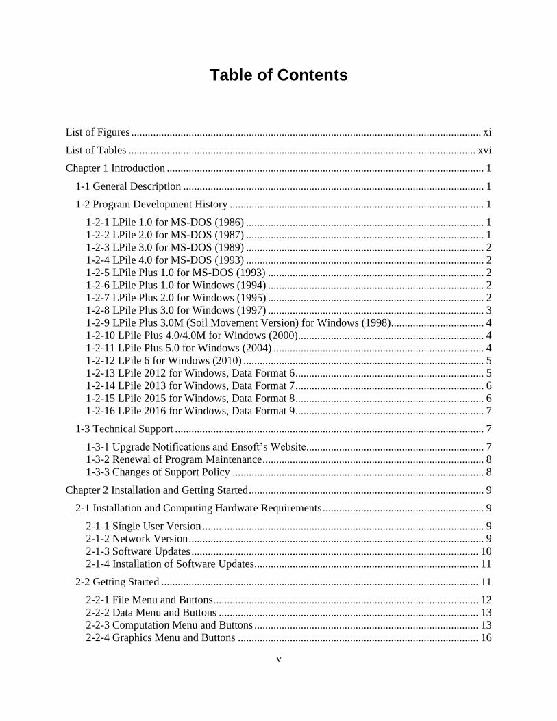
Table of Contents
List of Figures ................................................................................................................................ xi
List of Tables ............................................................................................................................... xvi
Chapter 1 Introduction .................................................................................................................... 1
1-1 General Description .............................................................................................................. 1
1-2 Program Development History ............................................................................................. 1
1-2-1 LPile 1.0 for MS-DOS (1986) ....................................................................................... 1
1-2-2 LPile 2.0 for MS-DOS (1987) ....................................................................................... 1 1-2-3 LPile 3.0 for MS-DOS (1989) ....................................................................................... 2 1-2-4 LPile 4.0 for MS-DOS (1993) ....................................................................................... 2
1-2-5 LPile Plus 1.0 for MS-DOS (1993) ............................................................................... 2 1-2-6 LPile Plus 1.0 for Windows (1994) ............................................................................... 2
1-2-7 LPile Plus 2.0 for Windows (1995) ............................................................................... 2 1-2-8 LPile Plus 3.0 for Windows (1997) ............................................................................... 3 1-2-9 LPile Plus 3.0M (Soil Movement Version) for Windows (1998) .................................. 4
1-2-10 LPile Plus 4.0/4.0M for Windows (2000) .................................................................... 4 1-2-11 LPile Plus 5.0 for Windows (2004) ............................................................................. 4
1-2-12 LPile 6 for Windows (2010) ........................................................................................ 5 1-2-13 LPile 2012 for Windows, Data Format 6 ..................................................................... 5 1-2-14 LPile 2013 for Windows, Data Format 7 ..................................................................... 6
1-2-15 LPile 2015 for Windows, Data Format 8 ..................................................................... 6 1-2-16 LPile 2016 for Windows, Data Format 9 ..................................................................... 7
1-3 Technical Support ................................................................................................................. 7
1-3-1 Upgrade Notifications and Ensoft’s Website ................................................................. 7
1-3-2 Renewal of Program Maintenance ................................................................................. 8 1-3-3 Changes of Support Policy ............................................................................................ 8
Chapter 2 Installation and Getting Started ...................................................................................... 9
2-1 Installation and Computing Hardware Requirements ........................................................... 9
2-1-1 Single User Version ....................................................................................................... 9 2-1-2 Network Version ............................................................................................................ 9
2-1-3 Software Updates ......................................................................................................... 10
2-1-4 Installation of Software Updates.................................................................................. 11
2-2 Getting Started .................................................................................................................... 11
2-2-1 File Menu and Buttons ................................................................................................. 12 2-2-2 Data Menu and Buttons ............................................................................................... 13 2-2-3 Computation Menu and Buttons .................................................................................. 13 2-2-4 Graphics Menu and Buttons ........................................................................................ 16
vi
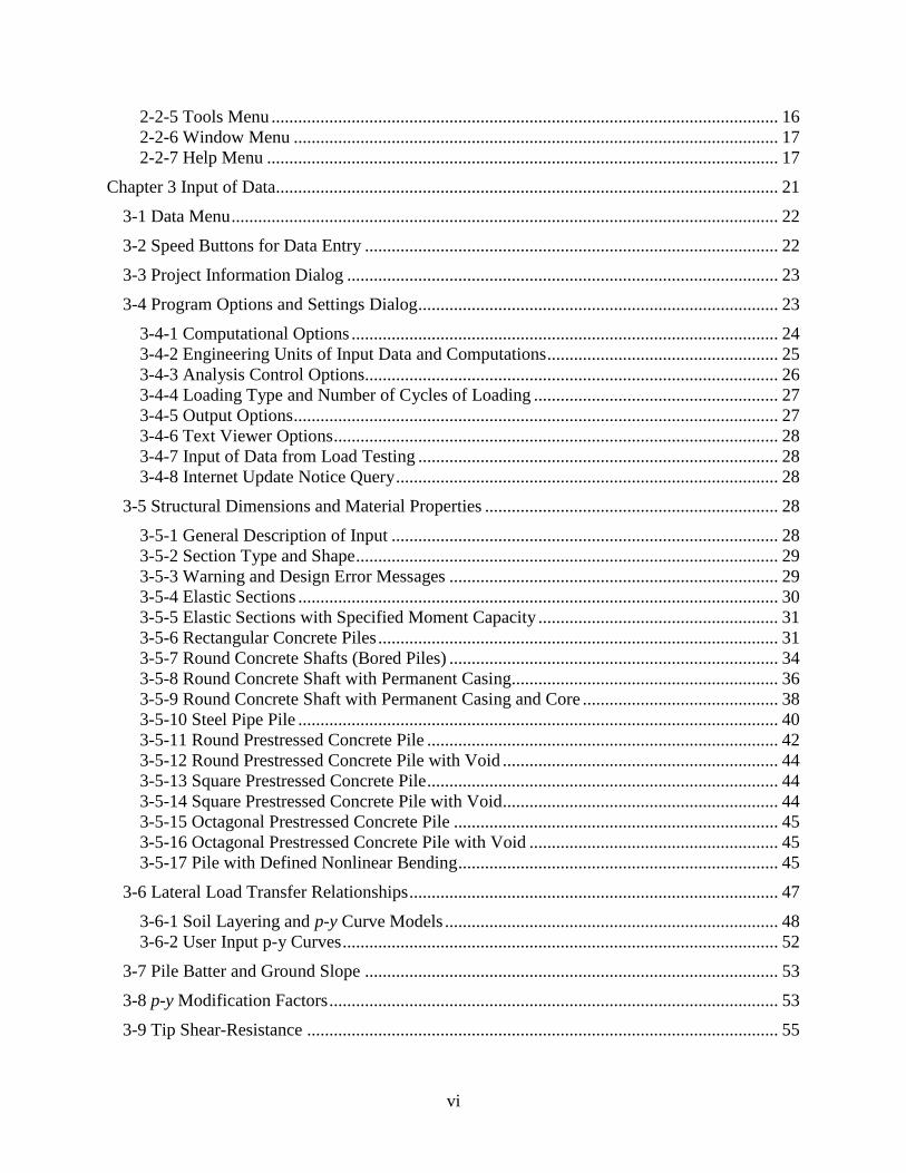
2-2-5 Tools Menu .................................................................................................................. 16 2-2-6 Window Menu ............................................................................................................. 17 2-2-7 Help Menu ................................................................................................................... 17
Chapter 3 Input of Data................................................................................................................. 21
3-1 Data Menu ........................................................................................................................... 22
3-2 Speed Buttons for Data Entry ............................................................................................. 22
3-3 Project Information Dialog ................................................................................................. 23
3-4 Program Options and Settings Dialog ................................................................................. 23
3-4-1 Computational Options ................................................................................................ 24
3-4-2 Engineering Units of Input Data and Computations .................................................... 25
3-4-3 Analysis Control Options............................................................................................. 26
3-4-4 Loading Type and Number of Cycles of Loading ....................................................... 27 3-4-5 Output Options ............................................................................................................. 27 3-4-6 Text Viewer Options .................................................................................................... 28 3-4-7 Input of Data from Load Testing ................................................................................. 28
3-4-8 Internet Update Notice Query ...................................................................................... 28
3-5 Structural Dimensions and Material Properties .................................................................. 28
3-5-1 General Description of Input ....................................................................................... 28 3-5-2 Section Type and Shape ............................................................................................... 29 3-5-3 Warning and Design Error Messages .......................................................................... 29
3-5-4 Elastic Sections ............................................................................................................ 30 3-5-5 Elastic Sections with Specified Moment Capacity ...................................................... 31
3-5-6 Rectangular Concrete Piles .......................................................................................... 31 3-5-7 Round Concrete Shafts (Bored Piles) .......................................................................... 34
3-5-8 Round Concrete Shaft with Permanent Casing............................................................ 36 3-5-9 Round Concrete Shaft with Permanent Casing and Core ............................................ 38
3-5-10 Steel Pipe Pile ............................................................................................................ 40 3-5-11 Round Prestressed Concrete Pile ............................................................................... 42
3-5-12 Round Prestressed Concrete Pile with Void .............................................................. 44 3-5-13 Square Prestressed Concrete Pile ............................................................................... 44 3-5-14 Square Prestressed Concrete Pile with Void .............................................................. 44 3-5-15 Octagonal Prestressed Concrete Pile ......................................................................... 45 3-5-16 Octagonal Prestressed Concrete Pile with Void ........................................................ 45
3-5-17 Pile with Defined Nonlinear Bending ........................................................................ 45
3-6 Lateral Load Transfer Relationships ................................................................................... 47
3-6-1 Soil Layering and p-y Curve Models ........................................................................... 48 3-6-2 User Input p-y Curves .................................................................................................. 52
3-7 Pile Batter and Ground Slope ............................................................................................. 53
3-8 p-y Modification Factors ..................................................................................................... 53
3-9 Tip Shear-Resistance .......................................................................................................... 55
vii
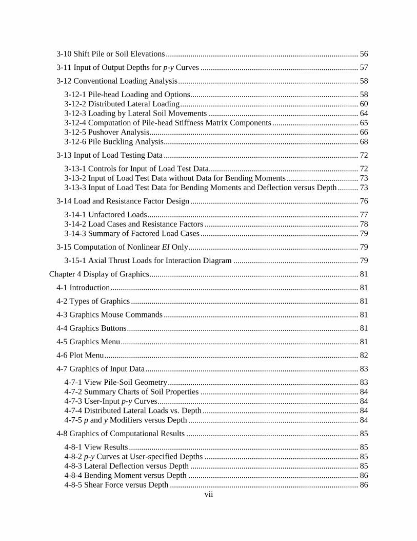
3-10 Shift Pile or Soil Elevations .............................................................................................. 56
3-11 Input of Output Depths for p-y Curves ............................................................................. 57
3-12 Conventional Loading Analysis ........................................................................................ 58
3-12-1 Pile-head Loading and Options.................................................................................. 58
3-12-2 Distributed Lateral Loading ....................................................................................... 60 3-12-3 Loading by Lateral Soil Movements ......................................................................... 64 3-12-4 Computation of Pile-head Stiffness Matrix Components .......................................... 65 3-12-5 Pushover Analysis...................................................................................................... 66 3-12-6 Pile Buckling Analysis............................................................................................... 68
3-13 Input of Load Testing Data ............................................................................................... 72
3-13-1 Controls for Input of Load Test Data......................................................................... 72
3-13-2 Input of Load Test Data without Data for Bending Moments ................................... 73 3-13-3 Input of Load Test Data for Bending Moments and Deflection versus Depth .......... 73
3-14 Load and Resistance Factor Design .................................................................................. 76
3-14-1 Unfactored Loads ....................................................................................................... 77
3-14-2 Load Cases and Resistance Factors ........................................................................... 78 3-14-3 Summary of Factored Load Cases ............................................................................. 79
3-15 Computation of Nonlinear EI Only ................................................................................... 79
3-15-1 Axial Thrust Loads for Interaction Diagram ............................................................. 79
Chapter 4 Display of Graphics ...................................................................................................... 81
4-1 Introduction ......................................................................................................................... 81
4-2 Types of Graphics ............................................................................................................... 81
4-3 Graphics Mouse Commands ............................................................................................... 81
4-4 Graphics Buttons ................................................................................................................. 81
4-5 Graphics Menu .................................................................................................................... 81
4-6 Plot Menu ............................................................................................................................ 82
4-7 Graphics of Input Data ........................................................................................................ 83
4-7-1 View Pile-Soil Geometry ............................................................................................. 83
4-7-2 Summary Charts of Soil Properties ............................................................................. 84 4-7-3 User-Input p-y Curves .................................................................................................. 84
4-7-4 Distributed Lateral Loads vs. Depth ............................................................................ 84 4-7-5 p and y Modifiers versus Depth ................................................................................... 84
4-8 Graphics of Computational Results .................................................................................... 85
4-8-1 View Results ................................................................................................................ 85 4-8-2 p-y Curves at User-specified Depths ........................................................................... 85
4-8-3 Lateral Deflection versus Depth .................................................................................. 85 4-8-4 Bending Moment versus Depth ................................................................................... 86 4-8-5 Shear Force versus Depth ............................................................................................ 86

viii
4-8-6 Mobilized Soil Reaction versus Depth ........................................................................ 86 4-8-7 Deflection, Moment, and Shear Force versus Depth ................................................... 86 4-8-8 Deflection, Curvature, and Moment versus Depth ...................................................... 86 4-8-9 Mobilized Pile EI versus Depth ................................................................................... 86
4-8-10 Load versus Top Deflection ....................................................................................... 86 4-8-11 Load versus Max Moment ......................................................................................... 87 4-8-12 Top Deflection versus Pile Length ............................................................................ 87 4-8-13 Moment versus Curvature .......................................................................................... 87 4-8-14 EI versus Moment ...................................................................................................... 87
4-8-15 Interaction Diagram ................................................................................................... 87 4-8-16 All K’s versus Deflection and Rotation ..................................................................... 87 4-8-17 All K’s versus Shear and Moment ............................................................................. 87 4-8-18 Individual K’s versus Force and Moment .................................................................. 88
4-8-19 Individual K’s versus Pile-head Deflection and Rotation .......................................... 88 4-8-20 Pushover Shear Force versus Top Deflection ............................................................ 89
4-8-21 Pushover Moment versus Top Deflection ................................................................. 89 4-8-22 Pile Buckling Thrust versus Top Deflection .............................................................. 89
4-8-23 Deflection and Soil Movement versus Depth ............................................................ 90
4-9 Presentation Charts ............................................................................................................. 90
4-9-1 Saving and Applying Presentation Chart Templates ................................................... 90
4-9-2 Exporting Presentation Charts ..................................................................................... 90 4-9-3 Creating Graphs for Reports ........................................................................................ 90
Chapter 5 Tools Menu .................................................................................................................. 93
5-1 Simple Calculator ................................................................................................................ 93
5-2 Battered Pile Load Calculator ............................................................................................. 94
5-3 Custom Reinforcing Bar Data Entry and Editing ............................................................... 95
5-4 Multi-File Analysis (Batch Run Utility) ............................................................................. 96
Chapter 6 Example Problems........................................................................................................ 99
6-1 Example 1 – Steel Pile in Sloping Ground ....................................................................... 101
6-2 Example 2 – Drilled Shaft in Sloping Ground .................................................................. 107
6-3 Example 3 – Offshore Pipe Pile ........................................................................................ 113
6-4 Example 4 - Buckling of a Pile-Column ........................................................................... 117
6-5 Example 5 – Computation of Nominal Moment Capacity and Interaction Diagram ....... 119
6-6 Example 6 – Pile-head Stiffness Matrix ........................................................................... 121
6-7 Example 7 – Pile with User-Input p-y Curves and Distributed Load ............................... 123
6-8 Example 8 – Pile in Cemented Sand ................................................................................. 125
6-9 Example 9 – Drilled Shaft with Tip Resistance ................................................................ 127
6-10 Example 10 – Drilled Shaft in Soft Clay ........................................................................ 130

ix
6-11 Example 11 – LRFD Analysis ........................................................................................ 131
6-12 Example 12 – Pile in Liquefied Sand with Lateral Spread ............................................. 133
6-13 Example 13 – Square Elastic Pile with Top Deflection versus Length .......................... 135
6-14 Example 14 – Pushover Analysis of Prestressed Concrete Pile ..................................... 137
6-15 Example 15 – Pile with Defined Nonlinear Bending Properties .................................... 139
6-16 Example 16 – Pile with Distributed Lateral Loadings .................................................... 139
6-17 Example 17 – Analysis of a Drilled Shaft ...................................................................... 140
6-18 Example 18 – Analysis of Drilled Shaft with Permanent Casing ................................... 141
6-19 Example 19 – Analysis of Drilled Shaft with Casing and Core ..................................... 141
6-20 Example 20 – Analysis of Embedded Pole ..................................................................... 143
6-21 Example 21 – Analysis of Tapered Elastic Pile .............................................................. 144
6-22 Example 22 – Analysis of Tapered Elastic-Plastic Pile .................................................. 145
6-23 Example 23 – Output of p-y Curves ............................................................................... 146
6-24 Example 24 – Analysis with Lateral Soil Movements .................................................... 149
6-25 Example 25- Verification of Elastic Pile in Elastic Subgrade Soil ................................. 152
6-26 Example 26 – Verification of P-Delta Effect ................................................................. 152
Chapter 7 Validation ................................................................................................................... 155
7-1 Introduction ....................................................................................................................... 155
7-2 Case Histories ................................................................................................................... 155
7-3 Verification of Accuracy of Solution ................................................................................ 157
7-3-1 Solution of Example Problems .................................................................................. 157
7-3-2 Numerical Precision Employed in Internal Computations ........................................ 158 7-3-3 Selection of Convergence Tolerance and Length of Increment ................................ 158
7-3-4 Check of Soil Resistance ........................................................................................... 160 7-3-5 Check of Equilibrium................................................................................................. 160 7-3-6 Use of Non-Dimensional Curves ............................................................................... 162 7-3-7 Use of Closed-form Solutions.................................................................................... 162 7-3-8 Concluding Comments on Verification ..................................................................... 164
Chapter 8 Line-by-Line Guide for Input ..................................................................................... 167
8-1 Key Words for Input Data File ......................................................................................... 167
8-2 TITLE Command .............................................................................................................. 168
8-3 OPTIONS Command ........................................................................................................ 168
8-4 SECTIONS Command ...................................................................................................... 169
8-5 SOIL LAYERS Command ............................................................................................... 179
x
8-6 PILE BATTER AND SLOPE Command ......................................................................... 186
8-7 TIP SHEAR Command ..................................................................................................... 186
8-8 GROUP EFFECT FACTORS Command ......................................................................... 187
8-9 LRFD LOADS Command ................................................................................................ 187
8-10 LRFD FACTORS AND CASES Command ................................................................... 188
8-11 LOADING Command ..................................................................................................... 188
8-12 P-Y OUTPUT DEPTHS Command ................................................................................ 189
8-13 SOIL MOVEMENTS Command .................................................................................... 189
8-14 AXIAL THRUST LOADS Command ............................................................................ 189
8-15 FOUNDATION STIFFNESS Command ....................................................................... 190
8-16 PILE PUSHOVER ANALYSIS DATA Command ....................................................... 190
8-17 PILE BUCKLING ANALYSIS DATA Command ........................................................ 191
8-18 LRFD Data File ............................................................................................................... 191
References ................................................................................................................................... 193
Appendix 1 Input Error Messages .............................................................................................. 195
Appendix 2 Runtime Error Messages ......................................................................................... 199
Appendix 3 Warning Messages .................................................................................................. 201

xi
List of Figures
Figure 1-1 Pile-head Stiffness Components ................................................................................... 3 Figure 2-1 Options for Type of License Installation .................................................................... 10 Figure 2-2 Options for Type of Network Installation ................................................................... 10
Figure 2-3 Check for Update Query ............................................................................................. 11 Figure 2-4 Principal Operations of LPile ...................................................................................... 11 Figure 2-5 Main Window of LPile................................................................................................ 12 Figure 2-6 File Menu .................................................................................................................... 12 Figure 2-7 File Speed Buttons ...................................................................................................... 13
Figure 2-8 Speed Buttons for Data Input for Different Analysis Modes ...................................... 13 Figure 2-9 Input Data Review Buttons ......................................................................................... 13
Figure 2-10 Computation Menu.................................................................................................... 14
Figure 2-11 Run Analysis and View Report Buttons ................................................................... 14 Figure 2-12 Graphics Buttons ....................................................................................................... 16 Figure 2-13 Tools Menu ............................................................................................................... 16
Figure 2-14 Help Menu ................................................................................................................. 17 Figure 2-15 Example of About LPile Dialog ................................................................................ 19
Figure 3-1 Data Menu ................................................................................................................... 22 Figure 3-2 Buttons for Data Entry and Manipulation for Conventional Analysis ........................ 22 Figure 3-3 Buttons for Data Entry and Manipulation for Computation of Nonlinear EI Only .... 23
Figure 3-4 Buttons for Data Entry and Manipulation for LRFD Analysis ................................... 23 Figure 3-5 Example of Project Information Input Dialog ............................................................ 23
Figure 3-6 Program Options and Settings Dialog ......................................................................... 24 Figure 3-7 Pile Section, Section Type Tab ................................................................................... 29
Figure 3-8 Dimensions Tab Page for Rectangular Concrete Section ........................................... 32 Figure 3-9 Concrete Tab Page for Rectangular Concrete Section ................................................ 32 Figure 3-10 Rebars Tab Page for Rectangular Concrete Section ................................................. 33
Figure 3-11 Rebar Layout Table for Rectangular Concrete Section ............................................ 33 Figure 3-12 Section Type, Dimensions, and Cross-section Properties Dialog for
Rectangular Concrete Section Showing Rebar Layout After Definition ................. 34 Figure 3-13 Tab Sheet for Selection of Section Type Showing Current Cross-section ............... 35 Figure 3-14 Tab Sheet for Reinforcing Bar Properties ................................................................. 36
Figure 3-15 Tab Sheet for Shaft Dimensions for Drilled Shaft with Permanent Casing .............. 37 Figure 3-16 Tab Sheet for Rebars for Drilled Shaft with Permanent Casing ............................... 37
Figure 3-17 Tab Sheet for Casing Material Properties for Drilled Shaft with Permanent
Casing ....................................................................................................................... 38
Figure 3-18 Tab Sheet forShaft Dimensions of Drilled Shaft with Casing and Core ................... 39 Figure 3-19 Tab Sheet for Casing and Core Material Properties .................................................. 40 Figure 3-20 Dimensions Tab Page for Steel Pipe Piles ................................................................ 41 Figure 3-21 Pipe-Casing-Core Properties Tab Page for Steel Pipe Pile ....................................... 41 Figure 3-22 Comparison of Moment vs. Curvature for (a) Steel Pipe Pile and (b) Elastic-
Plastic Pipe Pile with Similar Properties .................................................................. 42
xii
Figure 3-23 Prestressing Tab Page Common to All Prestressed Pile Types ................................ 43 Figure 3-24 Automatic Prestressing Arrangements for Square Prestressed Piles ........................ 44 Figure 3-25 Nonlinear EI Tab Page .............................................................................................. 46 Figure 3-26 Table for Entering Axial Thrust Forces for Nonlinear Bending Data ...................... 46
Figure 3-27 Tables for Entry of (a) Nonlinear Moment versus Curvature Data and (b)
Nonlinear Moment versus Bending Stiffness ........................................................... 47 Figure 3-28 Dialog for Definition of Soil Layering and Soil Properties ...................................... 48 Figure 3-29 Dialog for Properties of Weak Rock ......................................................................... 51 Figure 3-30 Dialog for Properties of Massive Rock ..................................................................... 51
Figure 3-31 Dialog for Effective Unit Weights of User-input p-y Curves ................................... 52 Figure 3-32 Dialog for User-input p-y Curve Values ................................................................... 52 Figure 3-33 Dialog for Definition of Pile Batter and Slope of Ground Surface ........................... 54 Figure 3-34 Dialog for p-Multipliers and y-Multipliers versus Depth Below Pile Head ............. 54
Figure 3-35 Dialog for Tip Shear Resistance versus Lateral Tip Displacement .......................... 55 Figure 3-36 Dialog for Shifting of Pile Elevation Relative to Input Soil Profile Showing a
Pile Head at the Top of the Soil Profile .................................................................... 56 Figure 3-37 Dialog for Shifting of Pile Elevation Relative to Input Soil Profile After
Shifting a Pile Head To Be Below the Ground Surface ........................................... 57 Figure 3-38 Output Depths of p-y Curves Below Pile Head, (a) Dialog for p-y Curve
Output Depths, (b) Measurement of Vertical Depths ............................................... 58
Figure 3-39 Dialog for Definition of Conventional Pile-head Loading ....................................... 59 Figure 3-40 Dialogs for Multiple Distributed Lateral Loads for Conventional Loading, (a)
3 Load Cases, (b) Distributed Load Profile Data for Load Case 1 ........................... 61 Figure 3-41 Dialog of Values of Distributed Lateral Loads versus Depth ................................... 62 Figure 3-42 Recommendation for Modeling of Lateral Force Applied Below the Pile Head ...... 63
Figure 3-43 Recommendation for Modeling of Moment Applied Below the Pile Head.............. 64
Figure 3-44 Dialog for Input of Soil Movements versus Depth Below Pile Head ....................... 65 Figure 3-45 Dialog for Controls for Computation of Stiffness Matrix ......................................... 66 Figure 3-46 Dialog for Controls for Pushover Analysis ............................................................... 67
Figure 3-47 Pile-head Shear Force versus Displacement from Pushover Analysis...................... 68 Figure 3-48 Maximum Moment in Pile versus Displacement from Pushover Analysis .............. 68
Figure 3-49 Dialog for Controls for Pile Buckling Analysis ........................................................ 69 Figure 3-50 Typical Results for a Pile Buckling Analysis ........................................................... 70
Figure 3-51 Computed Pile Buckling Result Shifted to the Left .................................................. 70 Figure 3-52 Redrawn Pile Buckling Results Used for Curve Fitting ........................................... 70 Figure 3-53 Results from Pile Buckling Analysis ........................................................................ 71 Figure 3-54 Example of Correct (green symbols) and Incorrect (red symbols) Pile
Buckling Analyses .................................................................................................... 72
Figure 3-55 Dialog for Control of Input and Saving of Load Testing Data ................................. 73 Figure 3-56 Dialog for Input of Pile-head Shear Force versus Lateral Deformation from
Load Testing, if input of Bending Moment and/or Lateral Movement versus
Depth is not specified. .............................................................................................. 74 Figure 3-57 Dialog for Input of Pile-head Shear Force versus Lateral Deformation from
Load Testing, if input of Bending Moment and Lateral Deflection versus
Depth are specified. .................................................................................................. 75

xiii
Figure 3-58 Dialogs for Input of Bending Moment and Lateral Deflection versus Depth
from Load Testing. ................................................................................................... 76 Figure 3-59 Dialog for Definition of Unfactored Pile-head Loadings for LRFD Analysis.......... 77 Figure 3-60 Dialog for LRFD Load Combinations and Structural Resistance Factors ................ 78
Figure 3-61 Summary Report of Computed Factored Load Combinations for LRFD
Analysis .................................................................................................................... 79 Figure 3-62 Dialog for Axial Thrust Forces for Computation of Interaction Diagram ................ 80 Figure 4-1 Speed Buttons for Graphics ........................................................................................ 81 Figure 4-2 Graphics Menu ............................................................................................................ 82
Figure 4-3 Plot Drop-Down Menu ................................................................................................ 83 Figure 4-4 Example of Summary Graphs of Soil Properties ........................................................ 84 Figure 4-5 Example of View Results Window ............................................................................. 85 Figure 4-6 Sub-menu for Pile-head Stiffnesses versus Pile-head Force and Moment ................. 88
Figure 4-7 Submenu for Pile-head Stiffnesses versus Deflection and Rotation ........................... 88 Figure 4-8 Example of Table for a Report Graph ......................................................................... 91
Figure 5-1 Tools Menu ................................................................................................................. 93 Figure 5-2 Simple Calculator ........................................................................................................ 93
Figure 5-3 Battered Load Calculator ............................................................................................ 95 Figure 5-4 Dialog for Editing of Custom Rebar Data ................................................................... 96 Figure 5-5 Dialog for Multi-File Analysis Controls ..................................................................... 97
Figure 6-1 General Description of Example 1 ............................................................................ 102 Figure 6-2 Dimensions and Properties Entered for Example 1 .................................................. 103
Figure 6-3 Generated Curve of Lateral Load versus Maximum Moment for Example 1. ......... 105 Figure 6-4 Generated Curve of Lateral Load versus Top Deflection for Example 1. ................ 105 Figure 6-5 Curve of Deflection versus Depth for Example 1, Second Analysis ........................ 106
Figure 6-6 Bending Moment versus Depth for Example 1, Second Analysis ............................ 107
Figure 6-7 Cross-section of Drilled Shaft for Example 2. .......................................................... 108 Figure 6-8 Factored Interaction Diagram for Example 2a. ......................................................... 109 Figure 6-9 Moment-Curvature Diagram for Example 2a. .......................................................... 109
Figure 6-10 Bending Stiffness versus Bending Moment for Example 2a. ................................. 110 Figure 6-11 Shear Force versus Top Deflection and Maximum Bending Moment versus
Top Shear Load for Free-head Conditions in Example 2b. .................................... 111 Figure 6-12 Shear Force versus Top Deflection and Maximum Bending Moment versus
Top Shear Load for Fixed-head Conditions in Example 2c. .................................. 111 Figure 6-13 Results for Free-head and Fixed-head Loading Conditions for Example 2d .......... 112 Figure 6-14 Top Deflection versus Pile Length for Example 2d ................................................ 112 Figure 6-15 Idealized View of an Offshore Platform Subjected to Wave Loading, Example
3 .............................................................................................................................. 113
Figure 6-16 Superstructure and Pile Details, Example 3 ............................................................ 114 Figure 6-17 Moment versus Curvature, Example 3 .................................................................... 115
Figure 6-18 Results of Initial Computation with p-y Curves, Example 3 .................................. 116 Figure 6-19 Pile Deflection and Bending Moment versus Depth for Vtop = 500 kN,
Example 3 ............................................................................................................... 117 Figure 6-20 Pile-head Deflection and Maximum Bending Moment versus Axial Thrust
Loading ................................................................................................................... 118 Figure 6-21 Results from LPile Solution for Buckling Analysis, Example 4 ............................ 119
xiv
Figure 6-22 Moment versus Curvature for Example 5 ............................................................... 120 Figure 6-23 Bending Stiffness versus Bending Moment, Example 5 ......................................... 121 Figure 6-24 Factored Interaction Diagram of Reinforced-concrete Pile, Example 5 ................. 121 Figure 6-25 Stiffness Matrix Components versus Displacement and Rotation, Example 6 ....... 122
Figure 6-26 Stiffness Matrix Components versus Force and Moment, Example 6 .................... 123 Figure 6-27 Pile and soil details for Example 7 .......................................................................... 124 Figure 6-28 User-input p-y Curves for Example 7 (Lower curve for Layer 7 not shown) ......... 124 Figure 6-29 Soil details for Example 8 ....................................................................................... 125 Figure 6-30 Comparison between Measured and Predicted Pile-head Load versus
Deflection Curves for the 5-m Pile of Example 8 .................................................. 126 Figure 6-31 Comparison between Measured and Computed Bending Moment versus Depth
for the 5-m Pile of Example 8 ................................................................................ 126 Figure 6-32 Shaft Geometry and Soil Properties for Example 9 ................................................ 127
Figure 6-33 Moment versus Curvature for Sections 1 and 2, Example 9 ................................... 129 Figure 6-34 Lateral Deflection and Bending Moment versus Depth, Example 9 ...................... 129
Figure 6-35 Top Deflection versus Pile Length, Example 9 ...................................................... 130 Figure 6-36 Summary Plots of Results for Example 10 ............................................................. 131
Figure 6-37 Example from Summary Report of LRFD Loadings, Example 11 ......................... 132 Figure 6-38 Message for Successful LRFD Analysis for Example 11 ....................................... 132 Figure 6-39 Pile and Soil Profile for Example 12....................................................................... 133
Figure 6-40 Lateral Spread Profile versus Depth for Example 12.............................................. 134 Figure 6-41 Summary Graphs for Example 12 ........................................................................... 135
Figure 6-42 Pile-head Load versus Deflection Curves Using Original and Modified p-y
Curves for Stiff Clay without Free Water and Percentage Reduction in
Stiffness for Example 13 ........................................................................................ 136
Figure 6-43 Curves of Pile Top Deflection versus Pile Length for Example 13 ........................ 136
Figure 6-44 Reinforcement Details for Prestressed Concrete Pile of Example 14 ..................... 137 Figure 6-45 Moment versus Curvature of Prestressed Pile for Example 14............................... 138 Figure 6-46 Results of Pushover Analysis of Prestressed Concrete Pile of Example 14 ........... 139
Figure 6-47 Pile and Soil Profile for Example 17....................................................................... 140 Figure 6-48 Moment versus Curvature for Dual Section Drilled Shaft of Example 17 ............. 141
Figure 6-49 Moment versus Curvature for Dual Section Drilled Shaft with Permanent
Casing of Example 18 ............................................................................................ 142
Figure 6-50 Moment versus Curvature for Dual Section Drilled Shaft with Permanent
Casing and Core of Example 19 ............................................................................. 142 Figure 6-51 Pile and Soil Profile for Embedded Pole of Example 20 ........................................ 143 Figure 6-52 Bending Moment and Plastic Moment Capacity versus Depth for Example 22 ..... 145 Figure 6-53 Program and Setting Dialog Showing Check for Generation of p-y Curves .......... 146
Figure 6-54 Pile and Soil Profile for Example 23....................................................................... 147 Figure 6-55 Standard Output of 17-point p-y Curves for Example 23 ....................................... 147
Figure 6-56 User-input p-y Curves Interpolated with Depth Using 17 Points for Example
23 ............................................................................................................................ 148 Figure 6-57 Output of User-input p-y Curves with Five Points for Example 23 ........................ 149 Figure 6-58 Pile and Soil Profile for Example 24....................................................................... 150 Figure 6-59 Program and Setting Dialog Showing Check for Inclusion of Loadings by
Lateral Soil Movements ......................................................................................... 150

xv
Figure 6-60 Input Dialog for Lateral Soil Movements versus Depth for Example 24 ............... 151 Figure 6-61 Results of Analysis for Example 24 ........................................................................ 151 Figure 6-62 Pile and Soil Profile for Verification of P-Delta Effect .......................................... 152 Figure 7-1 Comparison of Maximum Bending Moments from Computations and from
Experimental Case Histories .................................................................................. 156 Figure 7-2 Comparison of Experimental and Computed Pile-head Deflections at Service
Load ........................................................................................................................ 157 Figure 7-3 Influence of Number of Increments on Computed Values of Pile-head
Deflection and Maximum Bending Moment .......................................................... 159
Figure 7-4 Plot of Mobilized Soil Resistance versus Depth ....................................................... 162 Figure 7-5 Verification of Pile Deflections ................................................................................ 164 Figure 7-6 Verification of Bending Moments ............................................................................ 165 Figure 7-7 Verification of Shear Forces ..................................................................................... 166
xvi
List of Tables
Table 2-1 File Types and File Extensions ..................................................................................... 14 Table 3-1 Mathematical Operators and Numerical Constants Used in LPile Input Dialogs ........ 21 Table 3-2 Recommended Ranges for Maximum Number of Iterations ....................................... 26
Table 6-1 Dimensions, Cross-sectional Area, and Bending Stiffness of Tapered Pile............... 144 Table 6-2 Interpolated Dimensional Properties, Cross-sectional Area, Moment of Inertia,
Bending Moment of Tapered Pile Computed by LPile .......................................... 145 Table 7-1 Comparison of Bending Moments and Deflections from Computer Analyses and
Experimental Case Histories .................................................................................. 155
Table 8-1 Key Words for Definition of Input Data .................................................................... 167 Table 8-2 Program Options and Settings .................................................................................... 168
Table 8-3 Pile Section Data ........................................................................................................ 169
Table 8-4 Properties for Rectangular Sections ........................................................................... 170 Table 8-5 Properties for Drilled Shafts ....................................................................................... 170 Table 8-6 Properties of Drilled Shafts with Casing .................................................................... 171
Table 8-7 Properties of Drilled Shafts with Casing and Core .................................................... 171 Table 8-8 Properties for Steel Pipe Piles .................................................................................... 171
Table 8-9 Properties for Circular Solid Prestressed Piles ........................................................... 172 Table 8-10 Properties for Circular Hollow Prestressed Piles ..................................................... 172 Table 8-11 Properties for Square Solid Prestressed Piles ........................................................... 172
Table 8-12 Properties for Square Hollow Prestressed Piles ....................................................... 172 Table 8-13 Properties for Octagonal Solid Prestressed Piles...................................................... 173
Table 8-14 Properties for Square Hollow Prestressed Piles ....................................................... 173 Table 8-15 Properties for Elastic Piles........................................................................................ 173
Table 8-16 Properties for Elastic Piles with Specified Moment Capacity.................................. 175 Table 8-17 Properties for Piles with Nonlinear Bending Properties ........................................... 177 Table 8-18 Concrete Properties .................................................................................................. 177
Table 8-19 Reinforcing Steel Properties ..................................................................................... 177 Table 8-20 Prestressing Strand Properties .................................................................................. 178
Table 8-21 Soil Layer Properties ................................................................................................ 179 Table 8-22 Properties for Soft Clay ............................................................................................ 180 Table 8-23 Properties for API Soft Clay..................................................................................... 181
Table 8-24 Properties for Stiff Clay with Free Water................................................................. 181 Table 8-25 Properties for Stiff Clay without Free Water ........................................................... 181
Table 8-26 Properties for Stiff Clay with Free Water Using k ................................................... 182 Table 8-27 Properties for Sand ................................................................................................... 182
Table 8-28 Properties for API Sand ............................................................................................ 182 Table 8-29 Properties for Liquefied Sand ................................................................................... 183 Table 8-30 Properties for Liquefied Sand Hybrid Model ........................................................... 183 Table 8-31 Properties for Weak Rock ........................................................................................ 183 Table 8-32 Properties for Vuggy Limestone .............................................................................. 184 Table 8-33 Properties for Piedmont Residual Soil ..................................................................... 184 Table 8-34 Properties for Massive Rock .................................................................................... 184

xvii
Table 8-35 Properties for Loess .................................................................................................. 185 Table 8-36 Properties for Cemented Silt .................................................................................... 185 Table 8-37 Properties for Elastic Subgrade ................................................................................ 186 Table 8-38 Properties for User-Input p-y Curves ....................................................................... 186
Table 8-39 Pile Batter and Ground Slope Properties .................................................................. 186 Table 8-40 Tip Shear Curve Properties ...................................................................................... 186 Table 8-41 Group Effect Properties ............................................................................................ 187 Table 8-42 LRFD Load Properties ............................................................................................. 187 Table 8-43 LRFD Load Factors and Loading Case Properties ................................................... 188
Table 8-44 Conventional Loading Properties ............................................................................. 188 Table 8-45 p-y Output Depth Properties ..................................................................................... 189 Table 8-46 Soil Movement Properties ........................................................................................ 189 Table 8-47 Axial Thrust Loads for EI Computations Only ........................................................ 189
Table 8-48 Foundation Stiffness Computations ......................................................................... 190 Table 8-49 Pushover Analysis Computations ............................................................................. 190
Table 8-50 Pile Buckling Analysis Data ..................................................................................... 191


1
Chapter 1 Introduction
1-1 General Description
LPile is a special purpose program that can analyze a pile or drilled shaft under lateral
loading. The program computes deflection, shear, bending moment, and soil response with
respect to depth in nonlinear soils. The program has graphical features for presentation of results
and has additional features for special analyses.
The soil and rock is modeled using lateral load-transfer curves (p-y curves) based on
published recommendations for various types of soils and rocks. The p-y curves are internally
generated by the program. Alternatively, the user can input values for p-y curves for a soil layer.
The program also contains specialized procedures for computing p-y curves in layered soil
profiles.
Several types of pile-head loading conditions may be selected, and the structural
properties of the pile may be varied along the pile length. Additionally, LPile can compute the
nominal-moment capacity and provide design information for rebar arrangements.
1-2 Program Development History
1-2-1 LPile 1.0 for MS-DOS (1986)
When the IBM XT® personal computer was introduced in 1984, Dr. Lymon C. Reese,
the founder of Ensoft, Inc., foresaw the benefits and improvements in analysis and design of pile
foundations from using improved computer software. The development of LPile for its first
commercial distribution was begun in 1985 and was completed in 1986. The general theory and
methodology of LPile 1.0 was similar in features to COM624, which was run on large
mainframe computers. LPile was completely rewritten using a new solver and features were
provided for interactive input. LPile was developed for analyzing single piles and drilled shafts
under lateral loading. This version of LPile was compiled using the IBM Fortran compiler to run
on the IBM XT personal computer. LPile Version 1.0 had the following features:
The program could generate p-y curves internally for soft clay, stiff clay with free water,
stiff clay without free water, and sand. The program also allowed users to input user-
defined p-y curves for a selected layer.
Modifications of the p-y curves for layered soils were introduced in the program based on
the recommendations of Georgiadis (1983).
A total of four boundary conditions and loading types were available for the pile head.
Distributed loading could also be specified at any pile depth.
An interactive input was provided for the user to prepare the input data step-by-step.
An analysis feature was provided for including tip-resistance curves.
1-2-2 LPile 2.0 for MS-DOS (1987)
With the introduction of improved graphics hardware for personal computers such as
color graphics monitors and an improved processor on IBM® AT-class computers, the features
for graphical display of computed pile deflection, bending moment, shear, and soil resistance
Chapter 1 – Introduction
2
became desirable for engineering software. LPile 2.0 was introduced in 1987 with a companion
graphics program. Improvements were also made on the main program and input data editor.
1-2-3 LPile 3.0 for MS-DOS (1989)
With the wide adoption of LPile by government agencies, universities, and engineering
firms during the first three years, improvements in ease-of-use were considered essential. LPile
3.0 was introduced in 1989 with an input data editor featuring pull-down menus, input tables,
and on-screen help commands. Color graphics for CGA, EGA, and VGA displays were added to
the output graphics post-processor program. The main program also added the new technical
features:
New p-y criteria for vuggy limestone/rock.
Options for modifying internally-generated p-y curves for group action effects.
The pile head could be positioned either above or below the ground surface.
1-2-4 LPile 4.0 for MS-DOS (1993)
LPile 4.0 was released in 1993, about four years after the previous upgrade. Features
added to this version were:
New p-y criteria for cemented soils whose strength is represented using both cohesion
and friction angle.
New p-y criteria for sand based on the recommendations of the American Petroleum
Institute’s API-RP2A (1987).
New p-y procedures for including the effect of sloping ground on p-y curves for clays and
sands.
New graphic plots for representing load versus deflection at the pile head and load versus
maximum bending moment.
1-2-5 LPile Plus 1.0 for MS-DOS (1993)
New technology for pile foundations enabled the incorporation of nonlinear properties for
the pile’s flexural rigidity during analysis of their lateral deflections. Earlier, a companion
computer program named STIFF was developed in 1987 to compute the relationship of applied
moment versus flexural rigidity of a pile, and to compute the ultimate bending capacity for a
specified structural section. LPile Plus was thus developed in 1993 by combining the capabilities
of LPile 4.0 and STIFF. With the added functionality obtained from STIFF, LPile Plus had the
capability to take into account the flexural rigidity of uncracked and cracked sections, which led
to a improved solution for the flexibility of a pile under lateral loading.
1-2-6 LPile Plus 1.0 for Windows (1994)
The introduction of Windows 3.1 from Microsoft, Inc. as the new platform for personal
computers pushed software development into a new era with a demand for user-friendly features.
LPile Plus 1.0 for Windows was released in 1994 with input preprocessor and output post-
processor developed specifically for the Windows operating system.
1-2-7 LPile Plus 2.0 for Windows (1995)
The initial windows version for LPile Plus was released in 1994. The preprocessor
program used a mouse with pull-down menu, dialog boxes, grid tables, and push buttons to
improve the process of data entry. The graphics program, also running within the Windows
Chapter 1 – Introduction
3
platform, supported any printer device recognized by the Windows environment. The main
program added a feature for users to specify the rebar area at each location.
1-2-8 LPile Plus 3.0 for Windows (1997)
With the 32-bit operating systems provided by Microsoft Windows 95 and Windows NT,
software developers were provided with tools to develop user interfaces with advanced, high-
resolution graphics. LPile Plus 3.0 was developed based on the technological advances for new
user interfaces. The significant new features of this upgrade are summarized as follows:
A new soil criterion for weak rock was added to the previously existing eight soil types.
The p-y criterion for weak rock is primarily applicable to the weathered sandstone,
claystone, and limestone with uniaxial compressive strengths of less than 1,000 psi.
An option was added to compute pile-head deflection versus pile length. This option
generated a graph of pile length versus pile-head deflection that is helpful for determining
the critical pile length.
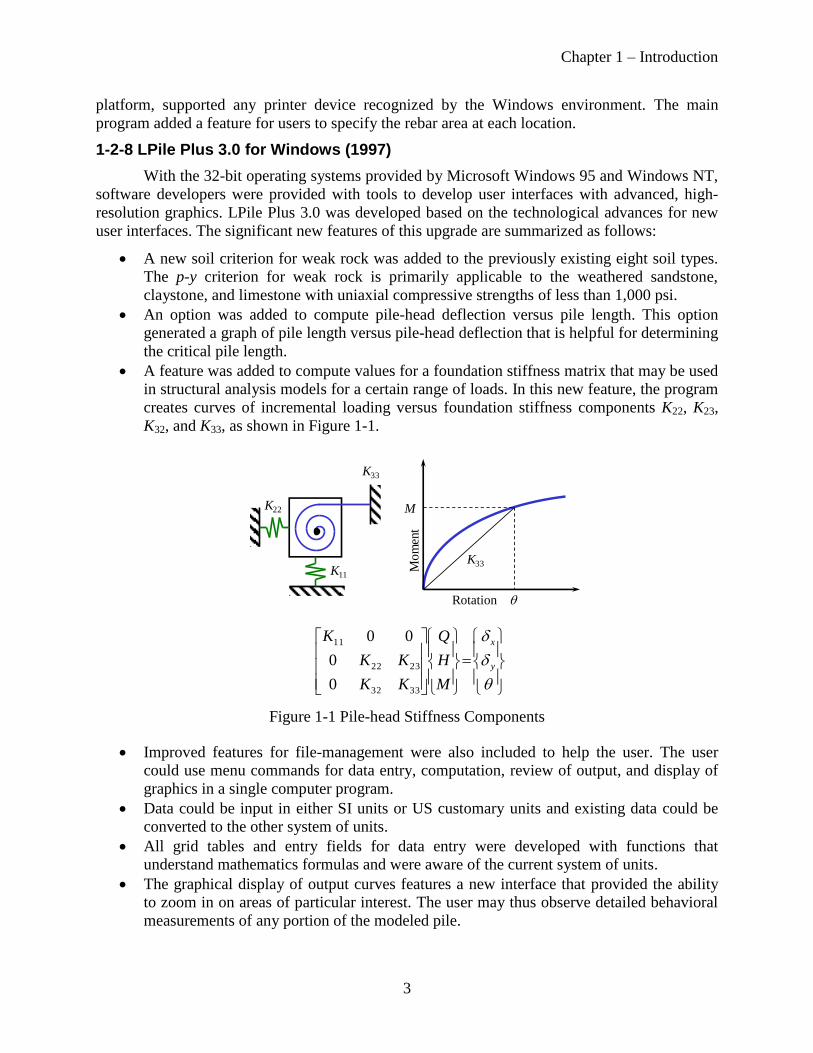
A feature was added to compute values for a foundation stiffness matrix that may be used
in structural analysis models for a certain range of loads. In this new feature, the program
creates curves of incremental loading versus foundation stiffness components K22, K23,
K32, and K33, as shown in Figure 1-1.
Figure 1-1 Pile-head Stiffness Components
Improved features for file-management were also included to help the user. The user
could use menu commands for data entry, computation, review of output, and display of
graphics in a single computer program.
Data could be input in either SI units or US customary units and existing data could be
converted to the other system of units.
All grid tables and entry fields for data entry were developed with functions that
understand mathematics formulas and were aware of the current system of units.
The graphical display of output curves features a new interface that provided the ability
to zoom in on areas of particular interest. The user may thus observe detailed behavioral
measurements of any portion of the modeled pile.
Rotation q
Mom
ent
M
K33
K33
K11
K22
q
y
x
M
H
Q
KK
KK
K
3332
2322
11
0
0
00
Chapter 1 – Introduction
4
1-2-9 LPile Plus 3.0M (Soil Movement Version) for Windows (1998)
An advanced version for LPile Plus was developed and was released in 1998 as Version
3.0M. The LPile Plus 3.0M software is the standard LPile Plus 3.0 version with the addition of
two additional capabilities:
The user is able to input a profile of soil movements versus depth as additional loading on
the pile. The soil movements of the soil may be produced from any action that causes soil
movements, such as movements due to slope instability, lateral spreading during
earthquakes, and seepage forces. Version 3.0M uses an alternative solver for the
governing differential equation to account for the lateral movement of the soils.
The user can input data for nonlinear curves of bending stiffness versus bending moment
for different pile sections. This feature is useful for cases where the pile has different
structural properties along its depth.
1-2-10 LPile Plus 4.0/4.0M for Windows (2000)
LPile 4.0/4.0M was developed for compatibility with Windows NT, 95, 98, and 2000.
Modules used for computations were compiled as dynamic link library functions, which
significantly improved performance. The new features for this upgrade can be summarized as
follows:
The program has the capability to generate and take into account nonlinear values of
flexural stiffness (EI). These values are generated internally by the program based on
cracked/uncracked concrete behavior and user-specified pile dimensions, and material
properties for reinforced concrete sections. The program adds a new feature for analyzing
prestressed concrete sections in Version 4.0.
The user can specify both deflection and rotation at the pile as a new set of boundary
conditions in Version 4.0.
LPile Plus 4.0 can perform pushover analyses and analyze the pile behavior after a plastic
hinge (yielding) develops.
Soil-layer data structures and input dialogs are improved in Version 4 to help the user
enter data conveniently with default values provided. More than 100 error-checking
messages are added into Version 4.0
Files opened recently will be listed under File Menu. New options for graphics title,
legends and plot of rebar arrangement are incorporated into Version 4.0.
New data and formats are added to the output file in Version 4.0
1-2-11 LPile Plus 5.0 for Windows (2004)
LPile Plus 5.0 was developed to meet needs for more versatility. Two more p-y criteria
were added into the program. The feature of specifying soil movement became a standard in the
program. The user can use a presentation graphics utility to prepare various engineering plots in
high quality for presentations and reports. The new features for this version can be summarized
as follows:
Version 5 allows the user to define multiple sections with nonlinear bending properties.
This feature permits the designer to place reinforcing steel on sections of a drilled shaft as
needed, depending on the computed values of bending moment and shear.
Chapter 1 – Introduction
5
Version 5 allows the user to enter externally computed moment vs. EI curves for multiple
sections.
Version 5 can analyze the behavior of piles subjected to free-field soil movement in
lateral direction. Free field displacements are soil motions that may be induced by
earthquake, nearby excavations, or induced by unstable soils.
The p-y criteria for liquefiable sand developed by Rollins, et al. (2005a, 2005b), and p-y
criteria for stiff clay with user-specified initial k values, recommended by Brown (2002),
were added into Version 5.0.
The types and number of graphs generated by Version 5 have increased over previous
versions. More importantly, the graphs may now be edited and modified by the user in an
almost unlimited number of ways.
Many hints and notes were added into input windows to assist the user in selecting proper
data for each entry.
1-2-12 LPile 6 for Windows (2010)
The procedures for computation of flexural rigidity (EI) of pile were completely rewritten
and introduced for Version 6. The new procedures are more numerically robust and generally
produce moment-curvature relationships that are smoother and, in the case of reinforced concrete
sections, slightly stiffer and stronger.
The input dialogs for structural sections now show the cross-section of the pile that
updates to illustrate the current section data. The cross-section, number, and type of
reinforcement are drawn to scale.
The user can specify either US customary units (pounds, inches, and feet) or SI units
(kilonewtons, millimeters, and meters) for entering and displaying data. Most commonly used
customary units such as lbs/ft2 for shear strength and lbs/ft
3 for effective unit weight are used in
Version 6.0. In general, units of inches or millimeters are used for cross-section dimensions, feet
or meters are used for depth and length dimensions, and pounds or kilonewtons are used for
force dimensions
Twelve p-y criteria for different types of soil and rock are included in Version 6.0.
The input dialogs for definition of soil properties have been improved to aid the user.
Default values for some input properties are provided. Hints and notes are also shown on input
dialogs to assist the user for data entry.
Over 175 error and warning messages have been provided, making it easy for
occasional users to run the program and to solve run-time errors.
LPile Version 6 has the capability of performing analyses for Load and Resistance Factor
Design. Up to 100 load combinations may be defined and up to 100 unfactored loads may be
defined. Load case combinations are defined by entering the load factors for each load type and
the resistance factors for both flexure and shear. Optionally, the user may enter the load and
resistance factor combinations by reading an external plain-text file.
1-2-13 LPile 2012 for Windows, Data Format 6
LPile is currently being sold with a software maintenance contract. Users with active
maintenance contracts may receive all updates and maintenance releases of LPile. In this system,
Chapter 1 – Introduction
6
the use of version numbers has been modified to permit the user to understand the basic
differences between different releases of the program.
The first number is the calendar year of the release of the program. The second number is
the data file format version number. Thus, all versions of the program that have the same data
file format number can exchange data files without modification. The third number in the version
number is the release version of the program since the data file format number was introduced.
The user should recognize that while all versions of the program with the same data file
format number are largely compatible with one another, that the later release numbers of the
program will often have additional features that earlier releases may lack. Thus, all users are
encouraged to use the latest version of the program.
1-2-14 LPile 2013 for Windows, Data Format 7
LPile 2013-7-01 introduced three analysis features to LPile. The first analysis feature was
a modification of the controls used for pile-head stiffness matrix values to permit more choices
by the user over how the computations were controlled. The second analysis feature added was
an automatic pushover analysis control that permitted the user to perform pushover analyses
using pile-head fixity options that were either free-head, fixed-head, or both for a range of pile-
head displacements controlled by the user. The third analysis feature was an automatic pile
buckling analysis with options for different pile-head fixity conditions.
Additional changes were made the user-interface. More speed buttons were provides to
enable quick access to input and editing of all types of data and for display of graphics. In
addition, new features were provided to check the Internet for new versions of the software and
to open the User’s Manual and Technical Manual.
1-2-15 LPile 2015 for Windows, Data Format 8
LPile 2015 introduced several new features, along with general improvements in the user
interface. The first analysis feature was the addition of
The p-y curve for massive rock developed by Liang et al. (2009).
Features to analyze multiple distributed loading profiles and multiple soil movement
profiles defined for different load cases in conventional analysis. The original features to
apply a single distributed load profile or a single soil movement profile to all cases were
retained.
The addition of input of a section’s shear capacity for evaluation in Load and Resistance
Factor Design analysis.
Soil layer profiles were added to all speed graphs displaying pile performance results
versus depth.
The ability to import load test data for pile-head shear versus lateral deflection and
bending moment versus depth for comparison to computed results.
Changes to the user interface included combination graphs of pile deflection, bending
moment, and shear force versus depth and pile deflection, pile curvature, and bending moment
versus depth, and modification of the existing graphs of soil movements versus depth to show
multiple soil movement profiles.

Chapter 1 – Introduction
7
1-2-16 LPile 2016 for Windows, Data Format 9
LPile 2016 introduced several new features. These features include:
The p-y curve for the hybrid model for liquefied sand developed by Franke and Rollins
(2013).
A feature to add additional sizes of reinforcing steel, including hollow bars and pipes.
This feature is included under the Tools Menu.
A feature for running a list of data files sequentially (also called batch run mode). This
feature is included under the Tools Menu.
The user interface and program options and settings remain similar to those used in LPile
2015.
1-3 Technical Support
Although LPile was programmed for ease of use and increased feedback to the user,
some users may still have questions with regard to technical issues. The Ensoft technical support
staff recommends users to request technical support via email. In all technical support requests
via email, please include the following information:
Software version, including maintenance release number (obtained from the Help/About
dialog),
a description of the user’s problem or concern,
attach a copy of input-data file (files with extension .lp9d) to the email, and
name and telephone number of the contact person and of the registered user (or name and
office location of the registered company).
Although immediate answers are offered on most technical support requests, please allow
up to two business days for a response in case of difficulties or schedule conflicts.
Technical help by means of direct calls to our local telephone number, (512) 244-6464, is
available, but is limited to the business hours of 9 a.m. to 5 p.m. (US central time zone, UTC
−6:00). The current policy of Ensoft is that all telephone calls for software support will be
answered free of charge if the user has a valid maintenance contract. The maintenance support is
free of charge within the first year of the software purchase. One calendar year of maintenance is
in effect for the first year after purchase. Annual maintenance policy and the invoice will be sent
to the user in advance before the maintenance contract expired.
1-3-1 Upgrade Notifications and Ensoft’s Website
Subscriptions for software updates are available for a fee (contact Ensoft for latest
pricing). All users who are subscribed to the software update compact disk service and who keep
their current address on file with Ensoft will receive update compact disks by mail quarterly
when new versions become available.
All users with active maintenance subscriptions may also obtain updates from Internet via
the Ensoft website at http://www.ensoftinc.com, plus additional information on software updates,
program demos, and new applications; technical news, and company information.

Chapter 1 – Introduction
8
1-3-2 Renewal of Program Maintenance
The cost to renew program maintenance will depend on the length of time for which the
program maintenance has been expired. The pricing policy for renewing program maintenance
can be found on the Ensoft website at http://www.ensoftinc.com.
1-3-3 Changes of Support Policy
The software support policy and associated expenses are subject to change without
notice, as many of the costs associated with technical support are outside of Ensoft’s direct
control. However, any change of policy will be provided during telephone calls for software
support.
9
Chapter 2 Installation and Getting Started
2-1 Installation and Computing Hardware Requirements
LPile is distributed with a black USB security device. This method of distribution is
compatible with Windows operating systems from Windows 95 through Windows Seven, has
better capabilities over other alternatives, and allows users to obtain software updates or
replacements via the Internet.
Before installing, your personal computer should be equipped with the following:
An open USB port
At least 50MB of free space on the hard disk drive
At least 2 GB of random access memory (RAM)
At least 128 MB of video memory
A monitor with a display resolution of 1,280 by 1,028 pixels or greater
Windows 2000, Windows XP, Windows Vista, Windows 7, or Windows 8 operating
systems with the latest service packs installed. While LPile is compiled as a 32-bit
application, it is compatible with both 32-bit and 64-bit operating systems.
To install the software from the distribution CD-ROM:
1. Insert the Ensoft USB security device into any open USB port.
2. Insert the compact disk from Ensoft. If the Autoplay disk feature is enabled, Windows
will ask you if you want to run Setup.exe. If Autoplay is not enabled then from My
Computer, double-click the drive into which the installation compact disk is inserted.
3. Select to install LPile, and then select on the radio button in the dialog shown in Figure
2-1 for “Single-User License” if installing a single-user version of the software or select
“Network License” if installing a network version of the software. Note: if the wrong
version for the license is selected and program installation is completed, it will be
necessary to completely uninstall the software prior to re-installation for the correct
license version
2-1-1 Single User Version
If your license is for a single-user, select that option and click next. Follow the directions
in the dialog boxes until the installation is completed.
2-1-2 Network Version
At the following dialog shown in Figure 2-2, choose the appropriate option for either
“Client Computer” or “Software Server.”
Note that the “Server” version should be installed by the network administrator while
logged in with full administrative privileges enabled and must be installed only on one server
computer. The USB security device must be plugged in to the software server after the software
installation is completed, and the Server computer must be logged onto the network in order for
“Client” users to access LPile.

Chapter 2 – Installation and Getting Started
10
Follow the displayed instructions until the installation process is complete.
Figure 2-1 Options for Type of License Installation
Figure 2-2 Options for Type of Network Installation
2-1-3 Software Updates
Ensoft will maintain the software, produce software improvements and/or fixes and place
the latest software programs on Ensoft’s website. Users with current maintenance contracts may
download the latest program update from http://www.ensoftinc.com. Downloads are free for the
user during the maintenance contract period.

Chapter 2 – Installation and Getting Started
11
2-1-4 Installation of Software Updates
LPile can display a query to check the Internet during program start up to see if there is a
newer version of the program, as shown in Figure 2-3. The user may turn off the automatic
display of this query during program start up by checking the box labeled “Do not show this
message again.” The user may restore the setting to display this query automatically using the
Program Options and Settings dialog.
Figure 2-3 Check for Update Query
If the user clicks Yes, LPile will start the default Internet browser on the computer,
connect to the Internet, and check the current version of the program against the latest update
version available for download from www.ensoftinc.com.
2-2 Getting Started
A flow chart showing the menu choices and features of LPile is presented in Figure 2-4.
The following paragraphs provide a description of the program functions and will guide the user
in using the program.
Figure 2-4 Principal Operations of LPile
Start the program by navigating to the shortcut in the start menu and clicking on it. The
main program window will appear, as shown in Figure 2-5. You should see a program window
with a toolbar at the top with the following choices: File, Data, Computation, Graphics, Tools,
Window, and Help. A button bar is displayed under the menu bar that provides quick access to
most of the features of LPile.
Data MenuComputation
Menu
Tools
Menu
Graphics
Menu
File Menu
Most menu commands are accessible via the button bar
Help
Menu
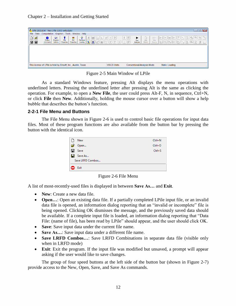
Chapter 2 – Installation and Getting Started
12
Figure 2-5 Main Window of LPile
As a standard Windows feature, pressing Alt displays the menu operations with
underlined letters. Pressing the underlined letter after pressing Alt is the same as clicking the
operation. For example, to open a New File, the user could press Alt-F, N, in sequence, Ctrl+N,
or click File then New. Additionally, holding the mouse cursor over a button will show a help
bubble that describes the button’s function.
2-2-1 File Menu and Buttons
The File Menu shown in Figure 2-6 is used to control basic file operations for input data
files. Most of these program functions are also available from the button bar by pressing the
button with the identical icon.
Figure 2-6 File Menu
A list of most-recently-used files is displayed in between Save As… and Exit.
New: Create a new data file.
Open…: Open an existing data file. If a partially completed LPile input file, or an invalid
data file is opened, an information dialog reporting that an “invalid or incomplete” file is
being opened. Clicking OK dismisses the message, and the previously saved data should
be available. If a complete input file is loaded, an information dialog reporting that “Data
File: (name of file), has been read by LPile” should appear, and the user should click OK.
Save: Save input data under the current file name.
Save As…: Save input data under a different file name.
Save LRFD Combos…: Save LRFD Combinations in separate data file (visible only
when in LRFD mode)
Exit: Exit the program. If the input file was modified but unsaved, a prompt will appear
asking if the user would like to save changes.
The group of four speed buttons at the left side of the button bar (shown in Figure 2-7)
provide access to the New, Open, Save, and Save As commands.

Chapter 2 – Installation and Getting Started
13
Figure 2-7 File Speed Buttons
2-2-2 Data Menu and Buttons
Please refer to Section 3-1 for a detailed discussion of this pull-down menu.
The group of buttons shown in Figure 2-8 provides access to the data editing commands
in the different modes of analysis.
(a) Buttons Available for Conventional Analysis
(b) Buttons Available for LRFD Analysis
(c) Buttons Available for Compute Nonlinear EI Only Analysis
Figure 2-8 Speed Buttons for Data Input for Different Analysis Modes
Four buttons are provided to review the input data in graphical form. The upper left
button shown in Figure 2-9 displays the pile and soil layer profile and the lower left button
presents a set of charts for reviewing the input soil and rock properties. The upper right button
presents a graph of distributed lateral loading versus depth. The lower right button presents a
three-panel graph of the p-modifier versus depth, y-modifier versus depth, and the ratio of p-
modifier over y-modifier versus depth.
Figure 2-9 Input Data Review Buttons
2-2-3 Computation Menu and Buttons
The Computation Menu shown in Figure 2-10 is provided to access commands to analyze
the input data and to view the input and output report files generated during an analysis.
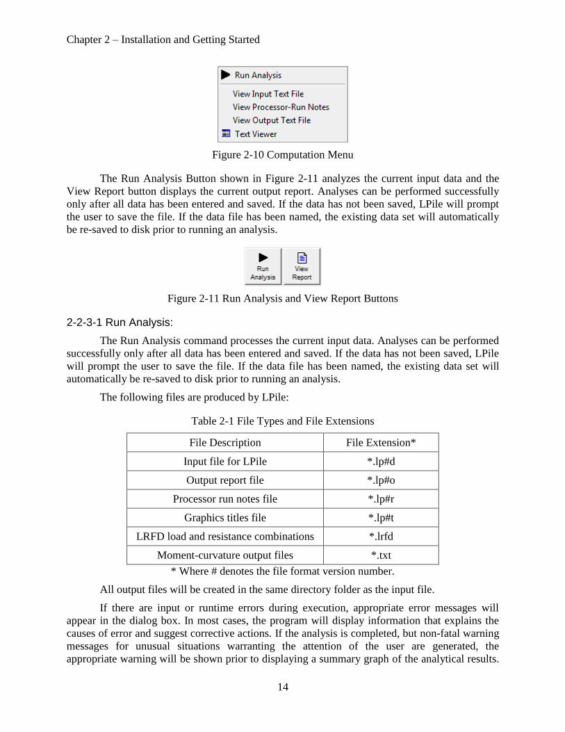
Chapter 2 – Installation and Getting Started
14
Figure 2-10 Computation Menu
The Run Analysis Button shown in Figure 2-11 analyzes the current input data and the
View Report button displays the current output report. Analyses can be performed successfully
only after all data has been entered and saved. If the data has not been saved, LPile will prompt
the user to save the file. If the data file has been named, the existing data set will automatically
be re-saved to disk prior to running an analysis.
Figure 2-11 Run Analysis and View Report Buttons
2-2-3-1 Run Analysis:
The Run Analysis command processes the current input data. Analyses can be performed
successfully only after all data has been entered and saved. If the data has not been saved, LPile
will prompt the user to save the file. If the data file has been named, the existing data set will
automatically be re-saved to disk prior to running an analysis.
The following files are produced by LPile:
Table 2-1 File Types and File Extensions
File Description File Extension*
Input file for LPile *.lp#d
Output report file *.lp#o
Processor run notes file *.lp#r
Graphics titles file *.lp#t
LRFD load and resistance combinations *.lrfd
Moment-curvature output files *.txt
* Where # denotes the file format version number.
All output files will be created in the same directory folder as the input file.
If there are input or runtime errors during execution, appropriate error messages will
appear in the dialog box. In most cases, the program will display information that explains the
causes of error and suggest corrective actions. If the analysis is completed, but non-fatal warning
messages for unusual situations warranting the attention of the user are generated, the
appropriate warning will be shown prior to displaying a summary graph of the analytical results.

Chapter 2 – Installation and Getting Started
15
If no error or warning messages are generate, the summary graph of results will be displayed
after the analysis is completed.
2-2-3-2 View Input Text:
This command activates the user-specified text editor to display the analytical input data
in plain-text format. This command is available after the input data has been saved to disk, or
when opening an existing input-data file. It is useful for experienced users who may just want to
change quickly one or two parameters using the text editor, or for users wishing to observe the
prepared input data in text mode.
2-2-3-3 View Processor Run Notes:
The program begins each analysis by first saving the current data to disk, then starting the
analysis routine that reads the input data from the saved disk file. If an error is detected, the
program will display a message dialog that informs the user about the type of error and, in many
cases, will suggest a solution for the error. Input errors may consist of missing data, erroneous
data, or inconsistent data. Usually, the content of the error message dialog is copied to the
processor run notes file. If the processor-run notes end without listing the line “The Execution is
in progress…,” the user should check the input corresponding to the last line read and the line
that immediately follows (that was not read). In some cases, the processor-run notes will also
include an error message.
2-2-3-4 View Output Report:
This command opens the output report in the text editor. This command becomes
available only after a successful run has been made. Some output files may be too large for
Microsoft Notepad to handle, so other text editors (Microsoft WordPad, for example) might need
to be used. Often, some versions of Microsoft Windows will automatically switch to the
alternative program without intervention by the user. Output report files usually contain the
following information:
1. Authorized user name, company, and security device serial number information.
2. The date and time of the analysis.
3. When nonlinear bending sections are part of the data, the output will contain results of
computations of nominal bending moment capacity and nonlinear moment curvature,
including bending stiffness as a function of axial thrust force, including a report of the input
data as well as tables of the computational results.
4. A report of input data for pile analysis. Users are strongly recommended to check this report
of input data for mistakes.
5. If selected, reports for selected p-y curves at user-specified output depths.
6. Tables of computed values of deflection, bending moment, shear, soil resistance, and related
information, as a function of depth for the pile.
7. Reports of convergence performance of the finite-difference approximations, providing data
about the maximum moment and lateral force imbalances observed during execution
(maximum imbalances should usually consist of small numbers).
8. Summary tables, containing information about the results and number of iterations performed
until convergence was reached.
9. An optional summary table of pile-head deflection versus pile length.
10. An optional summary table of foundation stiffness matrix components.

Chapter 2 – Installation and Getting Started
16
2-2-4 Graphics Menu and Buttons
Please refer Chapter 4 of this manual for a detailed discussion of the Graphics Menu.
The group of buttons shown in Figure 2-12 provides access to the graphs generated by
LPile. The enabling of buttons depends on the options selected and the output generated in the
analysis.
Figure 2-12 Graphics Buttons
2-2-5 Tools Menu
The Tools Menu has the five entries shown in Figure 2-13.
Figure 2-13 Tools Menu
The first entry provides a simple calculator for the user’s convenience.
The second entry provides a special calculator to compute axial and transverse forces
acting on battered piles from horizontal and vertical loadings.
The third to fifth entries provide a means of entering addition sizes of reinforcing steel
bar sizes to LPile. Note that this feature provides a means of entering hollow bars and steel
access tubes.
The third entry displays an input table to enter and edit the data for the custom
reinforcing bar sizes.
The fourth entry will transfer the data for custom reinforcing bars into the memory of
LPile and enter the names of the bars into the drop-down combination edit controls for selection
of the size of reinforcing bars. Note that the custom bar sizes are at the bottom of the drop-down
lists for bar sizes available for normally reinforced concrete sections.
The fifth entry saves the custom bar sizes to a data file named Custom_Rebar.dat. This
data file is stored in the same program folder as the main LPile program. When LPile is started,
LPile checks the program folder for a file with this name. If the file is found, it is read and the
data is stored into program memory. Thus, it is not necessary for the user to re-enter the custom
bar data each time the program is run. Whenever the user wishes to exchange data files with
another user, the data file for custom bar sizes should also be provided to the other user, as the
list of custom bar sizes is not included as part of the LPile data file.
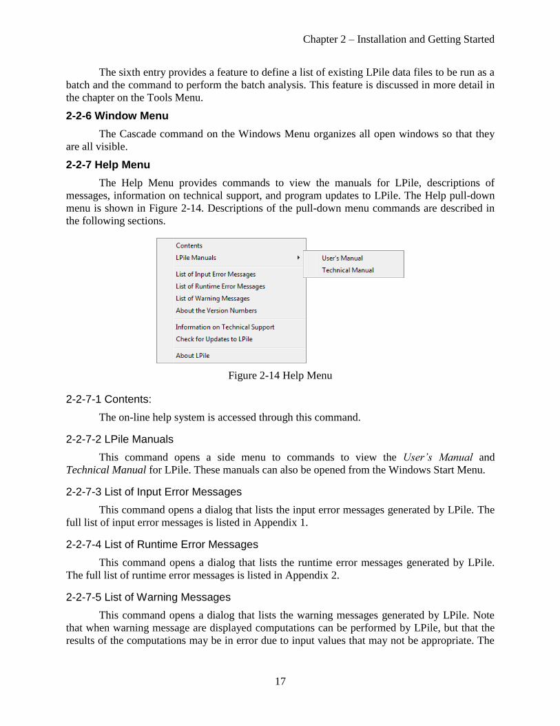
Chapter 2 – Installation and Getting Started
17
The sixth entry provides a feature to define a list of existing LPile data files to be run as a
batch and the command to perform the batch analysis. This feature is discussed in more detail in
the chapter on the Tools Menu.
2-2-6 Window Menu
The Cascade command on the Windows Menu organizes all open windows so that they
are all visible.
2-2-7 Help Menu
The Help Menu provides commands to view the manuals for LPile, descriptions of
messages, information on technical support, and program updates to LPile. The Help pull-down
menu is shown in Figure 2-14. Descriptions of the pull-down menu commands are described in
the following sections.
Figure 2-14 Help Menu
2-2-7-1 Contents:
The on-line help system is accessed through this command.
2-2-7-2 LPile Manuals
This command opens a side menu to commands to view the User’s Manual and
Technical Manual for LPile. These manuals can also be opened from the Windows Start Menu.
2-2-7-3 List of Input Error Messages
This command opens a dialog that lists the input error messages generated by LPile. The
full list of input error messages is listed in Appendix 1.
2-2-7-4 List of Runtime Error Messages
This command opens a dialog that lists the runtime error messages generated by LPile.
The full list of runtime error messages is listed in Appendix 2.
2-2-7-5 List of Warning Messages
This command opens a dialog that lists the warning messages generated by LPile. Note
that when warning message are displayed computations can be performed by LPile, but that the
results of the computations may be in error due to input values that may not be appropriate. The

Chapter 2 – Installation and Getting Started
18
purpose of the warning messages is to call the user’s attention to input values that may not be
correct. The full list of warning messages is listed in Appendix 3.
2-2-7-6 About the Version Numbers
Displays information about how the version numbers current used for LPile are defined.
2-2-7-7 Technical Support Information
Displays information about eligibility for receiving technical support and how to receive
technical support from Ensoft.
2-2-7-8 Check for Updates
Opens the LPile update page in the user’s default browser.
Note that some anti-virus programs may require the user to grant permission to LPile to
open the Internet browser program.
2-2-7-9 About LPile
This command provides a dialog describing the program version, date, and methods for
accessing technical support. Other information about the program licensing and maintenance
expiration date, program version, and program release date are also shown. An example is shown
below.
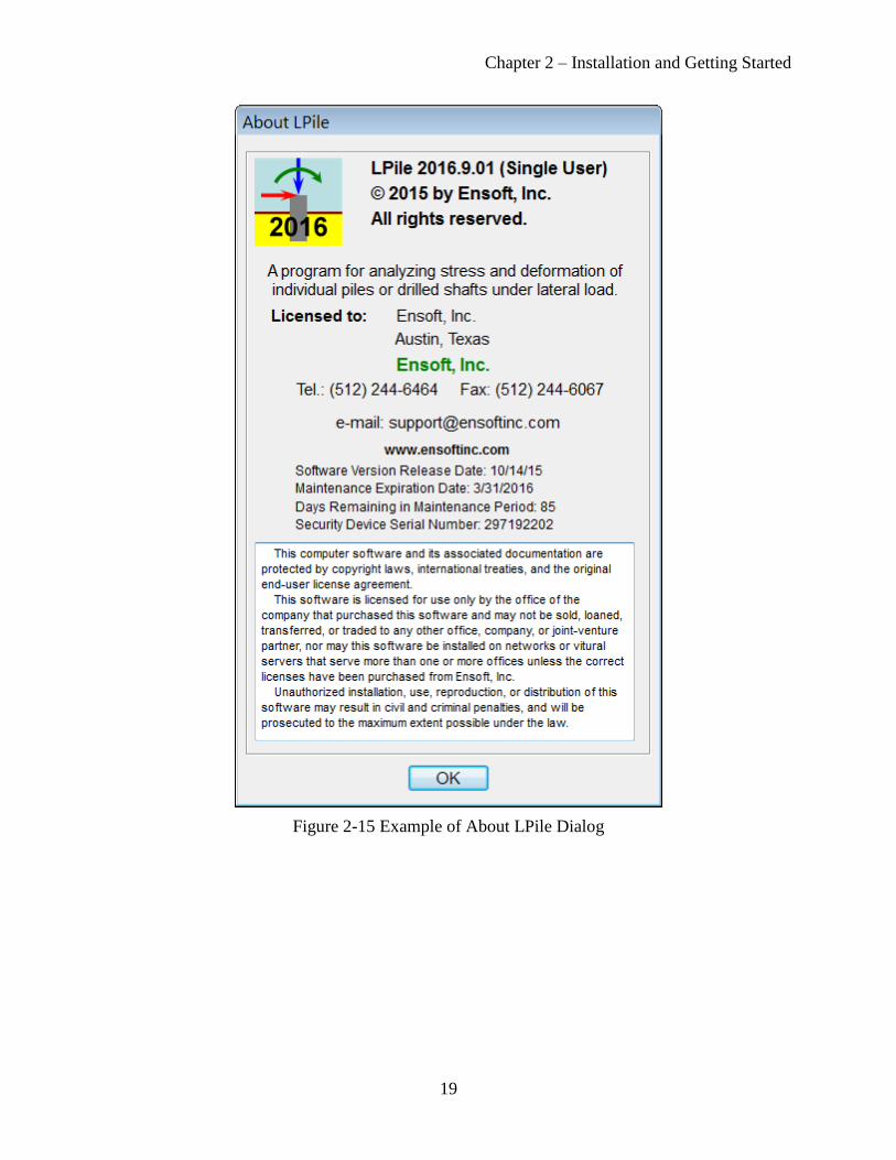
Chapter 2 – Installation and Getting Started
19
Figure 2-15 Example of About LPile Dialog

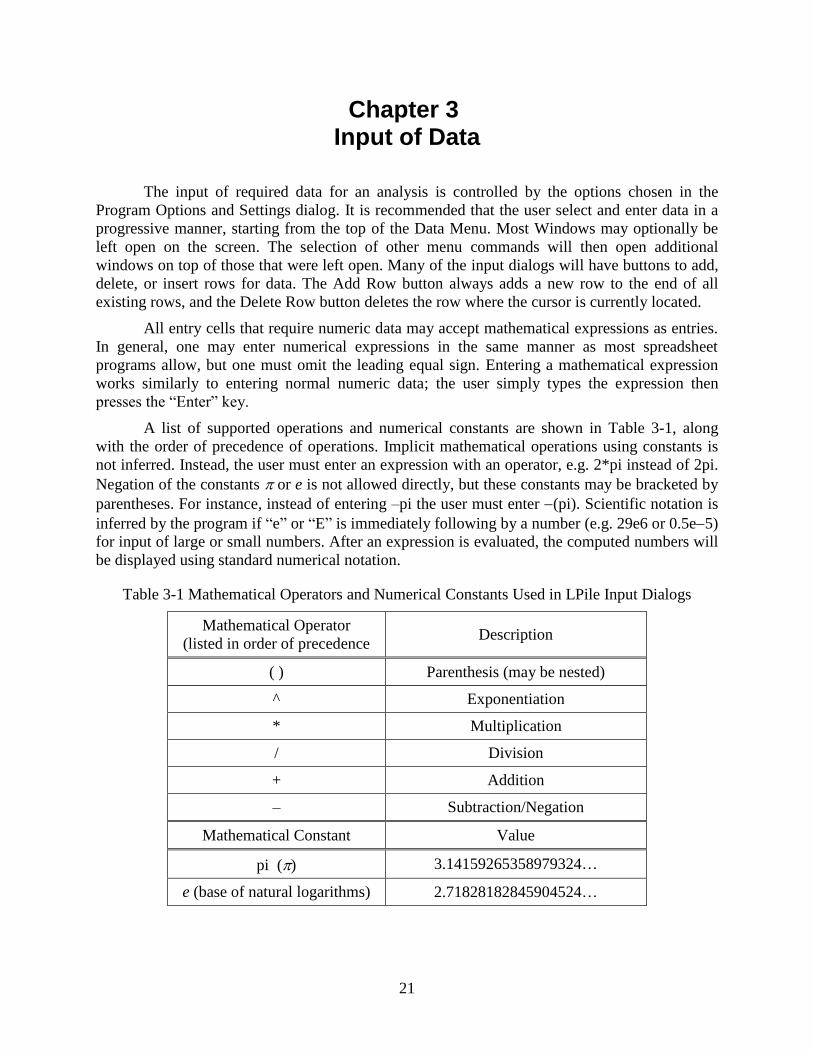
21
Chapter 3 Input of Data
The input of required data for an analysis is controlled by the options chosen in the
Program Options and Settings dialog. It is recommended that the user select and enter data in a
progressive manner, starting from the top of the Data Menu. Most Windows may optionally be
left open on the screen. The selection of other menu commands will then open additional
windows on top of those that were left open. Many of the input dialogs will have buttons to add,
delete, or insert rows for data. The Add Row button always adds a new row to the end of all
existing rows, and the Delete Row button deletes the row where the cursor is currently located.
All entry cells that require numeric data may accept mathematical expressions as entries.
In general, one may enter numerical expressions in the same manner as most spreadsheet
programs allow, but one must omit the leading equal sign. Entering a mathematical expression
works similarly to entering normal numeric data; the user simply types the expression then
presses the “Enter” key.
A list of supported operations and numerical constants are shown in Table 3-1, along
with the order of precedence of operations. Implicit mathematical operations using constants is
not inferred. Instead, the user must enter an expression with an operator, e.g. 2*pi instead of 2pi.
Negation of the constants or e is not allowed directly, but these constants may be bracketed by
parentheses. For instance, instead of entering –pi the user must enter (pi). Scientific notation is
inferred by the program if “e” or “E” is immediately following by a number (e.g. 29e6 or 0.5e5)
for input of large or small numbers. After an expression is evaluated, the computed numbers will
be displayed using standard numerical notation.
Table 3-1 Mathematical Operators and Numerical Constants Used in LPile Input Dialogs
Mathematical Operator
(listed in order of precedence Description
( ) Parenthesis (may be nested)
^ Exponentiation
* Multiplication
/ Division
+ Addition
– Subtraction/Negation
Mathematical Constant Value
pi () 3.14159265358979324…
e (base of natural logarithms) 2.71828182845904524…

Chapter 3 – Input of Data
22
3-1 Data Menu
The editing commands are presented on the Data Menu shown in Figure 3-1. The
commands in the upper three sections of the Data Menu are enabled by default when LPile is
started. The commands in the bottom section of the Data Menu are enabled by activation of the
relevant program options.
Figure 3-1 Data Menu
The icons shown in the Data Menu are the same as those used to access the same editing
dialogs via the button bar.
3-2 Speed Buttons for Data Entry
The button bar contains a set of buttons to open the dialogs for the entry and
manipulation of data. The buttons for data entry for conventional analysis are shown in Figure
3-2, for Computation of EI only are shown in Figure 3-3, and for LRFD Analysis are shown in
Figure 3-4.
Figure 3-2 Buttons for Data Entry and Manipulation for Conventional Analysis
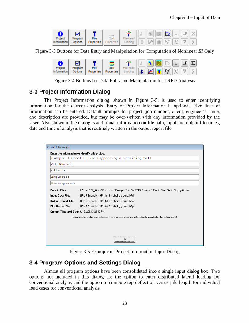
Chapter 3 – Input of Data
23
Figure 3-3 Buttons for Data Entry and Manipulation for Computation of Nonlinear EI Only
Figure 3-4 Buttons for Data Entry and Manipulation for LRFD Analysis
3-3 Project Information Dialog
The Project Information dialog, shown in Figure 3-5, is used to enter identifying
information for the current analysis. Entry of Project Information is optional. Five lines of
information can be entered. Default prompts for project, job number, client, engineer’s name,
and description are provided, but may be over-written with any information provided by the
User. Also shown in the dialog is additional information on file path, input and output filenames,
date and time of analysis that is routinely written in the output report file.
Figure 3-5 Example of Project Information Input Dialog
3-4 Program Options and Settings Dialog
Almost all program options have been consolidated into a single input dialog box. Two
options not included in this dialog are the option to enter distributed lateral loading for
conventional analysis and the option to compute top deflection versus pile length for individual
load cases for conventional analysis.
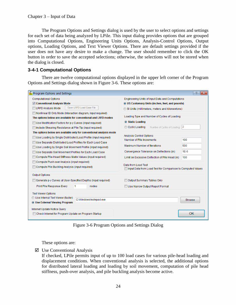
Chapter 3 – Input of Data
24
The Program Options and Settings dialog is used by the user to select options and settings
for each set of data being analyzed by LPile. This input dialog provides options that are grouped
into Computational Options, Engineering Units Options, Analysis-Control Options, Output
options, Loading Options, and Text Viewer Options. There are default settings provided if the
user does not have any desire to make a change. The user should remember to click the OK
button in order to save the accepted selections; otherwise, the selections will not be stored when
the dialog is closed.
3-4-1 Computational Options
There are twelve computational options displayed in the upper left corner of the Program
Options and Settings dialog shown in Figure 3-6. These options are:
Figure 3-6 Program Options and Settings Dialog
These options are:
Use Conventional Analysis
If checked, LPile permits input of up to 100 load cases for various pile-head loading and
displacement conditions. When conventional analysis is selected, the additional options
for distributed lateral loading and loading by soil movement, computation of pile head
stiffness, push-over analysis, and pile buckling analysis become active.
Chapter 3 – Input of Data
25
Use Load and Resistance Factors
If checked, LPile will perform Load and Resistance Factor Design (LRFD) computations.
In this mode, the user may enter up to 100 unfactored shear and moment loads of various
loading types (dead load, live load, etc.). All loads are assumed to be for shear and
moment pile-head loading conditions. The program will then add all loads of the same
load type to obtain the total unfactored load for each loading type. Optionally, the LRFD
case load combinations may be either read from or saved to an external file (with the file
type of lrfd) or may be entered by the user.
Compute Nonlinear EI Only
If checked, LPile will compute nonlinear moment-curvature relations and nominal
(unfactored) and ultimate (factored) moment capacities of the pile sections for the
specified axial thrust force values.
Include Modification Factors for Group Action: Activates p-y Modification Factors for
Group Action under the Data Menu.
Include Shearing Resistance at Pile Tip: Activates Shear Resistance Curve at Pile-Tip
under the Data Menu.
The following options become active only when using conventional analysis.
Use loading by single distributed lateral loading profile
Use separate distributed loading profiles per load case
Use loading by single soil movement profile.
Use separate soil movement profiles per load case.
Compute Pile-Head Stiffness Matrix Values
If this option is selected, LPile computes the pile-head stiffness matrix values according
to the control values set by the user in the Controls for Computation of Stiffness Matrix
dialog discussed in Section 3-12-4.
Compute pushover analysis
If this option is selected, LPile computes the pushover analysis according to the controls
set by the use in the Controls for Pushover Analysis dialog discussed in Section 3-12-5.
Compute pile buckling analysis
If this option is selected, LPile computes the pile-buckling analysis according to the
controls set by the user in the Controls for Pile Buckling analysis discussed in Section 3-
12-6.
3-4-2 Engineering Units of Input Data and Computations
Here the user can specify either US Customary System (USCS) units using pounds,
inches, and feet or the International System of Units (Système international d’unités or SI) units
using millimeters, meters, and kilonewtons for entering and displaying data. The prior setting for
engineering units is remembered by the program. Thus, when LPile is started, the default units
are the engineering units used in the prior analysis. If a data file is read by LPile, the engineering
units are switched to the units specified in the data file.
All input data is converted to consistent units of length and force before computations are
made. The consistent units are either pounds and inches or kilonewtons and meters.
Chapter 3 – Input of Data
26
3-4-3 Analysis Control Options
The Analysis Control Options are used to specify the number of pile increments, the
maximum number of iterations, the convergence tolerance on deflections, the limit on excessive
deflection of the pile head, and the number of pile increments.
3-4-3-1 Number of Pile Increments
The quality of the finite-difference numerical solution obtained by LPile is proportional
to the square of the length of the pile increment. The length of the pile increment is computed by
dividing the length of the pile by the number of pile increments.
The error in the solution computed by LPile is defined as the difference between the
approximation and the exact analytical solution. The two sources of error in finite difference
methods are round-off error, the loss of precision due to computer rounding of decimal
quantities, and truncation error or discretization error, the difference between the exact solution
of the finite difference equation and the exact quantity assuming perfect arithmetic (that is,
assuming no round-off error).
The default number of pile increments is 100, the minimum number of pile increments is
40, and maximum number of pile increments is 500.
Often the user may opt to use an odd number of increments to obtain computed results at
specific rounded valued of depth. For example, a user may opt to use 140 increments to obtain
results for every 0.5 feet of depth for a 70-ft-long pile.
3-4-3-2 Maximum Number of Iterations
The maximum number of iterations performed by the program for the pile solution can be
set by the user. Many problems will converge in fewer than 50 iterations unless a plastic hinge is
being developed in an analysis using nonlinear EI. If a pushover analysis is being performed
using the displacement and moment pile-head boundary condition, the iterations limit should be
set to the maximum value of 1,000 iterations to allow plastic hinges to develop in the pile.
Table 3-2 Recommended Ranges for Maximum Number of Iterations
Recommended 500 to 750
Lower Limit 100
Upper Limit: 1,000
The user should be aware that specifying 1,000 iterations has a special feature. If the
problem is solved using fewer than 1,000 iterations, the solution has met the convergence
tolerance and excessive deflection criteria. However, if the program reached the limit of 1,000
iterations, the program is highly unlikely to obtain convergence. Instead, the program outputs the
last iterative solution obtained and the solution stops.
3-4-3-3 Convergence Tolerance
The value entered for convergence tolerance is used to stop an analysis when the absolute
value of the change in deflection of every nodal point on the pile is less than the convergence
Chapter 3 – Input of Data
27
tolerance. The default value for convergence tolerance is 0.00001 inches or 2.54×10⁻⁷
meters.
Using a smaller value for convergence tolerance usually does not improve the quality of the
solution and in some conditions may result in failure to obtain a solution. Using a larger
convergence tolerance is sometimes required, but the user should cautious when using values
larger the 0.0001 inches or 2.54×10⁻⁶
meters.
3-4-3-4 Limit on Excessive Lateral Pile Deflection
The limit on excessive lateral pile deflection is used to end analyses in which the iterative
solution is diverging without limit. The user should enter a value of deflection for the pile head
that is grossly excessive to stop the analysis. The default value is 100 inches or 2.54 meters. If
the user wished to modify this value, a recommended value is 10 times the pile diameter.
Lowering the Excessive Deflection Value to less than 100 inches or 2.54 meters is not
recommended.
3-4-4 Loading Type and Number of Cycles of Loading
The user can specify either static or cyclic loading in the option group for Loading Type
and Number of Cycles of Loading. Selection of type of loading is important when analyzing
piles under lateral forces. Further information on the influence of loading type is included in the
Technical Manual.
In general, cyclic loading is primarily used for low frequency, large amplitude storm
wave or wind loads. Dynamic loading from earthquakes and machine vibrations are not the same
as cyclic loads considered in LPile. When cyclic loading is selected, the user must also specify
the number of cycles of loading, ranging from 2 to 5,000 cycles. The effect of cyclic loading is to
change how the soil resistance is computed for the p-y curves, as described in the Technical
Manual.
Dynamic loading from earthquakes can be analyzed by LPile if equivalent pseudo-static
loads are input. Pseudo-static loads are sized in a manner that results in computed moments and
deflections that roughly equivalent to those developed during seismic loading events.
Dynamic loading from machine vibrations or most other sources of harmonic loading
should not be analyzed using LPile because LPile is not capable of determining the frequency
response of the foundation and other inertial effects. Instead, the user is directed to the use of the
DynaN, DynaPile, or DynaMat programs from Ensoft or some other program for performing
dynamic response analyses.
3-4-5 Output Options
Several options are provided to control the output reports generated during LPile
analyses. These options are enabled by checking the check boxes described below.
3-4-5-1 Generate p-y Curves at User-Specified Depths
Checking activates the feature to output p-y curves at the depths specified by the user.
Note that for battered piles, the specified depth is the vertical depth below the pile head, not the
distance along the axis of the pile.

Chapter 3 – Input of Data
28
3-4-5-2 Print Summary Tables Only
Checking this option activates the printing of summary tables only for computations of
pile bending stiffness and pile response.
3-4-5-3 Printing Increment
The user may also specify the output increment for where results will be printed in the
table of output. As a default, results are printed at every finite increment of pile length. This
option is disabled if the user has a check mark on the Only Print Summary Tables option. A
value of 1 prints the values at every node; 2 prints values at every other nodes, etc. Note that the
printing increment is used only for the generation of the output report, but not for the generation
of output graphs.
3-4-5-4 Use Narrow Output Report Format
This option controls the printed width of the output reports, permitting printing on letter-
size paper without word wrapping of long lines. It is necessary to specify a fixed-pitch font of 10
point or smaller size to display the output correctly. The user should be aware that only the most
important columns of output results are displayed when this option is selected.
3-4-6 Text Viewer Options
The user should enter the complete path and command line for their preferred text editor
or word processor. As a default, the command line c:\windows\notepad.exe sets Microsoft
Notepad as the default text editor. An internal text editor can also be selected. The selected text
editor will be used for View Input Text File, View Processor Run Notes, View Output Text File,
and Text Viewer under the Computation Menu.
3-4-7 Input of Data from Load Testing
It is possible to enter and save load test data input into LPile and to display the load test
data along with the results computed by LPile on the graphs of pile-head shear force versus pile-
head deflection and bending moment versus depth. The ability to enter and save load test data is
enabled by checking this option.
3-4-8 Internet Update Notice Query
Checking the Show Internet Update Notice Query on Program Startup restores the
automatic display of this query dialog if this option has been turned off.
3-5 Structural Dimensions and Material Properties
3-5-1 General Description of Input
LPile has features to evaluate the nominal moment capacity and nonlinear bending
stiffness relationships for deep foundations made from normally-reinforced concrete, pipe
sections, and prestressed concrete. These features can determine how the effective bending
stiffness will vary as the concrete cracks in tension and the reinforcing steel yields.
Use of the features to evaluate ultimate moment capacity and nonlinear bending stiffness
is essential when analyzing the behavior of drilled shafts under lateral loading.
The user must click the OK button in order to save the accepted selections; otherwise, the
selections will not be saved when the input dialog is closed.

Chapter 3 – Input of Data
29
3-5-2 Section Type and Shape
The tab page for Section Type and Shape is shown in Figure 3-7. There are 14 general
types of sections and a pile may have up to 20 different sections of different section types. The
default section type is an elastic (non-yielding) section. All other section types have either
specified or computed structural moment capacities and will have non-linear moment-curvature
relationships.
The dialog box shown in Figure 3-7 is for an H-pile defined as an elastic section, after
definition of the structural shape. Once the section shape and dimensions have been properly
defined, a scale drawing of the section or section profile is displayed, as shown below.
The user should note the tab pages shown in the input dialog. For an elastic section, only
two tabs are shown. For other types of sections, the number of tab pages shown will depend on
the types of materials used in the section type selected.
The light yellow memo shown below the tab pages gives a general description of the
section type and may provide special guidance in its use and construction.
Figure 3-7 Pile Section, Section Type Tab
3-5-3 Warning and Design Error Messages
LPile provides warning messages and advice for design for several of the structural types.
The purpose for these warning messages is to alert the user either to design geometries that may
be difficult to construct and to alert the user if inappropriate design parameters have been
specified by the user. A short discussion of several types of the warning messages follows.
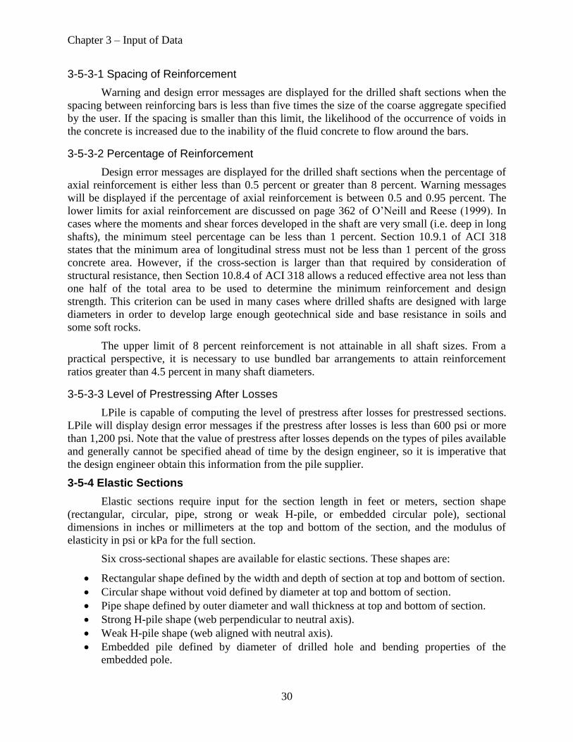
Chapter 3 – Input of Data
30
3-5-3-1 Spacing of Reinforcement
Warning and design error messages are displayed for the drilled shaft sections when the
spacing between reinforcing bars is less than five times the size of the coarse aggregate specified
by the user. If the spacing is smaller than this limit, the likelihood of the occurrence of voids in
the concrete is increased due to the inability of the fluid concrete to flow around the bars.
3-5-3-2 Percentage of Reinforcement
Design error messages are displayed for the drilled shaft sections when the percentage of
axial reinforcement is either less than 0.5 percent or greater than 8 percent. Warning messages
will be displayed if the percentage of axial reinforcement is between 0.5 and 0.95 percent. The
lower limits for axial reinforcement are discussed on page 362 of O’Neill and Reese (1999). In
cases where the moments and shear forces developed in the shaft are very small (i.e. deep in long
shafts), the minimum steel percentage can be less than 1 percent. Section 10.9.1 of ACI 318
states that the minimum area of longitudinal stress must not be less than 1 percent of the gross
concrete area. However, if the cross-section is larger than that required by consideration of
structural resistance, then Section 10.8.4 of ACI 318 allows a reduced effective area not less than
one half of the total area to be used to determine the minimum reinforcement and design
strength. This criterion can be used in many cases where drilled shafts are designed with large
diameters in order to develop large enough geotechnical side and base resistance in soils and
some soft rocks.
The upper limit of 8 percent reinforcement is not attainable in all shaft sizes. From a
practical perspective, it is necessary to use bundled bar arrangements to attain reinforcement
ratios greater than 4.5 percent in many shaft diameters.
3-5-3-3 Level of Prestressing After Losses
LPile is capable of computing the level of prestress after losses for prestressed sections.
LPile will display design error messages if the prestress after losses is less than 600 psi or more
than 1,200 psi. Note that the value of prestress after losses depends on the types of piles available
and generally cannot be specified ahead of time by the design engineer, so it is imperative that
the design engineer obtain this information from the pile supplier.
3-5-4 Elastic Sections
Elastic sections require input for the section length in feet or meters, section shape
(rectangular, circular, pipe, strong or weak H-pile, or embedded circular pole), sectional
dimensions in inches or millimeters at the top and bottom of the section, and the modulus of
elasticity in psi or kPa for the full section.
Six cross-sectional shapes are available for elastic sections. These shapes are:
Rectangular shape defined by the width and depth of section at top and bottom of section.
Circular shape without void defined by diameter at top and bottom of section.
Pipe shape defined by outer diameter and wall thickness at top and bottom of section.
Strong H-pile shape (web perpendicular to neutral axis).
Weak H-pile shape (web aligned with neutral axis).
Embedded pile defined by diameter of drilled hole and bending properties of the
embedded pole.
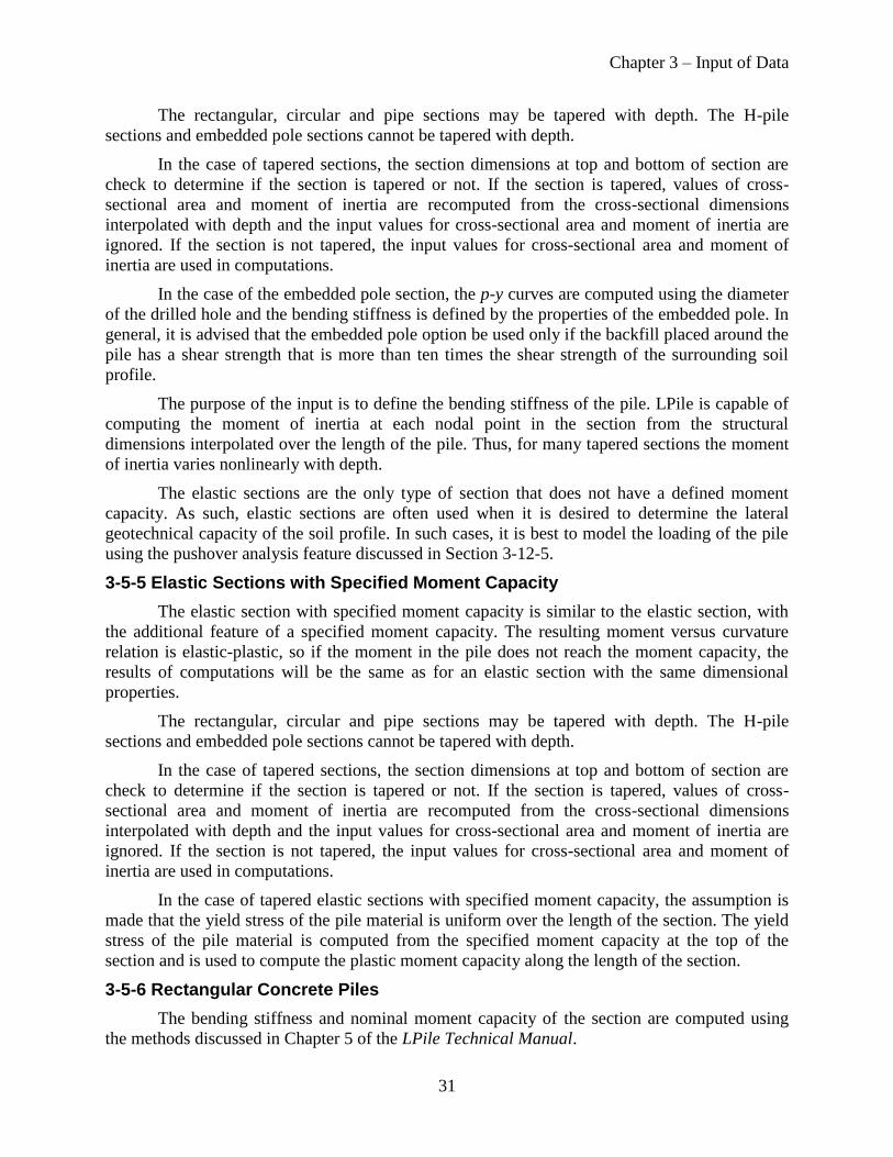
Chapter 3 – Input of Data
31
The rectangular, circular and pipe sections may be tapered with depth. The H-pile
sections and embedded pole sections cannot be tapered with depth.
In the case of tapered sections, the section dimensions at top and bottom of section are
check to determine if the section is tapered or not. If the section is tapered, values of cross-
sectional area and moment of inertia are recomputed from the cross-sectional dimensions
interpolated with depth and the input values for cross-sectional area and moment of inertia are
ignored. If the section is not tapered, the input values for cross-sectional area and moment of
inertia are used in computations.
In the case of the embedded pole section, the p-y curves are computed using the diameter
of the drilled hole and the bending stiffness is defined by the properties of the embedded pole. In
general, it is advised that the embedded pole option be used only if the backfill placed around the
pile has a shear strength that is more than ten times the shear strength of the surrounding soil
profile.
The purpose of the input is to define the bending stiffness of the pile. LPile is capable of
computing the moment of inertia at each nodal point in the section from the structural
dimensions interpolated over the length of the pile. Thus, for many tapered sections the moment
of inertia varies nonlinearly with depth.
The elastic sections are the only type of section that does not have a defined moment
capacity. As such, elastic sections are often used when it is desired to determine the lateral
geotechnical capacity of the soil profile. In such cases, it is best to model the loading of the pile
using the pushover analysis feature discussed in Section 3-12-5.
3-5-5 Elastic Sections with Specified Moment Capacity
The elastic section with specified moment capacity is similar to the elastic section, with
the additional feature of a specified moment capacity. The resulting moment versus curvature
relation is elastic-plastic, so if the moment in the pile does not reach the moment capacity, the
results of computations will be the same as for an elastic section with the same dimensional
properties.
The rectangular, circular and pipe sections may be tapered with depth. The H-pile
sections and embedded pole sections cannot be tapered with depth.
In the case of tapered sections, the section dimensions at top and bottom of section are
check to determine if the section is tapered or not. If the section is tapered, values of cross-
sectional area and moment of inertia are recomputed from the cross-sectional dimensions
interpolated with depth and the input values for cross-sectional area and moment of inertia are
ignored. If the section is not tapered, the input values for cross-sectional area and moment of
inertia are used in computations.
In the case of tapered elastic sections with specified moment capacity, the assumption is
made that the yield stress of the pile material is uniform over the length of the section. The yield
stress of the pile material is computed from the specified moment capacity at the top of the
section and is used to compute the plastic moment capacity along the length of the section.
3-5-6 Rectangular Concrete Piles
The bending stiffness and nominal moment capacity of the section are computed using
the methods discussed in Chapter 5 of the LPile Technical Manual.

Chapter 3 – Input of Data
32
The properties for the rectangular concrete pile are defined by the length, width, and
depth of section; the compressive strength of concrete; and the number, positions, yield stress,
and modulus of elasticity of the reinforcing steel bars. The tab pages for this data are shown in
Figure 3-8 through Figure 3-10.
Figure 3-8 Dimensions Tab Page for Rectangular Concrete Section
Figure 3-9 Concrete Tab Page for Rectangular Concrete Section
The positions of the reinforcing steel bars are defined using an x-y coordinate system with
the origin positioned at the centroid of the section. The user must enter the positions of the bars
and must select the size of bars from the available sizes programmed in LPile. The rebar layout
table is shown in Figure 3-11. Once the position and size of reinforcing steel has been entered,
LPile will display a scale drawing of the section as shown in Figure 3-12.
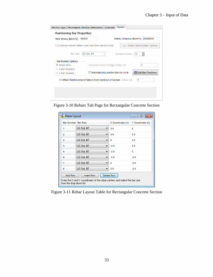
Chapter 3 – Input of Data
33
Figure 3-10 Rebars Tab Page for Rectangular Concrete Section
Figure 3-11 Rebar Layout Table for Rectangular Concrete Section

Chapter 3 – Input of Data
34
Figure 3-12 Section Type, Dimensions, and Cross-section Properties Dialog for Rectangular
Concrete Section Showing Rebar Layout After Definition
3-5-7 Round Concrete Shafts (Bored Piles)
The properties of drilled shafts (also called bored piles) are defined by the length and
outer diameter of the shaft; the number, positions, yield stress, and modulus of elasticity of the
reinforcing steel bars; and the compressive strength of concrete. Features are provided in LPile to
compute the positions of circular bar arrangements with single-bar, two-bar, and three-bar
bundles utilizing the clear cover dimension and any offset of the bar cage from the shaft center.
In addition, the position and size of bars can be manually edited if desired.
The dialog shown in Figure 3-13 is an example of the Section Type page after the Round
Concrete Shaft (Bored Pile) option has been selected. This drawing of the cross-section shows
the current size, number, bundling, and positions of the reinforcing bars selected.
The Shaft Dimensions tab page shows the shaft dimensions. All data entry cells for which
input is not required are disabled. In the case of a round concrete shaft, the only required
dimensions are the section length in feet or meters and diameter in inches or millimeters.
The Concrete tab page, shown before in Figure 3-9, shows the compressive strength of
concrete and the maximum size of coarse aggregate. The maximum size of coarse aggregate is
used when LPile checks the spacing dimension between bars to ensure that sufficient space is
provided for the concrete to flow during placement of concrete.
Chapter 3 – Input of Data
35
Figure 3-13 Tab Sheet for Selection of Section Type Showing Current Cross-section
The layout of reinforcement is defined by specifying the size of reinforcement, number of
bars, bar bundle size, concrete cover thickness, and offset of the reinforcement cage from the
centroid (if any) as shown in Figure 3-14. The drawing of the cross-section automatically
updates to indicate any changes in the geometric properties of the reinforcing bars.
When entering data for the arrangement of reinforcing steel, the user’s attention is drawn
to the advice of the comment note in the lower third of the dialog shown above. It is important
for the designer to anticipate whether or not temporary casing is used. When temporary casing is
used in construction, best design practice is to specify a concrete cover thickness of 4 inches
(100 mm) so that standard size shaft spacers (typically 3 inches or 75 mm) can be used to center
the reinforcing steel inside the temporary casing. After concrete is placed and the temporary
casing is removed, the concrete in the shaft will flow outward to fill the volume left by the casing
and the annular space outside of the casing.

Chapter 3 – Input of Data
36
Figure 3-14 Tab Sheet for Reinforcing Bar Properties
3-5-8 Round Concrete Shaft with Permanent Casing
The properties of round concrete drilled shafts with permanent casing are defined by the
length and outer diameter of the casing; the wall thickness of the casing; the yield stress and
modulus of elasticity of the casing; the number, positions, yield stress, and modulus of elasticity
of the reinforcing steel bars; and the compressive strength of concrete.
The Dimensions tab page, shown in Figure 3-15 shows the dimensions for the outer
diameter and wall thickness of the permanent casing. The drawing of the cross-section will
automatically update to show any changes in the shaft geometric properties for casing or
reinforcing bars.

Chapter 3 – Input of Data
37
Figure 3-15 Tab Sheet for Shaft Dimensions for Drilled Shaft with Permanent Casing
The tab page for reinforcement is similar to that used for drilled shafts, except that the
label for the entry cell for concrete cover has be modified to indicate that the cover dimension is
measured inside the permanent casing as shown in Figure 3-16.
Figure 3-16 Tab Sheet for Rebars for Drilled Shaft with Permanent Casing
The tab page for casing material properties, shown in Figure 3-17, is visible only for the
drilled shaft sections that utilize permanent casing. The material properties required for
permanent casing are the yield stress and modulus of elasticity.

Chapter 3 – Input of Data
38
Figure 3-17 Tab Sheet for Casing Material Properties for Drilled Shaft with Permanent Casing
3-5-9 Round Concrete Shaft with Permanent Casing and Core
The properties of round concrete drilled shafts with permanent casing and core are
defined by:
the length and outer diameter of the casing;
the wall thicknesses of the casing and core;
the yield stress and modulus of elasticity of the casing and core;
the number, positions, yield stress, and modulus of elasticity of the reinforcing steel bars;
and
the compressive strength of concrete.
In addition, the user may specify if the core is filled with concrete by checking the box on the
casing and core materials tab page.
The Shaft Dimensions tab page for a drilled shaft with casing and core is shown in Figure
3-18. The drawing of the cross-section will automatically update to show any changes in the
shaft geometric properties for casing, core, or reinforcing bars.
The values entered for the wall thickness values of the casing and core may be zero to
model a shaft without a casing or core. This feature enables one to model a drilled shaft with a
structural steel insert. This is done by entering a set of core diameter and wall thickness that has
a moment of inertia equal to that for the structural steel insert.

Chapter 3 – Input of Data
39
Figure 3-18 Tab Sheet forShaft Dimensions of Drilled Shaft with Casing and Core
An example of the computation of an equivalent wall thickness is as follows. Suppose
that a 14x89 H-pile is being used as a structural insert. The flange width is 14.7 inches and the
moment of inertia is 904 in4. The equivalent wall thickness of a pipe section of the same width
and moment of inertia is
in. 866.02
)904)(64(7.147.14
2
644
44
4
Idd
too
The moment of inertia will be computed as a check on the computation for t. A check
computation yields a result of 903.90 in4, which is acceptable because a closer match would have
required more significant digits for t.
The tab page for material properties of the casing and core is shown in Figure 3-19. Also
shown on this tab page is the check box to indicate if the core is filled or unfilled with concrete.

Chapter 3 – Input of Data
40
Figure 3-19 Tab Sheet for Casing and Core Material Properties
In most problems, the influence of the concrete inside the core has little effect on the
computed bending stiffness, but may have a noticeable effect on the computed axial compressive
structural capacity of the section.
The tab page for rebar is identical to that shown for drilled shaft with permanent casing.
It is not necessary to include reinforcing bars when modeling a section with a structural
insert. To omit the bars, enter zero for the number of bars.
3-5-10 Steel Pipe Pile
The properties of steel pipe piles are defined by the length, outside diameter, and wall
thickness of the pile section as shown in Figure 3-20. The material properties are the yield stress
and modulus of elasticity as shown in Figure 3-21.
The computed curve of moment versus curvature for a steel pipe pile is shown in Figure
3-22(a).
Alternatively, a steel pile section could be modelled as an elastic-plastic section.
However, the development of plastic yielding across the cross-section will not be modelled and
the utilized moment versus curvature relationship is bilinear as shown in Figure 3-22(b).
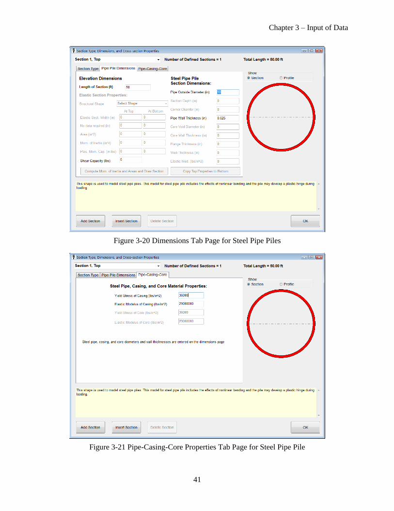
Chapter 3 – Input of Data
41
Figure 3-20 Dimensions Tab Page for Steel Pipe Piles
Figure 3-21 Pipe-Casing-Core Properties Tab Page for Steel Pipe Pile

Chapter 3 – Input of Data
42
(a)
(b)
Figure 3-22 Comparison of Moment vs. Curvature for (a) Steel Pipe Pile and (b) Elastic-Plastic
Pipe Pile with Similar Properties
3-5-11 Round Prestressed Concrete Pile
The properties of round prestressed concrete piles are defined by the length and diameter
of the pile, the compressive strength of concrete, the prestressing reinforcement details, and the
loss of prestress.
LPile 2015.8.03, © 2015 by Ensoft, Inc.
Curvature, radians/inch0.00060.00040.00020.0
Mo
me
nt, in
-kip
s
6,500
6,000
5,500
5,000
4,500
4,000
3,500
3,000
2,500
2,000
1,500
1,000
500
0
LPile 2015.8.03, © 2015 by Ensoft, Inc.
Curvature, radians/inch0.00060.00040.00020.0
Mo
me
nt, in
-kip
s
6,500
6,000
5,500
5,000
4,500
4,000
3,500
3,000
2,500
2,000
1,500
1,000
500
0

Chapter 3 – Input of Data
43
The usual procedure for the LPile user is to enter the pile dimensions, compressive
strength of concrete, the number and size of prestress reinforcement strands, and concrete cover
dimension. The Prestressing tab page for entering prestressing data for all types of prestressed
concrete piles is shown in Figure 3-23. Once the prestressing size, number, and geometry are
entered, the cross-section of the pile should be drawn by LPile. If the cross-section is not drawn
properly, there is an error in the input data.
Figure 3-23 Prestressing Tab Page Common to All Prestressed Pile Types
As a designer, the engineer can specify the length, diameter, concrete compressive
strength, and reinforcement of a prestressed pile, but must find out from the pile supplier what
value the expected fraction of loss of prestress is expected to be. Sometimes, the supplier will
provide the final prestress after losses. The engineer can then determine what the fraction of loss
of prestress is, provided the initial prestressing forces before losses is provided. The common
practice for pile suppliers is to use 70 percent of the rated prestressing capacity of the
reinforcement as the prestress force. This value is programmed in LPile for the listed sizes and
types or prestress reinforcement.
Next, the user enters the fraction of loss provided by the pile supplier. For preliminary
computations prior to selecting a pile supplier, the user may enter a value in the typical range
between 0.10 and 0.20. The value of prestress after losses is computed by LPile by pressing the
button to Compute 70% Prestress Force and Stress. The value computed by LPile will be shown
in the dialog and will be classified as OK if the prestress after losses is in the range of 600 to
1,200 psi (4.14 to 8.27 MPa), or as too high or too low if outside of this range.

Chapter 3 – Input of Data
44
3-5-12 Round Prestressed Concrete Pile with Void
The properties of round prestressed concrete piles with void are defined by the length and
diameter of the pile, the diameter of the hollow core void, the compressive strength of concrete,
and the prestressing reinforcement and loss of prestress.
The input for the round prestressed concrete pile with void is the same as for the round
prestressed pile without void, with the exception of the entry of the diameter of the core void.
Please refer to the discussion in Section 3-5-11 for information about the computation of
prestress after losses.
3-5-13 Square Prestressed Concrete Pile
The properties of square prestressed concrete piles are defined by the length and width of
the pile, the size of the corner chamfer, the compressive strength of concrete, and the prestressing
reinforcement and loss of prestress.
The input for the square prestressed concrete pile is the largely same as for the round
prestressed pile without void, with the exception of the entry of the dimensions for the pile width
and corner chamfer. Please refer to the discussion in Section 3-5-11 for information about the
computation of prestress after losses.
An additional feature for the square prestressed pile is the feature to generate
automatically rectangular strand layouts with circular, square, or weak square arrangements as
shown in Figure 3-24. The different layout patterns will be displayed in the cross-section
drawing when the number of prestressing strands is varied.
(a) Circular (b) Square (c) Weak Square
Figure 3-24 Automatic Prestressing Arrangements for Square Prestressed Piles
3-5-14 Square Prestressed Concrete Pile with Void
The properties of square prestressed concrete piles with void are defined by the length
and width of the pile, the size of the corner chamfer, the diameter of the hollow core void, the
compressive strength of concrete, and the prestressing reinforcement and loss of prestress.
The input for the square prestressed concrete pile with void is the largely same as for the
round prestressed pile with void, with the exception of the entry of the dimensions for the pile
Chapter 3 – Input of Data
45
width and corner chamfer. Please refer to the discussion in Section 3-5-11 for information about
the computation of prestress after losses and to Section 3-5-13 for information about automatic
prestressing strand arrangements.
3-5-15 Octagonal Prestressed Concrete Pile
The properties of octagonal prestressed concrete piles are defined by the length and width
of the pile, the compressive strength of concrete, and the prestressing reinforcement and loss of
prestress. The procedures used to compute the nonlinear bending properties for the octagonal
shape are identical to those used for the square prestressed pile except that the size of the corner
chamfer is defined internally to produce the octagonal shape.
3-5-16 Octagonal Prestressed Concrete Pile with Void
The properties of octagonal prestressed concrete piles with void are defined by the length
and width of the pile, the diameter of the hollow core void, the compressive strength of concrete,
and the prestressing reinforcement and loss of prestress. The procedures used to compute the
nonlinear bending properties for the octagonal shape are identical to those used for the square
prestressed pile with void except that the size of the corner chamfer is defined internally to
produce the octagonal shape.
3-5-17 Pile with Defined Nonlinear Bending
The properties of piles with nonlinear bending are defined by the length and width of the
pile and the defined nonlinear bending properties. Nonlinear bending properties are defined by
levels of axial thrust force and associated curves of either nonlinear bending stiffness versus
bending moment or nonlinear bending moment versus bending curvature.
The type of nonlinear data is selected by the user by checking the appropriate radio
button for the Type of Nonlinear Bending Input Data on the Nonlinear EI tab page shown in
Figure 3-25. The buttons used to enter nonlinear bending data are enabled once the type of
nonlinear bending data has been selected. Next, the user enters the values of axial thrust force for
which curves for nonlinear bending are to be entered in the data table shown in Figure 3-26.
If more than one section with defined nonlinear bending is being defined, the values of
axial thrust force of Section 1 are copied to the other section(s).
A curve of nonlinear bending data is required for each input value for axial thrust force
by pressing the button to the right of the thrust force value shown in Figure 3-26 to open the
input tables shown in Figure 3-27.
. The table shown will depend on the type of nonlinear bending data that was selected. It is
possible to enter nonlinear bending data by either reading an external text file or pasting values
from the Windows clipboard.

Chapter 3 – Input of Data
46
Figure 3-25 Nonlinear EI Tab Page
Figure 3-26 Table for Entering Axial Thrust Forces for Nonlinear Bending Data

Chapter 3 – Input of Data
47
(a) (b)
Figure 3-27 Tables for Entry of (a) Nonlinear Moment versus Curvature Data and (b) Nonlinear
Moment versus Bending Stiffness
To enter data from an external text file, the user located the text file using the browse
button and then pressing the Read Values from File button. The format of the external text file
requires that values are entered with the moment value first and either the EI or curvature value
second with one data pair per line. A maximum of 150 data points may be entered.
It is important for the user to understand that LPile cannot validate the input data for
nonlinear bending. Consequently, it is left to the user to examine the charts of the input data and
to verify that the input data is correct.
3-6 Lateral Load Transfer Relationships
Three types of data can be entered in LPile to define the lateral load-transfer relationships
between the pile and soil. Most basic of these are the definitions of soil layering, soil types, and
soil properties used to compute the lateral load-transfer (p-y) curves. The soil layering and p-y
curves are discussed in Section 3-6-1.
The p-y curves can be affected by the combined pile batter and ground slope. The input
of pile batter and ground slope angles is discussed in Section 3-7

Chapter 3 – Input of Data
48
The p-y curves may be modified by the p-y modification factors to account for the effects
of group action for pile groups and earth retaining structures. The input of p-y modification
factors is discussed in Section 3-8.
It is also possible to define lateral load-transfer at the tip of the pile in addition to p-y
curves that define lateral load-transfer along the length of the pile. The tip shear versus tip
movement curves are generally important only for short piles for which significant movement of
the pile tip can develop. The development of tip shear is highly dependent on the construction
practices used to install the pile. Consequently, no dependable methods have been developed to
compute the curves of tip shear resistance and most relationships are determined from the results
of site-specific load testing programs. The input of tip shear resistances is discussed in Section 3-
9
A key concept in LPile is the definition of the vertical coordinate system used to define
soil layering and pile properties. The origin of this coordinate system is always located at the pile
head. If it is desired to vary the vertical position of the pile head relative to the soil layering, it
will be necessary to correct the data defining the soil layering. A utility function is included in
LPile to assist in this task and is discussed in Section 3-10.
3-6-1 Soil Layering and p-y Curve Models
This dialog for Soil Layers is used to specify the different types of soil to be used for the
automatic generation of lateral load-transfer curves (p-y curves). LPile will automatically
generate the selected curves unless the user specifies and enters user-input p-y curves. An
example of this dialog is shown in Figure 3-28.
Figure 3-28 Dialog for Definition of Soil Layering and Soil Properties
The following is a description of the input data for this dialog.
Layer Number: The soil layer number is assigned automatically to each soil layer with
Layer 1 being the uppermost layer. This number is automatically provided by the program as
additional rows of soil layers are created. The maximum number of soil layers that may be
entered is 40.
p-y Curve Model: There are 14 internal types of soils plus user-input p-y curves that can
be specified in LPile using the dropdown box, plus user-input p-y curves. These types are:
1. Soft Clay (Matlock)
2. Stiff Clay with Free Water (Reese)
3. Stiff Clay without Free Water (Reese)

Chapter 3 – Input of Data
49
4. Modified Stiff Clay without Free Water
5. Sand (Reese)
6. API Sand (O’Neill)
7. Liquefied Sand (Rollins)
8. Weak Rock (Reese)
9. Strong Rock (Vuggy Limestone)
10. Piedmont Residual
11. Silt (cemented c-)
12. Loess
13. Elastic Subgrade
14. User-input p-y curves
15. API soft clay with J
16. Massive rock.
Top of Soil Layer Below Pile Head: Values for the top of the soil layer are entered
relative to the origin of the depth coordinates. The origin of depth coordinates is the pile head,
which is the point of application of boundary conditions and corresponding loads.
A positive value for the Top Layer entry indicates a distance measured downward from
the top of the pile. A negative value indicates a distance measured above the top of the pile (only
used for when the pile head is embedded below the ground surface). The value of zero may be
used in the first layer if the pile head is at the level of the ground line.
Bottom of Soil Layer Below Pile Head: Values for the bottom of the soil layer are also
entered according to the origin of coordinates. The coordinate of the bottom of each layer should
always be equal to the coordinate of the top of the immediately consecutive layer. The bottom of
the last soil layer must at least reach the same depth as the bottom of the modeled pile
Soil Properties: The last column contains a context-sensitive button that varies depending
on the p-y curve soil type selected. The table button activates a soil type specific data entry
dialog where the user enters effective unit weight, shear strength parameters, and any other
required soil/rock property parameters, depending on the soil type selected. Descriptions follow:
3-6-1-1 Comments on p-y Curve Models
The following comments are made above the different p-y curve models.
With the exception of the silt model for cemented c- materials, all of the models are
based on load tests of full sized piles in which the pile diameter is typically in the range of 300 to
1,200 mm (12 to 48 inches). While it is possible to test piles with larger diameters, it is usually
not possible to load such large diameter pile to failure. Consequently, if a significant variation of
lateral load transfer characteristics due to pile diameter exists, it may not be accurately modeled
by the p-y curve formulations.
The p-y curve for silt (cemented c- soil) was not based on a load-testing program on
full-sized piles. Consequently, reliable recommendations for k and 50 cannot be made for this
model. However, if it is possible to perform a lateral load test in the field, it may be possible to
fit these parameters to a site-specific load test to calibrate the model. In such cases, the
performance of the model may be significantly improved.
Chapter 3 – Input of Data
50
Stiff clay with free water, in general, is used to represent soil conditions where stiff clay
is the top layer in the soil profile and there is water existing above the ground line or in any
conditions where it is believed that any annular space between the pile and soil may fill with
water.
A discussion of the theory of p-y curves for different types of soils is included in the
Technical Manual.
3-6-1-2 Common Soil Properties for p-y Curves
Effective Unit Weight: Values of effective unit weight for each soil depth are entered in
units of force per unit volume. The program will linearly interpolate values of unit weight
located between the top and bottom depths of the layer. Soil layers should be sub-divided
anywhere step changes in values are needed, such as at the depth of the water table.
k Value for Soil Layers: This is the value for k used in the equation Es = k x. This
constant is in units of force per cubic length and depends on the type of soil and lateral
loading imposed to the pile group. It has two different uses: (1) to define the initial
(maximum) value of Es on internally generated p-y curves of stiff clays with free water
and/or sands; and (2) to initialize the Es array for the first iteration of pile analysis.
Undrained Shear Strength: Values of undrained shear strength (cu) for clays and silts at
each depth are entered in standard units of force per unit area. The undrained shear
strength is not needed for sand layers. The undrained shear strength is generally taken as
half of the unconfined compressive strengths.
Internal Friction (degrees): Values of the angle of internal friction for sands and/or
silts at each soil depth are entered in degrees.
Strain Factor E50: Values of 50 strain at 50% of the maximum stress. The strain factor
50 for clays and/or silts at each soil depth are entered in dimensionless units of strain.
If soil test data are available, the user may enter the value based on the stress-strain
curves measured in the soil laboratory. The p-y curves for weak rocks need a strain parameter krm
which is analogous to 50. More information regarding krm and 50 can be found in the Technical
Manual.
Initial Mass Modulus for Weak Rock: The initial mass modulus for weak rock should be
entered for this value. This value may be measured in the field using an appropriate test or may
be obtained from the product of the modulus reduction ratio and Young’s modulus measured on
intact rock specimens in the laboratory
Uniaxial Compressive Strength: This value is the uniaxial compressive strength of weak
rock at the specified depth. Values at elevations between the top and bottom elevations will be
determined by linear interpolation.
Any input values that are considered unreasonable are flagged in the output file and a
warning dialog box is displayed. However, the analysis is performed normally.
Rock Quality Designation: The secondary structure of the weak rock is described using
the Rock Quality Designation (RQD). Enter the value of RQD in percent for the weak rock.
Strain Factor krm: The parameter krm for weak rock typically ranges between 0.0005 and
0.00005. The input dialog for weak rock is shown in Figure 3-29 as an example.

Chapter 3 – Input of Data
51
Figure 3-29 Dialog for Properties of Weak Rock
The input for massive rock requires strength parameters defined using the Hoek-Brown
strength criterion. In addition to effective unit weight and uniaxial compressive strength, these
parameters include:
Hoek-Brown Material index, mi, is a dimensionless number ranging from 4 to 32 that
depends on the type of rock.
Poisson’s Ratio. Guidance for selecting a value for Poisson’s ratio as a function of the
compression and shear wave velocities in rock is discussed in the Technical Manual.
Geologic Strength Index, GSI, is a dimensionless number ranging from zero to 100 that
depends on the quality of the massive rock.
Two options are provided for determining the rock mass modulus for massive rock. For
Option 1, the user inputs a value for the intact rock modulus and leaves the input for rock mass
modulus equal to zero. In Option 1, the program computes a value of rock mass modulus based
in the input data. For Option 2, the user inputs a non-zero value for rock mass modulus. In
Option 2, the program will ignore any value input for the intact rock modulus. The input dialog
for massive rock is shown in Figure 3-30 as an example.
Figure 3-30 Dialog for Properties of Massive Rock

Chapter 3 – Input of Data
52
3-6-2 User Input p-y Curves
Data for user-input p-y curves are input using two linked dialog boxes. The first dialog
box is used to enter values of effective unit weight at the top and bottom of the soil layer and to
open the input dialog box for entry of the p-y curve data.
Figure 3-31 Dialog for Effective Unit Weights of User-input p-y Curves
The second input dialog box is used to enter the p-y curve data. The user may enter data
in one of three ways. The user may add enough rows to accommodate the data and enter the data
manually, the user by paste the data into the table via the Windows clipboard, or read an external
text data file. The input dialog is shown below. The graph in the dialog shows the current data. It
may be necessary for the user to move the cursor to an adjacent cell to update the graph of the p-
y curve. An example of the input dialog for a user-input p-y curve is shown in Figure 3-32.
Figure 3-32 Dialog for User-input p-y Curve Values

Chapter 3 – Input of Data
53
This layer type allows the user to enter specific relationships of soil resistance (p) and
lateral movement of the pile (y) at specified depths. These cases usually arise when local data for
the soil response are available. To use external p-y curves, the user needs to select User Input p-y
Curves under the p-y Curve Soil Model column in the Soil Layers dialog. Then, clicking on the
context-sensitive button in the far right column opens a dialog where the user can input the
effective unit weight of the soil. Finally, the user can define lateral deflection and soil resistance
values for points in the upper and lower curves by clicking on the corresponding External p-y
Curve for Layer button in the far right column. A general description for the data needed for
User-Input p-y Curves is listed below:
1. Lateral Deflection: y-values of lateral movement must be entered in units of length. As a
reference, a review of the theory of “Soil Response” is included in Part II, Chapter 3 of
the Technical Manual.
2. Soil Resistance: p-values of lateral load intensity must be entered in units of load per unit
depth. As a reference, a review of the theory of “Soil Response” is included in Part II,
Chapter 3 of the Technical Manual.
3-7 Pile Batter and Ground Slope
The user specifies the ground slope and batter angles using the Ground Slope and Batter
dialog shown in Figure 3-33. The drawing in the dialog realistically illustrates the ground slope
and pile batter angles along with the sign convention for loading. If flat ground slope is selected
and the pile is vertical, the angles will be zero.
Slope Angle: This is the angle, in degrees, formed between a sloped ground surface and
the horizontal surface. As indicated in the following figure, the value of the slope angle is
positive if the pile tends to move downhill upon application of the lateral load. The lateral
capacity provided by soils in a positive slope is thus reduced. Piles that tend to move
uphill in a sloping ground use negative values of slope angle. The lateral capacity
provided by soils in a negative slope is thus increased.
Batter Angle: The sign convention that is used to account for battered piles also depends
on the direction of the applied lateral load and is shown in the figure.
3-8 p-y Modification Factors
This input dialog allows the user to enter modification factors for soil resistance (p)
and/or lateral movement of the pile (y) at specified depths. A maximum of 80 entries of
modification factors for p-y curves may be used in an analysis. The program allows the input of
modification factors for any depths of the soil profile. The p-y modification factors only apply to
p-y curves that are internally generated by the program. If the user requests a report of internally-
generated p-y curves, the output curves will include the changes produced by the specified p-y
modification factors. An example of this input dialog is shown in Figure 3-34.
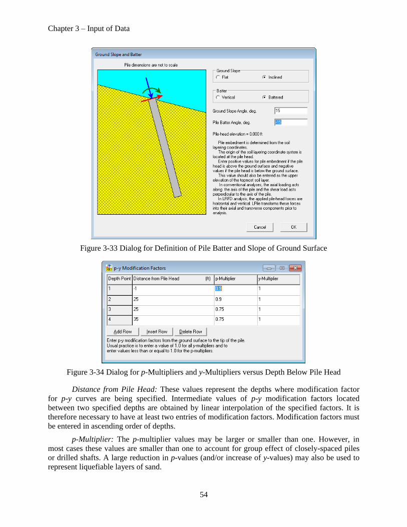
Chapter 3 – Input of Data
54
Figure 3-33 Dialog for Definition of Pile Batter and Slope of Ground Surface
Figure 3-34 Dialog for p-Multipliers and y-Multipliers versus Depth Below Pile Head
Distance from Pile Head: These values represent the depths where modification factor
for p-y curves are being specified. Intermediate values of p-y modification factors located
between two specified depths are obtained by linear interpolation of the specified factors. It is
therefore necessary to have at least two entries of modification factors. Modification factors must
be entered in ascending order of depths.
p-Multiplier: The p-multiplier values may be larger or smaller than one. However, in
most cases these values are smaller than one to account for group effect of closely-spaced piles
or drilled shafts. A large reduction in p-values (and/or increase of y-values) may also be used to
represent liquefiable layers of sand.
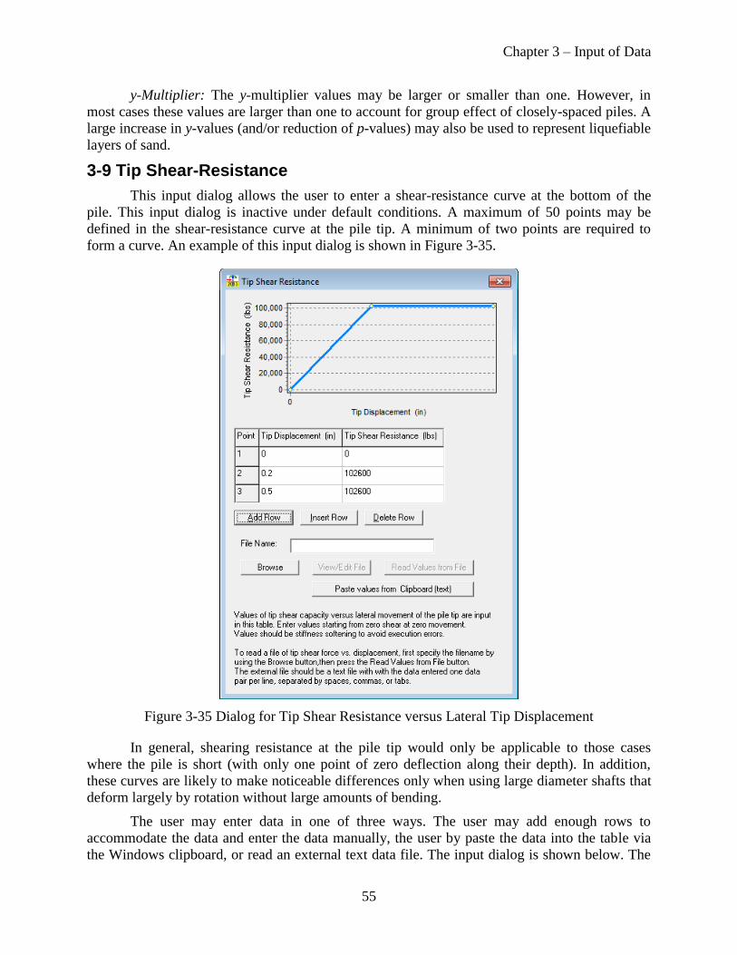
Chapter 3 – Input of Data
55
y-Multiplier: The y-multiplier values may be larger or smaller than one. However, in
most cases these values are larger than one to account for group effect of closely-spaced piles. A
large increase in y-values (and/or reduction of p-values) may also be used to represent liquefiable
layers of sand.
3-9 Tip Shear-Resistance
This input dialog allows the user to enter a shear-resistance curve at the bottom of the
pile. This input dialog is inactive under default conditions. A maximum of 50 points may be
defined in the shear-resistance curve at the pile tip. A minimum of two points are required to
form a curve. An example of this input dialog is shown in Figure 3-35.
Figure 3-35 Dialog for Tip Shear Resistance versus Lateral Tip Displacement
In general, shearing resistance at the pile tip would only be applicable to those cases
where the pile is short (with only one point of zero deflection along their depth). In addition,
these curves are likely to make noticeable differences only when using large diameter shafts that
deform largely by rotation without large amounts of bending.
The user may enter data in one of three ways. The user may add enough rows to
accommodate the data and enter the data manually, the user by paste the data into the table via
the Windows clipboard, or read an external text data file. The input dialog is shown below. The

Chapter 3 – Input of Data
56
graph in the dialog shows the current data. It may be necessary for the user to move the cursor to
an adjacent cell to update the graph of the tip shear curve.
3-10 Shift Pile or Soil Elevations
Occasionally the user may have the need to raise or lower the position of the pile in the
soil profile or may desire to check the entry depths of soil and rock layers against elevation data
for the project site. These actions can be performed by using the Shift Pile Elevation command
under the Data Menu.
An example of the Shift Pile Elevation input dialog is shown in Figure 3-36. In this
example, the pile head is initially positioned at the ground surface, so the depth of the top of
layer 1 is zero (remember that the position of the pile head is the origin of the vertical coordinate
system used in LPile).
Figure 3-36 Dialog for Shifting of Pile Elevation Relative to Input Soil Profile Showing a Pile
Head at the Top of the Soil Profile
If the user wishes to move the pile vertically within an entered soil profile, the user enters
the elevation shift in the upper data edit box and presses the Shift Pile Elevation button. To move
the pile downwards, the user enters a positive number and to move the pile upwards the user
enters a negative number. The Shift Pile Elevation dialog shown below shows the results for a
case in which the pile was moved down by 2 meters. The summary report shown in Figure 3-37
shows that the top of the first layer has been moved to −2 meters, but that the thicknesses of the
layers are unchanged.

Chapter 3 – Input of Data
57
Figure 3-37 Dialog for Shifting of Pile Elevation Relative to Input Soil Profile After Shifting a
Pile Head To Be Below the Ground Surface
If the user wishes to compare the depths of the soil layer profile to elevation data, the user
enters a value for the elevation of the ground surface and presses the View Elevations Report
button. The Shift Pile or Soil Elevations dialog can display the report in two formats that are
selected by pressing the appropriate Elevation Coordinate Type radio button. The default format
is the LPile Depth Coordinates and the other format is the Elevations Relative to Datum. The
dialog box shown below is an example where the ground surface elevation is 6 meters and the
Elevations Relative to Datum option has been selected.
3-11 Input of Output Depths for p-y Curves
The user may generate and plot p-y curves at user-specified depths. These curves are not
used in the analysis, as LPile computes exact values of p for every corresponding value of y for
every node along the length of the pile. Many of the various parameters needed to compute the
output p-y curves are output in the output report file from LPile.
The depths can be entered in any order. LPile will sort the depth values from top to
bottom and eliminate duplicate entries prior to performing computations. No p-y curves will be
computed if an output depth is either above the ground surface or below the pile tip and a
warning message will be output by the program.
An example of the input dialog for p-y Output Depths is shown in Figure 3-38. It should
be noted that the depth is the vertical depth below the pile head, not the depth along the axis of
the pile.

Chapter 3 – Input of Data
58
(a) (b)
Figure 3-38 Output Depths of p-y Curves Below Pile Head, (a) Dialog for p-y Curve Output
Depths, (b) Measurement of Vertical Depths
3-12 Conventional Loading Analysis
The conventional loading analysis is the same type of analysis used in all versions of
LPile older than Version 6. In this type of analysis, up to 100 pile-head loadings of various types
can be specified. In addition, distributed lateral loading can be specified and the distributed
lateral loading will be applied to all pile-head loading cases.
3-12-1 Pile-head Loading and Options
The Pile-head Loading and Options dialog shown in Figure 3-39 allows the user to enter
the desired boundary conditions and corresponding loading at the pile head. There are five
options for boundary conditions at the pile head. The user selects the desired boundary condition
using a dropdown list of the choices described below. The program allows up to 100 rows of
boundary conditions and corresponding loading at the pile head. In addition, the user may
specify the computation of pile top deflection versus pile length for any of the specified load
cases. In general, user should restrict use of this option to cases using any of the first three pile-
head conditions, as the pile-head deflection will not vary for the fourth and fifth pile-head
loading conditions.
3-12-1-1 Pile-Head Loading Types
Shear and Moment: This boundary condition is selected to specify values of applied
lateral load in units of force and applied moment in units of force length at the pile head. This
condition implies that the pile head is free to rotate and move laterally. The lateral force is
considered positive when applied from left-to-right. The moment is considered positive when
applied clockwise.
Shear and Slope: In this boundary condition, the user defines the applied lateral load in
units of force and the slope in radians at the pile head. The lateral force is considered positive
when applied from left-to-right. The slope is positive when the pile head rotates
counterclockwise. A fixed-head condition (with no restrictions to lateral movements) may be
modeled by specifying a slope equal to zero.
Shear and Rotational Stiffness: For this boundary condition, the user defines the applied
lateral load in units of force and a value for rotational stiffness (moment per radian of rotation) at
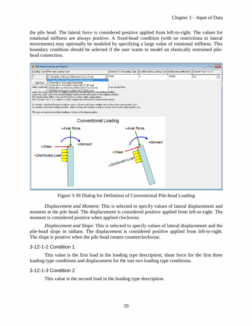
Chapter 3 – Input of Data
59
the pile head. The lateral force is considered positive applied from left-to-right. The values for
rotational stiffness are always positive. A fixed-head condition (with no restrictions to lateral
movements) may optionally be modeled by specifying a large value of rotational stiffness. This
boundary condition should be selected if the user wants to model an elastically restrained pile-
head connection.
Figure 3-39 Dialog for Definition of Conventional Pile-head Loading
Displacement and Moment: This is selected to specify values of lateral displacement and
moment at the pile head. The displacement is considered positive applied from left-to-right. The
moment is considered positive when applied clockwise.
Displacement and Slope: This is selected to specify values of lateral displacement and the
pile-head slope in radians. The displacement is considered positive applied from left-to-right.
The slope is positive when the pile head rotates counterclockwise.
3-12-1-2 Condition 1
This value is the first load in the loading type description; shear force for the first three
loading type conditions and displacement for the last two loading type conditions.
3-12-1-3 Condition 2
This value is the second load in the loading type description.
Chapter 3 – Input of Data
60
3-12-1-4 Axial Load
This value is input in units of force. It is applied at the pile head and may be entered after
specifying the boundary conditions as well as the corresponding loading. Axial loads entered in
this column are used in two parts of the computations. Firstly, the axial thrust force is used in the
computations of nonlinear moment-curvature behavior. Secondly, the axial force is used to
account for secondary moments produced when the pile deflects (also known as P- effects).
3-12-1-5 Compute Top y versus L
This column contains a drop-down yes/no option for performing computations of top
deflection versus pile length for this pile-head loading condition if pile-head loading condition
does not prescribe the pile-head lateral deflection value. No computations of top deflection
versus pile length will be made if either of the displacement-moment or displacement-slope pile-
head conditions is specified.
3-12-2 Distributed Lateral Loading
The data entry for distributed lateral loading for conventional analysis is controlled either
using a single input dialog if a single distributed load profile is used for all conventional loading
cases or using two linked input dialogs if distributed loading profiles are defined independently
for the various conventional loading cases.
In the first dialog, the user checks whether to include distributed lateral loads. If the
option is checked, the button to show the input dialog is enabled and the user may display the
input dialog for distributed lateral loading. Examples of these dialogs are shown in Figure 3-40.
The program allows up to 50 different input points of lateral load values, which are
placed in units of load per unit length of pile. The user must enter values in increasing
magnitudes of depth. The program linearly interpolates the values of lateral loads existing
between specified depths. A minimum of two entries (two depths) of distributed lateral loading
are needed.
The user may enter data in three ways. The user may add enough rows to the table and
enter the data manually, the user may paste the data into the table via the Windows clipboard, or
the user may direct LPile to read an external text file containing the data. The Distributed Lateral
Loads dialog is shown in Figure 3-41. The graph in the dialog shows the current data. It may be
necessary for the user to move the cursor to a different cell to update the graph of the distributed
lateral loading.
It is not possible for LPile to verify data. It is left to the user to view the graph of the
distributed load data and to verify its correctness.

Chapter 3 – Input of Data
61
(a) (b)
Figure 3-40 Dialogs for Multiple Distributed Lateral Loads for Conventional Loading, (a) 3 Load
Cases, (b) Distributed Load Profile Data for Load Case 1
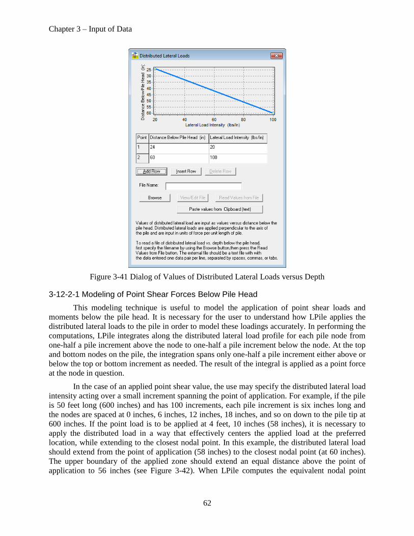
Chapter 3 – Input of Data
62
Figure 3-41 Dialog of Values of Distributed Lateral Loads versus Depth
3-12-2-1 Modeling of Point Shear Forces Below Pile Head
This modeling technique is useful to model the application of point shear loads and
moments below the pile head. It is necessary for the user to understand how LPile applies the
distributed lateral loads to the pile in order to model these loadings accurately. In performing the
computations, LPile integrates along the distributed lateral load profile for each pile node from
one-half a pile increment above the node to one-half a pile increment below the node. At the top
and bottom nodes on the pile, the integration spans only one-half a pile increment either above or
below the top or bottom increment as needed. The result of the integral is applied as a point force
at the node in question.
In the case of an applied point shear value, the use may specify the distributed lateral load
intensity acting over a small increment spanning the point of application. For example, if the pile
is 50 feet long (600 inches) and has 100 increments, each pile increment is six inches long and
the nodes are spaced at 0 inches, 6 inches, 12 inches, 18 inches, and so on down to the pile tip at
600 inches. If the point load is to be applied at 4 feet, 10 inches (58 inches), it is necessary to
apply the distributed load in a way that effectively centers the applied load at the preferred
location, while extending to the closest nodal point. In this example, the distributed lateral load
should extend from the point of application (58 inches) to the closest nodal point (at 60 inches).
The upper boundary of the applied zone should extend an equal distance above the point of
application to 56 inches (see Figure 3-42). When LPile computes the equivalent nodal point

Chapter 3 – Input of Data
63
loads for this example, one-third of the applied force result is a applied at the nodal point above
the point of load application and the remain two-thirds is applied at the closest node.
Figure 3-42 Recommendation for Modeling of Lateral Force Applied Below the Pile Head
It is important for the user to recognize that if the nodal point spacing changes for any
reason, the boundaries of the equivalent loading zone must be re-computed by the user.
3-12-2-2 Modeling of Moments Below Pile Head
There are more restrictions in modeling in the case of modeling concentrated moments in
the pile. It is only possible to apply a concentrated moment about a nodal point, not any arbitrary
location. To model concentrated moments, it is necessary to apply equal and opposite in action
distributed lateral loads to the nodal increments above and below the nodal point where the
moment is to be applied. The reason for this is the integration of distributed lateral loads is
performed for each nodal point. If the two distributed loads were applied over a single increment,
the equal and opposite forces would cancel each other. Figure 3-43 illustrates the principle of
applying equal and opposite equivalent forces to model a concentrated moment in the pile.
V = p dx
Uniform distributed load p
is centered about point of
load application and extends
to closest nodal point.
h
dx
p
V = p dx
Uniform distributed load p
is centered about point of
load application and extends
to closest nodal point.
h
dx
p
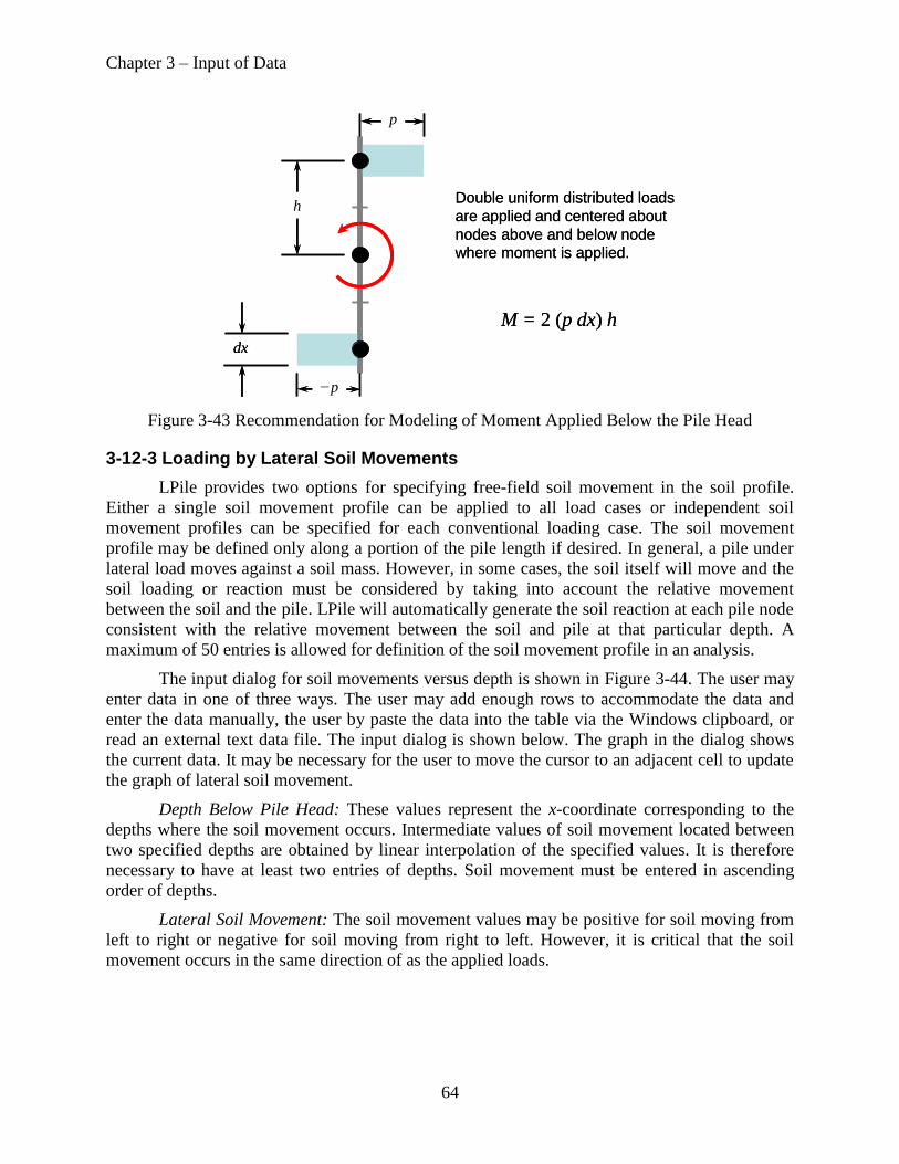
Chapter 3 – Input of Data
64
Figure 3-43 Recommendation for Modeling of Moment Applied Below the Pile Head
3-12-3 Loading by Lateral Soil Movements
LPile provides two options for specifying free-field soil movement in the soil profile.
Either a single soil movement profile can be applied to all load cases or independent soil
movement profiles can be specified for each conventional loading case. The soil movement
profile may be defined only along a portion of the pile length if desired. In general, a pile under
lateral load moves against a soil mass. However, in some cases, the soil itself will move and the
soil loading or reaction must be considered by taking into account the relative movement
between the soil and the pile. LPile will automatically generate the soil reaction at each pile node
consistent with the relative movement between the soil and pile at that particular depth. A
maximum of 50 entries is allowed for definition of the soil movement profile in an analysis.
The input dialog for soil movements versus depth is shown in Figure 3-44. The user may
enter data in one of three ways. The user may add enough rows to accommodate the data and
enter the data manually, the user by paste the data into the table via the Windows clipboard, or
read an external text data file. The input dialog is shown below. The graph in the dialog shows
the current data. It may be necessary for the user to move the cursor to an adjacent cell to update
the graph of lateral soil movement.
Depth Below Pile Head: These values represent the x-coordinate corresponding to the
depths where the soil movement occurs. Intermediate values of soil movement located between
two specified depths are obtained by linear interpolation of the specified values. It is therefore
necessary to have at least two entries of depths. Soil movement must be entered in ascending
order of depths.
Lateral Soil Movement: The soil movement values may be positive for soil moving from
left to right or negative for soil moving from right to left. However, it is critical that the soil
movement occurs in the same direction of as the applied loads.
M = 2 (p dx) h
Double uniform distributed loads
are applied and centered about
nodes above and below node
where moment is applied.
h
dx
−p
p
M = 2 (p dx) h
Double uniform distributed loads
are applied and centered about
nodes above and below node
where moment is applied.
h
dx
−p
p

Chapter 3 – Input of Data
65
Figure 3-44 Dialog for Input of Soil Movements versus Depth Below Pile Head
3-12-4 Computation of Pile-head Stiffness Matrix Components
The feature for computation of pile-head stiffness matrix values has three options to
control how the values are computed. In the first method, which is identical to the method used
in versions of LPile prior to LPile 2013, the loads used for computation of pile-head stiffness are
those specified in load case 1 for conventional loading. This method does not allow the user to
control the lateral displacement and pile-head rotation, so the second and third options were
added to provide this capability. In the second method, the maximum displacement and rotation
are set by the values computed for load case 1 for conventional loading. In the third method, the
user may specify the maximum pile-head displacement and rotation.
The dialog for Controls for Computation of Stiffness Matrix is shown in Figure 3-45.

Chapter 3 – Input of Data
66
Figure 3-45 Dialog for Controls for Computation of Stiffness Matrix
The definitions of the pile-head stiffness values and their engineering units computed by
LPile are the following:
radian
m-kNor
radian
lbs-in
rotation head-pile
reactionmoment head-pile
radian
kNor
radian
lbs
rotation head-pile
reaction forceshear head-pile
meter
m-kNor
inch
lbs-in
deflection head-pile
reactionmoment head-pile
meter
kNor
inch
lbs
deflection head-pile
reaction forceshear head-pile
33
23
32
22
K
K
K
K
3-12-5 Pushover Analysis
The program feature for pushover analysis has options for different pile-head fixity
options and the setting of the range and distribution of pushover deflection. The output of the
pushover analysis is displayed in graphs of pile-head shear force versus deflection and maximum
moment developed in the pile versus deflection.
The pushover analysis is performed by running a series of analyses for displacement-zero
moment pile-head conditions for pinned head piles and analyses for displacement-zero slope
pile-head conditions for fixed head piles. The displacements used are controlled by the maximum
and minimum displacement values specified and the displacement distribution method. The
displacement distribution method may be either logarithmic (which requires a non-zero, positive
minimum and maximum displacement values), arithmetic, or a set of user-specified pile-head
displacement values. The number of loading steps sets the number of pile-head displacement
values generated for the pushover analysis.
The axial thrust force used in the pushover analysis must be entered in the dialog. If the
pile being analyzed is not an elastic pile, the user should make sure that the axial thrust force
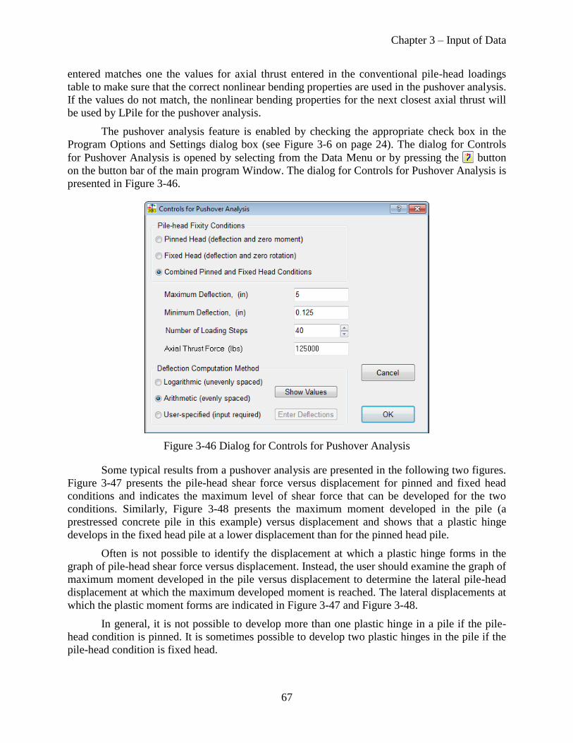
Chapter 3 – Input of Data
67
entered matches one the values for axial thrust entered in the conventional pile-head loadings
table to make sure that the correct nonlinear bending properties are used in the pushover analysis.
If the values do not match, the nonlinear bending properties for the next closest axial thrust will
be used by LPile for the pushover analysis.
The pushover analysis feature is enabled by checking the appropriate check box in the
Program Options and Settings dialog box (see Figure 3-6 on page 24). The dialog for Controls
for Pushover Analysis is opened by selecting from the Data Menu or by pressing the button
on the button bar of the main program Window. The dialog for Controls for Pushover Analysis is
presented in Figure 3-46.
Figure 3-46 Dialog for Controls for Pushover Analysis
Some typical results from a pushover analysis are presented in the following two figures.
Figure 3-47 presents the pile-head shear force versus displacement for pinned and fixed head
conditions and indicates the maximum level of shear force that can be developed for the two
conditions. Similarly, Figure 3-48 presents the maximum moment developed in the pile (a
prestressed concrete pile in this example) versus displacement and shows that a plastic hinge
develops in the fixed head pile at a lower displacement than for the pinned head pile.
Often is not possible to identify the displacement at which a plastic hinge forms in the
graph of pile-head shear force versus displacement. Instead, the user should examine the graph of
maximum moment developed in the pile versus displacement to determine the lateral pile-head
displacement at which the maximum developed moment is reached. The lateral displacements at
which the plastic moment forms are indicated in Figure 3-47 and Figure 3-48.
In general, it is not possible to develop more than one plastic hinge in a pile if the pile-
head condition is pinned. It is sometimes possible to develop two plastic hinges in the pile if the
pile-head condition is fixed head.
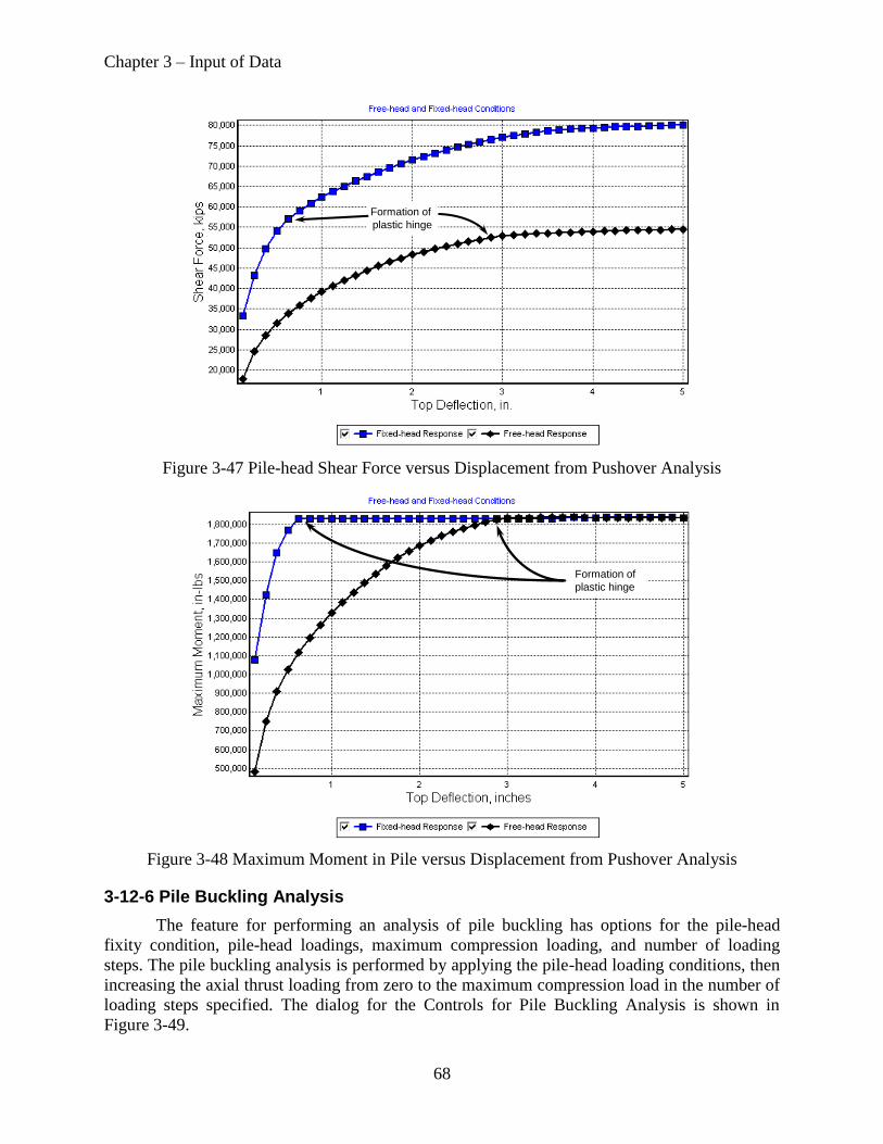
Chapter 3 – Input of Data
68
Figure 3-47 Pile-head Shear Force versus Displacement from Pushover Analysis
Figure 3-48 Maximum Moment in Pile versus Displacement from Pushover Analysis
3-12-6 Pile Buckling Analysis
The feature for performing an analysis of pile buckling has options for the pile-head
fixity condition, pile-head loadings, maximum compression loading, and number of loading
steps. The pile buckling analysis is performed by applying the pile-head loading conditions, then
increasing the axial thrust loading from zero to the maximum compression load in the number of
loading steps specified. The dialog for the Controls for Pile Buckling Analysis is shown in
Figure 3-49.
Formation of
plastic hinge
Formation of
plastic hinge
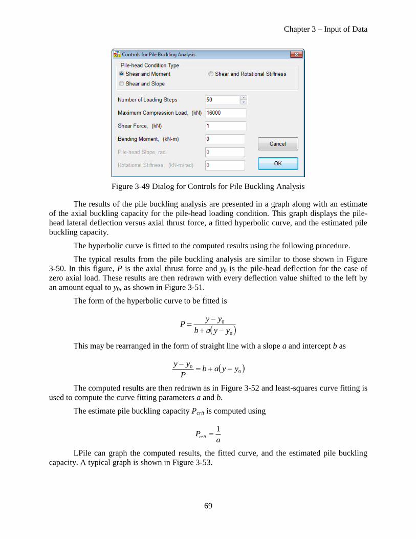
Chapter 3 – Input of Data
69
Figure 3-49 Dialog for Controls for Pile Buckling Analysis
The results of the pile buckling analysis are presented in a graph along with an estimate
of the axial buckling capacity for the pile-head loading condition. This graph displays the pile-
head lateral deflection versus axial thrust force, a fitted hyperbolic curve, and the estimated pile
buckling capacity.
The hyperbolic curve is fitted to the computed results using the following procedure.
The typical results from the pile buckling analysis are similar to those shown in Figure
3-50. In this figure, P is the axial thrust force and y0 is the pile-head deflection for the case of
zero axial load. These results are then redrawn with every deflection value shifted to the left by
an amount equal to y0, as shown in Figure 3-51.
The form of the hyperbolic curve to be fitted is
0
0
yyab
yyP
This may be rearranged in the form of straight line with a slope a and intercept b as
00 yyab
P
yy
The computed results are then redrawn as in Figure 3-52 and least-squares curve fitting is
used to compute the curve fitting parameters a and b.
The estimate pile buckling capacity Pcrit is computed using
aPcrit
1
LPile can graph the computed results, the fitted curve, and the estimated pile buckling
capacity. A typical graph is shown in Figure 3-53.
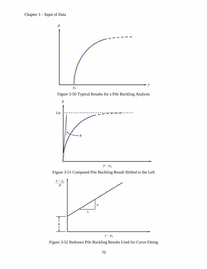
Chapter 3 – Input of Data
70
Figure 3-50 Typical Results for a Pile Buckling Analysis
Figure 3-51 Computed Pile Buckling Result Shifted to the Left
Figure 3-52 Redrawn Pile Buckling Results Used for Curve Fitting
y0
P
y
y – y0
1/a
P
b
a
y – y0
b
1
P
yy 0

Chapter 3 – Input of Data
71
Figure 3-53 Results from Pile Buckling Analysis
In this graph, the response curve is plotted with symbols and the fitted curve is drawn
without symbols. The filled curve overlies the curve for computed pile response, so the line for
computed pile response is not visible but the symbols on the response curve are visible.
When performing a pile buckling analysis, the user must guard against specifying a
maximum axial load that is too high. This can be checked by examining the sign of deflection of
the lateral deflection value for zero axial load. In a proper analysis, the magnitude of lateral
deflection at higher values of axial thrust will have the same sign as that for zero axial thrust and
the deflection values will be larger in magnitude, as shown in Figure 3-53.
The estimated pile buckling capacity for elastic piles is computed from the shape of the
pile-head response curve and is not based on the magnitude of maximum moment compared to
the plastic moment capacity of the pile. For nonlinear piles, the buckling capacity may be
determined by either the maximum axial compression capacity or plastic moment capacity of the
pile. For piles with nonlinear bending behavior, the buckling capacity estimated by the
hyperbolic curve may over-estimate the actual buckling capacity if the buckling capacity is
controlled by the pile’s plastic moment capacity. Thus, for analyses of nonlinear piles, the user
should compare the maximum moment developed in the pile to the plastic moment capacity. If
the two values are close, the buckling capacity should be reported as the last axial thrust value
for which a solution was reported.
If the section is either a drilled shaft (bored pile) or prestressed concrete pile with low
levels of reinforcement, it may be possible to obtain buckling results for axial thrust values
higher than the axial buckling capacity, but the sign will be reversed. The reason for this is a
large axial thrust value will create compression over the full section. This causes the moment
Free-head Condition
Pile Response Computed by LPilegfedcb Fitted Hyperboloic Buckling CurvegfedcbBuckling Capacity = 10,531 kNgfedcb
Top Deflection, m0.060.040.020
Axia
l T
hru
st L
oa
d, kN
10,500
10,000
9,500
9,000
8,500
8,000
7,500
7,000
6,500
6,000
5,500
5,000
4,500
4,000
3,500
3,000
2,500
2,000
1,500
1,000
500
0

Chapter 3 – Input of Data
72
capacity to be controlled by crushing of the concrete and not by yield of the reinforcement. An
example of a pile buckling analysis that used axial thrust values that were too high is shown in
Figure 3-54.
Figure 3-54 Example of Correct (green symbols) and Incorrect (red symbols) Pile Buckling
Analyses
3-13 Input of Load Testing Data
Data for pile response measured during lateral load testing may be entered into LPile and
displayed along with computed results. When this option is selected, the user is required to enter
values of pile-head shear force loading versus lateral deformation. Optionally, the user may enter
values of moment developed in the pile versus depth below the pile head for each pile-head shear
force value.
3-13-1 Controls for Input of Load Test Data
Entry of load test data is controlled using the dialog box shown in Figure 3-55. The basic
data entered are the pile-head shear versus displacement data. Optionally, the user may also enter
values of bending moment and/or lateral displacement versus depth. Lastly, the user may select
whether or not the load test values are included in the graphs generated by LPile.
It is also possible for LPile to save load test data that has been entered as a text file and to
read a text file containing the load test data.
0
50
100
150
200
250
300
350
400
450
-0.5 -0.4 -0.3 -0.2 -0.1 0 0.1 0.2
Axia
l T
hru
st F
orc
e, kN
Pile-head Deflection, meters
Correct
Incorrect
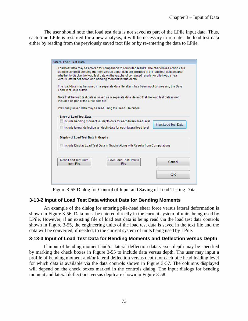
Chapter 3 – Input of Data
73
The user should note that load test data is not saved as part of the LPile input data. Thus,
each time LPile is restarted for a new analysis, it will be necessary to re-enter the load test data
either by reading from the previously saved text file or by re-entering the data to LPile.
Figure 3-55 Dialog for Control of Input and Saving of Load Testing Data
3-13-2 Input of Load Test Data without Data for Bending Moments
An example of the dialog for entering pile-head shear force versus lateral deformation is
shown in Figure 3-56. Data must be entered directly in the current system of units being used by
LPile. However, if an existing file of load test data is being read via the load test data controls
shown in Figure 3-55, the engineering units of the load test data is saved in the text file and the
data will be converted, if needed, to the current system of units being used by LPile.
3-13-3 Input of Load Test Data for Bending Moments and Deflection versus Depth
If input of bending moment and/or lateral deflection data versus depth may be specified
by marking the check boxes in Figure 3-55 to include data versus depth. The user may input a
profile of bending moment and/or lateral deflection versus depth for each pile head loading level
for which data is available via the data controls shown in Figure 3-57. The columns displayed
will depend on the check boxes marked in the controls dialog. The input dialogs for bending
moment and lateral deflections versus depth are shown in Figure 3-58.
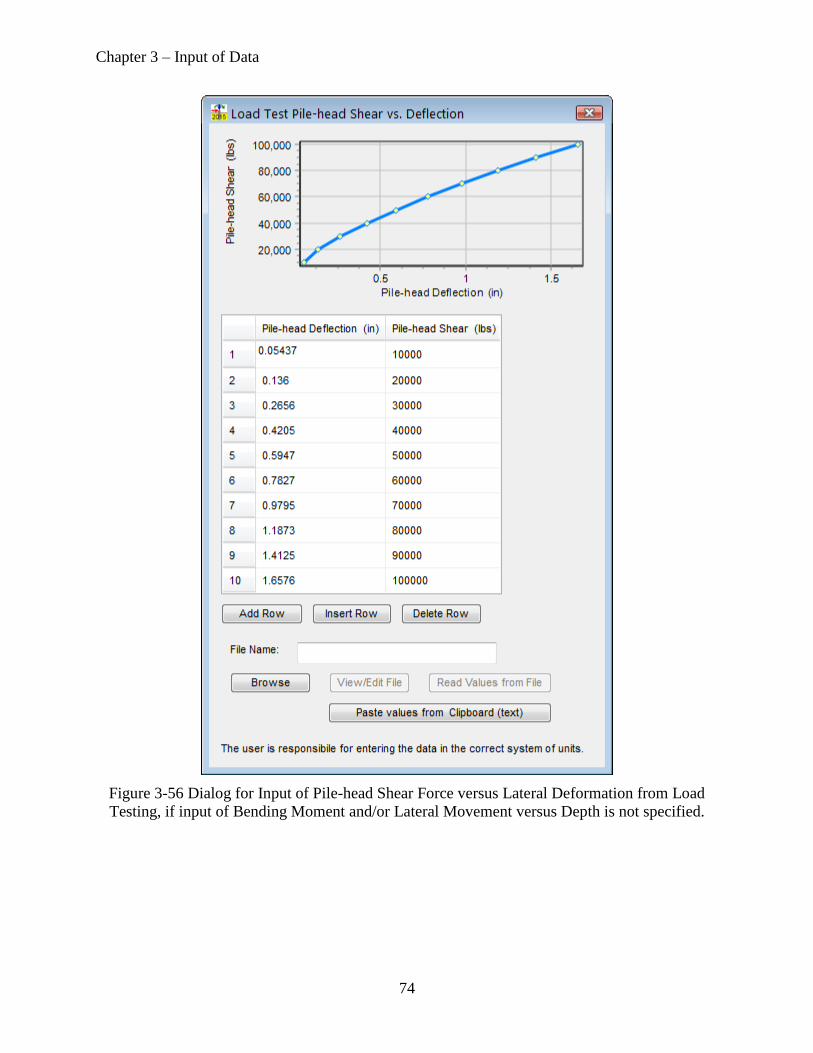
Chapter 3 – Input of Data
74
Figure 3-56 Dialog for Input of Pile-head Shear Force versus Lateral Deformation from Load
Testing, if input of Bending Moment and/or Lateral Movement versus Depth is not specified.

Chapter 3 – Input of Data
75
Figure 3-57 Dialog for Input of Pile-head Shear Force versus Lateral Deformation from Load
Testing, if input of Bending Moment and Lateral Deflection versus Depth are specified.
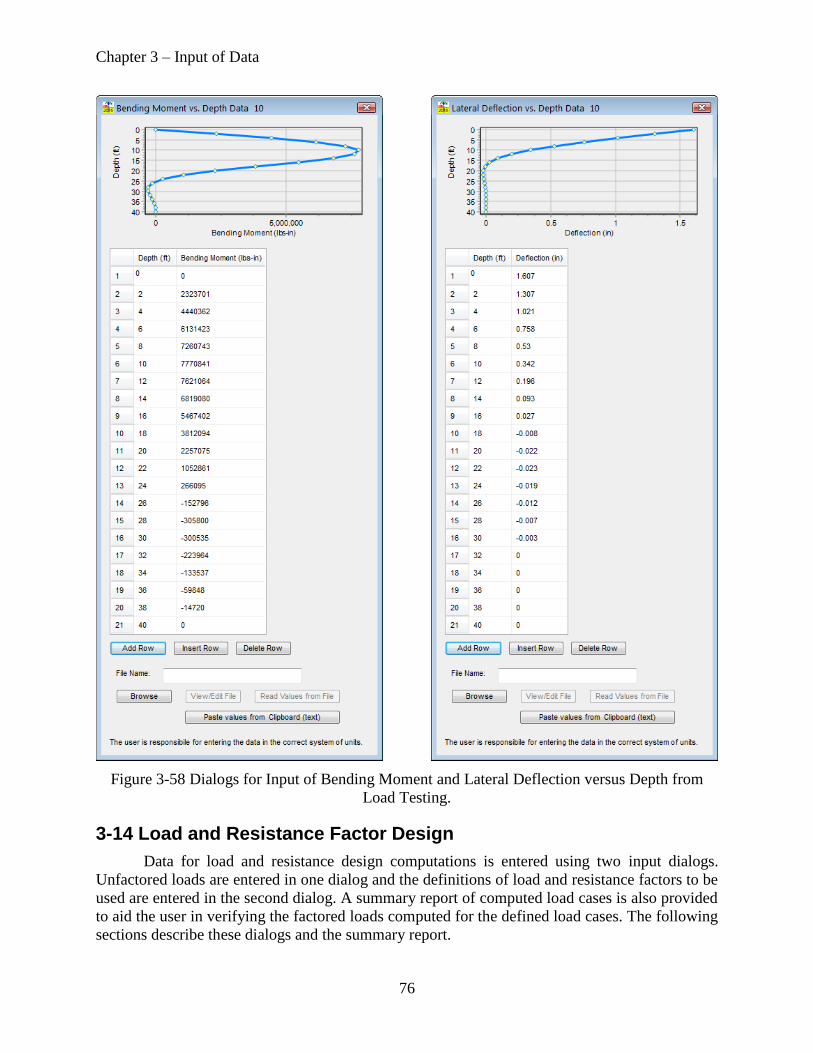
Chapter 3 – Input of Data
76
Figure 3-58 Dialogs for Input of Bending Moment and Lateral Deflection versus Depth from
Load Testing.
3-14 Load and Resistance Factor Design
Data for load and resistance design computations is entered using two input dialogs.
Unfactored loads are entered in one dialog and the definitions of load and resistance factors to be
used are entered in the second dialog. A summary report of computed load cases is also provided
to aid the user in verifying the factored loads computed for the defined load cases. The following
sections describe these dialogs and the summary report.

Chapter 3 – Input of Data
77
3-14-1 Unfactored Loads
The input dialog for unfactored loads shown in Figure 3-59 allows the user to define the
type of load, horizontal force, vertical force, overturning moment, and to control the use and
input of distributed loading data. All unfactored loads must be defined as combinations of
horizontal shear force, over-turning moment, axial thrust force, and distributed lateral loads
normal to the axis of the pile.
Figure 3-59 Dialog for Definition of Unfactored Pile-head Loadings for LRFD Analysis
The unfactored load definition includes the type of load. The load types are:
Dead load
Live load
Earthquake
Impact
Wind
Water
Ice
Horizontal Soil Pressure
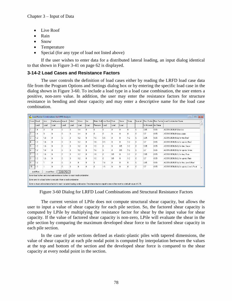
Chapter 3 – Input of Data
78
Live Roof
Rain
Snow
Temperature
Special (for any type of load not listed above)
If the user wishes to enter data for a distributed lateral loading, an input dialog identical
to that shown in Figure 3-41 on page 62 is displayed.
3-14-2 Load Cases and Resistance Factors
The user controls the definition of load cases either by reading the LRFD load case data
file from the Program Options and Settings dialog box or by entering the specific load case in the
dialog shown in Figure 3-60. To include a load type in a load case combination, the user enters a
positive, non-zero value. In addition, the user may enter the resistance factors for structure
resistance in bending and shear capacity and may enter a descriptive name for the load case
combination.
Figure 3-60 Dialog for LRFD Load Combinations and Structural Resistance Factors
The current version of LPile does not compute structural shear capacity, but allows the
user to input a value of shear capacity for each pile section. So, the factored shear capacity is
computed by LPile by multiplying the resistance factor for shear by the input value for shear
capacity. If the value of factored shear capacity is non-zero, LPile will evaluate the shear in the
pile section by comparing the maximum developed shear force to the factored shear capacity in
each pile section.
In the case of pile sections defined as elastic-plastic piles with tapered dimensions, the
value of shear capacity at each pile nodal point is computed by interpolation between the values
at the top and bottom of the section and the developed shear force is compared to the shear
capacity at every nodal point in the section.

Chapter 3 – Input of Data
79
3-14-3 Summary of Factored Load Cases
The summary of factored load cases is provided for the user to view the factored loads
computed by LPile. LPile computes this summary by first adding all pile-head loading of the
same type together, then multiplying the sum by relevant load factor.
In the case of distributed loads, the program integrates the individual distributed load
profiles and computes the equivalent concentrated forces at nodes on the pile, adds all forces
from the same load type together, and then multiplies the sum by the relevant load factor.
The summary report has three general sections. The first section shows the totals of the
unfactored loads. The second part shows the computed factored loads for each load case in turn.
The third part shows the factored load cases in tabular form. The content of the summary report
is saved under the filename of the data file with the file extension of LRFD_Summary_Report.
An example of the summary report is shown in Figure 3-61.
Figure 3-61 Summary Report of Computed Factored Load Combinations for LRFD Analysis
3-15 Computation of Nonlinear EI Only
3-15-1 Axial Thrust Loads for Interaction Diagram
If the user selects the program option to Compute Nonlinear EI Only, the user may
generate a structural interaction diagram by entering multiple axial thrust values. The thrust
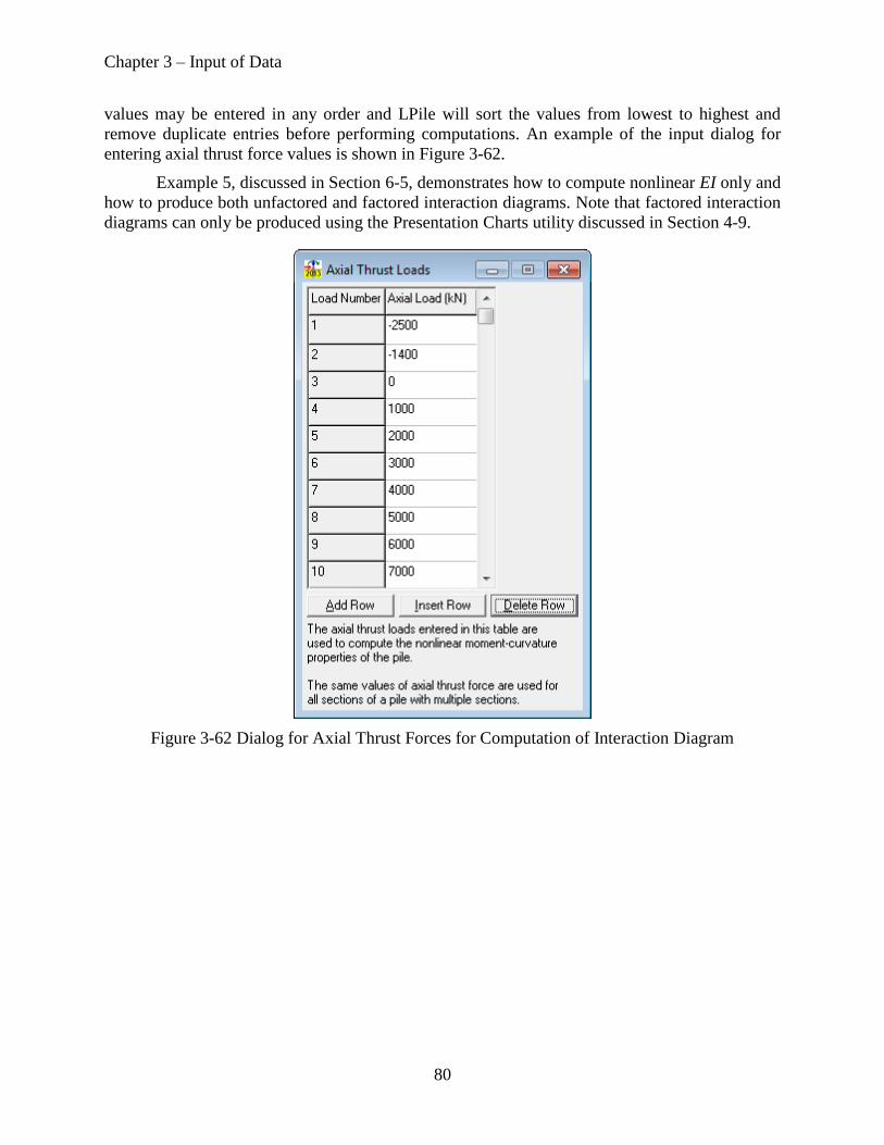
Chapter 3 – Input of Data
80
values may be entered in any order and LPile will sort the values from lowest to highest and
remove duplicate entries before performing computations. An example of the input dialog for
entering axial thrust force values is shown in Figure 3-62.
Example 5, discussed in Section 6-5, demonstrates how to compute nonlinear EI only and
how to produce both unfactored and factored interaction diagrams. Note that factored interaction
diagrams can only be produced using the Presentation Charts utility discussed in Section 4-9.
Figure 3-62 Dialog for Axial Thrust Forces for Computation of Interaction Diagram

81
Chapter 4 Display of Graphics
4-1 Introduction
The Graphics Menu is used to display graphs of output data after a successful analysis.
Options for the display of graphs under the Graphics Menu are only enabled after a successful
analysis has been made. Even after performing a successful analysis, some graphing options may
be disabled since the types of graphical output are controlled by the selected program options.
4-2 Types of Graphics
Two types of graphics are provided by LPile; fast graphics and presentation graphics.
Fast graphics are graphs that can be displayed either from the Graphics Menu or by clicking a
button on the button bar. Fast graphics have limited features for modifying the graphs and their
contents. Presentation charts are displayed using the Presentation Charts command from the
Graphics Menu or by pressing the button on the button bar.
4-3 Graphics Mouse Commands
The following mouse commands are available within a graphic window:
Mouse Action Event Description
Left click and drag down and right Magnifies the area within the drag/release
Right click Zoom out
Double click on legend entry Turns the selected curve on or off
4-4 Graphics Buttons
The buttons shown in Figure 4-1 will display charts of the computed results when
enabled after an analysis. If the program feature required to generate a graph is not activated, the
corresponding button will not be enabled.
Figure 4-1 Speed Buttons for Graphics
4-5 Graphics Menu
The Graphics Menu is shown in Figure 4-2.
Graphs for which buttons exist on the button bar have the identical icon as shown in the
Graphics Menu entries.
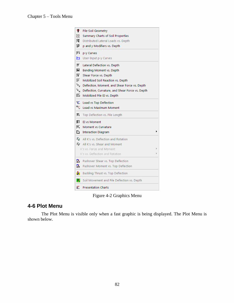
Chapter 5 – Tools Menu
82
Figure 4-2 Graphics Menu
4-6 Plot Menu
The Plot Menu is visible only when a fast graphic is being displayed. The Plot Menu is
shown below.
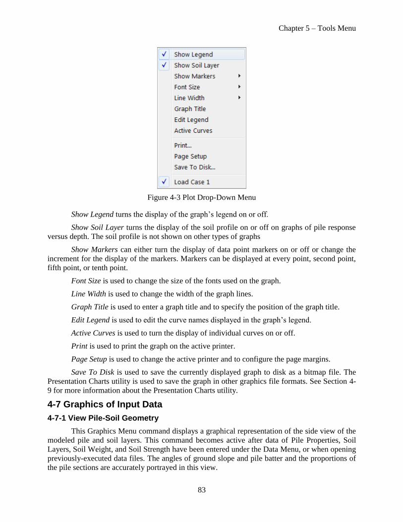
Chapter 5 – Tools Menu
83
Figure 4-3 Plot Drop-Down Menu
Show Legend turns the display of the graph’s legend on or off.
Show Soil Layer turns the display of the soil profile on or off on graphs of pile response
versus depth. The soil profile is not shown on other types of graphs
Show Markers can either turn the display of data point markers on or off or change the
increment for the display of the markers. Markers can be displayed at every point, second point,
fifth point, or tenth point.
Font Size is used to change the size of the fonts used on the graph.
Line Width is used to change the width of the graph lines.
Graph Title is used to enter a graph title and to specify the position of the graph title.
Edit Legend is used to edit the curve names displayed in the graph’s legend.
Active Curves is used to turn the display of individual curves on or off.
Print is used to print the graph on the active printer.
Page Setup is used to change the active printer and to configure the page margins.
Save To Disk is used to save the currently displayed graph to disk as a bitmap file. The
Presentation Charts utility is used to save the graph in other graphics file formats. See Section 4-
9 for more information about the Presentation Charts utility.
4-7 Graphics of Input Data
4-7-1 View Pile-Soil Geometry
This Graphics Menu command displays a graphical representation of the side view of the
modeled pile and soil layers. This command becomes active after data of Pile Properties, Soil
Layers, Soil Weight, and Soil Strength have been entered under the Data Menu, or when opening
previously-executed data files. The angles of ground slope and pile batter and the proportions of
the pile sections are accurately portrayed in this view.

Chapter 5 – Tools Menu
84
4-7-2 Summary Charts of Soil Properties
This Graphics Menu command displays summary charts of soil properties. The number
of charts varies from four to eight charts, depending on the soil layer types contained in the soil
profile. An example of the Summary Charts of Soil Properties is shown in Figure 4-4.
Figure 4-4 Example of Summary Graphs of Soil Properties
4-7-3 User-Input p-y Curves
This Graphics Menu command displays charts of any user-input p-y curves entered as
data. If no curves are input, this Graphics command will not be enabled.
The user-input p-y curves displayed by this graphics command are plotted using the input
data for the curves at the top and bottom of the soil layer. The curves displayed with this
graphics command are not interpolated with depth.
4-7-4 Distributed Lateral Loads vs. Depth
This Graphics Menu command displays charts of distributed lateral loads versus depth for
both conventional analysis and LRFD analysis modes of computation.
4-7-5 p and y Modifiers versus Depth
This Graphics Menu command displays charts of p and y modifiers versus depth and the
ratio of the p and y modifiers versus depth. In computations, the ratio of the p and y modifiers is
used to adjust the p-y curves when computing the effective soil modulus. Thus, if the ratio is
equal to the default ratio of 1, the p-y curves are not modified in the computations.

Chapter 5 – Tools Menu
85
4-8 Graphics of Computational Results
4-8-1 View Results
The View Results button displays summary charts of the principal results from the last
computation. The type and number of charts displayed in the View Results window depends on
the Program Options selected for the computation. The minimum number of charts displayed is
three and the maximum number of charts displayed is eight. An example of the View Results
window is shown in Figure 4-5.
Figure 4-5 Example of View Results Window
4-8-2 p-y Curves at User-specified Depths
LPile is capable of generating graphs of internally generated p-y curves at user-specified
depths located between the lower of the ground surface or top of pile and the pile tip. This
graphics command is enabled if the user asked the program to print p-y curves for verification
purposes by checking in the Program Options and Settings dialog (see Section 3-4-4 for further
information). When specified, the graphics dialog will show the p-y curves for all specified
depths. If no p-y curves were output, this Graphics command will not be enabled (grayed out).
4-8-3 Lateral Deflection versus Depth
This Graphics Menu command displays a graph lateral deflection versus depth for the
modeled pile. This curve is automatically generated in all analytical runs for a laterally loaded
pile. The number of points on the deflection curve is equal to the selected number of pile
increments. Several curves may be contained in this graphics if the user selects to input several
load cases.

Chapter 5 – Tools Menu
86
4-8-4 Bending Moment versus Depth
This Graphics Menu command displays a graph bending moment versus depth along the
pile. This curve is automatically generated in all analytical runs for a laterally loaded pile. The
number of points on the moment curve is equal to the selected number of pile increments.
Several curves may be contained in this graphics if the user selects to input several load cases.
4-8-5 Shear Force versus Depth
This Graphics Menu command displays a graph of shear force versus depth along the
pile. This curve is automatically generated in all analytical runs for a laterally loaded pile. The
number of points on the shear curve is equal to the selected number of pile increments. Several
curves may be contained in this graphics if the user selects to input several load cases.
4-8-6 Mobilized Soil Reaction versus Depth
This Graphics Menu command displays a graph of soil reaction versus depth along the
pile. This curve is automatically generated in all analytical runs for a laterally loaded pile. The
number of points on the soil-reaction curve is equal to the selected number of pile increments.
Several curves may be contained in this graphics if the user selects to input several load cases.
4-8-7 Deflection, Moment, and Shear Force versus Depth
This Graphics Menu command displays three side-by-side graphs of pile deflection,
bending moment, and shear force versus depth along the pile. This graphical display can be
shown for all analytical runs for a laterally loaded pile. The scaling for the depth axis is the same
for all three graphs and allows for comparison of pile deflection, bending moment and shear
force values versus depth along the pile.
4-8-8 Deflection, Curvature, and Moment versus Depth
This Graphics Menu command displays three side-by-side graphs of pile deflection,
bending curvature, and bending moment versus depth along the pile. This graphical display can
be shown for all analytical runs for a laterally loaded pile. The scaling for the depth axis is the
same for all three graphs and allows for comparison of pile deflection, bending curvature, and
bending moment values versus depth along the pile. This graph may be useful in analyses of pile
response due to loading by lateral spread of soil after seismic events.
4-8-9 Mobilized Pile EI versus Depth
This Graphics Menu command is available when the pile has a nonlinear moment-
curvature relationship. This chart shows the value of mobilized EI along the length of the pile.
This chart is useful to display the sections with either cracked-section EI or where plastic hinges
develop.
4-8-10 Load versus Top Deflection
This Graphics Menu command is enabled if the user specifies two or more load cases in the input
data. The specified load cases must have varying lateral loads with or without changes in applied
moments or applied axial loads. The user may select this Graphics command to display a graph
of curve of applied lateral load versus pile-top deflection.

Chapter 5 – Tools Menu
87
4-8-11 Load versus Max Moment
This Graphics Menu command is enabled if the user specifies two or more load cases in
the input data. The specified load cases must have varying lateral loads with or without changes
in applied moments or applied axial loads. The user may select this Graphics command to
display a graph of applied lateral load versus maximum bending moment along the pile length.
4-8-12 Top Deflection versus Pile Length
This Graphics Menu command is enabled if the user selects Generate Pile Length versus
Top Deflection option for a load case for conventional loading. The user may select this
Graphics command to display a graph of pile length versus pile-head deflection for the load
cases evaluated with this option.
4-8-13 Moment versus Curvature
This Graphics Menu command is enabled whenever the nonlinear bending is evaluated
for a pile section. The user may select this Graphics command to display a graph of bending
moment versus curvature. These curves are helpful to find the ultimate bending moment of the
modeled cross section. The number of curves depends on the number of axial loads used for
section analysis or the number of axial thrust forces defined by the pile-head loading conditions.
4-8-14 EI versus Moment
This Graphics Menu command is enabled whenever the nonlinear bending is evaluated
for a pile section. The user may select this Graphics command to display a graph of bending
stiffness versus bending moment. Values of bending stiffness shown in these curves are used
internally in each finite increment of pile analysis when the user selects the analysis of pile
response with nonlinear EI. The number of curves depends on the number of axial loads
specified for section analysis.
4-8-15 Interaction Diagram
This Graphics Menu command is enabled if the user selected to perform a section
analysis and inputs several axial thrust load cases for the analysis. The user may select this
Graphics command to display an unfactored interaction diagram (ultimate bending moment
versus axial load) of the modeled cross section. These curves are helpful to find the ultimate
bending moment for several axial load cases in the modeled cross section. The number of curves
depends on the number of axial loads used for section analysis or the number of axial thrust
loads defined by the pile-head loading conditions.
4-8-16 All K’s versus Deflection and Rotation
This Graphics Menu command displays six charts simultaneously of K22, K23, K32, K33
versus pile-head displacement and rotation plus pile-head reactions and displacements for free-
head and fixed-head pile fixity conditions.
4-8-17 All K’s versus Shear and Moment
The Graphics Menu command displays six charts simultaneously of K22, K23, K32, K33
versus pile-head shear and moment plus pile-head reactions and displacements for free-head and
fixed-head pile fixity conditions.

Chapter 5 – Tools Menu
88
4-8-18 Individual K’s versus Force and Moment
This Graphics Menu command opens a submenu for displaying the individual curves of
pile-head stiffnesses versus force and moments. The submenu is shown in Figure 4-6.
Figure 4-6 Sub-menu for Pile-head Stiffnesses versus Pile-head Force and Moment
4-8-18-1 K22 versus Pile-head Shear Force
This Graphics Menu command is enabled when the Generate Foundations Stiffness
option is selected. When enabled, the selection of this command will show a curve of the K22
(shear force/deflection) component of a 66 foundation stiffness matrix. The user should refer to
Section 3-12-4 for more information about the feature for computing pile-head stiffnesses.
4-8-18-2 K23 versus Pile-head Shear Force
This Graphics Menu command is enabled when the Generate Foundations Stiffness
option is selected. When enabled, the selection of this command will show a curve of the K23
(shear force/rotation) component of a 66 foundation stiffness matrix. The user should refer to
Section 3-12-4 for more information about the feature for computing pile-head stiffnesses.
4-8-18-3 K32 versus Pile-head Moment
This Graphics Menu command is enabled when the Generate Foundations Stiffness
option is selected. When enabled, the selection of this command will show a curve of the K32
(moment/deflection) component of a 66 foundation stiffness matrix. The user should refer to
Section 3-12-4 for more information about the feature for computing pile-head stiffnesses.
4-8-18-4 K33 versus Pile-head Moment
This Graphics Menu command is enabled when the Generate Foundations Stiffness
option is selected. When enabled, the selection of this command will show a curve of the K33
(moment/rotation) component of a 6×6 foundation stiffness matrix. The user should refer to
Section 3-12-4 for more information about the feature for computing pile-head stiffnesses.
4-8-19 Individual K’s versus Pile-head Deflection and Rotation
This Graphics Menu command opens a submenu for displaying the individual curves of
pile-head stiffnesses versus pile-head deflection and rotation. The submenu is shown in Figure
4-7.
Figure 4-7 Submenu for Pile-head Stiffnesses versus Deflection and Rotation

Chapter 5 – Tools Menu
89
4-8-19-1 K22 versus Pile-head Deflection
This Graphics Menu command is enabled when the Generate Foundations Stiffness
option is selected. When enabled, the selection of this command will show a curve of the K22
(shear force/deflection) versus pile top deflection.
4-8-19-2 K23 versus Pile-head Rotation
This Graphics Menu command is enabled when the Generate Foundations Stiffness
option is selected. When enabled, the selection of this command will show a curve of the K23
(shear force/rotation) versus pile top rotation.
4-8-19-3 K32 versus Pile-head Deflection
This Graphics Menu command is enabled when the Generate Foundations Stiffness
option is selected. When enabled, the selection of this command will show a curve of the K32
(moment/deflection) versus pile top deflection.
4-8-19-4 K33 versus Pile-head Rotation
This Graphics Menu command is enabled when the Generate Foundations Stiffness
option is selected. When enabled, the selection of this command will show a curve of the K33
(moment/rotation) versus pile top rotation.
4-8-20 Pushover Shear Force versus Top Deflection
This Graphics Menu command is available only if the Pushover Analysis option was
selected. This graph may contain either one or two curves depending on the pile-head fixity
condition selected in the Controls for Pushover Analysis. This graph shows the pile-head shear
force developed as a function of pile-head deflection. For piles with nonlinear bending, it may be
possible to see the point at which a plastic hinge develops, but this point may be more easily seen
in the graph of pushover moment versus top deflection, discussed subsequently.
4-8-21 Pushover Moment versus Top Deflection
This Graphics Menu command is available only if the Pushover Analysis feature was
activated. This graph may contain either one or two curves depending on the pile-head fixity
condition selected in the Controls for Pushover Analysis. The moment value displayed in the
graph is the maximum moment developed in the pile. If the pile has a single section with
nonlinear bending properties, it is possible to see at which value of top deflection the moment
capacity is reached by where the curve becomes horizontal. If the pile has more than one section
with different moment capacities, it may not be possible to determine when the moment capacity
is reached in sections with lower moment capacities.
4-8-22 Pile Buckling Thrust versus Top Deflection
This Graphics Menu command is available only in the Pile Buckling Analysis feature
was activated. LPile can graph both the pile buckling thrust versus computed pile top deflection,
the fitted hyperbolic curve, and the estimated pile buckling capacity determined from the fitted
hyperbolic curve. A typical graph for pile buckling analysis is shown in Figure 3-53.

Chapter 5 – Tools Menu
90
4-8-23 Deflection and Soil Movement versus Depth
This Graphics Menu command displays a combined chart of lateral pile deflection and
input soil movements versus depth.
4-9 Presentation Charts
This Graphics Menu command opens a graphing tool to customize the various aspects of
a presentation chart, such as font type, size, and style, line colors, styles, and widths, data point
markers, legend text and font, and axis and grid scaling. A detailed description of each function
and options are given in the associated Help file for the Presentation Charts tool.
The Presentation Charting utility can generate up to 28 different types of graphs. The
type of chart is selected from the drop-down combo box above the chart. Note that only the
charts capable of being drawn are offered in the drop-down combo box.
If desired by the user, two graphs can be displayed side-by-side. While both graphs may
be edited and exported, chart templates can be saved and applied to only the left chart.
4-9-1 Saving and Applying Presentation Chart Templates
After the left chart has been edited for export, a chart template with these chart features
and font styles may be saved for later application for each type of chart (i.e. use separate
templates for graphs of p-y curves, lateral deflection vs. depth, moment vs. depth, etc.). The chart
template files are saved in the same folder as the other data and output files for LPile. The chart
template files will have the filename extension “tee.”
The chart settings saved in the chart template include the axis scaling settings. If a chart
template contains fixed axis scaling settings, the chart may not display the complete range of
results after it has been applied and require some editing to restore the display of the full range of
results. Thus, it is recommended that the chart axis scaling remain in the automatic mode prior to
saving the chart template.
4-9-2 Exporting Presentation Charts
It is possible to export and save the presentation charts in several graphics formats. In
addition, it is possible to copy graphs to the Windows clipboard for pasting into word processing
or graphical presentation programs such as Microsoft Word and Microsoft PowerPoint. Most
users find using the Enhanced Windows Metafile graphics format to be most flexible in use,
highest in quality, and to result in the smallest word processing file size.
4-9-3 Creating Graphs for Reports
The following procedure has been found to be useful to prepare graphics for reports that
are uniform in format.
1. Create an empty table to contain each graph. This table should contain one cell for the
graph that is formatted with fixed dimensions to be the standard size for the report graph.
Cell borders and title blocks to contain graph title information and company logos can
also be included and be formatted to the desired dimensions and styles.
2. Save the empty table as a separate file for re-use later.
3. Copy the empty table for each required graph.
4. Fill in the cells with the necessary title blocks and company logos.

Chapter 5 – Tools Menu
91
5. Create the graphs using the Presentation Graphics utility in LPile, applying a presentation
chart template to assure uniformity in appearance.
6. Click the button to Edit or Print Chart.
7. Modify the graph as desired (this may not be required if a presentation chart template is
being applied.
8. Click the Export tab on the top tab row.
9. Select “as Metafile” and check the box for Enhanced
10. Click the Copy button to copy the graph to the Windows Clipboard.
11. Switch back to the word processing program and position the cursor in the cell for the
graph.
12. Paste the graph into the cell. The size of the graph may need to be resized to fit the table
cell.
An example of a report graph prepared using the procedure above is shown in Figure 4-8.
Insert Title for Figure Here
Insert Company Logo
Insert Project Title Block Here
Insert Figure Numbering Here
Figure 4-8 Example of Table for a Report Graph
Lateral Deflection vs. Depth
Loading Case 1gfedcb Loading Case 2gfedcb
Deflection, in.0.70.60.50.40.30.20.10-0.1
De
pth
, ft
25
20
15
10
5
0

Chapter 5 – Tools Menu
92
(This page was deliberately left blank)
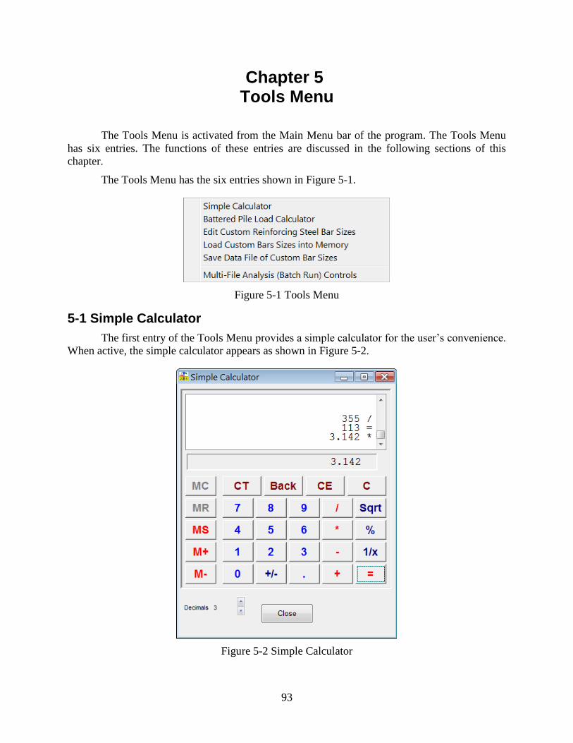
93
Chapter 5 Tools Menu
The Tools Menu is activated from the Main Menu bar of the program. The Tools Menu
has six entries. The functions of these entries are discussed in the following sections of this
chapter.
The Tools Menu has the six entries shown in Figure 5-1.
Figure 5-1 Tools Menu
5-1 Simple Calculator
The first entry of the Tools Menu provides a simple calculator for the user’s convenience.
When active, the simple calculator appears as shown in Figure 5-2.
Figure 5-2 Simple Calculator

Chapter 5 – Tools Menu
94
The calculator has two display areas. A “tape” display is shown on top. The tape display
shows the sequence of calculator operations. The answer display is shown below the tape
display.
The buttons on the top of the calculator buttons have the following functions:
CT Clears the content of the tape display,
Back Deletes the last digit entered (a backspace key),
CE Clears the last full number entered into the calculator, and
C Clears all the numbers entered into the calculator.
The function buttons on the right-hand side of the calculator have the following
functions:
Sqrt Computes the square root of the current number,
% Divides the current number by 100 to express the number as a percentage, and
1/x Computes the reciprocal of the current number.
The buttons on the left-hand side of the calculator control the memory functions. The
memory functions are:
MS Store a number to memory,
M+ Add the current number to the number stored in memory,
M– Subtract the current number from the number stored in memory,
MC Clear (erase) the number stored in memory, and
MR Recall the number stored in memory.
Note that the MC and MR buttons are enabled only when a number is stored in memory.
5-2 Battered Pile Load Calculator
The second entry of the Tools Menu provides a special-purpose calculator to compute
axial and transverse forces acting on battered piles from horizontal and vertical loadings.
This calculator is intended only for use with conventional analyses in which lateral
loading is applied perpendicular to the axis of the unbent pile and axial loads are applied along
the axis of the pile.
This calculator obtains the batter angle of the pile from the input value for pile batter and
the values of horizontal and vertical loading from the input fields of the calculator.
Values of transverse shear force and axial force for the specified batter angle are
computed when the user presses the button to Compute and Chart Rotated Forces. The Chart that
is generated shows how the rotated forces vary over batter angles ranging from –45 to +45
degrees. The symbols on the curves indicate the values for the specified batter angle.
The computation performed by the calculator is
v
H
A
T
P
V
P
V
cossin
sincos
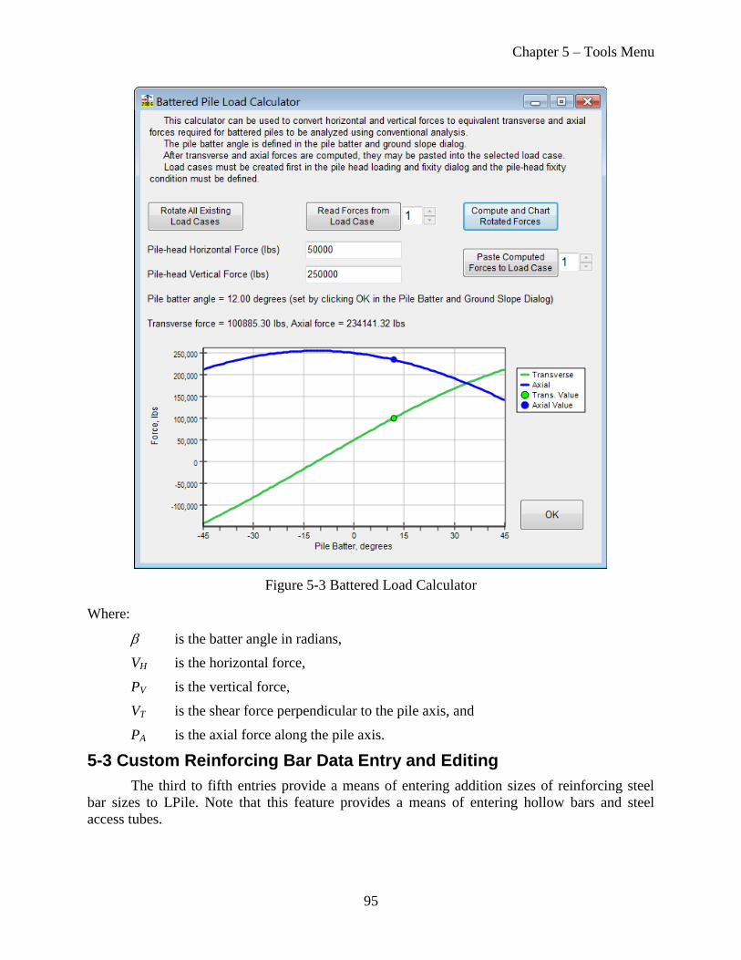
Chapter 5 – Tools Menu
95
Figure 5-3 Battered Load Calculator
Where:
is the batter angle in radians,
VH is the horizontal force,
PV is the vertical force,
VT is the shear force perpendicular to the pile axis, and
PA is the axial force along the pile axis.
5-3 Custom Reinforcing Bar Data Entry and Editing
The third to fifth entries provide a means of entering addition sizes of reinforcing steel
bar sizes to LPile. Note that this feature provides a means of entering hollow bars and steel
access tubes.

Chapter 5 – Tools Menu
96
Figure 5-4 Dialog for Editing of Custom Rebar Data
The third entry displays an input table to enter and edit the data for the custom
reinforcing bar sizes.
The fourth entry will transfer the data for custom reinforcing bars into the memory of
LPile and enter the names of the bars into the drop-down combination edit controls for selection
of the size of reinforcing bars. Note that the custom bar sizes are at the bottom of the drop-down
lists for bar sizes available for normally reinforced concrete sections.
The fifth entry saves the custom bar sizes to a data file named Custom_Rebar.dat. This
data file is stored in the same program folder as the main LPile program. When LPile is started,
LPile checks the program folder for a file with this name. If the file is found, it is read and the
data is stored into program memory. Thus, it is not necessary for the user to re-enter the custom
bar data each time the program is run.
Whenever the user wishes to exchange data files with another user, the data file for
custom bar sizes should also be provided to the other user, as the full list of custom bar sizes is
not included as part of the LPile data file.
5-4 Multi-File Analysis (Batch Run Utility)
The sixth entry provides a feature to define a list of existing LPile data files to be run as a
batch and the command to perform the batch analysis.
The control dialog for multi-file analysis is shown in Figure 5-5. The dialog is operated
by adding a file to the list by pressing the Add File to List button. The Add File to List button
will open an input dialog in which either single or multiple files can be selected from any folder.
The list of selected files is shown in the upper text pane of the control dialog.

Chapter 5 – Tools Menu
97
Figure 5-5 Dialog for Multi-File Analysis Controls
If needed, files can be deleted from the list by entering the file number and pressing the
Delete File No. button.
The file list may be cleared by pressing the Clean the File List button.
Once the file list is complete, the user directs LPile to process the list of files by pressing
the Run All Analyses button.
The processing time for each file and the warning or error message status of each file is
shown in the lower text pane of the control dialog. This text pane displays the Run Messages
If desired the file list can be saved and re-opened by pressing the appropriate buttons.
Lastly, if the user wishes to save the Run Messages, he may do so by pressing the Save
Run Msg File button.

Chapter 5 – Tools Menu
98
(This page was deliberately left blank)

99
Chapter 6 Example Problems
The problems in this chapter are provided as examples of the types of applications that
may be solved using LPile. Each example focuses on a particular computational feature of the
program. The input files for the examples are automatically copied to a sub-folder named
Lpile2013-Examples under the common Ensoft folder on the root directory of the computer
during installation. The data files are named with descriptive names and are copied to separate
sub-folders. For example, the path to Example 1 is
C:\Ensoft\Lpile2013-Examples\Example 1 Elastic Steel Pile in Sloping Ground\
Example problems provide information on input and output of various cases, and present
a quick tutorial for different applications. The user is encouraged to study these examples and,
with modifications, may use them to solve similar problems. However, by no means can these
limited examples explore the full functions and features provided by LPile.
The main features of each example included with LPile are summarized as follows.
Example 1 – Steel pile supporting a retaining wall. Among other aspects, this problem uses
sample applications of the following program features:
pile made of a standard structural steel shape, modeled as elastic pile with specified
moment capacity,
pile-head fixed against rotation,
report of internally-generated p-y curves at different depths for verification purposes,
application of several lateral loads, and
sloping ground surface.
Example 2 – Bored pile supporting a retaining wall. This example includes the following
program features:
pile is a drilled shaft,
comparison of values obtained with pile head fixed and free against rotations,
application of several lateral loads,
analysis with nonlinear bending stiffness, and
usage of sloping ground surface.
Example 3 – Steel pile supporting an offshore platform. Includes the following program features:
pile made of two different steel sections,
pile with head elastically restrained against rotations, and
cyclic loading.
Example 4 – Buckling of a pile column. This example includes the following program features:
steel pipe pile,
pile head free to rotate, and
application of several axial loads.
Example 5 – Ultimate bending moment for bored piles. Includes the following program features:

Chapter 6 – Example Problems
100
reinforced concrete pile of circular cross section,
nonlinear materials,
report of interaction diagram, and
report of nonlinear flexural rigidity.
Example 6 – Foundation Stiffness of Concrete Pile with Nonlinear Flexural Rigidity. Includes
the following program features:
reinforced concrete pile of circular cross section,
pile with head free to rotate,
nonlinear materials,
report of interaction diagram,
report of nonlinear flexural rigidity, and
generation of foundation stiffness components.
Example 7 – User Input of Distributed Load and External p-y Curves. Includes the following
program features:
reinforced concrete pile of circular cross section with two different section properties,
pile with head free to rotate,
input of distributed lateral load on a section length of pile with linear variation, and
input of externally-specified p-y curves.
Example 8 – Case Study of Piles in Cemented Sands. Includes the following program features:
reinforced concrete pile of circular cross section,
pile with head free to rotate,
input of several lateral loads, and
use of internal p-y curves for silts.
Example 9 – Sample of Various Program Options. Includes the following program features:
drilled shaft with reinforced concrete cross-section and belled bottom,
pile with head free to rotate,
sample coordinates for embedded pile head,
use of p-reduction factors assuming closely spaced piles,
use of several soil layers,
input of shear-resistance curve at pile tip, and
determination of top deflections versus varying pile lengths.
Example 10 – Drilled shaft in soft clay
multi-section drilled shaft with under-ream and toe, and
uniform rebar cage in upper sections.
Example 11 – LRFD analysis
input of unfactored loads
input of load and resistance factor combinations
Example 12 – Liquefied sand with lateral spread
lateral spread modelled using lateral soil movement versus depth

Chapter 6 – Example Problems
101
Example 13 – Top y versus pile length for square elastic pile
example compares standard and modified versions of p-y curves for stiff clay without
free water, and
computation of curves of top deflection versus pile length for multiple levels of loading.
Example 14 – Pushover analysis of prestressed concrete pile
Example 15 – Pile with input nonlinear bending properties
Example 16 – Analysis of pile loaded by distributed lateral loads
Example 17 – Analysis of double-section, rock socketed drilled shaft
Example 18 – Analysis of drilled shaft with permanent casing
Example 19 – Analysis of drilled shaft with permanent casing and core
Example 20 – Design analysis of embedded pole
Example 21 – Analysis of a tapered elastic pile
Example 22 – Analysis of a tapered elastic-plastic pile
Example 23 – Output of p-y curves at user specified depths
Example 24 – Analysis of pile loaded by soil movements
Example 25 – Verification of elastic pile in elastic subgrade
Example 26 – Verification of the P- effect
6-1 Example 1 – Steel Pile in Sloping Ground
The general description and geometrical configuration of Example 1 is shown in 5-1. The
pile is a standard structural steel shape (HP14×89), two layers of soil are present, and the ground
surface is sloping downward with respect to the lateral loading.
In an actual design, the data shown in this example problem might be for a particular trial
run. That is, the selection of the particular section for the pile and its length might change in the
course of the computations. Furthermore, the soil profile has been idealized and in an actual case
there would almost certainly be a need for consideration of the variation of the soil properties
with depth and across the site.
The axial service load on the pile axis is 88.8 kN (20 kips). If the load factor (global
factor of safety) is taken as 2.5, the axial load P to be used in the computations is 222 kN (50
kips). As it will be seen, the bending moment capacity is affected only slightly by the presence of
the axial load.
The sketch of the pile in Figure 6-1 shows that its top is fixed against rotation. Thus, it is
assumed that the top of the steel section projects a sufficient distance into the reinforced-concrete
base of the retaining wall so that no rotation of the top of the pile will occur. This assumption is
not strictly true, but research is yet to be done to yield expressions for the rotation of an
embedded steel member into a concrete mat. The assumption of pile-head fixity is conservative
because the maximum bending moment will occur at the top of the pile and any rotation of the
pile head will cause a decrease in the maximum moment.

Chapter 6 – Example Problems
102
The computations that follow are aimed at finding the lateral load V that will cause a
plastic hinge to develop at the top of the pile. Secondly, the computations should reveal if there
is a possibility of excessive deflection, which is thought to be unlikely for most retaining walls.
Figure 6-1 General Description of Example 1
The pile section type selected for the analysis is the Elastic Pile with Specified Moment
Capacity. With this type of section, it is possible to have the pile behave elastically up to the
specified moment capacity then form a plastic-hinge when the moment in the pile equals the
specified moment capacity.
The strong axis of the H-pile is perpendicular to the direction of loading, and data for this
axis were included in Figure 6-1. From the steel handbook, the width of the section is 373 mm
(14.696 in.) and the depth is 352 mm (13.86 in.).
The first consideration is the “diameter” to assign to the shape because the
recommendations for p-y curves are based strongly on the results of experiments with cylindrical
shapes. At the outset, it can be assumed that the soil in the flanges will move with the pile and
that it will behave as a rectangular shape. Secondly, the equivalent diameter of the pile can be
computed, as a first approximation, by finding a circular section with the same area as the
rectangular section. Thus,
inches 1.16mm 408)mm 351)(mm 373(4
)mm 351)(mm 373(4
2
e
e
d
d
10
HP14 89Ix = 3.76 10-4 m4
fy = 276 MPa
Stiff Clayg = 18.7 kN/m3
c = 96.5 kPa50 = 0.007
Sandg ‘ =9.9 kN/m3
f = 35
15.2 m
P
V

Chapter 6 – Example Problems
103
As shown above, this computation yields a diameter that is less than 10 percent larger than the
width of the steel section.
The equivalent diameter may be entered as the width of the pile, or, conservatively, the
actual width of 373 mm (14.686 in.) may be entered. The decision of which value to be entered
is left to the user, but the actual width will be used in this example. The values used in this
example are shown in Figure 6-2 below.
Figure 6-2 Dimensions and Properties Entered for Example 1
The user should understand how the values entered for Dimensions and Properties can be
manipulated to enter the desired data to LPile. LPile is programmed to compute values of cross-
sectional area and moment of inertia from the input dimension values when the user presses the
button to Compute Moment of Inertia and Areas and Draw Section. In the case of H-piles, often
the computed areas of area and moment of inertia differ from the standard values published for
design. If the user wishes to replace the computed value, the user may enter the standard values
directly, but must remember not to the button to compute values. If the user presses the button to
compute values, the manually entered values will be replaced by the computed values.
The yield moment for the section may be computed by a procedure proposed by Horne
(1978). With no axial compression load and with bending about the strong axis, the plastic
moment strength is computed the product of the yield stress and plastic modulus as follows:

Chapter 6 – Example Problems
104
m-kN 660
m-MN 660.0
1039.2276 3
p
p
p
yp
M
M
M
ZFM
Considering the effect of axial load:
kips-in 5,815 m-kN 657
)000,276()0258.0)(0156.0(660
mm 0258.0
)000,276)(0156.0)(2(
222
2
2
p
p
ywpp
yw
x
M
M
fatMM
a
a
ft
Pa
In other cases where the pile extends above the ground surface, the designing engineer
will need to consider the compact section properties of the pile. In some H-pile sections, the pile
flanges may buckle at stress levels below the yield stress of steel and the section is called “non-
compact.” For this pile section, the compact section stress criterion is 131.7 MPa. To consider
the compact section criterion one substitutes the compact section stress for the yield stress.
The loading from a retaining wall is a sustained static loading, not a cyclic load. In some
cases, the designer is faced with the problem of estimating the consolidation and creep of the
clay and/or the additional deflection due to vibration of the sand. The value of shear strength
indicates that the clay is overconsolidated; thus, as a first approximation, no significant
consolidation or creep is assumed. In addition, the sand, well below the ground surface, is
assumed not to densify due to possible vibration. These assumptions will need to be carefully
reviewed after a preliminary solution is obtained.
The above discussion shows that static loading is appropriate for both the clay and the
sand. Further, the recommendations for stiff clay above the water table are most appropriate. The
next step is to find the value of pile-head shear force, V, that will develop a bending moment in
the pile of 657 kN-m (5,815 in.-kips).
The results of the preliminary computations using the displacement-slope pile-head
condition are shown in Figure 6-3 and Figure 6-4. As may be seen, the computations show that
the pile will fail structurally when the axial load is held at 222 kN (50 kips) and the lateral load
reaches a value of 410 kN (92 kips). The pile-head deflection at the failure loading was
computed to be about 27 mm (1.06 in.). This deflection is considered tolerable; therefore, the
failure of the pile is taken to be due to the development of a plastic hinge.
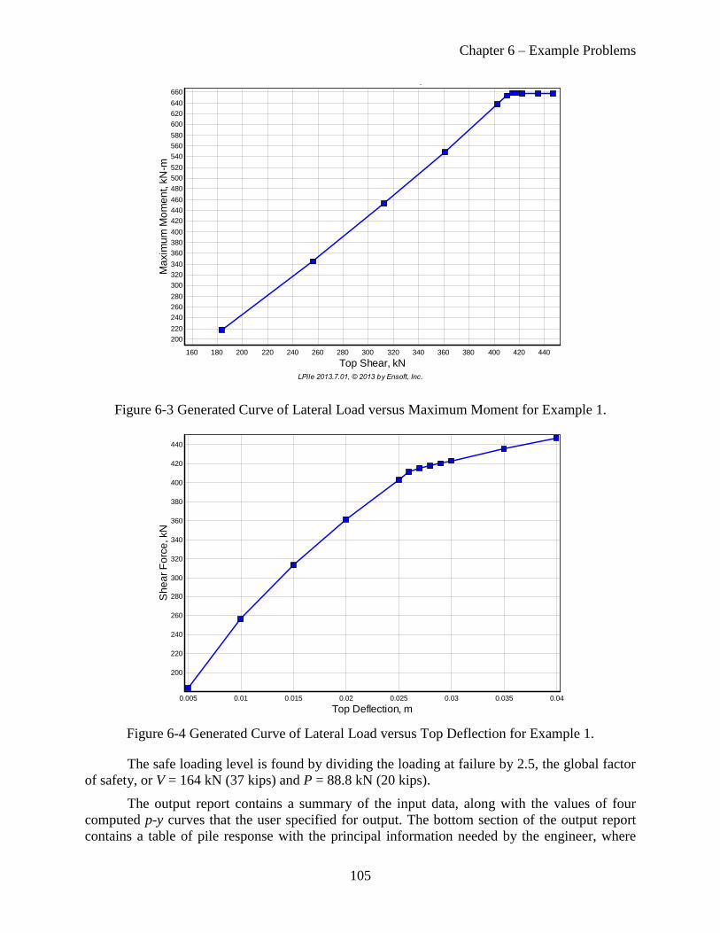
Chapter 6 – Example Problems
105
Figure 6-3 Generated Curve of Lateral Load versus Maximum Moment for Example 1.
Figure 6-4 Generated Curve of Lateral Load versus Top Deflection for Example 1.
The safe loading level is found by dividing the loading at failure by 2.5, the global factor
of safety, or V = 164 kN (37 kips) and P = 88.8 kN (20 kips).
The output report contains a summary of the input data, along with the values of four
computed p-y curves that the user specified for output. The bottom section of the output report
contains a table of pile response with the principal information needed by the engineer, where
Maximum Moment vs. Top Shear
LPile 2013.7.01, © 2013 by Ensoft, Inc.
Top Shear, kN440420400380360340320300280260240220200180160
Ma
xim
um
Mo
me
nt, k
N-m
660
640
620
600
580
560
540
520
500
480
460
440
420
400
380
360
340
320
300
280
260
240
220
200
Shear Force vs. Top Deflection
LPile 2013.7.01, © 2013 by Ensoft, Inc.
Top Deflection, m0.040.0350.030.0250.020.0150.010.005
Sh
ea
r F
orc
e, kN
440
420
400
380
360
340
320
300
280
260
240
220
200

Chapter 6 – Example Problems
106
computed values are given as a function of depth. The table indicates that the length of the pile
may be decreased to 10 m (33 ft) and that there will be three points of zero deflection, a
sufficient number to ensure that the pile behaves as a long pile. By reducing the length of the
pile, some unneeded output can be eliminated and, further, the amount of internal computations
performed by the computer is reduced.
Plots of lateral deflection and bending moment as a function of depth are shown in Figure
6-5 and Figure 6-6. The loadings for the second analysis were a V of 164 kN (37 kips) and P of
88.8 kN (20 kips). The computed deflection at the top of the pile was to be 4.0 mm (0.16 in.) and
the maximum bending moment was 186 kN-m (138.5 ft-kips), a value that is well below 657 kN-
m (485 ft-kips) that would cause the pile to fail. The next step is to find the value of Pt that will
develop a bending moment in the pile of 657 kN-m (5,815 in.-kips).
Figure 6-5 Curve of Deflection versus Depth for Example 1, Second Analysis
The curve shown in Figure 6-6 shows that the maximum bending moment occurs at the
top of the pile, where it is fixed against rotation. If the pile head is permitted to rotate slightly,
the negative moment at the pile head will decrease and the value of the maximum positive
moment, now at a depth of 2.9 m (9.5 ft), will increase. Further, it is of interest to note that the
bending moment is virtually zero at depths of 5 m (16.4 ft) and below.
The input data and output files have the filename Example 1a HP 14x89 in sloping
ground.lp9d. These files are found in the Examples folder with the program. The filename
extensions for the files are shown in Table 2-1. The output files are not shown in this User’s
Manual due to their length.
The filename for the second run is named Example 1b HP 14x89 in sloping ground,
second run.lp9d. The input and output files are not shown here due to their length.
Lateral Deflection vs. Depth
LPile 2013.7.01, © 2013 by Ensoft, Inc.
Loading Case 1gfedcb
Deflection, m0.0040.00350.0030.00250.0020.00150.0010.00050-0.0005
De
pth
, m
15
14
13
12
11
10
9
8
7
6
5
4
3
2
1
0

Chapter 6 – Example Problems
107
Figure 6-6 Bending Moment versus Depth for Example 1, Second Analysis
6-2 Example 2 – Drilled Shaft in Sloping Ground
This example is similar to Example 1, but in this case, the pile is replaced by a drilled
shaft (bored pile). The soil properties and ground slope angle are the same as those used in
Example 1. The design issue with a reinforced-concrete pile is to find the nominal bending
moment capacity and an appropriate value of flexural stiffness (EI) to use in the computations.
As in Example 1, an axial thrust load of 88.8 kN (20 kips) is assumed. The pile head is
assumed fixed against rotation in the first loading case and free to rotate in the second loading
case. The problem is to find the lateral load for each case that will cause the shaft to fail. Both of
these loading cases might be used in a practical problem to establish the bounds for the solution
if the rotational restraint caused by embedment of the top of the pile causes the pile head to be
between fixed and free.
A drilled shaft with an outside diameter of 760 mm (30 in.) and a length of 15.2 m (50 ft)
is used in this example. The reinforcing steel consists of 12 bars with outside diameter of 25 mm
(corresponding to No. 8 bars in US practice) and spaced equally around a 610 mm (24 in.)
diameter circle as shown in Figure 6-7. The ultimate strengths of the reinforcing steel and the
concrete are 414 MPa (60 ksi) and 27.6 MPa (4.0 ksi), respectively.
Example 2a is the computation and plotting of the unfactored interaction diagram. This
problem is configured by selecting the Compute Nonlinear EI Only option in the Program
Options and Settings dialog and by entering the structural dimensions and material properties of
the pile’s cross-section.
When computing an interaction diagram, the user must enter the axial thrust forces for
the analysis. This means that the user must determine the maximum compressive and tensile
axial capacities along with a number of intermediate axial thrust values. Usually, a bored pile in
soil will fail by axial bearing capacity before the pile section will fail by crushing, so the upper
limit may be limited by the computed axial bearing capacity, if this value is available. Otherwise,
the user may opt to make two analyses, the first with zero axial thrust and the second with a
Bending Moment vs. Depth
LPile 2013.7.01, © 2013 by Ensoft, Inc.
Loading Case 1gfedcb
Bending Moment, kN-m806040200-20-40-60-80-100-120-140-160-180-200
De
pth
, m
15
14
13
12
11
10
9
8
7
6
5
4
3
2
1
0
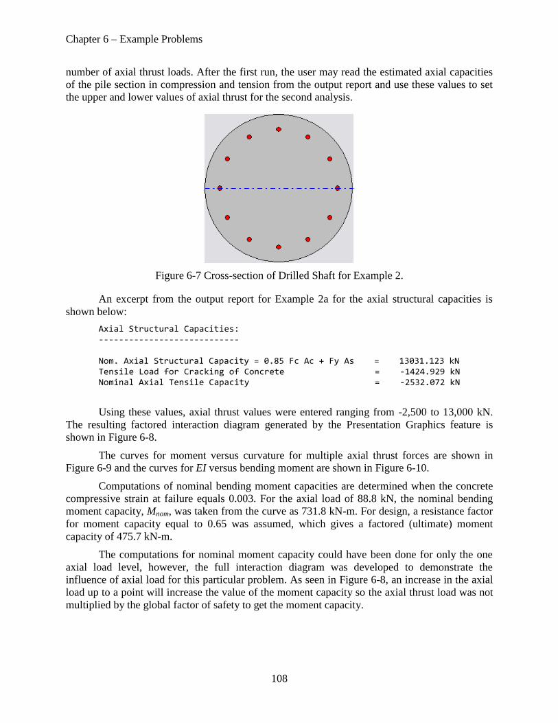
Chapter 6 – Example Problems
108
number of axial thrust loads. After the first run, the user may read the estimated axial capacities
of the pile section in compression and tension from the output report and use these values to set
the upper and lower values of axial thrust for the second analysis.
Figure 6-7 Cross-section of Drilled Shaft for Example 2.
An excerpt from the output report for Example 2a for the axial structural capacities is
shown below:
Axial Structural Capacities: ---------------------------- Nom. Axial Structural Capacity = 0.85 Fc Ac + Fy As = 13031.123 kN Tensile Load for Cracking of Concrete = -1424.929 kN Nominal Axial Tensile Capacity = -2532.072 kN
Using these values, axial thrust values were entered ranging from -2,500 to 13,000 kN.
The resulting factored interaction diagram generated by the Presentation Graphics feature is
shown in Figure 6-8.
The curves for moment versus curvature for multiple axial thrust forces are shown in
Figure 6-9 and the curves for EI versus bending moment are shown in Figure 6-10.
Computations of nominal bending moment capacities are determined when the concrete
compressive strain at failure equals 0.003. For the axial load of 88.8 kN, the nominal bending
moment capacity, Mnom, was taken from the curve as 731.8 kN-m. For design, a resistance factor
for moment capacity equal to 0.65 was assumed, which gives a factored (ultimate) moment
capacity of 475.7 kN-m.
The computations for nominal moment capacity could have been done for only the one
axial load level, however, the full interaction diagram was developed to demonstrate the
influence of axial load for this particular problem. As seen in Figure 6-8, an increase in the axial
load up to a point will increase the value of the moment capacity so the axial thrust load was not
multiplied by the global factor of safety to get the moment capacity.
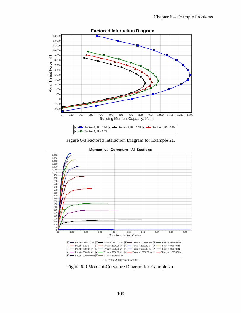
Chapter 6 – Example Problems
109
Figure 6-8 Factored Interaction Diagram for Example 2a.
Figure 6-9 Moment-Curvature Diagram for Example 2a.
Factored Interaction Diagram
LPile 2013.7.01, © 2013 by Ensoft, Inc.
Section 1, Rf = 1.00gfedcb Section 1, Rf = 0.65gfedcb Section 1, Rf = 0.70gfedcbSection 1, Rf = 0.75gfedcb
Bending Moment Capacity, kN-m1,3001,2001,1001,0009008007006005004003002001000
Axia
l T
hru
st F
orc
e, kN
13,000
12,000
11,000
10,000
9,000
8,000
7,000
6,000
5,000
4,000
3,000
2,000
1,000
0
-1,000
-2,000
Moment vs. Curvature - All Sections
LPile 2013.7.01, © 2013 by Ensoft, Inc.
Thrust = -2500.00 kNgfedcb Thrust = -2000.00 kNgfedcb Thrust = -1425.00 kNgfedcb Thrust = -1000.00 kNgfedcbThrust = 0.00 kNgfedcb Thrust = 1000.00 kNgfedcb Thrust = 2000.00 kNgfedcb Thrust = 3000.00 kNgfedcbThrust = 4000.00 kNgfedcb Thrust = 5000.00 kNgfedcb Thrust = 6000.00 kNgfedcb Thrust = 7000.00 kNgfedcbThrust = 8000.00 kNgfedcb Thrust = 9000.00 kNgfedcb Thrust = 10000.00 kNgfedcb Thrust = 11000.00 kNgfedcbThrust = 12000.00 kNgfedcb Thrust = 13000.00 kNgfedcb
Curvature, radians/meter0.090.080.070.060.050.040.030.020.010.0
Mo
me
nt, k
N-m
ete
rs
1,300
1,250
1,200
1,150
1,100
1,050
1,000
950
900
850
800
750
700
650
600
550
500
450
400
350
300
250
200
150
100
50
0

Chapter 6 – Example Problems
110
Figure 6-10 Bending Stiffness versus Bending Moment for Example 2a.
In earlier versions of LPile, the user had to select a constant value of bending stiffness to
use in an analysis. This is no longer needed, as LPile will automatically vary the value of
bending stiffness in proportion to the bending curvature developed in the pile.
The load-deflection curves and moment versus shear force curves for free-head
conditions are shown in Figure 6-11 and for fixed-head conditions are shown in Figure 6-12. The
scales of the two figures have been set equal to aid comparing the two sets of graphs.
The free-head shaft reaches its nominal moment capacity at a shear load of approximately
530 kN and its factored moment capacity at a shear load of 346 kN at a deflection of 0.035 m.
The fixed-head shaft reaches it nominal moment capacity at a shear load of 550 kN and its
factored moment capacity at a shear load of 352 kN at a deflection of 0.0076 m. By
happenstance, the load-carrying capacity of the two pile-head conditions are nearly equal.
However, the load-deflection response of the fixed-head shaft is substantially stiffer.
To illustrate the differences in deflection and bending moment versus depth for the two
pile-head fixity conditions, a fourth analysis was performed for pile-head shear loads equal to
346 for the free-head shaft and 352 kN for the fixed-head shaft. The results of this analysis are
shown in Figure 6-13.
The length of the pile may be reduced if there are more than two points of zero
deflection, which ensures that the pile acts as a stable pile. The LPile can perform a series of
analyses with different lengths of piles, so the user can compare pile length versus deflection at
the pile head. The curves of top deflection versus pile length for free and fixed-head conditions is
shown in Figure 6-14.
EI vs. Moment - All Sections
LPile 2013.7.01, © 2013 by Ensoft, Inc.
Thrust = -2500.00 kNgfedcb Thrust = -2000.00 kNgfedcb Thrust = -1425.00 kNgfedcb Thrust = -1000.00 kNgfedcbThrust = 0.00 kNgfedcb Thrust = 1000.00 kNgfedcb Thrust = 2000.00 kNgfedcb Thrust = 3000.00 kNgfedcbThrust = 4000.00 kNgfedcb Thrust = 5000.00 kNgfedcb Thrust = 6000.00 kNgfedcb Thrust = 7000.00 kNgfedcbThrust = 8000.00 kNgfedcb Thrust = 9000.00 kNgfedcb Thrust = 10000.00 kNgfedcb Thrust = 11000.00 kNgfedcbThrust = 12000.00 kNgfedcb Thrust = 13000.00 kNgfedcb
Bending Moment, kN-m1,3001,2001,1001,0009008007006005004003002001000
EI, k
N-m
²520,000
500,000
480,000
460,000
440,000
420,000
400,000
380,000
360,000
340,000
320,000
300,000
280,000
260,000
240,000
220,000
200,000
180,000
160,000
140,000
120,000
100,000
80,000
60,000
40,000
20,000
0

Chapter 6 – Example Problems
111
Figure 6-11 Shear Force versus Top Deflection and Maximum Bending Moment versus Top
Shear Load for Free-head Conditions in Example 2b.
Figure 6-12 Shear Force versus Top Deflection and Maximum Bending Moment versus Top
Shear Load for Fixed-head Conditions in Example 2c.
Shear Force vs. Top Deflection
Top Deflection, m0.150.140.130.120.110.10.090.080.070.060.050.040.030.020.010
Sh
ea
r F
orc
e, kN
800
750
700
650
600
550
500
450
400
350
300
250
200
150
100
50
0
Maximum Moment vs. Top Shear
Top Shear, kN800750700650600550500450400350300250200150100500
Ma
xim
um
Mo
me
nt, k
N-m
750
700
650
600
550
500
450
400
350
300
250
200
150
100
50
0

Chapter 6 – Example Problems
112
Figure 6-13 Results for Free-head and Fixed-head Loading Conditions for Example 2d
Figure 6-14 Top Deflection versus Pile Length for Example 2d
Perhaps it is of interest to note that the lateral loads that were computed for the steel pile
and for the bored pile were of significant magnitude, indicating that different types of piles can
be used economically to sustain lateral loads.
Free-head Shaftgfedcb Fixed-head Shaftgfedcb
Deflection, m0.0350.030.0250.020.0150.010.0050-0.005
De
pth
, m
10
9
8
7
6
5
4
3
2
1
0
Free-head Shaftgfedcb Fixed-head Shaftgfedcb
Bending Moment, kN-m5004003002001000-100-200-300-400-500
De
pth
, m
10
9
8
7
6
5
4
3
2
1
0
Free-head Shaftgfedcb Fixed-head Shaftgfedcb
Pile Length, m109876543210
To
p D
efle
ctio
n, m
0.17
0.16
0.15
0.14
0.13
0.12
0.11
0.1
0.09
0.08
0.07
0.06
0.05
0.04
0.03
0.02
0.01

Chapter 6 – Example Problems
113
6-3 Example 3 – Offshore Pipe Pile
The illustration in Figure 6-15 shows an offshore platform of the type used in water
depths of 100 m or more. Thousands of such structures have been built where a structure is
fabricated on shore, barged or floated to the site, and placed by lifting or controlled
submergence. For the case indicated, the weight of the jacket causes the extensions of the legs to
push into the soil. With the top of the template above still water, piles are stabbed and driven
through the main legs. The tops of the piles are trimmed, and welded to the jacket, and the
annular space between the outside of the piles and the inside of the jacket leg is filled with grout.
Finally, a deck section is lifted and its support columns are stabbed into the tops of the main legs
and then welded.
Figure 6-15 Idealized View of an Offshore Platform Subjected to Wave Loading, Example 3
The soil profile at the site is not shown in the sketch. In this example, it is soft clay with
some overconsolidation due to wave action at the mudline, but with an increase in strength with
depth as for normal consolidation. An assumption is made that some scour will occur around the
piles to a depth of 1.5 meters (5 feet). The undrained strength of the clay at that depth is 24 kPa
(500 psf) and the strength at 30 m is 72 kPa (1,500 psf). The submerged unit weight is 9.00
kN/m3 (57 pcf); 50 is 0.02 at 1.5 m (5.0 ft) and decreases to 0.01 at 30 meters (98 feet).
The sketches of Figure 6-16 show one of the piles from the structure with the rotational
restraint given approximately by an equation. The number 3.5 indicates that the bracing has been
discounted and that the member is acting as one whose far end is intermediate between fixed and
free. The approximation is adequate for a preliminary solution but, for the final analysis, the
superstructure and the piles should be considered as continuous, and the piles analyzed as a
group.

Chapter 6 – Example Problems
114
Figure 6-16 Superstructure and Pile Details, Example 3
The critical loading occurs during a severe storm, and Figure 6-15 shows the approximate
position of a wave as it moves past the structure. The selection of a particular wave height and
velocity of the wind is a problem in statistics, and the factor of safety to be employed is related to
those selections. For this problem, it is assumed that a load factor of 2.4 is appropriate. The axial
loading of the pile that is analyzed is 1,250 kN (281 kips); thus, the load in the design
computations is 3,000 kN (674 kips). A solution consists of finding the lateral loading that will
cause a plastic hinge to develop in the pile, and the safe load by dividing that load by the global
factor of safety.
The sketch in Figure 6-16 shows that the pile to a distance of 4.0 m (13.1 ft) from its top
consists of two pipes that are acting together. The outside diameter of this combined section is
838 mm (33 in.), the wall thickness is 28.14 mm (1.11 in.), and its moment of inertia is
5.87610-3
m4 (4,117 in
4). The lower section has an outside diameter of 762 mm (30 in.), a wall
thickness of 19.05 mm (0.75 in.), and a moment of inertia of 3.07010-3
m4 (7,376 in
4). The
ultimate strength of the steel for the piles is assumed is 0.395 MPa (57,290 psi).
Figure 6-17 shows the results of computations for the moment versus curvature analysis
of the sections of the pile in the example. As shown in the Technical Manual, the stress-strain
curve for the steel is assumed as bilinear; thus, the ultimate bending moment will continue to
increase slightly as the full section of the pile approaches the plastic range. It was decided to
accept the value of Mnom as the value where the maximum curvature is 0.015 radians/meter. For
the upper section, a nominal moment capacity of 7,140 kN-m was computed. The corresponding
value for the lower section of the pile was 4,040 kN-m.
4 m
h = 6.1 m
d = 762 mmIp = 3.07 x 10⁻³ m4
E = 2 x 10⁸ kPa
d = 838 mmIc = 5.876 x 10⁻³ m4
t
c
t MEI
hS
5.3
V
M
MV

Chapter 6 – Example Problems
115
Figure 6-17 Moment versus Curvature, Example 3
The soil conditions at the site are in the range of soft clay below the water, and the
recommendations for that soil are employed in the computations. Cyclic loading is employed
because the design is to reflect the response of the structure to a storm.
Some comment is needed about the number of cycles of loading. If the documentation is
reviewed for the experiments that resulted in the development of the recommendations, it will be
noticed that the cycles of loading were continued until an apparent equilibrium was reached;
thus, the criteria reflect the limiting condition (or worst condition). However, during a particular
storm, there may be only a small number of loads of the largest magnitude during the peak of the
storm. Therefore, the recommendations may be somewhat more conservative than necessary, but
at the present, recommendations are unavailable to allow the introduction of the number of
cycles into the procedure.
In reference to the previously shown Figure 6-16, initial computations were necessary to
learn if the lateral loading on the selected pile would cause a critical moment in the upper or
lower section. A series of computer runs and plots were made of the maximum moment as a
function of Vtop for both the upper and lower sections. Figure 6-18 shows that the maximum
moment for the upper section, 7,140 kN-m and negative in sign, occurred with a lateral load of
1,200 kN. At that value of Vtop, the maximum moment for the lower section was about 2,500 kN-
m, which was far less than the yield value of 4,040 kN-m. Thus, the upper section of the pile
controls the loading.
The deflection of the top of the pile, ytop, for the failure loading of 1,200 kN was
computed to be 339 mm and, in some designs, the deflection might have controlled the loading.
However, the computed deflection will be much less when the factored load is used; furthermore,
excessive deflection is rarely a problem in the design of an offshore platform. It is true that
personnel could experience distress on a deck that was moving radically; however, in normal
Section 1, Thrust = 1250.00 kNgfedcb Section 2, Thrust = 1250.00 kNgfedcb
Curvature, radians/meter0.0250.02250.020.01750.0150.01250.010.00750.0050.00250.0
Mo
me
nt, k
N-m
7,500
7,000
6,500
6,000
5,500
5,000
4,500
4,000
3,500
3,000
2,500
2,000
1,500
1,000
500
0

Chapter 6 – Example Problems
116
circumstances, the personnel are removed from the platform during the occurrence of the design
storm.
Figure 6-18 Results of Initial Computation with p-y Curves, Example 3
Employing a load factor of 2.4 (global factor of safety), the service value of pile-head
shear force Vtop is 500 kN and, as noted before, the axial thrust force Q is 1,250 kN. The resulting
moment diagram is shown in Figure 6-19. The computed value of pile-head deflection ytop, not
plotted here, was 62 mm, which is acceptable.
An examination of Figure 6-19 finds that the moment diagram is virtually zero below a
depth of 21 m; therefore, the selection of the thickness of the wall of the pile below this depth
will be based on the requirements of pile driving analysis and axial pile capacity, rather than
lateral loading. Additionally, it is evident that the maximum bending moment could be reduced
significantly if the designer has some control over the value of the rotational restraint at the
mudline. Thus, the opportunity exists for minimizing the cost of the foundation by a judicious
selection of the manner in which the piles are connected to the superstructure. For example, a
less expensive solution could have been achieved if shims had been used at the bottom of jacket-
leg extension and at the joints, with the result that no grouting would have been needed. Finally,
the thick-walled section of the pile, whatever the final design, will be needed in the upper 21 m;
therefore, the methods of installation must be such that the pile can be installed to the required
penetration into the soil profile.
0
1,000
2,000
3,000
4,000
5,000
6,000
7,000
8,000
0 250 500 750 1,000 1,250
Mo
men
t, k
N-m
Pile-head Shear, kN
Sect. 1 Mmax
Sect. 2 Mmax
Sect. 1 Mnom
Sect. 2 Mnom

Chapter 6 – Example Problems
117
Figure 6-19 Pile Deflection and Bending Moment versus Depth for Vtop = 500 kN, Example 3
6-4 Example 4 - Buckling of a Pile-Column
One analytical feature of LPile is an automatic analysis for buckling capacity of a pile. It
is not often that such a problem is encountered in practice, but a rational solution is desired if
such a problem occurs.
In this example, the lateral load at the pile head is 44.5 kN (10 kips) and the loading was
static. The lateral load and the axial load are applied at the top of the pile, which was 2.5 m (8.3
ft) above the groundline. The bending moment at the pile head is zero.
The solution to the problem seeks the same answer as does the Euler solution for a
column, but, because the response of the soil is nonlinear, an Eigen value solution is not
applicable. Rather, the answer is obtained by successive solutions of the nonlinear, beam-column
equation with the axial load being increased until excessive lateral deflection is computed or the
bending moment capacity of the pile is fully mobilized.
The example pile is an elastic steel pipe, 610 mm (24 in.) in outside diameter, and with a
wall thickness of 22.2 millimeters (0.875 inch). The EI is 354,312 kN-m
2 (1.23510
11 lb-in
2).
The length is 15.2 meters (50 feet). Had the portion of the pile above the groundline been greater
than 2.54 m (8.33 ft), the buckling load that was found would have been much less than the
computed value.
The soil profile is sand with an angle of internal friction of 35 degrees. The water table is
below the tip of the pile. The effective unit weight of the sand is 19 kN/m3 (121 pcf).
The p-y curves for static loading of sand above the water table are appropriate for the
problem. Presumably, the soil properties are those that exist after the pile has been installed.
The results from the pile buckling analysis are shown in Figure 6-20. Note that this figure
was drawn for this manual and was not generated by LPile, The deflection at the top of the pile,
Deflection, m0.070.060.050.040.030.020.010-0.01
De
pth
, m
25
24
23
22
21
20
19
18
17
16
15
14
13
12
11
10
9
8
7
6
5
4
3
2
1
0
Bending Moment, kN-m1,0005000-500-1,000-1,500-2,000-2,500
De
pth
, m
25
24
23
22
21
20
19
18
17
16
15
14
13
12
11
10
9
8
7
6
5
4
3
2
1
0

Chapter 6 – Example Problems
118
as a function of the axial thrust force is shown as the black line and the maximum bending
moment as the blue line. The estimated buckling capacity is shown by the red line (19,592 kN).
Figure 6-20 Pile-head Deflection and Maximum Bending Moment versus Axial Thrust Loading
LPile estimates the pile buckling capacity by fitting a hyperbolic curve to the computed
results of top deflection versus axial thrust force. The procedure used to fit the hyperbolic curve
is discussed in Section 3-12-6. A graph of the pile buckling analysis results generated by LPile
for Example 4 is shown in Figure 6-21.
While the solution to the problem appears to be rather straightforward using LPile, there
presently are no other analytical solutions for pile buckling available to take the nonlinear load
transfer from the pile to the soil into account. It is also important to note that the pile buckling
analysis feature of LPile can also be used to investigate the effects of the eccentric application of
axial loading and the effect of accidental batter.
0
0.005
0.01
0.015
0.02
0.025
0.03
0.035
0.04
0.045
0
100
200
300
400
500
600
700
800
900
0 5,000 10,000 15,000 20,000
Pil
e T
op
Defl
ec
tio
n, m
ete
rs
Ma
xim
um
Mo
me
nt,
kN
-m
Axial Thrust Force, kN
Top Deflection
Max. Moment
Est. Buckling Cap.

Chapter 6 – Example Problems
119
Figure 6-21 Results from LPile Solution for Buckling Analysis, Example 4
6-5 Example 5 – Computation of Nominal Moment Capacity and Interaction Diagram
Example 5 is presented to illustrate a feature of LPile for computation of the nominal
bending moment capacity and to display an interaction diagram. A total of 17 axial loads were
specified for the program to compute the ultimate bending moment at each axial load and to
construct the interaction diagram (ultimate bending moment versus axial load).
The ultimate bending moment of a reinforces-concrete section is taken at a maximum
compressive strain in concrete of 0.003 based on the ACI 318 code. It should be noted that the
bending stiffness (EI), corresponding to the ultimate bending moment, is significantly lower than
that of the uncracked EI value. Therefore, the user should also pay attention to the variation of EI
versus moment for nonlinear piles. In general, the moment distribution in the pile is not affected
much by the EI used in the computation. However, if the deflection is more critical for the
design, then analysis using nonlinear values of EI should be done.
Curves showing the development of moment versus curvature for various axial thrust
values are shown in Figure 6-22. The curves showing the greatest amount of ductility are the
curves with tensile axial thrust loadings. In general, the amount of ductility decreases as the axial
thrust level increases.
Free-head Condition
LPile 2013.7.07, © 2014 by Ensoft, Inc.
Pile Response Computed by LPile Fitted Hyperbolic Buckling Curve
Buckling Capacity = 19,592 kN
Top Deflection, m0.040.030.020.010
Axi
al T
hru
st L
oa
d, kN
20,000
19,000
18,000
17,000
16,000
15,000
14,000
13,000
12,000
11,000
10,000
9,000
8,000
7,000
6,000
5,000
4,000
3,000
2,000
1,000
0

Chapter 6 – Example Problems
120
Figure 6-22 Moment versus Curvature for Example 5
Curves of bending stiffness versus bending moment are shown in Figure 6-23. In general,
three ranges of EI magnitude can be found in the output. The first range of EI magnitude is
associated with the uncracked stage. The concrete is uncracked and the EI is more-or-less
constant and is equal to the calculated EI for the gross section. The second range of EI magnitude
is for the cracked stage. A significant decrease in the EI value takes place as cracks continue
propagating. The third range of EI magnitude is for the cracked and large strain stage. The EI
value is further reduced because the concrete stress-strain curve (shown in the Technical
Manual) is softened at large strains.
The curves for tensile axial thrust show a behavior that is not found for compressive axial
thrusts. For these curves (see the blue and black curves in the lower left corner of the graph), the
bending stiffness rises at higher levels of bending moment. The reason for this is the cracking
and tensile thrust decreases the size of the compression zone in the cross-section. This causes a
larger fraction of the moment to be carried by the reinforcing steel. Since the steel has a higher
modulus than that for the concrete, the bending stiffness is seen to increase at higher levels of
moment.
The resulting interaction diagram for the reinforced concrete section is shown in Figure
6-24. Note that this graph was produced using the presentation graph utility in order to show the
factored curves.
Moment vs. Curvature - All Sections
LPile 2013.7.01, © 2013 by Ensoft, Inc.
Thrust = -250.00 kipsgfedcb Thrust = -125.00 kipsgfedcb Thrust = 0.00 kipsgfedcbThrust = 200.00 kipsgfedcb Thrust = 400.00 kipsgfedcb Thrust = 600.00 kipsgfedcbThrust = 800.00 kipsgfedcb Thrust = 1000.00 kipsgfedcb Thrust = 1200.00 kipsgfedcbThrust = 1400.00 kipsgfedcb Thrust = 1600.00 kipsgfedcb Thrust = 1800.00 kipsgfedcbThrust = 2000.00 kipsgfedcb Thrust = 2200.00 kipsgfedcb Thrust = 2439.00 kipsgfedcbThrust = 2600.00 kipsgfedcb Thrust = 2800.00 kipsgfedcb
Curvature, radians/inch0.00080.00060.00040.00020.0
Mo
me
nt, in
-kip
s11,000
10,000
9,000
8,000
7,000
6,000
5,000
4,000
3,000
2,000
1,000
0

Chapter 6 – Example Problems
121
Figure 6-23 Bending Stiffness versus Bending Moment, Example 5
Figure 6-24 Factored Interaction Diagram of Reinforced-concrete Pile, Example 5
6-6 Example 6 – Pile-head Stiffness Matrix
This example is presented to illustrate the capability of LPile to perform analyses that can
yield results of direct benefit to the designer of a reinforced-concrete pile. The pile is 30-inches
in diameter and 25-ft in length. The pile is embedded in dense sand with an angle of internal
friction of 38 degrees. The program will compute the nonlinear moment-curvature behavior and
bending moment capacity as the first step. Loading and preliminary data on piles are selected,
EI vs. Moment - All Sections
LPile 2013.7.01, © 2013 by Ensoft, Inc.
Thrust = -250.00 kipsgfedcb Thrust = -125.00 kipsgfedcb Thrust = 0.00 kipsgfedcbThrust = 200.00 kipsgfedcb Thrust = 400.00 kipsgfedcb Thrust = 600.00 kipsgfedcbThrust = 800.00 kipsgfedcb Thrust = 1000.00 kipsgfedcb Thrust = 1200.00 kipsgfedcbThrust = 1400.00 kipsgfedcb Thrust = 1600.00 kipsgfedcb Thrust = 1800.00 kipsgfedcbThrust = 2000.00 kipsgfedcb Thrust = 2200.00 kipsgfedcb Thrust = 2439.00 kipsgfedcbThrust = 2600.00 kipsgfedcb Thrust = 2800.00 kipsgfedcb
Bending Moment, kips-in.11,00010,0009,0008,0007,0006,0005,0004,0003,0002,0001,0000
EI, k
ips-i
n.²
180,000,000
160,000,000
140,000,000
120,000,000
100,000,000
80,000,000
60,000,000
40,000,000
20,000,000
0
Factored Interaction Diagram
LPile 2013.7.01, © 2013 by Ensoft, Inc.
Section 1, Rf = 1.00gfedcb Section 1, Rf = 0.65gfedcb Section 1, Rf = 0.70gfedcbSection 1, Rf = 0.75gfedcb
Bending Moment Capacity, lb-in.11,00010,0009,0008,0007,0006,0005,0004,0003,0002,0001,0000
Axia
l T
hru
st F
orc
e, kip
s
2,800
2,600
2,400
2,200
2,000
1,800
1,600
1,400
1,200
1,000
800
600
400
200
0
-200
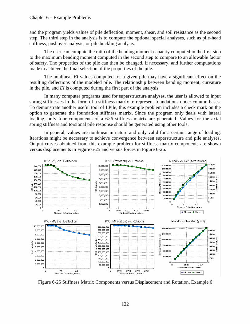
Chapter 6 – Example Problems
122
and the program yields values of pile deflection, moment, shear, and soil resistance as the second
step. The third step in the analysis is to compute the optional special analyses, such as pile-head
stiffness, pushover analysis, or pile buckling analysis.
The user can compute the ratio of the bending moment capacity computed in the first step
to the maximum bending moment computed in the second step to compare to an allowable factor
of safety. The properties of the pile can then be changed, if necessary, and further computations
made to achieve the final selection of the properties of the pile.
The nonlinear EI values computed for a given pile may have a significant effect on the
resulting deflections of the modeled pile. The relationship between bending moment, curvature
in the pile, and EI is computed during the first part of the analysis.
In many computer programs used for superstructure analyses, the user is allowed to input
spring stiffnesses in the form of a stiffness matrix to represent foundations under column bases.
To demonstrate another useful tool of LPile, this example problem includes a check mark on the
option to generate the foundation stiffness matrix. Since the program only deals with lateral
loading, only four components of a 6×6 stiffness matrix are generated. Values for the axial
spring stiffness and torsional pile response should be generated using other tools.
In general, values are nonlinear in nature and only valid for a certain range of loading.
Iterations might be necessary to achieve convergence between superstructure and pile analyses.
Output curves obtained from this example problem for stiffness matrix components are shown
versus displacements in Figure 6-25 and versus forces in Figure 6-26.
Figure 6-25 Stiffness Matrix Components versus Displacement and Rotation, Example 6

Chapter 6 – Example Problems
123
Figure 6-26 Stiffness Matrix Components versus Force and Moment, Example 6
6-7 Example 7 – Pile with User-Input p-y Curves and Distributed Load
This example is included to illustrate a common case in which a 16-in. (406 mm)-
diameter pipe pile is subjected to both, concentrated loads at the pile head and distributed loads
along the pile. The head of the pile will be assumed unrestrained against rotations (free-head
case) with no applied moment. A lateral load of 5,000 lbs (22 kN) will be applied at the pile
head. The non-uniform distributed loads are 20 lbs/in (3.5kN/m) at the depth of 2 ft (0.6 m) and
linearly increase to 100 lbs/in. (17.5 kN/m) at the depth of 5 feet (1.5 meters). Figure 6-27 shows
a general view of the pile and soil. The distributed load in this case occurs over a pile length of 3
feet (0.9 meters), and an increment length of 0.25 feet (0.075 meters); therefore, the distributed
lateral load can be properly reflected by the 12 increments of length of the pile.
To demonstrate another feature of LPile, the p-y curves shown in Figure 6-28 will be
entered for this problem. The program interpolates linearly between points on a p-y curve and
between depths of p-y curves.

Chapter 6 – Example Problems
124
Figure 6-27 Pile and soil details for Example 7
Figure 6-28 User-input p-y Curves for Example 7 (Lower curve for Layer 7 not shown)
5 ft
20 ft
30 ft
Soft Clay
Loose Sand
Medium Clay
16-in. O.D. Pipe Pile
E = 29,000,000 psi
t = 0.75 in.
I = 1,047 in4
16-in. O.D. Pipe Pile
E = 29,000,000 psi
t = 0.5 in.
I = 732 in4
Layer 1, Upper p-y Curve, Depth = 5.00 ft Layer 1, Low er p-y Curve, Depth = 6.33 ft
Layer 2, Upper p-y Curve, Depth = 6.33 ft Layer 2, Low er p-y Curve, Depth = 7.67 ft
Layer 3, Upper p-y Curve, Depth = 7.67 ft Layer 3, Low er p-y Curve, Depth = 9.00 ft
Layer 4, Upper p-y Curve, Depth = 9.00 ft Layer 4, Low er p-y Curve, Depth = 11.67 ft
Layer 5, Upper p-y Curve, Depth = 11.67 ft Layer 5, Low er p-y Curve, Depth = 15.67 ft
Layer 6, Upper p-y Curve, Depth = 15.67 ft Layer 6, Low er p-y Curve, Depth = 17.83 ft
Layer 7, Upper p-y Curve, Depth = 17.83 ft
Lateral Deflection y, in.6.05.04.03.02.01.00.0
Lo
ad
In
ten
sity p
, lb
/in
.
400
350
300
250
200
150
100
50
0

Chapter 6 – Example Problems
125
6-8 Example 8 – Pile in Cemented Sand
A field test for behavior of laterally loaded, bored piles in cemented sands (c- soil) was
conducted in Kuwait (Ismael, 1990). Twelve bored piles that were 0.3-m in diameter were tested.
Piles 1 to 4 were 3-m long, while piles 5 to 12 were 5-m long. The study was on the behavior of
both single piles and piles in a group. The measured load versus deflection curves at the pile
head for a 3-m long single pile and a 5-m long single pile are presented in the paper and can be
studied by using the soil criteria for c- soils.
The piles were reinforced with a 0.25-m diameter cage made of four 22-mm bars for the
3 m-long piles and six 22-mm bars for the 5 m-long piles. In addition, a 36-mm reinforcing bar
was positioned at the center of each pile.
The Young’s modulus for concrete was measured during a cylinder test and a
representative value of 3,200 psi (22 MPa) was selected. The flexural rigidity EI varies with the
applied moment but a constant value was reported. After lateral-load tests were completed, the
soil to a depth of 2 m was excavated to expose the level of the strain gauges for a calibration test.
The pile was reloaded and the curvature was calculated from the measurements of strain. The
moment in the pile at the strain gauges was determined from statics and the moment versus
curvature relationship was determined. The reported flexural rigidity was calculated from the
initial slope of the moment-curvature curves as 20.2 MN-m2, which seems to be on the upper
extreme of the normal range for a bored pile with the reported concrete and reinforcing
properties.
The subsurface profile at the test site consisted of two layers as shown in Figure 6-29.
The upper layer, described as medium dense cemented silty sand, was about 3 m in thickness.
The values of c and for this layer were found by drained triaxial compression tests and were 20
kPa and 35 degrees respectively. The upper layer was underlain by medium dense to very dense
silty sand with cemented lumps. The values of c and were zero kPa and 43 degrees,
respectively.
Figure 6-29 Soil details for Example 8
Medium DenseCemented Silty Sand (SM)
Medium Dense to Very Dense Silty Sand with Cemented Lumps (SM)
End of Borehole
N60
13
24
26
21
60
90
w%
1.4
2.7
3.8
3.9
3.1
4.4
g
1.81
1.83
1.87
1.80
1.90
1.99
LL
30.5
25.2
26.0
none
none
none
PI
7.0
4.0
NP
NP
NP
NP
SL
22.5
17.7
18
−
−
−
Depth(m)
0
1
2
3
4
5
Soil Description
0 50 100
Soil CompositionPercent of Total
Mg/m3
Sand
Silt
Clay

Chapter 6 – Example Problems
126
LPile, employing the c- criteria was used to predict curves of load versus deflection at
the pile head for 5-m pile. Good agreement was found between measured and predicted behavior,
for pile-head load versus deflection and is shown in Figure 6-30. A comparison between
measured and predicted behavior for bending moment versus depth is shown in Figure 6-31.
Figure 6-30 Comparison between Measured and Predicted Pile-head Load versus Deflection
Curves for the 5-m Pile of Example 8
Figure 6-31 Comparison between Measured and Computed Bending Moment versus Depth for
the 5-m Pile of Example 8
0
20
40
60
80
100
120
140
160
180
0.000 0.005 0.010 0.015 0.020 0.025
Sh
ea
r F
orc
e, k
N
Deflection, meters
Computed by LPile
Load Test
0
1
2
3
4
5
-5 0 5 10 15 20 25 30 35
Dep
th,
me
ters
Bending Moment, kN-m
Computed by LPile
Load Test
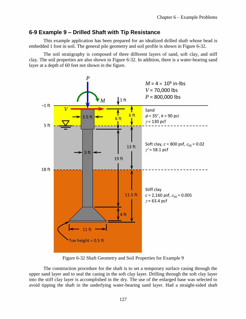
Chapter 6 – Example Problems
127
6-9 Example 9 – Drilled Shaft with Tip Resistance
This example application has been prepared for an idealized drilled shaft whose head is
embedded 1 foot in soil. The general pile geometry and soil profile is shown in Figure 6-32.
The soil stratigraphy is composed of three different layers of sand, soft clay, and stiff
clay. The soil properties are also shown in Figure 6-32. In addition, there is a water-bearing sand
layer at a depth of 60 feet not shown in the figure.
Figure 6-32 Shaft Geometry and Soil Properties for Example 9
The construction procedure for the shaft is to set a temporary surface casing through the
upper sand layer and to seal the casing in the soft clay layer. Drilling through the soft clay layer
into the stiff clay layer is accomplished in the dry. The use of the enlarged base was selected to
avoid tipping the shaft in the underlying water-bearing sand layer. Had a straight-sided shaft
Sand = 35, k = 90 pcig = 130 pcf
Soft clay, c = 800 psf, 50 = 0.02g = 58.1 pcf
Stiff clayc = 2,160 psf, 50 = 0.005g = 63.4 pcf
−1 ft
5 ft
18 ft
11 ft
3 ft
M = 4 106 in-lbsV = 70,000 lbsP = 800,000 lbs
P
M
V
19 ft
4 ft
11.5 ft
13 ft
Toe height = 0.5 ft
6 ft
1 ft
3.5 ft 6 ft
Chapter 6 – Example Problems
128
been used, the overall shaft length would have been 30 feet longer and drilling with slurry would
have been required. In this case, the use of a shorter shaft with an enlarged base would result in
faster and more economical construction. The final shaft dimensions consists of four sections,
which are a 6-ft long straight section of 42-in. diameter, 19-ft long straight section of 3-ft (0.91-
m) diameter, a 4-ft (1.22-m) long section with a 11-ft (3.35-m) diameter enlarged base at the
bottom with a 0.5-ft toe section.
The loads shown acting at the top of the pile are primarily axial and the axial bearing
capacity and settlement must be checked to withstand the axial load using a separate analysis.
The analysis using LPile is performed to check the lateral performance and to design the shaft
reinforcement.
The reinforcement in the shaft was sized so that one reinforcement cage could be placed
over the full length of the shaft. The reinforcement chosen was 14 No. 9 bars, sized with a
diameter that had a 6-inch cover in the upper 42-inch section and a 3-inch cover in the 36 inch
section. This amount of reinforcement provided 1.01% reinforcement in the 42-inch section and
1.38% reinforcement in the 36-inch section.
The enlarged base sections were modeled as elastic sections, with the specified
dimensions and an elastic modulus of 3,500,000 psi.
A first run of the problem showed that the shaft acted mainly as a short pile with lateral
movements observed at the bottom of the shaft. The design engineer then decided to account for
the additional amount of soil resistance provided by the large shear forces developed at the
enlarged base of the shaft. This was accomplished by checking the option in the Program
Options and Settings dialog to include shear resistance at pile tip. Inclusion of tip shear
resistance had little effect on the top deflection, reducing the top deflection from 0.994 inches
without tip shear to 0.909 inches with tip shear.
The computer-generated p-y curves were adjusted to account for closely spaced piles by
utilizing p-reduction factors that varied with depth from 0.75 for the straight shaft down to 0.3 at
the bottom of the enlarged base.
Curves of moment versus curvature for Sections 1 (42-inch) and 2 (36-inch) are shown in
Figure 6-33. The factored moment capacities for these two sections for a resistance factor of 0.65
are 14,000 and 11,600 in-kips respectively
The curves of lateral deflection and bending moment versus depth are shown in Figure
6-34.
In addition, the program was asked to generate a plot of pile length versus pile-top
deflections in order to optimize the design length. The resulting plot included in Figure 6-35
shows that the pile length should not be further reduced in order to have an appreciable factor of
safety from the critical length nor could the length of shaft be increased without the base of the
shaft coming too close to the water-bearing sand layer below.

Chapter 6 – Example Problems
129
Figure 6-33 Moment versus Curvature for Sections 1 and 2, Example 9
Figure 6-34 Lateral Deflection and Bending Moment versus Depth, Example 9
Deflection, in.10.90.80.70.60.50.40.30.20.10-0.1
De
pth
, ft
28
26
24
22
20
18
16
14
12
10
8
6
4
2
0
Bending Moment, in-kips8,0007,0006,0005,0004,0003,0002,0001,0000
De
pth
, ft
28
26
24
22
20
18
16
14
12
10
8
6
4
2
0
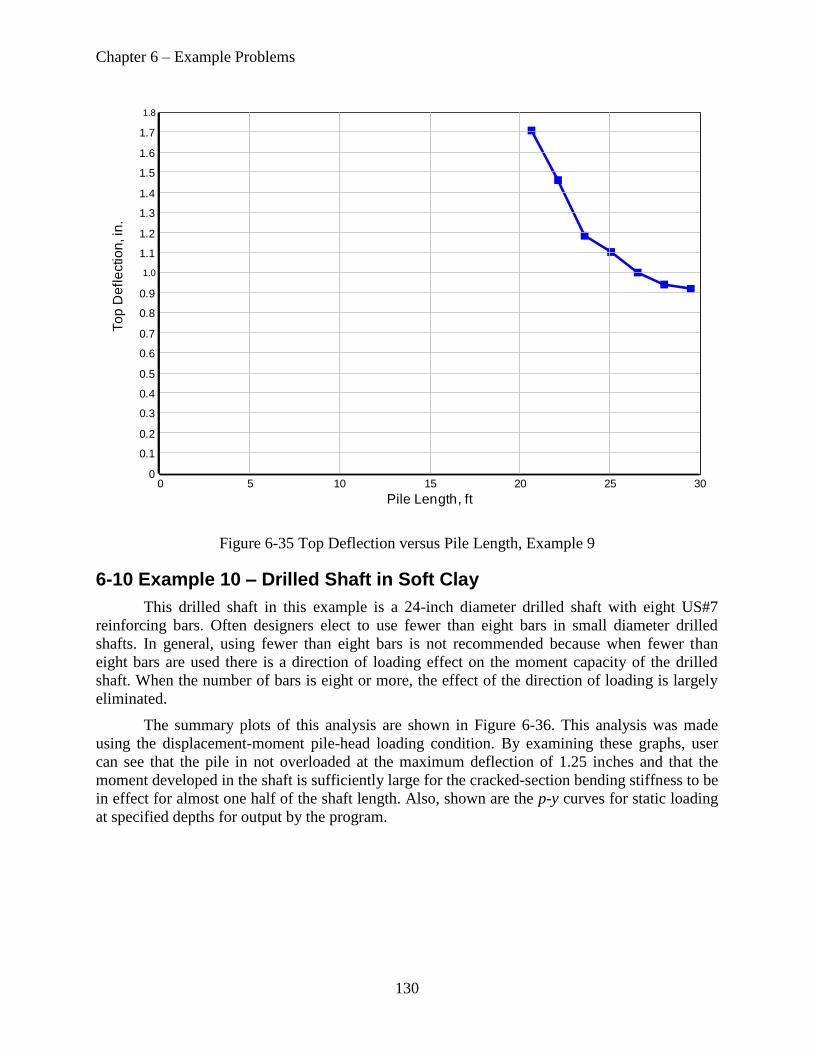
Chapter 6 – Example Problems
130
Figure 6-35 Top Deflection versus Pile Length, Example 9
6-10 Example 10 – Drilled Shaft in Soft Clay
This drilled shaft in this example is a 24-inch diameter drilled shaft with eight US#7
reinforcing bars. Often designers elect to use fewer than eight bars in small diameter drilled
shafts. In general, using fewer than eight bars is not recommended because when fewer than
eight bars are used there is a direction of loading effect on the moment capacity of the drilled
shaft. When the number of bars is eight or more, the effect of the direction of loading is largely
eliminated.
The summary plots of this analysis are shown in Figure 6-36. This analysis was made
using the displacement-moment pile-head loading condition. By examining these graphs, user
can see that the pile in not overloaded at the maximum deflection of 1.25 inches and that the
moment developed in the shaft is sufficiently large for the cracked-section bending stiffness to be
in effect for almost one half of the shaft length. Also, shown are the p-y curves for static loading
at specified depths for output by the program.
Pile Length, ft
302520151050
To
p D
efl
ectio
n, in
.1.8
1.7
1.6
1.5
1.4
1.3
1.2
1.1
1.0
0.9
0.8
0.7
0.6
0.5
0.4
0.3
0.2
0.1
0
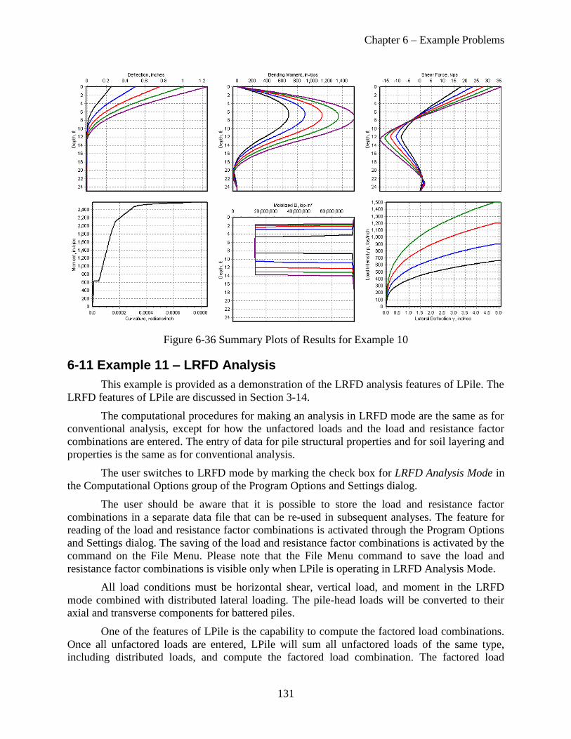
Chapter 6 – Example Problems
131
Figure 6-36 Summary Plots of Results for Example 10
6-11 Example 11 – LRFD Analysis
This example is provided as a demonstration of the LRFD analysis features of LPile. The
LRFD features of LPile are discussed in Section 3-14.
The computational procedures for making an analysis in LRFD mode are the same as for
conventional analysis, except for how the unfactored loads and the load and resistance factor
combinations are entered. The entry of data for pile structural properties and for soil layering and
properties is the same as for conventional analysis.
The user switches to LRFD mode by marking the check box for LRFD Analysis Mode in
the Computational Options group of the Program Options and Settings dialog.
The user should be aware that it is possible to store the load and resistance factor
combinations in a separate data file that can be re-used in subsequent analyses. The feature for
reading of the load and resistance factor combinations is activated through the Program Options
and Settings dialog. The saving of the load and resistance factor combinations is activated by the
command on the File Menu. Please note that the File Menu command to save the load and
resistance factor combinations is visible only when LPile is operating in LRFD Analysis Mode.
All load conditions must be horizontal shear, vertical load, and moment in the LRFD
mode combined with distributed lateral loading. The pile-head loads will be converted to their
axial and transverse components for battered piles.
One of the features of LPile is the capability to compute the factored load combinations.
Once all unfactored loads are entered, LPile will sum all unfactored loads of the same type,
including distributed loads, and compute the factored load combination. The factored load

Chapter 6 – Example Problems
132
combinations can be reviewed prior to analysis by pressing the Display Summary of LRFD
Loadings (the button on the button bar). An excerpt from an example of a summary report is
shown in Figure 6-37.
Figure 6-37 Example from Summary Report of LRFD Loadings, Example 11
After running the LRFD analysis, an information message will be displayed to alert the
user whether or not all load case combinations have been met. The message for a successful
analysis is displayed as Figure 6-38.
Figure 6-38 Message for Successful LRFD Analysis for Example 11
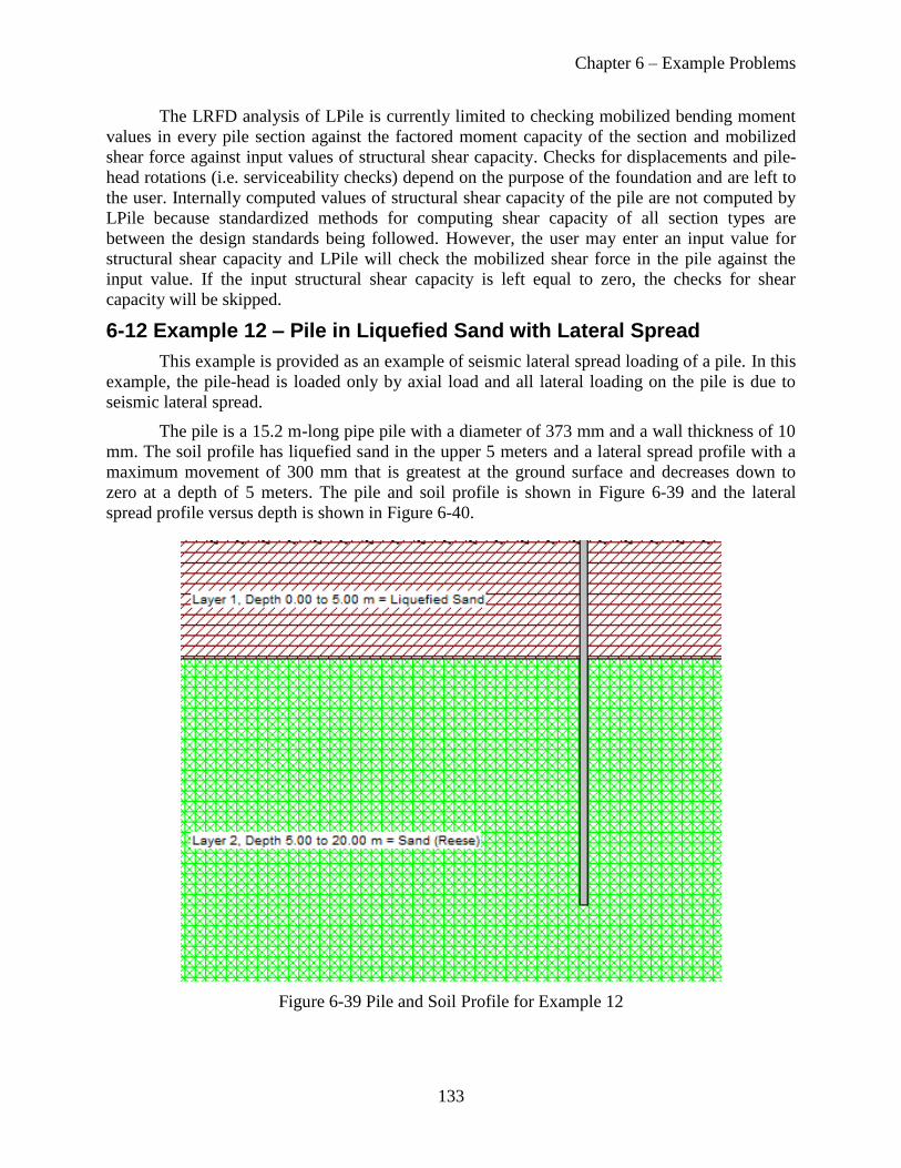
Chapter 6 – Example Problems
133
The LRFD analysis of LPile is currently limited to checking mobilized bending moment
values in every pile section against the factored moment capacity of the section and mobilized
shear force against input values of structural shear capacity. Checks for displacements and pile-
head rotations (i.e. serviceability checks) depend on the purpose of the foundation and are left to
the user. Internally computed values of structural shear capacity of the pile are not computed by
LPile because standardized methods for computing shear capacity of all section types are
between the design standards being followed. However, the user may enter an input value for
structural shear capacity and LPile will check the mobilized shear force in the pile against the
input value. If the input structural shear capacity is left equal to zero, the checks for shear
capacity will be skipped.
6-12 Example 12 – Pile in Liquefied Sand with Lateral Spread
This example is provided as an example of seismic lateral spread loading of a pile. In this
example, the pile-head is loaded only by axial load and all lateral loading on the pile is due to
seismic lateral spread.
The pile is a 15.2 m-long pipe pile with a diameter of 373 mm and a wall thickness of 10
mm. The soil profile has liquefied sand in the upper 5 meters and a lateral spread profile with a
maximum movement of 300 mm that is greatest at the ground surface and decreases down to
zero at a depth of 5 meters. The pile and soil profile is shown in Figure 6-39 and the lateral
spread profile versus depth is shown in Figure 6-40.
Figure 6-39 Pile and Soil Profile for Example 12
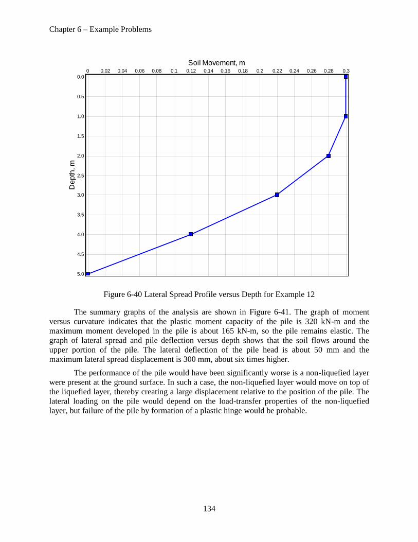
Chapter 6 – Example Problems
134
Figure 6-40 Lateral Spread Profile versus Depth for Example 12
The summary graphs of the analysis are shown in Figure 6-41. The graph of moment
versus curvature indicates that the plastic moment capacity of the pile is 320 kN-m and the
maximum moment developed in the pile is about 165 kN-m, so the pile remains elastic. The
graph of lateral spread and pile deflection versus depth shows that the soil flows around the
upper portion of the pile. The lateral deflection of the pile head is about 50 mm and the
maximum lateral spread displacement is 300 mm, about six times higher.
The performance of the pile would have been significantly worse is a non-liquefied layer
were present at the ground surface. In such a case, the non-liquefied layer would move on top of
the liquefied layer, thereby creating a large displacement relative to the position of the pile. The
lateral loading on the pile would depend on the load-transfer properties of the non-liquefied
layer, but failure of the pile by formation of a plastic hinge would be probable.
Soil Movement, m0.30.280.260.240.220.20.180.160.140.120.10.080.060.040.020
De
pth
, m
5.0
4.5
4.0
3.5
3.0
2.5
2.0
1.5
1.0
0.5
0.0

Chapter 6 – Example Problems
135
Figure 6-41 Summary Graphs for Example 12
6-13 Example 13 – Square Elastic Pile with Top Deflection versus Length
This example is to demonstrate the feature to compute pile top deflection versus pile
length and the use of the modified stiff clay without water p-y curve. The pile is modeled as a 25-
foot long, 14-inch square elastic pile with a Young’s modulus of 3,500,000 psi.
The pile-head loads are shear forces of 5,000, 10,000, 20,000, 30,000, and 40,000 lbs,
zero moment, and an axial thrust load of 150,000 lbs. The option to compute pile top deflection
versus pile length is turned on in the Pile-head Loadings and Options dialog.
The properties of the modified stiff clay without free water are an effective unit weight of
108 pcf, undrained shear strength of 2,000 psf, k of 500 pci, and 50 of 0.005.
The primary use of the modified stiff clay without free water is to generate a p-y curve
with a softened initial slope. In some areas, load testing has found that the original p-y curve
computations result in p-y curves that have initial slopes that are too stiff. As an example, pile-
head load versus deflection curves were computed using both the original and modified p-y curve
formulations. Theses curves along with the percentage of reduction in stiffness are graphed in
Figure 6-42.
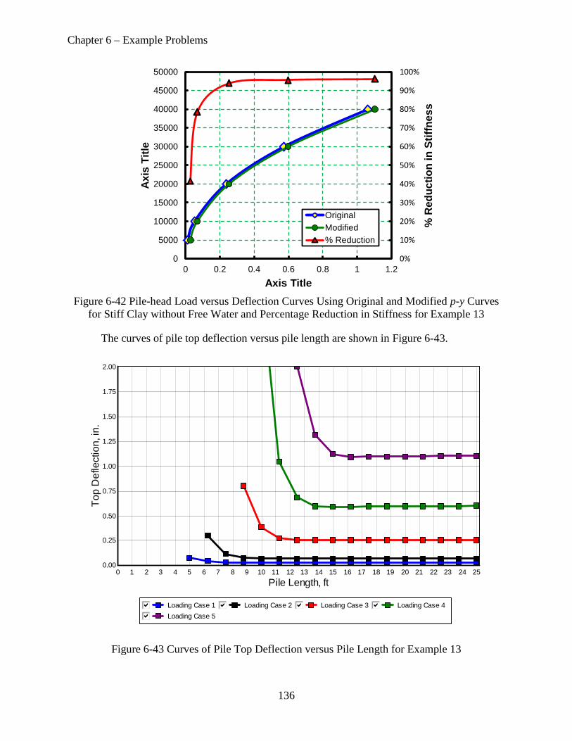
Chapter 6 – Example Problems
136
Figure 6-42 Pile-head Load versus Deflection Curves Using Original and Modified p-y Curves
for Stiff Clay without Free Water and Percentage Reduction in Stiffness for Example 13
The curves of pile top deflection versus pile length are shown in Figure 6-43.
Figure 6-43 Curves of Pile Top Deflection versus Pile Length for Example 13
0%
10%
20%
30%
40%
50%
60%
70%
80%
90%
100%
0
5000
10000
15000
20000
25000
30000
35000
40000
45000
50000
0 0.2 0.4 0.6 0.8 1 1.2
% R
ed
uc
tio
n in
Sti
ffn
es
s
Ax
is T
itle
Axis Title
Original
Modified
% Reduction
Loading Case 1gfedcb Loading Case 2gfedcb Loading Case 3gfedcb Loading Case 4gfedcbLoading Case 5gfedcb
Pile Length, ft252423222120191817161514131211109876543210
To
p D
efle
ctio
n, in
.
2.00
1.75
1.50
1.25
1.00
0.75
0.50
0.25
0.00

Chapter 6 – Example Problems
137
It should be noted that the length of pile needed to reach the “long pile” behavior (i.e.
when the curve becomes horizontal) is depended on the level of loading being consider. Thus, it
is important to specify the generation of the pile top deflection versus pile length curve for the
maximum loading being considered. It should also be noted that if the pile top deflection is too
large for the “long pile” portion of the curve, the deflection can be lowered only by re-
configuring the foundation to use either larger diameter piles or more piles.
6-14 Example 14 – Pushover Analysis of Prestressed Concrete Pile
This example is provided as an example of a pushover analysis of a prestressed concrete
pile. The pile is a 25-foot long, 14-inch wide, prestressed concrete pile with 1-inch chamfered
corners. The reinforcement details for the pile are shown in Figure 6-44.
Figure 6-44 Reinforcement Details for Prestressed Concrete Pile of Example 14
It should be noted that the value for Fraction of Loss of Prestressed must be obtained
from the pile manufacturer and that this number can vary from supplier to supplier because the
procedures and materials used for the pile vary. The magnitude of prestressed after losses
typically varies from 600 to 1,200 psi in the United States, with pile driven in softer soils
typically having higher prestress values to permit higher resistance to tensile stresses during pile
driving. The use of higher levels of prestress also permits lifting of longer piles without damage.
This example uses the Pushover Analysis option available in the Program Options and
Settings dialog. One useful feature of the pushover analysis is to determine the lateral deflection
and load required to fail a pile under lateral loading.
As will all LPile analyses for piles with nonlinear bending properties, LPile computes the
curve of nonlinear bending versus curvature. The curve generated for Example 14 is shown in

Chapter 6 – Example Problems
138
Figure 6-45 for the two values of axial thrust specified in the Pile-head Loading and Options
dialog. The curve shown here indicates that the plastic moment capacity for the pile is
approximately 2,100 in-kips.
Figure 6-45 Moment versus Curvature of Prestressed Pile for Example 14
The results of the pushover analysis are shown in the two graphs of Figure 6-46. These
graphs shown the results for both fixed-head and free-head loading conditions for lateral
displacements up to 5 inches. For fixed-head conditions, the plastic moment capacity is
mobilized at a pile top deflection of 0.625 inches and a shear load of 60,900 lbs. For free-head
conditions, the plastic moment capacity is mobilized at a pile top deflection of 2.75 inches and a
shear load of 56,300 lbs. Other information gained from these graphs is maximum lateral
capacity is approximately 85,000 lbs for fixed-head conditions and is 58,400 lbs for free-head
conditions.
When interpreting these results, the designer is faced with the decision about which curve
is most representative of the pile design being analyzed. For prestressed concrete pile, the answer
depends on the pile-head connection conditions utilized for the pile. If the pile is attached to the
pile cap with dowels and an inset of a few inches, the pile-head fixity condition is very close to
the free-head condition. If the pile is deeply embedded into the pile cap, say 2.5 pile widths or
more, the pile-head fixity condition is very close to the fixed-head condition.
For pile-head embedments in between the two conditions discussed above, the pile-head
fixity condition is likely to be elastically restrained. Evaluation of the stiffness of the elastic
restraint will depend on the structural properties of the pile cap and the pile to pile cap
Thrust = 100.00 kipsgfedcb Thrust = 125.00 kipsgfedcb
Curvature, radians/inch0.00060.00050.00040.00030.00020.00010.0
Mo
me
nt, in
-kip
s
2,250
2,000
1,750
1,500
1,250
1,000
750
500
250
0

Chapter 6 – Example Problems
139
reinforcement details. It will be necessary to use a special computer program to evaluate these
conditions.
Figure 6-46 Results of Pushover Analysis of Prestressed Concrete Pile of Example 14
6-15 Example 15 – Pile with Defined Nonlinear Bending Properties
This example was provided as an example of a pile with defined nonlinear bending
properties. Two analyses were made. The first analysis was of a drilled shaft with internally
generated nonlinear bending properties. The second analysis was of a pile with defined nonlinear
bending properties in which the output file of curvature and moment values was input. Both SI
and USCS unit versions of these data files are provided. A check of the pile response computed
by LPile for the two types of piles found that the pile responses were identical, as they should be.
6-16 Example 16 – Pile with Distributed Lateral Loadings
This example was provided as an example of pile with distributed lateral loading. In this
example, the pile extends 20 feet above the ground surface and the distributed lateral load is a
uniform loading of 50 lbs/inch.
The uniform distributed loading can be checked by evaluating the computed shear force
and bending moment at the ground line. The computed shear force at the ground line is
lbs 000,12)0()50(
)240()50(20
0
xpdxpV DLDL
The computed bending moment at the ground line is
lbs-in 000,440,12
240)240)(50(
2
LLpM DL
Fixed-head Responsegfedcb Free-head Responsegfedcb
Top Deflection, in.54321
Sh
ea
r F
orc
e, kip
s
85,000
80,000
75,000
70,000
65,000
60,000
55,000
50,000
45,000
40,000
35,000
30,000
25,000
20,000
Free-head and Fixed-head Conditions
Fixed-head Responsegfedcb Free-head Responsegfedcb
Top Deflection, inches54321
Ma
xim
um
Mo
me
nt, in
-lb
s
2,100,000
2,000,000
1,900,000
1,800,000
1,700,000
1,600,000
1,500,000
1,400,000
1,300,000
1,200,000
1,100,000
1,000,000
900,000
800,000
700,000
600,000
500,000
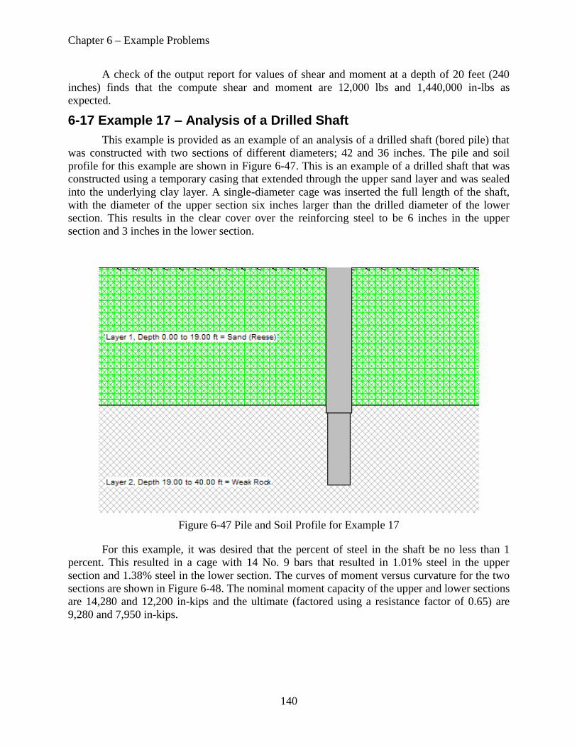
Chapter 6 – Example Problems
140
A check of the output report for values of shear and moment at a depth of 20 feet (240
inches) finds that the compute shear and moment are 12,000 lbs and 1,440,000 in-lbs as
expected.
6-17 Example 17 – Analysis of a Drilled Shaft
This example is provided as an example of an analysis of a drilled shaft (bored pile) that
was constructed with two sections of different diameters; 42 and 36 inches. The pile and soil
profile for this example are shown in Figure 6-47. This is an example of a drilled shaft that was
constructed using a temporary casing that extended through the upper sand layer and was sealed
into the underlying clay layer. A single-diameter cage was inserted the full length of the shaft,
with the diameter of the upper section six inches larger than the drilled diameter of the lower
section. This results in the clear cover over the reinforcing steel to be 6 inches in the upper
section and 3 inches in the lower section.
Figure 6-47 Pile and Soil Profile for Example 17
For this example, it was desired that the percent of steel in the shaft be no less than 1
percent. This resulted in a cage with 14 No. 9 bars that resulted in 1.01% steel in the upper
section and 1.38% steel in the lower section. The curves of moment versus curvature for the two
sections are shown in Figure 6-48. The nominal moment capacity of the upper and lower sections
are 14,280 and 12,200 in-kips and the ultimate (factored using a resistance factor of 0.65) are
9,280 and 7,950 in-kips.

Chapter 6 – Example Problems
141
Figure 6-48 Moment versus Curvature for Dual Section Drilled Shaft of Example 17
6-18 Example 18 – Analysis of Drilled Shaft with Permanent Casing
This example is based on Example 17, except that a permanent casing is modeled for the
upper section. The nominal moment capacities of the upper and lower sections are 47,900 and
12,200 in-kips and the ultimate (factored using a resistance factor of 0.65) are 31,100 and 7,950
in-kips. The moment capacity of the second section is identical to the second section of Example
17 because the section properties are identical. The curves of moment versus capacity are shown
in Figure 6-49.
6-19 Example 19 – Analysis of Drilled Shaft with Casing and Core
This example is based on Example 18, except that a permanent core has been added. In
modeling of this pile, it was assumed that the core extended over the full length of the shaft and
that the interior of the core was void of concrete.
When modeling the lower section, the section type was drilled shaft with casing and core,
but the wall thickness of the casing was set equal to zero to model the section with an interior
core only.
The nominal moment capacity of the upper and lower sections are 51,900 and 16,990 in-
kips and the ultimate (factored using a resistance factor of 0.65) are 33,700 and 11,040 in-kips.
The curves of moment versus curvature are shown in Figure 6-50.
Section 1, Thrust = 100.00 kipsgfedcb Section 2, Thrust = 100.00 kipsgfedcb
Curvature, radians/inch0.00040.00030.00020.00010.0
Mo
me
nt, in
-kip
s
15,000
14,000
13,000
12,000
11,000
10,000
9,000
8,000
7,000
6,000
5,000
4,000
3,000
2,000
1,000
0
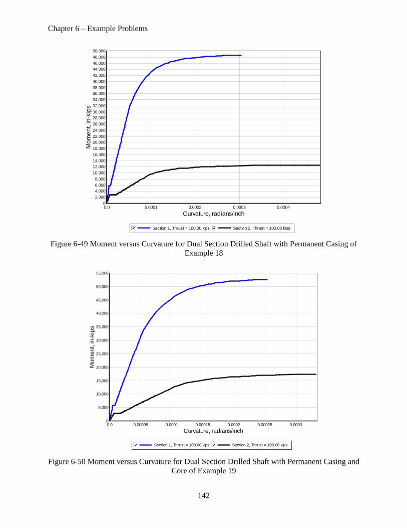
Chapter 6 – Example Problems
142
Figure 6-49 Moment versus Curvature for Dual Section Drilled Shaft with Permanent Casing of
Example 18
Figure 6-50 Moment versus Curvature for Dual Section Drilled Shaft with Permanent Casing and
Core of Example 19
Section 1, Thrust = 100.00 kipsgfedcb Section 2, Thrust = 100.00 kipsgfedcb
Curvature, radians/inch0.00040.00030.00020.00010.0
Mo
me
nt, in
-kip
s
50,000
48,000
46,000
44,000
42,000
40,000
38,000
36,000
34,000
32,000
30,000
28,000
26,000
24,000
22,000
20,000
18,000
16,000
14,000
12,000
10,000
8,000
6,000
4,000
2,000
0
Section 1, Thrust = 100.00 kipsgfedcb Section 2, Thrust = 100.00 kipsgfedcb
Curvature, radians/inch0.00030.000250.00020.000150.00010.000050.0
Mo
me
nt, in
-kip
s
55,000
50,000
45,000
40,000
35,000
30,000
25,000
20,000
15,000
10,000
5,000
0

Chapter 6 – Example Problems
143
6-20 Example 20 – Analysis of Embedded Pole
This example is provided as an example of the embedded pole option. Embedded poles
are commonly used in the electrical utility industry. The typical utility pole in the United States
is embedded to a depth of 10 percent of the overall pole length, plus 2 feet. Thus, the embedded
pole of Example 20 has an overall length of 40 feet and an embedment of 6 feet. The pile and
soil profile for this example is shown in Figure 6-51.
Figure 6-51 Pile and Soil Profile for Embedded Pole of Example 20
The output computed using LPile for this problem is conservative because there are load-
transfer mechanisms between the foundation and soil that not included in the LPile analysis.
These mechanisms are any vertical shear stresses developed along the sides of the pile and any
shear that might develop at the tip of the pole.
In practice, the computation of these additional load-transfer mechanisms present some
difficulties because of uncertainties related to how the poles are constructed. In some
applications, an oversize hole is drilled, the pole is inserted on one side of the hole, and backfill
is compacted in the open void on one side of the pole. In other applications, the pole is placed in
the center of an oversized hole and a cemented-stabilized, flowable fill is placed in the annular
space around the pole.
The loading on the pole is representative of a 100-mph wind loading on the pile and
transformer mounted on top of the pole (the transformer is not shown in the above figure). The
wind load is equivalent to a uniform pressure of 40 psf acting over the projected area of the pole
and transformer. The weight of the transformer is in pile-head loading for the pole. The
computed pile-head deflection is 3.14 inches and the ground line deflection is 0.0127 inches.
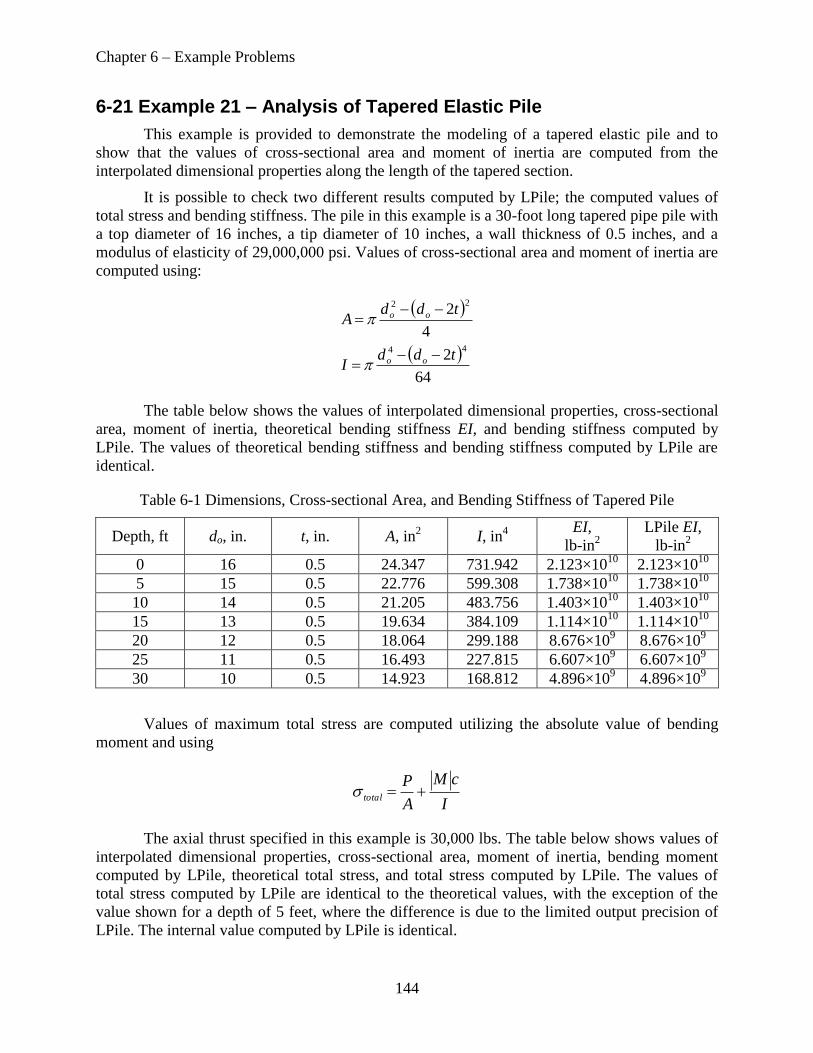
Chapter 6 – Example Problems
144
6-21 Example 21 – Analysis of Tapered Elastic Pile
This example is provided to demonstrate the modeling of a tapered elastic pile and to
show that the values of cross-sectional area and moment of inertia are computed from the
interpolated dimensional properties along the length of the tapered section.
It is possible to check two different results computed by LPile; the computed values of
total stress and bending stiffness. The pile in this example is a 30-foot long tapered pipe pile with
a top diameter of 16 inches, a tip diameter of 10 inches, a wall thickness of 0.5 inches, and a
modulus of elasticity of 29,000,000 psi. Values of cross-sectional area and moment of inertia are
computed using:
64
2
4
2
44
22
tddI
tddA
oo
oo
The table below shows the values of interpolated dimensional properties, cross-sectional
area, moment of inertia, theoretical bending stiffness EI, and bending stiffness computed by
LPile. The values of theoretical bending stiffness and bending stiffness computed by LPile are
identical.
Table 6-1 Dimensions, Cross-sectional Area, and Bending Stiffness of Tapered Pile
Depth, ft do, in. t, in. A, in2 I, in
4
EI,
lb-in2
LPile EI,
lb-in2
0 16 0.5 24.347 731.942 2.123×10¹⁰
2.123×10¹⁰
5 15 0.5 22.776 599.308 1.738×10¹⁰
1.738×10¹⁰
10 14 0.5 21.205 483.756 1.403×10¹⁰
1.403×10¹⁰
15 13 0.5 19.634 384.109 1.114×10¹⁰
1.114×10¹⁰
20 12 0.5 18.064 299.188 8.676×10⁹ 8.676×10
9
25 11 0.5 16.493 227.815 6.607×10⁹ 6.607×10
9
30 10 0.5 14.923 168.812 4.896×10⁹ 4.896×10
9
Values of maximum total stress are computed utilizing the absolute value of bending
moment and using
I
cM
A
Ptotal
The axial thrust specified in this example is 30,000 lbs. The table below shows values of
interpolated dimensional properties, cross-sectional area, moment of inertia, bending moment
computed by LPile, theoretical total stress, and total stress computed by LPile. The values of
total stress computed by LPile are identical to the theoretical values, with the exception of the
value shown for a depth of 5 feet, where the difference is due to the limited output precision of
LPile. The internal value computed by LPile is identical.
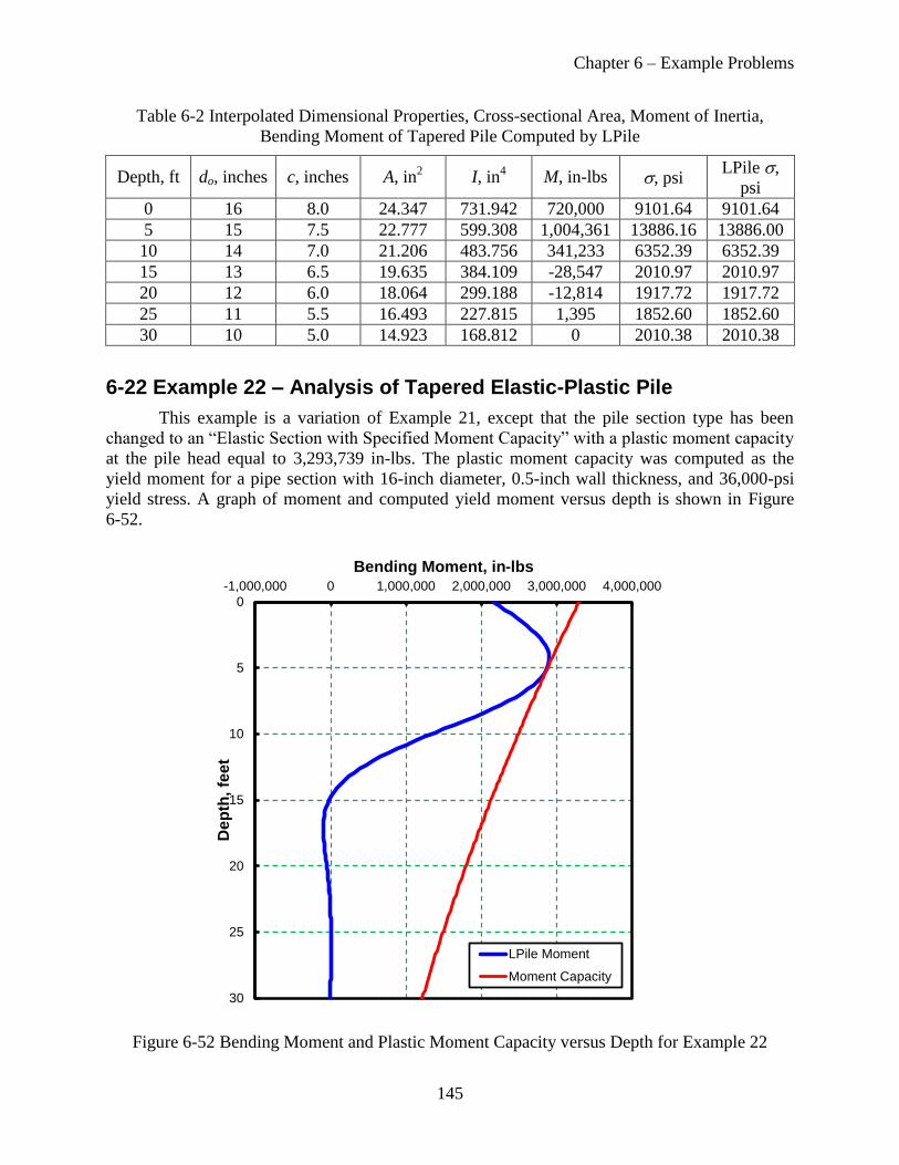
Chapter 6 – Example Problems
145
Table 6-2 Interpolated Dimensional Properties, Cross-sectional Area, Moment of Inertia,
Bending Moment of Tapered Pile Computed by LPile
Depth, ft do, inches c, inches A, in2 I, in
4 M, in-lbs , psi
LPile ,
psi
0 16 8.0 24.347 731.942 720,000 9101.64 9101.64
5 15 7.5 22.777 599.308 1,004,361 13886.16 13886.00
10 14 7.0 21.206 483.756 341,233 6352.39 6352.39
15 13 6.5 19.635 384.109 -28,547 2010.97 2010.97
20 12 6.0 18.064 299.188 -12,814 1917.72 1917.72
25 11 5.5 16.493 227.815 1,395 1852.60 1852.60
30 10 5.0 14.923 168.812 0 2010.38 2010.38
6-22 Example 22 – Analysis of Tapered Elastic-Plastic Pile
This example is a variation of Example 21, except that the pile section type has been
changed to an “Elastic Section with Specified Moment Capacity” with a plastic moment capacity
at the pile head equal to 3,293,739 in-lbs. The plastic moment capacity was computed as the
yield moment for a pipe section with 16-inch diameter, 0.5-inch wall thickness, and 36,000-psi
yield stress. A graph of moment and computed yield moment versus depth is shown in Figure
6-52.
Figure 6-52 Bending Moment and Plastic Moment Capacity versus Depth for Example 22
0
5
10
15
20
25
30
-1,000,000 0 1,000,000 2,000,000 3,000,000 4,000,000
De
pth
, fe
et
Bending Moment, in-lbs
LPile Moment
Moment Capacity

Chapter 6 – Example Problems
146
A close examination of Figure 6-52 will find that the variation in plastic moment capacity
is nonlinear with depth due to the tapered dimensions. This is because LPile will compute the
yield stress of the pile material from the dimensional properties and input value of plastic
moment capacity at the top of the section. LPile then computes the plastic moment capacity at
other points in the section using the dimensions interpolated with depth and the interpreted value
of yield stress.
LPile does not perform computations for tapered sections if the geometric shape is
specified as an H-pile section. In those cases, the plastic moment capacity of the full section is
set equal to the input value for plastic moment capacity for the section.
6-23 Example 23 – Output of p-y Curves
LPile is capable of generating 17-point p-y curves at user-specified depths. Example 23 is
provided as a demonstration of this feature of LPile. The feature to generate p-y curves for output
is enabled by checking the box in the Output Options of the Program Options and Settings dialog
as shown in Figure 6-53.
Figure 6-53 Program and Setting Dialog Showing Check for Generation of p-y Curves
The pile and soil profile for Example 23 is shown in Figure 6-54. The soil profile is
composed of a number of different soil types, plus the lowest layer is defined as having user-
input p-y curves.
When the graph of p-y curves is created, 17-points along the curves are generated. The
spacing of the points depends on the formulation of the p-y curves. For most types of p-y curves,
the points are representative of the shape of the curves, but for others, the y-values are chosen as

Chapter 6 – Example Problems
147
fixed fractions of the pile diameter. In these cases, the plotted shape of the p-y curve is accurate
only at the data points. The graph of p-y curves for Example 23 is shown in Figure 6-55.
Figure 6-54 Pile and Soil Profile for Example 23
Figure 6-55 Standard Output of 17-point p-y Curves for Example 23
p-y Curves
LPile 2013.7.01, © 2013 by Ensoft, Inc.
Depth = 2.00 ftgfedcb Depth = 4.00 ftgfedcb Depth = 6.00 ftgfedcbDepth = 8.00 ftgfedcb Depth = 9.90 ftgfedcb Depth = 12.00 ftgfedcbDepth = 14.00 ftgfedcb Depth = 16.00 ftgfedcb Depth = 18.00 ftgfedcbDepth = 22.50 ftgfedcb Depth = 27.00 ftgfedcb Depth = 31.00 ftgfedcbDepth = 33.00 ftgfedcb Depth = 40.00 ftgfedcb Depth = 49.00 ftgfedcb
Lateral Deflection y, in.5.04.54.03.53.02.52.01.51.00.50.0
Lo
ad
In
ten
sity p
, lb
/in
.
7,000
6,500
6,000
5,500
5,000
4,500
4,000
3,500
3,000
2,500
2,000
1,500
1,000
500
0
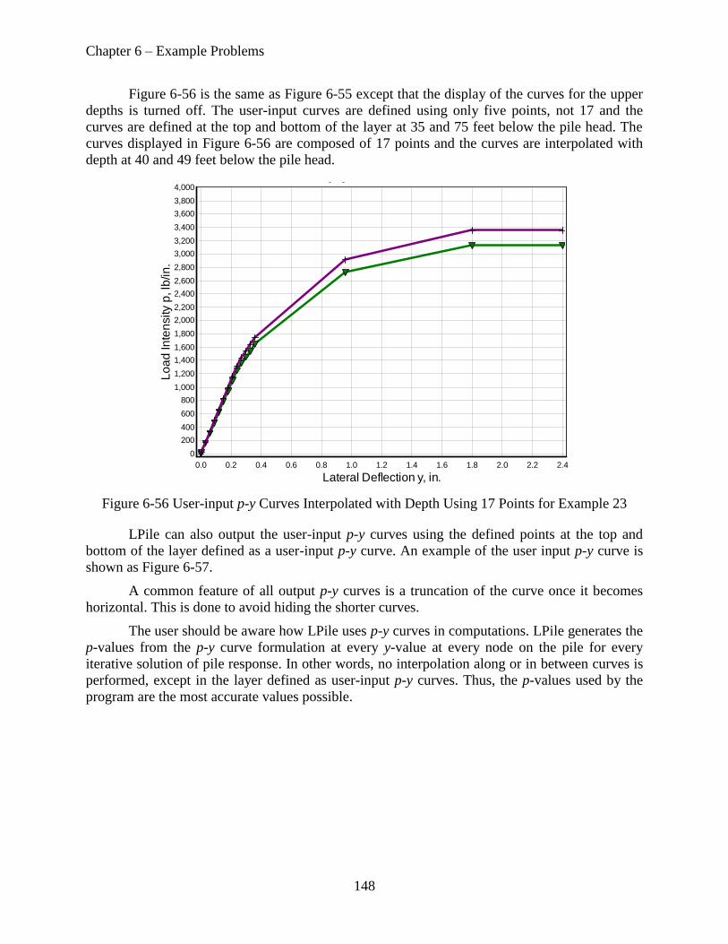
Chapter 6 – Example Problems
148
Figure 6-56 is the same as Figure 6-55 except that the display of the curves for the upper
depths is turned off. The user-input curves are defined using only five points, not 17 and the
curves are defined at the top and bottom of the layer at 35 and 75 feet below the pile head. The
curves displayed in Figure 6-56 are composed of 17 points and the curves are interpolated with
depth at 40 and 49 feet below the pile head.
Figure 6-56 User-input p-y Curves Interpolated with Depth Using 17 Points for Example 23
LPile can also output the user-input p-y curves using the defined points at the top and
bottom of the layer defined as a user-input p-y curve. An example of the user input p-y curve is
shown as Figure 6-57.
A common feature of all output p-y curves is a truncation of the curve once it becomes
horizontal. This is done to avoid hiding the shorter curves.
The user should be aware how LPile uses p-y curves in computations. LPile generates the
p-values from the p-y curve formulation at every y-value at every node on the pile for every
iterative solution of pile response. In other words, no interpolation along or in between curves is
performed, except in the layer defined as user-input p-y curves. Thus, the p-values used by the
program are the most accurate values possible.
p-y Curves
LPile 2013.7.01, © 2013 by Ensoft, Inc.
Depth = 2.00 ftgfedc Depth = 4.00 ftgfedc Depth = 6.00 ftgfedcDepth = 8.00 ftgfedc Depth = 9.90 ftgfedc Depth = 12.00 ftgfedcDepth = 14.00 ftgfedc Depth = 16.00 ftgfedc Depth = 18.00 ftgfedcDepth = 22.50 ftgfedc Depth = 27.00 ftgfedc Depth = 31.00 ftgfedcDepth = 33.00 ftgfedc Depth = 40.00 ftgfedcb Depth = 49.00 ftgfedcb
Lateral Deflection y, in.2.42.22.01.81.61.41.21.00.80.60.40.20.0
Lo
ad
In
ten
sity p
, lb
/in
.
4,000
3,800
3,600
3,400
3,200
3,000
2,800
2,600
2,400
2,200
2,000
1,800
1,600
1,400
1,200
1,000
800
600
400
200
0

Chapter 6 – Example Problems
149
Figure 6-57 Output of User-input p-y Curves with Five Points for Example 23
6-24 Example 24 – Analysis with Lateral Soil Movements
This example is provided as a demonstration of how to model a pile foundation subjected
to lateral spreading. The pile and soil profile for this problem is shown in Figure 6-58. The soil
profile is composed of a stiff clay crust, overlying a layer of liquefied sand, overlying a deep
layer of stiff clay with free water. This soil profile was used because it represents the type of soil
profile for which lateral spread problems are most severe.
The pile is a 48-inch drilled shaft with 18 No. 9 reinforcing bars. This reinforcement
provides 0.99 percent steel. The nominal moment capacity of the shaft was computed to be
21,360,000 in-lbs and the factored moment capacities ranged from 13,880,000 in-lbs to
16,020,000 in-lbs for resistance factors of 0.65 to 0.75.
The option for loading by soil movements is enabled by checking the box for “Include
Loading by Lateral Soil Movements” in the Program Options and Settings dialog, shown in
Figure 6-59. Once this box is checked, the input of the lateral soil movement profile versus depth
is activated. The input dialog for lateral soil movements is shown in Figure 6-60.
User-input p-y Curves
LPile 2013.7.01, © 2013 by Ensoft, Inc.
Layer 8, Upper p-y Curve, Depth = 35.00 ftgfedcbLayer 8, Low er p-y Curve, Depth = 75.00 ftgfedcb
Lateral Deflection y, in.2.42.22.01.81.61.41.21.00.80.60.40.20.0
Lo
ad
In
ten
sity p
, lb
/in
.
4,000
3,800
3,600
3,400
3,200
3,000
2,800
2,600
2,400
2,200
2,000
1,800
1,600
1,400
1,200
1,000
800
600
400
200
0

Chapter 6 – Example Problems
150
Figure 6-58 Pile and Soil Profile for Example 24
Figure 6-59 Program and Setting Dialog Showing Check for Inclusion of Loadings by Lateral
Soil Movements

Chapter 6 – Example Problems
151
Figure 6-60 Input Dialog for Lateral Soil Movements versus Depth for Example 24
The results of the analysis with loading by soil movements are shown in Figure 6-61. In
this problem, the upper clay crust moves along with the spreading liquefied sand layer. As a
result, the maximum moment developed in the drilled shaft is 17,990,000 in-lbs and the factored
moment capacity of the shaft is exceeded.
Figure 6-61 Results of Analysis for Example 24
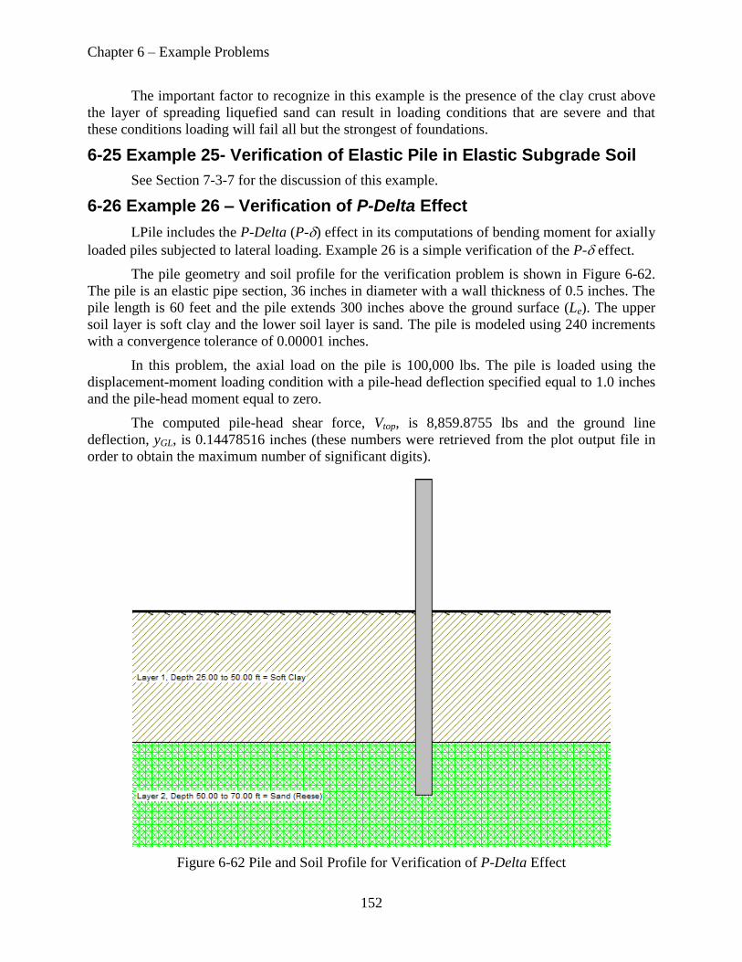
Chapter 6 – Example Problems
152
The important factor to recognize in this example is the presence of the clay crust above
the layer of spreading liquefied sand can result in loading conditions that are severe and that
these conditions loading will fail all but the strongest of foundations.
6-25 Example 25- Verification of Elastic Pile in Elastic Subgrade Soil
See Section 7-3-7 for the discussion of this example.
6-26 Example 26 – Verification of P-Delta Effect
LPile includes the P-Delta (P-) effect in its computations of bending moment for axially
loaded piles subjected to lateral loading. Example 26 is a simple verification of the P- effect.
The pile geometry and soil profile for the verification problem is shown in Figure 6-62.
The pile is an elastic pipe section, 36 inches in diameter with a wall thickness of 0.5 inches. The
pile length is 60 feet and the pile extends 300 inches above the ground surface (Le). The upper
soil layer is soft clay and the lower soil layer is sand. The pile is modeled using 240 increments
with a convergence tolerance of 0.00001 inches.
In this problem, the axial load on the pile is 100,000 lbs. The pile is loaded using the
displacement-moment loading condition with a pile-head deflection specified equal to 1.0 inches
and the pile-head moment equal to zero.
The computed pile-head shear force, Vtop, is 8,859.8755 lbs and the ground line
deflection, yGL, is 0.14478516 inches (these numbers were retrieved from the plot output file in
order to obtain the maximum number of significant digits).
Figure 6-62 Pile and Soil Profile for Verification of P-Delta Effect

Chapter 6 – Example Problems
153
The moment at the ground line, MV, from the pile-head shear force is
lbs-in 652,657,962.)in. 300)(lb 8755.859,8( etopV LVM
The P- moment due to the eccentricity of the axial load, MP, is equal to the relative
displacement of the pile-head to the ground line displacement multiplied by the axial thrust
force.
lbs-in 85,521.484 )in. 14478516.0in. 0.1(lbs .000,100)( GLtopP yyPM
The total moment at the ground line due to the shear force and eccentric axial load is
PVtotal MMM lbs-in 1342,743,484.
The computed moment by LPile at the ground line is 2,743,484.100 in-lbs.
The error in the computed moment is −0.034 in-lbs. This is an error of 1.24×10⁻⁶
percent.

Chapter 6 – Example Problems
154
(This page was deliberately left blank)

155
Chapter 7 Validation
7-1 Introduction
Two approaches are used to validate the computations of the computer program. Firstly,
case studies are shown that give the comparison of maximum bending moments from experiment
and from computation. Secondly, suggestions are made for checking the output to ensure that the
equations of mechanics are satisfied.
7-2 Case Histories
The engineering literature contains a number of papers that present the results of load
tests of piles under lateral load; however, in only a small number of these paper present values of
bending moment measured by instrumentation along the length of the pile. The case studies
presented herein are concerned with these latter cases because the failure of a pile is frequently
due to the development of a plastic hinge.
A list of case histories where bending moment was measured is presented in Table 7-1.
The table shows the location of the experiment, the reference citation, a general description of
the soil and the position of the water table, the computed lateral load at a load factor of 2.5, and
the kind and size of pile. For each of the cases, a preliminary computation was made, using the
analytical methods presented herein, to find the lateral load Pult that would cause the maximum
bending moment to occur. The next step was to find the experimental bending moment and the
computed bending moment at the load of Pult/2.5. The reason for the comparison at the reduced
loading is that the load actually applied to the pile would be reduced by a factor of safety and a
value of 2.5 is reasonable.
Table 7-1 Comparison of Bending Moments and Deflections from Computer Analyses and
Experimental Case Histories
Case Mmax, kN-m
Pt,fail, kN
Pt,serv, kN
yt,comp, mm
yt,exp, mm
Mcomp, kN-m
Mexp, kN-m
Factor of Safety
Bagnolet 2 204 138 76.7 9.6 9.6 104 95 2.15
Bagnolet 3 204 130 72.2 9.4 9.5 105 112 1.82
Houston Static 2030 950 432 20.2 26 702 600 3.38
Houston Cyclic 2030 900 409 26 34 742 642 3.16
Japan 55.9 50 28 22 28 19.6 21.9 2.55
Lake Austin Static 231 145 81 35 35 110 106 2.18
Lake Austin Cyclic 231 113 63 22 46 79 110 2.10
Sabine Static 231 99 55 49 36 103 96 2.41
Sabine Cyclic 231 72 40 27 41 68 82 2.82
Manor Static 1757 693 385 11 9.7 760 715 2.46
Manor Cyclic 1757 543 302 13.1 10.2 710 610 2.88
Mustang Island Static 640 324 180 16 16 305 305 2.10
Mustang Island Cyclic 640 295 164 15 15 320 320 2.00
Garston 15900 4520 2055 33 40 6600 7500 2.12
Los Angeles 4400 1779 809 21 22 1640 1890 2.33
San Francisco 17740 8670 3940 2 3 7030 6640 2.67
A comparison of maximum bending moments from computations and from experiment is
presented in Figure 7-1. As it may be seen in the figure, the agreement is excellent over three
orders of magnitude. However, it is important to indicate that some of the experiments were used
to develop the criteria for the response of soils under lateral loading that are used in the analyses.
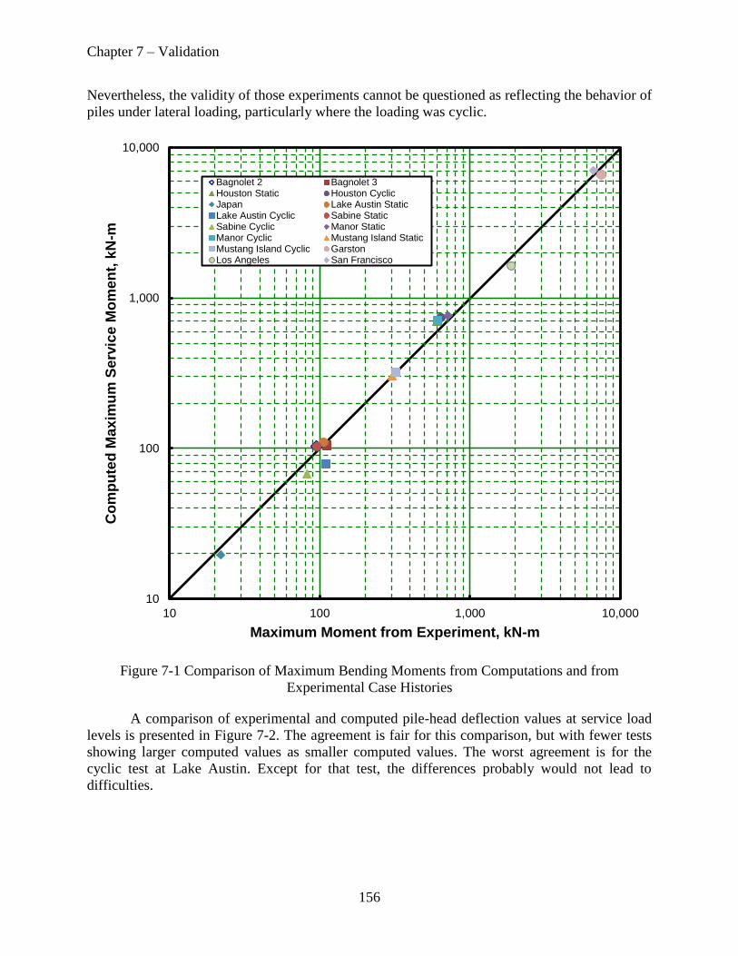
Chapter 7 – Validation
156
Nevertheless, the validity of those experiments cannot be questioned as reflecting the behavior of
piles under lateral loading, particularly where the loading was cyclic.
Figure 7-1 Comparison of Maximum Bending Moments from Computations and from
Experimental Case Histories
A comparison of experimental and computed pile-head deflection values at service load
levels is presented in Figure 7-2. The agreement is fair for this comparison, but with fewer tests
showing larger computed values as smaller computed values. The worst agreement is for the
cyclic test at Lake Austin. Except for that test, the differences probably would not lead to
difficulties.
10
100
1,000
10,000
10 100 1,000 10,000
Co
mp
ute
d M
ax
imu
m S
erv
ice
Mo
me
nt,
kN
-m
Maximum Moment from Experiment, kN-m
Bagnolet 2 Bagnolet 3Houston Static Houston CyclicJapan Lake Austin StaticLake Austin Cyclic Sabine StaticSabine Cyclic Manor StaticManor Cyclic Mustang Island StaticMustang Island Cyclic GarstonLos Angeles San Francisco
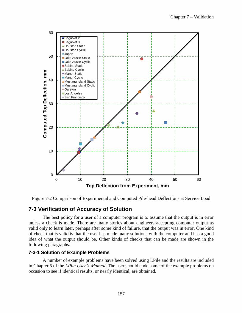
Chapter 7 – Validation
157
Figure 7-2 Comparison of Experimental and Computed Pile-head Deflections at Service Load
7-3 Verification of Accuracy of Solution
The best policy for a user of a computer program is to assume that the output is in error
unless a check is made. There are many stories about engineers accepting computer output as
valid only to learn later, perhaps after some kind of failure, that the output was in error. One kind
of check that is valid is that the user has made many solutions with the computer and has a good
idea of what the output should be. Other kinds of checks that can be made are shown in the
following paragraphs.
7-3-1 Solution of Example Problems
A number of example problems have been solved using LPile and the results are included
in Chapter 5 of the LPile User’s Manual. The user should code some of the example problems on
occasion to see if identical results, or nearly identical, are obtained.
0
10
20
30
40
50
60
0 10 20 30 40 50 60
Co
mp
ute
d T
op
De
fle
cti
on
, m
m
Top Deflection from Experiment, mm
Bagnolet 2
Bagnolet 3
Houston Static
Houston Cyclic
Japan
Lake Austin Static
Lake Austin Cyclic
Sabine Static
Sabine Cyclic
Manor Static
Manor Cyclic
Mustang Island Static
Mustang Island Cyclic
Garston
Los Angeles
San Francisco
Chapter 7 – Validation
158
Another example problem was analyzed and the results are shown in the following pages.
The output from this example problem will be checked to illustrate some of the procedures
employed for verification.
7-3-2 Numerical Precision Employed in Internal Computations
All real values are programmed as IEEE 64-bit reals, ranging in magnitude from
5.0×10−324
to 1.7×10308
, with a mantissa of 16 significant figures. This numerical precision was
chosen because the difference-equation method requires that a relatively large number of
significant figures be employed in order to avoid significant round-off errors.
7-3-3 Selection of Convergence Tolerance and Length of Increment
The convergence tolerance is a number that is input to control the accuracy of the
solution. The values of deflection for successive iterations are retained in memory and the
differences at corresponding depths are computed. All of the differences must be less than the
convergence tolerance to end the iterative computations. The convergence tolerance used in most
of the example problems of Chapter 5 of the LPile User’s Manual, and in the study of this
Chapter, was l10–5
in. (2.5410–7
m), which is the default value provided by the computer
program.
The user has control over the convergence tolerance, but the default value appears to be a
good selection for the majority of problems. If a significantly larger value had been selected,
inaccurate computations could have resulted; had a significantly smaller value been selected, the
number of iterations would be increased and, in fact, a very small value could prevent the
achievement of convergence. Verification of accuracy in the solution of the difference equations
has been demonstrated and results agree closely with those from the closed-form solution. In
addition, the exercise presented below demonstrates to a certain extent that accurate solutions are
being obtained. Convergence is usually obtained with 30 or fewer iterations when the pile is in
the elastic range, which does not require much time on most computers.
The user must select the length of the increments into which the pile is divided by
specifying the number of pile increments. The total length of the pile is the embedded length plus
the portion of the pile extending above the ground surface. In cases where the pile being
analyzed is extremely long, such as an oil well conductor, one may decide to shorten the length
of the modeled pile to where there are just a few points of zero deflection. The behavior of the
upper portion of the pile is unaffected as the length is reduced to the point where there are at
least two or three points of zero deflection. The number of points of zero deflection is listed on
the output for convenience.
A possible exception to shortening the pile to facilitate the computations may occur if the
lower portion of the pile is embedded in rock or very strong soil. In such a case, small deflection
could generate large values of soil resistance that in turn could influence the behavior of the
upper portion of the pile.
With the length of the pile adjusted so that there is no exceptionally long portion at the
bottom where the computed pile deflection is oscillating about the axis with extremely small
deflections and soil resistances, the user may wish to make a few runs with the pile subdivided
into various numbers of increments. Such a study was done for the example shown in this
chapter. Figure 7-3 shows a plot of the computed values of groundline deflection and maximum
bending moment as a function of the number of increments into which the pile is subdivided.

Chapter 7 – Validation
159
These values become virtually constant with the pile subdivided into 50 increments or more.
Errors are introduced if the number of increments is 40 or less.
Figure 7-3 Influence of Number of Increments on Computed Values of Pile-head Deflection and
Maximum Bending Moment
Errors would have been introduced if solutions had been made for large numbers of
increments, at some point beyond 500. The computed deflections at successive increments would
have been so close to each other that differences would have disappeared and round-off errors
would have been introduced. The number of increments at which such errors are introduced will
depend, of course, on the number of significant figures employed in the computations of the
particular computer being used. The computer used for the examples presented herein, with the
computer program using double-precision arithmetic, employs 8 bytes of storage for a number,
which translates into a word length of approximately 16 decimal digits.
For the particular problem that was solved, the pile length was 12.7 m (42 ft) and the
diameter was 0.914 meters (36 inches).
The increment length at which good results apparently were obtained was 0.25 m (10 in.)
(equal to 50 increments) which is about one-third or one-fourth of the pile diameter. However, it
0.5514
0.5515
0.5516
0.5517
0.5518
0.5519
0.5520
0.5521
0.5522
0.5523
0 100 200 300 400 500
Top
Def
lect
ion
, in
che
s
Number of Increments
9,445,000.0000
9,446,000.0000
9,447,000.0000
9,448,000.0000
9,449,000.0000
9,450,000.0000
9,451,000.0000
0 100 200 300 400 500
Max
imu
m M
om
en
t, i
n-lb
s
Number of Increments

Chapter 7 – Validation
160
is not only the pile diameter, but also the relative stiffness of the pile compared to the stiffness of
the soil that controls the results.
7-3-4 Check of Soil Resistance
A drilled shaft, with a length of 12.7 m and a diameter of 0.9144 m, was constructed in
sand with an angle of internal friction of 35 degrees and a unit weight of 18.7 kN/m3. The top of
the pile is unrestrained, a lateral load of 445 kN is applied, and the loading is static.
A p-y curve was printed for a depth of 1.524 meters. Initially, it will be assumed that the
curve is correct. The computed deflection at a depth of 1.524 m is reported as 0.007032m (0.28
in.) and the soil reaction is 204.6997 kN/m. The linear interpretation of the p-y curve that is
reported for the depth of 1.524 m is
p = 204.1049 kN/m
The close agreement in the tabulated and computed values of soil resistance is reassuring.
Some difference would have been expected between the two values of p because the computer
uses the equations for the p-y relationship and the check was done by linear interpolation.
The next step is to ascertain that the p-y values that are printed are consistent with the
equations that are given in the Technical Manual. As noted in the computer output, the loading is
static, the soil is sand with an angle of internal friction of 35 degrees, and a unit weight of 18.7
kN/m3. The pile has a diameter of 0.9144 m and the initial modulus of subgrade reaction of
24,400 kN/m3.
Computations of the ultimate resistance, using the equations in the Technical Manual for
response of the near-surface soils, yields 217.2 kN/m for pu and for the soils at depth pu is
1,398.1 kN/m. The former value controls. The deflection at yu is equal to 3b/80 and is 0.0343 m.
The value of pu is computed by multiplying 217.2 by the value of As (equal to 1.67, found from
Figure 3-25, of the Technical Manual) and becomes 362 kN/m (2,069 lbs/in.). These values
confirm the last four values in the output for p shown in the computer listing.
The value of ym is b/60 and is 0.0152 meter. The value of pm is found from Bs ps and is
found to be 260 kN/m (reading a value of Bs = 1.20 from Figure 3-26 of the Technical Manual).
This value confirms another point on the computer output. By referring to the curves giving the
characteristic shape of the p-y curves for sand, it can be seen that two significant points on the p-
y curve have been confirmed. Other points can be checked, but it will be assumed here that those
points are also correct.
7-3-5 Check of Equilibrium
The values of soil resistance that are listed in the computer output were plotted as a
function of depth along the pile, and the plot is shown in Figure 7-4. The squares were counted
and the forces that were computed from the area under the curve are shown in the figure. The
following check was made of the summation of the forces in the horizontal direction.
Fh = 445 657 + 227 15 = 0

Chapter 7 – Validation
161
The forces are in equilibrium, which is quite fortuitous in view of the lack of precision in the
procedure for numerical integration.
The next step is to make a check of the position of the point of the maximum moment. As
shown in Figure 7-4, the curve of soil resistance was integrated numerically and the position of
zero shear force (where the area under the soil-resistance curve is 445 kN) was at approximately
2.8 m from the top of the pile. The output in the appendix shows that the depth to zero shear
force is between 2.71 m and 2.88 m, which confirm the results of the numerical integration.
To obtain a rough check of the value of the maximum moment, the centroid of the area
under the curve equal to 445 kN is assumed to be approximately 1.8 m from the top of the pile or
1.0 m from the point of maximum moment; thus, the following equation can be written:
Mmax = (445)(2.8) − (445)(1.0)
Mmax = 806 kN-m
The tabulated value of the maximum moment is 711kN-m, and the rough check shown
above is considered acceptable.
The next step in verifying the mechanics is to make an approximate solution for the
deflection. Several assumptions are made, as will be seen. Figure 7-4 shows that zero deflection
occurs at depths of approximately 4.9 m and 10.9 m (where the soil resistance is zero), so the
assumption is made that a zero slope exists in the deflection curve at midway between these two
points, or at a depth of 7.9 meters. The deflection at the top of the pile can be computed by
taking moments of the M/EI diagram about the top and down to the point of zero slope.
In order to simplify the computations, a further assumption is made that concentrated
loads can be used to obtain the moment diagram instead of the distributed loads. Referring to
Figure 7-4, the concentrated loads to be used in the analysis are a pile-head shear load of 445 kN,
a resisting load of 657 kN at approximately 2.2 m from the top of the pile, and a resisting load of
165 kN at approximately 6.8 m from the top of the pile. The following equation results:
in. 0.053 m 0134.0
742038,64134,73000,734
1
3
)1.1)(2(8.6
2
)1.1(165
3
)7.5)(2(2.2
2
)7.5(657
3
)9.7(445
000,734
1 223
ty
The analysis found yt to be 0.0134 meters (0.52 inch). The agreement is close, in view of
the assumptions that were made.
This computation completes the checking of the mechanics of the output from a computer
run. While the results are not fully definitive, there is ample reason to trust the coding if a proper
selection is made of a computer, the number of increments for a particular run, and the value of
the tolerance used for concluding the iterations.
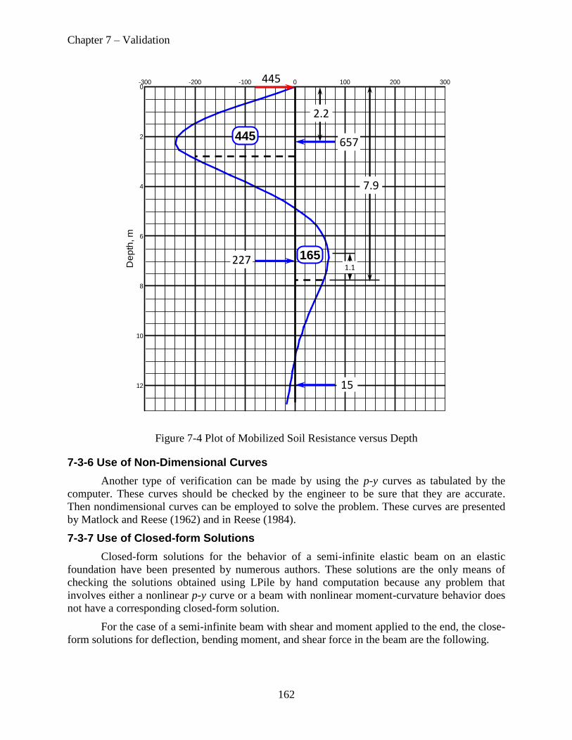
Chapter 7 – Validation
162
Figure 7-4 Plot of Mobilized Soil Resistance versus Depth
7-3-6 Use of Non-Dimensional Curves
Another type of verification can be made by using the p-y curves as tabulated by the
computer. These curves should be checked by the engineer to be sure that they are accurate.
Then nondimensional curves can be employed to solve the problem. These curves are presented
by Matlock and Reese (1962) and in Reese (1984).
7-3-7 Use of Closed-form Solutions
Closed-form solutions for the behavior of a semi-infinite elastic beam on an elastic
foundation have been presented by numerous authors. These solutions are the only means of
checking the solutions obtained using LPile by hand computation because any problem that
involves either a nonlinear p-y curve or a beam with nonlinear moment-curvature behavior does
not have a corresponding closed-form solution.
For the case of a semi-infinite beam with shear and moment applied to the end, the close-
form solutions for deflection, bending moment, and shear force in the beam are the following.
Mobilized Soil Reaction, p , kN/m3002001000-100-200-300
De
pth
, m
12
10
8
6
4
2
0
2.2
7.9
227
445
1651.1
15
657
445

Chapter 7 – Validation
163
Define the modulus of elasticity, E, and moment of inertia, I, of the beam, and the
subgrade constant, k. Compute the constant as
4
4EI
k
Timoshenko (1941) states that the pile is considered “long” if the product of and the pile length
(L) is greater than 4.
The closed-form solution for pile deflection, y, moment, M, and shear force, V, along the
length of the pile (x) as a function of pile-head shear, Vt, and pile-head moment, Mt, is
xxMxV
EI
ey t
t
x
sincoscos2 2
xxMx
VeM t
tx
cossinsin
xMxxVeV tt
x sin2sincos
Analyses of elastic piles in elastic soils can be performed using LPile using the elastic
subgrade soil model. The elastic subgrade constant k is computed as the product of the pile
diameter times the elastic modulus of subgrade reaction.
For the verification problem, define the following input for LPile.
An elastic pile with diameter = 12 inches, a wall thickness of 0.5 inch, and a Young’s
modulus of elasticity of 29,000,000 psi. This results in a moment of inertia of
187613.29964
1112
64
4444
io ddI in
4
Use the elastic subgrade soil model in LPile with a subgrade modulus of 500 pci.
Compute the elastic subgrade constant k using
000,6)12)(500( dEk s psi
Define Vt = 10,000 lbs and Mt = 250,000 in-lbs
The data file for this verification is provided as Example 25.
To provide the best check on the accuracy of the computations performed by LPile, the
equations above were programed in an electronic spreadsheet program and the computed results
were imported into the spreadsheet program from the plot output file in which all output is
written in scientific notation. Graphs of closed-form versus computed solutions were prepared
for lateral deflection, bending moment, and shear force. The graphs of the closed-form versus
computed results are presented in Figure 7-5 through Figure 7-7, along with regression

Chapter 7 – Validation
164
equations. As can be seen, for a linear regression, the coefficient of determination, R2, is 1.0 in
all cases, indicating that the accuracy of the solution is excellent.
Figure 7-5 Verification of Pile Deflections
7-3-8 Concluding Comments on Verification
The discussion above presents some procedures that can be used for verifying the
accuracy of the output from the computer. The point cannot be made too strongly that the
engineer should make verification a priority in working with LPile.
The user, if desired, may easily perform some of the elementary computations shown in
this chapter.
With regard to the static equilibrium of the lateral force on a single pile, the values of soil
resistance can be computed and plotted along the length of the pile. With the lateral loads at the
top of the pile, a check on the equilibrium of lateral forces can be made. A satisfactory check has
been made by estimation; a more comprehensive check can be made by use of numerical
integration of the distributed loads. The program will also conduct such checks internally to
ensure the force equilibrium.
-0.02
0
0.02
0.04
0.06
0.08
0.1
0.12
-0.02 0 0.02 0.04 0.06 0.08 0.1 0.12
Defl
ec
tio
n C
om
pu
ted
by L
Pil
e, in
ch
es
Deflection Computed by Theory, inches

Chapter 7 – Validation
165
Figure 7-6 Verification of Bending Moments
The final internal check relates to the computed movement of the system. The first step is
to refer to the computer output to confirm that the distributed load (soil resistance) and the
distributed deflections along the length of the pile are consistent with the p-y curves that were
input. If equations were used to compute the values of p and y, it is necessary to interpret the
equations at a sufficient number of points to shown that the soil criteria for lateral load was
followed. The second step with respect to lateral load is to employ the diagram is Step 1 and to
use principles of mechanics to ascertain that the deflection of the individual piles was computed
correctly.
While employing the steps shown above have confirmed the internal functioning of
LPile, the application of the program to results of field experiments is useful. The book by Reese
and Van Impe (2011) presents a discussion of the development of the methods used in LPile and
applies the methods to several cases.
-100,000
0
100,000
200,000
300,000
400,000
-100,000 0 100,000 200,000 300,000 400,000
Mo
me
nt
Co
mp
ute
d b
y L
Pil
e, in
-lb
s
Moment Computed by Theory, in-lbs

Chapter 7 – Validation
166
Figure 7-7 Verification of Shear Forces
-10,000
-5,000
0
5,000
10,000
15,000
-10,000 -5,000 0 5,000 10,000 15,000
Sh
ea
r F
orc
e C
om
pu
ted
by L
Pil
e, lb
s
Shear Force Computed by Theory, lbs

167
Chapter 8 Line-by-Line Guide for Input
The input file for LPile Format Version 8 is an ASCII text file. The data file is updated
with the latest data contained in the data editing dialogs of LPile immediately before every
analysis is made. The computation functions in LPile begin by reading the input data file.
The general format is a series of key words that denote the start of a section of data. The
key words may be entered in any order, but the order of input in each section must follow a
specific sequence.
The content of the input data file is designed to be easily understandable by the user.
8-1 Key Words for Input Data File
The following table lists the key words that define sections of data. The key words may
be entered in any order.
Table 8-1 Key Words for Definition of Input Data
Input Command Word Data Type Defined by Key Word
LPILEP8 Input file format version number
TITLE Title lines for data file (five lines)
OPTIONS Program and analysis options
SECTIONS Pile section and material properties
AXIAL THRUST LOADS Axial thrust loads used in nonlinear moment-curvature
computations
SOIL LAYERS Soil profile dimension and soil properties used for p-y
curve computations
TIP SHEAR Tip shear versus lateral tip movement data
PILE BATTER AND SLOPE Pile batter and slope data
LRFD LOADS Unfactored loads for LRFD analysis
LRFD FACTORS AND CASES Load and resistance factors and load combination data
LOADING Pile-head boundary conditions and loading data for
conventional analysis
SOIL MOVEMENTS Soil movement versus depth data
GROUP EFFECT FACTORS Group effect factors (p and y-multiplier) data
P-Y OUTPUT DEPTHS Output depths for reported p-y curves
FOUNDATION STIFFNESS Control data for computation of foundation stiffness
PILE PUSHOVER ANALYSIS DATA Control data for computation of pile pushover analysis
PILE BUCKLING ANALYSIS DATA Control data for computation of pile buckling analysis
END Terminates reading of input data

168
8-2 TITLE Command
The TITLE keyword indicated that the following five lines of text are entered for the
problem title. Entering fewer or more than five lines of text will result in an execution error and
input of data is ended.
By default, the following lines of text are predefined in LPile, but may be changed to
anything that the user wishes to enter. The default lines are:
Project Name:
Job Number:
Client:
Engineer:
Description:
8-3 OPTIONS Command
The OPTIONS keyword begins the definition of program options selected by the user.
Some options are either Yes or No options and the other options require numerical input. The
order of the options must be in the following sequence.
Table 8-2 Program Options and Settings
Options Keyword
(without spaces) Defines Option for Permissible Values
Units Engineering units USCS, SI
UseLRFD Perform LRFD analysis YES, NO
ComputeKmatrix Compute pile-head stiffness
matrix component values YES, NO
UseTipShear Use tip shear resistance curve YES, NO
UseDistributedLoading Include loading by distributed
lateral loading
ALL, ONE, NO
To enter multiple distributed
load profiles for every load
case enter “ALL.”
To enter a single distributed
lateral load profile to apply to
all load cases enter “ONE.”
To omit distributed lateral
loading enter “NO.”
UseSoilMovement Include loading by soil
movements
ALL, ONE, NO
To enter multiple soil
movement profiles for every
load case enter “ALL.”
To enter a single soil
movement profile to apply to
all load cases enter “ONE.”

169
Options Keyword
(without spaces) Defines Option for Permissible Values
To omit soil movements enter
“NO.”
UsePYModifiers Use p-y modifiers for group
action YES, NO
ComputeEIOnly
Compute nonlinear moment-
curvature values and nominal
moments capacity only
YES, NO
Loading Number of cycles of loading
If for static loading enter:
“STATIC”, followed by 5
spaces, then “1”
If for cyclic loading enter:
“CYCLIC”, followed by
number of cycles of loading,
5000 = maximum
IterationsLimit Maximum number of iterations
for numerical solution
500 = default value,
1,000 = maximum value
ConvergenceTolerance Convergence tolerance for
numerical solution 1.010
5 inches = default
value
NumberPileIncrements Number of pile increments for
numerical solution
100 = default, 40 = minimum,
500 = maximum
PrintSummaryOnly Print summary tables only YES, NO
PrintIncrement Printing increment for pile
response 1 = default value
PrintPYCurves Report p-y curves at user-
specified depths YES, NO
ComputeInteration Compute interaction diagram
only YES, NO
ComputePushover Compute pushover analysis YES, NO
ComputePileBuckling Compute pile buckling analysis YES, NO
8-4 SECTIONS Command
The SECTIONS keyword begins the definition of structural properties of the pile to be
analyzed. The order of the input data must be in the following sequence. The input data consists
of one or more numbers followed by an optional comment. Data written by LPile will be
followed by a comment that describes the input data and the engineering units of the data.
Table 8-3 Pile Section Data
SECTIONS Line Number Input Value
1 Total Number of Sections 1 = minimum, 10 = maximum
2 Section number 1 = top section, sections number
consecutively from top to bottom of pile

170
SECTIONS Line Number Input Value
3 Section Type
0 = rectangular,
1 = drilled shaft,
2 = drilled shaft with casing,
3 = drilled shaft with casing and core filled
with concrete,
-3 = drilled shaft with casing and void core
4 = steel pipe
5 = circular solid prestressed pile,
6 = circular hollow prestressed pile
7 = square solid prestressed pile,
8 = square hollow prestressed pile,
9 = octagonal solid prestressed pile,
10= octagonal hollow prestressed pile,
11 = elastic pile,
12 = elastic-plastic pile
13 = pile with user-defined nonlinear bending
properties in terms of EI and moment values
-13 = pile with user-defined nonlinear
bending properties in terms of moment and
curvature values
Follow by section dimensions for specific Section Type
Table 8-4 Properties for Rectangular Sections
Properties for rectangular sections Lines 3.0
3.0.1 Section dimension Length of section, ft or m
3.0.2 Shear capacity Shear capacity of section, lbs or kN
3.0.3 Section dimension Section depth, inches or mm
3.0.4 Section dimension Section width inches or mm
Follow with concrete properties (Lines 4) and rebar properties (Lines 5) to complete
section data.
Table 8-5 Properties for Drilled Shafts
Properties for Drilled Shaft Sections Lines 3.1
3.1.1 Section dimension Length of section, ft or m
3.1.2 Shear capacity Shear capacity of section, lbs or kN
3.1.3 Section dimension Section diameter, inches or mm
3.1.4 Section dimension Section width inches or mm
Follow with concrete properties (Lines 4) and rebar properties (Lines 5) to complete
section data.
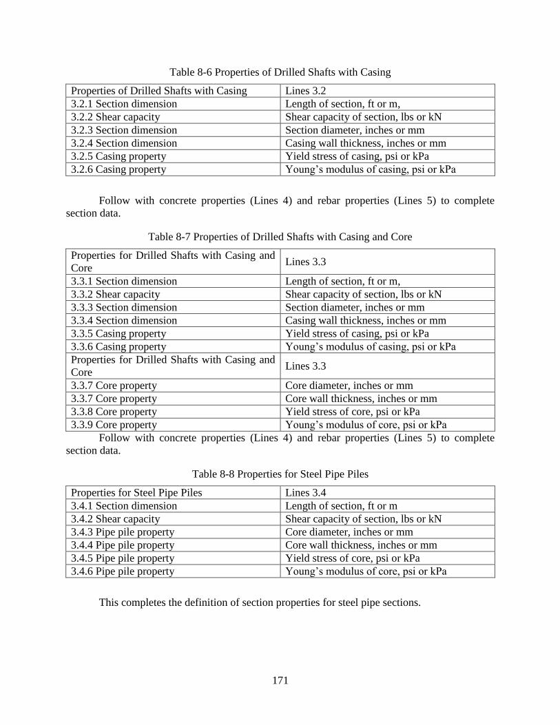
171
Table 8-6 Properties of Drilled Shafts with Casing
Properties of Drilled Shafts with Casing Lines 3.2
3.2.1 Section dimension Length of section, ft or m,
3.2.2 Shear capacity Shear capacity of section, lbs or kN
3.2.3 Section dimension Section diameter, inches or mm
3.2.4 Section dimension Casing wall thickness, inches or mm
3.2.5 Casing property Yield stress of casing, psi or kPa
3.2.6 Casing property Young’s modulus of casing, psi or kPa
Follow with concrete properties (Lines 4) and rebar properties (Lines 5) to complete
section data.
Table 8-7 Properties of Drilled Shafts with Casing and Core
Properties for Drilled Shafts with Casing and
Core Lines 3.3
3.3.1 Section dimension Length of section, ft or m,
3.3.2 Shear capacity Shear capacity of section, lbs or kN
3.3.3 Section dimension Section diameter, inches or mm
3.3.4 Section dimension Casing wall thickness, inches or mm
3.3.5 Casing property Yield stress of casing, psi or kPa
3.3.6 Casing property Young’s modulus of casing, psi or kPa
Properties for Drilled Shafts with Casing and
Core Lines 3.3
3.3.7 Core property Core diameter, inches or mm
3.3.7 Core property Core wall thickness, inches or mm
3.3.8 Core property Yield stress of core, psi or kPa
3.3.9 Core property Young’s modulus of core, psi or kPa
Follow with concrete properties (Lines 4) and rebar properties (Lines 5) to complete
section data.
Table 8-8 Properties for Steel Pipe Piles
Properties for Steel Pipe Piles Lines 3.4
3.4.1 Section dimension Length of section, ft or m
3.4.2 Shear capacity Shear capacity of section, lbs or kN
3.4.3 Pipe pile property Core diameter, inches or mm
3.4.4 Pipe pile property Core wall thickness, inches or mm
3.4.5 Pipe pile property Yield stress of core, psi or kPa
3.4.6 Pipe pile property Young’s modulus of core, psi or kPa
This completes the definition of section properties for steel pipe sections.
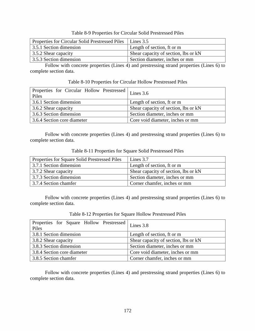
172
Table 8-9 Properties for Circular Solid Prestressed Piles
Properties for Circular Solid Prestressed Piles Lines 3.5
3.5.1 Section dimension Length of section, ft or m
3.5.2 Shear capacity Shear capacity of section, lbs or kN
3.5.3 Section dimension Section diameter, inches or mm
Follow with concrete properties (Lines 4) and prestressing strand properties (Lines 6) to
complete section data.
Table 8-10 Properties for Circular Hollow Prestressed Piles
Properties for Circular Hollow Prestressed
Piles Lines 3.6
3.6.1 Section dimension Length of section, ft or m
3.6.2 Shear capacity Shear capacity of section, lbs or kN
3.6.3 Section dimension Section diameter, inches or mm
3.6.4 Section core diameter Core void diameter, inches or mm
Follow with concrete properties (Lines 4) and prestressing strand properties (Lines 6) to
complete section data.
Table 8-11 Properties for Square Solid Prestressed Piles
Properties for Square Solid Prestressed Piles Lines 3.7
3.7.1 Section dimension Length of section, ft or m
3.7.2 Shear capacity Shear capacity of section, lbs or kN
3.7.3 Section dimension Section diameter, inches or mm
3.7.4 Section chamfer Corner chamfer, inches or mm
Follow with concrete properties (Lines 4) and prestressing strand properties (Lines 6) to
complete section data.
Table 8-12 Properties for Square Hollow Prestressed Piles
Properties for Square Hollow Prestressed
Piles Lines 3.8
3.8.1 Section dimension Length of section, ft or m
3.8.2 Shear capacity Shear capacity of section, lbs or kN
3.8.3 Section dimension Section diameter, inches or mm
3.8.4 Section core diameter Core void diameter, inches or mm
3.8.5 Section chamfer Corner chamfer, inches or mm
Follow with concrete properties (Lines 4) and prestressing strand properties (Lines 6) to
complete section data.

173
Table 8-13 Properties for Octagonal Solid Prestressed Piles
Properties for Octagonal Solid Prestressed
Piles Lines 3.9
3.9.1 Section dimension Length of section, ft or m
3.9.2 Section dimension Section diameter, inches or mm
Follow with concrete properties (Lines 4) and prestressing strand properties (Lines 6) to
complete section data.
Table 8-14 Properties for Square Hollow Prestressed Piles
Properties for Square Hollow Prestressed
Piles Lines 3.10
3.10.1 Section dimension Length of section, ft or m
3.10.2 Shear capacity Shear capacity of section, lbs or kN
3.10.3 Section dimension Section diameter, inches or mm
3.10.4 Section core diameter Core void diameter, inches or mm
Follow with concrete properties (Lines 4) and prestressing strand properties (Lines 6) to
complete section data.
Table 8-15 Properties for Elastic Piles
Properties for Elastic Piles Lines 3.11
3.11.1 Section dimension Length of section, ft or m
3.11.2 Geometric shape code
Enter:
1 = rectangular, follow by Lines 3.11.3.1
2 = circular solid, follow by Lines 3.11.3.2
3 = pipe , follow by Lines 3.11.3.3
4 = strong H-pile, follow by Lines 3.11.3.4
5 = weak H-pile, follow by Lines 3.11.3.5
6 = embedded pole, follow by Lines 3.11.3.6
Properties of elastic rectangular sections Lines 3.11.3.1
3.11.3.1.1 Section property Young’s modulus, psi or kPa
3.11.3.1.2 Section dimension Width at top, inches or mm
3.11.3.1.3 Section dimension Width at bottom, inches or mm
3.11.3.1.4 Section dimension Depth at top, inches or mm
3.11.3.1.5 Section dimension Depth at bottom, inches or mm
3.11.3.1.6 Section dimension Area at top, sq. inches or sq. mm
3.11.3.1.7 Section dimension Area at bottom, sq. inches or sq. mm
3.11.3.1.8 Section property Moment of inertia at top, in.4 or mm
4
3.11.3.1.9 Section property Moment of inertia at bottom, in.4 or mm
4

174
Properties of elastic circular sections Lines 3.11.3.2
3.11.3.2.1 Section property Young’s modulus, psi or kPa
3.11.3.2.2 Section dimension Width at top, inches or mm
3.11.3.2.3 Section dimension Width at bottom, inches or mm
3.11.3.2.4 Section dimension Area at top, sq. inches or sq. mm
3.11.3.2.5 Section dimension Area at bottom, sq. inches or sq. mm
3.11.3.2.6 Section property Moment of inertia at top, in.4 or mm
4
3.11.3.2.7 Section property Moment of inertia at bottom, in.4 or mm
4
Properties of elastic pipe sections Lines 3.11.3.3
3.11.3.3.1 Section property Young’s modulus, psi or kPa
3.11.3.3.2 Section dimension Width at top, inches or mm
3.11.3.3.3 Section dimension Width at bottom, inches or mm
3.11.3.3.4 Section dimension Wall thickness at top, inches or mm
3.11.3.3.5 Section dimension Wall thickness at bottom, inches or mm
3.11.3.3.6 Section dimension Area at top, sq. inches or sq. mm
3.11.3.3.7 Section dimension Area at bottom, sq. inches or sq. mm
3.11.3.3.8 Section property Moment of inertia at top, in.4 or mm
4
3.11.3.3.9 Section property Moment of inertia at bottom, in.4 or mm
4
Properties of strong H-pile sections Lines 3.11.3.4
3.11.3.4.1 Section property Young’s modulus, psi or kPa
3.11.3.4.2 Section dimension H section flange width, inches or mm
3.11.3.4.3 Section dimension H section depth, inches or mm
3.11.3.4.4 Section dimension H section flange thickness, inches or mm
3.11.3.4.5 Section dimension H section web thickness, inches or mm
3.11.3.4.6 Section dimension H section area, sq. inches or sq. mm
3.11.3.4.7 Section dimension H section moment of inertia, in.4 or mm
4
Properties of weak H-pile sections Lines 3.11.3.5
3.11.3.5.1 Section property Young’s modulus, psi or kPa
3.11.3.5.2 Section dimension H section flange width, inches or mm
3.11.3.5.3 Section dimension H section depth, inches or mm
3.11.3.5.4 Section dimension H section flange thickness, inches or mm
3.11.3.5.5 Section dimension H section web thickness, inches or mm
3.11.3.5.6 Section dimension H section area, sq. inches or sq. mm
3.11.3.5.7 Section property H section moment of inertia, in.4 or mm
4
Properties of elastic embedded pole Lines 3.11.3.6
3.11.3.6.1 Section property Young’s modulus, psi or kPa
3.11.3.6.2 Section dimension Pole width at top, inches or mm
3.11.3.6.3 Section dimension Pole width at bottom, inches or mm
3.11.3.6.4 Section dimension Pole area at top, sq. inches or sq. mm
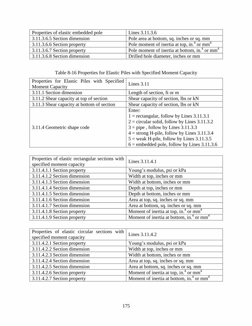
175
Properties of elastic embedded pole Lines 3.11.3.6
3.11.3.6.5 Section dimension Pole area at bottom, sq. inches or sq. mm
3.11.3.6.6 Section property Pole moment of inertia at top, in.4 or mm
4
3.11.3.6.7 Section property Pole moment of inertia at bottom, in.4 or mm
4
3.11.3.6.8 Section dimension Drilled hole diameter, inches or mm
Table 8-16 Properties for Elastic Piles with Specified Moment Capacity
Properties for Elastic Piles with Specified
Moment Capacity Lines 3.11
3.11.1 Section dimension Length of section, ft or m
3.11.2 Shear capacity at top of section Shear capacity of section, lbs or kN
3.11.3 Shear capacity at bottom of section Shear capacity of section, lbs or kN
3.11.4 Geometric shape code
Enter:
1 = rectangular, follow by Lines 3.11.3.1
2 = circular solid, follow by Lines 3.11.3.2
3 = pipe , follow by Lines 3.11.3.3
4 = strong H-pile, follow by Lines 3.11.3.4
5 = weak H-pile, follow by Lines 3.11.3.5
6 = embedded pole, follow by Lines 3.11.3.6
Properties of elastic rectangular sections with
specified moment capacity Lines 3.11.4.1
3.11.4.1.1 Section property Young’s modulus, psi or kPa
3.11.4.1.2 Section dimension Width at top, inches or mm
3.11.4.1.3 Section dimension Width at bottom, inches or mm
3.11.4.1.4 Section dimension Depth at top, inches or mm
3.11.4.1.5 Section dimension Depth at bottom, inches or mm
3.11.4.1.6 Section dimension Area at top, sq. inches or sq. mm
3.11.4.1.7 Section dimension Area at bottom, sq. inches or sq. mm
3.11.4.1.8 Section property Moment of inertia at top, in.4 or mm
4
3.11.4.1.9 Section property Moment of inertia at bottom, in.4 or mm
4
Properties of elastic circular sections with
specified moment capacity Lines 3.11.4.2
3.11.4.2.1 Section property Young’s modulus, psi or kPa
3.11.4.2.2 Section dimension Width at top, inches or mm
3.11.4.2.3 Section dimension Width at bottom, inches or mm
3.11.4.2.4 Section dimension Area at top, sq. inches or sq. mm
3.11.4.2.5 Section dimension Area at bottom, sq. inches or sq. mm
3.11.4.2.6 Section property Moment of inertia at top, in.4 or mm
4
3.11.4.2.7 Section property Moment of inertia at bottom, in.4 or mm
4

176
Properties of elastic pipe sections with
specified moment capacity Lines 3.11.4.3
3.11.4.3.1 Section property Young’s modulus, psi or kPa
3.11.4.3.2 Section dimension Width at top, inches or mm
3.11.4.3.3 Section dimension Width at bottom, inches or mm
3.11.4.3.4 Section dimension Wall thickness at top, inches or mm
3.11.4.3.5 Section dimension Wall thickness at bottom, inches or mm
3.11.4.3.6 Section dimension Area at top, sq. inches or sq. mm
3.11.4.3.7 Section dimension Area at bottom, sq. inches or sq. mm
3.11.4.3.8 Section property Moment of inertia at top, in.4 or mm
4
3.11.4.3.9 Section property Moment of inertia at bottom, in.4 or mm
4
Properties of strong H-pile sections with
specified moment capacity Lines 3.11.4.4
3.11.4.4.1 Section property Young’s modulus, psi or kPa
3.11.4.4.2 Section dimension H section flange width, inches or mm
3.11.4.4.3 Section dimension H section depth, inches or mm
3.11.4.4.4 Section dimension H section flange thickness, inches or mm
3.11.4.4.5 Section dimension H section web thickness, inches or mm
3.11.4.4.6 Section dimension H section area, sq. inches or sq. mm
3.11.4.4.7 Section property H section moment of inertia, in.4 or mm
4
Properties of weak H-pile sections with
specified moment capacity Lines 3.11.4.5
3.11.4.5.1 Section property Young’s modulus, psi or kPa
3.11.4.5.2 Section dimension H section flange width, inches or mm
3.11.4.5.3 Section dimension H section depth, inches or mm
3.11.4.5.4 Section dimension H section flange thickness, inches or mm
3.11.4.5.5 Section dimension H section web thickness, inches or mm
3.11.4.5.6 Section dimension H section area, sq. inches or sq. mm
3.11.4.5.7 Section property H section moment of inertia, in.4 or mm
4
Properties of elastic embedded pole with
specified moment capacity Lines 3.11.4.6
3.11.4.6.1 Section property Young’s modulus, psi or kPa
3.11.4.6.2 Section dimension Pole width at top, inches or mm
3.11.4.6.3 Section dimension Pole width at bottom, inches or mm
3.11.4.6.4 Section dimension Pole area at top, sq. inches or sq. mm
3.11.4.6.5 Section dimension Pole area at bottom, sq. inches or sq. mm
3.11.4.6.6 Section property Pole moment of inertia at top, in.4 or mm
4
3.11.4.6.7 Section property Pole moment of inertia at bottom, in.4 or mm
4
3.11.4.6.8 Section dimension Drilled hole diameter, inches or mm
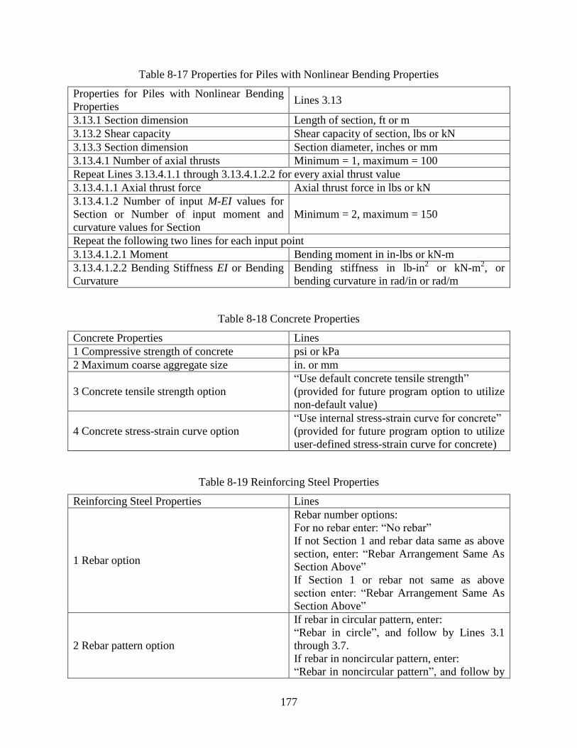
177
Table 8-17 Properties for Piles with Nonlinear Bending Properties
Properties for Piles with Nonlinear Bending
Properties Lines 3.13
3.13.1 Section dimension Length of section, ft or m
3.13.2 Shear capacity Shear capacity of section, lbs or kN
3.13.3 Section dimension Section diameter, inches or mm
3.13.4.1 Number of axial thrusts Minimum = 1, maximum = 100
Repeat Lines 3.13.4.1.1 through 3.13.4.1.2.2 for every axial thrust value
3.13.4.1.1 Axial thrust force Axial thrust force in lbs or kN
3.13.4.1.2 Number of input M-EI values for
Section or Number of input moment and
curvature values for Section
Minimum = 2, maximum = 150
Repeat the following two lines for each input point
3.13.4.1.2.1 Moment Bending moment in in-lbs or kN-m
3.13.4.1.2.2 Bending Stiffness EI or Bending
Curvature
Bending stiffness in lb-in2 or kN-m
2, or
bending curvature in rad/in or rad/m
Table 8-18 Concrete Properties
Concrete Properties Lines
1 Compressive strength of concrete psi or kPa
2 Maximum coarse aggregate size in. or mm
3 Concrete tensile strength option
“Use default concrete tensile strength”
(provided for future program option to utilize
non-default value)
4 Concrete stress-strain curve option
“Use internal stress-strain curve for concrete”
(provided for future program option to utilize
user-defined stress-strain curve for concrete)
Table 8-19 Reinforcing Steel Properties
Reinforcing Steel Properties Lines
1 Rebar option
Rebar number options:
For no rebar enter: “No rebar”
If not Section 1 and rebar data same as above
section, enter: “Rebar Arrangement Same As
Section Above”
If Section 1 or rebar not same as above
section enter: “Rebar Arrangement Same As
Section Above”
2 Rebar pattern option
If rebar in circular pattern, enter:
“Rebar in circle”, and follow by Lines 3.1
through 3.7.
If rebar in noncircular pattern, enter:
“Rebar in noncircular pattern”, and follow by
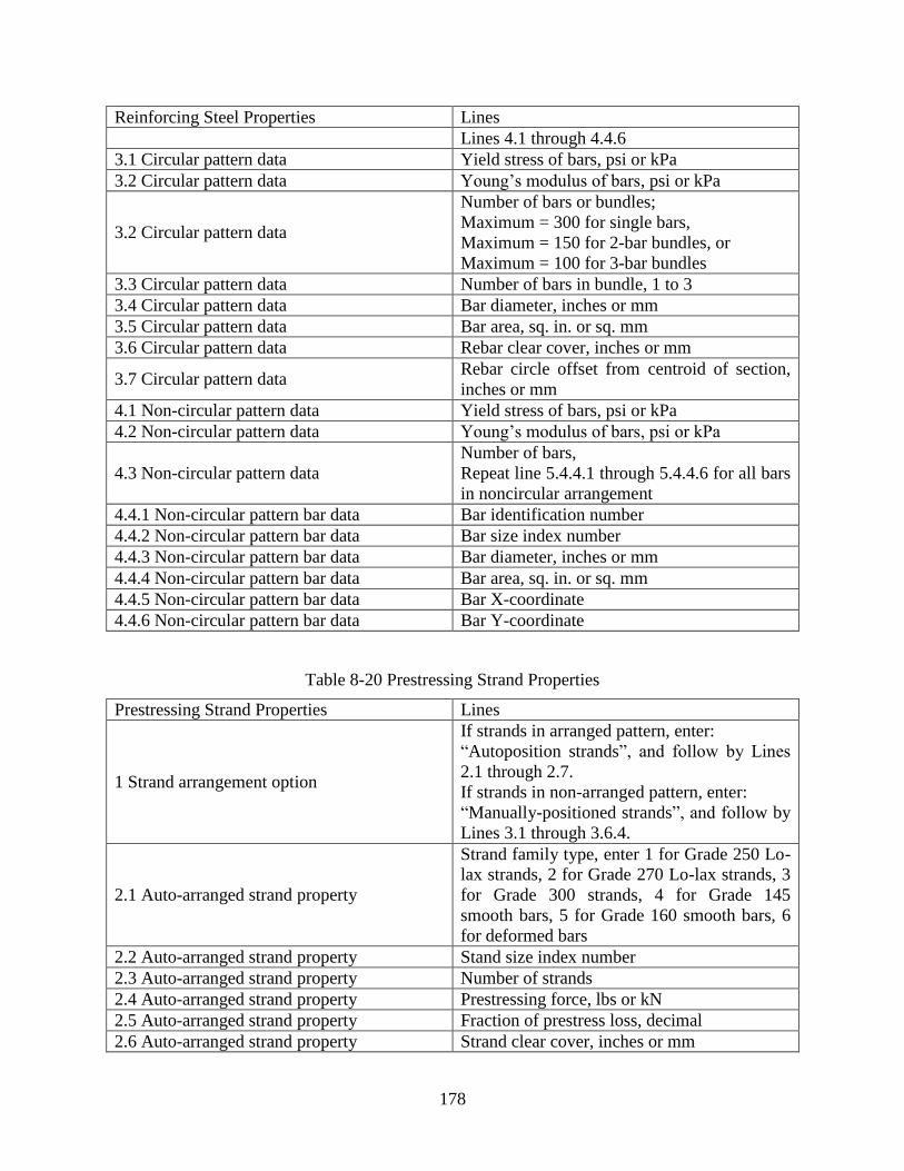
178
Reinforcing Steel Properties Lines
Lines 4.1 through 4.4.6
3.1 Circular pattern data Yield stress of bars, psi or kPa
3.2 Circular pattern data Young’s modulus of bars, psi or kPa
3.2 Circular pattern data
Number of bars or bundles;
Maximum = 300 for single bars,
Maximum = 150 for 2-bar bundles, or
Maximum = 100 for 3-bar bundles
3.3 Circular pattern data Number of bars in bundle, 1 to 3
3.4 Circular pattern data Bar diameter, inches or mm
3.5 Circular pattern data Bar area, sq. in. or sq. mm
3.6 Circular pattern data Rebar clear cover, inches or mm
3.7 Circular pattern data Rebar circle offset from centroid of section,
inches or mm
4.1 Non-circular pattern data Yield stress of bars, psi or kPa
4.2 Non-circular pattern data Young’s modulus of bars, psi or kPa
4.3 Non-circular pattern data
Number of bars,
Repeat line 5.4.4.1 through 5.4.4.6 for all bars
in noncircular arrangement
4.4.1 Non-circular pattern bar data Bar identification number
4.4.2 Non-circular pattern bar data Bar size index number
4.4.3 Non-circular pattern bar data Bar diameter, inches or mm
4.4.4 Non-circular pattern bar data Bar area, sq. in. or sq. mm
4.4.5 Non-circular pattern bar data Bar X-coordinate
4.4.6 Non-circular pattern bar data Bar Y-coordinate
Table 8-20 Prestressing Strand Properties
Prestressing Strand Properties Lines
1 Strand arrangement option
If strands in arranged pattern, enter:
“Autoposition strands”, and follow by Lines
2.1 through 2.7.
If strands in non-arranged pattern, enter:
“Manually-positioned strands”, and follow by
Lines 3.1 through 3.6.4.
2.1 Auto-arranged strand property
Strand family type, enter 1 for Grade 250 Lo-
lax strands, 2 for Grade 270 Lo-lax strands, 3
for Grade 300 strands, 4 for Grade 145
smooth bars, 5 for Grade 160 smooth bars, 6
for deformed bars
2.2 Auto-arranged strand property Stand size index number
2.3 Auto-arranged strand property Number of strands
2.4 Auto-arranged strand property Prestressing force, lbs or kN
2.5 Auto-arranged strand property Fraction of prestress loss, decimal
2.6 Auto-arranged strand property Strand clear cover, inches or mm
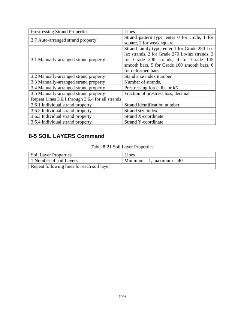
179
Prestressing Strand Properties Lines
2.7 Auto-arranged strand property Strand pattern type, enter 0 for circle, 1 for
square, 2 for weak square
3.1 Manually-arranged strand property
Strand family type, enter 1 for Grade 250 Lo-
lax strands, 2 for Grade 270 Lo-lax strands, 3
for Grade 300 strands, 4 for Grade 145
smooth bars, 5 for Grade 160 smooth bars, 6
for deformed bars
3.2 Manually-arranged strand property Stand size index number
3.3 Manually-arranged strand property Number of strands,
3.4 Manually-arranged strand property Prestressing force, lbs or kN
3.5 Manually-arranged strand property Fraction of prestress loss, decimal
Repeat Lines 3.6.1 through 3.6.4 for all strands
3.6.1 Individual strand property Strand identification number
3.6.2 Individual strand property Strand size index
3.6.3 Individual strand property Strand X-coordinate
3.6.4 Individual strand property Strand Y-coordinate
8-5 SOIL LAYERS Command
Table 8-21 Soil Layer Properties
Soil Layer Properties Lines
1 Number of soil Layers Minimum = 1, maximum = 40
Repeat following lines for each soil layer
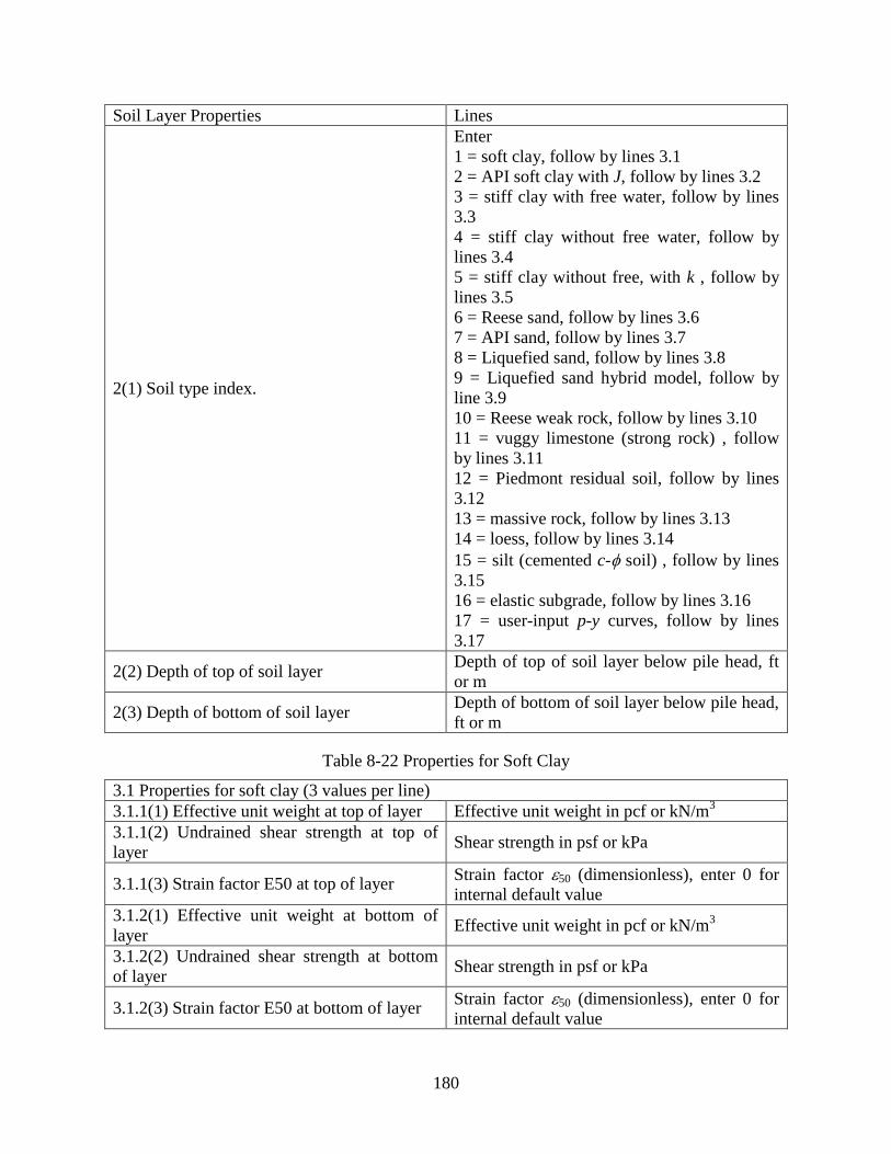
180
Soil Layer Properties Lines
2(1) Soil type index.
Enter
1 = soft clay, follow by lines 3.1
2 = API soft clay with J, follow by lines 3.2
3 = stiff clay with free water, follow by lines
3.3
4 = stiff clay without free water, follow by
lines 3.4
5 = stiff clay without free, with k , follow by
lines 3.5
6 = Reese sand, follow by lines 3.6
7 = API sand, follow by lines 3.7
8 = Liquefied sand, follow by lines 3.8
9 = Liquefied sand hybrid model, follow by
line 3.9
10 = Reese weak rock, follow by lines 3.10
11 = vuggy limestone (strong rock) , follow
by lines 3.11
12 = Piedmont residual soil, follow by lines
3.12
13 = massive rock, follow by lines 3.13
14 = loess, follow by lines 3.14
15 = silt (cemented c- soil) , follow by lines
3.15
16 = elastic subgrade, follow by lines 3.16
17 = user-input p-y curves, follow by lines
3.17
2(2) Depth of top of soil layer Depth of top of soil layer below pile head, ft
or m
2(3) Depth of bottom of soil layer Depth of bottom of soil layer below pile head,
ft or m
Table 8-22 Properties for Soft Clay
3.1 Properties for soft clay (3 values per line)
3.1.1(1) Effective unit weight at top of layer Effective unit weight in pcf or kN/m3
3.1.1(2) Undrained shear strength at top of
layer Shear strength in psf or kPa
3.1.1(3) Strain factor E50 at top of layer Strain factor 50 (dimensionless), enter 0 for
internal default value
3.1.2(1) Effective unit weight at bottom of
layer Effective unit weight in pcf or kN/m
3
3.1.2(2) Undrained shear strength at bottom
of layer Shear strength in psf or kPa
3.1.2(3) Strain factor E50 at bottom of layer Strain factor 50 (dimensionless), enter 0 for
internal default value

181
Table 8-23 Properties for API Soft Clay
3.2 Properties for API soft clay with J
3.2.1(1) Effective unit weight at top of layer Effective unit weight in pcf or kN/m3
3.2.1(2) Undrained shear strength at top of
layer Shear strength in psf or kPa
3.2.1(3) Strain factor E50 at top of layer Strain factor 50 (dimensionless),
enter 0 for internal default value
3.2.1(4) Parameter J at top of layer dimensionless
3.2.2(1) Effective unit weight at bottom of
layer Effective unit weight in pcf or kN/m
3
3.2.2(2) Undrained shear strength at bottom
of layer Shear strength in psf or kPa
3.2.2(3) Strain factor E50 at bottom of layer Strain factor 50 (dimensionless),
enter 0 for internal default value
3.2.1(4) Parameter J at bottom of layer dimensionless
Table 8-24 Properties for Stiff Clay with Free Water
3.3 Properties for stiff clay with free water (4 values per line)
3.3.1(1) Effective unit weight at top of layer Effective unit weight in pcf or kN/m3
3.3.1(2) Undrained shear strength at top of
layer Shear strength in psf or kPa
3.3.1(3) Strain factor E50 at top of layer Strain factor 50 (dimensionless), enter 0 for
internal default value
3.3.1(4) p-y modulus k at top of layer k in lbs/in
3 or kN/m
3, enter 0 for internal
default value
3.3.2(1) Effective unit weight at bottom of
layer Effective unit weight in pcf or kN/m
3
3.3.2(2) Undrained shear strength at bottom
of layer Shear strength in psf or kPa
3.3.2(3) Strain factor E50 at bottom of layer Strain factor 50 (dimensionless), enter 0 for
internal default value
3.3.1(4) p-y modulus k at bottom of layer k in lbs/in
3 or kN/m
3, enter 0 for internal
default value
Table 8-25 Properties for Stiff Clay without Free Water
3.4 Properties for stiff clay without free water (3 values per line)
3.4.1(1) Effective unit weight at top of layer Effective unit weight in pcf or kN/m3
3.4.1(2) Undrained shear strength at top of
layer Shear strength in psf or kPa
3.4.1(3) Strain factor E50 at top of layer Strain factor 50 (dimensionless),
enter 0 for internal default value
3.4.2(1) Effective unit weight at bottom of
layer Effective unit weight in pcf or kN/m
3
3.4.2(2) Undrained shear strength at bottom Shear strength in psf or kPa

182
3.4 Properties for stiff clay without free water (3 values per line)
of layer
3.4.2(3) Strain factor E50 at bottom of layer Strain factor 50 (dimensionless),
enter 0 for internal default value
Table 8-26 Properties for Stiff Clay with Free Water Using k
3.5 Properties for stiff clay without free water using k (4 values per line)
3.5.1(1) Effective unit weight at top of layer Effective unit weight in pcf or kN/m3
3.5.1(2) Undrained shear strength at top of
layer Shear strength in psf or kPa
3.5.1(3) Strain factor E50 at top of layer Strain factor 50 (dimensionless), enter 0 for
internal default value
3.5.1(4) p-y modulus k at top of layer k in lbs/in
3 or kN/m
3, enter 0 for internal
default value
3.5.2(1) Effective unit weight at bottom of
layer Effective unit weight in pcf or kN/m
3
3.5.2(2) Undrained shear strength at bottom
of layer Shear strength in psf or kPa
3.5.2(3) Strain factor E50 at bottom of layer Strain factor 50 (dimensionless),
enter 0 for internal default value
3.5.2(4) p-y modulus k at bottom of layer k in lbs/in
3 or kN/m
3, enter 0 for internal
default value
Table 8-27 Properties for Sand
3.6 Properties for Reese sand (3 values per line)
3.6.1(1) Effective unit weight at top of layer Effective unit weight in pcf or kN/m3
3.6.1(2) Friction angle at top of layer Friction angle in degrees
3.6.1(3) p-y modulus k at top of layer k in lbs/in
3 or kN/m
3, enter 0 for internal
default value
3.6.2(1) Effective unit weight at bottom of
layer Effective unit weight in pcf or kN/m
3
3.6.2(2) Friction angle at bottom of layer Friction angle in degrees
3.6.2(3) p-y modulus k at bottom of layer k in lbs/in
3 or kN/m
3, enter 0 for internal
default value
Table 8-28 Properties for API Sand
3.7 Properties for API sand (3 values per line)
3.7.1(1) Effective unit weight at top of layer Effective unit weight in pcf or kN/m3
3.7.1(2) Friction angle at top of layer Friction angle in degrees
3.7.1(3) p-y modulus k at top of layer k in lbs/in
3 or kN/m
3, enter 0 for internal
default value
3.7.2(1) Effective unit weight at top of layer Effective unit weight in pcf or kN/m3
3.7.2(2) Friction angle at bottom of layer Friction angle in degrees
3.7.2(3) p-y modulus k at bottom of layer k in lbs/in3 or kN/m
3, enter 0 for internal

183
3.7 Properties for API sand (3 values per line)
default value
Table 8-29 Properties for Liquefied Sand
3.8 Properties for liquefied sand (1 value per line)
3.8.1 Effective unit weight at top of layer Effective unit weight in pcf or kN/m3
3.8.2 Effective unit weight at bottom of layer Effective unit weight in pcf or kN/m3
Table 8-30 Properties for Liquefied Sand Hybrid Model
3.9 Properties for liquefied sand hybrid model (4 values per line)
Option 1 is to enter values for effective unit weight and SPT blowcount and zeros for residual
strength and 50. Option 2 is to enter non-zero values for effective unit weight and for residual
strength and 50.
3.9.1(1) Effective unit weight at top of layer Effective unit weight in pcf or kN/m3
3.9.1(2) SPT blowcount at top of layer SPT (N1)60-cs blows/ft or blows/0.3 m
3.9.1(3) Residual strength at top of layer Sr in psf or kPa
3.9.1(4) 50 at top of layer 50
3.9.2(1) Effective unit weight at bottom of
layer Effective unit weight in pcf or kN/m
3
3.9.2(2) SPT blowcount at bottom of layer SPT (N1)60-cs blows/ft or blows/0.3 m
3.9.2(3) Residual strength at bottom of layer Sr in psf or kPa
3.9.2(4) 50 at bottom of layer 50
Table 8-31 Properties for Weak Rock
3.10 Properties for weak rock (5 values per line)
3.10.1(1) Effective unit weight at top of layer Effective unit weight in pcf or kN/m3
3.10.1(2) Uniaxial compressive strength qu at
top of layer Uniaxial compressive strength in psi or kPa
3.10.1(3) Initial rock mass modulus at top of
layer Emass in psi or kPa
3.10.1(4) RQD at top of layer RQD in percent
3.10.1(5) Parameter krm at top of layer k in lbs/in
3 or kN/m
3,
enter 0 for internal default value
3.10.2(1) Effective unit weight at bottom of
layer Effective unit weight in pcf or kN/m
3
3.10.2(2) Uniaxial compressive strength qu at
bottom of layer Uniaxial compressive strength in psi or kPa
3.10.2(3) Initial rock mass modulus at bottom
of layer Emass in psi or kPa
3.10.2(4) RQD at bottom of layer RQD in percent
3.10.2(5) Parameter krm at bottom of layer k in lbs/in
3 or kN/m
3,
enter 0 for internal default value

184
Table 8-32 Properties for Vuggy Limestone
3.11 Properties for vuggy limestone (2 values per line)
3.11.1(1) Effective unit weight at top of layer Effective unit weight in pcf or kN/m3
3.11.1(2) Uniaxial compressive strength qu at
top of layer Uniaxial compressive strength in psi or kPa
3.11.2(1) Effective unit weight at bottom of
layer Effective unit weight in pcf or kN/m
3
3.11.2(2) Uniaxial compressive strength qu at
bottom of layer Uniaxial compressive strength in psi or kPa
Table 8-33 Properties for Piedmont Residual Soil
3.12 Properties for Piedmont residual soil (6 values per line)
3.12.1(1) Effective unit weight at top of layer Effective unit weight in pcf or kN/m3
3.12.1(2) Test type index
Enter 1 for SPT,
2 for cone penetrometer,
3 for dilatometer, or
4 for pressuremeter modulus
3.12.1(3) SPT blowcount at top of layer Blows/foot or blows/ 0.3 m
3.12.1(4) Cone tip resistance at top of layer qtip in psi or kPa
3.12.1(5) Dilatometer modulus at top of layer psi or kPa
3.12.1(6) Pressuremeter modulus at top of
layer psi or kPa
3.12.2(1) Effective unit weight at bottom of
layer Effective unit weight in pcf or kN/m
3
3.12.2(2) Test type index
(a value must be entered but is ignored for
bottom of layer)
Enter 1 for SPT,
2 for cone penetrometer,
3 for dilatometer, or
4 for pressuremeter modulus
3.12.2(3) SPT blowcount at bottom of layer Blows/foot or blows/ 0.3 m
3.12.2(4) Cone tip resistance at bottom of
layer qtip in psi or kPa
3.12.2(5) Dilatometer modulus at bottom of
layer psi or kPa
3.12.2(6) Pressuremeter modulus at bottom of
layer psi or kPa
Table 8-34 Properties for Massive Rock
3.13 Properties for massive rock
3.13.1(1) Effective unit weight at top of layer Effective unit weight in pcf or kN/m3
3.13.1(2) Uniaxial compressive strength of
intact rock at top of layer
Uniaxial compressive strength of intact rock
in psi or kPa
3.13.1(3) Material index for layer Hoek-Brown material index mi
3.13.1(4) Poisson’s ratio for layer Poisson’s ratio
3.13.1(5) GSI for layer Geologic Strength Index
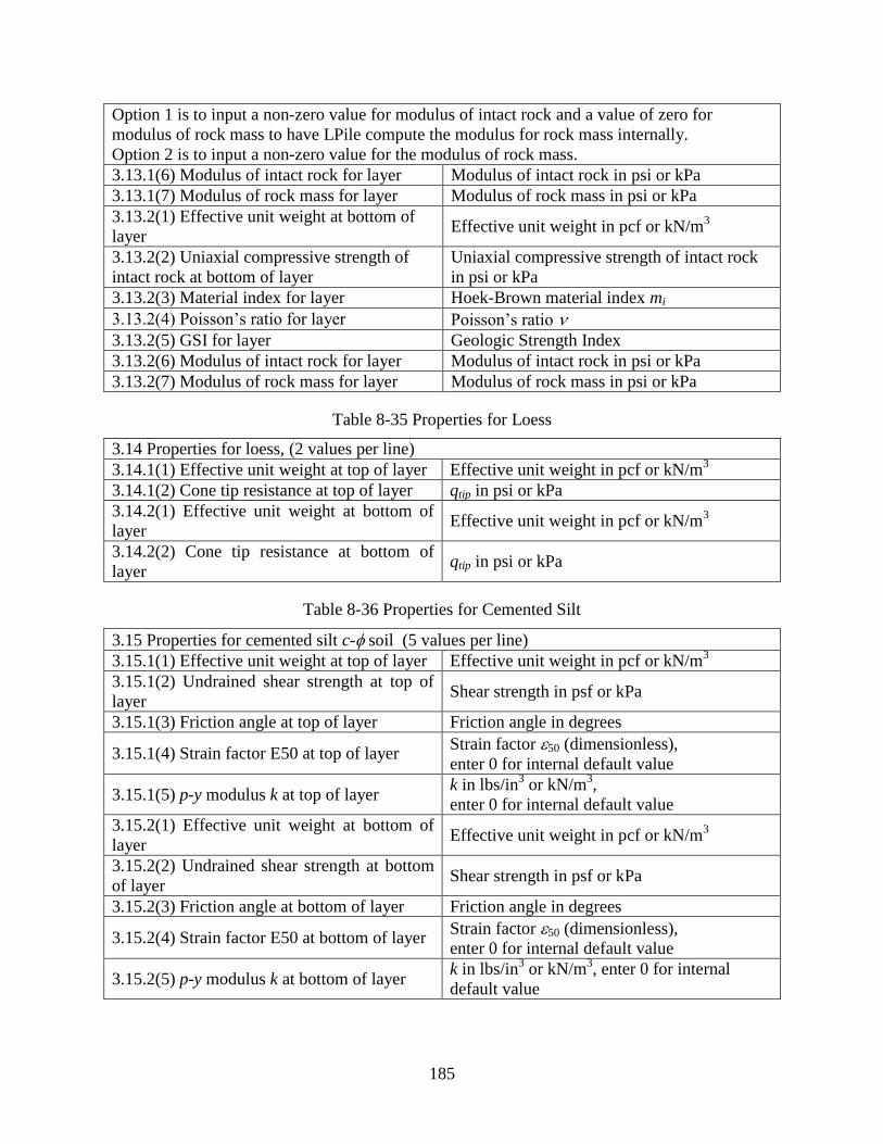
185
Option 1 is to input a non-zero value for modulus of intact rock and a value of zero for
modulus of rock mass to have LPile compute the modulus for rock mass internally.
Option 2 is to input a non-zero value for the modulus of rock mass.
3.13.1(6) Modulus of intact rock for layer Modulus of intact rock in psi or kPa
3.13.1(7) Modulus of rock mass for layer Modulus of rock mass in psi or kPa
3.13.2(1) Effective unit weight at bottom of
layer Effective unit weight in pcf or kN/m
3
3.13.2(2) Uniaxial compressive strength of
intact rock at bottom of layer
Uniaxial compressive strength of intact rock
in psi or kPa
3.13.2(3) Material index for layer Hoek-Brown material index mi
3.13.2(4) Poisson’s ratio for layer Poisson’s ratio
3.13.2(5) GSI for layer Geologic Strength Index
3.13.2(6) Modulus of intact rock for layer Modulus of intact rock in psi or kPa
3.13.2(7) Modulus of rock mass for layer Modulus of rock mass in psi or kPa
Table 8-35 Properties for Loess
3.14 Properties for loess, (2 values per line)
3.14.1(1) Effective unit weight at top of layer Effective unit weight in pcf or kN/m3
3.14.1(2) Cone tip resistance at top of layer qtip in psi or kPa
3.14.2(1) Effective unit weight at bottom of
layer Effective unit weight in pcf or kN/m
3
3.14.2(2) Cone tip resistance at bottom of
layer qtip in psi or kPa
Table 8-36 Properties for Cemented Silt
3.15 Properties for cemented silt c- soil (5 values per line)
3.15.1(1) Effective unit weight at top of layer Effective unit weight in pcf or kN/m3
3.15.1(2) Undrained shear strength at top of
layer Shear strength in psf or kPa
3.15.1(3) Friction angle at top of layer Friction angle in degrees
3.15.1(4) Strain factor E50 at top of layer Strain factor 50 (dimensionless),
enter 0 for internal default value
3.15.1(5) p-y modulus k at top of layer k in lbs/in
3 or kN/m
3,
enter 0 for internal default value
3.15.2(1) Effective unit weight at bottom of
layer Effective unit weight in pcf or kN/m
3
3.15.2(2) Undrained shear strength at bottom
of layer Shear strength in psf or kPa
3.15.2(3) Friction angle at bottom of layer Friction angle in degrees
3.15.2(4) Strain factor E50 at bottom of layer Strain factor 50 (dimensionless),
enter 0 for internal default value
3.15.2(5) p-y modulus k at bottom of layer k in lbs/in
3 or kN/m
3, enter 0 for internal
default value
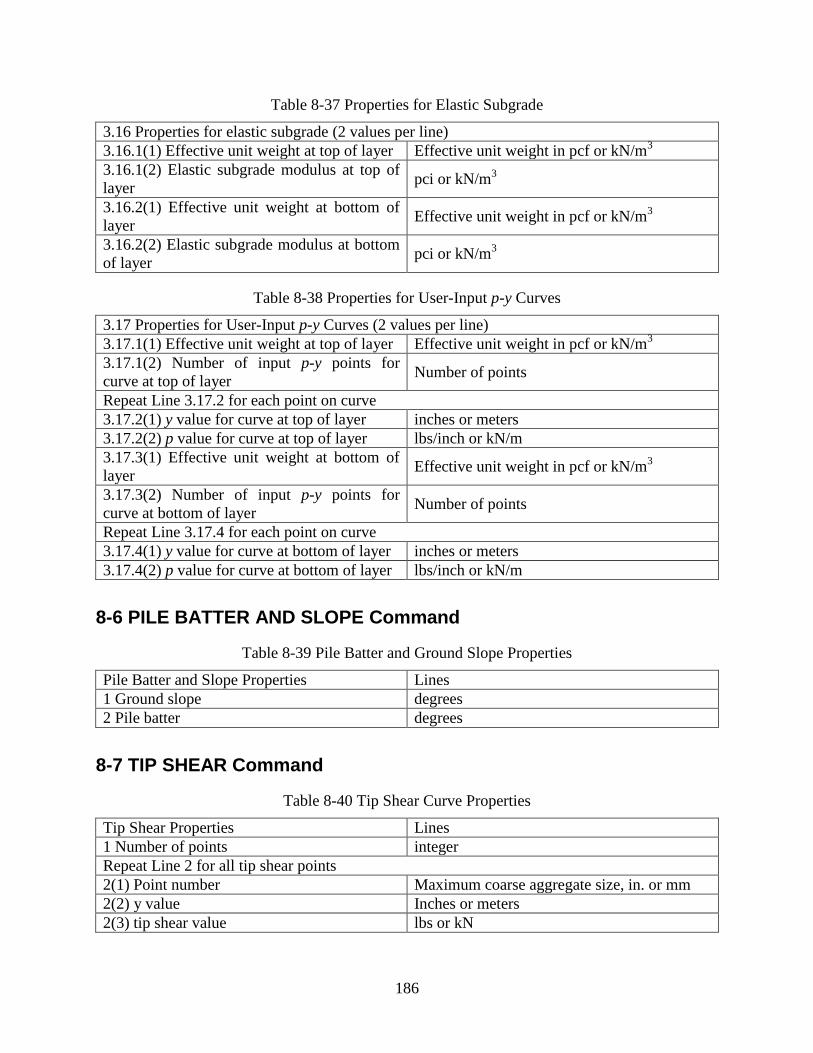
186
Table 8-37 Properties for Elastic Subgrade
3.16 Properties for elastic subgrade (2 values per line)
3.16.1(1) Effective unit weight at top of layer Effective unit weight in pcf or kN/m3
3.16.1(2) Elastic subgrade modulus at top of
layer pci or kN/m
3
3.16.2(1) Effective unit weight at bottom of
layer Effective unit weight in pcf or kN/m
3
3.16.2(2) Elastic subgrade modulus at bottom
of layer pci or kN/m
3
Table 8-38 Properties for User-Input p-y Curves
3.17 Properties for User-Input p-y Curves (2 values per line)
3.17.1(1) Effective unit weight at top of layer Effective unit weight in pcf or kN/m3
3.17.1(2) Number of input p-y points for
curve at top of layer Number of points
Repeat Line 3.17.2 for each point on curve
3.17.2(1) y value for curve at top of layer inches or meters
3.17.2(2) p value for curve at top of layer lbs/inch or kN/m
3.17.3(1) Effective unit weight at bottom of
layer Effective unit weight in pcf or kN/m
3
3.17.3(2) Number of input p-y points for
curve at bottom of layer Number of points
Repeat Line 3.17.4 for each point on curve
3.17.4(1) y value for curve at bottom of layer inches or meters
3.17.4(2) p value for curve at bottom of layer lbs/inch or kN/m
8-6 PILE BATTER AND SLOPE Command
Table 8-39 Pile Batter and Ground Slope Properties
Pile Batter and Slope Properties Lines
1 Ground slope degrees
2 Pile batter degrees
8-7 TIP SHEAR Command
Table 8-40 Tip Shear Curve Properties
Tip Shear Properties Lines
1 Number of points integer
Repeat Line 2 for all tip shear points
2(1) Point number Maximum coarse aggregate size, in. or mm
2(2) y value Inches or meters
2(3) tip shear value lbs or kN

187
8-8 GROUP EFFECT FACTORS Command
Table 8-41 Group Effect Properties
Group Effect Properties Lines
1 Number of points integer
Repeat Line 2 for all points
2(1) Point number integer
2(2) Depth below pile head ft or meters
2(3) p-multiplier Dimensionless
2(4) y-multiplier Dimensionless
8-9 LRFD LOADS Command
Table 8-42 LRFD Load Properties
LRFD Load Properties Lines
1 Number of LRFD unfactored loads integer
Repeat line 2 and .3 for every load
2(1) Load number (starting with 1)
2(2) Load type index
Enter:
1 for dead load
2 for live load
3 for earthquake load
4 for impact load
5 for wind load
6 for water load
7 for ice load
8 for horizontal soil pressure
9 for live roof load
10 for rain load
11 for snow load
12 for temperature load
13 for special load
2(3) Horizontal shear force lbs or kN
2(4) Moment in-lbs or kN-m
2(5) Vertical load force lbs or kN
2(6) Number of distributed lateral load points integer
Repeat line 12.3 for each distributed lateral load point for this unfactored load
3.(1) Point number integer
3(2) Depth below pile head in or meters
3(3) Lateral load intensity lbs/in or kN/m
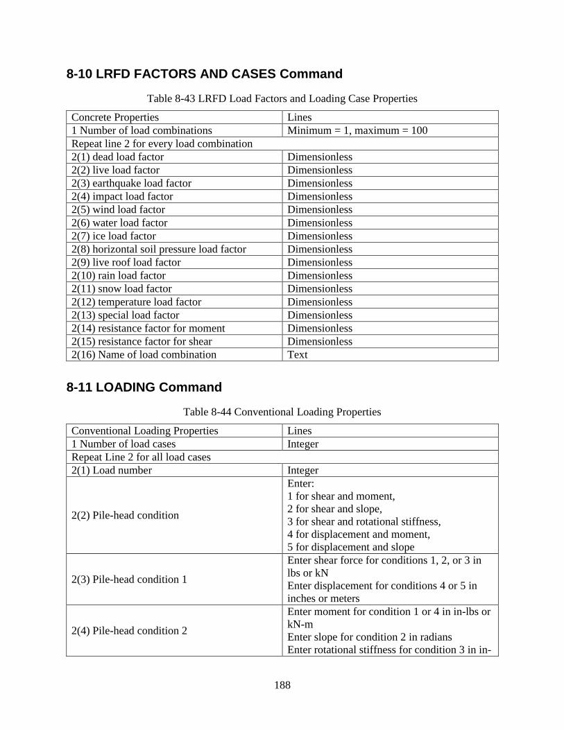
188
8-10 LRFD FACTORS AND CASES Command
Table 8-43 LRFD Load Factors and Loading Case Properties
Concrete Properties Lines
1 Number of load combinations Minimum = 1, maximum = 100
Repeat line 2 for every load combination
2(1) dead load factor Dimensionless
2(2) live load factor Dimensionless
2(3) earthquake load factor Dimensionless
2(4) impact load factor Dimensionless
2(5) wind load factor Dimensionless
2(6) water load factor Dimensionless
2(7) ice load factor Dimensionless
2(8) horizontal soil pressure load factor Dimensionless
2(9) live roof load factor Dimensionless
2(10) rain load factor Dimensionless
2(11) snow load factor Dimensionless
2(12) temperature load factor Dimensionless
2(13) special load factor Dimensionless
2(14) resistance factor for moment Dimensionless
2(15) resistance factor for shear Dimensionless
2(16) Name of load combination Text
8-11 LOADING Command
Table 8-44 Conventional Loading Properties
Conventional Loading Properties Lines
1 Number of load cases Integer
Repeat Line 2 for all load cases
2(1) Load number Integer
2(2) Pile-head condition
Enter:
1 for shear and moment,
2 for shear and slope,
3 for shear and rotational stiffness,
4 for displacement and moment,
5 for displacement and slope
2(3) Pile-head condition 1
Enter shear force for conditions 1, 2, or 3 in
lbs or kN
Enter displacement for conditions 4 or 5 in
inches or meters
2(4) Pile-head condition 2
Enter moment for condition 1 or 4 in in-lbs or
kN-m
Enter slope for condition 2 in radians
Enter rotational stiffness for condition 3 in in-

189
Conventional Loading Properties Lines
lbs/rad. or kN-m/rad.
Enter slope for condition 4 in radians
2(5) Axial thrust load Lbs or kN
2(6) Toggle for computation of top deflection
versus pile length for this load condition Enter 0 for no, 1 for yes
If UseDistributedLoading NO has been input under OPTIONS, omit lines 3 and 4.
If UseDistributedLoading ONE has been input under OPTIONS, enter lines 3 and 4once.
If UseDistributedLoading ALL has been input under OPTIONS, enter lines 3 and 4 for every
load case
3 Number of distributed lateral loading points
Enter 0 for no distributed lateral loading,
Enter number of loading points to enter
distributed lateral loading data
Repeat Line 4 for all distributed lateral loading points
4(1) Load point number dimensionless
4(2) Depth below pile head Feet or meters
4(3) Distributed lateral loading intensity lbs/inch or kN/m
8-12 P-Y OUTPUT DEPTHS Command
Table 8-45 p-y Output Depth Properties
p-y Output Depth Properties Lines
1 Number of output depths integer
Repeat Line 2 for all depths
2 Depth of output p-y curve ft or meters
8-13 SOIL MOVEMENTS Command
Table 8-46 Soil Movement Properties
Soil Movement Properties Lines
1 Number of soil movement points integer
Repeat Line 2 for all depths
3 Depth below pile head ft or meters
4 Lateral soil movement inches or millimeters
8-14 AXIAL THRUST LOADS Command
Table 8-47 Axial Thrust Loads for EI Computations Only
Axial Thrust Properties Lines
1 Number of axial thrust values Compressive strength of concrete, psi or kPa
Repeat Line 2 for all axial thrust values
2 Thrust load number, axial thrust Two values per line (thrust number, thrust
value)

190
8-15 FOUNDATION STIFFNESS Command
Table 8-48 Foundation Stiffness Computations
Controls for Computation of Foundation
Stiffness Computations Lines
1 Computation method
Integer
1 = Use force and moment from Load Case 1
2 = Use pile-head deflection and rotation from
Load Case 1
3 = Use specified values of pile-head
deflection and rotation
2 Number of points to compute Integer
3 Point distribution method
Integer,
0 = logarithmic distribution,
1 = arithmetic distribution
If computation method = 2, enter values for pile-head deflection and rotation
4 Pile-head deflection Inches or meters
5 Pile-head rotation Radians
8-16 PILE PUSHOVER ANALYSIS DATA Command
Table 8-49 Pushover Analysis Computations
Controls for Pile Pushover Analysis
Computations Lines
1 Computation method
Integer
0 = pinned head
1 = fixed head
2 = pinned and fixed head
2 Point distribution method
Integer,
0 = logarithmic distribution,
1 = arithmetic distribution
2 = user-specified displacements
If point distribution method = 0 or 1, enter Lines 3, 4, and 5
3 Number of points to compute Integer
4 Maximum pile-head deflection Inches or meters
5 Minimum pile-head deflection Inches or meters
If point distribution method = 2, enter Lines 6 and 7
6 Number of user-specified displacements Integer
Repeat Line 7 for every user-specified pushover displacement
7 User-specified pushover displacement Inches or meters
8 Axial thrust force Lbs or kN
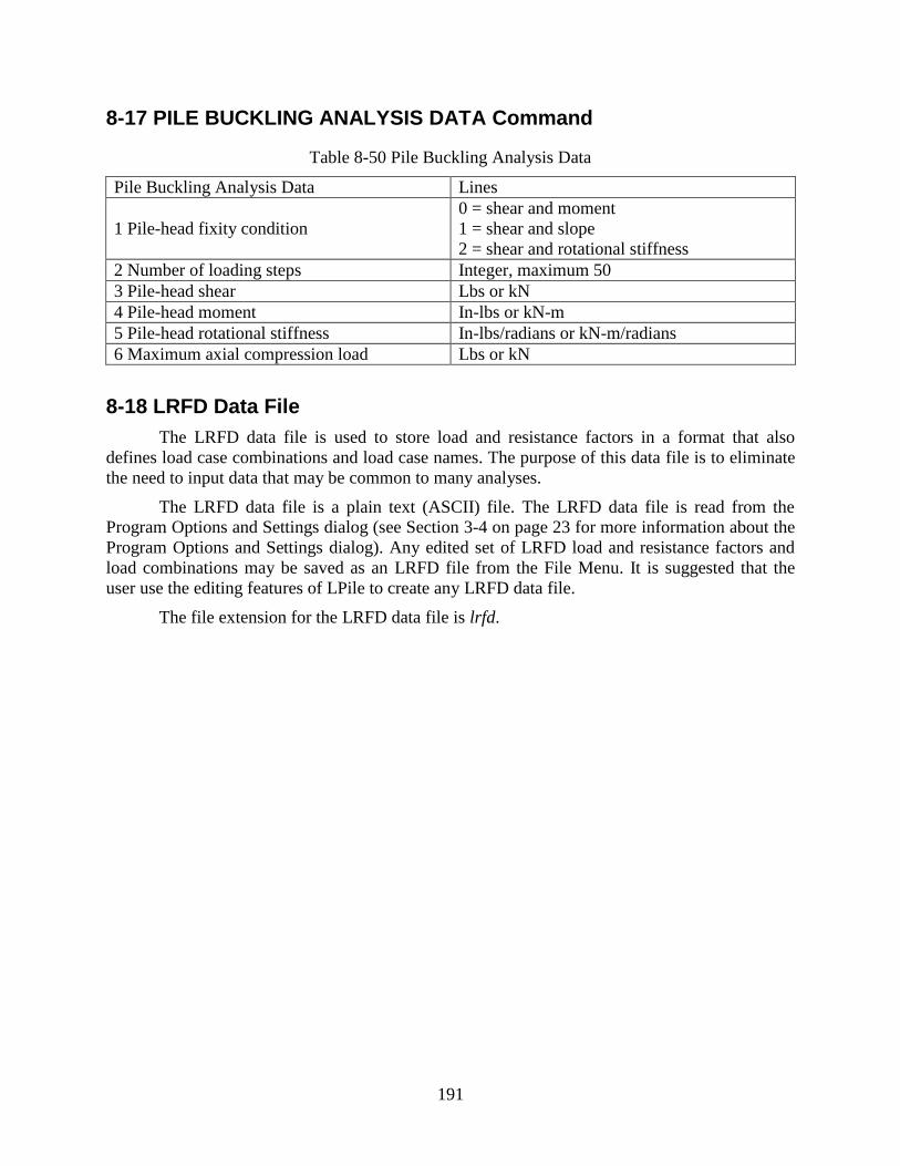
191
8-17 PILE BUCKLING ANALYSIS DATA Command
Table 8-50 Pile Buckling Analysis Data
Pile Buckling Analysis Data Lines
1 Pile-head fixity condition
0 = shear and moment
1 = shear and slope
2 = shear and rotational stiffness
2 Number of loading steps Integer, maximum 50
3 Pile-head shear Lbs or kN
4 Pile-head moment In-lbs or kN-m
5 Pile-head rotational stiffness In-lbs/radians or kN-m/radians
6 Maximum axial compression load Lbs or kN
8-18 LRFD Data File
The LRFD data file is used to store load and resistance factors in a format that also
defines load case combinations and load case names. The purpose of this data file is to eliminate
the need to input data that may be common to many analyses.
The LRFD data file is a plain text (ASCII) file. The LRFD data file is read from the
Program Options and Settings dialog (see Section 3-4 on page 23 for more information about the
Program Options and Settings dialog). Any edited set of LRFD load and resistance factors and
load combinations may be saved as an LRFD file from the File Menu. It is suggested that the
user use the editing features of LPile to create any LRFD data file.
The file extension for the LRFD data file is lrfd.

192
(This page was deliberately left blank)
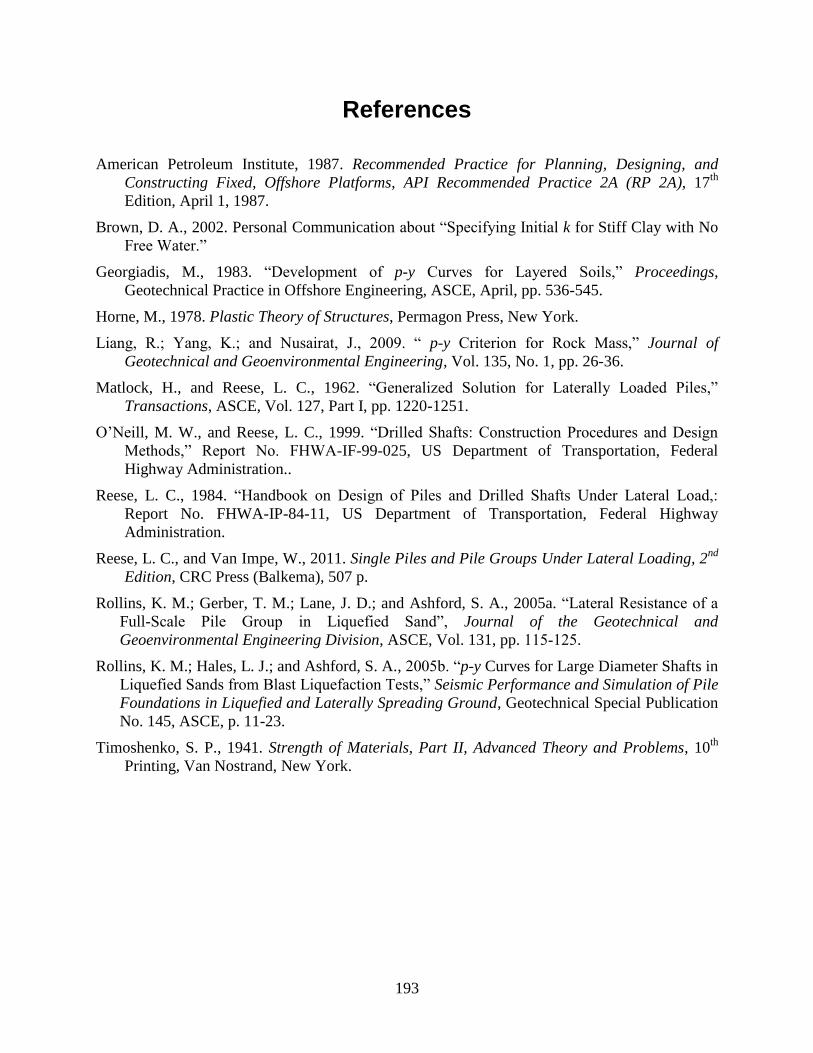
193
References
American Petroleum Institute, 1987. Recommended Practice for Planning, Designing, and
Constructing Fixed, Offshore Platforms, API Recommended Practice 2A (RP 2A), 17th
Edition, April 1, 1987.
Brown, D. A., 2002. Personal Communication about “Specifying Initial k for Stiff Clay with No
Free Water.”
Georgiadis, M., 1983. “Development of p-y Curves for Layered Soils,” Proceedings,
Geotechnical Practice in Offshore Engineering, ASCE, April, pp. 536-545.
Horne, M., 1978. Plastic Theory of Structures, Permagon Press, New York.
Liang, R.; Yang, K.; and Nusairat, J., 2009. “ p-y Criterion for Rock Mass,” Journal of
Geotechnical and Geoenvironmental Engineering, Vol. 135, No. 1, pp. 26-36.
Matlock, H., and Reese, L. C., 1962. “Generalized Solution for Laterally Loaded Piles,”
Transactions, ASCE, Vol. 127, Part I, pp. 1220-1251.
O’Neill, M. W., and Reese, L. C., 1999. “Drilled Shafts: Construction Procedures and Design
Methods,” Report No. FHWA-IF-99-025, US Department of Transportation, Federal
Highway Administration..
Reese, L. C., 1984. “Handbook on Design of Piles and Drilled Shafts Under Lateral Load,:
Report No. FHWA-IP-84-11, US Department of Transportation, Federal Highway
Administration.
Reese, L. C., and Van Impe, W., 2011. Single Piles and Pile Groups Under Lateral Loading, 2nd
Edition, CRC Press (Balkema), 507 p.
Rollins, K. M.; Gerber, T. M.; Lane, J. D.; and Ashford, S. A., 2005a. “Lateral Resistance of a
Full-Scale Pile Group in Liquefied Sand”, Journal of the Geotechnical and
Geoenvironmental Engineering Division, ASCE, Vol. 131, pp. 115-125.
Rollins, K. M.; Hales, L. J.; and Ashford, S. A., 2005b. “p-y Curves for Large Diameter Shafts in
Liquefied Sands from Blast Liquefaction Tests,” Seismic Performance and Simulation of Pile
Foundations in Liquefied and Laterally Spreading Ground, Geotechnical Special Publication
No. 145, ASCE, p. 11-23.
Timoshenko, S. P., 1941. Strength of Materials, Part II, Advanced Theory and Problems, 10th
Printing, Van Nostrand, New York.

194
(This page was deliberately left blank)

195
Appendix 1 Input Error Messages
Un-numbered: Version mismatch between main program and dynamic link library for
computation files.
Input Data Error No. 1: An error was detected in the input data for computing a p-y curve using
the API sand criteria. A value of zero was input for the friction angle of the sand.
Input Data Error No. 2: An error was detected in the input data when computing a p-y curve
using the API criteria for sand. The angle of the ground slope cannot be greater than the internal
friction angle of the sand at the ground surface.
Input Data Error No. 3: The pile tip is below the deepest extent of the input data for soil shear
strength versus depth.
Input Data Error No. 4: The pile extends below the deepest extent of the input data for soil shear
strength versus depth.
Input Data Error No. 5: The pile tip is below the deepest extent of the input curve for soil shear
strength versus depth.
Input Data Error No. 6: Use of p-y multipliers cannot be specified for use with user-specified p-y
curves.
Input Data Error No. 7: The number of points defining effective unit weight versus depth is zero
and number of input p-y curves is also zero.
Input Data Error No. 8: A value of zero was input for the friction angle for a sand when
computing a p-y curve using the Reese et al. criteria.
Input Data Error No. 9: The angle of the slope cannot be greater than the friction angle of the
sand at the ground surface.
Input Data Error No. 10: A negative or zero value was input for the friction angle for silt.
Input Data Error No. 11: The angle of the ground surface slope cannot be greater than the angle
of internal friction angle of the silt (c-phi) soil at the ground surface.
Input Data Error No. 12: An error was detected that is related to an incompatibility between the
input data defining soil layering and soil shear strength values when computing a p-y curve using
the Matlock soft clay criteria.
Input Data Error No. 13: A cohesion of zero was input for a stiff clay without free water.
Input Data Error No. 14: An error was detected in the input data used to compute p-y curves in
stiff clay with free water. A value of zero was input for the cohesion of a stiff clay.
Input Data Error No. 15: The pile extends below the deepest extent of the input curve for
effective unit weight versus depth.
Input Data Error No. 16: The input value for the compressive strength of a weak rock was input
as negative or zero.

Appendix 1 – Input Error Messages
196
Input Data Error No. 17: The value number of points to define the pile properties is 2 to 40.
Either too few or too many points were input for the definition of pile properties.
Input Data Error No. 18: The depth at the bottom of the last layer is higher than the tip of the
pile.
Input Data Error No. 19: The depth of the first point of the data for effective unit is not located at
the ground surface.
Input Data Error No. 20: The depth of the first point of the soil strength profile is not located at
the ground surface.
Input Data Error No. 21: The depth for the first data point for p-multipliers is not located at the
ground surface.
Input Data Error No. 22: Loading was specified to be cyclic, but the number of cycles of loading
was specified outside the range of 2 to 5000.
Input Data Error No. 23: Deleted.
Input Data Error No. 24: Deleted.
Input Data Error No. 25: The input file is empty. No analysis can be performed.
Input Data Error No. 26: The number of rebar cannot exceed 300 in this version of LPile.
Input Data Error No. 27: Zero values were entered for one of pile diameter, pile area, or moment
of inertia.
Input Data Error No. 28: Cyclic loading type was specified and the number of cycles of loading
are outside the valid range of 2 to 5,000.
Input Data Error No. 29: A depth above the ground surface was specified for the printing of a p-y
curve.
Input Data Error No. 30: A depth below the pile tip was specified for the printing of a p-y curve.
Input Data Error No. 31: The pile extends below the deepest extent of the input data for RQD
versus depth.
Input Data Error No. 32: Type of reinforcement is unrecognized by LPile.
Input Data Error No. 33: Tapered rebar option type is unrecognized.
Input Data Error No. 34: Specified rebar cover is greater than one-half of pile diameter.
Input Data Error No. 35: Too many pile sections specified for analysis.
Input Data Error No. 36: Deleted.
Input Data Error No. 37: Deleted.
Input Data Error No. 38: Deleted.
Input Data Error No. 39: Deleted.
Input Data Error No. 40: Deleted.
Input Data Error No. 41: Deleted.
Input Data Error No. 42: Deleted.

Appendix 1 – Input Error Messages
197
Input Data Error No. 43: Pile section type unrecognized.
Input Data Error No. 44: Units of computation option unrecognized by program.
Input Data Error No. 45: Input data for pile properties specifies a negative pile station
coordinate.
Input Data Error No. 46: Input data for pile properties specified a pile station below the pile tip.
Input Data Error No. 47: The depth of the top of a layering is greater than or equal to the depth of
the bottom of the layer.
Input Data Error No. 48: A negative or zero value was input for the cohesion for silt.
Input Data Error No. 49: The interpolated value of RQD used for p-y curves in weak rock was
found to be invalid because it was either less than zero or more than 100 percent.
Input Data Error No. 50: The pile-tip movement data for shear resistance at the pile tip is in
error. Either the first point is not zero or one of the other points is less than or equal to the
previous point.
Input Data Error No. 51: The nonlinear bending stiffness input by the user varies by more than a
factor of 100 for a given axial thrust force. This indicates that either unrealistic or erroneous data
was input.
Input Data Error No. 52: The nonlinear bending stiffness input by the user exhibits strain
hardening behavior. LPile can handle nonlinear bending cases only with strain softening
behavior.
Input Data Error No. 53: The number of lines of soil movement data is outside the range of 2 to
50.
Input Data Error No. 54: The top and bottom elevations for weak rock layer are equal.
Input Data Error No. 55: The specified number of pile increments is less than 40.
Input Data Error No. 56: The specified number of pile increments is more than 500.
Input Data Error No. 57: The input value for pile length is zero.
Input Data Error No. 58: The pile tip is below the deepest extent of the input curve for weak rock
parameter krm versus depth.
Input Data Error No. 59: The number of input pile diameters is more than 40.
Input Data Error No. 60: An error was detected in the shear strength of soil input data when
interpolating to obtain values of cohesion or uniaxial compressive strength. The depth increment
between the upper and lower soil depths in a layer is zero.
Input Data Error No. 61: The depth of the bottom of the top soil layer is less than or equal to
zero. This will cause the algorithm for layering correction to p-y curves to generate incorrect p-y
curves for layers below the top layer.
Input Data Error No. 62: An error was detected for input values for uniaxial compressive
strength. Values cannot be less than zero.
Input Data Error No. 63: The input value of krm is less than or equal to zero for weak rock.
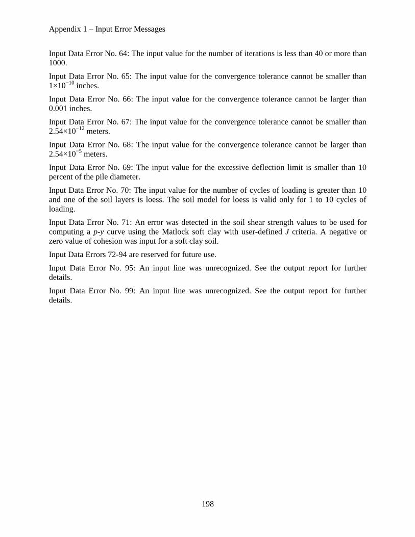
Appendix 1 – Input Error Messages
198
Input Data Error No. 64: The input value for the number of iterations is less than 40 or more than
1000.
Input Data Error No. 65: The input value for the convergence tolerance cannot be smaller than
1×10⁻¹⁰
inches.
Input Data Error No. 66: The input value for the convergence tolerance cannot be larger than
0.001 inches.
Input Data Error No. 67: The input value for the convergence tolerance cannot be smaller than
2.54×10⁻¹²
meters.
Input Data Error No. 68: The input value for the convergence tolerance cannot be larger than
2.54×10⁻⁵
meters.
Input Data Error No. 69: The input value for the excessive deflection limit is smaller than 10
percent of the pile diameter.
Input Data Error No. 70: The input value for the number of cycles of loading is greater than 10
and one of the soil layers is loess. The soil model for loess is valid only for 1 to 10 cycles of
loading.
Input Data Error No. 71: An error was detected in the soil shear strength values to be used for
computing a p-y curve using the Matlock soft clay with user-defined J criteria. A negative or
zero value of cohesion was input for a soft clay soil.
Input Data Errors 72-94 are reserved for future use.
Input Data Error No. 95: An input line was unrecognized. See the output report for further
details.
Input Data Error No. 99: An input line was unrecognized. See the output report for further
details.

199
Appendix 2 Runtime Error Messages
Runtime Error No. 1: Internal error occurred in the LPile computation dynamic link library. This
error is reported when the dynamic link library fails to load into memory.
Runtime Error No. 2: Contents of file NAMES.DAT is corrupted. This file contains the path and
name of all data and output files used by LPile.
Runtime Error No. 3: The name of the input data file is corrupted.
Runtime Error No. 4: The name of the output report file is corrupted.
Runtime Error No. 5: The name of the plot output file is corrupted.
Runtime Error No. 6: The name of the runtime message file is corrupted.
Runtime Error No. 7: The user name is corrupted.
Runtime Error No. 8: User company name is corrupted.
Runtime Error No. 9: The computed deflection of the pile head is larger than the allowable
deflection. This error may be due to overloading the pile or bad input data.
Runtime Error No. 10: LPile was unable to obtain an answer within the specified convergence
tolerance within the specified limit on iterations.
Runtime Error No. 11: The numerical solution failed due to a small pivot number.
Runtime Error No. 12: An error occurred because the computed value of compressive strain in
concrete is larger than 0.001. This indicates that that the drilled shaft has failed due to crushing
of concrete.
Runtime Error No. 13: Deleted.
Runtime Error No. 14: An internal error occurred in computing area of concrete for prestressing
computations.
Runtime Error No. 15: An error occurred in computing area of steel for prestressing
computations.
Runtime Error No. 16: The location of neutral axis was not found within 1,000 iterations during
computation of non-linear moment-curvature behavior.
Runtime Error No. 17: Filename information corrupted. No analysis can be performed.
Runtime Error Nos. 18-21: Deleted.
Runtime Error No. 22: A runtime error was caused by the input value krm being less than or equal
to 0.
Runtime Error No. 23: A runtime error was caused by the input value for combined ground slope
and pile batter being greater than the angle of friction of a silt layer.
Runtime Error No. 24: The input value for axial thrust force is greater than the structural
capacity in compression.
Appendix 2 – Runtime Error Messages
200
Runtime Error No. 25: The input value for axial thrust force is greater than the structural
capacity in tension.
Runtime Error No. 26: An LRFD load case value for axial thrust force is greater than the
structural capacity in compression.
Runtime Error No. 27: An LRFD load case value for axial thrust force is greater than the
structural capacity in tension.
Runtime Error No. 28: An unrecoverable numerical error has occurred. Either pile-top deflection
or computed maximum change in deflection is not a number and further computations are
impossible.
Runtime Error No. 29: A layer thickness was too thin to contain a nodal point. This prevents the
correct computation of the layer’s p-y curve.
Runtime Error No. 30: An error occurred in the computation of the undrained shear strength
value for a soil layer.
Runtime Error No. 31: The computed value of soil modulus computed in Reese sand is not-a-
number. This is due to one or more of the required soil properties being equal to zero. See the
output report for more information.
Runtime Error No. 32: The default value of soil modulus computed in Reese sand is not-a-
number. This is due to one or more of the required soil properties being equal to zero. See the
output report for more information.
Runtime Error No. 33: The default value of soil modulus computed in soft clay is not-a-number.
This is due to one or more of the required soil properties being equal to zero. See the output
report for more information.
Runtime Error No. 34: The computed value of soil modulus computed in soft clay is not-a-
number. This is due to one or more of the required soil properties being equal to zero. See the
output report for more information.
Runtime Error No. 35: The default value of soil modulus computed in API soft clay is not-a-
number. This is due to one or more of the required soil properties being equal to zero. See the
output report for more information.
Runtime Error No. 36: The computed value of soil modulus computed in API soft clay is not-a-
number. This is due to one or more of the required soil properties being equal to zero. See the
output report for more information.

201
Appendix 3 Warning Messages
1
Warning Message No. 300: Multiple warning messages have been generated. See the output
report file for more details.
Warning Message No. 301: An unreasonable input value for k has been specified See the output
report file for more details.
Warning Message No. 302: An unreasonable input value for friction angle has been specified for
a soil layer defined using the sand criteria. See the output report file for more details.
Warning Message No. 303: An unreasonable input value for friction angle has been specified for
a soil layer defined using the API sand criteria. See the output report file for more details.
Warning Message No. 304: An unreasonable input value for shear strength has been specified for
a soil layer defined using the soft clay criteria. See the output report file for more details.
Warning Message No. 3041: An unreasonable input value for shear strength has been specified
for a layer defined using the soft clay criteria. The input value is greater than 1,250 psf (8.68 psi).
Warning Message No. 3042: An unreasonable input value for shear strength has been specified
for a layer defined using the soft clay criteria. The input value is greater than 59.85 kPa. See the
output report file for more details.
Warning Message No. 305: Too many values were calculated for moment-curvature. This may
indicate that the pile is too weak or is under-reinforced. You should examine your input data and
increase the amount of steel reinforcement if necessary.
Warning Message No. 3051: An unreasonable input value for shear strength has been specified
for a layer defined using the stiff clay with free water criteria. The input value is less than 500
psf (3.47 psi).
Warning Message No. 3052: An unreasonable input value for shear strength has been specified
for a layer defined using the stiff clay with free water criteria. The input value is greater than
8,000 psf (55.55 psi).
Warning Message No. 3053: An unreasonable input value for shear strength has been specified
for a layer defined using the stiff clay with free water criteria. The input value is less than 23.94
kPa.
Warning Message No. 3054: An unreasonable input value for shear strength has been specified
for a layer defined using the stiff clay with free water criteria. The input value is greater than
383.04 kPa. See the output report file for more details.
Warning Message No. 306: Negative values of bending moment were computed in nonlinear EI
computations. This may indicate that the pile is too weak or is under-reinforced and that all
reinforcing steel has yielded.
1 Note, the warning message number is not displayed by LPile
Appendix 3 – Warning Messages
202
Warning Message No. 3061: An unreasonable input value for shear strength has been specified
for a layer defined using the stiff clay without free water criteria. The input value is less than 500
psf (3.47 psi).
Warning Message No. 3062: An unreasonable input value for shear strength has been specified
for a layer defined using the stiff clay without free water criteria. The input value is greater than
8,000 psf (55.55 psi).
Warning Message No. 3063: An unreasonable input value for shear strength has been specified
for a layer defined using the stiff clay without free water criteria. The input value is less than
23.94 kPa.
Warning Message No. 3064: An unreasonable input value for shear strength has been specified
for a layer defined using the stiff clay without free water criteria. The input value is greater than
383.04 kPa.
Warning Message No. 307: The input data for nonlinear bending appears to be have been input
incorrectly. Negative values of bending moment should not be input.
Warning Message No. 3071: An unreasonable input value for the uniaxial compressive strength
has been specified for a layer defined using the weak rock criteria. The input value is less than
100 psi.
Warning Message No. 3072: An unreasonable input value for unconfined compressive strength
has been specified for a soil defined using the weak rock criteria. The input value is greater than
1,000 psi.
Warning Message No. 3073: An unreasonable input value for unconfined compressive strength
has been specified for a soil defined using the weak rock criteria. The input value is less than
689.5 kPa.
Warning Message No. 3074: An unreasonable input value for unconfined compressive strength
has been specified for a soil defined using the weak rock criteria. The input value is greater than
6895 kPa.
Warning Message No. 308: An unreasonable input value for uniaxial compressive strength has
been specified for a layer defined using the vuggy limestone (strong rock) criteria.
Warning Message No. 309: An unreasonable input value for compressive strength of concrete
has been specified.
Warning Message No. 3091: An unreasonable input value for compressive strength of concrete
has been specified. The input value is either smaller than 2,000 psi or larger than 8,000 psi.
Warning Message No. 3092: An unreasonable input value for compressive strength of concrete
has been specified. The input value is either smaller than 13,790 kPa or larger than 55,160 kPa.
Warning Message No. 310: An unreasonable input value for modulus of elasticity for steel has
been specified.
Warning Message No. 311: An unreasonable input value for yield strength of reinforcement has
been specified.

Appendix 3 – Warning Messages
203
Warning Message No. 3101: An unreasonable input value for modulus of elasticity has been
specified for the reinforcing steel. The input value is either smaller than 27,500,000 psi or larger
than 30,500,000 psi.
Warning Message No. 3102: An unreasonable input value for modulus of elasticity has been
specified for the reinforcing steel. The input value is either smaller than 189,600,000 kPa or
larger than 210,300,000 kPa.
Warning Message No. 3111: An unreasonable input value for yield strength of reinforcing steel
has been specified. The input value is either smaller than 38,000 psi or larger than 80,000 psi.
Warning Message No. 3112: An unreasonable input value for yield strength of reinforcing steel
has been specified. The input value is either smaller than 262,000 kPa or larger than 551,600
kPa.
Warning Message No. 312: An input value for cover of reinforcement has been specified that
may be unreasonable.
Warning Message No. 3121: An unreasonable input value for concrete cover thickness has been
specified. The input value is either smaller than 0.8 inches or larger than 6 inches.
Warning Message No. 3122: An unreasonable input value for concrete cover thickness has been
specified. The input value is either smaller than 0.02 meters or larger than 0.16 meters. You
should check your input for accuracy.
Warning Message No. 313: An unreasonable input value for loss of prestress has been specified.
Warning Message No. 314: An unreasonable input value for prestressing force has been
specified.
Warning Message No. 315: Pile deflection has exceeded the failure deflection for the vuggy
limestone criteria for one or more of the loading cases analyzed. You should check the computed
output for both deflection and bending moment.
Warning Message No. 316: The input value for krm used by the weak rock criteria is smaller than
0.00005. This value is outside the recommended range of 0.00005 to 0.0005.
Warning Message No. 317: The input value for krm used by the weak rock criteria is larger than
0.0005. This value is outside the recommended range of 0.00005 to 0.0005. You should check
your input data for accuracy.
Warning Message No. 318: The pile deflection is less than 1×10⁻¹⁴
. LPile used the limiting
value of soil modulus when computing the p-y curve for soft clay.
Warning Message No. 3261: An unreasonable input value for shear strength has been specified
for a layer defined using the stiff clay without free water criteria with user-defined k. The input
value is less than 500 psf (3.47 psi).
Warning Message No. 3262: An unreasonable input value for shear strength has been specified
for a layer defined using the stiff clay without free water criteria with user-defined k. The input
value is greater than 8,000 psf (55.55 psi).
Warning Message No. 3263: An unreasonable input value for shear strength has been specified
for a layer defined using the stiff clay without free water criteria with user-defined k. The input
value is less than 23.94 kPa.

Appendix 3 – Warning Messages
204
Warning Message No. 3264: An unreasonable input value for shear strength has been specified
for a layer defined using the stiff clay without free water criteria with user-defined k. The input
value is greater than 383.04 kPa.
Warning Message No. 351: Values entered for effective unit weights of soil were outside the
limits of 0.011574 pci (20 pcf) or 0.0810019 pci (140 pcf). This data may be erroneous.
Warning Message No. 352: Values entered for effective unit weights of soil were outside the
limits of 3.15 kN/m3 or 22 kN/m
3. This data may be erroneous.
Warning Message No. 353: Values of effective unit weight cannot be checked because general
units have been selected.
Warning Message No. 354: The maximum depth of a soil layer defined as liquefiable sand is
greater than meters or 236.22 inches. This is greater than the maximum depth recommended for
this p-y curve criteria.
Warning Message No. 355: Computation of nonlinear bending stiffness found that moment
capacity was developed at compressive strains smaller than 0.003. This usually indicates that a
section is under-reinforced or the level of prestressing is too small.
Warning Message No. 400: One or more of the LRFD load cases have overloaded the structural
capacity of the pile. See the LRFD Performance by Load Case Combination section of the output
report file for more details.