user-centric traffic engineering in - University of Plymouth ...

University of Plymouth

PEARL https://pearl.plymouth.ac.uk

04 University of Plymouth Research Theses 01 Research Theses Main Collection

2017

User-Centric Traffic Engineering in

Software Defined Networks

Bakhshi, Taimur

http://hdl.handle.net/10026.1/8202

University of Plymouth

All content in PEARL is protected by copyright law. Author manuscripts are made available in accordance with

publisher policies. Please cite only the published version using the details provided on the item record or

document. In the absence of an open licence (e.g. Creative Commons), permissions for further reuse of content

should be sought from the publisher or author.

USER-CENTRIC TRAFFIC ENGINEERING IN

SOFTWARE DEFINED NETWORKS

by

TAIMUR BAKHSHI

A thesis submitted to the University of Plymouth in partial fulfilment for the degree of

DOCTOR OF PHILOSOPHY

School of Computing, Electronics and Mathematics Faculty of Science and Engineering

January 2017

ii

Copyright Statement

This copy of the thesis has been supplied on condition that anyone who consults it is understood to

recognise that its copyright rests with its author and that no quotation from the thesis and no

information derived from it may be published without the author's prior consent.

iv

Abstract

User-Centric Traffic Engineering in Software Defined Networks

Taimur Bakhshi

Software defined networking (SDN) is a relatively new paradigm that decouples individual

network elements from the control logic, offering real-time network programmability, translating

high level policy abstractions into low level device configurations. The framework comprises of the

data (forwarding) plane incorporating network devices, while the control logic and network services

reside in the control and application planes respectively. Operators can optimize the network fabric

to yield performance gains for individual applications and services utilizing flow metering and

application-awareness, the default traffic management method in SDN. Existing approaches to

traffic optimization, however, do not explicitly consider user application trends. Recent SDN traffic

engineering designs either offer improvements for typical time-critical applications or focus on

devising monitoring solutions aimed at measuring performance metrics of the respective services.

The performance caveats of isolated service differentiation on the end users may be substantial

considering the growth in Internet and network applications on offer and the resulting diversity in

user activities. Application-level flow metering schemes therefore, fall short of fully exploiting the

real-time network provisioning capability offered by SDN instead relying on rather static traffic

control primitives frequent in legacy networking.

For individual users, SDN may lead to substantial improvements if the framework allows operators

to allocate resources while accounting for a user-centric mix of applications. This thesis explores the

user traffic application trends in different network environments and proposes a novel user traffic

profiling framework to aid the SDN control plane (controller) in accurately configuring network

elements for a broad spectrum of users without impeding specific application requirements.

This thesis starts with a critical review of existing traffic engineering solutions in SDN and highlights

recent and ongoing work in network optimization studies. Predominant existing segregated

application policy based controls in SDN do not consider the cost of isolated application gains on

parallel SDN services and resulting consequence for users having varying application usage.

Therefore, attention is given to investigating techniques which may capture the user behaviour for

possible integration in SDN traffic controls. To this end, profiling of user application traffic trends is

identified as a technique which may offer insight into the inherent diversity in user activities and

offer possible incorporation in SDN based traffic engineering.

vi

A series of subsequent user traffic profiling studies are carried out in this regard employing network

flow statistics collected from residential and enterprise network environments. Utilizing machine

learning techniques including the prominent unsupervised k-means cluster analysis, user generated

traffic flows are cluster analysed and the derived profiles in each networking environment are

benchmarked for stability before integration in SDN control solutions. In parallel, a novel flow-

based traffic classifier is designed to yield high accuracy in identifying user application flows and the

traffic profiling mechanism is automated.

The core functions of the novel user-centric traffic engineering solution are validated by the

implementation of traffic profiling based SDN network control applications in residential, data

center and campus based SDN environments. A series of simulations highlighting varying traffic

conditions and profile based policy controls are designed and evaluated in each network setting

using the traffic profiles derived from realistic environments to demonstrate the effectiveness of

the traffic management solution. The overall network performance metrics per profile show

substantive gains, proportional to operator defined user profile prioritization policies despite high

traffic load conditions. The proposed user-centric SDN traffic engineering framework therefore,

dynamically provisions data plane resources among different user traffic classes (profiles), capturing

user behaviour to define and implement network policy controls, going beyond isolated application

management.

viii

Contents

Contents ……………………………………………………………………………………………………………………………… viii

List of Figures ...........................................................................................................................xiv

List of Tables .......................................................................................................................... xviii

Acknowledgement ................................................................................................................... xx

Author’s Declaration ............................................................................................................... xxii

Chapter 1 Introduction ........................................................................................................ 24

1.1 Introduction ......................................................................................................................... 24

1.2 Research challenges and intiatives ..................................................................................... 25

1.2.1 Application and service improvement ............................................................................... 25

1.2.2 Control plane centralization ............................................................................................... 26

1.2.3 Security vulnerabilities ....................................................................................................... 26

1.2.4 Standardization efforts ....................................................................................................... 27

1.2.5 Industry pragmatism and operational requirements ............................................................. 27

1.3 Aims and objectives ............................................................................................................. 27

1.4 Thesis organization .............................................................................................................. 28

Chapter 2 Software Defined Networking Technologies .......................................................... 32

2.1 Introduction ............................................................................................................................... 32

2.2 Background and complementary technologies......................................................................... 33

2.2.1 Centralized network control............................................................................................... 33

2.2.2 Real-time network programmability .................................................................................. 35

2.2.3 Network virtualization ........................................................................................................ 37

2.2.4 Requirement for SDN ......................................................................................................... 39

2.3 Architectural overview .............................................................................................................. 40

2.4 Communication APIs ................................................................................................................. 43

2.4.1 Southbound communication protocols ............................................................................. 43

2.4.2 Northbound communication protocols ............................................................................. 49

ix

2.5 Network controllers and switches ............................................................................................. 52

2.5.1 SDN controllers .................................................................................................................. 52

2.5.2 SDN compliant switches ..................................................................................................... 55

2.6 Simulation, development and debugging tools ........................................................................ 55

2.6.1 Simulation and debugging platforms ................................................................................. 55

2.6.2 Software switch implementations ..................................................................................... 57

2.6.3 Debugging and troubleshooting tools ................................................................................ 59

2.7 SDN applications ....................................................................................................................... 61

2.7.1 Data centers and cloud environments ............................................................................... 61

2.7.2 Campus and high speed networks ..................................................................................... 62

2.7.3 Residential networks .......................................................................................................... 63

2.7.4 Wireless communications .................................................................................................. 64

2.8 Research challenges .................................................................................................................. 64

2.8.1 Controller scalability and placement .................................................................................. 65

2.8.2 Switch and controller design .............................................................................................. 67

2.8.3 Security ............................................................................................................................... 68

2.8.4 Application performance.................................................................................................... 70

2.8.5 Limitations of current work ................................................................................................ 75

2.9 Conclusion ................................................................................................................................. 76

PART I – Residential Traffic Management .................................................................................. 78

Chapter 3 Profiling User Application Trends ................................................................... 80

3.1 Introduction ............................................................................................................................... 80

3.2 QoS and Profiling based Traffic Engineering ............................................................................. 80

3.3 Traffic classification challenges ................................................................................................. 83

3.4 User traffic characterization ...................................................................................................... 83

3.5 Profiling design .......................................................................................................................... 84

3.5.1 Defining application tiers ................................................................................................... 85

3.5.2 Analysing user activity – feature vector design.................................................................. 85

x

3.5.3 K-means clustering algorithm ............................................................................................ 86

3.6 Evaluation .................................................................................................................................. 87

3.6.1 Data collection .................................................................................................................... 87

3.6.2 Clustering users .................................................................................................................. 88

3.6.3 Results ................................................................................................................................ 89

3.7 Applicability in software defined networking ........................................................................... 91

3.8 Conclusion ................................................................................................................................. 93

Chapter 4 Evaluating User Traffic Profile Stability ....................................................... 96

4.1 Introduction ............................................................................................................................... 96

4.2 Multi-device user environments ............................................................................................... 97

4.3 Profiling implementation .......................................................................................................... 99

4.3.1 Application categorization ................................................................................................. 99

4.3.2 Monitoring setup ................................................................................................................ 99

4.3.3 Data Collection and Pre-processing ................................................................................. 100

4.3.4 Traffic profiling ................................................................................................................. 101

4.4 Evaluation ................................................................................................................................ 103

4.4.1 Cluster Analysis ................................................................................................................ 103

4.4.2 Results .............................................................................................................................. 106

4.4.3 Profile Consistency ........................................................................................................... 109

4.5 Effective network management in residential SDN ................................................................ 111

4.6 Conclusion ............................................................................................................................... 112

Chapter 5 User-Centric Residential Network Management ............................................... 114

5.1 Introduction ............................................................................................................................. 114

5.2 Design ...................................................................................................................................... 115

5.2.1 Profile derivation framework ........................................................................................... 116

5.2.2 Traffic management application ...................................................................................... 116

5.2.3 Test Profiles ...................................................................................................................... 118

5.2.4 Setting User Profile Priority .............................................................................................. 119

xi

5.2.5 Queue computation and re-evaluation ............................................................................ 120

5.3 Evaluation ................................................................................................................................ 122

5.3.1 Discussion ......................................................................................................................... 127

5.3.2 Perspective on additional controls ................................................................................... 127

5.4 Conclusion ............................................................................................................................... 128

PART II – Enterprise Traffic Management ................................................................................ 130

Chapter 6 Classification of Internet Traffic Flows ....................................................... 132

6.1 Introduction ............................................................................................................................. 132

6.2 Background ............................................................................................................................. 133

6.2.1 Traffic classification methodologies and related work .................................................... 133

6.2.2 K-Means clustering ........................................................................................................... 138

6.2.3 C5.0 machine learning algorithm ..................................................................................... 138

6.3 Methodology ........................................................................................................................... 139

6.3.1 Data collection .................................................................................................................. 140

6.3.2 Customising NetFlow records .......................................................................................... 141

6.3.3 Extracting flow classes (k-means clustering) .................................................................... 142

6.3.4 Feature selection .............................................................................................................. 143

6.4 Unsupervised flow clustering .................................................................................................. 144

6.4.1 Calculating flow classes per application – value of k ....................................................... 144

6.4.2 Analysis ............................................................................................................................. 146

6.5 C5.0 Decision tree classifier..................................................................................................... 149

6.5.1 Classifier evaluation ......................................................................................................... 149

6.5.2 Confusion matrix analysis ................................................................................................. 151

6.5.3 Sensitivity and specificity factor ....................................................................................... 152

6.6 Qualitative comparison ........................................................................................................... 153

6.6.1 Comparative accuracy ...................................................................................................... 155

6.6.2 Computational performance ............................................................................................ 157

6.6.3 Scalability .......................................................................................................................... 160

xii

6.7 Conclusion ............................................................................................................................... 161

Chapter 7 OpenFlow-Enabled User Profiling in Enterprise Networks ................................... 164

7.1 Introduction ............................................................................................................................. 164

7.2 Design ...................................................................................................................................... 165

7.2.1 OpenFlow traffic monitor ................................................................................................. 166

7.2.2 Traffic profiling engine ..................................................................................................... 168

7.3 User traffic profiles .................................................................................................................. 170

7.3.1 Extracted profiles ............................................................................................................. 170

7.3.2 Profile stability .................................................................................................................. 174

7.3.3 Profiling computational cost ............................................................................................ 175

7.3.4 Control-channel overhead................................................................................................ 176

7.4 Application: campus traffic management ............................................................................... 179

7.5 Conclusion ............................................................................................................................... 180

Chapter 8 User-Centric Network Provisiong in Data Center Environments ............................. 181

8.1 Introduction ............................................................................................................................. 181

8.2 Design overview ...................................................................................................................... 183

8.3 User traffic profiling methodology ...................................................................................... 184

8.3.1 Flow statistics ................................................................................................................... 185

8.3.2 Profile stability and regeneration ..................................................................................... 186

8.4 Traffic Management Approach ............................................................................................... 186

8.4.1 Profile priority and application hierarchy ........................................................................ 186

8.4.2 External route construction ............................................................................................. 188

8.4.3 Internal route construction .............................................................................................. 189

8.4.4 OpenFlow route installation scheme ............................................................................... 190

8.4.5 Real-time route scheduling frequency ............................................................................. 192

8.5 Evaluation ................................................................................................................................ 193

8.5.1 Traffic profile derivation ................................................................................................... 193

8.5.2 Profile Stability ................................................................................................................. 197

xiii

8.5.3 Simulation environment ................................................................................................... 198

8.5.4 Throughput and bandwidth results .................................................................................. 200

8.5.5 Flow management overhead ........................................................................................... 206

8.5.6 Time complexity analysis ................................................................................................. 208

8.5.7 OpenFlow control traffic .................................................................................................. 210

8.6 Conclusion ............................................................................................................................... 211

Chapter 9 Conclusions and Future Work ............................................................................. 213

9.1 Achievements of the research ................................................................................................ 213

9.2 Limitations of the research project ......................................................................................... 216

9.3 Suggestions and scope for future work ................................................................................... 218

9.4 The future of traffic engineering in SDN ................................................................................. 219

References ……………………………………………………………………………………………………………………………..221

APPENDIX – 1 ......................................................................................................................... 241

APPENDIX – 2 ......................................................................................................................... 251

APPENDIX – 3 ......................................................................................................................... 259

APPENDIX – 4 ......................................................................................................................... 269

APPENDIX – 5 ......................................................................................................................... 283

APPENDIX – 6 ......................................................................................................................... 327

xiv

List of Figures

Figure 2.1. Key developments in complementary and SDN-specific technologies ............................. 34

Figure 2.2. Diagram illustrating (a) Decentralized and (b) SDN based Centralized Control ................ 42

Figure 2.3. OpenFlow Pipeline Processing .......................................................................................... 44

Figure 2.4. XMPP Client-Server Communication ................................................................................. 47

Figure 2.5. RESTful Application Programming Interface (API) ............................................................ 50

Figure 2.6. Open Services Gateway Initiative (OSGi) .......................................................................... 51

Figure 2.7. SDN Controller Schematic ................................................................................................. 53

Figure 3.1. Individual application flows metering in SDN ................................................................... 82

Figure 3.2. User Traffic Profiles ........................................................................................................... 90

Figure 3.3. (a) Aggregate traffic distribution per profile and (b) Users per traffic profile (30 days) .. 91

Figure 3.4. Incorporating User Profiling Controls in SDN Framework ................................................. 92

Figure 4.1. A typical multi-device user network (residential) ............................................................. 98

Figure 4.2. Network monitoring setup .............................................................................................. 100

Figure 4.3. Identifying correct number of clusters (wss vs. k) .......................................................... 104

Figure 4.4. K-distance graph (ε- eps estimation) ............................................................................... 105

Figure 4.5. User Traffic Profiles ......................................................................................................... 107

Figure 4.6. (a) Number of devices per profile, (b) Number of User premises per profile and

(c) Averange household devices per profile ...................................................................................... 108

Figure 4.7. (a) Average duration of transmitted flows and (b) Average duration of received flows 108

Figure 4.8. (a) Total number of flows per profile and (b) Total data volume per profile (Bytes) ..... 109

Figure 4.9. Pearson Correlation Co-efficient between Device Profiles ............................................. 110

Figure 5.1. Traffic Profiling Engine .................................................................................................... 117

Figure 5.2. Traffic Monitoring and Control ....................................................................................... 118

Figure 5.3. User Traffic Profiles ......................................................................................................... 120

Figure 5.4. (a) Queue calculation algorithm and (b) re-evaluation schedule ................................... 121

Figure 5.5. Mininet Home Network Topology ................................................................................... 122

Figure 5.6. (a) Available Bandwidth (b) Packet Loss (%) and (c) Network Latency per User Profile . 124

Figure 5.7. (a) Available Bandwidth (b) Packet Loss (%) and (c) Network Latency per User Profile . 126

Figure 6.1. Traffic classification scheme ............................................................................................ 140

Figure 6.2. Data collection and pre-processing workflow ................................................................. 141

Figure 6.3. 17-tuple bi-directional NetFlow records ......................................................................... 142

Figure 6.4. Inner-cluster variance vs. k – (a) YouTube, (b) NetFlix and (c) DailyMotion ................... 145

xv

Figure 6.5. Inner-cluster variance vs. k – (a) Skype, (b) GTalk and (c) Facebook (Messenger) ......... 145

Figure 6.6. Inner-cluster variance vs. k – (a) DropBox, (b) GoogleDrive and (c) OneDrive ............... 146

Figure 6.7. Inner-cluster variance vs. k – (a) VUZE, (b) BitTorrent and (c) 8-ball Pool ...................... 146

Figure 6.8. Inner-cluster variance vs. k – (a) TreasureHunt, (b) Thunderbird and (c) Outlook ......... 146

Figure 6.9. Classifier Sensitivity and Specificity Factor per Traffic Class ........................................... 153

Figure 6.10. Comparative and average overall accuracy of ML algorithms for each traffic class ..... 156

Figure 6.11. Classifier CPU Utilization (%) (a) flow records processed and (b) bytes processed ...... 159

Figure 6.12. Classifier Memory Usage (MB) (a) flow records processed and (b) bytes processed ... 159

Figure 6.13. Classifier timeframes for (a) training and (b) processing time ...................................... 160

Figure 7.1. Data collection setup: campus network segment ........................................................... 167

Figure 7.2. Traffic monitoring schematic .......................................................................................... 168

Figure 7.3. Traffic profling engine ..................................................................................................... 169

Figure 7.4. Optimal cluster determination – wss. vs. k ..................................................................... 170

Figure 7.5. User traffic profiles .......................................................................................................... 171

Figure 7.6. Probability distribution: (a) profile memership and (b) traffic volume ........................... 172

Figure 7.7. Flow transfer rates: (a) upstream traffic and (b) downstream traffic ............................. 173

Figure 7.8. Flow statistics: (a) flow inter-arrival time and (b) total flows (hourly) ........................... 173

Figure 7.9. Profiling overhead: (a) memory and (b) CPU utilization ................................................. 175

Figure 7.10. Traffic profiling duration vs. traffic records processed ................................................. 176

Figure 7.11. Control channel overhead evaluation – Mininet topology ........................................... 177

Figure 7.12. Control channel (a) control packets (b) control traffic rate (kbps) ............................... 178

Figure 8.1. Schematic representing centralized control in SDN based DC ........................................ 182

Figure 8.2. Traffic profile derivation and network management ...................................................... 184

Figure 8.3. User generated traffic flows per application .................................................................. 185

Figure 8.4. Profile and application hierarchy .................................................................................... 188

Figure 8.5. Three layer data center topology .................................................................................... 188

Figure 8.6. External (external) and Internal (internal) route construction ....................................... 191

Figure 8.7. OpenFlow pipeline processing –flow installation and route implementation ............... 191

Figure 8.8. Route update scheduling scheme ................................................................................... 192

Figure 8.9. Application clusters (k): wss vs. k graph .......................................................................... 194

Figure 8.10. User traffic profiles ........................................................................................................ 196

Figure 8.11. Flow rates per profile (zin||out) and (b). Flow inter-arrival time per profile (Δtin||out) ..... 196

Figure 8.12. Aggregate flow rate and inter-arrival time threshold per profile ................................. 198

Figure 8.13. Simulated data center environment ............................................................................. 199

xvi

Figure 8.14. Frame delivery ratio and throughput measurement .................................................... 202

Figure 8.14. Frame delivery ratio and throughput measurement (continued) ................................ 203

Figure 8.15. Flow statistics and latency measurement ..................................................................... 209

Figure 8.16. Average OpenFlow control channel traffic (kbps)......................................................... 211

xviii

List of Tables

Table 2.1. Complementary Technologies ............................................................................................ 34

Table 2.2. OpenFlow Flow Table Entries ............................................................................................. 45

Table 2.3. OpenFlow Message Specification ....................................................................................... 46

Table 2.4. Popular OpenFlow Compliant Controller Implementations ............................................... 54

Table 2.5. Common OpenFlow Compliant Switches and Standalone Stacks ...................................... 56

Table 2.6. Common OpenFlow Compliant Utilities ............................................................................. 58

Table 2.7. Summary of SDN Research Initiatives ................................................................................ 66

Table 3.1. Application Groups ............................................................................................................. 86

Table 3.2. Traffic Composition Vectors [30/11/2014] ......................................................................... 87

Table 3.3. Clusters vs Membership Size .............................................................................................. 88

Table 3.4. Traffic Statistics per Profile ................................................................................................. 90

Table 4.1. Updated Application Groups ............................................................................................ 100

Table 4.2. Traffic Composition Statistics [01/02/2015]..................................................................... 101

Table 4.3. Profile Membership Distribution per Cluster (hclust and k-means) ................................ 104

Table 4.4. Profile Membership Distribution per Cluster (DBSCAN) .................................................. 106

Table 4.5. Average Probability of Profile Change (/24 Hrs) .............................................................. 111

Table 4.6. Average Probability of Inter-Profile Transition (/24 Hrs) ................................................. 111

Table 5.1. Average Data Transfer Rates and Sample Profile Priority Level ....................................... 120

Table 5.2. Traffic Generation Scheme ............................................................................................... 123

Table 5.3. Uplink and Downlink Queue Assignments [TC:TD] ............................................................. 125

Table 6.1. Traffic Classification Approaches ...................................................................................... 135

Table 6.2. Traffic Collection Summary .............................................................................................. 142

Table 6.3. NetFlow Feature Sets for C5.0 Classifier Training ............................................................ 145

Table 6.4. Segregated Flows per Application .................................................................................... 147

Table 6.5. Feature Sets vs. Classifier Accuracy .................................................................................. 150

Table 6.6. Misclassification Table for Best Feature-Set Combination (Training Stage) .................... 150

Table 6.7. Flow Attribute Usage ........................................................................................................ 151

Table 6.8. Confusion Matrix Calculation for Optimal Classifier (Evaluation Stage) .......................... 152

Table 6.9. Overall Statistics ............................................................................................................... 152

Table 7.1. Application Tiers ............................................................................................................... 169

Table 7.2. Average Probability of Profile Change (/24 Hours) .......................................................... 174

Table 7.3. Inter-Profile Transition Probability (/24 Hours) ............................................................... 175

xix

Table 7.4. Traffic Configuration Parameters of Simulation ............................................................... 178

Table 8.1. User profiles and inter-server flow parameters ............................................................... 187

Table 8.2. Application Tiers ............................................................................................................... 194

Table 8.3. Average probability of profile regularity (/24 hour time-bins) ........................................ 197

Table 8.4. Sample profile priority table ............................................................................................. 200

Table 8.5. Basic Parameters – Profile 3 Enterprise Front-end .................................................. 201

Table 8.6. Basic Parameters – Profile 5 Enterprise Front-end .................................................. 201

Table 8.7. Profile 5 Routing Path: User Enterprise Front-end ...................................................... 201

Table 8.8. Basic Parameters – Profile 1 Streaming Front-end .................................................. 203

Table 8.9. Profile 1 Routing Path: Streaming Front-end User ...................................................... 203

Table 8.10. Basic Parameters – Inter-server Traffic .......................................................................... 205

Table 8.11. Routing Path: Web browsing [Pod8:Pod1] ..................................................................... 205

xx

Acknowledgement

This PhD work would not have been possible without the guidance and untiring support of my

Director of Studies, Dr. Bogdan Ghita. Thanks go to him for his timely and motivating advice

throughout the PhD process, from conducting experiments to publishing research papers.

Thanks must also go to the Centre for Security, Communications and Network Research (CSCAN) at

University of Plymouth for providing a congenial and pleasant research atmosphere. Thanks also go

to my fellow researchers within the CSCAN group for their support and interesting discussions.

Finally, I would like to thank my mother, Prof. Rubeena Bakhshi who encouraged me to study for a

PhD degree and supported me in every way possible throughout the duration of my research

project. This work is dedicated to her.

xxii

Author’s Declaration

At no time during the registration for the degree of Doctor of Philosophy has the author been

registered for any other University award without prior agreement of the Graduate Committee.

Relevant seminars and conferences were regularly attended at which work was often presented

and several papers were published in the course of this research project.

Word count of main body of thesis: 58,240 words.

Signed ____________________

Date 5th January, 2017_ _

24

Chapter 1 Introduction

1.1 Introduction

Software defined networking (SDN) is a relatively new paradigm introduced in the world of

computer networking, promising a fundamental shift in the way network configuration and real-

time traffic management is performed. While the term itself is relatively new, the salient history of

SDN can be traced back to the roots of several traffic engineering and network control mechanisms

developed through the years [1-4]. The underlying objective of deriving and centralizing network

control primitives has always been to improve the overall network performance and to introduce

some degree of network control in at least a particular segment of a much larger network. SDN is

seen by many in industry and academia as a culmination of these efforts. The Open Networking

Foundation (ONF) [5], an industry consortia furthering work in several areas of SDN development

defines the term as “the physical separation of the network control plane from the forwarding

plane and where a control plane controls several devices” [1]. The SDN framework tends to make

the data plane completely programmable and separated from the control logic and, therefore,

eliminates the existing manually intensive regime of fine tuning individual hardware components.

The paradigm introduces a centralized control structure, which dynamically configures and governs

all underlying hardware based on end user application requirements. Software developers and

network managers can collaboratively utilize the high level of network abstraction offered via the

control plane to define network resource utilization models and optimize the underlying network

fabric according to evolving service requirements. The resulting ease in management of diverse set

of network appliances according to real-time traffic conditions provides substantial benefits to

operators and managers in efficiently provisioning resources as well as introducing technological

and business updates in a seamless fashion. In addition to ONF industry conglomerate, the

OpenFlow Network Research Center (ONRC) was created to particularly focus academic research in

SDN [6], with major standardization bodies such as ETSI, IETF, ONF, 3GPP, and IEEE itself working

towards standardizing different SDN aspects. However, despite the stated advantages and the

promise of simplified management, the SDN framework encounters challenges in practical

implementation hampering its functionality and resulting performance in avenues ranging from the

cloud to data center networking.

The present chapter highlights prominent research challenges in SDN and presents the aims and

objectives of the present thesis along with a description of the thesis structure. The remainder of

25

this chapter is organized as follows. Section 1.2 briefly discusses existing SDN research challenges

and initiatives. Section 1.3 details the aims and objectives of the present research. The organization

of this thesis is presented in section 1.4.

1.2 Research challenges and intiatives

The continued development and deployment of the SDN framework has presented new

application opportunities in several avenues ranging from data centers to wireless communications.

The increasing adoption of SDN based traffic engineering solutions in turn has also provided

academia and industry with new research challenges. Some of the prominent areas of investigation

and initiatives being taken in the context of SDN are summarized as follows.

1.2.1 Application and service improvement

A prominent area of focus in a number of SDN traffic optimization studies has concentrated

on improving application and service performance using per-application flow metering [58][59][62].

A range of network control primitives utilizing the centralized SDN control plane have been

employed in efforts to offer differentiated quality of service (QoS) primarily for voice and video

streaming applications [60][61][115]-[118]. Focus on application and service prioritization has also

led to the development of novel SDN based monitoring solutions and test-beds to benchmark

individual application and protocol performance metrics [120-124]. A significant amount of work in

application and service improvement has also considered the use of information-centric

approaches using the centralized SDN control plane to offer optimized content delivery for certain

services from caching servers geographically closer to the end user [125-130]. From a physical layer

perspective, a few studies have also considered the scope of optimizing service delivery in

heterogeneous and legacy networks using the SDN paradigm resulting in enhanced application

performance [55][133][134].

The devised SDN traffic management policies in the above studies, are however, typically tied to a

single (or set of) applications or services. While isolated service improvement using QoS guarantees

may offer increased performance for certain applications such as streaming, voice and other real-

time communication, it may also result in negative experience for users having diverse application

requirements and when several workload profiles are present in the network. To accurately capture

user behaviour, network administrators can instead derive traffic profiles based on user application

26

trends. The resulting profiles may subsequently be integrated in the SDN framework to allow

improved traffic management and resource optimization in view of user trends. Utilizing profiling

based traffic engineering, network operators can fully take into account the user-centric mix of

applications and implement real-time network policies through the SDN control plane. The scheme

may offer significant benefits in terms of devising and applying user-centric network policies over

the presently prevalent method of individual application improvement in SDN.

1.2.2 Control plane centralization

In addition to the considerable amount of work undertaken in application and service

improvement studies other major areas of investigation in SDN have focused on increasing the real-

time scalability of the centralized SDN control plane (controller). The SDN controller(s) while

allowing seamless management of the underlying networking gear also introduces additional

network latency during device-controller communication requiring optimal placement solutions

and suitable redundancy in case of failure [34][35]. The amount of time it takes for network nodes

to communicate with SDN controller and subsequent fetching of flow forwarding instructions can

affect some end user applications. Additionally, another important aspect is the requirement of

having a suitable level of redundancy in controllers and if more than one controller is deployed,

placement of controller(s) and latency involved in inter-controller communication channels.

The rapid detection of network topology changes by the control plane when a network node

becomes unresponsive is dependent on availability of the communication channel between the

controller and network elements [41][42]. The level of control delegated to network devices has,

therefore, also been the topic of interest in SDN. The level of control delegated to data plane

(switches) depends on business requirements and required redundancy; sometimes allowing both

SDN based centralized control as well as legacy switching and routing capability for fail-safe

operation. There is no perfect scheme and the resulting solution is highly dependent on trade-offs

between operational requirements, costs and speedy re-convergence in case of failures.

1.2.3 Security vulnerabilities

In parallel with application performance and controller placement solutions, a number of

studies concentrating on SDN security aspects have sought to address SDN controller vulnerabilities.

Centralized control infrastructure offered by SDN may allow malicious traffic to compromise not

only the underlying network devices but also the controller, giving away control of the entire

27

network [46][48][64]. While the technology is relatively new, integration with existing security

technologies is either absent or needs to be custom aligned to the SDN framework [43].

Administrators therefore, need to focus on permitting access to management traffic in an

intelligent manner as well as segregate traffic from several organizations in multi-tenant

deployments such as cloud environments to contain and address security incidents.

1.2.4 Standardization efforts

Finally, with regards to standardization efforts, the SDN paradigm may be easier to implement

with a standard set of application programming interfaces (APIs) and protocols. However, such

standardized protocols may not work in all cases and diversity in SDN programming interfaces will

nonetheless grow. For example, while the majority of vendors have opted for the OpenFlow [17]

open standard as their primary choice for data-control plane southbound protocol, industry giants

like Juniper and Cisco have selected other solutions such as XMPP [20] and OpFlex [63] to ensure

that customers are limited to their technology solution. There are no standard network operating

systems, routers or switches as such to be specifically used for SDN and multiple vendors have

come up with proprietary technologies in each plane of the SDN architecture advocating ideal

solutions.

1.2.5 Industry pragmatism and operational requirements

If industry finds an easier way to solve the same problems offering automation, real-time

programmability, centralized control, improved monitoring, support for virtualization and dynamic

provisioning by other methods in future, those methods may win. A prominent historical example

of this is ATM vs MPLS [9], where the latter took over as the preferred method, despite several

years of development, improvement, and deployment spent on ATM based architectures.

1.3 Aims and objectives

The aim of this research is to investigate the application usage trends among users in different

networking environments and to establish whether the existing SDN traffic management solutions

focusing on individual service improvement (application flow metering), may lead to performance

penalties for users frequenting a diverse set of applications. Furthermore, the research aims to

propose a user behaviour profiling framework that can accurately capture user application trends

28

and integrate user traffic profiles in the SDN control plane, leading to user-centric traffic

management policies.

In order to achieve this, the research work is divided into the following distinct objectives.

1. To compose a comprehensive review of state-of-the-art in software defined networking

technologies and the inherent traffic management approaches.

2. To investigate the diversity of user activities by profiling user traffic and the potential

benefits of integrating user-centric (profiling based) controls in the software defined

networking framework.

3. To design and propose a method for extracting user traffic profiles in different network

environments, focusing on residential and enterprise networks, and analyse temporal

variation in the derived profiles for subsequent utilization in an SDN traffic management

solution.

4. To propose a novel SDN traffic control framework utilizing the derived profiles in

monitoring and managing the respective SDN environment including residential and

enterprise networking.

5. To benchmark effectiveness of the proposed user-centric (profiling) controls by carrying out

a series of simulation tests in each network setting and monitoring network performance

metrics under varying traffic conditions.

1.4 Thesis organization

The organization of this thesis as follows. Chapter 2 presents a comprehensive review of state-

of-the-art in software defined networking and the remaining chapters are divided into two logical

parts. Part 1 discusses Residential Traffic Management in SDN (chapter 3, 4, 5) and Part 2

concentrates on Enterprise Traffic Engineering (chapter 6, 7, 8). A brief description of each chapter

is summarized below.

Chapter 2 begins by reviewing a brief history of complementing technologies leading to the

development of SDN along with a discussion of popular SDN protocols, platforms, and application

avenues. The review seeks to highlight the benefits of centralized control and programmability

offered by SDN. Existing traffic engineering solutions are discussed, which primarily target

individual application performance, and the need for user oriented network policy controls that can

29

provide the administrator with a more meaningful traffic management primitive is identified.

Furthermore, due to the relatively early phase of SDN technology development and deployment

some notable issues in SDN design, scalability, and security are also considered.

Chapter 3 presents the beginning of Part 1, focusing on SDN based traffic management in

residential networks and discusses the feasibility of deriving user traffic profiles from network flow

measurements. For this purpose user traffic profiling is carried out on traffic generated from

individual user premises in a residential building using unsupervised k-means cluster analysis. The

initial work uses IP and port-based mapping of popular Internet applications to identify user traffic

flows. The extracted profiles present significant discrimination in user activities, establishing the

need for going beyond isolated application improvement, which may otherwise penalize certain

users (profiles). The chapter also presents some initial ideas on the utilization of user traffic profiles

in SDN based traffic controls.

Chapter 4 further builds on the user profiling methodology and evaluates the stability of the

extracted user traffic profiles in the residential network employed in chapter 3. Using updated

traffic flow measurements, different clustering techniques are also evaluated, aiming to identify the

approach that leads to a more meaningful set of user traffic classes (profiles). The profiles derived

using k-means clustering remain significantly better in terms of expressing describing user trends.

The study further investigates the inter-profile transitions among user devices belonging to the

same user premises, reporting an overall high level of stability for subsequent utilization in SDN

based traffic management.

Chapter 5 provides a novel traffic management framework for residential settings using

software defined networking. The study designs an SDN traffic management application for

dynamic bandwidth allocation among multiple residential users according to a profile priority

primitive defined by the residential network administrator/ user. The residential SDN controller and

traffic management application in turn employs hierarchical token bucket queueing to dynamically

assign per user bandwidth between the service provider and residential gateway router. Using the

previously derived user traffic profiles from chapter 4, simulation tests are carried out under

varying traffic conditions (user loads) to evaluate the effectiveness of the proposed approach in

catering to prioritized users (profiles).

30

Chapter 6 presents the beginning of Part 2, focusing on enterprise traffic management using

SDN framework. This chapter proposes a real-time application traffic classification approach using

flow based measurements. The study focuses on the improvement of classifying user traffic flows

from the relatively basic IP address and port based traffic identification used in chapter 3 and

chapter 4 to an automated machine learning based classification. The study investigates the

features in typical flow measurements (NetFlow) and designs a two-phase traffic classifier using

unsupervised cluster analysis in tandem with supervised decision tree training to yield optimal per-

flow classification accuracy. The resulting classifier is validated against flows from fifteen popular

Internet applications reporting high classification accuracy for the examined applications. The

chapter concludes by recommending the extension of the proposed method to other applications

to achieve highly granular real-time application flow classification and applying the derived

classifier in future user traffic profiling and traffic classification studies.

Chapter 7 investigates and evaluates the use of the OpenFlow protocol for traffic profile

derivation in campus based SDN. The study assesses the OpenFlow protocol features to derive user

traffic profiles for network monitoring and management in campus network environments. The

investigation aims to utilize and collect OpenFlow traffic statistics via the SDN control plane

(controller), eliminating reliance on external flow accounting methods (such as NetFlow) in campus

networking where network devices may be geographically dispersed and operators can benefit

from a centralized user profiling mechanism. A test campus network access switch is used for

collection of OpenFlow based traffic statistics and fed into the previously derived traffic profiling

mechanism. The derived profiles are analysed and benchmarked for stability to ascertain their

viability of network monitoring and management in the campus environment. Additionally, the

study uses simulation tests to appraise the management overhead of the proposed approach.

Chapter 8 presents a novel traffic profiling and network control framework for the data center

(DC) SDN. The study profiles user activity in an enterprise network, segregating users into different

traffic profiles based on varying usage of enterprise data sources and highlights the performance

caveats the end users may experience due to conventional DC load balancing techniques. A novel

user profiling based traffic management scheme is, subsequently proposed for the DC environment,

utilizing operator defined global (user) profile and application hierarchy to manage external and

internal DC traffic. The proposed framework tracks real-time profile memberships and dynamically

configures the individual DC network elements via the SDN control plane (controller). A series of

simulation tests are carried out using different user loads to compare the design performance of

31

the derived user profiling based solution against conventional load balancing schemes. Furthermore,

the chapter concludes by evaluating the real-time scalability and management overhead of the

proposed approach.

Finally, Chapter 9 presents the conclusions from this research, highlighting the project

achievements and limitations. Future research and development related to the work carried out in

thesis are also suggested in this concluding chapter.

32

Chapter 2 Software Defined Networking Technologies

2.1 Introduction

Computer networks consist of a diverse number of network devices serving several

functionalities ranging from security and access control to load balancing and supporting a range of

distributed and complex protocols. Changing application and traffic demands necessitate that

administrators update network parameters, involving manual translation of high level-policies into

low-level device configuration commands. In addition to being repetitive and prone to errors, the

underlying lack of automation in network management hinders quick provisioning for relatively

new applications such as cloud services. Present network virtualization and automated device

programmability mechanisms, although ease network administration and allow some degree of

dynamic scalability, they remain far from an ideal solution. Software defined networking on the

other hand, as mentioned earlier in chapter 1 decouples the network into a management and

traffic forwarding plane. The paradigm allows for both real-time network programmability as well

as the integration of virtualized network functions [1][2]. Continued adoption of SDN, however,

greatly depends on the development of its underlying constituent technologies. Despite being a

relatively new, industry and academia has been involved in furthering the SDN paradigm through

the development and deployment of new SDN-specific as well as legacy communication protocols

and platforms in the SDN ecosystem. The present chapter examines state-of-the-art in software

defined networking by providing a brief historical perspective of the field as well as detailing the

SDN architecture. Prominent SDN communication protocols, the controller and switch platforms in

use as well as tools for SDN simulation and development are reviewed. Furthermore, major

operational challenges and recently proposed solutions are presented in detail to provide a

comprehensive discussion of issues such as application-level traffic prioritization, real-time SDN

scalability and security.

The remainder of this chapter is organized as follows. Section 2.2 presents provides a brief

background to SDN and complementary technologies while also highlighting present day

networking requirements that led to the emergence of SDN. Section 2.3 discusses the SDN

architecture. A detailed review of prominent communication APIs and protocols being deployed in

relation to the SDN framework are detailed in section 2.4. Section 2.5 reviews the available SDN

controller and switch platforms, while SDN simulation and development tools are discussed in

Section 2.6. Section 2.7 summarizes the progress in several SDN typical deployment scenarios such

33

as data centers, campus environments, wireless communications and residential networks. A

discussion of key technological and research challenges inherent in the present SDN framework is

presented in section 2.8. Final conclusions are drawn in section 2.9.

2.2 Background and complementary technologies

It is rather difficult to examine the etymology of ‘software defined networking’ as the

fundamental requirement of introducing network programmability has been around since the

inception of computer networks. The term however, was first coined in an article in 2009 [7], to

describe work done in developing a standard called OpenFlow giving network engineers access to

flow tables in switches and routers from external computers for changing network layout and traffic

flow in real-time. However, technologies supporting the centralization of network control,

introducing programmability and virtualization have existed prior to SDN and over the years

matured to varying degrees of adoption among operators catering to individual application

requirements. The following sub-sections briefly highlight some of these key supporting

technologies in centralizing network control, introducing network programmability and virtualizing

the network fabric to provide a better understanding of their similarities and inadequacies in

comparison with SDN. Table 2.1 gives a summarization of these complementing technologies. A

timeline depicting development of key complimentaing and SDN specific technologies is presented

in Fig. 2.1.

2.2.1 Centralized network control

Centralization of network control dates back to at least the early 1980s when AT&T

introduced the network control point (NCP), offering a centralized database of telephone circuits

and out-of-band signalling mechanism for calling card machines [206]. The idea of control and data

plane separation was also used in BSD4.4 routing sockets in the early 1990s, allowing route tables

to be controlled by a simple command line or by a router daemon [207]. Another significant

milestone in the development of centralized network control includes the Forwarding and Control

Element Separation (ForCES) project which started as an IETF working group in 2001. ForCES

employs a control element to formulate the routing table in traffic forwarding elements [8]. Each

control element interacts with one or more forwarding elements, in turn managed by a control and

forwarding element manager offering increased design scalability. With the development and wider

adoption of generalized and multi-protocol label switching (G/MPLS), network routers were

34

Table 2.1. Complementary Technologies

Functionality Control Functions, APIs Complimentary Technologies

Centralized Control Centralized /delegated control framework

ForCES [8], PCE [10], OPENSIG [11], NCP [206], BSD4.4 Routing Sockets [207], GSMP [12], 4D [13], Ethane [14], G/MPLS [9]

Network Programmability

Low level network abstraction Active Networks [18], XMPP [20], DCAN [19]

High level network abstraction ALTO [21], I2RS [22], Cisco onePK [23]

Configuration API NETCONF [31], SNMP [32], GeoPlex [208]

Virtualization Network device virtualization and overlays

Tempest [25], VINI [26], Cabo [27], VXLAN [28], NVGRE [29], STT [30], NFV [33]

required to perform complex computations for path determination while satisfying multiple

constraints ranging from backup route calculations to using paths which conformed to a given or

required bandwidth [9]. Individual routers, however, to a great extent lacked the computing power

or network knowledge to carry out the required route construction. Following this, the IETF path

computation engine (PCE) working group developed a set of protocols that allowed a client such as

a router to get path information from the computation engine, which could be centralized or partly

distributed, in every router [10]. The technology has attracted significant interest, having more than

twenty-five RFCs at the time of writing. In spite of its benefits, the scheme, however, lacks a

dedicated control or path computation engine discovery mechanism and provides only a reactive or

on-demand facilitation of information to computation clients. The Open Signalling (OPENSIG) group

Figure 2.1. Key developments in complementary and SDN-specific technologies

35

started in 1998 aimed to make the ATM, Internet and mobile networking both programmable as

well as open [11]. The group worked towards allowing access to network hardware via

programmable interfaces offering distributed and scalable deployment of new services on existing

devices. The IETF took this idea to standardize and specify the General Switch Management

Protocol (GSMP), a protocol managing network switch ports, connections, monitoring statistics as

well as updating and assigning switch resources via a controller [12]. The 4D project, initiated in

2004, proposed network design that separated the traffic forwarding logic and the protocols used

for inter-element communication [13]. The framework proposed the control or "decision" plane

having a global view facilitated by planes further down the hierarchy responsible for providing

element state information and also forwarding traffic. More recently, and a direct predecessor to

enabling SDN technology was the Ethane project [14]. Proposed in 2007, the domain controller in

Ethane computed flow table entries based on access control policies and used custom switches

running on OpenWRT [15], NetFPGA [16] and Linux systems to implement the traffic forwarding

constructs. Due to the constraints of requiring customized hardware Ethane, however, was not

taken up by many industry vendors as anticipated. In comparison the present scheme for SDN uses

existing hardware and vendors are only required to expose interfaces to flow tables on switches

with OpenFlow [17] protocol providing capability of controller-switch communication. Growth in

centralized network control has not been in insolation and efforts have continued in parallel to

bring automation and programmability to the network appliances as examined in the following

section.

2.2.2 Real-time network programmability

Network administrators have long yearned for ease in programmability of network devices

as the present method of configuration (mainly via CLI) despite being effective is rather slow and

requires laborious work in changing configurations, growing significantly with the size of the

network. The US defense and advanced research projects agency (DARPA) in the late-1990s

envisioned the underlying problems in integrating new technology in conventional networking and

the elaborate and tedious re-configurations required hampering acceleration of innovation. The

term active networks was proposed around the same time and advocated custom computation on

packets to significantly reduce pre-determination of traffic forwarding constructs required in

individual devices [18]. An example of this would have been trace programs running on routers and

the idea of active nodes downloading new service instructions to for example, serve as firewall or

offer other application services. However, not having a clear application at the time such as present

36

day cloud networking and lack of cheap network support, the idea did not fully achieve fruition.

Another network programming initiative in the mid-1990s was the Devolved Control of ATM

Networks (DCAN) [19]. The underlying aim of DCAN was the designing and development of

infrastructure and services required to achieve scalability in controlling and programming ATM

networks. The working principle of the technology is that ATM switch control decisions should be

decoupled from the devices and delegated to external entities, the DCAN manager. The DCAN

manager in turn uses programming instructions to manage the network elements, similar to

present day SDN. Another similar project aimed at incorporating programmability in the network

elements was AT&T's GeoPlex [208]. The project utilized Java programming language to implement

middleware functionality in networking gear. GeoPlex was meant to be a service platform

managing networks and services using the operating systems running on Internet connected

computers. The resulting soft switch abstraction, however, could not re-program physical devices

due to incompatibility with proprietary operating systems running on these devices. Another vital

addition to network programmability came in the form of the extensible message and presence

protocol (XMPP). XMPP described in RFC6121 works quite similar to SMTP but is targeted at near

real-time communication offering additional functionalities of monitoring presence along with

messaging [20]. Each XMPP client sets up a connection with the server in the network which

maintains contact addresses of clients and lets other clients know when a contact is online.

Messages are pushed (real-time) as opposed to polled as in SMTP/POP and the protocol is now

being used in data center networking as well as the upcoming Internet of things (IoT) paradigm to

manage network elements. Network devices run XMPP clients which respond to XMPP messages

containing CLI management requests. Juniper Networks have chosen it as the southbound protocol

of choice for the SDN controller to network element (control-data plane) communication in a

substantial number of hardware devices.

From a network configuration perspective, legacy technologies such as SNMP [32] and NETCONF

[31] have and continue to remain widely deployed in several networking environments. The

configuration APIs give administrators the ability to install, change and update the configuration of

network devices as well as aid in collating and organizing information about the managed routers,

switches and other network devices. Although promising in terms of automating configuration as

well as the monitoring of networking gear, the need for bringing further automation and

programmability to networks especially emerging cloud and data center environments continues.

Offering an even higher level of abstraction from a network administrator or service provider’s

perspective is the Application Layer Traffic Optimization (ALTO) protocol. ALTO started by an IETF

37

working group and originally aimed at optimizing P2P traffic by identifying nearby peers has seen

further extension for locating resources in data centers [21]. ALTO clients produce a list of

resources, their underlying constraints such as memory, storage, and bandwidth and power

consumption and present this information to the server. The ALTO server gathers knowledge about

the available resources and allows a detailed orchestration of the network fabric to be used by the

running applications. The Interface to the Routing System project (I2RS) of IETF also allows a similar

routing strategy and proposes the splitting of traffic management decision-making process

between a centralized management system and individual applications [22]. Unlike SDN, I2RS

proposes using traditional routing protocols executed on network hardware in parallel to offering

centralized control. The scheme uses distributed routing while allowing individual applications to

influence routing decisions as required. Developments in network programmability however, have

not been limited solely to standardization bodies and workgroups. Lately, technology vendors such

as Cisco have also taken up the SDN paradigm to enable programmers to develop applications that

can integrate with the network fabric. The Cisco Open Network Environment Platform Kit (Cisco

onePK) provides an SDN programmable framework allowing operators to customize traffic flows

and visualize network information for easier deployment according to changing business needs [23].

The framework is now being folded in to Cisco’s Application Centric Infrastructure (ACI) [24], which

seeks to further integrate software and hardware driven by operational requirements.

2.2.3 Network virtualization

Network virtualization can be described as the representation of one or more network

topologies residing on the same infrastructure. Virtualization has seen several phases of

deployment from relatively basic VLANs, to various intermediate technologies and test-beds. A few

milestone projects worth mentioning include Tempest, VINI and Cabo. Tempest originated at

Cambridge in 1998 and proposed the idea of switch virtualization as well as a separation of control

framework from switches as well as [25]. Tempest proved to be an early attempt at decoupling

traffic forwarding and control logic, specifically in the context of ATM networks. Similar to present

day SDN, Tempest project put emphasis on having open programming interfaces and additional

support for network virtualization. On a slightly separate strand, network virtualization focusing on

testing new protocols and services was the Virtual network infrastructure (VINI). VINI came to light

in 2006, offering researchers a virtual networking testbed to deploy and evaluate multiple ideas

simultaneously on different network topologies using realistic routing software, user traffic and

networking events [26]. A VINI-enabled network also allowed operators to run multiple protocols

38

on the same underlying physical network, independently controlling traffic forwarding in individual

network devices for each virtual switch. For service providers relying on hardware infrastructure

from multiple infrastructure vendors, the Cabo project in 2007 proposed a separation of

infrastructure from services [27]. Using virtualization and programmable traffic routing, CABO

offers the ability for service providers to run multiple services on networking gear belonging to

disparate infrastructure providers. Virtualization in presently deployed networks offers improved

resource sharing which can either be multiple logical routing devices on a shared platform allowing

resource slicing such as dedicated memory allocation or independent traffic forwarding software

utilities, all running on the same general purpose computing hardware.

In addition to device virtualization projects, network overlays such as the Virtual Extensible Local

Area Network (VXLAN) technology were developed as a means to mitigate the limitations of

present networking technology and allow service extensibility in larger data center and cloud

deployments [28]. VXLANs utilize MAC-in-IP tunnelling, creating stateless overlay tunnels between

endpoint switches performing encapsulation. Similar to VXLAN is the Network Virtualization using

GRE (NVGRE) [29]. NVGRE also embeds MAC-in-IP tunnelling, with a slight difference in the header

format. VXLAN packets use UDP-over-IP packet formats sent as unicast between two endpoint

switches to assist load balancing while NVGRE uses the GRE standard header. Another relatively

new virtualization technique is the Stateless Transport Tunnelling (STT) again using MAC-in-IP

tunnelling [30]. While the general idea of a virtual network exists in STT, it is however, enclosed in a

more general identifier called a context ID. STT context IDs are 64 bits, allowing for a much larger

number of virtual networks and a broader range of service models. STT attempts to achieve

performance gains over NVGRE and VXLAN by leveraging the TCP Segmentation Offload (TSO)

found in the network interface cards (NICs) of many servers. TSO allows large packets of data to be

sent from the server to the NIC in a single send request, thus reducing the overhead. STT, as the

name implies, is also stateless and packets are unicast between tunnel end points, utilizing TCP in a

stateless manner (without TCP windowing scheme) associated with TSO. In addition to network

virtualization, services such as DNS, access control, firewalls and caching can also be decoupled

from the underlying virtual network to solely run as software applications on high volume

dedicated hardware and storage. Such virtualization of network functionality (NFV) generally aims

at reducing the operational and capital expenditure for organizations minimizing dedicated

hardware requirements [33].

39

2.2.4 Requirement for SDN

While the network virtualization technologies promise greater benefits when compared to

conventional and legacy protocols and architectures, the growth in Internet, public and private

network infrastructure, as well as the evolving range of applications requires a comprehensive re-

vamping of the existing networking framework. The use of distributed protocols and coordination

of changes in conventional networks remains incredibly complex involving the implementation of

distributed protocols on the underlying network hardware to facilitate multiple services from traffic

routing, switching and guaranteeing quality of service applications to providing authentication.

Keeping track of the state of several network devices and updating policies becomes even more

challenging when increasingly sophisticated policies are implemented through a constrained set of

low-level configuration commands on commodity networking hardware. This frequently results in

misconfigurations as changing traffic conditions require repeated manual interventions to

reconfigure the network, however, the tools available might not be sophisticated enough to

provide enough granularity and automation to achieve optimal configurations.

The fundamental requirement of an overall framework that catered for a range of operational

requirements such as ease of programmability, dynamic deployment and provisioning while fully

facilitating an innovative range of applications and services such as the cloud, dictated newer

network architecture capable of fulfilling these prerequisites. The following list details the

technology and operational concerns eventually leading to development of the SDN traffic

management framework corroborated during this review.

Automation: An increased level of automation to reduce the overall operational

expenditure as well as facilitate effective troubleshooting, reducing unscheduled

downtimes, ease of policy enforcement and provisioning of network resources and

corresponding application workloads as required.

Dynamic Scalability: Dynamically changing the size of the network, updating the topology

and the assigned network resources, which may be further aided by network virtualization

Orchestration: Orchestrating control of the complete range of network appliances by

hundreds or even thousands such as in data centers or larger campus network

environments.

Multi-tenancy Support: With growing proliferation of cloud based services, tenants prefer

complete control over their addresses, topology, routing and security and consequently

there is a requirement to separate the infrastructure from tenant hosted services.

40

Open APIs: Users having a full choice of modular plug-ins, offering abstraction, defining

tasks by APIs and not being specifically concerned about implementation details. For

example, communication between two nodes may be furnished without the specification of

the exact protocol.

Greater Programmability: A fundamental requirement in present network provisioning is

the ability to change device behaviour and configuration in real-time according to the

prevalent traffic conditions.

Improved Performance: A control framework offering the ability to incorporate innovative

traffic engineering solutions, capacity calculation, load-balancing and a higher level of

utilization to reduce carbon footprint.

Multiple Service Integration: The ability to include multiple services seamlessly such as

load-balancers, firewalls, intrusion detection systems which can be provisioned on-demand

and placed in the traffic path as and when required.

Network Virtualization: The ability to provision network resources without concerns about

the location of individual components such as routers, switches, etc.

Visibility and Real-time Monitoring: Improving the real-time monitoring and connectivity

of devices.

A centralized view of the distributed network through the SDN control plane provides a more

efficient orchestration and automation of network services. While legacy protocols can react after

services come online, SDN can foresee additional service requirements and take pro-active

measures to allocate resources. Furthermore, SDN based network applications deliver highly

granular network policies on per-application traffic flows. The following section examines the

architecture of the SDN framework in detail.

2.3 Architectural overview

The basic architecture of SDN utilizes modularity based abstractions, quite similar to formal

software engineering methods [1][3]. A typical SDN based network architecture divides processes

such as configuration, resource allocation, traffic prioritization and traffic forwarding in the

underlying hardware in three basic layers namely application, control and data planes. Each of the

planes has well defined boundaries, a specific role, and relevant application programmable

interfaces (APIs) to communicate with adjacent planes. A comparison between the existing

41

distributed traffic control of individual devices and the centralized SDN architecture is illustrated in

Fig 2.2. The key components of the framework entail the following.

Data (forwarding) Plane: The data plane is a set of network components which can be

switches, routers, virtual networking equipment, firewalls, etc. The sole purpose of data

plane is to forward network traffic as efficiently as possible based on a certain set of

forwarding rules which are instructed by the control plane. SDN architecture makes the

networking hardware rather inoculate by removing forwarding intelligence and isolated

configuration per network element and moving these functionalities to the control plane.

Communication between data and control planes is achieved by APIs (southbound). At

present the OpenFlow protocol [17], serves as a prominent southbound communication

protocol supported by several vendors including the ONF [5].

Control Plane: The control plane is responsible for making decisions on how traffic would

be routed through the network from one particular node to another based on end user

application requirements and communicating the computed network policies to the data

plane. The central component of a control plane is the SDN controller. An SDN controller

translates individual application requirements and business objectives such as the need for

traffic prioritizing, access control, bandwidth management, QoS etc. into relevant

forwarding rules which are communicated to data plane components. Based on the size of

the network there can be more than one SDN controller to provide additional redundancy

[34][35]. By introducing network programmability through the control plane, it becomes

possible to manipulate flow tables in individual elements in real-time based on network

performance and service requirements. The controller gives a clear and centralized view of

the underlying network giving a powerful network management tool to fine tune network

performance.

Application Plane: The application plane comprises of network and business applications.

An abstract view of the underlying network is presented to applications via a controller

northbound API. The level of abstraction may include network parameters like delay,

throughput, and availability descriptors giving the applications a wider view of the network

[58]-[62]. Applications in return request connectivity between end nodes and once the

application or network services communicate these requirements to the SDN controller, it

42

Figure 2.2. Diagram illustrating (a) Decentralized Network Control and (b) SDN based Centralized

Control

correspondingly configures individual network elements in the data plane for efficient

traffic forwarding. Centralized management of network elements provides additional

leverage to administrators giving them vital network statistics to adapt service quality and

customize network topology as needed [58], [59], [62]. For example, during periods of high

network utilization certain bandwidth consuming services such as video streaming, large

file transfers, etc. can be load balanced over dedicated channels. In other scenarios, such as

during an emergency (fire alarms, building evacuations, etc.) services such as VoIP can take

43

control of the network i.e. telephony taking precedence over everything else. A brief

overview of the SDN controller and control-service communication protocols is presented

in the following sections.

2.4 Communication APIs

SDN framework utilizes the link between the data and control plane to control traffic

forwarding elements. The link should therefore, present high availability as well as security. One of

the major southbound protocols in this category is the OpenFlow protocol [17]. The protocol offers

communication between the switches and the controller(s) using Transport Layer Security (TLS) and

certificate exchanges between the switches and the controller. In addition to OpenFlow protocol

SDN implementations may also utilize legacy technologies such as XMPP [20], Cisco OpFlex [63] or

even legacy NETCONF [31] for controller-switch communication.

In addition to controller-switch communication, external applications and services may require

information about the network topology, state and network device capabilities to manage traffic

forwarding and define network policies. However, unlike the controller-switch communication

protocols, there is no standardized northbound programming interface and solutions are applied on

an ad-hoc basis depending on controller support and compatibility [1][2]. The architecture and APIs

(northbound) of SDN applications vary between vendors. Some vendors have incorporated SDN

controllers inside applications while others have defined custom northbound APIs for policy

translation between controllers and proprietary higher application layer SDN services. Prominent

programming paradigms such as the Representational State Transfer (RESTful) protocol [36] and

Java based Open Services Gateway Interface (OSGI) [37] have found increasing applicability across a

wide range of controller platforms to serve northbound (controller-application) communication

requirements.

2.4.1 Southbound communication protocols

Southbound APIs provide the network control required by the SDN controller to dynamically

make network changes as per real-time requirements. The OpenFlow protocol [17] maintained and

updated by ONF [5] is the first and most prominent southbound communication interface.

OpenFlow defines controller-data plane interaction facilitating administrators to manage traffic

44

according to changing business requirements. Using OpenFlow, flow forwarding constructs can be

added and removed in switch flow tables to make the network fabric more responsive to service

demands. A number of networking vendors have signed up to support implementation of

OpenFlow including Big Switch, Arista, Brocade, Dell, IBM, NoviFlow, HP, Cisco, Extreme Networks

and NEC among others. While OpenFlow is quite well-known it is not the only one available or

under development. Besides, the OpenFlow protocol, Cisco OpFlex [63] has gained momentum

among southbound APIs. The extensible messaging and presence protocol (XMPP) [20] has found a

certain degree of traction for further deployment especially in hybrid SDN which uses a bulk of

legacy protocols such as OSPF, MPLS, BGP, and IS-IS to interconnect with SDN architecture. The

operational functionality of OpenFlow, XMPP and OpFlex are further detailed in the following sub-

sections.

a) OpenFlow protocol

OpenFlow is a major Southbound API developed in the early stages of SDN paradigm and is

meant to communicate control messages between the SDN controller and the networking

components in the data plane [17]. A typical OpenFlow compatible switch comprises of one or

more flow tables, matching incoming flows (and packets) with policy actions such as prioritization,

queueing, packet dropping etc. The SDN controller can manipulate the flow tables either in (a) real-

time, reactively, by interrogating the controller to ask for forwarding information (e.g., if the

forwarding path for a packet is unknown) or (b) proactively, by sending complete flow entries based

on requirements dictated by higher applications residing in the application plane. The OpenFlow

pipeline processing through flow tables is depicted in Fig. 2.3 and a descriptive table with flow table

entries is given in Table 2.2.

Figure 2.3. OpenFlow Pipeline Processing

45

Table 2.2. OpenFlow Flow Table Entries

Parameter Match Fields Counters Instructions

Functionality Matching packet headers, ingress ports, instructions and previous table meta data

Update respective counters based on packet matches

Apply per-flow actions

Purpose Traffic segregation for further processing

Measuring flow statistics, real-time traffic monitoring

Flow routing, metering, queueing, QoS, etc.

OpenFlow allows multiple flow tables to offer specific control instructions to be applied in a

sequential order and flow segregation. Once a packet arrives at the switch, matching is performed

in either a single flow table and sent to its destination (outgoing port) or sent to other flow tables

as dictated by the network control logic provided by the controller. Flow matching occurs on the

basis of a prioritization mechanism in table entries, with the top matching (first match) entry in the

flow table and corresponding action to be executed. If no match is found (called a “table miss”) the

packet is either dropped or a request for processing instructions is sent to the controller (packet_in).

The controller in turn has the prerequisite knowledge regarding location of the target destination,

such as campus server(s) or the Internet gateway discovered during service initiation. The controller

sends a packet_out message to the respective switch and flow_mod messages to each switch along

the destined path of the flow describing forwarding actions.

Packets transverse switch flow tables in the form of metadata communicated between different

tables. Flow entries can also point the packet to a set of particular group actions. Group actions

allow a set of complex policies to be executed on the packets compared to flow tables such as route

aggregation, multicasting, etc. Packets arriving at the ingress port of a switch are generically

processed in the following sequence.

1. Highest priority matching flow entry in the first flow table is found based on ingress port,

metadata and packet headers. Priority is calculated on a top to bottom approach with

entries at the top carrying higher priority.

2. Relevant instructions are applied:

Modify the packet as instructed in actions list.

Update the action set by adding and deleting actions in the actions list.

Update metadata.

3. Send match data and action set to the next table for further processing.

46

The fundamental difference between an action list and action set is the time of execution [5]. An

action list is executed as soon as a packet leaves the flow table to make necessary changes to this

data whereas an action set keeps accumulating actions which are executed once the packet(s)

transverses through all relevant flow tables. Flow tables are assigned numbers in sequence and

match data along with its action set can generally only be sent from a table of lower sequence to

higher, assuring that packets move in forward direction instead of backward through a switch. The

flow-entries, once installed in switch tables, conform to pre-set idle_timeout and hard_timeout

values. An OpenFlow compliant switch maintains a TLS control channel with the SDN controller and

periodically sends keepalive “hello” messages to communicate state information. The

communication uses the TCP protocol to ensure reliability in message delivery between the

controller and switch. Well known TCP ports for OpenFlow traffic are 6633 and 6653 (official IANA

port since 18-07-2013) [17]. OpenFlow versions have evolved over the past few years offering bug

fixes and enhancements. The latest version available at the time of writing is v1.5 [17].

The OpenFlow protocol also allows multi-part read-state messages to retrieve traffic statistics from

switches via the SDN controller. The three prominent message types used are (i) Controller-to-

switch, initiated by the controller to manage and inspect switch state, (ii) Asymmetric, initiated by

the switch to notify of network events and (iii) Symmetric, initiated by either entity to keepalive

the control channel [17]. Each message comprises of further sub-types for specific actions. Some

well-known message types and their size are presented in Table 2.3. The controller, however, does

not orchestrate flow-forwarding behaviour based on any collected statistical information on its own.

Using the controller northbound programming interface (API), allows administrators to poll

OpenFlow switch counters and utilize this information in a monitoring solution to manage the

underlying network.

Table 2.3. OpenFlow Message Specification

Type Message OpenFlow Switch Conformance Spec.

v1.3.1

Size

Flow forwarding and control Packet_In OFPT_PACKET_IN 160 bits+ first flow packet

Packet_Out OFPT_PACKET_OUT 160 bits+ update packet

Statistics, counter polling Table_Stat OFPC_TABLE_STATS 32.3 bytes

Flow_Stat OFPC_FLOW_STATS 448 bits

Switch event Flow_Rem OFPT_FLOW_REMOVED 352 bits

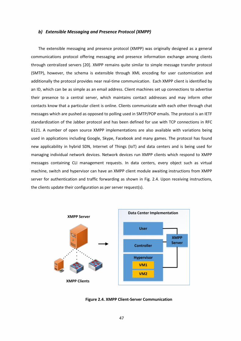
47

b) Extensible Messaging and Presence Protocol (XMPP)

The extensible messaging and presence protocol (XMPP) was originally designed as a general

communications protocol offering messaging and presence information exchange among clients

through centralized servers [20]. XMPP remains quite similar to simple message transfer protocol

(SMTP), however, the schema is extensible through XML encoding for user customization and

additionally the protocol provides near real-time communication. Each XMPP client is identified by

an ID, which can be as simple as an email address. Client machines set up connections to advertise

their presence to a central server, which maintains contact addresses and may inform other

contacts know that a particular client is online. Clients communicate with each other through chat

messages which are pushed as opposed to polling used in SMTP/POP emails. The protocol is an IETF

standardization of the Jabber protocol and has been defined for use with TCP connections in RFC

6121. A number of open source XMPP implementations are also available with variations being

used in applications including Google, Skype, Facebook and many games. The protocol has found

new applicability in hybrid SDN, Internet of Things (IoT) and data centers and is being used for

managing individual network devices. Network devices run XMPP clients which respond to XMPP

messages containing CLI management requests. In data centers, every object such as virtual

machine, switch and hypervisor can have an XMPP client module awaiting instructions from XMPP

server for authentication and traffic forwarding as shown in Fig. 2.4. Upon receiving instructions,

the clients update their configuration as per server request(s).

Figure 2.4. XMPP Client-Server Communication

48

While XMPP is defined in an open standard and follows an open systems development and

application approach allowing interoperability among multiple infrastructures, it also suffers a few

weaknesses. The protocol requires an assured message delivery extension to guarantee QoS of

message exchanges between the XMPP client and the server. Additionally, the protocol does not

allow end-to-end encryption, a fundamental requirement in the modern dispersed and multi-

tenanted network architectures. Extensions are, however, available dealing with assured message

delivery, and the encryption of messages.

c) Cisco OpFlex

Cisco OpFlex is another example of a southbound SDN protocol facilitating control-date plane

communication with a goal of becoming a standard, enabling policy application across multiple

physical and virtual environments. In comparison with OpenFlow protocol, which centralizes all the

network control functions using the SDN controller, the Cisco OpFlex protocol instead concentrates

primarily on implementing and defining the policies [63]. The reason for enhanced focus on policies

is to remove the controller scalability and control channel communication from becoming the

network bottleneck and pushing some level of intelligence to the devices using legacy protocols.

The framework allows policy definition within a logical, centralized repository in the SDN controller,

and the OpFlex protocol communicates and enforces the respective policies within a subset of

distributed elements on the switches. The protocol allows bidirectional communication of policies,

networking events and statistical monitoring information. Real-time provision of information may

in turn be used to make networking adjustments. The switches contain an OpFlex agent supporting

the Cisco OpFlex protocol. Cisco is currently developing an open source, interoperable OpFlex agent.

Some of the industry giants, including Microsoft, IBM, F5, Citrix and Red Hat, have shown

commitment to embedding OpFlex agent in their product lines [63]. OpFlex relies on traditional and

distributed network control protocols to push commands to the embedded agents in switches. One

of the main reasons for the early adaption of OpenFlow has been the level of control it can offer to

developers for designing network control applications with minimal support from network vendors.

Therefore, in order to standardize OpFlex, Cisco has also submitted the protocol to IETF

standardization process and several vendors are presently working to standardize as well as

increase the adoption of the protocol [63].

49

2.4.2 Northbound communication protocols

Since the inception of SDN, a number of networking vendors have started actively developing

SDN oriented applications with the aim of reducing the OPEX and CAPEX of future IT network

infrastructures. The applications themselves vary in scope with some providing a comprehensive

network monitoring and control solution while others solely target a particular aspect of load

balancing, security and traffic optimization through SDN controllers. The architecture and APIs

(northbound) of SDN applications vary between vendors. Some have incorporated SDN controllers

inside applications while others have defined custom northbound APIs for policy translation

between controllers and their own higher application layer SDN services. As per the ONF SDN

framework [1], applications might act as an SDN controller in their own right or liaise with one or

more SDN controllers to gain exclusive control of resources exposed by controllers. Applications can

exist at any level of abstraction with a general perception that the further north (higher) we go in

SDN framework, the greater the level of abstraction. A specific distinction between applications and

controller is not precise [2][3]. A controller-application interface may mean different things to

different vendors. However, the fundamental principle of abstracting network resources and

presenting network state to applications provides real-time network programmability, the

cornerstone of SDN.

The ONF constituted a special working group in June 2013 towards standardizing the northbound

interface (NBI) architecture across the industry [5]. Although there is considerable debate within

industry whether such a standardized interface is even required, the benefits of having an open

northbound API are also significant. Open northbound API allows developers from different areas of

industry and research to develop a network application, as opposed to only equipment vendors. It

also gives network operators the ability to quickly modify or customize network control. Despite

initially proposing it, the ONF consortium has, therefore, subsequently avoided northbound API

standardization to allow maximum innovation and experimentation. As a direct result, more than

20 different SDN controllers that are currently available feature varying northbound APIs based on

the needs of the applications and the orchestration systems residing above. There is a chance there

will never ever be a standardized northbound API. Routing and switching vendors that traditionally

rely on network-based applications and features to differentiate their hardware are positioning

themselves to maintain profitability in the SDN arena. These vendors may invest in custom software,

while using standard southbound protocols such as OpenFlow to run concurrently alongside their

operating system and complement the existing control plane. The result would definitely be a

50

complex and crowded SDN ecosystem. The following subsections review the two popular

northbound APIs, the RESTful [36] and Java based OSGi [37] interface prevalent in SDN controllers.

a) Representational State Transfer (RESTful)

Representational state transfer, or simply REST, follows the software architecture style

developed for World Wide Web consortium (W3C) encompassing all client-server communications.

The concept was originally introduced by Roy Fielding in [36]. The main goals of the scheme are to

offer scalability, generality, and independence and allow the inclusion of intermediate components

between clients and servers to facilitate these necessary functionalities. Both clients and servers

can be developed independently or in tandem, there is no particular necessity to have both

developed by same vendor. A schematic diagram representing RESTful calls is shown in Fig. 2.5. The

server component is stateless and clients keep track of their individual states to allow scalability.

Server responses can be cached for a specified time. Every entity or global resource can be

identified with global identifiers such as URIs and is able to respond to create, read, update and

delete (CRUD) operations. The uniform interface for each resource is GET (read), POST (Insert), PUT

(write) and DELETE (remove). Data types can define network components such as controller,

firewall rule, topology, configuration, switch, port, link and even hardware. RESTful is prevalent in

most controller architectures as the northbound interface of choice along with Java APIs. One of

the major drawbacks of RESTful however, is the lack of public subscription or live feed informing

the SDN controller of network state changes. Like HTTP, REST cannot determine when a page has

changed and requires frequent refresh. Application developers therefore, use loop calls at periodic

time intervals to retrieve and subsequently post updates to individual switches based on pre-

defined policies.

Figure 2.5. RESTful Application Programming Interface (API)

51

b) Open Services Gateway Initiative (OSGi)

The open services gateway initiative (OSGi) is a set of specifications for dynamic application

composition using reusable Java components called bundles [37]. Bundles publish their services

with OSGi service registry and can find/use services of other bundles as depicted in Fig. 2.6. Bundles

can be installed, started, stopped, updated and uninstalled using a lifecycle API. Modules define

how a bundle can import/export code. The security layer handles security and execution

environment defines what methods and classes are available in a specific platform. A bundle can

get a service or it can listen for a service to appear or disappear. Each service has properties that

allow other services to select among multiple bundles offering the same service. Services are

dynamic and a bundle can decide to withdraw its service, which will cause other bundles to stop

using it. Bundles can be installed and uninstalled on the fly. The OpenDaylight project [71] is one

major example of a SDN controller platform built using the Java based OSGi framework. OSGi allows

the starting, stopping, loading and unloading of Java based network (module) functionalities. In

comparison, platforms such as Ryu [70], do not offer OSGi support and the controller has to be

stopped and restarted with the needed modules or a custom REST method is built with all the

required functionalities included to avoid controller restarts. A few other SDN platforms supporting

OSGi include Beacon [75], Floodlight [76] and ONOS [93].

Figure 2.6. Open Services Gateway Initiative (OSGi)

52

2.5 Network controllers and switches

The SDN controller provides a programming interface for administrators to control the

underlying network elements. Network administrators and application developers can

collaboratively use the controller to perform management tasks as well as introduce newer

functionalities such as flow metering for QoS, re-routing and load-balancing as well as providing

access control. The level of abstraction offered to the operator, therefore, depicts the underlying

network switches as a single system which can be updated in real-time according to service

requirements. The SDN framework can be applied to a wide range of services and heterogeneous

networking technologies as well as media including virtual and physical networking gear and wired

and wireless networks. Since the inception of SDN, there have been a number of controller

platforms developed for the purposes of academic research as well as several vendors producing

proprietary carrier-grade solutions. The support for southbound and northbound APIs in controller

platforms, however, varies with each platform [40]. While the previous sections discussed about

the architectural components and interactions, this section refers to the physical components and

how the architecture links to an actual implementation. SDN controller and SDN-compliant switch

features are elaborated further in the following sub-sections.

2.5.1 SDN controllers

The SDN controller maintains and applies network policies as required by higher applications

and services, and translates and configures these policies in individual network devices. As

mentioned earlier, once a packet arrives at switch, in case of a table miss (absence of flow entry) it

may get forwarded to the controller, which determines the next course of action for the respective

traffic flow. A schematic representing generic controller architecture is given in Fig.2.7. Depending

on the deployed redundancy measures, switches may communicate with either a single or several

controllers [34]. Inter-controller communication is usually served by an external legacy protocol

such as the Border Gateway Protocol (BGP) or the Session Initiation Protocol (SIP) over TCP

channels to exchange routing information. Multiple controllers can improve the reliability of the

system. In case of failure of one controller or control channel, the switch can obtain flow

forwarding instructions from another controller instance. The number of controllers and their

placement depends on the topology and operational requirements of an organization. Two popular

schemes proposed include the vertical approach, where multiple controllers are in effect controlled

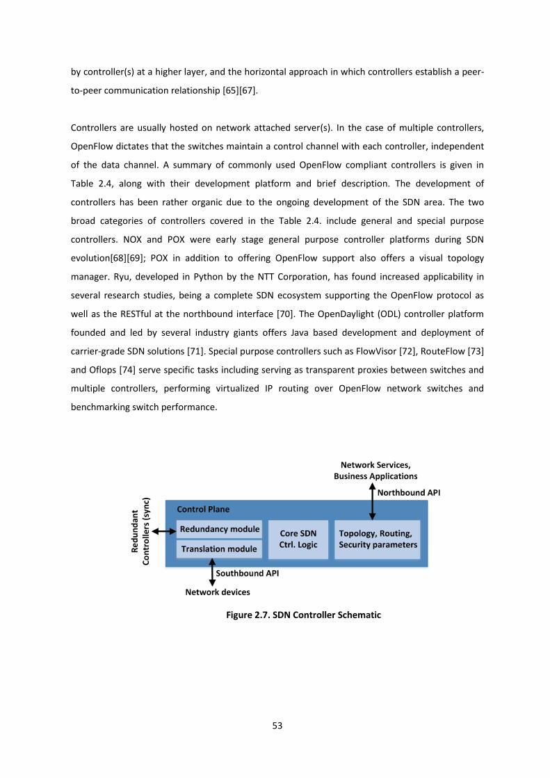
53

by controller(s) at a higher layer, and the horizontal approach in which controllers establish a peer-

to-peer communication relationship [65][67].

Controllers are usually hosted on network attached server(s). In the case of multiple controllers,

OpenFlow dictates that the switches maintain a control channel with each controller, independent

of the data channel. A summary of commonly used OpenFlow compliant controllers is given in

Table 2.4, along with their development platform and brief description. The development of

controllers has been rather organic due to the ongoing development of the SDN area. The two

broad categories of controllers covered in the Table 2.4. include general and special purpose

controllers. NOX and POX were early stage general purpose controller platforms during SDN

evolution[68][69]; POX in addition to offering OpenFlow support also offers a visual topology

manager. Ryu, developed in Python by the NTT Corporation, has found increased applicability in

several research studies, being a complete SDN ecosystem supporting the OpenFlow protocol as

well as the RESTful at the northbound interface [70]. The OpenDaylight (ODL) controller platform

founded and led by several industry giants offers Java based development and deployment of

carrier-grade SDN solutions [71]. Special purpose controllers such as FlowVisor [72], RouteFlow [73]

and Oflops [74] serve specific tasks including serving as transparent proxies between switches and

multiple controllers, performing virtualized IP routing over OpenFlow network switches and

benchmarking switch performance.

Figure 2.7. SDN Controller Schematic

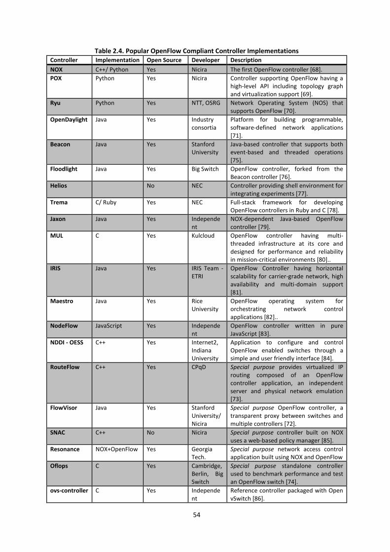
54

Table 2.4. Popular OpenFlow Compliant Controller Implementations Controller Implementation Open Source Developer Description

NOX C++/ Python Yes Nicira The first OpenFlow controller [68].

POX Python Yes Nicira Controller supporting OpenFlow having a high-level API including topology graph and virtualization support [69].

Ryu Python Yes NTT, OSRG Network Operating System (NOS) that supports OpenFlow [70].

OpenDaylight Java Yes Industry consortia

Platform for building programmable, software-defined network applications [71].

Beacon Java Yes Stanford University

Java-based controller that supports both event-based and threaded operations [75].

Floodlight Java Yes Big Switch OpenFlow controller, forked from the Beacon controller [76].

Helios No NEC Controller providing shell environment for integrating experiments [77].

Trema C/ Ruby Yes NEC Full-stack framework for developing OpenFlow controllers in Ruby and C [78].

Jaxon Java Yes Independent

NOX-dependent Java-based OpenFlow controller [79].

MUL C Yes Kulcloud OpenFlow controller having multi-threaded infrastructure at its core and designed for performance and reliability in mission-critical environments [80]..

IRIS Java Yes IRIS Team - ETRI

OpenFlow Controller having horizontal scalability for carrier-grade network, high availability and multi-domain support [81].

Maestro Java Yes Rice University

OpenFlow operating system for orchestrating network control applications [82]..

NodeFlow JavaScript Yes Independent

OpenFlow controller written in pure JavaScript [83].

NDDI - OESS C++ Yes Internet2, Indiana University

Application to configure and control OpenFlow enabled switches through a simple and user friendly interface [84].

RouteFlow C++ Yes CPqD Special purpose provides virtualized IP routing composed of an OpenFlow controller application, an independent server and physical network emulation [73].

FlowVisor Java Yes Stanford University/ Nicira

Special purpose OpenFlow controller, a transparent proxy between switches and multiple controllers [72].

SNAC C++ No Nicira Special purpose controller built on NOX uses a web-based policy manager [85].

Resonance NOX+OpenFlow Yes Georgia Tech.

Special purpose network access control application built using NOX and OpenFlow

Oflops C Yes Cambridge, Berlin, Big Switch

Special purpose standalone controller used to benchmark performance and test an OpenFlow switch [74].

ovs-controller C Yes Independent

Reference controller packaged with Open vSwitch [86].

55

2.5.2 SDN compliant switches

In addition to the several network controllers on offer, several types of SDN software and

hardware switches are currently available. A summary of current OpenFlow switch

implementations are presented in Table 2.5, along with their brief description and development

platform (language). The software switches can be used to run SDN test simulations as well as

develop protocols and services. Open vSwitch for example, is now a part of the Linux kernel (as of

version 3.3) and facilitates both the ability to serve as virtual gateway between physical and virtual

services as well as a testing platform to be used in tandem with SDN topology simulation tools such

as Mininet [103]. In addition to software switches, companies such as IBM, HP and NEC have also

brought physical carrier-grade switches to market. The networking industry has taken keen interest

in SDN evidenced by the availability of a number of commercial hardware switches which are

OpenFlow-enabled.

2.6 Simulation, development and debugging tools

The development of SDN has seen the advent of several key simulation and emulation test-

beds to carry out feasibility studies and introduce new protocols and services. The set of tools

available for the purpose can be broadly divided into three categories (i) simulation and emulation

platforms (ii) software switch implementations and (iii) debugging and troubleshooting tools. A

summary description of major utilities within each category and their description are given in Table

2.6. An overview of the tools is given below.

2.6.1 Simulation and debugging platforms

a) Mininet: Among the emulation tools, Mininet [103] is the most prominent. The platform

allows an entire network based on OpenFlow to be emulated on a single hosted machine.

Mininet simplifies the development and deployment of new services by providing a

software platform to create virtual machines, hosts and network switches connected to an

in-built (ovs-reference) or user-defined controller for testing purposes. The latest Mininet

v2.2.1 supports OpenFlow versions up to 1.3 (along with Open vSwitch v2.3). While Mininet

supports Open vSwitch [86] by default, it can also be customized to use an external user

space switch such as the softswitch13 [90].

56

Table 2.5. Common OpenFlow Compliant Switches and Standalone Stacks

Switch Implementation Category Description

Open vSwitch C/ Python Software OpenFlow stack that is used both as a virtual switch and ported to multiple hardware platforms [86].

Indigo C Software Software running on hardware switching implementations and based on the Stanford reference [87].

OpenFlowJ Java Software OpenFlow stack written in Java [88].

OpenFaucet Python Software Python implementation of the OpenFlow 1.0 protocol [89].

ofsoftswitch13 C/ C++ Software User-space software switches implementation [90].

Pantou C Software OpenFlow port to the OpenWRT wireless environment [91].

Oflib-node JavaScript Software OpenFlow protocol library for Node.js converting between the protocol messages and JavaScript objects [92].

OpenFlow Reference C Software Minimal OpenFlow reference stack that tracks the specification [17].

Open Source Network Operating System (ONOS)

Java Software Open source scalable control plane cluster offering GUI and OpenFlow as well as NetCONF support [93].

Pica8 C Physical and software

Software platform for hardware switching chips which includes L2/L3 stack [94].

A10 Networks –AX Series

Proprietary Physical and software

Physical and software appliances (AX Series), offering L4-7 programming [95].

Big Switch Networks - Big Virtual Switch


Data center network virtualization application built upon an OpenFlow switches [96].

Brocade ADX Series Proprietary Physical and software

Secure and scalable application service infrastructures using the RESTful API on northbound interface [97].

NEC ProgrammableFlow Switch Series


Series offers network virtualization, multipath routing, security, and programmability [98].

ADVA Optical - FSP 150 & 3000

Proprietary Physical FSP 150 carrier Ethernet and FSP 3000 transport layer products [99].

IBM RackSwitch G8264 Proprietary Physical Offers low cost flexible connectivity for high-speed server and storage devices in DC environments [100].

HP 2920, 3500, 3800, 5400 series

Proprietary Physical Advanced modular switch series built on programmable ASICs offering scalable QoS and security [101].

Juniper Junos MX, EX, QFX Series

Proprietary Physical Series supports different versions of OpenFlow varying with model [102].

57

b) NS-3: The network simulator has long been used by the networking community to test and

develop networking protocols and services. The latest ns-3 simulator offers support for

OpenFlow switches, however, it is limited to a very early version of OpenFlow v0.89 [104].

While official work is continuing on introducing newer updated versions of OpenFlow, a

specialist OpenFlow 1.3 module for ns-3 namely OFSwitch13 module has been designed

independently [105]. The module relies on the ofsoftswitch13 library providing a data path

(switch) implementation in the user pace and to convert OpenFlow v1.3 messages from

wire format.

c) OMNeT++: The OMNet++ is a discrete event simulator allowing the development and

testing of SDN based network models [106]. SDN oriented projects can be integrated with

OMNeT++ using an OpenFlow components and an INET Framework.

2.6.2 Software switch implementations

A non-exhaustive summary of software switches which are also used for experimentation and

new service development were given earlier in Table 2.5. Well-adopted implementations such as

the Open vSwitch have been implemented in multiple platforms including Mininet and ns-3. A brief

overview of some of the well-known software switches presently available is given below.

a) Open vSwitch: The Open vSwitch is one of the most widely deployed software switches. It

employs an OpenFlow stack that can be used both as a virtual switch in virtualized network

topologies and has also been ported to multiple hardware/ commodity switch platforms. [86]

The Open vSwitch has been built in the Linux kernel since version 3.3 [17].

b) ofsoftswitch13: The ofsoftswitch13 running in the user space also provides support for

multiple OpenFlow versions [90]. The soft switch supports Data Path Control (Dpctl), a

management utility to directly control the OpenFlow switch, allowing the addition and

deletion of flows, query switch statistics and modify flow table configurations. Although

ofsoftswitch13 supports a variety of OpenFlow features, it has recently run into some

compatibility issues with latest versions of Linux (Ubuntu 14.0 and beyond) and developer

support has also stagnated.

58

Table 2.6. Common OpenFlow Compliant Utilities

Category Purpose Software and tools

Emulation and simulation

Emulating network topologies as well as providing a reference for network event simulation

Mininet [103], ns-3 [104], OMNeT++ [106]

Software switches and platforms

A software platform to test and validate switch-controller behaviour and southbound protocol working

Open vSwitch [86], ofsoftswitch13 [90], Indigo [87], Pica8 PicOS [94], ONOS [93], Pantou [91]

Debugging and troubleshooting

Specialist tool set to debug SDN behaviour at the switch and controller level

STS [107], Open vSwitch [86], NICE [108], OFTest [109], Anteater [110], VeriFlow [111], OFRewind [112], NDB [113], Wireshark [114]

c) Indigo: The Indigo project is an open source implementation of OpenFlow which can be run

on a range of physical switches and utilizes the hardware features of existing Ethernet switch

ASICs to run OpenFlow pipeline at line rates [87]. The implementation is based on the original

OpenFlow Reference Implementation and currently supports all features required in the

OpenFlow 1.0 standard.

d) Pica8 PicOS: The PicOS by Pica8 is a network operating system allowing network

administrators to build flexible and programmable networks using white box switches with

OpenFlow [94]. The proprietary software allows the integration of OpenFlow rules to be used

in legacy layer 2 / layer 3 networks, without disrupting existing network and creating a new

one from scratch.

d) Open source network operating system (ONOS): Although not specifically a soft switch

implementation, the mission of ONOS is to develop an operating system resilient for

carrier-grade deployment of software defined networks [93]. The ONOS GUI provides the

multi-layer view of the underlying network and allows operators to peruse network devices,

links, and errors.

e) Pantou: Pantou modifies a commercial wireless router and access point to an OpenFlow

enabled switch. The OpenFlow protocol is implemented as an application on top of

OpenWRT platform [91]. The OpenWRT platform used is based on the BackFire release

(Linux v2.6.32) while the OpenFlow module is based on the Stanford reference

implementation in user space.

59

2.6.3 Debugging and troubleshooting tools

Debugging and troubleshooting tools serve as vital resources for development and testing

of SDN based services. The following list presents some of the popular SDN debugging and

verification tools.

a) SDN troubleshooting system (STS): STS simulates the network devices of your

network while also allowing enough programmatically to generate and examine

various test case deployments. Users can interactively visualize the network states,

the real-time changes and also automatically determine the events that trigger

deviant behaviour and identify bugs. The implementation is based on the POX

controller platform, with the feasibility to use other OpenFlow compliant controllers

supporting OpenFlow v1.0.

b) Open vSwitch specific tools: The Open vSwitch comes with a comprehensive set of

tools to debug the switch and network behaviour. The utilities comprise of the

following:

ovs-vsctl: Used for configuring the switch (daemon) configuration database (known

as ovs-db.)

ovs-ofctl: A command line tool for monitoring and administering OpenFlow

switches.

ovs-dpctl: Used to administer Open vSwitch datapaths (switches). In addition to

Open vSwitch ovs-dpctl, a reference dpctl comes with the OpenFlow reference

distribution and enables visibility and control over a single switch's flow table. The

syntax of commands used by the utilities is quite different.

ovs−appctl: Used for querying and controlling Open vSwitch daemons.

c) NICE: NICE offers an automated testing tool used to identify and check bugs in

OpenFlow programs [108]. The tool applies model checking to explore the entire

state of the controller, the switches, and the hosts. To address scalability issues, the

tool uses model checking with symbolic execution of event handlers (identifying the

representative packets that exercise code paths on the controller). NICE prototype

tests Python applications using the NOX platform.

60

d) OFTest: OFTest is an OpenFlow switch test framework built in Python and also

includes a collection of test cases [109]. The tool is based on the unittest function,

which is included in the standard Python distribution. OFTest hosts the switch under

test and the OFTest code runs on the test switch. Both control plane and data plane

side of switch connections can be tested by sending and receiving packets to the

switch as well as polling switch counters.

e) Anteater: Anteater attempts to check network invariants that exist in the

networking devices, such as connectivity or consistency [110]. The main benefit of

using Anteater is that it is agnostic to protocols and will catch errors that result from

faulty firmware as well as control channel communication.

f) VeriFlow: VeriFlow allows real-time verification and resides between the controller

and the data plane elements (switches) [111]. The framework allows pruning of flow

rules that may result in anomalous network behaviour.

g) OFRewind: OFRewind is another tool that allows debugging of network events both

in the control and data plane and to log these at different levels of detail to be

replayed later in examining problematic scenarios and localize troubleshooting

efforts [112].

h) Network debugger (NDB): NDB implements traffic breakpoints and packet-

backtraces for an SDN environment [113]. Similar to the popular software

debugging utility gdb, users can isolate networking events that may have led to an

error during traffic forwarding. It works using the OpenFlow API to configure

switches and generate debugging events. NDB then acts as a proxy intercepting

OpenFlow messages between switches and the controller. The debugger relies on

OpenFaucet python module implementing OpenFlow v1.0.

i) Wireshark: The popular network analyser Wireshark can be deployed on the

controller or Mininet host to view OpenFlow exchange messages between the

controller and individual switches. The OpenFlow dissector is available in the

current Wireshark release [114]. OpenFlow control packets can be directly filtered

while capturing using the TCP control channel traffic ports (6633 and 6653). The

61

captured packets provide a useful learning tool to understand switch-controller

behaviour.

2.7 SDN applications

Software-defined networking has found a great deal of applicability in a wide range of

networking avenues. Real-time programmability through the centralized controller has presented

opportunities in data center networking, large campus environments as well as experimental

designs focusing on enhancing end user experience and making residential networks more

manageable. Furthermore, mobile operators have also shown keen enthusiasm in bringing the

technology to 5G/ LTE mobile networks to allow simplified yet rapid development and deployment

of new services. Some of the key applications of SDN are highlighted as follows.

2.7.1 Data centers and cloud environments

Optimal traffic engineering, network control, and policy implementation are absolute

requirements when operating at large scales, as is the case for data centers. Increased latency,

faults and prolonged troubleshooting may result not only in negative end user experience but

significant cost penalties for operators. Data center (DC) SDN implementations, therefore, using a

centralized control framework monitor and manage hundreds of network devices and services

promising effective resource provisioning for operators. Google for example, has used SDN

technology to connect its geographically dispersed data centers around the globe, allowing

increased resilience and manageability [38].

Cloud computing has also seen the integration of SDN based traffic engineering solutions to

increase service scalability and automated network provisioning. A notable example is the

Microsoft public cloud [201]. The study highlights SDN based load balancing solution Ananta, a layer

4 load balancer employing commodity hardware to provided multitenant cloud management. Using

host agents, packet modification is localized enabling high scalability across the DC. The project has

seen a significant level of deployment in the Microsoft Azure public cloud, allowing high throughput

for several tenants allocated a single public IP address. Another SDN deployment in cloud

environment is NTT's software-defined edge gateway automation system [314]. The gateway uses

OpenFlow protocol for maximum flexibility in network provisioning and evaluates possible

62

extension to existing OpenFlow features, baselining the SDN stack to allow robust cloud gateway

deployment.

On a slightly separate strand, reducing energy consumption in data centers has also been an area of

focus for operators to reduce operational costs. Since most DCs are overprovisioned for peak traffic,

the energy efficiency during periods of underutilization is minimal. SDN technologies such as

ElasticTree allow network wide power management by switching off redundant switches from the

controller side during low traffic demand [39]. DC network environments to-date remains one of

the primary beneficiaries of the SDN framework.

2.7.2 Campus and high speed networks

Enterprise networks may show a great deal of variability in traffic patterns requiring

proactive management to adjust network policies and fine tune performance using a

programmable SDN framework. A centralized control plane may also aid in effective monitoring and

utilization of network resources for re-adjustment. An additional benefit may be to eliminate

middle boxes providing services such as NAT, firewalls, access control and service differentiation

solutions and load balancers [41-43]. With increasing use of fibre technologies in enterprise

networks, the Optical Transport Working Group (OTWG) created by the Open Network

Foundation (ONF) envisions applying southbound protocols such as OpenFlow to improve optical

network management flexibility. Inclusion of an SDN controller for optimal network provisioning,

while offering simplicity, also allows external third-party network administration of the enterprise

network and added support for visualization [44].

The integration of heterogeneous networking technologies using OpenFlow enabled network

elements and a centralized controller has seen a great deal of applicability in optical high-speed

networking. High speed optical communications require an appreciation of the existing OpenFlow

framework and possible extensions to achieve a higher level of integration [316]. Using centralized

real-time programmability, SDN enabled hardware from multiple vendors and optical packet based

as well as circuit-switched networks can be placed under the SDN controller. Gudla et. al [315], for

example used NetFPGA [16] along with Wavelength Selective Switching (WSS) for packet and circuit

switching facilitated using the OpenFlow protocol. Liu et. al. [317] used virtual Ethernet based

interfaces to demonstrate OpenFlow based wavelength path controlling in optical networking. A

commodity SDN controller such as NOX, POX, etc., can operate the optical light paths using

OpenFlow by mapping virtual Ethernet interfaces to physical ports of an optical cross-connect node.

63

The evaluation of network performance metrics included in the study detailed promising results in

reducing latency of path setup and verification of routing and wavelength assignment allocation

using dynamic node control providing paving the way for future software defined optical

networking (SODN). In comparison with the typical distributed GMPLS protocol, SDON using a

unified control protocol for QoS metrics offers greater capacity and performance optimization in

optical burst switching [318]. The application of SDN, and in particular OpenFlow based controls in

high speed and campus networking, therefore, continues to grow resulting in new as well as hybrid

solutions to achieve greater network programmability.

2.7.3 Residential networks

Software defined networking has also been considered as an efficient means to manage

residential and small office home office networks. Management of residential networks presents a

key challenge for residential users and service providers alike, including the benchmarking of home

user activities through collection of traffic metrics and the setup involved. One of the fundamental

benefit of such networks is that operators and residential users are provided with a greater degree

of visibility into network usage through effective monitoring using the SDN framework [45-47]. To

relieve the burden of network management on residential gateways, Dillon and Winters [49]

proposed the introduction of virtual residential gateways (data plane) using software defined

networking controller(s) at the service provider side to allow providers remote management

flexibility as well as innovative service delivery to homes. The residential router or gateway may be

controlled and managed remotely via an SDN controller at the service provider premises, with the

latter being responsible for fine tuning and troubleshooting the residential network [46][48-50].

Some contrasting schemes propose giving users more control and incorporating SDN based

monitoring in the residential environment to change network policies [49][51][52].

From a security perspective, it has been argued that an SDN based anomaly detection system in a

residential SDN environment provides more accuracy and higher scalability than intrusion detection

systems deployed at Internet service provider side [48]. Feamster in [46], proposed completely

outsourcing residential network security utilizing programmable network switches at the customer

premises to allow remote management. By employing the outsourced technical expertise,

management and running of tasks such as software updates and updating anti-virus utilities may be

done more effectively as the external operator also has a wider view of network activity and

emerging threat vectors. The privacy of end users where technical operations related to residential

network management are outsourced also requires consideration [47]. The inclusion of SDN

64

framework in residential networking, given its benefits to end users, remains an active area of

academic and industry research.

2.7.4 Wireless communications

Due to the real-time programmability and potential to seamlessly introduce new services

and applications to consumers, the SDN paradigm has also been ported to mobile communication

networks. A programmable wireless data plane, offering flexible physical and MAC address based

routing in comparison to the layer 3 logical address based traffic forwarding, allowed developers to

fine tune mobile communications performance [53][56]. Using the control plane, user traffic can be

segregated and routed over different protocols such as WiMAX, 3GPP or advanced LTE.

Furthermore, there have been growing efforts to include the SDN layering model in the upcoming

5G mobile communications realm and move from a flat topology, which increasingly relies on the

core, to a more modular control and traffic forwarding framework. Similar to information-centric

networking, data may be cached locally at certain points within the 5G network, as coordinated by

the SDN controller, to reduce latency in service delivery to end users [54-55].

Finally, within 5G networks, efficient resource management is essential to allow maximum

utilization, network slicing, and guaranteeing fairness among several QoS classes [319]. Using SDN

to maximize energy efficiency in 5G networking has, therefore, been the subject of investigation in

several studies. SDN has also been test-implemented in 5G to allow rapid application service

provisioning while adhering to stringent QoS requirements. At the more local level such as Wi-Fi

access networks, SDN could be used to offer a great deal of ubiquity in connecting to different

wireless infrastructures belonging to different providers using user device identity management

which is in turn coordinated and proactively managed by the SDN controller [57].

2.8 Research challenges

Increasing application of SDN framework in several network settings have also highlighted areas

of concern ranging from application performance to security inadequacies inherent in the present

architecture, briefly detailed in chapter 1. The present section discusses the major investigations

and research advances made in several SDN areas in detail. A summary of the key areas of research

and subsequent initiatives in software defined networking is presented in Table 2.7.

65

2.8.1 Controller scalability and placement

The SDN controller is responsible for managing data plane switches and providing traffic

forwarding rules that affect individual packet behaviour. In larger network environments, the

placement of the SDN controller is highly pertinent in achieving optimized network connectivity

[135]. The connections between controller(s) and switches in the data plane require low latency for

seamless operation [136]. To address scalability concerns, having more than one controller serving

the data plane are, therefore, usually required. In critical network infrastructures, multiple

controllers, may also be required in order to offer a greater level of redundancy. Prevalent research

in this area seeks to deploy multiple controllers in several network locations and consequentially

determining the exact point of controller placement is critical [135-139].

The controller placement problem was first identified by Heller et. al. in [136] as an NP-hard

problem focusing on the determination of exact number and optimal location for SDN controllers.

The study highlighted that the best controller placement solution should minimize the controller to

switch control traffic latency. Similarly, Sallahi et. al. [137] considered the placement problem from

an operational perspective discussing the cost involved in deploying and installing controllers and

connecting these to the wider network fabric. Both studies used traversal search algorithms

perusing through the best solutions to find an optimal candidate, a time consuming process

proportional to the size of the network. Some of the topologies took an order of magnitude greater

than 30 hours to find a satisfactory placement solution. From a controller workload standpoint, Yao

et. al. [138] highlighted the fact that the placement solution should also consider the workload for

each controller and that it does not exceed controller capacity. The proposed placement solution

used k-center algorithm [140] to minimize the value of k (controllers) that meet the workload and

capacity requirements. In a similar work, Yao et. al. [141], discussed placing controllers at network

hotspots where switches carry most of the traffic. The switches in the proposed solution may utilize

less overloaded controllers, migrating from one to another with changing traffic demand.

Ros et. al [142] focused on network reliability, highlighting a positive correlation between fault

tolerance and controller placement. The study used heuristic algorithms to compute controller

placement and the maximum number of controllers which may be deployed to meet network

reliability. Zhang et. al [135] used the min-cut method discussed in [143] to separate the network

into smaller networks, each having its own controller. Similarly Guo et. al. [144] generated a

hierarchical tree [145] of network nodes, dividing it into k clusters or subnetworks. Nodes with

maximum closeness to other nodes were selected for controller deployment. In [146], a greedy

66

Table 2.7. Summary of SDN Research Initiatives

Area of concentration

Brief description Research initiatives

Controller scalability and placement

Controller placement in large SDN environments offers a complexity optimization problem affecting latency, capacity and fault tolerance. The design of the control plane remains a multi-faceted topic of several research studies.

Reducing latency by solving optimal controller placement problem (NP-hard).

Solutions minimizing controller workload with respect to controller placement.

Placement schemes offering greater reliability using heuristic and greedy algorithms to refactor larger network into smaller (separate controller) sub-networks.

Combinatorial approaches optimizing multiple network performance metrics in relation to controller placement, providing a trade-off between performance gains and operational requirements.

Distributed control architectures considering hierarchical controller clusters to address scalability issues.

Switch and controller design

Studies aimed at improving northbound API standardization among multiple application platforms, level of control delegation appropriate for data plane elements and optimal hardware architectures.

Standardization of the northbound API, involving studies in designing a policy abstraction language compatible with several platforms and offering vertical and horizontal integration with parallel services and underlying network fabric.

Greater level of control delegation to network switches aimed at reducing controller overhead and increasing fail-safe redundancy.

New architectures for controller and switch design.

Security SDN due to centralized network control creates potential security challenges directed at control plane (traffic) and data plane elements including network appliances and middle boxes.

Designing SDN security reference models focusing on securing the control plane to avoid network disruption and security compromise.

Control channel and application-controller traffic monitoring and anomaly detection.

Network /state information storage and retrieval for post-even and forensic examination.

Application performance

Improving the performance of individual network applications and services in the SDN framework using novel optimization techniques in wired, wireless and heterogeneous settings.

Increasing SDN application-awareness and optimizing time-critical application services using flow metering.

Development of SDN monitoring tools for evaluating performance gains in heterogeneous network environments.

Embedding network services such as authentication, firewalls, proxies, etc. in the data plane fabric.

Information-centric approaches exploiting location-based data caching.

67

algorithm was used to enhance controller placement reliability in the event of network state

changes as well as single link failures in tandem with the optimal controller placement. Hu et. al

[147] used multiple algorithms including l-w greedy, and simulated annealing and brute force

searching with brute force offering the best optimal solution.

Other notable works such as Onix [65], HyperFlow [66] and Kandoo [67] propose a distributed

control architecture allowing a significant level of scalability and reliability in large SDNs. HyperFlow

details a flat or horizontal scaling of controllers, while Kandoo and Onix use a hierarchical structure.

The schemes allow multiple controllers to manage the data plane. The distributed architecture

comprises of root and localized controllers each control-level having a different view of the

underlying network. Another category of distributed controller design includes Difane [148] and

DevoFlow [149] which delegate some control functions to the SDN switches to reduce the

controller overhead. Offloading workload helps in improving network scalability, however, requires

significant modifications in switching hardware to accommodate functional requirements. SDN

controller placement, therefore, remains an active area of research with several solutions and

approaches pursued to achieve a greater deal of scalability allowing greater network performance.

2.8.2 Switch and controller design

Innovations and proposals in controller and switch design seek to circumvent some of the

problems associated with policy implementation while simultaneously addressing additional areas

needing improvement including controller and switch scalability. Although controller-switch

interaction is served by standard southbound APIs such as OpenFlow [17], XMPP [20] or ForCES [8],

as mentioned earlier, a similar level of standardization is not available at the application-controller

northbound interface. Since the northbound interface purely relies on the application logic, the

supporters of non-standardization (of northbound API) argue that the present framework allows for

greater degree of innovation with custom northbound communication fitting the application or

service using the SDN. A number of controller utilities and platforms described earlier in the

chapter allow applications to interact with each other as well as the underlying network elements

for traffic engineering purposes. The application developer, however, needs an in-depth knowledge

of the controller implementation to deploy application APIs.

A few proposals have highlighted the need for network configuration language that can seamlessly

express the administrator policies seamlessly on the underlying controller implementation [150-

153]. Policy description language such as Procera [150] and Frenetic [151] build a policy layer on

68

existing controllers, interfacing with configuration, graphical interfaces and other network monitors

to translate administrator defined policies to flow level details which can be used by the controller.

Other examples exploring network configuration languages include FML [152] and Nettle [153].

Feamster and Kim [107], propose using policy definitions for network configuration and

management according to changing network conditions. The northbound communication API may

be further used in such cases to allow the SDN to apply segregated policies on same application

flows based on destination or source IP address. Monsanto et. al [154] on the other hand introduce

the concept of modularized policy implementation which ensures that flow rules for one network

application task do not interfere or replace rules for other tasks. As mentioned earlier, the chances

of ONF or the industry standardizing the northbound API look slim and operators will continue to

develop and deploy custom Pro-active implementation of policies in the switches lead to a

substantial lowering of control overhead generated during real-time operation [148][149].

In terms of switch design innovation, Luo et. al [156] discuss the replacement of ASIC based

counters for rule-matching in switches to ones processed in the CPU. Other technologies such as

FLARE [155] allow for complete programmability of not only the data and control planes but also

the control channel between them. A single controller may be able to handle up to 6 million to 12

million flows per second [157][75]. However, lowering propagation latency and increasing fault-

tolerance and robustness also requires controller architectures using horizontal and hierarchical

clusters [65-67].

2.8.3 Security

The increasing interest in SDN in the networking community also initiated a significant debate

highlighting the inherent security challenges of an SDN framework. The OpenFlow switch

specification [86] includes relatively basic security incorporation in SDNs using optional transport

layer security (TLS) allowing mutual controller-switch authentication without specifying the exact

TLS standard. TLS although, has not been given much thought in Several open source controller and

switch platforms, however, have not implemented TLS, which may lead to anomalous rule insertion

in flow tables [299]. Centralized control makes the scheme vulnerable to attacks directed at the

control plane which may disrupt the entire network. The intelligence in the centralized control

plane may offer hackers the opportunity to explore security vulnerabilities in the controller and

take over the entire network [64][158]. On the positive side, it is argued that the information

generated from traffic analysis or anomaly detection in the network can be regularly transferred to

69

the SDN controller, having a global network-wide view to analyse and correlate feedback for

efficient security [307].

In addition to securing the controller, targeted attacks on the network (e.g. DDoS) and subsequent

controller failure may result in substantial network service downtime until the controller is up and

running and the threat has been mitigated. The control channel between the controller and

network devices has to be secure enough to reject anomalous injection; the same is true for

application-controller communication. Effectively establishing trust among all the network devices

and the applications on top are considered a key security concern. Vulnerability analysis, mitigation

studies and a standardized framework for SDN security has therefore, been the focus of multiple

deliberations [308-311] with a great deal of focus in the security domain laid on controller-switch

and inter-controller communication. Shin and Gu [308] for example, undertake vulnerability

evaluation of SDN by evaluating the feasibility of fingerprinting attacks. The study fingerprinted the

SDN equipment such as OpenFlow switches and targeted the respective elements with denial of

service (DoS) attack on the controller via control channel and on the data plane elements by

exploiting flow tables. Both entities are identified as significant areas of SDN vulnerability. Similarly,

Smeliansky [309] discussed communication protocol security with consideration for infrastructure

and software services, concluding that control-data plane and control to control plane

communication requires substantial hardening to mitigate security threats. Some of the solutions in

controller-switch communication challenges propose replication of SDN controllers and network

applications to provide redundancy and fail-safe operations, which may arise due to

misconfigurations and software bugs [312]. Other investigations propose service mobility, to

counter security threats [299]. The controller functionality for example, could be continuously

shifted across several network elements making targeted attacks on the controller more

challenging for those seeking to exploit the control-plane.

SDN security has also been the subject of work in particular avenues including wireless

communications and cloud computing, for the technology to gain wider acceptance in

[310][311][313]. Schehlmann et. al in [310] discuss potential improvements in network

management costs, as well as attack detection and mitigation by using SDN framework itself as a

potential barrier to security vulnerabilities. SDN enables the incorporation of certain security

functionalities through decoupling of network control from forwarding logic where traffic filtering

can be achieved using key traffic (packet) identifiers usually requiring dedicated firewalls and

intrusion detection/ preventions systems in legacy networking. Additional security layers may be

70

added on top of existing SDN layers as well as by the introduction of agents in data plane elements

to incorporate granular traffic filtering in heterogeneous wireless networks [311]. Security

approaches may focus on securing the network itself by embedding intelligent security alarms in

the network elements such as switches and controllers or include SDN oriented security utilities in

the functional entities such as application servers and storage clusters. Similarly, in SDN-enabled

cloud computing, additional security may be introduced at each SDN layer based on underlying

operational requirements to make intra and inter-cloud communication more secure [313].

In addition to specific application avenues real-time SDN monitoring has to be robust enough to

offer timely detection of anomalous network events and containment [48]. The monitoring

information not only provides insight into traffic but quite similar to the case of legacy network

systems, may also have enough storage capacity system to satisfy technical (forensic) as well as

legal requirements [43]. Organizations such as OpenFlowSec [159] focus on security challenges

presented by the SDN paradigm and OpenFlow enabled devices. Development work has considered

designing reference implementations of security features at different layers of the OpenFlow stack.

A detailed taxonomy of security threats in the SDN paradigm is presented in [160]. Beyond the basic

SDN architecture, the deployment of robust security in the SDN paradigm is still very much an area

requiring further study. It is however, a widely held belief that without a significant increase in

focus on SDN security, the paradigm may not see adoption beyond private DC infrastructures or

autonomous organizational deployments.

2.8.4 Application performance

Application performance improvement has been the primary area of focus in a number of SDN

related studies ranging from application-aware SDNs, utilizing the framework for optimizing time-

critical applications to the development of novel application performance monitoring solutions. The

following sub-sections discuss the studies carried out in this regard.

a) Application-awareness in SDN

Traffic optimization carried out on the basis of network applications to a significant extent

focuses on increasing specific service performance(s) in SDN. Supporters of ‘application-aware’ SDN

infrastructure consider the benefits the framework brings in offering enhanced performance for

specific applications. While southbound APIs such as OpenFlow are capable of Layer-2/3/4 based

policy enforcement they lack high level application awareness and are mainly responsible for

71

configuring the underlying network elements. Network management primitives are, therefore,

employed which customize traffic forwarding policies for individual applications and the SDN

controller translates these into device configuration using a southbound API such as OpenFlow. The

concentration in this domain has seen several studies particularly concentrating on video streaming

(IPTV, YouTube, P2P video, etc.) and voice communications (VoIP), using the SDN architecture to

improve the respective application quality of service. Qazi et. al [60] in one such ‘application-aware’

SDN work discuss Atlas, a crowd sourcing approach which deploys software agent on user devices

and collects the netstat logs, in turn exported to the SDN control plane. Using the exported logs in

tandem with machine learning classification the scheme identifies approximately forty applications

(from Google Play Store). The SDN controller in turn applies pre-defined policy actions to the

respective flows as well as collects flow statistics per application for monitoring purposes. Mekky et.

al [115] proposes a similar per application flow metering approach using the SDN framework.

Applications are identified in the data plane and the relevant policies applied using individual

application tables. The proposed scheme minimizes SDN control channel overhead. The study

showed significantly good application forwarding performance with low overhead when tested and

implemented using a content-aware server selection application along with multiple virtual IP pool

of services.

b) Video streaming and real-time communication

Focusing on video streaming applications, Egilmez et. al [116], devised an analytical framework

for traffic optimization at the control layer offering dynamic and enhanced Quality of Service (QoS).

The study reported significant improvement for streaming of encoded videos under several coding

configurations and congestion scenarios. Jarschel et. al [61] instead focused specifically on

improving YouTube streaming experience for end users. The study used Deep Packet Inspection

(DPI) and demonstrated how application detection along with application state information can be

used to enhance Quality of Experience (QoE) and improve resource management in SDN. Ruckert et.

al [117] developed Rent a Super Peer (RASP), a peer-to-peer (P2P) streaming mechanism using the

OpenFlow network. RASP employs a cross-layered approach, allowing service providers to facilitate

P2P based live video streaming over two OpenFlow-based service components: a network proxy

application and software defined multicast (SDM) application, while the controller is responsible for

integrating components and providing an interface to RASP functionality. The proposed

methodology results in efficient delivery of P2P video streaming traffic to be used in future service

provider networks. Another example of video streaming optimization is the CastFlow [118] which

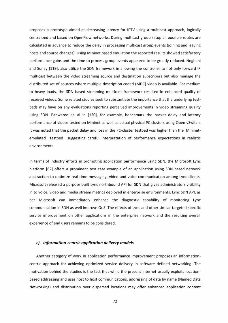
72

proposes a prototype aimed at decreasing latency for IPTV using a multicast approach, logically

centralized and based on OpenFlow networks. During multicast group setup all possible routes are

calculated in advance to reduce the delay in processing multicast group events (joining and leaving

hosts and source changes). Using Mininet based emulation the reported results showed satisfactory

performance gains and the time to process group events appeared to be greatly reduced. Noghani

and Sunay [119], also utilize the SDN framework in allowing the controller to not only forward IP

multicast between the video streaming source and destination subscribers but also manage the

distributed set of sources where multiple description coded (MDC) video is available. For medium

to heavy loads, the SDN based streaming multicast framework resulted in enhanced quality of

received videos. Some related studies seek to substantiate the importance that the underlying test-

beds may have on any evaluations reporting perceived improvements in video streaming quality

using SDN. Panwaree et. al in [120], for example, benchmark the packet delay and latency

performance of videos tested on Mininet as well as actual physical PC clusters using Open vSwitch.

It was noted that the packet delay and loss in the PC-cluster testbed was higher than the Mininet-

emulated testbed suggesting careful interpretation of performance expectations in realistic

environments.

In terms of industry efforts in promoting application performance using SDN, the Microsoft Lync

platform [62] offers a prominent test case example of an application using SDN based network

abstraction to optimize real-time messaging, video and voice communication among Lync clients.

Microsoft released a purpose built Lync northbound API for SDN that gives administrators visibility

in to voice, video and media stream metrics deployed in enterprise environments. Lync SDN API, as

per Microsoft can immediately enhance the diagnostic capability of monitoring Lync

communication in SDN as well improve QoS. The effects of Lync and other similar targeted specific

service improvement on other applications in the enterprise network and the resulting overall

experience of end users remains to be considered.

c) Information-centric application delivery models

Another category of work in application performance improvement proposes an information-

centric approach for achieving optimized service delivery in software defined networking. The

motivation behind the studies is the fact that while the present Internet usually exploits location-

based addressing and uses host to host communications, addressing of data by name (Named Data

Networking) and distribution over dispersed locations may offer enhanced application content

73

delivery to end users. Information-centric content delivery mechanisms may then be combined

with SDN to allow greater deal of network programmability and serve as a key enabler for content

distribution. Studies including [125-130] propose the use of SDN and OpenFlow protocol to support

customized matching of packet headers for service delivery to end users from content servers with

significant performance gains.

d) Data center solutions

Traffic measurements in data centers, however, show signification variation in network

workload hosting multiple applications on the same physical or virtual network fabric [5]. The SDN

paradigm as mentioned in the earlier in section 2.7.1, brings automation and on-demand resource

allocation in data center networking [1][2]. Using SDN, the DC environment can afford faster state

changes, a fundamental necessity of modern data centers [38][286]. Several prior works have

discussed the improvement of individual applications and services in the DC network environment.

Application connectivity models were used in [289] and [21] to allocate per-application network

bandwidth. However, application delivery constraints are prevalent in data centers where virtual

machines from several applications may be simultaneously competing for resources. To address

bandwidth contention, Kumar et. al [38] employed user space daemons running on application

servers to predict anticipated traffic and assigning forwarding paths to applications using operator-

configured policies. Fang et. al [286] proposed implementing host congestion controls to prevent

excessive traffic influx into the network and multipath selection to achieve optimal network

resource utilization. Jeyakumar et. al [290] viewed application bandwidth guarantees to be too

stringent and proposed a weighted bandwidth sharing model among nested service endpoints

allocating resources hierarchically at core fabric, rack, and individual machine level. The resulting

operator defined per-application bandwidth sharing schemes are, however, highly dependent on

the stability of application demands for long enough periods to optimize network traffic.

Efforts to relieve bandwidth contention from a topology perspective have seen the deployment of

Clos networks gain momentum which counters link oversubscription by using large number of

smaller switches, making failures much more localized and architecture more cost-effective [291].

Greenberg et. al [287] proposed VL2, a data center framework using 3-layer Clos topology with de-

centralized load balancing to spread traffic across all available paths but instead of using per-

application bandwidth allocation heavily relied only on TCP windowing to rate limit flows. Data

center for the Facebook social networking website also reported using Clos topology to cope with

74

substantially high internal data center traffic [288]. Despite clustering per-application servers in

proximity, the resulting Clos topology and cabling was considered to be incredibly complex. High-

end network vendors propose similar solutions recommending unification of services to improve

performance [292]. However, the application differentiation available at system and network level

to assign machine limits and create end-to-end network topology per application does not explicitly

consider user’s application trends. Resource provisioning on a per-application basis, therefore,

leads operators to pre-set network provisioning models dictating end-user experience regardless of

real-time network conditions. A more user-centric approach where user requirements and activities

are captured may present a resource abstraction model, which could offer service providers the

ability to fine tune network resource share on the basis of user traffic classes in view of business

and user requirements instead of isolated applications.

e) Application performance monitoring

Recent advances in virtualization and technologies have seen a range of application being

hosted on multiple servers in cloud environments and private data centers. Monitoring and

improving the performance of hosted applications requires the development of niche tools able to

monitor the application traffic in virtual platforms and apply traffic management policies. SDN again

due to decoupling of control logic from forwarding elements is seen as a key enabling technology in

this domain. Liu G. and Wood T. [121] describe NetAlytics, a platform for large scale performance

analysis which uses NFV technology to deploy software-based packet monitors in the network and

an SDN management overlay to direct packets (flows) to these monitors. The system aims to

diagnose application performance issues and the collected statistics also offer administrators an

insight into application popularity. Maan et. al [122] developed a system for monitoring network

flows at the edge, closer to the users in cloud based data centers. The work explores enabling flow

monitoring in virtual switches in servers and proposes EMC2, a scalable network monitoring utility

in cloud data centers to be used for performance evaluation of switch flow accounting methods.

The evaluation recommends NetFlow [123], providing good network coverage with minimal use of

computing resources to monitor application traffic in virtual environments and cloud based data

centers. Hwang et. al [124] in addition to application monitoring, propose NetVM, providing

customizable data plane processing services including firewalls, proxies and routers to be

embedded with virtual servers. The authors highlight the benefits achieved in dynamically scaling,

deploying and reprogramming of the embedded network applications using the SDN control plane.

75

f) Service improvement in heterogeneous network environments

Application delivery and service improvement to a significant extent also depends on the

architecture and suitability of network elements in the data plane to efficiently implement

customized traffic forwarding policies. The present and future trends in networking highlight the

fact that heterogeneous networks ranging from wired, wireless, cellular, ad-hoc to vehicular

environments and their inter-connection capability, together exponential growth in data usage [131]

will play a crucial part in application delivery. SDN therefore, may offer operators the ability to

integrate and share capacity on different shared physical media, a substantially challenging task

with legacy networking infrastructure [132]. Applications and networks services can potentially use

the SDN paradigm for routing and resource allocation in networks with heterogeneous

characteristics such as different topology, physical medium and stability of connections. A few

studies [55], [133] and [134] have, therefore, examined the scope of application delivery in

different infrastructures including WiMAX, Wi-Fi access, etc. using SDN with satisfactory results. The

OpenRoads [55] project for example, discusses seamless user service delivery between multiple

wireless infrastructures. Other efforts carried out in [130], [133] and [134] offer enhanced

application performance in wireless mesh environments using OpenFlow.

2.8.5 Limitations of current work

The majority of studies highlighted in the above discussion offer promising performance gains

for individual applications utilizing a range of network management models ranging from a more

‘application-aware’ SDN paradigm to the use of novel SDN based monitoring techniques allowing

performance measurement and QoS guarantees for certain services. The prevalent work in SDN

based traffic optimization, therefore, focuses on improving the quality of individual applications

and services such as video streaming or voice communications in several different network

environments ranging from typical residential and enterprise networks to data centers. Other

studies involving information-centric networking focus on bringing the data sources closer to the

network edge, to again improve traffic conditions for the hosted application(s). Existing studies,

however, do not specifically consider the impact that prioritising specific applications may have on

other application traffic traversing the SDN fabric. Regardless of whether the network comprises of

compatible or heterogeneous networking components, the end users in realistic environments may

frequent a range of applications albeit in different proportions. SDN based traffic engineering

schemes, therefore, need to consider the mix of user applications, which may result in several

76

workload profiles in the network, and the performance caveats the end users may experience as a

consequence of individual service improvement.

This thesis seeks to highlight the effects isolated application performance models may have in SDN

environments where users are frequenting a diverse range of applications. The presented research

further aims to investigate methods for accurately capturing and incorporating user application

trends in any subsequent SDN based traffic-engineering solution.

2.9 Conclusion

The present chapter considered the software defined networking technologies in detail. The

northbound and southbound communication interfaces allow for several key protocols to be used

in the SDN framework. Protocols such as OpenFlow on the southbound and RESTful API on the

northbound controller interfaces, however, have seen significant adoption in both academic and

industry research. In addition to communication protocols, recent years have also seen the

development of several key controller platforms aimed at furthering the SDN paradigm and

bringing substantial technical variety for researchers and operators to experiment and explore.

Implementation of the SDN framework has seen production and test deployments in a range of

avenues from data centers to residential premises. The SDN framework remains the subject of

several research studies ranging from improving individual application and service performance to

scalability studies finding an optimal solution to the controller placement problem in large networks.

This thesis focuses on investigating the adverse impact that prioritising isolated application

performance in SDN environments may have on users employing a mix of applications. The

presented research further seeks to develop novel SDN traffic management solution, which

accounts for user application trends in the network. The following section of the thesis (Part I)

builds on this narrative and presents a feasibility study evaluating individual application usage ratios

among residential users and also discusses the effects isolated application performance may have

on the end users in an SDN framework. Furthermore, the section also discusses a profiling based

traffic management scheme to be used in an SDN residential framework.

78

PART I – Residential Traffic Management

80

Chapter 3 Profiling User Application Trends

3.1 Introduction

Traffic classification and statistical trend analysis remain vital ingredients for designing effective

traffic engineering and efficient resource management solution in computer networks. Previous

studies highlighted several application classification techniques from packet and flow level network

measurements and compared the accuracy evaluations of a number of approaches [161][163].

Application classification although, is only the first step in evaluating user network behaviour to

create network management policies. Classified data flows are usually further subjected to QoS

policies and the underlying network resources provisioned according to business requirements.

However, as discussed previously in chapter 2, implementing QoS guarantees for individual

application basis may not suit all the end users, especially those users frequenting a diverse range

of applications. The present chapter details the utilization of profiling based traffic engineering as a

substitute, employing actual network behaviour rather than individual services for implementing

traffic management policies The derived profiling scheme offers operators a viable means of

allocating network resources in view of actual user workload.

The remainder of this chapter is organized as follows. Section 3.2 compares typical QoS based

traffic engineering model with a profiling based network management approach. Section 3.3 briefly

highlights traffic classification challenges. Section 3.4 explores methods of characterizing user traffic

behaviour by grouping user Internet activity attributes. Section 3.5 details the design methodology

followed in the present chapter for extracting user traffic profiles. Section 3.6 discusses data

collection methodology, inherent limitations and evaluates the resulting profiles. Section 3.7

further elaborates the proposed architecture and the potential application of utilizing the extracted

user traffic profiles in software defined networks. Section 3.8 draws final conclusions.

3.2 QoS and Profiling based Traffic Engineering

Quality of service (QoS) aims at allocating priorities to different application flows to offer a

certain level of network performance for the respective traffic. QoS policies may guarantee

parameters such as data (bit) rate, delay, packet loss and jitter for individual services. In a typical

SDN framework as depicted in Fig. 3.1, applications request connectivity between network

81

elements (NEs) through a centralized control plane and define individual QoS requirements per

application. In view of limited network capacity, QoS policies implemented by the control plane for

popular applications such as streaming, VoIP, interactive games, etc. ensure improved performance

for the respective service. QoS schemes may rely on using legacy approaches such as Differentiated

services (DiffServ) utilizing a prioritized model, marking packets according to the desired type of

service (ToS). The centralized network controller or traffic management application, in response to

these markings, can implement various queueing strategies in the data plane to offer isolated

performance for the respective application traffic. Additionally, the SDN controller can also reserve

resources such as the per-application routing paths and allocate bandwidth to reduce the effects of

(any) network congestion on individual services. Application-awareness in SDN therefore, as

highlighted earlier in chapter 2, allows the creation of forwarding policies offering performance for

typical time-critical applications [58-61][167]. However, allowing one or more applications to

control traffic forwarding by a forwarding construct that requires the use of new or existing

resources may adversely affect other users who might be using an entirely different subset of

applications. This would have a significant impact when, due to network congestion, applications

such as VoIP or video conferencing would usually take priority over non time-sensitive services. For

example, users frequenting applications such as web browsing and social networking may

experience degraded performance during periods of peak traffic or perhaps due to prevalent

constraints in networking resources as opposed to users watching live video streams due to

network policy primitives favouring streaming applications.

Traffic profiling based policy implementation follows a relatively different network management

approach. Meaningful statistical traffic patterns depicting user behaviour (profiles) can be extracted

from classified traffic to be used in multiple areas, ranging from capacity planning, trend analysis to

hardening network security [164][165]. User traffic profiles based on segregation of application

usage data offer a detailed insight into traffic patterns and user behaviour and can be utilised for

real-time workload characterisation and network management. However, integration of profiling

controls in traditional fixed topology networks has remained substantially challenging. As discussed

in [166], the sheer amount of network-wide flow data, summarised in network accounting schemes

such as NetFlow or IPFIX records, remains largely unexplored for introducing user behaviour

profiling based network intelligence and control. One of the primary reasons of lack of profiling

based real-time service provisioning models is that due to change in traffic usage patterns, user

traffic profiles may also change over time and the number of users in each derived profile is also

subject to real-time variation. Consequently, traffic trend predictions based on lower layer network

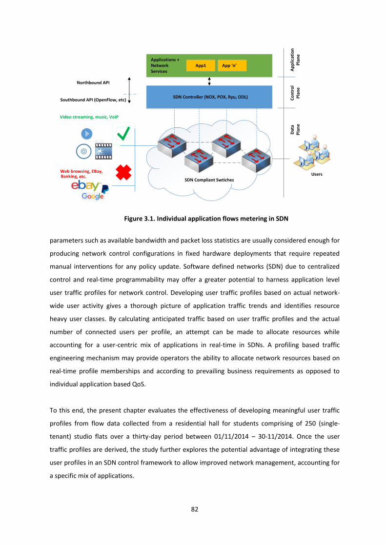
82

Figure 3.1. Individual application flows metering in SDN

parameters such as available bandwidth and packet loss statistics are usually considered enough for

producing network control configurations in fixed hardware deployments that require repeated

manual interventions for any policy update. Software defined networks (SDN) due to centralized

control and real-time programmability may offer a greater potential to harness application level

user traffic profiles for network control. Developing user traffic profiles based on actual network-

wide user activity gives a thorough picture of application traffic trends and identifies resource

heavy user classes. By calculating anticipated traffic based on user traffic profiles and the actual

number of connected users per profile, an attempt can be made to allocate resources while

accounting for a user-centric mix of applications in real-time in SDNs. A profiling based traffic

engineering mechanism may provide operators the ability to allocate network resources based on

real-time profile memberships and according to prevailing business requirements as opposed to

individual application based QoS.

To this end, the present chapter evaluates the effectiveness of developing meaningful user traffic

profiles from flow data collected from a residential hall for students comprising of 250 (single-

tenant) studio flats over a thirty-day period between 01/11/2014 – 30-11/2014. Once the user

traffic profiles are derived, the study further explores the potential advantage of integrating these

user profiles in an SDN control framework to allow improved network management, accounting for

a specific mix of applications.

83

3.3 Traffic classification challenges

User traffic classification methods have been extensively researched, with a common

denominator being the fact that detecting individual application packets is not an easy task in both

conventional and software defined networks. Port based application classification is prone to errors,

as most Internet applications use dynamic ports, with some using tunnelling via HTTP/S and SRTP

which makes classification virtually impossible. Standard QoS requirements embedded in packet

headers are also often ignored [60]. Deep packet inspection (DPI) is useful, however, owing the

computational cost associated with this technique, especially in real-time traffic identification,

somewhat limits its wide adoption. Other methods for traffic classification include crowdsourcing

based machine learning, application state analysis using DPI and DNS rendezvous classification

[168]. Application traffic classification based on payload analysis or using other novel techniques is

a research problem on its own and even crude classification can provide a great deal of insight even

if based on port-based classifications from flow logs [166]. In order to satisfy the scalability issues,

this chapter proposes a simple methodology of examining destination ports and IP addresses to

identify application traffic from raw flow records. The presented work focuses on extracting

meaningful user traffic profiles from readily available Netflow logs, ubiquitous in both legacy and

SDN-based networking equipment and their viability in making potential traffic management

decisions, specifically in the SDN. The approach integrates well with conventional and OpenFlow

compliant hardware and software switches (e.g., Open vSwitch), which can collect/export NetFlow

records for use in traffic analysis [123].

3.4 User traffic characterization

A number of features can characterize network traffic behaviour at varying levels of network

hierarchy. For example, traffic characterization at the network prefix level considered in [166],

presented a detailed overview of traffic characteristics at an ISP/backbone level using various

features such as daily aggregate traffic, frequently used application ports and flow size distribution

for traffic projection. Humberto et. al. in [169] characterized broadband user behaviour by

analysing flow records and employed consumer behavioural modelling graphs (CBMG) to

understand state transitions between application usage, while using k-means algorithm to classify

residential and SOHO customers as per their usage trends. The present study intended to

characterize traffic behaviour and associated flow statistics at user level by analysing user Internet

activity or application usage. However, instead of focusing on destination port numbers and generic

84

characterization based on IANA allocated ports, real world applications and websites were grouped

into specific tiers and user traffic behaviour was studied in relation to their corresponding usage of

these grouped applications. After collecting the statistical data for these applications, users were

also grouped into unique classes using machine learning techniques (clustering) based on similarity

in application usage ratios. The concept of correlating variables by using clustering algorithms for

pattern extraction is not new and has been previously used in numerous contexts. Heer and Chi in

[170] used similar clustering for classifying web user traffic composition for three specific websites

for capacity analysis. Yingqiu, Wei and Yunchun in [171] employed both supervised and un-

supervised machine learning techniques on flow data to classify application level traffic and

reported an accuracy of over 90% using k-means algorithm. However, these studies focused on

application classification from flow records using clustering, while this study seeks to utilize the k-

means algorithm for segregating users into classes based on their application trends. The next

section examines the study design including categorization of network traffic and cluster analysis

steps.

3.5 Profiling design

This study is based on the premise that per-user application level traffic and associated lower

layer statistics can provide a thorough, discriminative measure of user activity. The defined user

activity can, in turn, be used to implement user-centric traffic engineering solutions in SDNs,

instead of formulating network policies around specific applications or lower layer network

statistics. The profiling design therefore, seeks to satisfy the following objectives: (a) To

discriminate among user activities, the application flows generated per user premises are collected

and cluster analysed to derive user profiles for the observation period. (b) Depending on the

diversity of user activities recorded in the resulting profiles, the study would aid in understanding

the mix of user applications for subsequent utilization in designing profiling based traffic controls in

SDN.

In order to determine short and medium variations of user activity in the present study, traffic from

a residential student hall having 250 studio flats was collected over a 30 day period [01/11/2014 –

30/11/2014] and analysed to view the diversity in application usage captured in resulting user

profiles. Each flat consisted of a single user, and the traffic collected per user premise presented an

aggregation of multiple device activity (between 1-3 devices). The following sub-sections describe

the design considerations and the k-means clustering algorithm used during the study.

85

3.5.1 Defining application tiers

The Office of National Statistics in the UK broadly grouped online user activities into eleven

different categories ranging from sending and receiving emails to attending an online course [172].

A great degree of behavioural replication and similarity in traffic characteristics, however, usually

exists among users’ online activities and isolating each individual activity or application usage for

user profiling would be counterintuitive. For example, online video streaming websites like

YouTube and Netflix fall under the same umbrella of activity with rather similar traffic signature and

can be tiered together under one category of user activity. Similarly Yahoo Mail, Gmail, Hotmail and

traffic originating via POP3, SMTP protocols can be grouped as Email traffic without compromising

the projection of actual activity. The motivation to use such a categorization technique is the fact

that, besides reducing the computational cost of the clustering algorithm, the use of representative

application tiers leads to fewer variables in corresponding feature vector for building meaningful

traffic classes. For the purpose of this study, using typical internet usage applications/web

visitations as presented in [52], user activity was broadly grouped in the following tiers: general

web browsing (w), emailing (e), socializing (s), downloading (d), video streaming (v), gaming (g),

communications (c) along with typical destination web sites and protocols, summarised in Table 3.1.

On average, approximately forty popular applications or websites were included in the application

groupings. Separate groups were created to account for any unknown traffic (t) originating outside

the defined application tiers as well as network utilities (z) running in the background such as DNS.

3.5.2 Analysing user activity – feature vector design

Grouping applications into specific tiers, as per Table 3.1, results in defining a session of online

activity per user by vector ui [wi, ei, si, di, vi, gi, ci, ti, zi]. Constituent application traffic parameters of

vector ui are unique website visits identified based on destination of user traffic, i.e. the destination

IP address and protocol (with port number). The destination IP addresses of applications included in

Table 3.1 were collected by running DNS queries on websites of interest repeatedly and in different

time frames to accredit round-robin webserver load-balancing techniques employed by major

websites which change destination IP addresses. These mappings were further cross referenced

against mappings pre-configured in commercial network analysis tools like NetFlow Analyzer and

[173] PRTG Network Monitor [174] for greater accuracy.

86

Table 3.1. Application Groups

Application Tier Sample Popular Websites, Destination Port

Web browsing(w) General browsing using http(s) except below categories

Emailing(e) Gmail, Ymail, AOL, Outlook.com, SMTP, POP3, IMAP

Socializing (s) Facebook, Twitter, Blogger, WordPress, Tumblr, LinkedIn

Downloading(d) BitTorrent, VUZE, uTorrent, FTP, SmartFTP, FileZilla, CoreFTP

Video Streaming(v) YouTube, Netflix, Lovefilm, Megavideo, Metacafe, DailyMotion

Games (g) n4g, uk-ign, freelotto, 8-ball pool, Warcraft, Team Fortress

Communication (c) Skype, Net2Phone, MSN Messenger, Yahoo Messenger, GTalk

Unknown Traffic (t) Unaccounted TCP and UDP traffic

Network utility (z) DNS queries, Multicast traffic

3.5.3 K-means clustering algorithm

The primary aim of using clustering in the present study was to derive a meaningful set of

user traffic profiles by partitioning users into different groups based on their application usage,

which would give a complete overview of all user activities across the entire subscriber base. This

required designing a computationally efficient clustering technique. As discussed earlier in section

3.2.3, k-means is a prominent clustering algorithm previously used in similar network related

studies. The profiling methodology in the present chapter therefore, primarily used k-means

clustering algorithm which aims at minimizing a given number of vectors by choosing k random

vectors as initial cluster centers and assigning each vector to a cluster as determined by a distance

metric comparison with the cluster center (a squared error function) given in Eq. (3.1). Cluster

centers are then recomputed as the average (or mean) of the cluster members. This iteration

continues repeatedly, ending either when the clusters converge or a pre-defined number of

iterations have passed [175]. Compared to other methods such as hierarchical clustering, k-means

works well with a large number of variables and produces tighter clusters.

𝐽 = ∑ ∑ ||𝑥𝑖𝑗

− 𝑐𝑗||2𝑛𝑖=1

𝑘𝑗=1 (3.1)

In the above equation, ||𝑥𝑖𝑗

− 𝑐𝑗||2 is distance between individual values in a given vector and the

cluster center cj, n equals the size of the sample space (number of users) and k is the chosen value

for number of unique clusters (centroids). Hence, using k-means, n entities can be partitioned into k

groups. Choosing a value of k is of significant importance as it directly influences the number of

resulting groups i.e. derived user traffic profiles in the present case. As evident from Eq. 3.1, the

closer the value of k (number of centroids) to the number of users n, the greater will be the

resemblance between adjacent user traffic profiles rendering them meaningless, whereas a smaller

87

value would reduce the internal cohesion among members of a profile and over-generalize the

uniqueness of users. This particular aspect will be discussed later in detail in section 3.6.2 while

examining results.

3.6 Evaluation

3.6.1 Data collection

The study used flow records collected from a residential hall for students comprising of 250

studio flats. Each of the flats had an independent user CPE (router) connected via LAN to central

switches and Netflow logs were collected at the building default gateway (router) for all outbound

traffic originating from each customer router. Each studio flat comprised a minimum of one and a

maximum three user devices. For the purpose of user traffic profiling, the study primarily

concentrated on outbound user generated flows as these give an accurate representation of user

actions, however, total traffic transferred for both inbound and outbound traffic was still collected

to further examine the traffic distribution per user profile. NetFlow logs were concatenated every

24 hours over 30 days and parsed [Appendix – 1.1], to calculate the application traffic composition

vector per user as depicted in Table. 3.2 (truncated due to space). Network traffic for a user u1 on a

specific day [30/11/2014] can therefore, be represented by vector as given in Eq. 3.2. Each entity in

Eq. 3.2 represents the percentage of flows generated by the user u1 towards each of the application

tiers given in Table 3.1, for the given day.

u1 [30/11/2014] = [83 0.5 1.7 1.8 2 0.1 0.7 9.9 0.1] (3.2)

To account for limitations of the previously discussed technique for mapping IP addresses to

website domains, individual user traffic vectors were excluded from subsequent profiling where

these mappings were unsuccessful in identifying greater than 10% user traffic (ti > 10%). As a whole

this did not significantly reduce the sample space (number of users for effective traffic profiling).

The percentage of users that were excluded due to unaccounted application level traffic was always

Table 3.2. Traffic Composition Vectors [30/11/2014]

ui = [wi, ei, si, di, vi, gi, ci , ti , zi]

i User router IP

Flows w % e % s % d % v % g % c % t % z %

1 10.0.1.22 115 83 0.5 1.7 1.8 2 0.1 0.7 9.9 0.1

. … … … … … … … … ... .... ....

88

considerably less than a maximum observed value of 12% over any consecutive 24 hours during the

30-day data collection time span.

3.6.2 Clustering users

A total of 7594 unique user traffic distribution vectors for the user were examined comprising

approximately 50.3 million flows. Once flow records were concatenated for each day k-means

clustering algorithm was implemented on resulting vectors (Table 3.2) using R script [176][Appendix

– 2.1]. Since user traffic profiling was based on application usage, the assigned source IP addresses

of user CPE (routers) and numeric value of total flows were scalar entities for this analysis and

ignored from a clustering perspective. In addition, since general network service traffic (zi) such as

DNS queries are not a user-triggered application but a functional one and technically generated by

other application traffic, it was also excluded while clustering users and later separately calculated

as a percentage of total network flows generated per profile.

As previously mentioned, the primary aim of the clustering algorithm was to identify a smaller

number of anticipated usage patterns (defining for user traffic profiles) that can cover the complete

subscriber base. The profiles had to be meaningful enough to reflect user activities without

compromising on the mutual exclusivity of the profiles. Therefore, using values of k starting from

k=2, the size of the clusters and number of users per cluster was analysed as given in Table 3.3.

Choosing a lower value k resulted in a substantial membership size per profile but the ratio of

application traffic distribution per profile showed a great deal of over fitting of users in resulting

profiles to give a useful perspective. With higher values of k >4, profiles were too refined with the

majority of users only falling in particular profiles, rendering the number of users and traffic

distribution among other groups negligibly small. For example, k=6, resulted in six unique profiles

Table 3.3. Clusters vs Membership Size

Number of clusters k

(profiles)

Cluster Membership Size

(number of users in respective profiles) 2 6866, 728

3 6089, 1018, 487

4 5913, 1143, 283, 255

5 3949, 2837, 781, 17, 10

6 4280, 2198, 726, 350, 26, 14

7 3915, 2473, 793, 373, 17, 14, 9

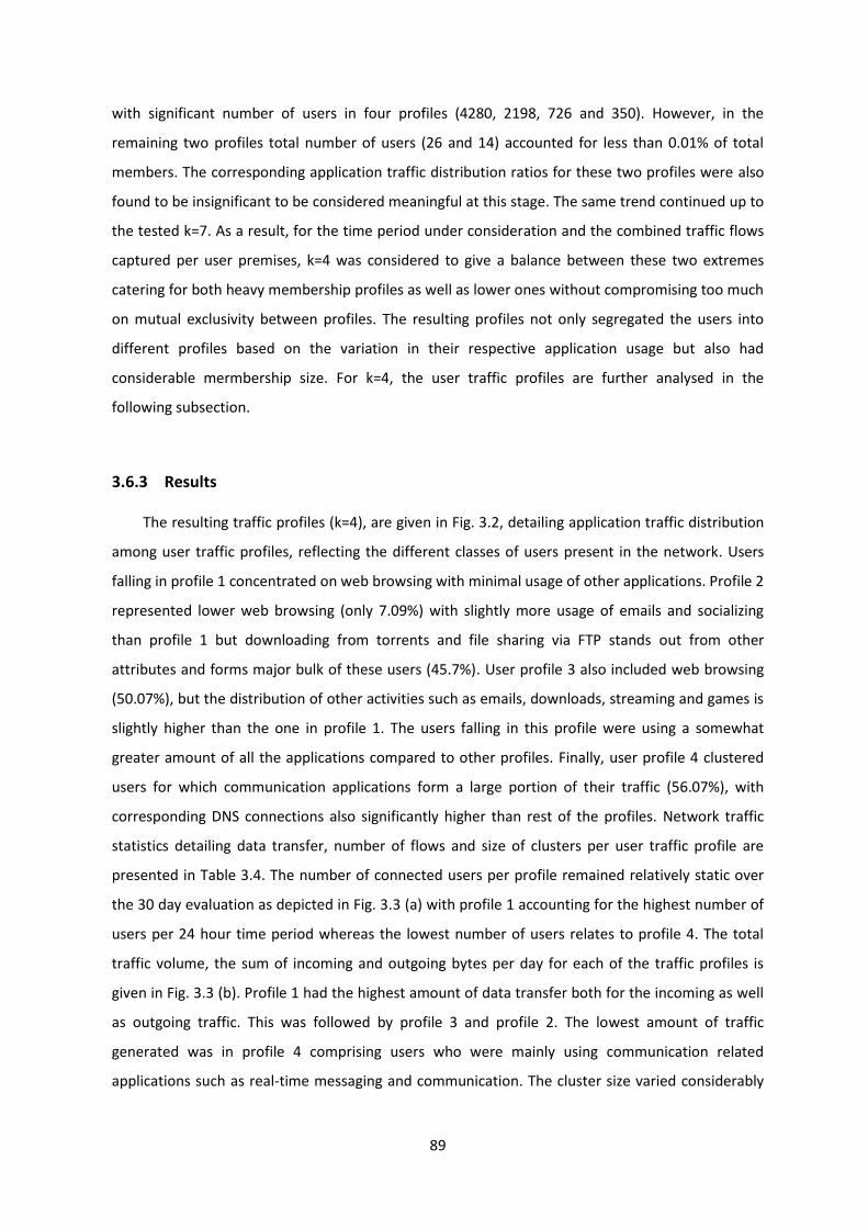
89

with significant number of users in four profiles (4280, 2198, 726 and 350). However, in the

remaining two profiles total number of users (26 and 14) accounted for less than 0.01% of total

members. The corresponding application traffic distribution ratios for these two profiles were also

found to be insignificant to be considered meaningful at this stage. The same trend continued up to

the tested k=7. As a result, for the time period under consideration and the combined traffic flows

captured per user premises, k=4 was considered to give a balance between these two extremes

catering for both heavy membership profiles as well as lower ones without compromising too much

on mutual exclusivity between profiles. The resulting profiles not only segregated the users into

different profiles based on the variation in their respective application usage but also had

considerable mermbership size. For k=4, the user traffic profiles are further analysed in the

following subsection.

3.6.3 Results

The resulting traffic profiles (k=4), are given in Fig. 3.2, detailing application traffic distribution

among user traffic profiles, reflecting the different classes of users present in the network. Users

falling in profile 1 concentrated on web browsing with minimal usage of other applications. Profile 2

represented lower web browsing (only 7.09%) with slightly more usage of emails and socializing

than profile 1 but downloading from torrents and file sharing via FTP stands out from other

attributes and forms major bulk of these users (45.7%). User profile 3 also included web browsing

(50.07%), but the distribution of other activities such as emails, downloads, streaming and games is

slightly higher than the one in profile 1. The users falling in this profile were using a somewhat

greater amount of all the applications compared to other profiles. Finally, user profile 4 clustered

users for which communication applications form a large portion of their traffic (56.07%), with

corresponding DNS connections also significantly higher than rest of the profiles. Network traffic

statistics detailing data transfer, number of flows and size of clusters per user traffic profile are

presented in Table 3.4. The number of connected users per profile remained relatively static over

the 30 day evaluation as depicted in Fig. 3.3 (a) with profile 1 accounting for the highest number of

users per 24 hour time period whereas the lowest number of users relates to profile 4. The total

traffic volume, the sum of incoming and outgoing bytes per day for each of the traffic profiles is

given in Fig. 3.3 (b). Profile 1 had the highest amount of data transfer both for the incoming as well

as outgoing traffic. This was followed by profile 3 and profile 2. The lowest amount of traffic

generated was in profile 4 comprising users who were mainly using communication related

applications such as real-time messaging and communication. The cluster size varied considerably

90

between profiles with the bulk of users falling in profile 1 (5913), followed by profile 3 (1143) while

profile 2 (283) and profile 4 (255) accounted for the smallest number of users.

Figure 3.2. User Traffic Profiles

Table 3.4. Traffic Statistics per Profile

Stats. Profile 1 Profile 2 Profile 3 Profile 4

Avg. outgoing bytes per day (GB) 17.40

1.61

2.87

0.19

Avg. incoming bytes per day (GB) 292.02

10.18

47.40

1.27

Avg. total traffic per day (GB) 309.42 11.79 50.26 1.46

Total traffic per month (GB) 9282.99 354.42 1508.48 22.84

Total traffic per day per user 1.57 1.31 1.32 0.09

Avg. users per day 197 9 38 8

Avg. % flows per day 57.74% 30.43% 11.80% 0.014%

Cluster size 5913 283 1143 255

91

Figure 3.3. (a) Aggregate traffic distribution per profile and (b) Users per traffic profile (30 days)

3.7 Applicability in software defined networking

From the user traffic profiling analysis, a significant degree of variation can, therefore, be

observed among users’ activities. While the majority of users fall within one user traffic profile (i.e.,

profile 1), there were however, a significant portion of subscribers who differed from the

mainstream in terms of their application usage ratios, and the amount of data transferred.

Implementing isolated application performance controls on users with such varying application

trends depicted in the extracted traffic profiles may definitely result in adverse performance for

some traffic classes. For example, improving performance of communication related applications

such as Skype in an SDN based environment by creating favourable flow forwarding constructs may

be of benefit to users in profile 4. During periods of high traffic which may lead to temporal

congestion due to constrained capacity, profile 4 users may continue to experience reasonable

performance due to VoIP QoS guarantees. However, other users in profile 1 and profile 3 who are

mainly engaged in web browsing activities may experience poor performance. Profiling user traffic

therefore gives network operators additional insight into user activities and resource utilization to

design and implement necessary network policies.

Extending the above rationale to the context of software defined networks, there is a potential to

employ user traffic profiles for effective traffic management. A diagram illustrating the

incorporation of profiling based controls in the SDN is presented in Fig. 3.4. The framework

comprises of a traffic profiling mechanism and a traffic manager. The traffic profiling framework

may collect flow measurements from the data plane, which are pre-processed and subjected to

cluster analysis to extract user traffic profiles. Utilizing the profile statistics as depicted earlier in

Table 3.4, the traffic manager gains a predictive view of traffic by monitoring number of connected

92

Figure 3.4. Incorporating User Profiling Controls in SDN Framework

users of each profile in real-time. The traffic profiles and incorporated statistics, can thereafter be

used for implementing profiling based traffic engineering such as the rate limiting of traffic flows

per user profile via flow tables in individual network elements, which are readily modifiable by the

controller using a southbound API such as the OpenFlow protocol.

Traffic could also be effectively load-balanced by the controller so that resource intensive traffic

profiles are off-loaded to high speed layer 1 links (e.g., optical cables) while others may be

redirected to or continue using relatively slower links as applicable based on the network topology.

Commercially, SDN controllers have already been developed to offload network traffic from specific

applications generating big data sets to optical networks in cloud data center environments for

improved efficiency [177]. User traffic profiling, however, employs actual user activities and

changing traffic conditions to balance network resources rather than rely on specific applications or

other L2/L3 criteria such as Differentiated Services Code Point (DSCP) for traffic management. An

operator using the SDN controller(s) may define policy control based on user profiles and

underlying network conditions to fully exploit real-time configuration capability of the data

forwarding plane by defining action sets, modifying flow entries and selecting outgoing ports/links

in NEs based on an accurate estimation and distribution of user traffic to balance or optimize

certain user classes.

93

Additionally, from a network monitoring perspective, once user traffic profiles have been derived,

the number of users and their respective data transfer trends, as depicted in Fig. 3.3 (a) and 3.3 (b),

reduce the need and frequency of profile re-computations, leading to only incremental adjustments

over time. For example, user traffic profiles may be computed in the offline mode once every

month, in a round-robin fashion, to avoid temporary overload while the total number of users and

their traffic volume (total data transfer) are monitored in real-time every 24 hours to check if these

conform to the expected values and match the profiles. If anomalies are observed (such as a

significant number of users falling out of trend with respect to total data transferred), the profiles

and relevant policies may be updated or re-evaluated.

3.8 Conclusion

This chapter proposed a method to derive user traffic profiles by extracting aggregate

application level data per user premises from NetFlow records and then clustering users together

based on their respective application usage trends. The resulting traffic profiles showed a

considerable degree of variation in user Internet activities and associated attributes such as average

number of flows, average data transferred and the distribution of users per profile. While prior

studies have offered isolated application level traffic engineering in SDNs, such methods may result

in inferior performance for a subset of users who combine a different range of applications or even

those using same applications with divergent usage ratios as evident from the derived profiles.

Integrating such user traffic profiles for traffic optimization is challenging in conventional fixed

topology networks due to ever-changing user activities and the manual interventions required in

updating policies. Software defined networks, however, through a centralized control framework

make real-time programmability of network elements much easier. The present chapter therefore,

proposed implementing flow metering and rate limiting based on user traffic profiles instead of

applications and also re-routing resource intensive traffic profiles over alternate links as applicable

depending on actual network topology. This would provide a much more comprehensive traffic

optimization solution in SDNs while accounting for a user-centric mix of applications.

Furthermore, the preliminary profiling investigation carried out in this chapter used aggregate

traffic from each of the residential housings comprising of multiple users /devices. The following

chapter explores profile extraction for each user device independently per customer premises,

employed in the present study. Profile derivation in multi-device user environments (such as

94

residential networks) provides further insight into user behaviour for designing and deploying

subsequent user-centric SDN based solutions in residential networking.

96

Chapter 4 Evaluating User Traffic Profile Stability

4.1 Introduction

User traffic characterization is of fundamental importance in modern networking environments

for understanding user behaviour that assists administrators and service providers in traffic

optimization, capacity planning, and improving security. Analysing network workload usually

requires collecting statistics around multiple traffic features, ranging from total traffic volume,

number and duration of user connections to application usage per consumer and provides network

managers the ability to anticipate both business and technological updates [169][178-183].

Proliferation of high speed residential broadband access over recent years, coupled with the

growing number of devices per household have compelled providers to seek ways of modelling and

understanding user behaviour for improved service differentiation and context based charging

[179][180]. As examined earlier in chapter 3, the segregation of users into traffic classes or profiles

as per their application usage simplifies the understanding and visualizing of user behaviour in the

context of network policy management. User traffic profiling in current residential and enterprise

networks, however, is no longer limited to a single device but multiple devices. Effective network

management particularly in modern networks, for example, residential premises where customers

usually have more than one device sharing a common internet connection, requires an

understanding of traffic patterns at the local level, inside the network as much as externally

[179][182]. Investigating and evaluating the frequency of profile transitions among multiple devices

per individual residential premises may give additional insight into user behaviour for subsequent

utilization in a residential SDN traffic management solution. This chapter, therefore, extends the

profiling methodology examined earlier to multiple users (devices) in each residential premises,

considered in chapter 3. Furthermore, three different clustering algorithms, the k-means,

hierarchical agglomerative technique and density-based spatial clustering (DBSCAN) are compared

to explore the resulting profiles and evaluate the technique which provides more meaningful

results. The derived profiles are benchmarked for stability and inter-profile transitions per user

device also studied, to ascertain the frequency of user behaviour changes with respect to each

device.

The profiling methodology follows (a) grouping popular internet applications into distinct categories

and classifying traffic using destination web server IP addresses and port numbers, (b) developing

device traffic profiles based on application usage trends using unsupervised cluster analysis and (c)

97

evaluating the probability of inter-profile changes among devices per premises to establish

transition trends and re-profiling frequency. Finally, the derived profile baselines are further

analysed for possible use in an SDN traffic monitoring and management solution targeting

residential networks.

The rest of this chapter is organized as follows. Section 4.2 highlights user behaviour

characterization in multi-device environments. Section 4.3 presents the technique used for data

collection of each user device from the respective residential CPE (routers), and feature based

clustering techniques. Section 4.4 evaluates the resulting traffic profiles and investigates profile

stability over the duration of the study as well as an analysis of inter-profile correlations. Section

4.5 discusses the incorporation of extracted profiles in residential SDN environments. Final

conclusions are drawn in section 4.6.

4.2 Multi-device user environments

The proliferation of high-speed residential broadband and increase in the number of devices

per household has highlighted the need to understand device traffic from inside the network for

effective network management and improved security. The predominant method of characterising

user behaviour in both enterprise and residential networks has been to cluster users based on

peculiarities in traffic features, using flow and packet based measurements or report these as

standalone attributes for monitoring overall network traffic as highlighted in [179], [181], [169] and

[182]. Xu. et. al [179], used IANA assignment of port numbers as the primary feature for clustering

device traffic inside user residences and identifying internet malware. To understand variations in

application usage among residential and SOHO broadband consumers, Humberto et. al [169]

employed k-means clustering and state transition graphs to depict the relationship between users’

Internet activities. Similarly, Jinbang et. al [182] studied user traffic profiling in modern enterprise

networks to understand the contrast between external and internal activities being carried out in

the network. From an external, service provider perspective, Jiang et. al [181] used k-means

clustering and aggregate consumer traffic flow to profile users on a number of traffic features

including application usage as well as flow-level parameters.

Profiling individual user devices in modern residential premises having multiple devices, as

illustrated in Fig. 4.1, presents an interesting avenue for understanding the temporal nature of user

98

Figure 4.1. A typical multi-device user network (residential)

activity per device. The profiling of application trends inside such multi-device environments aids in

determining whether the derived traffic classes lend considerable consistency over time to serve as

an effective tool for network monitoring and management. In residential SDN based traffic

engineering, for example, the enhanced trend visualization and application usage offered by traffic

profiles could aid in the creation of per profile dynamic resource allocation policies, according to

the requirements of the residential subscribers or externally by the service provider.

The primary necessity in user traffic profiling, however, remains, the need to classify application

traffic. As highlighted in chapter 3, novel methods such as machine learning classification

algorithms or deep packet inspection techniques either involve substantial processing overhead or

highly sanitized and pre-processed records for getting meaningful results as detailed in [183-186].

Service providers and network administrators have an imminent need for extrapolating subscriber

application usage and rely on commodity tools like NetFlow Analyser [173] and PRTG Network

Monitor [174] which partially circumvent the traffic identification problem by including pre-defined

customisable webserver IP addresses of frequently used applications and websites, matching these

to user requests for accounting. This scheme may seem limited but with careful planning and

continuous updating can be effectively used to report top applications and website visitations. The

present chapter, therefore, continued to utilize the IP address and port mapping method previously

employed from chapter 3 for identifying user application traffic. The next section discusses the

99

methodology employed for data collection as well as the different clustering techniques used for

user traffic profiling.

4.3 Profiling implementation

The present study, building on the preliminary investigation carried out in chapter 3 aimed

at profiling user devices in each residential premises based on the respective devices’ application

trends. The frequency of change in user activity was further assessed by observing profile

transitions per user-device to evaluate if derived profiles granted significant stability over time to

serve as benchmarks for formulating network management policies. The following subsections

detail the updates to application groupings and the monitoring setup employed for per device

profile derivation and describe the clustering algorithms used.

4.3.1 Application categorization

User traffic was classified by matching user requests (NetFlow records) against destination IP

addresses and ports used by popular internet applications as mentioned earlier. These were further

cross-referenced against commercial tools such as NetFlow Analyser [173] and PRTG Network

Monitor [174] for greater accuracy [Appendix – 1.1]. To account for replication in nature of user

activities, applications were once again grouped into distinct categories as depicted in Table 4.1.

Given the replication of traffic footprint between social tier and the web browsing tier observed

during the profiling analysis in chapter 3, the social tier was merged with browsing to concise the

application groupings and the resulting profiles. A unique website visitation or application usage on

user device could, therefore, be defined by the updated vector uij given in Eq. 4.1.

uij = [wij, eij, dij, vij, gij, cij , tij , zij] (4.1)

In equation 4.1 above, i and j are unique per user premises and user device respectively and

remaining entities represent the application usage percentage in accordance with the updated

application group given in Table 4.1.

4.3.2 Monitoring setup

The study used NetFlow records exported from the default gateway of a residential student

complex housing 250 user premises (studio flats) over a span of four weeks from 01/02/2015 to

100

28/02/2015. Each flat comprised a single user, having their CPEs such as home routers for

connecting multiple devices to the Internet. Each user had between one and three devices and all

user (premises) routers connected to the dedicated ports on two distribution switches, responsible

for forwarding and receiving traffic from the default gateway as shown in Fig 4.2. The SNMP

instances running on the distribution switches were used to report the IP address of each user

device connected to each customer router (mapped to the respective distribution switch port), to

account per device traffic flows.

4.3.3 Data Collection and Pre-processing

NetFlow records collected by the central collector were concatenated and customised

every 24 hours to build flow records incorporating traffic statistics. The resulting logs were

processed to quantize user device activity (flows) as a percentage of application usage in

accordance with Table 4.1. Afterwards, SNMP monitoring information from access switches was

used to associate the individual devices to user premises. Table 4.2 depicts a snapshot of the traffic

Table 4.1. Updated Application Groups

Application Tier Sample Popular Websites, Destination Port

Web browsing(w) Web browsing: http(s) except below groups

Emailing(e) Gmail, Ymail, AOL, Outlook.com, SMTP, POP3, IMAP

Downloading(d) BitTorrent, VUZE, uTorrent, FTP, SmartFTP, FileZilla, CoreFTP

Video Streaming(v) YouTube, Netflix, Lovefilm, Megavideo, Metacafe, DailyMotion

Games (g) n4g, uk-ign, freelotto, 8-ball pool, Warcraft, Team Fortress

Communication (c) Skype, Net2Phone, MSN Messenger, Yahoo Messenger, GTalk

Unknown Traffic (t) Unaccounted TCP and UDP traffic

Network utility (z) DNS queries, Multicast traffic

Figure 4.2. Network monitoring setup

101

composition matrix for a single day. Network activity for a user device u1,1 on a specific 24hour

interval, e.g. [01/02/2015], could therefore be represented by the application distribution vector

given in Eq. 4.2. In Eq. 4.2 each quantity represents the percentage of flows generated by the user’s

device towards the application tiers given in Table 4.1.

u1,1 [01/02/2015] = [76 0.2 1.1 1.4 7 0.3 1.8 12.2] (4.2)

Once application distribution vectors per user device were collected, traffic profiling was done

using both agglomerative hierarchical clustering as well as Hartigan and Wong implementation of k-

means [189] and DBSCAN [209], using R [176] [Appendix - 2.1, 2.2, 2.3]. To gain a better overall

understanding of the different users, unidentified traffic (z) was not excluded during cluster analysis

(as done previously in chapter 3), but included as a feature during clustering. The resulting traffic

profiles and associated analysis is detailed in the following section.

4.3.4 Traffic profiling

The objective of this profiling study is to seggregate user devices from the user premises into

unique profiles. Furthermore, the profiling scheme has to extract profile clusters, ideally eliminating

or minimizing outlier groups to a minimum. Eliminiation of outliers would contribute to having a

reasonable membership size (e.g., 10-20 members) for even a minimal activity profile. The

extracted device profiles may then be accordingly used to define user-centric network management

primitives in a residential SDN framework.

To achieve the above objectives in terms of profile extraction, three prominent un-supervised

clustering techniques were employed: hierarchical agglomerative clustering [187], k-means [175],

and density-based spatial clustering of applications with noise (DBSCAN) [209]. Hierarchical

clustering puts each observation in its own cluster and then calculates the distances between all

Table 4.2. Traffic Composition Statistics [01/02/2015]

User and Device ID Flo

ws

Application Usage

uij = [wij, eij, dij, vij, gij, cij , tij , zij]

;l

Flow

Duration

Data Volume

Us

er

(i)

Devi

ce (j)

SrcIP Flo

ws

w

%

e

%

d

%

v

%

g

%

c

%

t

%

z% Tx

Flo

w

Dur.

Rx

Flo

w

Dur.

Tx

(B)

Rx (B)

1 1 10.0.1.

22

115 76 0.

2

1.

1

1.

4

7 0.

3

1.

8

12.

2

4.74

6

2.12

3

388

6

98756

6 1 2 10.0.2.

75

85 24 2

3

1

5

9 0.

2

3 2.

3

32.

5

2.79

8

1.79

8

856

97

55587

26 … … … … … … … … … … … … … … … …

102

observations, pairing the closest two in a recurring fashion. The linkage function between the (pair-

wise) sets of observations may use the maxmimum distance (or complete linkage) or the more

advanced Ward’s method, which uses the decrease in variance for the respective clusters being

merged. K-means on the other hand, as mentioned earlier minimizes a given number of vectors by

choosing k random vectors as initial cluster centers and assigning each vector to a cluster as

determined by distance metric (Euclidean) comparison with the cluster center (a squared error

function) as given in Eq. 3.1, earlier in chapter 3. Cluster centers are then recomputed as the

average of the cluster members and the iteration continues repeatedly, ending either when the

clusters converge or after performing a specified number of iterations [175]. In Eq. 3.1, with respect

to multi-device user environments, cj continues represents the cluster center, n the size of the

sample space and k the chosen value for number of unique clusters (centroids). Hence, using k-

means, n entities, translating for user devices in the present case, can be partitioned into k groups

or profiles. The value of k is of significant importance as it directly influences the number of traffic

profiles and affects over-fitting of users into profiles. Rather than relying exclusively on manual

examination of trends in each cluster, as used earlier, the optimal value of k was calculated using

the automated Everitt and Hothorn technique [188], in tandem with manual examination of

derived profiles. The technique aims at finding the curve in cluster convergence with respect to

increasing k, with only minor variation beyond a certain level i.e the knee of the plot suggesting a

suitable value for cluster numbers.

In addition to k-means and hierarchical cluster analysis, the DBSCAN algorithm is among the

common techniques used in unsupervised cluster analysis. Given a set of data points in space, the

algorithm groups points that are closer together (having many neighbours). Data points falling in

low-density regions with minimum nearby neighbours are classified as outliers. As with all data

mining techniques, DBSCAN also requires prior parameter estimation for successful clustering.

However, unlike k-means, DBSCAN does not require an identification of the number of clusters in

the data a priori. The algorithm requires two parameters: ε, the size of the epsilon neighbourhood,

and minPts, the number of minimum data points that are required to define a dense region.

DBSCAN starts by selecting an arbitrary data point not visited before and computes its ε-

neighbourhood leading to the start of a cluster if the value conforms to the minPts defined by the

user. If the data point is found to be dense enough (according to ε and minPts), data points within

ε-neighbourhood also form a part of this cluster. The process continues until all the density-

connected points are found resulting in a complete cluster. If, however, the value of data points

within ε is below minPts, the selected data point is labelled as noise, which may or may not be

103

made a part of a cluster in subsequent iterations. The process continues with the selection of a new

un-visited data point. With regards to parameter estimation, the value of ε may be computed using

a k-distance graph (k-NN plot), where the curve in the graph points to an appropriate value of ε

[266]. A very small value may result in a great deal of noise points and unclustered data, while a

large value may result in majority of data points being under the same cluster. The minPts

parameter may be computed according to minPts ≥ D + 1, where D is the dimension of the data

points to be clustered. Again, a minimum value for minPts such as 1 would result in each data point

forming a cluster, while a very large value may result in the merging of otherwise independent

clusters. Parameter estimation and resulting clusters, translating in user traffic profiles in the

present case for the respective clustering algorithms will, therefore, be considered in detail to

derive meaningful user profiles during evaluation in section 4.4.

4.4 Evaluation

4.4.1 Cluster Analysis

A total of 10095 unique traffic distribution vectors for user devices were examined comprising

approximately 178.21 million flows. The resulting vectors were subjected to hierarchical and k-

means clustering and cluster memberships were evaluated for cluster sizes ranging between 2 to 10

as depicted in Table 4.3. Using the default maximum distance linkage (or complete) method in

hierarchical clustering, profile membership numbers resulted in minimal number of observations in

some clusters. The more advanced Ward’s method and k-means, however, resulted in much more

significant membership numbers across all the derived clusters. The next step was finding the

optimal number of clusters (translating for traffic profiles) that would appropriately reflect user

activities. Clusters derived using k-means were examined starting from k=2, using Everitt and

Hothorn technique given in [188]. This technique aims to find the curve in plot of ‘within groups

sum of squares distance’ per observation in each cluster against k for suggesting an appropriate

number of profiles that fit the input data. The corresponding plot for the present data is given in Fig.

4.3 where a significant drop can be seen up to a cluster size k=6, with minimal variations up to k=15,

which indicates an optimal value of 6 profiles. Application distribution ratios for profiles derived

using both hierarchical clustering (Ward’s method) and k-means were afterwards, compared to

ascertain which set presented meaningful results. While profile membership numbers per cluster

using either method were quite similar, profiles derived using k-means gave a much clearer

segregation of user activities. For example, for six profiles, hierarchical clustering resulted in three

104

Table 4.3. Profile Membership Distribution per Cluster (hclust and k-means)

# Clusters

Hierarchical Clustering (method= max)

Hierarchical Clustering (method=ward)

k-means

2 10094, 1 6316, 3779

8236, 1859

3 10002, 92, 1 6316, 2365, 1414

6172, 2576, 1347

4 9742, 260, 92, 1 6316, 2365, 1216 , 198

5013, 2642, 1272, 1168

5 9742, 255, 92, 5, 1 3904, 2365, 2412, 1216 , 198

6339, 2473, 970, 228, 85

6 8815, 927, 255, 92, 5, 1 3904, 2412, 2365, 687, 529, 198

5013, 2644, 1249, 880, 224, 85

7 7868, 947, 920, 255, 92, 5, 1

3904, 2412, 1253, 1112, 687, 529, 198

3965, 2660, 1538, 828, 224, 795, 85

8 7868, 947, 920, 255,

90, 7, 5, 1 3904, 2412, 1253, 1022, 687, 529, 198, 90

3736, 2607, 1574, 765, 693, 417, 218, 85

9 7868, 947, 920, 255, 90, 7, 5, 2, 1

3904, 2412, 1253, 757, 687, 529 , 265, 198, 90

4318, 2637, 944, 699, 602, 439, 222, 180, 54

10 7868, 920, 905, 255, 90, 42, 7, 5, 2, 1

2412, 2186, 1718, 1253, 757, 687, 529, 265, 198, 90

3623, 2399, 1018, 856, 667, 626, 359, 248, 214, 85

Figure 4.3. Identifying correct number of clusters (wss vs. k)

profiles having similar web-browsing ratios of 92.26 %, 83.45% and 77.39% compared to only two

profiles with high web-browsing and well-parted usage ratios of 90.04 % and 62.84 % derived by k-

means. This trend continued up until the maximum examined value of ten profiles.

To calculate an approximate value for the eps value (ε) to be used in DBSCAN clustering, a k-

distance graph was plotted (using k= ‘dimension of data D’ +1 =9), based on the 8-dimensional

application tiers given in Table 4.1 [266]. The relevant 9-NN distance vs data points plot is depicted

in Fig. 4.4. The ‘knee of the curve’ in the graph provides an approximation of the eps (ε) distance to

be around 8, 10 or 12. Additionally, as discussed earlier, selection of the second minPts parameter

is equally important in dictating the efficacy of the resulting clusters. Therefore, three different

105

values were chosen to be used with each approximate eps (ε) value. A relatively smaller value of 5

(default in R dbscan package) [210] was selected to generate the maximum number of clusters and

analyse their respective membership and noise. Afterwards higher values of minPts (minPts ≥ D +

1) i.e. 10 and 50 were chosen to reduce the total number of clusters and observe the variation in

resulting per-cluster membership. The derived clusters for each eps (ε) and minPts combination are

given in Table 4.4. As with hierarchical clustering, the DBSCAN clusters depicted in Table 4.4

showed a great deal of over-fitting of data points. For the smaller value of minPts=5 or minPts=10,

for each selected ε value, DBSCAN clustering resulted in a large number of clusters (between 7 to

17). However, significant variation in membership distribution of the data points was observed in

the derived clusters. While a few clusters comprised the majority of data points, remaining had

substantially low membership rendering them meaningless for profiling purposes. Relatively larger

value of minPts=50, resulted in far fewer clusters (3 to 4). However, it was again noted that either

one or two clusters contained the majority of the data points with remaining clusters having

minimum membership. The number of outliers for minPts=50 was also quite high, ranging between

244-1060, and denoting that a significant number of data points did not associate with any of the

derived clusters and were considered as noise. This did not fit well with the earlier stated

requirement of reducing outliers to a minimum. Despite using different minPts values with each ε

approximation, the clusters derived using DBSCAN did not therefore present satisfactorily

expressive results, when compared to the clusters derived using k-means. The profiles derived

using k-means (k=6), in the present case, represented a more meaningful balance catering for both

heavy membership profiles as well as lower ones without compromising too much on mutual

exclusivity or overfitting of users. The application usage per profile derived using k-means clustering

is analysed in the following sub-section.

Figure 4.4. K-distance graph (ε- eps estimation)

106

Table 4.4. Profile Membership Distribution per Cluster (DBSCAN)

# Clusters ε- eps minPts Membership Size Noise Points

17 8 5 9396, 183, 47, 36, 23, 13, 13, 7, 7, 7, 7, 5, 5, 5, 5, 4, 4

327

10 8 10 9152, 130, 176, 36, 36, 23, 14, 13, 13, 12 490

4 8 50 8169, 621, 132, 113 1060 15 10 5 9530, 186, 51, 37, 23, 13, 13, 9, 6, 6, 8, 7, 6,

6, 4 190

7 10 10 9457, 184, 39, 37, 23, 13, 13 329

3 10 50 9079, 124, 168 724 11 12 5 9621, 195, 74, 28, 19, 17, 11, 6, 5, 5, 3 111 5 12 10 9571, 186, 63, 17, 14 244

3 12 50 9241, 124, 177 553

4.4.2 Results

The application usage distribution for each of the six derived traffic profiles is given in Fig. 4.5.

Compared to the profiles derived in chapter 3, the updated design accounting for individual user

devices in each customer premises as well as the inclusion of unidentified traffic flows resulted in

the addition of two more profiles. The corresponding graphs illustrating per-profile membership

and flow statistics over the observed duration are presented in Fig. 4.6 – Fig. 4.7.

Profile 1 concentrated mainly on web browsing (68.92%), with minimal usage of other applications,

including downloads (3.46%), streaming (1.29%), communications (1.67%) and significant unknown

traffic (8.68%). The devices in this profile may therefore, be summarized as high intensity web-

surfers. Profile 1 also had the highest number of device membership. Moving on, profile 2 also

concentrated on heavily on web browsing, and although the browsing component was significantly

higher (>90%) as compared to high intensity surfers, other application usage was minimum, apart

from unknown traffic flows (2.06%). The devices in profile 2 could be labelled as low-intensity web

surfers, having a comparatively lower traffic volume than profile 1 and second highest number of

profile membership. Profile 3 also inclined towards web browsing, but traffic distribution among

other activities such as emails (2.19%), downloads (3.59%), streaming (1.60%) and games (2.19%)

was slightly higher than both high and low intensity surfers. The unknown traffic flows in this profile

were substantial (23.25%). Closer examination of the unknown traffic samples revealed that

approximately 57%-59% of traffic flows targeted online gaming servers. Due to their proportional

use of many applications in addition to gaming such as communications and streaming, devices in

this profile can be categorized under all-rounders (or gamers). User devices in Profile 4 were heavily

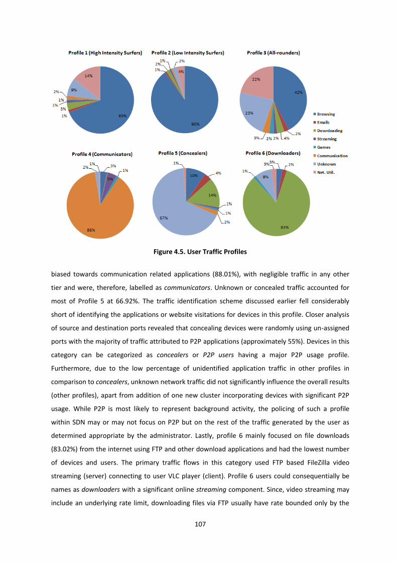
107


biased towards communication related applications (88.01%), with negligible traffic in any other

tier and were, therefore, labelled as communicators. Unknown or concealed traffic accounted for

most of Profile 5 at 66.92%. The traffic identification scheme discussed earlier fell considerably

short of identifying the applications or website visitations for devices in this profile. Closer analysis

of source and destination ports revealed that concealing devices were randomly using un-assigned

ports with the majority of traffic attributed to P2P applications (approximately 55%). Devices in this

category can be categorized as concealers or P2P users having a major P2P usage profile.

Furthermore, due to the low percentage of unidentified application traffic in other profiles in

comparison to concealers, unknown network traffic did not significantly influence the overall results

(other profiles), apart from addition of one new cluster incorporating devices with significant P2P

usage. While P2P is most likely to represent background activity, the policing of such a profile

within SDN may or may not focus on P2P but on the rest of the traffic generated by the user as

determined appropriate by the administrator. Lastly, profile 6 mainly focused on file downloads

(83.02%) from the internet using FTP and other download applications and had the lowest number

of devices and users. The primary traffic flows in this category used FTP based FileZilla video

streaming (server) connecting to user VLC player (client). Profile 6 users could consequentially be

names as downloaders with a significant online streaming component. Since, video streaming may

include an underlying rate limit, downloading files via FTP usually have rate bounded only by the

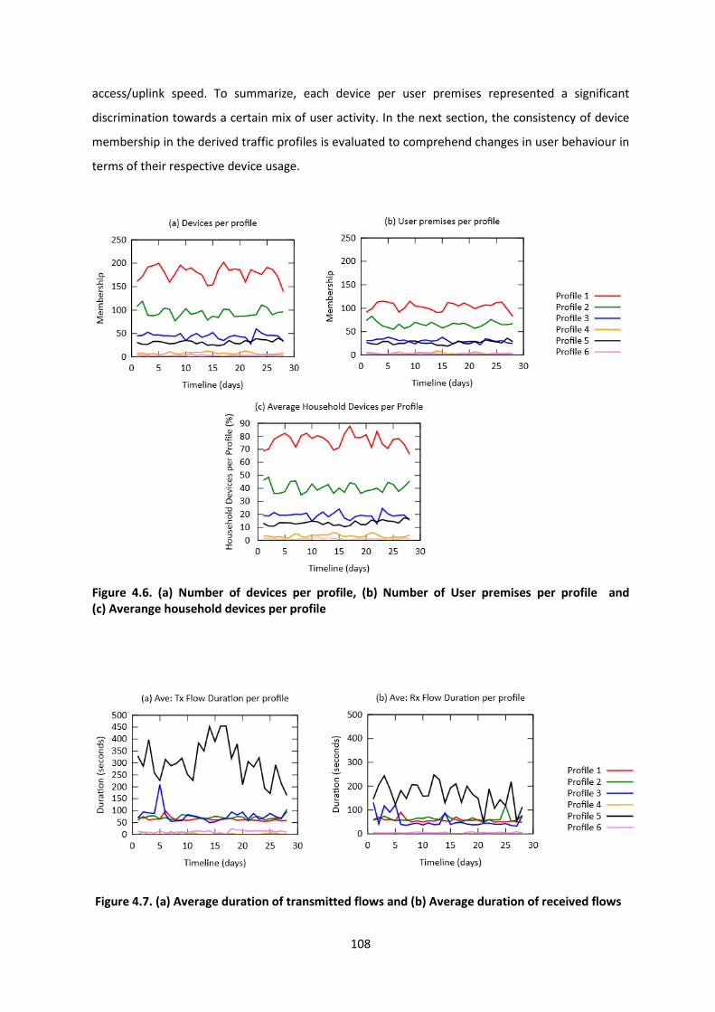
108

access/uplink speed. To summarize, each device per user premises represented a significant

discrimination towards a certain mix of user activity. In the next section, the consistency of device

membership in the derived traffic profiles is evaluated to comprehend changes in user behaviour in

terms of their respective device usage.

Figure 4.6. (a) Number of devices per profile, (b) Number of User premises per profile and (c) Averange household devices per profile

Figure 4.7. (a) Average duration of transmitted flows and (b) Average duration of received flows

109

Figure 4.8. (a) Total number of flows per profile and (b) Total data volume per profile (Bytes)

4.4.3 Profile Consistency

Profile consistency emphasises the importance of gaining a better insight to changes in user

activity per device as well as requirements or frequency for re-profiling. A user that browses for one

hour on a particular day might be clustered in a different profile if using a range of applications for

a much longer duration (e.g, 10 hours) on a different day due to bigger overall traffic/activity. To

determine the number of devices per profile and their mutual correlations, the Pearson’s

correlation coefficient [190] was used with the results given in Fig. 4.9. A negative correlation co-

efficient would indicate an inverse relationship with one profile gaining more devices and the other

losing, however, not necessarily among the same profile pairs. Positive values refer to an increase

in devices for both pairs. Values closer to zero represent no meaningful relationship, translating for

minimal increase or decrease in devices per profile pair. As shown in Fig. 4.6, there is a blend of

both negative and positive correlations representing changes in number of devices per profile.

Using Fisher’s transformation, the average value of correlation co-efficient was calculated to be -

0.0931 [191]. The relatively low average indicates no significant change in device numbers per

profile, with a slight bias towards an inverse relationship between each profile pair. To further

evaluate, the user device profile retention, the average probability of change in device profiles per

subsequent day of study was computed and is given in Table 4.5. Downloaders showed the highest

consistency in retaining profiles at 97% while all-rounders showed lowest at 81%. The probability of

a profile gaining or losing a device every 24 hours is also highlighted in Table 4.5 The downloaders

had the highest probability of gaining a device (60%) with high intensity web surfers having highest

probability of losing a device (59%).

110

Where devices did change profiles, the average probabilities of inter-profile transitions every 24

hours are given in Table 4.6. It was observed that where devices transitioned to a different profile,

it was always to profiles having somewhat similar application usage ratios to their own. For

example, low surfers would transition to high surfers (8%) compared to other profiles. Concealers

did not show any significant change in profile, except to all-rounders which was also quite minimal

(5%). This further emphasized the fact that majority of devices within this group more closely

followed an application dictated pattern of behaviour mainly due to P2P activities. Downloaders

seldom changed profiles highlighting that the small number of devices in this profile were also

being dedicatedly used for streaming videos from the internet-based servers. Hence, where there

was a transition observed among the traffic profiles, it was only due to variation in the same user

activity rather than a complete change of role per device. Users, therefore, continued to use the

same devices for same kind of activity albeit in varying proportions rather than showing drastic

changes in their normal routine.

Figure 4.9. Pearson Correlation Co-efficient between Device Profiles

111

Table 4.5. Average Probability of Profile Change (/24 Hrs)

User Profiles Probability of No Change

Probability of Change

Change Prob. Device Gain Prob. Device Loss

H. Int Surfer 0.87 0.13 0.40 0.59

L. Int Surfer 0.88 0.11 0.46 0.53

All-rounder 0.81 0.18 0.42 0.57

Comms. 0.84 0.15 0.57 0.42

Concealers 0.87 0.12 0.48 0.52

Downloaders 0.97 0.03 0.60 0.40

Table 4.6. Average Probability of Inter-Profile Transition (/24 Hrs)

User Profiles High Int. WS Surf

Low Int. WS

All-rounders

Commmunicators Concealers Downloaders

High Int. WS 0.87 0.08 0.03 0.0015 0.007 0.001

Low Int. WS 0.08 0.88 0.01 0.01 0.008 0.002

All-Rounders 0.11 0.03 0.82 0.003 0.032 0.0005

Communicators 0.09 0.06 0.05 0.84 0.001 0.001

Concealers 0.03 0.03 0.05 0.0006 0.87 0.002

Downloaders 0.0005 0.001 0.0001 0.0004 0.0005 0.97

4.5 Effective network management in residential SDN

The derived traffic profiles showed a high level of consistency in terms of membership numbers.

Hence, once the traffic profiles have been derived based on application usage ratios, the baselines

of network traffic per profile as depicted in Fig. 4.6 - Fig. 4.7 provides an intuitive means to monitor

the residential network. Daily aggregate traffic can be effectively examined by analysing value

changes in traffic metrics per profile with any anomalies serving as an advisory to trigger a re-

evaluation of profiles and identify network abnormalities. For end users wanting to better manage

their data usage, service providers may employ traffic profiling to place users into correct

subscription models while also providing them with their daily traffic projections through service

provider portals or customer home gateways.

Traffic profiling therefore, provide administrators with enhanced capability to monitor network

activity and update capacity based on anticipated user behaviour for achieving better quality of

experience. It may also aid in protecting users from security threats or in enforcing policies. For

example, in the present case concealers (P2P users) either could be rate-limited or blocked by

making provisions in the individual customer routers shown in Fig. 4.2 to enforce the underlying

network usage policy.

112

Furthermore, despite growing Internet speeds, the last mile access infrastructure of the service

provider remains a source of network contention due to an ever-increasing range of greedy,

bandwidth demanding applications. By using an SDN based traffic engineering framework between

the residential gateway and the service provider, provisions may be made that allow residential

users to prioritize certain user profiles within their network to better manage the last mile

bandwidth. The utilization of policy primitives that dictate the distribution of available bandwidth

among different profiles, may allow fine-tuning the resource (bandwidth) allocation among multiple

residential users with relative ease. The next chapter presents an SDN based traffic management

application to this effect.

4.6 Conclusion

The present work focused on profiling multi-device user traffic in a residential network based

on application usage using three different analysis techniques i.e. k-means, hierarchical and

DBSCAN unsupervised clustering. The profiles derived using k-means presented a more meaningful

view of application usage among different classes. The six unique user profile extracted were

further benchmarked every 24 hours to ascertain their stability. Over the four-week observation

period, the analysis indicates that the number of users and devices per profile remained fairly

consistent. Any inter-profile transitions were mainly due to proportional variation in same kind of

user activity triggering a device profile change (to a somewhat similar profile in terms of application

usage). The overall high rate of profile consistency reported even in this multi-device environment

enhances the feasibility of validates using the extracted profiles for effective network management

and defining and implement network policies.

Despite recent improvements in the Internet broadband speed, residential users often experience

bandwidth contention, especially when several users are simultaneously using bandwidth intensive

applications. As a test case, the following chapter utilizes the extracted profiles in a custom

designed SDN application to effectively manage the residential network. The framework allows

residential users to create network policy primitives which define the bandwidth allocation priority

among different user profiles when several users are simultaneously connected to the Internet. The

application is tested in a simulation environment to validate the employability of traffic profiles in

residential based SDN for network monitoring and management purposes.

114

Chapter 5 User-Centric Residential Network Management

5.1 Introduction

Residential networks are getting increasingly difficult to manage due to the ever-growing

number of devices, diversity in application usage and evolving traffic patterns of end users. A typical

residential network incorporates several end user devices sharing the same Internet connection,

each with varying application usage [192][193]. Despite a substantial increase in internet uplink and

downlink speeds [194], managing uplink and downlink bandwidth, a finite resource, among several

users in the same premises is a challenging task [47][49][107]. Changing traffic patterns in

residential networks may require repeated manual interventions to adjust policies at the residential

router to satisfy individual user requirements, coupled with the fact that there is seldom a clear

understanding of the application usage mix of all users to correctly implement user based rate-

limiting or bandwidth capping [195]. Real-time re-programming provided by SDN may significantly

improve flexibility in resource management inside the service provider’s network [51], but equally

important is the effective allocation of resources for users residing towards the edge, more

specifically users inside the residential network. Prior studies such as [49], proposed virtualization

of residential gateways and their inclusion into the service provider SDN framework for simplifying

administration. Other approaches suggest reactive traffic shaping based on performance

monitoring of data retrieved from residential gateways and managing bandwidth usage by

allocating data usage caps to each device [107]. While this reduces the burden of residential

network management from the end user, such an arrangement also raises user privacy concerns

and presents scalability issues for the service provider SDN controller in managing routers for

individual end users. To allow greater user control over their network, Mortier et al. in [47]

proposed a similar strategy leveraging SDN technology for managing residential routers while

Chetty and Feamster in [195] argued for better user interfaces allowing users to accurately set up

network policies based on usage quotas. Existing approaches of controlling network congestion

through dynamic queue management in both SDNs and legacy networks look promising in

mitigating latency and packet loss at the application level [197-199].

The refactoring of the residential network through abstracted high level policy based management

via a software defined networking framework although appears to be a viable choice

[47][49][51][52][196], it raises prioritization issues to determine which user devices to cap and what

applications to expedite. As identified in chapter 4, per user application usage ratios may vary

115

significantly within residential networks. Employing the default method of flow metering specific

applications to control forwarding constructs in SDNs or using advanced congestion control

adaption schemes such as active queue management [197-199], to better manage packet queueing

may fall short of satisfying individual user requirements in terms of real-time resource allocation.

In this context, it is vital to understand the users’ behaviour inside the residential network to

accurately define and apply any such resource allocation policies in the first place. Instead of using

individual applications, user traffic profiling can be used to derive different user classes present in

the network on the basis of actual application usage while also providing an estimation of per-

profile bandwidth consumption to achieve better traffic management schemes catering to all users

[200]. As previously discussed in chapter 3 and chapter 4, user traffic profiles may be derived based

on the percentage of generated flows (NetFlow records) per user for each pre-defined application

tier and further subjected to unsupervised k-means clustering to derive unique user traffic classes.

Characterizing network workload using per-user application distribution ratios (user profiles)

accurately expresses user activities and aids in implementing user-centric traffic engineering

solutions. The present chapter, therefore, proposes and develops a dynamic queueing based user-

centric traffic optimization scheme utilizing the extracted user traffic profiles and user defined

profile priorities to effectively manage the allocated downlink and uplink bandwidth among several

users in a residential SDN. As part of the validation phase, an SDN application is designed for

allocating per profile bandwidth among residential users, and tested in a Mininet based simulation

environment under different traffic scenarios to evaluate its effectiveness.

The remainder of this chapter is organized as follows. Section 5.2 details the traffic management

design, highlighting user profile prioritization and the queue assignment algorithm for per-profile

resource allocation. Section 5.4 evaluates the proposed design and resulting improvements, and

conclusions are drawn in Section 5.5.

5.2 Design

The user-centric traffic management design proposed in the present chapter employs a Ryu

SDN controller [30] supporting OpenFlow architecture [17] and utilizes egress QoS queueing for

rate-limiting per-profile traffic and allocating of link capacity to individual user flows. The design

comprises of two components (i) a profile derivation framework and (ii) an SDN based traffic

116

management application. The details of each component are further discussed in the following sub-

sections.

5.2.1 Profile derivation framework

Due to their scalability of use, NFV and SDN technologies such as Open vSwitch as well as many

vendor hardware switches and OpenFlow ports on other platforms (OpenWRT, Pantou, etc.)

support flow-based monitoring and are capable of exporting NetFlow logs [48]. As previously

discussed in chapter 4, NetFlow can be used to derive user traffic profiles based on the percentage

of generated flows per user for each pre-defined application tier and further subjected to

unsupervised k-means clustering to derive unique user traffic classes. Applications can be identified

using destination webserver IP addresses or using other Layer 7 classifiers. A typical residential

router is, therefore, able to export NetFlow logs either by default or by operating system updates.

The resulting flow records can be cluster analysed internally in the residential gateway (provided an

enough memory and CPU resource is available) or exported to an external server for profile

derivation, which may also act as the network attached SDN controller.

An architectural view of the profiling engine designed based on studies in earlier chapters for

deriving profiles of user devices connected to the residential gateway of an OpenFlow capable

switch (e.g. OpenWrt) [15][17][200] is given in Fig. 5.1 [Appendix – 2.4]. Individual applications can

be identified using reverse DNS lookup on destination webserver IP addresses or other Layer 7

classifiers. The resulting profiles are stored and continuously monitored with any flight from

benchmarked baselines triggering re-profiling.

5.2.2 Traffic management application

The traffic management application employs the Ryu SDN framework. Ryu provides several

software modules with well-defined APIs making it possible to create real-time network monitoring

and control applications with ease [30]. The controller component has built-in support for

managing network devices, using the popular southbound OpenFlow protocol. The Ryu framework

provides three primary methods for QoS prioritization of flows: ingress policing of incoming flows

via rate-limiting, egress traffic shaping by associating outgoing flows to assigned queues and lastly

by meter tables [17]. The first two schemes have been implemented in OpenFlow compatible

switches such as the Open vSwitch [86]; however, meter tables, although a part of the OpenFlow

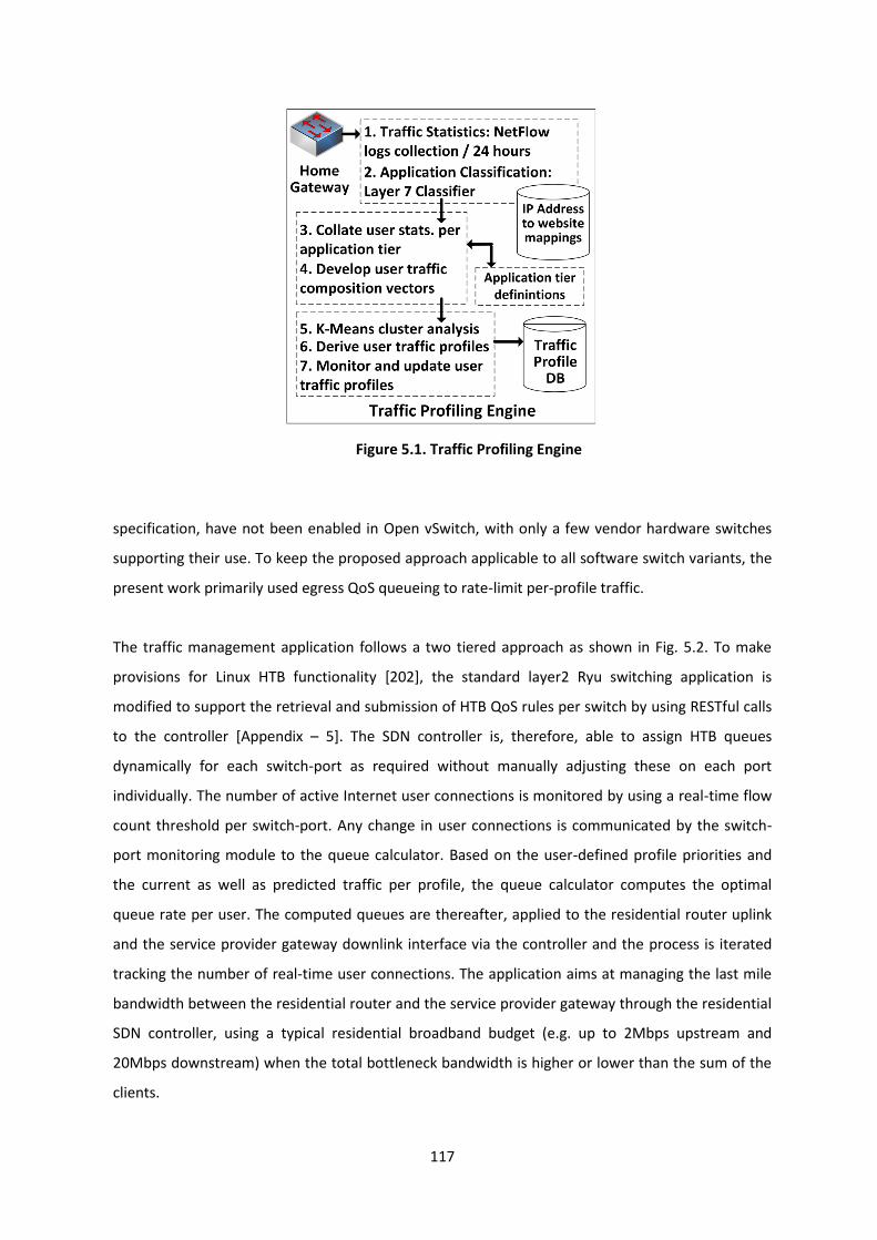
117

Figure 5.1. Traffic Profiling Engine

specification, have not been enabled in Open vSwitch, with only a few vendor hardware switches

supporting their use. To keep the proposed approach applicable to all software switch variants, the

present work primarily used egress QoS queueing to rate-limit per-profile traffic.

The traffic management application follows a two tiered approach as shown in Fig. 5.2. To make

provisions for Linux HTB functionality [202], the standard layer2 Ryu switching application is

modified to support the retrieval and submission of HTB QoS rules per switch by using RESTful calls

to the controller [Appendix – 5]. The SDN controller is, therefore, able to assign HTB queues

dynamically for each switch-port as required without manually adjusting these on each port

individually. The number of active Internet user connections is monitored by using a real-time flow

count threshold per switch-port. Any change in user connections is communicated by the switch-

port monitoring module to the queue calculator. Based on the user-defined profile priorities and

the current as well as predicted traffic per profile, the queue calculator computes the optimal

queue rate per user. The computed queues are thereafter, applied to the residential router uplink

and the service provider gateway downlink interface via the controller and the process is iterated

tracking the number of real-time user connections. The application aims at managing the last mile

bandwidth between the residential router and the service provider gateway through the residential

SDN controller, using a typical residential broadband budget (e.g. up to 2Mbps upstream and

20Mbps downstream) when the total bottleneck bandwidth is higher or lower than the sum of the

clients.

118

Figure 5.2. Traffic Monitoring and Control

5.2.3 Test Profiles

In order to ensure that the proposed method matches a real network scenario, the present

study utilized profiles derived earlier in chapter 4, from a residential network housing

approximately 250 user premises. The unknown traffic flow component for each derived profile

was accounted using offline destination IP and port address analysis. User profiles and traffic

statistics were accordingly updated. Identification of unknown traffic (z), merging of browsing (w)

and Email tiers (e) resulted in the application tiers being reduced to five to better reflect the user

activities. Fig. 5.3 summarizes the application usage for each profile as a percentage of user

generated flows. Profile 1 concentrated mainly on web browsing (85%) with limited usage of other

applications and remained as high intensity web-surfers. Profile 2 also concentrated on web

browsing (95%); however, with extremely limited usage of any other application and also lower

data usage as compared to high intensity surfers, hence users in this profile were called low-

intensity web surfers. Profile 3 inclined towards online video streaming via FileZilla FTP server, and

traffic distribution among other activities (emails, downloads and games) was relatively lower than

both high and low intensity surfers. These users were therefore, accordingly named streamers. User

devices in Profile 4 heavily tilted towards using communication related applications (88%), and

therefore, labelled as communicators. Online games traffic accounted for most of Profile 5 at 60%.

Users in this profile were categorized as gamers. Profile 6 mainly focused on downloading using P2P

clients. A substantial proportion of traffic flows in this profile comprised of unknown traffic that

was attributed to P2P usage (55%), as examined earlier in chapter 4 and, therefore, named as P2P

users in the present work. Additionally, to account for guest users, representing one-off network

users or users not having any statistical usage information for profile derivation, a guest profile was

created. Table 5.2 represents the average upload and download rate per profile and total data

119

consumption every 24 hours. Streamers had the highest average data transfer rates having 270kbps

upstream and up to 6300kbps downstream. This was followed by P2P users and communicators.

Low intensity web surfers accounted for lowest data rates at 75kbps upstream and up to 175kbps

downstream per user. Hence, the average data rates varied for each user category with some users

such as low intensity web surfers only consuming a small proportion of bandwidth compared to

others and residential users may want to prefer certain user categories over others when multiple

users are connecting to the internet and simultaneously competing for bandwidth.

5.2.4 Setting User Profile Priority

Traffic congestion in residential networks can cause performance degradation for users even

with a decent speed connection depending on other users’ activities [203][204]. The derived user

traffic profiles provide residential users with a useful insight into the mix of user classes, their

application trends and resource consumption to help alleviate network management difficulties. To

give the residential users control over which users to prioritize in terms of bandwidth allocation the

proposed policy language uses a prioritization value associated with each derived profile to

coordinate the challenges of managing shared network bandwidth. Table 5.1 depicts a sample

priority level for queue assignment and the corresponding required data transfer (queue) rates per

user. Low-intensity web surfers (with minimal bandwidth footprint) have been allocated the highest

priority while guest users are allotted the lowest priority and placed in the default root queue (q0).

However, this is to be used as an example and the priority policy can be set by the home user on

demand. The profiles may be further benchmarked for stability and continuously monitored, with

any deviation from baseline values triggering re-profiling using the automated traffic profiling

engine/ script [Appendix – 2.3]. The traffic management scheme, therefore, removes the burden of

continuously reconfiguring the network from the user with input required only following any profile

re-evaluation or priority updating. As evident from the Table 5.1, depending on number of user

connections, only a subset of profiles (in order of priority) may be allocated their required upstream

and downstream data (queue) rates. The subsequent queue calculation algorithm for this purpose

is detailed in the next section.

120


Table 5.1. Average Data Transfer Rates and Sample Profile Priority Level

User Profile (i) Avg. Data Transfer Rate (kbps)|| Queue (µ)

Protocol Ratio TCP: UDP

Data vol./24 hours (GB)

Sample Priority Level

Up. Dn.

WebSurf (L) 75 175 3:2 0.05 – 1.1 1 (High)

WebSurf (H) 300 500 3:2 0.15 – 1.42 2

Comms. 500 650 5:1 0.3 – 2.1 3

Streamers 270 6300 2:1 1.9 – 3.5 4

Gamers 400 500 1:4 0.25 – 1.8 5

P2P Users 1450 2000 8:1 1.5 – 3.9 6

Guest Users def:q0 def:q0 - - 7 (Low)

5.2.5 Queue computation and re-evaluation

The queue assignment algorithm follows the bandwidth division and re-allocation approach

given in Fig. 5.4(a). If the sum of required queue rates µ of n connected users from all m profiles is

less than or equal to the respective available uplink or downlink bandwidth (Σi=1,m Σj=1,n µij ≤ β) then

all the users are allocated their required queue rates as given in Table 5.1. If however, the available

bandwidth is less than the sum of required user bandwidth, queues are assigned based on the

121

user’s profile priority and for multiple users from the same profile on a first come first serve basis.

Once the total available bandwidth has been allocated any remaining users (profiles) are allocated

the default queue (q0). Despite using the HTB primitive (performing hierarchical rate distribution

among configured queues), per-profile queue re-evaluation is required to accommodate changing

real-time profile memberships and to resolve the resulting bandwidth contention in an optimal

fashion. To reduce the subsequent SDN controller management overhead, queue re-evaluation

triggered by an update to user connections only requires the flows (queues) of the respective

profile and any subsequent users in lower priority profiles to be updated. As depicted in Fig. 5.4(b),

addition or deletion of active users in profile k will result in queue re-assignment of profiles k, l and

m leaving pre-installed flows of profile i and j in force.

Figure 5.4. (a) Queue calculation algorithm and (b) re-evaluation schedule

m = number of profiles, n = number of users per profile, β = uplink || downlink bandwidth µij = required queue rate per user j for profile i qij =assigned queue rate per user j for profile i, q0 = default root queue if [Σi=1,m Σj=1,n µij ≤ β ] all n users per profile i are allocated their required queue rates; end if else for (i=1; i≤m; i++); for (j=1; j≤n; j++); if β ≥ µij qij += µij; β = β - qij; end if else ∀ qi = q0; end else end for end for end else

122

5.3 Evaluation

The proposed design was evaluated on the profiles depicted in Fig. 5.3 using Mininet topology

which is shown in Fig. 5.5, and Ostinato software was used for traffic generation [103][205]. The

network comprised 10-18 user machines and 5-10 web servers added at different stages to observe

variation in traffic statistics, along with two switches (s1 and s2) representing the home-gateway

and ISP side router [Appendix – 4.1]. To model an average broadband connection, the effective

uplink and downlink bandwidth between the home gateway (s1-eth1) and the Internet service

provider (ISP) edge (s2-eth1) were limited to the maximum of 2Mbps and 20Mbps respectively

using the root queue class (q0) on the respective interfaces. The flow threshold was set to one flow

per user in the simulation to identify active Internet users. In order to comparatively test the impact

of the traffic management algorithms, the following three scenarios were sequentially enabled.

1) When the sum of client transfer rates both upstream and downstream was less than the

service provider allocated budget, i.e. 2Mbps upstream and 20Mbps downstream [0:tA].

2) When upstream data transfer rates exceeded the uplink bandwidth and downstream was

within assigned limit [tA:tB], and

3) When both upstream and downstream data rates were breached causing congestion at

both ends of the service provider to residential gateway link [tB:tC].

The relevant time intervals and user connections for each scenario are given in Table 5.2. Iperf

utility was used to measure the TCP bandwidth from the user clients to the servers over each time

interval. To gain packet loss information Iperf UDP tests were done between the users and web

servers over the same intervals while network latency (RTT) was measured by observing PING

responses.

Figure 5.5. Mininet Home Network Topology

123

During [0:tA], users were randomly selected from different profiles such that the sum of their

upstream and downstream traffic remained within the budget. For a total of five users, the total

uplink and downlink traffic was 1.550Mbps and 8.125Mbps respectively. As given in the Fig. 5.6, the

packet loss and network latency observed per profile during [0:tA] was minimal regardless of

variation in individual data transfer rates per user. However, with a P2P user connecting to the

internet during [tA:tB], the upstream transfer rate of 2.7Mbps exceeded the allocated bandwidth

causing reduction in average bandwidth per user (0.465Mbps) and increase in both the packet loss

(12.52%) and the latency (275ms). Addition of more users during the time interval [tB:tC] resulted

in traffic on the downstream (25.875Mbps) also exceeding the allocated bandwidth causing both

downstream and upstream link congestion and a further decrease in available bandwidth

(0.035Mbps) per user with a corresponding spike in the packet loss (49.93%) and latency (525ms).

As a minimum requirement for maintaining good link quality, the packet loss should not go over 1%.

A high packet loss rate results in the generation of a lot of TCP segment retransmissions which will

in turn affect the bandwidth. During the total duration [0:tC], as long as data transfer rates

remained within available bandwidth i.e. [0:tA], there was minimal packet loss and latency per user

regardless of the number of connections and a traffic management scheme was not needed.

However, in instances where either the uplink or downlink bandwidth was breached, a substantial

decrease in per user bandwidth and an increase in packet loss and latency were observed. The

absence of a traffic management framework in such cases required all users to compete for last

mile bandwidth resulting in high packet losses and latency despite the nature of their online activity

or how crucial it may be from an end user’s perspective.

Table 5.2. Traffic Generation Scheme

Time Seq. Connected Users Uplink Traffic (Mbps)

Downlink Traffic (Mbps)

Avg. pkt. loss/ user

Avg. BW / user (Mbps)

0:tA

1 High Int web surfer 1 Low Int web surfer 1 Communicator 1 Streamer 1 Gamer

1.550 8.125 0% 1.464

tA:tB + 1 P2P User 2.700 10.125 12.52% 0.465

tB:tC +1 Streamer +1 Communicator +1 P2P User +2 Guests

5.500 25.875 46.23% 0.035

124

To evaluate the results of dynamic bandwidth allocation based on user-defined profile priorities

employing the proposed design, it can be assumed that the residential network chooses to

prioritize traffic as per the profile priority table depicted earlier in Table 5.1. This would accord low

intensity web surfers highest priority and guest users the lowest. The priority table is however, an

example and the end home user can set a different priority policy as required. The uplink queue

assignments required to balance the uplink bandwidth among eleven connected users (between

0:tC), based on their respective profile priorities are given in Table 5.3. The first four profiles were

allocated their required queue rates. For one gaming user requiring 400kbps and two P2P users

requiring 2900kbps, however, the remaining bandwidth β = 35kbps, was insufficient and these user

profiles along with guest users were, therefore, allocated the default queue on the uplink interface.

Limiting upstream traffic from residential router is relatively inconsequential in controlling the

(a)

(b) (c)

Figure 5.6. (a) Available Bandwidth (b) Packet Loss (%) and (c) Network Latency per User Profile

125

downlink congestion from the service provider’s gateway requiring additional downlink control. Any

Ingress policing at the residential router’s uplink interface is also relatively insignificant as by the

time packets arrive there from the provider side, the last mile bandwidth has already been

consumed and dropping packets might lead to further congestion, for example by generating more

repeat requests in the case of TCP traffic. En-queueing traffic per profile at service provider

downlink interface, however, may more effectively mitigate downlink saturation. To implement

downlink queues, a separate control queue may be created to facilitate in-band OpenFlow

communication between the residential SDN controller and the service provider router. The service

provider’s centralized controller(s) may employ customer identification schemes such as VLAN

tagging and a dedicated in-band TLS control channel (to accommodate security implications of the

control delegation), and authorize residential SDN controller in managing the OpenFlow compliant

service provider downlink (switch port) interface leading to additional bandwidth control for

residential users [49]. In accordance with the profile priority given in Table 5.1 earlier, a scheme of

downlink queue assignments per user profile is also given in Table 5.3. The uplink queue

assignments also remain in force. The sum of download data rates for all eleven users (19.075Mbps)

was less than the downlink budget (20Mbps). Hence, all user profiles were allocated downlink

queues according to their required average download rates with the exception of guest users who

were placed in the default queue. The corresponding changes in average bandwidth, packet loss

and latency for each user profile after uplink and downlink queue assignments [tC:tD] are given in

Table 5.3. Uplink and Downlink Queue Assignments [TC:TD]

Sample

Priority

Usert traffic

profile

User

membership

Req. BW per user

(kbps)

Queue Assignments

(kbps)

Uplink Downlink Uplink Downlink

1 Low Int web

surfers

1 75 175 q1:75 q1:175

2 High Int web

surfers

1 300 500 q2:300 q2:500

3 Communicators 2 500 650 q3:1000 q3:1300

4 Streamers 2 270 6300 q4:540 q4:12600

5 Gamers 1 400 500 q0:400 q5:500

6 P2P Users 2 1450 2000 q0:2900 q6:4000

7 Guests 2 - - q0:Def. q0:Def.

- In-band Control - 50 - qCTRL:50 -

126

Fig. 5.7. Due to guaranteed queue rates, the available bandwidth per profile was more consistent as

shown in Fig. 7(a), resulting in reduced packet loss for higher profile users. Users in profiles 1-4

were no longer competing for shared bandwidth but remained within their allocated queues. At the

lower end, profiles such as gamers experienced higher packet loss than the first four profiles due to

having default queue allocation on the uplink. Similarly, other profiles without committed uplink

queues such as P2P users having high data rate requirement, the average available bandwidth on

the uplink did not improve. However, allocation of dedicated downlink queues and reduced

bandwidth deviation, resulted in reduced packet loss (11%) and latency (300ms). For two guest

users having a streamer and gamer profile (data transfer rate) respectively, the latency increased to

750ms due to further reduction in available bandwidth in the default queue and inconsistent data

transfer rates on the uplink as well as downlink.

(a)

(b) (c)

Figure 5.7. (a) Available Bandwidth (b) Packet Loss (%) and (c) Network Latency per User Profile

127

5.3.1 Discussion

Prior to enabling the queue scheduling algorithm, light web users suffered approximately 15%

of UDP packet loss and average bandwidth fluctuated from 800kbps to 200kbps during [tA:tB]

almost similar to other profiles. The adaptive nature of many applications, the vast majority of

which (including streaming etc.) use TCP would mean that such inconsistent bandwidth range and

high probability of packet loss would lead to substantial TCP segment re-transmissions and the light

web users would struggle to see web pages. Adequate queue bandwidth allocations that take user

profiles with typical traffic requirements into account can benefit the performance of high priority

users witnessed during [tC:tD]. Additionally, the queue scheduling algorithm ensures that any

further addition or disconnection of users, for example, beyond [tC:tD] only results in updating of

assigned flows to the respective user profile and any users in lower profiles as per the hierarchy

given in Table 5.1, minimizing queue management and associated computational overhead. While

the residential router without having an SDN controller in place could also measure RTT etc. and

then apply a scheduling algorithms such as HTB by itself to the individual flows going through it, this

would only allow upstream traffic management on the uplink. Implementing a queueing scheme

employing OpenFlow protocol and SDN architecture allows controlling bandwidth of application

flows based on user's profile from both the residential router and the service provider gateway.

Additionally, in contrast to previously proposed approaches of the ISP SDN controller steering

millions of residential gateways raising significant scalability and user privacy concerns. Having

residential-based SDN controller ensures that profiling and queue computations are done locally.

An in-band OpenFlow channel from the controller is responsible for directly updating flows in the

service provider downlink interface thereby, reducing ISP controller workload.

5.3.2 Perspective on additional controls

The derived user traffic profiles and the SDN traffic management application designed can be

put to use to apply additional controls both in terms of time of the day usage as well as total data

usage per profile on a monthly by users at home. Several priority tables similar to Table 5.1 can be

constructed in order to prioritize traffic for a different profile of users. For example, to give

streamers or gaming users more bandwidth allocation later in the day, the relevant profile priority

can be moved up via the traffic management application at a specified time and then re-adjusted

again during the day. Additionally, the switch monitoring application may monitor and profile the

total data usage per user, then implement further automated rate-limiting for certain user profiles

128

to avoid going beyond the total allocated data package. The real-time programmability offered by

the SDN framework therefore, allows network policy controls at a much more granular level

compared to the relatively stagnant control primitives used at present in residential networking.

5.4 Conclusion

The present chapter evaluated the use of a dynamic queue rate calculation and

implementation mechanism for efficiently distributing last mile bandwidth between multiple

residential users using profile priority levels. Instead of using a per-application rate-limiting

approach the proposed profiling scheme accounted for a user-centric mix of applications to

facilitate meaningful controls for the end users using an SDN framework. Utilizing user-defined

profile priorities for bandwidth allocation through hierarchical token bucket queue assignments at

the residential and service provider gateway resulted in a significant improvement in packet loss

and network latency for selected high priority users during simulation tests. Compared to

previously proposed approaches of integrating SDN controllers on the service provider side driving

millions of residential gateways, the present work evaluated the use of a local profiling engine and

controller incorporated in the residential network itself offering greater design scalability. The

chapter also proposed some additional controls, such as temporal profile priorities and data usage

allocations per profile that may be implemented to allow residential users more control over their

network usage.

The work so far has discussed the derivation of user traffic profiles in residential networks,

investigated a SDN based traffic engineering framework utilizing user traffic profiles for resource

provisioning (bandwidth allocation) in residential networking and derived a flow-based application

classifier. Furthermore, the residential user traffic profiling investigated in chapter 3 and chapter 4

and further utilized in an experimental residential SDN framework in the present chapter relied on

using IP address mappings of popular applications to classify user traffic flows. The approach

presented a scalable and computationally effective solution to traffic classification, leading to the

derivation and analysis of user traffic profiles. Traffic identification using IP address and port

mappings is well-suited for environments where a more accurate data source addressing scheme is

available to network administrators (e.g., enterprise servers, data centers), to accurately map user

flows to service usage. For residential networks, however, and enterprise environments where

users are frequenting a range of Internet services, traffic classification using IP address and port

numbers is far from an ideal solution. As examined during chapter 4, the IP and port addressing

129

used for traffic identification scheme fell short of classifying P2P and gaming traffic. The respective

unknown traffic flows had to be manually examined by reverse DNS lookups on destination IP

addresses and port mappings to estimate representative application usage.

Part 2 of this thesis therefore, starts by investigating and designing an automated flow based traffic

classification approach employing two popular machine learning techniques used in tandem. The

proposed per-flow classification method aims to yield highly accurate classification results and can

be used for Internet application identification in real-time, for user traffic profiling in residential as

well as enterprise environments. Additionally, part 2 also investigates and analyses the benefits of

using profiling based SDN traffic management in enterprise environments, offering operators

increased level of granularity in provisioning network resources through the centralized SDN

control plane.

130

PART II – Enterprise Traffic Management

132

Chapter 6 Classification of Internet Traffic Flows

6.1 Introduction

Traffic classification methods using flow and packet based measurements have been

previously researched using various techniques ranging from automated machine learning (ML)

algorithms to deep packet inspection (DPI) for accurate application identification. Port and protocol

analysis, once the default method for traffic identification, is now considered obsolete as most

applications use dynamic ports, employ HTTPS or encrypted SRTP, or use tunnelling, which makes

classification close to impossible. Deep packet inspection (DPI) is useful, however, the

computational overhead and additional hardware required for packet analysis severely limits its

practical implementation for network operators [211]. Moreover, aggregation based traffic

monitoring techniques using flow measurements have proliferated in recent years due to their

inherent scalability and ease of implementation as well as compatibility with existing hardware

using standardized export formats such as NetFlow and IPFIX [12]. However, despite an increase in

use, flow based network monitoring also encountered traffic classification challenges mainly due to

frequent obfuscation and encryption techniques employed by many applications [213-215]. Most

automated machine learning classification algorithms utilizing NetFlow involve significant

processing overhead and sometimes employ sanitized input requiring simultaneous computations

on flow records and packet traces to obtain meaningful results [213][216-217]. Additionally,

popular Internet applications generate convoluted sets of flows representing content specific and

auxiliary control flows, making application identification on a per-flow basis even more challenging.

Accurate traffic classification of user traffic flows however, is fundamental to user profiling and

achieving greater precision in understanding user trends for subsequent integration in an SDN

based traffic engineering framework.

The present chapter, therefore, proposes a per-flow C5.0 decision tree classifier by employing a

two-phased machine learning approach while solely utilizing the existing quantitative attributes of

NetFlow records. Flow records for fifteen popular internet applications were first collected and

unique flow classes were derived per application using k-means clustering. Based on these pre-

classified flows (the ground truth data), the C.50 classifier is subsequently trained for highly

granular per-flow application traffic classification. The classified applications include YouTube,

Netflix, Daily Motion, Skype, Google Talk, Facebook video chat, VUZE and Bit Torrent clients,

133

Dropbox, Google Drive and OneDrive cloud storage, two interactive online games, and the

Thunderbird and Outlook email clients.

The remainder of this chapter is organized as follows. Section 6.2 presents related background work

in traffic classification and gives an overview of k-means clustering along with C.50 algorithm with

respect to flow based application classification. Section 6.3 elaborates on data collection, pre-

processing and feature selection methodology. Section 6.4 details flow clustering using k-means

and discusses the derived flow classes. Section 6.5 evaluates the accuracy of the resulting C5.0

classifier while section 6.6 compares the performance and computation overhead of the proposed

approach with state of the art ML based classification schemes. Final conclusions are presented in

section 6.7.

6.2 Background

The following subsections present a comprehensive overview of state of the art in traffic

classification as well as consider related work in addressing flow level classification

challenges using supervised, unsupervised and cascaded ML techniques. A brief outline of

k-means clustering and C5.0 machine learning techniques in the context of traffic

classification is detailed afterwards.

6.2.1 Traffic classification methodologies and related work

Traffic classification serves as a fundamental requirement for network operators to differentiate

and prioritize traffic for a number of purposes, from guaranteeing quality of service to anomaly

detection and profiling user resource requirements. Consequentially a large body of research

focused on traffic classification, such as [218-223], along with comprehensive surveys [224-226],

which reflect the interest of the networking community in this particular area. From a high-level

methodology perspective, traffic classification research can be broadly divided into port and packet

payload based classification, behavioural identification techniques and statistical measurement

based approaches [226]. A summary of the prevalent classification approaches, their traffic feature

usage and associated algorithms is given in Table 6.1. While port-based classification techniques are

now considered obsolete given the frequent obfuscation techniques and dynamic range of ports

used by applications, packet payload inspection methods remain relevant primarily due to their

high classification accuracy. Payload based classifiers inspect packet payloads using deep packet

134

inspection (DPI) to identify application signatures or utilize a stochastic inspection (SPI) of packets

to look for statistical parameters in packet payloads. Although the resulting classification is highly

accurate, it also presents significant computational costs [226-228] as well as being error-prone in

dealing with encrypted packets. In comparison, behavioural classification techniques work higher

up the networking stack and peruse the total traffic patterns of the end-points (hosts and servers)

such as the number of machines contacted, the protocol used and the time-frame of bi-directional

communication to identify the application being used on the host [229-232]. Behavioural

techniques are highly promising and provide a great deal of classification accuracy with reduced

overhead compared to payload inspection methods [218][223]. However, behavioural techniques

focus on end-point activity and require parameters from a number of flows to be collected and

analysed before successful application identification. With increasing ubiquity of flow-level network

monitoring which presents a low-cost traffic accounting solution, specifically utilizing NetFlow due

to scalability and ease of use, statistical classification techniques utilizing flow measurements have

gained momentum [212][218-222][233]. Statistical approaches exploit application diversity and

inherent traffic footprints (flow parameters) to characterize traffic and subsequently derive

classification benchmarks through data mining techniques to identify individual applications [234].

Statistical classification is considered lightweight and highly scalable from an operational point of

view, especially when real-time or near real-time traffic identification is required. While traffic

classification in the network core is increasingly challenging and seldom implemented, application

flow identification at the edge or network ingress, as detailed in [226], allows operators to shape

the respective traffic further upstream. Statistical flow based traffic classification however, due to

minimal number of available features in a typical flow record such as NetFlow, leads to low

classification accuracy and increasingly rely on additional packet payload information to produce

effective results [218-222]. The present work picks up from this narrative and solely utilizes

NetFlow attributes using two-phased machine learning (ML), incorporating a combination of

unsupervised k-means based cluster analysis and C5.0 based decision tree algorithm to achieve high

accuracy in application traffic classification.

Typical statistical flow-level classification can be further sub-divided based on the type of ML

algorithm being used i.e. supervised or unsupervised. Unsupervised methods alone do not rely on

any training data for classification and, while being time and resource efficient, especially with large

data sets, encompass significant limitations hampering their wider adoption. Firstly, cluster analysis

is mostly done offline and relies on evaluating stored flow records in statistical applications for

135

Table 6.1. Traffic Classification Approaches

Category Classification Methodology

Attribute(s) Used Granularity Processing time

Sample Tools/ ML Techniques

Port based Protocol port Protocol ports High Low Any (custom), PRTG network monitor [174], Nagios [284], Wireshark[256]

Payload Inspection

Deep packet inspection

Payload inspection of e.g., first n packets, first packet per direction

High High OpenDPI [211], nDPI [253], L7 (TIE) [245]

Stochastic packet inference

Statistical properties inherent in packet header and payload

High High Netzob [282], Polyglot [283], KISS[222]

Behavioural techniques

End-point behaviour monitoring

Identifying host (communication) behaviour pattern

Low Moderate BLINC [251], SVM [271], Naïve Bayes [267]

Traffic accounting

Heuristic analysis of inspected packets, flows

High High ANTCs [281], Naïve Bayes [267], Bayesian Network [274]

Statistical approaches

Packet based Packet and payload size, inter-packet arrival time

High Moderate kNN [266], Hidden Markov/ Gaussian Mixture Models

Flow based Duration, transmission rate, multiple flow features

Low Low k-Means/ Hierarchical clustering [237], J48 [240], C5.0 [241], BFTree [269], SVM [271]

cluster learning and traffic identification [235][236]. Secondly, unsupervised clustering quite often

also requires additional information from packet level traces requiring specialized hardware and is

therefore considered an expensive option for network operators [237][238]. Lastly, once traffic

records have been clustered, defining optimal value ranges of classification attributes for real-time

systems is seldom easy and highly dependent on the dataset used [239].

Supervised ML algorithms, in contrast, require a comprehensive training dataset to serve as primary

input for building the classifiers; the completeness of the dataset, together with the ability of the

method to discriminate between classes, is the decisive factor for the accuracy of the method.

136

Although considered favourable in terms of presenting a discrete rule set or decision tree for

identifying applications, supervised training also falls short of presenting a complete solution to

classification challenges, as a highly accurate training/test data set (also referred to as ground-truth

data) is required prior to further use. To aid in obtaining accurate ground-truth data, several ideas

have been explored. Separate offline traffic identification systems were used to pre-process and

generate training data for online classifiers in [240]. Custom scripts were employed in [241] on

researcher machines to associate flow records and packets with application usage. Deep packet

inspection was used to obtain application names for labelling training data in [242]. However,

obtaining accurate ground-truth data considering only singular application class labels for

subsequent training of the supervised ML classifier falls significantly short of recognizing the

different flows generated per application [235-242]. Internet applications generate a convoluted

set of flows, including both application initiated content-specific or auxiliary control flows as well as

other functional traffic such as DNS or multicasts. Per-flow traffic classification hence requires a full

appreciation of the peculiar traits and types of flows (classes) generated per application to

eliminate the classification system relying on time window analysis or packet derivative information

to achieve higher classification accuracy.

To increase the flow classification accuracy, cascaded classification methodologies employing a

combination of algorithms as well as semi-supervised ML approaches have also been previously

explored. Foremski et. al [243] combined several algorithms using a cascaded principle where the

selection of the algorithm to be applied for each IP flow classification depends on pre-determined

classifier selection criteria. Jin et. al [233] combined binary classifiers in a series to identify traffic

flows while using a scoring system to assign each flow to a traffic class. Additionally, collective

traffic statistics from multiple flows were used to achieve greater classification accuracy. Similarly,

Carela-Espanol et. al [244] used k-dimensional trees to implement an online real-time classifier

using only initial packets from flows and destination port numbers for classification. Donato et. al

[245] introduced a comprehensive traffic identification engine (TIE) incorporating several modular

classifier plug-ins, using the available input traffic features to select the classifier(s), merging the

obtained results from each and giving the final classification output. A similar approach was

followed in Netramark, [248] incorporating multiple classifiers to appraise the comparative

accuracy of the algorithms as well as use a weighted voting framework to select a single best

classification output. Another prominent ML tool used in traffic classification studies is Weka [249],

incorporating a java-based library of supervised and unsupervised classifiers, which can be readily

implemented on test data-set to evaluate the accuracy of the results from each methodology. Using

137

multiple classifiers and selecting the best choice for classifying each traffic flow through voting or

even combining the results for a final verdict, however, does not specifically consider refining the

ground-truth data to fully account for the multiple flow classes (per application) and their

subsequent identification. Additionally, merging multiple instances of classifiers raises scalability

issues with regards to their real-time implementation.

Semi-supervised learning techniques on the other hand, use a relatively small amount of labelled

data with a large amount of unlabelled records to train a classifier [278]. Two ML algorithms,

unsupervised and supervised, were combined in [279] and the scheme used a probabilistic

assignment during unsupervised cluster analysis to associated clusters with traffic labels. Zhang et.

al [280] proposed using a fractional amount of flows labelled through cluster analysis to train and

construct a classification model specifically focusing on zero-day application identification. The sole

use of cluster analysis to serve as a means for identifying applications and generating training data

without either additional manual or automated validation may, however, lead to incorrect traffic

labelling. Unmapped flow clusters from unsupervised learning were for example, attributed to

unknown traffic in [279]. Error-prone labelling of flows through cluster analysis using semi-

supervised approaches may therefore result in significant misclassification penalties.

Sub-flow qualification is paramount to fully apply network policies such as guaranteeing application

QoS, profiling user activity and accurately detecting network anomalies. Furthermore, correct sub-

flow identification aids in reducing the over-time degradation of supervised algorithms by

accounting for the multiple types of flow classes and their respective parameters per application,

reducing the unseen examples. The approach presented in this chapter refines the acquired

ground-truth data by segregation of pre-labelled application flows through independent

unsupervised clustering, thereafter used to train a supervised C5.0 decision tree. The resulting

classifier is hence, able to recognize the multiple flow classes even from the same application

without combining the results from multiple classifiers or using popular voting. This also increases

the scalability of the final decision tree which can be implemented as a stand-alone system at

suitable traffic aggregation points in the network capable of real-time traffic classification.

Finally, as noted in [246], [247], and [235], given the variety of classification methodologies,

dissimilar traffic traces as well as the diversity in flow classification features, benchmarking the

performance of classification algorithms is a difficult undertaking. In the present work, the widely

used classification tool Weka [249] was employed to yield a qualitative comparison in terms of the

138

accuracy and computational overhead of the proposed design against some state of the art

classification methods.

6.2.2 K-Means clustering

Flow-level clustering requires partitioning the collected flows per application into groups based

on exported NetFlow attributes. Based on the computational efficiency documented in several

recent traffic classification studies the present scheme uses the prominent unsupervised k-means

clustering for unsupervised segregation of traffic flows from each examined application. The k-

means clustering algorithm is preferred over other methods such as hierarchical clustering due to

its enhanced computational efficiency [219][242]. As observed during the profiling evaluation study

carried out in chapter 4, k-means led to producing tighter and more meaningful profile clusters

compared to other techniques. In the present context, using k-means clustering Eq. 3.1., cj

represents cluster centre, n equals the size of the sample space (collected flows) and k is the chosen

value for number of unique clusters (flow classes). Hence, using k-means, n flows can be partitioned

into k classes. To calculate the optimal number of clusters, the previously tested Everitt and

Hothorn graphical approach [188],is utilized.

6.2.3 C5.0 machine learning algorithm

The C5.0 algorithm and its predecessor C4.5 described in [240], attempt to predict a

dependent attribute by finding optimal value ranges of an independent set of attributes. At each

stage of iteration, the algorithm aims to minimize information entropy by finding a single attribute

that best separates different classes from each other. The process continues until the whole sample

space is split into a decision tree isolating each class. Hence, in a sample space comprising n

application flow classes, if training data is given by pre-classified samples given by vector S, Eq. 6.1.

Each sample flow fn may consists of a j-dimensional vector, Eq. 6.2, where, zj represents

independent attributes which are used to identify the class in which fn falls.

S = [f1, f2, f3, fn] (6.1)

fn = [z1, z2, z3, zj] (6.2)

C5.0 could therefore, be used to build a decision tree utilizing flow attributes zj of each sample fn

from pre-classified training data. C5.0 also includes advanced options for boosting, pruning and

winnowing to enhance accuracy and computational efficiency of the resulting decision-tree

139

classifier [241]. The adaptive boosting proposed in [32] generates a batch of classifiers instead of a

single classifier and uses vote count from each classifier on every examined sample to predict the

final class. Advanced pruning options remove parts of the classification tree representing relatively

high error rate at every stage of iteration and once finally for the complete tree to reduce

performance caveats. Finally enabling winnowing reduces the feature-set required for classification

by removing covariates with low predictive ability during classifier training and cross validation

stage.

6.3 Methodology

To address the challenges of obtaining high quality ground truth data incorporating flow class

segregation and identification in each of the examined applications, the proposed classification

technique utilizes unsupervised cluster analysis and supervised classifier training in tandem. A high

level overview of the traffic classification scheme is shown in Fig. 6.1 with a description of principal

steps as follows.

Pre-processing: Internet traffic is collected from end-user machines and marked with

application labels accordingly (e.g. Skype, YouTube, etc.) using a localized operational

packet level classifier. Application labelled traffic is afterwards exported as flows using a

flow exporting utility for unsupervised cluster analysis.

Cluster analysis: Using unsupervised k-means, flows belonging to individual applications are

separately cluster analysed to extract unique sub-classes per application, offering a finer

granularity of the classification (e.g. YouTube and Netflix flows would be classed as

Streaming and Browsing).

Classifier training: Flows marked with their k-means clusters, indicating the sub-class they

belong to, are afterwards fed to a C5.0 classifier for supervised training, leading to a

decision tree.

Evaluation: A separate data set is used for testing the accuracy of the algorithm. For each

NetFlow record the trained C5.0 classifies the application and the sub-class of the flow

based on their respective attributes, ingrained during decision tree creation.

140

Figure 6.1. Traffic classification scheme

The following subsections detail the methodology used for collecting NetFlow records from user

machines, flow customization, k-means clustering and designing feature-sets for the C5.0 classifier.

6.3.1 Data collection

To increase the scalability of the resultant classifier in identifying traffic from different

network settings, NetFlow records were collected from two environments (i) a typical residential

premises using broadband connection and (ii) an academic setting using corporate Internet as

depicted in Fig 6.2. In order to accurately isolate traffic for each of the fifteen examined

applications, a localized extension of packet-level classifier nDPI [253] was used on the researcher’s

machines excluding references to application data or the end-point identity of users for anonymity

similar to [250] and [251]. The nDPI is based on the libcap and OpenDPI library [46] and is

continuously updated to increase the number of applications and protocols that can be successfully

identified. Once the traffic from the examined applications was identified and marked with

application names, it was converted to the NetFlow format using the softflowd utility [252]. A total

of approximately 13.6 million flows were collected and marked with application labels. Table 6.2

presents a summary of collected flows including the bytes, flows, timeframe of the traffic collection

and the duration associated with each application. The NetFlow records were afterwards subjected

to further pre-processing i.e. feature-set expansion using the nfdump utility [255] and creation of

bi-directional flows before being exported to individual application storage filers as detailed in the

following section.

141

Figure 6.2. Data collection and pre-processing workflow

6.3.2 Customising NetFlow records

NetFlow by default outputs 5-tuple address, port and protocol connection information

<SrcIP, DstIP, SrcPo, DstPo., Proto.> along with the timing and interface relating to each flow.

Transmitted and received flows are, however, not correlated by default. Generally considered as

lacking an extensive set of attributes, it further extrapolates the use of packet traces for traffic

identification as highlighted in [239-239]. To fully explore the prediction ability of NetFlow

attributes with the proposed methodology, nfdump [255] was used to expand the NetFlow output

to display flow duration, number of packets, data rate (bits per second), packet transfer rate (pps)

and output bytes per packet (Bpp) for each flow, then transmitted and received flows were

correlated to output a 17 tuple bi-directional flow as shown by the snippet in Fig. 6.3.

142

Table 6.2. Traffic Collection Summary

Traffic Class

Application

Bytes (x106)

Flows

Dates

Duration

(hrs)

Video streaming YouTube 16093.87 879641 [09-12]/09/2015 6.89

Netflix 11586.61 454985 [08-09]/09/2015 5.65

DailyMotion 11258.12 398412 [15-16]/03/2016 5.31

Video Chat/ VoIP Skype 6251.06 1492380 [08-17]/10/2015 9.45

Gtalk 4584.02 1025260 [14-18]/03/2016 4.25

Facebook Messenger 7824.13 1158302 [15-21]/03/2016 3.28

P2P Torrent VUZE Torrent 131611.31 1318749 [20-23]/09/2015 4.28

Bit Torrent 154138.97 1308881 [20-23]/09/2015 3.56

Cloud Storage Drop Box 211833.57 408677 [11-23]/09/2015 1.56

Google Drive 158923.52 358426 [20-23]/03/2016 2.31

OneDrive 186358.21 325854 [21-27]/03/2016 1.81

Online Games

8ball Pool 953.91 1358425 [10-13]/10/2015 0.35

Treasure Hunt 1158.28 1592362 [15-22]/03/2016 2.11

Email Client Thunderbird 1401.36 821484 [15-31]/08/2015 2.21

Outlook 1854.54 698722 [19-31]/03/2016 3.55

Figure 6.3. 17-tuple bi-directional NetFlow records

6.3.3 Extracting flow classes (k-means clustering)

Popular applications such as YouTube or Skype generate an intricate set of flows between

various web servers and the client depending on their underlying content distribution, load

balancing and authentication schemes [256-259]. While DPI based traffic classification is useful in

identifying the respective applications, it does not specifically segregate different flows generated

per application attributed to the primary application content or control signalling, session

establishment, embedded webpage advertisements, etc. Per-flow classification consequently

143

requires a separation of content specific and supplementary flows to retrieve the different flow

classes generated per application for subsequently training and testing the classifier. Flow

classification is not possible using supervised ML alone due to lack of information about the flow

classes generated by an application, requiring an independent technique for per-application flow

segregation. The K-means algorithm was therefore, independently applied on paired bi-directional

flows generated per application in order to retrieve the respective flow classes. Due to extensive

repetition of source and destination IP addresses, port numbers and protocol information in the

collected data, these were deemed scalar entities for analysis and excluded while clustering. The

remaining attributes chosen to isolate application specific flows from auxiliary data per application

for further analysis comprise the following:

(i) Transmitted/Received bytes Tx.(B)|| Rx.(B): The traffic volume (bytes) that is

transmitted/received per flow.

(ii) Transmitted/Received packets Tx.(pkt)||Rx.(pkt): The number of packets per flow.

(iii) Transmitted/Received flow duration Tx.s|| Rx.s: The total flow duration.

The clustering vector per application could therefore, be represented by the following Eq. 6.3.

Fij = [Tx.Bij, Tx.pktij, Tx.sij, Rx.Bij, Rx.pktij, Rx.sij] (6.3)

In Eq. 6.3 above, i and j are unique per application and per flow respectively. Additionally, using the

per-flow measurements given in Eq. 6.3, the data rate (bits and packets per second) and packet

size (bytes per packet) can be output from the nfdump utility. The bidirectional flows represented

by vector Fij once split into k clusters represent the types of flows per application. Once segregated,

the flows per application were subsequently labelled with the respective flow class before datasets

for all the fifteen examined applications were combined and split in equal proportions (~50%) for

training and testing the C5.0 ML classifier.

6.3.4 Feature selection

Feature set selection is of paramount importance for training the classifier, given that these

should be predictive and must correctly classify the application traffic. The selected features must

also closely link to the flow classes derived from k-means clustering and utilize their NetFlow values

to discriminate between different application flows. NetFlow attributes can be broadly grouped by

transport layer parameters and network layer traffic statistics for each flow. Both groups were

144

studied for classifier training individually and in combination to examine their efficiency for

classification. Additionally, minimizing the set of features for traffic classification also minimizes the

processing overhead involved in creating decision trees and reduced classification time. Four sets of

features sets were, therefore, devised around transport and network layer features translating for

the independent attributes zj, given in Eq. 6.2 as shown in Table 6.3. Set 1 included source and

destination port numbers along with protocol information. Set 2 used source and destination ports

but, rather than using actual port numbers these were labelled as Known (0-1023) and

Registered/Unknown (>1023) aiming to evaluate classification accuracy on basic port information

alone. Set 3 included 12 flow attributes excluding source and destination IP addresses, port and

protocol information while Set 4 represented the same as ratios thereby, reducing the feature set

to 6 covariates with the intention of compressing the size of resulting decision tree even further.

6.4 Unsupervised flow clustering

6.4.1 Calculating flow classes per application – value of k

A total of 6.8 million bi-directional flows were cluster analysed independently for each

application using the computationally efficient Hartigan and Wong implementation of k-means in R

[175]. Since the value of k influences directly the number of flow clusters (classes) per application,

the Everitt and Hothorn method was employed to determine the k number per application [188].

This graphical technique plots within cluster sum of square values (wss) against the number of

clusters k, with the curve in plot signifying an appropriate number of clusters that fit the input data.

The plot of wss vs. k of flow records for each application is given in Fig 6.4 - 6.8 [Appendix – 3.1].

The maximum within-cluster variance between successive values was calculated according to

Everitt and Hothorn criteria in reaching the optimal cluster number per application. The respective

flow records were afterwards marked with the individual cluster colour. Table 6.4 details the

optimal number of clusters translating for different types of flows classes determined per

application along with the ‘within sum of squares’ per cluster to ‘total sum of square distance’

between clusters (wss / total_ss) representing the tightness of these clusters in covering the entire

sample space i.e. flow records. A small sample set comprising approximately 1K bi-directional flows

from each cluster was afterwards analysed offline to assign the respective flow labels as detailed in

the following section.

145

Table 6.3. NetFlow Feature Sets for C5.0 Classifier Training

Set 1 Set 2

Protocol and Port information:

• Source and Destination Port Num

• Protocol (TCP, UDP)

Protocol and Port information:

• Source and Destination Port Labels

• Protocol (TCP, UDP)

Set 3 Set 4

Flow Parameters: • Received and Transmitted Packets (Rx.Pkts, Tx.Pkts)

• Received and Transmitted Packet Rate (Rx.pps, Tx.pps)

• Received and Transmitted Data Rate (Rx.bps, Tx.bps)

• Received and Transmitted Bytes per Packet (Tx.Bpp, Rx.Bpp)

• Received and Transmitted Data (Rx.B, Tx.B)

• Received and Transmitted Flow Duration (Tx.s, Rx.s)

Flow Parameter Ratios: • Received Packets to Transmitted Packets (Rx.Pkts/Tx.Pkts)

• Received to Transmitted Packet Rate (Rx.pps/Tx.pps)

• Received to Transmitted Data Rate (Rx.bps/Tx.bps)

• Received to Transmitted Bytes per Packet (Rx.Bpp/Tx.Bpp)

• Received to Transmitted Data (Rx.B/Tx.B)

• Received to Transmitted Flow Duration (Rx.s/Tx.s)

Figure 6.4. Inner-cluster variance vs. k – (a) YouTube, (b) NetFlix and (c) DailyMotion

Figure 6.5. Inner-cluster variance vs. k – (a) Skype, (b) GTalk and (c) Facebook (Messenger)

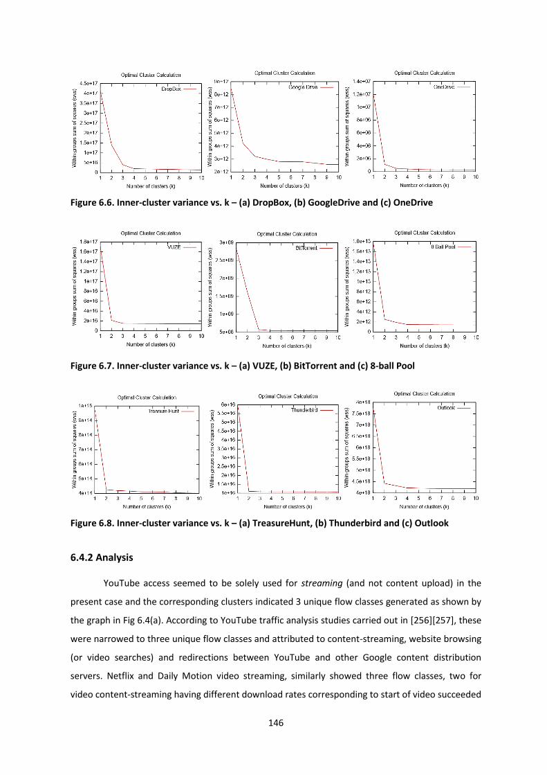
146

Figure 6.6. Inner-cluster variance vs. k – (a) DropBox, (b) GoogleDrive and (c) OneDrive

Figure 6.7. Inner-cluster variance vs. k – (a) VUZE, (b) BitTorrent and (c) 8-ball Pool

Figure 6.8. Inner-cluster variance vs. k – (a) TreasureHunt, (b) Thunderbird and (c) Outlook

6.4.2 Analysis

YouTube access seemed to be solely used for streaming (and not content upload) in the

present case and the corresponding clusters indicated 3 unique flow classes generated as shown by

the graph in Fig 6.4(a). According to YouTube traffic analysis studies carried out in [256][257], these

were narrowed to three unique flow classes and attributed to content-streaming, website browsing

(or video searches) and redirections between YouTube and other Google content distribution

servers. Netflix and Daily Motion video streaming, similarly showed three flow classes, two for

video content-streaming having different download rates corresponding to start of video succeeded

147

by steady buffering stage and a third for user searches. For these applications, video streaming

flows were labelled as ‘streaming’ while website searches and server redirections as ‘browsing’.

The Skype client was used for video with voice communication rather than file sharing or instant

messaging. Subsequent clustering produced two highly discriminate clusters given by the knee-

point of the graph in Fig 6.5(a). Skype stores user information in a decentralized manner with Skype

clients acting has host nodes that initiate connections with super nodes for registering with a Skype

login server and exchanging continuous keep-alive messages [258]. The resulting overlay peer to

peer network employs both TCP and UDP connections both for communication between host and

super nodes as well as between two hosts running the client application [259][260]. One flow

cluster was hence, determined to be directly associated with control features servicing connections

and authentication between host and super nodes, having a much lower data volume and receiving

rate and a significant number of unidirectional flows compared to the second group. The second

flow cluster comprised of video calls between Skype clients having substantially higher data rate

Table 6.4. Segregated Flows per Application

Traffic Class Application Cluster (k) wss/ total_ss Content Specific Flows

Auxiliary Flows

Streaming YouTube 3 87.3% Streamin

g

Browsing

Netflix 3 94.6% Streamin

g

Browsing

DailyMotion 3 95.1% Streamin

g

Browsing

Comms./VoIP Skype 2 98.8% Comms. Comm. Ctrl

Gtalk 2 97.21% Comms. Comm. Ctrl.

Facebook Messenger

3 92.12% Comms. Comm. Ctrl.,

Browsing Torrents/P2P VUZE 3 97.9% Torrent Torr.Ctrl.

Bit Torr. 3 91.2% Torrent Torr.Ctrl.

Cloud Storage DropBox 3 89.2% Up/Dwnl

d.

Browsing

Google Drive 3 88.15% Up/Dwnl

d

Browsing

OneDrive 3 92.14% Up/Dwnl

d

Browsing

Gaming 8ballPool 2 88.4% Game ctrl Game Setup

TreasureHunt

2 91.98% Game ctrl Game Setup

Email Thunderbird 2 99.14% Email

msg

Dir. Lookups

Outlook 2 97.45% Email

msg

Dir. Lookups

148

and total data volume. The respective flows were labelled as ‘Comms. control’ and ‘Comms.’

accordingly. The same number of clusters were observed for Gtalk attributed to voice

communication and control signalling with the Google content server with the later having a lower

traffic footprint with respect to flow transmission duration and the average bit rate of the flows

compared to the former. For Facebook messenger, however, three optimal clusters were observed,

one with a high bit rate and duration similar to the VoIP calls observed in Skype and Gtalk, one for

connection establishment and lastly one for the background live newsfeed being continuously

updated on the Facebook page. The clusters were, thus accordingly labelled under ‘Comms’,

‘Comms. Control’ and ‘Browsing’ classes.

For online cloud storage, usually requiring low user interactivity as highlighted in [261], Drop box,

Google Drive and OneDrive were examined. The applications employed file transfers ranging in size

from 25KB to 1.5 GB, frequently in batches of 1, 5 and 10 files. Cluster analysis on generated traffic

featured around 3 optimal flow clusters as represented by Fig 6.6. The three distinct flow clusters,

after analysis were labelled as one each for file ‘uploads’ and ‘downloads’ and a third for interaction

with the hosting website tagged ‘browsing”.

To examine torrent applications, the original Bit Torrent and VUZE derivative client were used on

researcher machines’ to search and download different combinations of files with sizes ranging

from 25 MB to over 1 GB. Cluster analysing these torrent flows resulted in three distinct clusters

representing actual file download labelled as ‘torrent’ and later two as ‘torrent control’ responsible

for further seeding of downloaded files and communication with other peers.

For online interactive Macromedia Flash player based pool and treasure hunt game, two clearly

distinct flow classes as depicted in Fig. 6.7(c) and Fig. 6.8(a), responsible for initial ‘game setup’ and

continued interactive ‘game control’ constituted all flows.

Lastly the email clients Thunderbird and Outlook were used with three distinct email accounts,

Yahoo, Gmail and a corporate account. Cluster analysis revealed two discrete types of flows shown

in Fig 6.8 (b) and (c). One flow cluster comprised sending and receiving email messages which in

this case could also be easily identified by looking at well-known destination port assignments for

SMTP, POP and IMAP protocols. The second flow class represented ‘directory lookups’ by the client

using HTTP and SSL having significantly lower total data volume per flow compared to email

messages.

149

Segregated flows of all applications were labelled with flow classes and combined into a single data

set. The next section details the splitting of training and testing data and evaluates the C5.0 ML

classifier.

6.5 C5.0 Decision tree classifier

Approximately 6.8 million flows were labelled with appropriate flow classes as a result of k-

means cluster analysis, in accordance with Table 6.3. In order to comprehensively test classifier

accuracy, the data set was further split in almost equal percentages (~50%) per flow class for

training and testing purposes.

6.5.1 Classifier evaluation

C5.0 ML was applied on the training data set using feature sets 1 to 4, with alternate pruning

and boosting options [Appendix – 3.2, 3.3]. As mentioned earlier, enabling pruning removes parts

of the decision tree representing relatively higher error rates than others while adaptive boosting

generates a batch of classifiers and uses voting on every examined sample to predict the final class.

Classifiers were derived by enabling both options to analyse improvements in accuracy using the

feature sets in Table 6.3. The resulting prediction accuracy for each attribute set is reported in

Table 6.5. Set 1 included source and destination port numbers along with protocol information and

resulted in in a maximum accuracy of 41.97% with the maximum allowed boosting factor of 100

and could easily be ruled out for use as standalone feature-set for classification. Set 2 used port

name labelling instead of actual numbers and protocol information, resulting in considerably low

accuracy even when compared to set 1 with uniformity in values regardless of boosting at 24.29%.

Set 3 included twelve flow attributes and resulted in a significantly improved accuracy of 84.97%

with a 10 boost. Finally, set 4 incorporating only flow ratio parameters led to a maximum accuracy

of 75.03% with 100 times boost. In this particular instance disabling pruning resulted in a more

accurate classifier at 75.70%. When used in combinations sets 2 and 4 presented lowest accuracy

peaking at 77.42% while sets 1 and 4 as well as 2 and 3 resulted in reasonable level of classifier

accuracy at 86.79% and 86.91% respectively. Set 1 and 3 combined showed a considerable

improvement with classification accuracy peaking at 96.67% with a 100 boost while even with a 10

boost or a single classifier (no boost) the prediction results were 94.52% and 92.37% respectively.

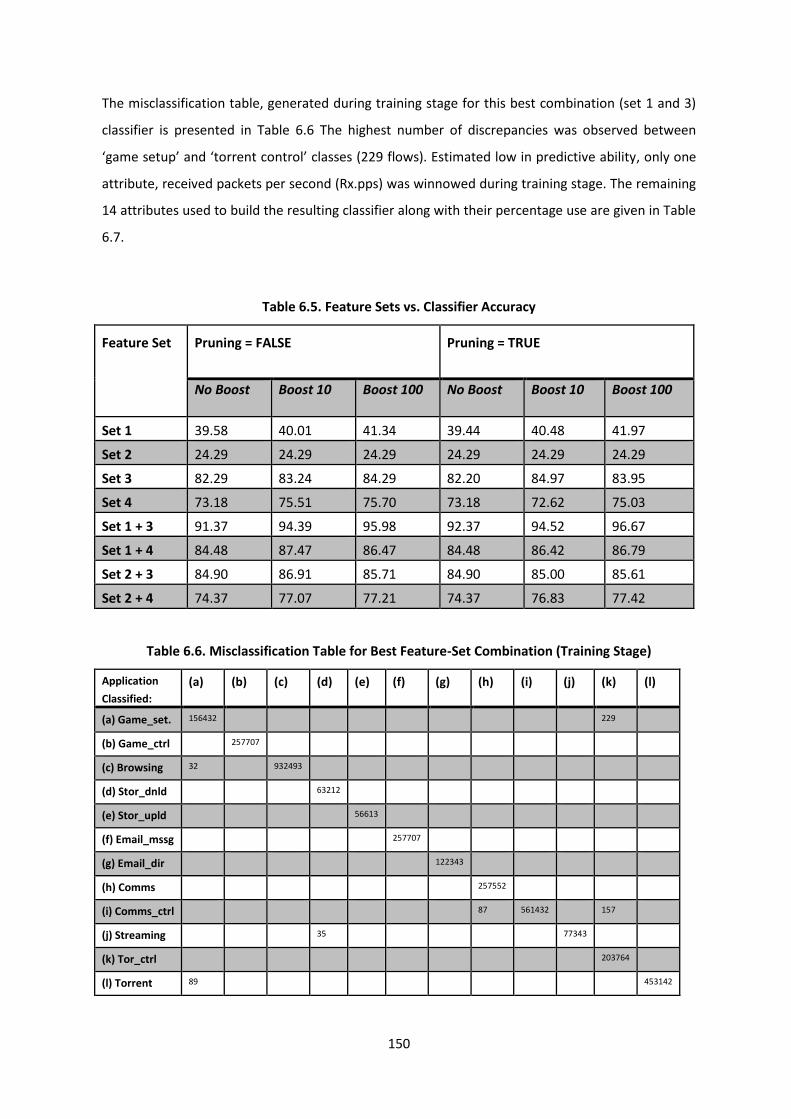
150

The misclassification table, generated during training stage for this best combination (set 1 and 3)

classifier is presented in Table 6.6 The highest number of discrepancies was observed between

‘game setup’ and ‘torrent control’ classes (229 flows). Estimated low in predictive ability, only one

attribute, received packets per second (Rx.pps) was winnowed during training stage. The remaining

14 attributes used to build the resulting classifier along with their percentage use are given in Table

6.7.

Table 6.5. Feature Sets vs. Classifier Accuracy

Feature Set Pruning = FALSE

Pruning = TRUE

No Boost Boost 10 Boost 100 No Boost Boost 10

Boost 100

Set 1 39.58 40.01 41.34 39.44 40.48 41.97

Set 2 24.29 24.29 24.29 24.29 24.29 24.29

Set 3 82.29 83.24 84.29 82.20 84.97 83.95

Set 4 73.18 75.51 75.70 73.18 72.62 75.03

Set 1 + 3 91.37 94.39 95.98 92.37 94.52 96.67

Set 1 + 4 84.48 87.47 86.47 84.48 86.42 86.79

Set 2 + 3 84.90 86.91 85.71 84.90 85.00 85.61

Set 2 + 4 74.37 77.07 77.21 74.37 76.83 77.42

Table 6.6. Misclassification Table for Best Feature-Set Combination (Training Stage)

Application

Classified:

(a) (b) (c) (d) (e) (f) (g) (h) (i) (j) (k) (l)

(a) Game_set. 156432 229

(b) Game_ctrl 257707

(c) Browsing 32 932493

(d) Stor_dnld 63212

(e) Stor_upld 56613

(f) Email_mssg 257707

(g) Email_dir 122343

(h) Comms 257552

(i) Comms_ctrl 87 561432 157

(j) Streaming 35 77343

(k) Tor_ctrl 203764

(l) Torrent 89 453142

151

Table 6.7. Flow Attribute Usage

Flow Attribute Usage in Selected C5.0 Classifier

Category Attribute Percentage Use

Protocol and Port Protocol 80.62%

Destination Port 100%

Source Port 100%

Transmitted Flow (Tx) Attributes Bytes [Tx.B] 100%

Packets [Tx.Pkt] 100%

Bits per second [Tx.bps] 100%

Packets per sec [Tx.pps] 96.25%

Bytes per package [Tx.Bpp] 100%

Duration [Tx.s] 95.48%

Received Flow (Rx) Attributes Bytes [Rx.B] 100%

Packets [Rx.Pkt] 100%

Bits per sec [Rx.bps] 100%

Bytes per package [Rx.Bpp] 100%

Duration [Rx.s] 98.61%

6.5.2 Confusion matrix analysis

The confusion matrix for selected classifier specifying cross-tabulation of predicted classes and

observed values with associated statistics between different flow classes is given in Table 6.8. The

highest errors occurred between ‘game control’ and ‘browsing’ flows (60114 or 1.76% of total

tested flows), while no misclassification errors were observed between ‘game setup’ and ‘torrent

control’ flows as witnessed during training cross-validation stage. The overall accuracy statistics are

presented in Table 6.9. The value for the kappa co-efficient [262][263], which takes into account

occurrences of accurately classified flows and is generally considered a more robust measure than

simple percent agreement calculation, was also significantly high at 95.31%. The overall accuracy

rate was also computed along with a 95 percent confidence interval (CI) for this rate (0.9364, 0.956)

and a one-sided test to see if the accuracy is better than the ‘no information rate,’ which is taken to

be the largest class percentage in the data (P-Value: Accuracy > NIR : < 2.2e-16) [264]. McNemar's

test p-value however, was not available due to sparse tables (bi-directional flow vectors having very

low or zero attribute values for some flow classes i.e. Skype control, etc.).

152

Table 6.8. Confusion Matrix Calculation for Optimal Classifier (Evaluation Stage)

Application

Classified:

(a) (b) (c) (d) (e) (f) (g) (h) (i) (j) (k) (l)

(a) Game_setup 156435

(b) Game_ctrl 257718 60114

(c) Browsing 632 25481 932494 4006

(d) Stor_dnld 63208

(e) Stor_upld 56611

(f) Email_mssg 257710

(g) Email_dir 3981 2561 122346

(h) Comms 257552

(i) Comms_ctrl 4587 561433

(j) Streaming 1335 77341

(k) Torrent 2078 453143

(l) Tor_ctrl 5843 6154 203766

Table 6.9. Overall Statistics

Statistical Property Value

Classifier Accuracy 96.67%

95% Confidence Interval (CI) (0.9364, 0956)

No Information Rate 0.3332

P-Value (Acc > NIR) < 2.2e-16

Kappa 0.9531

McNemar’s Test P-value NA

6.5.3 Sensitivity and specificity factor

For a given flow, the classifier’s ability to accurately predict the flow class is characterized by

the classifier sensitivity factor and to differentiate this flow from other flow classes, by its specificity

factor. Both parameters are of significant importance an ascertaining a classifier’s suitability for

both flow identification and discrimination. The sensitivity and specificity bar graph for each flow

class for the selected classifier are given in Fig. 6.9. Lowest sensitivity was recorded for cloud

storage flows (87.67-89.89%) among all classes, also evident from Fig. 6.9 due to a higher mismatch

between storage download and streaming (1335 or 0.039%) as well as storage upload and browsing

flows (4006 or 0.11% of total tested flows). The corresponding specificity values for both storage

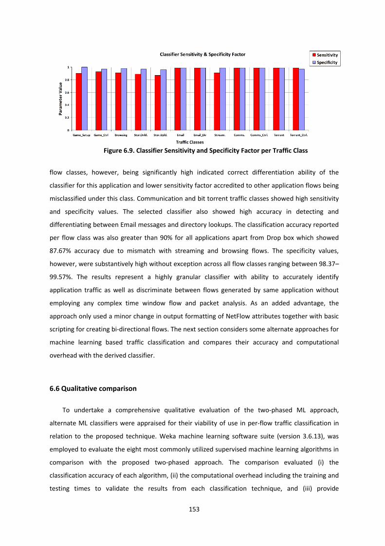
153

Figure 6.9. Classifier Sensitivity and Specificity Factor per Traffic Class

flow classes, however, being significantly high indicated correct differentiation ability of the

classifier for this application and lower sensitivity factor accredited to other application flows being

misclassified under this class. Communication and bit torrent traffic classes showed high sensitivity

and specificity values. The selected classifier also showed high accuracy in detecting and

differentiating between Email messages and directory lookups. The classification accuracy reported

per flow class was also greater than 90% for all applications apart from Drop box which showed

87.67% accuracy due to mismatch with streaming and browsing flows. The specificity values,

however, were substantively high without exception across all flow classes ranging between 98.37–

99.57%. The results represent a highly granular classifier with ability to accurately identify

application traffic as well as discriminate between flows generated by same application without

employing any complex time window flow and packet analysis. As an added advantage, the

approach only used a minor change in output formatting of NetFlow attributes together with basic

scripting for creating bi-directional flows. The next section considers some alternate approaches for

machine learning based traffic classification and compares their accuracy and computational

overhead with the derived classifier.

6.6 Qualitative comparison

To undertake a comprehensive qualitative evaluation of the two-phased ML approach,

alternate ML classifiers were appraised for their viability of use in per-flow traffic classification in

relation to the proposed technique. Weka machine learning software suite (version 3.6.13), was

employed to evaluate the eight most commonly utilized supervised machine learning algorithms in

comparison with the proposed two-phased approach. The comparison evaluated (i) the

classification accuracy of each algorithm, (ii) the computational overhead including the training and

testing times to validate the results from each classification technique, and (iii) provide

154

perspectives on the scalability of the two-phased machine learning classifier. The classifiers used

the same ratio of training and testing data set pools (marked with respective application class),

where 50% of the flows were used for training the respective classifier and the remaining 50% flows

were used for testing purposes. The machine learning algorithms evaluated are briefly described as

follows.

J48/C4.5 decision tree, constructs a tree structure, in which each node represents feature tests,

each branch represents a result (output) of the test, and each leaf node represents a class label i.e.

application flow label in the present work [240][265]. In order to use a decision tree for

classification, a given tuple (which requires class prediction) corresponding to flow features, walks

through the decision tree from the root to a leaf. The label of the leaf node is the classification

result. The algorithm was enabled with default parameters (confidence factor of 0.25 and reduced-

error pruning by 3 fold) in the WEKA implementation of the present experiment to optimize the

resulting decision tree.

K-nearest neighbours (KNN), computes the distance (Euclidean) from each test sample to the k

nearest neighbours in the n-dimensional feature space. The classifier selects the majority label class

from the k nearest neighbours and assigns it to the test sample [266]. For the present evaluation

k=1 was utilized.

Naïve Bayes (NB), considered a baseline classifier in several traffic classification studies selects

optimal (probabilistic) estimation of precision values based on analysis of training data using Bayes’

theorem, assuming highly independent relationship between features [267][268].

Best-first decision tree (BFTree), uses binary splitting for nominal as well as numeric attributes and

uses a top-down decision tree derivation approach such that the best split is added at each step

[269]. In contrast to depth-first order in each iterative tree generation step [61][62], the algorithm

expands nodes in best-first order instead of a fixed order. Both the gain and gini index are utilized in

calculating the best node in tree growth phase. The algorithm was implemented with post-pruning

enabled and with a default value of 5 folds in pruning to optimize the resulting classifier.

Regression tree representative (REPTree), is a fast implementation of decision tree learning which

builds a decision/regression tree using information gain and variance with reduced-error pruning

along with back fitting. Reptree uses regression tree logic to create multiple trees and selects the

155

best from all the generated trees. The algorithm only sorts values for numeric attributes once. It

was implemented with pruning enabled with the default value of 3 folds.

Sequential minimal optimization (SMO), a support vector classifier trained using a sequential

minimal optimization algorithm by breaking optimization problem into smaller chunks, solved

analytically. The algorithm transforms nominal attributes into binaries and by default normalizes all

attributes [271][272]. It was implemented using WEKA with normalization turned on along with the

default parameters (the complexity parameter C=1, and polynomial exponent P=1).

Decision tables and naïve bayes (DTNB), is a hybrid classifier which combines decision tables along

with naïve bayes and evaluates the benefit of dividing available features into disjoint sets to be

used by each algorithm respectively [65]. Using a forward selection search, the selected attributes

are modelled using NB and decision table (conditional probability table) and at each step,

unnecessary attributes are removed from the final model. The combined model reportedly [273]

performs better in comparison to individual naive Bayes and decision tables and was implemented

with default parameters. The final classifier selected and used 5 attributes (out of 16 using

backward elimination and forward selection search).

Bayesian network (BayesNet), an acyclic graph (directed) that represent a set of features as its

vertices, and their probabilistic relationship as the graph edges [274]. While using the Bayes' rule

for probabilistic inference, under invalid conditional independence assumption (in Naïve Bayes)

BayesNet may outperform NB and yield better classification accuracy [275]. The default parameters

i.e. SimpleEstimator was used for estimating the conditional probability tables of a BN in the WEKA

implementation of BN on the training set.

The following sub-sections highlight a qualitative comparison between the above machine learning

classification techniques and the proposed two-phased approach.

6.6.1 Comparative accuracy

The respective accuracy of each examined traffic class for multiple classifiers is given in Fig. 6.10.

Overall, the two-phased approach surpassed or equated in per-flow classification with the alternate

classification techniques. The algorithm achieved the highest accuracy for the game setup class of

flows. For game control flows, alternate approaches such as kNN and REPTree provide a better

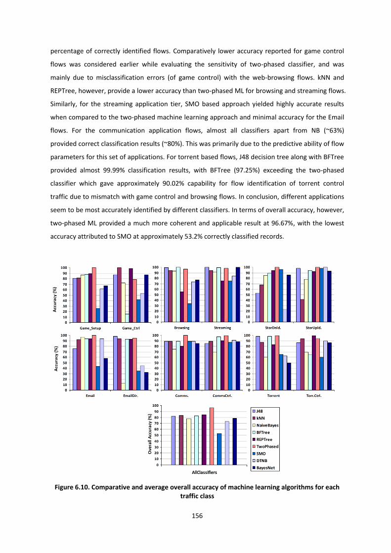
156

percentage of correctly identified flows. Comparatively lower accuracy reported for game control

flows was considered earlier while evaluating the sensitivity of two-phased classifier, and was

mainly due to misclassification errors (of game control) with the web-browsing flows. kNN and

REPTree, however, provide a lower accuracy than two-phased ML for browsing and streaming flows.

Similarly, for the streaming application tier, SMO based approach yielded highly accurate results

when compared to the two-phased machine learning approach and minimal accuracy for the Email

flows. For the communication application flows, almost all classifiers apart from NB (~63%)

provided correct classification results (~80%). This was primarily due to the predictive ability of flow

parameters for this set of applications. For torrent based flows, J48 decision tree along with BFTree

provided almost 99.99% classification results, with BFTree (97.25%) exceeding the two-phased

classifier which gave approximately 90.02% capability for flow identification of torrent control

traffic due to mismatch with game control and browsing flows. In conclusion, different applications

seem to be most accurately identified by different classifiers. In terms of overall accuracy, however,

two-phased ML provided a much more coherent and applicable result at 96.67%, with the lowest

accuracy attributed to SMO at approximately 53.2% correctly classified records.

Figure 6.10. Comparative and average overall accuracy of machine learning algorithms for each traffic class

157

6.6.2 Computational performance

To evaluate the computational performance of the classifiers, each was independently

implemented on a test machine (PC), an Intel based i54310-M processor chipset with two 2.70 GHz

CPUs and 16GB of memory. The operating system used a GNU/Linux kernel (3.14.4 x64) and it was

verified that no other user processes (apart from the WEKA software suite) were consuming CPU

cycles or any of the operating system processes were CPU or I/O intensive. The two-phased ML

evaluation included the combined cluster analysis and subsequent C5.0 training phase from

labelled flows. This was done solely to examine the computational requirements of the

unsupervised and supervised machine learning ensemble, excluding the ground-truth acquisition

and refinement (i.e. DPI based application flow perusal and sub-class marking) which can be done

offline and continuously on much greater data-sets in a practical network implementation. To give a

realistic comparison, the alternate classifiers used the same application labelled flows (ground-

truth). The average CPU utilization for each classifier in terms of the flow records and bytes

processed (testing) are given in Fig. 6.11. A linear relationship was observed between the CPU

utilization and the amount of records processed for all classifiers followed by a steady-state pattern

albeit different consumption footprints. The kNN classifier had the highest CPU usage at up to 5.32%

with a gradual decrease steadying at 4.21%. NB classifier had the lowest consumption at 1.61%

while two-phased ML reported around 4.31% usage. Similarly the average memory usage per

classifier in processing flow records and bytes of data are provided in Fig. 6.12. The BFTree

algorithm had the highest memory usage at 190.28MB with the two-phased ML at 175.31MB.

BayesNet had the lowest memory footprint with a steady-state value of approximately 50.14MB.

The average training and testing times with respect to three different sizes of flow sets (1000, 1

million and 3 million) for each classifier are depicted in Fig. 6.13. The training time for two-phased

classifier was significantly high compared to other classifiers for flow-record size of 1000 flows. This

was due to the in tandem processing of the two embedded algorithms used. The training-time

relationship for most classifiers with respect to the size of training data at larger values of the latter

was, however, non-linear. The training time for J48 for example, for both 1M and 3M flows was

approximately the same averaging at around 59.35 minutes. Similarly, BFTree approximated at

60.12 minutes for 1M to 63.45 minutes for 3M flows respectively. The two-phased classifier also

reported between 80.87 minutes to 84.51 minutes for the respective flow records in the training

phase. This yields approximately on average 0.88 seconds spent training around 1K flows with a

standard deviation (σ) of 1.137 between 1M and 3M flows. Hence, the proposed technique results

in better performance in terms of training times in the steady-state with relatively larger data-sets.

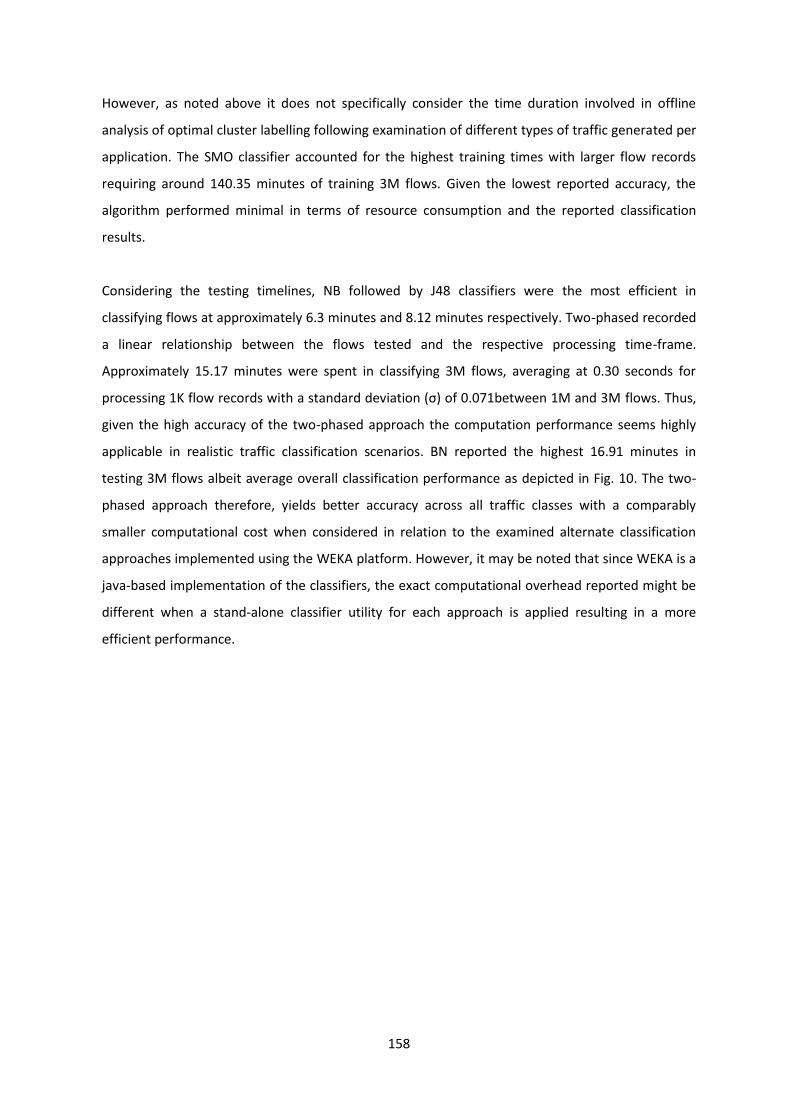
158

However, as noted above it does not specifically consider the time duration involved in offline

analysis of optimal cluster labelling following examination of different types of traffic generated per

application. The SMO classifier accounted for the highest training times with larger flow records

requiring around 140.35 minutes of training 3M flows. Given the lowest reported accuracy, the

algorithm performed minimal in terms of resource consumption and the reported classification

results.

Considering the testing timelines, NB followed by J48 classifiers were the most efficient in

classifying flows at approximately 6.3 minutes and 8.12 minutes respectively. Two-phased recorded

a linear relationship between the flows tested and the respective processing time-frame.

Approximately 15.17 minutes were spent in classifying 3M flows, averaging at 0.30 seconds for

processing 1K flow records with a standard deviation (σ) of 0.071between 1M and 3M flows. Thus,

given the high accuracy of the two-phased approach the computation performance seems highly

applicable in realistic traffic classification scenarios. BN reported the highest 16.91 minutes in

testing 3M flows albeit average overall classification performance as depicted in Fig. 10. The two-

phased approach therefore, yields better accuracy across all traffic classes with a comparably

smaller computational cost when considered in relation to the examined alternate classification

approaches implemented using the WEKA platform. However, it may be noted that since WEKA is a

java-based implementation of the classifiers, the exact computational overhead reported might be

different when a stand-alone classifier utility for each approach is applied resulting in a more

efficient performance.

159

Figure 6.11. Classifier CPU Utilization (%) (a) flow records processed and (b) bytes processed

Figure 6.12. Classifier Memory Usage (MB) (a) flow records processed and (b) bytes processed

160

Figure 6.13. Classifier timeframes for (a) training and (b) processing time

6.6.3 Scalability

Given the classification accuracy comparisons among several classifiers, it is apparent that

the prediction ability of a scheme is highly dependent on analysing a correct measure of variation

between the selected flow attributes for each traffic class. Traditionally the bi-directional flow

features utilized in the present research have shown considerable applicability in multiple classifiers

to attain a (somewhat) acceptable degree of traffic identification. However, as highlighted in [224]

and [226] the wide majority of the classification algorithms are infeasible with respect to their

application in the network backbone by ISPs. The reasons for this lack of applicability range from

the tremendous amount of traffic generated in the network core to the actual methodology of the

approach, for example, sometimes requiring analysis of end-point behaviour for classification

[226][276]. In addition flow-based techniques often rely on statistical information from bi-

directional traffic (specifically TCP), and placing the traffic measurement or collection point as close

to the ingress or the edge of the network as possible to collect the necessary features from

outbound as well as inbound flows. An alternate approach to address this limitation is provided by

161

[69], which introduces an algorithm for predicting the inbound traffic flow attributes based on the

unidirectional transmitted TCP flows. However, the present approach proposes using the former

technique of placing flow-measurements as close to the ingress or edge of the network to

corroborate the relation between upstream and downstream flows per host to generate bi-

directional flow features and keep the operational and computational cost of implementing the

two-phased approach to a minimal.

The proposed two-phased approach is significantly reproducible due to the utilization of NetFlow,

ubiquitous in present ISP networking equipment, network edges such as residential routers in home

based networks and the edge (gateway) switches in enterprise networks. Additionally, the derived

classifier reported high efficiency in dealing with large data (flow records) with high level of

accuracy, again a basic traffic classification requirement in user traffic profiling. The synergetic

combination of classifiers, in the present case produced comprehensive traffic classification results

and a comparatively lower processing overhead while using non-specialized hardware. The

classifier can therefore, be put to use in the traffic classification phase during user traffic profiling

resulting in greater accuracy of user trend depiction as compared to the previously used technique

of IP address and port mappings based application classification.

6.7 Conclusion

The present chapter used a twofold machine learning approach for traffic classification on a per-

flow basis by solely using NetFlow attributes and without depending on packet derivatives or

complex time window analysis. During the unsupervised phase, approximately 6.8 million bi-

directional flows for all applications were collected and cluster analysed resulting in 12 unique flow

classes. The supervised phase used four different feature-sets of NetFlow attributes from the

derived flow classes to test and train the C5.0 ML decision tree classifier. The foremost feature-set

comprising 14 NetFlow attributes, reported an average prediction accuracy of 92.37% increasing to

96.67% with adaptive boosting. The sensitivity factor of the classifier was also exceedingly high

ranging above 90% with only cloud storage flows (file upload and downloads) reporting relatively

low values between 87.67% - 89.89% due to misclassification with general web browsing and

streaming flows. The corresponding specificity factor, indicating classifier flow discrimination ability

ranged between 98.37% – 99.57% across all applications. Furthermore, the substantive accuracy of

the presented approach in achieving highly granular per-flow application identification and the

computational efficiency in comparison with other machine learning classification methodologies

162

paves way for future work in extending this method to include other applications for real-time or

near real-time flow based classification.

The following chapter investigates and evaluates the use of OpenFlow protocol features for traffic

profile derivation in campus based SDN environments. The study assesses OpenFlow protocol

based flow monitoring information to derive user traffic profiles for visualization of user traffic

trends in campus network environments. The proposal seeks to eliminate reliance on external flow

accounting methods (such as NetFlow) for recording user traffic information in larger campus

environments where networking devices may be geographically dispersed and operators can

benefit from a low cost centralized user profiling mechanism.

164

Chapter 7 OpenFlow-Enabled User Profiling in Enterprise Networks

7.1 Introduction

The OpenFlow protocol [17] provides flow monitoring and management of OpenFlow compliant

SDN switches through a sophisticated set of controller to device message exchanges. The OpenFlow

protocol also offers individual service improvement by guaranteeing quality of service through

isolated application flow metering. Existing OpenFlow based traffic monitoring solutions are

therefore, inclined towards using the protocol for flow monitoring and control, while aiming to

keep the associated management overhead to a minimum. Studies such as [300], [301] and [302]

have sought to establish the trade-off between resource consumption, control channel traffic load

and monitoring accuracy by changing switch flow idle time out, using adaptive switch polling

frequency and varying the time interval between configuration messages sent to switches. Prior

work has also focused on highlighting the benefits of using asymmetric OpenFlow control messages

to reduce the overall control channel overhead [303], as well as employing OpenFlow monitoring

information along with anomaly and intrusion detection algorithms to harden SDN security [304].

However, no previous work has specifically focused on leveraging OpenFlow based monitoring

information to profile user behaviour in an SDN framework. As evaluated in earlier chapters, user

traffic profiling aims to understand real-time user behaviour and to help network administrators in

visualizing user trends in subsequently implementing user-centric policies. Profiling user traffic

based on application trends may more accurately express user activities and aid administrators in

aligning optimization solutions to the inherent campus user classes instead of individual

applications [200]. The implementation of user profiling controls, in larger campus and enterprise

SDN environments, however, may require exporting flow measurements externally from dispersed

network switches resulting in a substantial management overhead. The present chapter proposes

profiling user application trends solely employing OpenFlow based monitoring information. The

proposed approach accounts user-generated flows (application usage) towards the campus servers,

using the OpenFlow counters in network switches polled via the SDN controller. Using the existing

OpenFlow control channel between the edge switches and the SDN controller, flow measurement

as well as profile extraction remains centralized eliminating requirement for external flow

accounting (NetFlow, IPFIX, etc.) and dedicated monitoring overlays. Furthermore, the design

focuses on retrieving traffic statistics nearer to the user i.e. the edge or access switches to account

for any local service (or application server) traffic which may not traverse the campus core. The

165

extracted profiles subsequently serve as a means to characterize and monitor the campus workload.

Utilizing per-profile traffic statistics, the SDN controller can anticipate real-time traffic conditions

based on changing profile memberships, assisting operators in implementing user-centric policies.

To validate the feasibility of the proposed approach, the study collected traffic statistics from a

virtual Open vSwitch [86] and Ryu SDN controller [70] instance connected to a realistic campus

edge to profile user activity. User statistics were monitored over a two-week time frame and

subjected to unsupervised k-means cluster analysis to segregate users into different classes based

on their application trends. The scalability of the design was further evaluated by simulating several

user profile loads in Mininet [103] to benchmark the monitoring message overhead as well as the

computational cost associated with user profiling.

The remainder of this chapter is organized as follows. Section 7.2 details the proposed user profiling

method using OpenFlow protocol. Section 7.3 discusses the derived profiles, also highlighting the

scalability evaluation of the design. Section 7.4 gives a perspective on profiling based traffic

engineering and final conclusions are drawn in section 7.5.

7.2 Design

The proposed traffic profiling methodology comprises of two main components (i) OpenFlow

traffic monitor and (ii) the traffic profiling engine.

The traffic monitor utilizes five primary OpenFlow message types presented earlier in Table 2.3 to

record the individual application usage of users connected to an OpenFlow compliant switch (such

as Open vSwitch) [Appendix – 5.5]. The resulting monitoring information collected per flow is a

seven-tuple record including the source and destination IP address and ports, duration of the flow,

the number of packets matching the flow and the total bytes transferred before flow termination

<SrcIP, DstIP, SrcPort, DstPort, Duration, Packets, Bytes>.

Following record collection, the profiling engine collates traffic composition statistics per user as a

percentage of user generated flows towards campus data sources, mapped according to their

respective destination IP address(es). The aggregate traffic composition vectors are afterwards fed

to a k-means clustering module, segregating users into different classes (profiles) based on their

application trends. The resulting profiles are stored in a central database and continuously

166

monitored to benchmark their stability with any deviation from pre-determined baseline values

triggering re-profiling [Appendix – 2.4]. The following sub-sections discuss the data collection setup,

the traffic monitor and the profiling engine in detail.

7.2.1 OpenFlow traffic monitor

To determine the feasibility of present traffic profiling approach, traffic records were collected

from a realistic academic network segment consisting of approximately 42 users in the computing

and engineering departments over a two week duration between 15/02/2016 and 29/02/2016.

Each user had a single computer, being used to connect to campus application servers. In order to

eliminate the impact of this study on production traffic, the setup used a Linux monitoring machine

(VM1) running an Open vSwitch (SW1) and Ryu SDN controller instance connected to the

departmental LAN as shown in Fig. 7.1. Port monitoring was enabled at the default gateway (SW2)

to replicate all traffic to and from each user to the VM1 interface (virtual switch SW1). The mirrored

traffic was processed through the Open vSwitch (SW1), however, not forwarded to any outside port,

since the objective was solely the collection of user traffic statistics. The traffic monitoring

application running on VM1 polled Open vSwitch (SW1) counters by issuing RESTful calls to the Ryu

controller to collect per user flow statistics. All user machines used static IP addressing scheme to

simplify accounting per user application usage from the collected OpenFlow records. Steps

describing the installation of flows in SW1, their subsequent updating, and user statistics collection

are detailed as follows.

1) Flow installation: Standard Ryu based layer3 routing function and the traffic monitor

application was implemented using the default OpenFlow behaviour with customized flow

routing as shown in Fig. 7.2. The first packet of incoming (mirrored) traffic on SW1 port1,

was matched against existing table0 entries for processing. In case of a table_miss, an

OpenFlow packet_in message consisting of the first packet of the flow was created and sent

to the controller. On receiving packet_in, the controller created a packet_out message

instructing SW1 to forward upstream LAN traffic via OpenFlow table1 and downstream

traffic (from campus servers and the internet) via table2 out port2. Since, the purpose of

the experiment was data collection and not actual flow forwarding, and OpenFlow does not

prevent flow installation towards a blocked port, virtual port2 on SW1 was set to blocking

mode (sink). This resulted in the installation of respective flows in SW1 with subsequent

flow packets negotiating table1 or table2 out port2, without consequences for live user

traffic and generating per user flow statistics. The Open vSwitch SW1, therefore, installed

167

and updated OpenFlow entries in each flow table as would be the case if directly connected

as the LAN default gateway to forward user traffic.

2) Statistics collection: The traffic monitor made RESTful calls to the Ryu controller to

determine the statistics for table1 and table2 entities. The controller, in turn, fulfilled these

polling requests by issuing OpenFlow flow_stats and table_stats messages to SW1, with the

respective counter for each flow and table entry sent to the traffic monitor. Since RESTful is

a non-subscription based API, the polling frequency of RESTful calls was manually set to 30

seconds, approximately half of the default idle_timeout value (60 seconds) to regularly

generate statistics. In addition to frequent polling, flow completion and idle_timeout

expiration triggered asymmetric flow_rem event message by SW1 to the controller, in turn

updating the traffic monitor. The monitor collected per user seven-tuple record entries,

collated every 24 hours and fed to the profiling engine to extract user profiles. The profiling

engine design is discussed in next subsection.

Figure 7.1. Data collection setup: campus network segment

168

Figure 7.2. Traffic monitoring schematic

7.2.2 Traffic profiling engine

The profiling engine design is depicted in Fig. 7.3. User traffic collected by the traffic monitor

was classified by matching seven-tuple traffic records against source and destination IP addresses

and ports used by the respective users and campus servers [Appendix – 1.3]. To further account for

replication in nature of user activities, and derive meaningful profiles, services were tiered into

distinct categories depicted in Table 7.1. A unique webpage visit or service usage on a user machine

could therefore, be defined by the vector ui given in Eq. 7.1. In Eq. 7.1, each entity represents the

percentage of user flows generated towards the application tiers given in Table 7.1.

ui = [ei, gi, vi, ci , pi, hi, ri, wi , zi] (7.1)

In equation (7.1) above, i uniquely identifies the user machine and the remaining entities represent

the service usage percentage in accordance with Table 7.2. Network activity for a user u1 over any

given 24 hour time-bin, e.g. [29/02/2016], could therefore be represented by the application

distribution in Eq. 7.2.

u1 [29/02/2016] = [43.2 15.1 0.2 9.6 4.1 2.1 17.4 4.4 2.9] (7.2)

169

Figure 7.3. Traffic profling engine

Once application distribution vectors per user machine were collected, the traffic profiling engine

implemented an R programming library of the Hartigan and Wong k-means function [18], to extract

user classes based on the application trends as used in earlier chapters (Eq. 3.1). Furthermore, to

benchmark the stability of the profiles, user profile transitions were evaluated every 24 hours over

the two weeks of study. The extracted user profiles, profile stability evaluation, and computational

cost of the design are described in the following section.

Table 7.1. Application Tiers

Application Tier Website, Destination Port

Emailing (e) Outlook, SMTP, POP3, IMAP

Storage (g) Central storage (://Z Drive, FTP)

Streaming (v) Podcasting, video content

Communications (c) Office communications server

Enterprise (p) Corporation information system, staff portal

Publishing (h) Content management system (document, print)

Software (r) Software distribution service

Web browsing (w) External Internet traffic

Network utility (z) DNS queries, Network Multicasts

170

7.3 User traffic profiles

A total of approximately 7.8 million records were collected over the two week study and the

corresponding user traffic composition vectors were afterwards subjected to k-means clustering.

The plot of wss vs. k of the user traffic composition vectors is given in Fig 7.4. The profiling engine

calculated the maximum within-cluster variance between each successive value of k, examined up

to k=20 to evaluate the optimal cluster number. As shown in Fig. 7.4, the variance between

individual values is maximum until k=6, however, subsequent values of k (≥6) show minimum

change in the successive overall variance (<0.05%). Therefore, for the present study, k=6 provided

an optimal number of user profiles fitting the sample space used for further analysis. The profiling

engine correspondingly marked the daily user traffic records with the individual cluster (profile)

colour. The next subsection examines the resulting six user traffic profiles.

7.3.1 Extracted profiles

The extracted user traffic profiles (for clusters k=6), highlighting the application trends as a

percentage of user generated flows are depicted in Fig. 7.5. From a monitoring and network

management perspective, the derived user profiles showed significant variation in activities among

the derived traffic classes. For example, Profile 1 concentrated mainly on web browsing (39%) with

relatively limited usage of other applications apart from the corporate information (20.5%) and

content management services (12.4%). Profile 2 focused on using office instant messenger and VoIP

largely (64.5%) with limited use of content management applications and web browsing (12.2%). In

comparison with other profiles, Profile 3 users heavily interacted with corporate information

services (50.3%) with a significant use of email service (10.1%). Profile 4 users concentrated on

document utilities and print content creation (57.7%) as well as using centralized storage (11.3%).

Figure 7.4. Optimal cluster determination – wss. vs. k

171

Figure 7.5. User traffic profiles

Profile 5 mainly used central storage filer (60.1%) with small use of content and corporate

information server. Profile 6 was a mix of web browsing, email usage, file storage and the staff

portal along with streaming (20.8%). Each of the derived campus user profiles, therefore,

represented a significant discrimination towards a certain mix of applications and services. The use

of software distribution was, however, significantly low compared to other applications among all

user profiles with profile 4 showing the highest proportion of software downloads (5.9%) from the

campus software store. To benchmark the traffic baseline for each profile, the maximum

probability for the number of users, total traffic volume along with upstream and downstream flow

rates and flow statistics was calculated and is given in Figs. 7.6-7.8. Profile 1 had the highest

number of users (10-14 users) during office hours (09:00-17:00hrs) followed by profile 3 (6-8 users)

while profile 6 membership increased during the evening. Despite having the lowest number of

users (1-5), profile 6 accounted for the greatest traffic volume, primarily due to the greater usage of

streaming application in this traffic class compared to other profiles. Minimum profile memberships

(active users) were recorded between 03:00-06:00hrs. Fig. 7.8 represents the corresponding upload

and download rate per user profile including per application and consolidated average data rates

(x). In terms of individual application tiers, storage (g) had the highest upstream and downstream

rates (4-5Mbps), followed by streaming (s) downloads (up to 5Mbps). Web browsing had the

172

minimum data rate footprint for both upstream (0.2Mpbs) as well as downstream (0.6Mpbs) traffic.

The minimum flow rate was due to web browsing generating low overall speeds, particularly when

using an HTTP1.1 connection (so the connection remains open between pages or the browser sends

keepalives for a while after the actual data transfer finished). The average data rates (x) remained

consistent across all profiles ranging between 1-1.5Mbps for the upstream compared to 1.8-2Mbps

on downloads. The corresponding inter-flow arrival times per profile (for active users) on an hourly

basis are given in Fig. 7.8. Profile 1 had the highest amount of flows generated and received (240-

260 flow) per hour for active users, again due to the greater profile membership attributed to this

user class. The lowest flow generation was for users in profile 2 (80-100 flows) mainly constituting

communication service usage. Similarly profile 4 had the minimum inter-flow arrival duration

(575ms) for transmitted flows, showing quick use of print services when active. Profile 6,

concentrating on streaming had the minimum inter-flow arrivals for downstream traffic (275ms)

mainly attributed to dynamic download of streaming content from multiple sources i.e. load-

balanced video servers. In view of the discriminative application trends, profile memberships and

associated flow measurements for the evaluated campus network segment depicted in the derived

user profiles, operators may want control over which users to prioritize in terms of bandwidth

allocation as well as select optimal routes for resource intensive profiles. An overview of integrating

profiling based controls in campus SDN is discussed further in section 7.4.

Figure 7.6. Probability distribution: (a) profile memership and (b) traffic volume

173

Figure 7.7. Flow transfer rates: (a) upstream traffic and (b) downstream traffic

Figure 7.8. Flow statistics: (a) flow inter-arrival time and (b) total flows (hourly)

174

7.3.2 Profile stability

Profile consistency highlights the significance of gaining a better insight to changes in user

activity as well as benchmark the stability of the extracted profiles and re-profiling frequency.

Therefore, to evaluate user profile retention, the average probability of profiles change for the

same users for each subsequent day of study was computed and is presented in Table 7.2. Profile 5

users showed the highest consistency in retaining profiles at 99.1% followed by profile 4 at 99%

while profile 6 showed the lowest at 96.1%. The reported profile retention of campus users was

greater in comparison with a similar study (chapter 4) aimed at evaluating profile stability for multi-

device residential users reporting the lowest profile consistency at 81% [293]. Campus users hence

showed a significantly greater degree of consistency in daily application usage in relation to

residential users. The probability of a profile gaining or losing a device every 24 hours is also given

in Table 3. Profile 1 had the highest probability of gaining users (93%) profile 6 had highest

probability of transitioning users (80%). The average probabilities of inter-profile transitions every

24 hours are given in Table 7.3. Profile 6 users showed a tendency (up to 3%) to transition to profile

1, the primary difference between the two profiles being proportional changes in streaming and

publishing tier respectively. Similarly, profile 1 users tilted towards profile 3 (1.1%) having greater

corporate information system and staff portal usage. Profile 4 with heavy publishing inclined

towards profile 1 (at 0.6%) having higher web access. It was therefore, noted that where users

transitioned to a different profile, it was always to profiles having somewhat similar application

usage ratios to their own. Inter-profile transitions were mainly due to proportional variation in the

same kind of user activity rather than a complete change of user roles, increasing the applicability

of derived profile baseline in campus network monitoring.

Table 7.2. Average Probability of Profile Change (/24 Hours)

User Profiles Probability of No Change Probability of Change

Change: Gain Loss

Profile 1 0.981 0.019 0.93 0.07

Profile 2 0.970 0.03 0.44 0.56

Profile 3 0.985 0.015 0.92 0.08

Profile 4 0.990 0.01 0.55 0.45

Profile 5 0.991 0.009 0.49 0.51

Profile 6 0.961 0.039 0.20 0.80

175

Table 7.3. Inter-Profile Transition Probability (/24 Hours)

User Profiles P1 P2 P3 P4 P5 P6

Profile 1 0.981 0.001 0.011 0.002 0.004 0.001

Profile 2 0.009 0.970 0.017 0.001 0.001 0.002

Profile 3 0.008 0.001 0.985 0.003 0.002 0.001

Profile 4 0.006 0.001 0.001 0.990 0.002 0.001

Profile 5 0.001 0.003 0.001 0.002 0.991 0.002

Profile 6 0.03 0.0091 0.001 0.0004 0.0003 0.961

7.3.3 Profiling computational cost

To evaluate the computational cost of the traffic profiling mechanism, memory and CPU

utilization were recorded during the profiling workload completion. The purpose of this exercise

was to appreciate the amount of computational resource needed in profiling user traffic from a

practical campus network setting. The test machine (PC) used an Intel based i54310-M processor

chipset with two CPUs, each at 2.70 GHz and 16GB of RAM. The operating system used a GNU/Linux

kernel (3.14.4 x64) and it was verified that no other user processes (apart from the profiling engine)

were consuming CPU cycles or any of the inherent operating system processes were CPU or I/O

intensive. Fig. 7.9 illustrates the memory and CPU utilization vs. the number of records processed.

The initial spike observed in CPU and memory utilization during start-up was followed by a brief

linear curve for both resources in relation to the number of flow records processed. However, with

continued increase in the number of records (≥1 million records) memory utilization reached a

steady-state pattern having a maximum observed value of 335MB. CPU utilization on the other

hand continued to increase with maximum value of 41.63% for the total 7.8 million records.

Similarly, the time duration involved in processing the records is given in Fig. 7.10.

Figure 7.9. Profiling overhead: (a) memory and (b) CPU utilization

176

Figure 7.10. Traffic profiling duration vs. traffic records processed

As evident from the graph a substantial portion of the total time was spent in clustering compared

to pre-processing (collating) per user statistics. The total duration for processing 7.8 million records

was approximately 103 minutes. The observed CPU and memory footprint required in processing

an order of x106 monitoring records highlight the viability of the proposed profiling mechanism in

an online campus implementation. A dedicated server with relatively additional memory,

particularly CPU power may be employed for profiling which may further expedite the clustering

process and reduce the total profiling duration.

7.3.4 Control-channel overhead

In addition to the profiling resource computation cost, it is important to consider the traffic

workload added to the OpenFlow control channel as a result of the statistics collection required for

traffic profiling. To evaluate the load attributed to the control channel due to the proposed

customization i.e. profiling traffic from an edge switch, the experimentation workload was

emulated in Mininet using Ostinato traffic generator utility [205]. The analysis of the workload

accounted (i) the monitoring information required for traffic profiling including the packet_in,

packet_out and flow_rem messages, and (ii) the polling of flow tables via flow_stat and table_stat

messages at regular 30s intervals. Fig. 7.11 presents the topology and the related traffic simulation

parameters are given in Table 7.4. The topology comprised of 12 user machines, six representing

each of the derived profile users and the remaining six sourcing campus server traffic. The traffic

load was gradually increased starting from 10 users per profile up to a maximum of 100 users per

profile to measure the control channel overhead generated by the edge switch. Employing the

default OpenFlow behaviour, packet_in messages included the first complete packet of incoming

flows as opposed to the alternate option of buffering the packet in the switch and sending buffer_id

with routing request to the controller which requires considerably greater switch memory [17].

Using default OpenFlow option ensured the evaluation scaled to typical switch configuration. The

resulting control channel traffic with varying workload is given in Fig. 7.12. The bulk of the traffic

177

comprised of flow control packet_in and packet_out messages from the controller with minimum

traffic attributed to statistics collection (flow_stat, table_stat, flow_rem) messages. This was

primarily due to the relative size of packet_in and packet_out messages compared to counter

polling messages. At the maximum user load of 600 users (100 users per profile), a total of 697

upload packets and control traffic rate of 326kbps was observed. On the downstream, the packet

rate remained lower due to absence of switch-controller flow_rem messages, peaking at 676

packets. Downstream traffic rate was approximately 353kbps suggesting swifter processing on the

controller side than upstream. The present scenario considered the messaging overhead of traffic

monitor in addition to the forwarding control messages, presenting majority of the edge switch

bound control traffic. Any additional flow control traffic, i.e. flow_mod messages sent to

intermediate campus switches, would be distributed depending on the underlying network

topology. For an edge switch catering to approximately 600 users, the maximum bi-directional

packet overhead (4.02%) and control traffic rate (4.96%) due to flow statistics collection alone

poses no significant impact on existing OpenFlow channel traffic. Operators may therefore, utilize

the existing network fabric (depending on capacity) to monitor edge switch user traffic from a

central controller without requiring additional monitoring overlay. The next section highlights some

of the applications of the proposed OpenFlow traffic monitoring solution.

Figure 7.11. Control channel overhead evaluation – Mininet topology

178

Table 7.4. Traffic Configuration Parameters of Simulation

Parameter Value Remarks

SDN related OpenFlow: v1.4 Default behaviour; idle_timeout 60s; traffic monitor polling 30s

Open vSwitch: v1.3.1

Ryu Controller: v3.3

Mininet: v2.21

Ostinato: v0.7.1

Workload 10-100 users per profile

Min: 60, Max: 600 users

Runtime 15 minutes per workload

-

Flow duration 5.61-31.13s Source: user profile flow statistics

Flow frequency

190-527 per hour Source: user profile flow statistics

Packet size 64-1480 Bytes Random variation by Ostinato generator

Figure 7.12. Control channel (a) control packets (b) control traffic rate (kbps)

179

7.4 Application: campus traffic management

The extracted user traffic profiles from the campus network segment represent varying user

application trends, giving network administrators an intuitive means to monitor an SDN based

environment. User profiling gives administrators the ability to appreciate user tendencies and

design user-centric solutions rather than focusing on individual applications as well as plan for

future updates. Three important avenues for integrating user profiling controls in the campus SDN

framework are highlighted in this regard.

1) Real-time network monitoring: User traffic profiles may provide a real-time visualization of

user activity to monitor the campus network. The six extracted profiles in Fig. 7.5 showed

considerable stability and consistency. Baseline of traffic profiles depicted in Fig. 7.6 – 7.8

including the time of the day profile memberships, traffic volume, the respective flow rates

as well as flow generation frequency may aid the network administrator in monitoring the

campus traffic in real-time via the proposed traffic monitor. Additionally, baseline statistics

associated with each profile could serve as an input for timely anomaly detection, with any

variation from anticipated trends triggering an alarm as well as serve as an indication for re-

evaluation of the derived profiles.

2) Link management: The extracted profiles assist in the identification of resource heavy from

lighter profiles. Implementation of a profile optimization scheme may allow operators to

rate-limit as well as balance selected profile traffic on the available links between several

departments. A similar profile prioritization and per profile traffic queueing approach

tested in residential SDN to rate-limit user to service provider traffic in chapter 5, yielded

greater bandwidth availability for high priority users under network congestion [305].

Furthermore, profile prioritization may also allow improved external campus-data center

route selection to minimize server switch (ToR) oversubscription effects on priority users.

3) Energy conservation: A growing number of energy conservation techniques in SDN rely on

switching off network components using customized controller-switch OpenFlow

implementations. Determining which device subsets to dynamically switch off, as well as

consolidating virtual machines to minimize active server instances, however, remains

challenging [306]. Time of the day variation in profile membership, and flow statistics offers

enhanced user traffic visualization which may aid operators in reducing energy

consumption at the network and server level. Using profile statistics, operators could

180

design optimal server placement algorithms according to real-time resource requirements

and in tandem reduce the number of active devices (and ports), to conserve energy

through efficient network provisioning.

7.5 Conclusion

The present work derived six unique user traffic profiles from a campus network segment

while solely using OpenFlow traffic monitoring attributes. The extracted profiles showed significant

application usage discrimination among users. Furthermore, the six profiles remained largely

consistent showing minimum user profile transitions over the two weeks of observation, making

them viable for intuitive real-time monitoring and management of the campus SDN. Additionally,

the low profiling computational cost and control channel overhead of the proposed design even at

high user loads offers increased scalability for campus-wide deployment. The integration of

OpenFlow-enabled user profiling controls may further allow operators to implement SDN specific

user-centric traffic engineering solutions, maximize link and server utilization as well as derive

energy efficient network provisioning models.

The next chapter discusses user traffic profiling in enterprise environments and presents a novel

traffic management framework, using operator defined global profile and application hierarchy to

dedicate network resources in data center software defined networks.

181

Chapter 8 User-Centric Network Provisiong in Data Center Environments

8.1 Introduction

Service providers depend on rapid application deployment to maintain business agility,

requiring frequent network provisioning updates in data centers. Swift coordination of changes for

service provisioning in conventional data center networking, however, is incredibly complex

involving the implementation of distributed protocols on network devices to facilitate multiple

services for traffic routing, switching and guaranteeing application quality of service [285]. The SDN

paradigm offers automated on-demand resource allocation in data centers, a significant

improvement over manually intensive conventional configuration techniques [1][2]. SDN affords

state changes much faster than distributed protocols, a fundamental necessity in modern data

centers [38][286]. As depicted in Fig. 8.1., using a southbound protocol, such as the OpenFlow, the

centralized SDN controller can communicate with DC switches to customize real-time flow

forwarding constructs [17]. Furthermore, deriving network abstraction models and subsequently

allocating resources in the DC is quite frequently based around individual application requirements.

Traffic measurements in data centers, however, show tremendous volatility in workload when

multiple applications are hosted on the same physical or virtual fabric [5]. Both enterprise users as

well as cloud subscribers may comprise of several user traffic classes representing varying

application trends sharing the same data center infrastructure. Using stringent application

bandwidth guarantees to optimize traffic utilizing conventional technologies such as spanning tree

protocol (STP) or dynamic equal cost load balancing over multiple paths (ECMP) does not fully

account for real-time application usage diversity among users often resulting in service trampling

with over use of one application affecting others [287][200]. Furthermore, chained service delivery

architecture of some applications necessitate communication between multiple servers to enable

user request fulfilment causing traffic fluctuations, rendering per-application bandwidth allocation

impractical [288]. For example, big data applications like MapReduce, requiring large data set

movements, may consume a substantial portion of the available network bandwidth, leaving users

frequenting basic tasks like accessing document management systems struggling for resources. Per-

application bandwidth guarantees and weighted bandwidth sharing models, therefore, fail to

provide operators the desired granularity to fully optimize real-time network provisioning in view of

actual user workloads. Seamless application delivery in data centers, therefore, demands a more

user-centric approach accounting for real-time user application trends and accurate customization

182

of prerequisite virtual and physical resources using SDN technology to meet user requirements. The

present chapter proposes profiling user application traffic in the data center and employing the

derived traffic classes to accurately assign network resource share among users. Understanding the

real-time application diversity among users through traffic profiling and subsequent prioritization of

profiles allows refined network policies offering balanced real-time resource distribution according

to internal and external data center traffic. To this end, the present chapter contributes as follows.

1) Improving workload characterization in data centers by deriving user traffic profiles based

on application trends captured using generic flow measurements and further allowing

operators to define global profile and application hierarchy for computing and assigning

network routing paths between service endpoints.

2) A traffic management algorithm employing the profile and application hierarchy along with

anticipated profile traffic statistics in computing and assigning external traffic routes

between users and front-end servers as well as internal inter-server traffic routes in the DC.

The remainder of this chapter is organized as follows. Section 8.2 gives the design overview, while

the profile derivation methodology is highlighted in section 8.3 and the network management

algorithms in section 8.4. Section 8.5 details the simulation environment and evaluates the

proposed design with a discussion of the resulting improvements and the associated management

overhead. Final conclusions are drawn in section 8.6.

Figure 8.1. Schematic representing centralized control in SDN based DC

183

8.2 Design overview

The proposed design comprises of two components a) a traffic profiling scheme used to

discriminate user classes based on application trends and b) a traffic management mechanism

utilizing the derived profiles to define and implement network provisioning policies as illustrated in

Fig. 8.2.

The traffic profiling scheme constitutes the measurement and application classification of

user-generated flow records (NetFlow) exported at the data center edge and subjected to

un-supervised cluster analysis to segregate users into traffic classes (profiles). The extracted

user profiles record application usage ratios along with anticipated user bandwidth

requirements which are used by the traffic manager (via the SDN controller) in computing

and provisioning network resources.

The traffic management algorithm allocates real-time network resources per-profile

according to operator defined user profile priority (table) while keeping track of the real-

time profile memberships. External traffic routes to and from front-end application servers

are computed in order of profile priority by monitoring the available link bandwidths

between network edge (core) and top of the rack (ToR/access) switches utilizing the pre-

logged inbound and outbound data transfer rates per profile. Internal server-server routes

are computed as per a global application prioritizing scheme derived according to

application usage weighting per profile, starting with the highest priority profile.

The computed flows for both external and internal traffic are installed and updated in individual

network elements (access, aggregate and edge switches) using OpenFlow protocol. Additionally

OpenFlow flow and table statistics serve to monitor real-time traffic, aiding the administrator in

detecting anomalous (out-of-profile) traffic and determining profile regeneration frequency. Since

user profiles are generated using aggregate flow exports (NetFlow) directly from the data plane

(core switches), the profiling scheme does not add additional workload on the SDN controller or

contribute to the existing control channel overhead. The specifics of profiling methodology and

traffic management scheme are detailed in the following sections.

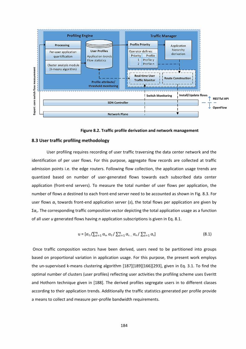
184

Figure 8.2. Traffic profile derivation and network management

8.3 User traffic profiling methodology

User profiling requires recording of user traffic traversing the data center network and the

identification of per user flows. For this purpose, aggregate flow records are collected at traffic

admission points i.e. the edge routers. Following flow collection, the application usage trends are

quantized based on number of user-generated flows towards each subscribed data center

application (front-end servers). To measure the total number of user flows per application, the

number of flows α destined to each front-end server need to be accounted as shown in Fig. 8.3. For

user flows αs towards front-end application server (s), the total flows per application are given by

Σαs. The corresponding traffic composition vector depicting the total application usage as a function

of all user u generated flows having n application subscriptions is given in Eq. 8.1.

u = [α1 /∑ α𝑛𝑠=1 s, α2 / ∑ α𝑛

𝑠=1 s … αn / ∑ α𝑛𝑠=1 s] (8.1)

Once traffic composition vectors have been derived, users need to be partitioned into groups

based on proportional variation in application usage. For this purpose, the present work employs

the un-supervised k-means clustering algorithm [187][189][166][293], given in Eq. 3.1. To find the

optimal number of clusters (user profiles) reflecting user activities the profiling scheme uses Everitt

and Hothorn technique given in [188]. The derived profiles segregate users in to different classes

according to their application trends. Additionally the traffic statistics generated per profile provide

a means to collect and measure per-profile bandwidth requirements.

185

Figure 8.3. User generated traffic flows per application

8.3.1 Flow statistics

Implementing per-profile traffic policies requires determining the projected flow rates between

a) users and front-end application servers per profile as well as b) internal intra-server traffic

generated per application in response to each user request. A list of flow parameters used for real-

time traffic management and monitoring profile stability are summarised in Table 8.1. Given the

per-profile transmitted and received data transfer rate z for each front-end application server

collected over time t, the maximum probability for data rate z to take on a given value using the

density function given by Eq. 8.2.

Pr [ x ≤ z ≤ y ] = ∫ 𝑓𝑦

𝑥 Z (z) dz (8.2)

The probability of z falling within a particular range of values is given by the integral of density of z

between the lowest and greatest values of the range (x, y). The maximum probability of z is

measured for both inbound and outbound traffic per profile for each subscribed application

independently The respective data transfer rates for inbound and outbound flows for application αi

belonging to profile Pk can therefore be given by Prmax [z in||out (Pk, αi)] and the corresponding flow

inter-arrival times by Prmax [Δtin||out (Pk, αi)]. While the external traffic between users and front-end

servers is relatively easy to measure and record, the internal flows generated between the

application servers are subject to significant variation and greatly depend on the application logic as

186

well as the respective server connectivity model. A maximum threshold value is therefore, defined

for the inter-flow arrival time Δtinternal and the respective data rate zinternal between internal servers

per-application in response to each user (profile) connection. To evaluate the proposed traffic

management scheme discussed later in section 8.5, flow rates were generated up to pre-set

threshold to understand the effects of varying inter-server traffic on the viability of proposed

approach.

8.3.2 Profile stability and regeneration

The baselines of network traffic per profile i.e. flow inter-transmission times and data transfer

rates summarised in Table 8.1 provide an intuitive means to continuously monitor profile

consistency via OpenFlow flow counters in DC core switches using multi-part flow_stat and

table_stat messages. Abnormalities in anticipated aggregate flow statistics with respect to real-time

profile memberships triggers as an advisory for network administrators to re-evaluate the profiles.

It also dictates the efficacy of the clustering algorithm and the subsequent traffic forwarding

performance. Additionally, real-time monitoring of out-of-profile traffic anomalies via OpenFlow

allows dynamic management of the respective flows. The real-time monitor and traffic manager in

the present context allow for a place holder profile (the guest profile) for policing out-of-profile

user traffic to minimize impact on existing flows until administrators can evaluate the respective

anomalies and regenerate the profiles. The introduction of new profiles or updating of existing

profiles may result in operators re-evaluating network policies in view of updated requirements.

8.4 Traffic Management Approach

This section describes the proposed traffic management scheme, comprising of five

procedures: profile and application hierarchy derivation, external flow management between users

and front-end application servers, internal flow forwarding between application servers, installation

of calculated per profile routes in individual switches (using the OpenFlow protocol) and finally the

scheduling management of the respective traffic management algorithms.

8.4.1 Profile priority and application hierarchy

Conventional Ethernet uses best effort delivery of traffic which is prone to dropping of frames

in face of network congestion in the data center. While technologies such as equal cost multipath

(ECMP) promise higher throughput by distributing traffic over multiple links over the legacy

187

spanning tree protocol (STP), these alone are inadequate in policing traffic in view of the inherent

mix of user classes present in the data center environment [286]. To account for the real-time

traffic load and different priority flow-forwarding requirement per user profile, the present design

proposes using operator-defined profile priority tables as shown in Fig. 8.4. The priority list aims to

reduce the effects of network congestion for user categories (in order of hierarchy) by routing flows

on different paths between the core, aggregate and access switches for external traffic between

the user and application servers. Based on the application usage weighting per-profile, a global

application hierarchy table is also derived. The table is used to create flow forwarding constructs

using multiple routes (in order of application hierarchy) to facilitate inter-server traffic between

application servers connected to different access switches. Applications higher up the chain

therefore, benefit in using lesser-congested links for internal internal data center traffic. The

approach translates operator defined priority per user profile to provision routes aimed at

increasing throughput and reducing the effects of network congestion, on not only external but also

internal flows which form the bulk of traffic within the data center. For example, resource intensive

profiles having higher business productivity may be placed at the top priority while the guest profile

comprising of out-of-profile and anomalous user traffic placed at the bottom. The proposal allows

operators greater leverage in defining network provisioning policies according to real-time user

application trends captured in user profiles instead of relying on isolated applications and services.

Table 8.1. User profiles and inter-server flow parameters

Entity Parameter Usage Technology Implementation

User traffic profiles

Flow rate (inbound and outbound) zin || zout

Aggregate value: Real-time profile monitoring

Per subscribed application: External route construction

User traffic profiling: NetFlow: core switch export

Real-time monitoring: OpenFlow: flow_stats, table_stats message

Route construction:

OpenFlow: flow_mod message

Flow arrival (inbound and outbound) Δtin || Δtout

Application servers

Inter-server data rate zinternal

Internal route construction Inter-server flow arrival

threshold Δtinternal

188

Figure 8.4. Profile and application hierarchy

Figure 8.5. Three layer data center topology

8.4.2 External route construction

A three-layer inter-connected network topology prevalent in modern data center architectures

to model and evaluate the proposed design is represented in Fig. 8.5. The network provisioning

algorithm used for optimizing external user flows is given in Fig. 8.6. The algorithm computes the

189

inbound and outbound forwarding links per profile for each front-end application server before

moving to the next, in order of profile and application hierarchy. A link threshold lT gives the

maximum available βmax bandwidth per link. If lT is greater than the required inbound or outbound

flow rate for u profile users (lT > u.z), the link is selected for forwarding. Otherwise users are split

between alternate routes with flows equating lT/z using the selected link and the rest (u=u- lT/z)

split over alternate links as computed during the subsequent iteration. The available bandwidth per

link is correspondingly updated (βl(E,D)|| (D,A) = βl(E,D)|| (D,A) – u.z inbound||outbound). The resulting flow

configurations are pushed via OpenFlow flow_mod messages to switches using the SDN controller

[1][17]. The same process is repeated as long as there exists at least one link between two nodes

with lT > 0, and for instances where all links are at full capacity, the respective flows are forwarded

via the last installed route, i.e. link used by preceding application/profile. The algorithm ensures

that higher priority profiles continue to experience higher throughput in the event of network

congestion by routing lower priority profile flows over links with relatively higher congestion.

Conventional load balancing schemes over multi paths (ECMP, DLMBP, etc.) split traffic flows at

frame level and each path having a different delay causes out-of-order frame delivery. This results

in TCP interpreting these reordered frames as a sign of congestion which ultimately results in

degraded performance [294][295]. Our proposed approach ensures that all frames per flow (for

each user) are forwarded over the same links to preserve ordered delivery and any splitting of user

traffic only occurs at the flow level.

8.4.3 Internal route construction

Similar to external traffic the proposed internal route construction algorithm given in Fig. 8.6

uses the available bandwidth β per link to optimize internal traffic between constituent application

servers. Application servers residing on adjoining pods are linked by same set of aggregation

switches (D) requiring route computation over links l(A,D), while communication between servers on

disjoint pods also requires route computations for flows traversing the core switches i.e. over links

l(D,E). The derived application hierarchy table utilizing the profile priority and respective application

weightage given in Fig. 8.4 determines the application precedence in assigning forwarding paths

between servers. Applications having greater weightage in higher priority profiles therefore, get

preference in using forwarding paths experiencing higher throughput and lesser congestion. The

maximum available bandwidth βmax over each link is given by the respective link threshold lT. If the

pre-set internal flow rate threshold zinternal per application for u users is greater than the link

threshold lT, the route is selected for flow forwarding. If however, lT < u.zinternal, then lT/zinternal flows

are forwarded through the link with the remaining flows split over alternate links determined by

190

the iteration. The process continues for each application as long as there exist one route with lT >0

between the respective switch pairs, otherwise the last installed route (link) is used for forwarding

traffic. The scheduling frequency of this route construction scheme to minimize the computational

and controller management overhead is presented in the next sub-section. Furthermore, since the

respective traffic management algorithms work in online mode, the time complexity for

implementation in realistic scenarios is considered during evaluations.

8.4.4 OpenFlow route installation scheme

To effectively split traffic according to the calculated flow forwarding constructs, network

address translation (NAT) is used to place users into segregated subnets each identified with a

VLAN ID. In view of limited switch memories (TCAM) [296][297], the scheme also results in

minimizing the OpenFlow table sizes despite substantial per profile user connections. An example

schematic representing OpenFlow pipeline processing of network traffic towards application server

through individual switches is depicted in Fig. 8.7. Table 0 in S1 (edge/core switch) translates and

sets NAT IP addresses to profile users and forwards processing to table 1. Flow table 1 assigns a

VLAN ID per subnet and the output port for outbound flows. Identification of per-profile flow traffic

(as well as distributed traffic from same profile) towards the application server can, in turn, be

identified only by the destination address and the VLAN ID to select subsequent outgoing ports in

each intermediate switch along the path. As seen in flow table 0 of switches S2 and S3, outgoing

traffic is now referred to by the destination server and VLAN IDs to select the outgoing port,

substantially reducing the forwarding tables for external flows. Internally within the DC, internal

server traffic, the respective server MAC addresses are used for traffic forwarding in respective

switch tables to further reduce latency and achieve traffic transfer close to line rate. Inter-server

traffic for same application or service in the implemented prototype during evaluation (section 8.6)

is therefore, split at the individual server level over multiple links using per server MAC addresses.

191

start function path_selection (external)

for (profile priority P=1, P<=n; P++)

for (application priority α=1; α <= n; α++)

#Path selection inbound & outbound traffic, *=last used link

do

for ∀ l(E,D)||(D,A)

lT (E,D)||(D,A)* = β l(E,D)||(D,A)*

umax(E,D)||(D,A) lT / z inbound||outbound

if umax(E,D)||(D,A) ≥ u && lT >0

flow_mod [l(E,D) , l(D,A)];

βl(E,D)|| (D,A) = βl(E,D)|| (D,A) – u . z inbound||outbound;

end if

else if umax(E,D)||(D,A) < u && lT >0

flow_mod (l(E,D), l(D,A))max_users;

βl(E,D)|| (D,A) = βl(E,D)|| (D,A) – u . z inbound||outbound;

u = u – umax;

end else

else if lT <0

flow_mod (l(E,D)*||l(D,A)*);

end else

end for

while u> 1;

end for

end for

end function

start function path_selection (internal)

for (application priority α=1; α <= n; α++)

#Path selection internal server-server traffic, *=last used link

do

for ∀ l(A,D)||(D,E)

lT (A,D)||(D,E)* = βl(A,D)||(D,E)*

flowmax = βl(A,D) || βl(D,E)

if lT(A,D)||(D,E) ≥ zinternal . u && lT >0

flow_mod [l(A,D) , l(D,E)];

βl(A,D) ||(D,E) = βl(A,D) ||(D,E) - zinternal . u;

end if

else if lT(A,D)||(D,E) < z internal . u && lT >0

flowmax = βl(A,D)max || βl(D,E)max / zinternal;

flow_mod [lT(A,D) , lT(D,E)];

u = u - flowmax . z;

βl(A,D) ||(D,A) = βl(A,D) ||(D,E) - zinternal . u;

end else

else if lT <0

flow_mod (l(E,D)*||l(D,E)*);

end else

end for

while u>1;

end for

end function

Figure 8.6. External (external) route construction algorithm Internal (internal) route construction

Figure 8.7. OpenFlow pipeline processing –flow installation and route implementation in switches

192

8.4.5 Real-time route scheduling frequency

Each installed route, by default can accommodate additional users dictated by flow inter-

arrival times Δt on each selected path. The external flow construction algorithm in Fig. 8.6 installs

flows per link utilizing zin||out flow rates, however, flow inter-arrival time of Δtin||out allows the

selected link to accommodate users equalling u(ED||DA) given by Eq. 8.3. Similarly, for inter-server

routes with flow inter-arrival time threshold Δtinternal, the selected link is capable of handling flows

flow(AD||DE) given by Eq. 8.4.

u(ED||DA) = umax / (1- Δtin||out ) (8.3)

flow(AD||DE) = flowmax / (1- Δtinternal) (8.4)

High inter-arrival times, therefore, translate into a higher tolerance of the installed flows to user

connection updates requiring less frequent re-evaluation. The SDN controller monitors real-time

user via edge/core switch port monitoring using an average flow threshold to track new/existing

and stale user connections. The controller periodically re-computes external and internal

forwarding over a link following additional user connections when u(ED||DA) > umax or

flow(AD||DE) > flowmax, and immediately on disconnections. Furthermore, re-evaluation of prior

installed routes only requires the forwarding routes of the respective profile (with user update) and

any subsequent routes in lower priority profiles to be updated. As depicted in Fig. 8.8, addition or

deletion of active users in profile k will result in re-computation and assignment of queues in

profiles k, l and m and associated inter-server links, leaving pre-installed flows of profile j in force.

Reducing control plane overhead remains an avenue of increasing research concentration as

highlighted in [297], [298] and [65], and the present flow scheduling scheme aims at decreasing the

relative management workload of the SDN controller to improve real-time design scalability.

Figure 8.8. Route update scheduling scheme

193

8.5 Evaluation

To evaluate the effectiveness of proposed traffic management method in an actual network

scenario, user traffic profiling was carried out in a realistic campus network segment, part of a

larger academic environment. The network comprised of 42 users from computing and engineering

departments. Each user had one computer and all user machines in the department connected to

local data center servers via the campus network to access hosted applications and services. The

user traffic profiles derived from this network segment were used in a simulated data center

network using Ryu SDN framework to optimize external traffic between users and the front-end

application servers as well as inter-server traffic within the data center. The derived user traffic

profiles, data center simulation topology and traffic optimization results are presented in the

following sections.

8.5.1 Traffic profile derivation

The profile derivation scheme used NetFlow records exported from the edge of the

departmental network, transmitted between user machines and consolidated application servers in

the data center over a span of ten weeks from 01/12/2015 to 15/02/2016. A total of approximately

72.2 million flows were examined. To account for replication in nature of user activities,

applications were further grouped into distinct categories as depicted in Table 8.2. User traffic was

classified by matching user flows against destination IP addresses and ports used by servers and the

resulting flows were concatenated every 24 hours [Appendix- 1.2]. The corresponding traffic

composition vector depicting application usage distribution as percentage of generated flows for a

user u1 as per Eq. 8.1, for one day of activity (01/12/2015) is given in Eq. 8.5 as follows.

u1 [01/12/2015] = [2.3 8.4 25.6 23.1 11.2 10.3 15.5 2.2 1.4] (8.5)

The resulting traffic composition vectors for all users were subjected to k-means cluster analysis Eq.

3.1 to determine the optimal number of clusters (translating for traffic profiles) appropriately

reflecting user activities, the derived clusters were examined starting from k=2, using Everitt and

Hothorn technique described earlier. The corresponding plot of ‘within groups sum of squares

distance’ per observation in each cluster against k for present data is given in Fig. 8.9 where a

significant drop can be seen up to a cluster size k=6, and minimal subsequent variations up to k=20,

indicating an optimal value of 6 profiles for the entire subscriber base. The resulting traffic profiles

194

Table 8.2. Application Tiers

Application Tier Applications

Web browsing (w) Internal and external website

Email (e) Webmail, Outlook, SMTP, POP3

Storage (g) Centralized storage, FTP

Streaming (s) Podcasting, video content

Communication (c) Office communications server

Enterprise (p) Corporate information system, staff portal

Publishing (h) Content management system (document, print)

Software (r) Software distribution service

Network utility (z) DNS queries, network multicast

Figure 8.9. Application clusters (k): wss vs. k graph

(k=6), detailing the application trends among user traffic profiles as a percentage of user generated

flows are given in Fig. 8.10. Since general network service traffic (z) such as DNS and multicast

traffic is not a user-triggered application but a functional one, hence, it was excluded while

clustering users and later separately calculated as a percentage of total network flows generated

per user profile. From a network management perspective the resulting profiles showed significant

variation in user activity. For example, Profile 1 concentrated mainly on web browsing (53.2%) with

relatively limited usage of other applications apart from the corporate information and content

management services. Profile 2 focused on using communication utilities i.e. the instant messenger

and VoIP with limited use of content management applications and minimal use of others. Profile 3

heavily inclined towards corporate information service (65.2%) with significant use of email service

195

(10.3%) compared to other profiles. Profile 4 heavily tilted towards document and print content

creation and using centralized storage facility (11.8). Profile 5 mainly used centralized storage

server with small use of content and corporate information server. Profile 6 was a mix of web

browsing, emails, storage and corporate applications. Hence, each enterprise user profile

represented a significant discrimination towards a certain mix of services. The use of software

distribution was, however, significantly low compared to other applications among all user profiles.

Fig. 8.11 (a) represents the upload and download rate per profile derived using the probability

density function given in Eq. 8.2. The corresponding inter-flow arrival times per profile are given in

Fig. 8.11 (b). In view of the discriminative application trends depicted in the derived user profiles

and varying flow rates, operators may want control over which users to prioritize in terms of

network bandwidth allocation. Furthermore, the stability of the derived profiles over 24 hour time-

bins and frequency of outliers in the respective flow statistics may aid administrators in triggering

real-time filtering of irregular traffic and minimizing consequences on priority user traffic. Profile

stability evaluation and threshold setting to filter out-of-profile flow frequency are discussed in

detail in the following section.

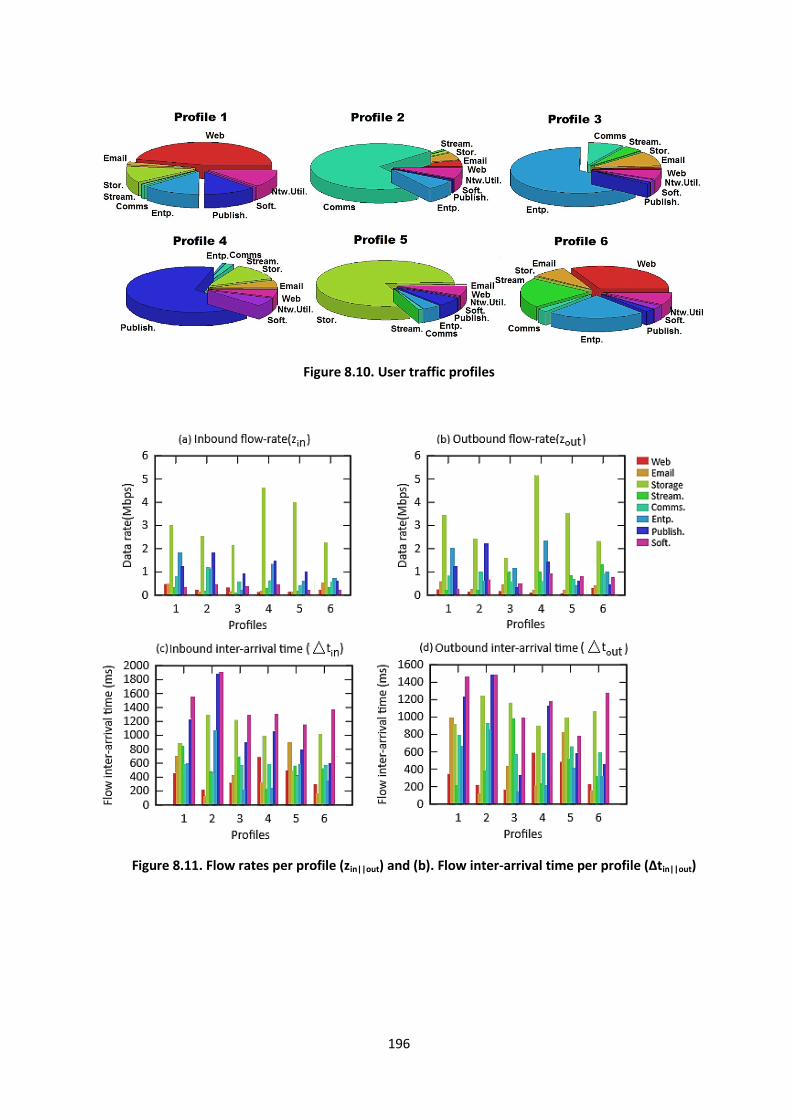
196

Figure 8.10. User traffic profiles

Figure 8.11. Flow rates per profile (zin||out) and (b). Flow inter-arrival time per profile (Δtin||out)

197

8.5.2 Profile Stability

Profile stability highlights the significance of gaining a better insight to change in user

activities and to benchmark the consistency of the extracted profiles and the re-profiling frequency.

The average stability of the six profiles derived earlier with respect to application trends over 24

hour time-bins are given in table 3. Profile 5 users showed the highest consistency in retaining

profiles at 99.8% followed by profile 4 at 99.4% while profile 6 showed the lowest at 96.9%. The

reported profile retention of campus users was greater in comparison with a similar study aimed at

evaluating profile stability for multi-device residential users reporting the lowest profile consistency

at 81%, undertaken in chapter 4 [293]. Campus users hence, showed a significantly greater degree

of consistency in daily application usage in relation to residential users. It was also noted that the

minimal irregularity observed was due to inter-profile transitions among users mainly due to

proportional variation in the same kind of user activity rather than a complete change of user roles

or introduction of new profiles. The consolidated inter-flow arrival times and flow rates per profile

are given in Fig. 8.12. As depicted in Table 8.1, from a network management perspective,

consolidated per-profile flow statistics aid administrators in setting a threshold to identify real-time

anomalous (out-of-profile) traffic for subsequent filtering and for profile regeneration. For example,

configuring the traffic manager to monitor real-time flow statistics according to per profile

aggregate flow statistics would result in automatically placing flows exceeding the threshold in the

guest profile to reduce consequence on priority profile traffic.

Table 8.3. Average probability of profile regularity (/24 hour time-bins)

User Profiles No Change Change (Outliers)

Profile 1 0.983 0.017

Profile 2 0.975 0.025

Profile 3 0.987 0.013

Profile 4 0.994 0.006

Profile 5 0.998 0.002

Profile 6 0.969 0.031

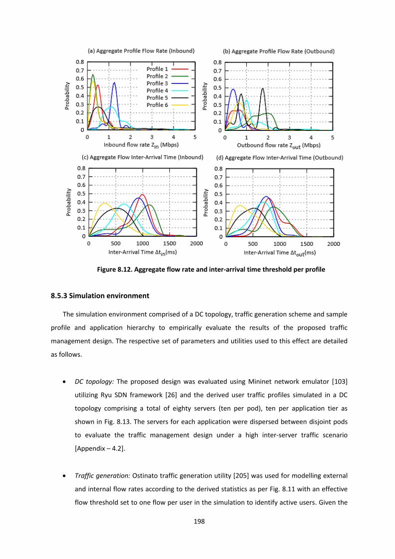
198

Figure 8.12. Aggregate flow rate and inter-arrival time threshold per profile

8.5.3 Simulation environment

The simulation environment comprised of a DC topology, traffic generation scheme and sample

profile and application hierarchy to empirically evaluate the results of the proposed traffic

management design. The respective set of parameters and utilities used to this effect are detailed

as follows.

DC topology: The proposed design was evaluated using Mininet network emulator [103]

utilizing Ryu SDN framework [26] and the derived user traffic profiles simulated in a DC

topology comprising a total of eighty servers (ten per pod), ten per application tier as

shown in Fig. 8.13. The servers for each application were dispersed between disjoint pods

to evaluate the traffic management design under a high inter-server traffic scenario

[Appendix – 4.2].

Traffic generation: Ostinato traffic generation utility [205] was used for modelling external

and internal flow rates according to the derived statistics as per Fig. 8.11 with an effective

flow threshold set to one flow per user in the simulation to identify active users. Given the

199

enormity of inter-server traffic within the DC compared to external traffic as discussed in

[286], [288] and [21], the threshold for internal flow rates between each pair of application

servers (zinternal) was set to randomly transmit at up to four times the external outbound

flows rates per-profile given in Fig. 8.11 (a). Correspondingly the flow inter-arrival time

(Δtinternal) for internal traffic between servers per application tier depicted in Fig. 8.11 (b)

was proportionally reduced to analyse the effects of network congestion on high and low

priority profiles with increasing user connections. To account for anomalous (out-of-profile)

traffic, percentage of user traffic per profile was varied in accordance with table 3,

exceeding the thresholds given in Fig. 12 at each simulated user load.

Sample profile and application hierarchy: A sample profile priority table was used with the

corresponding application hierarchy based on application usage weighting starting with

highest profile represented in Table 8.4.

Traffic management: Using Table 8.4, along with the current as well as predicted traffic per

profile, the SDN traffic manager computed the optimal user to front-end server routes

along with the flow forwarding constructs for inter-server traffic. The computed flows were

afterwards installed in network switches via the controller using OpenFlow protocol and

the iteration continued tracking the number of real-time user connections [Appendix – 5.4].

Figure 8.13. Simulated data center environment

200

Table 8.4. Sample profile priority table

Profile priority Profiles Application Hierarchy

1 Profile 3 Enterprise Email Communication Streaming Software Publishing Web-browsing Storage

2 Profile 2

3 Profile 1

4 Profile 6

5 Profile 4

6 Profile 5

7 Guest

8.5.4 Throughput and bandwidth results

The simulation results measured the effectiveness of the proposed profiling based real-time

traffic optimization against conventional traffic management schemes i.e. ECMP and STP.

Employing ECMP or STP to optimize a specific application in isolation would result in improved

performance of the respective application, in relation to other data center hosted services. The

present simulation, however, provisioned DC links among all applications equally using the

conventional schemes to provide an overall comparison of the results against the proposed

profiling mechanism. The simulation therefore, aims to evaluate the benefit of profiling based

traffic management over individual application weightage models, regardless of the particular

application being optimized by ECMP or STP, using the SDN framework. Furthermore, to monitor

the traffic statistics varying user loads, effective throughput between users and front-end servers

(SW[1-2], SW[11-18]) as well as between individual application servers (SW[11-18]) residing on

disjoint pods was recorded using OpenFlow switch port statistics.

The first test compared STP, ECMP and the proposed profiling-based scheme frame delivery ratio

and throughput (total received frames) performance for the external inbound traffic for the top

priority profile 3 and lowest priority profile 5, for highest priority application (Enterprise) while

increasing user loads across all profiles. The corresponding parameters are given in Tables 8.5-8.8.

As shown in Fig. 8.14(a) and (b) profile 3 users consistently experienced high frame delivery and

throughput using profiling based optimization compared to the ECMP and STP scheme. STP used a

loop free environment limiting utilization of all available links while ECMP equally balanced the

traffic across all links. The absence of profiling-based forwarding, resulted in profile 3 users

experiencing significantly lower frame delivery (≤ 21%) and throughput (≤ 35%) with increasing user

loads (> 300 users per profile) despite being high priority users. Similarly, profiling based traffic

optimization of the lowest priority profile 5 resulted in improved frame delivery (~39%) and

201

throughput (~37%) using the profiling scheme shown in Fig. 8.14(c) and (d). The resulting

improvement was due to the higher application priority of the enterprise tier despite sharing links

with other lower priority application servers on adjacent pods (i.e. the publishing tier) at increasing

user loads (≥ 300 users per profile) As evident from the profile 5 routing paths given in Table 8.7, at

very high user loads (≥ 600 users per profile), profiling based optimization ensured profile 5 traffic

continued to use the SW1:SW6:SW14 path. The effects of oversubscription were hence, localized

on the alternative SW2:SW6:SW14 path, mainly carrying internal inter-server traffic using the

profile prioritization scheme.

Table 8.5. Basic Parameters – Profile 3 Enterprise Front-end

Name Value

Profile 3 zin 0.214Mbps

Profile 3 zout 1.134Mbps

Profile 3 Δtin 857ms

Profile 3 Δtout 952ms

Table 8.6. Basic Parameters – Profile 5 Enterprise Front-end

Name Value





Table 8.7. Profile 5 Routing Path: User Enterprise Front-end

User load Inbound Traffic Scheme Route

Pod4

(Gbps)

Pod3+4

(Gbps)

P5 Entp.

(Gbps)

Preceding P5, Entp.

(Gbps)

600 users

14.889 38.568 0.348 3.144 Profiling SW1:SW6:SW14

ECMP SW[1-2]:SW[5-6]:SW14

STP SW1:SW6:SW14

700 users


ECMP SW[1-2]:SW[5-6]:SW14

STP SW1:SW6:SW14

202

Figure 8.14. Frame delivery ratio and throughput measurement

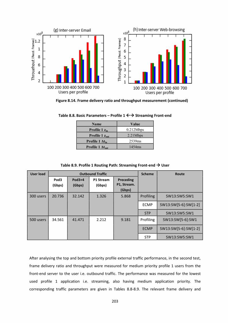
203

Figure 8.14. Frame delivery ratio and throughput measurement (continued)

Table 8.8. Basic Parameters – Profile 1 Streaming Front-end

Name Value





Table 8.9. Profile 1 Routing Path: Streaming Front-end User

User load Outbound Traffic Scheme Route

Pod3

(Gbps)

Pod3+4

(Gbps)

P1 Stream

(Gbps)

Preceding P1, Stream.

(Gbps)

300 users


ECMP SW13:SW[5-6]:SW[1-2]

STP SW13:SW5:SW1

500 users

34.561 41.471 2.212 9.181 Profiling SW13:SW[5-6]:SW1

ECMP SW13:SW[5-6]:SW[1-2]

STP SW13:SW5:SW1

After analysing the top and bottom priority profile external traffic performance, in the second test,

frame delivery ratio and throughput were measured for medium priority profile 1 users from the

front-end server to the user i.e. outbound traffic. The performance was measured for the lowest

used profile 1 application i.e. streaming, also having medium application priority. The

corresponding traffic parameters are given in Tables 8.8-8.9. The relevant frame delivery and

204

throughput statistics are given in Fig. 8.14 (e) and (f) respectively. It was observed that the that

profiling-based optimization significantly outperformed ECMP and STP (≥ 300 users per profile) due

to ECMP load-balancing traffic over all links as shown in routing paths depicted in Table 8.8 while

profiling scheme routing profile 1 traffic over the first path [SW13:SW5:SW1] and forwarding the

subsequent lower priority traffic over alternate links. For 300 users per profile, the total traffic out

of pod 3was 20.736Gbps, the external priority traffic preceding profile 1 streaming users around

5.868Gbps and profile 1 streaming users at 1.326Gbps. The two outbound links (20Gbps) from the

access switch SW13, the first link [SW13:SW5:SW1] therefore, carried outbound profile 1 streaming

traffic without penalty. ECMP in comparison load-balanced traffic over all paths resulting in

decreased frame delivery ratio (98.16%) and throughput (0.314 million frames). The trend scaled

well up to 500 users, where traffic out of pod 3 increased to 34.561Gbps with profile 1 streaming

traffic accounting for approximately 2.21Gbps and the priority traffic preceding profile 1 being

around 9.18Gbps. Hence, of two links out of pod 4, profile 1 traffic was split over first link

(0.82Gbps) and second link (0.39Gbps). Since the second path [SW13:SW6:SW1], also carried inter-

server traffic and was oversubscribed, the frame delivery ratio using profiling management,

dropped to approximately, 81.34%. The trend continued further, with increasing user connections

(in higher priority profiles), and users in profile 1 pushed to the second link, closing the gap

between ECMP and profiling based optimization up to 700 users per profile. Hence, even for

medium priority profile and mid-tier application, the performance throughput was considerably

better even with substantially high user loads when compared with conventional load-balancing

techniques.

To evaluate inter-server traffic performance between same application servers residing on disjoint

pods, throughput for the Email tier closer to the top of the global application hierarchy table and

web-browsing towards the bottom was tested and is given in Fig.8.14 (g) and (h). The

corresponding traffic parameters are given in Tables 8.10-8.11. For the Email tier, the throughput

was measured between switches SW12 and SW17 (pods 2 and 7) and for web browsing servers

between SW11 and SW18 (pods 1 and 8), owing the location of the respective servers. Profiling

optimization gave improved overall throughput between pods 2 and 7 for Email traffic even at

maximum user load of 700 per profile, owing higher priority among other applications traversing

the same links i.e. web-browsing, software and storage tiers via the aggregate and core switches. At

a load of approximately 600 users per profile, the external outbound traffic preceding inter-pod

Email traffic forced Email traffic to split over two paths SW17:SW9 the primary and SW17:SW10 the

alternative with the later carrying remaining application traffic from software tier. As observed

205

Table 8.10. Basic Parameters – Inter-server Traffic

Name Value

Inter-server Email traffic (e) zinternal 1.528– 6.112Mbps

Email (e) Δtinternal 0 - 125ms

Inter-server Browsing traffic (w) zinternal 1.134 – 4.536Mbps

Browsing (w) Δtinternal 0 - 625ms

Table 8.11. Routing Path: Web browsing [Pod8:Pod1]

User load

Outbound Traffic Scheme Route

Pod8

(Gbps)

Browsing

(Gbps)

Preceding Browsing

(Gbps)

400 users

23.218 1.143 7.332 Profiling SW18:SW10:SW1:SW3

ECMP SW18:SW[9-10]:SW[1-2]:SW3

STP SW18:SW10:SW1:SW3

500 users

29.023 1.429 9.165 Profiling SW18:SW9:SW1:SW3

SW18:SW10:SW1:SW3

ECMP SW18:SW[9-10]:SW[1-2]:SW3

STP SW18:SW10:SW1:SW3

during external traffic management, any increase in preceding (priority) traffic, low priority

application traffic may fully shift to secondary links that may be oversubscribed without substantial

consequence for high priority Email tier. For web-browsing server tier, both profiling and ECMP

based traffic management perform equally up until the maximum user load of 700 users per profile.

For 400 users per profile, browsing server traffic from pod 8 to pod2 was around 1.143Gbps carried

over path SW18:SW10, preceding priority traffic out of pod8 being 7.332Gbps out of pod8 and

remaining inter-server traffic (mainly storage tier) approximating 14.743Gbps was split over both

SW18:SW10 and SW18:SW9 paths. Since the total outward traffic exceeded the combined link

capacity (20Gbps), uniform load balancing across all links using ECMP resulted in lower throughput

performance for browsing than the devised profiling based management scheme.

At 500 user load of users per profile, external pod8 traffic having higher priority than browsing

traffic approximated at 9.165Gbps. The web browsing server traffic reaching 1.429Gbps, was, split

into using the SW18:SW10 path (0.715Gbps) with remaining (0.714Gbps) routed over the

oversubscribed SW18:SW9 path carrying approximately 19Gbps traffic. The trend continued with

further increase in preceding traffic resulting in web-tier shifting to oversubscribed links resulting in

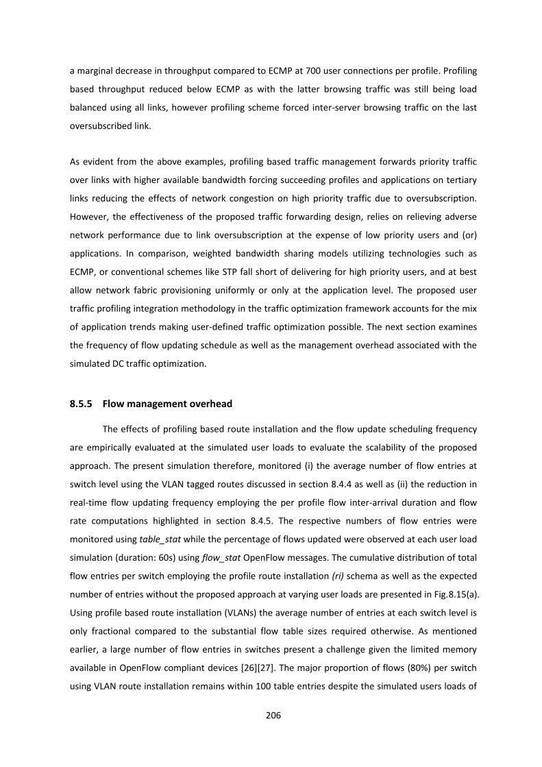
206

a marginal decrease in throughput compared to ECMP at 700 user connections per profile. Profiling

based throughput reduced below ECMP as with the latter browsing traffic was still being load

balanced using all links, however profiling scheme forced inter-server browsing traffic on the last

oversubscribed link.

As evident from the above examples, profiling based traffic management forwards priority traffic

over links with higher available bandwidth forcing succeeding profiles and applications on tertiary

links reducing the effects of network congestion on high priority traffic due to oversubscription.

However, the effectiveness of the proposed traffic forwarding design, relies on relieving adverse

network performance due to link oversubscription at the expense of low priority users and (or)

applications. In comparison, weighted bandwidth sharing models utilizing technologies such as

ECMP, or conventional schemes like STP fall short of delivering for high priority users, and at best

allow network fabric provisioning uniformly or only at the application level. The proposed user

traffic profiling integration methodology in the traffic optimization framework accounts for the mix

of application trends making user-defined traffic optimization possible. The next section examines

the frequency of flow updating schedule as well as the management overhead associated with the

simulated DC traffic optimization.

8.5.5 Flow management overhead

The effects of profiling based route installation and the flow update scheduling frequency

are empirically evaluated at the simulated user loads to evaluate the scalability of the proposed

approach. The present simulation therefore, monitored (i) the average number of flow entries at

switch level using the VLAN tagged routes discussed in section 8.4.4 as well as (ii) the reduction in

real-time flow updating frequency employing the per profile flow inter-arrival duration and flow

rate computations highlighted in section 8.4.5. The respective numbers of flow entries were

monitored using table_stat while the percentage of flows updated were observed at each user load

simulation (duration: 60s) using flow_stat OpenFlow messages. The cumulative distribution of total

flow entries per switch employing the profile route installation (ri) schema as well as the expected

number of entries without the proposed approach at varying user loads are presented in Fig.8.15(a).

Using profile based route installation (VLANs) the average number of entries at each switch level is

only fractional compared to the substantial flow table sizes required otherwise. As mentioned

earlier, a large number of flow entries in switches present a challenge given the limited memory

available in OpenFlow compliant devices [26][27]. The major proportion of flows (80%) per switch

using VLAN route installation remains within 100 table entries despite the simulated users loads of

207

up to 700 users per profile. The core switches comprise of smallest forwarding table sizes with

maximum of 97 entries (excluding the NAT functionality) compared to access and distribution table

sizes recording a maximum of 106 and 119 entries per switch respectively. The expected flow table

sizes without profiling route installation scheme, however, are considerably larger with maximum

core switch table size of around 2320 entries per switch and distribution and access switches going

beyond 250 entries per switch. The potential reduction in table sizes using the route installation

scheme therefore, presents a saving of approximately 23% - 95% entries in the DC switches at

simulated user loads. Since, most SDN compatible hardware the flow tables need to be

implemented in TCAM, relatively expensive and larger than standard memory (RAM) and therefore,

reducing the average flow entries per switch scales well in SDN based DC.

The cumulative distribution of the total flow updates to varying user load ratio, using the route

scheduling (rs) scheme is given in Fig. 8.15(b). The flow update frequency at the core switch level

was lowest followed by access and the distribution switches. Minimum updating at the core level

was due to the minimum and less frequent changes required in the core switches with variation in

user loads. The management overhead saving of the route scheduling (rs) scheme utilizing flow rate

and inter-arrival interval computations to accommodate a greater number of users on installed

routes and thereby reduce flow modifications was substantial. The frequent updating of installed

flows via the SDN controller increases the OpenFlow control channel overhead (traffic) increasing

latency involved in implementing updated rules and subsequently affecting real-time traffic

forwarding [297-298][65]. The potential decrease in overhead ranged between 18% - 31% using

intelligent route scheduling compared to the lack of an efficient updating scheme. Furthermore, to

visualize the result of the flow scheduling on profile traffic, three profiles and three application tiers

were selected from the top, medium and bottom of the respective hierarchies, depicted in Fig. 8.15

(c) and (d). The medium priority profile6 showed maximum flow update frequency followed by core

and guest profiles. For the highest priority profile3 the saving in flow updates due to route

scheduling ranged between 49% - 64%. Guest profile accounting for out-of-profile traffic showed

the lowest flow updates mainly attributed to the minimum total flow installations catering

anomalous traffic. Among the applications, total potential savings in route updates due to the route

scheduling scheme ranged between 39% - 55% at varying user loads, the highest reduction

recorded for the highest priority communications tier. Profiles and applications higher up the

priority table therefore, showed a lower flow update frequency compared to lower priority traffic

as due to route scheduling scheme, the former remain relatively unaffected by updates further

208

down the hierarchy. The latency and controller overhead reduction achieved due to profiling based

route scheduling are considered in the following subsections.

8.5.6 Time complexity analysis

Further to improvements in the management overhead using reduced tables and scheduling

it is also important to evaluate the time complexity benefit of the approach. The average latency

involved in computing routes and completing flow installations in individual switches was therefore,

calibrated and illustrated in Fig. 8.15(e). The analysis considered the total duration of OpenFlow

flow_mod message generation via the controller and respective flow activation in the switch. To

measure the processing of flow_mod messages, an OpenFlow barrier_request was sent after

sending all flow_mod messages per switch [Appendix – 5.4]. The OpenFlow barrier_request

message ensures that the switch completes processing of all sent messages before issuing a

barrier_reply, indicating the flow-mod message has been fully processed at the switch. The results

show that minimal flow update frequency employed by the route scheduling scheme (rs) translates

into comparatively lower latency in creating flow constructs in switches. The highest average

latency was observed in updating access switch routes approximating at 2248ms. Access switches

serve both internal and external traffic and therefore, the average computational and processing

latency attributed to the lowest level in the switch hierarchy was greater than the aggregate and

core level. The average maximum recorded per core and distribution switch approximated at

2120ms and 1998ms respectively. The overall reduction in latency due to route scheduling ranged

between 23% - 41% (135ms-725ms) per switch level at varying user loads. The route computation

and installation duration comprised 0.67% - 3.6% of the total simulation duration (60s) per user

load across the entire DC switching fabric. The route scheduling scheme therefore, showed

considerably reduced dynamic route construction latency following profile membership updates.

In addition to the flow update latency involved at switch level, the time complexity involved in

detecting and re-routing of the simulated anomalous traffic is also considered. The latency

measurement comprises of the traffic monitor detecting the anticipated profile flow threshold

violation(s) followed by flow_mod message processing to route traffic under the lowest priority

guest profile. As depicted in Fig. 8.15(f), the detection latency remained largely within 1000ms and

the installation (or updating) of flows ranged between 1185ms - 1400ms. The total timespan of

detection and re-routing of anomalous flows under lowest guest priority therefore, averaged at

approximately 2293ms, or 3.8% per simulation duration at varying loads. From a real-time traffic

management perspective, the recorded latency presents swift real-time re-routing of out-of-profile

209

traffic minimizing the adverse consequences on remaining flows, until the network manager can

examine the anomalies; possibly re-evaluate the user profiles or the existing profile prioritization.

Figure 8.15. Flow statistics and latency measurement

210

8.5.7 OpenFlow control traffic

The average OpenFlow control channel traffic generated between the controller and DC

switches as a result of OpenFlow monitoring and flow installation/update messages is measured at

each simulated user load and illustrated in Fig. 8.16. Using the route scheduling scheme, the

maximum upstream and downstream traffic recorded at the core switch ranged at 187kbps and

789kbps respectively. Higher core switch control traffic using route scheduling at core switches was

due to the VLAN addressing functionality generating a significantly greater amount of flow_mod

messages downstream and corresponding flow_stat and table_stat message replies upstream

tracking the increase in profile memberships. The distribution control traffic recorded a maximum

of 87kbps upstream and 412kbps downstream. The average access switch control traffic, however,

remained comparatively low with the uplink maximum at 67kbps and downlink at 235kbps despite

the greater share of total inter-server traffic routes carried by access switches. Lower average

control traffic overhead per access switch was attributed to uneven distribution of the total access

switch control traffic, with few switches having bulk of the control traffic share in relation to a more

uniform division at aggregation points higher up the DC switch hierarchy. At each level of switch

hierarchy except the core the total upstream and downstream traffic remained significantly lower

employing the profile route scheduling. The average reduction in control traffic across access and

distribution DC switches due to profile route scheduling switches ranged between 7-16% on the

upstream and 21%-46% on the downlink respectively. To further streamline and balance the control

traffic, operators may utilize several controllers each catering to particular switch subset(s) for

improved redundancy. However, the placement of the controllers as well as the employability of in-

band or an external overlay for carrying the OpenFlow controller-switch traffic would greatly

depend on the DC topology and the prevailing traffic conditions. In the present scenario, however,

decreased flow update frequency resulted in significant reduction in the control overhead at the

distribution and access levels while using a single controller.

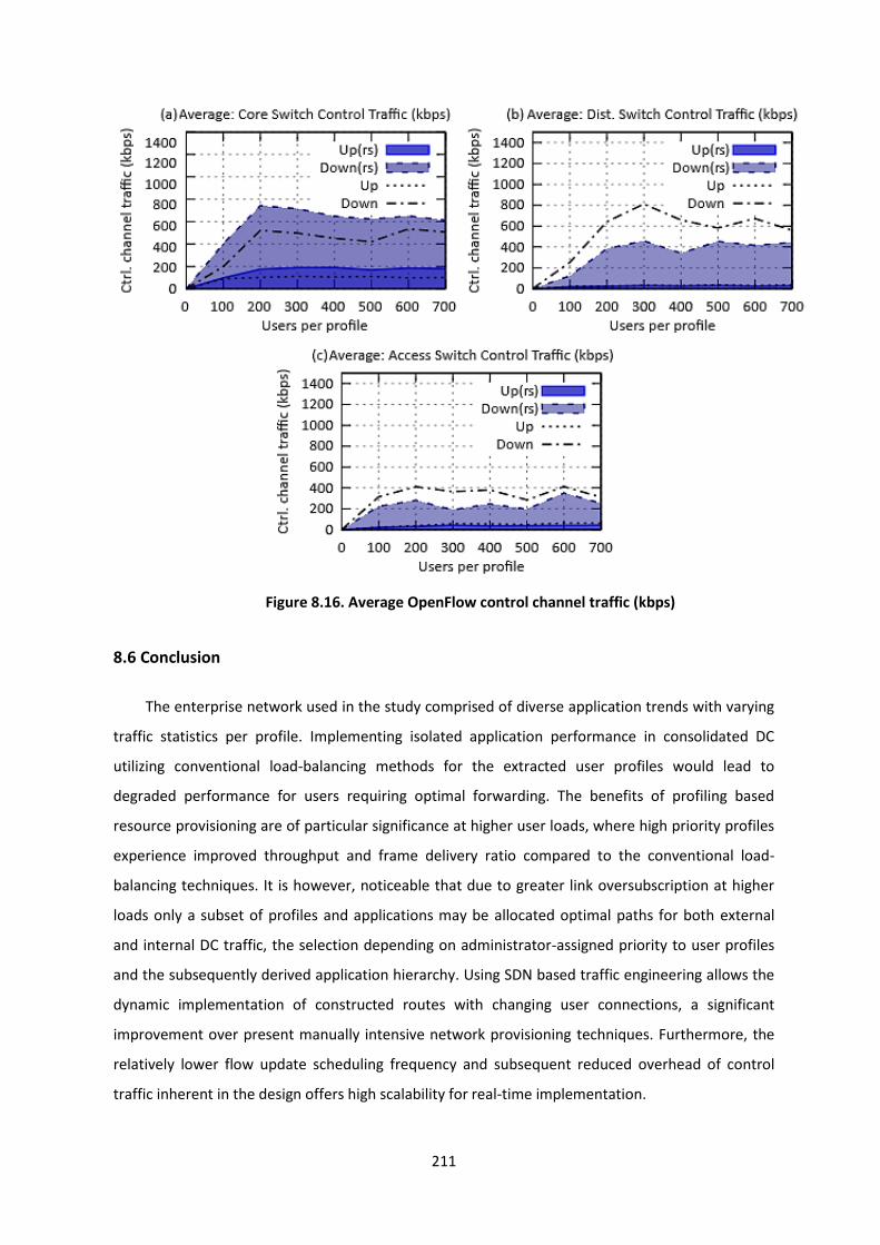
211

Figure 8.16. Average OpenFlow control channel traffic (kbps)

8.6 Conclusion

The enterprise network used in the study comprised of diverse application trends with varying

traffic statistics per profile. Implementing isolated application performance in consolidated DC

utilizing conventional load-balancing methods for the extracted user profiles would lead to

degraded performance for users requiring optimal forwarding. The benefits of profiling based

resource provisioning are of particular significance at higher user loads, where high priority profiles

experience improved throughput and frame delivery ratio compared to the conventional load-

balancing techniques. It is however, noticeable that due to greater link oversubscription at higher

loads only a subset of profiles and applications may be allocated optimal paths for both external

and internal DC traffic, the selection depending on administrator-assigned priority to user profiles

and the subsequently derived application hierarchy. Using SDN based traffic engineering allows the

dynamic implementation of constructed routes with changing user connections, a significant

improvement over present manually intensive network provisioning techniques. Furthermore, the

relatively lower flow update scheduling frequency and subsequent reduced overhead of control

traffic inherent in the design offers high scalability for real-time implementation.

212

To conclude the work of this thesis, the following chapter provides a summarization of the research

project including key achievements, limitations and scope for future work in the SDN traffic

engineering domain.

213

Chapter 9 Conclusions and Future Work

The present chapter summaries the thesis by reviewing the main achievements of this

research and discussing its limitations. The chapter also highlights future research directions within

user-centric traffic engineering solutions in software defined networking.

9.1 Achievements of the research

Overall, the project has achieved all the objectives initially set out in chapter 1, with a series of

investigations and experimental simulations undertaken towards the development of a user traffic

profiling mechanism to be used in the SDN framework. The full achievements are listed as follows.

1. An experimental investigation of the feasibility of user traffic profiling through flow-based

measurements (chapter 3 and chapter 4). An experimental study was conducted on real

user application usage from a residential building housing around 250 users. Firstly, by

utilising the k-means clustering algorithm, traffic profiles were derived based on user

generated traffic over a one-month time frame. The resulting profiles presented significant

discrimination in user activity, from a network management perspective. The profile

derivation method was further compared to other popular clustering algorithms

(hierarchical clustering and DBSCAN) and the stability of profiles was benchmarked to

ascertain their suitability for integration in a real-time SDN traffic management solution

(chapter 4). Since each residential user premises during the study consisted of multiple

devices (mobiles, laptops, etc.), the work also evaluated the inter-profile migration for each

user device. The extracted traffic profiles per user premises show a great deal of stability

over the examined 24-hour time-bins, showing a probability of profile change varying

between 3-19%. Any inter-profile transition for a specific user device is mainly attributed to

proportional variation in the same activity rather than a complete change of roles. This high

level of profile stability, even in a multi-device user environment, successfully demonstrates

the potential of user traffic profiling based controls for creating user-centric network policy

primitives in SDN.

2. The design and evaluation of a novel traffic engineering framework integrating user traffic

profiling controls in residential SDN (chapter 5). Software defined networking (SDN)

provides a centralized control framework with real-time control of network components

214

including residential customer routers to allow automated per-user bandwidth allocation.

However, employing dynamic traffic shaping for efficient bandwidth utilization among

residential users is a challenging task. In this context, user traffic profiling was employed in

residential networking to understand application usage requirements for each individual

user and translating them into network policies. The proposal is implemented using the

previously derived user traffic profiles (chapter 4) and an SDN traffic monitoring and

management application is designed for implementing hierarchical token bucket (HTB)

queues customized for individual user profiles in real-time, according to user-defined

profile priorities. The traffic management scheme scales well under both upstream and

downstream network congestion simulations by dynamically allocating dedicated

bandwidth to users based on their profile priority, resulting in a decreased packet loss and

latency for a selected set of high priority users. Compared to previously proposed

approaches of integrating SDN controllers on the service provider side driving millions of

residential gateways, the use of a local profiling engine and SDN controller incorporated in

the residential network offers greater design scalability. The proposed framework can also

easily provide additional controls, such as temporal profile prioritization and data usage

allocations per profile, allowing residential users more control over their network usage.

3. The investigation and design of a machine learning based traffic flow classifier for use in

real-time application identification and subsequent profiling in practical settings (chapter 6).

IP address and port based traffic classification although scalable and computationally

efficient remains far from an ideal solution, especially in environments where users are

frequenting a range of Internet services as opposed to locally hosted data sources (servers).

Despite widespread use, flow accounting methods are considered inadequate for

classification purposes or require additional packet and host behaviour information limiting

their practical adoption. To overcome these challenges, a per-flow classification mechanism

was proposed using a two-phased machine learning approach incorporating k-means and

C5.0 algorithms, with flow records (NetFlow) as input. The individual flow classes were

derived per-application through k-means and then further used to train a C5.0 decision tree

classifier. As part of validation, the initial unsupervised phase used flow records of fifteen

popular Internet applications collected and independently subjected to k-means clustering

to determine unique flow classes generated per application. The derived flow classes were

then used to train and test a supervised C5.0 based decision tree. The resulting classifier

presented an average accuracy of 92.37% on approximately 3.4 million test cases,

215

increasing to 96.67% with adaptive boosting. The classifier specificity factor, which

accounts for differentiating content-specific from supplementary flows ranged between

98.37–99.57% for the analysed dataset. Furthermore, the computational performance and

accuracy of the proposed methodology in comparison with similar machine learning

approaches led to recommending its extension to other applications in achieving highly

granular real-time traffic classification, to be used in subsequent user traffic profiling.

4. The investigation, integration and evaluation of user traffic profiling based controls in data

center SDN (chapter 7). Existing data center (DC) resource provisioning schemes are

investigated which predominantly rely on conventional load-balancing technologies

utilizing application performance models for traffic optimization. Through profiling user

application trends in an enterprise network, it was determined that the diversity in

application usage can be extended beyond residential networks towards data center

networking and individual application prioritization through conventional load balancing

remains a performance caveat for users with varying application trends. Integration of user

traffic profiling was, therefore, proposed to capture user application trends within the DC

by measuring user traffic flows at the DC edge switches. The resulting profiles were

subsequently used to create forwarding policies for external and internal DC traffic. The

proposed network-provisioning scheme further allows operators to define a global profile

and application hierarchy to prioritize the extracted user traffic classes. The associated

traffic management framework uses software defined networking paradigm with OpenFlow

protocol to dynamically configure the individual network elements, while tracking real-time

profile memberships. Using a sample profile and application priority table and high user

load simulations, the design led to superior results when compared to conventional traffic

management schemes, offering significantly higher frame delivery ratio (21-39%) and

effective throughput (35-37%) for sample priority profiles, despite the inherent link

oversubscriptions in the DC. Furthermore, the reduced real-time flow installation and

update frequency of the proposed approach offered a substantial decrease in the overall

SDN control channel overhead and high design scalability.

5. Investigation and evaluation of an OpenFlow based user traffic profiling solution for

campus and enterprise environments (chapter 8). Present studies in SDN primarily employ

216

the control-data plane OpenFlow protocol for real-time reconfiguration and monitoring of

SDN switches. In order to allow the use of OpenFlow protocol for enhanced network

monitoring and visualization via user traffic profiling, an investigation was undertaken to

evaluate whether OpenFlow protocol features may be used to derive per application user

traffic flow statistics. A test campus network access switch was used for collection of

OpenFlow based traffic statistics and fed into the previously derived traffic profiling

mechanism, using k-means cluster analysis for derivation of user profiles based on user

generated flow statistics. The derived profiles indicate significant separation among user

application trends divided into six user traffic classes which report high level of stability

(96.1-99%), making them viable for monitoring purposes. Additional simulation tests at

varying user loads attribute minimum computational cost and low additional OpenFlow

control overhead (less than 5%) to the proposed approach. While flow records such as

NetFlow are directly exported from the networking appliances, the use of OpenFlow

enabled traffic profiling results in elimination of separate traffic accounting mechanism

using monitoring information directly from the SDN control plane (controller). This is

especially of relevance in campus networking where networking devices may be

geographically dispersed and can benefit from the centralized user profiling demonstrated

offering increased scalability and low management overhead for real-time monitoring and

resource provisioning.

A number of papers related to the research project have been presented and published in refereed

journal and conferences (Appendix 6). In particular, the author was awarded a best research paper

award at the 6th Internet Technologies and Applications Conference (ITA’15). The research

presented by this thesis may, therefore, be deemed to have strengthened the SDN traffic

engineering domain, especially in the field of user-centric network optimization.

9.2 Limitations of the research project

Despite the research objectives stated above having been met, a number of limitations

associated with the project can be identified. The key limitations of the research are summarised as

follows.

1. The traffic profiling carried out in chapter 3 and chapter 4 primarily relied on application

identification through IP address and port mappings. This resulted in a portion of user

217

application flows in each derived residential user profile falling in the unknown traffic tier.

Although the overall percentage of unknown traffic was low in comparison with accurately

identified application usage ratio per profile, the resulting user traffic classes could have

matched user activities more closely if using layer 7 classification. In order to alleviate the

limitations of IP/port classification, manual examination and labelling of unknown traffic

flows in the profiling studies was used to improve the accuracy. Furthermore, an

independent flow level classifier (chapter 6) was designed and evaluated for future use in

practical environments where data sources could not be identified merely by relying on IP

address and port mappings.

2. The time-frame for traffic flow collection as part of user traffic profiling studies in

residential and enterprise environments comprised of durations ranging from a maximum

of approximately ten weeks to a minimum of two weeks. Although the collected user traffic

statistics contained a significant number of application activities, investigation over a longer

profile period accounting for changes in user behaviour, for example, due to vacation or

episodes of lower employee attendance in the campus coupled with an understanding of

user demographics (age, sex, etc.) would have provided much more insight into the derived

user profiles. Such detailed profile analysis may further contribute in aiding operators to

design and implement user-centric network policies as well as assess technological and

business requirements.

3. The residential SDN traffic management framework (chapter 5) utilized average profile flow

statistics in computing the required queue rates for per profile bandwidth allocation. While

the results reported by the SDN traffic management application offered significant

improvement for the chosen profile priority table (sample), a more accurate estimation of

queue rates could be obtained by using a probability density function to compute per

profile bandwidth utilization and requirement. Therefore, the traffic management

application in data center simulations used the maximum probabilities of per profile

statistics as a metric in creating external and internal flow constructs tracking real-time

profile connections.

4. The test simulations focused on evaluating the core function of network provisioning and

performance for the end users allowed by the respective SDN applications. This

demonstrated the benefits of user traffic profiling integration in residential, data center

218

and campus networking controls. However, a more realistic incorporation of the profiling

controls in traffic management may require the designed SDN applications to integrate at

multiple levels with existing network services. User profile identification in the test

simulations, for example, was achieved by allocating respective users known IP address

ranges in each profile. The deployed SDN applications could, therefore, track real-time

profile memberships by monitoring IP addresses of the respective users. In a realistic

implementation, user to profile mapping (owing dynamic IP allocation) would need to be

tracked and tied to either existing or new authentication systems (usernames, accounts,

Active Directory, LDAP, etc.) or perhaps utilize the tracking of DHCP IP allotments starting

from service initiation/ profile derivation. The implementation of the appropriate user

identification scheme would depend significantly on the deployed operational setting.

9.3 Suggestions and scope for future work

The research presented by this thesis strengthens the domain of user-centric traffic

engineering in software defined networking. Nonetheless, there are a number of areas in which

future work could be carried out to further advance upon the findings of this research. The details

of future work are listed as follows.

1. Design a modular user-centric SDN application software collection package compatible with

multiple controller platforms. This would enable the deployment of user traffic monitoring,

profiling and integration of user profiling based controls as a monolithic, yet customizable

application ready to be utilized in SDN technology.

2. Extension of the devised flow-based traffic classifier to include more applications by the

collection of respective application traffic flows, unsupervised cluster labelling and

subsequent employment in classifier training. This would further aid in increasing the real-

time user traffic profiling accuracy, especially in residential networking where IP address

and port mapping of data sources may not yield a high level of accuracy in identifying user

traffic flows. Traffic classification, user profiling and subsequent deployment of user

profiling based controls in a live environment would also allow a comprehensive evaluation

of the profiling technique based on collecting real participant feedback.

219

3. Further investigation of the data storage and computational resources required for the user

traffic profiles. As the profile derivation was carried out offline on an average machine (PC),

the recorded computational cost and storage consumed by the traffic records and

subsequent profile statistics did not pose any issue. However, the storage space in

residential routers and even carrier grade switches has to be taken into consideration if

embedding the respective profiling algorithm and in network appliances. Whilst this is not a

particular problem for scenarios where traffic flow measurements utilize an external

collector (server) machine also serving as a monitoring station, the storage of traffic profiles,

retention of historical statistics, and privacy need to be considered.

4. While the present research mainly concentrated on wired network communication for user

traffic profiling and SDN based traffic management, the scheme can be equally

implemented in upcoming wireless environments such as 5G mobile networks.

Identification of application traffic trends and consequently the derivation of mobile user

profiles can help operators in optimizing the traffic of certain user profiles based on

business requirements as well as allow a greater range of subscription models targeting

user requirements capture through traffic profiling features.

9.4 The future of traffic engineering in SDN

The popularity and development of software defined networking has been steadily increasing

since the inception of the paradigm a couple of years ago. An increasing number of operators and

organizations are seeking SDN traffic management solutions to meet scalability due to the inherent

ease of deploying services owing the real-time network programmability and centralized controlled

offered by SDN. As evaluated during user traffic profiling, however, the application diversity among

the end users in residential as well as enterprise environments is significant and a fundamental

requirement of dynamic service provisioning and resource allocation remains end user satisfaction.

Typical traffic engineering in legacy networking as well as SDN though, concentrates on isolated

application improvement. A substantial number of earlier studies have hence targeted network

optimization of typical time critical applications such as video streaming, VoIP, or generic real-time

communication. The traffic management framework and network policies, therefore, lack the level

of granularity required to define and construct network policies catering to a wider range of users

depicted in the derived traffic profiles.

220

As the SDN technology progresses and the centralized control framework is extended to other

areas, such as high speed mobile services and other legacy installations, the trend to isolate

individual services for prioritization will continue to exist. The lack of a standardized northbound

SDN control interface means that network control applications continue to be offered and designed

as standalone modules that may or may not have any horizontal integration with other SDN

services or applications and would therefore make it more difficult for operators to define network

policies. However, the performance degradation associated with standalone service optimization

may be more significant if the chosen application or service does not comply with end user

application trends. In this current context and the foreseeable future, as the technology sees

further adoption, the requirement for understanding and capturing user trends for SDN solutions

remains significant.

Despite many studies currently undertaken to optimize application traffic flows in SDN, this thesis

emphasises the need for a robust and reliable user behaviour profiling mechanism which integrates

with SDN technology and offers network administrators in fine tuning resource provisioning

according to end user requirements. To this end, this research project investigated the derivation of

user traffic profiles in residential as well as enterprise networks and carried out experimentation

using several simulation tests to evaluate the viability of incorporating user profiling based resource

allocation policies in SDN. The observed results demonstrated significant improvement in network

performance metrics for prioritized users (profiles) allowing network administrator to go beyond

individual application optimization.

To conclude, understanding user behaviour by profiling users’ application trends will be crucial in

the near future as more applications and services emerge and the SDN technology matures and

finds greater deployment in present network infrastructures. It is envisaged the ever-growing

breadth of applications available to end users could become the primary motivation for network

administrators to investigate and focus on user trends as a means to design and automate network

policy controls.

221

References

[1] SDN Architecture (2014), Issue 1, Open Networking Foundation. Website:

https://www.opennetworking.org/images/stories/downloads/sdn-resources/technical-

reports/TR_SDN_ARCH_1.0_06062014.pdf

[2] Akyilidiz I, Lee A, Wang P, Luo M, Chou W (2014),”A roadmap for traffic engineering in SDN-OpenFlow

networks”, Computer Networks 71, 1-30, Elsevier Publications.

[3] Feamster N, Rexford J and Zegura E (2013), “The road to SDN: An Intellectual History of Programmable

Networks”, Queue – Large Scale Implementations Vol 11, Issue 12, ACM, New York.

[4] N. McKeown, T. Anderson, H. Balakrishnan, G. Parulkar, L. Peterson, J. Rexford, S. Shenker, and J. Turner.

Openflow: enabling innovation in campus networks. ACM SIGCOMM Computer Communication Review,

38(2):69–74, 2008.

[5] Open Networking Foundation (ONF). https://www.opennetworking.org/about

[6] Open Networking Research Center (ONRC). http://onrc.net

[7] Greene K, (2009), “TR10: Software-defined networking. MIT Technology Review, March/April 2009”

http://www2.technologyreview.com/article/412194/tr10-software-defined-networking/

[8] ForCES: http://datatracker.ietf.org/doc/rfc3746

[9] MPLS Fundamentals, By Luc De Ghein Nov 21, 2006 (ISBN 1-58705-197-4)

[10] PCE: http://datatracker.ietf.org/wg/pce/

[11] A.T. Campbell, I. Katzela, K. Miki, and J. Vicente. Open signaling for atm, internet and mobile

networks (opensig’98). ACM SIGCOMM Computer Communication Review, 29(1):97–108, 1999.

[12] A. Doria, F. Hellstrand, K. Sundell, and T. Worster. General Switch Management Protocol (GSMP)

V3. RFC 3292 (Proposed Standard), June 2002.

[13] A. Greenberg, G. Hjalmtysson, D.A. Maltz, A. Myers, J. Rexford, G. Xie, H. Yan, J. Zhan, and H.

Zhang. A clean slate 4d approach to network control and management. ACM SIGCOMM Computer

Communication Review, 35(5):41–54, 2005.

[14] M. Casado, M.J. Freedman, J. Pettit, J. Luo, N. McKeown, and S. Shenker. Ethane: Taking control of

the enterprise. ACM SIGCOMM Computer Communication Review , 37(4):1–12, 2007.

[15] OpenWrt. https://openwrt.org/

[16] Netfpga platform. http://netfpga.org

[17] OpenFlow Specification (ONF). https://www.opennetworking.org/images/stories/downloads/sdn-

resources/onf-specifications/openflow/openflow-spec-v1.4.0.pdf

[18] D.L. Tennenhouse and D.J. Wetherall. Towards an active network architecture. In DARPA Active

NEtworks Conference and Exposition, 2002. Proceedings, pages 2–15. IEEE, 2002.

[19] Devolved Control of ATM Networks. http://www.cl.cam.ac.uk/research/srg/netos/old-

projects/dcan/#pub

[20] P. Saint-Andre et. al, “XMPP The Definite Guide”, O’ Reilly, 2009, 320 pp, ISBN 9780596521264 (Safari

Book)

222

[21] ALTO: Y. Lee et.al, ”ALTO Extension for collecting data center resource in real-time”,

http://datatraceker.ietf-org/doc/draft-lee-alto-ext-dc-resource/

[22] I2RS. https://datatracker.ietf.org/wg/i2rs/charter/

[23] Cisco OnePK. https://developer.cisco.com/site/onepk/

[24] Cisco ACI. http://www.cisco.com/c/en/us/solutions/data-center-virtualization/application-centric-

infrastructure/index.html

[25] J.E. Van der Merwe, S. Rooney, I. Leslie, and S. Crosby. The tempest-a practical framework for network

programmability. Network, IEEE, 12(3):20–28, 1998.

[26] Bavier, Andy et. al, “In VINI veritas: realistic and controlled network experimentation”. ACM SIGCOMM

Comp. Comm. Review, vol. 36, no. 4, ACM, 2006.

[27] N. Feamster, L. Gao, and J. Rexford. How to lease the internet in your spare time. SIGCOMM Comput.

Commun. Rev., 37(1):61{64, 2007.

[28] Mahalingam M, Dutt D, Duda K, Agarwal P, Kreeger L, Sridhar T, et al. VXLAN: a framework for overlaying

virtualized layer 2 networks over layer 3 networks. Internet Engineering Task Force; August 26, 2011 [internet

draft].

[29] Sridharan M, Duda K, Ganga I, Greenberg A, Lin G, Pearson M, et al. NVGRE: network virtualization using

generic routing encapsulation. Internet Engineering Task Force; September 2011 [internet draft].

[30] Davie B, Gross J. STT: a stateless transport tunneling protocol for network virtualization (STT). Internet

Engineering Task Force; March 2012 [internet draft].

[31] R. Enns. NETCONF Configuration Protocol. RFC 4741 (Proposed Standard), December 2006.

Obsoleted by RFC 6241.

[32] J. D. Case, M. Fedor, M. L. Schoffstall, and J. Davin. Simple network management protocol (snmp),

rfc1157, 1990.

[33] Duan, Q., Yan, Y.H., Vasilakos, A.V., "A Survey on Service-Oriented Network Virtualization toward

Convergence of Networking and Cloud Computing," IEEE Transactions on Network and Service

Management, vol.9, no.4, pp.373–392, December 2012.

[34] Asten, B.J.V, Adrichem N and Kuipers F.A., (2014), “Scalability and resilience of software defined

networking: an overview”, Cornell University Library, Subjects: Networking and Internet Architecture (cs.NI)

Cite as: arXiv:1408.6760

[35] Banks, E (2013), “What to look for in an SDN Controller”, NetworkWorld Online Article. Website:

http://www.networkworld.com/article/2172062/lan-wan/what-to-look-for-in-an-sdn-controller.html

[36] Fielding, Roy Thomas (2000). "Chapter 5: Representational State Transfer (REST)". Architectural Styles

and the Design of Network-based Software Architectures (Ph.D.). University of California, Irvine.

[37] Cummins, Holly; Ward, Tim (March 28, 2013), Enterprise OSGi in Action (1st ed.), Manning Publications, p.

376, ISBN 978-1617290138

[38] Alok Kumar, Sushant Jain, Uday Naik, Anand Raghuraman, Nikhil Kasinadhuni, Enrique Cauich Zermeno, C.

Stephen Gunn, Jing Ai, Björn Carlin, Mihai Amarandei-Stavila, Mathieu Robin, Aspi Siganporia, Stephen Stuart,

223

and Amin Vahdat. 2015. BwE: Flexible, Hierarchical Bandwidth Allocation for WAN Distributed Computing. In

Proceedings of the 2015 ACM Conference on Special Interest Group on Data Communication (SIGCOMM '15).

ACM, New York, NY, USA, 1-14. DOI= http://dx.doi.org/10.1145/2785956.2787478

[39] B. Heller, S. Seetharaman, P. Mahadevan, Y. Yiakoumis, P. Sharma, S. Banerjee, and N. McKeown.

Elastictree: Saving energy in data center networks. In Proceedings of the 7th USENIX conference on

Networked systems design and implementation, pages 17–17. USENIX Association, 2010.

[40] Hu, Y.-N.,Wang,W.-D., et al ., “On the Placement of Controllers in Software-Defined Networks,”

http://www.sciencedirect.com/science/article/pii/S1005888511604 38X, October 2012.

[41] Beheshti, N.,Zhang, Y., “Fast Failover for Control Traffic in Software-Defined Networks,” Next-

Generation Networking and Internet Symposium(Globecom), Ericsson Research, 2012.

[42] Metzler, J., "Understanding Software-Defined Networks," InformationWeek Reports, pp.1–25,

http://reports.informationweek.com/abstract/6/9044/Data-Center/research-understanding-software-

defined-networks.html , October 2012.

[43] Marsan, C.D., “IAB Panel Debates Management Benefits, Security Challenges of Software-Defined

Networking,” IETF Journal, October 2012.

[44] Optical transport working group otwg. In Open Networking Foundation ONF , 2013.

[45] K.L. Calvert, W.K. Edwards, N. Feamster, R.E. Grinter, Y. Deng, and X. Zhou. Instrumenting home

networks. ACM SIGCOMM Computer Communication Review, 41(1):84–89, 2011.

[46] N. Feamster. Outsourcing home network security. In Proceedings of the 2010 ACM SIGCOMM

workshop on Home networks , pages 37–42. ACM, 2010.

[47] R. Mortier, T. Rodden, T. Lodge, D. McAuley, C. Rotsos, AW Moore, A. Koliousis, and J. Sventek.

Control and understanding: Owning your home network. In Communication Systems and Networks

(COMSNETS), 2012 Fourth International Conference on, pages 1–10. IEEE, 2012.

[48] S. Mehdi, J. Khalid, and S. Khayam. Revisiting traffic anomaly detection using software defined

networking. In Recent Advances in Intrusion Detection, pages 161–180. Springer, 2011.

[49] Dillon, M.; Winters, T., "Virtualization of Home Network Gateways," in Computer , vol.47, no.11, pp.62-

65, Nov. 2014

[50] Jinyong J., Lee S. and Jongwon K., "Software-defined home networking devices for multi-home visual

sharing," in Consumer Electronics, IEEE Transactions on , vol.60, no.3, pp.534-539, Aug. 2014

[51] Takacs A., Bellagamba E. and Wilke, J.A., Software-defined networking: The service provider

perspective," in Ericsson Review , February 2013.

[52] Yiakoumis Y., Yap K.K., Katti S., Parulkar G., and McKeown N. 2011. Slicing home networks. In

Proceedings of the 2nd ACM SIGCOMM workshop on Home networks (HomeNets '11). ACM, New York, NY,

USA, 1-6.

[53] M. Bansal, J. Mehlman, S. Katti, and P. Levis. Openradio: a programmable wireless dataplane. In

Proceedings of the first workshop on Hot topics in software defined networks , pages 109–114. ACM,

2012.

224

[54] K.K. Yap, R. Sherwood, M. Kobayashi, T.Y. Huang, M. Chan, N. Handigol, N. McKeown, and G.

Parulkar. Blueprint for introducing innovation into wireless mobile networks. In Proceedings of the second

ACM SIGCOMM workshop on Virtualized infrastructure systems and architectures, pages 25–32. ACM,

2010.

[55] K.K. Yap, M. Kobayashi, R. Sherwood, T.Y. Huang, M. Chan, N. Handigol, and N. McKeown.

Openroads: Empowering research in mobile networks. ACM SIGCOMM Computer Communication Review,

40(1):125–126, 2010.

[56] [85] L.E. Li, Z.M. Mao, and J. Rexford. Toward software-defined cellular networks. In Software Defined

Networking (EWSDN), 2012 European Workshop on, pages 7–12, 2012.

[57] Lalith Suresh, Julius Schulz-Zander, Ruben Merz, Anja Feldmann, and Teresa Vazao. Towards

programmable enterprise wlans with odin. In Proceedings of the first workshop on Hot topics in

software defined networks, HotSDN ’12, pages 115–120, New York, NY, USA, 2012. ACM.

[58] S. Gringeri, K. Shuaib, R. Egorov, A. Lewis, B. Khasnabish and B. Basch, “Traffic shaping, bandwidth

allocation, and quality assessment for MPEG video distribution over broadband networks,” IEEE Network,

vol.12, no.6, pp. 94-107, December, 1998.

[59] A. Ziviani, J.F. de Rezende, and O.C. Duarte, “Evaluating the expedited forwarding of voice traffic in a

differentiated services network”, International Journal of Communication Systems, vol. 15, no. 9, pp. 799-813,

January, 2002.

[60] Z. Qazi, J. Lee, T. Jin, G. Bellala, M. Arndt and G. Noubir, “Application awareness in SDN”, SIGCOMM

Computer Communication Review, vol. 43, no. 4, pp. 487-488, October, 2013.

[61] M. Jarschel, F. Wamser, T. Hohn, T. Zinner and P. Tran-Gia, “SDN-Based Application-Aware Networking

on the Example of YouTube Video Streaming,” In the Proceedings of the Second European Workshop on

Software Defined Networks (EWSDN), pp. 87-92, Berlin, Germany, October, 2013.

[62] Microsoft Lync SDN API. https://msdn.microsoft.com/en-us/library/office/dn387069.aspx

[63] Cisco OpFlex. http://www.cisco.com/c/en/us/solutions/collateral/data-center-virtualization/application-

centric-infrastructure/white-paper-c11-731302.html

[64] Dan Levin, Andreas Wundsam, Brandon Heller, Nikhil Handigol, and Anja Feldmann. Logically

centralized?: state distribution trade-offs in software defined networks. In Proceedings of the first

workshop on Hot topics in software defined networks, HotSDN ’12, pages 1–6, New York, NY, USA, 2012.

ACM.

[65] T. Koponen, M. Casado, N. Gude, J. Stribling, L. Poutievski, M. Zhu, R. Ramanathan, Y. Iwata, H. Inoue, T.

Hama, et al. Onix: A distributed control platform for large-scale production networks. OSDI, Oct, 2010.

[66] A. Tootoonchian and Y. Ganjali. Hyperflow: A distributed control plane for openflow. In Proceedings of

the 2010 internet network management conference on Research on enterprise networking, pages 3–3.

Association, 2010.

225

[67] Soheil Hassas Yeganeh and Yashar Ganjali. Kandoo: a framework for efficient and scalable offloading of

control applications. In Proceedings of the first workshop on Hot topics in software defined networks,

HotSDN ’12, pages 19–24, New York, NY, USA, 2012. ACM.

[68] NOX Repo Website, About NOX: http://www.noxrepo.org/nox/about-nox/

[69] POX. http://www.noxrepo.org/pox/about-pox/.

[70] Ryu. http://osrg.github.com/ryu/

[71] Project OpenDayLight Website: http://www.opendaylight.org/project/technical-overview

[72] R. Sherwood, M. Chan, A. Covington, G. Gibb, M. Flajslik, N. Handigol, T.Y. Huang, P. Kazemian, M.

Kobayashi, J. Naous, et al. Carving research slices out of your production networks with openflow. ACM

SIGCOMM Computer Communication Review, 40(1):129–130, 2010.

[73] Marcelo R. Nascimento, Christian E. Rothenberg, Marcos R. Salvador, Carlos N. A. Correa, Sidney C. de

Lucena, and Maurıcio F. Magalhaes. Virtual routers as a service: the routeflow approach leveraging software-

defined networks. In Proceedings of the 6th International Conference on Future Internet Technologies,

CFI ’11, pages 34–37, New York, NY, USA, 2011. ACM.

[74] Oflops. http://archive.openflow.org/wk/index.php/Oflops

[75] David Erickson. The beacon openflow controller, 2012.

[76] Project FloodLight Website: http://www.projectfloodlight.org/floodlight/#sthash.Jc34YP61.dpuf

[77] Helios by nec. http://www.nec.com/

[78] Trema openflow controller framework. https://github.com/trema/trema

[79] Jaxon:java-based openflow controller. http://jaxon.onuos.org/

[80] Mul. http://sourceforge.net/p/mul/wiki/Home/

[81] IRIS. http://openiris.etri.re.kr/

[82] Maestro. Z. Cai, AL Cox, and TSE Ng. Maestro: A system for scalable openflow control. Technical Report

TR10-08, Rice University, December 2010.

[83] The nodeflow openflow controller. http://garyberger.net/?p=537

[84] Network development and deployment initiative - OESS. https://github.com/globalnoc/oess

[85] SNAC. http://snacsource.org

[86] Open vSwitch. Website: http://openvswitch.org/support/

[87] Indigo: Open source openflow switches. http://www.openflowhub.org/display/Indigo/

[88] OpenFlowJ: https://github.com/floodlight/loxigen/wiki/OpenFlowJ-Loxi

[89] OpenFaucet: https://github.com/rlenglet/openfaucet

[90] ofsoftswitch13 - cpqd. https://github.com/CPqD/ofsoftswitch13

[91] Pantou: Openflow 1.0 for openwrt. http://www.openflow.org/wk/index.php/

[92] Node.js. http://nodejs.org/

[93] ONOS project. http://onosproject.org/

[94] Pica8. http://pica8.com/products/

[95] A10 Networks. https://www.a10networks.com/products/ax-application_delivery_controller

226

[96] Big vSwitch. http://www.bigswitch.com/sites/default/files/sdnresources/bvsdatasheet.pdf

[97] Brocade ADX Series. http://www.brocade.com/en/products-services/software-networking/application-

delivery-controllers.html

[98] NEC programmable switch series. https://www.necam.com/sdn/

[99] ADVA Optical - FSP 150 & 3000. http://www.advaoptical.com/en/products/scalable-optical-

transport/fsp-3000.aspx

[100] IBM RackSwitch G8264. http://www.redbooks.ibm.com/abstracts/tips0815.html

[101] HP 2920, 3500, 3800, 5400 series. http://pro-networking-

h17007.external.hp.com/tr/en/products/switches/index.aspx

[102] Juniper Junos MX, EX, QFX Series.

http://www.juniper.net/techpubs/en_US/junos15.1/topics/concept/virtual-chassis-ex-qfx-series-mixed-

understanding.html

[103] Mininet. http://mininet.org/

[104] ns-3 simulator. https://www.nsnam.org/docs/release/3.13/models/html/openflow-switch.html

[105] OpenFlow v1.3 support for ns-3. http://www.lrc.ic.unicamp.br/ofswitch13/

[106] OMNeT++: https://omnetpp.org/

[107] Sdn troubleshooting simulator. http://ucb-sts.github.com/sts/

[108] NICE: https://code.google.com/archive/p/nice-of/

[109] OFTest: http://archive.openflow.org/wk/index.php/OFTestTutorial

[110] Haohui Mai, Ahmed Khurshid, Rachit Agarwal, Matthew Caesar, P. Brighten Godfrey, and Samuel

Talmadge King. 2011. Debugging the data plane with anteater. In Proceedings of the ACM SIGCOMM 2011

conference (SIGCOMM '11). ACM, New York, NY, USA, 290-301.

[111] Ahmed Khurshid, Wenxuan Zhou, Matthew Caesar, and P. Brighten Godfrey. 2012. VeriFlow: verifying

network-wide invariants in real time. In Proceedings of the first workshop on Hot topics in software defined

networks (HotSDN '12). ACM, New York, NY, USA, 49-54.

[112] Andreas Wundsam, Dan Levin, Srini Seetharaman, and Anja Feldmann. 2011. OFRewind: enabling

record and replay troubleshooting for networks. In Proceedings of the 2011 USENIX conference on USENIX

annual technical conference (USENIXATC'11). USENIX Association, Berkeley, CA, USA, 29-29.

[113] Nikhil Handigol, Brandon Heller, Vimalkumar Jeyakumar, David Mazieres, and Nick McKeown.

Where is the debugger for my software defined network? In Proceedings of the first workshop on Hot

topics in software defined networks, HotSDN ’12, pages 55–60, New York, NY, USA, 2012. ACM.

[114] Wireshark. https://www.wireshark.org/

[115] Hesham Mekky, Fang Hao, Sarit Mukherjee, Zhi-Li Zhang, and T.V. Lakshman. 2014. Application-aware

data plane processing in SDN. In Proceedings of the third workshop on Hot topics in software defined

networking (HotSDN '14). ACM, New York, NY, USA, 13-18.

[116] Egilmez, H.E. "Distributed QoS Architectures for Multimedia Streaming over Software Defined

Networks," Multimedia, IEEE Transactions on, vol.16, no.6, pp.1597, 1609, Oct. 2014.

227

[117] J. Ruckert, J. Blendi and D. Hausheer, “RASP: Using OpenFlow to Push Overlay Streams into the

Underlay,” Proceedings of 2013 IEEE Thirteenth International Conference on Peer-to-Peer Computing

(P2P), Trento, Italy, September 2013.

[118] C. A. C. Marcondes, T. P. C. Santos, A. P. Godoy, C. C. Viel and C. A. C. Teixeira, "CastFlow: Clean-slate

multicast approach using in-advance path processing in programmable networks," Computers and

Communications (ISCC), 2012 IEEE Symposium on, Cappadocia, 2012, pp. 000094-000101.

[119] K. A. Noghani and M. O. Sunay, "Streaming Multicast Video over Software-Defined Networks," 2014

IEEE 11th International Conference on Mobile Ad Hoc and Sensor Systems, Philadelphia, PA, 2014, pp. 551-

556.

[120] Panwaree P., Jongwon K. and Aswakul C., "Packet Delay and Loss Performance of Streaming Video over

Emulated and Real OpenFlow Networks", Conference: Proceedings of the 29th International Technical

Conference on Circuit/Systems Computers and Communications (ITC-CSCC), 2014, At Phuket, Thailand

[121] G. Liu and T. Wood, "Cloud-Scale Application Performance Monitoring with SDN and NFV", Proc. IC2E,

pp. 440-445

[122] V. Mann, A. Vishnoi and S. Bidkar, "Living on the edge: Monitoring network flows at the edge in cloud

data centers," 2013 Fifth International Conference on Communication Systems and Networks (COMSNETS),

Bangalore, 2013, pp. 1-9.

[123] NetFlow: http://www.cisco.com/c/en/us/products/ios-nx-os-software/ios-netflow/index.html

[124] J. Hwang, K. K. Ramakrishnan and T. Wood, "NetVM: High Performance and Flexible Networking Using

Virtualization on Commodity Platforms," in IEEE Transactions on Network and Service Management, vol. 12,

no. 1, pp. 34-47, March 2015.

[125] Xuan-Nam Nguyen, Damien Saucez, and Thierry Turletti. Efficient caching in Content-Centric

Networks using OpenFlow. In 2013 IEEE Conference on Computer Communications Workshops (INFOCOM

WKSHPS), pages 67–68. IEEE, April 2013.

[126] L. Veltri, G. Morabito, S. Salsano, N. Blefari-Melazzi, and A. Detti. Supporting information-centric

functionality in software defined networks. IEEE ICC Workshop on Software Defined Networks, June 2012.

[127] N. Blefari-Melazzi, A. Detti, G. Mazza, G. Morabito, S. Salsano, and L. Veltri. An openflow-based

testbed for information centric networking. Future Network & Mobile Summit, pages 4–6, 2012.

[128] Junho Suh, Hyogi Jung, Taekyoung Kwon, and Yanghee Choi. C-flow: Content-oriented networking

over openflow. In Open Networking Summit, April 2012.

[129] D. Syrivelis, G. Parisis, D. Trossen, P. Flegkas, V. Sourlas, T. Korakis, and L. Tassiulas. Pursuing a

software defined information-centric network. In Software Defined Networking (EWSDN), 2012 European

Workshop on , pages 103–108, Oct.

[130] X.N. Nguyen. Software defined networking in wireless mesh network. Msc. thesis, INRIA, UNSA, August

2012

[131] Cisco visual networking index: Global mobile data traffic forecast update, 2011–2016. Technical

report, Cisco, February 2012.

228

[132] B. Rais, M. Mendonca, T. Turletti, and K. Obraczka. Towards truly heterogeneous internets: Bridging

infrastructure-based and infrastructureless networks. In Communication Systems and Networks (COMSNETS),

2011 Third International Conference on, pages 1–10. IEEE, 2011.

[133] A. Coyle and H. Nguyen. A frequency control algorithm for a mobile adhoc network. In Military

Communications and Information Systems Conference (MilCIS), Canberra, Australia, November 2010.

[134] P. Dely, A. Kassler, and N. Bayer. Openflow for wireless mesh networks. In Proceedings of 20th

International Conference on Computer Communications and Networks (ICCCN), pages 1–6. IEEE, 2011.

[135] Y. Zhang, N. Beheshti, M. Tatipamula, On resilience of split-architecture networks, in: Global

Telecommunications Conference (GLOBECOM 2011), 2011 IEEE, 2011, pp. 1-6.

[136] B. Heller, R. Sherwood, N. Mckeown, The controller placement problem, 420 Acm Sigcomm Computer

Communication Review 42 (4) (2012) 7-12.

[137] A. Sallahi, M. St-Hilaire, Optimal model for the controller placement problem in software definedd

networks, IEEE Communications Letters 19 (1)(2015) 30-33.

[138] G. Yao, J. Bi, Y. Li, L. Guo, On the capacitated controller placement 425 problem in software defined

networks, IEEE Communications Letters 18 (8) (2014) 1339-1342.

[139] M. F. Bari, A. R. Roy, S. R. Chowdhury, Q. Zhang, Dynamic controller provisioning in software defined

networks, in: 2013 9th International Conference on Network and Service Management (CNSM), 2013, pp. 18-

25.

[140] F. A. zsoy, M. . Pnar, An exact algorithm for the capacitated vertex p-center problem, Computers and

Operations Research 33 (5) 1420-1436.

[141] L. Yao, P. Hong, W. Zhang, J. Li, Controller placement and ow based dynamic management problem

towards sdn, in: IEEE International Conference on Communication Workshop, 2015.

[142] F. J. Ros, P. M. Ruiz, On reliable controller placements in software-defined networks, Computer

Communications 77 (2015) 41-51.

[143] T. Erlebach, A. Hall, L. Moonen, A. Panconesi, F. Spieksma, D. Vukadinovi, Robustness of the internet at

the topology and routing level, Access and Download Statistics 4028 (2006) 260-274.

[144] M. Guo, P. Bhattacharya, Controller placement for improving resilience of software-defined networks,

in: International Conference on Networking and Distributed Computing, 2013, pp. 23-27.

[145] A. Clauset, M. E. Newman, C. Moore, Finding community structure in very large networks., Physical

Review E Statistical Nonlinear and Soft Matter Physics 70 (6) (2004) 264-277.

[146] Guo, S. Yang, Q. Li, Y. Jiang, Towards controller placement for robust software-defined networks, in:

IEEE International PERFORMANCE Computing and Communications Conference, 2015, pp. 1-8.

[147] Y. Hu, W. Wang, X. Gong, X. Que, S. Cheng, Reliability-aware controller placement for software-defined

networks, Wireless Communication Over Zigbee for Automotive Inclination Measurement China

Communications 11 (2) (2013) 672-675.

229

[148] Minlan Yu, Jennifer Rexford, Michael J. Freedman, and Jia Wang. 2010. Scalable flow-based networking

with DIFANE. In Proceedings of the ACM SIGCOMM 2010 conference (SIGCOMM '10). ACM, New York, NY,

USA, 351-362.

[149] Andrew R. Curtis, Jeffrey C. Mogul, Jean Tourrilhes, Praveen Yalagandula, Puneet Sharma, and Sujata

Banerjee. 2011. DevoFlow: scaling flow management for high-performance networks. SIGCOMM Comput.

Commun. Rev. 41, 4 (August 2011), 254-265.

[150] Andreas Voellmy, Hyojoon Kim, and Nick Feamster. Procera: a language for high-level reactive

network control. In Proceedings of the first workshop on Hot topics in software defined networks ,

HotSDN ’12, pages 43–48, New York, NY, USA, 2012. ACM.

[151] Nate Foster, Rob Harrison, Michael J. Freedman, Christopher Monsanto, Jennifer Rexford, Alec

Story, and David Walker. Frenetic: a network programming language. In Proceedings of the 16th ACM

SIGPLAN international conference on Functional programming , ICFP ’11, pages 279–291, New York, NY, USA,

2011. ACM.

[152] Timothy L. Hinrichs, Natasha S. Gude, Martin Casado, John C. Mitchell, and Scott Shenker.

Practical declarative network management. In Proceedings of the 1st ACM workshop on Research on

enterprise networking, WREN ’09, pages 1–10, New York, NY, USA, 2009. ACM.

[153] Andreas Voellmy and Paul Hudak. Nettle: taking the sting out of programming network routers.

In Proceedings of the 13th international conference on Practical aspects of declarative languages ,

PADL’11, pages 235–249, Berlin, Heidelberg, 2011. Springer-Verlag.

[154] Christopher Monsanto, Joshua Reich, Nate Foster, Jennifer Rexford, and David Walker.

Composing software-defined networks. In Proceedings 10th USENIX Symposium on Networked Systems

Design and Implementation, NSDI’13, 2013.

[155] Akihiro Nakao. Flare : Open deeply programmable network node architecture.

http://netseminar.stanford.edu/101812.html

[156] Yan Luo, Pablo Cascon, Eric Murray, and Julio Ortega. Accelerating openflow switching with network

processors. In Proceedings of the 5th ACM/IEEE Symposium on Architectures for Networking and

Communications Systems, ANCS ’09, pages 70–71, New York, NY, USA, 2009. ACM.

[157] Controller performance comparisons. http://www.openflow.org/wk/index.php/

[158] Metzler, J., "Understanding Software-Defined Networks,"InformationWeek Reports, pp.1–25,

http://reports.informationweek.com/abstract/6/9044/Data-Center/research-understanding-software-

defined-networks.html , October 2012.

[159] OpenFlowSec: http://www.openflowsec.org/

[160] J. Hizver. Taxonomic modeling of security threats in software defined networking. In BlackHat

Conference, 2015.

[161] K. Myung-Sup, Y.J. Won, H.J. Lee, J.W. Hong and R. Boutaba “Flow-based Characteristic Analysis of

Internet Application Traffic,” In Proceedings of the 2nd Workshop on End-to-End Monitoring Techniques and

Services, pp.62-67, San Diego, USA, October, 2004.

230

[162] T. Bujlow, V. Carela-Español and P. Barlet-Ros, “Independent comparison of popular DPI tools for traffic

classification”, Computer Networks, vol. 76, no. 15, pp.75-89, January, 2015.

[163] N. Williams, S. Zander and G. Armitage, “A preliminary performance comparison of five machine

learning algorithms for practical IP traffic flow classification”. SIGCOMM Computer Communication Review,

vol. 36, no. 5, pp. 5-16, October, 2006.

[164] E.H. Chi, A. Rosien and J. Heer , “LumberJack: Intelligent Discovery and Analysis of Web User Traffic

Composition”, WEBKDD 2002 - Mining Web Data for Discovering Usage Patterns and Profiles, Lecture Notes

in Computer Science, vol. 2703, pp. 1-16, Springer, 2003.

[165] P.O. Ignasi, C.U. Ismael, P. Barlet-Ros, D. Xenofontas D and S. Josep, “Practical Anomaly Detection based

on Classifying Frequent Traffic Patterns”, 5th IEEE Global Internet Symposium (GI), Orlando, FL, USA, March,

2012.

[166] H. Jiang, Z. Ge, S. Jin, and Jia Wang., “Network prefix-level traffic profiling: Characterizing, modeling,

and evaluation”. Computer Networks, vol. 54, no. 18, pp. 3327-3340, December, 2010.

[167] R. Wallner and R. Cannistra, “An SDN Approach: Quality of Service using Big Switch’s Floodlight Open-

source Controller”, In the Proceedings of the Asia-Pacific Advanced Network 2013, vol. 35, pp. 14-19, 2013.

[168] D. Plonka and P. Barford, “Flexible Traffic and Host Profiling via DNS Rendezvous”, In Proceedings of the

Workshop on Securing and Trusing Internet Names (SATIN '11), April, 2011.

[169] T.M. Humberto, C.D. Leonardo, H.C. Pedro, M.A. Jussara, M. Wagner and A.F.A. Virgilio, “Characterizing

Broadband User Behavior”, In the Proceedings of the 2004 ACM workshop on Next-generation residential

broadband challenges (NRBC’04), pp. 11-18, NY, USA, October 15, 2004.

[170] J. Heer, E.H. Chi and H. Chi, “Identification of Web User Traffic Composition using Multi-Modal

Clustering and Information Scent”, In the Proceedings of the Workshop on Web Mining 2000, pp. 51-58

University of California, Berkeley, USA, 2000.

[171] L. Yingqiu, L. Wei and L. Yunchun, “Network Traffic Classification Using K-means Clustering," In the

Proceedings of Second International Multi-Symposiums on Computer and Computational Sciences, 2007

(IMSCCS 2007), pp. 360-365, August, 2007.

[172] Statistical bulletin: Internet Access - Households and Individuals, 2013, Office for National Statistics UK.

Available: http://www.ons.gov.uk/ons/rel/rdit2/internet-access---households-and-individuals/2013/stb-ia-

2013.html

[173] NetFlow Analyzer: https://www.manageengine.com/products/netflow/

[174] PRTG Network Monitor: https://www.paessler.com/prtg

[175] MacQueen, J., “Some methods for classification and analysis of multivariate observations.” In the

Proceedings of the Fifth Berkeley Symposium on Mathematical Statistics and Probability, vol. 1, pp. 281-297,

Berkeley, University of California Press. 1967.

[176] R programming language. https://www.r-project.org/

[177] CALINET Technologies, “Solutions: Software Defined Packet-Optical Datacenter Networks, Big Data at

Ligh Speed”, 2013. Available: http://www.calient.net/solutions/software-defined-datacenter-network

231

[178] Callado A., Kamienski C., Szabo G., Gero B., Kelner J., Fernandes S., Sadok D.,"A Survey on Internet

Traffic Identification," Communications Surveys & Tutorials, IEEE 2009, vol.11, no.3, pp.37-52.

[179] Kuai X., Feng W., Lin G., Jianhua G., Yaohui J., “Characterizing home network traffic: an inside view”.

Personal and Ubiquitous Computing, 2014, 18(4): pp. 967-975.

[180] Dainotti, A., Pescape A, Claffy K, "Issues and future directions in traffic classification," Network, IEEE

2012, vol.26, no.1, pp.35-40.

[181] Hongbo Jiang, Zihui Ge, Shudong Jin, Jia Wang, “Network prefix-level traffic profiling: Characterizing,

modeling, and evaluation”. Comput. Netw. 2010, 54, 18, pp.3327-3340.

[182] Jinbang Chen., Wei Zhang., Urvoy-Keller, Guillaume., "Traffic profiling for modern enterprise networks:

A case study," IEEE 20th International Workshop on LAMAN, 2014, vol.1, no.6, pp.1,6, 21-23

[183] Iliofotou M., Gallagher B., Eliassi-Rad T., Xie G., Faloutsos M., “Profiling-By-Association: a resilient traffic

profiling solution for the internet backbone”. Proceedings of Co-NEXT 2010. ACM, NY, USA

[184] Williams N., Zander S., Armitage G., “A preliminary performance comparison of five ML algorithms for

practical IP traffic flow classification”. SIGCOMM Commun. Rev. 36, 5, 2006, pp.5-16.

[185] Camacho J., Padilla P., García-Teodoro P., Díaz-Verdejo J., “A generalizable dynamic flow pairing method

for traffic classification”, Computer Networks, Vol 57, Iss 14, 4, 2013, pp.2718-2732.

[186] Bujlow T., Carela-Español V., Barlet-Ros P., “Independent comparison of popular DPI tools for traffic

classification”, Computer Networks, Volume 76, 15 January 2015, pp.75-89.

[187] Murtagh, F. and P. Legendre, “Ward’s Hierarchical Agglomerative Clustering Method: Which Algorithms

Implement Ward’s Criterion?” Journal of Classification, 2014. 31(3): p. 274-295.

[188] Brian S. Everitt and Torsten Hothorn, “A Handbook of Statistical Analyses Using R”, Boca Raton, FL:

Chapman & Hall/CRC, 2006.

[189] Hartigan, J. A. and Wong, M. A., “A K-means clustering algorithm”. Applied Statistics 28, 1979, pp.100–

108.

[190] Keshav S., “Mathematical foundations of computer networking”, Addison Wesley; 1 edition, NY, 15

April 2012.

[191] Faller, A. J., “An Average Correlation Coefficient”. Journal of Applied Metereology Vol 20, p 203-205,

1981.

[192] Chetty M., Banks R., Brush A.J., Donner J. and Grinter R.E.. 2011. UNDER DEVELOPMENT: While the

meter is running: computing in a capped world. interactions 18, 2 (March 2011), 72-75.

[193] Sundaresan S., Donato W., Feamster N., Teixeira R., Crawford S., and Pescapè A.. 2011. Broadband

internet performance: a view from the gateway. In Proceedings of the ACM SIGCOMM 2011 conference

(SIGCOMM '11). ACM, New York, NY, USA, 134-145.

[194] Ofcom Research Study: UK fixed-line broadband performance for home users, November 2014 Website:

http://ofcom.org.uk/market-data/

[195] Chetty M and Feamster N. 2012. Refactoring network infrastructure to improve manageability: a case

study of home networking. SIGCOMM Comput. Commun. Rev. 42, 3 (June 2012), 54-61.

232

[196] Jinyong J., Lee S. and Jongwon K., "Software-defined home networking devices for multi-home visual

sharing," in Consumer Electronics, IEEE Transactions on , vol.60, no.3, pp.534-539, Aug. 2014

[197] Sivaraman A., Winstein K., Subramanian S., and Balakrishnan H.. 2013. No silver bullet: extending SDN

to the data plane. In Proceedings of the Twelfth ACM Workshop on Hot Topics in Networks. ACM, New York,

NY, USA, , Article 19 , 7 pages.

[198] Ghobadi M., Hassas S.Y., and Ganjali Y.. 2012. Rethinking end-to-end congestion control in software-

defined networks. In Proceedings of the 11th ACM Workshop on Hot Topics in Networks. ACM, New York, NY,

USA, 61-66.

[199] Nichols K. and Jacobson V.. 2012. Controlling Queue Delay. Queue 10, 5, Pages 20, May 2012.

[200] Bakhshi T. and Ghita B, “User traffic profiling in a software defined networking context”, Sixth

International Conference on Internet Technologies & Applications, Wrexham, Wales, U.K. Sep 2015.

[201] P. Patel et al., “Ananta: Cloud scale load balancing,” in Proc. ACM SIGCOMM Conf., 2013, pp. 207–218.

[202] Linux HTB: http://luxik.cdi.cz/~devik/qos/htb/manual/userg.htm

[203] Brundell P., Crabtree A., Mortier R., Rodden T., Tennent P., and Tolmie P.. 2011. The network from

above and below. In Proceedings of the first ACM SIGCOMM workshop on Measurements up the stack (W-

MUST '11). ACM, New York, NY, USA

[204] Chetty M., Banks R., Harper R., Regan T., Sellen A., Gkantsidis C., Karagiannis T., Key P., Who's hogging

the bandwidth: the consequences of revealing the invisible in the home, Proceedings of the SIGCHI

Conference on Human Factors in Computing Systems, April 10-15, 2010, Atlanta, Georgia, USA

[205] Ostinato: Packet Traffic Generator and Analyzer, Website: http://ostinato.org/

[206] Ronayne, John P (1986). The Digital Network Introduction to Digital Communications Switching (1 ed.).

Indianapolis: Howard W. Sams & Co., Inc. ISBN 0-672-22498-4

[207] Eric S. Raymond. "The Art of Unix Programming: Origins and History of Unix, 1969–1995". Retrieved

2014-07-18.

[208] CERIAS : GeoPlex: Universal Service Platform for IP Network-based Services - 10/17/1997".

Cerias.purdue.edu. Retrieved 26 October 2014.

[209] Ester, Martin; Kriegel, Hans-Peter; Sander, Jörg; Xu, Xiaowei (1996). Simoudis, Evangelos; Han, Jiawei;

Fayyad, Usama M., eds. A density-based algorithm for discovering clusters in large spatial databases with

noise. Proceedings of the Second International Conference on Knowledge Discovery and Data Mining (KDD-

96). AAAI Press. pp. 226–231. ISBN 1-57735-004-9.

[210] Hahsler, M., Piekenbrock, M., Arya, S. and Mount, D. (2016), Package DBSCAN: A fast reimplementation

of several density-based algorithms of the DBSCAN family for spatial data. Website: https://cran.r-

project.org/web/packages/dbscan/dbscan.pdf

[211] Bujlow T., Carela-Español V., Barlet-Ros P., “Independent comparison of popular DPI tools for traffic

classification”, Computer Networks, Volume 76, 15, pp.75-89. Jan 2015.

[212] R., Sperotto A., Hofstede R., Brownlee N., “Flow-based Approaches in Network Management: Recent

Advances and Future Trends”. International Journal of Network Management, pp. 219-220, 2014.

233

[213] Iliofotou M., Gallagher B., Eliassi-Rad T., Xie G., Faloutsos M., “Profiling-By-Association: a resilient traffic

profiling solution for the internet backbone”. Proceedings of the 6th International COnference (Co-NEXT '10).

ACM, New York, NY, USA. 2010.

[214] Williams N., Zander S., Armitage G., “A preliminary performance comparison of five machine learning

algorithms for practical IP traffic flow classification”. SIGCOMM Comput. Commun. Rev. 36, 5, pp.5-16., 2006.

[215] Camacho J., Padilla P., García-Teodoro P., Díaz-Verdejo J., “A generalizable dynamic flow pairing method

for traffic classification”, Computer Networks, Vol 57, Iss 14, 4, pp.2718-2732., 2013.

[216] A. Dainotti, A. Pescapè, and K. Claffy, "Issues and future directions in traffic classification", IEEE Network,

vol. 26, no. 1, pp. 35--40, 2012.

[217] Stewart L, Armitage G, Branch P and Zander S., “An Architecture for Automated Network Control of QoS

over Consumer Broadband Links” TENCON, IEEE Region 10 International Conference - TENCON , 2010.

[218] Bermolen, P., Mellia, M., Meo, M., Rossi, D., Valenti, S., “Abacus: Accurate behavioral classification of

P2P-TV traffic”. Elsevier Computer Networks 55(6), 1394–1411. 2011.

[219] Bernaille, L., Teixeira, R., Salamatian, K., “Early application identification”. In: Proc. of ACM CoNEXT 2006,

Lisboa, PT. Dec 2006.

[220] Crotti, M., Dusi, M., Gringoli, F., Salgarelli, L., “Traffic classification through simple statistical

fingerprinting”. ACM SIGCOMM Computer Communication Review 37(1), 5–16. 2007.

[221] Dainotti, A., Pescap ́e, A., Sansone, C., “ Early Classification of Network Traffic through Multi-

classification”. In: Domingo-Pascual, J., Shavitt, Y., Uhlig, S. (eds.) TMA 2011. LNCS, vol. 6613, pp. 122–135.

Springer, Heidelberg 2011.

[222] Finamore, A., Mellia, M., Meo, M., Rossi, D., “Kiss: Stochastic packet inspection classifier for udp traffic”.

IEEE/ACM Transaction on Networking 18(5), 1505–1515. 2010.

[223] Fu, T.Z.J., Hu, Y., Shi, X., Chiu, D.M., Lui, J.C.S., “PBS: Periodic Behavioral Spectrum of P2P Applications”.

In: Moon, S.B., Teixeira, R., Uhlig, S. (eds.) PAM 2009. LNCS, vol. 5448, pp. 155–164. Springer, Heidelberg 2009.

[224] Hyunchul Kim, KC Claffy, Marina Fomenkov, Dhiman Barman, Michalis Faloutsos, and KiYoung Lee.,

“Internet traffic classification demystified: myths, caveats, and the best practices”. In Proceedings of the 2008

ACM CoNEXT Conference (CoNEXT '08). ACM, New York, NY, USA, , Article 11 , 12 pages. 2008.

[225] Li, W., Canini, M., Moore, A.W., Bolla, R., “Efficient application identification and the temporal and

spatial stability of classification schema”. Computer Networks 53(6), 790–809 (2009)

[226] S. Valenti., Rossi, D., Dainotti A., Pescape A., Finamore A., and Mellia M., “Reviewing Traffic

Classification. Data Traffic Monitoring and Analysis”. Volume 7754 of the series Lecture Notes in Computer

Science pp 123-147. 2013.

[227] Wulf, W.A., Mckee, S.A., “Hitting the memory wall: Implications of the obvious”. Computer Architecture

News 23, 20–24. 1995.

[228] Kumar, S., Crowley, P., “Algorithms to accelerate multiple regular expressions matching for deep packet

inspection”. In: Proceedings of the Annual Conference of the ACM Special Interest Group on Data

Communication (SIGCOMM 2006), pp. 339–350. 2006.

234

[229] Karagiannis, T., Broido, A., Faloutsos, M., Claffy, K.C., “Transport layer identification of P2P traffic”. In:

4th ACM SIGCOMM Internet Measurement Conference (IMC 2004), Taormina, IT. Oct 2004.

[230] Karagiannis, T., Papagiannaki, K., Taft, N., Faloutsos, M., “Profiling the End Host”. In: Uhlig, S.,

Papagiannaki, K., Bonaventure, O. (eds.) PAM 2007. LNCS, vol. 4427, pp. 186–196. Springer, Heidelberg

2007.

[231] Xu, K., Zhang, Z.-L., Bhattacharyya, S.: Profiling internet backbone traffic: behavior models and

applications. ACM SIGCOMM Comput. Commun. Rev. 35(4), 169–180 (2005)

[232] Iliofotou, M., Pappu, P., Faloutsos, M., Mitzenmacher, M., Singh, S., Varghese, G.: Network monitoring

using traffic dispersion graphs (tdgs). In: Proc. of IMC 2007, San Diego, California, USA (2007)

[233] Y. Jin, N. Duffield, J. Erman, P. Haffner, S. Sen, and Z. L. Zhang, “A Modular Machine Learning System for

Flow-Level Traffic Classification in Large Networks”. ACM Transactions on Knowledge Discovery from Data,

Vol. 6, No. 1, pp. 1-34. 2012.

[234] Moore, A., Zuev, D., Crogan, M.: Discriminators for use in flow-based classification. Technical report,

University of Cambridge (2005)

[235] Jeffrey Erman, Martin Arlitt, and Anirban Mahanti., “Traffic classification using clustering algorithms”. In

Proceedings of the 2006 SIGCOMM workshop on Mining network data (MineNet '06). ACM, New York, NY,

USA, 281-286. 2006.

[236] Liu Yingqiu; Li Wei; Li Yunchun, "Network Traffic Classification Using K-means Clustering," Computer and

Computational Sciences, 2007. IMSCCS 2007. Second International Multi-Symposiums on , vol., no.,

pp.360,365, 13-15 Aug. 2007.

[237] Valentín Carela-Español, Pere Barlet-Ros, and Josep Solé-Pareta: "Traffic classification with Sampled

NetFlow", Technical Report, UPC-DAC-RR-CBA-2009-6, Feb. 2009.

[238] Dario Rossi and Silvio Valenti. “Fine-grained traffic classification with netflow data”. In Proceedings of

the 6th International Wireless Communications and Mobile Computing Conference (IWCMC '10). ACM, New

York, NY, USA, 479-483. 2010.

[239] Yu Wang, Yang Xiang, Jun Zhang, Wanlei Zhou, Guiyi Wei, Laurence T. Yang, "Internet Traffic

Classification Using Constrained Clustering," IEEE Transactions on Parallel and Distributed Systems, vol. 25, no.

11, pp. 2932-2943, Nov 2014.

[240] A.B.Mohammed, S.M. Nor, Near Real Time Online Flow-Based Internet Traffic Classification Using

Machine Learning (C4.5), International Journal of Engineering, Computer Science Journals 2009;3(4)370-379.

ISSN: 1985-2312

[241] T Bujlow, T Riaz, JM Pedersen A method for classification of network traffic based on C5.0 Machine

Learning Algorithm, International Conference on Computing, Networking and Communications (ICNC), 2012,

237-24.

[242] Oriol Mula-Valls, A practical retraining mechanism for network traffic classification in operational

environments, Master Thesis in Computer Architecture, Networks and Systems, Universitat Politecnica de

Catalunya, 2011.

235

[243] P. Foremski., C. Callegari and M. Pagano, “Waterfall: Rapid Identification of IP Flows Using Cascade

Classification”. Computer Networks. Volume 431 of the series Communications in Computer and Information

Science pp 14-23. 2014.

[244] V. Carela-Español, P. Barlet-Ros, M. Sole-Simo, A. Dainotti, W. de Donato and A. Pescape ,“K-

Dimensional Trees for Continuous Traffic Classification”. Traffic Monitoring and Analysis Volume 6003 of the

series Lecture Notes in Computer Science pp 141-154. 2010.

[245] W. de Donato, A. Pescape and A. Dainotti, “Traffic Identification Engine: An Open Platform for Traffic

Classification”. IEEE Network, Volume 28, Issue 2, pp 56 – 64. 2014.

[246] Salgarelli, L., Gringoli, F., Karagiannis, T.: Comparing traffic classifiers. ACM SIGCOMM Comp. Comm.

Rev. 37(3), 65–68 (2007)

[247] Bakerand, F., Fosterand, B., Sharp, C.: Cisco Architecture for Lawful Intercept in IP Networks. IETF RFC

3924 (Informational) (October 2004)

[248] S. Lee, H.C. Kim, D. Barman, S. Lee, C.K. Kim and T. Kwon, “NeTraMark: A Network Traffic Classification

Benchmark”. ACM SIGCOMM Computer Communication Review. Volume 41, Number 1, Jan 2011

[249] Mark Hall, Eibe Frank, Geoffrey Holmes, Bernhard Pfahringer, Peter Reutemann, Ian H. Witten (2009);

The WEKA Data Mining Software: An Update; SIGKDD Explorations, Volume 11, Issue 1.

[250] P. Haffner, S. Sen, O. Spatscheck, D. Wang ACAS: automated construction of application signatures

MineNet ’05: Proceeding of the 2005 ACM SIGCOMM Workshop on Mining Network Data, ACM Press, New

York, NY, USA (2005), pp. 197–202

[251] Thomas Karagiannis, Konstantina Papagiannaki, and Michalis Faloutsos. 2005. BLINC: multilevel traffic

classification in the dark. In Proceedings of the 2005 conference on Applications, technologies, architectures,

and protocols for computer communications (SIGCOMM '05). ACM, New York, NY, USA, 229-240.

DOI=http://dx.doi.org/10.1145/1080091.1080119

[252] SoftflowDaemon. Available: http://www.mindrot.org/projects/softflowd/

[253] Ntopng Traffic Classifier. Available: http://www.ntop.org/products/traffic-analysis/ntop/

[254] Libcaplibrary. Available : http://www.tcpdump.org/

[255] Nfdump Tool Suite. Avaialable: http://nfdump.sourceforge.net/

[256] Michael Zink, Kyoungwon Suh, Yu Gu, Jim Kurose, Characteristics of YouTube network traffic at a

campus network – Measurements, models, and implications, Computer Networks, Volume 53, Issue 4, 18

March 2009, pp. 501-514, ISSN 1389-1286.

[257] Xu Cheng; Jiangchuan Liu; Dale, C., "Understanding the Characteristics of Internet Short Video Sharing:

A YouTube-Based Measurement Study," Multimedia, IEEE Transactions on , vol.15, no.5, pp.1184,1194, Aug.

2013.

[258] Skype: “What are P2P Communications?” Website: https://support.skype.com/en/faq/FA10983/what-

are-p2p-communications

236

[259] Baset, S.A.; Schulzrinne, H.G., "An Analysis of the Skype Peer-to-Peer Internet Telephony Protocol,"

INFOCOM 2006. 25th IEEE International Conference on Computer Communications. Proceedings , vol., no.,

pp.1,11, April 2006 doi: 10.1109/INFOCOM.2006.312

[260] Sinam, T.; Singh, I.T.; Lamabam, P.; Ngasham, N., "An efficient technique for detecting Skype flows in

UDP media streams," Advanced Networks and Telecommuncations Systems (ANTS), 2013 IEEE International

Conference on , vol., no., pp.1,6, 15-18 Dec. 2013.

[261] Pedro Casas, Raimund Schatz, Quality of Experience in Cloud services: Survey and measurements,

Computer Networks, Volume 68, 5 August 2014, Pages 149-165, ISSN 1389-1286.

[262] Cohen, J., "Weighed kappa: Nominal scale agreement with provision for scaled disagreement or partial

credit". Psychological Bulletin 70 (4): 213–220. 1968.

[263] Carletta, Jean., “Assessing agreement on classification tasks: The kappa statistic”. Computational

Linguistics, 22(2), pp. 249–254. 1996.

[264] Kuhn, M., “Building predictive models in R using the caret package”. Journal of Statistical Software,

2008. Website: http://www.jstatsoft.org/v28/i05/

[265] Quinlan, J. R. C4.5: Programs for Machine Learning. Morgan Kaufmann Publishers, 1993.

[266] Altman, N. S. (1992). "An introduction to kernel and nearest-neighbor nonparametric regression". The

American Statistician 46 (3): 175–185.

[267] Caruana, R.; Niculescu-Mizil, A. (2006). An empirical comparison of supervised learning algorithms. Proc.

23rd International Conference on Machine Learning. CiteSeerX: 10.1.1.122.5901.

[268] John, George H.; Langley, Pat (1995). Estimating Continuous Distributions in Bayesian Classifiers. Proc.

Eleventh Conf. on Uncertainty in Artificial Intelligence. Morgan Kaufmann. pp. 338–345.

[269] Haijian Shi, “Best-first decision tree learning. Hamilton”, NZ. 2007.

[270] Jerome Friedman, Trevor Hastie, Robert Tibshirani (2000). Additive logistic regression : A statistical view

of boosting. Annals of statistics. 28(2):337-407.

[271] Platt, John (1998), Sequential Minimal Optimization: A Fast Algorithm for Training Support Vector

Machines, CiteSeerX: 10.1.1.43.4376

[272] Chang, Chih-Chung; Lin, Chih-Jen (2011). "LIBSVM: A library for support vector machines". ACM

Transactions on Intelligent Systems and Technology 2 (3).

[273] Hall, M. & Frank, E.(2008). Combining Naive Bayes and Decision Tables. In D.L. Wilson & H. Chad (Eds),

Proceedings of Twenty-First International Florida Artificial Intelligence Research Society Conference, AAAI

Press, Coconut Grove, Florida, USA, 15-17 May, 2008(pp. 318-319).

[274] Pearl, J. (1985). Bayesian Networks: A Model of Self-Activated Memory for Evidential Reasoning (UCLA

Technical Report CSD-850017). Proceedings of the 7th Conference of the Cognitive Science Society, University

of California, Irvine, CA. pp. 329–334. Retrieved 2009-05-01

[275] Neapolitan, Richard E. (1989). Probabilistic reasoning in expert systems: theory and algorithms. Wiley.

ISBN 978-0-471-61840-9.

[276] G.Szabo, I.Szabo and D. Orinscay. Accurate traffic classification in IEEE WoWMoM, June 2007

237

[277] J. Erman, M. Arlitt, A. Mahanti, and C. Williamson, “Identifying and Discriminating Between Web and

Peer-to-Peer Traffic in the Network Core”. In WWW, May 2007.

[278] O.Chapelle, B. Scholkopf,and A.Zien, "Semi-Supervised Learning". MIT Press, Cambridge, MA, 2006.

[279] J. Erman, A. Mahanti, M. Arlitt, I. Cohen, and C. Williamson, “Semisupervised network traffic

classification,” ACM Int. Conf. Measurement and Modeling of Comput. Syst. (SIGMETRICS)

Performance Evaluation Rev., vol. 35, no. 1, pp. 369–370, 2007.

[280] J. Zhang, X. Chen, Y. Xiang, W. Zhou and J. Wu, "Robust Network Traffic Classification," in IEEE/ACM

Transactions on Networking, vol. 23, no. 4, pp. 1257-1270, Aug. 2015.doi: 10.1109/TNET.2014.2320577

[281] Li, Wei; Abdin, Kaysar; Dann, Robert; Moore, Andrew, "Approaching real-time network traffic

classification (ANTCs)", Department of Computer Science Research Reports; Queen Mary College, University

of London, RR-06-12 - October 2006

[282] Netzob G. Bossert, F. Guihery, and G. Hiet. Towards Automated Protocol Reverse Engineering using

Semantic Information. In Proc. of ASIACCS, 2014.

[283] J. Caballero, H. Yin, Z. Liang, and D. Song. Polyglot: Automatic Extraction of Protocol Message Format

using Dynamic Binary Analysis. In Proc. of CCS, 2007.

[284] Nagios IT Infrastructure Monitoring. Available: https://www.nagios.org/

[285] Santana G., “Data Center Virtualization Fundamentals: Understanding Techniques and Designs for

Highly Efficient Data Centers with Cisco Nexus, UCS, MDS, and Beyond”, Cisco Press 2013. ISBN 1587143240

[286] Shuo Fang; Yang Yu; Chuan Heng Foh; Khin Mi Mi Aung, "A loss-free multipathing solution for data

center network using software-defined networking approach," in APMRC, 2012 Digest , vol., no., pp.1-8, Oct.

31 2012-Nov. 2 2012.

[287] Albert Greenberg, James R. Hamilton, Navendu Jain, Srikanth Kandula, Changhoon Kim, Parantap Lahiri,

David A. Maltz, Parveen Patel, and Sudipta Sengupta. 2009. VL2: a scalable and flexible data center network.

In Proceedings of the ACM SIGCOMM 2009 conference on Data communication (SIGCOMM '09). ACM, New

York, NY, USA, 51-62. doi: http://dx.doi.org/10.1145/1592568.1592576

[288] Farrington, N.; Andreyev, A., "Facebook's data center network architecture," in Optical Interconnects

Conference, 2013 IEEE, vol., no., pp.49-50, 5-8 May 2013.

[289] Hitesh Ballani, Paolo Costa, Thomas Karagiannis, and Ant Rowstron. 2011. Towards predictable

datacenter networks. SIGCOMM Comput. Commun. Rev. 41, 4 (August 2011), 242-253. doi:

http://dx.doi.org/10.1145/2043164.2018465

[290] V. Jeyakumar, A. Kabbani, J. C. Mogul, and A. Vahdat, "Flexible Network Bandwidth and Latency

Provisioning in the Datacenter," 2014. Available Online: http:// http://arxiv.org/abs/1405.0631

[291] Arjun Singh, Joon Ong, Amit Agarwal, Glen Anderson, Ashby Armistead, Roy Bannon, Seb Boving,

Gaurav Desai, Bob Felderman, Paulie Germano, Anand Kanagala, Jeff Provost, Jason Simmons, Eiichi Tanda,

Jim Wanderer, Urs Hölzle, Stephen Stuart, and Amin Vahdat. 2015. Jupiter Rising: A Decade of Clos Topologies

and Centralized Control in Google's Datacenter Network. SIGCOMM Comput. Commun. Rev. 45, 4 (August

2015), 183-197.

238

[292] Cisco Virtualized Multiservice Data Center Framework, 2016. Available Online:

http://www.cisco.com/enterprise/data-center-designs-cloud-computing/white_paper_c11-714729.html

[293] T. Bakhshi and B. Ghita, "Traffic Profiling: Evaluating Stability in Multi-device User Environments," 2016

30th International Conference on Advanced Information Networking and Applications Workshops (WAINA),

Crans-Montana, 2016, pp.731-736. doi: 10.1109/WAINA.2016.8

[294] T.Chim, K. Yeung, and K. Lui, “Traffic distribution over equal-cost-multi-paths,” Computer Networks, vol.

49, no. 4, pp. 465-475, 2005.

[295] S. Kandula, D. Katabi, S. Sinha, and A. Berger, ”Dynamic load balancing without packet reordering,” ACM

SIGCOMM Computer Communication Review, vol. 37, no. 2, pp. 51-62, 2007.

[296] Nanxi Kang, Zhenming Liu, Jennifer Rexford, and David Walker. 2013. Optimizing the "one big switch"

abstraction in software-defined networks. In Proceedings of the ninth ACM conference on Emerging

networking experiments and technologies (CoNEXT '13). ACM, New York, NY, USA, 13-24. doi:

http://dx.doi.org/10.1145/2535372.2535373

[297] Y. Kanizo, D. Hay and I. Keslassy, "Palette: Distributing tables in software-defined networks," INFOCOM,

2013 Proceedings IEEE, Turin, 2013,pp.545-549.doi: http://dx.doi.org/10.1109/INFCOM.2013.6566832

[298] Li, Jian, Yoo, Jae-Hyoung and Hong, James Won-Ki, "Dynamic control plane management for software-

defined networks", International Journal of Network Management 2016; 26(2): 111-130. doi:

http://dx.doi.org/10.1002/nem.1924

[299] K. Benton, L. J. Camp, and C. Small, “OpenFlow vulnerability assessment,”in Proc. 2nd ACM SIGCOMM

Workshop Hot Topics Software Defined Networking, 2013, pp. 151–152.

[300] P. H. Isolani, J. A. Wickboldt, C. B. Both, J. Rochol and L. Z. Granville, "Interactive monitoring,

visualization, and configuration of OpenFlow-based SDN," 2015 IFIP/IEEE International Symposium on

Integrated Network Management (IM), Ottawa, ON, 2015, pp. 207-215.

[301] N. L. M. van Adrichem, C. Doerr and F. A. Kuipers, "OpenNetMon: Network monitoring in OpenFlow

Software-Defined Networks," 2014 IEEE Network Operations and Management Symposium (NOMS), Krakow,

2014, pp. 1-8.

[302] S. Chowdhury, M. Bari, R. Ahmed, and R. Boutaba, “PayLess: A low cost network monitoring

framework for Software Defined Networks,” in Proc. of the 14th IEEE/IFIP Network Operations and

Management Symposium (NOMS), 2014, pp. 1–9.

[303] C. Yu, C. Lumezanu, Y. Zhang, V. Singh, G. Jiang, and H. V. Madhyastha, “FlowSense: Monitoring

Network Utilization with Zero Measurement Cost,” in Proc. of the 14th International Conference on Passive

and Active Measurement (PAM) , March 2013, pp. 31– 41.

[304] Y. Zhang, “An Adaptive Flow Counting Method for Anomaly Detection in SDN,” in Proc. of the 9th

ACM CoNEXT, 2013, pp. 25–30.

[305] T. Bakhshi and B. Ghita, “User-centric traffic optimization in residential software defined networks”,

23rd International Telecommunications Conference, Thessaloniki Gr., 2016, pp. 247-252.

239

[306] H. Shirayanagi, H. Yamada and K. Kono, "Honeyguide: A VM migration-aware network topology for

saving energy consumption in data center networks," Computers and Communications (ISCC), 2012 IEEE

Symposium on, Cappadocia, 2012, pp. 460-467.

[307] S. Scott-Hayward, S. Natarajan and S. Sezer, "A Survey of Security in Software Defined Networks," in

IEEE Communications Surveys & Tutorials, vol. 18, no. 1, pp. 623-654, Firstquarter 2016.

[308] S. Shin and G. Gu, “Attacking software-defined networks: The first feasibility study,” in Proc. 2nd ACM

SIGCOMM Workshop Hot Topics Softw. Defined Netw., 2013, pp. 165–166.

[309] R. Smeliansky, “SDN for network security,” in Proc. 1st Int. Sci. Technol. Conf. MoNeTeC, 2014, pp. 1–5.

[310] L. Schehlmann, S. Abt, and H. Baier, “Blessing or curse? Revisiting security aspects of software-defined

networking,” in Proc. 10th Int. CNSM, 2014, pp. 382–387.

[311] A. Y. Ding, J. Crowcroft, S. Tarkoma, and H. Flinck, “Software defined networking for security

enhancement in wireless mobile networks,”Comput. Netw., vol. 66, pp. 94–101, Jun. 2014.

[312] D. Kreutz, F. Ramos, and P. Verissimo, “Towards secure and dependable software-defined networks,” in

Proc. 2nd ACM SIGCOMM Workshop Hot Topics Softw. Defined Netw., 2013, pp. 55–60.

[313] M. Tsugawa, A. Matsunaga, and J. A. Fortes, “Cloud computing security: What changes with software-

defined networking?” in Secure Cloud Computing. New York, NY, USA: Springer-Verlag, 2014, pp. 77-93.

[314] S. Natarajan, A. Ramaiah, and M. Mathen, “A software defined cloudgateway automation system using

OpenFlow,” in Proc. IEEE 2nd Int. Conf. CloudNet, Nov. 2013, pp. 219–226.

[315] V. Gudla, S. Das, A. Shastri, G. Parulkar, N. McKeown, L. Kazovsky, and S. Yamashita. Experimental

demonstration of openflow control of packet and circuit switches. In Optical Fiber Communication (OFC),

collocated National Fiber Optic Engineers Conference, 2010 Conference on (OFC/NFOEC), pages 1–3, 2010.

[316] Dimitra E. Simeonidou, Reza Nejabati, and Mayur Channegowda. Software defined optical networks

technology and infrastructure: Enabling software-defined optical network operations. In Optical Fiber

Communication Conference/National Fiber Optic Engineers Conference 2013, page OTh1H.3. Optical Society

of America, 2013.

[317] Lei Liu, T. Tsuritani, I. Morita, Hongxiang Guo, and Jian Wu. Openflow-based wavelength

path control in transparent optical networks: A proof-of-concept demonstration. In Optical

Communication (ECOC), 2011 37th European Conference and Exhibition on , pages 1–3, 2011.

[318] A.N. Patel, P.N. Ji, and Ting Wang. Qos-aware optical burst switching in openflow based software-

defined optical networks. In Optical Network Design and Modeling (ONDM), 2013 17th International

Conference on, pages 275–280, 2013.

[319] R. Trivisonno, R. Guerzoni, I. Vaishnavi and A. Frimpong, "Network Resource Management and QoS in

SDN-Enabled 5G Systems," 2015 IEEE Global Communications Conference (GLOBECOM), San Diego, CA, 2015,

pp. 1-7.

241

APPENDIX – 1

1. Traffic Classification Script (IP/DNS)

1.1 Traffic Classification Script for Residential Users

1.2 Traffic Classification Script for Enterprise Environment

243

1.1 IP address Lookup Traffic Classification Script (Residential Users – Chapter 3 and Chapter 4)

#! /bin/awk -f

BEGIN {

FS=" ";

}

{

if ($2 !~ /224.0/) {

ips[$1]=$1;

#ipd[$1]=$2;

flows[$1]++;

bytes_as_source[$1]+=$6;

bytes_as_dest[$1]+=$12;

duration_as_source[$1]+=$8;

duration_as_dest[$1]+=$14;

bps_t[$1]+=$9;

bps_r[$1]+=$15;

#General Distribution

if ($5 == 53 ) {dnss[$1]++;}

if ($5 ==80 || $5 ==443 || $5 ~ /8170/ || $5 ~ /8171/) {http[$1]++;}

if ($5 ==20) {ftp[$1]++;}

if ($5 ==21) {ftpc[$1]++;}

#Email

if ($2 ~ /207.46.96.145/ || /209.191.93.53/ || /209.131.36.159/ ||

/69.147.114.224/ || /74.125.45.100/ || \

/216.239.34.10/ || /216.239.38.10/ || /207.46.105.172/ )

{email_ip[$1]++;}

if ($5 ~ /25/ || $5 ~ /110/ || $5 ~ /587/ || $5 ~ /465/ || $5 ~

/995/ || $5 ~ /993/ || $5 ~ /8089/ || $5 ~ /8096/ )

{email_port[$1]++;}

email[$1] = email_ip[$1]+email_port[$1];

#Social

#if ($2 ~ /^199.16.156/ || /^199.16.159/ || /^31.13.93/

|| /69.63.187.1[6-9]/ || \

# /69.63.187.2[0-9]/ || /69.63.187.3[0-9]/ || /69.63.189.40/

|| /69.63.176.188/ || \

# /69.63.178.40/ || /69.63.178.62/ || /69.63.180.4[0-

9]/ || /69.63.180.50/ || /69.63.184.142/ || \

# /69.63.181.1[0-9]/ || /69.63.181.2[0-9]/ || /69.63.181.3[0-

9]/ || /69.63.181.4[0-9]/ || /69.63.181.50/ ||\

# /69.63.181.10/ || /74.125.91.191/ ||

/74.125.127.191/ || /74.125.159.191/ || /63.135.80.49/ || \

# /216.178.38.116/ || /168.143.171.84/ || /168.143.161.20/

|| /128.121.146.228/ || /168.143.162.68/ || \

244

# /128.121.243.228/ || /128.121.146.100/ || /168.143.162.52/

|| /168.143.162.116/ || /168.143.162.36/ || \

# /209.237.233.34/ || /68.142.214.24/ ) {social_ip[$1]++;}

#if ($5 ~ /5010/ || $5 ~ /5190/ || $5 ~ /5222/ || $5 ~ /5269/ || $5

~ /3920/ || \

# $5 ~ /5190/ || $5 ~ /532/ || $5 ~ /119/ || $5 ~ /2195/ ||

$5 ~ /5678/) {social_port[$1]++;}

# social[$1] = social_ip[$1]+social_port[$1];

#Stream

if ($2 ~ /^173.194.112/ || /^54.244.221/ ||

/74.125.127.100/ || /216.178.40.84/ || /199.181.132.250/

|| /206.220.42.32/ || \

/209.85.227.10[0-2]/ || /209.85.225.10[0-2]/ || /66.102.9.10[0-2]/

|| /216.239.59.10[0-2]/ || /74.125.159.10[0-2]/ || \

/64.233.169.10[0-2]/ || /209.85.135.10[0-2]/ || /74.125.19.10[0-2]/

|| \

/149.126.74.140/ || /82.221.111.20/ || /178.236.6.207/

|| /178.236.7.162/ || /176.32.109.244/ || /104.20.5.77/

|| \

/104.20.6.77/ || /104.20.4.77/ || /104.20.7.77/

|| /104.20.31.76/ || /81.17.18.254/ || /69.167.127.57/

|| \

/69.167.127.59/ || /23.61.255.243/ || /23.61.251.99/

|| /195.8.215.137/ || /195.8.215.136/ || /195.8.215.138/

||\

/195.8.215.139/ || /23.61.251.8/ || /23.61.255.241/

|| /2.20.183.162/ || /2.20.183.160/ || /104.28.7.65/

|| /104.28.6.65/ ||\

/54.175.9.128/ || /104.28.20.16/ || /104.28.21.16/

|| /5.79.78.78/ || /74.113.233.128/ || /^216.58.208/

|| /216.58.208.46/ || \

/62.212.83.1/ || /141.0.174.3[4-9]/ || /141.0.174.4[0-4]/

|| /31.192.117.132/ || /31.192.112.104/ || /64.188.63.185/

|| /31.192.116.179/ ) {stream_ip[$1]++;}

if ($5 ~ /8554/ || $5 ~ /1755/ || $5 ~ /7007/ || $5 ~ /1090/ || $5

~ /1900/ || $5 ~ /7070/ || $5 ~ /554/ || $5 ~ /1935/ ||\

$5 ~ /697[0-9]/ || $5 ~ /698[0-9]/ || $5 ~ /7000/ || $5 ~ /5353/ ||

$5 ~ /3689/ || $5 ~ /8088/ || $5 ~ /42000/ || $5 ~ /42999/ )

{stream_port[$1]++;}

stream[$1] = stream_port[$1]+stream_ip[$1];

#Comms

if ($2 ~ /212.8.163.94/ || /157.56.114.105/ || /91.190.218.46/

|| /91.190.216.21/ || /46.105.44.115/ || /54.235.93.201/ ||

/50.16.213.80/ || /86.64.162.35/ || \

/63.111.29.132/ || /198.41.176.169/ || /198.41.180.169/ ||

/198.41.178.169/ || /198.41.179.169/ || /198.41.177.169/ || \

245

/69.65.41.15/ || /184.173.191.49/ || /173.239.38.100/ )

{comms_ip[$1]++;}

if ($5 ~ /5060/ || $5 ~ /33033/ || $5 ~ /5351/ || $5 ~ /5050/ ||

$5 ~ /1863/ || $5 ~ /6801/ || \

$5 ~ /10200/ || $5 ~ /1034/ || $5 ~ /1035/ || $5 ~ /2644/ || $5 ~

/8000/ || $5 ~ /9900/ || $5 ~ /9901/ || $5 ~ /8443/

|| \

$5 ~ /2074/ || $5 ~ /2076/ || $5 ~/5061/ || $5 ~/1720/ || $5 ~

/1638[4-9]/ || $5 ~ /1639[0-9]/ || $5 ~ /1640[0-3]/ || $5 ~ /2427/

|| $5 ~ /2944/ || \

$5 ~ /3478/ || $5 ~ /4379/ || $5 ~ /4380/ || $5 ~ /1500/ || $5 ~

/3005/ || $5 ~ /3101/ || $5 ~ /28960/ ||\

$5 ~ /500/ || $5 ~/4500/ || $5 ~ /5060/ || $5 ~ /506[1-9]/ || $5

~ /5070/ || $5 ~/8008/ || $5 ~ /123/ ) {comms_port[$1]++;}

comms[$1]= comms_ip[$1]+comms_port[$1];

#Download

if ($2 ~ /87.248.210.253/ || /87.248.210.254/ || /94.242.253.64/ ||

/94.242.253.65/ || /94.242.253.66/ || \

/^108.160.165/ || /154.53.224.142/ || /205.196.120.6/ ||

/205.196.120.8/ || /78.46.142.98/ || \

/144.76.0.3/ || /188.40.125.151/ || \

/109.163.227.73/ || /78.138.99.144/ || /195.3.147.99/ ||

/95.215.61.203/ || /62.210.141.210/ || /178.73.214.217/ ||

/162.159.253.82/ || \

/162.159.254.82/ || /162.159.254.81/ || /162.159.255.81/ ||

/162.159.252.82/ || /91.233.116.126/ || /185.61.148.120/ ||\

/195.85.215.50/ || /82.146.44.36/ || /109.74.151.239/ ||

/95.215.45.119/ || /91.219.238.121/ || /185.25.51.66/ ||

/46.41.129.5/ || \

/151.236.23.10/ || /193.169.189.220/ || /89.46.101.100/ ||

/104.28.29.41/ || /104.28.28.41/ || /198.41.190.233/ ||

/198.41.189.233/ || \

/31.7.59.14/ || /87.248.214.58/ ||\

/188.92.20.182/ || /46.38.62.42/ || /94.242.57.26/ ||

/80.92.65.144/ || /198.41.201.25/ || /198.41.200.25/ || \

/67.23.44.19/ || /31.7.59.14/ || /67.212.76.52/ ||

/5.45.73.241/ || /104.28.27.77/ || /104.28.26.77/ ||

/88.80.6.5/ || \

/198.72.123.87/ || /185.37.100.119/ || /104.28.6.59/ ||

/104.28.7.59/ || /5.45.72.88/ || /195.189.227.28/ || \

/69.172.201.208/ || /199.27.135.71/ || /199.27.134.71/ ||

/46.105.165.17/|| /104.28.18.42/ || \

/104.28.19.42/ || /50.56.218.189/ || /72.52.4.120/ ||

/141.101.118.[30-31]/ || /198.41.202.40/ || /198.41.203.40/ || \

/95.215.60.87/ || /66.135.33.31/ || /104.28.10.73/ ||

/104.28.11.73/ || /141.8.225.72/ || /64.182.240.12/ || \

/82.80.246.51/ || /217.70.184.38/ || /104.28.10.69/ ||

/104.28.11.69/ || \

/198.41.200.25/ || /198.41.201.25/ || /198.41.200.42/ ||

/198.41.203.40/ || /67.212.76.52/ ||\

/5.45.72.88/ || /5.45.73.241/ ) {dload_ip[$1]++;}

246

if ($5 ~ /688[1-9]/ || $5 ~ /20/ || $5 ~ /21/ || $5 ~ /6346/ ||

$5 ~ /39720/ || $5 ~ /8530/ || \

$5 ~ /5223/ || $5 ~ /69/ || $5 ~ /115/ || $5 ~ /139/ || $5 ~

/7777/ || $5 ~ /548/ || $5 ~ /2336/ || $5 ~ /3004/ || \

$5 ~ /2703[1-9]/ || $5 ~ /2704[0-9]/ || $5 ~ /27050/ || $5 ~

/6881/ || $5 ~ /6459[1-9]/ || $5 ~ /6457[1-9]/ || $5 ~ /6454[1-9]/ )

{dload_port[$1]++;}

dload[$1]=dload_ip[$1]+dload_port[$1];

#Gaming

if ($2 ~ /^199.108.4/ || /^199.108.5/ || /210.175.169.130/ ||

/^198.107.156/ || /^203.105.76/ || \

/23.61.255.224/ || /23.61.255.216/ || /64.30.228.84/ ||

/64.30.228.81/ || /185.31.18.129/ || /185.31.19.192/ ||

/173.192.10.254/ || \

/166.78.41.198/ || /166.78.34.229/ || /166.78.40.244/ ||

/174.143.185.146/ || /162.209.67.97/ || /216.168.44.139/ ||

/64.30.228.82/ ||\

/195.13.205.17/ || /195.13.205.11/ || /89.167.143.67/ ||

/89.167.143.66/ || \

/89.167.143.46/ || /89.167.143.47/ || /67.228.244.148/ ||

/209.34.224.72/ || /166.78.40.244/ || \

/162.209.67.97/ || /166.78.41.198/ || /166.78.41.198/ ||

/64.30.228.82/ || /216.69.227.108/ || \

/195.93.85.49/ || /195.13.205.24/ || /195.13.205.19/ ||

/209.114.51.96/ || /50.19.100.226/ || /74.86.58.192/ ||\

/195.13.205.9/ || /195.13.205.19/ || /64.64.12.224/ ||

/192.33.31.51/ || /104.20.4.17/ || /104.20.5.17/ || \

/173.255.217.211/ || /54.148.109.249/ || /108.162.206.85/ ||

/108.162.205.85/ || \

/104.28.26.119/ || /104.28.27.119/ || /66.216.14.131/ ||

/54.243.154.238/ || /54.208.208.217/ || /88.221.39.235/ || \

/209.200.152.198/ || /134.170.29.210/ || /134.170.29.82/ ||

/64.14.48.177/ || /69.172.201.47/ || /23.46.124.9/ || \

/184.169.130.235/ || /54.195.250.211/ || /54.195.250.208/ ||

/54.248.80.100/ || /184.169.136.110/ || \

/46.30.212.169/ || /194.97.109.24[2-3]/ || /84.45.254.106/ ||

/213.208.119.44/ || /194.105.226.147/ || /84.142.85.2/ ||

/54.248.91.3/ || /174.129.20.105/ ) {game_ip[$1]++;}

if ($5 ~ /4871/ || $5 ~ /5090/ || $5 ~ /32887/ || $5 ~ /32019/ ||

$5 ~/2300/|| $5 ~/3074/ ||\

$5 ~ /1728/ || $5 ~/554/ || $5 ~/2300/ || $5 ~/1935/ || $5 ~/5550/

|| $5 ~/5555/ || $5 ~/18051/ || $5 ~/18055/ || \

$5 ~ /28960/|| $5 ~/6667/ || $5 ~/7777/ || $5 ~ /7778/ || $5 ~

/1640[3-9]/ || $5 ~ /1641[0-9]/ || $5 ~ /1642[0-9]/ ||\

$5 ~ /1643[0-9]/ || $5 ~ /1644[0-9]/ || $5 ~ /1645[0-9]/ || $5 ~

/1646[0-9]/ || $5 ~ /1647[0-2]/ || \

$5 ~ /4380/ || $5 ~ /27000/ || $5 ~ /2700[1-9]/ || $5 ~ /2702[0-9]/

|| $5 ~ /27030/ || \

$5 ~ /3478/ || $5 ~ /3074/ || $5 ~ /3479/ || $5 ~ /3480/ || $5 ~

/9293/ ) {game_port[$1]++;}

247

game[$1]=game_ip[$1]+game_port[$1];

#Browsing

if ($5 ==80 || $5 ==443 || $5 ~ /8170/ || $5 ~ /8171/)

{web[$1]=http[$1]-game_ip[$1]-dload_ip[$1]-stream_ip[$1]-

email_ip[$1]-comms_ip[$1];}

}

}

END {

printf ("ipadd\t\tFlows dns web email dload stream games comms

unknown\tTx(s)\tRx(s)\tTx(B)\tRx(B)\tTx(Bps)\tRx(Bps)\n");

for (i in ips) printf

("%s\t%d\t%.1f %.1f %.1f\t%.1f\t%.1f\t%.1f\t%.1f\t%.1f\t%.3f\t%.3f\

t%d\t%d\t%.2f\t%.2f\n",\

ips[i], flows[i], \

dnss[i]/flows[i]*100,\

web[i]/flows[i]*100,\

email[i]/flows[i]*100,\

dload[i]/flows[i]*100,\

stream[i]/flows[i]*100, game[i]/flows[i]*100,\

comms[i]/flows[i]*100, \

unknown[i]=100-

((web[i]/flows[i]*100)+(email[i]/flows[i]*100)+(dnss[i]/flows[i]*10

0)+(game[i]/flows[i]*100)+(dload[i]/flows[i]*100)+(comms[i]/flows[i

]*100)+(stream[i]/flows[i]*100)),\

duration_as_source[i]/flows[i],

duration_as_dest[i]/flows[i],bytes_as_source[i], bytes_as_dest[i],

bps_t[i]/flows[i]/8,bps_r[i]/flows[i]/8); }

1.2 Traffic Classification Script (Enterprise Environment – Chapter 7 and Chapter 8)

#! /bin/awk -f

BEGIN {

FS=" ";

}

{

# As Destination flows, destination IP is inside subnet, source IP

is external

if ($2 ~ /^192.168.200/ && $1 !~ /^192.168.200/)

{

ipd[$2]=$2;

flows_as_dest[$2]++;

bytes_as_dest[$2]+=$6;

if ($4 ~ /53/ ) {dnsd[$2]++;}

if ($4 ~ /80/ || $4 ~ /443/ ) {wwwd[$2]++;}

248

}

# As Source FLows, source IP inside, destination IP outside subnet

else if ($1 ~ /^192.168.200/ && $2 !~/^192.168.200/ ) {

ips[$1]=$1;

flows_as_source[$1]++;

bytes_as_source[$1]+=$6;

#General Distribution

if ($5 ~ /53/ ) {dnss[$1]++;}

if ($5 ~ /80/ || /443/ ) {http[$1]++;}

if ($5 ~ /20/) {ftp[$1]++}

#Emailing (MS Office Outlook, SMTP, POP3, IMAP)

if ($2 ~ /141.163.66.145/ || /141.163.66.98/ || /141.163.66.99/ ||

$5 ~ /25/ || $5 ~ /110/ || \

$5 ~ /110/ || $5 ~ /465/ || $5 ~ /995/) {email[$1]++;}

#Storage Services (Virtual Sever Instances, Windows Sever, DB

Storage)

if ($2 ~ /141.163.159.151/ || /141.163.159.152/ ||

/141.163.159.153/ || /141.163.159.154/ || /141.163.159.155/ || \

/141.163.159.161/ || /141.163.159.161/ ||

/141.163.159.162/ || /141.163.159.163/) {sts[$1]++;}

#Video Streaming (Online Training, AV and Media Management, AV

Content Capture)

if ($2 ~ /141.101.127.128/ || /141.163.10.6/ || /141.163.1.250/ ||

/141.163.159.150/ || /141.163.79.196/ || \

/141.163.79.197/ || /141.163.79.199/) {vds[$1]++;}

#Communications (Office Communications Services)

if ($2 ~ /141.163.159.33/ || /141.163.159.8/ ||

/141.163.160.3/ || /141.163.161.2/ || /141.163.161.3/ || \

/141.163.163.171/ || /141.163.163.241/ ||

/141.163.201.221/ || /141.163.201.222/ || /141.163.222.100/)

{comms[$1]++;}

#Enterprise (Corporate Information Systems, Staff Portal, E-

Portfolio)

if ($2 ~ /141.163.222.101/ || /141.163.222.102/ ||

/141.163.222.112/|| /141.163.222.14/ || /141.163.222.160/ || \

/141.163.222.166/ || /141.163.222.33/ || /141.163.222.43/

|| /141.163.222.91/ || /141.163.231.102/ || \

/141.163.231.198/ || /141.163.231.241/ ||

/141.163.231.93/ || /141.163.231.94/ || /141.8.226.14/ ||

/141.85.216.241/) {etp[$1]++;}

#Publishing (Content Management System, Document Scanning and

Printing)

if ($2 ~ /141.163.231.96/ || /141.163.236.221/ ||

/141.163.246.123/|| /141.163.246.124/ || /141.163.254.160/ || \

249

/141.163.66.102/ || /192.168.135.122/ ||

/192.168.135.127/) {pub[$1]++;}

#Software Services (Software Distribution Service, Specialist

Software Services)

if ($2 ~ /141.163.66.130/ || /141.163.66.131/ || /141.163.66.132/||

/141.163.66.134/) {sfs[$1]++;}

#Web Browsing (Internet Traffic)

if ($5 ==80 || $5 ==443 && http[$1] > email[$1] && http[$1] >

sts[$1] && http[$1] > vds[$1] && http[$1] > comms[$1] && http[$1] >

etp[$1] && http[$1] > pub[$1] && http[$1] > sfs[$1] )

{web[$1]=http[$1]-email[$1]-sts[$1];}

#Internal,external website

#if ($2 ~ / 141.163.1.14/ || / 141.163.1.15/ || / 172.20.0.97/|| / #172.20.4.9/ || / 172.20.7.2/) {web[$1]++;}

}

}

END {

printf ("ipadd\t\tflows dns web email sts vds comms etp pub sfs\t

Tx(s)\tRx(s)\tTx(B)\tRx(B)\tTx(Bps)\tRx(Bps) \n");

for (i in ips) printf

("%s\t%d\t%.1f %.1f %.1f\t%.1f\t%.1f\t%.1f\t%.1f\t%.1f\t%.1f\t%.1f\

t%.1f\t%.1f\t%.1f\t%.1f\n",\

ips[i], flows[i], dnss[i]/flows[i]*100,

web[i]/flows[i]*100,email[i]/flows[i]*100, sts[i]/flows[i]*100,

vds[i]/flows[i]*100, comms[i]/flows[i]*100, etp[i]/flows[i]*100,

pub[i]/flows[i]*100, sfs[i]/flows[i]*100, \

duration_as_source[i]/flows[i],

duration_as_dest[i]/flows[i],bytes_as_source[i], bytes_as_dest[i],

bps_t[i]/flows[i]/8, bps_r[i]/flows[i]/8);

}

251

APPENDIX – 2

2. Cluster Analysis Scripts

2.1 K-Means Cluster Analysis (R-Code)

2.2 Hierarchical Cluster Analysis (R-Code)

2.3 DBSCAN Clsuter Analysis (R-Code)

2.4 Automated Profiler (BASH)

253

2.1 K-Means Clustering (Chapter 3 and Chapter 4)

***Calculating correct value of k***

analysis.features <- scale (analysis.features) #Optional

wss <- (nrow(analysis.features)-

1)*sum(apply(analysis.features,2,var))

for (i in 2:15) wss[i] <-

sum(kmeans(analysis.features,centers=i)$withinss)

plot(1:15, wss, type="o", xlab="Number of Clusters(k)",

ylab="Within groups sum of squares(wss)", lty=3, cex =0.6,

cex.axis=0.7, cex.main=0.7, cex.lab=0.7)

***Deriving Clusters based on the graphical ‘knee in graph’ value

of k ***

analysis_month =

read.csv("C:/Users/tbakhshi/Downloads/project2/Complete_Profiling/m

onth_report.csv")

analysis.features= analysis_month

analysis.features$date <- NULL

analysis.features$time <- NULL

analysis.features$srcip <- NULL

analysis.features$dstip <- NULL

analysis.features$srcp <- NULL

analysis.features$dstp <- NULL

analysis.features$In_dur <- NULL

View(analysis.features)

profiles <- kmeans (analysis.features, 6)

profiles

print ("***PROFILING WITH 6 CLUSTERS***")

print (profiles)

table1 <- table(analysis_month$ipadd, profiles$cluster,

analysis_month$Date)

print(table1)

table2 <- table(analysis_month$User, profiles$cluster,

analysis_month$Date)

print(table2)

sink("C:/Users/tbakhshi/Downloads/project2/clusters-flows_6.txt" ,

append=TRUE)

2.2 Hierarchical Clustering (Chapter 4)

applications =

read.csv("C:/Users/tbakhshi/Downloads/Project2/v2/report_month_non_

neg.csv")

View (applications)

applications.features=applications

applications.features$ipadds <- NULL

applications.features$Flows <- NULL

254

applications.features$Tx.s. <- NULL

applications.features$Rx.s. <- NULL

applications.features$Tx.B. <- NULL

applications.features$Rx.B. <- NULL

applications.features$Tx.Bps. <- NULL

applications.features$Rx.Bps. <- NULL

applications.features$dns <- NULL

applications.features$Date <- NULL

applications.features$Port <- NULL

applications.features$Gateway <- NULL

applications.features$User <- NULL

View (applications.features)

library (cluster)

applications.features.dist=dist(applications.features)

applications.features.hclust = hclust(applications.features.dist,

method=ward)

plot(applications.features.hclust,labels=applications$ipadds,main='

Default from hclust')

groups.6 = cutree(applications.features.hclust,6)

sapply(unique(groups.6),function(g)applications$ipadds[groups.6 ==

g])

aggregate(applications.features,list(groups.6),median)

***To check what would be the potential cluster sizes between 2 and

6***

counts =

sapply(2:6,function(ncl)table(cutree(applications.features.hclust,n

cl)))

names(counts) = 2:6

counts

2.3 DBSCAN Clustering (Chapter 4)

library("dbscan", lib.loc="~/R/win-library/3.2")

library (fpc)

kNNdistplot(d, k = 5)

abline(h=10, col = "red", lty=2)



res <- dbscan(d, eps = 8)

DBSCAN clustering for 10095 objects.

Parameters: eps = 8, minPts = 5

The clustering contains 17 cluster(s) and 327 noise points.

0 1 2 3 4 5 6 7 8 9 10 11 12

13 14 15 16 17

327 9396 183 47 23 4 36 13 5 13 7 7 5

7 5 5 7 5


res




255

0 1 2 3 4 5 6 7 8 9 10 11 12

13 14 15

190 9530 186 51 23 9 37 6 6 13 13 8 6

7 6 4

Available fields: cluster, eps, minPts


res




0 1 2 3 4 5 6 7 8 9 10 11

111 9621 195 74 28 17 19 11 3 6 5 5


Changing minPts:

> res <- dbscan(d, eps = 12, minPts = 10)

> res




0 1 2 3 4 5

244 9571 186 63 17 14



> res




0 1 2 3

553 9241 124 177



> res




0 1 2 3 4 5 6 7 8 9 10

490 9152 130 176 36 23 36 14 13 13 12


256


> res




0 1 2 3 4

1060 8169 113 621 132



> res




0 1 2 3 4 5 6 7

329 9457 184 39 23 37 13 13



> res




0 1 2 3

724 9079 124 168


2.4 Automated Profiler (BASH Scripts) (a) Flow Records Concatenation Script

[Input: NetFlow, OpenFlow statistics. Output: Application Usage Report Per User] #!/bin/bash

for dom in {01..31};

do

flow-cat ft-v05.2015-01-$dom.* > ftlog01$dom.dat;

ft2nfdump -r ftlog01$dom.dat | nfdump -w nflog01$dom.dat;

nfdump -r nflog01$dom.dat -o

"fmt:%sa %da %pr %sp %dp %byt %pkt %td %bps %pps %bpp %fl" -q >

raw_data01$dom.dat

cat raw_data01$dom.dat| awk -f bytes.awk | sed "s/M//g" | column -

t > fmt_data01$dom.dat

cat fmt_data01$dom.dat| awk '$2 ~ /^192.168/ && $1 !~ /^192.168/

{print $0}' > incoming$dom.dat

257

cat fmt_data01$dom.dat | awk '$1 ~ /^192.168/ && $2 !~/^192.168/ &&

$2 !~ /^224.0/ {print $0}' > outgoing$dom.dat

awk

'NR==FNR{a[$2,$1,$5,$4]=$20FS$6"\t"$7"\t"$8"\t"$9"\t"$10"\t"$11\t"$

12";next}{$21=a[$1,$2,$4,$5];print}' OFS=' ' incoming$dom.dat

outgoing$dom.dat | column -t > flowrecords$dom.dat

#using the application identifaction script from appendix: 1.1, 1.2.

cat flowrecords$dom.dat | awk -f nfprofiler.awk | column -t >

report01_$dom;

rm ftlog01$dom.dat nflog01$dom.dat raw_data01$dom.dat

fmt_data01$dom.dat incoming$dom.dat outgoing$dom.dat

flowrecords$dom.dat;

done;

cat report01_$dom | awk '$10 <= 10.50 && $10 > 0 {print $0}' | tr

'\t' ',' > log$dom.csv

cat log$dom.csv >> data.csv # (Application Usage Report)

(b) K-Means Cluster Analysis Script(s)

[Input: Application Usage Report. Output: Clusters (profiles) and Flow Statistics] wss.sh

#!/bin/bash

./wss_calculator.r > wss_file.raw

cat wss_file.raw | awk '{print $2" "$3" "$4" "$5" "$6" "$7}' |

xargs > wss_file.new

awk '{for (i=1;i<=NF;i++) {print $i}}' wss_file.new > wss_file.dat

awk '{print NR, $0}' wss_file.dat > wss_plot.dat

rm wss_file.raw wss_file.new wss_file.dat

gnuplot plotscript

wss_calculator.r

#!/usr/bin/env Rscript

# R code goes here

d = read.csv ("data.csv")

#View (d)

d.app <- d[4:11]

#View (d.app)

wss_app <- (nrow(d.app)-1)*sum(apply(d.app,2,var))

for (i in 2:20) wss_app[i] <- sum(kmeans(d.app, centers=i,

iter.max=30)$withinss)

wss_app

./cluster_calculator.r > profiles.dat

cat profiles.dat

plotscript

258

# Scale font and line width (dpi) by changing the size! It will

always display stretched.

set terminal svg size 400,300 enhanced fname 'arial' fsize 10 butt

solid

set output 'out.svg'

# Key means label...

set key inside bottom right

set xlabel 'k'

set ylabel 'wss. vs. k'

set title 'Wss vs. k'

plot "wss_plot.dat" using 1:2 title 'wss. vs k' with lines

pause -1 "Hit any key to continue"

profiler.sh

#!/usr/bin/bash

./cluster_calculator.r > cluster.raw

cat cluster.raw | sed -n -e '/Cluster/,$p' | sed -e

'/Clustering/,$d' > /home/controller/results/cluster_result.dat;

cat cluster.raw | grep between_SS >>

/home/controller/results/cluster_result.dat;

cat cluster.raw | sed -e '1,/table/d' | sed -e '/>/,$d' | sed

'/^\s*$/d' | sed '1s/^/ipadd /' | column -t | tr -s ' ' ',' >

/home/controller/results/clusteredfile.csv;

done;

echo

===================================================================

echo "CLUSTERS:"

echo

===================================================================

cat /home/controller/results/cluster_result.dat

awk 'NR==FNR{a[$1]=$19FS$2","$3;next}{$17=a[$1];print}' FS=','

/home/controller/results/clusteredfile.csv report.csv | tr -s ' '

',' > complete_report.csv

cluster_calculator.r

#!/usr/bin/env Rscript

d=read.csv ("data.csv")

d.app <- d[4:11]

app_cluster_k = kmeans (d.app, 4)# sample for four profiles

app_cluster_k

259

APPENDIX – 3

3. Machine Learning based Traffic Classification

3.1 K-Means Cluster Analysis (wss. Vs. k) per application (R-Code)

3.2 C.50 Classifier Training (Chapter 6)

3.3 C.50 Classifier Decision Tree Derivation (R-Code)

261

3.1 Machine Learning based Traffic Classification (Chapter 6)

***Calculating clusters vs. wss graph for each application ***

analysis_month =

read.csv("C:/Users/tbakhshi/Downloads/Project3/email.csv")

View (analysis_month)

email.features = analysis_month

email.features $sno <- NULL

email.features $SrcIP <- NULL

email.features $DstIP <- NULL

email.features $SrcPo <- NULL

email.features $DstPo <- NULL

email.features $Prot. <- NULL

View (email.features)

email.features .features <- scale (email.features) #Optional

wss <- (nrow(email.features)-1)*sum(apply(email.features ,2,var))


sum(kmeans(email.features,centers=i)$withinss)




analysis_month =

read.csv("C:/Users/tbakhshi/Downloads/Project3/game.csv")


game.features = analysis_month

game.features$sno <- NULL

game.features$SrcIP <- NULL

game.features$DstIP <- NULL

game.features$SrcPo <- NULL

game.features$DstPo <- NULL

game.features$Prot. <- NULL

View (game.features)

game.features <- scale (game.features) #Optional

wss <- (nrow(game.features)-1)*sum(apply(game.features,2,var))


sum(kmeans(game.features,centers=i)$withinss)




analysis_month =

read.csv("C:/Users/tbakhshi/Downloads/Project3/stream1.csv")


stream1.features = analysis_month

stream1.features$sno <- NULL

stream1.features$SrcIP <- NULL

stream1.features$DstIP <- NULL

stream1.features$SrcPo <- NULL

stream1.features$DstPo <- NULL

stream1.features$Prot. <- NULL

View (stream1.features)

262

analysis_month =

read.csv("C:/Users/tbakhshi/Downloads/Project3/storage.csv")


storage.features = analysis_month

storage.features$sno <- NULL

storage.features$SrcIP <- NULL

storage.features$DstIP <- NULL

storage.features$SrcPo <- NULL

storage.features$DstPo <- NULL

storage.features$Prot. <- NULL

View (storage.features)

dropbox.features <- scale (storage.features) #Optional

wss <- (nrow(storage.features)-1)*sum(apply(storage.features,2,var))


sum(kmeans(storage.features,centers=i)$withinss)




analysis_month =

read.csv("C:/Users/tbakhshi/Downloads/Project3/torrents.csv")


torrents.features = analysis_month

torrents.features$sno <- NULL

torrents.features$SrcIP <- NULL

torrents.features$DstIP <- NULL

torrents.features$SrcPo <- NULL

torrents.features$DstPo <- NULL

torrents.features$Prot. <- NULL

torrents.features$Tag <- NULL

View (torrents.features)

torrents.features <- scale (torrents.features) #Optional

wss <- (nrow(torrents.features)-

1)*sum(apply(torrents.features,2,var))


sum(kmeans(torrents.features,centers=i)$withinss)




analysis_month =

read.csv("C:/Users/tbakhshi/Downloads/Project3/comms.csv")


comms.features = analysis_month

comms.features$sno <- NULL

comms.features$SrcIP <- NULL

comms.features$DstIP <- NULL

comms.features$SrcPo <- NULL

comms.features$DstPo <- NULL

comms.features$Prot. <- NULL

comms.features$Tag <- NULL

View (comms.features)

263

comms.features <- scale (comms.features) #Optional

wss <- (nrow(comms.features)-1)*sum(apply(comms.features,2,var))


sum(kmeans(comms.features,centers=i)$withinss)




***Run clusters <- kmeans (k, Application_Data)for each set of

application flows as per computation of k***

3.2 C.50 Classifier Training (Chapter 6)

****IMPLEMENTING C50 IN R****

***IN R AFTER ADDING FUNCTION C5.0.GRAPHVIZ AND LIBRARY(C50)

applications =

read.csv("C:/Users/tbakhshi/Downloads/applications.csv")

View (applications)

X <- applications[,1:15] #Feature Set

Y <- applications[,16] #Comparison/Classification Vector

treeModel <- C50::C5.0(X, Y, control= C5.0Control(minCases = 1,

fuzzyThreshold = TRUE, noGlobalPruning = FALSE))

summary (treeModel)

C5.0.graphviz(treeModel,

"C:/Users/tbakhshi/Downloads/Project3/c50.txt")

***IN LINUX***

ubuntu@ubuntu:/mnt/hgfs/Downloads$ dot -Tpng c50.txt > output.png

****Analysing Confusion Matrix****

applications =

read.csv("C:/Users/tbakhshi/Downloads/Project3/dataset3.csv")

X <- applications[,3:17] #Feature Set

Y <- applications[,18] #Comparison/Classification Vector

trainx <- X[1:210600,]

trainy <- Y[1:210600]

testx <- X[210700:421300,]

testy <- Y[210700:421300]

treeModel <- C50::C5.0(trainx, trainy, control=

C5.0Control(minCases = 1, fuzzyThreshold = TRUE, noGlobalPruning =

FALSE, winnow=TRUE))

summary (treeModel)

p <- predict(treeModel, testx, type="class" )

sum( p == testy ) / length( p )

confusionMatrix (p, testy)

Case 1



FALSE, winnow=TRUE))

264



Case 2

treeModel <- C50::C5.0(trainx, trainy, trials=10, control=


FALSE, winnow=TRUE, earlyStopping=TRUE))



Case 3



TRUE, winnow=TRUE))



Case 4

treeModel <- C50::C5.0(trainx, trainy, trials=10, control=


TRUE, winnow=TRUE, earlyStopping=TRUE))



> sensitivity <- senspec [,c(2)]

> specificity <- senspec [,c(3)]

> height <- rbind (sensitivity, specificity)

> mp <- barplot(height, beside = TRUE, cex =0.8, cex.axis=1,

cex.main=1, cex.lab=1, ylim = c(0, 1), xlab = "Flow Classes", ylab

= "Sensitivity / Specificity Value", names.arg = senspec$FlowClass,

legend.text =TRUE, args.legend = locator(1))

> applications =


> View (applications)

> applications =


> View (applications)

3.3 C.50 Classifier Decision Tree Derivation (Chapter 6)

#---------------------------------------------------------#

# This code implements C5.0.graphviz conversion routine #

#---------------------------------------------------------#

C5.0.graphviz <- function( C5.0.model, filename, fontname

='Arial',col.draw ='black',

col.font ='blue',col.conclusion ='lightpink',col.question =

'grey78',

shape.conclusion ='box3d',shape.question ='diamond',

bool.substitute = 'None', prefix=FALSE, vertical=TRUE ) {

library(cwhmisc)

library(stringr)

treeout <- C5.0.model$output

treeout<- substr(treeout, cpos(treeout, 'Decision tree:',

start=1)+14,nchar(treeout))

265

treeout<- substr(treeout, 1,cpos(treeout, 'Evaluation on training

data', start=1)-2)

variables <- data.frame(matrix(nrow=500, ncol=4))

names(variables) <- c('SYMBOL','TOKEN', 'TYPE' , 'QUERY')

connectors <- data.frame(matrix(nrow=500, ncol=3))

names(connectors) <- c('TOKEN', 'START','END')

theStack <- data.frame(matrix(nrow=500, ncol=1))

names(theStack) <- c('ITEM')

theStackIndex <- 1

currentvar <- 1

currentcon <- 1

open_connection <- TRUE

previousindent <- -1

firstindent <- 4

substitutes <- data.frame(None=c('= 0','= 1'), yesno=c('no','yes'),

truefalse=c('false', 'true'),TF=c('F','T'))

dtreestring<-unlist( scan(text= treeout, sep='\n', what

=list('character')))

for (linecount in c(1:length(dtreestring))) {

lineindent<-0

shortstring <- str_trim(dtreestring[linecount], side='left')

leadingspaces <- nchar(dtreestring[linecount]) - nchar(shortstring)

lineindent <- leadingspaces/4

dtreestring[linecount]<-str_trim(dtreestring[linecount],

side='left')

while (!is.na(cpos(dtreestring[linecount], ': ', start=1)) ) {

lineindent<-lineindent + 1

dtreestring[linecount]<-substr(dtreestring[linecount],

ifelse(is.na(cpos(dtreestring[linecount], ': ', start=1)), 1,

cpos(dtreestring[linecount], ': ', start=1)+4),

nchar(dtreestring[linecount]) )

shortstring <- str_trim(dtreestring[linecount], side='left')

leadingspaces <- nchar(dtreestring[linecount]) - nchar(shortstring)

lineindent <- lineindent + leadingspaces/4

dtreestring[linecount]<-str_trim(dtreestring[linecount],

side='left')

}

if (!is.na(cpos(dtreestring[linecount], ':...', start=1)))

lineindent<- lineindent + 1

dtreestring[linecount]<-substr(dtreestring[linecount],

ifelse(is.na(cpos(dtreestring[linecount], ':...', start=1)), 1,

cpos(dtreestring[linecount], ':...', start=1)+4),

nchar(dtreestring[linecount]) )

dtreestring[linecount]<-str_trim(dtreestring[linecount])

stringlist <- strsplit(dtreestring[linecount],'\\:')

stringpart <- strsplit(unlist(stringlist)[1],'\\s')

if (open_connection==TRUE) {

variables[currentvar,'TOKEN'] <- unlist(stringpart)[1]

variables[currentvar,'SYMBOL'] <-

paste('node',as.character(currentvar), sep='')

variables[currentvar,'TYPE'] <- shape.question

variables[currentvar,'QUERY'] <- 1

theStack[theStackIndex,'ITEM']<-variables[currentvar,'SYMBOL']

theStack[theStackIndex,'INDENT'] <-firstindent

266

theStackIndex<-theStackIndex+1

currentvar <- currentvar + 1

if(currentvar>2) {

connectors[currentcon - 1,'END'] <- variables[currentvar - 1,

'SYMBOL']

}

}

connectors[currentcon,'TOKEN'] <-

paste(unlist(stringpart)[2],unlist(stringpart)[3])

if (connectors[currentcon,'TOKEN']=='= 0')


as.character(substitutes[1,bool.substitute])

if (connectors[currentcon,'TOKEN']=='= 1')


as.character(substitutes[2,bool.substitute])

if (open_connection==TRUE) {

if (lineindent<previousindent) {

theStackIndex <- theStackIndex-(( previousindent- lineindent) +1 )

currentsymbol <-theStack[theStackIndex,'ITEM']

} else

currentsymbol <-variables[currentvar - 1,'SYMBOL']

} else {

currentsymbol <-theStack[theStackIndex-((previousindent -

lineindent ) +1 ),'ITEM']

theStackIndex <- theStackIndex-(( previousindent- lineindent) )

}

connectors[currentcon, 'START'] <- currentsymbol

currentcon <- currentcon + 1

open_connection <- TRUE

if (length(unlist(stringlist))==2) {

stringpart2 <- strsplit(unlist(stringlist)[2],'\\s')

variables[currentvar,'TOKEN'] <-

paste(ifelse((prefix==FALSE),'','Class'), unlist(stringpart2)[2])

variables[currentvar,'SYMBOL'] <-

paste('node',as.character(currentvar), sep='')

variables[currentvar,'TYPE'] <- shape.conclusion

variables[currentvar,'QUERY'] <- 0

currentvar <- currentvar + 1

connectors[currentcon - 1,'END'] <- variables[currentvar -

1,'SYMBOL']

open_connection <- FALSE

}

previousindent<-lineindent

}

runningstring <- paste('digraph g {', 'graph ', sep='\n')

runningstring <- paste(runningstring, ' [rankdir="', sep='')

runningstring <- paste(runningstring,

ifelse(vertical==TRUE,'TB','LR'), sep='' )

runningstring <- paste(runningstring, '"]', sep='')

for (lines in c(1:(currentvar-1))) {

runningline <- paste(variables[lines,'SYMBOL'], '[shape="')

runningline <- paste(runningline,variables[lines,'TYPE'], sep='' )

runningline <- paste(runningline,'" label ="', sep='' )

runningline <- paste(runningline,variables[lines,'TOKEN'],

sep='' )

267

runningline <- paste(runningline,

'" style=filled fontcolor=', sep='')

runningline <- paste(runningline, col.font)

runningline <- paste(runningline,' color=' )

runningline <- paste(runningline, col.draw)

runningline <- paste(runningline,' fontname=')

runningline <- paste(runningline, fontname)

runningline <- paste(runningline,' fillcolor=')

runningline <- paste(runningline,

ifelse(variables[lines,'QUERY']== 0 ,col.conclusion,col.question))

runningline <- paste(runningline,'];')

runningstring <- paste(runningstring, runningline , sep='\n')

}

for (lines in c(1:(currentcon-1))) {

runningline <- paste (connectors[lines,'START'], '->')

runningline <- paste (runningline, connectors[lines,'END'])

runningline <- paste (runningline,'[label="')

runningline <- paste (runningline,connectors[lines,'TOKEN'],

sep='')

runningline <- paste (runningline,'" fontname=', sep='')

runningline <- paste (runningline, fontname)

runningline <- paste (runningline,'];')

runningstring <- paste(runningstring, runningline , sep='\n')

}

runningstring <- paste(runningstring,'}')

cat(runningstring)

sink(filename, split=TRUE)

cat(runningstring)

sink()

}

269

APPENDIX – 4

4. Mininet Topologies

4.1 Residential Network Topology

4.2 Data Center Network Topology

4.3 Campus Network Topology – Profiling Overead Computation

271

4.1 Residential Network Topology (Chapter 5)

#!/usr/bin/python

"""

Script created by VND - Visual Network Description (SDN version)

"""

from mininet.net import Mininet

from mininet.node import Controller, RemoteController,

OVSKernelSwitch, IVSSwitch, UserSwitch

from mininet.link import Link, TCLink

from mininet.cli import CLI

from mininet.log import setLogLevel

def topology():

"Create a network."

net = Mininet( controller=RemoteController, link=TCLink,

switch=OVSKernelSwitch )

print "*** Creating nodes"

s1 = net.addSwitch( 's1', listenPort=6673,

mac='00:00:00:00:00:01' )


mac='00:00:00:00:00:02' )

h3 = net.addHost( 'h3', mac='00:00:00:00:00:03',

ip='10.0.0.3/8' )


ip='10.0.0.4/8' )


ip='10.0.0.5/8' )


ip='10.0.0.6/8' )


ip='10.0.0.7/8' )


ip='10.0.0.8/8' )


ip='10.0.0.9/8' )


ip='10.0.0.10/8' )

c20 = net.addController( 'c20' )


ip='10.0.0.22/8' )


ip='10.0.0.23/8' )


ip='10.0.0.24/8' )


ip='10.0.0.25/8' )

print "*** Creating links"

net.addLink(h25, s1, 0, 13)


net.addLink(s1, h23, 11, 0)

272


net.addLink(s1, s2, 9, 3)









net.addLink(s1, s2, 1, 1)

print "*** Starting network"

net.start()

c20.start()

print "*** Running CLI"

CLI( net )

print "*** Stopping network"

net.stop()

if __name__ == '__main__':

setLogLevel( 'info' )

topology()

4.2 Data Center Network Topology (Chapter 7)

#!/usr/bin/python

"""


"""







def topology():

"Create a network."

net = Mininet( controller=Controller, link=TCLink,



s1 = net.addSwitch( 's1', protocols='OpenFlow10',

listenPort=6673, mac='00:00:00:00:00:01' )


listenPort=6674, mac='00:00:00:00:00:02' )


listenPort=6675, mac='00:00:00:00:00:03' )

273


listenPort=6676, mac='00:00:00:00:00:04' )


listenPort=6677, mac='00:00:00:00:00:05' )


listenPort=6678, mac='00:00:00:00:00:06' )


listenPort=6679, mac='00:00:00:00:00:07' )


listenPort=66710, mac='00:00:00:00:00:08' )


listenPort=66711, mac='00:00:00:00:00:09' )


listenPort=66712, mac='00:00:00:00:00:10' )


listenPort=66713, mac='00:00:00:00:00:11' )


listenPort=66714, mac='00:00:00:00:00:12' )


listenPort=66715, mac='00:00:00:00:00:13' )


listenPort=66716, mac='00:00:00:00:00:14' )


listenPort=66717, mac='00:00:00:00:00:15' )


listenPort=66718, mac='00:00:00:00:00:16' )


listenPort=66719, mac='00:00:00:00:00:17' )


listenPort=66720, mac='00:00:00:00:00:18' )


listenPort=66721, mac='00:00:00:00:00:19' )


listenPort=66722, mac='00:00:00:00:00:20' )


listenPort=66723, mac='00:00:00:00:00:21' )


listenPort=66724, mac='00:00:00:00:00:22' )


listenPort=66725, mac='00:00:00:00:00:23' )


listenPort=66726, mac='00:00:00:00:00:24' )


ip='10.0.0.25/8' )


ip='10.0.0.26/8' )


ip='10.0.0.27/8' )


ip='10.0.0.28/8' )


ip='10.0.0.29/8' )


ip='10.0.0.30/8' )

274


ip='10.0.0.31/8' )


ip='10.0.0.32/8' )


ip='10.0.0.42/8' )


ip='10.0.0.43/8' )


ip='10.0.0.44/8' )


ip='10.0.0.45/8' )


ip='10.0.0.46/8' )


ip='10.0.0.47/8' )


ip='10.0.0.48/8' )


ip='10.0.0.49/8' )


ip='10.0.0.50/8' )


ip='10.0.0.51/8' )


ip='10.0.0.52/8' )


ip='10.0.0.53/8' )


ip='10.0.0.54/8' )


ip='10.0.0.55/8' )


ip='10.0.0.56/8' )


ip='10.0.0.57/8' )


ip='10.0.0.58/8' )


ip='10.0.0.59/8' )


ip='10.0.0.60/8' )


ip='10.0.0.61/8' )


ip='10.0.0.62/8' )


ip='10.0.0.63/8' )


ip='10.0.0.64/8' )


ip='10.0.0.65/8' )


ip='10.0.0.66/8' )

275


ip='10.0.0.67/8' )


ip='10.0.0.68/8' )


ip='10.0.0.69/8' )


ip='10.0.0.70/8' )


ip='10.0.0.71/8' )


ip='10.0.0.72/8' )


ip='10.0.0.73/8' )


ip='10.0.0.74/8' )


ip='10.0.0.75/8' )


ip='10.0.0.76/8' )


ip='10.0.0.77/8' )


ip='10.0.0.78/8' )


ip='10.0.0.79/8' )


ip='10.0.0.80/8' )


ip='10.0.0.81/8' )


ip='10.0.0.82/8' )


ip='10.0.0.83/8' )


ip='10.0.0.84/8' )


ip='10.0.0.85/8' )


ip='10.0.0.86/8' )


ip='10.0.0.87/8' )


ip='10.0.0.88/8' )


ip='10.0.0.89/8' )


ip='10.0.0.90/8' )


ip='10.0.0.91/8' )


ip='10.0.0.92/8' )


ip='10.0.0.93/8' )

276


ip='10.0.0.94/8' )


ip='10.0.0.95/8' )


ip='10.0.0.96/8' )


ip='10.0.0.97/8' )


ip='10.0.0.98/8' )


ip='10.0.0.99/8' )


ip='10.0.0.10/8' )


ip='10.0.0.10/8' )


ip='10.0.0.10/8' )


ip='10.0.0.10/8' )


ip='10.0.0.10/8' )


ip='10.0.0.10/8' )


ip='10.0.0.10/8' )


ip='10.0.0.10/8' )


ip='10.0.0.10/8' )


ip='10.0.0.10/8' )


ip='10.0.0.11/8' )


ip='10.0.0.11/8' )


ip='10.0.0.11/8' )


ip='10.0.0.11/8' )



net.addLink(s17, h11)








net.addLink(h10, s16)




277





net.addLink(s16, s17)



















































278
























































279
























































280







net.build()

c30.start()


CLI( net )


net.stop()

if __name__ == '__main__':


topology()

4.3 Campus Network Topology – Profiling Overead Computation (Chapter 8)

#!/usr/bin/python

"""


"""







def topology():

"Create a network."

net = Mininet( controller=RemoteController, link=TCLink,




mac='00:00:00:00:00:01' )


ip='10.0.0.2/8' )


ip='10.0.0.3/8' )


ip='10.0.0.4/8' )


ip='10.0.0.5/8' )


ip='10.0.0.6/8' )

281


ip='10.0.0.7/8' )


ip='10.0.0.8/8' )


ip='10.0.0.9/8' )


ip='10.0.0.10/8' )


ip='10.0.0.11/8' )


ip='10.0.0.12/8' )


ip='10.0.0.13/8' )







net.addLink(s1, h9)

net.addLink(s1, h8)

net.addLink(h7, s1)

net.addLink(h6, s1)

net.addLink(h5, s1)

net.addLink(h4, s1)

net.addLink(h3, s1)

net.addLink(h2, s1)


net.start()

c26.start()


CLI( net )


net.stop()

if __name__ == '__main__':


topology()

283

APPENDIX – 5

5. RYU Control Scripts

5.1 Switching Application (with QoS support)

5.2 RESTful Flow Configuration Support Module

5.3 SwitchPort Monitoring and Queue Calculator Constructs

5.4 DC Traffic Monitor and Route Installer

5.5 OpenFlow Traffic Measurement

285

5.1 Switching Application (with QoS support)

from ryu.base import app_manager

from ryu.controller import ofp_event

from ryu.controller.handler import CONFIG_DISPATCHER,

MAIN_DISPATCHER

from ryu.controller.handler import set_ev_cls

from ryu.ofproto import ofproto_v1_3

from ryu.lib.packet import packet

from ryu.lib.packet import ethernet

from ryu.lib.packet import ether_types

from ryu.lib import pcaplib

class SimpleSwitch13(app_manager.RyuApp):

OFP_VERSIONS = [ofproto_v1_3.OFP_VERSION]

def __init__(self, *args, **kwargs):

super(SimpleSwitch13, self).__init__(*args, **kwargs)

self.mac_to_port = {}

self.pcap_pen = pcaplib.Writer(open('mypcap.pcap', 'wb'))

# Creating an instance with a PCAP filename

@set_ev_cls(ofp_event.EventOFPSwitchFeatures, CONFIG_DISPATCHER)

def switch_features_handler(self, ev):

datapath = ev.msg.datapath

ofproto = datapath.ofproto

parser = datapath.ofproto_parser

# install table-miss flow entry

#

# We specify NO BUFFER to max_len of the output action due

to

# OVS bug. At this moment, if we specify a lesser number,

e.g.,

# 128, OVS will send Packet-In with invalid buffer_id and

# truncated packet data. In that case, we cannot output

packets

# correctly. The bug has been fixed in OVS v2.1.0.

match = parser.OFPMatch()

actions = [parser.OFPActionOutput(ofproto.OFPP_CONTROLLER,

ofproto.OFPCML_NO_BUFFER)]

self.add_flow(datapath, 0, match, actions)

def add_flow(self, datapath, priority, match, actions,

buffer_id=None):



inst =

[parser.OFPInstructionActions(ofproto.OFPIT_APPLY_ACTIONS,

actions)]

if buffer_id:

286

mod = parser.OFPFlowMod(datapath=datapath,

buffer_id=buffer_id,

priority=priority, match=match,

instructions=inst, table_id=1)

else:


priority=priority,

match=match, instructions=inst,

table_id=1)

datapath.send_msg(mod)

@set_ev_cls(ofp_event.EventOFPPacketIn, MAIN_DISPATCHER)

def _packet_in_handler(self, ev):

# If you hit this you might want to increase

# the "miss_send_length" of your switch

if ev.msg.msg_len < ev.msg.total_len:

self.logger.debug("packet truncated: only %s of %s

bytes",

ev.msg.msg_len, ev.msg.total_len)

msg = ev.msg

self.pcap_pen.write_pkt(msg.data)

datapath = msg.datapath



in_port = msg.match['in_port']

pkt = packet.Packet(msg.data)

eth = pkt.get_protocols(ethernet.ethernet)[0]

if eth.ethertype == ether_types.ETH_TYPE_LLDP:

# ignore lldp packet

return

dst = eth.dst

src = eth.src

dpid = datapath.id

self.mac_to_port.setdefault(dpid, {})

self.logger.info("packet in %s %s %s %s", dpid, src, dst,

in_port)

# learn a mac address to avoid FLOOD next time.

self.mac_to_port[dpid][src] = in_port

if dst in self.mac_to_port[dpid]:

out_port = self.mac_to_port[dpid][dst]

else:

out_port = ofproto.OFPP_FLOOD

actions = [parser.OFPActionOutput(out_port)]

# install a flow to avoid packet_in next time

if out_port != ofproto.OFPP_FLOOD:

match = parser.OFPMatch(in_port=in_port, eth_dst=dst)

287

# verify if we have a valid buffer_id, if yes avoid to

send both

# flow_mod & packet_out

if msg.buffer_id != ofproto.OFP_NO_BUFFER:

self.add_flow(datapath, 1, match, actions,

msg.buffer_id)

return

else:

self.add_flow(datapath, 1, match, actions)

data = None

if msg.buffer_id == ofproto.OFP_NO_BUFFER:

data = msg.data

out = parser.OFPPacketOut(datapath=datapath,

buffer_id=msg.buffer_id,

in_port=in_port, actions=actions,

data=data)

datapath.send_msg(out)

5.2 RESTful Flow Configuration Support Module

import logging

import json

import re

from webob import Response

from ryu.app import conf_switch_key as cs_key

from ryu.app.wsgi import ControllerBase, WSGIApplication, route


from ryu.controller import conf_switch


from ryu.controller import dpset


from ryu.controller.handler import MAIN_DISPATCHER

from ryu.exception import OFPUnknownVersion

from ryu.lib import dpid as dpid_lib

from ryu.lib import mac

from ryu.lib import ofctl_v1_0



from ryu.lib.ovs import bridge




from ryu.ofproto import ofproto_v1_3_parser

from ryu.ofproto import ether

from ryu.ofproto import inet

# =============================

# REST API

# =============================

#

288

# Note: specify switch and vlan group, as follows.

# {switch-id} : 'all' or switchID

# {vlan-id} : 'all' or vlanID

#

# about queue status

#

# get status of queue

# GET /qos/queue/status/{switch-id}

#

# about queues

# get a queue configurations

# GET /qos/queue/{switch-id}

#

# set a queue to the switches

# POST /qos/queue/{switch-id}

#

# request body format:

# {"port_name":"<name of port>",

# "type": "<linux-htb or linux-other>",

# "max-rate": "<int>",

# "queues":[{"max_rate": "<int>", "min_rate": "<int>"},...]}

#

# Note: This operation override

# previous configurations.

# Note: Queue configurations are available for

# OpenvSwitch.

# Note: port_name is optional argument.

# If does not pass the port_name argument,

# all ports are target for configuration.

#

# delete queue

# DELETE /qos/queue/{swtich-id}

#

# Note: This operation delete relation of qos record from

# qos colum in Port table. Therefore,

# QoS records and Queue records will remain.

#

# about qos rules

#

# get rules of qos

# * for no vlan

# GET /qos/rules/{switch-id}

#

# * for specific vlan group

# GET /qos/rules/{switch-id}/{vlan-id}

#

# set a qos rules

#

# QoS rules will do the processing pipeline,

# which entries are register the first table (by default table id

0)

# and process will apply and go to next table.

#

# * for no vlan

# POST /qos/{switch-id}

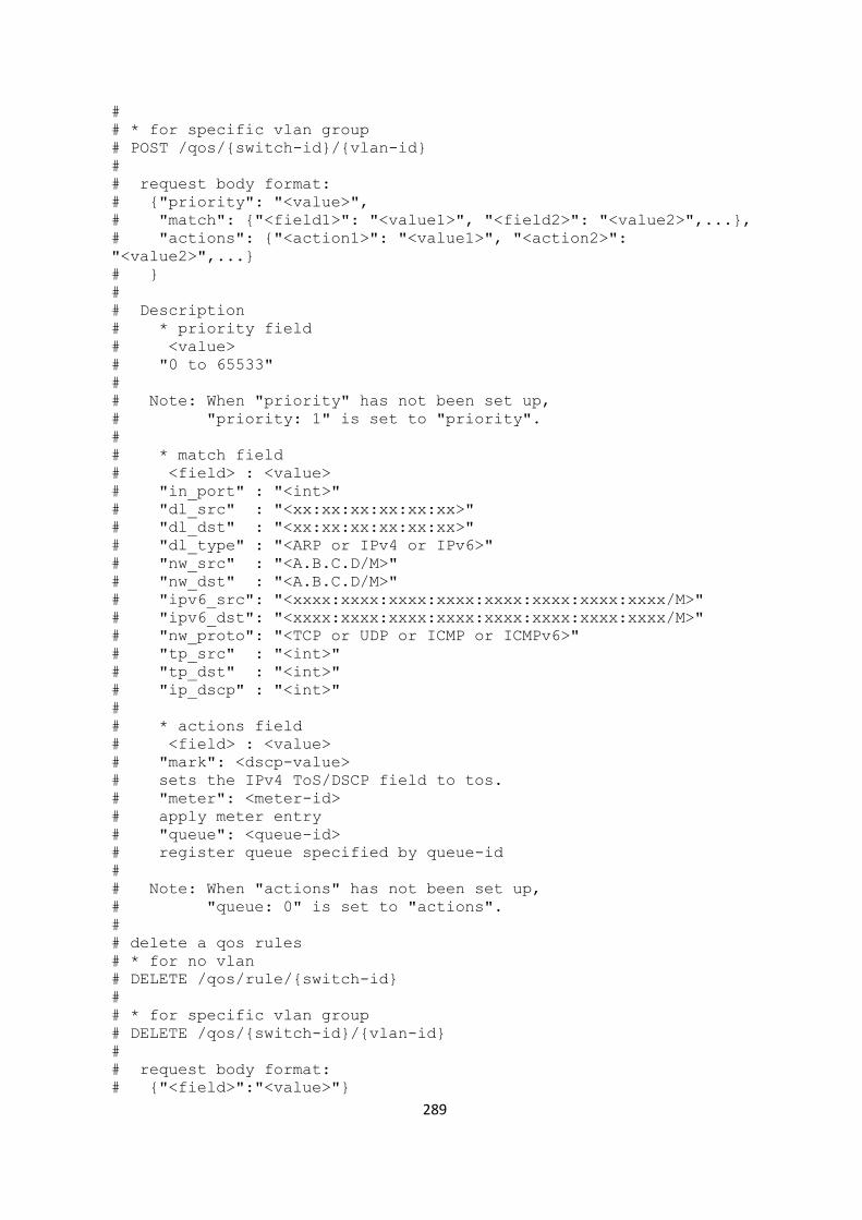
289

#


# POST /qos/{switch-id}/{vlan-id}

#


# {"priority": "<value>",

# "match": {"<field1>": "<value1>", "<field2>": "<value2>",...},

# "actions": {"<action1>": "<value1>", "<action2>":

"<value2>",...}

# }

#

# Description

# * priority field

# <value>

# "0 to 65533"

#

# Note: When "priority" has not been set up,

# "priority: 1" is set to "priority".

#

# * match field

# <field> : <value>

# "in_port" : "<int>"

# "dl_src" : "<xx:xx:xx:xx:xx:xx>"

# "dl_dst" : "<xx:xx:xx:xx:xx:xx>"

# "dl_type" : "<ARP or IPv4 or IPv6>"

# "nw_src" : "<A.B.C.D/M>"

# "nw_dst" : "<A.B.C.D/M>"

# "ipv6_src": "<xxxx:xxxx:xxxx:xxxx:xxxx:xxxx:xxxx:xxxx/M>"

# "ipv6_dst": "<xxxx:xxxx:xxxx:xxxx:xxxx:xxxx:xxxx:xxxx/M>"

# "nw_proto": "<TCP or UDP or ICMP or ICMPv6>"

# "tp_src" : "<int>"

# "tp_dst" : "<int>"

# "ip_dscp" : "<int>"

#

# * actions field

# <field> : <value>

# "mark": <dscp-value>

# sets the IPv4 ToS/DSCP field to tos.

# "meter": <meter-id>

# apply meter entry

# "queue": <queue-id>

# register queue specified by queue-id

#

# Note: When "actions" has not been set up,

# "queue: 0" is set to "actions".

#

# delete a qos rules

# * for no vlan

# DELETE /qos/rule/{switch-id}

#


# DELETE /qos/{switch-id}/{vlan-id}

#


# {"<field>":"<value>"}

290

#

# <field> : <value>

# "qos_id" : "<int>" or "all"

#

# about meter entries

#

# set a meter entry

# POST /qos/meter/{switch-id}

#


# {"meter_id": <int>,

# "bands":[{"action": "<DROP or DSCP_REMARK>",

# "flag": "<KBPS or PKTPS or BURST or STATS"

# "burst_size": <int>,

# "rate": <int>,

# "prec_level": <int>},...]}

#

# delete a meter entry

# DELETE /qos/meter/{switch-id}

#


# {"<field>":"<value>"}

#

# <field> : <value>

# "meter_id" : "<int>"

#

SWITCHID_PATTERN = dpid_lib.DPID_PATTERN + r'|all'

VLANID_PATTERN = r'[0-9]{1,4}|all'

QOS_TABLE_ID = 0

REST_ALL = 'all'

REST_SWITCHID = 'switch_id'

REST_COMMAND_RESULT = 'command_result'

REST_PRIORITY = 'priority'

REST_VLANID = 'vlan_id'

REST_PORT_NAME = 'port_name'

REST_QUEUE_TYPE = 'type'

REST_QUEUE_MAX_RATE = 'max_rate'

REST_QUEUE_MIN_RATE = 'min_rate'

REST_QUEUES = 'queues'

REST_QOS = 'qos'

REST_QOS_ID = 'qos_id'

REST_COOKIE = 'cookie'

REST_MATCH = 'match'

REST_IN_PORT = 'in_port'

REST_SRC_MAC = 'dl_src'

REST_DST_MAC = 'dl_dst'

REST_DL_TYPE = 'dl_type'

REST_DL_TYPE_ARP = 'ARP'

REST_DL_TYPE_IPV4 = 'IPv4'

REST_DL_TYPE_IPV6 = 'IPv6'

291

REST_DL_VLAN = 'dl_vlan'

REST_SRC_IP = 'nw_src'

REST_DST_IP = 'nw_dst'

REST_SRC_IPV6 = 'ipv6_src'

REST_DST_IPV6 = 'ipv6_dst'

REST_NW_PROTO = 'nw_proto'

REST_NW_PROTO_TCP = 'TCP'

REST_NW_PROTO_UDP = 'UDP'

REST_NW_PROTO_ICMP = 'ICMP'

REST_NW_PROTO_ICMPV6 = 'ICMPv6'

REST_TP_SRC = 'tp_src'

REST_TP_DST = 'tp_dst'

REST_DSCP = 'ip_dscp'

REST_ACTION = 'actions'

REST_ACTION_QUEUE = 'queue'

REST_ACTION_MARK = 'mark'

REST_ACTION_METER = 'meter'

REST_METER_ID = 'meter_id'

REST_METER_BURST_SIZE = 'burst_size'

REST_METER_RATE = 'rate'

REST_METER_PREC_LEVEL = 'prec_level'

REST_METER_BANDS = 'bands'

REST_METER_ACTION_DROP = 'drop'

REST_METER_ACTION_REMARK = 'remark'

DEFAULT_FLOW_PRIORITY = 0

QOS_PRIORITY_MAX = ofproto_v1_3_parser.UINT16_MAX - 1

QOS_PRIORITY_MIN = 1

VLANID_NONE = 0

VLANID_MIN = 2

VLANID_MAX = 4094

COOKIE_SHIFT_VLANID = 32

BASE_URL = '/qos'

REQUIREMENTS = {'switchid': SWITCHID_PATTERN,

'vlanid': VLANID_PATTERN}

LOG = logging.getLogger(__name__)

class RestQoSAPI(app_manager.RyuApp):

OFP_VERSIONS = [ofproto_v1_0.OFP_VERSION,

ofproto_v1_2.OFP_VERSION,

ofproto_v1_3.OFP_VERSION]

_CONTEXTS = {

'dpset': dpset.DPSet,

'conf_switch': conf_switch.ConfSwitchSet,

'wsgi': WSGIApplication}


292

super(RestQoSAPI, self).__init__(*args, **kwargs)

# logger configure

QoSController.set_logger(self.logger)

self.cs = kwargs['conf_switch']

self.dpset = kwargs['dpset']

wsgi = kwargs['wsgi']

self.waiters = {}

self.data = {}

self.data['dpset'] = self.dpset

self.data['waiters'] = self.waiters

wsgi.registory['QoSController'] = self.data

wsgi.register(QoSController, self.data)

def stats_reply_handler(self, ev):

msg = ev.msg

dp = msg.datapath

if dp.id not in self.waiters:

return

if msg.xid not in self.waiters[dp.id]:

return

lock, msgs = self.waiters[dp.id][msg.xid]

msgs.append(msg)

flags = 0

if dp.ofproto.OFP_VERSION == ofproto_v1_0.OFP_VERSION or \

dp.ofproto.OFP_VERSION == ofproto_v1_2.OFP_VERSION:

flags = dp.ofproto.OFPSF_REPLY_MORE

elif dp.ofproto.OFP_VERSION == ofproto_v1_3.OFP_VERSION:

flags = dp.ofproto.OFPMPF_REPLY_MORE

if msg.flags & flags:

return

del self.waiters[dp.id][msg.xid]

lock.set()

@set_ev_cls(conf_switch.EventConfSwitchSet)

def conf_switch_set_handler(self, ev):

if ev.key == cs_key.OVSDB_ADDR:

QoSController.set_ovsdb_addr(ev.dpid, ev.value)

else:

QoSController._LOGGER.debug("unknown event: %s", ev)

@set_ev_cls(conf_switch.EventConfSwitchDel)

def conf_switch_del_handler(self, ev):

if ev.key == cs_key.OVSDB_ADDR:

QoSController.delete_ovsdb_addr(ev.dpid)

else:

QoSController._LOGGER.debug("unknown event: %s", ev)

@set_ev_cls(dpset.EventDP, dpset.DPSET_EV_DISPATCHER)

def handler_datapath(self, ev):

if ev.enter:

QoSController.regist_ofs(ev.dp, self.CONF)

293

else:

QoSController.unregist_ofs(ev.dp)

# for OpenFlow version1.0

@set_ev_cls(ofp_event.EventOFPFlowStatsReply, MAIN_DISPATCHER)

def stats_reply_handler_v1_0(self, ev):

self.stats_reply_handler(ev)

# for OpenFlow version1.2 or later

@set_ev_cls(ofp_event.EventOFPStatsReply, MAIN_DISPATCHER)

def stats_reply_handler_v1_2(self, ev):



@set_ev_cls(ofp_event.EventOFPQueueStatsReply, MAIN_DISPATCHER)

def queue_stats_reply_handler_v1_2(self, ev):



@set_ev_cls(ofp_event.EventOFPMeterStatsReply, MAIN_DISPATCHER)

def meter_stats_reply_handler_v1_2(self, ev):


class QoSOfsList(dict):

def __init__(self):

super(QoSOfsList, self).__init__()

def get_ofs(self, dp_id):

if len(self) == 0:

raise ValueError('qos sw is not connected.')

dps = {}

if dp_id == REST_ALL:

dps = self

else:

try:

dpid = dpid_lib.str_to_dpid(dp_id)

except:

raise ValueError('Invalid switchID.')

if dpid in self:

dps = {dpid: self[dpid]}

else:

msg = 'qos sw is not connected. : switchID=%s' %

dp_id

raise ValueError(msg)

return dps

class QoSController(ControllerBase):

_OFS_LIST = QoSOfsList()

294

_LOGGER = None

def __init__(self, req, link, data, **config):

super(QoSController, self).__init__(req, link, data,

**config)

self.dpset = data['dpset']

self.waiters = data['waiters']

@classmethod

def set_logger(cls, logger):

cls._LOGGER = logger

cls._LOGGER.propagate = False

hdlr = logging.StreamHandler()

fmt_str = '[QoS][%(levelname)s] %(message)s'

hdlr.setFormatter(logging.Formatter(fmt_str))

cls._LOGGER.addHandler(hdlr)

@staticmethod

def regist_ofs(dp, CONF):

if dp.id in QoSController._OFS_LIST:

return

dpid_str = dpid_lib.dpid_to_str(dp.id)

try:

f_ofs = QoS(dp, CONF)

f_ofs.set_default_flow()

except OFPUnknownVersion as message:

QoSController._LOGGER.info('dpid=%s: %s',

dpid_str, message)

return

QoSController._OFS_LIST.setdefault(dp.id, f_ofs)

QoSController._LOGGER.info('dpid=%s: Join qos switch.',

dpid_str)

@staticmethod

def unregist_ofs(dp):

if dp.id in QoSController._OFS_LIST:

del QoSController._OFS_LIST[dp.id]

QoSController._LOGGER.info('dpid=%s: Leave qos switch.',

dpid_lib.dpid_to_str(dp.id))

@staticmethod

def set_ovsdb_addr(dpid, value):

ofs = QoSController._OFS_LIST.get(dpid, None)

if ofs is not None:

ofs.set_ovsdb_addr(dpid, value)

@staticmethod

def delete_ovsdb_addr(dpid):

ofs = QoSController._OFS_LIST.get(dpid, None)

ofs.set_ovsdb_addr(dpid, None)

@route('qos_switch', BASE_URL + '/queue/{switchid}',

methods=['GET'], requirements=REQUIREMENTS)

295

def get_queue(self, req, switchid, **_kwargs):

return self._access_switch(req, switchid, VLANID_NONE,

'get_queue', None)


methods=['POST'], requirements=REQUIREMENTS)

def set_queue(self, req, switchid, **_kwargs):


'set_queue', None)


methods=['DELETE'], requirements=REQUIREMENTS)

def delete_queue(self, req, switchid, **_kwargs):


'delete_queue', None)

@route('qos_switch', BASE_URL + '/queue/status/{switchid}',


def get_status(self, req, switchid, **_kwargs):


'get_status', self.waiters)

@route('qos_switch', BASE_URL + '/rules/{switchid}',


def get_qos(self, req, switchid, **_kwargs):


'get_qos', self.waiters)

@route('qos_switch', BASE_URL + '/rules/{switchid}/{vlanid}',


def get_vlan_qos(self, req, switchid, vlanid, **_kwargs):

return self._access_switch(req, switchid, vlanid,

'get_qos', self.waiters)



def set_qos(self, req, switchid, **_kwargs):


'set_qos', self.waiters)



def set_vlan_qos(self, req, switchid, vlanid, **_kwargs):


'set_qos', self.waiters)



def delete_qos(self, req, switchid, **_kwargs):


'delete_qos', self.waiters)



def delete_vlan_qos(self, req, switchid, vlanid, **_kwargs):

296


'delete_qos', self.waiters)

@route('qos_switch', BASE_URL + '/meter/{switchid}',


def get_meter(self, req, switchid, **_kwargs):


'get_meter', self.waiters)



def set_meter(self, req, switchid, **_kwargs):


'set_meter', self.waiters)



def delete_meter(self, req, switchid, **_kwargs):


'delete_meter', self.waiters)

def _access_switch(self, req, switchid, vlan_id, func, waiters):

try:

rest = json.loads(req.body) if req.body else {}

except SyntaxError:

QoSController._LOGGER.debug('invalid syntax %s',

req.body)

return Response(status=400)

try:

dps = self._OFS_LIST.get_ofs(switchid)

vid = QoSController._conv_toint_vlanid(vlan_id)

except ValueError as message:

return Response(status=400, body=str(message))

msgs = []

for f_ofs in dps.values():

function = getattr(f_ofs, func)

try:

if waiters is not None:

msg = function(rest, vid, waiters)

else:

msg = function(rest, vid)

except ValueError as message:

return Response(status=400, body=str(message))

msgs.append(msg)

body = json.dumps(msgs)

return Response(content_type='application/json', body=body)

@staticmethod

def _conv_toint_vlanid(vlan_id):

if vlan_id != REST_ALL:

vlan_id = int(vlan_id)

if (vlan_id != VLANID_NONE and

297

(vlan_id < VLANID_MIN or VLANID_MAX < vlan_id)):

msg = 'Invalid {vlan_id} value. Set [%d-%d]' %

(VLANID_MIN,

VLANID_MAX)


return vlan_id

class QoS(object):

_OFCTL = {ofproto_v1_0.OFP_VERSION: ofctl_v1_0,

ofproto_v1_2.OFP_VERSION: ofctl_v1_2,

ofproto_v1_3.OFP_VERSION: ofctl_v1_3}

def __init__(self, dp, CONF):

super(QoS, self).__init__()

self.vlan_list = {}

self.vlan_list[VLANID_NONE] = 0 # for VLAN=None

self.dp = dp

self.version = dp.ofproto.OFP_VERSION

self.queue_list = {}

self.CONF = CONF

self.ovsdb_addr = None

self.ovs_bridge = None

if self.version not in self._OFCTL:

raise OFPUnknownVersion(version=self.version)

self.ofctl = self._OFCTL[self.version]

def set_default_flow(self):

if self.version == ofproto_v1_0.OFP_VERSION:

return

cookie = 0

priority = DEFAULT_FLOW_PRIORITY

actions = [{'type': 'GOTO_TABLE',

'table_id': QOS_TABLE_ID + 1}]

flow = self._to_of_flow(cookie=cookie,

priority=priority,

match={},

actions=actions)

cmd = self.dp.ofproto.OFPFC_ADD

self.ofctl.mod_flow_entry(self.dp, flow, cmd)

def set_ovsdb_addr(self, dpid, ovsdb_addr):

# easy check if the address format valid

_proto, _host, _port = ovsdb_addr.split(':')

old_address = self.ovsdb_addr

if old_address == ovsdb_addr:

return

if ovsdb_addr is None:

298

if self.ovs_bridge:

self.ovs_bridge.del_controller()

self.ovs_bridge = None

return

self.ovsdb_addr = ovsdb_addr

if self.ovs_bridge is None:

ovs_bridge = bridge.OVSBridge(self.CONF, dpid,

ovsdb_addr)

self.ovs_bridge = ovs_bridge

try:

ovs_bridge.init()

except:

raise ValueError('ovsdb addr is not available.')

def _update_vlan_list(self, vlan_list):

for vlan_id in self.vlan_list.keys():

if vlan_id is not VLANID_NONE and vlan_id not in

vlan_list:

del self.vlan_list[vlan_id]

def _get_cookie(self, vlan_id):

if vlan_id == REST_ALL:

vlan_ids = self.vlan_list.keys()

else:

vlan_ids = [vlan_id]

cookie_list = []

for vlan_id in vlan_ids:

self.vlan_list.setdefault(vlan_id, 0)

self.vlan_list[vlan_id] += 1

self.vlan_list[vlan_id] &=

ofproto_v1_3_parser.UINT32_MAX

cookie = (vlan_id << COOKIE_SHIFT_VLANID) + \

self.vlan_list[vlan_id]

cookie_list.append([cookie, vlan_id])

return cookie_list

@staticmethod

def _cookie_to_qosid(cookie):

return cookie & ofproto_v1_3_parser.UINT32_MAX

# REST command template

def rest_command(func):

def _rest_command(*args, **kwargs):

key, value = func(*args, **kwargs)

switch_id = dpid_lib.dpid_to_str(args[0].dp.id)

return {REST_SWITCHID: switch_id,

key: value}

return _rest_command

@rest_command

def get_status(self, req, vlan_id, waiters):


299

raise ValueError('get_status operation is not

supported')

msgs = self.ofctl.get_queue_stats(self.dp, waiters)

return REST_COMMAND_RESULT, msgs

@rest_command

def get_queue(self, rest, vlan_id):

if len(self.queue_list):

msg = {'result': 'success',

'details': self.queue_list}

else:

msg = {'result': 'failure',

'details': 'Queue is not exists.'}

return REST_COMMAND_RESULT, msg

@rest_command

def set_queue(self, rest, vlan_id):



'details': 'ovs_bridge is not exists'}


self.queue_list.clear()

queue_type = rest.get(REST_QUEUE_TYPE, 'linux-htb')

parent_max_rate = rest.get(REST_QUEUE_MAX_RATE, None)

queues = rest.get(REST_QUEUES, [])

queue_id = 0

queue_config = []

for queue in queues:

max_rate = queue.get(REST_QUEUE_MAX_RATE, None)

min_rate = queue.get(REST_QUEUE_MIN_RATE, None)

if max_rate is None and min_rate is None:

raise ValueError('Required to specify max_rate or

min_rate')

config = {}

if max_rate is not None:

config['max-rate'] = max_rate

if min_rate is not None:

config['min-rate'] = min_rate

if len(config):

queue_config.append(config)

self.queue_list[queue_id] = {'config': config}

queue_id += 1

port_name = rest.get(REST_PORT_NAME, None)

vif_ports = self.ovs_bridge.get_port_name_list()

if port_name is not None:

if port_name not in vif_ports:

raise ValueError('%s port is not exists' %

port_name)

vif_ports = [port_name]

300

for port_name in vif_ports:

try:

self.ovs_bridge.set_qos(port_name, type=queue_type,

max_rate=parent_max_rate,

queues=queue_config)

except Exception as msg:



'details': self.queue_list}


def _delete_queue(self):


return False

vif_ports = self.ovs_bridge.get_external_ports()

for port in vif_ports:

self.ovs_bridge.del_qos(port.port_name)

return True

@rest_command

def delete_queue(self, rest, vlan_id):

self.queue_list.clear()

if self._delete_queue():

msg = 'success'

else:

msg = 'failure'


@rest_command

def set_qos(self, rest, vlan_id, waiters):

msgs = []

cookie_list = self._get_cookie(vlan_id)

for cookie, vid in cookie_list:

msg = self._set_qos(cookie, rest, waiters, vid)

msgs.append(msg)


def _set_qos(self, cookie, rest, waiters, vlan_id):

match_value = rest[REST_MATCH]

if vlan_id:

match_value[REST_DL_VLAN] = vlan_id

priority = int(rest.get(REST_PRIORITY, QOS_PRIORITY_MIN))

if (QOS_PRIORITY_MAX < priority):

raise ValueError('Invalid priority value. Set [%d-%d]'

% (QOS_PRIORITY_MIN, QOS_PRIORITY_MAX))

match = Match.to_openflow(match_value)

actions = []

action = rest.get(REST_ACTION, None)

301

if action is not None:

if REST_ACTION_MARK in action:

actions.append({'type': 'SET_FIELD',

'field': REST_DSCP,

'value':

int(action[REST_ACTION_MARK])})

if REST_ACTION_METER in action:

actions.append({'type': 'METER',

'meter_id':

action[REST_ACTION_METER]})

if REST_ACTION_QUEUE in action:

actions.append({'type': 'SET_QUEUE',

'queue_id':

action[REST_ACTION_QUEUE]})

else:

actions.append({'type': 'SET_QUEUE',

'queue_id': 0})

actions.append({'type': 'GOTO_TABLE',

'table_id': QOS_TABLE_ID + 1})

flow = self._to_of_flow(cookie=cookie, priority=priority,

match=match, actions=actions)

cmd = self.dp.ofproto.OFPFC_ADD

try:


except:

raise ValueError('Invalid rule parameter.')

qos_id = QoS._cookie_to_qosid(cookie)


'details': 'QoS added. : qos_id=%d' % qos_id}

if vlan_id != VLANID_NONE:

msg.setdefault(REST_VLANID, vlan_id)

return msg

@rest_command

def get_qos(self, rest, vlan_id, waiters):

rules = {}

msgs = self.ofctl.get_flow_stats(self.dp, waiters)

if str(self.dp.id) in msgs:

flow_stats = msgs[str(self.dp.id)]

for flow_stat in flow_stats:

if flow_stat['table_id'] != QOS_TABLE_ID:

continue

priority = flow_stat[REST_PRIORITY]

if priority != DEFAULT_FLOW_PRIORITY:

vid = flow_stat[REST_MATCH].get(REST_DL_VLAN,

VLANID_NONE)

if vlan_id == REST_ALL or vlan_id == vid:

rule = self._to_rest_rule(flow_stat)

rules.setdefault(vid, [])

rules[vid].append(rule)

302

get_data = []

for vid, rule in rules.items():

if vid == VLANID_NONE:

vid_data = {REST_QOS: rule}

else:

vid_data = {REST_VLANID: vid, REST_QOS: rule}

get_data.append(vid_data)

return REST_COMMAND_RESULT, get_data

@rest_command

def delete_qos(self, rest, vlan_id, waiters):

try:

if rest[REST_QOS_ID] == REST_ALL:

qos_id = REST_ALL

else:

qos_id = int(rest[REST_QOS_ID])

except:

raise ValueError('Invalid qos id.')

vlan_list = []

delete_list = []

msgs = self.ofctl.get_flow_stats(self.dp, waiters)

if str(self.dp.id) in msgs:

flow_stats = msgs[str(self.dp.id)]

for flow_stat in flow_stats:

cookie = flow_stat[REST_COOKIE]

ruleid = QoS._cookie_to_qosid(cookie)

priority = flow_stat[REST_PRIORITY]

dl_vlan = flow_stat[REST_MATCH].get(REST_DL_VLAN,

VLANID_NONE)

if priority != DEFAULT_FLOW_PRIORITY:

if ((qos_id == REST_ALL or qos_id == ruleid)

and

(vlan_id == dl_vlan or vlan_id ==

REST_ALL)):

match =

Match.to_mod_openflow(flow_stat[REST_MATCH])

delete_list.append([cookie, priority,

match])

else:

if dl_vlan not in vlan_list:

vlan_list.append(dl_vlan)

self._update_vlan_list(vlan_list)

if len(delete_list) == 0:

msg_details = 'QoS rule is not exist.'

if qos_id != REST_ALL:

msg_details += ' : QoS ID=%d' % qos_id


'details': msg_details}

else:

303

cmd = self.dp.ofproto.OFPFC_DELETE_STRICT

actions = []

delete_ids = {}

for cookie, priority, match in delete_list:

flow = self._to_of_flow(cookie=cookie,

priority=priority,

match=match,

actions=actions)


vid = match.get(REST_DL_VLAN, VLANID_NONE)

rule_id = QoS._cookie_to_qosid(cookie)

delete_ids.setdefault(vid, '')

delete_ids[vid] += (('%d' if delete_ids[vid] == ''

else ',%d') % rule_id)

msg = []

for vid, rule_ids in delete_ids.items():

del_msg = {'result': 'success',

'details': ' deleted. : QoS ID=%s' %

rule_ids}

if vid != VLANID_NONE:

del_msg.setdefault(REST_VLANID, vid)

msg.append(del_msg)


@rest_command

def set_meter(self, rest, vlan_id, waiters):


raise ValueError('set_meter operation is not supported')

msgs = []

msg = self._set_meter(rest, waiters)

msgs.append(msg)


def _set_meter(self, rest, waiters):

cmd = self.dp.ofproto.OFPMC_ADD

try:

self.ofctl.mod_meter_entry(self.dp, rest, cmd)

except:

raise ValueError('Invalid meter parameter.')


'details': 'Meter added. : Meter ID=%s' %

rest[REST_METER_ID]}

return msg

@rest_command

def get_meter(self, rest, vlan_id, waiters):

if (self.version == ofproto_v1_0.OFP_VERSION or

self.version == ofproto_v1_2.OFP_VERSION):

raise ValueError('get_meter operation is not supported')

304

msgs = self.ofctl.get_meter_stats(self.dp, waiters)


@rest_command

def delete_meter(self, rest, vlan_id, waiters):

if (self.version == ofproto_v1_0.OFP_VERSION or

self.version == ofproto_v1_2.OFP_VERSION):

raise ValueError('delete_meter operation is not

supported')

cmd = self.dp.ofproto.OFPMC_DELETE

try:

self.ofctl.mod_meter_entry(self.dp, rest, cmd)

except:

raise ValueError('Invalid meter parameter.')


'details': 'Meter deleted. : Meter ID=%s' %

rest[REST_METER_ID]}


def _to_of_flow(self, cookie, priority, match, actions):

flow = {'cookie': cookie,

'priority': priority,

'flags': 0,

'idle_timeout': 0,

'hard_timeout': 0,

'match': match,

'actions': actions}

return flow

def _to_rest_rule(self, flow):

ruleid = QoS._cookie_to_qosid(flow[REST_COOKIE])

rule = {REST_QOS_ID: ruleid}

rule.update({REST_PRIORITY: flow[REST_PRIORITY]})

rule.update(Match.to_rest(flow))

rule.update(Action.to_rest(flow))

return rule

class Match(object):

_CONVERT = {REST_DL_TYPE:

{REST_DL_TYPE_ARP: ether.ETH_TYPE_ARP,

REST_DL_TYPE_IPV4: ether.ETH_TYPE_IP,

REST_DL_TYPE_IPV6: ether.ETH_TYPE_IPV6},

REST_NW_PROTO:

{REST_NW_PROTO_TCP: inet.IPPROTO_TCP,

REST_NW_PROTO_UDP: inet.IPPROTO_UDP,

REST_NW_PROTO_ICMP: inet.IPPROTO_ICMP,

REST_NW_PROTO_ICMPV6: inet.IPPROTO_ICMPV6}}

@staticmethod

def to_openflow(rest):

305

def __inv_combi(msg):

raise ValueError('Invalid combination: [%s]' % msg)

def __inv_2and1(*args):

__inv_combi('%s=%s and %s' % (args[0], args[1],

args[2]))


__inv_combi('%s=%s and %s=%s' % (

args[0], args[1], args[2], args[3]))


__inv_combi('%s and %s' % (args[0], args[1]))


__inv_combi('%s and %s=%s' % (args[0], args[1],

args[2]))

match = {}

# error check

dl_type = rest.get(REST_DL_TYPE)

nw_proto = rest.get(REST_NW_PROTO)

if dl_type is not None:

if dl_type == REST_DL_TYPE_ARP:

if REST_SRC_IPV6 in rest:

__inv_2and1(

REST_DL_TYPE, REST_DL_TYPE_ARP,

REST_SRC_IPV6)

if REST_DST_IPV6 in rest:

__inv_2and1(


REST_DST_IPV6)

if REST_DSCP in rest:

__inv_2and1(

REST_DL_TYPE, REST_DL_TYPE_ARP, REST_DSCP)

if nw_proto:

__inv_2and1(


REST_NW_PROTO)

elif dl_type == REST_DL_TYPE_IPV4:


__inv_2and1(

REST_DL_TYPE, REST_DL_TYPE_IPV4,

REST_SRC_IPV6)


__inv_2and1(


REST_DST_IPV6)

if nw_proto == REST_NW_PROTO_ICMPV6:

__inv_2and2(


REST_NW_PROTO, REST_NW_PROTO_ICMPV6)

elif dl_type == REST_DL_TYPE_IPV6:

if REST_SRC_IP in rest:

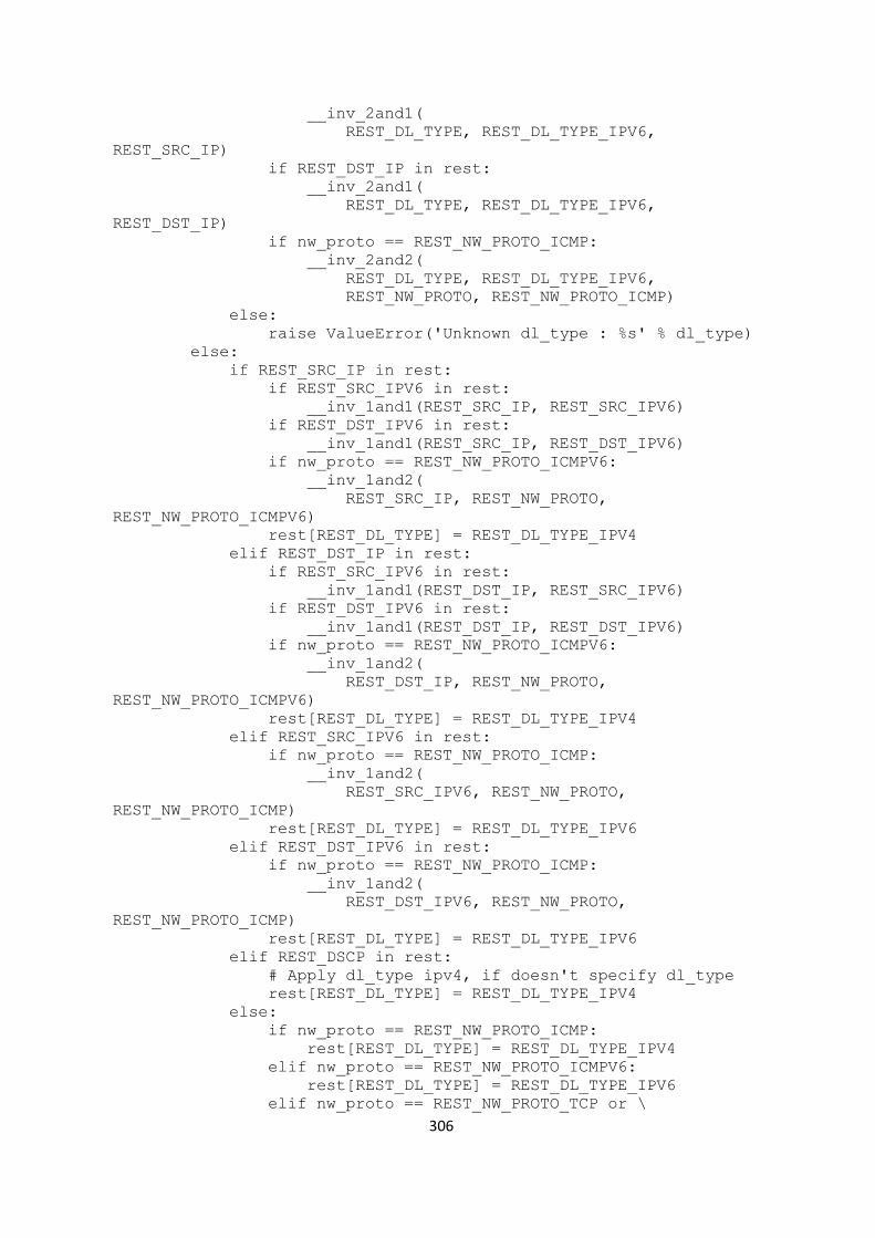
306

__inv_2and1(


REST_SRC_IP)

if REST_DST_IP in rest:

__inv_2and1(


REST_DST_IP)

if nw_proto == REST_NW_PROTO_ICMP:

__inv_2and2(


REST_NW_PROTO, REST_NW_PROTO_ICMP)

else:

raise ValueError('Unknown dl_type : %s' % dl_type)

else:

if REST_SRC_IP in rest:


__inv_1and1(REST_SRC_IP, REST_SRC_IPV6)


__inv_1and1(REST_SRC_IP, REST_DST_IPV6)


__inv_1and2(

REST_SRC_IP, REST_NW_PROTO,

REST_NW_PROTO_ICMPV6)

rest[REST_DL_TYPE] = REST_DL_TYPE_IPV4

elif REST_DST_IP in rest:


__inv_1and1(REST_DST_IP, REST_SRC_IPV6)


__inv_1and1(REST_DST_IP, REST_DST_IPV6)


__inv_1and2(

REST_DST_IP, REST_NW_PROTO,

REST_NW_PROTO_ICMPV6)


elif REST_SRC_IPV6 in rest:


__inv_1and2(

REST_SRC_IPV6, REST_NW_PROTO,

REST_NW_PROTO_ICMP)


elif REST_DST_IPV6 in rest:


__inv_1and2(

REST_DST_IPV6, REST_NW_PROTO,

REST_NW_PROTO_ICMP)


elif REST_DSCP in rest:

# Apply dl_type ipv4, if doesn't specify dl_type


else:



elif nw_proto == REST_NW_PROTO_ICMPV6:


elif nw_proto == REST_NW_PROTO_TCP or \

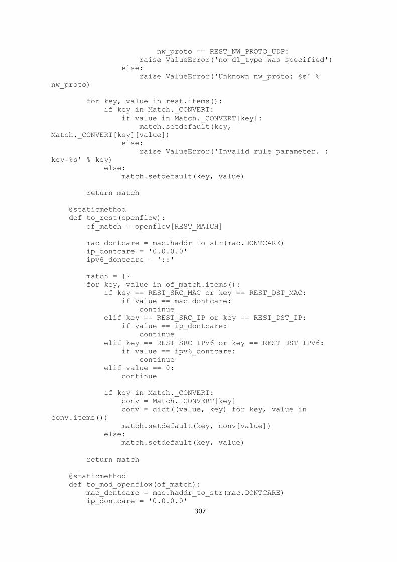
307

nw_proto == REST_NW_PROTO_UDP:

raise ValueError('no dl_type was specified')

else:

raise ValueError('Unknown nw_proto: %s' %

nw_proto)

for key, value in rest.items():

if key in Match._CONVERT:

if value in Match._CONVERT[key]:

match.setdefault(key,

Match._CONVERT[key][value])

else:

raise ValueError('Invalid rule parameter. :

key=%s' % key)

else:

match.setdefault(key, value)

return match

@staticmethod

def to_rest(openflow):

of_match = openflow[REST_MATCH]

mac_dontcare = mac.haddr_to_str(mac.DONTCARE)

ip_dontcare = '0.0.0.0'

ipv6_dontcare = '::'

match = {}

for key, value in of_match.items():

if key == REST_SRC_MAC or key == REST_DST_MAC:

if value == mac_dontcare:

continue

elif key == REST_SRC_IP or key == REST_DST_IP:

if value == ip_dontcare:

continue

elif key == REST_SRC_IPV6 or key == REST_DST_IPV6:

if value == ipv6_dontcare:

continue

elif value == 0:

continue

if key in Match._CONVERT:

conv = Match._CONVERT[key]

conv = dict((value, key) for key, value in

conv.items())

match.setdefault(key, conv[value])

else:


return match

@staticmethod

def to_mod_openflow(of_match):

mac_dontcare = mac.haddr_to_str(mac.DONTCARE)

ip_dontcare = '0.0.0.0'

308

ipv6_dontcare = '::'

match = {}

for key, value in of_match.items():

if key == REST_SRC_MAC or key == REST_DST_MAC:

if value == mac_dontcare:

continue

elif key == REST_SRC_IP or key == REST_DST_IP:

if value == ip_dontcare:

continue

elif key == REST_SRC_IPV6 or key == REST_DST_IPV6:

if value == ipv6_dontcare:

continue

elif value == 0:

continue


return match

class Action(object):

@staticmethod

def to_rest(openflow):

if REST_ACTION in openflow:

actions = []

for action in openflow[REST_ACTION]:

field_value = re.search('SET_FIELD: {ip_dscp:(\d+)',

action)

if field_value:

actions.append({REST_ACTION_MARK:

field_value.group(1)})

meter_value = re.search('METER:(\d+)', action)

if meter_value:

actions.append({REST_ACTION_METER:

meter_value.group(1)})

queue_value = re.search('SET_QUEUE:(\d+)', action)

if queue_value:

actions.append({REST_ACTION_QUEUE:

queue_value.group(1)})

action = {REST_ACTION: actions}

else:

action = {REST_ACTION: 'Unknown action type.'}

return action

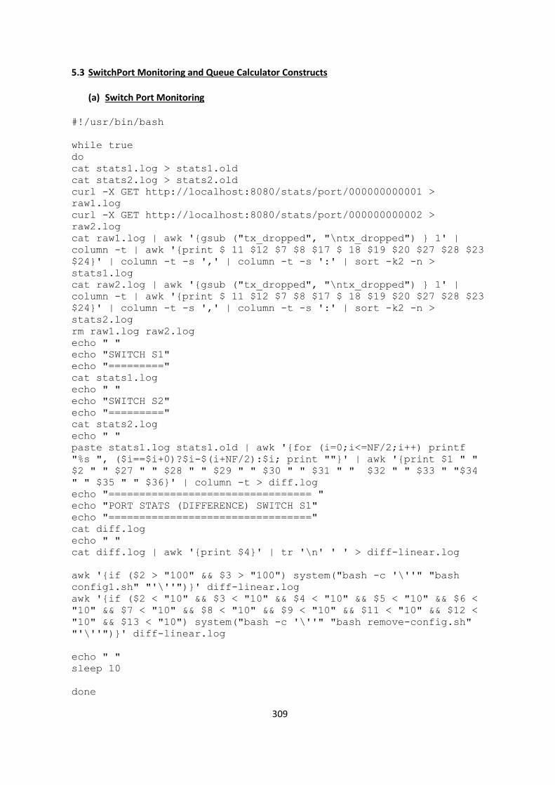
309

5.3 SwitchPort Monitoring and Queue Calculator Constructs

(a) Switch Port Monitoring #!/usr/bin/bash

while true

do

cat stats1.log > stats1.old

cat stats2.log > stats2.old

curl -X GET http://localhost:8080/stats/port/000000000001 >

raw1.log

curl -X GET http://localhost:8080/stats/port/000000000002 >

raw2.log

cat raw1.log | awk '{gsub ("tx_dropped", "\ntx_dropped") } 1' |

column -t | awk '{print $ 11 $12 $7 $8 $17 $ 18 $19 $20 $27 $28 $23

$24}' | column -t -s ',' | column -t -s ':' | sort -k2 -n >

stats1.log

cat raw2.log | awk '{gsub ("tx_dropped", "\ntx_dropped") } 1' |

column -t | awk '{print $ 11 $12 $7 $8 $17 $ 18 $19 $20 $27 $28 $23

$24}' | column -t -s ',' | column -t -s ':' | sort -k2 -n >

stats2.log

rm raw1.log raw2.log

echo " "

echo "SWITCH S1"

echo "========="

cat stats1.log

echo " "

echo "SWITCH S2"

echo "========="

cat stats2.log

echo " "

paste stats1.log stats1.old | awk '{for (i=0;i<=NF/2;i++) printf

"%s ", ($i==$i+0)?$i-$(i+NF/2):$i; print ""}' | awk '{print $1 " "

$2 " " $27 " " $28 " " $29 " " $30 " " $31 " " $32 " " $33 " "$34

" " $35 " " $36}' | column -t > diff.log

echo "================================= "

echo "PORT STATS (DIFFERENCE) SWITCH S1"

echo "================================="

cat diff.log

echo " "

cat diff.log | awk '{print $4}' | tr '\n' ' ' > diff-linear.log

awk '{if ($2 > "100" && $3 > "100") system("bash -c '\''" "bash

config1.sh" "'\''")}' diff-linear.log

awk '{if ($2 < "10" && $3 < "10" && $4 < "10" && $5 < "10" && $6 <

"10" && $7 < "10" && $8 < "10" && $9 < "10" && $11 < "10" && $12 <

"10" && $13 < "10") system("bash -c '\''" "bash remove-config.sh"

"'\''")}' diff-linear.log

echo " "

sleep 10

done

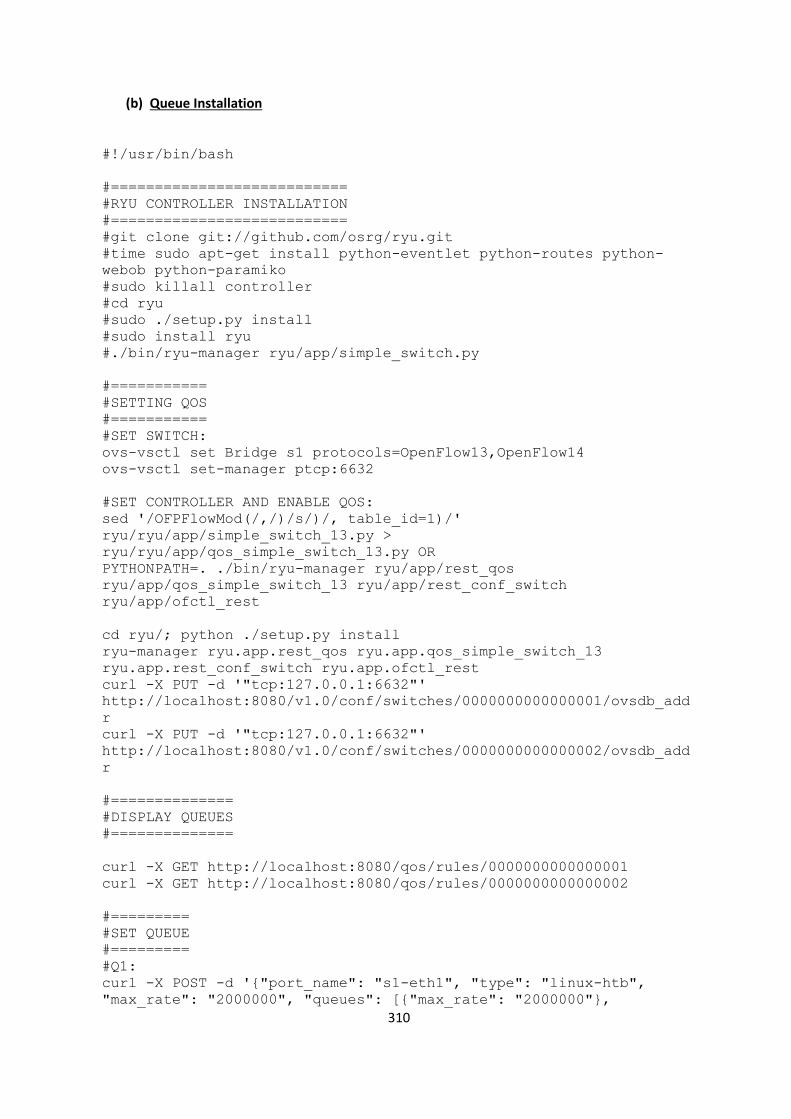
310

(b) Queue Installation

#!/usr/bin/bash

#===========================

#RYU CONTROLLER INSTALLATION

#===========================

#git clone git://github.com/osrg/ryu.git

#time sudo apt-get install python-eventlet python-routes python-

webob python-paramiko

#sudo killall controller

#cd ryu

#sudo ./setup.py install

#sudo install ryu

#./bin/ryu-manager ryu/app/simple_switch.py

#===========

#SETTING QOS

#===========

#SET SWITCH:

ovs-vsctl set Bridge s1 protocols=OpenFlow13,OpenFlow14

ovs-vsctl set-manager ptcp:6632

#SET CONTROLLER AND ENABLE QOS:

sed '/OFPFlowMod(/,/)/s/)/, table_id=1)/'

ryu/ryu/app/simple_switch_13.py >

ryu/ryu/app/qos_simple_switch_13.py OR

PYTHONPATH=. ./bin/ryu-manager ryu/app/rest_qos

ryu/app/qos_simple_switch_13 ryu/app/rest_conf_switch

ryu/app/ofctl_rest

cd ryu/; python ./setup.py install

ryu-manager ryu.app.rest_qos ryu.app.qos_simple_switch_13

ryu.app.rest_conf_switch ryu.app.ofctl_rest

curl -X PUT -d '"tcp:127.0.0.1:6632"'

http://localhost:8080/v1.0/conf/switches/0000000000000001/ovsdb_add

r

curl -X PUT -d '"tcp:127.0.0.1:6632"'

http://localhost:8080/v1.0/conf/switches/0000000000000002/ovsdb_add

r

#==============

#DISPLAY QUEUES

#==============

curl -X GET http://localhost:8080/qos/rules/0000000000000001

curl -X GET http://localhost:8080/qos/rules/0000000000000002

#=========

#SET QUEUE

#=========

#Q1:

curl -X POST -d '{"port_name": "s1-eth1", "type": "linux-htb",

"max_rate": "2000000", "queues": [{"max_rate": "2000000"},

311

{"max_rate": "250000"}, {"max_rate": "62500"}, {"max_rate":

"510000"}, {"max_rate": "600000"}, {"max_rate": "100000"},

{"max_rate": "175000"}]}'

http://localhost:8080/qos/queue/0000000000000001

#Q2:




"680000"}, {"max_rate": "900000"}, {"max_rate": "100000"}]}'


#Q3:




"680000"}, {"max_rate": "600000"}]}'


#Q1: Service Proiver:




"1000000"}, {"max_rate": "2000000"}, {"max_rate": "3000000"}]}'


#===========

#APPLY QUEUE

#===========

#OUTBOUND QUEUES

#===============

curl -X POST -d '{"match": {"nw_src": "10.0.0.3"},

"actions":{"queue": "1"}}'

http://localhost:8080/qos/rules/0000000000000001






















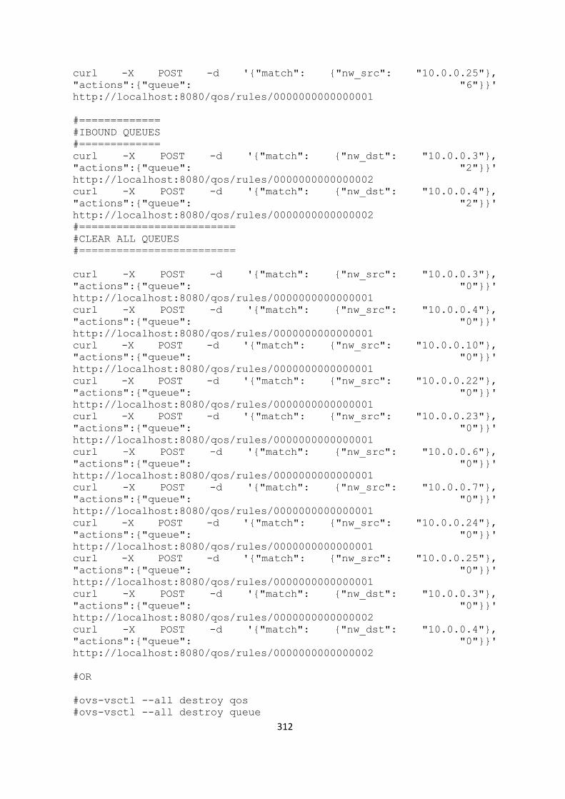
312




#=============

#IBOUND QUEUES

#=============

curl -X POST -d '{"match": {"nw_dst": "10.0.0.3"},






#=========================

#CLEAR ALL QUEUES

#=========================


































#OR

#ovs-vsctl --all destroy qos

#ovs-vsctl --all destroy queue

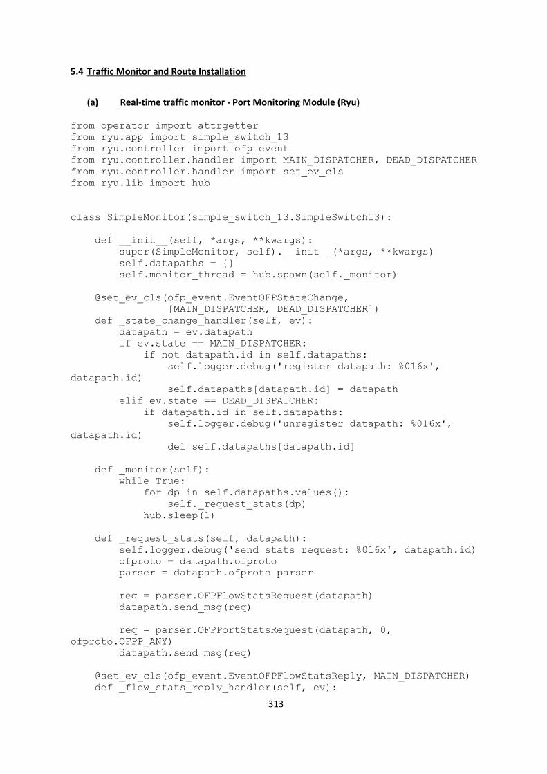
313

5.4 Traffic Monitor and Route Installation

(a) Real-time traffic monitor - Port Monitoring Module (Ryu)

from operator import attrgetter

from ryu.app import simple_switch_13


from ryu.controller.handler import MAIN_DISPATCHER, DEAD_DISPATCHER


from ryu.lib import hub

class SimpleMonitor(simple_switch_13.SimpleSwitch13):


super(SimpleMonitor, self).__init__(*args, **kwargs)

self.datapaths = {}

self.monitor_thread = hub.spawn(self._monitor)

@set_ev_cls(ofp_event.EventOFPStateChange,

[MAIN_DISPATCHER, DEAD_DISPATCHER])

def _state_change_handler(self, ev):

datapath = ev.datapath

if ev.state == MAIN_DISPATCHER:

if not datapath.id in self.datapaths:

self.logger.debug('register datapath: %016x',

datapath.id)

self.datapaths[datapath.id] = datapath

elif ev.state == DEAD_DISPATCHER:

if datapath.id in self.datapaths:

self.logger.debug('unregister datapath: %016x',

datapath.id)

del self.datapaths[datapath.id]

def _monitor(self):

while True:

for dp in self.datapaths.values():

self._request_stats(dp)

hub.sleep(1)

def _request_stats(self, datapath):

self.logger.debug('send stats request: %016x', datapath.id)



req = parser.OFPFlowStatsRequest(datapath)

datapath.send_msg(req)

req = parser.OFPPortStatsRequest(datapath, 0,

ofproto.OFPP_ANY)


@set_ev_cls(ofp_event.EventOFPFlowStatsReply, MAIN_DISPATCHER)

def _flow_stats_reply_handler(self, ev):

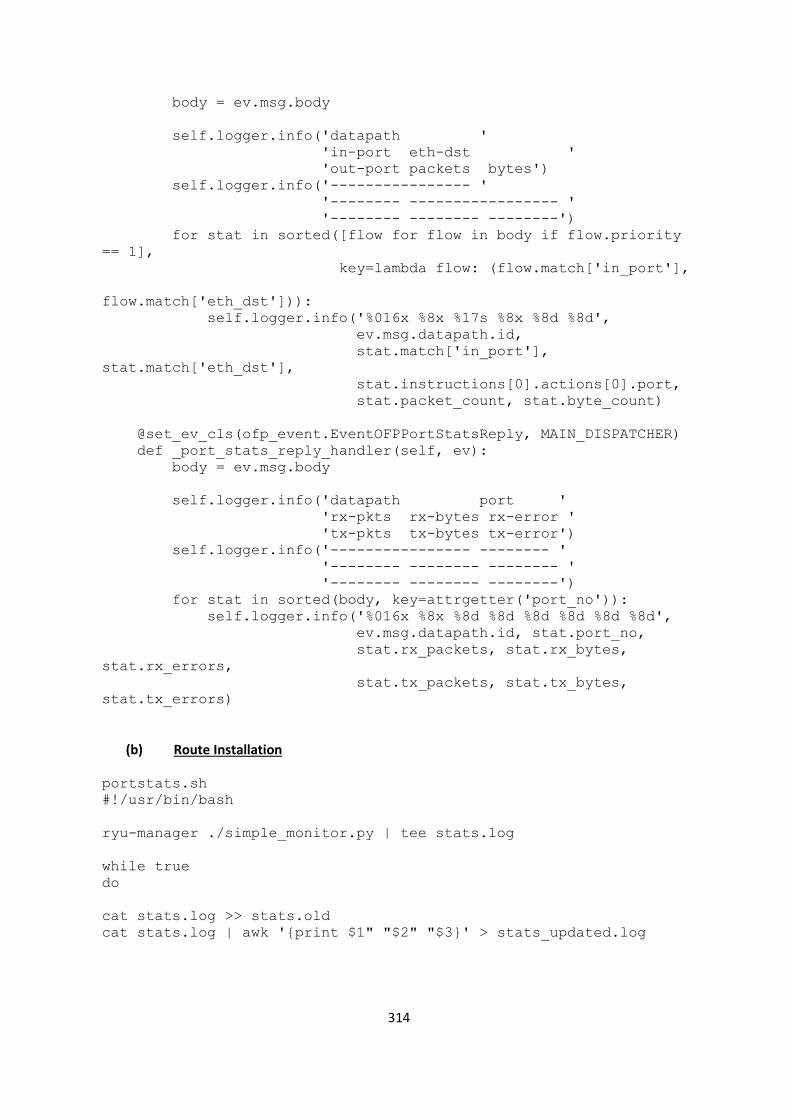
314

body = ev.msg.body

self.logger.info('datapath '

'in-port eth-dst '

'out-port packets bytes')

self.logger.info('---------------- '

'-------- ----------------- '

'-------- -------- --------')

for stat in sorted([flow for flow in body if flow.priority

== 1],

key=lambda flow: (flow.match['in_port'],

flow.match['eth_dst'])):

self.logger.info('%016x %8x %17s %8x %8d %8d',

ev.msg.datapath.id,

stat.match['in_port'],

stat.match['eth_dst'],

stat.instructions[0].actions[0].port,

stat.packet_count, stat.byte_count)

@set_ev_cls(ofp_event.EventOFPPortStatsReply, MAIN_DISPATCHER)

def _port_stats_reply_handler(self, ev):

body = ev.msg.body

self.logger.info('datapath port '

'rx-pkts rx-bytes rx-error '

'tx-pkts tx-bytes tx-error')

self.logger.info('---------------- -------- '

'-------- -------- -------- '

'-------- -------- --------')

for stat in sorted(body, key=attrgetter('port_no')):

self.logger.info('%016x %8x %8d %8d %8d %8d %8d %8d',

ev.msg.datapath.id, stat.port_no,

stat.rx_packets, stat.rx_bytes,

stat.rx_errors,

stat.tx_packets, stat.tx_bytes,

stat.tx_errors)

(b) Route Installation

portstats.sh

#!/usr/bin/bash

ryu-manager ./simple_monitor.py | tee stats.log

while true

do

cat stats.log >> stats.old

cat stats.log | awk '{print $1" "$2" "$3}' > stats_updated.log

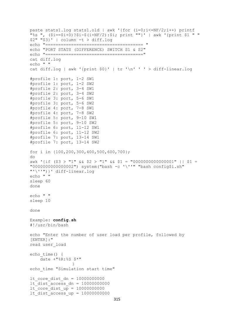
315

paste stats1.log stats1.old | awk '{for (i=0;i<=NF/2;i++) printf

"%s ", ($i==$i+0)?$i-$(i+NF/2):$i; print ""}' | awk '{print $1 " "

$2" "$3}' | column -t > diff.log

echo "====================================== "

echo "PORT STATS (DIFFERENCE) SWITCH S1 & S2"

echo "======================================"

cat diff.log

echo " "

cat diff.log | awk '{print $0}' | tr '\n' ' ' > diff-linear.log

#profile 1: port, 1-2 SW1














for i in {100,200,300,400,500,600,700};

do

awk '{if ($3 > "1" && $2 > "1" && $1 = "0000000000000001" || $1 =

"0000000000000002") system("bash -c '\''" "bash config$i.sh"

"'\''")}' diff-linear.log

echo " "

sleep 60

done

echo " "

sleep 10

done

Example: config.sh

#!/usr/bin/bash

echo "Enter the number of user load per profile, followed by

[ENTER]:"

read user_load

echo_time() {

date +"%R:%S $*"

}

echo_time "Simulation start time"

lt_core_dist_dn = 10000000000

lt_dist_access_dn = 10000000000

lt_core_dist_up = 10000000000

lt_dist_access_up = 10000000000

316

for p in {1..7}

do

for app_direction in {1..8}

do

for dn in {1..2}

#compute core-dist link

#total links: 4

do while user_load > 1

for l in {1..4}

do

B=$(cat B_profile_$p_$app_$direction.dat)

lt_$l = lt_core_dist_dn

u_max_core_dist_$dn = "$lt_l /$B" | bc

if u_max_core_dist_$dn >= user_load && lt_l > 0

for i in {1..2}

do

for j in {1..7}

do

for x in {1..8}

do

curl -X POST -d '{"match":

{"nw_src": "10.'$j'.0.0/16"}, "actions":{"table1"}}'

http://localhost:8080/qos/rules/000000000000000'$i'


{"table_id": "1","nw_src": "10.'$j'.0.0/16", "nw_dst":

"10.0.0.'$x'"}, "actions":{set "vlan_id":"1'$j$dn'",

"output":"$l"}}'


echo_time

#barrier message

curl -X POST -d

'{ "OFPBarrierRequest": {} }

'http://localhost:8080/qos/rules/000000000000000'$i'

echo_time

echo "Core - Routes

Installed"

done

done

lt_l = "$lt_core_dist_dn - $user_load * $B" | bc

if u_max_core_dist_dn >= user_load && lt_l > 0

max_users = user_load - user_load/lt_l

for i in {1..2}

do

for j in {1..7}

do

for x in {1..8}

do


{"nw_src": "10.'$j'.0.0/16"}, "actions":{"table2"}}'


317


{"table_id": "2","nw_src": "10.'$j'.0.0/16", "nw_dst":

"10.0.0.'$x'"}, "actions":{set "vlan_id":"2'$j$dn'",

"output":"$l"}}'


echo_time

#barrier message

curl -X POST -d



echo_time

echo "Core - Routes

Installed"

done

done

done

for l in {1..2}

do

B=$(cat B_profile_$p_$app_$direction.dat)

lt_$l = lt_core_dist_dn

u_max_core_dist_$dn = "$lt_l /$B" | bc

if u_max_core_dist_$dn >= user_load && lt_l > 0

for i in {1..2}

do

for j in {1..7}

do

for x in {1..8}

do


{"nw_dst": "10.0.0.'$x'/16", "vlan_id":"10'$j'"},

"actions":{"output":"$l"}}'

http://localhost:8080/qos/rules/000000000000000'$k'

echo_time

#barrier message

curl -X POST -d



echo_time

echo "Core - Routes

Installed"

done

done

lt_l = "$lt_core_dist_dn - $user_load * $B" | bc

if u_max_core_dist_dn >= user_load && lt_l > 0

max_users = user_load - user_load/lt_l

for i in {1..2}

do

for j in {1..7}

do

318

for x in {1..8}

do


{"nw_dst": "10.0.0.'$x'/16", "vlan_id":"10'$j'"},

"actions":{"output":"$l"}}'

http://localhost:8080/qos/rules/000000000000000'$k'

echo_time

#barrier message

curl -X POST -d



echo_time

echo "Core - Routes

Installed"

done

done

done

for m in {11..18}

for z in {1..8}

do

curl -X POST -d '{"match": {"dl_src": "aa:bb:cc:11:11:$m", "dl_dst":

"aa:bb:cc:11:11:1'$z'"}, "actions":{"output":"1"}}'

http://localhost:8080/qos/rules/000000000000000'$z'

curl -X POST -d '{"match":"dl_src": "aa:bb:cc:11:11:$m"}}'

http://localhost:8080/stats/aggregateflow/$z

echo_time

#barrier message

curl -X POST -d '{ "OFPBarrierRequest": {} }

'http://localhost:8080/qos/rules/000000000000000'$z'

echo_time

echo "East West Traffic (Access, Distribution) - Routes Installed"

done

done

echo " "

echo "Traffic Statistics"

for u in {1..18}

do

curl -X GET http://localhost:8080/stats/table/$u

curl -X GET http://localhost:8080/stats/flow/$u

curl -X POST -d '{"match":{"vlan_id":"10'$j'"}}'

http://localhost:8080/stats/aggregateflow/$u

done

done

done

(c) Barrier Request Support Added to Ryu Switching Application (simple_switch_13)

Barrier Request Message

def send_barrier_request(self, datapath):

ofp_parser = datapath.ofproto_parser

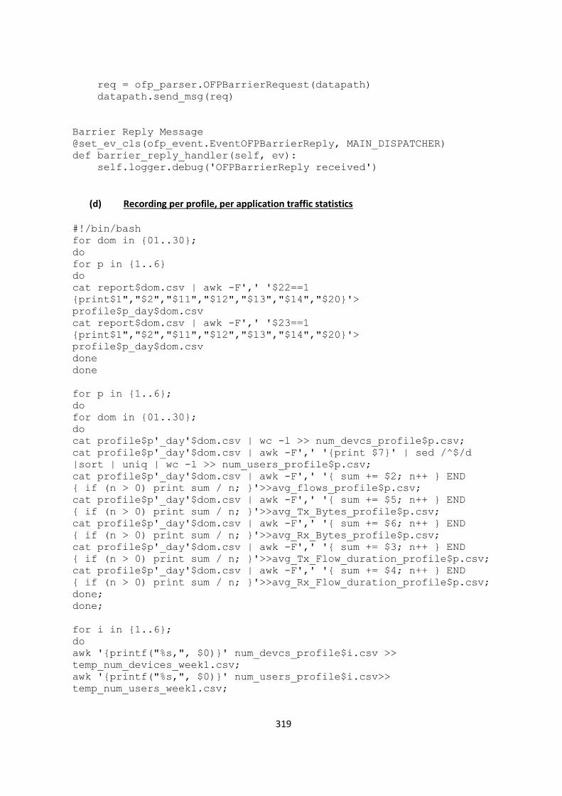
319

req = ofp_parser.OFPBarrierRequest(datapath)


Barrier Reply Message

@set_ev_cls(ofp_event.EventOFPBarrierReply, MAIN_DISPATCHER)

def barrier_reply_handler(self, ev):

self.logger.debug('OFPBarrierReply received')

(d) Recording per profile, per application traffic statistics

#!/bin/bash


do

for p in {1..6}

do

cat report$dom.csv | awk -F',' '$22==1

{print$1","$2","$11","$12","$13","$14","$20}'>

profile$p_day$dom.csv

cat report$dom.csv | awk -F',' '$23==1

{print$1","$2","$11","$12","$13","$14","$20}'>

profile$p_day$dom.csv

done

done

for p in {1..6};

do


do

cat profile$p'_day'$dom.csv | wc -l >> num_devcs_profile$p.csv;

cat profile$p'_day'$dom.csv | awk -F',' '{print $7}' | sed /^$/d

|sort | uniq | wc -l >> num_users_profile$p.csv;

cat profile$p'_day'$dom.csv | awk -F',' '{ sum += $2; n++ } END

{ if (n > 0) print sum / n; }'>>avg_flows_profile$p.csv;


{ if (n > 0) print sum / n; }'>>avg_Tx_Bytes_profile$p.csv;


{ if (n > 0) print sum / n; }'>>avg_Rx_Bytes_profile$p.csv;


{ if (n > 0) print sum / n; }'>>avg_Tx_Flow_duration_profile$p.csv;


{ if (n > 0) print sum / n; }'>>avg_Rx_Flow_duration_profile$p.csv;

done;

done;

for i in {1..6};

do

awk '{printf("%s,", $0)}' num_devcs_profile$i.csv >>

temp_num_devices_week1.csv;

awk '{printf("%s,", $0)}' num_users_profile$i.csv>>

temp_num_users_week1.csv;

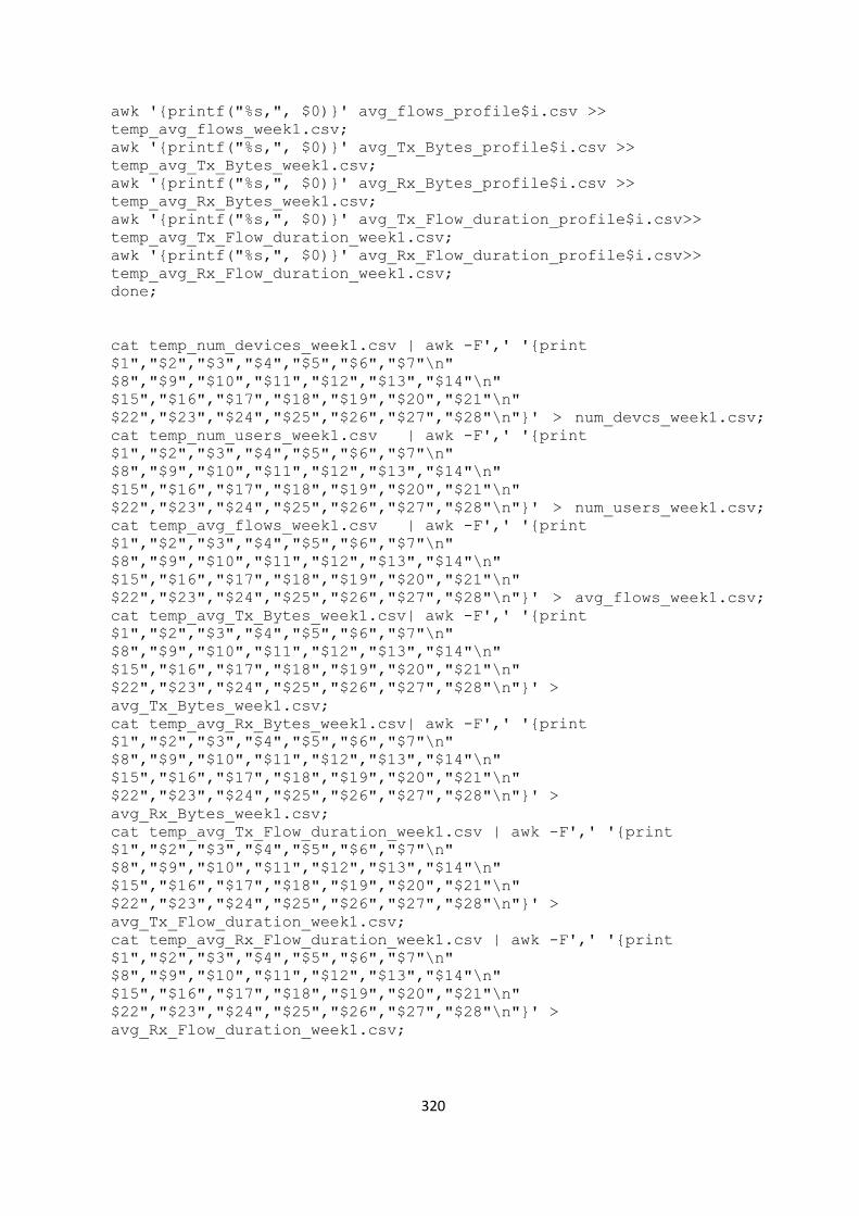
320

awk '{printf("%s,", $0)}' avg_flows_profile$i.csv >>

temp_avg_flows_week1.csv;

awk '{printf("%s,", $0)}' avg_Tx_Bytes_profile$i.csv >>

temp_avg_Tx_Bytes_week1.csv;

awk '{printf("%s,", $0)}' avg_Rx_Bytes_profile$i.csv >>

temp_avg_Rx_Bytes_week1.csv;

awk '{printf("%s,", $0)}' avg_Tx_Flow_duration_profile$i.csv>>

temp_avg_Tx_Flow_duration_week1.csv;

awk '{printf("%s,", $0)}' avg_Rx_Flow_duration_profile$i.csv>>

temp_avg_Rx_Flow_duration_week1.csv;

done;

cat temp_num_devices_week1.csv | awk -F',' '{print

$1","$2","$3","$4","$5","$6","$7"\n"

$8","$9","$10","$11","$12","$13","$14"\n"

$15","$16","$17","$18","$19","$20","$21"\n"

$22","$23","$24","$25","$26","$27","$28"\n"}' > num_devcs_week1.csv;

cat temp_num_users_week1.csv | awk -F',' '{print

$1","$2","$3","$4","$5","$6","$7"\n"

$8","$9","$10","$11","$12","$13","$14"\n"

$15","$16","$17","$18","$19","$20","$21"\n"

$22","$23","$24","$25","$26","$27","$28"\n"}' > num_users_week1.csv;

cat temp_avg_flows_week1.csv | awk -F',' '{print

$1","$2","$3","$4","$5","$6","$7"\n"

$8","$9","$10","$11","$12","$13","$14"\n"

$15","$16","$17","$18","$19","$20","$21"\n"

$22","$23","$24","$25","$26","$27","$28"\n"}' > avg_flows_week1.csv;

cat temp_avg_Tx_Bytes_week1.csv| awk -F',' '{print

$1","$2","$3","$4","$5","$6","$7"\n"

$8","$9","$10","$11","$12","$13","$14"\n"

$15","$16","$17","$18","$19","$20","$21"\n"

$22","$23","$24","$25","$26","$27","$28"\n"}' >

avg_Tx_Bytes_week1.csv;

cat temp_avg_Rx_Bytes_week1.csv| awk -F',' '{print

$1","$2","$3","$4","$5","$6","$7"\n"

$8","$9","$10","$11","$12","$13","$14"\n"

$15","$16","$17","$18","$19","$20","$21"\n"

$22","$23","$24","$25","$26","$27","$28"\n"}' >

avg_Rx_Bytes_week1.csv;

cat temp_avg_Tx_Flow_duration_week1.csv | awk -F',' '{print

$1","$2","$3","$4","$5","$6","$7"\n"

$8","$9","$10","$11","$12","$13","$14"\n"

$15","$16","$17","$18","$19","$20","$21"\n"

$22","$23","$24","$25","$26","$27","$28"\n"}' >

avg_Tx_Flow_duration_week1.csv;

cat temp_avg_Rx_Flow_duration_week1.csv | awk -F',' '{print

$1","$2","$3","$4","$5","$6","$7"\n"

$8","$9","$10","$11","$12","$13","$14"\n"

$15","$16","$17","$18","$19","$20","$21"\n"

$22","$23","$24","$25","$26","$27","$28"\n"}' >

avg_Rx_Flow_duration_week1.csv;

321

rm temp_num_devices_week1.csv temp_num_users_week1.csv

temp_avg_flows_week1.csv temp_avg_Tx_Bytes_week1.csv

temp_avg_Rx_Bytes_week1.csv temp_avg_Tx_Flow_duration_week1.csv

temp_avg_Rx_Flow_duration_week1.csv

for p in {1..6}

do

for app in {1..8}

do

for direction in {1..2}

do

awk -f nfprofiler.awk segmented_report_month.csv >

B_profile_$p_$app_$direction.dat

done

done

done

rm num_users_profile$p.csv num_devcs_profile$p.csv

avg_flows_profile$p.csv avg_Tx_Bytes_profile$p.csv

avg_Rx_Bytes_profile$p.csv avg_Tx_Flow_duration_profile$p.csv

avg_Rx_Flow_duration_profile$p.csv;

5.5 OpenFlow Traffic Measurements

(a) Output Port Selection and Flow_REM flag setting in Ryu Switching Application

from ryu.controller import handler

from ryu.controller import dpset



from ryu.ofproto import ofproto_v1_3_parser


from ryu.ofproto.ofproto_parser import MsgBase, msg_pack_into,

msg_str_attr

class OF13(app_manager.RyuApp):


_CONTEXTS = {

'dpset': dpset.DPSet,

}


super(OF13, self).__init__(*args, **kwargs)

def add_flow(self, datapath, priority, match, actions):



inst =

[parser.OFPInstructionActions(ofproto.OFPIT_APPLY_ACTIONS,

322

actions)]


priority=priority,

match=match, instructions=inst,

flags=ofproto.OFPFF_SEND_FLOW_REM)

datapath.send_msg(mod)

@handler.set_ev_cls(dpset.EventDP, dpset.DPSET_EV_DISPATCHER)

def handler_datapath(self, ev):

if ev.enter:

print "join"

dp = ev.dp

actions = [dp.ofproto_parser.OFPActionOutput(2)]

match = dp.ofproto_parser.OFPMatch(in_port=1)

self.add_flow(dp, 1, match, actions)

(b) Resource Monitoring Script

#! /bin/bash

# unset any variable which system may be using

while true

do

echo_time() {

date +"%R:%S $*"

}

# clear the screen

clear

unset tecreset os architecture kernelrelease internalip externalip

nameserver loadaverage

while getopts iv name

do

case $name in

i)iopt=1;;

v)vopt=1;;

*)echo "Invalid arg";;

esac

done

if [[ ! -z $iopt ]]

then

{

wd=$(pwd)

323

basename "$(test -L "$0" && readlink "$0" || echo "$0")" >

/tmp/scriptname

scriptname=$(echo -e -n $wd/ && cat /tmp/scriptname)

su -c "cp $scriptname /usr/bin/monitor" root && echo

"Congratulations! Script Installed, now run monitor Command" ||

echo "Installation failed"

}

fi

if [[ ! -z $vopt ]]

then

{

echo -e "tecmint_monitor version 0.1\nDesigned by

Tecmint.com\nReleased Under Apache 2.0 License"

}

fi

if [[ $# -eq 0 ]]

then

{

# Define Variable tecreset

tecreset=$(tput sgr0)

# Check if connected to Internet or not

ping -c 1 google.com &> /dev/null && echo -e '\E[32m'"Internet:

$tecreset Connected" || echo -e '\E[32m'"Internet: $tecreset

Disconnected"

# Check OS Type

os=$(uname -o)

echo -e '\E[32m'"Operating System Type :" $tecreset $os

# Check OS Release Version and Name

cat /etc/os-release | grep 'NAME\|VERSION' | grep -v 'VERSION_ID' |

grep -v 'PRETTY_NAME' > /tmp/osrelease

echo -n -e '\E[32m'"OS Name :" $tecreset && cat /tmp/osrelease |

grep -v "VERSION" | cut -f2 -d\"

echo -n -e '\E[32m'"OS Version :" $tecreset && cat /tmp/osrelease |

grep -v "NAME" | cut -f2 -d\"

# Check Architecture

architecture=$(uname -m)

echo -e '\E[32m'"Architecture :" $tecreset $architecture

# Check Kernel Release

kernelrelease=$(uname -r)

echo -e '\E[32m'"Kernel Release :" $tecreset $kernelrelease

# Check hostname

echo -e '\E[32m'"Hostname :" $tecreset $HOSTNAME

# Check Internal IP

internalip=$(hostname -I)

324

echo -e '\E[32m'"Internal IP :" $tecreset $internalip

# Check External IP

externalip=$(curl -s ipecho.net/plain;echo)

echo -e '\E[32m'"External IP : $tecreset "$externalip

# Check DNS

nameservers=$(cat /etc/resolv.conf | sed '1 d' | awk '{print $2}')

echo -e '\E[32m'"Name Servers :" $tecreset $nameservers

# Check Logged In Users

who>/tmp/who

echo -e '\E[32m'"Logged In users :" $tecreset && cat /tmp/who

# Check RAM and SWAP Usages

free -h | grep -v + > /tmp/ramcache

echo -e '\E[32m'"Ram Usages :" $tecreset

cat /tmp/ramcache | grep -v "Swap"

echo_time >> swap_usage.log

cat /tmp/ramcache | grep -v "Swap" >> swap_usage.log

echo -e '\E[32m'"Swap Usages :" $tecreset

cat /tmp/ramcache | grep -v "Mem"

echo_time >> ram_usage.log

cat /tmp/ramcache | grep -v "Mem" >> ram_usage.log

# Check Disk Usages

df -h| grep 'Filesystem\|/dev/sda*' > /tmp/diskusage

echo -e '\E[32m'"Disk Usages :" $tecreset

cat /tmp/diskusage

# Check Load Average

loadaverage=$(top -n 1 -b | grep "load average:" | awk '{print $10

$11 $12}')

echo -e '\E[32m'"Load Average :" $tecreset $loadaverage

echo_time >> cpuload.log

echo -e '\E[32m'"Load Average :" $tecreset $loadaverage >>

cpuload.log

# Check System Uptime

tecuptime=$(uptime | awk '{print $3,$4}' | cut -f1 -d,)

echo -e '\E[32m'"System Uptime Days/(HH:MM) :" $tecreset $tecuptime

# Unset Variables

unset tecreset os architecture kernelrelease internalip externalip

nameserver loadaverage

# Remove Temporary Files

rm /tmp/osrelease /tmp/who /tmp/ramcache /tmp/diskusage

}

fi

shift $(($OPTIND -1))

sleep 1

done

325

Packet Capture Library (Control Channel Traffic)

PCAP reader (module)

pcapsave.py


from ryu.lib.packet import packet

frame_count = 0

# iterate pcaplib.Reader that yields (timestamp, packet_data)

# in the PCAP file

for ts, buf in pcaplib.Reader(open('test.pcap', 'rb')):

frame_count += 1

pkt = packet.Packet(buf)

print("%d, %f, %s" % (frame_count, ts, pkt))

PCAP writer (module)

pcapread.py


class SimpleSwitch13(app_manager.RyuApp):



super(SimpleSwitch13, self).__init__(*args, **kwargs)

self.mac_to_port = {}

# Create pcaplib.Writer instance with a file object

# for the PCAP file

self.pcap_writer = pcaplib.Writer(open('test.pcap', 'wb'))

...

@set_ev_cls(ofp_event.EventOFPPacketIn, MAIN_DISPATCHER)

def _packet_in_handler(self, ev):

# Dump the packet data into PCAP file

self.pcap_writer.write_pkt(ev.msg.data)

Switch and Flow Table Statistics Collection

#!/usr/bin/bash

while true

do

curl -X GET http://localhost:8080/stats/table/1

curl -X GET http://localhost:8080/stats/flow/1

echo " "

sleep 30

done

327

APPENDIX – 6

List of publications

[1] T. Bakhshi and B. Ghita: User Traffic Profiling In a Software Defined Networking Context. Sixth International Conference on Internet Technologies and Applications, Wrexham, U.K., September 8-11, 2015. DOI: 10.1109/ITechA.2015.7317376 [Best paper award]

[2] T. Bakhshi and B. Ghita: Traffic Profiling: Evaluating Stability in Multi-device User Environments. The 30th IEEE International Conference on Advanced Information Networking and Applications, Crans-Montana, Switzerland, March 23-25, 2016. DOI: 10.1109/WAINA.2016.8

[3] T. Bakhshi and B. Ghita: User-centric traffic optimization in residential software defined networks. 23rd International Conference on Telecommunications, Thessaloniki, Greece, 14-16 May 2016. DOI: 10.1109/ICT.2016.7500389

[4] T. Bakhshi and B. Ghita: On Internet Traffic Classification: A Two-Phased Machine Learning Approach. Journal of Computer Networks and Communications, vol. 2016, Article ID 2048302, 21 pages, 2016. DOI: 10.1155/2016/2048302

[5] T. Bakhshi and B. Ghita: OpenFlow-Enabled user traffic profiling in software defined networks. 12th IEEE International Wireless & Mobile Comp. Conference, New York. 17-19 Oct 2016. DOI: 10.1109/WiMOB.2016.7763235

[6] T. Bakhshi and B. Ghita: User-centric network provisioning in software defined data center environments. 41st IEEE Local Computer Networks Conference, Dubai, 7-9 Nov 2016. DOI: 10.1109/LCN.2016.57

https://doi.org/10.1109/ITechA.2015.7317376

https://doi.org/10.1109/WAINA.2016.8

https://doi.org/10.1109/ICT.2016.7500389

http://dx.doi.org/10.1155/2016/2048302

https://doi.org/10.1109/WiMOB.2016.7763235

https://doi.org/10.1109/LCN.2016.57

user-centric traffic engineering in - University of Plymouth ...

Documents

Transcript of user-centric traffic engineering in - University of Plymouth ...