Use of productivity-defined indicators to assess exposure of grassland-based livestock systems to...

Crop and Pasture Science, 2013, 64(7)

1

Use of productivity-defined indicators to assess exposure of

grassland-based livestock systems to climate change and variability

Marion Sautier A,B,C

, Michel Duru A

and Roger Martin-Clouaire B

AINRA, UMR 1248 AGIR, BP 52627, F-31326 Castanet Tolosan, France.

BINRA, UR875 MIAT, BP 52627, F-31326 Castanet Tolosan, France.

CCorresponding author: [email protected]; [email protected]

Summary Livestock systems that rely on pasture resources are threatened by increasing climatic variability

and, in the long run, by climate change.

This study presents two methods to characterise variability and change by clustering climatic-year

patterns and rating the frequency of anomalies.

Such assessments can be used to foster discussion among researchers, advisers and farmers to

design grassland systems adapted to new climatic conditions.

Abstract Climate change research that aims to accelerate the adaptation process of agricultural

production systems first requires understanding their climatic vulnerability, which is in part

characterised by their exposure. This paper’s approach moves beyond traditional metrics of

climate variables and proposes specific indicators for grassland-based livestock systems. They

focus on the variation in seasonal boundaries and seasonal and yearly herbage productivity in

response to weather conditions. The paper shows how statistical interpretations of these

indicators over several sites and climatic years (past and future) enable the characterisation of

classes of climatic years and seasons as well as their frequencies of occurrence and their

variation from the past to the expected future. The frequency of occurrence and succession of

seasonal extremes is also examined by analysing the difference between observed or predicted

seasonal productivity and past mean productivity. The data analysis and corresponding

statistical graphics used in our approach can help farmers, advisers and scientists envision site-

specific impacts of climate change on herbage production patterns. An illustrative analysis is

performed on three sites in south-western France using a series of climatic years covering two

30-year periods in the past and the future. We found that the herbage production of several

clusters of climatic years can be identified as “normal” (i.e. frequent) and that the most

frequent clusters in the past become less common in the future, though some clusters remain

common. In addition, the year-to-year variability and the contrast between spring and summer-

fall herbage production are expected to increase.

Additional key words: herbage balance, rainfall, temperature, abnormal weather pattern

Introduction Climate is a primary determinant of agricultural productivity. In particular, livestock systems that

rely on pasture resources are increasingly exposed to threats from increased climatic variability

and, in the long run, to climate change (Graux et al. 2013). Abnormal changes in air temperature

and rainfall and resulting increases in frequency and intensity of drought events have long-term

implications for the viability of these production systems. Designing new systems adapted to new

climatic contexts is therefore necessary. Addressing this issue first requires a better understanding

of such systems’ exposure to climate change at particular locations and periods in the future.

Exposure to climate is an external dimension of a system’s vulnerability and usually refers to the

duration, extent and frequency of weather perturbations that impact it (Adger 2006). Classically,

exposure is assessed by analysing temporal patterns of raw physical variables (e.g. temperature,

precipitation, evapotranspiration) (McCrum et al. 2009; Fraser et al. 2011). To contribute to


2

farmer-centred redesign of production systems, the notion of exposure must be re-engineered in a

way that corresponds to farmers’ mental models and facilitates connecting scientific knowledge

with action (Meinke et al. 2009). In contrast to climatologists who emphasise the physical and

natural science dimension, farmers make sense of climate change primarily through their

perception of potential risks encountered in their production systems (Hulme et al. 2009). Through

their experiences and memories, they can build implicit categories of “normal” or “abnormal”

climatic patterns and events. However, retaining and recalling past weather is often biased towards

extremes or exceptional episodes, such as the 2003 drought in Europe (Ciais et al. 2005).

Livestock farms, especially those which are essentially grassland-based, are highly

vulnerable to climatic trends and variability because feedstuffs are mainly provided by grasslands

through cutting and grazing (Hopkins and Del Prado 2007). These systems, due to soil and climate

induced constraints, are unable to grow annual crops (especially irrigated), dual-purpose crops (e.g.

maize for grain or silage) or intercrops to cope with climate variability. They also cannot rapidly

change plant genotypes when their grassland system is based on permanent pastures. In temperate

regions, the impact of climatic trends and variability on livestock farms can be assessed through

two main features relating weather to feeding management: (i) the dates and periods when grazing

is sufficient to feed the herd and surplus herbage yield transformed into hay or silage (ii) and when

there is a herbage shortage for grazing and feedstuffs should be supplied as hay or silage (Girard et

al. 2001). Accordingly, exposure indicators should be determined according to herbage production

at a seasonal scale, although most approaches in applied research use annual production as the

primary indicator. When season-scale approaches are considered, unrealistic assumptions are often

made, such as fixed calendar-based definitions of seasons (e.g. Graux et al. 2013); these

approaches also refer to and use ad-hoc expertise that is difficult to generalise (Chapman et al.

2008). Furthermore, exposure assessments should consider inter-annual variability (Chapman et al.

2008) and alternation of favourable and unfavourable weather episodes because feeding system

exposure depends less on the occurrence of a single unfavourable event than on a succession of two

or more (Charpenteau and Duru 1983; Gibbons and Ramsden 2008).

The essence of farm management deals with change and uncertainty, in both the short and

long term. Technical activities (day-to-day actions) are driven by management strategies that

coherently organise activities over time as a function of farm resources and production objectives.

These strategies incorporate flexibility to deal with weather variability, enabling them to cope with

perturbations that are within the bounds of typical variability (Sebillotte and Soler 1990; Vanclay

2004). With larger deviations (e.g. the 2003 drought) the usual flexibility is no longer sufficient,

which can prompt farmers to consider a far-reaching farming system redesign.

Regarding future climate, most farmers in France consider high annual weather variability

a greater problem than long-term climate change (Duru et al. 2012). Similar observations have

occurred in other countries (e.g. Australia; Pannell 2010), where extreme events are more intense

and frequent than in temperate regions such as the one considered in this paper. Farmers have

almost no benchmarks for future climate conditions; at most they have heard about global-change

scenarios with little regional contextualisation (Zhang et al. 2007). Thus, they need site-specific

projections of the weather and its impacts on production. Model-based agronomic knowledge can

help to assess the potential consequences of new climatic conditions, which is a first step toward

designing adapted systems. For this purpose, we previously proposed (Sautier et al., 2013) six

model-based exposure indicators that outline key distinguishing features of the behaviour of a

grassland-based livestock system under a given climatic scenario. Briefly, these indicators

characterise a climatic year, also called a “forage year”, as three productivity-defined seasons. For

each season, the herbage shortage or surplus at grazing is assessed with respect to the herd’s

feeding demand. Identifying the boundaries of these weather-dependent seasons and calculating

seasonal surplus or shortage contribute directly to characterising climatic exposure as a function of

the duration and extent of the impact (Sautier et al., 2013). The frequency dimension involved in

defining exposure requires consideration of a set of climatic years and the performance of statistical

analyses of the values of each indicator each year. This paper presents two frequency-focused

analyses of the exposure of grassland-based livestock systems using the seasonal-scale indicators

mentioned above. The first analysis identifies clusters of climatic years in past and future datasets

according to forage productivity and the timing of production and compares the resulting cluster

frequencies between past and future. The second analysis examines the frequency of extreme


3

values of seasonal balances. It highlights a change in the frequency of anomalies, whose amplitudes

are reported as multiples of standard deviations (σ) from the mean of past years’ seasonal balances.

Material and methods Exposure indicators

We followed the method described in a previous article (Sautier et al., 2013) to calculate six

exposure indicators specific to grassland-based livestock systems: the dates of the beginning of

spring, summer-fall and winter (resp. Bsp, Bsf and Bw) and the balance between herbage availability

and herd feed requirements for each season (resp. Balsp, Balsf and Balw).

Each exposure indicator is calculated from the “average available herbage” (AAH), defined

as the mean daily herbage growth (HG) over n years as follows

with n the number of years of the whole period, length (year) the number of days in the year

considered, and jdoy the day-of-year number. Calculated for a given period and location, AAH

represents daily mean herbage availability. In a balanced system, AAH is the daily feed required by

the herd per area unit (g/m²/day). Daily HG can be predicted by any simulation model that

considers grassland characteristics and defoliation practises due to grazing and cutting operations.

As explained in Sautier et al. (2013), we used the herbage growth model developed by Duru et al.

(2009) to calculate daily HG. Herbage growth was simulated with a constant set of parameters

characterising soil (e.g. soil water-holding capacity = 80 mm), species (cocksfoot - Dactylis

glomerata L.) and fertilisation rate enabling 80% of potential growth to calculate variations in

herbage growth that are due purely to weather conditions. We chose intermediate harvest frequency

(early cut before flowering followed by 2 or 3 grazing periods) and grazing intensity (residual

sward height of 4 cm) to limit the effect of defoliation management upon herbage growth rate.

A year is divided into three productivity-defined seasons – spring, summer-fall and winter

(Fig. 1) – defined from AAH. The beginning of spring (Bsp) is the theoretical beginning of grazing.

Summer and fall are aggregated into the compound summer-fall season because year-to-year

variability of herbage growth in fall prevented identification of a fall starting date. The beginning

of summer-fall (Bsf) is the first day after the spring peak when full-time grazing is impossible.

Winter begins (Bw) when grazing stops and ends when the next spring begins. Practically, during a

phase of accelerating herbage growth (e.g. between winter and spring), spring grazing can begin

once sufficient herbage has accumulated. In this case, grazing begins before herbage growth equals

AAH, which means that the spring threshold of herbage growth could be set to any value less than

AAH. In the same way, during a phase of decelerating herbage growth (e.g. between spring and

summer or fall and winter), grazing can be extended beyond the date at which daily herbage growth

equals AAH to graze the herbage accumulated during the latest surplus period, which means that

the summer-fall and winter thresholds of herbage growth could be set to any value less than AAH.

As explained in Sautier et al. (2013), we smoothed daily herbage-growth values over 10-day

windows and applied the method with a spring threshold of 0.75×AAH, a summer-fall threshold of

0.75×AAH and a winter threshold of 0.5×AAH.

The balance between herbage availability and herd feed requirements (Balsea, in g/m2) is

defined as the sum of the difference between HG and AAH over the entire season. Balsea can be

positive (i.e. surplus that can be cut for hay or silage) or negative (i.e. shortage that requires feeding

the herd with hay or silage) and can be converted into feeding days. One feeding day represents the

amount of herbage needed per area unit to feed the herd for one day, which equals AAH in a

balanced system.

Clustering years and characterising abnormality and frequency of seasons

Climatic-year clustering according to the exposure indicators

Variability in seasonal conditions for herbage growth is often analysed empirically by grouping

seasons with roughly similar profiles (e.g. early vs. late start of growth, short vs. long summer

period, high vs. low annual production) (Chapman et al. 2008). We retained the idea of dividing

climatic years into classes (clusters) with similar natures, which is useful for understanding and

length( year )n n

year

jdoyyear 1 jdoy 1 year 1

AAH HG length( year )( ) /


4

summarising large datasets. Clusters were defined by agglomerative hierarchical clustering (AHC)

of the exposure indicators using Ward’s criterion.

We built eight clusters of climatic years by performing AHC of their seasonal

characteristics (season beginning and herbage balance) for the 60-year dataset presented below (30

years each in the past and future, see “Case Study” section). To facilitate visual comparison,

clusters were ranked by letter according to decreasing annual herbage production (i.e. cluster “A”

the highest and cluster “H” the lowest). ANOVAs and multiple-range tests were performed to

determine which indicators were most discriminating between the clusters. Then, for each site, the

relative frequency of each cluster (the number of years in the cluster divided by the sample size)

was calculated for the past and future periods. Cumulative distributions of the relative frequency of

clusters, put in order of decreasing relative frequency, were used to visualise differences between

past and future and identify the smallest set of clusters that covered at least 80% of the years. These

years were considered “normal” years. All statistical analyses were performed using Statgraphics

(StatPoint Technologies, Warrenton, VA, USA).

Standard-deviation classification

A second kind of statistical analysis was performed to highlight the years with extreme values of

seasonal herbage balance and to study the change in their frequencies from past to future. Several

studies consider the standard deviation of a dataset as the typical magnitude of variations and its

multiples (up to 3) as anomalies (Anwar et al. 2012; Hansen et al. 2012;). In this manner, Niu et al.

(2009) classified climate data using long-term means and standard deviations.

The mean and standard deviation of each indicator over the 30 years of the past scenario

were used to classify the indicator’s annual value in both past and future scenarios. The deviation

of the indicator’s annual value from its past mean was divided by its past standard deviation to

determine its class. Seven classes were defined from σ-based intervals: ]-∞, -3σ], ]-3σ, -2σ], ]-2σ, -

σ], ]-σ, σ[, [σ, 2σ[, [2σ, 3σ[, and [3σ, +∞[. The further the interval from 0, the more abnormal the

season compared to its usual variability in the past.

Case study

The approach was applied in a research project aimed at assessing the climatic vulnerability of

grasslands and livestock-farming systems in mainland France. Typically, when dealing with short-

term adaptations, farmers and advisors tend to discuss small changes in farm structure and

management. The 2050 time horizon was chosen because considering long-term adaptations

encourages stakeholders to propose more substantial changes. We used 1980-2010 weather data

(precipitation, potential evapotranspiration, solar radiation and mean temperature) for the past and

scenarios of climate patterns generated for 2035-2065. For these future scenarios we used climate

simulations of the IPCC A1B SRES scenario (Nakicenovic et al. 2000). Climate simulations were

provided by Météo France via the ARPEGE-Climat model (Déqué et al. 1994) and were

statistically downscaled by the CERFACS using the Boé08 method (Pagé et al. 2008) to generate

the weather series at local scale (8 x 8 km).

The southern Midi-Pyrenees (France) was chosen as a case-study region to develop and

discuss climate-change adaptation options in livestock-farming systems. Three locations were

selected (Table 1):

- Aulus, located in the Pyrenees Mountains. Farms are beef-cattle production systems based

on semi-natural grasslands practising long-distance transhumance for summer pasturing.

- Saint Girons, located in the Pyrenean foothills. Farms are beef- and dairy-cattle production

systems based on grasslands (e.g. grass-legume mixtures) for beef-cattle farms and forage

crops (e.g. silage maize) for dairy farms.

- Toulouse, located in the Garonne River valley, was used as a reference to compare its current

climate to the future climate of Saint Girons and Aulus. Currently, the agriculture of this

zone is essentially oriented toward cash crops, with a small amount of livestock production.

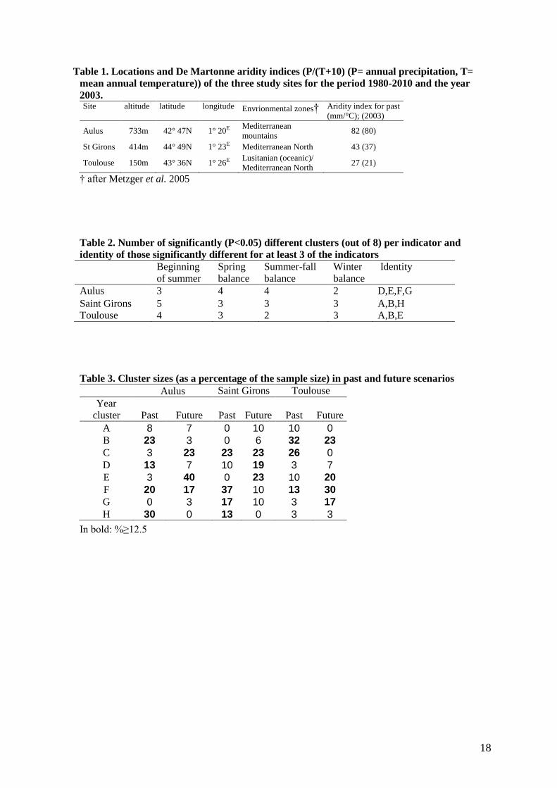
The past climate of the three locations can roughly be compared with the de Martonne

aridity index (Table 1), defined as P/(T+10), where P is annual precipitation (mm) and T mean

annual temperature (°C). Due to hot and dry summer, Toulouse has the lowest index. Aulus has the

highest index thanks to its mountainous location.Toulouse is the most arid.


5

Results

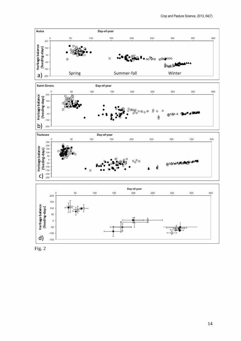
Inter-annual variability of seasonal indicators for past and future periods

A visual examination of the indicators for past and future periods for each site reveals that some

features are common to the three locations (Fig. 2a, b, c):

- beginning dates and herbage balances in winter were significantly correlated, meaning that

either variable can be used for further analysis;

- the variability in beginning date was lower for spring than for summer-fall and winter, and

the variability in herbage balance was higher for spring than for other seasons;

- compared to the past scenario, the future scenario had an earlier summer and later winter,

and to a lesser extent, earlier spring and lower herbage surplus (or greater shortage) in

summer.

Comparing sites (Fig. 2d), we noticed (i) a small shortage of herbage in summer in Aulus

but a large one in Toulouse, (ii) the difference in herbage balance between spring and summer was

the lowest in Aulus and the highest in Toulouse, and (iii) the difference in herbage balance between

spring and winter was the lowest in Toulouse and the highest in Aulus.

Clustering of forage climatic years according to seasonal indicators

As the above analysis showed that the beginning of spring had low variability and the winter start

date and herbage balance were correlated, the indicators “beginning of spring” and “beginning of

winter” were excluded from the clustering. Thus, the AHC was performed on the basis of four

indicators: the seasonal herbage balance for each season (Bals, Balsf and Balw) and the beginning of

summer-fall (Bsf).

The clustering resulted in distinct classes of forage years. The ANOVA of clusters per site

based on the four exposure indicators shows that three clusters (out of eight) for each site

significantly (P<0.05) differed from each other (Table 2) for at least three of the indicators. When

considering only three of the four indicators, the number of distinct clusters grew from three to four

(data not shown). The multiple-range test for the four indicators indicates that, depending on the

site and the indicator considered, two to five clusters (out of eight) significantly (P<0.05) differed

from each other (Table 2).

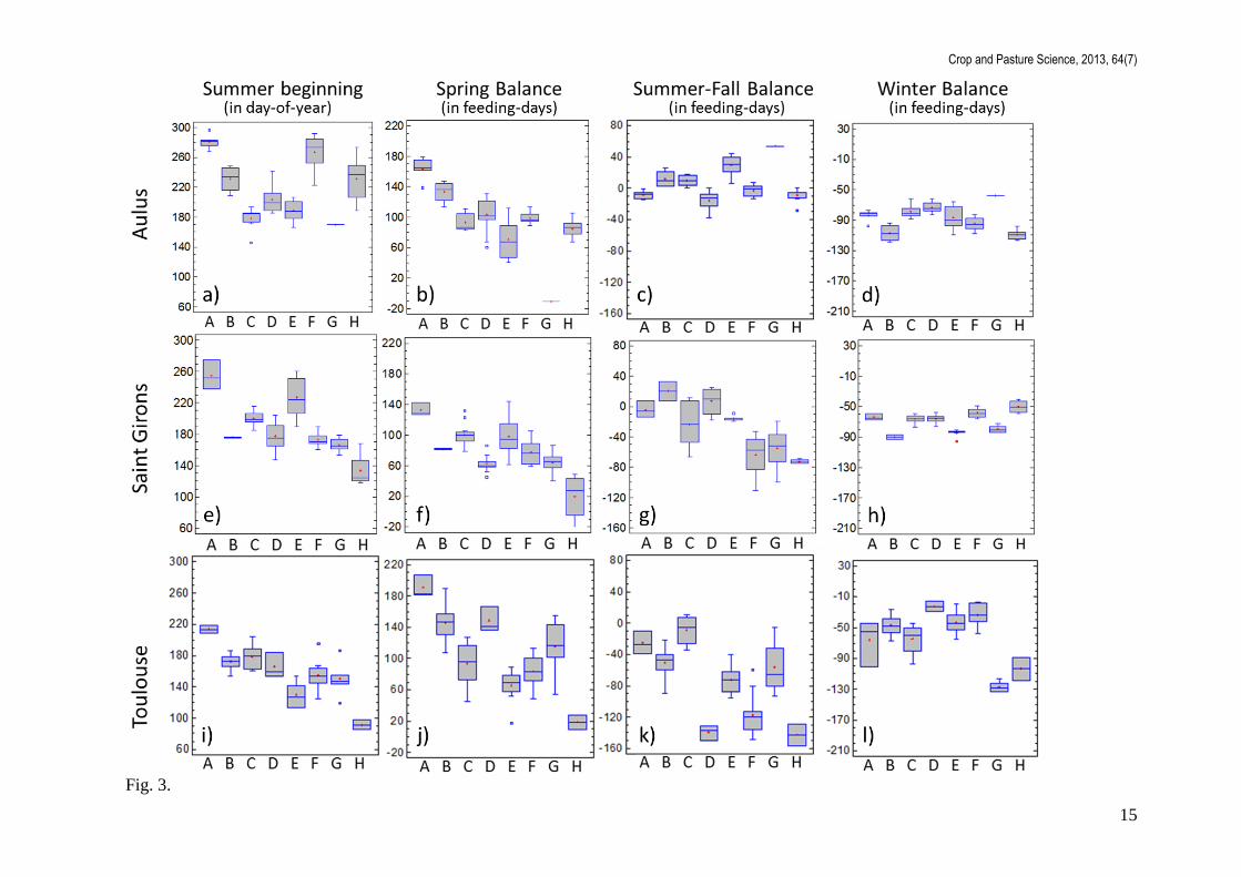
Annual herbage production was discriminated most by spring surplus, then by the summer

beginning and the herbage balance of summer-fall (as shown in Fig. 3). For each row (site) and

each column (indicator) of the figure, the 8 clusters (from A to H on the x-axis of each case) of

climatic years (30 years each in the past and future) are ranked according to decreasing annual

herbage production; the y-axis (labelled on top of each column) is expressed as day-of-year for the

date and feeding days for the herbage balance. For each indicator, the range is kept constant over

locations and criteria. When the boxplot panel exhibits a negative slope for a given indicator, the

order of clusters according to this indicator is consistent with the order induced by the annual

production. In all three sites, the higher the herbage surplus in spring, the higher annual production

(panels b, f and j). In Saint Girons and Toulouse (panels e and i), the beginning of the summer-fall

season was correlated with annual herbage production (a late summer-fall corresponding to high

annual production). In Saint Girons the summer-fall herbage balance had a significant influence on

annual production (panel g), meaning that a high-production year resulted most often from the

conjunction of a favourable spring and favourable summer.

In Toulouse and only there, the median and mean values of the summer-fall herbage

balance were negative for every cluster (Fig. 3, panels c, g and k). For Saint Girons and Aulus, both

negative and positive values were observed. Putting the clusters together (i.e. considering the full

sample of 60 years), large variability was observed in the spring balance at the three sites (panels b,

f and j). Variability in the summer-fall balance was larger for Toulouse and Saint Girons and

smaller for Aulus (panels c, g and k). Variability in the winter balance was relatively large in

Toulouse due to the high variability in the beginning of winter (panels d, h and l).

Similar annual production can be achieved with different distributions of herbage

production during the year (Fig. 3). Indeed, different combinations of seasonal balances were

observed for forage-year clusters with similar annual herbage production (i.e. two clusters of

adjacent rank). For example, in Aulus, a high spring balance and a negative summer balance were

observed for cluster D, whereas a low spring balance and positive summer balance were observed


6

for cluster E. Similar phenomena were observed in Toulouse and Saint Girons with the pairs of

clusters (B, C) and (D, E), respectively.

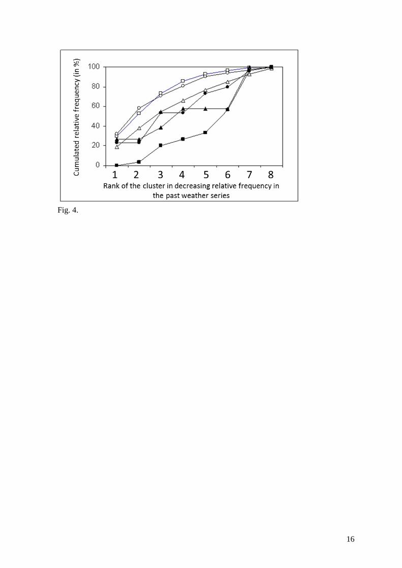
Depending on the site and the time series considered, covering 80% of the sample required

grouping three to five forage-year clusters. Therefore, no single cluster could be identified as a

prototype of “normal” forage years. For all sites and both periods, at least three clusters occurred

more than 12.5% of the time. This threshold (Table 3) represents an equal distribution of years

among clusters (100% divided by 8 clusters = 12.5%). A cluster was subsequently considered

“frequent” if its relative frequency exceeds 12.5%. For each site, there was a highly frequent cluster

(relative frequency ≥ 16%) in both the past and the future (cluster F in Aulus, C in Saint-Girons

and B in Toulouse) (Table 3).

The relative frequencies of clusters differed significantly between past and future scenarios,

with the most frequent clusters in the past becoming less common in the future and vice versa (new

clusters appearing in the future, some disappearing). Some common clusters in the past were not

observed or were infrequent in the future (e.g. clusters B and H in Aulus, F and H in Saint Girons,

C in Toulouse) (Table 3). The opposite was true for clusters C in Aulus, E in Saint Girons and F in

Toulouse (Table 3). Broadly speaking, from the past to the future, the frequency of years with high

annual herbage production (clusters A and B) decreased in Aulus and Toulouse, but increased in

Saint Girons. At the same time, the frequency of years with low herbage production (clusters G and

H) decreased in Aulus and Saint Girons but increased in Toulouse. After reordering clusters of

years according to decreasing frequency (from 1 to 8 in Fig. 4), a clear change was identified in the

characteristics of dominant forage years from past to future climates. The three most common

clusters in the past covered more than 71% of cases, whereas these three clusters covered at most

53% of cases in the future (Fig. 4). The greatest change was observed in Aulus (greatest distance

between past and future curves in Fig. 4). Moreover, the three most frequent clusters in the past

included 71-77% of past years, whereas the three most frequent clusters in the future included 65-

80% of future years.

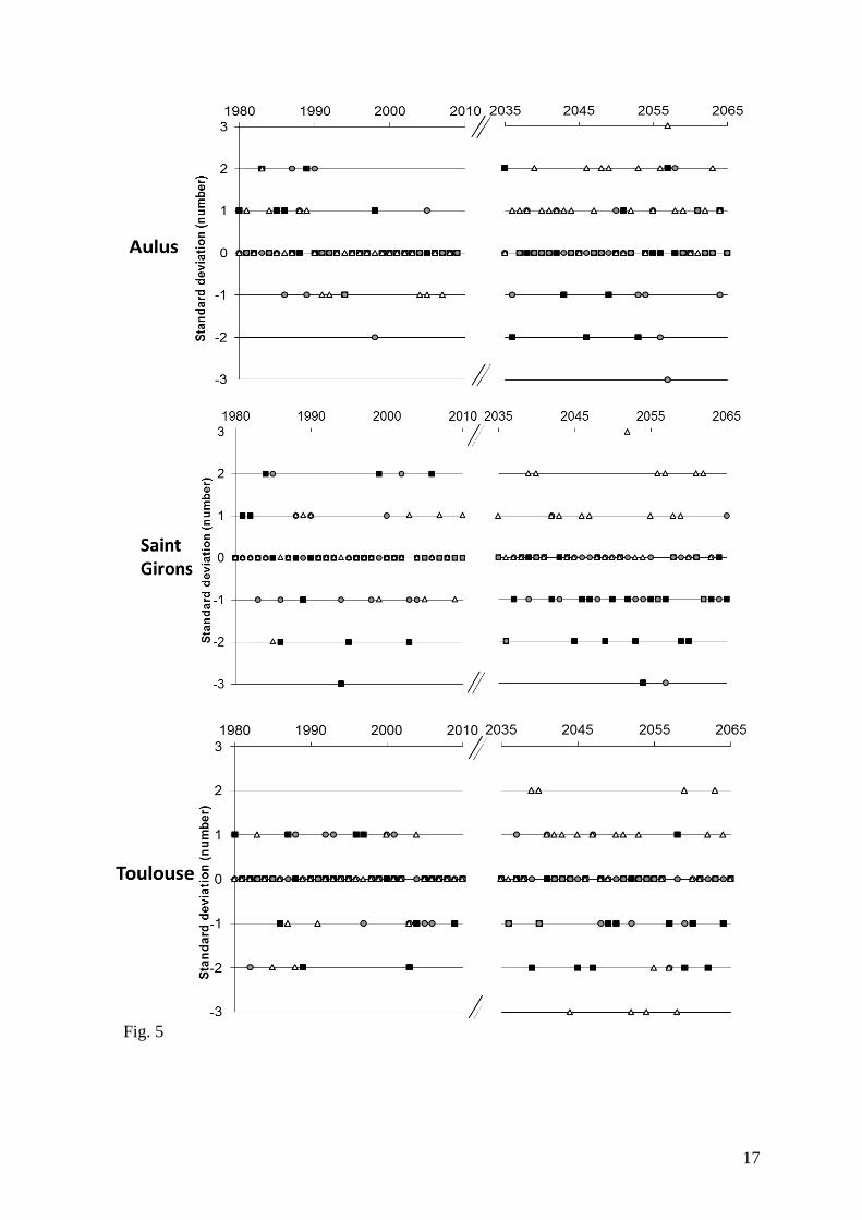
Standard-deviation classification based on past mean seasonal herbage balance

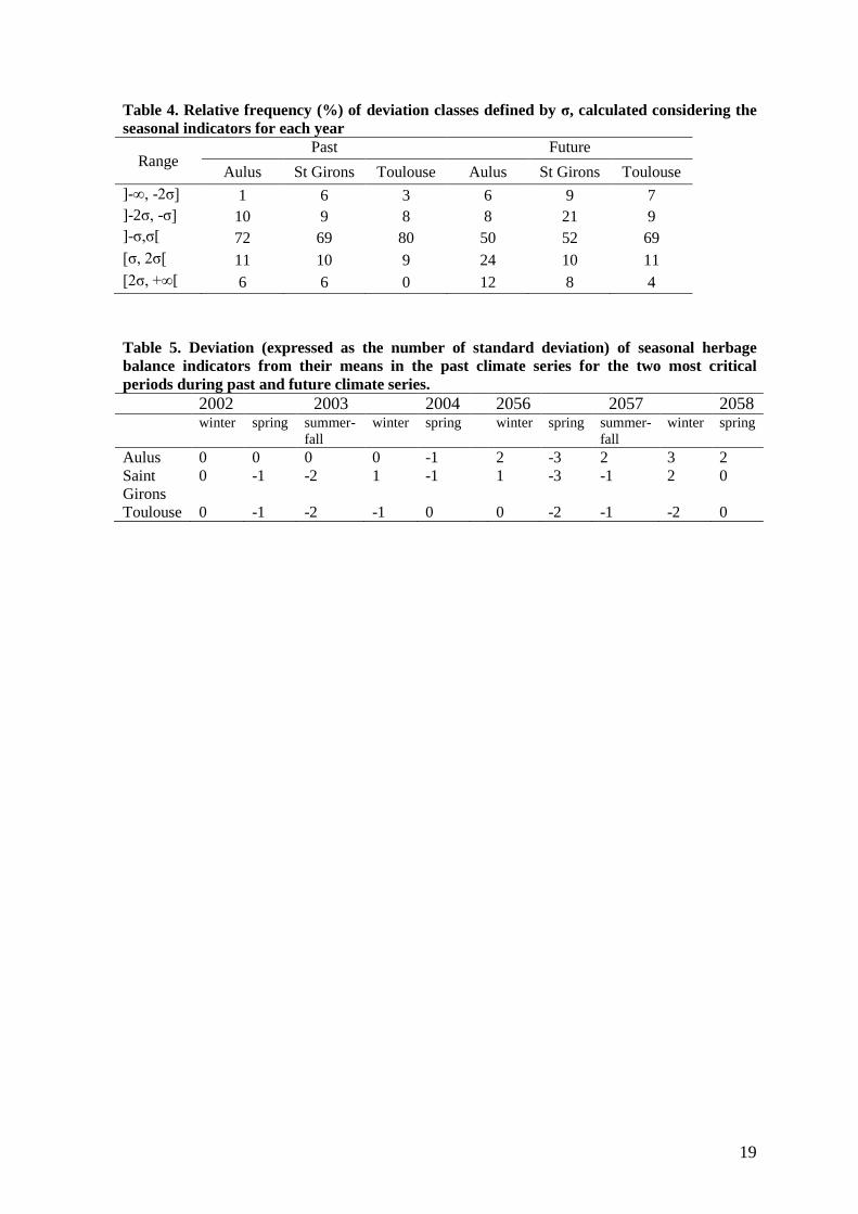
The standard-deviation classification reveals and quantifies the amplitude and frequency of

divergence of seasonal balances compared to their means in the past. The percentage of seasons in

classes ]-∞, -2σ] and [2σ, +∞[ changed from 7% in the past to 18% in the future in Aulus, 12% in

the past to 17% in the future in Saint Girons, and 3% in the past to 11% in the future in Toulouse

(Table 4). Consequentially, the frequency of seasons corresponding in the ]-σ, σ[ interval decreased

by at least 11% in the future (Table 4). Seasons in the extreme classes (above 3σ or below -3σ)

were exceptional in the past (only one case observed in Saint Girons), whereas the future time

series shows two, three and four seasons in the extreme classes in Aulus, Saint Girons and

Toulouse, respectively (Fig. 5). The largest deviations were generally positive in winter and

negative in summer-fall in the future climate (Fig. 5).

Sequences of seasons are also worth studying because the consequences of climate change

are more severe for farmers when two consecutive seasons fall into extreme classes. Examination

of sequences of seasons during the most critical years in the past (2003) and the future (2057, Fig.

5) showed that in Toulouse, herbage balance lay below the mean for three consecutive seasons

(especially summer-fall, which lay 2-3σ below) (Table 5). A similar pattern was observed in Saint

Girons, but nothing significant was noticed in Aulus. In the future, the number of successive

seasons below the mean was greater in Toulouse than in the other two sites, and there was a trend

toward a worsening situation (the balance decreases further below the mean for two seasons but

less so for the last season).

Discussion Lessons about climate change and variability

The indicators break down annual potentials into seasonal potentials, making it possible to: (i)

predict whether productivity-defined seasons become hindrances or opportunities, (ii) determine,

over several years, whether a favourable productivity-defined season can counterbalance an

unfavourable one and (iii) compare sites.

Regardless of the method used for characterising years (year clustering or σ-based classes),

we found it nearly impossible to define a single average or normal productivity-oriented climatic


7

year for past or future climate series. For a given site, we identified several clusters of forage years

with a significantly high probability of occurrence. Such climatic years, however, differ in the

characteristics of their seasons, which can have favourable or unfavourable forage production.

Sometimes above-average grass production occurs in the spring, followed by a dry summer, while

in other years the inverse occurs. These differences between years are particularly important from a

management perspective. Unusual patterns of favourable or unfavourable seasons induce

constraints that strongly impact on management (Charpenteau and Duru 1983), especially in the

case of a dry spring, even when followed by a wet summer (Aulus in 1998).

In contrast with research that focuses only on summer biomass production (e.g. Lamarque

2012), our results show that the amount of herbage surplus in spring (depending on temperature

and water availability) and surplus or shortage in summer (depending on water availability) need to

be considered jointly for the adaptation of grassland-based livestock systems. The year 2003 in

Toulouse, which was considered exceptional at the European level (Ciais et al. 2005), brought

about the greatest deviation from mean herbage balance (-σ for spring and -2σ for summer); i.e. it

simultaneously exhibited the lowest herbage surplus in spring, the greatest herbage shortage in

summer-fall and the earliest beginning of summer-fall (cluster H, Fig. 3). The two other sites,

located at higher altitudes, did not experience such dramatic consequences, which is consistent with

de Martonne aridity indices (Table 1).

For the future climate, results of several crop simulation models predict that the expected

impact of climate change on grassland production depends greatly on the geographic area and time

horizon considered. After a slight increase in forage production in the first half of the 21st century, a

reduction is expected in France (e.g. Graux et al. 2013) and the rest of Europe (Höglind et al.

2012). More specifically, Ruget et al. (2010) showed that for France in the near future (2020-

2050), a production increase is expected in almost all regions, while towards the end of the century

the trends differ by region, with a production decrease expected, especially in south-western

France. Comparing the periods 1980-2010 and 2035-2065, we found an average decrease in

biomass production for Toulouse (-6%) and Saint Girons (-12%) and a slight increase for Aulus

(+2%) (Sautier et al., 2013). These results are within the range of changes obtained in the above

mentioned studies that concerned lower scales (national or regional rather than local) and different

(although overlapping) periods. They corroborate the intuitive prediction that the switch from

increasing to decreasing annual production will occur later in mountainous zones. In addition to

these results, we found that climatic shifts are expected in four ways:

- infrequent forage-year clusters in the past become frequent in the future;

- some clusters with high annual herbage production in the past are expected to disappear

(cluster B in Aulus and clusters A or C in Toulouse);

- clusters with low annual herbage production that did not occur in the past are likely to occur

in the future (cluster G in Aulus and Saint Girons);

- variability in seasonal herbage production increases.

Based on comparison of forage-year clusters (Figs. 3 and 4), as well as quantification of

variations from the mean (Fig. 5), we substantiated the claim that a shift in seasonal biomass

production is expected. Clusters of climatic years infrequent in the past will become more common,

and new clusters will emerge. The magnitude and direction of change in weather induced by

climate change indicate that a substantial readjustment in management practices will be required.

Therefore, incremental adaptations will probably be insufficient to cope with climate change.

Instead, transformational (e.g. land-use) changes (Rickards and Howden 2012) and adaptive risk-

management approaches will be required.

Consistent with Seneviratne et al. (2012), our simulation results indicate a probable

increase in year-to-year climate variability and an accentuation of the contrast between spring and

summer-fall herbage balance (productivity increases for spring and decreases for summer-fall).

These changes, highlighted by the methods presented here, have important management

implications for farmers. Shifting the grazing period due to an earlier spring and summer requires

organisational adaptations. It could lead to changing the temporal distribution of work, with more

harvesting in spring due to higher herbage growth and more time spent distributing conserved feed

in summer due to a shorter grazing period. More generally, higher seasonal variability requires

specific risk-management strategies (e.g. larger forage stocks or other feeding resources), and this

need increases if between-year variability also increases.


8

Contribution to the participative design process

The data analysis and corresponding statistical graphics used in our approach can help farmers,

advisers and scientists envision site-specific impacts of climate change on herbage production

patterns. Such information can provide useful material for participatory design workshops focusing

on adaptation of grassland systems to new climatic conditions (Duru et al. 2012).

The originality of our two methods of weather-pattern characterisation stems from the

concept of a “forage year”, defined as seasonal dynamics of forage production and intake. The

seasonal assessment of herbage surplus or deficit makes it possible either to categorise a series of

years into a small number of clusters or to classify seasons according to their deviations from past

means. When represented graphically, these synthetic and quantitative descriptions can become

generic tools due to the model-based assessment involved, its suitability for any soil or climatic

context and the ease of obtaining the required data. Climatic years and seasons are quantified as the

number of days of feed available (Fig. 3), which fits well with farmers’ management-oriented

mental models, as previously experienced in grazing management projects (Duru et al. 2000; Cros

et al. 2004). Such representations are therefore cognitive tools (Duru and Martin-Clouaire 2011)

that can be used to raise agricultural stakeholders’ awareness of climate change and its likely

consequences on grassland systems.

The approach for characterising climate exposure presented in this paper applies to roughly

defined grassland systems. It does not deal, for instance, with specific field characteristics (e.g.

topography, soil bearing capacity). Other indicators sensitive to these aspects are required when

more elaborate characterisation of livestock systems’ climatic exposure is needed.

These two methods were developed as part of a project to design grassland-based livestock

systems that are less vulnerable to climate change and variability. The vehicle for implementing the

methodology is a series of participative-design workshops. Each workshop begins with the

facilitator introducing the game-based design methodology (Martin et al. 2011) and playing

material. The system to design must initially comply with the system features desired by the

participants and then consider the weather conditions encountered, which takes the form of a

weather time-series and contextual data about past weather and projected future weather. This part

of the method is specifically described in the present paper. The design problem consists of

dimensioning the system, configuring and planning land-use, and devising conditional adjustments

to cope with adverse situations or to take advantage of opportunities. Participative design is truly an

iterative, on-going interactive process. Participants are provided a methodology to continually

assess the system under construction and adapt to newly introduced constraints or changes. The

interaction between farmers in the workshops promotes understanding and learning about the

potential threat brought by climate change and ways to reduce the system vulnerability (Fleming

and Vanclay 2010). In the design process, the visual and tangible representations of climate change

and variability provide a science-based account of the uncertainty about possible future weather.

The tools presented in this paper contribute insightful design information by enabling comparison

of forage-year clusters in time and space. For instance, for clusters that were rare in the past and are

likely to become common in the future, farmers can design systems similar to those that survived

such difficult weather conditions in the past. Also, by comparing sites at different altitudes or

biogeographic regions, farmers can exploit a design-by-analogy approach that considers the future

weather of a site is likely to be similar to that experienced at a different site in the past.

Conclusion The exposure of grassland-based livestock systems to climate change and variability drives the

identification and evaluation of management adaptations. However, exposure is difficult to assess

from only climate data given the joint effects of weather variables on grass growth throughout the

year. Therefore, we proposed two methods for defining and ranking clusters of “forage years” to

characterise climate change and variability. The methods were tailored to produce outputs that can

serve as cognitive tools for farmers and agricultural advisors. Forage years were defined from

exposure indicators specific to grazing systems: starting dates of seasons and seasonal grass

production surplus or deficit. The first method clustered years with similar herbage growth profiles,

while the second classified the deviation of seasonal herbage balances from their respective means.

Both methods can be used as an initial step for designing farming system adaptations for feeding

herds. They provide a synthetic and quantitative view of problematic weather patterns likely to


9

occur in the future. Since exposure indicators were based on generic grass-growth models, the

method is easily applicable to other sites and periods than those considered here. The main lessons

from the case studies are the following.

- Several “normal” forage years can be identified, albeit with different seasonal patterns.

- While no trend of change was observed in exposure indicators over the last 30 years, a shift

is expected for the medium future (2050 ± 15 years); the most frequent clusters of climatic

years in the past become less common, although some clusters remain common.

- An increase in year-to-year variability in seasonal herbage balance and an accentuation of

the contrast between spring and summer-fall herbage balance are expected, which call for

substantial adaptations to livestock systems.

Acknowledgements

This work was funded by the French National Research Agency through the project O2LA

(Organismes et Organisations Localement Adaptés) (contract ANR-09-STRA-09), the INRA Meta-

programme ACCAF through the project FARMATCH and the PSDR project Climfourel INRA-

Midi-Pyrenees region. We thank Mathilde Piquet for her early contribution to the analysis of

exposure indicators.

References

Adger WN (2006) Vulnerability. Global Environmental Change 16(3), 268–281.

doi:10.1016/j.gloenvcha.2006.02.006.

Anwar MR, Liu DL, Macadam I, Kelly G (2012) Adapting agriculture to climate change: a review.

Theoretical and Applied Climatology 113, 225–245. doi:10.1007/s00704-012-0780-1.

Chapman DF, Kenny SN, Beca D, Johnson IR (2008) Pasture and forage crop systems for non-

irrigated dairy farms in southern Australia. 2. Inter-annual variation in forage supply, and

business risk. Agricultural Systems 97(3), 126–138. doi:10.1016/j.agsy.2008.02.002.

Charpenteau JL, Duru M (1983) Simulation of some strategies to reduce the effect on climatic

variability on farming. The case of Pyrenees Mountains. Agricultural Systems 11(2), 105–

125. doi:http://dx.doi.org/10.1016/0308-521X(83)90025-2.

Ciais P, Reichstein M, Viovy N, Granier a, Ogée J, Allard V, Aubinet M, Buchmann N, Bernhofer

C, Carrara a, Chevallier F, De Noblet N, Friend a D, Friedlingstein P, Grünwald T, Heinesch

B, Keronen P, Knohl a, Krinner G, Loustau D, Manca G, Matteucci G, Miglietta F, Ourcival

JM, Papale D, Pilegaard K, Rambal S, Seufert G, Soussana JF, Sanz MJ, Schulze ED, Vesala

T, Valentini R (2005) Europe-wide reduction in primary productivity caused by the heat and

drought in 2003. Nature 437(7058), 529–33. doi:10.1038/nature03972.

Cros M., Duru M, Garcia F, Martin-Clouaire R (2004) Simulating management strategies: the

rotational grazing example. Agricultural Systems 80(1), 23–42.

doi:10.1016/j.agsy.2003.06.001.

Déqué M, Dreventon C, Braun A, Cariolle D (1994) The ARPEGE/IFS atmosphere model: a

contribution to the French community climate modelling. Climate Dynamics 10, 249–266.

doi:10.1007/BF00208992.

Duru M, Adam M, Cruz P, Martin G, Ansquer P, Ducourtieux C, Jouany C, Theau JP, Viegas J

(2009) Modelling above-ground herbage mass for a wide range of grassland community

types. Ecological Modelling 220(2), 209–225. doi:10.1016/j.ecolmodel.2008.09.015.

Duru M, Ducrocq H, Bossuet L (2000) Herbage volume per animal: a tool for rotational grazing

management. Journal of Range Management 53, 395–402. doi:10.2307/4003750.

Duru M, Felten B, Theau JP, Martin G (2012) A modelling and participatory approach for

enhancing learning about adaptation of grassland-based livestock systems to climate change.

Regional Environmental Change 12(4), 739–750. doi:10.1007/s10113-012-0288-3.


10

Duru M, Martin-Clouaire R (2011) Cognitive tools to support learning about farming system

management: a case study in grazing systems. Crop and Pasture Science 62, 790–802.

doi:10.1071/CP11121.

Fleming A, Vanclay F (2010) Farmer responses to climate change and sustainable agriculture. A

review. Agronomy for Sustainable Development 30(1), 11–19. doi:10.1051/agro/2009028.

Fraser EDG, Dougill AJ, Hubacek K, Quinn CH, Sendzimir J, Termansen M (2011) Assessing

Vulnerability to Climate Change in Dryland Livelihood Systems: Conceptual Challenges and

Interdisciplinary Solutions. Ecology and Society 16(3), art3. doi:10.5751/ES-03402-160303.

Gibbons JM, Ramsden SJ (2008) Integrated modelling of farm adaptation to climate change in East

Anglia, UK: Scaling and farmer decision making. Agriculture, Ecosystems & Environment

127, 126–134. doi:10.1016/j.agee.2008.03.010.

Girard N, Bellon S, Hubert B, Lardon S, Moulin C-H, Osty P-L (2001) Categorising combinations

of farmers’ land use practices: an approach based on examples of sheep farms in the south of

France. Agronomie 21(5), 435–459. doi:10.1051/agro:2001136.

Graux A-I, Bellocchi G, Lardy R, Soussana J-F (2013) Ensemble modelling of climate change risks

and opportunities for managed grasslands in France. Agricultural and Forest Meteorology

170, 114–131. doi:10.1016/j.agrformet.2012.06.010.

Hansen J, Sato M, Ruedy R (2012) Perception of climate change. Proceedings of the National

Academy of Sciences of the United States of America 109(37), E2415–23.

doi:10.1073/pnas.1205276109.

Höglind M, Thorsen SM, Semenov MA (2012) Assessing uncertainties in impact of climate change

on grass production in Northern Europe using ensembles of global climate models.

Agricultural and Forest Meteorology 170, 103–113. doi:10.1016/j.agrformet.2012.02.010.

Hopkins A, Del Prado A (2007) Implications of climate change for grassland in Europe: impacts,

adaptations and mitigation options: a review. Grass and Forage Science 62(2), 118–126.

doi:10.1111/j.1365-2494.2007.00575.x.

Hulme M, Dessai S, Lorenzoni I, Nelson DR (2009) Unstable climates: Exploring the statistical

and social constructions of “normal” climate. Geoforum 40(2), 197–206.

doi:10.1016/j.geoforum.2008.09.010.

Lamarque P (2012) Une approche socio-écologique des services écosystémiques. Cas d’étude des

prairies subalpines du Lautaret. Ph.D. thesis, Université de Grenoble, France.

Martin G, Felten B, Duru M (2011) Forage rummy: A game to support the participatory design of

adapted livestock systems. Environmental Modelling & Software 26, 1442–1453.

doi:10.1016/j.envsoft.2011.08.013.

McCrum G, Blackstock K, Matthews K, Rivington M, Miller D, Buchan K (2009) Adapting to

climate change in land management: the role of deliberative workshops in enhancing social

learning. Environmental Policy and Governance 19(6), 413–426. doi:10.1002/eet.525.

Meinke H, Howden SM, Struik PC, Nelson R, Rodriguez D, Chapman SC (2009) Adaptation

science for agriculture and natural resource management—urgency and theoretical basis.

Current Opinion in Environmental Sustainability 1(1), 69–76.

doi:10.1016/j.cosust.2009.07.007.

Metzger MJ, Bunce RGH, Jongman RHG, Mücher CA, Watkins JW (2005) A climatic

stratification of the environment of Europe. Global Ecology and Biogeography 14, 549–563.

doi:10.1111/j.1466-822x.2005.00190.x.

Nakicenovic N, Alcamo J, Davis G, De Vries B, Fenhann J, Gaffin S, Gregory K, Grubler A, Jung

TY, Kram T, Emilio la overe E, Michaelis L, Mori S, Morita T, Pepper W, Pitcher H, Price L,

Riahi K, Roehrl A, Rogner HH, Sankovski A, Schlesinger M, Shukla P, Smith S, Swart R,

Van Rooyen S, Victor N, Dadi Z (2000) Emissions Scenarios. A Special Report of Working


11

Group III of the Intergovernmental Panel on Climate Change. SUMMARY FOR

POLICYMAKERS.

Niu X, Easterling W, Hays CJ, Jacobs A, Mearns L (2009) Reliability and input-data induced

uncertainty of the EPIC model to estimate climate change impact on sorghum yields in the

U.S. Great Plains. Agriculture, Ecosystems & Environment 129(1-3), 268–276.

doi:10.1016/j.agee.2008.09.012.

Pagé C, Terray L, Boé J (2008) Projections climatiques à échelle fine sur la France pour le 21ème

siècle: les scénarii SCRATCH08. Technical Report TR/CMGC/10/58, SUC au CERFACS,

URA CERFACS/CNRS No. 1875 France.

Pannell DJ (2010) Policy for climate change adaptation in agriculture. In “54th Annual Conference

of the Australian Agricultural and Resource Economics Society,” Adelaide, Australia. P 18.

(Adelaide, Australia)

Rickards L, Howden SM (2012) Transformational adaptation: agriculture and climate change. Crop

and Pasture Science 63(3), 240. doi:10.1071/CP11172.

Ruget F, Moreau J, Cloppet E, Souverain F (2010) Effect of climate change on grassland

production for herbivorous livestock systems in France. InSchnyder H, Isselstein J, Taube F,

Auerswald K, Schellberg J, Wachendorf M, Herrmann A, Gierus M, Wrage N, Hopkins A

(eds) “Grassland in a Changing World,” Kiel, Germany. Pp 75–77. (Organising Committee of

the 23th General Meeting of the European Grassland Federation: Kiel, Germany)

Sautier M, Martin-Clouaire R, Faivre R, Duru M (2013) Assessing climatic exposure of grassland-

based livestock systems with seasonal-scale indicators. Climatic Change 120, 341–355.

doi:10.1007/s10584-013-0808-2.

Sebillotte M, Soler LG (1990) Les processus de décision des agriculteurs. I. Acquis et questions

vives. “Modélisation systémique et systèmes agraires.” (Eds J Brossier, B Vissac, J.

Lemoigne), (INRA Editions: Paris)

Seneviratne SI, Nicholls N, Easterling D, Goodess CM, Kanae S, Kossin J, Luo Y, Marengo J,

McInnes K, Rahimi M, Reichstein M, Sorteberg A, Vera C, Zhang X (2012) Changes in

climate extremes and their impacts on the natural physical environment. In: Managing the

Risks of Extreme Events and Disasters to Advance Climate Change Adaptation. “A Special

Report of Working Groups I and II of the Intergovernmental Panel on Climate Change

(IPCC).” (Eds CB Field, V Barros, TF Stocker, D Qin, DJ Dokken, KL Ebi, MD Mastrandrea,

KJ Mach, G-K Plattner, SK Allen, M Tignor, PM Midgley) pp.109–230. (Cambridge

University Press,: Cambridge, UK, and New York, NY, USA)

Vanclay F (2004) Social principles for agricultural extension to assist in the promotion of natural

resource management. Australian Journal of Experimental Agriculture 44, 213–222.

doi:10.1071/EA02139.

Zhang B, Valentine I, Kemp PD (2007) Spatially explicit modelling of the impact of climate

changes on pasture production in the North Island, New Zealand. Climatic Change 84(2),

203–216. doi:10.1007/s10584-007-9245-4.


12

Figure captions

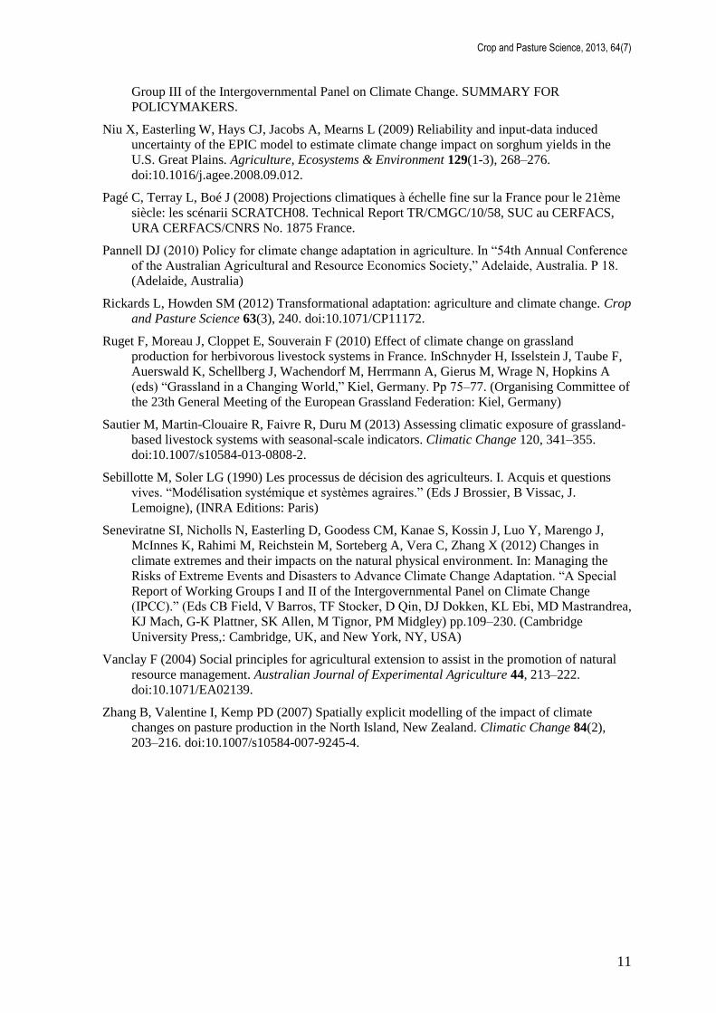
Fig. 1. Determination of season boundaries and surplus or shortage of grazing resources according

to the herbage-growth profile.

The dark blue region under the dashed line indicates when the livestock is fed (partially in summer-

fall and totally in winter) with silage or hay.

Fig. 2. Scatter plot of exposure indicators at the seasonal level (spring, summer-fall, winter) for the

past (1980-2010, unfilled symbols) and future (2035-2065, filled symbols).

2a, b, c: Herbage balance (y-axis in feeding days) and beginning date of season (x-axis in day-of-

year) in Aulus, Saint Girons and Toulouse. Each symbol corresponds to one season in a given year

(□ = spring, ○ = summer-fall, ∆ = winter).

2d: summary of 2a, 2b and 2c. Means and standard deviations of beginning date of season (x-axis)

and seasonal herbage balance (y-axis) for past (1980-2010, unfilled symbols) and future (2035-

2065, filled symbols) climates for Aulus (□), Saint Girons (∆) and Toulouse (○). Seasonal herbage

balance equals herbage production minus the amount of herbage needed to feed animals.

Fig. 3. Medians (lines), inter-quartile ranges (boxes), and outliers (dots) of the beginning of

summer (left) and seasonal herbage balances for spring, summer-fall and winter (right). .

Fig. 4. Cumulative relative frequency of forage-year clusters ranked (from 1 to 8) according to

decreasing relative frequency in the past weather series for three sites (Aulus (□), Saint Girons (∆)

and Toulouse (○)). The three upper curves represent the past (open shapes), while the other three

concern the future (filled shapes).

Fig. 5. Deviations of herbage balances in spring ( ), summer-fall (■) and winter (∆) in past and

future climate series from their means in the past climate series. Classes based on the number of

standard deviations are denoted by a number from -3 to 3, where -3 represents ]-∞, -3σ]; -2

represents ]-3σ, -2σ]; -1 represents ]-2σ, -σ]; 0 represents ]-σ, σ[; 1 represents [σ, 2σ[; 2 represents

[2σ, 3σ[; and 3 represents [3σ, +∞[.


13

Fig. 1


14

Fig. 2


15

Fig. 3.

16

Fig. 4.

17

Fig. 5

18

Table 1. Locations and De Martonne aridity indices (P/(T+10) (P= annual precipitation, T=

mean annual temperature)) of the three study sites for the period 1980-2010 and the year

2003. Site altitude latitude longitude Envrionmental zones† Aridity index for past

(mm/°C); (2003)

Aulus 733m 42° 47N 1° 20E Mediterranean

mountains 82 (80)

St Girons 414m 44° 49N 1° 23E Mediterranean North 43 (37)

Toulouse 150m 43° 36N 1° 26E Lusitanian (oceanic)/

Mediterranean North 27 (21)

† after Metzger et al. 2005

Table 2. Number of significantly (P<0.05) different clusters (out of 8) per indicator and

identity of those significantly different for at least 3 of the indicators

Beginning

of summer

Spring

balance

Summer-fall

balance

Winter

balance

Identity

Aulus 3 4 4 2 D,E,F,G

Saint Girons 5 3 3 3 A,B,H

Toulouse 4 3 2 3 A,B,E

Table 3. Cluster sizes (as a percentage of the sample size) in past and future scenarios

Aulus Saint Girons Toulouse

Year

cluster Past Future Past Future Past Future

A 8 7 0 10 10 0

B 23 3 0 6 32 23

C 3 23 23 23 26 0

D 13 7 10 19 3 7

E 3 40 0 23 10 20

F 20 17 37 10 13 30

G 0 3 17 10 3 17

H 30 0 13 0 3 3

In bold: %≥12.5

19

Table 4. Relative frequency (%) of deviation classes defined by σ, calculated considering the

seasonal indicators for each year

Range Past Future

Aulus St Girons Toulouse Aulus St Girons Toulouse

]-∞, -2σ] 1 6 3 6 9 7

]-2σ, -σ] 10 9 8 8 21 9

]-σ,σ[ 72 69 80 50 52 69

[σ, 2σ[ 11 10 9 24 10 11

[2σ, +∞[ 6 6 0 12 8 4

Table 5. Deviation (expressed as the number of standard deviation) of seasonal herbage

balance indicators from their means in the past climate series for the two most critical

periods during past and future climate series.

2002 2003 2004 2056 2057 2058

winter spring summer-

fall

winter spring winter spring summer-

fall

winter spring

Aulus 0 0 0 0 -1 2 -3 2 3 2

Saint

Girons

0 -1 -2 1 -1 1 -3 -1 2 0

Toulouse 0 -1 -2 -1 0 0 -2 -1 -2 0

20

Supplementary Material

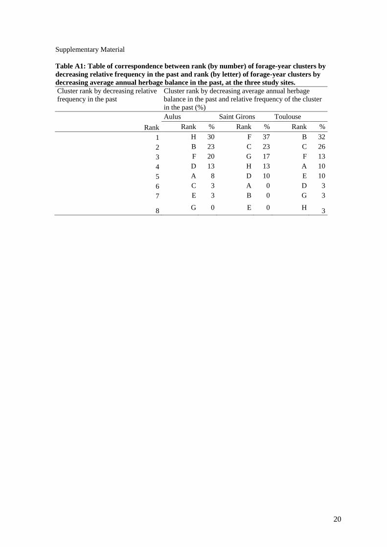
Table A1: Table of correspondence between rank (by number) of forage-year clusters by

decreasing relative frequency in the past and rank (by letter) of forage-year clusters by

decreasing average annual herbage balance in the past, at the three study sites.

Cluster rank by decreasing relative

frequency in the past

Cluster rank by decreasing average annual herbage

balance in the past and relative frequency of the cluster

in the past (%)

Aulus Saint Girons Toulouse

Rank Rank % Rank % Rank %

1 H 30 F 37 B 32

2 B 23 C 23 C 26

3 F 20 G 17 F 13

4 D 13 H 13 A 10

5 A 8 D 10 E 10

6 C 3 A 0 D 3

7 E 3 B 0 G 3

8 G 0 E 0 H

3

Use of productivity-defined indicators to assess exposure of grassland-based livestock systems to...

Documents

Transcript of Use of productivity-defined indicators to assess exposure of grassland-based livestock systems to...