USE OF POOR QUALITY WATER IN AGRICULTURE

Editors R K Yadav R L Meena H S Jat R K Singh K Lal S K Gupta

Afro-Asian Rural Development Organization (AARDO),

New Delhi, IndiaCENTRAL SOIL SALINITY RESEARCH INSTITUTE

KARNAL – 132 001 (INDIA)

Ministry of Rural Development, Govt. of India, New Delhi

Yadav, R K, Meena, R L, Jat, H S, Singh, R K, Lal, K and Gupta, S K (2010). Use of poor quality Water in Agriculture, Central Soil Salinity Research Institute, Karnal, India, p265. Sponsored by: Afro-Asian Rural Development Organisation (AARDO), New Delhi Financed by: Ministry of Rural Development, New Delhi Published by: Director

Central Soil Salinity Research Institute, Karnal-132 001 (India) Telephone: +91-184-2290501 Fax: +91-181-2290480 E-mail: director@cssri.ernet.in Website: http://www.cssri.org

The views expressed in this book are of the authors of the respective chapters. CSSRI, Karnal and ICAR, New Delhi assumes no responsibility of the statement made and not liable for any loss resulting from the use of this book. Printing: Intech Printers & Publishers

# 353, Mughal Canal Market, Ground Floor Karnal – 132 001 (Haryana) Contact Nos.: 0184-3292951, 4043541 E-mail: jobs.ipp@gmail.com

Acknowledgments An International Training Programme on “Use of Poor Quality Water in Agriculture” for AARDO (Afro-Asian Rural Development Organization) member countries delegates financed by Ministry of Rural Development, Govt. of India is being organized at Central Soil Salinity Research Institute, Karnal during December 1 to 14, 2010. The lectures delivered during the programme have been compiled and published in a book form. Lectures incorporated in this publication address important issues related to poor quality water use in agriculture in AARDO member countries. Characterization and judicious use of ground water including poor quality water drainage effluents and waste water to augment the fresh water supplies to meet the crop irrigation requirements for better productivity. The topics included appropriate agronomic practices, modern methods of irrigation, groundwater recharge and use of RS and GIS for diagnosis and effective management of natural resources. This publication has come to the present shape with the efforts made by the Scientist of CSSRI, an institute of Indian Council of Agricultural Research (Ministry of Agriculture, Govt. of India), New Delhi, support from the guest faculty and Ministry of Rural development, Govt. of India, New Delhi. The editors wish to place on record the heartiest thanks to AARDO for sponsoring and Ministry of Rural Development, Govt. of India, New Delhi for financing this international training programme. We acknowledge our sincere gratitude to the federal Governments of Malaysia, Yemen, Syria, Iraq, Oman, Mauritius and Bangladesh for delegating the participants in this training programme. We are also obliged to the Director, CSSRI, Karnal who has been a source of inspiration, guidance and encouragement in conducting this international training programme. Editors wish to record special appreciation for all the resource persons who contributed manuscripts and agreed to share their valuable expertise and thoughts during the training. Last but not the least we are thankful to one and all who have directly or indirectly involved in the organization of this training programme, compilation and publication of this manuscript.

Editors

CONTENTS

Page

Acknowledgements i

1 An Overview of Water Logging and Soil Salinity Problems in Three AARDO Countries S.K. Gupta

1

2 Geochemistry and Hydrological Cycles – Sources of Origin of Poor Quality Waters A.K. Mandal

10

3 Origin of Salinity - Sodicity in Soils and Underground Water of Indus Plains of the Indian Sub-continent Raj Kumar, S. K. Ghabru, N. T. Singh and R. L. Ahuja

21

4 Remote sensing and GIS for waterlogged salt affected soils Madhurama Sethi

33

5 Irrigation Water Salinity and Nutrient Interactions R. Chhabra

41

6 Integrated Nutrient Management – An Option for Minimizing Adverse Effects of RSC Water Irrigation N.P.S. Yaduvanshi

44

7 Raising Horticultural Crops under Saline Environment Dheeraj Singh, M.K. Choudhary, M.L. Meena and Hari Dayal

55

8 Practical Assessment of RSC, SAR, Adj. SAR and RNa in Irrigation Water Khajanchi Lal

67

9 In-situ examination of salt affected soil profile for reclamation and management A. K. Mandal

70

10 Agro-practices for management of saline irrigation water R.K. Yadav, H.S. Jat and Khajanchi Lal

77

11 Gypsum/Amendment Requirement in Sodic/Saline Water – A Practical Assessment P. Dey

87

12 Physiological Mechanisms of Tolerance to Salinity and Sodicity Stresses S.K. Sharma

92

13 Cultivation of Industrial and Non-Conventional Crops in Salt Affected Conditions Parveen Kumar and R.K. Yadav

98

14 Using SURFER for Analysis and Interpretation of Poor Quality Soil and Water C.K. Saxena

104

15 Drip Irrigation in Horticultural Crops: Suitability for Saline Water Use Satyendra Kumar

117

16 Recharge and Skimming- Opportunities and Techniques for Poor Quality Ground Water Areas S.K. Kamra

134

17 Characterization of Wastewater for Irrigation Khajanchi Lal, R.K. Yadav and R.L. Meena

145

18 Wastewater Use in Agriculture: Issues and Strategies R.K. Yadav, Khajanchi Lal and R.L. Meena

152

19 Crop Growth with High RSC Irrigation Water and Strategies for its Efficient Use R.K. Yadav, H.S. Jat, R.L. Meena and Khajanchi Lal

161

20 Irrigation Induced Soil Degradation in Command Areas S.K. Chaudhari

178

21 Fluoride and Nitrate Pollution in Groundwater D.S. Bundela and Khajanchi Lal

182

22 Drip Irrigation with Wastewater in Vegetables and Fruit Crops R.S. Pandey

191

23 Breeding for Salt Tolerance in Rice Krishna Murthy, S. L.

199

24 Nuclear Techniques for Inducing Salt Tolerance in Crops P.C. Sharma

208

25 Physiological Attributes Associated with Sodicity Tolerance Ali Qadar

219

26 Genetic Improvement for Salt Tolerance in Wheat Neeraj Kulshreshtha

227

27 Bioremediation: pollution fighting tool Madhu Choudhary

233

28 Financial Appraisal and Socio-Economic Benefits of Sodic and saline land Reclamation R.S. Tripathi

240

29 Aquaculture in Agriculturally Poor Quality Water: An Integral Component of Natural Resources Management Sharad Kumar Singh

248

30 Impact of High RSC Water Irrigation on Cultivation of Vegetable Crops S.K. Sharma, Sanjay Kumar, Vinod Phogat, A.C. Yadav and Avtar Singh

259

An Overview of Water Logging and Soil Salinity Problems in Three AARDO Countries S. K. Gupta Central Soil Salinity Research Institute, Karnal - 132 001(Haryana), India Afro-Asian Rural Development Organization (AARDO) Afro-Asian Rural Development Organization (AARDO) formed in 1962, is an autonomous inter governmental organization comprising thirty members from Africa and Asia. AARDO is devoted to develop understanding among members for better appreciation of each others' problems and to collectively explore the opportunities for coordination of efforts to promote welfare and eradication of thirst, hunger, illiteracy, disease and poverty amongst hundreds of millions of rural people. The current training programme is envisaged under the two scenarios mentioned in the charter of AARDO i.e. i) to seek close collaboration and effective networking with the centers of excellence and other international institutions for innovation and application of technology and ii) to double AARDO’s strength by way of doubling its training programmes, workshops and seminars, study visits, enriching AARDO’s website and development of pilot projects. I propose to highlight progress made in three AARDO countries namely Egypt, Pakistan and Ethiopia in respect of land reclamation programmes and use of poor quality waters in agriculture. Since Indian experiences would be discussed during the training in greater details, it is not included in this chapter to avoid repetition. Global Scene on Soil Salinity and Land Drainage Out of total world crop land of 1500 m ha, 1110 m ha is rain fed while only 390 m ha is irrigated. It has been reported that the globally human-induced salinisation is to an extent of 76.6 million ha (21.2 m ha strong, 20.8 m ha moderate and 34.6 m ha slightly salinized). This area is distributed with 52.7 m ha in Asia (69%), 14.8 m ha in Africa (19%) and 3.8 m ha in Europe (5%). A total of 31.2 m ha can be attributed to secondary salinisation of non-irrigated and 45.4 m ha in irrigated areas (Table 1). In terms of percent of the irrigated land, the area varies from 9% to about 34%. As per the above estimate nearly 67.5 % of the water logged salt affected lands are in Asia and Africa impacting the food grains production to a large extent. Thus, concerted efforts are needed to collectively deal with this problem through AARDO set-up. Drainage has been known to the key element in improving the production and productivity of rain fed as well as irrigated areas. While most of the rain fed cropped land (90%) is not drained, it is estimated that nearly 250-300 m ha is in immediate need of drainage improvement. Out of an irrigated land of 390 m ha, 190 m ha is provided with some kind of drainage infrastructure yet only 60 m ha is provided with adequate drainage improvement. Statistics related to land drainage of irrigated lands in some select countries is provided in Table 2. Egypt has the largest area under land drainage in terms of percent of the irrigated area provide with land drainage. Table 1. Global estimate of secondary salinization in the world’s irrigated lands Country Cropped

area, (M ha) Irrigated area, (M ha)

Share of irrigated to cropped area (%)

Salty area, (M ha)

Share of salty to irrigated land (%)

China 96.97 44.83 46.2 6.70 15.0 India 168.99 42.10 24.9 7.00 16.6 CIS States 232.57 20.48 8.8 3.70 18.1 United States 189.91 18.10 9.5 4.16 23.0 Pakistan 20.76 16.08 77.5 4.22 26.2 Iran 14.83 5.74 38.7 1.72 30.0 Thailand 20.05 4.00 19.9 0.40 10.0 Egypt 2.69 2.69 100.0 0.88 33.0 Australia 47.11 1.83 3.9 0.16 8.7 Argentina 35.75 1.72 4.8 0.58 33.7 South Africa 13.17 1.13 8.6 0.10 8.9 Subtotal 842.80 158.70 18.8 29.62 20.0 World 1473.7 227.11 15.4 45.4 20.0

2

Table 2. Drainage of irrigated lands in select countries

Country Arable land (m ha)

Irrigated area (m ha)

Drained area (m ha)

Proportion of drained area (%)

USA 179 22 48 27 China 136 50 20 15 Canada 46 0.7 9 20 Russia 127 5 7 6 Pakistan 22 18 6 27 India 170 55 6 5 (11)* Mexico 27 6.5 5.2 19 Germany 12 0.4 4.9 41 Great Britain 6 0.1 4.6 77 Poland 14 0.1 4.2 30 Egypt 3.3 3.3 3 91 * % of irrigated land Egypt With a total area of one million km2 (230 million feddan), agriculture in Egypt has always been confined to the Nile Valley and Delta comprising of about 3.6% of the country’s land surface. The Nile River Valley of Egypt has been one of the oldest agricultural areas in the world having been under continuous cultivation for more than 5000 years. With an average annual rainfall of 10 mm/annum, varying from 28 mm at Cairo to 190 mm at Alexendria, 86% of the total area is classified as extremely arid while 14% as arid. The construction of Aswan high dam during 1960-68, brought agricultural lands under perennial irrigation, raised the cropping intensity to 200% and more and eliminated the seasonal floods. To save the land from water logging and soil salinization, open drainage systems have been constructed since 1933 and by 1966 covered 3.2 million feddans. The drainage policy was revised in the year 1978 to provide in the long run all cultivated lands with tile drainage. As such, the Egyptian Public Authority for Drainage Projects (EPADP) was created in 1973. The drainage activities spread fast and today more than 90% of irrigated lands are covered under drainage. Some of the revised subsurface drainage parameters recommended for use in Egypt are as follows. Drainage coefficient For calculation of lateral drain spacing a coefficient of 1.0 mm day-1 was taken and the same has now been revised to 1.25 mm day-1 in the northern parts of the Nile Delta between contours 5 and 3 m above MSL and 1.50 mm day-1 north of contour 3 m above MSL. For the design of collectors, design discharge rate is taken as 3 mm day-1 for non-rice and 4 mm day-1 for rice areas with appropriate safety factors. Lateral spacing A minimum spacing of 30 m was recommended on the basis of economy while 60 m is the upper limit. Recently it has been recommended that spacing as obtained from theory may be used with a minimum cap of 20 m. Summary status of the land drainage projects up to year 2000 is shown in Table 3. The yield improvement through land drainage has justified the drainage activities (Table 4). Table 3. Summary status of land drainage projects

Tile drained area Area in 1 000 fed. Total areas provided with drainage up to 30.6.1988* 3 202 000 Areas to be covered during the remaining period of the Five-Year National Plan 87/88 – 91/92 (financed by the World Bank and other donors)

763 000

Areas to be covered during the next Five-Year Plan (91/92 – 96/97) and up to year 2000

1 150 000

Total 5 115 000 Land area remaining and still in need of drainage 1 914 000 *Does not include newly reclaimed areas

3

Reuse of Drainage Water Annually about 13.5 x 109 m3 of drainage water is discharged from the drains. The average salinity of drainage water varies from drain to drain ranging from 400 to 5000 ppm. It is clear that most of the drainage water is fit for reuse either as stand alone or after blending it with fresh Nile water. It is assessed that the about 9 x 109 m3 of water has salinity less than 2000 gm m-3 and is suitable for reuse. Since the water is limited, a great progress has been made in the reuse of drainage water for irrigation as well as for land reclamation. Table 4. Crop yield at Mashtul Pilot area

Intervention Yield (t/fed.) Wheat Berseem Maize Rice

Drained* 1.0 2.0 1.0 2.2 Non-drained 2.4 3.1 1.5 2.4 *Yield is average of 7 years after drainage Pakistan Pakistan covers an area of about 800 000 km2. The estimated population in 1997 was about 135 million, and this number is likely to double by the year 2020. This population growth will place enormous pressure on land resources in Pakistan. The whole of Pakistan (except a narrow belt in the north) is arid to semiarid and has a low, variable rainfall. Annual precipitation is highest (around 1500 mm) on the southern slopes of the Himalayas and gradually decreases to the south-west. Only 9% of the country receives more than 508 mm of rain per year. A further 22% receives between 254 and 508 mm and about 69% receives less than 254 mm of rain per year. For most of the Pakistan, the rainfall occurs primarily (70-80%) in the monsoon months of July, August and September. Some areas (especially in the north and west) have a rainfall distribution with two peaks, mid-winter being the second rainy season. Irrigation is therefore, used on about three-quarters of the cultivated land. Rise in water table and accumulation of salts at the soil surface is characteristic of arid and semiarid environments, especially where irrigation is practiced. By the end of the dry season, about 13% of irrigated land has water table less than 1.5 m. However, immediately after the monsoon, the percentage of land with water table less than 1.5 m increases to 26%. Salinisation occurs both naturally (‘primary’ salinity) and as a result of human activities (‘second’ salinity). About 6.3 million ha are affected, about half of this lying in the Canal Command Areas. Apart from a few localized areas, salt-affected soils are confined to the Indus Plain. The characterization of salt affected soils (Table 5, Table 6 and Table 7) revealed the following kinds of problems:

• Slightly saline-sodic or saline-gypsiferous soils (0.7 million ha). • Porous saline-sodic or saline-gypsiferous soils (1.9 million ha). • Severely saline-sodic and saline-gypsiferous soils (1.1 million ha). • Soils with sodic tube well water (2.3 million ha).

Four major approaches are being used to deal with salinity and sodicity in Pakistan.

• Engineering approach • Reclamation approach • Saline agricultural approach • No intervention

Table 5. Classes of soil salinity

Salinity class Salinity (ECe or ECs) range (dS m-1) Salt-free (non-saline) Less than 4 Slightly saline 4-8 Moderately saline 8-15 Strongly saline More than 15 Source: Water and Power Development Authority (1981)

4

Table 6. Classes of soil sodicity in terms of the SAR of the soil saturation extract

Sodicity class SAR Non-sodic Less than 13 Slightly sodic 13-25 Moderately sodic 25-45 Strongly sodic More than 45 Table 7. Classes of soil drainage in terms of depth to water table

Soil drainage class Depth to water table (m) Very poorly drained (W1) 0-0.9 Poorly drained (W2) 0.9-1.8 Moderately drained (W3) 1.8-3.3 Well drained (W4) More than 3.0 Source : Adopted from Water Power Development Authority (1981) In 1954, there were renewed investigations on the control of water logging and salinity under a technical assistance program with the United States. These led to the first Salinity Control and Reclamation Project (SCARP). A formal agreement for SCARP-1 was signed in 1957, and the project was completed in 1963. The key strategy of SCARP-1 was to install large-capacity tube wells for the pumping of aquifers. These tube wells also provided extra irrigation water to leach salts and increase cropping intensity. It is estimated that by December 1996, there were more than 19 000 publicly owned (Water and Power Development Authority 1997) and 243 000 privately owned tube wells. In addition, about 11 000 km of drains had been constructed (Water and Power Development Authority 1997). In 1968, WAPDA created the SCARP Monitoring Organization to evaluate the performance and effectiveness of SCARPs in terms of their design characteristics and planned objectives. Following benefits were documented: • Increased cropping intensities from 84 to 117% • Decreased areas with severe water logging from 16 to 6% • Increased areas of salt-free (surface salinity) land from 49 to 74% • Increased gross value of production by 94% In spite of these successes, the present strategy suffers from a number of critical deficiencies. • Many salt-affected soils are not treatable • The costs of the interventions are very high • The sustainability of the approach is questionable • The projects are of large scale. • The criteria for determining the success of projects are inadequate. As such strategy was shifted from vertical drainage to subsurface drainage in critical areas and reclamation approach in other areas specially the alkali lands. The reclamation approach includes the following: • Leaching • Use of gypsum, other amendments such as acids, farmyard manure and waste byproducts such as press

mud from sugar mills etc. • Physical methods such as surface scraping • Biological methods such as use of salt and water logging – tolerant plants.

The use of saline/alkali waters have also received considerable attention in Pakistan although large areas have been reported to have become alkali due to use of alkali or sodic water. The classification of waters is still being done as per the classification proposed by USDA although the parameter of RSC has been added to this classification (Table 5).

5

Table 8. Water quality classification in Pakistan

Classification EC (dS/m) SAR RSC Useable (C1S1R1) Less than 1.5 (C1) Less than 10 (S1) Less than 2.5 (R1) Marginal (C2S2R2) 1.5 – 3.0 (C2) 10-18 (S2) 2.5-5.0 (R2) Hazardous (C3S3R3) More than 3.0 (C3) More than 19 (S3) More than 5.0 (R3) Ethiopia Agriculture is the mainstay of the Ethiopian Economy. The Government of Ethiopia expects the dominance of agriculture in the economy to continue till some more time to come. On the contrary, a major challenge is to help farmers increase production while maintaining the traditional diversity on their farms in order to ensure household food security. Besides, farmers needs to be convinced to change the management practices for their domestic animals so as to restrict grazing and go for stall feeding in order to make better use of the feed resources available as well as to conserve the energy of the animals. It should be possible when constraints for remunerative arable cropping are removed and farmers are enabled to grow arable and fodder crops on their grazing lands. Vertisols particularly highland vertisols in such a scenario pose special problems as these are severally waterlogged during the rainy season. Vertisols Vertisols, the dark-coloured clays are widespread on the globe with an estimated area of at least 280 million ha located mainly in Africa, Australia, India and the USA. In Ethiopia, vertisols cover 12.6 million ha or 10.3% of Ethiopia. In addition, there are 2.5 million ha of soils with vertic properties. These soils occur in the lowlands (<1500 m), at intermediate altitudes (1500-1800 m) and in highlands (2000 m or higher), nearly 7.6 million ha being located in the highlands. Only one quarter of the vertisols are presently cropped and constitute 24% of all highland soils cropped in Ethiopia, which indicates their importance in Ethiopian agriculture. Remaining fraction of the vertisols is used as grazing land. Rain fed crops such as teff (Eragrostis tef), durum wheat, chickpea, lentils (Lens culinaris Med), linseed, noug (Guizotia abyssinica), and bread wheat are generally grown on vertisols. Small farmers grow sorghum, haricot beans, maize and other lowland crops. Irrigated crops such as cotton, sugarcane, citrus, and some vegetables are grown in the lowlands. Besides what has been stated, vertisols have an enormous yield potential but more often it remains unrealized due to many constraints. Some of the major constraints are: Workability of these soils is hampered by their stickiness when wet and hardness when dry. High clay

content, type of clay mineral, unfavourable consistency and absence of pores make them difficult to work in both dry and wet conditions.

Water logging and erosion. The physical characteristics of Vertisols, being characterized by high clay content particularly

expanding lattice clays. A substantial amount of rainfall is needed to wet a dry vertisol. The rain tends to move into cracks rapidly. While it wets the deeper layers, surface is left relatively dry. Thus, achieving optimum moisture conditions for cultivation is difficult under present management practices.

Limited resources to implement scientific drainage management options. As such, crop production on these soils is only a fraction of what could be realized. Average yield of 500-800 kg ha-1 for cereals, 500-700 kg ha-1 for highland pulses and 300 kg ha-1 for oil crops are only realized against a potential of 4-6 times these yields. The data in Table 9 attests to these figures. It is mainly because of the fact that once the rainy season starts and the surface is wet, cultivation is virtually impossible. Thus, wheat, lentil, chickpea and vetch grow to maturity entirely on residual soil moisture after establishment at the end of the rainy season. The problem of water logging and soil salinity The highland Vertisol areas are generally characterized by smallholder mixed cereal-livestock farming systems with a marked subsistence orientation. Land cultivation is almost exclusively done using oxen-drawn implements. The area is characterized by high rainfall (>900 mm year-1) and low evaporative demand due to moderate temperatures, which vary widely with altitude, but might average 15°C annually. As a result, most vertic soils are severely waterlogged (estimated at 2.5 million ha, especially vertic Cambisols and vertic Luvisols). In Oromia also, most of the high lands of Arsi, Bale, N.Shoa and others are exposed to surface as well as subsurface (soil profile root zone) drainage problems.

6

Table 9. Crop yields in highland vertisols in Ethiopia

Crop Yield (kg/ha) Teff (Eragrotis tef) 530 Barley 860 Durum wheat 610 Average Cereals 667 Faba bean 750 Lentils 500 Chickpea 600 Field pea 730 Grass pea 690 Average Pulses 654 Linseed 300 Noug (Niger seed) 290 Average oil seeds 295 The extent of water logging in rain fed areas of North Shoa, Bale, West Arsi and Bale alone covers more than 4.6 lakh ha area (Table 10). Table 10. Extent of water logging in rain fed areas of Arsi, Bale and North Shoa

District/site Problem area (ha) North Shoa Chancho-Kore roba 3,914 Chancho 18,127 Wuchale-Likime 5,319 Bedoye gimbichu 1,525 Jida 21,811 Kibibit-Segele/Basoserabi 5,298 Total 78,419 Bale Sinana 45,851 Goro 979 Ginir 1,323 Gasara 4,345 Goba 9,710 Total 80,947 West Arsi Adaba 11,863 Asasa 14,705 Kofele 19,631 Dodola 20,837 Kore 8,189 Total 75,225 Arsi Sude 28,871 Bele Gasgar 12,963 Robe 30,210 Limu and Bilbilo 31,561 Tiyo 10,115 Chole 4,052 Amigna 15,174 Shirka 16,048 Digalu Xicho 24,302 Diksis 15,686 Muneesa 28,435 Guna 9,430 Total 226,847 Grand total 461, 438 As a result of poor drainage, crops sown in early June suffer from prolonged water logging-these are stunted and show signs of poor aeration and nutrient deficiency. Grain yields are low. Besides erosion is a serious

7

problem as most vertisols in Ethiopia are located on either relatively flat or slightly sloping land. Under the present management, especially on fallow cultivated lands and on some sloping land in the highlands, erosion occurs during the rainy season. As per the National Task Force, salt affected soils in Ethiopia cover a total land area of 1.1 million ha. By the end of 2025, area under irrigation would be more than 4 times the current irrigated area (Table 11). Since water logging and soil salinity normally appears 10-15 years after the introduction of canal irrigation, some of the areas currently irrigated might face the problems then. It seems that the figures reported on water logging are from the irrigated lands and as such even currently the figures of water logging and soil salinity might exceed the reported values considering the waterlogged areas under rain fed conditions. For example at some of the project sites in North Shoa, Arsi, West Arsi and Bale more than 4.65 lakh ha land has been identified as waterlogged needing surface/subsurface drainage (Table 10). Kidane et al. (2006) seems to have rightly suggested that Ethiopia should have the capacity to undertake SD in 30,000 ha and SSD in 9000 ha per year. It echoes the feeling that the technology of surface and subsurface drainage particularly in its integrated mode has vast replication potential. Therefore, current efforts should be supported by all organizations in developing and preparing national guidelines on land drainage. Table 11. Salt affected and water logging in irrigated areas (Kidane et al., 2006)

Land area Present ( hectares) Future in 20 years (hectares) Irrigated 161,136 730,000 Area in need of drainage Waterlogged and salinized areas* 13,000 180,000 Waterlogged and salinized areas@ 13,000 180,000 *Require SSD; @ Require improved drainage Farmers’ response to water logging/drainage It is commonly believed that farmers are not aware of the water logging problem or they don’t intend to take remedial options. The field observations however, prove that farmers are quite aware and respond to the problem within their means. Following observations clearly support this viewpoint.

Farmers practice late-season planting to avoid the serious drainage problems in these soils during the rainy season.

The farmers shift from wheat to teff and oats in areas with poor drainage since these two crops are relatively more tolerant to water logging than wheat.

Wherever drainage conditions are favourable, more remunerative crops such as faba bean, field peas and barley are cultivated.

Conventional drainage practices Drainage furrows: In some parts of central highlands (Shewa and Gojam), the drainage furrows are made by ploughing across the contour at varying distances (3-6m). Using this method, drainage furrows of 15-20 cm width and depth are scooped out on about 10-15% of the fields. Ridges and furrows: In high rainfall areas and on lower slopes, ridges and furrows are made with traditional ox drawn plough, and crops such as durum wheat are planted on top of the ridges. The ridges and furrows are constructed at an interval ranging from 40 to 60 cm. The height of ridges from the bottom of the furrows varies from 10 to 15 cm. Hand made broad beds and furrows: In this method, fields are cultivated several times before the crop is sown. Next, narrow furrow lines approximately 80 cm apart are demarcated. Following these furrow lines, soil is scooped from either side of the line to construct the broad beds and furrows by hand. Improved surface drainage practices Camber beds: An adaptation of the bedding system of drainage, camber beds consists of 6 m wide beds followed by 1m of furrow (Fig. 1). Camber beds are constructed using a mould board plough where the soil is turned from the furrow side to form the beds. While the crop is planted on the 6 m wide beds, furrow serves to drain the water. It has been reported that yield is about 50 % higher than that obtained under the conventional farming.

8

Fig. 1. A schematic view of a camber bed

Broad beds and furrows: Broad beds and furrows are similar in nature as the camber beds. The main difference being that the beds and furrows in this case are narrower than camber beds. While crop is planted on the beds, furrows help to drain the water. Ethiopian Agricultural Research Institute (EARI) has come out with Broad Bed Maker (BBM), which is quite handy and can be pulled by a pair of ox. Unlike the old version which required two farmers to handle the BBM, the latest version of the equipment could be handled by a single farmer. Since the yield increase in this system is also of similar magnitude as that in the camber beds, it seems a better alternative and should be popularized through extension activities. Major limitations of the conventional and improved surface drainage practices are:

The furrows in most cases are not connected to the natural drainage system. Root zone clearing is very shallow. These methods are very difficult to be adapted at the community level (camber beds) because of the

non-availability of equipments. Requires extension and custom hiring kiosks. Still there is a difficulty in cultural practices like weeding because of soil saturation during major

growing period.

Fig. 2. Schematic view of broad beds and furrows Ethiopian versus Indian Scene In the Indian context, we are concerned about

• It is prevention versus reclamation • Subsurface drainage versus vertical/bio-drainage • Drainage versus agronomic manipulations

In the context of Ethiopia, the people are debating on

• Surface versus subsurface drainage • Surface/Subsurface drainage versus rice cultivation

9

But it must be noted that no one option can replace the other option fully. One must identify the problem with proper scientific investigations to arrive at site specific solution of the problem. It might be possible that an integration of many options would be the most cost effective solution. Suggested Readings Kidane, G. et al. 2006. Report of the National Task Force on Assessment of Salt Affected Soils and

Recommendations on Management Options for Sustainable Utilization. Ethiopian Agricultural Research Organization, Addis Ababa.

10

Geochemistry and Hydrological Cycles – Sources of Origin of Poor Quality Waters A.K. Mandal Central Soil Salinity Research Institute, Karnal – 132 001 (Haryana) India All natural water contains certain quantity of salts either dissolved or suspended form. The chemical nature and quantity of salts vary with the origin and course through which it passes and accumulate in certain landscape on the earth. Although aridity promotes the processes of soil salinization, the possibility of salt accumulation in soil and water should always be taken into consideration under arid and semiarid conditions. The accumulation of electrolytes in soils and water is a complex processes which can be interpreted as a simple consequences of climatic factors. The type of climate influence the geochemical salt accumulation, with increasing aridity and decreasing leaching possibilities salts –some of which are formed in situ as weathering products of rocks and some of which are transported by water and wind, etc. – accumulate in the underground layers of soils and in the ground and surface waters. Besides, aridity index, seasonal dynamics of salts in soils and underground waters are also responsible to a great extent for the diverse properties and global distribution of salt affected soils under different climatic conditions. The annual duration and seasonal rhythms of salt accumulation is different in various regions and under certain conditions the accumulation or leaching of salt is promoted by one season while under other circumstances it is promoted by another season (Fig. 1). Such regularities sometimes have a dominating influence not only on the types of salts which develop but also on the way in which it can be utilized. Modern landscape geochemistry, which has been developed from the classical geochemical cycle aspects of Pedology and the achievements of Clarke, Fersman, Vernadsky, Polynov and others represents a holistic approach to the mass and energy flows which lead to the formation of salt affected soils and water. According to this approach, besides the influence of climate, geochemical and biogeochemical processes determining the mass flow that affects soil formation. Comparatively few elements play a decisive role in the development of salt affected soils. Their geochemistry must be described and the accumulation or leaching in the landscape must be studied so that the preconditions for the occurrence of salinity and / or alkalinity affecting the soils, waters and vegetation in a given territory can be clearly established. Polynov considered vegetation, soils, underlying rocks, water, geomorphology, and geology to be interrelated and carried out complex investigations to discover the qualitative and quantitative relationships between the factors making up the geochemistry of landscape. He considered the landscape as a dynamic system, constantly changing to result in natural processes having different and often opposite directions. Relief and newly arising factors take part in these changes and determine the direction of soil forming processes as well as shape of the landscape. Polynov’s interpretation of a landscape includes the interrelationships and interactions of the lithosphere, the hydrosphere, and the daylight surface of these geospheres in contact with the atmosphere. He also emphasized the effect of living animals (the biosphere) on the development and appearance of the landscape. All these factors, their interrelations and influences, determine migration of salts in a given place.

Fig. 1. Seasonal dynamics of salts in the soils depending on the type of climate: (1) continental tropical (2) continental subtropical (3) monsoon tropical and subtropical (4) Mediterranean and continental sub-boreal with a mild winter, (5) continental boreal and sub-boreal with a frosty winter (Source: Kovda 1947)

11

In order to interpret the geochemical laws governing the formation and distribution of salts, it is necessary to characterize the elemental composition of the earths crust that play a primary or sometimes secondary role in these processes. The chemical composition of rocks and soils play a vital role in salinization and alkalization of soil and water. Studies revealed that these elements occupy a transitional place between the dominating and rare elements in rocks and soils. A comparison of their chemical composition showed that all the cations which cause soil salinity and alkalinity can be found in higher concentration in rocks than in soils. The ratio in favor of rocks is nearly 2 for Ca, more than 3 for Mg and Na, and nearly 2 for K. Among the elements and their compounds, only a few play a decisive role in the salinization and alkalization of soils and waters. These are Cations: Ca2+, Mg2+, Na+, K+, Al3+, Fe3+ and H+ Anions: Cl-, SO42-, HCO3-, CO32-, SiO32- and S- Fersman compiled some of the dominant elements in sequence of extraction. As the number of sequence rises the mobility of the elements decreases during the weathering processes. Sequence of extraction I : Cl-, Br-, NO3-, SO42-, CO32- II: Na+, K+, Ca2+, Mg2+, III: SIO32- and IV Fe3+, Al3+ In recent times, the weathering of rocks has been the primary source of soluble salts entering natural waters, sediments and soils. The geochemistry of salts in any given place is determined by the mobility of the compounds formed and by the sequence of precipitation of the weathering products. The mobility of the rock-forming elements depend s on the following factors: a. The stability of the crystalline network b. The radius of ions formed during weathering c. The charge of the ions formed during weathering It is found that the elements and compounds which play a dominant role in salinization and alkalization are mainly found in sequence I and II; i, e they are capable of intensive migration. The global situation with respect to these problems is very complex. For this, the average chemical composition of river water on different continents and of the oceans and seas are determined and studied. The Aral Sea contains only one third of the average salt content of the oceans, while the Baltic Sea is even more diluted, it is because of the fact that Aral Sea is surrounded by desert while Baltic Sea has humid climate. Keeping in mind the different environmental conditions of these seas, the importance of geochemical factors other than climate may be recognized. Similar differences are occurring in the chemical composition of water in Volga and Amu Daria in terms of salinity content. While the latter flows through the desert and semi desert regions, the Volga collects water from mainly non-arid territories. Considering differences in geochemical characteristics, it was concluded that the elements causing salinity on the continents are more concentrated in the seas than in the rivers. The quantity of airborne salts was studied and it was found that with the exception of some coastal districts, the quantity of airborne salts is negligible. Among the possible sources of salts, Kovda also mentioned the biological processes (in arid region) where the ash of halophytes may contribute to the salinity of soils and waters. However, it is difficult to say whether it is a cause or consequence in terms of landscape geochemistry, because halophytes grow as a result of the intensive salinity environment. The chemical composition of rocks showed that different elements causing salinity are found in various igneous rocks in different proportions. Magnesium for instance is present in ultra-basic rocks, while sodium is more pronounced in granite rocks. The elements playing a leading role in salinization occur in lower percentage in sedimentary rocks than in igneous rocks. It is interesting to note that both types of rocks completely lack the most common anion taking part in the process of salinization: Chloride. When studying clay minerals which is considered as comparatively mobile substances within the soils, it is found that percentage of important elements such as sodium and calcium which are important for salinity are much lower in most clay minerals than in the earth crusts. Therefore, elements and compounds causing salinity appeared to be highly mobile in order to accumulate in soils and waters. The average soil composition is always associated with certain amounts of sodium compounds in non-mobile form. The percentage of non-mobile sodium is usually the same in salt affected and non-salt affected soils. The mobile (exchangeable and water soluble) sodium compound, however, are present in different ratios in the saline and non-saline soils. A study conducted among four types of soils viz, alkaline and saline-alkali from Hungary, a Salorthid and Calciorhtid from Syria showed that the exchangeable and water soluble substances occur in fairly high quantities in the first three SAS while their level is low in the last soil profile, while the contents of non-mobile compounds (total) are same in all four soils.

12

Role of landscape Continental sediments have primary importance in the formation of salt affected soils and poor quality waters. These sediments which are distributed diversely on geophysical elements and are transported mainly by water, occupy different places with varied petrographical and chemical composition along the slope (Fig. 2) The displacement and accumulation of different chemical compounds can be seen from the massive primary rock downwards to the ground water table and to the catchment area. When describing the weathering processes and the geochemistry of continental sediments, Polynov identified three sediment types for the distribution of weathering products in a saline depressions located in Gobi desert that demonstrated distribution of weathering products along various positions of the landscape (Figure 3). In section I, alluvial material with CaCO3 content cover the elevated points of the watershed while sediments containing sulfates and chlorides occur in the depressions or in the saline lakes. The accumulation of calcareous sediments in slopes overlaying sulfates and chlorides can be found in depressions. The accumulation of salts associated with Laterite rocks on the most elevated places of the landscape is demonstrated in section III. Thus, the geomorphology plays a decisive role in the distribution of materials in all the types of landscapes as mentioned above. In most cases water is the main carrier, both on the surface of the soils and underground, transporting the salts towards the places where they will accumulate. It is also mainly water which removes the salts after the weathering processes from other territories, leaching the soils and the sediments (Fig. 3).

Fig. 2. Distribution of continental sediments: (a) massive primary rock (b) allitic eluviate (c) eluvial overlaying layer (d) level of ground water G-O = level of catchment, AA-GG = region of sulfate-chloridic, BB-AA = region of carbonate accumulation, C – BB = region of siallitic type of accumulation (Source Kovda 1947)

Fig. 3. Scheme of soil clay fraction montmorillonitization in accumulative mountain landscape (Modified from Kovda 1947)

13

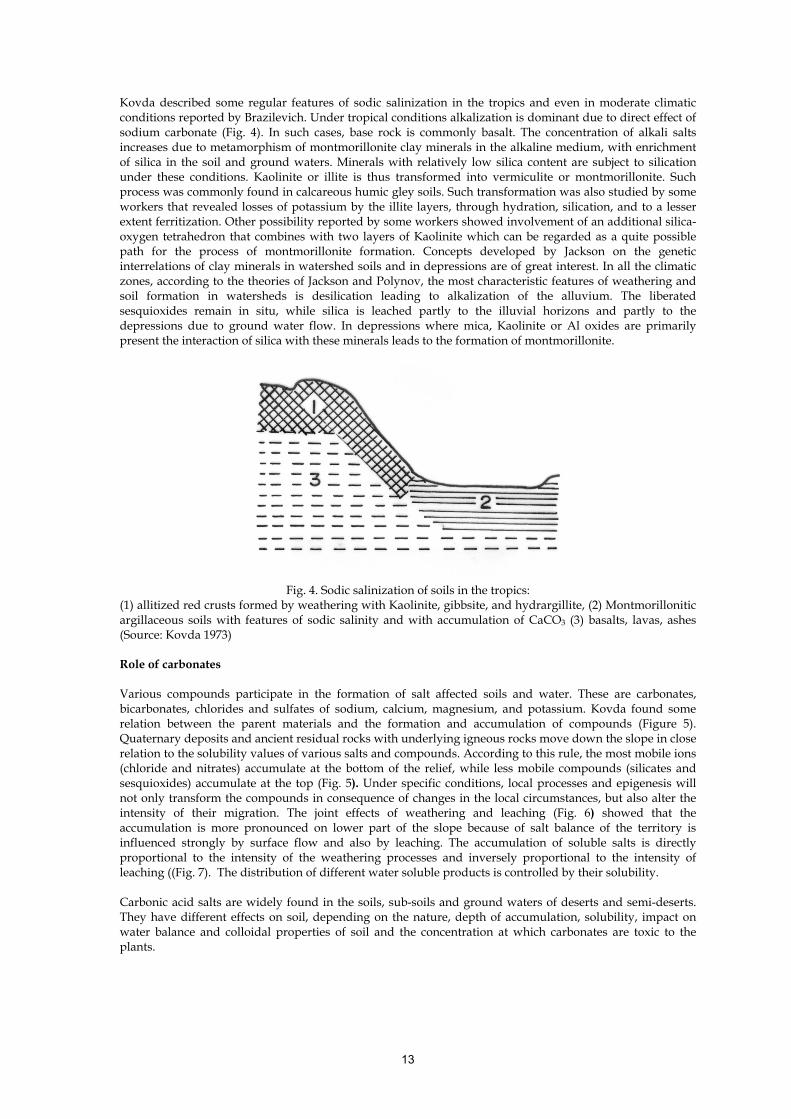
Kovda described some regular features of sodic salinization in the tropics and even in moderate climatic conditions reported by Brazilevich. Under tropical conditions alkalization is dominant due to direct effect of sodium carbonate (Fig. 4). In such cases, base rock is commonly basalt. The concentration of alkali salts increases due to metamorphism of montmorillonite clay minerals in the alkaline medium, with enrichment of silica in the soil and ground waters. Minerals with relatively low silica content are subject to silication under these conditions. Kaolinite or illite is thus transformed into vermiculite or montmorillonite. Such process was commonly found in calcareous humic gley soils. Such transformation was also studied by some workers that revealed losses of potassium by the illite layers, through hydration, silication, and to a lesser extent ferritization. Other possibility reported by some workers showed involvement of an additional silica-oxygen tetrahedron that combines with two layers of Kaolinite which can be regarded as a quite possible path for the process of montmorillonite formation. Concepts developed by Jackson on the genetic interrelations of clay minerals in watershed soils and in depressions are of great interest. In all the climatic zones, according to the theories of Jackson and Polynov, the most characteristic features of weathering and soil formation in watersheds is desilication leading to alkalization of the alluvium. The liberated sesquioxides remain in situ, while silica is leached partly to the illuvial horizons and partly to the depressions due to ground water flow. In depressions where mica, Kaolinite or Al oxides are primarily present the interaction of silica with these minerals leads to the formation of montmorillonite.

Fig. 4. Sodic salinization of soils in the tropics:

(1) allitized red crusts formed by weathering with Kaolinite, gibbsite, and hydrargillite, (2) Montmorillonitic argillaceous soils with features of sodic salinity and with accumulation of CaCO3 (3) basalts, lavas, ashes (Source: Kovda 1973) Role of carbonates Various compounds participate in the formation of salt affected soils and water. These are carbonates, bicarbonates, chlorides and sulfates of sodium, calcium, magnesium, and potassium. Kovda found some relation between the parent materials and the formation and accumulation of compounds (Figure 5). Quaternary deposits and ancient residual rocks with underlying igneous rocks move down the slope in close relation to the solubility values of various salts and compounds. According to this rule, the most mobile ions (chloride and nitrates) accumulate at the bottom of the relief, while less mobile compounds (silicates and sesquioxides) accumulate at the top (Fig. 5). Under specific conditions, local processes and epigenesis will not only transform the compounds in consequence of changes in the local circumstances, but also alter the intensity of their migration. The joint effects of weathering and leaching (Fig. 6) showed that the accumulation is more pronounced on lower part of the slope because of salt balance of the territory is influenced strongly by surface flow and also by leaching. The accumulation of soluble salts is directly proportional to the intensity of the weathering processes and inversely proportional to the intensity of leaching ((Fig. 7). The distribution of different water soluble products is controlled by their solubility. Carbonic acid salts are widely found in the soils, sub-soils and ground waters of deserts and semi-deserts. They have different effects on soil, depending on the nature, depth of accumulation, solubility, impact on water balance and colloidal properties of soil and the concentration at which carbonates are toxic to the plants.

14

Fig. 5. Distribution types of weathering products in saline depressions: (a) primary rock (b) calcareous eluvial rocks (c) siallitic rocks, (d) Allitic rocks,

(e) chlorite-sulfate sediments, (f) carbonates, (g) siallitic sediments (Source: Polynov 1956)

Fig. 6. Diagram of the differentiation of compounds during salt accumulation on continents

(Source: Kovda 1947)

Fig. 7. The joint action of weathering and leaching (Source: Perelman 1961)

15

Calcium carbonate The most common salt found as calcite and dolomite (calcium-magnesium carbonate). It has a very low solubility in water (9.8 ppm) in calcite and even lower for dolomite. Since the salt is formed from a weak acid and strong base, alkaline hydrolysis takes place in an aqueous medium, leading to the formation of Ca (OH)

2 and Ca (HCO2). A saturated aqueous solution of calcium carbonate has a pH of 8.3 to 8.4. The solubility depends on the CO2 concentration and pH of the solution. An increase in CO2 concentration leads to a decrease in soil pH, thus increasing the solubility of calcium carbonate. Due to low solubility the mobility of this compound is also low. It is frequently found in soil-forming rocks and soils. In the case of soils, its occurrence may be primary (the soil forming rock itself contains calcium carbonate) or secondary being formed during the soil-forming process. Among the rocks it is chiefly found in sedimentary origin. It is found in every climatic zones but it is characteristic of arid and semiarid regions where it is precipitated as micro-crystalline structure due to its low solubility and poor mobility. It is generally accumulated in the lower part of the B2 horizon in a sodic soil or transported in ground water along with if the soil texture and aridity conditions are favorable. Magnesium carbonate The mineral found in soil-forming rocks and soils in the form of magnetite (MgCO3) dolomitize calcite and dolomite. The solubility ranges from poor to moderate. In aqueous solution alkaline hydrolysis takes place and the aqueous solution has a pH of around 10. It is a component of sedimentary rocks and soils. The primary formation of magnesium carbonate stems from the chemical decomposition of crystalline rocks. As a decomposed product, it is transported by the solution from the decomposed rock into the sedimentary rock, where it accumulates. As a lattice forming element, magnesium plays an important role in clay formation, being bound to clays in a significant extent. Due to alkaline reaction, solution of magnesium carbonate is toxic to plants. Sodium carbonate Sodium carbonate can be formed in nature in numerous ways. It dissolves readily in water. The aqueous solution is subject to alkaline hydrolysis. The pH of the aqueous solution is alkaline (9 to 11) depending on the concentration of the solution. The Na+, CO32-, HCO32-, and OH- ions during dissolution are able to form ion pairs. Due to excellent solubility, it is mobile. Kovda found increase in the concentration of Na2CO3 in the solution when total salt concentration limits to 0.3 to 0.5 g/l while it decreases when the TSS increases beyond 5g/l. In ground water this decrease is associated with pronounced increase in CaSO4, indicating joint occurrence of NaHCO3, Na2CO3 and CaSO4 is rare in moderate or strongly mineralized soils. In nature, the formation of sodium carbonate is governed by the interaction of silicates and CO2-containg water. During this process, bicarbonates of Ca, Mg, Na and K are formed. Upon evaporation, Ca and Mg carbonates are precipitated, while NaHCO3 gradually loses CO2 and is transformed into Na2CO3. According to Hillgard, sodium carbonate may be formed by the action of NaCl, Na2SO4 on CaCO3: 2 NaCl + CaCO3 = Na2CO3 + CaCl2 Na2SO4 + CaCO3 = Na2CO3 + CaSO4 Gedroitz, Kelly and Sigmond associate sodium carbonate formation with the fine structure of soils, and with processes taking place in the colloid fraction according to the following equation: (adsorbing complex) - 2Na+ + H2CO3 = (adsorbing complex) – Ca2+ + Na2CO3 (adsorbing complex) - 2Na+ + CaCO3 = (adsorbing complex) – Ca2+ + Na2CO3 Sodium carbonate can be easily transformed in the presence of carbon dioxide under the conditions of intensive decomposition of organic matter and at low temperatures. Due to the formation of bicarbonates the alkalinity of the solution decreases. The transformation of carbonate to bicarbonate is a reversible process, and a decrease in CO2 concentration in the solution provokes the formation of carbonate from bicarbonate. This occurs when the activity of the microorganisms is weak and the organic matter content is low. A precondition for the formation of saline –sodic soils is that where soda is present in the water and/or in the deposit with high sodium carbonate and bicarbonate contents, the sodium carbonate should be able to accumulate in sufficient quantities. Another precondition, besides the presence of soda in the water and/or parent rock, is the absence of gypsum.

16

Sulfates and sulfides The sulfate compound in natural waters, sediments and soils are mainly weathering products of the minerals of volcanic and sedimentary rocks. Calcium sulfate occurs in the natural waters, sediments, and soils in all regions under different climatic conditions as a product of weathering of sulfide minerals, due to the reaction of sulfide ions with the calcium removed from calcium bearing minerals. Calcium sulfate also accumulates secondarily by the reaction of sodium sulfate and calcium chloride in sediments and soils. In semiarid and arid regions the sediments and rocks containing large quantities of calcium sulfate precipitated during the evaporation of saline lacustrine waters and ground waters. Calcium sulfate usually occur in soils as gypsum. Gypsum crystallizes in soils in a great variety of forms, from the transparent to large nodules, concretions, or regularly shaped slabs also. Gypsum sometimes forms a spongy porous mass in soils, causing cementation in the horizon of accumulation on the surface, or in the entire profile. Under the very dry climate of deserts the gypsum may be dehydrated and turn into a dry powdery mass of calcium sulfate hemi-hydrate. Magnesium sulfate which has a high solubility is mainly a product of weathering. It is a typical component of seawater, occurs in saline ground waters, in saline lakes and accumulates in the form of epsomite (MgSO4. 7H2O) in the saline soils of desert and semi-desert regions. It is never available in pure form, mostly associated with sodium sulfate, sodium chloride and magnesium chloride. Sodium sulfate is mainly a weathering product with high solubility and high mobility. High concentration of sodium sulfate may be present in saline ground waters, saline lakes, and sea water. It is of common occurrence in salt affected soils of desert and semi desert regions. At low temperatures, it precipitates as mirabilite (Na2SO4. 10H2O) which, with increase in temperature and a decrease in humidity, dehydrates and turns into white powdery thenardite (Na2SO4). Calcium sulfate may accumulate in soils in large quantities. It is slightly toxic to plants due to its low solubility. The compact layer of gypsum accumulation on the surface or the root zone of soils may be impenetrable by water, air, and plants roots, and may have an adverse effect on plants. The calcium ion of calcium sulfate reacts with sodium salts capable of alkaline hydrolysis and with the exchangeable sodium in the soil. If gypsum is present in the soil, it neutralizes the sodium salts capable of alkaline hydrolysis, forming poorly soluble salts with the anion of the weak base, while the cation forms salts dissociating with a neutral reaction. The calcium ion of calcium sulfate replaces exchangeable sodium according to the extent to which the sodium adsorption ratio decreases in the equilibrium solution. If the sulfate type of salinization occurs the leaching of sodium sulfate causes an increase in the solubility of calcium sulfate and this phenomenon promotes the ameliorative effects. Gypsum and other materials containing calcium sulfate are widely used for the reclamation of sodic and alkali soils. Silicates Silicon is the major element in the earth crust and in the soil materials plays a substantial role in all soil-forming processes, but mainly as the main constituent of soil minerals and lattice layers. However, the compounds of silicic acid play an important part in the formation of alkali soils. The main compound in this respect is sodium silicate, which accumulates in considerable amounts on the surface of alkali soils and in the upper layers of their profiles. The common features of these compounds is that they contain SiO4 tetrahedra in their crystal lattices, either isolated or linked through one or more of the oxygen atoms, forming groups, continuous chains, sheets, and three-dimensional structures. The availability of silicates depends on the pH of the solution. It is evident from the fig. 8 that there is a slight increase in the silicic acid concentration in aqueous solution if the pH value drops below 3.5. The increase in solubility is very sharp if the pH of the medium increases to over 9. The saturation concentration of silicic acid depends even more on the pH value in the case of a soil-solution system. The increase in H+ ion concentration of the solution i.e. the acidic reaction of the medium promotes the dissolution of metal-aluminum silicates through the desilification of rocks and minerals and the formation of orthosilicic acid: M-Al-silicate + a H+ + b H2O = M2+ + c HSiO4 + Al (silicate residue) The sharp increase in silicic acid concentration when the pH value is higher than 9 is due to the ionization of mono-silicic acid: Si(OH) 4 + OH- ----> Si(OH)3O- + H2O

17

Fig. 8. Solubility of Al and SiO2 at various pH values (Source: Szabolcs 1989)

Chlorides Calcium chloride is rarely present in soils. Magnesium chloride is more common in soils but it accumulates in large quantities where there is high salinity. It’s solubility is also high, and as a result, it has high toxicity. It is common in arid zone where because of their hygroscopic character, certain spots remain continually humid. Sodium chloride together with sodium and magnesium sulfate is the most common component of saline soils. It has high solubility and high toxicity. The leaching of saline soils containing both sodium chloride and calcium sulfate is very easy. But in the absence of calcium sulfate, the leaching of sodium chloride may cause the alkalization of the soil. Ion exchange in soils Soil colloids and ion exchange are of great importance in soil classification, soil utilization, and soil amelioration. The ion exchange phenomenon is a function of the chemistry of both the liquid and solid phases of the soil as well as of the original soil colloidal and mineralogical media in the soil. The term ion exchange indicates the reversible process cations and anions are exchanged between the solid and liquid phases, if these are in close contact with each other. Theoretically several approaches can be used to express the distribution of ions between solid and liquid phases at equilibrium. In practice, most of the theories lead to equations identical with the mass action relationship. (Aad) n (Am+ ) n -------- = KAB -------------- (Bad) m (B n+ ) m Where (Aad) and (Bad) = the activity of Am+ and B n+ ions on the adsorbent; (Am+) and (B n+) = the activity of the same ions in the intermicellar solute; and m and n = the valences of cations A and B, respectively. It is evident that the kind and quantity of ions adsorbed on the surface of soil particles depend on: the activity ratio of cations in the solution, the valences of the cations in case of non-symmetrical exchange, and the total concentration of the intermicellar solution. It has been proved in several experiments that the relative replacing power of cations depends on the valences of the adsorbed and counter ions. In the case of nonsymmetrical exchanges, the relative replacing power of the cations increases with the valence and follows the order M+ < M2+ < M3+. The greater the dilution of soil solution with cations of different valence, the greater the displacement of equilibrium in favor of higher valence. Increasing the ionic concentration of the intermicellar solution, the equilibrium shifts in favor of cations with lower valence. In asymmetrical exchange of sodium and calcium ions, the adsorption shifts in favor of the calcium ions as the ionic concentration of free solution decreases. The preference of Ca over Na is due to an increase in the difference between the concentrations of the micellar and intermicellar solutions and to an increase in the potential differences between the surface of the adsorbent and the free solution. The preference of sodium ion adsorption comes to the fore as the concentration of free electrolytes increases, the solution-adsorbent ratio increases, or the CEC of the adsorbent increases. The decisive role of the sodium ions in the soil solution is strengthened by the different abilities of cations to form ion-pairs. The different degree of ion-pair formation in the case of sodium, calcium, and magnesium ion, raises the SAR value in the soil solution. The increase in the SAR value due to ion-pair formation becomes more important as the ionic concentration of the soil solution increases and shifts the balance of exchangeable cations in favor of sodium. In carbonate-containing

18

system sodium ions dominate in the intermicellar solutions as a result of the poor solubility of calcium carbonate and the adsorbent has a high degree of sodium saturation even if the ionic concentration of the liquid phase is low. In these cases, the pH of the medium determines the solubility of calcium carbonate, and consequently has an effect on the cation-exchange equilibria of soil-solution systems. Investigation carried out in phase equilibrium systems showed that the influence of the pH value on soil colloidal systems not only manifests itself in changes in the solubility of poorly soluble salts but also affects the degree of dispersion, the cation exchange capacity and surface charge density of the adsorbent. The distribution quotient of 24-Na decreases as a rule with an increase in the concentration of the solution in the presence of chlorides and sulfates, but it increases and reaches a maximum value if sodium salts capable of alkaline hydrolysis are present in the free electrolyte solution (Fig. 9). Salts accumulate in soils in reverse sequence of their solubility, and as the total concentration increases, the ratio of sodium ions also increases. On the other hand, the ion exchange equilibrium shifts in favor of cations with two valences during leaching, and not only soluble sodium, but also exchangeable sodium is leached from the soil, which thus becomes non-saline and non-alkaline. This exchangeable sodium during desalinization is often counteracted by the increasing alkalinity of the soil solution. The increase in pH value involves the participation of calcium ions in the form of calcium carbonate, an increase in the degree of dispersion, and the redistribution of exchange sites on the surface of the adsorbent. The result of these changes is the formation of alkali soils with natric horizon.

Fig. 9. Dependence of bentonite Na-24 activity as a percentage of the total Na-24 activity on equilibrium concentration in bentonite-NaCl, Na2SO4 and Na2CO3 solution systems.

Horizontal axis: Na+ concentration of the equilibrium solution, meq/l. Vertical axis: S0 = total Na-24 activity, SL = activity of the equilibrium solution

(Source: Szabolcs 1989) Distribution of poor quality ground water in India The salt content of the ground water is dependent upon the source of water and geological formation or parent materials including rocks and minerals. The quality and development of ground water depends on several factors, such as net balance between annual evaporation, precipitation and runoff; rate of local rock weathering and solubilization; salt content transported in the region by streams, wind and rain; permeability and hydraulic gradient of the aquifer; the rate of ground water circulation and salt accumulation and inherent saline ground water (Fig. 10 and 11). In the arid and semiarid regions, due to low rainfall, insufficient leaching and high evaporation, salts in general accumulate in the soils and ground water particularly in the sandy tracts of Rajasthan, Indo-Gangetic plain, Peninsular and Coastal regions. In the sandy tract of Thar Desert, high evaporation, low rainfall, intense mineralization, intrusion of salt from the sea through drainage channels and intensive use for agriculture facilitated formation of salt enriched ground water dominated by chlorides, sulfates and carbonates. As a result about two third of western and part of eastern Rajasthan State is affected by saline ground water (8 dS/m) and is used for irrigation, drinking and other purposes such livestock. It has been reported that there were alternating humid and arid climates in the Thar desert of India. During such phase there was a well integrated river system in the Rajasthan desert that was responsible for vast alluvial deposits. It has been found that once upon a time the Vedic rivers Saraswati and Drishtavati used to flow through Rajasthan desert. They gradually shifted westward and ultimately flowed through Jaisalmer and Barmer districts. The Sutlej used to join the Saraswati near Jakhal, Sirsa and Hanumangarh. In arid climate, with intense desertification, precipitation becomes too little to keep

19

these drainage systems alive. Gradually the drainage system dried up, become disorganized and buried under sand (Ghosh, 1996). Geo-morphological studies have established that both types of saline lands- one formed by natural processes (for example, Rann of Kachchh or saline depressions or lakes) and the other caused through irrigation and agriculture have one common associated geomorphic feature that is paleo-drainage channels.

Fig. 10. Hydrolytic dissolution of sodium bearing minerals and sodiumisation of soils

(Source: Bhargava and Bhattacharjee 1982)

Fig. 11. Release of sodium from sodic/saline soils as a function of time

(Source: Bhargava and Bhattacharjee 1982)

In Punjab Bajwa et al. (1975) compiled the water quality information through extensive studies of 16527 water samples collected from wells and tube wells. The study reported that low to medium alkalinity existed in 47% of the water samples in the State. Out of that 19% water showed EC >4 dS/m and RSC > 5 me/l and are categorized as unsuitable for irrigation. The maximum values for RSC were as high as 30-35 me/l and are located in the arid and semiarid regions of north-west Punjab. The study also revealed that about 40% waters in the Bathinda, Sangrur and Ferozpur districts were high in EC and / or RSC. Similar situation existed in north-west (Amritsar), southern part of Ludhiana, Patiala, Sangrur and Faridkot districts. On the whole water containing sufficient bicarbonates were found about 25% of the Punjab state that pose serious problems for agriculture such as paddy and wheat. The hydrological studies revealed that southwest part of Punjab commonly developed from Quaternary alluvium consisting of sand silt and clay particles with occasional kankar and gravel layers. Such deposits form good repositories of ground water, though saline in

20

this area. Sand and silt with occasional gravel form potential aquifers. Waterlogging conditions exist in saline areas in Sangrur districts where depth to water is 10 m bgl. While the shallow aquifers are under unconfined state, the deeper aquifers occur under semi-confined conditions. The ground water mineralization is low in the northern and the north western parts while is high in the south and southwestern part of the state. The salinity of the water increases in the south-west direction with decrease in the rainfall isohyets suggesting ground water picks up salts as it passes from recharge to discharge or transport zones. Haryana state is an extensive closed basin with mainly inland drainage conditions caused by location between Siwalik hill in the northeast and the Thar Desert in the south west. The climate is arid to semiarid and sub-humid in southwest to northeast. About 48.5% of water is brackish and saline. Manchanda (1976) compiled the chemical analysis of 13725 water samples collected from 2276 wells and tube wells. The study revealed that 11% is marginally saline (D, 4-8 dS/m, SAR <10, nil RSC), 19% sodic (B, <4 dS/m, SAR <10, >2.5 RSC) and 26% saline-sodic (E, <4 dS/m, SAR >10 and >2.5 RSC). The hydrological information revealed that most of the poor quality water lies in the quaternary alluvium with high aridity and occasional kankar and gravel layers. The alluvial deposits are good aquifers though the formation of water in these areas is saline. The shallow aquifer down to a depth of 50 m is in unconfined state, while the deeper aquifers are confined and leaky. In Uttar Pradesh 65% of the area receives irrigation with ground waters. About 14 districts fall under semiarid zone while rest id under sub-humid zone. Dixit (1971) reported about 50% of the water of Agra, Aligarh, Etah , Mainpuri and Mathura districts have salinity < 3 dS/m and RSC >2.5 me/l. About 10% of the water in these areas are SAR >10.

21

Origin of Salinity - Sodicity in Soils and Underground Water of Indus Plains of the Indian Sub-continent Raj Kumar, S. K. Ghabru, N.T. Singh and R.L. Ahuja Punjab Agricultural University, Ludhiana-141 004 (Punjab), India Salt affected soils constitute a global problem as they occur practically everywhere on the globe covering about 10 per cent of the total surface of dry lands and no continent is free from this problem (Szabolcs, 1989). Salinization of land resources is a major impediment to their optimal utilization in many arid and semi-arid regions of the world including India. Growing need to produce more food and fiber for the expanding population necessitates the increased use of salt-affected land resources in the near future (Qadir et al. 2001a and 2001b). Soil salinization arises due to the build up of soluble salts at or near the soil surface. Salts accumulate by primary and secondary processes that alter the physical and chemical properties of soils and may lead to direct and indirect soil degradation. Soil salinization is one of the major causes of declining agricultural productivity in many arid and semiarid regions of the world. Soluble salts produce harmful effects to plants by increasing the salt content of the soil solution and by increasing the degree of saturation of exchange materials in soil with exchangeable sodium (Richards 1954). The former effect in measured in term of electrical conductivity (EC) whereas, later is estimated as exchangeable sodium percent (ESP). Sodic soils are characterized by the occurrence of excess sodium (Na+) to levels that can adversely affect soil structure and disturb availability of some nutrients to plants. There are large areas of the world that exist under sodic soils and need attention for efficient, inexpensive and environmentally feasible amelioration. In India a major part of the Indus and Ganges plains, where more than 75 per cent of sodic soils occur (Mehta, 1983) is occupied by undeveloped (Entisols) and slightly developed soils (Inceptisols). These plains also represent 81 per cent of the total area occupied by underground saline water in India (CGWB, 1997) Soils in these plains have developed on alluvium deposited in the basin between the peninsular region and the extra-peninsular region (Himalayan region). Sodic soils of Indo-Gangetic plains have been reported to derive their sodicity due to in-situ weathering of alkali alumino-silicates (Bhargava et al. 1981). Sodium feldspars have also been advocated as the diffused source of sodium (Gupta and Gupta, 1989). Kovda (1964) proposed a similar mechanism earlier for European soils, who advocated the formation of sodic soils from basaltic and volcanic parent materials. However, owing to near absence of such parent materials in the catchments of saline and sodic soils of the northern parts of the Indian sub-continent, the exact mechanism of their formation is still obscure. Methodology This investigation divulges on the genesis of soil sodicity in the Indus plains through a comprehensive analytical approach encompassing ground truth, detailed soil analyses, x-ray diffraction studies on coarse and fine fractions of soils, weathering sequence studies of primary and secondary minerals in sodic environment, study of the make up of different geological formations in the catchments area and interpretation of remote sensing data in the context of Himalayan Orogeny. Investigations included intensive consultation of literature available about Salt Range in north-east of Pakistan, Siwalik Range in Himalayas and Indus Plains of north-west India, and Tibet Plateau in China. Earlier, these areas have remained subjected to repeated tectonic movements and orogenic upheavals. Forty-four pedons were studied to represent wide variations in the geomorphology, rainfall and temperature in the Indus plains of the Indian Sub-continent. However, to maintain brevity, data for only four typifying pedons are discussed in detail. Representative soil samples from the selected horizons were used for mineralogical analysis. The samples were analyzed for important physical and chemical characteristics and were classified based on Soil Taxonomy (Soil Survey staff, 1999). The air dried soil samples (<2 mm) were used to achieve dispersion of soils after removal of soluble salts, organic matter and free iron oxides using the recommended procedure of Jackson (1975). Clay fractions were quantitatively separated by sedimentation. The sand (2.00-0.05mm) and silt (0.05-0.002mm) fractions were separated by sedimentation after removing organic matter, soluble salts, carbonates and oxides of iron and aluminum as recommended by Jackson (1975). However, as far as removal of carbonates is concerned, after addition of NaOAc-buffer soil was kept for overnight only. This soil suspension was not digested in a near boiling water bath for 30 minutes as recommended by Jackson (1975). So there could be some residual carbonate in some cases. Random powder X-ray diffraction (XRD) patterns were obtained from samples packed in an aluminum sample holder. Since HCl- treatment was not given to sand and silt fractions, absence of kaolinite could not be confirmed; values are expressed as chlorite + kaolinite. The XRD patterns were obtained using Philips PW 1050 diffractometer with Ni-filtered Cu K α radiation. Semi-quantitative estimates were prepared based on relative peak area ratio after necessary corrections for background

22

following the procedures of Gjems (1967) and Ghosh and Datta (1972). Saturation extract from the soil samples of the salt rich lower horizons was subjected to slow evaporation under room temperature. Dry salts so obtained were analysed using X’Pert PRO X-ray diffracton system . Various peaks in the he diffractograms were identified with the help of X’Pert High Score Plus software. Various elements in the salt were analysed using ICAP. Clay samples used for X-ray diffraction analysis were saturated with Mg as well as K separately as per the ion saturation procedure of Jackson (1975). X-ray diffraction pattern of basally oriented clay specimens on glass slides were obtained after Mg-saturation, glycolation, K-saturation and heat treatments. To differentiate between kaolinite and chlorite clay samples were boiled with 4N HCl for half an hour. X-ray diffraction pattern were obtained using Philips PW 1050/25 vertical goniometer with Ni-filtered Cu K α

radiation. Semi-quantitative estimates were prepared from the relative peak area ratio after necessary corrections for back ground (Gjems, 1976 and Ghosh and Datta, 1972). Simplified equilibrium equations for various alumino-silicate minerals were developed by employing the thermodynamic model for predicting the weathering and stability of minerals as given by Rai and Lindsay (1975) by utilizing the Gibb’s standard free energy of formation (∆ Go). Occurrence of salt affected soils in different landforms Forty four pedons occurring in 245 km long transect having six different physiographic units: Siwalik Hills, upper piedmont, lower piedmont, upper alluvial plain, lower alluvial plain and alluvial plains with reworked sand dunes were studied (Table 1). Sodic soils have been found to occur from hills and piedmont plains having udic to ustic moisture regimes with rainfall varying between 1000 mm and 1125 mm (Ramgarh and Lalru pedons), to upland areas of alluvial plains with less than 450 mm rainfall having ustic to aridic moisture regimes (Bathinda-Burj Mehima and Sirsa pedons) (Figs. 1 to 3). Table 1. Location and site characteristics of pedons

Site characteristics Pedon 1 Pedon II Pedon III Pedon IV Local name Ramgarh

(Haryana) Lalru (Punjab)

Burj Mehima (Bathinda-Punjab)

Sirsa (Haryana)

Location 76o52’53” E 30o38’11” N Panchkula to Yamuna Nagar Road, 4 km to Panchkula near Chandigarh

76o49’22” E 30o21’16” N Village Lalru, on Ambala to Chandigarh Road

74o49’09” E 30o16’13” N 20 km to Village Lohara on Bathinda to Muktsar road

74o54’1” E 29o26’11” N Village Madhosingh Wala, Sirsa to Elnabad road

Physiography Siwalik Hills Piedmont plain Alluvial plain Alluvial plain

Topography Hills with 30% slope

Gently sloping level, 3-5% slope

Level to gently sloping 1-3%

With occasional sand dunes, level to gently sloping, 1-3% slope

Drainage Excessively drained Moderately well drained

Moderately well drained

Moderately well drained

Land use Scruby forest Cultivated Uncultivated Cultivated Elevation 380 m 225 m 205 m 198 m Rainfall 1100 mm 1050 mm 450 mm 410 mm Soil moisture regime

Udic-Ustic Ustic Ustic – Aridic Aridic

Soil Taxonomy Fine loamy, mixed, hyperthermic, Typic Ustorthent

Coarse loamy mixed hyperthermic Typic Ustifluvent

Coarse loamy, mixed hyperthermic Typic Haplustept

Coarse loamy, mixed hyperthermic, Typic Haplustept

In these areas slope varies from 30% in Siwalik Hills to nearly level in the alluvial plains. Drainage class varies from excessively drained to moderately well drained. Macro-morphology studies in the field indicated that sodic soils have number of lithological discontinuities. These also occur sometimes below the normal soils indicating different cycles of parent material deposition. Surface colour of these soils varies

23

from reddish brown in Siwalik Hills to yellowish brown in alluvial plains. These soils are conspicuous by the presence of silt loam as the dominant soil texture in most of the sub surface horizons. The pH2 of soil: water (1:2) varies from 8.4 to 10.7. The electrical conductivity (EC2) varies between 0.73 to 22.0 dS/m. The organic carbon content of epipedon is always higher than the underlying horizons. Almost all horizons of the soils are calcareous. Distribution CaCO3 is erratic with depth. In general, the soil horizons that have high pH also have high silt content. The pH of saturation paste (pHs) varied from 8.4 to 10.5. Saturation paste pHs is somewhat lower than that of the 1:2 soil: water extract. Electrical conductivity of the saturation extract (ECe) varied between 1.08 and 214.01 dS/m. Na+ followed by Ca++ + Mg++ and K+ generally dominates exchange complex of these soils.

Cation exchange capacity (CEC) of these soils as determined by Belyayeva (1967) procedure for calcareous and salt affected soils, varied from 4.9 to 23.6 c mol/ kg. Exchangeable sodium percent (ESP) of these soils varied between 14 and 90 (Table 2). Comparison of texture, pH, EC and exchangeable sodium percentage (ESP) on different physiographies indicated that present geomorphology, local topography and rainfall do not seem to have significant influence on the development of sodicity in these areas (Raj Kumar et al. 1994 a ,b and Raj Kumar 1998). All the sodic soils were calcareous and invariably have higher silt content. Another significant observation is the dominance of Na+ and Cl- ions in the saturation extract of sodic horizons of soils located in the Siwalik Hills.

Correlation of ground truth and small scale remote sensing data of northern plains indicated the occurrence of salt affected soils mainly along the river courses and in palaeochannels of the rivers. These observations provide reasons for fresh thinking on the origin of salt impregnated soils of these plains. Table 2. Characteristics of pedons

Depth (cm)

Horizon pHs

ECe (dS/m)

Satur-ation (%)

CEC (cmol/kg)

Exchangeable cations (cmol/kg)

ESP

Na+ K+ Ca+++Mg++ Pedon I (Ramgarh) 0-10 A1 8.6 1.08 43 18.9 4.5 0.21 14.2 24

10-46 C1 8.4 1.12 46 23.6 3.3 0.35 20.0 14 46-100 C2 8.5 1.43 46 18.5 3.8 0.25 14.0 20 Pedon II (Lalru) 0-5 Ap 9.2 3.92 22 4.9 2.6 0.49 1.8 54 5-10 A3 10.2 13.69 48 7.8 6.0 0.25 1.5 77 10-25 IIC1Ca 10.4 20.63 47 14.6 12.4 0.30 1.9 85 25-39 IIC2 10.4 21.90 43 14.7 12.7 0.35 1.6 87 39-97 IIIC3Ca 10.2 19.40 46 13.8 12.0 0.37 1.4 87 97-108 III C4 10.3 10.48 41 12.9 11.0 0.38 1.5 85 108-120 III C5 9.9 1.81 39 9.5 7.0 0.21 2.3 73 Pedon III (Bathinda- Burj Mehima) 0-10 A1 8.6 13.39 22 5.8 2.4 0.41 3.0 42 10-67 AB 8.4 15.27 29 7.1 2.9 0.22 4.0 41 67-89 B1 9.0 38.32 35 6.8 3.4 0.31 3.1 50 89-126 BC 10.4 48.40 36 7.1 5.4 0.38 1.3 77 126-147 IIC11Ca 10.5 193.80 46 14.3 11.5 0.33 2.5 81 147-170 IIC12Ca 10.5 168.01 44 14.7 13.1 0.29 1.3 89 170-210 IIC13Ca 10.6 214.01 43 19.5 17.5 0.27 1.7 90 Pedon IV (Sirsa)

0-15 Ap 8.5 4.9 40 8.3 2.6 0.21 5.5 31 15-57 B1 8.6 8.3 41 10.4 3.3 0.15 7.0 32 57-85 B21 8.8 8.9 41 9.0 4.0 0.12 4.9 44 85-155 B22 8.9 9.5 37 9.9 4.5 0.14 5.2 46

24

Mineral assemblage and geochemistry Random powder X-ray diffraction (XRD) patterns were obtained for the sand (2-0.05 mm) and silt (0.05-0.002 mm) separates of the soils from selected horizons of the pedons. The coarse fraction of the horizons representing normal as well as sodic soils were dominated by quartz followed by plagioclase, mica, orthoclase chlorite, kaolinite, calcite amphiboles and mixed layer minerals. Fine fraction (<0.002 mm) mineralogy of these soils was dominated by illite followed by smectite, mixed layer minerals, chlorite, kaolinite and vermiculite (Table 3). A similar mineral assemblage of coarse and fine fraction of these sodic as well as adjoining normal soils (non-sodic) has been reported earlier (Raj-Kumar et al. 1993a, 1993b, 1995). Transformation of illite to vermiculite appears to have occurred before transportation in the geological stage itself. The excessively drained steeply sloping geological formations contributing to the alluvium contained as much as 43 per cent smectite. Smectite as well as kaolinite have been inherited as constituent of alluvium. The geological formations contributing to the alluvium contained as much as 43 per cent smectite. The occurrence, weathering and transformation of clay minerals in these soils should be interpreted only in the light of mineralogical composition of the geological formations believed to be the source of this alluvium. Smectite present in these clays is not the result of any pedogenic activity but instead belongs to much older formations in the geological history. These depositions must have occurred under marine environment of Tethys basin in the Eocene period (Raj-Kumar, 1998). Evidence of soil degradation impeding soil tillage and irrigation in cultivated soils in Pakistan is identified, described and represented in a general process of degradation. Based on a chemical analysis of soil characteristics, it is shown that a more general geochemical degradation process may occur in these soils. Two paths of salinization, i.e. neutral salinization and alkalization inducing a process of sodification, are identified (Condom et al, 1999) Weathering of alumino-silcate minerals The weathering of soil minerals is mostly looked in terms of the chemical composition of the minerals involved. The composition of soil solution is generally considered in qualitative terms. Very low solubility and slow rates of dissolution and precipitation of common soil minerals under most conditions require the study of equilibrium reactions of soil minerals with soil solutions as described by thermodynamics (Kittrick, 1971). The pHs and cation composition of ambient soil solution control the solubility/weathering or stability of common alumino-silicates. Weathering of alumino-silicates releases various ions into solution. Equilibrium reactions between soil minerals and ambient soil solution control the stability or weatherability of the alumino-silicates (Table 4).

25

Table 3. Semi-quantitative estimates of clay size minerals

Table 4. Equilibrium reactions used to construct the stability diagrams for alumino-silicates

Reaction no.

Mineral Chemical reactions* log Ko

Primary alumino-silicate minerals 1. Low albite NaAl Si3O8 + 4H+ +4H2O = Na+ + Al3+ + 3H4SiOo4 2.74 2. Microcline KAl Si3O8 + 4H+ + 4H2O = K+ + Al3+ + 3 H4SiO04 1.00 3. Muscovite KAl2(AlSi3O10)(OH)2 + 10H+ = K+ + 3Al3+ + 3 H4SiO04 13.44 Secondary alumino-silicate minerals 4. Kaolinite Al2Si2O5(OH)4 + 6 H+ = 2 Al3+ + 2 H4SiO04 5.45 7. Illite K0.6Mg0.25Al2.3Si3.5O10(OH)2 + 8H+ + 2H2O =0.6K+ + 0.25Mg++

+2.3Al3+ + 3.5 H4SiO04 10.35

8. Montmorill-onite

Mg0.2(Si3.81Al1.71Fe(III)0.22 Mg0.29)O10(OH)2 + 6.76H+ + 3.24H2O = 0.22Fe3+ + 0.49Mg++ +1.71Al3+ + 3.81 H4SiO04

2.68

9. Chlorite Mg5Al2Si3O10(OH)8 + 16H+ = 5 Mg+++ 2Al3+ + 3H4SiO04 + 6H2O

60.30

10. Vermiculite (Mg2.71Fe(II)0.02Fe(III)0.46Ca0.06K0.1)Si2.91Al1.14O10(OH)2 + 10.36 H+ = 2.71 Mg++ 0.02Fe++ + 0.46Fe+++ + 0.06Ca++ 0.1K+ + 1.14Al3+ + 2.91 H4SiO04 + 0.36 H2O

38.14

Elementary thermodynamics has been used to understand the stability of those primary and secondary minerals whose presence was confirmed by the x-ray diffraction analysis. Minerals that maintain lowest Al3+ activity at a given H4SiOo4 activity are most stable. Al3+ activity as maintained in all the studied pedons at their constituent cation activity level and H4SiO4 activity of 10-4 M has been plotted against the respective pH of soil solution (pHS ). These stability diagrams clearly indicate that the Al3+ activities of primary (Fig. 4) as well as secondary alumino-silicates minerals (Fig. 5) decreases considerably with increase in pHS. Thus, the stability of most primary and secondary minerals increases with increase in pHS. Beyond pHS 8.5, Al (OH)2+ species dominate instead of Al3+. Under such circumstances Al3+ activity decreases by 5.02 per unit increase in pHs. The results of this investigation corroborate well with the earlier observations of Rai and Lindsay (1975), Lindsay (1979), Rai, and Kittrick (1989).

Depth Smectite Chlorite Vermiculite Illite Mixed layer

Kaolinite Quartz Others

Pedon I (Ramgarh) 0-10 40 7 - 36 5 8 1 3 10-46 41 8 - 45 6 6 2 2 46-100 43 8 - 34 5 7 1 2 Pedon II (Lalru) 0-5 5 4 7 68 8 7 - 1 10-25 11 8 10 56 7 5 1 2 97-108 18 11 12 44 6 5 1 3 Pedon III (Bathinda- Burj Mehima) 0-10 4 10 3 66 8 7 1 1 67-89 9 10 4 57 9 8 1 2 170-210 15 11 4 52 7 8 1 2 Pedon IV (Sirsa) 0-15 15 12 5 52 9 4 1 2 57-85 18 11 7 50 7 4 1 2

26

Fig. 4. The activity of Al3+ maintained by primary minerals as affected by pHs

Fig. 5. The activity of Al3+ maintained by secondary minerals as affected by pHs Na feldspar (albite): Soils of the Indus and Gange plains have considerable amounts of plagioclases. These are mostly alkali-calcic and/or alkalic plagioclases type. Alkali plagioclases are known to be more stable than calcic and/or calcic-alkalic plagioclases (Rai and Kittrick, 1989). Na feldspar (albite) an alkali plagioclase is mostly present in the coarse fraction of the soils. Na2O content of sand fraction (representing mostly alkali feldspars-albite) was found to be poorly related (r = 0.16) to the pH of saturation paste (pHs). Na2O content of both sodic and normal pedons was almost identical (2.0 to 2.1 per cent) under pHs range from 7.5 to 9.8 indicating uniformity in the parent material (Raj-Kumar et al. 1995). An investigation on understanding the role of gypsum in reclamation of sodic soils indicated that soluble Na content decreased from 4.50 g kg-1 to 0.79 g/kg, whereas insoluble Na content remained unchanged even after twenty years of reclamation (Table 5). These results clearly establish the uniformity of parent material of alkali and adjoining normal soils and do not establish any linkage between sodicity and alkali feldspars. Thus, the chances of alkali feldspars acting as diffused source of Na seemed doubtful.

27

Table 5. Effect of reclamation with gypsum on water soluble and insoluble sodium in the epipedon of Ghabdan series in Sangrur district of Punjab

Treatment Reclamation period (years)

pHs Water soluble Na (g/kg)

Na content in the soil separates (g/kg) Sand Silt Clay Soil

Unreclaimed sodic soil

- 10.1 4.5 11.2 13.6 7.2 11.7

Reclaimed sodic soil

5 9.0 1.1 11.2 14.4 5.6 12.0

Reclaimed sodic soil

10 9.1 0.9 12.0 15.2 3.6 12.2

Reclaimed sodic soil

20 8.2 0.8 12.0 12.8 6.4 11.6

The primary minerals (albite, microcline and muscovite) as well as secondary minerals (kaolinite, illite, montmorillonite, chlorite and vermiculite) have been found to be highly stable in these sodic soils (Fig. 4 & 5). Earlier reports suggesting weathering of alumino-silicates in high pH environment and low stability of albite in sodic soils do not support our results as well as those of Lindsay (1979) and Rai and Kittrick (1989). Had the hypothesis behind these reports (Na- feldspars are less stable in high pH environment) been operating, the prevailing climate would not have permitted the presence of normal soils in Indus and Ganges plains. Further, the silicate mineral weathering as source of sodium cannot explain the appreciable presence of Cl- ions in these soils. It is quite possible that certain highly water soluble minerals like halite (NaCl), trona [Na3H(CO3)2.2H2O], thenardite (Na2SO4), mirabilite etc, which are, generally not detected by conventional X-ray diffraction procedure for clays, might have contributed salts to these alluvia. Some of these minerals have been detected in the geological formations (Shali-formation) in the Himachal Pradesh Himalayas. Efflorescent crusts consisting predominantly of the sodium carbonate minerals trona (Na2CO3 ● NaHCO3●2H2O) with minor thermonatrite (Na2CO3●H2O) are commonly developed on less vegetated portions of the Indo-Gangetic Plains of the state of Uttar Pradesh in India. Being highly soluble, the presence of trona alone explains the high alkalinity (pH 10.5) of the soils (Saugata Datta et al., 2002). Salt impregnated strata in Indus alluvium A recent investigation on the soils of village Burj Mehima in Bathinda district in south west of Punjab (Pedon IV) indicated the presence of highly sodic soils below the normal soils (Fig 3). Salts extracted from the lower horizons having high pH and high electrical conductivity contained high contents of chloride followed by potassium, sodium, sulphur, nitrates, boron, molybdenum, arsenic and many other elements (Table 6). NO3-N concentration ranging between nil to 48.2 mg/L have been found in the underground water of District Firozpur in the south-west of Punjab (India) adjoining Pakistan (Balwinder Singh, 2008). NO3-N concentration was positively correlated with electrical conductivity, Cl-, Ca++, Mg++, Na+ , and K+. There existed no relationship between NO3-N concentration and fertilizer application in this area. Such a high concentration of salts in the underground water may be due to contributions from the salt impregnated layers below these soils. Such results again points towards the geogenic origin of these salts. Table 6. Elemental composition of salt extracted from lower horizons of village Burj Mehima in Bathinda

district of Punjab (µg/g)

NH4-N NO3-N P K Ca Mg S 118 4972 29.5 99932 154 7271 16142

Fe Mn Cu Zn Mo B Cl 0.71 0.35 0.45 0.03 15.0 41.9 128325 Na Al As Cd Co Cr Ni Pb 22181 1.61 5.87 0.10 0.91 0.54 1.06 1.12 Soluble minerals in the saline strata: X-ray diffraction a non-destructive analysis technique is used to identify unknown minerals by comparing diffraction peaks with reference database maintained by Inorganic Crystal Structure Database (ICSD) or International Center for Diffraction Data (ICDD). In this investigation, the standard base fill method was used to prepare the slides for scanning. The samples were scanned for about 6 hours each (step size: 0.022, step time: 8.0 seconds) from 5.0° to 65° two theta, using XPERT-PRO MPD diffraction system with a generator settings of 40 mA and 45 kV. The scan results were analysed using XPERT-PLUS software backed by ICSD database. Identification of various elements was further confirmed by using energy dispersive X-ray fluorescence spectrometer (EDXRF: Minipal-2).

28

The diffractogram of salts extracted from saline strata, exhibit large number of sharp peaks confirming the presence of many soluble minerals. Among these four soluble minerals contain nitrate, nitrite and ammonium nitrogen. The most important being niter (KNO3) and potassium nitrate (KNO2). The Halite (NaCl) is the second dominant mineral followed by anhydride (CaSO4). Three minerals in these salts comprises of compounds of lithium, Boron, Erbium and Magnesium (Diomignite, Lithium Erbium Oxide – Beta, Boracite low) . Five soluble minerals indicate the presence of Fluoride, Uranium and Lanthanum salts (Potassium Calcium Hydride Fluoride, Lanthanum Calcium Manganese Oxide Fluoride, Arrojadite, Uranium (V) Fluoride, Calcium Uranate). Presence of Selenium, Uranium and Nickel has been confirmed by the presence of small peaks of Potassium Selenide (K3Se3), Maekinenite (Ni Se) and Disodium bis (selenato (VI)), Dioxouranate tetrahydrate (H8 Na2 O14 Se2 U). Soluble compounds of Chromium, Erbium, Prasemodium and Mercury have also been identified (Chromium (IV) fluoride – beta, Chromium dierbium tetrasulfide, Praseodymium nickel oxide – Lt, Mercury phosphate). Identification of Rappoldite, Potassium tetracopper (II) triasenate, Johillerite and Tetra zinc arsenate in the salts confirm the presence of soluble minerals of Arsenic, Lead and Zinc. Besides these, soluble minerals of phosphate and calcium have also been identified. X-ray diffraction study conclusively demonstrates that the salt extracted from the saline strata (locally known as Saltpeter/Nitre/Shora), is the source of soluble minerals having at least twenty seven elements viz: hydrogen, lithium, boron, nitrogen, oxygen, fluorine, sodium, magnesium, phosphorus, sulphur, chlorine, potassium, calcium, chromium, manganese, nickel, copper, zinc, arsenic, selenium, molybdenum, mercury, lead, lanthanum, praseodymium, erbium and uranium (Table 7). These minerals could not be identified earlier is basically due to two facts: firstly, soluble minerals are normally washed out during sample preparation for the routine x-ray diffraction analysis; secondly, availability of advanced version of X-ray diffraction machine (X’Pert Pro MPD) with facility for precision step scanning and matching identification softwares. Uranium and other rare earth elements in the saline strata: As group, rare earth elements constitute the fifteenth most abundant component of the earth’s crust; thus they are not uncommon at all (Reiners 2001, Brown et al., 1990, Topp 1965, Fachschaft Chemie 2005, Richter and Schermanz 2006). Under natural conditions, lanthanides exist as oxides, silicates, carbonates, phosphates and halogen compounds in minerals. Considerably elevated mean concentrations of U, V and Mo have been reported in agricultural drainage and evaporation ponds of the San Joaquin Valley (California-USA) compared to saline waters of Salton Sea and Mono Lake. Relatively high correlation coefficients were observed between U, Mo and salinity (Bradford, 1990). Average abundance of Pr and Er- rare earth elements in the earth’s crust is 5.5 and 2.5 mg/kg respectively (Evans 1983). Considerably elevated mean concentrations of U, V and Mo have been reported in agricultural drainage and evaporation ponds of the San Joaquin Valley (California-USA) compared to saline waters of Salton Sea and Mono Lake. Rare earth elements are mined from a great variety of ores, principally bastnasite and monazite (Zhang, 1995). Monazite grains from Greater Himalayan Sequence gneisses, Langtang valley, Nepal, have been chemically mapped and then dated in situ via Th–Pb ion-microprobe analysis (Kohn, 2005). Occurrence of U–Th-rich zircon and monazite minerals have been reported in the granitoids of Indus and Shyok suture zone from Ladakh Himalaya (Anonymous, 2007). When the geological formations of the Himalayas show the abundance of minerals containing rare earth elements, their occurrence in small amounts in the salt impregnated strata below the alluvium of the north India is not unanticipated. Nevertheless, the concentration of these poisonous elements may not be very high in the soil, water or the air. High concentrations of arsenic in the oxidizing (aerobic) aquifers with high groundwater pH values (>8) typically in the arid or semi-arid environments are commonly associated with high concentrations of other anion- and oxyanion- forming elements such as fluoride, boron, uranium, vanadium, and selenium (BGS, 2009). However, once these elements are in the food chain, their concentration is bound to accumulate over the years in the body of ultimate consumer i.e. human beings. Origin of salinity-sodicity in soils and underground water Geologically the Indian subcontinent is divided into two parts, viz. Peninsula (south of Vindhyans) and extra-Peninsula (mountainous region of Himalayas). On the contrary, the extra-Peninsula, consisting the mountainous region of Himalayas and the northern states of India, remained under the saline water of the sea for greater part of the earth history and has thus been covered by successive marine deposits (Wadia, 1979). Because of convergence of Indian and Asian plates, a number of lakes have formed on either side of Indus Suture Zone. These lakes are either brackish or freshwater (Philip, 2008).

29

Table 7. Soluble minerals identified in the salt extracted from the saline strata

No. Compound Name Chemical Formula Nitate, Nitrite, Ammonia 1 Niter K NO3 2 Potassium Nitrate(III) K NO2 3 Sodium Nitrate(III) Na NO2 4 Diamminecopper Nitrate(V) {Cu (N H3)2}(N O3)2 Chloride 5 Halite NaCl Sulphur, Molybdenum, Calcium 6 Anhydrite Ca SO4 7 Molybdenum disulfide (Molybdenite) MoS2 Lithium, Boron, Erbium, Magnesium 8 Diomignite Li2 (B4O7) 9 Lithium Erbium Oxide - Beta Er Li O2 10 Boracite low Mg3 B7 O13 Cl Fluoride, Uranium, Lanthanum 11 Potassium Calcium Hydride Fluoride

(1/1/1.76/1.24) H 1.764 Ca F 1.236 K

12 Lanthanum Calcium Manganese Oxide Fluoride (0.6/0.4/1/2.78/0.18)

Ca 0.4 F 0.175 La 0.6 Mn O 2.775

13 Arrojadite K Na4 Ca Mn++4 Fe++10 Al (PO4)12 (OH,F)2 14 Uranium(V) Fluoride – Alpha U F5 15 Calcium Uranate Ca U O4 Selenium, Uranium, Nickel 16 Disodium Bis(selenato (VI))dioxouranate

Tetrahydrate H8 Na2 O14 Se2 U1

17 Potassium Selenide (5/3) K5 Se3 18 Maekinenite Ni Se Chromium, Erbium, Praseodymium, Mercury 19 Chromium(IV) Fluoride - Beta Cr F4 20 Chromium Dierbium Tetrasulfide Cr Er2 S4 21 Praseodymium Nickel Oxide - Lt Pr2 Ni O4 22 Mercury Phosphate Hg3 (PO)4 Arsenic, Lead, Zinc 23 Rappoldite As2 Co Ni 0.64 H4O10 Pb Zn0.36 24 Potassium Tetracopper(II) Tris(arsenate) KCu4 As3 O12 25 Johillerite Na0.77 K0.03 Mg2.18 Zn0.13 Cu1.55 Fe3+0.26 Al0.06 As2.96 P0.04 O12 26 Tetrazink Bis(arsenate(V)) Oxide - Lt As2 O9 Zn4 Phosphorus, Calcium 27 Calcium Bis(dihydrogenphosphate(I)) CaH4O8P2 28 Potassium Cyclo-hexaphosphate(III)

Octahydrate H16 K6 O20 P6

29 Epidote Ca2Al2(Fe3+;Al)(SiO4)(Si2O7)O(OH) 30 Scolecite CaAl2Si3O10·3H2O 31 Alinite Al2 Ca 19.2 Cl2 Mg2.8 O36 Si6 During the Permo-carboniferrous period, this sea called the Tethys Sea covered the present site of the Himalayas, the Salt Range, the Balochistan, and the Sindh, and an arm of the sea stretched into Narmada Valley. It is equally hard to determine whether the alluvia were deposited under marine or fresh water conditions. It is however, possible that thick marine sediments raised during Orogenic episodes were part of the alluvium that later descended into foredeep (Raj-Kumar, 1992 and 1999; Singh, 2005). In between the extra-Peninsula and Peninsula lie the great alluvial plains of the Indus and Ganges river system. In fact, these plains are formed mainly from alluvial deposits of the Indus and Ganges rivers borne down from extra-Peninsula, which has earlier remained under saline water of the Tethys Sea. Presence of ≈ 21,000 km2 soda plains and salt lakes in Tibet plateau, ≈ 300 km long Salt Range in Pakistan-Himalayas, brine springs, rock salt and saline marine deposits in India and Pakistan-Himalayas; smectite, salt, silt and carbonate rich geological formations in Siwalik Hills; and general presence of salt impregnated soils along the river courses and in the palaeochannels of rivers as evident from the satellite imageries; points towards the geological (marine) origin of salinity. Presence of salt laden strata below sand dunes and normal soils in south-west Punjab further supports our hypothesis and explains the reasons for occurrence of poor quality

30

underground waters in these areas. These salt rich formations, which are an aftermath of upliftment of Himalayas from within the Tethys sea (Himalayan Orogeny), have contributed lavishly to these alluvia deposited by the ancient river system, resulting in the formation of vast salt impregnated alluvial plains in the north of the Indian sub-continent. The alluvial tract of the Indus, the Ganges and their tributaries separate peninsular India from the extra-peninsular region. Dominance of sodicity or salinity in soils as well as in underground water at different locations is largely governed by different proportions of various size fractions of soil separates, nature of mineral assemblage and dynamics of water both above and below the ground. A favorable combination of high silt, smectite, sodium, salts, calcium carbonates, may lead to highly impermeable saline strata with numerous entrapped soluble minerals, while a similar soil with slightly less silt content (<45 %) and more sand favoring increased infiltration may be just non sodic or normal in the near vicinity. Presence of hitherto unheard elements such as As, Se, B, Cr, Ni, F in significant amounts or rare earths such as La, Pr, Er and U in the salt impregnated strata owes its origin to the marine nature of these sediments. Saline strata at varying depths underlie not only the soils of Punjab but also in the states of Haryana, Rajasthan, Uttar Pradesh and Indus plains of the neighboring Pakistan. A few windows of such strata are open in the districts of Bathinda and Patiala in Punjab and in adjoining Ambala district in Haryana. Saltpeter is being mined from such saline strata in number of districts in the Indus and Ganges plains. Seventy five per cent of sodic soils in India are concentrated in the Indus and Ganges plains (Mehta, 1983). Of the total area (1, 93,438 km2) underlain with saline (EC ≥ 4S/m) ground water about 1, 56,894 km2 (81%) lie in the states falling under the Indus and Ganges Plain (CGWB, 1997). Soluble minerals of the saline strata are source of at least twenty seven elements including many poisonous elements (F, Cr, As, Se La, Pr, Er, U,). Thus, it is logical to conclude that origin or genesis of poisonous elements is linked to the formation of saltpeter viz.- a- viz. saline strata and saline underground water viz.- a- viz formation of salt affected soils. As of now, the concentration of these poisonous elements may or may not be very high in the soil, water or the air. However, once these elements are in the food chain (underground water-soil-plant-animal-human); their concentration is bound to accumulate over the years in the tissues of ultimate consumer i.e. human beings. As a result ultimate consumer in the food chain cannot escape from the wrath of elevated contents of these elements, which later on shows up in the form of serious health complications. Suggested Readings Anonymous. 2008. A report on the three-day national seminar on ‘Magmatism, Tectonism and

Mineralization (MTM-2007)’ and the decennial convention of the South Asian Association of Economic Geologists (SAAEG-India Chapter) organized during 29–31 October 2007 in the Department of Geology, Kumaun University, Meeting report, Current Science, Vol. 94,no. 8, p 970.

Balwinder Singh. 2008. Delineation and Mapping of nitrate contamination in soil and water in heavily fertilized and intensively cultivated districts of the country- District Firozpur. In: Consolidated final report - ICAR Ad-hoc Scheme (2005-2008), p73. Indian Institute of Soil Science, Nabi Bagh, Bhopal, India.

BGS. 2009. Water quality fact sheet: Arsenic. p2. British Geological Survey, National Environment Research Council. Kingsley Dunham Centre, Keyworth, Nottingham, NG12 5GG, UK.

Belyayeva, N.I. 1967. Rapid method for simultaneous determination of exchange capacity and content of Exchangeable cations in Solonetzic soil. Soviet Soil Science. 1409 -1413

Bhargava, G.P., Abrol, I.P., Kapoor, B.S. and Goswami, S.C. 1981. Characteristics and genesis of some sodic soils in the Indo-Gangetic alluvial plains of Haryana and Uttar Pradesh. J. Indian Soc. Soil Sci. 29 (1): 61-70.

Bradford, G.R., Bakhtar, D. and Westcot. D. 1990. Uranium, Vanadium, and Molybdenum in Saline Waters of California. Journal of Environmental Quality. 19:105-108.

Brown, P.H, Rathjen, A.H., Grahahm, R.D. and Tribe D.E. 1990. Rare earth elements in biological systems, in: Gschneidner Jr. K. A., Eyring, L. Roy (Eds.), Handbook on the physics and chemistry of rare earths, volume 13, 92, 423 - 453. Amsterdam,Oxford: Elsevier North-Holland.

CGWB. 1997. Inland Groundwater Salinity in India. Government of India, ministry of Water resources, Central Ground Water Board, Faridabad, Haryana, p 62.

Condom, N., Kuper, M., Marlet , S., Valles , V. and Kijne. J. 1999. Salinization, alkalinization and sodifi-cation in Punjab (Pakistan): characterization of the geochemical and physical processes of degradation. Land Degradation & Development. 1: 123 – 140.

Evans, C.H. 1983. Interesting and useful biochemical properties of lanthanides. Trends in Biochemical Sciences. 8(12): 445 – 449

Fachschaft Chemie U.F. 2005. Lanthanoide. World Wide Web, http://www.fschemie. uni-freiburg.de/files/acII_kersting_kap07.pdf,. accessed 19. September 2005.

31

Ghosh, S.K. and Datta, N.P. 1972. X-ray investigations of clay minerals in the soils of West Bengal. Proc. Indian Nat. Sci. Acad. B. 40: 138-150

Gjems, O. 1967, Studies on clay minerals and clay mineral formation in soil profiles in Scandinavia. Meddelesser fra Det Norshee Skogforoksveson, Vollbeek, Norway., Bind 21, p.81.

Gupta, R.K., and Gupta, Raj K. 1989. Influence of mineral assemblage on the ion exchange equilibria and physico-chemical properties of salt affected soils. Annual Report (1989-90), C.S.S.R.I., Karnal, India, 25-29.

Jackson, M.L. 1975. Soil Chemical Analysis - Advanced Courses. 2nd Edition, 10th printing, published by the author, Madison, Wis. 53705.

Kittrick, J.A. 1971. Soil solution composition and stability of clay minerals. Soil Sci. Soc. Am. Proc. 35: 450-454.

Kohn, M.J., Wieland. M.S., Parkinson, C.D., and Upreti, B.N. 2005. Five generations of monazite in Langtang gneisses: implications for chronology of the Himalayan metamorphic core. Journal of Metamorphic Geology. 23 : 5, 399 -406

Kovda, V.A. 1964. Alkaline soda-saline soils. Agrokem Talajt. 14:15. Lindsay, W.L. 1979. Chemical Equilibria in Soils. John Wiley & Sons. New York. Mehta, K.K. 1983. Reclamation of alkali soils in India. Oxford and IBH Publisher, New Delhi. p.283 Philip, G. and Mathew, John. 2005. Climato-tectonic impression on trans Himalayan lakes: A case study of

Kyun Tso basin of Indian of the Indus Suture zone in NW Himalaya using remote sensing techniques. Current Science. 89 (11): 1941-1947

Qadir, M Ghafoor A and Murtaza G. 2001a. Amelioration strategies for saline soils: a review. Land Degradation & Development. 11 (6): 501 – 521.

Qadir, M., Schubert, S., Ghafoor A. and Murtaza, G. 2001b. Amelioration strategies for sodic soils: a review. Land Degradation & Development. 12 (4): 357- 386.

Rai Dhanpat and Lindsay, W.L. 1975. A thermodynamic model for predicting the formation, stability and weathering of common soil minerals. Soil Science Society of America Proc. 39: 991-996.

Rai, Dhanpat, and Kittrick, J. 1989. Mineral equilibria and soil system. In: Minerals in soil environment (Ed. J. B. Dixon, S.B. Weed and R.C. Dinawer). Soil Science Society of America- Book Series I. Washington: 161-198.

Raj Kumar, 1992. Genesis of alkali Soils at different geomorphic locations in Haryana. Ph.,D Dissertation, C.C.S., Haryana Agricultural University, Hisar, India. p338. Raj Kumar, Ahuja, R.L. , Singh, N.T. and Ghabru, S.K. 1995. Characteristics and classification of alkali soils in

Siwaliks Hills of Satluj Yamuna Divide, NW India. Agropedology. 5: 29-35. Raj Kumar, Ahuja, R.L., Singh, N.T. and Ghabru, S.K. 1994. Occurrence of sodic soils at different geomorphic

locations and climate in the Satluj- Yamuna Divide of NW India. J. Indian Soc. Soil Sci. 42: 114-119 Raj Kumar, Ghabru, S. K. Ahuja, R. L. and Singh, N. T. 1994. Elemental composition and mineralogy of alkali

soils in the Siwalik Hills. Agropedology. 4:59-68. Raj Kumar. 1999 Use of remote sensing for comprehending the role of Himalayan Orogeny in the genesis of

salinity in the Indian sub-continent. Proc International symposium on RS and GISfor monitoring soils and geomorphic processes to assist integrated development of mountainous lands, held at Kathmandu-Nepal, 22-29 August 1999. p.114-118. (Ed. Michel Moulder, Dhruba Pika Shreshtha, Olav Slaymaker, Alfred Zinck), ITC, Netherlands.

Raj Kumar, Ghabru, S.K. Ahuja, R.L. and Singh, N.T. and Jassal, H.S. 1993a. Clay minerals in the alkali soils of Ghaggar river basin of Satluj-Yamuna divide in North-West India. Clay Research. 12: 33-42

Raj Kumar, Ghabru, S.K. Ahuja, R.L.and Singh, N.T. and Jassal, H.S. 1993b. Clay minerals in the alkali soils of Saraswati-Drsadvati river basin in the Satluj-Yamuna divide in North-West India. Clay Research. 12: 43-51

Raj Kumar, Ghabru, S.K. Ahuja, R.L.and Singh, N.T. and Jassal, H.S. 1995. Elemental and mineralogical composition of the coarse fraction of the normal and alkali soils of the Satluj-Yamuna divide of north-west India. Clay Research 14: 29-48

Raj Kumar. 1998. Role of Himalayan Orogeny in the formation of salt affected soils of the Indian sub-continent. Proc. 16th World Congress of Soil Science, held at Montpellier, France. Aug. 20-26, 1998. Symposium: 15 Reg No: 277.

Reiners, C.S. 2001.Was ist das Seltene an den Seltenen Erden. Chemie in unserer Zeit, 35(2): 110–115, 2001. Richards, L.A. 1954. Diagnosis and Improvement of Saline and Alkali Soils. Agriculture Handbook no. 60.

USDA, Washington DC 20402. p160. Richter H., and K. Schermanz. 2006.Seltene Erden, in: Dittmayer R., Keim W., Kreysa G.,Oberholz A.(Eds.),

Chemische Technik - Prozesse und Produkte Band 6b Metalle, volume 5. Wiley-VCHVerlag, Weinheim, p 147 - 208.

Saugata Datta, Yves Thibault, W.S. Fyfe, M.A. Powell, B.R. Hart, R.R. Martin, and S. Tripthy. 2002. Occurrence of trona in alkaline soils of the Indo-Gangetic Plains of Uttar Pradesh (U.P.), India Episodes. 25(4): 236-239.

32

Singh, N.T. 2005. Irrigation and Soil Salinity in the Indian Sub-continent-past and present. Bethlehem Lehigh University Press USA. p404.

Soil Survey Staff. 1999. Soil Taxonomy- A basic system of soil classification for making and interpreting soil surveys . United States Department of Agriculture, NRCS, Agriculture Handbook , Number 436, US Government Printing office.

Szabolcs, I. 1989. Salt Affected Soils, CRC Press Inc. Florida. p. 1-5. Topp N.E. 1965. The Chemistry of the Rare-Earth Elements. Elsevier Publishing Company, Amsterdam,

London, New York. Wadia, D.N. 1979. Geology of India. Tata Mc Graw Hill Publication. Zhang, P.Z., Yang, K. Tao, and Z. Yang. 1995. Mineralogy and Geology of Rare Earths in China. Science

Press, Bejing, China.

33

Remote sensing and GIS for waterlogged salt affected soils Madhurama Sethi Central Soil Salinity Research Institute, Karnal-132 001 (Haryana), India The challenge for sustainable food production is heightened by the expected population expansion. To meet the demand for food, we need to increase crop yield, consistently, by over 2% every year. Notwithstanding advances in technology, increasing food production would certainly lead to intensification of agriculture in areas that are already cropped, and necessitate conversion of other lands such as forests and grasslands into cropping systems. Much of the changes will happen in semi-arid regions and on lands that are marginally suitable for cultivation, increasing the risk of soil erosion, accelerated water use, salinity/alkalinity and further land degradation. The resulting land-use changes will be the single cause for global change over the next century. Consequently managing soil and water resources and conserving them requires intense futuristic research to enhance the ability to predict the future. Salt affected and waterlogged soils are a serious impediment to agriculture. Found both as geogenic deposits and in irrigated areas, they are widespread over the world in arid, semi arid and sub humid areas. Soil salinity is currently spreading at the rate of 2mha per year. An estimated 1,965 million ha of land are subject to some kind of degradation all over the world. Of this, 1094 million ha are subject to soil erosion by water and wind (UNEP/ISRIC 1991). In addition, an estimated 954.8 million hectares of arable land are affected by soil salinity and/or sodicity (Szabolcs, 1992). In India, alone, an estimated 6.73mha (Singh, 1993) million ha suffer salinisation and or alkalization, water logging. Salinity is present in most irrigation commands over India and is estimated at a current 6.73mha indicating the need for managing their sustainability by providing information that is efficient and accurate.

Management needs reliable, timely and accurate data supply coupled with powerful, automated tools of analysis and interpretation to support the planning and decision-making process. The advances in Remote Sensing technologies complemented by advances in computational methods in signal processing open up new possibilities for the integrated acquisition of multi-sensor, multi-spectral, multi-resolution data to provide spatial information describing our environment. The developments in the domains of Computer Science, Earth Observation and Environmental Sciences are all too often treated in isolation. We expect new insights and opportunities to emerge in a context where the integration of intelligent techniques, remote sensing and environmental sciences will come together to provide solutions for monitoring and management. The Predicament Remote sensing and GIS have been used extensively for the study of salinity and water logging but because of extreme variability in their occurrence a standard methodology has been difficult to put in place. However as research into mapping these lands intensify there is a greater understanding of the techniques and the levels that they can be used to map, manage and monitor these lands. Even though efforts have been made to create information on the extent and spread of these lands, there is an absence of a comprehensive data base. The existing data base on SAS is limited and scattered because mapping salt affected soils in the field is difficult as they are interspersed with normal soils and form no contiguous pattern. The variation of salinity/alkalinity levels in the field is extensive and techniques useful for mapping and monitoring the salt affected soils need to be experimented with and explored. Remotely sensed data is being utilized for identifying SAS but the success has been limited because of absence of either infrastructure or a detailed methodology on identifying and mapping their occurrence, characteristics and spread. Development of methodology Although initial efforts in 1986 for application of visual interpretation techniques in land use mapping as a part of Remote Sensing Application Missions Projects, the major thrust for operational methodology (visual, digital) came from the project on nationwide land use/land cover mapping. As stipulated by the Planning commission, district-wise information on agricultural land use during both the cropping seasons under different agro-SAS. Research is on to identify the best possible sequence to identify and map the extent of waterlogged and SAS. GIS has been used by scientists of various disciplines for spatial queries, analysis and Integration for the last few decades. GIS can be a powerful tool for developing solutions for water resources problems for assessing water quality, and water availability, preventing flooding, understanding the natural environment, and managing water resources on a local or regional scale. Though there are a number of spatial modeling techniques available with respect to application in GIS, spatial interpolation techniques through Inverse Distance Weighted (IDW) approach has been used mostly to delineate the locational

34

distribution of water pollutants or constituents. This method uses a defined or selected set of sample points for estimating the output grid cell value. It determines the cell values using a linearly weighted combination of a set of sample points and controls the significance of known points upon the interpolated values based upon their distance from the output point thereby generating a surface grid as well as thematic isolines. For ground water the Physico-chemical analysis of the groundwater samples collected from predetermined locations form the attribute database for study, based on which, spatial distribution maps of major water quality parameters are prepared using curve fitting method in Arc View GIS software. Remote sensing of monitoring water quality uses an empirical approach to estimate suspended sediments using radiance, reflectance and estimating suspended sediment, turbidity which are used to determine spectral reflectance value and between the in situ water quality parameters. Spectral reflectances can provide information about the bands or wavelengths suitable for particular water quality parameters. Sources snd types of soils snd crop inventory data Data sources Generally, the sources of data can be broadly classified according to whether they are primary or secondary and digital or non-digital. Table 1. Data Sources for salt affected, waterlogged soils crop inventory and water quality parameters (some examples)

Primary Secondary Non-digital Field mapping Field Hand-recorded data

Laboratory analyzed soil and crop samples data Soil & Crop reflectance ground radiometry data

Maps Tables

Digital GPS (Global Positioning System), Digital field observation Location. Data bases. Field instruments with data loggers Automatic weather station meterological data Remote sensing data, Satellite Imagery, Hard copy/CD-ROM

Primary data

• Field maps and ground truth maps are prepared in the field. Field maps in the form of records of observations on air photograph/satellite images or topographic base maps are generated.

• Field hand recorded data, such as onsite auger data, soil profile morphological properties, crop conditions, water quality parameters etc. are the primary source of data.

• Primary data of soil physico-chemical properties and crop bio-physical properties are now collected to a large extent by instrument that record digitally such as the digital pH and EC meters the spadometer for chlorophyll content and the GPS. Instruments like the Greenseeker is used to measure the NDVI (Normalised vegetation index) and the plant canopy analyser is used to study the stress that the plants maybe facing under salty and waterlogged environments. Water quality information is gathered by ground collection and surface water by studying turbidity etc.

• Geographic locations of sample sites, in many cases, established by hand from identifiable ground features shown on topographic base maps. Location on base maps may be digitized on a digitizing table or measured directly in the field with Global Positioning System (GPS) instruments using satellites.

Secondary Data Secondary data sources: - Many of the commonly used sources of secondary spatial soils and crop inventory data are not in digital form, such as maps, tables, laboratory analyzed data on paper etc. Digital secondary data include digital crop inventory/land use /land cover and soil maps, digital topographic map, preprocessed field observed instrumental digital data, ground water quality maps and well data. General objectives of RS & GIS for identifying and characterising SAS and waterlogging are:

• Inventory (delineation and mapping) • Monitoring temporal change • Creation of spatial and non-spatial databases • Evaluation of status/conditions of natural resources • Integrating analysis following. • Environmental Impact Assessment

35

• Cost-benefit analysis Selection of remote sensing data Selection of Remote Sensing data for RS & GIS application project depends on several factors such as scale of mapping; complexity of spatial distribution pattern of natural resources; complexity of the resource; frequency of temporal analysis; extraction 3-dimensional information (elevation/height) of the terrain etc. Mapping scale R.S. data requirements 1:100,000 to 1:500, 000 or smaller IRS-LISS l, LANDSAT MSS 1:50, 000 to 1:100, 000 IRS-LISS II & LISS III, LANDSAT, IRS-P6 LISS IV

TM, SPOT MSS, Small scale/high altitude aerial Photographs (>12 km). 1:25,000 to 1:50,000 IRS-LISS + PAN; SPOT-MSS

+PAN; Medium scale/medium altitude aerial photographs (3 - 12 km).

1:10, 000 to 1:25, 000 IRS-1C/1D-PAN,SPOT-PAN, Quickbird and IKONOS, GEOEYE 1 and WORLDVIEW 1data. Large scale aerial photograph /low altitude aerial photograph.

1:5,000 to 1:10,000 Large, very large scale aerial photographs. Softwares

• GIS Software 1. ARC/INFO (PC based, Workstation based) 2. ILWIS (PC based) 3. Mapinfo (PC based) 4. Geomedia

• DIP Software 1. ILWIS (PC based) 2. EASI/PACE (PC based, Workstation based) 3. ERDAS/Imagine (PC based, Workstation based) 4. ER-MAPPER (PC based) 5. ENVI

Image interpretation Image interpretation of remotely sensed data can be attempted either by visual or digital techniques of analysis. The purpose of applying either of the above two techniques is for feature identification and classification. Visual interpretation The methodology for conducting visual interpretation of multi-date satellite comprises the following six major steps:

1. Selection and acquisition of data: Standard FCC imagery of IRS/SPOT/IKONOS/QUICKBIRD data of Kharif and Rabi seasons also for study of surface water features.

2. Preliminary visual interpretation: for different seasons are interpreted individually making uses of the interpretation keys. The boundaries of land use/land cover classes are digitized from topographical maps.

3. Ground data collection and verification: Following the previously drawn scheme and transverse plan, ground truth information is collected as per specific guidelines to cover at least 80 percent of the district as a reconnaissance initially in areas where no mapping has been conducted using the GPS. 10 percent once the mapping criteria have been established. Areas of doubtful preliminary interpretation are particularly verified.

36

4. Final interpretation and modification: Based on the ground truth data, modifications are affected on salt affected,waterlogged as well water features boundaries refined using GIS.

5. Area estimation: Areas under different classes are estimated digitally by conducting a supervised classification and creation of training sets.

6. Final mapping of salt affected, waterlogged and ground water parameters.

Delineation of salinity and waterlogging Data acquisition: Satellite data either IRS P-6, IC LISS III,SPOT,QUICKBIRD or LANDSAT TM multispectral scenes and bands needs to be acquired during dry season Feb-March during which it is much more possible to accurately identify barren and severe salt affected areas and the areas with poor crop. Soil samples of the whole profile and topsoils (0-15 cm depth) are collected simultaneously during satellite over pass. Water samples from wells may be collected and surface water sources. Digital image registration: If reference satellite image is not available the Survey of India toposheet is scanned and used as an image for digitally registering acquired satellite data through image to image transformation. This is done by identifying ground control points (GCPs) There should be a minimum of 9 GCPs. All these bands i.e. green (0.52-0.59 µm), red (0.62-0.68 µm) and near infrared (0.77-0.86 µm) are registered to each other. Ground truth and training site selection Ground truth data collections for delineating salinity as well as water logging are in the forms of morphological and chemical analysis data for salt affected soil profiles. Soil saturation extracts are prepared to determine ion types and content. EC and pH for representative soil samples of individual salinity/alkalinity classes. Other ancillary data (ground cover type and percentage of organic matter content, crust type and color also recorded. For water logging the ground truth information normally includes extent of surface water logging, type of aquatic vegetation, slope gradient and its direction and depth of standing water above ground surface. The ground water samples collected should be analysed for EC, pH, RSC etc.

• Training set should be representative and intensive • Training sets should be adequate and uniformly distributed for each of the information class. • Training sets should be located accurately on SOI toposheet (1:50:000 scale).

Training sets of information classes such as soil salinity or water logging are marked in the false color composite (FCC) of IRS 1C LISS III. In general training set should be homogeneous and composed of many pixels usually an average of 10 pixels of training data are collected for extraction. Ground water quality parameters are mapped using GIS and krigging. Supervised image classification Image classification through supervised training constitutes signature generation, spectral separability and pixel labeling using a maximum likelihood classifier. Signature generation Training set information such as chemical analysis of representative soil samples and other surface water conditions are used to establish relationship between spectral variance and the various information classes of our interest. Spectral response pattern is generated for salt affected soils, water logged soil and crop land. The spectral response pattern of salt affected soils is relatively higher than other two categories namely water logged areas and crop lands in the three bands except for NIR where vegetation reflects the maximum. Also spectral response decreases with increasing wavelength. This could be due to presence of moisture on the soil surface that tends to absorbs the incident radiation in near infrared region. Pixel labeling After selecting optimum spectral bands, a false color composite is generated. Salt affected soils can be detected by a dull white to bright white color and irregular shape within the crop lands which are seen in red color in the FCC. Waterlogged saline soils appear blue white and have lower spectral response than barren salt affected soils and are identified by their mixed signatures. The maximum likelihood algorithm is used for digitally classifying the various spectral or information classes.

37

Classification accuracy assessment Classification accuracy assessment has now becomes an integral part of satellite derived land use/ land cover mapping. Classification accuracy is mainly evaluated with the aid of confusion or error matrix. For classification accuracy assessment, it is necessary to compare two sources of information (1) classified image (2) reference test information or training sites map. The way data are analyzed depends upon the architecture of the available software. Some systems will provide dedicated programs, which are designed to perform specialized tasks; other systems will provide a range of programs that, in combination with each other, will perform a similar task. In the later case, a higher degree of flexibility will be traded off for the higher degree of efficiency of the former case.

• Construction of legend • Preparation of base map from Survey of India toposheet • Peruse the image to enable quick look analysis of the terrain/land forms, land use/land cover,

of the area. • Identify and detect the salt affected lands as per legend. • Prepare the overlays of the thematic details. • Assign the symbols to the mapping units. • Mark the doubtful areas for ground truth verification. Prepare field traverse program to cover

maximum doubtful areas which are easily accessible in the field. Ensure each traverse covers as many units as possible. Collect soil /water samples for laboratory analysis.

• Enter field details directly on the preliminary interpreted maps. • Interact with villagers/officials. • Make necessary corrections on the interpreted maps. • Analyze the soil samples for EC, pH, CEC, salt content, mechanical composition etc. Analyze

water samples. • Update preliminary map in all aspects.

State of the art With launch of IRS-IC in 1995, space-borne spectral measurements made at the same point of time with at unique combination of sensors having different spatial resolution and swath width become a reality. Taking advantage of the opportunity, a study was carried out to map salt-affected soils and waterlogged areas at 1:12, 500, 1:25,000 and 1:125,000 scale over part of Uttar Pradesh using IRS-IC, PAN LISS III and WiFS data (National Remote Sensing Agency 1997b) in collaboration with the Remote Sensing Applications Centre, Uttar Pradesh by superimposing cadastral map after digital/optical reduction to compatible scale over salt-affected soil map at 1:12, 500 scale derived from IR 1C LISS III and PAN - merged data, individual fields with salinity and alkalinity problem could be identified. Subsequently, multi-temporal LISS III and PAN data were used for monitoring the success and progress of the ongoing land reclamation programme under a World Band aided project for reclamation of salt affected soils and waterlogged areas delineated from IRS-1C LISS III data through computer-assisted digital analysis revealed that the overall accuracy achieved from this data is relatively poor than the one derived from using IRS-1B.The survey and mapping is being carried out by the Regional Remote Sensing Service Centers (RRSSC’s) and the State Remote Sensing Centers and Soil Survey Departments of concerned States for mapping salt-affected soils at 1:250,000 scale for the entire country and for Mainpuri district of UP and Ahmedabad district of Gujarat at 1:50,000 scale. In this project not only the nature of salt-affected soils, namely saline, saline-sodic and sodic but also the magnitude of the problem in terms of slight, moderate and strong based on pH, electrical conductivity (EC) and exchangeable sodium percentage (ESP) has been brought out. IRS-1B LISS II data were used for mapping and monitoring salt-affected soils in Nagajunsagar Right and Left Bank canal command areas, in Andhra Pradesh, and Periyar-Viagai command area in Tamil Nadu (National Remote Sensing Agency, 1995a, 1996 and 1997a). Dubey et al mapped the SAS of all of the state of Gujarat using IRS IB data on 1:1m scale. This study based on visual interpretation and Ground truth. The SAS waterlogged soils were mapped by Sethi and Gupta in the Ukai-Karapar command area using VI and Grounth truth. The SAS of Kanpur district was mapped using IRS IB imagery on 1:50,000 scale by Sethi et al. A digital analysis showed the area affected to be 11.9 percent of the total district. In the presence of substantial vegetation cover, the spectral response measured by a sensor is essentially from vegetation alone. In case of native vegetation, a correlation may exist between vegetation and the underlying salt-affected soils. Some attempts have been made to derive information on salt-affected soils in

38

partially or fully vegetated terrain (Worcester and Seelig, 1976; Dalsted et al 1979; Taylor et al., 1994). Though these studies were experimental in nature, they provided an insight into the possibility of generating information on salt-affected soils in the vegetated terrain. The spectral similarity between normal and salt-affected black soils, and sandy areas makes difficult to delineate them on the space borne multi spectral data. The spectral measurements made in the narrow spectral bands of the order of a few manometers, may enable detection of otherwise spectrally similar features. Taylor et al. (1995) observed absorption at 1400, 1900 and 2500 nm due to water in saline soils containing MgCl2 while measuring the spectral response from vegetated and bare salt-affected soils with a 23-channel field spectrometer operating in the short-wave infrared region. The mapping of SAS and waterlogged soils is presently being attempted by Sethi et al in phase I of the Upper Krishna command area. Using both visual interpretation and ground truth. They established classes of SAS based on severity. They found that of EC of the surface soil unrelated to the spectral variance. In fact pH of the soils was LISS II data with 36.5 m spatial resolution (Dwivedi and Sreenivas, 1998). It was attributed to higher intra-class spectral variations resulting from high spatial resolution data. The IRS-IC PAN data were used for mapping and monitoring ravenous lands in western UP (Singh et al. 1998). The salt affected soils with salt encrustation at the surface are, generally, smoother than non-saline surface and cause high reflectance in the visible and near infrared bands (Everitt et al. 1988). Kalra and Joshi (1994) observed the maximum spectral response from natural or in situ salt-affected soils with salt encrustation at the surface, followed by sodic soils formed due to irrigation with high residual sodium carbonate (RSC) water, natural saline soils, and saline soils formed due to irrigation with saline water. Csillag et al. (1993) found the visible (0.55 to 0.57µm, 2.15 - 2.30µm and 2.33 - 2.40µm) as the key spectral bands in characterizing the salinity status of soils. The thermal infrared region registers features caused by energy absorption of sulphates, phosphates and chlorides (Siegel and Gellespic, 1980; Mulders, 1987). Latz et al. (1984) studies the spectral reflectance characteristics of selected eroded Alfisols of United States. Further, attempts have also been made to identify a three-band combination from Landsat-TM data which is ideal for mapping salt-affected soils in the Indo-Gangetic alluvial plain (Dwivedi and Rao, 1992). The mapping of salt-affected soils was attempted by using Apollo-9 (Wiegand et al. 1971) and Skylab (Everitt et al. 1977) data. In India, the Landsat-MSS data was used for the first time at the National Remote Sensing Agency, Hyderabad for mapping salt-affected soils (Venkataratnam and Rao, 1977; Singh et al. 1977). Subsequently, Landsat-MSS (Sharma and Bhargava, 1988; Singh Dwivedi, 1989), Landsat-TM(Wheaton et al., 1992; Metterricht and Zink, 1997; Rao et al, 1991; Verma et al. 1994), SPOT-MLA (Sharma and Bhargava, 1987; Leonardo et al. 1996), Salyut-7 (Rao and Venkataratnam, 1987) and the Indian Remote Senssing Satellite (IRS01A/1B, Linear Imaging Self-scanning Sensor (LISS-I and II) data (Dwivedi and Venkararatnam 1992; Hooda and Manchanda, 1992) were used for mapping salt-affected soils. Apart from inventorying salt-affected soils, studies were also carried out to monitor their temporal behaviour using concurrent and historical satellite data/erial photographs (Venkataratnam, 1981; Sharma et al. 1989; Dwivedi, 1992; Singh, 1994). GIS can be a powerful tool for developing solutions for water resources problems for assessing water quality, determining water availability, preventing flooding, understanding the natural environment, and managing water resources on a local or regional scale. Suggested Readings Abrol, A. P. and Bhumbla, D. R. 1971. Saline and alkali soils in India- Their occurrence and management.

World Soil Resources. Report No. 41042, FAO, Rome. Anonymous. 1991. Waterlogging, soil salinity and alkalinity. Reprot of the Working group on Problem

identification in irrigated areas with Suggested Remedial Measures. Ministry of Water Resources, Government of India, New Delhi.

Bali, J.S. 1985. Problems of gullied and ravinous area - Policy, programmes and proc. Nat. Sem. Soil Conserv. Watershed Mgmt. New Delhi.

Conclklin, H.C., 1957. Hanunoo agriculture. FAO, Forestry Development paper No. 12, FAP Rome pp. 109. Csillag, F., Pasztor, L., and Biehl, 1993. Spectral band selection for the Characterization of salinity status of

soils Remote Sensing of Environment. 43, 231-242. Das, D.C. 1985. Problem of soil erosion and land degradation in india, Proc. Nat. Semi. Soil conserv.

Watershed Mgmt. New Delhi. Daslted, K.J., Worcester, B.K. and Brus, L.J. 1979. Detection of saline seeps by remote sensing techniques.

Photogrammetric Engineering and Remote Sensing 45 (3), 285-291.

39

Dwivedi, R.S. and Rao, B.R.M. 1992. The selection of the best possible Landsat-TM band combinations for delineating salt-affected soils. Int. J. Remote Sensing. 13(11): 2051-2058.

Dwivedi, R.S. and Sreenivas, K. 1998. Delineation of salt-affected soils and waterlogged areas in the Indo-Gengetic plains using IRS-IC LISS-III data. Int. J. Remote Sensing 19(14): 2739-2751.

Dwivedi, R.S. and Venkataratnam, L. 1992. Land degradation studies using IRS-1A data. In R.L. Karale edited Natural Resources Management; A new Perspective. NNRMS, Bangalore pp. 153-169.

Dwivedi, R.S. 1992. Monitoring and the study of the effects of image scale on delineation of salt-affected soils in the Indo-Gangetic alluvial plains. Int. J. Remote Sensing. 13(8): 1527-1536.

Everitt, J.H., Gertermann, A.H. and Cuellar, J.Q. 1977. Distinguishing saline from non-saline range lands with Skylab. Photogrammetric. Engineering and Remote Sensing 43: 1041-1047.

Everitt. J.; Escobar, D.; Gerbermann, Al., and Alaniz, M. 1988. Detecting saline soils with video imagery. Photogrammetric. Engineering and Remote Sensing. 54, 1283 - 1287.

Hooda, R.S. and Manchanda, M.L. 1992. Mapping and monitoring of salt-affected soils in Karnal district of Haryana using remote sensing data. In: R.L. Karale (ed). Natural resources.

Kalra, N.K. and Joshi, D.c. 1994. Spectral reflectance characteristics of salt-affected soils of Rajasthan. Photonirvachak. J. of Indian Soc. of Soil Sci. 22(3): 183-193.

Latz, K.; Weismiller, R.A.; Van Scoyoc, G.E. and Baumgardner, M.F. 1984. Characteristics variations in spectral reflectance of selected eroded Alfisols. Soil Sci. Soc. Am. J. 48: 1130-1134.

Leonardo, P.M., Weigand, C.L., Hector, S.S. and Carlos, R.Z. 1996. Using Landsat-TM and SPOT satellite images to identify salinity in irrigated areas of Mexico proc.16th Int.

Metternicht, G and Zinck, J.A. 1997. Spatial discrimination of salt and sodium affected soil, soil surfaces. Int. J. Remote Sensing. 18 (12): 2571 - 2586.

Mulders, M.A. 1987. Remote Sensing in Soil Science, Developments in Soil Science (Amsterdam Elsevier), p. 379.

National Commission on Agriculture. 1976, Chapter-V, Ressources Development. Ministry of Agriculture. Govt. of India. New delhi.

National Remote Sensing Agency. 1991, IRS utilization programme: soil erosion mapping. Project report, National Remote Sensing Agency, Hyderabad.

National Remote Sensing Agency. 1995a. Satellite assessment of waterlogging and soil salinity/alkalinity in Nagarjuan Sagar Left Bank canal command area. Project report.

National Remote Sensing Agency, 1995b. Study of land degradation problems in Sharda Sahayak command area for sustaibable agriculture development. Project report.

National Remote Sensing Agency. 1996a. Salt-affected soils in coastal districts of Andhra Pradesh: A remote sensing-based inventory. Project report.

National Remote Sensing Agency. 1996b. Satellite assessment of waterlogging and soil salinity and alkalinity in Nagarjun Sagar Right canal area. Project Report.

National Remote Sensing Agency. 1997a. Satellite assessment of waterlogging and soil salinity and/alkalinity in the Pariyar - Vaigai command area. Vol. - I. Project Report.

National Remote Sensing Agency. 1997b. Evaluation if IRS-IC data for mapping soil resources and degraded lands. Technical Report.

Rao, B.R.M., Dwivedi, R.S., Venkataratnam, L., Ravi Shankar, T., Thammappa, S.S., Bhargava, G.P. and Singh, A.N. 1991. Mapping the magnitude of soil sodicity in part of the Indo-Gangetic plains of Uttar Pradesh, Northern India using Landsat-TM data. Int. J. Remote Sensing 12: 419-425.

Rao, B.R.M. and Venkataratnam, L. 1987. Monitoring of salt-affected soils- A case study using aerial photographs and SALYUT - 7 space photographs. Proc. (Abstrct) Nat. Symp. On Remote Sensing for Land Transformation and Management. Dec. 21-23, 1987 Hyderabad.

Schlippe, P. De. 1956. Shifting cultivation in Africa routledge and Kepen, London. Sharma, P.K., Bajwa, S.S. and Singh Charanjit. 1989. Land transormation in Kapurthala district J. Indian Soc.

Remote Sensing. 17(4), 39-44. Sharma, R.C. and Bhargava, G.P. 1987. Operational use of SPOT-1 image in mapping and management of

alkali soils. Proc. Nat. Symp. Remote Sensing in land Transormation and management, Hyderaband. National Remote Sensing Agency, Hyderabad.

Sharma, R.C. and Bhargava, G.P. 1988. Landsat imagery for mapping saline soils and wetlands in north-west India. Int. J. Remote Sensing. 9, 39-44.

Siegel, B. and Gillespic, A. 1980. Remote Sensing in Geology (New York, John Wiley). Singh, A.N., Sharma, Y.K. and Singh, S. 1998. Evaluation of IRS-IC-PAN data for monitoring gullied and

ravinous lands of Western U.P. Singh, A.N. 1994. Monitoring change in the extent of salt-affected soils in Northern India Int. J. Remote

Sensing. 19(14): 2739-2751. Singh, A.N. and Dwivedi, R.S. 1989. Delineation of salt affected soils through digital analysis of Landsat-

MSS data, Int. J. Remote Sensing. 10(1): 83.

40

Singh, A.N., Baumgardner, M.F. and Kristof, S.T. 1977. Deleating salt affected soils in part of Indo-Gangetic plain by digital analysis of landsat data, Tech. Report 111477, LARS, Purdue University, West Lafayette, Indian, USA.

Szabolcs, I. 1992. Salinization of soil and water and its relation to desertification. Desertification Control Bull. 21: 32-37.

Taylor, G.R., Bennnett, B.A., Mah, A.H. and Hewson, R.D. 1994. Spectral properties of salinized land and implicatiaons for interpretation of 24 - channel imaging spectrometry. Proc. 1st Intl. Airborne remote sensing conference and exhibition. Strasbourg, France, 11-15 Sept., 1994.

UNEP/IRSIC, 1991. Global assessment of Soil Degradation (GLASOD), Nairobi, Wageningen. Venkataratnam, L.and Rao, K.R. 1977. Proc. Remote Sensing Hydrology, Agriculture and Mineral

Resources. InSA-ISRO PRS. Ahmedabad. Venkataratnam, L. 1981. Delineation and mapping of problem soils with remotely sensed data. Interactive

Sysmp. And Workshop on Applications of Remote Sensing for Rice Production, Hyderabad. September 9-13, 1981.

Verma, D. and Singh, A.N. 1999. Monitoring change in the status of sodic lands in part of Uttar Pradesh plains consequent upon reclamation. Present at the Nat. Symp. on Remote Sensing. Application for Natural Resources; Retrospective and Perspective. Jan. 19-21, 1999, Bangalore

Verma, K.S., Saxena, R.K., Barthwal, A.K. and Deshmukh. 1994. Remote sensing techniques for mapping salt-affected soils. Int. J. Remote Sensing. 15: 1901 - 1914.

Wheaton, F.A., Wallace, J.F., MCFarlane, D.J. and Campbell, N.A. 1992. Mapping salt-affected land in Western Australia. Proc. Sixth Australian Remote Sensing Conference, New Zealand, 1992.

41

Irrigation Water Salinity and Nutrient Interactions R. Chhabra Former Head, Division of Soil and Crop Management Central Soil Salinity Research Institute, Karnal-132 001 (Haryana), India E-mail:chhabra1945@gmail.com Irrigation has long realized as one of the essential input to increase yield and to sustain crop production. In the absence of good quality (canal) water, underground saline waters are increasing being used to meet the irrigation needs of the crops in arid and semi-arid regions India and many other parts of the world. This together with natural weathering of minerals results in increase in concentration of soluble salts in the soil solution, which affects the growth, quality and yield of most crop plants. In contrast of alkali soils, saline soils/ soils irrigated with saline waters contain an excess of neutral soluble salts, mostly Cl- and SO42- of Na+, Ca 2+, and Mg 2+. pH of the saturated soil paste of less that 8.2 and exchangeable sodium percentage is <15. Poor plant growth in saline soils / soils irrigated with saline waters, is due to high osmotic pressure of soil solution causing low physiological availability of water, direct toxic effect of individual ions (mostly Cl- and SO42- ), and a complex interaction among cations (Na+, Ca 2+, K+ and Mg 2) and anions (Cl- , SO42-, NO3 - and HPO4 -) resulting in the disturbed equilibrium of these elements in plant. In addition to other agronomic practices, harmful effects of low of moderate salinity can be alleviated by judicious use of fertilizers. It has been observed that moderate soil salinity may even interact positively with the added plant nutrients and enhance the metabolism resulting in more dry matter production and ultimately increased yields. For most crop plants, yield decreases with increase in salinity but for a given salinity level the yields can be increased by application of fertilizers. The three possible types of interaction between salinity and fertility level of the soil. In the first case, response to salinity is proportionally (but not arithmetically) the same at low and high levels of fertility meaning thereby that, in general, there will be increase in yield due to increased fertility at all the salinity levels. This is the situation when there is absolute deficiency of the nutrient. Under such a situation, there is no significant interaction between salinity and fertility of the soil. In second case, the effect of salinity is low at high fertility level, indicating that at high salinity increasing fertility status of soil can minimize harmful effects. In third case, the salinity effect is greater at the higher fertility level, indicating the salts used to increase fertility may themselves have an additive effect on the adverse response of salinity and /or the crop is very sensitive to even low levels of salinity. Under such situation there is always adverse affect of additional application of nutrients. Responses to added fertilizer are generally observed at low to medium levels of salinity, normally below 8 to 10 dS/m. At higher salinity levels, the yields are poor because of the adverse effect of salinity itself. Excess soluble salts in the root environment have a confounding influence on the mineral nutrition of plants, which can accentuate the yield limitation imposed by osmotic effects of salinity. Quite often it is believed that addition of inorganic fertilizers may aggravate the problem caused by excess salts. Due to higher solubility salt index of N and K fertilizers is more than the P-fertilizers. In most of the developing countries, however, inherent lack of essential nutrients is responsible for reduced productivity of many saline soils. Also, when saline soils are reclaimed by leaching with large quantities of water, some of the essential plant nutrients are lost in the process. This further necessitates the application of fertilizers in adequate amounts to get satisfactory yields. Salinity affects the nutrient availability by modifying the retention, fixation, and transformation of the nutrients in soils; by interfering with the uptake and/or absorption of nutrients by roots due to ionic competition and reduced root growth and by disturbing the metabolism of nutrients within the plants, mainly through water stress, and thus reducing their effectiveness. The interaction of different nutrient elements with soil salinity/irrigation with saline waters is discussed below. Nitrogen Some of the important factors that govern N fertilization of crops grown in saline soils are: a) Decreased rate of nitrification of ammonia due to high salinity and direct toxic effects of Cl- on the

bacterial activity.. After 3 days of incubation, hydrolysis of urea was 78.5, 90 and 97% at ECe of 16, 4 and

42

0.3 dSm-1, respectively. Thus higher concentration of salts inhibits nitrification, resulting in reduced production of NO3 -- N. Hence, those plants which can absorb N only as NO3- will show a deficiency of N even though it may be present in saline soil. Therefore, it is better to use NO3 – - N than NH4 +- N fertilizers in saline soils. Nitrification is slower in Cl- -dominated than in SO42- dominated saline conditions.

b) Reduced uptake of NO3 - due to antagonistic effect of Cl – and SO42-. Nitrate absorption is inhibited more under Cl – - than under SO42- salinity.

c) Poor symbiotic N fixation due to toxic effects of salts on Rhizobia leading to drastic reduction in nodulation.

d) Reduced N metabolism within the plant due to water stress brought about by high osmotic pressure of the soil solution.

Responses to applied N in saline soils are, therefore, due to their poor N status caused by the above factors. Generally, in saline soils, responses to applied N have been observed at lower levels, up to 80 kg N ha-1, of application than in alkali and normal soils. Response to added fertilizer–N decreases with increase in EC of the soil/irrigation water. Under fellow-wheat conditions response to added N decreased from 52 to 7% with increase in ECiw from 3 to 12 dS/m.

Not only the amount but also the method, times of application, and source of N affects its efficiency in saline soils. Split application of N in saline soils is as effective as in normal and alkali soils. On inland saline soils, top dressing of N should be done after and not before irrigation, because salinity in the root zone increases between the two irrigations. The increased salts, just before the irrigation, prevent its nitrification and availability to the plants.

Foliar application of N (3 per cent solution of urea, 20 kg N/ha) along with soil application is very economical and beneficial in saline soils. This also saves one irrigation (a definite advantage in areas with poor quality water) that otherwise is to be given to dissolve and effectively distribute the top-dressed fertilizer. Among the different N sources, urea gives better results than CAN and (NH4)2SO4 under low to medium salinity. But at higher salinity, it is better to use NO3- rather than NH4+- containing fertilizers. When the underground waters contain NO3-, these can be used to partially meet the N requirement of the crops. However, sometimes NO3- content of the groundwater can become toxic to the plants. Apart from being harmful to the human beings, live stock and birds, these waters are used for drinking purposes, continuous irrigation with such waters pushes up vegetative growth, delays maturity, and affects grain filling adversely. Normally, the grains are shriveled and are of poor quality. For such areas, the last two irrigations should be given by non-saline canal waters and, instead of grain crops, fodder crops should be grown. Phosphorus Soil’s salinity or saline irrigation water modifies availability of phosphorus to the plants by precipitation of applied phosphorus; by higher retention of soluble P by the soil; anion competition due to high amounts of Cl- and by reducing the root growth As a consequence, generally P application increases with yields in saline soils. In moderately saline soils, symptoms regarded as due to salt injury e.g. leaf-tip necrosis and reddish colour of lower leaves of wheat, barley, oats and other small grain crops are also associated with P deficiency. Under such situations application of large quantities of phosphatic fertilizers increases yields and alleviates these symptoms. Further, responses to applied P fertilizers in non-saline soils can not be explained on the basis of soil test values alone, as the saline soils even containing high amounts of extractable P have shown positive responses to applied phosphorus. This is because, in saline soils, the availability of P is more a function of plant root length and area and the antagonistic effect of excess chloride on P absorption by roots. Application of phosphatic fertilizers in saline soils help in increasing the crop yields by directly providing P and by decreasing the absorption of toxic elements such as Cl- and F. Thus while application of P fertilizers may be missed in the initial years of alkali soil reclamation, their addition is must in saline soils. Potassium Saline soils quite often contain medium to high amounts of available potassium But due to presence of high amounts of salts the absorption of K is adversely affected due to antagonistic effect of Na and Ca. Further,

43

due to high absorption of K and Ca the Na:K and Ca:K ratio may get disturbed leading to K deficiency. Under such situations application of potassic fertilizers may increase plant yields. Magnesium salinity fertility interaction Most saline waters have Mg2+/ Ca2+> 1.0. The range may go up to 6 or even more as in case waters near the coastal belts. As the proportion of Mg2+ relative to Ca2+ increases, it enhances the sodication in soils and causes dispersion of clay particles. In addition to the reduced permeability of soil, higher Mg2+/ Ca2 ratio adversely affects Ca nutrition of plants. The best way to minimize adverse effect of Mg2+ rich waters is to treat them with gypsum so as to bring Mg2+/ Ca2 ratio within 3. Chloride-sulphate interaction Under Cl- -dominated conditions (Cl-: SO42-, 7:3), concentration of S in the plant decreases. As a consequence of that S requirement of plants under Cl- dominated saline condition (saline soils and or saline irrigation water) increases. This also indicates that utilization of Cl- dominated saline waters can be increased by minimizing the injurious effect of Cl- through the use of S containing materials like gypsum, pyrites, presumed etc., in spite of some increase in salt load of the soil. Micronutrients Often, there is a decrease in micronutrient content of plants with an increase in salinity but even in the highest salinity treatment, the concentration of these nutrients remained with in physiological limits necessary for plant growth. Fertilizer application and Cl-1 toxicity In many cases, the observed effects of high soil salinity can infect be traced to the toxic effects of high concentration of Cl- in the soil solution. Chloride toxicity is characterized by leaf burn, starting at the tip of the older leaves and progressing along the leaf margin. In many woody species it may also lead to early leaf drop and may be responsible for growth retardation at high salinity. Proper application of N and P fertilizers can decrease the toxic concentration of soil absorbed Cl- in the plants. Application of adequate amounts of nutrients may also help shorten the vegetative growth period and hasten maturity, thus minimizing the number of irrigations required for completing the life cycle of the plant. The amount and time of application of N fertilizers can be adjusted so as to hasten the maturity or at least avert unnecessary delay in maturity. Application P and K in deficient soils and/or under high salinity conditions can avert delay in maturity of wheat, oats, soybean, corn, and grapes. Zinc fertilization in deficient soils hastens the maturity of beans, corn, and rice. Hence, the balanced use of fertilizers can help in better utilization of soil moisture, increase the water-use efficiency, and minimize the total irrigation requirement of the crops and thus help save water, availability of which is the moist important constraint in saline soils. Suggested Readings Chhabra, R. 1996. Principles Governing Fertilizer Application in Salt-affected Soils. Chapter 5. In: Soil

Salinity and Water Quality. Oxford and IBH Publication, New Delhi. Pp 112-155.

44

Integrated Nutrient Management – An Option for Minimizing Adverse Effects of RSC Water Irrigation N.P.S. Yaduvanshi Central Soil Salinity Research Institute, Karnal -132 001 (Haryana), India E-mail: npsingh@cssri.ernet.in Introduction In many arid and semi-arid regions of the world sodic groundwater is the main or only source of irrigation and its use poses a threat to agricultural production. Application of gypsum as soil or water amendment is commonly recommended to offset the deteriorating effects of that type of water. Gypsum effectiveness on soil reclamation has been extensively reported (Oster, 1982, Yaduvanshi and Swarup, 2005). The rapid growth of groundwater irrigation in South Asia and the North China plains has been at the heart of an agrarian boom in the region after 1970. With the economic value of groundwater use estimated at some US $10 billion annually allowing agricultural outputs worth US $ 40-60 billion per year and thereby making groundwater economy of South Asia and China as the backbone of increasingly productive agricultural and rural livelihood systems of these regions (Shah et. al., 2001; and Debroy and Shah, 2003). Out of 188 Mha-m/year total water resources of India, contribution of groundwater is 69 Mha-m/year. However, actually utilizable water resources are only 110.8 Mha-m/year and of which 38% comes from groundwater. Due to ever decreasing availability of good-quality water and continuously increasing food demand for burgeoning population, farmers in the arid and semi-arid regions have little choice except to use available saline and/ or sodic groundwater for irrigation. This problem is particularly acute in northwestern arid and semi-arid India because majority (41 to 84%) of this part is characterized by water scarcity underlain with aquifers of poor quality containing high concentrations of NaHCO3 and varying soluble salt concentrations (Minhas and Gupta, 1992; Minhas and Bajwa, 2001). A prolonged use of such waters creates sodicity / salinity problems and induces severe nutritional disorders/imbalances in the irrigated soils and crops leading to reduced crop yields (Yadav, 1989; Bajwa et al., 1993). The use of sodic waters increases pH, SAR and ESP in the soils and leaves adverse effects on crop yields (Bower et al., 1968; Bingham et al., 1979; Shainberg et al., 1981; Ayers and Westcot, 1985; Bajwa and Josan, 1989; Rhoades et al., 1992; Minhas and Bajwa, 2001; Chaudhary et al, 2004; Sharma and Minhas, 2004). Irrigation with sodic water also leads to soil dispersion and clogging of pores due to clay migration (Grattan and Oster, 2003). Eventually, soil aeration and permeability are adversely affected. Indiscriminate use of such water poses serious threat to sustainability of agricultural production, natural resources and environment. The solutions needed to achieve sustainable soil quality and plant production using sodic water are salt tolerant plant species, cropping strategies that maintain favourable agronomic conditions, and optimum and balanced nutrient availability at active crop growth stages, periodic application of non-sodic irrigation waters, routine monitoring of soil solution chemistry and irrigation water quality, and periodic application of chemical amendments to neutralize sodium hazards on irrigated soils (Oster and Shainberg, 2001). Based on the understanding developed, information on specialized integrated nutrient management practices for controlling the build up of ESP, maintaining the physical and chemical properties of sodic water irrigated soils and sustaining crop production are discussed in the following section. The criteria for classification of poor quality water on the basis of EC, SAR and RSC in table 1.

Table 1. Criteria for classification of poor quality groundwater for irrigation

Water quality category EC (dS/m) SAR (mmol/L)1/2 RSC (meq/L) Main Sub class Good < 2 < 10 < 2.5 Saline Marginally Saline 2 - 4 < 10 < 2.5 Saline > 4 < 10 < 2.5 High SAR-Saline > 4 > 10 < 2.5 Sodic/Alkali Marginally Sodic < 4 < 10 >2.5 Sodic > 4 < 10 > 4.0 Strongly Sodic Variable > 10 > 4.0

45

Management of sodic water The major approaches to improving and sustaining agricultural productivity in any stress including sodic environment involve: (i) modifying the environment to suit the available plants physiology; and (ii) modifying the plants to suit the sodic environment. They could be used separately or together to make possible the productive utilization of sodic water without compromising the sustainability of the production resource at different management levels. This chapter discusses the issues arising from use of sodic water and approaches their for sustainable management. Sodic water has low total salt concentration (EC < 4 dS/m) and composition of salts is often dominated by sodium (> 70%) with very small proportion of Ca and Mg. such water usually have NaHCO3 as predominant salt making their RSC > 2.5 meq/L. Some times Ca-salts are nearly absent in sodic water. Irrigation with sodic/alkali water leads to increase in soil sodicity and sodium saturation. The increase in ESP adversely affects soil physical properties like infiltration, aeration and soil structure. Such soils upon wetting get dispersed and clog soils pores affecting aeration, root respiration and development, but on drying they become very hard. Poor respiration cause yellowing of crop seedlings during early irrigation. The irrigation water with low Ca2+ (< 2 meq/L) and high CO32- result in specific toxicity like scorching and leaf burning at early crop growth stage. Choice of crops The guiding principle for choosing the right kind of crops and cropping patterns suitable for particular sodic water is to select only those crops whose sodicity tolerance limits are lower than the soil sodicity (ESP) expected to build with use of that water. Under average conditions of water use, the expected root zone sodicity can be approximated by 1.5 × SARiw in fallow- wheat, 2.0 × SARiw in millet- wheat and 3.0 × SARiw in rice-wheat cropping sequences. Thus, based on the expected ESP to be developed, the suitable crops and their varieties can be chosen from the list of sodicity tolerant crops given in table 2 and 3. Table 2. Relative tolerance to sodicity of soils

ESP Crops 10-15 Safflower, Mash, Peas, Lentil, Pigeon-pea, Urd-bean, Banana 16-20 Bengal gram, Soybean, Papaya, Maize, Citrus 20-25 Groundnut, Cowpea, Onion, Pearl-millet, Guava, Bel, Grapes 25-30 Linseed, Garlic, Guar, Palmarosa, Lemon grass, Sorghum, Cotton 30-50 Mustard, Wheat, Sunflower, Ber, Karonda, Phalsa, Vetiver, Sorghum, Berseem 50-60 Barley, Sesbania, Paragrass, Rhoades grass 60-70 Rice, Sugarbeat, Karnal grass Table 3. Promising cultivars of different crops for sodic environments

Crop Varieties Wheat KRL 1-4, KRL 19, Raj 3077, HI 1077, WH 157 Rice CSR 23, CSR 27, CSR 30, CSR 36 P. millet MH 269, 280, 427, HHB 392 Mustard CS 15, CS 52, CS 54, CS 56, Varuna, DIRA 336 Cotton HY 6, LRA 5166, Sarvottam Sorghum SPV 475, 1010, CSH 1, 11, 14 Barley CSB 1, 2, 3, DL 4, 106, 120, 200, 348, Ratna, BH 97, DHS 12 The ESP range indicated against specific category of crops is the limit for 50% relative yield of respective crops. Since use of sodic water requires repeated application of gypsum, it is advisable to select only tolerant and semi tolerant crops and their varieties having low water requirement and high sodicity tolerance such as barley, wheat, mustard, oat, pearl-millet and sorghum etc. The other guidelines pertinent to selecting crops suitable for sodic waters are:

• Cultivation of high water requirement crops like sugarcane and rice should be avoided with sodic water use as its irrigation lead to ESP build up in surface soil layer.

• Fields should be kept fallow during kharif (summer) in low rainfall areas (< 400 mm) where good quality water is not available. However, only tolerant and semi-tolerant crops like barley, wheat and mustard should be grown during rabi (winter).

• Sorghum-wheat, cluster bean-wheat, pearl millet-wheat and cotton-wheat rotations can be grown successfully in areas having rainfall > 400 mm/annum provided that sowing of kharif crops is done

46

with rain or good quality water and only 2 to 3 sodic water irrigations can be applied to kharif crops.

• In alluvial plains with rainfall ≥600 mm, rice-wheat, rice-mustard, sorghum-mustard, and Sesbania (GM)-wheat rotations can be successfully practiced with gypsum application.

• Sodic water should not be used for summer crops in the months of April to June. Use of amendments Sodic water can be safely and economically used after treating with calcium carrying amendments like gypsum. Gypsum is the cheapest source of Ca and it is available in abundance in our country. Other amendments like phospho-gypsum, pyrites, acids or those forming acids [H2SO4, FeS2, S, Al2(SO4)] can also be used which on reaction with soil CaCO3 release Ca2+. However, due to low cost, abundant supply and ease of handling of gypsum, it is most suitable amendment for improving for creating favorable Na: Ca ratio and increasing crop growth. Requirement of gypsum depends on RSC level of water, existing levels of soil sodicity, cropping intensity and crop water requirements. Field observations suggests that gypsum application increases or maintains the yield of rice based cropping systems when irrigated with water of RSC > 5 meq L-1 under, 500 mm rainfall conditions, whereas in case of fallow-wheat system irrigated with water of up to 10 meq L-1 can be used safely on light texture soils without addition of gypsum. However, after ascertaining about role of gypsum amendment, its amount, mode and time of application can be decided as under. Methods and timing of gypsum application in soil: It is easier to apply gypsum in soil than through water. Required quantity of powdered gypsum should be broadcasted on previously leveled field and mixed with cultivator or disking in shallow depth of 10 cm. The amount of agricultural grade gypsum (70% purity) for neutralization of each meq/L of RSC is about 12 kg/ha/cm depth of irrigation. The best time for application of gypsum is after harvest of rabi crops, preferably in May or June, if some rains are received. Otherwise, its application should be postponed till the first good monsoon showers are received. Gypsum can be applied in the standing water also. The soil should be subsequently ploughed upon attaining proper soil moisture condition. Gypsum applied after harvest of rabi crops will also help in considerable improvement of the soil prior to the onset of kharif season. Pyrite has also been used for amending the deleterious effects of high RSC waters. Pyrite application once before sowing of wheat is better than its split application with all irrigations or mixing with irrigation water (Chauhan et al. 1986) Nutrient management Management of nutrients is one of the most vital factors for sustaining crop production on sodic soils or soils irrigated with sodic water. Optimum supply of nutrients to plants provides essential elements and help in overcoming the adverse affects of salts and specific ions stress. However, like the amelioration techniques, the principle for rate and time of nutrients supply, and the processes governing their availability differ to a great extent with the nature of the salt problem in soil. Solubility, transformations, chemical forms and availability of many essential nutrients is affected by excess ESP, high > 8.2 pH, presence of substantial amounts of CaCO3, soluble NaHCO3, unstable soil structure and poor physical conditions of alkali soils arising due to irrigation with sodic water. Sustained alkali water irrigation for 15 years in cotton/pear millet/maize – wheat system grown on sandy loam soils has been found to cause significant reduction in available N, K, Zn and Mn while P and Cu remained unaffected. In fact irrigation water without RSC resulted in higher available status of these nutrients. (Table 4; Sharma et al., 2005) However, analyses of soil samples from other field experiments on sodic water irrigation have shown that sodic soils or soils irrigated with sodic water generally become deficient in Ca, N, Zn, Fe, Mn and other micronutrients. Also sodic water irrigation increases volatilization losses of applied N; and low Ca2+ (<2 meq/L) or high HCO3-/CO32- result in specific toxicity in crops at early crop growth stages. Therefore crops respond to rates and methods of application of different fertilizers under these conditions. Processes of their transformations and availability under alkali soil conditions are discussed as under.

47

Table 4. Status of available nutrients in long-term (15 years) sodic water irrigated soil

Water quality Status of available nutrients (kg/ha) EC SAR RSC N P K Fe Zn Mn Cu 2 10 5 127 17.6 143 5.50 1.78 7.51 1.40 2 10 10 128 17.1 138 6.08 2.09 7.22 1.40 2 20 5 129 15.5 144 6.18 2.06 7.62 1.14 2 20 10 125 15.9 142 5.96 2.67 7.55 1.34 4 10 5 120 15.9 143 5.70 1.91 6.91 1.28 4 10 10 122 18.4 152 6.14 1.40 6.56 1.32 4 20 5 127 12.6 153 5.46 2.69 7.91 1.33 4 20 10 124 16.0 155 5.76 2.03 6.25 1.37 2 20 0 118 13.0 132 9.80 2.83 13.60 1.46 Good water 149 17.1 183 6.96 3.55 14.14 1.32 CD (0.05) 11.9 2.1 18.2 1.65 0.93 3.23 NS Calcium Alkali soils contain sufficient amount of exchangeable Na (ESP >15) to cause soil dispersion and increase the pH (> 8.5), thereby adversely affecting both the physical and nutritional properties of soil with consequent reduction in crop growth, significantly or entirely. The soils are deficient in both soluble and exchangeable calcium. Similarly sodic water irrigation causes precipitation of soluble Ca into sparingly soluble CaCO3 and thus decreasing its availability to crop plants. Further, increasing soil ESP with sodic water and its high SAR causes Na antagonism to Ca uptake in crop plants. Thereby in alkali conditions, crop plants are affected in two ways i.e. sodicity sensitive plants accumulate toxic levels of Na in high sodicity conditions and in moderately alkali conditions lack of supply of adequate Ca affect its availability (Table 5). Absolute Ca contents and its concentrations in relation to Na are good indices of proper growth of crop plants under sodic environments. Table 5. Ca and Na contents of some crop plants under different soil sodicity levels

ESP Safflower Raya Cowpea Ca Na Ca Na Ca Na

8.0 1.36 1.01 2.98 0.50 2.35 0.16 16.0 1.28 1.85 2.80 1.00 2.24 0.25 40.0 0.63 2.81 1.84 3.02 1.72 0.66 Calcium can be supplied through addition of Ca-bearing chemical amendments, acids and acid forming substances as indicated in the above section (amendment requirements) of this chapter, which upon reaction with native CaCO3 release Ca. Another option can be use of organic manures like FYM or presmud which under anaerobic conditions during flooding of sodic soils create increased pCO2 and help in solubilisation of native CaCO3 and release Ca and in turn removes Na from exchange complex. Similarly growing of grasses, crops and other plantations also increase solubility of native CaCO3 through biological actions of their roots, thus adequate addition of amendments and adopting the agronomic practices which enhance native CaCO3 solubility and neutralization of sodicity of irrigation water to avoid further precipitation of native Ca are helpful in reclamation of alkali soils and thus production of good crops. Nitrogen Alkali soils are very low in organic matter and available N throughout the soil profile. Because of this, most crops suffer from inadequate N supply. Nitrogen transformations are adversely affected by high pH and sodicity. Mineralization of organic matter and organic forms of N under reduced infiltration and poor physical conditions is restricted to ammonification stage only due to lack of aeration or more specifically O2 . A major amount (10-60%) of accumulated NH3 is liable to volatilization under field moisture range. Ammonia volatilization loss rate follow a first order reaction and its half life range from nearly 62 days at field capacity to only 10 days under irrigation with alkali water causing waterlogged conditions. The results of a experimental indicate that ammonium fertilizers were broadcasted directly on the soil without incorporation, NH3 volatilization losses ranged from 10 to 60 % of the fertilizer - N applied. Losses of ammonia were higher at the field moisture range and in unreclaimed alkali soils. Another field studies showed that ammonia volatilization losses decreased significantly with FYM or green manuring combined with urea - N application compared with urea - N application alone. The losses of NH3 volatilization from green manuring combined with urea - N were lower (13.4%) as compared to alone urea - N application (19.5%), the use of green

48

manuring could be save 6 per cent fertilizer - N (Table 6) , possibly because in the former, nitrifying population could adequately oxidize the ammoniacal - N slowly mineralized from green manuring (Yaduvanshi 2001). Rao and Batra (1983) also reported lower losses from green manuring (5.6%) as compared to urea - N (30%) under laboratory incubation studies. Yaduvanshi (2001) also reported that ammonia volatilization losses is more up to 24 hours of urea application and sharply declined during the next 48 hours. Significant decreases in ammonia losses were measured when addition of second and third split urea - N application in compared to first urea - N basal application. The benefits were attributed to reduce N losses through volatilization thereby increasing the absorption of NH3 - N by plant at the time of second and third split application. Table 6. Ammonia losses from integrated nutrient management system in rice field under reclaimed sodic soil

Treatment combination Urea application

Total N lost % Urea N lost pH

Ist 2nd 3rd Control 1. 23 - - 1. 23 - 8.56N120 8.49 8.21 6.76 23.46 19.55 8.49 N120 P22 8.28 7.35 6.70 22.33 18.61 8.48 N120 P22 K42 8.14 7.24 6.65 21.75 18.13 8.45 N120 P22 K42 + GM 5.82 5.20 5.06 16.08 13.40 8.10 N120 P22 K42 + FYM 6.73 5.74 5.28 17.75 14.79 8.15 N180 P39 K63 12.12 10.60 9.48 32.20 17.89 8.49 Mean 8.26 7.39 6.66 CD(P=0.05) Stage of Urea application

0.51 0.91 1.19 0.32

Amount of fertilizer nitrogen Salt affected soils in the Indo-Gangetic alluvial plains have low organic matter. Surface and profiles soil samples analyzed in these soils and reported all of them to be containing less than 0.4 per cent organic carbon content. Majority of these soils had less than 0.2 per cent organic carbon. These soils can be considered to be universally deficient in nitrogen and, therefore crops greatly respond to the application of nitrogenous fertilizers. Many experiments conducted in salt affected soils show the trends in responses of rice and wheat to applied N in reclaimed sodic soils. These observation clearly suggest that both rice and wheat crops respond to much higher levels of N under sodic soil conditions than that commonly recommended (120 kg N/ha) under normal soil conditions. The application of 150 kg N/ha is therefore, a common recommendation for both rice and wheat grown in initial reclaimed alkali soils. The crop responses to higher levels of N may be attributed to low inherent organic matter status of these soils, losses of N through volatilization and the beneficial effect of N in increasing the ability of plant to tolerate higher salinity or sodicity. Method and time of N application To get the maximum advantage from the applied fertilizer – N, it must be given in right quantity, at the right time and place, from the right source, and in the right combination. Nitrogen application should synchronies with the growth stage at which plants have the maximum requirement for this nutrient. For grain production rice and wheat plants use nitrogen most efficiently when it is applied at the maximum tillering stage. Rice plant use N around the panicle initiation/jointing stage also. Therefore, split application of N for wheat (1/2 at sowing, remaining 1/2 N in two splits at tillering (21 days) and 42 days after sowing and for rice (half at transplanting + 1/4 at tillering + 1/4 at panicle initiation) resulted maximum efficiency (Dargan and Gaul, 1974). Another field experiments have shown that maximum yields of rice and wheat were obtained when N was applied in 3 equal splits, as basal and at 3 and 6 weeks after transplanting/sowing under sodic water conditions (Yaduvanshi and swarup 2005). Proper management of fertilizer N is thus necessary for better N use efficiency. Because of the adverse physical-chemical conditions, the recovery can be expected to be still lower in the salt – affected soils. Based on the above, it is recommended that to increase crop production and fertilizer-N efficiency, i) apply 25% more N in initially reclaimed sodic soils than the recommended doses for non-sodic soils, normally add 120-150 kg N/ha; ii) Split N application in to three doses, 50% as basal, 25% as top dressing after 21 days and another 25 % after 25 days of transplanting/sowing; iii) practice green manuring with Sesbania, which will add N equivalent to 60-80 kg N through urea, and minimize N – losses; and iv) Apply fertilizer at the time of puddling and mix in the soil rather than broadcast on the surface to minimize N –losses. Another factor for low N levels under these conditions is reduced symbiotic fixation of atmospheric nitrogen because of sensitivity of microbes to high sodicity and reduced growth of host leguminous crop

49

plants. Losses of N can be regulated with reduction of pH of alkali soil submergence 1-week prior to crop planting or through substitution of some of rapidly hydrolyzing urea with slow release organic manures. Ammonia volatilization losses can also be reduced substantially by altering the method of N application. It has been observed that placement of N fertilizers at 5-6 cm depth in upland crops and about 7-8 cm in paddy fields can restrict up to 90% volatilization losses. Split application of urea can be a viable option to reduce peak NH4 levels and NH3 losses thereby improve its use efficiency (Table 7). Table 7. NH3 losses and rice grain yield with different urea application methods and pre-submergence

periods

Treatment Grain Yield (t ha-1) Ammonia volatilization losses (kg ha-1) I II III Split

N (kg ha-1) 3.61 1.43 0.00 0.00 N0 4.60 6.01 6.42 5.57 N60 4.83 8.31 7.48 6.74 N120 5.13 9.90 9.30 9.09 N180 0.22 0.93 0.63 0.75 LSD (P=0.05) Method of urea application Before puddling 4.73 6.16 5.68 5.24 After puddling 4.38 6.66 5.93 5.43 LSD (P=0.05) 0.24 0.38 0.16 0.12 Pre-submergence period 0-week 4.44 6.91 6.10 5.62 1-week 4.68 5.88 5.40 5.06 LSD (P=0.05) 0.11 0.53 0.66 0.61

Phosphorous Next to nitrogen, P is the most critical nutrient required for efficient crop production in normal soils. As such, sodic water irrigation does not alter the availability of P initially. However, with continuous use causing development of sodicity in soil its solubility is enhanced and availability pattern becomes similar to alkali soils. Due to high pH and the presence of soluble carbonates and bicarbonates, sodium phosphates are formed in these soils which are water soluble. Sodic soils are reported to contain high amount of soluble phosphorus. Research conducted at CSSRI has revealed no response to added phosphorus on sodic soils early years after reclamation. However, other studies indicate that sodic soils are not always high in available phosphorus and significant increase in yields of some crops is obtained with application of P fertilizer. Using amendments in these soils and growing rice under submerged conditions. Long term field studies were conducted on a gypsum amended alkali soil (pHe 8.6, ESP 32) with sodic water (pH 9.00 and RSC 8.5 meq L-1) used in rice- wheat cropping sequence and NPK fertilizer use for 10 years (1994-95 to 2003-04). The sources of N.P and K were urea, single super phosphate and muriate of potash respectively. Phosphorus applied at a rate of 26 kg P ha-1 to both rice and wheat crop in rotation significantly enhanced the grain yield of rice (Yaduvanshi and Swarup 2005). When Olsen,s extractable P in 0-15 cm. soil depth had come the initial level of 14.8 kg/ha to 8.50 kg/ha which is very close to widely used critical soil test value of 11.2 kg P/ha. Wheat responded to apply P when available P came down close to 8.7 kg P/ha in 0-15 cm soil depth and nearly close to critical level (11.6 kg P ha-1) in the lower depths (15-30 cm). Further studies that crop responses to applied P were limited to only level i.e. 11 kg in the initial years of cropping and that too only to rice crop in a rice-wheat cropping sequence. Application of 26 kg p/ha significantly affected the rice and wheat yield (Table 8). Application of gypsum improves soil physical conditions including infiltration rate in the process of reclamation resulting in movement of soluble salts and P to deeper depths. Due to these processes taking place under alkali conditions and the reclamation process, rice and wheat grown alkali conditions do not respond to P application during initial years. Rice starts responding to P application after 5 years of reclamation process in comparison to 7-8 years in case of wheat. Rice, being shallow rooted (30 cm) crop responds early because of depletion of surface layers but wheat continues to explore reasonably deeper (75 cm) for about 30 extra days as it is deep rooted and relatively longer duration crop. These results indicate that P fertilization should be made early in rice than wheat.

50

Table 8. Effects of NPK fertilizers use on yield of rice and wheat under sodic water conditions

Treatments Rice grain yield (Mg ha-1) Mean 1994 1995 1996 1997 1998 1999 2000 2001

T1 N0P0K0 3.42 3.15 2.11 2.20 2.25 2.76 2.71 2.78 2.67 T2 N120 P0 K0 4.84 4.75 3.02 3.23 3.31 4.37 4.04 4.27 3.98 T3 N120 P26 K0 5.58 5.76 4.16 4.10 4.16 5.07 4.33 4.79 4.74 T4 N120 P26 K42 5.46 5.65 4.23 4.24 4.32 5.45 4.38 4.81 4.82 T5 N120 P26 K42 + Zn 5.45 5.81 4.25 4.84 4.73 5.49 4.53 4.94 5.01 LSD (P=0.05) 0.51 0.56 0.54 0.41 0.34 0.53 0.49 0.44 0.46 Treatments

Wheat grain yield (Mg ha-1) Mean 94-95 95-96 96-97 97-98 98-99 99-00 00-01 01-02

T1 N0P0K0 1.44 1.65 1.68 1.64 1.67 1.77 1.86 1.69 1.68 T2 N120 P0 K0 2.47 2.85 2.84 2.79 2.65 3.24 3.25 3.17 2.91 T3 N120 P26 K0 2.82 3.56 3.28 3.36 3.76 3.84 3.88 3.92 3.55 T4 N120 P26 K42 2.88 3.55 3.38 3.44 3.91 3.92 4.09 4.00 3.65 T5 N120 P26 K42 + Zn 2.83 3.65 3.68 3.64 4.22 3.96 4.29 4.09 3.80 LSD (P=0.05) 0.32 0.45 0.33 0.33 0.31 0.27 0.29 0.32 0.32 Potassium Application of K fertilizer to either or both the crops had no effect on yields of rice and wheat (Table 5, Yaduvanshi and Swarup 2005). Lack of crop responses to applied K in these soils is attributed to high available K status due to presence of K bearing minerals and ii) large contribution of non-exchangeable K (97%) towards total K uptake by plants and reduced the release of K from non-exchangeable reserves. Studies conducted so far suggest that application of K fertilizer to rice-wheat system can be avoided with out having any adverse effect on crop productivity and K fertility status. The Contribution of the non-exchangeable K towards total potassium removal was about 94.9 % in the absence of applied K decreased 69.9% with use of K. The decreased was about 50.6 % with use of K combined use with organic manures. Zinc Continuous use of sodic water leads to development of alkali soils. Though these have been observed to be sufficient (40-100 ppm) in total Zn but low in its available fraction as only 3.3% of total amount has been found as exchangeable, complexes, organically bound and occluded forms, which are considered as available during crop growth period. Reasons for low contents of available fractions of Zn under sodic/alkali conditions are high pH, formation or presence of CaCO3, high soluble P and low organic matter. Availability of Zn in these conditions is regulated by solubility of Zn(OH)2 and specifically ZnCO3 with sodic water irrigation , the immediate reaction products after its application. Zn deficiency has been found to be widely prevalent in rice with symptoms appearing as white appearance of young leaves at early stages, delayed crop maturity and reduced yields. Application of 25 kg of ZnSO4 ha-1 per annum is though essential but sufficient for crops of both seasons where sodic water is used for irrigation. In arid and semi-arid regions where soils are generally calcareous the availability of all micronutrients in general and Zn in particular decreases when irrigation with high sodicity water is practiced. Singh (1999) had also recorded that with use of sodic water (RSC 10 & 20 meq/L), Zn application at 20 kg/ha improved the grain yield of rice under no gypsum treatment (Table 9) but in presence of gypsum increase was found to be non-significant. Iron Availability of iron is reduced with sodic water irrigations because of following reasons, i) decreased solubility with increase in soil pH ii) Presence of CO32- and HCO3- in irrigation water induce iron chlorosis in different crops leading to reduced growth and poor metabolism. Another factor which influences iron availability is deterioration in soil physical conditions creating reduced conditions. Reports indicate that application of FeSO4, a soluble salt could not overcome iron deficiency under alkali conditions (Swarup 1980). Application of Fe should be practiced with use of amendments based on soil test reports. Manganese Similar to Fe, solubility and availability of Mn is also governed by pH and oxidation-reduction status of the soils achieved after irrigation with sodic water. Presence of RSC in irrigation water decreases Fe availability to upland crops like wheat taken after low land rice. This is because during submergence Mn solubilises after conversion to reduced state and leaches to deeper depths particularly so in coarse textured soils. It

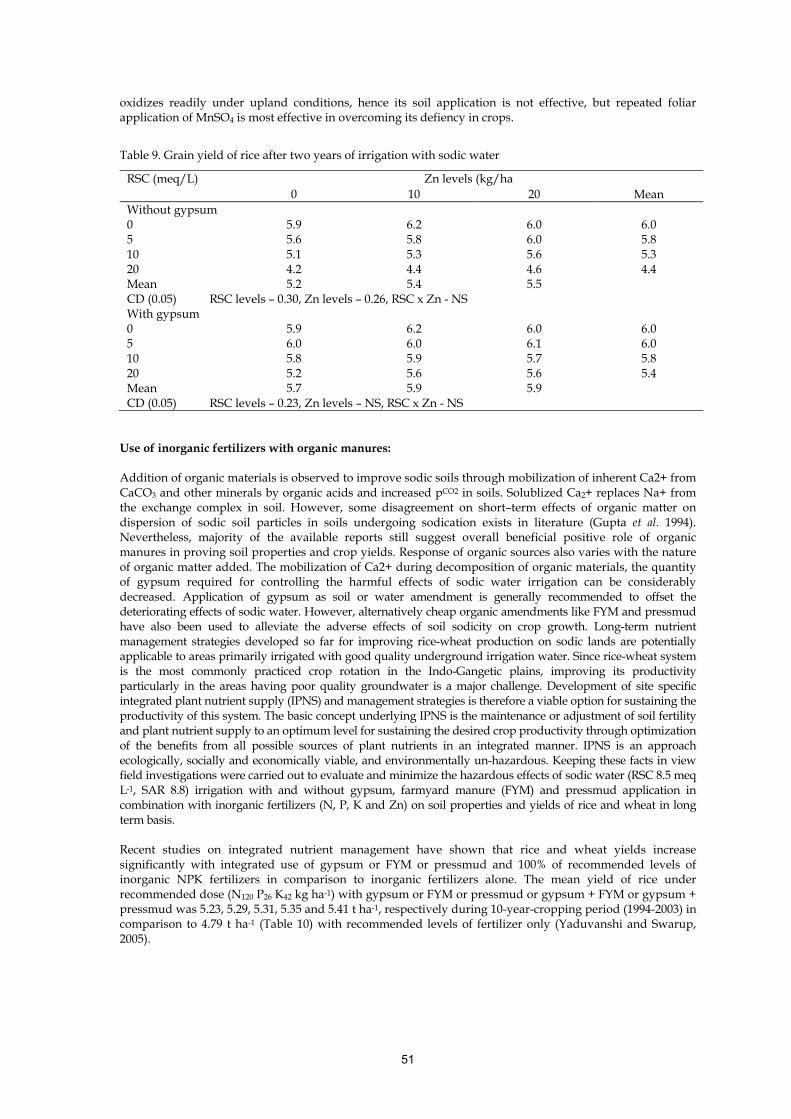
51

oxidizes readily under upland conditions, hence its soil application is not effective, but repeated foliar application of MnSO4 is most effective in overcoming its defiency in crops.

Table 9. Grain yield of rice after two years of irrigation with sodic water

RSC (meq/L) Zn levels (kg/ha 0 10 20 Mean

Without gypsum 0 5.9 6.2 6.0 6.0 5 5.6 5.8 6.0 5.8 10 5.1 5.3 5.6 5.3 20 4.2 4.4 4.6 4.4 Mean 5.2 5.4 5.5 CD (0.05) RSC levels – 0.30, Zn levels – 0.26, RSC x Zn - NS With gypsum 0 5.9 6.2 6.0 6.0 5 6.0 6.0 6.1 6.0 10 5.8 5.9 5.7 5.8 20 5.2 5.6 5.6 5.4 Mean 5.7 5.9 5.9 CD (0.05) RSC levels – 0.23, Zn levels – NS, RSC x Zn - NS

Use of inorganic fertilizers with organic manures: Addition of organic materials is observed to improve sodic soils through mobilization of inherent Ca2+ from CaCO3 and other minerals by organic acids and increased pCO2 in soils. Solublized Ca2+ replaces Na+ from the exchange complex in soil. However, some disagreement on short–term effects of organic matter on dispersion of sodic soil particles in soils undergoing sodication exists in literature (Gupta et al. 1994). Nevertheless, majority of the available reports still suggest overall beneficial positive role of organic manures in proving soil properties and crop yields. Response of organic sources also varies with the nature of organic matter added. The mobilization of Ca2+ during decomposition of organic materials, the quantity of gypsum required for controlling the harmful effects of sodic water irrigation can be considerably decreased. Application of gypsum as soil or water amendment is generally recommended to offset the deteriorating effects of sodic water. However, alternatively cheap organic amendments like FYM and pressmud have also been used to alleviate the adverse effects of soil sodicity on crop growth. Long-term nutrient management strategies developed so far for improving rice-wheat production on sodic lands are potentially applicable to areas primarily irrigated with good quality underground irrigation water. Since rice-wheat system is the most commonly practiced crop rotation in the Indo-Gangetic plains, improving its productivity particularly in the areas having poor quality groundwater is a major challenge. Development of site specific integrated plant nutrient supply (IPNS) and management strategies is therefore a viable option for sustaining the productivity of this system. The basic concept underlying IPNS is the maintenance or adjustment of soil fertility and plant nutrient supply to an optimum level for sustaining the desired crop productivity through optimization of the benefits from all possible sources of plant nutrients in an integrated manner. IPNS is an approach ecologically, socially and economically viable, and environmentally un-hazardous. Keeping these facts in view field investigations were carried out to evaluate and minimize the hazardous effects of sodic water (RSC 8.5 meq L-1, SAR 8.8) irrigation with and without gypsum, farmyard manure (FYM) and pressmud application in combination with inorganic fertilizers (N, P, K and Zn) on soil properties and yields of rice and wheat in long term basis.

Recent studies on integrated nutrient management have shown that rice and wheat yields increase significantly with integrated use of gypsum or FYM or pressmud and 100% of recommended levels of inorganic NPK fertilizers in comparison to inorganic fertilizers alone. The mean yield of rice under recommended dose (N120 P26 K42 kg ha-1) with gypsum or FYM or pressmud or gypsum + FYM or gypsum + pressmud was 5.23, 5.29, 5.31, 5.35 and 5.41 t ha-1, respectively during 10-year-cropping period (1994-2003) in comparison to 4.79 t ha-1 (Table 10) with recommended levels of fertilizer only (Yaduvanshi and Swarup, 2005).

52

Table 10. Effect of gypsum with and without different organic manures on yield of rice and wheat and soil properties

Treatments Mean Yield (t/ha) Soil pH OC (%) Rice (94-03) Wheat (94-04)

N120 P26 K42 (100 % recommended) 4.79 3.69 8.52 0.26 N120 P26 K42 + FYM 5.29 4.16 8.38 0.43 N120 P26 K42 + gypsum 5.23 4.10 8.18 0.37 N120 P26 K42 + Pressmud (PM) 5.31 4.46 8.29 0.42 N120 P26 K42 + FYM + gypsum 5.35 4.22 8.28 0.42 N120 P26 K42 + PM+ gypsum 5.41 4.52 8.28 0.40 CD at 5 % 0.42 0.34 0.08 0.60 Initial Soil Properties 8.6 0.40

The NPK fertilizer with 10 t ha-1 FYM, 5 t ha-1 gypsum or 10 t ha-1 pressmud produced higher yields over the years as compared to application of recommended dose of inorganic NPK alone. The residual effect of FYM, gypsum and pressmud was significant on wheat yields after 5 years. Though yields of both crops improved further when gypsum was applied with FYM or pressmud, but the profit was not beneficial over the FYM and pressmud alone treatment. Application of recommended NPK fertilizer combined with FYM or pressmud gave the highest profit followed by gypsum treatments. The cost/benefit ratio from 10 t ha-1 each pressmud (1.65) or FYM (1.59) were higher in comparison to gypsum application (1.38). There was substantial improvement in organic carbon and available nitrogen, phosphorus, potassium and zinc in soil over the initial status. The results of this study clearly show the beneficial effects of FYM and pressmud for rice and wheat yield under sodic water irrigation. It will become more crucial in the future because of increasing cost of chemical amendments. Large quantities of combine harvested rice and wheat straw are being produced in states of Punjab, Haryana and Uttar Pradesh. The residues are being burnt, presently, to clear the fields for timely sowing of crops and convenient disposal of waste. Large quantities of rice and wheat residues are available (37.87 Tg) for recycling and its potential was 0.634 Tg as a source of N, P and K nutrients. One tone of rice residues contains approximately 6.1 kg N, 0.8 kg P and 11.4 kg K, while one tone of wheat residues contains 5.1 kg N, 1.2 kg P and 10.5 kg K. Rice-wheat cropping system occupies about 10 million hectares area in India. In another field study under sodic water conditions, incorporation of wheat residue 50 days prior to rice transplanting either alone or with green manuring or with sulphitation pressmud (a sugarcane waste byproduct) and recommended dose of 120 kg N and 26 kg P ha-1 resulted in significant improvement in rice yield as compared to recommended dose of chemical N and P fertilizer alone. The mean yield improvement in both the crops due to incorporated of various organic sources over 100 % of recommended dose of NP was 26.1%, while it was only 6.6% in the treatment where the residue was burnt. Sodic water irrigation over three years period of experimentation, increased soil pH by 0.1-0.16 units (Table 11). However, in treatments with organic sources, pH remained nearly at the initial level (Yaduvanshi and Sharma 2007a and b). As crop residues are rich source of organic mater, nutrients and energy, they must be returned to the soil. Besides the loss of organic matter and plant nutrients, burning of crop residues also cause atmospheric pollution in form of toxins and green house gases. Table11. Effect of crop residue management on yield (mean of 3 years) and soil properties of alkali soil under

poor quality water

Treatments Grain yield (t/ha) pH OC (%) Rice Wheat

N0 P0 1.05 0.87 9.35 0.25 N90 P19.5 (75 % NP) 2.69 2.31 9.35 0.25 N120 P26 (100 % NP) 3.49 2.94 9.31 0.26 100 % NP + wheat residue Burning 3.72 2.99 9.33 0.30 100 % NP + Incorporated wheat residue 4.34 3.19 9.20 0.35 100 % NP+ Incorporated wheat residue + GM 4.45 3.35 9.18 0.35 100 % NP+Incorporated wheat residue+ SPM 4.41 3.34 9.20 0.34 CD (0.05) 0.58 0.45 - 0.02 The results from studies on tillage practices have shown that no-tillage (NT) practice increases organic carbon and infiltration rate of sodic water irrigated soil in comparison to conventional tillage conditions. No-tillage practice also decreased soil pH and SAR. The NT either alone or with residual effect of gypsum or pressmud or FYM has been found as an effective option to sustain higher yields of wheat under use of sodic

53

water irrigation in a rice-wheat system; besides saving of 7.22 cm of irrigation water and three disking and planking operations (Yaduvanshi and Sharma 2008). Suggested Readings Bajwa, M.S., Josan, A.S. and Chaudhary, O.P. 1993. Effect of Frequency of Sodic and Saline-Sodic Irrigation

and Gypsum on the Build up of Sodium in Soil and Crop Yields. Irrigation Science. 13: 21–26. Bower C.A., Ogata G. and Tucker J.M. 1968. Sodium hazard of irrigation waters as influenced by leaching

fraction and by precipitation or solution of calcium carbonate. Soil Science. 106: 29-34. CGWB, 1997. Inland ground water salinity in India. GOI, Ministry of Water Resources, Central Ground

Water Board, Faridabad. pp.62. Chaudhary, O. P., Josan, A. S., Bajwa, M. S. and Kapur, M.L. 2003. Effect of sustained sodic and saline-sodic

irrigation and application of gypsum and FYM on yield and quality of sugarcane. Field Crop Research. 87: 103-116.

Chauhan, R.P.S., Chauhan, C.P.S. and Singh, V.P. 1986. Use of pyrites in minimizing the adverse effects of sodic waters. Indian Journal of Agriculture Science. 56: 717-721.

Chhabra, R. 1985. Crop responses to phosphorus and potassium fertilization of a sodic soil. Agron. J. 77: 699-702

Dargan, K.S. and Gaul, B. L. 1974. Optimum nitrogen levels for dwarf varieties of paddy in semi-reclaimed alkali soils. FertiL News. 19(10):24-25.

DebRoy, Aditi and Tushaar Shah. 2003. “Socio-ecology of groundwater irrigation in India.” In: Groundwater intensive use: Challenges and opportunities. (Eds. R. Llamas and E. Custodio). The Netherlands: Swets and Zetlinger Publishing Co.

Gupta, R.K., Singh, N.T. and Sethi, M. 1994. Groundwater Quality for Irrigation in India (1:6 million scale). Tech. Bull. No. 19, CSSRI, Karnal – 132001, India. P.16.

Grattan, S.R. and J.D. Oster. 2003) Use/Reuse of Saline-Sodic Waters for Irrigation of Crops. In: S.S.Goyal, S.K.Sharma and D.W.Rains (eds.), Crop Production in Saline Environments: Global and Integrative Perspectives. Haworth Press, New York. pp 131-162.

Josan A. S., Bajwa, M. S. and Chaudhary, O. P. 1998. Effect of sustained sodic irrigations on soil physical properties and root growth in a Typic Ustochrept soil under two cropping systems. Journal of Research (Punjab agricultural University). 35: 125-131.

Minhas Neetu and I. M. Chhiba (1999). Zn Transformations in Rice Soil Irrigated with Sodic Water. Indian Journal Agricultural Science. 69: 251-254.

Minhas, P.S. 1996. Saline water management for irrigation in India. Agricultural Water Management. 30: 1-24.

Minhas, P.S., and Bajwa, M.S. 2001. Use and Management of Poor Quality Water in Rice – Wheat Production System. Journal Crop Production. 4: 273-306.

Minhas, P.S., and Gupta, R.K. 1992. Quality of Irrigation Water- Assessment and Management. Information and Publication Section, Indian Council of Agricultural Research, Krishi Bhawan, New Delhi – 110 001, India. pp. 123.

Oster J.S. 1982. Gypsum usage in irrigated agriculture: a review. Fertilizer Research 3: 73-89. Oster, J.D. and Shainberg, I. 2001. Soil Responses to Sodicity and Salinity: Challenges and Opportunities.

(Personal Correspondence, J. D. Oster, Manuscript Submitted for Publication, Forthcoming, 2001). Department of Environmental Sciences, University of California, Riverside, CA 92521, USA, and Soil and Water Institute, The Volcani Center, POB 6, Bet Dagan, Israel.

Rao, D.L.N. and Batra, L. 1983. Ammonia volatilization from applied nitrogen in alkali soils. Pl. Soil. 20: 219-228.

Rhoades J.D., Kandiah, A. and Mishali, A.M. 1992. The use of saline waters for crop production. Food and Agriculture Organization Irrigation and Drainage Paper No. 48, Food and Agriculture Organization, Rome, Italy. pp 133.

Shah, Tushaar, Aditi Debroy, Asad Qureshi and Jinxia Wang. 2001. Sustaining Asia’s Groundwater Boom: An Overview of Issues and Evidence. Natural Resources Forum. 27 (2003): 130-141

Shainberg, I., Sumner, M.E., Miller, W.P., Farina, M.P.W., Pavan, M.A. and Fey, M.V. 1989. Use of gypsum on crops. A Review. Advances in Soil Science. 9:1-112.

Sharma, D.R. and Minhas, P.S. 2001. Response of Rice-Wheat to Alkali Water Irrigation and Gypsum Application. Journal Indian Society Soil Science. 49: 324-327.

Sharma, D.R. and Minhas, P.S. 2004. Soil properties and yields of upland crops as influenced by long-term use of water having variable residual alkalinity, salinity and sodicity . Journal of the Indian Society of Soil Science. 1: 100-104.

Shekhon, M.S. and Bajwa, M.S. 1993. Effect of Incorporation of OM and Gypsum in Controlling Sodic Irrigation Effects on Soil Properties under Rice – Wheat Maize System. Agricultural Water Management. 24: 15-25.

54

Singh, B. and Bajwa, M.S. 1990. Effect of Poor Quality Water on Ammonia Volatilization Losses. Journal of Indian Society Soil Science . 30: 779-781.

Singh Joginder. 1999. Interactive Effects of Zinc, Gypsum and Sodic Irrigation Water on Transformations and Availability of Micro-Nutrients to Rice and Wheat. Ph. D. Thesis Submitted to PAU, Ludhiana.

Swarup, A. 1980. Effect of Submergence and Farm Yard Manure Application on Yield and Nutrition of Rice Under Sodic Conditions. Journal of Indian Society Soil Science. 28: 532-534.

Swarup, A. and Yaduvanshi, N.P.S. 2004. Response of Rice and Wheat to Organic and Inorganic Fertilizers and Soil Amendment Under Sodic Water Irrigated Conditions. IRRI News Letter. 29(1): 49-51.

Yadav J.S.P. 1989. Irrigation Induced Soil Salinity and Sodicity. Proceeding of World Food Day Symposium on Environmental Problems Affecting Agriculture in the Asia and Pacific Region held at FAO, Bangkok, Thailand. pp. 47-62.

Yadav, R.K. and Kaledhonkar, M. J. 1998. Effect of Toposequential Differences and Ground Water Quality on Performance of Cotton and Egyptian Clover. Central Soil Salinity Research Institute, Annual Report. pp. 28-29.

Yaduvanshi N. P.S. 2001. Ammonia volatilization losses from integrated nutrient management in rice field of alkali soil. Journal of the Indian Society of Soil Science. 49: 276-280.

Yaduvanshi, N.P.S. 2003. Substitution of inorganic fertilizers by organic manures and the effect on soil fertility in a rice-wheat rotation on reclaimed sodic soil in India. Journal of Agriculture Science (Cambridge). 140 : 161-169.

Yaduvanshi, N.P.S. and Swarup, A. 2005. Effect of Continuous Use of Sodic Irrigation Water with and without Gypsum, Farm Yard Manure, Pressmud and Fertilizer on Soil Properties and Yields of Rice and Wheat in a Long Term Experiment. Nutrient Cyclic in Agroecosystems. 73: 111-118.

Yaduvanshi, N.P.S., and D.R. Sharma (2007a). Use of Wheat Residue and Manures to Enhance Nutrient Availability and Rice-Wheat Yields in Sodic Soil under Sodic Water Irrigation. Journal of Indian Society Soil Science. 55(3): 330-334.

Yaduvanshi, N.P.S., and Sharma, D.R. 2007b. Incorporate Wheat Residue with Green Manure for Sustaining Rice-Wheat Production in Sodic Water. Indian Farming. 57(9): 15-17.

Yaduvanshi, N.P.S., and Sharma, D.R. 2008. Tillage and Residual Organic Manures/Chemical Amendment Effects on Soil Organic Matter and Yield of Wheat under Sodic Water Irrigation. Soil and Tillage Research. 98: 11-16.

55

Raising Horticultural Crops under Saline Environment Dheeraj Singh, M.K. Choudhary, M.L. Meena and Hari Dayal Central arid Zone Research Institute, KVK, Pali (Rajasthan), India Introduction According to the Food and Agriculture Organization (FAO) and the United Nations Educational, Scientific and Cultural Organization (UNESCO), the world has 397 million ha of saline soils and 434 million ha of sodic soils. About 12.6 million ha are considered to be under acid-sulphate soils distributed along coastal regions. Of the current 230 million ha of irrigated land, 45 million ha are salt-affected. Of the almost 1500 million ha of dry land agriculture, 32 million ha are salt-affected in varying degrees by human-induced processes. Be that as it may, it is possible to increase wasteland productivity in terms of food, fuelwood, forage, medicinal drugs and biodiversity if it is planted with trees. In particular, salt-affected wastelands hold promise for agroforestry. However, without adequate fresh water for irrigation, the dry areas are not arable enough for forest and horticultural crops. But there is plenty of water beneath many of the world's deserts with saline water reserves. Studies conducted at the Central Soil Salinity Research Institute, Karnal, India, showed that salt-affected soils and saline waters can be satisfactorily utilized in raising some forest and fruit tree species, forage grasses, conventional and nonconventional crops, oil-yielding crops, aromatic and medicinal plants of high economic value, petro-crops and flower-yielding plants using appropriate techniques. Salts occur naturally in all soils. Rain dissolves these salts, which are then swept through stream and riven to the sea. Where rainfall is sparse or there is no quick route to the sea, some of this water evaporates and the dissolved salts become more concentrated. In arid areas, this can result in the formation of salt lakes or in brackish groundwater, salinized soil, or salt deposits. There are three possible domains for the use of salt-tolerant plants. These are: (i) Farmlands salinized by poor irrigation practices; (ii) Arid areas that overlie reservoirs of brackish water; and (iii) Coastal deserts. In some regions, there are millions of hectares of salinized farmland resulting from poor irrigation practices. These lands would require large (and generally unavailable) amounts of water to leach away the salts before conventional crops could be grown. However, there may be useful salt-tolerant plants that can be grown on them without this intervention. Although the introduction of salt-tolerant plants will not necessarily restore the soil to the point that conventional crops can be grown, soil character is often improved and erosion reduced. Moreover, many arid areas overlie saline aquifers-groundwater containing salt levels too high for the irrigation of conventional, salt sensitive crops. Many of these barren lands can become productive by growing selected salt-tolerant crops and employing special cultural techniques using this store of brackish water for irrigation. Throughout the world, there are extensive coastal deserts where seawater is the only water available. Although growing crops in sand and salty water is not a benign prospect for most farmers, for saline agriculture they can complement each other. The disadvantages of sand for conventional crops become advantages when saline water and salt-tolerant plants are used. Sand is inherently low in the nutrients required for plant growth, has a high rate of water infiltration, and has low water-holding capacity. Therefore, agriculture on sand requires both irrigation and fertilizer. Surprisingly, 11 of the 13 mineral nutrients needed by plants are present in seawater in adequate concentrations for growing crops. In addition, the rapid infiltration of water through sand reduces salt build-up in the root zone when seawater is used for irrigation. The high aeration quality of sand is also valuable. This characteristic allows oxygen to reach the plant roots and facilitates growth. Although careful application of seawater and supplementary nutrients are necessary, the combination of sand, saltwater, sun, and salt-tolerant plants presents a valuable opportunity for many countries. Of these three possibilities for the introduction of salt tolerant plants (salinized farmland, undeveloped barren land, and coastal deserts), the reclamation of degraded farmland has several advantages: people, equipment, buildings, roads, and services are usually present and a social structure and market system already exist. The potential use of saline aquifers beneath barren lands depends on both the concentration

56

and nature of the salts. The direct use of seawater for agriculture is probably the most challenging potential application. Most contemporary crops have been developed through the domestication of plants from non-saline environments. This is unfortunate since most of the earth's water resources are too salty to grow them. From experience in irrigated agriculture, Miyamoto (personal communication) suggested the following classification of potential crop damage from increasing salt levels (Table 1). Table 1. Classification of potential crop damage from increased salt levels

Irrigation water Salts, ppm Crop problems Fresh <125 None Slightly saline 125-250 Rare Moderately saline 250-500 Occasional Saline 500-2,500 Common Highly saline 2,500-5,000 Severe Soil salinity The salt concentration in the water extracted from a saturated soil (called saturation extract) defines the salinity of this soil. If this water contains less than 3 grams of salt per litre, the soil is said to be non saline (Table 2). If the salt concentration of the saturation extract contains more than 12 g/l, the soil is said to be highly saline. Table 2. Classifying soil salinity based on salt concentration of soil water

Salt concentration of soil water (saturation extract) Salinity Gram/litre Millimhos/cm 0 - 3 0 - 4.5 non saline 3 - 6 4.5 - 9 slightly saline 6 - 12 9 - 18 medium saline more than 12 more than 18 highly saline Table 3. Classification of plants tolerant to high salt concentration

Highly tolerant Moderately tolerant Sensitive Date palm Wheat, Tomato, Oats, Red clover, Peas Barley Alfalfa, Rice, Maize, Beans, Sugarcane Sugarbeet Flax, Potatoes, Carrot Pear, Apple Cotton Onion, Cucumber, Pomegranate Orange, Prune Asparagus Fig, Olive, Grape Plum, Almond Spinach Apricot, Peach The highly tolerant crops can withstand a salt concentration of the saturation extract up to 10 g/l. The moderately tolerant crops can withstand salt concentration up to 5 g/l. The limit of the sensitive group is about 2.5 g/l. Colorado River water, used for irrigation in the western United States, contains about 850 ppm of salts; seawater typically contains 32,000-36,000 ppm of salts. Salinity levels are usually expressed in terms of the electrical conductivity (EC) of the irrigation water or an aqueous extract of the soil; the higher the salt level, the greater the conductivity. The salinity of some typical water sources is shown in Table 4. There are three broad approaches to utilizing saline water, depending on the salt levels present. These include the use of marginal to poor irrigation water with electrical conductivities (ECs) up to about 4 dS/m, the use of saline ground waters such as those in Israel's Negev Desert with ECs up to about 8 dS/m, and the use of even more saline waters with salt concentrations up to that of seawater. At low, but potentially damaging, salt levels, Rhoades and co-workers (1988) have grown commercial crops without the yield losses that would normally be anticipated.

57

Table 4. Water salinity

Salinity measurement Irrigation water quality Colorado River

Alamo River

Negev Groundwater

Pacific Ocean Good Marginal

EC (dS/m)* 0-1 1-3 1.3 4.0 4.0-7.0 46 Dissolved solids, ppm 0-500 500-1500 850 3000 3000 - 4500 35000 *1 dS/m = 1 mmho/cm = (approx.) 0.06% NaCl = (approx.) 0.01 mole/l Nacl 10,000 ppm = 10 o/oo (parts per thousand) = 10 grams per liter = 1.0% In the International System of Unit (SI), the unit of conductivity is the Siemens symbol, S, per meter. The equivalent unit commonly appearing in the literature is the mho (reciprocal ohm); 1 mho equals 1 Siemen. Source: Adapted from Epstein, 1983; Pastemak and De Malach, 1987; and Rhoades et al. 1988

At higher salt levels, Pasternak and co-workers (1985) have developed approaches that involve special breeding and selection of crops and meticulous water control. The agriculture of Negev settlements in Israel is based on the production of cotton with higher yields, quality tomatoes for the canning industry, and quality melons for export-all grown with EC 4-7 dS/m groundwater. Experimental yields of a wide variety of traditional crops grown in Israel with water with ECs up to 15 dS/m. The use of water with still higher salt levels up to, including, and even exceeding that of seawater for irrigation of various food, fuel, and fodder crops has been reported by many researchers including Aronson (1989), Boyko (1966), Epstein (1985), Gallagher (1985), Glenn and O'Leary (1985), Iyengar (1983), Pasternak (1987), Somers (1975), Yensen (1988), and others. These scientists have produced grains and oilseeds; grass, tree, and shrub fodder; tree and shrub fuel wood; and a variety of fiber, pharmaceutical, and other products using highly saline water. Thus, depending on the soil or water salinity levels, salt-tolerant plants can be identified that will perform well in many environments in developing countries. The salt tolerance of some of these plants enables them to produce yields under saline conditions that are comparable to those obtained from salt-sensitive crops grown under non-saline conditions. The maximum amount and kind of salt that can be tolerated by halophytes and other salt-tolerant plants varies among species and even varieties of species. Many halophytes have s special and distinguishing feature-their growth is improved by low levels of salt.

Fig. 1. Growth response to salinity. Many halophytes, such as Sueada maritima have increased

yields at low salinity levels. Salt-tolerant crops, such as barley, maintain yields at low salinity levels but decrease as salt levels exceed a certain limit. Yields of salt-sensitive crops, such as beans,

decrease sharply even in the presence of low levels of salt. Source: Adapted from Greenway and Munns, 1980; Maas 1986; and Yensen, et al., 1985

Other salt-tolerant plants grow well at low salt levels but beyond a certain level growth is reduced. With salt-sensitive plants, each increment of salt decreases their yield (Fig. 1). Such data provide only relative guidelines for predicting yield of crops grown under saline conditions. Absolute yields are subject to numerous agricultural and environmental effects. Interactions between salinity and various soil, water, and climatic conditions all affect the plant's ability to tolerate salt. Some halophytes require fresh water for germination and early growth but can tolerate higher salt levels during later vegetative and reproductive stages. Some can germinate at high salinities but require lower salinity for maximal growth. Traditional farming efforts usually focus on modifying the environment to suit the crop. In saline agriculture, an alternative is to allow the environment to select the crops, to match salt-tolerant plants with desirable characteristics to the available saline resources.

58

In many countries extensive areas of degraded and arid land are publicly owned and readily accessible for government sponsored projects. These lands are often located in areas of high nutritional and economic need as well. If saline water is available, the introduction of salt-tolerant plants in these regions can improve food or fuel supplies, increase employment, help stem desertification, and contribute to soil reclamation. Salt-affected soils and saline waters At least five groups of salt-affected soils are influenced by different chemical types of electrolytes, which not only represent different salts, but also have different effects on soil formation. For practical use, salt-affected lands in the Indian subcontinent are identified as saline, alkali/sodic and saline-alkali. CSSRI groups salt-affected soils as either saline or alkaline.

Limitations Undomesticated salt-tolerant plants usually have poor agronomic qualities such as wide variations in germination and maturation. Salt-tolerant grasses and grains are subject to seed shattering and lodging. The foliage of salt-tolerant plants may not be suitable for fodder because of its high salt content. Nutritional characteristics or even potential toxicities have not been established for many edible salt-tolerant plants. When saline irrigation water is used for crop production, careful control is necessary to avoid salt build-up in the soil and to prevent possible contamination of freshwater aquifers. Most importantly, salt-tolerant plants should not be cultivated as a substitute for good agricultural practice nor should they be used as a palliative for improper irrigation. They should be introduced only when and where conventional crops cannot be grown. Also, currently productive coastal are= (such as mangrove forests) should be managed not converted for other uses. All of these limitations are impediments to the use of conventional methods for culture and harvest of salt-tolerant plants and the estimation of their production economics.

Fruits Ahmad' has described a technique developed in Pakistan and India to grow salt-sensitive fruits on saline land. This involves grafting a salt-sensitive shoot on a salt-tolerant rootstock. For example, shoots of Ziziphus mauritiana (salt sensitive, but yielding fleshy berries) have been grafted on the roots of Z. nummularia (salt tolerant, but yielding smaller berries) to allow fruit production on saline land. Similarly, shoots of Manilkara zapota (salt sensitive, but bearing large fruit) have been grafted on rootstocks of M. hezandra (salt tolerant, but bearing small fruit) to combine the desirable qualities of both. Pasternak (1987) reported that pear cultivars can tolerate irrigation water of 6.2 dS/m when grafted on a quince rootstock. Salvadora pereica and S. oleoidea are small evergreen trees or shrubs. Both species yield edible fruits. Their seeds contain about 40 percent of an oil with a fatty acid composition (lauric, 20 percent; myriatic, 55 percent; palmitic, 20 percent; oleic, 5 percent), which makes an excellent soap. The seed oil is inedible because of the presence of various substituted dibenzylureas. Both are multipurpose trees in India and Pakistan, providing fodder and wood as well as fruit. In India, S. persica occurs on saline soils and in coastal regions just above the high-water line. Before the introduction of canal irrigation in Pakistan, S. oleoides occupied much of the worst salt affected land. There are about a dozen species of Lycium in the United States. Although most bear edible fruit, they are commonly cultivated as ornamentals. L. fremontii seems to have agronomic promise. It is a thorny shrub native to southern Arizona and the Gulf of California region in adjacent Mexico. It thrives on desert soils, upper beaches, and semi saline and alkaline flats both near the coast and on inland deserts. The quandong (Santalum acuminatum) is widely distributed across Australia's arid inland. This small tree averaging about 4 m high, has bright red cherry-sized fruit with edible flesh and a stone with an edible kernel. The flesh is a good source of carbohydrate (1423 percent). It was a staple of the aboriginal's diet and has been popular with other Australians in jam and pie. The kernel is roasted before being consumed and has a high oil (58 percent) and energy content. The quandong is reported to be highly resistant to drought, high temperatures, and salinity. An experimental orchard in southern Australia has been irrigated for seven years with water with a conductivity of 4.7 dS/m. The seagrape (Coccoloba uvifera) is readily established on sandy shores. When fully exposed on windswept seacoasts, the seagrape is dwarfed and bushy (to 2.5 m high) and forms dense colonies. Inland, it becomes a spreading, low-branched tree (to 15 m high). The wood makes excellent fuel and can also be used for furniture and cabinetwork. The fruits are popular in the Caribbean and are sold in local markets. The flowers yield abundant nectar and result in a fine honey.

59

Traditional crops In Israel, a number of commercial crops are grown with underground brackish water. These include melons, tomatoes, lettuce, Chinese cabbage, and onions. A study on market tomatoes showed that fruits produced under saline conditions were smaller than the controls, but developed a better color and had a much better taste. However, their shelf life tended to be shorter. Taste testing of other crops grown in brackish water showed that in melons, the fresh fruits were tastier than the controls. For lettuce, the salinity of the irrigation water had no discernible effect on the taste. Yields obtained in seventeen saline irrigation experiments are shown in Table 5. Table 5. Experimental yields of vegetable and grains at the Ramat Nagev Experimental Station

Crop System Yield (t/ha) at EC (irrigation water) Species 1.2 3.5-

5.5 6-8 8-10 10-

15 Vegetables Asparagus d 6.6 6.6 - - - A. Officinalis; 4-year-old plot Broccoli d 23.4 21.8 - 19.0 14.3 Brassica oleracea Beetroot s 55.5 52.7 - - - Beta vulgaris Carrot d 45.8 41.2 33.8 0 - Daucus carota Celery s 155.0 171.0 - - - Apium graveolens Chinese cabbage

d 135.0 118.0 108.0 109.0 - Brassica perkinenis

Chinese cabbage

d 58.0 58.0 55.0 65.0 - Brassica chinensis

Kohlrabi d 30.0 20.3 17.4 11.7 - Brassica caulorapa Lettuce d 67.7 64.5 52.8 58.3 - Lactuca sativa Melon d 27.0 24.0 24.0 22.0 - Cucumis melo Onion d 50.1 28.4 4.1 0.4 - Allium cepa Onion d 50.1 34.0 27.9 22.4 - A. cepa, saline irrigation from 64th day

after planting Tomato d 86.5 72.9 - 62.7 53.0 Lycoperisicon esculentum Grains: (yield of grain at 12% moisture) Maize d 7.1 4.6 3.1 1.3 - Zea mays Maize d 7.0 6.7 7.0 5.2 - Z. mays; saline irrigation from 21st day

after germination Sorghum s 10.0 8.4 - - - Sorghum vulgare Wheat s 6.8 6.7 - - - Triticum vulgare *d = drip irrigation, s = sprinkler irrigation Source: Pastemak and De Malach, 1987 Asparagus (Asparagus officinalis) is commonly considered a temperate crop, dormant in the winter with spears harvested in the spring, and summer fern growth terminated by cooler fall weather. In tropical areas it can be grown using the "mother fern" technique. After plants are established, the first two or three spears are allowed to grow to fern; thereafter, spears are harvested as they develop. Twice during the year old fern is replaced by new fern, but asparagus is produced year-round with annual yields exceeding those obtained in temperate climates. In Tunisia, asparagus is grown near Zarzis, where the salinity the irrigation water is 6.5 g per liter. Yields (48 tons per hectare) are about the same as in areas irrigated with fresh water. It has also been grown experimentally in Israel's Negev desert. In the United States, University of Delaware researchers found A. oficinalis growing wild at the edge of a salt marsh. Using commercial asparagus varieties, they germinated thousands of seeds in fresh water and transferred the seedlings to salt water. Most died, but some grew well at salinities of 30 parts per thousand. Asparagus is an excellent crop for developing countries because it is relatively labor intensive. Although several years are required before a marketable crop is obtained, production continues for 15-25 years. Water requirements for asparagus are somewhat greater than for cotton, and a light soil and careful management are required.

60

Fiber and other products Salt tolerant plants can be used to produce economically important materials such as essential oils, gums, oils, and resins, pulp and fiber, and bioactive compounds. Further, salt tolerant plants can be cultivated for landscape use and irrigated with saline water, thereby conserving fresh water for other uses. Essential oils The male flowers of kewda (Pondanus fascicularis), a common species of screw pine in India, are used to produce perfume and flavouring ingredients. The kewda plant is salt tolerant and has been planted in coastal areas to check drifting sand. Propagation is through suckers or stem cuttings, and flowering starts 3-4 year after planting. An annual income of US$8 per plant has been estimated. Mentha and other species In India, economic yields of a number of essential oils were obtained from plants grown on saline alkaline soil. Two Mentha species were evaluated. M. piperita (for peppermint oil) and M. arvensis (for menthol) both gave yields comparable to those obtained on normal soil. Other plants giving satisfactory yields on saline alkaline soil included Matricaria chamomilla, Vetiveria zizanioides, Cymbopogon nardus and C. winterianus (for citronella oil), Tagetes minuta, Ocimum kilimandscharicum, and Anethum gravcolens (English dill). Palamarosa grass (C. martinii), a commercially important essential oil plant, is also reported to grow under moderately saline conditions. The production of essential oils to provide a new source of income in rural areas is one of the objectives of the Ciskei Essential Oils Project, established in southern Africa in 1972. This effort was planned to provide an income for rural dwellers that was derived from familiar, indigenous resources and required relatively little capital. Over the past four years, this project has produced and exported US$1 million worth of essential oils and provided employment to hundreds of rural dwellers during the harvest season. Gums, oils and resins Sesbania bispinosa, commonly known as dhaincha in India, is an important legume and fodder crop. It is an erect, multibranched annual, about 2.5 m tall at maturity that grows readily on alkaline saline soils. Often grown for use as a green manure (about 12 tons per hectare), its stalks are sources of fiber and fuel, and the seeds yield a galactomannan gum that can be used for sizing and stabilizing purposes. The seed meal can be used for poultry and cattle feed. S. eceban and S. specioea are salt-tolerant perennials used as green manure. S. scaban can tolerate water logging and salt concentrations of 1.0 percent as a seedling and 1.4 percent as it matures. Grindelia camporum is a 0.5-1.5 m resinous perennial shrub. It exudes large amounts of aromatic resins that cover the surface of the plant. The resins are non-volatile mixtures of bicyclic terpene acids, esters, and related structures that are insoluble in water but soluble in organic solvents. The plant appears to be salt tolerant, populations are found in saline flats and near salt lakes and springs. Several species of Grindelia occur along the North American Pacific Coast in estuaries or salt marsh habitats. These include G. humilis, C. stricta, G. latifolio, and G. integrifolia. Grindelia resins have properties similar to the terpenoids in wood and gum rosins, which are used commercially in adhesives, varnishes, paper sizings, printing inks, soaps, and numerous other industrial applications. With increasing costs and declining supplies of these wood-based materials, substitutions with Grindelia resins in this market (700,000 tons per year) may become practical. Sapium aebiferum, the Chinese tallow tree, is a small marshland tree native to subtropical China. It has been cultivated there for more than 1,000 years as a source of specialty oils, medicines, and vegetable dyes. The Chinese tallow tree possesses several valuable characteristics: it can be seeded directly; it grows rapidly in warm, waterlogged saline soils; and it re-sprouts readily. The major economic potential for this tree is in its high yield of oilseed-more than 10 tons per hectare according to the USDA. The seed contains both an edible hard vegetable fat and inedible liquid oil, which

61

comprise 45-50 percent of its weight. Five years after planting, when seed production begins, a net return of US$3,200 per hectare per year has been estimated. Jojoba (Simrnondsia chinensis) is a perennial desert shrub with seeds that contain a unique oil. About half of the seed's weight is an oil with a structure similar to sperm whale oil-an eater of a C20-22 straight chain alcohol with a C20-22 straight chain acid. Both the alcohol and the acid have a terminal double bond, providing a readily accessible site for diverse chemical reactions. Currently there are about 18,000 hectares of jojoba plantations in the south-western United States and other plantations in Mexico, Australia, Israel, Argentina, and South Africa and other African nations. Jojoba is relatively salt tolerant. In California, plants are growing satisfactorily with water containing 0.2 percent salts. In laboratory testing, one variety of jojoba showed no reduction in flower production with 0.6 percent salt. In Israel, jojoba is growing well near the Dead Sea irrigated with brackish water (5-6 dS/m). Rubber rabbitbush (Chrysothamnus nauseosus) is a common desert shrub native to western North America. It grows under a wide range of environmental conditions from Mexico to Canada, comlilonly appearing on disturbed sites and saline soil. In addition - to its forage value, it contains natural rubber and a hydrocarbon resin, and it has constituents that are potential insecticides and fungicides. The perennial desert shrub, guayule (Parthenium argentatum), also has considerable degree of salt tolerance. More recent reports on guayule (Hoffman et al., 1988; Maas et al., 1988) indicate the root-zone salt-tolerance threshold to be about 7.5 dS/m; above this, rubber production is reduced 6.1 percent per unit increase of soil salinity. Rubber samples from Hevea, Parthenium, and Chrysotharnnus appear to be structurally identical. Rubber contente as high as 6.5 percent for Chrysothamnus nave been reported. If rubber yields of 2 percent are assumed, a plantation would produce 370 kg per hectare after 6 years' growth (guayule yields from California production were higher-about 1,000 kg per hectare after 2 years; Hevea yields are about 1,300 kg per hectare per year). Resin contents as high as 21 percent have been reported for Chrysothamnas, and some of its hydrocarbon components may find use as insecticide8 and fungicides.

Palms Several salt-tolerant palms are sources of fiber and other materials for a wide variety of uses. Fronds from the nips palm, for example, are also used for thatching, basketry, mats, and similar applications. Cocas nucifera, the familiar coconut palm, is commonly found on sandy beaches but also occurs in low marshy areas occasionally flooded by seawater. The uses of the nut for food, its value as a source of oil, and tapping of the inflorescence for toddy and sugar are all well known. In addition, leaves are used for thatching, walls, and screens and leaflets are woven into baskets, plates, hats, mats, and other articles for daily use. Elacis oleifera is found in coastal swamp forests from the lower basin of the Amazon to southern Mexico. Often called the American oil palm, it is closely related to the African oil palm (E. guineensis). The fruits are a source of oil, tallow, and chicken feed. The tree has a low-growing habit, which simplifies fruit harvest. Licuala spinosa is a palm found in tidal forests immediately behind the mangroves from the Malay Peninsula to the Andaman Islands. Its leaves are used for roofing and for wrapping food. Oncosperma filimentosa, the nibung palm, grows on brackish lowlands just behind mangrove stands in India, Sri Lanka, and the Philippines. The trunk is used for construction and the spines are used as darts in blowpipes and as tips on fish spears. The leaves are used for making baskets and the bracts as buckets. Raphia vinifera, the bamboo palm, grows in tidal bays and creeks in tropical West Africa. Fiber from the leaf bases is used for fishing lines and for animal snares and cordage. It is also exported for use in the manufacture of brooms, industrial brushes, and upholstery stuffing.

Landscape and ornamental use Many attractive halophytes can be used as landscape plants, especially in areas with constraints on the use of fresh water for watering or irrigation. In Israel, trees such as Conocarpus erectun, Eucalyptus sargentii, and Melaleuca halnsaturorum, and shrubs such as Maireana sedifolia, Borrichea frutescens and, Clerodendrum inerme are sold for amenity planting to allow Irrigation with saline water. The striking floral display of the Butea monosperma tree bark earned it the name flame of the forests. In addition, plants such as Limonium species

62

have potential for floral use. For example, sea lavender (Limonium azillcre) can be irrigated with seawater and used to produce cut flowers.

Table 6. Salt-tolerant ornamental plants

Plants Flower color Flowering season

Average height (m)

Salt resistance

Trees: Acacia gerrardii Cream July-Oct 5 1 A, horrida Yellow May-Sept. 8 1 A. raddiana Cream Mar-Apr

Oct-Dec. 5 1

A. salicina Cream Mar and Sept 8 1 A. tortilis Cream Spring and fall 5 1 Casiarina glauca Apr 8 1 Conocarpus erectus 5 1 Elaeagnus angustifolia white Apr-May 4 1 Eucalyptus sargentii Yellowish-white 6 1 Moringa peregrine White to pink Mar-May 6 1 Parkinsonia aculeata Yellow May-June 8 2

Phoenix dactylifera 12 2 Prosopis juliflora White Apr-May 6 1 Tamarix aphylla White May-June 8 2 Shrubs: Atriplex barclayana 1.5 2 A. cinerea 1 2 A. nummularia 1.5-2 2 Callistemon rigidus Red Ap;r 2 1 Cassia Mexicana Yellow Apr-Sept. 0.5-0.75 1 Colutea Istria Yellow Mar-Apr 2 1 Maireana sedifolia 2 2 Melaleuca nesophila Lilac May-July 3 1 Retama raetam White/purple Mar-Apr 2 1 Tamarix chinensis “mapu” violet 3 1 Succulents and Semi-succulents:

Agava Americana White Apr-July 2 1 Arthrocnemum fruticosum* 0.6 3 A. Macrostachyum 0.5 3 Batis maritima 0.3 3 Biennial and Perennial ground cover

Arctotis grandis Assorted Dec-Apr 1 Aster alpines Blue Dec-Apr 1 Catharansus raseus White/ pink Most of year 1 Cineraria maritima Violet Apr-June 1 Crithmum maritimum Yellow May-June 2 Gazania splendens Assorted Dec-May 1 Inula crithmoides Yellow June-July 3 Nitraria billardieri White Apr-May 3 Sesuvium verrucosum Lilac June-July 3 Lawn Grasses: Cynodon dactylon 2 Paspatum vaginatum 2

63

Some salt tolerant horticultural plants of economic importance from India Lana (Haloxylon salicornicum (Moq.) Bunge ex Boiss.) This species is commonly found in sandy tract but also in mild saline areas. It grows naturally in sandy undulating hummocky plains, dunes, interdunes and in the former river courses of the ancient river Saraswati (Shankar and Kumar, 1984). It is distributed in patches in Bikaner, Jaisalmer and Sriganganagar districts of western Rajasthan. It flowers during October-November. Fruiting starts from last week of October and continues upto December. During the survey for germplasm collection of Lana, it was observed that natural cover of Lana has declined to a great extent. However, some of its natural stands especially in Nachna tehsil in Jaisalmer and Pugal tehsil in Bikaner district are still having considerable plant density and diverse germplasm.

Khara Lana (Haloxylon recarvum (Moq.) Bunge ex Boiss.) This stem succulent halophyte shrub is native to salt deserts. It is found mainly in saline habitats of Anupgarh and Suratgarh in Sriganganagar and other parts in western Rajasthan. This pale halophytic shrub is commonly found in sandy- saline habitats in Bikaner, Jaisalmer, Jodhpur and Sriganganagar districts of western Rajasthan. It is low to high growing, much branched, spreading shrub. The stem is slender and twiggy; new shoots are bright and reddish in colour. The leaves appear in clusters of small balls that are triangular and scale- like. They are minute, alternate, sub-orbicularand fleshy. Table 7. Old and recent local names of shrubs in salt ranges in Punjab and Rajasthan

Species Old local names Present prevalent local name Haloxylon recurvum (Moq.) Bunge ex Boiss. Kari lana Khara lana, Saji lana, Kangansajj H. salicomicum Bunge ex Boiss. Metra lana, Sheri lana Lana Salsola baryosma (Roam. & Schult) Dandy Meti lana, Gora lana Lani Suaeda fruficosa (L.) Forsk. Bagg lana Chati lana Luni, Lunaki, Pichki lana S. nudiflora (Willd.) Moq. Khari lana Lunaki

This shrub gives peculiar unpleasant odour of rotting fish when crushed particularly when in flowering stage. Two plant types of batyosma, i.e. tall and short were noticed during the germplasth survey. Most of the collections from the Lunkaransar (Bikaner) and Suratgarh (Sriganganagar) were tall type while from Phalodi (Jodhpur) was the short type: The short forms of most Selsole are said to be more browsed by camel and goats. Luni (Suaeda fruficosa (L.) Forsk.) This is a glabrous halophyte shrub naturally found in saline areas near Suratgarh (Sriganganagar), Tal Chhaper (Churu) and Pachpadra in western Rajasthan. It is silvery green, erect much-branched shrub that turns black when dried. It is divaricately branched with glaucous stems.

Khara Jal (Salvadora persica L.) It is popularly called as Meswak, Arak, Rak and Toothbrush tree in the Arab and Khara Jal in India. It is native of Sub-tropical to Tropical Africa and also reported to be grown widely in Egypt, Tanzania, Middle East, India, China, Persia and Malaysia. In India, the natural area or range of distribution is confined to Rajasthan, Gujarat, Haryana, and Punjab and to some extent in Andhra Pradesh, Karnataka and Tamil Nadu. It has a wider distribution as compared to S. oleoides, and occurs often on saline soils. It is also planted on the bunds of the tanks and in open places near the villages and sometimes planted in cemeteries. The fruits and leaves of this species have peculiar pungent flavour. Mitha Jal (S. Oleoides bruce) It is known as Mitha Jal; fresh fruits are commonly refered as Pill, grape of the desert and dry fruits as Khakan. S. oleoides is more abundant in sand dune regions near Indo-Pakistan border. Its occurrence in all the habitats particularly in ranns and Khadins (low lying depression zones in the piedmonts of plateau where runoff is embanked for the entire rainy season) shows that it is facultative halophyte, which has remarkable tolerance to aridity, salinity and water logging. Natural regeneration of Salvadora is by seeds,

64

coppice, natural layering and mostly by root suckers. A thicket of impenetrable growth is often formed by a parent shrub surrounded by a ring of root suckers, while seedlings spring up under its shade. Table 8. Multiple uses of few arid horticultural plants

S. No. Uses Species 1 Fuel Phog (Cailigonurn polygonoides), Angreji babool (Prosopis juliflora) 2 Fodder Sordi (Ziziphus numrnularia), Lana (Haloxylon salicorniourn) 3 Gums & Resins Bawli (Aoacia jacquernontii), Gugal (Cornrniphora wighti) 4 Dyes & Tannins Henna (Lawsonia inermis), Anwal (Cassia ouriculate) 5 Food & Fruits Kair (Capperis decidua), Ber (Ziziphus mourtione), Anar (Punica granatum) 6 Fibres Kheep (Leptadenia pyrotechnica), Aak (Calotropis procera) 7 Medicines Gugal (C. wightii), Senna (Cassia angustifolio), Aak (Calotropis procera) 8 Ornamentals Bougainvilleas, Kaner (Nerium spp.)

Table 9. Multiple uses of few arid horticultural plants

S. No. Local name Botanical name Product of economic value 1. Mehndi Lawsonia inermis Leaves containing orange natural dye 2. Guggal, Commiphora wightii Gum oleo-resin from stem 3. Senna Cassia angustifolia Foliage containing sennocide 4. Kair, Capparis deciduas Fruits for vegetable and pickle 5. Karonda, Carissa carandas Fruits 6. Jharberi, Ziziphus nummularia Fruits, fodder and biofencing 7. Aswangandha, Witiiania somnifera Roots 8. Ketki, Agave canfala Fibre and biofencing 9. Kuwarpatha, Aloe barbadensis Leaf jelly as medicine and leaf as vegetable 10. Phog, Calligonum polygonoides Quality fuel wood and flowers as food 11. Lana, Haloxylon salicornicum Fodder for sheep and goats 12. Gangani, Grewia tenax Fruits, seeds and bark 13. Akra and Calolropis procera Fibre 14. Kheep Leptadenia pyroiechnica Hut making and fibre Mehndi (Lawsonia inermis) Henna (Lawsonia inermis) popularly known as mehndi belonging to family Lythraceae, is a white or pink flowered and highly branched perennial shrub which survive up to 40-50 years. It grows well in open places and forests in drier parts of the country ranging from Rajasthan to South India. It grows well under diverse soil conditions ranging from sandy soils, stony soils to wastelands that are not suitable for cultivation of any other crop. Mehndi leaves contain lawsone (2-hydroxy-l ,4 napthoquinine) a pleasant orange natural dye, which is used to color palms, nails, feet, silk, hairs and wool. With the growing fear of cardnogenic effects of synthetic dyes, the use of mehndi as hairdye is increasing day by day: Mehndi is also an effective treatment for conditioning hair and as a powerful anti-dandruff agent which accelerates hair growth. Hence, to meet its ever increasing demand from Europe, USA, Egypt, Middle East, there is an urgent need to bring more and more marginal and wasteland under mehndi cultivation. The plants can be propagated either by cuttings or seed. However, for high foliage yield and superior leaf quality and colour, seed propagation is preferred. Mehndi gives economic yields from the second year onwards. Farmers can get one or two cuts in a year, i.e. November-December and April-May. In agroforestry system plant should be cut at 0.5 m height and in sole plantation at 10-15 cm height and dried in shade, the leaves are separated and suitably packed for marketing. Cost of cultivation is initially high for the first year bid quite low in subsequent years. It yields 2500 kg dry leaves in second year and 3200 kg or more after third year. A farmer can fetch a net profit upto Rs. 36000 per ha at current minimum price of Rs. 20 per kg dry leaves in Sojat market yard.

Kair (Capparis decidua) Kair (Capparis decidua) belonging to family Capparidaceae is a leafless shrub found as wild in arid and semi-arid regions of India. It is an important indigenous fruit of Rajasthan and Gujarat It is also found in dry regions of Haryana, Punjab, Madhya Pradesh, Uttar Pradesh and Deccan Peninsula.

65

Kair is most suited on wasteland and neglected sites where a few species can grow. It is shrub with many dense thorny branches, leaves are very small caducous. Its immature fruits are used as vegetable and in pickle making. Ripe fruits are edible and liked much by children. Fruits have medicinal value in cardiac improvement and biliousness. Bark is used in cough, asthma, inflammation and rheumatism. Kair can easily be grown in various types of wastelands but its root development is better in sandy soils, It can tolerate salinity to a greater extent. One year old seedlings are planted in the pits of 60 cm size fitted with a mixture of soil and FYM (50:50). The distance of planting may be kept 3 m both ways. The planting is done in the beginning of monsoon. Planting of Kair on field boundaries as a biofence is more remunerative than the sole raising because it will protect amble crop besides giving fruits and fuelwood on lopping. Kair shrubs raised from seeds start bearing 7-8 years after planting. where as vegetatively propagated shrub starts fruiting after 4-5 years. The main season of flowering is spring i.e. March-April. The green immature fruits become ready for harvesting in May-June, A 10- year old Kair shrub yields about 5-7 kg fruits.

Karonda (Carissa carandus) Karonda is an evergreen spiny shrub of family Apocynaeae. Due to its hardy habit, it can be grown ala wide range of soils in tropical and subtropical climate, It also grows well on wasteland of dry areas. Karonda can be easily propagated by seed and to raise seedlings, the fresh seeds are sown in the nursery in the month of August or September. Under good management, seedlings become ready in 6-8 months for plantation. Propagation of Karonda Softwood grafting is also successful in Karonda and is very useful technique for in-situ propagation in arid areas. Air layering is quite successful in Karonda. It is done in the beginning of monsoon. Rooted layers are obtained after 3-4 months of layering. For plantation, the pits of 30-45cm3 are dug and filled with organic manure and soil in the ratio of 1:1. The planting distance in hedge/fence is recommended at Ito 1.5 m and regular planting at 2 m both ways. The best time for planting is the beginning of monsoon. Karonda starts bearing flowers and fruits from third year of its planting. The plant starts bearing flower in the month of February and ripe fruits are available in the month of August. However, unripe fruits are available from May onward. About 10-15 kg and 4-5 kg fruits per plant are obtained under good management and wastelands, respectively. Jharberi (Ziziphus nummularia) Jharberi or China ber (Ziziphus nummularia) belonging to family Rhamnaceae is a thorny, bushy shrub armed with twin stipular spines. It is the most hardy fruit fodder shrub of arid region. It is always a bush usually 1.8- 2.4 m high, forming irregular rounded masses of spines, with numerous clustered stems, and suckers thrown up from the roots. Leaves are oblong, elliptical and prominently three nerved. Flowers 10- 20, greenish yellow occurring in axillary cymes. Fruits 5.3 mm in diameter, red, glabrous, shining when ripe. Ziziphus nummularia is common throughout north-west India and in other parts of south India. It is mainly found in the dry arid region of Punjab, Rajasthan and Gujarat. The shrub exhibits xerophylic characteristics and goes to dormant condition during summer. Its tap root system is extensive and grows deep into the soil within a short period enabling it to draw water from deep soil. Leaf scales on buds, thick cuticle, sunken stomata on leaves and presence of thorns help in reducing water losses from plant system. It can also tolerate saline and alkaline soil conditions. Therefore, it grows extensively on wide variety of neglected soil and best suited for planting in arid wasteland where other plant species cannot survive easily. Different plant parts of Ziziphus species have medicinal value. In Ayurveda its roots and leaves are used to cure kapha, biliousness and headache. The roots are also used for treatment of fever, wounds and ulcers. The bark is useful in dysentery and diarrhoea. The leaves of Ziziphus nummularia are a rich source of protein and minerals, It is a popular fodder shrub in arid region since it grows and regenerate very quickly even under stress condition. A Jharberi shrub easily provides 2.5 to 3.0 kg air dried leaves (pala) per year. Palatability of air dried leaves for both sheep and goat is higher than that of the leaves of Khejri (Prosopis cineria) which is a prominent fodder tree of the Thar Desert.

66

Research needs Increased research on the development of salt-tolerant cultivars of crop species could, with appropriate management, result in the broader use of saline soils. In the early selection and breeding programs of crop species for use in non-saline environments, performance was improved through the considerable genetic variability present in the unimproved crops and in their wild relatives. Since few crops have been subjected to selection for salinity tolerance, it is possible that variation in this characteristic may also exist. Conversely, few undomesticated salt-tolerant plants have been examined for variability in their agronomic qualifies, and it is even more likely that such characteristics can be improved through breeding programs. In addition, germplasm collection and classification, breeding and selection, and development of cultural, harvest, and postharvest techniques are all needed. Basic information on the way in which plants adapt to salinity would significantly assist their economic development and in making compatibility with socioecological systems. Exploration for new species should continue to identify socioecological systems for economic development. Research can then begin on ways to improve the agronomic qualities of these plants and to utilize their genetic traits. For example, seed from a wild tomato found on the seashore of the Galapagos Islands produced tomatoes that were small and bitter. When this species was crossed with a commercial tomato cultivar, flavorful fruit the size and color of cherry tomatoes were obtained in 70 percent seawater. Recent advances in plant biotechnology include work on salinity tolerance and productivity. New techniques for in vitro selection of genotypes tolerant to high salinity levels have been found to improve the adaptability of conventional crops as well as assist in the selection of desired genotypes from a wide range of natural variability in individual salt-tolerant plants. Genotypes with increased tolerance to water and salinity stress have been identified and followed in genetic crosses with conventional genotypes UP -3 new techniques in gene mapping and cell physiology. Stress genes are now the target of research in genetic engineering. The transfer of these genes from sources in salt-tolerant species to more productive crops will require modifications in cultural practices as well as treatment of the plant products. Interdisciplinary communication is particularly important in research on salt- tolerant plants. Co-relation among plant ecologists, plant physiologists, plant breeders, soil scientists and agricultural engineers could accelerate development of economic crops. Further, universities could introduce special programs to allow broad study of the special characteristics of saline agriculture to serve growing needs in this field.

67

Practical Assessment of RSC, SAR, Adj. SAR and RNa in Irrigation Water Khajanchi Lal Central Soil salinity Research Institute, Karnal-132 001 (Haryana), India

In determining the water availability for irrigation, both quality as well as quantity must be evaluated; however, quality is oftenly neglected. Qualities of the water refer to its suitability for use and express the effects, which it is going to impose on soil and plant growth if used for irrigation. The amount and kind of salt present will determine the suitability of water for irrigation. With poor water quality, various soil and cropping problems are expected to arise. The parameters measured to decide the suitability of water for irrigation purposes are:

1 Electrical Conductivity (EC) 2 Residual sodium concentration (RSC) 3 Sodium adsorption ratio (SAR) 4 Specific ion toxicity namely B, Cl, Na

Electrical Conductivity (EC) EC determines the amount of salts present in water. If the total quantity of salts in the irrigation water is high enough then the availability of water to the crops is decreased and crop yield are affected. It is estimated as given above. Based upon the total dissolved salt (mg/L), the waters are classified as: Fresh < 500 Marginal 500-1500 Brackish 1500-5000 Saline >5000 Barine 35000 Bitter >350000 Residual sodium concentration (RSC) It is one of the methods to evaluate the sodicity hazards of carbonate and bicarbonate rich waters. Carbonates and bicarbonates affects the soil permeability thus water availability to the crops. The residual sodium carbonate may be calculated by subtracting the quantity of Ca+++Mg++ from total of carbonate and bicarbonate determined separately in a given sample and expressed in me L-1. Thus, RSC = (CO3 + HCO3) – (Ca + Mg)

Presence of such anions in irrigation waters results in precipitation of calcium and magnesium of the soil and thus increase sodicity hazard. Based upon the concept of Eaton (1950) waters with more than 2.5 RSC are not suitable for irrigation. Waters containing 1.25 to 2.50 meq L-1 are marginal, and those containing less than 1.25 meq L-1 RSC are probably safe. Good management practices and proper use of amendments might make it possible to use successfully some of the marginal waters. Sodium adsorption ratio (SAR)

The SAR procedure encompasses the infiltration problems due to an excess of sodium in relation to calcium and magnesium. High SAR waters can cause severe permeability problems. Meeting the crop water under these conditions may become extremely difficult. SAR can be calculated by the following equation: Na SAR =

(Ca+Mg)/2 Where Na, Ca and Mg are in me/L For SAR values greater than 6 to 9, the irrigation water is expected to cause permeability problem on the shrinking swelling types of soil. Permeability refers to the ease with which water enters and percolates down through the soil and is usually measured and reported as infiltration rate. An infiltration rate as low as

68

3mm/hour is considered low while a rate above 12 mm/hour is relatively high. At a given SAR, infiltration rate increases as water salinity increases. Adjustable SAR (Adj. SAR) Sodium remains soluble and in equilibrium with exchangeable soil sodium at all the times. Out side influences have little effect on Na solubility or precipitation. Calcium, however, does not remain completely soluble or in constant supply but its content is constantly changing due to dissolution of soil minerals or precipitation as CaCO3. Soon after irrigation, dissolution or precipitation may occur, changing the supply of calcium and establishing equilibrium at a new Ca concentration, different to that in the applied water. SAR equation does not take into account the changes in Ca resulting from precipitation or dissolution during or following irrigation therefore somewhat in error. Therefore, SAR procedure has been modified and now called Adjusted Sodium Adsorption Ratio (adj. SAR). The adj. SAR is calculated using following equation: Na Adj. SAR = [1+(8.4-pHc)] Ayers and Wescot (1976) (Ca+Mg)/2 Where pHc = (pk’2 – pk’c) + p(Ca+Mg) +p alk. pk’2 and pk’c are the negative logarithms of the second dissociation constant of H2CO3 and solubility product of CaCO3, respectively both corrected for ionic strength. p(Ca+Mg) and p alk are the negative logarithm of the molal concentration of Ca+Mg and equivalent concentration of titrateable bases (CO3+HCO3) pHc is calculated using table which relate to the concentration values from the water analysis. The table values are then substituted in the pHc equation. (pk’2 – pk’c) is obtained from table 1 using the sum of Ca + Mg +Na in me/l p(Ca+Mg) is obtained from table 1 using the sum of Ca + Mg in me/l p alk is obtained from table 1 using the sum of CO3 + HCO3 in me/l pHc is a theoretical, calculated pH of the irrigation water in contact with lime and in equilibrium with soil CO2. Values of pHc above 8.4 indicate a tendency to dissolve lime from the soil through which the water moves; values below 8.4 indicate a tendency to precipitate lime from the water applied.

Adj. RNa SAR is more and more frequently reported as RNa and not SAR. The terms are synonymous. The Adj. SAR procedure presented by Ayers and Wescot (1976) is no longer recommended as it overpredicts the sodium hazard. It was suggested that if this procedure is used it should be further adjusted by 0.5 factor to evaluate more correctly the effects of HCO3 on calcium precipitation (adj. SAR x 0.5). As an alternative procedure, newer adj. RNa (adjusted Sodium Adsorption Ratio) procedure of Suarez (1981) is recommended. It adjusts the calcium concentration of the irrigation water to the expected equilibrium value following irrigation, and includes the effects of CO2; of HCO3 and of salinity (ECw) upon the calcium originally present in the applied water but now a new part of the soil water. The procedure assumes a soil source of calcium – from soil lime (CaCO3) or other soil minerals such as silicates – and no precipitation of magnesium. It can be used to predict more correctly potential infiltration problems due to relatively high sodium (or low calcium) in irrigation water supplies. The equation for calculation of adj. RNa equation is as follows: Na Adj. RNa = (Cax+Mg)/2 Where Na = Sodium in the irrigation water in me/l Cax = a modified Ca value taken from the table 2 reported in me/l. Cax represents Ca in applied irrigation water but modified due to salinity of the applied water (ECw), its HCO3/Ca ratio (HCO3 and Ca in me/l) and the estimated partial pressure of CO2 in the surface few millimeters of soil (PCO@ = 0.0007 atmospheres) Mg = magnesium in the irrigation water reported in me/l To use the Cax table, first find HCO3/Ca ratio and ECw from water analysis. The content of HCO3 and Ca taken in me/l and ECw in dS/m. An appropriate range of calculated HCO3/Ca ratios appears on the left side of the table and range of ECw across the top. Note Cax value against the nearest HCO3/Ca ratio and corresponding to ECw from the table. The Cax value shown represents the me/l of Ca that is expected to remain in solution in the soil water at equilibrium and is to be used in the equation.

69

Solved exercise: Water analysis report of a given water sample is

Ca = 2.54 me/l Mg = 1.34 me/l Na = 6.87 me/l EC = 1.1 dS/m CO3 = 0.38 me/l HCO3 = 4.21 me/l

Find RSC, SAR, Adj. SAR and adj. RNa RSC = (CO3 + HCO3) – (Ca + Mg) in me/l =(0.38+4.21) – (2.54+1.34) =4.59 – 3.88 = 0.71 me/l SAR

Na = (Ca+Mg)/2 Where Na, Ca and Mg are in me/l 6.87 = _____________ = 4.93

(2.54+1.34)/2

Na Adj. SAR = _______________ [1+(8.4-pHc)] Ayers and Wescot (1976) (Ca+Mg)/2 Sum of Ca + Mg +Na = 2.54+1.34+6.87 = 10.75 me/l (pk’2 – pk’c) obtained from the table using sum of Ca + Mg +Na = 10.75 me/l is 2.3 Sum of Ca+Mg = 2.54+1.34 = 3.88 me/l p(Ca+Mg) obtained by using sum of Ca+Mg = 3.88 me/l is 2.7 Sum of CO3 + HCO3 = 0.38 + 4.21 = 4.59 me/l p(alk.) obtained by using the sum of CO3 + HCO3 = 4.59 me/l is 2.3 pHc = 2.3+2.7+2.3 = 7.3 Adj. SAR = 4.93 [1+(8.4-7.3) = 4.93[2.1] = 10.35 Adj. RNa EC is 1.1dS/m, HCO3/Ca ratio 4.21/2.54 = 1.66 Cax value from table corresponding to the nearest values of HCO3/Ca and ECw is 1.43

Na = -

(Cax+Mg)/2 = 6.87 _________________ = 6.87/1.18 = 5.82 (1.43+1.34)/2 Suggested Readings Ayers, R.S. and Wescot, D.W. 1976. Water Quality for Agriculture. Bulletin 29, FAO, Rome Ayers, R.S. and Wescot, D.W. 1985. Water Quality for Agriculture. Bulletin 29, FAO, Rome

70

In-Situ Examination of Salt Affected Soil Profile for Reclamation and Management A.K. Mandal Central Soil salinity Research Institute, Karnal - 132 001 (Haryana), India Soil profile study is the first step in understanding soil genesis or formation and is also considered as a basis for soil classification. A soil profile is a freshly prepared exposed undisturbed pit with a dimension of approx. 5’x 5’x 6’. It is used for studying observable and measurable characteristics of soil called soil morphology under field condition. The soil morphology is expressed by the number, kind and arrangement of soil horizon. The diagnostic layers, called soil horizon, reflect essentially the soil formation processes. During soil profiles studies, a soil horizon is commonly identified using differentiating characteristics such as color, texture, structure, consistence and the presence or absence of carbonates. Other properties such as presence of absence of concretions, mottles, salts; distribution of roots, pores and slickensides, gilgai, micro-relief, drainage and lithological parameters are studied for characterizing specific landscape. The measurements in the laboratory such as particle size analysis are required to supplement field observations. Apart from soil morphology, other characteristics such as relief, slope, erosion, salinity/ alkalinity, parent materials, land use / vegetation, infrastructure (irrigation), landform, moisture condition, surface stoniness and rock out crops data are also collected for soil classification. The fundamental soil formation processes include the addition of organic and mineral matters to the soil, losses of these minerals from the soil, translocation of these mineral from one point in the soil profile and deposition at another and transformation of the mineral and organic matter in the soil and formation of definite layers or specific features by means of a variety of reactions. The processes by which organic materials are decomposed and synthesized to a new organic substance (humus) are called humification. The humus largely controls fixation and release of nutrients to maintain soil optimum fertility status. The processes of mobilization and translocation of inorganic and organic soil constituents such as humus, Fe2O3, Al2O3, SiO2, CaCO3 and soluble salts is called eluviation. The reverse process which is immobilization and accumulation of mineral and organic soil components at a depth below the soil surface is called illuviation. Apart from these, important processes such as salinization, alkalization, calcification, gypsification, argillation, gleization are occurring in salt affected and waterlogged soils. While salinization is the process of accumulation of soluble salts alkalization (solonization) refers to the process of developing higher exchangeable sodium percentage (ESP) and shift of soil pH showing alkaline character. It is usually associated with higher concentration of sodium carbonate and bicarbonates in soil saturation extract in a sodic soil. In the arid and semi arid climatic condition, accumulation of calcium carbonate and gypsum usually occur a depth below the soil surface. Such processes, called calcification and gypsification, are often found in the salt affected soils profiles restricting leaching and movement of salts. The movement and accumulation of clay and finer soil particles from the upper to the lower soil horizon is called argillation a typical process commonly found in the salt affected soils. Selection and description of soil profile In India, salt affected soils are essentially characterized by the surface encrustation of soluble salts in semiarid and arid regions and surface salt efflorescence in the irrigated and coastal regions. Several methodology such as analysis of remote sensing data in the form of false color composites (FCC) and aerial photographs are used for detection and delineation of salt affected soils. The contrasting tone, texture and pattern of image elements pertaining to barren and partially cropped salty land are used for interpretation of salt affected soils. Typical spectral pattern of severely, moderately and slightly salty surfaces are generated from the computer aided analysis of digital remote sensing data and correlated with the field checks or ground truths data. During ground survey, preliminary soil information such as landform, physiography, and topography, vegetation and land uses, elevation, slope and aspects, erosion and deposition and drainage patterns are studied for selecting a soil profile. The surface and sub-surface features and climatic conditions representative of the area are also considered prior to site selection. In general a profile pit to a depth of 1.5 m is exposed for such study. The soil horizons are identified based on the soil depth, horizon boundary, texture, structure, consistency and color followed by critical analysis of finer elements like concretions, mottling, cutans, roots, pores that reflect pedogenic processes (Fig. 1). The presence of clay cutans, iron (Fe) and manganese (Mn) mottling, and calcium carbonate concretions are typical indicators of the soil formation processes and genesis of salt affected soils. The textural analysis is carried out using feel method that needs a certain amount of soil mixed with a minimum quantity of water to prepare a ribbon with continuous pressing between thumb and the first finger. A loamy soil enables formation of a smooth ribbon while ribbon formed in a clayey soil is different due to higher stickiness and plasticity. Contrarily a sandy soil facilitates quick ribbon formation but lacks adequate stickiness and

71

plasticity and stability. Soil structure refers to the aggregation of soils particles into compound particles or clusters of primary particles, which are separated from adjoining aggregates by surfaces of weakness. A natural aggregate is called a ped, in contrast to a clod, caused by the disturbance such as plowing or digging, a fragment caused by the rupture of a soil mass across natural surfaces of weakness and a concretion caused by the local concentration of compounds that irreversibly cement the soil grains together.

Fig. 1. Surface of a sodic soil: Cracking after drying A wide range of soil texture is available from various combinations of primary soil particles such as sand, silt and clay. Field description of soil structure includes shape and arrangement, the size, and the distinctness and durability of visible aggregates or peds. Thus, the terminology of various structures consists of separate sets of terms designating each of these three qualities which by combination form the names of structure. The shape and arrangement of structure is designed as type, size of peds as class; and the degree of distinctness, as grades. Thus, structure and texture studies of soils directly participate in soil classification and indirectly influence soil aeration and soil productivity (Fig 2). Soil color is the most obvious and easily determined soil characteristics. Although it has little direct influence on the functioning the soil, one may infer a great deal about a soil from is its color. The content of organic matter in soil is directly related to soil color. It is also associated with the drainage characteristics of soils. The presence of inorganic constituents of soils such as iron and manganese oxides, carbonates of calcium and sodium is also reflected by the increase or decrease of soil color. Similarly, it varies with the moisture content of the soil. Reproducible quantitative measurements of color are obtained at two moisture contents: air dry and field capacity. The later may be obtained with sufficient accuracy for color measurements by moistening a sample and reading the color as soon as visible moisture films have disappeared.

Fig. 2. Schematic profile of an alkali soils with structural B horizon The color of soil is measured using a Munsell color chart prepared by the 175 different colored papers or chips, systematically arranged according to their Munsell notations. The arrangement is made by the hue, value and chroma that combine to give all soil color. Hue is the dominant spectral (rainbow) color; it is related to the dominant wavelength of light. Value refers to the relative lightness of color and is a function of the total amount of light. Chroma is the relative purity or strength of the spectral color and increases with decreasing grayness. The symbol for hue is the letter abbreviation of the color of the rainbow ranging from R (red), YR (yellowish red) and Y (yellow) preceded by numbers from 0 to 10. The notations for value consist

72

of numbers from 0 for absolute black to 10 for absolute white. The notations for chroma consist of numbers beginning at 0 for neutral gray and to a maximum of about 20.

73

Codes and description of soil horizons The master horizons usually present in the salt affected soils are designated as O, A, E, B, C, R (Fig. 3). The detailed description of the horizons and its symbols is presented as follows:

Fig. 3. Columnar structures in the B horizon of and alkali soil Master horizon O: It is the organic horizon of a mineral soil formed by the accumulation and decomposition of an organic matter derived from plants and animals and deposited on the surface or at any depth beneath the surface in buried soils. Due to arid and semiarid climate the formation such horizon is meager in salt affected soils. However, such horizon is prominent in the coastal zone under humid tropical climate. A: The mineral horizon consisting of humified organic matter intricately mixed with mineral fraction, and a transitional horizons to an underlying E, B, or C with properties resulting from cultivation, pasturing, or similar other disturbances. B: The dominant fraction constitutes one or more of the following: • Illuvial concentration of silicate clay, iron, aluminum oxides, humus, carbonates, gypsum, or silica alone

or its combination, • Evidence of removal of carbonates • Coatings of sesquioxides adequate to give conspicuously darker/ redder color, • Alteration that forms silicate clay or liberates oxides or both and that forms granular, blocky, or

prismatic structure if volume changes accompany changes in moisture content, or • Brittleness C: A mineral horizon or layer, excluding bed rock, that is either like or unlike the mineral from which the solum is presumed to have formed, relatively little affected by pedogenic process. R: Hard bedrock Transitional and combination horizons The master horizons may not be uniform in character by which they have been designated and may be having subordinate properties of other. These horizons are subdivided using the symbols as AB, EB, BE, BC, etc. The master horizon symbol that is given first designates the kind of horizon whose properties dominate the transitional horizon. An AB horizon, for example, has characteristics of both an overlying A horizon and an underlying B horizon, but it is more like the A than like the B. Horizons in which distinct parts have recognizable properties of the two kinds of master horizons indicated in the capital letters. The two capital letters are separated by a virgule (/), as E/B, B/E, or B/C. Most of the individual parts of one of the components are surrounded by the other. Subordinate distinctions within the master horizons and layers Lower letters are used as suffixes to designate specific kinds of master horizons and layer. The symbols and their meanings are as follows:

74

c: Concretions and nodules. This symbol is used to indicate significant accumulation of concretions or nodules. Cementation is required. The cementing agent does not include silica, dolomite or calcite, or more soluble salts, but includes minerals that contain iron, aluminum, manganese, or titanium, k: Accumulation of carbonates. This symbol is used to indicate the accumulation or higher concentration of alkaline earth carbonates, commonly calcium carbonate, m: Cementation or induration. This symbol is used to indicate continuous cementation by 90% and is physically root restrictive. If the horizon is cemented by carbonates, “km” is used; by silica, “qm”; by iron, “sm”; by gypsum, “ym”; by both lime and silica, “kqm”; by salts more soluble than gypsum”zm”, n: Accumulation of sodium. This symbol is used to indicate an accumulation of exchangeable sodium, q: Accumulation of silica. This symbol is used to indicate the accumulation of secondary silica, t: Accumulation of silicate clays. This symbol is used to indicate an accumulation of silicate clay that has formed and subsequently translocated within the horizon or has been moved into the horizon by illuviation or both, y: Accumulation of gypsum. This symbol is used to indicate the accumulation of gypsum, z: Accumulation of salts more soluble than gypsum. This symbol is used to indicate the accumulation of salts more soluble than gypsum. Diagnostic subsurface horizons: Taxonomy is a unit of classification that is concerned with relationships and is the systematic ordering and naming of type groups within a subject field. Taxon reflects soil properties or a set of soil properties that are diagnostic for differentiation of pedons. The differentiae are the soil properties that can be observed in the field or measured in the laboratory or can be inferred either from other properties that are observable in the field or from the combined data of soil science and related disciplines. The diagnostic both surface and subsurface, a number of soil properties, soil moisture and temperature regimes have been used to define soil taxa. Among the diagnostic subsurface horizons, the argillic and nitric horizons are important in classifying salt affected soils. Argillic horizon Argillic (L. argilla, white clay) is an illuvial horizon in which layer lattice silicate clays have accumulated to a significant extent by illuviation. The process of illuviation does not preclude concurrent formation of clay in the illuvial horizon. It has a variety of forms It has two important features. If it is associated with a overlying Ap horizon the textural difference between the eluvial and illuvial horizons would be distinct and the boundary between the two would be clear or abrupt in general. In some soils it is gradual and commonly irregular. The illuvial horizon has distinctly finer texture than the overlaying eluvial horizon or the underlying parent material if the mantle is uniform throughout its depth. The ration of clay content is in general close to 1.2 or larger. In general, an increase in clay content to an extent of 20% or more clay occurs within a vertical distance of 15 cm. In some cases, it is 30 cm associated with a transition zone. The lower boundary of the argillic horizon is gradual and commonly irregular. There is a coating of oriented clay on the surface of pores and of peds. Commonly, it is present at the base of the horizon. The ratio of fine clay to total clay is usually larger in the illuvial horizon than in the eluvial horizon. Natric horizon The nitric (L. natrium, sodium) horizon is a special kind of argillic horizon enriched with sodium ion. It is commonly occurring in barren sodic soils. It has a prismatic or columnar structure in some part and hard enough to break into blocks. The SAR is > 13 (or 15% or more saturation with exchangeable sodium) in some sub-horizons within 40 cm of the upper boundary. Or contain more exchangeable magnesium plus sodium than calcium plus exchange acidity (at pH 8.2) in some sub-surface horizon within 40 cm of the upper boundary if the SAR is >13 (or ESP > 15) in some horizon within 2 m of the surface (Fig. 4a).

75

Fig. 4 a. Typical Calcic horizon and 4 b Typical Natric horizon developed in an alkali soil profile Equipments: Equipments required for soil profile studies are as follows:

• Digging and excavating tools such as pick axe, shovel, spade, knife, khurpi • Post hole and screw type augers with extension or attachments up to 2 m depth • Global Positioning System (GPS) to record location and Abney level to record slope • Hand lens or magnifying glass 10x20 x magnification for identification of structure, clay cutans etc. • Measuring tape, dilute HCl (6 N), water bottle, soil pH kit (test tube, universal indicators, barium

sulfate and pH chart), base maps, topo-sheets, satellite imageries etc. • Munshell Color Chart, data recording books, profile examination forms, hard clip board, drawing

/ cartographic materials/ stationery, marker pen, polythene bags, cloth bags, rubber bands, tray with shoulder

• Brass cores, hammer, aluminum boxes for cores Collection and processing of soil samples Soil samples are collected either by using an auger or from a soil profile (Fig. 4b) scrapping each horizon uniformly from the lower to the upper boundary of the horizon separately up to the parent material. The soils are thoroughly mixed and transferred to a polythene bag with prior labeling for profile No. horizon designation, depth, location and date of sampling (Fig. 6). Such bag is further transferred to a cloth bag with similar labels or tags. In the laboratory these soils are air dried and crushed with a mortar pestle and passed through a < 2mm sieve and collect the sieved soil sample in a polythene bag and store properly for laboratory analysis. The residue left from sieving is also collected if the soil contains adequate concretions collected from a Kankar horizon. Such materials are collected separately and weighed to record it as a percentage of Kankar material > 2mm size fraction.

76

Fig. 6. Sodic soil with angular soil structure and hard CaCO3 layer restrict water movement in soil

Fig. 7. Schematic representations of some physical, chemical and physico-chemical

properties of and alkali soil with structural B horizon Suggested Readings Soil Survey Staff. 1998. Keys to Soil Taxonomy. United States Department of Agriculture, Natural Resource

Conservation Service, Washington D. C. Soil Survey Staff. 1960. Soil Classification: A comprehensive system. United States Department of

Agriculture, Natural Resource Conservation Service, Washington D. C. AIS&LUS. 1971. Soil Survey Manual Revised Edition All India Soil and Land Use Survey, IARI, New Delhi Szabolcs, I. 1971. European Solonetz Soils and Their Reclamation. Academia KIADO, Budapest, Biswas, T.D. and Mukherjee. 1988. Text Book of Soil Science .Tata Mac-Graw Hill Publishing Company

Limited New Delhi. Bhargava, G.P. 2003. Training Manual Undertaking Genesis of Sodic/Alkali Soils. Division of Soil and Crop

Management, CSSRI Karnal.

77

Agro-practices for management of saline irrigation water R.K. Yadav, H.S. Jat and Khajanchi Lal Central Soil Salinity Research Institute, Karnal-132 001 (Haryana), India Introduction Availability of fresh water supplies to agriculture sector in future is likely to reduce world over and particularly in the Asian countries due to alarming population pressure, high living standards and inter-sector competition. Inadequacy of water for irrigation is often a major factor limiting crop production in arid and semi-arid regions. The estimates for India show that reduction could be 10 to 12 % by 2025. In the back drop of this grim scenario, agriculture sector will be left with no alternative than to use poor quality water for its irrigation requirement. The ground water surveys in India indicate that different states use of poor quality ground water constitutes about 30-80 per cent of total ground water development. Groundwater of arid regions is largely saline and in semi-arid regions it is sodic in nature. Groundwater is being increasingly exploited to meet the water requirement of crops or to bridge the shortfall of water available from other sources vis-à-vis the water required by the crops. A shift towards the rice based cropping systems in the semiarid parts of north western India has forced the farmers to exploit ground waters to the maximum for supplementing the limited surface water resources. This over-mining of groundwater is causing decline in ground water levels at alarming rates in better ground water quality zones while in other areas, farmers are left with no option but to use poor quality underground waters. However, 30-80 % of the groundwater aquifers especially in the states of Rajasthan, Haryana and Uttar Pradesh are considered unfit for irrigation, as their use is likely to build-up salinity, sodicity or toxicity in the soils. Salinity and sodicity of underground irrigation water coupled with nutrient deficiencies and/or specific ion toxicity pose a serious problem for sustaining crop productivity in the country. Indiscriminate use of poor quality water for irrigation deteriorates productivity of soils through salinity, sodicity and toxic effects. In addition to reduced productivity, it deteriorates the quality of produce and also limits the choice of cultivable crops. The use of marginal and poor quality waters is not considered safe for irrigation since the continuous use of such water causes salinity and sodicity hazards in the soils. It is now known that with appropriate techniques i.e. specialized soil–water-crop management practices, the waters that are conventionally considered unfit be profitably used for crop production. The management practices for optimal crop production with saline and sodic water irrigation must aim at preventing the build-up of salinity/sodicity and toxic ions in the root zone to levels that limit the productivity of soils, control the salt balances in soil-water system as well as minimize the damaging effects on crop growth. Efficient, balanced and integrated nutrient management strategies are extremely important to increase yields to match the potential yields obtained under good quality irrigation water. Therefore, we focus on the ionic interactions and nutrient dynamics as influenced by salinity/sodicity of irrigation water and discuss how these issues relate to the nutritional problems and suggest long-term remedial measures to utilize poor quality waters for improving and sustaining crop productivity. Many more areas with good quality acquifers are endangered with contamination as a consequence of excessive withdrawl of ground water. Classification of Irrigation Water Systematic attempts have been made so far in the country to classify the poor quality irrigation water. Irrigation water is classified based on electrical conductivity (EC), sodium adsorption ratio (SAR) and residual sodium carbonate (RSC). However, from management point of view, the groundwater in different agro-ecological regions can be grouped into three classes i.e. (a) good, (b) saline and (c) alkali/sodic. Depending on the degree of restriction, each of the two poor quality water classes has been further grouped into three homogenous subgroups (Table 1). Management technologies for saline water use

The available management options mainly includes the selection of biotypes, improved agronomic practices, improved fertilizer management, leaching, chemical and other cultural practices. But there seems to be no single management measure to control salinity and sodicity of irrigated soil, however, several practices interact and should be considered in an integrated manner. It has been established that the success with poor quality water irrigation can only be achieved if factors such as rainfall, climate, water table, and water quality, soils and crops are integrated with appropriate crop and irrigation management practices.

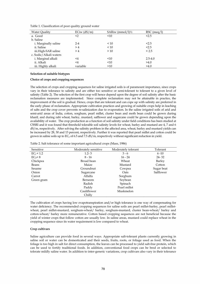
78

Table 1. Classification of poor quality ground water

Water Quality ECiw (dS/m) SARiw (mmol/l)½ RSC (meq/l) a. Good <2 <10 <2.5 b. Saline i. Marginally saline 2-4 < 10 <2.5 ii. Saline > 4 < 10 <2.5 iii.High-SAR saline > 4 > 10 < 2.5 c. Sodic/Alkali waters i. Marginal alkali <4 <10 2.5-4.0 ii. Alkali <4 <10 >4.0 iii. Highly alkali variable >10 >4.0

Selection of suitable biotypes

Choice of crops and cropping sequences The selection of crops and cropping sequences for saline irrigated soils is of paramount importance, since crops vary in their tolerance to salinity and are either too sensitive or semi-tolerant to tolerant to a given level of salinity (Table 2). The selection of the first crop will hence depend upon the degree of soil salinity after the basic reclamation measures are implemented. Since complete reclamation may not be attainable in practice, the improvement of the soil is gradual. Hence, crops that are tolerant and can cope up with salinity are preferred in the early phase of reclamation. Appropriate cultivation practices and growing of suitable crops help in leaching of salts and the crop cover prevents re-salinization due to evaporation. In the saline irrigated soils of arid and semi-arid areas of India, cotton, sorghum, pearl millet, cluster bean and moth bean could be grown during kharif, and during rabi wheat, barley, mustard, safflower and sugarcane could be grown depending upon the availability of water. The crop production as a function of soil salinity under field conditions has been studied at CSSRI and it was found that threshold tolerable soil salinity levels for wheat, barley and mustard are 4, 7 and 6 dS/m, respectively. After solving the salinity problem in the affected area, wheat, barley and mustard yields can be increased by 28, 30 and 13 percent, respectively. Further it was reported that pearl millet and cotton could be grown in saline soils up to ECe of 6.5 and 7.5 dS/m, respectively without significant reduction in yield. Table 2. Salt tolerance of some important agricultural crops (Mass, 1986)

Sensitive Moderately sensitive Moderately tolerant Tolerant ECt < 1.2 EC0< 8

1.2- 3 8 - 16

3 - 6 16 - 24

6 -10 24- 32

Chickpea Broad bean Wheat Barley Beans Maize Mustard Cotton Sesame Groundnut Cowpea Sugar beat Onion Sugarcane Oats Safflower Carrot Alfalfa Sorghum Green gram Berseem Soybean Radish Spinach Paddy Pearl millet Cauliflower Muskmelon Chilly

The cultivation of crops having low evapotranspiration and/or high tolerance is one way of compensating for water deficiency. The recommended cropping sequences for saline soils are pearl millet-barley, pearl millet-wheat, pearl millet-mustard, sorghum-wheat/ barley, sorghum-mustard, cluster bean-wheat/ barley and cotton-wheat/ barley more remunerative. Cotton based cropping sequences are not beneficial because the yield of winter crops that follow cotton are usually low. In saline areas, mustard could replace wheat in the cropping sequence since its water requirement is low compared to wheat. Crop cultivars Saline agriculture can provide food in several ways. Appropriate salt-tolerant plants currently growing in saline soil or water can be domesticated and their seeds, fruits, roots, or foliage used as food. When the foliage is too high in salt for direct consumption, the leaves can be processed to yield salt-free protein, which can be used to fortify traditional foods. In addition, conventional food crops can be bred or selected to tolerate mildly saline water. In addition to inter-generic variations, crop cultivars also vary in their tolerance

79

to salinity. Such cultivars (Table 3) have been identified on their rating for high yield potential, salt tolerance and stability under saline environments. Table 3. Promising Cultivars for saline and alkaline environments

Crop Saline environment Alkali environment Wheat Raj 2325, Raj 2560, Raj 3077, WH 157 KRL1-4, KRL19, Raj 3077, HI1077, KRL 210,

KRL 213 P. millet MH269, 331, 427, HHB-60 MH 269, 280, 427, HHB 392 Mustard CS416,CS330,-1, Pusa Bold CS15, CS52, Varuna, DIRA 336, CS 54, CS 56 Cotton DHY 286, CPD 404, G 17060, GA, JK276-10-5,

GDH 9 HY6, Sarvottam, LRA 5166

Safflower HUS 305, A-1, Bhima Manjira, APRR3, A300 Sorghum SPV-475, 881, 678, 669, CSH 11 SPV 475, 1010, CSH 1, 11, 14 Barley Ratna, RL345, RD103, 137, K169 DL4, 106, 120, DHS 12 Paddy CSR 30, CSR 36 CSR 10, CSR 13, CSR 23, CSR 30, CSR 36, Tree species In conditions where crop production with saline water use is neither feasible nor economical, there such water can be used to raise tree species especially on lands those are already degraded. The preferred choice of species should be Azadirachta indica, Acacia nilotica, A. tortilis, A. farnesiana, Cassia siamea, Eucaluyptus teretecornis, Feronia limonia, Prosopis juliflora, P. cineraria, Pithecellobium dulce, Salvadora persica, S. oleoides, Tamarix etc. Medicinal plants Some medicinal plants like Isabgol (Plantag ovata), Aloe and Kalmeg have also been found promising alternative to arable crops under saline irrigation conditions. Improved agronomic practices Establishing a good crop stand in saline irrigated soils is a challenging task. Unlike normal soils, the agronomic practices for crop production in saline irrigated soils are different. An ideal package of cultural practices besides soil fertility and irrigation water management can ensure a good crop stand vis-à-vis good yield. Pre-sowing irrigation In saline soils, salt often accumulate in the top few centimeters of the soil during non-crop periods. Where high water table exists, fallowing may result in excessive salt accumulation in the root zone particularly in arid and semi-arid regions. Under these conditions both germination and yields are adversely affected. A heavy pre-sowing irrigation to leach the accumulated salts from the root zone is very useful and essential to improve germination and early growth. Wherever available, pre-sowing irrigation should be given with good quality canal water. Deep tillage and inversion helps to reduce salinity hazard. Seed rate and spacing Due to inhospitable soil environment, germination is adversely affected. Mortality of young seedlings and poor tillering of the crops are common in saline soils. The plant growth is hindered compared to normal soils. Higher seed rate and closer spacing are advisable to counter these effects. For cotton, pearl millet, sorghum, wheat, barley and mustard 25% higher over the recommended seed rate for normal soils ensures good crop stand. In case of transplanted crops, the number of seedlings per hill should be increased. Priming of seeds/seedling The chemical treatment of seeds and seedlings has been reported to induce salt tolerance. In a field experiment on saline soils (ECe 12 dS/m), irrigated with saline water (ECiw 10.5 dS/m), the highest yield of wheat was obtained when seeds were pre soaked in 3 percent sodium sulphate solution.

80

Practices for sowing/planting Sowing/planting practices can often be modified to obtain a more favourable salt distribution in relation to seed location or growing roots. Since salt tends to accumulate on the ridges under furrow method of irrigation, furrow planting may help to obtain better crop stand and yield under saline conditions. The sowing of sugar beet on one side of the ridge half way between top and bottom, opposite to the sun direction gave significantly higher yield than flat and ridge sowing. The salt concentration in the root zone under this method of sowing was comparatively less owing to more accumulation of salts on southern face of the ridge due to direct and intensive solar radiation on this face. Similarly in case of sugarcane, trench method of planting gave significantly higher yield than flat planting attributable to low concentration of salts, as salts move to the top of the adjoining ridges. Moreover, the seeds should be sown in lines at an optimum depth with bullock or tractor driven seed drills. Seed-cum-fertilizer drill should be preferred to ensure uniform placement of seeds and fertilizers at the optimum depth and early emergence of seedlings. If seed drill is not available, sowing should be done by kera or pora method. Residue management Crop residue at the soil surface reduces evaporative water losses, thereby limiting the upward movement of salt (from shallow, saline groundwater) into the root zone. Evaporation and thus, salt accumulation, tends to be greater in bare soils. Fields need to have 30 percent to 50 percent residue cover to reduce evaporation significantly. Under crop residue, soils remain wetter, allowing fall or winter precipitation to be more effective in leaching salts, particularly from the surface soil layers where damage to crop seedlings is most likely to occur. Plastic mulches used with drip irrigation effectively reduce salt concentration from evaporation. Sub-surface drip irrigation pushes salts to the edge of the soil wetting front, reducing harmful effects on seedlings and plant roots. Improved water management In saline soils, evapotranspiration needs of crops are modified by the presence of soluble salts. The water availability decreases with increasing salinity of the soil. In this case both matric potential and osmotic potential must be considered while deciding irrigation scheduling in crops. Light and frequent irrigations have to be adopted to keep the soil-water potential at low levels. Successful operation of field application must supply water to the plants at the right time in appropriate quantity and quality with minimum waste and at the place where the plants need it for optimum growth. On-farm water management technology includes proper land leveling and shaping, efficient design and layout of irrigation methods, scientific scheduling of irrigation under both adequate and deficient water supply conditions, irrigation management under high water table depths and crop planning for optimum water use. The guidelines for using saline water to field crops are presented in Table 4. Table 4. Guidelines for using saline irrigation water (RSC < 2.5 meq/1)

Soil texture (% clay)

Crop tolerance Upper limits of ECiw (dS/m) in rainfall regions 350 mm 350-550 mm 550-750 mm

Fine (> 30) S 1.0 1.0 1.5 ST 1.5 2.0 3.0 T 2.0 3.0 4.5

Moderately Fine (20-30)

S 1.5 2.0 2.5 ST 2.0 3.0 4.5 T 4.0 6.0 8.0

Moderately Coarse (10-20)

S 2.0 2.5 3.0 ST 4.0 6.0 8.0 T 6.0 8.0 10.0

Coarse (< 10)

S - - 3.0 3.0 ST 6.0 7.5 9.0 T 8.0 10.0 12.5

S, ST and T denote sensitive, semi-tolerant and tolerant crops. Laser land leveling Undulated soil surface influences the farming operations, energy use, aeration, crop stand and yield mainly through nutrient-water interactions. Laser land leveling, the process of smoothening the land surface within + 2 mm from its average elevation using laser equipped drag scrapper is one of the few mechanical inputs in intensively cultivated irrigated farming, that meets the objectives of achieving a better crop stand, save

81

irrigation water, improve the input use efficiencies and uniform distribution of salts on the soil surface to reduce the patchy growth. The general, practices of land leveling used by the farmers in India is either through use of plankers drawn by draft animals or by small tractors. But, these leveling practices are not so perfect even after best effort for leveling which results in less input use efficiencies and low yield at the cost of more water. Land leveling is a precursor to good agronomic, soil and crop management practices and the levelness of the land surface has significant influence on all the farming operations including salt distribution. Precision land leveling is one of the few mechanical inputs in intensively cultivated irrigated farming that meets the twin objectives of achieving a better crop stand, save irrigation water and improves the input use efficiencies. Irrigation methods Selection of suitable irrigation method is of vital significance to efficient operation of an irrigation project. The selected method should aim at regulating soil moisture and meeting the crop requirement with a minimum potential of creating drainage or salinity problem without any adverse effect on soil or crop. The irrigation methods are generally of three types, surface, subsurface and sprinklers/drip. Surface method includes free flooding, check basin, border strip, furrows and corrugations. The subsurface method is used only under specialized conditions and therefore, the choice is limited to the surface and sprinklers/drip. Drip method of irrigation is relatively a recent development. Leaching of saline soil with irrigation water is reported to be more efficient when the soil is maintained in unsaturated condition and the rate of water flow is kept relatively slow. Therefore, flood method of irrigation is relatively more inferior to sprinkler and trickle methods in leaching of saline soils. The drip method of irrigation is also suitable for saline water irrigation and helps in maintaining a zone of low salt concentration and higher moisture content resulting in favorable condition for crop growth. Water application managements In addition to leaching salt below the root zone, salts can also be moved to areas away from the primary root zone with certain crop bedding and surface irrigation systems. Figures 1 to 3 illustrates several ways to manage salt accumulation in this manner. The goal is to ensure the zones of salt accumulation stay away from germinating seeds and plant roots. Irrigation uniformity is essential with this method. Without uniform distribution of water, salts will build up in areas where the germinating seeds and seedling plants will experience growth reduction and possibly death. Modifications in seedbed e.g. sowing near the bottom of the furrows on both sides of the ridges and applying irrigation in alternate row and to seed on the north-east side of the ridges, is recommended. For the larger seeded crops, the seeds can be planted in the furrows. The furrow irrigation and bed planting system (FIRB) has been found better than conventional planting in cotton /pearl millet –wheat rotations. Adoption of measures for better intake of rainwater (tillage to open up soil) and its conservation in soil via checking unproductive evaporation losses (soil/straw mulching) is recommended during monsoon season (Fig 1)

Fig 1. Bed planting system (FIRB) of wheat cultivation and salt distribution in the system

Alternate furrow irrigation may be desired for single-row bed systems. This is accomplished by irrigating every other furrow and leaving alternating furrows dry. Salts are pushed across the bed from the irrigated side of the furrow to the dry side. Care is needed to ensure that enough water is applied to wet all the way across the bed to prevent build up in the planted area. This method of salinity management can still result in plant injury if large amounts of natural rainfall fill the normally dry furrows and push salts back across the bed toward the plants. This phenomenon also occurs if the normally dry furrows are accidentally irrigated.

82

Fig. 2. Salt management in single-row bed systems. Uniform, healthy plants with alternate furrow irrigation (salt accumulates in the dry furrows).

Irregular growth due to variable accumulation of salt (plants may overcome this situation if roots can grow out of the saline area).

Double-row bed systems require uniform wetting toward the middle of the bed. This leaves the sides and shoulders of the bed relatively free from injurious levels of salinity. Without uniform applications of water (one furrow receiving more or less than another), salts accumulate closer to one side of the bed. Periodic leaching of salts down from the soil surface and below the root zone may still be required to ensure the beds are not eventually salted out.

Fig. 3. Salt management in double-row bed system. Good uniformity: salts accumulate in the center of the bed and away from plants.

Poor uniformity: salts accumulate toward edge of bed near one row.

Irrigation scheduling The important concepts that are adopted in scheduling irrigation are (i) depth interval (ii) soil moisture depletion (iii) crop growth stage (iv) plant symptoms and (v) climate. The time, frequency and quantity of irrigation depend largely on water requirement of crops, climatic conditions, and soil characteristics including texture, infiltration rate, moisture- tension relationship, irrigation methods, water quality and water table. Sorghum, pearl millet, cotton, guar, moth, wheat, barely and mustard cannot tolerate standing water and also relatively wet moisture regime whereas linseed and sugar beet will perform better with such a regime. Enough moisture should be present at the time of flowering and seed development stage. Proper scheduling of irrigation if water table remains high within certain limits and underground water is of good quality could effect substantial saving in irrigation water. The depths of critical water table, beyond which the yield are reduced significantly, depend upon the crop, water quality and soil type. Many crops can be grown without irrigation if water table remains within a specified depth provided groundwater is of good quality. A proper understanding of soil-water-plant-climate relationship under different conditions is essential for deciding the most appropriate irrigation practices. Despite irrigation water is costly; water management has been neglected in India, thereby resulting in widespread problems of water logging and soil salinity. Urgent steps are needed to prevent all avoidable water losses and to achieve most efficient and economic use of water resources

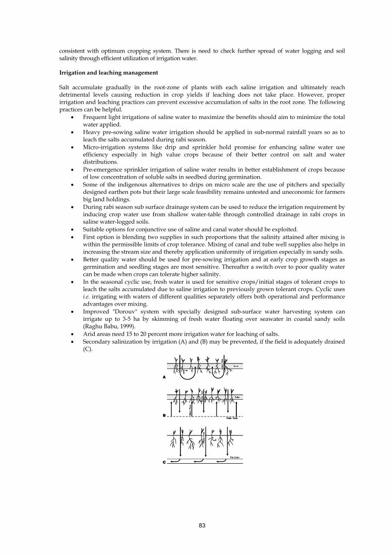
83

consistent with optimum cropping system. There is need to check further spread of water logging and soil salinity through efficient utilization of irrigation water. Irrigation and leaching management Salt accumulate gradually in the root-zone of plants with each saline irrigation and ultimately reach detrimental levels causing reduction in crop yields if leaching does not take place. However, proper irrigation and leaching practices can prevent excessive accumulation of salts in the root zone. The following practices can be helpful.

• Frequent light irrigations of saline water to maximize the benefits should aim to minimize the total water applied.

• Heavy pre-sowing saline water irrigation should be applied in sub-normal rainfall years so as to leach the salts accumulated during rabi season.

• Micro-irrigation systems like drip and sprinkler hold promise for enhancing saline water use efficiency especially in high value crops because of their better control on salt and water distributions.

• Pre-emergence sprinkler irrigation of saline water results in better establishment of crops because of low concentration of soluble salts in seedbed during germination.

• Some of the indigenous alternatives to drips on micro scale are the use of pitchers and specially designed earthen pots but their large scale feasibility remains untested and uneconomic for farmers big land holdings.

• During rabi season sub surface drainage system can be used to reduce the irrigation requirement by inducing crop water use from shallow water-table through controlled drainage in rabi crops in saline water-logged soils.

• Suitable options for conjunctive use of saline and canal water should be exploited. • First option is blending two supplies in such proportions that the salinity attained after mixing is

within the permissible limits of crop tolerance. Mixing of canal and tube well supplies also helps in increasing the stream size and thereby application uniformity of irrigation especially in sandy soils.

• Better quality water should be used for pre-sowing irrigation and at early crop growth stages as germination and seedling stages are most sensitive. Thereafter a switch over to poor quality water can be made when crops can tolerate higher salinity.

• In the seasonal cyclic use, fresh water is used for sensitive crops/initial stages of tolerant crops to leach the salts accumulated due to saline irrigation to previously grown tolerant crops. Cyclic uses i.e. irrigating with waters of different qualities separately offers both operational and performance advantages over mixing.

• Improved "Dorouv" system with specially designed sub-surface water harvesting system can irrigate up to 3-5 ha by skimming of fresh water floating over seawater in coastal sandy soils (Raghu Babu, 1999).

• Arid areas need 15 to 20 percent more irrigation water for leaching of salts. • Secondary salinization by irrigation (A) and (B) may be prevented, if the field is adequately drained

(C).

84

Improved fertilizer management At a given level of salinity, growth and yields of crops are depressed more when crop nutrition is disturbed than when it is normal. The salt affected soils are often poor in most of the essential plant nutrients owing to lack of vegetation and low organic matter content. Nitrogen deficiency is widespread in saline soils and a large fraction of the applied nitrogen is lost in gaseous forms under high soil salinity. Availability of phosphorus increases up to a moderate level of salinity but thereafter it decreases. The accumulated salts in saline soils can affect the nutrient availability for plants in following ways: by changing the forms in which the nutrients are present in soils; by increasing the losses through leaching when the saline soils are leached heavily or as in nitrogen through denitrification or by precipitation in soils; through interactive effects of cations and anions; and through the effects of complementary (non-nutrient) ions on nutrient uptake. Organic manures The use of manures and fertilizers is very important in sodic water irrigated soils. Application of the organic manures, besides adding plant nutrients, brings out improvement in the chemical, physical and biological properties of the soil. Increased crop growth resulting from the addition of manures tends to promote soil aggregation, reduces crust formation and causes rapid increase in the biological activity of the soil. Application of the FYM or compost or green manures also improved soil physical, chemical and biological properties. Amongst the several green manuring crops, dhaincha has been found to be the most efficacious in alkali soils. Field studies revealed that best results were obtained when rice was transplanted immediately after the burial of the dhaincha green manure crop. It was found that green manuring with dhaincha during summer produced rice yield as much as 80 kg N ha-1. Subsequent studies showed that incorporation of 60 days old dhaincha turns about 60 kg N ha-1. FYM and other organic materials have not only the nutritive value, but play an important role in structural improvements. This further influences leaching of salts and reduce their accumulation in the root zone. The other advantages of these materials in saline water irrigated soils are in terms of reducing the volatilization losses and enhancing nitrogen-use efficiency and the retention of nutrients in organic forms for longer periods also guards against their leaching and other losses. Therefore, the addition of FYM and other organic/green manure should be made to the maximum possible extent. Experimental evidences at CSSRI, Karnal showed that at a given salinity level, increasing application of organic materials improved yields of all the field crops. However, when salinity of the irrigation water was higher, the percent response was reduced when referenced to yields where no organics were applied. It seems that addition of organic materials temporarily immobilize the NH4 - N and subsequently release the organically bound N to crops during the growth season. Increased responses to N fertilizers in the presence of organic materials suggest its role in reducing the volatilization losses and enhance the N-use efficiency under saline environment. A combination of organic and inorganic sources saved N or 50% in rabi and 25% in kharif crops. Nitrogen management The Indian soils are mostly deficient in nitrogen, which need to be supplemented through fertilizer sources. The nitrogen requirement of crops is higher in saline soils than in normal soils. High concentration of salts (KCl or K2SO4 ) inhibits nitrification and resultant NH4-N accumulation. The plants, which absorb N only as NH3-N, would show nitrogen deficiency even if nitrogen is present in the soil. Field experiments at CSSRI, Karnal on saline soils indicated significant response of wheat, barley, mustard, pearl millet and cotton up to 160, 120, 100, 120 and 80 kg N ha-1, respectively. Nitrogenous fertilizers should be applied in split doses to reduce nitrogen losses through volatilization and denitrification. The required quantity of phosphorus and potash along with first dose of nitrogen (one third for pearl millet, wheat and barley and half for cotton and mustard) should be applied at or before sowing. The remaining quantity of nitrogen should be applied in two equal splits at first and second irrigation i.e. 25 and 45 days after sowing in pearl millet, wheat and barley and in one dose in cotton (60 days after sowing) and mustard (30 days after sowing). Under limited water supply conditions, nitrogen in wheat and barley should be applied in two equal doses at sowing and during first irrigation. Urea is by far the most widely used N source for crops. Urea is first hydrolysed to ammonia and carbon dioxide by the enzyme urease and the process has the most commonly expressed disadvantage of loss of N via NH3- volatilization. (Kumar et al., 1995; 2000). Following the application of N through inorganic fertilizer sources, there is a sudden burst in microbial activity and a large pool of NH4 + is generated. Thus, ammonia volatilization is extensive in salt affected soils which lead to low N-use efficiency by crops. Additional doses of nitrogenous fertilizers are recommended to compensate for volatilization losses occurring under saline environments. Proper splitting of fertilizer N doses so as to meet crop demands, deep incorporation, slow release N-fertilizers, application of urease inhibitors and use of organic-N sources have all been reported to

85

increase N-use efficiency by reducing the N-losses. Interactions between fertilizers and salinity have been studied at large. However, the evaluation of the concept of alleviating salinity stress through enhanced fertility brings out that such a strategy of additional application of fertilizer nitrogen to reduce/overcome the adverse effect of salts may not pay off well. In general, when salinity is not a yield limiting factor, the applied nitrogenous fertilizers will increase the yield of crops, proportionately more than when the salinity become the limiting factor. (Dayal et al., 1994; Swarup and Yaduvanshi, 2004). A better strategy for improving N-use efficiency therefore, seems to be to substitute a part of inorganic fertilizer requirements through organic materials. Phosphorus management On the other hand, increasing the level of phosphorus over the recommended dose seemed to mitigate the adverse affects of salinity. Type of salinity has also been observed to influence the response of crops to phosphorus application. Under saline condition, nearly 50 per cent more phosphorus is required than the recommended dose under normal conditions when the soil is low in available phosphorus. Application of phosphorus helps in increasing the yields of crops in saline soils by directly providing phosphorus or by decreasing the absorption of toxic elements like fluoride and chloride. It was observed that yields of wheat and mustard increased significantly with the application of 13 kg P ha-1 as compared to control with saline water irrigation. Soils irrigated with chloride rich waters respond to higher phosphate application, because the chloride ions reduce availability of soil phosphorus to plants. For sulphate rich waters, no additional application of phosphate fertilizers is required and the dose recommended under normal conditions may be applied. When wheat and barley crops were irrigated with chloride dominated waters, the yield response to phosphate application was higher as compared to sulphate dominated waters. Results show the application of phosphatic fertilizers most likely will improve the threshold limits of crops to the use of chloride dominated saline waters (Manchanda et al., 1982; Chauhan et al., 1991). Probably rice with a shallow root system fails to make use of higher P status of lower soil depths unlike wheat, which is able to tap P from lower depths. Thus sub-soil fertility plays an important role in P nutrition of crops with deeper root system relative to rice. The generalization of results with fertilizer use under saline conditions seems difficult but it can be stated that in most cases moderate levels of salinity can perhaps be compensated by increased fertilizer doses so long salinity levels are not excessively high and the crops under consideration are salt sensitive. Potassium management Saline soils are generally medium to high in available potassium but plants grown under high salinity may show K deficiency due to antagonistic effect of sodium and calcium on potassium absorption and or disturbed sodium/potassium ratio. Under such conditions application of potassium fertilizer might increase yield. On moderately saline soils, application of potassic fertilizers may increase the crop yields either by directly supplying K or by excluding the uptake of Na, Ca and Mg. However, under high salinity conditions it is difficult to effectively exclude Na from the plant by use of potassic fertilizers. A judicious application of bulky organic manures and chemical fertilizers would be inevitable to ensure stable crop yield. Micronutrient management In general, micronutrient (Fe, Mn, Cu and Zn) deficiencies have not been widely reported in saline soils. For micro-nutrients such as zinc, the recommended doses based on soil test values should be applied. Zinc deficiency has been reported in alkali soil and the crop responds favorably to its application. In alkali soils, application of zinc significantly increases the yield of rice and berseem fodder as compared to no zinc application. Basal application of 20-25 kg zinc sulphate ha-1 only to rice crop (first crop) was enough. After 3-4 years when the alkali status is reduced, its application may not be necessary. Conclusions From the foregoing discussion, it is inferred that selection of crops and adoption of the package of management practices developed with scientific validation, can only ensure successful crop production in saline irrigated soils. It is only then that the reclamation of salt affected soils may be made more attractive to the farming community. Since the salt affected soils vary considerably in their nature and characteristics, it is imperative that only location specific management practices are developed and adopted.

86

Suggested Readings Chauhan, C.P.S., Singh, R.B., Minhas, P.S. , Agnihotri, A.K. and Gupta, R.K. 1991. Response of wheat to

irrigation with saline waters varying in ionic constituents and phosphorous application. Agricultural Water Management. 20: 223-231.

Dayal, B., Minhas, P.S., Chauhan, C.P.S. and Gupta, R.K. 1994. Effect of supplementary saline irrigation and applied Nitrogen on performance of dry land mustard (Brassica Juncea L.) Experimental Agriculture. 341: 423-428.

Kumar, D., Swarup, A. and Kumar, V. 1995. Effect of rates and methods of Urea-N application and presubmergence period on ammonia volatilization losses from rice fields in a sodic soil. Journal of Agricultural Science (Cambridge), 125: 95-98.

Kumar, D., Swarup, A. and Kumar, V. 2000. Effect of temperature on kinetics of urea hydrolysis and ammonia volatilization in submerged alkali soils. Fertilizer News 45(11): 57-63.

Manchanda, H.R., Verma, S.L. and Khanna, S.S. 1982. Identification of some factors for use of sodic waters with high residual sodium carbonate. Journal of Indian Society of Soil Science 30: 353-360.

Mass E.V. 1986. Salt tolerance of plants, Applied Agricultural Research 1: 12–26. Raghu Babu, M., Prasad, P. R. K., Subbaiah, G.V. Khan, M. and Minhas, P. S. 1999. Subsurface Fresh Water

Skimming System; Improved Doruvu Technology, Bulletin No. 1/99, 19p. Central Soil Salinity Research Institute, Kamal.

Swarup, A. and Yaduvanshi, N.P.S. 2004. Response of ice and wheat to organic and inorganic fertilizers and soil amendment under sodic water irrigated conditions. IRRN 29(1): 49-51.

87

Gypsum/Amendment Requirement in Sodic/Saline Water – A Practical Assessment P. Dey Central Soil Salinity Research Institute, Karnal -132 001 (Haryana), India Water quality vis-à-vis sources Four hazards such as salinity, sodicity, alkalinity and specific ion toxicity hazard (fluoride, nitrate and boron) for irrigation and public health are determined from water quality parameters. Salinity hazard on the basis of total concentration of soluble salts is the single most important criteria used for determining quality of irrigation water. It is measured in terms of electrical conductivity (EC) in deciSiemen per metre (dS/m). Water which may be suitable for irrigation on the basis of EC may not be suitable if the concentration of sodium is high and leads to sodicity hazard to soil. Sodicity hazard is measured in terms of SAR (sodium adsorption ratio) of the water

2)( MgCa

NaSAR+

=

Where, ions in the equations are expressed as milli equivalent per litre (meq/l). Alkalinity hazard to soils is expected when irrigation water containing sum of bicarbonate and carbonate higher than the sum of calcium and magnesium ions. It is measured in terms of RSC (residual sodium carbonate). It leads to development of alkali soils upon long-term irrigation. Specific ion toxicity hazard is assessed for individual ion and is considered for fluoride, nitrate and boron ions of interest to agriculture and public health. )()( 33 MgCaCOHCORSC +−+= Where, ions in the equations are expressed as milli equivalent per litre (meq/l). Rainwater is the purest form of water having lowest salt content. Generally, the quality of rainwater varies widely and is dependent on the distance from the sea. Most of the river and spring waters in the country under natural conditions contain bicarbonate and sulphate, and calcium and sodium as the predominant cations and anions, respectively. These ions tend to precipitate on evaporation in the quantities of one third to one half of the total salts as calcium carbonate. This, however, leads to decrease in actual salinity, but causes alkalization in due course of time. In north Indian rivers, calcium, magnesium and bicarbonate are dominant ions whereas in south Indian rivers, sodium dominates over calcium and magnesium ions. EC and RSC values of south Indian river waters along with Yamuna river water are relatively higher. The waters from the Tungbhadra and Cauvery rivers in Tamil Nadu are relatively more alkaline and contain RSC up to 2 meq/l. Similar is the case with waters of the rivers draining in the Rann of Kuchchh. The water quality may further deteriorate on course due to pollution from the industrial and sewage waters. Canal waters originating from the rivers or their reservoirs represent the quality of parent rivers unless contaminated on course. Therefore, canal waters are usually as good as river waters. Canal waters in Uttar Pradesh and Haryana have low EC (< 0.5 dS/m) and are free from SAR, RSC or toxic elements whereas canal waters in Rajasthan are of good quality with pH, EC, SAR and RSC as 7.8, 0.4, 6.0 and 1.36, respectively. On conversely, EC of canal waters in the Sunderban area of West Bengal varies from 17 to 26 dS/m and is not suitable for irrigation. However, this is due to the proximity to the sea coast. Tanks form an important source of irrigation in rainfed agriculture in southern India particularly and their quality is variable. Some tanks contain good quality waters which are suitable for irrigation whereas others contain saline or alkaline waters. The quality of inland lake waters varies from most good to most saline. Groundwater occurs in regionally extensive aquifers constituting over 97% of earth’s good quality water. According to an estimate by CGWB, only 58% of available ground water resources in the country have so far been developed, being highest of 170% in Delhi. The salt content of groundwater depends on the source of water and path/course over which it travelled. Mineralization of groundwater is governed by laws of dissolution. Changes in the salt content in the recharge process result from reduction in base exchange medium, transpiration, evaporation, and precipitation. While groundwater is flowing, soil and rocks act as ion exchange and cations in the water reach equilibrium with the soil cations. General salt content increases due to evapotranspiration or dissolution and is mostly affected by the climate. While deep groundwater does not have seasonal fluctuation of salt content, the salt content of shallow groundwater changes as a function of evaporation, rainfall, drainage and irrigation practices. The groundwater over major portion of the country is of good quality. The marginal and poor quality groundwater constitutes a greater part in the states of arid and semi arid regions of the country. Estimate of groundwater in the states of Rajasthan,

88

Haryana and Uttar Pradesh reveals that 25 to 84% waters are of marginal or poor quality. Moderate to high salinity groundwater also occurs in the northern Karnataka, eastern Andhra Pradesh, and northern and central parts of Tamil Nadu. Some groundwater could be more saline than the sea water. Categorization of groundwater Groundwater has varying characteristics depending upon its first use and/or the formation it has passed through. As such, to characterize the groundwater is the first step to decide interventions on electrical conductivity (EC), Sodium Adsorption Ratio (SAR) and Residual Sodium Carbonate (RSC), water has been categorized as good, saline, high SAR saline and alkali (Table 1). Water is also categorized as toxic based on the presence of some ions such as sodium, chlorine, boron, nitrate, iron, manganese, cadmium, lead, arsenic or other heavy metals etc. Moreover, groundwater is getting polluted in areas where high doses of chemicals are applied in agriculture. A study conducted in Ludhina district indicated that during the post monsoon periods, 35% of the water sampled had nitrogen (NO3-N) more than 15 mg/l. Concern on toxic waters has multiplied recently because pesticides and other cacogenic substance have been observed in groundwater of Punjab, Haryana and other states due to non-point sources of pollution. Table 1. Grouping of the marginal quality ground waters

Water quality ECiw

(DS/m) SARiw

(mmol/liter)1/2 RSC (meq/liter)

A. Good < 2 < 10 < 2.5

B. Saline 1. Marginally saline 2. Saline 3. High –SAR saline

2-4 >4 >4

< 10 < 10 > 10

< 2.5 < 2.5 < 2.5

C. Alkali water 1. Marginally alkali 2. Alkali 3. High-SAR alkali

. < 4 < 4 Variable

< 10 < 10 > 10

2.5-4.0 > 4.0 > 4.0

D. Toxic Water The toxic water has variable salinity, SAR and RSC but has excess of specific ions such as nitrate, boron, fluoride, chloride, sodium or heavy metals such as selenium, cadmium, lead and arsenic etc.

Water quality analysis Irrigation water, irrespective of its source, always contains some soluble salts. Continuous use of such water may affect crop growth and soil properties depending upon the quality and quantity of the salts present. Therefore, knowledge of the quality of water and its nutrient content is essential for judging its suitability for irrigation purposes and contribution to plant nutrient supply. In laboratory the water samples must be analyzed for decide the suitability of water for irrigation purposes. The following parameters are mainly determined besides specific ion toxicity related to B, Cl, Na and toxicity of heavy metals namely Cr, Cd, Ni and Hg:

• Electrical Conductivity • Sodium adsorption ratio (SAR) • Residual sodium carbonate (RSC) • Boron (B)

Electrical conductivity (EC) The electrical conductivity of irrigation water samples are measured by conductivity meter as per method given in the procedure of EC determination in soils saturated paste. Determination of conductivity of water: Rinse and fill the cell with the test water to be measured and its conductance is recorded. The specific conductance (dS/m) is calculated by using the equation: Lt = K C where, Lt is the electrical conductivity of the test water.

89

The temperature of the solution is taken into account in the calculation of the result. The electrical conductance of water increases approximately 2% per degree C. Electrical conductivity calculated at temperature (t) is corrected by multiplying it with temperature factor (ft). The values of ft are given in Annexure I. For example to convert values measured at 20°C to the values at 25°C, multiply by a factor of 1.112. For intermediate temperatures, linear relations between the two nearest values may be used. Based upon the total dissolved salt (mg/litre), the waters are classified as follows:

Good < 500 mg/l Marginal 500-1500 mg/l Brackish 1500-5000 mg/l Saline > 5000 mg/l Brine 35000 mg/l Bitter > 350000 mg/l

Sodium adsorption ratio (SAR) The sodium adsorption ratio is a Na concentration in meq/l to the square root of half the concentration of Ca and Mg in meq/l. Na+ SAR = [(Ca2+ + Mg2+)/2]0.5 where Na+, Ca2+ and Mg2+ are in meq/l Classification of poor quality water Water Quality ECiw (dS/m) SAR iw RSC (me/l) A. Good <2 <10 <2.5 B. Saline waters Marginal saline 2-4 <10 <2.5 Saline >4 <10 <2.5 High SAR saline >4 >10 <2.5 C. Alkali waters Marginal alkali <4 <10 2.5-4.0 Alkali <4 <10 >4.0 High alkali Variable >10 >4.0 Residual sodium carbonate (RSC) The residual sodium carbonate is the sum of concentration of carbonate plus bicarbonate in meq/l minus the concentration of calcium plus magnesium in meq/l. RSC = (CO32- + HCO3-) - (Ca2+ + Mg2+) The water sample has to be analyzed for the determination of the concentration of Na+, Ca2+, Mg2+ and CO32-

, HCO3- in meq/l to estimate SAR and RSC by way of assessing sodicity hazard. Laboratory procedure Sodium Principle: Sodium is readily excited in a flame and emits characteristic radiation of 589.6 nm wavelength producing an intense yellow light. The emitted light is passed through a sodium filter (yellow glass), the intensity of the emission may be measured photoelectrically and related to the concentration of sodium in the solution. Apparatus: Flame photometer with sodium filter Reagent:

1. Standard sodium solution, 1000 ppm stock solution. Dissolve 2.54 g of NaCl in water and makeup the final volume 1 litre.

2. Working standard solution containing 10, 20, 30, 40 and 50 ppm sodium. Take 5, 1, 2, 3, 4 and 5 ml of stock solution (1000 ppm) in to 100 ml measuring flasks and makeup the mark with distilled water.

Procedure: Sodium determine in water sample. Adjust flame photometer reading to 0 by atomizing distilled water or 0 ppm Na standard after placing Na filter opposite air-propane blue flame, and then atomize 20 ppm Na solution and adjust flame photometer reading to 100. Repeat atomization of 0 and 20 ppm Na

90

solution, and check the flame photometer reading. If necessary again adjust the flame photometer reading. Then atomize the intermediate Na standards. If flame photometer reading is found in the range of 0 to 100, and if range is higher 100, then water sample diluted 50 to 100 times and reading and corresponding dilution must be noted. Determine Na concentration (ppm), in diluted water sample by the following equation. Calculation: Reading water sample X times of dilution Na+ (meq/l) = 23 Calcium and Magnesium Principle: Calcium and magnesium react with Ethylene tetra acetic acid (versenate) at different pH values and form stable complexes. Sn, Cl, Zn, Mn and Fe may interfere in the determination of Ca and Mg. This interference may be prevented by using carbonate. In general, negligible amount of interfering elements are found in soil saturation extracts. In Ca estimation a known amount of soil extract is titrated with standard EDTA solution (0.01N) using murexide indicator in presence of NaOH at pH 12, the colour changes at end point from orange red to purple, while for Ca+Mg Eriochrome black T indicator is used in the presence of NH4OH+NH4Cl buffer at pH 10, the colour changes at end point from wine red to blue. Reagent:

1. Standard 0.01N calcium solution: Take 0.5 g of AR grade calcium carbonate and dissolve it in 10 ml of 3N HCl. Boil it to expel CO2 and then transfer into one litre volumetric flask and make the volume with distilled water.

2. Standard EDTA solution: Weigh 2 g of sodium salt of EDTA (Na-EDTA), dissolve in water in a beaker and then transfer to 1 litre volumetric flask and make the volume with distilled water.

3. Ammonium chloride-ammonium hydroxide buffer solution: Dissolve 67.5 g of ammonium chloride in 570 ml of concentrated ammonium hydroxide and then transfer to 1 litre volumetric flask and make the volume with distilled water.

4. Eriochrome black T indicator: Dissolve 0.5 g of EBT and 4.5 g of hydroxylamine hydrochloride in 100 ml of 95% ethanol.

Procedure: Pipette about 2-5 ml aliquot of water sample in 150 ml Erlenmeyer flask. Add 10 drops of ammonium chloride-ammonium hydroxide buffer and 4 drops of EBT indicator. Mixed and titrate the contents with 0.01N EDTA solution till the colour changes from wine red to blue and there should not remain any tinge of wine red colour. Calculation: Volume of EDTA used, ml X Normality of EDTA X 1000 Ca2+ + Mg2+ (meq/l) = Volume of aliquot taken, ml Carbonate and Bicarbonate Principle: Carbonate and bicarbonate in a solution can be determined by titrating the solution against standard acid using phenolphthalein and methyl orange/methyl red indicators respectively. When the colour of phenolphthalein discharged, it indicates half the neutralization of carbonate. At this stage methyl red indicator is added and the titration continued. When the colour changes from yellow to rose red, it is the end point for complete neutralization of bicarbonate. 2Na2CO3 + H2SO4 = 2NaHCO3 + Na2SO4

Phenolphthalein: pink Phenolphthalein: colourless 2NaHCO3 + H2SO4 = Na2SO4 + H2O + CO2 methyl red: yellow Methyl red: rose red Appearance of pink colour indicates the presence of carbonates. Apparatus: Pipette, porcelin dishes, glass road, wash bottle. Reagent:

1. Dissolve 0.25 g of Phenolphthalein indicator powder in 100 ml of 60% ethanol. 2. 0.01% methyl orange indicator 3. 0.01N Sulphuric acid: 2.8 ml of concentrated sulphuric acid into 500 ml distilled water. Dilute to 1

litre to get approximately 0.1N H2SO4. Dilute 100 ml of this solution to 1litre. Procedure: Carbonate: Take 2 ml of the water sample in a clean porcelain dish, add 1 drop of phenolphthalein indicator. If pink colour appears then carbonates are present. Titrate the solution against 0.01N H2SO4 till the pink colour disappears. Note the reading (A). Bicarbonate: Add 2-3 drops of methyl red indicator, yellow colour appears. Titrate against, 0.01N H2SO4 till rose red rose colour appears. Note the second reading (B).

91

Calculation: 2 A X Normality of H2SO4 X 1000 CO32- (meq/l) = Volume of aliquot taken (ml) where, A is final end point of disappearance of pink colour. (B - 2 A) X Normality of H2SO4 X 1000 HCO3- (meq/l) = Volume of aliquot taken (ml) where, B is final end point of change of colour from yellow to rose red. Boron Boron toxicity in waters usually has toxic level of B for many crops. The margin between deficiency and toxicity of B, particularly in irrigation water is too narrow and hence, require proper analysis for detection of the same. Principles: Azomethine-H method is usually adopted to determine B. The procedure is based on the formation of a stable coloured complex of H3BO3 in aqueous media at pH 5.1 which is independent of presence of wide variety of salts. The absorbance of coloured complex at 420 nm is proportional to that of B concentration. Apparatus

1. Spectrophotometer 2. Refrigerator 3. Water cooled reflux Condenser 4. Polypropylene test tubes

Regents: 1. Buffer solution: Dissolve 250 g ammonium acetate and 15 g disodium salt of EDTA in 400 ml

distilled water. Add 125 ml glacial acetic acid slowly and mix the content. 2. Standard B solution: Dissolve 0.286 g of boric acid in distilled water and adjust the volume to 1000

ml. One ml of this solution contains 50 µg B. Dilute 0.2, 0.5, 1.0, 2.0, 4.0, 6.0, 8.0, 10.0, 12.0, 16.0 and 20.0 ml of the 50 µg B solution to 100 ml volumetric flask with distilled water to have a series of standard solution containing 0.10, 0.25, 0.50, 1.0, 2.0, 3.0, 4.0, 5.0, 6.0, 8.0 and 10.0 µg B/ml standard solution. The solutions are used to prepare a calibration curve.

3. Azomethine-H reagent: Dissolve 0.45 g azomethine-H in 100 ml 1% ascorbic acid solution in polypropylene reagent bottle. The solution should be kept in refregerator and should be consumed within a week.

4. 0.01M CaCl2.2H2O solution: Dissolve 1.47 g of CaCl2.2H2O in distilled water and adjust the volume to 1000 ml.

Preparation of Standard Curve: Pipette 1 ml aliquot of each standard B solutions in a 10 ml polypropylene tube, add 2 ml buffer solution and mix thoroughly. Add 2 ml azomethine-H reagent, mix thoroughly. Run a blank simultaneously. After 30 minutes the absorbance of coloured solutions is read at 420 nm to prepare standard curve of absorbance versus B concentration. Estimation: Transfer 1 ml aliquot of the filtrate or water sample in 10 ml polypropylene tube, add 2 ml buffer solution and mix thoroughly. Add 2 ml azomethine-H reagent, mix thoroughly and after 30 minutes read the absorbance at 420 nm. The concentration is determined from the standard curve. Calculation: Soil: B (mg/kg) = µg of B in analyzed sample (read from standard curve) x 10 Water: B (mg/l) = µg of B in analyzed sample (read from standard curve) Water quality rating for boron Degree of problem Limit (mg B/l) Low hazard 1.0 Medium hazard 1.0-2.0 High hazard 2.0-4.0 Very high hazard >4.0 Precaution Boron free glasswares are very fragile besides being very costly and should be handled with extra care.

92

Physiological Mechanisms of Tolerance to Salinity and Sodicity Stresses S.K. Sharma Central Soil Salinity Research Institute, Karnal – 132 001 (Haryana), India Salinity and sodicity stresses are ever-present threats to crop yields, especially in countries where irrigation is an essential aid to agriculture. Plants growing under saline and sodic environment are invariably faced with the increased concentrations of toxic ions in their tissues resulting from increased uptake of ions mainly Na and Cl under salinity, and Na under sodicity. Although the tolerance of saline conditions by plants is variable, crop species are generally intolerant of one-third of the concentration of salts found in seawater. Salt

tolerance is complex genetically and physiologically with glycophytes and halophytes and relatively less tolerant crop plants showing a wide range of adaptations.

Glycophytes and halophytes Majority of plants are unable to tolerate saline and sodic conditions permanently. Depending upon their response to there stresses, plants have been categorized into glycophytes and halophytes. The term halophyte literally means salt plants, but is used specifically for plants that can grow in presence of high concentrations of sodium salts and may be described as native flora of saline soils. Examples of halophytes are Atriplex, Sueda, Salicornia and Artemesia species. On the other hand, the plants that can not grow in presence of salts are called Glycophytes or sweet plants. Almost all the crop species are glycophytes. Glycophytes have a selective advantage in non-saline soils over halophytes, because their growth rates are generally faster. The level of salinity, nature of salt responsible for salinization also has an important role to play in the growth and development of plants. Effect of salinity on plants Salts in the soil water may inhibit plant growth for the three reasons. First, the presence of salt in the soil solution reduces the ability of the plant to take up water, and this leads to reduction in the growth rate. This is referred to as the osmotic or water-deficit effect of salinity. Second, if the excessive amounts of salt enter the plant in the transpiration stream there will be injury to cells in the transpiring leaves and this may cause further reductions in growth. This is called the salt-specific or ion-toxicity effect of salinity (Greenway and Munns, 1980, Sharma and Gupta, 1986). Thirdly, it could be due to nutritional imbalance that may be caused by selective higher uptake of few elements while there may be depressed uptake of the others. Since the ions that are nutritionally important gets affected in this way, this effect is usually described as nutritional imbalance effect. As salinity is often caused by rising water tables, it can be accompanied by waterlogging. Waterlogging itself inhibits plant growth and also reduces the ability of the roots to exclude salt, thus increasing the uptake rate of salt and its accumulation in shoots. The definition of salt tolerance is usually the percent biomass production in saline soil relative to plants in non-saline soil, after growth for an extended period of time. For slow-growing, long-lived, or uncultivated species it is often difficult to assess the reduction in biomass production, so percent survival is often used. Variability in Salinity and Sodicity Tolerance in Crops and Species

The criterion of relative yield in saline and non-saline conditions has been widely used to describe salt tolerance or relative salt tolerance of crops. Evaluation of salt tolerance of crops, vegetables and fruit trees have been made by the US Salinity Laboratory (Fig. 1) and Central Soil Salinity Research Institute, Karnal (Tables 2, 3). If growth suppression is typically initiated at some threshold value of salinity, which varies with crop tolerance and external environmental factors which influence the need of the plant for water, especially the evaporative demand of the atmosphere (temperature, relative humidity, windspeed, etc.) and the water-supplying potential of the rootzone, and increases as salinity increases until the plant dies. The curve in fig. 1 shows that the salt tolerances of various crops could be expressed (after Maas and Hoffman 1977), in terms of relative yield (Yr), threshold salinity value (a), and percentage decrement value per unit increase of salinity in excess of the threshold (b); where soil salinity is expressed in terms of ECe, dS/m), as follows: Yr = 100 - b (ECe - a) where Yr- is the percentage of the yield of the crop grown under saline conditions relative to that obtained under non-saline, but otherwise comparable, conditions. This use of ECe to express the effect of salinity on yield implies that crops respond primarily to the osmotic potential of the soil

Cultivated crops can be categorized into sensitive, moderately-tolerant and tolerant species according to their specific salt tolerance (fig.1) and these ratings are different for saline soil, sodic soil and saline water irrigated

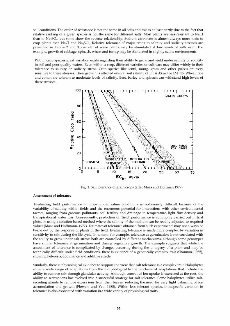
93

soil conditions. The order of resistance is not the same in all soils and this is at least partly due to the fact that relative ranking of a given species is not the same for different salts. Most plants are less resistant to NaCl than to Na2SO4, but some show the reverse relationship. Sodium carbonate is almost always more toxic to crop plants than NaCl and Na2SO4. Relative tolerance of major crops to salinity and sodicity stresses are presented in Tables 2 and 3. Growth of some plants may be stimulated at low levels of salts even. For example, growth of cabbage, spinach, wheat and turnip may be stimulated in slightly saline environments. Within crop species great variation exists regarding their ability to grow and yield under salinity or sodicity in soil and poor quality waters. Even within a crop, different varieties or cultivars may differ widely in their tolerance to salinity or sodicity stress. Crop species like lentil, mung, gram and other pulses are very sensitive to these stresses. Their growth is affected even at soil salinity of EC 4 dS m-1 or ESP 15. Wheat, rice and cotton are tolerant to moderate levels of salinity. Beet, barley and spinach can withstand high levels of these stresses.

Fig. 1. Salt tolerance of grain crops (after Maas and Hoffman 1977) Assessment of tolerance Evaluating field performance of crops under saline conditions is notoriously difficult because of the variability of salinity within fields and the enormous potential for interactions with other environmental factors, ranging from gaseous pollutants, soil fertility and drainage to temperature, light flux density and transpirational water loss. Consequently, prediction of ‘field’ performance is commonly carried out in trial plots, or using a solution-based method where the salinity of the medium can be readily adjusted to required values (Maas and Hoffmann, 1977). Estimates of tolerance obtained from such experiments may not always be

borne out by the response of plants in the field. Evaluating tolerance is made more complex by variation in sensitivity to salt during the life cycle. In tomato, for example, tolerance at germination is not correlated with the ability to grow under salt stress: both are controlled by different mechanisms, although some genotypes have similar tolerance at germination and during vegetative growth. The example suggests that while the assessment of tolerance is complicated by changes occurring during the ontogeny of a plant and may be technically difficult under field conditions, there is evidence of a genetically complex trait (Shannon, 1985), showing heterosis, dominance and additive effects.

Similarly, there is physiological evidence to support the view that salt tolerance is a complex trait. Halophytes show a wide range of adaptations from the morphological to the biochemical adaptations that include the ability to remove salt through glandular activity. Although control of ion uptake is exercized at the root, the ability to secrete ions has evolved into a successful strategy for salt tolerance. Some halophytes utilize salt-secreting glands to remove excess ions from their leaves, reducing the need for very tight balancing of ion accumulation and growth (Flowers and Yeo, 1988). Within less tolerant species, intraspecific variation in tolerance is also associated with variation in a wide variety of physiological traits.

94

Causes of the growth reduction under saline conditions The effects of a saline soil are two-fold: there are effects of the salt outside the roots, and there are effects of the salt taken up by plants. The salt in the soil solution (the “osmotic stress”) reduces leaf growth and to a lesser extent root growth, and decreases stomatal conductance and thereby photosynthesis (Munns, 1993). The rate at which new leaves are produced depends largely on the water potential of the soil solution, in the same way as for a drought-stressed plant. Salts themselves do not build-up in the growing tissues at concentrations that inhibit growth: meristematic tissues are fed largely by the phloem from which salt is effectively excluded, and rapidly elongating cells can accommodate the salt that arrives in the xylem within their expanding vacuoles. So, the salt taken up by the plant does not directly inhibit the growth of new leaves.

The salt within the plant enhances the senescence of old leaves. Continued transport of salt into transpiring leaves over a long period of time eventually results in very high Na+ and Cl- concentrations, and they die. The rate of leaf death is crucial for the survival of the plant. If new leaves are continually produced at a rate greater than that at which old leaves die, then there might be enough photosynthesising leaves for the plant to produce some flowers and seeds. However, if the rate of leaf death exceeds the rate at which new leaves are produced, then the plant may not survive to produce seed. For an annual plant there is a race against time to initiate flowers and form seeds, while the leaf area is still adequate to supply the necessary photosynthate. For perennial species, there is an opportunity to enter a state of dormancy, and thus survive the stress. The two responses occur sequentially, giving rise to a two-phase growth response to salinity. The first phase of growth reduction is quickly apparent, and is due to the salt outside the roots. It is essentially a water stress or osmotic phase, for which there is surprisingly little genotypic difference. Then there is a second phase of growth reduction, which takes time to develop, and results from internal injury. The two-phase growth response is illustrated in Fig. 2. The experiment was conducted with two genotypes with contrasting rates of Na+ uptake, and known differences in salt tolerance. Fig. 2 shows that during the first 3-4 weeks after the soil was salinised, there was a large growth reduction in both genotypes. This is called the 'Phase 1' response, and is due to the osmotic effect of the salt. Then after 4 weeks, the genotypes separated; the one with the low Na+ uptake rate continued to grow, although still at a reduced rate compared to the controls in non-saline solution, but the one with the high Na+ uptake rate produced little biomass and many individuals died. This is the 'Phase 2' response, and is due to genotypic differences in coping with the Na+ or Cl- ions in the soil, as distinct from the osmotic stress. Physiological mechanisms of plant Injury under salt and water stresses The interaction of salts with plant physiological processes is obviously complex. There are many salt species, many mechanisms, and many organs, tissues and cells involved. Reasons for the observed reduced growth and damage to tissues include:

1. Reduced water uptake and ‘physiological drought,’ 2. Injury to cell membranes, 3. Na+-K+ selectivity, 4. Ca2+- Na+ selectivity, transport and leakage, osmotic adjustment through solute accumulation in the

symplast, 5. Salt accumulation in the apoplast (cell wall) resulting in cell dehydration, 6. Damage to developed tissue, resulting in decreased photosynthetic surface and lack of sufficient

metabolites for growing tissue, 7. The cost of osmotic adjustment, compartmentation and exclusion, 8. Hormonal balance in the plant and 9. Nutrient deficiencies, especially N and K.

Under saline conditions, water deficit is usually experienced first, followed by toxicity effects, and then nutritional effects. However, the temporal separation of these effects and their relative severity are determined by genotype and environment. Plants growing under saline conditions are invariably faced with the increased concentrations of toxic ions in their tissues. Plants growing under saline conditions are invariably faced with the increased concentrations of toxic ions in their tissues. This results from increased uptake of ions like mainly Na and Cl under salinity, and Na under sodicity. The concentration of salts is higher in the sensitive crops than the resistant ones. In chickpea, salt

95

tolerance depends upon exclusion of Na+ and Cl- from the shoot; Na+ was more excluded than Cl- as Cl- concentrations were 2-4 times higher than Na (Sharma and Kumar, 1992; Sharma, 1997). In wheat, Na was more in the top than Cl and was more in the shoots of sensitive than the resistant genotype (Sharma, 1996) indicating that the concentrations of Na+ and Cl- determine their relative salt resistance. It is also true about a number of other crops like rice, wheat, barley and many other crops. There is a lot of evidence correlating reduced Na with salt tolerance (Greenway and Munns, 1980; Jeschke, 1984; Schachtman et al., 1991; Sharma, 1996).

In wheat, ion exclusion preferentially maintained lower Na+ and Cl- levels in the apical tissue, as the leaf to leaf gradient in Na+ and Cl- became steeper as the external salinity increased, although there were significant differences between sensitive and tolerant cultivars (Sharma, 1996). Correlation analysis on individual plants indicated that excluding Na+ at low salinity, and Na+ and Cl- at high salinity, were correlated significantly with growth performance, although it was clear that some other factors were also involved.

Although it is difficult to distinguish clearly whether the toxic effects are due to Na+ or Cl-, the data for chickpea indicated that injury was more due to Cl- than Na+. Chloride accumulation increased with longer duration of salt exposure as evidenced by the increased concentrations of Na+ and Cl- at the second and third sampling stages in the older plants. Decreasing rates of plant growth and increasing concentrations of ions with prolonged exposure to salinity suggested the failure of plants to adapt to salinity, more so in the salt sensitive genotype (CSG 8890).

Fig. 2. Two accessions of the diploid wheat progenitor Ae. tauschii grown in hydroponics in control solution (closed symbols) and in 150 mM NaCl (open symbols). Circles denote the tolerant accession, triangles the sensitive one. The arrow marks the time at which symptoms of salt injury could be seen on the sensitive accession; at that time the proportion of dead leaves was 10% for the sensitive and 1% for the tolerant accession (Munns et al., 1995).

Chickpea plants showed higher salt sensitivity despite negligible effects on their K+ concentrations. Chloride is the prevalent anion accompanying Na+ and K+ and its concentration was in the same range as the sum of Na+ and K+. Only a small number of experiments have attempted to determine the direct toxicity of Cl-, and their interpretation is not straightforward. There is sufficient evidence to be confident that salt tolerance is a multi-genic trait. Research on the physiology of salt tolerance also suggests that the overall trait is determined by a number of sub-traits any of which might, in turn, be determined by any number of genes. These sub-traits generally include an ability to minimize the net accumulation of sodium and/or chloride ions and to select potassium from a background of high sodium concentration. Physiological mechanisms of plant injury under salt and water stresses Plants differ markedly within and between species in their salt tolerance. Depending on the source of salinity and pattern of rainfall or irrigation in farmer’s fields, crop plants may experience salt stress transiently at

96

different stages of the growth cycle, or continuously throughout the season. The impact on yield depends on the timing, speed of onset, intensity and duration of the stress and stage of the crop. These deleterious effects may cause short and long-term responses. Short -term growth responses Earliest response of plants after exposure to salinity is reduction in leaf growth because of water deficit: the response is very rapid (within minutes, Matsuda and Riazi, 1981), and is usually proportional to the osmotic potential of the external solution, and is rapidly reversible (Munns et al 1981; Rawson and Munns, 1984). Plants exposed to salinity show immediate cessation of growth and loss in water status and may be followed by recovery if the stress is of a moderate level (Table 1 ). Plants may suffer severe injury and mortality if the stress is of a higher level. Therefore, it should be a standard practice when applying saline solutions to plants in pot culture to minimize osmotic shock by increasing salinity concentrations in gradual small increments over a period of several days unless the experiment is specifically aimed at determining the effects of sudden osmotic shock to the plants. Table 1. Changes in plant fresh, dry weights, leaf diffusive resistance (LDR), transpiration rates and leaf

water potential (LWP) of third fully expanded leave Days after salinization

Fresh weight (g)

Dry weight (g)

LDR (S/cm)

Transpiration (g/cm²/s)

LWP (-MPa)

Normal 47.8 8.2 1.7+0.2 11.7+2.1 0.8+0.2 2 43.3 8.7 15.8+2.2 1.2+0.3 1.8+0.3 4 53.2 9.0 6.0+0.6 5.1+1.6 1.6+0.2 6 57.4 9.6 5.3+0.6 7.0+1.1 1.4+0.2 9 66.9 12.1 3.7+0.4 7.9+1.0 1.4+0.2 Long -term growth responses In the longer- term, being weeks for a short-lived annual to months or years for long-lived species, prolonged transpiration will cause salts to build up in the leaves. Thus a specific effect of ions on leaves and parts will occur. In non-halophytes, the fully expanded leaves are adversely affected long before the young leaves, as salt concentrations at a given time of exposure to salinity are always higher in the oldest leaves, and the oldest leaves die long before the effects on younger leaves become apparent. The higher salt concentrations in the older leaves may result entirely from a product of time by transpiration rate (Greenway and Munns, 1980) or at least partly from an exclusion of specific ions from the xylem vessels supplying the younger leaves (Yeo and Flowers, 1982). Salt concentrations in individual leaves usually increase with time. Glycophytes show no signs of regulation of the salt concentration in their leaves unlike many halophytes which can maintain constant salt concentrations (Flowers and Yeo, 1986). Thus, for non-halophytes it is inevitable that ion concentrations will eventually build up in the older leaves, and they will die. The concentrations at which this occurs will depend upon the ability of the species to compartment the salts in the vacuole, and the time it takes to happen will depend mainly on the salinity level, the ability of the roots to exclude the salt, and the ambient conditions affecting the rate of transpiration. Salt build-up in the cytoplasm interferes with metabolism, and in cell wall causes loss of turgor and then excessive loss of water. Death of many older leaves limits productivity due to decreased photosynthetic leaf area. This results in the decline in the production of carbohydrate and ultimately production per plant falls below the levels that plants are not able to sustain growth.

These processes are not mutually exclusive, and may act separately or combined. Some may operate over a short term and others over a long term. Some play a more important role on certain crops, some on others. Because of the differences in the effect of salinity on various enzymes, cells and organs it is difficult to distinguish between the osmotic and ionic effects of salinity on various plant processes. The most common method available for distinguishing between secondary osmotic and primary salt injury is to compare the effects of isotonic solutions of salts with those of organic substances. Organic substances like mannitol, sugars and preferably polyethylene glycol (having molecular weights in the range of 6,000 to 10,000) are used.

97

Suggested Readings Flower, T.J. and Yeo, A.R. 1986. Ionic relations of plants under drought and salinity. Australian Journal of

Plant Physiology. 13: 75-91. Flowers, T.J. and Yeo, A.R. 1988. Ion relation of salt tolerance. In: Baker, D.A., Hall, J.L. Eds. Solute transport

in plant cells and tissues. Harlow: Longman Scientific and Technical. 392-413. Greenway H., Munns R. 1980. Mechanisms of salt tolerance in non-halophytes. Ann. Rev. Plant Physiol.

31:149-190. Jeschke, W.D. 1984. K+ - Na+ exchange at cellular membranes, intracellular compartmentation for crop

improvement. Eds. R.C. Staples and G.H. Toenissen. Pp 37-66, Jphn Wiley and Sons Inc. New York. Matsude, K. and Riazi, A. 1981. Stress induced osmotic adjustment in growing regions of barley leaves. Plant

Physiology. 68: 571-576. Mass, E.V. and Hoffman, G.J. 1977. Crop salt tolerance-current assessment. J. Irrigation and Drainage. ASCE.

103(IRI): 115-134. Munns, R. 1993. Physiological processes limit plant growth in saline soils: some dogmas and hypothesis.

Plant, Cell Envion. 16: 15-24. Munns, R. Schachtman, D.P. Condon, A.G. 1995. The significance of a two phase growth response to salinity

in wheat and barley. Australian J. of Plant Physiology. 22: 561-569. Rawson, H.M. and Munns, R. 1984. Leaf expansion in sunflower as influenced by salinity and short term

changes in carbon fixation. Plant, Cell and Environ. 7: 207-13. (Soils and Fert. Absts. 47: 10135; 1984).

Schachtman, D.P., Munns, R. and Whitecross, M.I. 1991. Variation of sodium exclusion and salt tolerance in Triticum tauschii. Crop science. 31: 992-997.

Sharma, S.K. and Gupta, I.C. 1986. Plant Growth and Saline Environments. Agro- Botanical Publishers, Bikaner. pp. 172.

Sharma, S. K. 1997. Plant growth, photosynthesis and ion uptake in chickpea as influenced by salinity. Ind. J. Plant Physiol. 2(2): 171-173.

Sharma, S.K. 1996. Significance of rates of uptake and distribution of Na+, K+ and Cl- in governing plant salt tolerance in genotypes of wheat differing in salt tolerance. Biologia Plant. 38(2): 261-267.

Sharma, S.K. and Kumar, S. 1992. Effect of salinity on Na+, K+ and Cl- content in different organs of chickpea and the basis of ion expression. Biol. Plant. 34(3-4): 311-317.

Shannon, M.C. 1985. Principles and strategies in breeding for higher salt tolerance. Plant and Soil. 89: 714-719.

Yeo, A.R. and Flower, T.J. 1982. Accumulation of localisation of sodium ions within the shotts of rice (Oryza sativa L.) varities differing in salinity resistance. Physiologia Plantarum. 56: 343-348.

98

Cultivation of Industrial and Non-Conventional Crops in Salt Affected Conditions Parveen Kumar and R.K. Yadav Central Soil Salinity Research Institute, Karnal – 132 001 (Haryana), India

India is endowed with rich wealth of medicinal plants. The curative properties of drugs are due to the presence of complex chemical substances of varied composition (present as secondary plant metabolites) in one or more parts of these plants. According to their composition these plant metabolites are grouped as alkaloids, glycosides, corticosteroids, essential oils, etc. On the other hand aromatic plants posses odoriferous and volatile substances which occur as essential oils, gum exudates, balsam and oleo-resin in one or more parts viz. root, wood, bark, foliage, flower and fruit.

Ayurveda, the art and science of perfect living is one of the oldest ways of health care in our country. In this system, plants and their extracts are being used to treat the physical and mental sufferings of humanity. Earlier information on medicinal uses of plants was based on folklores but Dr. J. W. Hershberger; an American economic botanist for the first time in 1896 established a distinct field of Ethno-botany. It is a branch of botany which deals in studies on relationship of mankind with plants and their beneficial uses. Recent evidences of side effects of active principal based allopathic drugs therapies have generated renewed global interest in Ayurveda which has five millennia old known history of treating and curing mankind. The herbal active constituents of medicinal and aromatic crops do not have side effects and so has led to increased global and local demand for these plants. Estimates suggest that the present annual world trade in herbal medicinal and aromatic products is about US $ 60 billion and it is expected to grow rapidly. India has annual trade of Rs. 5.5 million with only 0.5% share in world herbal market, but the country has potential to increase this share to a great extent because of suitable geographical location, agro-ecological and edaphic conditions for cultivation of a number of medicinal and aromatic crops. The cultivation of medicinal and aromatic plants therefore is gaining importance for two reasons; first, to increase our share in this rapidly growing market and second to take advantage of magical healing power without side effects by avoiding extinction of these species. To achieve the above objectives Union Ministry of Health and Family Welfare has constituted a National Medicinal Board for sustainable development and marketing of these crops. Since there is already much pressure on good cultivable lands in over populated countries like ours for production of food , fibre, fodder and other agricultural commodities which allows a very little scope for cultivation of medicinal and aromatic crops on good arable lands. However, the possibility of their cultivation on degraded and salt affected soils and poor quality water areas needs to be explored as these plants in general have better adaptability than other arable crops.

Salt tolerance of medicinal and aromatic crops

The indigenous system of using wild plants for treating mental and physical sufferings of humanity thrives on naturally occurring floral diversity referred as medicinal plants. Till now more than 250000 plant species have been identified and of which over 7000 species are used by different ethnic communities in our country. One–third of these are trees and equal numbers are herbs including grasses while remaining one-third are shrubs and climbers. The information on salinity and sodicity tolerance limits of some medicinal and aromatic crops is compiled in table 1. Assessment on salt tolerance of medicinal and aromatic crops by some researchers (Patra and Singh, 1995; Dagar et al. 2004; Tomar and Minhas 2004a & b) has shown promise for cultivation of some medicinal and aromatic plants on degraded salt affected soils and irrigation with poor quality water. Observations of different researchers indicated that in general medicinal and aromatic plants are comparatively more tolerant to salinity than sodicity. Very useful information on cultivation of certain medicinal and aromatic crops under saline environment has been compiled by (Patra and Singh, 1995; Tomar and Minhas, 2002 a & b). Dagar et al. (2004 and 2005) have demonstrated that medicinal and aromatic crops as Isabgol, Periwinkle, Tulsi, Aloe, Vasaka, Jatropha and different aromatic grasses like Palmarosa, Lemon grass and Vetiver can be successfully grown on salt affected soils and irrigation with saline water (10-12 dS/m). Threshold limits of soil salinity for Periwinkle and German chamomile is 10 and 12 dS/m as against the less tolerant medicinal plants like Egyptian henbane, Tulsi and Mentha. Isabgol can tolerate about 8-9 dS/m of salinity. Results from micro-plot studies using irrigation water of salinity 8.0 dSsm-1 did not show any adverse impacts on grain or straw yield of this crop. Senna and garden cress have also shown good promise for cultivation under saline conditions. Field studies on salinity tolerance of these crops have indicated that yield and quality of these two species was not affected adversely when irrigated respectively with 10 and 17 dS/m salinity water. Reports also indicated that salinity or sodicity of soils or irrigation water did not have any adverse effect on their oil yield or quality. Moreover, there are reports that quality with

99

respect to active principle components improves under salt stress. Lodha (2005) also reported higher sennosides content in Senna and garden cress oil content and quality under salt stress. Table 1. Salinity and sodicity tolerance of different medicinal and aromatic plants

Crop Salinity tolerance (EC dS/m) Sodicity tolerance Aromatic crops Soil (ECe) Irrigation water Soil (pHs) ESP Palmarosa 9-12 14-16 9.5 55 Lemon grass 8-10 7-8 9.0 50 Citronella 4-5 5-6 8.5 25 Jamrosa 10-12 9-10 10.0 45 Vetiver 9-10 10-11 9.5 55 Marigold 4-5 5-6 8.8 40 Medicinal plants German Chamomile 10-12 8-10 9.5 -- Isabgol 7-8 11-12 9.5 -- Periwinkle 6-8 8-10 10.0 -- Rye for ergot of rye 10-12 12-15 9.6 -- Egyptian Henbane 7-8 8-10 8.9 -- Artemisia 8-10 8-10 8.4 -- Sowa/Dill 8-9 6-8 8.6 -- Vasaka -- 8-10 -- -- Aloe 8-10 10-12 8.4 -- Kair 18-20 15-18 8.6 -- Euphorbia 12-14 10-12 8.8 -- Jamalghota 6-8 6-8 8.7 -- Tulsi -- 8-10 8.6 -- Senna 9-10 10-12 8.7 -- Chanrasura/Halim 10-12 15-17 8.6 -- Satavari 7-8 10-12 8.2 -- Aswagandha 8-10 10-12 8.4 -- Mentha 4-5 4-5 8.6 --

A brief account of net return as shown below in Table 2 revealed that the vetiver cultivated in alkali (sodic) soils of pH 9.0 and 10.0 gave net return of Rs. 20,480 and Rs. 13,427 /ha, respectively. Table 2. Yield (root and oil) and economic return from vetiver in sodic soil

Soil pH EC (ds/m) Yield kg/ha Net return (Rs./ha) Root Oil

I 9.0 2.5 27.2 16.3 20,480 II 10.0 2.6 19.9 11.3 13,427 The results from field experiments involving varieties of two aromatic grasses viz. palmarosa and lemongrass grown on sodic soil indicated that in some cases herb yield reduced due to high sodicity but since the oil content under stress condition was higher, the oil yield was not considerably affected as compared to normal soil. It was further observed that active ingredient in palmarosa (geraniol) and lemongrass (citral) also increased under sodic conditions compared to normal soils (Table 3). Table 3. Yield (herb and oil) and quality of oil of varieties of aromatic grasses under sodic and normal soil

Yield/yield attributes

Palmarosa Lemongrass PRC-1 RRL B77 Pragati Jor lab L 2

Yield (t/ha) of herb 3 cuts

38.5(47.4) 39.3(52.5) 29.0(35.9) 30.9(37.6)

Oil content (%) 0.75(0.63) 0.65(0.57) 0.65(0.52) 0.64(0.52) Oil yield (kg/ha) 288.8(298.6) 255.4(299.2) 188.5(186.2) 197.8(195.5) Geraniol/citral (%) 90.0(89.2) 88.5(87.5) 85.0(76.0) 89.2(76.2) Figures in parentheses give the corresponding values under normal soil . Patra et al. (1997)

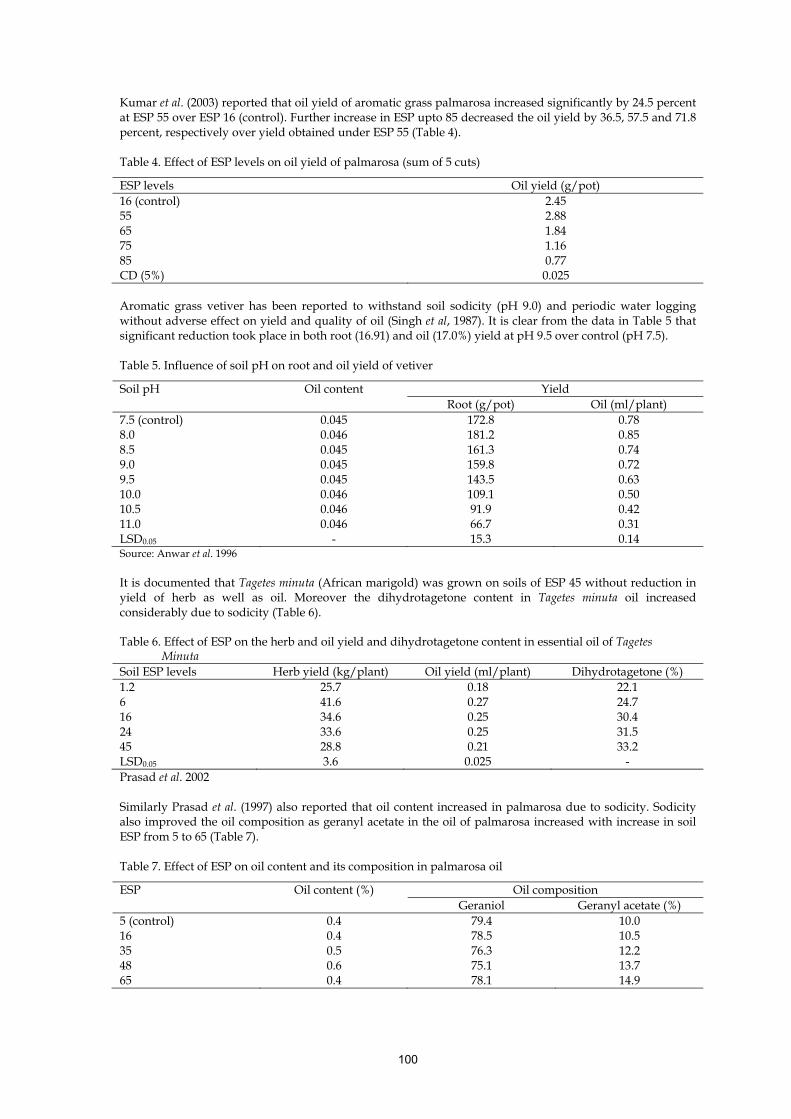
100

Kumar et al. (2003) reported that oil yield of aromatic grass palmarosa increased significantly by 24.5 percent at ESP 55 over ESP 16 (control). Further increase in ESP upto 85 decreased the oil yield by 36.5, 57.5 and 71.8 percent, respectively over yield obtained under ESP 55 (Table 4). Table 4. Effect of ESP levels on oil yield of palmarosa (sum of 5 cuts)

ESP levels Oil yield (g/pot) 16 (control) 2.45 55 2.88 65 1.84 75 1.16 85 0.77 CD (5%) 0.025 Aromatic grass vetiver has been reported to withstand soil sodicity (pH 9.0) and periodic water logging without adverse effect on yield and quality of oil (Singh et al, 1987). It is clear from the data in Table 5 that significant reduction took place in both root (16.91) and oil (17.0%) yield at pH 9.5 over control (pH 7.5). Table 5. Influence of soil pH on root and oil yield of vetiver

Soil pH Oil content Yield Root (g/pot) Oil (ml/plant)

7.5 (control) 0.045 172.8 0.78 8.0 0.046 181.2 0.85 8.5 0.045 161.3 0.74 9.0 0.045 159.8 0.72 9.5 0.045 143.5 0.63 10.0 0.046 109.1 0.50 10.5 0.046 91.9 0.42 11.0 0.046 66.7 0.31 LSD0.05 - 15.3 0.14 Source: Anwar et al. 1996 It is documented that Tagetes minuta (African marigold) was grown on soils of ESP 45 without reduction in yield of herb as well as oil. Moreover the dihydrotagetone content in Tagetes minuta oil increased considerably due to sodicity (Table 6). Table 6. Effect of ESP on the herb and oil yield and dihydrotagetone content in essential oil of Tagetes Minuta Soil ESP levels Herb yield (kg/plant) Oil yield (ml/plant) Dihydrotagetone (%) 1.2 25.7 0.18 22.1 6 41.6 0.27 24.7 16 34.6 0.25 30.4 24 33.6 0.25 31.5 45 28.8 0.21 33.2 LSD0.05 3.6 0.025 - Prasad et al. 2002 Similarly Prasad et al. (1997) also reported that oil content increased in palmarosa due to sodicity. Sodicity also improved the oil composition as geranyl acetate in the oil of palmarosa increased with increase in soil ESP from 5 to 65 (Table 7). Table 7. Effect of ESP on oil content and its composition in palmarosa oil

ESP Oil content (%) Oil composition Geraniol Geranyl acetate (%)

5 (control) 0.4 79.4 10.0 16 0.4 78.5 10.5 35 0.5 76.3 12.2 48 0.6 75.1 13.7 65 0.4 78.1 14.9

101

Results of the experiments conducted at CSSRI farm at Hisar indicated that medicinal plants like Isabgol Tulsi and aloe produced equivalent yield with saline irrigation water compared to canal irrigation water (Table 8). Similarly aromatic plants also produced good yield with saline irrigation water alone or alternate use of saline and canal water irrigation (Table 9). Table 8. Yield of some medicinal plants with saline water irrigation

Crops Botanical name SW CW CW/SW LSD0.05 Isabgol, (unhusked grain yield, t/ha)

Plantago ovata 1.014 1.059

1.091 NS

Periwinkle, (flower yield t/ha)

Catharanthus roseus

0.12 1.15 0.18 0.69

Tulsi, (dry wt. of shoot, t/ha)

Ocimmum sanctum

0.91 1.06 0.93 NS

Aloe, (fresh wt./plant, kg)

Aloe barbadensis 5.56 3.18 2.59 -

SW=saline water; CW=canal water Table 9. Biomass of some aromatic plants with saline water irrigation

Crops Dry weight of shoot biomass (t/ha) LSD0.05 SW CW CW/SW

Palmarosa, 24.3 34.0 29.1 4.8 Lemon grass 14.0 19.2 15.1 2.1 Vetiver 7.26 9.47 9.38 1.73 SW=saline water; CW=canal water Uses of salt tolerant medicinal and aromatic crops The information on drugs or aroma yielding plants and their efficiency in medicines is available and updated regularly in many authentic sources as Indian Pharmaceutical Codex, British Pharmaceutical Codex, United States Pharmaceutical Codex and National Formulary etc. The drugs extracted from medicinal and aromatic plants have been found successful in controlling serious diseases as cancerous tumors, HIV, hypertension, rheumatoid arthritis, digestive disorders, used as contraceptives and treatment of many other ailments. Extracts of different medicinal and aromatic crops are used in pharmaceutical, food, flavor and cosmetic industries. However, some of the medicinal and other important specific uses of salt tolerant medicinal and aromatic crop species compiled from literature are presented in Table 8. The economics of these crops in comparison to other cultivated conventional crops needs to be assessed in addition to availability of the local market for sale of the produce that can boost their cultivation. Table 10. Medicinal uses of different medicinal and aromatic plants

Crop/species Medicinal uses Aromatic crops Palmarosa (Cymbopogon martinii) Oil contains geraniol, and emit rose like aroma used in

perfumes, tobacco, soaps, medicines Lemon grass (Cymbopogon flexuosus) Contains citral used in vitamin-A, other edible recepies,

perfumery, cosmetics Citronella ((Cymbopogon nardus) Oil has mosquito repellant characteristics, also used in

cosmetics and perfumery Vetiver (Vetiveria zizanioides Linn.) oil from roots used in perfumery, cosmetics and flavouring

sherbets Medicinal plants German Chamomile (Matricaria chamomilla L.).

Flowers yield essential oil used as expectorant, sedative, perfumery, gastric stimulant

Isabgol (Plantago ovata Forsk.) Mucilage present in husk helps in cure of various intestinal, blood and cough ailments

Periwinkle (Catharanthus roseus) All parts are used for treatment of tumors, menorrhagia, leukemia and antibacterial uses

Rye for ergot (Claviceps purpurea) Dried sclerotium used in contraction of uterus and bladder, controls bleeding. Ergotamine used for migraine

Satavar (Asparagus racemosus) Roots rich source of minerals and other chemicals used for gas and lever, leucoria and as tonic

102

Aswagandha (Withania somnifera) Alkaloids are anti-cancer, anti-sleeplessness and immune system motivators

E. henbane (Hyoscyamus muticus). Tropane and hyscine are used in treatment of cold, cough, lever pain and apoplexy

Sowa/Dill (Anethum graveolens) Essential oil is given to children for flatulence, seeds are used as carminative and stomachic

Vasaka (Adathoda vasica) Bark and leaves extract has antiviral activity, used in cold, cough, bronchitis, rheumatic pain etc.

Aloe (Aloe barbadensis) Extract is cathartic, used in lever, spleen, piles, rectal, menstrual and constipation problems

Kair (Capparis deciduas) Fruit used in cardiac problems, bark used in cough and asthma. Fruits are used as pickles.

Mint (Mentha citrata) Mint oil has great industrial value and also used in flavors of candies, anta-acids and other fresheners

Euphorbia (Euphorbia antisyphilitica) Extract antisyphlatic and is a potential petro-crop Jamalghota (Jatropha carcus Linn.) Extract used in toothache, diarrhea, skin infections Tulsi (Ocimum sanctum Linn.) Leaves stimulants, anti-cough, yield essential oil Senna (Cassia angustifolia) Leaves and fruits laxative, vermifuge, purgative Chandrasura (Lepidium sativa) Oil is rubifacient/antinflamatory and galactogogic Reclamation of salt affected soils Several studies have established that cultivation of medicinal plant as Isabgol and aromatic grasses like Palmarosa, Lemon grass and Vetiver can reduce pH, EC, ESP and Na of salt affected soils (Table 11 and 12). In case of aromatic grasses the reclamation process occurs through improvement of physico-chemical properties of sodic soils due to extensive growth of roots which increase permeability of soil. As a result of decomposition of roots, CO2 may be evolved which resulted in solubilisation of native CaCO3 . This process takes place much effectively in the fields of vetiver which has the ability to withstand even under water logged conditions in sodic soils. A marked decrease in the ESP of soils and changes in their Na and pH after the harvesting of vetiver has proved the ameliorative potential of this crops on such soils (Table 12) German chamomile could also help in ameliorating the sodic soils through higher update of sodium a especially harmful cation. It is reported that this crop absorbed sodium to the extent of 66 meqNa/100 g of dry matter and improve alkali soils through ion uptake. Table 11. Ameliorative effects of different aromatic grasses on salt affected soils

Crop Soil pH (1:2.5) Soil EC (dS/m) ESP Authors Initial Harvest Initial Harvest Initial Harvest

Palmarosa (2yrs) 10.62 9.40 4.80 0.64 93.0 43.8 Prasad et. al 1995 Lemongrass 9.80 8.95 1.25 1.35 60.0 52.8 Patra et al 2002 Vetiver 10.50 9.50 -- -- 82.0 -- Anwar et.al 1996 Vetiver 9.50 9.00 -- -- 56.5 38.7 Anwar et.al 1996 Isabgol 10.00 9.70 1.25 0.81 60.0 48.4 Patra et al 2002 Table 12. ESP and Na of sodic soil before planting and after harvesting of vetiver

Before planting After harvest of crop ESP pH (1:2.5) Na (me/l) ESP pH (1:2.5) Na (me/l) 10 8.0 87.6 9 7.5 83.6 15 8.5 89.9 14 8.0 86.8 30 9.0 108.9 28 8.3 100.1 50 9.5 122.5 35 9.0 114.1 65 10.0 125.4 42 9.3 118.6 80 10.5 135.9 50 9.5 132.1 85 11.0 152.5 61 9.6 147.6

Conclusions Quite a significant area of earth surface is affected with excess salts and water logging characterized by poor productivity of crops. The reclamation of these soils is very costly because these require additional inputs as

103

amendments, irrigation and provision of drainage. Growing salt tolerant hardy medicinal and aromatic species is a viable alternate approach for productive utilization of these salt affected and waterlogged soils. Available information indicate that many high value medicinal and aromatic crops have higher tolerance to salinity, sodicity and water logging without any degradation in their quality, rather better quality has been observed under abiotic stress conditions. Immediate gains are quite encouraging in terms of high crop productivity to demands of raw material in national and international market, high economic return, employment generation and agriculture-industry linkage. Suggested Readings Anwar, M., Patra, D. D. and Singh, D.V. 1996. Influence of soil sodicity on growth, oil yield and nutrient

accumulation in aromatic grasses. Annals of Arid Zone. 35 (1): 49-52. Dagar, J. C. and Dagar, H. C. 2004. Ethano-medicinal wealth: historical perspective, resources and strategies.

In: Khan, I.A. and Khanum, A. (eds.) Ethno-medicine and Human Welfare Vol. II, Ukaaz Publications, Hyderabad. pp. 105-117.

Dagar, J. C., Tomar, O.S., Yadav, R. K. and Tyagi, N. K. 2005. Performance of some under explored crops with saline irrigation in semi-arid climate of north-west India. Land Degradation & Development. 16.

Lodha, Vandana. 2005. Sennoside content, ion accumulation and yield of Cassia aungustifolia under saline irrigation. In proceedings: International Conference on Soil, Water and Environmental Quality-Issues and Strategies, New Delhi. Pp. 316.

Parsad Arun, Anwar, M., Patra, D. D. and Singh, D.V. 1995. Tolerance of mint plants to soil salinity. J. Indian Soc. Sci. 44: 184-186.

Parsad, A., Kumar, D. and Singh, D.V. 1997. Effect of soil sodicity on the growth and cation composition of palmarosa and lemongrass. J. Herbs spices and Med. Plants. 5(3): 51-59.

Parsad, A., Krishna, A., Garge, S.N., Naqui, A. and Bhasney, S. 2002. Effect of soil sodicity and foliar spray of sodium chloride on the yield, essential oil composition and cation accumulation of Tagetes minuta. Indian Perf. 46(4): 365-371.

Patra, D. D. and Singh, D. V. 1995. Medicinal and aromatic plants for salt affected soils. Current Research on Medicinal and Aromatic Plants. 17 (3-4): 378-381.

Patra, D.D., Anwar, M., Tajuddin and Singh, D.V. 1997. Growth of aromatic grasses in sodic and normal soils under sub-tropical conditions. J. Herbs spices and Med. Plants. 5(2): 11-20

Patra, D. D., Parsad Arun, Anwar, M., Deepti Singh, Sukhmal singh, Balak Ram, R.S. Katiyar and Sushil Kumar. 2002. Performance of lemon grass cultivars intercropped with Chamomile under sodic soils. Comm. Soil Sci. Plant Anal. 33(11/12):1707-1721.

Singh, A., Singh, M. and Singh, D.V. 1987. Vetiver-A promising crop for problem soil. Pafai J. 9: 27-29. Tomar, O. S. and Minhas, P. S. 2002a. Relative performance of aromatic grasses under saline irrigation.

Indian Journal of Agronomy. 49 (3): 207-209. Tomar, O. S. and Minhas, P. S. 2002b. Performance of medicinal plant species under saline irrigation. Indian

Journal of Agronomy. 49 (3): 209-212.

104

Using SURFER for Analysis and Interpretation of Poor Quality Soil and Water C.K. Saxena Central Institute of Agricultural Engineering, Bhopal-462 038 (Madhya Pradesh), India Introduction Both land and water are finite resources essential to sustain various forms of life on the earth. Their proper utilization is essential for sustainable food production and economic development. Recent estimates indicate that 6.74 m ha (NRSA, CSSRI, NBSS&LUP, 2006) area in India is affected by soil salinity and alkalinity. The ground water quality in the country has been estimated to have about 25% of ground waters as sodic and/or saline. In the state of Rajasthan alone, more than 80% of the ground water resources are of poor quality and are unfit for irrigation to agricultural crops (Singh, 2008). Both the temporal and spatial data on poor quality resources have been collected and analyzed by several research and development institutions. Mapping of such spatial information is the most common method for representation and better interpretation for researchers and planners. Several software tools are being used to geostatistically analyze these observations of the data, which are necessary to characterize the spatial distribution of poor quality soils and waters at farm and regional scales. Various geostatistical methods have been extensively used to describe the spatial distribution of soil or water properties in agriculture (Cambardella et al., 1994; Meirvenne and Hofman, 1989). For example, the knowledge of salinity variability and characterization of spatial distribution in the fields are important for evaluating areas of low and high salt contents, and providing proper management recommendations. Such methods are also important to determine the spatial dependency between the measurements which are necessary for recommending optimum sampling scheme.

Surfer is a software package that runs under Microsoft Windows and is used for contouring and 3D surface mapping. It quickly and easily converts data obtained within or even outside a command area (generally regularly/ irregularly spaced XYZ or spatial data and/or observations) into outstanding contour, surface, wireframe, vector, image, shaded relief, and post maps (Fig.1). Virtually all the aspects of maps can be customized to produce exactly the desired presentation.

When a contour map is created, the grid or DEM (Digital Elevation Model) file is read into the plot window as an internal array of XYZ grid nodes. The grid nodes consist of rows and columns of Z values. The rows contain grid nodes with the same Y coordinate, and the columns contain grid nodes with the same X coordinate. Grid file columns and rows are sometimes referred to as X grid lines and Y grid lines, respectively. The intersection of a row and column is defined as a grid node. Grid files define the XY location of each grid node over the extent of the map, and the interpolated Z value at each node. A contour is a line (generally in smooth curves) generated by interpolating between grid nodes. In Fig.2, it is shown as an example with straight-line segments that define the contour line for a value at 50 units in the map. The dots have been added to show the ends of each line segment. When Surfer creates a contour map, the contour lines are drawn as a series of straight-line segments between adjacent grid lines. The point where a contour line intersects a grid line is determined by interpolation between Z values at adjacent grid nodes. It can be done with the help of several gridding options like Natural Neighborhood or Universal Krigging. The elevation data contained in USGS DEM files are regularly spaced, but the direction of the grid lines may not exactly coincide with the grid edges. This is due to the variable angle between the UTM coordinate system (used in

Fig.1. Sample terrain in Surfer 7.0 window showing contour, wireframe, image, shaded relief and 3D maps (clockwise from right top)

Fig.2. Example for path of a contour line (Z = 50) passing through a square grid

105

some DEM files) and true north. This results in the potential for a regular, stair-stepped arrangement of the grid nodes along the edges of the map, which can translate to, blanked grid nodes along the edges of maps produced in Surfer. If the DEM file contains three-second arc coordinates, the coordinates are automatically converted to latitude/longitude coordinates in Surfer. The grid limits define the extent of contour maps. Once a grid file is created, it cannot produce a contour map larger than the extent of the grid file. However, the use the Map | Limits command can be used to specify a subset of the grid used to create the contour map. Many features like physical and chemical properties of top soil and aquifer, surface topography, climate, vegetation, production, productivity, groundwater depth & quality, distribution of hazardous chemicals etc. could be requied to present in the form of a map. Any quantifiable spatial data of any such kind of property can be placed and analyzed using Surfer 7.0. It may be simple plotting of sample data location and/or its values to line or surface joining equal values to spatial variation analysis and much more. In the present chapter, the following major maps/ features/ facilities that can be dealt by the SUFER 7.0 are discussed.

1. Contour Map 2. 3D Surface Map 3. 3D Wireframe Map 4. Vector Map 5. Image Map 6. Shaded Relief Map 7. Post Map 8. Base Map 9. Map overlays 10. Gridding 11. Variograms 12. Fault and Break lines 13. Digital Elevation Model (DEM) Files 14. Worksheets and Object Manager 15. Additional Utilities and Features

Contour maps

Surfer contour maps give full control over all map parameters. The Surfer intelligent defaults can be as such employed to automatically create contour map, or double-click a map to easily customize map features. Contour maps over any contour range and contour interval can be displayed, or specified the desired contour levels to be displayed on the map. And with Surfer we can add color fill between contours to produce dazzling displays of maps, or produce gray scale fills for dramatic black and white printouts (Fig. 3).

Fig.3. Water table elevation contour map (June 2001) of some parts of Rohtak-Jhajjar Districts of Haryana – Observed and Simulated

Source: Gupta,S.K.(2004)

106

3D Surface maps A three dimensional or 3D surface map uses shading and color to emphasize your data features. Change the lighting, display angle and tilt is possible. Overlay several surface maps are used to generate informative block diagrams, which is helpful to illustrate the geology of the terrain. As an example of this, Great Lake Ladoga on the margin of the Baltic (Fennoscandian) Shield is shown in Fig.4.

Fig.4. Series of overlaid surface maps creats a 3D surfaces 3D Wireframe maps Surfer wireframe maps are three-dimensional representations of a grid file. These are are block diagrams generated by drawing lines representing the grid X and Y lines (the grid columns and rows). At each intersection of a column and row (i.e. at each grid node), the height of the surface is proportional to the grid Z value at that point i.e., the number of columns and rows in the grid file determines the number of X and Y lines drawn on the wireframe map. A wireframe map can be used to display any combination of X,Y, and Z lines. It uses color zones, independent X,Y,Z scaling, orthographic or perspective projections at any tilt or rotation angle, and different inations of X, Y and Z lines to produce exactly the surface we want. Drape a color-filled contour map over a wireframe map to create the most striking color or black-and-white representations of your data. The possibilities are endless. Wireframe maps Wireframe maps are block diagrams generated by drawing lines representing the grid X and Y lines (the grid columns and rows). The number of columns and rows in the grid file determines the number of X and Y lines drawn on the wireframe map.

Fig. 5. Emitter discharge distribution shown as a wireframe 3D map in a drip field

Vector maps A vector map is a graphical presentation comprised of a field of small arrows. Each arrow shows a direction and a magnitude associated with the location at which the arrow is drawn. For example, a vector map can depict the local gradients of a topographic surface: the arrows point in the direction of steepest ascent and the size of the arrows are scaled to the magnitude of the local slopes. Surfer offers two types of vector maps: a 1-grid vector map and a 2-grid vector map. In a 2-grid vector map, the two components of the vectors (i.e. magnitude and direction, or DX and DY) are provided by two separate grid files. The two components of a 1-grid vector map are automatically generated from a single grid file by numerically calculating the gradient of the represented surface. By default, the 1-

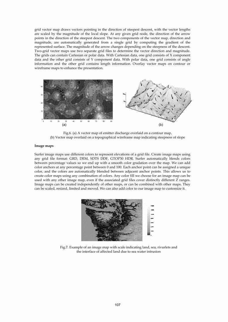
107

grid vector map draws vectors pointing in the direction of steepest descent, with the vector lengths are scaled by the magnitude of the local slope. At any given grid node, the direction of the arrow points in the direction of the steepest descent. The two components of the vector map, direction and magnitude, are automatically generated from a single grid by computing the gradient of the represented surface. The magnitude of the arrow changes depending on the steepness of the descent. Two-grid vector maps use two separate grid files to determine the vector direction and magnitude. The grids can contain Cartesian or polar data. With Cartesian data, one grid consists of X component data and the other grid consists of Y component data. With polar data, one grid consists of angle information and the other grid contains length information. Overlay vector maps on contour or wireframe maps to enhance the presentation.

0 10 20 30 40 50 60 70 80 900

10

20

30

40

(a) (b)

Fig.6. (a) A vector map of emitter discharge overlaid on a contour map,

(b) Vector map overlaid on a topographical wireframe map indicating steepness of slope Image maps Surfer image maps use different colors to represent elevations of a grid file. Create image maps using any grid file format: GRD, DEM, SDTS DDF, GTOP30 HDR. Surfer automatically blends colors between percentage values so we end up with a smooth color gradation over the map. We can add color anchors at any percentage point between 0 and 100. Each anchor point can be assigned a unique color, and the colors are automatically blended between adjacent anchor points. This allows us to create color maps using any combination of colors. Any color fill we choose for an image map can be used with any other image map, even if the associated grid files cover distinctly different Z ranges. Image maps can be created independently of other maps, or can be combined with other maps. They can be scaled, resized, limited and moved. We can also add color to our image map to customize it.

Fig.7. Example of an image map with scale indicating land, sea, rivurlets and the interface of affected land due to sea water intrusion

108

Fig.8. Shaded relief map of India and adjoining areas indicating overlaid sea and land boundaris Shaded relief maps Surfer Shaded Relief maps create a shaded relief map from a grid [.GRD] file or USGS DEM file. These maps use different colors to indicate surface slope and slope direction relative to a user-defined light source direction. Surfer determines the orientation of each grid cell on the surface, and assigns a unique color to each grid cell. Colors on shaded relief maps are associated with light striking the surface. The light source can be thought of as the sun shining on a topographic surface. Surfer automatically blends colors between percentage values so we end up with a smooth color gradation over the map. We can add color anchors so each anchor point can be assigned a unique color, and the colors are automatically blended between adjacent anchor points. This allows us to create color maps using any combination of colors. Shaded relief maps can be created independently of other maps, or can be combined with other maps in map overlays (using the Overlay Maps command). Shaded Relief maps can be scaled, resized, limited, and moved in the same way as other types of maps in Surfer. Post maps Post maps show X,Y locations with fixed size symbols or proportionally scaled symbols of any color. Surfer creates post maps independent of other maps on the page, or overlay the posted points on a base, contour, vector, or surface map. For each posted point, you can specify the symbol and label type, size, and angle, as the plus sign has been used in Fig.9 (a).

Av(30-150)

0 10 20 30 40 50 60 70 80 900

10

20

30

40

(a) (b)

Fig.9. (a) A post map indicating 13 x 10 plant locations in litchi field,

(b) Classed post map of an area indicating class intervals spread over a sample area

It also creates classed post maps that identify different ranges of data by automatically assigning a different symbol or color to each data range. Post your original data point locations on a contour map to show the distribution of data points on the map, and to demonstrate the accuracy of the gridding methods we use. Fig.9 (b) shows an example of a classed post map overlaid on a wireframe map and 3D label lines have been added to lift the symbols up off the map surface.

109

Base maps

Surfer can import maps in many different formats to display geographic information. We can combine base maps with other maps throughmap overlays or can create stand alone base maps independent of other maps on the page. We can load any number of base maps on a page. Base maps can be imported from DXF, GSI, BLN, SHP, LGO, BNA, GSB, DLG, LGS, MIF, E00, USGS, SDTS, DLG, DDF, EMF, WMF, TIF, PCX, BMP, PLT, CLP, TGA, PCX, JPG, PNG, DCX, WPG, PCt and other formats. It is easy to overlay a base map on a contour or surface wireframe map allowing us to display geographic information in combination with the three dimensional data. Base maps in Surfer alone or overlay them on other maps.

0 10 20 30 40 50 60 70 80 900

10

20

30

40

Fig.10. Example of a base map indicating 13 x 10 litchi plants in field, a jpeg photograph has been used as the background in the base map

Map overlays Map overlays give us a way to combine any number of contour, wireframe, vector, base, and post maps. Draping a filled contour map over a wireframe map produces the most striking display of 3D data possible. And because we can overlay any number of maps, we can show any amount of data on a single map. Using map overlays Fig.11 illustrates the contaminate spread in the Maydell mine area in the USA, this example was created by overlaying two contour maps, a basemap and a wireframe map in order to display the information.

Fig.11. Example of a map overlay using contour maps of contaminants in the air, a base map showing roads/boundaries and a wireframe map of the topography

Gridding The gridding methods in Surfer allow us to produce accurate contour, surface, wireframe, vector, image, and shaded relief maps from our XYZ data. The data can be randomly dispersed over the map area, and Surfer's gridding will interpolate data onto a grid. We have a multitude of gridding methods to choose from, so you can produce exactly the map we want. With each gridding method we have complete control over the gridding parameters. If our data are already collected in a regular rectangular array, we can create a map directly from our data. Computer generated contour maps have never been more accurate.

110

Variograms Use the variogram modeling subsystem to quantitatively assess the spatial continuity of data. Variograms may be used to select an appropriate variogram model when gridding with the Kriging algorithm. Surfer uses a variogram grid as a fundamental internal data representation and once this grid is built, any experimental variogram can be computed instantaneously.

Fig.12. Variograms in Surfer to quantitatively assess the spatial continuity of

data. Faults and breaklines Faults and breaklines are specified when gridding data in Surfer. The data on one side of the fault will not be directly used to calculate grid node values on the other side of the fault. When the gridding algorithm sees a breakline, any data points that lie directly on the breakline take precedence over an interpolated value (Fig. 13). Use break lines to define streamlines, ridges, and other breaks in slopes. Unlike faults, breaklines are not barriers to information flow and the gridding algorithm can cross the breakline to use a point on the other side. The gridding methods that support faults are: Inverse Distance to a Power, Minimum Curvature, Nearest Neighbor, and Data Metrics. Breaklines are supported by: Inverse Distance to a Power, Kriging, Minimum Curvature, Nearest Neighbor, Radial Basis Function, Moving Average, Data Metrics, and Local Polynomial gridding methods.

Fig.13. A contour map featuring a fault USGS digital elevation model (DEM) files

• Use DEM files with any Surfer command that uses GRD files • Directly use the SDTS DEM file format in native form • Display information about the DEM • Create contour, vector, shaded relief, image, and wireframe maps from DEM files

Digitize boundaries • Find XY coordinates • Automatically write coordinates to ASCII data files

111

• Automatically save digitized coordinates as BLN files • Create boundary files for use with other maps • Display different properties for base map features

Worksheet Surfer includes a full-featured worksheet for creating, opening, editing, and saving data files. Data files can be up to 1 billion rows, subject to available memory. We can use the Windows Clipboard functions to Cut, Copy, and Paste data within the Surfer worksheet, or between applications [Fig.14 (a)]. Object manager The object manager [Fig.14 (b)] makes the editing of any object simple. It displays all the objects in the document in an easy-to-use hierarchical tree arrangement. Select objects in the object manager to easily edit them and to show or hide them.

(a) (b)

Fig.14. (a) Worksheet showing a blank active cell (b) Objective manager showing different elements Additional utilities and features

• Export maps in DXF, SHP, BNA, BLN, MIF, GSI, GSB, EMF, WMF, CLP, CGM, TIF, BMP, JPG, TGA, PNG, PCX, DCX, WPG, PCT, formats

• Windows Clipboard support for copying maps to other applications • Combine any number of maps on a single page • Use the mouse to resize objects on the screen • Define default preferences • Define custom line styles and colors and save for use on other maps • Add any number of text blocks at any position on the map, using TrueType fonts • Include superscripts, subscripts and Greek or other characters in text • Compute volumes, planar and surface areas • Calculate residuals between data and surface • Print to any Windows supported printer or plotter • Easily clip boundaries or posted points to contour map limits • Display and print subsets of completed maps, complete with subset axes • Add arrowheads to lines • Adjust the number of undo levels • Use the reshape tool to edit areas and curves • Floatable toolbars

System requirements

• PC running Windows 98, Me, 2000, XP, or higher • 25 MB of free hard disk space • 32 MB RAM minimum, 64 MB or higher recommended • 800 x 600 minimum monitor resolution

112

Practical exercise(s) The most common application of Surfer is to create a grid-based map from an XYZ data file. The Grid Data command uses an XYZ data file to produce a grid file. The grid file is then used by most of the Map menu commands to produce maps viz. contour maps, wireframe maps or shaded relief maps etc. (Fig.15). Post maps and base maps do not use grid files.

Fig.15. Relationship between XYZ data files, grid file, contour map and wireframe map Creating an XYZ data file An XYZ data file is a file containing at least three columns of data values. The first two columns are the X and Y coordinates for the data points. The third column is the Z value assigned to the XY point. Although it is not required, entering the X coordinate in Column A, the Y coordinate in Column B, and the Z value in Column C is a good idea. Surfer looks for these coordinates in these columns by default. Opening an existing data file To look at an example of an XYZ data file, open TEST_PH.DAT into a worksheet window:

1. Choose the File | Open command, or click the Open tool. The Open dialog box is displayed. This allows us to select the XYZ data file to display in the worksheet window.

2. In the list of files, click TEST_PH.DAT and the name appears in the File name edit box. Click Open and the file is displayed in the worksheet window.

3. Notice that the X coordinate (Easting) is in Column A, the Y coordinate (Northing) is in Column B, and the Z value (Elevation) is in Column C. Although it is not required, the header text (the text in row 1) is helpful in identifying the type of data in the column, and this information is used in dialog boxes when selecting worksheet columns.

Creating a new data file & saving the data file The Surfer worksheet can also be used to create a data file. To open a worksheet window and begin entering data:

1. Choose the File | New command or click the New tool. Click the Worksheet option in the New dialog box. Click OK to display a new empty worksheet window.

2. The active cell is selected by clicking on the cell or by using the arrow keys to move between cells. The active cell is indicated by a heavy border and the contents of the active cell are displayed in the active cell edit box. When a cell is active, enter a value or text, and the information is displayed in both the active cell and the active cell edit box. The BACKSPACE and DELETE keys can be used to edit data while typing. Press the ENTER key and the data are entered into the cell. Surfer uses almost similar commands to that of MS Excel applications for spreadsheet saving and editing.

When we have completed entering all of the data:

1. Choose the File | Save command, or click the Save tool. The Save As dialog box is displayed if we have not previously saved the data file.

113

2. In the Save File as Type drop-down list box, choose the Golden Software Data (*.DAT) option from the list.

3. Type the name of the file into the File name edit box. Click OK and the file is saved in the Golden Software Data [.DAT] format with the file name we specified. The name of the data file appears at the top of the worksheet window.

Creating a grid file Grid files are required to produce a grid-based map. Grid-based maps include contour maps, image maps, shaded relief maps, vector maps, and wireframe maps. Grid files are created using the Grid | Data command. The Data command requires data in XYZ columns. To produce a grid file from TEST_PH.DAT:

1. Choose the Grid | Data command. The Open dialog box is displayed. This allows us to select the XYZ data file used to produce the grid file.

2. In the list of files, click the file TEST_PH.DAT. The name appears in the File name edit box below the list of data files. Click Open and the Scattered Data Interpolation dialog box is displayed. Alternatively, we can double-click the data file name to display the Scattered Data Interpolation dialog box.

3. The Scattered Data Interpolation dialog box allows us to control the gridding parameters. Take a moment to look over the various options in each tab of the dialog box. Do not make changes at this time, as the default parameters create an acceptable grid file.

The Data Columns group under the Data tab specifies the columns containing the X and Y

coordinates, and the Z values in the data file. The Grid Line Geometry group under the General tab specifies the XY grid limits, the grid

spacing, and the number of grid lines (also referred to as rows and columns) to include in the grid file.

The Gridding Method group under the General tab specifies the interpolation method to use and the parameters controlling the interpolation.

The Output Grid File group under the General tab specifies the path and file name for the grid file created.

The Generate Report option under the General tab specifies whether to create a statistical report for the data.

The Search tab specifies the search radius for each grid node. The Faults and Breaklines tab specifies the file name that contains the fault or breakline used

while gridding. 4. Click OK. In the status bar at the bottom of the window, a display indicates the progress of the

gridding procedure. When gridding is complete, the grid file TEST_PH.GRD is created and Surfer beeps to indicate that the grid file has been produced. By accepting the defaults, the grid file uses the same path and file name as the data file, but the grid file has a [.GRD] extension. If Generate Report is checked, a Data Filter Report is displayed.

Creating a contour map The Map | Contour Map command creates a contour map based on a grid file. To create a contour map of the TEST.GRD file you just created:

1. Choose the Map | Contour Map | New Contour Map command, or click on the Contour tool . The Open Grid dialog box is displayed. The grid file you just created (TEST.GRD) is automatically entered in the File name edit box. Click Open, and the Contour Map Properties dialog box is displayed.

2. The default parameters in the Contour Map Properties dialog box create an acceptable contour map. To accept the default parameters, click OK. A contour map is created from TEST.GRD.

3. If we want the contour map to fill the window, choose the View | Fit to Window command. The view of the contour map is magnified so the map fills the entire plot window.

The following additional efforts can also be performed.

• Changing Contour Levels

114

• Changing Contour Line Properties • Adding Color Fill between Contour Lines • Add, Delete, and Move Contours • Modifying an Axis • Saving a Map • Exporting 3D Contours

Creating a wireframe map

1. Choose the File | New command, or click the New tool . The New dialog box is displayed. Select Plot Document, and click OK. A new empty plot window is displayed.

2. Choose the Map | Wireframe command or click the Wireframe Map tool . The Open Grid dialog box is displayed. Choose the grid file TEST_PH.GRD from the list of files, and click OK. The Wireframe Properties dialog box is displayed.

3. Click OK to accept the defaults. A wireframe map based on TEST_PH.GRD is drawn. Wireframe maps are drawn with a Z-axis in addition to the other axes.

Changing the orientation of a wireframe map Although this example uses a wireframe map to illustrate orientation and tilt, we can perform this operation on most map types in Surfer (excluding image maps and shaded relief maps). To change orientation and tilt:

1. Click the wireframe map and selection handles appear surrounding the map. 2. Choose the Map | 3D View command. The View dialog box is displayed. This box allows us to

control the tilt, rotation, and projection type for the selected map. 3. Use the Rotation scroll bar to change the rotation to 210°. As we change the rotation angle, the

graphic image in the dialog box changes to indicate the orientation. 4. Use the Tilt scroll bar to change the angle to 40°. 5. Click OK in the dialog box and the wireframe map is redrawn at the new orientation and tilt

angles. Changing the scaling of a wireframe map We can change the scaling of any map in each of the three cardinal dimensions. In this example, the Z scaling is changed, and the wireframe map becomes somewhat exaggerated in the Z dimension. To change the Z scaling:

1. Click the wireframe map, and selection handles appear surrounding the wireframe. 2. Choose the Map | Scale command to display the Scale dialog box. This allows us to set the

scaling in each of the three cardinal dimensions on the selected map. We can set scaling by entering the number of map units per inch, or by entering the length for the map in page coordinates.

3. In the Length edit box of the Z Scale group, type 3. The Map units value changes to reflect the change we made.

4. Click OK and the wireframe map is redrawn exaggerated in the Z dimension. Adding color zones to a wireframe map We can change the line colors of any wireframe map by applying color zones. In this example, we will change color zones gradationally and individually. To add a color zone to a wireframe map:

1. Double-click on the wireframe map, and the Wireframe Properties dialog box is displayed. 2. Click on the Color Zones tab. 3. Click on the Line button to display the Line Spectrum dialog box. 4. Click on the Minimum Line Properties button and the Line Properties dialog box is displayed.

From here, we can select the line color, style, or thickness.

115

5. Click on the Color button and select the color Blue. Click OK and to return to the Line Spectrum dialog box.

6. Click on the Maximum Line Properties button and change the line color to red using the steps above.

7. Click OK in the Line Spectrum dialog box. 8. In the Wireframe Properties dialog box, click the Apply Zones to Lines of Constant X and Y. 9. Click OK and the wireframe map is displayed with the gradational colors.

To change the properties of an individual Z value:

1. Double-click the wireframe map and the Wireframe Properties dialog box is displayed. 2. On the Color Zones tab, double-click the line sample for the contour level at Z = 70. The Line

Properties dialog box is displayed. 3. From here we can select the line color, style, or width for the selected line. In the Width edit

box, click the up arrow and change the width value to 0.030 in. Click OK and the Color Zones tab is updated to reflect the change.

4. Click OK in the Wireframe Properties dialog box and the map is redrawn. The color zone at Z = 70 is drawn with a thicker line, and is emphasized on the map.

Overlay post and contour maps When a new post map is created, it is independent of any other maps in the current plot window. When the two maps are displayed, notice that two sets of axes are also displayed, one set for each map. When we use the Map | Overlay Maps command, the two maps are combined into a single map overlay with one set of axes. To overlay maps:

1. Choose File | Open to display the Open dialog box. Choose TEST_PH.SRF and click the Open button to display the contour map contained in TEST_PH.SRF.

2. Choose Map | Post Map | New Post Map or click the Post Map tool . The Open dialog box is displayed. This allows us to select the data file used to produce the post map.

3. In the list of files, click TEST_PH.DAT and the name appears in the File name edit box. Click Open and the Post Map Properties dialog box is displayed.

4. Click the Symbol button and the Symbol Properties dialog box is displayed. 5. Choose the filled circle symbol from the Symbol palette and click OK. The selected symbol

appears in the Symbol button. This symbol appears at the posted data points on the map. 6. In the Fixed Size edit box of the Symbol Size group, specify a size of 0.09 in. 7. Click OK and the post map is drawn over the contour map. The contour map and post map are

two separate maps on the page. If we look closely at the X-axis, you will notice the two sets of axis tick labels for the two maps.

8. To see the two separate maps, place the mouse pointer in the center of the maps and click. Press and hold the left mouse button and move the pointer slightly in any direction. Release the button and the two maps are offset.

9. Press the CTRL+A on the keyboard to select both maps. 10. Choose the Map | Overlay Maps command and the two maps are combined in a single overlay.

Creating a 1-grid vector map We can create a 1-grid vector map and overlay it on a wireframe map to produce a map showing the flow of water on a topographic surface.

1. Choose the File | New command, or click the New tool . The New dialog box is displayed. Select Plot Document, and click OK. A new empty plot window is displayed.

2. Choose the Map | Vector Map | New 1-Grid Vector Map command. The Open Grid dialog box is displayed. The grid file we just created (TEST_PH.GRD) is automatically entered in the File name edit box. Click Open, and the Vector Map Properties dialog box is displayed.

3. The default parameters in the Vector Map Properties dialog box create an acceptable vector map. To accept the default parameters, click OK. A vector map is created from TEST_PH.GRD.

4. Choose the Map | Wireframe command or click the Wireframe Map tool . The Open Grid dialog box is displayed. Choose the grid file TEST_PH.GRD from the list of files, and click OK. The Wireframe Properties dialog box is displayed.

116

5. Select Plot Lines of Constant Z. Deselect the Plot Lines of Constant X and Plot Lines of Constant Y. Click OK to accept the remaining default parameters. A wireframe map based on TEST_PH.GRD is drawn.

6. Press CTRL-A, or choose the Edit | Select All command to select both the vector map and the wireframe map. Choose the Map | Overlay Maps command to overlay the two maps.

7. If we want the map to fill the window, choose the View | Fit to Window command. The view of the map is magnified so the map fills the entire plot window.

Suggested Readings Cambardella, C.A., Moorman, T.B., Novak, J.M., Karlen, T.B., Karlen, D.L., Turco, R.F. and A.E.

Konopka. 1994. Field-scale variability of soil properties in central Iowa soils. Soil Sci. Soc. Am. J. 58:1501-1511.

Gupta S.K. 2004. Develop Regional Salt Balance Models. PSR 16. Final Report, NATP. Centeral Soil Salinity Research Institute, Karnal pp.184.

Meirvenne, M.V., and G. Hofman. 1989. Spatial variability in topsoil micronutrients in a 1-ha cropland plot. Comm. Soil Sci. Plant Anal. 120:103-110.

Singh, Gurbachan 2008. Conservation Agriculture for Managing Soil and Water Resources. Eds. Lal, K., Meena, R.L., Gupta, S.K,, Bundela, D.S., Yadav, R.K., Singh, G. Conjunctive use of canal and groundwater. National level training course on Conjunctive Use of Canal and Groundwater Including Use of Brackish Water. Central Soil Salinity Research Institute, Karnal.1-12.

SURFER 1999. Surfer 7.0 – User Guide. Goden Software Inc. 809, 14 Street, Golden, Colorado, USA.

117

Drip Irrigation in Horticultural Crops: Suitability for Saline Water Use Satyendra Kumar Central Soil Salinity Research Institute, Karnal – 132 001 (Haryana), India Global fruit and vegetable production has increased to 1.34 billion MT in 2003, up from 396 million MT in 1961 (FAO, 2005). Largest producers of fruit are the developing countries in Asia followed by developed countries. However, China is the largest producer of vegetables followed by India. Horticulture sector can play an important role in improving the productivity of land, generating employment, improving economic conditions of the farmers and entrepreneurs and providing nutritional security to the people. Fruits and vegetables not only improve the quality of our diet but also provide essential ingredients like carbohydrates, proteins, fats, vitamins and minerals. Apart from nutritional security, cultivation of these crops provides profitable sources of income for farmers. Studies from the developing countries of Asia and Africa consistently show that farmers engaged in the cultivation of fruits and vegetables earn higher net farm incomes than the farmers engaged in cereal production alone (Francisco 2004). Fruit and vegetable producers in India, generate five to eight times more profits than cereal farmers, depending on the crop. In Kenya, the production of fruit, vegetables and flowers for export is providing farmers with six to twenty times more profits than maize, depending on the crop (Minot and Ngigi 2004). Horticulture crop production provides jobs more than twice the number of jobs compared to cereal crop production per hectare (Ali et al. 2002). The shifting of cereal production toward high value horticulture crops is already increasing employment opportunities in developing countries (Joshi et al. 2003). Irrigation of horticultural crops Irrigation is provided to counter water stress during on crop production. It is estimated that there are now about 260 million irrigated hectares of land worldwide compared to less than 100 million ha in 1950. They constitute less than 17% of the world's total cultivated farmland but produce 40% of the food and fiber. At present, irrigation is the largest single consumer of water on the planet; accounting for about 20% of the total fresh water used and about two thirds of the total diverted for human uses. Irrigation has major environmental impacts on water quantity, water and soil quality and has permanently changed the social fabric of any regions around the world (Fereres and Evans 2006). It is general perception that fruit trees can withstand water stress for longer period, although not much fruit is produced. If tree irrigate properly, will grow vigorously and produce good crops. Irrigation of fruit trees not only provides some security in protecting a large investment with potentially high returns against droughts, but serves also to increase and stabilize production. In addition, it has been shown that proper irrigation practices can have a positive influence on the quality of the harvested produce and any resulting processed product. For example, adequate soil moisture must be maintained throughout the growing season of pomegranate, particularly as harvest approaches to greater diurnal temperature variation, when it helps in minimizing fruit splitting. An efficient, uniform and reliable irrigation and nutrient delivery is required in order to produce quality crops of uniform size and maturity (Kumar et al 2007a). Most vegetables are shallow rooted and even short period of two- three days of stress can affect marketable yield. Vegetables are having 80 to 95 percent water and their yield and quality suffer very quickly from water stress during critical production period. If water shortage occurs early in the crop’s development, maturity may be delayed and yield often reduced, while moisture shortage in latter growing seasons also affect produce quality even though yield is not affected. Irrigation is likely to increase size and weight of individual fruit and to prevent defects such as toughness, strong favor, poor tip fill and pod fill, cracking blossom-end rot and misshapen fruit. On the other hand, it reduces soluble solids in muskmelons and capsicum in hot pepper, if applied during fruit development. Irrigation also influences keeping quality of the produce (Kumar et al. 2007b). Systems for irrigating horticultural crop Most orchards are irrigated with the traditional irrigation systems involving flooding, furrow, border and basin methods. Water diverts from the head and allows spreading to the entire field. These systems revolved around the concept of replenishing the moisture level to field capacity only after depletion of 50-60% of available water . The present systems do not restrict irrigation water to root zone level, thus causes excessive deep percolation and other losses. Since, microirrigation involving drip, bubbler, microsprayer etc. ( Fig. 1) has been evolved with the concept to irrigate root zone of the

118

plant rather than the entire field, result into saving of a considerable amount of irrigation water. Research activities carried out in India and abroad categorically exhibited beneficial effect of microirrigation, which can save up to 50 to 100 percent water with enhancement of yield up to 60-100 percent of different crops under varied agro-climatic conditions as compare to conventional methods of irrigation. Table 1 summarizes some findings related to water requirements of different horticultural crops including pomegranate. Table 1. Water use efficiency in drip system for various horticultural crops

Crops Yield increase (%)

Water saving (%)

Increase in water useefficiency (%)

Water Melon 88 36 195 Pomegranate 45 45 167 Sugarcane 33 56 204 Tomato 50 31 119 Banana 52 45 176 Chilly 45 63 291 Grapes 23 48 136 Groundnut 91 36 197 Sweet Lime 50 61 289

Drip system of irrigation Drip irrigation is not a substitute for other proven methods of irrigation. It is just another way to irrigate tree and crops, i.e. prevent the crops from ever becoming stressed. Most of the times, drip system maintains soil moisture at or very close to the field capacity (Fig. 2). Drip system operates under low pressure with small-sized wetting patterns and low discharges and applies water directly to the soil surface or subsurface (Fig 3). It allows the water to dissipate under low pressure in a predetermined pattern. A wetted profile develops in the plant's root zone beneath each dripper. Ideally, the area between rows or individual plants remains dry and receives moisture only from incidental rainfall. Suitability Drip irrigation system can be used to irrigate almost all type of crop in all type of soil with almost all type of water (Goldberg et al., 1971; Kumar et al., 2000a). Drip irrigation has been extensively used throughout the world to irrigate marginal soils and terrain that could not be irrigated by other methods. Moreover, desert pavement and leached tropical soils, adapt poorly to surface or sprinkler irrigation, but can be irrigated successfully with drip systems. Drip irrigation has been proven to be an efficient and effective technique for establishing vegetation on steep slopes of abandoned mines, road embankments, etc., without erosion hazard. It is also suitable for irrigating slowly permeable soil and even irregular small plots. Irregularly shaped lawn and landscaped areas are difficult to irrigate by sprinkling resulting in over spray of paved surfaces and lack of uniformity. Drip irrigation enables water to be applied with high uniformity and may eliminate runoff and overspray. Subsurface drip on turf grass and sport fields does not interfere with the continuous use of the area (Zoldoske et al., 1995).

119

Fig

1.

Typi

cal s

ketc

h di

agra

m o

f diff

eren

t mic

roir

riga

tion

syst

ems

120

Fig 2. Moisture availability for crops under different irrigation methods

Surface drip system

121

Fig 3. A view of surface and sub surface drip system installed in horticultural crops Efficient water application Injudicious use of water through traditional irrigation methods results into water logging and salinity in these areas with inadequate drainage facility. The main challenge for efficient water management is to check the excess seepage from distributaries that leads to fluctuation in ground water and less water availability for crop production (Singh, 2003). The high water application efficiency in drip system offers opportunity to use available water judiciously, effectively and efficiently (Table 2). Drip system is usually applied water with solid-set (stationary) system, which ensures accurate and localized application, at predetermined amounts and at constant rates. Wu and Gitlin (1975) reported that an application efficiency of 90% could easily be achieved for drip irrigation as compared to 60-80% for sprinkler and 40-60% for surface irrigation. The manufacturing variation less than 5% of many of the modern emitter results in a uniformity coefficient of more than 95%. The higher water use application efficiency contributes towards water saving when crop is irrigated with drip as compared to surface irrigation methods (Singh et al., 2001). Uniform application of water in the field also depends upon selection of appropriate emitting devices. The commonly used drippers in horticultural crops and their possible application are summarized in table 2 and presented in fig. 4 . Table 2: Some features of drippers of different types commonly used are given in the below

Dripper type Application Vari Flow Dripper

Suitable for trees having high water requirement. Recommended for sandy soils / desert conditions

Turbo Stake Dripper

Recommended for fruit orchards, requiring one or more drippers around the trunk of the tree.

Micro Dripper

Used as a linear flow dripper in drip systems

Trickle Stik

Ideally used for Irrigation of Bag Culture Recommended to use where dispositioning of tubing is a problem

Turbo Seal Emitter

Recommended for fruit orchards, vegetables and floricultural plants Used in high vandalism area whose operable dripper is difficult to maintain

Pressure compensating dripper

Recommended for undulating terrain & steep slopes Allows longer lateral run Suitable for orchards, fruit crops, vegetables, nurseries & flowers

Jet-Loc Emitter

Suitable for vegetables, closely spaced row crops, glass/green houses & nurseries

Mini Inline Emitter

Recommended for fruit orchards, requiring one or more drippers around the trunk of the tree

Inline dripper Recommended for vegetable and other close growing crops Suitable for plastic mulching

(Source : Jain Irrigation System Ltd , Jalgoan, India)

Sub-surface drip system

122

Economic use of fertilizer The crop response to the fertilizer is better in the presence of proper moisture in the soil. It has been observed that 30% of fertilizer applied could be lost or leached with deep percolated water under conventional irrigation method. Drip irrigation offers the opportunity of using fertilizer with irrigation water (fertigation) and enables users to put fertilizers directly in plant root zone in desired frequency, amount and concentration at appropriate time (Kumar et at., 2000b; Singh, 2003). It helps in judicious and economical use of fertilizers for maximizing crop production without creating any environmental hazards. Fertigation not only saves the money by conserving a significant amount of fertilizers to be leached as in traditional application method. Various research studies conducted in different parts of the world have proved that supplying liquid soluble fertilizers through drip system can lead to savings in fertilizer applied to the extent of 40 to 60 per cent without affecting the yield and a much higher application efficiency compared to the conventional methods. This is in addition to the savings in water applied which could be anywhere from 50 to 70 per cent, besides quality of produce being added advantages.

Vari Flow Dripper

Turbo Stake Dripper

Micro Dripper

Trickle Stik

Turbo Seal Emitter

Turbo Seal PC Emitter

Jet-Loc Emitter

Mini Inline Emitter

In line dripper

Fig 4. Different types of emitting devices commonly used for irrigating horticultural crops

123

Opportunity to utilize saline water Drip irrigation has stupendous scope of utilizing the saline water for crop production by conjunctive use of saline water and good· quality surface water (Meiri et al., 1992). This contributed in proper use of ground water as well as available surface water for crop production without creating any environmental hazards like water logging, or salinity. Drip system makes possible to bring new areas under irrigation with the same amount of available good quality surface water. Drip system makes the soil moisture tension very low and reduces the salt concentration near the root zone (Bresler, 1977). In drip irrigation water flows laterally and unwanted salts move to the outer edge of wetted zone (Fig. 5). Hence, osmotic potential offers great scope for sustainable crop production with use of marginal quality of ground water.

Fig. 5. Salt accumulation pattern in soil irrigated with drip system

Saline water as a source for irrigation In the recent years, both surface and groundwater resources have come under tremendous pressure due to burgeoning population, improved living standard and unprecedented industrial growth. Agriculture sector is a major consumer of available water resource and will remain. But, water demand of other sectors i.e. domestic, industrial, recreation, power generation etc. is also increasing day by day. The competition would become furious in coming years not only for the quantity but also for the quality of water. The estimates show that by 2025, 1.8 billion people of the world will live with absolute water scarcity. Most countries in the Middle East and North Africa can be classified as having absolute water scarcity today (Kumar 2003). By 2025, these countries will be joined by Pakistan, South Africa, and large parts of India and China. This means that they will not have sufficient water resources to maintain their current level of per capita food production from irrigated agriculture even at high levels of irrigation efficiency and also to meet reasonable water needs for domestic, industrial, and environmental purposes. Further, to meet other sector’s requirements, water will have to be transferred out of agriculture. To overcome water shortage, agriculture sector would be forced to switchover to other water sources. Marginal quality groundwater seems to be important sources of water for agriculture in coming future. Use of saline water by adopting new skills and knowledge could be the one opportunity to tide over the anticipated water scarcity problem in agriculture. Utilization of saline water for irrigation is associated with salt accumulation in the soil, which might be harmful to plants, and diminishing yields. The salt effects on physiological process result from lowering of the soil water potential and the toxicity of specific ions. On the other hand it has been reported that non-toxic highly saline water has an agricultural potential. If, irrigation can be managed in such a way that provides high soil moisture content and, consequently, high soil water potential within the whole root zone, the osmotic effects will be damped (Michelakis et al., 1993). Moreover,

124

when saline water is skillfully used for irrigation, it can be beneficial for agricultural production, particularly in orchards (Hoffman et al, 1986). Saline water use for agricultural production offers several additional benefits: i) re-use (instead of disposal as with fresh water) during the entire year, with minimal environmental risk of ground water deterioration (Oron, 1993); and ii) a premium market price for the fruits and vegetable products because of a high content of total soluble solids and an extended shelf life, due to the adaptation of the plant to the stressful growing conditions (Mizrahi & Pasternak. 1985). The basic principles to produce crops in saline environment are now well understood, and these advocate the adoption of special management practices. Saline water can be used for irrigating crop successfully if factors such as rainfall, climate, water table and water quality characteristics, soils and crops are integrated with appropriate crop and irrigation management practices. Drip and other microirrigation techniques help in achieving better salt and water regimes in root zone. The use of saline waters through such systems has revolutionized the production of some high-value crops and orchards in countries like Israel. Drip irrigation for saline water use

Soluble salts reduce availability of water in almost direct proportion to their total concentration in the soil solution. If, irrigation frequency is increased so that the moisture content of irrigated soils are maintained as high and salinity as low as is practicable, especially during seedling establishment and the early stage of vegetative growth. The most practical way to accomplish this is through use of drip irrigation. Drip irrigation is able to apply water at low discharge rate and high frequency over a long period of time, resulting in a condition to maintain high soil water content in root zone all the time, and minimize salinity levels in the soil water due to leaching (Keller and Bliesner, 1990). Meanwhile, because of the point-source characteristic of drip irrigation, the salts along with water can be pushed toward the fringes of wetting area, and forming a desalinization zone in the center of wetting area, in close proximity to the dripper (Goldberg et al., 1977). Thus, drip irrigation is widely regarded as a suitable system for applying saline water to crops (Malash et al., 2008). The saline water irrigation through drip system has enhanced the production of some high-value crops and orchards in countries like Israel and elsewhere. Regular and frequent water supply through drip system is able to enhance the threshold limits of salt tolerance of crop by modifying the patterns of salt distribution and maintenance of constantly higher matric potentials. The crop roots are known to follow the path of least resistance, most roots are found below the surface drippers. Hence, drip system seems to be the best method of saline water application as it avoids leaf injury to plants as with sprinklers and maintains optimum conditions for water uptake by plant roots. Superiority in yield and water use efficiency as well as size and quality of vegetable even with the use of saline water was reported (Aggarwal and Khanna 1983). Solutes movement, root distribution and water uptake under drip irrigation Solutes and water uptake of plant is perhaps the most difficult to quantify as far as root zone solute and soil water dynamics are concerned. Most, if not all, of the uptake models that exist, contain parameters for uptake that have to be adjusted for a specific crop and for the specific conditions under which it is growing. Spatial distribution of plant roots is an integral part of water extraction functions or models. Root systems can be expressed in several ways, such as root percentage distribution, root density distribution and root length density (RLD) distribution. Phene et al. (1991) explained that it is especially important in drip irrigation to define these root parameters, since it is widely believed that drip irrigation may limit the wetted soil volume and, therefore, the extent of root development But root distributions have been found to depend mostly on the availability of the water, type of irrigation system, crops and soils (Phene et al., 1991; and Zhang et al., 1996). Although root distribution is a highly dynamic process, Ehlers et al. (1991) assumed steady state conditions for their development of a model linking root density and water uptake. If soils are frequently irrigated, especially from the surface, they will remain relatively wet there and most of the root water uptake will then take place in the upper soil layers (Klepper, 1991). Alaerts et al. (1985) compared the performance of some macroscopic root uptake models. In most cases the important difference between these various models is the way in which the root water uptake term was derived or as Cardon and Letey (1992) put it, the uniqueness of each model depends on its formulation. High transpiration rates can cause large flux of nutrients towards the root, and rapid accumulation of nutrients at the soil-root interface may lead to high and detrimental nutrient concentrations around

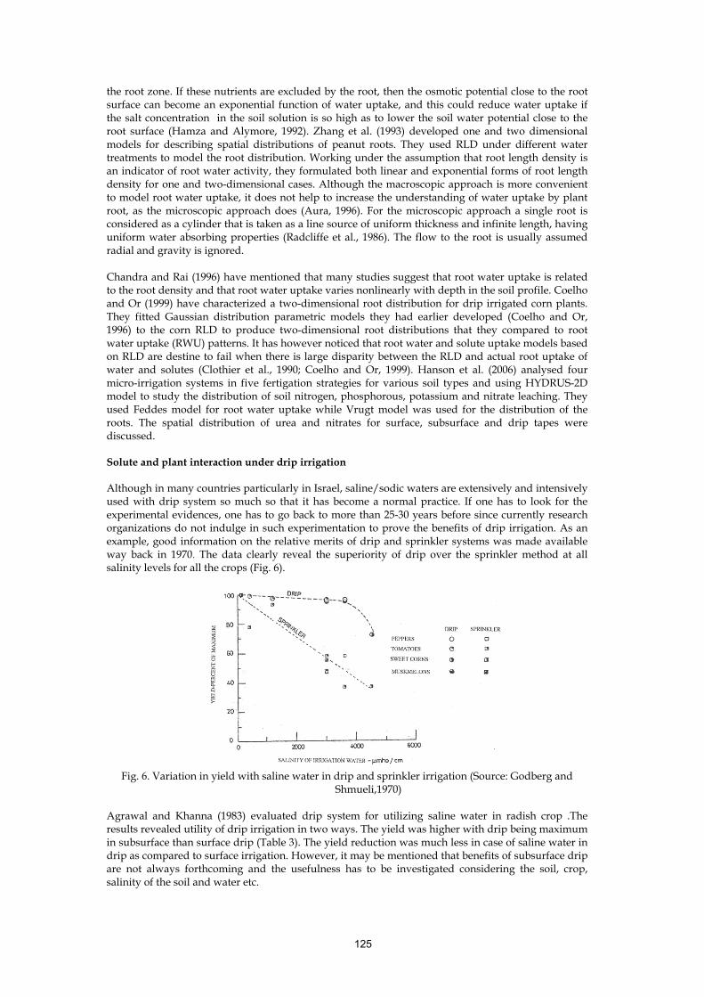
125

the root zone. If these nutrients are excluded by the root, then the osmotic potential close to the root surface can become an exponential function of water uptake, and this could reduce water uptake if the salt concentration in the soil solution is so high as to lower the soil water potential close to the root surface (Hamza and Alymore, 1992). Zhang et al. (1993) developed one and two dimensional models for describing spatial distributions of peanut roots. They used RLD under different water treatments to model the root distribution. Working under the assumption that root length density is an indicator of root water activity, they formulated both linear and exponential forms of root length density for one and two-dimensional cases. Although the macroscopic approach is more convenient to model root water uptake, it does not help to increase the understanding of water uptake by plant root, as the microscopic approach does (Aura, 1996). For the microscopic approach a single root is considered as a cylinder that is taken as a line source of uniform thickness and infinite length, having uniform water absorbing properties (Radcliffe et al., 1986). The flow to the root is usually assumed radial and gravity is ignored. Chandra and Rai (1996) have mentioned that many studies suggest that root water uptake is related to the root density and that root water uptake varies nonlinearly with depth in the soil profile. Coelho and Or (1999) have characterized a two-dimensional root distribution for drip irrigated corn plants. They fitted Gaussian distribution parametric models they had earlier developed (Coelho and Or, 1996) to the corn RLD to produce two-dimensional root distributions that they compared to root water uptake (RWU) patterns. It has however noticed that root water and solute uptake models based on RLD are destine to fail when there is large disparity between the RLD and actual root uptake of water and solutes (Clothier et al., 1990; Coelho and Or, 1999). Hanson et al. (2006) analysed four micro-irrigation systems in five fertigation strategies for various soil types and using HYDRUS-2D model to study the distribution of soil nitrogen, phosphorous, potassium and nitrate leaching. They used Feddes model for root water uptake while Vrugt model was used for the distribution of the roots. The spatial distribution of urea and nitrates for surface, subsurface and drip tapes were discussed. Solute and plant interaction under drip irrigation Although in many countries particularly in Israel, saline/sodic waters are extensively and intensively used with drip system so much so that it has become a normal practice. If one has to look for the experimental evidences, one has to go back to more than 25-30 years before since currently research organizations do not indulge in such experimentation to prove the benefits of drip irrigation. As an example, good information on the relative merits of drip and sprinkler systems was made available way back in 1970. The data clearly reveal the superiority of drip over the sprinkler method at all salinity levels for all the crops (Fig. 6).

Fig. 6. Variation in yield with saline water in drip and sprinkler irrigation (Source: Godberg and

Shmueli,1970) Agrawal and Khanna (1983) evaluated drip system for utilizing saline water in radish crop .The results revealed utility of drip irrigation in two ways. The yield was higher with drip being maximum in subsurface than surface drip (Table 3). The yield reduction was much less in case of saline water in drip as compared to surface irrigation. However, it may be mentioned that benefits of subsurface drip are not always forthcoming and the usefulness has to be investigated considering the soil, crop, salinity of the soil and water etc.

126

Kumar and Sivanappan (1983) concluded that drip irrigation gave higher crop yield than any other irrigation method when irrigating with saline water. They developed iso-soil salinity curves for the root-zone at different durations from the day of application of 5 levels of saline water (EC 0.85, 2.5, 5.0, 7.5, and 10.0 dS/m) in equal amount by micro-tube, nozzle and orifice type emitters. They prescribed that saline water having an EC of 75 dS/m is safe for growing crop with the drip irrigation Jain (1984) reported that drip lines installed at 90 and 150 cm distance in paired rows of tomato and cotton increased the yields almost 3 times over the conventional flood irrigation method and attained 30-50 per cent economy in water use. He also reported that salt concentration in root zone under drip was minimum at the drip points. Table 3. Water use efficiency of different irrigation methods with saline and good quality water

Compared to the drip points, salt concentration was twice at 10-15 cm distance and thrice at 30-60 cm. Similarly moisture content at drip points was 20 and 40 per cent higher respectively as compared to those at 30 and 60 cm distance The major drawback of irrigation with drippers is the high salt concentration that develops at the wetting front Accumulated salt cause difficulties in the planting of subsequent crops because effective leaching of salts require flooding. Another problem reported is the clogging of drippers due to precipitation of salts. Subba Rao et al. (1987) observed up to 50 per cent decrease in yield of tomato when EC of irrigation water exceeded 6 dS/m. Singh and Kumar (1988) studied the comparative performance of drip and subsurface irrigation systems on tomato at different EC and IW/PET ratios. Results reported in table 5 explain the effect of irrigation scheduling on yield and salt build-up. Apparently, a low IW/PET ratio for irrigation scheduling seems to be preferable to get high yields, save water and to minimize salt build-up. Table 4. Yield, irrigation depth, water use efficiency and soil EC for tomato

Field experiments were also conducted at CCS HAU farm for tomato, cauliflower, cabbage, brinjal, watermelon, grapes, cotton, and sugarcane under deep water table conditions (> 5m) and shallow water table conditions (1.5m) in sandy loam soils to study the comparative performance of drip irrigation with saline tube well water (EC=6.5 dS/m) and good quality canal water (EC = 0.28 dS/m) for different irrigation schedules based on ratio of the depth of irrigation to the potential evapotranspiration (IW/PET) varying from 0.3 to 1.0. Drip irrigation performed better under deep water table conditions but the performance of drip irrigation under shallow water table conditions was mixed (Singh et at., 1990 and Singh and Kumar, 1994). Jain and Pareek (1989) observed that salt accumulation was minimal in drip irrigation when saline waters of EC ranging from 2.7 to 9.0 were used to irrigate date palm trees. Similar results were reported by Singh et al. (1990) when sodic waters containing RSC 2.1, 8.45 and 12.45 meq/l were applied to grow the kinnow (Citrus reticulata) plantation. Drip irrigation system was also found more effective in the establishment of fruit garden on salt affected soils (Dwivedi et al., 1990) whereas Pampattiwar et al. (1993) reported higher water use efficiency with drip method of irrigation over the conventional method. Irrigating tomato and brinjal crops through drip using canal water, and waters of 4 and 8 dS/ m at three IW/CPE levels (0.75, 1.00 and 1.25) at different irrigation intervals of 2, 3 and 4 days gave better yield at higher

Method of irrigation

Good quality water (EC= 0.25 dS/ m)

Saline water (EC= 6.5 dS/ m)

Yield (t/ ha)

WUE (kg/ ha-cm)

Yield (t/ ha)

WUE (kg/ ha-

cm) Subsurface drip 2.68 3000 2.36 2600 Surface drip 175 1900 1.57 1800 Surface irrigation at 35 mm CPE 1.64 1400 0.99 900 Surface irrigation at 60 mm CPE 1.39 1200 0.67 600

Year IW/PET Yield (t/ ha)

Irrigation depth (cm)

WUE (kg/ ha- cm)

EC (ds/m)

1986

0.7 5.47 40.4 135 2.03 0.5 15.14 29.4 515 0.82 0.3 14.22 21.2 610 0.70

1987

0.7 13.06 38.1 343 0.83 0.5 12.23 30.0 397 032 0.3 7.83 23.5 333 0.55

127

IW/CPE ratios (CSSRI, 2000). It was also observed that when total amount of water application remained constant, 13 and 33 per cent higher yield was observed at irrigation intervals of 3 and 4 days in comparison to the interval of 2 days. In another study on tomato under drip, the yield decreased from 38.7 to 29.8 t ha·1 as salinity of irrigation water increased from 0.21 to 5 dS/m, which was about 24 per cent less over the normal water application (Kadam and Patel, 2001). Ma et al. (2005) determined the effects of drip rate, saline water irrigation amount and water quality on water and salt movement. The results indicated that the power function fitted well to the advances of horizontal wet front and ponding water area with time under the conditions of sufficient water supply. It was also observed that smaller drip rate conformed to less salt content along the soil depth, and larger drip rate resulted to a more indistinct tendency of salt content to increase with distance. It was also observed that irrigation water volume was a key factor to control salt accumulation when irrigating with saline water. Insufficient irrigation cannot guarantee enough leaching of salts in soil with small infiltration volume. Besides, the increase in the salt content of irrigated water will increase the salt content of the surface soil. Abd El Warth (2005) compared the performance of surface and subsurface drip irrigation system with saline irrigation water. Field experiments were carried out at some farms in EI-Gebeel, south Sinai, Egypt. Tomato plants (Lycopersicon esculentum cv. G.S.) were transplanted and irrigated with irrigation water of four salinity levels 1.90, 3.98, 6.20 and 10.00 dS/m. Fresh water was used as control (0.88 dS m'1). Results obtained indicated that the rate of salt accumulation in the first layer (0-20 cm) was relatively higher in soil irrigated using subsurface drip system than that under surface drip irrigation system. Moreover, the second layer had relatively low value of salt accumulation under subsurface drip irrigation system compared with surface drip irrigation. Tomato yield decreased in the successive seasons under salt stress, but under subsurface drip irrigation the decrease in yield was lower than that under surface drip irrigation. Water use efficiency significantly decreased with increasing irrigation water salinity. Water use efficiency was higher in subsurface drip system compared to surface drip. Malash et al. (2008) evaluated drip and furrow irrigation systems using saline drainage water (electrical conductivity of 4.2-4.8 dS/m) in blending and cyclic mode of application for tomato. Their results indicated that the growth parameters, yield and the water use efficiency remained higher in drip than in furrow irrigated tomato, but with increasing salinity these parameters gave a decreased trend among all the cases. In both drip and furrow, the soil moisture one day after irrigation was higher at the top 20 cm layer and at the location of the irrigation water source; it was minimum in the root zone (20-40 cm layer), but showed a gradual increase at 40-60 and 60-90 cm and was stable at 90-120 cm depth. Soil water content decreased gradually as the distance from the irrigation water source increased. Soil salinity at the irrigation source was lower at a depth of 15 cm (surface layer) than that at 30 and 60 cm, and was minimal in deeper layers (i.e. 90 cm). Salinity increased as the distance from the irrigation source increased particularly in the surface layer. The results indicated that the salinity followed the water front. They recommended the use of drip irrigation as the fruit yield per unit of water used was on an average one-third times higher than furrow irrigation. The use of blended fresh water with low to medium saline water led to only a slight reduction in yield when compared to cyclic treatment. Drip irrigation studies at CSSRI, Karnal/AICRP Centers Studies on drip irrigation have been conducted at CSSRI, Kamal since its inception. Three levels of RSC 0.6, 4 and 8 meq /l (at a fixed value of EC of 3 dS/m) were given through drip irrigation in kinnow orchards at 3 lph at an irrigation interval of 3 days. The distribution of moisture, chlorides, SAR and the nutrient status were monitored in the root zone (CSSRI, 1986). Since rainfall during monsoon season leached down the salts, no build-up of salts was observed over the years. A study conducted on sugarcane at Trichurapalli centre of AICRP on Salt Affected Soils and Use of Saline Water in Agriculture revealed that irrigation scheduling under drip with alkali waters (pH 8.8, EC 2.2 dS/m, RSC 12.9 meq 1.1 and SAR 18.2) at 60 per cent of pan evaporation (PE) gave higher water use efficiency than 80 and 100 per cent of PE and farmers' practice (surface irrigation), under both the sub-treatments of no gypsum or 50 per cent application of gypsum requirement (Table 5) (CSSRI, 2000).

128

Table 5. Effect of irrigation schedules on growth and yield of sugarcane under drip irrigation Main treatments of irrigation at percentage of PE

Yield (t/ ha) Depth of

water applied

(cm)

Reduction in water applied

(%)

Water use efficiency (t/ ha- cm)

50 per cent of gypsum

requirement

No gypsum application

50 per cent of gypsum

requirement

No gypsum application

100 99.3 95.6 44.8 7.14 2.21 2.13 80 107.4 98.5 33.8 42.01 3.18 2.91 60 96.6 91.1 23.0 108.69 4.20 3.96

Farmers’ practice

99.5 93.8 48.0 - 2.07 1.95

Saxena and Gupta (2006) evaluated the growth of litchi (Litchi cheninsis Sonn.) under drip irrigation in a varying sodic environment (pH value ranging from 7.34 -10.01). At an over all water application uniformity of 0.75, linear decline was observed in plant height and percent increase in height with increase in pH. In the soil having pH up to 8.1 the annual growth in plant height was recorded above 50 per cent, whereas it was less than 5 per cent in the plants grown in pH more than 9.0. Subsurface drip gave 1.5 times more yield of okra crop over surface drip using poor quality domestic sewage water, while yield increase in the case of cabbage was not observed (Pandey et al., 2008) while comparing the surface and subsurface drip for irrigation with saline water, favourable and unfavourable results have been reported calling for more researches on this issue. Singh et al. (2000) compared the plant performance and the soil salinity before and after three years of application of 0.4, 4.0, 8.0 and 12.0 dS/m saline water through drip and basin irrigation in sapota crop at Khanpur farm, CSSRI-RRS, Anand, Gujarat. Drip irrigation had better growth of plant and less salinity build- up as compared to the basin methods in all the treatments. The tolerance of tomato-chilli rotation with treatment combinations of saline irrigation water (Canal, ECiw 4 and 8 dS/m) and irrigation schedule (IW/CPE ratio 0.75, 1.00 and 1.25) was assessed (CSSRI, 2007). Drip irrigation interval was 4 days and 4 cm water was applied in each irrigation. The fruit yield of tomato decreased significantly with increasing ECiw in both drip and surface irrigation system. With ECiw 4 and 8 (dS/m), the tomato fruit yield reduced by 18 and 37 in 2003-04 and 28 and 49 percent in 2004-05 in drip irrigation and 17 and 39 and 23 and 48 percent in surface irrigation system respectively (Table 6). Since the yield in surface and drip methods of irrigation did not vary much, it could be inferred that drip irrigation method could not play a significant role in case of tomato at these salinity levels Table 6. Interaction effect between EC and IW/CPE ratio on fruit yield (t/ha) of tomato and chilli in drip and surface irrigation IW/CPE ratio

ECiw levels (dS/m) Mean ECiw levels (dS/m) Mean Control 4 8 Control 4 8

Drip Irrigation Surface Irrigation

Tomato 2003-2004 0.75 26.47 21.74 18.66 22.29 26.45 22.48 17.31 2208 1.00 28.63 23.46 17.07 2305 26.39 22.54 16.95 21.96 1.25 28.52 23.72 16.98 23.07 27.79 21.99 1500 21.61 Mean 27.87 2297 17.57 26.87 22.34 16.42

2004-2005

0.75 53.02 37.95 27.51 39.49 50.03 40.83 25.05 38.64 1.00 53.58 37.78 26.31 39.22 44.64 33.43 24.6 34.22 125 50.59 37.88 25.78 38.08 44.44 32.93 22.55 33.31

Mean 52.40 37.87 26.53 46.37 35.73 24.07

Chilli 2004

129

0.75 1.71 0.14 0.62 2.40 0.08 0.83

1.00 2.05 0.50 1.02 2.74 0.24 0.99 1.25 2.44 0.70 1.05 2.76 0.41 1.06 Mean 2.07 0.45 2.63 0.24 2005 0.75 4.80 3.25 0.10 2.72 4.92 2.85 2.59 1.00 501 2.76 0.10 2.62 5.11 1.74 2.28 1.25 5.45 288 0.10 2.81 501 1.62 2.21

Mean 509 2.96 0.10 501 432 The saline irrigation affected chilli more in 2003 compared to 2004. The yield with ECiw 4 (dS/m) declined by 78 percent in 2004 and 42 percent in 2005 over SAW. At higher ECiw 8 dS/m crop failed completely in both the years. Overall, growing of the chilli crop is not advisable with saline water during summer season. The fruit yield of chilli in 2005-06 (winter season) significantly decreased with increasing ECiw levels in both drip and surface irrigation system (Table 7). The ECiw 4 and 8 dS/m reduced the fruit yield by 36 and 40 percent in drip irrigation and 40 and 54 percent in surface irrigation system, respectively. The IW/CPE ratio treatments were found non-significant. Limitations of drip system Economic consideration usually limits the use of drip irrigation despite of several advantages in water management. In addition to that, the main constraint of using saline water is encountered as clogging of drippers. Precipitation of salts may occur on the outlet of emitters especially on drying of waters containing higher soluble salts. The main causes of clogging of emitters are suspended matter, chemical precipitation and bacterial growth (Adin and Sacks, 1991). Bucks et at. (1982) proposed a classification of irrigation water quality for potential clogging hazard (Table 8). They classified the clogging problems into three categories: physical-caused by sand grains, sediment or foreign materials such pieces of plastic or insect fragments; chemical precipitation of carbonates at high pH, iron and manganese complexing with the aid of bacteria, and sulfur deposit-plant roots. In most cases the initial cause of flow reduction was a physical factor, with subsequent development of biological or chemical precipitates (Gilbert et at., 1981). Emitter types differ greatly as to their susceptibility to clogging depending on orifice size, path length, flow velocity, flushing characteristics and pressure compensation (Gilbert et at., 1981; Adin and Sacks, 1991; Hills and Tarjishy 1995). Hills and El-Ababy (1990) evaluated the clogging characteristics of several self -cleaning emitters. These have expandable orifices allowing particles to pass at either high or low pressures. They found that all tested emitters were relatively successful in self-cleaning when the water impurities were inorganic. Organic impurities, however, resulted in gradual clogging (Hills and El-Ababy, 1990). The emitter internal design can be improved by shortening, widening, rounding the edges, and removing dead areas in the flow path, plus enlarging the orifice entrance to act as a filter for larger particles (Adin and Sacks, 1991). The solution of clogging problems is to avoid flow reduction by preventing foreign material from entering the system, by adequate filtration and by chemical treatment of the water according to the water quality. Table 7. Effect of EC and IW/CPE ratio on yield (t/ha) of chilli in drip and surface irrigation

IW/CPE ratio ECiw levels (dS/m) Mean ECiw levels (dS/m) Mean Control 4 8 Control 4 8

Drip Irrigation Surface Irrigation 0.75 15.40 9.82 9.43 11.55 10.24 6.38 5.60 7.41 1.00 15.60 9.87 9.26 11.58 10.34 6.36 4.34 7.01 1.25

14.74

9.52

8.64

10.97

10.30

5.63

4.28

6.74

Average 15.21 9.74 9.10 10.30 6.13 4.74 CD % Salinity 6.8 IW/CPE ratio NS EC x IW/CPE NS

130

Table 8. Criteria for classying water used in drip irrigation Factor Clogging hazard

Slight Moderate Severe Physical

Suspended solids (mg/l) < 50 50-l00 > 100 Chemical pH < 7.0 7.0-8.0 > 8.0 Dissolved solids (mg/l) < 500 500-2000 > 2000 Manganese (mg/I) < 0.1 0.1-1.5 > 1.5 Iron (mg/l) < 0.1 0.1-1.5 > 1.5 Calcium and Magnesium (mg/l) < 20 20-50 > 50 Hydrogen sultide (mg/l) < 0.5 0.5-1.5 > 1.5 Biological Bacteria population (No. of bacterialml) 10,000 10,000-50,000 > 50,000

Source : Buck el ai., 1982. Methods to remove clogging Flushing Routine flushing of pipelines is required to prevent emitter plugging from the gradual accumulation of particles which are too small to be filtered, but which settle out or flocculate at the distal ends of pipelines. Flushing velocities must be high enough (at least 0.6 m/sec) to transport and discharge heavy particulate matter from the pipelines. Flushing should be more frequent when large amounts of debris are present, while less frequent flushing may be adequate if only small amounts of debris are flushed. Applying surfactants or dispersing agents such as sodium hexametaphosphate through the micro-irrigation system help in reducing plugging problems by preventing the accumulation of silts and colloidal clays, allowing them to easily pass through the emitters or flushed from pipelines. Automated flush valves are sometimes used, as at the ends of the laterals to help flush fine particulates at the start of every irrigation, however, periodic manual flushing is still required. Use of these valves is not recommended since they tend to leak and waste water, requiring extra maintenance. Chlorination Chlorine injection is the most common and least expensive method to prevent clogging by biological growth (algae, colonial protozoa, sulfur bacteria, and other mucous organisms). Iron and manganese precipitating bacteria can be controlled by chlorine treatments, aeration or polyphosphates. Chlorine injection will cause oxidation and precipitation of iron and manganese (plus kill any iron and sulfur precipitating bacteria. The general recommendations are to inject I ppm of free chlorine/0.7 ppm soluble iron or 1.33 ppm free chlorine per ppm soluble manganese before the filtration system. Calcium and magnesium problems are best addressed by the injection of acids to maintain a water pH between 6.0 and 6.6. Temporary storage or aeration of water is a recommended pretreatment for elevated levels of iron and manganese to facilitate oxidation and precipitation before entering the irrigation system. Chemigation Chemigation is required for sustainable operation of micro-irrigation and includes the injection of chlorine, nutrients, pesticides and cleaning agents for pipeline and emitter washing. The use of chemicals through micro-irrigation systems requires an in-depth understanding of the water and soil chemistry of each field and a clear idea of the objectives. Micro-irrigation inherently offers tremendous benefits for chemical injection and applications. Consistent soil water contents and wetted soil volumes tend to increase plant uptake efficacy of many chemicals. Water soluble nutrients can be injected to closely match crop requirements, increase nutrient use efficiencies, and reduce costs.

131

Suggested Readings Abd EI Warth, M. 2005. Effect of surface and subsurface drip irrigation systems with different water

salinity on the distribution of soil salinity and tomato yield in South Sinai, Moshtohor Annals of Agricultural Science 43 : 13411355.

Adin, A. and Sacks, M. (1991) Dripper clogging factors in waste water irrigation. J Irrig. Drain Eng. ASCE, Vol. 117 : 8 13-826.

Aggarwal, M. C. and Khanna, S.S. 1983. Efficient Soil and Water Management in Haryana. Bulletin HAU, Hissar. 118 p.

Alaerts, M., Badji, M. and Feyen, J. 1985. Comparing the performance of root-water-uptake Models. Soil Science. 139(4): 289-296.

Ali, M. (2002). The vegetable sector in Indochina: A synthesis. The vegetable sector in Indochina countries: Farm and household perspectives on poverty alleviation.Bangkok: AVRDC-ARC.

Aura, E. 1996. Modeling non-uniform soil water uptake by a single plant root. Plant and soil. 186: 237-243.

Bernstein, L. and Francois, L.E. (1973) Comparison of drip, furrow and sprinkler i: rigation. SoiL Sci., Vol. 15 : 73-86.

Bresler E. 1977. Trickle-drip irrigation: Principles and application to soil-water management. Adv. Agron. 29 343-393

Bresler, E., J. Heller, N. Diner, J. Ben-Asher, A Brandt and D. Goldberg 1971. Infiltration from a trickle source II Experimental data and theoretical predictions. Soil Science Society of America Proceedings, 35: 683-689

Bucks, D.A., Nakayama, KS. and Warrick, A. W. (1982) Principles, practices and potentialities of trickle (drip) irrigation. Adv Irrig., Vol. 1 : 219-297.

Cardon, G.E. and Letey, J. 1992. Plant water uptake terms evaluated for soil water and solute movement models. Soil Science Society of America Journal.. 32: 1876-1880.

Chandra, S.P. and Rai, AK.1996. Nonlinear root-water uptake model. American Society of Civil Engineers. Journal of Irrigation and Drainage Engineering 122(4): 198-202.

Coelho, Eugenio F. and Or, Dani. 1999. Root distribution and water uptake patterns of corn under surface and subsurface drip irrigation. Plant and Soil. 206123-136.

Coelho, FE and 0., Dani. 1996. A parametric model for two-dimensional water uptake intensity by corn roots under drip irrigation. Soil Science Society of America Jouma/60: 1039-1049.

CSSRI, 1986. Annual Report, 1986. Central Soil Salinity Research Institute, Kamal. CSSRI, 2000. Evaluation of irrigation schedules for sugarcane using alkali water through drip

irrigation. Biennial Report (1998-2000). CSSRI, 2007 . Biennial Report (2004-2006). AICRP on Management of Salt Affected Soils and Use of

Saline Water in Agriculture. Coordinating Unit, CSSRI, Kamal Dwivedi, PN., Venna, L.P., Ali, A, Singh, V.K., Dixit, RS. and Singh, RK. 1990. Studies on combined

effect of drip irrigation system and soil conservation techniques on plant perfonnance and runoff water quality in salt effected soils. Proc. of 14th Intemational Congress on Irrigation and Drainage, Rio-de-Janerio. Brazil. No/.1-B: 431-443.

Ehlers,W., Hainblin, AP., Tennant, D. and van der Ploeg, RR 1991. Root system parameters determining water uptake of field crops. Irrigation science. 12: 115-124.

FAO (2005). FAOSTAT data, http://www.fao.org. Fereres, E., Evans, R.G., 2006. Irrigation of fruit trees and vines: an introduction. Irrigation Science

24, 55-57. Francisco, S. (2004). (unpublished data compiled for the USDA-AVRDC project) Economic Analysis of

Periurban Vegetable Production in Manila. Shanhua: AVRDC. Gilbert, R.C., Nakayama, F.S., Bucks, D.A., French, O.F. and Adamson, K.G. (1981) Trickle irrigation

Emitter clogging and flow problems. Agric Water Manage.,'Vol. 3 : 159-178. . Goldberg, D. and Shamueli, M. (1977) Sprinkler and trickle irrigation of green peppers in an arid

zone. Hart. SeL, Vol. 6(6) : 559-562. Goldberg, D., Gornot, B. and Bar Yosef, B. (1971) Distribution of roots, water and minerals as a result

of trickle· irrigation. J. Am. Soc. Hart. Sc., Vol. 96 : 645-648. Hamza, MA and Alymore, LAG. 1992. Soil solute concentration and water uptake by single lupin and

radish plant roots. 1. Water extraction and solute accumulation. Plant and soil 145: 187-196. Hanson,B., Schwankl,L., Grattan,S., Prichard,T. 1996. Drip irrigation for row crops: water

management handbook series (Publication 93-05) University of California-Davis, Calif. Hills, D.,J. and Tajirshy, M. (1995) Treatments requirements of secondary eftluent for micro-irrigation.

Proc Fifth Intern Microir Congr Orlando, Florida ASAE, Publ., Vol. 4 : 887-890. Hills,D.,J. and EI-Ababy KG. (1990) Evaluation of micro-irrigation self-cleaning emitters. AppL. Eng.

Agric., Vol. 6 : 441-445.

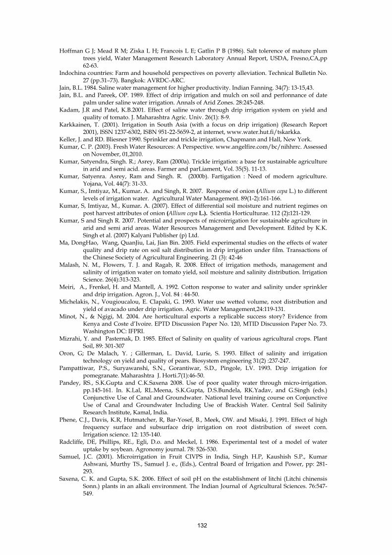
132

Hoffman G J; Mead R M; Ziska L H; Francois L E; Gatlin P B (1986). Salt tolerence of mature plum trees yield, Water Management Research Laboratory Annual Report, USDA, Fresno,CA,pp 62-63.

Indochina countries: Farm and household perspectives on poverty alleviation. Technical Bulletin No. 27 (pp.31–73). Bangkok: AVRDC-ARC.

Jain, B.L. 1984. Saline water management for higher productivity. Indian Fanning. 34(7): 13-15,43. Jain, B.L. and Pareek, OP. 1989. Effect of drip irrigation and mulch on soil and perfonnance of date

palm under saline water irrigation. Annals of Arid Zones. 28:245-248. Kadam, J.R and Patel, K.B.2001. Effect of saline water through drip irrigation system on yield and

quality of tomato. J. Maharashtra Agric. Univ. 26(1): 8-9. Karkkainen, T. (2001). Irrigation in South Asia (with a focus on drip irrigation) (Research Report

2001), ISSN 1237-6302, ISBN 951-22-5659-2, at internet, www.water.hut.fi/tskarkka. Keller, J. and RD. Bliesner 1990. Sprinkler and trickle irrigation, Chapmann and Hall, New York. Kumar, C. P. (2003). Fresh Water Resources: A Perspective. www.angelfire.com/bc/nihhrrc. Assessed

on November, 01,2010. Kumar, Satyendra, Singh. R.; Asrey, Ram (2000a). Trickle irrigation: a base for sustainable agriculture

in arid and semi acid. areas. Farmer and parLiament, Vol. 35(5). 11-13. Kumar, Satyenra. Asrey, Ram and Singh. R. (2000b). Fartigation : Need of modern agriculture.

Yojana, Vol. 44(7): 31-33. Kumar, S., Imtiyaz, M., Kumar. A. and Singh, R. 2007. Response of onion (Allium cepa L.) to different

levels of irrigation water. Agricultural Water Management. 89(1-2):161-166. Kumar, S, Imtiyaz, M., Kumar. A. (2007). Effect of differential soil moisture and nutrient regimes on

post harvest attributes of onion (Allium cepa L.). Scientia Horticulturae. 112 (2):121-129. Kumar, S and Singh R. 2007. Potential and prospects of microirrigation for sustainable agriculture in

arid and semi arid areas. Water Resources Management and Development. Edited by K.K. Singh et al. (2007) Kalyani Publisher (p) Ltd.

Ma, DongHao, Wang, QuanJiu, Lai, Jian Bin. 2005. Field experimental studies on the effects of water quality and drip rate on soil salt distribution in drip irrigation under film. Transactions of the Chinese Society of Agricultural Engineering. 21 (3): 42-46

Malash, N. M., Flowers, T. J. and Ragab, R. 2008. Effect of irrigation methods, management and salinity of irrigation water on tomato yield, soil moisture and salinity distribution. Irrigation Science. 26(4):313-323.

Meiri, A., Frenkel, H. and Mantell, A. 1992. Cotton response to water and salinity under sprinkler and drip irrigation. Agron. J., Vol. 84 : 44-50.

Michelakis, N., Vougioucalou, E. Clapaki, G. 1993. Water use wetted volume, root distribution and yield of avacado under drip irrigation. Agric. Water Management,24:119-131.

Minot, N., & Ngigi, M. 2004. Are horticultural exports a replicable success story? Evidence from Kenya and Coste d’Ivoire. EPTD Discussion Paper No. 120, MTID Discussion Paper No. 73. Washington DC: IFPRI.

Mizrahi, Y. and Pasternak, D. 1985. Effect of Salinity on quality of various agricultural crops. Plant Soil, 89: 301-307

Oron, G; De Malach, Y. ; Gillerman, L. David, Lurie, S. 1993. Effect of salinity and irrigation technology on yield and quality of pears. Biosystem engineering 31(2) :237-247.

Pampattiwar, P.S., Suryawanshi, S.N., Gorantiwar, S.D., Pingole, LV. 1993. Drip irrigation for pomegranate. Maharashtra J. Horti.7(1):46-50.

Pandey, RS., S.K.Gupta and C.K.Saxena 2008. Use of poor quality water through micro-irrigation. pp.145-161. In. K.Lal, RL.Meena, S.K.Gupta, D.S.Bundela, RK.Yadav, and G.Singh (eds.) Conjunctive Use of Canal and Groundwater. National level training course on Conjunctive Use of Canal and Groundwater Including Use of Brackish Water. Central Soil Salinity Research Institute, Kamal, India.

Phene, C.J., Davis, K.R, Hutmatcher, R, Bar-Yosef, B., Meek, OW. and Misaki, J. 1991. Effect of high frequency surface and subsurface drip irrigation on root distribution of sweet corn. Irrigation science. 12: 135-140.

Radcliffe, DE, Phillips, RE., Egli, D.o. and Meckel, I. 1986. Experimental test of a model of water uptake by soybean. Agronomy journal. 78: 526-530.

Samuel, J.C. (2001). Microirrigation in Fruit CIVPS in India, Singh H.P, Kaushish S.P., Kumar Ashwani, Murthy TS., Samuel J. e., (Eds.), Central Board of Irrigation and Power, pp: 281-293.

Saxena, C. K. and Gupta, S.K. 2006. Effect of soil pH on the establishment of litchi (Litchi chinensis Sonn.) plants in an alkali environment. The Indian Journal of Agricultural Sciences. 76:547-549.

133

Singh, H.P.; Kumar, Ashwani and Samuel, J.C. (2000). Micro-irrigation- for horticultural crops. Indian Horticultute Vol. 45(1) : 7-18.

Singh, P., Kumar, R, Agarwal, M.C., and Mangal, J.L. 1990. Performance of drip and surface irrigation for tomato in heavy soils. Proc. XI International Convention on Use of Plastics in Agriculture, NCPA, New Delhi. 67-72.

Singh, Pratap and Kumar, R. 1994. Effect of irrigation methods for cauliflower grown in heavy soils with shallow watertable. J Agril. Engg., ISAE. 31:36-43.

Singh, Rajbir, Kumar Satyendra and Kumar, Ashwani.2001. Studies on performance of drip irrigated kinnow orchard in south-western Punjab-A case study. In Microirrigation (H.P. Singh. S.P. Kaushish, Ashwani Kumar, TS. Murthy and J.e. Samuel, (Eds). Central Board of Irrigation and Power, pp : 300-308.

Singh. A. K. 2003. On farm water managemenl. Issue and priorities. Proceeding of summer school on use of modern tools for increasing on farm water use efficiently. 1-10.

Subba Rao, N. Subbiah, G.V. and Ramaiah, B. 1987. Effect of saline water on tomato yield. And soil properties. Jlndian Sac Soil Sci Research. 5(2):407-409

Weinberger, K., and Lumpkin, T. A. 2005. High value agricultural products in Asia and the Pacific for smallholder farmers: Trends, opportunities and research priorities. Rome: GFAR. http://www.egfar.org/documents

Wu, J.P. and Gitlin, H.M. . 1975. Irrigation efficiencies of surface, sprinkler and drip irrigation Proc 2nd World Congr on Water Resource Water for human needs, New Delhi, India pp. 191-199.

Zhang, J, Elliott R. L. and Ketring, D. L.1993 Root distribution models applied to peanuts. Transactions of the American Society of Agricultural Engineer 36(3) 727-734.

Zhang, M., Alva, A. K., Li, Y.C. and Calvert, DV. 1996. Root distribution of grapefruit trees under dry granular broadcast vs. fertigation method. Plant and soil 183: 79-84.

Zoldoske, D.F., Genito, S., Torgensen, G.S. 1995. Surface drip irrigation on turf grass, a university experience.Proc Fifth Intern Microir Congr Orlando, Florida ASAE, Publ. Yol. 4 : 300-302.

134

Recharge and Skimming- Opportunities and Techniques for Poor Quality Ground Water Areas S.K. Kamra Central Soil Salinity Research Institute, Karnal – 132 001 (Haryana), India E-mail: skkamra@cssri.ernet.in Introduction About 60 percent of irrigation and 80 percent of drinking water requirements of India are met from groundwater sources. Proliferation of about 20 million private open wells/ shallow tubewells and 90000 deep public tubewells has been vital for about seven- fold increase in India’s irrigation potential over the last five decades. Due to easy access, operational convenience and private ownership, the groundwater development has been quick but unregulated and has resulted in alarming decline of water tables in about one seventh of country’s geographical area. In the susceptible states of Andhra Pradesh, Bihar, Gujarat, Haryana, Karnataka, Kerala, Madhya Pradesh, Maharashtra, Punjab, Rajasthan, Tamil Nadu and Uttar Pradesh, declining water levels are facing gradual deepening of the existing abstraction structures causing escalation in the cost of pumping. At current rate of development, about two fifth of the country’s area is likely to be over-exploited (groundwater abstraction > 85 % of annual replenishment) by 2017.

Declining water levels in the arid and semi- arid areas are often accompanied by increase in solute concentrations and deterioration of ground water quality. Saline water ingress has occurred in the coastal regions of West Bengal, Gujarat, Tamil Nadu, Pondicherry and other states due to excessive pumping and declining ground water levels. Upconing is a phenomenon due to which the interface of fresh and saline waters rises to enter the lower end of the well screen, resulting in a gradual deterioration in the pumped water quality. Besides extensive coastal regions of the country, upconing is prevalent in inland areas where excessive withdrawal of usable fresh water overlying saline groundwater results in inferior water quality and degradation of the aquifer. In particular, irrigated areas in many arid and semiarid regions are underlain by aquifers of poor quality where very little groundwater development takes place resulting in waterlogging and secondary soil salinization like in a significant part of Haryana, Rajasthan, Gujarat and Punjab. Under these conditions, it is aimed that the saline water is not disturbed and the fresh water accumulated over saline groundwater in thin layers is selectively pumped through specially designed skimming structures and by enhancing groundwater recharge. In this paper, basic features of different skimming structures are discussed in the context of Indian conditions. Further, field experiences on a number of new technologies for skimming and recharging of fresh water in saline groundwater regions of Haryana, Andhra Pradesh, Gujarat and Tamil Nadu under a National Agricultural Technology Project are reviewed. Further, initial results of an extensive project on individual farmer based groundwater recharge structures for augmenting groundwater, improving quality and enhance water productivity in 100 farmers’ fields in declining water table areas of Haryana, Punjab, utatr Pradesh and Gujarat are presented. Groundwater Skimming Structures Various skimming well configurations such as single, multi-strainer, radial collector and scavenger wells (Fig. 1) can be used to abstract fresh water from thin layers overlying saline groundwater. The basic concept of skimming structures is to modify the flow lines in such a way to maximize horizontal contribution of aquifer zones of acceptable quality to pumped water (Sufi et al., 1998). A single well (Fig. 1a) is used in unconfined aquifers in most parts of India. While using these wells in saline groundwater regions, well penetration is kept deep into the fresh water layer with a large gap between the bottom of the well and the fresh- saline water interface. These types of tubewell drainage projects have been executed at Masitawali in IGNP (Hooja et al., 1995), Ghaggar depressional areas in Rajasthan and in Fatehabad branch area of Haryana. A multi-strainer well (Fig. 1b), with relatively shallower penetration than single well, can be used for water table control to reduce upconing in fresh water layers of restricted depth. The system consists of closely spaced interconnected wells, each of low capacity, pumped by a central suction pump. Such structures are being extensively used close to canals/ distributaries in Punjab in India (Shakya, 2002)

135

and in the Indus plains of Pakistan (Sufi et al., 1998; Mazhar Saeed et al., 2003). There are sporadic reports on the use of these systems in marginally saline regions of Haryana, Rajasthan, Andhra Pradesh and Tamil Nadu in India. Air leakage and priming problems have been reported from these studies.

Radial collector wells consisting of an open well and input radial drains on one or more sides (Fig. 1c) involve shallower penetration than a single vertical well operating at the same discharge. Since the radial drains collect water from shallow depths, upconing of saline water from lower depths is prevented. Large diameter open skimming wells experimented at Hisar in Haryana (Kumar and Singh, 1995) and at Luni- Ki- Dhani in Rajasthan (Hooja et al., 1995) and a drain line - sump based Doruvu technology embarked on a large scale in coastal sandy soils of Andhra Pradesh (Raghu Babu et al., 1999; Raghu Babu et al., 2004, NATP, 2005) are the local variants of radial collector wells. Scavenger wells (Fig. 1d) involve simultaneous abstraction of fresh and saline waters through two wells having screens in different quality zones, for controlling the rise of interface. The scavenger wells have been tested in the lower Indus basin of Pakistan (Sufi et al., 1998) and have shown their potential in skimming of fresh water. Despite apparent problem of disposal of saline water, the scope of scavenger wells needs testing for cases involving two cavity wells (non- strainer tubewells common in saline groundwater regions of Indo- Gangetic plains) installed at different depths or a combination of a strainer and a cavity wells. Geological, hydrological and geo- chemical characteristics of the aquifers must be studied in an integrated way to study the hydraulics and evaluate the performance of these skimming structures. National agricultural technology project (NATP) A NATP ‘Technologies for Skimming and Recharging Fresh Water in Saline Groundwater Regions’ is being operated at CSSRI (the lead center) and four collaborating centers. Over a period of about 5 years, the project has made impressive accomplishments in proposing, testing and evolving groundwater skimming and recharging technologies in saline groundwater regions of Haryana, Andhra Pradesh, Gujarat and Tamil Nadu. Features of the promising technologies are briefly discussed below: Haryana : The north- western Indian State of Haryana is a part of Indo- Gangetic alluvial plains. About two third of the geographical area is currently underlain with saline groundwater and the situation is deteriorating further due to disproportionate pumping vis- a- vis groundwater recharge. In most of the marginally saline groundwater regions, low discharge shallow cavity wells are used for irrigation, which are inexpensive pumping structures not requiring strainer. Deep tubewells are not feasible due to increasing groundwater salinity with depth while many shallow tubewells are abandoned due to upconing of saline water from the deeper layers. A skimming cum recharge structure (Fig. 2) was constructed at a downstream location prone to runoff flooding at village Jagsi/ Sarfabad in Saffidon block of Jind District. The system consists of two cavity tubewells, installed at 7 m and 40 m depth in the respective fresh and saline groundwater zones, which can be operated separately or together to obtain water of different qualities. The system is similar in features to a scavenger type skimming structure (Fig. 1d) discussed above but consists of cavity wells instead of strainer tubewells. A recharge chamber of 6 m x 2.5 m x 2 m size and containing a graded filter of fine sand, coarse sand, gravel and boulders was constructed close by to facilitate recharging of one or both cavities with filtered runoff during rainy season or excess canal water. The objective was to increase the availability of good water in upper cavity or improve the quality of lower cavity for possible use at time of water scarcity. Kamra et al. (2006) report general improvement in the groundwater regime of area due to combined effect of the natural and imposed recharge interventions. The estimated recharge rates through injection in cavity wells were low at about one quarter of the pumping rates under shallow groundwater conditions. Coastal sandy soils of Andhra Pradesh and Tamil Nadu: In Andhra Pradesh, about 1.74 lakh ha coastal sandy soils are characterized by good quality water floating over saline ground water at shallow depths which cannot be extracted with conventional tube wells. These soils occur in a 10 km wide and 972 km long strip extending from Ichapuram in Srikakulam district to Tada in Nellore district. The annual rainfall in this belt ranges from 700 - 1200 mm with an average of 855 mm. Farmers traditionally draw out manually the fresh water that collects in dug out conical pits locally

136

called doruvus and use it for cultivation of vegetables, flower plants and raising crop nurseries. Similar practices involving shallow pits (locally called Oothu Kuzhi) are prevalent in nearly 600 km long coast line and 6.8 lakh ha coastal area in Tamil Nadu. These doruvus waste about 20 % fraction of the productive coastal sands and are also subjected to high evaporation losses. Over last decade, a radial collector well type (Fig. 1c) skimming structure, called ‘Improved Doruvu’, had been evolved through All India Coordinated Research Project on Saline Water Scheme at Bapatla in Guntur District of Andhra Pradesh. The radial arms (perforated drain lines of 30- 40 m length) installed at 2- 4 m depth skim fresh water from thin zones and carry it to an open well (called sump) from one or more sides. The system yields a discharge of 5 to 15 lit/sec or more depending upon number of arms and nature of sand and can operate in combination with sprinkler/ drip system. The system has been extensively adopted at more than 70 sites in 20 villages in Guntur and Prakasam districts of Andhra Pradesh. A major deterrent for large- scale adoption among small and marginal farmers had been the high cost and lack of optimal designs and layouts for sustained supply of fresh water. Geo- hydrological and geophysical studies, conducted under NATP in Guntur district in Andhra Pradesh and Nagapattinam district in Tamil Nadu, indicate the existence of a sand layer of less than 8- 10 m followed by a clay layer saturated with saline water. The EC of water increases with depth and with increasing nearness to the sea. Radial collector wells of different designs (2 to 4 drain lines at same or variable depth and drain length) were evaluated for hydraulics and economics at a number of sites in these districts of Andhra Pradesh and Tamil Nadu. Pumping tests indicated 90 m as the safe spacing between two skimming wells. The tracer studies revealed that radial arm contribute 80% of pumped water while the remaining 20 % comes from the bottom of the well. Multiple filter point systems (Fig. 1b), tested at a number of sites in these districts, indicated limited scope for skimming due to insufficient water in the flow domain. The improved Doruvu technology was found to increase the farmers’ income by 25 to 40 % due to enhanced crop yield but is extremely costly at about Rs. 75000/ for two arm wells. Horizontal drilling of radial drains needs to be standardized for sandy soils to reduce the cost of installation of these structures. Groundwater recharge in saline groundwater regions of Gujarat and Tamil Nadu: Under NAT project, groundwater recharge through farm and percolation ponds was evaluated for saline groundwater regions in the rocky regions of Gujarat and Tamil Nadu. The site Khapat in Porbander district of Gujarat (annual rainfall ≅ 500 mm) had 1.0 – 1.5 m thick clayey soil followed by sedimentary fractured aquifers. Two dug well at this site were recharged separately using runoff from rainfall harvested in two farm ponds after filtration through a designed sand - gravel- boulder filter. The concept is displayed in Fig. 3. The enhanced recharge during 2004 resulted in improved groundwater availability and as well as significant reduction in salinity of waters (from 9.50 to 0.90 dSm-1 and 3.7 to 1.20 dS/m respectively) in two wells. Similarly the recharge potential of percolation ponds (of about 3000 m3 capacity) constructed in shallow clayey soils underlain by igneous fractured rocks using harvested runoff was evaluated at two sites (Aruppukottai, district: Virudhunagar, Fig. 4; Ramanathapuram, district: Ramanathpuram) in Tamil Nadu. At Aruppukottai, studies on recharging an abandoned open well using filtered excess runoff provided very promising results in terms of improvement in availability and quality of well water. The research output of NAT project is paving the way for commissioning of larger groundwater skimming projects in coastal sandy regions of Andhra Pradesh and Tamil Nadu and artificial recharge projects in Haryana, Gujarat and Tamil Nadu. Further details on the features and performance evaluation of the above and a few additional groundwater skimming and recharge structures can be found in NATP (2005). Salient observations and emerging issues of NATP

1. Radial collector well type structures have considerable scope in coastal sandy soils for skimming of fresh water from thin sandy zones. The cost of the system can be considerably reduced by standardizing the techniques for horizontal drilling of drains in sandy soil.

2. The performance of skimming structures in coastal sandy soils is significantly influenced by the depth and nature (coarse/ fine) of sand. Govt. may provide subsidy for installation of these structures in the identified areas. Multiple well point systems have restricted scope for skimming in coastal sandy soils due to limited depth of sand column.

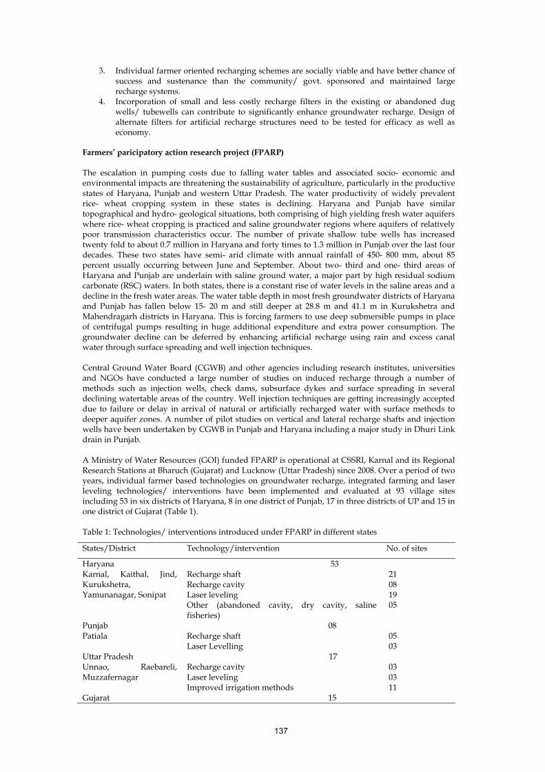
137

3. Individual farmer oriented recharging schemes are socially viable and have better chance of success and sustenance than the community/ govt. sponsored and maintained large recharge systems.

4. Incorporation of small and less costly recharge filters in the existing or abandoned dug wells/ tubewells can contribute to significantly enhance groundwater recharge. Design of alternate filters for artificial recharge structures need to be tested for efficacy as well as economy.

Farmers’ paricipatory action research project (FPARP) The escalation in pumping costs due to falling water tables and associated socio- economic and environmental impacts are threatening the sustainability of agriculture, particularly in the productive states of Haryana, Punjab and western Uttar Pradesh. The water productivity of widely prevalent rice- wheat cropping system in these states is declining. Haryana and Punjab have similar topographical and hydro- geological situations, both comprising of high yielding fresh water aquifers where rice- wheat cropping is practiced and saline groundwater regions where aquifers of relatively poor transmission characteristics occur. The number of private shallow tube wells has increased twenty fold to about 0.7 million in Haryana and forty times to 1.3 million in Punjab over the last four decades. These two states have semi- arid climate with annual rainfall of 450- 800 mm, about 85 percent usually occurring between June and September. About two- third and one- third areas of Haryana and Punjab are underlain with saline ground water, a major part by high residual sodium carbonate (RSC) waters. In both states, there is a constant rise of water levels in the saline areas and a decline in the fresh water areas. The water table depth in most fresh groundwater districts of Haryana and Punjab has fallen below 15- 20 m and still deeper at 28.8 m and 41.1 m in Kurukshetra and Mahendragarh districts in Haryana. This is forcing farmers to use deep submersible pumps in place of centrifugal pumps resulting in huge additional expenditure and extra power consumption. The groundwater decline can be deferred by enhancing artificial recharge using rain and excess canal water through surface spreading and well injection techniques.

Central Ground Water Board (CGWB) and other agencies including research institutes, universities and NGOs have conducted a large number of studies on induced recharge through a number of methods such as injection wells, check dams, subsurface dykes and surface spreading in several declining watertable areas of the country. Well injection techniques are getting increasingly accepted due to failure or delay in arrival of natural or artificially recharged water with surface methods to deeper aquifer zones. A number of pilot studies on vertical and lateral recharge shafts and injection wells have been undertaken by CGWB in Punjab and Haryana including a major study in Dhuri Link drain in Punjab.

A Ministry of Water Resources (GOI) funded FPARP is operational at CSSRI, Karnal and its Regional Research Stations at Bharuch (Gujarat) and Lucknow (Uttar Pradesh) since 2008. Over a period of two years, individual farmer based technologies on groundwater recharge, integrated farming and laser leveling technologies/ interventions have been implemented and evaluated at 93 village sites including 53 in six districts of Haryana, 8 in one district of Punjab, 17 in three districts of UP and 15 in one district of Gujarat (Table 1). Table 1: Technologies/ interventions introduced under FPARP in different states

States/District Technology/intervention No. of sites

Haryana 53 Karnal, Kaithal, Jind, Kurukshetra, Yamunanagar, Sonipat

Recharge shaft 21 Recharge cavity 08 Laser leveling 19 Other (abandoned cavity, dry cavity, saline fisheries)

05

Punjab 08 Patiala Recharge shaft 05 Laser Levelling 03 Uttar Pradesh 17 Unnao, Raebareli, Muzzafernagar

Recharge cavity 03 Laser leveling 03

Improved irrigation methods 11 Gujarat 15

138

Bharuch Recharge well 12 Renovation of farm pond/IFS 03 Total 93 The watertable depth in most selected sites in four states varies between 10- 30 m and has been falling @ 20- 60 cm every year. Despite semi- arid climate at selected sites, there are depressional areas where water accumulates during rainy season and can be recharged to groundwater. About one third sites of Haryana and all sites of Punjab have high groundwater salinity and residual sodium carbonate (RSC) problems. Groundwater in Unnao district has high fluoride concentration that is adversely affecting the health of the people and livestock. Technologies Groundwater recharge systems are based on well injection techniques and involve passing of excess rain and canal water under gravity to suitable aquifer after filtration. The demonstration sites were identified based on interaction with farmers, local tubewell mechanics and NGOs. Selection of recharge structures of different designs, depths and costs (recharge shafts, recharge cavities, recharge wells, dry cavities, and abandoned wells) was based on hydro- geological investigations and quantum of potential runoff water available at specific locations. A typical recharge structure consists of a recharge well coupled to a recharge filter. The integrated farming systems involve horticultural crops and fisheries in fresh and saline groundwater regions while laser levelling and improved irrigation interventions aim to increase uniformity of water application for enhancement of water productivity and farmers’ income.

(a) Recharge Shaft (26 sites, Fig. 5a): It consists of a bore hole of 45 cm φ filled with gravel to

carry filtered recharge water to subsurface sandy zones. The surface runoff is first passed through a recharge filter consisting of layers of coarse sand, small gravel and boulders in a small masonry chamber to safeguard against clogging. A high pressure PVC pipe, of 12.5 cm φ and slotted in sandy zones, is provided for cleaning of clogged sediments in the shaft with compressed air, if needed. The depth of recharge shafts was decided based on the criterion to provide minimum 10 m cumulative sand layers for recharge.

(b) Recharge Cavity (11 sites, Fig. 5b): A recharge cavity is similar to a cavity tubewell coupled with a graded sand filter of the type used in recharge shaft. It is constructed by drilling a bore hole until a sandy layer is found below a clay layer. A blind PVC casing pipe is drilled into the clay layer and sand is pumped out until a stable cavity is developed below the clay layer. A recharge cavity can also be used for occasional pumping. In Uttar Pradesh, strainer well (slotted pipe) in sandy zones was combined with cavity for recharging of water.

(c) Recharge Wells (12 sites): Installed in Bharuch district of Gujarat, the recharge wells are similar to recharge shaft except that boreholes of different sizes (17.5- 40 cm φ) and filter chambers of different shapes have made at different sites. Placement of 12.5 cm φ PVC pipes and 8-20 mm φ pebbles in the bore hole was facilitated through air compressor; pebbles not used in 2 sites having rocky substratum.

(d) Laser Leveling (25 sites): The laser guided leveler is a new farm implement that is making a major headway in saving irrigation water vis-a- vis conventional leveling implements in rice- wheat cropping system in Indo- Gangetic states. The implement costs about Rs. 3.5 lakh and is operated with a high HP tractor. It has been introduced in large numbers in Punjab in a custom hiring mode and is also coming up fast in Haryana. Under FPARP, laser leveling intervention was demonstrated in one acre fields and compared with convention leveling systems in terms of improvement in water productivity.

(e) Improved Irrigation Methods (11 sites): Based on location and stream size of irrigation water and general slope estimated by contour survey, demonstrations on border (45- 60 m long, 5-6 m wide) and check basin (10 m x 10 m to 15m x 15 m) irrigation methods were made. The saving in applied water and improvement in yield of wheat were recorded.

(f) Pond Renovation (3 sites): Renovation of existing farm ponds (desilting, deepening and shaping) helped in rainwater conservation and further use to provide supplemental irrigation to crops. At one site in rocky substratum, rain water conservation achieved through an open well and a recharge well to provide irrigations in agri- horticultural system of Mango- Soybean.

Brief features and cost of main technologies are summarized in Table 2.

139

Table 2. Features of demonstrated recharge structures and interventions Structure Depth (m) Thickness of sandy

layers (m) Cost (Rs.)

Recharge Shaft 30- 46 10- 18 35000- 48000 Recharge cavity 40- 55 NA 35000- 45000 Recharge cavity cum strainer well 50 25 55000- 58000 Recharge well 25- 45 15- 18 22000- 31000 Laser leveling and improved irrigation methods

- - 4000- 5000/ ha

Pond renovation - - 10000-20000/ (g) Other Technologies (5 sites): These included recharge of abandoned cavities, dry cavities and

saline fisheries. Evaluation of recharge technologies Individual farmers can construct recharge structures at any low lying location where runoff gets accumulated and adversely affects the production of rice during monsoon rains and of wheat during occasional winter rains. At selected sites in Haryana and Punjab, runoff water from 10-20 ha surrounding area was available during 2009 monsoon for recharge through these structures. There are encouraging results on the effectiveness of recharge shaft and recharge cavities to replenish groundwater and improve its quality. Depth to groundwater and EC, pH and RSC of groundwater were determined periodically to assess the impact of recharge structures. During 2009 rainy season, 0.6-3.3 m rise in water table and 0.2 – 2.4 dS/m reduction in groundwater salinity due to recharged water were observed at different sites in Haryana and Punjab. The temporal changes in depth, EC and RSC or pH of groundwater at one representative site in Haryana and one site in Gujarat are presented in Fig. 6. It is seen that recharge events, indicated by arrows, cause both a rise in water table depth and reduction in EC as well as RSC of groundwater. The clogging of the recharge filter has been observed to be a major constraint in the performance of recharge structures. Farmers need to be trained to clean the deposited sediments on the sand layer of recharge filter after every recharge event and replaced with new or washed sand to maintain optimal water intake. Mechanisms for farmers’ involvement and marginal sharing of cost of recharge structures need to be developed. Field and lab studies are in process to devise improved designs of recharge filters to minimize clogging problem. Thickness of upper sand layer of recharge filter has been found to be a primary factor influencing clogging, while size of gravel in the middle layer also controls effectiveness of sand as a filter. Impact The results of 1-2 rainy seasons indicate these structures to be highly effective in augmentation of groundwater and improving its quality. • Runoff water from 10- 20 ha surrounding area was available for recharge at sites in Haryana and

Punjab during 2009. The recharge structures were successful in saving of transplanted paddy in all or a part of water submerged area. Considering the volume of flood water, additional structures are needed at some sites for which farmers were keen using their own resources. Field hydrological studies and socio- economic surveys with farmers at selective sites indicate that

• 21.4 cm rainfall occurring in 4 storms of 5 cm or more over 2-3 consecutive days during July- September, 2009 produced 10.4 cm cumulative runoff at specific sites in Haryana. Based on results of one rainy season, capital investment cost has been worked out @ Rs. 3.5 to Rs. 2.1 / m3

recharge water for locations collecting runoff from 12- 20 ha area. • At 2 sites having 20 ha and 12 ha water contributing areas, recharge structures reduced damage

to basmati rice in 2 ha and 1 ha area by 30 % and 25 % respectively. This translates into a net saving of Rs. 58800/ and Rs. 24500/ from rice crop only and payback period of 1-2 years for these systems.

• Based on limited studies, recharge capacity of recharge shafts and cavities installed in Haryana and Punjab has been estimated @ 4-6 litre/ sec or 2500- 3500 m3 per week provided sediments retained in recharge filter are cleaned timely. The life of recharge structures, with periodic

140

cleaning of clogged sediments in subsurface layers, is expected to be 15- 20 years. The farmers prefer recharge cavities over recharge shafts due to the possibility of its occasional use for pumping water for irrigation.

• There are encouraging results on the effectiveness of recharge structures to replenish groundwater and improve its quality. During 2009 rainy season, 0.6- 3.3 m rise in water table and 0.2 – 2.4 dS/m reduction in groundwater salinity due to recharge water were observed at different sites in Haryana and Punjab.

• GR through 12 recharge wells constructed in Bharuch district of Gujarat also resulted in prolonged availability and improvement in quality of groundwater during rainy season of 2009. At one site (Borebhata), reduction in groundwater salinity from 1.9 dS/m to 0.3 dS/m resulted in 37.5 % increase in income (Rs. 2.0 lakh to 2.75 lakh/ ha) in Banana plantations and 14.3 % increase in income (Rs. 3.5 lakh to 4.0 lakh /ha) in papaya plantations. At another site (Netrang), well recharge caused 2.3 m rise in watertable and reduction in groundwater salinity from 1.02 to 0.15 dS/m. This resulted in improvement in yields and additional incomes of Rs. 14000/ha and Rs. 33250/ ha in Soybean crop and mango plantations.

• GR of excess canal water through newly installed recharge cavities at 3 sites in Unnao district of UP reduced fluoride concentration of groundwater from 2.0 ppm to 1.2 ppm, i.e below prescribed limit of 1.5 ppm for drinking water during March 2010. The reductions are likely to be significantly more during rainy season in fluoride affected villages.

• Laser levelling is a highly effective tool to improve water productivity. Results from 6 farmers’ fields in Haryana during 2009- 2010 indicate that laser levelling reduced mean irrigation water application in rice and wheat by 18.6 and 21.1 % and increased yields by 8.3 and 11.0 % respectively. This meant an additional income of Rs. 10910/ ha (Rs. 5040/ ha in rice and Rs. 5870/ ha in wheat) due to laser levelling over conventionally levelled fields. The corresponding increase in water productivity (Kg/ m3 of applied water) are 34.6 % and 37.6 % for rice and wheat or Rs. 4.7/ m3 for rice and Rs. 5.9/ m3 of applied water in wheat.

• Properly designed border and check basin irrigation methods also resulted in water saving of 10- 40 % in 10 farmers’ fields in Raebareli district of UP.

Suggested Readings Hooja, R., Shrinivas, V., Sharma, G., 1995. Waterlogging and salinity problems in IGNP, Rajasthan. In:

Rao, K.V.G.K., Agarwal, M.C., Singh, O.P., Oosterbaan, R.J. (Ed.) Reclamation and Management of Waterlogged Saline Soils, National Seminar Proc. CSSRI, Karnal and HAU, Hissar (Indo- Netherlands Collaborative Project): 141- 159.

Kamra, S.K., Anchal, V., Aswal, S., and Lal, K. 2006. Groundwater recharge through cavity wells in saline groundwater regions. In: Recharge systems for protecting and enhancing groundwater resources. Proc. 5th International Symposium on Management of Aquifer Recharge (ISMAR5), Berlin (Germany), June 11- 16, 2005, IHP – VI Series on Groundwater No. 13, 699- 704

Kumar, R. and Singh, J. 1995. Drainage systems for groundwater management. In: Rao, K.V.G.K., Agarwal, M.C., Singh, O.P., Oosterbaan, R.J. (Ed.) Reclamation and Management of Waterlogged Saline Soils, National Seminar Proceedings CSSRI, Karnal and HAU, Hissar (Indo- Netherlands Collaborative Project): 50- 62.

Mazhar Saeed, M., Ashraf, M. and Asghar, M.N. (2003). Hydraulic and hydro- salinity behavour of skimming wells under different pumping regimes. Agricultural Water Management, 61(3), 163- 177.

National Agricultural Technology Project (2005). Technologies for Skimming and Recharging Fresh Water in Saline Groundwater Regions, Final Progress Report, Central Soil Salinity Research Institute, Karnal (Haryana), India.

Ragu Babu, M, Prasad, P.R.K., Subbaiah, G.V., Khan, M. and Minhas, P.S., 1999. Subsurface fresh skimming system : Improved doruvu technology., Bulletin No. 1/99, 19p. Central Soil Salinity Research Institute, Karnal, 39 pp (+125 pages appendices).

Raghu Babu, M., Rajendra Prasad, B. and Srikanth, I. (2004). Subsurface skimming techniques for coastal sandy soils. NATP Bulletin No.1/ 2004, Saline Water Scheme, Bapatla (Andhra Pradesh), India.

Shakya, S.K. (2002). Agricultural drainage under actual farming conditions on watershed basis. Department of Soil and Water Engineering, Punjab Agricultural University, Ludhiana (Punjab), India.

Sufi, A.B., Latif, M., Skogerboe, G.V. 1998. Simulating skimming well techniques for sustained exploitation of groundwater. Irrigation and Drainage Systems. 12: 203- 226.

141

Fig.1 Different types of fresh water skimming wells

Fig. 2 Groundwater Skimming cum Recharging Structure at Jagsi/ Sarfabad

(Distt. Jind, Haryana)

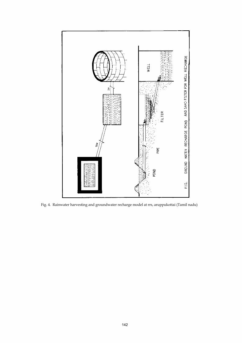
142

Fig. 4. Rainwater harvesting and groundwater recharge model at rrs, aruppukottai (Tamil nadu)

143

W S N -2.64 m- --1 m -- E Spoil Bank Catchment Area (100 acre.) Trapezoidal Channel Existing Natural Stream Road Bank Percolation Pond 3000m3 Open Recharge cum Well Filter bed Waste Weir Existing Channel Fig. 5. Rain water harvesting and recharging into ground water for farmstead

144

Water source

Bore hole (45 cm φ)

Round gravel (1.5- 2.0 cm φ)

G.L.

1.8 m

1.65 m

Coarse sand (0.5- 1.0 mm φ)

Gravel (1.0- 1.2 cm φ)

44 m

Inlet channel

12.5 cm φ PVC slotted pipe (10kg/cm2

pressure) for compressed air circulation

Slotted pipe

Water

Recharge Shaft

Recharge arm

Water sourceG.L.

1.8 m

1.65 m

Coarse sand (0.5- 1.0 mm φ)Gravel (1.0- 1.2 cm φ)

44 m

Inlet channel

15 cm φ PVC blind pipe (10kg/cm2 pressure) for recharge

Water

Recharge cavity

Boulder (10- 12 cm φ)Recharge arm

table

Cavity

(a) (b) Fig. 5.: Design features of recharge shaft (a) and recharge cavities (b) installed in Haryana, Punjab and Uttar Pradesh

(a)

0

2

4

6

8

10

wat

er ta

ble

dept

h ,m

0

1

2

3

4

5

6

7

8

9

June 08 Sept June 09 July Aug Sept Oct Nov 09

EC (d

S/m

), pH

WTD EC pHRecharge Recharge

(b)

Fig 6. Effect of recharge structures on water table depth and groundwater quality at

(a) Nabiabad (Karnal, Haryana) and (b) Chhapra (Bharuch, Gujarat)

145

Characterization of Wastewater for Irrigation Khajanchi Lal, R.K. Yadav and R.L. Meena Central Soil Salinity Research Institute, Karnal-132 001 (Haryana), India

Growing water scarcity threatens economic development, sustainable human livelihoods, and environmental quality around the world particularly in arid and semi-arid countries. Agriculture is the single largest user which consumes about 70% of the total fresh water abstraction. In coming years because of increased quantities of fresh water to be allocated to other remunerative sector like industry, municipalities etc., the availability of good quality water for agriculture would decrease. Presently, about 15% of India’s water resources are consumed to fulfill domestic and industrial requirements; the share of these two sectors is expected to grow up to 30% by 2050. It is predicted that industrial water use will outdo the combined use for domestic and agricultural purposes and expected to be double in next two decades. In high income countries, industrial water use already accounts for about 59 per cent of total fresh water abstraction; almost twice the amount used in agriculture. Under fresh water scarcities, we are forced to consider any sources of water including wastewater which might be used economically and effectively to promote further development.

Increasing allocation of fresh water to industry and municipalities leads to increased generation of wastewater. The Central Public Health Engineering Organization had estimated that 70 to 80% of the total water supplies turned into wastewater. According to Central Pollution Control Board, the annual water consumption in Indian industry is 40 billion cubic meter and the annual wastewater discharge is about 31 billion cubic meter (CPCB, Status and trends, 1990–2001). To assimilate such huge quantities of wastewater is beyond the capacity of natural systems. The application of wastewater to the soil as irrigation is most appropriate particularly in land locked areas. Under the fresh water scarcity, it is increasingly used in crops and vegetables. Wastewater usage has certain negative environmental impacts in the form of pathogens causing diseases, heavy metal accumulation and soil salinization. Domestic municipal wastewater is generally has high salt content, organic loads and pathogen while industrial wastewater often contains metals and metalloids and volatile compounds. The contamination of soils with toxic elements present in wastewaters tends to be cumulative and irreversible. Once introduced into the soil environment, metals are difficult to remove and remain present at low environmental concentrations indefinitely. Moreover, these pollutants find their way to ground water where pollution before certain limit is irreversible. Presently, discharge of untreated domestic wastewater is single major cause of water pollution in India. With the current emphasis on environmental health and water pollution issues, there is an increasing demand to formulate technologies to dispose of these wastewaters safely and beneficially. For development of such technologies, the first step is the characterization of wastewater for various physico-chemical parameters so that appropriate actions can be taken based upon its composition.

Wastewater and its characterization Urban wastewater refers to the water that has been used in domestic or industrial processes and whose quality has been deteriorated during the utilization process. It consists of effluents from municipalities, industries, commercial establishments and storm water. Wastewaters is mainly water that is >95% but generally contaminated with salt, organic materials like faeces, food, plant material, humus with high biochemical oxygen demand (BOD) and chemical oxygen demand (COD), nutrients (N, P, K and micronutrients), pathogens (bacteria, viruses, parasitic worms etc.); and heavy metals and metalloids toxic elements such as arsenic, cadmium, chromium, copper, lead, mercury, zinc etc. The solid portion contains 40-50% organics, 30-40% inert materials, 10-15% bio-resistant organics and 5-8% miscellaneous substances on the oven dry basis. Table 1 shows the levels of the major constituents of strong, medium and weak domestic wastewaters (UN Department of Technical Cooperation for Development, 1985). Composition of wastewater depends on the source of water supply, type and numbers of industrial units discharging effluents and level of treatment given. The risks posed are because of high total dissolved salts bearing wastes generated by industries like pharmaceuticals, rayon plants, chemicals, caustic soda, soap detergents and generation of toxic compound from pesticides, smelters organic chemicals, steel plants, tanneries pharmaceuticals etc. Fertilizer plants generate toxic wastes as cyanide and arsenic. Steel plants and oil refineries contribute to phenols while engineering units, refineries and vanaspati (hydrogenated vegetable oil) industry release oils and greases in the environment. Tanneries add Cr and fertilizer units also

146

add fluoride to the system. Similarly, caustic soda units release Hg in environment. The major problems associated with wastewater produced from different industries are given in table 2. Table 1. Major constituents (mg/ L) of typical domestic wastewater

Constituents Strong Medium Weak Total solids 1200 700 350 Dissolved solids (TDS)1 850 500 250 Suspended solids 350 200 100 Nitrogen (as N) 85 40 20 Phosphorus (as P) 20 10 6 Chloride1 100 50 30 Alkalinity (as CaCO3) 200 100 50 Grease 150 100 50 BOD52 300 200 100 1 The amounts of TDS and chloride should be increased by the concentrations of these constituents in the carriage water. 2 BOD5 is the biochemical oxygen demand at 20°C over 5 days and is a measure of the biodegradable organic matter in the wastewater. Table 2. Pollution aspects of industrial wastewaters

Industry Pollution aspects Distillery Very high organic load, low ph, colour, grease, putribility, H2S and CH4 Fertilizer (N) Free NH4, As and promotes eutrophication Textiles High pH, Na, colour and toxicity Paper and pulp High pH, Na, colour and lignin Tannery High pH, high Cr, oil and grease, colour Sugar mill High BOD, oil and grease, ready putribility Electroplating Low pH, cyanide, cyanates, Ni, Fe and other heavy metals.

Sewage effluents are usually alkaline because of detergents, have low to medium salinity, low SAR, high BOD (100-750mg/L) and good amount of micro and macro plant nutrients as is evident from the average composition of untreated sewage water of Haryana, India presented in table 3 (Yadav et al., 2003). Table 3. Average characteristics of untreated sewage waters of Haryana

Parameters Range Average Pollution (pH) 7.1-8.3 7.5 BOD (mg/l) 176-345 255 COD (mg/l) 223-457 315 TDS (mg/l) 600-3300 1700 NO3-N (mg/l) 3.2-21.3 6.5 Health E.Coli (MPN/100ml) 5x103- 4x109 4x106 Toxic constituents Cd (µg/l) 20-179 76 Cr (µg/l) 93-1130 244 Ni (µg/l) 50-535 294 Pb (µg/l) 92-1357 652 Irrigation EC dS/m 0.9-3.2 1.9 RSC (me/l) Nil-8.6 5.3 SAR 1.4-6.2 3.5 Nutrients N (mg/l) 30-65.7 45.9 P (mg/l) 3.0-11.1 6.9 K (mg/l 19-265 62.4

Pathogenic micro- and macro-organisms are the contaminants of greatest concern from health point of view in agricultural use of wastewater. Pathogenic viruses, bacteria, protozoa and helminths may be present in raw municipal wastewater at the levels indicated in Table 4 (Feachem et al., 1983). Pathogenic bacteria will be present in wastewater at much lower levels than the coliform group of bacteria, which are much easier to identify and enumerate (as total coliforms/100ml). Escherichia coli are the most widely adopted indicator of faecal pollution and they can also be isolated and identified fairly simply, with their numbers usually being given in the form of faecal coliforms (FC)/100 ml of wastewater.

147

Table 4. Possible levels of pathogens in wastewater

Type of pathogen Possible concentration per litre in municipal1

Viruses: Enteroviruses 2 5000 Bacteria: Pathogenic E. coli3 ?

Salmonella spp. 7000 Shigella spp. 7000

Protozoa: Entamoeba histolytica 4500 Helminths: Ascaris Lumbricoides 600

Hookworms4 32 Schistosoma mansoni

1

Taenia saginata 10 Trichuris trichiura 120

?Uncertain 1Based on 100 lpcd of municipal sewage and 90% inactivation of excreted pathogens 2Includes polio-, echo- and coxsackieviruses 3Includes enterotoxigenic, enteroinvasive and enteropathogenic E. coli 4Anglostoma duedenale and Necator americanus

A brief description of wastewater constituents, parameters and possible impacts are given in table 5. Table 5. Potential hazards/impact of pollutants/contaminants in wastewater

Pollutant/ Constituent

Measured parameter Impacts

Plant food nutrients

N, P, K etc Excess N causes injury, excessive vegetative growth, eutrophication, nitrate leaching

Suspended solids Volatile compounds, settleable suspended and colloidal impurities

Development of sludge deposits, plugging of equipments, sprinklers

Pathogens Viruses, bacteria, Feacal coli forms, helminthes

Causes diseases like diarrhea, typhoid, fever, cholera, gastroenteritis, food poisoning

Biodegradable organics

BOD, COD Depletion of dissolved oxygen, development of septic conditions, fish mortality

Dissolved inorganic

TDS, Na, Ca, Mg, Cl and B Causes salinity, phytotoxicity, affect permeability

Heavy metals Cd, Ni, Pb, Zn, As, Hg Toxic to plants and animals, possible health hazards, make the wastewater unsuitable

Quality parameters of significance for health and agriculture Health The practice of wastewater irrigation is very pervasive and widely adopted by resource poor farmers as a low-cost alternative to conventional irrigation water overlooking the potential health risks. The principal health hazards are associated with the chemical constituents of wastewaters. The level of organic chemicals in municipal wastewaters usually is very low and causes heath problem only on prolonged use. This is not likely to occur with agricultural/aquacultural use of wastewater, unless cross-connections with potable supplies occur or agricultural workers are not properly instructed. Aldrin, benzene, carbon tetrachloride, chloroform, 2,4 D, DDT, 1,2 Dichloroethane, 1,1 Dichlorethylene, heptachlor, trichlorophenol are major the organic constituents. Whereas arsenic, cadmium, chromium, cyanide, lead, fluoride, mercury, nitrate and selenium are major inorganic constituents from health point of view. In peri-urban areas such waters have been exceedingly used for cultivation of vegetables, food and fodder crops consequently contaminating them with high levels of heavy metals, helminthes and E. coli. Dietary intake of contaminated food or consumption of meat and milk obtained from the animal fed on fodder produced with the wastewater are the major sources of food chain contamination which poses serious human health and is likely a key pathway for epidemics. It causes several health problems like diarrhea, typhoid, fever, cholera, gastroenteritis, food poisoning. A survey along the Musi River in India revealed the transfer of metal ions from wastewater to cow’s milk through fodder (para grass) irrigated with wastewater.

148

About 4% of grass samples showed excessive amounts of cadmium, and all samples showed excessive lead. Milk samples were contaminated with metal ions ranging from 1.2 to 40 times permissible levels (Minhas and Samra 2004). In 2002, about 2.4 million people died from water and sanitation-associated diseases, nearly all in developing countries (Prüss-Ustün et al. 2008). The contribution of wastewater irrigation towards it may be relatively small and is not yet known exactly. Epidemological studies have established definitive adverse health impacts because of use of wastewater in agriculture (Shuval et al., 1985). Transmission of helminthic diseases caused by Ascaris and Trichuris spp. is likely to occur through the consumption of salad crops and/or vegetables eaten uncooked which are irrigated with untreated sewage. Sewage farm workers are also liable to become infected with cholera if practising irrigation with raw wastewater. Indictor organisms important from the health point of view are: Coliforms and Faecal Coliforms, Faecal Streptococci and Clostridium perfringens. The estimation of pathogenic parameters like Salmonella spp. Enteroviruses,. Rotaviruses and Intestinal Nematodes can only be considered if suitable laboratory facilities and suitably trained staff are available. Agriculture The water characteristics of importance in agricultural irrigation are specific chemical elements and compounds that affect plant growth or soil permeability. Consequently, when obtaining data to evaluate a wastewater irrigation system, it is often necessary to sample and analyze the wastewater. Routine measurements of municipal wastewater pertain to water pollution parameters like BOD, suspended solids and COD. But agriculturally important parameters that affect soil properties and crop growth such as salt content, sodium adsorption ratio, residual sodium carbonate, major and micro nutrients and toxic metal contents are rarely monitored. The guidelines formulated for water quality classification are equally applicable to evaluate wastewaters for irrigation purposes in terms of their chemical constituents, such as dissolved salts, relative sodium content and toxic ions.

a. Salinity: In general, as salinity in wastewater increases, the chance for development of soil salinity also increases. Establishing a net downward flux of water and salt through the root zone by having good drainage is the only practical way to manage a salinity problem. Long-term use of reclaimed wastewater for irrigation is not generally possible without adequate drainage.

b. Specific ion toxicity: Toxicity due to a specific ion occurs when that ion is taken up by the plant and accumulates in the plant in amounts that result in damage or reduced yield. The ions of most concern in treated wastewater are sodium, chloride, and boron. The source of boron is usually household detergents or discharges from industrial plants. Chloride and sodium also increase during domestic usage, especially where water softeners are used. For sensitive crops, toxicity is difficult to correct without changing the crop or the water supply. The problem is usually accentuated by severe (hot) climatic conditions (Westcot and Ayers, 1985).

c. Soil permeability: In addition to their effects on the plant, sodium in irrigation water may affect soil structure and reduce the rate at which water moves into the soil as well as reduce soil aeration. Sometimes, wastewaters are relatively high in sodium and the resulting high SAR is a major concern in planning wastewater reuse projects. Chemical or biological amendments are needed over time to prevent soil structural degradation when irrigating exclusively with sodic water.

d. Nutrients: The nutrients in treated municipal wastewater provide fertilizer value to crop or landscape production but in certain instances are in excess of plant needs and cause problems related to excessive vegetative growth, delayed or uneven maturity, or reduced quality. Nutrients occurring in important quantities include nitrogen and phosphorus and occasionally potassium, zinc, boron, and sulphur (Westcot and Ayers, 1985). The nutrients in reclaimed wastewater can contribute to crop growth, but periodic monitoring is needed to avoid imbalanced nutrient supply.

e. Microbiological content: Wastewater often contains a variety of pollutants that can harm human health and the environment. An expert committee of the World Health Organization examined the health concerns of wastewater use in agriculture. Microbial water quality guidelines for irrigation water were relaxed in 1989 to 1000 fecal coliforms per 100 ml, based on the findings of epidemiological studies of wastewater irrigation. In addition, a quality guideline for intestinal nematodes was recommended as less than 1 intestinal nematode egg per liter (WHO, 1989). The latest guidelines (WHO, 2006) for the safe use of wastewater in agriculture have been revised considerably. The faecal coliform guideline has been replaced by a focus on attributable risks and disability-adjusted life years (DALYs) (Table 6).

F. Miscellaneous problems: Clogging problems with sprinkler and drip irrigation systems have been reported when treated municipal wastewater is used. The most frequent clogging problems occur with drip irrigation systems. Another possible problem of the wastewater reuse is the excessive

149

residual chlorine in treated effluent. Residual chlorine less than 1mg/l should not affect plant foliage, but when chlorine residual is in excess of 5mg/l, severe plant damage can occur.

G. Heavy metals: Municipal wastewater effluents may contain a number of toxic elements, including heavy metals. Some of them may be removed during the treatment process but others will persist and could present phytotoxic problems. Thus, municipal wastewater effluents should be checked for trace element toxicity hazards, particularly when trace element contamination is suspected. Table 7 presents phytotoxic threshold levels of some selected trace elements (National Academy of Sciences (1972) and Pratt (1972).

Table 6. Health-based targets for wastewater use in agriculture

Exposure scenario Health-based target (DALY per person per

year)

Log10 pathogen reduction needed

Number of helminth eggs per litre

Unrestricted irrigation ≤10−6 Lettuce 6 ≤1 Onion 7 ≤1 Restricted irrigation ≤10−6

Highly mechanized 3 ≤1 Labour intensive 4 ≤1 Localized (drip) irrigation ≤10−6 High-growing crops 2 No recommendation Low-growing crops 4 ≤1 The health-based targets are based on quantitative microbial risk assessment (QMRA), indicating log10 pathogen reduction required to achieved 10−6 DALY for different exposures. The disability-adjusted life year (DALY) is a measure of overall disease burden. DALYs are calculated by taking the sum of “years of life lost” and “years lived with disability”. Table 7. Threshold levels of trace elements for crop production

Element Maximum conc.(mg/l)

Remarks

Al 5.0 Can cause non-productivity in acid soils (pH < 5.5), but more alkaline soils at pH > 7.0 will precipitate the ion and eliminate any toxicity.

As 0.10 Toxicity to plants varies widely, ranging from 12 mg/l for Sudan grass to less than 0.05 mg/l for rice.

Be 0.10 Toxicity to plants varies widely, ranging from 5 mg/l for kale to 0.5 mg/l for bush beans.

Cd 0.01 Toxic to beans, beets and turnips at concentrations as low as 0.1 mg/l in nutrient solutions. Conservative limits recommended due to its potential for accumulation in plants and soils to concentrations that may be harmful to humans.

Co 0.05 Toxic to tomato plants at 0.1 mg/l in nutrient solution. Tends to be inactivated by neutral and alkaline soils.

Cr 0.10 Not generally recognized as an essential growth element. Conservative limits recommended due to lack of knowledge on its toxicity to plants.

Cu 0.20 Toxic to a number of plants at 0.1 to 1.0 mg/l in nutrient solutions. Fe 5.0 Not toxic to plants in aerated soils, but can contribute to soil acidification and

loss of availability of essential phosphorus and molybdenum. Overhead sprinkling may result in unsightly deposits on plants, equipment and buildings.

Mn 0.20 Toxic to a number of crops at a few-tenths to a few mg/l, but usually only in acid soils.

Ni 0.20 Toxic to a number of plants at 0.5 mg/l to 1.0 mg/l Pb 5.0 Can inhibit plant cell growth at very high concentrations. Se 0.02 Toxic to plants at concentrations as low as 0.025 mg/l and toxic to livestock if

forage is grown in soils with relatively high levels of added selenium. As essential element to animals but in very low concentrations.

Zn 2.0 Toxic to many plants at widely varying concentrations; reduced toxicity at pH > 6.0.

150

Livelihood issues and profitability of wastewater use Wastewater is a resource of growing global importance and that sustainably managed, it can greatly enhance livelihoods and improve environmental quality. In developed countries treated wastewater is used in public lawns and tree plantations. In developing economies it is increasingly used for irrigating high value agricultural crops like vegetables, fruits, food grains, fodder and industrial crops in peri-urban areas and is a choice and not an option. Use of wastewater is increasing because of combination of many complimentary factors: water scarcity, absence of alternative water sources, assured irrigation, lack of alternate sources, proximity to market for perishable items and affordable source of nutrient. India, China, Vietnam and many other developing and underdeveloped countries are good examples where wastewater is increasing practiced. Estimates indicate that in India sewage waters can annually irrigate about 1.5 million hectares of land area and has a potential to contribute about one million tonnes of nutrients and 130 million man-days of employment. Irrigation with various sewage or sewage mixed with industrial effluents resulted in saving of 25 to 50 per cent of N and P fertilizer and 15-27 % higher crop productivity over the normal waters (Anonymous 2004, Scott et al., 2004). In many cities 60%–90% of vegetables are produced within the city or at the city’s edge. In Pakistan 26% of the national vegetable production and in Hanoi 80% comes from wastewater irrigated agriculture (Ensink et al., 2004; Lai 2000).

The amount of nutrients in 1000 m3 of wastewater irrigation per hectare supply variable amount of nutrient: 16-62 kg total nitrogen, 4-24 kg phosphorus, 2-69 kg potassium, 18-208 kg calcium, 9-100 kg magnesium and 27-182 kg sodium (Qadir et al., 2007). In peri-urban areas because of wastewater use, farmers usually adopt year round, intensive vegetable production systems (300-400% cropping intensity) or to other perishable commodity like fodder and earn up to 4 times more from a unit land area compared to freshwater (Minhas and Samra, 2004). Management options and policy guidelines To safeguard and strengthen livelihoods and food security, mitigate health and environmental risks and conserve water resources, appropriate policies and measures suited to the end use of wastewater need to the formulated. World Health Organization formulated some guidelines which regulates wastewater irrigation based upon number of nematodes and faecal coli forms for restricted (like industrial crops cotton, sisal, sunflower etc. not intended for direct human consumption) and unrestricted uses (crops for direct human consumption like vegetable). The WHO guidelines are in fact difficult to follow in true practical sense. Some of the precautions can be low cost interventions like wearing of shoes while working with wastewater, adoption of appropriate modern irrigation methods, post-harvest technology, reduction of toxic contaminants in wastewater at source, information on hygiene, crop restriction with wastewater irrigation, regular treatment of farmers and their families with antihelminthic drugs to prevent worm infections, education and awareness programs for all stakeholders, including the public at large. Some of the easily adaptable and low cost practices which can be recommended include growing of crops on ridges for minimize the contact with wastewater, the removal of outermost two leaves in cabbage, bed planting of ridge gourd, repeated washings, sun drying for 3 to 4 hours of vegetables and harvesting of Egyptian clover and sorghum 5- 10 cm above ground were found to be quite effective in reducing the pathogen load to a great extent (Minhas et al., 2006). Cultivation of non-edible crops like flower (gladiolus, chrysanthemum) and aromatic grasses (Vetiver) is advocated as an economic alternative to avoid the entry of heavy metals in food chain and for phyto-remediation of soils metal contaminated soils (Lal et al., 2008). Other viable low-cost, low-tech removal methods proposed are a variety of lignacious biomasses like activated charcoal, press mud, rice husk and sawdust which have the ability to strongly reduce the prevalence of metals in the wastewater based on sorption principles (Indo-US AKI Report, 2010). Under the situations where land has become contaminated through waste material disposal and food crops are not permitted, alternate land uses of wastewater irrigation like establishment of man made forests with high economic value, high transpiration rate system trees like sisal, mahogany, Eucalyptus, poplar, bamboo (Bambusa arundinacea), neem (Azadirachta indica), shisham (Dalbergia sissoo) etc. for non-edible products like fuel and timber and developing green belts around the cities can be another approach to overcome health hazards. Such plants can transpire water several time equivalent to the potential evapo-transpiration from the soil matrix alone remediate wastewater. Although water use could be as high as 2500 mm annually in 6 year old plantation, the exact amount of water and nutrients taken up by Eucalyptus depend upon climate and vigour (Annual Report CSSRI, 2007; Rockwood et al., 1996; Rockwood et al., 2004).

151

Suggested Readings Annual Report 2007-08. Central Soil Salinity Research Institute, Karnal-132 001, India. pp44. Anonymous 2004. NATP – MM project report on ‘Use of Urban and Industrial Effluent in Agriculture’

CSSRI, Karnal. CPCB (1990 – 2001) CSE Down to Earth Supplement on Water use in industry "CPCB Water quality in India

(Status and trends). old.cseindia.org/dte-supplement/.../misuse. Ensink, J. H. J., C. A. Scott, S. Brooker and S. Cairncross. 2010. Sewage disposal in the Musi-River, India:

water quality remediation through irrigation infrastructure. Irrig Drainage Syst. 24:65–77. Feachem R.G., Bradley D.J., Garelick H. and Mara D.D. 1983. Sanitation and Disease: Health Aspects of

Excreta and Wastewater Management. John Wiley, Chichester. Indo-US AKI Report, 2010. Bio-drainage and Use of Wastewater in Agriculture. Water Harvesting for

Ground Water Recharge and Bio-drainage for Salinity Control. CSSRI, Karnal 132 001 India pp47. Lai, T.V. 2000. “Perspectives of Peri-urban Vegetable Production in Hanoi.” Background paper prepared for

the Action Planning Workshop of the CGIAR Strategic Initiative for Urban and Peri-Urban Agriculture (SIUPA), Hanoi, 6–9 June. Convened by International Potato Center (CIP), Lima.

Lal, K., P.S. Minhas, Shipra, R.K. Chaturvedi and R.K. Yadav. 2008. Extraction of Cadmium and Tolerance of Three Annual Cut Flowers on Cd-contaminated Soils. Bioresource Technology 99: 1006-1011.

Minhas, P.S. and Samra, J.S. Waste water use in peri-urban agriculture: Impacts and opportunities. Bulletin No. 2, 2004, CSSRI, Karnal, India.

Minhas, P.S., N. Sharma, R.K. Yadav and P.K. Joshi. 2006. Prevalence and control of pathogenic contamination in some sewage irrigated vegetables, forage and cereal grain crops. Bio-Resource Technology 97: 1174-1178.

National Academy of Sciences and National Academy of Engineering. (1972) Water quality criteria. US Environmental Protection Agency, Washington DC. Report No. EPA-R373-033. 592 p.

Pratt P.F. (1972) Quality criteria for trace elements in irrigation watsrs. California Agricultural Exteriment Station. 46 p.

Prüss-Üstün A, Bos R, Gore F, Bartram J (2008) Safer water, better health: costs, benefits and sustainability of interventions to protect and promote health. World Health Organization, Geneva.

Qadir, M. Dennis Wichelns, Liqa Raschid-Sally, Paramjit Singh Minhas, Pay Drechsel, Akiça Bahri, and Peter McCornick. 2007. Agricultural use of marginal-quality water— opportunities and challenges. www.iwmi.cgiar.org

Rockwood, D.L., Naidu, C.V., Carter, D.R., Rahman. M., Spriggs, T.A., Lin, C., Alker, G.R., Isebrands, J.G. and Segrest, S.A. 2004. Short rotation woody crops and phytoremediation: Opportunities for agroforestry. Agroforestry System 61: 51-63.

Rockwood, D.L., Pisano, S.M. and McConnell W.V. 1996. Superior cottonwood and Eucalyptus clones for biomass production in waste bioremediation system. Pp. 254-261. In proc. Bioenergy , 7th national Bioenergy Conference, September 15-20, 1996, Nashville, TN.

Scott, C.A., Faruqui, N I,and Raschid-Sally, L (eds) 2004. Wastewater Use in Irrigated Agriculture. Confronting Livelihhod and Environmental Realities. CAB International in Association with IWMI: Colmbo, Sri Lanka, and IDRC: Ottawa, Canada.

Shuval H.I., Yekutiel P. and Fattal B. (1985) Epidemiological evidence for helminth and cholera transmission by vegetables irrigated with wastewater. Jerusalem - case study. Water Science and Technology 17(4/5):433-442.

Yadav, R.K., R.K. Chaturvedi, S.K. Dubey, P.K. Joshi and P.S. Minhas. 2003. Potential and hazards associated with sewage irrigation in Haryana. Indian Journal of Agricultural Sciences 73 (5): 249-255.

UN Department of Technical Cooperation for Development. 1985. The use of non-conventional water resources in developing countries. Natural Water Resources Series No. 14. United Nations DTCD, New York.

Westcot, D.W., Ayers, R.S., 1985. Irrigation water quality criteria. In: Pettygrove, G.S., Asano, T. (Eds.), Irrigation with Reclaimed Municipal Wastewater—A Guidance Manual. Lewis Publishers, Inc., Chelsea, MI.

World Health Organization (WHO), 1989. Health guidelines for the use of wastewater in agriculture and aquaculture. Technical Report Series 778, Geneva.

World Health Organization (WHO) (2006) ‘Guidelines for the Safe Use of Wastewater, Excreta and Greywater’. Volume 2: Wastewater use in agriculture World Health Organization, Geneva.

152

Wastewater Use in Agriculture: Issues and Strategies R. K. Yadav, Khajanchi Lal and R. L. Meena Central Soil Salinity Research Institute, Karnal – 132001 (Haryana), India rkyadav@cssri.ernet.in Introduction Increasing urbanization and industrialization puts extreme pressure on fragile and dwindling fresh water resources and over-burdened sanitation systems, leading to production of huge quantities of wastewaters. In near future, generation of wastewater will further increase as higher quantities of fresh water has to be allocated to more remunerative sectors of industry and municipalities. The Central Public Health Engineering Organization had estimated that 70 to 80% of the total water supplies to these more paying sectors turn into wastewater. Presently, about 15% of India’s water resources are consumed to fulfill domestic and industrial requirements; the share of these two sectors is expected to grow up to 30% by 2050. According to Central Pollution Control Board, the annual water consumption in Indian industry is 40 b m3 and the annual wastewater discharge is about 31 b m3 (CPCB, Status and trends, 1990 – 2001). Assimilation of such huge quantities of wastewater is beyond the capacity of natural systems. The application of wastewater to the soil is most appropriate particularly in land locked areas where wastewater disposal into surface streams is banned. Under such situation, agriculture is the most logical sink, which at present consumes about 70% of the total fresh water abstraction. Under the fresh water scarcity, it is increasingly being used in crops and vegetables in peri-urban areas because it is a valuable source of irrigation and plant nutrient and supports livelihoods particularly those of poor farmers.

Where regulations and treatment processes are not adequate or because of prohibitive costs of conventional treatment particularly in developing countries, these untreated waste streams are directly introduced into the riparian environment. Indiscriminate and unregulated use of wastewater is a serious threat for water quality of groundwater and surface water bodies. Presently also, discharge of untreated domestic wastewater is single major cause of water pollution in India. Soils also have limited capacity to absorb toxic contaminants without impairing their productivity. Wastewater use has certain negative environmental impacts in the form of pathogens causing diseases, heavy metal accumulation and soil salinization. Toxic metal presence in agricultural lands is a first step in a transport chain leading to chronic human exposure. The contamination of soils with toxic elements present in wastewaters tends to be cumulative and irreversible. Chronic low-level exposure to metals can lead to human and animal health risks. Once introduced into the soil environment, metals are difficult to remove and remain present at low environmental concentrations indefinitely. Moreover, these pollutants find their way to ground water where pollution before certain limit is irreversible.

So the challenge is to identify viable low-cost, low-tech treatment methods which do not threaten the substantial livelihoods dependent on wastewater and protect the valuable natural resources from further degradation. For planned strategic wastewater use, a coherent programme involving government policies, ‘polluter pays’ principle, awareness, regular health check up, forest establishment, efficient microbial strains, wet lands, cultivation of remunerative non-edible crops, application of organic and inorganic amendments, bio-filters is to be framed and implemented.

Urban wastewater

Urban wastewater refers to the water that has been used in domestic or industrial processes and whose quality has been deteriorated during the utilization process. It consists of effluents from municipalities, industries, commercial establishments and storm water. Wastewaters is mainly water that is >95% but generally contaminated with salt, organic materials like faeces, food, plant material, humus with high biochemical oxygen demand (BOD) and chemical oxygen demand (COD), nutrients (N, P, K and micronutrients), pathogens (bacteria, viruses, parasitic worms etc.); and heavy metals and metalloids. The solid portion contains 40-50% organics, 30-40% inert materials, 10-15% bio-resistant organics and 5-8% miscellaneous substances on the oven dry basis. Composition of wastewater depends on the source of water supply, types and numbers of industrial units discharging effluents and level of treatment given. Sewage effluents are usually alkaline because of detergents, have low to medium salinity, low SAR, high BOD (100-750mg/L) and good amount of micro and macro plant nutrients as is evident from the average composition of untreated sewage water of Haryana, India presented in table 1 (Yadav et al., 2003). Routine measurements of municipal wastewater pertain to water pollution parameters like BOD, suspended solids and COD. But agriculturally important parameters that affect soil properties and crop growth such as salt content, sodium adsorption ratio, residual sodium carbonate, major and micro nutrients and toxic metal contents are rarely

153

monitored. A brief description of wastewater constituents, parameters and possible impacts are given in table 2.

Table 1. Average characteristics of untreated sewage waters of Haryana

Parameters Range Average Pollution (pH) 7.1-8.3 7.5 BOD (mg/l) 176-345 255 COD (mg/l) 223-457 315 TDS (mg/l) 600-3300 1700 NO3-N (mg/l) 3.2-21.3 6.5 Health E.Coli (MPN/100ml) 5x103- 4x109 4x106 Toxic constituents Cd (µg/l) 20-179 76 Cr (µg/l) 93-1130 244 Ni (µg/l) 50-535 294 Pb (µg/l) 92-1357 652 Irrigation EC dS/m 0.9-3.2 1.9 RSC (me/l) Nil-8.6 5.3 SAR 1.4-6.2 3.5 Nutrients N (mg/l) 30-65.7 45.9 P (mg/l) 3.0-11.1 6.9 K (mg/l 19-265 62.4

Domestic municipal wastewater is generally has high salt content, organic loads and pathogen, while industrial wastewater often contains metals and metalloids and volatile compounds. The moment domestic wastewater got mixed with industrial effluent particularly untreated one; it is loaded with heavy metals like Cd, Ni, Cr, Pb etc. and becomes more culprits. Distilleries, paper mill and sugar industries are mainly responsible for high organic loads (BOD). Table 2. Potential hazards/impact of pollutants/contaminants in wastewater Pollutant/ Constituent

Measured parameter Impacts

Plant food nutrients

N, P, K etc Excess N causes injury, excessive vegetative growth, eutrophication, nitrate leaching

Suspended solids

Volatile compounds, settleable suspended and colloidal impurities

Development of sludge deposits, plugging of equipments, sprinklers

Pathogens Viruses, bacteria, Feacal coli forms, helminthes

Causes diseases like diarrhea, typhoid, fever, cholera, gastroenteritis, food poisoning

Biodegradable organics

BOD, COD Depletion of dissolved oxygen, development of septic conditions, fish mortality

Dissolved inorganic

TDS, Na, Ca, Mg, Cl and B Causes salinity, phytotoxicity, affect permeability

Heavy metals Cd, Ni, Pb, Zn, As, Hg Toxic to plants and animals, possible health hazards, make the wastewater unsuitable

The health risks posed by the industrial wastewaters are because of high total dissolved salts bearing wastes generated by industries like pharmaceuticals, rayon plants, chemicals, caustic soda, soap detergents and generation of toxic compound from pesticides, smelters organic chemicals, steel plants, tanneries pharmaceuticals etc. Fertilizer plants generate toxic wastes as cyanide and arsenic. Steel plants and oil refineries contribute to phenols while engineering units, refineries and vanaspati (hydrogenated vegetable oil) industry release oils and greases in the environment. Tanneries add Cr and fertilizer units also add fluoride to the system. Similarly, caustic soda units release Hg in environment. The major problems associated with wastewater produced from different industries are given in table 3.

154

Table 3. Pollution aspects of industrial wastewaters

Industry Pollution aspects

Distillery Very high organic load, low ph, colour, grease, putribility, H2S and CH4

Fertilizer (N) Free NH4, As and promotes eutrophication

Textiles High pH, Na, colour and toxicity

Paper & pulp High pH, Na, colour and lignin

Tannery High pH, high Cr, oil and grease, colour

Sugar mill High BOD, oil and grease, ready putribility

Electroplating Low pH, cyanide, cyanates, Ni, Fe and other heavy metals. Wastewater generation and treatment status Water supply ensures wastewater because the depleted fraction of domestic and residential water use is typically only 15–25% with the remainder returning as wastewater. Although the numbers of urban dwellers in developing countries that continue to rely on septic tanks, cesspits etc. is unexpectedly high, growing numbers are connected to sewers that deliver wastewater – largely untreated – to downstream areas. At present, more than 80% of the sewage generated in developing countries is discharged without any treatment and half of the population depends on polluted water resources for various uses including irrigation (UNESCO, 2003). As per estimates in Asia 35% of wastewater is treated, in Latin America 14% and in Africa only a negligible portion of wastewater is treated (Scott et al., 2006).

In India, presently about 15% of water resources are consumed in domestic and industrial requirements, the share of these two sectors will grow up to 30% by 2050. Out of the 16625 MLD of wastewater generated in India, 72% is collected and only 24% is treated before release. Treating these wastewaters up to the desirable levels before disposal as per guidelines is a costly affair and prohibitively expensive. As per estimates made by Central Pollution Control Board in 2001, about 73% of India’s wastewater was disposed of untreated into rivers, irrigated canals and other surface water bodies and that an investment of US$ 65 billion would be needed to build the required wastewater treatment facilities: 10 times the amount which the Indian government plans to spend (Kumar, 2003). This situation is likely to deteriorate further as India’s population will grow by almost 285 million people in the next twenty years, with approximately 85% of this growth taking place in cities (UNDP, 2003). Increased water withdrawals to meet the water requirement of urban population will generate higher amount of wastewater. The total sewage generation from Class-I cities and Class-II towns together in India today, is about 38.3 MLD, out of which only 11.8 MLD (30%) is treated, with a capacity gap of 26,467 MLD (70%) (CPCB, 2009). As per estimates made by CSE based on the wastewater discharged data published by CPCB in "Water quality in India (Status and trends) 1990 – 2001, the total wastewater generated from all major industries in India is 83048 MLD that includes 66700 MLD of cooling water generated from thermal power plants. Out of remaining 16,348 MLD of wastewater, thermal power plants generate another 7,275 MLD as boiler blow down water and overflow from ash ponds. The second larger contributors of wastewater in terms of volume are engineering industries. A major part of the industries in this category is in small scale sector. Under this category the major polluting industries are electroplating units. The other significant contributors are paper mill, textiles industries, steel plants and sugar industries (Fig. 1).

In developing countries 70% of industrial wastes are dumped without treatment. Even after treatment some of the amount of heavy metals remained in wastewater, which may range from 40-60 percent. Industrial water demand is expected to grow by 17% annually, from ~40 BCM currently to ~ 250 BCM by 2025. As per the CPCB, only around 21% of the total waste water generated from industrial sources is treated. Big industrial houses are exploring the options such as recycling waste water and desalination to meet their growing water demand. More awareness needs to be created among medium and small scale industries by enforcing regulations and legislations on wastewater discharge quality and mandating installations of effluent treatment plants.

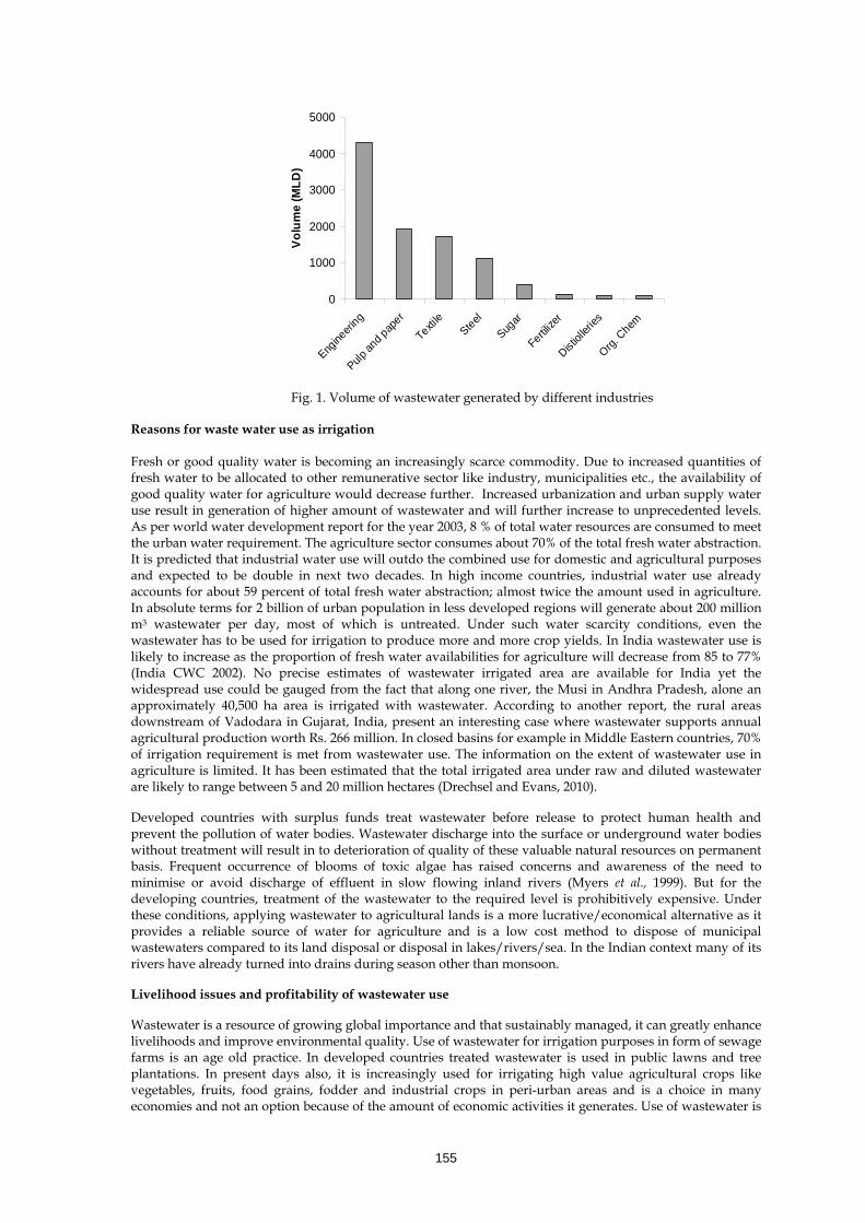
155

0

1000

2000

3000

4000

5000

Engine

ering

Pulp an

d pap

er

Textile

Steel

Sugar

Fertilize

r

Distiol

leries

Org. C

hem

Volu

me

(MLD

)

Fig. 1. Volume of wastewater generated by different industries Reasons for waste water use as irrigation Fresh or good quality water is becoming an increasingly scarce commodity. Due to increased quantities of fresh water to be allocated to other remunerative sector like industry, municipalities etc., the availability of good quality water for agriculture would decrease further. Increased urbanization and urban supply water use result in generation of higher amount of wastewater and will further increase to unprecedented levels. As per world water development report for the year 2003, 8 % of total water resources are consumed to meet the urban water requirement. The agriculture sector consumes about 70% of the total fresh water abstraction. It is predicted that industrial water use will outdo the combined use for domestic and agricultural purposes and expected to be double in next two decades. In high income countries, industrial water use already accounts for about 59 percent of total fresh water abstraction; almost twice the amount used in agriculture. In absolute terms for 2 billion of urban population in less developed regions will generate about 200 million m3 wastewater per day, most of which is untreated. Under such water scarcity conditions, even the wastewater has to be used for irrigation to produce more and more crop yields. In India wastewater use is likely to increase as the proportion of fresh water availabilities for agriculture will decrease from 85 to 77% (India CWC 2002). No precise estimates of wastewater irrigated area are available for India yet the widespread use could be gauged from the fact that along one river, the Musi in Andhra Pradesh, alone an approximately 40,500 ha area is irrigated with wastewater. According to another report, the rural areas downstream of Vadodara in Gujarat, India, present an interesting case where wastewater supports annual agricultural production worth Rs. 266 million. In closed basins for example in Middle Eastern countries, 70% of irrigation requirement is met from wastewater use. The information on the extent of wastewater use in agriculture is limited. It has been estimated that the total irrigated area under raw and diluted wastewater are likely to range between 5 and 20 million hectares (Drechsel and Evans, 2010).

Developed countries with surplus funds treat wastewater before release to protect human health and prevent the pollution of water bodies. Wastewater discharge into the surface or underground water bodies without treatment will result in to deterioration of quality of these valuable natural resources on permanent basis. Frequent occurrence of blooms of toxic algae has raised concerns and awareness of the need to minimise or avoid discharge of effluent in slow flowing inland rivers (Myers et al., 1999). But for the developing countries, treatment of the wastewater to the required level is prohibitively expensive. Under these conditions, applying wastewater to agricultural lands is a more lucrative/economical alternative as it provides a reliable source of water for agriculture and is a low cost method to dispose of municipal wastewaters compared to its land disposal or disposal in lakes/rivers/sea. In the Indian context many of its rivers have already turned into drains during season other than monsoon.

Livelihood issues and profitability of wastewater use

Wastewater is a resource of growing global importance and that sustainably managed, it can greatly enhance livelihoods and improve environmental quality. Use of wastewater for irrigation purposes in form of sewage farms is an age old practice. In developed countries treated wastewater is used in public lawns and tree plantations. In present days also, it is increasingly used for irrigating high value agricultural crops like vegetables, fruits, food grains, fodder and industrial crops in peri-urban areas and is a choice in many economies and not an option because of the amount of economic activities it generates. Use of wastewater is

156

increasing because of combination of many complimentary factors: water scarcity, absence of alternative water sources, assured irrigation, lack of alternate sources, proximity to market for perishable items and affordable source of nutrient. India, China, Vietanam and many other developing and underdeveloped countries are good examples where wastewater is increasing practiced. Estimates are that in India sewage waters can annually irrigate about 1.5 Mha (million hectares) of land area and has a potential to contribute about one million tonnes of nutrients and 130 million man-days of employment. Irrigation with various sewage or sewage mixed with industrial effluents resulted in saving of 25 to 50 per cent of N and P fertilizer and 15-27 % higher crop productivity over the normal waters (Anonymous, 2004; Scott et al., 2004). In many cities 60%–90% of vegetables are produced within the city or at the city’s edge. In Pakistan 26% of the national vegetable production and in Hanoi 80% comes from wastewater irrigated agriculture (Ensink et al., 2000).

According to an estimate the quantities of various chemical nutrients which are likely to go as waste along with the huge quantities of wastewater are 19.0 million tones of nitrogen, 12.0 million tones of phosphorus and 6.6 million tones of potash annually. Whereas the requirement of these chemicals as fertilizer is 5.5 million tones, 2.0 million tones and 0.1 million tones, respectively, every year. The amount of nutrients in 1000 m3 of wastewater irrigation per hectare supply variable amount of nutrient: 16-62 kg total nitrogen, 4-24 kg phosphorus, 2-69 kg potassium, 18-208 kg calcium, 9-100 kg magnesium and 27-182 kg sodium (Qadir et al., 2007). In untreated sewage water of Haryana, average contents of major plant nutrients, i.e., N, P and K, averaged 45.9, 6.9 and 62.4 ppm, respectively were recorded by Yadav et al. (2003). During surveys to establish database on sewage and agro-industrial effluents, it was noticed that the farmers in peri-urban areas depend largely on these waters for their livelihood and supply of majority of the N and P and also the organic matter for conditioning the soil. Estimates are that in India sewage waters can annually irrigate about 1.5 M-ha of land area and has a potential to contribute about one million tonnes of nutrients and 130 million man-days of employment. In addition to the benefits in terms of nutrients, irrigation and livelihood, the soil acts as a sink for reducing pollution load when the wastewaters are recycled for crop production. In peri-urban areas because of wastewater use, farmers usually adopt year round, intensive vegetable production systems (300-400% cropping intensity) or to other perishable commodity like fodder and earn up to 4 times more from a unit land area compared to freshwater (Minhas and Samra, 2004). It also enhances employment opportunities through labour intensive operation like plucking, harvesting, transportation etc. and supports countless poor people across Asia, Africa and Latin America. Policy makers have to take the importance for local livelihoods and food security into account when making decisions regarding direct wastewater use. Stopping or over-regulating these practices could remove the only income many landless people have. However, long-term sustainability of irrigation with such waters depends on several factors such as site-specific soil, climate, crop, application techniques and socio-political environment.

Wastewater use impact

The use of wastewater in agriculture is centuries old but is receiving renewed attention because with the increasing scarcity of fresh water so view as a resource for irrigation in agriculture and ill effects on natural resources and environmental hazards associated with its long term usage. The long-term waste water irrigation results in changes in soil pH, higher soil organic matter and consequently higher soil microbial biomass C, soil salinity and build up of total as well as available N, P and K and other constituents such as heavy metals. The improvement in soil fertility status depends upon the concentration of nutrients in wastewater, quantities of wastewater, crop and soil type and initial fertility of soil. The increased crop yields with wastewater use are ascribed to added nutrients but it is seldom known which nutrients are the most beneficial and what their optimum quantities are, suggesting periodic monitoring to avoid imbalanced nutrient supply. The use of sewage and industrial effluents also has been observed to enhance the available metal status of agricultural soils by 2-100 times. The indiscriminate and excessive use of heavy metal laden wastewater will cause a gradual pollution of water resources and soil with heavy metal contamination to the levels that might become toxic to crop plants. Some of the data on the build of heavy metal with wastewater irrigation at different locations in India are summarized and presented in Table 4 (Minhas and Samra, 2004).

The wastewater effects on plant growth are a function of three factors i.e. type of pollutants and essential nutrients, concentration of pollutants, and plant response to modify the environmental influence. It is mainly the enrichment of the nutrients in the root zone along with excessive under decomposed organic matter and microorganisms in case of untreated sewage water irrigation. Wastewater induced uptake of toxic ions and higher incidence of diseases may have net effect on growth and thus cause a reduction in crop yields and potential loss of income to farmers. Excessive accumulation of heavy metals in soils can be toxic to most plants leading to reduction in seed germination, root elongation and biomass production, inhibition of chlorophyll biosynthesis as well as disturbance in cellular metabolism and chromosome distortion. Several researchers have reported increasing content of heavy metals in vegetables, fruit crops and other field crops

157

grown on soils irrigated with wastewater. The concentrations of Pb, Zn, Cd, Cr and Ni in vegetables grown in wastewater-irrigated areas at Titagarh, 24-Parganas (North), West Bengal, India were beyond the safe limits (Table 5), which may pose public health hazards (Gupta et al., 2008).

Leafy vegetables and tuber crops are hyper-accumulator of heavy metals in edible parts. The rate of application of heavy metals must not exceed that which will allow normal crop growth and still not exceed permissible concentration in farm produce. Therefore, before application, such municipal wastewaters should be checked to evaluate the possible toxicity hazards. The WHO critical limits of heavy metals in edible portion of vegetables are presented in Table 8.

Table 4. Heavy metal status (mg kg-1) in Indian soils receiving wastewater irrigation

Source Tr. Fe Zn Cu Mn Cd Pb Ni Cr Ahmadabad SI+IEI 16.6 12.1 7.0 6.0 0.1 8.6 0.5 0.01

NSI 14.2 7.6 3.2 8.1 0.1 27.2 0.4 0.02 Kolkata 50-60 yrs

SI 22120 1210 198 382 3.72 385 61 164 NSI 9090 26 52 446 0.04 24.2 25 24.8

Faridabad (20 yrs)

SI 2207 261 60 241 4.2 − 73 79 NSI 966 53 23 188 1.1 − 19 23

Indore (40yrs)

SI 26.3 14.5 27.4 53.9 0.17 12.1 − 1.14 NSI 16.4 3.7 2.7 39.5 0.04 1.85 − 0.10

Jaipur SI − 2.8-5.3 1.8-6.3 − 0.1-0.2 − − −NSI − 3.4 1.15 − 0.15 − − −

Patancheru S I 11.7 2.1 1.2 12.7 0.42 3.84 2.74 4.14 NSI 2.3 0.2 0.6 2.2 0.03 0.05 0.03 0.12

Permissible limits

50 2 5 10 0.5 5 2 2

Toxic levels 150 20 10 − 1 10 5 5 SI: Sewage irrigation, NSI- Non-sewage irrigation, IEI Industrial effluent irrigation

Table 5. Heavy metal content (dry weight basis) in plants grown in wastewater-irrigated soils

Plant Pb Zn Cd Cr Cu Ni Lettuce 35 171 13.4 61 25 52 Mint 22 139 10.4 68 26 54 Cauliflower 31 97 13.8 87 16 59 Celery 24 93 12.0 35 21 43 Spinach 50 154 14.6 96 34 69 Coriander 31 136 14.0 48 25 51 Chinese onion 34 125 11.5 46 18 47 Radish 58 139 17.8 78 28 63 Safe limita 2.5 50 1.5 20 30 1.5 aSource: Awashthi, 2000

Health hazards

The practice of wastewater irrigation is very pervasive and widely adopted by resource poor farmers as a low-cost alternative to conventional irrigation water overlooking the potential health risks. In peri-urban areas such waters have been exceedingly used for cultivation of vegetables, food and fodder crops consequently contaminating them with high levels of heavy metals, helminthes and E. coli. Nearly two decades ago, Paul Lunven estimated that at least 10% of the world’s population consumes food irrigated with wastewater (WHO 2006). Dietary intake of contaminated food or consumption of meat and milk obtained from the animal fed on fodder produced with the wastewater are the major sources of food chain contamination which poses serious human health and is likely a key pathway for epidemics. It causes several health problems like diarrhea, typhoid, fever, cholera, gastroenteritis, food poisoning. A survey along the Musi River in India revealed the transfer of metal ions from wastewater to cow’s milk through fodder (para grass) irrigated with wastewater. About 4% of grass samples showed excessive amounts of cadmium, and all samples showed excessive lead. Milk samples were contaminated with metal ions ranging from 1.2 to 40 times permissible levels (Minhas and Samra, 2004). In 2002, about 2.4 million people died from water and sanitation-associated diseases, nearly all in developing countries (Priuss-Ustiin et al., 2008). The contribution of wastewater irrigation towards it may be relatively small and is not yet known exactly.

158

Heavy metals once accumulated in the human body are nearly impossible to remove. Cadmium is a potent kidney toxicant; mercury and lead are potent neurological toxicants. Chromium VI is a known human carcinogen. Other metals too are potent sources of renal, neurological, skin diseases and blue baby syndrome affecting infants.

Management options and policy guidelines

The benefits of wastewater irrigation could be offset by the health and environmental impacts associated with it in the long run. To safeguard and strengthen livelihoods and food security, mitigate health and environmental risks and conserve water resources by confronting the realities of wastewater use in agriculture, appropriate policies and measures which are cost-effective and suited to the end use of wastewater need to the formulated and adopted. World Health Organization formulated some guidelines which regulates wastewater irrigation based upon number of nematodes and faecal coli forms for restricted (like industrial crops cotton, sisal, sunflower etc. not intended for direct human consumption) and unrestricted uses (crops for direct human consumption like vegetable). The guidelines for untreated wastewater where sufficient treatment of wastewater is not feasible should also be formulated. The WHO guidelines are in fact difficult to follow in true practical sense. Some of the precautions can be low cost interventions like wearing of shoes while working with wastewater, adoption of appropriate modern irrigation methods, post-harvest technology, reduction of toxic contaminants in wastewater at source, information on hygiene, crop restriction with wastewater irrigation, regular treatment of farmers and their families with antihelmintic drugs to prevent worm infections, education and awareness programs for all stakeholders, including the public at large (The Hyderabad Declaration on Wastewater Use in Agriculture 14 November 2002, Hyderabad, India). Some of the easily adaptable and low cost practices which can be recommended include growing of crops on ridges for minimize the contact with wastewater, the removal of outermost two leaves in cabbage, bed planting of ridge gourd, repeated washings, sun drying for 3 to 4 hours of vegetables and harvesting of Egyptian clover and sorghum 5- 10 cm above ground were found to be quite effective in reducing the pathogen load to a great extent (Minhas et al., 2006). Cultivation of non-edible crops like flower (gladiolus, chrysanthemum) and aromatic grasses (Vetiver) is advocated as an economic alternative to avoid the entry of heavy metals in food chain and for phyto-remediation of soils metal contaminated soils (Lal et al., 2008). Based on various morphological, physiological and biochemical tests, microbial cultures identified as Enterobacter intermedius and Alcaligenes cupidus and Aspergillus flavus Link were found efficient in reducing BOD, COD and coli form count. Laboratory experiments conducted at CSSRI, Karnal for bioremediation of heavy metals through microorganisms found substantial removal of lead and cadmium from liquid medium by fungal cultures (Aspergillus awamorii, Trichoderma viride and P. chryosporium) (Annual Report 2007-08, CSSRI, Karnal). Other viable low-cost, low-tech removal methods proposed are a variety of lignacious biomasses like activated charcoal, press mud, rice husk and sawdust which have the ability to strongly reduce the prevalence of metals in the wastewater based on sorption principles (Indo-US AKI Report, 2010). Under the situations where land has become contaminated through waste material disposal and food crops are not permitted, alternate land uses of wastewater irrigation like establishment of man made forests with high economic value, high transpiration rate system trees like sisal, mahogany, Eucalyptus, poplar, bamboo (Bambusa arundinacea), neem (Azadirachta indica), shisham (Dalbergia sissoo) etc. for non-edible products like fuel and timber and developing green belts around the cities can be another approach to overcome health hazards. Such plants can transpire water several time equivalent to the potential evapo-transpiration from the soil matrix alone remediate wastewater. Although water use could be as high as 2500 mm annually in 6 year old plantation, the exact amount of water and nutrients taken up by Eucalyptus depend upon climate and vigour (Annual Report CSSRI, 2007; Rockwood et al., 2004). Eucalyptus can also reduce N and P leaching up to 75% where sewage effluents were applied. Under above systems the quality of groundwater was also not affected by effluent application, heavy metals in soil were low and any changes observed were independent of wastewater rates. However, to avoid the heavy metal accumulation in soil, the loading rate equivalent to crop removal was suggested (Rockwood et al., 2004). Eucalyptus plantation responded wastewater application up to 2.5 to 3.0 times of the evaporation rate and at these rates ground water was also not deteriorated (Indo-US AKI Report, 2010; Hasselgren, 1998). Biochemical oxygen demand removal efficiency of tree plantations was observed to be 80.0 to 94.3% (Thawale et al., 2006). Wastewater-irrigated agroforestry could also be a potential strategy to dispose of urban wastewater and rehabilitating and greening wastelands. The benefits of agroforestry include reduced irrigation requirements, and therefore reduced exposure of farmers to wastewater. During the dry season, vegetable crops need irrigation at alternate days while tree crops are irrigated every ten days. Furthermore, an

159

agroforestry system could increase income from the produce substantially. In the peri-urban areas of Hubli, Karnataka, two important tree species were sapota and guava, and other common species were coconut, mango, arecanut and teak. Field crops grown included irrigated groundnut in the dry season and sorghum in the kharif. Vigorous incidence of weeds likes Parthenium hysterophorus and insect pests because in general low uses of pesticide in agroforestry system are some of the main constraint to agroforestry. Additional crop problems caused by wastewater-irrigation were early dropping of fruit from trees and the softening of fruit while still growing (Bradford et al., 2003).

Natural remediation efficiency of the river system aided by the construction of irrigation infrastructure, particularly weirs could also dramatically improve river water quality as evidenced by reduced helminthes egg and E. coli concentrations, lower biochemical oxygen demand and higher dissolved oxygen down the stream Musi river, Hyderabad (Ensink et al., 2010). The treatment efficiency of the above system was comparable to that of a well designed waste stabilization pond system, the recommended method for wastewater treatment in arid and semi-arid developing countries (Mara, 1997). The improvements were found mainly because of a set of different remediation processes: principally sedimentation, dilution, aeration, natural die-off and exposure to UV-light.

Suggested Readings

Annual Report. 2007-08. Central Soil Salinity Research Institute, Karnal-132 001, India. pp44. Anonymous. 2004. NATP – MM project report on ‘Use of Urban and Industrial Effluent in Agriculture’

CSSRI, Karnal. Arora, M., Bala Kiran, Shweta Rani, Anchal Rani, Barinder Kaur and Neeraj Mittal. 2008. Heavy metal

accumulation in vegetables irrigated with water from different sources. Food Chemistry 111: 811-815.

Awashthi, S.K. 2000. Prevention of food Adulteration Act no 37 of 1954.Central and State rules as amended for 1999, 3rd edn, Ashoka Law House, New Delhi.

Bradford, A., Brook, R. and Hunshal, C. S. 2003. Wastewater irrigation in Hubli–Dharwad, India: implications for health and livelihoods Environment and Urbanization15; 157-170.

CPCB. 1990 – 2001. CSE Down to Earth Supplement on Water use in industry "CPCB Water quality in India (Status and trends). old.cseindia.org/dte-supplement/.../misuse.

CPCB. 2009. Status of water supply and wastewater generation and treatment in Class-I cities and Class-II towns of India.

Ensink, J.H.J., Mehmood, T. and Hoek van der, W Raschid-Sally, L., and Amerasinghe, F.P. A Nation-wide Assessment of Wastewater Use in Pakistan : An Obscure Activity or a Vitally Important One? Water Policy 2004, 6, 197-2006.

Ensink, J. H. J., C. A. Scott, S. Brooker and S. Cairncross. 2010. Sewage disposal in the Musi-River, India: water quality remediation through irrigation infrastructure. Irrig Drainage Syst. 24:65–77.

Gupta, N., D. K. Khan, S. C. Santra. 2008. An Assessment of Heavy Metal Contamination in Vegetables Grown in Wastewater-Irrigated Areas of Titagarh, West Bengal, India. Bull Environ Contam Toxicol 80:115–118.

Indo-US AKI Report, 2010. Bio-drainage and Use of Wastewater in Agriculture. Water Harvesting for Ground Water Recharge and Bio-drainage for Salinity Control. CSSRI, Karnal 132 001 India pp47.

Hasselgren, K. 1998. Use of municipal wastewater in short durationenergy forestry – full scale application, pp835-838. In: Biomass for energy and industry. 10th European Conference and Technology Exhibition 8-11 June, Wurzburg, Germany.

Jimenez, B. and Asano, T. Acknowledge All Approaches: The Global Outlook on Reuse. Water 21 December, 2004, 32-37.

Kumar, R. M. (2003). Financing of wastewater treatment projects. Infrastructure development finance corporation and confederation of Indian industries. Water Summit.

Lai, T.V. 2000. “Perspectives of Peri-urban Vegetable Production in Hanoi.” Background paper prepared for the Action Planning Workshop of the CGIAR Strategic Initiative for Urban and Peri-Urban Agriculture (SIUPA), Hanoi, 6–9 June. Convened by International Potato Center (CIP), Lima.

Lal, K., P.S. Minhas, Shipra, R.K. Chaturvedi and R.K. Yadav. 2008. Extraction of Cadmium and Tolerance of Three Annual Cut Flowers on Cd-contaminated Soils. Bioresource Technology 99: 1006-1011.

Mara, D. (1997). Design manual for waste stabilization ponds in India. Lagoon Technology International Ltd, Leeds.

Minhas, P.S. and Samra, J.S. Waste water use in peri-urban agriculture: Impacts and opportunities. Bulletin No. 2, 2004, CSSRI, Karnal, India.

Minhas, P.S., N. Sharma, R.K. Yadav and P.K. Joshi. 2006. Prevalence and control of pathogenic contamination in some sewage irrigated vegetables, forage and cereal grain crops Bio-Resource Technology 97: 1174-1178.

160

Myers, B.J., Bond, W.J., Benyon, R.G., Falkiner, R.A., Polglase, P.J., Smith, C.J. Snow, V.O. and Theiveyanathan, S. 1999. Sustainable Effluent –Irrigated Plantation: An Australian Guideline. CSIRO Forestry and Forest Product, Canberra, 293pp.

National Academy of Sciences and National Academy of Engineering. (1972) Water quality criteria. US Environmental Protection Agency, Washington DC. Report No. EPA-R373-033. 592 p.

Pay Drechsel & Alexandra E. V. Evans 2010. Wastewater use in irrigated agriculture. Irrigation and Drainage System 24:1–3.

Pescod, M.B. 19921. Wastewater treatment and use in agriculture - FAO irrigation and drainage paper 47 FOOD AND AGRICULTURE ORGANIZATION OF THE UNITED NATIONS Rome.

Pratt P.F. (1972) Quality criteria for trace elements in irrigation watsrs. California Agricultural Exteriment Station. 46 p.

Prüss-Üstün A, Bos R, Gore F, Bartram J (2008) Safer water, better health: costs, benefits and sustainability of interventions to protect and promote health. World Health Organization, Geneva.

Qadir, M. Dennis Wichelns, Liqa Raschid-Sally, Paramjit Singh Minhas, Pay Drechsel, Akiça Bahri, and Peter McCornick. 2007. Agricultural use of marginal-quality water— opportunities and challenges. www.iwmi.cgiar.org/Water%20for%20Food%20Water%20for%20Life/.../Chapter%2011%20MQ%20Water.pdf -

Rockwood, D.L., Naidu, C.V., Carter, D.R., Rahman. M., Spriggs, T.A., Lin, C., Alker, G.R., Isebrands, J.G. and Segrest, S.A. 2004. Short rotation woody crops and phytoremediation: Opportunities for agroforestry. Agroforestry System 61: 51-63.

Rockwood, D.L., Pisano, S.M. and McConnell W.V. 1996. Superior cottonwood and Eucalyptus clones for biomass production in waste bioremediation system. Pp. 254-261. In proc. Bioenergy , 7th national Bioenergy Conference, September 15-20, 1996, Nashville, TN.

Scott, C.A., Faruqui, N I,and Raschid-Sally, L. 2006. Wastewater use in irrigated agriculture: Management challenges in developing countries. Proceedings of the International Conference on Soil, water and Environmental Quality-Issues and Strategies organized by Indian Society of Soil Science, New Delhi, India. pp 139-145.

Scott, C.A., Faruqui, N I,and Raschid-Sally, L (eds) 2004. Wastewater Use in Irrigated Agriculture. Confronting Livelihhod and Environmental Realities. CAB International in Association with IWMI: Colmbo, Sri Lanka, and IDRC: Ottawa, Canada.

Thawale, P. R., Juwarkar, A. A. and. Singh, S. K. 2006. Resource conservation through land treatment of municipal wastewater. Current Science 90: 704-711.

UNPD (2003) http://esa.un.org/unup/ (Accessed in May 2010) Yadav, R.K., R.K. Chaturvedi, S.K. Dubey, P.K. Joshi and P.S. Minhas. 2003. Potential and hazards associated

with sewage irrigation in Haryana. Indian Journal of Agricultural Sciences 73 (5): 249-255. UNESCO (2003) Water for People, Water for Life. United Nations/World Water Assessment Programme,

UNESCO, Paris and Berghahn Books, New York. World Health Organization (WHO) (2006) ‘Guidelines for the Safe Use of Wastewater, Excreta and

Greywater’. World Health Organization, Geneva

161

Crop Growth with High RSC Irrigation Water and Strategies for its Efficient Use R. K. Yadav, H. S. Jat, R.L. Meena and Khajanchi Lal Central Soil Salinity Research Institute, Karnal -132001 (Haryana), India E-mail: rkyadav@cssri.ernet.in Johannesburg World Summit on Sustainable Development (2002) emphasized that water is the most crucial factor among the five declared drivers i.e. water, agriculture, health, energy and biodiversity for sustainable development of the society. It is evident from the fact that the demand for clean water is continuously rising, mainly due to population growth, consequent increase in food demand and change in life style on a global scale. At present, the agricultural sector is estimated to draw two-thirds of world water withdrawals and accounts for 85% of total water consumption in the world, however, this share is likely to reduce to about 65% by the year 2050 (Shiklomanov, 1997). Domestic per capita water use has increased with growth of gross domestic product (GDP), but in many developed countries this increase has come to an end; in some countries, domestic per capita water use is now even decreasing as the water resources at the surface are declining gradually because of contamination, climatic changes and other hazards. This causes additional stress on the available groundwater resources, which are vital for the water supply particularly in semi-arid and arid regions. In the context of increasing stress on groundwater, it is very aptly quoted that, “Groundwater will be an enduring gauge of this generation’s intelligence in water and land management; and nowhere will this intelligence be put to a harder test than in Asia, which uses some 500 M m3 of the total 750 M m3 of groundwater used for agriculture in the world”. Africa’s groundwater reserves are modest but it uses only a small fraction of it. The US, Australia and Europe though use groundwater considerably but largely for municipal and industrial uses. The rapid growth of groundwater irrigation in South Asia and the North China plains has been at the heart of an agrarian boom in the region after 1970. With the economic value of groundwater use estimated at some US$10 billion annually allowing agricultural outputs worth US$ 40-60 billion per year and thereby making groundwater economy of South Asia and China as the backbone of increasingly productive agricultural and rural livelihood systems of these regions (Shah et. al., 2001; and Debroy and Shah, 2003). Out of 188 Mha-m yr-1 total water resources of India, contribution of groundwater is 69 Mha-m yr-1. However, actually utilizable water resources are only 110.8 Mha-m yr-1 and of which 38% comes from groundwater. Groundwater has proved more amenable to poverty-targeting than large surface irrigation systems as governments can’t build large canal systems exclusively for the poorer sections of society, but they can design pump subsidies or build public tube wells. Thus, groundwater development has done more to alleviate water deprivation than public irrigation projects. But, now with unregulated development, the groundwater depletion, pollution and quality deterioration cause concerns for the agrarian economies and millions of rural livelihoods which depend upon groundwater for irrigation. Due to ever decreasing availability of good quality water and continuously increasing food demand for burgeoning population, farmers in the arid and semi-arid regions have little choice except to use available saline and/ or sodic groundwater for irrigation. This problem is particularly acute in northwestern arid and semi-arid India because majority (41 to 84%) of this part is characterized by water scarcity underlain with aquifers of poor quality containing high concentrations of NaHCO3 and varying soluble salt concentrations (Minhas and Gupta, 1992; Minhas and Bajwa, 2001). Long term use of such water results in increased soil pH, and accumulation of exchangeable Na, creating a hostile environment in the soil rhizosphere, which adversely affects plant growth. Irrigation with sodic water also leads to soil dispersion and clogging of pores due to clay migration (Grattan and Oster, 2003). Eventually, soil aeration and permeability are adversely affected. Indiscriminate use of such water poses serious threat to sustainability of agricultural production, natural resources and environment. It necessitates the development of special physiological, agronomical and nutrient management practices to minimize the adverse effects on soil properties and crop yield. The solutions needed to achieve sustainable soil quality and plant production using sodic water are salt tolerant plant species, cropping strategies that maintain favourable agronomic conditions, and optimum and balanced nutrient availability at active crop growth stages, periodic application of non-sodic irrigation water, routine monitoring of soil solution chemistry and irrigation water quality, and periodic application of chemical amendments to neutralize sodium hazards on irrigated soils (Oster and Shainberg, 2001). Water quality researches over past few decades have enabled development of technological options to cope up with the problems of saline and sodic water use. Possibilities have now emerged to safely use the water otherwise designated unfit. Consistent efforts made at different research centers in India have resulted in acquiring first hand information on extent and distribution of poor quality groundwater, fair understanding on the basic principles of soil-water-plant relationship systems, chemistry of adverse impacts of unscientific irrigation with sodic water and the ways for their safe utilization in agriculture. Based on the understanding

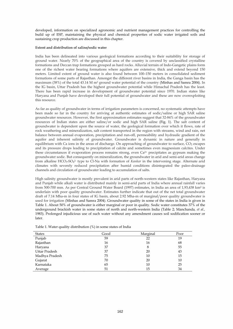
162

developed, information on specialized agronomic and nutrient management practices for controlling the build up of ESP, maintaining the physical and chemical properties of sodic water irrigated soils and sustaining crop production are discussed in this chapter.

Extent and distribution of saline/sodic water India has been delineated into various geological formations according to their suitability for storage of ground water. Nearly 70% of the geographical area of the country is covered by unclassified crystalline formations and Deccan trap formations grouped as hard rocks. Alluvial terrain of Indo-Gangetic plains form one of the richest water bearing formations where aquifers are extensive, thick and extend beyond 150 meters. Limited extent of ground water is also found between 100–150 meters in consolidated sediment formations of some parts of Rajasthan. Amongst the different river basins in India, the Ganga basin has the maximum (38%) of the total 43.14 M m3 ground water potential of the country (Minhas and Samra 2004). In the IG basin, Uttar Pradesh has the highest groundwater potential while Himachal Pradesh has the least. There has been rapid increase in development of groundwater potential since 1970. Indian states like Haryana and Punjab have developed their full potential of groundwater and these are now overexploiting this resource. As far as quality of groundwater in terms of irrigation parameters is concerned, no systematic attempts have been made so far in the country for arriving at authentic estimates of sodic/saline or high SAR saline groundwater resources. However, the first approximation estimates suggest that 32-84% of the groundwater resources of Indian states are either saline/or sodic and high SAR saline (Fig. 1). The salt content of groundwater is dependent upon the source of water, the geological formation over which it flows, rate of rock weathering and mineralization, salt content transported in the region with streams, wind and rain, net balance between annual evaporation, precipitation and run-off, permeability and hydraulic gradient of the aquifer and inherent salinity of groundwater. Groundwater is dynamic in nature and generally in equilibrium with Ca ions in the areas of discharge. On approaching of groundwater to surface, CO2 escapes and its pressure drops leading to precipitation of calcite and sometimes even magnesium calcites. Under these circumstances if evaporation process remains strong, even Ca2+ precipitates as gypsum making the groundwater sodic. But consequently on mineralization, the groundwater in arid and semi-arid areas change from alkaline HCO3-SO42- type to Cl-Na with formation of Kankar in the intervening stage. Alternate arid climates with severely reduced precipitation after humid conditions disintegrated the paleo-drainage channels and circulation of groundwater leading to accumulation of salts. High salinity groundwater is mostly prevalent in arid parts of north-western states like Rajasthan, Haryana and Punjab while alkali water is distributed mainly in semi-arid parts of India where annual rainfall varies from 500-700 mm. As per Central Ground Water Board (1997) estimates, in India an area of 1,93,438 km2 is underlain with poor quality groundwater. Estimates further indicate that out of the net total groundwater draft of 7.14 Mha-m in four states of IG basin, about 2.92 Mha-m of marginal/poor quality groundwater is used for irrigation (Minhas and Samra 2004). Groundwater quality in some of the states in India is given in Table 1. About 50% of groundwater is either marginal or poor in quality. Sodic water constitutes 37% of the underground brackish water in some states of north and north-western India (Table 2; Manchanda, et al., 1983). Prolonged injudicious use of such water without any amendment causes soil sodification sooner or later. Table 1. Water quality distribution (%) in some states of India

States Good Marginal Poor Punjab 59 22 19 Rajasthan 16 16 68 Haryana 37 8 55 Uttar Pradesh 37 20 43 Madhya Pradesh 75 10 15 Gujarat 70 20 10 Karnataka 65 10 25 Average 51 15 34

163

Fig. 1. Groundwater Quality for Irrigation in India (1:6 million scale; legends used indicate Good Water = EC < 2 dS/m and SAR <10; Saline Water = EC > 2

dS/m and SAR <10; High SAR Saline Water = EC > 4 dS/m and SAR >10; Alkali Water = EC & SAR variable and RSC > 2.5)

( Source: Gupta et. al., 1994)

Table 2. Percent distribution of brackish waters in India

States Categories Saline Sodic High SAR-saline

Punjab 22 54 24 Haryana 24 30 46 Rajasthan 16 35 49 Gujarat 20 28 52 Average 20 37 43

Salinity and sodicity parameters and guidelines for irrigation The first step while dealing with water quality problem is to get the water analyzed for its chemical composition. The requisite information on chemical composition can be obtained by analysis of a representative water sample from any soil-testing laboratory. The important parameters which ascertain water quality rating are: 1. Total salt concentration The most important criterion for evaluating salinity hazards is the total concentration of salts. The quantity of salts dissolved in water is usually expressed in terms of electrical conductivity (EC), mg L-1 or meq L-1 or dSm-1 (EC mg L-1 = 640 x EC dSm-1 or meq L-1 = 10 x EC dSm-1). The cations Na+, Ca2+ and Mg2+ and the anions Cl-, SO42-, HCO3- and CO32- are the major constituents of saline water. Other ions may be present, but usually in low concentrations is potassium, nitrate, silica or boron. Water suitability for supplemental irrigation can be assessed on the basis of a reduction in soil physical properties like infiltration rate, aggregate stability or crop yield in relation to canal water. Plant growth is adversely affected by saline water, primarily through excessive salts raising the osmotic pressure of the soil solution, resulting in reduced water availability. In field situations, the first reaction of plants to the application of saline water is reduced germination. This reduced initial growth results in smaller plants (lower leaf area index). Experimental evidence indicates that the interplay of several factors, such as the evaporative demand, salt content, soil type, rainfall, water table conditions and type of crop and water management practices, determines salinity build-up in the soil and crop performance resulting from long-term application of saline water.

164

2. Sodium hazard Some water, when used for the irrigation of crops, have tendency to produce alkalinity/sodicity hazards, depending upon the absolute and relative concentrations of specific cations and anions. The alkalinity is generally measured in terms of the sodium adsorption ratio (SAR), residual and sodium carbonate (RSC).

1. RSC (meq. L-1) = (CO32- + HCO3-) – (Ca2+ + Mg2+)

_________ 2. SAR = Na/ √ Ca+Mg/2

Irrigation with sodic water containing more Na+ relative to Ca2+ and Mg2+ and high carbonate (CO32- and HCO3-) leads to increase in alkalinity and sodium saturation in soils. The increase in exchangeable sodium percentage (ESP) of soil with use of such water adversely affects soil physical properties, including infiltration and aeration. In the early stages of sodic water irrigation, large amounts of divalent cations (Ca2+ and Mg2+) are released into the soil solution from exchange sites and replaced by Na+. In a monsoonal type climate condition of India, alternating sodic water irrigation and rainwater induces cycles of precipitation and dissolution of salts. Several field observations have shown that, although steady-state conditions are never reached in a monsoonal climate, a quasi-stable salt balance is reached within 4–5 years of sustained sodic irrigation, while a further rise in pH and ESP is very low (Minhas and Tyagi, 1998). Based on extensive research conducted in different agro-ecological regions of the country and farmers perceptions on impact of saline/sodic water irrigation on soil properties and crop yields, the following classification (Table 3) has been made for groundwater resource development and their suitable management considering specific needs. Table 3. Criteria for classification of poor quality groundwater for irrigation

Water quality category EC (dS/m) SAR (mmol /L)1/2 RSC (meq/L) Good < 2 < 10 < 2.5 Saline Marginally Saline 2 - 4 < 10 < 2.5 Saline > 4 < 10 < 2.5 High SAR-Saline > 4 > 10 < 2.5 Sodic/Alkali Marginally Sodic < 4 < 10 2.5 – 4.0 Sodic > 4 < 10 > 4.0 Strongly Sodic Variable > 10 > 4.0

Further considering field experience and results from different saline and sodic water use experiments, Central Soil Salinity Research Institute, Karnal in consultation with Scientists from Haryana Agricultural University, Hisar and Punjab Agricultural University, Ludhiana has prepared some guidelines for efficient utilization of given poor quality water (Table 4) These guidelines emphasize on long term influence of water quality on crop production, soil conditions and farm management with assumption that all rainwater received in field is being conserved for leaching and desalinizing upper root zone. Table 4. Suitability limits of alkali water for irrigation based on soil textural class

Soil texture (% clay)

Upper limits of Remarks SAR

(mmol/L)1/2 RSC

(meq/L) Fine (>30) 10 2.5-3.5 Limits pertain to kharif fallow– rabi crop rotation

when annual rainfall is 350-550 mm Moderately fine (20-30)

10 3.5-5.0 When water has Na < 75%, Ca+Mg >25% or rainfall > 550mm, the upper limit of RSC becomes safe

Moderately coarse (10-20)

15 5.0-7.5 For double cropping, RSC neutralization with gypsum is essential based on quantity of water used during rabi season. Grow low water requiring crops during kharif.

Coarse (<10) 20 7.5-10.0

165

Management of sodic water The major approaches to improving and sustaining agricultural productivity in any stress including sodic environment involve: (i) modifying the plants to suit the sodic environment; and (ii) modifying the environment to suit the available plants physiology. They could be used separately or together to make possible the productive utilization of sodic water without compromising the sustainability of the production resource at different management levels. Sodic water has low total salt concentration (EC < 4 dSm-1) and composition of salts is often dominated by sodium (> 70%) with very small proportion of Ca and Mg. such water usually have NaHCO3 as predominant salt making their RSC > 2.5 meq L-1. Some times Ca-salts are nearly absent in sodic water. Irrigation with sodic/alkali water leads to increase in soil sodicity and sodium saturation. The increase in ESP adversely affects soil physical properties like infiltration, aeration and soil structure. Such soils upon wetting get dispersed and clog pores affecting aeration, root respiration and development, but on drying they become very hard (Fig 2). Poor respiration cause yellowing of crop seedlings during early irrigation. The irrigation water with low Ca2+ (< 2 meq L-1) and high CO32- result in specific toxicity like scorching and leaf burning at early crop growth stage.

Flocculated soil Dispersed soil

Fig 2. Soil particles in different shapes

Crop selection The guiding principle for choosing the right kind of crops and cropping patterns suitable for particular sodic water is to select only those crops whose sodicity tolerance limits are lower than the soil sodicity (ESP) expected to build with use of that water. Under average conditions of water use, the expected root zone sodicity can be approximated by 1.5 × SARiw in fallow- wheat, 2.0 × SARiw in millet- wheat and 3.0 × SARiw in rice-wheat cropping sequences. Thus, based on the expected ESP to be developed, the suitable crops and their varieties can be chosen from the list of sodicity tolerant crops given in table 5, 6 and 7. Table 5. Relative tolerance to sodicity of soils

ESP Crops 10-15 Safflower, Mash, Peas, Lentil, Pigeon-pea, Urd-bean, Banana 16-20 Bengal gram, Soybean, Papaya, Maize, Citrus 20-25 Groundnut, Cowpea, Onion, Pearl-millet, Guava, Bel, Grapes 25-30 Linseed, Garlic, Guar, Palmarosa, Lemon grass, Sorghum, Cotton 30-50 Mustard, Wheat, Sunflower, Ber, Karonda, Phalsa, Vetiver, Sorghum, Berseem 50-60 Barley, Sesbania, Paragrass, Rhoades grass 60-70 Rice, Sugarbeat, Karnal grass

166

Table 6. Promising cultivars of different crops for sodic environments

Crop Varieties Wheat KRL 1-4, KRL 19, Raj 3077, HI 1077, WH 157 Rice CSR 23, CSR 27, CSR 30, CSR 36 P. millet MH 269, 280, 427, HHB 392 Mustard CS 15, CS 52, CS 54, CS 56, Varuna, DIRA 336 Cotton HY 6, LRA 5166, Sarvottam Sorghum SPV 475, 1010, CSH 1, 11, 14 Barley CSB 1, 2, 3, DL 4, 106, 120, 200, 348, Ratna, BH 97, DHS 12

The ESP range indicated against specific category of crops is the limit for 50% relative yield of respective crops. Since use of sodic water requires repeated application of gypsum, it is advisable to select only tolerant and semi tolerant crops and their varieties having low water requirement and high sodicity tolerance such as barley, wheat, mustard, oat, pearl-millet and sorghum etc. The choice of promising crops can be made from the list given in table 5 and 7. The other guidelines pertinent to selecting crops suitable for sodic waters are: • Cultivation of high water requirement crops like sugarcane and rice should be avoided with sodic

water use as its irrigation lead to ESP build up in surface soil layer. • Fields should be kept fallow during kharif (summer) in low rainfall areas (< 400 mm) where good

quality water is not available. However, only tolerant and semi-tolerant crops like barley, wheat and mustard should be grown during rabi (winter).

• Sorghum-wheat, cluster bean-wheat, pearl millet-wheat and cotton-wheat rotations can be grown successfully in areas having rainfall > 400 mm/annum provided that sowing of kharif crops is done with rain or good quality water and only 2 to 3 sodic water irrigations can be applied to kharif crops.

• In alluvial plains with rainfall ≥600 mm, rice-wheat, rice-mustard, sorghum-mustard, and Sesbania (GM)-wheat rotations can be successfully practiced with gypsum application.

• Sodic water should not be used for summer crops in the months of April to June. Table 7. ESP tolerance of crops in alkali soils and irrigated with alkali waters

Crop Soil under reclamation Alkali water irrigation ESPt* Slope ESP75** ESPt Slope ESP75

Cotton -- -- -- 14.9 1.3 34.1 Pearl millet 13.6 2.6 23.2 6.1 1.3 25.3 Rice 24.4 0.9 52.1 20.1 1.6 35.7 Wheat 16.1 2.1 28.0 16.2 1.9 29.4

* Threshold ESP, ** ESP for 75 % yield Irrigation management Among methods of irrigation, conventional irrigation practices such as basin irrigation can be adopted successfully; however, emphasis should be to minimize irrigations of sodic/alkali water because adverse impacts on soil depend directly on the quantity of such water used. Sodicity hazard can be reduced to good extent by using sodic water by mixing with or its cyclic use with good water. This can reduce the requirement of gypsum and simultaneously additional area can be brought under protective irrigation. The sodicity (ESP) of surface soil where the most roots interact defines the potentiality of dispersion, surface crusting and ultimately the infiltration problems. For practical purposes, information on above aspects is required for deciding the suitability of water for periodic build up of salinity and sodicity in the agriculturally most important soil layer (surface 0.3 m). The sodicity build up in surface 30 cm layer with irrigation of sodic water alone and in cyclic mode with good quality canal water is depicted in figure 3.

167

Fig. 3. Sodicity build-up (ESP, surface 0.3 m) in soils irrigated with various blending and

cyclic use modes of alkali (AW) and good (GW) quality waters Continued irrigation with alkali water alone (AW; ECw 2.3 dSm-1, RSC 11.7 meq L-1, SAR 15) in paddy-wheat rotation for 6 years has been observed to increase pH, ECe, SARe and ESP of sandy loam soil (pHs 7.8, ECe 0.7 dSm-1, ESP 5.3, organic matter 2.9 g kg-1 soil, clay 15%) compared with good quality water (GW; ECw 0.5 dSm-1, RSC nil). However, the rate of increase remains high during the initial years; thereafter these parameters get more or less stabilized. This is evident from figure 4, where the average values of pH, ECe, SARe and ESP at the end of experiment in soil irrigated with AW were 8.71, 3.80 dSm-1, 19.1 mmol L-1 and 27.3, respectively (Minhas et. al., 2007). The development of sodicity depends on the equilibrium between the processes of precipitation of calcite and other minerals on concentration of soil solutions with water uptake during the irrigation season and the rainfall induced release of divalent cations both from exchange sites and dissolution of calcite and other minerals. Quasi-equilibrium seems to be established with in about 4–5 years of irrigation depending upon the nature of crops grown, soil characteristics and the climate especially the annual rainfall at the site (Bajwa et al., 1993; and Manchnada, 1993).

Fig. 4. Periodic changes in pHs, ECe and SARe in surface (30 cm) soils irrigated with blending and cyclic use modes of alkali (AW) and good (GW) quality water. (W-99, P-99, W-00, P-00, W-01, P-01, W-02, P-02 and W-03 refer to samples drawn after harvest of wheat (1998–1999), paddy (1999), wheat (1999–2000), paddy

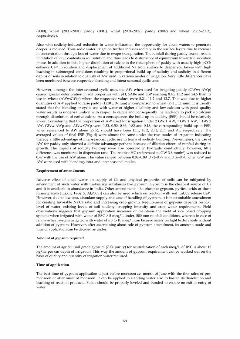
168

(2000), wheat (2000–2001), paddy (2001), wheat (2001–2002), paddy (2002) and wheat (2002–2003), respectively).

Also with sodicity-induced reduction in water infiltration, the opportunity for alkali waters to penetrate deeper is reduced. Thus sodic water irrigation further induces sodicity in the surface layers due to increase in concentration through loss of water due to evapo-transpiration. The rainfall during paddy season results in dilution of ionic contents in soil solution and thus leads to disturbance of equilibrium towards dissolution phase. In addition to this, higher dissolution of calcite in the rhizosphere of paddy with usually high pCO2 enhance Ca2+ in solution and displacement of additional Na from surface to deeper soil layers with high leaching in submerged conditions resulting in proportional build up of salinity and sodicity in different depths of soils in relation to quantity of AW used in various modes of irrigation. Very little differences have been monitored between respective blending and intera-seasonal cyclic uses. However, amongst the inter-seasonal cyclic uses, the AW when used for irrigating paddy (GWw: AWp) caused greater deterioration in soil properties with pH, SARe and ESP reaching 8.45, 15.2 and 24.5 than its use in wheat (AWw:GWp) where the respective values were 8.24, 11.2 and 12.7. This was due to higher quantities of AW applied to raise paddy (1210 ± 97 mm) in comparison to wheat (271 ± 11 mm). It is usually stated that the blending or cyclic use with water of higher alkalinity and low calcium with good quality water results in under-saturation with respect to calcite and consequently the tendency to pick up calcium through dissolution of native calcite. As a consequence, the build up in sodicity (ESP) should be relatively lower. Considering that the proportion of AW used for irrigation under 2 GW:1 AW, 1 GW:1 AW, 1 GW:2 AW, GWw:AWp and AWw:GWp were 0.33, 0.50, 0.66, 0.82 and 0.18, the corresponding build up in ESP, when referenced to AW alone (27.5), should have been 13.1, 18.2, 20.1, 23.5 and 9.8, respectively. The averaged values of final ESP (Fig. 4) were almost the same under the two modes of irrigation indicating thereby a little advantage of inter-seasonal cyclic use in terms of sodicity build-up. Nevertheless, the use of AW for paddy only showed a definite advantage perhaps because of dilution effects of rainfall during its growth. The impacts of sodicity build-up were also observed in hydraulic conductivity; however, little difference was monitored in dispersion ratio. The relative HC (referenced to GW 3.6 mmh-1) was reduced to 0.47 with the use of AW alone. The value ranged between 0.82–0.89, 0.72–0.79 and 0.56–0.70 when GW and AW were used with blending, intra-and inter seasonal modes. Requirement of amendments Adverse effect of alkali water on supply of Ca and physical properties of soils can be mitigated by amendment of such water with Ca-bearing substances like gypsum. Gypsum is the cheapest source of Ca and it is available in abundance in India. Other amendments like phospho-gypsum, pyrites, acids or those forming acids [H2SO4, FeS2, S, Al2(SO4)] can also be used which on reaction with soil CaCO3 release Ca2+. However, due to low cost, abundant supply and ease of handling of gypsum, it is most suitable amendment for creating favorable Na:Ca ratio and increasing crop growth. Requirement of gypsum depends on RSC level of water, existing levels of soil sodicity, cropping intensity and crop water requirements. Field observations suggests that gypsum application increases or maintains the yield of rice based cropping systems when irrigated with water of RSC > 5 meq/L under, 500 mm rainfall conditions, whereas in case of fallow-wheat system irrigated with water of up to 10 meq/L can be used safely on light texture soils without addition of gypsum. However, after ascertaining about role of gypsum amendment, its amount, mode and time of application can be decided as under. Amount of gypsum required The amount of agricultural grade gypsum (70% purity) for neutralization of each meq/L of RSC is about 12 kg/ha per cm depth of irrigation. This way the amount of gypsum requirement can be worked out on the basis of quality and quantity of irrigation water required. Time of application The best time of gypsum application is just before monsoon i.e. month of June with the first rains of pre-monsoon or after onset of monsoon. It can be applied in standing water also to hasten its dissolution and leaching of reaction products. Fields should be properly leveled and bunded to ensure no exit or entry of water.

169

Gypsum bed Another way to reclaim sodic water is passing it through gypsum beds, a specially designed chamber filled with gypsum clods. The gypsum chamber is a brick-cement-concrete chamber (Fig. 5). Size of chamber depends on tube well discharge and RSC of water. This chamber is connected to water fall box of tube well on one side and to water channel on the other side. A net of iron bars covered with wire net (2 mm×2 mm) is fitted at a height of 10 cm from the bottom of the bed.

Fi. 5. Cross-section diagram and picture of gypsum or pyrite beds

Farmers can also convert waterfall chamber of their tube wells into gypsum chamber with little modifications. Sodic water flowing from below dissolves gypsum placed in chamber and reclaims it. RSC of water from tube well discharge of 6 lt/sec decreased from 5. 5 to 1.9 meq/L by passing it through a chamber of size 2 .0 ×1.5 ×1.0 m in this method. However, this method is not suitable for reclaiming very high RSC water (> 12 meq L-1) because the size of the chamber required to fill the huge quantity of gypsum needed to neutralize such high RSC becomes too large. It has also been observed that the gypsum bed water quality improvement technique does not dissolve > 8 meq/L of Ca. The response of crops to the application of equivalent amounts of gypsum, either by passing the water (RSC 9 meq/L) through gypsum beds where the thickness of bed was maintained at 7 and 15 cm, or the soil application of gypsum is presented in table 8. Though crops under both the rotations (paddy-wheat, sorghum-mustard) responded to the application of gypsum in either of the methods, overall response of crops was slightly more in case of sodic water which was ameliorated (3-5 meq/L) after passing through gypsum beds. Thus, it seems that gypsum bed technique can help in efficient utilization of gypsum. Table 8. Average (1993-03) paddy-wheat and mustard-sorghum yields (Mg/ha- and soil properties* with gypsum applied to soil or passing sodic water through gypsum beds

Treatment Paddy Wheat pHs ESP Mustard Sorghum pHs ESP Control (T1) 3.08 2.68 9.6 66 2.27 1.18 9.5 61

Gypsum through beds 3.3 meq/L (T2)

3.97 3.73 8.0 19 3.06 1.98 8.0 25

5.2 meq/L (T3)

4.24 3.93 8.0 18 3.18 2.13 8.0 24

Equivalent soil application As in T2 (T4) 4.31 3.71 8.2 20 2.86 1.92 8.0 26

As in T3(T5) 4.52 3.89 8.1 20 3.00 2.05 8.1 24 LSD( p=0.05)

0.43 0.46 0.38 0.24

* At the harvest of rabi (2002-03) crops. (AICRP Saline Water 2002) Nutrient management Management of nutrients is one of the most vital factors for sustaining crop production on sodic soils or soils irrigated with sodic water. Optimum supply of nutrients to plants provides essential elements and help in overcoming the adverse affects of salts and specific ions stress. However, like the amelioration techniques, the principle for rate and time of nutrients supply, and the processes governing their availability differ to a

170

great extent with the nature of the salt problem in soil. Solubility, transformations, chemical forms and availability of many essential nutrients is affected by excess ESP, high > 8.2 pH, presence of substantial amounts of CaCO3, soluble NaHCO3, unstable soil structure and poor physical conditions of alkali soils arising due to irrigation with sodic water. Sustained alkali water irrigation for 15 years in cotton/pear millet/maize – wheat system grown on sandy loam soils has been found to cause significant reduction in available N, K, Zn and Mn while P and Cu remained unaffected. In fact irrigation water without RSC resulted in higher available status of these nutrients. (Table 9; Sharma et al., 2005) Table 9. Status of available nutrients in long-term (15 years) sodic water irrigated soil

Water quality Status of available nutrients (kg/ha) EC SAR RSC N P K Fe Zn Mn Cu 2 10 5 127 17.6 143 5.50 1.78 7.51 1.40 2 10 10 128 17.1 138 6.08 2.09 7.22 1.40 2 20 5 129 15.5 144 6.18 2.06 7.62 1.14 2 20 10 125 15.9 142 5.96 2.67 7.55 1.34 4 10 5 120 15.9 143 5.70 1.91 6.91 1.28 4 10 10 122 18.4 152 6.14 1.40 6.56 1.32 4 20 5 127 12.6 153 5.46 2.69 7.91 1.33 4 20 10 124 16.0 155 5.76 2.03 6.25 1.37 2 20 0 118 13.0 132 9.80 2.83 13.60 1.46

Good water 149 17.1 183 6.96 3.55 14.14 1.32 CD (0.05) 11.9 2.1 18.2 1.65 0.93 3.23 NS

However, analyses of soil samples from other field experiments on sodic water irrigation have shown that sodic soils or soils irrigated with sodic water generally become deficient in Ca, N, Zn, Fe, Mn and other micronutrients. Also sodic water irrigation increases volatilization losses of applied N; and low Ca2+ (< 2 meq L-1) or high HCO3-/CO32- result in specific toxicity in crops at early crop growth stages. Therefore crops respond to rates and methods of application of different fertilizers under these conditions. Processes of their transformations and availability under alkali soil conditions are discussed as under. Calcium Though alkali soils contain a wide range (traces to 35%) of CaCO3 but availability of Ca in these soils is not sufficient to meet requirements of crop plants due to low status of exchangeable Ca and its sparingly soluble nature under high pH conditions. Similarly sodic water irrigation causes precipitation of soluble Ca into sparingly soluble CaCO3 and thus decreasing its availability to crop plants. Further, increasing soil ESP with sodic water and its high SAR causes Na antagonism to Ca uptake in crop plants. Thereby in alkali conditions, crop plants are affected in two ways i.e. sodicity sensitive plants accumulate toxic levels of Na in high sodicity conditions and in moderately alkali conditions lack of supply of adequate Ca affect its availability (Table 10). Calcium deficiency arising with sodic water (Yadav and kaledhonkar, 1999) use has been reported to cause physiological disorders as poor boll opening in cotton and fruit end rot in tomato. Absolute Ca contents and its concentrations in relation to Na are good indices of proper growth of crop plants under sodic environments. Table 10. Ca and Na contents of some crop plants under different soil sodicity levels

ESP Safflower Raya Cowpea Ca Na Ca Na Ca Na

8.0 1.36 1.01 2.98 0.50 2.35 0.16 16.0 1.28 1.85 2.80 1.00 2.24 0.25 40.0 0.63 2.81 1.84 3.02 1.72 0.66

Calcium can be supplied through addition of Ca-bearing chemical amendments, acids and acid forming substances as indicated in the above section (amendment requirements) of this chapter, which upon reaction with native CaCO3 release Ca. Another option can be use of organic manures like FYM or presmud which under anaerobic conditions during flooding of sodic soils create increased pCO2 and help in solubilisation of native CaCO3 and release Ca and in turn removes Na from exchange complex (Swarup, 2004). Similarly growing of grasses, crops and other plantations also increase solubility of native CaCO3 through biological actions of their roots, thus adequate addition of amendments and adopting the agronomic practices which

171

enhance native CaCO3 solubility and neutralization of sodicity of irrigation water to avoid further precipitation of native Ca are helpful in reclamation of alkali soils and thus production of good crops. Nitrogen Alkali soils or soils where sodic water irrigation is practiced are generally low in organic matter and available N throughout soil profile, thus most crops respond to N supply. Nitrogen transformations are further adversely affected by high pH and sodicity arising out of sodic water irrigations, thereby affect the use efficiency of applied N. Mineralization of organic matter and organic forms of N under reduced infiltration and poor physical conditions is restricted to ammonification stage only due to lack of aeration or more specifically O2 . A major amount (10-60%) of accumulated NH3 is liable to volatilization under field moisture range. Ammonia volatilization loss rate follow a first order reaction and its half life range from nearly 62 days at field capacity to only 10 days under irrigation with alkali water causing waterlogged conditions. Singh and Bajwa (1990) observed increasing NH3 volatilization losses with increase in EC, RSC and SAR of irrigation water (Fig. 6).

Fig. 6. Effects of increasing levels of (a) EC (b) RSC and SAR in water on ammonia volatilization losses from sandy loam soils

They recorded losses as high as 37, 40 and 24% in sandy loam soils when irrigated with sodic/saline waters of RSC 15 meq L-1, EC 4 dSm-1 and SAR 50, respectively. Increase in pH with sodic water irrigation has further deteriorating impact by increasing volatilization. In addition to amount of salts, type of salts present in irrigation water also influence N transformations as Bhan et al. (1996) found that ammonification was accelerated while nitrification was retarded in Cl than SO4 or HCO3 salts (Table 11). Table 11. Effect of different salts of irrigation water on total ammonia volatilization

Type of salt Soil pH (1:1 soil: water) NH3 volatilization (% of applied N) Control 8.1 17.6 NaCl 7.9 20.4 Na2SO4 8.1 34.8 NaHCO3 9.4 32.9

Another factor for low N levels under these conditions is reduced symbiotic fixation of atmospheric nitrogen because of sensitivity of microbes to high sodicity and reduced growth of host leguminous crop plants. Losses of N can be regulated with reduction of pH of alkali soil submergence 1-week prior to crop planting or through substitution of some of rapidly hydrolyzing urea with slow release organic manures. Ammonia

172

volatilization losses can also be reduced substantially by altering the method of N application. It has been observed that placement of N fertilizers at 5-6 cm depth in upland crops and about 7-8 cm in paddy fields can restrict up to 90% volatilization losses. Split application of urea can be a viable option to reduce peak NH4 levels and NH3 losses thereby improve its use efficiency (Table 12; Swarup, 1998). Other option to compensate for higher losses is to supply additional dose of N fertilizer as higher yields of rice and wheat have been realized with higher i.e. 150 kg than 120 kg N ha-1; further improvement is also made possible with 3-splits in comparison to single application. Similarly supplementing extra dose of N at the time of first and second irrigations have been found to alleviate N deficiency and increase uptake of P, K and Zn and yields of crops. Foliar application of 3% solution of urea in addition to basal dose of N has been found to reduce volatilization losses, save about 40 – 60 kg N ha-1 and improve NUE in alkali soils. Table 12. NH3 losses and rice grain yield with different urea application methods and pre-submergence

periods Treatment Grain Yield (t/ha) Ammonia volatilization losses (kg/ha)

I II III Split N (kg ha-1) 3.61 1.43 0.00 0.00 N0 4.60 6.01 6.42 5.57 N60 4.83 8.31 7.48 6.74 N120 5.13 9.90 9.30 9.09 N180 0.22 0.93 0.63 0.75 LSD (P=0.05) Method of urea application Before puddling 4.73 6.16 5.68 5.24 After puddling 4.38 6.66 5.93 5.43 LSD (P=0.05) 0.24 0.38 0.16 0.12 Pre-submergence period 0-week 4.44 6.91 6.10 5.62 1-week 4.68 5.88 5.40 5.06 LSD (P=0.05) 0.11 0.53 0.66 0.61

Phosphorous As such, Sodic water irrigation does not alter the availability of P initially. However, with continuous use causing development of sodicity in soil its solubility is enhanced and availability pattern becomes similar to alkali soils. The amounts of water soluble P has been found to increase with soil pH in all major soil series of Indo-Gangetic plains. But when alkali soils are reclaimed, surface layers become poorer progressively due to its movement to lower depths, crop removal and increased immobilization. Reports indicate that a positive correlation exists between the electrical conductivity and extractable P status of these soils. This is because of presence of high amounts of soluble salts of Na2CO3 and NaHCO3, which upon reaction with native insoluble Ca3 (PO4) result in formation of soluble Na-phosphates as shown in the following equation: Insoluble Ca3 (PO4) + 3 Na2CO3 → 3 CaCO3 + 2 Na3PO4 (Soluble) Sorption of applied P in high ESP soils during initial years of reclamation remains very low and thus its release continues to be sufficient for crops even under low levels of P application. Another reason for continuous release of P is its enhanced solubility under high pH in Na-dominated soils which reverses in Ca-dominated normal soils. But during process of reclamation extractable P in surface soil tends to decrease due to movement of soluble forms to deeper depths; greater sorption of soluble P with decreasing ESP and pH of soil; immobilization and conversion of soluble Na3PO4 to Ca3(PO4) with addition of gypsum; and removal by growing plants. Application of gypsum improves soil physical conditions including infiltration rate in the process of reclamation resulting in movement of soluble salts and P to deeper depths. Due to these processes taking place under alkali conditions and the reclamation process, rice and wheat grown alkali conditions do not respond to P application during initial years. Crops response to applied P depends on nature of soil and stage of its reclamation, initial P value, crop to be grown and amendments used. Observations on rice-wheat; pearl millet-wheat sequences grown on alkali soils after addition of gypsum indicated that rice and wheat started responding to P application when Olsen’s P level of surface soils reached to 12.0 and 8.0 kg ha-1,

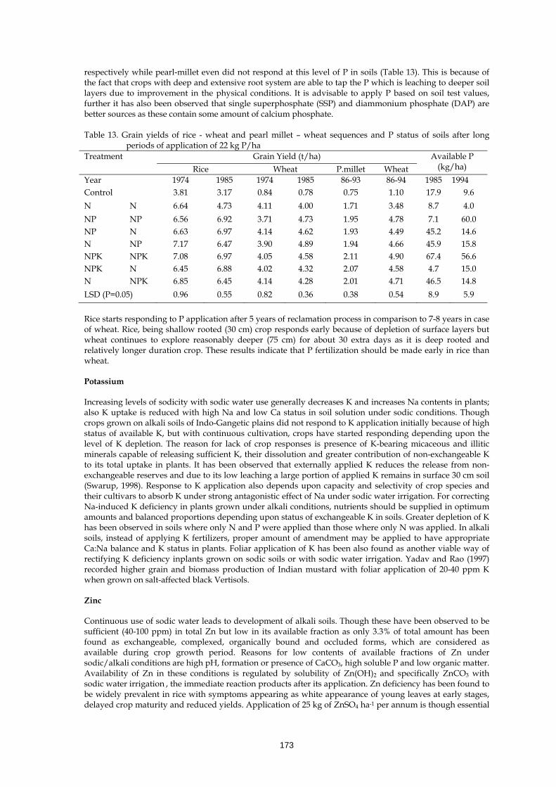
173

respectively while pearl-millet even did not respond at this level of P in soils (Table 13). This is because of the fact that crops with deep and extensive root system are able to tap the P which is leaching to deeper soil layers due to improvement in the physical conditions. It is advisable to apply P based on soil test values, further it has also been observed that single superphosphate (SSP) and diammonium phosphate (DAP) are better sources as these contain some amount of calcium phosphate. Table 13. Grain yields of rice - wheat and pearl millet – wheat sequences and P status of soils after long

periods of application of 22 kg P/ha Treatment Grain Yield (t/ha) Available P

(kg/ha) Rice Wheat P.millet Wheat Year 1974 1985 1974 1985 86-93 86-94 1985 1994 Control 3.81 3.17 0.84 0.78 0.75 1.10 17.9 9.6 N N 6.64 4.73 4.11 4.00 1.71 3.48 8.7 4.0 NP NP 6.56 6.92 3.71 4.73 1.95 4.78 7.1 60.0 NP N 6.63 6.97 4.14 4.62 1.93 4.49 45.2 14.6 N NP 7.17 6.47 3.90 4.89 1.94 4.66 45.9 15.8 NPK NPK 7.08 6.97 4.05 4.58 2.11 4.90 67.4 56.6 NPK N 6.45 6.88 4.02 4.32 2.07 4.58 4.7 15.0 N NPK 6.85 6.45 4.14 4.28 2.01 4.71 46.5 14.8 LSD (P=0.05) 0.96 0.55 0.82 0.36 0.38 0.54 8.9 5.9 Rice starts responding to P application after 5 years of reclamation process in comparison to 7-8 years in case of wheat. Rice, being shallow rooted (30 cm) crop responds early because of depletion of surface layers but wheat continues to explore reasonably deeper (75 cm) for about 30 extra days as it is deep rooted and relatively longer duration crop. These results indicate that P fertilization should be made early in rice than wheat. Potassium Increasing levels of sodicity with sodic water use generally decreases K and increases Na contents in plants; also K uptake is reduced with high Na and low Ca status in soil solution under sodic conditions. Though crops grown on alkali soils of Indo-Gangetic plains did not respond to K application initially because of high status of available K, but with continuous cultivation, crops have started responding depending upon the level of K depletion. The reason for lack of crop responses is presence of K-bearing micaceous and illitic minerals capable of releasing sufficient K, their dissolution and greater contribution of non-exchangeable K to its total uptake in plants. It has been observed that externally applied K reduces the release from non-exchangeable reserves and due to its low leaching a large portion of applied K remains in surface 30 cm soil (Swarup, 1998). Response to K application also depends upon capacity and selectivity of crop species and their cultivars to absorb K under strong antagonistic effect of Na under sodic water irrigation. For correcting Na-induced K deficiency in plants grown under alkali conditions, nutrients should be supplied in optimum amounts and balanced proportions depending upon status of exchangeable K in soils. Greater depletion of K has been observed in soils where only N and P were applied than those where only N was applied. In alkali soils, instead of applying K fertilizers, proper amount of amendment may be applied to have appropriate Ca:Na balance and K status in plants. Foliar application of K has been also found as another viable way of rectifying K deficiency inplants grown on sodic soils or with sodic water irrigation. Yadav and Rao (1997) recorded higher grain and biomass production of Indian mustard with foliar application of 20-40 ppm K when grown on salt-affected black Vertisols. Zinc Continuous use of sodic water leads to development of alkali soils. Though these have been observed to be sufficient (40-100 ppm) in total Zn but low in its available fraction as only 3.3% of total amount has been found as exchangeable, complexed, organically bound and occluded forms, which are considered as available during crop growth period. Reasons for low contents of available fractions of Zn under sodic/alkali conditions are high pH, formation or presence of CaCO3, high soluble P and low organic matter. Availability of Zn in these conditions is regulated by solubility of Zn(OH)2 and specifically ZnCO3 with sodic water irrigation , the immediate reaction products after its application. Zn deficiency has been found to be widely prevalent in rice with symptoms appearing as white appearance of young leaves at early stages, delayed crop maturity and reduced yields. Application of 25 kg of ZnSO4 ha-1 per annum is though essential

174

but sufficient for crops of both seasons where sodic water is used for irrigation. In arid and semi-arid regions where soils are generally calcareous the availability of all micronutrients in general and Zn in particular decreases when irrigation with high sodicity water is practiced. Minhas and Chhiba (1999) found that water soluble plus exchangeable Zn fraction increased while insoluble residual fraction decreased with increase in RSC of irrigation water. This could be due to formation of soluble sodium zincate. Singh (1999) had also recorded that with use of sodic water (RSC 10 & 20 meq/L), Zn application at 20 kg/ha improved the grain yield of rice under no gypsum treatment (Table 14) but in presence of gypsum increase was found to be non-significant. Table 14. Grain yield of rice after two years of irrigation with sodic water

RSC (meq /L)

Zn levels (kg/ha) 0 10 20 Mean

Without gypsum 0 5.9 6.2 6.0 6.0 5 5.6 5.8 6.0 5.8 10 5.1 5.3 5.6 5.3 20 4.2 4.4 4.6 4.4 Mean 5.2 5.4 5.5 CD (0.05) RSC levels – 0.30, Zn levels – 0.26, RSC x Zn - NS

With gypsum 0 5.9 6.2 6.0 6.0 5 6.0 6.0 6.1 6.0 10 5.8 5.9 5.7 5.8 20 5.2 5.6 5.6 5.4 Mean 5.7 5.9 5.9 CD (0.05) RSC levels – 0.23, Zn levels – NS, RSC x Zn - NS

Iron Availability of iron is reduced with sodic water irrigations because of following reasons, i) decreased solubility with increase in soil pH ii) Presence of CO32- and HCO3- in irrigation water induce iron chlorosis in different crops leading to reduced growth and poor metabolism. Another factor which influences iron availability is deterioration in soil physical conditions creating reduced conditions. Reports indicate that application of FeSO4, a soluble salt could not overcome iron deficiency under alkali conditions (Swarup 1980). Similarly significant decrease in DTPA extractable iron in soils irrigated with sodic water for 9 years were recorded by Bajwa et al. (1992). Application of Fe should be practiced with use of amendments based on soil test reports. Manganese Similar to Fe, solubility and availability of Mn is also governed by pH and oxidation-reduction status of the soils achieved after irrigation with sodic water. Presence of RSC in irrigation water decreases Fe availability to upland crops like wheat taken after low land rice. This is because during submergence Mn solubilises after conversion to reduced state and leaches to deeper depths particularly so in coarse textured soils. It oxidizes readily under upland conditions, hence its soil application is not effective, but repeated foliar application of MnSO4 is most effective in overcoming its defiency in crops. Integrated nutrient management Application of gypsum as soil or water amendment is generally recommended to offset the deteriorating effects of sodic water. However, alternatively cheap organic amendments like FYM and pressmud have also been used to alleviate the adverse effects of soil sodicity on crop growth. Long-term nutrient management strategies developed so far for improving rice-wheat production on sodic lands are potentially applicable to areas primarily irrigated with good quality underground irrigation water. Since rice-wheat system is the most commonly practiced crop rotation in the Indo-Gangetic plains, improving its productivity particularly in the areas having poor quality groundwater is a major challenge. Development of site specific integrated plant nutrient supply (IPNS) and management strategies is therefore a viable option for sustaining the productivity of this system. The basic concept underlying IPNS is the maintenance or adjustment of soil fertility and plant nutrient supply to an optimum level for sustaining the desired crop productivity through optimization of the benefits from all possible sources of plant nutrients in an integrated manner. IPNS is an approach ecologically, socially and economically viable, and environmentally un-hazardous. Keeping these facts in view field

175

investigations were carried out to evaluate long-term effects of sodic water (RSC 8.5 meq L-1, SAR 8.8) irrigation with and without gypsum, farmyard manure (FYM) and pressmud application in combination with inorganic fertilizers (N, P, K and Zn) on soil properties and yields of rice and wheat.

Recent studies on integrated nutrient management have shown that rice and wheat yields increase significantly with integrated use of gypsum or FYM or pressmud and 100% of recommended levels of inorganic NPK fertilizers in comparison to inorganic fertilizers alone. The mean yield of rice under recommended dose (N120 P26 K42 kg/ha) with gypsum or FYM or pressmud or gypsum + FYM or gypsum + pressmud was 5.23, 5.29, 5.31, 5.35 and 5.41 t/ha, respectively during 10-year-cropping period (1994-2003) in comparison to 4.79 t /ha (Table 15) with recommended levels of fertilizer only.

Table 15. Effect of gypsum with and without different organic manures on yield of rice and wheat and soil properties

Treatments Mean Yield (t/ha) Soil pH OC (%) Rice

(1994-2003) Wheat

(1994-2004) N120 P26 K42 (100 % recommended) 4.79 3.69 8.52 0.26 N120 P26 K42 + FYM 5.29 4.16 8.38 0.43 N120 P26 K42 + gypsum 5.23 4.10 8.18 0.37 N120 P26 K42 + Pressmud (PM) 5.31 4.46 8.29 0.42 N120 P26 K42 + FYM + gypsum 5.35 4.22 8.28 0.42 N120 P26 K42 + PM+ gypsum 5.41 4.52 8.28 0.40 CD (5%) 0.42 0.34 0.08 0.60 Initial Soil Properties 8.6 0.40

The NPK fertilizer with 10 t ha-1 FYM, 5 t ha-1 gypsum or 10 t ha-1 pressmud produced higher yields over the

years as compared to application of recommended dose of inorganic NPK alone. The residual effect of FYM, gypsum and pressmud was significant on wheat yields after 5 years. Though yields of both crops improved further when gypsum was applied with FYM or pressmud, but the profit was not beneficial over the FYM and pressmud alone treatment. Application of recommended NPK fertilizer combined with FYM or pressmud gave the highest profit followed by gypsum treatments. The cost/benefit ratio from 10 t ha-1 each pressmud (1.65) or FYM (1.59) were higher in comparison to gypsum application (1.38). There was substantial improvement in organic carbon and available nitrogen, phosphorus, potassium and zinc in soil over the initial status. The results of this study clearly show the beneficial effects of FYM and pressmud for rice and wheat yield under sodic water irrigation. It will become more crucial in the future because of increasing cost of chemical amendments. Use of organic amendments like pressmud and FYM with inorganic fertilizers were found effective in improving and maintaining fertility of sodic soil under sodic water irrigation (Yaduvanshi and Swarup, 2005; Swarup and Yaduvanshi, 2004). Large quantities of combine harvested rice and wheat straw are being produced in states of Punjab, Haryana and Uttar Pradesh. The residues are being burnt, presently, to clear the fields for timely sowing of crops and convenient disposal of waste. Large quantities of rice and wheat residues are available (37.87 Tg) for recycling and its potential was 0.634 Tg as a source of N, P and K nutrients. One tone of rice residues contains approximately 6.1 kg N, 0.8 kg P and 11.4 kg K, while one tone of wheat residues contains 5.1 kg N, 1.2 kg P and 10.5 kg K. Rice-wheat cropping system occupies about 10 million hectares area in India. In another field study under sodic water conditions, incorporation of wheat residue 50 days prior to rice transplanting either alone or with green manuring or with sulphitation pressmud (a sugarcane waste byproduct) and recommended dose of 120 kg N and 26 kg P ha-1 resulted in significant improvement in rice yield as compared to recommended dose of chemical N and P fertilizer alone. The mean yield improvement in both the crops due to incorporated of various organic sources over 100 % of recommended dose of NP was 26.1%, while it was only 6.6% in the treatment where the residue was burnt. Sodic water irrigation over three years period of experimentation, increased soil pH by 0.1-0.16 units (Table 16). However, in treatments with organic sources, pH remained nearly at the initial level (Yaduvanshi and Sharma 2007a and b). As crop residues are rich source of organic mater, nutrients and energy, they must be returned to the soil. Besides the loss of organic matter and plant nutrients, burning of crop residues also cause atmospheric pollution in form of toxins and green house gases.

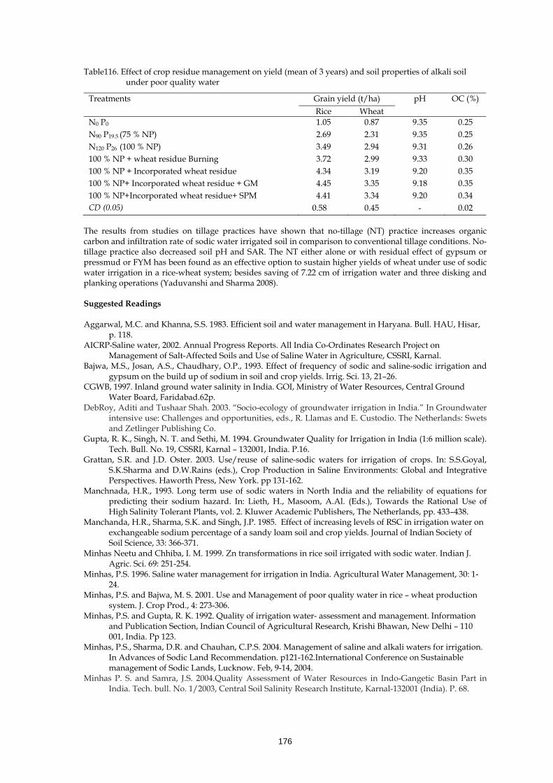
176

Table116. Effect of crop residue management on yield (mean of 3 years) and soil properties of alkali soil under poor quality water

Treatments Grain yield (t/ha) pH OC (%) Rice Wheat

N0 P0 1.05 0.87 9.35 0.25 N90 P19.5 (75 % NP) 2.69 2.31 9.35 0.25 N120 P26 (100 % NP) 3.49 2.94 9.31 0.26 100 % NP + wheat residue Burning 3.72 2.99 9.33 0.30 100 % NP + Incorporated wheat residue 4.34 3.19 9.20 0.35 100 % NP+ Incorporated wheat residue + GM 4.45 3.35 9.18 0.35 100 % NP+Incorporated wheat residue+ SPM 4.41 3.34 9.20 0.34 CD (0.05) 0.58 0.45 - 0.02

The results from studies on tillage practices have shown that no-tillage (NT) practice increases organic carbon and infiltration rate of sodic water irrigated soil in comparison to conventional tillage conditions. No-tillage practice also decreased soil pH and SAR. The NT either alone or with residual effect of gypsum or pressmud or FYM has been found as an effective option to sustain higher yields of wheat under use of sodic water irrigation in a rice-wheat system; besides saving of 7.22 cm of irrigation water and three disking and planking operations (Yaduvanshi and Sharma 2008). Suggested Readings Aggarwal, M.C. and Khanna, S.S. 1983. Efficient soil and water management in Haryana. Bull. HAU, Hisar,

p. 118. AICRP-Saline water, 2002. Annual Progress Reports. All India Co-Ordinates Research Project on

Management of Salt-Affected Soils and Use of Saline Water in Agriculture, CSSRI, Karnal. Bajwa, M.S., Josan, A.S., Chaudhary, O.P., 1993. Effect of frequency of sodic and saline-sodic irrigation and

gypsum on the build up of sodium in soil and crop yields. Irrig. Sci. 13, 21–26. CGWB, 1997. Inland ground water salinity in India. GOI, Ministry of Water Resources, Central Ground

Water Board, Faridabad.62p. DebRoy, Aditi and Tushaar Shah. 2003. “Socio-ecology of groundwater irrigation in India.” In Groundwater

intensive use: Challenges and opportunities, eds., R. Llamas and E. Custodio. The Netherlands: Swets and Zetlinger Publishing Co.

Gupta, R. K., Singh, N. T. and Sethi, M. 1994. Groundwater Quality for Irrigation in India (1:6 million scale). Tech. Bull. No. 19, CSSRI, Karnal – 132001, India. P.16.

Grattan, S.R. and J.D. Oster. 2003. Use/reuse of saline-sodic waters for irrigation of crops. In: S.S.Goyal, S.K.Sharma and D.W.Rains (eds.), Crop Production in Saline Environments: Global and Integrative Perspectives. Haworth Press, New York. pp 131-162.

Manchnada, H.R., 1993. Long term use of sodic waters in North India and the reliability of equations for predicting their sodium hazard. In: Lieth, H., Masoom, A.Al. (Eds.), Towards the Rational Use of High Salinity Tolerant Plants, vol. 2. Kluwer Academic Publishers, The Netherlands, pp. 433–438.

Manchanda, H.R., Sharma, S.K. and Singh, J.P. 1985. Effect of increasing levels of RSC in irrigation water on exchangeable sodium percentage of a sandy loam soil and crop yields. Journal of Indian Society of Soil Science, 33: 366-371.

Minhas Neetu and Chhiba, I. M. 1999. Zn transformations in rice soil irrigated with sodic water. Indian J. Agric. Sci. 69: 251-254.

Minhas, P.S. 1996. Saline water management for irrigation in India. Agricultural Water Management, 30: 1-24.

Minhas, P.S. and Bajwa, M. S. 2001. Use and Management of poor quality water in rice – wheat production system. J. Crop Prod., 4: 273-306.

Minhas, P.S. and Gupta, R. K. 1992. Quality of irrigation water- assessment and management. Information and Publication Section, Indian Council of Agricultural Research, Krishi Bhawan, New Delhi – 110 001, India. Pp 123.

Minhas, P.S., Sharma, D.R. and Chauhan, C.P.S. 2004. Management of saline and alkali waters for irrigation. In Advances of Sodic Land Recommendation. p121-162.International Conference on Sustainable management of Sodic Lands, Lucknow. Feb, 9-14, 2004.

Minhas P. S. and Samra, J.S. 2004.Quality Assessment of Water Resources in Indo-Gangetic Basin Part in India. Tech. bull. No. 1/2003, Central Soil Salinity Research Institute, Karnal-132001 (India). P. 68.

177

Minhas, P.S., Dubey, S.K. and Sharma D.R. (2007). Comparative affects of blending, intera/inter-seasonal cyclic uses of alkali and good quality waters on soil properties and yields of paddy and wheat. Agril. Water. Manage. 87: 83-90.

Minhas, P. S. and Tyagi, N. K. (eds.) 1998. Agricultural Salinity Management in India. Central Soil Salinity Research Institute, Karnal, India – 132001. pp 509.

Raghu Babu, M., P.R.K. Prasad, G.V. Subbaiah, M. Khan and P.S. Minhas. (1999). Subsurface Fresh Water Skimming System; Improved Doruvu Technology, Bulletin No. 1/99, 19p. Central Soil Salinity Research Institute, Kamal

Oster, J.D. and I. Shainberg, 2001. Soil responses to sodicity and salinity: challenges and opportunities. (Personal correspondence, J. D. Oster, manuscript submitted for publication, forthcoming, 2001). Department of Environmental Sciences, University of California, Riverside, CA 92521, USA, and Soil and Water Institute, The Volcani Center, POB 6, Bet Dagan, Israel.

Shah, Tushaar, Aditi Debroy, Asad Qureshi and Jinxia Wang. 2001. Sustaining Asia’s groundwater boom: An overview of issues and evidence. Natural Resources Forum, 27(2003): 130-141

Sharma, D.R. and Minhas, P.S. 2001. Response of rice-wheat to alkali water Irrigation and gypsum application. J. Indian Soc. Soil Sci. Vol. 49: pp. 324-327.

Sharma, D.R., Kumar, C., Kaledhonkar, M. J. and Minhas, P. S. 2005. Effect of sustained alkali water irrigation on soil properties, growth and yield of maize-wheat system. Central Soil Salinity Research Institute, Karnal – 132001, India. Pp.

Shekhon, M.S. and Bajwa. 1993. Effect of incorporation of OM and gypsum in controlling sodic irrigation effects on soil properties under rice – wheat maize system. Agric Water Manage. 24: 15-25

Shiklomanov, I.A. Ed., Assessment of Water Resources and Water Availability in the World (World Meteorological Organization/Stockholm Environment Institute, Geneva, Switzerland, 1997.

Singh., S.D., Gupta, J.P. and Singh, P. 1978. Water economy and saline water use by drip irrigation. Agron. J. 70: 948-951.

Singh, B. and Bajwa, M. S. 1990. Effect of poor quality water on ammonia volatilization losses. J. Ind. Soc. Soil Sci. 30: 779-781.

Singh Joginder 1999. Interactive effects of zinc, gypsum and sodic irrigation water on transformations and availability of micro-nutrients to rice and wheat. Ph. D. Thesis submitted to PAU, Ludhiana.

Swarup, A. 1980. Effect of submergence and farm yard manure application on yield and nutrition of rice under sodic conditions. J. Ind. Soc. Soil Sci. 28: 532-534.

Swarup, A. 1998. Nutrient management for crop production in alkali conditions. In: Salinity Management in Agriculture (eds. S.K. Gupta, S. K. Sharma and N. K. Tyagi) CSSRI, Karnal. Pp. 99-107.

Swarup, A. 2004. Chemistry of sodic soils and fertility management. In Advances in Sodic Land Reclamation. International Conference on Sustainable Management of Sodic Lands, Lucknow, Feb. 9-14, 2004. pp. 27- 52.

Swarup, A. and Yaduvanshi, N.P.S. (2004). Response of rice and wheat to organic and inorganic fertilizers and soil amendment under sodic water irrigated conditions. IRRI News Letter: 29.1, 49-51.

Yadav, R. K., and Rao, G. Gururaja. 1997. Influence of foliar application of K+ on growth and yield of Indian mustard on saline black soils. Indian J. Agric. Sci. 67 (6): 279-82

Yadav, R. K. and Kaledhonkar, M. J. 1998. Effect of toposequential differences and ground water quality on performance of cotton and Egyptian clover. Central Soil Salinity Research Institute, Annual Report. Pp 28-29.

Yaduvanshi, N. P. S. and Swarup, A. 2005. Effect of continuous use of sodic irrigation water with and without gypsum, farm yard manure, pressmud and fertilizer on soil properties and yields of rice and wheat in a long term experiment. Nutrient Cyclic in Agroecosystems. 73: 111-18.

Yaduvanshi, N.P.S. and Sharma, D.R. (2007a). Use of wheat residue and manures to enhance nutrient availability and rice-wheat yields in sodic soil under sodic water irrigation. J. Indian Soc. Soil. Sci. 55(3): 330-334.

Yaduvanshi, N.P.S. and Sharma, D.R.(2007b). Incorporate wheat residue with green manure for sustaining rice-wheat production in sodic water. Indian Farming, 57 (9):15-17.

Yaduvanshi, N. P. S. and Sharma, D. R. 2008. Tillage and residual organic manures/chemical amendment effects on soil organic matter and yield of wheat under sodic water irrigation. Soil Tillage Res. 98:11-16.

178

Irrigation Induced Soil Degradation in Command Areas S.K. Chaudhari Central Soil Salinity Research Institute, Karnal -132 001 (Haryana), India skc@cssri.ernet.in India has made significant investments in creating an irrigation potential of > 50 M ha. However, the irrigated areas, which have contributed significantly in increasing food grain production are now facing serious problem of rise in ground water table and soil salinization. Such problems are now serious in areas that have received canal irrigation. The impact of soil degradation in irrigated areas due to soil salinization and waterlogging has not been evaluated adequately. In the Nagarajunasagar project command area, nearly 25,000 ha of the 140,000 ha under irrigation have been affected by salinity and waterlogging in a period of 14 years. Extent of human induced soil degradation is presented in Table 1. Table 1. Extent of soil degradation(human induced) under different degradation types

Degradation type Degree of degradation Area affected (%) Slight Moderate Strong Extreme Total

Water erosion a.Loss of topsoil(Wt) b.Terrain deformation(Wt) Wind erosion a.Loss of topsoil(Wt) b.Loss of topsoil/terrain deformation(Et/Ed) c.Terrain deformation/over blowing(Ed/Co) Chemical deterioration a.Loss of nutrients(Cn) b.Salinization(Cs) Physical deterioration Waterlogging(w)

27.3 27.3

-

0.3 0.3 - -

6.5 3.7 2.8

6.4 6.4

111.6 99.8 11.8

10.1 5.5 4.6

-

7.3 -

7.3

5.2 5.2

5.4 5.4 -

3.1 0.4 -

2.7 - - - - -

4.6 -

4.6 - - - - - - - - -

148.9 132.5 16.4

13.5 6.2 4.6

2.7

13.8 3.7 10.1

11.6 11.6

45.3 40.3 5.0

4.1 1.9 1.4

0.8

4.2 1.1 3.1

3.5 3.5

Total (affected area) 40.5 134.2 8.5 4.6 187.8 57.1 Land not fit for agriculture Stable terrain Under natural condition(Sn)

18.2

32.2

5.5

9.8 Total geographical area of India 328.7 100.0 It is clear that non-judicious use of irrigation water, irrespective of its quality, lead to soil salinisation and sodification. Continuous accumulation of salts in root zone results into soil salinisation. These salts may come from irrigation water, mineral dissolution, precipitation, capillary rise or all of these. The process of sodification initiates with replacement of exchangeable calcium by sodium. Irrigated soils exhibit differential physico-chemical behaviour at temporal scale. Physical properties of irrigated soils limit its productivity. Irrigated soils, if not managed properly, deteriorate in hydraulic properties e.g. infiltration rate, saturated hydraulic conductivity, unsaturated hydraulic conductivity, soil-water diffusivity, soil-water retention etc. The exchange phase-solution phase behaviour of these soils is highly sensitive to water management inputs. Flocculation, deflocculation, dispersion, swelling, ESR-SAR relationships are the major processes responsible to bring changes in hydro-physical behaviour of soils due to irrigation induced salinisation or sodification. When irrigation is practiced, water remains in equilibrium with soil and slowly infiltrates downward. The composition of the soil solution is decided by mineralogy, water quality and exchange phase-solution phase behaviour of the soils. Besides several parameters of the soil solution at equilibrium, sodium adsorption ratio (SAR) and total electrolyte concentration are the major attributes, which decides the hydro physical

179

behaviour of irrigated soils. SAR is a relation between soluble sodium and soluble divalent cations, which can be used to predict the exchangeable sodium fraction of soil equilibrated with a given solution. The increased irrigation by tubewells, supplemented by canal irrigation, has resulted in depletion and lowering of underground water at the rate of almost 1m per year in the central Punjab causing concern of depleting groundwater resource for the posterity and increasing the groundwater table in the southwestern sectors resulting in the problem of salinization and changes in land use. Effect of irrigation on soil degradation due to waterlogging and accumulation of salts in soils of Punjab was studied and it was observed that in the Sangrur and Kapurthala districts, the total salt-affected areas appreciably decreased from 98,000 ha to 66,000 ha. On the other hand, such areas in the Faridkot district, during the same period, markedly increased form 6,500 ha to 82,000 ha. Whereas, the ground water table in Faridkot district rose at the rate of 0.5-1.0 meter per annum, the ground water table in the Sangrur and Kapurthala districts receded at the rate of about 0.2 meter per annum in the past. The rise in the groundwater table in Faridkot appeared to be due to seepage from newly-constructed canals, inadequate drainage, influx of groundwater-table due to lower topographic position and insufficient water expenses. Because of the brackish nature of ground water, the rise in water-table was, accompanied by accumulation of salts at the surfaces during dry months, leading to the formation of salt-affected soils. On the other hand, the installation of a large number of tube-wells for pumping out underground water for irrigation in Sangrur and Kapurthala districts and the general gradient of ground water towards south-western sectors resulted in lowering of the ground water in these areas. The changes in groundwater table followed by salinization/sodification and/or amelioration of the salt-affected areas under study have obliged farmers to changes in land-use pattern in favour of wheat-paddy rotation at the cost of maize, cotton or citrus cultivation. The Faridkot areas, once known for cotton production in the state, is now being increasingly used for paddy production where irrigation water is available and thus aggravating the problem of waterlogging and salinity due to the addition of large quantities of salts through tube-well waters of marginal quality for irrigation. On the other hand, the Sangrur and Kapurthala areas which were previously abandoned for cultivation because of sodicity problem, have now being reclaimed and brought under paddy-wheat rotation after rectifying the soils with gypsum. Maintaining quality of soil resource Maintaining soil quality by ameliorating degraded land and increasing organic matter content is imperative for sustaining agricultural productivity. Soil organic matter is probably the most important indicator of soil quality (Rasmussen and Collins, 1991); and that an increase in per cent organic matter content is suggestive of positive change in soil quality through reduction of soil erosion by increasing water table aggregates. Farmers using alternative cropping practices, such as green manures often report improvements in soil tilth. Some of the new land-use systems have disregarded the time tested, highly effective system of crop rotation as well as the practice of green manuring. Experimental evidences of growing green manure crop before paddy transplantation, do suggest a better yield even without the addition of fertilizers, apart from its positive effects on soil tilth and pore space. Although microbial life of the soil is often considered as a key element of soil health or quality, more research data are needed to evaluate the economic potential of new options and their impact on the soil resource. The impact of soil degradation processes is not limited to national boundaries. There are evidences to show that the land degradation processes, such as loss of organic matter and increase in carbon dioxide contents are contributing to global changes affecting adversely the humanity at large. This will warrant efforts to combat soil degradation not only at national level but also at international level. Similar concern has recently been raised while estimating the stock of SOC in black cotton soils of India, SOC stock in different physiographic regions of India, soil organic matter status of various soils in Indian, the total carbon stock of the Indo-Gangetic Plains of India, and while estimating the formation of secondary carbonates in Indian soils. Irrigation induced land degradation in Mula Command of Maharashtra : A case study Irrigation induced salinisation and alkalisation has emerged as twin problems in the command areas under different agro-ecological situations in general and under arid and semi-arid ecosystems in particular. In order to understand the menace of irrigation induced land degradation in arid and semi-arid zones, results of a case study carried out in Mula Command Area of Maharashtra is presented here. The study was carried-out with the following objectives.

180

1. To study the changes in hydro-physical behaviour of dominant soil series with change in irrigation intensity and irrigation induced salinisation and alkalisation.

2. To study the effect of irrigation induced salinisation and alkalisation on dispersion and swelling behaviour of these soils.

3. To study the dynamics of ESR-SAR relationships of these soils. 4. To determine threshold electrolyte concentrations to maintain stable hydraulic properties.

Mula Command Area is located in Ahmednagar district of Maharashtra with two major canal systems viz; Mula Right Bank Canal (MRBC) and Mula Left Bank Canal (MLBC). MRBC covers about 1,03,749 ha of land across the length of 58 km and MLBC covers about 14,453 ha of land across the length of 18 km. Canals were made operational and irrigation started between 1971 and 1976. In head and middle reaches of the command area, high water demanding sugarcane and cotton based cropping systems are prominent, whereas in tail reaches, sorghum based cropping systems are followed by the farmers. About 60, 25 and 15 percent soils can be texturally categorized under fine, medium to fine and coarse to medium, respectively. However, 50, 28 and 22 per cent cultivated lands can be classified as deep, medium and shallow, respectively. Soil profiles were selected on the basis of degree of severity of the problem. In the whole command area, 40 soil profiles were selected. In MRBC, distributory No. 3, Chanda minor and Deogaon Branch No.II were selected in head, middle and tail reaches. However, in MLBC, profiles were selected in head, middle and tail reaches. Soil profiles from outside the command were also selected on the basis of soils series. In MRBC, 9, 8 and 7 profiles were selected in head, middle and tail reaches, respectively. In MLBC, three profiles each in head, middle and tail ends of the canal were selected. Three profiles each representing fine (Clay), medium to fine (Clay Loam) and coarse to medium (Sandy Clay Loam) were selected from the area outside the command. Depth-wise bulk soil samples were collected at the interval of 20 cm. Entire command area is represented by three dominating soil series viz; Otur (fine montmorillonitic isohyperthermic family of Typic Haplustert), Sawargaon (Fine loamy montmorillonitic isohyperthermic family of Vertic Haplustept) and Sibneri (Fine loamy mixed isohyperthermic family of tropic Lithic Ustorthent). Infiltration studies were carried out nearby the sampling profile sites. Metallic cores for studying saturated hydraulic conductivity were also collected depth-wise at the interval of 20 cm. Important properties of dominant and representative soils of different reaches of the command area are presented in Table 1. It is clear from the data that most of the soils were clay in texture. All the fine and medium textured soils were calcareous in nature containing appreciable amounts of CaCO3 with high pH. Most of the soils of head reaches in both MLBC and MRBC were alkaline, those of middle reaches were saline and those of tail reaches were normal in reaction. Hazards of irrigation induced land degradation were more prominent in MLBC than MRBC. Clay soils with alkaline reaction were highly prone to dispersion. Dispersion index of about 20 per cent was observed in the clay soils of head reaches. This may be because of higher sodium contents on exchangeable sites. Swelling behavior of soils was measured in terms of Coefficient of Linear Extensibility (COLE), which was high for alkaline soils. This may be because of increased distance of separation between clay platelets of montmorillonite. Fine textured soils outside the command area were normal in reaction, calcareous in nature with normal swelling and dispersion behaviour. If these soils are brought under stressed irrigation in tail end, the soils remain normal with accumulation of some salts in MRBC. If the same soils are brought under frequent irrigation, as at middle end, soils become saline in reaction with EC > 8.0 dSm-1. However, under intense and heavy irrigation situations, as at head end, soils tern alkaline with pH>8.5. This observation is well supported by the data obtained on Ca2++Mg2+, Na+ and CaCO3 content. Calcium carbonate played a major role in degradation of these soils. As the intensity of irrigation increased, exchange sites occupied by calcium and magnesium were replaced by sodium resulted in precipitation of calcium as CaCO3. This observation also indicates that development of salinisation and alkalisation starts simultaneously but the hazard of salinisation appears much earlier than alkalisation. Infiltration rate was determined near the profiles using double ring infiltrometers. Clay, clay loam and sandy clay loam soils outside the command area had steady state infiltration rate of 4.5, 9.2 and 54.0 mm/hr, respectively. Infiltration rate reduced drastically with the intensity of irrigation. Such reduction was large in clay as compared with clay loam and sandy clay loam soils. Saturated hydraulic conductivity values also showed the similar trend. In fine textured alkaline soils of head reach, it was difficult to determine saturated hydraulic conductivity even with falling head method. Moisture characteristics curves for each soil and depth were developed using pressure plate apparatus at 0.1, 0.2, 0.33, 0.5, 1.0, 3.0, 5.0 ,7.0, 10, 15 MPa suction points. Comparison of soils at head, middle, tail reaches and outside the command area under same soil series is presented in Figure 2. Water retention at a given suction

181

point was observed in the order clay>clay loam>sandy clay loam owing to their clay contents. Irrespective of texture and series, water retention behavior increased with increase in intensity of irrigation over soils present outside the command area. The tendency of retaining more water with increase in intensity of irrigation was more prominent in fine textured soils over medium and coarse. This is mainly because of (i) increase in alkalization facilitated higher dispersion of clay and silt particles and (ii) relatively higher swell-shrink potential of these soils. Dispersion and swelling increased the total surface area exposed by the clay minerals resulted in higher water retention. Unsaturated hydraulic conductivity (K-θ) functions of soil in head, middle, tail reaches and outside the command area in three soil series was studied. Soil in Otur series, being fine textured, exhibited poorer conductivity values than soils in Sawargaon and Sibneri series. A net decline in K-θ of all the soils was observed with increased intensity of irrigation over the respective soils outside the command area. This showed that the intensive irrigation practices lead to poor hydraulic conductivity and may result into waterlogging. Irrigation induced changes were more prominent in clay soils under low water content range and in sandy clay loam in high water content range. However, clay loam soils exhibited little changes only in low water content range. Soil-water diffusivity data presented in Figure 3 also showed the similar behaviour to that of K-θ data. Due to enhanced dispersion of silt and clay, flowing water might have carried dispersed particles and plugged the conducting pores. Also swelling of clay might have pushed pore-walls closer that brought down the effective diameter of conducting pores. Hence the magnitude of change was large in fine textured soils than medium and course. High micro-porosity could be the major reason of large changes in low water content range in fine textured soils. Degree of deterioration was much less in clay loam than the clay soil. This may be because of differences in clay mineralogy of the two soils. The case study clearly brought-out the ill effects of injudicious use of irrigation water on fine textured soils of Maharashtra. Management options for reclaiming irrigation induced degraded lands Keeping in view the fact that plant growth can be restricted or entirely prevented by increased levels of salinity and alkalinity in the soil, these soils have to be reclaimed so that they become productive. The processes of accumulation of salts and build-up of ESP have to be reversed. To achieve these objectives, provision of adequate drainage, replacement of Na+ ions from the exchange complexes and leaching out of soluble salts below root zone have to be ensured. Without adequate drainage and leaching of salts, proper reclamation cannot be achieved on a long term basis. In addition to decreasing salts and ESP levels in the root zone and maintaining them below the permissible limits (which depend upon salt and Na+ ion tolerance of the crops), soil and water management practices must ensure prevention from reverting the salinity and ESP to the original conditions. Systematic planning for reclamation work requires characterization of the problem (e.g. extent and kind of salinity or alkalinity/sodicity) as the first step. Thereafter, for each specific problem, specific systems of management have to be followed. The physical, hydro-technical, chemical and biological methods are normally used for the management of irrigation induced degraded lands. Physical methods include deep ploughing, sub-soiling, sanding, profile inversion, scrapping etc. Hydro-technical techniques include leaching of salts, provision of drainage, use of leaching curves etc. Under chemical methods, application of gypsum is the prominent one. Other chemical techniques include application of calcium chloride, calcite, phospho-gypsum and iron pyrites etc. Biological methods include green manuring, addition of FYM and other organic manures, incorporation of crop residues, pressmud etc.

182

Fluoride and Nitrate Pollution in Groundwater D.S. Bundela and Khajanchi Lal Central Soil Salinity Research Institute, Karnal-132 001 (Haryana), India Introduction Groundwater has been a major source for irrigation and drinking water supplies as it meets substantial demands of irrigation and drinking water, respectively. Chemical quality determines its suitability as a source of water for irrigation and drinking purposes. The composition of groundwater reflects inputs from the rain and irrigation, from water-soil and rock interactions in flow path, as well as from pollutant sources such as agriculture, land clearance, deforestation, mining, domestic and industrial wastes. Incidences of fluoride and nitrate contamination in groundwater have been reported increasingly from several parts of the contnent. Of late, Indian national groundwater quality data published by the Central Ground Water Board has revealed the presence of unhealthy quantities of fluoride and nitrate in many parts of the country (CGWB, 2005). Twenty and twenty two states in the country have been affected with high fluoride and nitrate in groundwater, respectively. As such, any degradation of groundwater quality by excessive fluoride and nitrate can have serious implications on agricultural produce quality as well as on human and animal health through food chain, direct consumption or both. Due to growing concern of contamination of drinking water by fluoride and nitrate, tubewell or canal based public water supplies are being provided to ensure safe drinking water to almost each village. But such waters are often used for growing crops, leafy vegetables and fodders and affect crop produce quality in terms of higher fluoride and nitrate contents which cause fluorosis and blue baby diseases, respectively, in humans and animals upon continuous ingestion. Small amounts of total fluoride through food and water are beneficial in prevention of dental caries in children and adults whereas small amount of nitrate in water and food does not harm humans and animals. But continuous ingestion of higher amount fluoride and nitrate results in serious implications on human and animal health. Fluoride in groundwater is mostly from geogenic source while nitrate from anthropogenic source. The high concentration of fluoride is negatively correlated with calcium ion and positively with HCO3, Na, SAR and RSC and is associated with HCO3-Na groundwater type whereas high concentration of nitrate is associated with Cl-Na type water. This article reviews source and distribution of high fluoride and nitrate in groundwater and their association with different water types, implications on agriculture and public health, and suitable mitigation measures to contain the diseases. Classification and distribution of groundwater Groundwater quality parameters such as pH, EC, Ca, Mg, Na, K, CO3, HCO3, SO4, Cl, fluoride and nitrate are determined using standard methods and procedures (APHA, 2005). The quality of groundwater is determined on the basis of the four hazards to agriculture and public health such as salinity, sodicity, alkalinity and specific ion toxicity hazard (fluoride and nitrate). Salinity hazard (total concentration of soluble salts) is the single most important criteria used for determining quality of irrigation water. It is measured in terms of electrical conductivity (EC) in deciSiemen per metre (dS/m). A water which might be suitable for irrigation on the basis of EC may not be suitable if the concentration of sodium is high and leads to sodicity hazard to soil. Its hazard is measured by sodium adsorption ratio (SAR) of the water using equation 1. Alkalinity hazard to soils is expected when irrigation water containing sum of carbonate and bicarbonate higher than the sum of calcium and magnesium ions. It is measured by residual sodium carbonate (RSC) using equation 2. It leads to development of alkali soils upon long-term irrigation. Specific ion toxicity hazard is assessed for individual ion and it is considered for fluoride ion of interest.

2)( MgCa

NaSAR+

= … (1)

)()( 33 MgCaCOHCORSC +−+= … (2) (Where, ions in the equations are expressed as milli equivalent per litre (me/l)). Groundwater in the country is grouped into four classes viz. good, saline, saline-sodic and sodic based on EC, SAR and RSC, fluoride and nitrate and the guidelines for suitability of irrigation are given in Table 1. A national groundwater quality map for irrigation with three classes viz. saline, high SAR saline and alkali, was prepared on the basis of information available with Central Ground Water Board (CGWB) and State Ground Water Departments. Saline, saline-alkali and alkali classes of waters are termed as marginal and poor quality waters, which constitute greater parts in the arid and semi-arid states of Rajasthan, Haryana, Uttar Pradesh, Gujarat, Andhra Pradesh, Karnataka, Maharashtra, Tamil Nadu and Punjab whereas the

183

groundwater over the major portion of the country is of good quality (Fig. 1 & Table 2). This map provides an insight into the poor quality groundwater scenario for irrigation of various states in the country. It also gives an idea to relate fluoride and nitrate contamination with these groundwater classes. However, the geochemistry of groundwater is governed by the diverse hydrometeorology, topography, drainage, geohydrology as well as anthropogenic activities like excessive surface water irrigation and overexploitation of groundwater.

Groundwater distribution depends upon the nature of geological formation, physiographic feature and climatic conditions. Interplay of geological pedological, topographical and agro-climatic conditions has a direct bearing on the chemical characteristics of groundwaters. According to an estimate by CGWB, only 58% of available ground water resources have so far been developed with highest being 178% in Delhi. The groundwater over major portion of the country is of good quality. Groundwater potential, annual draft and distribution of good, marginal and poor quality water in the states covering arid and semi-arid regions reveals that 25 to 84% waters are marginal and poor in quality (Table 2). Such waters are often associated with natural occurrence of fluoride and nitrate. Groundwater types in the states of arid and semi-arid regions vary with change of salinity (Table 3). Bicarbonates of magnesium and sodium are dominant in lower salinity waters whereas chloride and sulphate of sodium are dominant in higher salinity waters.

Table 1. Guidelines for groundwater suitability for irrigation

S No Water quality EC (dS/m) SAR (m-mol/l)1/2

RSC (me/l) Fluoride mg/l

Nitrate mg/l

1. Good < 2 < 10 < 2.5 < 1.5 < 45 2. Saline > 2-4 < 10 < 2.5 < >1.5 < > 45 3. High SAR

saline (saline-sodic)

> 4 > 10 < 2.5 < >1.5 < > 45

4. Alkali (sodic) water

< 4 < 10 > 2.5 < >1.5 < > 45

Fig. 1. Natural occurring marginal and poor quality groundwaters in the country

Distribution and association of high fluoride in groundwater Most natural surface waters usually contain small amounts of fluoride and nitrate, unless polluted, but groundwater contains high concentrations of fluoride mostly from geogenic source, and seldom from anthropogenic source in industrialized areas whereas nitrate is mainly anthropogenic source, and not often from geogenic source. Fluoride content in groundwater varies from region to region and is dependent upon the factors such as amount of rainfall, air temperature, source of water recharge, type of geological formation and soil and rock minerals. When rainfall/irrigation water percolates through soils and rocks, it leaches out

184

fluoride to groundwater. Groundwater continuously interacts with fluoride rich rock minerals within saturated zone and is contaminated with high fluoride. Natural occurrence of high fluoride in groundwater is not only a national problem but also a global problem. Globally, it has been reported in 25 countries of the world and in 12 Asian countries including China, Bangladesh, Sri Lanka, Pakistan, Iran and Iraq (WHO, 2006). In India, it is spread across different physiographical/ agro-ecological regions viz. Thar desert, Gangetic alluvial plains, Deccan plateau, etc and has been reported to occur in 203 affected districts in 20 states viz. Andhra Pradesh, Assam, Bihar, Chhattisgarh, Delhi, Gujarat, Haryana, Jharkhand, Karnataka, Kerala, Madhya Pradesh, Maharashtra, Orissa, Punjab, Rajasthan, Tamil Nadu, Uttar Pradesh, Uttarakhand, West Bengal and Chandigarh. The first ever case of high fluoride groundwater in India was detected in Andhra Pradesh in the early 1930s. The higher concentration of fluoride in groundwater occurs mostly in the northwest part of the country (Fig. 2) due to fast chemical weathering and arid climate. Table 2. Groundwater potential, draft & distribution of various quality waters in arid and semi-arid region

State Utilizable potential

(m ha-m/yr)

Annual draft (m ha-m)

Distribution of groundwater (%) Good Marginal Poor

Andhra Pradesh 3.65 1.49 68 25 7 Gujarat 1.58 1.15 70 20 10 Haryana 0.93 0.95 37 8 55 Karnataka 1.59 1.07 62 12 26 Madhya Pradesh 3.72 1.71 75 10 15 Punjab 2.38 3.12 59 22 19 Rajasthan 1.16 1.30 16 16 68 Tamil Nadu 2.31 1.77 # # # Uttar Pradesh 7.64 4.88 32 22 46 Total: 24.96 17.44

Note: # denotes data not available Table 3. Ionic types in groundwaters in the northwest part of the country

EC (dS/m) Punjab Haryana Rajasthan Gujarat U.P. 0-1.6 HCO3-Cl-SO4 HCO3-Cl-SO4 HCO3-Ca-Mg HCO3-Ca-Mg HCO3-Ca-Mg 1.6-5 Cl- HCO3- SO4

SO4-Cl- HCO3 Cl- HCO3- SO4

SO4-Cl- HCO3 HCO3-Cl Cl-SO4- HCO3

Cl- HCO3 Cl-HCO3- SO4

5-15 -- Cl- SO4-Na Cl- SO4-Na SO4-Cl

Cl- SO4-Na Cl-SO4- HCO3

>15 -- Cl- SO4-Na Cl- SO4 Cl- Na Cl- SO4-Na The highest concentration of 48 mg/l has been reported from Rewari district in Haryana and the second highest (42.5 mg/l) from Muktsar district in Punjab (Table 4). In north-west India, 61 districts out of 79 (32, 4, 8 and 17 in Rajasthan, Delhi, Punjab and Haryana, respectively) have been plagued with the problem. Of late, seventeen districts in Haryana state have been put on fluoride red alert from its geogenic source except in Panchkula, Ambala and Yamunanagar districts. The average concentrations of fluoride in irrigation groundwater in the state range between 1.52-12.80 mg/l with the highest concentration reported in the Karoli village of Rewari district. Groundwater is also contaminated with fluoride to some extent by local units/industries such as brick kiln, aluminium, steel and phosphatic fertilizers. These industries sometimes release their effluent water treated partially or fully onto the ground surface or into the groundwater. The rocks rich in fluoride are fluorspar (CaF2) in sedimentary rocks, lime stones and sand stones), cryolite (Na3AlFPO6) in igneous and granite rocks, and fluorapatite (Ca3(PO)2Ca(FCl)2) and hydroxylapatite and are the sources of fluoride.

185

Fig.2. Area affected in state with natural occurrence of high fluoride (%) in the country

Table 4. Highest concentration of fluoride in groundwaters of affected states in decreasing order

(Note: Conc. stands for concentration) Geochemistry of groundwater is determined by the direction of groundwater flow in order to target the distribution of high fluoride areas and their association with different groundwater types, unless contaminated. The most of the Haryana state is covered under arid and semi-arid region except Panchkula, Ambala and Yamunanagar being sub-humid. The geologic formations of the state belong to three main groups viz. pre-cambrian rocks represented by Aravalli and Delhi systems in the south, tertiary rocks represented by Tundapathar series to the Shivalik rocks in the north, and quarternary alluvium. Quarternary alluvium occupies about 97 % of the area of the state. The north and north eastern parts and southern part of the state have higher elevation and the state has bowl shape topography with flat areas in south-central part creating a scenario of saline soils and groundwaters. Groundwater elevation contours in the state follow the topography. The highest water table contour is 496.1 m above the mean sea level in Panchkula district while the lowest is 176 m above the mean sea level in Sirsa district. Groundwater has three major flow directions viz. north to south, north-east to south-west and south south-west to north north-east (Fig. 3a). All these directions of flow result in natural ground water flow towards parts of Rohtak, Bhiwani and Hisar districts. This ultimately causes sluggish ground water movement resulting in large water logged areas. In the northern part of the state, the groundwater is of good quality (EC< 2 dS/m, SAR < 10 (m mol/l)1/2 and RSC < 2.5 me/l) and of HCO3-Ca type (Fig. 3b). This type of groundwater is seldom rich in fluoride due to high concentrations of calcium and magnesium ions. Groundwater in parts of Sonipat, Jind, Karnal, Kaithal, Fatehabad and Sirsa districts is of low salinity (EC < 4, SAR < or > 10 and RSC either 2.5-4.0 or > 4) and of Na-HCO3 type. This type of water also occurs in southern part of Bhiwani and eastern parts of Mahendragarh, Rewari, Gurgaon and Faridabad districts. High fluoride contents have mainly been associated with HCO3-Na type of groundwater which has relatively low calcium and magnesium and high Na and HCO3 concentrations. Such water types usually have high pH values above 7. This information on chemical composition of groundwater can be used as an indicator to identify areas of potential high fluoride problems. The composition of groundwater changes progressively along a flowpath from HCO3 –Na zone to Cl-Na zone (HCO3 HCO3 + SO4 SO4 + HCO3 SO4 + Cl Cl). The groundwater in parts of Rohtak, Jhajjar, Bhiwani and Hisar districts is of high salinity (EC either 2-4 or > 4, SAR < or > 10 and RSC < 2.5) and

S No State (district) Highest conc. S No State (district) Highest conc.

1. Haryana (Rewari) 48.0 mg/l 8. Orissa (Koraput) 9.2 mg/l 2. Punjab (Muktsar) 42.5 ,, 9. Bihar (Gaya) 8.1 ,, 3. Rajasthan (Nagaur) 40.0 ,, 10. Karnataka (Kolar) 7.8 ,, 4. NCT (Delhi) 32.5 ,, 11. Uttar Pradesh (Kannauj) 7.7 ,, 5. Assam (Karbi

Anglong) 23.4 ,, 12. Andhra Pradesh (Krishna) 7.1 ,,

6. West Bengal (Birbhum)

14.5 ,, 13. Tamil Nadu (Erode) 7.0 ,,

7. Gujarat (Mehsana) 12.9 ,,

186

of Na-Cl type. This type of water contains moderate level of fluoride due to high sodium and low bicarbonate concentrations. Subsequently, four potential zones of fluoride have been identified (Fig. 3c) on the basis of groundwater types and their association with natural fluoride. Implications of high fluoride on agriculture and public health Agricultural crops viz. food, vegetables and fodders are often grown with fluoride rich groundwaters. High fluoride is tolerated by the most crops and does not affect crop germination and yield and soil properties, but the fluoride is up-taken excessively and accumulated the unhealthy quantities in plant parts which join the food chain that poses a serious threat to human and animal health. The fluoride content of food, vegetables and fodders vary from northern part to southern part of the state. Only in southern districts, significant amount is contributed from food whereas in the majority of endemic areas, the main contribution comes from drinking water. In non-endemic areas, all food and vegetables contain permissible quantities of fluoride and the total daily intake through an average human diet is small whereas in endemic areas, the fluoride content of food and vegetables are high. Therefore, the contribution of food to the total daily intake of fluoride is also high. Fluoride content from all sources determines the daily human intake of fluoride. There is no safe prescribed limit of fluoride for irrigation water, food, vegetables and fodders by the national or world health agencies. Therefore, total daily safe fluoride intake for an average adult is suggested and it is 6.0 to 8.0 mg per day from all the sources (Raja Reddy & Deme, 2000). It is less for children and those affected with kidney disease. Staple diets rich in sorghum, ragi or bajra grown in south-western districts of the state contain high fluoride which aggravates endemicity of fluorosis. Fluoride content in food and vegetables was found to be moderate in the state, being the highest in Rajasthan and the lowest in Punjab. Within food crops, cereals, pulses and legumes retain the maximum fluoride content and the nuts and oil seeds also contain relatively higher fluoride content (Table 5). Tea and black salt are most commonly used and have exceptionally high fluoride contents which vary from 122-260 mg/l or more in different brands. Each cup of tea may supply 0.3-0.5 mg of fluoride. The daily intake of fluoride in endemic regions of the country varies from 10 to 35 mg from winter to summer months.

(a) (b)

187

(c)

Fig. 3. (a) Groundwater flow direction and (b) groundwater quality and (c) four potential zones of Fluoride in Haryana

Fluorosis, caused by excessive intake of fluoride rich food, drinking water or both, is a public health disease. It is locally known as bankapatti in Rajasthan, lunjpunj in UP, wah in Gujarat, and genu valgum in Madhya Pradesh and Andhra Pradesh. It is a neglected disease in public health domain and has no treatment, but can be cured easily with a few interventions at individual level. Excess intake of fluoride can lead to three tyeps of fluorosis viz. dental, skeletal and neurological. Fluoride intake dependent upon consumption of food and drinking water is determined by various factors such as body size, physical activity, food habits and variations in air temperature and humidity. Since India being a tropical country, the daily fluoride intake is very high in the affected areas. Farmers and farm labourers eat nutritionally poor or unbalanced diet and drink lot of high fluoride water and are at risk of developing manifestations of fluorosis. In the country, 25 million population are actually affected with fluorosis and 66 million people are at risk including 6 million children in the 6-14 years age group in the country (UNICEF, 1999). Fluorosis in Haryana is taking its toll with a sharp rise in the number of people with dental fluorosis. The cases of skeletal fluorosis in form of arthritis are on the rise in the state and are further aggravated by fluorosis. Due to growing concern of high intake of fluoride through drinking water, tubewell or canal based public water supply scheme are being commissioned to almost each village to supply safe drinking water under Rajiv Gandhi Drinking Water Supply Scheme. This has reduced fluoride intake through drinking water substantially. People in villages still uses drinking water from their private tubewells and hand pumps which pose threat to human health. Affluent farmers can afford to install deflouridation system to get low fluoride water or mineral water whereas poor farmers and labourers can not afford and will be affected most with the disease sooner or later. All children living in endemic areas may have developed dental fluorosis or would develop it soon. Those exposed to excess ingestion of fluoride beyond the age of 14 years would develop advance stages of fluorosis. Dental fluorosis affects the entire dental structure, resulting in intense pain and decay of teeth with chalky and friable nature. Skeletal fluorosis is formed due to higher intake of total fluoride (>10 mg/day) through diet and water and its symptoms are body pain, lethargy, tingling sensations, abdominal breathing and bending of bones hindering natural movements. Remedial measures Fluorosis can not be treated but can easily be prevented by taking simple interventions. In case of dental fluorosis, a mass awareness campaign is needed to let people know the problem and possible solutions at their end. Nutritional enhancement of the diet by high organic calcium, magnesium and vitamin-C supplementation needs to be provided to children and adults to prevent further damages from fluorosis. Fluoride rich food, vegetables and other edible items should be avoided. Besides this, an alternate source of fluoride safe drinking water also needs to be provided. In case of skeletal and crippling forms of fluorosis, it is important to assess daily intake of fluoride from both food and water. Fluoride rich food, vegetables and drinking water, immediately be discontinued. The food with rich fluoride content such as sorghum, ragi or bajra and tea be avoided as far as possible to control the disease. A diet with high content of organic calcium, magnesium and vitamin-C needs to be given. An alternate source of safe drinking water from canal, rainwater harvesting tank or defluoridated water employing one of fluoride removal techniques (adsorption

188

and ion exchange, precipitation, electro-chemical and membrane technique) needs to be provided to the affected people in the village. The Nalgonda (precipitation) technique at village level needs to be installed through panchayat institution. In long term, fluoride rich groundwaters may be diluted by enhancing groundwater recharge from rainfall and canal water through appropriate recharge structures. The incidences of fluorosis are less where people have milk and dairy based food habit. Animals ingested with fluoride rich fodders and forages suffer from various stages of fluorosis viz. dental and skeletal. High fluoride can also cause the uptake of food from the paunch to decline and it can disturb the development of claws and causes low birth-weights. Animals continuous ingested with fluoride contaminated fodders and waters develop a disease of the teeth and bones of cattle called 'darmous'. Table 5. Fluoride content of food, vegetables and other edible items

S No Food item Fluoride (mg/kg) S No Food item Fluoride (mg/kg) 1. Wheat 4.6 13. Carrot 4.1 2. Rice 5.9 14. Mint 4.8 3. Maize 5.6 15. Tea 60 - 112 4. Gram 2.5 16. Coconut water 0.32 - 0.6 5. Soybean 4.0 17. Coriander 2.3 6. Cabbage 3.3 18. Garlic 5.0 7. Tomato 3.4 19. Ginger 2.0 8. Cucumber 4.1 20. Turmeric 3.3 9. Ladyfinger 4.0 21. Rock salts 200–250 10. Spinach 2.0 22. Areca nut (supari) 3.8–12.0 11. Brinjal 1.2 23. Beetle leaf (pan) 7.8–12.0 12. Potato 2.8 24. Tobacco 3.2–38

(Source: Adapted from Susheela, 2003) Distribution and association of high nitrate in groundwater Most natural surface waters usually contain small amounts of nitrate, unless polluted, but groundwater contains high concentrations of nitrate mainly from anthropogenic source, and seldom from geogenic source in some states. Nitrate in groundwater varies from region to region and may be produced by excessive inputs from anthropogenic sources such as nitrogenous fertilizer, animal and domestic wastes in most cases but few cases of geogenic sources of nitrates are also reported. Concentrations may also be increased by evaporation under hot and arid conditions. The high concentrations were accompanied by high salinity and may reflect evaporative concentration processes rather than pollutant inputs. Groundwater continuously interacts with nitrate rich rock minerals within saturated zone and is contaminated with high nitrate. In the country, incidences of high nitrate concentration have been reported to occur in 148 districts of 22 states (Table 6) viz. Andhra Pradesh, Assam, Bihar, Chhattisgarh , Delhi , Gujarat , Haryana, HP , J & K, Jharkhand, Karnataka, Kerala, Madhya Pradesh, Maharashtra, Orissa, Punjab, Rajasthan, Tamil Nadu, Uttar Pradesh, Uttarakhand, West Bengal and Chandigarh. A recent study indicated that nitrate in groundwater in the country was in the range 0.1–1870 mg/l with an average of 65 mg/l whereas high nitrate has been reported from the northwest part of the country. In Punjab and Haryana, nitrate level in groundwater ranges from level <25 mg/l to 1800 mg/l whereas in Delhi, it ranges from <20–1600 mg/l (Datta, 2005). In Haryana, twelve districts viz. Ambala, Bhiwani, Jind, Gurgaon, Faridabad, Hissar, Sirsa, Karnal, Kurukshetra, Rohtak, Sonipat and Mahendragarh have been affected with excess nitrate concentration. The Mandori village in Sonipat district has nitrate content as high as 900 mg/l in groundwater. The districts affected with high nitrate in the various states are given in. A significant correlation exists between amount of nitrogenous fertilizers applied per unit area per year and nitrate concentration of tubewell waters of Punjab (Singh, 2002) In Haryana, the main causes attributed to nitrate contamination are improper and excessive use of chemical fertilizers to crops, indiscriminate disposal of human and animal waste on land, discharges from municipal sewage, industries, barn-yard and silo wastes, and decaying plant debris. Occurrence of high nitrate is associated with Cl-Na groundwater types in the states of arid and semi-arid regions. Nitrate concentration is influenced by geogenic source of potassium nitrate occurring in southern Haryana and other states. Lower concentration of nitrate is associated with bicarbonates type groundwaters. Due to its high mobility of nitrate, it also can leach into groundwater.

189

Table 6. Districts affected by nitrate contamination in groundwater in the country

S No State Affected

districts Name of districts affected by excess nitrates (over 45 mg/l)

1. Andhra Pradesh

10 Prakasam, Khammam, Nellore, Nalgonda, Nizamabad, Guntur, Kurnool, Karimnagar, Mahaboobnagar & Vijaywada

2. Assam 1 Lakhimpur 3. Bihar 6 Gaya, Patna, Nalanda, Nawada, Bhagalpur & Banka 4. Chhattisgarh 1 Raipur 5. Delhi 2 West, & Southwest 6. Gujarat 8 Amreli, Banaskantha, Bhavnagar, Gandhinagar, Jamnagar, Junagarh,

Kachchh & Mehsana 7. Haryana 12 Ambala, Bhiwani, Faridabad, Gurgaon, Hisar, Jind, Kurukshetra,

Karnal, Mahendragarh, Rohtak, Sonipat & Sirsa 8. HP 1 Una 9. J & K 1 Kathua 10. Jharkhand 2 Palamu & Sahebganj 11. Karnataka 12 Bijapur, Bangalore, Belgaum, Bellary, Chitradurga, Dharwar,

Gulbarga, Hassan, Kolar, Mandya,Raichur & Shimoga 12. Kerala 5 Idukki, Kottayram Palghat, Pathanamithitta & Mallapuram 13. Madhya

Pradesh 2 Sehore & Ujjain

14. Maharashtra 23 Ahmednagar, Amravati, Akola, Aurangabad, Bhndara, Beed, Buldana, Chndrapur, Gadchiroli, Dhule, Jalgaon, Jalna, Kolhapur, Latur, Nagpur, Nanded, Osmanabad, Pune, Sangli, Satara, Sholapur, Thane & Wardha

15. Orissa 14 Angul, Bargarh, Bolangir, Boudh, Cuttack, Ganjam, Jagatsinghpur, Kalahandi, Keonjhar, Malkangiri, Nawapara, Rayagada, Sambalpur & Sundargarh

16. Punjab 5 Bhatinda, Faridkot, Ferozepur, Patiala, Sangrur 17. Rajasthan 16 Ajmer, Alwar, Bharatpur, Bikaner, Bundi, Churu, Dholpur,

Ganganagar, Jaipur, Jaisalmer, Jhalawar, Jhunjhunu, Jodhpur, Nagaur, Sawai Madhopur & Udaipur

18. Tamil Nadu 7 Coimbatore, Periyar, Salem, NA Ambedkarnagar, T Kottabomman, Dindigul –Anna & VR Padayachi

19. Uttar Pradesh 9 Aligarh, Agra, Banda, Etawah, Jhansi, Kanpur, Mainpuri, Mathura & Pilibhit

20. Uttarakhand 1 Nainital 21. West Bengal 9 Uttar Dinajpur, Malda, Birbhum, Murshidabad, Nadia, Bankura,

Purulia, Howrah & Medinipur 22. Chandigarh 1 Chandigarh Total 148

Implications of high nitrate on agriculture and public health Nitrate in irrigation water is beneficial to plants but high nitrate content in water results in vigorous plant growth, delayed crop maturity, increased succulence resulting in lodging, poor grain filling and shriveled grains. At the same time, plant accumulates nitrates in plant tissues, particularly in their leaves and stems when high nitrates are present in soil through irrigation water than the required amount. Ingestion of nitrate itself in small amounts is not toxic to humans and animals. In high amounts, nitrate is a harmful constituent of food and water. If people or animals ingest nitrate rich food and leafy vegetables (Table 7) and water, it causes methemoglobinemia in infants (blue baby disease) and nitrate poisoning in adults and animals. Infected persons show blueness around the mouth, hands, and feet. Diagnosis can be confirmed by spectrophotometric analysis of blood samples. Patients may show asthenia (loss of muscular strength), dizziness, headache, drowsiness, dyspnoea, chest pain, nausea, diarrhoea and troubled breathing. In extreme cases, there is marked lethargy, stupor, an increase in the production of saliva, loss of consciousness and seizures and ultimately, the patient may collapse.

190

Table 7. Nitrate content in crops, vegetables and fruits

S No Crop/item Nitrate content (mg/kg) 1. Cereals 20-67 2. Pulses 39-114 3. Leafy vegetables 30-270 4. Roots and tubers 31-2043 5. Spices and pickles 145-4680 6. Milk 1000 microgram/litre

Remedial measures Mild cases of blue baby disease or nitrate poisoning do not require immediate treatment. Nitrate rich crops, leafy vegetables, fruits and water should be avoided. The root and tubers, and spices particularly contain quite high nitrate and must be avoided. Affected patients usually recover within 24 to 72 hours. Severely affected person requires to be admitted to public health centres. Dietary intake of enhanced vitamin C and E is beneficial to help maintain lower levels of nitrate in blood. Farmers should ensure that food and vegetables are safe from high nitrate levels and they should be advised to adopt integrated nutrient management for growing food crops and vegetables with balance fertilizer application to the crop to reduce the nitrate content of crops. Nitrate can be removed from the drinking water by adopting one of three techniques viz. distillation, reverse osmosis and ion exchange. Nitrate water can be used for irrigation of leafy vegetables after some remediation by removing excessive nitrate ion. Remediation techniques include water table adjustments to increase denitrification, bioremediation, etc. Nitrate in groundwater can be diluted by enhancing recharge from rainfall and canal water. Conclusions Occurrence of high fluoride and nitrate in groundwater is a national problem and is further aggravating due to overexploitation of groundwater and excessive application of fertilizers, unsafe disposal of domestic and industrial effluents, etc. The high fluoride from geogenic source is mainly associated with HCO3–Na type of groundwater whereas high nitrate is associated with Cl-Na type waters occurring in different parts of the country. Intake of such waters for drinking purpose has been reduced by providing safe drinking water through dedicated national drinking water mission programme. Irrigation of food, leafy vegetables and fodders with such waters results in unhealthy accumulation of fluoride and nitrate in agricultural produces which ultimately affect human and animal health leading to fluorosis and blue baby diseases, respectively. Rural people need to be sensitized of these diseases and their symptoms through mass awareness and action programmes at government and community level. Adoption of long-term remedial measures such dilution of fluoride and nitrate by enhancing groundwater recharge from rain and canal waters are necessary to solve these problems. Suggested Readings APHA, 2005. Standard Methods for the Examination of Water and Wastewater, 21st Edition, American

Public Health Association, Washington. D.C.1368p CGWB. 2005. Statewise contamination of ground water in some areas of the districts due to various

contaminants. Central Ground Water Board, Faridabad, http:/cgwd.gov.in Minhas, P.S. and Samra, J.S. 2003. Quality assessment of water resources in the Indo-Gangatic basin part in

India. Bulletin No. 1/2003, Central Soil Salinity Research Institute, Karnal Raja Reddy, D. & Deme, S.R. 2000. Skeletal Fluorosis. Apollo Hospital and Fluorosis Vimukthi Vedika,

Hyderbad, Andhra Pradesh. http://fluorosisinandhra.org Susheela, A.K., 2003. Fluorosis in developing countries: Remedial measures and approaches. Proc. Indian

Natn. Sci. Acad. (PINSA) B68, 389-400. Singh, Bijay 2002. Soil pollution and its control in fundamentals of Soil Science, ISSS, New Delhi, 4999-514 UNICEF, 1999. Fluoride in water: An Overview. Unicef, UNO, NewYork

http://www.unicef.org/programme/wes/info/fluor.htm WHO 2006. Fluoride in drinking water. Fawell, J., Bailey, K., Chilton, J., Dahi, E., Fewtrell, L. and Magara

(Editors), Y. WHO and IWA Publishing, London

191

Drip Irrigation with Wastewater in Vegetables and Fruit Crops

R.S. Pandey Central Soil Salinity Research Institute, Karnal-132 001 (Haryana), India

The wastewater can be broadly grouped into two major categories – the sewage water and the industrial wastewater. In most cities and towns these two waters are disposed off together. If these are disposed off together their quality may change from place to place depending upon the nature of the industry. Though, the quality of sewage water differs from place to place, season-to-season, per capita consumption and the quality of community water supply, but in general these waters are neutral to slightly alkali in reaction, low in salt content and high in pathogenic microorganism. The water rarely contains heavy metals unless mixed with industrial wastewater, which may be toxic to plants and may cause adverse affect to human being by entering into food chain. It contains nutrients and organic matter, which may increase the soil fertility. The constituents of concern in wastewater treatment and wastewater irrigation are listed in Table 1. Table 1. Constituents of concern in wastewater treatment and irrigation with reclaimed wastewater

Constituents Measured parameters Reason for concern Suspended solids

Suspended solids including volatile and fixed solids

Suspended solids can lead to the development of sludge deposits and anaerobic conditions when untreated wastewater is discharged in the aquatic environment. Excess amount of suspended solids cause plugging in the irrigation system.

Biodegradable organics

Biochemical oxygen demand, Chemical oxygen demand

Principally composed of proteins, carbohydrates, and fats. If discharged to the environment, their biological decomposition can lead to the depletion of dissolved oxygen in receiving waters and to development of septic condition

Pathogens Indicator organisms, total and fecal coliform bacteria

Communicable diseases can be transmitted by the pathogens in wastewater: bacteria. Virus, parasites

Nutrients Nitrogen Phosphorus Potassium

Nitrogen, phosphorus, and potassium are essential nutrients for plant growth, and their presence normally enhances the value of water for irrigation. When discharged to the aquatic environment, nitrogen and phosphorus can lead to the growth of undesirable aquatic life. When discharged in excessive amounts on land, nitrogen can also lead to the pollution of ground water.

Stable (refractory) Organics

Specific compounds ( e.g., phenols, pesticides, chlorinated hydrocarbons)

These organics tend to resist conventional methods wastewater treatment. Some organic compounds are toxic in environment and their presence may limit the suitability of wastewater.

Hydrogen ion activity

pH The pH of wastewater affects metal solubility as well as alkalinity of the soil. Normal range is 6.5-8.5, but industrial waste can alter pH significantly.

Heavy metal Specific elements ( e.g., Cd, Zn. Ni, Hg)

Some heavy metals accumulate in the environment and are toxic to plants and animals. Their presence may limit the suitability of wastewater to irrigation.

Dissolved inorganics

Total dissolved solid, electrical conductivity, specific elements ( e.g. .Na, Ca, Mg, Cl, B)

Excess salinity may damage some crops. Specific ions such as chlorine, sodium, boron, are toxic to some crops. Sodium may pose soil permeability problem.

Residual chlorine

Free and combine chlorine Excess amount of free available chlorine (> 0.05 mg/l Cl2 ) may cause leaf tip burn and damage some sensitive crops. However, most chlorine in reclaimed wastewater is in combined form, which does not cause crop damage. Some concerns are expressed as to the toxic effect of chlorinated organics in regard to groundwater contamination.

Source: Asano et al., 1986

192

Different approaches to manage sewage water

• Disposal into surface water body • Disposals into low lying areas and ponds • Soak pit disposal • Sewage treatment plants • Soil aquifer treatment system • Oxidation ponds and fish culture; and • Sewage for agriculture

Mostly in India, the municipalities collect sewage through sewer system and pump it out directly from the main sewer or collection tank (sump) into a nearby drain, stream or river body, which ultimately joins the river of the area. Almost all the rivers including Ganga and Yamuna and many sea beaches have thus been polluted to an alarming level. Where such outlets are not naturally available, it is simply dumped into near by low-lying area or pond. As a result of such an unplanned disposal of municipal waste, many big lakes of sewage can be seen in and around the big cities causing ground water and surface water contamination and environmental pollution. Soak pit disposal system is generally used for individual household. Sewage is allowed to go in to the pit without any pre-treatment, from where it is ultimately soaked into the soil, which contaminates the groundwater. In sewage treatment plant sewage water is stored in ponds, which are arranged in parallel and/or series. The size and depth of ponds varies to allow different retention time and make the possibility of aerobic and anaerobic decomposition of organic matter of sewage water. Sludge is removed from the sewage, which reduces its BOD and concentration of toxic elements. Depending upon the degree of purification, the effluent is called as primary, secondary and tertiary treated sewage wastewater. The treated wastewater can be used for irrigation purpose and/or safely discharged into the river body. Sewage for agriculture Irrigation methods Different methods are used or could be used to apply good quality irrigation water. The efficiency of these methods differs from each other on account of variation in deep percolation and evaporation losses (Table 2). Thus to save irrigation water and energy and to enhance productivity, selection of advanced irrigation method would be necessary. This increase in productivity is attributed to conditions of optimum moisture in the root zone, that effect in proper aeration to the plants and reduced periods of moisture stress. This condition can be easily maintained by the drip irrigation, where it is possible to make frequent irrigation as per requirement of the crops. Table 2. Application efficiencies of different irrigation methods

Sr. No. Type of irrigation method Application efficiency 1 Flood, Border, Furrow, Check basin, Bed and furrow <60 2 Sprinkler 80 –85 3 Drip 90 –95 The evaporation losses are maximum in the case of flood, border, and check basin. The evaporation losses are reduced in the basin and furrows, as only a part of the soil is flooded. The evaporation losses are further reduced in the case of sprinkler irrigation as most of the water is held by capillarity. In the case of drip irrigation flooding can be altogether avoided, which reduces the evaporation losses. Moreover in most cases it would be not necessary to wet the entire field. For example in the case of vegetable crops, only 80% of the wetted area can serve the purpose where as in the case of fruit trees approximately 20% the area is required to be irrigated. In the case of subsurface drip irrigation there is maximum reduction in evaporation losses as emitters are buried in the soil which reduces the moisture content on the soil surface. Expansion of drip irrigation The area under drip irrigation has increased globally from a mere 40 ha in 1960 to more than 2.7 m ha in 1998. The major countries where it is being adapted are USA, Australia, Israil, Mexico, India, and to a lesser

193

extent in Canada, Cyprus, France, Iran, New Zealand, U.K., and Greece (Singh et al.,2001). In Russia, 2% irrigated area is under Drip Irrigation and it has rising trend (Valerey and Alexey, 2010) Research experiments on drip irrigation in India were initiated in the early seventies in many state agricultural universities and research organizations. The spread was quite fast during the last decade, when its coverage touched 0.3 million ha (Table 3). Table 3. Growth of area (in thousand ha) under drip irrigation, India

Year 1970 1985 1989 1994 1999 2002

Area (,000) ha Nil 1.5 12.0 70.9 300.0 355.4 (Source: Kumar and Singh, 2002; Praveen Rao, 2002) This spread is mostly for good quality water and saline water. The highest coverage is in the state of Maharashtra followed by Karnataka, Tamil Nadu, Andhra Pradesh and Rajasthan. According to Sivanappan (1999), about 28.5 m ha could be covered under drip irrigation, which is likely to be achieved by the year 2020/25. However, at a annual compound growth rate of adoption of drip irrigation assessed at present at 12 per cent, it would take about 8 years to bring additional one million hectare area under drip irrigation. Crop wise area distribution under drip irrigation Area coverage under drip system for different crops in 1992 and 1998 are given in Table 4, showing an increase in its adoption particularly in fruits, vegetables, sugarcane and cotton. Major increase in drip irrigated area has been in banana, citrus, coconut, grapes, mango, and pomegranate under fruit crops. There is also a substantial increase in the area under cash crops of sugarcane and cotton. Table 4. Area (ha) coverage under drip irrigation for selected crops in India

Crops Year 1992 1998

Sugarcane 3888 18000 Cotton 383 5462 Vegetable 1537 4515 Fruits 39500 186600 Arecanut 208 5665 Banana 6767 26565 Bear 704 4700 Citrus 3879 22210 Coconut 2596 48361 Grapes 12048 29630 Guava 1543 4930 Mango 4747 21863 Papaya 873 2115 Pomegranate 5437 15250 Sapota 849 5125 Strawberry 200 1700 Economic analysis of drip irrigation in India Reddy et al., (2004) made an economic analysis of the important crops grown with drip irrigation in India. Data on average yield, water requirement, water saving, fertilizer saving and their cost were collected from literature and prices of agriculture commodities were taken from Govt. of India reports. Yield pattern (Table 5) reveal that maximum yield increase was in vegetables (60%) followed by fruits (40%), sugarcane (33%) and cotton (27%). Similarly water saving ranged from 53 to 56%. The saving in fertilizer was about 30% for all the selected crops. Based on the above data, additional income expected by using drip system were calculated and is presented in Table 5. Additional returns due to increase in yield ranged from Rs.16, 767 to 29,568/ha, with maximum in sugarcane and minimum in cotton. The benefit from water saving ranged from Rs. 660 to Rs.3612/ha (approximate water price Rs. 3/ha-mm, Tiwari et.al.1998). The benefit from fertilizer saving was estimated at Rs. 450 to R.600/ha for existing rate of fertilizer. The cost of fertilizer is estimated based on the recommended dose for the respective crops.

194

Table 5. Total returns expected from selected crops under drip irrigation system

Input Cost economics Crops Sugarcane Cotton Fruits Vegetable

s Yield t/ha

Increase (%) Selling price (Rs/t) Additional Returns (Rs/ha)

128 33 700

29568

2.3 27

27000

16767

9 40

6000

21600

11 60

4000

26400

Water Required (mm/ha) Saving (%) Benefit (Rs/ha)

2150

56 3612

895

53 1423

1200

55 1980

400

55 660

Fertilizer Cost (Rs/ha)

Saving (%) Benefit (Rs/ha)

2000 30 600

1700 30

510

1500 30

450

1500 30 450

Total Return (Rs/ha)

33780 18700 24030 27510

The cost benefit ratio was calculated for these crops (Table 6). The maximum cost benefit ratio was found for fruits followed by sugarcane, vegetables and cotton. The net benefit is the maximum for sugarcane followed by fruits, vegetable and cotton. Table 6. Benefit cost ratio for selected crops under drip system

Crop Cost of drip system (Rs/ha)

Benefit (Rs/ha)

B: C Ratio

Total Annual Total Net Sugarcane 50000 14000 33780 19780 2.41 Cotton 50000 14000 18700 4700 1.34 Fruits 25000 7000 24030 17030 3.43 Vegetables 65000 18200 27510 9310 1.51 Utilization of sewage water through drip irrigation Water shortage associated with intensive depletion of underground aquifers has prompted the search for alternative water sources. It has led to secondary treated domestic wastewater being considered for irrigation of field crop and raw eaten vegetable crops (Oron et al., 1991). Secondary domestic wastewater is now being used on a relatively large scale, mostly in developed countries, for field crops and landscape irrigation, groundwater recharge, and storage in recreational centers. In a few cases, tertiary or advanced treatment of the wastewater is required ( Kirkpatrik and Asano, 1986). The concept of water saving might seem to contradict the idea of maintaining maximum yield from irrigated crops. The conflict might be more significant in arid zones with limited natural, high quality and permanent water source. A possible remedy to this conflict is to use non-conventional water, such as domestic treated wastewater applied by drip irrigation. Using a subsurface drip irrigation system can further increase the efficiency of water application (Phene et al., 1985). The other advantages of use of drip irrigation system with sewage water are that no aerosols are formed, water logging due to runoff and deep percolation is negligible and the only contact with the water occurs when the product to be consumed touches the soil; the product of the plants growing above the soil being

195

practically devoid of pathogens when the drip system is buried in the soil or covered by the plastic sheets (Capra and Scicolone, 2004). It is evident from above examples that some degree of treatment was provided to untreated municipal wastewater before it could be used for agricultural or landscape irrigation. This is the prevalent norms and practice in the developed countries. The degree of pre application treatment is considered to be an important factor in the planning, design, and management of wastewater irrigation system. Pre-application treatment of wastewater is practiced keeping in view the following reasons (Asano et al., 1985). 1. Protect public health 2. Prevent nuisance condition during storage 3. Prevent damage to crops and soils Present status of utilization of sewage water in India Currently, about 30% of untreated sewage water are being utilized to grow vegetable crops around urban center using surface method of irrigation. This practice, besides a health risk to the farmers and the consumers of the product, is causing enormous ground water contamination since excessive deep percolation losses can not be avoided. Moreover, the productivity of land and water is quite less, which could be increased substantially by adapting drip irrigation. Around 60 % of sewage water is directly disposed off in surface water bodies and low lying areas causing groundwater and surface water contamination and inefficient use of our water resources. Visualizing the alarming level of environmental pollution, around 10 % of sewage water is being treated in conventional sewage treatment plants generating mostly primary treated sewage water. These waters are also utilized for irrigation purpose with surface method of irrigation. A case study on the use of domestic wastewater through drip irrigation At Central Soil Salinity Research Institute, Karnal, sewage water is collected in sump through gravity and it is pumped into a unlined pond after every 24 hours. The amount of sewage water is around 83000 lit / day. The quality of the domestic wastewater is shown in Table 7. The most of the sewage water in the pond was recharging the groundwater and there was foul smell near the pond. For safe, economical and efficient utilization of sewage water an experiment was conducted to irrigate ladies finger and cabbage crop with untreated domestic wastewater through drip irrigation. Both surface and subsurface drip irrigation were tried. In subsurface drip irrigation emitters were laid 30 cm below the soil surface. A separate emitter was provided for each plant in both the methods of irrigation. The sand and screen filters were provided in series, whose description is given in Table 8. The ladies finger crop was grown during April to September. The amount of domestic wastewater applied was 53 cm whereas total crop water requirement was 89 cm (Table 9). The rest crop water requirement was met by rainfall. The Cabbage crop was grown during October to February. The amount of domestic wastewater applied was 19.4 cm while total water requirement was 26.83 cm (Table 10).The other part of the crop water requirement was met by rainfall. The yield of ladies finger crop was higher i.e. 14.72 t/ha. in the case of subsurface drip irrigation compared to 8.0 t/ha. in the case of surface drip irrigation ( Table 9 ). In the case of cabbage crop the yield was higher in the case of surface drip irrigation i.e. 33.56 t/ha compared to 29.00 t/ha in the case of subsurface drip irrigation (Table 10). Low yield in the case of cabbage crop during subsurface irrigation may be due to the shallow root system of the cabbage plants and the depth of subsurface emitters (30 cm) which prevented adequate water supply.

196

Table 7. Composition of domestic wastewater at CSSRI, Karnal

S. No. Parameter Values 1 PH 7.93 2 EC (dS/m) 0.98 3 BODs (mg/l) 198 4 COD (mg/l) 249 5 NH4-N (mg/l) 12.9 6 NO3-N (mg/l) 2.43 7 HCO3 (m eq. /l) 7.89 8 P (mg/l) 4.06 9 K (m eq./l) 0.29 10 Na (m eq./l) 2.38 11 Ca (m eq./l) 2.19 12 Mg (m eq./l) 3.20 13 Zn (mg/l) 0.24 14 Fe (mg/l) 0.94 15 Mn (mg/l) 0.03 16 Pb (mg/l) 0.16 17 Cd (mg/l) 0.01 18 Cr (mg/l) N.D. 19 E. coli /100 ml 1010 20 Total suspended solid (mg./l) 100 Table 8. Description of sand and screen filters

Sr. No. Type of the filter

Capacity, (m3/hr)

Nominal pressure, (Kg/m2 )

Pressure difference, (Kg/m2 )

Nominal size

Mesh size, micron

1 Sand filter 18 2.50 1.0 - - 2 Screen filter 25 1.50 0.50 2(6.3) 100 Table 9. Water use efficiency in the case of ladies finger crop during surface and subsurface drip irrigation

Total water requirement (cm)

Sewage water applied

Yield of ladies finger (t/ha)

Water use efficiency (t/ha/cm)

Surface Subsurface Surface Subsurface 89.11

53.07 8.05 14.72 0.089 0.174

Table 10. Water use efficiency in the case of cabbage crop during surface and subsurface drip irrigation Total water requirement (cm)

Sewage water applied

Yield of cabbage (t/ha)

Water use efficiency (t/ha/cm)

Surface Subsurface Surface Subsurface 26.83

19.41 33.56 29.00 1.27 1.16

Clogging of the emitters and its effect on application efficiency One of the advantages of drip irrigation is its potential to attain high application efficiency. But clogging of the emitters may encounter this advantage. During three years of experimentation, the emitters were clogged to some extent resulting in decrease in application efficiency (Table 11 & 12). Clogging of the emitters affected the hydraulics performance of the system in two ways: it reduced the discharge rate of the emitters as well as it affected the uniformity coefficient, which is inversely proportion to the coefficient of variation. In the case of surface drip irrigation emitters discharge rate reduced to 0.5% compared to 12 % in the case of subsurface drip irrigation. The coefficient of variation increased to .16 and 0.23 in the case of surface and subsurface drip irrigation respectively from their initial values of 0.077 and 0.078 in the time span of 3 years. Clearly there was more clogging effect in the case of subsurface drip irrigation compared to surface drip irrigation. This could be due to the entry of soil particles in the subsurface emitters.

197

Table 11. Variation in discharge rate and coefficient of variation of emitters flow during three years of experimentation

Mean discharge rate Coefficient of variation Surface drip Subsurface drip Surface Subsurface

Initial After 3 Years

Initial After 3 Years

Initial After 3 years

Initial After 3 years

3.85 3.83 3.87 3.37 0.077 0.16 0.078 0.23 Table 12. Estimated application efficiency during 3 years of experimentation in drip irrigation methods and its

comparison to border irrigation

Surface drip irrigation Subsurface drip irrigation Border Initial After 3 years Initial After 3 years 92 85 92 72 60 Deep percolation losses The drip irrigation system saves the water in two ways: (1) Reduction in evaporation losses could reduce the net application of irrigation water and (2) increase in application efficiency could further reduce the deep percolation losses. The estimated deep percolation losses are shown in Table 13. There was 48 cm of deep percolation losses in the case of border irrigation compared to only 20 cm in the case of subsurface drip irrigation after 3 years of use of the wastewater. Reducing the clogging of the emitters can reduce the deep percolation losses and it may attain the value of 4.3 cm. Table 13. Estimated deep percolation losses in different irrigation methods

Crop Surface drip Subsurface drip Border Initial After 3 years Initial After 3 years

Ladies finger 4.0 8.5 3.0 14.4 35.3 Cabbage 1.5 3.1 1.3 5.6 12.9 Soil and crop produce contamination Soil and plant produce contamination depends to a large extent on the applied effluent quality, soil conditions, and the technology of application. The microorganism content in the effluent was quite high i.e. around 1010/ 100 ml. (Table 7) which reduced to 104/ 100 gm of soil in the case of surface drip irrigation (Table 14). In the case of subsurface drip irrigation, soil surface was found free from pathogenic microorganism indicated by E. coli (Table 14). Plant produces i.e. ladies finger and cabbage balls were found free from contamination of pathogens in both the irrigation methods. Apart from crop produce, uncontaminated soil surface may also save farm workers to be affected by disease during inter culture operation in the case of subsurface drip irrigation. Utilization of Sewage Water through Subsurface Drip Irrigation on Fruit Crops In vegetable crops almost whole area is irrigated which increases the chances of contamination and closure spacing of dippers and laterals increases the cost of drip system. To get better results experiment is being conducted on fruit crops. The two fruit crops i.e. Guava and Amla were grown with spacing of 4.5 m and 6.0 m. In initial three years to utilize the space between the fruit crops, the papaya seedlings were transplanted with the spacing of 1.5 m as an inter fruit crops. In this case pressure-compensating drippers were used which may neutralize the better results in case of clogging as obtained in previous vegetable crop experiment.

198

Table 14 . Distribution of the pathogenic microorganism indicated by E.coli in the soil irrigated with surface and subsurface drip irrigation

S. No. Distance from the plant

(cm)

Depth from the plant

(cm)

E.coli /100 gm of soil

Surface Subsurface 1 0 0 104 0 2 0 30 103 104 3 25 0 102 0 4 25 30 102 102 Conclusions Drip irrigation technology ensures increased crop yield, high water use efficiency, reduced water and energy consumption. Drip irrigation has a potential of utilizing sewage water in agriculture. Disposal of the sewage wastewater is a serious problem especially in developing countries, which is causing groundwater and surface water contamination and creating environmental pollution. The conventional method of disposal of sewage water (sewage treatment plants) are cost intensive and beyond the reach of many municipalities. The use of sewage water through subsurface drip irrigation may help to solve the disposal problem and finding a solution, which may be economically viable. Though its adaptation for efficient utilization of good quality and saline water is steadily increasing in India, however, there are few challenges. Investment needs being high, the technology could be popularized through one window system of financial assistance including subsidy. Its large-scale expansion will reduce many of its shortcomings, which will also encourage the use of sewage water through drip irrigation. Suggested Readings Asano, T., R.G.Smith, and G. Tchobangoglous, 1986. Municipal wastewater: Treatments and reclaimed water

characterists. In irrigation with Reclaimed Municipal Wastewater-A Guidance Manual, edited by G. Stuart Pettygrove and Takashi Asano.

Capra, A. and B. Scicolone, 2004. Emitters and filter tests for wastewater reuse by drip irrigation. Agricultural Water Management, 68, 135-149.

Kirkham, W.R., and Asano, T.(1986). Evaluation of tertiary treatment system for wastewater reclamation and reuse. Water Sci. Tech., 18 (10), 83-95.

Kumar, Ashwani and A.K. Singh. 2002. Improving nutrient and water use efficiency through fertigation. J. Water Management. 10(1&2): 42-48.

Oron, Gideon, Joel Demalach, Zafrir Hoffman and Rodica Cabotaru, 1991. Subsurface microirrigation with effluents. Journal of Irrigation and Drainage Engineering. 117(1), 25-37.

Praveen Rao, V. 2002. Drip irrigation and its application in farmers’ fields of India. In: Recent Advances in Irrigation Management for Field Crops. Ed. Chinnamuthu, C.R., Velayutham, A., Ramasamy, S., Sankaran, N. and S.D. Sundersingh. Centre of Advance Studies in Agronomy, Tamil Nadu Agric. Univ., Coimbatore. 66 – 70.

Phene, C.J., Hutmacher, R.B.., Davis, K.R.,andMcCormic, R.L.(1985). Subsurface drip irrigation offers success. Calif.-Ariz. Farm press, 7/8(40), 24-31.

Reddy, K.S., R.M.Singh, K.,Rao and D.M.Bhandarkar,2004. Economic feasibility of drip irrigation system in India. Agriculture Engineering Today, 28(1-2), pp 65-69.

Singh, H.P., S.P.Kaushik, Ashwani Kumar, T.S.Murthy, Joce C. Samuel. 2001. Micro Irrigation, CBIP, pp. 794. Sivanappan, R.K. 1999. Status and perspectives of micro-irrigation research in India. Proceedings of the

National Seminar on Micro-Irrigation Research in India: Status and Perspectives for the 21st Century, Bhubaneswar. July 27-28, 1998. Institution of Engineers (India): 17-29.

Valerey, Yshain and Kulik Alexey, 2010. Seminar of Two Russian Scientist on 1-10-2010 at Central Soil Salinity Research Institute, Karnal, Harayana, India on topic Reclamation of Salted Soils and their Management.

199

Breeding for Salt Tolerance in Rice Krishna Murthy, S. L. Central Soil Salinity Research Institute, Karnal – 132 001 (Haryana), India Introduction

The occurrence of salts in soil and water poses a serious constraint to crop productivity especially in those areas where irrigation is essentially required. Agricultural salinity affects about 1000 million hectare land globally and therefore poses a formidable task of taking up agriculture and enhancing productivity in these areas. About 100 million hectare in South and South-east Asia are covered by problematic soils where rice is the staple crop. In India, studies on mapping of salt affected areas indicate that about 6.73 million hectare area is salt affected out of which 3.77 and 2.96 million hectare are afflicted, respectively by sodic and saline soils. Harnessing the potential of such salt afflicted areas can play a significant role in increasing and sustaining our food security. Moreover, these disadvantageous agro-ecosystems are often inhabited by resource poor inhabitants and any improvement in the agricultural productivity is directly linked with poverty alleviation. Salinity/alkalinity hazards The most important criterion for evaluating salinity hazards is the total concentration of salts. The quantity of salts dissolved in water is usually expressed in terms of electrical conductivity (EC), mg/l (ppm.) or meq/l. The cations Na+, Ca2+ and Mg2+ and the anions Cl-, SO4-2, HCO3- and CO32- are the major constituents of saline water. Plant growth is adversely affected by saline water, primarily through excessive salts raising the osmotic pressure of the soil solution, resulting in reduced water availability. In field situations, the first reaction of plants to the application of saline water is reduced germination. This reduced initial growth results in smaller plants (lower leaf-area index). Interplay of several factors, such as the evaporative demand, salt content, soil type, rainfall, water-table conditions and type of crop and water-management practices, determines salinity build-up in the soil and crop performance resulting from long-term application of saline water. Irrigation of saline/alkaline water has a tendency to produce alkalinity/sodicity hazards, depending upon the absolute and relative concentrations of specific cations and anions. The alkalinity is generally measured in terms of the sodium adsorption ratio (SAR), residual sodium carbonate (RSC) and adjusted SAR. Irrigation with sodic water contaminated with Na+ relative to Ca2+ and Mg2+ and high carbonate (CO32- and HCO3-) leads to an increase in alkalinity and sodium saturation in soils. The increase in exchangeable sodium percentage (ESP) adversely affects soil physical properties, including infiltration and aeration. In the early stages of sodic irrigation, large amounts of divalent cations are released into the soil solution from exchange sites. In a monsoonal climate, alternating irrigation with sodic water and rainwater induces cycles of precipitation and dissolution of salts. Rice in salt affected soils The year 2004 was declared as International Year of Rice by UNO to mark the importance of the crop in meeting major food requirements of the world population. Generally, rice is the only feasible crop in the coastal saline areas. Rice crop is ideally suited to start with the reclamation of sodic soils due to many advantages. Since, the nursery is grown in normal soils, rice planting in salt affected soils also permits early stage stress escape. Unlike, other crops rice culture involves water stagnation which allows the dilution and percolation of excessive salts thus making hospitable soil environment for other crops as well. The recommended technology for ameliorating barren sodic soils includes rice as the first crop during reclamation process because continuous cultivation of rice under submerged water conditions improves soil properties. Besides, profuse root biomass left over after the harvest especially of tolerant rice varieties decomposes leading to formation of organic acids to neutralize the alkalinity to some extent. Genetic tailoring of salt tolerant rice

Amelioration of problematic soils by chemical amendments and drainage interventions could be one option but it invariably involves higher costs which are generally beyond the economic access of poor and marginal farmers inhabiting such areas. Another approach could be genetic tailoring of the crop plants to suit these conditions involving conventional plant breeding and recent molecular techniques that offer several benefits. The approach is simple and economical to adopt and also ensures eco-preservation. Third approach is combination approach, based on harnessing the synergies between the environment modifying technologies and genetically enhanced plant types. This is perceived to be more practical, economically viable and efficient approach with tremendous potential. Generally a gypsum dose of 50% gypsum

200

requirement (50 %GR) is recommended which is about 15 t ha-1 for starting cultivation of barren sodic soils, however recent studies indicate that 25% GR in combination with salt tolerant rice varieties can achieve almost the same level of yield at just the half of gypsum cost. This is more pertinent in view of resource poor socio- economic conditions of farmers particularly in states like U.P. and Bihar. Enormous variability within cultivated rice (Oryza sativa L.) for tolerance to soil salinity has been explored and documented. Therefore, breeding and use of salt tolerant rice varieties are very important to sustain and increase rice productivity and profitability in these fragile eco-systems.

Screening and evaluation methods Effective screening of germplasm requires homogeneous salinity/sodicity field or plot to know their true performance. However, salt affected fields often suffer from field heterogeniety or spatial variability. This offsets the reproducible screening and response of genotypes in salt affected soils. Therefore, making a homogeneous soil environment representative of particular stress situation is a key to successful screening and breeding process. A site or field intended for evaluation should be characterized for the type (salinity or sodicity) and severity of stress (pH or ESP for sodicity and EC for salinity) with proper soil sampling techniques and analysis before, during and after crop experimentation. This is required to know consistent performance of genotypes across stress levels, locations and years. Reliable and reproducible screening techniques constitute the core of successful rice improvement programme. Though screening techniques vary with crop species, growth stage and type of stress imposed but ideally it should be rapid, reproducible, easy and less expensive. There are different methods being used to screen rice germplasm for their performance under salt affected conditions at CSSRI, Karnal. These include saline hydroponics/solution culture, saline/sodic trays, saline/sodic microplots or lysimetrs and saline/sodic fields. Each method has both advantages and disadvantages in terms of precision and space. Therefore a combination of different methods depending upon the objective will help in making a right choice. Different screening methods are discussed below: (i) Field evaluation This is the real site for validation of crop germplasm or varieties for salt tolerance for making practical impact. However, it suffers from inherent problem of uneven distribution of salts in natural field conditions resulting in spatial variability to adversely affect the screening efficiency and reliability. The original screening work started in the naturally occurring barren fields, which remained uncultivated for an unknown period. That is why not much success could be achieved in this endeavour in the past. Considering this problem, modifications in the lay out plans, designs of experiments, replicated experiments along with other screening aids enhanced the screening efficiency. For field experiments, it is desirable to have 2 to 5 long rows of 10 to 30 meters with space planting for each genotype to minimize the effect of spatial variability. For lesser number of genotypes (<30), randomized block design with at least 3 replication is ideal. For more number of genotypes, we may resort to incomplete block design or augmented design in which a set of check varieties is repeated many times without repeating test entries. The initial soil sampling for stress monitoring within a field allows the “local control” which is a pre-requisite for any experiment. Accordingly within replication, stress variation should be minimum as compared to between replications. (ii) Screening in micro plots/lysimeters To obviate the problems of soil heterogeneity and spatial variability, a state of art facility of mini-salt fields called as microplots or lysimeters was created at CSSRI, Karnal. These are having the desired and varying levels of controlled salinity and sodicity environments. It is possible to create and maintain desired levels of sodicity and salinity in these microplots simulating field conditions minus the soil heterogenenty. The plot size in these plots is kept small because of a good “local control” over micro-environment and to accommodate more number of genotypes. This constitutes the landmark facility for salinity research and rice improvement. Currently, the breeding programs at CSSRI, Karnal are actively using this facility in rice, wheat and mustard improvement for salt tolerance. These facilities also forms excellent plot form for phenotyping the stabilized mapping populations for molecular tagging of genes controlling sodicity/salinity tolerance.

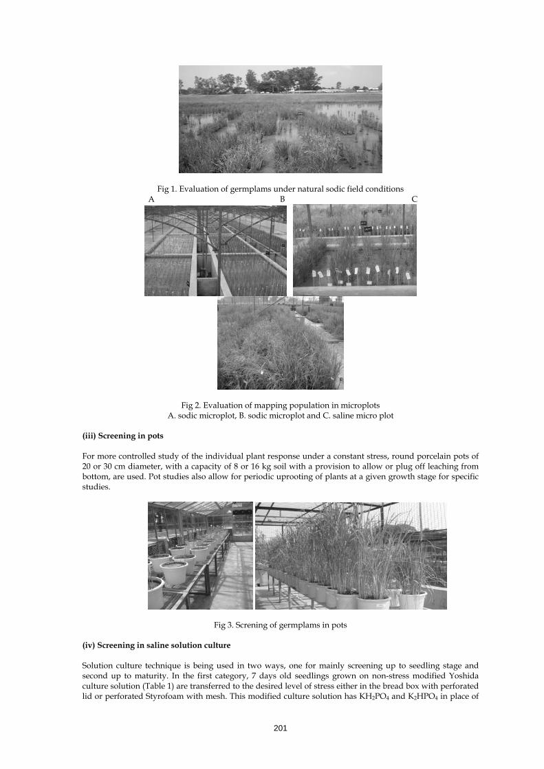
201

Fig 1. Evaluation of germplams under natural sodic field conditions A B C

Fig 2. Evaluation of mapping population in microplots A. sodic microplot, B. sodic microplot and C. saline micro plot

(iii) Screening in pots For more controlled study of the individual plant response under a constant stress, round porcelain pots of 20 or 30 cm diameter, with a capacity of 8 or 16 kg soil with a provision to allow or plug off leaching from bottom, are used. Pot studies also allow for periodic uprooting of plants at a given growth stage for specific studies.

Fig 3. Screning of germplams in pots

(iv) Screening in saline solution culture Solution culture technique is being used in two ways, one for mainly screening up to seedling stage and second up to maturity. In the first category, 7 days old seedlings grown on non-stress modified Yoshida culture solution (Table 1) are transferred to the desired level of stress either in the bread box with perforated lid or perforated Styrofoam with mesh. This modified culture solution has KH2PO4 and K2HPO4 in place of

202

NaH2PO4 as sodium salt within culture solution may increase the Na ion concentration. Initial salinisation of culture solution with 50mM NaCI (equivalent to about 4.9 dS/m) for three days followed by increase in stress level unto 70 to 100 mM (approx. 6.8 – 9.5 dS/m) is good enough for screening of genotypes for salinity at seedling stage. After 10 to 15 days, treated seedlings are used for morphological, physiological or biochemical analyses. The adult plants uprooted from nursery can also be screened for reproductive stage tolerance under this saline hydroponics but with large spacings between plants inserted in the saline medium through holes on the thermocol sheets. Alternatively, for the adult plant stage tolerance screening, plants are grown in ½ kg capacity soil filled pots and the desired salinity level of rhizosphere is maintained through time automated circulatory irrigation system. However the screening under solution culture requires frequent changing of nutrient solution with maintenance of pH around 4.5 for better nutrient availability. Recently, we started growing seed of large number of segregating progenies of rice on the nylon mesh tops floating on nutrient solution under glass house conditions. This is followed by transferring about 25 days’ old seedlings on the highly salinized (12-14 dS/m) nutrient medium to select few but most robust tolerant progenies for seedling stage tolerance. Few surviving seedling stage tolerant plants are then planted in pots having normal soil for advancing their generations during off-season under environmentally controlled glass house conditions. This method could be extremely useful particularly for those locations where only one crop of rice can be taken due to winter season. Table 1. Chemical composition of Rice Culture Solution (Modified Yoshida Solution)

Stock Reagent gram per litre 1 NH4NO3 91.4 2 K2SO4 71.4 3 a KH2PO4 23.1 b K2HPO4 4.3 4 CaC126H2O 175 5 MgSO47H2O 324 6 Minor Nutrients a MnCl24H2O 1.5 b (NH4)6 Mo7O244H2O 0.074 c H3BO3 0.93 d ZnSO47H2O 0.035 e CuSO45H2O 0.03 7 FeNaEDTA* 10.5 8 FeSO4 (made fresh) 2.5 *replace regularly, 1.25ml each stock solution per liter culture solution pH 4.5 to be adjusted with nitric acid

Fig 4. Screning of germplams under hydroponic condition

203

(v) Screening in trays This method is particularly useful for rapid screening of large number of lines but is restricted only up to seedling stage. For this, salt affected soil is filled in shallow depth in the wooden or metal germination trays provided with a polythene sheet lining on the inner side. These are quite handy for screening lines with appropriate control on salinity, sodicity and moisture. The trays can also be conveniently shifted from one growth chamber to another.

Fig 5. Screning of Germplams in trays (vi) Screening in petri dishes

This method is useful for screening of germination stage tolerance particularly in those crops where seeds come in direct contact with salts after sowing in saline and sodic soils. Seeds kept on filter paper are salinized with saline treatments under laboratory conditions. Screening and selection criteria The screening parameter or trait which shows clear difference between genotypes subjected to salt stress in a reproducible manner that qualifies for a reliable screening criterion. In addition, the ideal screening parameter should also preferably influence the final economic yield. The more the intimate relationship between/among the morphological, physiological or biochemical trait with final yield, more indispensable would it prove for any successful breeding programme. Unfortunately, no single clear cut trait or criterion other than economic yield has emerged so far which is linked with yielding ability under salt stress. However, these screening criteria perceived to contribute to overall tolerance and being used at CSSRI is described below: A. Morphological parameters (i) Germination studies: Germination percentage, coleoptile and radicle length under varying degree of salt stress are good indicator of salt tolerance at initial stages. Extensive studies conducted in rice revealed that higher soil ESP and salinity delays or reduces the germination. It is a rapid screening technique in laboratory conditions. (ii) Survival of the plant: It is mainly limited to the seedling studies; however, in some of the adult plant studies it has also been considered. Under moderate stress, plant survival is not a problem. But under high stress, it is a good selection criterion to select few robust and tolerant segregants from large populations or lines from large collections. (iii) Injury score: Individual plant or group of genotypes are scored usually on 1 to 5 or 1 to 9 scale where lower score indicates tolerant and higher score denotes sensitive genotypes. Vigour score for individual plant

1- Good growth and tillering and no symptoms of stress. 3- Growth nearly to normal but few tillers and leaves become discoloured whitish (sodic), rolled (saline) 5- Reduced growth, less number of tillers, many leaves of plant show discoloured whitish (sodic), rolled (saline)

204

7- Growth completely ceases 1-2 tillers and almost all leaves become dry. 9- No tillers, yellowing of all leaves and almost like dead plant.

(iv) Phenotypic expression: Excessive tip burning especially in younger leaves, spikelet sterility and stunted growth are considered for the overall phenotypic expression of the genotype under stress environment. (v) Root/shoot growth: Salt stress severely hampers the root/shoot dry as well as fresh weight. In rice sodicity affected both root and shoot fresh and dry weights but genotypic differences were observed for the degree of reduction. (vi) Grain yield: It is the major selection criterion usually followed for screening and evaluation of the collections and advanced breeding materials. Generally, in the absence of any simple and reliable selection criteria, grain yield performance of the genotypes under salt stress remains the practical measure of tolerance. (vii) Stress susceptibility index (SSI): Stress susceptibility index is a better criterion of adjudging the tolerant genotypes than stress performance per se of genotype because it accounts for the differences in yield potential too. Through this method, better performance under stress can be traced back either to better yield potential or to true stress tolerance. Tolerance to salt stress has been worked out by stress susceptibility index (S) on the principle of yield minimization under stress compared to non stress environment (Fischer and Maurer, 1978). The S values for individual genotype are calculated as:

Where S= Stress susceptibility index, Ys= Mean grain yield of a genotype under stress Yp= Mean grain yield of the same genotype under non stress

D = Stress intensity, which was calculated as under: D = 1- mean Ys of all genotypes/mean of Yp of all genotypes

The higher value of ‘S’ means more stress susceptibility and vice- versa. The low values of ‘S’ indicates those genotypes which perform well under stress with sufficient plasticity to respond to the potential environment. Moreover, D value also reflects the degree of stress imposed. B. Physiological parameters Physiological mechanisms influencing tolerance include various attributes like Na exclusion, tissue tolerance, low Na/K ratio, efficient salt partitioning ability within plant to retain harmful salts in functionally less active organs like vacuoles and older plant parts. Negative effects of salts are also offset by higher uptake of K, Zn and P. Since earlier results showed that no single mechanism could confer the absolute tolerance, pyramiding genes for diverse physiological mechanisms into one genetic background has been initiated and good breeding populations have been generated. A wide spectrum of germplasm in rice has been evaluated and categorized based on tissue tolerance, Na+ exclusion, K+ uptake, Na+/ K+ ratio and reproductive stage tolerance for using these as donors for augmenting breeding program (Table 2). Salt stress- genetics and physiological responses Major plant symptoms of salt injury are: white leaf/panicle tip followed by burning (salinity), leaf browning and necrosis (sodicity), stunted growth, low tillering, spikelet sterility, low harvest index, less number of florets, low grain yield, leaf rolling, poor root growth and patchy growth in field. Salinity leads to injury on rice plant and manifests symptoms like stunted growth, tip burning/ white leaf tip, leaf scorching from lamina to lower portion, low tillering, spikelet sterility and death of plant because it affects growth in varying degrees. In sodicity, almost all the symptoms remain same except leaf browning and necrosis in place of white leaf tip. Rice is tolerant during germination, becomes very sensitive during early seedling, gains tolerance at vegetative, reverts to being sensitive during anthesis and fertilization, and becomes tolerant at maturity. Genetics for salt tolerance at vegetative and reproductive stages has been amply studied revealing the polygenic control of the tolerance. Combining ability studies confirmed the importance of both additive and non-additive gene actions, the former showing rather more preponderance (Mishra et al., 1990; Flowers, 2004). Information on genetic components of salinity tolerance has been incorporated in the breeding strategy. Anther culture protocol for rapid development of salt tolerant recombinants has been standardized. Information on maintainers and restorers status is available for CSR germplasm/varieties for developing salinity tolerant ‘WA’ rice hybrids (Gautam and Singh, 2004).

205

Table 2. Salt tolerance mechanism based grouping of rice genotype

Genetics of salt tolerance The inheritance of sodicity tolerance was inferred from the scores observed in F1 and bulked F3 generation of 2 crosses between two tolerant parents (CSR10 and CSR11) and two sensitive parents (Basmati 370 and Pakistani basmati) under artificially created sodic soils (pH 9.8) in lysimeters. All the F3 plants, scores based on IRRI scoring method at adult stage, showed continuous variation suggesting that sodicity tolerance is controlled by polygenic trait acting additively in most of the cases along with interactions between the alleles at some loci. Results of a similar inheritance study involving same populations indicated the role of few major genes along with numerous minor genes for salinity tolerance. It was also inferred that salinity tolerance trait is polygenic in nature and lacks maternal influence. Enormous variability for tolerance to soil salinity has been explored and documented in rice. Hence, vast opportunities exist and also amply harnessed with regard to these biological benefits. Salinity tolerance being complex and polygenically trait, CSSRI used multi-pronged genetic and physiological approaches to introduce salinity tolerance into well adapted and agronomically better genetic backgrounds. Consequently, success in terms of development and release of better salt tolerant varieties could be achieved. Breeding methodology A. Conventional methods of breeding Conventional breeding has been very successful in developing the salt tolerant varieties of rice by CSSRI. Screening, evaluation and plant breeding work started with the introduction, collection, evaluation and hybridization of available Indian and exotic germplasm of rice. The salt tolerant rice varieties Damodar (CSR1), Dasal (CSR2) and Getu (CSR3) are the pure line selections of the local traditional cultivars prevailing in the Sunderban areas in West Bengal. The varieties adapted to salinity stress were first introduced in sodic areas of Karnal and later identified possessing the genes for sodic tolerance too. Hence CSR1 was involved as one of the donors for salt tolerance in our hybridization programme. Breeding methods used to develop the varieties tolerant to salinity /sodicity in rice are: • Pedigree method • Modified bulk pedigree method • Single seed descent method • Mutation breeding using irradiation and chemical mutagens • Shuttle breeding involving simultaneous evaluation of material at different locations. B. Non conventional methods of breeding CSSRI, Karnal also got success by employing following techniques for crop improvement for salt tolerance with the development of suitable material.

• Molecular marker assisted selection • Transgenic approach

Group1 Group 2 Group 3 Group 4 Group 5 Group 6 Tissue tolerance to Na+

Na+ excluder K+ miners Low Cl Uptake

Low Na+/K+ ratio

Early vigor

SR26B, CSR21, CSR26, CSR27, Pokkali, GR11

CSR1, PAC-831, CSR8,CSR10, CSR13, CSR19, CSR20, CSR22, CSR23,CSR24, CSR25

Hathwan, Swarndhan, Achhi, CSR23, IR36, CSR21, GR11, SR26B, CSR1, CSR10, CSR11, CSR20, Panvel23

HKR128, Jaya, CSR10, PR108, CSR19

PR108, Achhi, CSR1, CSR19, ADT36, IR4630-22-2-5-1-3, CSR18, SLR1214, CSR10, IR42

CSR-92-5, 89-H1-1-3 (96389), 91-H2-6-B-2 (96529), 92-H5-4 (96228), 93122,KR1-24, CSR11, CSR1, CSR27

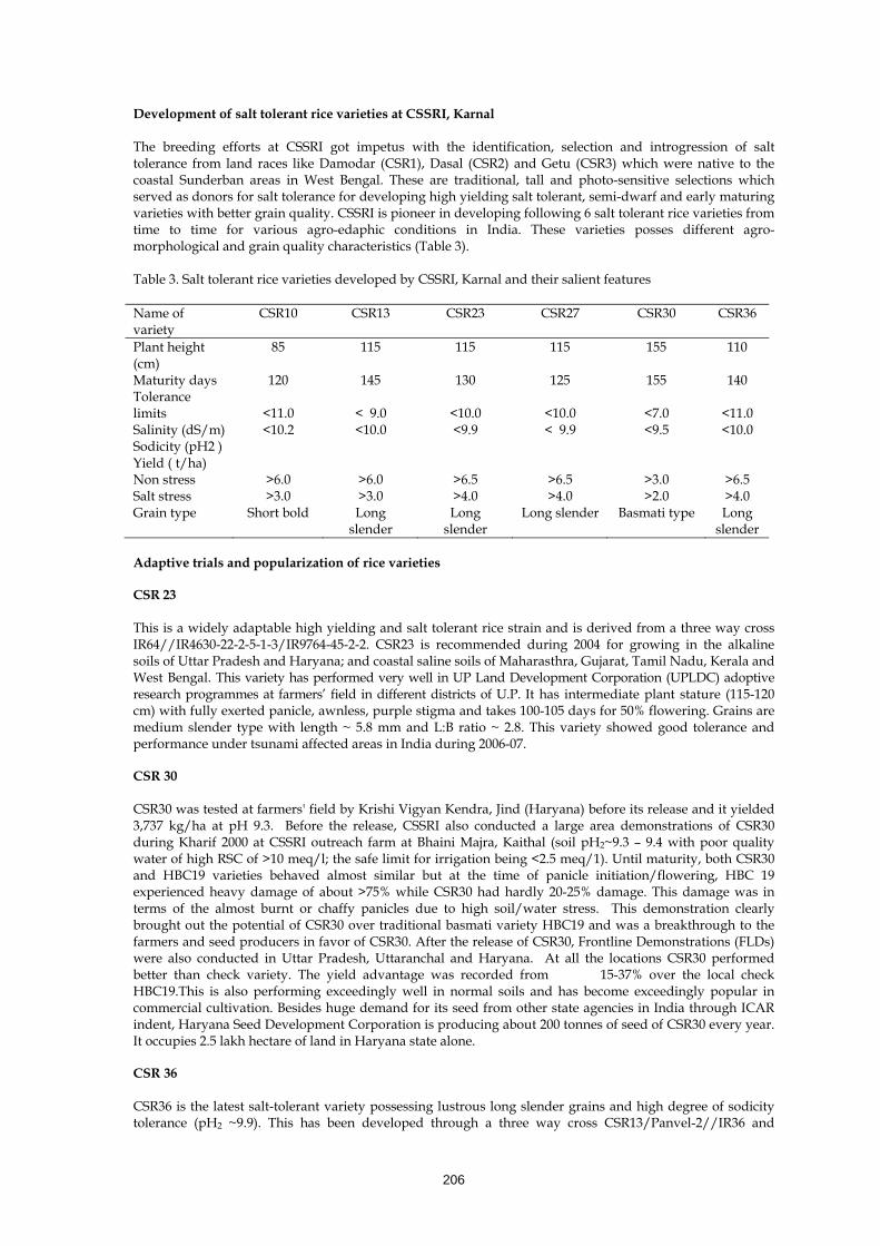
206

Development of salt tolerant rice varieties at CSSRI, Karnal

The breeding efforts at CSSRI got impetus with the identification, selection and introgression of salt tolerance from land races like Damodar (CSR1), Dasal (CSR2) and Getu (CSR3) which were native to the coastal Sunderban areas in West Bengal. These are traditional, tall and photo-sensitive selections which served as donors for salt tolerance for developing high yielding salt tolerant, semi-dwarf and early maturing varieties with better grain quality. CSSRI is pioneer in developing following 6 salt tolerant rice varieties from time to time for various agro-edaphic conditions in India. These varieties posses different agro-morphological and grain quality characteristics (Table 3). Table 3. Salt tolerant rice varieties developed by CSSRI, Karnal and their salient features Name of variety

CSR10 CSR13 CSR23 CSR27 CSR30 CSR36

Plant height (cm)

85 115 115 115 155 110

Maturity days 120 145 130 125 155 140 Tolerance limits Salinity (dS/m) Sodicity (pH2 )

<11.0 <10.2

< 9.0 <10.0

<10.0 <9.9

<10.0 < 9.9

<7.0 <9.5

<11.0 <10.0

Yield ( t/ha) Non stress Salt stress

>6.0 >3.0

>6.0 >3.0

>6.5 >4.0

>6.5 >4.0

>3.0 >2.0

>6.5 >4.0

Grain type Short bold Long slender

Long slender

Long slender Basmati type Long slender

Adaptive trials and popularization of rice varieties CSR 23 This is a widely adaptable high yielding and salt tolerant rice strain and is derived from a three way cross IR64//IR4630-22-2-5-1-3/IR9764-45-2-2. CSR23 is recommended during 2004 for growing in the alkaline soils of Uttar Pradesh and Haryana; and coastal saline soils of Maharasthra, Gujarat, Tamil Nadu, Kerala and West Bengal. This variety has performed very well in UP Land Development Corporation (UPLDC) adoptive research programmes at farmers’ field in different districts of U.P. It has intermediate plant stature (115-120 cm) with fully exerted panicle, awnless, purple stigma and takes 100-105 days for 50% flowering. Grains are medium slender type with length ~ 5.8 mm and L:B ratio ~ 2.8. This variety showed good tolerance and performance under tsunami affected areas in India during 2006-07. CSR 30 CSR30 was tested at farmers' field by Krishi Vigyan Kendra, Jind (Haryana) before its release and it yielded 3,737 kg/ha at pH 9.3. Before the release, CSSRI also conducted a large area demonstrations of CSR30 during Kharif 2000 at CSSRI outreach farm at Bhaini Majra, Kaithal (soil pH2~9.3 – 9.4 with poor quality water of high RSC of >10 meq/l; the safe limit for irrigation being <2.5 meq/1). Until maturity, both CSR30 and HBC19 varieties behaved almost similar but at the time of panicle initiation/flowering, HBC 19 experienced heavy damage of about >75% while CSR30 had hardly 20-25% damage. This damage was in terms of the almost burnt or chaffy panicles due to high soil/water stress. This demonstration clearly brought out the potential of CSR30 over traditional basmati variety HBC19 and was a breakthrough to the farmers and seed producers in favor of CSR30. After the release of CSR30, Frontline Demonstrations (FLDs) were also conducted in Uttar Pradesh, Uttaranchal and Haryana. At all the locations CSR30 performed better than check variety. The yield advantage was recorded from 15-37% over the local check HBC19.This is also performing exceedingly well in normal soils and has become exceedingly popular in commercial cultivation. Besides huge demand for its seed from other state agencies in India through ICAR indent, Haryana Seed Development Corporation is producing about 200 tonnes of seed of CSR30 every year. It occupies 2.5 lakh hectare of land in Haryana state alone. CSR 36 CSR36 is the latest salt-tolerant variety possessing lustrous long slender grains and high degree of sodicity tolerance (pH2 ~9.9). This has been developed through a three way cross CSR13/Panvel-2//IR36 and

207

recommended during 2005 for the sodic soils of Haryana, UP and Pondicherry.CSR36 has intermediate plant height (about 100cm), awnless with fully exserted panicles and takes about 140 days for maturity. It has in-built resistance to biotic stresses like blast, rice tungro disease, and green leafhopper. CSR36 possesses dark green leaves; erect flag leaf, green coleoptile and white stigma. It has extra long slender grains (6.76 mm) with good cooking quality characteristics like high head rice recovery (67.5%), intermediate amylose content (25.0%), better gel consistency and very occasional chalkiness. CSR36 also showed good tolerance and performance under tsunami affected areas in India during 2006-07. It performed very well in farmer’s field at Jagsi (Sonipet) and Ismail (Rothak) during kharif 2010. Conclusion

Rice is the most suitable crop to start with reclamation and cultivation of sodic soils due to different advantages. This is also inherently adapted crop for the coastal saline soils. However, screening and breeding salt tolerant cultivars with higher yielding ability under such agro-edaphic conditions have paid rich dividends. CSR10 was the first semi-dwarf, photo-insensitive sodicity tolerant rice variety bred in India by CSSRI, Karnal. This was followed by the development of other fine grained varieties CSR13, CSR23, CSR27, CSR30 and CSR36 mostly for inland saline and sodic soils of the country. This was the outcome of systematic efforts on germplasm collection, hybridization, shuttle breeding, extensive evaluation of segregating material under target stress conditions which were supplemented by novel breeding techniques from time to time. National salinity networks and International programs mainly with IRRI, Philippines accelerated the overall varietal improvement program. Therefore, perpetual development of salt tolerant varieties possessing higher yielding ability and their cultivation through recommended agronomic practices will reap higher productivity from salt affected soils. Suggested Readings Ammar, M.H.M., Pandit, A., Tyagi, K., Khandelwal, V., Rai,V., Gaikwad, K., Singh, A.K, Singh, R.K,

Gautam, R.K. and Singh, N.K. 2006. Mapping of QTLs for salt tolerance traits in indica rice variety CSR27. In Proc. 2nd International Rice Congress held at New Delhi during Oct.9-13, 2006, Abstract (Id 5315) 300.

Blumwald, E. and Grover, A. 2006. Salt tolerance. In Plant Bio-technology (Editor Nigel Halford). John Wiley and Sons Ltd. 206-224.

Flowers,T.J. 2004. Improving crop salt tolerance. Journal of Experimental Botany 55: 307-319. Gautam, R.K. and Singh, R.K. 2004. Identification of salt tolerant varieties as restorers and maintainers for

cytoplasmic-genic male sterility for developing salt tolerant rice hybrids. In Proc. International Symposium on Rice: From Green Revolution to Gene Revolution held at Hyderabad during Oct. 4-6, 2004. p109-110.

Mishra, B., Akbar, M. and Seshu, D.V. 1990. Genetic studies on salinity tolerance in rice towards better productivity in salt affected soils. Rice Research Seminar. International Rice Research Institute, Philippines, July 12, 1990.

NRSA and Associates, 1996. Mapping salt affected soils of India, 1:250,000 mapsheets, Legend, NRSA, Hyderabad.

Ren, Z.H., Gao, J.P., Li, G., Cai, X.L., Huang, W., Chao, D.Y., Zhu, M.Z., Wang, Z.Y., Luan, S and Lin, H.X. 2005. A quantitative trait locus for salt tolerance encodes a sodium transporter. Nature Genetics, 37(10):1141-1146.

Singh, R.K, Singh, K.N., Mishra, B., Sharma, S.K. and Tyagi, N.K. 2004. Harnessing plant salt tolerance for overcoming sodicity constraints: an Indian Experience.In: Advances in Sodic Land Reclamation. International Conference On Sustainable Management of Sodic Lands held at Lucknow during Feb 9-14, 81-120.

Singh, R.K., Mishra, B. and Gautam, R.K. 2004. Recombination strategy to enhance the level of salt tolerance in rice. In Proc. International Symposium on Rice: From Green Revolution to Gene Revolution held at Hyderabad during Oct. 4-6, 2004 pp: 69-70.

Yeo, A.R., Yeo, M.E., Flowers, S.A. and Flowers, T.J. 1990. Screening of rice (Oryza sativa L.) genotypes for physiological characters contributing to salinity resistance and their relationship to overall performance.Theor.Appl.Genet. 79:377-384.

Zhang, G. Y., Guo,Y., Chen, S. L. and Chen, S.Y. 1995. RFLP tagging of a salt tolerance gene in rice. Plant Science 110:227-234.

208

Nuclear Techniques for Inducing Salt Tolerance in Crops P.C. Sharma Central Soil salinity Research Institute, Karnal-132 001 (Haryana), India Introduction The pioneering discoveries by Roentgen of X-rays in 1895; Beaquerel’s discovery of radioactivity in 1896; and Marie and Pierre Curie’s of radiaoactive elements in 1898 led eneventually to the report in the 1920’s of the effects of radiation on genes. Discovery of induced mutations in fruit fly Drosophila melanogaster in 1927 and in barley (Stadler, 1930) by X-rays initiated a new area of induced mutagenesis as a tool in crop improvement strategies. Soon after this discovery may plant breeders started investigating the use of radiation induced mutations for changing different characters in plant architecture. During the past 75 years, more than 2500 varieties have been officially released as listed in the IAEA/FAO mutant varieties database, including 534 rice lines, 205 wheat lines and 71 maize lines (http://www-infocris.iaea.org/MVD/). Of these, 60% were released from 1985 onwards. Mutant varieties have been released in more than 50 countries. Top six countries in which most mutant varieties were released are China (27%), India (12%), USSR and Russia (10%), Netherlands (8%), USA (6%) and Japan (5%). From these officially released varieties, approx. 70% are in agricultural crops and remaining mutant varieties in ornamental and decorative plants including mutants of Chrysanthemum, dahlia etc. Since the effects of mutations on ornamental plants are clearly visible and selection for altered flower colour, shape or size is relatively easy, the application of mutation techniques in the breeding of these crops has a high success rate. Conventional mutagenesis of seed propagated crops Seeds are the most commonly used materials for induced mutation. Mutagenic treatments fall into two main classes: physical (ionizing radiation, UV) and chemical (mostly alkylating agents) as detailed in Table 1 and 2 . Fig. 1 gives a general scheme for conventional mutagenesis. Once seed of a parental line has been treated with a mutagen, it is referred to as M0 seed and on germination produces M1 plant. Some rare dominant mutants can be detected among the M1 population, but since M1 plants exhibit chimeras and physiological disorders (as a carryover from the mutagenic treatment) selection is not normally practiced until later generations. Since plant selections can be made in M2 population for the most obvious phenotypic mutants, but more subtle quantitative effects are best screened for at M3 and validated in subsequent generations. Once a mutant has been selected, it is normally multiplied from a single source and tested for homozygosity. Since mant traits of interest to plant breeders are quantitative (e.g. yield, quality, stress tolerance), the process of mutation detection and evaluation is time consuming, upto four generations can elapse before mutant lines are entered into crossing programmes. Table 1. Classification of some commonly used chemical mutagens

Type of chemical agent

Mode of action Examples of chemical agents

Base analogs Structurally resemble purins and pyramidines and cause mutations through incorporation into DNA in place of normal bases during DNA replicaton. They cause transitions (purine to purine or pyramidine to pyramidine) and tautomerization (existing in two forms between which they interconvert e.g. guanine can exist in keto or enol forms).

Bromouracil (BU), a synthetic compound that resembles thymine (has Br atom instead of methyl group) and incorporates into DNA, pairing with adenine (A0 just like thymine (T). Displays high propensity to tautomerization to the enol form (BU*) 2-aminopurine (2AP), an A analog which pairs with T or (less frequently and efficiently) with C. It also causes A:T to G:C or G:C to A:T transitions.

209

Chemical agents that modify the structure and pairing properties of bases

They act through deamination, the replacement of cytosine by uracil which can pair with A and thus from subsequent cycles of replication lead to transitions (where C is replaced by T, and G is replaced by A on the other strand of DNA). They react with bases and add methyl or ethyl groups and depending on the affected atom, the alkylated base may then degrade to yield a baseless site, which is mutagenic and recombinogenic, or mispair to result in mutations upon DNA replication.

Nitrous acid, causes C to uracil (U), methylcytosine (meC) to T, and A to hypoxanthine deaminations. Hypoxanthine in DNA pairs with C and therefore subsequently causes transitions. Alkylating agents e.g. ethylethane sulfonate, ethylmethane sulfonate, hydroxylamine (NH2OH), N-methyl-N’-nitro-N-nitrosoguanidine (MNNG)

Intercalating agents These are flat, multiple ring molecules that by interacting with bases of DNA insert between them. This insertion causes a stretching of the DNA duplex and the DNA polymerase in turn recognizes this stretch as an additional base and inserts an extra base opposite at this stretched (intercalated) molecule. The result is that intercalating agents cause frameshifts i.e. an alteration of the reading frame: since codons are groups of three nucleotides

Acridine orange, proflavin, ethidium bromide

Agents altering DNA structure

This encompasses a wide range of chemical agents with different activities

Large molecules which bind to bases in DNA and cause them to be noncoding, referred to as bulky lesions (e.g. NAAAF). They block transcription and DNA replication. Agents that cause intra- and inter strand crosslinks (e.g. Psoralens) Chemical agents that cause DNA strand breaks (e.g. peroxides)

Table 2. Classification of some commonly used physical mutagens

Type of chemical agent

Mode of action Examples of chemical agents

Electromagnetic spectrum (EM) which includes visible light and other forms of radiation

Causes covalent bonding between adjacent pyramidines leading pyrimidine dimmers. These dimmers are bulky and can block transcription and DNA replication. They can also stimulate mutations and chromosome rearrangements.

Ultraviolet (UV) radiation is the biologically important one as its wavelength is preferentially absorbed by DNA and amino acids with important biological and genetic implications

Ionizing radiation They produce reactive ions (charges particles) when they react with biological systems, especially in the presence of water producing reactive oxygen species-oxygen; superoxide anion; peroxide; hydroxyl radical; and hydroxyl ion. Their effects on DNA either through the free radicles produced or through direct action include: Single or double strand breaks Damage to or loss of bases Crosslinking of DNA to itself or to the proteins

X-, Gamma- and cosmic rays; particle radiation such as fast and thermalneutrons; and alpha- and beta- particles

210

General procedures for using induced mutations The general procedures for using induced mutations are rather simple and have a strong basis in the laws of genetics. Dormant seeds of the so called parent variety are irradiated or treated with a chemical mutagen. Mutagenic treatments can cause chromosomal rearrangements or change some genes to some other allelic forms. Plants grown from mutagenised seeds are called M1 plants. When a multicellular tissue like the seed embryo is treated with a mutagen, the plant developing from treated seed has a chimeric structure from genetic point of view. After meiosis, the seeds developed on M1 plants are already the M2 generation. The seeds are sown in experimental plots and a segregating M2 population is subjected to various screening procedures for desired characters. Screening for quantitatively inherited characters is usually done in M3 generation where selection on a line, rather than on a single plant basis can be initiated. Selected mutants from the M2 or M3 generation are usually checked by homozygosity in the M3 or M4 generations respectively. Promising homozygotic mutants can be used directly for multiplication, this will lead to the development of so called direct mutant variety (e.g. barley cv. Diamant in CSSR; rice cv. Calrose 76 in USA) or they can be used in a cross breeding programme (e.g. linseed mutants M1589 and M1722). Mutagenic treatment M1 plants Seeds of homozygous parent variety Chimeric, partially heterozygous M0 Growth in good conditions, without selection M3 generation M2 generation Segregating for mutant lines Segregating for mutated individuals, Selection on a mutant line basis Deficit of recessive, homozygous mutants Homozygosity test of mutants selected Selection on single plant basis M2 generation M4 generation Homozygosity test of mutants selected Entry into a breeding programme in M3 generation Preliminary evaluation of mutants

Fig 1. Development of mutant lines using conventional mutagenesis

Procedure for optimally inducing mutations in rice using a chemical mutagen EMS

• Select disease free seeds with uniform size and shape. Viable seeds with high germination rates must be used.

• Choose a wide range of the concentration of the chemical for use in the induction treatments with varying time durations in order to determine the optimum concentration-by-time for mutation induction. A minimum of three hours duration is usually required for EMS treatments.

• Use 40-50 seeds per treatment with a minimum of three replications • Put the seeds in a polyethylene mesh bag, fold the bag and hold in place with plastic clip. • Label the bag appropriately (e.g. indicating the variety name, date and treatments carried out) • A control, i,e, not treated with EMS should be included. • EMS is carcinogenic • It should be labeled properly as carcinogen when sued • Wear gloves during the above procedures • Use disposable pipette and balloon for pipetting • Work should be done in confined area and under hood. If hood is not available, use face mask.

211

• Dispose of the unused EMS solution and all the liquid waste by adding 4% Na OH and excess water.

Current status and most significant achievements In the group of crop species, around 70% of the varieties have been released as direct mutant varieties and rest 30% were obtained from crosses with mutated parents (Maluszynski et al., 2000). Among the agricultural crops, mutant varieties involving cereals dominate with 64%. Rice is in the first place (25%) followed by barley, wheat, maize, durum wheat and others (oat, millet, sorghum, raya etc.). Most of the rice mutant varieties were released as direct mutants means direct seed multiplication from selected mutants. Nevertheless some mutants such as ‘Reimei’ (Japan) and ‘Calrose 76’ (USA) were successfully used in extensive cross breeding prgrammes. Semi dwarfness and earliness were the often selected characters in treated populations. On the list of improved characters are also traits desired for increasing sustainability in rice production, such as cold and salt tolerance or photoperiod insensitivity. In rice, as in other crops, radiation was more often used to generate desirable traits (190 varieties) while some (923) were induced by chemical mutagenesis. Some mutant varieties have high economic impact. Rutger (1992) discussed that11 mutant rice varieties were grown on an annual area of over one lakh hectares each. Among them are the Chinese varieties Zhefu 802 and Yuanfengzao on more than one million hectares. The successful development and release of cotton variety NIAB 78 in Pakistanin 1983 is another example. It was developed by crossing a US and a local variety by irradiating with gamma rays, which led to doubling of the production of cotton in Pakistan. In central European country, malting barley is an important crop. It is generally grown on more than 25% of cereal acreage. Dry seeds of variety Valticky were irradiate dwith 10 kR of X rays. Selection for improved characters was initiated in M2 generation. A selected mutant designated as X2-228 became the progenitor of new variety ‘Diamant’ released in 1965. The mutant differed from the parent variety ‘Valticky’, a relatively tall variety (92cm) which is highly susceptible to lodging under increased levels olf nitrogen fertilizer in such important agrono,ic traits as reduction of culm length (15 cm), resistance to lodging, semi-prostate growth habit, higher tillering ability, 12 % increase in grain yield. It also showed slow initial development. This character lead to prolonged period of organogenesis during tillering and as a consequence, to a greater number of spike bearing tillers. Resistance to lodging and high tillering resulted in substantially increased productivity of the mutant. Later more than 85 varieties developed from the mutant ‘Diamant’ were released in various European countries. The case of golden promise Mutant cultivars or mutant lines have usually been investigated only for a character or characters directly related to solving a particular breeding program. Mutants kept in collections are very seldom investigated for other characters not related to an already described mutated trait. This was the case in rice mutant variety ‘Atomita 2’ released in Indonesia in 1983, selected for earliness and brown plant hopper resistance and later discovered to carry a mutated gene for slat tolerance in Vietnam. ‘Golden Promise’ is a direct mutant variety developed by gamma ray treatment of the barley cultivar Maythorpe’ in UK in 1966. This variety was extremely important in UK barley industry, and dominated the Scottish barley acreage in 1970’s to mid 1980’s. It is still in the standard for malt quality in Scotland. Mutated genes from ‘Golden Promise’ were transferred to other genetic backgrounds, leading to the release of 17 other barley mutant cultivars in UK. In salt tolerance tests at Scottish Crop Research Institute, a significant difference (50%) has been detected between shoot Na accumulation of ‘Golden Promise’ plants and its parent variety ‘Maythorpe’ under slat stress conditions. The results imply that the mutational difference between a mutant variety and its parent is also responsible for increased tolerance to salt. Mutational analysis of the Arabidopsis genome In barley, maize, pea and tomato, large mutant germplasm collections have been established and used for genetic analysis and plant breeding. Recently, due to intensive mutation efforts, Arabidopsis has become, most probably, the genus with the highest number of induced mutants. Arabidopsis mutants have been characterized as mutations affecting basic metabolism and been obtained following seed treatment with EMS. Chemical and physical mutagens have also been widely used to induce mutations in this model plant. Using EMS mutagenesis, oil composition was genetically modified by increasing oleic acid content from 15 to 86% with parallel reduction in linoleic acid from 18 to below 2%. The use of shuttle mutagenesis in crop improvement with induced mutations in Arabidopsis was also demonstrated, where, genes for herbicide resistance obtained through microspore mutagenesis in Brassica napus, have been cloned and transferred into canola and tobacco to elevate levels of herbicide tolerance. Many studies have demonstrated that the

212

steps leading to successful gene transfer such as gene identification, characterization and cloning and to gene expression in transgenic plants can be more easily achieved in this model plant Arabidopsis. Mutation techniques for crop improvement programmes Generation of desired variability Exploiting natural or induced genetic diversity is a proven strategy in the improvement of all major food crops, and the use of mutagenesis to create novel variation is particularly valuable in those crops with restricted genetic variability. Historically the use of mutagenesis in breeding has involved forward genetic screens and the selection of individual mutants with improved traits and their incorporation into breeding programmes. Although this approach has clearly proved very successful, there are limitations imposed by, for example, the difficulty of identifying a small number of individuals with novel phenotypes within a large population, or by the genetic redundancy present in many plant species as a result of gene duplication and polyploidy, such that many mutations have no detectable effect on the plant. Recently, reverse genetic approaches have permitted the silencing or interruption of individual candidate genes, Whilst mutations occur spontaneously in nature, the frequency of such mutations is too low to rely on alone for accelerated plant breeding. The degree of mutation is dependent on the tissue and degree of exposure (dosage×time). Mutations at single nucleotide pairs are generally of the most interest to breeders because large-scale changes to chromosome structures usually have severely negative results. However, the use of mutagens that alter chromosome structure to increase the number of recombination events and break undesirable linkages is also extremely valuable. Critically, mutations in important traits or genes (e.g. in nutritional quality, resource use efficiency, architecture or phenology) can be readily exploited by plant breeders without the legislative restrictions, licensing costs, and societal opposition applied to GM approaches. This is despite the fact that transcriptomic analyses have shown that large-scale plant mutagenesis may induce greater changes in gene expression patterns than transgene insertion (Batista et al., 2008). This review briefly discusses recent advances in the detection of mutations and the potential of this approach for crop improvement. The creation of mutagenized populations forms the foundations of the reverse genetic approaches, although collections of accessions containing natural polymorphisms can also be used. To ensure that any gene of interest carries sufficient significant mutations, the populations of induced mutations may need to be very large; the size required is dependent on the dosage of mutagen and the level of gene duplication created by recent or ancient polyploidization events. Mutant populations have now been created for many cereal crops, including rice (Suzuki et al., 2008), maize (Till et al., 2004), sorghum (Xin et al., 2008), barley and both hexaploid bread wheat (Slade et al., 2005) and durum wheat, mostly created by treating seeds or pollen with chemical mutagens. To increase the efficiency of mutation detection it is advisable to optimize mutagen dose to achieve a high mutation rate while avoiding serious effects on germination and plant development. In diploid species this can be difficult as even relatively low levels of mutation can result in the almost complete loss of male or female fertility, resulting in a need for very large populations if saturated coverage is required. By contrast, polyploid species such as wheat have a very high tolerance of mutations due to the complementation of essential genes by homeologous copies and thus populations saturated with mutations can be much smaller, resulting in more cost-effective screening for mutations. However, a consequence of this genetic buffering is that recessive mutations in single homeologues of genes in polyploid species are less likely to show a phenotype, and it becomes necessary to identify mutations in each homeologous copy of the target gene and bring these together by crossing. The choice of chemical mutagen will also influence the maximum permissible mutation rate achievable: EMS creates a larger proportion of non-sense mutations, involving the introduction of novel stop codons, than a mutagen such as MNU, due to the specificity of EMS in creating mainly G–A and C–T transitions, and any individual mutations is therefore more likely to have a phenotypic effect. This may partly explain the high mutation frequency achieved in rice using MNU, although the mutation rate in this population was also enhanced by the selection of M1 plants with reduced fertility, which had previously been shown to be associated with higher rates of visible phenotypes in the M2. Use of in vitro haploid technology The mutant production cycle can be significantly shortened by the application of doubled haploid (DH) techniques. Depending upon the plant species, various techniques can be used. Beversdorf and Kott (1987) developed a mutagenesis and in vitro selection system using microspore cultures in rapeseed. This system involved gamma rays or chemical mutagen treatment of uninucleate, potentially embryogenic microspores followed by a selection of developing embryo like structures or plantlets on a medium with a selecting factor (Swanson et al., 1989). Further, in barley, anther culture, bulbosum method or microspore culture can be

213

used for rapid production of true to type mutants. The use of a mutagen in various in vitro systems usually significantly decreases their regeneration ability. Using a M1 plant as a donor of anthers or microspores for production of DH, almost all problems relating to the somatic effects of mutagen on tissue could be avoided. In the DH2 generation from mutated barley plants, more than 25% of true to type mutants were observed, among them with some mutants with useful characters such as semi dwarfness or uniculm plant type. Mutation techniques in heterosis It is well known that radiation and chemical mutagenesis can induce male sterility in plants (Rutger 1992). Chaudhary et al., (1994) have clearly demonstrated the potential of mutagenesis for induction of male sterile mutants. A large M2 population (more than 2 lakh seeds) of Arabidopsis was developed from EMS mutagenized seeds and screened for male sterile plants. Nineteen putative mutants were selected. Among the few of them genetically analyzed, 4 non-allelic mutants with different blocks of pollen development were found. It is important to note that in these mutants the vegetative growth and female fertility was not altered. The mutant heterosis has also been confirmed in maize and barley. In vitro culture, mutagenesis and somaclonal variation The technique of mutation induction and in vitro culture seem to be ideally suited for the improvement of vegetatively propagated plants. Food crops, such as cassava, banana, sweet potato, potato and sugarcane are vegetatively propagated and are used a staple diet in many countries. Large number of plants can’t be used for mutagenesis due to the large size of conventional propagule, hence in vitro culture is used for mutagenesis. This also provides relatively uniform and large population of cells and tissues in disease free situations for irradiation. It can be achieved by successive culture of buds or regeneration of shoots and somatic embryos from cell suspension and callus cultures derived from irradiated tissues and explants. Irradiation in combination with in vitro culture has proved to be a valuable method of producing desired variation and rapid propagation. Both somaclonal variation and mutations result in the production of new genotypes with a limited change in the original genome. As a source of variation, somaclonal variation mimics induced mutations. Somaclonal variation has been associated with changes in chromosome number and structure, point mutations, DNA methylation, changes in cytoplasm and plastids, activation of transposons etc. For selection of mutagenised cells or tissues, selection pressure can be applied either at the cell population level or on the plant regenerated from cell cultures and followed by selection in conventional field plots. The potential high efficiency of in vitro selection system is based on the fact that it is possible to grow millions of cells in a petri dish or in a flask and achieve rapid multiplication of cell populations on a defined media. Addition of sodium chloride, fungal toxin, herbicides, antibiotics to the medium or exposure of cell to heat, cold and freezing is used for selection of desired variants. While a great number of radiation induced mutants have been released as new cultivars, somclonal variants have been so far of limited value in plant improvement. Both somaclonal variation and conventional mutagenesis are complementary to and not a replacement for conventional plant breeding. Use of mutations for enhancing salinity tolerance Salinity is a major environmental stress limiting plant growth and productivity. Further salt tolerance is known to e multigenic character controlled by large number of genes. Accordingly, it is often concluded that mutation induction has no role to play in enhancing salinity tolerance of crop plants. However, examples from literature reveals otherwise. Both gain of function as well as loss of function has been reported in different crops with respect to salinity tolerance. Examples of rice and Indian mustard are discussed here. Lee et al., (2003) have reported radiation induced salinity tolerant lines in rice. Many scientists have followed the approach of inducing mutations in cells or tissues and then selecting for salinity tolerant lines. Rice Rice is a major staple food and is consumed by more than half of the world’s population. Rice is sensitive to salinity (Mass and Hoffman, 1977), hence salinity tolerant lines are urgently required. Success in obtaining abiotic tolerant lines using an in vitro culture in combination with radiation techniques has been attained in several crop plants including rice (Shehata et al., 2009). The successful identification of salt tolerant lines obtained from in vitro mutagenesis was carried out at germination, seedling stage and the maturation period on a medium (solution or saline field) (Sathish et al., 1997). NaCl tolerant cell lines were selected from irradiated calluses (Lee et al., 2003). M1 regenerates were obtained from the salt tolerant callus cultured on the auxin free medium for 30 days. Some regenerates were more tolerant than the parent variety on a

214

medium containing 0.75% NaCl. Seeds (M3, 5000 lines) derived from M2 lines were grown to the three leaf stage. M3 lines were soaked with 0.75% salt solution for 3 weeks and 350 salt tolerant genotypes were selected. Among the M3 350 lines, 40 tolerant lines were selected from a saline field (EC 10-14 mS) near the sea coast. Of the 40 lines, two (18-1 and 50-1) showed more improved plant height, panicle length, tillering number, spikelet number and yield than those of the original variety. They also screened 30 RAPD primers and two RAPD markers were identified, which appeared in both salt tolerant lines. From DNA hybridization experiments, it appeared that the fragment arose from the middle repetitive copy sequences. The transcript involved in the marker showed a higher expression in the salt tolerant lines than the sensitive lines. These salt tolerant were further used as a resource in salt tolerant breeding. Shehata et al., (2009) have also reported the development of four mutant rice lines with early maturity, non-lodging and higher salinity tolerance, employing gamma rays mutation induction. These mutant lines Sakha 101-M30, Sakha 102-M20, AC-M50 and Egyptian Jasmine M30 were selected in M6 generation and evaluated for two years under saline conditions (EC 6-6.5 dS/m). Indian mustard Oilseed crops are important to Indian economy and Brassica juncea is being grown in areas having saline underground waters for irrigation. Experiments were initiated at CSSRI Karnal for inducing variability in high yielding and improved lines of B. juncea by the use of radiation and chemical mutagenesis, five genotypes were selected viz. Rohini and Varuna (high yielding genotypes) in one group and CS 614-4-1-4, CS 245-2 and CS 33-4-9, which were improved for salt tolerance and developed at CSSRI, Karnal as another group. These were radiated with 20, 40, 60, 80, 100 and 120 kR doses. Approx. 1200 seeds each, from the seven radiation treatments from each of the five genotypes were selected in each generation for advancing the generation upto M5. Variability was recorded in growth and yield parameters. All the radiation treatments showed increase in main shoot length in all the genotypes compared to controls. The increase in main shoot length with increase in radiation treatment varied from 6% (40, 60 and 100 Kr) through 10% (20 and 80 Kr) to 13% (120 Kr). Further in Varuna, main shoot length increased by 22% at 120 Kr treatments compared to controls. This is an important character to be observed for higher yield under salt affected soils. Significant differences in seed yield were recorded in different radiation treatments. Amongst different genotypes, seed yield declined by 18% in CS 614-4-1-4 to an increase of 10% in CS 245-2 compared to controls. Seed yield increased by 63% in 100 Kr plants in CS 245-2 and by 19% in 40 Kr plants in CS 33-4-9 respectively. The mutant germplasm was also characterized for salinity tolerance at germination and seedling emergence stage. Radiation treatments also showed positive effects on seedling emergence under salinity stress with 32% increase in CS 614-4-1-4 (20 Kr), 27% increase in CS 245-2 (80 Kr) and 25% increase in CS 33-4-9 (40 Kr) respectively. At the highest salinity level of EC 22 dS/m, seedling emergence ranged from nil to around 20% in different genotypes. Maximum seedling emergence was noticed at 60 and 80 Kr radiation treatments at EC 22 dS/m. Mutant plants have been selected recording highest seedling emergence at salinity level of EC 22 dS/m. In general, radiation showed positive effects with respect to toxic ion accumulations as lesser Na ions were accumulated in radiation treatments plants compared to control values. The mutant plants selected showed lesser accumulation of Na/K showing higher salt tolerance compared to control plants. Maximum Na/K (1.75) was observed in Rohini (20 Kr) whereas minimum Na/K (0.95) accumulation was seen in Varuna (60 Kr) plants. The seeds obtained in M4 and M5 generations were evaluated for their salt tolerance potential at germination and seedling emergence stages to select tolerant as well as sensitive mutants for initial development stages. These seeds were also evaluated under field conditions for their whole plant tolerance to salinity and alkalinity. A total of 752 mutant plants (approx 150 plants from each variety, total 752 plants) from each of the radiation treatments from five varieties were evaluated under two types of stresses. Further, segregants of interest were also selected by imposing selection pressure for salt tolerance at seedling and flowering stages in M4 generation by exposing the plants to salinity stress in field. Main shoot length differed significantly under salinity stress and under increasing radiation treatments. The percentage decline in main shoot length was lesser in radiation plants compared in controls in all the genotypes evaluated. Overall, the main shoot length increased by 8% to 12% in radiation treated plants. The longest main shoot length (104.5) was recorded in CS 33-4-9 at 40 Kr (104.5), whereas maximum percentage increase (34%) in main shoot length was observed in CS 33-4-9 followed by 10% in CS 245-2 on mean basis. In general, mean seed yield declined with increase in salinity stress, except in CS 33-4-9 and Varuna where it showed an increase of 11% and 3% respectively under salinity stress compared to controls. However, it increased with increase in radiation treatments. Overall, seed yield increased by 12% (20 Kr) to 25% (80 Kr) under radiation treatments.

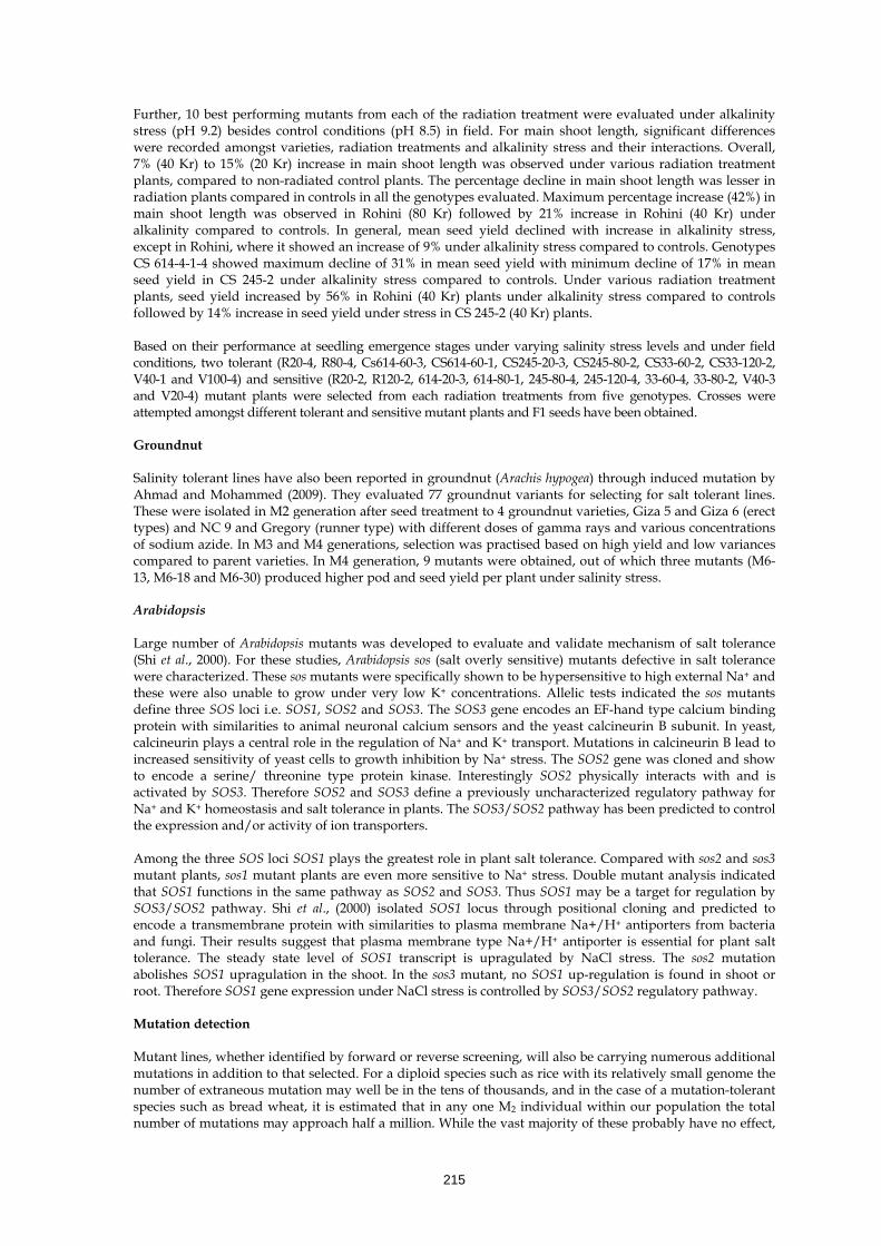
215

Further, 10 best performing mutants from each of the radiation treatment were evaluated under alkalinity stress (pH 9.2) besides control conditions (pH 8.5) in field. For main shoot length, significant differences were recorded amongst varieties, radiation treatments and alkalinity stress and their interactions. Overall, 7% (40 Kr) to 15% (20 Kr) increase in main shoot length was observed under various radiation treatment plants, compared to non-radiated control plants. The percentage decline in main shoot length was lesser in radiation plants compared in controls in all the genotypes evaluated. Maximum percentage increase (42%) in main shoot length was observed in Rohini (80 Kr) followed by 21% increase in Rohini (40 Kr) under alkalinity compared to controls. In general, mean seed yield declined with increase in alkalinity stress, except in Rohini, where it showed an increase of 9% under alkalinity stress compared to controls. Genotypes CS 614-4-1-4 showed maximum decline of 31% in mean seed yield with minimum decline of 17% in mean seed yield in CS 245-2 under alkalinity stress compared to controls. Under various radiation treatment plants, seed yield increased by 56% in Rohini (40 Kr) plants under alkalinity stress compared to controls followed by 14% increase in seed yield under stress in CS 245-2 (40 Kr) plants. Based on their performance at seedling emergence stages under varying salinity stress levels and under field conditions, two tolerant (R20-4, R80-4, Cs614-60-3, CS614-60-1, CS245-20-3, CS245-80-2, CS33-60-2, CS33-120-2, V40-1 and V100-4) and sensitive (R20-2, R120-2, 614-20-3, 614-80-1, 245-80-4, 245-120-4, 33-60-4, 33-80-2, V40-3 and V20-4) mutant plants were selected from each radiation treatments from five genotypes. Crosses were attempted amongst different tolerant and sensitive mutant plants and F1 seeds have been obtained. Groundnut Salinity tolerant lines have also been reported in groundnut (Arachis hypogea) through induced mutation by Ahmad and Mohammed (2009). They evaluated 77 groundnut variants for selecting for salt tolerant lines. These were isolated in M2 generation after seed treatment to 4 groundnut varieties, Giza 5 and Giza 6 (erect types) and NC 9 and Gregory (runner type) with different doses of gamma rays and various concentrations of sodium azide. In M3 and M4 generations, selection was practised based on high yield and low variances compared to parent varieties. In M4 generation, 9 mutants were obtained, out of which three mutants (M6-13, M6-18 and M6-30) produced higher pod and seed yield per plant under salinity stress. Arabidopsis Large number of Arabidopsis mutants was developed to evaluate and validate mechanism of salt tolerance (Shi et al., 2000). For these studies, Arabidopsis sos (salt overly sensitive) mutants defective in salt tolerance were characterized. These sos mutants were specifically shown to be hypersensitive to high external Na+ and these were also unable to grow under very low K+ concentrations. Allelic tests indicated the sos mutants define three SOS loci i.e. SOS1, SOS2 and SOS3. The SOS3 gene encodes an EF-hand type calcium binding protein with similarities to animal neuronal calcium sensors and the yeast calcineurin B subunit. In yeast, calcineurin plays a central role in the regulation of Na+ and K+ transport. Mutations in calcineurin B lead to increased sensitivity of yeast cells to growth inhibition by Na+ stress. The SOS2 gene was cloned and show to encode a serine/ threonine type protein kinase. Interestingly SOS2 physically interacts with and is activated by SOS3. Therefore SOS2 and SOS3 define a previously uncharacterized regulatory pathway for Na+ and K+ homeostasis and salt tolerance in plants. The SOS3/SOS2 pathway has been predicted to control the expression and/or activity of ion transporters. Among the three SOS loci SOS1 plays the greatest role in plant salt tolerance. Compared with sos2 and sos3 mutant plants, sos1 mutant plants are even more sensitive to Na+ stress. Double mutant analysis indicated that SOS1 functions in the same pathway as SOS2 and SOS3. Thus SOS1 may be a target for regulation by SOS3/SOS2 pathway. Shi et al., (2000) isolated SOS1 locus through positional cloning and predicted to encode a transmembrane protein with similarities to plasma membrane Na+/H+ antiporters from bacteria and fungi. Their results suggest that plasma membrane type Na+/H+ antiporter is essential for plant salt tolerance. The steady state level of SOS1 transcript is upragulated by NaCl stress. The sos2 mutation abolishes SOS1 upragulation in the shoot. In the sos3 mutant, no SOS1 up-regulation is found in shoot or root. Therefore SOS1 gene expression under NaCl stress is controlled by SOS3/SOS2 regulatory pathway. Mutation detection Mutant lines, whether identified by forward or reverse screening, will also be carrying numerous additional mutations in addition to that selected. For a diploid species such as rice with its relatively small genome the number of extraneous mutation may well be in the tens of thousands, and in the case of a mutation-tolerant species such as bread wheat, it is estimated that in any one M2 individual within our population the total number of mutations may approach half a million. While the vast majority of these probably have no effect,

216

it is obviously unwise to conclude that any observed phenotype observed at M3 or later generations is due to the single point mutation under study. Mutation detection by TILLING A number of techniques have been developed that can be used to exploit mutagenized populations and diversity collections through identification of point mutations and small indels in specific genes. Although a number of different methods of genotyping single nucleotide polymorphisms are available, having been developed largely for human studies, low allele frequencies at individual loci within most mutagenized populations is a major issue and thus sensitivity and throughput at reasonable cost are important factors in the selection of a suitable platform. One method that has been used is denaturing HPLC (DHPLC), a chromatographic technique that can discriminate between homoduplex and heteroduplex (mismatched) DNA, generated by re-annealing a mixture of wild-type and mutant DNA fragments. This was first used to detect single nucleotide polymorphisms in the human Y chromosome and was adopted by McCallum and colleagues, working at the University of Washington in Seattle, to identify point mutations in an EMS-mutagenized population of Arabidopsis (McCallum et al., 2000). These authors introduced the acronym TILLING (Targeting Induced Local Lesions IN Genomes) to describe their overall approach. To ensure the presence of heteroduplex DNA from lines homozygous for mutations, DNA samples from several lines were pooled up to 5-fold, thereby also increasing the throughput of the technique. This technique was promoted for rapid spread of the technology into other model and crop plants and in animal species. Thus, there now exist TILLING platforms and associated mutagenized populations in pea, sorghum (Xin et al., 2008), soybean (Cooper et al., 2008), oilseeds (Wang et al., 2008), bread wheat (Slade et al., 2005), durum wheat, barley, rice (Suzuki et al., 2008) and maize (Till et al., 2004), Various groups have modified or improved upon the Cel1-based TILLING method to increase its fidelity or throughput. At the other extreme, agarose gel electrophoresis of unlabelled Cel1 cleavage products is also possible (Raghavan et al., 2007), rendering the TILLING process feasible without major capital expenditure. A number of bioinformatics tools has been created to aid in the selection of amplicons for TILLING and in the prioritization of the resulting mutations for subsequent analysis. CODDLE (www.proweb.org/coddle/) uses alignments of related sequences and takes into account both the mutagen used and the coding sequence to identify regions of the target gene most likely to generate deleterious mutations; CODDLE sends this information to Primer3 to generate suitable primers. GelBuddy (www.proweb.org/gelbuddy/) can be used to automate band calling in the electrophoretic gel images, while PARSESNP (www.proweb.org/parsesnp/) analyses the resulting sequenced mutations and attempts to predict the likely consequence for gene function using a protein homology model. Alternative mutation detection platforms Although Cel1-based TILLING is very efficient for detecting mutations in large (1–2 kbp) exon-rich amplicons from target genes, it is less productive when used to screen genes with multiple small exons separated by larger introns, as mutations in introns, except those at splice junctions, rarely affect gene function. High-resolution melt analysis (HRM) has been established as an alternative screening platform for such targets. HRM depends on the loss of fluorescence from intercalating dyes bound to double-stranded DNA during thermal denaturation. Accurate control of temperature and continuous monitoring of fluorescence in instruments such as the Lightscanner (Idaho Technology Inc., Salt Lake City, USA) or the Rotor-Gene (Qiagen, Hilden, Germany) allows detection of single base mismatches in amplicons up to 500 bp. As the costs of large-scale DNA sequencing continue to fall dramatically, this more direct approach to mutation discovery seems likely to become a serious competitor to the methods based on mismatch detection. The current DNA sequencing technologies generate between 500 Mb and 20 Gb of data per run, suggesting that it should be feasible to sequence several targets across a large population at reasonable cost, even allowing for the oversampling required to eliminate sequencing errors and uneven pooling. Prospects for crop improvement The last few years have seen the release of the first genome sequences for model plant species and the more genetically simple crops (Arabidopsis Genome Initiative, 2000; International Rice Genome Sequencing Project, 2005). Exploitation of these sequence data and associated tools for functional genomics has led to rapid progress in understanding the roles of individual genes, particularly in plant development and defence against pathogens. However, utilization of this knowledge for genetic improvement of more complex crops has been variable due to a combination of factors including lack of complete genome

217

sequences, lack of genomic resources such as insertional knockout libraries and, for some species, the absence of high throughput transformation systems. However, the mutation screening technologies described above should make progress much more rapid by facilitating both the deployment of candidate genes identified in model species and also increasing available variation in genes of known agronomic value. This will be further enhanced by the explosion in sequence data for crop species that will undoubtedly follow the development of next generation sequencing technologies, enabling facile identification of genes for modification. One negative factor is that random mutagenesis is much more likely to generate loss of function mutations rather than conferring improved or new properties on the targeted gene, and thus will only be an appropriate strategy in a proportion of cases. Furthermore, in contrast to technologies such as RNAi which, in principle, can target multiple genes simultaneously, point mutagenesis can only target a single copy of a group of related genes, whether paralogues or homeologues, and mutations in different gene copies may have to be brought together by crossing in order to achieve the desired effect. Mutagenesis is currently not regarded as genetic manipulation, as the random base changes involved are identical to those occurring naturally; indeed, as described above, many current crop varieties contain genetic material with origins in mutagenesis programmes. It seems likely, therefore, that reverse genetic selection of beneficial mutations through the screening approaches outlined above will have a major impact on crop breeding in the near future. TILLING and similar techniques have reawakened interest in random mutagenesis for crop improvement, as illustrated by the rapid development of mutagenized populations and reverse genetic screening platforms in many crop species. An equally rapid deployment of novel alleles for crop improvement is certain to follow. A major obstacle in many crop species is the lack of complete genome sequence information, which slows the development of suitable TILLING targets. However, advances in sequencing technology are also likely to relieve this bottleneck within the relatively near future, as sequencing even very complex crop genomes such as wheat becomes practicable. Mutagenized populations can be created at relatively low cost, although diploid species that are intolerant of high mutation frequencies require much larger populations for full coverage. Conversely, highly-mutagenized lines of polyploid species may require significant backcrossing to remove extraneous mutations before they can be assessed for phenotypes or used in plant breeding. Importantly, the use of such novel alleles in crops will not be impeded by the tough regulatory regimes that cover GM crops; this alone should assure the rapid deployment of this technology in plant breeding. Suggested Readings Arabidopsis genome initiative. 2000. Analysis of the genome sequence of the flowering plant Arabidopsis

thaliana. Nature 408: 796-815. Ahmad, M.S.H. and Mohammed, S.M.S. 2009. Improvement of groundnut (Arachis hypogea L.) productivity

under saline conditions through induced mutation. World J. Agric. Sci. 5 (6): 680-685. Batista, R., Saibo, N., Lourenco, T. and Oliveira, M.M. 2008. Microarray analysis reveal that plant

mutagenesis may induce more transcriptomic changes than transgene insertion. Proc. Natl. Acad. Sci. USA 105: 3640-3645.

Beversdorf, W.D. and Kott, L.S. 1987. An in vitro mutagenesis/ selection system for Brassica napus. Iowa State J. Res. 61: 435-443.

Chaudhary, A.M., Lavithis, M., Taylor, P.E., Craig, S., Singh, M.B., Signer, E.R., Knox, R.B. and Dennis, E.S. 1994. Genetic control of male fertility in Arabidopsis thaliana: structural analysis of premeiotic developmental mutants. Sex Plant Reprod. 7: 17-28.

Cooper, J.L., Till, B.J. and Laport, R.G. 2008. Tilling to detect induced mutations in soybean. BMC Plant Biol. 8: 1-2.

Lee, I.S., Kim, D.S., Lee, S.J., Somg, H.S., Lim, Y.P. and Lee, Y.I. 2003. Selection and characterization of radiation induced salinity tolerant lines in rice. Breed. Sci. 53 : 313-318.

Maas, E.V. and Hoffman, G.J. 1977. Crop salt tolerance-current assessment. J. Irrig. Drainage Div. ASCE 103 : 115-134.

MaCallum, C.M., Comai, L., Greena, E.A. and Henikoff, S. 2000. Targetted screening for induced mutations. Nature Biotech. 18: 455-457.

Maluszynski, M., Ahloowalia, B.S. and Sigurbjornsson, B. 1995. Application of in vivo and in vitro mutation techniques for crop improvement. Euphytica 85 : 303-315.

Maluszynski, M., Nichterlein, K., van zanten, L. and Ahloowalia, B.S. 2000. Officially released mutant varieties-the FAO/IAEA database. Mut. Breed. Rev. 12 : 1-84.

Parry, M.A.J., Madgwick, P.J., Bayon, C., Tearall, K., Hernandez-Lopez, A., Baudo, M., rakszegi, M., Hamada, W., YAssin, A.A., Ouabbou, H., Labhilili, M. and Phillips, A.L. 2009. Mutation discovery for crop improvement. J. Exp. Bot. 60 (10) : 2817-2825.

218

Raghvan, C., Naredo, M.E.B., Wang, H.H., Atienza, G., Liu, B., Qiu, F.L., McNally, K.L. and Leung, H. 2007. Rapid method for detecting SNPs on agarose gels and its application in candidate gene mapping. Mol. Breed. 19: 87-101.

Rutger, J.N. 1992. Impact of mutation breeding in rice – a review. Mutat. Breed. Rev. 8: 1-24. Sathish, P., GAmborg, O.L. and Nabores, M.W. 1997. Establishment of stable NaCl resistant rice plant lines

from anther culture: distribution pattern of K/Na in callus and plant cells. Theor. Appl. Genet. 95 : 1203-1209.

Shehata, S.M., AbdAllah, A.A. and zayed, B. 2009. Development of salt tolerant lines through mutation breeding. J. Agric. Res. Kafrelsheikh Univ. 35 (4) : 954-963.

Shi, H., Ishitani, M., Kim C. and Zhu, J.K. 2000. The Arabidopsis thaliana salt tolerance gene SOS1 encodes a putative Na+/H+ antiporter. Proc. Natl. Acad. Sci. 97 (12) : 6896-6901.

Szarejko, I. and Forster, B.P. 2007. Doubled haploidy and induced mutation. Euphytica. 158 : 359-370. Slade, A.J., Fuerstenberg, S.I., Loeffler, D., Steine, M.N. and Facciotti, D. 2005. A reverse genetic, non-

transgenic approach to wheat crop improvement by TILLING. Nature Biotech. 23 : 75-81. Stadler, L.J. 1930. Some genetic effects of X-rays in plants. J. Hered. 21 : 2-19. Suzuki, T., Eiguchi, M., Kumamaru, T., Satoh, H., Matsusaka, H., Moriguchi, K., Nagato, Y. and Kurata, N.

2008. MNU induced mutant pools and high performance TILLING enable finding of any gene mutation in rice. Mol. Gen. Geno. 279 : 213-223.

Swanson, E.B., Herrgesell, M.J., Arnoldo, M., Sippell, D. and Wong, R.S.C. 1989. Microspore mutagenesis and selection: Canola plants with field tolerance to imidazolinones. Theor. Appl. Genet. 78: 525-530.

Till, B.J., Reynolds, S.H. and Weil, C. 2004. Discovery of induced point mutations in maize genes by TILLING. BMC Plant Biol. 4 : 12.

Wang, N., Wang, Y.J., Tian, F., King, G.J., Zhang, C.Y., Long, Y., Shi, L. and Meng, J.L. 2008. A functional genomics resource for Brassica napus: development of an EMS mutagenized population and discovery of FAE1point mutations by TILLING. New Phytol. 180 : 751-765.

Xin, Z.G., Wang, M.L., Barkley, N.A., Burow, G., Franks, C., Pederson, G. and Burke, G. 2008. Applying genotyping (TILLING) and phenotyping analysis to elucidate gene function in a chemically induced sorghum mutant population. BMC Plant Biol. 8 : 324-335.

219

Physiological Attributes Associated with Sodicity Tolerance Ali Qadar Central Soil Salinity Research Institute, Karnal – 132 001 (Haryana), India

Total surface area of the world is about 132 billion hectare (bha). The arable land at world level is not more than seven bha of which 1.5 bha is under cultivation (Massoud. 1981). Salinity and sodicity are two important adverse edaphic factors for agriculture in arid and semiarid tropics and are reported in more than 100 countries in all the continents. It is estimated that approximately 831 million hectare (mha) are salt affected world wide, which account for more than 6 % of the world total area (Martinez-Beltran and Manzur, 2005). Of the total salt affected area, 434 mha are sodic and 397 mha are saline. More areas are going out of cultivation where irrigation is not applied judiciously and more specifically where farmers are using saline/sodic water for irrigation. Of the current 275 mha of irrigated land (273 mha in ha in 2001: http://apps.fao.org., January 2004), about 20 % (55 mha) is salt affected with some estimate being as high as 50% (Pitman and Lauchli, 2004; FAO 2005) and of the almost 1,500 mha of dry land agriculture, 32 mha are salt affected (2.1 %) to varying degrees by human –induced processes (Ghassemi, et al.1995; GM and Saline Tolerance- FAO 2008). Secondary salinisation of agricultural land is particularly widespread in arid and semiarid where irrigation is unavoidable to achieve good production. The area affected by salinity and sodicity in India is about 6.73 mha (2.96 mha saline and 3.77 mha sodic, NRSA and Associates, 1996) and distributed in 15 states. Saline soils invariably have neutral salts and predominant cation is sodium (Na+) with chloride (Cl-) and sulphate (SO42-) as dominant anions. The electrical conductivity (EC) is higher (>4 dSm-1), pH is less than 8.5 and sodium adsorption (SAR) is below 15. Saline soil has enough soluble salts as to affect significantly colligative properties of soil solution. Higher concentration of soluble salts, which are predominantly Cl-

/SO42- of Na+ in saline soils results decrease in osmotic potential of soil solution. This reduction in osmotic potential has long been considered to be the prime cause of adverse effects of salinity on plants growth. Excess uptake of Na+ and Cl- by the plants may lead to ion toxicity. In addition to this, higher concentrations of these in soil solution may create nutrient imbalance. Interaction between Na+ and other cations and between, Cl-, OH- or HCO3- and other anions are of general importance in mineral nutrition of plants. Sodic soils have high pH (> 8.5 and even up to 10.5), exchangeable sodium percentage (ESP) >15 and have carbonates (CO32-) and bicarbonates (HCO3-) as predominant anions. Excess of Na+ on exchange complex causes dispersion of clay, resulting poor soil physical conditions including reduced infiltration, soil compactness and anaerobiosis. Sodic soils invariably have hard pan at some depth (0.5-1.5 m) from the surface formed as a result of precipitation of calcium carbonate. Majority of the plants do not require Na+ at least in such a high concentrations as found in saline and sodic soils and its excess uptake creates problem of ion toxicity. Some plants do respond to Na and are often referred as Natrophilic plants. Higher Na+ concentration in soil solution or on exchange complex causes nutrient imbalance, which may lead to deficiency of K and Ca because of its antagonistic effect on the uptake of these two (K, Ca) elements. Sodium induced Ca/K deficiency has often been reported in the literature. Increased in nutrients supply is often reported helpful to alleviate the adverse effects of salinity and sodicity stresses especially when their availability is compromised because of their low concentrations and also decrease in their activities. Germination, growth and yield of majority of the plant species including crops are adversely affected by salinity and sodicity stresses and plants may even die before reaching to maturity. Out of 354 families of flowering plant, 129 families are having clear salt tolerance. Interestingly only 20 families have more than half of the 500 known halophytic genera. Among monocotyledoneae, the Poacea contains more halophytic genera (45 genera out of 650) than other family. In dicotyledoneae, the Chenopodiaceae has by far the highest proportion of halophytic genera (44 genera out of 100). Majority of the plants are non-halophytic and their growth and development are adversely affected with increase in salt stress. Various factors affecting growth and yield are as follows:

220

Factors Associated with Salinity and Sodicity Stresses on Plants Salinity Sodicity

↓ ↓ ________________________ _______________________

↓ ↓ ↓ ↓ Physical Factors Chemical Factors Physical Factors

Osmotic Effects Specific Ion Effects Poor Soil Physical Conditions Anaerobiosis Nutrient Imbalance (reduced infiltration, Soil

and Deficiency compactness, anaerobiosis)

(decreased activity, and antagonism)

High pH (influences Nutrients solubility)

Crops show good variability in their response to salt stress both among themselves and also at varietal level and tolerance of a crop varies with its stage of growth and development. Sometimes even cultivars response depends on the nature of ions present in the ambient solution of the roots. Plants adapt various strategies to minimise the impact of salt stress when challenged to it. Study with a number of crops including rice and their genotypes have shown that plants, which are more tolerant to these stresses invariably, had lower concentrations of potentially toxic ions like Na+ (in saline and sodic conditions) and Cl- (in saline condition) in their shoots. Variability in salt tolerance among the crops/genotypes is often explained on their ability to exclude potentially toxic ion like Na+ from shoot and exclusion from shoot is only a broad physiological mechanism which is based on many integrated physiological attributes like (i) controlled uptake at plasma-lemma and tonoplast of cortex, (ii) release of ions in the xylem, (iii) reabsorption of ions by xylem parenchyma. Partitioning of ions at organs (more retention in relatively older plant parts including leaves) and cellular (better sequestering in the vacuole) levels can further influence tolerance of plants. Different plant response to salt stress, adverse effects and possible adaptations can be outlined as:

Plant Response to salt stress _____________________ ↓________________________ ↓ ↓ Ion Uptake No Ion Uptake __________↓_________ ___________↓___________ ↓ ↓ ↓ ↓ Adverse effects Adaptation Adaptation Adverse effects “Ion excess” (specific ion toxicity), Nutrient imbalance, K, Ca deficiency

Compartmentation at organ and cellular levels

a. Retention of toxic ions in old parts and

sequestering in the vacuole

b. High tissue tolerance c. Excretion of toxic ions (Na+, Cl-)

Avoidance of internal water deficit a. Synthesis of organic solutes b. Increase in leaf thickness (succulence), growth stimulation and total dissolved solids

“Water deficit (decrease in cell expansion, CO2 fixation, protein synthesis

Osmotic stress and osmotic adjustment Presence of excess of salts in soil solution reduces its water potential and plants exposed to such conditions seek osmotic adjustment to avoid loss of cellular water. Chemi-osmotic adjustment is achieved by accumulating osmotically active solutes (ions and organic compounds). For this purpose, halophytes rely mainly on ion (Na+) uptake. In crop plants, its excess uptake creates danger of ion toxicity. Accumulation of osmotically active organic substances includes amino acids, sugars, glycerol, sorbitol and glycinebetaine etc. assists plants to maintain favourable water balance and also protect cells from dehydration. Sequestering of potentially toxic ion like Na+ in vacuole helps plants to restrict its concentration in the cytoplasm thus minimizing the adverse effects of Na+ on various biochemical processes. The ability of the plants to synthesise various organic osmotica and their accumulation (preferably in cytoplasm) may vary from crop to crop and even in their varieties.

221

Specific ion toxicity and processes associated with salt tolerance Salt affected soils have disproportionately higher concentrations of certain ions (Na+, Cl-, HCO3-, and CO32-) and which are not only toxic to plants, but adversely affect the uptake of other nutrients resulting in imbalance in their concentrations and their ratios. Plants thriving under these conditions are required to maintain fairly stable intracellular ionic environment. Among glycophytes, this thriving capacity is commonly correlated with the ability to restrict the increase in the concentrations of those ions such as Na+ in the shoot, which are not required at least in such high concentrations. Chloride is a micronutrient for plants, but the essentiality of Na as a nutrient has not been proved. Nevertheless, it is suggested to be a mineral nutrient for some C4 species (natrophilic species) and many halophytes. Later often show stimulated growth in presence of Na+, but they have not shown absolute requirement for it. Even some of the crop plants do respond to low Na+ concentration in soil when K+ is inadequate or even adequate. The concentration of Na+ in salt affected soil by far exceeds this demand and lead to toxicity in non-tolerant plants. In many herbaceous crops, grapevine and fruit trees, salt injury occurs even at low levels of salt stress where water deficit is not a problem and in citrus, high Cl- (in saline condition) toxicity is major constrain. Exclusion of Na+ (both under sodicity and salinity) and Cl- from shoot appears to be important for salt tolerance in glycophytes (Table 1).

Table 1. Example of species where salt tolerance has been associated to ion exclusion

Family Crop Excluded ion Gramineae Agropyron Na+, Cl- Barley Na+, Cl- Rice Na+, Cl- Wheat Na+, Cl- Leguminoceae Gram Cl- Ground nut Cl- Soybean Cl- Root Stocks Avocado Cl- Citrus Cl- Grapevines Cl- Stone fruit Na+, Cl- This can be achieved in different ways such as: i) Selective uptake and efficient efflux of potentially toxic ion (Na+, Cl-) at root level ii) Reabsorption of Na+ by xylem parenchyma of the mature roots during translocation to shoot. iii) Retention of Na+ in the older leaves or in metabolically less active parts and in non-photosynthetic

tissues iv) Its partitioning at cellular levels v) Retranslocation of Na+ from leaf to root and finally to the growth medium. Legumes are invariably more sensitive to salt stress compared to other crops. Also, different cultivars of a crop often show good differences in tolerance to both sodicity and salinity stresses. However, a crop or its genotypes tolerant to sodicity stress may or may not be tolerant to salinity stress and vice versa. Good variability in plant to plant response in salt tolerance has also been reported within cultivar of both self (rice, tomato) as well as cross pollinated crops like Trifolium repens. Most of the salt tolerant genotypes have comparatively less Na+ in their shoot compared to sensitive ones (Table 2). In case of wheat, Triticum durum cultivars were more sensitive to salt stress than T. aestivum (bread wheat) and within T. aestivum, the tolerant cultivars often have less Na+ in their shoot/leaves compared to sensitive one. Accumulation of less Na+ in shoot may not always explain the observed differences in salt tolerance. For example, Tritordeum (hybrid between T. durum and Hordeum chilense) had less Na+ than barley (Hordeum vulgare), but later was more tolerant to salinity (Table 3).

222

Table 2. Na+ and Cl- contents of the leaves of tolerant (T) and sensitive (S) varieties (% dry wt.)

Crop NaCl ext. conc. (mM/) pH2

Na+ Cl- T S T S

NaCl Barley 125 2.99 3.68 2.49 3.55 Rice 70 0.86 1.14 0.95 1.93 Wheat 60 2.21 4.15 - - pH2 Rice 9.6 1.50 1.85 Wheat 9.4 1.42 3.46 Table 3. Leaf Na and K concentrations (mol m-3 expressed sap) in hexaploid Tritordeum and related species grown at 50 mol m-3 NaCl (+2.5 mol m-3 CaCl2)

Species Na K Triticum aestivum 61 208 Triticum durum 191 118 Hordeum vulgare 175 116 Tritordeum (hexaploid) 103 142 Tritordeum is hybrid between Triticum durum and Hordeum. chilense

The average values of Na+ for whole shoot are likely to mislead in interpreting salt tolerance as many genotypes of rice which were having Na+ concentration at par or even significantly less than tolerant check, but were found to be relatively more sensitive to sodicity stress (Table 4). Basmati grain type materials are invariably more sensitive than coarse and medium grain types. Several of these materials like, Pusa Basmati No. 1, Basmati 385, Haryana Basmati and Hasan Sarai do accumulate higher Na in their shoot and leaves compared to tolerant checks (CSR10, Trichi) both under saline and sodic conditions indicating that exclusion of Na+ from shoot may be a good indicator of salt tolerance. Nevertheless, many others (88H3-4-17-2, 88H5-1-1-1-2 and 88H6-1-3) have comparable Na+ concentration in their shoot or leaves with that of checks, but showed higher sensitivity to salt stress (Table 5). This indicates that concentration of Na+ in shoot or leaf alone may not be adequate to explain observed differences in tolerance of various cultivars to salt stress. This might be due to differences in the ability of the rice genotypes in distribution pattern of Na+ at organ/cellular levels. Higher retention of Na+ in older leaves or its better sequestering in the vacuole at cellular level can influence the response of a crop or its variety to salt stress. Table 4. Effect of sodicity on Na, K concentrations and Na/K ratio in shoots of rice genotypes after 45 days

of transplanting _________________________________________________________________________________________________ Variety / pH2 8.5 9.8 mean 8.5 9.8 mean 8.5 9.8 mean _________________________________________________________________________________________________ Na (% dry wt.) K (% dry wt.) Na/K CSR 3 0.33 1.73 1.03 2.89 1.08 1.99 0.11 1.61 0.86 CSR 1 0.30 1.76 1.03 3.04 1.19 2.12 0.10 1.48 0.79 IR4630-22-2-5-1-2 0.47 2.01 1.24 2.91 0.69 1.80 0.16 2.93 1.55 M-224 0.36 1.29 0.83 3.15 1.36 2.26 0.12 0.95 0.54 MCM-1 0.34 1.55 0.95 2.96 1.06 2.01 0.12 1.46 0.79 Karekagga 0.69 1.80 1.25 2.07 0.90 1.49 0.33 2.01 1.17 Mean 0.41 1.66 2.92 0.96 0.15 1.85 _________________________________________________________________________________________________ CD (p=0.05) Sodicity (S) 0.02 0.03 0.05 Variety (V) 0.07 0.01 0.15 SxV 0.09 0.14 0.21 _________________________________________________________________________________________________ Preferential retention of potentially toxic ions in more older leaves or other plants parts least involved in active metabolism will delay build up of Na+ to toxic level in relatively younger and metabolically active

223

parts. Also, sequestering of Na+ in the vacuole at cellular level will help to keep its concentration relatively lower in cytoplasm, which is hub of all metabolic activities. Its higher concentration in cytoplasm may cause disruption in metabolic processes and disintegration of macromolecules like chlorophyll and proteins etc. Retention of Na+ in cell wall will lead to dehydration of tissue. So the differences in these attributes may be associated with observed variability in salt tolerance among those genotypes, which have almost same Na+ concentration on whole shoot basis. Relatively younger leaf of rice genotypes and also of Leptochloa fusca, a salt excreting halophyte and natrophilic had less Na+ in the younger leaves compared to next older leaf whereas reverse was true for K+ (Table 6). The salt excreting bodies are found both on abaxial and adaxial surfaces of leaves and also on the exposed side of their leaf sheaths. Younger leaves of the many other cops also have relatively less Na+ compared to next older ones under salt stress. This helps plant to delay the build up of Na+ to toxic level in younger, but metabolically more active leaves. Contrary to Na, the younger leaves have more K+ than relatively older ones. Table 5. Effect of sodicity on Na, concentrations in shoot at 30 days after transplanting and grain yield of few

selected Basmati grain type materials

Genotype Na (% dry weight) pH2 8.2 10.0 Mean

Grain yield (g/pot) pH2 8.2 10.0 Mean

Trichi (T check) 0.24 0.97 0.61 54.2 43.8 49.0 CSR 10 (T. check) 0.41 1.48 0.95 57.5 32.9 45.2 CSR30* 0.32 1.58 0.95 64.2 13.0 38.6 Pusa Basmati No.1* 0.49 1.72 1.11 54.0 19.4 36.7 Basmati 385* 0.42 1.85 1.14 42.3 7.6 25.0 Haryana Basmati* 0.47 2.17 1.32 46.2 5.2 25.7 Hasan Sarai* 0.38 2.23 1.31 40.7 5.8 23.3 88H3-4-17-2* 0.37 1.49 0.93 35.3 16.2 25.8 88H5-1-1-1-2* 0.28 1.58 0.93 59.8 17.0 34.5 88H6-1-3* 0.29 1.46 0.88 58.1 15.4 36.8 Mean 0.37 1.65 51.2 17.6

CD (P=0.05) CD (P=0.01) Sodicity 0.07 3.2 Variety 0.16 7.3 Sodicity x variety 0.22 10.3 T. check = Tolerant check, * Fine grain type rice including Basmati materials Table 6. Distribution of K+ and Na+ in different laminae (L1-L4) of two rice varieties and Leptochloa fusca

(Kallar grass) under sodic conditions (% dry wt.) Variety Element pH2 8.1 pH2 9.8 L1 L2 L3 L4 L1 L2 L3 L4 CSR 1 K+ 1.50 1.72 1.77 1.67 0.86 0.79 0.70 0.55

Na+ 0.09 0.09 0.08 0.08 0.74 0.85 0.93 1.28 Jaya K+ 1.44 1.52 1.55 1.63 0.71 0.62 0.49 0.28

Na+ 0.09 0.12 0.11 0.12 0.71 0.87 0.97 1.47 Leptochloa K+ 1.33 1.14 1.05 0.88 1.06 0.90 0.74 0.69 Na+ 0.31 0.40 0.48 0.60 0.87 1.11 1.28 1.48 There were differences in per cent retention of Na+ among different leaves of rice genotypes and in the fourth oldest leaf (from top) it varied from 35 to 51% (Table 7). As mentioned above, Basmati type rices are relatively more sensitive to salt stress compared to others. This is in spite of the fact that and some of Basmati materials showed good exclusion of Na+ from leaves and were as effective as tolerant check in partitioning it in different leaves (Table 5, 7). Higher sensitivity of Basmati materials to salt stress seems to be due to low tissue tolerance as reflected by sharp decline in chlorophyll per 100 ppm Na+ in third and fourth leaves from top at flowering stage (Table 8).

224

Table 7. Concentration of Na+ (% dry wt.) in flag leaf (L1), the immediate second (L2), third (L3) and fourth (L4) leaves at flowering and ability of genotypes for leaf-to-leaf compartmentation (soil pH2 9.8)

Genotype

Leaf L1 L2 L3 L4

Total

% Retention of Na+ in leaf L1 L2 L3 L4

CSR 10 0.100 0.177 0.397 0.564 1.239 8.1 14.3 32.0 45.6 Pusa Bas. No.1 0.083 0.198 0.348 0.466 1.095 8.3 19.8 34.8 37.1 88-H5-1-1-1 0.072 0.199 0.158 0.252 0.601 12.0 19.8 26.3 41.9 89-H6-1-3 0.070 0.103 0.149 0.165 0.487 14.4 21.2 30.6 33.8 88-H3-4-17-2 0.089 0.144 0.270 0.465 0.967 9.2 14.9 27.8 48.1 88-H5-92941 0.066 0.077 0.137 0.287 0.567 11.6 13.6 24.2 50.6 Table 8 Chlorophyll concentration (g/L extract) in flag leaf (L1), the immediate second (L2), third (L3) and

fourth (L4) leaves at flowering of rice genotypes at pH2. 9.8

Genotype Chlorophyll /100 ppm Na+ in Leaf L1 L2 L3 L4

Mean

CSR 10 7.3 8.9 5.8 4.2 6.6 Pusa Basmati No.1 4.0 2.0 0.7 0.2 1.7 89-H6-1-3 3.1 2.5 1.8 0.5 2.0 88H-5-92941 4.2 4.1 2.6 0.8 2.9 CD (P=0.01) Genotype 0.9 Leaf 0.3 Interaction 1.8 Nutrient imbalance Sodium is known for its antagonistic effects on uptake of K+ and Ca2+ thus, creating nutrient imbalance under salt stress conditions. There is invariably decrease in K+ concentration with increase in Na+ and Na+/K+ ratio in the shoot of glycophytes (Table 4). Most of the halophytes are characterised by Na+/K+ ratio less than one. Genotypes tolerant to sodicity show relatively less imbalance in their K+ concentration and Na+/K+ in shoot compared to sensitive ones. Also, the levels of nutrients like P and K considered to be adequate to meet plant requirement under non-stress conditions become inadequate for plant growth under salt stress. Accumulation of ions like K+ for osmotic adjustment and restriction of Na+ and Cl- accumulation in immature leaves appear to be involved in P enhancement of salt tolerance of tomato plants. Application of P helped rice plants to restrict increase of Na+ concentration under salinity (Naheed, et al. 2008). In pot culture studies with sodic soils where HCO3- and CO3-- are dominant anions, rice genotypes showed higher requirement of P with increase in sodicity stress (Qadar, 1995, 1998). Seedlings of CSR13 and Jaya (moderately tolerant to sodicity) did not show any problem of survival and growth at pH2 8.0, with Olsen’s P 8.5 kg ha-1 but failed to survive at pH2 9.7 and 9.9 where Olsen’s P was 12.5 and 14.8 kg ha-1 respectively. However, there was no problem of survival or growth at these sodicity levels when Olsen’s P was raised to 17.6 and 20.8 kg ha-1 respectively and plants reached to maturity and produced grain (Table 9). CSR10, a sodicity tolerant genotype showed less response to added P. Plants fertilized with P had less Na+, a potentially toxic ion in the shoot. It is likely that internal plant requirement of P is higher under stress for restricting uptake of Na+ at root level and its better regulation at tissues/cellular levels (sequestering in the vacuole). This is reflected with higher chlorophyll contents in the leaves of P fertilized plants in sodic soil (Table 10) (Qadar, and Ansari 2006). High Na+/Ca2+ ratio in the ambient solution may result in an increase in membrane permeability leading to loss of nutrients and other metabolites from the plants. In fact membrane resistance to this change of several halophytes and glycophytes seems to be related with salt tolerance and greater recovery of K+ uptake in salt tolerant variety has been found when transferred to low salt solution. It is not unusual to see the symptoms of nutrients (e.g. K, Ca and Zn) deficiency on plants growing in sodic soils. Zinc (Zn) deficiency is most commonly reported problem in sodic soils. Total Zn may not be low, but available Zn (DTPA extractable Zn) is reported to be low in sodic soil as per unit increase in pH above 7 decreases its availability by 100 times. This is because of various factors including being tightly held by magnesite (MgCO3), dolomite (CaMgCO3) and CaCO3 minerals and change from Zn++ to Zn (OH)+, Zn (HCO3)+ and ZnCO3.

225

Table 9. Grain yield (g/pot) of three rice genotypes as influenced by fertilization of sodic soils with P and alone or in combination Treatment kgha-1

Genotype pH2 8.0 9.3 9.7 9.9

K0P0

CSR 10 44.9 28.1 19.7 14.0 CSR 13 59.0 23.7 0.0* 0.0* Jaya 46.7 22.1 0.0* 0.0*

K60P0

CSR 10 44.6 33.3 21.7 15.7 CSR 13 56.6 23.2 0.0* 0.0* Jaya 50.5 22.1 0.0* 0.0*

K0P60

CSR 10 55.9 42.4 34.9 25.0 CSR 13 60.0 50.5 34.5 19.6 Jaya 60.2 47.1 38.4 18.5

K60P60

CSR 10 54.7 42.2 33.9 26.3 CSR 13 60.3 46.3 36.1 18.3 Jaya 60.9 47.6 37.4 25.4

CD (P=0.01)

Fertilizer (F) Sodicity (S) Genotype (G)

2.2 2.2 1.9

FxS 4.4 FxG 3.8 GxS 3.8

FxGxS 7.6

* Plants failed to reach maturity, Source: Qadar, 1998) Table 10. Total chlorophyll / 100 ppm Na load in top three leaves of rice at pH2 9.7 in response to

phosphorus and potassium fertilization Leaf Phosphorus fertilization Mean

P0 P20 P40 P60 P80 Flag leaf 2.95 3.80 4.57 4.26 4.71 4.06 Next lower leaf 3.12 3.12 4.57 4.22 4.00 3.67 3rd lower leaf 1.58 1.98 2.81 3.11 3.25 2.55 Mean 2.55 2.97 3.87 3.80 3.95 CD (P=0.01) Leaf (L) 0.25, Phosphorus levels (P) 0.32 CD (P=0.05) LxP 0.47 Source: Qadar and Ansari, 2006) Salt excretion Many halophytic species maintain low concentration of potentially toxic ion like Na+ by excreting it out through salt glands salt hairs and thrive well in salt affected without any visible adverse effects on their growth. Even they show positive response to presence of Na+. Leptochloa fusca is one such grass, which is not only tolerant to sodicity, but produced more biomass at pH2 9.8 compared to normal soil pH2 8.2. It has salt gland on both the sides of leaf as well as on leaf sheath. Similarly Sporobolus is another salt excreting sodicity tolerant grass. Contrary to these two grasses, Desmostachia bipinnata exclude Na+ at root level with very little increase of it in the leaves even at pH2 10 and at the same time it maintains K+ concentration in the leaves. Wild rice (Porteresia coarctata) is able to grow in seawater as it has salt hair on its leaves, which accumulate salts and are shed off periodically, thus keeping low Na+ and Cl- concentrations in the leaves. Summary The growth and yield of almost all the crops are adversely affected with increasing levels of salinity and sodicity stress. Contrary to this, most of the halophytes show positive response to salt stress in terms of dry matter production. In general, cereals are more tolerant than legumes. The differences in salt tolerance are not confined to species only, but exist at varietal level also. The ability of a crop or its variety to exclude Na+ from shoot/leaves retaining it in more mature leaves or non-photosynthetic parts and high tissue tolerance (sequestering of Na+ in vacuole) are considered to be associated with the salt tolerance. Accumulation of organic osmotica in response to stress helps in osmotic adjustment. Excess of Na+ adversely affects uptake of other essential nutrients like K+ and Ca2+ leading to hidden hunger or even visible deficiency symptoms. Tolerant materials also exhibits least imbalance in Na+/K+ indicating that their potential to extract K+ is not much altered even under known antagonistic effect of Na+. The level of nutrients such as P and K considered to be adequate to meet plant requirement under non-stress conditions may be inadequate under stress. Zinc deficiency is serious problem in sodic soil and its deficiency also impairs the permeability of cell membrane.

226

Suggested Readings FAO, 2005. Global Network on Integrated Soil Management for Sustainable Use of Salt Affected Soils.

Rome,Italy: FAO Land and plant nutrition management service. http://www.fao.org./ag/agl/agll/spush/).

GM and Saline Tolerant Crops FAO 2008. http://www.fao.org./ag/agl/agll/spush/). Martinez-Beltran J., and Manzur, C.L. 2005. Overview of Salinity Problems in the World and FAO Strategies

to Address the Problem. International Salinity Forum Managing Saline Soils and Water: Science Technology and Social Issues. Riverside Convention Centre, Riverside, California, USA 25-28 April, 2005, pp. 311-314

Massoud, F.I. 1981. Salt Affected Soils at Global scale and Concepts for Control. FAO Land and Water Development Division Technology Paper, Rome, Italy

Pitman, M.G., and Lauchli, A. 2004. Global Impact of Salinity and Agricultural Ecosystem. In : Salinity: Plants-Molecules, Springer, pp. 3-20

Qadar, A. 1998. Alleviation of Sodicity Stress on Rice Genotypes by Phosphorus Fertilization. Plant Soil 203, pp. 269-277

Qadar, A., and Ansari, Z.M.A. 2006. Phosphorus Requirements of Rice grown in Soils with Different Sodicity. Journal of Plant Nutrition 29, pp. 2105-2117

227

Genetic Improvement for Salt Tolerance in Wheat

Neeraj Kulshreshtha Central Soil salinity Research Institute, Karnal -132 001 (Haryana), India

Introduction In India 6.73 million hectare area is affected by either salinity or sodicity out of which 3.77 and 2.96 m ha are affected, respectively by sodic and saline soil. Wheat is one of the major crops grown in these soils. Breeding wheat varieties for salt affected soils may help to a great extent in stabilizing production for the rapidly growing population of the country. Wheat yields are very poor and uneconomical in initial 4-5 years of reclamation and management practices will continue to play an important role in getting better yields of wheat in such soil. However, salt tolerant varieties play a very important role by requiring lesser inputs in the form of chemical amendments. Moreover under situations where the poor quality water is the only source of irrigation, salt tolerant varieties offer the best technology for the farmers to adopt. Therefore it is now a great concern to breed wheat varieties for salt affected soils, which may help to a great extent in stabilizing production for the rapidly growing population of the country. Selection of suitable crop varieties is of great economic importance in exploiting saline alkali lands. Crop genotypes/ cultivars differ in their ability to grow on salt affected soils based on inherent tolerance mechanisms. Plant breeders can exploit this variation to develop suitable wheat varieties for such areas. In India lot of work related to mechanisms of salt tolerance (Sharma, 1987) and screening and evaluation of genotypes under stress has been carried out and documented (Mishra, 1994, 1996; Mishra et al. 1997, Singh, 1991, 2005 and Singh et al., 2005). Genotypic selection for salt tolerance The major concern for breeding under stress is to increase the selection efficiency under stress. Unlike breeding for normal environments selection under actual field condition may not be rewarding always. Although the ideal situation will be to screen for grain yield under actual stress environment but the level of soil heterogeneity in such fields are very high. This results in the selection of some of the genotypes which are not otherwise tolerant. These genotypes get selected due to normal soil patches in between stress. Therefore there is need to select genotypes under artificially created environments along with target sites. For an effective and efficient selection under stress environments, following point must be considered.

• Selection in the target site itself (field) • Proper designing in the field to reduce the error due to soil heterogeneity • Knowledge and use of threshold stress level, slope and tolerance indices • Duplication of salt stress in lab, pots or microplots • Identification of precise growth stage that limit productivity • Selection under different stress levels • Involvement of physiological parameters • Selection based upon multiple salt tolerance indices • Knowledge of yield components correlated with tolerance and yield • Determine genetic variance for desired characteristics • Knowledge of heritability, variability and nature of gene action of different yield attributes • Use of stability parameters

Artificial environments Microplots

• Soil heterogeneity and spatial variability hinders the reliability of the response of the genotypes in true and dependable way. At CSSRI mini field environments have been developed with varying levels of controlled salinity and sodicity environments. It is possible to create and maintain desired levels of salinity and sodicity in these microplots simulating field conditions minus the soil heterogeneity. Although the plot size is very small but there is good control over micro environment.

Pots For more precise study of the individual plant response under a constant stress, round porcelain pots of 20 or 30 cm diameter, with a capacity of 8 or 16 Kg. soil with a provision to allow or plug off leaching from bottom, are used.

228

Trays For large scale screening of varieties at germination and seedling stage, shallow-depth wooden germination trays provided with polythene sheet lining on the inner face are being used. They are very useful in control of salinity, sodicity and moisture. They allow a simulation of germination response of the field. These studies give indications about relative germination and survival rates. These trays are used for seedling stage studies only.

In situ field evaluation The field gradient of soil salinity is determined by the soil tests at small intervals of space and a long strip running full length across the salinity/sodicity gradient is allotted to each genotype. The plots generally measured 2 to 3 rows of each variety, 20-30m long. This allows exposure of all genotypes to a varying salt stress conditions to a comparable degree. The layout of such a test is generally an augmented design in which a set of check variety is replicated many times or an incomplete block design such as simple lattice with a set of check varieties (both tolerant and sensitive). It is further possible to cut across the long plots in several parts to obtain varietal performance at varying levels of soil sodicity. There has thus been an overall increase in selection efficiency. While advancing the materials to minimum numbers, the limited varieties are evaluated in randomized block design with 3-4 replications involving national and local checks for initial yield evaluation. The involvement of more number of checks has been found better in data processing and finalizing the tolerant lines. Selected genotypes are further evaluated as station trial on bigger plot basis to evaluate their yield potential. Estimation of salt tolerance Salt tolerance is the ability of the plant to withstand the effects of high salts in the root zone or on the plant’s surfaces without a significant adverse effect. It is a complex function of yield decline across a range of salt concentrations. The salt tolerance in a particular crop can be measured on the basis of the following two parameters. Threshold EC or pH and salt tolerance index Crop yields are generally not decreased significantly until the ECe or pH or ESP exceeds a specific value for each crop. This value is known as the threshold level for that crop which varies widely for different crops. However, the ralative tolerance of a crop is evaluated on the salinity/alkalinity level at which 50% decrease in yield may be expected as compared to yield on normal soil under comparable growing conditions. In wheat the threshold salinity level is 6.0 dSm-1 and 50% yield reduction is observed at 14.0 dSm-1. Threshold EC is the salinity that is expected to cause the initial significant reduction in the maximum expected yield Ymax. Slope (s) : This is % of yield expected to be reduced for each unit of added salinity above the threshold value. The relative yield (Y) at any salinity (ECs) exceeding EC, can be calculated as

Y = 100 - s(ECs-EC,), 1 The salt tolerance Index S = Ys/Yc 2 S = (1-( Ys/ Yc))/(1-D) 3 Where Ys : Yield under salinity Yc : Yield under non saline conditions D : Mean of all genotypes under stress/ mean of all genotypes under normal Germination studies as a selection criteria Large number of investigations on differential responses of crops or varieties has been reported at germination stage and attempts have been made to utilize this information in extrapolating tolerance limits

229

for the final performance of those crops or varieties. More than often such attempts are likely to be frustrating because tolerance characteristics at the two stages may be quiet unrelated, for example in our experiments, we have found that one variety is comparatively more tolerant at germination but another variety is relatively better than that for grain yield. Therefore, the tolerance of crops/varieties has to be assessed in relation to the specific component and specific situation at particular stage of plant development and trait which is responsible for the economic yield. Standardization of screening techniques is an essential pre-requisite before the screening is undertaken and plant variables are adequately monitored so that performance of a genotype is suitable assessed. The evaluation can be made by measuring different parameters like germination under salt stress, absolute yield under salt stress and yield and growth under salt stress conditions compared to be performance under normal soil conditions. Soil salinity/alkalinity may affect germination by (a) increasing the osmotic pressure of soil solution to the point that will restrict the intake of water or by (b) causing toxicity to the embryo. Both factors retard/prevent the germination, resulting in poor stand of the crop. Among the vegetative growth phase, seedling stage is the most efficient stage for screening large number of genotypes for salt tolerance. Germination rate is another way to distinguish between genotypes under stress. For measuring germination rate/emergence rate counting of germinated seeds starts on 6th day when the first coleoptiles emerged and continued until the 24th day when data is recorded on 6 days interval during the period of observations for the calculation of germination rate index. Total germination in case of different varieties under study is expressed as percentage of germinated seeds. Germination rate or emergence rate is calculated by a slight modification of the method suggested by Maguire (1962). Singh and Rana (1989) used this method in wheat and found it very useful for screening of large number of genotypes for salinity and alkalinity conditions. Genotypic values of this index are calculated as follows: Percentage of emerged seedlings + % of additionally emerged seedlings + days to first count days to second count % of additional emerged seedlings days to final count The values obtained at each count are summed up at the end of the germination test to obtain the emergence index. With the help of these values, it is possible to differentiate between two genotypes which are having some value of germination percentage under same salt stress conditions. Means faster in germination is considered to be better under salt stress conditions. Physiological parameters for salt tolerance The concentration of toxic ions increases in the saline solution. For example, Na+ concentration in saline soil solutions may exceed that of K+ and yet the Na+: K+ ratio in plants growing on these soils may be near one or even less. This high specifically for K uptake is present in wide range of plants. Higher K+/Na+ (or lower Na+/K+ ) ratio would characterize a tolerant variety and a low ratio value, the relatively susceptible one. The salt tolerant Kharchia materials of wheat have relatively low Na+/K+ ratio in comparison to susceptible varieties HD2009, or HD4530. In preliminary analysis of leaf samples of 10 varieties (through ICP technique) grown under drained sodic conditions, clear toxicities due to Al and Fe in most varieties was observed in the microplots at CSSRI Karnal. Additional toxicities of Na, B and Mn also occur in several varieties. Grain yield under sodic stress was found to be correlated with leaf Ca, Mg and S concentrations. Selection for grain yield under sodic stress can be done indirectly by selecting genotypes based on there higher K/Na ratio, leaf Ca, Mg and S concentrations and lower Na, Al and Fe concentrations in the initial growth stage. Yield components, character association and combining ability studies Tolerance to salt stress conditions is very complex genetic phenomenon. Germination, plant stand, vegetative growth, fertility and other yield components are important criteria for diversity of tolerance to salt stress conditions. Character association has been found to undergo changes under the influence of sodicity and salinity. Sodicity tolerance have been found to be correlated with tillers/plant and biomass per plant (Singh et al. 2006). Intensive selection should be exercised in developing improved varieties for salt affected soils based on the yield attributing characters. Singh and Rana (1987a); Singh 1988 and Singh and Chatrath (1997) reported combining ability of grain yield and contributing traits in diallel sets of bread wheat varieties under salt stress conditions. Both additive and non additive gene effects were found important for the inheritance of all the studied traits. Best general and specific combiners were found as parents HD 2285, KRL 1-4, PBW 65 and cross KRL 3-4 x KRL 1-4 respectively.

230

Genetic variability for salt tolerance A large number of Indian and exotic varieties have been screened at CSSRI, Karnal under sodicity and salinity. These varieties have been categorized under four categories: tolerant, medium tolerant: medium sensitive and sensitive for the purpose of standardization and making comparisons. The list of some of the known varieties belonging to different classes has been given in the following table. Tolerant1 Medium Tolerant2 Medium Sensitive3 Sensitive4 Kharchia 65 KRL 3-4 KRL 99

KRL 1-4 KRL 19 KRL 210 KRL 213 KRL 35

HD 2009 HD 2285 HD 2851 HD 2329 UP 2338 PBW 343 PBW 502 WH 542

HD 4502 HD 4530 Raj 911 Moti Hira Mexicalli 75 Altar 84

1. Grows well and sets viable seed upto soil pH2 9.6 or ECe 8.5 dS m-1 2. Grows well and sets viable seed upto soil pH2 9.3 or ECe 6.5 dS m-1 3. Grows well and sets viable seed upto soil pH2 9.1 or ECe 5.5 dS m-1 4. Grows well and sets viable seed upto soil pH2 8.5 or ECe 5.0 dS m-1 In wheat it has been demonstrated that diversity for salt tolerance was greater among countries within regions while diversity among different species of wheat was greater than among ploidy levels (Singh and Chatrath, 1993). Screening more germplasm from the arid and semi arid regions especially from salt affected soils has been advocated (Sayed, 1985). Breeding for salt tolerance Genetic adaptation of crops to salinity requires that sufficient heritable variability exists within species to permit selection of salt tolerant strains and those plant characteristics which confer salt tolerance, be identified. By exploiting the inherent variability in wild species such as crested wheat grass, it has been suggested that the production under saline conditions could be more than double. In case of salt resistance, it would seem that it is essential to work hand to hand with the plant physiologists and soil scientists to provide appropriate conditions for selection and development of effective selection parameters for salinity tolerance. Germplasm collection and evaluation The present day varieties have a relatively narrow genetic base and are poorly adapted to adverse environments such as salinity. However, endemic genotypes from problem environments may provide the basic germplasm for breeding salt tolerant varieties with acceptable yield potential. Genetic resources collected as populations samples of specific stress environments should be maintained as population without the loss of their genetic integrity. The environments where the genetic resources are to be rejuvenated should provide equal opportunities for all seeds to grow and produce progenies; otherwise genetic drift may occur due to poor performance of certain portion of the population. The classification of germplasm or genetic material with respect to tolerance under stress is a very important task. It is not possible many times to screen genetic material under different salinity/stress levels under field conditions. Nevertheless, a soil scientist can describe precisely what is causing the stress in terms of salinity, pH and mineral toxicity/deficiency. It is possible to duplicate the salt stress under laboratory conditions. Thus various levels of combinations can be experimentally constructed and screening of genotypic can be done. Use of wild relatives to improve salt tolerance in wheat There is considerable variability in salt tolerance amongst members of the Triticeae, with the tribe even containing a number of halophytes. The halophytes display a capacity of Na+ exclusion and in some cases Cl-

exclusion even at relatively high salinity. Some of the halophytic members of the tribe Triticeae such as tall wheatgrass spp. (Thinopyrum spp.), Eltrygia elongata and sea barleygrass (Hordeum marinum), are more salt

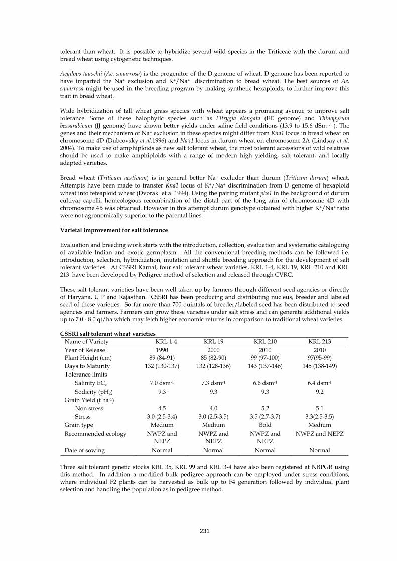
231

tolerant than wheat. It is possible to hybridize several wild species in the Triticeae with the durum and bread wheat using cytogenetic techniques. Aegilops tauschii (Ae. squarrosa) is the progenitor of the D genome of wheat. D genome has been reported to have imparted the Na+ exclusion and K+/Na+ discrimination to bread wheat. The best sources of Ae. squarrosa might be used in the breeding program by making synthetic hexaploids, to further improve this trait in bread wheat. Wide hybridization of tall wheat grass species with wheat appears a promising avenue to improve salt tolerance. Some of these halophytic species such as Eltrygia elongata (EE genome) and Thinopyrum bessarabicum (JJ genome) have shown better yields under saline field conditions (13.9 to 15.6 dSm -1 ). The genes and their mechanism of Na+ exclusion in these species might differ from Kna1 locus in bread wheat on chromosome 4D (Dubcovsky et al.1996) and Nax1 locus in durum wheat on chromosome 2A (Lindsay et al. 2004). To make use of amphiploids as new salt tolerant wheat, the most tolerant accessions of wild relatives should be used to make amphiploids with a range of modern high yielding, salt tolerant, and locally adapted varieties. Bread wheat (Triticum aestivum) is in general better Na+ excluder than durum (Triticum durum) wheat. Attempts have been made to transfer Kna1 locus of K+/Na+ discrimination from D genome of hexaploid wheat into teteaploid wheat (Dvorak et al 1994). Using the pairing mutant phe1 in the background of durum cultivar capelli, homeologous recombination of the distal part of the long arm of chromosome 4D with chromosome 4B was obtained. However in this attempt durum genotype obtained with higher K+/Na+ ratio were not agronomically superior to the parental lines.

Varietal improvement for salt tolerance Evaluation and breeding work starts with the introduction, collection, evaluation and systematic cataloguing of available Indian and exotic germplasm. All the conventional breeding methods can be followed i.e. introduction, selection, hybridization, mutation and shuttle breeding approach for the development of salt tolerant varieties. At CSSRI Karnal, four salt tolerant wheat varieties, KRL 1-4, KRL 19, KRL 210 and KRL 213 have been developed by Pedigree method of selection and released through CVRC. These salt tolerant varieties have been well taken up by farmers through different seed agencies or directly of Haryana, U P and Rajasthan. CSSRI has been producing and distributing nucleus, breeder and labeled seed of these varieties. So far more than 700 quintals of breeder/labeled seed has been distributed to seed agencies and farmers. Farmers can grow these varieties under salt stress and can generate additional yields up to 7.0 - 8.0 qt/ha which may fetch higher economic returns in comparison to traditional wheat varieties.

CSSRI salt tolerant wheat varieties

Name of Variety KRL 1-4 KRL 19 KRL 210 KRL 213 Year of Release 1990 2000 2010 2010 Plant Height (cm) 89 (84-91) 85 (82-90) 99 (97-100) 97(95-99) Days to Maturity 132 (130-137) 132 (128-136) 143 (137-146) 145 (138-149) Tolerance limits Salinity ECe 7.0 dsm-1 7.3 dsm-1 6.6 dsm-1 6.4 dsm-1 Sodicity (pH2) 9.3 9.3 9.3 9.2 Grain Yield (t ha-1) Non stress 4.5 4.0 5.2 5.1 Stress 3.0 (2.5-3.4) 3.0 (2.5-3.5) 3.5 (2.7-3.7) 3.3(2.5-3.5) Grain type Medium Medium Bold Medium Recommended ecology NWPZ and

NEPZ NWPZ and

NEPZ NWPZ and

NEPZ NWPZ and NEPZ

Date of sowing Normal Normal Normal Normal Three salt tolerant genetic stocks KRL 35, KRL 99 and KRL 3-4 have also been registered at NBPGR using this method. In addition a modified bulk pedigree approach can be employed under stress conditions, where individual F2 plants can be harvested as bulk up to F4 generation followed by individual plant selection and handling the population as in pedigree method.

232

Sugested Readings Dubcovsky J., Santa-Maria G.M.C., Epstein, E. L. and Dvorak, J.1996. Mapping of the K/Na discrimination

locus Kna1 in wheat. Theoretical and Applied Genetics 92, 448-454. Dvorak J., Noaman, M.M., Goyal, S. and Gorham, J. 1994. Enhancement of salt tolerance of Triticum turgidum

L by the Kna1 locus transferred from Triticum aestivum L. chromosome 4D by homoeologous recombination. Theoretical and Applied Genetics 87, 872-877.

Lindsay, M.P., Lagudah, E.S., Hare, R.A. and Munns, R. 2004. A locus for sodium exclusion (Naxl), a trait for salt tolerance, mapped in durum wheat. Functional Plant Biology 31, 1105-1114.

Maguire, J.D. 1962 Speed of germination: Aid in selection and evaluation for seedling emergence and vigour. Crop Sci. 2:176-177.

Mishra B. 1994. Breeding for Salt tolerance in crops. In: Rao et al (Eds) 1994. Salinity Management for Sustainable Agriculture-25 years of research at CSSRI, Central Soil salinity Research Institute,Karnal pp 226-259.

Mishra, B. 1996. Highlights of research on crops and varieties for salt affected soils. Technical Bulletin published by CSSRI, Karnal 28p.

Mishra, B., Singh R.K. and Senadhira, D. 1997. Enhancing genetic resources and breeding for problem soils. In: Online book-Using Diversity: Enhancing and maintaining genetic resources on-farm. Ed. by L.Sperling and M. Loevinsohn. IDRC on Live Book Catalogue: http://www.idrc.ca/library/document/104582/mishra.html 13p.

Sayeed, H.I. 1985.Diversity of salt tolerance in germplasm collection of wheat. Theor. Appl. Genet. 69: 651-657.

Sharma, S.K. 1987. Mechanism of tolerance in wheat genotypes differing in sodicity tolerance. Pl. Physiol. Biochem.14(1):87-94.

Singh, K.N. 1988. Combining ability in wheat in normal and sodic soils. Indian J. Genet. 48(1): 99-102. Singh, K.N.1991. Recent approaches to breeding for salt tolerance in crop plants. In Genetic Research and

Education. Current trends and the next fifty years (Eds.: B.Sharma et al.). Indian Society of Genetics and Plant Breeding, New Delhi: pp.490-499.

Singh, K.N. 2005. Breeding wheat varieties for salt tolerance. In: Crop Improvement for Management of Salt affected soils, Manual of lectures for the training program on "Method of Screening and Development of Varieties and Germplasm of various crops for salt affected soils: held at Central Soil Salinity research Institute, Karnal 132001,India Janaury 17-22,2005 pp 65-68.

Singh, K.N. and Chatrath, R. 1993. Genetic divergence in bread wheat (Triticun aestivum L. em Thell) under sodic soil conditions. Wheat Information service, Japan 76 : 35-38.

Singh, K.N. and Chatrath,R. 1997. Combining ability studies in bread wheat (Triticum aestivum, L em.Thall) under salt stress environments. Indian J.Genet, 57(2): 13-18.

Singh, K.N., Kulshreshtha, N. and Mohan Surender, 2005. Screeing wheat and rice for salt tolerance under conrolled conditions In: Crop Improvement for Management of Salt affected soils, Manual of lectures for the training program on "Method of Screening and Development of Varieties and Germplasm of various crops for salt affected soils: held at Central Soil Salinity research Institute, Karnal 132001,India Janaury 17-22,2005 pp 210-216.

Singh, K.N., Kulshreshtha, N., Kumar, V. and Setter Tim, 2006. Genetic variability of wheat (Triticum aestivum) lines for grain yield and component characters grown under sodic and waterlogged conditions. Indian Journal of Agricultural Sciences 76(7): 414-419

Singh, K.N. and Rana, R.S. 1987. Combining ability for yield components in bread wheat grown in salt affected soils. Indian J. agric. Sci. 57: 771-773.

Singh, K.N. and Rana, R.S. 1989. seedling emergence rating : A criterion for differential varietal responses to salt stress in cereals. Agric. Sci. Digest. 9: 71-73.

Singh, K.N.and Tyagi, N.K.1997. Genetic improvement for suppressive/salt affected soils. In: Proceddings of the International Group Meeting on "Wheat Research Needs beyond 2000 AD" held at Directorate of Wheat Research, Karnal from Aug. 12-14, 1997. (Ed. by S. Nagarajan, Gyanendra Singh and B.S.Tyagi), Narosa Publishing House pp. 1

233

Bioremediation: pollution fighting tool Madhu choudhary Central Soil Salinity Research Institute, Karnal- 132 001 (Haryana), India

The production, distribution, use, misuse, disposal or accidental spills of many chemicals polluted the environment to levels that threaten the health of humans, livestock, wildlife and indeed, whole ecosystems. Waste products resulting from anthropogenic activities posed a serious problem. The current pattern of industrial activity alters the natural flow of materials and introduces novel chemicals into the environment (Faisal and Hasnain, 2004). The effluents are discharged into the environment especially water bodies have been on the increase as a result of urbanization. Most of these effluents contain toxic substances especially heavy metals. Heavy metals are metallic elements which have a high atomic weight and a density much greater (at least 5 times) than water. Heavy metals are natural components of the Earth's crust and cannot be degraded or destroyed. Heavy metals can enter a water supply by industrial and consumer waste, or even from acidic rain breaking down soils and releasing heavy metals into streams, lakes, rivers and groundwater. Mineral rock weathering and anthropogenic sources provides two main types of metals into the soil. According to Ross (1994) the anthropogenic sources of metal contamination can be divided in to five main groups:

1. Metalliferous mining and smelting (arsenic, cadmium, lead, mercury) 2. Industry (arsenic, cadmium, chromium, cobalt, copper, mercury, nickel, zinc) 3. Atmospheric deposition (arsenic, cadmium, chromium, copper, lead, mercury, uranium) 4. Agriculture (arsenic, cadmium, copper, lead, selenium, uranium, zinc) 5. Waste disposal (arsenic, cadmium, chromium, copper, lead, mercury, zinc).

There are 35 metals that concern us because of occupational or residential exposure; 23 of these are the heavy elements or "heavy metals": antimony, arsenic, bismuth, cadmium, cerium, chromium, cobalt, copper, gallium, gold, iron, lead, manganese, mercury, nickel, platinum, silver, tellurium, thallium, tin, uranium, vanadium and zinc. Heavy metals are classified into the following three categories (Volesky, 1990 and Bishop, 2002): 1. Toxic metals (Hg, Cr, Pb, Zn, Cu, Cd, As, Co & Sn etc) 2. Precious metals (Pt, Ag, Ni, Au & Ru etc) 3. Radionuclides (U, Th, Ra & Am etc). Interestingly, small amounts of these elements are common in our environment and diet and are actually necessary for good health, but large amounts of any of them may cause acute or chronic toxicity (poisoning). Heavy metals are dangerous because they tend to bioaccumulate. Bioaccumulation means an increase in the concentration of a chemical in a biological organism over time, compared to the chemical's concentration in the environment. Compounds accumulate in living things any time they are taken up and stored faster than they are broken down (metabolized) or excreted. Adverse effects of heavy metals Heavy metals can directly influence behavior by impairing mental and neurological function, influencing neurotransmitter production and utilization and altering numerous metabolic body processes. Systems in which toxic metal elements can induce impairment and dysfunction include the blood and cardiovascular, eliminative pathways (colon, liver, kidneys, skin), endocrine (hormonal), energy production pathways, enzymatic, gastrointestinal, immune, nervous (central and peripheral), reproductive and urinary. In general, heavy metals (HM) are systemic toxins with specific neurotoxic, nephrotoxic, fetotoxic and teratogenic effects. The degree to which a system, organ, tissue or cell is affected by a heavy metal toxin depends on the toxin itself and the individual's degree of exposure to the toxin. For some heavy metals, toxic levels can be just above the background concentrations naturally found in nature. Therefore, it is important for us to inform ourselves about the heavy metals and to take protective measures against excessive exposure.

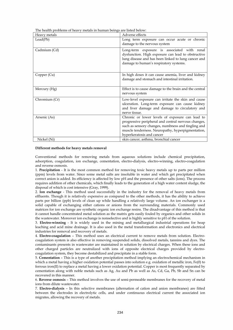
234

The health problems of heavy metals in human beings are listed below: Heavy metals Adverse effects Lead(Pb) Long term exposure can occur acute or chronic

damage to the nervous system

Cadmium (Cd) Long-term exposure is associated with renal dysfunction. High exposure can lead to obstructive lung disease and has been linked to lung cancer and damage to human’s respiratory systems.

Copper (Cu) In high doses it can cause anemia, liver and kidney damage and stomach and intestinal irritation.

Mercury (Hg) Effect is to cause damage to the brain and the central nervous system

Chromium (Cr) Low-level exposure can irritate the skin and cause ulceration. Long-term exposure can cause kidney and liver damage and damage to circulatory and nerve tissue.

Arsenic (As)

Chronic or lower levels of exposure can lead to progressive peripheral and central nervous changes, such as sensory changes, numbness and tingling and muscle tenderness. Neuropathy, hyperpigmentation, hyperkeratosis and cancer

Nickel (Ni) skin cancer, asthma, bronchial cancer Different methods for heavy metals removal Conventional methods for removing metals from aqueous solutions include chemical precipitation, adsorption, coagulation, ion exchange, cementation, electro-dialysis, electro-winning, electro-coagulation and reverse osmosis. 1. Precipitation - It is the most common method for removing toxic heavy metals up to parts per million (ppm) levels from water. Since some metal salts are insoluble in water and which get precipitated when correct anion is added. Its efficiency is affected by low pH and the presence of other salts (ions). The process requires addition of other chemicals, which finally leads to the generation of a high water content sludge, the disposal of which is cost intensive (Gray, 1999). 2. Ion exchange - This method used successfully in the industry for the removal of heavy metals from effluents. Though it is relatively expensive as compared to the other methods, it has the ability to achieve parts per billion (ppb) levels of clean up while handling a relatively large volume. An ion exchanger is a solid capable of exchanging either cations or anions from the surrounding materials. Commonly used matrices for ion exchange are synthetic organic ion exchange resins. The disadvantage of this method is that it cannot handle concentrated metal solution as the matrix gets easily fouled by organics and other solids in the wastewater. Moreover ion exchange is nonselective and is highly sensitive to pH of the solution. 3. Electro-winning - It is widely used in the mining and metallurgical industrial operations for heap leaching and acid mine drainage. It is also used in the metal transformation and electronics and electrical industries for removal and recovery of metals. 4. Electro-coagulation – This method uses an electrical current to remove metals from solution. Electro-coagulation system is also effective in removing suspended solids, dissolved metals, tannins and dyes. The contaminants presents in wastewater are maintained in solution by electrical charges. When these ions and other charged particles are neutralized with ions of opposite electrical charges provided by electro-coagulation system, they become destabilized and precipitate in a stable form. 5. Cementation – This is a type of another precipitation method implying an electrochemical mechanism in which a metal having a higher oxidation potential passes into solution e.g. oxidation of metallic iron, Fe(0) to ferrous iron(II) to replace a metal having a lower oxidation potential. Copper is most frequently separated by cementation along with noble metals such as Ag, Au and Pb as well as As, Cd, Ga, Pb, Sb and Sn can be recovered in this manner. 6. Reverse osmosis – This method involves the use of semi-permeable membranes for the recovery of metal ions from dilute wastewater. 7. Electro-dialysis – In this selective membranes (alternation of cation and anion membranes) are fitted between the electrodes in electrolytic cells, and under continuous electrical current the associated ion migrates, allowing the recovery of metals.

235

However, chemical precipitation and electrochemical treatment are ineffective, especially when metal ion concentration in aqueous solution is among 1 to 100 mg L−1. Ion exchange, membrane technologies and activated carbon adsorption process are extremely expensive when treating large amount of water and wastewater containing heavy metal in low concentration, they cannot be used at large scale. Another major disadvantage with conventional treatment technologies is the production of toxic chemical sludge and its disposal/ treatment becomes a costly affair and is not eco-friendly. Volesky (2001) summarized the advantages and disadvantages of those conventional metal removal technologies. A growing public awareness and concern about environmental pollutants fostered for the development of safe and cost-effective alternative approaches for dealing with wastes. Of the technologies that have been investigated, bioremediation has emerged as the most desirable approach for cleaning up many environmental pollutants. Bioremediation is an option that offers the possibility to destroy, transform or render harmless various contaminants using natural biological activity. Bioremediation is a combination of two words – bio which means biological, and remediation, which means to remedy. Bioremediation describes several technologies and practices that take advantage of natural systems and processes to clean up pollution. Bioremediation can be defined as any process that uses microorganisms or their enzymes to return the environment altered by contaminants to its original condition. Some microorganisms that live in soil and groundwater naturally eat certain chemicals that are harmful to people and the environment. Bioremediation is not a new technology. It is one of the world’s oldest and yet newest pollution fighting tools. There has been evidence that compost piles existed as far back as 6000 BC, and in 1891 the first biological sewage treatment plant was created in Sussex, UK both of these are types of bioremediation. Bioremediation is proving effective in treating hazardous materials ranging from toxic chemicals and heavy metals to oil and nuclear waste. Bioremediation is an eco- friendly, cost-effective and natural technology targeted to remove heavy metals, radionuclides, xenobiotic compounds, organic waste, pesticides etc. from contaminated sites or industrial discharges through biological means. Bioremediation have relatively low-cost, low-technology techniques, which generally have a high public acceptance and can often be carried out on site. The result of remediation depends upon type of contaminants, time duration and methodology. In order for the microorganisms to do their work, the right temperature, nutrients and amount of oxygen must be present in the soil and groundwater. Generally, bioremediation technologies can be classified as:

1. in situ (at the site of contamination) 2. ex situ (contaminant taken out of the site of contamination and treated elsewhere).

There are advantages and disadvantages to both in situ and ex situ strategies. In situ method is generally the most desirable options due to lower cost and fewer disturbances since they provide the treatment in place avoiding excavation and transport of contaminants. In situ biodegradation involves supplying oxygen and nutrients by circulating aqueous solutions through contaminated soils to stimulate naturally occurring bacteria to degrade organic contaminants. It can be used for soil and groundwater. Bioventing is the most common in situ treatment and involves supplying air and nutrients through wells to contaminated soil to stimulate the indigenous bacteria. Bioventing employs low air flow rates and provides only the amount of oxygen necessary for the biodegradation while minimizing volatilization and release of contaminants to the atmosphere. It works for simple hydrocarbons and can be used where the contamination is deep under the surface. Biosparging involves the injection of air under pressure below the water table to increase groundwater oxygen concentrations and enhance the rate of biological degradation of contaminants by indigenous microorganisms. Biosparging can be used to reduce petroleum constituents that are adsorbed to soil within the capillary fringe, below the water table or dissolved in groundwater. Biosparging is commonly used at sites with mid-weight petroleum products such as diesel fuel; lighter petroleum products tend to volatilise swiftly and are removed very rapidly through sparging. Soil permeability is a key factor in the effectiveness of the technology. Bioaugmentation- Bioremediation frequently involves the addition of microorganisms indigenous or exogenous to the contaminated sites in order to reinforce the natural biological processes. Bioaugmentation is more commonly and successfully used on contaminants removed from the original site, such as in municipal wastewater treatment facilities. In situ biodegradation involves supplying oxygen and nutrients by circulating aqueous solutions through contaminated soils to stimulate naturally occurring bacteria to degrade organic contaminants. It can be used for soil and groundwater.

236

Ex situ strategies removes the contaminants and places them in a contained environment. This contained environment allows for easier monitoring and maintaining of conditions and progress, thus making the actual bioremediation process faster. However, the removal of the contaminant from the contaminated site is time consuming, costly and potentially dangerous. By bringing the contaminants to the surface, the workers and the general public have increased exposure to the toxic material. There are some methods of Ex situ bioremediation mentioned below: Landfarming is a simple technique in which contaminated soil is excavated and spread over a prepared bed and periodically tilled until pollutants are degraded. The goal is to stimulate indigenous biodegradative microorganisms and facilitate their aerobic degradation of contaminants. Since landfarming has the potential to reduce monitoring and maintenance costs, as well as clean-up liabilities, it has received much attention as a disposal alternative. Composting is a technique that involves combining contaminated soil with nonhazardous organic amendants such as manure or agricultural wastes. The presence of these organic materials supports the development of a rich microbial population and elevated temperature characteristic of composting which convert degradable organic waste into humus like substance. Bioreactors Slurry reactors or aqueous reactors are used for ex situ treatment of contaminated soil and water pumped up from a contaminated plume. A bioreactor may refer to any device or system that supports a biologically active environment. Bioremediation in reactors involves the processing of contaminated solid material (soil, sediment, sludge) or water through an engineered containment system. The bioremediation strategies listed above can be combined in different ways, or integrated with other strategies such as chemical or physical remediation technologies to develop effective waste cleanup of contaminants in soils, as well as in water. Bioremediation depends on the natural biological processes of microorganisms, one of which is metabolism. Metabolism refers to all the chemical reactions that happen in a cell or organism. All living processes are based on a complex series of chemical reactions. Metabolic processes fall into two types – those that build complex molecular structures from simpler molecules, called anabolism, and those that break down complex molecules into simpler molecules, called catabolism. Chemicals present in contaminated sites can be remediated through either, or both, of these processes. Chemicals present at contaminated sites become part of the anabolism and catabolism process. For example, hydrocarbons (part of the carbon family) present at sites with petroleum products can be taken up by microorganisms and used as building blocks for cell components. Other chemicals that are important to a microorganism include chemical compounds in the phosphorus, potassium, calcium and sodium group. Microorganisms also need trace elements of other chemicals, including chromium, cobalt, copper, and iron, all of which can be available in abundance at contaminated sites. Essential factors for microbial bioremediation

Microbes reported for removal of different heavy metals A number of bacteria and fungi are used for heavy metal removal. Some of them are listed below:

Factors Desired Conditions Microbial population Suitable kinds of organisms that can biodegrade all the different types

of contaminants Oxygen Enough to support aerobic biodegradation (about 2% oxygen in the gas

phase or 0.4 mg/L in the soil water) Nutrients Nitrogen, phosphorus, sulfur, and other nutrients to support good

microbial growth to accelerate bioremediation Water In soil bioremediation soil moisture should be from 50–70% of the

water holding capacity of the soil Temperature Appropriate temperatures for microbial growth (0–40˚C)

pH Best range is from 6.5 to 7.5

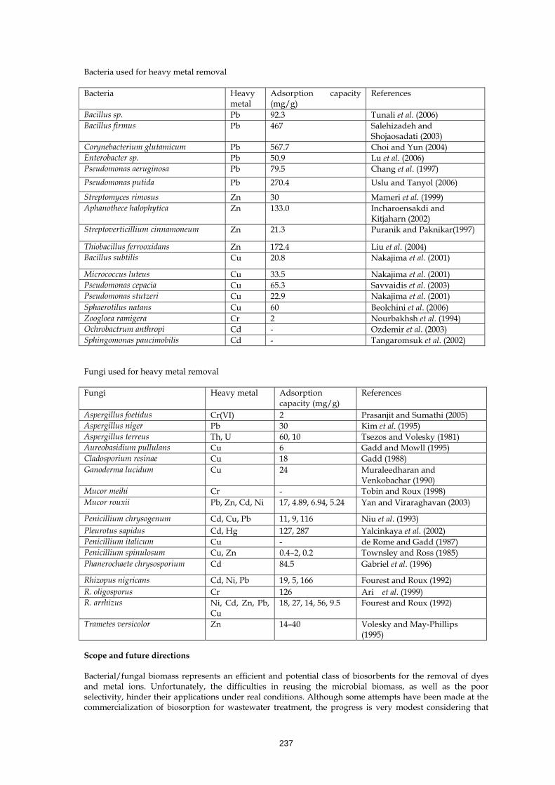
237

Bacteria used for heavy metal removal Bacteria Heavy

metal Adsorption capacity (mg/g)

References

Bacillus sp. Pb 92.3 Tunali et al. (2006) Bacillus firmus Pb 467 Salehizadeh and

Shojaosadati (2003) Corynebacterium glutamicum Pb 567.7 Choi and Yun (2004) Enterobacter sp. Pb 50.9 Lu et al. (2006) Pseudomonas aeruginosa Pb 79.5 Chang et al. (1997) Pseudomonas putida Pb 270.4 Uslu and Tanyol (2006)

Streptomyces rimosus Zn 30 Mameri et al. (1999) Aphanothece halophytica Zn 133.0 Incharoensakdi and

Kitjaharn (2002) Streptoverticillium cinnamoneum Zn 21.3 Puranik and Paknikar(1997)

Thiobacillus ferrooxidans Zn 172.4 Liu et al. (2004) Bacillus subtilis Cu 20.8 Nakajima et al. (2001)

Micrococcus luteus Cu 33.5 Nakajima et al. (2001) Pseudomonas cepacia Cu 65.3 Savvaidis et al. (2003) Pseudomonas stutzeri Cu 22.9 Nakajima et al. (2001) Sphaerotilus natans Cu 60 Beolchini et al. (2006) Zoogloea ramigera Cr 2 Nourbakhsh et al. (1994) Ochrobactrum anthropi Cd - Ozdemir et al. (2003) Sphingomonas paucimobilis Cd - Tangaromsuk et al. (2002) Fungi used for heavy metal removal Fungi Heavy metal Adsorption

capacity (mg/g) References

Aspergillus foetidus Cr(VI) 2 Prasanjit and Sumathi (2005) Aspergillus niger Pb 30 Kim et al. (1995) Aspergillus terreus Th, U 60, 10 Tsezos and Volesky (1981) Aureobasidium pullulans Cu 6 Gadd and Mowll (1995) Cladosporium resinae Cu 18 Gadd (1988) Ganoderma lucidum Cu 24 Muraleedharan and

Venkobachar (1990) Mucor meihi Cr - Tobin and Roux (1998) Mucor rouxii Pb, Zn, Cd, Ni 17, 4.89, 6.94, 5.24 Yan and Viraraghavan (2003)

Penicillium chrysogenum Cd, Cu, Pb 11, 9, 116 Niu et al. (1993) Pleurotus sapidus Cd, Hg 127, 287 Yalcinkaya et al. (2002) Penicillium italicum Cu - de Rome and Gadd (1987) Penicillium spinulosum Cu, Zn 0.4–2, 0.2 Townsley and Ross (1985) Phanerochaete chrysosporium Cd 84.5 Gabriel et al. (1996)

Rhizopus nigricans Cd, Ni, Pb 19, 5, 166 Fourest and Roux (1992) R. oligosporus Cr 126 Ari� et al. (1999) R. arrhizus Ni, Cd, Zn, Pb,

Cu 18, 27, 14, 56, 9.5 Fourest and Roux (1992)

Trametes versicolor Zn 14–40 Volesky and May-Phillips (1995)

Scope and future directions Bacterial/fungal biomass represents an efficient and potential class of biosorbents for the removal of dyes and metal ions. Unfortunately, the difficulties in reusing the microbial biomass, as well as the poor selectivity, hinder their applications under real conditions. Although some attempts have been made at the commercialization of biosorption for wastewater treatment, the progress is very modest considering that

238

there has been more than a decade of fundamental research. The important features required for the successful application of bioremediation technology to real situations include, but are not limited to:

• Screening and selection of the most promising biomass, with sufficiently high biosorption capacity and selectivity.

• Optimizing the conditions for maximum biosorption, including optimization of pH, temperature, ionic strength and co-ion effects, etc

• Improving the selectivity and uptake via chemical and/or genetic modification methods. • Examining the mechanical strength of biomass and if insufficient for reuse, improving rigidity by

proper immobilization or other chemical methods. • Testing the performance of biosorbents under different modes of operation. • Analyzing the behavior of biosorbent for use with real industrial effluents and simultaneously

analyzing the impact of water quality on the biosorption uptake of the specific pollutant of interest. Conversely, it is no small feat to replace well established conventional techniques. However, in addition to being cost effective, bioremediation technology has huge potential, as many biosorbents are known to perform well, if not better than most conventional methods. Also being aware of the hundreds of biosorbents able to bind various pollutants, sufficient research has been performed on various biomaterials to understand the mechanism responsible for biosorption. Therefore, through continued research, especially on pilot and full-scale biosorption process, the situation is likely to change in the near future, with bioremediation technology becoming more beneficial and attractive than currently used technologies. Suggested Readings Ari�, A.B., Mel, M., Hasan, M.A., Karim, M.I.A. 1999. The kinetics and mechanisms of lead(II) biosorption

by powderized Rhizopus olgisporus. World Journal of Microbiology Biotechnology. 15: 291–298. Beolchini F, Pagnanelli R, Toro L, Veglio F. 2006. Ionic strength effect on copper biosorption by Sphaerotilus

natans: equilibrium study and dynamic modeling in membrane reactor. Water Research. 40:144–52. Bishop, P.L. 2002. Pollution prevention: fundamentals and practice. Beijing: Tsinghua University Press. Chang JS, Law R, Chang C.C. 1997. Biosorption of lead, copper and cadmium by biomass of Pseudomonas

aeruginosa PU21. Water Research. 31:1651–8. Choi SB, Yun YS. 2004. Lead biosorption by waste biomass of Corynebacterium glutamicum generated from

lysine fermentation process. Biotechnol Letter. 26:331–6. De Rome, L., Gadd, G.M., 1987. Copper adsorption by Rhizopus arrhizus, Cladosporium resinae and Penicillium

italicum. Applied Microbiology Biotechnology 26, 84–90. Faisal M, Hasnain S. 2004. Microbia conversion of Cr (vi) into Cr (iii) in industrial effluent. African Journal

Biotechnol. 3 (11): 610-617 Fourest, E., Roux, J.C., 1992. Heavy metal biosorption by fungal mycelial by-products: mechanism and

influence of pH. Applied Microbiology Biotechnology 37, 399–403. Gabriel, J., Vosahlo, J., Baldrian, P., 1996. Biosorption of Cadmium to mycelial pellets of wood rotting fungi.

Biotechnology Techniques. 10:345–348. Gadd, G.M., 1988. Accumulation of metals by microorganisms and algae. In: Rehm, H.J. (Ed.),

Biotechnology, special Microbial Processes, vol. 6b. VCH Verlagsgellschaft, Weinheim, pp. 401–433. Gadd, G.M., Mowll, H., 1995. Copper uptake by yeast cell, hypae and chlamydospores of Aureobasidium

pullulans. Experimental Mycology. 9: 230–240. Gray, N.F., 1999. Water Technology. John Wiley & Sons, New York, pp. 473–474. Incharoensakdi A, Kitjaharn P. 2002. Zinc biosorption from aqueous solution by a halotolerant

cyanobacterium Aphanothece halophytica. Curr Microbiol. 45: 261–4. Kim, Y.H., Yoo, Y.J., Lee, H.Y., 1995. Characteristic of lead adsorption by Undaria pinnatfida. Biotechnology

Letters 17, 345–350. Liu HL, Chen BY, Lan YW, Cheng YC. 2004. Biosorption of Zn(II) and Cu(II) by the indigenous Thiobacillus

thiooxidans. Chem Eng J. 97:195–201. Lu WB, Shi JJ, Wang CH, Chang JS. 2006. Biosorption of lead, copper and cadmium by an indigenous isolate

Enterobacter sp J1 possessing high heavy-metal resistance. J Hazard Matter. 134: 80–6. Mameri N, Boudries N, Addour L, Belhocine D, Lounici H, Grib H. 1999. Batch zinc biosorption by a

bacterial nonliving Streptomyces rimosus biomass. Water Res. 33:1347–54. Muraleedharan, T.R., Venkobachar, C., 1990. Mechanism of Biosorption of copper (II) by Ganoderma lucidium.

Biotechnology & Bioengineering. 35: 320–325. Nakajima A, Yasuda M, Yokoyama H, Ohya-Nishiguchi H, Kamada H. 2001. Copper biosorption by

chemically treated Micrococcus luteus cells. World J Microbiol Biotechnol. 17:343–7. Niu, H., Xu, X.S., Wang, J.H., 1993. Removal of lead from aqueous solutions by penicillin biomass.

Biotechnology & Bioengineering. 42: 785–787.

239

Nourbakhsh M, Sag Y, Ozer D, Aksu Z, Kutsal T, Caglar A. 1994. A comparative study of various biosorbents for removal of chromium(VI) ions from industrial wastewaters. Process Biochem. 29:1–5.

Ozdemir G, Ozturk T, Ceyhan N, Isler R, Cosar T. Heavy metal biosorption by biomass of Ochrobactrum anthropi producing exopolysaccharide in activated sludge. Bioresour Technol 2003; 90:71–4.

Prasanjit, B., Sumathi, S. 2005. Uptake of chromium by Aspergillus foetidus. Journal of Material Cycles and Waste Management. :7: 88–92.

Puranik PR, Paknikar KM. 1997. Biosorption of lead and zinc from solutions using Streptoverticillium cinnamoneum waste biomass. J Biotechnol. 55: 113–24.

Ross, S. 1994. Toxic metals in Soil-Plant Systems. John Wiley & Sons, Chichester, UK Salehizadeh H, Shojaosadati SA. 2003. Removal of metal ions from aqueous solution by polysaccharide

produced from Bacillus firmus. Water Res. 37: 4231–5. Savvaidis I, Hughes MN, Poole RK. 2003. Copper biosorption by Pseudomonas cepacia and other strains.

World. J. Microbiol. Biotechnol. 19:117–21. Tangaromsuk J, Pokethitiyook P, Kruatrachue M, Upatham ES. 2002. Cadmium biosorption by Sphingomonas

paucimobilis biomass. Bioresour. Technol. 85:103–5. Tobin, J.M., Roux, J.C., 1998. Mucor biosorbent for chromium removal from tanning e�uent. Water Research.

32 (5): 1407–1416. Townsley, C.C., Ross, I.S., 1985. Copper uptake by Penicillium spinulosum. Microbes. 44: 125–134. Tsezos, M., Volesky, B., 1981. Biosorption of uranium and thorium. Biotechnology & Bioengineering. 23:

583–604. Volesky, B. 1990. Removal and recovery of heavy metals by biosorption. Biosorption of Heavy Metals. CRC

Press, Boca Raton, FL. Volesky, B. 2001. Detoxification of metal bearing effluents: biosorption for the next centry. Hydrometallurgy.

59: 203-16. Volesky, B., May-Phillips, H.A., 1995. Biosorption of heavy metals by Saccharomyces cerevisiae. Applied

Microbiology & Biotechnology. 42: 797–806. Yalcinkaya, Y., Arica, M.Y., Soysal, L., Denzili, A., Genc, O., Bektas, S., 2002. Cadmium and mercury uptake

by immobilized Pleuritus sapidus. Turk Journal of Chemistry. 26: 441–452. Yan, G., Viraraghavan, T., 2003. Heavy-metal removal from aqueous solution by fungus Mucor rouxii. Water

Research. 37: 4486–4496.

240

Financial Appraisal and Socio-Economic Benefits of Sodic and saline land Reclamation

R.S. Tripathi Central Soil Salinity Research Institute, Karnal – 132 001 (Haryana), India Soil salinity and sodicity have direct impact on growth and development of agricultural economy. The consequences of degrading land resources due to salinity and sodicity are witnessed at farm level, regional level and national level. At the farm level adverse effects are (i) threat to the sustainability of land resources and (ii) decrease farm production by (a) decline in resource productivity, (b) abandon crop production and (c) cut-back in resource use. Studies have shown that the yield and income effects of salt affected soils are quite high. The land degradation severely affects the production of important crops like rice, wheat, cotton, sugarcane, groundnut, etc. At the regional level, consequences are (i) displacement of labour from agriculture, (ii) widen income disparities and (iii) affect the sustainability of secondary and tertiary sectors. At the national level, consequences are (i) decline in agricultural production, (ii) affect gross domestic product, (iii) bring down export potential of important crops and (iv) increase import bill. The brief description of agro-physical, socio-economical and environmental impact of soil salinity and sodicity are as follows. Impact on Crop Production

• Various degrees of salinity and sodicity can cause serious and severe decline in soil productivity and crop yields (Table 1).

• To overcome reduction in yield farmers increase inputs such as seeds, fertilizers, etc. • In salt-affected soils, response to any input is low: e.g., crop yield response to fertilizer application

is less as salinity is a limiting factor. • Less possibility for alternative land use: e.g., farmers are forced to cultivate only salt-tolerant crops,

which might not always be high-income cash crops. • Salinity and sodicity reduce efficient use of water (i.e. crop yield per unit water) causing reduction

in return from capital investment and labour inputs. • Salt-affected soils are more fragile with greater risk and always subjected to other forms of

degradation: e.g., salinity and sodicity reduce land green cover and soil becoming subject to other degradation processes such as wind and water erosion.

• In salt-affected soil environment, saline watertable can enhance salinity of fresh waters in rivers and other water sources through seepage.

• The rehabilitation programmes require high investment cost in reclamation of salt-affected soils as compared to other types of degraded lands, in general.

Table 1. Grain yield of major crops under various environments (t/ha)

Crop Normal soils Salt affected soils Waterlogged soils Rice 3.99 2.18 (45) 2.30 (42)Wheat 2.59 1.57 (40) 1.85 (38)Cotton 1.63 0.61 (63) 0.37 (77)Sugarcane 63.68 33.02 (48) 24.74 (61)Figures in parentheses indicate percentage loss over normal soils. Impact on Socio-Economic Conditions

• Abandonment of the land where severe salinity and sodicity degradation occurred which increased the number of landless farmers.

• Low food security due to low food production and supply. • Reduce labour use efficiency: e.g., reclamation of salt-affected soils needs more labour, crop yield

declines and input requirement reduces which ultimately would reduce labour use efficiency in these soils. Reclamation programmes and improved farming systems often involve high costs being capital investment of the Government.

• Lower farm income of resource poor small farmers: e.g., as a consequence of salinity and sodicity farmers force to work on land of others or migrate to outside the area in search of other sources of livelihood.

241

Impact on Environment Most studies of long-term experiments provide information only about biophysical impacts of sodicity and salinity at the site of the experiment. There are also off-site environmental impacts of salinity development. These may be at least as important as those on-site. Chemical effects contribute because nutrients are leached from the soil during leaching processes of salt-affected soils and contaminate water supplies. Biological effects because of the loss of organic matter, which weaken the strength of soil aggregates, increase the loss of nutrients in run-off, and increase carbon dioxide and methane released to the atmosphere. Nutrient losses by leaching are most often observed where nitrogenous fertilizers are being used injudiciously and where organic manures are concentrated and the effluent arising is allowed to reach streams or rivers. Washing of soil nutrients, organic matter and even nutrient rich topsails in to streams and rivers is a serious cause of eutrophication. The nutrients and organic matter cause a proliferation of water borne organisms, which use oxygen in the water and deplete it, at the expense of fish. Until now there have been few studies in which a comprehensive attempt has been made to quantify fully the off-site effects of salt-affected soil development on environment. Where irrigation systems are established it is necessary that proper attention be given to inclusion of adequate drainage systems to dispose of the saline drainage waters so that salinization does not become an environmental hazard. Financial appraisal of salt affected land reclamation projects

The financial appraisal of salinity and sodicity management projects is aimed to find out whether the project is economically reasonable and able to provide justified return on the investment made on it. The financial feasibility involves detail analysis of the capital requirement for installation of the systems, annual operational and maintenance cost of the project and benefits generated by the project. In the land reclamation projects, the initial investment is made once for installation of the system whereas the returns obtained from the project is spread over several years in future.

The financial appraisal of project mainly includes costs and benefits analyses for estimation of economic parameters. The cost-benefit analysis is a decision-making tool for investment choice with respect of total costs and total benefits. It helps in comparing the cost and benefit of alternative technologies. Nevertheless, all the costs and benefits are difficult to quantify in financial terms because a new technology may have negative and positive side effects on the life quality of society and accordingly required to be accounted for the assessment. When side effects of a technology are accounted both direct and indirect benefits and costs, it is called social cost-benefit analysis. Generally, for the financial feasibility we consider only tangible direct benefits and costs viewing the simplicity of estimation procedure.

There are many tools and measures to evaluate the feasibility of the land reclamation technologies. Some important cost-benefit analysis measures are described here which are used widely to find out the financial and commercial viability of the technologies. 1. Pay Back Period 2. Simple Rate of Return 3. Net Present Worth 4. Present Worth of Benefit-Cost Ratio 5. Internal Rate of Return. Pay back period (PBP)

The pay back period measures the number of years it will take for the net undiscounted benefits to repay the investment. If the pay out period is longer than some arbitrary limit (say five years) the project is rejected. If shorter, it is accepted. Thus, the pay back is the time period for an investment to generate sufficient incremental cash to recover its initial capital outlay in full. The following formula is used to calculate the pay back period, if the cash flows are uniform. I

P = ------------- E

Where P = Number of years required for pay back the investment, I = Initial capital investment, and E = Annual net earning (benefits).

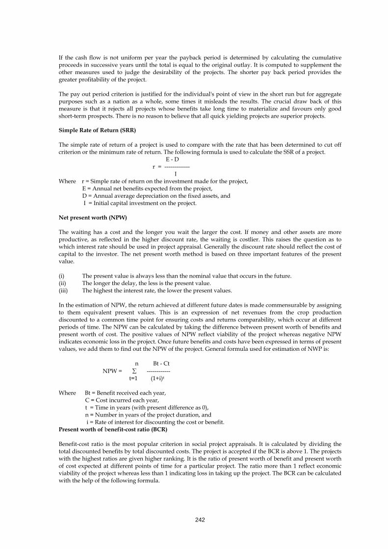
242

If the cash flow is not uniform per year the payback period is determined by calculating the cumulative proceeds in successive years until the total is equal to the original outlay. It is computed to supplement the other measures used to judge the desirability of the projects. The shorter pay back period provides the greater profitability of the project.

The pay out period criterion is justified for the individual's point of view in the short run but for aggregate purposes such as a nation as a whole, some times it misleads the results. The crucial draw back of this measure is that it rejects all projects whose benefits take long time to materialize and favours only good short-term prospects. There is no reason to believe that all quick yielding projects are superior projects. Simple Rate of Return (SRR)

The simple rate of return of a project is used to compare with the rate that has been determined to cut off criterion or the minimum rate of return. The following formula is used to calculate the SSR of a project. E - D

r = ------------- I

Where r = Simple rate of return on the investment made for the project, E = Annual net benefits expected from the project, D = Annual average depreciation on the fixed assets, and I = Initial capital investment on the project.

Net present worth (NPW)

The waiting has a cost and the longer you wait the larger the cost. If money and other assets are more productive, as reflected in the higher discount rate, the waiting is costlier. This raises the question as to which interest rate should be used in project appraisal. Generally the discount rate should reflect the cost of capital to the investor. The net present worth method is based on three important features of the present value.

(i) The present value is always less than the nominal value that occurs in the future. (ii) The longer the delay, the less is the present value. (iii) The highest the interest rate, the lower the present values. In the estimation of NPW, the return achieved at different future dates is made commensurable by assigning to them equivalent present values. This is an expression of net revenues from the crop production discounted to a common time point for ensuring costs and returns comparability, which occur at different periods of time. The NPW can be calculated by taking the difference between present worth of benefits and present worth of cost. The positive values of NPW reflect viability of the project whereas negative NPW indicates economic loss in the project. Once future benefits and costs have been expressed in terms of present values, we add them to find out the NPW of the project. General formula used for estimation of NWP is:

n Bt - Ct

NPW = ∑ ------------ t=1 (1+i)t Where Bt = Benefit received each year, C = Cost incurred each year, t = Time in years (with present difference as 0), n = Number in years of the project duration, and i = Rate of interest for discounting the cost or benefit. Present worth of benefit-cost ratio (BCR) Benefit-cost ratio is the most popular criterion in social project appraisals. It is calculated by dividing the total discounted benefits by total discounted costs. The project is accepted if the BCR is above 1. The projects with the highest ratios are given higher ranking. It is the ratio of present worth of benefit and present worth of cost expected at different points of time for a particular project. The ratio more than 1 reflect economic viability of the project whereas less than 1 indicating loss in taking up the project. The BCR can be calculated with the help of the following formula.

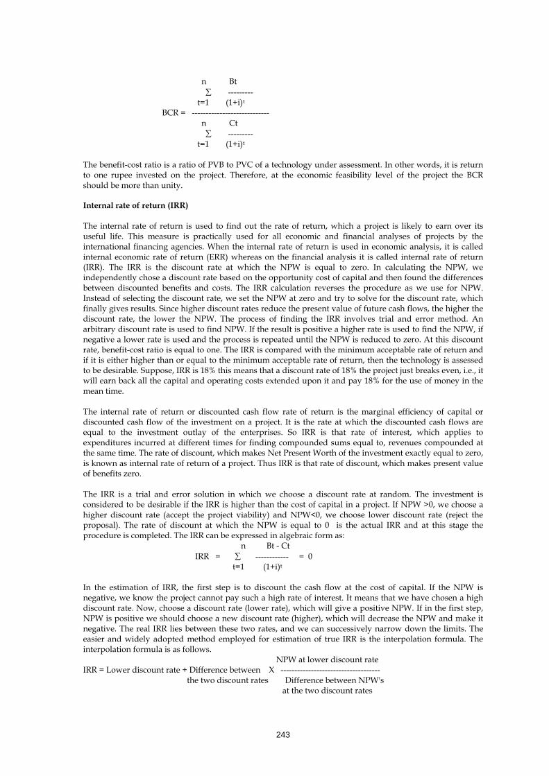
243

n Bt

∑ --------- t=1 (1+i)t BCR = ---------------------------- n Ct

∑ --------- t=1 (1+i)t

The benefit-cost ratio is a ratio of PVB to PVC of a technology under assessment. In other words, it is return to one rupee invested on the project. Therefore, at the economic feasibility level of the project the BCR should be more than unity. Internal rate of return (IRR)

The internal rate of return is used to find out the rate of return, which a project is likely to earn over its useful life. This measure is practically used for all economic and financial analyses of projects by the international financing agencies. When the internal rate of return is used in economic analysis, it is called internal economic rate of return (ERR) whereas on the financial analysis it is called internal rate of return (IRR). The IRR is the discount rate at which the NPW is equal to zero. In calculating the NPW, we independently chose a discount rate based on the opportunity cost of capital and then found the differences between discounted benefits and costs. The IRR calculation reverses the procedure as we use for NPW. Instead of selecting the discount rate, we set the NPW at zero and try to solve for the discount rate, which finally gives results. Since higher discount rates reduce the present value of future cash flows, the higher the discount rate, the lower the NPW. The process of finding the IRR involves trial and error method. An arbitrary discount rate is used to find NPW. If the result is positive a higher rate is used to find the NPW, if negative a lower rate is used and the process is repeated until the NPW is reduced to zero. At this discount rate, benefit-cost ratio is equal to one. The IRR is compared with the minimum acceptable rate of return and if it is either higher than or equal to the minimum acceptable rate of return, then the technology is assessed to be desirable. Suppose, IRR is 18% this means that a discount rate of 18% the project just breaks even, i.e., it will earn back all the capital and operating costs extended upon it and pay 18% for the use of money in the mean time.

The internal rate of return or discounted cash flow rate of return is the marginal efficiency of capital or discounted cash flow of the investment on a project. It is the rate at which the discounted cash flows are equal to the investment outlay of the enterprises. So IRR is that rate of interest, which applies to expenditures incurred at different times for finding compounded sums equal to, revenues compounded at the same time. The rate of discount, which makes Net Present Worth of the investment exactly equal to zero, is known as internal rate of return of a project. Thus IRR is that rate of discount, which makes present value of benefits zero.

The IRR is a trial and error solution in which we choose a discount rate at random. The investment is considered to be desirable if the IRR is higher than the cost of capital in a project. If NPW >0, we choose a higher discount rate (accept the project viability) and NPW<0, we choose lower discount rate (reject the proposal). The rate of discount at which the NPW is equal to 0 is the actual IRR and at this stage the procedure is completed. The IRR can be expressed in algebraic form as:

n Bt - Ct IRR = ∑ ------------ = 0 t=1 (1+i)t In the estimation of IRR, the first step is to discount the cash flow at the cost of capital. If the NPW is negative, we know the project cannot pay such a high rate of interest. It means that we have chosen a high discount rate. Now, choose a discount rate (lower rate), which will give a positive NPW. If in the first step, NPW is positive we should choose a new discount rate (higher), which will decrease the NPW and make it negative. The real IRR lies between these two rates, and we can successively narrow down the limits. The easier and widely adopted method employed for estimation of true IRR is the interpolation formula. The interpolation formula is as follows.

NPW at lower discount rate IRR = Lower discount rate + Difference between X ------------------------------------

the two discount rates Difference between NPW's at the two discount rates

244

It is very important to note that interpolation should not be carried out between a wider spread of discount rates (not more than five per cent). Since interpolation is a higher linear algebraic technique and the changes in IRR, NPW do not follow this pattern. In reality, the IRR rectified by actual verification and by narrowing down the limits between the two discount rates.

Socio-economic benefits of the land reclamation There are numbers of socio-economic and environmental benefits of the sodic land reclamation, which have changed the face of villages and scenario of rural development in many states of India like Haryana and Punjab where almost all the problematic lands have been reclaimed either completely or partially. The most sodicity affected states Haryana and Punjab alone contribute nearly 50% food grains to the central pool every year after getting their sodic lands reclaimed. The sodic land reclamation has direct influence on poverty and livelihood of the rural poor. The impact of sodic land reclamation is quite visible in terms of additional food production, employment, farm income, resource-use, farm assets, capital formation, land value, soil health and quality of life and environment. It helps in eliminating poverty and inequity amongst the rural society. The social impact can also be seen as increased literacy level, declined birth and death rates and high life expectancy of the affected people. Sodic land reclamation has emphasized social aspects to ensure stakeholders commitment in sustaining the activities to manage sodic lands. The major socio- environmental impacts of sodic land reclamation are discussed in the following paragraphs. (i) Food production A rapid increase in food grains production was witnessed in the northern states of India during sixties and seventies mainly due to introduction of high yielding verities of rice and wheat, on one hand and acreage expansion under these crops by reclamation of sodic lands, on the other. The additional annual production of rice and wheat on sodic lands after reclamation is estimated to be 5 and 3 t ha-1, respectively, after 3rd year of reclamation under farmer’s resource constraints. The yield of rice and wheat due to adoption of reclamation technology at full extent in Haryana is presented in Table 2. It indicates that reclamation of sodic land played important role in augmenting the agricultural production and food security of the country. Estimates are that, if 1 million ha sodic lands have been reclaimed for crop production so far, about 8 million tonne food grains are being added annually from these lands to the food basket of the country. It is reported that the sodic land reclamation has contributed 27% to the total increase in rice and wheat production in Punjab, 14% in Haryana and 12% in Uttar Pradesh. It clearly highlights the importance of sodic land reclamation in food grains production of the country. Table 2. Yield obtained in sodic land after reclamation in selected farms of Haryana

Reclamation year Rice yield (t ha-1 )

Wheat yield (t ha-1)

Total yield (t ha-1)

1st year 4.0 2.0 6.0 2nd year 5.0 2.5 7.5 3rd year 5.0 3.0 8.0 (ii) Employment generation One of the important benefits from the sodic land reclamation is employment opportunity to the marginal farmers and landless labourers in rural sector. Roughly 165 man-days ha-1 employment could be generated in the first year of reclamation. The employment potential through reclamation of sodic lands is estimated to 30 man-days ha-1 in bunding, levelling and gypsum application and 94 and 41 days ha-1 in rice and wheat cultivation, respectively. In subsequent years, nearly 135 man-days ha-1 would be employed for rice-wheat cropping system at farmer’s field. The potential and achieved labour employment due to reclamation of sodic land in Haryana farming situation is shown in Table 3. The total employment potential in the 1st year of reclamation at full-fledged level of technology is estimated to 214 man-days ha-1 including rice and wheat cultivation whereas 160 man-days ha-1 employment could be generated during the subsequent years in areas with high degree of mechanization of agricultural operations at Haryana and Punjab situations. It ranges between 207 and 237 man-days ha-1 in areas with low degree of mechanization of Uttar Pradesh. The rough estimates revealed that reclamation of alkali lands is annually generating jobs for about 181000 farmers and landless labourers in Punjab and Haryana whereas nearly 78000 people are getting employment per annum in Uttar Pradesh because of sodic land reclamation. In case of afforestation of alkali lands, roughly 213 man-days ha-1 employment can be generated in the form of initial establishment work. It is indeed encouraging that the land once characterized as barren and lying uncultivated because of sodicity would generate remarkable productive employment after reclamation.

245

Table 3. Potential and achieved labour employment due to reclamation of sodic land

Particulars Estimated man-days ha-1) Potential at full-fledged level

of technology Achieved at farmer’s

field Labour demand for reclamation 54 30 Labour demand for rice cultivation 99 94 Labour demand for wheat cultivation 61 41

Toal employment in 1st year 214 165 Employment in subsequent years 160 135

(iii) Family income The progressive improvement of salt affected lands has contributed significantly to the agricultural development. Among the multiple benefits of land reclamation, one of the important social benefits is a continuous income generation and war against poverty in rural areas. The land reclamation programme has not been limited to merely treatment of salt affected soils but also emphasized on proper soil and water management practices with the objective to develop a sustainable reclamation and production system. It has been reported in a sample survey that before adopting the reclamation technology, the bottom 50% farmers had only 30% share of the total income, which rose to 36% after land reclamation. It indicates the fact that dissemination of such programmes in a state like Uttar Pradesh is important for raising income and purchasing power of the rural poor who own salt affected lands and lives in abject poverty. Post-project changes triggered significant increases in family income. Annual household income of erstwhile landless households (now marginal farmers) has increased more than 100%. Income from reclaimed land constitutes about 44% of incremental income for those households who did not have access to a productive land before reclamation. Due to project intervention, C-class barren lands have come under double crop from no-crop level and B-class mono-cropped lands turned to double cropped. The erstwhile landless labourers are enabled to earn on an average Rs 17,600 per annum from their owned land because of sodic land reclamation programme. Their non-farm income confined mostly to wages, which has also gone up due to combined effect of rise in employment days and wage rate. The impact studies showed that after the land reclamation, sizable growth has been noticed in many agro-based and auxiliary industries such as poultry, dairying, farm machinery workshops, etc. these rural industries are providing a good amount of income to those who are associated with these units directly or indirectly. (iv) Farm assets and capital formation The farm assets and capital formation increase remarkably even on partial adoption of the reclamation technology. The studies show that farm assets and gross capital formation at different levels of technology adoption in Haryana are quite encouraging (Table 4). The total capital formation on technology adopter farms, on an average, was Rs 4,71,000 per farm, out of which 48% was on farm building, 28% on farm machinery, 14% on irrigation structures and rest on livestock. The gross capital formation was highest on high level of technology and lowest on the low level of technology adoption. The capital assets showed an increasing trend with increase in the level of technology adoption. The farm machinery got maximum emphasis at high-level technology adoption. It indicates that sodic land reclamation has remarkable favourable impact on farm assets and capital formation, which ultimately enhance the investment capacity of the farmers. Table 4. Capital formation at different levels of reclamation on selected farms of Haryana

Technology Levels (Based on gypsum use)

Gross capital (Rs /farm)

Percentage of total capital Building Machinery Irrigation Livestock

Very low (< 5.75 t ha)-1 3,52,000 49 25 15 11 Low (5.75-9.50 t ha-1) 4,73,000 47 28 15 10 Medium (9.5-13.25t ha-1) 4,94,000 47 28 14 11 High (>13.25 t ha-1) 5,03,000 48 31 13 08 Overall average 4,71,000 48 28 14 10

246

(v) Resource use The use of input resources increases tremendously in the sodic lands after reclamation. The time series analysis during sodic land reclamation showed that the use of all the crucial farm inputs such as labour, machine, irrigation, fertilizers, etc. increase significantly on farmer’s endowment (Table 5). The consumption of nitrogenous fertilizer increases between 77 to 88%, irrigation hours 88% in rice and 12% in wheat cultivation after land reclamation. Machine power increases between 92 to 117% whereas human labour use rises to 19% in rice cultivation. It could be attributed to anticipated higher productivity and profitability of the crops despite high input costs in the later period. Farm production and profitability of the crops could be increased further through reallocation of the resources particularly fertilizer and machine use in rice and wheat crops. Table 5. Changes in resource-use on rice and wheat after sodic land reclamation (per ha) Input resources Rice Crop Wheat Crop

Initial reclamation stage

After 5 years of reclamation

Initial reclamation stage

After 5 years of reclamation

Labour (days) 69 82 45 44Machine (hours) 6 13 12 23Irrigation (hours) 101 190 67 75Nitrogen (kg) 64 113 52 98Zinc (kg) - 24 - 4

(vi) Land value The value of land is a symbol of prestige in the society to the owner, decides credit worthiness of the farmer and plays an important role in decision-making processes of the farm. The reclamation of sodic lands substantially increases value of the land due to increased production potential and source of income to the owner. It is estimated that the average value of sodic land increases from Rs 10,000 to Rs 2,00,000 ha-1 depending on the location and availability of infrastructure in and around the area. The U.P. Sodic Lands Reclamation Project showed tremendous increment in value of land over a period of 7 years. The value of B+ class land has increased from Rs 1,15,000 ha-1 before reclamation to Rs 1,70,00 ha-1 after reclamation whereas value of B and C class lands increased from Rs 55,000 and Rs 30,000 ha-1 to Rs 1,55,000 and Rs 1,25,00 ha-1

after reclamation, respectively. It shows that value of reclaimed land has gone up by about 48% in case of B+ class land, 108% in B class and 317% in C class land. The reclamation enhances not only the value of land but also the social status of the landowner. (vii) Poverty alleviation The sodic land reclamation programme provides unique opportunity to the rural people for alleviation of poverty, particularly for marginal and small farmers, who are bound to struggle for their livelihood and delimited by the vicious circle of poverty, i.e. low investment - low output – low savings. Project intervention in Uttar Pradesh resulted in decline of participant households below poverty line from 80% to 55 % during a short period of 7 years (Table 6). Thus, the sodic land reclamation programme proved exemplary model for poverty alleviation in the sodicity-affected areas.

Table 6. Status of households before and after sodic land reclamation

Households Pre – project status Post – project status

Bellow poverty line (%) Above poverty line (%) Landless labourers 88 76 Marginal farmers 84 67 Small farmers 72 33 Large farmers 69 26 Overall average 80 55 (viii) Quality of life and literacy

The intervention through land reclamation increases cropping intensity, crop yield and employment opportunities. These all have positive impact on household economy and quality of life of the beneficiaries. The literacy improves remarkably over the years in the areas where sodic land reclamation takes place. It has

247

been proved in the selected villages of Uttar Pradesh after execution of reclamation project. The male literacy was invariably more than female literacy in the project area irrespective of the category of households. The project has provided maximum benefits to schedule costs and erstwhile landless labourers. Male literacy improved by 7% and female literacy by 9 percent. It is attributed to the increased awareness among people about education. The number of children enrolled at school registered remarkably high as compared to the number registered before reclamation in those areas where reclamation project has launched. These facts reflect impact of land reclamation on various important aspects of daily life and decision-making capabilities of the rural people, which have direct positive correlation with the standard of living. (ix) Environmental Impact

The important social impact of the sodic land reclamation is improved quality of environment. Utilization of rainwater by reducing surface runoff and soil erosion during rainy season are the brighter aspect of reclamation as about 40% of the total irrigation requirement of the newly reclaimed areas of rice and wheat is met from the rainwater conservation. It is ultimately resulting to increase in ground water recharge and improvement in the soil quality. It further helps in controlling flood hazards by reducing peak runoff during the heavy rainstorms. Thus by adoption of the sodic land reclamation technology, the flood hazards minimize, recharge to ground water increases and waterlogging reduces. The combined effect of all these are resulting to considerable environmental improvement in the area. There has been reduced incidence of malaria, filaria and other water borne diseases to a large extent. Another important environmental benefit is the change in landscape after reclamation of unproductive barren, undulated and unmanaged lands. The properly managed soil, water, road, path, vegetation and landscape improve the overall microclimate of the area.

248

Aquaculture in Agriculturally Poor Quality Water: An Integral Component of Natural Resources Management Sharad Kumar Singh Centarl Soil Salinity Research Institute, Karnal-132 001 (Haryana), India Aquaculture is the farming of aquatic organisms, including fish, mollusks, crustaceans and aquatic plants. Aquaculture plays an important role in the national economy, in poverty alleviation and providing additional employment, income and foreign exchange besides supplying fish protein. However all these apply to saline as well as freshwater aquaculture, the amount of the specific role varies considerably in different countries. In general, aquaculture is viewed as a means of producing nutritional crops and also high valued cash crops. Shortage of water has become common, with water table falling, lakes shrinking and wetlands disappearing. Globally water consumption has increased to an unprecedented scale and many parts of world show sign of acute shortage. Agricultural, industrial and urban demands have been on rise since 1950 putting pressure on aquatic ecological limits. City-dwellers and farmers compete and claim to the same limited supply of water, which are expected to be more serious and intensive in future than now. Many countries not having water stress face serious challenge of managing their water seasonally. Water is abundant in monsoons or rainy seasons and scarce in dry seasons. They are striving hard to strike and maintain a balance between use of water, and its availability on and under the ground, especially when water table is dropping down fast in many parts of the world. The per capita availability of water presently in India is less than 1/3 compared to three decade before. Infact, irrigated agriculture and industry stand out as most consumptive sectors. It is estimated that depending on the soil type, production of one kilogram of rice needs over 1500-2700 liters of water, whereas production of one ton of paper and steel needs about 700 and 240 tons of water respectively. Under the situation, equitable share of water for aquaculture is need of hours. With in the framework of integrated resource management, importance of aquaculture needs to be considered in land use planning and water conservancy programs. Energy requirement in fish production is meager as compared to plant and other animal production system. In this direction application of non conventional energy resources are need of the hours for upliftment of rural economy. 1. Importance of fisheries sector

In addition to contributing to nutritional security, the fisheries sector has been providing livelihood to millions of people world wide, who are involved in small scale fisheries. About 200 million gain income and substance indirectly come through the processing and trade of fish. Fish is highly nutritious, tasty and easily digested. It is much sought after by a broad cross-section of the world’s population, particularly in developing countries. It is estimated that around 60 percent of people in many developing countries depend on fish for over 30 percent of their animal protein supplies. While almost 80 per cent in most developed countries obtain less than 20 percent of their animal protein from fish. Indian fisheries sector has been providing employment to over 6 million in capture and culture fisheries and a net foreign exchange earner at the tune of Rs. 8608 crore during 2008-09. 2. Indian perspective of aquaculture Aquatic organisms which are exploitable by the public as common property resource with or without appropriate licenses are the harvest of fisheries. Farming implies some form of intervention in the rearing process to enhance production such as regular stocking, feeding, protection from predators etc. Farming also implies individual or corporate ownership of the stock being cultivated. For statistical purposes, aquatic organisms which are harvested by an individual or corporate body which has owned them through out their rearing period contribute to aquaculture, Aquaculture production has increased tremendously during past decade. Aquaculture production is estimated to be about 75-80% in total inland fish production. Two, major aqua produced carps and prawn in freshwater aquaculture and shrimps in brackish water aquaculture have contributed to the bulk as well as value of inland aquaculture sector. There are basically four types of aquaculture practices followed in India and they are i) freshwater aquaculture, ii) brackishwater aquaculture, iii) marine aquaculture and iv) cold water aquaculture. The optimum physico-chemical parameters for three type of aquaculture are presented in table 1. 2.1. Freshwater aquaculture The tanks and ponds, which are the major resource of fresh water aquaculture production, account for 2.3 million ha, while the oxbow lakes and derelict water bodies account for 1.3 million ha. Reservoirs, which spread over the area of 3.15 million ha, offer a great scope for enhancing of fish production. The total length of various river systems and canal network in the country is about 1.91 lakh kilometers. Various freshwater

249

aquaculture practices of fish culture is taken up by farmers in different regions with production ranging from 3 to 15 tons/ha and thus making significant contribution to the total fish production. 2.2. Brackish water/coastal aquaculture Brackish water, as the term denotes, is a water medium with characteristics between seawater and freshwater, salinities ranging from 1 to 35%0. Coastal aquaculture production in the country largely on account of shrimp farming is estimated that out of about 1.23 million ha identified as potential areas for brackish water fish farming in the country, of the total area, about 13% area is being farmed at present. Of this area, about 80% is under traditional farming systems and the remaining is under extensive and semi-extensive shrimp farming on commercial scale are taken up in the states of Andhra Pradesh, Orissa and Tamilnadu. The traditional farming systems are located in West Bengal and Kerala. Commercial shrimp farming is more than a decade old in India in both shrimp seed production and farming practices as well. Most of the coastal lands are owned by the state for aquaculture to develop in new areas there is a need for farming clear-cut land lease policies. 3. Aquaculture in agriculturally poor quality water The saline and sodic waters adversely affect the agronomical crop yields. Their direct use are not much profitable compared to conjunctive use with fresh water canal. The growing problem of salinity-sodicity needs to be minimized or eliminated as early as possible since it is growing at alarming rate of 10% every year. Soil salinity has become an acute problem rendering crop productivity to decline or making the soil unfit for cultivation. Prolonged non-utilization of this water on one hand is increasing the salinity status of ground saline water on the other hand, it is facilitating saline waterlogged conditions at many places. Aquaculture in sodic/ inland saline water provide another source of cultivation for freshwater and brackish water fish species depending of their tolerance in different degree of alkalinities&hardness, salinities with overall view of agriculturally poor quality of water. 3.1. Aquaculture in inland saline waters The salt content of ground water has been found varying degree of salinities from less than 0.5 to 50 dS/m (0.32-32 parts per thousand-ppt). Utilization of such water is foreseen for aquaculture purposes by scientist across the country. Thus, the problem of soil salinity and saline ground water conditions are alarming and needs immediate attention of the executors. These challenges provide new opportunity for aquaculture in non-traditional area like inland saline waters.

Marginal inland saline water aquaculture

Aquaculture with freshwater finfish and shell fish species based poly culture for marginal saline water are seen as major option for productive utilization of resource (Table 2).

ii) Grow-out of Indian major carp and Chinese carps Indian major carps - catla (Catla catla), rohu (Labeo rohita), mrigal (Cirrhinus mrigala) and chinese carps - common carp (Cyprinus carpio) and grass carp (Ctenopharyngodon idella) have been found to grow well up to 5 ppt salinity in inland saline water. Polyculture of these species has shown a production of around 3,000 kg/ha/yr when stocked with one season-old fingerlings. ii) Indian magur culture Indian (desi) magur (Clarias batrachus) is another freshwater fish species which has been found suitable for culture in lowsaline (<5 ppt) water. Since this is an air-breathing fish and fetches very high price in the market, it may provide better income to the farmers. iii) Ornamental fish culture Freshwater ornamental fishes like koi carp, goldfish, mollies, platies and gouramis have been found to survive and grow well in low-salinity inland water (<5 ppt). Thus, these species also provide avenues for culture in inland saline water. Some ornamental fish species like koi carp, mollies, platies and blue gorami have been breeding in low-salinity inland water in pond as well in indoor hatchery conditions.

250

Table 1. Optimum Physico-Chemical Parameters for Three Type of Aquaculture

S.No. Parameter Freshwater Brackish water Sea water 1 Colour Clear water with

greenish brown Clear water with greenish brown

Clear water with greenish brown

2 Transparency (cm) 20-35 26-35 26-35 3 Clay turbidity (mg/l) <30 <30 <30 4 Solids(mg/l) Total <500 <500 <500

Suspended 30-200 25-200 25-200 5 Temperature

(0C) Tropical climate 25-32 25-32 25-32 Temperate climate 10-12 10-12 10-12

6 pH 6.7-9.5 7.0-8.7 7.0-8.5 7 Hardness (mg/l) 30-180 >50 >50 8 Alkalinity (mg/l) 50-300 >50 >50 9 Chlorides (mg/l) 31-50 >500 >500 10 Salinity (ppt) <0.5 1.0-25 >25 11 Dissoloved oxygen (mg/l) 5-10 5-10 5-10 12 Free CO2(mg/l) <3 <3 <3 13 Ammonia

Nitrogen- (NH3-N(mg/l)

Unionized-NH3 0-0.1 0-0.1 0-0.1 Ionized-NH+4 0-1.0 0-1.0 0-1.0

14 Nitrite Nitrogen-NO2(mg/l) 0-0.5 0-0.5 0-0.5 15 Nitrate Nitrogen-NO3(mg/l) 0.1-3.0 0.1-3.0 0.1-3.0 16 Total Nitrogen (mg/l) 0.5-4.5 0.5-4.5 0.5-4.5 17 Total phosphorous (mg/l) 0.05-0.4 0.05-0.5 0.05-0.5 18 Potassium (mg/l) 0.5-10 >0.5 >0.5 19 Calcium (mg/l) 75-150 >75 >75 20 Magnesium (mg/l) 20-200 200-1350 >1350 21 Sulphate (mg/l) 20-200 200-885 >885 22 Silica (mg/l) 4-16 >5 >5 23 Iron (mg/l) 0.01-0.3 0.01-0.3 0.1-0.3 24 Manganese (mg/l) 0.001-0.002 0.002-0.02 0.002-0.02 25 Zinc (mg/l) 0.002-0.01 0.002-0.01 0.002-0.01 26 Copper (mg/l) 0.003-0.005 0.003-0.005 0.003-0.005 27 Cobalt (mg/l) <0.003 <0.003 <0.003 28 BOD (mg/l) <10 <15 <15 29 BOD (kg/ha/day) <150 <100 <75 30 COD (mg/l) <50 <70 <70 31 Hydrogen sulphide (mg/l) <0.002 <0.003 <0.003 32 Residual Chlorine (mg/l) <0.003 <0.003 <0.003 33 Primary productivity (mg/c/m3/day) 1000-3000 1000-2500 1000-2500 34 Plankton (ml/100 litre) 2 1 1 35 Chlorophyll-a(µg/l) 20-275 20-250 20-250 36 Redox potential (volts) 0.40-0.52 0.40-0.52 0.40-0.52 iv) Seed production of giant freshwater prawn Giant freshwater prawn has a bi-phasic life cycle. It requires 12 ppt brackish water for the completion of 11-stage larval cycle. The source of 12 ppt brackish water for larval rearing in hatcheries is generally met with coastal seawater and rarely with synthetic seawater as it is enormously costly. Since seawater is cost effective in the coastal belt, all hatcheries of this species exist in coastal states. However, the raw ground saline water was found unfit for the larval cycle of prawn predominantly due to the high and low level of calcium and potassium respectively. These ions were amended through a simple cost effective methodology and larval cycle was closed successfully with an over all survival of 40%. Now to some extent seed of this species is no problem for the North –western states of the country.

251

Table 2. Candidate Species Suitable for Fish Farming in Marginal Saline Water Species Salinity

tolerance (ppt)

Feeding habit

Growth in freshwater (g/yr)

Breeding in hatchery

Seed availability

Market price (Rs/kg)

Labeo rohita 0-5 Herbivore 800-1000g Yes Hatchery 90-120 Catla catla 0-4 Herbivore 1000-1500 Yes Hatchery 85-110 Cirrhinus mrigala 0-5 Herbivore 700-1000 Yes Hatchery 80-100 Cyprinus carpio 0-9 Omnivore 900-1200 Yes Natural

in ponds & Hatchery

85-100

Hypophthalmichthys molitrix

0-8 Herbivore 1200-1500 Yes Hatchery 80-100

Ctenopharygodon idella 0-12 Herbivore 1200-1500 Yes Hatchery 85-110 Macrobrachium rosenbergii

0-15 Omnivore 50-100 Yes Hatchery 150-250

Clarias batrachus 0-10 Carnivore 100-250 Yes Hatchery 150-200 Hetroneustis fossilus 0-10 Carnivore 75-150 Yes Hatchery 200-300 Channa marulius Carnivore 1000-1500 Yes Hatchery 100-150 Anabas testidunius 0-10 Carnivore 40-60 Yes Hatchery 100-150 Ornamental Species 0-5 Omnivore - Yes Hatchery More

than one/live fish

Tilapia species 0-30 Omnivore 800-1200 Yes Natural in ponds& Hatchery

150-250

v) Grow-out of giant prawn The giant prawn (scampi) is well known for culture in fresh water and low salinity seawater. However, the species is not farmed in inland ground saline water in the country. Recent studies has indicated that it can be successfully culture scampi in raw inland waters of salinity less than 5 ppt. Two- phase culture trials of nursery phase of 45 days followed with grow-out phase of three months have shown that this prawn in nursery phase could be cultured with 60% survival rate and in grow-out phase a survival up to 77% with a production of 1267 kg/ha is possible to achieve. Thus these trials have opened prospects for the utilization of low salinity inland waters for the commercial farming of giant prawn. The laboratory and field experiments conducted on raw inland saline ground water of salinity range 7-10 ppt revealed that survival of giant prawn post-larvae is very poor in comparison to fresh and low salinity (<4 ppt) water that limit the culture viability of this prawn in moderate ground saline water. The indoor experiments with the amendment of potassium (Muriate of Potash) however was found to enhance growth and survival to 80% in a 45 days culture trial whereas, prawns reared in raw saline water of similar salinity died within 30 days. Thus prawns can be cultured in inland saline water up to 10 ppt salinity with amendment of potassium. 3.1.2. High inland saline water aquaculture Aquaculture with brackish water/coastal marine fish species for high inland saline water are seen as major option for productive utilization of resource. In this regard following aquaculture intervention and species cultivation is the needs of the hours (Table 3). i) Grow-out of milkfish (Chanos chanos) Milkfish, a euryhaline brackishwater finfish of coastal water, has been identified as an important species for culture in low and high salinity inland ground waters of northwestern India. The seed of milkfish (25-35 mm) was procured from coastal states and successfully reared in 23 ± 1 ppt salinity inland ground water. The stocking density was maintained at 17,000/ha in an earthen pond of 0.1 ha and fed on farm-made feed

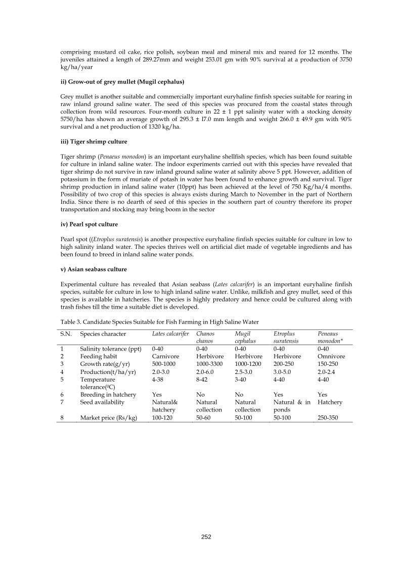
252

comprising mustard oil cake, rice polish, soybean meal and mineral mix and reared for 12 months. The juveniles attained a length of 289.27mm and weight 253.01 gm with 90% survival at a production of 3750 kg/ha/year ii) Grow-out of grey mullet (Mugil cephalus) Grey mullet is another suitable and commercially important euryhaline finfish species suitable for rearing in raw inland ground saline water. The seed of this species was procured from the coastal states through collection from wild resources. Four-month culture in 22 ± 1 ppt salinity water with a stocking density 5750/ha has shown an average growth of 295.3 ± l7.0 mm length and weight 266.0 ± 49.9 gm with 90% survival and a net production of 1320 kg/ha. iii) Tiger shrimp culture Tiger shrimp (Penaeus monodon) is an important euryhaline shellfish species, which has been found suitable for culture in inland saline water. The indoor experiments carried out with this species have revealed that tiger shrimp do not survive in raw inland ground saline water at salinity above 5 ppt. However, addition of potassium in the form of muriate of potash in water has been found to enhance growth and survival. Tiger shrimp production in inland saline water (10ppt) has been achieved at the level of 750 Kg/ha/4 months. Possibility of two crop of this species is always exists during March to November in the part of Northern India. Since there is no dearth of seed of this species in the southern part of country therefore its proper transportation and stocking may bring boom in the sector iv) Pearl spot culture Pearl spot ((Etroplus suratensis) is another prospective euryhaline finfish species suitable for culture in low to high salinity inland water. The species thrives well on artificial diet made of vegetable ingredients and has been found to breed in inland saline water ponds. v) Asian seabass culture Experimental culture has revealed that Asian seabass (Lates calcarifer) is an important euryhaline finfish species, suitable for culture in low to high inland saline water. Unlike, milkfish and grey mullet, seed of this species is available in hatcheries. The species is highly predatory and hence could be cultured along with trash fishes till the time a suitable diet is developed. Table 3. Candidate Species Suitable for Fish Farming in High Saline Water

S.N. Species character Lates calcarifer Chanos chanos

Mugil cephalus

Etroplus suratensis

Peneaus monodon*

1 Salinity tolerance (ppt) 0-40 0-40 0-40 0-40 0-40 2 Feeding habit Carnivore Herbivore Herbivore Herbivore Omnivore 3 Growth rate(g/yr) 500-1000 1000-3300 1000-1200 200-250 150-250 4 Production(t/ha/yr) 2.0-3.0 2.0-6.0 2.5-3.0 3.0-5.0 2.0-2.4 5 Temperature

tolerance(0C) 4-38 8-42 3-40 4-40 4-40

6 Breeding in hatchery Yes No No Yes Yes 7 Seed availability Natural&

hatchery Natural collection

Natural collection

Natural & in ponds

Hatchery

8 Market price (Rs/kg) 100-120 50-60 50-100 50-100 250-350

253

vi) Control of pond seepage and secondary salinizatiion UV-stabilized poly qua-lining of PVC (poly vinyl chloride) material of thickness 0.5 to 0.7mm has been found highly suitable for laying in aquaculture ponds. This lining has been found to help in total control of pond seepage and nutrient loss and is safe for culture of fishes and prawns. Since the disposal of high saline inland water from aquaculture ponds has been a matter of great concern from the environment point of view, ponds lined with this film could be used to serve as salt evaporation basins for the treatment of the waste water. Thus, it will solve the problem of secondary salinization and the salt produced could be utilized as a raw material by the industry. 4. Aquaculture in sodic/alkaline soil and waters Alkali soils (also called sodic soil) contain high amounts of salts mainly sodium carbonate due to which they have very high pH, high exchangeable sodium, dispersed soils, low infiltration rate, low organic carbon, low available nitrogen an very less soluble calcium. Thus they are considered unsuitable for agriculture and fish culture. However ground water in alkaline soil area is suitable for fish culture. When water is added to alkaline soil, the pH of soil is reduced to a certain extent. The major problems in construction of ponds in alkali soils for fish culture are seepage and evaporation, high pH, high turbidity and low dissolved oxygen. Many parts of country is having high alkali (<4dS/m EC, <10(mmol-1)1/2, SAR, >4 meq/l RSC ground water. The ideal range of total alkalinity for freshwater fish is 60-300mg/l as CaC03.In general, freshwater fish in hard water (100-150mg/l CaC03) tend to spend less energy on osmoregulation, resulting in better growth. The very high limit of alkalinity may also be related to its effect on osmoregulation at high ion concentrations. Desirable levels of total hardness for fish culture generally fall with in the range of 50-200 mg/l.As a general rule, the most productive waters for fish culture have total hardness and total alkalinity values of approximately the same magnitude. For example, water with a total alkalinity of 150 mg/l and a total hardness of 25mg/l is not as good for fish culture as water in which the total alkalinity is 150 mg/l and total hardness is 135 mg/l. Similarly very hard water and low alkalinity pose problem to fish and its growth. This is more evident in case of early part of life of fish rearing. If total alkalinity and total hardness are too low, they may be raised by liming. Application of Allum-Al2 (SO4)3.14H2O (25-50 kg/ha) or Gypsum-CaSO4. 2H2O (250-500 Kg/ha) is found good for reducing adverse relation of alkalinity and hardness and lowering of turbidity and high pH of sodic water. Sodic water with or without certain chemical amendments can be used for productive utilization of aquaculture purpose depending upon suitable size of stocking material ie.fish. Various aspect of aquaculture management is described below: i) Pond construction During pond excavation, surface soil up to 8-10 cm need to be scraped. Before starting the construction of ponds, a survey is required to know the level of hard Kankan pan CaCO3. If hard Kankan pan found at 1.25-1.5 m depth then the excavation works to be stopped 20-30 cm above the pan for avoiding seepage from the pond or if below the profile good soil condition persist then further deepening of pond can be taken up. The repeated puddling and continuous manuring of the pond is required to reduce the seepage rate. Embankments are to be constructed with proper ramming. Slopes were made with a ratio of 3:1 on inner side and 2:1 on the other side. The embankment around ponds in sodic soil is made wider than clay loam soil. Top of bundh is used for growing vegetable and fruits. The sides of every embankment were properly turfed with doob grass (Cynodon dactylon). ii) Reclamation of pond bottom soil Diagnosis of the nature of the soil problem is very essential for making appropriate recommendations for the reclamation and /or management of salt affected soils. Proper pond bottom leveling is the most important and essential prerequisite for achieving successful reclamation. It ensures uniform and better reclaiming action of the amendment. A simple relationship between the soil texture and pH has been developed at this Institute to find out gypsum requirement is depicted in table-4. In the reclamation of alkali soils, the basic reaction involved is the reduction of exchangeable sodium of the soil to a sufficient level. The exchangeable sodium in the soil is replaced with calcium through the addition of gypsum. The chemical reaction involved is as below: Na2-clay+Ca SO4↔Ca-Clay+Na2 SO4

254

Table 4. Gypsum requirement (tons/ha) in relation to pH

pH Sandy texture soil Sandy-loam texture soil Loam texture soil >9.0 Not needed Not needed Not needed 9.2 1.7 2.5 0.4 9.4 3.4 5.0 6.8 9.6 5.0 7.0 10.0 9.8 6.8 10.0 14.6 10.0 8.5 12.5 15.0 10.2 and above 10.0 15.0 15.0

iii) Stocking of ponds Both size and density of fish are important to achieve high yields. Stocking of smaller size of fishes may results higher mortalities and slow growth during the initial months. Fingerlings of 60-150mm size are best stocking material. The stocking is done during the cool hours of the day in the morning or evening by acclimatizing them to the new habitat. Stocking densities of 5000-10,000 fingerlings/ha are usually safe under scientific management. An adjustment of species ratio is the main criteria for optimum production. Manipulation of species ratio is essential for competition for food availability at various trophic levels and zones in a pond. Normal ratio is 4:3:3 or 3:4:3 or 3:3:4 for surface feeder, column feeder andbottom feeder fishes respectively. For sodic soil condition pond first criteria is generally important. A combination of six species e.g. catla, silver carp, rohu, grass carp, mrigal, and common carp has proven to ideal combination for carp culture in India. Of these criteria of species catla and silver carp are surface feeders, rohu is column feeder, grass carp is a macro vegetation feeder and mrigal and common carp are bottom feeders. The species specific ratio for sodic soil pond is Catla-25%, Silver carp 15%, Rohu-25%, Mrigal-20%, common carp-10%, Grass carp 5%. Depending upon seed availability and environmental condition of pond the species ratio may be changed. iv) Supplementary feeding Feed is the main governing factor in determining the growth rate of fish. Natural fish food production remains limited, there for getting higher production food from outside needed. Locally available materials like oil cake, brans, fish meals etc. are the main constituents of fish feed. They include ground nut oil cake, rice brans, soyabean meal, mustard oil cake, wheat bran, fish meal etc. Assessment of requirement of feed is important since under feeding depresses growth while over feeding results in wastage of feed, the costliest input leading to deterioration of water quality and disease problem. When manuring and fertilization is done on regular basis feeding@1-3% body weight of biomass is sufficient. Grass carp are fed with preferred aquatic vegetation. Generally feed is given once in the morning or day hours. The most practiced feeding ingredient in carp culture is rice bran and oil cake in the ratio of 1:1.Sometimes we have to stop the feeding schedule keeping in view of water temperature specially during winter. The feed can be given in the farm of dough or pelleted form either in a basket, tray, perforated bag etc. Regular monitoring of feed is very much essential for successful fish culture. Nowadays for advanced state of aquaculture, commercial pelleted feed are used for the purpose. The formulated feed in the following ratio is good for getting higher fish production. Feed ingredient Per cent Ground nut oil cake 35-40 Rice polish 38-40 Soya bean meal 20-15 Fish meal 5-3 Vitamin, mineral etc. 2-2 v) Pond maintenance General checkup of pond water level maintenance, oxygen level of water and periodic samplings of fish are prime need for higher survival and production. For marketable size fish production fishes are reared for 9-12 months. The growth of fishes is steady reaching a kilogram in one year. Silver carp and grass carp register the fastest growth followed by common carp, catla, rohu and mrigal. Regular supply of grass/vegetable leaf is essential prerequisites of grass carp growth. Prior to stocking, the fingerlings should be given bath with 3% common salt or 3-5 ppm KMnO4 for 30-60 seconds. During winter months disease problems become

255

acute. Lime application at the rate of 100kg/ha can control the infection at preliminary stage. For severe infection, a second dose may also be applied. In case other disease problems, necessary treatment measures may be taken after due consultation with experts. Birds, otters and snakes also do considerable damage to fish crop by predating fry and fingerlings. The fish stand the risk of poaching. Poaching through cast netting and gillnetting is most common. This can be easily prevented and minimized by placing bushy plants and bamboo twigs in the ponds. However, the risks involved in fish farming are mostly managerial and could be effectively dealt with proper precaution and vigil. vi) Growth and production Growth of fishes in one year of culture operation under reclaimed sodic soil and water condition is found to be catla -700-800 g, silver carp 900-1000 g of, grass carp -1000-1200 g, rohu-600-700 g and 500-600 g in case of mrigal. Overall survival of fingerlings is 60-75%. The fish production in such condition has been found to be 3-5 tons/ha/year. 5. Integrated Fish Farming in Sodic/Alkaline Soil and Water Condition The principle of integrated fish farming involves farming of fish along with livestock or/and agricultural crops. These types of farming offer great efficiency in resource utilization (such as sodic /alkaline soil and water), as waste or byproduct from one system is effectively recycled. It also enables effective utilization of available farming space for maximizing production. The rising cost of protein-rich fish food and chemical fertilizer as well as the general concern for energy conservation has created awareness in the utilization of rice and other crop fields and livestock wastes for fish culture. Fish culture in combination with agriculture or livestock is a unique and lucrative venture and provides a higher farm income, makes available a cheap source of protein for the rural population, increases productivity on small land holdings and increases the supply of feeds for the farm livestock. The scope of integrated farming is considerably wide. Ducks are raised in pond, and pond dykes are used for horticultural and agricultural crop products and animal addition to fish. Hence this system provides better production, provides more employment, and improves socio-economic status of farmers and betterment of rural economy. This type of integrated farming system approach will be very much fruitful in different canal command areas due to sodicity of water from the seepage. This will be an appropriate enterprise in waterlogged area with the incorporation of polyculture fish species. In these condition apart from agri & livestock/other animal produce fish production has been achieved at the level of 3-4 tons ha/year. 6. Aquaculture for treatment of waste/sewage water It is increasingly being recognized that sewage is just not a pollutant but also a nutrient resource. Traditional practices of recycling sewage through agriculture, horticulture and aquaculture have been in vogue in several countries. The sewage-fed fish culture of Munich in Germany and Bheries in Calcutta are world famous. Distillery effluent based fish culture in Chennai, India is another feather in this direction. Aquaculture based on duckweeds (aquatic macrophytes) has been attempted in well plan manner in the country at Cuttack for treatment of domestic sewage. In this, duckweeds act as nutrient pump by accumulating excess amount of nutrients available in water body and thereby treat waste water. The approximate growth rates of different duckweed species in sewage fed culture system were recorded such as Sprodella polyrrhiza 350g/m3/d, Wolfia arrhiza 280g/m3/d, and Lemna minor 275g/m3/d(CIFA,1996).There were two ways of advantages achieved after treatment of waste water bodies:1) duckweeds treated water bodies were, later, utilized for cultivation of Indian and exotic carp and 2)harvested duckweeds were utilized as fish food. Studies have shown that higher rates of fish production (3-4 ton/ha/yr) can be achieved by using sewage alone based on ASTP, CIFA, Cuttack model. In this study during one year culture period in sewage-fed fish pond system, the followings were the weight gain of individual carp species on average weight basis: Catla 600 g; Rohu 700 g; Mrigal 700 g; Silver carp 800 g and Common carp 650 g .Consequently, the economic benefit earned was 39%per year, excluding the entire operational cost. Besides, duckweeds act as host for a variety of nitrogen, fixing epiphyte microflora and beneficial microorganisms such as bacteria, cynobacteria and diatoms. These microorganisms serve as scavenger in removing both organic and inorganic waste. Estimation revealed that degraded organic matter was found up to 12.9%N and 2.6%P on dry weight basis in domestic sewage and sludge, whereas non degradable residues contained 7% N and 1% P after endogenous respiration; and in the process, the rest was released back to medium itself. In this model every care has been taken in terms of marketing ponds as depuration measures for rearing fish before harvesting. However, in other mode of aquaculture for utilization of sewage, it is advocated that only primary treated sewage be used in instead of raw form. Further, depuration measures for a period of at least 15 days after final harvest of fish grown in sewage water are suggested to be mandatory in order to avoid any possible risk of human health hazard. Owing to its tremendous potentiality to treat waste water, the

256

duck weeds are reported being utilized as remover in the biological sewage treatment and recycling process through aquaculture in different countries in globe. Near the periurban area of many cities, sewage water is being recirculated and this is being used for culture of carps,catfishes,chichlids and air breathing fishes. Farmers are culturing Thai Magur and obtain a production of more than 70 tons per hectare. They use all kinds of waste from slaughter houses, vegetable markets, and are able to reduce pollution at market fish at a price of Rs. 50-60 per Kg. Though culture of some of exotics e.g. Big-head, Tilapia and Thai Magur etc.are illegal but it opens up a new challenge that the culture of these fishes can be attempted with the use of organic wastes at specific locality. This will not only help in solving the pollution problem and generate animal and plant protein food at low cost. However, their culture should be done with proper care and management to avoid all kind of health hazards 7. Constraints and proposed measure for aquaculture adoption There are certain technical and socio-economic constraints responsible for the non- adoption of aquaculture in the agriculturally poor quality water area which are discussed hereunder. i) Identification of Thrust Areas of R & D The progress of R & D in the field of inland saline water aquaculture needs to be speeded up so as to keep pace with the demand of the situation. It is needed to identify the gaps and research projects shall be formulated accordingly. Capacity building and networking of R & D efforts are also essential. Collaborative research programmes involving local organization, transfer of technology agency and departments need top priority ii) Seed production of suitable species The availability of the seed of those species that can be farmed in saline water is a serious problem, particularly for small and marginal farmers. Information is essential on natural seed collection centres both in private and governments sector and provided to State Fisheries Departments. Fisheries Department of inland states shall develop suitable mechanism with private as well as government organization of coastal states to help in the procurement of seed in which inland States shall set up “Seed supply centre’ which can procure seed from coastal States in large quantity and later distribute them to local farmers. More number of hatcheries of M. rosenebrgii for larvae and post larvae production shall also be developed. Intervention of financial support from various agencies may be made for this purpose. iii) Transfer of Technology Financial support shall be provided to the organization to set up at least one saline aquafarm in each. These farms would serve as centres of technology development and demonstration under collaborative R & D programmes. Specific training programmes including tour to coastal states shall have to be organised for the benefit of state governments fisheries officers concerned and also for the farmers and entrepreneurs. Information, communication and technology can be used for the popularization of this type of aquaculture. iv) Environmental consideration The development of saline water aquaculture will require continuous abstraction of saline ground water and its impoundment in ponds. There are possibilities of horizontal movement of saline water during the process of abstraction and during its holding in farm ponds. Both these processes may contaminate the fresh water aquifers which are already limited. The disposal of fish pond effluents will also be a serious threat to surrounding environment, if discharged untreated. Therefore, it will be required to formulate ‘Environment Management Plans’ at the beginning itself, that include safe methods of water abstraction and pond construction with no seepage loss. vi) Socio-economic concern The saline water resources are mainly found in semi-arid and arid parts of northern and northeast India, The primary occupation of land owners in this part of the country is agriculture and dairying. The shift from agriculture to aquaculture will not be easy due to difficulties of social acceptance. The success of inland saline water aquaculture is however expected to bring changes in the land use and land holding patterns. Considering this, it is to be ensured that there will be minimal and unavoidable social problems. The farmers who own salt affected lands and are primarily dependent on agriculture income only have very low or

257

marginal earnings, thus having a poor economic status, which prevents them from adoption of salinewater aquaculture. The situation may even force them to sell off their land holding. Once it happens, it will bring changes in the land holding pattern and lead to economic disparity. vii) Technical issues There will be many technical issues with regard to development of inland saline aquaculture. These may be related to availability of facilities for infrastructure development, pond construction, electricity, skilled manpower, approach roads, marketing of products etc. If the salinity of water is 35 ppt or above it may be difficult to maintain the salinity of pond at permissible limits as it may go very high during summers and cause high fish mortality. viii) Techno-entrepreneurship promotion The inland saline water aquaculture could be better developed through techno-entrepreneurship promotion schemes technically qualified fisheries professionals shall be encouraged to adopt saline water aquaculture. Banks may be attuned to in a way that loan assistance could be provided through agency which may develop a programme of making available loan assistance to those owning saline lands for their conversion into saline water ponds with inlets and outlets as needed. ix) Need for common consensus There are multiple issues related to development of inland saline water aquaculture using salt affected lands with the requirement of saline water. There are also specific issues that involve certain agencies and disciplines. Thus, the activity is multidisciplinary in nature with the requirement of aquaculture specialists, environmentalists, social scientists, economists, hydrologists, geologists etc. The various connected issues are also of concern to state fisheries department, ground water departments, pollution control board, irrigation department, stake holders etc. Each one of the departments concerned will have their own views and concerns. To get over this problem, it is wise to have consensus that the starting phase of the activities itself could be achieved through a national debate among concerned agencies. Conclusion It was specified that building of a truly sustainable way of life it would require the integration of action in three key areas i.e. economic growth & equity, conserving natural resources and the environment, and social development. Developing technologies for utilisation of saline water resources in inland regions through aquaculture-based activities will reduce the pressure on freshwater resources that could be spared for drinking purposes. They would also optimise the use and productivity of waste lands and water, provide an occupation to marginal and poor farmers, and ensure socio-economic independence and food security to resource-deprived farming communities. Inland Saline aquaculture to take an integrated approach for improving food security by various means including promotion of science based programmes to increase the productivity of land and the efficient use of water, by adopting policies and laws that guarantee well-defined and enforceable land and water use rights and by using market-based incentives to promote growth in rural areas. The most major problem in this millennium is degradation of organic material and recycling of organic and industrial wastes. For this purpose, microbiological techniques and consortia of bacteria should be used for breakdown, degradation and recycling of the wastes so that cheap and in expensive nutrients available from organic wastes can be used to produce foods. Suggested Readings Abrol, I.P., Dargan, K.S. and Bhumbla, D.R. 1973. Reclaiming alkali soils. Bulletin No.2, CSSRI, Karnal, India:

58p Adhikari, S., Chaurasia, V.S., Naqvi, A.A. and Pillai, B.R. 2007.Survival and growth of M.rosenbergii (dMan)

juvenile in relation to calcium hardness and bicarbonate alkalinity. Turkish Journal of Fisheries and Aquatic Sciences, 7: 23-26.

Ayyappan, S. 2000. Duckweed and fish based aquaculture sewage treatment system: status and prospects In: Waste Recycling and Resource Management in the Developing World:59-63

Banerjea, S.M.1967. Water quality and soil condition of fish ponds in some states of India in relation to fish production. Ind.J.Fish. 14:115-144

Boyd, C.E. 1984.WaterQuality Management for Pond Fish Culture, Elsevier Scientific Publishing Company:318p

258

CIFA. 2008. Brainstorming Meet on Aquaculture 2025(Souvenir) 7-8 June 2008, CIFA, Bhubaneswar, India: 77p.

CIFE. 2008. Inland Saline Aquaculture: Perspectives & Prospects (BROCHURE): 4p CSSRI. 2008. Integrated Farming System Model for waterlogged sodic

soils.Tech.Bull.No.1/2008CSSRI,Station, Lucknow: 12 p. CSSRI. 2009. Eco-friendly Integrated Multienterprise Model for Livelihood Security in Small Farm Holdings.

Tech.Bull.No.05/2009, CSSRI Karnal: 28p. Chandra, Suresh.1999-2000. Annual reports of ORP centre of CIFA, Allahabad. Department of Water Affairs and Forestry. 1996. South African Water Quality Guidelines (IInd edition).

Volume6: Agricultural Water Use: Aquaculture, In: S Holmes (Ed.), CSIR Environmental Services. Edwards, P. 1996. A note on wastewater-fed aquaculture systems: status and prospects. NAGA, ICLARM,

19:33-35 Ghosh, A., Saha, S.K., Roy, A.K. and Chakrabarty, P.K. 1985. Package of practices for using domestic sewage

in carp production..CIFRI Aquaculture Extension Manual.New Series 8, Barrackpore, India: 1-19. Gupta, I.C.1990.Use of Saline Water in Agriculture. Oxford & IBH Publishing Co. Pvt. Ltd. New Delhi: 308p Gupta, S.K. 2010. Management of Alkali Water. CSSRI. Technical Bulletin, 01: 62p ISFP. 2002. Biology of Brackishwater Fin Fishes &Shell Fishes of India (NEWSLETTER) 4(2): 19p Jain, A.K. 2007.Sustainable Inland Saline Water Aquaculture Development-Issues Of Concern, Fishing

Chimes, 27(7):10-14&53 Pandey, A.C. and Kumar, R. 1998. A preliminary study on the soil characteristics of fish ponds located under

sodic soil conditions.Geobios, 25:180-182 Rao, A.P., Tiwari, N.P., Singh, R. 1999. Culture of exotic and major carps in alkaline/sodic soils: A case

study. The Fourth Indian Fisheries Forum Proceedings 24-28 Nov., 1996:223-225 Saharan, N., Prakash, C. and Raizada, S. 2004. Soil, water and aquatic biota analysis- A methods manual,

CIFE, Mumbai:128p. Sarkar, S.K. 2004. Sodic soil fish ponds: Studies on the features of their ecosystem and management

practices. Fishing Chimes, 24(3):52-53 Singh, S.K. and Sushil Kumar. 2010. Growth performance of different carp species in reclaimed sodic soil

pond condition. (ABS) National Seminar on Soil Salinity and Water Quality (January19-21,2010,CSSRI Karnal:10 (Full paper submitted)

Tiwari, N.P., Rao, A.P. and Singh, R. 1991. Development of suitable growing conditions in Usar land for fish production. In: Aquaculture Productivity: 383-387

259

Impact of High RSC Water Irrigation on Cultivation of Vegetable Crops S.K. Sharma, Sanjay Kumar, Vinod Phogat, A.C. Yadav and Avtar Singh

CCS Haryana Agricultural University, Hisar -125 004 (Haryana), India The continuous increase in the earth’s population requires increasing quantities of water for domestic, industrial and agricultural needs. Presently about 15% of India’s water resources are consumed in domestic and industrial requirements and share of these two sectors will grow to about 30% by 2050 (Minhas and Samra, 2004). The progressive requirement for more water to irrigate crops for food when water resources are limited has lead to use of poor quality water in agriculture (Bouwer, 1994; Ragab, 2005). Irrigation with saline water has become necessary not only in parts of the world with limited supplies of good quality water but also in areas affected by shallow groundwater where the main purpose is to reduce the depth of water table. In Haryana, canal water supplies are not adequate to meet the crop water requirements. Under such situations, exploitation of ground water is essential to achieve crops yield potentials. Its exploitation is also necessary to arrest the rise in water table due to seepage from canal system. Unfortunately, all the ground waters are not of good quality and contain various amounts of salts and as such may affect the soil health and crop yields. In the state, 37 percent of the ground water is of good quality, 8 % marginal and 55 % are of poor quality. Amongst poor quality water 18 % is sodic, 11 % saline and 26% saline-sodic in nature. Salinity disrupts homeostasis in water potential and ionic distribution which influence various physiological and biochemical processes. The continuous use of such waters without amendments adversely affects the soil physical conditions and at the same time, it adversely affects the mineral composition, uptake and yield of crops under most situations. Vegetable production is threatened by increasing soil salinity particularly in irrigated croplands which provide 40% of the world’s food (FAO, 2001). Although India is the second largest producer of vegetables next only to China but productivity of most of vegetables is far less than the world average. One of the main reasons behind low productivity may be use of poor quality water for irrigation. The scarcity of good quality surface as well as groundwater is the main constraints for success of agriculture in most of arid and semi-arid regions of the country. Continuous use of sodic water for irrigation as such causes soil sodification and at the same time, it adversely affects the growth and yield of crops under most situations. Total area under vegetable crops in India is 7.2 mha and its production is 113.5 million-ton, whereas, in Haryana, the area under vegetables is 0.28 mha and its production is 3.3 million-ton. Although lot of research work has been done on various field crops by using sodic waters with amendments like farm yard manure (FYM) and gypsum, yet there is a lack of information on vegetable crops under poor quality water. Criteria for judging water quality The first step while dealing with water quality problem is to get the water analysed for its chemical composition. The requisite information on chemical composition can be obtained by sending a representative water sample to a soil-testing laboratory. Each sub-divisional centre in the state has one soil and water-testing laboratory. The important parameters which determine water quality rating are: Total salt concentration: It is expressed by the electrical conductivity (EC) of the irrigation water, expressed as dS/m. The major cations in the irrigation water include sodium, magnesium and calcium, and the anions may comprise of chloride, sulphate, bicarbonate and carbonates. Other ions may be present, but usually in low concentration is potassium, nitrate, silica or boron. Sodium hazard: The sodium hazard is denoted by residual sodium carbonate (RSC) and sodium adsorption ratio (SAR) of the irrigation water which are defined as:

)()( )/( 33 MgCaHCOCOlmeRSC +−+=

21

21

2

Na )/(

⎭⎬⎫

⎩⎨⎧ +

=MgCa

lmmolSAR

260

Table 1. Water Quality Classification Criteria (Manchanda, 1976)

Water quality category EC (dS/m) SAR (mmol/l)1/2 RSC (meq /l) Good < 2 < 10 Usually < 2.5 Marginal 2.0 - 4.0 < 10 Absent Poor a) Sodic < 4 > 10 Usually> 2.5 b) Saline > 4 < 10 Absent c) Saline sodic > 4 > 10 Usually absent * Good water with RSC > 2.5 me/l when used copiously during kharif as well as rabi also tend to behave like sodic waters Effect of high RSC water on soil properties and plant growth: Sodic waters adversely affect soil physical properties. The increased ESP resulting from their long term

use leads to break down of soil structure due to swelling and dispersion of clay particles. A thin crust is often formed at the surface, which acts as a barrier to penetration of water and seed and

seedling emergence. Increase in soil pHband ESP results in reduced availability of a number of plant nutrients like N, Zn, Fe

etc. Decrease in availability of Ca and Mg and toxicity of sodium. Excessive availability and consequent toxicity of elements like boron, molybdenum, fluorine, lithium

and selenium takes place. Effect of high RSC water along with FYM and gypsum in vegetables. Since accumulation of the sodium ion on the exchange complex is mainly responsible for poor soil physical properties, irrigation water having a alkalinity hazard could be improved by increasing the soluble calcium status of the water, thereby decreasing the proportion of sodium to the divalent cations and therefore its adsorption on the soil exchange complex. Applied soluble calcium salts will also neutralize the bicarbonate and carbonate ions thereby reducing the alkalinity hazard of the water. To offset the harmful effects of alkali waters application of calcium-containing amendment such as gypsum is commonly recommended (Puntamkar et al., 1972; Bajwa et al., 1983; Ayers and Westcot, 1985). The other amendments are acid or acid forming substances (sulphuric acid or pyrites), which react with inherent mineral sources (such as CaCO3) to release Ca to the soil solution. The gypsum requirement for neutralizing residual alkalinity in alkali water is of recurring nature and is determined by factors such as current level of soil deterioration, cropping intensity and water requirement of the crops to be grown. The quality of gypsum for neutralization of each me/l of RSC is 86 kg/ha for 10 cm depth of irrigation. Heavy dressings of organic manures, regular incorporation of crop residues, application of such organic materials as rice hulls, sawdust, sugar factory wastes, etc., have all been found useful in maintaining and improving soil physical properties and in counteracting the adverse effect of high levels of exchangeable sodium. Wherever feasible therefore, organic matter application is recommended if irrigation water has a alkalinity hazard. However, additions of organic amendments alone without gypsum are not capable to alleviate the harmful effects of alkali water. The combined effect of FYM and gypsum has been investigated at Hisar centre in long-term experiments. These studies have shown that FYM along with gypsum significantly increased the yields of potato, tomato, brinjal, broccoli, cluster bean, cauliflower, cabbage, knol khol, bottle gourd, ridge gourd and bitter gourd under alkali water (RSC 11.6 me/l; SAR 14.0 (mmol/l)1/2) irrigation as compared to control treatment. The maximum yields of these crops were recorded with 100 % GR (F2 & F4) and FYM @ 20 t/ha (F2). The magnitude of increase was much higher with gypsum application than FYM. The alkalinity tolerance of crops was in the order: potato> tomato> brinjal>broccoli>cluster bean (Table 2) on the basis of the recovery of crop with the addition of FYM and gypsum. Cluster bean was found to be the most sensitive crop for alkali water tolerance. The yield variation of crops in various treatments was more pronounced because substantial ESP (40-45) has developed due to prior application of alkali water on the test plots.

261

Table 2. Effect of gypsum and FYM treatments on mean yields (q/ha) of different crops

Treatments Potato (3 years)

Tomato 3 years)

Brinjal (2 years)

Broccoli (4 years)

Cluster bean (3years)

FoGo 134.09 16.56 3.80 1.40 0.68 FoG1 210.93 236.04 167.25 43.17 95.73 FoG2 213.06 316.34 228.67 59.51 105.38 F1Go 190.91 22.91 13.50 14.47 1.93 F1G1 241.01 313.43 215.38 66.01 106.21 F1G2 248.62 400.65 264.27 92.91 114.43 F2Go 196.07 31.84 26.18 30.42 2.42 F2G1 252.78 304.19 236.47 81.25 111.04 F2G2 265.15 382.08 288.90 101.01 118.46 CD (5 %) Gypsum 24.68 10.94 28.83 10.54 6.10 FYM 24.68 10.94 28.83 10.54 6.10 GXF 31.01 16.45 NS NS NS F0= no FYM; F1= 10 t/ha; F2= 20 t/ha; G0= no gypsum; G1= 50%; G2= 100% In another long-term experiment at Hisar (Annual reports, Hisar, 2002-2009), the mean yield of cauliflower, cabbage, knol khol, bottle gourd, ridge gourd and bitter gourd increased by 16.1, 28.9, 9.1, 29.7 and 17.5%; and 30.3, 49.9, 24.2, 53.62 and 114.9%, respectively with the addition of FYM @ 10 t/ha (G0F1) and FYM @ 20 t/ha (G0F2) over control (Table 3). However addition of gypsum resulted in tremendous increase in the yields of all the crops. The combined addition of FYM and gypsum (F2G4) recorded the maximum yield in all the crops, which was statistically significant as compared to other treatments. The results of this experiment further confirmed that the addition of gypsum along with organic amendments has triggered the process of amelioration of alkali water and consequently enhanced the yields of crops. Singh et al. (2002) have reported the synergistic effects of adding FYM and gypsum in improving the sugar yield when applied to alkali water irrigated soil than the soil irrigated with saline alkali water. However Gupta et al. (1984) cautioned against the use of organic manure on the soils undergoing alkalization process through irrigation with alkali waters. Organic matter was shown to enhance dispersion of soils due to greater inter-particle interactive forces at high pH. Table 3. Effect of gypsum and FYM treatments on mean yields (q/ha) of different crops

Treatments Cauliflower (2 years)

Cabbage (2 years)

Knol khol (3 years)

Bottle gourd (3 years)

Ridge gourd (2 years)

Bitter gourd (1 year)

G0F0 72.71 114.25 16.00 40.15 35.60 1.03 G0F1 84.43 147.30 17.46 52.08 54.30 1.21 G0F2 94.72 171.34 19.87 61.68 76.50 1.8 G1F0 90.52 147.97 50.53 58.19 42.80 5.92 G1F1 97.92 174.80 61.94 71.11 62.90 12.86 G1F2 103.55 190.36 74.39 82.15 80.70 14.66 G2F0 112.29 181.90 66.77 75.22 45.30 8.49 G2F1 115.50 212.31 89.81 82.03 67.30 14.66 G2F2 130.91 224.76 97.81 88.23 85.40 20.58 G3F0 118.04 207.14 79.76 128.13 44.30 12.09 G3F1 131.80 247.22 96.37 169.48 71.70 21.92 G3F2 138.94 275.68 105.13 172.25 89.80 23.72 G4F0 123.17 231.47 95.93 141.63 49.70 14.66 G4F1 156.63 259.92 107.29 179.04 72.40 24.48 G4F2 150.97 334.16 122.51 188.22 92.60 30.09 CD (5%) Gypsum 8.33 15.84 5.41 1.83 2.40 1.47 FYM 6.44 12.27 4.18 1.42 2.10 1.44 GXF 10.72 19.74 7.46 3.18 3.80 2.5

F0= no FYM; F1= 10 t/ha; F2= 20 t/ha G0= no gypsum; G1= 25%; G2= 50%; G3= 75% and G4= 100%

262

Yadav et al. (2002a) demonstrated that the alkali water irrigation reduced the tuber emergence, plant height, fresh foliage weight, No. of tubers/plot and tuber yield significantly (Table 4). The adverse impact of the alkali water ameliorated with the addition of gypsum and FYM showed a remarkable increase in the growth and yield parameters of the crop. However the magnitude of increase was higher with gypsum over FYM. They suggested that the delayed emergence of tuber under alkalinity may be due to higher alkalinity induced high pH which disturbed the physico-chemical environment of the rhizosphere. Toxic effects of sodium in soil solution are also greatly responsible for reduced tuber emergence of potato. Formation of hard crust on soil surface due to precipitated carbonates and bicarbonates further delayed the emergence of germinated tubers. Table 4. Effect of gypsum and FYM under alkali water irrigation on potato yield

Treatments Yield of tuber (kg/plot) Total yield of tuber (kg/plot)

Total yield (q/ha) Large size Medium size Small size

2001 2002 2001 2002 2001 2002 2001 2002 2001 2002 Control 5.90 6.70 13.47 12.95 2.93 3.15 22.30 22.80 247.77 253.33 FoGo 0.80 0.72 1.28 2.05 1.23 2.33 3.02 5.10 33.51 56.64 FoG1 3.03 3.31 11.07 11.38 2.13 2.47 16.23 17.16 180.35 190.63 FoG2 3.20 4.33 10.57 10.88 2.07 2.53 15.83 17.74 175.91 197.12 F1Go 0.50 1.30 3.47 5.53 2.17 3.08 6.13 9.92 68.13 110.17 F1G1 3.57 4.98 11.40 11.05 2.10 2.72 17.07 18.75 189.62 208.33 F1G2 4.37 5.98 11.10 10.15 2.10 3.22 17.57 19.35 195.17 214.98 F2Go 0.60 1.60 3.53 5.83 1.93 3.80 6.07 11.23 67.40 124.81 F2G1 4.10 6.05 11.57 10.37 1.77 3.22 17.43 19.63 193.68 218.13 F2G2 5.47 7.25 13.33 10.75 2.13 3.88 20.93 21.88 232.57 243.14 CD (5%) 0.32 0.28 0.41 0.47 0.12 0.10 1.23 1.45 13.66 16.13

F = FYM @ 10 and 20 t/ha; and G = Gypsum @ 0, 50 and 100% RSC neutralization Effect of amelioration on soil properities Infiltration rate The results of the experiments conducted at Hisar centre revealed that infiltration rate decreased with the increase in the FYM and increased with increasing levels of gypsum (Table 5). In case no gypsum, the mean basic infiltration rate decreased by 11.0 and 29.62 % in F1 (FYM @ 10 t/ha) and F2 (FYM @ 20 t/ha) respectively as compared to F0 (No FYM). However, addition of gypsum @ 50 (G1) and 100 % (G2) increased the infiltration rate by 71.42 and 128.57%, respectively when compared with gypsum control. Similar results were obtained in another study under cole crops-cucurbits crop rotation. The infiltration rate decreased at higher FYM level due to the dispersion of FYM under alkali condition which resulted in the clogging of the pores. The infiltration rate was well correlated (R2 =0.86) with the ESP build up in the soil (Fig.1). Besides it was observed that addition of FYM and gypsum increased the penetration by 12.12 and 33.3 % at the highest level of FYM and gypsum, respectively as compared to control. The minimum value was recorded in F0G0 (0.27 KN) treatment. It showed that the workability of soil could be improved by application of amendments and FYM. Table 5. Effect of gypsum and FYM treatments on infiltration rate of soil

Treatments Infiltration rate (cm/hr) 2002-03 2004-05

F0G0 0.19 0.16 F0G1 0.32 0.28 F0G2 0.48 0.37 F1G0 0.16 0.14 F1G1 0.28 0.25 F1G2 0.35 0.33 F2G0 0.14 0.13 F2G1 0.21 0.19 F2G2 0.23 0.26

CD (5 %) Gypsum 0.02 0.02 FYM 0.02 0.02 GXF 0.035 0.03

263

y = -0.009x + 0.49R2 = 0.86

0

0.1

0.2

0.3

0.4

0.5

0 10 20 30 40 50 60

ESP (%)In

filtra

tion

rate

(cm

/hr)

Fig.1. Relationship between ESP and infiltration rate

The addition of organic amendments like FYM, besides ameliorating the harmful effects of alkali water also contribute to the organic matter pool of the soil which is the reservoir of the available plant nutrients. The results revealed that the mean organic carbon of the soil increased from 0.36 to 0.61 with the addition of FYM @ 10 t/ha and from 0.38 to 0.71 with 20 t/ha registering an increase of 73 and 84%, respectively over control (no FYM) in a time span of 15 years (Table 6). Table 6. Organic carbon (%) build-up in soil due to application of FYM and gypsum

Treatments OC (%) 1994 2002 2009

F0G0 0.32 0.35 0.34 F0G1 0.31 0.36 0.37 F0G2 0.31 0.36 0.38 F1G0 0.35 0.45 0.54 F1G1 0.36 0.49 0.62 F1G2 0.35 0.52 0.68 F2G0 0.39 0.47 0.6 F2G1 0.38 0.54 0.72 F2G2 0.38 0.58 0.8 The results of a series of experiments indicated that application of gypsum improved the soil physical and chemical properties and reduced the harmful effects of alkali water by bringing down the pH and ESP of the soil and consequently improved the permeability of the soil (Fig.2 and Fig.3). The reduction in pH is owing to the release of acids on decomposition of FYM which in turn decreased the pH of the soil. Similarly, the ESP of the soil decreased with the addition of gypsum in both the years (Phogat et.al., 2010)

8

8.2

8.4

8.6

8.8

9

9.2

9.4

9.6

F0G0 F0G1 F0G2 F1G0 F1G1 F1G2 F2G0 F2G1 F2G2

Treatments

pH

0-15 15-30 30-45 45-60

Fig. 2: Depth wise pH of the soil at the time of harvesting of broccoli as affected by FYM and gypsum

addition

264

8

8.2

8.4

8.6

8.8

9

9.2

9.4

G0F0

G0F1

G0F2

G1F0

G1F1

G1F2

G2F0

G2F1

G2F2

G3F0

G3F1

G3F2

G4F0

G4F1

G4F2

Treatments

pH

0-15 15-30 30-45 45-60

Fig. 3. Effect of FYM and gypsum levels on the pH at time of harvest of cabbage

Exchangeable sodium percentage (ESP) is another property of the soil which is greatly influenced by the alkali water application. The addition of gypsum and organic amendments has a direct bearing on the amelioration of ESP of the soil. The results of long-term experiments (Annual reports, Hisar 2002-09) have shown that the ESP of the soil decreased tremendously with the addition of gypsum and FYM (Fig. 4). The reduction with gypsum application was more pronounced than FYM.

0

10

20

30

40

50

60

FoGo FoG1 FoG2 F1Go F1G1 F1G2 F2Go F2G1 F2G2Treatments

ESP

(%)

ESP 2002 ESP 2003

ESP 2005 ESP 2008

Fig. 4. Effect of different FYM and gypsum treatments on ESP of the soil

Economic gains from cropping There is sometimes a wrong notion that use of alkali waters for irrigation may not be a sound proposition since gypsum has to be added to the soil, repeatedly. The B:C ratio estimated for alkali water use along with FYM and gypsum at Hisar centre for tomato, broccoli, cauliflower, cabbage and bottle gourd were 3.02, 2.83, 2.46, 3.12 and 2.92 respectively (Table 7). The economic analysis has shown that use of brackish water for vegetable production is a viable technology if they are used judiciously along with amendments. Table 7. Economic analysis of vegetable crops grown with alkali water ameliorated with gypsum and FYM

Name of crop Cost of production (Rs./ha)

Gross returns (Rs./ha)

Net returns (Rs./ha)

B:C ratio

Tomato 23653 71433 47780 3.02 Broccoli 20558 58212 37654 2.83 Cauliflower 24556 60421 35865 2.46 Bottle gourd 19298 56466 37168 2.92 Cabbage 24546 76812 39204 3.12

265

Conclusions: • The 100 % neutralization of RSC with gypsum + 20 tons of FYM gave the best benefit-cost ratio i.e. 3.02 :

1, 3.1 : 1 and 2.83 : 1 in tomato, brinjal and broccoli, respectively. • Maximum benefit-cost ratio (2.46:1) in cauliflower was obtained with RSC neutralization (100 %) + FYM

(10 tons). • In cabbage, the best B:C ratio (3.12: 1) was obtained with 20 tons of FYM along with 100 % neutralization

of RSC. • Ten tons of FYM + 75 % neutralization of RSC gave the most economical yield of bottle-gourd (benefit-

cost ratio = 2.92). • Application of FYM alone as an amendment was not helpful in mitigating the adverse effect of the sodic

water. Suggested Readings Annual report, Hisar. 2002-2009. AICRP on Management of salt affected soils and use of saline water in

agriculture. Ayers, R.S. and Westcot, D.W. 1985. Water quality for agriculture. Irrigation and Drainage Paper No. 29,

Rev. 1, FAO, Rome, p 174. Bajwa, M.S., Hira, G.S. and Singh, N.T. 1983. Effect of sodium and bicarbonate irrigation waters on sodium

accumulation and on maize and wheat yields in northern India. Irri. Sci. 4: 191-199. Bouwer, H. 1994. Irrigation and global water outlook. Agric. Water Manage. 25: 221–231. FAO. 2001. Climate variability and change: A challenge for sustainable agricultural production. Committee

on Agriculture, Sixteenth Session Report, 26-30 March, Rome, Italy. Gupta, R.K., Bhumbla, D.K. and Abrol, I.P. 1984. Effect of sodicity, pH, organic matter and calcium

carbonate on the dispersion behaviour of soils. Soil Sci. 137: 245-251. Manchanda, H.R. 1976. Quality of ground waters in Haryana, 160 pp. Haryana Agri. Univ., Hisar. Minhas, P.S. and Samra, J.S. 2004. Waste Water Use inPeri-urban Agriculture: Impact and Opportunities.

Tech. Bull. No. 2, CSSRI, Karnal. Phogat, V., Sharma, S.K., Kumar Sanjay, Satyavan and Gupta, S.K. 2010. Vegetable cultivation with poor

quality water. Tech. Bull., pp 72, Department of Soil Science, CCS Haryana Agricultural University, Hisar-125 004, India.

Puntamkar, S.S., Mehta, P.C. and Seth, S.P. 1972. Effect of gypsum and manure on the growth of wheat irrigated with bicarbonate rich waters. J. Indian Soc. Soil Sci. 20: 281-28.

Ragab, R. 2005. Advances in integrated management of fresh and saline water for sustainable crop production: Modelling and practical solutions. International J. Agric. Water Manage. 78(1–2): 1–164, Elsevier, Amsterdam.

Singh, S., Balyan, D.S., Yadav, A.C., Rana, M.K. and Singh, N. 2002. Influence of FYM and gypsum in reducing the adverse effect of sodic water on attributes related to yield and quality of potato. Haryana J. Hort. Sci. 31(1&2): 123-126.

Yadav, A.C., Sharma, S.K., Kapoor, A.K., Mangal, J.L. and Batra, B.R. 2002b. Effect of sodic water, FYM and gypsum on the soil, growth and yield of Brinjal. Annals of Agri-Bio Research 7 (1): 73-77.