
Use of Multi-Criteria Decision Analysis (MCDA) for Mapping ...
25
Citation: Cartwright, J.H.; Shammi, S.A.; Rodgers, J.C., III. Use of Multi-Criteria Decision Analysis (MCDA) for Mapping Erosion Potential in Gulf of Mexico Watersheds. Water 2022, 14, 1923. https://doi.org/10.3390/w14121923 Academic Editors: S. Kossi Nouwakpo, Jason Williams and Frédéric Darboux Received: 15 April 2022 Accepted: 13 June 2022 Published: 15 June 2022 Publisher’s Note: MDPI stays neutral with regard to jurisdictional claims in published maps and institutional affil- iations. Copyright: © 2022 by the authors. Licensee MDPI, Basel, Switzerland. This article is an open access article distributed under the terms and conditions of the Creative Commons Attribution (CC BY) license (https:// creativecommons.org/licenses/by/ 4.0/). water Article Use of Multi-Criteria Decision Analysis (MCDA) for Mapping Erosion Potential in Gulf of Mexico Watersheds John H. Cartwright 1, * , Sadia Alam Shammi 1 and John C. Rodgers III 2 1 Geosystems Research Institute, Mississippi State University, Starkville, MS 39762, USA; [email protected] 2 Department of Geosciences, Mississippi State University, Starkville, MS 39762, USA; [email protected] * Correspondence: [email protected] Abstract: The evaluation of soil erosion is often assessed using traditional soil-loss models such as the Revised Universal Soil-Loss Equation (RUSLE) and the Soil and Water Assessment Tool (SWAT). These models provide quantitative outputs for sediment yield and are often integrated with geographic information systems (GIS). The work described here is focused on transitioning towards a qualitative assessment of erosion potential using Multi-Criteria Decision Analysis (MCDA), for improved decision-support and watershed-management prioritization in a northern Gulf of Mexico coastal watershed. The foundation of this work conceptually defined watershed erosion potential based on terrain slope, geomorphology, land cover, and soil erodibility (as defined by the soil K-factor) with precipitation as a driver. These criteria were evaluated using a weighted linear combination (WLC) model to map generalized erosion potential. The sensitivity of individual criteria was accessed with the one-at-a-time (OAT) method, which simply removed one criterion and re- evaluated erosion potential. The soil erodibility and slope were found to have the most influence on erosion-potential modeling. Expert input was added through MCDA using the Analytical Hierarchy Process (AHP). The AHP allows for experts to rank criteria, providing a quantitative metric (weight) for the qualitative data. The individual AHP weights were altered in one-percent increments to help identify areas of alignment or commonality in erosion potential across the drainage basin. These areas were used to identify outliers and to develop an analysis mask for watershed management area prioritization. A comparison of the WLC, AHP, ensembled model (average of WLC and AHP models), and SWAT output data resulted in visual geographic alignment between the WLC and AHP erosion- potential output with the SWAT sediment-yield output. These observations yielded similar results between the qualitative and quantitative erosion-potential assessment approaches, with alignment in the upper and lower ranks of the mapped erosion potentials and sediment yields. The MCDA, using the AHP and ensembled modeling for mapping watershed potential, provided the advantage of more quickly mapping erosion potential in coastal watersheds for improved management of the environmental resources linked to erosion. Keywords: watershed; erosion potential; MCDA; WLC; AHP; ensembled model 1. Introduction Sediment is the largest volumetric nonpoint-source pollutant to surface waters [1–3] and one of the most important water-quality problems in the United States [4–6]. Upland watershed erosion is a serious issue for estuaries and the coastal region of the southeastern United States. During precipitation events, overland and streambank erosion increases in the watershed, often resulting in degradation to downstream resources in the associated estuary. Erosive rates are amplified in areas experiencing active land use changes with agriculture, and increasing urbanization and industrialization [7,8]. The influence of the growing human population and unrestricted development in coastal watersheds is proving to be very detrimental to the overall integrity of the fragile, yet highly productive estuarine Water 2022, 14, 1923. https://doi.org/10.3390/w14121923 https://www.mdpi.com/journal/water
-
Upload
khangminh22 -
Category
Documents
-
view
1 -
download
0
Transcript of Use of Multi-Criteria Decision Analysis (MCDA) for Mapping ...

Citation Cartwright JH Shammi
SA Rodgers JC III Use of
Multi-Criteria Decision Analysis
(MCDA) for Mapping Erosion
Potential in Gulf of Mexico
Watersheds Water 2022 14 1923
httpsdoiorg103390w14121923
Academic Editors S
Kossi Nouwakpo Jason Williams
and Freacutedeacuteric Darboux
Received 15 April 2022
Accepted 13 June 2022
Published 15 June 2022
Publisherrsquos Note MDPI stays neutral
with regard to jurisdictional claims in
published maps and institutional affil-
iations
Copyright copy 2022 by the authors
Licensee MDPI Basel Switzerland
This article is an open access article
distributed under the terms and
conditions of the Creative Commons
Attribution (CC BY) license (https
creativecommonsorglicensesby
40)
water
Article
Use of Multi-Criteria Decision Analysis (MCDA) for MappingErosion Potential in Gulf of Mexico WatershedsJohn H Cartwright 1 Sadia Alam Shammi 1 and John C Rodgers III 2
1 Geosystems Research Institute Mississippi State University Starkville MS 39762 USA ss4445msstateedu2 Department of Geosciences Mississippi State University Starkville MS 39762 USA
rodgersgeoscimsstateedu Correspondence johncgrimsstateedu
Abstract The evaluation of soil erosion is often assessed using traditional soil-loss models suchas the Revised Universal Soil-Loss Equation (RUSLE) and the Soil and Water Assessment Tool(SWAT) These models provide quantitative outputs for sediment yield and are often integratedwith geographic information systems (GIS) The work described here is focused on transitioningtowards a qualitative assessment of erosion potential using Multi-Criteria Decision Analysis (MCDA)for improved decision-support and watershed-management prioritization in a northern Gulf ofMexico coastal watershed The foundation of this work conceptually defined watershed erosionpotential based on terrain slope geomorphology land cover and soil erodibility (as defined by thesoil K-factor) with precipitation as a driver These criteria were evaluated using a weighted linearcombination (WLC) model to map generalized erosion potential The sensitivity of individual criteriawas accessed with the one-at-a-time (OAT) method which simply removed one criterion and re-evaluated erosion potential The soil erodibility and slope were found to have the most influence onerosion-potential modeling Expert input was added through MCDA using the Analytical HierarchyProcess (AHP) The AHP allows for experts to rank criteria providing a quantitative metric (weight)for the qualitative data The individual AHP weights were altered in one-percent increments to helpidentify areas of alignment or commonality in erosion potential across the drainage basin Theseareas were used to identify outliers and to develop an analysis mask for watershed management areaprioritization A comparison of the WLC AHP ensembled model (average of WLC and AHP models)and SWAT output data resulted in visual geographic alignment between the WLC and AHP erosion-potential output with the SWAT sediment-yield output These observations yielded similar resultsbetween the qualitative and quantitative erosion-potential assessment approaches with alignmentin the upper and lower ranks of the mapped erosion potentials and sediment yields The MCDAusing the AHP and ensembled modeling for mapping watershed potential provided the advantageof more quickly mapping erosion potential in coastal watersheds for improved management of theenvironmental resources linked to erosion
Keywords watershed erosion potential MCDA WLC AHP ensembled model
1 Introduction
Sediment is the largest volumetric nonpoint-source pollutant to surface waters [1ndash3]and one of the most important water-quality problems in the United States [4ndash6] Uplandwatershed erosion is a serious issue for estuaries and the coastal region of the southeasternUnited States During precipitation events overland and streambank erosion increases inthe watershed often resulting in degradation to downstream resources in the associatedestuary Erosive rates are amplified in areas experiencing active land use changes withagriculture and increasing urbanization and industrialization [78] The influence of thegrowing human population and unrestricted development in coastal watersheds is provingto be very detrimental to the overall integrity of the fragile yet highly productive estuarine
Water 2022 14 1923 httpsdoiorg103390w14121923 httpswwwmdpicomjournalwater
Water 2022 14 1923 2 of 25
ecosystems This growth and development have increased pollution inputs loss of habitatand nutrients and has led to degraded ecologic conditions [1ndash3] These trends of degradedconditions due to human influence will continue to impact estuaries creating higherinstances of eutrophication hypoxia and anoxia
Coastal watersheds and their estuaries are important to the overall coastal environ-ment and are areas of high biologic productivity [910] The high level of productivity isin part due to the transition zone created by the mixing of the upland drainage of freshwater with saline seawater these areas are referred to as the nurseries of the sea [11]
Modeling erosion in coastal watersheds is a complex task that involves a wide range ofknowledge from several scientific and engineering disciplines An effective understandingof coastal watersheds requires several inputs such as coupling landscape characterizationand hydrologic processes [1213] Developments in geographic information systems (GIS)and other geospatial technologies have greatly increased the quality and quantity of dataavailable for hydrologic modeling [13ndash16] The coupling of GIS with other models isan approach that is effective in the management of the resources of coastal watershedsNumerous hydrologic soil-erosion and landscape-characterization models can couplewith geospatial technologies such as GIS for improved data processing analysis andvisualization [13ndash17]
The design of soil-erosion models allows them to work in conjunction with GIS andother geospatial applications Examples include the Water Erosion Prediction Project(WEPP) Soil and Water Assessment Tool (SWAT) and the open-source version of the Non-point Source Pollution and Erosion Comparison Tool (OpenNSPECT) These models areoften described as traditional soil-loss models and are either mechanistic (ie SWAT) or em-pirical such as the Revised Universal Soil-Loss Equation (RUSLE) and Modified Soil-LossEquation [18] Soil erosion across the landscape has traditionally been characterized usingmodels such as the RUSLE [1920] and the WEPP [21ndash23] The combination of many of thesemodels with GIS helps with the transition from models to decision-support and analysisModeling approaches are typically either classified as qualitative or quantitative [24] Aquantitative model is data driven and it is difficult to apply this model in data-poor regionsAdditionally a quantitative model is not enough to determine erosion potential when thereare several factors influencing the erosion of the zone [25] On the other hand a quali-tative model has fewer data requirements It can easily identify the primary factors thatare responsible for erosion potential [25] Additionally the use of quantitative models indecision-support and analysis is beneficial however the execution and data requirementsof the models often limit updated assessments for specific management needs Theselimitations are increased as many of the managers lack the resources needed to readilyexecute the models
Geospatial technologies have provided several contributions to watershed modelingthrough their ability to utilize large temporal datasets from monitoringsampling locations(eg hydrometric and climatic stations) [16] Remote sensing has created a pathway for theclassification of land-useland-cover changes in coastal watersheds which help to visualizelandscape changes arising from the increasing population and developments [26] Thesetypes of classifications coupled with GIS and spatial analyses are allowing environmentaldecision-makers to identify and rank land-use patterns for the implementation of bestmanagement practices for nonpoint-source pollutants and other related issues [27] TheseGIS and spatial analysis methods allow relationships to be established between sedimentloading and the watershed landscape to help identify and prioritize management areasefficiently [2829] The mapping of watershed erosion potential focused on watershedlandscape characterizations provides a needed measure of assessment and aids in theidentification of sediment sources contributing to degraded conditions within a watershedand the associated estuarine environment These characterizations are derived from land-useland-cover changes and practices (ie land disturbance) terrain analyses physicalproperties of soils and other geomorphologic features such as surface drainage densityPreviously factors such as slope gradient precipitation NDVI (normalized difference
Water 2022 14 1923 3 of 25
vegetation index) land use soil texture and slope aspect were studied for soil-erosionrisk assessment [25] additionally drainage density slope land usecover and runoffmeasurement were used for identifying potential zones for rainwater harvesting [30] etcTherefore based on the availability of data in the specified zone the number of factors maybe varied as an input to the models
Multi-criteria decision analysis (MCDA) methods have become very popular for spatialplanning and management issues and are a significant tool for decision makers especiallyfor multicriteria assessment [31] The applications of MCDA are wide It is appliedto identify priority areas for soil-erosion risk measurement [25] to calculate landscapedeformation index [31] to identify potential zones for rainwater harvesting [30] in the fieldof transport for determining suitable management [32] to generate the ranking of greenbonds in corporate office management [33] etc
Hence expanding GIS utilization for MCDA has improved decision-support modelsfor land-based suitability evaluations These expanding efforts have increased the needfor ways to evaluate the performance of the models and tools utilized as well as thesensitivity of the variables or layers used [3435] There are numerous procedures thatare used with GIS for MCDA examples include Boolean overlay weighted linear combi-nation (WLC) ordered weighted averaging (OWA) and the analytical hierarchy process(AHP) [36] The WLC is one of the most commonly used decision-support tools in theGIS environment [3738] Additionally GIS coupled with the AHP [39] is proving to bean important tool for MCDA [4041] GIS utilizing AHP is an established and credited ap-proach to MCDA for land-resource-management decisions [4243] and is an important partof sustainable land-planning approaches [4445] The AHP has been found to be a robustmethod for determining criteria weights based on expert input [46] and works well withMCDA in the GIS environment Additionally the combination of GIS and AHP is usefulfor MCDA in the management of natural resources related to soil-erosion mapping [47]While models and tools of this type do not allow for the quantification of sediment yieldsor soil-loss rates due to erosion they do offer resource managers and decision makers thenecessary information to better manage and prioritize watersheds and the related resources
Therefore qualitative modeling approaches are often driven by MCDA typically withexpert input This makes them very useful in the decision-making process specifically fortasks such as vulnerability assessments and other methods [48] The qualitative natureof MCDA often requires nontraditional methods of uncertainty assessment Sensitivityanalysis is one of the common methods used to reduce uncertainty in the variable weightswhich can assist with identifying stability in model performance with changing criteriaweights [34] Sensitivity analysis with GIS-based MCDA can also provide insights intothe spatial aspects of the changing criteria weights Feick and Hall suggested that effortsto analyze criteria weight sensitivity can help to geographically visualize the sensitivityof the results [49] Another approach to reducing uncertainty in the modeling approachis the combination of different models using the average which is termed as ensembledmodel [5051] The ensembled model is a useful combinational approach and can enhancethe strength of prediction mapping while reducing the weakness of each source map [51]Studies showed betterimproved prediction in clay content mapping for soil-quality as-sessment and decision making in land use [50] and for combining digital soil-propertymaps derived from disaggregated legacy soil-class maps and scorpan-kriging (using soilpan data) [51] from the ensembled model respectively
The primary aim of this research is to develop a qualitative assessment to map erosionpotential using WLC AHP and ensembled modeling approaches for watersheds associatedwith the northern Gulf of Mexico This assessment will provide a process to resourcemanagers for the identification and prioritization of watershed management areas Themapped erosion potential found from these models will be compared to the sediment yieldfrom the SWAT model (httpsswattamuedu) The SWAT model is widely used acrossthe globe in assessing soil-erosion prevention control nonpoint-source pollution controland regional management in watershed (httpsswatplusgitbookiodocs) The SWAT
Water 2022 14 1923 4 of 25
was used in the development of the Weeks Bay Watershed Management plan The modeldelineated the Weeks Bay watershed into 237 sub-watersheds (197 for the Fish River and40 for the Magnolia River) these are used to produce the computational hydrologic responseunits (HRUrsquos) in SWAT Sediment-yield results from this model were based on 2011 landusecover and it was reported that over half of the sediment yield was produced fromabout one-third of Weeks Bay watershed [52]
Therefore the comparisons will be limited to basic observations between the quali-tative and quantitative output of the data The comparisons will show a general visualalignment in sub-basins of increasing development and headland drainage areas in thestudy area The comparison against the output of the SWAT model will help the resourcemanagers to look at scenarios or management priorities without the understanding andexecution of more complex soil-loss models The ensembled model will aid in the visu-alization of the priorities of the management areas The models will serve as a base forthe multi-criteria decision analysis (MCDA) of erosion potential by decision makers andresource managers
2 Materials and Methods21 Study Area
The Weeks Bay watershed is located on the eastern shore of Mobile Bay in Alabama Itis an ideal basin for the assessment of erosion potential as it relatively small and secludedfrom surrounding watersheds The watershed is limited to inputs from two major rivers(Fish and Magnolia) that both directly drain to Weeks Bay (Figure 1) The Weeks Bay water-shed is a diverse natural and anthropogenically influenced landscape with natural forestedagricultural and developed areas that are reflective of the regionrsquos natural resources anddemographics [52] The area is within the humid subtropical climate region characterizedby warm summers and relatively mild winters Average annual precipitation averagesabout 165 cm due to winter storms (cold fronts) summer thunderstorms (including thosefrom the sea breeze) and tropical systems The abundant water resources in the area makefor a range of very productive land uses from timber production cash-grain crops andforage production [53] The Fish River provides nearly 75 of the total discharge to the bayitself and is made up of three sub-watersheds (Upper Middle and Lower Fish River) TheMagnolia River provides the remaining discharge and consist of a single sub-watershed
22 Data Collection and Processing
The process used to map soil-erosion potential was based on several geospatial vari-ables National data sources were used for these variables to ensure transition betweendifferent watersheds and scalability Below we describe the most relevant variables to beincluded in the model
221 Slope
The slope for the study area was calculated using the USGS (United States GeologicalSurvey) 30-m National Elevation Dataset (httpswwwusgsgov3d-elevation-programaccessed on 9 October 2019) The slope calculation for each raster cell was based on theamount of descent between it and the surrounding eight cell neighborhoods using Hornrsquosalgorithm [54] The maximum value of descent was thus recorded as the cellrsquos slope andcould be calculated in percent or degrees The slope raster was then normalized to 0ndash1
222 Soil Erodibility
The soil erodibility (K-factor) was from the 30-m gridded USDA (United State Depart-ment of Agriculture) Soil Survey Geographic Database (httpswwwnrcsusdagovwpsportalnrcsmainsoilssurvey accessed on 10 March 2020) K-factor accounts for boththe susceptibility of a cell to soil erosion based on soil texture and rate of runoff Valuesless than 02 are considered as low erodibility 02 to 04 as moderate and greater than 04as high according to the National Soil Survey Handbook developed by the US Department
Water 2022 14 1923 5 of 25
of Agriculture Natural Resources Conservation Service (httpwwwnrcsusdagovwpsportalnrcsdetailsoilsrefcid=nrcs142p2_054242 accessed on 1 April 2019) The valueswere normalized to 0049ndash1
Water 2022 14 x FOR PEER REVIEW 5 of 28
Figure 1 The Weeks Bay watershed located on the eastern shore of Mobile Bay in Alabama United States along the northern Gulf of Mexico with the four sub-basins labeled
22 Data Collection and Processing The process used to map soil-erosion potential was based on several geospatial vari-
ables National data sources were used for these variables to ensure transition between different watersheds and scalability Below we describe the most relevant variables to be included in the model
221 Slope The slope for the study area was calculated using the USGS (United States Geological
Survey) 30-m National Elevation Dataset (httpswwwusgsgov3d-elevation-program accessed on 9 October 2019) The slope calculation for each raster cell was based on the amount of descent between it and the surrounding eight cell neighborhoods using Hornrsquos algorithm [54] The maximum value of descent was thus recorded as the cellrsquos slope and could be calculated in percent or degrees The slope raster was then normalized to 0ndash1
Figure 1 The Weeks Bay watershed located on the eastern shore of Mobile Bay in Alabama UnitedStates along the northern Gulf of Mexico with the four sub-basins labeled
223 Stream Density
The stream density was a 30-m raster collected from the USGS National HydrographyDataset (httpswwwusgsgovnational-hydrographynational-hydrography-datasetaccessed on 9 October 2019) Higher instances of stream density are associated withincreased erosion rates specifically as they relate to the dissection of the landscape and land-drainage system interactions [55] Similar data layers are used in soil-erosion analysis [56]and are also used in numerous landscape evolution models that simulate erosion anddeposition [57] The density function used for calculation utilized a neighborhood areawith a specified search radius all stream segments intersecting the area were counted and acontinuous surface with the specified cell size was returned The default search radius usedin commercial GIS software is based on the minimal spatial dimension of the dataset [58]
Water 2022 14 1923 6 of 25
The derived density surface was normalized by the maximum value within the Weeks BayWatershed The resulting data layer was a continuous index of stream density with unitlessvalues ranging from 0055ndash1
224 Soil Brightness
The soil brightness was calculated dynamically from the tasseled cap transformationof the 30-m Land cover raster from USGS Global Land Survey Dataset (httpswwwusgsgovlandsat-missionsglobal-land-survey-gls accessed on 9 October 2019) Hence thesoil brightness band of the Tasseled Cap transformation provided an index of measure forsoil reflectanceexposure and not just the lack of vegetation [59] The soil brightness datafrom the GLS dataset were extracted subset to the Weeks Bay Watershed and normalizedby the maximum value The resulting data layer was a continuous index of soil brightnesswith unitless values ranging from 0018ndash1
225 Precipitation
The precipitation data were collected from the 4-km 30-year normal grid of PRISMdataset (httpsprismoregonstateedunormals accessed on 15 March 2020) for rainfallvariation across the basin These data were extracted from the database for the region ofinterest normalized by the maximum value and resampled to 30 m (from 4 km) Theresulting data layer was a continuous index of annual precipitation climatology withunitless values ranging from 096ndash1
23 Model Description
The concept of watershed erosion is summarized as the total erosion for the combina-tion of physical erodibility land sensitivity and precipitation erosivity factors [20234156]For this study area the physical erodibility was measured by slope and stream density landsensitivity included measures of soil K-factor and soil brightness (exposure) and rainfallerosivity was measured as average precipitation of the watershed (rainfall variation) Aschematic diagram of the modeling approach for watershed erosion potential is indicatedin Figure 2 The algorithm used for this WLC mapping was a standard weighted linearcombination (WLC) for the summation of the five raster data layers ie slope streamdensity soil brightness soil erodibility and precipitation [37] The weights for the AHPmodel were calculated using Saatyrsquos method of a continuous rating scale for pairwise com-parison [46] This procedure set each data layer with a possible data range of zero to onefor a common scale of assessment Zero would be a minimal impact on erosion potentialwith values of one having the greatest impact The scale for the AHP model is shown inTable 1 Each data layer was then compared individually with the other data layers as theyrelate to erosion potential Weights for each data layer were assigned based on results fromthe pairwise comparison matrix (Table 1) With all layers standardized and weighted theWLC was used to apply the weights from the expert input for the assessment of erosionpotential This allowed each data layer to be multiplied by the expert-defined weight andthen summed for a continuous surface of overall erosion potential The algorithm for theWLC and AHP model is shown in the Equations (1) and (2) respectively
EPWLC = a(S + SD + K + SB + P) (1)
EPAHP = a1 lowast S + a2 lowast SD + a3 lowast K + a4 lowast SB + a5 lowast P (2)
where EP is the watershed erosion potential P is the average Precipitation K is the soilerodibility S is the slope length and steepness SB is the soil brightness and SD is thestream density of this region a is the standard weight for the WLC model and a1 a2 a3a4 and a5 are weights expected from running the AHP model
Water 2022 14 1923 7 of 25
Water 2022 14 x FOR PEER REVIEW 7 of 28
ie slope stream density soil brightness soil erodibility and precipitation [37] The weights for the AHP model were calculated using Saatyrsquos method of a continuous rating scale for pairwise comparison [46] This procedure set each data layer with a possible data range of zero to one for a common scale of assessment Zero would be a minimal impact on erosion potential with values of one having the greatest impact The scale for the AHP model is shown in Table 1 Each data layer was then compared individually with the other data layers as they relate to erosion potential Weights for each data layer were assigned based on results from the pairwise comparison matrix (Table 1) With all layers standard-ized and weighted the WLC was used to apply the weights from the expert input for the assessment of erosion potential This allowed each data layer to be multiplied by the ex-pert-defined weight and then summed for a continuous surface of overall erosion poten-tial The algorithm for the WLC and AHP model is shown in the Equations (1) and (2) respectively 119864119875 = 119886 119878 119878119863 119870 119878119861 119875 (1) 119864119875 = 119886 lowast 119878 119886 lowast 119878119863 119886 lowast 119870 119886 lowast 119878119861 119886 lowast 119875 (2)
where 119864119875 is the watershed erosion potential 119875 is the average Precipitation 119870 is the soil erodibility 119878 is the slope length and steepness 119878119861 is the soil brightness and 119878119863 is the stream density of this region 119886 is the standard weight for the WLC model and 119886 119886 119886 119886 and 119886 are weights expected from running the AHP model
Figure 2 A schematic of WLC AHP and ensembled model for watershed erosion-potential map-ping
Table 1 Scale for AHP Comparisons
Scale Definition 9 Extremely
More Important 7 Very Strongly 5 Strongly 3 Moderately 1 Equally Important
Figure 2 A schematic of WLC AHP and ensembled model for watershed erosion-potential mapping
Table 1 Scale for AHP Comparisons
Scale Definition
9 Extremely
More Important
7 Very Strongly
5 Strongly
3 Moderately
1 Equally Important
13 Moderately
Less Important15 Strongly
17 Very Strongly
19 Extremely
The erosion potential (EPEN) from the ensembled model was calculated and is men-tioned in Equation (3)
EPEN =n
sumi=1
EPi (3)
where EPEN is the ensembled erosion-potential model n is the number of models and EPiindicates the erosion potential from each of the ith models
24 Sensitivity Analysis
A basic sensitivity assessment was performed for the WLC model variables Theassessment was a simplistic one-at-a-time (OAT) procedure wherein a single variable orlayer was removed and the erosion-potential analysis was processed again The procedurefollowed the method used by Chen et al [34] and Romano et al [36]
25 Ranking of the Management Area
The study area was divided into 18 management areas based on the smaller streamsin the watershed The management areas were ranked or prioritized based on the average
Water 2022 14 1923 8 of 25
EP value for each zone The average EP values found in the WLC AHP and SWAT modelswere compared to visualize the similarities in the zonesrsquo priorities for management tosupport improved decision making for management and prioritization of resources
3 Results31 WLC Model
Potential watershed erosion cells were mapped with a standard weighted linearcombination (WLC) to build a foundation for the qualitative assessment for watershederosion Criteria sensitivity was evaluated using the one-at-a-time (OAT) method to betterunderstand the influence of the landscape layers The WLC model was executed using thefive raster data layers weighted equally for the initial assessment of generalized erosionpotential The output of the WLC model was a continuous surface of erosion potentialbased on physical erodibility land sensitivity and 30-year precipitation for the WeeksBay watershed Mean erosion potential was calculated for the entire watershed (0527SD = 0057) and the four sub-basins within the Weeks Bay watershed Field observationsduring site visits showed that the upland head water areas of the watershed and theareas dominated by cultivated agricultural areas are expected to have higher erosionpotential Lower erosion-potential values are expected in the densely vegetated riparianand marsh areas
The erosion-potential data were classified based on the standard deviation spreadfrom the mean erosion potential across the drainage basin to better define areas based onthe upper and lower ranks of erosion potential This resulted in seven classes that wereused to define the ranks for the cells with class 1 having the lowest potential and class 7having the highest potential At the watershed level 15 of the cells are in the upper-mosterosion-potential ranks (classes 6 and 7) approximately 14 are in the moderate erosion-potential rank (class 5) and the lower erosion-potential ranks (classes 1ndash3) are similar indistribution to the upper ranks (classes 5ndash7)
Erosion potential across the four sub-basins level are varied in comparison The twodownstream basins (Magnolia and Lower Fish) have decreased proportions of cells aroundthe mean erosion potential and the two upstream basins (Upper and Middle Fish) haveincreased cell proportions around the mean erosion potential The Magnolia River sub-basin has the largest count of cells in the upper erosion-potential ranks (classes 5ndash7) at23 The Lower Fish River sub-basin has the next highest count with almost 17 of thesub-basin in the upper erosion-potential ranks and the Upper and Middle Fish sub-basinshave 12 or less in the upper ranks Table 2 provides a complete description of cell counts(with upper and lower ranks) at the basin and sub-basin levels
Table 2 Descriptive statistics of erosion potential in WLC model
Class Name Upper Fish Middle Fish Lower Fish Magnolia Weeks Bay
Class 1 0 1 5279 50 5330Class 2 1436 825 5225 1335 8821Class 3 22586 16072 19899 15938 74495Class 4 141679 89391 90602 71948 393620Class 5 21206 12331 22433 23872 79842Class 6 2287 1147 1908 2788 8130Class 7 109 26 62 188 385
Minimum 0356 0353 0231 0294 0231Maximum 0801 0770 0771 0787 0801
Range 0445 0417 0540 0493 0570Mean 0527 0526 0520 0537 0527SD 0050 0050 0069 0059 0057
SD = Standard Deviation
Water 2022 14 1923 9 of 25
32 WLC Model Criteria Sensitivity Assessment
The sensitivity of individual criteria was accessed using the one-at-a-time (OAT)method by removing one criterion from the WLC model and recalculating erosion potentialThis resulted in five additional WLC model outputs of erosion potential produced byequally weighting four of the five criteria the detailed results are mentioned in Table 3 Thefive additional OAT WLC models were compared to the initial WLC model to understandthe influence of each variable in the WLC The OAT WLC models all had moderate- to-strong correlations with the initial WLC model
Table 3 Descriptive statistics and Pearson correlation for sensitivity analysis
Statistical Parameter WLC ModelVariable Removed from the WLC Model
Slope Stream Density K-Factor SoilBrightness Precipitation
Mean 0527 0634 0539 0511 0540 0411Median 0529 0635 0542 0513 0542 0414Mode 0518 0573 0398 0520 0552 0444SD 0057 0072 0061 0052 0061 0072
Variance 0003 0005 0004 0003 0004 0005Kurtosis 0467 minus0033 minus0103 0724 0418 0416
Skewness minus0328 minus0152 minus0103 minus0292 minus0184 minus0304Range 0570 0632 0611 0560 0544 0711
Minimum 0231 0288 0269 0277 0270 0046Maximum 0801 0920 0881 0837 0814 0757
Count 570623 570623 570623 570623 570623 570623Pearson Correlation - 0940 0882 0788 0881 1000
The model without the precipitation variable had the strongest correlation (R = 100)followed by the model run without slope input (R = 094) The runs without streamdensity and soil brightness were moderately correlated R = 088 The run with the weakestcorrelation was the one without K-factor R = 079 The correlation results showed thatthe WLC model was most sensitive to the K-factor variable moderately sensitive to thevariables of stream density and soil brightness and least sensitive to the precipitation andslope variables
33 AHP Model
This Analytical Hierarchy Process (AHP) model was executed on the five raster datalayers utilized in the WLC model The AHP experts input defined weights for each ofthe five layers with the pairwise comparison The weight assignments for each of layerswere based on scores from the expertsrsquo qualitative ranking of factors The most weightwas given to terrain slope at 338 with lesser weights given to geomorphology landcover and soil erodibility (~150 for each) The 30-year precipitation was effectively leftunchanged at 205 The AHP mean erosion potential for the entire watershed (0472SD = 0051) decreased as compared to the WLC erosion potential The range of the AHPerosion potential increased slightly from that of the WLC and was strongly correlated witha Pearsonrsquos R value of 0923
The AHP erosion-potential data were classified into seven classes based on a standarddeviation spread (Figure 3b) of just the WLC erosion-potential data (Figure 3a) At thewatershed level 27 of the cells are in the upper-most erosion-potential ranks (classes 6and 7) and approximately 12 are in the moderate erosion-potential rank (class 5) Thelower erosion-potential ranks (classes 1 and 2) are similar to the upper ranks with 227 ofthe cells The AHP model produces slightly more cells in the lower ranks than the upperranks of erosion potential (Table 4) The spatial differences between the AHP model andthe WLC model erosion-potential class changes are seen in Figure 3c highlighting the areaswhere the AHP increased or decreased erosion potential from the WLC model
Water 2022 14 1923 10 of 25
Water 2022 14 x FOR PEER REVIEW 11 of 28
(a)
Figure 3 Cont
Water 2022 14 1923 11 of 25
Water 2022 14 x FOR PEER REVIEW 12 of 28
(b)
Figure 3 Cont
Water 2022 14 1923 12 of 25Water 2022 14 x FOR PEER REVIEW 13 of 28
(c)
Figure 3 The WLC map (a) AHP map (b) and the differences in mapped erosion cells between the AHP and WLC map (c) are shown In the difference erosion-potential map the orange cells are where erosion potential increased with the expert input from the AHP and green cells are where it decreased
Figure 3 The WLC map (a) AHP map (b) and the differences in mapped erosion cells betweenthe AHP and WLC map (c) are shown In the difference erosion-potential map the orange cells arewhere erosion potential increased with the expert input from the AHP and green cells are whereit decreased
Table 4 Erosion-potential changes between WLC and AHP model
Class Name WLC Model AHP Model Change
Class 1 5330 4927 minus403Class 2 8821 8012 minus809Class 3 74495 72206 minus2289Class 4 393620 404415 10795Class 5 79842 68674 minus11168Class 6 8130 10482 2352Class 7 385 1907 1522
Water 2022 14 1923 13 of 25
The AHP weights were altered in one-percent increments to identify outliers withAHP model runs An example of weight alteration in the AHP model for 41 iterations for asingle layer is displayed in Appendix A Table A1 The percentage of outliers at each map(or grid) cell was calculated to look at variations spatially A threshold of 25 was usedto define areas with minimal alignment between AHP runs About 375 of the mappedwatershed cells were producing inconsistent or varying erosion-potential results About625 of the mapped watershed cells were in alignment with 75 of the model runs withno outliers This area of the watershed is where the AHP model runs were in alignmentfor the upper and lower ranks of erosion potential Erosion cell counts in this area for themoderate and upper ranks (classes 5 6 and 7) decreased proportionally The proportionaldecrease shows that the higher instances of outliers are not clumped within the lower orupper ranks of erosion potential This provides the definition of a focus area (an analysismask) for increased erosion potential in the Weeks Bay watershed (Figure 4) This analysismask serves as spatial filter for mapped erosion-potential cells for improved agreement inthe modeled outputs
Water 2022 14 x FOR PEER REVIEW 15 of 28
Figure 4 The area highlighted in yellow represents where the AHP model agreed based on one-percent changes to criteria weights with minimal outliers
Figure 4 The area highlighted in yellow represents where the AHP model agreed based on one-percent changes to criteria weights with minimal outliers
Water 2022 14 1923 14 of 25
34 WLC and AHP Model Comparison
Comparisons between the WLC and AHP models were expanded to include an evalu-ation of the outputs with a SWAT model for the Weeks Bay Watershed This comparisonwent beyond the mapped potential erosion cells to evaluate the outputs for watershedmanagement scenarios The comparison took the classified erosion cells for the WLC andAHP models and mapped them with the sediment-yield data for 237 sub-watersheds fromthe SWAT model output The WLC and AHP data were similar with an apparent alignmentin the southwestern and northeastern areas of the watershed with the higher ranks ofmapped erosion potential aligned with the SWAT sediment yield (Figure 5) Additionallythe AHP data highlighted hillslope areas in the headland areas of the watershed due to theexpertsrsquo emphasis on topography
Water 2022 14 x FOR PEER REVIEW 16 of 28
(a)
Figure 5 Cont
Water 2022 14 1923 15 of 25Water 2022 14 x FOR PEER REVIEW 17 of 28
(b)
Figure 5 The WLC (a) and AHP (b) mapped erosion-potential cells with SWAT sediment-yield data Mapped erosion-potential cells for the higher ranks are displayed in red with increasing SWAT sediment yield displayed in brown
35 Management-Priority Area Ranking The final comparison was an aggregate of the mapped erosion-potential cells from
the WLC AHP and ensemble model runs and the SWAT model sediment-yield data to the management areas of the Weeks Bay watershed (Figure 6) The average erosion-po-tential values and the SWAT sediment-yield data were summarized for each of the man-agement areas for ranked prioritization Observational trends in the summarized data ex-hibited spatial alignment in the WLC and AHP upper erosion-potential ranks with higher SWAT sediment-yield data for the watershed management areas Both the qualitative AHP model and the numerical SWAT model agreed in mapping the management area
Figure 5 The WLC (a) and AHP (b) mapped erosion-potential cells with SWAT sediment-yield dataMapped erosion-potential cells for the higher ranks are displayed in red with increasing SWATsediment yield displayed in brown
35 Management-Priority Area Ranking
The final comparison was an aggregate of the mapped erosion-potential cells fromthe WLC AHP and ensemble model runs and the SWAT model sediment-yield data to themanagement areas of the Weeks Bay watershed (Figure 6) The average erosion-potentialvalues and the SWAT sediment-yield data were summarized for each of the managementareas for ranked prioritization Observational trends in the summarized data exhibitedspatial alignment in the WLC and AHP upper erosion-potential ranks with higher SWATsediment-yield data for the watershed management areas Both the qualitative AHP modeland the numerical SWAT model agreed in mapping the management area ranked with the
Water 2022 14 1923 16 of 25
highest erosion Figure 6 shows the management area rankings for the WLC AHP andSWAT models with the ranking of each area based on calculated erosion or sediment yieldfor the respective model output The WLC AHP and SWAT ranks for the higher ranks oferosion aligned approximately 70 of the time
Water 2022 14 x FOR PEER REVIEW 18 of 28
ranked with the highest erosion Figure 6 shows the management area rankings for the WLC AHP and SWAT models with the ranking of each area based on calculated erosion or sediment yield for the respective model output The WLC AHP and SWAT ranks for the higher ranks of erosion aligned approximately 70 of the time
(a)
Figure 6 Cont
Water 2022 14 1923 17 of 25
Water 2022 14 x FOR PEER REVIEW 19 of 28
(b)
Figure 6 Cont
Water 2022 14 1923 18 of 25
Water 2022 14 x FOR PEER REVIEW 20 of 28
(c)
Figure 6 Cont
Water 2022 14 1923 19 of 25
Water 2022 14 x FOR PEER REVIEW 21 of 28
(d)
Figure 6 Management area rankings for the WLC (a) AHP (b) ensembled (c) and mapped erosion cells compared with SWAT sediment yield (d) Agreement of the rankings in upper ranks provides prioritization of management areas for the Weeks Bay watershed
Similarly the mapped erosion potential from the ensemble model was averaged and summarized for the management areas and similar rankings were found to that of the SWAT model Three of the four management areasmdashPensacola Branch Waterhole Branch and Turkey Branchmdashaligned with areas ranked by the SWAT model for high sed-iment yield In the lower ranks alignment was found with the Weeks Branch and Weeks Bay management areas (Table 5) Overall the ensembled model produced similar results
Figure 6 Management area rankings for the WLC (a) AHP (b) ensembled (c) and mapped erosioncells compared with SWAT sediment yield (d) Agreement of the rankings in upper ranks providesprioritization of management areas for the Weeks Bay watershed
Similarly the mapped erosion potential from the ensemble model was averaged andsummarized for the management areas and similar rankings were found to that of theSWAT model Three of the four management areasmdashPensacola Branch Waterhole Branchand Turkey Branchmdashaligned with areas ranked by the SWAT model for high sedimentyield In the lower ranks alignment was found with the Weeks Branch and Weeks Baymanagement areas (Table 5) Overall the ensembled model produced similar results tothat of the WLC and AHP models with agreement in mapped erosion potential in areas ofhigher ranks
Water 2022 14 1923 20 of 25
Table 5 Weeks Bay management area rankings from ensemble model and SWAT model
Name of theManagement Area Sub-Basin Name Rank in
Ensemble ModelRank in
SWAT Model
Pensacola Branch Middle Fish 1 1Perone Branch Upper Fish 12 2
Waterhole Branch Lower Fish 2 3Turkey Branch Lower Fish 4 4Picard Branch Upper Fish 15 5Corn Branch Upper Fish 3 6
Barner Lower Fish 16 7Magnolia River Magnolia 9 8Polecat Creek Middle Fish 14 9
Cowpen Creek Lower Fish 13 10Baker Branch Middle Fish 10 11
Unknown Middle Fish 7 12Three Mile Creek Upper Fish 6 13
Green Creek Lower Fish 5 14Bay Branch Upper Fish 11 15
Weeks Branch Lower Fish 17 16Upper Fish River Upper Fish 8 17
Weeks Bay Lower Fish 18 18
4 Discussion
The erosion potential for a watershed along the northern Gulf of Mexico was mappedqualitatively using layers representative of physical erodibility land sensitivity and 30-yearprecipitation for the Weeks Bay watershed The criteria used to define these layers werebased on regional availability and input from watershed managers and stakeholders onerosional trends in this area The approach used a WLC model and was set up withcriteria similar to numerical models such as RUSLE [19] Other approaches to soil-erosionmapping include empirical conceptual physically based and hybrid models [60] Somehydrodynamic numerical models ie 1-D (one-dimensional) and 2-D hydrodynamicmodels showed better efficiency in urban-flood-risk mapping [61] Compared to theconceptual models ie the Hydrologic Simulation Program (HSPF) and SWAT [60] thisstudy proposed a WLC model which is also applicable to larger areas with less complexityAdditionally the AHP model in the study area considered the factorsrsquo importance in termsof being responsible for regional watershed erosion However this study did not showany physically based model which could be a future demand for better estimation oferosion risk at a large scale In addition factors such as surface hydrology slope aspectand storm events could be used in 2-D physically based simulation models such as GSSHA(Grided SurfaceSubsurface Hydrologic Analysis) DWSM (Dynamic Watershed SimulationModels) etc
In this study the northern headland and the southern agricultural regions of thewatershed had the highest erosion potential as expected [128] Overall erosion potential inthe Weeks Bay watershed tends to be lower in densely vegetated riparian and marsh areasMany of these areas especially in the southern area near the bay are part of the Weeks BayNational Estuarine Research Reserve Areas in the watershed with higher erosion potentialare more associated with transitional-type lands that appear to be more agricultural ordynamic in terms of land practices The southeast region of the watershed reflects this as itis an area dominated by agricultural practices such as cultivated crops and turf-grass farms
Land sensitivity accessed by soil erodibility (as defined by the soil K-factor and soilexposure or brightness) was the criterion that had the most influence on mapped erosionpotential with the WLC model The K-factor is used in USLE and RUSLE applications thatrepresents soil texture and composition [192024] and was the most influential of the layersSoil brightness is indicative of disruptive land uses and increases in erosion potential fromthis variable are apparent in agriculture-dominated areas of the watershed The physical
Water 2022 14 1923 21 of 25
erodibility (topographic) criteria for slope and stream density moderately influenced theWLC-modeled erosion potential These areas of increased potential are indicative of higherconcentrations of stream reaches with more surface interaction with runoff waters andlower soil infiltration rates [55] and proximity to active stream and river channels
The assessment was enhanced with expert input through the AHP model allowingexperts to rank the criteria The ranking of criteria quantified the weights based on theirrelative importance in the study area The physical erodibility criterion of slope wasidentified as the most important by the experts In this the AHP model differs from thetraditional soil-erosion models with the expertsrsquo minimal emphasis on land cover or landsensitivity [1921] This difference is also concerning due to the increased erosion rates dueto development in the watersheds in this region of the Gulf of Mexico [52] The AHP modelproved to be beneficial in mapping areas of increased erosion potential as defined by theupper ranks in the classified data These shifts of the mapped erosion cells from the WLCmodel align with similar approaches using MCDA techniques [4255] The AHP model isnot a typical numerical model and can be better-suited to qualitative geospatial assessmentfor mapping erosion potential with MCDA
The variations in the AHP weights are normally used to identify shifts (increasingand decreasing) in the mapped erosion-potential cells Data outliers were used for theidentification of areas of model alignment for the high ranks of erosion potential Thisapproach allowed for an analysis (management) mask to be generated for these areas thatwere consistently high irrespective of the variation in criteria weights The areas identifiedwere generally associated with higher slopes which were associated with stream andchannel networks The outlier analysis was successful in helping to identify managementareas however a suitable model approach would allow for a quantification shift betweenranks of erosion potential [343945]
The WLC and AHP erosion-potential models were run as an ensemble to improvethe reliability of the output The outputs (from models) were compared with the SWATsediment yield the comparisons were used to help identify if there were any visualalignments or trends between the qualitative and quantitative outputs The comparisonswere very similar with the primary difference being the focus of higher erosion-potentialvalues in the WLC and AHP models The alignment of the data was most apparent inareas of transition with expanding development and agricultural land practices The AHPmodel however produced some areas that were more focused on topographic featuresbecause of the expertsrsquo input placing more emphasis on physical erodibility (slope andother terrain measures) This was most apparent in the headland area of the watershedwhere the landscape has more dissection The comparison of prioritization and ranking ofthe mapped erosion-potential cells for Weeks Bay Watershed management areas displayedalignment for select areas of higher erosion potential
These management areas include the Pensacola Branch Waterhole Branch and TurkeyBranch basins of the Weeks Bay Watershed Each of these management areas have ex-perienced increased erosion due to expanding land development associated with thesurrounding communities The management areas with the lowest ranks were also inagreement This coupled with the alignment in the upper ranks indicates a generalizedagreement between the qualitative and quantitative assessments for the prioritization ofmanagement areas The approach has limitations in management areas that would beconsidered to be of intermediate concern with regard to erosion This is in part due tovarious reasons including the added emphasis by the experts on terrain characteristics andtemporal generalizations in layers used in the WLCAHP models and the SWAT model
However these areas of upper and lower erosion ranks are indicative of the agreementbetween the qualitative and quantitative modeling approaches supporting the use ofMCDA for management decisions and improved applications for watershed managers
Water 2022 14 1923 22 of 25
5 Conclusions
The watersheds that drain areas along the northern Gulf of Mexico have dynamiclandscapes that experience erosion and contribute volumes of sediment to the associatedestuaries These watersheds and their estuaries are important for both their services andthe resources they provide To maintain the function and value of these services andresources these areas require proper management in terms of soil-loss and erosion Thoseinvolved in the management of these watersheds and the associated resources need to haveinformation that is both accurate and timely This study took an approach that focused on aqualitative assessment with GIS and MCDA for mapping erosion potential to facilitate theprioritization of watershed management areas for improved management decisions Thisaim of this approach was to provide watershed managers with a process to quickly maperosion potential and prioritize areas for management This will allow for better and moreefficient allocation of resources to be utilized in watershed management for areas such asthe Weeks Bay watershed
Field measurements and numerical models are critical to accurately measure andestimate sediment yield and erosion as they provide quantitative information to facilitatemanagement plans and decisions Qualitative assessments can produce similar resultsand help in the management process Qualitative assessments do not provide numericalsediment-yield information but often provide more rapid assessments with a more sim-plistic approach and execution The design of these assessments needs to be similar tonumerical modeling approaches using similar criteria and inputs Their design can alsoallow for expert input for situation-specific applications due to their understanding of theprocesses and issues unique to the watershed of interest A WLC model and an AHP modelwere used to map erosion potential based on terrain slope geomorphology land cover soilerodibility and long-term precipitation trends
The WLC and AHP models developed for this study mapped erosion potential to cellsas defined by the input layers for the Weeks Bay watershed The mapped erosion potentialaligned with the erosion trends described in the Weeks Bay Watershed ManagementPlan with increased erosion occurring in areas associated with agricultural practicesand expanding areas of urban and suburban development The MCDA with the AHPmodel mapped areas that are most susceptible to erosion as evidenced by the shifts ofcells in the upper ranks This coupled with the analysis mask generated by the criteriaweighting variations identified areas of alignment or commonality in erosion potentialin the Weeks Bay watershed These areas in both the WLC and AHP models were inagreement with the SWAT sediment-yield data from the Weeks Bay Watershed ManagementPlan The qualitative approach was effective in prioritizing management areas in theWeeks Bay watershed and offers a simplified approach to mapping erosion potentialThis simplified approach provides watershed managers with the means to define andprioritize management actions This does not replace the need for numerical modeling forquantitative soil-erosion metrics it does however provide management alternatives whenneeded There are numerous pathways for future research for this work Refinement andadaptation of the qualitative approach will continue to improve reliability as comparedwith numerical model outputs such as sediment yield This will involve more interactionswith modelers and watershed managers (and stakeholders) Scaling the approach to aregional level in future efforts could be beneficial in prioritizing modeling needs andguidance in watershed management plan needs This coupled with more development ofgeospatial tools would help to transition these types of approaches to a more operationalenvironment allowing for enhanced planning and management-scenario development
Author Contributions Conceptualization JHC SAS JCRIII Data curation JHC Formalanalysis JHC SAS JCRIII Funding acquisition JHC Investigation JHC MethodologyJHC SAS Supervision JCRIII Validation JHC SAS Visualization JHC SAS Writingmdashoriginal draft JHC SAS Writingmdashreview amp editing JHC SAS JCRIII All authors have readand agreed to the published version of the manuscript
Water 2022 14 1923 23 of 25
Funding This paper was supported through the Geospatial Education and Outreach Project fundedby the National Oceanic and Atmospheric Administration Regional Geospatial Modeling Grantaward NA19NOS4730297
Conflicts of Interest The authors declare no conflict of interest The funders had no role in the designof the study in the collection analyses or interpretation of data in the writing of the manuscript orin the decision to publish the results
Appendix A
Table A1 Criteria weight variation example for 41 iterations in each data layer in the AHP model
No of Iterations Slope Stream Density K-Factor Soil Brightness Precipitation
minus20 0270 0184 0166 0158 0222minus19 0274 0183 0165 0157 0221minus18 0277 0182 0164 0156 0220minus17 0281 0181 0164 0155 0219minus16 0284 0180 0163 0154 0219minus15 0287 0180 0162 0154 0218minus14 0291 0179 0161 0153 0217minus13 0294 0178 0160 0152 0216minus12 0297 0177 0159 0151 0215minus11 0301 0176 0158 0150 0214minus10 0304 0175 0158 0149 0213minus9 0308 0175 0157 0148 0213minus8 0311 0174 0156 0148 0212minus7 0314 0173 0155 0147 0211minus6 0318 0172 0154 0146 0210minus5 0321 0171 0153 0145 0209minus4 0324 0170 0153 0144 0208minus3 0328 0169 0152 0143 0208minus2 0331 0169 0151 0143 0207minus1 0335 0168 0150 0142 02060 0338 0167 0149 0141 02051 0341 0166 0148 0140 02042 0345 0165 0147 0139 02033 0348 0164 0147 0138 02024 0352 0164 0146 0137 02025 0355 0163 0145 0137 02016 0358 0162 0144 0136 02007 0362 0161 0143 0135 01998 0365 0160 0142 0134 01989 0368 0159 0142 0133 0197
10 0372 0158 0141 0132 019711 0375 0158 0140 0132 019612 0379 0157 0139 0131 019513 0382 0156 0138 0130 019414 0385 0155 0137 0129 019315 0389 0154 0137 0128 019216 0392 0153 0136 0127 019117 0395 0153 0135 0127 019118 0399 0152 0134 0126 019019 0402 0151 0133 0125 018920 0406 0150 0132 0124 0188
References1 Basnyat P Teeter LD Flynn KM Lockaby BG Relationships between landscape characteristics and nonpoint source pollution
inputs to coastal estuaries Environ Manag 1999 23 539ndash549 [CrossRef] [PubMed]2 Wang Y Yu X He K Li Q Zhang Y Song S Dynamic simulation of land use change in Jihe watershed based on CA-Markov
model Trans Chin Soc Agric Eng 2011 27 330ndash3363 Zhang X Zhou L Zheng Q Prediction of landscape pattern changes in a coastal river basin in south-eastern China Int J
Environ Sci Technol 2019 16 6367ndash6376 [CrossRef]4 Neary DG Swank WT Riekerk H An overview of nonpoint source pollution in the Southern United States In Proceedings of
the symposium The Forested Wetlands of the Southern United States Orlando FL USA 12ndash14 July 1988 pp 1ndash75 Wang S Zhang Z Wang X Land use change and prediction in the Baimahe Basin using GIS and CA-Markov model In IOP
Conference Series Earth and Environmental Science IOP Publishing Bristol UK 2014 Volume 17 p 012074
Water 2022 14 1923 24 of 25
6 Ward ND Bianchi TS Medeiros PM Seidel M Richey JE Keil RG Sawakuchi HO Where carbon goes when waterflows Carbon cycling across the aquatic continuum Front Mar Sci 2017 4 7 [CrossRef]
7 Jones BG Killian HE Chenhall BE Sloss CR Anthropogenic effects in a coastal lagoon Geochemical characterization ofBurrill Lake NSW Australia J Coast Res 2003 19 621ndash632
8 Reusser L Bierman P Rood D Quantifying human impacts on rates of erosion and sediment transport at a landscape scaleGeology 2015 43 171ndash174 [CrossRef]
9 Sanger D Blair A Di Donato G Washburn T Jones S Riekerk G Holland AF Impacts of coastal development onthe ecology of tidal creek ecosystems of the US Southeast including consequences to humans Estuaries Coasts 2015 38 49ndash66[CrossRef]
10 Turner RE Of manatees mangroves and the Mississippi River Is there an estuarine signature for the Gulf of Mexico Estuaries2001 24 139ndash150 [CrossRef]
11 Kennish MJ Environmental threats and environmental future of estuaries Environ Conserv 2002 29 78ndash107 [CrossRef]12 Sivapalan M Kalma JD Scale problems in hydrology Contributions of the Robertson Workshop Hydrol Processes 1995 9
243ndash250 [CrossRef]13 Sanzana P Gironaacutes J Braud I Branger F Rodriguez F Vargas X Hitschfeld N Muntildeoz JF Vicuntildea S Mejiacutea A et al A
GIS-based urban and peri-urban landscape representation toolbox for hydrological distributed modeling Environ Model Softw2017 91 168ndash185 [CrossRef]
14 Briak H Moussadek R Aboumaria K Mrabet R Assessing sediment yield in Kalaya gauged watershed (Northern Morocco)using GIS and SWAT model Int Soil Water Conserv Res 2016 4 177ndash185 [CrossRef]
15 Maidment DR GIS and hydrologic modeling Environ Modeling GIS 1993 147 16716 Patino-Gomez C GIS for Large-Scale Watershed Observational Data Model PhD Dissertation University of Texas Austin TX
USA 200517 Hancock GR Coulthard TJ Martinez C Kalma JD An evaluation of landscape evolution models to simulate decadal and
centennial scale soil erosion in grassland catchments J Hydrol 2011 398 171ndash183 [CrossRef]18 Coulthard TJ Neal JC Bates PD Ramirez J de Almeida GA Hancock GR Integrating the LISFLOODmdashFP 2D
hydrodynamic model with the CAESAR model Implications for modelling landscape evolution Earth Surf Processes Landf 201338 1897ndash1906 [CrossRef]
19 Renard KG Foster GR Yoder DC McCool DK RUSLE revisited Status questions answers and the future J Soil WaterConserv 1994 49 213ndash220
20 Patowary S Sarma AK GIS-based estimation of soil loss from hilly urban area incorporating hill cut factor into RUSLE WaterResour Manag 2018 32 3535ndash3547 [CrossRef]
21 Laflen JM Elliot WJ Simanton JR Holzhey CS Kohl KD WEPP Soil erodibility experiments for rangeland and croplandsoils J Soil Water Conserv 1991 46 39ndash44
22 Laflen JM Flanagan DC The development of US soil erosion prediction and modeling Int Soil Water Conserv Res 2013 11ndash11 [CrossRef]
23 Yousuf A Singh MJ Runoff and soil loss estimation using hydrological models remote sensing and GIS in Shivalik foothills Areview J Soil Water Conserv 2016 15 205ndash210 [CrossRef]
24 Terranova O Antronico L Coscarelli R Iaquinta P Soil erosion risk scenarios in the Mediterranean environment using RUSLEand GIS An application model for Calabria (Southern Italy) Geomorphology 2009 112 228ndash245 [CrossRef]
25 Zhang H Zhang J Zhang S Yu C Sun R Wang D Zhu C Zhang J Identification of Priority Areas for Soil and WaterConservation Planning Based on Multi-Criteria Decision Analysis Using Choquet Integral Int J Environ Res Public Health 202017 1331 [CrossRef] [PubMed]
26 Yang X Liu Z Using satellite imagery and GIS for land-use and land-cover change mapping in an estuarine watershed Int JRemote Sens 2005 26 5275ndash5296 [CrossRef]
27 Euaacuten-Avila JI Liceaga-Correa MA Rodriacuteguez-Saacutenchez H GIS for Assessing Land-Based Activities That Pollute CoastalEnvironments In GIS For Coastal Zone Management CRC Press Boca Raton FL USA 2004 pp 229ndash238
28 Hassen MB Prou J A GIS-Based assessment of potential aquacultural nonpoint source loading in an Atlantic bay (France) EcolAppl 2001 11 800ndash814 [CrossRef]
29 Zhang Q Ball WP Moyer DL Decadal-scale export of nitrogen phosphorus and sediment from the Susquehanna River basinUSA Analysis and synthesis of temporal and spatial patterns Sci Total Environ 2016 563 1016ndash1029 [CrossRef] [PubMed]
30 Al-Ghobari H Dewidar AZ Integrating GIS-Based MCDA Techniques and the SCS-CN Method for Identifying Potential Zonesfor Rainwater Harvesting in a Semi-Arid Area Water 2021 13 704 [CrossRef]
31 Valkanou K Karymbalis E Papanastassiou D Soldati M Chalkias C Gaki-Papanastassiou K Assessment of NeotectonicLandscape Deformation in Evia Island Greece Using GIS-Based Multi-Criteria Analysis ISPRS Int J Geo-Inf 2021 10 118[CrossRef]
32 Broniewicz E Ogrodnik K A Comparative Evaluation of Multi-Criteria Analysis Methods for Sustainable Transport Energies2021 14 5100 [CrossRef]
33 Lombardi Netto A Salomon VAP Ortiz Barrios MA Multi-Criteria Analysis of Green Bonds Hybrid Multi-MethodApplications Sustainability 2021 13 10512 [CrossRef]
Water 2022 14 1923 25 of 25
34 Chen Y Yu J Khan S Spatial sensitivity analysis of multi-criteria weights in GIS-based land suitability evaluation EnvironModel Softw 2010 25 1582ndash1591 [CrossRef]
35 Rahmati O Tahmasebipour N Haghizadeh A Pourghasemi HR Feizizadeh B Evaluating the influence of geo-environmental factors on gully erosion in a semi-arid region of Iran An integrated framework Sci Total Environ 2017 579913ndash927 [CrossRef] [PubMed]
36 Romano G Dal Sasso P Liuzzi GT Gentile F Multi-criteria decision analysis for land suitability mapping in a rural area ofSouthern Italy Land Use Policy 2015 48 131ndash143 [CrossRef]
37 Malczewski J On the use of weighted linear combination method in GIS Common and best practice approaches Trans GIS2000 4 5ndash22 [CrossRef]
38 Malczewski J GISmdashBased multicriteria decision analysis A survey of the literature Int J Geogr Inf Sci 2006 20 703ndash726[CrossRef]
39 Yalew SG Van Griensven A Mul ML Van der Zaag P Land suitability analysis for agriculture in the Abbay basin usingremote sensing GIS and AHP techniques Modeling Earth Syst Environ 2016 2 101 [CrossRef]
40 Jankowski P Integrating geographical information systems and multiple criteria decision-making methods Int J Geogr Inf Syst1995 9 251ndash273 [CrossRef]
41 Jankowski P Andrienko N Andrienko G Map-centred exploratory approach to multiple criteria spatial decision making IntJ Geogr Inf Sci 2001 15 101ndash127 [CrossRef]
42 Malczewski J Rinner C Exploring multicriteria decision strategies in GIS with linguistic quantifiers A case study of residentialquality evaluation J Geogr Syst 2005 7 249ndash268 [CrossRef]
43 Akıncı H Oumlzalp AY Turgut B Agricultural land use suitability analysis using GIS and AHP technique Comput ElectronAgric 2013 97 71ndash82 [CrossRef]
44 Tudes S Yigiter ND Preparation of land use planning model using GIS based on AHP Case study Adana-Turkey Bull EngGeol Environ 2010 69 235ndash245 [CrossRef]
45 Mosadeghi R Warnken J Tomlinson R Mirfenderesk H Comparison of Fuzzy-AHP and AHP in a spatial multi-criteriadecision making model for urban land-use planning Comput Environ Urban Syst 2015 49 54ndash65 [CrossRef]
46 Saaty TL Fundamentals of Decision Making and Priority Theory with the Analytic Hierarchy Process RWS Publications Pittsburg PAUSA 2000 Volume 6
47 Wu Q Wang M A framework for risk assessment on soil erosion by water using an integrated and systematic approach JHydrol 2007 337 11ndash21 [CrossRef]
48 Kachouri S Achour H Abida H Bouaziz S Soil erosion hazard mapping using Analytic Hierarchy Process and logisticregression A case study of Haffouz watershed central Tunisia Arab J Geosci 2015 8 4257ndash4268 [CrossRef]
49 Feick R Hall B A method for examining the spatial dimension of multi-criteria weight sensitivity Int J Geogr Inf Sci 2004 18815ndash840 [CrossRef]
50 Zhao D Wang J Zhao X Triantafilis J Clay Content Mapping and Uncertainty Estimation Using Weighted Model AveragingCatena Gzira Malta 2022 Volume 209 p 105791 ISSN 0341-8162 [CrossRef]
51 Malone PB Minasny B Odgers PN McBratney BA Using model averaging to combine soil property rasters from legacy soilmaps and from point data Geoderma 2014 232ndash234 34ndash44 [CrossRef]
52 Mobile Bay National Estuary Program (MBNEP) Weeks Bay Watershed Management Plan Thompson Engineering Project No16ndash1101ndash0012 Mobile Bay National Estuary Program Mobile AL USA 2017
53 United States Department of Agriculture (USDA) Land Resource Regions and Major land Resource Areas of the United States theCaribbean and the Pacific Basin Major Land Resources Regions 2008 USDA Agriculture Handbook 296 United States GovernmentPrinting Washington DC USA 2017
54 Horn BK Hill shading and the reflectance map Proc IEEE 1981 69 14ndash47 [CrossRef]55 Clubb FJ Mudd SM Attal M Milodowski DT Grieve SW The relationship between drainage density erosion rate and
hilltop curvature Implications for sediment transport processes J Geophys Res Earth Surf 2016 121 1724ndash1745 [CrossRef]56 Kheir RB Abdallah C Khawlie M Assessing soil erosion in Mediterranean karst landscapes of Lebanon using remote sensing
and GIS Eng Geol 2008 99 239ndash254 [CrossRef]57 Tucker G Lancaster S Gasparini N Bras R The channel-hillslope integrated landscape development model (CHILD)
In Landscape Erosion and Evolution Modeling Springer Boston MA USA 2001 pp 349ndash38858 Silverman BW Density Estimation for Statistics and Data Analysis CRC Press Boca Raton FL USA 1986 Volume 2659 Kauth RJ Lambeck PF Richardson W Thomas GS Pentland AP Feature extraction applied to agricultural crops as seen
by Landsat In Proceedings of the Large Area Crop Inventory Experiment (LACIE) Symposium Houston TX USA July 1979pp 705ndash721
60 Hajigholizadeh M Melesse AM Fuentes HR Erosion and Sediment Transport Modelling in Shallow Waters A Review onApproaches Models and Applications Int J Environ Res Public Health 2018 15 518 [CrossRef]
61 Cea L Costabile P Flood Risk in Urban Areas Modelling Management and Adaptation to Climate Change A ReviewHydrology 2022 9 50 [CrossRef]
- Introduction
- Materials and Methods
-
- Study Area
- Data Collection and Processing
-
- Slope
- Soil Erodibility
- Stream Density
- Soil Brightness
- Precipitation
-
- Model Description
- Sensitivity Analysis
- Ranking of the Management Area
-
- Results
-
- WLC Model
- WLC Model Criteria Sensitivity Assessment
- AHP Model
- WLC and AHP Model Comparison
- Management-Priority Area Ranking
-
- Discussion
- Conclusions
- Appendix A
- References
-
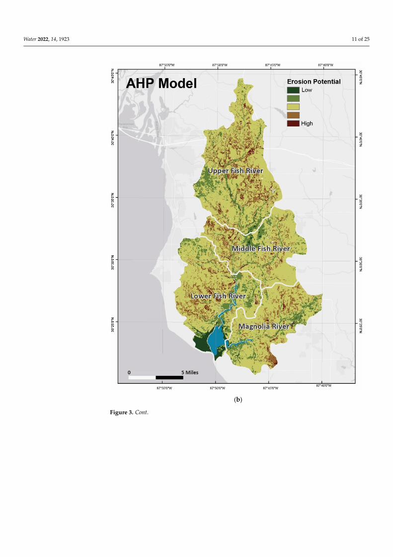
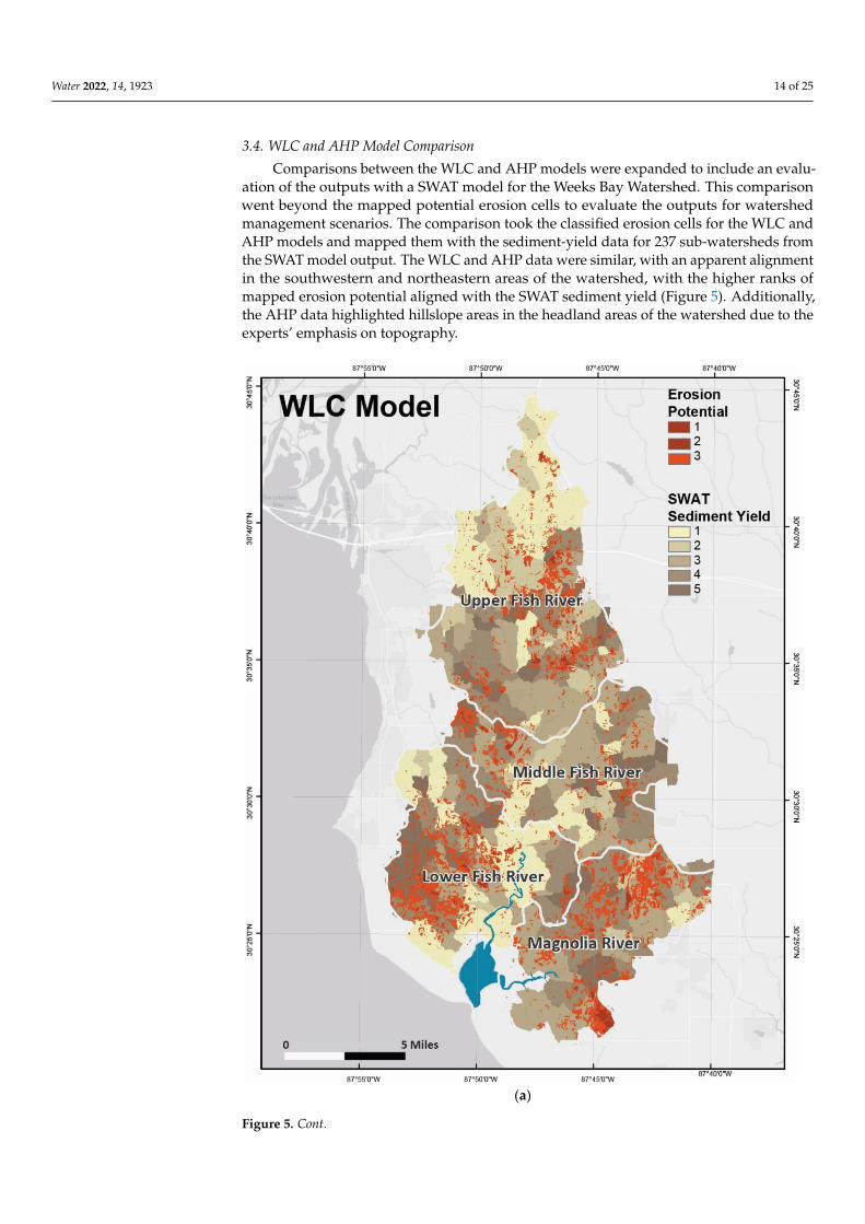