Decision criteria for climate projects1

by

Petter Osmundsen* and Magne Emhjellen**

* University of Stavanger

** Petoro AS

This article analyses commercial decision criteria for climate projects. The latter will

normally be executed by private players, for whom decision criteria developed from a

commercial perspective are important. But such criteria are also important for the government

in calculating the size of subsidies required for various measures. A ranking of different

solutions in a socio-economic context must rest on calculations made from a commercial

perspective. Examples of the subjects covered include the calculation of abatement unit costs

and cost estimating for climate projects. The carbon capture project at the Kårstø gas-fired

power station in south-west Norway is used as a case throughout the analysis.

* Petter Osmundsen, department of industrial economics and risk management, University of Stavanger, NO-4036 Stavanger, Norway. E-mail: Petter.Osmundsen@uis.no, home page: http://www5.uis.no/kompetansekatalog/visCV.aspx?ID=08643&sprak=BOKMAL

** Magne Emhjellen, Petoro AS, P O Box 300 Sentrum, NO- 4002 Stavanger, Norway. E-mail: Magne.Emhjellen@petoro.no

1 Thanks are due to Johan Gjærum, Per Ivar Gjærum, Kåre Petter Hagen and Knut Einar Rosendahl for constructive comments. We would also like to thank a number of specialists in business and the civil service for useful comments and proposals.

1. Introduction

Many socio-economic studies and calculations of climate projects have been conducted.2

However, little attention has been devoted to profitability assessments based on commercial

considerations. Calculating climate projects on that basis is the subject of this article. The

planned carbon capture and storage (CCS) project at the Kårstø gas processing complex north

of Stavanger is used throughout as a case study. This case is unique in a CCS context in the

sense that it contains detailed cost and income data which are publicly available.3 However,

the underlying methodology applied in the article can also be used with other climate projects.

Because of the popularity of the concept of abatement unit costs , we first discuss

how such costs are calculated for CO2 abatements. The article then looks at the profitability of

carbon capture from gas-fired power stations under various conditions and with the aid of the

net present value (NPV) method, which analyses the issue as a now-or-never decision. We

then look at more realistic circumstances in which the carbon capture project could also be

realised at a later date.

We have reviewed the available literature on CCS. The general conclusion appears to

be that CCS at existing gas-fired power stations is not a relevant climate measure today. In a

presentation, McLemore (2008) evaluates CCS from a commercial perspective. He concludes

that the prospects are poor. It would require very substantial investment, while uncertainty

related to future global regulation of carbon emissions is very high. To realise investments in

CCS, the carbon price must be far higher than is the case today.

Aune et al (2009) compare costs for carbon capture from coal- and gas-fired power

stations and industrial emissions. They conclude that retrofitting a capture plant in an existing

power station, which is the solution being studied at Kårstø and at the Mongstad industrial

complex north of Bergen, is clearly the most expensive CCS measure, and that this would not

become profitable until substantial cost reductions or a considerable increase in carbon prices

are achieved.

The International Energy Agency (IEA) notes in the November 2009 issue of its

World Energy Outlook publication that CCS for gas-fired power stations cannot be regarded

at present as a cost-effective measure.

This article has the following disposition. Section 2 explains unit costs for carbon

emission abatement and cites some examples. We also explain the choice of required return

2 See the list of references. 3 For a more detailed project analysis, see Osmundsen and Emhjellen (2010).

from carbon capture projects as an input parameter for our NPV analysis in section 3. In

section 4, we present a simple option value model with one uncertainty variable (carbon

emission allowance prices), and illustrate this with a project example. Section 5 presents

results, and we round off in section 6 with a discussion.

2. Abatement unit costs

Two types of economic calculations are conducted in climate analyses: 1) NPV analyses 2)

calculations of cost annuity, known as abatement unit costs. The first of these represents the

normal decision criterion for projects in both public and private sectors, and provides an

accurate impression of project economics. The second

much used in climate analyses to

compare various treatment measures

is not really a decision criterion but can function as one

under specified circumstances. The basis for this type of calculation is that the climate

problem is global, so it makes no difference which source is used to achieve the emission

abatement.

Annuities seem to have become an established standard for calculating environmental

costs. One advantage is probably the educational aspect

abatement unit cost can be

compared with the price of allowances, and projects of differing duration can be compared.

But today s allowance price is not necessarily comparable with an annuity cost. Allowance

prices will vary over time. Using annuities in a decision context presupposes a stable carbon

price.

Another problem is that the annuity method as such is not actually used in climate

calculations, but only a rough approximation of it. As we understand it, capital expenditure

(Capex) is distributed over the economic life of a measure, but not operating expenditure

(Opex). A reference year is chosen and the carbon price compared with the annuity for Capex

and Opex for a given expected capacity utilisation in the reference year. This is an arbitrary

and discretionary approach, where much depends on the choice of reference year. Using this

type of quasi-annuity in a decision context implicitly includes the assumption that carbon

emissions in the project will reduce steadily over time.

That requirement is not fulfilled for the capture plant at Kårstø because of great

variations in capacity utilisation. This is the actual business concept for the power station

a

flexible facility which can be shut down when relevant prices are unfavourable. When

capacity utilisation in a project varies, as is common in the oil industry, calculations must be

based on the whole cash flow and not simply on a selected reference year. The Norwegian

Water Resources and Energy Directorate (NVE, 2006) bases its calculations for the CCS plant

at Kårstø on 8 000 operating hours. That represents 100 per cent uptime, and is completely

unrealistic. It provides a good example of the strategic choice of reference year.

In other words, the annuity criterion appears to be basically useful for choosing

between various climate measures, since it permits the cost per tonne of carbon emissions

abated to be compared for various measures. But this is not entirely straightforward because

of differing volumes and time frames. Efforts can be made to overcome the problem by

establishing a representative year, but that is incomplete and subject to discretionary choices.

A better solution would be to calculate a genuine annuity for the costs

in other words,

apportion the NPV of all the costs over the expected economic life of the measure.

Strictly speaking, an optimisation model must be used when allocating scarce

investment funds in which total emission abatements are maximised within a given budget

(linear programming).4 A simplified method applied in the business sector is a NPV index.

The NPV of the project is divided by the NPV of the investment to produce a common

indicator for comparing projects. In a climate context, a NPV index could be similarly

compiled, calculated per tonne of emission abatement.

To sum up, the annuity cost will provide a good deal of information if correctly

calculated but is insufficient. It is accordingly important to operate with both annuities and

NPVs. In a number of contexts, the latter are also more informative for the general public.

The fact that a carbon capture measure, for instance, costs USD 330 per tonne is worth

knowing, 5 but so is information on the scale involved

the overall investment required and

the fact that the NPV would be negative at USD 1.7 billion, for example. The portfolio of

possible projects must be measured against available funds. This should be supplemented by a

cash-flow analysis

overall and for individual projects

and an analysis which shows the

burden on government budgets over time.

The discussion on annuity calculation for abatement unit costs will be illustrated more

formally below. A company is indifferent about investing in a climate project if the NPV is

zero

in other words, where the NPV of the carbon abatement gain (expressed as the NPV of

4 See Emhjellen et al (2006). 5 Monetary amounts have been converted from Norwegian kroner (NOK) to US dollars (USD) at an exchange

rate of NOK 6 = USD 1.

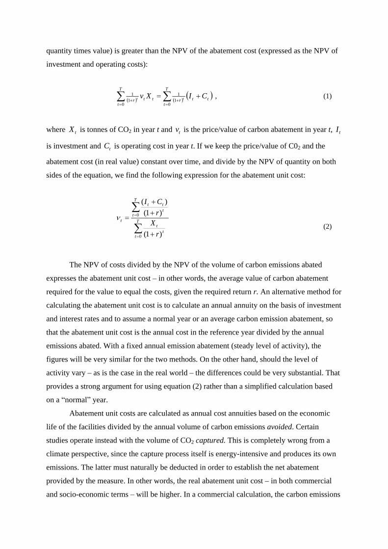
quantity times value) is greater than the NPV of the abatement cost (expressed as the NPV of

investment and operating costs):

T

tttr

T

tttr

CIXv tt

01

1

01

1 , (1)

where tX is tonnes of CO2 in year t and tv is the price/value of carbon abatement in year t, tI

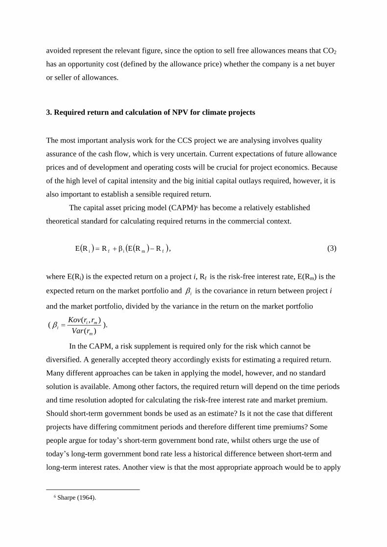
is investment and tC is operating cost in year t. If we keep the price/value of C02 and the

abatement cost (in real value) constant over time, and divide by the NPV of quantity on both

sides of the equation, we find the following expression for the abatement unit cost:

T

tt

t

T

tttt

t

r

Xr

CI

0

0

)1(

)1(

)(

(2)

The NPV of costs divided by the NPV of the volume of carbon emissions abated

expresses the abatement unit cost

in other words, the average value of carbon abatement

required for the value to equal the costs, given the required return r. An alternative method for

calculating the abatement unit cost is to calculate an annual annuity on the basis of investment

and interest rates and to assume a normal year or an average carbon emission abatement, so

that the abatement unit cost is the annual cost in the reference year divided by the annual

emissions abated. With a fixed annual emission abatement (steady level of activity), the

figures will be very similar for the two methods. On the other hand, should the level of

activity vary

as is the case in the real world

the differences could be very substantial. That

provides a strong argument for using equation (2) rather than a simplified calculation based

on a normal year.

Abatement unit costs are calculated as annual cost annuities based on the economic

life of the facilities divided by the annual volume of carbon emissions avoided. Certain

studies operate instead with the volume of CO2 captured. This is completely wrong from a

climate perspective, since the capture process itself is energy-intensive and produces its own

emissions. The latter must naturally be deducted in order to establish the net abatement

provided by the measure. In other words, the real abatement unit cost

in both commercial

and socio-economic terms

will be higher. In a commercial calculation, the carbon emissions

avoided represent the relevant figure, since the option to sell free allowances means that CO2

has an opportunity cost (defined by the allowance price) whether the company is a net buyer

or seller of allowances.

3. Required return and calculation of NPV for climate projects

The most important analysis work for the CCS project we are analysing involves quality

assurance of the cash flow, which is very uncertain. Current expectations of future allowance

prices and of development and operating costs will be crucial for project economics. Because

of the high level of capital intensity and the big initial capital outlays required, however, it is

also important to establish a sensible required return.

The capital asset pricing model (CAPM)6 has become a relatively established

theoretical standard for calculating required returns in the commercial context.

fmifi RRERRE , (3)

where E(Ri) is the expected return on a project i, Rf is the risk-free interest rate, E(Rm) is the

expected return on the market portfolio and i

is the covariance in return between project i

and the market portfolio, divided by the variance in the return on the market portfolio

()(

),(

m

mii rVar

rrKov).

In the CAPM, a risk supplement is required only for the risk which cannot be

diversified. A generally accepted theory accordingly exists for estimating a required return.

Many different approaches can be taken in applying the model, however, and no standard

solution is available. Among other factors, the required return will depend on the time periods

and time resolution adopted for calculating the risk-free interest rate and market premium.

Should short-term government bonds be used as an estimate? Is it not the case that different

projects have differing commitment periods and therefore different time premiums? Some

people argue for today s short-term government bond rate, whilst others urge the use of

today s long-term government bond rate less a historical difference between short-term and

long-term interest rates. Another view is that the most appropriate approach would be to apply

6 Sharpe (1964).

the government bond rate which lies closest to the duration of the project, because that

provides the most accurate reflection of the risk-free capital commitment for a given period.

Where a market portfolio is concerned, the normal approach today would be to consider a

world portfolio

often represented by a proxy, such as Morgan Stanley s world index. The

question then is which currency should be used. Should this be the currency of the project

country or the one in which the bulk of the costs or revenues is denominated?

Despite differing views on the principles for selecting the correct risk-free interest rate

and market premium, model users will in practice often opt for estimates based on figures

from historical periods and today s financial markets. The same will have to be done for

estimating beta, with an ex post estimate used to specify an ex ante estimate for beta based on

share prices in a listed company. However, a practical problem arises when no representative

listed company is available with virtually the same system risk as the project. What is then to

be done? As far as we can see, no market data are available which can say anything about the

way investors regard the net cash flow risk for a CCS project at a gas-fired power station. As

a result, no exact basis exists for estimating the project beta. An alternative could be to look at

the beta for different cash flows in a project.

It follows from the value additivity principle (Shall, 1972) that the NPV of a project is

provided by the sum of the NPVs of the project s subordinate cash flows:

iM

1jiji XV , (4)

where Xij is the NPV of the individual cash flow j in project i discounted by the correct

required return for j, E(Rij). Mi is the number of subordinate cash flows in project i. The

expected return for a project is equal to the sum of the value-weighted expected return for the

individual cash flows:

iM

1jijiji REwRE . (5)

In equation (5), we have i

ijij V

Xw

and iM

1jij 1w . From the CAPM, the expected return for

the individual cash flow j can be written as:

fmijfij RRERRE )( . (6)

By integrating (6) in (5), i can be written as

iM

1jijiji w . (7)

With a carbon abatement project where no observable required return can be found for

a company or a project which makes it possible to estimate the investors assessment of the

systematic risk for the net cash flow, better information might be available on the risk for the

subordinate cash flows in the project. These can then be valued separately.

3.1 Calculated required return for a CCS project

We will seek in the following to analyse systematic risk in CCS projects. Investment costs for

such projects comprise various development expenditures for the capture facility as well as

transport and storage (injection below ground). Much of this risk will be unsystematic, but

such aspects as steel prices, equipment deliveries and hourly pay rates are likely to involve

systematic risk since these will often be correlated with GDP growth. That also applies to

hourly rates related to operating costs. Another cost relates to energy prices, since substantial

amounts of electricity and steam are required to operate the capture plant. Market information

will be available here. The revenue side for a CCS facility is the value of the carbon abated.

Information available from the allowance market can be used in this context to estimate a

required return. However, the time series are short, feature many structural shifts related to

political conditions and provide limited opportunities for predictions. But allowance prices

can be seen to move in step with the level of economic activity, and consequently contain a

systematic element which recalls the volatility of oil and gas prices. Gas and carbon prices

will typically be correlated because a high level of the former makes it more expensive to

switch from consuming coal, and the carbon price must accordingly rise if emissions are to be

abated. Electricity prices also move in line with oil and gas prices. See Asche et al (2006). As

a result, both revenue and cost sides will be related to the systematic risks faced by oil

companies. The underlying activities in the project

development, transport and injection

are also the same as in the petroleum sector. In addition, we assume that

should the project

be approved

it will be executed as a turnkey delivery by an oil company of a certain size and

experience. These have the best qualifications for managing such a complex project.7

A number of calculations have been made and surveys conducted on required returns

in the oil industry. Since these are often not directly comparable, however, a number of

challenges are faced with regard to consistency. The same risk-free interest rate, for instance,

is meant to be incorporated in the first and second stages of the CAPM. This is a logical

standard which has been carefully documented in the literature

see Damodaran (2002), p

161, for instance

and which must be observed. However, that requires a substantial

commitment since the people calculating the market premium generally do not in fact specify

the risk-free interest rate they have applied. A nominal required return is also often used, so

that separate adjustments must be made for inflation.

The oil companies use the CAPM to calculate a starting point for the required return,

but then add management-related

premiums. One reason given for this is the need to ration

capital in order to avoid growth costs when the organisation has more prospective prospects

than it can handle. This consideration is less relevant today than it used to be. Most of the

large oil companies are currently struggling to replace their reserves and do not have the same

need as before to ration their resources.

Management-related premiums make it relevant to identify the required return actually

applied by the oil companies. The Boston Consulting Group (2005) concludes that 12% is a

representative real required return. The real discount rate (assuming 2.5% inflation) for total

capital varied between 5.5% and 15%, with a 10% average. Goldman Sachs (2000), Global

Equity Research, specifies an actual nominal required return in the petroleum sector of 13-

18%, with a median of 15.5%. Another relevant survey for the nominal required return on

capital employed is reproduced in Gjesdal and Johnsen (1999), table 1.17. An unweighted

average for the four participating companies was 12.8%.

Where our case is concerned, a good deal of international commercial literature is

available on estimating the cost of CCS facilities for coal-fired power stations. See Al-Juaied

and Whitmore (2009) for an overview. The real required return applied in these analyses is

10%.

A required return is very dependent on the time when it is estimated, since the risk-

free interest rate in particular varies a great deal over time. In addition, beta and the expected

7 Were a different kind of organisation chosen to execute the project, or were contracts with complex interfaces selected, we would have had to increase the cost estimate substantially while reducing the probability of success.

market premium could naturally vary a lot. For practical purposes in this analysis, we have

chosen to estimate beta on the basis of beta figures for a selected industrial group. See

Damodaran s website.8 We believe that the power (equity beta without debt of 0.46) and oil

and gas integrated (0.74) industry groups can provide an indication of an interval for beta in a

CCS project. Selecting 0.7 as an estimate for beta, a relatively high market premium of 6%

and a long-term risk-free interest rate of 4% gives us an estimate of 8.2% for the nominal

required return. Assuming 2% inflation, this yields a real required return of 6.2% (given 100%

equity), which we round off to 6%. We will apply this conservative required return in our

calculations.

An alternative, based on the separate cash flow valuation method discussed briefly in

chapter 3, would be to estimate separate betas for investment cost, operating cost and revenue

cash flow from allowances prices (multiplied by carbon abatement volumes). A reasonable

proxy for the investment cash flow could then be the construction industry group with an

unlevered beta of 0.54 (Damodaran, NYU, January 2010, net), while operating costs

incorporating a large proportion of power-related expenses could have a systematic risk

related to this industry group (unlevered beta of 0.46). The question then is which industry

group would be closely linked to the systematic risk presented by allowance prices. Claims

could be made that this represents a basic requirement for the world in the future. That could

be an argument for a beta similar to industry groups such as power (0.46), water utilities

(0.34) and general utilities (0.38). On the other hand, many people could claim that allowance

prices are likely to be highly volatile for the foreseeable future and more likely to resemble oil

and metal prices (oil/gas production and exploration 0.96 and precious metals 0.74). A

separate cash flow valuation analyses of this project, with a higher discount rate for revenue

than for costs, would have the effect of reducing its NPV. The estimated betas above are

calculated from their relative share price movements. This assumes that such movements are

caused by information related to changes in future net cash flow for the companies. Since net

cash flow is revenue less cost, an additional problem arises when using the net cash flow beta

to estimate the cost of revenue beta in that we do not know their relative weights or their

sizes. Information may be available in the market prices of oil, metals, gas and electricity

which can be used to estimate revenue betas. This could be a topic for further research, but we

go no further with this approach here.

8 http://pages.stern.nyu.edu/~adamodar/

4. Cost estimation

To make a commercial calculation of the CCS project at Kårstø, we must first obtain a cost

estimate based on a commercial standard. We have reviewed the cost estimates in NVE

(2006), and have the following comments and adjustments:

a) Has sufficient account been taken of an asymmetric cost distribution?

When costs are asymmetrically distributed (overruns are more likely than

underspending

a long right-hand tail in the distribution), and inadequate account is

taken of this when estimating the costs, the estimates obtained will not be accurate in

terms of expectations. This is a particularly relevant issue for immature

groundbreaking projects like the CCS development at Kårstø. In analysing petroleum

projects, Emhjellen et al (2002, 2003) find that the oil industry underestimates costs

by 10% because it fails to take sufficient account of the asymmetrical cost distribution.

We have applied this percentage as a correction to Capex. That represents a cautious

adjustment for the CCS project, given the long right-hand tail in the cost distribution

for immature projects.

b) Has sufficient account been taken in the cost estimate of utility systems and the early

phase of the project?

Utilities

including compressors and cooling systems

can be underestimated. To

adjust for this, we have increased Capex by 10%.

c) The NVE operates with a contingency reserve of 18%. A number of factors argue for

a higher figure. 1) This is a mega-project involving substantial management

challenges. 2) The plant will scale up existing capture facilities by 10 times their

current size, and represents a groundbreaking technological development. 3) The

project has a demanding interface with the political authorities, who give varying

signals. 4) Contingency reserves are normally higher in the early phase and decline as

the project matures. We have adjusted the contingency reserve to 40%, which

represents a normal overrun for this type of mega-project.9 In other words, we have

increased the NVE s contingency reserve by roughly 20%.

d) Cambridge Energy Research Associates (CERA) has a cost index for land-based

petroleum fields, which has risen by 40% from 2006 to 2008. We have upwardly

adjusted Capex by 40%.

The oil industry is criticised from time to time for taking a conservative approach in its

investment analyses, including applying an excessive contingency reserve to cope with

unforeseen costs and being too restrained in estimating revenues. However, empirical

evidence indicates that the average project nevertheless experiences cost overruns. A pertinent

question is whether the companies are sufficiently varied in tailoring their practice to the

individual project, or largely use the same methods to assess both big immature projects such

as CCS and circumscribed and mature developments such as supplementary work on

producing fields. A number of observations indicate that the risk allowance made by the

companies is too small in immature projects and excessive in small and mature developments.

Our revised cost estimates are similar to the figures reached in the Climate Cure

report, and it is not our impression that the estimates are controversial. A contribution in our

approach is to explain in some detail how we have adjusted the costs, thus indicating how it

was possible for NVE to seriously underestimate the costs four years ago.

4.1 Operating period

Generally speaking, the Kårstø gas-fired power station will generate electricity when the

clean spark spread

(electricity price

(gas price + allowance price )) is positive in other

words, when the price of power is greater than the sum of gas and allowance prices. However,

the picture is somewhat more complicated. Account must also be taken of other variable

operating costs. Furthermore, costs are incurred during start-up and shut-down in swing

production, which makes this a dynamic optimisation problem. Swing costs are said to been

higher than expected. The power station has long stood idle for lengthy periods. However, gas

prices (with opportunity costs/revenues corresponding to spot prices in Europe) have

contributed in recent months to the power station remaining operational even in periods when

9 Flyvberg et al. (2003).

electricity prices have been relatively low. Forecasting the future clean spark spread is

difficult. The Norwegian electricity market is characterised by excess capacity and low prices.

Future developments will be determined in part by the extent to which power-intensive

industry is phased out, the development of new generating capacity, demand trends and the

scope of new power transmission cables to other countries. The gas market is currently weak

because of the financial crisis and increased supply in the form of liquefied natural gas (LNG)

and shale gas, but is expected to recover. Allowance prices have been weakened in the wake

of the financial crisis, but are also expected to increase. The net effect here is uncertain, but

political moves in the direction of low electricity prices in Norway do not augur well for the

Kårstø power station s uptime.

This facility currently enjoys free allowances which expire in 2012. A recent European

Union directive (2009/29/EC) has proposed that free allowances cease for power stations after

2012. Since the Kårstø station has sold free allowances when it has been shut down, however,

the allowance price has always represented an opportunity cost when reaching operational

decisions.

4.2 Cost estimate in 2009 and calculation of abatement unit cost

We have increased Capex by 80% in relation to NVE (2006), comprising a 40% increase in

industry costs since 2006, an increase of 20% in the contingency reserve, a 10% adjustment to

obtain an accurate value estimate and 10% for utilities. After rounding off, we apply the

following investments in our project analyses.

Investment in treatment plants 1 000

Investment in transport and storage 500

Total 1 500

Table 3.1: Revised cost estimate for CCS at Kårstø in USD million, 2010 value.

The project can potentially abate carbon emissions by about one million tonnes per

year (the NVE estimate is 1.05 million tonnes). We estimate that the actual abatement will be

only 50% of this level, since the gas-fired power station is expected to be operational for half

the time. Estimated operating costs in the NVE report totalled USD 62 million (including an

anticipated 15.7% output loss for the power station). We round this up to USD 75 million in

2010 value per annum

again based on the immaturity and uncertainty of the estimate as well

as some upward adjustment to the output loss, which is lower in the NVE analysis than in

other estimates. The NVE report expects the plant to have an economic life of 25 years. We

assume a real required return of 6%.

Based on equation (2), we obtain an abatement unit cost of USD 192 per tonne of CO2.

v=(1500+960)/12.8=192 (8)

The figure above assumes 100% uptime (8 000 hours per year) which captures an

annual volume of about one million tonnes of CO2. Halving the operating time, which is more

realistic, will almost double the abatement unit cost since the investment will be the same.

Some studies operate with the volume of captured CO2 rather than the more correct net gain

in carbon abatement (the capture process requires energy and produces emissions), or avoided

CO2. With these important adjustments, the abatement unit cost will rise to more than USD

333 per tonne. This is 20 times higher than today s allowance price in the EU, which currently

ranges from USD 13-16 per tonne.

Figure 1: Abatement unit cost for carbon capture at Kårstø with varying percentages of uptime.

0

100

200

300

400

500

600

30%

40%

50% 60% 70% 80%

90%

100%

Abatement cost Abatement cost adjusted net CO2

As we can see from figure 1, the abatement unit cost will rise substantially with reduced

operating time because of the big early investment, which must be distributed over a lower

volume of carbon abatement.

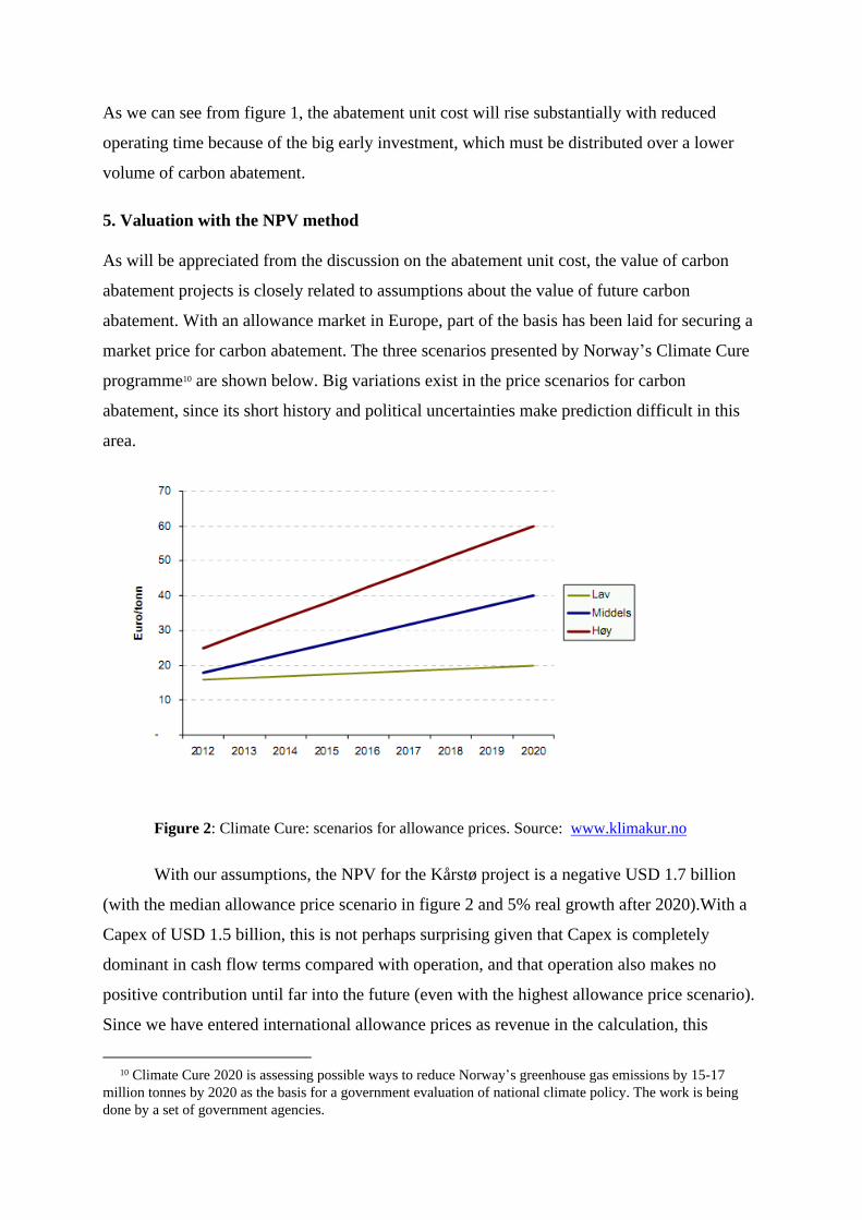
5. Valuation with the NPV method

As will be appreciated from the discussion on the abatement unit cost, the value of carbon

abatement projects is closely related to assumptions about the value of future carbon

abatement. With an allowance market in Europe, part of the basis has been laid for securing a

market price for carbon abatement. The three scenarios presented by Norway s Climate Cure

programme10 are shown below. Big variations exist in the price scenarios for carbon

abatement, since its short history and political uncertainties make prediction difficult in this

area.

Figure 2: Climate Cure: scenarios for allowance prices. Source: www.klimakur.no

With our assumptions, the NPV for the Kårstø project is a negative USD 1.7 billion

(with the median allowance price scenario in figure 2 and 5% real growth after 2020).With a

Capex of USD 1.5 billion, this is not perhaps surprising given that Capex is completely

dominant in cash flow terms compared with operation, and that operation also makes no

positive contribution until far into the future (even with the highest allowance price scenario).

Since we have entered international allowance prices as revenue in the calculation, this

10 Climate Cure 2020 is assessing possible ways to reduce Norway s greenhouse gas emissions by 15-17 million tonnes by 2020 as the basis for a government evaluation of national climate policy. The work is being done by a set of government agencies.

negative USD 1.7 billion will also provide an estimate for the extra cost to Norway of abating

carbon emissions through this particularly cost-intensive measure rather than buying

allowances. The NPV corresponds to an annuity of just over USD 133 million, which will be

an estimate for the annual subsidies required to implement the CCS project at Kårstø.

Figure 3 presents cash flows for the project under the three price scenarios (we have

also assumed a 5% real growth rate for prices from 2021 to the end of the project s economic

life in the two other price scenarios). The extremely high level of investment in relation to

revenue means that the project is very negative under all the scenarios. The negative NPVs

are USD 2 billion and USD 1.3 billion for the low- and high-price scenarios respectively.

Note that the whole cash flow is negative under the low-price scenario. With the median price

scenario, cash flow first becomes positive in 2029. In other words, the project will deliver a

negative NPV even without the high investment costs. Should the company have other taxable

revenues in Norway, the annual losses would be somewhat reduced through tax consolidation

and the NPV would not be quite so negative.

-1600

-1400

-1200

-1000

-800

-600

-400

-200

0

200

400

2011

2013

2015

2017

2019

2021

2023

2025

2027

2029

2031

2033

2035

Base Low High

Figure 3: Cash flows before tax.

It is otherwise unclear whether the estimate used by the Climate Cure for future allowance

prices takes full account of the latest trends in this area. An annual increase of 10% in

allowance prices might seem optimistic. The inability to reach agreement on a new climate

agreement in Copenhagen as well as a politically weakened President Obama are not

encouraging for a rise in allowance prices. The financial crisis has also caused a decline in

carbon prices (and emissions) because the economic recession has weakened the ability and

willingness to implement cuts. A steady growth curve for carbon prices accordingly seems

unlikely. A company considering whether to invest in a climate project which involves

irreversible investments will probably apply relatively conservative estimates for allowance

price developments. This makes it not unlikely that the lowest curve in the Climate Cure

scenarios would be the one chosen by such a company.

We have made conservative estimates for operating costs in calculating NPV. Like

NVE (2006), these are kept fixed in real prices. That contrasts sharply with the revenue side,

which increases by 10% per annum. Operating costs largely comprise electricity, gas and

payroll. It is reasonable to assume real price growth for these. And a sharp rise in carbon

allowance prices and constant prices for electricity and gas do not necessarily appear mutually

consistent. A company is unlikely to make these assumptions, and its estimate of the

commercial NPV would probably be below rather than above the one we have calculated.

We have made a very substantial upward adjustment to Capex. However, the

conclusion that the project is extremely unprofitable is very robust. At our estimated Capex of

USD 1.5 billion, the project has a negative NPV of almost USD 1.7 billion. In other words,

the project economics are also very poor even with a much smaller increase in Capex

and

actually without any adjustment at all.

Figures 4 and 5 below present the NPV and abatement unit cost for 100% and 50%

project uptime respectively under the Climate Cure s median allowance price scenario.

Because the cash flow is totally dominated by Capex, and the project generates only a small

cash flow during its operating phase

see figure 3

the NPV shows little alteration when

changes are made to the required return. A rather unusual result is that the NPV actually rises

(becomes less negative) when the required return increases. This is because net cash flow in

the operating phase is negative. For the same reason, NPV goes up when uptime declines. The

abatement unit cost rises with an increase in the required return, but its level is determined

first and foremost by operating time. We have assumed that operating costs are 50% lower at

50% uptime. This is probably an optimistic assumption.

-2200

-2000

-1800

-1600

-1400

-1200

-1000

-800

-600

-400

-200

0

200

400

5% 6% 7% 8% 9% 10%

NPV Abatement cost

Figure 4: Net present value and abatement unit cost at various discount rates (100% uptime) Positive

figures are costs in USD per tonne CO2 abated. Negative figures are NPV in USD billion (reference

year for NPV is the year before project start, here 2011).

-2000

-1800

-1600

-1400

-1200

-1000

-800

-600

-400

-200

0

200

400

600

5% 6% 7% 8% 9% 10%

NPV Abatement cost

Figure 5: Net present value and abatement unit cost at various discount rates (50% uptime)

Positive figures are costs in USD per tonne CO2 abated. Negative figures are NPV in USD

billion (reference year for NPV is the year before project start, here 2011).

How high must the allowance price be over time for the project to be profitable? If we

assume a price development in line with the highest estimate in the curve above

EUR 26 per

tonne in 2012

and that the price rises by 14.5% per annum to EUR 670 per tonne in 2036,

our example project will yield a marginally positive NPV with a 6% real required return. In

other words, the allowance price in 2036 must be the equivalent of USD 617 per tonne for the

project to pay. This is very unlikely, and substantially above the highest estimate made by the

Climate Cure. The unrealistic allowance price scenario will be outside figure 2, with an

allowance price of EUR 77 per tonne in 2020 and EUR 151 per tonne as early as 2025.

Even with quota prices at this level, however, it is not given that the project will be

realised. This is because one forgets that these projects can be initiated at a later date when

more information has become available. There is basically little point in analysing the option

value of waiting when a deterministic NPV analysis shows that the project is highly

unprofitable (would not be commenced in any event). However, it could be relevant to

demonstrate in general terms that, even with an expected positive NPV, climate projects will

not be launched when uncertainty over the value of carbon abatement is high. Postponing a

decision on CCS at Kårstø would give access, for instance, to new and improved technology,

a clarification of the feasibility of integrating capture with transport and storage, and more

information about developments in energy and allowance prices. When retrofitting in an

existing power station, on the other hand, allowance must be made for the fact that the

generating facility has a limited economic life.

It could be interesting to calculate how large a subsidy would be required per kilowatt-

hour generated by the station. Applying our basic assumption of 50% capacity utilisation for

the facility (of a total of 8 000 hours) gives us 4 000 operating hours. Generating capacity is

420 megawatts, or 354 MW after adjusting for the loss of output from CCS. This yields an

annual electricity output of 1.4 terawatt-hours. Realising a development with a negative NPV

in the order of USD 1.7 billion would therefore require a fixed asset subsidy (one-off

payment) of just under USD 1.2 per kWh of expected annual output. Alternatively, this

support could be provided in the form of roughly USD 0.1 per kWh spread over the whole

economic life of the facility. Assuming the normal spot price for power in Norway, that

represents more than double the price of electricity from the station.

Based on the discussion of the appropriate required return for various cash flows, one

option could be to look at the required return for the various cash flows in a carbon abatement

project for a gas-fired power station. A possible breakdown based on the probable level of

systematic risk could then be obtained by applying different discounts for different types of

subordinate cash flows. It could be appropriate in this context to place investment and

operating costs in one group, and the value of abatement (allowance price) and loss of power

sales (because of reduced generating capacity) in another. Equation (2) can then be written as:

T

tt

t

T

tt

tT

tttt

a

Xa

C

c

CI

v

0

0

2

0

1

)1(

)1()1(

)(

(9)

Where 1tC is operating cost in year t and 2

tC is the loss of power sales in year t. c and a

are

new discount rates which reflect systematic risk for investment and operating costs

respectively versus the value of carbon emission reductions and prices for lost electricity

sales. Emhjellen and Osmundsen (2009) find that investment and operating costs have a lower

systematic risk than raw material prices. In our example project, if c is 6% in real terms and

a

is 10% in real terms, the abatement unit cost will be USD 240 per tonne with full capacity

utilisation of the power station. This illustrates that setting the correct level for the required

return is crucial in estimating the level of abatement unit cost. That naturally also applies

when using the same required return for all cash flows (net cash flow), which is the usual

approach in practice.

6. Valuation with option pricing

The NPV method gives the value of the project for a now-or-never decision, which takes no

account of the opportunity to initiate projects at a later date when more information has

become available. The option value of waiting can be quantified by the use of decision trees

or by more formalised methods such as option value formulae or stochastic programming. A

key element in the option concept is decision flexibility

the opportunity to amend project

design or decisions when new information becomes available.

6.1 Example

The basic concepts can be illustrated with a simplified example based on our CCS case, since

this is fundamentally unprofitable in commercial terms. We therefore modify the case to

illustrate the option point

enhancing profitability by applying unrealistic assumptions in the

form of 100% uptime and a very high net allowance price (allowance price less operating

costs).

A company is considering an irreversible investment in carbon abatement. The project

requires an initial investment of USD 1.5 billion and will yield a carbon abatement of one

million tonnes per annum on a permanent basis. The net allowance price for one tonne of CO2

is expected to be USD 83 (USD 158 gross because of USD 75 spent on operation), but the

price will change in year one. There is s probability that the allowance price will be high

(USD 133 per tonne) and (1-s) that it will be low (USD 33). Following the price change, the

net allowance price will remain unchanged for ever. In addition, we assume that the risk

related to the future net allowance price is completely diversifiable (in other words, unrelated

to the macro economy). Consequently, the company must discount future cash flows by the

risk-free interest rate, which we set at 4%.

If s is 0.5, the NPV is given by:

NPV= -1500+1

575)04.1(83t

t . (10)

The NPV is positive and USD 575 million

which indicates that the investment must

be made now. This is not correct, however, since the calculation ignores the opportunity cost

related to investing now instead of waiting and thereby retaining the opportunity to refrain

from investing if the allowance price falls. If we assume that it is possible to postpone the

start to the investment by one year, the expected NPV is given by:

NPV=0.5 1883)04.1(13304.1/15001t

t . (11)

The result shows that it would be correct in to wait for a year before investing. Increased

information about quota prices means that the investment can be avoided if allowance prices

are low. In this case, the flexibility option is worth 1308 million USD (1883 less 575).

In more general analyses of the value of waiting with carbon capture projects,

uncertainties about allowance prices and expected future reductions in carbon abatement costs

(technology advances) will make it commercially appropriate to postpone such developments

for gas-fired power stations even with allowance prices substantially higher than today s.

An existing power station will have a limited economic life. Should a decision on

retrofitting be postponed, the remaining economic life would be reduced

which would lower

the value of waiting for this specific case. That type of time-criticality would not apply to

carbon abatement projects for new power stations.

6.2 A common stochastic process for modelling price uncertainty

Another assumption made in the practical modelling of an uncertain variable is that the

uncertain variable follows some stochastic process. Practical asset pricing models using

option theory make use of such processes in their approach to valuation (Lohrentz and

Dickens, 1993). The most common stochastic process used in modelling uncertainty related to

projects is the geometric Brownian motion with drift (Dixit and Pindyck 1994).

Geometric Brownian motion with drift has the following characteristics:

xdzxdtdx

, (12)

and 2

1

))(( dttdz

with )1,0(~)( Nt . is a constant drift variable, and

is a constant

variance parameter. Because percentage changes in x are normally distributed, and since these

changes are in the natural logarithm of x, the absolute changes in x are lognormally

distributed.

If x(t) is given by equation (12) then F(x)=log x is given by:

dzdtdF )( 212 , (13)

so that, over a finite time interval t, the change in the logarithm of x is normally distributed

with mean t)( 212

and variance t2 . For x itself, if x(0) =x0, the expected value of x(t)

is:

textx 0)( , (14)

and the variance of x(t) is:

)1()(222

0 eextxv t (15)

This result for the expectation of a geometric Brownian motion can be used to

calculate the expected present value of x(t) over some time period. For example:

)/()( 0

0

)(0

0

rxdtexdtetx trrt , (16)

provided the discount rate r exceeds the growth rate .

6.3 Obtaining values

Dixit and Pindyck (1994), p 151, show that, providing the uncertain variable follows a

geometric Brownian motion, the value of the option F(V) must satisfy

0)`()()``(2212 rFVVFrVFV

, (17)

Subject to the boundary conditions:

F(0)=0, (18)

F(V)=V*-I, (19)

F'(V*) =1 . (20)

where I is the project development cost. Equation 18 arises from the observation that if V

goes to zero it will stay at zero. The option to invest will therefore be of no value when V=0.

V* is the price at which it is optimum to invest, and (19) is the value-matching condition

where the firm receives V*-I if it invests. Finally, condition (20) is the smooth pasting

condition where, if F(V) were not continuous and smooth at the critical exercise point V*, one

could do better by exercising at a different point.

To satisfy condition (18), the solution must take the form;

KAVVF )( , (21)

where K is a known constant whose value depends on the parameters and on the differential

equation. By substituting (20) into (18) and (19) and rearranging:

IK

KV

1* , (22)

and

11** )(/)1()/()( KKKK IKKVIVA . (23)

The value of the investment opportunity is given by equations (21) to (23). Because

K>1 and V*>I, irreversibility and uncertainty give a different decision criterion than the

deterministic NPV rule.

Function 20 satisfies function 17 given that K is a root of the quadratic equation:

0)()1(212 pKrKK

The first root is (the first boundary equation rules out the second root):

22^

2212 /2

2

1/)(/)( rrrK

6.4 The example

We use our previous assumptions related to the Kårstø carbon abatement project.

To recap, this involves a new development with an indeterminate economic life and an

investment in year zero of USD 1.5 billion. The project abates carbon emissions by one

million tonnes per annum with annual operating costs of USD 75 million. The real required

return (r) is assumed to be 6%.

Given these assumption, we simplify further by assuming that operating costs are

fixed and part of the investment at time zero. I is then equal to USD 2 750 million (investment

plus present value of operating cost at r equal to 6%). We show values for sigma from 0.01 to

0.2.

Table 6.4 Assuming an expected price of USD 165 per tonne (yield 6%)

Option multiple (K/K-1) (two decimals)

V*

(K/K-1)*I

Option value of waiting, F(V)

0.01 1.029 2831 81

0.05 1.155 3177 427

0.1 1.33 3667 917

0.15 1.53 4226 1476

0.2 1.77 4861 2111

The results show that the option multiple and the option value of waiting increase with

the uncertainty in price (sigma). Since the uncertainty of the future emission allowance price

is large, it is reasonable to suggest that, even with an allowance price of USD 165 per tonne,

the project is a long way from implementation because of the high option value of waiting.

The option value of waiting will decrease with a rise in the payout ratio (the expected price of

emission allowances). With a yield of 10%, indicating a carbon price of USD 275 per tonne, the option

multiple is 1.22 and the option value decreases from 1476 to 608 million USD (with sigma equal to

15%). The current carbon price is a long way short of these levels, of course, which makes this point

rather irrelevant.

With an investment of USD 1.67 billion, down from USD 2.75 billion, F(V) would be 375

million USD (at sigma 0.15, yield 6% and r equal to 6%). The option value of waiting is reduced from

1476 to 375 million USD owing to the increased profitability of the project. Of greater interest,

however, is today s expectation that the real value of carbon removal costs will decline in the future as

a result of technology development. That will increase the option value of waiting, since investors will

believe that carbon removal may be achieved more cheaply in the future. The combined effect of

today s low emission allowance price, the high level of uncertainty in emission allowance pricing and

expectations of lower investment costs in the future will be detrimental to making carbon investments

now because the option value of waiting will be large.

6.5 Assessment of an option pricing approach for practical calculation of the carbon

project value

Many assumptions must be made in order to calculate the option value of waiting. The results

should therefore only be used as an indication that a positive NPV is not enough to ensure

implementation of the project. We mention below some of the problems related to the

quantifications necessary when trying to quantify real options.

Figlewski (1997) has noted that the logarithmic diffusion process does not hold for

security prices. He states that absolute changes in security returns do not follow a lognormal

distribution as required, that volatility changes over time, and that the actual distribution of

security returns has "fat tails". There are more very large changes and very small changes than

a lognormal distribution calls for (Figlewski (1997), p 6).

Use of the lognormal diffusion process in option pricing is therefore approximate. The

assumption that the model holds for asset values or asset prices is not usually justified, and its

use could introduce unknown errors into the valuation process.

Even if some logarithmic model is assumed to describe the future behaviour of prices,

it is difficult to see how the problem of defining the model and its parameters can be solved.

That is particularly the case since a long-term market for CO2 does not exist.

Even if a constant sigma is assumed, the problem of obtaining an estimate for sigma

remains. Implied volatility cannot be calculated because no long-term (10-15 years) futures

market exists for CO2. Estimates for the sigma of prices using historical data, which are very

short for CO2, are at best approximations of the true ex ante sigma owing to the fact that

sigma changes over time (Figlewski, 1997).

Using the historical behaviour of prices to create a model which explains the future

behaviour of prices rests on the assumption that past behaviour will reflect future behaviour.

That is at best a strong assumption. In addition, the absence of a long-term market leaves one

observing short-term future prices. The dynamics of short-maturity futures prices may be

significantly different from the dynamics of long-maturity futures prices. In utilising data on

short-maturity futures to value assets with long horizons, significant room for estimation error

arises.

(Baker et al, 1998 p 144.)

Sick (1990) questioned the sense of utilising hypothesised oil price models to calculate

option values for oil projects. It makes little sense to use numerical techniques to calculate

the option price to an accuracy of 1% or 2% when the underlying asset price is only known to

an accuracy of 10%, as in real options.

The arguments above are valid and raise issues concerning the actual size of the

estimate concerning the option value of waiting. However, in the case of carbon projects it is

likely that this option value of waiting will be large.

7. Discussion

We have shown that abatement unit costs for climate measures should take the whole

economic life of the project into account, not just a selectively chosen reference year. That

applies particularly to our case, CCS, since uptime can vary a great deal from year to year.

Low expected uptime gives high expected abatement unit costs. The same objection applies,

for instance, to calculating the supply of electricity from shore for power offshore fields. On

existing fields, plateau production will end after some years and the production profile go into

decline. Average production over the remaining economic life of the field will accordingly be

lower than the plateau level. Choosing a base year during the plateau production phase will

accordingly overestimate production (and the volume of CO2 emitted)

in other words, the

actual abatement unit cost would be underestimated. This illustrates that genuine annuities

should generally be used when calculating abatement unit cost. That applies in particular to

the petroleum sector, where capacity utilisation in a facility can vary a great deal over time.

Our conclusion in relation to the case is that CCS at Kårstø is a very unprofitable and

cost-inefficient climate measure. It would require more than USD 1.7 billion, or in excess of

USD 133 million for each year the plant is in operation. That corresponds to roughly USD 0.1

per kWh, or more than a double the price of electricity from the station. The cost per tonne of

carbon abated is about USD 333, which is roughly 20 times the international allowance price

and several times higher than alternative domestic climate measures.

In evaluating the case, we have upwardly adjusted the cost estimates cited in NVE

(2006) in the way we believe a private company would have done. The oil industry is

criticised from time to time for taking a conservative approach in its investment analyses,

including applying an excessive contingency reserve to cope with unforeseen costs and being

too restrained in estimating revenues. However, empirical evidence indicates that the average

project nevertheless experiences cost overruns. A pertinent question is whether the companies

are sufficiently varied in tailoring their practice to the individual project, or largely use the

same methods to assess both big immature projects such as CCS and circumscribed and

mature developments such as supplementary work on producing fields. A number of

observations indicate that the risk allowance made by the companies is too small in immature

projects and excessive in small and mature developments. Devising simpler and quicker

evaluation procedures is also important for the latter.

We have made the point that, even at much higher allowance prices, it is unlikely that

the project would be implemented owing to the option value of waiting. This indicates that the

market will not invest in a carbon abatement project of this kind. It will therefore be up to the

politicians, with the help of the taxpayers, to make any such investments for the foreseeable

future. Such investments should be undertaken where the maximum carbon abatement can be

achieved for the minimum expenditure. In other words, cost effectiveness should be the only

criterion for tackling this global problem. In particular, neither location nor type of industry

should be an evaluation criterion.

References

Al-Juaied, M A and A Whitmore (2009), Realistic Costs of Carbon Capture , discussion paper 2009-

08, Cambridge, Mass: Belfer Center for Science and International Affairs,

http://www.osti.gov/bridge/servlets/purl/960194-GpDT0k/960194pdf

Asche, F, Osmundsen, P and M Sandsmark (2006), UK markets for natural gas, oil and electricity

are they decoupled? , Energy Journal 27, no 2, 27-40.

Aune, F R Aune, Golombek, R, Greaker, M, Kittelsen, S and O Røgeberg (2009), CCS in Europe:

The long awaited magic silver bullet

or yet another fiscal burden? , article presented at the annual

conference of the International Association for Energy Economics (IAEE), Vienna, 7-10 September

2009.

Black, F and Scholes, M 1973. The Pricing Options and Corporate Liabilities , Journal of Political

Economy, vol 81, pp 637-654.

Boston Consulting Group (2005) Investment Criteria, Methods, Decision-making Cultures

Benchmarking

May 2005 Results , October 2005.

Brealy, R A and Myers, S C 1991. Principles of Corporate Finance, fourth edition, McGraw-Hill.

Brennan, M and Schwartz, E 1985. "Evaluating Natural Resource Investments", Journal of Business,

vol 58, pp 135-157.

CERA (2008): Capital Costs Analysis Forum

Upstream: Market Review.

Dixit, A K and Pindyck, R S 1994. Investment Under Uncertainty, Princeton University Press, New

Jersey.

Emhjellen, M, Hausken, K and P Osmundsen (2006), The Choice of Strategic Core - Impact of

Financial Volume", International Journal of Global Energy Issues, vol 26, no 1/2, pp 136-157.

Emhjellen, M and Alaouze, C M 2002 Project Valuation When There are Two Cashflow Streams ,

Energy Economics, vol 24, September, pp 455-467.

Emhjellen, K, Emhjellen, M and Osmundsen, P 2002. Investment Cost Estimates and Investment

Decisions", Energy Policy, vol 30, pp 91-96.

Emhjellen, K, Emhjellen, M and P Osmundsen (2003), Cost Overruns and Cost Estimation in the

North Sea , Project Management Journal, 34, no 1, pp 23-29.

Emhjellen, M and P Osmundsen (2009), Separate Cash Flow Evaluations - Applications to

Investment Decisions and Tax Design , working paper 2009/16, University of Stavanger;

http://econpapers.repec.org/paper/hhsstavef/2009_5f016.htm, to be published in International Journal

of Global Energy Economics.

Figlewski, S 1997. "Forecasting Volatility" Financial Markets, Institutions & Instruments, vol 6, pp 1-

88.

Flyvberg, B, Bruzelius, N and W Rothengatter (2003), Megaprojects and Risk, an Anatomy of

Ambition, Cambridge University Press.

Geske, R 1979. The Valuation of Compound Options , Journal of Financial Economics, vol 7, pp

63-81.

Gjesdal, F and T Johnsen (1999), Kravsetting, lønnsomhetsmåling og verdivurdering, Cappelen

Akademiske Forlag.

Goldman Sachs (2000), Global Equity Research.

Hanson, A, Anshelm, J and M Lind (2009), Usikker månelanding , article in Dagsavisen, 30

September 2009, http://www.dagsavisen.no/meninger/article442631.ece

International Energy Agency (IEA) (2009), World Energy Outlook, November 2009.

Kemna, A G Z 1993. Case Studies on Real Options , Financial Management, New York, vol 22, pp

259-270.

Lintner, J 1965. "Security Prices, Risk and Maximal Gains from Diversification", Journal of Finance,

vol 20, pp 587-615.

Lewellen, W G 1977. "Some Observations on Risk-Adjusted Discount Rates", Journal of Finance, vol

32, pp 1331-1337.

McKinsey (2009), Pathways to a Low-carbon Economy , vol 2.

McLemore, D (2008), CCS Business Models

Gaps Preventing Development Insights from a CCS

Value Chain Assessment , Chevron Technology Ventures, Pozna , Polen, 11 December 2008.

McMillan, J (1992), Games, Strategies & Managers, Oxford University Press.

Official Norwegian Report (NOU) 2009:16, Globale miljøutfordringer

norsk politikk,

http://www.regjeringen.no/pages/2207933/PDFS/NOU200920090016000DDDPDFS.pdf

Official Norwegian Report (NOU) 1999: 11, Analyse av investeringsutviklingen på

kontinentalsokkelen, http://www.regjeringen.no/nb/dep/oed/dok/NOU-er/1999/NOU-1999-

11.html?id=141693

NVE report, 2006:13. CO2-håndtering på Kårstø. Fangst, transport, lagring.

Osmundsen, P (2008), Time Consistency in Petroleum Taxation

the Case of Norway , paper

prepared for the IMF conference on Taxing Natural Resources: New Challenges, New Perspectives,

Washington DC, 25-27 September 2008. To be included in the forthcoming book Handbook of

Resource Taxation, edited by the IMF.

Osmundsen, P (2007), "Bygge- og konstruksjonsprosjekter - Optimal utforming av insentiver og

kontrakter", Magma, Tidsskrift for Økonomi og Ledelse 9, 5-6, pp 146-151.

Osmundsen, P (1999a), "Kostnadsoverskridelser på sokkelen; noen betraktninger ut i fra kontrakts- og

insentivteori", Beta, Tidsskrift for bedriftsøkonomi, 1/99, pp 13-28.

Osmundsen, P (1999b), Risikodeling og anbudsstrategier ved utbyggingsprosjekter i Nordsjøen; en

spillteoretisk og insentivteoretisk tilnærming , Praktisk Økonomi & Finans 1, pp 94-103.

Osmundsen, P and M Emhjellen, Beslutningskriterier for klimaprosjekter , working paper.

Osmundsen, P and M Emhjellen, Karbonfangst fra gasskraftverket på Kårstø? - En

bedriftsøkonomisk analyse , working paper.

Schall, L D 1972. "Asset Valuation, Firm Investment, and Firm Diversification", Journal of Business,

vol 45, pp 11-28.

Sharpe, W 1964. "Capital Asset Prices: a Theory of Capital Market Equilibrium Under Conditions of

Risk", Journal of Finance, vol 19, pp 425-442.

Wonnacott, T H and R J Wonnacott (1990), Introductory Statistics, fifth edition, John Wiley & Sons,

Inc.

This document was created with Win2PDF available at http://www.win2pdf.com.The unregistered version of Win2PDF is for evaluation or non-commercial use only.This page will not be added after purchasing Win2PDF.