USE OF MICROLOGS AND ELECTRICAL BOREHOLE ...

USE OF MICROLOGS AND ELECTRICAL BOREHOLE

IMAGES FOR FRACTURE DETECTION,

NATURAL BUTTES FIELD,

UINTA BASIN, UTAH

by

Mahmood Ahmadi

ii

A thesis submitted to the faculty and Board of Trustees of the Colorado School of

Mines in partial fulfillment of the requirements for the degree of Master of Science

(Petroleum Engineering)

Golden, Colorado

Date ___________

Signed: _____________________

Mahmood Ahmadi

Approved: ___________________

Dr. Erdal Ozkan

Thesis Advisor

Approved: ___________________

Dr. Neil F.Hurley

Thesis Advisor

Golden, Colorado

Date ___________

_______________________

Dr. Craig W.Van Kirk

Professor and Head,

Department of Petroleum Engineering

iii

ABSTRACT

Natural fracture detection is an important goal for geologists, geophysists and petroleum

engineers alike, because open fractures assist flow from reservoir rocks to the wellbore. The

Formation Micro-Imager (FMI) and Electrical MicroImaging (EMI) logs are frequently used to

detect fractures, but they are relatively expensive to run. Moreover, these tools only became

available in the late 1980’s. In the Natural Buttes field, relatively few wells have been logged by

FMI and EMI for fracture detection. On the other hand, several hundred wells in the field have

micrologs or equivalent logs available, but no borehole images.

Water-based saline mud that fills fractures has a much lower resistivity than neighboring

rocks. Therefore, fractured intervals may appear as high conductivity zones on resistivity logs.

This motivated us to find a way to develop a correlation between natural fractures determined by

borehole images and by micro-resistivity logs in the study area.

The micrologs are shallow resistivity devices mainly used to detect mudcake of

permeable zones and the resistivity of the flushed zone. The microlog measures two different

resistivities: deeper-reading micronormal and shallow-reading microinverse. The difference

between these two readings is known as “separation”. This microlog separation can be compared

to fracture indications of the EMI/FMI. Intervals with separations were compared with fractured

zones and other borehole features such as breakouts, washouts, and keyseats in this study.

Statistical analysis showed that borehole elongation (especially borehole breakouts) and induced

fractures have a significant effect on microlog response. Microlog anomalies that correspond to

iv

natural fractures observed in FMI/EMI logs showed a maximum of 30% correlation. The fact that

the microlog is a directional tool, may explain the lack of correlation between natural fractures

and microlog anomalies.

An existing FORTRAN program provided by Baker Atlas was adapted to study the

effect of fractures near the borehole wall on the micro-resistivity tool response. The program is

1-D and therefore limited to fractures that are parallel to the micro-resistivity pad and do not

intersect the borehole. To evaluate the sensitivity of the micro-resistivity tool, we developed

petrophysical models for the fractured intervals. Modeling results show that there are limitations

on fracture identification based upon fracture aperture, mud resistivity, fracture density and

fracture distance from the borehole wall. Results show that the micro-resistivity tool is capable of

detecting a low aperture fracture in low resistivity mud environment in a short distance from the

wellbore. We also used the program to determine the limitations of the tool using actual data from

three wells in the study area. Results show that conductivity anomalies occur in intervals with

natural fractures, breakouts, washouts, and drilling-induced fractures. When breakouts and

washouts are eliminated using caliper logs, the micro-resistivity logs prove to be good fracture

indicators.

Based on full log evaluation, an Rxo curve can be calculated in non-breakout and non-

washed out zones. The comparison between the calculated and measured Rxo curves can be used

as an indication of fracture volume. To conclude, this procedure is recommended for future work.

v

TABLE OF CONTENTS

Pages

ABSTRACT……………………………………………………………….......................iii

LIST OF FIGURES……………………………………………………………………. viii

LIST OF TABLES……………………………………………………………………... xxi

ACKNOWLEDGEMENTS…………………………………………………………... xxiii

CHAPTER 1 ....................................................................................................................... 1

INTRODUCTION .......................................................................................................... 1

1.1 Introduction........................................................................................... 1

1.2 Purpose of Study................................................................................... 2

1.3 Research Contributions......................................................................... 3

CHAPTER 2 ....................................................................................................................... 4

GEOLOGICAL SETTING ............................................................................................. 4

2.1 Location of the Study Area ................................................................................... 4

2.2 Stratigraphy........................................................................................................... 4

2.2.1 Regional Stratigraphy ........................................................................ 4

2.2.2 Local Stratigraphy.............................................................................. 8

2.2.2.1 Mesaverde Group (Upper Cretaceous) ........................................... 8

2.2.2.2 Wasatch Formation ...................................................................... 16

2.3 Structure.............................................................................................................. 17

2.3.1 Regional Structure ........................................................................... 17

2.3.2 Local Structure................................................................................. 17

2.4 Production Geology ............................................................................................ 20

CHAPTER 3 ..................................................................................................................... 27

BOREHOLE IMAGE LOGS........................................................................................ 27

3.1 Background ......................................................................................................... 27

3.2 Data Available .................................................................................................... 41

3.3 Borehole Image Log Processing ......................................................................... 41

3.4 Borehole Image Quality...................................................................................... 41

3.5 Methods of Borehole Image Log Interpretation ................................................. 46

vi

3.6 Depth Shifting..................................................................................................... 50

3.7 Elongation Definition......................................................................................... 51

3.7.1 Resample.......................................................................................... 57

3.7.2 Tool Rotation ................................................................................... 57

3.7.3 No Elongation .................................................................................. 57

3.7.4 Washouts.......................................................................................... 60

3.7.5 Keyseats ........................................................................................... 60

3.7.6 Borehole Breakout and Elongation Direction.................................. 65

3.8 Microfault Interpretation..................................................................................... 65

3.9 Fracture Analysis ................................................................................................ 68

3.9.1 Vertical Fractures............................................................................. 72

3.9.2 Polygonal Fractures ......................................................................... 72

3.9.3 Mechanically Induced Fractures ...................................................... 72

3.9.4 Fracture Morphology ....................................................................... 76

3.9.5 Halo Effect around Resistive Fractures ........................................... 80

3.10 Results............................................................................................................... 80

3.10.1 Stress Orientation from Borehole Breakout................................... 80

3.10.2 Stress Orientation from Mechanically Induced Fractures ............. 82

3.10.3 Comparison of SHmax and Fracture Orientations......................... 82

3.10.4 Quality-Ranking System for Stress Orientation .......................... 107

3.11 Discussion ....................................................................................................... 107

3.11.1 Comparison of SHmax and Fracture Orientations....................... 112

3.11.2 Comparison of Obtained SHmax with SHmax Map for the ..............

United States ........................................................................................... 112

3.11.3 Elongation .................................................................................... 114

CHAPTER 4 ................................................................................................................... 116

MICRO-RESISTIVITY.............................................................................................. 116

4.1 Microlog............................................................................................................ 116

4.1.1 General Information....................................................................... 116

4.1.2 Equipment Description .................................................................. 116

4.1.3 Principles of Micrologging ............................................................ 118

4.1.4 Microlog Behavior in Different Formations .................................. 119

4.1.5 Microlog Interpretation in Permeable and Impervious Beds......... 121

4.2 Micro Cylindrically Focused Log (MCFL) ...................................................... 124

4.2.1 General Information....................................................................... 124

4.2.2 Equipment Description .................................................................. 124

4.2.3 Fracture Detection by MCFL......................................................... 126

4.3 Results............................................................................................................... 127

4.4 Discussion ......................................................................................................... 135

vii

CHAPTER 5 ................................................................................................................... 140

FRACTURE MODELING ......................................................................................... 140

5.1 Tool Response................................................................................................... 140

5.2 Effect of Natural Fractures on the Tool Response............................................ 142

5.2.1 Results............................................................................................ 142

5.2.2 Discussion ...................................................................................... 143 5.3 Effect of Mud Resistivity and Fracture Aperture on Tool Response................ 143

5.3.1 Results............................................................................................ 143 5.3.2 Discussion ...................................................................................... 151

5.4 Effect of Invasion on Tool Response................................................................ 151

5.4.1 Results............................................................................................ 151

5.4.2 Discussion ...................................................................................... 155

5.5 Effect of Fracture Density on Tool Response................................................... 155

5.5.1 Results............................................................................................ 155

5.5.2 Discussion ...................................................................................... 155

5.6 Effect of the Flushed and Uninvaded Zones Resistivities on Tool Response .. 157

5.6.1 Results............................................................................................ 157

5.6.2 Discussion ...................................................................................... 159

5.7 Application to Borehole.................................................................................... 159

5.8 Effect of Washouts and Breakouts.................................................................... 165

5.9 Model Application ............................................................................................ 165

5.10 Discussion ....................................................................................................... 170

CHAPTER 6 ................................................................................................................... 174

CONCLUSIONS AND RECOMMENDATIONS ..................................................... 174

6.1 Conclusions....................................................................................................... 174

6.2 Recommendations............................................................................................. 176

REFERENCES ............................................................................................................... 176

APPENDIX A................................................................................................................. 181

viii

LIST OF FIGURES

Pages

Figure 2-1. Location of Uinta basin. ................................................................................... 5

Figure 2-2. Location of Greater Natural Buttes field ......................................................... 6

Figure 2-3. Location of three study wells in the field......................................................... 7

Figure 2-4. Stratigraphic column for Greater Natural Buttes (GNB) gas field ................. 9

Figure 2-5.Generalized stratigraphic correlation chart . ................................................... 10

Figure 2-6. Generalized west-east cross-section showing Upper Cretaceous and Lower

Tertiary stratigraphic units in Uinta basin. ............................................................... 11

Figure 2-7. West-east chronostratigraphic chart.. ............................................................. 12

Figure 2-8. Gamma ray (GR), micronormal (MNOR), and microinverse (MINV) logs . 13

Figure 2-9. Orientation of maximum horizontal compressive stress. ............................... 20

Figure 2-10. Generalized stress map of the continental United States. ............................ 21

Figure 2-11. Rose diagram of the 62 vertical extension fractures in the………………

east-central Piceance basin. ...................................................................................... 22

Figure 3-1. The Formation MicroImager (FMI) Tool of Schlumberger .......................... 28

Figure 3-2. Pad and flap assembly and sensor detail from Schlumberger FMI .............. 29

Figure 3-3. Borehole coverage for FMI and FMS tools. .................................................. 30

Figure 3-4. Electrical Micro Imaging tool uses pad-mounted electrodes to make high-

definition resistivity measurement of subsurface formations. .................................. 34

ix

Figure 3-5. Images viewed inside out. .............................................................................. 37

Figure 3-6. Static image and dynamic image ................................................................... 39

Figure 3-7. Static normalization and dynamic normalization........................................... 40

Figure 3-8. DMAX and DMIN show a dramatic decrease and poor quality images........ 45

Figure 3-9. The effective bit size . .................................................................................... 47

Figure 3-10. Debris builds up . ......................................................................................... 48

Figure 3-11. Dip angle and dip azimuth . ......................................................................... 49

Figure 3-12. Depth shifting .............................................................................................. 52

Figure 3-13. Cross sectional view of a borehole breakout ............................................... 53

Figure 3-14. Plot of P1AZ and HAZI vs. depth, Well Glenbench 822-27P. .................... 58

Figure 3-15. Plot of P1AZ and HAZI vs. depth, Well NBU1022-9E............................... 59

Figure 3-16. A washout .................................................................................................... 61

Figure 3-17. Plot of calipers vs. depth, Well Glenbench 822-27P. .................................. 62

Figure 3-18. Key seats . .................................................................................................... 63

Figure 3-19. Plots of calipers, P1AZ and HAZI vs. depth, Well Glenbench 822-27P. .... 64

Figure 3-20. Plot of calipers vs. depth, well Glenbench 822-27P. .................................. 66

Figure 3-21. DMAX shows an increase and DMIN matches bit size. The image log is

dark, which indicates elongation............................................................................... 67

Figure 3-22. Fault identification and difference between faults and fractures. ................ 69

Figure 3-23. Fracture identification. ................................................................................. 70

Figure 3-24. Fault is indicated by the termination of bedding planes on the fault plane,

Well NBU 1022-9E................................................................................................... 71

x

Figure 3-25. Polygonal fracture in a carbonate reservoir. ................................................ 73

Figure 3-26. Near-vertical induced fracture, Well Glenbench 822-27P........................... 74

Figure 3-27. Relationship between SHmax, water-flooding, and hydraulic fracturing.... 75

Figure 3-28. En-echelon induced fractures in a deviated interval .................................... 77

Figure 3-29. Open natural fracture.................................................................................... 78

Figure 3-30. Healed fracture. ............................................................................................ 79

Figure 3-31. A cemented fracture showing characteristic halo effects due to the

insulating thin sheet formed by the fracture cement................................................. 81

Figure 3-32. Strike azimuth of SHmax obtained from caliper logs, Well………

Glenbench 822-27P................................................................................................... 83

Figure 3-33. Strike azimuth of SHmax obtained from EMI log inspection, Well

Glenbench 822-27P................................................................................................... 84

Figure 3-34. Strike azimuth of SHmax obtained from caliper logs, Well NBU 1022-9E.85

Figure 3-35. Strike azimuth of SHmax obtained from EMI log inspection,

Well NBU 1022-9E................................................................................................... 86

Figure 3-36. Strike azimuth of SHmax obtained from caliper logs, Well NBU 222........ 87

Figure 3-37. Strike azimuth of SHmax obtained from FMI log inspection, Well

NBU 222. .................................................................................................................. 88

Figure 3-38. Dip direction of breakout. ............................................................................ 89

Figure 3-39. Strike azimuth rose diagram for continuous breakout intervals................... 90

Figure 3-40. Frequency histogram of vector means of SHmax from continuous………….

breakout, Well Glenbench 833-27P.......................................................................... 90

Figure 3-41. Strike azimuth rose diagram for continuous breakout from EMI log

inspection, Well Glenbench 822-27P. ...................................................................... 91

xi

Figure 3- 42. Frequency histogram of vector means of SHmax from continuous

breakout intervals obtained from EMI log inspection, Well Glenbench 822-27P.... 91

Figure 3-43. Strike azimuth rose diagram for continuous breakout, Well NBU 1022-9E.

................................................................................................................................... 92

Figure 3-44. Frequency histogram of vector means of SHmax from continuous

breakout interpreted by caliper logs, Well NBU 1022-9E....................................... 92

Figure 3-45. Strike azimuth rose diagram for continuous breakout intervals fom

EMI log inspection, Well NBU 1022-9E................................................................. 93


breakout intervals interpreted by EMI log inspection, Well NBU1022-9E.............. 93

Figure 3-47. Strike azimuth rose diagram for continuous breakout from borehole

breakouts obtained from caliper logs, Well NBU 222.............................................. 94


breakout intervals interpreted by caliper logs, Well NBU 222................................. 94

Figure 3-49. Strike azimuth rose diagram for continuous breakout intervals from

borehole breakouts obtained from FMI log inspection, Well NBU 222................... 95


breakout intervals interpreted by FMI log inspection, Well NBU 222..................... 95

Figure 3-51. Strike azimuth of SHmax obtained from induced fractures,

Well Glenbench 822-27P.......................................................................................... 96

Figure 3-52. Strike azimuth rose diagram for continuous induced fractures shows

orientation of maximum horizontal compressive stress (SHmax),

Well Glenbench 822-27P.......................................................................................... 97


intervals of induced fractures, Well Glenbench 822-27P. ........................................ 97


Well NBU 1022-9E................................................................................................... 98

xii


mean orientation of maximum horizontal compressive stress (SHmax),

Well NBU 1022-9E................................................................................................... 99


intervals of induced fractures, Well NBU1022-9E................................................... 99


Well NBU 222 ........................................................................................................ 100



Well NBU 222. ....................................................................................................... 101


intervals of induced fractures, Well NBU 222........................................................ 101

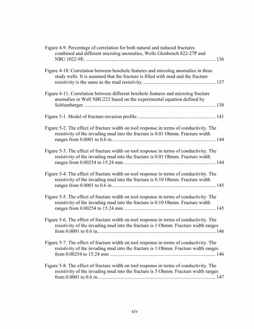
Figure 3-60. Rose frequency histogram for open natural fracture strikes in

Glenbench 822-27P................................................................................................. 102

Figure 3-61. Frequency histogram of vector means for open natural fractures in

Glenbench 822-27P................................................................................................. 102

Figure 3-62. Rose frequency histogram for open natural fracture strikes in

NBU 1022-9E. ........................................................................................................ 103


NBU1022-9E. ......................................................................................................... 103

Figure 3-64. Rose frequency histogram for open natural fracture strikes in NBU 222.. 104


NBU 222. ................................................................................................................ 104

Figure 3-66. Rose frequency histogram for healed fracture strike in the

Gglenbench 822-27P............................................................................................... 105

Figure 3-67. Frequency histogram for resistive fractures in Glenbench 822-27P.......... 105

Figure 3-68. Rose frequency histogram for healed fracture strikes in NBU 1022-9E. .. 106

xiii

Figure 3-69. Frequency histogram for resistive fractures in NBU 1022-9E................... 106

Figure 3-70. Diagram showing the three subsurface stress tensors. ............................... 108



Well NBU 222. ....................................................................................................... 110

Figure 3-72. Rose diagram of the 62 vertical extension fractures in the east-central

Piceance basin . ...................................................................................................... 113

Figure 3-73. Strike azimuth rose diagram for continuous breakout intervals shows

mean orientation of SHmax from borehole breakouts obtained from caliper logs,

Well NBU 222. ....................................................................................................... 115


breakout intervals interpreted by caliper logs, Well NBU222................................ 115

Figure 4-1. The 2-arm microlog apparatus . ................................................................... 117

Figure 4-2. Response of the microlog in front of permeable, shaly, and tight

formations ............................................................................................................... 120

Figure 4-3. Permeable beds (P) and impervious beds (I) ............................................... 123

Figure 4-4. Portion of MCFL pad showing current patterns and equipotential

surfaces .................................................................................................................. 125

Figure 4-5. Micronormal and microinverse logs vs. depth, Well Glenbench 822-27P .. 128

Figure 4-6. Correlation between borehole features and microlog anomalies, Well

Glenbench 822-27P................................................................................................. 131

Figure 4-7. Correlation between borehole features and microlog anomalies,

Well NBU 1022-9E................................................................................................. 132

Figure 4-8. Correlation between borehole features and microlog anomalies,

Well NBU 222. ....................................................................................................... 134

xiv

Figure 4-9. Percentage of correlation for both natural and induced fractures

combined and different microlog anomalies, Wells Glenbench 822-27P and

NBU 1022-9E. ........................................................................................................ 136

Figure 4-10. Correlation between borehole features and microlog anomalies in three

study wells. It is assumed that the fracture is filled with mud and the fracture

resistivity is the same as the mud resistivity. .......................................................... 137

Figure 4-11. Correlation between different borehole features and microlog fracture

anomalies in Well NBU222 based on the experimental equation defined by

Schlumberger. ......................................................................................................... 138

Figure 5-1. Model of fracture-invasion profile. .............................................................. 141

Figure 5-2. The effect of fracture width on tool response in terms of conductivity. The

resistivity of the invading mud into the fracture is 0.01 Ohmm. Fracture width

ranges from 0.0001 to 0.6 in. .................................................................................. 144



ranges from 0.00254 to 15.24 mm. ......................................................................... 144



ranges from 0.0001 to 0.6 in ................................................................................... 145



ranges from 0.00254 to 15.24 mm. ......................................................................... 145


resistivity of the invading mud into the fracture is 1 Ohmm. Fracture width ranges

from 0.0001 to 0.6 in............................................................................................... 146



from 0.00254 to 15.24 mm ..................................................................................... 146



from 0.0001 to 0.6 in............................................................................................... 147

xv



from 0.00254 to 15.24 mm ..................................................................................... 147

Figure 5-10. The response of the tool in fractured intervals for different mud resistivities.

A vertical fracture is located 2 in (5.08 cm) away from the wellbore.. .................. 148

Figure 5-11. The response of the tool in fractured intervals for different mud

resistivities. A vertical fracture is located 4 in (10.16 cm) away from the wellbore.

................................................................................................................................. 148



................................................................................................................................. 148



................................................................................................................................. 148


resistivities. A vertical fracture is located 10 in (25.4 cm) away from the wellbore. .

................................................................................................................................. 150


resistivities. A vertical fracture is located 12 in (30.48 cm) away from the wellbore

wall.......................................................................................................................... 150

Figure 5-16. Relationship between fracture width and mud resistivity for a vertical

fracture at different distances from the wellbore. ................................................... 152


fracture at different distances from the wellbore. ................................................... 153

Figure 5-18. The effect of invasion radius on conductivity in a fractured interval. ....... 154

Figure 5-19. The effect of invasion radius on conductivity in a non-fractured zone...... 154

Figure 5-20. The effect of fracture density on conductivity for different fracture spacing.

................................................................................................................................. 156

xvi

Figure 5-21. The effect of fracture density on MCFL tool response. ............................. 156

Figure 5-22. Tool response for various values of Rxo and Rt .. .................................. 158

Figure 5-23. Radius of investigation of different resistivity tools. ................................. 160

Figure 5-24. Rxo8 and related sharp peak in the middle of the fracture ....................... 162

Figure 5-25. Natural fractures interval, well NBU 222. The log shows a peak in this

interval whereas the HLLD and HLLS logs show only a small curvature change. 163

Figure 5-26. The Rxo8 log shows a sharp peak in a non-fractured tight sandstone,

whereas the HLLD and HLLS logs show small curvature changes in the opposite

direction .................................................................................................................. 164

Figure 5-27. Drilling-induced fracture interval.The Rxo8 log shows a peak, whereas

the HLLD and HLLS logs have a small curvature change in the opposite direction

................................................................................................................................. 166

Figure 5-28. Drilling-induced fracture interval.The Rxo8 log shows peaks, whereas

the HLLD and HLLS logs appear as constant values, well NBU 222.................... 167

Figure 5-29. The effect of washout on Rxo8, HLLD, and HLLS. ............................... 168

Figure 5-30. The effect of breakout on Rxo8, HLLD, and HLLS................................. 169

Figure 5-31. Different readings in micrologs ( R >RINV NOR ) in sandstone intervals,

well NBU 1022-9E. ................................................................................................ 172

Figure 5-32. The RDFL log shows a higher or equal value than RHDRS, and

RHMRS logs in intervals that have gas................................................................. 173

xvii

LIST OF TABLES

Pages

Table 2-1. Stratigraphic column, geologic history, and petroleum systems in the

Uinta basin. ............................................................................................................... 14

Table 2-2. Total Petroleum System (TPS) and Assessment Units (AU) in Piceance

basin .......................................................................................................................... 26

Table 3-1. FMI specifications . ......................................................................................... 31

Table 3-2. EMI specifications........................................................................................... 35

Table 3-3. FMI applications ............................................................................................. 42

Table 3-4. List of wells in this study with FMI and EMI data ......................................... 44

Table 3-5. Statistical analysis of the tectonic stress from two methods for quality-

ranking system, well Glenbench 822-27P. ............................................................. 109

Table 3-6. Statistical analysis of tectonic stress, Well NBU 1022-9E............................ 109

Table 3-7. Statistical analysis of tectonic stress,Well NBU 222. ................................... 109

Table 3-8. Quality-ranking system for stress orientations. ............................................. 110

Table 3-9. Quality -ranking system for stress orientation in three wells of this study. .. 110

Table 4-1. Microlog interpretation ................................................................................. 122

Table 4-2. A selected interval (6786.3-6788.6 ft) shows an anomaly less than

Minus 5 Ohmm, well NBU 1022-9E. ..................................................................... 129

Table 4-3. Comparison of microlog anomalies to other borehole features,

Well Glenbench 822-27P........................................................................................ 130

xviii


Well NBU 1022-9E................................................................................................. 132


Well NBU 222. ....................................................................................................... 133

Table 4-6. Different anomalies related to natural and induced fractures combined,

wells Glenbench 822-27P and NBU 1022-9E. ....................................................... 136

Table 4-7. Comparison of microlog anomalies to other borehole features in three

study wells. ............................................................................................................. 137

Table 4-8. Comparison of microlog fracture anomalies based on the experimental

equation by Schlumberger and other borehole features, well NBU 222. ............... 138

xix

ACKNOWLEDGEMENTS

Praise and glory be to God, the most gracious, the most merciful. He enabled me

to successfully complete this research.

I would like to express my sincere appreciation to my advisors, Dr. Neil F. Hurley

and Dr. Erdal Ozkan, who encouraged and supported me financially for part of my study.

Again, I greatly appreciate Dr. Neil F. Hurley for proposing this project, his extreme

patient and kind attention, and his technical and emotional help during my study. Special

thanks go to my committee members, Prof. Max Peeters, who helped, encouraged, and

guided me a lot, and Dr. Richard Christiansen, who also provided guidance along the

way. I extend my special thanks to Jerry Cuzella at Kerr McGee Corporation, who helped

to provide required data unsparingly.

I specially thank Dr. Connie Knight, who taught and helped me enormously to

interpret the image logs. I extend my special thanks to Dr. Dick Merkel, who helped and

guided me for log interpretation.

I am grateful to Mrs. Janine Carlson for all of the work she did on the image logs,

and her patient and extreme attention to help me accomplish my project.

I would like to thank Mrs. Charlie Rourke, who always smiles and makes me feel

free of any difficulties. Thank you, Charlie, and I will always remember your help.

I acknowledge the National Iranian Oil Company (N.I.O.C) for financial support

to complete my degree at the Colorado School of Mines for two years, and the Society of

Professional Well Log Analysts (SPWLA) for a student grant in 2005.

Finally, I need to express my special thanks to my family, who endured lots of

difficulties for my whole life. Mom, Dad, Brothers, and Sisters, thanks for the patience,

understanding and for supporting me for being here. I love all of you and without your

enormous support, I could never get to this point in my life.

1

CHAPTER 1

INTRODUCTION

1.1 Introduction

Natural fracture detection is one of the most important goals in reservoir

characterization for petroleum engineers, geophysists and geologists alike. To date,

various tools have been used to detect fractures. The Greater Natural Buttes (GNB) gas

field, located in the east-central part of the Uinta basin in northeastern Utah, is the subject

field for fracture detection in this study. Typically, the two target formations in the field

are the Tertiary Wasatch Formation and the Upper Cretaceous Mesavarde Group. Both

formations are low-permeability, layered intervals that contain dry gas. Both formations

have fractured intervals. Three wells, which are the focus of this study (NBU 1022-9E,

Glenbench Federal 822-27P, and NBU 222), have been logged by borehole image and

micro-resistivity logs. Logs from two other wells (Pawwinnee 3-181 and NBU 921-29)

have been examined in the same study area.

2

1.2 Purpose of Study

The main purpose of this study is to look for a correlation between the microlog

response and responses of the Formation MicroImager (FMI) and Electrical

MicroImaging (EMI) logs in naturally fractured intervals. Such a correlation may be used

to find fractured intervals in the field for hundreds of wells that have no FMI/EMI logs.

The specific objectives are:

• Determine the depth of borehole elongations from caliper logs in three

borehole image logs. Micrologs have a very small investigation radius, so

they can be influenced by well elongation. Therefore, the first step of this

project is to find the intervals which show elongation. Elongations can

occur in the form of breakouts, keyseats, and washouts.

• Confirm the depths of elongated intervals from FMI/EMI logs. Borehole

image logs can be used to find fractured intervals, breakouts and other

features.

• Determine the measured depths of natural fractures and drilling-induced

fractures using borehole image logs.

• Determine the fracture height for all fractures using borehole image logs.

• Compare the depths of microlog anomalies to the depths of washouts,

breakouts, and fractures observed in FMI/EMI logs.

3

• Study the effect of fractures near the borehole wall on the micro-resistivity tool

response using a modeling program developed by Baker Atlas.

• Develop petrophysical models for the fractured intervals.

• Determine the limitations of the microlog tool using actual data from three wells

in the study area.

1.3 Research Contributions

The major contributions of this research are:

• The present-day maximum horizontal stress (SHmax) direction, based on two

methods (borehole breakouts and induced fractures) is WNW-ESE in the study

area.

• Natural fracture orientation aligns with SHmax in the Natural Buttes field. This is

very important for reservoir drainage.

• Borehole elongations have a significant effect on micro-resistivity tool response.

• Microlog anomalies that correspond to natural fractures observed in FMI/EMI

logs show a maximum of 30% correlation. Borehole breakouts and induced

fractures have the maximum correlation when compared to other borehole

features. Therefore, there is no consistent rule to detect natural fractures from

micrologs.

• Based on several petrophysical models developed in this study, micro-focused log

tools are capable of detecting fractures under certain conditions. Fracture distance

from the wellbore, fracture aperture, fracture density, mud resistivity, and the

resistivity of the flushed and uninvaded zones play important roles for detection

of fractures by the MCFL.

4

CHAPTER 2

GEOLOGICAL SETTING

2.1 Location of the Study Area

The Uinta basin is a topographic and structural trough that encompasses an area

of more than 9,300 2mi (14,900 2km ) in northeast Utah (Figure 2-1). The Greater Natural

Buttes (GNB) gas field is located in the east-central part of the Uinta basin (Figure 2-2).

The field is 15 mi (24 km) in length from north to south in T8-12S and 36 mi (58 km) in

length from east to west in R18-24E, Uintah County, Utah. This study focuses on three

wells, Glenbench Federal 822-27P, NBU (Natural Buttes Unit) 1022-9E, and NBU 222 in

the field. Figure 2-3 shows the location of these wells.

2.2 Stratigraphy

2.2.1 Regional Stratigraphy

During the Cenozoic, along the southern flank of the Uinta Mountains, the Uinta

basin subsided. This basin is now the most significant source of gas in the state of Utah.

“The basin is bounded on the north by the Precambrian sandstones and shales of the

Uinta Mountains and on the west by the Charleston overthrust segment of the Cretaceous

Sevier Orogenic Belt. To the southwest, the Cretaceous and Tertiary beds rise onto the

Wasatch Plateau. On the south, outcrops of Upper Cretaceous Mesaverde sandstones,

shales and coals are exposed in the Book Cliffs, which are deflected northward around

the north end of the San Rafael swell west of the Green River, and northward around the

5

Figure 2-1. Location of Uinta basin.(USGS,

htpp://www.cdc.noaa.gov/USclimate/states.fast.html).

6

Figure 2-2. Location of Greater Natural Buttes field in the northeast Uinta basin.

(Longman, 2003).

7

Figure 2-3. Location of three study wells in the field. (Kerr McGee Company, 2005).

Glen Bench Federal 822-27P

NBU 1022-9E

NBU 222

T8S

T10S

T9S

R 22 E R 21 E R 23 E

N

8

northwest plunging end of the Uncompahgre uplift east of the Green River in easternmost

Utah adjacent to Colorado. To the east, the Douglas Creek arch separates the Uinta basin

from the Piceance basin” (Osmond, 2003).

Most non-associated gas accumulated in the eastern part of the basin in the lower-

Eocene North Horn Formation and the Paleocene and Eocene Wasatch, Colton, and

Green River Formations, and in the Cretaceous Mesaverde Group (Fouch et al., 1992).

Gas in the Green River sandstones may be a mixture of gas from two sources: lacustrine

source beds deeper in the basin and Mesaverde carbonaceous beds (Osmond, 1992).

There are three important stratigraphic traps in the field that control gas production:

marginal lacustrine sandstones in the Eocene Green River Formation, fluvial sandstones

enclosed in red beds of the Paleocene and Eocene Wasatch Formation (the main

production), and braid-plain sandstones interbedded with carbonaceous shales and coal in

the Upper Cretaceous Mesaverde Group (Osmond, 1992). The Wasatch Formation and

Mesaverde Group in the Greater Natural Buttes (GNB) area are the two main formations

in this study.

2.2.2 Local Stratigraphy

The stratigraphic and chronostratigraphic diagrams of GNB are shown in Figures

2-4, 2-5, 2-6, and 2-7. Figure 2-8 shows the gamma ray and microresistivity logs and

formation tops in a typical well, Glenbench 822-27P. Sandstones of the Wasatch

Formation and Mesaverde Group are the major producers in the field. Table 2-1 shows

the stratigraphic column, geologic history and petroleum systems in the Uinta basin

(Osmond, 2003).

9

Figure 2-4. Stratigraphic column for Greater Natural Buttes (GNB) gas field showing

formations which produce gas and oil in GNB and nearby fields. (Osmond et al., 1992).

10

Figure 2-5.Generalized stratigraphic correlation chart for the Uinta basin (Shade et al.,

1992).

11

Figure 2- 6. Generalized west-east cross-section showing Upper Cretaceous and lower

Tertiary stratigraphic units in Uinta basin, western Piceance basin, Utah and Colorado.

(Johnson et al.

12

003).

Figure 2- 7. West-east chronostratigraphic chart showing temporal relations of Upper

Cretaceous-lower Tertiary rocks in Uinta basin, Utah. (Johnson et al., 2003)..

13

GR versus Depth

7950

8000

8050

8100

8150

8200

8250

8300

8350

025

50

75

100

125

150

GR (GAPI)

Depth (ft)

GR

DARK CYN Mesaverde

Wasatch Form

ation

MesaverdeUnit

MesaverdeUnit

4

MNOR and MINV versus Depth

7950

8000

8050

8100

8150

8200

8250

8300

8350

0.1

110

100

MNOR and MINV (ohmm)

Depth (ft)

MNOR

MINV

GR versus Depth

7950

8000

8050

8100

8150

8200

8250

8300

8350

025

50

75

100

125

150

GR (GAPI)

Depth (ft)

GR

DARK CYN Mesaverde

Wasatch Form

ation

MesaverdeUnit

MesaverdeUnit

4

GR versus Depth

7950

8000

8050

8100

8150

8200

8250

8300

8350

025

50

75

100

125

150

GR (GAPI)

Depth (ft)

GR

DARK CYN Mesaverde

Wasatch Form

ation

MesaverdeUnit

MesaverdeUnit

4

Wasatch Form

ation

MesaverdeUnit

MesaverdeUnit

4


7950

8000

8050

8100

8150

8200

8250

8300

8350

0.1

110

100


Depth (ft)

MNOR

MINV

Figure 2-8. Gam

ma ray (GR), micronorm

al(M

NOR), and microinverse(M

INV) logs showing tops of the form

ations,

well Glenbench

822-27P.

14

Table 2-1. Stratigraphic column, geologic history and petroleum systems in the Uinta

basin. To follow the chronology, read this table from bottom to top. (Modified after

Osmond, 2003).

PERIOD GEOLOGIC

HISTORY

STRATIGRAPHY AND

THICKNESS

STRUCTURE PETROLEUM

SYSTEM

Oligocene-

present

Regional erosion of

< 3,000 ft,

Regional uplift of 10,000 ft.

Uinta Mtn. Uplift pulses

eroded into Precambrian.

Lake Uinta evaporates and

disappears.

Duchesnse River Fm. >5,000 ft,

southward thinning wedge of redbeds

with boulders.

Uinta Fm., <5,000 ft, Varicolored

alluvial transition with Green River Fm.

Towanta earthquake,

NE strike.

Maximum basin

subsidence.

Duchesne Fault Zone,

East-West strike.

Continued strong uplift

of E-W, concave south,

Uinta Mtns.

Bituminous sand deposits

on basin margins, set,

12 BBO

NW striking vertical

gilsonite dikes.

Gas and oil in fluvial sands

in lower Uinta Fm.

Paleocene-

Eocene

Lake Uinta expands and

contracts rapidly over long

distances.

Initial uplift and erosion of

Uinta Mtns.

Lakes SW of basin.

Green River Fm., 3,800-800 ft,

Lacustrine (oil shale) & marginal

lacustrine.

Wasatch Fm., 2,000-200 ft, alluvial

redbeds with channel sands. Flagstaff

lacustrine ls. 0-1,000 ft.

North Horn Fm.

(Cret.-Tert)

Pulses of uplift in Uinta

Mtns. begin. NE

faulting during lower

Green River deposition.

Rejuvenation of

Uncompahgre Uplift.

Rise of Douglas Crk.

Arch and San Rafael

Swell.

Oil & gas from lacustrine

shales in “cooking pot” at

ltamont field.

Dry gas from Mesaverde

coals captured in lenticular

sandstones in Mesaverde

Group and Wasatch Fm.

Cretaceous Sea regresses eastward

before alluvial fan/braid

plain/deltas.

Sea transgresses to west.

Streams flow east.

Mesaverde Group, 3,000-2,000 ft.

Numerous “Regressive sands” in lower

Kmv, deltaic, pinchout into Kmc

successively farther east as sea retreated.

Castlegate Ss., 400-0 ft.

Mancos Shale, 5,000 ft.

Mancos ”B” silts., 200 ft.

Ferron Fm., deltaic sand, shale and coal,

< 800 ft.

Dakota/Cedar Mtn./ Buckhorn Ss.,

fluvial, 100-200 ft.

Sevier Orogenic belt to

west, eastward

overthrusting

commences.

Gassy coal mines.

Indigenous Coalbed

Methane (CBM).

Gas in fault traps and

stratigraphic traps on

Douglas Creek Arch.

Drunkard’s Wash and

Helper CBM.

Gas on east and south

margins.

Jurassic Alluvial with streams

flowing East. Sea from

North.

Eolian desert.

Sea from West Eolian

desert

Morrison Fm., 650 ft.

Curtis marine ss, sh and ls, 150 ft.

Entrada Fm., 160-800 ft.

Twin Crk ls., 100-700 ft.

Carmel redbeds, 700-1000 ft.

Navajo Ss., 700-1000 ft.

Kayenta

Wingate.

Arapien Trough with

evaporates to west.

Gas in E & SE basin

Oil in NW Colorado.

Gas in SE basin.

Oil at Blaze Cyn, SE of

basin.

15

Table 2-1 (Continued). Stratigraphic column, geologic history and petroleum systems in

the Uinta basin. To follow the chronology, read this table from bottom to top. (Modified

after Osmond, 2003).

PERIOD GEOLOGIC

HISTORY

STRATIGRAPHY

AND THICKNESS

STRUCTURE PETROLEUM

SYSTEM

Triassic Sea regressed to West. Chinle Fm.,0-500 ft,

redbeds

Shiarump conglomerate, 50

ft.

Moenkopi Fm., 750 ft,

redbeds

Sinbad ls mbr, 100 ft

Twin Creek-Thaynes

Trough to West

Indigenous oil in lower

part of Moenkopi at

Grassy Trial, midway

between Price and Green

River.

Permian Sea transgressed from

Northwest.

Phosphoria/ Kaibab/Park

City ls. and phosphatic

shales, 0-600 ft.

Source of oil produced

from Penn. Sandstones at

Ashley Valley and

Rangley and trapped in Tar

Sands Triangle.

Pennsylvanian “Sand Sea,” eolian, desert.

Uncompahgre Mtns.

Eroded to Precambrian.

Sea regressed to West

(Oquirrh Basin).

Weber/ White Rim eolian

Ss., 0- 1000 ft, toward Mtns.

grades

Into Maroon alluvial redbeds

and conglomerates near

ancestral mtns.

Morgan marine ls and shale,

500-1,300 ft.

Uncompahgre Mtns., part

of Ancestral Rockies

extend NW under Uinta

Basin SE comer of basin;

Penn. to Trias. Onlap

Mtns.

Mississippian Marine invasion. Doughnut/Humbug/Manning

Canyon Shales, 700 ft.

RedwallDesert/

Leadville/Madison ls/dol,

900 ft.

Stable Gas @ North Spring, south

of Price.

Reservoir for oil and gas

from Penn. Black shales in

Paradox Basin to south.

Devonian-Cambrian Stable; erosion of Craton

with sea in geosyncline to

West.

Very thin patches or absent. Stable.

Ord. Basin dikes strike

NW in Uinta Mtns.

Proterozoic Rifting at south margin of

Wyoming Archean plate.

Uinta Mountain Group,

predominantly sandstone,

20,000 ft.

Aulacogen, fault bounded

basin subsequently rose to

form Uinta Mountains.

Chuarr Fm source beds in

Grand Cyn. Not known in

Uinta Basin. Few wells to

Precambrian.

16

2.2.2.1 Mesaverde Group (Upper Cretaceous)

The thickness of the Mesaverde Group is about 2,000 to 3,000 ft (610 to 915 m).

The depositional environment is interpreted as alluvial fan and deltaic sandstones. The

gas found in the Mesaverde Group is contained in structural and stratigraphic traps. The

lowest part of the Mesaverde Group in GNB is the Castlegate Sandstone, 350 ft (107 m)

thick, with upward coarsening from fine to coarse-grained sandstones. This unit overlies

the 5,000 ft (1,525 m) thick Mancos Shale. The Mancos is a dark gray shale. The lower

part of the Mesaverde Group, the Neslen Formation, comprises approximately one-third

of the main body of the Mesaverde Group and contains coal and carbonaceous shale.

Siltstone and shale are interbedded in this formation and quartz-lithic sandstones and very

fine to fine-grained quartzose sandstones were deposited in a deltaic environment

(Osmond et al., 1992). Two formations, the Tuscher and Farrer, in the upper part of the

Mesaverde also represent the change from deltaic to alluvial conditions. Studies have

shown that the most probable source of gas in the Mesaverde Group is the marine

Mancos Shale (Osmond et al., 1992).

2.2.2.2 Wasatch Formation

The thickness of the Wasatch Formation is about 200 to 2,000 ft (61 to 525 m).

The formation is thicker in the western GNB, but thinner in the eastern part. The Wasatch

Formation was deposited when the basin subsided during the late Cretaceous and early

Tertiary. The stratigraphic relationships of the Wasatch Formation with the underlying

and overlying formations are not simple, nor are they consistent over the entire extent of

the basin. The Upper Wasatch Formation contact is complex and is extensively

intertongued with the overlying Green River Formation. In the southern part of the basin,

the Wasatch is transitional with the underlying Paleocene to Eocene Flagstaff Limestone

(Shade et al., 1992). The Wasatch Formation sandstones are generally medium to well-

17

sorted, fine to medium-grained, and subangular to subrounded with calcite, dolomite,

ankerite and silica cement between grains (Brooks, 2002). The source of hydrocarbons in

the Wasatch Formation is from organic-rich siltstones and mudstones, carbonaceous

shales, and coals of the underlying Mesaverde Group (Osmond et al., 1992).

2.3 Structure

2.3.1 Regional Structure

The Uinta basin is parallel to the east-west trending Uinta Mountains. The basin is

an asymmetric syncline, deepest in the north-central area. The north flank dips from 10 to

35 degrees into the basin and is bounded by a large north-dipping basement thrust. The

southern flank dips from 4 to 6 degrees north (Chisdey et al., 1992). The regional dip

across GNB to the northwest is 162 ft/mi (31 m/km) on top of the Green River Formation

and 194 ft/mi (37 m/km) on top of the Wasatch Formation (Osmond, 1992). The

difference between the dips was caused by uplift of the eastern margin of the Uinta basin

(Douglas Creek Arch in western Colorado) during the Eocene and subsidence to the north

of the axis of the Uinta basin during the late Eocene-early Oligocene.

2.3.2 Local Structure

Based on detailed analysis of well logs and seismic data, features such as faults

and fractures are found in the study area.

Faults: During deposition of the lower part of the Green River Formation, normal faults

with throws of up to 170 ft (58 m) occurred (Osmond, 1992). This allowed gas from

Mesaverde Group rocks to migrate upward into the Wasatch Formation and possibly into

the Green River Formation. Because of the discontinuous nature of the beds in the

18

Wasatch and Mesaverde units, these faults are not easily recognized. The faulting

occurred during deposition of the Douglas Creek member of the Green River Formation.

The main northwest-trending faults probably controlled deposition of sandstones in the

lower Green River Formation, as proposed by Osmond (1992). In the River Junction-

Duck Creek field in central T9S-R20E, normal faults occur as north-west to west-

trending sets in the west-central and south-central parts of the basin.

Fractures: Regional fracture systems in the Uinta basin are near-parallel and are possibly

genetically related to major structural features that border the basin. Fractures in the

Uinta basin began to develop during the burial of the Wasatch and Green River

Formations. Hydrocarbon generation, with resultant overpressuring, may have caused

fractures to form in the deeper parts of the basin. Fractures also developed as the result of

tectonic stress in the region. Subsequent uplift of the Tertiary section expanded these

existing fracture networks and possibly created additional fracture systems. Locally, the

abundance and orientation of fractures are controlled by folds. Fracture distribution and

abundance are strongly controlled by lithology and bedding characteristics (Chidsey et

al., 1992).

Present-day Stress: According to Zoback and Zoback (1989), four major plate-tectonic

provinces generally coincide with stress provinces in the United States: San Andreas

transform, Rocky Mountain/ Intermountain Intraplate, Cascade convergent, and midplate

central and eastern United States. The Rocky Mountain plate-tectonic province includes

three distinct stress provinces: Cordillera extensional, Colorado Plateau interior, and the

southern Great Plains. This plate-tectonic province includes areas of the classic “basin

and range” structures in Nevada and parts of Utah, Oregon, Arizona, New Mexico,

Colorado, Idaho, and Wyoming (Zoback and Zoback, 1989).

Zoback and Zoback (1989) applied a variety of indicators, including earthquake focal

mechanisms, borehole breakouts, hydraulic fracturing, and young fault slip and volcanic

19

alignment, to map the maximum horizontal stress in the United States. Figure 2-9 shows

the orientation of maximum compressive in-situ stress in the study area. These

orientations were obtained by at least one of the stress indicators. Figure 2-10

summarizes the stress orientations for each area in the United States. Zoback and Zoback

(1989) presented the E-W oriented extensional stress for the study area. According to

Lorenz (2003), the strike of natural fractures, which is parallel to compressive in-situ

stress, is dominantly WNW-ESE in the Piceance basin (Figure 2-11).

2.4 Production Geology

Because this study focuses on the Greater Natural Buttes (GNB) area, two target

formations in this field, the Wasatch Formation and Mesaverde Group will be discussed

in this section. According to Nuccio et al. (1992), most gas-bearing reservoirs are

lenticular fluvial sandstones within two major sedimentary systems. They are:

• Upper Cretaceous, impermeable, fluvial rock. Reservoirs are within the Price

River, Castlegate, Sego, Blackhawk, Neslen, Tuscher, and Farrer Formations,

which are assigned to the Mesaverde Group.

• Lower Eocene North Horn Formation and Paleocene and Eocene Wasatch and

Colton Formations.

Wasatch Formation: The gas-bearing sandstones in the Wasatch and Mesaverde were

classified as “tight reservoirs” by the Utah Board of Oil, Gas and Mining in 1981 and

accepted as such by the U.S. Internal Revenue Service. The in-situ permeability in these

reservoirs is less than 0.10 md, exclusive of fracture permeability (Osmond, 1992; and

Nuccio et al., 1992). Wasatch sandstones have the following characteristics (Osmond,

1992):

20

Study Area

Study Area

Figure 2-9. Orientation of maximum horizontal compressive stress. (W

orld Stress Map.com, 2005).

21

Figure 2-10. Generalized stress map of the continental United States. Outward-pointing

arrows show areas characterized by extensional deformation. Inward-pointing arrows

show areas characterized by compressional tectonism. CC = Cascade convergent

province; PNW = Pacific Northwest; SA = san Andreas province; CP = Colorado Plateau

interior; and SGP = southern Great Plains (Zoback and Zoback, 1989).

Study Area

0 500

KM

22

Figure 2-11. Rose diagram of 62 vertical extension fractures in the east-central Piceance

basin, Colorado. The dominant strike is WNW-ESE (Lorenz, 2003).

23

• The reservoir thickness of individual sandstones is up to 40 ft (12 m).

• Productive sandstones are laterally discontinuous, and generally correlate for less

than 0.5 mi (0.8 km).

• Three to nine sandstones are perforated per well, with an average of 5.5.

• Net perforated intervals range in thickness from 30 to 140 ft (9 to 42 m) per well,

with an average of 67 ft (20 m).

• Gross perforated intervals are up to 2,000 ft (600 m) in thickness, with an average

of 965 ft (289 m).

• Depth ranges from 2,800 ft (840 m) in the southeast corner to 8,100 ft (2,430 m)

in the northwest part of the field.

• Porosity is as high as 18% on the basis of density and neutron porosity logs.

• Average porosity for producing sandstones ranges from 10-14%; commonly the

higher values occur in the lower parts of the sandstones.

• Initial production rates from the Wasatch range from a few hundred MCFD of gas

to 6,000 MCFD of gas, and average about 1,600 Mcfgpd.

• Uncorrected pressures from 35 DSTs show the Wasatch reservoir has a normal

pressure gradient. However, some information suggests that the Wasatch

Formation, along with the lowermost Green River Formation, is overpressured

(fluid-pressure gradients > 0.5 psi/ft) (Chidsey et al., 1992).

The amount of sulphur in Wasatch gas is very low. Gas-oil ratio (GOR) is 136,000:1,

or about 1 barrel of condensate per 136 MCF of gas. One barrel of water per 300 MCF of

gas is the general rate of water production in Wasatch wells. CO2 content in the

Wasatch is less than 0.5%.

Mesaverde Group: Mesaverde Group Sandstones have the following characteristics

(Osmond, 1992):

24

• The reservoir thickness of individual sandstones is up to 70 ft (21 m).

• The Mesaverde reservoirs are the tightest reservoirs in the field.

• Porosity is as high as 18% on the basis of porosity logs and core analysis.

• Average porosity for producing sandstones ranges from 8-12%.

• Permeability in normally pressured formations is less than 1 md.

• Production usually declines more rapidly than other formations in the field.

• Wells in this formation may produce water to the extent that it becomes a

problem.

• Initial production rate ranges from a few hundred MCFD of gas to 4,000 MCFD

of gas, and averages about 1,100 MCFD of gas.

• The Mesaverde sandstones are typically slightly overpressured.

• The depth of production in the Mesaverde sandstones ranges from 4,500 ft (1,372

m) in the southeastern GNB to 8,600 ft (2,623 m) in the northwestern part of the

field.

CO2content in the Mesaverde is less than 2%, which is greater than that of Wasatch

gas.

Source Rocks: The main source rocks in the Mesaverde are carbonaceous shales and

coals. Two reasons, higher geothermal gradient and slight overpressuring may reflect

present-day generation of gas in the Mesaverde (Nuccio et al., 1992). The geothermal

gradient in the Mesaverde is 1 oF / 49 ft (1 oC /27 m) at a depth of 7,000-10,000 ft (2,135-

3,050 m), which varies from the 1 oF /44 ft (1 oC /24 m) gradient at a depth of 3,500-7,000

ft (1,076-2,135 m) in the Wasatch wells. Wasatch rocks are immature for the generation

of gas at GNB. Some of this generated gas in the Mesaverde was trapped in the

Mesaverde and some migrated along faults and natural fractures to Wasatch sandstones.

25

During this migration, some of the CO2 content in the gas combined with water in the

strata through which it passed. By these chemical reactions, some minerals may be

formed which yield porosity reduction in the sandstones very close to faults and natural

fractures (Osmond, 1992). The Green River lacustrine beds are also immature for

hydrocarbon generation in the GNB area.

Petroleum System: The USGS assessment for undiscovered (some of non-associated and

associated) conventional oil and gas and continuous (unconventional) oil and gas,

including coal-bed gas is listed in the Table 2.2 (USGS, 2005).

26

Table 2-2. Total Petroleum System (TPS) and Assessment Units (AU) in Piceance basin

(USGS, 2003).

27

CHAPTER 3

BOREHOLE IMAGE LOGS

3.1 Background

Borehole images are logs that provide an electronic map of the borehole wall

obtained by measuring the electrical resistivity or ultrasonic properties of the rocks and

fluids. The focus of this study is on resistivity logs. The borehole image logs used in this

study are Schlumberger’s FMI (Formation MicroImager) and Haliburton’s EMI

(Electrical MicroImaging).

The FMI is an openhole microresistivity imaging tool with a maximum

temperature and pressure of o o350 F (175 C) and 20,000 psi (1.39 Kpa) (Schlumberger,

2004). The FMI tool has four arms and four hinged flapper pads. This allows a large

borehole coverage. There are 24 buttons on each pad, for a total of 192 image buttons.

Figures 3-1 and 3-2 show the FMI tool configuration. The FMI tool has a high vertical

resolution of about 0.2 in (5.1 mm) and its coverage is approximately 80% in an 8 in

(20.3 cm) borehole (Hurley, 2004; Grace et al., 1998; and Schlumberger, 2004). Figure 3-

3 shows the coverage of the FMI tool for different diameters of the borehole. In this

figure, FMS is the Formation MicroScanner tool, another tool designed by Schlumberger.

The maximum recording speed is 1,800 ft/hr (545 m/hr) for image acquisition.

For dipmeter acquisition, the maximum speed is 3,200 ft/hr (970 m/hr) (Grace et al.,

1998; Hurley, 2004). Other FMI specifications are shown in Table 3-1.

The FMI tool includes a general purpose inclinometry cartridge, which provides

accelerometer and magnetometer data. The triaxial accelerometer gives speed

28

Figure 3-1. The Formation MicroImager (FMI) Tool of Schlumberger. (Modified after

Schlumberger, 2004).

Digital Telemetry

Cartridge

Digital Telemetry Adapter

Tool for Depth

Correlation

Controller

Cartridge

Upper Electrode

Flex Joint

Inclinometer

Acquisition

Cartridge

Insulating Sub

Four-Arm

Sonde

Current

Pad Flap

29

Figure 3-2. Pad and flap assembly and sensor detail from Schlumberger FMI logging

tool. (Modified after Schlumberger, 2004).

Sensor Array Pad and flap assembly

0.2” 0.1”

Insulation

Electrode

button

0.16”

0.24”

Borehole view of 8 pad tool

8”

Hinge

Hinged

flap

2*12 Buttons

Pad

2*12 Buttons 5.7”

0.1”

Sensor Button

30

Borehole

Coverage

(%)

Borehole Diameter (in)

Figure 3-3. Borehole coverage for FMI and FMS tools. For example, the coverage of an 8

in (20.3 cm) borehole is 80% for the FMI tool (Grace et al., 1998).

31

Table 3-1. FMI specifications (Schlumberger, 2004).

1- Application: structural geology, stratigraphy, reservoir

analysis, heterogeneity, fine-scale

features, real-time answers

2- Vertical resolution: 0.2 in (0.5 cm), with 50-micron features

visible

3- Azimuthal resolution: 0.2 in (0.5 cm), with 50-micron features

visible

4- Measuring electrodes: 192

5- Pads and flaps: 8

6- Coverage: 80% in 8-in (20.3 cm) borehole

(fullbore image mode)

7- Max pressure: 20,000 psi

8- Max Temperature: o o350 F(175 C)

9- Borehole diameter:

• Minimum: 5.875 in (14.92 cm)

• Maximum: 21 in (53.34 cm)

10- Maximum hole deviation: o90

11- Logging speed

• Fullbore image mode: 1,800 ft/hr (540 m/hr) with real-time

processed image

• Four-pad mode: 3,600 ft/hr (970 m/hr) with real-time

processed image

• Dipmeter mode: 5,400 ft/hr (1,640 m/hr) with real-time dip

processing

• Inclinometer mode: 10,000 ft/hr (3,040 m/hr)

32

12- Maximum mud resistivity: 50 Ohmm

13- FMI tool:

• Maximum diameter: 5 in (12.7 cm)

• Makeup length: 24.4 ft (7.43 m)

• Makeup length with flex joint: 26.4 ft (8 m)

• Weight in air: 433.7 lbm (196.7 kg)

• Compressional strength: 12,000 lbf (safety factor of 2)

14- Maximum pad pressure: 44 lbf (19.95 kgf)

15- Combinability: Top combinable with openhole wireline

tools

33

determination and allows recomputation of the exact position of the tool. The

magnetometers determine tool orientation (Grace et al., 1998).

The Electrical Micro Imaging Tool (EMI) configuration is shown in Figure 3-4.

Although the general features of the two tools (FMI and EMI) are the same, there are

some differences between them. The EMI tool, designed by Halliburton, consists of six

spring-loaded pads with 25 electrodes on each pad for a total of 150 electrodes (Figure 3-

4). The maximum and minimum applicable hole diameters of the EMI tool are 20 in

(50.8 cm) and 6.25 in (15.9 cm), respectively (Fam, 1995).

The EMI tool is an electrical device that needs conductive drilling mud. The

electrical radius of investigation is small, generally less than 1 in (2.5 cm) beyond the pad

face (Hurley, 2004). Image quality is a function of the uniformity and quality of the pad

contact with the borehole wall. To reach this aim, the mechanical linkages of all arms to

the body are independent of each other. Also, each pad is mounted on a vertical swivel,

allowing data acquisition even if the tool body is off-center or the borehole cross-section

is not round (Seiler et al., 1994).

Logging speed varies in the range of 1,600 to 1,800 ft/hr (500 to 550 m/hr). High

vertical resolution, rapid sampling, normally 120 samples/ft, and high pad coverage (60

percent azimuthal coverage in an 8 inch borehole) are advantages of the tool.

Additionally, azimuthal orientation of the image makes dip measurements possible. Other

EMI specifications are shown in Table 3-2 (Thompson, 2000).

As the tool (EMI/FMI) is pulled up, the pads and flaps are pressed against the

borehole wall and each microelectrode emits a focused alternating current (AC) into the

formation. As the current interacts with the rock, the data are recorded by remote sensors.

The current emitted from a button is initially focused on a small volume of the formation

directly facing the button. Then, the current expands and covers a large volume of the

formation between the lower and upper electrodes (Luthi, 2000). According to Fam

(1995), “In addition to the simple variation of the survey current from the individual

34

Figure 3-4. Electrical Micro Imaging tool uses pad-mounted electrodes to make high-

definition resistivity measurement of subsurface formations. Each of the six pads features

25 electrodes. Button number 13 is the central button that measures the absolute emitted

current on each pad (Thompson, 2000).

35

Table 3-2. EMI specifications (Thompson, 2000).

1- Maximum Temperature o350 F ( o175 C )

2- Maximum Pressure 20,000 psi (1,400 bars)

3- Length 39.5 ft (12 m)

4- Weight 500 lbs (227 kg)

5- Logging Speed

• Imaging 1,800 ft/hr (550 m/hr)

• Dipmeter 3,600 ft/hr (1,100 m/hr)

6- Outside Diameter 5.0 in (12.7 cm)

7- Maximum Hole Size 21 in (51 cm)

8- Minimum Hole Size 6.25 in (16 cm)

9- Operating Conditions

• Water Base-Mud

• Can be run in horizontal wells.

• Can be run in oil-based mud in dipmeter mode using scratcher electrodes.

36

sensing buttons, the EMI tool can also accurately measure the absolute current emitted

by the central button (button number 13) on each pad. This additional capability yields

six high-definition, quantitative resistivity measurements that are well focused.”

The emitted current from each electrode is a function of the formation resistivity

in front of it and is continually measured. Two components of the emitted current are:

• Low-resolution signal covers the zone between the lower and upper electrodes

and provides petrophysical and lithological information (Schlumberger, 2004).

• High-resolution signal is modulated by the resistivity variations in the formation

that face the button directly. This signal is used for imaging and dip interpretation

and is presented as 8 strips for the FMI and 6 strips for the EMI. Button current-

intensity measurements, which reflect micro-resistivity variations, are converted

to variable-intensity gray or color images. The strips are presented as a two-

dimensional unrolled cylinder, split along true North. In other words, the

FMI/EMI resistivity “map” is a o360 image of the borehole wall and is presented

as a flat picture on a computer monitor (Figure 3-5) (Doupe, 2005).

The observation and analysis of the images provide information related to

changes in rock composition and texture, structure, or fluid content. Other measurements

of the tool are azimuth, inclination, caliper readings, accelerometer and magnetometer

readings and depth.

According to Grace et al. (1998), images provided by microelectrodes have some

special features. They are:

• Very large dynamic range- from less than 0.1 Ohmm to more than 10,000 Ohmm.

• High sensitivity, allowing detection of very thin events (fractures) that have an

aperture on the order of a few microns or tens of microns, or with low contrast in

resistivity.

37

Figure 3-5. Images viewed inside out. (A) 3-D borehole images, (B) unrolled cylinder to

show inner surface of borehole, (C) two-dimensional surface of borehole on the computer

monitor. Borehole image is presented as eight strips in FMI format and six strips in EMI

format. Dipping surfaces are represented as sinusoids. (D) Dip and azimuth are shown on

a dipmeter tadpole plot (Modified after Rider, 1996).

N

E

S

W N

E S W

A. Borehole B. Inner surface of borehole

C. Borehole image unrolled D. Dipmeter

N E S W N

0 90 180 270 360

N

Dip

0 60

Dipping bed

Dip azimuth = low point

Tangent = dip angle

Horizontal bed

38

• High sampling rate, one sample each 0.1 in (2.5 mm), in vertical and lateral

offset.

• Low sensitivity to heavy mud, borehole ovalization, and rugosity.

The FMI/EMI tools have an additional advantage in that they are combinable with

other logging tools. Therefore, fewer trips in the borehole are needed to run all logs. The

tool can be run in “Pads Only” and “Dipmeter Only” modes. If time is more critical than

increased hole coverage, the dipmeter can be run (Grace et al., 1998).

Because the tool emits current into the formation, it theoretically works only in

water-based mud. Different types of electrical borehole-imaging tools are commercially

available for oil-based mud. Currently, there is no cased-hole application. To get high

image quality, mud resistivity should not exceed 50 Ohmm; however, the mud must not

be too conductive. For good image quality, the ratio of formation resistivity to the mud

should be below 1,000 for the FMI tool (Grace et al., 1998). In the case of conductive

mud, the current tends to flow into the borehole. Reduced sharpness of the images is the

result of this phenomenon. Another impact on image quality is borehole deviation. With

borehole deviation less than o10 , the centralized tool minimizes poor pad contact caused

by oblique positioning of the tool relative to the borehole axis (Grace et al., 1998).

Blurred images can be the result of imperfect pad contact. This phenomenon occurs due

to the resistivity contrast between rock and mud which has filled the rugose or elongated

intervals.

The image display consists of two main types: static and dynamic. The static

images assign a color scale to resistivity values throughout the entire well, whereas the

dynamic images assign a color scale to resistivity values over short intervals to enhance

the contrast (Figure 3-6). Dynamic normalization enhances the contrast and reveals subtle

features. Figure 3-7 shows the process of static and dynamic normalization. By

convention, dark colors in the image logs indicate low-resistivity rocks and fluids,

39

Figure 3-6. Static image (left side) and dynamic image (right side), NBU1022-9E well.

Note the enhanced contrast in the dynamic image. Depth scale is in ft. GR is gamma ray;

DMAX is maximum borehole diameter; DMIN is minimum borehole diameter; and

TENS is tension.

Static Image Dynamic Image

40

Figure 3-7. Static normalization compares image data and assigns a color scale over the

entire logged interval. Dynamic normalization is a moving contrast adjustment through a

portion of the well, assigning a color scale to a sample population of the data values

(Modified after Rider, 1996).

Static Normalization

Resistivity

Dynamic Normalization

Sample population

Pixel color scale

Resistivity

Frequency

Frequency

Entire well

Pixel color scale

41

whereas light colors represent high-resistivity materials. In general, the light colors

correspond to sandstones or carbonates and the dark colors to shales. Features such as

bed boundaries, faults, breakouts and fractures can be interpreted from image logs. Table

3-3 lists applications of the FMI tool.

3.2 Data Available

Three borehole image logs are available for this study. Two images are EMI logs

and another is an FMI log. The locations of these three wells were shown in Figure 2-3.

Table 3-4 shows the available data for these three wells.

3.3 Borehole Image Log Processing

The software used for interpretation of EMI logs was Baker Atlas

Review/ TMRecall at the Colorado School of Mines. The FMI log for NBU 222 was

interpreted using Geoframe software (Schlumberger) by Mirna Slim (M.S. thesis in

progress). For this study, I used her interpretation. EMI logs were processed by Janine

Carlson. Connie Knight did the initial interpretation of bed boundaries and fractures for

the EMI logs.

The borehole diameter for both Glenbench 822-27P and NBU 1022-9E is 7.875

in (20 cm), and for NBU 222 is 6.25 in (15.8 cm). Static and dynamic images are

available.

3.4 Borehole Image Quality

In general, image quality is very good for all 3 wells. The Glenbench 822-27P

well has a sudden decrease in caliper readings at a depth of 8420 to 8440 ft (Figure 3-8).

This may be due to either closed pads, which means insufficient pad pressure, or a

42

Table 3-3. FMI applications (Schlumberger, 2004).

1- Structural geology

• Structural dip, even in fractured and conglomeratic formations

• Faults

2- Sedimentary features

• Sedimentary dip

• Paleocurrent direction

• Sedimentary bodies and their boundaries

• Anisotropy, permeability barriers and paths

• Thin-bedded reservoirs

3- Rock Texture

• Qualitative vertical grain size profile

• Carbonate texture

• Secondary porosity

• Fracture systems

4- Complement to whole core, sidewall core and formation tester programs

• Depth matching and orientation for whole cores

• Reservoir description of intervals not cored

• Depth matching for sidewall core samples and MDT (Modular Formation

Dynamics Tester probe settings)

5- Geomechanical analysis

• Drilling-induced features

• Calibration for Mechanical Earth Modeling

• Mud weight selection

6- Geology and Geophysics workflow

• Deterministic reservoir modeling

43

Table 3-4 (continued). FMI applications (Schlumberger, 2004).

• Distribution guidance for stochastic modeling

• Realistic petrophysical parameters

44

Table 3-5. List of wells in this study with FMI and EMI data and the intervals recorded.

Well Name FMI EMI

Top of FMI/EMI

Interval

Bottom of FMI/EMI

Interval Totals

(ft) (ft) (ft)

Glenbench 822-27P *

7545 8493 948

NBU 1022-9E *

6489 8865 2376

NBU 222 *

6852 9606 2754

45

Figure 3-8. DMAX and DMIN show a dramatic decrease from 8,420 to 8,440 ft. Poor

quality images occur in that interval, Glenbench 822-27P well. Depth scale is in ft. GR is

gamma ray; DMAX is maximum borehole diameter; DMIN is minimum borehole

diameter and TENS is tension.


Poor Quality Interval

46

technical problem during the logging run in this particular interval. Another factor that

can affect the quality of the image is borehole size. In this case, imperfect contact

between pads and wall will occur. Figure 3-9 shows an interval with irregular borehole

size. This can happen because of rock spalling. To interpret this elongated interval, the

term “effective bit size” was defined. In fact, an 8 in (20.3 cm) borehole diameter for the

depth of 6,489 to 6,756 ft and 8.6 in (21.8 cm) borehole diameter for the depth of 6,757

to 7,620 ft was considered as effective bit size. This criterion is based on elongation

definition. Because this will be discussed later in this chapter, any type of borehole

elongation interpreted as a change in effective bit size has to show a sudden sharp

change, not a gradual change. Another factor that can impact image quality is tool

sticking during logging. Streaked images indicate that the tool stuck and then released.

Streaked images occur when either the tool is traveling too fast, or mud or debris builds

up on the pads. The fast traveling happens when the high tension releases the tool on the

wireline (Minton, 2000). Figure 3-10 shows an example of debris build up.

3.5 Methods of Borehole Image Log Interpretation

The EMI log interpretation for two wells (Glenbench 822-27P and NBU 1022-9E)

was done at the Colorado School of Mines using Baker Atlas RECALL/REVIEW

software and the third well (NBU 222) was interpreted using Geoframe software. EMI

logs were displayed in two dimensions on the computer monitor, with both static and

dynamic images adjacent to each other. Sine waves fit to planar features provide the

following measurements:

• Dip magnitude is the angle between a horizontal plane and a dipping plane. Dip

magnitude is proportional to amplitude of the sine wave in a vertical well (Figure

3-11). It should be noted, when we calculate dips directly from images, apparent

dips would result. Apparent dip is the dip in relation to the borehole. In a

47

DMax and DMin vs Depth

6470.00

6670.00

6870.00

7070.00

7270.00

7470.00

7670.00

7870.00

5 10 15 20 25

Hole Diamater (in)

Depth (ft)

DMax

DMin

Bit Size

Figure 3-9. Two intervals (arrows) show a gradual increase in diameter going up the hole.

For identified intervals the effective bit size has been defined, NBU1022-9E well.

DMAX is maximum borehole diameter; and DMIN is minimum borehole diameter.

48

Figure 3-10. Debris build up in pad 2 as shown by arrow, NBU 1022-9E well. Pad 4 has

poor image quality. Depth scale is in ft. GR is gamma ray; DMAX is maximum borehole

diameter; DMIN is minimum borehole diameter; and TENS is tension.


49

W N E S W

Figure 3-11. Dip angle and dip Aazimuth (Modified after Grace et al., 1998).

A+BAverage Depth =

2

-1A-B

Apparent Dip Angle, α = tanBorehole Diameter (in)

o+Strike = Dip Azimuth at X 90-

A

B

A

Depth

Dip Azimuth

50

completely vertical well, both apparent and true dip are the same. However,

where the well is deviated, the true dip has to be computed by the software. To

calculate dip on images, it is necessary to pick at least three points on each sine

wave. If more than three points are selected, a least-squares fit is calculated,

taking all points into consideration. It is a good practice to pick at least one point

on each pad (Grace et al., 1998).

• Dip azimuth is the compass direction of the maximum dip. In the two dimensional

image, the lowest point of the sine wave is the location of the dip azimuth in a

vertical well (Figure 3-11).

It is useful to compare image logs to other openhole logs, such as gamma ray,

calipers, spontaneous potential, and resistivity logs. From image logs, some features such

as natural fractures (open and resistive), drilling induced fractures, borehole breakouts,

and microfaults are recognized. The procedure of interpretation for each feature will be

discussed in this chapter.

3.6 Depth Shifting

As logging tools are run, because of borehole wall rugosity, accelerations, and

different logging runs, the tools can become depth shifted with respect to each other. This

phenomenon causes a small change in the result curves for two separate tools in the same

well.

Because FMI/EMI logs are accelerometer corrected, these tools have more

accurate depths than tools such as conventional porosity and resistivity tools. Therefore,

depth shifting should be the first step of any log interpretation. In this study, we shifted

all curves to match the gamma ray log from the FMI/EMI. In the first step, the gamma

ray curve measured by conventional tools is shifted to the reference gamma ray

(FMI/EMI). In the second step, all other conventional curves are shifted based on the new

51

gamma ray. In this case study, the amount of shifting was not constant and varied at

different depths. The maximum amount of depth shift was about 2 ft (0.6 m). All depth-

shifting was done using Recall/Review software. The processing method was to select a

similar interval from two different gamma rays and match them. The rest of the curve

shifts automatically adjusting itselves with the selected interval. This job was done for

three wells in Natural Buttes field. As an example, Figure 3-12 shows the gamma ray

curves for both FMI and conventional logs before and after depth shifting in well

NBU 222.

3.7 Elongation Definition

When a well is drilled, borehole elongation can occur. Borehole elongation can

appear in the following different shapes.

• Rugosity: Wells are known to corkscrew due to torque on the bottom hole assembly,

and this process produces a tendency for the drill string to work against the borehole

wall unevenly. This phenomenon causes an elliptical shape in the wellbore, and the

degree of this ellipticity is known as the hole ”rugosity.” Rugosity arising from

corkscrewing appears on caliper logs as an elongation that spirals with depth

(Bosworth, 1989).

• Breakout: As boreholes are drilled deeper in the search for new hydrocarbon reserves,

failures known as “breakouts” are increasingly common due to high stresses at depth.

Borehole breakouts are elongations caused by unequal stress concentrations around a

borehole. This results in shear failure of the borehole wall and creates hole elongation

in a direction parallel to minimum horizontal in-situ stress (Figure 3-13). In other

words, breakouts that define relatively broad and flat curvilinear spalling surfaces of

the borehole wall are mostly like to occur along the azimuth of minimum horizontal

stress where the tangential stress is the highest (Zoback et al., 1985).

52

GR vs. Depth

7250.00

7255.00

7260.00

7265.00

7270.00

7275.00

7280.00

7285.00

7290.00

7295.00

7300.00

0 50 100 150 200

GR, GAPI

Depth (ft)

GR_ beforeShifting

GR_FMI

GR_afterShifting

Figure 3-12. The green line is the reference GR (FMI) and the dashed line is the GR for

the conventional log before shifting. The red line shows the conventional GR after

shifting, well NBU 222. The arrows show the depth shifts applied.

53

Figure 3-13. Cross sectional view of a borehole breakout (Zheng et al., 1989). SHmax is

the maximum in-situ stress and SHmin is the minimum in-situ stress.

54

Borehole elongations are actually created by compressive failure when the

tangential stress exceeds the unconfined compressive strength of the rock. Borehole

breakout can also be explained by a fracture-intersection mechanism. In this mechanism,

borehole elongation is aligned with the strike of steeply dipping natural fractures (Plumb

et al., 1985). Evidence for breakouts is based on correlation with stress directions inferred

from earthquakes or a nearby stress measurement (Plumb et al., 1985).

Analyses and observations of borehole breakouts raise some important questions.

These questions can include: How are the shape and size of the breakouts related to

magnitudes of the stresses in the rock? What is the effect of the mud overbalance

pressure on breakout? Zheng et al. (1989), Zoback et al. (1985), and Bosworth (1989)

discussed these questions. Assume the uniform fluid pressure p has filled the wellbore

and 1σ and 3σ (with 1 3σ σ> ) are the maximum and minimum in-situ stresses of the field.

If this is the case, then the tangential or “hoop” stress around the hole is 3 13 pσ σ− − on

the face perpendicular to 1σ , and 1 33 pσ σ− − on the face parallel to 1σ as presented by

Bosworth (1989). If 3 13p σ σ> − then tensile stresses will exist on the face perpendicular

to 1σ . According to Bosworth (1989), if these local stresses exceed the fracture strength

of the rock, then failure will occur. This will take the form of shear fractures and

subsequent spalling of the face normal to 3σ , and/or hydrofractures parallel to 1σ . Mud

weights are generally kept low enough during drilling to avoid induced hydrofracturing.

Theory then predicts that the hole will become elongated parallel to the least principal

far-field stress (Bosworth, 1989; Zoback et al., 1985).

According to Zoback et al. (1985), the edges of the breakouts steepen as the stress

ratio ( 1

3

σσ) increases. Evidence is based on some assumptions. The hole is assumed to be

cylindrical in a thick, homogeneous, isotropic elastic plate subjected to effective

minimum and maximum stresses. Irregular deep breakouts may have continued to grow

55

after their initial formation. The strong influence of p∆ (the difference between the fluid

pressure in the borehole and that in the formation) on the size and shape of breakouts is

due to the change in normal stress on potential failure planes near the wellbore. Positive

p∆ (excess pressure in the borehole) increases normal stress on those planes and inhibits

failure, whereas negative p∆ lowers normal stresses and promotes failure. Also, for a

given stress ratio and cohesive strength, much smaller breakouts result for larger values

of µ (friction coefficient), especially for larger stress ratios as presented by Zoback et al.

(1985). To analyze borehole breakouts accurately, some factors must be considered.

According to Zheng et al. (1989), these factors are:

• Inclined borehole: “there is some evidence to suggest that borehole breakout is

more severe in inclined boreholes than it is in vertical boreholes.”

• Non-axisymmetric rock stress: it is important to analyze experimentally the

effects of differential rock stresses on borehole breakouts.

• Pore fluid flow: “the flow of pore fluids into a borehole (or the flow of mud into

the formation) changes the value of the effective stress in the rock.” Because of

that, it has to be examined.

• Physicochemical effects of drilling fluids: “physicochemical effects are known to

be very important in fracture mechanics, especially in subcritical crack growth.

The extensile cracks that produce borehole breakouts almost certainly propagate

by subcritical crack growth.”

• Fracture gradients measurement.

• Type of rocks, especially shales.

• Size effect (stresses will increase as borehole diameter decreases).

• Anisotropic rock strength.

• Temperature: temperature of rock and fluid produce thermal strains that affect the

values of the stresses around the borehole.

• Time dependence.

56

Based on the above discussion, the importance of borehole elongation is now

clear. To interpret borehole breakouts accurately and see the shape and size of elongation,

the best tool is the borehole televiewer. The borehole televiewer is an ultrasonic logging

tool that provides high-resolution information about borehole elongation and the

distribution of natural fractures (Plumb et al., 1985). Dipmeters or borehole images are

the common tools used to interpret borehole elongation. In the dipmeter, the pads are

pressed against the borehole wall. The reference pad, pad 1, is magnetically oriented and

independent calipers measure the borehole diameter. In this study, to interpret breakouts,

I used caliper curves obtained by EMI/FMI. The EMI has six calipers that measure the

diameter of the hole in three different directions. These calipers are pads 1-4, 2-5, and

3-6. The FMI tool has 4 calipers that measure the borehole diameter in two directions of

pads 1-3 and pads 2-4.

According to Plumb et al. (1985), detection of breakouts from dipmeters or

borehole images depends on three factors. Calipers record borehole elongation if: (1) the

breakout width is greater than pad width, (2) the length of breakout is greater than the

length of the pad, and (3) the depth of the breakout is sufficient to interrupt the normal

tool rotation (clockwise as viewed from above due to cable torque) as it is pulled out of

the hole.

Depth intervals for borehole breakouts were selected from Uinta basin caliper

logs using the following workflow:

• Resample the logs to a chosen depth interval.

• Detect intervals where the logging tool rotated.

• Identify intervals of no elongation.

• Identify washout zones.

• Identify keyseats.

• Determine elongation direction.

• Determine maximum horizontal stress orientation.

57

3.7.1 Resample

Digital open-hole logs were resampled at a 0.1 ft (3 cm) depth interval for two

wells, NBU 1022-9E, and Glenbench 822-27P. Data were sampled at 0.5 ft (15.4 cm) for

well NBU 222. For the 6-arm EMI tool, curves needed are GR (gamma ray), C14

(caliper, pads 1-4), C25 (caliper, pads 2-5), C36 (caliper, pads 3-6), DEVI (hole

deviation), HAZI (hole azimuth), and P1AZ (pad 1 azimuth). For the 4-arm FMI tool, the

calipers are C13 (caliper, pads 1-3) and C24 (caliper, pads 2-4).

3.7.2 Tool Rotation

Intervals where the logging tool was freely rotating were removed from the data

set. This was determined from plots of the P1AZ curve, where the curve was changing

and not stabilized. If the tool was not rotating freely, the tool was locked in the borehole,

which is a good indication of borehole elongation. As an approximate criterion, the data

which showed one degree change per each foot of measured depth were eliminated from

the data set. Figures 3-14 and 3-15 depict intervals in which the tool was rotating freely,

and was locked in the wellbore, respectively.

3.7.3 No Elongation

No elongation occurs in intervals where the hole diameter does not show

elongation in any direction. For the 6-arm dipmeter, intervals where (C14+C25+C36)/3 is

within 0.25 in (0.6 cm) of bit size have been eliminated from the data set. This number is

an arbitrary value, but it assumes that elongations smaller than 0.25 in (0.6 cm) are not

breakouts. Typically, even where the hole is essentially round, one electrode pair shows

slightly wider separation. The effect is probably due to tool calibration errors and slight

hole irregularities (Babcock, 1978). In the 4-arm tool, intervals where the maximum

58

8000.00

8050.00

8100.00

8150.00

8200.00

8250.00

8300.00

8350.00

8400.00

0 90 180 270 360

Azimuth (Degree)

Depth (ft)

P1AZ

HAZI

Figure 3-14. Plot of P1AZ and HAZI vs. depth. Arrows show intervals in which the tool

has was rotated rotating freely, well Glenbench 822-27P.

59

Azimuth (Degree)

7000.00

7020.00

7040.00

7060.00

7080.00

7100.00

7120.00

7140.00

7160.00

7180.00

7200.00

0 90 180 270 360Depth (ft)

P1AZ

HAZI

Figure 3-15. Plot of P1AZ and HAZI vs. depth. Arrows show intervals in which the tool

is locked. This can be a good indication of borehole elongation, well NBU1022-9E.

60

caliper diameter (C13 or C24) is within 0.25 in (0.6 cm) of bit size have been eliminated

from the data set.

3.7.4 Washouts

The hole may be washed out due to erosion of poorly consolidated materials

(Figure 3-16). This happens mostly in shaly intervals. By convention, a washout is a zone

for which the smallest caliper is 1 in (2.5 cm) or larger than the bit size (Figure 3-17).

This was determined from comparison of the C14, C25, and C36 to the bit size in the 6-

arm dipmeter, and C13 and C24 in the 4-arm dipmeter.

3.7.5 Keyseats

When a drill string rubs against the borehole wall, its point of contact is of a

smaller diameter than the bit itself. This can result in a hole that is somewhat pear-shaped

in cross section (hence the term keyseat). This wear may cause borehole elongation in

deviated parts of the well when the azimuth of borehole deviation (HAZI) coincides with

the azimuth of borehole elongation. In fact, in a keyseat, off-centering of the sonde can

result in one caliper reading undergauge (Figures 3-18 and 3-19). In a 6-arm dipmeter, to

determine the keayseats, P1AZ is compared with HAZI, HAZI+60° , HAZI+120° ,

HAZI+180° , HAZI+ 240° , and HAZI+300° . This is done because any one of the 6 pads

can be aligned with the keyseat and pad 1 is the only oriented pad. Intervals where P1AZ

is within plus or minus 10°of any of these six values were eliminated from the data set.

The same method is applied for the 4-arm dipmeter to determine keyseats. The only

difference is the angle compared to P1AZ. In this case, P1AZ is compared with HAZI,

HAZI+ o90 , HAZI+ o180 , and HAZI+ o270 .

61

in

0 2 4

Figure 3-16. A washout with elongation in the direction of pads 1, 2, 3 and 4.

1

4

2

3

62

Calipers and Bit Size vs. Depth

7500.00

7550.00

7600.00

7650.00

7700.00

7750.00

7800.00

4 6 8 10 12 14 16


Depth (ft)

Caliper 1-4

Caliper 2-5

Caliper 3-6

Bit Size

Wash Out

Bit Size

Figure 3-17. Plot of calipers vs. depth. Arrows show intervals that are washouts, well

Glenbench 822-27P.

Washout

63

Figure 3-18. Key seats occur where the sonde is not centered in the borehole. This may

result in one caliper reading being less than bit size (in this case, caliper 1-3).

4

3 in

0 2 4

1

2

64

P1AZ and HAZI vs. Depth

8100.00

8110.00

8120.00

8130.00

8140.00

8150.00

0120

240

360

Azimuth (Degree)

Depth (ft)

P1AZ

HAZI

HAZI+120

HAZI+180


8100.00

8110.00

8120.00

8130.00

8140.00

8150.00

68

10

12

14


Depth (ft)

Caliper 1-4

Caliper 2-5

Caliper 3-6

Bit Size

Figure 3-19. Plots of calipers, P1AZ, and HAZI vs. depth. Arrows show theintervals eliminated as keyseats,

well Glenbench822-27P.


8100.00

8110.00

8120.00

8130.00

8140.00

8150.00

0120

240

360

Azimuth (Degree)

Depth (ft)

P1AZ

HAZI

HAZI+120

HAZI+180


8100.00

8110.00

8120.00

8130.00

8140.00

8150.00

68

10

12

14


Depth (ft)

Caliper 1-4

Caliper 2-5

Caliper 3-6

Bit Size


8100.00

8110.00

8120.00

8130.00

8140.00

8150.00

0120

240

360

Azimuth (Degree)

Depth (ft)

P1AZ

HAZI

HAZI+120

HAZI+180


8100.00

8110.00

8120.00

8130.00

8140.00

8150.00

0120

240

360

Azimuth (Degree)

Depth (ft)

P1AZ

HAZI

HAZI+120

HAZI+180


8100.00

8110.00

8120.00

8130.00

8140.00

8150.00

68

10

12

14


Depth (ft)

Caliper 1-4

Caliper 2-5

Caliper 3-6

Bit Size


8100.00

8110.00

8120.00

8130.00

8140.00

8150.00

68

10

12

14


Depth (ft)

Caliper 1-4

Caliper 2-5

Caliper 3-6

Bit Size

Figure 3-19. Plots of calipers, P1AZ, and HAZI vs. depth. Arrows show theintervals eliminated as keyseats,

well Glenbench822-27P.

65

3.7.6 Borehole Breakout and Elongation Direction

After intervals of rotation, no elongation, washout, and keyseat are eliminated

from the data set, the remaining intervals are candidates for breakouts. If breakout

elongation occurs in the wellbore, it will appear as an increase in one set of calipers,

whereas the other calipers closely match the size of the bit (Figures 3-20 and 3-21).

Elongation direction for the 6-arm dipmeter is determined as follows:

• If elongation occurs in the caliper 1-4 direction, SHmax will be P1AZ- o90 or

P1AZ+ o90 .

• If elongation occurs in the caliper 2-5 direction, SHmax will be P1AZ- o30 or

P1AZ+ o150 .

• If elongation occurs in the caliper 3-6 direction, SHmax will be P1AZ+ o30 or

P1AZ- o150 .

For the 4-arm dipmeter, the elongation direction is determined as follows:

• If elongation occurs in the caliper 1-3 direction, SHmax will be P1AZ+ o90 or

P1AZ- o90 .

• If elongation occurs in the caliper 2-4 direction, SHmax will be P1AZ or

P1AZ- o180 .

Elongation direction is reported as a number between 0 and o180 .

3.8 Microfault Interpretation

Microfaults, which are defined as cm-scale offsets of rock layers, can be

recognized from borehole images. Faults occur when external forces displace rock

masses along a plane of breakage. In general, there are three types of faults: normal,

reverse, and strike-slip. According to Grace et al. (1998), parameters which can be

determined for faults are:

66


7780.00

7790.00

7800.00

6 8 10 12 14

Borehole Diameter (in)Depth (ft)

Caliper 1-4

Caliper 2-5

Caliper 3-6

Bit Size

Figure 3-19. Plot of calipers vs. depth. Arrows show intervals that are breakouts, well

Glenbench 822-27P.

Breakout

67

Figure 3-20. DMAX shows an increase at the depth of 7784 to 7792 ft. DMIN matches

bit size. The image log is dark, which indicates elongation at this particular depth, well

Glenbench 822-27P. Depth scale is in ft. GR is gamma ray; DMAX is maximum

borehole diameter; DMIN is minimum borehole diameter; and TENS is tension.


Breakout Interval

Breakout Interval

68

• Depth of fault is defined as the midpoint of the sine wave.

• Strike of fault is perpendicular to the dip azimuth.

• Dip magnitude of the fault is the angle between horizontal and the fault plane.

• Sealing of fault is defined on the basis of conductivity of fill material along the

fault plane.

Faults and microfaults in borehole images show termination of bedding planes on

the fault plane (Luthi, 2000). Figures 3-22, 3-23, and 3-24 show fracture planes and fault

planes in the images.

3.9 Fracture Analysis

Image logs are one of the best tools used to detect fractures. Resistivity contrast

between the fracture and host rock is the reason why fractures appear on electrical

images. This difference is readily apparent in open fractures because the drilling fluid in

the open fracture aperture is less resistive than the host rock. In the case of resistive

fractures, cement materials fill the fracture space, and these have high resistivity.

Electrical images are influenced by three factors (Grace et al., 1998; and Luthi, 2000):

• mR , resistivity of the mud at formation temperature.

• xoR , resistivity of the flushed zone.

• Fracture Geometry (aperture and length).

According to Grace et al. (1998), characterization of fractures includes

identification, definition, and orientation. Fracture identification includes fracture type

such as vertical, polygonal and mechanically induced. Fracture definition includes open,

mineral-filled or vuggy. Orientation is the dip/strike.

69

Depth

N S N

Depth

N S N

Figure 3-21. Fault identification and difference between faults and fractures.

Fracture Plane

Fault Plane

70

Figure 3-22. Fracture identification. A sine wave is fitted to each open natural fracture,

well NBU 1022-9E. Depth scale is in ft. GR is gamma ray; DMAX is maximum borehole



71

Figure 3-23. Fault is indicated by the termination of bedding planes on the fault plane,

well NBU 1022-9E. Depth scale is in ft. GR is gamma ray; DMAX is maximum borehole



72

3.9.1 Vertical Fractures

A vertical or steeply dipping fracture has a dip magnitude higher than o75 (Grace

et al., 1998). A vertical fracture can be open or mineral filled.

3.9.2 Polygonal Fractures

Polygonal fractures create a highly irregular fracture network on electrical

images. Systematic orientation can be defined for these fracture networks. Normally, they

occur during deposition, as collapse breccias during karstification, as chemical or

mechanical dewatering features, or during tectonic movement in fault zones (Luthi, 2000;

and Grace et al., 1998). Figure 3-25 shows an example of this type of fracture.

3.9.3 Mechanically Induced Fractures

Typically, the drilling process causes stress concentration around the wellbore.

The tensile failure of the wall of the wellbore is the result of this stress concentration.

These fractures are called “tensile wall fractures” because they develop only in the

wellbore wall (Barton et al., 2002). Because induced fractures are created at the time of

drilling or hydraulic fracturing, they are always open (Figure 3-26). The strike orientation

of induced fractures and maximum in-situ stress orientation are parallel. According to

Luthi (2000), “the strike of induced fractures is important to know as it will be the same

for large-scale hydraulic fracturing, and it will therefore dictate the drainage direction

within the reservoir.” As a matter of fact, the induced fracture will occur along the strike

of the maximum stress direction (Figure 3-27).

Because of the importance of this type of fracture, some criteria will be discussed

to differentiate them from natural fractures on electrical images (Barton et al., 2002;

Grace et al., 1998; and Luthi, 2000).

73

Figure 3-24. Polygonal fracture in a carbonate reservoir (Grace et al., 1998).

74

Figure 3-25. Near-vertical induced fracture, well Glenbench 822-27P. Depth scale is in ft.

GR is gamma ray; DMAX is maximum borehole diameter; DMIN is minimum borehole

diameter; and TENS is tension.


75

Figure 3-26. Relationship between SHmax, water-flooding, and hydraulic fracturing.

Strike of induced fractures is parallel to SHmax, which sweeps the oil in the SHmin

direction (modified after Bell et al., 1986). In the “bad array,” induced fractures connect

the water-injection wells with production wells, and cause less recovery of oil than the

“good array,” which distributes the water and drives oil towards production wells.

Producing well

Water-injection well

Vertical fracture

induced buy water

injection

Oil swept towards a

producing well by

water flood

BAD WELL ARRAY

GOOD WELL ARRAY

BREAKOUT AZIMUTH

SHmax

Reservoir

edge

76

• Drilling-induced fractures do not cross the borehole, i.e., they do not make a sine

wave. Because the drilling-induced tensile-wall fractures are discontinuous

around the wellbore (they can propagate only in the tensile region of the

borehole), they cannot be fitted with a sinusoidal shape.

• They often have curvature at termination.

• They are always open-not vuggy or mineral filled.

• They cannot be micro-faulted.

• They are usually near-vertical.

• They are oriented parallel to maximum horizontal stress, and their orientations are

very consistent.

• They often cut across bed boundaries.

In deviated wells (Figure 3-28), drilling-induced fractures form as en-echelon

features. This is because of the sensitivity of the drilling-induced tensile–wall fractures to

in-situ stress (Barton et al., 2002). Figure 3-28 shows en-echelon induced fractures.

3.9.4 Fracture Morphology

In another category, fractures can be grouped as open, mineral-filled, or vuggy. In

the open fractures, the mud invades the fracture and creates a conductive layer inside of

the fracture. As mentioned before, this conductivity depends on the resistivity of the mud,

flushed zone, and the fracture geometry. The appearance of fractures on the images will

be enhanced in a salt mud system, whereas a fresh mud will decrease the contrast. The

fractures appear as highly conductive (dark) traces on the FMI/EMI log. Mineral-filled

fractures can be fully or partially mineral filled. Such fractures are less conductive than

open fractures. Figure 3-29 shows an open natural fracture and Figure 3-30 shows a

healed fracture. Vuggy fractures can have irregular enlargements along the fracture plane,

77

Figure 3-27. En-echelon induced fractures in a deviated interval, well NBU 1022-9E.

Depth scale is in ft. GR is gamma ray; DMAX is maximum borehole diameter; DMIN is

minimum borehole diameter; and TENS is tension.


78

Figure 3-28. Open natural fracture, well NBU 1022-9E. Depth scale is in ft. GR is

gamma ray; DMAX is maximum borehole diameter; DMIN is minimum borehole

diameter; and TENS is tension.


79

Figure 3-29. Healed fracture, well NBU 1022-9E. Depth scale is in ft. GR is gamma ray;

DMAX is maximum borehole diameter; DMIN is minimum borehole diameter; and

TENS is tension.


80

especially in carbonate reservoirs. In this study, four categories of natural fractures were

identified: 1- open fractures imaged on only 2 pads; 2- open fractures imaged on 3 or

more tool pads; 3- lithologically bound fractures; and 4- healed or resistive fractures.

Orientations of open fractures imaged on more than two pads are generally more reliable

than those imaged on a fewer number of tool pads. Lithologically bound fractures are

those fractures that terminate at bed boundaries (Knight, 2004).

3.9.5 Halo Effect around Resistive Fractures

As an image tool is pulled up during logging, buttons are variably positioned

relative to the fractures. Depending on the resistivity contrast between cement in the

fracture aperture and the host rock, a halo effect can appear. For a mineral-filled fracture,

when the tool gets very close to the fracture, the current lines are squeezed, giving rise

to an artificial high resistivity. On the other hand, when the tool passes the fracture, the

current lines start to diverge and the apparent resistivity is lower than it should be. This

change of resistivity from one side of the fracture to the other creates a halo effect on the

images (Luthi, 2000). This phenomenon is shown in Figure 3-31.

3.10 Results

This section summarizes the results obtained from borehole image logs in 3 wells

in GNB field.

3.10.1 Stress Orientation from Borehole Breakout

Borehole breakouts are analyzed to determine the orientation of maximum

horizontal in-situ stress (SHmax).

81

Figure 3-30. A cemented fracture at the top, showing characteristic halo effects due to the

insulating thin sheet formed by the fracture cement. The lower feature shows the same

halo effect (Luthi, 2000). Depth scale is in m.

82

We used two types of data to plot SHmax direction from borehole breakouts. The

first is caliper logs, as discussed in this chapter. The second is the actual borehole images.

Continuous breakouts identified from caliper logs resulted in 90, 131, and 25 separate

intervals for Glenbench 822-27P, NBU 1022-9E, and NBU 222, respectively. After that,

we computed the SHmax vector mean for each of these intervals. Details are included in

the attached CD Rom. Figures 3-32 through 3-37 show the strike azimuth of SHmax

obtained from both caliper logs and borehole-image inspection in three wells. Figure 3-38

shows an example of breakouts identified from actual images.

Strike azimuth, rose diagrams, and frequency histograms were used to evaluate

the orientation of SHmax in the study area. Figures 3-39 to 3-50 show orientation

diagrams for borehole breakouts in three wells.

The dominant SHmax strike azimuth is generally E-W in both the NBU 222 and

Glenbench 822-9E well. In contrast, the result in NBU 222 well is significantly different,

especially in the case of SHmax interpreted from caliper logs. This difference will be

discussed in this chapter in the Discussion section.

3.10.2 Stress Orientation from Mechanically Induced Fractures

Another way to determine the direction of SHmax is to use induced fracture

orientations. Continuous induced fractured intervals have been recognized from image

logs. Figures 3-51 through 3-59 show SHmax azimuth vs. depth cross plots, strike

azimuth rose diagrams, and frequency histograms for three wells, Glenbench 822-27P,

NBU1022-9E, and NBU 222.

3.10.3 Comparison of SHmax and Fracture Orientations

Figures 3-60 through 3-69 show the behavior of natural and healed fractures strike

orientation in the three wells. Natural fractures in the field are closely parallel to SHmax

83

Strike Azimuth Cross Plot

7500.00

7600.00

7700.00

7800.00

7900.00

8000.00

8100.00

8200.00

8300.00

8400.00

8500.00

10 30 50 70 90 110 130 150 170

Strike azimuth of SHmax (Degree)

Depth (ft) Shmax related

to caliperbreakout

Figure 3-31. Strike azimuth of SHmax obtained from caliper logs, well Glenbench 822-

27P.

84


7500.00

7600.00

7700.00

7800.00

7900.00

8000.00

8100.00

8200.00

8300.00

8400.00

8500.00

10 30 50 70 90 110 130 150 170

Strike Azimuth of SHmax (Degree)

Depth (ft)

SHmax related toEMI breakout

Figure 3-32. Strike azimuth of SHmax obtained from EMI log inspection, well

Glenbench 822-27P.

85


6400.00

6600.00

6800.00

7000.00

7200.00

7400.00

7600.00

7800.00

8000.00

8200.00

8400.00

8600.00

8800.00

10 30 50 70 90 110 130 150 170


Depth (ft) SHmax

related tocaliperbreakout

Figure 3-33. Strike azimuth of SHmax obtained from caliper logs, well NBU 1022-9E.

86


6400.00

6600.00

6800.00

7000.00

7200.00

7400.00

7600.00

7800.00

8000.00

8200.00

8400.00

8600.00

8800.00

10 30 50 70 90 110 130 150 170


Depth (ft)

SHmaxrelated toEMIbreakout

Figure 3-34. Strike azimuth of SHmax obtained from EMI log inspection, well NBU

1022-9E.

87


6850.00

7050.00

7250.00

7450.00

7650.00

7850.00

8050.00

8250.00

8450.00

8650.00

8850.00

9050.00

9250.00

9450.00

9650.00

10 30 50 70 90 110 130 150 170

Strike Azimuth of SHmax (Degree)Depth (ft)

SHmaxrelated tocaliperbreakout

Figure 3-35. Strike azimuth of SHmax obtained from caliper logs, well NBU 222.

88


6850

7050

7250

7450

7650

7850

8050

8250

8450

8650

8850

9050

9250

9450

9650

10 30 50 70 90 110 130 150 170


Depth (ft)

SHmaxrelated toFMIbreakout

Figure 3-36. Strike azimuth of SHmax obtained from FMI log inspection, well NBU 222.

89

Figure 3-37. DMAX shows an increase at the depth of 7722 to 7724 ft. DMIN matches

bit size. The image log is dark, which indicates elongation at this particular depth, well

Glenbench 822-27P. Dip direction of identified breakout is 110 degree, which is parallel

to SHmax. Depth scale is in ft. GR is gamma ray; DMAX is maximum borehole



Breakout

90

Figure 3-38. Strike azimuth rose diagram for continuous breakout intervals shows mean

orientation of SHmax from borehole breakouts obtained from caliper logs, well

Glenbench 822-27P.

0

10

20

30

40

50

0 20 40 60 80 100 120 140 160 180

Caliper SHMax Frequency

Frequency

SHMax

Figure 3-39. Frequency histogram of vector means of SHmax from continuous breakout

intervals interpreted by caliper logs, well Glenbench 833-27P.

Mean Vector Orientation = 103

91


orientation of SHmax from borehole breakouts obtained from EMI log inspection, well

Glenbench 822-27P.

0

10

20

30

40

50

60

70

0 20 40 60 80 100 120 140 160 180

EMI SHMax Frequency

Frequency

SHMax


intervals interpreted by EMI log inspection, well Glenbench 822-27P.

Mean Vector Orientation = 103.6

92


orientation of SHmax from borehole breakouts obtained from caliper logs, well NBU

1022-9E.

0

5

10

15

20

25

0 20 40 60 80 100 120 140 160 180

Ca lip er SHM ax Frequency

Frequency

S HMax


intervals interpreted by caliper logs, well NBU 1022-9E.


93


orientation of SHmax from EMI log inspection, well NBU 1022-9E.

0

10

20

30

40

50

0 20 40 60 80 100 120 140 160 180

EM I S HMax F req ue nc y

Frequency

S HM ax


intervals interpreted by EMI log inspection, well NBU1022-9E.


94


orientation of SHmax from borehole breakouts obtained from caliper logs, well

NBU 222.

0

2

4

6

8

1 0

0 2 0 4 0 6 0 8 0 1 0 0 1 2 0 1 4 0 1 6 0 1 8 0

E M I S H m a x F req u e nc y

Frequency

S H M a x


intervals interpreted by caliper logs, well NBU 222.

Mean Vector Orientation =30.2

95


orientation of SHmax from borehole breakouts obtained from FMI log inspection, well

NBU 222.

0

5

1 0

1 5

2 0

2 5

3 0

3 5

0 2 0 4 0 6 0 8 0 1 0 0 1 2 0 1 4 0 1 6 0 1 8 0

F M I S H M a x F r e q u e n c y

Frequency

S H M a x


intervals interpreted by FMI log inspection, well NBU 222.


96


7500.00

7600.00

7700.00

7800.00

7900.00

8000.00

8100.00

8200.00

8300.00

8400.00

8500.00

10 30 50 70 90 110 130 150 170

Strike Azimuth SHmax (Degree)

Depth (ft)

SHmaxrelated toInducedFracture

Figure 3-50. Strike azimuth of SHmax obtained from induced fractures, well

Glenbench 822-27P. Mean vector orientation is 91.4o.

97


orientation of maximum horizontal compressive stress (SHmax), well Glenbench

822-27P.

0

1

2

3

4

5

6

7

0 2 0 4 0 6 0 8 0 1 0 0 1 2 0 1 4 0 1 6 0 1 8 0

I n d u c e d F ra c tu r e S H m a x

Frequency

S H M a x

Figure 3-52. Frequency histogram of vector means of SHmax from continuous intervals

of induced fractures, well Glenbench 822-27P.


98


6400.00

6600.00

6800.00

7000.00

7200.00

7400.00

7600.00

7800.00

8000.00

8200.00

8400.00

8600.00

8800.00

10 30 50 70 90 110 130 150 170


Depth (ft)

Shmaxrelated toInducedFracture

Figure 3-53. Strike azimuth of SHmax obtained from induced fractures, well NBU 1022-

9E. Mean vector orientation is 114.8o.

99

Figure 3-54. Strike azimuth rose diagram for continuous induced fractures shows mean

orientation of maximum horizontal compressive stress (SHmax), well NBU 1022-9E.

0

5

1 0

1 5

2 0

2 5

3 0

3 5

4 0

0 2 0 4 0 6 0 8 0 1 0 0 1 2 0 1 4 0 1 6 0 1 8 0

In d u c e d f r a c tu re S H m a x

Frequency

S H M a x


of induced fractures, well NBU1022-9E.


100


6850.00

7050.00

7250.00

7450.00

7650.00

7850.00

8050.00

8250.00

8450.00

8650.00

8850.00

9050.00

9250.00

9450.00

9650.00

10 30 50 70 90 110 130 150 170

Strike Azimuth SHmax (Degree)

Depth (ft) SHMax

related toInducedFractures

Figure 3-56. Strike azimuth of SHmax obtained from induced fractures, well NBU 222.

Mean vector orientation is 106.4o.

101


orientation of maximum horizontal compressive stress (SHmax), well NBU 222.

0

10

20

30

40

50

60

70

80

0 20 40 60 80 100 120 140 160 180

Induced Frac ture 's SHMax

Frequency

S trike Azimuth (Degree)


of induced fractures, well NBU 222.


102

Figure 3-59. Rose frequency histogram for open natural fracture strikes in Glenbench

822-27P. The dominant orientation is essentially E-W.

0

5

1 0

1 5

0 2 0 4 0 6 0 8 0 1 0 0 1 2 0 1 4 0 1 6 0 1 8 0

N a tu r a l F r a c t u r e S tr i k e A z im u th

Frequency

S t r ik e A z im u th (D e g r e e )


Glenbench 822-27P. The dominant frequency is between 90 and 100 degrees.


103

Figure 3-61. Rose frequency histogram for open natural fracture strikes in NBU 1022-9E.

The dominant orientation is essentially E-W.

0

5

1 0

1 5

2 0

2 5

3 0

3 5

4 0

0 2 0 4 0 6 0 8 0 1 0 0 1 2 0 1 4 0 1 6 0 1 8 0

O p en F ra c tu re s S trik e

Frequency

S t r ik e A z im u th (D eg re e )


NBU1022-9E. The dominant frequency is between 100 and 110 degrees.


104

Figure 3-63. Rose frequency histogram for open natural fracture strikes in NBU 222.

0

2

4

6

8

10

12

14

0 20 40 60 80 100 120 140 160 180

O pen F rac tu re 's S tr ike

Frequency

S tr ike A z im u th (D eg ree )


NBU 222.


105

Figure 3-65. Rose frequency histogram for healed fracture strike in the Gglenbench 822-

27P. N-S is the dominant orientation.

0

0.5

1

1.5

2

2.5

3

3.5

0 20 40 60 80 100 120 140 160 180

Hea ld Fracture S trikes A zim uth

Frequency

S trike Azim uth (D egree)

Figure 3-66. Frequency histogram for resistive fractures in Glenbench 822-27P.


106

Figure 3-67. Rose frequency histogram for healed fracture strikes in NBU 1022-9E.

0

1

2

3

4

5

6

7

0 20 40 60 80 100 120 140 160 180

Healed F rac ture Strike Az im uth

Frequency

S trike Azimuth (Degree)

Figure 3-68. Frequency histogram for resistive fractures in NBU 1022-9E.


107

and healed fractures are parallel to SHmin (Figure 3-70).

3.10.4 Quality-Ranking System for Stress Orientation

There is a quality-ranking system defined by Zoback and Zoback (1989) that is

used to characterize how accurately a breakout interpretation records the tectonic stress.

This quality ranking is defined based on a statistical analysis of the accuracy of the data.

According to Zoback and Zoback (1989), there are four ranks, A through D, with the

highest quality for A and the lowest quality for D. Strike azimuth of SHmax ranges from

o o10 to 15 for A, o o20 to 25 for B, plus or minus o25 for C, and more than o25 for D.

Tables 3-5 through 3-7 show the ranking analysis for three wells in the GNB field. Table

3-8 shows the quality-ranking system presented by Zoback and Zoback (1989). For

wellbore breakouts, the quality is ultimately linked to the standard deviation (S.D).

Additionally, a certain number and a certain length of breakouts must be achieved. On the

basis of the analysis, breakouts interpreted from EMI/FMI images have a ranking-quality

of A, for three study wells. On the other hand, the ranking-quality for breakouts related to

caliper SHmax varies from B for Glenbench 822-27P to D for wells NBU 1022-9E and

NBU 222. The result is shown in Table 3-9.

Well Glenbench 822-27P shows very close quality rank for two different methods

to determine SHmax, whereas wells NBU 1022-9E and NBU 222 show significant

variability.

3.11 Discussion

This section discusses the results obtained from borehole image logs in 3 wells in

GNB field.

108

Figure 3-69. Diagram showing the three subsurface stress tensors (Knight, 2004).

Vertical Stress

Max Horiz. Stress; sHmax;

Insitu Stress Min.

Horiz.

Stress

Closed

Fracture

Open

Fracture

109

Table 3-6. Statistical analysis of the tectonic stress from two methods for quality- ranking

system, well Glenbench 822-27P.

EMI SHmax Frequency Caliper SHmax Frequency

Minimum 85 Minimum 43.49

Maximum 126 Maximum 160.42

Std Deviation 6.89 Std Deviation 17.4

Points 123 Points 90

Total Breakout Length (m) 63.2 Total Breakout Length

(m) 62.8

Total No. of Breakouts 123 Total No. of Breakouts 90


system, well NBU 1022-9E.

EMI SHmax Frequency Caliper SHmax Frequency




Points 91 Points 131

Total Breakout Length (m) 172 Total Breakout Length

(m) 101



system, well NBU 222.

FMI SHmax Frequency Caliper SHmax Frequency




Points 55 Points 8

Total Breakout Length (m) 85 Total Breakout Length (m) 4.87


110

Table 3-9. Quality-ranking system for stress orientations. Modified after Zoback and

Zoback (1989).

A B C D

Mechanism

(FM)

Average P-axis or formal inversion of four or more

single-event solutions in

close geographic proximity (at least one

event

M>= 4.0.

Well-constrained single-event solution (M>= 4.5)

or average of two well-

constrained single-event solutions (M>= 3.5)

determined from first

motions and other methods (e.g., moment

tensor wave-form

modeling, or inversion)

Single-event solution (constrained by first

motions only, often based

on author’s quality assignment)(M>= 2.5)

Average of several well-

constrained composites

Single composite solution

Poorly constrained single event

solution

Single event

solution for M<2.5

event

Wellbore

Breakout

(IS-BO)

Ten or more distinct breakout zones in a single

well with S.D ≤ o12

and/or combined length>

300m

Average of breakouts in two or more wells in

close geographic

proximity with combined length> 300m and

S.D ≤ o12

At least six distinct breakout zones in a single

well with S.D ≤ o20

and/or combined length>

100m

At least four distinct breakout with

S.D< o25 and/or

combined length>30 m

Less than four consistently oriented

breakouts o r <30 m

combined length in a single well

Breakouts in a single well

with S.D o25≥

Hydraulic

Fracture

(IS-HF)

Four or more hydrofrac orientations in single well

with S.D o12≤ ,

depth>300 m

Average of hydrofrac orientations for two or

more wells in close

geographic proximity,

S.D o12≤

Three or more hydrofrac orientations in a single

well with S.D o20≤

Hydrofrac orientations in

a single well with o o20 <S.D<25

Hydrofrac orientations in a single well with

o o20 <S.D<25 . Distinct

hydrofrac orientation

change with depth,

deepest measurements assumed valid

One or two hydrofrac

orientations in a single

well

Single hydrofrac measurement at< 100 m

depth

Petal

Centerline

Fracture

(IS-PO)

Mean orientation of fractures in a single well

with S.D o20<

Overcore

(IS-OC)

Average of consistent

(S.D o12≤ )

measurements in two or more boreholes extending

more than two excavation

radii from the excavation wall, and far from any

known local disturbances,

depth > 300 m

Multiple consistent

(S.D < o20 )

measurements in one or more boreholes extending

more than two excavation

radii from excavation

well, depth > 100 m

Average of multiple

measurements made near

surface (depth> 5- 10 m) at two or more localities

in close proximity with

S.D o25≤

Multiple measurements at

depth > 100 m with

o o20 <S.D<25

All near-surface measurements with S.D>

o15 , depth < 15 m

All single measurements

at depth

Multiple measurements at

depth with S.D o25>

S.D is standard deviation

111

Table 3-10. Quality -ranking system for stress orientation in three wells of this study.

Quality Ranking / Well Name Glenbench 822-27P NBU 1022-9E NBU 222

EMI/FMI SHmax Quality

Ranking A A A

Caliper SHmax Quality Ranking B D D

112

3.11.1 Comparison of SHmax and Fracture Orientations

There are three principal stress axes defined in the subsurface (Figure 3-70). One

is vertical and two are horizontal (SHmax and SHmin). Vertical stress is a result of

overburden pressure and usually exceeds the two horizontal components.

Drilling-induced fractures tend to form parallel to the direction of SHmax. Natural

fractures may or may not align with SHmax. This is very important in terms of reservoir

drainage. When SHmax and natural fractures are parallel, the fractures are commonly

propped open by differential stress (Knight, 2004). On the other hand, natural fractures

perpendicular to SHmax or parallel to SHmin are commonly closed (Figure 3-70). As a

result, the vector mean of strike orientation for 26, 128, and 49 open natural fractures for

Glenbench 822-27P, NBU 1022-9E, and NBU 222 are o91.8 , o98.8 , and o110 ,

respectively, which is close to the SHmax direction in these three wells. On the other

hand, the strike direction of the resistive fractures is o6 in Glenbench 822-27P, which is

close enough to be parallel to SHmin. The strike direction of resistive fractures in NBU

1022-9E is scattered. In well NBU 222, the number of resistive fractures was just two.

Because of that, it is not plotted here. In summary, there exists a relationship between

natural fractures and SHmax that is optimal for reservoir drainage.

3.11.2 Comparison of Obtained SHmax with SHmax Map for the United

States

The SHmax orientation from two applied methods (borehole breakout and

induced fracture) shows the WNW-ESE orientation. Zoback and Zoback (1989) and

Lorenz (2003) found a similar orientation for the compressive in-situ stress and natural

fracture strike. Therefore, there exists a good match and reliable value for the SHmax in

the field area. Figures 3-71 and 3-72 show an example of SHmax direction from this

study and Lorenz’s (2003) results.

113


orientation of maximum horizontal compressive stress (SHmax), well NBU 222. The

dominant strike is WNW-ESE.

Figure 3-71. Rose diagram of the 62 vertical extension fractures in the east-central

Piceance basin, Colorado. The dominant strike is WNW-ESE (Lorenz, 2003).

114

3.11.3 Elongation

The orientation of SHmax can be determined from borehole breakouts and

induced fracture orientations. In this study, there is a difference between the SHmax

directions obtained from these methods. Possible explanations are:

• Breakouts from borehole image inspection may be more accurate than breakouts

recognized from caliper logs. Some of the criteria used to analyze the data from

caliper logs were arbitrary. By changing values, different breakout intervals will

result. Additionally, very small breakouts can be seen in borehole images, whereas

these intervals may be eliminated from caliper logs because of tool rotation. In fact,

the tool cannot be stuck in small elongated intervals. The pads of the borehole image

tools might be too “clumsy.”

• Using arbitrary values to analyze the caliper logs to determine borehole breakouts

yields some short intervals. Some identified breakouts are just a point (0.1 ft) (3 cm).

For example in NBU 222, 25 breakouts were detected, although 17 of them have a

height less than 0.3 ft (9 cm). As a suggestion, we should count breakouts, for

example, which have a length greater than the tool-pad length. Figures 3-73 and 3-74

show 8 continuous breakout intervals for well NBU 222, after eliminating the short

intervals.

As a summary, for being more accurate and getting a better perception for

borehole elongation intervals, a combination of methods has to be applied. For example,

the result of recognized SHmax for NBU 222 determined from breakouts related to

caliper logs is not reliable.

115


orientation of SHmax from borehole breakouts obtained from caliper logs, well NBU

222. Breakouts intervals bigger than pad length are used.

0

1

2

3

4

5

0 2 0 4 0 6 0 8 0 1 0 0 1 2 0 1 4 0 1 6 0 1 8 0

C a l ip e r S H M a x F re q u e n c y

Frequency

S H M a x


intervals interpreted by caliper logs, well NBU222. Breakout intervals bigger than pad

length are used.


116

CHAPTER 4

MICRO-RESISTIVITY

4.1 Microlog

4.1.1 General Information

The microlog is a pad-type resistivity device that primarily detects mudcake

(Hilchie, 2003). The microlog evolved into a tool used to detect permeable zones in

those areas where the SP log cannot give a satisfactory answer (Schlumberger, 1958;

Doll, 1950). Where the formations are much more resistive than mud (for example, in

limestone fields), the SP log may detect the presence of permeable zones, but does not

detect bed boundaries accurately. The microlog is more accurate in that case and also

when the beds are thin (Schlumberger, 1958).

4.1.2 Equipment Description

The microlog device has two insulating rubber pads with three electrodes

mounted on each, one inch apart in a vertical line (Figure 4-1). These electrodes are

placed in the middle of the pad. The modern hydraulic pad is filled with oil and pressed

against the borehole wall to contact the formation perfectly (Hilchie, 2003). Therefore, it

is electrically shielded from the short-circuiting action of the mud (Schlumberger, 1958).

The two rubber pads are mounted on separate arms of a spring guide. The applied

pressure to open the arms is independent of the diameter of the hole. This diameter ranges

117

Figure 4-1. The 2-arm microlog apparatus consists of a rubber pad, which is pressed

against the wall of the drill hole (Schlumberger, 1958).

118

from 14 "2

to 16" for the standard spring guides presently in use. Under these

circumstances, the system measures the average resistivity of the small volume of the

material directly in front of the pad.

4.1.3 Principles of Micrologging

The microlog measures two different resistivities; micronormal ( R2" ) and

microinverse (R1"*1" ). In a 2 in normal, the lower electrode (electrode A) acts as the

current electrode and the upper electrode (electrodeM2 ) is a potential measurement

electrode. In 1 in by 1 in (1"*1"or 1.5" ) model, the lower electrode (electrode A) is the

current electrode and the two upper electrodes (electrodes M1 and M2) are the

differential potential measurements (Figure 4-1) (Hilchie, 2003). Based on these

electrode arrangements, the depth of investigation for the micronormal tool will be

different from the microinverse tool. They are 4 in and 1.5 in, respectively.

In a permeable formation, because of mud filtrate, mudcake can build up.

Therefore, detection of mudcake by the microlog is a good indication of invasion and

permeable formations. In front of permeable zones, the micronormal log shows a higher

value than the microinverse log. This occurs because part of the matrix resistivity is

included in the micronormal measurements, whereas the microinverse tool measures the

mudcake resistivity and some resistivity of the flushed zone. This is due to the

investigation radius difference between the normal and inverse logs. The difference

between these two values is known as “separation.” Positive separation is defined when

the micronormal trace shows higher values than the microinverse trace.

Based on the above discussion, positive separation appears in front of permeable

zones. Positive separation can also be created in a rugose borehole wall because the pad

is not being firmly pressed against the formation. In a highly resistive formation

(impervious or tight section), positive separation may also occur. On the other hand,

119

insufficient invasion may cause a negative separation opposite a permeable zone.

Negative separation can also be created in water-bearing zones. Positive separation

cannot be seen when saltwater muds or gypsum-based muds are used (Schlumberger,

1958). According to Asquith et al. (1982), the reason is that mudcake may not be strong

enough to keep the pad away from the formation. Where the pad is in contact with the

formation, negative separation occurs (Asquith et al., 1982).

4.1.4 Microlog Behavior in Different Formations

Delineation of different formations by the microlog are summarized below

(Schlumberger, 1958):

• Porous and permeable beds: both micronormal and microinverse logs show low

resistivities (Figure 4-2); generally, not more than 20 times the mud resistivity.

Positive separation occurs when the mudcake is not very thin, mud is not very

saline or invasion is not very shallow and the formation is not salt-water bearing.

Normally the mudcake effect levels out the resistivity readings, therefore, there is

no sharp variation opposite a permeable bed.

• Tight sections: in this case, a thin mud film separates the electrodes from the

formation. The thickness of this mud film can be 1 "16

or less. This will result in

high resistivity readings. Both micronormal and microinverse logs show at least

20 times the mud resistivity (Figure 4-2). Based on the pad distance from the

borehole wall, due to mud film thickness and irregularity of the borehole wall, the

emitted current from the electrode can escape towards the mud column. Thus, the

separation may be positive or negative, accordingly.

• Shales: similar to tight formations, a thin mud film may build up on the borehole

wall to separate the pads from the formation. If there is no caving in the shales,

120

Figure 4-2. Response of the microlog in front of permeable, shaly, and tight formations

(Schlumberger, 1958). Permeable zones show positive separation and low resistivity.

Mostly

Shale

Hard with

shale streaks

Permeable

and porous

BIT SIZE: 8 5/8”

Rm of BHT: 0.5 Ohmm

121

the resistivity reading is equal to or less than the shale resistivity (Schlumberger,

1958). As a result, the separation may be negative, zero, or positive (Figure 4-2).

Based on experiments presented by Schlumberger (1958), the negative separation

in shale may be due to the anisotropy of shale. However, to get a better perception

for shale interpretation, use of other curves such as the SP log or GR log is

recommended.

• Caved hole: Caved hole may occur opposite shales or other type of formations.

The two readings (micronormal and microinverse) in a deep cave show equal

readings as the mud resistivity (Schlumberger, 1958). This is because the pad

does not firmly contact the borehole wall.

• Fractures: Similar to a caved hole, opposite of fractured intervals, both

resistivities may show equal values as the mud resistivity.

4.1.5 Microlog Interpretation in Permeable and Impervious Beds

Doll (1950) summarized microlog interpretation for permeable and impervious

formations in five different categories. They are:

• Category I1: the two microresistivities (normal and reverse) are higher than

Rlim ( 20 to 30 times the mud resistivity).

• Category I2 : the separation is negative.

If the microinverse reading is less thanRlim , the SP log has to be applied.

• Category I3 : no separation or very small and the SP log trend is positive.

• Category P1: no separation or very small and the SP log trend is negative.

122

• Category P2 : large positive separation (more than 20 percent).

In all of the above, “I” and “P” are the abbreviations for “Impervious” and

“Permeable,” respectively. Figure 4-3 shows an example for impervious and permeable

zones. This discussion has been summarized in Table 4-1.

Table 4-1. Microlog interpretation (Modified after Doll, 1950).

R1"*1" > Rlim

Impervious

Zone Category I1

R2" < R1"*1"

(Large negative separation)

Impervious

Zone Category I2

Positive

SP trend

Impervious

Zone Category I3

R2" ; R1"*1"

(separation nil or small) Negative

SP trend

Permeable

Zone Category P1

R1"*1" < Rlim R2">R1"*1"

(Large positive separation)

Permeable

Zone Category P2

Where Rlim is about:

• (10-15)*Rm for fresh mud.

• (20-30)*Rm for average mud.

• (40-50)*Rm for very salty mud.

123

Figure 4-3. Permeable beds (P) and impervious beds (I) (Doll, 1950).

124

4.2 Micro Cylindrically Focused Log (MCFL)

4.2.1 General Information

The Micro Cylindrically Focused Log (MCFL) is a relatively new device designed

by Schlumberger. Because most microdevices (Microlog, Microlaterolog, and Proximity

log) are sensitive to the mudcake thickness ( hmc ) and mudcake resistivity (Rmc ), they

cannot give a reliable answer for Rxomeasurements. However, the new tool is designed

to render a much more accurate value for Rxo . The three parameters Rxo , Rmc , and

hmc are also estimated in real time (Eisenmann et al., 1994). The tool has a vertical

resolution of less than 1 in, which is used to detect very thin beds.

The MCFL tool responds to the following focusing challenges, as presented by

Eisenmann et al. (1994). They are:

• “Radial divergence of the current beam before the limit of the flushed zone.”

• “Strong vertical constraint of the current beam.”

• “Azimuthal insensitivity to the environment of the borehole wall.”

The tool should be insensitive to a wide range of mudcake thickness. In this case,

the tool is independent of mudcake thickness up to 0.4 in (Eisenmann et al., 1994).

4.2.2 Equipment Description

The pad surface of the MCFL device is shown in Figure 4-4. Because of pad

symmetry, only the left upper quarter is shown. Three small measurement buttons, B0 ,

B1, and B2 are placed within the larger A0electrode (Eisenmann et al., 1994). The

emitted current from B0 flows horizontally and diverges azimuthally to the correct depth

125

Figure 4-4. Portion of MCFL pad showing current patterns and equipotential surfaces

(Eisenmann et al., 1994).

126

of investigation. Electrodes B1 and B2, which are located at the edge of the pad, have a

shallower depth of investigation. In fact, the tool provides three different resistivity

measurements at three different depths of investigation, as presented by Eisenmann et al.

(1994). The equipotential surfaces have a cylindrical shape close to the center of the pad.

This is originated at the central button to focus the current into the formation perfectly

before escaping towards the mud (Eisenmann et al., 1994).

4.2.3 Fracture Detection by MCFL

Schlumberger (2005) introduced an experimental equation based on the acquired

data from the MCFL tool to detect fractures (Richards, S. pers. commun., 2005). The

equation is as follows:

Where:

HCAL = Hole diameter.

HCAL [-1] = Hole diameter for one sample before the picked sample.

HCAL [1] = Hole diameter for one sample after the picked sample.

HCAL [-9] = Hole diameter for 9 samples before the picked sample.

HCAL [3] = Hole diameter for 3 samples after the picked sample.

AIT 90 = measured resistivity 90 in behind the borehole wall or deep resistivity.

Rxo8 = measured resistivity 8 in behind the wellbore.

( )

X =ABS HCAL[-1]-HCAL[1]+HCAL[-9]-HCAL[3]8

AIT 90X = 9 Rxo8

Data.Fracture_Flag = if (X <0.05) and (X >2.0) and (AIT90>25)8 9

Fracture = Data.Fracture_Flag*5

127

4.3 Results

This study is focused on fracture detection by microresistivity logs. Therefore,

interpretations of other possibilities, such as permeable zones, impervious beds, and shale

intervals were not considered. The obtained results for natural fractures and other

borehole features are discussed in the next section.

4.3.1 Fracture Analysis by Microdevices (Microlog and MCFL)

Microlog anomalies are defined based on arbitrary values of the separation

between the micronormal and microinverse curves. They are termed Plus 5/10 Ohmm

and Minus 5/10 Ohmm of separation. Any continuous intervals with separation values

more than Plus 5/10 Ohmm or less than Minus 5/10 Ohmm are counted as an anomaly.

Each continuous interval is counted as one separate interval for statistical analysis. Figure

4-5 shows an example of an anomaly Plus 10 Ohmm. Table 4-2 shows a continuous

interval for the amount of separation less than Minus 5 Ohmm. Anomalous intervals are

compared with fractured zones and other borehole features such as borehole breakouts, as

interpreted from borehole images. For example, Table 4-2 demonstrates that the anomaly

is related to natural fractures and borehole breakouts. Number 1 means that the related

feature has occurred in that interval and number 0 means that the related feature has not

occurred in that interval. Tables 4-3, 4-4, and 4-5 and Figures 4-6, 4-7, and 4-8 show the

results for the three study wells. Details are included in the attached CD Rom. The

maximum 14% correlation between natural fractures and microlog anomalies in well

Glenbench 822-27P occurs with anomalies more than Plus 10 Ohmm. The maximum

correlation of 33% in well NBU 1022-9E for natural fractures also occurs with more

than Plus 10 Ohmm of microlog separation. On the other hand, no fracture observed in

well NBU 222 corresponds to any microlog anomaly. No anomaly is observed related to

any other type of features. This means that the microlog curves have little or no

128


7985

7987

7989

7991

7993

7995

7997

7999

0 20 40 60 80 100


Depth (ft)

MNOR

MINV

Figure 4-5. Micronormal and microinverse logs vs. depth, well Glenbench 822-27P.

Interval 7791-7794 shows anomaly Plus 10 Ohmm. Micronormal shows a higher value

than microinverse (positive separation).

Positive Separation

(Anomaly Plus 10 Ohmm)

129

Table 4-2. A selected interval (6786.3-6788.6 ft) shows an anomaly less than Minus 5

Ohmm, well NBU 1022-9E.

#DEPTH

(ft)

Separati

on

(Ohmm)

Anomaly

Number

Natural

Fracture

Induced

Fracture

Resistive

Fracture

Micro-

Faults

EMI

Breakout

Caliper

Breakout

Tool

Rotation

No

Elongation

Wash-

out

Key-

Seat

6786.30 -5.21 Minus 42

0 0 0 0 0 1 0 0 0 0

6786.40 -5.61 Minus

42 0 0 0 0 0 1 0 0 0 0

6786.50 -6.03 Minus

42 0 0 0 0 0 1 0 0 0 0

6786.60 -6.61 Minus 42

0 0 0 0 0 1 0 0 0 0

6786.70 -7.19 Minus

42 0 0 0 0 0 1 0 0 0 0

6786.80 -7.77 Minus

42 0 0 0 0 0 1 0 0 0 0

6786.90 -8.35 Minus 42

0 0 0 0 0 1 0 0 0 0

6787.00 -8.94 Minus

42 1 0 0 0 0 1 0 0 0 0

6787.10 -8.62 Minus

42 1 0 0 0 0 1 0 0 0 0

6787.20 -8.31 Minus 42

1 0 0 0 0 1 0 0 0 0

6787.30 -8 Minus

42 1 0 0 0 0 1 0 0 0 0

6787.40 -7.69 Minus

42 1 0 0 0 0 1 0 0 0 0

6787.50 -7.38 Minus 42

1 0 0 0 0 1 0 0 0 0

6787.60 -7.45 Minus

42 1 0 0 0 0 1 0 0 0 0

6787.70 -7.53 Minus

42 1 0 0 0 0 1 0 0 0 0

6787.80 -7.61 Minus 42

1 0 0 0 0 1 0 0 0 0

6787.90 -7.68 Minus

42 1 0 0 0 0 1 0 0 0 0

6788.00 -7.75 Minus

42 1 0 0 0 0 1 0 0 0 0

6788.10 -7.71 Minus 42

1 0 0 0 0 1 0 0 0 0

6788.20 -7.67 Minus

42 1 0 0 0 0 1 0 0 0 0

6788.30 -7.63 Minus

42 1 0 0 0 0 1 0 0 0 0

6788.40 -7.59 Minus 42

1 0 0 0 0 1 0 0 0 0

6788.50 -7.55 Minus

42 0 0 0 0 0 1 0 0 0 0

130

Table 4-3. Comparison of microlog anomalies to other borehole features, well Glenbench

822-27P.

Anomaly Plus 10 (Glenbench 822-27P)

Natural

Fracture

Induced

Fracture

Resistive

Fracture Fault

EMI

BreakOut

Caliper

BreakOut

Tool

Rotation

No

Elongation WashedOut

Key

Seats

Number of anomaly related to the feature 2 4 0 0 4 3 12 2 2 0

PERCENTAGE 14.29% 28.57% 0.00% 0.00% 28.57% 21.43% 85.71% 14.29% 14.29% 0.00%

Total Anomaly Number 14

Anomaly Minus 10 (Glenbench 822-

27P)

Natural

Fracture

Induced

Fracture

Resistive

Fracture Fault

EMI

BreakOut

Caliper

BreakOut

Tool

Rotation

No


Key

Seats


PERCENTAGE 5.56% 15.28% 1.39% 0.00% 43.06% 48.61% 59.72% 19.44% 4.17% 4.17%


Anomaly Plus 5 (Glenbench 822-27P)

Natural

Fracture

Induced

Fracture

Resistive

Fracture Fault

EMI

BreakOut

Caliper

BreakOut

Tool

Rotation

No


Key

Seats


PERCENTAGE 13.43% 14.93% 1.49% 0.00% 14.93% 19.40% 71.64% 20.90% 4.48% 1.49%


Anomaly Minus 5 (Glenbench 822-27P)

Natural

Fracture

Induced

Fracture

Resistive

Fracture Fault

EMI

BreakOut

Caliper

BreakOut

Tool

Rotation

No


Key

Seats


PERCENTAGE 13.21% 10.38% 1.89% 0.94% 38.68% 42.45% 66.04% 24.53% 4.72% 2.83%


131

Microlog Anomaly, Percentage of Correlations, Vs. Borehole Features, Well Glenbench 822-

27P

0.0%

10.0%

20.0%

30.0%

40.0%

50.0%

60.0%

70.0%

80.0%

90.0%

100.0%

Natural Fracture

Induced Fracture

Resistive Fracture

Fault

EMI BreakOut

Caliper BreakOut

Tool Rotation

No Elongation

WashedOut

Key Seats

Borehole Feature

Anomaly Percentage of correlation, %

Anomaly Plus 10 ohmm

Anomaly Minus 10 ohmm

Anomaly Plus 5 ohmm


Figure 4-6. Correlation between borehole features and microlog anomalies, well

Glenbench 822-27P.

132

Table 4-4. Comparison of microlog anomalies to other borehole features, well NBU

1022-9E.

Anomaly Plus 10 (NBU 1022-9E)

Natural

Fracture

Induced

Fracture

Resistive

Fracture Fault

EMI

BreakOut

Caliper

BreakOut

Tool

Rotation

No


Key

Seats

Number of anomaly related to the

feature 2 3 0 0 0 0 6 0 0 0

PERCENTAGE 33.33% 50.00% 0.00% 0.00% 0.00% 0.00% 100.00% 0.00% 0.00% 0.00%


Anomaly Miuus 10 (NBU 1022-

9E)

Natural

Fracture

Induced

Fracture

Resistive

Fracture Fault

EMI

BreakOut

Caliper

BreakOut

Tool

Rotation

No


Key

Seats


feature 59 17 7 2 12 78 134 5 0 38

PERCENTGE 27.70% 7.98% 3.29% 0.94% 5.63% 36.62% 62.91% 2.35% 0.00% 17.84%


Anomaly Plus 5 (NBU 1022-9E)

Natural

Fracture

Induced

Fracture

Resistive

Fracture Fault

EMI

BreakOut

Caliper

BreakOut

Tool

Rotation

No


Key

Seats


feature 5 1 0 0 10 8 25 0 0 0

PERCENTAGE 16.13% 3.23% 0.00% 0.00% 32.26% 25.81% 80.65% 0.00% 0.00% 0.00%


Anomaly Minus 5 (NBU 1022-

9E)

Natural

Fracture

Induced

Fracture

Resistive

Fracture Fault

EMI

BreakOut

Caliper

BreakOut

Tool

Rotation

No


Key

Seats


feature 82 34 12 3 25 114 193 6 5 48

PERCENTAGE 28.08% 11.64% 4.11% 1.03% 8.56% 39.04% 66.10% 2.05% 1.71% 16.44%


0.0%

10.0%

20.0%

30.0%

40.0%

50.0%

60.0%

70.0%

80.0%

90.0%

100.0%

Natural Fracture

Induced Fracture

Resistive Fracture

Fault

EMI BreakOut

Caliper BreakOut

Tool Rotation

No Elongation

WashedOut

Key Seats

Borehole Features

Anomaly Percentage of Correlation, %



Anomaly Plus 5 ohmm


Figure 4-7. Correlation between borehole features and microlog anomalies, well NBU

1022-9E.

133

Table 4-5. Comparison of microlog anomalies to other borehole features, well NBU 222.

Anomaly Plus 10 (NBU 222)

Natural

Fracture

Induced

Fracture

Resistive

Fracture Fault

EMI

BreakOut

Caliper

BreakOut Tool Rotation

No

Elongation

Washed-

Out

Key-

Seats


PERCENTAGE 0.00% 0.00% 0.00% 0.00% 0.00% 0.00% 0.00% 0.00% 0.00% 0.00%


Anomaly Minus 10 (NBU 222) Natural

Fracture

Induced

Fracture

Resistive

Fracture Fault

EMI

BreakOut

Caliper


No


Key

Seats


PERCENTGE 0.00% 0.00% 0.00% 0.00% 0.00% 0.00% 0.00% 0.00% 0.00% 0.00%


Anomaly Plus 5 (NBU 222)

Natural

Fracture

Induced

Fracture

Resistive

Fracture Fault

EMI

BreakOut

Caliper


No


Key

Seats


PERCENTAGE 0.00% 0.00% 0.00% 0.00% 0.00% 0.00% 0.00% 0.00% 0.00% 0.00%


Anomaly Minus 5 (NBU 222)

Natural

Fracture

Induced

Fracture

Resistive

Fracture Fault

EMI

BreakOut

Caliper


No


Key

Seats


PERCENTAGE 0.00% 0.00% 0.00% 0.00% 0.00% 0.00% 0.00% 0.00% 0.00% 0.00%


134

Microlog Anomaly, Percentage of Correlations, vs. Borehole Features, Well NBU 222

0.0%

10.0%

20.0%

30.0%

40.0%

50.0%

60.0%

70.0%

80.0%

90.0%

100.0%

Natural Fracture

Induced Fracture

Resistive Fracture

Fault

EMI BreakOut

Caliper BreakOut

Tool Rotation

No Elongation

WashedOut

Key Seats

Borehole Features

Anomaly Percentage of Correlation, %



Anomaly Plus 5 ohmm


Figure 4-8. Correlation between borehole features and microlog anomalies, well NBU

222. No microlog anomalies are present in this well.

135

separation. All anomalies were also compared with both natural and induced fractures

together in another view. The result is shown in Table 4-6 and Figure 4-9. Generally,

borehole breakouts have the highest correlation with microlog anomalies among all

borehole features.

As discussed earlier, in fractured zones, the microlog should show the same value

as mud resistivity. Based on this assumption, three study wells (Glenbench 822-27P,

NBU 1022-9E, and NBU 222) were analyzed and the results are shown in Table 4-7 and

Figure 4-10. In this case, the difference between mud resistivity and microlog resistivities

is calculated as ( )ABS (R - R ) and ABS (R - R )2" m 1"*1" m

. ABS (R - R )2" m

is the

absolute difference between micronormal resistivity reading and mud resistivity and

ABS (R - R )1"*1" m

is the absolute difference between microinverse reading and mud

resistivity. The sensitivity value is assumed as 1 Ohmm. In other words, where

(R - R )<1m2" and (R - R )<1m1"*1" , it is assumed that the microlog shows the same

value as mud resistivity. According to this assumption, the data analyzed and the results

are listed in the Table 4-7. In two study wells (Glenbench 822-27P, and NBU 1022-9E),

the maximum correlation is assigned to borehole breakouts, which is around 55%. In well

NBU 222, induced fractures had the maximum correlation of 74%. Borehole breakouts in

this case have a maximum 40% correlation.

Well NBU 222 was also analyzed according to Schlumberger’s experimental

equation, to detect fractures. This well is the only well, among the three study wells, that

was measured by the MCFL. Table 4-8 and Figure 4-11 show the obtained results. The

maximum correlation of 81% for the induced fractures is the result of this analysis.

Natural fractures had only 13% correlation with found anomalies.

4.4 Discussion

The continuous intervals which showed anomalies were compared with different

136

Table 4-6. Different anomalies related to natural and induced fractures combined, wells

Glenbench 822-27P and NBU 1022-9E.

Anomaly Plus 10 (Glenbench 822-27P) Anomaly Plus 10 (NBU 1022-9E)

Number of anomalies related to Natural and Induced Fractures 6 Number of anomalies related to Natural and Induced Fractures 5

Percentage 42.86% Percentage 83.33%

Total Anomaly Number 14 Total Anomaly Number 6

Anomaly Minus 10 (Glenbench 822-27P) Anomaly Minus 10 (NBU 1022-9E)




Anomaly Plus 5 (Glenbench 822-27P) Anomaly Plus 5 (NBU 1022-9E)




Anomaly Minus 5 (Glenbench 822-27P) Anomaly Minus 5 (NBU 1022-9E)

Number of anomalies related to Natural and Induced Fractures 23 Number of anomalies related to Natural and Induced Fracturs 106



0.0%

10.0%

20.0%

30.0%

40.0%

50.0%

60.0%

70.0%

80.0%

90.0%

100.0%

Anomaly Plus 10 Anomaly Minus 10 Anomaly Plus 5 Anomaly Minus 5

Different Anomalies

Correlation Percentage, %

Well Glenbench 822-27P

Well NBU 1022-9E

Figure 4-9. Percentage of correlation for both natural and induced fractures combined and

different microlog anomalies, wells Glenbench 822-27P and NBU 1022-9E.

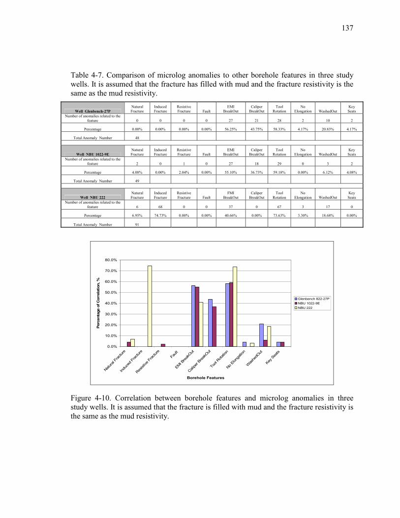
137

Table 4-7. Comparison of microlog anomalies to other borehole features in three study

wells. It is assumed that the fracture has filled with mud and the fracture resistivity is the

same as the mud resistivity.

Well Glenbench-27P

Natural

Fracture

Induced

Fracture

Resistive

Fracture Fault

EMI

BreakOut

Caliper

BreakOut

Tool

Rotation

No


Key

Seats

Number of anomalies related to the

feature 0 0 0 0 27 21 28 2 10 2

Percentage 0.00% 0.00% 0.00% 0.00% 56.25% 43.75% 58.33% 4.17% 20.83% 4.17%


Well NBU 1022-9E

Natural

Fracture

Induced

Fracture

Resistive

Fracture Fault

EMI

BreakOut

Caliper

BreakOut

Tool

Rotation

No


Key

Seats


feature 2 0 1 0 27 18 29 0 3 2

Percentage 4.08% 0.00% 2.04% 0.00% 55.10% 36.73% 59.18% 0.00% 6.12% 4.08%


Well NBU 222

Natural

Fracture

Induced

Fracture

Resistive

Fracture Fault

FMI

BreakOut

Caliper

BreakOut

Tool

Rotation

No


Key

Seats


feature 6 68 0 0 37 0 67 3 17 0

Percentage 6.95% 74.73% 0.00% 0.00% 40.66% 0.00% 73.63% 3.30% 18.68% 0.00%


Microlog Anomaly, Percentage of Correlation, vs. Borehole Features

0.0%

10.0%

20.0%

30.0%

40.0%

50.0%

60.0%

70.0%

80.0%

Natural Fracture

Induced Fracture

Resistive Fracture

Fault

EMI BreakOut

Caliper BreakOut

Tool Rotation

No Elongation

WashedOut

Key Seats

Borehole Features

Percentage of Correlation, %

Glenbench 822-27P

NBU 1022-9E

NBU 222

Figure 4-10. Correlation between borehole features and microlog anomalies in three

study wells. It is assumed that the fracture is filled with mud and the fracture resistivity is

the same as the mud resistivity.

138

Table 4-8. Comparison of microlog fracture anomalies based on the experimental

equation by Schlumberger and other borehole features, well NBU 222.

Well NBU 222 Natural

Fracture

Induced

Fracture

Resistive

Fracture Fault

FMI

Breakout

Caliper

BreakOut

Tool

Rotation

No


Key

Seats

Number of anomalies related to the feature 13 79 0 0 14 0 72 4 25 0

PERCENTAGE 13.40% 81.44% 0.00% 0.00% 14.43% 0.00% 74.23% 4.12% 25.77% 0.00%


Microlog Anomaly, Percentage of Correlation, vs. Borehole Feature, Well NBU 222

0.0%

10.0%

20.0%

30.0%

40.0%

50.0%

60.0%

70.0%

80.0%

90.0%

100.0%

Natural Fracture

Induced Fracture

Resistive Fracture

Fault

FMI Breakout

Caliper BreakOut

Tool Rotation

No Elongation

WashedOut

Key Seats

Borehole Features

Percentage of Correlation, %

NBU 222

Figure 4-11. Correlation between different borehole features and microlog fracture

anomalies, well NBU222. In this case, the experimental equation defined by

Schlumberger is used.

139

borehole features that occur in the wellbores. The goal of this study is to find a

correlation between microlog anomalies and natural fractures. However, the maximum

obtained correlation was related to borehole breakouts and induced fractures. For the

same borehole features, anomaly Plus/Minus 10 Ohmm had a larger percentage range of

correlation than Plus/Minus 5 Ohmm. Therefore, no rule exists to make a correlation

between natural fractures and microlog anomalies. On the other hand, the result for NBU

222, based on the experimental equation by Schlumberger, suggests that the equation is a

good indicator of induced fractures, not natural fractures.

In summary, results suggest that it is not possible to consistently find natural

fractures using microlog signatures in Natural Buttes field. Because, the microlog is a

directional tool, which may explain the lack of correlation between natural fractures and

microlog anomalies.

140

CHAPTER 5

FRACTURE MODELING

Statistical analyses applied to micro-resistivity logs in fractured intervals did not

show a satisfactory correlation. This motivated us to evaluate the tool sensitivity and

limitations in fractured and non-fractured intervals. The logging tool used for the study is

the Micro Cylindrically Focused Log (MCFL). There is existing FORTRAN software

(XLOG and NSLV), provided by Baker Atlas for the Micro Spherically Focused Log

(MSFL), which we adopted for use in the correlation. Because, the geometry of the

MSFL and the MCFL tools are similar.

5.1 Tool Response

The input file is included in the XLOG program. The input file contains

information such as tool diameter, electrode configuration, and number of zones

(Briceno, 2003). This program calculates the resistivity of the formation in only one

direction (Figure 5-1). Depending on the assumptions made, the number of zones (n) can

change. For example, in Figure 5-1, there are five different zones. They are; 1- the

borehole, 2- invaded zone before the natural fracture, 3- the natural fracture, 4- invaded

zone behind the fracture, and 5- uninvaded zone. The program uses the inside of the

borehole as the first zone. The diameter of each zone varies in different models. For each

model, the input data includes the number of zones and the resistivity value for each

zone. The resistivity immediately behind the wellbore is the resistivity of the flushed

zone (Rxo ) and the resistivity of the last zone is equal to the resistivity of the uninvaded

zone or true resistivity ( Rt ). The output file of the XLOG program is the input file for

141

Figure 5-1. Model of fracture-invasion profile. In this model, there are five different

zones; 1- the wellbore, 2-invaded zone before the natural fracture, 3 the natural fracture,

4-invaded zone behind the fracture, and 5- undisturbed zone (Briceno, 2003).

Impermeable Bed

Impermeable Bed

Permeable

Bed

Undisturbed

Zone

RRtt

Invaded

Zone

RRxoxo

Mud-cake

ddii

Impermeable Bed

Impermeable Bed

Permeable

Bed

Undisturbed

Zone

RRtt

Invaded

Zone

RRxoxo

Invaded

Zone

RRxoxo

Mud-cakeMud-cake

ddiiddii

Measurement

Direction

Natural Fracture

142

the NSLV program. The procedure is to make a copy from the XLOG output and paste as

the NSLV input. According to the input data, NSLV gives a measured resistivity that is

obtained by the log using the specific tool and formation property entered in the model

(Briceno, 2003). According to Briceno (2003), the measured resistivity (Rmeas ) is

different from the apparent resistivity (Ra). This equation shows the relationship

between apparent and measured resistivities.

RmeasR [Ω.m]= .1[m]a Rh

where Rh is a normalization factor. The value of Rh is 6.914, which is the tool response

for a homogenous formation with resistivities for all zones equal to 1 Ohmm (Briceno,

2003). Appendix A shows an example of input and output files for the XLOG and NSLV

programs.

5.2 Effect of Natural Fractures on the Tool Response

5.2.1 Results

In the programs XLOG and NSLV, we put a single vertical fracture parallel to the

pad surface of the MSFL/MCFL, at different distances away from the wellbore. The

resistivity of the flushed zone (Rxo ) and uninvaded zone ( Rt ) were kept constant in all

cases, and are 15 Ohmm and 30 Ohmm, respectively. Based on actual logs, these

resistivity numbers are typical for the study area.

In the program, a vertical natural fracture was introduced at different locations

from 2 to 14 in (5.08 to 35.56 cm) away from the wellbore, and the fracture width ranged

from 0.0001 in (0.0025 mm) to 0.6 in (15.24 mm). This is done for 4 different mud

resistivities (0.01, 0.10, 1.0, and 5.0 Ohmm). It is also assumed that mud invades the

143

fractures, not mud filtrate, and that all formation fluids would be displaced by the

invading mud. Water-based mud that fills fractures has less resistivity than neighboring

rocks. Therefore, fractured intervals may appear as high-conductivity zones in the

resistivity logs. To simplify, all results are presented in terms of conductivity for two

different units for fracture width (inch and millimeter), as illustrated in Figures 5-2

through 5-9.

5.2.2 Discussion

The models show that fracture distance from the wellbore has a significant effect

on the tool response. Mud resistivity is also important. In a very salty mud (0.01 Ohmm,

Figure 5-2), the model demonstrates that the tool is unable to detect any fracture more

than 12 in (30.48 cm) away from the wellbore. This decreases to around 8 in (20.32 cm)

for mud resistivity of 5.0 Ohmm (Figure 5-8). Therefore, fractures with large apertures at

distances greater than 12 in (30.48 cm) do not show any significant effect on the tool

response. Two general results can obtained from these modeling results: 1- fracture

distance away from the wellbore is an important factor on the tool response, 2- fracture

aperture plays a role for certain fracture distances away from the wellbore (a large effect

for shorter distances and less effect for longer distances).

5.3 Effect of Mud Resistivity and Fracture Aperture on Tool Response

5.3.1 Results

The previous model was run for different mud resistivity values, ranging from

0.01 Ohmm to 5.0 Ohmm. A vertical natural fracture was introduced at different

locations from 2 to 12 in (5.08 to 30.48 cm) away from the wellbore, and the fracture

width ranged from 0.0001 in (0.0025 mm) to 0.6 in (15.24 mm), as illustrated in Figures

5-10 through 5-15.

144

0

50

100

150

200

250

0.0001 0.001 0.01 0.1 1

Fracture width, in

Conductivity, mmho/m Fracture at 2 in

Fracture at 4 in

Fracture at 6 in

Fracture at 8 in

Fracture at 10 in

Fracture at 12 in

Fracture at 14 in


fracture is located at different distances from 2 to 14 in (5.08 to 35.56 cm) away from the

wellbore. The resistivity of the invading mud into the fracture is 0.01 Ohmm. Fracture

width ranges from 0.0001 to 0.6 in. Rxo and Rt are 15 and 30 Ohmm, respectively.

0

50

100

150

200

250

0.001 0.01 0.1 1 10 100

Fracture width, mm


Fracture at 4 in

Fracture at 6 in

Fracture at 8 in

Fracture at 10 in

Fracture at 12 in

Fracture at 14 in




width ranges from 0.00254 to 15.24 mm. Rxo and Rt are 15 and 30 Ohmm,

respectively.

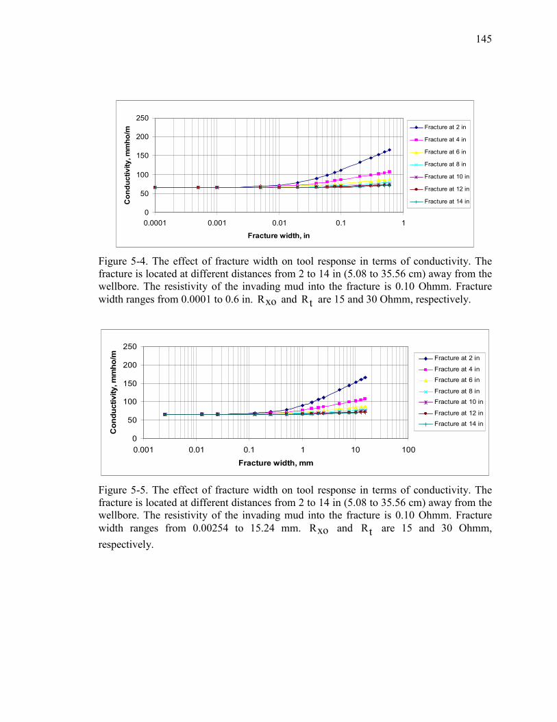
145

0

50

100

150

200

250

0.0001 0.001 0.01 0.1 1

Fracture width, in

Conductivity, mmho/m

Fracture at 2 in

Fracture at 4 in

Fracture at 6 in

Fracture at 8 in

Fracture at 10 in

Fracture at 12 in

Fracture at 14 in




width ranges from 0.0001 to 0.6 in. Rxo and Rt are 15 and 30 Ohmm, respectively.

0

50

100

150

200

250

0.001 0.01 0.1 1 10 100

Fracture width, mm


Fracture at 4 in

Fracture at 6 in

Fracture at 8 in

Fracture at 10 in

Fracture at 12 in

Fracture at 14 in





respectively.

146

0

50

100

150

200

250

0.0001 0.001 0.01 0.1 1

Fracture width, in


Fracture at 2 in

Fracture at 4 in

Fracture at 6 in

Fracture at 8 in

Fracture at 10 in

Fracture at 12 in

Fracture at 14 in



wellbore. The resistivity of the invading mud into the fracture is 1 Ohmm. Fracture width

ranges from 0.0001 to 0.6 in. Rxo and Rt are 15 and 30 Ohmm, respectively.

0

50

100

150

200

250

0.001 0.01 0.1 1 10 100

Fracture Width,mm


Fracture at 4 in

Fracture at 6 in

Fracture at 8 in

Fracture at 10 in

Fracture at 12 in

Fracture at 14 in




ranges from 0.00254 to 15.24 mm. RXO and Rt are 15 and 30 Ohmm, respectively.

147

0

50

100

150

200

250

0.0001 0.001 0.01 0.1 1

Fracture width, in


Fracture at 2 in

Fracture at 4 in

Fracture at 6 in

Fracture at 8 in

Fracture at 10 in

Fracture at 12 in

Fracture at 14 in




ranges from 0.0001 to 0.6 in. Rxo and Rt are 15 and 30 Ohmm, respectively.

0

50

100

150

200

250

0.001 0.01 0.1 1 10 100

Fracture Width, mm


Fracture at 4 in

Fracture at 6 in

Fracture at 8 in

Fracture at 10 in

Fracture at 12 in

Fracture at 14 in


fracture is located at different distances from 2 in to 14 in (5.08 to 35.56 cm) away from

the wellbore. The resistivity of the invading mud into the fracture is 5 Ohmm. Fracture


respectively.

148

0

60

120

180

240

0.0001 0.0010 0.0100 0.1000 1.0000Fracture Width, in

Conductivity,mmho/m Rm=0.01 ohmm

Rm=0.05 ohmm

Rm=0.1 ohmm

Rm=0.3 ohmm

Rm=0.5 ohmm

Rm=0.8 ohmm

Rm=1 ohmm

Rm=3 ohmm

Rm=5 ohmm

Figure 5-10. The response of the tool in fractured intervals for different mud resistivities

(0.01 Ohmm to 5.0 Ohmm). A vertical fracture is located 2 in (5.08 cm) away from the

wellbore.Rxo and Rt are 15 and 30 Ohmm, respectively. Fracture width is in the range

of 0.0001 in (0.00254 mm) to 0.6 in (15.24 mm). The invasion radius was assumed to be

12 in (30.48 cm).

0

60

120

180

240

0.0001 0.0010 0.0100 0.1000 1.0000

Fracture Width, in

Conductivity, mmho/m Rm =0.01 ohmm

Rm=0.05 ohmm

Rm=0.1 ohmm

Rm=0.3 ohmm

Rm=0.5 ohmm

Rm=0.8 ohmm

Rm=1 ohmm

Rm=3 ohmm

Rm=5 ohmm



wellbore. Rxo and Rt are 15 and 30 Ohmm, respectively. Fracture width is in the range


12 in (30.48 cm).

149

0

60

120

180

240

0.0001 0.0010 0.0100 0.1000 1.0000

Fracture Width, in

Conductivity, mmho/m Rm=0.01 ohmm

Rm=0.05 ohmm

Rm=0.1 ohmm

Rm=0.3 ohmm

Rm=0.5 ohmm

Rm=0.8 ohmm

Rm=1 ohmm

Rm=3 ohmm

Rm=5 ohmm





12 in (30.48 cm).

0

60

120

180

240

0.0001 0.0010 0.0100 0.1000 1.0000

Fracture Width, in


Rm=0.05 ohmm

Rm=0.1 ohmm

Rm=0.3 ohmm

Rm=0.5 ohmm

Rm=0.8 ohmm

Rm=1 ohmm

Rm=3 ohmm

Rm=5 ohmm





12 in (30.48 cm).

150

0

60

120

180

240

0.0001 0.0010 0.0100 0.1000 1.0000

Fracture Width, in


Rm=0.05 ohmm

Rm=0.1 ohmm

Rm=0.3 ohmm

Rm=0.5 ohmm

Rm=0.8 ohmm

Rm=1 ohmm

Rm=3 ohmm

Rm=5 ohmm



wellbore. Rxo and Rt are 15 and 30 Ohmm, respectively. Fracture width is in the

range of 0.0001 in (0.00254 mm) to 0.6 in (15.24 mm). The invasion radius was assumed

to be 12 in (30.48 cm).

0

60

120

180

240

0.0001 0.0010 0.0100 0.1000 1.0000

Fracture width, in


Rm=0.05 ohmm

Rm=0.1 ohmm

Rm=0.3 ohmm

Rm=0.5 ohmm

Rm=0.8 ohmm

Rm=1 ohmm

Rm=3 ohmm

Rm=5 ohmm



wellbore wall. Rxo and Rt are 15 and 30 Ohmm, respectively. Fracture width is in the

range of 0.0001 in (0.00254 mm) to 0.6 in (15.24 mm). The invasion radius was assumed

to be 12 in (30.48 cm).

151

5.3.2 Discussion

A relation exists between mud resistivity and fracture aperture for each fracture

location behind the wellbore (Figures 5-16). Figure 5-17 is a portion of Figure 5-16 at a

different scale. This is done to expand the data, because most of the data are in this range.

Therefore, it may show more data scattering than Figure 5-16. Each line indicates the

maximum mud resisitivity to detect fractures for a certain fracture aperture. For example,

in Figure 5-17, if there is a vertical fracture 2 in (5.08 cm) away from the wellbore, any

mud resistivity less than 0.76 Ohmm is appropriate to detect the fracture with the

minimum aperture of 0.03 in (0.76 mm). The maximum mud resistivity of 0.57 Ohmm

and 0.4 Ohmm similarly applies to vertical fractures at 4 in (10.16 cm) and 8 in (20.32

cm) away, respectively. In another words, for detecting a fracture with a certain aperture,

lower mud resistivity is needed at greater distances away from the wellbore.

5.4 Effect of Invasion on Tool Response

5.4.1 Results

The program was also run to evaluate invasion effects for fractured and non-

fractured zones. Rxo and Rt were kept constant at 15 and 30 Ohmm, respectively. In

the first model (fractured zone), fracture aperture was assumed to be 0.2 in (5.08 mm),

and the mud resistivity as 0.1 Ohmm. A vertical fracture is located 2, 4, and 6 in (5.08,

10.16, and 15.24 cm) away from the wellbore wall. The invasion radius ranged from 2 to

30 in (5.08 to 76.2 cm). The result is shown in Figure 5-18.

In the second model (non-fractured zone), the only variable was the radius of

invasion, which influenced the radius of the invaded zone (Rxo ) in the model. Other

parameters stayed the same as in the first model. Figure 5-19 shows the result.

152

0

0.5

1

1.5

2

2.5

3

3.5

4

4.5

5

0 0.1 0.2 0.3 0.4 0.5 0.6

Fracture Width, in

Rm, ohmm

Fracture at 2 in

Fracture at 4 in

Fracture at 6 in

Fracture at 8 in

Fracture at 10 in

Fracture at 12 in

Linear (Fracture at8 in)Linear (Fracture at6 in)Linear (Fracture at4 in)Linear (Fracture at


fracture at different distances from the wellbore. Fracture width ranges from 0.0001 in

(0.00254 mm) to 0.6 in (15.24 mm) and mud resistivity ranges from 0.01 Ohmm to 5.0

Ohmm. Rxo and Rt are 15 and 30 Ohmm, respectively. The invasion radius was

assumed to be 12 in (30.48 cm).

153

0

0.2

0.4

0.6

0.8

1

1.2

1.4

1.6

0 0.03 0.06 0.09 0.12 0.15

Fracture Width, in

Rm, ohmm

Fracture at 2 in

Fracture at 4 in

Fracture at 6 in

Fracture at 8 in

Fracture at 10 in

Fracture at 12 in

Linear (Fracture at8 in)Linear (Fracture at6 in)Linear (Fracture at4 in)Linear (Fracture at


fracture at different distances from the wellbore. Fracture width ranges from 0.0001 in

(0.00254 mm) to 0.10 in (2.54 mm) and mud resistivity ranges from 0.01 Ohmm to 1.6

Ohmm. Rxo and Rt were 15 and 30 Ohmm, respectively. The invasion radius was

assumed to be 12 in (30.48 cm). Arrows show the maximum mud resistivity to detect a

fracture with the aperture of 0.03 in at different distances from the wellbore wall.

Maximum Mud

Resistivity to

Detect Fractures

at Different

154

0

20

40

60

80

100

120

140

0 4 8 12 16 20 24 28 32

Invasion Radius, in


Fracture at 2 in

Fracture at 4 in

Fracture at 6 in

Figure 5-18. The effect of invasion radius on conductivity in a fractured interval.

Invasion radius ranges from 2 to 30 in (5.08 to 76.2 cm). Fracture location varies from 2

to 6 in (5.08 to 15.25 cm) away from the wellbore. Fracture width assumed was 0.2 in

(5.08 mm) and the resistivity of the mud invading the fracture was 0.10 Ohmm.

0

20

40

60

80

100

120

140

0 5 10 15 20 25 30

Invasion Radius, in


Figure 5-19. The effect of invasion radius on conductivity in a non-fractured zone.

Invasion radius ranges from 2 to 30 in (5.08 to 76.2 cm). Rxo and Rt are 15 and 30

Ohmm.

155

5.4.2 Discussion

Figure 5-18 indicates that the effect of invasion is negligible in the fractured

intervals. Figure 5-19 demonstrates that the effect of invasion faded for distances longer

than 12 in (30.48 cm) away from the wellbore. In another words, the effect of Rtis

negligible for an invasion radius larger than 12 in (30.48 cm). This confirms that the tool

is unable to detect any type of anomaly beyond 12 in (30.48 cm) from the wellbore wall.

5.5 Effect of Fracture Density on Tool Response

5.5.1 Results

Fracture density (number of fractures) is a factor that may influence the MCFL

tool response. To evaluate, we developed two different models. Fracture density, fracture

aperture, and fracture spacing are the variable parameters in these models. In the first

model, the fracture widths were kept constant as 0.2 in (5.08 mm), whereas fracture

spacing changes from 1 to 5 in (2.54 to 12.7 cm). Fracture density ranges from 1 to 10.

The result is shown in Figure 5-20. The first fracture is assumed to be 2 in (5.08 cm)

away from the wellbore wall.

In the second model, fracture spacing was kept constant 2 in (5.08 cm). Fracture

aperture ranges from 0.0001 in (0.00254 mm) to 0.6 in (15.24 mm) and mud resistivity

was assumed to be 0.10 Ohmm. The model was run for different fracture density from 1

to 6. The result is shown in Figure 5-21.

5.5.2 Discussion

According to Figure 5-20, for fracture density more than 2, the tool does not show

156

130

135

140

145

150

155

160

0 1 2 3 4 5 6 7 8 9 10

Fracture Density


Fracture spacing=1 in





Figure 5-20. The effect of fracture density on conductivity for different fracture spacing.

Rxo and Rt are 15 and 30 Ohmm. Fracture width assumed was 0.2 in (5.08 mm) and the

resistivity of the mud invading the fracture was 0.10 Ohmm. The invasion radius was

assumed to be 12 in (30.48 cm).

0

50

100

150

200

0.0001 0.001 0.01 0.1 1

fracture aperture, in


Number of Fractures=1






Figure 5-21. The effect of fracture density on MCFL tool response. Rxo and Rt are 15

and 30 Ohmm. Fracture width ranges from 0.0001 in (0.00254 mm) to 0.6 in (15.24 mm)

and the resistivity of the mud invading the fracture was 0.10 Ohmm. The invasion radius

was assumed to be 12 in (30.48 cm).

157

a significant effect. This is correct for fracture spacing more than 2 in (5.08 cm).

Although, for fracture spacing of 1 in (2.54 cm), fracture density more than 2 does not

show a significant difference in the conductivity, but for fracture density more than 5 and

6 the conductivity becomes constant. According to Figure 5-21, the effect of fracture

density is negligible for any fracture aperture less than 0.002 in (0.05 mm). It also

demonstrates that, for a certain fracture aperture, fracture density more than 2 does not

affect the tool response significantly. For a certain fracture aperture, there is also no

significant difference on conductivity between fracture density of 1 and 2. A possible

explanation is that part of the induced current in the formation prefers to go through the

first fracture behind the wellbore. This occurs because of low mud resistivity inside of the

fracture. The rest of the current that has less intensity than the initial current. Therefore,

the effect of fractures located further away from the wellbore will be negligible on the

tool response. This is because induced current will diminish due to fractures close to the

wellbore.

5.6 Effect of the Flushed and Uninvaded Zones Resistivities on Tool Response

5.6.1 Results

The resistivity of the flushed zone and uninvaded zone are two input parameters

for the input file. Several assumed values for Rxo (10 to 70 Ohmm) and Rt (10 to 150

Ohmm) were applied to the model. The range of 10 to 70 for Rxo and 10 to 150 for

Rt were considered, only to cover possible values in the study area. In this model, a

vertical fracture was assumed at 4 in (10.16 cm) away from the wellbore with a 0.2 in

(5.08 mm) aperture, filled by mud with resistivity of 0.10 Ohmm. The result is presented

in Figure 5-22.

158

0

20

40

60

80

100

120

140

160

180

200

0 20 40 60 80 100 120 140 160

Rt, ohmm


Rxo=10 ohmm

Rxo=20 ohmm

Rxo=30 ohmm

Rxo=40 ohmm

Rxo=50 ohmm

Rxo=60 ohmm

Rxo=70 ohmm

Figure 5-22. Tool response for various values of Rxo and Rt . Invasion radius was

assumed to be 5 in (12.7 cm). A vertical fracture with an aperture of 0.2 in is located 4 in

(10.16 cm) away from the wellbore. The resistivity of the invading mud that fills the

fracture is 0.10 Ohmm.

159

5.6.2 Discussion

According to Figure 5-22, for Rxo less than 30 Ohmm and Rt less than 50

Ohmm, the tool shows small response. In another words, for Rxo less than 30 Ohmm, the

effect of Rt more than 50 Ohmm is negligible. On the other hand, an increase in Rxo up

to 70 Ohmm does not show any influence from Rt on the tool measurement. Therefore,

using this tool for high values of Rxo and Rt is not recommended.

5.7 Application to Borehole

Based on the above evaluation, the MCFL tool is capable of detecting natural

fractures under certain conditions. Accordingly, we plotted resistivity log data from a

selected well (NBU 222) measured by MCFL versus depth. Then, we compared the

resistivity logs with image logs. Three different resistivity logs were utilized to find

a correlation for natural fracture zones determined by image logs. They are: 1- the

resistivity of the flushed zone (Rxo8 ), 2- deep laterolog resistivity (HLLD), and 3-

shallow laterolog resistivity (HLLS). We assume that if an open natural fracture exists

close to the wellbore, Rxo8 (log related to MCFL tool) may detect it, when mud is

appropriately salty and fracture aperture is high enough. Based on the radius of

investigation for different logs (HLLD and HLLS higher than Rxo8, Figure 5-23), HLLD

and HLLS can be influenced by fracture conductivity zones.

Mud resistivity at each depth was calculated based on the mud resistivity of the

measured sample at the surface temperature. They were 0.02, 0.70, and 0.50 Ohmm, for

NBU 222, NBU 921-29N, and Pawwinnee 3-181, respectively. According to the

correlation between fracture aperture and mud resistivity in Figures 5-16 and 5-17,

natural fractures with a minimum aperture of 0.005 in (0.12 mm), 0.03 in (0.7 mm), and

160

Figure 5-23. Radius of investigation of different resistivity tools. Laterologs

(shallow/deep) cover more rock volume in their measurements than micro-resistivity logs

(Peeters, 2004).

Laterologs (shallow/ deep)

Micro-resistivity

161

0.02 in (0.5 mm) can be detected in wells NBU 222, NBU 921-29N, and Pawwinnee

3-181, respectively. The mentioned resistivity logs were plotted versus depth in terms of

conductivity. Then, they were compared to the detected fractures from image logs.

Comparison of resistivity and image logs indicates a correlation with a sharp peak in the

Rxo8 log at fracture locations. The HLLD (deep laterolog) and HLLS (shallow

laterolog), however, show only small curvatures at fracture locations, as illustrated in

Figures 5-24 and 5-25.

Note that the drilling-induced shallow fractures did not show these effects. The

possible explanation can be based on radius of investigation. In other words, the HLLD

and HLLS consider greater volume of material in their measurements than the Rxo8 log.

In fact, the effect of Rt on the HLLD and HLLS logs is higher than the effect of shallow

drilling-induced fractures on these logs. On the other hand, the Rxo8 log measures the

resistivity of the volume of material close to the wellbore. Therefore, it can be affected by

the presence of induced fracture near the wellbore. Non-fractured intervals did not also

show any effect on the HLLD and HLLS. Figure 5-26 shows a non-fractured interval.

The Rxo8 log shows a sharp peak, while the HLLD and HLLS logs show small

curvatures in the reverse direction. Comparing this type of feature to the image and GR

logs, sandstone beds have been confirmed. The probable explanation is that mud has

infiltrated into the tight sandstones, while the invasion is not deep enough to influence the

HLLD and HLLS logs. Therefore, based on the investigation radius, the Rxo8 log is

influenced by fractures more than the other resistivity logs (HLLD and HLLS logs).

Drilling-induced fractures did not show consistent behavior on the resistivity logs. In

fact, the Rxo8 log shows a peak, but the HLLD and HLLS logs appear in variable trends.

I looked at all induced fracture intervals for three wells in the study area (NBU 222,

162

0

20

40

60

80

100

120

140

160

180

9490 9492 9494 9496 9498 9500 9502 9504 9506 9508 9510

Depth, ft


Rxo8HHLDHLLS

Figure 5-24. A natural fracture in the interval 9496-9502 ft, well NBU 222. Rxo shows a

sharp peak in the middle of the fracture (at 9499.5 ft), whereas HLLD and HLLS show

only a small curvature change. The estimated mud resistivity at formation condition is

0.02 Ohmm.

Natural Fracture

163

0

10

20

30

40

50

60

70

80

90

100

7490 7492 7494 7496 7498 7500 7502 7504 7506 7508 7510

Depth, ft


Rxo8HHLDHLLS

Figure 5-25. Two natural fractures in the interval 7497-7503 ft, well NBU 222. The

Rxo8 log shows a peak in this interval whereas the HLLD and HLLS logs show only a

small curvature change. The estimated mud resistivity at formation condition is 0.02

Ohmm.

`

Natural Fractures

164

Figure 5-26. The Rxo8 log shows a sharp peak in a non-fractured tight sandstone,

whereas the HLLD and HLLS logs show small curvature changes in the opposite

direction in the interval 8322.5-8324.5 ft, well NBU 222. The image log shows a highly

resistive sandstone (light color) and the GR log confirms a sandstone interval.

0

20

40

60

80

100

120

140

8320 8321 8322 8323 8324 8325 8326 8327 8328

Depth, ft


Rxo8HHLDHLLS

165

Pawwinnee 3-181, and NBU 921-29N) but no consistent results were observed. Figures

5-27 and 5-28 present two different appearances for induced fractures on the resistivity

logs.

5.8 Effect of Washouts and Breakouts

Intervals with breakouts and washouts show significant effects on the response of

resistivity logs. In the elongated intervals, the tool cannot be pressed against the wellbore

wall. This creates a distance between the measuring buttons and the wellbore wall. This

standoff is filled by mud. Because mud has low resistivity, in the case of large

washouts/breakouts, the tool measurement partially includes the mud resistivity. Figures

5-29 and 5-30 show washout and breakout effects on the resistivity logs.

5.9 Model Application

We applied the results of this investigation to two other wells (Pawwinnee 3-181

and NBU 921-29N) to detect natural fractures. The mud resistivity for Pawwinnee 3-181

Well is 1.225 Ohmm at the surface temperature, which is 0.5 Ohmm at formation

conditions. Before looking at image logs, we reviewed the resistivity log results to see

any “peaks.” Then, we looked at the caliper logs to see if any peaks could be related to

washout or breakouts. This indicated that 98 percent of the peaks were in

washout/breakout intervals. Furthermore, the image logs confirmed the breakout sections.

When breakouts and washouts are removed with caliper logs, the micro-resistivity logs

proved to be good fracture indicators in this well.

Well NBU 921-29N has a mud resistivity of 1.71 Ohmm at the surface

temperature and a calculated value of 0.7 Ohmm at formation conditions. According to

Figures 5-16 and 5-17, with optimal conditions of a fracture being 2 in (5.08 cm) behind

166

0

10

20

30

40

50

60

70

80

90

8330 8331 8332 8333 8334 8335

Depth, ft


Rxo8HHLDHLLS

Figure 5-27. The Rxo8 log shows a peak, whereas the HLLD and HLLS logs have a

small curvature change in the opposite direction in the interval 8331.5-8333.5 ft, well

NBU 222. The image log shows a drilling-induced fracture in this interval.

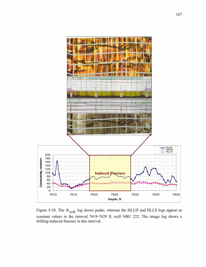
167

0

20

40

60

80

100

120

140

160

180

200

7610 7615 7620 7625 7630 7635 7640

Depth, ft


Rxo8HHLDHLLS

Figure 5-28. The Rxo8 log shows peaks, whereas the HLLD and HLLS logs appear as

constant values in the interval 7619-7629 ft, well NBU 222. The image log shows a

drilling-induced fracture in this interval.

`

Induced Fracture

168

8520

8530

8540

8550

8560

8570

8580

6 6.5 7 7.5 8 8.5

Borehole Diameter, in

Depth, ft

Bit Size

Caliper 1-3

Caliper 2-4

0

50

100

150

200

250

8520 8530 8540 8550 8560 8570 8580

Depth, ft


Rxo8HHLDHLLS

Figure 5-29. The effect of washout on Rxo8 , HLLD, and HLLS. Calipers show a

borehole washout from 8540 ft to 8570 ft, well NBU 222.

Washout

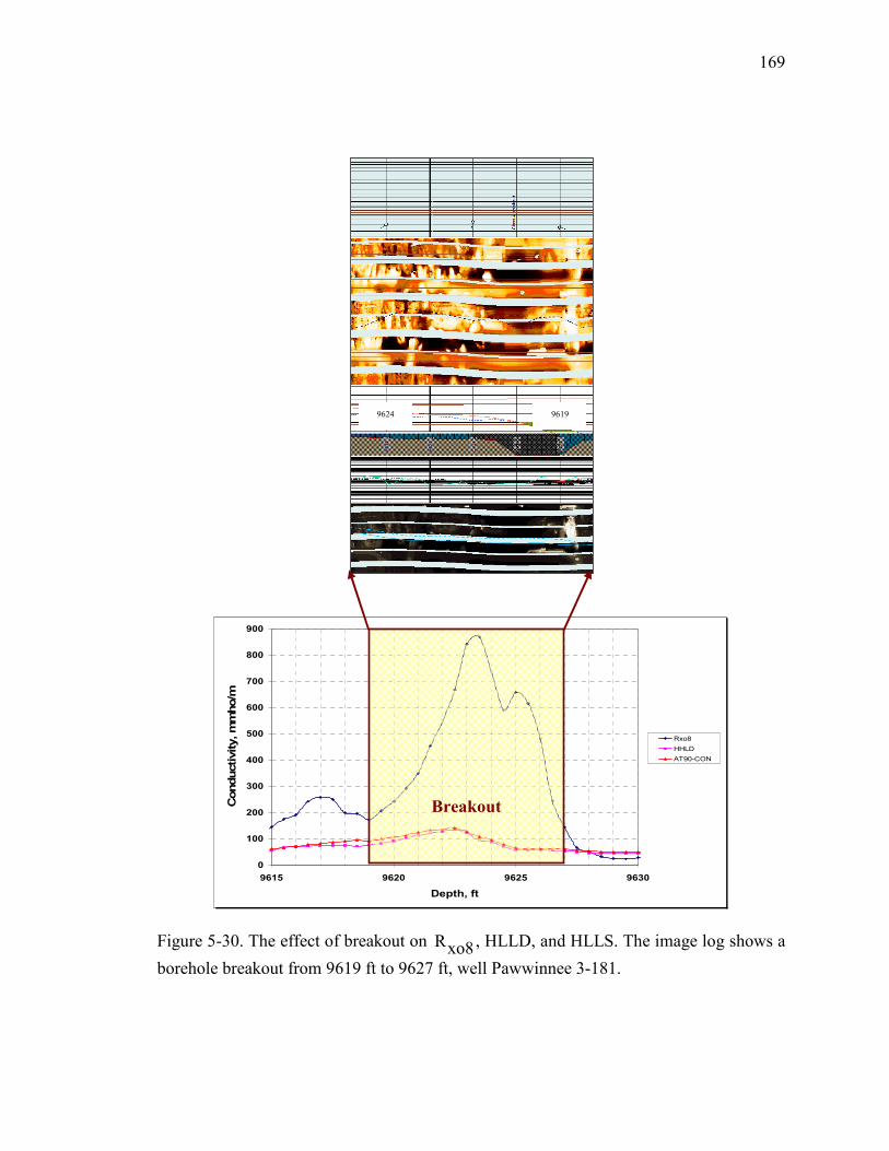
169

0

100

200

300

400

500

600

700

800

900

9615 9620 9625 9630

Depth, ft


Rxo8

HHLD

AT90-CON

Figure 5-30. The effect of breakout on Rxo8 , HLLD, and HLLS. The image log shows a

borehole breakout from 9619 ft to 9627 ft, well Pawwinnee 3-181.

9619 9624

Breakout

170

the wellbore for detecting natural fractures with this mud resistivity, a minimum fracture

aperture of 0.03 in (0.76 mm) is needed. Thus, we could not detect fractures accurately.

Based on logs interpreted by Schlumberger, image logs show a maximum fracture width

of 0.01 in (0.254 mm) in only a few intervals. Thus, the majority of fractures are smaller

than 0.01 in (0.254 mm). Therefore, one should not expect to detect fractures with micro-

resistivity logs. The same is true for the Pawwinnee 3-181 well.

5.10 Discussion

In Chapter 4, several approaches were applied to find a correlation between

natural fractures determined by image logs and micro-resistivity logs. Inconsistent results

motivated us to use existing FORTRAN software provided by Baker Atlas to evaluate the

sensitivity and limitation of the tool in fractured intervals. In fact, here we wanted to

prove that the MCFL tool is capable of detecting natural fractures under certain

conditions. As discussed earlier, this program calculates resistivity in one direction. We

put a single vertical fracture at different distances from the wellbore. We also assumed

that there is no intersection between fractures and wellbore. Of course, these assumptions

do not satisfy the real cases. In reality, we may have a fracture network in which no

fracture is vertical. In the applied model, if we use two or more vertical fractures, it

would be difficult to analyze. This is because the distance between the fractures and

fracture aperture for each single fracture comes into the assumptions. Of course, this is

done for two simple models in the section on fracture density. Resistivity of the flushed

zone and uninvaded zone is assumed as a constant for all applied models. During

invasion, we also assumed that mud has swept the formation hydrocarbons or formation

water. But in reality, we have irreducible water or hydrocarbon in the formation, which

affects the resistivity measurement. In addition, the resistivity of the mud can increase by

mixing with formation material during the drilling process. This increase also causes an

additional problem in mud resistivity for detecting fractures. This can be totally different

171

from the calculated resistivity value at formation temperature. Based on drilling records,

brine pills are the most common additive materials to mud in GNB to kill wells prior to

logging. According to the available information, these additive brine pills have not been

circulated in the borehole. If this is true, not only the resistivity of mud changes due to

the field temperature gradient, but also it appears as totally different resistivities at

different depths. This causes different readings in micrologs (R >RINV NOR ), which is

opposite from what is expected. This magnifies, especially in the sandstone intervals that

have gas, where density-neutron logs show crossover. Normally, RINV should be very

low in intervals with shallow invasion. But this is not true in the sandstone intervals

containing gas in the study area. In the same intervals, other resistivity logs showed the

same problem. RDFL , which is the RXO focused-log reading, shows higher value than

deep (RHDRS ) and medium (RHMRS ) resistivities while the deeper logs (RHDRS )

and (RHMRS ) should have higher resistivities thanRDFL . This is disturbing in the

sandstone intervals that have gas, where density-neutron logs show crossover. All of

these problems are seen in wells NBU 1022-9E and Glenbench 822-27P. The problem

was discussed with a log analyst (Dr. Dick Merkel) and he believed that the resistivity

logs obtained from well Glenbench 822-27P are not correct. According to Dick Merkel

(pers.commun., 2005) the resistivity logs obtained from NBU 1022-9E are also not

reliable. Examples are shown in Figures 5-31 and 5-32.

172

Figure 5-31. Different readings in micrologs (R >RINV NOR ) in sandstone intervals,

well NBU 1022-9E.

Micronormal

Microinverse

Sandstone

Interval

GR

173

Figure 5-32. The RDFL log shows a higher or equal value than RHDRS , and RHMRS

logs in intervals that have gas. Density-neutron logs show crossover in gas intervals (well

NBU 1022-9E).

Density-neutron

cross-over

HDRS (Red Line)

DFL (Black Line)

174

CHAPTER 6

CONCLUSIONS

AND

RECOMMENDATIONS

6.1 Conclusions

The purpose of this study was to investigate the relationship between natural

fractures detected by image logs and micro-resistivity logs. The major conclusions and

significant outcomes for this research are:

• Various approaches based on microlog separation were used to find a correlation

between natural fractures detected from image logs and microlog anomalies. They

did not show consistent results. Induced fracture detection from image logs (not

natural fractures) and borehole breakouts showed maximum correlation.

However, in one case (well NBU 222), no microlog anomalies were observed at

all.

• Several petrophysical models showed that the MCFL tool is capable of detecting

natural fractures parallel to the measuring pad but with restrictions on several

parameters. They are:

o Fracture distance from the wellbore wall: the models showed that the

MCFL tool cannot detect any fracture located further than 12 in (30.48

175

cm) for low mud resitivity (0.01 Ohmm) and 8 in (20.32 cm) away from

the wellbore wall for high mud resistivity (5.0 Ohmm).

o Fracture aperture and mud resistivity: study results showed that the MCFL

tool is capable of detecting a low aperture fracture in low resistivity mud

environment at a short distance from the wellbore.

o Fracture density: number of fractures (fracture density) more than 2 did

not show a significant effect on the MCFL tool response. However, the

response of the MCFL tool showed a small effect of fracture density when

the number of fractures increased from 1 to 2.

o Flushed zone and uninvaded zone resistivities: the model showed that low

resistivity for the flushed zone and uninvaded zone are recommended to

use the MCFL tool as a fracture detector.

• Based on the study wells, conductivity anomalies occur in intervals with natural

fractures, breakouts, washouts, and drilling induced fractures. When breakouts

and washouts are removed with caliper logs, the micro-resistivity logs proved to

be good fracture indicators (refer to attached CD Rom).

• Intervals of borehole elongation influence shallow resistivity tools response.

Therefore, to use micro-resistivity tools as a fracture indicator, the borehole

elongation must be identified independently.

• Two applied methods (borehole breakout and induced fracture) show the WNW-

ESE orientation for the SHmax direction in the study area.

• Study results in Natural Buttes field show that natural fracture orientation aligns

with maximum horizontal stress (SHmax) in the study area. This is very important

in terms of reservoir drainage.

176

6.2 Recommendations

Based on porosity and deep resistivity logs, an Rxo curve can be calculated. In a

borehole interval where the micro-resistivity is not affected by washouts and breakouts,

the difference between the calculated flushed zone resistivity and the measured micro-

resistivity could be a good fracture indicator. Documentation and verification of this

procedure is recommended for future work.

177

REFERENCES

Asquith, G., and Gibson, C., 1982, Basic well log analysis for geologists: AAPG

Methods in Exploration Series, No. 3, p. 43-44.

Babcock, E.A., 1978, Measurement of subsurface fractures from dipmeter logs: AAPG

Bulletin, v. 62, p. 1111-1126.

Barton, C.A., Moos, D., Peska, P., and Zoback, M.D., 1997, Utilizing wellbore image

data to determine the complete stress tensor: Application to Permeability

Anisotropy and Wellbore Stability: The Log Analyst, v. 38, No. 6, p. 21-33.

Bell, J.S., and Gough, D.I., 1986, Northeast-southwest compressive stress in Alberta:

Evidence from oil wells: Earth and Planetary Science Letters, v. 45, p. 475-482.

Bosworth, W.P., 1989, Use of borehole breakout studies in marathon production and

Exploration: Unpublished report, Marathon Oil Company, p. 21-33.

Briceno, M.G., 2003, Invasion profiles derived from shallow wireline logs:

Upublished thesis, Colorado School of Mines, Golden, CO, 230 p.

Brooks, M., 2002, Hydraulic fracture optimization on the Wasatch and Mesaverde

Formations of the Uinta Basin, Utah, USA: Unpublished paper, Schlumberger

Company.

178

Chidsey, C.T., Michael, D.L., and Jr., 1992, The fractured Green River and

Wasatch Formation of the Uinta Basin, Utah: Targets for horizontal

drilling, in Fouch, T.D., Nuccio, V.F., and Chidsey, T.C., Jr., eds.,

Hydrocarbon and mineral resources of the Uinta Basin, Utah and Colorado:

Utah Geological Association Guidebook 20, p. 123-126.

Climate diagnostics center, 2005, http://www.cdc.noaa.gov/USclimate/states.fast.html.

Doll, H.G., 1950, The Microlog- A new electrical logging method for detailed

determination of permeable beds: T. P. 2880, in Transactions of the AIME:

American Institute of Mining, Metallurgical and Petroleum Engineers, v. 189, p.

155-164.

Doupe, K.H., 2005, Structural compartmentalization at Cave Gulch field, Wind

River Basin, Wyoming: Unpublished thesis, Colorado School

of Mines, Golden, Co, 243 p.

Eisenmann, P., Gounot, M.T., Juchereah, B., Trouiller, J.C., and Whittaker, S.J., 1994,

Improved Rxo measurements trough semi-active focusing: Paper SPE-28437

in SPE Annual Technical Conference and Exhibition Proceedings, New Orleans,

LA, U.S.A, p. 781-794.

Fam, M.Y., Chemali, R., Seiler, D., Haugland, M., Stewart, W.F., 1995, Applying

electrical micro-imaging logs to reservoir characterization: Paper SPE-30608 in

SPE Annual Technical Conference and Exhibition, Dalas, Texas.

Fouch, T.D., Nuccio, V.F., Osmond, J.C., Logan, M., William, B.C., and Wandrey,

C.J., 1992, Oil and gas in uppermost Cretaceous and Tertiary rock, Uinta

Basin, Utah, in Fouch, T.D., Nuccio, V.F., and Chidsey, T.C., Jr., eds.,



Grace, M., Newberry, B., and Koepsell, R., 1998, Geologic application of dipmeter and

borehole electrical images: Unpublished text book, Schlumberger Oilfield

Services, Marathon, Houston, Texas.

179

Hilchie, D.W., 2003, Old electrical log interpretation: AAPG Methods in

Exploration Series No.15, p. 61-70.

Hurley, N., Asquith, G., Krygowski, D., Henderson, S., 2004, Basic well log

analysis: AAPG Methods in Exploration Series, No.16, p. 151-163.

Johnson, R.C., Roberts, S.B., 2003, The Mesaverde total, petroleum system, Uinta-

Piceance province, Utah and Colorado in Petroleum systems and geologic

assessment of oil and gas in the Uinta-Piceance province, Utah and Colorado:

USGS, Uinta-Piceance Assessment Team, Chapter 7, p. 7-8.

Knight C.D., 2004, Borehole image analysis: Unpublished report, Kerr Mc Gee

Company.

Longman, M., Basse, R., and Pope, J., 2003, Characteristics of the Glenbench

Sandstone reservoir, Eocene Green River Formation, Glenbench Field,

Uintah County, Utah: The Mountain Geologist, v. 40, No. 4, p. 129-141.

Lorenz, J.C., 2003, Fracture system in the Piceance Basin: Overview and comparison

with fractures in the San Juan and Green River Basins in Peterson, K.M., Olson,

T.M., Anderson, D.N., Piceance Basin 2003 Guidebook: The Rocky Mountain

Association of Geologists, p.75-94.

Luthi, S.M., 2000, Geological well logs, their use in reservoir modeling, Springer- Verlag

Berlin- Heidelberg, Germany, P. 74-118.

Minton, G.E., 2000, Subsurface study of the Lewis Shale in the southern

Washakie and Sand Wash Basins using borehole images, core, well log,

and seismic data: Unpublished thesis, Colorado School of Mines, Golden,

Co, 220 p.

180

Nuccio,V.F., Schmoker. J.W., and Fouch, T.D., 1992, Thermal maturity, porosity,

and lithofacies relationships applied to gas generation and production in

Cretaceous and Tertiary low-permeability (tight) sandstones, Uinta Basin,

Utah, in Fouch, T.D., Nuccio, V.F., and Chidsey, T.C., and Jr., eds.,



Osmond, J.C., 2003, History of oil and gas exploration in the Uinta Basin, Utah:

The Mountain Geologist, v. 40, No. 4, p. 101-110.

Osmond, J.C., 1992, Greater Natural Buttes gas field, Uintah County, Utah, in

Fouch, T.D., Nuccio, V.F., Chidsey, T.C., and Jr., eds., Hydrocarbon and mineral

resources of the Uinta Basin, Utah and Colorado: Utah Geological Association

Guidebook 20, p. 143-159.

Peeters, M., 2004, Advanced formation evaluation course: Power Point presentation.

Plumb, R.A., and Hickman, S.H., 1985, Stress-induced borehole elongation: A

comparison between the four-arm dipmeter and the borehole televiewer in the

Auburn geothermal well: Journal of Geophysical Research, v. 90, No. B7,

p. 5513-5521.

Rider, M., 1996, The geological interpretation of well logs: Whittles Publishing,

Scotland, 280 p.

Schlumberger well Surveying corporation, 1958, Microdevices: Document No. 8,

Chapter 6, p. 71-81.

Schlumberger, 2004, http://www.slb.com/media/services/evaluation/geology/fmi.pdf?

Seiler, D., King, G., and Eubanks, D., 1994, Field test results of a six arm

microresistivity borehole imaging tool: SPWLA 35th Annual Logging

Symposium, Houston, Texas, p. W1-W21.

181

Shade, M.E., and Hansen, D.K.T., 1992, Drilled sidewall cores aid in interpretation of

the Tertiary Wasatch Formation, Natural Buttes Field, Utah in Fouch, T.D.,

Nuccio, V.F., Chidsey, T.C., and Jr., eds., Hydrocarbon and mineral resources of

the Uinta Basin, Utah and Colorado: Utah Geological Association Guidebook 20,

p. 193-196.

Thompson, L.B., 2002, Atlas of borehole imagery: AAPG/Datapages Discovery series 4,

CD ROM.

USGS, 2005, http://pubs.usgs.gov/fs/fs-0026-02/fs-0026-02.pdf

Zheng, Z., Ewy, R.T., and Cook, N.G.W., 1989, Topical report on rock physics of

borehole breakouts: Gas Research Institute, Department of Materials Science and

Engineering University of California, Berkeley.

Zoback, M.D., Moos, D., Mastin, L., and Anderson, R.N, 1985, Wellbore breakout and

in-situ stress: Journal of Geophysical Research, v. 90, No. B7, p. 5523-5531.

Zoback, M.L., and Zoback, M.D., 1989, Tectonic stress field of the continental United

States: GSA Memoir 172, p. 523-537.

182

APPENDIX A

BAKER ATLAS PROGRAM (XLOG & NSLV)

A.1 Example of Input File for XLOG

A vertical fracture is assumed being 2 in away from the wellbore. Fracture

aperture is 0.10 in. The resistivity of mud invading the fracture is 0.10 ohmm. Rxo and

Rt are 15 and 30 ohmm, respectively. Invasion radius is 12 in away from the wellbore.

XLOG V2.5b INPUT

NMODES 1 DFERR_FOR_DFUN 1.D-8 RERR_FOR_DCADRE 1.D-8 TOL_FOR_DLAGF0 1.D-8 NTOL_FOR_DLAGF0 1 SPERR_FOR_DSPLINE 0.D0 FORMATION_CASES NZONES 5 DIAMETER 8.D0 10.D0 10.01D0 20.D0 RES_H 0.1D0 15.D0 0.1D0 15.D0 30.D0 TOOL_ID MLL_1D TOOL_DIA 8.D0 SEG_LENGTH 0.1D0 TOOL_OFFSET 0.D0 ELECTRODES 94. 4 0.2 0 2.4 2 0.2 0 0.8 1 0.2 0 2.4 2 0.2 0 34. 4 0.2 0

183

4.0 3 0.2 0 39. 4 END SEGMENTATION 2 1.0 4 5.0 7 2.0 8 4.0 9 10.0 10 20.0 END LARMOR 5

RARMOR 1.4

A.2 Example of Output for XLOG File (Input for NSLV File)

XLOG V2.5b OUTPUT

TOOL_ID = MLL_1D TOOL DIAMETER = 8.0000 INCHES BASIC SEGMENT LENGTH = 0.1000 INCHES TOOL OFFSET = 0.0000 INCHES NUMBER OF MODES = 1 TOOL LAYOUT: 1) EACH NUMBER IN THE SEQUENCE BELOW DESIGNATES A SEGMENT AND INDICATES ITS FUNCTION. 2) THE NUMBER 0 INDICATES THAT THE SEGMENT IS AN INSULATOR. 3) A NUMBER EQUAL TO 1 OR GREATER INDICATES THAT THE SEGMENT IS AN ELECTRODE. 4) ALL ELECTRODE SEGMENTS HAVING THE SAME NUMBER ARE CONNECTED TOGETHER. # 0 - 0.1000 INCHES # 1 - 0.1000 INCHES # 2 - 1.0000 INCHES # 3 - 0.1000 INCHES # 4 - 5.0000 INCHES DESCRIPTION OF CASES RUN ======================================== CASE 1 ZONE OUTSIDE DIA. RESISTIVITY (INCHES) (OHM-M)

184

1 8.0000 1.000E-01 2 10.0000 1.500E+01 3 10.0100 1.000E-01 4 20.0000 1.500E+01 5 INF. 3.000E+01 ======================================== ERROR PARAMETERS DFERR = 1.000E-08 (DFUN COMPUTATION) RERR = 1.000E-08 (DCADRE) TOL = 1.000E-08 (DLAGF0) NTOL = 1 (DLAGF0) SPERR = 0.000E+00 (DSPLINE) NOTES FOR READING THE DATA TABULATED BELOW 1) THE ELECTRODE SEGMENT CURRENTS ARE FOR THE CASE WHERE ALL SEGMENT VOLTAGES ARE SIMULTANEOUSLY 1.0 VOLT. 2) THE SEGMENT CURRENTS READING FROM LEFT TO RIGHT CORRESPOND TO THE ELECTRODE SEGMENTS (OMITTING INSULATORS) IN THE TOOL LAYOUT. DIAGRAM READING THAT DIAGRAM FROM LEFT TO RIGHT. 3) THE INTEGERS ABOVE AND TO THE LEFT OF THE MUTUAL RESISTANCE ARRAY INDICATE ELECTRODE NUMBERS. INTEGER NO. 5 INDICATES THE INFINITY ELECTRODE. ***** CASE NO 1 ***** INTEGRATION INFORMATION IN DLAGF0: NOFUN = 340 IERR = 0 IN DCADRE: DCADRE INTEGRATION PERFORMED TO SPECIFIED ACCURACY # OF RADIAL ZONES = 5 ZONE OUTSIDE DIA. RESISTIVITY (INCHES) (OHM-M) 1 8.0000 1.000E-01 2 10.0000 1.500E+01 3 10.0100 1.000E-01 4 20.0000 1.500E+01 5 3.000E+01

185

# OF ELECTRODES = 4 MUTUAL RESISTANCES 1 2 3 4 5 1 0.00000E+00 1.57756E+01 4.08325E+04 1.11151E+02 9.49273E+02 2 1.57756E+01 0.00000E+00 5.56422E+03 9.35840E+00 1.32406E+02 3 4.08325E+04 5.56422E+03 0.00000E+00 1.07912E+01 2.16113E+02 4 1.11151E+02 9.35840E+00 1.07912E+01 0.00000E+00 3.23787E+00 5 9.49273E+02 1.32406E+02 2.16113E+02 3.23787E+00 0.00000E+00 NOTES: 1) THE INTEGERS ABOVE AND TO THE LEFT OF THE MUTUAL RESISTANCE ARRAY INDICATE ELECTRODE NUMBERS. 2) INTEGER NO. 5 INDICATES THE INFINITY ELECTRODE.

A.3 Example of Output File for NSLV

NSLV.out

SOURCE = XLOG v2.5b TOOL_ID = MLL_1D TOOL OFFSET = 0.0000 INCHES RESPONSE_NAME MLL RESPONSE_ID MLL BHDia DiaInv Rmud Rxo Rtru Rmeas 8.0 0.0 0.100 0.000 0.000 98.209600

A.4 Calculation of Apparent Resistivity

98.209600RmeasR [Ω.m]= .1[m]= =14.20445 ohmma R 6.914h

USE OF MICROLOGS AND ELECTRICAL BOREHOLE ...

Documents

Transcript of USE OF MICROLOGS AND ELECTRICAL BOREHOLE ...