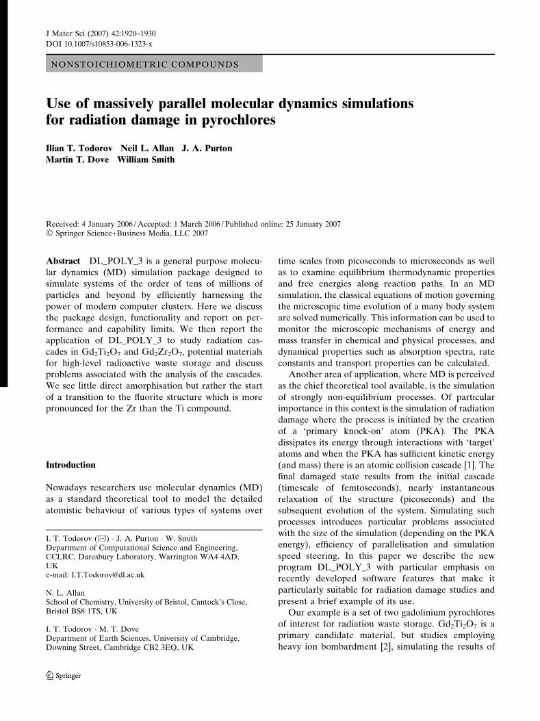
NONSTOICHIOMETRIC COMPOUNDS

Use of massively parallel molecular dynamics simulationsfor radiation damage in pyrochlores

Ilian T. Todorov Æ Neil L. Allan Æ J. A. Purton ÆMartin T. Dove Æ William Smith

Received: 4 January 2006 / Accepted: 1 March 2006 / Published online: 25 January 2007� Springer Science+Business Media, LLC 2007

Abstract DL_POLY_3 is a general purpose molecu-

lar dynamics (MD) simulation package designed to

simulate systems of the order of tens of millions of

particles and beyond by efficiently harnessing the

power of modern computer clusters. Here we discuss

the package design, functionality and report on per-

formance and capability limits. We then report the

application of DL_POLY_3 to study radiation cas-

cades in Gd2Ti2O7 and Gd2Zr2O7, potential materials

for high-level radioactive waste storage and discuss

problems associated with the analysis of the cascades.

We see little direct amorphisation but rather the start

of a transition to the fluorite structure which is more

pronounced for the Zr than the Ti compound.

Introduction

Nowadays researchers use molecular dynamics (MD)

as a standard theoretical tool to model the detailed

atomistic behaviour of various types of systems over

time scales from picoseconds to microseconds as well

as to examine equilibrium thermodynamic properties

and free energies along reaction paths. In an MD

simulation, the classical equations of motion governing

the microscopic time evolution of a many body system

are solved numerically. This information can be used to

monitor the microscopic mechanisms of energy and

mass transfer in chemical and physical processes, and

dynamical properties such as absorption spectra, rate

constants and transport properties can be calculated.

Another area of application, where MD is perceived

as the chief theoretical tool available, is the simulation

of strongly non-equilibrium processes. Of particular

importance in this context is the simulation of radiation

damage where the process is initiated by the creation

of a ‘primary knock-on’ atom (PKA). The PKA

dissipates its energy through interactions with ‘target’

atoms and when the PKA has sufficient kinetic energy

(and mass) there is an atomic collision cascade [1]. The

final damaged state results from the initial cascade

(timescale of femtoseconds), nearly instantaneous

relaxation of the structure (picoseconds) and the

subsequent evolution of the system. Simulating such

processes introduces particular problems associated

with the size of the simulation (depending on the PKA

energy), efficiency of parallelisation and simulation

speed steering. In this paper we describe the new

program DL_POLY_3 with particular emphasis on

recently developed software features that make it

particularly suitable for radiation damage studies and

present a brief example of its use.

Our example is a set of two gadolinium pyrochlores

of interest for radiation waste storage. Gd2Ti2O7 is a

primary candidate material, but studies employing

heavy ion bombardment [2], simulating the results of

I. T. Todorov (&) � J. A. Purton � W. SmithDepartment of Computational Science and Engineering,CCLRC, Daresbury Laboratory, Warrington WA4 4AD,UKe-mail: I.T.Todorov@dl.ac.uk

N. L. AllanSchool of Chemistry, University of Bristol, Cantock’s Close,Bristol BS8 1TS, UK

I. T. Todorov � M. T. DoveDepartment of Earth Sciences, University of Cambridge,Downing Street, Cambridge CB2 3EQ, UK

J Mater Sci (2007) 42:1920–1930

DOI 10.1007/s10853-006-1323-x

123

a-decay, have shown this undergoes amorphisation

which in turn leads to an increase in the leach rate of

Pu by an order of magnitude. Also using heavy ion

bombardment, Wang et al. [3] have demonstrated a

striking variation in radiation tolerance in Gd2(ZrxTi1–

x)2O7 (x = 0–1) such that radiation tolerance increases

with increasing Zr content and Gd2Zr2O7 is predicted

to withstand radiation damage for millions of years (cf.

100s of years for Gd2Ti2O7). Gd2(ZrxTi1–x)2O7 and

other pyrochlores have now received considerable

experimental attention [4–10]. The Gd zirconate end

member (x = 1) is indeed largely insensitive to irradi-

ation damage remaining highly crystalline to high

doses even at very low temperatures undergoing a

radiation-induced transition to a defect fluorite struc-

ture in which the Gd3+ and Zr4+ cations are disordered

and which is itself highly radiation resistant. We use

very large simulation cells in this paper and

DL_POLY_3 to compare displacement cascades in

Gd2Ti2O7 and Gd2Zr2O7. For a comprehensive recent

review of pyrochlores in the context of nuclear waste

disposal see Ewing et al. [11].

DL_POLY_3 Foundations

DL_POLY_3 [12] is a modern MD code conceived to

harness the power of HPC clusters by embedding the

domain decomposition strategy with linked cells meth-

odology. It has recently been re-engineered in For-

tran 90 taking full advantage of the modularisation

concept to separate and distribute logically common

(science-, maths- and semantics-wise) sets of variable

declarations, methods and initialisations in modules.

Adopting modularisation allows a lego-like build of

further enhancements and new implementations such

as force fields, scientific methodologies and numerical

algorithms. The inter-CPU communication is imple-

mented using MPI as most of the communication in the

code is implicit, based on dedicated functions and

subroutines developed as methods in a communication

dedicated module.

Domain decomposition (DD) is widely used to

parallelise various sorts of problems. The MD cell is

divided equi-spatially into geometrically identical

regions (domains) and each region is allocated to a

node (a CPU). The mapping of the domains on the

array of nodes is a non-trivial problem in general,

although specific solutions for certain numbers of

nodes (e.g., hypercubes) are much easier to obtain.

The domains are divided into sub-cells (link-cells) with

width slightly greater than the potential cut off for the

system force-field. The coordinates of the atoms in

link-cells adjacent to the boundaries of each domain

are passed onto neighbouring nodes sharing the same

boundaries (exchange of boundary data) to create the

so called domain halo. After this, each node may

proceed to calculate all pair interactions in its region

independently using the linked-cell method. No further

communication between the nodes is necessary until

after the equations of motion have been integrated.

If bond constraints are present in the system, the

equations of motions are modified to include constraint

solvers, RATTLE [13] for Velocity Verlet and

SHAKE [14] for Lepfrog Verlet integrators [15].

These constraint solvers are iterative algorithms that

add incremental corrections to the positions, velocities

and forces of constrained particles until the bond

lengths for all constraints in the system equal the

corresponding pre-defined constraint bond lengths to

within a given tolerance. Constraint algorithms involve

extra communication at each iteration when constraint

bonds cross domains. A domain crossing constraint

bond exists on two domains and one of the constrained

particles is on the domain halo of the other. Since

constraint particle positions, velocities and forces

change at each iteration it is necessary to refresh the

constraint particles that lie in the halo by updating

their positions, velocities and forces. Thus systems with

constraints are bound to have lower parallelisation

efficiency than systems without constraints. After the

equations of motion have been integrated the particles

which have moved out of their original domain must be

reallocated to a new domain.

In the exchange of boundary data to build domain

halos, it is crucial that data are only passed in

successively complementary directions (in 3D: north-

south and back, east-west and back and up-down and

back) at any given instant and in between exchanges,

the exchanged data must be re-sorted before the next

exchange. This is necessary to ensure the corner and

edge link-cell data are correctly exchanged between

domains sharing edges and corners, rather than faces.

The linked-cell method (LC) [16, 17] is a simple

serial algorithm linearly dependent on the number of

particles comprising the domain and its surrounding

halo. It assigns each atom to its appropriate sub-cell

and a linked list is used to construct a logical chain

identifying common cell members. A subsidiary header

list identifies the first member of the chain. This allows

all the atoms in a cell to be located quickly. The

calculation of the forces is treated as a sum of

interactions between sub-cells, in the course of which

all pair forces are calculated. It is straightforward to

allow for periodic boundary conditions. The algorithm

greatly reduces the time spent in locating interacting

123

J Mater Sci (2007) 42:1920–1930 1921

particles when the potential cut off is very short in

relation to the size of the domain. This makes the LC

algorithm particularly powerful as it enables extremely

large systems to be simulated very cost-effectively.

Although the DD algorithm is originally designed

for systems with short-range forces, it can also be used

for systems with Coulombic forces. DL_POLY_3 relies

on a new DD adaptation of the Smoothed Particle

Mesh Ewald method (SPME) [18] for calculating long

range forces in molecular simulations. In this adapta-

tion [19] two strategies are employed to optimise the

traditional Ewald sum. The first is to calculate the

(short-ranged) real space contributions to the sum

using the DD method as outlined above. The second is

to use a fine-grained mesh in reciprocal space and

replace the Gaussian charges by finite charges on mesh

points. The mesh permits the use of 3D Fast Fourier

Transforms (3D FFTs) [20]. DL_POLY_3 uses a novel,

fully memory distributed, parallel implementation of

the 3D FFT—the Daresbury Advanced Fourier Trans-

form (DAFT) [21]—that exploits the DD concept.

DL_POLY_3 also offers a great number of control

options [22]. However, it suffices here to outline only

the few that are of particular use to radiation damage

simulations. The variable timestep option requires the

user to specify an initial guess for a reasonable

timestep for the system (in picoseconds). The simula-

tion is unlikely to retain this as the operational

timestep as the latter may change in response to the

dynamics of the system. The option is used in

conjunction with two variables mindis (default

0.03 A) and maxdis (default 0.1 A; note max-

dis ‡ 2.5 mindis). These distances serve as control

values in the variable timestep algorithm, which

calculates the greatest distance a particle has travelled

in any timestep during the simulation. If the maximum

distance is exceeded, the timestep variable is halved

and the step repeated. If the greatest move is less than

the minimum allowed, the timestep variable is doubled

and the step repeated. In this way the integration

timestep self-adjusts in response to the dynamics of the

system; the simulation slows down to account accu-

rately for the dynamics during the initial stages in the

radiation damage cascade simulations far from equi-

librium and then speeds up to utilise CPU time

effectively when the system cools down.

The defect detection tool uses an algorithm that

compares the simulated MD cell to a reference MD

cell. The former defines the actual positions of the

particles and their atom types and the latter is taken

here to be the structure of the undamaged lattice. If a

particle, p, is located in the vicinity of a site, s, defined

by a sphere with centre this site and a user defined

radius, 0.3 A £ Rdef £ 1.3 A (default value 0.75 A),

then the particle is a first hand claimee of s, and the site

is not vacant. Otherwise the site is presumed vacant

and the particle is presumed a general interstitial. If a

site, s, is claimed while another particle, p¢, is located

within the sphere around it, then p¢ becomes an

interstitial associated with s. After all particles and all

sites are considered, it is clear which sites are vacan-

cies. Finally, for every claimed site, distances between

the site and its first hand claimee and interstitials are

compared and the particle with the shortest one

becomes the real claimee. If a first hand claimee of s

is not the real claimee it becomes an interstitial

associated with s. At this stage it is clear which

particles are interstitials. The sum of interstitials and

vacancies gives the total number of defects in the

simulated MD cell. Note that the algorithm cannot be

applied safely if Rdef is larger than half the shortest

interatomic distance within the reference MD cell since

a particle may claim or/and be an interstitial associated

with more than one site. Low values of Rdef are likely

to lead to slight overestimation of the number of

defects. If the simulation and reference MD cell have

the same number of atoms then the total number of

interstitials is always equal to the total number of

vacancies.

Performance and capability

To evaluate DL_POLY_3 performance and scalability

a set of test MD simulations were run on the HPCx

(IBM SP4 cluster—http://www.hpcx.ac.uk) super-clus-

ter at Daresbury Laboratory (the UK’s 1st and world’s

46th fastest1). The tests were based on three model

systems; (i) Solid Ar, (ii) NaCl and (iii) SPC Water,

with increasing complexity of their force-fields as

outlined in Table 1 and carried out at conditions as

outlined in Table 2. All test cases were set up using

values for the simulation cell parameters obtained

from previous equilibration runs using the same force-

fields as listed in Table 1(a–c) and at the same

simulation conditions as in Table 2. The size-per-

CPU and cut off values for each system were chosen

to ensure that all systems have the same domain halo

volume on average, so that relatively the same volume

of MPI messaging for domain boundary data exchange

is required between neighbouring domains for each

system at any timestep. Thus the difference in paral-

lelisation performance between the three systems is

1 Ranking in http://www.top500.org at the time of writing inJanuary 2006.

123

1922 J Mater Sci (2007) 42:1920–1930

based on the complexity of the different force fields

and on the additional communication these involve.

To detect and compare the parallelisation efficiency

of different systems and of different processor counts

the following construction was employed. Whenever

the number of CPUs was doubled the simulated

systems were also doubled in size,2 ensuring that the

link-cell algorithms and the domain halo volume for

each system remained the same for any processor

count. Thus, if parallelism were ideal the simulation

time-per-timestep for each system would be the same

for any processor count.

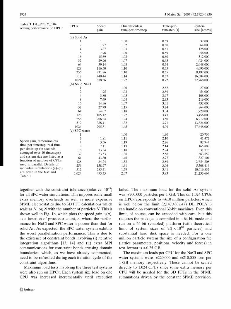
Table 3(a–c) present simulation performance data

for systems (i)–(iii). The tables list the time-per-

timestep and system size as a function of processor

count. Also listed for comparison are the dimensionless

time-per-timestep, s, and the speed gain, c, defined by

s nð Þ ¼ MtnMt1

; c nð Þ ¼ Mt1

Mtn ð1Þ

where Dtn is the time-per-time step at processor count

n. s and c for all three systems are plotted as a function

of the processor count in Fig. 1a, b respectively.

Perfect parallelisation corresponds to s(n) = 1, good

parallelisation corresponds to 25% increase at each

doubling of the processor count. Figure 1a shows that

for all three systems s increases logarithmically until

32 CPUs and then almost linearly. The logarithmic

increase in s at low processor counts is associated with

the population of the first logical partition (LPAR) of

HPCx. HPCx comprises 38 LPARs, each running its

own copy of the AIX operating system, and connected

via high performance ‘federation’ switches. The linear

increase of s at high processor counts is related to the

incremental increase of (i) time for MPI organisation

and (ii) global (collective) communication operations.

The results show that parallelisation is excellent for all

three systems.

The SPME summation accuracy (10–6) was kept

constant3 for all NaCl and SPC water simulations

Table 2 Simulation parameters of the model systems tested using DL_POLY_3

System Size per CPU[particles]

Ensemble [type] Short-range potential cutoff [A]

Equilibriumtemperature [K]

Equilibrium pressure[k atm]

Solid Ar 32,000 NVE 9 4.2 0.001NaCl 27,000 NVE 12 500 0.001SPC water 20,736 NPT Berendsen 0.5 0.75 8 300 0.001

NPT ensembles are characterised by thermostat and barostat relaxation times in picoseconds

Table 1 Force-fields for the tested systems as discussed in the text

(a) Solid Ar with mass of 39.95 Da and zero charge

Interaction Type e [eV] r [A]

Ar–Ar Lennard–Jones 4.2 0.001

(b) NaCl with m(Na) = 22.9898 Da, q(Na) = 1e, m(Cl) = 35.453 Da and q(Cl) = –e

Interaction Type A [eV] < [A–1] r [A] C [eV A6] D [eV A8]

Na–Na Born–Huggins–Meyer 2544.35 3.1545 2.340 10117.0 4817.7Na–Cl 2035.48 3.1545 2.755 67448.0 83708.0Cl–Cl 1526.61 3.1545 3.170 698570.0 1403200.0

(c) SPC Water with m(H) = 1.00797 Da, q(H) = 0.365e, m(O) = 16.9994 Da and q(O) = –0.73 e, and constraints H1,2–O = 1.03 A andH1–H2 = 1.681982 A

Interaction Type e [eV] r [A]

O–O Lennard–Jones 0.16 3.196

The Lennard–Jones and Born–Huggins–Meyer potentials have forms defined by

U rij

� �¼ r

rij

� �12

� rrij

� �6" #

andU rij

� �¼ A exp B r� rij

� �� �� C

r6ij

� D

r8ij respectively

2 System sizes were doubled cyclically in the a, then b and then cdirections.

3 This corresponded in a 64 · 64 · 64 grid for the FFT perdomain (CPU).

123

J Mater Sci (2007) 42:1920–1930 1923

together with the constraint tolerance (relative, 10–5)

for all SPC water simulations. This imposes some small

extra memory overheads as well as more expensive

SPME electrostatics due to 3D FFT calculations which

scale as N log N with the number of particles N. This is

shown well in Fig. 1b, which plots the speed gain, c(n),

as a function of processor count, n, where the perfor-

mance for NaCl and SPC water is poorer than that for

solid Ar. As expected, the SPC water system exhibits

the worst parallelisation performance. This is due to

the existence of constraint bonds involving (i) iterative

integration algorithms [13, 14] and (ii) extra MPI

communications for constraint bonds crossing domain

boundaries, which, as we have already commented,

need to be refreshed during each iteration cycle of the

constraint algorithms.

Maximum load tests involving the three test systems

were also run on HPCx. Each system size load on one

CPU was increased incrementally until execution

failed. The maximum load for the solid Ar system

was �700,000 particles per 1 GB. This on 1,024 CPUs

on HPCx corresponds to �610 million particles, which

is well below the limit (2,147,483,647) DL_POLY_3

can handle on conventional 32-bit machines. Even this

limit, of course, can be exceeded with care, but this

requires the package is compiled in a 64-bit mode and

run on a 64-bit (enabled) platform (with theoretical

limit of system sizes of 9.2 · 1018 particles) and

substantial hard disk space is needed. For a one

million particle system the size of a configuration file

(lattice parameters, positions, velocity and forces) in

text format is �0.25 GB.

The maximum loads per CPU for the NaCl and SPC

water systems were �220,000 and �210,000 ions per

1 GB memory respectively. These cannot be scaled

directly to 1,024 CPUs since some extra memory per

CPU will be needed for the 3D FFTs in the SPME

summations driven by the constant SPME precision.

Table 3 DL_POLY_3.04scaling performance on HPCx

Speed gain, dimensionlesstime-per-timestep, real time-per-timestep (in seconds,averaged over 10 timesteps)and system size are listed as afunction of number of CPUsused in parallel. Details ofindividual simulations (a)–(c)are given in the text andTable 1

CPUs Speedgain

Dimensionlesstime-per-timestep

Time-per-timestep [s]

Systemsize [atoms]

(a) Solid Ar1 1 1.00 0.59 32,0002 1.97 1.02 0.60 64,0004 3.87 1.03 0.61 128,0008 7.96 1.00 0.59 256,000

16 15.69 1.02 0.60 512,00032 29.96 1.07 0.63 1,024,00064 59.14 1.08 0.64 2,048,000

128 116.50 1.10 0.65 4,096,000256 231.86 1.10 0.65 8,192,000512 448.44 1.14 0.67 16,384,000

1024 838.36 1.22 0.72 32,768,000(b) Solid NaCl

1 1 1.00 2.82 27,0002 1.95 1.02 2.89 54,0004 3.80 1.05 2.97 108,0008 7.69 1.04 2.93 216,000

16 14.96 1.07 3.01 432,00032 27.79 1.15 3.24 864,00064 54.07 1.18 3.34 1,728,000

128 105.12 1.22 3.43 3,456,000256 206.24 1.24 3.50 6,912,000512 388.41 1.32 3.71 13,824,000

1024 705.81 1.45 4.09 27,648,000(c) SPC water

1 1.00 1.90 20,7362 1.81 1.11 2.10 41,4724 3.36 1.19 2.26 82,9448 7.11 1.13 2.14 165,888

16 13.54 1.18 2.24 331,77632 23.53 1.36 2.58 663,55264 43.80 1.46 2.77 1,327,104

128 84.24 1.52 2.89 2’654,208256 158.97 1.61 3.06 5,308,416512 285.41 1.79 3.41 10,616,832

1,024 495.35 2.07 3.93 21,233,664

123

1924 J Mater Sci (2007) 42:1920–1930

However, our estimate is a 1,000 fold load on

1,024 CPUs. The reduced maximum load per CPU

for the latter two systems relative to that in the solid Ar

simulation is readily explained. The maximum load per

CPU is dependent on the available memory per CPU

after force field arrays are allocated. The larger the

complexity and/or the higher the accuracy of the force

field description, the lower the limit of the maximum

load per CPU.

Overall, DL_POLY_3 exhibits excellent parallelisa-

tion performance over large processor counts and

ability to utilise available memory extremely efficiently

allowing loads as large as �220,000 ions per 1 GB

memory for systems with force-fields as complex as

that for SPC water.

Cascade simulations

In this section we report molecular dynamics simula-

tions of collision cascades for PKAs with energies

E £ 3 keV, 3 keV < E < 10 keV and E = 10 keV

using cubic simulation cells of 88,000, 152,064 and

193,336 atoms respectively. These large cell sizes

ensure that a cascade should not normally interact

with its periodic images for all practical purposes in our

simulations. Initial simulation cell lengths were set to

the appropriate multiple of the experimental lattice

parameter, corresponding to 10, 12 and 13 unit cells in

each direction respectively. The initial temperature of

the simulation was set to 300 K and the simulation

allowed to equilibrate for 10 ps within the NPT-

ensemble, using a timestep of 2 fs.

Each ion in the pyrochlores is assigned its formal

charge, i.e. 3+, 4+ and 2– for Gd, Ti/Zr and O

respectively. Ions can approach each other closely

particularly at the start of the simulations and it is vital

to use potentials that are likely to be accurate over a

wide range of internuclear separations and especially

at short distances. The potentials here have been

calculated using the modified Gordon–Kim electron-

gas model [23]. They have been used previously in

simulation studies of a wide range of binary and

ternary oxides (e.g., Ref. [24]) including problems

involving defects where the interatomic distances close

to the defect after relaxation may be very different

from those in the perfect lattice at equilibrium [25].

The potential parameters for O–O, Ti–O, Gd–O and

Zr–O, collected together in Table 4, were generated by

fitting an exponential of the form A exp(–r/q) (where A

and q are constants) to the electron-gas interaction

energies. A comparison of experimental and calculated

lattice parameters, and bond lengths for the two

pyrochlores is given in Ref. [26]. Devanathan and

Weber have recently used potentials for the Ti and Zr

compounds very similar to our own [27].

The production of a cascade was started from the

energetic recoil of a single atom, the PKA. All

simulations used for the PKA a U atom substituted

Table 4 Short range potential parameters used for the pyroch-lores and the primary knock-on’ atom (PKA) with cut off of 8 A

Interaction A/eV q/A

O–O 249.3764 0.3621Ti–O 3878.4225 0.2717Gd–O 4651.9633 0.2923Zr–O 8769.5930 0.2619U–O 4792.4400 0.3009

The form of the Buckingham potential is Vij ¼ A exp �rij=q� �

Fig. 1 DL_POLY_3 (a) dimensionless time-per-timestep and(b) speed gain from the simulation data in Table 1(a–c) plottedas a function of processor count. The green dotted line indicatesthe parallelisation limit also called perfect or embarrassingparallelisation. The red line indicates the standard for a goodparallelisation (time-per-timestep increase of 25% for eachdoubling of the processor count)

123

J Mater Sci (2007) 42:1920–1930 1925

for a native Gd ion, with the U–O potential also given

in Table 4. The subsequent collisions, displacements

and recombination of atoms with vacant sites were

followed, so that the complete structure and evolution

of the cascade could be monitored. A 5 ps evolution of

a 5 keV PKA cascade in an MD cell of 152,064

particles takes 3.5 h of CPU time on 16 processors of

the Dirac cluster at the University of Bristol (48 dual

processor Pentium 4 Xeon on 2 GHz nodes with

Myranet 2000 interconnect). A 10 ps evolution of a

10 keV PKA cascade for the largest MD cell used in

this study takes 9 h of CPU time on 16 processors on

the same cluster. Here in all simulations the initial

velocity of the PKA was along a body-diagonal of the

MD cell (eight directions). The creation of a radiation

cascade results in an initial sharp rise in the global

temperature of the simulation cell, no larger than

1,150 K for the simulation cells in this paper, and the

temperature then decreases during the simulation.

Timestep lengths vary during the development of a

cascade. Typically for the 10 keV cascades reported in

this paper, timesteps are very short (approximately a

few 10–3 fs) at the beginning of the cascade simulation

(up to 0.25 ps of the simulation time) and remain

relatively unchanged from after a few picoseconds

(1 ‚ 5 ps of simulation time) to the end of the

simulation (total simulation time 8–12 ps).

Analysis of the cascades can be carried out in

several useful ways. We start as in Ref. [28] by

defining a ‘defect’ in terms of displacements, i.e., as

an ion that has moved more than half the average of

the first-neighbour interatomic distances. This is

determined with respect to the position of an ion

after the equilibration phase of the simulation.

Alternative definitions [29] are discussed below.

Calculated limiting values of the mean-square dis-

placements for the parent pyrochlores (no cascades)

indicate that self-diffusion processes are negligible

after the final formation of the cascade and so do not

influence the number of defects on this relatively

short timescale.

For a given PKA energy the number of such

‘defects’ is larger for Gd2Zr2O7 than Gd2Ti2O7, as is

clear in Fig. 2, which plots the running totals of

‘defects’ as a function of time during a 10 keV cascade.

In Table 5 we break down this total for the 10 keV

cascades. The numbers of each type of atom which

have been displaced by a given distance are listed,

together with the total distance travelled by the PKA.

More atoms are displaced in the Zr than the Ti

compound. The PKA has travelled further in the Zr

case, and fewer heavier Zr ions are displaced than

lighter Ti ions. Nevertheless, the number of cations

displaced overall is comparable in both compounds,

while more anions are displaced in the Zr pyrochlore.

This appears to be in conflict with results from

high-energy ion bombardment experiments [3], where

the resistance to amorphization in Gd2Ti2–xZrxO7

increases with increasing Zr content. We have

Fig. 2 Instantaneous number of ‘defects’ plotted as a function oftime during a 10 keV cascade (U PKA) in the Ti and Zrpyrochlores (Gd–Ti–O triangles, Gd–Zr–O squares). There areseparate plots for the damage on the cation (empty symbols) andanion (filled symbols) sublattices. As discussed in the text wehere define a ‘defect’ as an ion that has moved more than half theaverage of the first-neighbour interatomic distances

Table 5 Structural damage data from 10 keV cascades in Ti andZr pyrochlores at 300 K and zero pressure

PKA directions Æ111æ Gd2Ti2O7 Gd2Zr2O7

Displaced: Species Species

Gd Ti O Gd Zr OBand (A)

<1 0 0 0 0 0 01–2 0 1 6 0.3 0 1532–3 1 2 212 3 2 2323–4 8 8 49 6 6 1324–5 0.5 1 30 3 2 515–6 0 0.5 13 0.8 1 186–7 0.3 0.8 4 0.8 1 87–8 0 0.8 4 0 0 28–9 0.5 0 3 0.5 0.3 29–10 0 0 1 0 0 1… … … … … … …Total 11 15 329 15 12 610

Final distance of PKA fromstarting position (A)

84 95

The primary knock-on’ atom (PKA) is a U ion. The table listshow many atoms of each species have moved a particular dis-tance given in the first column from their original lattice posi-tions. The second column and the third column list the meanvalues from all eight cascades in Æ111æ directions for Ti and Zrpyrochlores respectively

123

1926 J Mater Sci (2007) 42:1920–1930

therefore examined the damage distribution in more

detail. We note first that the increase in damage on the

oxygen sublattice is largely due to a substantial

increase in the Zr compound of the numbers of O

ions moving between 1 A and 2 A (by over 150) and

between 3 A and 4 A, relative to those in the Ti

compound. The numbers of oxygen atoms moving

between 2 A and 3 A or more than 4 A from their initial

positions are broadly similar. We obtain further insight

into the oxygen disorder after each cascade by plotting

the number of ions displaced vs. distance rather than

tabulating this information in broad bands as in Table 5.

This plot is shown in Fig. 3 for the two materials, and it is

clear that this plot is highly structured with well defined

peaks up to�6 A for each compound. The differences in

the number of atoms displaced at short distances

(<2.7 A) between the Zr and Ti compounds are partic-

ularly striking in this figure, with pronounced peaks at

just below and just above 2 A for the former which are

almost completely absent in the curve for the latter.

Many oxygens are thus displaced a small amount in the

Zr compound. The differences in the two curves for

larger displacement distances (>3.5 A) are smaller and

the sign of the difference between the two curves

changes with distance.

It is particularly instructive to consider not just the

displacements of individual ions but to consider the

structure of the damaged compound itself. We examine

the number of atoms not located at lattice sites, using

the defect detection algorithm described in the previ-

ous section, thus changing our operating definition of a

defect and avoiding the previous somewhat arbitrary

definition of a defect in terms of displacements.

Table 6 lists the number of defects, both interstitials

and vacancies, defined in this new way, in the simula-

tion cell (193,336 atoms) for a PKA of 10 keV for each

compound. The variation in the number of interstitial

defects from one atom type to another and from the Ti

to the Zr pyrochlore are the same as for the totals of

each atom type displaced in each compound (e.g.,

Table 5).

A measure based on a point defect description can

be misleading in certain situations. For example in the

presence of dislocation-type extended defects every

atom associated with the extended defect will count

towards the defect total even in a region where there is

significant local order. This consideration has led us to

calculate the oxygen–oxygen radial distribution func-

tions (RDFs) for the undamaged and damaged mate-

rials. These and the differences between the two are

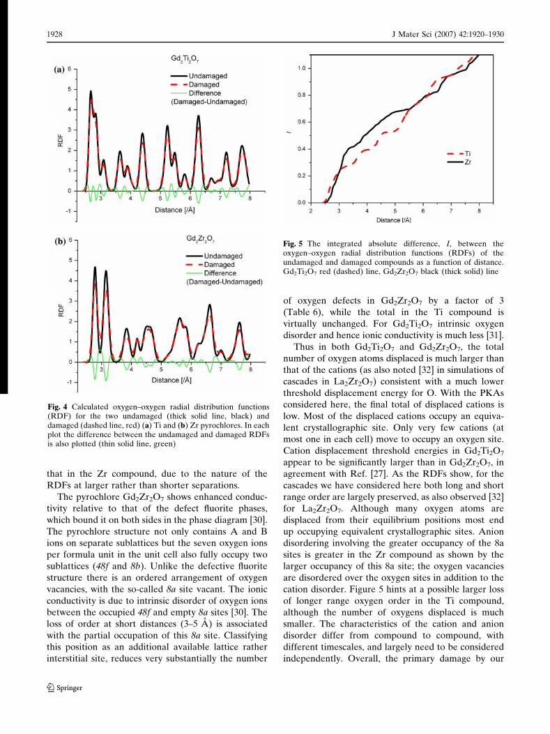
plotted in Fig. 4a–b. Although some oxygen atoms

move by a small amount (Fig. 3) this shows that, Fig. 4

does not mean that there are any such short oxygen–

oxygen separations in the damaged materials. Overall,

as indicated by the sharp negative peaks in Fig. 4, there

is a loss of order and there are clear differences

between the Ti and Zr compounds. One way of

investigating this a little more quantitatively is to sum

the absolute values of the areas under the difference

curves in Fig. 4a–b for each compound. In Fig. 5 the

integral of the absolute difference between the oxy-

gen–oxygen RDFs of the undamaged and damaged

material is plotted as a function of distance. There is a

larger loss of order in the Zr pyrochlore at shorter

separations (3–5 A), whereas at larger distances there

appears to be a slightly larger loss of order for the Ti

compound. The total integral is approximately 2%

larger for the Ti than for the Zr compound. This is of

course a small difference but nevertheless this mea-

sure, unlike those based on oxygen displacements

considered earlier, at least suggests that overall the

loss of oxygen order is at least comparable in the Ti to

Fig. 3 Mean final number of oxide ions displaced as a functionof distance moved for all 10 keV cascades (U PKA) in the Ti andZr pyrochlores (Gd–Ti–O triangles, Gd–Zr–O squares)

Table 6 Averaged final numbers of interstitials and vacancies byatom type and antisite defects in the simulation cell associatedwith cascades in each pyrochlore Gd2X2O7 (X = Ti,Zr) for aprimary knock-on’ atom (PKA) of 10 keV with initial tempera-ture 300 K

Compound Defects Gd-X

Gd X O

int vac int vac int vac int¢

X = Ti 2.3 2.8 4.0 3.0 16.0 16.5 15.8 8.3X = Zr 4.3 5.0 3.3 2.8 244.0 243.8 74.8 12.0

The final column for oxygen interstitials (headed int¢) is the totalnumber recalculated for the three compounds classifying the 8asite as a lattice rather than interstitial site, as described in the text

123

J Mater Sci (2007) 42:1920–1930 1927

that in the Zr compound, due to the nature of the

RDFs at larger rather than shorter separations.

The pyrochlore Gd2Zr2O7 shows enhanced conduc-

tivity relative to that of the defect fluorite phases,

which bound it on both sides in the phase diagram [30].

The pyrochlore structure not only contains A and B

ions on separate sublattices but the seven oxygen ions

per formula unit in the unit cell also fully occupy two

sublattices (48f and 8b). Unlike the defective fluorite

structure there is an ordered arrangement of oxygen

vacancies, with the so-called 8a site vacant. The ionic

conductivity is due to intrinsic disorder of oxygen ions

between the occupied 48f and empty 8a sites [30]. The

loss of order at short distances (3–5 A) is associated

with the partial occupation of this 8a site. Classifying

this position as an additional available lattice rather

interstitial site, reduces very substantially the number

of oxygen defects in Gd2Zr2O7 by a factor of 3

(Table 6), while the total in the Ti compound is

virtually unchanged. For Gd2Ti2O7 intrinsic oxygen

disorder and hence ionic conductivity is much less [31].

Thus in both Gd2Ti2O7 and Gd2Zr2O7, the total

number of oxygen atoms displaced is much larger than

that of the cations (as also noted [32] in simulations of

cascades in La2Zr2O7) consistent with a much lower

threshold displacement energy for O. With the PKAs

considered here, the final total of displaced cations is

low. Most of the displaced cations occupy an equiva-

lent crystallographic site. Only very few cations (at

most one in each cell) move to occupy an oxygen site.

Cation displacement threshold energies in Gd2Ti2O7

appear to be significantly larger than in Gd2Zr2O7, in

agreement with Ref. [27]. As the RDFs show, for the

cascades we have considered here both long and short

range order are largely preserved, as also observed [32]

for La2Zr2O7. Although many oxygen atoms are

displaced from their equilibrium positions most end

up occupying equivalent crystallographic sites. Anion

disordering involving the greater occupancy of the 8a

sites is greater in the Zr compound as shown by the

larger occupancy of this 8a site; the oxygen vacancies

are disordered over the oxygen sites in addition to the

cation disorder. Figure 5 hints at a possible larger loss

of longer range oxygen order in the Ti compound,

although the number of oxygens displaced is much

smaller. The characteristics of the cation and anion

disorder differ from compound to compound, with

different timescales, and largely need to be considered

independently. Overall, the primary damage by our

Fig. 4 Calculated oxygen–oxygen radial distribution functions(RDF) for the two undamaged (thick solid line, black) anddamaged (dashed line, red) (a) Ti and (b) Zr pyrochlores. In eachplot the difference between the undamaged and damaged RDFsis also plotted (thin solid line, green)

Fig. 5 The integrated absolute difference, I, between theoxygen–oxygen radial distribution functions (RDFs) of theundamaged and damaged compounds as a function of distance.Gd2Ti2O7 red (dashed) line, Gd2Zr2O7 black (thick solid) line

123

1928 J Mater Sci (2007) 42:1920–1930

low energy events shows the beginnings of the forma-

tion of the fluorite-like phase, rather than amorphisa-

tion per se, though this is less for the Ti compound.

Sickafus et al. [33] have proposed that oxygen-

deficient fluorites, with the same basic A2B2O7 struc-

ture as pyrochlores but a random arrangement of the

cations, have a greater propensity for resisting radia-

tion damage (see also Ref. [34]). The lower the cation

antisite defect energy (e.g., Gd2Zr2O7) the more

readily will a transition under irradiation to the

disordered fluorite structure take place and the more

radiation resistant the compound. Alternatively, if the

antisite defect is large (e.g., Gd2Ti2O7) then there is an

irradiation-induced crystalline to amorphous transi-

tion. The cation antisite defect energies are smaller the

closer these ions are in size [35, 36].

How do such trends relate to the simulations

reported here? Overall our calculations suggest the

connection between ease of damage and the formation

of defect cascades over the first few ps is more complex

than anticipated hitherto. Different measures of

damage (displacements, defect totals, RDFs) need

careful consideration. The simulations see no direct

amorphisation but rather a transition to the fluorite

structure which is more pronounced for the Zr

compound (greater occupancy of the 8a site) than the

Ti system, which also contains a smaller number of

antisite defects. The total number of displaced atoms is

larger for the Zr pyrochlore, but the loss of long range

order as indicated by the change in the oxygen–oxygen

radial distribution indicates this is comparable or less

for the Zr than the Ti pyrochlore.

There are a number of caveats. Our simulations

have been limited to small initial PKA energies

because of the problem of cascade overlap. The

creation of a defect cascade is only part of the process

of the formation of the damaged state. Our simulations

are not able to probe the healing process and deter-

mine the ultimate fate on longer timescales of the

interstitial ions and vacancies (e.g., formation of defect

clusters, dislocations). Nevertheless, we might expect

thermal annealing via order-disorder in Gd2Zr2O7

(which is an ionic conductor) to be faster than for

structural recovery in Gd2Ti2O7. It will be interesting

in future work to try and build up correlations between

ease of damage formation and ease of amorphisation

with measures calculated in molecular dynamics sim-

ulations of the type presented here, and the ability to

study ever larger cells will permit the study of more

energetic PKAs.

Conclusions

DL_POLY_3 is a new generation molecular dynamics

software with inherent parallelisation design based on

domain decomposition and linked cells methodologies.

It exhibits excellent parallel performance and ability to

handle simulations of systems of order of tens of

millions of particles and beyond on any high processor

counts. DL_POLY_3 offers a wide variety of tolls and

controls, including additional functionality to help

highly non-equilibrium simulations. Re-engineered in

a modular, free-format FORTRAN 90 manner, it

guarantees full portability (completely self-contained)

and allows for easier support and user development.

Application of the code to study radiation cascades in

Gd2Ti2O7 and Gd2Zr2O7, has revealed marked differ-

ences between the two compounds, and we have

discussed different methods for the analysis of the

extensive disorder produced by these cascades.

Acknowledgements ITT acknowledges support from NERC.The work was also supported by two JREI awards (the Mott(RAL) and Dirac (Bristol) supercomputer clusters).

References

1. Weber WJ, Ewing RC, Catlow CRA, Diaz de la Rubia T,Hobbs LW, Kinoshita C, Matzke Hj, Motta AT, Nastasi M,Salje EKH, Vance ER, Zinkle SJ (1998) J Mater Res 13:1434

2. Wang SX, Wang LM, Ewing RC, Govindan Kutty KV (2000)Nucl Instrum Methods Phys Res B 169:135

3. Wang SX, Begg BD, Wang LM, Ewing RC, Weber WJ,Govindan Kutty KV (1999) J Mater Res 14:4470

4. Gupta HC, Brown S, Rani N, Gohel VB (2001) J RamanSpect 32:41

5. Hess NJ, Begg BD, Conradson SD, McCready DE, GassmanPL, Weber WJ (2002) J Phys B 106:4663

6. Lian J, Wang L, Chen J, Sun K, Ewing RC, Matt Farmer J,Boatner LA (2003) Acta Materialia 51:1493

7. Lian J, Chen J, Wang LM, Ewing RC, Matt Farmer J,Boatner LA, Helean KB (2003) Phys Rev B 68:134107

8. Nachimuthu P, Thevuthasan S, Engelhard MH, Weber WJ,Shuh DK, Hamdan NM, Mun BS, Adams EM, McCreadyDE, Shutthanandan V, Lindle DW, Balakrishnan G, PaulDM, Gullikson EM, Perera RCC, Lian J, Wang LM, EwingRC (2004) Phys Rev B 70:100101

9. Nachimuthu P, Thevuthasan S, Shutthanandan S, AdamsEM, Weber WJ, Begg BD, Shuh DK, Lindle DW, GulliksonEM, Perera RCC (2005) J Appl Phys 97:033518

10. Nachimuthu P, Thevuthasan S, Adams EM, Weber WJ, BeggBD, Mun BS, Shuh DK, Lindle DW, Gullikson EM, PereraRCC (2005) J Phys Chem B 109:1337

11. Ewing RC, Weber WJ, Lian J (2004) J Appl Phys 95:594912. Todorov IT, Smith W (2004) Phil Trans R Soc Lond A

362:1835

123

J Mater Sci (2007) 42:1920–1930 1929

13. Andersen HC (1983) J Comput Phys 52:2414. Ryckaert JP, Ciccotti G, Berendsen HJC (1977) J Comp

Phys 23:32715. Allen MP, Tildesley DJ (2002) In: Computer simulation of

liquids. Clarendon Press, Oxford16. Pinches MRS, Tildesley D, Smith W (1991) Mol Simulation

6:5117. Hockney RW, Eastwood JW (1981) In: Comp simulation

using particles. McGaw-Hill, New York18. Essmann U, Perera L, Berkowtz ML, Darden T, Lee H,

Pedersen LG (1995) J Chem Phys 103:857719. Bush IJ, Todorov IT, Smith W (2006) Comput Phys

Commun 175:32320. Brigham EO (1988) In: The fast Fourier transform and its

applications. Prentice Hall, Singapore21. Bush IJ (1999) In: The Daresbury advanced Fourier trans-

form. Daresbury Laboratory22. Todorov IT, Smith W (2005) In: The DL_POLY_3 user

manual. version 3.05, http://www.cse.clrc.ac.uk/msi/software/DL_POLY/

23. Allan NL, Mackrodt WC (1994) Phil Mag B 69:871

24. Allan NL, Mackrodt WC (1993) Adv Solid State Chem 3:22125. Allan NL, Mackrodt WC (1994) Mol Simul 12:8926. Purton JA, Allan NL (2002) J Mat Chem 12:292327. Devanathan R, Weber WJ (2005) J Appl Phys 98:086111028. Deng HF, Bacon DJ (1996) Phys Rev B 53:1137629. Todorov IT, Allan NL, Purton JA, Dove MT (2006) J Phys

Condens Matter 18:221730. van Dijk MP, de Vries KJ, Burggraaf AJ (1983) Solid State

Ionics 9/10:91331. Tuller HL (1994) J Phys Chem Solids 55:139332. Chartier A, Meis C, Crocombette J-P, Rene Corrales L,

Weber WJ (2003) Phys Rev B 67:17410233. Sickafus KE, Minervini L, Grimes RW, Valdez JA, Ishimaru

M, Li F, McClellan KJ, Hartmann T (2000) Science 289:74834. Sickafus KE, Minervini L, Grimes RW, Valdez JA, Hart-

mann T (2001) Rad Effects Def Sol 155:13335. Minervini L, Grimes RW, Sickafus KE (2000) J Am Ceram

Soc 83:187336. Minervini L, Grimes RW, Tabira Y, Withers RL, Sickafus

KE (2002) Phil Mag A 82:123

123

1930 J Mater Sci (2007) 42:1920–1930