USDA’s Economic Research Service has provided this report for historical

research purposes.

Current reports are available in AgEcon Search

(http://ageconsearch.umn.edu) and on https://www.ers.usda.gov.

United States Department of Agriculture Economic Research Service https://www.ers.usda.gov

A93.44AGES84 529

United StatesDepartment ofAgriculture

EconomicResearchService

InternationalEconomicsDivision

Analysis of theFeed- LivestockSector of theEuropeanCommunityDale J. Leuck

WAITE MEMORIAL BOOK

COLLECTiOlcrDEPT. OF AGF?iC. AND

APPLIED ECONOMICS

WAITE MEMORIAL BOOK COLLECTIONDEPT. OF AG. AND APPLIED ECONOMICS

1994 BUFORD AVE. - 232 COBUNIVERSITY OF MINNESOTAST. PAUL, MN 55108 U.S.A.

ANALYSIS OF THE FEED-LIVESTOCK SECTOR OF THE EUROPEAN COMMUNITY. By Dale J.

Leuck. International Economics Division, Economic Research Service, U.S. Department

of Agriculture, Washington, D.C. January 1985. ERS Staff Report No. AGES840529.

ABSTRACT

ACKNOWLEDGMENT

7-Both price incentives and increases in efficiency have been

responsible for increased livestock production and feed use in

the European Community. Econometric estimates from 1964 to

1979 suggest that increased efficiency was a more important

factor for poultry meat, eggs, and pork, while price

incentives were more important for beef and dairy. Feed

demand for grains and oilseed meal responded mainly to the

growth in livestock products, but was limited by increases in

the use of nongrain feeds. Simulation results suggest that

lower price supports would have significantly reduced milk

production and feed use, while an increase in the price of

oilseed meals woul4.have had little effect on the demand for

total oilseed mealj

Keywords: European Community (EC), Common Agricultural Policy

(CAP), EC pricing policies, feed-livestock sector, feeding

efficiency, feed conversion rates.

* * * * * * * * * * * * * * * * * * * * * * * * * * * *

* This report was reproduced for limited distribution *

* to the research community outside the U.S. Depart-

* ment of Agriculture.* * * * * * * * * * * * * * * * * * * * * * * * * * * *

Comments were made on earlier drafts of this report by Reed

Friend, Steve Magiera, Michael Lopez, and Ron Trostle of the

Economic Research Service; Wayne Sharp, former Agricultural

Counselor to the European Community; Fred Mangum of the

Foreign Agricultural Service; and Wesley Peterson of Texas A&M

University. Typing was provided by Deborah Hood, Barbara

Brygger, and Pamela Palmer.

CONTENTS

A .q3.(41-1 eA cEs

Page 8/65,27

DEFINITIONS • • • • • • • . • • • • . • • • • • • • • • • • • • • • • • • • • • • • • • • • • • • •

SUMMARY •••••••••••••••••••••••••••••••••••••••••••••

iv

vi

INTRODUCTION 0000000000.0000.00000.00.00000000000.000000 1

Influences of the Common Agricultural Policy andTechnology 0....00000.0000000000.0000000000000000 2

Policy Issues Confronting the United States and theEuropean Community 0041.0000000.00000.00.000.00.000 8

COMPARISON AND AGGREGATION OF DATA AND MODEL STRUCTURE 9Prices, Feed Conversion, and Production in

EC Countries 000..000.000000.000000.0000000000000 10Differences in Feed Composition Among Countries .... 15Aggregation and Model Structure .0000000000000000000 18

LIVESTOCK PRODUCTION 0000000000000..0000000000000.0.0.00 25Factors Affecting Structural Changes in Pig and

Poultry Production 00000.000000000.0.00.000000000 26Implications of Production Characteristics for

Econometric Estimation .000.00000.0.00.00..00.0.0 28Special Characteristics of the Pig Sector .......... 29Statistical Results for Pigs and Poultry 0.00.00000. 32Cattle Inventories and Slaughter 00000.00000.0000000 35Econometric Model for Milk Yield and Beef

Production 000.0000.00..0000..000000000.000000000 38Statistical Results for Cattle Inventories

and Beef and Milk Production 0...0000000000000000 39

FEED DEMAND 0000000000000.0.00.00.000001.000.000000.00000

Adjustment 'of Actual Feed Use For Variations • inSelected,Nongrain Feeds from Their Base YearLevels ..........................................

Econometric,Model of Feed Demand 0000000000000000.100Statistical Results for Feed Demand ................

SIMULATIONS OF SELECTED EC PRICINGBase Run 0.000000.00.00.0000.0Higher Soybean Meal Prices ...Convergence of EC Grain PricesDecreases in Both EC Grain and

POLICIES 00009000W.0000000000000000000000

00000.00.000.06.0000000

to World Levels .....Livestock Prices ....

CONCLUSION • . • • • • • • • • • • • • • • • • • • • • • • • • • • • • • • • • • • • • • • • • • • •

REFERENCES • • • • • • • • . • • • • • • • • • • • • • • • • • • • • • • • • • • • • • • • • • • • •

APPENDIX I: SUMMARY OF DATA • • • • • • • • • • • • • • • ••• • • • • • • • • • • •

APPENDIX II:. SUMMARY OF MODEL • • • • • • • • • . • • • • • • • • • • • • • • • •

39

414850

• 5458606062

64

68

71

73

LIST OF TABLES-

Number

1. EC self-sufficiency for selected commodities,1964-65 and 1978-79 averages 411110•0.0001,000.00•41.000 4

2. EC animal product to feed price ,ratios, 1964-65and 1978-79 averages 0000000000000000100000000000000

3. Animal products produced in the EC, 1964-65and 1978-79 averages 000000.0000000000000.000.00000 5

4. Feed use in the EC, 1964-65 and 1978-79 averages ..... 7

5. EC feed price ratios, 1964-65 and 1978-79 averages ... 7

6. Distribution of livestock in the EuropeanCommunity, 1968 and 1979 .......................... 11

7. Price ratios of selected products in EC countries,1978-79 average ..0.9004100000.000000110000000000.00. 12

8. Feed conversion rates for livestock in the ECcountries, 1970 and 1977 0410000000410000000000000000 13

9. Livestock distribution by holding, EC and membercountries, 1970 and 1980 ..........................

10 Egg and poultry meat production, feed conversion,and feed composition, 1976 000080000000000000000000

14

16

11. Pork, beef, and milk production, feed conversion,and feed composition, 1976 and 1979 .............. 17

12. Percentage composition of livestock feeds inEC countries, 1976 ................................ 19

13. Percentages used to derive livestock feed prices ...... 24

14. Changes in feed conversion and prices for pigs,broilers, and eggs, 1964-66 and 1977-79 averages .. 27

15. Structure of the EC pig sector, 1964-79 .............. 31

16. Short- and longrun elasticities for the pig,poultry meat, and egg equations of the EC 33

17. Statistical results for the cattle sector ............ 40

18. Changes in the aggregate Dutch feed ration in theabsence of import levies ......... ............... 42

19. Prices and feed characteristics of major feedcomponents in the Netherlands--dry basis, 1980 .... 45

11

20. Aggregate effects of cassava, corn gluten, andoilseed meal substitution for grain on thenutritional characteristics of the EC feed mix 47

21. Changes in quantity variables and grain demand inresponse to a 10-percent change in barley andwheat availability ............................. 52

22. A comparison of own price elasticities foroilseed meal demand 54

23. A comparison of actual EC prices used in thebaseline scenario and the simulated prices usedin scenarios II and III, 1971-1979 57

24. Dynamic simulation characteristics 59

DEFINITIONS Adjusted feed ingredients--the dependent variables in the feed

'demand equations. These are the quantities of each major feed

ingredient actually used in feeding, adjusted to levels thathave prevailed if the use of the major nongrain feeds of

cassava, corn gluten, and potatoes had remained at thepercentages observed in 1976. This adjustment places feeddemand on the same basis as feed units.

Common Agricultural Policy (CAP)--the set of guidelines,derived from the Treaty of Rome, which regulate the common

market for agriculture. The objectives of these policyguidelines are to (a) increase agricultural productivity, (b)ensure a fair standard of living for the agriculturalcommunity, (c) stabilize markets, (d) assure the availabilityof supplies, and (e) assure reasonable prices to consumers.

EC pricing policies--the principal means of achieving theabove goals of the CAP in the context of a managed market foragriculture. These policies have maintained agriculturalprices at high and stable levels in order to support farmincomes. The prices of less expensive imports are raised toEC levels by means of variable levies equal to the differencebetween EC and world prices.

European Community (EC)--a customs union established March 25,

1957, with the signing of the Treaty of Rome, by France, WestGermany, Netherlands, Belgium, Luxembourg, and Italy tofacilitate a common market for industrial and agriculturalgoods. Denmark, Ireland, and the United Kingdom becamemembers on January 1, 1973, and Greece became the tenth member

on January 1, 1981. This study focuses only on the first nine

members, excluding Greece.

European Currency Unit (ECU)--the accounting unit which serves

as the denominator for the exchange rate, credit, and

intervention mechanisms in the monetary system of the EC.Support prices, import levies, and export subsidies are all

set in ECU's. The value of the ECU is calculated from a

weighted basket of currencies representing all membercountries.

Feed conversion rates--show the quantity of feed required perunit of each livestock product in each country. In thisreport, the feed conversion rates for milk and beef production

represent the total quantities of feed grains and oilseed mealused per unit of production in 1979, while the feed conversion

rates for pork, broilers, and egg production vary from year toyear.

Feed units--the main explanatory variables in the feed demandequations, representing the tons of each' major feed ingredientrequired for all animal products. Each feed unit is derivedby multiplying the quantity of each, animal product by the tonsof each major feed ingredient used and summing over livestockproducts. The tonage of each feed used is calculated fromlivestock rations having the percentage feed compositionobserved in 1976.

iv

Livestock units--represent the feed requirements of all'animals on a comparable basis by converting all animals into acommon denominator, such as a dairy cow equivalent. This isdone by multiplying the number of each type of animal by therelative quantity of feed it consumes and summing the results.

Major feed ingredients--these ingredients comprised 69 percentof total feed use in 1980, and include corn, wheat, barley,and oilseed meal.

Metric measures--are used throughout this report:1 metric ton (ton) = 2,204.6 pounds•1 kilogram (kg) = 2.2 pounds.

SUMMARY Surpluses of grain and livestock products have emerged in the

European Community (EC) as a result of price policies and increased

feeding efficiency. An econometric model in this study shows thatlower EC price supports would reduce growth in livestock productionand feed demand, especially the production of milk and the feed useof wheat, the commodities in greatest surplus within the Community.

•

•••

•

U.S. policymakers believe' that reductions in support prices for

grains and livestock would reduce surplus livestock and grain ,

production in the EC. The results of such a reduction would be

increased use of U.S. feed grains worldwide and higher world prices

for feed grains, as well as lower costs to EC consumers and theCommunity's budget.

Econometric results in this report suggest that increases in feed

conversion efficiency have been the main factor responsible for

growth in egg, poultry meat, and pork production, while prices have

been the dominant force explaining growth in milk and beef

production, over the estimation period of 1964 to 1979. Limited

variation in EC grain prices have little impact on substitution

among grains in the model. Much of the increase in oilseed meal fed

was a response to technical changes in feeding and livestock

production and lagged effects resulting from the establishment of

the variable levies on grain in the early 1960's.

Three policy simulations of the model are carried out. In the first

scenario, the effects of a 10-percent increase in soybean meal

prices on livestock production and feed demand are investigated. A

, rise in soybean meal prices might occur because of a worldwide

shortage in oilseed meal or a tax imposed by the EC on vegetable oil

as a means of raising revenue and encouraging greater use of EC

, grains. The simulation reveals little sensitivity in livestock

production or feed demand to the higher soybean meal price.

A second simulation assumes gradual realignment of EC grain prices

to world levels between 1971 and 1979. Increases occur in the

'pr,oduction of beef, milk, pork, and eggs of 19, 13, 8, and 6^percent, respectively, above the base level values in 1979. In this

simulation the feeding of corn, barley, and oilseed meal increases

by 20, 5, and 36 percent, respectively, while the quantity of wheat

fed declines' by 15 percent.

In the third scenario, both grain and livestock prices are reduced

." to world levels. In response, the surplus of milk declines below

its 1979 base level, but little reduction in pork, poultry meat, or

egg production occurs. The use of wheat, barley, and oilseed meal

declines by 21, 13, and 14 percent, respectively, but corn use

increases by 12 percent. The use of corn increases because corn

prices decline relatively more than wheat or barley prices.

Results from linear programming models of livestock feeding in this

study suggest that declines in grain prices would have reduced the

feeding of nongrain feeds and further increased the feeding of

grains, but would have had little effect on the feeding of oilseed

meal.

vi

INTRODUCTION

Analysis of theFeed- LivestocSector of theEuropeanCommunityDale J. Leuck

•%

,

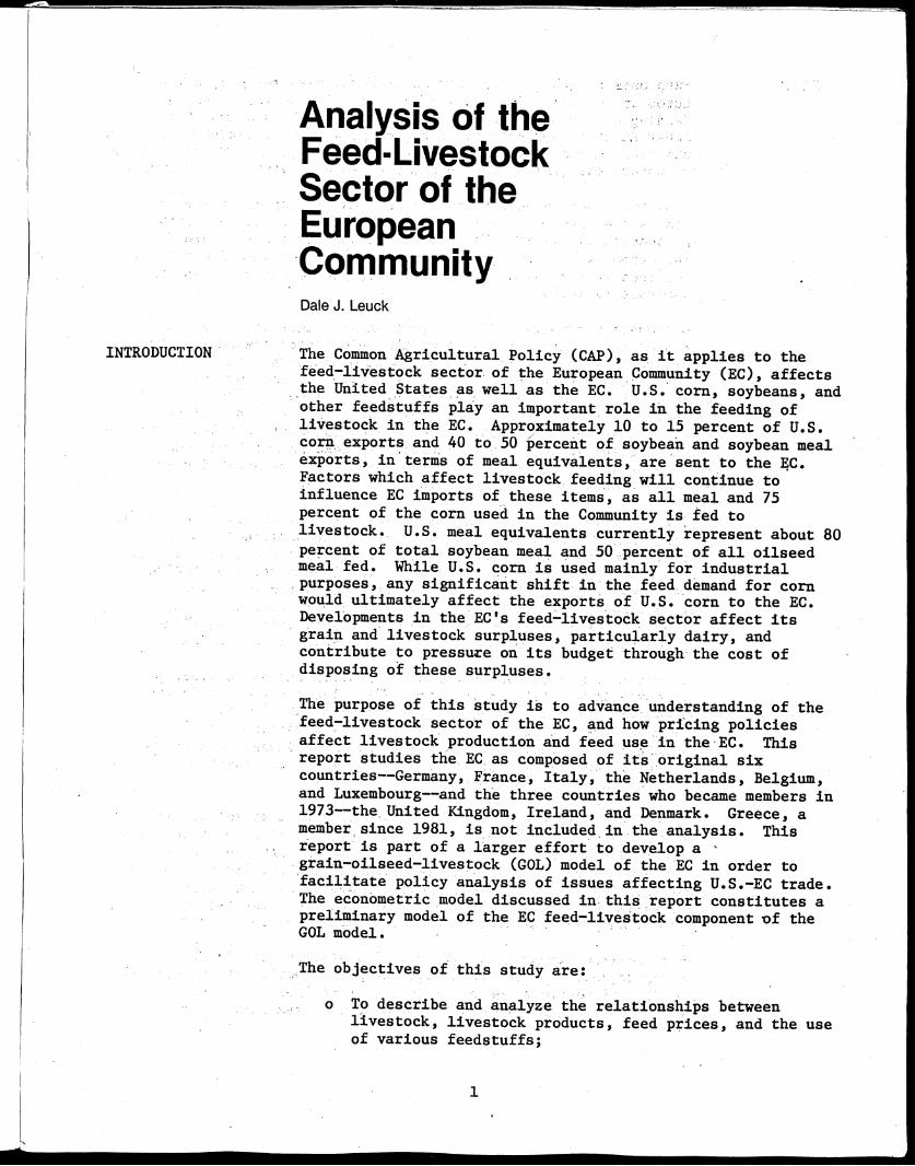
The Common Agricultural Policy (CAP), as it applies to thefeed-livestock sector of the European Community (EC), affectsthe United States as well as the EC. U.S. corn, soybeans, andother feedstuffs play an important role in the feeding oflivestock in the EC. Approximately 10 to 15 percent of U.S.corn exports and 40 to 50 Percent of soybean and soybean mealexports, in terms of meal equivalents, are sent to the gc.Factors which ,affect livestock feeding will continue toinfluence EC imports of these items, as all meal and 75percent of the corn used in the Community is fed tolivestock. U.S. meal equivalents currently represent about 80percent of total soybean meal and 50 percent of all oilseedmeal fed. While U.S. corn is used mainly for industrialpurposes, any significant shift in the feed demand for cornwould ultimately affect the exports of U.S. corn to the EC.Developments in the EC's feed-livestock sector affect itsgrain and livestock surpluses, particularly dairy, andcontribute to pressure on its budget through the cost ofdisposing of these surpluses.

The purpose of this study is to advance understanding of thefeed-livestock sector of the EC, and how pricing policiesaffect livestock production and feed use in the EC Thisreport studies the EC as composed of its original sixcountries--Germany, France, Italy, the Netherlands, Belgium,and Luxembourg--and the three countries who became members in1973--the United Kingdom, Ireland, and Denmark. Greece, amember since 1981, is not included in the analysis. Thisreport is pert of a larger effort to develop agrain-oilseed-livestock (GOL) model of the EC in order tofacilitate policy analysis of issues affecting U.S.-EC trade.The econometric model discussed in this report constitutes apreliminary model of the EC feed-livestock component 'of theGOL model.

The objectives of this study are:

o To describe and analyze the relationships betweenlivestock, livestock products, feed prices, and the useof various feedstuffs;

Influences of the Common Agricultural Policy and Tech-nology

To estimate an econometric model quantifying the aboverelationships over the period 1964 to 1979 for use as a

basis for further econometric research on the ECfeed-livestock sector; and

o To assess the impact of selected EC pricing policies onlivestock production, feed use, and trade in grains,oilseeds, and other feedstuffs during the estimation

period.

The livestock products covered in this report are pork, eggs,

poultry meat, milk, and beef, which account for nearly all

grains and oilseed meal fed in the EC. Although numerous,

other animals do not use sufficient amounts of grain and

oilseed meal to justify coverage.

Feed demand equations for corn, wheat, barley, and oilseed

meal are estimated. Feed use of these four commodities

totaled 84.2 million tons, or approximately 69 percent of the

total 121.3 million tons of feed concentrates used in the EC

during 1980. Another 10 million tons of other grains (largely

oats) were fed mostly to horses. In addition, grain

by-products, cassava, corn gluten feed, skim milk powder, and

corn gluten meal accounted for 9.0, 5.0, 3.3, 1.9, and 1.3

million tons of nongrain feeds, respectively, which were fed

mainly in response to availability. If the 10 million tons of

other grains and the 20.5 million tons of nongrain feeds are

omitted from the analysis, the four major feed ingredients

covered in the report account for 93 percent of feed use.

However, potatoes, cassava, and corn gluten feed are included

in the model because they have been the most important

nongrain feeds influencing feeding practices in the EC. They

are treated as exogenous variables because supply has been the

major limitation to their use.

The CAP has influenced the trends in EC prices and, together

with technology, has also influenced the growth in livestock

production and feed use. Under the CAP, an intervention, or

floor price is set for domestic grain, and a higher threshold,

or minimum import price, is set for imported grain. 1/ A

variable levy brings the price of imported grain up to the

threshold price. Except for a few years in the early and

mid-sixties, the production of wheat and barley has been

sufficient to drive their prices close to the intervention

price. The market price for corn, of which the EC imports

substantial amounts, is supported by the threshold price.

Surplus wheat and barley have been exported with the aid of

subsidies, while bread wheat has been subsidized for feeding

between 1967 and 1974. Despite these measures, the EC still

carries large stocks of both grains.

The price support system for dairy is similar to the system

for grains in that threshold and intervention prices are

1/ Observed market prices are often below the intervention

price because of transportation costs.

2

specified, but the system applies to dairy products ratherthan raw milk. Since dairy products generally have been insurplus, market prices of whole milk have been supported byintervention buying of butter and skimmed milk powder (SMP).Large surpluses of SMP have always existed in the EC, whilebutter and cheese have been surplus commodities only since themidseventies. Historically, butter has been eventuallydisposed of through subsidized exports or domesticconsumption, although sizable stocks currently exist. MostSMP is ultimately subsidized for use in animal feeds in theEC.

The beef intervention system is also similar to that forgrains, except that a "guide" price functions in lieu of athreshold price. Although once in deficit, the EC has been asurplus producer of beef since 1980. Consequently, marketprices have been more influenced by the intervention price andthe levels of export subsidies in recent years.

No intervention buying exists for poultry and egg-s. Instead,imports are discouraged by sluicegate, or minimum importprices, computed in reference to production costs in worldmarkets. Although some countries are deficit producers ofpoultry meat and eggs, overall surpluses have developed andare exported from the EC with the aid of export subsidies.

The EC has always been about 100 percent self-sufficient inpork. Consequently, prices have been less influenced by the

intervention and minimum import prices. Occasionally,intervention buying occurs or export subsidies are granted.Storage subsidies help dampen fluctuations in the pig cycleand thus stabilize price fluctuations from year to year.

The above mechanisms give the EC considerable control overprices. Setting prices to achieve self-sufficiency has been amajor goal of the GAP. However, the willingness of farmers torespond to price incentives and to adopt more efficienttechnologies has pushed the EC into a position of surplus formost major agricultural products (table 1). Only in pork havedemand and supply remained about in balance. The EC hassignificantly reduced imports of corn by raising itsself-sufficiency in corn and other grains. The 97-percentlevel of self-sufficiency in beef and veal for 1978-79 issomewhat misleading because the level has been quite variablein the last few years. But since 1980, it has been above 100percent.

Although the self-sufficiency percentages do not appearespecially large, the quantities of surplus commodities areindeed great. The EC currently has the largest stocks of skimmilk powder and butter in the world and carries substantialstocks of grains. In 1980 and 1981, the EC was the secondlargest exporter of beef and veal, next to Australia. In the

. early 1960's, the EC was the largest importer of poultry, butin 1970 it surpassed the United States to become the world'slargest exporter. The EC currently accounts for about 35

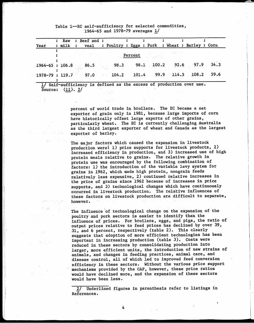
Table 1--EC self-sufficiency for selected commodities,1964-65 and 1978-79 averages 1/

: Raw : Beef and :Year : milk : veal : Poultry : Eggs : Pork : Wheat : Barley : Corn

Percent

1964-65 :• 106.8 86.5 98.3 98.1 100.2 92.6 97.9 34.3

-1978-79 : 119.7 97.0 104.2 101.4 99.9 114.5 108.2 59.6

1/ Self-sufficiency is defined as the excess of production over use.Source: (11). 2/

percent of world trade in broilers. The EC became a net

exporter of grain only in 1981, because large imports of corn

have historically offset large exports of other grains,particularly wheat. The EC is currently challenging Australia

as the third largest exporter of wheat and Canada as the largest

exporter of barley.

The major factors which caused the expansion in livestockproduction were 1) price supports for livestock products, 2)

increased efficiency in production, and 3) increased use of high

protein meals relative to grains. The relative growth in

protein use was encouraged by the following combination of

factors: 1) the introduction of the variable levy system for

grains in 1962, which made high protein, nongrain feeds

relatively less expensive, 2) continued relative increases in

the price of grains since 1962 because of increases in price

supports, and 3) technological changes which have continuously

occurred in livestock production. The relative influences of

these factors on livestock production are difficult to separate,

however.

The influence of technological change on the expansion of the

poultry and pork sectors is easier to identify than the

influence of prices. For broilers, eggs, and pigs, the ratio of

output prices relative to feed prices has declined by over 39,31, and 6 percent, respectively (table 2). This clearly

suggests that adoption of more efficient technologies has been

important in increasing production (table 3).. Costs were

reduced in these sectors by consolidating production into

larger, more efficient units, the introduction of new strains of

animals, and changes in feeding practices, animal care, and

disease control, all of which led to improved feed conversion

efficiency in these sectors. Without the various price support

mechanisms provided by the CAP, however, these price ratios

would have declined more, and the expansion of these sectors

would have been less.

2/ Underlined figures in parenthesis refer to listings in

References.

Table 2--EC animal product to feed price ratios,1964-65 and 1978-79 averages 1/

: Dairy dairy : Beef/beef : Broiler/broiler Eggs/egg : Pigs/pigYear : feed : feed • feed : feed : feed

1964-65 : 1.052

1978-79 : 1.230

Change

Ratio

6.312 7.250

7.550 4.400

Percent

17 20 -39

7.771 6.905

5.345 6.458

-6

1/ Price data are taken from aggregate prices derived, according to themethodology discussed later in this report.

Source: (11).

Table 3--Animal products produced in the EC,1964-65 and 1978-79 averages

Year : Milk : Beef and veal : Poultry Eggs Pork

1964-65 89,618 4,203

1978-79 : 111,410 6,104

Change

1,000 tons

2,021

3,820

Percent

3,274 6,566

3,916 9,761

24 45 89 20 49

Source: (11).

5

Technological change in the cattle sector mainly involved a

shift from pasture to concentrate feeding, especially grain

and protein meal. This occurred in response to higher

opportunity costs for land, and in order to realize the higher

genetic qualities which were bred into cattle. Genetically

superior cattle, with higher potentialmilk yields, require

greater amounts of balanced proteins in order for yield

potential to be realized (3, 21). While the entire breeding

herd, including that which is exclusively beef, increased by

only 3.5 percent, the number of dairy and dual-purpose cows

dropped slightly. Therefore, the entire increase in milk

production occurred because of higher yield per cow (table

3). Beef production increased not only because of a larger

breeding herd, but more importantly because of a substantial

shift from veal to beef production (table 3). The greater use

of concentrates in milk and beef production was accommodated

by increases in the ratios of milk and beef prices to feed

prices (table 2).

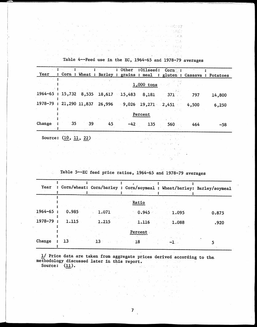
Total corn and wheat fed increased by 35 and 39 percent,

respectively, while total barley fed increased 45 percent

(table 4). The relatively larger increase in barley use

occurred because of greater use onfarm and greater use of

barley in compound feeds for cattle. The price of barley

relative to wheat changed little because market prices for

these grains have always ridden on or near their intervention

prices, which have been increased by similar percentages

(table 5).

Feed demand for oilseed meal grew more (135 percent) than did

demand for grains (40 percent on average), suggesting that

significant substitution of oilseed meal for grains has

occurred. This happened because throughout the sixties and

seventies grains became relatively more expensive and the

production of compound feeds increased dramatically throughout

the sixties and seventies. During the 16 years from 1964

through 1979, the corn-soybean meal price ratio rose by 18

percent, although the barley-soybean meal price ratio rose

considerably less (table 5). The most favorable movement in

the relative price of soybean meal came in the early sixties

when the EC fully adopted CAP grain prices. In the

Netherlands, the 2-year average of the corn-soybean meal price

ratio rose by 10 percent, from 0.67 to 0.74, in the 6 years

between 1960-61 and 1966-67 (27). Variable levies also were

responsible for other nongrain feeds becoming relatively less

expensive.

The availability of feed ingredients which did not have

variable levies imposed on them, such as oilseed meal,

cassava, corn gluten, and citrus pellets, and structural

changes in livestock production encouraged the production of

compound feeds. Between 1960 and 1979, production of compound

feed in the EC expanded by 247 percent (in 7, table 7).

Compound feeds could be more efficiently mixed in the

large-volume feed mills which emerged near port areas.

Without the availability of the entire complex of nongrain

4

Table 4--Feed use in the EC, 1964-65 and 1978-79 averages

: Other :Oilseed: Corn',Year : Corn : Wheat Barley : grains : meal : gluten : Cassava : Potatoes

1,000 tons

1964-65 : 15,732 8,535 18,617 15,483 8,181 371 , 797 14,800

1978-79 : 21,290 11,837 26,996 9,026 19,271 2,451 - 4,500 6,250

Percent

Change : 35 39 45 -42 135 560 464 -58

Source: (10, 22)

Table 5--EC feed price ratios, 1964-65 and 1978-79 averages

Year Corn/wheat: Corn/barley': Corn/soymeal : Wheat/barley: Barley/soymeal

1964-65 : 0.985

1978-79 : 1.115

Change : 13

1.071

1.215

13

Ratio

' 0.945 -

1.116

Percent‘

1.095 0.875

1.088 .920

18 5

1/ Price data are taken from aggregate prices derived according to themethodology discussed later in this report.Source: (11).

7

Policy Issues Confrontins the United States and the European Community

feeds, however, it is doubtful that compound feed production

,and oilseed meal use:would have increased as much as they

did. Much of the growth in compound feed production

throughout the sixties occurred as oilseed crushing and feed

mixing capacity were developed as lagged responses to the

establishment of variable levies.

Technical changes in European livestock production made output

more responsive to protein meals, thereby increasing the

demand for protein meals at a given price, and reducing the

sensitivity of demand to changes in price. Pressure to reduce

costs led to the shift of cattle from pasture to more

Intensive feeding, improved breeds of livestock, and better

nutritional and medicinal practices. As a result, the

livestock sector became consolidated into larger production

units. The genetic potential of newer breeds of animals,

particularly dairy cattle, could only be realized through

feeding higher levels of protein (3, 21). Reduction of

disease problems allowed the greater potential of protein in

feeding efficiency to be realized, while the consolidation of

production allowed compound feeds to be more efficiently

distributed to a larger number of animals.

The use of other nongrain feeds, such as corn gluten and

cassava, has also increased rapidly in the EC because of

favorable price relationships. The use of potatoes has

declined because of the high labor costs associated with their

production.

The use of protein has increased more rapidly than the use of

energy because of the above reasons,. The use of protein

Increased by more than 57 percent between 1964 and 1979, while

digestible energy only increased by 25 percent, based on the

energy and protein content of the eight major feedstuffs in

table 4. 3/ Since feeds which are high in protein are more

efficient in promoting meat and milk production than those

high in energy, the shift in feeding habits was also a factor

underlying increased meat and dairy, production in the EC.

The CAP has created economic problems for both the United

States and the EC. The growing surpluses of EC grains, dairy

products, beef, poultry, and eggs depress prices on

International markets and displace traditional exporters from

their markets. Furthermore, by insulating its producers from

fluctuations in international prices, the EC imposes the

burden of resource adjustment on other countries (14, 16,

32). With more Adjustment centering on fewer countries, world

prices, exports, and returns to resources in the rest of the

world are all subject to wider variation.

The GAP has shut the United States entirely out of EC poultry

markets and has displaced potential exports of U.S. feed

grains with EC wheat and barley. The United States has,

3/ The energy and protein content of these feedstuffs is

detailed in table 19.

however, been a - major beneficiary of.the EC market for oilseedmeal. Although exports of U.S. corn to the Community haverisen over 25 percent since the early sixties, corn imports bythe EC have declined from the high levels of themidseventies. Previous analyses suggest that the majorbenefits to the United States' of the EC's adopting world grainprices would be through greater U.S. wheat and feed grainexports to non-EC markets and generally higher world grainprices, but' little additional U.S. feed grain exports to theEC (14, 26).

Agricultural sUrpluses have imposed high storage costs andexport subsidies on the EC. Since, 1983 these growing costshave placed. the EC in danger of exceeding its budget, whichacquires resources from variable levies on agriculturalimports, tariffs, and up to 1 percent of the common base fornational value added taxes (VAT). While prospects for highereconomic growth will increase revenues from the VAT and higherworld grain prices will decrease export refunds in the nearfuture, a budget crisis did occur in 1984 because significantchanges were not made in budgetary 'receipts and expenditures.Josling and Pearson suggest that the budget crises will hinderthe achievement of policy goals and may interfere withenlargement of the Community to include Spain and Portugal(17).

11.1.11111,

,

Although little consumer resistance has occurred in responseto the CAR, its high costs to the consumer will eventuallyprovoke greater consumer response. A 1969 USDA study (19)estimated 'the annual cost of the CAP to European consumers tobe $6.4 billion dollars, while a 1982 Australian study (29)suggests that the average annual cost to' EC consumers and taxpayers between 1971 And 1981 was $9.6 billion.

'While pressure in the EC is building for new fund raisingschemes, such as 'a tax on fats and oils, recent EC proposalssuggest changes in relative grain prices will also occur (6).Suggestions for a tax on oilseed meal have also been made, butno proposal for such a tax is expected in the near futurebecause of firm opposition from several northern EC countries,and 'the United States. This atudy may provide some insight ,onthese issues by explaining the relationships between prices,livestock production, and feed demand.

't

COMPARISON AND The differences among EC countries in production structuresAGGREGATION OF DATA and price levels are important because they illustrate theAND MODEL STRUCTURE potential for some countries to increase production and the

limitations other countries may face in raising production inthe future. Future increases in livestock production and feeddemand depend on the potential for some countries to becomemore efficient livestock producers.

9

Prices, Feed Conversion, and Production in EC Countries

Significant diversity exists in prices, technologies, and the

types of livestock raised and feeds used among the countries

of the EC (5). Some EC countries with strong currencies have

higher price levels than countries with weak currencies

because the system of. border taxes and subsidies, known as

MCA's, enables countries to avoid the price adjustments

implied by changes in market exchange rates (9).

Transportation costs, the historical structure of farming

(35), and other factors interact with the MCA system to result

in prices and price ratios which vary considerably among the

EC countries.

Countries with higher levels of feeding efficiency, as

measured by lower output-to-feed conversion rates, may

generally be expected to have lower margins between the prices

of their livestock and the major feed ingredients consumed.

Although the EC pricing policies support market prices rather

extensively, output-to-feed price margins are allowed to fall

in response to efficiency gains to levels determined by the

pricing system. While other factors may obscure the

relationship between price margins and feeding efficiency, the

potential of achieving greater production is in those

countries with less efficient sectors. Furthermore, any

reduction in the price margins may accelerate growth in output

because the resulting cost-price squeeze on producers may

elicit adoption of more efficient technologies.

Among the four largest broiler producers (table 6), France and

Italy have the highest broiler-to-corn price margins, while

the United Kingdom and the Netherlands have the lowest (table

7). However, France is the most efficient producer of

broilers, while Italy is the least efficient (table 8). Data

on farm structure clearly show a significant reduction in both

the number of holdings and the average number of birds per

holding in France (table 9). Growth in the French broiler

sector has apparently occurred at the expense of medium-size

producers. Therefore, the feeding efficiency in France may be

largely due to the emergence of a few large producers of birds

for export. Italy has both the least efficient farm structure

.and feed conversion rate, while the Netherlands is high in

feeding efficiency and has the most efficient farm structure.

Except for France, the trend in these four countries has been

toward a more highly concentrated sector, although this trend

has been less rapid in Italy.

Among the four major producers of eggs, France and Italy have

the highest egg-to-corn price margins and Germany and the

United Kingdom the lowest. In this sector, the United Kingdom

has the lowest price margin, the highest level of feeding

efficiency, and the most efficient farm structure. As in

broilers, both Italy and France have the least concentrated

sectors of the four. However, the French sector is highly

efficient in feeding, while the Italian sector is law in

feeding efficiency and has the most inefficient farm

structure. Moreover, the Italian sector has become more

concentrated and more efficient less rapidly than the sectors

in the other three countries.

10

Table 6--Distribution of livestock in the European Community, 1968 and 1979

Country : Cattle : Pigs : Layers : Chicken meat 1/

: 1968 : 1979 : 1968 : 1979 : , 1968 : 1979 : 1968 : 1979

1,000 head - - Metric tons - -

Denmark : 3,004 2,944 7,982 9,566 6,330 4,669 52 85France : 21,896 23,558 9,546 10,525 61,600 69,180 393 840Ireland : 5,086 6,169 1,062 1,119 4,700 3,368 17 33Italy : 10,070 8,808 7,298 8,807 66,900 82,300 375 583Belgium-Luxembourg : 2,231 2/2,378 3/757 1,296 400 2/379 85 112Netherlands : 3,694 - 5,028 74:,861 10,044 16,700 2/27,400 183 361United Kingdom : 12,094 13,318 7,969 7,815 65,800 1763,651 374 548West Germany : 14,061 15,050 18,378 22,374 67,400 1759,900 107 255

:Total 817: 72,136 77,253 57,853 71,546 289,830 310,847 1,586 2

:: Percent :

Denmark : 4.2 3.8 13.8 13.4 2.2 1.5 3.3 3.0France : 30.4 30.5 16.5 14.7 21.3 22.3 24.8 29.8Ireland : 7.1 8.0 1.8 1.6 1.6 1.1 1.1 1.2Italy : 14.0 11.4 12.6 12.3 23.0 26.5 23.6 20.7Belgium-Luxembourg •. 3.1 3.1 1.3 1.8 .1 .1 5.4 4.0Netherlands : 5.1 6.5 8.4 14.0 5.8 8.8 11.5 12.8United Kingdom : 16.8 17.2 13.8 10.9 - 22.7 20.5 23.6 19.4West Germany : 19.5 19.5 31.8 31.3 23.3 19.3 6.7 9.1

:100.0 100.0 100.0 100.0Total : 100.0 100.0 100.0 100.0

::

Note: Percentage totals may not add to 100 because of rounding.

1/ Foreign Agricultural Service, USDA.27 1978.37 1969.-Source: (7, 8).

Table 7--Price ratios of selected products in EC countries, 1978-79 average 1/

: West : :Nether- : Belgium/ :United :Products :Germany : France : Italy : lands :Luxembourg :Kingdom :Ireland :Denmark

Price ratios

Broiler/corn 3.98 4.71 4.85 3.81 3.94 3.91 NA NA

Eggs/corn : 5.39 6.29 5.69 3.76 3.34 4.42 • NA NA

Pork/barley : 6.06 7.74 6.61 6.43 6.72 6.86 7.66 7.05

Milk/barley : 1.28 1.39 1.51 1.26 1.16 1.27 1.29 1.5

Beef/barley : 7.59 9.85 8.55 8.23 8.88 8.08 8.56 8.0

Corn/barley : 1.15 1.31 1.06 1.21 1.33 1.39 NA NA

Wheat/barley : 1.06 1.12 1.19 1.04 1.13 1.08 1.08 1.07

Corn/wheat : 1.08 1.17 .89 1.16 1.18 1.28 NA NA

Soymeal/ :barley : .87 1.28 1.02 1.02 1.07 1.21 1.23 1.12

Soymeal/corn : .76 .98 .96 .84 .80 .87 NA NA

NA = Not available.Source: (11).

Of the six biggest pork-producing countries, France and Denmarkhave the highest pork-to-barley price margins, the Netherlandsand West Germany the lowest. All four countries are high infeeding efficiency, although Denmark is the most efficient.Denmark has a much smaller pig sector than Germany, but onemuch more concentrated, with 128 pigs per holding, versusGerman's 41. The percentage increase in pigs per holding isalso significantly higher in Denmark. While the relationshipbetween the price margins and feeding efficiency in Denmark iscontrary to expecta.tioon, the Dutch sector is high in feedingefficiency, is the most concentrated; and has the greatestpercentage increase in the number of pigs per holding.

High price margins have probably allowed significant increasesin output by relatively less efficient producers, such as thebroiler and layer industries in Italy. Any reduction inlivestock prices relative to feed prices would discourageproduction by less efficient producers in these countries andmay induce further technical changes.

Countries with less efficient sectors have the potential forincreasing production by modernizing their sectors. The

12

Table 8--Feed conversion rates for livestockin the EC countries, 1970 and 1977

Country and : : :year : Broilers 1/ : Eggs : Pigs 1/

:: Kilogram of feed per kilogram of output

West Germany: :1970 2.30 4.10 3.82

1977 : 1.90 3.50 3.65:

France: :1970 2/ 2.20 2/ 3.40 3.75

1977 : 1.90 3.00 3.64

Italy: :1970 2/ 2.90 2/ 4.30

1977 : 2.50 2./ 3.90:

Netherlands: :1970 : 2.071977 : 1.97

:Belgium/ :Luxembourg: :1970 : 2.23 2.88 2 3.70

1977 : 2.12 2.72 3.50

:United Kingdom: :1970 : 2/ 2.23 . 2/ 3.00 3.70

1977 : 2.20 ' 2.76 3.30

Ireland:1970 2/ 2.301977 2.20

Denmark:19701977

2.272.05

2/ 4.604.40

2.84 3.742.71 3.61

3.10 3.702.80 3.41

2/ 3.49 2/ 3.60-- 2.97 3.27

1/ For/broilers and pigs feed conversion is measured on the basis of

liveweight gain.2/ Estimated by Western Europe Branch IED, ERS.-Source : (22).

13

Table 9--Livestock distribution by holding, EC and member countries, 1970 and 1980

Pigs PoultryHoldings : Pigs per Holdings with : Broilers per : Holdings with 4 Layers perwith pigs : holding : broilers holding : layers :. .holding

Country 1970 : 1980 : 1970 1980 : 1970 : 1980 : 1970 : .1980 : 1970 : 1980 : 1970 : 1980 :: --1,000---- - Head - - --1,000-- - Head - - - 1,000 - -:

Germany : 751 ' 547 26 41 30 99France : 655 349 16 30 775 537Italy : 858 1,017 7 9 852 805Netherlands : 76 47 73 207 3 2Belgium : 84 44 45 117 12 7Luxembourg : 5 2 22 45 * 1United :Kingdom : 85 35 95 223 8 4 6,071 12,755 137 78 640 ' 914

Ireland : 68 10 18 112 10 11 308 373 159 106 26 43Denmark : 118 73 70 128 6 3 1,089 2,470 67 35 92 186

:EC-9 2,700 2,124 24 35 1,698 1,469 140 178 3,737 2,798 72 103

- - Head - -

GermanyFranceItalyNetherlandsBelgiumLuxembourgUnitedKingdomIrelandDenmark

731 182 726 ,467 70 120706 106 1,204 924 36 6470 84 1,305 1,130 33 39

10,735 17,686 49 9 366 3,333908 1,446 87 46 171 34579 16 5 3 45 41

Percent change between 1970 and 1980

-27 55 229 -75 -35 71-47 85 -71 -85 -23 7819 28 -5 21 , 13 18-38 183 -21 65 -82 810-47 162 -45 59 -47 102-60 106 200 -80 -40 -8

-59 135 -46 110 -43 43-85 539 6 21 -33 65-38 83 -47 127 -48 102

:EC-9 : -21 50 -13 27 -25 43

* = less than 500 holdings.Source: (8, 37).

Differences in Feed Composition Among Countries

French and Germans, on the other hand, may increase poultrymeat and egg production by increasing the number of birdsper holding. Germany appears to have significant potentialfor increasing pork production by increasing both feedingefficiency and the number of pigs per holding. Most ,important, Italy, with law numbers of all animals perholding and low rates of feeding efficiency, has significantpotential for increasing production of poultry meat, eggs,and. pork.

The French dairy sector also has the second highestoutput-to-feed price margin, next to Italy, but one withyields-per-caw of about 75 percent that of Germany and theNetherlands (4). Thus, significant potential exists forproducers to adopt more efficient production technologiesunder the proper set of incentives. Such adoption couldsignificantly increase EC milk production since France hasabout one-third of the dairy caws in the EC.

Generally, less expensive feed ingredients are used inlarger proportions in the feeding rations than moreexpensive ones. However, differences in the types oflivestock grown and onfarm use of grains, which is not sosensitive to market prices, also influence the compositionof feed. The price ratios of the feed ingredients in table7 show, for example, that corn has the lowest price relativeto other grains in Italy and the highest relative priee inthe United Kingdom. The relative price of soybean meal islowest in West Germany and highest in France.

The quantities of livestock products, the feed-to-livestockproduct conversion rates, and the quantities of feedingredients used for livestock in each country are presentedin tables 10 and 11.. The feed conversion rates for pigs andbroilers are derived from the liveweight feed conversionrates in table 8 by dividing the liveweight rates by 0.7,which represents the proportion of these animals' totalweight which is meat. The feed conversion rates for milkand beef are derived from aggregate EC rates provided by IEDanalysts, which are disaggregated according to informationcompiled by Neville-Rolfe (22).

The composition of total feed is also derived from datapresented by Neville-Rolfe (22). These data are modified sothat the total of each feed ingredient fed to all livestockclasses in a country approximately equals the total quantityof that ingredient actually fed in the country in 1976. Forpoultry meat, eggs, and pigs, the total feed used includesall feed ingredients, but for beef and dairy, the" totalsonly include grains and oilseeds.

Corn is the largest single feed ingredient for egg andpoultry meat production, while barley is more important forpork, dairy, and beef (tables 10 and 11). Approximatelyone-half of the corn fed in the EC is consumed by poultry.Oilseed meal use is most important in pork production, but

15

Table 10--Egg and poultry meat production, feed conversion, and feed composition, 1976

West : : : Nether- : Belgium/ : United :Item : Unit : Germany France : Italy : lands : Luxembourg : Kingdom

:Eggproduction : 1,000 tons : 854 755 572 342 236

Feed : Kilogram of :conversion feed per :

: kilogram of :: eggs 1/ : 3.50 3.00 3.90 2.71 2.72 2.76 2.80 2.97 3.15

Feed used : 1,000 tons : 2,989 2,265 2,233 927 642 2,368 117 211 11,752Corn : do. : 1,793 1,087 1,340 501 193 687 60 95 5,756Wheat : do. : 598 272 100 - 0 64 521 0 32 1,587Oilseed : do. : 299 385 380 139 96 . 237 12 70 1,618 '

: Ireland : Denmark : EC-9

858 39 71 3,727

Poultry •

production : 1,000 tons : 290 871 900 336 106 662 41 97 3,303

Feed : Kilogram of :conversion 2/: feed per :

-- : kilogram of: meat 1/ :

Feed used : 1,000 tons : 787 2,364 3,214 946 321 2,081 129 284 10,126Corn : do. : 386 1,537 2,250 454 ‘96 364 72 128 5,287Wheat do. : 126 .165 ,- 50 0 32 812 0 43 1,228Oilseed : do. : 126 591 804 284 80 208 13 95 2,201

•

2.71 2.71 3.57 2.81 3.03 3.14 3.14 2.93 3.07

1/ Feed conversion per kilogram of meat is defined by dividing the liveweight feed conversion weights by 0.7, because broilers yield'approximately 70 percent meat per liveweight.

2/ Since feed conversion rates are rounded to the nearest hundreth, feed used may not exactly equal livestock production multiplied by feedconversion.

Source: Production data--(11); Feed conversion rates--(22).

Table 11--Pork, beef, and milk production, feed conversion, and feed composition, 1976 and 1979 1/ 2/

Item

Porkproduction

Feedconversion 3/

Feed usedCornWheatBarleyOilseed .

• : West :: Unit : Germany : France

: 1,000 tons : 2,776 1,572

Kilogram of :: feed per: kilogram of :: meat: .: 1,000 tons :

do.do.do. :do. :

: Italy '

5.21 5.20

14,475 '8,175521 1,136 .

1,983 2,207 -4,589 2,0441,563 1,226

: Nether- : Belgium/ : United :: lands : Luxembourg : Kingdom : Ireland : Denmark : EC-9

753 1,022 643 848 126

6.29

4,7332,012151890464

5.16

5,271864840

944

5.00

3,215299510

611

4.71

3,998600264

1,299480

724 8,464

4.87 4.67

61411123

15484

3,3823333

2,604595

5.2

43,8635,5764,79611,5805,967

Beef .production :

Feedconversion :

Feed used 4/ :CornWheatBarleyOilseed

1,000 tons :

Kilogram of :feed perkilogram of :meat 2/

1,000 tons :do.do.do.do.

1,348 1,535 655 292 248 1,013

.61 .84 1.39 .34 .77•

818 1,295 912 100 1910 263 636 ' 0 41

187 334 0 0 0244 554 189 47 98387 144 87 53 52

385 242 5,718

1.47 .32 1.25 .92

1,494357416595126

123 302 5,2350 0 1,2970 0 93790 218 2,03533 84 966

Milkproduction

Feedconversion 3/

Feed used 4/Corn •WheatBarleyOilseed

1,000 tons : 22,189 25,878 9,739 10,490

Kilogram of :feed per :kilogram of :

milk : .11 .18 .27 .05

1,000 tons : 2,436 4,649 2,637 554do. : 0 1,304 1,935 0do. : 0 605 0 0do. : 1,038 2,248 420 113do. : 1,398 492 282 441 .

3,842 14,384 3,858 5,045 95,425

.21 .34 .14 .26 .19

825 4,914 525 1,307 17,847205 263 100 0 3,8070 340 0 0 945

459 3,923 350 941 9,492161 388 75 366 3,603

1/ Feed conversion per kg. meat is defined by dividing the liveweight feed conversion rate by 0.7, because pigs yield approximately

70 percentmeat per liveweight.2/ Feed conversion rates for pork are for 1976, while those for beef and dairy are for 1979.-5/ Since feed conversion rates are rounded to the nearest hundreth, feed used may not exactly equal livestock production multiplied

by feed conversion.4/ Total feed for beef and dairy do not include other grain?, forages, and nongrain feeds.'Source: Production data -- (11); Feed conversion -- (22) for pork, and IED/ERS estimates for beef and dairy.

Aggregation and Model Structure

is also used heavily in dairy because increasing milk yieldsrequire larger amounts of protein. Table 12 summarizes thedata on feed composition from tables 10 and 11 in percentageform. The use of other grains and nongrain feeds in therations for poultry meat, eggs, and pork is represented bythe difference of the totals from 100 percent. Althoughthese differences are quite large in some cases, no attemptis made in this study to explain them.

In general, relatively inexpensive feeds exhibit a higher'relative percentage use in the rations. Corn, for example,is used relatively more heavily in all livestock rationsthan other grain in Italy, where it is relativelyinexpensive (table 7), as compared, for example, to theUnited Kingdom. Except for cattle, West Germany, France,and the Netherlands use relatively more corn than the UnitedKingdom or Belgium/Luxembourg, where corn is relatively moreexpensive. In West Germany and the Netherlands, little cornis fed to cattle because of the abundance of relativelyinexpensive nongrain feeds, especially corn gluten.Relatively less barley is fed in Italy because of the morefavorable price relationship held by corn. Barley is usedexclusively for feeding pigs and cattle in all countriesbecause its relatively high fiber content causes digestionproblems in poultry.

The relationship between feed prices and oilseed meal use ismore complicated. France, with the highest relative soybeanmeal price (table 7), uses more oilseed meal in poultry andpig rations than West Germany, with the lowest relativeprice. However, West Germany uses larger amounts of othernongrain feeds which are high in protein. If these areaccounted for, the percentage of protein in the West Germanration would be at least as great as in France. With theexception of the layer ration, the Dutch, who also face arelatively low soybean meal price, use a larger percentageof oilseed meal in their rations than the French.

Policies which reduce EC grain prices will not only cause anincrease in the demand for feed, but will encourage a changein the composition of feed. Those countries which areheavily dependent upon imported corn and oilseed meal, suchas Denmark, the United Kingdom, and the Netherlands, may beexpected to reduce the percentages of these feed ingredientsin their rations. Increases in livestock production mayencourage an absolute increase in the use of thesefeedstuffs, however.

The model is intended to represent the major behavioralrelationships of the feed-livestock sector in order tofacilitate policy analysis. The policy scenarios areconcerned with the response of livestock production and feeddemand to selected EC pricing policies over a 5- to 10-yearperiod. Cyclical relationships underlying livestockproduction and forecasts of quarterly or biannual values ofthe different components of the feed-livestock sector are

18

Table 12--Percentage composition of livestock feeds in EC countries, 1976 1

• : : .Product and• : West : France : Italy :Netherlands : Belgium/ : United : Ireland : Denmark : EC-9

feed : Germany : : : :Luxembourg : Kingdom• : : :

:: Percent :

Eggs: :Corn : 60.0 48.0 60.0 54.0 30.0 29.0 51.0 45.0 49 -.0Wheat : 20.0 12.0 4.5 0 10.0 22.0 0 15.0 13.5Oilseed meal : 10.0 ' 17.0 17.0 15.0 15.0 10.0 10.0 33.0 13.8

:Poultry meat:

Corn : 49.0 65.0 70.0 48.0 30.0 17.5 56.0 45.0 52.2Wheat ' 16.0 7.0 1.6 0 10.0 39.0 0 15.0 12.1Oilseed meal : 16.0 25.0 25.0 30.0 25.0 10.0 ,10.0 33.3 21.8

Pigmeat: :1-aQD Corn : 3.6 13.9 42.5. 16.4 9.3 15.0 18.0 1.0 12.7

Wheat : 13.7 27.0 3.2 1.6 1.6 6.6 3.8 1.0 10.9Barley : 31.7 25.0 18.8 0 0 32.5 25.0 77.0 26.4

Oilseed meal : 10.8 15.0 9.8 17.9 19.0 12.0 13.6 17.6 13.6:

Beef: :Corn : 0 20.3 69.7 0 21.5 23.9 0 0 24.8

Wheat 22.9 25.8 0 0 0' 27.8 0 0 17.9Barley : 29.8 42.8 20.7 47.0 51.3 39.8 73.2 72.2 38.9Oilseed meal : 47.3 11.1 9.5 53.0 27.2 8.4 26.8 27.8 18.5

Milk: :Corn .: 0 28.1 73.4 0 24.8 5.4 19.1 0 21.3Wheat : 0 13.0 0' 0 0 6.9 0 0 5.3Barley . : 42.6 48.4 15.9 20.4 55.6 79.8 66.7 72.0 53.2Oilseed meal : 57.4 10.6 10.7 79.6 19.5 7.9 14.3 28.0 20.2

: 1/ These percentages are derived from (22). The percentages for eggs, broilers, and pigmeat are the levels of each feed used

divided by total feed as shown in tables 10 and 11. For beef and milk, the percentages are for the four ingredients only. Allpecentages are rounded to the nearest hundreth.

not needed. Consequently, annual data are used and only theelements of the livestock sector necessary for these'purposes are modeled. Cattle are divided into theinventories of breeding cattle, nonbreeding cattle, thenumber of slaughtered animals, and surviving calves. Hogsare divided into the number of farrowed pigs which surviveand all others. Poultry meat and egg production areestimated directly. Behavioral equations represent thebehavior of producers in the context of annualdecisionmaking periods.

Feed demand equations are generally specified as functionsof livestock units and prices. Livestock units express thenumber of all livestock in terms of one particular kind of,

!livestock in order to avoid the multicollinearity problemsassociated with including several variables in an equation..Livestock units are computed by weighting the inventories orsupply of each livestock by the relative quantity of feedrequired to produce it, and summing the results. Thecoefficient which is estimated for the livestock unitsvariable in each feed demand equation expresses the quantityof each feed ingredient used by the category of livestock inwhich the livestock units variable is denominated. Thequantity of each feed ingredient used by other livestock maybe derived from the weighting procedure. 4/

This study takes a similar approach by expressing the supplyof livestock products in terms of the quantities of eachmajor feed ingredient used by livestock, which are termedfeed units. A feed units variable is derived for each ofthe four feed ingredients from data on feed conversion andthe composition of livestock feeds observed in EC countriesin 1976 (tables 10 and 11). Each of the four feed unitsrepresents the quantity of that feed ingredient that wouldhave been utilized by the supply of all livestock productshad the composition of all livestock feeds remained stablein all countries.

The feed units variables then function in the same way as alivestock units variable in 'explaining feed demand, exceptthat they are expressed in terms of tons of each feed usedand assume the composition of livestock feeds to be fixed.The actual use of each feed ingredient in each year isadjusted for the effects which the difference in the actuallevels of cassava, corn gluten, and potatoes from theirlevels in 1976 had on feed use. Without this adjustment,the coefficients of explanatory variables would pick up thevariation in the composition of feed use from its base leveland be biased. This adjustmentis made on the basis of

4/ For example, if all livestock were expressed in termsof dairy cows, and if 10 piga equal 1 dairy cow, theaddition of 1 pig increases the livestock unit by 0.1 of adairy cow. A coefficient of 0.2 on the livestock unit in alinear corn equation would imply that corn demand increasesby 0.02 tons (0.l 'x 0.2) for each additional pig.

20

results from a linear programing formulation of livestockfeeding. The adjusted levels of each feed ingredient are usedas the dependent variables. In the absence of changing feedprices and other factors, the feed units of each feedingredient is equal to the adjusted level of its correspondingfeed ingredient. Therefore, the coefficients of the feedunits variables are constrained to equal. 1.0. Other variablesalso affect the demand for the adjusted level of the feedingredients.

The major advantage of using the feed units approach is thatit extends the traditional livestock units approach by usingprior information on feed. composition and nongrain feed usefor each livestock type in each country. In the feed unitsapproach, the quantity of each feed ingredient that would beused if other factors were constant is derived. Thetraditional livestock units approach, on the other hand, onlyprovides statistical estimates of the quantity of each feedingredient used.

EC pricing policies influence the structure of the model bylimiting movements in market prices, which are thereforetreated as exogenous. 5/ As a result, ordinary least squaresare used to estimate all equations, which are recursivelylinked, according to the structure depicted in figure 1.

The four blocks of exogenous -variables,which drive the modelare aggregated from country data and are partial feedconversion rates (which express the quantity of each feedingredient used per unit of livestock product), total feedconversion rates, livestock product prices, and the prices ofthe four, major feed ingredients. The prices of the feedingredients are then used to derive prices for differentlivestock feeds according to the composition of each feedobserved in 1976. The production of pork, poultry meat, andeggs is then determined from total feed conversion rates,livestock products prices, and feed prices. Beef and dairyproduction are only determined by prices. The quantity oflivestock production and the partial feed conversion ratesthen determine the amount of feed units that would be consumedby livestock. Feed units, feed prices, and other variablesdetermine demand for each feed ingredient adjusted for the useof cassava, corn gluten, and potatoes. Finally, actual feeddemand for oilseed meal and each grain is determined throughidentities.

Livestock numbers, livestock producti, and feed demand are1

aggregated as simple summations of the number of survivinganimals, livestock products produced, and feeds used,.respectively, in the member countries. Aggregate grain andlivestock product prices' are first'transformed from localcurrencies to the European Currency Unit (ECU) using marketexchange rates from (11).

5/ Whether market prices can indeed be treated as exogenousis a subject for further research.

21

Dissagregated Variables

Composition oflivestock feeds

Grain & oilseed feedconversion ratesfor milk & beef

Figure 1--Flow Chart of the EC Feed-Livestock Model

Exogenous Variables Endogenous Variables

Total feed conversionrates for pork,

eggs, & broilers

Distributionof livestock

Partial feedconversion rates

Total feedconversion rates

Legend

Ommillt weighted by percent of usein each animal ration.

mmEmv weighted by percent of livestocktype produced in each country.

weighted by percent of feedused in each country.

Livestockproducts

Feed-units oflivestock products

Producer prices for animal products

Animal productprices

ECU's perlocal currency

Prices of major immummesommo#feed ingredientsFeedprices

Adjusted grain &oilseed fed

XGrainprices

Other

V'ariables

Soybean mealprices

Variations innongrain feeds

Actual grain &oilseed fed

The country prices are then aggregated into a single EC priceby weighting them by the proportion of the total of eachlivestock product or feed associated with each country in1976. Mathematically, the aggregate prices of beef, milk,pork, broiler, egg, corn, wheat, and barley prices are:

Pit = 1Fe (Pict) (EXct) Fic76 (t = 1964,...1979) (1)

where:

Pit

Pict

Fic76

= price of livestock product or feed in year t (i =beef, milk, pork, broilers, eggs, corn, wheat,barley),

= price of livestock product or feed i in country cin year t (c = Belgium, Luxembourg, Denmark,France, West Germany, Italy, Netherlands, UnitedKingdom Ireland),

= exchange rate between the currency of country c andthe ECU in year t,

= the fraction of total livestock (table 6) or.feed grain of type i (derived from tables 10 and11) associated with country c in 1976.

Since grain and livestock prices in the major producingcountries have greater weight in the EC price, the greatereffect of price variations in these countries on total EClivestock production and feed demand is captured. Soybean mealprices are the West Germany import price transformed intoECU's. A single soybean meal price is used because a completeand reliable series of soybean meal prices is unavailable forall countries. In practice, the difference among soybean mealprices in different areas of the EC is due to differences intransportation costs. As a result, soybean meal prices in allregions can be expected to vary from year to year by themagnitude of their variation in Hamburg.

The feed prices for different livestock products are derived asweighted averages of the prices of the four major feedingredients. The percentages of non forage feed ingredientsused during 1976 in the production of each type of livestockproduct are presented in the top' half of table 13. Thedifference between 100 percent and the total of each columndenotes the amount of nongrain feed and miscellaneous grainused. Limited data on the beef and dairy rations restrict theanalysis to the four main feed ingredients .for these livestockproducts. Consequently, the totals for the columns with thepercentages for beef and, dairy add up to 100 percent. Theweights applied to each feed ingredient are derived by dividingthe percentages in the upper half of table 13 by the totalpercentage of the feeds, and are presented in the bottom oftable 13.

Table 13--Percentages used to derive livestock feed prices

Feed : Pork : Eggs : Broilers : Beef : Milk :: Percentage of livestock ration 1/: .

Barley : 26.5 0 0 38.9 53.2

Corn : 12.7 48.9 52.2 24.8 21.3

Wheat : 10.1 13.5 12.1 17.9 5.3

Oilseed meal : 13.6 13.8 20.8 18.5 20.2

: I

Total : 62.9 76.2 85.1 100.0 100.0

:: Percentages used as weights-to derive feed prices 2/

:Barley : 42.0 0 0 38.9 53.2

Corn : 20.0 64.0 61.3 24.8 21.3

Wheat : 16.0 18.0 14.2 17.9 5.3

Oilseed meal : 22.0 18.0 24.4 18.5 20.2

:Total : 100.0 100.0 99.9 100.1 100.0

:

1/ Source: Table 12.17 Note: These weights are computed by dividing the percentages of

different feed ingredients in the top half of table 13 by the totals.

Feed units are derived by first constructing a time series of

total feed conversion rates for each country. A trend line of

the following form is fit to each of the 24 pairs of feed

conversion rates in table 8.

ln(FC1c) = Bo + BlYR (2)

FCle refers to the feed conversion rate for livestock

product 1 in country c and YR are the years 1970 and 1977.

Feed conversion rates are then interpolated for all other

years from each of the 24 equations.

Time series of data are unavailable on the milk and beef feed

conversion rates for individual countries. Therefore, the

feed conversion rates estimated for each country from table 11

are used as constant feed conversion rates throughout the time

period.

Each of the feed conversion rates are then multiplied by the

percentage composition of each livestock feed in each country

(table 12), and the fraction of the respective livestock

produced in that country (table 6). The product of these

terms is then summed over all countries to compute partial

feed conversion rates for each combination of feed ingredient

and livestock product.

24

The partial feed, conversion rates are computed by:

PFCflt =(FR1ct)(FC1ct)(PCf1c76)

where:

PFC = partial feed conversion rate,FC = total feed conversion rate,PC = percentage composition of livestock feed,FR = fraction of total livestock produced in a

country,f = feed (barley, wheat, corn, oilseed meal),1 = livestock product (poultry meat, eggs, pork,

beef, milk),c =,country,t = year.

(3)

Equation (3) represents 18 partial feed conversion rates--oneto transform each livestock product into the quantity of eachfeed required to produce it, except for barley which is notused in the poultry meat and egg rations.

. The feed unit variables for barley, corn, wheat, and oilseedmeal are derived by multiplying each livestock product by itspartial feed conversion rate and summing: •

FUft =li(PFCfit )(11)1t) (4)

where:

FUft = livestock units of feed,

PFCfit. = partial feed conversion rate,•

Pplt = production of livestock product,

and f 1, and t are defined in equation (3).

Aggregate feed conversion rates for use in the pig, poultrymeat, and egg equations are:

FCit t)(FCict). (5)

LIVESTOCK The livestock equations'consist of four behavioralPRODUCTION relationships explaining annual 'production of beef, milk,

poultry meat, and eggs; three behavioral relationshipsexplaining the ending (December) inventories of breedingcattle, nonbreeding cattle, and pigs; two behavioral •relationships explaining annual pig.farrowings*and annualcalving numbers; two identities which determine the annualslaughter of' cattleand pigs; and an identity determining porkproduction from slaughter numbers.

25.

Factors AffectingStructural Changes in Pig and Poultry Production

The poultry meat, egg, and pig sectors share severaltechnological developments which have induced large increasesin production and which have specific implications formodeling. These developments reduced costs and consequentlycaused declines in real prices and, along with newopportunities outside agriculture, led to larger and morespecialized operating units.

Historically, most pig production in the EC had been dispersedamong many small farmers using relatively high labor and lowcapital per unit of output. Farrowing was accomplished inmultipurpose barns or small buildings constructed with ,familylabor. Pigs were often fattened in open lots, with feedmanually transported from storage to the feeding area. Muchof the feed was grown and mixed on the ,farm. Manure wascollected and disposed of frequently. - Under this system,-disease caused substantial mortality and feed conversion waspoor.

In the fifties, pig buildings were designed which reducedlabor costs. In these systems, manure is broken down intoliquid form in large collection tanks underneath the buildingand pumped into implements from which it is spread on thefields. Efficient ventilation systems and climate controlallow both sows and their offspring to be raised indoors untilready for market, while cages allow pigs of similar ages to besegregated. Disease and mortality rates were therebyreduced. Indoor feeding is more efficient because feed isstored nearby and transported to the pigs by a system ofaugers and conveyors. Similar operating systems havesubstantially reduced the costs of poultry meat and eggproduction. The labor costs in egg production have beenfurther reduced by mechanical devices for collecting, sortingand packaging eggs.

Significant increases in feeding efficiency and declines inmortality have also occurred in response to scientificadvances in breeding, nutrition, and disease control. Thedevelopment of fast-growing and high-laying strains of birdshad a strong effect on feeding efficiency in poultry meat andegg production. Nutrition research led to the development ofrations for specific types of birds in specific stages ofgrowth. The incidence of disease-related problems was reducedthrough vaccines and the addition of antibiotics to feeds.

Table 14 summarizes the changes in feeding efficiency,production, and prices in the pig, broiler, and egg sectors.Feeding efficiency increased by 23 and 21 percent,respectively, in the broiler and egg sectors, but only by 9.6percent in the pig sector. The adoption of efficienttechnologies significantly influenced the prices for all threecommodities. The rises in broiler and egg prices were lessrapid than those for pork because feeding efficiency improvedless rapidly in the pork sector. Output prices relative tofeed prices declined 38 and 28 percent, respectively, forbroilers and eggs, but slightly less than 6 percent for pork.

26

Table 14--Changes in feed conversion and prices for pigs,broilers, and eggs, 1964-66 and 1977-79 averages

3-year average

Feed conversion:1964-661977-79

Production:1964-661977-79

Pigs Broilers :Eggs/

Egg layer

: Kilogram of liveweight gain per kilogram of feed

0.2515 0.390 0.256.2756 .479 .31

6.6069.601

MINDS.M,

Million ton Number

2.074 3.314 1773.743 3.901 238

ECU's Per 100 kg.Output prices:1964-66 : 56.231 59.929 62.9531977-79 : 103.700 76.202 93.226

Output to feed price: :1964-66 : 7.062 7.162 7.6221977-79 : 6.640 4.451 5.457

Percentage change

Feed conversion:1964-66 to 1977-79 : 9.580 22.821 21.094

111,111.01.

.11MMIA.M1

Production:1964-66 to 1977-79 45.33§ 80.473 17.713 34

Output prices:1964-66 to 197779 : 84.418 27.154 48.088

Output to feed prices : -5.976 737.853 -28.405

Real consumer prices : -30.452 -52.588 -42:674

MINIM

= Not relevant.Sources: Feed conversion (22); all other data is from (11). Feed prices are

derived from equation (I).

27

_J

Implications of Pro-duction Character-istics for Econo-metric Estimation

The same situation is also reflected in the significantlylarger declines in the real consumer prices for broilers andeggs than for pork.

Adoption of the new technologies created larger average scalesof production by increasing both the production potential ofany operating unit of a particular physical size, and theoptimum physical size of all units. For the EC, the number ofeggs per layer increased from 177 to 238 between 1964 and1979, or by 34 percent. The growing period for broilers inthe United Kingdom declined from 60 to 52.4 days between 1970and 1980, which increased the average number of growingperiods per year by almost 17 percent, from 6 to 7 (28).During the same period of time, the slaughter weight per birdincreased from 4.0 to 4.3 pounds, which, together with the•increase in the number of production periods increasedpotential broiler production per unit by 25 percent. Althoughreliable data are not available, the average number of growingperiods and annual production per operating unit increased byabout 5 percent for pork.' A large number of producers who wereunable to adopt the new technologies because of inadequatefinances or management skills were forced out of business bythe declining ratios of output-to-feed prices. Since mostlythe small, inefficient producers were put out of business,they may account for only a small number of animals.

The data in table 9 reveal the significant decline in the -number of holdings and the increase in the average number'ofanimals per holding in the EC. Considerable variability amongcountries exists in these data, with the behavior of certainsectors in France, Germany, and Italy being contrary to theaverage. The large but less efficient Italian sectors weighheavy in reducing the EC averages. For the EC, the number ofholdings with pigs decreased by 21 percent, from 2.7 millionto 2.1 million, while the number of pigs per holding increasedby almost 50 percent, from 24 to 35. The numbers of holdings

'with broilers decreased by 13 percent, from 1.7 million to 1.5million, while the number of broilers per holding increased by27 percent, from 140 to 178. The number of holdings withlayers declined from 3.7 million to 2.8 million, or 25percent, while the number of layers per holdingincreased by, 43 percent, from 72 to 103. The number o eggsper layer increased by 34 percent, from 1970 to 1980.

The absence of a method to fully measure thehousing andmaterials-handling technologies limits the analysis to anestimation of the effects of prices and feed conversionrates on production. The feed conversion rates are mainlymeasures of changes in the biological technologies, althoughto some extent they also capture the innovations in housing.The need- to independently measure the effects of the housingand materials-handling technologies is small because much ofthis technology was adopted prior to 1964, and most of thepost-1964 adoption occurred because the increase in feedconversion rates made it profitable, although some post-1964adoption did occur because of 'a lagged response to earlierdevelopments.

28

A time trend is often used as a measure of technologicalchange when it can be assumed these changes have been rathercontinuous. However, the use of the feed conversion rates hasthe advantage that in making projections the value of thisvariable may be set so that it converges to some knowntechnical optimum. Since the feed conversion rate used inthese equations is an aggregation of feed conversion ratesamong all EC countries, the impact of anticipated futuretechnological changes in particular countries can also beassessed.

In the absence of financial and knowledge constraints,producers would adopt the level and types of technologies thatwould result in "desired" levels of output. These desiredlevels of poultry meat and egg production are specified as loglinear functions of FC, the feed conversion rate, and of P,the output price to feed price ratio. The adoption of the newtechnologies is limited by capital availability and delays inrecognizing their profitability. Therefore, a partialadjustment model is specified. The estimated model forpoultry meat and eggs is:

ln(Yi) = (Bin + Bil ln(FCi) + B12 ln(Pi))A1 + (6)(l-Ai)ln(Y(-l))

where the Bi's are longrun elasticities, the Al's arepartial adjustment coefficients, the Pi's are price ratios,and the Yi's are the dependent variables for poultry meatand egg production.

Special The biological characteristics of hogs are such that porkCharacteristics of production cannot be estimated directly. While hog producersthe Pig Sector do have considerable flexibility in changing pork production

during a given year,longer gestation and feeding periods meanthat biological limitations play a greater role indecisionmaking. A gestation period of about 114 days allows asow which is pregnant at the beginning of the year to bear anaverage sized litter of 7-8 living piglets by the last week inApril. Piglets farrowed by late April mature by late October,after a 5- to 5.5-month feeding period, and may then be bredor slaughtered. Thus, flexibility exists regarding whetherfemale pigs from this litter are slaughtered, or retained forfarrowing piglets late in the calendar year. Flexibility alsoexists in deciding whether to slaughter young pigs counted inthe beginning inventory, or to add them to the breeding herd:after the first of the year. The timing and magnitude ofculling also affects annual slaughter and ending inventories.The useful reproductive period for a sow is about 5 years,although variations in profitability do affect this period.

Pork production is determined by the number of pigsslaughtered and the slaughter weightS of each animal. Onlythose pigs which mature by the end of the year are candidatesfor slaughter within that year. The number of animalsslaughtered is the sum of the number of pigs in the beginninginventory which are sold into slaughter instead of shifted

29

into breeding, the number of breeding animals in the beginninginventory which are culled from the herd, and the number ofpigs farrowed early enough in the year to be sold intoslaughter instead of shifted into breeding.

The flexibility in farrowing means that annual pork productionis mainly limited by the size of the beginning inventory ofpigs and the number of pigs farrowed during the year. Thecomposition of the beginning inventory is not so important inplanning for annual pork production. Annual production may bedecreased by culling breeding pigs early in the year orincreased by breeding some older pigs for the first time earlyin the year so their offspring may be marketed by the end ofthe year. Thus, the three major decision variables to bemodeled with annual data are the numbers of pigs slaughtered,farrowed, and on hand at the end of the year.

The flexibility of pig producers to change production duringthe year is illustrated in table 15 by the increase in thenumber of pigs farrowed and slaughtered relative to total herdsize. Sufficient time exists for farrowings and slaughter, asa proportion of total herd size, to vary in the samedirection, as they have done in every consecutive 2 yearperiod except 1970/71, 1972/73, and 1975/76. In addition, thenumber of breeding sows has been maintained as a constantpercentage of herd size. This implies that farrowings may bespecified as a function of total herd size; rather than thebreeding herd, for which complete and reliable data areunavailable.

Producers are assumed to respond to average annual prices.The dampening of price variations by the CAP imposessubstantial stability on the trend in output-to-feed-priceratios and allows changes in current price ratios to be highlyindicative of changes in future price ratios. Furthermore,optimum producer response does imply a desire for marginalchanges in herd size over the course of a year in order tomaximize profits from changes in relative prices.

Econometric equations are specified which determine the endingherd size, HSPK, and the annual number of living pigs farrowedduring the year, ADPK. The number of pigs glaughtered, SLPK,then follows from the identity:

SLPK = HSPK(-1) - HSPK + ADPK (7)

Data on the number of pigs farrowed are computed by reversingthis identity. Thus, pigs which died before being slaughteredor retained in the herd for another year are treated as ifthey had never been born. Although the slaughter weightvaries among countries (for example, leaner pigs are producedin Denmark and heavier pigs in West Germany), the averageslaughter weight in the EC only fluctuates between 80 and 82kilograms (kg) per pig. Pork production is then computed bymultiplying pig slaughter by the average slaughter weight of81.3 kg per animal.

30

Table 15--Structure of the EC pig sector, 1964-79

Year :-Total herdHerd structure

: Breeding : Numbersize sows : farrowed

1964 : 55,496-1965 : 55,4241966 : 59,7941967 : 59,7131968 : -64,497

1969 : 69,5841970 : 68,1351971 : 68,6371972 70,5671973 69,793

19741975197619771978

68,55470,12672,13075,00676,125

1979 77,293

- 1,000 head

NANANA

NANANA

7,5577,272

7,3427,6307,5587,6197,743

Number: slaughtered

82,652 _82,59980,356 80,42886,309 81,93987,684 87,76592,301 87,517

98,760 93,67399,783 101,232102,015 101,513102,915 100,985102,952 103,726

100 976 102,215105,392 103,820110,774 108,770116,933 114,056121,342 120,224

7,969 122,235 120,329

Percentage oftotal herd size

: Breeding : Number : Numbersows : farrowed : slaughtered

Percent

NA 148.9 148.8NA 145.0 145.1NA 144.3 137.0NA 146.8 147.0NA 143.0 135.7

NA 142.0 134.6NA 146.4 148.6NA 148.6 147.910.7 145.8 143.010.4 147.5 .148.6

10.7 147.3 149.110.9 150.0 151.010.5 153.6 150.810.2 155.9 152.110.2 159.4 157.9

10.3 158.1 155.7

NA = Reliable data were unreliable because of deficiencies in Italian data.1/The number of pigs farrowed is calculated as the change in total herd size plus

the number of animals slaughtered..Source: Herd size and'slaughter--(11); Breeding sows-- unpublished data.

The desired number of animals in the ending inventory is afunction of the feed conversion rate and theoutput-to-feed-price ratio. The small variation in theaverage age of the pigs comprising the ending inventory isassumed to not affect production. Capital limitations affectthe timeliness of constructing more operating units andpurchasing or retaining animals for breeding. Time lags .restrict the dissemination of price information and biologicallimitations do restrict the adjustment of actual herd size toannual changes in the price ratio. Therefore, a partialadjustment model is specified and the ending herd inventoryfor pigs is:

ln(HSPK) = (Blo B11111 (FCPK) + 13121n(P))A + (8)(1-A)1n(HSPK(-1))

where:

P = output-price-to-feed-price-ratio,FCPK = feed conversion rate for pork,

A = partial adjustment coefficient.

The number of pigs farrowed is a function of the herd size,the feed conversion rate, and the price ratio. Since thenumber of breeding animals is proportionate to total herdsize, an increase in the ending inventory of pigs implies anincrease in the number of pigs farrowed. Increased feedingefficiency has been associated with a shortened feeding period•required to bring pigs to slaughter weight, which increasesthe capacity of operating units. Therefore, pigs may beshifted into the breeding herd earlier in the year andretained for an additional farrowing before being culled.

No prior expectation exists about the influence of the outputto feed price ratio on farrowings. An increase in the priceratio positively affects farrowing6 by increasing the value ofthe farrowed pigs at slaughter. However, by increasing theculled value of breeding animals, this price ratio also has anegative effect on farrowings. The farrowing equation is:

ln(ADPK) = B10 + B11111 + 13 (FCPK) 121n(P) + (9)13131n(HSPK).

Statistical Results The estimated coefficients and longrun elasticities forfor Pigs and Poultry the pork, poultry meat, and egg equations are presented in

table 16. The Hooke-and-Jeeves search, similar to theCochran-Orcutt method, is used to correct for serialcorrelation where necessary. The author recognizes thismethod results in biased coefficients in the presence oflagged endogenous variables because they are correlated withthe disturbance term. Attempts to correct this specificationerror with an instrumental variables and iterative approach,such as that discussed in Johnston (15), resulted in unstablecoefficients because of the introduction of greatermulticollinearity into the X matrix. Moreover, many of theestimated coefficients took on unreasonable values.

32

_

Degrees of freedom

Standard erroi\

Table 16--Short- and longrun elasticities for the pig,

poultry meat, and egg equations of the EC 1/

Item

-

: Pigs : Poultry :

: Herd size : Farrowing : meat : Eus

:: Elasticities

: Short- Long- Long- Short- Long- Short- Long-

: run run run run run run run

Exogenous variables :

' Intercept : 5.855 NA: (1.9)

2.818 2.56 NA 2.34 NA

(1.30) (1.55) (1.18)

Price ratio : 0.267 _ .64 - .231 .008 .03 .047 .19

(Output to feed) : (2.2) (-2.5) (0.08) (0.68)

Feed conversion : 1.316 3.17 .817 .62 2.48 .254 .96

: (2.04) (1.70) (1.24) _ (1.20)

Lagged endogenous : .585 NA NA .74 NA .744 NA

variable : (2.94) _ (4.70) (3.45)

.:Pig herd size : NA NA .921 NA NA NA

: (6.30)

Regression statistics ::

Coefficient of :determination : .93 NA . . .98 .99 .97

N

F - value : 67.71 NA 249.00 319.78 ' 47.90

•

: (3/12) NA (3/12) (3/12) (3/12):

: .027 NA .02 .02 .02

Durbin - Watson : 2/ .165 NA 1.77 2/ .285 2/- .316

Rho value _ NA. NA .17 .055

: \

NA =.Not applicable. .1/ The terms in patent4esiiare:t values.,

The Durbin h statistic is used to test for autocOrrelation: in equations where

lagged variables are included as 'egressors. .This statistic is tested as a standard

normal deviate; thus if the h statistic were greater than 1.645, or less than -1.645,

• one would reject the hypothesis of zero aiitocorrelation at the - 5-percent level.

- '33

Therefore, the coefficients from the Hooke-and-Jeeves-searchwere used since they did not appear unsupportable.

Mel coefficients Of determination and estimated elasticitiesof reasonable signs and magnitudes are obtained for allequations. The longrun elasticities imply that pig productionexpands by 3.17 percent for .a 1-percent increase in the feedconversion rate, while poultry meat and egg production expandby 2.5 and 0.96 percent, respectively. The lack ofstatistical significance on the broiler and egg price ratiossuggests little output contraction occurred in these sectorsbecause of lower real prices.. The elasticity for the priceratio iU the pig sector implies that the herd size declines by

-0.64 percent for a 1-percent decline in that ratio.

The lack of statistical significance for the priceelasticities in the poultry meat and egg equations and thesmall price elasticity in the pork equation can be explained'in several ways. At face value, .these results suggest that.technological -changes simply overshadowed the role of prices.The most 'likely explanation, however, is that the CAP pricingpolicies simply did not allow the output-to-feed-price-ratiosto•decline into the range where. yearly variations in L theratios .would have significantly affected Output. This wouldbe consistent with a main objective of the CAP, which is to .

•.protect the less efficient, small producers who would need theoutput.to feed price ratio kept high in order to compensatethem .for their less efficient rates of feed conversion.

These. results suggest that the adoption of new technology wasa major force underlying the *rapid increase' in production overthe period of estimation. The absence of statisticalsignificance for the price ratios in the poultrysectors andthe small value of the coefficient associated with the price.ratio of the pig sector suggests that_the decline in thenumber of holdings--21, 13, and 25 percent, respectively, forpigs, broilers, and eggs-represented an insignificant amountof production. . Available data suggest that in 1970 the 23pe,rcent of holdings with only 1 breeding sow. accounted foronly 3.4 percent of the 7.2 million breeding sows in the EC..(37). These small holdings did not have the capital ormanagement necessary to adopt .the more efficient technologiesnecessary ..for continued existence .in view of a declining price

-ratio and probably went out of business. .The disappearance ofthese holdings would roughly explain the-decline'of 3.8percent inthe .pig herd size implied by the longrun priceelasticity. The historical structure/of holdings in thepoultry meat and egg sectors has been similar to pork, so thatthe same conclusion may apply to these sectors.

These results also suggest tti:#t the adoption of new technologyhad different impacts on each of these sectors. The greaterresponse of the pig herd to higher levels of feedingefficiency suggests that greater potential for adoptinglabor-saving technologies existed in this sector for a givenpercentage increase in feeding efficiency. None of the

34

sectors showed much response to the downward trend in theoutput-to-feed-price ratio. Although this price ratio isstatistically significant in the pig sector, the small longrunprice elasticity (0.64) and the .5.95-percent decline in theprice ratio imply a decline of only 3.8 percent in herd size,as compared with a total increase of 45.4 percent in porkproduction.

The absence of statistically significant price ratios does notimply that future variations in the price ratios will notaffect production. The influence of technology will likelydecline in the future as adoption becomes more common and asadvances in new technology slow down. Consequently, as thesesectors mature, the response of production to movements in theprice ratio will become more elastic.

Cattle Inventories Most breeding cattle in the EC furnish both meat and milk.and Slaughter Calves are weaned early and finished for veal or beef, while

the milk is marketed commercially. The cattle inventory isdivided into the breeding herd over 2 years old and all othercattle on hand for the December inventory. These twoinventories, annual slaughter numbers, calving rates, beefproduction, and milk production are determined in this blockof the model.

The dynamics of the ending cattle herd inventory and slaughternumbers is illustrated in Figure 2. The ending inventory ofnonbreeding cattle is equal to the beginning inventory ofnonbreeding cattle minus the number which are slaughtered forbeef or which become breeding herd additions or replacements,plus the excess of the number of calves born over the numberslaughtered for veal, plus or minus the net imports of liveanimals. The ending breeding herd inventory is equal to thebeginning breeding herd inventory plus the additions to thebreeding herd drawn from the beginning inventory of othercattle minus the numlier of breeding animals culled forslaughter. The number of animals slaughtered during the yearis equal to the number of calves slaughtered for veal, thenumber of breeding animals culled from the herd, and thenumber of beef animals slaughtered from the beginninginventory of nonbreeding animals.

The dynamics of adjustment in the size of cattle herds areinfluenced by the current and expected future ratios of outputto feed prices for the joint products of milk and beef (13).Measures of gross returns are used as explanatory variables.For beef, the explanatory variable is the price ratio of beefrelative to its feed price, but for dairy the explanatoryvariable is the milk-price-to-feed-price ratio multiplied bythe increasing milk yield. The CAP maintains significantcontrol over these price ratios and has been explicit' in itspolicy goals. We therefore assume that producers base theirexpectations of future price ratios on the policy-inducedchanges in current ratios. Therefore, desired herd size isspecified as a function of the current ratios of milk and beefprices to feed prices. A partial adjustment relationship of

35

Figure --Flow Diagram of Cattle Production

Ending Inventories Annual Flow

Nonbreeding Cattle Breeding CattleCull

Nonbreeding Cattle

4,

Breeding Cattle

VealCalves [Slaughter I.

actual to desired levels of inventory' is specified becausebiological factors, capital constraints, and lags in thedissemination of information limit the adjustment of actual todesired inventories.

The inventory equations for breeding and nonbreeding cattleare:

lq(BHBV) = (Bll "I" B121n(PPMK*YDMK/FPMK) +B131n(PPBF/FPBF))A3 +(1-A3)11141n(BHBV(-1))

ln(OHBV) = CB --21 + B221n(PPMK*YDMK/FPMK) +B231n(PPBF/FPBF))A4 +(1-A4)B241n(OHBV(-1))

where:

PPBF = producer price of beefFPBF = price of beef feedPPMK = producer price of milkFPMK = price of dairy feedYDMK = milk yield per cowA3 = partial adjustment coeA4.= partial adjustment coe

(ECU/100 kg),(ECU/100 kg),(ECU/100 kg),(ECU/100 kg),(tons/cow),

fficient,fficient.

(10)

The number of cattle slaughtered is determined by the identity:

SLBV_= ADBV - (BHBV - BHBV(-1)) - (OHBV - OHBV(-1))+ IMBV

where:•

SLBV = number of cattle slaughteredADBV = number of calves born ,BHBV = number of breeding cattleOHBV = number of nonbreeding cattleIMBV = imports of live animals

(1,000 head),(1,000 head),(1,000 head),(1,000 head),(1,000 head).

The number of calves born during the year is expressed asfunction of the ending inventory of breeding cattle: 6/

ADBV = B*BHBV

where B is an estimated coefficient.

6/ The ending inventory worked much better than thebeginning inventory in this equation. Beginninginventories include animals which are culled and do not (calve, and exclude additions to the breeding herd whichdo calve. These animals seem to be more important thananimals in the beginning inventory which calve and areculled ,before the December census.

(12)

a

(13)

Econometric Model Milk yield per cow increased in the EC throughout the sixtiesfor Milk Yield and seventies. This was caused by advances in breeding, whichand Beef Production in turn increased the need for feeding compound feeds and

silage, rather than pasture. The high cost of pasture furtheraccentuated this trend. The rate of shift from pasture hasbeen rather constant. A time trend measures the effects ofthe declining availability of pasture and the secular increasein the use of pasture substitutes on milk yield. The prices'of milk relative to the prices of barley and oilseed mealaccount for the additional use and influence of these feeds onmilk yield.

Because perfect information does not prevail and capital 'constraints limit the adoption of the optimum quality of cowsand feed mix, actual milk yields adjust only partially tochanges in the desired milk yield. Therefore, a partialadjustment mechanism is specified. The yield equation is:

ln(YDMK) = (B0 + Billn(PPITUIPSM) •+ 13121n(PPMK/PPBL))A5 +(1-A5)1n(YDMK(-1))

where:

YDMK = milk yield per cow (ton/caw),PPMK = producer price of milk (ECU/100 kg),PPBL = producer price of barley (ECU/100 kg),IPSM = the import price of soybean meal (ECU/100 kg),

A5 = partial adjustment coefficient.

(14)

Cattle slaughtered are divided into veal and beef. A, full andreliable time series on veal prices is not available and ashort series from 1971 to 1979 gave no statisticallysignificant results. Therefore, the desired quantity of beefproduced per number of animals slaughtered is specified simplyas a function of the producer price of beef divided by thefeed price for beef. Rigidities in the production system,caused by fixed capital investments which are different forveal and beef, and information lags constrain the adjustmentof actual yield to the desired yield. The switch from veal to

• beef production requires significant capital adaptation andthe shifting of calves from farms specializing in veal tofarms specializing in beef. The partial adjustment model forbeef yield is:

ln(PDBF/SLBV) = (B30 + B31ln(PPBF/FPBF))A6 + (15)(1-46)1n(YDBF(-1)/SLBV(-1))

where:

PDBF = production of beef (1,000 tons),SLBV = animals slaughtered for

beef and veal (1,000 head),PPBF = producer price of beef •(ECU/100 kg),FPBF = feed price of beef feed (ECU/100 kg),A6 = partial adjustment coefficient.

38

Statistical Results for Cattle Inven-tories and Beef and Milk Production

FEED DEMAND

The statistical results are presented in table 17:All but a few coefficients are statistically significantat the 5-percent level and all are of reasonablemagnitudes and expected signs. Positive serial correlationexiats in the inventory and milk yield equations, asevidenced by the positive rho-values from theHooke-and-Jeeves procedure. The coefficients ofdetermination are all high and the standard errors ofregression are small, except in the breeding cattle-equation. The small coefficient of determination of only0.15 in this equation is not unreasonable because littlevariability exists in the number of breeding cattle, andthe breeding herd only grew by 3.5 percent over theestimation period.

The coefficient Of 0.896 in the calf equation implies that,on average,, a net annual 'addition of animalsto the herd. results' n the addition of 89.6 calves. Thiscoefficient captures calves bora, to breeding animals. culledduring the year and calves. born to new entrants into thebreeding herd. The calving - coefficient•Is less than onebecause the '9-month gestation period of cows and heifersimplies that additions .to the.breeding.herd after. Marchwill not drop calves- during the year, and not all culled..animals. will .have calved during theyear.. In .addition, thecalves • which die at birth or during the year are notcounted in the. calving equation.

An increase in the price ratio of beef relative to beeffeed causes an increase in the inventories of both breedingand nonbreeding animals. Higher returns to beef especiallyinduce an increase in nonbreeding animals at the expense ofveal slaughter. An increase in the value of milk per cowrelative to feed price has no effect on breeding animals,but reduces the inventory of nonbreeding animals.

In the milk-yield equation, the low coefficient on laggedmilk yield implies relatively rapid adjustment in the dairysector to any change in desired yield. This is reasonablesince dairy is a sector where rapid adjustment is requiredin order to maintain profit margins. The high. coefficientand its t-value which are associated with lagged beef yieldimply a very slow adjustment from veal to beef, or beef toveal production, and that capital constraints andinformation lags are important determinants of the divisionbetween veal and beef production. Many dairy producersproduce veal as a minor byproduct of their dairy operationsand have not developed the marketing channels, expertise,

or capital to rapidly switch into beef production.

The quantity of livestock products is the most impottantvariable in determining feed demand. In addition, thefollowing five factors have influenced feed demand and thetypes of feedstuffs used:

39

Table 17--Statistical results for the cattle sector 1/

Explanatoryvariables

Behavioral equation for:Breeding : Nonbreeding: Milk : Beef

Calves : cattle : cattle yield : production

Exogenous:Price of beef :divided by : NA 0.101 0 .26 NA 0.133beef feed price : NA (1.1) (2.4) NA (2.34)

Returns to milk :per cow divided : NA ' - .019 - .104 NA NAby milk price : NA (-.3) (-1.6) NA NA

Milk price :divided by •. NA NA NA 0.25 NAbarley price : ilA NA NA (2.17) NA

Milk pricedivided by : NA NA NA .05 NAsoymeal price : NA NA NA (1.81) NA

Time trend : NA NA NA .005 NANA NA NA ( .5) NA

Constant

Endogenous:Breeding animals :

Lagged variables: :BreedinganimalsNon-breedinganimalMilk yield .

Beef productionper animal

•

NA 6.313 2.221 .655 -.3724NA (2.5) (2.3) (2.52) (-2.07)

(0.896) NA NA NA NA(161.02) NA NA NA NA

: NA .373 NA NA NA: NA (1.5) NA NA NA: NA NA :76 NA NA: NA NA (7.9) NA NA: NA NA NA .348 NA: NA NA NA (1.3) NA

.92(18.76)

:Statistics: :Coefficient of :determination .. .82 .15 .87 .87 .98Degrees of :freedom : (0/15) (2/12) . (3/12) (4/11) (2/13)F-value : 67.9 1.9 . 34.7 25.4 484.3Standard error : 687.0 .095 .097 .017 .011Durbin-Watson : 1.72 1.41 2/1.22 1.48 2/ .233Rho-value : _b... .42 .40 .40 NA

NA = Not applicable. ,1/ Terms in parenthesis are t-values.2] The Durbin h statistic is reported for these two equations only. Zero

serial correlation is not rejected at the 5-percent level because the h-statisticsare less than 1.645. The absence of statistical significance for the laggedvariables in the breeding cattle and milk yield equations do not allow the hstatistic to be a valid indicator of autocorrelation in those equations.

40

Adjustment of Actual Feed Use For Variations in Selected Nongrain Feeds from Their Base Year Levels

o The degree of substitutability or complementarity betweenthe four major feeds--corn, wheat, barley, and oilseedmeal--and cassava, corn gluten, and potatoes.

o The degree of substitution among the four major feedsresulting from price changes.

o The shift of cattle from pasture to compound feeds.

o The feed requirements of breeding pigs.

o The increase in oilseed meal use in all livestock feeds.

Feed units specify the quantity of each of the four majorfeeds used in livestock products if the percentage of otherfeed ingredients and feed prices had been held constant atlevels observed in 1976. The feed units for each majoringredient are derived by first multiplying the feedconversion rates, the percentage composition of each livestockfeed in each country in 1976 (table 12), and the proportion ofanimals in each country (table 6). These results are thensummed over countries in order to obtain partial feedconversion rates for each feed-livestock product combination(see equation (3)). Each partial feed conversion rate is thenmultiplied by the quantity of its corresponding livestockproduct and these results are summed over livestock productsto obtain the feed units of each feed (see equation (4)).

The increased use of cassava and corn gluten, and thedecreased use of potatoes, in fact, have caused thecomposition of feed to vary from year to year. Therefore,actual feed use is adjusted for the difference in actual useof cassava, corn gluten, and potatoes from their levels in thebase year of 1976.

In order to establish aggregate historical relationships amonggrains and nongrain'feedstuffs, Paarlberg's linear programmingmodel of the Dutch dairy, pork, and broiler sectors is solvedwith and without the variable levies on grain (25). Theestablishment of the variable levy system created theincentives for nongrain feeds to be used in place of grains inlivestock feeding at the levels of relative prices associatedwith the variable levy system. The use of cassava and corngluten in displacing grains was limited only by the supply ofcassava and corn gluten.

Establishment of the aggregate relationships between grainsand nongrain feeds allows the dependent variables in the feeddemand equations to be adjusted to the same dimension as thefeed units variables, which are based on the levels of cassavaand corn gluten fed in 1976. Without variable levies ongrain, Dutch grain prices decline about 40 percent ih 1980,and cassava and corn gluten drop put of the rations. Therations are solved for the quantities of ingredients thatwould have summed to the quantities of compound feeds producedfor all pigs, dairy, and poultry in 1979.

41

The relationship of the nongrain feeds (NGF's), cassava andcorn gluten, with grains and oilseed meal differ among therations of different livestock, and are summarized in table18. The solutions are not identical with actual quantitiesfed because the nutritional constraints in the programs referto particular ages and types of animals, and because allcompounders do not face the same prices throughout the year oruse identical constraints in their LP's. The 3.0 and 2.5million tons of cassava and corn gluten use implied by thelinear program are significantly more than actual use in 1979and 1980 (cassava--2.4 and 2.5 million tons; corn gluten--1.3and 1.6 million tons), while total implied grain use (0.6million tons) is much less than the actual 2.5 million tons ofgrain actually used in 1979. These differences illustrate thedifficulty of developing accurate linear programs of an entireindustry, as opposed to a single compounder.

In the pig and poultry rations, corn gluten, cassava, andoilseed meal are complements to each other and, along withother nongrain feeds, substitute for the grains. In the dairyration, however, corn gluten is a substitute for both grainand oilseed meal. In the aggregate, however, cassava and corngluten tend to be complements to each other and together

Table 18--Changes in the aggregate Dutch feed rationin the absence of import levies

: Livestock ration : Feed : Pigs : Poultry : Dairy cows :Aggregate

. ingredients : : No : : No : : No : change: Levy : levy: Levy : levy : Levy : levy :

Million tons

Wheat : 0 3.1 0 0 0 2.7 5.7Coarse grain : 0.6 1.1 0 1.8 0 0 2.3Corn gluten : .7 0 0.1 0 1.6 0 -2.5Cassava : 2.1 0 .9 0 0 0 -3.0Oilseed meal : 1.1 .8 .6 .4 * .4 -.1Grain :byproducts : .9 0 .1 0 0 0 -1.1

Pulp : .1 .1 0 0 1.4 .8 -.5Dried brewers:grains : 0 0 0 0 1.1 .6 -.5Animal fat : .1 * .3 .1 * 0 -.5Other : .5 .9 .5 .4 .4 .1 *

Total 1/ : 6.0 6.0 2.7 2.7 4.7 4.7 0

Note: The sum of the changes in individual rations may not sumto the aggregate change because of rounding error.* = Less than 50,000 tons.1/ Source: Totals--(7, table 4). The quantities of feed

ingredients for each livestock group is determined from thepercentage solutions of the LP model.

42

substitute for grain, while cassava and oilseed meal arecomplements which together also substitute for grain.

The substitution of cassava and corn gluten for grain occursbecause the imposition of variable levies on grain raised therelative price of grain. EC grain prices were significantlyabove world price levels for grain throughout the studyperiod. Results of unpublished LP's suggest that corn glutensubstitutes for oilseed meals in response to small changes inthe prices of corn gluten or oilseed meal when variable levieswere applied to grains.

The feed unit variables and grain and oilseed meal actuallyfed are made compatible by adjusting the latter for variationsin the actual use of cassava, corn gluten, and potatoes fromtheir base year use. These adjustments are based onsuggestions made about the aggregate relationships of nongrainfeeds with grain and oilseeds, and judgments aboutrelationships of nongrain feeds with particular grains derivedfrom the LP results.

Discussions with European experts suggest that, in theaggregate, either of the following rations substitute for 1metric ton of grain:

(a) 600 kg of cassava + 400 kg of corn gluten feed.

(b) 800 kg of cassava + 200 kg of oilseed meal.

Rations (a) and (b) are not compatible with the dairy solutionration because cassava is not used in the dairy rationsolution. However, the LP with the levies significantlyunderestimates oilseed meal use for dairy by about 0.4 milliontons (table 11) and grain use by pigs and poultry by about 1.9.million tons (tables 10 and 11). Since oilseed meal has twicethe protein content as corn gluten, corn gluten isoverestimated by about 0.8 million tons in the dairy rationbecause it substitutes for oilseed meal. Furthermore, theunderestimation of grain use for pigs and poultry suggeststhat the cassava-corn gluten combination in these rations isoverestimated, with some of it belonging in the dairy ration.Neville-Rolfe (22) suggests that cassava and corn glutencomprise 7 and 19 percent, respectively, of nonforage feed fordairy. These two adjustments would increase the ratio ofcassava to corn gluten and lessen the incompatibility betweenrations (a) and (b) and the dairy ration solution.

In the absence of a better method, rations (a) and (b) areused to derive an aggregate relationship among cassaya, corngluten, the grains, and oilseed meal. The amount of cassava,CSCG, combining with corn gluten in ration (a) is:

CSCG = (600/400)*FDCG = 1.5*FDCG (16)

where FDCG is the amount of corn gluten available and 1.5 isthe proportion in which cassava combines with corn gluten.

43

The residual amount of cassava is the difference between total

cassava imports, FDCS, and CSCG, or:

CSOM = FDCS CSCG = FDCS 1.5*FDCG (17)

The residual cassava combines with oilseed meal in the

proportion of 200 kg of meal to 800 kg of cassava, or in a

ratio of 1 to 4. The total amount of grain replaced is:

NGSB = (FDCG + CSCG) + (CSOM + 0.25*CSOM)= (FDCG + 1.5*FDCG) + (FDCS-1.5*FDCG +

0.25*FDCS-0.375*FDCG)

(18)

where FDCG refers to total corn gluten fed and CSCG is the

cassava which is combined with the corn gluten ration (a) and

determined by equation (16), CSOM represents the residual

cassava which is combined with oilseed meal, and 0.25*CSOM

represents the oilseed meal used as being 25 percent of the

CSOM in ration (b). Substituting from equations (16) and (17):

NGSB = 1.25*FDCS + 0.625*FDCG (19)

A comparison of the solutions in table 18 with the

implications of equations (17) and (19) may indicate the kind

of relative shifts expected between grains, oilseed meal, and

nongrain feeds, although the absolute levels are inaccurate.

Using equations (17) and (19) to substitute grain for the 2.5

million tons of corn gluten and 3.0 million tons of cassava

which drop out of the LP solution when the variable levies are

eliminated implies that cassava and corn gluten substitute for

5.3 million tons of grain and bring 0.61 million tons of

oilseed meal into the Dutch ration. The 5.3 million tons of

grain displaced is 2.7 million tons less than the total change

in grain of 8.0 million tons implied by the LP. The residual

quantity of 2.7 million tons of grain not accounted for by the

substitution of cassava and corn gluten implied by equations

(17) and (19) may be substituted for by the 2.5 million tons

of grain byproducts, pulp, brewers grains, animal fat, and

other NGF's which enter the ration in the presence of variable

levies.

The substitution of oilseed meal for other NGF's somewhat

offsets its complementarity to cassava and explains why

equations (17) and (19) imply a reduction in oilseed use which

is slightly greater than that implied by the LP. An important

implication of both equation (17) and the LP is that

elimination of the variable levies has little influence on

oilseed meal use. While oilseed meal use decreases in the pig

and poultry rations in the absence of variable levies, it

increases in the dairy ration in order to offset the decline

in protein associated with the elimination of corn gluten from

the ration. The LP results do suggest that while equations

(17) and (19) may lead to reasonable conclusions in the

aggregate for both grains and oilseed meal, other

substitutions, such as between oilseed meal and corn gluten in

the dairy sector, clearly exist.

44

The nutritional characteristics and prices of various feedingredients and rations (a) and (b) are presented in table19. Both rations (a) and (b) are cheaper thanground corn,the only coarse grain used in the Netherlands, and wheat,which is used more extensively in the rest of the EC.

The proportions which define the substitution of thecassava-corn gluten mix, NGSB, with grains are derived from

Table 19--Prices and feed characteristics of majorfeed components in the Netherlands--dry basis, 1980

Nutritional characteristicsDigestible : Crude : Price perFeed : energy : protein : Fiber : 100 kilograms

:: MCal/kilogram - - - Percent - - - Guilders

Ground corn :- 3.47 10.0 2.0 , 53.5Wheat : 3.47 11.5 3.0 49.6Barley : 3.65 13.9 6.0 53.544 percent :soymeal : 3.15 49.6 7.0 55.2Cassava : 3.47 2.8 5.0 39.1 ,Corn gluten : 3.19 ' 25.0 9.0 41.2Fresh potatoes : 3.48 '9.6 2.0 NABeet pulp : 3.44 8.0 22.0 36.1Distilled corn : 3.70 29.5 - 13.0 39.7Grain by- 1products • : 3.52 13.5 9.0 38.0

Nongrain feedsubstitutecombinations:

60 percentcassava +40 percentcorn gluten : 3.36 11.7 6.6 40.4

:80 percent :-cassava + :20 percent :oilmeal : 3.41 12.2 5.4 ' 42.3_

NA = Not available.( Source: Nutritional characteristics--(34); Prices--Agricultural attache cables.Note: These nutritional characteristics are for dairy cattle. While the levels ofdigestible energy would be different for other animals, the data in this table areindicative of relative magnitudes.

45

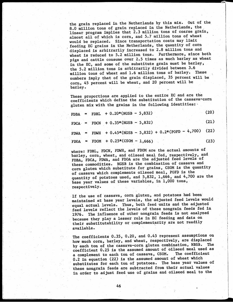
the grain replaced in the Netherlands by this mix. Out of the

8.0 million tons of grain replaced in the Netherlands, the

linear program implies that 2.3 million tons of coarse grain,

almost all of which is corn, and 5..7 million tons of wheat

would be replaced. Since transportation costs may limit

feeding EC grains in the Netherlands, the quantity of corn

displaced is arbitrarily increased to 2.8 million tons and

wheat is reduced to 5.2 million tons. Furthermore, since both

pigs and cattle consume over 2.5 times as much barley as wheat

in the EC, and some of the substitute grain must be barley,

the 5.2 million tons is arbitrarily divided between 3.6

million tons of wheat and 1.6 million tons of barley. These

numbers imply that of the grain displaced, 35 percent will be

corn, 45 percent will be wheat, and 20 percent will be

barley.

These proportions are applied to the entire EC and are the

coefficients which define the substitution of the cassava-corn

gluten mix with the grains in the following identities:,

FDBA = FDBL + 0.20*(NGSB - 5,832) (20)

FDGA = FDCN + 0.35*(NGSB - 5,832) (21)

FDWA = FDWH + 0.45*(NGSB - 5,832) + 0.2*(POFD - 4,700) (22)

FDOA = FDOM + 0.25*(CSOM - 1,666) (23)

where: FDBL, FDCN, FDWH, and FDOM are the actual amounts of

barley, corn, wheat, and oilseed meal fed, respectively, and

FDBA, FDCA, FDWA, and FDOA are the adjusted feed levels of

these commodities. NGSB is the combination of cassava and

corn gluten which substitute for grains, CSOM is the quantity

of cassava which complements oilseed meal, POFD is the

quantity of potatoes used, and 5,832, 1,666, and 4,700 are the

base year values of these variables, in 1,000 tons,

respectively.

If the use of cassava, corn gluten, and potatoes had been

maintained at base year levels, the adjusted feed levels would

equal actual levels. Thus, both feed units and the adjusted

feed levels reflect the levels of these nongrain feeds fed in

1976. The influence of other nongrain feeds is not analyzed

because they play a lesser role in EC feeding and data on

their substitutability or complementrity are not readily

available.

The coefficients 0.35, 0.20, and 0.45 represent assumptions on

how much corn, barley, and wheat, respectively, are displaced

by each ton of the cassava-corn gluten combination, NBSB. The

coefficient 0.25 is the assumed amount of oilseed meal used as

a complement to each ton of cassava, CSOM. The coefficient

0.2 in equation (22) is the assumed amount of wheat which

substitutes for each ton of potatoes. The base year values of

these nongrain feeds are subtracted from their actual values

in order to adjust feed use of grains and oilseed meal to the

46

base year. For example, if each ton of NGSB substitutes for0.35 tons of corn, the adjusted level of corn (FDCA) wouldhave been 2.04 million tons less than the actual corn fed(FDCN) when the level of NGSB is at the base year level of 5.8million tons instead of at zero tons (in some hypotheticalearlier year)?

Potatoes in the EC have been fed mainly to pigs in Germany(30). Because of rising labor costs, total potatoes fed inthe EC declined from about 15 million tons in 1964 to only 4.5million in 1979. Furthermore, in order to release theirmaximum nutritional value, the potatoes must be cooked, whichIs also labor-intensive. Since less than 5 percent of thegrain fed to pigs in Germany is corn, the only substitutionpotential for potatoes is with barley and wheat. The ECintervention system has maintained the price of wheat aboveits feed value in most years and led to a surplus. Declinesin potato use allowed wheat feeding to increase. Potatoes aregenerally considered to be worth 20 percent of grain in termsof weight. Therefore, 1 metric ton of potatoes is assumed tosu15stitute for 200 kg of wheat.

The effect of substituting cassava and corn gluten on thenutritional characteristics of the aggregate feed ration maybe observed in table 20. Total energy in the ration declinesby 991,000 calories, while protein and fiber increase by22,000 and 264,000 tons, respectively. While insignificant inproportion to the total nutrient composition of the ration,

Table 20—Aggregate effects of cassava, corn gluten, andoilseed meal substitution for grain on the nutritional characteristics

of the EC feed mix

Feed component: Substitute nongrain feeds :

: Corn : Oilseed :Item : Cassava: gluten : meal Barley: Corn :

Feed

Energy

: 5,000

Displaced grains : Net

Wheat : change

1,000 tons

3,000 125 -1,625 -2,844 -3,656 0

1,000 calories

: 17,350 9,750 394 -5,931 -9,868 -12,686 -991

1,000 tons :

Protein : 140 750 62 -226 -284 -.420 22Fiber : 250 270 9 -98 -57 -110 264

:Source: Calculated from equations (22) and (24), according to the

nutritional characteristics in table 16.

47

Econometric Model of Feed Demand

the substitution of protein for energy is compatible withcommon notions about the changing composition of EC feedrations.

In the absence of changes in prices, feeding intensity, andother factors, the feed units variables and the adjusted feedvariables are identical. Both would refer to the total ofeach feed required to produce the livestock products in eachyear at the base year levels of nongrain feed use. Therefore,in estimating actual feed demand, the coefficient on the feedunits variable is restricted to 1.0. The feed units variablesare mathematically derived in equation (4), and represent thequantities of each major feed ingredient fed in the production

of all livestock products.

Substitution effects caused by price changes are accounted forby entering the price ratios of the four major feedingredients in each equation. Since the levels of animalproducts are maintained invariant to feed prices in thefeed-demand equations by the feed units variables, changes infeed prices induce movements along an isoquant representing

fixed levels of animal products. Therefore, priceelasticities represent the average substitution taking placeamong feeds over all livestock rations and are hypothesized to

be negative.

In free markets where prices are unconstrained, all feed

prices equal their marginal value products. Wheat prices in

the EC have sat on the intervention (floor) price, except for

the years 1967 to 1973 when denaturing premiums paid to

farmers for feeding wheat of breadmaking quality pushed feed

wheat prices below the intervention price. However, the value

of wheat for onfarm feeding has increased for farmers unable

to take advantage of selling wheat into intervention because

of high transportation costs. Consequently, the relativemarket prices of wheat to other grains do not accurately

reflect the relative values of these two sets of grains.

Significant problems occurred in obtaining statisticallysignificant price coefficients in the feed demand equations.

The introduction of quantity variables provides a reasonablealternative for obtaining the substitution relationships among

the different grains. While market prices for corn and barley

accurately reflect their relative onfarm values, the relative

onfarm value of wheat could not be measured by a price ratio.

However, the relative values of two grains are mainly

determined by their availabilities (production plus stocks) in

a given year. • Therefore, the availabilities of barley and

wheat are used as proxies to measure the relative value of

wheat to barley in the barley equation. Since cornavailability is perfectly elastic at the threshold price, the

feed use of wheat is used to measure the relative value of -

wheat in the corn equation. In the wheat equation, corn fedand the production of wheat proved better alternatives thancorn use and wheat availability. The use of barleyavailability or production had no advantage over the priceratio of wheat to barley in the wheat equation.

48

The increase in the use of grains in compound feed can beascribed to the shift away from pasture, variations in theprices and availabilities of various concentrates, andvariations in milk production. The growth in compound feeduse directly caused by shifts away from pasture has occurredat a fairly constant rate. Therefore, a time trend isincluded in all grain equations to account for the effect ofthis constant rate of growth on grain used in compound feeds.

Much of the feed used by breeding pigs is excluded from thefeed units variable. The feed used by pigs which is includedin feed units is calculated as the weighted product of porkproduction and the feed conversion rate for raising pigs toslaughter weight. Pork produced from culled breeding animalsis treated as if it were pork produced from slaughter animalsweighing about 180 pounds. However, breeding pigs are fed toand maintained ,at weights far exceeding 180 pounds.Therefore, pork production is entered separately in all grainequations. This variable is entered instead of the number ofbreeding pigs because the data on the number of breeding pigs,before 1970 are unreliable, and feed use per breeding pig hasincreased because of larger litters and hence more porkproduction per breeding animal.

Increased use of oilseed meal is important for all animals,but particularly for pork and dairy, which account for overtwo-thirds of the oilseed meal used. Much of the increase indairy production in the EC has resulted from increased use ofoilseed meal. In pork, broiler, and egg rations, protein hasbeen substituted for energy to obtain higher levels of feedconversion and shorter growing periods.

In addition to declining soybean meal to grain price ratios,the use of oilseed meal per unit of livestock product has alsoincreased as a result of consolidation of livestock productioninto larger, more efficient units, the adoption of dairy cowshaving higher potential milk yields, and other technologicalchanges in breeding, nutrition, and medication. These lattertwo factors increased the marginal productivity of oilseedmeal at all feed price ratios. The resulting greater use ofoilseed meal per animal resulted in more efficient feedconversion rates for all animals and higher milk yield percow. In addition, the increasing price ratio of milk tosoybean meal provided further incentive for the dairy sectorto use more oilseed meal. Therefore, the feed conversion ratefor pork, and the product of the milk yield (per cow) and theratio of milk price to soybean meal price are used to accountfor increased intensity of oilseed meal use. Sinceexperimentation with putting these variables in the gr4insequation did not yield the expected results, they are omittedfrom the grain equations.,

The feed demand equations are:

ln(FDBA) = B10 + l*ln(FUBL) Bll*ln (FPBL/FPCN) + (24)B12*ln(FPBL/IPSM) + B13*ln(AliBL) +B14*ln (AVWH) + B15*ln(PDPE) + BleT

49

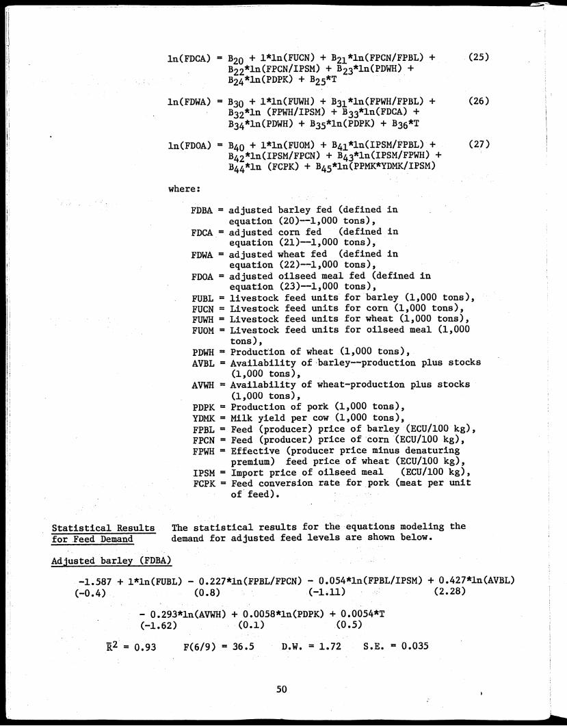
ln(FDCA) = B-20 + l*ln(FUCN) + B21*ln(FPCN/FPBL) + (25)

B22*ln (FPCN/IPSM) + B23*ln(PDWH) +

B24*ln (PDPK) + B25*T

ln(FDWA) = 830 + l*ln(FUWH) + Ba*ln(FPWH/FPBL) + (26)B32*ln (FPWH/IPSM) + B33*ln(FDCA) +

B34*ln(PDWH) + B35*ln(PDPK) + B36*T

ln(FD0A) = B40 + l*ln(FUOM) + B41*ln(IPSM/FPBL) + (27)B42*ln(IPSM/FPCN) + B43*ln(IPSM/FPWH) +

B44*ln (FCPK) + Bo*ln(PPMK*YDMK/IPSM)

where:

FDBA = adjusted barley fed (defined inequation (20)--1,000 tons),

FDCA = adjusted corn fed (defined inequation (21)-1,000 tons),

FDWA = adjusted wheat fed (defined inequation (22)-1,000 tons),

FDOA = adjusted oilseed meal fed (defined inequation (23)-1,000 tons),

FUBL = livestock feed units for barley (1,000 tons),

FUCN = Livestock feed units for corn (1,000 tons),FUWH = Livestock feed units for wheat (1,000 tons),

FUOM = Livestock feed units for oilseed meal (1,000tons),

PDWH = Production of wheat (1,000 tons),

AVBL = Availability of barley--production plus stocks(1,000 tons),

AMMH = Availability of wheat-production plus stocks(1,000 tons),

PDPK = Production of pork (1,000 tons),

YDRK = Milk yield per cow (1,000 tons),

FPBL = Feed (producer) price of barley (ECU/100 kg),FPCN = Feed (producer) price of corn (ECU/100 kg),

FPWH = Effective (producer price minus denaturingpremium) feed price of wheat (ECU/100 kg),

IPSM = Import price of oilseed meal (ECU/100 kg),FCPK = Feed conversion rate for pork (meat per unit

of feed).

Statistical Results The statistical results for the equations modeling the

for Feed Demand demand for adjusted feed levels are shown below.

Adjusted barley (FDBA)

-1.587 + l*ln(FUBL) 0.227*ln(FPBUFPCN) 0.054*ln(FPBUIPSM) + 0.427*ln(AVBL)

(-0.4) (0.8) (-1.11) (2.28)

- 0.293*ln(AVWH) + 0.0058*ln(PDPK) + 0.0054*T(-1.62) (0.1) (0.5)

= 0.93 F(6/9) = 36.5 D.W. = 1.72 S.E. = 0.035

50

Adjusted corn (FDCA)

3.266 + l*ln(FUCN) - 0.090*ln(FPCN/FPBL) - 0.12*ln(FPCN/IPSM) - 0.215*ln(FDWA)(1.03) -(0.35) (-2.19) (-2.0)

+ 0.214*1r(PDPK) + 0.03305*T(0.5) (3.18)

= 0.95 F(5/10) = 54 D.W. = 2.13 S.E. = 0.04

Adjusted wheat (FDWA)

5.76 + l*ln(FUWH) - 0.82*ln(FPWH/FPBL) 0.184*ln(FPWH/IPSM) 1.54*ln(FDCA)(0.48) (-1.47) (-1.36) (-2.52)

+ 0.349*ln(PDWH) + 0.611*ln(PDPK) + 0.04*T(0.5) (2.91) (1.05)

= 0.78 F(6/9) = 9.8 D.W. = 2.51 S.E. = 0.85

Adjusted oilseed meal (FDOA)

4.80 + l*ln(FUOM) + 0.59*ln(IPSM/FPBL) + 0.18*ln(IPSM/FPCN) - 0.33*ln(IPSM/FPWH)(3.01) (0.97) (0.43) (-1.0)

R2 = 0.95

+ 4.15*ln(FCPK) + 0.5*ln(PPMK*YD4K/IPSM)(4.38) (1.71)

F(5/9) = 53 D.W. = 1.59 S.E. = 0.06

Note: R2 = coefficient of determination.F(x/y) = F-value with x and y degrees of freedom.D.W. = Durbin-Watson statisticS.E. = Standard error

In view of the following limitations, the results appearreasonable. Multicollinearity in the data presents significantproblems because all explanatory variables exhibit trends.More important, however, the relative inflexibility of EC grainprices and the insensitivity of onfarm feed demand to pricesmake it difficult to explain variability in feed demand withprices alone. The quantity variables thus serve to pick upconsiderable variation in feed demand.

Most of the variation in feed use is explained by feed 'units,the quantity variables, the feed conversion rate for pigs, andthe milk variable. The only price variable which isstatistically significant at the 5-percent level is therelative price of corn to soybean meal in the corn equation.In the oilseed meal equation, only the relative price of wheatto oilseed meal has the expected negative sign. All prices dosignificantly affect feed demand through their effect on milk,

51

beef, and pork production. The relative price of corn to

soybean meal also significantly affects the feed demand for

corn and wheat through its effects on the quantity variables.

The coefficients associated with the quantity variables do not

appear unreasonable in view of the changes in the amounts of

grain fed which they imply. Table 21 contains the average

values of the exogenous quantity variables, the average values

of the adjusted amounts of grain fed, and the response of the

quantities fed to a 10-percent increase in barley and wheat

availability. Wheat production increases by 11.9 percent in

order to generate a quantity of wheat which increases wheat

availability by 10 percent. The percentage change in barley

fed in response to an increase in availabilities is taken

directly from the econometric results, while the percentage

responses of wheat and corn are derived from reduced form

equations.

An increase of 4.0 million tons of only barley availability

increases barley fed by 0.9 million tons, but does not decrease

the quantity of any other, grain fed. The increase in barley

fed would be expected to be significantly less than the full

increase in barley available because milk production is held

constant in the equation and limited substitution of pasture

exists. The barley not fed would be exported or held in stock.

Variation in wheat production and availability do influence the

use of other grains because wheat is not a popular ingredient

in dairy rations (tables 10-12) and hence is not profitable as

a pasture substitute. An increase of 4.5 million tons in wheat

production and availability increases wheat fed by 0.7 million

tons, but reduces barley fed by the same amount, and reduces

both corn and total feed by 0.3 million tons. One would expect

each additional unit of wheat fed to be offset by a decline in

a similar quantity of barley and corn.

Thus, while the effects of the quantity variables must be

viewed with some caution, they do appear to explain some

• Table 21--Changes in quantity variables and grain demand in

response to a 10-percent change in barley and wheat availability

: Exogenous variables

Item : Unit : AVBL AVWH PDWH FDBA FDCA FDWA

Average : Millionvalues : tons : 39.9 44.9 37.7 23.1 18.4 10.8

: •Change : Percent : 10.0 0 0 4.0 0 0

Change : do. : 0 10.0 11.9 -2.9 -1.4 6.2

_Change : Million.: 4.0,•0 • 0 .9 0 0

: tons .• •

Change : do. .• 0 4.5 4.5 -.7 -.3 .7

Endogenous variables

52

onfarm use of grains which prices could not pick up. Quantityvariables have been used for similar purposes in other studies

Pork production appears reasonable to explain the increase inwheat fed to breeding pigs. The 50-percent increase in porkproduction increases the quantity of adjusted wheat fed by areasonable 31 percent, or by about 2.6 million tons over itsinitial level of 8.3 million tons. Assuming the number ofbreeding sows remains a constant 11 percent of the total herd,herd expansion from 55.5 to 77.3 million implies an increaseof 2.4 million breeding animals. At an average of 7 pounds offeed a day (21); this implies an increase of about 2.8 milliontons of feed for breeding animals, somewhat above theestimated 2.6 million tons. Other grains are also fed tobreeding animals, but pig production is not statisticallysignificant in these equations.

The time trend is only statistically significant in the cornequation and implies an increase of about 3.3 percent per yearin the quantity of adjusted corn fed to cattle. This impliesthat dairy cattle accounted for over 50 percent of the growthin adjusted corn fed from 1964 to 1979, or about 7.0 milliontons. Total corn consumption by cattle in the 1976 base yearwas only 5.1 million tons. _Since much of the 1.9 million tondifference could have been made up by cassava and corn gluten,these results do not appear unreasonable. However, the timetrend could be picking up other factors. The absence of anystatistical significance in the barley equation for the timetrend .is troublesome because barley has been a more importantfeed for cattle, totaling 11.5 million tons in 1976.

The coefficients on both the feed conversion rate for pork andthe returns to milk prodiaction per cow relative to the soybeanmeal price in the soybean meal equation are statisticallysignificant. The feed conversion rate for pork increased by10.6 percent and the returns to milk production per cowrelative to soybean meal prices increased by about 30percent. These increases, multiplied by the two coefficients,imply increases of 44 and 15.3 percent, respectively, in theuse of adjusted oilseed meal for pigs and cattle, or 3.9 and1.4 million tons, respectively, in absolute terms. In thebase year of 1976, pigs and dairy used 6.0 and 3.6 milliontons, respectively, of oilseed meal. As we do not know howmuch oilseed meal was used per unit of output at the beginningof the estimation period for pigs and dairy, it is notpossible to say how realistic these implied increases may be.However, since these implied increases cover the entireestimation period, but are significantly smaller than the'quantities used in the base period, they do not necessarilyappear to be unreasonably high.

Although the lack of statistical significance for all pricesimplies an own price elasticity of demand for oilseed meal ofzero, this result is not discouraging in view of the resultsof other studies (12, 18, 24,36), which are summarized in

53

SIMULATIONS OFSELECTED ECPRICING POLICIES

table 22. Both the time periods covered and the structure ofthe equations in these earlier studies lead one to expect aless negative elasticity than found in these studies. Bycovering the period of time in the early sixties when the CAPpricing policy became effective, these studies captured theinitial reaction of the EC to higher relative grain prices.After 1964, the price ratios between oilseeds and grains didnot exhibit much trend. The rapid expansion of oilseed mealuse after 1964 was a reaction to the price changes in theearly sixties and shifted the demand function for oilseed meal

to the right, causing it to become more inelastic.

With the exception of Williams (36), these studies estimated

the demand for only soybean meal, which is more elasticbecause other oilseed meals may be substituted for soybean

meal. Neither Houck (12) or Paarlberg (24) included variablesto pick up the effects of increased livestock production onoilseed meal demand, so that the slight downward trend inoilseed meal prices would pick up the effects of livestockproduction through a more negative price elasticity. WhileWilliams (36) and 1.41ipscheer (18) included livestock unitsmeasuring livestock production, they did not explicitly allowfor increased feeding per unit of livestock production, sothat other variables in their equations were allowed to pick

up this effect.

Two types of simulations are carried out for the purpose of

assessing the reliability of the econometric model. First, a

comparison of historical data with simulated values associatedwith the actual values of exogenous variables serves to revealthose equations which do not track the historical datareliably. Secondly, simulated policy changes are used tolocate unreliable structural relationships due to errors in

the specification or estimation of equations.

Table 22--A comparison of own price elasticitiesfor oilseed meal demand

: : Assumptions Study : E : Period : Product : LU

:Houck, and :

• others (12) : -0.68 1950-67 Soybean meal No

Paarlberg (24) : -.30 1960775 Soybean meal No

Williams (36) : -.28 1960-78 High protein Yes_Knipscheer, and :others (18) : -.23 1961-76 Soybean meal Yes

:Current study : 0 1964-79 All oilseed

: meal YesE = Own price elasticity.LU = Livestock units. •

1/ High protein includes all oilseed meals except copra andpalm kernel meal.

54

Projections are not done because the main purpose of thisstudy is to present preliminary research leading to thedevelopment of a reliable historical model of thefeed-livestock sector. An historical simulation of policyalternatives avoids the necessity of modifying the behavioralrelationships in the system in order to provide reliableprojections of the future effects that alternate EC pricingpolicies might have. The behavioral relationships expressedby any econometric model are technically valid only over therange of values and the economic structure associated with theestimation period covered by the data. Thus, using the modelfor projections would require judgments about the futurevalues of exogenous variables and behavioral relationships,which are beyond the scope of the present research.

The historical policy simulations in this section provideevidence of the model's reliability in performing policyanalysis, in view of three possible structural limitations ofthe model suggested by the econometric results. First,limitations in price variability limited the potential of themodel in estimating the effects which large changes in priceswould play in influencing livestock production and thesubstitution among feeds. Secondly, the variables measuringthe reasons for increased feeding intensity of oilseed mealwere less than desirable. Finally, only rough approximationswere made of the influence which the increased feeding of corngluten and cassava have had on grain and oilseed meal fed.Since these structural limitations do not lead to unreasonableresults in the policy simulations, the model could be updatedfor use in policy projections, if desired. However, somejudgments would have to be made regarding the structure ofthe behavioral relationships and the values of exogenousvariables in the future.

Three scenarios of interest to U.S. policymakers are simulated:

I. Soybean meal prices having been 10 percent higher thanactual prices throughout the estimation period.

II. EC grain prices linearly converging to world pricesbeginning in 1971 and ending in 1979, but with livestockprices remaining at actual EC levels.

III. Prices of animal products reduced in conformity with ECgrain prices.

The simulation of a higher soybean meal price illustrates thesensitivity of the model to increases in oilseed meal pricesbecause of decreased availability to the EC or an import taximposed by the EC. While a tax on oilseed meal would be aviolation of the zero-level binding in the General Agreementon Tariffs and Trade (GATT), and is not expected, a tax onvegetable oils is possible. Such a tax would, however,increase the price of meal by reducing the amount of oilseedscrushed in the EC. A tax on vegetable oil is possible becauseit could relieve pressure on a financially strapped budget

55

both by raising tax revenue and by making surplus EC grains

more attractive to livestock producers through its effect on

meal prices. The EC contends that imported oilseeds increase

the cost of grain _export refunds by substituting for feed

grains, requiring the latter to be exported to world markets

with a subsidy.

U.S. officials have argued that a reduction in EC grain prices

would solve the EC's problem of large imports of oilseed meal,

cassava, and corn gluten, and substantially increase the use

of surplus EC wheat and barley, as well as imported U.S.

corn. It is also argued that such a policy would result in

more U.S. corn being sold in markets where surplus EC wheat

and barley are currently disposed of. The United States also

contends that without concurrent declines in the prices of EC

animal products, lower EC grain prices would increase the EC's

surplus in dairy and other animal products.. Additional

livestock surpluses would add to EC budget costs, further

depress world livestock prices, and further reduce livestock

feeding in third-party countries, as they become markets for

surplus EC livestock products. These countries would

otherwise' purchase U.S. corn for use in domestic feeding.

Accordingly, both the United States and the EC have an

interest in seeing EC grain and livestock prices reduced.

The effects. of reductions in EC grain and livestock prices are

investigated by simulating what would have occurred had EC

prices of these commodities been gradually reduced below their

actual levels between 1971 and 1979. 'EC prices for corn,

barley, and wheat are computed to rise in a linear fashion

from 1971'to 1979, but more slowly than actual EC prices rose

during this period. Thus, although the simulated EC grain

prices continue rising in this scenario, the gap between

simulated and world prices narrows, such that they are equal

in 1979. In scenario II, livestock prices are held at their

actual levels, while they are reduced in line with grain

,prices in scenario III.

Analysis of these policies is limited to the effects which

they have on EC livestock production and feed demand. Limited

conclusions are drawn regarding the net effects of these

policies on the United States and the EC. An analysis of

secondary effects on world prices and trading patterns is

beyond the objectives of this study.

Actual EC grain and livestock prices are compared in table 23

with prices used for simulations ,II and III. In 1970, actual

and simulated EC prices are equal. Both sets of prices rise,

but the prices used in the policy simulations rise more

slowly, so that by 1979 they are identical with world prices

and below actual EC prices. The simulated and world price for

corn in 1979 is only 57 percent of the actual price which

prevailed in the EC. Comparable figures for wheat and barley

are 81 and 78 percent, respectively, of actual EC prices. The

smaller percentage for corn is because the actual EC corn

price is determined by the threshold (minimum import) price,

56

Table 23--A comparison of actual EC prices used in the baseline scenarioand the simulated prices used in scenarios II and III, 1971-79

Prices : 1970 : 1971 : 1972 : 1973 : 1974.: 1975 : 1976 : 1977 1978 : 1979 :

: Simulated pricesas percentof actual EC

prices in 1979Actual prices 1 ECU's per 100 kilograms Percent -

Corn : 8.98 9.11 10.42 11.51 13.22 14.20 15.90 16.69 17.46 18.09 NAWheat : 7.59 7.74 8.22 10.11 11.97 12.83 14.60 15.06 15.54 16.35 NABarley : 7.99 8.18 8.52 10.24 11.43 12.28 14.14 14.11 14.23 15.08 NABroiler : 55.96 56.87 58.46 66.09 66.38 69.31 73.32 75.21 75.09 78.31 NAEggs : 58.19 64.78 65.30 84.38 77.20 79.79 89.37 93.56 89.54 96.61 NAPig : 60.84 62.64 74.40 85.94 81.54 100.12 102.78106.15 100.84 104.11 NAMilk : 9.33 10.59 11.32 12.13 13.90 15.75 16.91 18.43 19.18 20.11 /IABeef : 58.21 66.69 81.43 82.04 85.43 98.87 107.07 115.53 122.17 122.16 NA

Simulated prices :prices used inscenarios II :and III 2/CornWheatBarley..Broiler.

8.98 9.13 9.28 9.43 9.58 9.74 9.89 10.04 10.19 10.34: 7.59 8.21 8.84 9.47 10.10 10.73 11.36 11.98 12.61 13.247.99 8.40 8.82 9.24 9.65 10.07 10.49 10.91 11.32 11.7455.96 56.79 57.62 58.45 59.28 60.10 60.93 61.76 62.59 63.42Egg.. 58.19 60.42 62.65 64.88 67.11 69.33 71.56 73.79 76.02 78.25Pig. -: 60 84 63.45 66.06 68.67 71.28 73.89 76.50 79.11 81.72 84.33Milk : 9.33 9.69 10.04 10.40 10.76 11.11 11.47 11.83 12.18 12.54Beef : 58.21 60.24 62.27 64.31 66.34 68.37 70.40 72.43 74.47 76.5

57.281.077.981.0

81.081.062.462.6

.NA = Not applicable.1/ Actual_ prices in the EC are computed by equation (1) from the data in (11). The simulatedprices for grain are equal to world prices for grains in 1979, and are taken from (20) and (31).Simulated livestock prices are arbitrarily reduced in line with relevant grain prices.2/ The simulated prices for grains are used in place of actual EC prices in scenarios II andIII. The simulated prices for livestock are used in place of actual EC prices in scenario III.

whereas wheat and barley prices are determined by the lower

internal intervention price. Thus, EC corn prices have

farther to fall in order to reach world levels than do wheat

or barley, so that corn becomes a relatively cheaper feed in

these scenarios.

In scenario III, the simulated 1979 prices for beef and milk

are assumed to be 62 percent below the actual levels

prevailing in 1979. This percentage decline is larger than

for barley and wheat prices, but lower than for corn prices.

The simulated prices for eggs, broilers, and pork have a lower

percentage decline from actual prices than for beef and milk.

This assumption is made because the milk surplus has been

greater than the surplus of small animal products, and cattle

consume more barley and wheat than they do corn (table 12).

Furthermore, as simulation II reveals, the production of milk

grows more rapidly than small animal production when only

grain prices are reduced. The prices for the small animal

products are assumed to follow the trend in simulated wheat

prices and to be 81 percent below the actual levels of prices

for those products in 1979.

Base Run

Since policy objectives in the EC may be to reduce EC grain

surpluses by encouraging greater feed use of domestic grain,

and not reductions in grain production, grain availability is

held constant by assuming that the EC would maintain incomes

to farmers through some scheme such as a deficiency payments

program. The implementation of such a program may be the only

way to reduce grain prices in view of the powerful grain lobby

in the EC. Thus, decreased grain prices directly affect only

livestock growers. The industrial use of grain is assumed to

be unresponsive to grain prices because use has not varied

appreciably with respect to grain prices in the past.

Surpluses in livestock production may only be reduced by

lowering incomes to livestock producers because consumer

demand is not expected to significantly increase with

reductions in prices. Therefore, livestock producers are

assumed to face falling prices in scenario III.

A dynamic simulation of the model using historical price data

reveals relatively small simulation errors in the absence of

extraordinary events (table 24). The largest errors are in

the feed demand equation for wheat and oilseed meal because of

substantial variation in the data--particularly for wheat.

Errors of 19.5, 21.1, and 24.1 percent occur for wheat in

1967, 1975, and 1976, and errors of 17.4 and 13.7 percent

occur for oilaeed meal in 1974 and 1975. Drought was largely

responsible for the large errors in the wheat variable because

it reduced the onfarm use of wheat without significantly

affecting price levels. Lower oilseed meal use in 1974 and

1975 than was simulated may have resulted from a lagged

response by EC feed compounders in building new capacity in

response to the fall in prices which followed the end of the

U.S. soybean embargo.

58

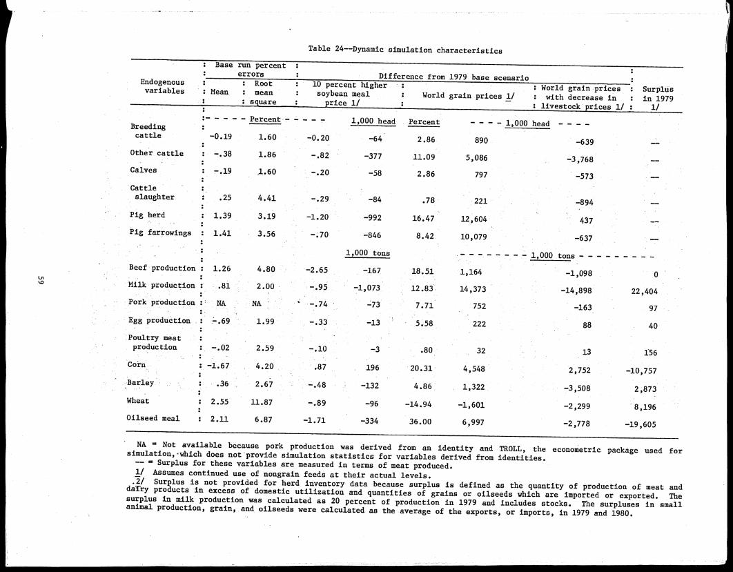
Table 24--Dynamic simulation characteristics

: Base run percent :errors Difference from 1979 base scenarioEndogenous : : Root : 10 percent higher : : World grain prices : Surplusvariables : Mean : mean : soybean meal : World grain prices 1/ : with decrease in : in 1979square : price 1/ .: : livestock prices 1/ : 1/:

: Percent 1,000 head Percent - - - - 1,000 head - - - -Breeding :cattle -0.19 1.60 -0.20 -64 2.86 890 -639:

Other cattle : -.38 1.86 -.82 -377 11.09 5,086 -3,768• :Calves : -.19 1.60 -.20 -58 2.86 797 -573:Cattleslaughter : .25 4.41 -.29 -84 .78 221 -894:

Pig herd : 1.39 3.19 -1.20 -992 16.47 12,604 437:Pig farrowings : 1.41 3.56 -:70 -846 8.42 10,079 -637:

1,000 tons 1,000 tons

Beef production : 1.26

Milk production .81. .Pork production NA

4.80 -2.65 -167 18.51 1,164 -1,098

2.00 - -.95 -1,073 12.83 14,373 -14,898

NA -.74 -73 7.71 752 -163

•••••

0

22,404

97

Egg production .: -.69 ' 1.99 -.33 -13 5.58 222 88 40:Poultry meat :production • -.02 2.59 -.10 -3 .80 32 13 156:

Corn -1.67 4.20 .87 196 '20.31 4,548 2,752 -10,757:Barley • , .36 2.67 •L'.48 -132 4.86 1,322 -3,508 2,873:Wheat : 2.55 11.87 -.89 -96 -14.94 -1,601 -2,299 8,196:Oilseed meal : 2.11 6.87 -1.71 -334 36.00 6,997 -2,778 -19,605

• NA = Not available because pork production was derived from an identity and TROLL, the econometric package used forsimulation, -which does not provide simulation statistics for variables derived from identities.= Surplus for these variables are measured in terms of meat produced.1/ Assumes continued use of nongrain feeds at their actual levels.:i/ Surplus is not provided for herd inventory data because surplus is defined as the quantity of production of meat anddaTry products in excess of domestic utilization and quantities of grains or oilseeds which are imported or exported. Thesurplus in milk production was calculated as 20 percent of production in 1979 and includes stocks. The surpluses in smallanimal production, grain, and oilseeds were calculated as the average of the exports, or imports, in 1979 and 1980.

Higher Soybean Meal Prices

Convergence of EC

Grain Prices to World Levels

The effects of the policy scenarios on endogenous variables is

determined by comparing the simulated values for these

variables in 1979 with their simulated values in the base

.run. It should be kept in mind that the results of these

policy simulations are subject to the limitations of the

econometric model and may therefore not reflect what would

actually have happened had these policy alternatives been

implemented. They are suggestive, however, of what might have

happened as they do not appear unreasonable.

If feed processors faced a higher price for soybean meal,

it would not have very large effects on any variables.

Oilseed meal demand would be reduced as expected, but,

contrary to expectations, demand for wheat and barley also

would decline. This is because higher soymeal costs would

induce a drop in the supply of livestock products that would

lower feed demand in general, more than offsetting the

substitution of wheat and barley for meal. The only grain for

which demand would rise, due to a strong substitution effect,

is corn-which the EC imports.

According to the model simulations, a 10-percent higher price

for soybean meal in each year from 1964 through 1979 would

decrease oilseed meal use by 1.7 percent below its value in

the simulated base run in 1979, barley by 0.48 percent, and

wheat by 0.89 percent. Corn use would rise by 0.87 percent,

beef production would decline by 2.65 percent, while all other

livestock production declines by less than 1 percent below the

base level in 1979.

The results of this scenario are reasonable in view of the

small proportion of total feed costs represented by oilseed

meal, and the two• major factors which were responsible for

,increased oilseed meal use. Oilseed meal represents about 18

percent of the concentrates used in producing eggs, pork, and

beef, 20 percent for milk, and 25 percent for poultry meat.

Much of the increase in oilseed meal use in the EC resulted

from the structural changes in livestock production and as a

lagged response to the shifts in price ratios after 1964.

Consequently, the feed demand equations show that there is

little price substitution between oilseed meal and the grains,

although significant substitution may exist among the

different kinds of meals. With the exception of corn, which

has the only statistically significant oilseed meal price

term, the substitution effects are more than offset by the

decline in feed demand induced by lower supplies of livestock

products.

The simulation results of a convergence of EC producer prices

for grains to world levels, without reductions in livestock

prices, underscores the necessity of the EC to concurrently

lower livestock prices. In the absence of lower livestock

prices, lower grain prices would increase the profitability of

livestock production and increase the level of livestock

surpluses, particularly dairy. These livestock surpluses

would be a further burden on the EC budget and would likely

60

displace U.S. feed grain exports from some countries where thesurplus livestock products would have to be sold.

The effect of this policy on EC grain use depends upon whethercassava and corn gluten continue to be used at their 1979levels or are eliminated from use. With continued use ofthese nongrain feeds at 1979 levels, corn use increases 4.6million tons above the base level. Wheat use declines andoffsets increased barley use by about 0.3 million tons. Ifcassava and corn gluten use are assumed to be zero, corn useincreases by 7.4 million tons, and wheat and barley useincrease by 5.0 million tons above the base level in 1979.Soybean meal use increases 7.0 million tons when nongrainfeeds are used at actual levels, and 6.87 million tons whennongrain feed use is assumed to be zero. Increased domesticuse of EC grains would allow more U.S. grain to be sold tocountries which currently use surplus EC wheat and barley.

Significant increases in livestock production occur under thisscenario. Beef production in 1979 would rise by 18.5 percentabove the base level and be in large surplus by 1979. Theestimated 12.8-percent rise in milk production would increasethe already large EC dairy surplus by 64 percent. Pork andegg production, being less price sensitive, would increase byonly 7.7 and 5.6 percent, respectively, but the resultingsurpluses would likely disrupt world markets. The EC poultrymeat surplus, already a problem for world poultry trade, wouldincrease 20 percent in response to the 0.8-percent increase inpoultry meat production.

The effect of a decrease in EC grain prices on feed usedepends upon what happens to nongrain feedstuffs. If cassavaand corn gluten use remain at actual levels in the ration, theconvergence of EC grain prices ,to world levels would notincrease the use of EC grain. Wheat demand would decline by1.6 million tons and barley demand would increase by 1.3million tons, so that the overall consumption of EC-producedgrain would actually decline by 0.3 million tons. Given .thesignificantly larger fall in the price of corn than in theprices of major EC produced grains, the substitution of cornfor wheat would raise corn use by 4.6 million tons. In theabsence of a deficiency payments program - to support theincomes of grain farmers, EC grain production would declineand result in even more corn, mainly of U.S. origin, beingfed.

If cassava and corn gluten use in the EC were assumed to bezero, an additional 2.8 million tons of corn, 1.6 million tonsof barley, and 3.7 million tons of wheat, and 0.125 millionton less oilseed meal would be used in the feed rations ,(table20). Consequently, the use of wheat increases to 2.1 milliontons above its base level, .as opposed. to the reduction inwheat use of 1.6 million tons shown in table 24 if cassava andcorn gluten levels are unchanged. This increased use of wheatis still well below the 8.2 million tons exported by the EC,on the average, in 1978 and 1979. The additional use of 1.6

61

Decreases in Both EC Grain and Livestock Prices

million tons of barley, to 2.9 million tons above its base

level roughlyequals average barley exports in 1978-79. The

additional use of 2.8 million tons of corn would significantly

increase the EC's deficit in corn, and benefit mainly the

United States. Thus, total elimination of corn gluten and

cassava from the ration, in combination with a convergence of

EC and world grain prices, would eliminate the EC's surplus

production of barley, but not its surplus of wheat

production.

Reductions in the use of nongrain feeds have limited but

identifiable benefits for both the United States and the EC.

Although the wheat surplus in the EC is significantly reduced,

a large 'surplus will continue to exist unless production is

reduced through reductions in price supports not compensated

for by deficiency payments. Gains to the United States from

increased use of corn would be limited because of reduced

demand and prices for corn gluten feed.

U.S. exports of corn and soybeans would provide for much of

the increase in feed demand in the EC, regardless of whether

corn gluten and cassava remain at actual levels or are

eliminated from the ration. The increased feeding of grain in

the EC would also open up markets for U.S. grain in

third-party countries. U.S. livestock producers would have

some costs since world prices for livestock products would

tend to be depressed. More importantly, an increase in the

surpluses of EC livestock products will reduce the demand for

U.S. feed grains in the countries receiving these surpluses as

they reduce domestic livestock production. Thus, while

Increased EC feeding will strengthen world grain prices, the

resulting growth in livestock surpluses will dampen both world

livestock and grain prices.

The results of this scenario are consistent with the findings

of other research (14, 24). The net effects of this pricing

policy on the United States and the EC, and the political

reactions of the United States and other countries are beyond

the scope of this study.

The EC is unlikely to reduce grain prices in the absence of

reductions in livestock prices because of the domestic and

international problems which larger dairy, beef, and poultry

surpluses would create, as just discussed. Concurrent

reductions in the prices of both EC grains and livestock

products would benefit the Community by reducing surpluses in

animal products below the levels in the base run. Export

subsidies to dispose of surpluses would be reduced. However,

the decline in livestock production would reduce feeding so

that EC wheat and barley surpluses would increase by 5.8

million tons if nongrain feeds remain at actual levels in the

ration, but increase by only 0.5 million tons if these

feedstuffs are removed from the ration. The United States

would benefit from this policy mainly by not having the

international prices for livestock products depressed and

demand reduced for feedstuffs by other, countries due to

62

imports of the EC's surplus livestock products. The use ofU.S. corn in the EC would be higher than in the base scenario,but not as high as if EC livestock prices were not reduced.Oilseed meal use would decline from the base scenario.

Under this scenario, the EC's milk surplus is reduced by 66percent, or 15 million tons from that which prevailed in thebase run. Beef production is reduced by 17.5 percent andbecomes a deficit commodity by 1.1 million tons. Presumably,the reduction in beef prices induces a switch from beef toveal production. The implication of this scenario is thatbeef prices would have to be reduced somewhat less than milkprices in order to decrease the milk surplus without reducingbeef production below consumption.

Pork production is reduced by 1.7 percent, or 0.16 milliontons below the level in the base scenario, causing the EC tobe slightly deficit in pork. Egg and poultry meat productionare only 2.2 and 0.4 percent above their 1979 base levels inthis scenario because corn prices fall by a larger percentagethan the prices for these livestock products. However, sincethe surpluses in eggs and poultry meat represent 1.4 and 4.2percent of production, these small increases in productionimply increases in their surpluses of 120 and 8.3 percent,respectively. Thus, the increases in surplus for eggs andpoultry of 0.09 and 0.013 million tons, respectively, are verylarge relative to actual levels of surplus in 1979.

Higher consumption of all livestock products may be expectedin response to lower prices. Although not modeled, estimatesfrom unpublished USDA research suggest that the domesticconsumption of meat and dairy products would increase from 0.1to 0.3 percent for each 1-percent decrease in prices. Using0.1 to indicate very low price elasticity of demand in the ECwould imply that demand for pork and poultry products wouldincrease 1,.9 percent from the base level in 1979 in responseto the 19-percent decline in prices assumed for thisscenario. Thus, the increase in pork and egg production intable 24 would be roughly offset by increases in consumption,while the 0.4-percent increase in poultry meat productionwould be more than offset by consumption. An increase of 3.8percent in beef and dairy consumption, in response to the38-percent decline in price, would further increase thedeficit in beef under this scenario, but redtce the dairysurplus by about 3.5 million tons. Adding this increase inmilk consumption to the 15 million tons by which production isreduced implies a reduction of 18.5 million tons in thesurplus of 22.4 million tons that existed in 1979.

If ,the use of cassava and corn gluten is held at actual .levels,* the decline in dairy production and the higherrelative price of oilseed meal combine to reduce oilseed mealdemand to 2.78 million tons below the base level in 1979.Declining milk, beef, and pork production reduce the use of -barley from the base level of 1979 by 3.5 million tons and theuse of wheat by 2.3 million tons. The use of corn increases

63

CONCLUSION

by 2.75 million tons. Without substantial reductions in grainprices or reductions in use of nongrain feedstuffs, the EC'ssurplus in barley and wheat will increase by almostone-fourth.

Elimination of cassava and corn gluten from the rationsincreases corn and wheat use to 5.55 and 1.4 million tons,respectively, above the base run in 1979. Barley use drops to1.9 million tons below the base level. Therefore, the ECsurplus in wheat and barley will still increase above the 11.1million tons in 1979, but by only a modest amount of 0.5million tons (1.9-1.4). The EC would realize significantadvantages under this scenario. The significant reduction inthe EC dairy surplus implies large savings to the EC budget.The convergence to world prices implies no disposal costs forgrain surpluses, however. Moreover, foreign exchange would besaved by the reduction in use of oilseed meal, cassava, andcorn gluten. These results do not' take into account thesignificant negative effects on EC 'livestock producers whowould be faced with a cost/price squeeze because livestockprices decline more than feed costs.

The United States would realize mixed results from such an ECpolicy. It would gain from the additional corn used in the ECand in countries which are currently supplied with EClivestock products, but lose from the reduction of 2.78million tons of oilseed meal used in the EC. Increased EC

'grain exports would have a small negative effect on the UnitedStates. Most of the increased demand for corn would besatisfied by the United States, while the United States would

incur about one-half the cost in reduced oilseed meal importssince the United States Accounts for about half of the ,oilseed meal supplies. If cassava and corn gluten are removedfrom the EC ration, the United States would further gain froman increase in 2.8 million .qms of corn used in the EC, butlose from reduced corn gluten prices and the reduction of0.125 million tons of oilseed meal.'

The net effects to the United States of this EC policy would

also depend upon changes in world prices and trading patterns,which have not been analyzed because they are beyond the scopeof this study. Net gains are likely because the smallreduction in U.S. soybean meal use would be offset by higher

world feed grain prices, and the larger share which U.S. cornwould play in satisfying higher EC imports (14, 26).Reductions in the price of corn gluten would, however, reducethe advantage to the United States.

Of the policy actions considered in this analysis, the leastbeneficial one for both the United States and the EC is onewhich results in a 10-percent higher price for oilseed meals.No significant changes in livestock production or feed demandoccur under this scenario. The United States increases cornexports by nearly 0.2 million tons while losing probablyone-half of the 0.33 million ton reduction in oilseed mealuse. The EC dairy surplus only declines by 1.07 million tons,

64

or 5 percent of its average surplus in 1979, while the use ofEC grain falls marginally.

In the absence of both reductions in livestock prices and theuse of nongrain feeds, a convergence of EC and world grainprices by 1979 encourages significant increases in corn andoilseed meal use of at least 4.6 and 7.0 million tons,respectively. About one-half of the increase in oilseed mealuse will come from U.S. soybeans. Thus, the United Stateswould realize significant direct benefits in the EC marketfrom such a policy. The EC, however, would be burdened withlarge increases in livestock products, and the EC grainsurplus would increase by a negligible 0.3 million tons. ECexport subsidies for grains would disappear, but increasesubstantially in order to dispose of the larger livestocksurpluses: Additional livestock surpluses would be placed onworld markets, where they would reduce world livestock prices,as well as grain and oilseed meal use, or be subsidized insidethe EC for feeding. In the latter case, additional EC grainexports would depress world grain prices and displace U.S.feed grain exports in third-party countries.

Under this scenario, the EC would benefit from reductions inexport subsidies for grains, but incur substantial increasesin subsidies associated with increased livestock surpluses.Markets for U.S. corn and soybean meal would open up in theEC, but be reduced in third-party countries as higher exportsof EC livestock products displaced feeding in thosecountries. Reductions in the use of nongrain feeds wouldresult in additional use of all grains in the EC, but changeoilseed meal usage only slightly.

The policy scenario assuming reductions in both EC grain andlivestock prices increases the feeding of U.S. corn butreduces the feeding of EC grains because of reduced EClivestock production. It the absence of reductions innongrain feed use, the EC wheat and barley surplus willincrease by 5.8 million tons, and U.S. corn use will increaseby 2.75 million tons. However, the United States would loseabout one-half of the 2.8 million ton decline in oilseed mealuse.

The major beneficiary of such a policy would be the EC, whichwould have nearly all export subsidy costs eliminated. Incometo EC livestock producers would fall, however. U.S. gains areless certain because the reductions in EC grain use caused bydeclines in feeding would exert downward pressure oninternational grain prices, while increased use of U.S. cornwould exert upward pressure. Advantages accruing to theUnited States from increased use of U.S. corn could also beoffset by reductions in oilseed meal use in the EC. Less' useof nongrain feeds in the EC:would further increase grain use,but the price of nongrain feeds would decline somewhat.

The model used in this study has several unique strengths forpolicy analysis. The advantages are mainly ones of structural

65

specification. Feed conversion rates are taken into account

in explaining the supply of poultry products, pig herd size,and in determining feed demand. Thus, the effects oftechnological changes on livestock production and feed demandare accounted for to a greater. extent than in other aggregatedmodels of the EC feed-livestock sector.

Proper structural specification of the dairy sector isimportant for policy analysis because the dairy sector iswhere most of the livestock surpluses occur. Increases in

milk yields are specified as a function of the price ratios ofmilk to soybean meal and to barley, the two concentrate feeds

most responsible for increased milk yields. Many of thecomplex technological factors which have increased milk yield

were not included in this equation because of datalimitations. The primary role of soybean meal and barley in

explaining much of the variation andtrend in milk yield givesresearchers high confidence in performing policy analysis with

this equation, however.

Structural changes in livestock feeding have been the major

determinants of increased oilseed meal use, as compared with

changes in relative prices. Relative prices have played only

a minor role in increased oilseed meal use since the early

sixties. The rapid increase of oilseed meal use per animal is

specified as a function of the feed conversion rate for pork

and the returns to milk production, in order to account for

the increases in livestock productivity which have been

associated with increased oilseed meal use.

Lastly, the influence which the three most important nongrain

feeds--corn gluten, cassava, and potatoes--have had on feed

use is incorporated in the model. Feed use is adjusted to

reflect the 1976 base year level of feed composition from

which the feed unit variables are derived. This adjustment is

necessary in order to avoid biased coefficients of the other

variables in the feed demand equations. Inclusion of corn

gluten, cassava, and potatoes also allows some limited policy

analysis to be performed regarding their influence on feed

demand.

For purposes of policy analysis, it is important to note that

the model has some limitations 'in tracking the effects of past

policies, and probably would have limited tracking of the

effects of policies in future years had these been analyzed.

Difficulty in accurately modeling producer response to changes

in the organizational and technological structure of crop and

livestock production contributes to both limitations. Changes

in these structures over time also contribute to analyzing

future policies.

The difficulty of modeling producer behavior involves the

diversity of production structures within the EC and thecomplexity of the factors which induce technical change. The

EC contains a variety of production structures, not only among

countries, but also within countries. Incomplete measurement

66

• of the effects of different livestock production structures onoutput• probably limits the usefulness of the model for policyanalysis by giving biased coefficients. In addition,averaging the relationships among these factors over countriescontributes further difficulties for policy analysis byignoring crucial changes in particular countries. In view ofthe difficulties in properly measuring these factors, however,the model contains the significant advantages discussed. above.

Predicting structural changes in agricultural production isimportant for assessing the effects of policies in thefuture. However, econometric estimates of future behavior arealways limited by the organizational and technologicalstructure of an industry during the time period covered in theestimation. Thus, even unbiased coefficients limit accuratepolicy analysis to the estimation period, since futurestructural changes also imply changes in producer response tothe explanatory variables.

These limitations exist to some extent with every econometricmodel and should not be interpreted as significantlyundermining the usefulness of this model for policy analysis.Instead, the model should be viewed as an approximation ofproducer response. The organizational and technologicalchanges in the EC's crop and livestock sectors need to bebetter understood in order to make adjustments in thestructure of the model. In the absenceof a fullerunderstanding of these factors, this model offers policymakerssignificant insights into the response of the ECfeed-livestock sector to changes in EC pricing policies.

Future research should concentrate on how different productionstructures influence producer behavior and on more refinedmethods of aggregating country data. This added informationwould help to overcome limitations in tracking the effects ofpast policies. In particular, research should be focused onthe dairy sector, which is a large user of grains and oilseedmeal, and which is responsible for much of the livestocksurpluses in the EC. More research is needed at the countrylevel to aid in drawing conclusions about the geographicdistribution of production and feed demand in response topolicy changes. Finally, the net effect of EC policies on•both the United States and the EC can only be fully understoodby further analysis of the effects of these policies on worldtrade and prices.

REFERENCES Analytical Tables of the European Community.Statistical Office of the European Communities,selected issues.

(2) Agri Research, Inc. The Impact of the European Common Market on U.S. Feed Grain Exports, Manhattan, Kansas,1970.

(3) Campbell, John, and John F. Lasley. The Science of Animals that Serve Mankind, McGraw-Hill, New York, 1975.

(4) EEC Dairy_facts and Figures Economic Division, MilkMarketing Board Surrey, U. K., 1981.

(5) Elleson, Ruth. Performance and Structure of Agriculture in Western Europe. FAER-184. Econ. Res.Serv., U.S. Dept. Agr.; August 1983.

(6) European Commission. Guidelines for European Agriculture. Commission of the European Community(Com(81) 608 of 23 October 1981), Brussels.

(7) European Feed Manufacturers Association. Feed and Food Statistical Yearbook--1980. Brussels, August 1980.

(8) Eurostat: Monthly Statistics of Meat. StatisticalOffice of the European Communities, Brussels, selectedissues.

(9) Fennell, Rosemary. The Common Agricultural Policy of the European Community. Granada Publishing Limited,London, 1979.

(10) Foreign Trade of Thailand. Department of Customs,Bangkok, selected issues.

(11) Herlihy, M., S. Magiera, G. Hasha, and D. Kelch. ECGrains, Oilseeds, and Livestock; Selected Statistics 1960-80. SB-703, Econ. Res. Serv., U.S. Dept. Agr.,December 1983.

(12) Houck, J.P., M. Ryan, and A. Subotnik. Soybeans and their Products, University of Minnesota Press,Minneapolis, 1972.

(13) Jarvis, Lavell S. "Cattle as Capital Goods andRanchers as Portfolio Managers," Journal of Political Economy, 82(1974), pp. 489-520.

(14) Johnson, D.G. "World Agriculture, Commodity Policy,and Price Variability," American Journal of Agricultural Economics, 57(1975): pp. 823-28.

(15) Johnston, J. Econometric Methods, 2d ed. McGraw-Hill,New York, 1972.

68

(16) Josling, Timothy. "Domestic Agricultural PricePolicies and their Interaction Through Trade." In A.McCalla and T. Josling (eds), Imperfect Markets in Agricultural Trade. Montclair, N. J., 1981, pp. 49-68.

(17) Josling, Timothy, and Scott Pearson. Developments in the Common Agricultural Policy of the European Community. FAER-172. Econ. Res. Serv., U.S. Dept Agr.,June 1982.

(18) Knipscheer, Hendrik C., Lowell D. Hill, and Bruce L.Dixon. "Demand Elasticities for Soybean Meal in theEuropean Community," American Journal of Agricultural Economics, 64(1982), pp. 249.

(19) Kruer, G., and B. Bernston. "Cost of the CommonAgricultural Policy," Foreign Agricultural Trade of the United States, U.S. Dept. Agr., October 1969.

(20) Marche Agricole. Commission of the European Community,Brussels, selected issues.

(21) Morrison, F.B. Feeds and Feeding, 22d ed. MorrisonPublishing Co., Claremont, Ont., Canada, 1959.

(22) Neville-Rolfe, Edmund.- Peed Use and Feed Conversion Ratios for Livestock in the Member Countries of the European Community. ESC§ Staff Report, U.S. Dept Agr.,January 1980.

(23) Oilworld. October 1980.

(24) Paarlberg, Philip L. "The Benefit of Free Entry ofSoybean Meal into the European Community." Contributedpaper to the Southern Agricultural EconomicsAssociation meeting, Hot Springs, Ark., February 3-6,1980.

(25) Paarlberg, Philip. The Development of a Linear Programming Model for the Dutch and British Swine and Broiler Feed Compounding Industries. FDCD Working -Paper, Econ. Res: Serv., U.S. Dept of Agr., March 30,1979.

(26) Paarlberg, Philip L., Lance McKinzie, and IvansHuerta."Costs of European Community Grains Pricing to UnitedStates Exports of Feedstuffs." Contributed paper,American Association of Agricultural Economists meeting, Purdue University, West Lafayette, Ind.,August 1983.

(27) Pearson, William E., and Reed E. Friend. TheNetherlands Mixed Feed Industry: Its Impact on Use of Grain for Feed. FAER-287, U.S. Dept. Agr., May 1970.

(28) Quarterly Broiler Bulletin, National Farmer's Union,Honiton Devon, U. K., January 7, 1980.

69

(29) Roberts, Ivan, and Graeme Tie. "The Emergence of the

EEC as a Net Exporter of Grain," Quarterly Review of

the Rural Economy, Vol.4, No.4, November 1982, pp. 40.

(310) Rossmiller, George E. The Grain-Livestock Economy of

West Germany. Institute of International Agriculture,

Michigan State University, East Lansing, Mich., 1968.

(31) Statistisches Bendesant Wiesbaden, German Office of

Statistics, Bonn, selected issues.

(32) Tangerman, Stephen. "Agriculture Trade Relations

Between the EC and Temperate Food Exporting Countries."European Review of Agricultural Economics, Vol. 5,

1978, pp. 201-20.

(33) The Agricultural Situation in the Community.

Commission of the European Communities, Brussels, 1982.

(34) The National Research Council. Nutrient Requirements

of Dairy Cattle. National Academy of Sciences,Washington, D.C., 1978.

(35) Tracy, Michael. Agriculture in Western Europe:

Challenge and Response, 1880-1980, 2nd ed. Granada

Publishing Limited, New York, 1982.

(36) Williams, Gary W. "The U.S. and World Oilseeds and

Derivatives Markets: Economic Structure and Policy

Intervention ." unpublished Ph.D. dissertation, Purdue

University, West Lafayette, Ind., May 1981.

(37) Yearbook of Agricultural Statistics. Statistical

Office of the European Communities, Brussels, 1979.

70

APPENDIX I:SUMMARY OF DATA

Positions:

The variables are defined by three sets of two-digit codes.The first code is associated with unaggregated variables andrefers to the country from which they, are aggregated. Thesecond two-digit code describes how the variable relates to thesubject of the variable as: 1) grain consumed by, 2) fractionof or feed conversion for, 3) feed price for, 4) production,5) slaughter, etc. The third two-digit code refers to thelivestock or feed type that is the subject of the variable.

(1) Country

WG = West GermanyFR = FranceIT = ItalyNE = NetherlandsBN = Belgium/LuxembourgUK = United KingdomIR = Ireland

• DN = Denmark

(2) Codes which describe the nature of the variable referring to each livestock or feed.

WI! = wheat fed per unit of livestock productionCN = corn fed per unit of livestock productionBL = barley fed per unit of livestock productionON = oilseed meal fed per unit of livestock productionFR = fraction of livestock productFC = feed conversion rate for livestock productionFP = feed price of a feed or for a livestock productFU = feed units of a particular feedPD = production of livestock productsSL = slaughter of livestockBH = breeding herd of livestockOH = nonbreeding herd 9f livestockHS = total herd sizeYD = yieldAD = number of animals added to a herdIM = imports of live animalsIP = import priceFD = feedNG = nongrain feedCS = cassava which complements with oilseed meal

(3) Types of livestock and feed

PL = poultryEG = eggsPK = porkBF = beefMK = milkBV = beef plus vealCN = cornWH = wheatBL = barleyON = oilseed meal

71

SM = soybean mealP0= potatoesCA .= adjusted level of corn fedWA = adjusted level of wheat fedBA = adjusted level of barley fedOA = adjusted level of oilseed meal fedSB = nongrain feeds which substitute for grainCP = nongrain feeds which complement oilseed mealCS = cassavaCG= corn gluten

Data Sources and With the exception of the soybean meal price, cassava, corn

Consistency gluten, and potatoes fed, the source of all data was (11). Thesources of these other data were as follows:

' Soybean meal price (IPSM)--(31), as they were recorded int-dam, the USDA/ERS data base.

World grain prices in 1979--(20, 31), as they were recorded int-dam, the USDA/ERS data base.

Cassava fed (FDCS)--(10).

Corn gluten fed (FDCG)--(23) for data from 1970 to 1979, (1)for previous years.

Potatoes fed (FDP0)--(23) for data from 1970 to 1979, personalestimates for previous years.

All feed variables, except for oilseed meal, are on anAugust/July crop year. Oilseed meal was recorded on a calendaryear, but was treated as if it belonged to the preceding cropyear.

The producer prices for cattle and pigs are on an April-March

and November-October marketing year, respectively.

The beginning inventories of cattle and pigs are those on hand

in the December of the first part of the marketing year and the

ending inventories are those on hand in the December after thesecond part of the marketing year ended. For example,beginning and ending inventories for the 1979 marketing year

were reeorded in December 1979 and December 1980, respectively,while slaughter and production for the 1979 marketing year wererecorded in the 1980 marketing year.

Egg and broiler prices were measured on a November/Octobermarketing year. The calendar year production for eggs and

.broilers was treated as the production corresponding to themarket prices in the previous marketing year, as with cattleand pigs.

72

APPENDIX II:SUMMARY OF MODEL

Aggregating Identities

J.

• •

•• •

•••

Partial feed conversion rates (tons of feed componentper ton of livestock product) 1/

WHPL == WGFRPL*WGFCPL*0.160 + FRFRPL*FRFCPL*0.070+ ITFRPL*ITFCPL*0.016 + NEFRPL*NEFCPL*0.000+ BNFRPL*BNFCPL*0.100 + UKFRPL*UKFCPL*0.390+ IRFRPL*IRFCPL*0.000 + DNFRPL*DNFRPL*0.150

WHEG == WGFREG*WGFCEG*0.200 ++ ITFREG*ITFCEG*0.045+ BNFREG*BNFCEG*0.100+ IRFREG*IRFCEG*0.000

FRFREG*FRFCEG*0.120+ NEFREG*NEFCEG*0.000+ UKFREG*UKFCEG*0.220+ DNFREG*DNFCEG*0.150

WHPK == WGFRPOWGFCP00.137 + FRFRPK*FRFCPK*0.270+ ITFRPK*ITFCPK*0.032 + NEFRPK*NEFCPK*0.016+ BNFRPK*BNFCPK*0.016 + UKFRPK*UKFCPK*0.066+ IRFRPK*IRFCPK*0.038 + DNFRPK*DNFCPK*0.010

WHBF == WGFRBF*0.138 + FRFRBF*0.218 + ITFRBF*0.000+ NEFRBF*0.000 + BNFRBF*0.000 + UKFRBF*0.410+ IRFRBF*0.000 + DNFRBF*0.000

WHMK == WGFRMK*0.000 +TRFRMK*0.023 + ITFRMX#0.000+ NEFR 4K*0.000 + BNFRMK#0.000 + 1JKFRMK*0.024+ IRFRMX#0.000 + DNFRMK*0.000

CNPL == WGFRPL*WGFCPL*0.490 + FRFRPL*FRFCPL*0.650+ ITFRPL*ITFCPL*0.700 + NEFRPL*NEFCPL*0.480+ BNFRPL*BNFCPL*0.300 UKFRPL*UKFCPL*0.175+ IRFRPL*IRFCPL*0.560

CN1G == WGFREG*WGFCEG*0.600 ++ ITFREG*ITFCEG*0.600+ BNFREG*BNFCEG*0.300+ IRFREG*IRFCEG*0.510

+ DNFRPL*DNFCPL*0.450

FRFREG*FRICEG*0.480+ NEFREG*NEFCEG*0.540+ UKFREG*UKFCEG*0.290+ DNFREG*DNFCEG*0.450

CNPK == WGFRPK*WGFCPK*0.036 + FRFRPK*FRFCPK*0.139+ ITFRPK*ITFCPK*0.425 + NEFRPK*NEFCPK*0.164+ BNFRPK*BNFCPK*0.093 + UKFRPK*UKFCPK*0.150+ IRFRPK*IRFCPK*0.180 + DNFRPK*DNFCPK*0.010

CNBF == WGFRBF*0.000 + FRFRBF*0.171 + ITFRBF*0.969+ NEFRBF*0.000 + BNFRBF*0.165 + UKFRBF*0.352+ IRFRBF*0.000 + DNFRBF*0.000

CNMK == WGFRMK*0.000 + FRFRMK*0.0504 + ITFRMK*0.198+ NEFRMK*0.000 + BNFRMK*0 :053 + UKFRMK*0.018+ IRFRMK*0.036 + DNFRMK*0.000

1/See equations (2) and (3) and the accompanying textfor a discussion of these variables. ,.For beef and milk,the coefficients represent the products of the constantfeed conversion rates in table 11 and the percentagefeed composition in table 12, computed before these datawere rounded to the nearest hundreth.

•

73

BLPK == WGFRPK*WGFCPK*0.317 + FRFRPK*FRFCPK*0.250+ ITFRPK*ITFCPK*0.188 + NEFRPK*NEFCPK*0.000+ BNFRPK*BNFCPK*0.000 + UKFRPK*UKFCPK*0.325+ IRFRPK*IRFCPK*0.250 + DNFRPK*DNFCPK*0.77

BLBF == WGFRBF*0.181 + FRFRBF*0.359 + ITFRBF*0.289+ NEFRBF*0.161 + BNFRBF*0.395 + UKFRBF*0.587+ IRFRBF*0.233 + DNFRBF*0.900

BLMK == WGFRMK*0.047 + FRFRMK#0.087 + ITFRMK*0.043+ NEFRMK*0.011 + BNFRMK*0.120 + UKFRMK*0.271

+ IRFRMK#0.123 + DNFRMK*0.187

OMPL == WGFRPL*WGFCPL*0.160 + FRFRPL*FRFCPL*0.250

+ ITFRPL*ITFCPL*0.250 + NEFRPL*FRFCPL*0.300

+ BNFRPL*BNFCPL*0.20 + UKFRPL*FRFCPL*0.100

+ IRFRPL*IRFCPL*0.100 + DNFRPL*FRFCPL*0.333

OMEG == WGFREG*WGFCEG*0.100 + FRFREG*FRFCEG*0.170

+ ITFREG*ITFCEG*0.170 + NEFREG*NEFCEG*0.150

+ BNFREG*BNFCEG*0.150 + UKFREG*UKFCEG*0.100

+ IRFREG*IRFCEG*0.100 + DNFREG*DNFCEG*0.330

OMPK == WGFRPK*WGFCPK*0.108 + FRFRPK*FRFCPK*0.150

+ ITFRPK*ITFCPK*0.098 + NEFRPK*NEFCPK*0.179

+ BNFRPK*BNFCPK*0.190 + UKFRPK*UKFCPK*0.120

+ IRFRDK*IRFCPK*0.136 + DNFRPK*DNFCPK*0.176

OMBF == WGFRBF*0.287 + FRFRBF*0.094 + ITFRBF*0.133

+ NEFRBF*0.182 + BNFRBF*0.210 + UKFRBF*0.124

+ IRFRBF*0.086 + DNFRBF*0.347

OMMK == WGFRMK*0.063 + FRFRMK#0.019 + ITFRMK*0.023

+ NEFRMK*0.042 + BNFRMK*0.041 + UKFRMM.027+ IRFRMK*0.023 + DNFRMK#0.072

Aggregate feed conversion rates (tons of total feed per

ton of livestock product)

FCPL == WGFRPL*WGFCPL + FRFRPL*FRFCPL + ITFRPL*ITFCPL +

+ NEFRPL*NEFCPL + BNFRPL*BNFCPL + UKFRPL*UKFCPL

+ IRFRPL*IRFCPL + DNFRPL*DNFCPL

FCEG == WGFREG*WGFCEG + FRFREG*FRFCEG + ITFREG*ITFCEG

+ NEFREG*NEFCEG + BNFREG*BNFCEG + UKFREG*UKFCEG

+ IRFREG*IRFCEG + DNFREG*DNFCEG

FCPK == WGFRPK*WGFCPK + FRFRPK*FRFCPK + ITFRPK*ITFCPK

+ NEFRPK*NEFCPK + BNFRPK*BNFCPK + ITFRPK*ITFCPK

+ IRFRPK*IRFCPK + DNFRPK*DNFCPK

Weighted average feed prices (ECU/100 kg)

FPPK == 0.20*FPCN + 0.16*FPWH + 0.42*FPBL + 0.22*IPSM

74

Behavioral Equations

FPEG == 0.64*FPCN + 0.18*FPWH + 0.18*IPSM

FPPL == 0.61*FPCN + 0.14*FPWH + 0.24*IPSM

FPBF == 0.25*FPCN + 0.18*FPWH + 0.39*FPBL + 0.18*IPSM

FPMK == 0.213*FPCN + 0.053*FPWH + 0.532*FPBL + 0.202*IPSM

Feed units (1,000 tons)

FUWH == WHPL*PDPL/0.7 + WHEG*PDEG + WHPK*PDPK/0.76 +WHBF*PDBF + WHMK*PDMK

FUCN == CNPL*PDPL/0.7 + CNEG*PDEG + CNPK*PDPK/0.76 +CNBF*PDBF + WHMK*PDMK

FUBL == BLPK*PDPK/0.76 + BLBF*PDBV + BLMK*PDMK

FUOM == OMPL*PDPL/0.7 + OMEG*PDEG + OMPK*PDPK/0.76 +OMBF*PDBF + OMMK*PDMK

Quantity of nongrain feeds substituting for grain (1,000 tons)

NGSB == 1.25*FDCS + 0.625*FDCG

Quantity of nongrain feeds complementing oilseed meal (1,000 tons)

CSOM == FDCS 1.5*FDCG

Milk Yield (tons/cow)

PDMK == YDMK*BRBV(-1)

Total cattle herd size (1 0 0 head)

HSBV == BHBV + OHBV

Total cattle slaughter (1,000 head)

SLBV == IMBV + ADBV - (HSBV- HSBV(-l))

Total pig slaughter (1,000 head)

SLPK==HSPK(-l) HSPK. ADPK

Total gross pork production (1,000 tons)

PDPK == SLPK#0.0815

Cattle breeding herd (1,000 head)

ln(BHBV) = 6.313 + 0.101*ln(PPBF/FPBF) -(2.5) (1.0)

75

0.019*ln(PPMK*YDMK/FPMK) + .373*ln(BHBV(-1))(0.3) (1.5)

p = 0.42 - R2 = 15 D.W. = 1.4 F(2/12) = 2.0S.E. = 0.095 COND(X) = 1300

Other cattle (1,000 head)

ln(OHBV) = 2.22 + 0.26*ln(PPBF/FPBF) - 0.104*ln(PPMK*YDMK/FPME)(2.3) (2.40) (-1.61)

+ 0.758*ln(OHBV(-1))(7.9)

p = 0.40 R; = 87 D.W. h = 1.2 F(3/12) = 35 S.E. =.0.097 COND(X) = 1400

Milk production (1,000 tons)

ln(YDMK) = 0.655 + 0.050*ln(PPMEJIPSM) + 0.251*1n(PPMK/FPMK) +(2.5) (1.8) (2.2)

0.005ft +0.3484*ln(YDMK(-1))(0.5) (1.3)

p = 0.4 R2 = 0.87 D.W. = 1.48 F(4/11) = 25 S.E =0.017 COND(X) = 123

Beef production (1,000 tons)

ln(PDBF/SLBV) = - 0.372 + 0.133*ln(PPBF/FPBF) +(-2.07) (2.3)

0.920*ln(PDBF(-1)/SLBV(-1))(19.0)

it2 = 98 D.W. h = 0.2 F(2/13) = 484 S.E. = 0.011CONDX = 159

Annual calving (1,000 head)

ADBV = 0.898*BHBV(161.0)

' 0.82 D.W. = 1.7 F(0/15) = 68 S.E. = 687 CONDX = 1

Pork herd 1,000 head)

ln(HSPK) = 5.85 + 6.267*ln(PPPK/FPPK) + 1.316*ln(l/FCPK) +(1.9) (2.2) (2.0)

0.585*ln(HSPK(-1))(2.9)

76

112 = 0.93 D.W. h = 0.17 F(3/12) = 68 S.E. = 0.027COND(X) = 1106

Annual farrowings (1,000 head)

ln(ADPK) = 2.818 + 0.921*.ln(HSPK) - 0.231*ln(PPPK/FPPK)(1.3) (63) (-2.5)

+ 0.818*ln,(1/FCP10(1.7)

it2 = 0.98 D.W. = 1.77 F(3/12) = 249 S.E. = 0.018COND (X) = 483

Egg production (1,000 tons)

ln(PDEG) = 2.339 + 0.0470*ln(PPEG/FPEG) + 0.254*In(l/FCEG) +(1.2) (-0.7) (1.2)

0.744*ln(PDEG(-1))(3.5)

p = 0.55 R4 = 0.97 D.W. h = -0.04 F(3/12) = 48S.E. = 0.02 COND(X) = 1132 .

Poultry meat production (1,000 tons) .

in (PDPL) = 2.556 + 0.008*ln(PPPL/FPPL) + 0.620*ln(1/FCPL) +(1.6) (0.08) (1.2)

0.747*ln(PDPL( -1))(4.7)

1) = 0.17 112 = 0.99 D.W. h = 0.27 F(3/12) = 320S.E. = 0.02 COND(X) = 711

Wheat fed (1,000 tons)

ln(FDWA) = 5.768 + 1.0*ln(FUWH) 0.824*ln(FPWH/FPBL) -(0.5) , (-1.5)

0.184*ln(FPWH/IPSM) + 0.325*ln(PDWH)(-1.4) , (0.5)

- 1.536*ln(FDCA) + .611*ln(PDPK) + 0.041*t(-2.5) (2.9) (1.05)

it2 = 0.80 D.W. = 2.26 g(4/11) = 16 S.E. = 0.076COND(X) = 112

Barley fed (1,000 tons)

ln(FDBA) = -1.588 + 1.0*ln(FUBL) - 0.227*ln(FPBUFPCN) -

(-0.4) (-0.8)

0.054*ln(FPBUIPSM) + .427114*ln (AVBL) -

(-1.1) (2.3)

0.293*ln(AVWH) + 0.006*ln(PDPK) + 0.005*t

(-1.6) (0.1) (-0.5)

= 0.93 D.W. = 1.72 F(6/9) = 36.5 S.E. = 0.035

COND(X) = 318

Corn fed (1,000 tons)

ln(FDCA) = 3.266 + 1.0*ln(FUCN) - 0.090*ln(FPCN/FPBL) -

(1.0) (-.35)

0.12*ln(FPCN/IPSM) - 0.215*ln (FDWH) +

(-2.2) (-2.0)

0.214*ln(PDPK) + 0.033*t

(0.5) (3.2)

= 0.95 D.W. = 2.13 F(5/10) = 54 S.E. = 0.04

COND(X) = 235

Oilseed meal fed (1,000 tons)

ln(FD0A) = 4.802 + 1.0*ln(FUOM) - 0.327*ln (IPSM/FPWH) +

(3.01) (-1.0)

0.176*ln(IPSM/FPCN) + 0.590*ln (IPSM/FPBL)

(.43) (0.97)

4.148*ln(l/FCP10+0.500*ln(PPNOYDMK/IPSM

(4.4) (1.7)

= 0.95 D.W. = 1.6 ''(5/9) = 53 S.E = 0.06 COND(X) = 305

Feed identities (1,000 tons)

FDCN == FDCA 0.35*(NGSB - 5,832)

FDBC == FDBA - 0.20*(NGSB - 5,832)

FDWH == FDWA 0.45*(NGSB - 5,832) - 0.2*(FDP0-4,700)

FDOM == PDOA + 0.25*(CSOM - 1,666)

Note: COND(X) = a measure of multicollinearity of the

explanatory variables, with zero indicating the absence of

multicollinearity.

78 *U.S. GOVERNMENT PRINTING OFFICE: I985-460-941:20022-ERS