1

Urban chaos and replacement dynamics in nature

and society

Yanguang Chen

(Department of Geography, College of Urban and Environmental Sciences, Peking University, Beijing

100871, P.R.China. E-mail: chenyg@pku.edu.cn)

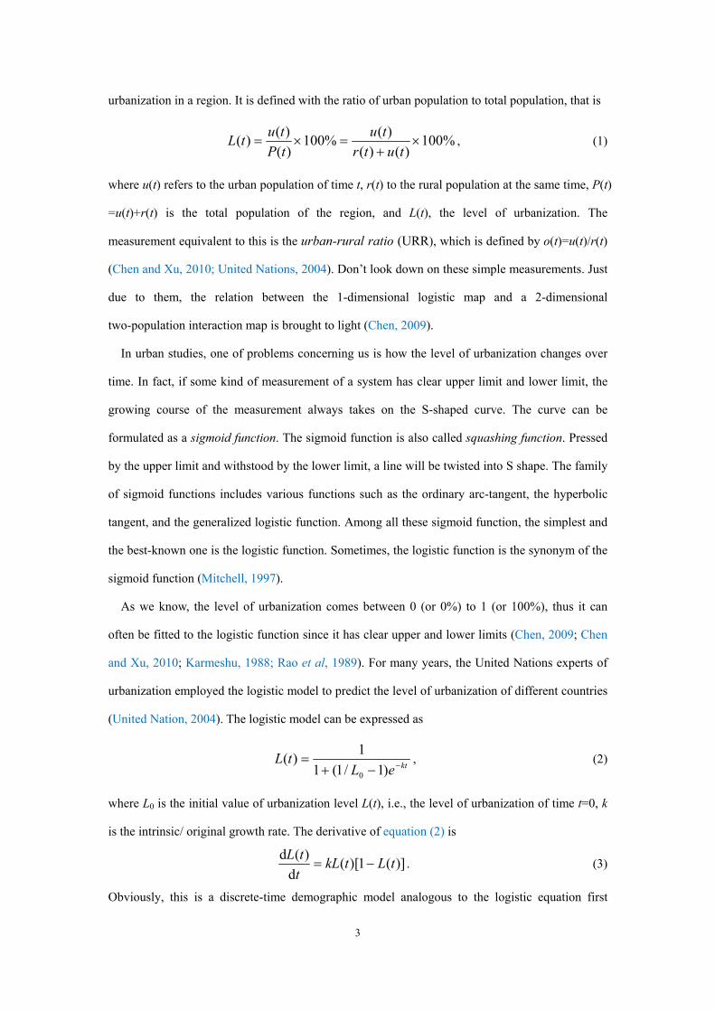
Abstract: Many growing phenomena in both nature and society can be predicted with sigmoid

function. The growth curve of the level of urbanization is a typical S-shaped one, and can be

described by using logistic function. The logistic model implies a replacement process, and the

logistic substitution suggests non-linear dynamical behaviors such as bifurcation and chaos. Using

mathematical transform and numerical computation, we can demonstrate that the 1-dimensional

map comes from a 2-dimensional two-group interaction map. By analogy with urbanization, a

general theory of replacement dynamics is presented in this paper, and the replacement process

can be simulated with the 2-dimansional map. If the rate of replacement is too high, periodic

oscillations and chaos will arise, and the system maybe breaks down. The replacement theory can

be used to interpret various complex interaction and conversion in physical and human systems.

The replacement dynamics provides a new way of looking at Volterra-Lotka’s predator-prey

interaction, man-land relation, and dynastic changes resulting from peasant uprising, and so on.

Key words: bifurcation; chaos; fractal dimension; logistical map; replacement dynamics;

Volterra-Lotka’s model; urbanization

1 Introduction

Logistic function typically reflects a kind of replacement in nature and society, and can be used

as one of the substitution models. In early literature, the law of logistic substitution was mainly

researched in economics, especially in industrial and technological studies. Fisher and Pry (1971)

once successfully used the logistic function to characterize the substitution of old technology by

2

new. Hermann and Montroll (1972) argued that the industrial revolution is a replacement process,

that is, the proportion of agricultural worker declines while that of nonagricultural workers

increases. Montroll (1978) generalized the notion of substitution to a variety of situations by

asserting technological and social evolution to be the consequence of a sequence of substitutions

of one technique by another. Treating technological innovations as structural fluctuations in a

self-organizing industrial system, Batten (1982) and Karmeshu et al (1985) gave a conceptual

rationale for Fisher-Pry’s law of technological replacement. A landmark of the replacement

dynamics is the work of Karmeshu (1988) and his co-workers, who extended the idea of

replacement process for the study of replacement of rural population by urban population and

revealed the pattern of urbanization in India. Recently, Chen (2009) and Chen and Xu (2010)

demonstrated that the replacement dynamics of urbanization may be associated with complex

dynamics such as bifurcation and chaos.

Today, it is time to develop a general theory of replacement dynamics by means of the idea

from fractals and chaos. The replacement is ubiquitous in both nature and society. Where there is a

logistic growth, there is a logistic substitution, and thus replacement behavior will arise. The new

points of this work lie in three aspects. First, a general principle of replacement dynamics is

proposed. Second, the two-group interaction model is employed to interpret the process of

replacement. Third, the periodic oscillations and chaos of replacement dynamics are used to

explain the catastrophic occurrences in natural and social evolution. The rest part of this paper is

organized as follows. In Section 2, the replacement of urbanization dynamics is advanced, and the

1-dimensional logistic map is linked with the 2-dimensional map of two-population interaction

map. In Section 3, the model of replacement dynamics is generalized to different fields such as

ecology, geography, and history. In Section 4, a general theory of replacement dynamics is

propounded, and the related questions are discussed. Finally, the paper is concluded by

summarizing the mains of this work.

2 Model: from 1-D map to 2-D map

2.1 The 1-D logistic map

The level of urbanization is the basic measurement which is used to describe the extent of

3

urbanization in a region. It is defined with the ratio of urban population to total population, that is

%100)()(

)(%100)()()( ×

+=×=

tutrtu

tPtutL , (1)

where u(t) refers to the urban population of time t, r(t) to the rural population at the same time, P(t)

=u(t)+r(t) is the total population of the region, and L(t), the level of urbanization. The

measurement equivalent to this is the urban-rural ratio (URR), which is defined by o(t)=u(t)/r(t)

(Chen and Xu, 2010; United Nations, 2004). Don’t look down on these simple measurements. Just

due to them, the relation between the 1-dimensional logistic map and a 2-dimensional

two-population interaction map is brought to light (Chen, 2009).

In urban studies, one of problems concerning us is how the level of urbanization changes over

time. In fact, if some kind of measurement of a system has clear upper limit and lower limit, the

growing course of the measurement always takes on the S-shaped curve. The curve can be

formulated as a sigmoid function. The sigmoid function is also called squashing function. Pressed

by the upper limit and withstood by the lower limit, a line will be twisted into S shape. The family

of sigmoid functions includes various functions such as the ordinary arc-tangent, the hyperbolic

tangent, and the generalized logistic function. Among all these sigmoid function, the simplest and

the best-known one is the logistic function. Sometimes, the logistic function is the synonym of the

sigmoid function (Mitchell, 1997).

As we know, the level of urbanization comes between 0 (or 0%) to 1 (or 100%), thus it can

often be fitted to the logistic function since it has clear upper and lower limits (Chen, 2009; Chen

and Xu, 2010; Karmeshu, 1988; Rao et al, 1989). For many years, the United Nations experts of

urbanization employed the logistic model to predict the level of urbanization of different countries

(United Nation, 2004). The logistic model can be expressed as

kteLtL −−+=

)1/1(11)(0

, (2)

where L0 is the initial value of urbanization level L(t), i.e., the level of urbanization of time t=0, k

is the intrinsic/ original growth rate. The derivative of equation (2) is

)](1)[(d

)(d tLtkLttL

−= . (3)

Obviously, this is a discrete-time demographic model analogous to the logistic equation first

4

created by mathematician Pierre François Verhulst (Banks, 1994). Suppose that the step length of

data sampling is ∆t=1. Discretizing equation (3) yields a 1-dimensional map in the form

21 )1( ttt kLLkL −+=+ . (4)

where Lt=ut/(ut+rt) is the discrete expression of L(t), and here rt and ut are the discrete expressions

of r(t) and u(t), respectively.

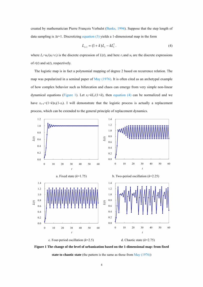
The logistic map is in fact a polynomial mapping of degree 2 based on recurrence relation. The

map was popularized in a seminal paper of May (1976). It is often cited as an archetypal example

of how complex behavior such as bifurcation and chaos can emerge from very simple non-linear

dynamical equations (Figure 1). Let xt=kLt/(1+k), then equation (4) can be normalized and we

have xt+1=(1+k)xt(1-xt). I will demonstrate that the logistic process is actually a replacement

process, which can be extended to the general principle of replacement dynamics.

a. Fixed state (k=1.75) b. Two-period oscillation (k=2.25)

c. Four-period oscillation (k=2.5) d. Chaotic state (k=2.75)

Figure 1 The change of the level of urbanization based on the 1-dimensional map: from fixed

state to chaotic state (the pattern is the same as those from May (1976))

0.0

0.2

0.4

0.6

0.8

1.0

1.2

0 10 20 30 40 50 60

L(t)

t

0.0

0.2

0.4

0.6

0.8

1.0

1.2

1.4

0 10 20 30 40 50 60

L(t)

t

0.0

0.2

0.4

0.6

0.8

1.0

1.2

1.4

0 10 20 30 40 50 60

L(t)

t

0.0

0.2

0.4

0.6

0.8

1.0

1.2

1.4

0 10 20 30 40 50 60

L(t)

t

5

2.2 The 2-D two-population interaction map

Because of equation (1), the 1-dimensional map can be converted into a 2-dimensional map of

urban-rural population interaction. The level of urbanization is defined by urban population and

rural population, thus the percent of urban population must be associated with urban and rural

population growth. By analogy with the Volterra-Lotka model in ecology (Dendrinos and Mullally,

1985), the urban-rural interaction model can be built as follows (Chen, 2009)

⎪⎪⎩

⎪⎪⎨

⎧

++=

+−=

)()()()()(

d)(d

)()()()()(

d)(d

tutrtutrdtcu

ttu

tutrtutrbtar

ttr

. (5)

This means that the growth rate of rural population, dr(t)/dt, is proportional to the size of rural

population, r(t), and the coupling between rural and urban population, but not directly related to

urban population size; the growth rate of urban population, du(t)/dt, is proportional to the size of

urban population, u(t), and the coupling between rural and urban population, but not directly

related to rural population size. It seems to be difficult to understand these, but the census dataset

of the United States (US) of America supports this model (Chen and Xu, 2010). What is more, the

two-population interaction can be generalized to two-group interaction.

If a study region is a close system, the decrease of rural population will be equal to the increase

of urban population resulting from urban-rural interaction, and thus we have b=d. In this instance,

from equations (1) and (5) follows

[ ])(1)()(d

)(d tLtLcabttL

−+−= . (6)

Let k=b-a+c, equation (6) is identical to equation (3). This suggests that the urbanization level

growth is associated with the process of urban and rural interaction. Discretizing equation (5)

yields a 2-dimenaional map such as

⎪⎪⎩

⎪⎪⎨

⎧

+++=

+−+=

+

+

tt

tttt

tt

tttt

ururducu

ururbrar

)1(

)1(

1

1

. (7)

For simplicity, the notation of parameters is not changed in spite of the error coming from the

continuous-discrete conversion. By means of the least squares calculation of the US census data

6

from 1790 to 1960, we have

⎪⎪⎩

⎪⎪⎨

⎧

++=

+−=

+

+

tt

tttt

tt

tttt

urur

uu

urur

rr

5044.0

3615.02584.1

1

1

.

I don’t adopt the data after 1960 as the US city definition varied from 1970.

US is not a close country of population, so it is not strange that b≈0.3615 is not equal to

d≈0.5044. What is strange is that c=0, this suggests that the growth rate of urban population is

only proportional to the coupling between rural and urban population, but not directly related to

rural and urban population sizes. However, if we think it deeply, it seems to be true. Despite cities

of long standing, the history of urbanization compared with the history of human being is not long.

There was no real urbanization before industrialization (Knox, 2005). If the growth rate of urban

population was proportional to its urban population size, urbanization should arise long ago. As a

matter of fact, urbanization began due to industrialization, development of transportation and so

on. Numerical simulation shows that, if c is significantly greater than 0, urban population and total

population in a region will grow ceaselessly. However, this is not the case in the real world.

Therefore, the c value is either zero or very small.

Table 1 The model parameters of urbanization and corresponding dynamical behaviors (a=0.25,

c=0)

Figure 1-D map (k=b-a+c) 2-D map (b=d) System behavior Figure 1(a)，Figure 2(a) 1.75 2.00 Fixed state Figure 1(b)，Figure 2(b) 2.25 2.50 Two-period oscillation Figure 1(c)，Figure 2(c) 2.50 2.75 Four-period oscillation Figure 1(d)，Figure 2(d) 2.75 3.00 Chaotic state

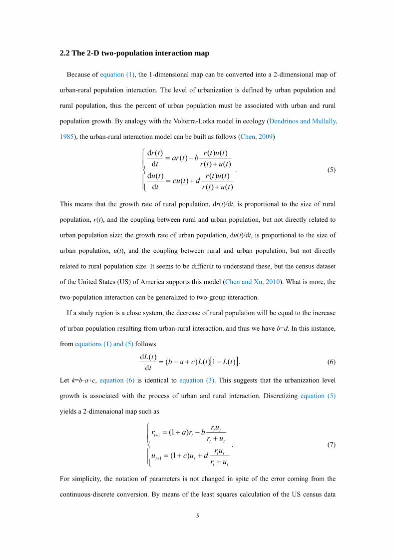
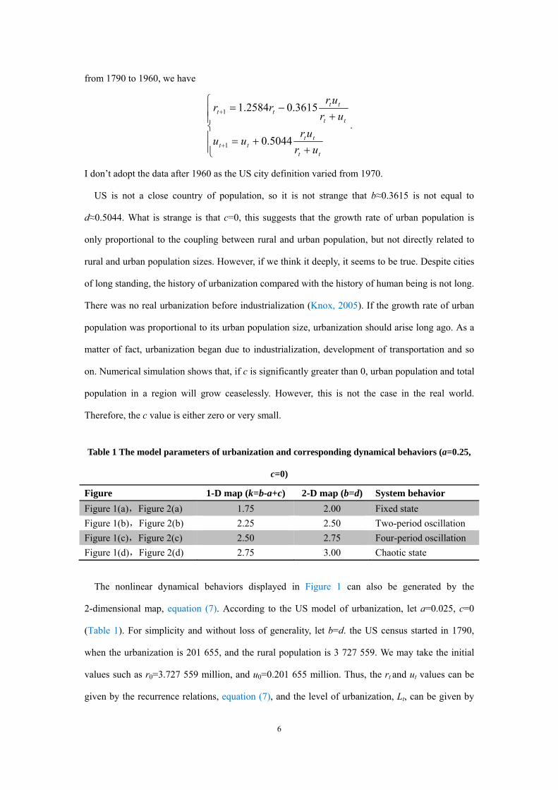
The nonlinear dynamical behaviors displayed in Figure 1 can also be generated by the

2-dimensional map, equation (7). According to the US model of urbanization, let a=0.025, c=0

(Table 1). For simplicity and without loss of generality, let b=d. the US census started in 1790,

when the urbanization is 201 655, and the rural population is 3 727 559. We may take the initial

values such as r0=3.727 559 million, and u0=0.201 655 million. Thus, the rt and ut values can be

given by the recurrence relations, equation (7), and the level of urbanization, Lt, can be given by

7

equation (1), or Lt=ut/(ut+rt). Changing the b and d values, we have various simple and complex

dynamical patterns such as sigmoid growth, periodic oscillations, and chaos (Figure 2). In fact, if

we remove various constraints imposed on the parameter a, b, c, and d, the dynamical behaviors of

the 2-dimenaional map are richer and more colorful than those of the 1-dimensiaonl map.

a. Fixed state (b=d=2) b. Two-period oscillation (b=d=2.5)

c. Four-period oscillation (b=d=2.75) d. Chaotic state (b=d=3)

Figure 2 The change of the level of urbanization based on the 2-dimensional map: from fixed

state to chaotic state (Chen, 2009)

3.3 Replacement dynamics

Urbanization is in fact a process of population replacement—the urban population substitute for

the rural population (Karmeshu, 1988). Generally speaking, the replacement equation is an

exponential function, can the replacement process can be expressed as a logit transform. As

indicated above, URR is defined by

)()()(

trtutO = . (8)

0.0

0.2

0.4

0.6

0.8

1.0

1.2

1.4

0 10 20 30 40 50 60

L(t)

t

0.0

0.2

0.4

0.6

0.8

1.0

1.2

1.4

0 10 20 30 40 50 60L(

t)

t

0.0

0.2

0.4

0.6

0.8

1.0

1.2

1.4

0 10 20 30 40 50 60

L(t)

t

0.0

0.2

0.4

0.6

0.8

1.0

1.2

1.4

0 10 20 30 40 50 60

L(t)

t

8

The level of urbanization can be expressed as

)(/111

)()()()(

tOtrtututL

+=

+= . (9)

In light of equation (2), URR proved to be an exponential function of time, namely

ktkt eOeL

LtL

tLtO 00

0 )1

(1)(

)()( =−

=−

= . (10)

where O0= L0/(L0-1) is the initial value of URR. Thus we have logit transform such as

ktL

LktOtL

tLtO +−

=+=−

=0

00 1

lnln)(1

)(ln)(ln , (11)

which is equivalent to

ktru

trtu

+=0

0ln)()(ln , (12)

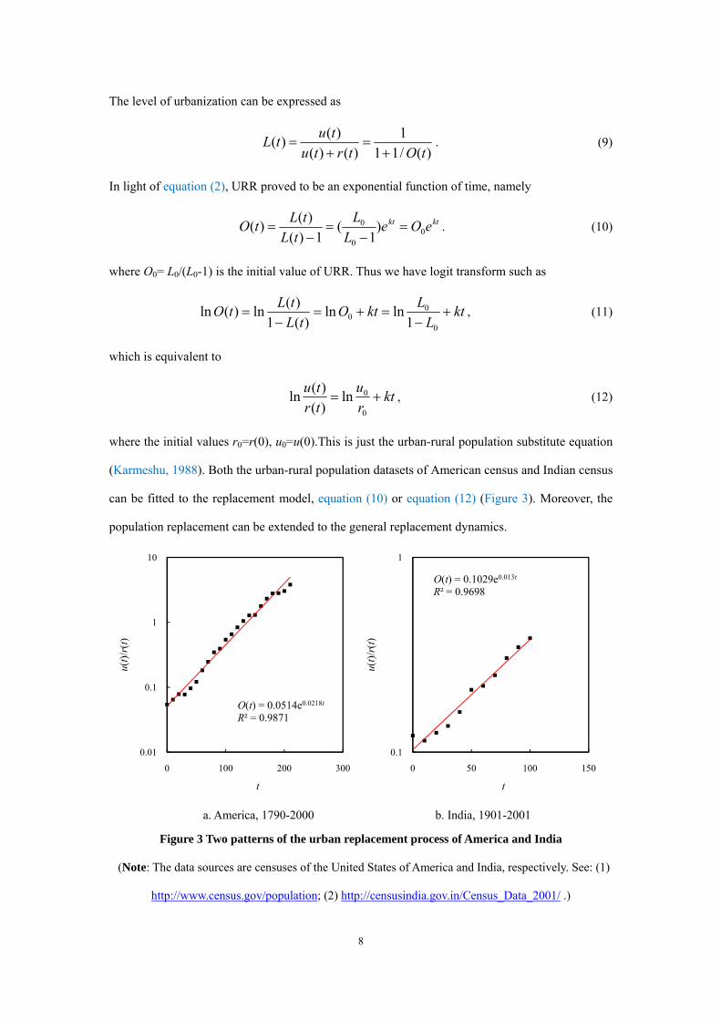
where the initial values r0=r(0), u0=u(0).This is just the urban-rural population substitute equation

(Karmeshu, 1988). Both the urban-rural population datasets of American census and Indian census

can be fitted to the replacement model, equation (10) or equation (12) (Figure 3). Moreover, the

population replacement can be extended to the general replacement dynamics.

a. America, 1790-2000 b. India, 1901-2001

Figure 3 Two patterns of the urban replacement process of America and India

(Note: The data sources are censuses of the United States of America and India, respectively. See: (1)

http://www.census.gov/population; (2) http://censusindia.gov.in/Census_Data_2001/ .)

O(t) = 0.0514e0.0218t

R² = 0.9871

0.01

0.1

1

10

0 100 200 300

u(t)/

r(t)

t

O(t) = 0.1029e0.013t

R² = 0.9698

0.1

1

0 50 100 150

u(t)/

r(t)

t

9

3 Generalization: the replacement dynamics in nature and society

3.1 Example 1: ecological replacement

The urban replacement came from technological replacement, can be generalized to many

different fields. Let’s see several examples. In ecology, the predator-prey interaction model is a

well-known nonlinear dynamical model (Dendrinos and Mullally, 1985). The model can be

revised by using the concept from replacement dynamics. Suppose there a close region such as an

island with two types of animals. One is predator (flesh-eater, carnivore, carnivorous animals), and

the other, the prey (vegetarian, herbivore, herbivorous animals). By analogy with the energy unit

“standard coal”, we can make a comparable unit for animals, namely, standard head. If the

predators and preys are x and y standard heads, respectively, then we can define a measurement,

the ratio of the biomass of predator to that of the entire animals p(t), in the form

%100)()(

)()( ×+

=tytx

txtp . (13)

where x represents the biomass of predator, y, the biomass of prey in the region. Accordingly, the

predator-prey ratio (PPR) can be given by o(t)=x(t)/y(t).

Clearly, there is upper limit and lower limit for p(t). Because of the squashing effect, the ratio of

the biomass of predator to that of the entire animals should follow the law of logistic growth. Thus,

Volterra-Lotka’s predator-prey interaction model can be revised in the form of equation (5), and

May (1976)’s logistic equation can be associated with the revised predator-prey model, which

differ in expression from the classical Volterra-Lotka’s model.

3.2 Example 2: geographical replacement

In geography, the very basic and important topic is the relation between man and land or natural

environment. Because of the man-land interaction, the primary productivity or even secondary

productivity are gradually consumed by human being. So far, man has used up more than 40% of

the primary productivity. In other words, human being has transformed the first nature into the

second nature and the third nature (Swaffield, 2002). Defined a new measurement, the ratio of the

primary productivity to the total productivity in a region p’(t), in the form

10

%100)()(

)()( ×′+′

′=′

tytxtxtp . (14)

where x’ represents the primary productivity, and y’ is the other productivity. Accordingly, the

ratio of the primary productivity to the other productivity (POR) can be defined by o(t)’=

x’(t)/y’(t).

The process of human being marauding nature is also a logistic process, and thus it is also a

nonlinear dynamics of replacement. In a sense, the man-land relation is unstable, and periodic

oscillations and chaos may arise since humankind depletes nature so rapidly.

3.3 Example 3: historical replacement

In the theory of class struggle, Marxist analysis of society identifies two main social groups:

labor (the proletariat or workers) and capital (the bourgeoisie or capitalists). The former includes

anyone who earns their livelihood by selling their labor power and being paid a wag/salary for

their labor time, and the latter include anyone who obtains their income not from labor as much as

from the surplus value that they appropriate from the workers who create wealth. Whether or not

you believe in Marxism, you will agree that the social system falls into two groups—the haves

(wealthy, men of wealth, the rich) and the have-nots (needy, poor people, the poor). Let x’’

represent the number of have-nots, and y’’ represent the number of the haves. Then we can define

a ratio of the have-nots to the total population such as

%100)()(

)()( ×′′+′′

′′=′′

tytxtxtp . (15)

Thus the poor-rich ratio (PRR) can be expressed as o’’(t)=x’’(t)/y’’(t). This process of replacement

is just so-called pauperization of a country.

In ancient China, for example, dynastic changes were always processes of land annexation and

concentration of landholding right. The rich annexed the land of the poor, first little by little, and

then more and more, so that about 20 percent of people held 80 percent of land or so, and about 80

percent people had little land. Land annexation can be regarded as a logistic process. It often led to

social pauperization, and then the nation lost its balance. Peasant uprising burst out, social

turbulence began. Hundreds responded to a single call, and as one (uprising) fell, another rose.

This seems to be the course from oscillations to chaos. The final result is that new dynasty

11

replaced old dynasty, or new regime replaced old regime.

4 Questions and discussion

The logistic substitute model can be employed to describe the process of replacement of one

activity by another (Karmeshu, 1988). The studies used to be confined in the fields of industrial

development and urbanization. However, you can find the replacement processes here and there in

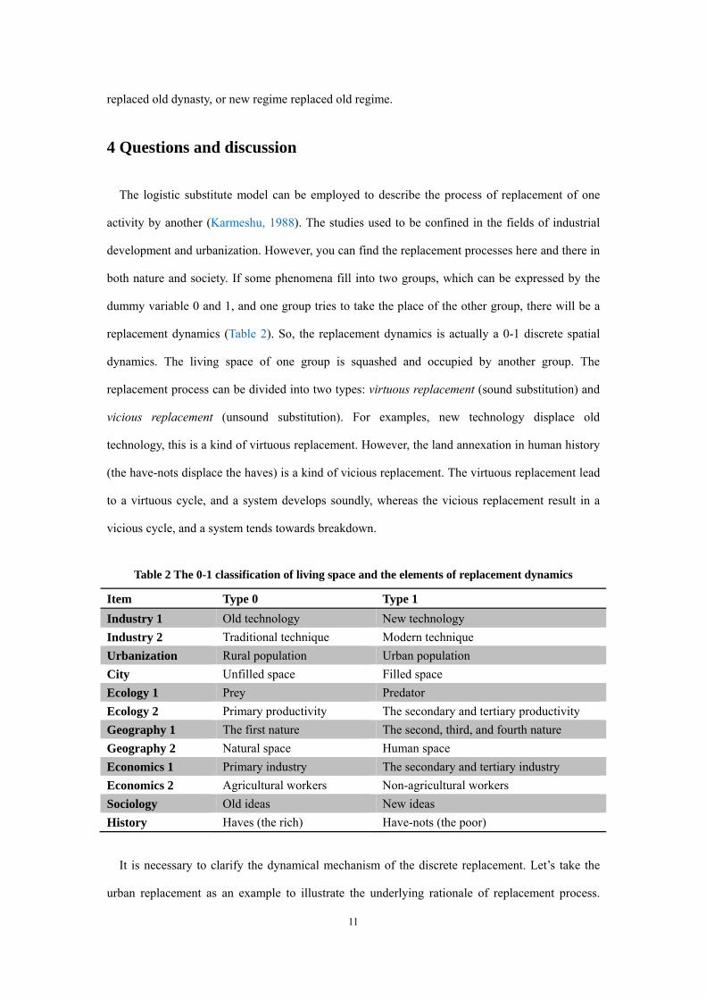
both nature and society. If some phenomena fill into two groups, which can be expressed by the

dummy variable 0 and 1, and one group tries to take the place of the other group, there will be a

replacement dynamics (Table 2). So, the replacement dynamics is actually a 0-1 discrete spatial

dynamics. The living space of one group is squashed and occupied by another group. The

replacement process can be divided into two types: virtuous replacement (sound substitution) and

vicious replacement (unsound substitution). For examples, new technology displace old

technology, this is a kind of virtuous replacement. However, the land annexation in human history

(the have-nots displace the haves) is a kind of vicious replacement. The virtuous replacement lead

to a virtuous cycle, and a system develops soundly, whereas the vicious replacement result in a

vicious cycle, and a system tends towards breakdown.

Table 2 The 0-1 classification of living space and the elements of replacement dynamics

Item Type 0 Type 1 Industry 1 Old technology New technology Industry 2 Traditional technique Modern technique Urbanization Rural population Urban population City Unfilled space Filled space Ecology 1 Prey Predator Ecology 2 Primary productivity The secondary and tertiary productivity Geography 1 The first nature The second, third, and fourth nature Geography 2 Natural space Human space Economics 1 Primary industry The secondary and tertiary industry Economics 2 Agricultural workers Non-agricultural workers Sociology Old ideas New ideas History Haves (the rich) Have-nots (the poor)

It is necessary to clarify the dynamical mechanism of the discrete replacement. Let’s take the

urban replacement as an example to illustrate the underlying rationale of replacement process.

12

Two models based on two postulates can be employed to explain the replacement dynamics of

urbanization. One the nonlinear dynamics model based on the postulate of two-population

coupling, as indicated by equation (5), the other is a linear dynamics model based on the postulate

of allometric growth such as (Bertalanffy, 1968; Chen and Jiang, 2009)

⎪⎪⎩

⎪⎪⎨

⎧

=

=

)(d

)(d

)(d

)(d

tuttu

trttr

β

α, (16)

where α and β are growth coefficients (α>0, β>0). The solutions to linear differential equations are

⎪⎩

⎪⎨⎧

=

=t

t

eutu

ertrβ

α

0

0

)(

)(. (17)

From equation (17) follows

ktktt eOerue

ru

trtutO 0

0

0)(

0

0

)()()( ==== −αβ , (18)

which is equivalent to equation (12). This suggests that the replacement model of urbanization can

be derived from the linear dynamics equations. Apparently we have

αβ −=k . (19)

Because k represents the difference between the relative growth ratio of rural population, α, and

that of urban population, β, the United Nations (2004) experts called it the urban-rural growth

difference (URGD). On the other hand, from equation (17) follows an allometric scaling relation

between urban and rural population in the form

btrtrrutu )()()()( /

/0

0 ηαβαβ == , (20)

where η=u0/r0β/α is proportionality coefficient, and

r

u

DDb ==

αβ

, (21)

is the allometric scaling exponent. Equation (20) was verified by Naroll and Bertalanffy (1956). In

equation (21), Du refers to the fractal dimension of urban population, and Dr, the fractal dimension

of rural population. This suggests that, if the replacement dynamics is based on the linear

differential equations, it is actually based on the allometric scaling law associated with fractal

13

geometry. The law of allometric growth is very significant in urban studies (see e.g. Batty and

Longley, 1994; Bettencourt et al, 2007; Chen, 2010; West et al, 2002). However, in the urban

replacement process, it seems to be the non-linear interaction rather than the allometric scaling

that dominates the dynamical evolution.

Discretizing equation (16) yields a 2-dimensional map such as

⎩⎨⎧

+=+=

+

+

tt

tt

uurr)1()1(

1

1

βα

. (22)

However, if we employ equation (22) to simulate the rural population, urban population, total

population, and the level of urbanization, the results do not tally with the actual situation—all the

population and the urbanization level go up unboundedly. In contrast, if we use the 2-dimensional

map defined by equation (7) to simulate the level of urbanization, the rural population, urban

population, and total population, the results conform to reality—the capacity values are limited

(Figure 4, Figure 5). This seems to imply that it is the nonlinear dynamics rather than the linear

dynamics that can be employed to interpret the replacement process. Despite this, the logistic

equation can be used as a bridge of understanding between the simple allometric scaling law and

the complex nonlinear interaction model (Table 3).

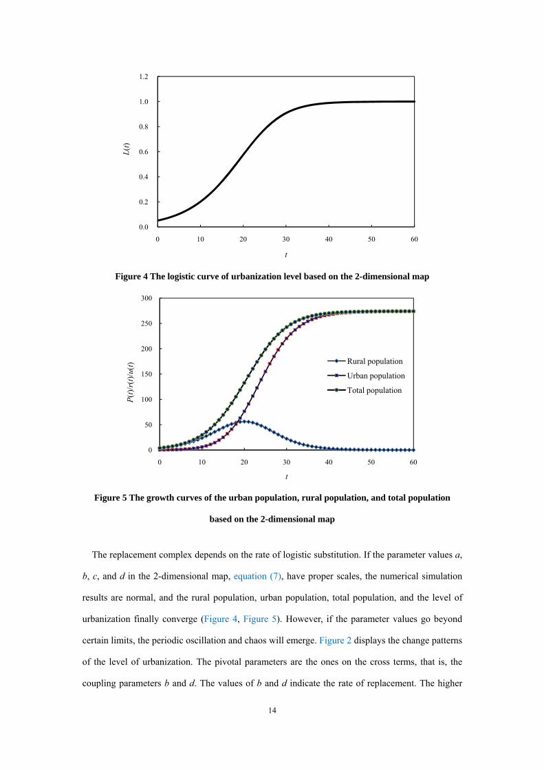
Table 3 Mathematical transform relation between the simple allometric scaling laws and

complex non-linear dynamics

Models Complex models Transformation Simple models

Equations

⎪⎪⎩

⎪⎪⎨

⎧

++=

+−=

)()()()()(

d)(d

)()()()()(

d)(d

tutrtutrdtcu

ttu

tutrtutrbtar

ttr

[ ])(1)(d

)(d tLtkLttL

−=

⎪⎪⎩

⎪⎪⎨

⎧

=

=

)(d

)(d

)(d

)(d

tuttu

trttr

β

α

Mathematical Solution

No kteLtL

−−+=

)1/1(11)(0 ⎪⎩

⎪⎨⎧

=

=t

t

eutu

ertrβ

α

0

0

)(

)(

Numerical Solution

Bifurcation and chaos No Simple curve

Theory Bifurcation and chaos Scaling laws Fractals

14

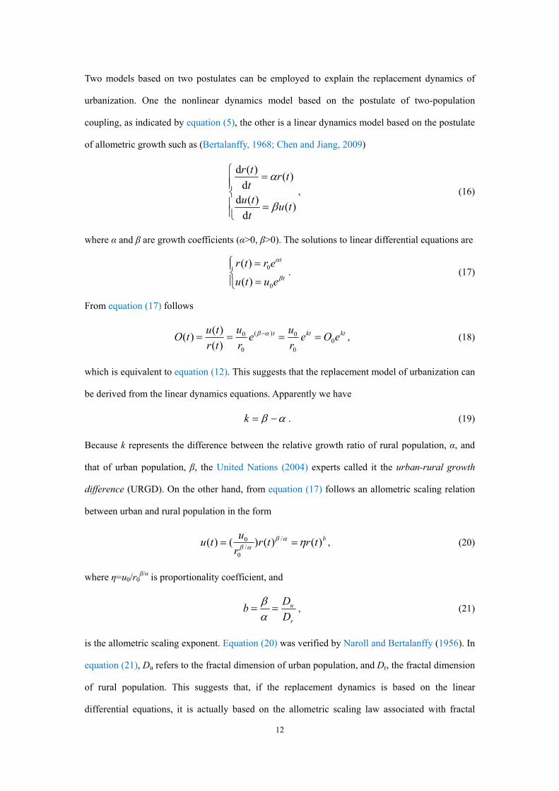
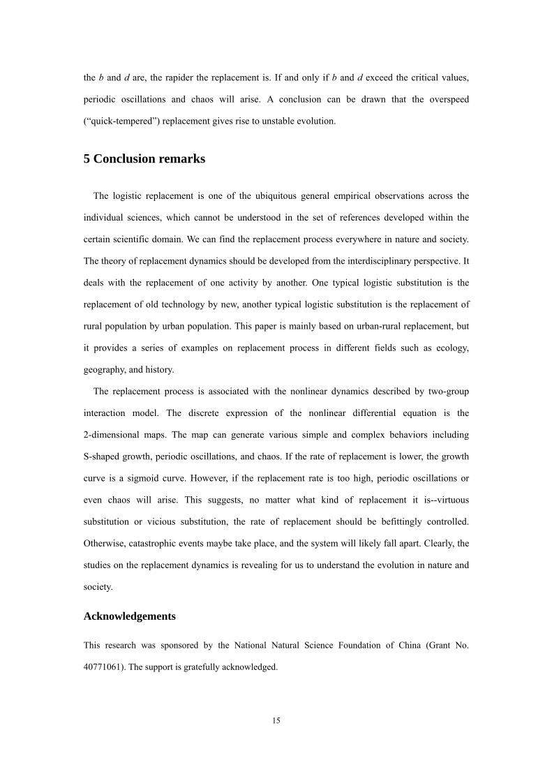
Figure 4 The logistic curve of urbanization level based on the 2-dimensional map

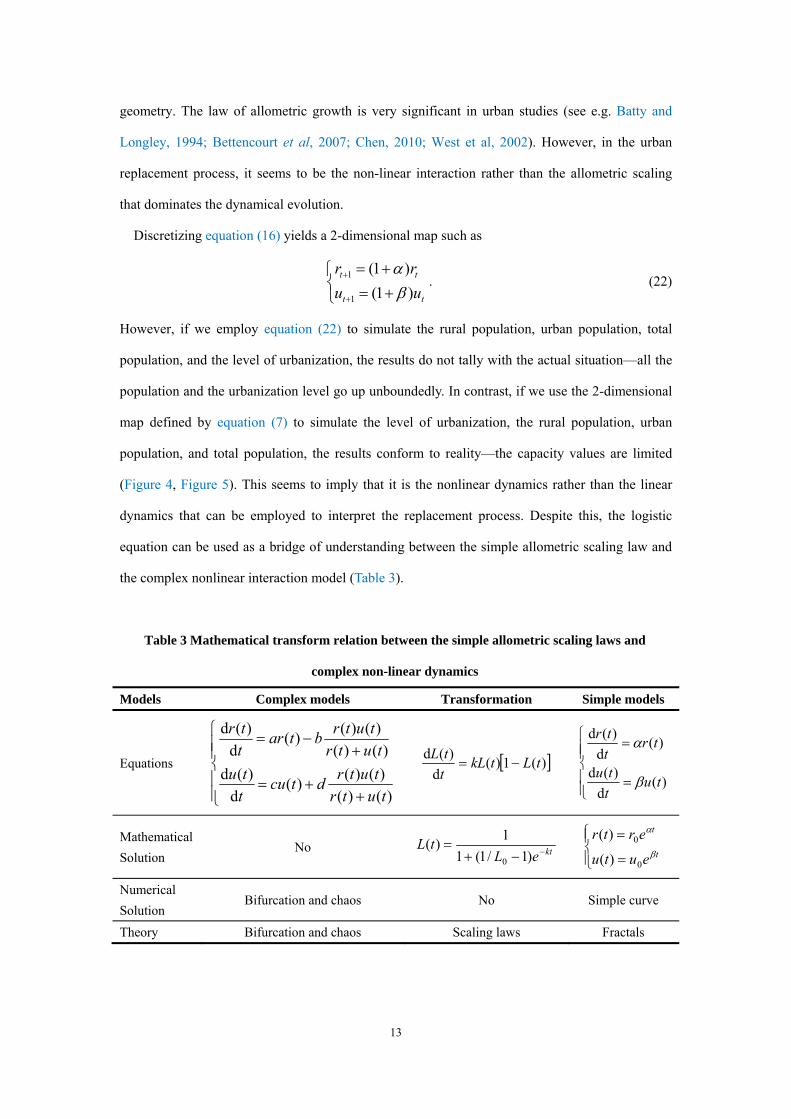
Figure 5 The growth curves of the urban population, rural population, and total population

based on the 2-dimensional map

The replacement complex depends on the rate of logistic substitution. If the parameter values a,

b, c, and d in the 2-dimensional map, equation (7), have proper scales, the numerical simulation

results are normal, and the rural population, urban population, total population, and the level of

urbanization finally converge (Figure 4, Figure 5). However, if the parameter values go beyond

certain limits, the periodic oscillation and chaos will emerge. Figure 2 displays the change patterns

of the level of urbanization. The pivotal parameters are the ones on the cross terms, that is, the

coupling parameters b and d. The values of b and d indicate the rate of replacement. The higher

0.0

0.2

0.4

0.6

0.8

1.0

1.2

0 10 20 30 40 50 60

L(t)

t

0

50

100

150

200

250

300

0 10 20 30 40 50 60

P(t)/

r(t)/

u(t)

t

Rural population

Urban population

Total population

15

the b and d are, the rapider the replacement is. If and only if b and d exceed the critical values,

periodic oscillations and chaos will arise. A conclusion can be drawn that the overspeed

(“quick-tempered”) replacement gives rise to unstable evolution.

5 Conclusion remarks

The logistic replacement is one of the ubiquitous general empirical observations across the

individual sciences, which cannot be understood in the set of references developed within the

certain scientific domain. We can find the replacement process everywhere in nature and society.

The theory of replacement dynamics should be developed from the interdisciplinary perspective. It

deals with the replacement of one activity by another. One typical logistic substitution is the

replacement of old technology by new, another typical logistic substitution is the replacement of

rural population by urban population. This paper is mainly based on urban-rural replacement, but

it provides a series of examples on replacement process in different fields such as ecology,

geography, and history.

The replacement process is associated with the nonlinear dynamics described by two-group

interaction model. The discrete expression of the nonlinear differential equation is the

2-dimensional maps. The map can generate various simple and complex behaviors including

S-shaped growth, periodic oscillations, and chaos. If the rate of replacement is lower, the growth

curve is a sigmoid curve. However, if the replacement rate is too high, periodic oscillations or

even chaos will arise. This suggests, no matter what kind of replacement it is--virtuous

substitution or vicious substitution, the rate of replacement should be befittingly controlled.

Otherwise, catastrophic events maybe take place, and the system will likely fall apart. Clearly, the

studies on the replacement dynamics is revealing for us to understand the evolution in nature and

society.

Acknowledgements

This research was sponsored by the National Natural Science Foundation of China (Grant No.

40771061). The support is gratefully acknowledged.

16

References

1. Banks R B (1994). Growth and Diffusion Phenomena: Mathematical Frameworks and

Applications. Berlin: Springer-Verlag

2. Batten D (1982). On the dynamics of industrial evolution. Regional Science and Urban

Economics, 12: 449-462

3. Batty M, Longley PA (1994). Fractal Cities: A Geometry of Form and Function. London:

Academic Press

4. Bertalanffy L von (1968). General System Theory: Foundations, Development, and

Applications. New York: George Breziller

5. Bettencourt LMA , Lobo J , Helbing D, Kühnert C , West GB (2007). Growth, innovation,

scaling, and the pace of life in cities. PNAS, 104(17): 7301-7306

6. Chen YG (2009). Spatial interaction creates period-doubling bifurcation and chaos of

urbanization. Chaos, Soliton & Fractals, 42(3): 1316-1325

7. Chen YG (2010). Characterizing growth and form of fractal cities with allometric scaling

exponents. Discrete Dynamics in Nature and Society, Volume 2010, Article ID 194715, 22

pages

8. Chen YG, Jiang SG (2009). An analytical process of the spatio-temporal evolution of urban

systems based on allometric and fractal ideas. Chaos, Soliton & Fractals, 39(1): 49-64

9. Chen YG, Xu F (2010). Modeling complex spatial dynamics of two-population interaction in

urbanization process. Journal of Geography and Geology, 2(1): 1-17

10. Dendrinos DS, Mullally H (1985). Urban Evolution: Studies in the Mathematical Ecology of

Cities. New York: Oxford University Press

11. Fisher JC, Pry RH (1971). A simple substitution model for technological change.

Technological Forecasting and Social Change, 3: 75-88

12. Hermann R, Montroll EW (1972). A manner of characterizing the development of countries.

PNAS, 69(10): 3019-3024

13. Karmeshu, Bhargava SC, Jain VP (1985). A rationale for law of technological substitution.

Regional Science and Urban Economics, 15(1): 137-141

14. Karmeshu. Demographic models of urbanization. Environment and Planning B: Planning

17

and Design, 1988, 15(1): 47-54

15. Knox PL (2005). Urbanization: An Introduction to Urban Geography (2nd edition). Upper

Saddle River, NJ: Prentice Hall

16. May RM (1976). Simple mathematical models with very complicated dynamics. Nature, 261:

459-467

17. Mitchell TM (1997). Machine Learning. Boston, MA: McGraw-Hill

18. Montroll EW (1978). Social dynamics and the quantifying of social forces. PNAS, 75(10):

4633-4637

19. Naroll RS, von Bertalanffy L (1956). The principle of allometry in biology and social

sciences. General Systems Yearbook, 1(part II): 76-89

20. Rao DN, Karmeshu, Jain VP. Dynamics of urbanization: the empirical validation of the

replacement hypothesis. Environment and Planning B: Planning and Design, 1989, 16(3):

289-295

21. Swaffield S (2002). Theory in Landscape Architecture: A Reader. Philadelphia: University of

Pennsylvania Press

22. United Nations (2004). World Urbanization Prospects: The 2003 Revision. New York: U.N.

Department of Economic and Social Affairs, Population Division

23. West GB, Woodruff WH, Brown JH (2002). Allometric scaling of metabolic rate from

molecules and mitochondria to cells and mammals. PNAS, 99((suppl. 1)): 2473-2478