urans and sas analysis of flow dynamics in a gdi nozzle

ILASS – Europe 2010, 23rd Annual Conference on Liquid Atomization and Spray Systems, Brno, Czech Republic, September 2010

1

URANS and SAS analysis of flow dynamics in a GDI nozzle

J.-M. Shi*, K. Wenzlawski*, J. Helie

†, H. Nuglisch

†, J. Cousin°

* Continental Automotive GmbH

Siemensstr. 12, 93055 Regensburg, Germany † Continental Automotive SAS

1 av. Paul Ourliac BP 1149, 31036 Toulouse Cedex 1, France

° Coria

INSA de Rouen, Campus du Madrillet - BP 8, 76801 Saint Etienne du Rouvray cedex, France

Abstract

URANS and SAS analysis of turbulent flow in a GDI nozzle was carried out. The vortex structures, velocity and

pressure distributions predicted based on the two different approaches were compared both for instant and statis-

tical values. FFT analysis was applied to the time series of mass flow rate, the velocity, pressure and turbulence

quantities at monitoring points. Only one dominant frequency was predicted by the URANS approach using the

SST turbulence model. A clear correlation was found among the frequency of the mass flow rate, pressure and

velocity at monitor points. In contrast, SAS predicted multiple frequencies. Though no simple correlation was

obtained, the frequency of big event in mass flow time series was found to be linked to the first dominant fre-

quency of the pressure monitors.

Introduction

The quality of spray and mixture formation in engine can be very different from fuel injection nozzle A to

nozzle B even under the same operating conditions. This indicates a strong effect of the in-nozzle flow on spray

formation. This work is an effort in pursuing understanding about the link between nozzle internal flow and

spray formation. For this purpose, high resolution zoomed spray visualization study in the proximity of the noz-

zle exit for a three-hole GDI injector were carried out at CORIA in cooperation with Continental Automotive.

The liquid ligaments in the process of primary breakup are clearly recognizable under an injection pressure up to

20bar. The obtained shot-to-shot spray images indicate that there exist multiple frequencies in the primary

breakup process. The simulation work reported here was to find the link between the in-nozzle flow and the pri-

mary breakup frequencies in order to obtain new understanding of atomization mechanism.

The flow in a fuel injection nozzle is characterized by high shear strain rate, high flow acceleration and de-

celeration, and high pressure gradient linked with throttle geometries. Therefore, vortex generation and their

dynamics in the nozzle is the key point to understand the flow dynamics. The simulation work was based on the

commercial CFD solver ANSYS-CFX12.0. The URANS approach based on the k-omega SST model [1] and the

Scale-Adaptive-Simulation (SAS) approach [2] were applied. The latter is also a RANS modelling approach but

with a DES-like capability, allowing to resolve the turbulence vortex structures in the region where the mesh size

is below the local physical turbulence scale. In this paper, we present a case study for the injection pressure

10 bar. The experience we made in house and also in literature [4] is that simulation of turbulent cavitating flow

in fuel injection nozzle is very sensitive to cavitation modelling. Here we restricted our study to deal with the

single-phase flow without considering cavitation. Best practice study for the mesh size and time step dependence

were carried out. Instant results and time average and RMS values of field variables and monitor quantities were

compared for 3 different computational grids. FFT analysis was applied to the time series of mass flow rate, the

velocity, pressure and turbulence quantities at monitoring points. Correlation or link between the mass flow rate,

pressure monitors, and the vortex motion was examined. The spray visualization study is still on going in order

to obtain a reliable statistics for the primary breakup frequencies. Here we mainly report the results from the

numerical study.

Simulation model and Numerical methods

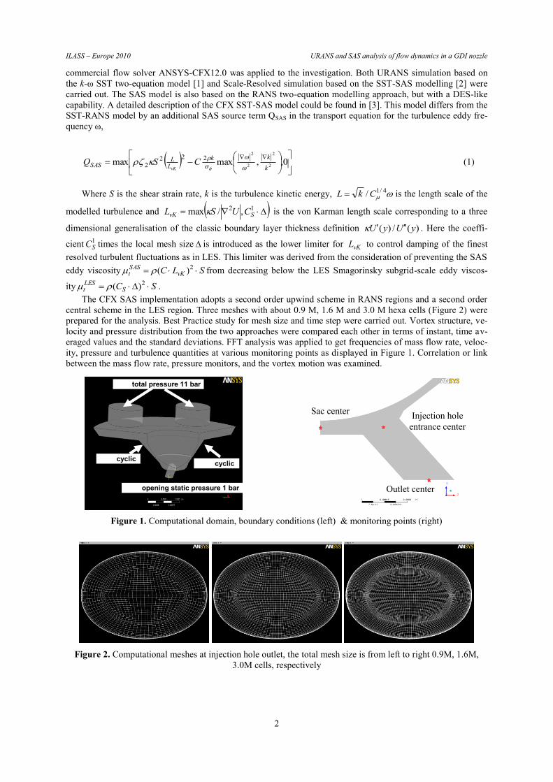
The nozzle is axis-symmetrical with three injection holes. A 120°-sector geometrical model was adopted in

simulation and a cyclic period condition was applied at the sector boundaries (see Figure 1, left). Three monitor-

ing points were defined (see Figure 1, right) in order to get time series of the local velocity, pressure, and turbu-

lence variables. The fluid applied was n-heptane, with a density 680 kg/m3 and a viscosity 3.885e-4 Pa∙s. Ne-

glecting the cavitation model, a single phase turbulent flow problem of incompressible fluid was considered. The

Corresponding author: [email protected]

ILASS – Europe 2010 URANS and SAS analysis of flow dynamics in a GDI nozzle

2

commercial flow solver ANSYS-CFX12.0 was applied to the investigation. Both URANS simulation based on

the k-ω SST two-equation model [1] and Scale-Resolved simulation based on the SST-SAS modelling [2] were

carried out. The SAS model is also based on the RANS two-equation modelling approach, but with a DES-like

capability. A detailed description of the CFX SST-SAS model could be found in [3]. This model differs from the

SST-RANS model by an additional SAS source term QSAS in the transport equation for the turbulence eddy fre-

quency ω,

0,,maxmax

2

2

2

2222

2 k

kk

LL

SAS CSQvK

(1)

Where S is the shear strain rate, k is the turbulence kinetic energy, 4/1/CkL is the length scale of the

modelled turbulence and 12 ,/max SvK CUSL is the von Karman length scale corresponding to a three

dimensional generalisation of the classic boundary layer thickness definition )(/)( yUyU . Here the coeffi-

cient 1SC times the local mesh size is introduced as the lower limiter for vKL to control damping of the finest

resolved turbulent fluctuations as in LES. This limiter was derived from the consideration of preventing the SAS

eddy viscosity SLC vKSASt 2)( from decreasing below the LES Smagorinsky subgrid-scale eddy viscos-

ity SCSLESt 2)( .

The CFX SAS implementation adopts a second order upwind scheme in RANS regions and a second order

central scheme in the LES region. Three meshes with about 0.9 M, 1.6 M and 3.0 M hexa cells (Figure 2) were

prepared for the analysis. Best Practice study for mesh size and time step were carried out. Vortex structure, ve-

locity and pressure distribution from the two approaches were compared each other in terms of instant, time av-

eraged values and the standard deviations. FFT analysis was applied to get frequencies of mass flow rate, veloc-

ity, pressure and turbulence quantities at various monitoring points as displayed in Figure 1. Correlation or link

between the mass flow rate, pressure monitors, and the vortex motion was examined.

Figure 1. Computational domain, boundary conditions (left) & monitoring points (right)

Figure 2. Computational meshes at injection hole outlet, the total mesh size is from left to right 0.9M, 1.6M,

3.0M cells, respectively

total pressure 11 bar at inlet

opening static pressure 1 bar at outlet

cyclic period cyclic

period

Sac center Injection hole

entrance center

Outlet center


3

Results and Discussion

Vortex visualization

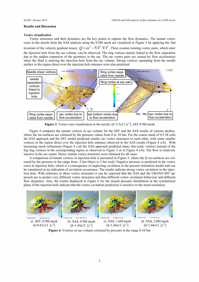
Vortex structures and their dynamics are the key points to capture the flow dynamics. The instant vortex

cores in the nozzle from the SAS analysis using the 0.9M mesh are visualized in Figure 3 by applying the 2nd

invariant of the velocity gradient tensor, VVQ

2 . Three counter-rotating vortex pairs, which enter

the injection hole from the sac-volume, can be observed. The ring vortices mainly linked to the flow separation

due to the sudden expansion of the geometry in the sac. The sac vortex pairs are caused by flow acceleration

when the fluid is entering the injection hole from the sac volume. Strong vortices separating from the needle

surface in the region direct over the injection hole entrance were also predicted.

Figure 3. Vortex core visualization in the nozzle, Q=2.5e11 [s-2

], SST 0.9M mesh.

Figure 4 compares the instant vortices in sac volume for the SST and the SAS results of various meshes,

where the iso-surfaces are coloured by the pressure values from 0 to 10 bar. For the coarse mesh of 0.9 M cells

the SAS approach and the SST model predicted similar sac vortex structures to each other, with some smaller

vortices in the region direct over the injection hole entrance observed in the SAS results (Figure 4 a-b). With

increasing mesh refinement (Figure 4 c-d) the SAS approach predicted many fine-scale vortices instead of the

big ring vortices in the corresponding region as observed in Figure 3 or in Figure 4 a-b). The flow is relatively

inactive in the sac centre. Hence similar vortex structures were obtained for all cases.

A comparison of instant vortices in injection hole is presented in Figure 5, where the Q iso-surfaces are col-

oured by the pressure in the range from -2 bar (blue) to 2 bar (red). Negative pressure is predicted in the vortex

cores in injection hole, which is a consequence of neglecting cavitation in the present simulation model and can

be considered as an indication of cavitation occurrence. The results indicate strong vortex cavitation in the injec-

tion hole. With reference to these vortex structures it can be expected that the SAS and the URANS-SST ap-

proach are to predict very different vortex structures and thus different vortex cavitation behaviour and different

flow dynamics. Also, the results displayed in Figure 6 for the instant pressure distribution at the symmetrical

plane of the injection hole indicate that the vortex cavitation prediction is sensitive to the mesh resolution.

Figure 4. Vortices in sac-volume coloured by pressure in the range 0-10 bar

a) SST, 0.9M mesh

Q=0.81e12 [s-2

] b) SAS, 0.9M mesh

Q=1.44e12 [s-2

]

d) SAS, 3.0M mesh

Q=1.44e12 [s-2

]

c) SAS, 1.6M mesh

Q=1.44e12 [s-2

]

Needle shear vortices

Ring vortex sepa-rated from needle

sac vortex due to flow acceleration

needle separation

vortices linked to injection

hole

Ring vortex at sac wall

sac bottom vortex due to flow acceleration

sac vortex due to flow acceleration

Ring vortex sepa-rated from needle


4

Figure 5. Vortices in injection hole coloured by pressure in the range -2 bar to 2 bar

Figure 6. Instant pressure at symmetrical plane coloured by pressure values in the range -2 bar to 2 bar

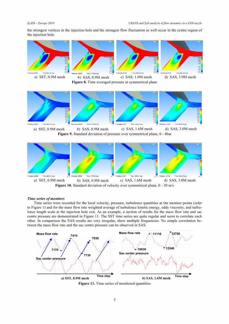
The corresponding time averaged vortex structures are displayed in Figure 8, coloured according to the pres-

sure fluctuation. The time averaged vortex structures in the sac volume are alike to each other and the ring vor-

tices as observed in Figure 3 are again recognizable in the statistics sense of the SAS results (Figure 7, top). In

contrast, the time statistical vortex structures in injection hole are less similar between the SAS and SST results.

The time mean vortex cores in SST simulation are similar to the instant vortices in Figure 5, with long and

smooth Q iso-surfaces. Due to multiple scale vortices with higher fluctuations were resolved in SAS, the time

average of the vortex cores are much shorter and more irregular than in SST (Figure 7, bottom). This difference

is also reflected in the time averaged pressure distribution over the symmetrical plane of the injection hole pre-

sented in Figure 8. However, these averaged pressure distributions show very similar pattern in all cases, and are

similar to the instant SST results presented in Figure 6. That suggests, URANS simulation is sufficient to capture

the mean flow features in the statistical sense.

Figure 7. Time averaged vortex structures in sac-volume (top, coloured by standard pressure deviation 0-1.5

bar) and in injection hole (bottom, coloured by standard pressure deviation 0-4 bar), Q=0.81e12 [s-2

]

In comparison, the colour of the iso-surfaces in Figure 7 indicate that the SAS approach predicted much

higher fluctuations than the SST model both in the sac volume and in injection hole. The standard deviation of

pressure and velocity over the symmetrical plane, displayed in Figure 9 and Figure 10, also confirm this conclu-

sion. With a reference to Figure 5, Figure 7, Figure 8, Figure 9 and Figure 10 together, it can be concluded that

a) SST, 0.9M mesh

Q=0.81e12 [s-2

] b) SAS, 0.9M mesh

Q=2.5e12 [s-2

]

d) SAS, 3.0M mesh

Q=2.5e12 [s-2

]

c) SAS, 1.6M mesh

Q=2.5e12 [s-2

]

a) SST, 0.9M mesh b) SAS, 0.9M mesh d) SAS, 3.0M mesh c) SAS, 1.6M mesh



5

the strongest vortices in the injection hole and the strongest flow fluctuation as well occur in the centre region of

the injection hole.

Figure 8. Time averaged pressure at symmetrical plane

Figure 9. Standard deviation of pressure over symmetrical plane, 0 - 4bar

Figure 10. Standard deviation of velocity over symmetrical plane, 0 - 30 m/s

Time series of monitors

Time series were recorded for the local velocity, pressure, turbulence quantities at the monitor points (refer

to Figure 1) and for the mass flow rate weighted average of turbulence kinetic energy, eddy viscosity, and turbu-

lence length scale at the injection hole exit. As an example, a section of results for the mass flow rate and sac

centre pressure are demonstrated in Figure 11. The SST time series are quite regular and seem to correlate each

other. In comparison the SAS results are very irregular, show multiple frequencies. No simple correlation be-

tween the mass flow rate and the sac centre pressure can be observed in SAS.

Figure 11. Time series of monitored quantities




Mass flow rate

7170

7415

7730

7930

Sac center pressure

Time step a) SST, 0.9M mesh

10030

11110

12240

Time step b) SAS, 1.6M mesh

12750 Mass flow rate

Sac center pressure


6

The arithmetic mean value of the monitoring quantities and the corresponding relative fluctuations based on

the standard deviations are summarized in Table 1. The mean values from SAS show a convergence trend with

increasing mesh refinement. Especially, the average values of the modelled turbulence quantities at the nozzle

outlet in SAS 1.6M mesh and in SAS 3.0M mesh are almost identical. This indicates a sufficient grid resolution.

The standard deviation values also show the similar trend except for the value of pressure monitor at the injec-

tion hole entrance centre. Considering that turbulence eddies larger than the mesh size is direct resolved in SAS,

the predicted (modelled) turbulence kinetic energy in SAS is much lower than the corresponding SST results.

The eddy viscosity in the SST simulation is two orders higher than the molecular viscosity. The modelled eddy

viscosity in SAS is about one order lower than the value from SST. The average length scale of the modelled

turbulence is about 10 μm in SAS, which is about one fourth of the corresponding SST result. In addition, the

standard deviations are much higher in the SAS results, indicating higher fluctuations predicted by the SAS ap-

proach. That is consistent with those results shown in Figure 7, Figure 9 and Figure 10.

Table 1. Mean and standard deviation values of the monitors

Parameter

Time mean value

Standard deviation / Time mean

* 100%

SST

0.9M

SAS

0.9M

SAS

1.6M

SAS

3.0M

SST

0.9M

SAS

0.9M

SAS

1.6M

SAS

3.0M

Mass flow rate [g/s] 1.218 1.222 1.200 1.198 0.7 1.17 0.95

1.24

Average modelled turbulence

length scale @outlet [mm] 4.2e-2 1.2e-2 9.76e-3 9.74e-3 2.3 5.7 4.7 5.16

Average modelled turbulence

kinetic energy @outlet [J/kg] 60.8 22.5 20.6 20.3 6.6 12.9 10.7 11.3

Average modelled eddy viscosity

@outlet [Pa s] 3.4e-2 4.2e-3 3.3e-3 3.3e-3 11.6 28.8 29.2 35.5

Pressure @ Sac-center [bar] 11.01 10.99 10.91 10.85 1.3 1.6 1.8 1.9

Pressure @ injection hole

entrance center [bar] 2.58 2.34 2.39 2.37 13.8 49.7 57.5 48.1

Velocity w @outlet center [m/s] 22.2 19.6 20.5 21.0 12.9 41.1 37.2 39.0

Velocity u @outlet center [m/s] 20.1 27.0 27.7 28.1 34.7 41.1 36.1 38.1

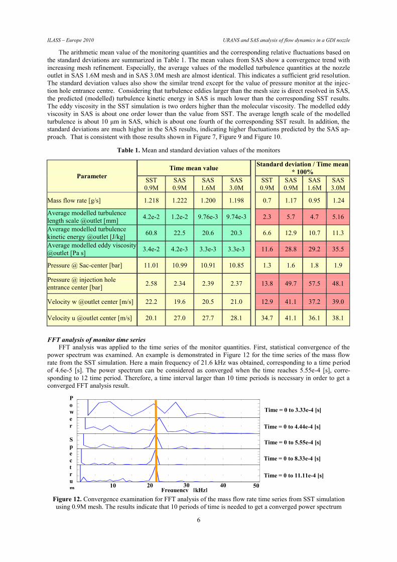
FFT analysis of monitor time series

FFT analysis was applied to the time series of the monitor quantities. First, statistical convergence of the

power spectrum was examined. An example is demonstrated in Figure 12 for the time series of the mass flow

rate from the SST simulation. Here a main frequency of 21.6 kHz was obtained, corresponding to a time period

of 4.6e-5 [s]. The power spectrum can be considered as converged when the time reaches 5.55e-4 [s], corre-

sponding to 12 time period. Therefore, a time interval larger than 10 time periods is necessary in order to get a

converged FFT analysis result.

Figure 12. Convergence examination for FFT analysis of the mass flow rate time series from SST simulation

using 0.9M mesh. The results indicate that 10 periods of time is needed to get a converged power spectrum

Time = 0 to 5.55e-4 [s]

Time = 0 to 8.33e-4 [s]

Time = 0 to 11.11e-4 [s]

Time = 0 to 3.33e-4 [s]

Time = 0 to 4.44e-4 [s]

Frequency [kHz] 0 10 20 40 50 30

P

o

w

e

r

S

p

e

c

t

r

u

m


7

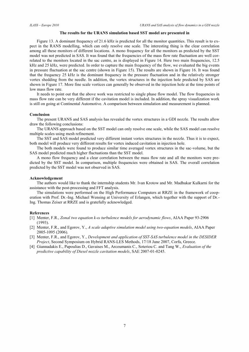
The results for the URANS simulation based SST model are presented in

Figure 13. A dominant frequency of 21.6 kHz is predicted for all the monitor quantities. This result is to ex-

pect in the RANS modelling, which can only resolve one scale. The interesting thing is the clear correlation

among all these monitors of different locations. A mono frequency for all the monitors as predicted by the SST

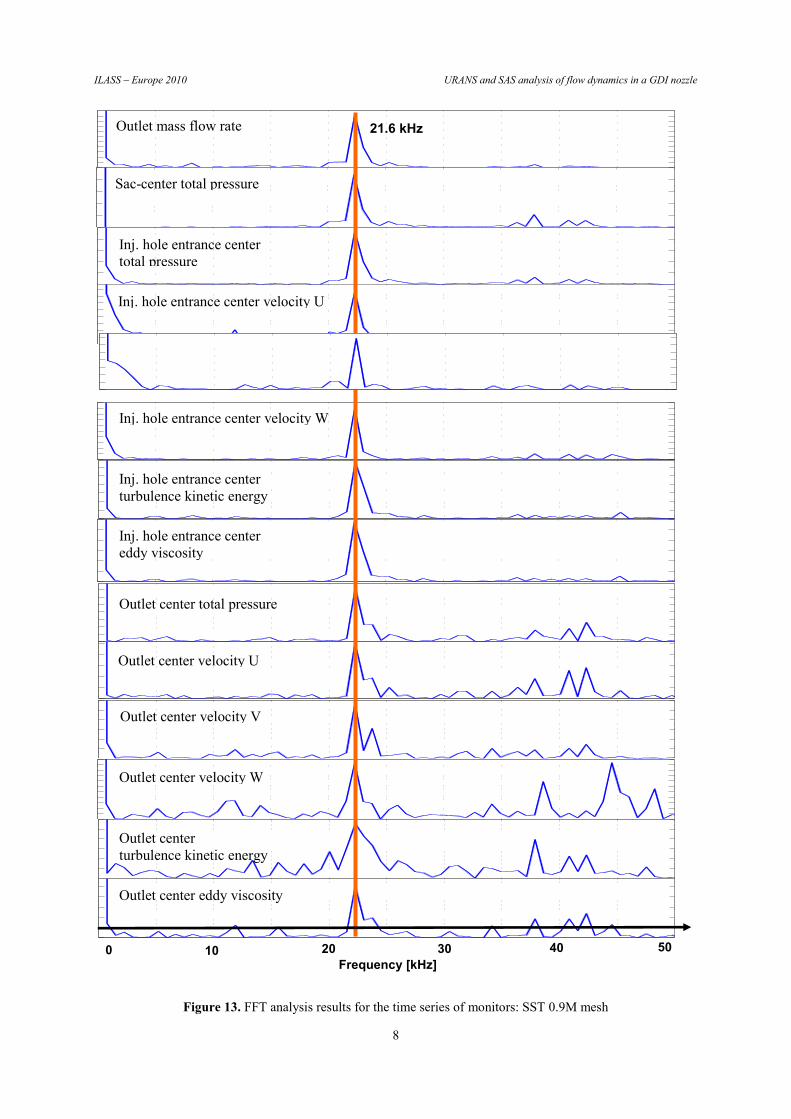
model was not predicted in SAS. It was found that the frequencies of the mass flow rate fluctuation are well cor-

related to the monitors located in the sac centre, as is displayed in Figure 14. Here two main frequencies, 12.5

kHz and 25 kHz, were predicted. In order to capture the main frequency of the flow, we evaluated the big events

in pressure fluctuation at the sac centre (shown in Figure 15). The results are shown in Figure 16. It was found

that the frequency 25 kHz is the dominant frequency in the pressure fluctuation and in the relatively stronger

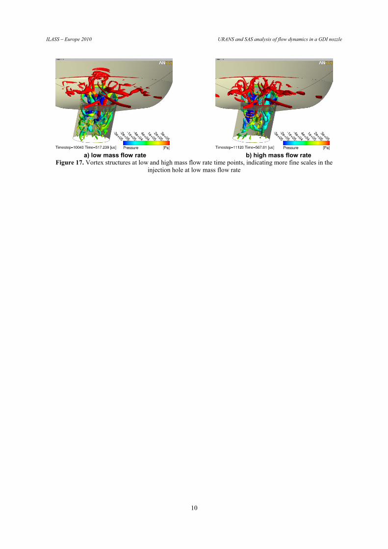
vortex shedding from the needle. In addition, the vortex structures in the injection hole predicted by SAS are

shown in Figure 17. More fine scale vortices can generally be observed in the injection hole at the time points of

low mass flow rate.

It needs to point out that the above work was restricted to single phase flow model. The flow frequencies in

mass flow rate can be very different if the cavitation model is included. In addition, the spray visualization work

is still on going at Continental Automotive. A comparison between simulation and measurement is planned.

Conclusion

The present URANS and SAS analysis has revealed the vortex structures in a GDI nozzle. The results allow

draw the following conclusions:

The URANS approach based on the SST model can only resolve one scale, while the SAS model can resolve

multiple scales using mesh refinement.

The SST and SAS model predicted very different instant vortex structures in the nozzle. Thus it is to expect,

both model will produce very different results for vortex induced cavitation in injection hole.

The both models were found to produce similar time averaged vortex structures in the sac-volume, but the

SAS model predicted much higher fluctuations than the SST model.

A mono flow frequency and a clear correlation between the mass flow rate and all the monitors were pre-

dicted by the SST model. In comparison, multiple frequencies were obtained in SAS. The overall correlation

predicted by the SST model was not observed in SAS.

Acknowledgement

The authors would like to thank the internship students Mr. Ivan Krotow and Mr. Madhukar Kulkarni for the

assistance with the post-processing and FFT analysis.

The simulations were performed on the High Performance Computers at RRZE in the framework of coop-

eration with Prof. Dr.-Ing. Michael Wensing at University of Erlangen, which together with the support of Dr.-

Ing. Thomas Zeiser at RRZE and is gratefully acknowledged.

References

[1] Menter, F.R., Zonal two equation k-ω turbulence models for aerodynamic flows, AIAA Paper 93-2906

(1993).

[2] Menter, F.R., and Egorov, Y., A scale adaptive simulation model using two-equation models, AIAA Paper

2005-1095 (2006).

[3] Menter, F.R., and Egorov, Y., Development and application of SST-SAS turbulence model in the DESIDER

Project, Second Symposium on Hybrid RANS-LES Methods, 17/18 June 2007, Corfu, Greece.

[4] Giannadakis E., Papoulias D., Gavaises M., Arcoumanis C., Soteriou C. and Tang W., Evaluation of the

predictive capability of Diesel nozzle cavitation models, SAE 2007-01-0245.


8

Figure 13. FFT analysis results for the time series of monitors: SST 0.9M mesh

0 10 20 30 40 50

Frequency [kHz]

Outlet mass flow rate

Sac-center total pressure

Inj. hole entrance center

total pressure

Inj. hole entrance center velocity U

Inj. hole entrance center velocity V

Inj. hole entrance center velocity W


turbulence kinetic energy


eddy viscosity

Outlet center total pressure

Outlet center velocity U

Outlet center velocity W

Outlet center

turbulence kinetic energy

Outlet center eddy viscosity

Outlet center velocity V

21.6 kHz

50


9

Figure 14. Correlation between the frequency of mass flow rate and the monitor quantities at sac centre

Figure 15. Big events evaluation for the sac centre pressure fluctuation

Figure 16. Big events frequency distribution in sac centre pressure (left) and mass flow rate (right)

0 10 20 30 40 50 60 70 80 90 100

[kHz]

1 2 3

Turbulence kinetic

energy

Eddy viscosity

Turbulence length

scale

0 10 20 40 50 30

Mass flow rate 12.5 kHz 25 kHz

Frequency [kHz]

Power Spectru

m

0 5 10 15 20 25 30 35 40 45 50

[kHz]

1 2

0.4 0.5 0.6 0.7 0.8 0.9 1.0 1.1 [ms]


10

Figure 17. Vortex structures at low and high mass flow rate time points, indicating more fine scales in the

injection hole at low mass flow rate

a) low mass flow rate b) high mass flow rate

urans and sas analysis of flow dynamics in a gdi nozzle

Documents

Transcript of urans and sas analysis of flow dynamics in a gdi nozzle