Giampaolo Orlandoni M. Josefa Ramoni P.

Instituto de Estadística Aplicada

Universidad de Los AndesVenezuela

SAS BASICO

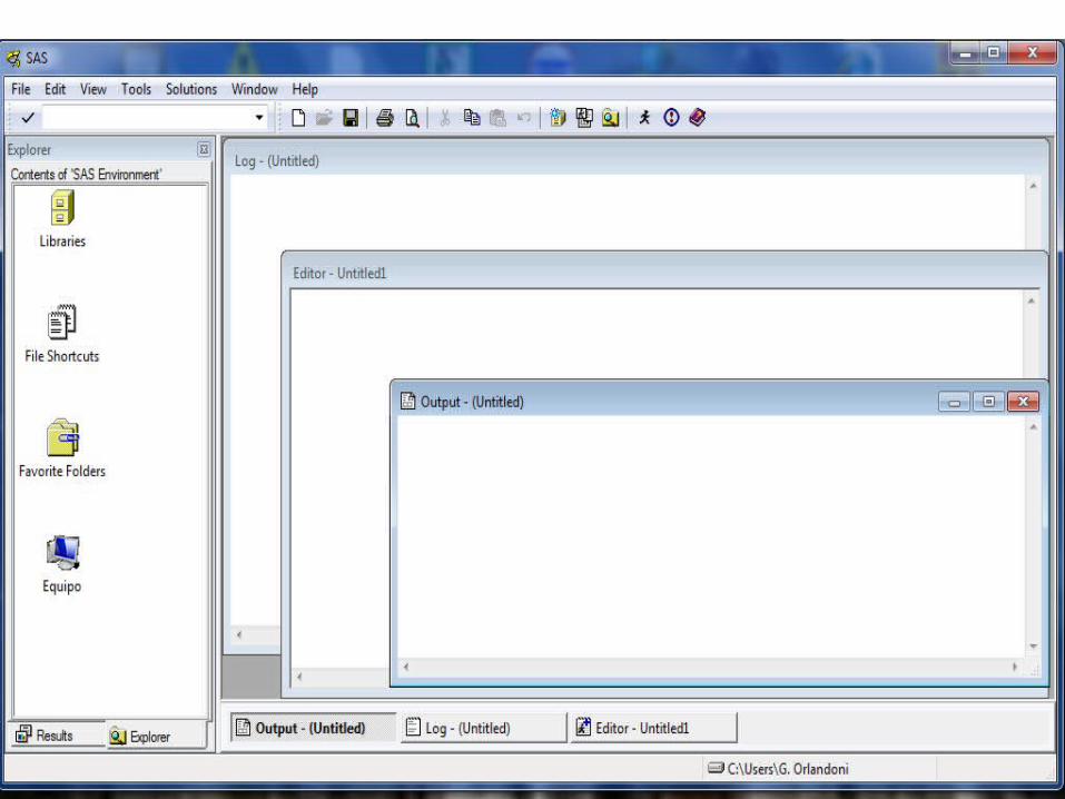
INTRODUCCION AL SAS1. Estructura SAS

2. Paso de Datos: Data

3. Paso de Procedimientos: Proc

4. Entrada de Datos: Input, Infile, Import

5. Formato de Datos: Lista, Columna, Formato

6. Procedimientos:1. Proc Print 2. Proc Sort3. Proc Contents

7. Creación de Archivos permanentes: Libname

8. Ejercicios

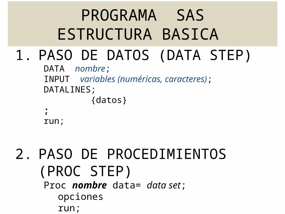
PROGRAMA SASESTRUCTURA BASICA

1. PASO DE DATOS (DATA STEP)DATA nombre;INPUT variables (numéricas, caracteres);DATALINES; {datos};run;

2. PASO DE PROCEDIMIENTOS (PROC STEP)Proc nombre data= data set;

opcionesrun;

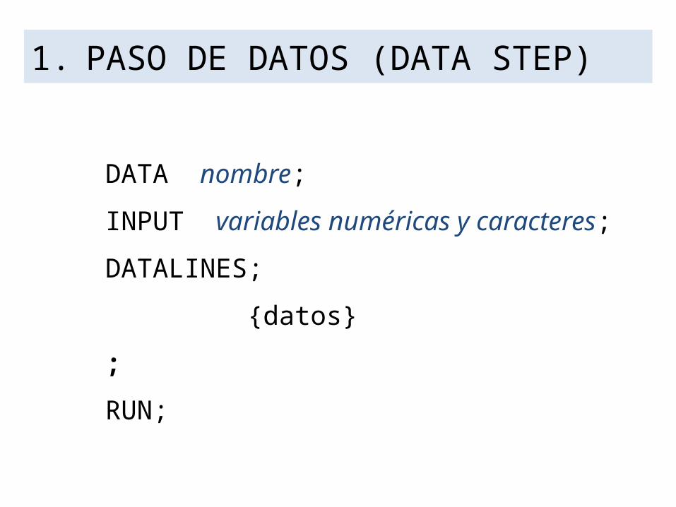
DATA nombre;INPUT variables numéricas y caracteres;DATALINES; {datos};RUN;

1. PASO DE DATOS (DATA STEP)

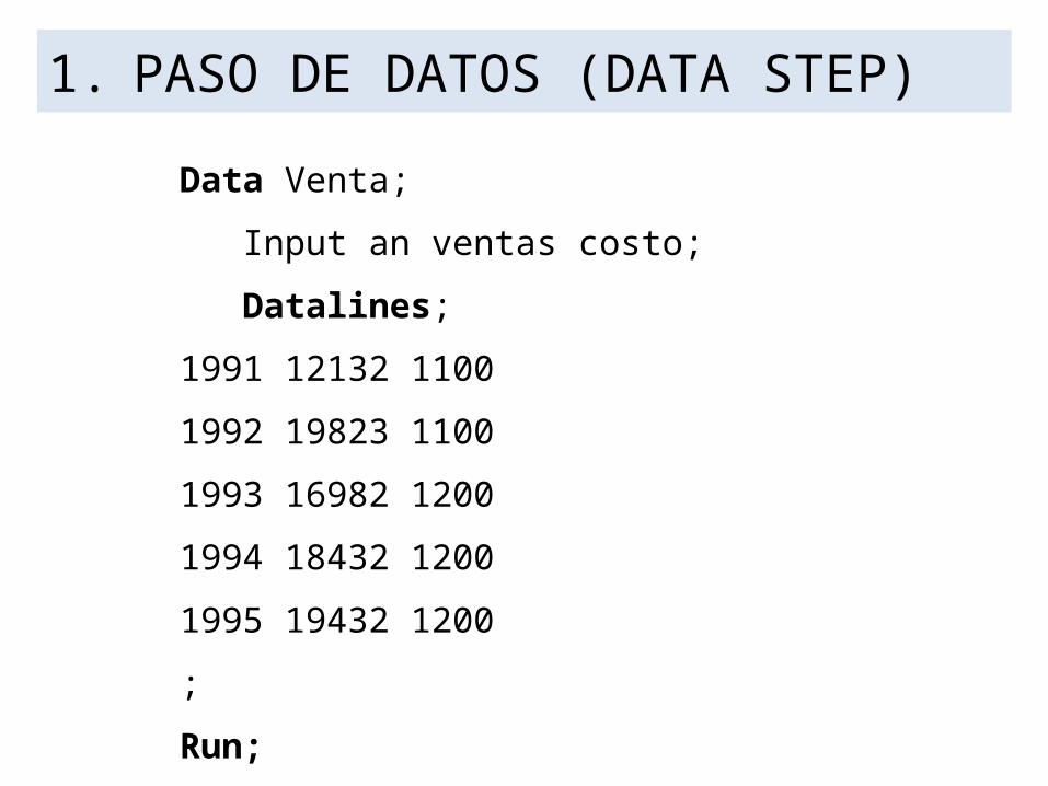
Data Venta; Input an ventas costo; Datalines;1991 12132 11001992 19823 11001993 16982 12001994 18432 12001995 19432 1200;Run;

1. PASO DE DATOS (DATA STEP)

2.2 Proc Print data=venta; Var an ventas;

Title 'Reporte 2';run;

2. PASO DE PROCEDIMIENTO (PROC STEP)2.1 Proc Print data=venta;

Title 'Reporte 1';run;

2.3 Proc Print data=venta; By costo;

Var an ventas;Title 'Reporte 3';run;

Forma General de PROC PRINT

Proc Print data= data set;Title ‘título';By variables;Var variables; run;

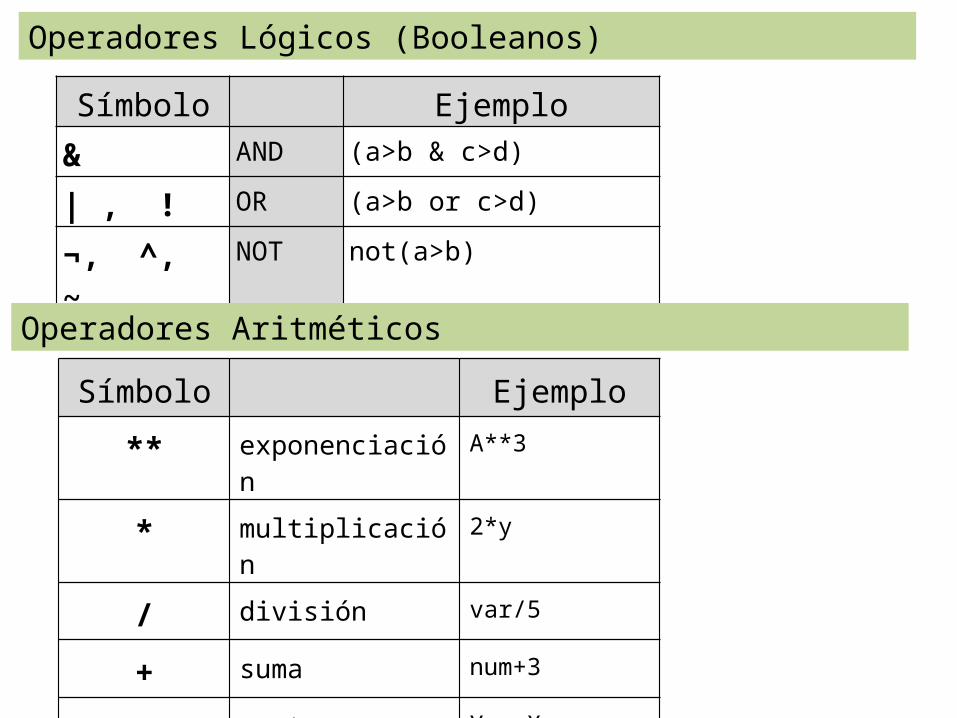
Operadores Lógicos (Booleanos)

Símbolo Ejemplo& AND (a>b & c>d)

| , ! OR (a>b or c>d)

¬, ^, ~

NOT not(a>b)

Símbolo Ejemplo** exponenciació

nA**3

* multiplicación

2*y

/ división var/5

+ suma num+3

- resta Y - X

Operadores Aritméticos

Símbolo

Definición Ejemplo

= EQ equal to a=3

^=, ¬=, ~=

NE not equal to a ne 3

> GT greater than Num >5

< LT less than Num <8

>= GE greater than or equal to

Y >= 300

<= LE less than or equal to

Y <=100

IN equal to one of a list

num in (3, 4, 5)

Operadores Comparativos

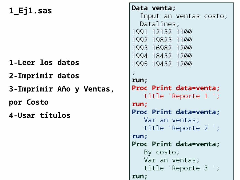
Data venta; Input an ventas costo; Datalines;1991 12132 11001992 19823 11001993 16982 12001994 18432 12001995 19432 1200;run;Proc Print data=venta; title 'Reporte 1 ';run;Proc Print data=venta; Var an ventas; title 'Reporte 2 ';run;Proc Print data=venta; By costo; Var an ventas; title 'Reporte 3 ';run;

1_Ej1.sas

1-Leer los datos2-Imprimir datos3-Imprimir Año y Ventas,por Costo4-Usar títulos

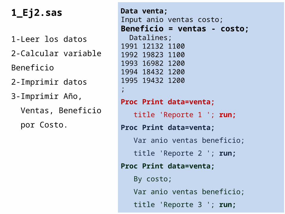
Data venta;Input anio ventas costo;Beneficio = ventas - costo; Datalines;1991 12132 11001992 19823 11001993 16982 12001994 18432 12001995 19432 1200;Proc Print data=venta; title 'Reporte 1 '; run;Proc Print data=venta; Var anio ventas beneficio; title 'Reporte 2 '; run;Proc Print data=venta; By costo; Var anio ventas beneficio; title 'Reporte 3 '; run;

1_Ej2.sas

1-Leer los datos2-Calcular variableBeneficio2-Imprimir datos3-Imprimir Año, Ventas, Beneficio por Costo.

Data venta; Input an ventas costo; Ben = ventas - costo;Datalines;1991 12132 11001992 19823 11001993 16982 12001994 18432 12001995 19432 1200;Proc Print Data=venta Split='*';Label ventas='Ventas * Año‘costo='Costo ‘ben='Beneficio antes *Impuesto';Format ventas costo ben dollar10.1;Id an;Sum ventas costo ben;Title 'PRINT con Totales'; run;

1_Ej3.sas

1-Leer los datos2-Imprimir datos con Labels.3-Calcular totales

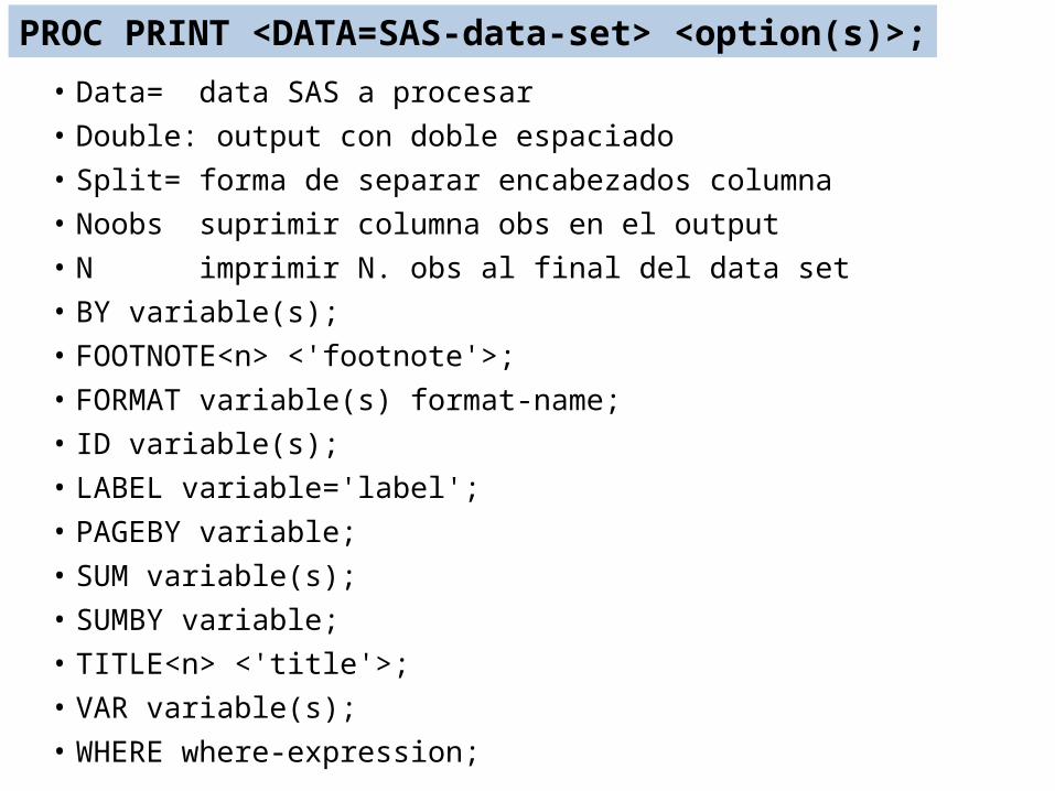
• Data= data SAS a procesar • Double: output con doble espaciado• Split= forma de separar encabezados columna• Noobs suprimir columna obs en el output• N imprimir N. obs al final del data set• BY variable(s); • FOOTNOTE<n> <'footnote'>; • FORMAT variable(s) format-name; • ID variable(s); • LABEL variable='label'; • PAGEBY variable; • SUM variable(s); • SUMBY variable; • TITLE<n> <'title'>; • VAR variable(s); • WHERE where-expression;

PROC PRINT <DATA=SAS-data-set> <option(s)>;

SUM variable(s): Identifies the numeric variables to total in the report. When also use the BY statement, the SUM statement produces subtotals each time the value of a BY variable changes.

SUMBY variable: Limits the number of sums that appear in the report. PROC PRINT reports totals only when variable changes value or when any variable that is listed before it in the BY statement changes value. Must use a BY statement with the SUMBY statement.

WHERE where-expression:

•Subsets the input data set by identifying certain conditions that each observation must meet before an observation is available for processing.

•Where-expression defines the condition.

•The condition is a valid arithmetic or logical expression that generally consists of a sequence of operands and operators.

Data venta;Input anio ventas costo;Beneficio = ventas - costo; Datalines;1991 12132 11001992 19823 11001993 16982 1994 18432 12001995 19432 1200;Proc Print data=venta; title 'Reporte 1 '; run;Proc Print data=venta; Var anio ventas beneficio; title 'Reporte 2 '; run;Proc Sort data=venta; by costo; run;Proc Print data=venta; By costo; Var anio ventas beneficio; title 'Reporte 3 '; run;

1_Ej2-1.sas• Qué sucede si hay algún dato faltanteen alguna de las variables?• Correr el programa con un dato faltantepara el costo del año 1993.• Indicar al SAS que ese dato es faltante con (.) Efectos.

1993 16982 .

Lectura de Datos

1. Input

2. Infile

3. Import

1. INPUT

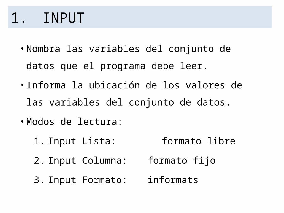
•Nombra las variables del conjunto de datos que el programa debe leer.

•Informa la ubicación de los valores de las variables del conjunto de datos.

•Modos de lectura:

1. Input Lista: formato libre

2. Input Columna: formato fijo

3. Input Formato: informats

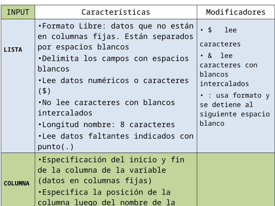
INPUT Características Modificadores

LISTA

•Formato Libre: datos que no están en columnas fijas. Están separados por espacios blancos•Delimita los campos con espacios blancos•Lee datos numéricos o caracteres ($)•No lee caracteres con blancos intercalados•Longitud nombre: 8 caracteres•Lee datos faltantes indicados con punto(.)

• $ lee

caracteres• & lee caracteres con blancos intercalados• : usa formato y se detiene al siguiente espacio blanco

COLUMNA

•Especificación del inicio y fin de la columna de la variable (datos en columnas fijas)•Especifica la posición de la columna luego del nombre de la variable •Lee variables caracter, usando $ luego del nombre de la variable

FORMATO

Permite dar instrucciones específicas: Informatname w.dw especifica ancho de campo (opcional). delimitador obligatoriod dígitos decimales (opcional)

•Apuntador Absoluto: @n: ir a la columna n

•Apuntador Relativo: +n: avanzar n columnas

INPUT EJEMPLO

LISTA INPUT Nombre $ Sexo $ Edad Altura Peso;

COLUMNA INPUT Nombre $ 1-8 Sexo $ 11 Edad 13-14 Altura 16-18 Peso 20-21;

FORMATOINPUT Nombre $8. @11 Sexo $1. +1 Edad 2. +1 Altura 4. +1 Peso 3.;

1 2 3 4 5 6 7 8 9 0 1 2 3 4 5 6 7 8 9 0 1J U A N             M   1 2 1 5 0 4 0P E D R O           M   1 4 1 6 0 5 0L U I S A           F   1 3 1 4 0 4 2A L F R E D O       M   1 5 1 5 8 4 8A L I C I A         F   1 5 1 5 0 4 7

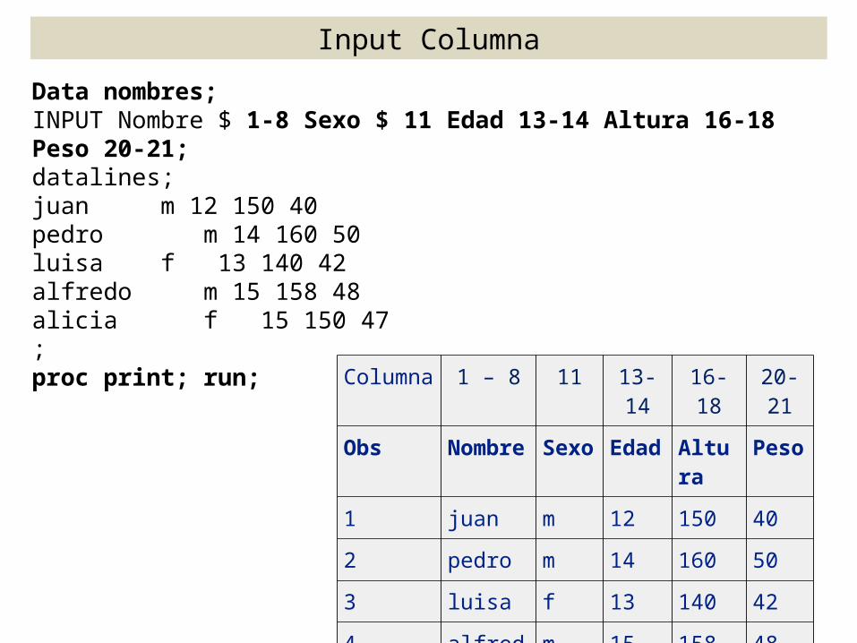
Columna 1 – 8 11 13-14

16-18

20-21

Obs Nombre Sexo Edad Altura

Peso

1 juan m 12 150 402 pedro m 14 160 503 luisa f 13 140 424 alfred

om 15 158 48

5 alicia f 15 150 47

Data nombres;INPUT Nombre $ 1-8 Sexo $ 11 Edad 13-14 Altura 16-18 Peso 20-21;datalines;juan m 12 150 40pedro m 14 160 50luisa f 13 140 42alfredo m 15 158 48alicia f 15 150 47;proc print; run;

Input Columna

1-Modificador @n:

• Ir a la columna Número n, para leer la variable indicada

• Permite leer variables en cualquier orden, saltar variables

2-Modificador @@

• Permite seguir leyendo variables en un mismo registro

• Debe ser el último elemento del INPUT.

MODIFICADORES @, @@

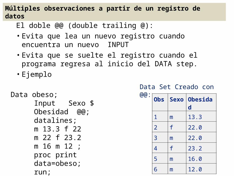
El doble @@ (double trailing @):•Evita que lea un nuevo registro cuando encuentra un nuevo INPUT

•Evita que se suelte el registro cuando el programa regresa al inicio del DATA step.

•Ejemplo Data Set Creado con @@:Data obeso;

Input Sexo $ Obesidad @@; datalines;m 13.3 f 22 m 22 f 23.2 m 16 m 12 ;proc print data=obeso; run;

Obs Sexo Obesidad

1 m 13.32 f 22.03 m 22.04 f 23.25 m 16.06 m 12.0

Múltiples observaciones a partir de un registro de datos

2. INFILE•Permite leer archivos de datos externo, en formato ASCII.

•Se ubica entre las sentencias DATA e INPUT:

• Data nombre;• INFILE ‘c:\DataSAS\Archivo.dat’;• Input var1 var2 .... varn;

•Opción MISSOVER: asigna valor faltante a datos que no tienen el símbolo (.)

• Data nombre;• INFILE ‘c:\DataSAS\Archivo.dat’ MISSOVER;• Input var1 var2 .... varn;

2. INFILE/* Definir archivos permanentes SAS; Uso de LIBNAME */

libname ventas 'c:\DataSas\dat'; ods html file='c:\DataSAS\html\1_LibVenta.html';

data ventas.TR1; INFILE 'C:\DataSas\dat\tr1.dat'; Input Depart $ Lugar $ Trim Ventas;proc print; run;

2. INFILE/* Dos formas de leer el archivo TR1 */

/* 1-Indicando el Path completo */Proc print data= 'c:\DataSAS\dat\TR1';Var Ventas; run;

/* 2-Usando el nombre asignado por libname */proc print data=ventas.TR1;var trim lugar depart ventas; run;ods html close;

..\..\..\..\..\..\..\DataSAS\html\1_LibVenta.html

/*Definir archivos permanentes SAS; LIBNAME */ libname ventas 'c:\DataSas\dat';NOTA: Libref VENTAS was successfully assigned as follows: Engine: V9 Physical Name: c:\DataSas\dat

2. INFILE con MISSOVERARCHIVO TR1.dat con dato faltante en la variable ventas.Usar MISSOVER para leer correctamente los datos.

Partes Sydney 1 4043.97Partes Atlanta 1 6225.26Partes Paris 1 3543.97Repar Sydney 1 5592.82Repar Atlanta 1 9210.21Repar Paris 1 8591.98Herram Sydney 1 1775.74Herram Atlanta 1 Herram Paris 1 5914.25

data ventas.TR1; INFILE 'C:\DataSas\dat\tr1.dat' MISSOVER; Input Depart $ Lugar $ Trim Ventas;proc print; run;

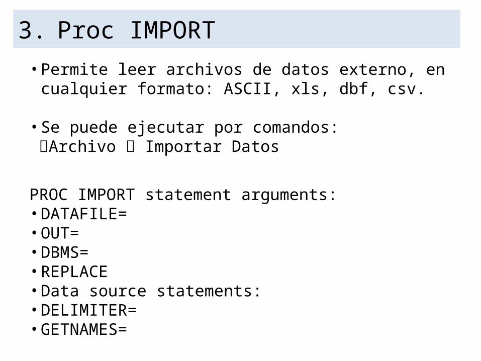
3. Proc IMPORT•Permite leer archivos de datos externo, en cualquier formato: ASCII, xls, dbf, csv.

•Se puede ejecutar por comandos: Archivo Importar Datos

PROC IMPORT statement arguments: •DATAFILE=•OUT=•DBMS=•REPLACE•Data source statements: •DELIMITER=•GETNAMES=

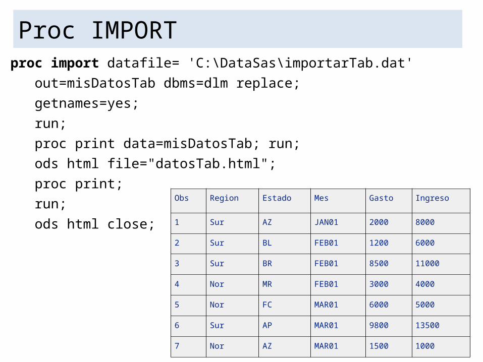
Proc IMPORTproc import datafile= 'C:\DataSas\importarTab.dat'

out=misDatosTab dbms=dlm replace; getnames=yes; run;proc print data=misDatosTab; run;ods html file="datosTab.html";proc print;run;ods html close;

Obs Region Estado Mes Gasto Ingreso

1 Sur AZ JAN01 2000 8000

2 Sur BL FEB01 1200 6000

3 Sur BR FEB01 8500 11000

4 Nor MR FEB01 3000 4000

5 Nor FC MAR01 6000 5000

6 Sur AP MAR01 9800 13500

7 Nor AZ MAR01 1500 1000

Proc Sort: Ordenar DatosPROC SORT <DATA=SAS-data-set>; BY variable(s);

PROC SORT DATA=SAS-data-set: ordena un SAS DS según los valores de variables listadas en el BY.

BY variable(s):

• Especifica las variables por las que PROC SORT ordena las observaciones del archivo.

• PROC SORT ordena el DS en orden ascendente.

Data venta;Input an mes $ ventas costo;Beneficio = ventas - costo; Datalines;1991 ene 12132 12001992 feb 19823 11001993 ene 16982 12001994 feb 18432 11001995 ene 19432 1200;run;Proc Sort data=venta;By mes costo; run;

Proc Print data=venta; By mes; Var an ventas costo beneficio; title 'Reporte Mes '; run;

Proc Print data=venta; By mes costo; Var an ventas beneficio; title 'Reporte Mes_Costo ‘;run;

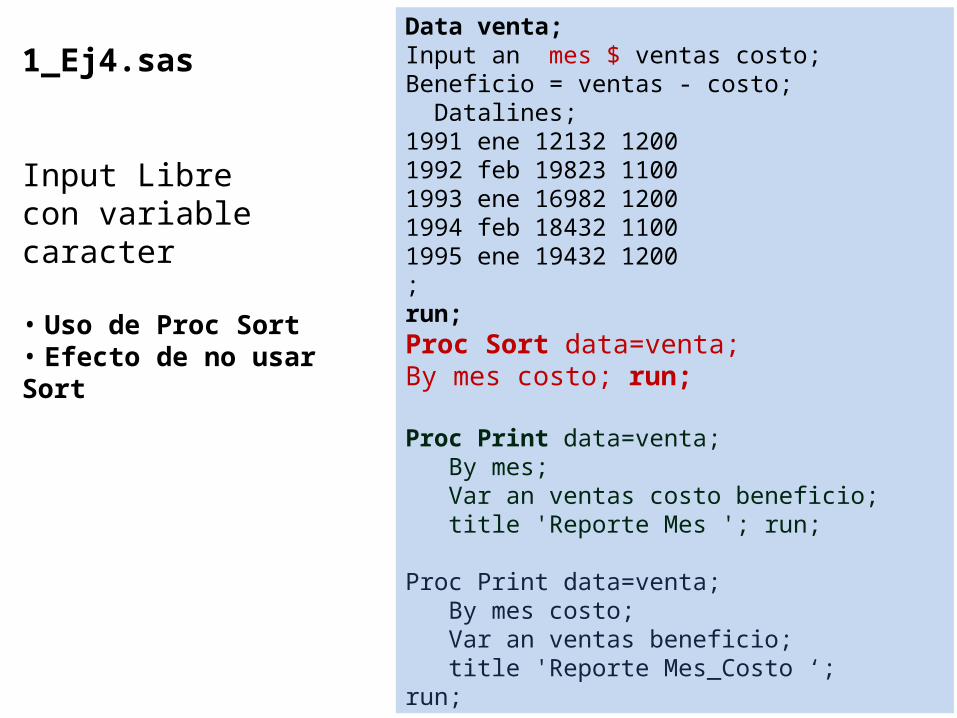
1_Ej4.sas

Input Librecon variable caracter

• Uso de Proc Sort• Efecto de no usarSort

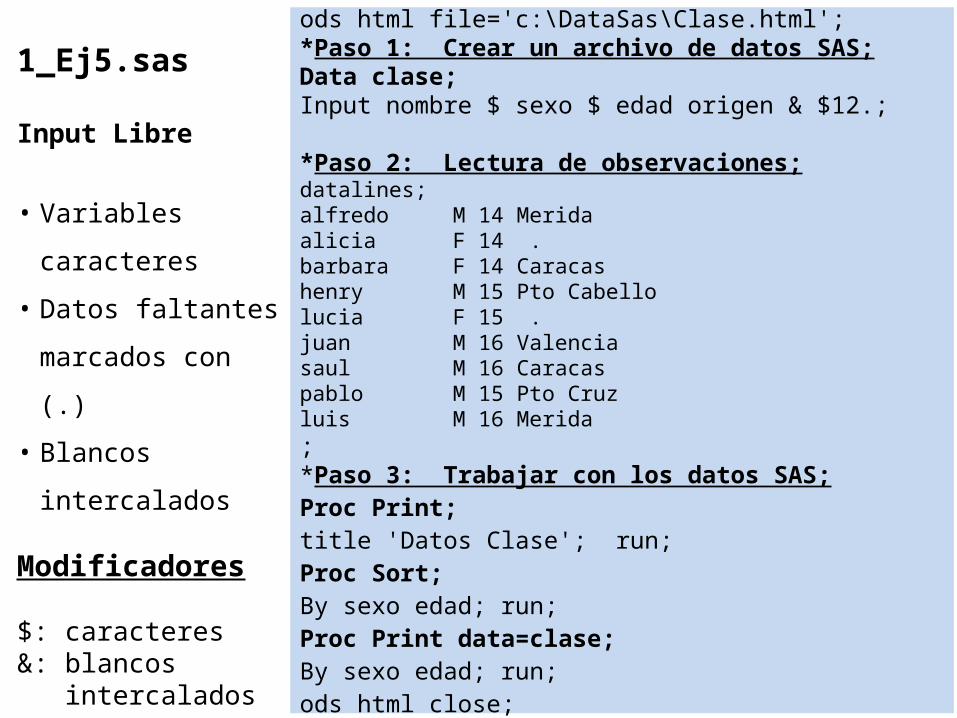
ods html file='c:\DataSas\Clase.html';*Paso 1: Crear un archivo de datos SAS;Data clase; Input nombre $ sexo $ edad origen & $12.;

*Paso 2: Lectura de observaciones;datalines;alfredo M 14 Meridaalicia F 14 .barbara F 14 Caracashenry M 15 Pto Cabellolucia F 15 .juan M 16 Valenciasaul M 16 Caracaspablo M 15 Pto Cruzluis M 16 Merida;*Paso 3: Trabajar con los datos SAS;Proc Print; title 'Datos Clase'; run; Proc Sort;By sexo edad; run;Proc Print data=clase;By sexo edad; run;ods html close;

1_Ej5.sas

Input Libre

• Variables caracteres

• Datos faltantes marcados con (.)

• Blancos intercalados

Modificadores

$: caracteres&: blancos intercalados

ods html file='c:\DataSas\1_Ej6.html';

DATA D1(TYPE=CORR) ; INPUT _TYPE_ $ _NAME_ $ V1-V12;Datalines;

N . 300 300 300 300 300 300 300 300 300 300 300 300STD . 2.48 2.39 2.58 3.12 2.80 3.14 2.92 2.50 2.10 2.14 1.83 2.26CORR V1 1.00 . . . . . . . . . . .CORR V2 .69 1.00 . . . . . . . . . .CORR V3 .60 .79 1.00 . . . . . . . . .CORR V4 .62 .47 .48 1.00 . . . . . . . .CORR V5 .03 .04 .16 .09 1.00 . . . . . . .CORR V6 .05 -.04 .08 .05 .91 1.00 . . . . . .CORR V7 .14 .05 .06 .12 .82 .89 1.00 . . . . .CORR V8 .23 .13 .16 .21 .70 .72 .82 1.00 . . . .CORR V9 -.17 -.07 -.04 -.05 -.33 -.26 -.38 -.45 1.00 . . .CORR V10 -.10 -.08 .07 .15 -.16 -.20 -.27 -.34 .45 1.00 . .CORR V11 -.24 -.19 -.26 -.28 -.43 -.37 -.53 -.57 .60 .22 1.00 .CORR V12 -.11 -.07 .07 .08 -.10 -.13 -.23 -.31 .44 .60 .26 1.00;Proc Print;run;

ods html close;

1_Ej6.sas

Lectura Matriz de Correlación

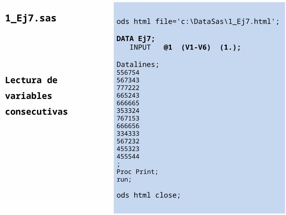
ods html file='c:\DataSas\1_Ej7.html';

DATA Ej7; INPUT @1 (V1-V6) (1.);

Datalines;556754567343777222665243666665353324767153666656334333567232455323455544;Proc Print;run;

ods html close;

1_Ej7.sas

Lectura de variables consecutivas

ods html file='c:\DataSas\1_Ej8.html';

DATA Ej8; INPUT equipo $ 13-16 @; IF equipo='rojo'; INPUT idn 1-4 pesoi 20-23 pesof 24-26; redpeso=pesoi-pesof;Datalines;1023 David rojo 189 1651049 Amelia azul 145 1241219 Alan rojo 210 1921246 Raul azul 194 1771078 Alicia rojo 127 1181221 Juan azul 220 .;Proc Print data=Ej8;run;PROC CORR DATA=Ej8 NOMISS; VAR pesoi pesof redpeso;run;

ods html close;

1_Ej8.sas

Lectura de un archivo dos veces, luego de una condición if

Subconjunto de datos creado con el símbolo @

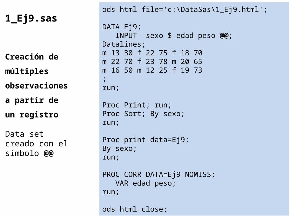
ods html file='c:\DataSas\1_Ej9.html';

DATA Ej9; INPUT sexo $ edad peso @@;Datalines;m 13 30 f 22 75 f 18 70m 22 70 f 23 78 m 20 65m 16 50 m 12 25 f 19 73;run;

Proc Print; run;Proc Sort; By sexo; run;

Proc print data=Ej9;By sexo;run;

PROC CORR DATA=Ej9 NOMISS; VAR edad peso;run;

ods html close;

1_Ej9.sas

Creación de múltiples observaciones a partir de un registro

Data set creado con el símbolo @@

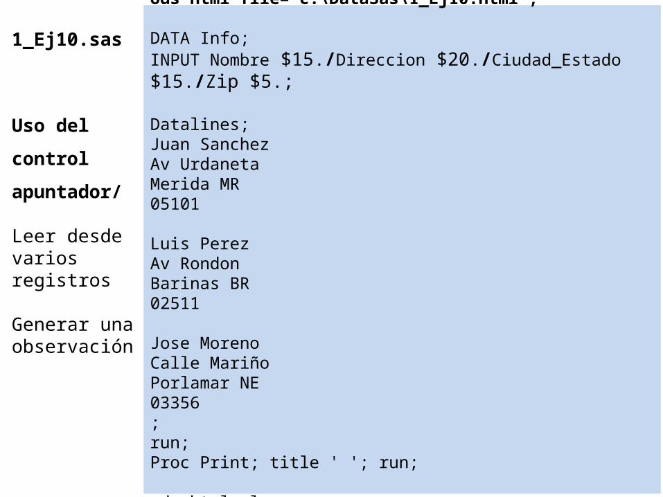
ods html file='c:\DataSas\1_Ej10.html';

DATA Info;INPUT Nombre $15./Direccion $20./Ciudad_Estado $15./Zip $5.;

Datalines;Juan SanchezAv UrdanetaMerida MR05101

Luis PerezAv RondonBarinas BR02511

Jose MorenoCalle MariñoPorlamar NE03356;run;Proc Print; title ' '; run;

ods html close;

1_Ej10.sas

Uso del control apuntador/

Leer desde varios registros

Generar una observación

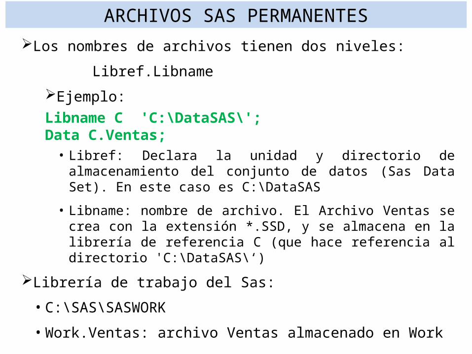
Los nombres de archivos tienen dos niveles:Libref.Libname

Ejemplo:Libname C 'C:\DataSAS\';Data C.Ventas;• Libref: Declara la unidad y directorio de almacenamiento del conjunto de datos (Sas Data Set). En este caso es C:\DataSAS

• Libname: nombre de archivo. El Archivo Ventas se crea con la extensión *.SSD, y se almacena en la librería de referencia C (que hace referencia al directorio 'C:\DataSAS\‘)

Librería de trabajo del Sas: •C:\SAS\SASWORK•Work.Ventas: archivo Ventas almacenado en Work

ARCHIVOS SAS PERMANENTES

ARCHIVOS SAS PERMANENTES: HERRAMIENTAS

Con Herramientas se crea Nueva Librería y se indica: • Nombre de la librería• Ruta: dirección física de la librería

Libname C 'C:\DataSAS\';ods html file='c:\DataSas\Lib3.html';Data C.Ventas;Input Region $ Venta; Datalines;R1 10R3 20R7 30R2 40R4 50R6 60R5 70R1 30R3 30R7 50R2 10R4 80R6 90R5 50R1 10R3 20R7 30R2 40R4 50R6 60R5 70R1 30R3 30R7 50R2 10R4 80R6 90R5 50;Proc Print; run; ods html close;

1_Ej11.sas

Creación de Archivos Permanentes

Uso deLibname

/* Crear archivo permanente SAS */libname ventas 'c:\DataSas\Venta2002';

Data ventas.TR1; Input Depart $ Lugar $ Trim Ventas;Datalines;Partes Sydney 1 4043.97Partes Atlanta 1 6225.26Partes Paris 1 3543.97Repar Sydney 1 5592.82Repar Atlanta 1 9210.21Repar Paris 1 8591.98Herram Sydney 1 1775.74Herram Atlanta 1 2424.19Herram Paris 1 5914.25;/* Dos formas de leer el archivo TR1 *//* 1-Indicando el Path completo */Proc means data= 'c:\DataSAS\Venta2002\TR1';Var Ventas; run;/* 2-Usando el nombre asignado por libname */Proc Print data=ventas.TR1;var trim lugar depart ventas; run;Proc means data= ventas.TR1;Var Ventas; run;

1_Ej12.sas

Creación de archivo permanente

Libname

Libname C 'C:\DataSAS\';ods html file='c:\DataSas\VentaLib3.html';Proc Sort Data= C.Ventas Out=C.VentasOrd; By Region;Data C.Totales(Keep=Region Total); Set C.VentasOrd; By Region; If First.Region then Total=0; Total+Venta; If Last.Region;Proc Print Data=C.Totales Noobs; Title 'Total Ventas 2000';run;ods html close;

1_Ej12.sas

Libname

Proc CONTENTS

•Contenido del data set.•Proc Contents data=Ventas;

Lista alfabética de variables y atributosNúm Variable Tipo Longitud5 Cantidad Numérica 81 Mes Alfanuméri

ca8

6 Precio Numérica 84 Tipo Alfanuméri

ca16

2 Trim Alfanumérica

8

3 Vendedor Alfanumérica

14

7 Venta Numérica 8

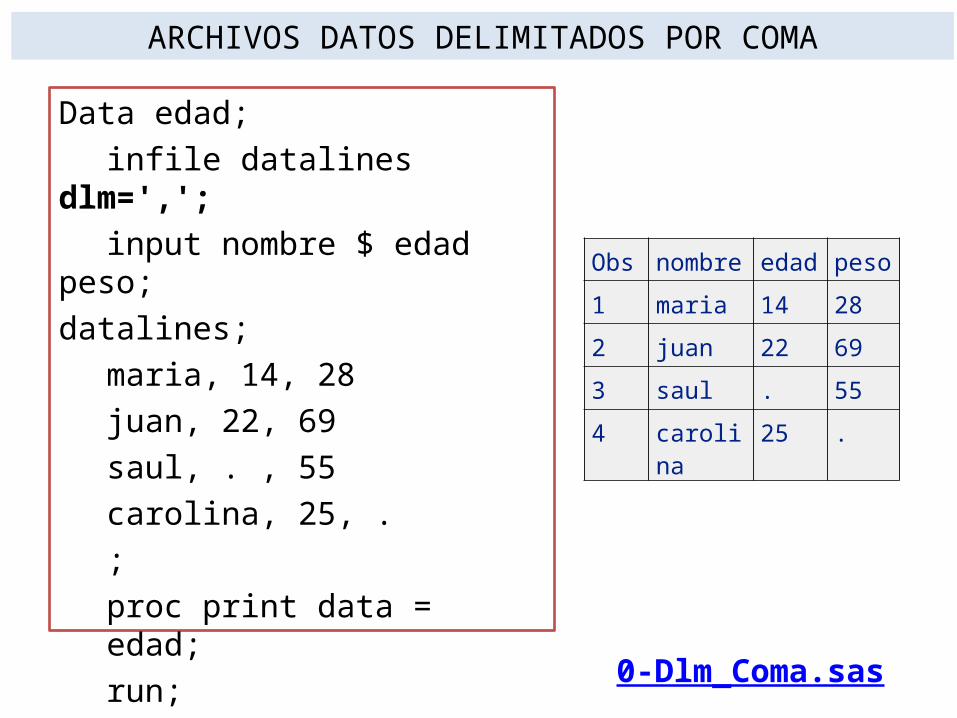
Data edad;infile datalines

dlm=',';input nombre $ edad

peso;datalines;

maria, 14, 28juan, 22, 69saul, . , 55carolina, 25, .;proc print data = edad;run;

ARCHIVOS DATOS DELIMITADOS POR COMA

0-Dlm_Coma.sas

Obs nombre edad peso1 maria 14 282 juan 22 693 saul . 554 caroli

na25 .

Default Delimiter used to read input data with list input: blank space. The delimiter-sensitive data (DSD) option, the DELIMITER= option, the DLMSTR= option, and the DLMSOPT= option affect how list input handles delimiters.

The DELIMITER= or DLMSTR= option specifies that the INPUT statement use a character other than a blank as a delimiter for data values that are read with list input. When the DSD option is in effect, the INPUT statement uses a comma as the default delimiter.

To read a value as missing between two consecutive delimiters, use the DSD option. When you use DSD, the INPUT statement treats consecutive delimiters separately. Therefore, a value that is missing between consecutive delimiters is read as a missing value. To change the delimiter from a comma to another value, use the DELIMITER= or DLMSTR= option.

Reading Delimited Data

1. Tabla de datos Notas:1. Crear el data set Notas2. Calcular la media de las

notas3. Calcular indice ponderado de

notasIndice=N1+N2/100

4. Número de niños y niñas.5. Calcular el Promedio y el

Indice por Sexo

2. Tabla de datos PRESIÓN:1. Crear un listado ordenado por

PS2. Calcular la presión

sanguínea promedio PSM= 2/3 PD + 1/3 PS

3. Promedio de PS, PD, PSM por sexo

Ejercicios NOTASID SEXO EDAD N1 N21 M 10 12 3602 M 11 15 4503 F 9 18 5404 M 9 14 4205 F 11 16 4806 F 12 10 3007 F 9 10 3008 M 10 11 3309 M 10 17 510

10 M 11 13 390

PRESIÓNID SEXO PS PD1 M 100 802 M 110 903 F 90 804 M 90 855 F 110 1006 F 120 1107 F 130 1008 M 150 1059 M 125 115

10 M 110 90

EJERCICIOSEJERCICIO1: Monto de multas de tráfico por estado

(USA). Imprimir el archivo de datos ordenado por monto y por estado.

EJERCICIO2: Imprimir el archivo de datos ordenados por ventas, departamento, vendedor. Calcular totales de venta por Departamento, por Vendedor

EJERCICIO3: Lectura de Datos con diferentes formatosEJERCICIO4: Ventas por departamento y vendedor.

Calcular comisiones por ventas. Tablas Frecuencia de ventas. Total comisiones por vendedor y por departamento

EJERCICIO5: Creación de Librerías y Archivos permanentes. Datos climáticos.

ods html file='c:\DataSas\Ejer1.html';

Data Ejer1; Input Estado $ Monto @@; Datalines;

AL 100 HI 200 DE 20 IL 1000 AK 300 CT 50 AR 100 IA 60 FL 250 KS 90 AZ 250 IN 500 CA 100 LA 175 GA 150 MT 70 ID 100 KY 55 CO 100 ME 50 NE 200 MA 85 MD 500 NV 1000 MO 500 MI 40 NM 100 NJ 200 MN 300 NY 300 NC 1000 MS 100 ND 55 OH 100 NH 1000 OR 600OK 75 SC 75 RI 210 PA 46.50 TN 50 SD 200 TX 200 VT 1000 UT 750WV 100 VA 200 WY 200 WA 77 Wi 300 DC. ; run;

ods html close;

1_Ejercicio1.Monto de multas de tráfico por estado (USA).Imprimir el archivo de datos ordenados por monto y por estado

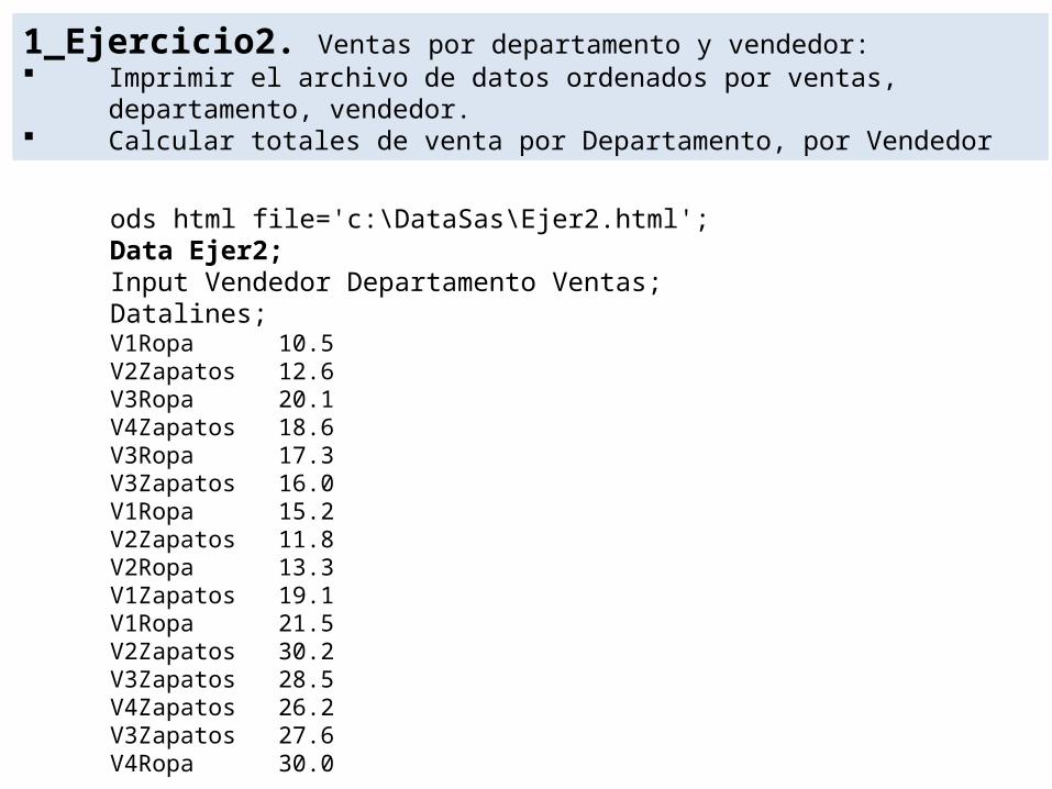
ods html file='c:\DataSas\Ejer2.html';Data Ejer2; Input Vendedor Departamento Ventas; Datalines; V1Ropa 10.5V2Zapatos 12.6V3Ropa 20.1V4Zapatos 18.6V3Ropa 17.3V3Zapatos 16.0V1Ropa 15.2V2Zapatos 11.8V2Ropa 13.3V1Zapatos 19.1V1Ropa 21.5V2Zapatos 30.2V3Zapatos 28.5V4Zapatos 26.2V3Zapatos 27.6V4Ropa 30.0

1_Ejercicio2. Ventas por departamento y vendedor: Imprimir el archivo de datos ordenados por ventas,

departamento, vendedor. Calcular totales de venta por Departamento, por Vendedor

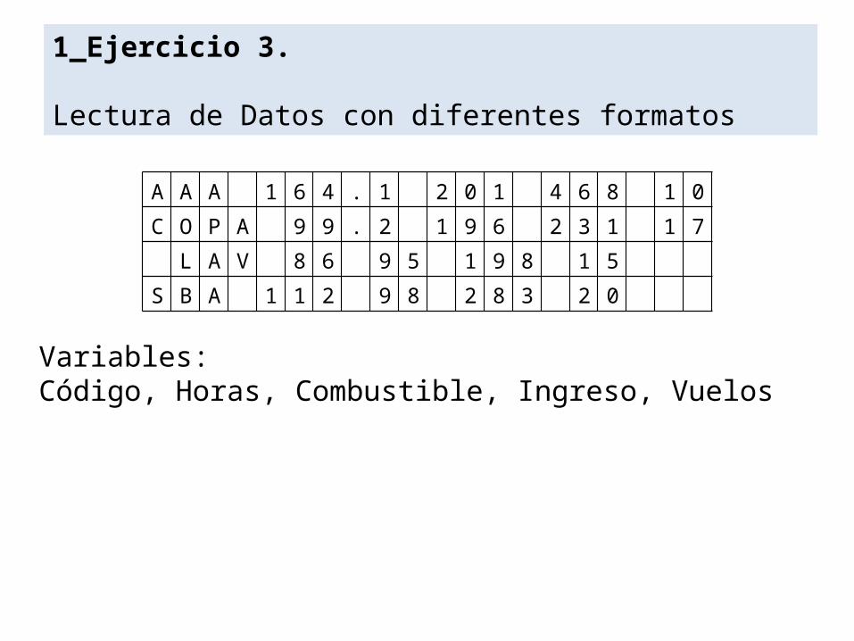
Variables:Código, Horas, Combustible, Ingreso, Vuelos

1_Ejercicio 3.

Lectura de Datos con diferentes formatos

A A A 1 6 4 . 1 2 0 1 4 6 8 1 0C O P A 9 9 . 2 1 9 6 2 3 1 1 7

L A V 8 6 9 5 1 9 8 1 5S B A 1 1 2 9 8 2 8 3 2 0

1-Calcular comisiones por ventas.Comisión:

• 5% de las ventas de ropa• 7% de las ventas de zapatos

2-Tablas de Frecuencia de ventas

3-Total comisiones por vendedor y por departamento

1_Ejercicio 4.

Ventas por departamento y vendedor

Ejemplo 1. Mostrar un mismo valor como: • Fecha: DATE• Hora: TIMEAMPM• Fecha y Hora: DATETIME

Función MONTH: extrae el mes del valor de Date1.

Ejemplo 2. Leer y escribir fechas• Lee fechas usando el informat MMDDYY8. • Escribe fechas calculadas usando el formato DATE9.

DATOS FECHAS (DATE- TIME)

Ejemplo 3. Leer fechas y calcular duración• Leer fechas usando Date9. • Calcular duración proyectos.

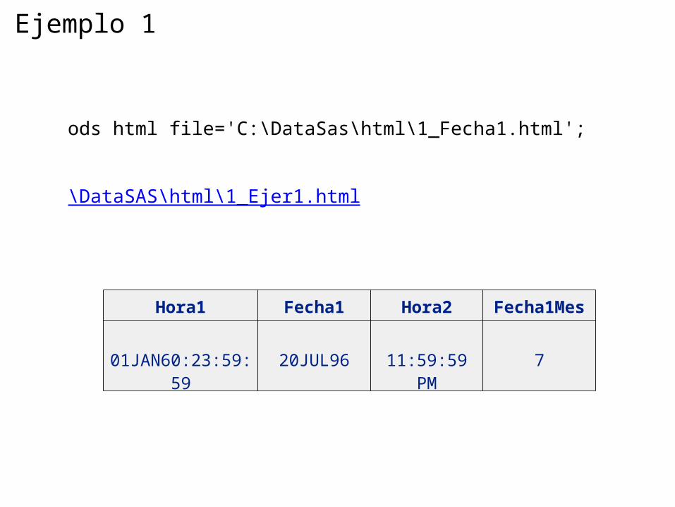
ods html file='C:\DataSas\html\1_Fecha1.html';

Data fecha; Hora1=86399; format Hora1 datetime.; Fecha1=86399; format Fecha1 date.; Hora2=86399; format Hora2 timeampm.; Fecha1Mes=month(Fecha1);run; Proc Print data=fecha noobs; title 'Mismo Número, Diferentes Valores SAS'; footnote1 'Hora1 es SAS DATETIME'; footnote2 'Fecha1 es SAS DATE '; footnote3 'Hora2 es SAS TIME '; footnote4 'Fecha1Mes es el mes de Fecha1';run;

title; footnote;ods html close;

Ejemplo 1

ods html file='C:\DataSas\html\1_Fecha1.html';

\DataSAS\html\1_Ejer1.html

Ejemplo 1

Hora1 Fecha1 Hora2 Fecha1Mes

01JAN60:23:59:59

20JUL96 11:59:59 PM

7

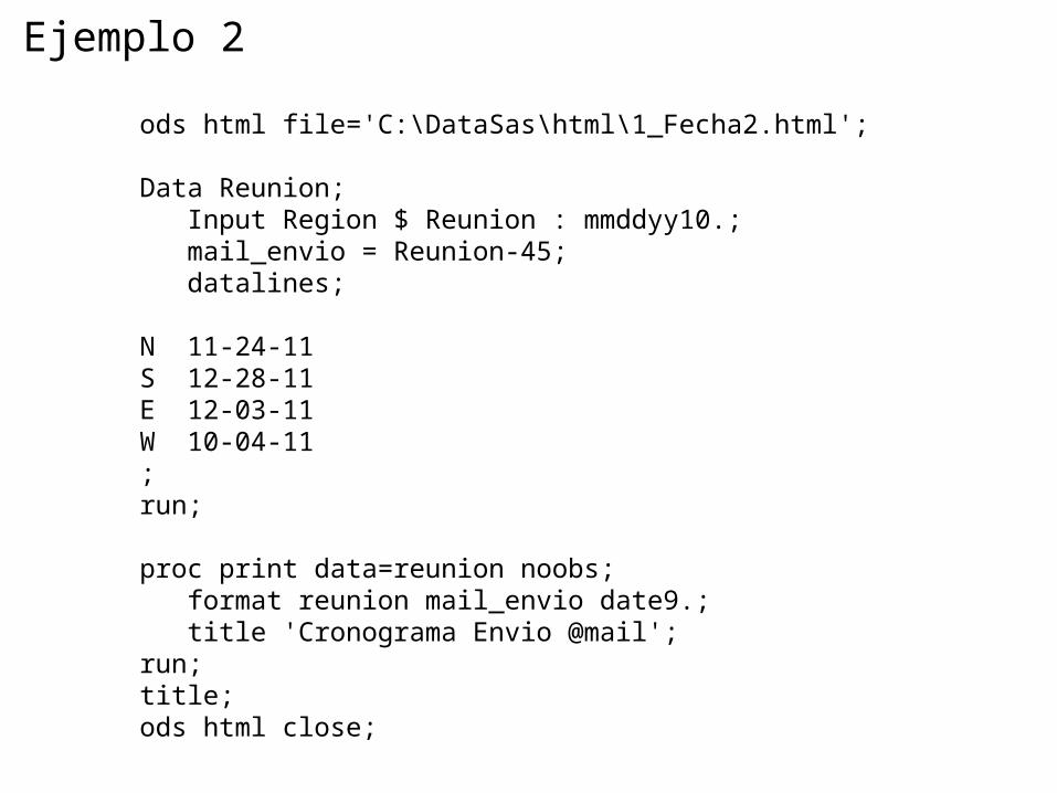
ods html file='C:\DataSas\html\1_Fecha2.html';

Data Reunion; Input Region $ Reunion : mmddyy10.; mail_envio = Reunion-45; datalines;

N 11-24-11S 12-28-11E 12-03-11W 10-04-11;run; proc print data=reunion noobs; format reunion mail_envio date9.; title 'Cronograma Envio @mail';run;title;ods html close;

Ejemplo 2

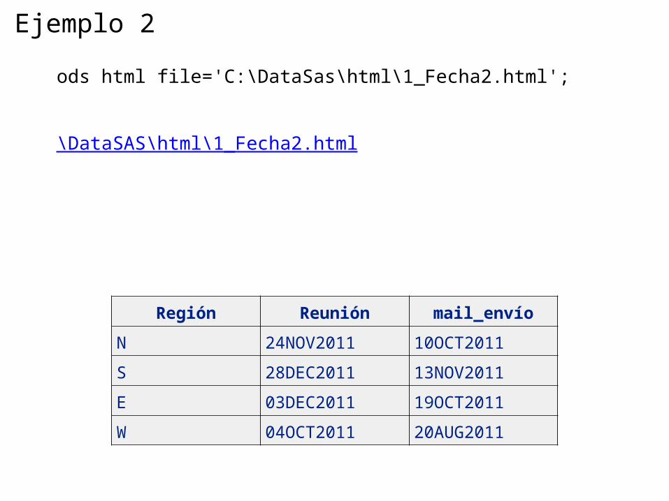
ods html file='C:\DataSas\html\1_Fecha2.html';

\DataSAS\html\1_Fecha2.html

Ejemplo 2

Región Reunión mail_envíoN 24NOV2011 10OCT2011S 28DEC2011 13NOV2011E 03DEC2011 19OCT2011W 04OCT2011 20AUG2011

2-ods html file='C:\DataSas\html\1_Fecha3.html';

\DataSAS\html\1_Fecha3.html

Ejemplo 3

Obs Proid IniFecha FinFecha Duracion

1 p398 17OCT1997 02NOV1997 162 p942 22JAN1998 10MAR1998 473 p167 15DEC1999 15FEB2000 624 p250 04JAN2001 11JAN2001 7

1-file='C:\DataSas\sas\1_Fecha3.sas';

\DataSAS\sas\Dia1bcv_IntroduccionSAS\1_Fecha3.sas

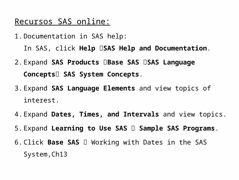
Recursos SAS online:1.Documentation in SAS help:

In SAS, click Help SAS Help and Documentation.

2.Expand SAS Products Base SAS SAS Language Concepts SAS System Concepts.

3.Expand SAS Language Elements and view topics of interest.

4.Expand Dates, Times, and Intervals and view topics.

5.Expand Learning to Use SAS Sample SAS Programs.

6.Click Base SAS Working with Dates in the SAS System,Ch13

Páginas de soporte y consulta SAS:

•http://support.sas.com/documentation/92/index.html

•SAS Technical Support Documents Documentation

http://support.sas.com/documentation/cdl/en/leforinforref/63324/HTML/default/n09mk4h1ba9wp1n1tc3e7x0eow8q.htm

•SAS Online Product Documentation

•http://support.sas.com/documentation/cdl/en/basess/58133/HTML/default/viewer.htm#a001334449.htm

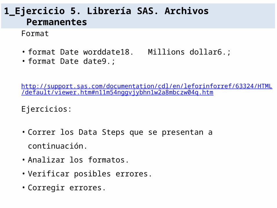
1_Ejercicio 5. Librería SAS. Archivos Permanentes

Format

• format Date worddate18. Millions dollar6.;• format Date date9.;

http://support.sas.com/documentation/cdl/en/leforinforref/63324/HTML/default/viewer.htm#n11m54nggvjybhn1w2a8mbczw04q.htm

Ejercicios:

• Correr los Data Steps que se presentan a continuación.

• Analizar los formatos.• Verificar posibles errores.• Corregir errores.

1-Crear el Data Set USCLIM.HURACANdata usclim.huracan; Input Estado Fecha Muertes Perdida Nombre;

format Fecha worddate18. Costo dollar6.; informat Estado $char11. Fecha date9.; label Perdida=‘Costo'; datalines;

Mississippi 14aug69 256 1420 Camille Florida 14jun72 117 2100 Agnes Alabama 29aug79 5 2300 Frederick Texas 15aug83 21 2000 Alicia Texas 03aug80 28 300 Allen ;

libname usclim 'C:\DataSAS'; data usclim.huracan; input @1 Estado $char11. @13 Fecha date7. Muertes Perdida Nombre $;

format Fecha worddate18. Perdida dollar6.; informat Estado $char11. Fecha date9.; label Millions='Daño'; datalines; Mississippi 14aug69 256 1420 Camille Florida 14jun72 117 2100 Agnes Alabama 29aug79 5 2300 Frederick Texas 15aug83 21 2000 Alicia Texas 03aug80 28 300 Allen ;Proc print; run;

1-DATA Step para crear el Data Set USCLIM.HURACAN

Obs Estado Fecha Muertes

Perdida

Nombre

1 Mississippi

August 14, 1969

256 $1,420 Camille

2 Florida June 14, 1972

117 $2,100 Agnes

3 Alabama August 29, 1979

5 $2,300 Frederic

4 Texas August 15, 1983

21 $2,000 Alicia

5 Texas August 3, 1980

28 $300 Allen

2- Crear el Data Set USCLIM.LOWTEMP

data usclim.lowtemp;

Input Estado $char14. Ciudad $char14. Temp_F Fecha $ Elevacion;

datalines; • Alaska Prospect Creek -80 23jan71 1100 • Colorado Maybell -60 01jan79 5920 • Idaho Island Prk Dam -60 18jan43 6285 • Minnesota Pokegama Dam -59 16feb03 1280 • North Dakota Parshall -60 15feb36 1929 • South Dakota McIntosh -58 17feb36 2277 • Wyoming Moran -63 09feb33 6770 ;

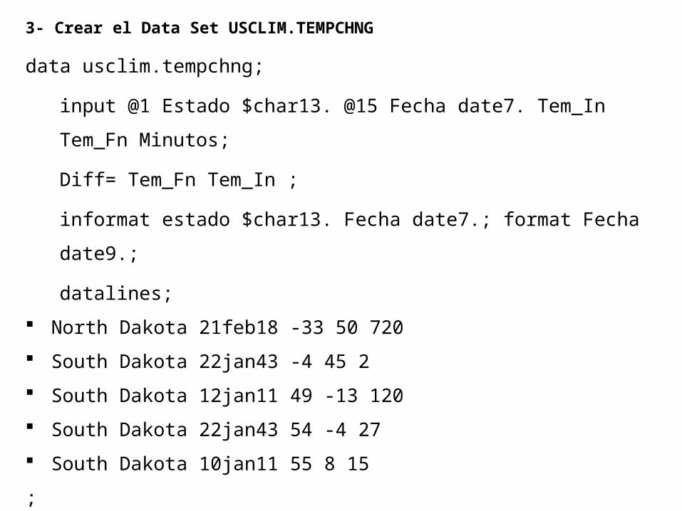
3- Crear el Data Set USCLIM.TEMPCHNG

data usclim.tempchng;

input @1 Estado $char13. @15 Fecha date7. Tem_In Tem_Fn Minutos;

Diff= Tem_Fn Tem_In ;

informat estado $char13. Fecha date7.; format Fecha date9.;

datalines; North Dakota 21feb18 -33 50 720 South Dakota 22jan43 -4 45 2 South Dakota 12jan11 49 -13 120 South Dakota 22jan43 54 -4 27 South Dakota 10jan11 55 8 15 ;

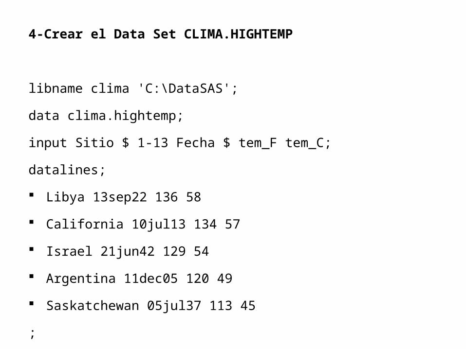
4-Crear el Data Set CLIMA.HIGHTEMP

libname clima 'C:\DataSAS';

data clima.hightemp;

input Sitio $ 1-13 Fecha $ tem_F tem_C;

datalines; Libya 13sep22 136 58 California 10jul13 134 57 Israel 21jun42 129 54 Argentina 11dec05 120 49 Saskatchewan 05jul37 113 45

;

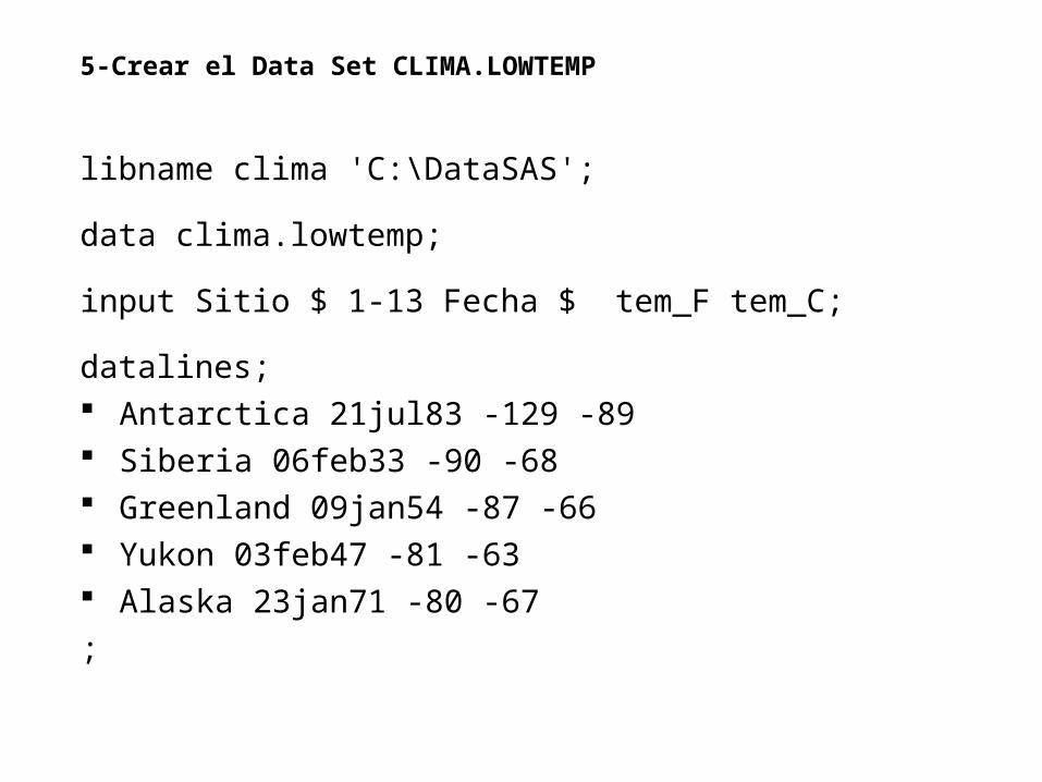
5-Crear el Data Set CLIMA.LOWTEMP

libname clima 'C:\DataSAS';

data clima.lowtemp;

input Sitio $ 1-13 Fecha $ tem_F tem_C;

datalines; Antarctica 21jul83 -129 -89 Siberia 06feb33 -90 -68 Greenland 09jan54 -87 -66 Yukon 03feb47 -81 -63 Alaska 23jan71 -80 -67 ;

6-Crear el Data Set PRECPITA.RAINdata precpita.rain; input Sitio $ 1-12 @13 Fecha date7. Inch Cms; format Fecha date9.; datalines; La Reunion 15mar52 74 188 Taiwan 10sep63 49 125 Australia 04jan79 44 114 Texas 25jul79 43 109 Canada 06oct64 19 49 ;

7-Crear el Data Set PRECPITA.SNOWdata precpita.snow; input Sitio $ 1-12 @13 Fecha date7. Inch Cms; format Fecha date9.; datalines; Colorado 14apr21 76 193 Alaska 29dec55 62 158 France 05apr69 68 173;

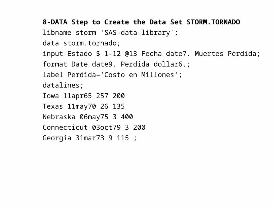
8-DATA Step to Create the Data Set STORM.TORNADOlibname storm 'SAS-data-library'; data storm.tornado; input Estado $ 1-12 @13 Fecha date7. Muertes Perdida; format Date date9. Perdida dollar6.; label Perdida=‘Costo en Millones'; datalines; Iowa 11apr65 257 200 Texas 11may70 26 135 Nebraska 06may75 3 400 Connecticut 03oct79 3 200 Georgia 31mar73 9 115 ;

SAS/ASSIST

SAS/ASSIST: DATA MANAGEMENT