
Untitled - Qucosa - TU Dresden
251
-
Upload
khangminh22 -
Category
Documents
-
view
0 -
download
0
Transcript of Untitled - Qucosa - TU Dresden


Fakultät Wirtschaftswissenschaften
Makespan Minimization in
Re-entrant Permutation Flow Shops
Dissertation
to achieve the academic degree
Doctor rerum politicarum (Dr. rer. pol.)
by
Richard Hinze
born on 02.05.1987 in Dresden
First reviewer: Prof. Dr. Udo Buscher
Second reviewer: Prof. Dr. Rainer Lasch
Date of submission: 01.02.2017
Date of defense: 29.08.2017

Contents
List of Figures V
List of Tables IX
List of Algorithms XII
List of Abbreviations XIV
List of Symbols XVI
1 Introduction 1
1.1 Motivation . . . . . . . . . . . . . . . . . . . . . . . . . . . . . . . . . . . 1
1.2 Structure and Methodology . . . . . . . . . . . . . . . . . . . . . . . . . 2
2 Machine Scheduling 6
2.1 Introduction . . . . . . . . . . . . . . . . . . . . . . . . . . . . . . . . . . 6
2.2 Classification of Machine Scheduling Problems . . . . . . . . . . . . . . . 7
2.3 Solution Approaches . . . . . . . . . . . . . . . . . . . . . . . . . . . . . 11
3 Re-entrant Scheduling Problems 27
3.1 Problem Assumptions and Classification . . . . . . . . . . . . . . . . . . 27
3.2 Literature Review . . . . . . . . . . . . . . . . . . . . . . . . . . . . . . . 30
3.2.1 Search Methodology . . . . . . . . . . . . . . . . . . . . . . . . . 31
3.2.2 Re-entrant Flow Shops . . . . . . . . . . . . . . . . . . . . . . . . 33
3.2.3 Re-entrant Job Shops . . . . . . . . . . . . . . . . . . . . . . . . . 38
3.2.4 Re-entrant Line Problems . . . . . . . . . . . . . . . . . . . . . . 41
3.3 A Mathematical Formulation for Re-entrant Permutation Flow Shops . . 51
4 Re-entrant Permutation Flow Shop Problems with Mixed Levels and Missing
Operations 56
4.1 Introduction . . . . . . . . . . . . . . . . . . . . . . . . . . . . . . . . . . 56
4.2 Mixed Levels . . . . . . . . . . . . . . . . . . . . . . . . . . . . . . . . . 57
4.3 Missing Operations . . . . . . . . . . . . . . . . . . . . . . . . . . . . . . 60
II

CONTENTS III
4.4 Mathematical Models . . . . . . . . . . . . . . . . . . . . . . . . . . . . . 63
4.4.1 Comparison of Sequence Variables . . . . . . . . . . . . . . . . . . 63
4.4.2 Basic Job Sequence . . . . . . . . . . . . . . . . . . . . . . . . . . 80
4.4.3 Influence of Missing Operations . . . . . . . . . . . . . . . . . . . 85
4.5 Initialization Methods . . . . . . . . . . . . . . . . . . . . . . . . . . . . 88
4.5.1 Constructive Heuristics for Separated Levels . . . . . . . . . . . . 89
4.5.2 Constructive Heuristics for Mixed Levels . . . . . . . . . . . . . . 92
4.5.3 Computational Experiments . . . . . . . . . . . . . . . . . . . . . 95
4.6 Neighborhood Structures in Re-entrant Permutation Flow Shops . . . . . 98
4.6.1 Swap Moves . . . . . . . . . . . . . . . . . . . . . . . . . . . . . . 98
4.6.2 Insertion Moves . . . . . . . . . . . . . . . . . . . . . . . . . . . . 100
4.6.3 Block Neighborhoods . . . . . . . . . . . . . . . . . . . . . . . . . 101
4.6.4 Computational Experiments . . . . . . . . . . . . . . . . . . . . . 108
4.7 Improvement Methods . . . . . . . . . . . . . . . . . . . . . . . . . . . . 111
4.7.1 Simple Local Search Algorithms . . . . . . . . . . . . . . . . . . . 111
4.7.2 Variable Neighborhood Search . . . . . . . . . . . . . . . . . . . . 113
4.7.3 Tabu Search . . . . . . . . . . . . . . . . . . . . . . . . . . . . . . 116
4.7.4 Simulated Annealing . . . . . . . . . . . . . . . . . . . . . . . . . 119
4.7.5 Computational Experiments . . . . . . . . . . . . . . . . . . . . . 121
4.7.6 Improvement of Metaheuristics . . . . . . . . . . . . . . . . . . . 131
4.8 Application on Job Shop Problems . . . . . . . . . . . . . . . . . . . . . 134
5 Re-entrant Permutation Flow Shop Problems with Mixed Levels, Missing
Operations and Lot Streaming 139
5.1 Introduction . . . . . . . . . . . . . . . . . . . . . . . . . . . . . . . . . . 139
5.2 Mathematical Models . . . . . . . . . . . . . . . . . . . . . . . . . . . . . 144
5.2.1 Consistent Sublots . . . . . . . . . . . . . . . . . . . . . . . . . . 144
5.2.2 Consecutive Sublots . . . . . . . . . . . . . . . . . . . . . . . . . 155
5.2.3 Equal Sublots . . . . . . . . . . . . . . . . . . . . . . . . . . . . . 161
5.2.4 Consecutive Equal Sublots . . . . . . . . . . . . . . . . . . . . . . 168
5.2.5 Resizing Sublots . . . . . . . . . . . . . . . . . . . . . . . . . . . 173
5.2.6 Summary of Sublot Properties . . . . . . . . . . . . . . . . . . . . 182
5.3 Neighborhoods in Re-entrant Permutation Flow Shops with Lot Streaming 184
5.4 A Variable Neighborhood Search for a Re-entrant Permutation Flow Shop
with Lot Streaming . . . . . . . . . . . . . . . . . . . . . . . . . . . . . . 186
5.4.1 Calibration . . . . . . . . . . . . . . . . . . . . . . . . . . . . . . 187
5.4.2 Computational Experiments . . . . . . . . . . . . . . . . . . . . . 189

CONTENTS IV
6 Conclusion 196
A Literature Review Search Methodology 200
B Test Instances 203
C Additional Computational Results of Metaheuristics 206
D Lot Streaming Results for Inc 3 Instances 209
Bibliography 210

List of Figures
1.1 Structure of the thesis . . . . . . . . . . . . . . . . . . . . . . . . . . . . . . 5
2.1 Classification of solution methods . . . . . . . . . . . . . . . . . . . . . . . . 12
2.2 First improvement . . . . . . . . . . . . . . . . . . . . . . . . . . . . . . . . 17
2.3 Best neighbor . . . . . . . . . . . . . . . . . . . . . . . . . . . . . . . . . . . 18
2.4 Simulated annealing . . . . . . . . . . . . . . . . . . . . . . . . . . . . . . . 19
2.5 Tabu search . . . . . . . . . . . . . . . . . . . . . . . . . . . . . . . . . . . . 23
2.6 Variable neighborhood search . . . . . . . . . . . . . . . . . . . . . . . . . . 24
3.1 Example of a machine sequence with re-entrant . . . . . . . . . . . . . . . . 29
3.2 Example of a permutation of three jobs in a regular flow shop . . . . . . . . 52
3.3 Example of a permutation of three jobs in a re-entrant flow shop . . . . . . . 52
4.1 Solution to the example with separated levels . . . . . . . . . . . . . . . . . 58
4.2 Solution to the example with mixed levels . . . . . . . . . . . . . . . . . . . 59
4.3 Example of missing operations case 1 . . . . . . . . . . . . . . . . . . . . . . 60
4.4 Example of missing operations case 2 . . . . . . . . . . . . . . . . . . . . . . 60
4.5 Example of missing operations case 3 . . . . . . . . . . . . . . . . . . . . . . 60
4.6 Solution to the example if missing operations are not properly managed . . . 61
4.7 Solution to the example if missing operations are appropriately managed . . 62
4.8 Starting times for job i in level l: invalid on the left and valid on the right . 64
4.9 Invalid starting times for a job i changing from level l to l + 1 . . . . . . . . 65
4.10 Valid starting times for a job i changing from level l to l + 1 . . . . . . . . . 65
4.11 Invalid starting times if yili′l′ = 1 . . . . . . . . . . . . . . . . . . . . . . . . . 66
4.12 Valid starting times if yili′l′ = 1 . . . . . . . . . . . . . . . . . . . . . . . . . . 67
4.13 Valid starting times if yili′l′ = 0. . . . . . . . . . . . . . . . . . . . . . . . . . 67
4.14 Average makespan deviations between model X and Y . . . . . . . . . . . . 73
4.15 Average computation times of models X and Y for n = 2 . . . . . . . . . . . 75
4.16 Average computation times of models X and Y for n = 3 . . . . . . . . . . . 76
4.17 Average computation times of models X and Y for n = 4 . . . . . . . . . . . 77
4.18 Average computation times of models X and Y for n = 5 . . . . . . . . . . . 78
V

LIST OF FIGURES VI
4.19 Average makespan deviations between model Y and model BS . . . . . . . . 82
4.20 Average computation times of models Y and BS for n = 2 . . . . . . . . . . 83
4.21 Average computation times of models Y and BS for n = 5 . . . . . . . . . . 84
4.22 Illustration of the swap move limits of a level . . . . . . . . . . . . . . . . . 99
4.23 Example of an invalid level swap . . . . . . . . . . . . . . . . . . . . . . . . 99
4.24 Illustration of relevant and irrelevant level swap moves . . . . . . . . . . . . 99
4.25 Example of the number of possible level swap moves (I) . . . . . . . . . . . . 99
4.26 Example of the number of possible level swap moves (II) . . . . . . . . . . . 99
4.27 Example of a job swap . . . . . . . . . . . . . . . . . . . . . . . . . . . . . . 100
4.28 Illustration of the insertion move limits and valid moves of a level . . . . . . 100
4.29 Example of a job insertion move . . . . . . . . . . . . . . . . . . . . . . . . . 101
4.30 Resulting permutation after the job insertion move . . . . . . . . . . . . . . 101
4.31 Example of identifying the critical path of operations . . . . . . . . . . . . . 102
4.32 Example of a Nowicki intra block swap if jil is not a block border . . . . . . 103
4.33 Example of a Chen intra block swap if jil is not a block border . . . . . . . . 103
4.34 Example of a Nowicki intra block swap if jil is a block border . . . . . . . . 104
4.35 Example of a Chen intra block swap if jil is a block border . . . . . . . . . . 104
4.36 Example of a Nowicki intra block insertion if jil is not a block border . . . . 104
4.37 Example of a Chen intra block insertion if jil is not part of the critical path 104
4.38 Example of a Nowicki intra block insertion if jil is a block border . . . . . . 105
4.39 Example of a Chen intra block insertion if jil is a block border . . . . . . . . 105
4.40 Example of a Nowicki across block swap if jil is not a block border . . . . . 105
4.41 Example of a Chen across block swap if jil is not a block border . . . . . . . 106
4.42 Example of a Nowicki across block swap if jil is a block border . . . . . . . . 106
4.43 Example of a Chen across block swap if jil is a block border . . . . . . . . . 106
4.44 Example of a Nowicki across block insertion if jil is not a block border . . . 106
4.45 Example of a Chen across block insertion if jil is not a block border . . . . . 107
4.46 Example of a Nowicki across block insertion if jil is a block border . . . . . . 107
4.47 Example of a Chen across block insertion if jil is a block border . . . . . . . 107
4.48 Frequency of obtaining best solutions for large Inc 1 problems . . . . . . . . 127
4.49 Frequency of obtaining best solutions for large Inc 3 problems . . . . . . . . 127
4.50 Average computation times for large Inc 1 instances (I) . . . . . . . . . . . . 129
4.51 Average computation times for large Inc 1 instances (II) . . . . . . . . . . . 130
4.52 Average computation times with changed neighborhood structures . . . . . . 133
4.53 Solution to the job shop example . . . . . . . . . . . . . . . . . . . . . . . . 136
4.54 Average number of CPLEX iterations for job shops . . . . . . . . . . . . . . 137
4.55 Average computation times for job shops . . . . . . . . . . . . . . . . . . . . 138

LIST OF FIGURES VII
5.1 Example of lot streaming . . . . . . . . . . . . . . . . . . . . . . . . . . . . . 140
5.2 Solution to the example with consistent sublots . . . . . . . . . . . . . . . . 147
5.3 Average makespan of consistent sublots compared to using no sublots (Inc 1) 149
5.4 Average makespan of consistent sublots compared to using no sublots (Inc 2) 150
5.5 Average computation time with consistent sublots (Inc 1) . . . . . . . . . . 152
5.6 Average computation time with consistent sublots (Inc 2) . . . . . . . . . . 153
5.7 Solution to the example with consecutive sublots . . . . . . . . . . . . . . . 157
5.8 Average makespan deviations with consecutive sublots (Inc 1) . . . . . . . . 158
5.9 Average makespan deviations with consecutive sublots (Inc 2) . . . . . . . . 159
5.10 Average computation times with consecutive sublots (Inc 1) . . . . . . . . . 160
5.11 Average computation times with consecutive sublots (Inc 2) . . . . . . . . . 161
5.12 Solution to the example with equal sublots . . . . . . . . . . . . . . . . . . . 163
5.13 Average makespan deviations with equal sublots (Inc 1) . . . . . . . . . . . 164
5.14 Average makespan deviations with equal sublots (Inc 2) . . . . . . . . . . . 165
5.15 Average computation times with equal sublots (Inc 1) . . . . . . . . . . . . . 166
5.16 Average computation times with equal sublots (Inc 2) . . . . . . . . . . . . . 167
5.17 Solution to the example with consecutive equal sublots . . . . . . . . . . . . 169
5.18 Average makespan deviations with consecutive equal sublots (Inc 1) . . . . . 170
5.19 Average makespan deviations with consecutive equal sublots (Inc 2) . . . . . 171
5.20 Average computation times with consecutive equal sublots (Inc 1) . . . . . . 172
5.21 Average computation times with consecutive equal sublots (Inc 2) . . . . . . 173
5.22 Solution to the example without resizing of sublots . . . . . . . . . . . . . . 175
5.23 Solution to the example with resizing of sublots . . . . . . . . . . . . . . . . 176
5.24 Average makespan deviations with resizing of sublots (Inc 1) . . . . . . . . . 181
5.25 Average computation times with resizing of sublots (Inc 1) . . . . . . . . . . 182
5.26 Example of a level swap of i = 1, l = 1 and i′ = 3, l′ = 1 . . . . . . . . . . . . 185
5.27 Example of a job swap of i = 1 and i′ = 3 . . . . . . . . . . . . . . . . . . . 186
5.28 Example of a level insertion of i = 1, l = 1 to the positions of i′ = 3, l′ = 1 . . 186
5.29 Example of a job insertion of i = 1 to the positions of i′ = 3 . . . . . . . . . 186
5.30 Lot streaming framework with equal sublots . . . . . . . . . . . . . . . . . . 187
5.31 Average makespan deviation to MIP solutions (Inc 1) . . . . . . . . . . . . . 190
5.32 Average number of sublots per job in best solution (Inc 1) . . . . . . . . . . 192
5.33 Average improvement of the Q = 3 STPTL solutions (Inc 1) . . . . . . . . . 193
5.34 Average makespan reductions compared to Q = 1 solutions (Inc 1) . . . . . 194
C.1 Average computation times for large Inc 3 instances (I) . . . . . . . . . . . . 207
C.2 Average computation times for large Inc 3 instances (II) . . . . . . . . . . . 208

LIST OF FIGURES VIII
D.1 Average improvement of the Q = 3 STPTL solutions (Inc 3) . . . . . . . . . 210
D.2 Average makespan reductions compared to Q = 1 solutions (Inc 3) . . . . . 210

List of Tables
3.1 Number of articles per year . . . . . . . . . . . . . . . . . . . . . . . . . . . 32
3.2 Number of articles per journal . . . . . . . . . . . . . . . . . . . . . . . . . . 32
3.3 List of machine characteristics . . . . . . . . . . . . . . . . . . . . . . . . . . 45
3.4 List of job characteristics . . . . . . . . . . . . . . . . . . . . . . . . . . . . . 46
3.5 List of objectives . . . . . . . . . . . . . . . . . . . . . . . . . . . . . . . . . 46
3.6 List of solution methods . . . . . . . . . . . . . . . . . . . . . . . . . . . . . 46
3.7 Literature Review 2010–2015 . . . . . . . . . . . . . . . . . . . . . . . . . . 47
3.8 Numbers of constraints of the Pan/Chen (2003) model . . . . . . . . . . . . 55
4.1 Parameters and variables in the re-entrant permutation flow shop models . . 57
4.2 Optimal permutation of the example with separated levels . . . . . . . . . . 58
4.3 Optimal permutation of the example with mixed levels . . . . . . . . . . . . 58
4.4 Number of possible permutations . . . . . . . . . . . . . . . . . . . . . . . . 59
4.5 Number of constraints of model Y . . . . . . . . . . . . . . . . . . . . . . . . 68
4.6 Number of constraints of model X . . . . . . . . . . . . . . . . . . . . . . . . 71
4.7 List of symbols in the model comparison . . . . . . . . . . . . . . . . . . . . 72
4.8 Influence of the number of machines on the models X and Y . . . . . . . . . 74
4.9 Influence of the number of levels per job on the models X and Y . . . . . . . 74
4.10 Influence of the number of jobs on the models X and Y . . . . . . . . . . . . 75
4.11 List of symbols for the evaluation of mixed and separated levels . . . . . . . 79
4.12 Influence of the number of machines on the models Y and PC . . . . . . . . 79
4.13 Influence of the number of levels per job on the models Y and PC . . . . . . 80
4.14 Influence of the number of jobs on the models Y and PC . . . . . . . . . . . 80
4.15 List of symbols in evaluation tables concerning basic sequence . . . . . . . . 81
4.16 Influence of the number of jobs on model Y with basic sequence . . . . . . . 84
4.17 Influence of the number of levels per job on model Y with basic sequence . . 85
4.18 Influence of the number of machines on model Y with basic sequence . . . . 85
4.19 Number of later entries / earlier exits . . . . . . . . . . . . . . . . . . . . . . 86
4.20 List of symbols in evaluation tables concerning missing operations . . . . . . 86
4.21 The influence of missing operations depending on the number of machines . 87
IX

LIST OF TABLES X
4.22 The influence of missing operations depending on the number of levels . . . 87
4.23 The influence of missing operations depending on the number of jobs . . . . 88
4.24 Comparison of makespan of the constructive heuristics . . . . . . . . . . . . 96
4.25 Best makespan frequencies of the constructive heuristics . . . . . . . . . . . 97
4.26 Mean makespan deviations ∆C initmax [%] of best neighbors for small problems . 109
4.27 Mean makespan deviations ∆C initmax [%] of best neighbors for large problems . 110
4.28 Average computation times [s] of best neighbor algorithms . . . . . . . . . . 111
4.29 Examined neighborhood hierarchies . . . . . . . . . . . . . . . . . . . . . . . 115
4.30 Average makespan deviation ∆CMIPmax [%] for small problems . . . . . . . . . 123
4.31 Average makespan deviation ∆Cbestmax [%] for large problems . . . . . . . . . . 124
4.32 Average makespan reductions ∆C initmax [%] for large problems . . . . . . . . . 126
4.33 Average makespan reductions ∆C∗max [%] for large problems . . . . . . . . . 132
5.1 Optimal permutation of the example with consistent sublots . . . . . . . . . 147
5.2 Influence of m on makespan if the sublots are consistent . . . . . . . . . . . 151
5.3 Influence of m on CPLEX iterations if the sublots are consistent . . . . . . . 153
5.4 Influence of L on makespan if the sublots are consistent . . . . . . . . . . . . 154
5.5 Influence of L on CPLEX iterations if the sublots are consistent . . . . . . . 154
5.6 Influence of n on makespan if the sublots are consistent . . . . . . . . . . . . 155
5.7 Influence of n on CPLEX iterations if the sublots are consistent . . . . . . . 155
5.8 Optimal permutation of the example with consecutive consistent sublots . . 156
5.9 Solution quality of consistent (I) and consecutive (II) sublots . . . . . . . . . 159
5.10 Influence of consecutive sublots on CPLEX iterations . . . . . . . . . . . . . 161
5.11 Optimal permutation of the example with equal sublots . . . . . . . . . . . . 162
5.12 Solution quality of consistent (I) and equal (II) sublots . . . . . . . . . . . . 165
5.13 Influence of equal sublots on CPLEX iterations . . . . . . . . . . . . . . . . 167
5.14 Optimal permutation of the example with consecutive equal sublots . . . . . 168
5.15 Solution quality of consistent (I) and consecutive equal (II) sublots . . . . . 171
5.16 Influence of consecutive equal sublots on CPLEX iterations . . . . . . . . . . 173
5.17 Optimal permutation of the example with consistent sublots . . . . . . . . . 174
5.18 Optimal permutation of the example with sublot resizing . . . . . . . . . . . 175
5.19 Number of constraints for lot streaming with consistent sublots . . . . . . . 183
5.20 Number of constraints for lot streaming with sublot resizing . . . . . . . . . 184
5.21 Neighborhood hierarchies with lot streaming . . . . . . . . . . . . . . . . . . 188
5.22 Average makespan reductions ∆CLSmax [%] with lot streaming . . . . . . . . . 191
5.23 Number of sublots per job in the best solutions of small problems (Inc 1) . . 191
5.24 Number of sublots per job in the best solution of large problems (Inc 1) . . . 192
5.25 Average computation times [s] with Q = 3 sublots per job . . . . . . . . . . 195

LIST OF TABLES XI
B.1 Incomplete level scheme . . . . . . . . . . . . . . . . . . . . . . . . . . . . . 203
B.2 Parameter settings of the test instances without lot streaming . . . . . . . . 204
B.3 Parameter settings of the test instances with lot streaming . . . . . . . . . . 205
C.1 Average makespan deviations ∆C initmax for small problems . . . . . . . . . . . 206
D.1 Number of sublots per job in the best solutions of small problems (Inc 3) . . 209
D.2 Number of sublots per job in the best solutions of large problems (Inc 3) . . 209

List of Algorithms
4.1 Longest total processing time jobs first rule . . . . . . . . . . . . . . . . . . 89
4.2 Shortest total processing time jobs first rule . . . . . . . . . . . . . . . . . . 90
4.3 NEH job algorithm . . . . . . . . . . . . . . . . . . . . . . . . . . . . . . . . 91
4.4 Service in random order job . . . . . . . . . . . . . . . . . . . . . . . . . . . 92
4.5 Longest and shortest total processing time level first rule . . . . . . . . . . . 93
4.6 NEH level algorithm . . . . . . . . . . . . . . . . . . . . . . . . . . . . . . . 94
4.7 Service in random order level . . . . . . . . . . . . . . . . . . . . . . . . . . 95
4.8 Identifying a critical path in a re-entrant flow shop . . . . . . . . . . . . . . 102
4.9 First improvement . . . . . . . . . . . . . . . . . . . . . . . . . . . . . . . . 112
4.10 Best neighbor . . . . . . . . . . . . . . . . . . . . . . . . . . . . . . . . . . . 113
4.11 Variable neighborhood search . . . . . . . . . . . . . . . . . . . . . . . . . . 114
4.12 Tabu search . . . . . . . . . . . . . . . . . . . . . . . . . . . . . . . . . . . . 117
4.13 Finding the value of the aspiration function . . . . . . . . . . . . . . . . . . 119
4.14 Simulated annealing . . . . . . . . . . . . . . . . . . . . . . . . . . . . . . . 120
XII

List of Abbreviations
ABC Artificial bee colony
ACO Ant colony optimization
B&B Branch and bound
B&C Branch and cut
BN Best neighbor
B&P Branch and price
CDS Algorithm of Campbell, Dudek and Smith
EA Evolutionary algorithms
EDD Earliest due date
FI First improvement
FL Fuzzy logic
GA Genetic algorithm
GRASP Greedy randomized search procedure
LB Limited buffer capacity
LPT Longest processing time first
LTPT Longest total processing time first
LTPTJ Longest total processing time job first
LTPTL Longest total processing time level first
MA Memetic algorithm
MIP Mixed integer programming
MO Missing operations
NEH Algorithm of Nawaz, Enscore and Ham
NEHJ NEH job
NEHL NEH level
NNC Non-negativity constraints
PN Petri nets
PR Priority rules
PSO Particle swarm optimization
RFS Re-entrant flow shop
RJS Re-entrant job shop
XIII

LIST OF ABBREVIATIONS XIV
RPFS Re-entrant permutation flow shop
SA Simulated annealing
SI Swarm intelligence
SIRO Service in random order
SIROJ Service in random order job
SIROL Service in random order level
SPT Shortest processing time first
ST Setup times
STPT Shortest total processing time first
STPTJ Shortest total processing time job first
STPTL Shortest total processing time level first
TA Threshold accepting
TP Throughput
TS Tabu search
VNS Variable neighborhood search
WIP Work-in-process

List of Symbols
A A sufficiently large number
a Neighborhood hierarchy index
b Block index
B Number of blocks in a permutation
BS Label indicating values concerning model Y with basic sequence
batch Batch processing
CBSmax Makespan obtained by model Y with basic sequence
Ci Completion time of job i
CImax (πt) Income makespan value of a permutation
Cmax Makespan
Cmax (π) Makespan of permutation π
COmax (πt) Outcome makespan value of a permutation
CPCmax Makespan obtained by the model of Pan/Chen (2003)
CQ, consistentmax Makespan with Q consistent sublots per job
CQ, consecutivemax Makespan with Q consistent consecutive sublots
CQ, consecutive equalmax Makespan with Q consecutive equal sublots per job
CQ, equalmax Makespan with Q equal sublots per job
CQmax Makespan obtained by the model with Q consistent sublots per job
CQ, resizemax Makespan with resizing of Q sublots per job
CQ, resize consecutivemax Makespan with resizing of Q consecutive sublots per job
CXmax Makespan obtained by model X
CY0max Makespan obtained by model Y with missing operations
CYmax Makespan obtained by model Y
∆C∗max Makespan reduction obtained by a metaheuristic
with a changed neighborhood setting
∆C3|1max Makespan reduction with Q = 3 instead of Q = 1 sublots per job
∆Cbestmax Makespan deviation between a certain solution and the best
of the generated solutions
∆C initmax Makespan deviation between the initial solution
and the solution obtained by an improvement method
XV

LIST OF SYMBOLS XVI
∆CLSmax Makespan reduction of using lot streaming without
predetermined number of sublots per job
∆Cmax Makespan deviation
∆CMIPmax Makespan deviation between the MIP solution
and the solution obtained by a metaheuristic
∆CQmax Makespan deviation between any tested lot streaming model and
a model with simple consistent sublots with Q sublots per job
∆CQ|Q−1max Makespan deviation if there is one sublot more per job
chains Chain precedence constraints
ct Computation time
ctBS Computation time with model Y with basic sequence
ctPC Computation time with the model of Pan/Chen (2003)
ctX Computation time with model X
ctY Computation time with model Y
ctY0 Computation time with model Y with missing operations
∆ct Computation time difference
D Number of parts in a job / lot size of a job
Di Number of parts in job i / lot size of job i
di Due date of job i
Di Absolute deviation between a job i’s completion and its due date di
Ei Earliness of job i
F Indicating a flow shop if α1 = F
F Total flow time
F asp Function value of an aspiration function in a tabu search
FI Income value of an aspiration function in a tabu search
fi (Ci) Sum objective function based on the on completions time of jobs
FI (Cmax (πt)) Income makespan value of a permutation πt
fmax (Ci) Bottleneck objective function based on completions time of jobs
FO Outcome value of an aspiration function in a tabu search
FO (Cmax (πt)) Outcome makespan value of a permutation πt
F ω Total weighted flow time
G Indicating a general shop if α1 = G
g, g′ Operation indices
G Graph representing precedence constraints
GQ Gap value for problems with a maximum of Q sublots per job
hkj Starting time of the jth member of a permutation of jobs
on machine k

LIST OF SYMBOLS XVII
i, i′, i′′ Job indices
I Total idle time of all machines
Inc 1 Set of test instances 1
Inc 2 Set of test instances 2
Inc 3 Set of test instances 3
Inc 4 Set of test instances 4
Inc 5 Set of test instances 5
intree Intree precedence constraints
It Number of CPLEX iterations
ItBS Number of CPLEX iterations with model Y with basic sequence
ItPC Number of CPLEX iterations with the model of Pan/Chen (2003)
ItQ Number of CPLEX iterations with a model with Q sublots per job
ItX Number of CPLEX iterations with model X
ItY Number of CPLEX iterations with model Y
ItY0 Number of CPLEX iterations with model Y with missing operations
∆It Difference of the numbers of iterations
J Number of positions in a permutation
J Indicating a job shop if α1 = J
j, j′, j′′, j′′′ Sequence position indices
ji Sequence of position of job i
jil Sequence of position of job i’ level l
jiql Sequence of position of job i’ sublot q in level l
k, k′, k′′ Machine indices
K, K Parameters used to calculate a new temperature
l, l′ Level indices
L Number of levels per job
Li Lateness of job i
m Number of machines
MRTk Machine ready time of machine k
n Number of jobs
N Neighborhood, denoted with “N” in figures
Navailable Set of available jobs
N at Neighborhood t in neighborhood hierarchy a
N ready Set of ready jobs
Nt Neighborhood t
N (π) Neighborhood of permutation π
O Indicating an open shop if α1 = O

LIST OF SYMBOLS XVIII
oi Number of operations of job i
outtree Outtree precedence constraints
Par Parallel machines
P Identical parallel machines
P Probability
p Processing time
PC Label indicating values concerning model Pan/Chen (2003)
pig Processing time of the gth operation of job i
pilk In Chapters 3 and 4:
Processing time of job i in level l on machine k
pilk In Chapter 5:
Processing time of one unit of job i in level l on machine k
plk Processing time of level l on machine k in an one-job problem
PMPM Multipurpose machines with identical processing speed
pmtn Job preemption
prec Precedence constraints
q, q′, q′′ Sublot indices
Q In Chapters 2: Denoting uniform parallel
machines in the α1 field of the 3-field classification scheme
Q In Chapters 5: Maximum number of sublots per job
Qmax Limit for incrementing the number of sublots per job level
QMPM Multipurpose machines with uniform processing speed
R Unrelated parallel machines
r Uniformly distributed random number, 0 ≤ r ≤ 1
recrc Re-entrant material flow
res Resource constraints
ri Release date of job i
Riqq′l Binary variable, takes the value 1 if sublot q of job i starts
into level l + 1 before sublot q′ of the same job finished level l
RTi Ready time of job i
RTil Ready time of job i’s level l
Si Squared deviation between completion time and due date of job i
sig Starting time of the gth operation of job i
silk Starting time of job i in level l on machine k
siqlk Starting time of job i’s sublot q in level l on machine k
slk Starting time of level l on machine k
t, t′ Iteration indices and subiterition indices

LIST OF SYMBOLS XIX
(Neighborhood indices for the variable neighborhood search)
Ti Tardiness of job i
tmax Maximum number of iterations of an heuristic
Tmin Minimum temperature in a simulated annealing algorithm
TPTi Total processing time of job i
TPTil Total processing time of level l of job i
T t Temperature in iteration t in a simulated annealing algorithm
t′tmax Maximum number of iteration on the tth temperature level
ub Last member of block b
Ui Unit penalty of job i
VNSa BN Variable neighborhood search with neighborhood hierarchy a and
best neighbor local search
VNSa BN* Variable neighborhood search with neighborhood hierarchy a and
best neighbor local search and Nowicki across block moves
VNSa FI Variable neighborhood search with neighborhood hierarchy a and
first improvement local search
VNSa FI* Variable neighborhood search with neighborhood hierarchy a and
first improvement local search and Nowicki across block moves
W Matrix containing all parameters wig
wig Integer parameter indicating on which machine
the gth operation of job i is performed
X Indicating a mixed shop if α1 = X
X Label indicating values concerning model X
X Remainder of parts after dividing the lot size of the job by Q
x, x′ Specific solutions of optimization problems
xilj Binary variable, takes the value 1
if level l of job i is scheduled on position j
X iq Size of job i’s sublot q
X iql Size of job i’s sublot q in level l
Xq Size of sublot q
Y Label indicating values concerning model Y
Y0 Label indicating model Y with missing operations
yii′ Binary variable, takes the value 1
if level l of job i is scheduled before the same level of job i′
yii′k Binary variable, takes the value 1
if job i is scheduled before job i′ on machine k
yili′l′ Binary variable, takes the value 1

LIST OF SYMBOLS XX
if level l of job i is scheduled before level l′ of job i′
yi′q′l′
iql Binary variable, takes the value 1 if sublot q of job i
in level l is scheduled before sublot q′ of job i′ in level l′
α Machine characteristics
β Job characteristics
γ Objective characteristics
π, π′ Permutations of job levels
πbest Best known permutation of job levels
πbestinit Best initial permutation of job levels
πBN Permutation of job levels obtained by a best neighbor search
πinit Initial permutation of job levels
πmeta Permutation of job levels obtained by a metaheuristic
πmeta∗ Permutation of job levels obtained by a metaheuristic
with changed neighborhood setting
πLSmeta Permutation of job level sublots obtained by a metaheuristic
with a framework dependent number of sublots per job
πQmeta Permutation of job level sublots obtained
by a metaheuristic with Q sublots per job
πQMIP Permutation of job level sublots obtained by
a mixed integer model with Q sublots per job
πt Permutation of job levels in iteration t
ωi Weight of job i in the objective value
◦ No value for a problem characteristic

1 Introduction
1.1 Motivation
Flow shops have received much research interest since 1954 when Johnson1 first addressed
the problem. The fundamental characteristic of a flow shop is that the sequence of
working stations to visit is the same for each production job. Common objectives for
defining the sequences of operations for all machines are to increase the machine usage
and to minimize the throughput times of production jobs in the manufacturing system.
Both objectives are competing.2 There is a multitude of extensions for the flow shop
problem, e.g. Setup times (ST) or sequence-dependent setup times, batch processing,
waiting time restrictions and lot streaming. An extension that receives great attention,
especially in the semiconductor industry, is a re-entrant material flow. This means that
the jobs need to visit at least one working station multiple times. The rising complexity of
production environments and material flows leads to a growing importance of re-entrant
characteristics in scheduling problems.
The literature review of Danping/Lee (2011) on re-entrant scheduling problems of
for the period between 1994 and 2009 contains 61 journal articles.3 After conducting
search queries for the time between 2010 and 2015, 94 journal articles on re-entrant
scheduling problems were found, indicating the emerging relevance of the topic. The
fields of applications are numerous. Specifically, Re-entrant flow shop (RFS) scheduling
problems occur in practical applications, such as the manufacturing of semiconductors
and electronic devices, airplane engines, and petrochemical production.4 In integrated
circuit manufacturing, a particular integrated circuit may return several times to the
photo-lithographic process in order to place several layers of patterns on the wafer.5 In
a painting shop, parts may move back and forth between the painting and baking de-
partments for successive coats of paint.6 Further occurrences of Re-entrant permutation
1 See Johnson (1954): Optimal two- and three-stage production schedules , pp. 61–68.2 See Gutenberg (1983): Produktion, p. 216.3 See Danping/Lee (2011): Review of research for re-entrant scheduling , p. 2222.4 See Hekmatfar/Fatemi Ghomi/Karimi (2011): Reentrant flow shops with setup times , p. 4530.5 See Kang/Lee (2007): Make-to-order scheduling in foundry semiconductor fabrication, p. 616.6 See Emmons/Vairaktarakis (2013): Flow shop scheduling , p. 271.
1

1.2 STRUCTURE AND METHODOLOGY 2
flow shop (RPFS) are found in the automotive industry7, weapon production8, mold and
die processes9, and the textile industry10.
The computational complexity of RPFS problems requires heuristic solution approaches
for large problem sizes. The problem provides interesting structural properties for the
application of a Variable neighborhood search (VNS) because of the repeated process-
ing of jobs on several machines. In addition, the effects of lot streaming have not been
investigated in connection with re-entrant characteristics for permutation flow shops un-
til now, despite the massive savings in makespan provided by applying lot streaming
in regular flow shop and job shop problems. Hence, the different characteristics of job
sublots and their impact on the makespan of a schedule are examined in this thesis and
the heuristic solution methods are adjusted to manage the problem’s extension.
1.2 Structure and Methodology
The aim of this work is to examine re-entrant permutation flow shops regarding makespan
minimization.
An overview of the current literature is provided, which has been selected based on a
search methodology described in Section 3.2. Within the literature review, the occurrence
of certain problem characteristics is quantified based on the 3-field classification scheme
for machine scheduling problems of Graham et al. (1979).11 An overview is also given
of the different methods of modeling and solving scheduling optimization problems that
are applied to re-entrant permutation flow shop problems. These methods can be divided
into exact methods, including Mixed integer programming (MIP) models, that are used
in connection with commercial solver software, such as CPLEX or Gurobi by applying
Branch and bound (B&B) or Branch and cut (B&C) algorithms. The second group of
solution methods contains heuristics. Within this group of solution methods constructive
heuristics can be differentiated from metaheuristics. Constructive heuristics also include
Priority rules (PR), which can be used to provide initial solutions for metaheuristic
improvement methods, such as Tabu search (TS), Simulated annealing (SA) and variable
neighborhood search.
Two modeling approaches are tested regarding their computational performance in
different problem sizes. The approaches differ in the kind of binary variables used to
7 See Chong/Jingshan (2010): Approximate Analysis of Reentrant Lines , p. 708 and See Liu/Li/Chiang (2010): Re-entrant lines with unreliable machines and finite buffers , p. 1151.
8 See Chen et al. (2012): Flexible job shop scheduling , p. 10016.9 See Gomes/Barbosa-Povoa/Novais (2013): Reactive scheduling , pp. 5120–5121.
10 See Topaloglu/Kilincli (2010): Shifting bottleneck heuristic for reentrant job shops , p. 790.11 See Graham et al. (1979): Optimization and approximation in sequencing and scheduling , pp. 288–
290.

1.2 STRUCTURE AND METHODOLOGY 3
represent the permutation. The models in Chapter 5 are based on the formulation that
performed best in the computational experiments in Section 4.4.1. Furthermore, the
necessity of including Missing operations (MO) in re-entrant permutation flow shops is
constituted. The structure of the permutation is justified based on the makespan values
achieved. The impact of both the structure of the permutation and the appropriate
management of missing operations on the makespan is examined with different MIP
models.
Various heuristics are developed due to the complexity of scheduling problems. The
solutions obtained by heuristics are compared to each other and to the results deliv-
ered by applying solver software to the suggested MIP models. The first group of the
proposed heuristics contains priority rules, mainly used for the initialization of the later
used metaheuristic improvement methods. The tested metaheuristics are tabu search,
simulated annealing, variable neighborhood search and simple local search approaches
such as Best neighbor (BN) and First improvement (FI). As suggested by a variable
neighborhood search, several mechanisms for modifying a solution are developed for the
problem and implemented within each improvement method. The computational exper-
iments compare the solution methods regarding solution quality and computation time.
All experiments are performed on a 64-bit Windows 10 system with a 2.5 GHz Intel
i7-4710HQ quad core processor and 16 GB RAM. IBM CPLEX 12.4 is used as the MIP
solver and the examined heuristics are coded in C++.
The models are extended to include lot streaming, which allows different modes of
sublots regarding size and processing sequence in re-entrant permutation flow shops.
The different constraints determining the characteristics of sublots are tested in different
MIP models. Additionally, the heuristic solution approaches are adjusted and tested for
the RPFS with lot streaming and the preferred form of sublots.
The examined research questions in this thesis are:
Q1: What is the state of research for re-entrant permutation flow shops?
Q2: How can missing operations and mixed levels be formulated in a mathematical
model and what are the effects on the optimal makespan of a schedule? What
problem sizes can be solved optimally?
Q3: How does the application of problem-specific constructive heuristics and adjusted
metaheuristics affect the solution quality and computational performance in re-
entrant permutation flow shop problems?
Q4: What is the impact of different forms of lot streaming on the makespan?
Q5: What numbers of sublots per job dependent on the problem size are suitable for

1.2 STRUCTURE AND METHODOLOGY 4
metaheuristics?
The structure of the thesis is shown in Figure 1.1. Chapter 1 discusses the motivation
for the work and explains the methodology. Chapter 2 describes the fundamentals in
scheduling and introduces expressions used in the following chapters. Chapter 3 contains
a survey on literature concerning the examined problem and answers research question
Q1. A model and heuristics for solving the re-entrant permutation flow shop problem
with missing operations are proposed and examined in Chapter 4 answering research
questions Q2 and Q3. The research questions Q4 and Q5 are answered in Chapter 5,
followed by the conclusion in Chapter 6.

1.2 STRUCTURE AND METHODOLOGY 5
Figure 1.1: Structure of the thesis
Chapter 1 – Introduction
• Motivation
• Research questions
• Structure
Chapter 2 – Machine Scheduling
• Scheduling problem types
• Solution methods
Chapter 3 – Re-entrant Scheduling Problems
• Literature review
⇒ Research question Q1
Re-entrant Permutation Flow Shops: Analysis of Characteristics and Solution Methods
Chapter 4
Mixed Levels and Missing Operations
• Mixed levels
→ Selection of sequence variable
• Missing operations
→ Model and analysis
⇒ Research question Q2
• Initialization methods
→ Pre-selection
• Metaheuristics
→ Calibration and selection
⇒ Research question Q3
Chapter 5
Lot Streaming
• Model extension
⇒ Research question Q4
• Adjustment of heuristics
⇒ Research question Q5
Chapter 6 – Conclusion
• Concluding remarks
• Further research

2 Machine Scheduling
This chapter provides insight into the problem classification and solution methods for
machine scheduling problems.
2.1 Introduction
Scheduling generally is a decision making process, which assigns limited resources to
tasks in the course of time to achieve predefined objectives.1 This assignment decision is
a combinatorial search problem under parameters describing the problem and its specific
characteristics. The combinatorial search problem becomes an optimization problem, if
an objective function is added.2
Pinedo (2002) listed five different cases for scheduling in manufacturing: i) project
scheduling, ii) machine scheduling, iii) scheduling of flexible assembly systems, iv) eco-
nomic lot scheduling and v) scheduling in supply chains.3 This work focuses on machine
scheduling. The machines of a production environment are the limited resources in this
problem class.4 The tasks that need to be assigned to machines are the operations to
finish production jobs. Hence the set of tasks can be divided into n subsets, each con-
taining all necessary operations to finish a single job. Sequencing the operations of all
jobs is the combinatorial search problem in machine scheduling.
This is one of the scheduling problems in manufacturing companies. B lazewicz et al.
(1996) described the instance of machine scheduling problems with three main parameter
sets, which are the set of tasks that need to be performed, the processors and the set
of additional resources necessary for production process. Machine scheduling problems,
considering an objective function, are optimization problems.5 The set of processors
includes all machines, which are operating the tasks. In the following the processors are
called machines.
Graham et al. (1979) proposed the 3-field classification scheme for machine schedul-
1 See Pinedo (2002): Scheduling: theory, algorithms, and systems , p. 1.2 See B lazewicz et al. (1996): Scheduling Computer and Manufacturing Processes , p. 11.3 See Pinedo (2005): Planning and Scheduling in Manufacturing and Services , p. 14.4 See Pinedo (2002): Scheduling: theory, algorithms, and systems , p. 1.5 See B lazewicz et al. (1996): Scheduling Computer and Manufacturing Processes , p. 57.
6

2.2 CLASSIFICATION OF MACHINE SCHEDULING PROBLEMS 7
ing problems α|β|γ.6 The scheme considers the fields machine environment (α), job
characteristics (β) and optimality criteria (γ) that can be represented by an objective
function. This categorization was extended by Brucker (1995) and B lazewicz et al.
(1996),7 and is further described in Section 2.2.
2.2 Classification of Machine Scheduling Problems
This section describes the extended 3-field categorization scheme of Brucker (1995) and
B lazewicz et al. (1996), explains the main expressions and problem types in machine
scheduling, and categorizes the examined problem of re-entrant permutation flow shops.
Machine Environment
The machine environment is described by the α-field and its two subcategories α1 and
α2. α1 describes which machines are able to process which jobs and the directions of
possible material flows. α2 indicates the number of processors.
α1 can take the symbols ◦, P, Q, R, PMPM, QMPM, G, X, O, J, and F . The
status of the machine environment in which each job consists of only one operation and
needs to be processed on a dedicated machine is represented by α = ◦. P, Q, R indicate
parallel machines. Each job needs to be processed just once on any of the machines to
be finished. P represents an environment with identical parallel machines, which means
that the processing times of a job are the same on each machine. Q indicates uniform
parallel machines. The processing speed differs between machines, but the relation of
processing speeds is independent from the jobs. Unrelated parallel machines (R) are
also characterized by different processing times for each job’s operation, but those time
variations depend on the assigned job.
PMPM,QMPM stand for multi-purpose environments. That means the machines
can perform different processing functions depending on the tools, they are equipped
with. The two forms vary in the two kinds of processing speed: identical (PMPM) and
uniform processing speed (QMPM).
A general shop (G) is a multi-operation model with dedicated machines. A certain set
of processing steps is defined for each job that should be operated by the machines. It
contains the three sub-forms open shop (O), job shop (J), flow shop (F ) and mixed shop
(X). There are no precedence constraints on the jobs’ operations in open shops. The
set of operations needs to be processed, but it does not matter in which sequence.8 The
6 Graham et al. (1979): Optimization and approximation in sequencing and scheduling , pp. 288–291.7 See Brucker (1995): Scheduling algorithms , pp. 2–7 and B lazewicz et al. (1996): SchedulingComputer and Manufacturing Processes , pp. 68–69.
8 See Gonzalez/Sahni (1976): Open Shop Scheduling to Minimize Finish Time, p. 665.

2.2 CLASSIFICATION OF MACHINE SCHEDULING PROBLEMS 8
operations of each job need to follow a certain sequence in a job shop. The predecessors
and successors of each operation are defined and may differ from job to job. Also in
flow shops, there is a defined order of operations, which is identical for each job. So, the
sequence of the machines to be processed on is the same for each job. The problem is
called permutation flow shop if the job sequence is the same on all machines. A mixed
shop environment is a combination of open and job shop. An additional class of flow
shop problems are hybrid or flexible flow shop problems. In this class of problems multi-
ple parallel machine resources are available for at least one processing step.9 The second
characterization parameter α2 can be a positive integer number or ◦. α2 indicates the
number of machines, i.e. the system contains two machines if α2 = 2. For α2 = ◦, the
number of machines is variable.
For the problem covered in this work, the α-parameters are: α1 = F and α2 = m. The
problem considered is a permutation flow shop with a number of dedicated machines m.
Job Characteristics
The job characteristics can be divided into six categories; hence there are β1, . . . , β9.
There are two options for β1. Job preemption, β1 = pmtn, allows interruptions and the
later resumption of any operation that needs to be processed. If interruptions are not
allowed, then β1 is not mentioned in the problem description or is represented by ◦.
β2 determines whether any additional resources are necessary to process the jobs in
addition to the machines. Such resources can be renewable, non-renewable and doubly
constrained. Renewable resources are only available at certain points of time, but the
amount of usage is not limited. Non-renewable resources are limited in quantity but not
connected to availability times. Doubly constrained resources are limited in availability
time and quantity. The requirement of additional resources is indicated with β2 = res,
otherwise β2 = ◦.
The precedence constraints between the jobs are represented by β3. To explain these
constraints, a graph G is used, which is acyclic and directed. The set of nodes in G
represents the jobs or the jobs’ operations, and the set of arcs A illustrates the precedence
relations between the jobs. If there is an arc i→ i′, then job i needs to be finished before
job i′ is allowed to begin. The parameter β3 = prec indicates precedence constraints
between jobs in general. If there is at most one successor for each job, then β3 = intree.
Hence, only the roots of the tree have an outdegree of zero, and all other nodes have
an outdegree of one. For β3 = outtree, all jobs have at most one direct predecessor
9 See Linn/Zhang (1999): Hybrid flow shop scheduling: a survey , p. 57 and Sriskandarajah/Sethi (1989): Scheduling algorithms for flexible flowshops , p. 143.

2.2 CLASSIFICATION OF MACHINE SCHEDULING PROBLEMS 9
that they need to wait for. In that case, the roots of G have no predecessor, and all
other nodes have only one predecessor. For the form β3 = chains there is a maximum
of one predecessor and one successor for each job. Another form of β3 is series-parallel.
Series parallel graphs include vertices, which can have more than one successor and
predecessor. The classification scheme is extended at this point by adding β3 = reentr
for jobs that enter the production environment multiple times. β3 = ◦ indicates no
precedence constraints between jobs.
If there is a release date ri given for any job i, β4 will be ri. The fifth job characteristic
β5 is related to the processing times. The jobs have a unit processing requirement if β5
is equal to 1. A β5 of p ≥ 0 indicates possible missing operations.
Due dates di for the jobs are represented in β6 = di.
β7 states the maximum number of operations necessary to finish a job in a job shop.
β7 = ◦ indicates no limits to the number of operations. When β7 = (oi ≤ m), the number
of operations for each job i = 1, . . . , n is not allowed to exceed m.
β8 indicates whether job waiting times are permitted or not. β8 = ◦ declares waiting
times as permitted, and β8 = no−wait indicates, that waiting times are not allowed. This
means that the processing of a job needs to start at a machine k+1 immediately after it
has been finished on machine k. B lazewicz et al. (1996) proposed a statement on the
buffer capacities of the machine environment within parameter β8.10 The buffers have an
unlimited capacity in the case of β8 = ◦. However, waiting times of jobs can also occur
in the case of Limited buffer capacity (LB) between machines. No buffer is necessary, if
β8 = no− wait. Grouping jobs into batches is indicated by β9 = batch. A batch of jobs
is processed on a machine without being interrupted by the processing of jobs of another
batch. Brucker (1995) indicates batch criteria with β611, B lazewicz et al. (1996) do
not indicate batch characteristics.
Preemptions are forbidden, and no resource constraints are required. Therefore, β1
and β2 are omitted. The re-entrant material flow is indicated by β3 = recrc. Drießel/
Monch (2012a) and Eskandari/Hosseinzadeh (2014) used the same notation to
indicate job re-entrants.12 Alternatively the scheduling of jobs in a re-entrant permuta-
tion flow shop can be characterized with β3 = chains if the permutation consists of the
(re-)entry levels of the jobs, since a level l+1 can just begin after level l is finished. The
occurrence of missing operations and the maximum processing time in the test instances
leads to a β5 of0 ≤ p ≤ 99. Ready times and deadlines are not considered, leading to
β4 = β6 = ◦. Also, β7, β8 and β9 are omitted, since the problem is not a job shop and
10 See B lazewicz et al. (1996): Scheduling Computer and Manufacturing Processes , p. 69.11 See Brucker (1995): Scheduling algorithms , pp. 6–7.12 See Drießel/Monch (2012a): Integrated scheduling and material-handling , p. 5968 and Eskan-
dari/Hosseinzadeh (2014, p. 3).

2.2 CLASSIFICATION OF MACHINE SCHEDULING PROBLEMS 10
the material buffers between the machines are not limited.
Optimality Criteria
The optimality criteria of scheduling problems are their objective functions. Two main
types of objective functions are categorized by Graham et al. (1979)13, which are called
bottleneck and sum objectives by Brucker (1995).14 Both types use cost functions,
fmax (C) and fi (Ci), which for each job are based on the completion times Ci of the n
jobs. The completion time is the point of time when a job is finished. The scheduling
problem is to find a valid solution that minimizes the cost function.
Bottleneck objectives are generally formulated with a cost function, which uses the
maximum cost value among all jobs as the objective value:
fmax (C) := maxi=1,...,n
fi (Ci) . (2.1)
The sum objectives use the total cost value over all jobs as objective value:
∑
fi (Ci) :=n∑
i=1
fi (Ci) . (2.2)
In the 3-field categorization scheme, γ can take the values fmax and∑
fi. Common
concrete objective values that are minimized are makespan Cmax = maxi=1,...,n Ci, the
total flow time∑n
i=1 Ci denoted with F , weighted total flow time F ω as∑n
i=1 ωiCi. The
makespan is the time between the start of the first operation of the schedule and the
end of the last operation. It is equal to the maximum flow time. Flow time is measured
per job and is also called completion time for jobs with release dates equal to 0. Flow
time begins with the release time of a job and ends for each job with the end of the last
operation of the job. Other common objectives include:
• Total lateness:∑n
i=1 Li with Li := Ci − di
• Total earliness:∑n
i=1 Ei with Ei := max {0, di − Ci}
• Total tardiness:∑n
i=1 Ti with Ti := max {0, Ci − di}
• Total absolute deviation:∑n
i=1 Di with Di := |Ci − di|
• Total squared deviation:∑n
i=1 Si with Si := (Ci − di)2
• Total unit penalty:∑n
i=1 Ui with Ui := 0 if Ci ≤ di and Ui := 1 if Ci > di
13 See Graham et al. (1979): Optimization and approximation in sequencing and scheduling , p. 290.14 See Brucker (1995): Scheduling algorithms , p. 6.

2.3 SOLUTION APPROACHES 11
The minimization of the total unit penalty is equal to minimizing the number of tardy
jobs. All of these objective functions can also be formulated as weighted sum objectives.
In addition, it is also possible to use the variables Li, Ei, Ti, Di, Si in bottleneck (weighted
bottleneck) formulations. This means that the maximum values of lateness, earliness,
tardiness and absolute or squared deviation can be minimized. Linear combinations of
the different objective functions are also possible optimization targets. In consideration of
the objective functions and constraints, a schedule is described as active, if the operations
cannot be scheduled earlier without violating any constraint. Semi-active schedules do
not allow an operation to be processed earlier without changing the processing sequence
or obtaining an invalid solution. An open γ field means, that a feasible solution should
be generated, without respect to any objective value.
The γ-parameter to classify the examined problem is γ = Cmax.
2.3 Solution Approaches
Solution methods for machine scheduling problems, as for other optimization problems,
can be divided into exact methods and heuristics. Heuristic solution approaches are used
to generate valid solutions with good objective values, since exact methods like branch
and bound, branch and cut and Branch and price (B&P) are not always appropriate
to solve the problem in an acceptable time. This section will give an overview of the
heuristics used for scheduling. Common methods for obtaining valid schedules for flow
shops are priority rules15, also called dispatching rules.16 Examples of these rules are
Shortest processing time first (SPT), Longest processing time first (LPT) and Earliest
due date (EDD). Random schedules are created with Service in random order (SIRO)
rules. As the considered problem within this thesis is a permutation flow shop problem,
the described priority rules are global rules. Furthermore, the Algorithm of Nawaz,
Enscore and Ham (NEH) and the Algorithm of Campbell, Dudek and Smith (CDS) are
other explained constructive heuristics. Metaheuristic solution approaches are performed
either on a single solution generated by constructive methods or on multiple solutions
generated by one or multiple constructive methods. The group of metaheuristics can be
divided into two main groups:17
• Trajectory methods,
• Population based methods.
15 See Hunsucker/Shah (1994): Analysis of priority rules in a constrained flow shop, p. 105.16 See Ruiz/Maroto (2005): Review and evaluation of permutation flowshop heuristics , p. 486.17 See Blum/Roli (2003): Metaheuristics in combinatorial optimization, pp. 272–292.

2.3 SOLUTION APPROACHES 12
Trajectory methods are performed on a single solution and apply changes to this sin-
gle solution successively. Simple trajectory methods are first improvement and best
neighbor, while simulated annealing, tabu search, variable neighborhood search, Greedy
randomized search procedure (GRASP) and Threshold accepting (TA) are more sophis-
ticated approaches. Population based algorithms work with multiple solutions in each
iteration by applying changing evaluation patterns and combination schemes to multi-
ple solutions. They can be divided into Evolutionary algorithms (EA) (e.g. Genetic
algorithm (GA) and Memetic algorithm (MA)) and Swarm intelligence (SI) algorithms
(e.g. Artificial bee colony (ABC), Ant colony optimization (ACO) and Particle swarm
optimization (PSO)).
This work focuses on trajectory methods.
The explained classification of some solution methods is summarized in Figure 2.1.
Figure 2.1: Classification of solution methods
Solution Methods
for Machine Scheduling Problems
Exact
• Complete enumeration
• B&B
• B&P
• Cutting planes
• Dynamic programming
• B&C
• Johnson’s rule in m = 2 flow shops
Heuristic
Constructive
• Priority rules:
– SPT
– LPT
– EDD
• SIRO
• NEH
• CDS
• Problem
• specific
Metaheuristics
• Trajectory:
– BN
– FI
– SA
– TA
– TS
– VNS
– GRASP
• Population
• based:
– EA:
• GA
• MA
– SI:
• ABC
• ACO
• PSO

2.3 SOLUTION APPROACHES 13
The terms “move”, “neighbor” and “neighborhood” are briefly explained here because
they are used to describe different solution methods in this thesis. The changes applied to
modify solutions are called moves. Two basic move strategies for permutation flow shops
are to swap the sequence positions of different permutation members (swap moves)18 or
to place an item at another position in the permutation (insertion moves)19. There
are different names for these move strategies: swap moves are also called exchange
moves20, interchange moves21, E-moves22 or S-moves23. Synonym names for insertion
moves are shift moves24 and I-moves25. The preferred terms in this thesis are swap and
insertion moves. The new solution obtained by moving is called neighbor. The set of all
(valid) neighbors that can be obtained by a specified move or set of moves is called a
neighborhood. A class of moves for makespan minimization problems that is based on
the critical path of a solution are block moves. All the moves considered for a re-entrant
permutation flow shop are explained in detail in Section 4.6.
Problem modeling and exact methods
This section gives an overview of the exact methods for solving machine scheduling
problems, specifically the methods used in the IBM ILOG CPLEX optimization studio
12.4 to solve optimization problems formulated as a mathematical programming model.
Machine scheduling problems are often formulated as MIP models26, which are math-
ematical programming models that involve integer variables. CPLEX uses linear pro-
gramming relaxations for its branch and cut algorithm. Linear programming relaxations
allow an MIP’s integer variables to be continuous. Heuristics are used to repair invalid
continuous solutions into valid integer solutions.27
There are three main groups of exact methods for solving combinatorial optimization
problems:
• Search tree methods / enumeration tree: explicit enumeration, implicit enumera-
tion (branch and bound, branch and price, dynamic programming)
• Cutting planes methods
18 See Grabowski/Pempera (2005): Local search algorithms for no-wait flow-shop problem, p. 2199.19 See Ogbu/Smith (1990): Simulated annealing for the n/m/C max flowshop problem, p. 246.20 See Chen/Pan/Wu (2007): Reentrant flow-shops and hybrid tabu search, p. 357.21 See Osman/Potts (1989): Simulated annealing for permutation flow-shop scheduling , p. 552.22 See Nowicki/Smutnicki (1996): Fast taboo search for the job shop problem, p. 162.23 See Grabowski/Pempera (2005): Local search algorithms for no-wait flow-shop problem, p. 2199.24 See Osman/Potts (1989): Simulated annealing for permutation flow-shop scheduling , p. 552.25 See Nowicki/Smutnicki (1996): Fast taboo search for the job shop problem, p. 162.26 See Table 3.7 in Section 3.2.27 See IBM (2011): CPLEX user’s manual , pp. 215–216.

2.3 SOLUTION APPROACHES 14
• Hybrid methods (branch and cut).
The explicit enumeration evaluates every possible solution. The best valid solution found
is the global optimum. Evaluating all possible solutions requires long computation times
for large NP-hard problems. Therefore, more structured enumerations can be used to
reduce the computational effort. Branch and bound is a structured implicit enumerative
approach to solve combinatorial optimization problems.
Implicit enumeration approaches are branch and bound, branch and price and dynamic
programming.28 Branch and bound algorithms divide optimization problems into sub-
problems. Based on the solutions of the subproblems, the lower / upper bounds of the
global solutions are calculated by solving either relaxations or specified bounds on the
specific problem. A common relaxation for combinatorial problems is the linear program-
ming relaxation29. A global minimum (maximum) is found if the lower (upper) bound
is equal to or higher (lower) than the objective value of the solution found. A lower
bound gives an approximation of the best possible objective value in a minimization if
the solution of the subproblem is extended to the complete problem. An upper bound is
the estimation of the best possible objective value in a maximization. A further search
for a better solution is not necessary if the gap between the bound and incumbent solu-
tion is closed. In the worst case, all combinatorial possibilities need to be evaluated. In
all other cases, at least one solution is evaluated implicitly. Ignall/Schrage (1965)
introduced a branch and bound procedure for two and three machine flow shop problems
in order to minimize the makespan or total completion time.30
Branch and price is a method of using column generation to generate new branches dur-
ing a branch and bound algorithm but is not explained in this thesis since it is not part
of the solver software CPLEX used.31 Further information on branch and price can be
found in Barnhart et al. (1998).32
Dynamic programming works by using recursion relations between solutions of different
problem sizes. The recursion used determines the type of dynamic programming. There
are forward and backward dynamic programming. Forward dynamic programming builds
a sequence from the beginning, whereas backward dynamic programming starts to build
a sequence at the rear end. Pinedo (2005) shows an example of both approaches for the
minimization of objective functions similar to the total flow time for a single machine
scheduling problem without preemption.33
The cutting plane approach tries to find additional constraints to an integer optimization
28 See B lazewicz et al. (2007): Handbook on Scheduling: From Theory to Applications , p. 33.29 See Domschke/Scholl/Voß (1997): Produktionsplanung , p. 42.30 See Ignall/Schrage (1965): Branch and bound technique to flow-shop scheduling , pp. 401–406.31 See IBM (2011): CPLEX user’s manual , p. 215.32 See Barnhart et al. (1998): Column generation for solving huge integer programs , pp. 316–329.33 See Pinedo (2005): Planning and Scheduling in Manufacturing and Services , pp. 397–399.

2.3 SOLUTION APPROACHES 15
problem in order to cut off non-integer solutions.34 An early cutting plane approach was
introduced by Gomory (1958). It applies the simplex algorithm to a linear MIP and
generates additional inequalities if the solution obtained is not an integer. Additional
inequalities are not allowed to affect the validity of the unknown integer optimal solution,
but exclude the current optimal continuous solution.35
The combination of cutting planes and branch and bound is called branch and cut.36
Johnson’s rule provides optimal solutions for the makespan minimization in two-machine
permutation flow shop problems in every case. The job with the shortest processing time
of all jobs is determined. If the corresponding operation is performed on the first ma-
chine, then the job is assigned to the first free position of the job sequence; otherwise
the job is placed on the last non-occupied position. This job’s processing times are then
removed from the list and the shortest processing time is searched again. The process
repeats until all jobs are assigned to sequence positions.37
Constructive heuristics
Priority rules, also called dispatching rules, are a group of constructive heuristics. This
group of solution methods can be divided based on their influence on the schedule. Local
priority rules determine which operation should be selected next for a single machine.
Global priority rules determine a sequence of jobs for machines at once.38 This subsection
introduces some priority rules. The focus is on global priority rules since the job sequence
in permutation flow shops does not differ between machines.
A global dispatching is the Shortest total processing time first (STPT) rule, which is
derived from the local SPT rule. The local rule says that if several jobs are available to
be processed on a machine, the job with the lowest processing time is preferred. The
global STPT rule determines a job sequence by sequencing the jobs in a non-increasing
order of each job’s total processing time. The rule is suggested to obtain a low total
completion time of jobs.
Longest total processing time first (LTPT) is another global rule. It operates in the
opposite way to the STPT rule because it sequences the jobs in a non-decreasing order
of their total processing time on all machines. The local equivalent is the LPT rule.
The SIRO rule can be used to check whether other priority rules have a relevant influence
on objective values. It puts operations (local version) or jobs (global version) in a random
sequence.
34 See Korte/Vygen (2012): Kombinatorische Optimierung: Theorie und Algorithmen, p. 129.35 See Gomory (1958): Outline of an algorithm for integer solutions to linear programs , p. 275.36 See Korte/Vygen (2012): Kombinatorische Optimierung: Theorie und Algorithmen, p. 624.37 See Johnson (1954): Optimal two- and three-stage production schedules , pp. 61–64.38 See Pinedo (2002): Scheduling: theory, algorithms, and systems , p. 336.

2.3 SOLUTION APPROACHES 16
A priority that is useful to achieve relatively low values of total tardiness is the EDD
rule. It sorts the jobs in a non-increasing order of their due date / delivery date. The
local version decides to perform the operation of the available job with the lowest due
date on a specific machine. Another priority rule based on due dates is the slack time
remaining rule. The remaining slack time of a job is calculated by subtracting the current
time, when the machine is empty, from the due dates of the single available jobs for the
machine. The job with the lowest slack time value is chosen to be processed on the
machine.
The first come first serve rule schedules the job amongst the available jobs on a machine
that becomes available first. The first come first serve rule is automatically a global rule
in all permutation flow shops, which provide job release dates different from zero, since
the job sequence of the first machine is the same for all other machines.
The CDS method divides the m > 3 machine flow shop into m − 1 subproblems
and applies the rule of Johnson to the problems. In every kth subproblem, with k =
1, . . . ,m − 1, the sum of the processing times of the machines k′ = 1, . . . , k represents
the processing times of the surrogate machine 1. The processing times of the second
surrogate machine are represented by the sum of processing times of the machine k′′ =
m+ 1− k, . . . ,m. The makespan values for m− 1 solutions are calculated and the best
solution selected.39
The NEH heuristic sequences jobs in a non-increasing order of the total processing
times of each job. The first job is selected and scheduled on the m machines. Each job
that is added to the sequence is inserted in all possible sequence positions and the best
configuration is chosen, then the next job is selected.40
Another constructive heuristic for the permutation flow shop is an insertion heuristic
proposed by Widmer/Hertz (1989) to obtain an initial solution for a tabu search.41
Eight different constructive heuristics are used to initialize the meta heuristics in
Chapters 4 and 5. These eight heuristics are based on the LTPT rule, STPT rule,
NEH algorithm and SIRO rule. The LTPT and STPT rule are selected because they
are common and simple. The NEH algorithm is tested to examine the influence of a
more sophisticated constructive heuristic on the initial solution. The solutions of the six
constructive heuristics based on the STPT rule, the LTPT rule and the NEH method
are compared to two randomly generated solutions per problem instance.
39 See Campbell/Dudek/Smith (1970): The n job, m machine sequencing problem, p. 631.40 See Nawaz/Enscore/Ham (1983): Heuristic for m-machine, n-job flow-shops , pp. 92–94.41 See Widmer/Hertz (1989): A new heuristic method for flow shops , pp. 187–188.

2.3 SOLUTION APPROACHES 17
Metaheuristics
Basic improvement methods like FI and BN are explained within this section as they
are part of the tested methods SA, TS and VNS, which are explained here in general.
Additionally the GRASP and TA are briefly explained because they are mentioned in the
literature review in section 3.2 The general elements of some population based algorithms
are also described to show the difference with trajectory methods.
First Improvement
The first improvement method is a fast local search. A random valid neighbor of a given
solution is selected, and the objective value calculated. The solution is accepted, and
the method terminates if an improvement of the initial objective value is achieved or the
objective values of all valid neighbors in the selected neighborhood are calculated and
no improvement has been found. The general procedure is shown in Figure 2.2.
Figure 2.2: First improvement
Start Input data
Initial solution
List of all valid neighbors in N
Choose random neighbor from list
Delete neighbor from list
Improved
y
nList empty
n
y
Output
best solutionEnd
Best Neighbor
The best neighbor local search calculates the objective values of all valid neighbors within
a given neighborhood and chooses the solution with the best objective value if it improves
the initial solution. A list with all valid moves is created and the list’s items respectively
the resulting solutions are successively evaluated as shown in Figure 2.3.

2.3 SOLUTION APPROACHES 18
Figure 2.3: Best neighbor
Start Input data
Initial solution
List of all valid neighbors in N
Choose next neighbor from list
Best
improved
y
n
Update solution
t = tmax
n
y
Output
best solutionEnd
Simulated Annealing
Simulated annealing is a metaheuristic improvement method first mentioned by Kirk-
patrick/Gelatt/Vecchi (1983) to solve traveling salesman problems.42 Cerny
(1985) developed the method independently from Kirkpatrick/Gelatt/Vecchi (1983)
and also applied it to the traveling salesman problem.43 The method is based on calcu-
lating the energetic state or thermodynamic equilibrium of a fluid or solid with a given
temperature. The energetic state is based on probabilistic behavior. A high energy
state can be reached by a material with a certain probability depending on the material
temperature. This behavior is applied to finding the solution in optimization problems.
A neighbor of an incumbent solution is selected and evaluated regarding the objective
value. The neighbor is accepted as a new incumbent solution if its objective value is bet-
ter than the objective value of the incumbent solution. If the neighbor delivers a worse
result, it can also be accepted with the probability P , i.e. if a uniformly distributed
random number r is lower or equal to P . Parameter t counts the temperature states,
i.e. the main iterations of the algorithm. P depends on the current temperature value
T t. The initial temperature is given by T 1. It is not allowed to fall below a temperature
42 See Kirkpatrick/Gelatt/Vecchi (1983): Optimization by Simulated Annealing , pp. 671-680.43 See B lazewicz/Kobler (2002): Properties of precedence graphs for scheduling problems , p. 41,
Cerny (1985): Thermodynamical approach to the traveling salesman problem, pp. 41-51 and Ogbu/Smith (1990): Simulated annealing for the n/m/C max flowshop problem, p. 244.

2.3 SOLUTION APPROACHES 19
Tmin. A solution is denoted with x and a newly generated neighboring solution is called
x′. f (x) is the objective value of solution x. t′ counts the iterations per temperature
level t. Figure 2.4 gives an overview of the procedure.
Figure 2.4: Simulated annealing
Start Input data
Initial solution
t = 0
t = t+ 1, t′ = 0
t′ = t′ + 1
Random neighbor
Improvedy
n
Best improvedn
y
Update best solution
Update solutionr[0; 1] ≤ P
y
n
t′ < t′tmax
y
n
T t+1 ≥ Tminy
n
Output
best solutionEnd
Osman/Potts (1989) determined the initial temperature in a simulated annealing
for a permutation flow shop dependent on the total processing time of all jobs, the num-
ber of jobs n as well as the number of machines m. The temperature follows a geometric
annealing scheme. The lowest possible temperature is set equal to 1. The number of
iterations with the same temperature was estimated by Osman/Potts (1989) to be the
2.3 SOLUTION APPROACHES 20
maximum of either 2000 or 3300 ln n + 7500 lnm − 18250, if n ≤ 100 and m ≤ 20. For
higher values of the number of jobs and machines, the number of iterations needs to be
less than 7500(lnm+ ln n) and less than 15.000ln(m+n). In one version, the neighbors
are selected via forward insertion moves. That means a job at position j of the permu-
tation will be placed at a position j′ > j. The job changes to any position j′ < j− 1 if a
backward insertion move is applied. Also swap moves are tested. The initial solution is
created by the NEH algorithm. The insertion moves deliver better results than the swap
moves.44 Ogbu/Smith (1990) initialized an SA with randomly generated solutions.
A candidate is created by applying the last improvement scheme to a neighborhood
that combines insertion and swap moves. A neighborhood consisting solely of insertion
moves delivered better results than that consisting of swap moves. The neighborhood
is searched in random sequence to find improvements. The latest found improvement
of the incumbent solution is selected after the last neighbor is evaluated. The initial
temperature is calculated during the first iteration and is based on the mean improve-
ment of the makespan over all possible candidates.45 The SA algorithms of Osman/
Potts (1989) and Ogbu/Smith (1990) are compared in Ogbu/Smith (1991). The
SA of Osman/Potts (1989) obtained better results than the version of Ogbu/Smith
(1990) but requires longer computation time.46 Zegordi/Itoh/Enkawa (1995) used
a restricted swap neighborhood in their SA approach. The initial temperature was also
calculated based on objective changes within the first iteration. The objective within
this problem is the makespan minimization.47
Threshold Accepting
Threshold accepting is similar to simulated annealing but with the difference of an equal
probability of accepting solutions that do not lead to improvement of the incumbent
objective value.48
Tabu Search
Tabu search was initially proposed by Glover (1986).49 Tabu search creates a list
of candidates within a specified neighborhood of the incumbent solution. One of the
candidates is selected to replace the current solution. The chosen candidate has the
best objective value amongst all the created candidates and the objective value of the
44 See Osman/Potts (1989): Simulated annealing for permutation flow-shop scheduling , pp. 553–556.45 See Ogbu/Smith (1990): Simulated annealing for the n/m/C max flowshop problem, pp. 244–252.46 See Ogbu/Smith (1991): Simulated annealing for the permutation flowshop problem, pp. 64–66.47 See Zegordi/Itoh/Enkawa (1995): Minimizing makespan for flow shop scheduling , pp. 517–523.48 See Dueck/Scheuer (1990): Threshold accepting , pp. 161–164.49 See Glover (1986): Integer programming and links to artificial intelligence, pp. 541–546.

2.3 SOLUTION APPROACHES 21
new solution does not necessarily need to be better than the current best solution. To
prevent falling back to previous solutions, certain moves are forbidden and noted in a
tabu list. If a candidate includes a forbidden change, it must not be selected. Either a
candidate is selected randomly via first improvement or the best candidate is selected.
A forbidden candidate can be accepted depending on an aspiration function.50,51 The
function allows the acceptance of forbidden moves, if a certain improvement is achieved.
This will prevent the algorithm from rejecting relatively large improvements. The tabu
tenure, which means the number of iterations a move is forbidden, may be constant
or may depend on the number of the current iteration of the algorithm. A restriction
of the neighborhood in a tabu search was proposed by Adenso-Dıaz (1992) for the
minimization of weighted tardiness in a proportionate permutation flow shop.52 The
initial solution is created by prioritizing jobs based on their influence on machine idle
time. A swap neighborhood is limited to moves within a certain range, which is defined
as the positions in the permutation between possible swap partners. The limits on the
range are changed depending on the current iteration.53 Armentano/Ronconi (1999)
also applied a tabu search to minimize total tardiness in permutation flow shops. The
initial solution is created by using a modified due date rule. The selected neighborhood
is an insertion neighborhood. The aspiration function allows a forbidden move to be
made, if the best solution found will be improved by the move. The tabu tenure is
variable and is adjusted every 20 iterations. The tabu search terminates after a certain
computation time depending on the problem size. The results are compared to the
ones achieved with the NEH algorithm and show improvements.54 Ben-Daya/Al-
Fawzan (1998) compared a tabu search approach for minimizing the makespan in a
permutation flow shop with a simulated annealing from Ogbu/Smith (1990). In this
tabu search approach, the neighborhood consisted of three parts. The first part contains
all the solutions that can be obtained by pairwise swaps of jobs. The second part
of the neighborhood can be accessed by performing insertion moves. The third part
considers inserting multiple jobs in a certain position of the permutation. A significant
improvement of results could not be registered, if a variable tabu list size is used. Thus,
the size of the tabu list and the tabu tenure are fixed in the suggested tabu search. The
aspiration criterion is the same as that in the tabu search of Armentano/Ronconi
50 See Glover (1986): Integer programming and links to artificial intelligence, p. 543.51 Nowicki/Smutnicki (1996): Fast taboo search for the job shop problem, p. 166.52 According to Ow (1985): Focused scheduling in proportionate flowshops , p. 852, the processing times
of jobs on a machine are similar to the processing times of other jobs on the same machine, i.e. thereare machines with a tendency to be visited for a relatively short processing time by all jobs, andmachines with relatively long processing times in a proportionate flow shop.
53 See Adenso-Dıaz (1992): Restricted neighborhood for the flowshop problem, pp. 28–30.54 See Armentano/Ronconi (1999): Total tardiness minimization in flowshops , pp. 224–225.

2.3 SOLUTION APPROACHES 22
(1999).55
A tabu search approach, especially for re-entrant flow shop and permutation flow
shop problems, was proposed by Chen/Pan/Wu (2007) and Chen/Pan/Wu (2008).
The proposed algorithms are hybrid tabu search algorithms, which is a traditional tabu
search combined with another heuristic. The objective of both algorithms is to reduce
the makespan. Within the first tabu search, the block criteria of Nowicki/Smut-
nicki (1996) were applied to identify promising moves. Although Nowicki/Smut-
nicki (1996) used insertion moves of operations to another block, Chen/Pan/Wu
(2007) used swap moves within the same block.56 The method is hybridized by apply-
ing constructive heuristics to random parts of the permutation of operations if the tabu
search cannot find improvements within a given number of iterations. The second hy-
brid TS is based on the approach of Chen/Pan/Wu (2007) but uses NEH to create
an initial solution and to hybridize the method.57
Grabowski/Pempera (2001) and Grabowski/Wodecki (2004) proposed a tabu
search for reducing the makespan in a permutation flow shop using block criteria based
on the critical path of the solution. The suggested promising moves are insertion moves
that place a job out of its block into a neighboring block. The neighborhood size is
reduced even further than by Nowicki/Smutnicki (1996).58
Furthermore, Solimanpur/Vrat/Shankar (2004) used the block criteria to iden-
tify promising neighborhoods for the reduction of the makespan in permutation flow
shops. This approach is an extension of the tabu search of Nowicki/Smutnicki (1996)
and also uses insertion moves to positions in another block. The algorithm is initialized
with a solution obtained by applying the NEH algorithm.59
The general tabu search procedure with its elements is shown in Figure 2.5, where t
counts the algorithm’s iterations.
55 See Ben-Daya/Al-Fawzan (1998): A tabu search for the flow shop scheduling problem, pp. 90–92.56 See Chen/Pan/Wu (2007): Reentrant flow-shops and hybrid tabu search, p. 356.57 See Chen/Pan/Wu (2008): Hybrid tabu search for re-entrant flow-shops , pp. 1925–1927.58 See Grabowski/Pempera (2001): New block properties for the permutation flow shop problem,
pp. 210–220 and Grabowski/Wodecki (2004): A very fast tabu search for the permutation flowshop problem, pp. 1891–1909.
59 See Solimanpur/Vrat/Shankar (2004): A neuro-tabu search for flow shops , pp. 2151–2164.

2.3 SOLUTION APPROACHES 23
Figure 2.5: Tabu search
Start Input data
Create initial solution
Candidate list
No candidate
n
y
Select best candidate
Delete first tabu
T. list overfull
y
nIn Tabu List
n
yProfitable
n
y
Add to tabu list
Delete candidate
Update solution
Best improved
n
yUpdate best solution
t < tmax
n
y
t = t+ 1
Output
best solutionEnd
Variable Neighborhood Search
Mladenovic/Hansen (1997) introduced the VNS for improving initial solutions. The
problem considered was a traveling salesman problem. A variable neighborhood search
defines different ways to change an existing solution. These different modification op-
tions are the variable neighborhoods. The procedure includes a local search method,
e.g. best neighbor or first improvement, and combines it with random moves within dif-
ferent neighborhoods. The neighborhood hierarchy is defined by the sequence in which
the neighborhoods are changed. Beginning with neighborhood N1, the algorithm then

2.3 SOLUTION APPROACHES 24
switches to a neighborhood Nt+1 if no improvement of the best solution is found in Nt.
A random neighborhood move is applied to the current best solution, after changing the
neighborhood. This happens to escape local optima. If an improvement to the current
best solution is found, the neighborhood is set back to N1.60 The method was applied
to a location problem in 1997.61
Figure 2.6: Variable neighborhood search
Start Input data
Initial solution
t = 1
t+ 1
Random neighbor in Nt
Local search
Best improvedy n
Update solution t = tmax
n
yOutput
best solutionEnd
GRASP
GRASP is a metaheuristic solution approach, which requires the construction of an
initial solution based on randomly choosing a construction step from a list of preselected
construction steps. The pre-selection of construction steps per iteration is done based on
the solution quality of the partial solutions, which would be obtained by performing the
construction steps. The approach further applies a local search mechanism to the initial
solution to achieve improvement of the objective values.62 In permutation flow shops,
the partial solution during the construction may be a permutation of a subset of jobs,
which are selected based on their influence on the makespan of the partial solution. The
construction steps can be adding additional jobs step-by-step to the permutation.63
60 See Mladenovic/Hansen (1997): Variable neighborhood search, pp. 1097–1100.61 See Hansen/Mladenovic (1997): Variable neighborhood search for the p-median, pp. 207–226.62 See Feo/Resende (1995): Greedy randomized adaptive search procedures , pp. 109–113.63 See Prabhaharan/Khan/Rakesh (2006): Grasp in flow shops , pp. 1026–1028.

2.3 SOLUTION APPROACHES 25
Genetic Algorithm
Genetic algorithms and also memetic or hybrid genetic algorithms are based on the
genetic operations performed by chromosomes. The initial point of the procedure is a
parent generation, where each parent represents a particular solution of an optimization
problem. These solutions do not necessarily need to be a valid solution to the problem.
A parent is “genetically” coded as a chromosome. Different operations can be applied to
the chromosomes to achieve a generation of children, i.e. a new solution of the problem.
Each child is evaluated by a fitness function that measures the performance of the solution
regarding a given objective. So, new solutions can be accepted or rejected depending
on their performance. The options to modify a parent generation are mutation and
cross-over. Cross-over operations combine existing solutions, i.e. different individuals
to generate new solutions (children generation), while mutations modify an existing
solution in selected characteristics.64 Transferring a solution unchanged to the next
iteration (next generation) is called reproduction.65
Ant Colony Optimization
Ant colony optimization generates multiple solutions step by step. A process of gener-
ating a solution is performed by a so-called artificial ant. The ant adds a component to
a partial solution in each iteration. The selection of an additional solution component
is based on probability functions. The values of the probability functions depend on a
component’s position in the new solution and its appearance in other promising solutions
at a proximal position. Promising solutions are identified by comparing their objective
values to other existing solutions. Multiple ants can operate in parallel, generating mul-
tiple solutions. For permutation flow shops, this means that jobs are subsequently added
to one or more sequences.66 Another artificial swarm intelligence algorithm is the ABC
algorithm, which is similar to ACO.67
Particle Swarm Optimization
The PSO generates multiple solutions in each iteration, and the solutions are called
particles. The particles are evaluated regarding an objective function. The solutions
not delivering the so far best result are adjusted to change the solution structure to
obtain a partial higher similarity to the best solution found at that time. The degree
of adjustment is called velocity in most PSO approaches. The different velocities in
64 See Pinedo (2005): Planning and Scheduling in Manufacturing and Services , pp. 431–432.65 See B lazewicz et al. (2007): Handbook on Scheduling: From Theory to Applications , p. 49.66 See Rajendran/Ziegler (2004): Ant-colony algorithms for permutation flowshops , pp. 428–438.67 See Karaboga/Akay (2009): A comparative study of artificial bee colony algorithm, pp. 113–114.

2.3 SOLUTION APPROACHES 26
each iteration depend on the differences in objective values between the solutions, the
previous velocity and random influences.68
Method selection
This thesis compares different configurations of the SA, TS and VNS, including first
improvement and best neighbor as integrated local search. The different configurations
of SA and the TS are mainly restricted to the neighborhoods included for choosing moves.
The VNS is chosen, because it can use different altering neighborhood structures that
exploit the problem’s specifications. The other methods are implemented since they are
common in scheduling and deliver results to evaluate the solution quality of the VNS.
Genetic algorithms are not considered in this thesis because they have been examined
in several publications.69
68 See Eberhart/Kennedy (1995): An optimizer using particle swarm theory , pp. 39–45.69 See section 3.2 for an overview of literature.

3 Re-entrant Scheduling Problems
This chapter describes the characteristics of re-entrant permutation flow shops and their
consideration in current literature. Section 3.3 describes a MIP model that is frequently
used as the basis for extended model formulations in re-entrant scheduling problems.
3.1 Problem Assumptions and Classification
The considered problem is classified with: α1 = F , α2 = m, β1 = ◦, β2 = ◦, β3 = chains
or β3 = recrc, β4 = ◦ for the first levels of each job, the ready times of the following
levels depend on the schedule, β5 = ◦ (for the test instances β5 = 0 ≤ p ≤ 99 is chosen),
β6 = ◦, β7 = ◦, β8 = ◦. The objective is γ = Cmax.
Within the 3-field classification scheme, the considered problem is denoted as
F,m|recrc, 0 ≤ p ≤ 99|Cmax or F,m|chains, 0 ≤ p ≤ 99|Cmax.
The general assumptions on flow shop problems are given in the following, since the
examined problem is a flow shop problem. These assumptions are also summarized in
Gupta/Stafford Jr (2006).1
The requirements and characteristics of the machine environment are described in
detail:
• There is only one machine available for each operation.
• All machines are available at the time 0.
• All machines operate independently.
• A machine cannot process more than one job at a time.
• No breakdowns or other causes of machine unavailability are assumed.
The assumptions regarding the jobs are:
• No release dates different from 0.
• Due dates cannot be changed.
1 See Gupta/Stafford Jr (2006): Flowshop scheduling research after five decades , pp. 701–703.
27

3.1 PROBLEM ASSUMPTIONS AND CLASSIFICATION 28
• The jobs are independent of each other.
• Each operation necessary to finish a job is dedicated to a single machine.
• Setup and transportation time are included within deterministic, finite processing
times, if not stated differently.
• Each job is not allowed to visit a machine multiple times.
• Waiting times are allowed.
• Operations are not postponed if all requirements to perform the operation are
fulfilled.
• Jobs are not allowed to be split into several sub-jobs.
• Jobs need to be finished.
• Operations are not allowed to be interrupted, so preemption is not allowed.
• Jobs cannot be on more than one machine at a time.
• There are no limits to buffer areas between machines.
• The machine environment is used exclusively by the jobs that need to be scheduled
within the considered period of time.
• The job sequence for each machine is the same (permutation flow shop).
The characteristic feature of a re-entrant flow shop is that jobs are processed more than
once on some machines due to repetitive processes, also known as levels2, layers3, loops4
or cycles5. After one level is finished, the job re-enters the manufacturing system to be
repeatedly processed and to accomplish the remaining levels. The jobs are not finished
until every level is completed. In general, a re-entrant flow shop differs from a simple
flow shop by the requirement that one or more jobs may need to be processed repeatedly
at one or more stations. The re-entrant may be determined initially by the process
flow or it may be caused by quality reasons. As described in Section 2.2, the problem
considered is different from the general flow shop assumptions of Gupta/Stafford Jr
(2006) based on several points:
2 See Lee et al. (2011): A genetic algorithm for bi-objective flow shops with re-entrants , p. 1106.3 See Chen/Chao-Hsien Pan (2006): Models for the re-entrant shop scheduling , p. 578.4 See Rifai/Nguyen/Dawal (2016): Large neighborhood search, p. 43.5 See Choi et al. (2009): Minimizing makespan under the maximum allowable due dates , p. 965.

3.1 PROBLEM ASSUMPTIONS AND CLASSIFICATION 29
• The members of a permutation are not independent of each other, since the struc-
ture is a β3 = chains.
• Jobs visit machines multiple times, since it is a re-entrant scheduling problem.
• Skipping of machines is allowed.
• Jobs are allowed to be split into several sublots in Chapter 5.
These assumptions are based on the problem characteristics in Arisha/Young/
El Baradie (2002).6 An example of a machine sequence for jobs in a re-entrant flow
is shown for a three-machine flow shop with two levels per job in Figure 3.1.
Figure 3.1: Example of a machine sequence with re-entrant
l k = 1 k = 2 k = 3
1
2
Emmons/Vairaktarakis (2013) identified five classes of re-entrant flow shop prob-
lems:7
• Cyclic re-entrants: All jobs are processed several times on every machine. There-
fore, the jobs move through the production system in levels, where each level starts
at the first machine and ends at machine m.
• Chain re-entrants: Each job needs to return to the first machine to be finished
after it has been processed on all m machines.
• Hub re-entrants: A central machine needs to be attended by each job before moving
to the next machine.
• V-re-entrants: The jobs start in the first machine and move to machine m step-
by-step. After being processed on machine m, the job moves successively back to
the first machine by attending all other machines in the reverse sequence.
• (1-2-1) re-entrants: The production system of this type consists of two machines.
Each job is operated once on the second machine and twice on the first one.
6 See Arisha/Young/El Baradie (2002): Flow shop scheduling , p. 544.7 See Emmons/Vairaktarakis (2013): Flow shop scheduling , pp. 270–271.

3.2 LITERATURE REVIEW 30
Wang/Sethi/van de Velde (1997) showed that (1-2-1)-re-entrant flow shop prob-
lems considering a makespan minimization, which belong to the simplest class of re-
entrants, are already NP-hard. The makespan minimization in other classes of re-entrant
flow shop problems is an NP-hard problem as well. This causes high computation times
for solving the model exactly. However, the model proposed in this thesis has the ability
to represent every form of re-entrant listed above.8
3.2 Literature Review
Graves et al. (1983) first proposed a scheduling problem called the re-entrant flow shop
problem and described an integrated circuit production in the early 1980s, which consists
of 69 working stations performing about 185 operations on each job. Some facilities need
to operate a single job up to eight times until it is completely finished.9 Uzsoy/Lee/
Martin-Vega (1992) and Uzsoy/Lee/Martin-Vega (1994) provided reviews of the
production planning in the semiconductor industry.10 These reviews also cover publica-
tions on re-entrant scheduling problems since they were first mentioned in Graves et al.
(1983). Later, Danping/Lee (2011) gave a survey on publications between 1994 and
2009 regarding re-entrant scheduling problems.11
In regard to queuing theory, Kumar (1993) introduced the term “re-entrant line”
and described this line as a closed shop scheduling problem, as mentioned by Graves
(1981), with the additional re-entrant product flow.12 Re-entrant line problems such as
closed shop problems require the calculation of lot or batch sizes and inventory position-
ing between different work stations beside the sequencing decisions.13 Re-entrant line
scheduling problems are cyclic scheduling problems according to Chu/Chu/Desprez
(2010). The problem focuses on determining job releases into a production system as
well as queuing theoretical aspects like finite buffer capacities and buffer sizing. The per-
formance measures for re-entrant lines are Work-in-process (WIP), Throughput (TP),
production rate, tardiness and cycle time.14
The task in re-entrant flow shop and job shop scheduling problems is to sequence
jobs on the machines of the production system. The main objectives are the makespan,
flow time, completion time, throughput time, and due date related targets such as the
tardiness or earliness of jobs.
8 See Wang/Sethi/van de Velde (1997): Minimizing makespan in reentrant shops , pp. 703–704.9 See Graves et al. (1983): Scheduling of re-entrant flow shops , pp. 197–207.
10 See Uzsoy/Lee/Martin-Vega (1992): Semiconductor industry part I , pp. 47–60 and Uzsoy/Lee/Martin-Vega (1994): Semiconductor industry part II , pp. 44–55.
11 See Danping/Lee (2011): Review of research for re-entrant scheduling , pp. 2221–2242.12 See Kumar (1993): Re-entrant lines , p. 106.13 See Graves (1981): A review of production scheduling , p. 655.14 See Chu/Chu/Desprez (2010): Series production in a basic re-entrant shop, p. 257.

3.2 LITERATURE REVIEW 31
Danping/Lee (2011) gave an overview of re-entrant scheduling between 1994 and
2009. Hence, this section will cover the literature published from 2010 until 2015, dis-
tinguishing between re-entrant shop problems and re-entrant lines.
3.2.1 Search Methodology
The years reviewed are 2010 until June 2015. Several data-bases and search engines
have been used to search the title, keywords and the abstract of articles for the following
phrases:
• “scheduling”,
• “flow shop” and “flowshop”,
• “job shop” and “jobshop”,
• “reentrant” and “re-entrant”.
The databases and search engines used to get an overview on recent literature are:
• Google Scholar
• Web of Science
• ScienceDirect
• Ebscohost
• Taylor and Francis
• IEEE Xplore
The detailed query logic for the search engines and databases is presented in Appendix
A.
The numbers of articles published between 2010 and June 2015 are given in Table 3.1.
The numbers in parentheses for Google Scholar are values that include inproceedings,
considering that Google Scholar had no filter to select journal articles only.

3.2 LITERATURE REVIEW 32
Table 3.1: Number of articles per year
Source Hits 2010 2011 2012 2013 2014 2015
Google Scholar 53 (78) 10 (15) 15 (18) 7 (13) 8 (15) 12 (15) 2 (2)
Web of Science 68 8 16 14 12 12 6
ScienceDirect 22 5 7 6 1 2 1
Ebscohost 23 4 6 4 4 2 3
IEEE Xplore 7 2 1 1 3 0 0
Taylor and Francis 3 1 0 1 0 1 0
Total (no redundancies) 94 16 20 21 16 15 6
Table 3.2: Number of articles per journal
Journal Hits
International Journal of Production Research 20
International Journal of Advanced Manufacturing Technology 7
IEEE Transactions on Semiconductor Manufacturing 5
Computers & Industrial Engineering 5
IEEE Transactions on Automation Science & Engineering 4
Applied Mechanics and Materials 3 (0)
European Journal of Operational Research 3
Expert Systems with Applications 3
Applied Soft Computing 2
CIRP Annals Manufacturing Research 2
Computer Integrated Manufacturing Systems 2 (0)
Advanced Materials Research 2
Journal of the Operational Research Society 1
Others 35
Total 94
More than 5000 articles containing the term “scheduling” in the title, abstract or as
a keyword were found in Science Direct. 59 articles with the term “reentrant” and 58
with “re-entrant” were found.
Contrary to the review by Danping/Lee (2011), the search does not include the term
“cyclic”, due to the definition given on cyclic scheduling in Hanen (1994).15 The search
query found 105 articles, which were mainly published in the International Journal of
Production Research, The International Journal of Advanced Manufacturing Technology,
15 See Hanen (1994): The recurrent job-shop, p. 83.
3.2 LITERATURE REVIEW 33
Computers & Industrial Engineering, IEEE Transactions on Semiconductor Manufactur-
ing, European Journal of Operational Research and Expert Systems with Applications.
The articles Cao/Peng/Wu (2010) and Qiao et al. (2010) in Computer Integrated
Manufacturing Research are written in Chinese. The articles by Bareduan/Gani
(2014) Pan/Ye/Zhou (2011) and Ye et al. (2014) are not relevant; therefore, no
articles in Applied Mechanics and Materials are relevant. The article by Danping/Lee
(2011) is included in the number of publications found but is not classified in the review
table 3.7 because it is a literature review itself.
The publications found are described in Sections 3.2.2, 3.2.3 and 3.2.4. The literature
reviewed in this section includes conference articles if they are closely related to the
research published in journal articles.
3.2.2 Re-entrant Flow Shops
Chu/Chu/Desprez (2010) examined the optimality criteria for the minimization of
the makespan and total flow time in a (1-2-1) re-entrant flow shop problem. Therefore
the number of machines is limited to m = 2. The jobs are processed on two machines
once and return to the first machine to be finished. Chu/Chu/Desprez (2010) tackled
the problem of minimizing the makespan by applying a rule to avoid idle time on the
first machine, since it is identified as the bottleneck machine of the (1-2-1) RFS. The
first operation of a job is called the A-operation, the last operation the C-operation, and
both are performed on machine k = 1. The rule of Chu/Chu/Desprez (2010) is to
not allow C-operations on machine k = 1 before all A-operations are performed. For
the minimization of total flow time, the C-operation of a job is performed before the
A-operation of its direct successor.16
Lee et al. (2011) performed a bi-objective optimization in a stochastic RFS. Therefore
a MIP model is suggested to minimize the total weighted tardiness of jobs and the
makespan of the schedule. The solution is generated in two phases. The first phase is to
generate a job sequence to minimize tardiness. The total weighted tardiness obtained is
added as a constraint to the model for the second phase, which minimizes the makespan
for the given tardiness value. Also a genetic algorithm is proposed to obtain near optimal
job sequences.17
Yan/Wang (2012) proposed a scheduling framework for a dynamic RFS. It consists
of two parts: the first one is to select a scheduling rule from a pool of given rules,
while the second part is to apply it in real time. The problem is modeled as a series of
discrete events. These events are the ends of each performed operation. The schedule
16 See Chu/Chu/Desprez (2010): Series production in a basic re-entrant shop, pp. 258–259.17 See Lee et al. (2011): A genetic algorithm for bi-objective flow shops with re-entrants , pp. 1105–1113.

3.2 LITERATURE REVIEW 34
is recalculated after an operation is finished. The aim is to minimize the tardiness and
earliness of jobs. Both values are connected with weights in a joint objective function.18
Eskandari/Hosseinzadeh (2014) proposed a MIP for a rework-related hybrid RFS
with parallel-unrelated machines. The formulation is operation-based, since the problem
considered is not a permutation flow shop. Additionally, a variable neighborhood search
is suggested for this hybrid re-entrant permutation flow shop with sequence-dependent
setup times. The re-entry feature of the problem appears through a rework probability
and is limited to a maximum of one rework operation per job. The initial solutions for
the VNS are created via dispatching rules. The integrated local search algorithm is a
first improvement method. The stochastic nature of the rework problem is simulated
with a Monte Carlo simulation module. The VNS is tested in two different versions: a
VNS, where the jobs are scheduled at the machines with the shortest queue, and a VNS
that assigns the jobs to machines with the shortest processing times. Both approaches
have been compared with several dispatching rules that have been outperformed.19
Dugardin/Amodeo/Yalaoui (2010) considered a hybrid re-entrant flow shop prob-
lem with the objectives makespan and total tardiness. The proposed solution method
is a so-called strength Pareto20 evolutionary algorithm, which is a special variation of
a genetic algorithm.21 This method is used to handle multiple objectives.22 The ap-
proach is improved by using Fuzzy logic (FL).23 The membership values of solutions in
previous iterations to fuzzy sets based on the obtained objective values and the degree
of how much a solution changed during an iteration determine the crossover and mu-
tation probabilities in the current iteration. In a later article, Dugardin/Amodeo/
Yalaoui (2011) compared a multi-objective ant colony system algorithm and fuzzy
ant colony system, showing that the implementation of a fuzzy logic controller also im-
proves the ant colony algorithm.24 For another multi-objective (bottleneck utilization
and makespan) hybrid RFS with stochastic characteristics regarding rework and machine
repairing, Dugardin/Yalaoui/Amodeo (2010) proposed a dominance relationship
genetic algorithm. It outperformed a strength Pareto evolutionary algorithm and a vari-
ation of a genetic algorithm as a specific evolutionary algorithm.25
18 See Yan/Wang (2012): Minimising earliness and tardiness of a re-entrant line, pp. 499–515.19 See Eskandari/Hosseinzadeh (2014): Variable neighbourhood search for flow-shops , pp. 1–10.20 Pareto optimality means that there is no possibility to improve one objective value without deteri-
orating another objective See Censor (1977): Pareto optimality in multiobjective problems , p. 43.21 See Dugardin/Amodeo/Yalaoui (2010): FLC-archive, pp. 324–327.22 See Zitzler/Laumanns/Thiele (2001): Strength Pareto Evolutionary Algorithm 2 , p. 2.23 The fuzzy set theory was introduced by Zadeh (1965). It assigns objects gradually to sets or classes
by determining a membership value. The membership value is between, at minimum (not assigneda considered set), 0 and 1 at maximum (only assigned to the considered set).
24 See Dugardin/Amodeo/Yalaoui (2011): Fuzzy Lorenz Ant Colony System, pp. 1–6.25 See Dugardin/Yalaoui/Amodeo (2010): Multi-objective method for reentrant hybrid flow shops ,
pp. 22–31.

3.2 LITERATURE REVIEW 35
Yalaoui et al. (2010) also applied a fuzzy logic controller on a hybrid re-entrant
flow shop problem in the framework of particle swarm optimization. Their publication
focuses on the minimization of total tardiness. The solutions obtained by particle swarm
optimization with a fuzzy logic controller are better than the solution without a fuzzy
logic controller.26
Chamnanlor et al. (2014) examined a re-entrant permutation flow shop problem
with missing operations and due windows in the context of hard disk drive manufacturing
with job families based on the results of Chamnanlor et al. (2012). The job families
differ in the machine sequence that they need to follow. The due windows are not allowed
to be infringed. The missing operations are necessary to model the possibility to re-enter
the production system on a machine different from k = 1 and to end a level on machine
different from k = m. The makespan is the considered objective. A hybrid genetic
algorithm with fuzzy logic is applied to the problem.27
For a two-stage flexible re-entrant flow shop problem, a hybrid genetic algorithm and
another modified genetic algorithm, called a random key genetic algorithm, have been
compared to modified versions of the SPT rule, LPT rule and NEH algorithm by Hek-
matfar/Fatemi Ghomi/Karimi (2011). The hybrid genetic algorithm obtained the
best results for makespan minimization. Additionally, an MIP model is suggested to
represent the problem.28
The same problem was also examined by Huang/Yu/Kuo (2014) and extended
with due dates for the jobs that need to be processed. Three algorithms are assessed for
the problem: an ant colonization algorithm, a particle swarm optimization and a tuned
particle swarm optimization approach. The latter outperformed the first two in regards
to the minimization of the total weighted earliness and tardiness.29
Also, Cho et al. (2011) examined the hybrid RFS with minimizing the makespan
and total tardiness as target functions in a multi-objective optimization. To solve this
problem, a genetic algorithm with a Pareto objective function is used. The algorithm is
compared to another variation of the genetic algorithm. The Pareto approach reaches
better objective values, but needs longer computation times.30
Pareto criteria for multi-objective optimization are also used by Ying/Lin/Wan
(2014). A greedy algorithm with Pareto criteria is suggested to minimize the makespan
and total tardiness of jobs in a hybrid re-entrant flow shop. Initial solutions are created
26 See Yalaoui et al. (2010): Particle swarm optimization for a hybrid Reentrant Flow Shops , pp. 1–6.27 See Chamnanlor et al. (2014): Re-entrant flow shops with time windows , pp. 2612–2629.28 See Hekmatfar/Fatemi Ghomi/Karimi (2011): Reentrant flow shops with setup times , pp. 4530–
4539.29 See Huang/Yu/Kuo (2014): Reentrant multiprocessor flow shop with due windows , pp. 1263–1276.30 See Cho et al. (2011): Bi-objective scheduling for reentrant hybrid flow shop, pp. 529–541.

3.2 LITERATURE REVIEW 36
randomly.31
The problem of scheduling the production of stacked chips in semiconductor manufac-
turing has been identified as a re-entrant flow shop problem under stochastic influences
by Han/Choi (2010), who tackled the problem with a framework based on Petri nets
(PN) 32 to maximize the system throughput.33
In Lin/Lee/Wu (2011) and Lin/Lee/Wu (2012), a genetic algorithm with an
integrated analytic hierarchy process34 was applied on a hybrid re-entrant flow shop. The
analytic hierarchy process is used to identify promising parents for the genetic operations
in order to optimize multiple criteria. These criteria are the total cost, total tardiness,
the number of tardy jobs and makespan. The proposed combination outperformed the
pure genetic algorithm. It was also compared to a first in first out dispatching rule,
which attempts to schedule the re-entering job as soon as possible in the job sequence.35
The objective in Lin/Lee/Wu (2012) is total weighted tardiness.36
The sequencing of moves of a robot arm in semiconductor test facilities was examined
by Sangsawang et al. (2015). The associated problem is modeled as hybrid no-wait
RFS with identical parallel machines. The re-entries occur on the robot arm since the
parts need to be repeatedly handled by the robot arm to be moved to different places
of the facility, which makes it a hub re-entrant problem. The schedules are created with
a hybrid genetic algorithm and a hybrid particle swarm optimization with makespan as
the objective.37
A Lagrangian decomposition algorithm was used by Kaihara/Kurose/Fujii (2012)
to solve a real-world semiconductor hybrid / flexible RFS problem with due dates and
identical parallel machines to minimize tardiness. The algorithm proposed is based on
the relaxation of the machine capacity constraint of a suggested MIP model.38
Choi/Kim/Lee (2011) suggested real-time dispatching rules for a five stage hybrid
31 See Ying/Lin/Wan (2014): Bi-objective reentrant hybrid flowshop scheduling , pp. 5735–5747.32 Petri nets are graphs that represent events and conditions. Conditions are represented by a set of
nodes, which are called places. Events are represented by a set of nodes, which are called transitions.The sets of nodes differ in their graphical representation. The status of a system is described bythe tokens at each place. Arcs connect places and transitions and describe possible changes in themodeled system, i.e. a change in the number of tokens at specific places. For further information,see Murata (1989): Petri nets: Properties, analysis and applications .
33 See Han/Choi (2010): A GSPN-based approach to stacked chips scheduling problem, pp. 4–12.34 The analytical hierarchy process is a structured way to evaluate alternative options in a decision
making process. The weights of evaluation criteria are determined by pairwise comparisons of thecriteria. The evaluations of the alternatives’ characteristics are also based on pairwise comparisonsof the alternatives. The total decision values are obtained over the eigenvectors of the evaluationmatrix and the criteria weight matrix. For more information see e.g. Saaty (1990): The analytichierarchy process .
35 See Lin/Lee/Wu (2011): Integrated GA and AHP for re-entrant flow shops , pp. 496–500.36 See Lin/Lee/Wu (2012): Analytical hierarchy process and genetic algorithm, pp. 1813–1824.37 See Sangsawang et al. (2015): Reentrant flexible flow shop with blocking , pp. 2395–2410.38 See Kaihara/Kurose/Fujii (2012): Actual-scale semiconductor manufacturing , pp. 467–470.

3.2 LITERATURE REVIEW 37
re-entrant flow shop in thin film transistor display manufacturing. The scheduling is
dynamic due to possible machine break downs. The considered objectives are flow time
and tardiness related values.39
The minimization of total tardiness is the objective in a (1-2-1) hybrid re-entrant flow
shop problem in the semiconductor industry investigated by Kim et al. (2011). The first
stage consists of multiple material handling machines. These machines load chips into
holding boards, which proceed to the machines in the second stage. These machines are
workstations to test the chips. After being tested the chips need to be unloaded by stage
one again. Several priority rules are suggested to create promising schedules.40
Lee/Lin (2010) minimized the makespan and total tardiness for a re-entrant per-
mutation no-wait flow shop without any hybrid characteristics. Within the objective
function, the tardiness of each job is multiplied with a special weight. A hybrid genetic
algorithm is used to solve the problem. Specific job weights are calculated according
to the number of re-entries of a job. The suggested methods are tested in a simulation
environment.41 The results have also been published in Lee et al. (2011).42
A multi-level genetic algorithm for makespan minimization in a resource constraint
re-entrant flow shop was proposed by Lin/Lee (2012) and Lin/Lee/Ho (2013). The
limited resources in these cases can be human resources.43,44
Qian et al. (2013b) proposed a so-called differential evolution algorithm for re-entrant
permutation flow shop problems in order to minimize the makespan. The results of the
suggested method show significant improvements compared to a hybrid genetic algorithm
developed by Chen/Pan/Lin (2008).45,46
A special case for a four-machine RFS was examined in Bareduan/Hasan (2010)
and Bareduan/Hasan (2012). Each job is operated twice on machines k = 3 and
k = 4. Therefore, a heuristic to minimize the makespan based on the identification of
bottleneck machines is developed. The identified bottlenecks in that system are machines
k = 1 and k = 4. The method produces improved results compared with the NEH
heuristic.47
Jeong/Kim (2014) developed a branch and bound algorithm for minimizing total tar-
diness in a two-machine re-entrant flow shop with sequence-dependent setup times for
39 See Choi/Kim/Lee (2011): Real-time scheduling for reentrant hybrid flow shops , pp. 3514–3521.40 See Kim et al. (2011): Minimizing tardiness in a semiconductor manufacturing system, pp. 14–26.41 See Lee/Lin (2010): Bi-objective flow shops with re-entrant jobs , pp. 1240–1245.42 See Lee et al. (2011): A genetic algorithm for bi-objective flow shops with re-entrants , pp. 1105–1113.43 See Lin/Lee (2012): Resource-Constrained Re-Entrant Flow Shop Scheduling Problem, pp. 653–657.44 See Lin/Lee/Ho (2013): Resource-constrained re-entrant scheduling , pp. 1282–1290.45 See Qian et al. (2013b): Reentrant permutation flow-shops with different job reentrants , pp. 22–27.46 See Chen/Pan/Lin (2008): A hybrid genetic algorithm for re-entrant flow-shops , pp. 572–572.47 See Bareduan/Hasan (2010): Internet-Based Collaborative Manufacturing , pp. 91–97 and See
Bareduan/Hasan (2012): Re-Entrant Flow Shop With Dominant Machines , pp. 81–93.

3.2 LITERATURE REVIEW 38
the second machine. The branch and bound procedure is compared to some dispatch-
ing rules and modified versions of the NEH algorithm and to an algorithm suggested in
Framinan/Leisten (2003), which is designed to minimize the total flow time in per-
mutation flow shops.48 The branch and bound procedure could find optimal solutions
for problems with ten jobs and one re-entry for each job.49
The makespan minimization in a re-entrant permutation flow shop problem with mixed
levels was examined in Li et al. (2013). A population-based algorithm combined with a
first improvement local search was used to solve the problem. The results are compared to
the solutions of a rebuilt genetic algorithm of Chen/Pan/Lin (2008) in computational
experiments. The suggested combination of a population-based solution scheme and the
simple local search obtained better results for the tested instances.50
Kaihara et al. (2010) examined the scheduling of jobs and maintenance operations
in an RFS. The objective in the suggested model and proposed Lagrangian relaxation
method is the total tardiness of jobs and maintenance operations. The approach was
tested in a simulation study and resulted in near optimal solutions.51
A memetic algorithm as a form of hybrid genetic algorithm is suggested for a re-entrant
permutation flow shop with separated job levels in Xu et al. (2014). It is a combination
of the operations cross-over and mutation of a genetic algorithm and the integration of
a local search phase. The initial population is generated randomly, while one individual
is generated by an NEH procedure. The results are compared to MIP solutions and are
near optimal for small instances.52
3.2.3 Re-entrant Job Shops
Re-entrant job shop (RJS) scheduling problems do not require the jobs to be processed
with the same machine sequence. Hence, a minimum of one machine needs to be visited
more than once by one or more jobs, since the problem is re-entrant. Hybrid or flexible
job shop problems have multiple parallel machines available on at least one production
stage, which is similar to hybrid / flexible flow shops.
Elmi et al. (2011) proposed an MIP for re-entrant job shops with manufacturing cells
to minimize the makespan. Furthermore, a simulated annealing algorithm is suggested
for the problem.53
An ant colony optimization algorithm for the re-entrant job shop with batch processing
48 See Framinan/Leisten (2003): Flowtime minimisation in permutation flow shops , pp. 311–317.49 See Jeong/Kim (2014): Two-machine re-entrant flowshop with setup times , pp. 72–80.50 See Li et al. (2013): Population-Based Learning Algorithm, pp. 1636–1641.51 See Kaihara et al. (2010): Proactive maintenance scheduling in a re-entrant flow shop, pp. 453–456.52 See Xu et al. (2014): A memetic algorithm for the re-entrant permutation flowshop, pp. 277–283.53 See Elmi et al. (2011): A simulated annealing algorithm for the job shop cell scheduling , pp. 171–178.

3.2 LITERATURE REVIEW 39
machines was proposed by Guo et al. (2012). The algorithm and underlying MIP aim
for a minimization of the makespan.54
Jung/Lee (2012) suggested a Petri net based solution approach for a hub re-entrant
job shop with finite buffer capacities between the machines in order to minimize the
makespan in a robotic cell. The robot arm in a robotic manufacturing cell is the re-
entrant machine, which the jobs need to use multiple times.55
Topaloglu/Kilincli (2010) tested a shifting bottleneck heuristic56 for a re-entrant
job shop in the textile industry. The target is to minimize the makespan, where the
shifting bottleneck heuristic is proposed for a regular job shop. The solution quality and
computational performance are compared to an MIP solved by LINGO 8.0.57
Bard et al. (2013) proposed an MIP for a flexible re-entrant job shop with precedence
constraints, setup times and due dates. The machines are assumed to be multi-tools,
which means that different machines are able to perform the same operation in the
flexible re-entrant job shop. The operation does not necessarily take the same amount of
time to be completed on different machines. The considered objectives are the makespan,
job waiting times and tardiness. Also, a GRASP is tested.58 An enhancement of the
approach is suggested by Bard et al. (2015).59
Assembly processes have strong precedence constraints since the job relations are an
intree. An MIP for a flexible re-entrant job shop in assembly is proposed by Gomes/
Barbosa-Povoa/Novais (2013). The objective is to minimize total waiting times
and the earliness and tardiness of jobs. Also, different reactive scheduling strategies are
compared in a predictive way for the case of new jobs entering the production system.
These strategies include partial changes, complete rescheduling and applying no changes
to the schedule.60
A flexible re-entrant job shop with setup times for identical parallel machines and
job due dates is considered by Chen et al. (2012). Makespan, machine idle time and
tardiness are optimized with a genetic algorithm.61
Drießel/Monch (2012a) decomposed a hybrid RJS problem for automated ma-
terial handling systems in semiconductor manufacturing in job-related and transport
subproblems. The job-related subproblems are re-entrant job shops with precedence
54 See Guo et al. (2012): Decomposition-based classified ant colony optimization, pp. 141–151.55 See Jung/Lee (2012): Model for Cluster Tool Scheduling Problems , pp. 186–199.56 The shifting bottleneck heuristic was proposed by See Adams et al. (1988): The Shifting Bottleneck
Procedure for Job Shop Scheduling , pp. 392–397 for job shop problems. The method sequences thejobs on each machine separately.
57 See Topaloglu/Kilincli (2010): Shifting bottleneck heuristic for reentrant job shops , pp. 785–792.58 See Bard et al. (2013): Scheduling at assembly and test facilities , pp. 7047–7070.59 See Bard et al. (2015): Optimisation and simulation for assembly and test operations , pp. 2617–2632.60 See Gomes/Barbosa-Povoa/Novais (2013): Reactive scheduling , pp. 5120–5141.61 See Chen et al. (2012): Flexible job shop scheduling , pp. 10016–10021.

3.2 LITERATURE REVIEW 40
constraints, release dates, setup times, due dates and batch processing. The transport
related subproblems are transformed into a scheduling problem with identical paral-
lel machines and setup times. The objective is to minimize the tardiness of jobs. A
shifting bottleneck heuristic is used to solve the job-related problems, while a VNS is
used to solve the transport related subproblems.62 The neighborhoods used in the VNS
are based on swap and insertion moves of operations on either a single machine or all
possible machines. These neighborhoods were examined for a non re-entrant job shop
in Drießel/Monch (2011).63 Shifting bottleneck heuristics are also applied to com-
plex job shops including re-entrant features by Drießel et al. (2010) and Drießel/
Monch (2012b). Complex job shops include sequence-dependent setup times, parallel
machines, batch processing, machine breakdowns and re-entrant product flows. For test-
ing the solution approach, a simulation environment designed by INTEL, called INTEL
minifab, was used. The optimization objective was the weighted tardiness.64,65
A hybrid re-entrant job shop scheduling problem with job release dates and batch
processing was investigated by Jampani/Mason (2010). The objective function of the
proposed MIP is the total weighted completion time. A column generation heuristic
based on the MIP is developed, due to the problem complexity. The objective gap to the
global optimal solution of the problem is between 2 and 13 % for the test instances.66
Johnson’s rule is the basis for a heuristic developed by Xie/Tang/Li (2011) to
schedule jobs in a hub re-entrant job shop and a hybrid hub re-entrant shop job. The
objective is makespan minimization. The re-entrant machine in the underlying practical
case is a crane in a packing process in the steel industry. The proposed heuristic in the
worst case is 20 % weaker than the optimal solution.67
Chen/Wang (2013) examined an RJS problem in the wafer manufacturing industry.
They considered uncertain re-entry numbers and processing times. A fuzzy logic was
applied to a dispatching rule to minimize the average flow time, flow time standard
deviation, maximum lateness and the number of tardy jobs. This method is considered
to lead to a disadvantageous schedule if the estimation of processing times and re-entries
is not accurate enough.68
Dispatching rules are suggested by Chiang/Fu (2012) to minimize mean tardiness
and maximum tardiness or to maximize the on-time delivery rate in a flexible RJS.69
62 See Drießel/Monch (2012a): Integrated scheduling and material-handling , pp. 5966–5985.63 See Drießel/Monch (2011): Jobs with precedence constraints and ready times , pp. 336–340.64 See Drießel et al. (2010): A parallel shifting bottleneck heuristic for complex job shops , pp. 81–86.65 See Drießel/Monch (2012a): Integrated scheduling and material-handling , pp. 413–418.66 See Jampani/Mason (2010): A column generation heuristic for complex job shop, pp. 108–118.67 See Xie/Tang/Li (2011): Hub reentrant job shop, pp. 743–753.68 See Chen/Wang (2013): A Fuzzy Rule for Multiobjective Job Dispatching , pp. 1–18.69 See Chiang/Fu (2012): Rule-based scheduling in wafer fabrication, pp. 2820–2835.

3.2 LITERATURE REVIEW 41
This approach was extended by Chiang (2013).70
A disjunctive graph model for an RJS with sequence-dependent setup times was devel-
oped by Dehghanian/Homayouni (2013). The applied solution method is a genetic
algorithm with an integrated fuzzy logic controller. The new method outperformed the
simple genetic algorithm with, on average, 5 % lower makespan values.71
Li/Linhao/Yunfeng (2012) developed three algorithms for makespan minimiza-
tion in a real re-entrant job shop. These include a genetic algorithm, memetic-climbing
algorithm and memetic simulated annealing algorithm. Memetic algorithms are genetic
algorithms combined with a trajectory method. The integration of local search algo-
rithms lead to better objective values.72
Beside the application on re-entrant flow shop problems, Qian et al. (2013a) also used
a differential evolution algorithm for re-entrant job shops, which they combined with a
problem-dependent local search for a multi-objective minimizing of total machine idle
time and maximum tardiness.73
Fattahi et al. (2010) proposed a mixed integer programming model for a bi-objective
re-entrant flexible job shop problem. The first objective is to minimize the working
load of the bottleneck machines by minimizing their idle time; the second one concerns
minimizing the WIP by reducing the total flow time of jobs.74
Yugma et al. (2012) developed an MIP formulation for a wafer fabrication scheduling
problem, which includes re-entrant characteristics. They proposed a priority-rule based
insertion method for job scheduling.75
3.2.4 Re-entrant Line Problems
The focus of a re-entrant line problem is on the increase of throughput rate, with low
and smooth WIP over the course of time. A main research point is the identification of
bottleneck machines and performance measurement. In some cases, a predefined order
of job release is given, but the jobs need to be assigned to parallel machines and the
activities of material handling devices, e.g. robot arms, need to be scheduled.76
Choi/Kim (2012) proposed a method to estimate the throughput in a re-entrant line
problem achieved by a greedy scheduling method if new jobs enter the system randomly.
The material flow is assumed to be re-entrant with finite buffer capacity between the
70 See Chiang (2013): Enhancing rule-based scheduling by evolutionary algorithms , pp. 524–535.71 See Dehghanian/Homayouni (2013): Re-entrant job shops with setup times , pp. 1–5.72 See Li/Linhao/Yunfeng (2012): Release control , pp. 977–990.73 See Qian et al. (2013a): Multi-objective reentrant job-shop scheduling problem, pp. 485–489.74 See Fattahi et al. (2010): A hybrid algorithm for re-entrant manufacturing systems , pp. 268–278.75 See Yugma et al. (2012): A batching and scheduling algorithm, pp. 2118–2132.76 See Wikborg/Lee (2013): Scheduling single-armed cluster tools , p. 700.

3.2 LITERATURE REVIEW 42
stages of the production system. Each stage consists of parallel identical machines.77
The determination of release dates of jobs in a re-entrant line with finite buffer capac-
ities was investigated by Dong/He (2012). Partial differential equations were used to
control the WIP and throughput.78
To reach a smooth WIP level over the course of time in a semiconductor wafer fab-
rication system, Hu et al. (2010) proposed a genetic algorithm. Avoiding idle times on
bottleneck machines was used to achieve a target level of WIP. The problem is described
for machines with stochastic break-downs. Side objectives are the minimization of tardy
jobs as well as jobs being finished too early.79
Jia/Jiang/Li (2013) considered identical parallel batch processing machines in a
re-entrant line. The set of jobs is segmented into job families with release and due dates.
The waiting times of jobs are not allowed to exceed a predetermined value. A genetic
algorithm and priority rules based on a Petri net formulation are applied to the problem
to minimize total weighted tardiness. The solution method is tested in a simulation
study. Further performance indices are flow time and WIP level.80 Also in Jia/Jiang/
Li (2015), a genetic algorithm was developed for a re-entrant line problem to sequence
job batches. The objective was also to minimize total weighted tardiness.81
A re-entrant line problem with stochastic processing times and machine break-downs
in the semiconductor industry with a given target flow time and throughput rate was
examined by Kim/Cox/Mabin (2010). A simulation study was used to determine how
much WIP and buffer capacity is necessary to reach certain target values.82
Liu/Li/Chiang (2010) considered a re-entrant line in the automotive industry with
exponentially distributed machine break downs. A method for estimating the production
rate is suggested. A dispatching rule for job assignment is applied which prefers jobs
that have spent the longest time in the production system.83 In a later publication,
methods were developed to identify bottlenecks and to approximate the throughput for
a system with machine break-downs, which are assumed to be exponentially distributed.
The average deviation from a target throughput obtained in 100 simulations is about 2
%. The bottleneck machine is identified by comparing scenarios with additional capacity
on different machines. The configuration with the highest improvement of throughput
indicates the bottleneck machine.84
77 See Choi/Kim (2012): Capacitated re-entrant line scheduling problem, pp. 2353–2362.78 See Dong/He (2012): A new continuous model for re-entrant manufacturing systems , pp. 659–668.79 See Hu et al. (2010): A decomposition based algorithm for scheduling , pp. 2066–2070.80 See Jia/Jiang/Li (2013): Real-time dispatching on parallel batch machines , pp. 4570–4584.81 See Jia/Jiang/Li (2015): Re-entrant batch-processing machines , pp. 4570–4584.82 See Kim/Cox/Mabin (2010): Protective inventory in a re-entrant line, pp. 4153–4178.83 See Liu/Li/Chiang (2010): Re-entrant lines with unreliable machines and finite buffers , pp. 1151–
1159.84 See Liu/Li/Chiang (2012): Performance approximation and bottleneck identification, pp. 977–990.

3.2 LITERATURE REVIEW 43
Petri net-based dispatching rules were used by Shin (2015) to increase the quality of
work in a re-entrant line problem with a single stage production system consisting of
multiple identical parallel machines. The performance measures are the process capa-
bility index, tardiness and cycle time. The process capability index shows the degree to
which it is possible to achieve a specified output level within a limited time.85
A re-entrant line problem with limited resources was considered by Liu et al. (2010).
The impact of dispatching rules on machine utilization and throughput in an example
system is examined in a simulation.86
Chong/Jingshan (2010) tested an approach to measure the performance in re-
entrant lines. The performance index is the system throughput. Also the estimation
of different WIP was examined.87 The estimation of flow time in re-entrant lines to
give information on due date assignments was examined by Tai/Pearn/Lee (2012).88
Another publication on performance estimation was prepared by Starkov et al. (2013),
who consider a re-entrant line scheduling problem with infinite buffer capacity. The in-
fluence of the buffer inventory on how the production output follows changes in demand
was examined, but sequencing decisions were not examined.89
A re-entrant line in a layer coating process was examined by Wu et al. (2011). A robot
arm handles the parts in a cluster tool with multiple workstations that perform coating
operations on wafers. The coating process places integrated circuits on the wafer. The
workstations and the robot are visited multiple times by the jobs. A Petri net model
represents the work-flow. The problem concerns the work station where the wafer needs
to be placed in order to have short movements for the robot. The target is to obtain a
schedule with the minimal makespan of a cyclic schedule.90
Yan/Hassoun/Meerkov (2012) analyzed two dispatching rules for loading a bot-
tleneck work-center with down times. The jobs are repeatedly processed at the work-
center without visiting other workstations between the operations. The work-center has
different buffers for different levels of re-entries. The first dispatching rule prefers jobs
from lower levels, while the other one prefers jobs on higher levels. The rule preferring
the lower levels yielded better results regarding WIP and the production rate.91
The decision about the size of limited buffers and individual release dates of jobs in
a re-entrant line was considered by Yang/Hsieh/Cheng (2011). By applying a drum
85 See Shin (2015): Dispatching in re-entrant production lines , pp. 249–259.86 See Liu et al. (2010): Dynamic reentrant scheduling simulation, pp. 2418-2422.87 See Chong/Jingshan (2010): Approximate Analysis of Reentrant Lines , pp. 708–715.88 See Tai/Pearn/Lee (2012): Cycle time estimation, pp. 581–592.89 See Starkov et al. (2013): Performance analysis of re-entrant manufacturing , pp. 1563–1586.90 See Wu et al. (2011): Petri Net-Based Scheduling , pp. 42–55.91 See Yan/Hassoun/Meerkov (2012): Equilibria, stability, and transients in re-entrant lines ,
pp. 211–229.
3.2 LITERATURE REVIEW 44
buffer rope scheduling method92 to the problem, the WIP, buffer occupation and flow
time are reduced in connection with an increase of the production rate for a thin-film
transistor liquid-crystal display manufacturing plant.93 A simplified drum buffer rope
approach to influence the performance of a so-called stochastic re-entrant flow shop is
suggested by Chang/Huang (2014). Despite referring to a flow shop in the title of the
publication, the problem is more related to re-entrant lines than to a classical re-entrant
flow shop. The performance measures to evaluate the simplified drum buffer rope are due
date related values, the average queue length of the capacity constraint resource, WIP,
throughput and flow time. These measures are influenced by assigning due dates and
release dates to jobs. The job sequence on every machine is determined by dispatching
rules. The simplified drum buffer rope control is tested in simulation with uniformly
distributed processing times and random machine breakdowns. The main result is an
increased utilization of the capacity constraint resource compared to previous methods.94
A machine learning approach for a single stage re-entrant line problem with parallel
machines in semiconductor test facilities is suggested by Zhang et al. (2011). The jobs
are processed in batches and require setup times. The objective is to minimize the total
weighted unsatisfied demand. The heuristic was able to reduce the objective values by
an average of 65 % in experiments compared to the industrial method.95
The determination of job release dates is the focus of Qiao/Wu (2013). Therefore, a
mechanism to identify the system bottleneck in a re-entrant line manufacturing system is
proposed. The throughput of the system bottleneck and, therefore, of the whole system
is increased by determining the job releases into the different parts of the manufacturing
system.96 In addition, Hu et al. (2013) examined the bottleneck identification in re-
entrant lines. Machine break downs are a special characteristic of the considered line.
They aim to protect the bottlenecks from being empty by smoothing the capacity usage
in non-bottleneck machines in order to increase the system throughput.97
Choi (2015) tested a mechanism to avoid deadlocks in a re-entrant line clustertool
with limited buffer capacity. The aim of the deadlock analysis and avoidance policy is
to increase system throughput.98
92 Drum buffer rope is a control policy that determines a series of operations by utilizing the resourcewith the tightest constraints. Such a resource or machine should not be empty, since its processingtime is considered the most valuable. The schedule of this machine is determined first and is calleddrum. The materials required for this operation are provided by the operation of the schedule onprevious working stations. Their schedule is derived from the drum. This mechanism is called rope.For more information, see Schragenheim/Ronen (1990).
93 See Yang/Hsieh/Cheng (2011): Lean-pull strategy in a re-entrant manufacturing , pp. 1511–1529.94 See Chang/Huang (2014): SDBR in a random reentrant flow shop environment , pp. 1808–1826.95 See Zhang et al. (2011): Semiconductor final test scheduling , pp. 446–458.96 See Qiao/Wu (2013): Layered Drum-Buffer-Rope-Based , pp. 178–187.97 See Hu et al. (2013): Multiple bottlenecks in wafer fabrication, pp. 111–120.98 See Choi (2015): Banker’s algorithm, pp. 2605–2616.

3.2 LITERATURE REVIEW 45
Optimality criteria for moves of a robot arm regarding total flow time in a cyclic sched-
ule for robotic cells were estimated by Foumani/Jenab (2012). A special characteristic
of the studied problem is the ability of the robot arm to exchange parts with a machine
without a loadlock being involved.99
Yan et al. (2013) aimed for smooth capacity usage, setup avoidance and a postponed
expiration of additional manufacturing equipment by applying a branch and cut approach
for a re-entrant lines problem in wafer manufacturing with litho machines.100
Comprehensive review
A comprehensive overview of the articles is provided in Table 3.7. The publications in-
cluded are journal articles only. The classification of the problem has a similar structure
to the 3-field classification scheme as presented in Section 2.2. Parallel machines are
denoted with Par. Parallel identical, uniform and unrelated machines are not distin-
guished. The last character in the column “Machines” tells the number of machines in
non-flexible / non-hybrid problems or the number of stages in the case of flexible shops.
Precedence constraints on the jobs are abbreviated with prec in the following Table 3.3.
No distinction is made between intree, outtree and series parallel precedence constraints.
All articles in Table 3.7 concern re-entrant scheduling problems.
The additional problem characteristics are abbreviated by the symbols shown in Tables
3.3, 3.4, 3.5 and 3.6.
Table 3.3 shows the symbols used to describe the machine characteristics.
Table 3.3: List of machine characteristics
Par Parallel machines
F Flow shop
J Job shop
m Arbitrary number of machines
The symbols addressing job properties are shown in Table 3.4.
99 See Foumani/Jenab (2012): Cycle time analysis in reentrant robotic cells , pp. 6372–6387.100 See Yan et al. (2013): Litho Machine Scheduling , pp. 928–937.

3.2 LITERATURE REVIEW 46
Table 3.4: List of job characteristics
prec Precedence constraints between the jobs
ri Release dates
batch Batch processing
ST Setup times
res Resource constraints
MO Missing operations
LB Limited buffer capacity
The third group of characteristics contains the objectives. An overview on the symbols
used for this group is given by Table 3.5.
Table 3.5: List of objectives
Cmax Makespan
Ci Total completion / cycle / flow time
WIP Work-in-process
I Total idle time / machine utilization
TP Through put
Ei / Ti Earliness / tardiness related objectives
The literature review in Table 3.7 uses the abbreviations of solution methods provided
by Table 3.6.
Table 3.6: List of solution methods
MIP Mixed integer programming
PN Petri nets
EA Evolutionary algorithms
SA Simulated annealing
PR Dispatching rules
VNS Variable neighborhood search
SI Swarm intelligence algorithms
FL Fuzzy logic

3.2
LIT
ERATUREREVIE
W47
Table 3.7: Literature Review 2010–2015
Job Characteristics Objectives Solution Method
Author Machines prec
r i batch
ST
res
MO
LB
Cmax
Ci
WIP
I TP
Ei/Ti
other
MIP
PN
EA
SA
PR
VNS
SI
FL
other
Bard et al. (2013) Par/J/m x x x x x x x x
Bard et al. (2015) Par/J/m x x x x x x x x
Chamnanlor et al. (2014) F/m x x x x
Chang/Huang (2014) m x x x x x
Chen et al. (2012) Par/J/m x x x x x
Cho et al. (2011) Par/F/m x x x x x
Choi/Kim/Lee (2011) Par/F/m x x x x x x x
Choi/Kim (2012) Par/m x x x
Choi (2015) Par/m x x x
Chong/Jingshan (2010) m x x x
Chu/Chu/Desprez (2010) F/2 x x x x
Dong/He (2012) Par/m x x x x x
Drießel/Monch (2012a) Par/J/m x x x x x x x x
Dugardin/Yalaoui/Amodeo
(2010)
Par/F/2 x x x
Elmi et al. (2011) J/m x x x
Eskandari/Hosseinzadeh
(2014)
Par/F/m x x x x x x x x
Foumani/Jenab (2012) 2 x

3.2
LIT
ERATUREREVIE
W48
Job Characteristics Objectives Solution Method
Author Machines prec
r i batch
ST
res
MO
LB
Cmax
Ci
WIP
I TP
Ei/Ti
other
MIP
PN
EA
SA
PR
VNS
SI
FL
other
Gomes/Barbosa-Povoa/
Novais (2013)
Par/J/m x x x x
Guo et al. (2012) J/m x x x x x
Han/Choi (2010) Par/F/6 x x x x x
Hekmatfar/Fatemi Ghomi/
Karimi (2011)
Par/F/2 x x x
Hu et al. (2013) m x x x x x x
Huang/Yu/Kuo (2014) Par/F/2 x x x
Jampani/Mason (2010) Par/J/m x x x x x
Jia/Jiang/Li (2013) Par/3 x x x x x x x
Jia/Jiang/Li (2015) Par/4 x x x x
Jung/Lee (2012) J/m x x x x
Kaihara et al. (2010) F/m x x x
Kaihara/Kurose/Fujii (2012) F/m x x x x
Kim/Cox/Mabin (2010) m x x
Kim et al. (2011) Par/F/2 x x
Lee et al. (2011) F/m x x x x
Li et al. (2013) F/m x x
Lin/Lee/Wu (2012) F/m x x x x
Liu et al. (2010) Par/m x x x x x x
Liu/Li/Chiang (2010) m x x

3.2
LIT
ERATUREREVIE
W49
Job Characteristics Objectives Solution Method
Author Machines prec
r i batch
ST
res
MO
LB
Cmax
Ci
WIP
I TP
Ei/Ti
other
MIP
PN
EA
SA
PR
VNS
SI
FL
other
Liu/Li/Chiang (2012) m x x
Qiao/Wu (2013) Par/m x x x x x x
Sangsawang et al. (2015) Par/F/2 x x x
Shin (2015) Par/1 x x x x x x x
Starkov et al. (2013) m
Tai/Pearn/Lee (2012) m x
Topaloglu/Kilincli (2010) J/m x x x
Wikborg/Lee (2013) Par/m x x x x
Wu et al. (2011) m x x x
Xie/Tang/Li (2011) Par/J/3 x x
Xu et al. (2014) F/m x x
Yan/Wang (2012) F/m x x x x
Yan/Hassoun/Meerkov
(2012)
m x x x x
Yan et al. (2013) Par/1 x x x x x
Yang/Hsieh/Cheng (2011) Par/m x x x x x
Ying/Lin/Wan (2014) Par/F/m x x x
Zhang et al. (2011) Par/1 x x x x x x
Total 6 7 7 10 4 7 14 22 9 6 7 16 21 9 17 5 10 1 16 2 3 2 21

3.2 LITERATURE REVIEW 50
Problem categories and applications
A strong motivation for investigating solution approaches and the modeling of re-entrant
scheduling problems comes from the semiconductor industry. Of 33 articles related to
real semiconductor factories or simulation tools, 4 articles deal with the production
and repair of electric components and machines as well as electronic devices, and 2
publications provide a background to the automotive industry. Specially discussed in this
content are hub re-entrants, which occur in the cluster tools of wafer fabrication facilities.
A robot serves several processing stations at once. It picks wafers, puts them into a
processing station and passes them to another processing station after the operation is
completed. The wafers, considered as manufacturing jobs, return to the robot before
they can be processed at another station/machine. The objectives of the considered
problems are the makespan, flow time, earliness/tardiness and work in process related in
equal proportions. Maximizing the utilization of a bottleneck machine is used to increase
the throughput rate. Another field of research in re-entrant scheduling problems is the
scheduling of rework, with 5 publications in the observed period. Rework cases are
mainly examined in flow shop environments. The re-entry for repair operations of a
job needs to be scheduled. The objective functions considered are the makespan, total
flow time, total idle time, and total earliness / tardiness. 19 articles consider flow shop
problems, 11 publications deal with job shops, and 23 articles are related to re-entrant
line problems. In 32 articles, parallel machines are considered. The ability to split jobs
into sublots and sequence the sublots, i.e. lot streaming, is not discussed in the reviewed
articles. Minimization of the makespan is the most frequently pursued objective, with 22
appearances, followed by due-date related objectives with 21 appearances. Re-entrant
line scheduling problems are often investigated in connection with limited buffer capacity
between workstations (14 times). Setup times are required for the operations to finish
the production lots in 10 publications. The work on re-entrant flow shops considers either
scheduling single operations or sequencing complete jobs. The sequencing of single job
levels has received little attention, although it represents a detailed permutation in re-
entrant permutation flow shops. Only 4 journal articles (Chamnanlor et al. (2014),
Cho et al. (2011), Kaihara/Kurose/Fujii (2012) and Eskandari/Hosseinzadeh
(2014)) consider skipping of machines in re-entrant flow shops. The suggested models
and algorithms schedule single operations but do not necessarily deliver a permutation
schedule. Specifically, the use of binary sequence variables for every single operation
instead of complete jobs or job levels in MIP results in high computational effort.

3.3 A MATHEMATICAL FORMULATION FOR RPFS 51
Solution methods
The nine major methods applied to the re-entrant scheduling problem in the reviewed
articles are listed in Table 3.7 under “Solution Method”. Other methods with just one
appearance are summarized in the column “other”. The most common exact method in
the context of optimizing one or more objective values is mathematical programming.
17 MIP models have been developed for problems with different characteristics, oper-
ating to sequence either complete jobs or single operations. For re-entrant scheduling
problems, dispatching rules are the most common heuristic approach to create sched-
ules. Shortest processing time, longest processing, earliest due date, individual designed
dispatching rules, etc. are applied in 16 articles. In 8 of the 16 articles, the rules are
used to create initial solutions for improvement methods. Most of the effort is put into
developing evolutionary algorithms (in 10 articles) and swarm intelligence algorithms (3
articles). A promising approach is the variable neighborhood search, because it is able to
integrate other solution methods. Drießel/Monch (2012a) and Eskandari/Hos-
seinzadeh (2014) used the approach either to solve the subproblem for a total tardiness
minimization or for makespan minimization.101 Tabu search, as another common solu-
tion method, is not applied in any of the 53 articles between 2010 and June 2015. The
author of this thesis proposed an iterated local search for the considered problem in
Hinze/Sackmann (2016).102
The literature review shows that, regarding problem characteristics, a permutation of
single job levels has not been examined deeply. The makespan is an eligible criterion to
compare solution approaches. Due to the structure of re-entrant permutation flow shops
and the possibility to schedule all levels of a job or only a single job level, the variable
neighborhood search seems to be a promising approach. Furthermore, it has not received
much attention in re-entrant scheduling problems until now.
3.3 A Mathematical Formulation for Re-entrant
Permutation Flow Shops
Three MIP formulations for the re-entrant permutation flow shop have been suggested
by Pan/Chen (2003). These formulations are based on the classic flow shop and job
shop MIP models of Wagner (1959), Manne (1960) and Wilson (1989).103 These
101 See Drießel/Monch (2012a): Integrated scheduling and material-handling , pp. 5968–5977 andEskandari/Hosseinzadeh (2014): Variable neighbourhood search for flow-shops , pp. 5–7.
102 See Hinze/Sackmann (2016): An Iterated Local Search for a Re-entrant Flow Shop, pp. 221–226.103 See Wagner (1959): An integer programming model for machine scheduling , pp. 137–138,
Manne (1960): On the job-shop scheduling problem, pp. 220–221 and Wilson (1989): Alternativeformulations of a flow-shop scheduling problem, pp. 396–397.

3.3 A MATHEMATICAL FORMULATION FOR RPFS 52
re-entrant scheduling models are used many times in research.104 The proposed models
determine a permutation of jobs for the flow shop105, but permutations in re-entrant
permutation flow shop problems actually consist of job levels. These levels represent
the different (re)-entries of the same job into the production environment. Pan/Chen
(2004) proposed a model for sequencing single operations in a re-entrant flow shop, which
does not guarantee the same permutation of job levels on every machine.106 In Chen/
Chao-Hsien Pan (2006), several integer programming models are suggested for re-
entrant non-permutation flow shops.107 An example of a permutation of three jobs in a
regular flow shop is shown in Figure 3.2. The symbol ji indicates the sequence position
of job i. The total number of different permutations in a regular permutation flow shop
is n!.
Figure 3.2: Example of a permutation of three jobs in a regular flow shop
j1 j2 j3
Contrarily, a permutation of three jobs in three levels in an RPFS is shown in Figure
3.3. The number of sequence positions increased from n to n ·L. The sequence position
of job i’s level l is represented by jil.
Figure 3.3: Example of a permutation of three jobs in a re-entrant flow shop
j11 j21 j31 j12 j22 j32 j13 j23 j33
To give a short introduction to modeling RPFS, the approach of Pan/Chen (2003)
based on the model of Manne (1960) is described in detail below. The variable used
to determine a sequence of jobs and their loops through the production system is yii′ ∈
{0; 1}. It equals 1, if job i precedes job i′ in every loop l = 1, . . . , L, otherwise it equals
0. The indexing of the sequence variables in connection with the restrictions (3.4) leads
to a schedule with separated job levels. The permutation begins with all levels l = 1 of
the n jobs. Then, the levels l = 2 follow, and so on. It is not allowed that a job’s level
l + 1 precedes another job’s level l. The total number of different permutations in a re-
entrant permutation flow shop with separated levels equals the number of permutations
104 See Chen/Pan/Wu (2008): Hybrid tabu search for re-entrant flow-shops , pp. 223–224 andLee et al. (2011): A genetic algorithm for bi-objective flow shops with re-entrants , pp. 1107–1108.
105 See Pan/Chen (2003): Minimizing makespan in re-entrant permutation flow-shops , pp. 643–647.106 See Pan/Chen (2004): Schedule-generation procedures for the reentrant shops , p. 316.107 See Chen/Chao-Hsien Pan (2006): Models for the re-entrant shop scheduling , pp. 584–588.

3.3 A MATHEMATICAL FORMULATION FOR RPFS 53
in a regular flow shop. The objective is to minimize the makespan:
minCmax. (3.1)
The jobs i = 1, . . . , n are operated by the machines k = 1, . . . ,m as in a regular flow
shop. Since the jobs are processed multiple times on each machine, it is necessary to
introduce a level index l = 1, . . . , L. A level represents a loop of the job within the
production system. The inequalities (3.2) describe a job level passing from machine to
machine. A level l of a job i starts on machine k = 1 and ends on machine k = m.
The passing from one machine k to a machine k + 1 is only possible after the operation
on machine k is finished. The end of the operation of job level i, l on machine k is
calculated by silk + pilk, thus the starting time of the next operation of the same level has
to be greater than or equal to the end time of the current operation.
silk + pilk ≤ sil,k+1 (3.2)
∀i = 1, . . . , n; l = 1, . . . , L; k = 1, . . . ,m− 1.
The re-entry of a job i, i.e. the change from one level l to the next level l+1 is controlled
by the constraints (3.3). The last operation of a job on level l is performed on machine
m. The end time of this operation is given by silm + pilm. The re-entry of a job on its
next level, l + 1, on the first machine must be greater than or equal to the end time of
the current level l.
silm + pilm ≤ sil+1,1 (3.3)
∀i = 1, . . . , n; l = 1, . . . , L− 1.
The relation between different levels l and l + 1 of different jobs i, i′ is regulated by the
inequalities (3.4). Without these restrictions, two succeeding levels of different jobs can
be assigned to machine k at the same time. A level l+1 of any job i′ is allowed to start
on a machine k if all levels l of all jobs i = 1, . . . , n have already been processed on that
machine.
silk + pilk ≤ si′
l+1,k (3.4)
∀i, i′ = 1, . . . , n; l = 1, . . . , L− 1; k = 1, . . . ,m.
The relation between different jobs on the same level l is regulated by the restrictions
(3.5) and (3.6). Variable yii′ equals 1 if job i precedes job i′, and the difference between
the starting of job i′ on machine k and the starting time of i on the same machine is

3.3 A MATHEMATICAL FORMULATION FOR RPFS 54
greater than or equal to the processing time pilk. This is ensured by inequalities (3.5).
The constraints (3.6) take effect in the contrary case, since the equations (3.5) have no
impact if the levels of job i′ precede the levels with the same level index l of job i. If i
does not precede i′, the difference between silk and si′
lk must be greater than or equal to
pi′
lk since i is only allowed to start on machine k when i′ is finished. The job index i is
not allowed to equal i′ as this would lead to a contradiction, where i must wait to start
on machine k until i is finished.
A (1− yii′) +(
si′
lk − silk)
≥ pilk, (3.5)
Ayii′ +(
silk − si′
lk
)
≥ pi′
lk (3.6)
∀i = 1, . . . , n; i′ = 1, . . . , n, (i′ < i) ; l = 1, . . . , L; k = 1, . . . ,m.
The original model of Pan/Chen (2003) considers the makespan as an objective. The
last operation of any job needs to be performed on the last machine k = m and during
a job’s last loop l = L in the production system. Thus, makespan Cmax needs to be
greater than or equal to the end of the last operation of each job i = 1, . . . , n.
siLm + piLm ≤ Cmax (3.7)
∀i = 1, . . . , n.
An alternative objective function is total flow time. The constraints (3.8) measure the
completion times of the jobs i = 1, . . . , n. Completion is described as the end of the last
operation of each job. The last operation in a regular re-entrant permutation flow shop
is performed on machine k = m and must be part of a job’s level L.
siLm + piLm ≤ Ci (3.8)
∀i = 1, . . . , n.
The inequalities (3.9) are the Non-negativity constraints (NNC).
silk ≥ 0 (3.9)
∀i = 1, . . . , n; l = 1, . . . , L; k = 1, . . . ,m.
The binary constraints are given by the restrictions (3.3).
yii′ ∈ {0; 1} ∀i, i′ = 1, . . . , n, (i′ < i) .
Table 3.8 gives an overview of the number of constraints of the Pan/Chen (2003)

3.3 A MATHEMATICAL FORMULATION FOR RPFS 55
model. The rows Cmax and Ci refer to the constraints necessary to measure the makespan
and job completion times.
Table 3.8: Numbers of constraints of the Pan/Chen (2003) model
Constraints Number
(3.2) n · L · (m− 1)
(3.3) n · (L− 1)
(3.4) n2 · (L− 1) ·m
(3.6) 12n · (n− 1) ·m · L
(3.7) 12n · (n− 1) ·m · L
Total n2 · (2L− 1) ·m− n
Cmax n
Ci n
NNC n · L ·m
Binary n · (n− 1)

4 Re-entrant Permutation Flow Shop
Problems with Mixed Levels and
Missing Operations
4.1 Introduction
The re-entries of a job are considered levels. A job enters a new level, when it leaves
the machine sequence 1, . . . ,m and returns to a machine to be processed again. The
permutation of a re-entrant permutation flow shop is a sequence of job levels. A sequence
of separated levels does not allow scheduling of single levels. In contrast to separated
level schedules, mixed levels allow processing of a level l + 1 of a job i before a level l
of a job i′ (i 6= i′). Missing operations allow the jobs to skip machines, re-entries into
the productions system on machines k > 1, and exits on machines k < m. Existing
approaches do have some weaknesses in time calculations if missing operations occur, as
is shown in subsection 4.4.3.
Sections 4.2 and 4.3 explain the mixed levels and missing operations in detail. Then
section (4.4) compares two different approaches to model mixed level permutation sched-
ules without using an operation index for the single processing steps of the jobs. The
preferred approach to model mixed levels is adjusted to deal with missing operations cor-
rectly. Furthermore, the reduction of the makespan by applying mixed levels and dealing
appropriately with missing operations is examined in computational experiments.
The models presented for a re-entrant permutation flow shop are based on the re-
entrant flow shop formulations of Pan/Chen (2003).1 They are originally derived from
a job shop formulation by Manne (1960)2 and a flow shop model proposed by Wilson
(1989)3. The number of possible permutations for problems with separated levels is n!,
which increases for a problem with mixed levels to (n · L)!/ (L!)n.4
Sections 4.5, 4.6 and 4.7 examine heuristic solution methods for the re-entrant permu-
1 See Pan/Chen (2003): Minimizing makespan in re-entrant permutation flow-shops , pp. 643–647.2 See Manne (1960): On the job-shop scheduling problem, pp. 219–221.3 See Wilson (1989): Alternative formulations of a flow-shop scheduling problem, pp. 395–397.4 See Li et al. (2013): Population-Based Learning Algorithm, p. 1637.
56

4.2 MIXED LEVELS 57
Table 4.1: Parameters and variables in the re-entrant permutation flow shop models
A Sufficiently large numberCmax MakespanCi Completion / cycle / flow time of job ii, i′ Job indicesj, j′, j′′ Sequence position indicesk, k′ Machine indicesL Total number of levels per jobm Total number of machinesn Total number of jobspilk Processing time of job i on machine k in level lsilk Starting time of job i on machine k in level lxilj Binary variable, takes the value 1 if level l of job i is on position jyili′l′ Binary variable, takes the value 1 if level l of job i is scheduled
before level l′ of job i′
tation flow shop with mixed levels and missing operations to obtain promising solutions
for larger problems. The problem with separated levels is already NP-hard as a regular
permutation flow shop, and the number of possible permutations increases for mixed
level schedules.
The preferred re-entrant permutation flow shop model is also able to solve job shop
problems. Section 4.8 compares the model with a traditional job shop model regarding
the performance in solving job shop problems.
The symbols used for modeling a re-entrant permutation flow shop with mixed levels
are summarized in Table 4.1.
4.2 Mixed Levels
An example that shows the effects of mixing levels consists of n = 3 jobs, which are
processed twice (L = 2) on each of the m = 2 machines. The processing times are given
by pilk:
p1lk =
1 1
1 2
, p2lk =
4 4
3 1
, p3lk =
1 1
4 3
.
The permutation resulting from applying the model of Pan/Chen (2003) to the
problem is shown in Table 4.2. First, all jobs start start on level l = 1, which is followed
by a section of the same jobs in level l = 2.

4.2 MIXED LEVELS 58
Table 4.2: Optimal permutation of the example with separated levels
Position 1 2 3 4 5 6
Job 1 3 2 1 3 2
Level 1 1 1 2 2 2
The starting times of every operation are summarized by the values of silk.
s1lk =
0 1
6 10
, s2lk =
2 6
11 15
, s3lk =
1 2
7 12
The resulting Gantt chart in Figure 4.1 visualizes the permutation and the start and
end times of every operation.
Figure 4.1: Solution to the example with separated levels
Time
2
1
Machine
0 1 2 3 4 5 6 7 8 9 10 11 12 13 14 15 16 17 18
Job 1
Job 2
Job 3
The makespan Cmax in this solution of the problem is 16 time units.
Applying an approach that allows mixed levels leads to a different optimal solution
from the one presented above. The permutation of the solution is presented in Table 4.3.
The job levels on the permutation positions j = 3 and j = 4 switched their positions.
The second level of job i = 1 starts after the level l = 1 of job i = 3 and before the level
l = 1 of job i = 2.
Table 4.3: Optimal permutation of the example with mixed levels
Position 1 2 3 4 5 6
Job 1 3 1 2 3 2
Level 1 1 2 1 2 2
Figure 4.2 shows the solution achieved using a model that allows mixed levels. The
starting times of the single operations are given below by the values silk. The makespan
of this solution is Cmax = 15. So, the objective value is reduced using a mixed levels

4.2 MIXED LEVELS 59
model. The problem itself still is a permutation flow since the sequence of job levels is
the same on each machine.
Figure 4.2: Solution to the example with mixed levels
Time
2
1
Machine
0 1 2 3 4 5 6 7 8 9 10 11 12 13 14 15 16 17 18
Job 1
Job 2
Job 3
The starting times for the jobs are provided by the values silk:
s1lk =
0 1
2 3
, s2lk =
3 7
11 14
, s3lk =
1 2
7 11
.
The possible reduction of objective values, while maintaining the structural benefits
of a permutation flow shop, is the motivation to examine a mixed level re-entrant per-
mutation flow shop.
Some examples of the numbers of possible sequences are presented in Table 4.4 to give
an impression of the problem size.
Table 4.4: Number of possible permutations
n L Separated levels Mixed levels
2 2 2 6
3 2 20
4 2 70
3 2 6 90
3 6 1680
4 6 34650
4 2 24 2520
3 24 369600
4 24 63063000
10 2 3628800 2.38 · 1015
5 3628800 4.91 · 1043
Changes in the number of jobs n have a greater effect on the number of possible
permutations than changes in the number of levels L. For instance there are 20 possible

4.3 MISSING OPERATIONS 60
permutations for a problem with n = 2 jobs and L = 3 levels facing 90 permutations for
n = 3 and L = 2.
4.3 Missing Operations
Missing operations can occur in three different ways in re-entrant flow shops:
1. Jobs re-enter the production system on a machine k > 1,
2. A level of processing is finished on a machine k < m,
3. The job skips one or more machines in a row on a specific level of processing.
The three cases are shown in Figures 4.3, 4.4 and 4.5 for a system withm = 3 machines,
which is passed by jobs in two levels (L = 2):
Figure 4.3: Example of missing operations case 1
l k = 1 k = 2 k = 3
1
2
Figure 4.4: Example of missing operations case 2
l k = 1 k = 2 k = 3
1
2
Figure 4.5: Example of missing operations case 3
l k = 1 k = 2 k = 3
1
2

4.3 MISSING OPERATIONS 61
To explain the impact of dealing appropriately with missing operations the following
example is considered. There are two jobs, i = 1 and i = 2, that need to be scheduled
on m = 3 machines. Both jobs run L = 2 times through the production system. During
the second level machine, k = 1 is skipped, so the jobs re-enter the system on machine
k = 2. The processing times p121 and p221 are set to 0 to represent the missing operation.
p1lk =
1 1 1
0 1 2
, p2lk =
4 2 2
0 1 2
.
The result of a makespan minimization, if missing operations are not considered as a
model property, is shown in Figure 4.6. The starting times of the operations are given
by the values silk. The minimum makespan in such a model would be Cmax = 13.
s1lk =
0 1 6
7 8 9
, s2lk =
1 5 7
9 10 11
.
It is necessary for the jobs’ operations in level l = 2 on k = 2 to wait to be processed
on machine k = 1 in the same levels, although the processing time is zero. The missing
operations are performed by machine k = 1 after seven and nine time units, which delays
the schedule compared to the optimal solution.
Figure 4.6: Solution to the example if missing operations are not properly managed
Time
3
2
1
Machine
0 1 2 3 4 5 6 7 8 9 10 11 12 13 14 15 16 17 18
Job 1
Job 2
The best possible solution results in a makespan of Cmax = 12 if a job does not need
to wait for an operation with a processing time of zero.
s1lk =
0 1 3
0 4 5
, s2lk =
1 5 7
1 9 10
.

4.3 MISSING OPERATIONS 62
Figure 4.7: Solution to the example if missing operations are appropriately managed
Time
3
2
1
Machine
0 1 2 3 4 5 6 7 8 9 10 11 12 13 14 15 16 17 18
Job 1
Job 2
Models with the possibility of scheduling particular job levels and that do not require
a free machine for missing operations are able to solve the different forms of re-entrant
flow shop problems mentioned by Emmons/Vairaktarakis (2013) and described in
Section 3.1. These problems are cyclic re-entrants, chain re-entrants, hub re-entrants,
V re-entrants and (1-2-1) re-entrants. The following examples show how to model these
forms with zero processing times.
Cyclic re-entrants:
A job is processed L times on every machine.
plk =
1 1 1 1
1 1 1 1
Chain re-entrants:
A job needs a finishing operation on machine k = 1.
plk =
1 1 1 1
1 0 0 0
Hub re-entrants:
The jobs return to a central machine before they are passed to the next machine.
plk =
1 1 0 0
1 0 1 0
1 0 0 1
V re-entrants:
The jobs pass from machine k = 1 step by step to machine k = m and in the reverse

4.4 MATHEMATICAL MODELS 63
order to machine k = 1.
plk =
1 1 1 1
0 0 1 0
0 1 0 0
1 0 0 0
(1-2-1) re-entrants:
The jobs are processed twice on machine k = 1 and once on machine k = 2 in a two-
machine system.
plk =
1 1
1 0
4.4 Mathematical Models
This section introduces two different approaches for modeling a re-entrant permutation
flow shop with mixed levels. The models differ in the kind of sequence variable that
is used. The first model is called model Y, while the second model is model X. Both
formulations are evaluated regarding their computational performance. Additionally, a
problem property called basic job sequence is examined regarding its influence on the
computation time and solution quality. One configuration of model Y in connection with
makespan and total flow time minimization was also published by Hinze et al. (2013).5
4.4.1 Comparison of Sequence Variables
Model Y
Model Y is tested regarding makespan minimization. The objective function is given by
equation (4.1).
minCmax. (4.1)
The time restrictions (4.2) and (4.4) are explained by describing the simplified non-
missing operation compatible restrictions (4.3) and (4.5).
pilk′(
silk′ + pilk′)
pilk ≤ pilrsilkp
ilk (4.2)
∀i = 1, . . . , n; l = 1, . . . , L; k = 2, . . . ,m; k′ = 1, . . . ,m− 1, (k′ < k).
5 See Hinze et al. (2013): A contribution to the reentrant flow-shop scheduling problem, pp. 718–723.

4.4 MATHEMATICAL MODELS 64
The inequalities (4.2) describe how a job i proceeds from machine 1 to machine m
within one level l. The inequalities (4.3) illustrate the restriction set of (4.2).
silk + pilk ≤ sil,k+1 (4.3)
∀i = 1, . . . , n; l = 1, . . . , L; k = 2, . . . ,m; k′ = 1, . . . ,m− 1, (k′ < k).
Figure 4.8 shows an example of how the constraints (4.2) can be violated by a job i on
its lth level in a machine environment with three machines. The left side of the figure is
an invalid schedule. The operation on the second machine starts before the operation on
the first machine is finished. The right part of the figure shows a possible valid schedule
for the considered job level.
Figure 4.8: Starting times for job i in level l: invalid on the left and valid on the right
Time
3
2
1
Machine
sil2 � si
l1 + pil1
Time
Machine
3
2
1
The job’s starting time on a machine k has to be greater than or equal to the end time
of all prior operations 1, . . . , k′ and k′ < k. The end time is computed by adding the
processing time pilk′ to the starting time silk′ of the operation. The multiplication of the
processing times of the job’s operation on machine k′ and k triggers the constraint. The
constraint does not take effect if any of these processing times equals 0. A zero operation
time stands for a missing operation. Both sides of the inequality equal zero if one of the
two considered operations is missing. There is no need to set any requirements to the
operation of the job on a machine k if the operation does not take place. On the other
hand, the starting time of the operation on machine k cannot be determined on the end
time of the operation on machine k′ if job i is not operated on machine k′ in level l. The
end time of the last operation with pilk′ > 0 before the job is processed on machine k is
checked by running the index k′ from 1 to k − 1. The processing times in previous job
levels are checked in the inequalities (4.4) if there are no operations with pilk′ > 0 in the

4.4 MATHEMATICAL MODELS 65
current level before silk.
pilk′(
silk′ + pilk′)
pil+1,k ≤ pilk′sil+1,kp
il+1,k (4.4)
∀i = 1, . . . , n; l = 1, . . . , L− 1; k, k′ = 1, . . . ,m.
The constraints (4.4) regulate the level transition from l to l + 1 for all jobs. The
simple form of this constraint is presented in the inequalities (4.5).
silk′ + pilk′ ≤ sil+1,k (4.5)
∀i = 1, . . . , n; l = 1, . . . , L− 1; k, k′ = 1, . . . ,m.
Job i is not allowed to start on any machine k in level l+1 before all of its processing
steps on the machines k = 1, . . . ,m in level l are completed. Again, the multiplication
of the processing times pilk′ and pil+1,k in the constraints (4.4) triggers the restrictions.
Figures 4.9 and 4.10 illustrate the functionality of the constraints (4.5) on level transi-
tion. The operation of level l on machine k = 3 and level l+1 on machine k = 1 overlap
in the schedule shown in Figure 4.9, which leads to invalid starting times.
Figure 4.9: Invalid starting times for a job i changing from level l to l + 1
Time
3
2
1
Machine
l
l
l
l+ 1
l+ 1
l+ 1
sil+1,1 � si
l3 + pil3
Figure 4.10: Valid starting times for a job i changing from level l to l + 1
Time
3
2
1
Machine
l
l
l
l+ 1
l+ 1
l+ 1
The inequality sets (4.6) and (4.7) ensure that only one job at a time can be processed

4.4 MATHEMATICAL MODELS 66
on a machine k. Therefore, the variables yili′l′ describe the job sequence. yili′l′ equals 1
if level l of job i precedes level l′ of i′ on all machines; otherwise, the variable 0. The
difference between the starting times of the two jobs i and i′ in their levels l and l′ on a
machine k should be greater than or equal to the processing time of the preceding job.
The term A(1− yili′l′) in the constraint set (4.6) equals 0 if level l of job i precedes level l′
of i′, because of yili′l′ = 1. In this case, level l′ of job i has to wait at least pilk time units
after the start of job i’s level l on machine k to start on the same machine. A(1− yili′l′) is
equal to A if level l of job i succeeds level l′ of i′. Then, the left side of the constraint is
greater than pilk, since A is a large enough number. In the case of yili′l′ = 0, level l′ of job
i′ precedes level l of job i. The inequalities (4.7) include the term Ayili′l′ , which becomes
zero if yili′l′ = 0. Then, job i’s level l needs to wait at least for job i′’s level l′ to finish
on machine k. The difference between both starting times silk and si′
l′k should be greater
than or equal to the processing time, pi′
l′k, of the job level that is scheduled on an earlier
sequence position.
A(1− yili′l′) + (si′
l′k − silk) ≥ pilk (4.6)
Ayili′l′ + (silk − si′
l′k) ≥ pi′
l′k (4.7)
∀i, i′ = 1, . . . , n; (i′ < i); l, l′ = 1, . . . , L; k = 1, . . . ,m.
Figure 4.11 shows an invalid assignment of operations if level l of job i precedes job
i′’s level l′, i.e. yili′l′ = 1. The operation of i′l′ on machine k = 2 is not allowed to start
(si′
l′2) before the operation of il on this machine is finished (sil2+ pil2). The valid schedule
for the same precedence relation of the two job levels is shown in Figure 4.12.
Figure 4.11: Invalid starting times if yili′l′ = 1
Time
3
2
1
Machine
il
il
il
i′l′
i′l′
i′l′
sj
l′,2� si
l2 + pil2

4.4 MATHEMATICAL MODELS 67
Figure 4.12: Valid starting times if yili′l′ = 1
Time
3
2
1
Machine
il
il
il
i′l′
i′l′
i′l′
The valid Gantt chart for the case of job i’s level l not preceding level l′ of job i′, i.e.
yi′l′
il = 0, is presented in Figure 4.13. All operations of il on the machines k = 1, 2, 3 are
necessary to start after the processing of i′l′ is finished.
Figure 4.13: Valid starting times if yili′l′ = 0.
Time
3
2
1
Machine
i′l′
i′l′
i′l′
il
il
il
The constraints (4.8) determine the makespan. The end times of all operations need
to be checked due to the fact that some jobs may not have their last processing time
greater than zero in the last level or on the last machine.
silk + pilk ≤ Cmax (4.8)
∀i = 1, . . . , n; l = 1, . . . , L; k = 1, . . . ,m.
The starting times and makespan need to be greater than or equal to 0.
Cmax ≥ 0 (4.9)
silk ≥ 0 (4.10)
∀i = 1, . . . , n; l = 1, . . . , L; k = 1, . . . ,m.

4.4 MATHEMATICAL MODELS 68
yili′l′ is a binary variable as previously described.
yili′l′ ∈ {0; 1} (4.11)
∀ i = 1, . . . , n; i′ = 1, . . . , n− 1, (j < i); l, l′ = 1, . . . , L.
Table 4.5: Number of constraints of model Y
Constraints Without missing operations With missing operations
(4.2) n · L · (m− 1) 12n · L ·m · (m− 1)
(4.4) n · (L− 1) n · (L− 1)m2
(4.6) 12n · (n− 1) ·m · L · (L+ 1) 1
2n · (n− 1) ·m · L · (L+ 1)
(4.7) 12n · (n− 1) ·m · L · (L+ 1) 1
2n · (n− 1) ·m · L · (L+ 1)
Total L (L ·m (n− 1) · n+m · n2)− n m · n ·(
m ·(
32L− 1
)
+L ·(
n− 32+ L · (n− 1)
))
Cmax n n · L ·m
Ci n n · L ·m
NNC n · L ·m n · L ·m
Binary n · L · (n · L− 1) n · L · (n · L− 1)
Basic Sequence 12n · (n− 1) · L 1
2n · (n− 1) · L
Model X
This model contains variables different from the ones used in model Y. The sequence
assignment is done by the variables xilj. The variable equals 1 if job i on level l is
assigned to position j and is 0 otherwise. The starting times for the jth job level on
the kth machine are represented by the variable hkj ∀k = 1, . . . ,m; j = 1, . . . , n · L.
The model X is capable of generating an optimal sequence with mixed levels, but not
for problems with missing operations. Nevertheless, its computational performance is
compared to the model Y’s concerning instances without missing operations in order to
find the superior sequence variable for extended formulations.
The objective is to minimize the makespan ((4.12) ).
minCmax. (4.12)
Each sequence position j has to be assigned to exactly one job level i, l, so the sum of

4.4 MATHEMATICAL MODELS 69
binary sequence variables over all jobs and levels must be 1 in the equations (4.13).
n∑
i=1
L∑
l=1
xilj = 1 (4.13)
∀j = 1, . . . , n · L;
Further, each job level must be assigned to exactly one sequence position, so the sum of
sequence variables over all positions j = 1, . . . , n · L needs to be 1 for every job level in
the constraints (4.14).
n·L∑
j=1
xilj = 1 (4.14)
∀i = 1, . . . , n; l = 1, . . . , L;
A level l + 1 of a job i needs be scheduled after the lth level of the same job. This
is ensured with the inequalities (4.15). The left side of the equation is 1 if level l + 1
is scheduled on one of the positions j = 1, . . . , j′, and level l on a later position j =
j′ + 1, . . . , n · L. This situation is not allowed.
j′∑
j=1
xi,l+1,j −j′∑
j=1
xilj ≤ 0 (4.15)
∀i = 1, . . . , n; l = 1, . . . , L− 1; j′ = 1, . . . , n · L;
The constraints (4.16) are equivalent to the restrictions (4.24) in model Y. They main-
tain a basic job sequence but permit a mixed level sequence.
j′′∑
j=1
xi′,l+1,j −n·L∑
j=j′+1
xilj −
j′∑
j=1
xi′lj +j′′∑
j=1
xi,l+1,j
≤ 0; (4.16)
∀i, i′ = 1, . . . , n(i < i′); j′, j′′ = 1, . . . , n · L, (j′ < j′′); l = 1, . . . , L− 1.
The inequalities (4.17) forbid a machine k to process two jobs at the same time and
ensure the correct order of job levels processed on the machine. A job level on position
j + 1, is allowed to start at machine k when the operation of the job that is on the
previous sequence position j, is finished on machine k.
hk,j+1 ≥ hkj +n∑
i=1
L∑
l=1
xilj · pilk (4.17)
∀i = 1, . . . , n; j = 1, . . . , n · L− 1; l = 1, . . . , L; k = 1, . . . ,m.

4.4 MATHEMATICAL MODELS 70
A job level il on position j needs to be processed completely on machine k before it is
allowed to move to machine k + 1 ((4.18)).
hk+1,j ≥ hkj +n∑
i=1
L∑
l=1
xilj · pilk (4.18)
∀i = 1, . . . , n; j = 1, . . . , n · L; k = 1, . . . ,m− 1.
The level transition is regulated by the constraints (4.19). Level l + 1 of job i is on
position j′ if∑j′
j=1 xi,l+1,j −∑n·L
j=j′ xi,l+1,j = 2, and level l + 1 of the same job i is on
position j′′ if∑j′′
j=1 xi,l+1,j −∑n·L
j=j′′ xi,l+1,j = 2. The constraints (4.19) take effect if these
requirements are met. Then the processing of the j′′th job level on machine m must be
finished before the j′th job level is allowed to start on machine k = 1.
A ·
2−j′∑
j=1
xi,l+1,j −n·L∑
j=j′
xi,l+1,j
+ A ·
2−j′′∑
j=1
xilj −n·L∑
j=j′′
xilj
+ (h1j′ − hmj′′) ≥ pmlk
(4.19)
∀i = 1, . . . , n; j′, j′′ = 1, . . . , n · L; l = 1, . . . , L− 1.
The makespan is calculated by the inequalities:
hm,n·L +n∑
i=1
xiL,n·LpiLm ≤ Cmax (4.20)
∀i = 1, . . . , n.
Table 4.6 gives an overview of the number of constraints of model X.

4.4 MATHEMATICAL MODELS 71
Table 4.6: Number of constraints of model X
Constraints Number
(4.13) n · L
(4.14) n · L
(4.15) n2 · L · (L− 1)
(4.17) n · (n · L− 1) · L ·m
(4.18) n2 · L · (m− 1)
(4.19) n3 · L2 (L− 1)
Total n2 · L2 · (n · L+m− n+ 1) + n · L · (n ·m− 2n−m+ 2)
Cmax n
Ci n2 · L
NNC n · L ·m
Binary n2 · L2
Basic Sequence ( (4.16) ) 14n2 · (n− 1) · (n · L− 1) · L · (L− 1)
Alternate Objective Function
The total flow time is the sum of the completion times of every job i = 1, . . . , n. The
objective function is given by equation (4.21).
minn∑
i=1
Ci (4.21)
The single completion times of the jobs are measured by the constraints (4.22). The
end time silk + pilk of every operation that is performed on the machines k = 1, . . . ,m
during the levels l = 1, . . . , L of a job i, needs to be lower than or equal to the completion
time Ci of the job.
silk + pilk ≤ Ci (4.22)
∀i = 1, . . . , n; l = 1, . . . , L; k = 1, . . . ,m.
Alternatively, the completion time can be measured by the constraints (4.23).
hm,j +n∑
i=1
xiLjpiLm ≤ Ci (4.23)
∀i = 1, . . . , n; j = 1, . . . , n · L.

4.4 MATHEMATICAL MODELS 72
Comparing models with two different sequence variables
The processing times of the test instances are uniformly distributed random numbers
1 and 99. The number are generated by the suggested method of Taillard (1993).6
This method of processing time generation is used in all the tests in Chapter 4. Missing
operations are not considered for comparing model Y and model X. The test will indicate,
what formulation is more suitable for RPFS problems. Ten test instances are solved for
each of the 64 problem sizes considered. The computation time is limited to 1 hour. The
number of jobs n varies between two and five jobs, as does the number of levels L. The
values for the numbers of machines m are two, five, six and ten.7
Explanations of the symbols used in the evaluation tables are listed in Table 4.7. The
average relative gap values and makespan deviations ∆Cmax are the measures for solution
quality. The average relative deviation of the performed iterations, ∆It, and the average
relative deviation of the computation time, ∆ct, are the measurements for computing
performance.
Table 4.7: List of symbols in the model comparison
∆Cmax ∆Cmax =(
CXmax/C
Ymax
)
− 1
ct Computation time
∆ct ∆ct =(
ctX/ctY)
− 1
Gap Gap between lower bound and best found solution either after
solving the problem or a computation time of 1 hour
It Number of iterations until a problem instance is solved
or the computation time limit is reached
∆It ∆It =(
ItX/ItY)
− 1
L Number of levels per job
m Number of machines
n Number of jobs
X Model with xilj as sequence variable
Y Model with yi′l′
il as sequence variable
The positive values in Figure 4.14 indicate better average results of model Y after
a computation time of 1 hour. The instances that are solved to optimality result in
the same makespan values for both models. The deviations increase with an increasing
problem size.
6 See Taillard (1993): Benchmarks for basic scheduling problems , pp. 279–280.7 See Table B.2 in Appendix B (p. 204) for detailed information on the problem sizes.

4.4 MATHEMATICAL MODELS 73
Figure 4.14: Average makespan deviations between model X and Y
∆C
max [%
]
22
52
62
102
23
53
63
103
24
54
64
104
25
55
65
105
0
5
10
15
20
25
30
Problem size
mL
n=2n=3n=4n=5
Table 4.8 compares the behavior of both models depending on the number of machines.
Model Y is not able to close the gap between the lower bound and best-found solution
for m = 2 and m = 5 machines. The gap to the optimal solution of these instances is
small enough that the deviation of makespan, ∆Cmax, between the models Y and X is
near zero, despite the fact that model X finds the optimal solution for each of m = 2 and
m = 5 instances. The positive deviation of ∆ct = 66.3 % occurs due to the single in-
stances with relatively high computation times of model X, e.g. an n = 3, L = 5, m = 2
instance with a computation time of 1 second for model Y and 7 seconds for model X,
leading to a relative deviation of 600 % for a single instance.
Model Y is superior for instances with a higher number of machines (m = 6 and m = 10).
It uses less computation time and iterations. The solution process for solving the m = 10
problems with model X requires 9679 more iterations than solving it with model Y. Most
of the high machine number instances are not solved by the X model within 1 hour, lead-
ing to a gap of 3 and 7 %. Also, the deviation of makespan increases with the increasing
number of machines.

4.4 MATHEMATICAL MODELS 74
Table 4.8: Influence of the number of machines on the models X and Y
m Gap Y [%] Gap X [%] ∆Cmax [%] ∆It [%] ∆ct [%]
2 1.68 0.00 0.00 309.68 66.30
5 0.07 1.67 0.47 1,251,671.01 13,832.35
6 0.00 3.07 0.94 242,996.54 15,928.13
10 0.00 7.00 3.14 967,914.71 33,488.72
The influence of the number of levels L on the performance of both models X and Y is
provided in Table 4.9. The highest gaps for both models occur for instances with three
levels. Small problems with just two levels are solved optimally by both models. The
gaps of model X are higher than those of model Y for three, four and five levels. Hence,
the deviation of makespan is positive, meaning the makespan obtained by model X is,
on average, higher than the best makespan values of model Y. The computational effort
of model X increases with increasing values of L.
The required computation time of model X is an average of 121 times higher than if
model Y is used for instances with five levels. Additionally 8310 times more iterations
are performed for model X.
Table 4.9: Influence of the number of levels per job on the models X and Y
L Gap Y [%] Gap X [%] ∆Cmax [%] ∆It [%] ∆ct [%]
2 0.00 0.00 0.00 6411.36 170.42
3 1.17 5.70 2.45 306,189.14 9048.95
4 0.38 3.23 1.15 535,994.05 21,130.43
5 0.78 4.79 1.92 831,014.25 12,057.65
The largest mean deviations of makespan are measured for problems that require five
jobs to be scheduled, as shown in Table 4.10. Neither model X nor model Y are able
to prove the solution they found after a computation time of 1 hour to be optimal, as
indicated by the gap values of both models. Despite that fact, the X model provides,
on average, a 0.92 % worse solution for n = 4 instances and 3.66 % worse makespan for
instances with five jobs on average. The computational effort in computing the solutions
is higher in all four problem classes for model X, as shown in columns ∆Iter and ∆ct.

4.4 MATHEMATICAL MODELS 75
Table 4.10: Influence of the number of jobs on the models X and Y
n Gap Y [%] Gap X [%] ∆Cmax [%] ∆It [%] ∆ct [%]
2 0.00 0.00 0.00 384.49 21.56
3 0.00 0.00 0.00 1,132,804.34 1940.63
4 0.00 3.42 0.92 1,012,697.84 37,792.37
5 1.74 8.69 3.66 252,030.28 14,464.58
Figure 4.15 shows the mean absolute computation time for all problem classes with
n = 2 jobs. The average computation times are between 1 and 2 seconds for all n = 2
problem sizes. Differences of more than 0.5 seconds occur only for problems with L = 5
levels. Model Y requires less time to solve these problem instances. However, both
models can find optimal solutions for the instances with two jobs in a short time.
Figure 4.15: Average computation times of models X and Y for n = 2
Com
puta
tion
tim
e [s
]
222
522
622
1022
232
532
632
1032
242
542
642
1042
252
552
652
1052
0.0
0.5
1.0
1.5
2.0
2.5
3.0
Problem size
mLn
Model YModel X
Figure 4.16 shows the mean absolute computation time for all problem classes with
n = 2 jobs. The mean computation times are between 1 and around 200 seconds for
all n = 3 problem classes. Only problem sizes with five levels per job exceed mean
computation times of 1 minute for model X. The mean computation times of model Y
for these problem classes remain about 1 second.

4.4 MATHEMATICAL MODELS 76
Figure 4.16: Average computation times of models X and Y for n = 3
Com
puta
tion
tim
e [s
]
223
523
623
1023
233
533
633
1033
243
543
643
1043
253
553
653
1053
0
50
100
150
200
250
Problem size
mLn
Model YModel X
A visualization of the mean computing times for solving problems with four jobs is
provided in Figure 4.17. While the computation times are relatively high for the X
model, the Y model solves the instances in a relatively short time period.

4.4 MATHEMATICAL MODELS 77
Figure 4.17: Average computation times of models X and Y for n = 4
Com
puta
tion
tim
e [s
]
224
524
624
1024
234
534
634
1034
244
544
644
1044
254
554
654
1054
0
1000
2000
3000
4000
Problem size
mLn
Model YModel X
The effect of having a high computation time for a low number of machines, if model
Y is used, can also be seen in Figure 4.18. The computation time decreases for higher
machine numbers. In contrast to this behavior of model Y, model X solves problems
with m = 2 machines in a short time frame.

4.4 MATHEMATICAL MODELS 78
Figure 4.18: Average computation times of models X and Y for n = 5
Com
puta
tion
tim
e [s
]
225
525
625
1025
235
535
635
1035
245
545
645
1045
255
555
655
1055
0
1000
2000
3000
4000
Problem size
mLn
Model YModel X
The number of jobs has the greatest influence on the computation time, before the
number of levels, as seen by comparing Figures 4.15, 4.16, 4.17 and 4.18.
The computational superiority of the Y model for higher numbers of jobs, levels and
machines compared to the X model leads to the decision to use the Y model in the
further considerations.
Influence of Mixed Levels
In this section the Pan/Chen (2003) model, which features separated job levels instead
of mixed levels, is compared to the mixed level solutions obtained with the Y model. The
test instances are the same as in section 4.4.1.8 The evaluation examines the models’
behavior regarding machine, level and job numbers.
The symbols used for evaluation of the effect of mixed levels are shown in Table 4.11.
8 See Table B.2 in Appendix B (p. 204) for detailed information on the problem sizes.

4.4 MATHEMATICAL MODELS 79
Table 4.11: List of symbols for the evaluation of mixed and separated levels
∆Cmax ∆Cmax =(
CPCmax/C
Ymax
)
− 1
ct Computation time
∆ct ∆ct =(
ctPC/ctY)
− 1
It Number of iterations until a problem instance is solved
or the computation time limit is reached
∆It ∆It =(
ItPC/ItY)
− 1
Gap Gap between lower bound and best found solution either after
solving the problem or a computation time of 1 hour
L Number of levels per job
m Number of machines
n Number of jobs
PC Model of Pan/Chen (2003)
Y Model Y
The biggest differences in the mean computation time and mean number of iterations
occur for two machine instances as shown in Table 4.12. For these instances, the number
of iterations is on average 75 % lower for the model with separated levels than for the
mixed level model and the mean computation time is 35 % lower. The positive value
for the mean relative deviation of the number of iterations used for the five machine
instances is due to an instance with three jobs and five levels, which does not require an
iteration by the mixed level model, but is 137 by the model of Pan/Chen (2003). The
makespan values of the mixed level model are exceeded by 1.97 % by the model with
separated levels.
Table 4.12: Influence of the number of machines on the models Y and PC
m Gap Y [%] Gap PC [%] ∆Cmax [%] ∆It [%] ∆ct [%]
2 1.68 0.00 1.97 −75.44 −35.05
5 0.07 0.00 0.99 167.44 −23.53
6 0.00 0.00 0.98 −41.47 −22.03
10 0.00 0.00 0.61 −26.87 −25.70
Table 4.13 shows the performance values depending on the number of levels. Model
Y achieves, on average, lower makespan values for each number of levels, L = 2, . . . , 5.

4.4 MATHEMATICAL MODELS 80
Table 4.13: Influence of the number of levels per job on the models Y and PC
L Gap Y [%] Gap PC [%] ∆Cmax [%] ∆It [%] ∆ct [%]
2 0.00 0.00 0.65 −29.63 −2.60
3 1.17 0.00 1.28 21.99 −46.48
4 0.38 0.00 1.37 −53.81 −36.60
5 0.78 0.00 1.31 6.49 −27.40
The mean reduction of the makespan of the Y model increases with the increasing
number of jobs, as shown in Table 4.14.
Table 4.14: Influence of the number of jobs on the models Y and PC
n Gap Y [%] Gap PC [%] ∆Cmax [%] ∆It [%] ∆ct [%]
2 0.00 0.00 0.77 −24.24 0.00
3 0.00 0.00 0.99 63.02 −3.75
4 0.00 0.00 1.39 71.54 −31.88
5 1.74 0.00 1.39 −86.54 −70.53
The model with mixed levels clearly outperforms the model with separated levels
regarding solution quality, but leads to longer computation times.
4.4.2 Basic Job Sequence
The equations (4.24) declare that the sequence of jobs should be the same in all levels.
If job i precedes a job i′ on a level l′, then all of its levels l = 1, . . . , L precede the
corresponding level l of job i′. This keeps a basic job sequence.
yi′lil = yi
′LiL (4.24)
∀i, i′ = 1, . . . , n, (i′ < i); l = 1, . . . , L.
The test problems are identical to the experiments in Section 4.4.1.9
The symbols used for comparison are described in Table 4.15.
9 See Table B.2 in Appendix B (p. 204) for detailed information on the problem sizes.

4.4 MATHEMATICAL MODELS 81
Table 4.15: List of symbols in evaluation tables concerning basic sequence
BS Model Y with basic sequence
∆Cmax ∆Cmax =(
CBSmax/C
Ymax
)
− 1
ct Computation time
∆ct ∆ct =(
ctBS/ctY)
− 1
Gap Gap between lower bound and best found solution either after
solving the problem or a computation time of 1 hour
It Number of iterations until a problem instance is solved
or the computation time limit is reached
∆It ∆It =(
ItBS/ItY)
− 1
L Number of levels per job
m Number of machines
n Number of jobs
Y Model Y
Figure 4.19 shows the average deviation of makespan values between the model without
prescribing a basic sequence and the model with a basic sequence. The deviations are
based on makespan values obtained using the model without a basic sequence. No average
deviations of the makespan are observed for the problem sizes n = 2, L = 2,m = 5,
n = 2, L = 3,m = 6, n = 2, L = 4,m = 5 as well as for n = 3, L = 2,m = 6. The mean
makespan deviations increase if the number of levels increases.

4.4 MATHEMATICAL MODELS 82
Figure 4.19: Average makespan deviations between model Y and model BS
∆C
max [%
]
22
52
62
102
23
53
63
103
24
54
64
104
25
55
65
105
0
1
2
3
4
Problem size
mL
n=2n=3n=4n=5
The impact of a basic level sequence on the computation time required to solve the
problems optimally is shown in Figure 4.20 for n = 2 job problems and in Figure 4.21
for n = 5 job problems. The mean computation times for n = 2 instances are around 1
second for every problem class and both models.

4.4 MATHEMATICAL MODELS 83
Figure 4.20: Average computation times of models Y and BS for n = 2
Com
puta
tion
tim
e [s
]
222
522
622
1022
232
532
632
1032
242
542
642
1042
252
552
652
1052
0.0
0.5
1.0
1.5
2.0
2.5
3.0
Problem size
mLn
Model YBasic sequence model Y
The average computation times for problems with five jobs in Figure 4.21 show some
differences between the models if the number of levels per job L ≥ 4. Then, the model
with a basic level sequence needs less time compared to the model without a basic
sequence constraint. For n = 2, L = 5,m = 2 both models require a high mean compu-
tation time close to 1 hour.

4.4 MATHEMATICAL MODELS 84
Figure 4.21: Average computation times of models Y and BS for n = 5
Com
puta
tion
tim
e [s
]
225
525
625
1025
235
535
635
1035
245
545
645
1045
255
555
655
1055
0
1000
2000
3000
4000
Problem size
mLn
Model YBasic sequence model Y
Table 4.16 shows the difference in solution quality and computational performance
of model Y with and without basic sequence constraints depending on the number of
jobs. The solution quality decreases with the increasing number of jobs since the average
makespan deviation is also increasing. Also, the gap values for the model with a basic
sequence are smaller than for those of the model without this constraint for every single
number of jobs tested.
Table 4.16: Influence of the number of jobs on model Y with basic sequence
n Gap Y [%] Gap BS [%] ∆Cmax [%] ∆It [%] ∆ct [%]
2 0.00 0.00 0.59 −6.09 2.19
3 0.00 0.00 0.65 97.07 3.75
4 0.00 0.00 0.76 89.42 −23.28
5 1.74 0.33 0.77 −59.57 −57.52
Looking at Table 4.17, it can be observed that higher numbers of re-entries lead to
weaker results of the model with a basic sequence.

4.4 MATHEMATICAL MODELS 85
Table 4.17: Influence of the number of levels per job on model Y with basic sequence
L Gap Y [%] Gap BS [%] ∆Cmax [%] ∆It [%] ∆ct [%]
2 0.00 0.00 0.37 −20.72 1.67
3 1.17 0.22 0.77 47.28 −37.34
4 0.38 0.00 0.78 −41.86 −30.41
5 0.78 0.19 0.87 44.51 −16.19
The influence of the number of machines is shown in Table 4.18. Mean gap values
greater than zero appear for m = 2 and m = 5 machines. Both models need more
computational effort if the number of machines is m = 2.
Table 4.18: Influence of the number of machines on model Y with basic sequence
m Gap Y [%] Gap BS [%] ∆Cmax [%] ∆It [%] ∆ct [%]
2 1.68 0.33 0.57 −38.75 −22.71
5 0.07 0.00 0.76 214.96 −18.09
6 0.00 0.00 0.82 −34.61 −17.51
10 0.00 0.00 0.61 −21.01 −16.91
A basic sequence between the job levels is not considered in the following experiments
in this thesis since it does not lead to much lower computation times for larger problems
if a time limit of 1 hour is applied, and the results are up to 3.10 % weaker than those
without a basic sequence.
4.4.3 Influence of Missing Operations
The different problem sizes and processing time generation procedure are identical to
the test instances in Section 4.4.1, 4.4.1 and 4.4.2.10
In contrast to the previous tests, missing operations or incomplete levels are considered.
Table 4.19 gives an overview of the number of generated later entries / earlier exits per
jobs depending on the number of levels L per job. There are four different problem sets.
The jobs in the problem set “Complete” need to be processed on all machines in every
level. The sets “Inc 1”, “Inc 2”, “Inc 3” and “Inc 4” allow earlier exits and later level
re-entries. The label “Inc” stands for incomplete levels because not all machines are
visited.11
10 See Table B.2 in Appendix B (p. 204) for an overview on the different problem sizes.11 See Table B.1 in Appendix B (p. 203) for an overview of missing operations.

4.4 MATHEMATICAL MODELS 86
Table 4.19: Number of later entries / earlier exits
Instance setLevels per job
Chapter / Section2 3 4 5 10 20 40
Complete 0 0 0 0 0 0 0 4.4.1, 4.4.2, 4.4.1
Inc 1 1 1 1 1 1 2 4 4.4.3, 4.5.3, 4.6.4, 4.7.5, 4.7.6, 5.2, 5.4
Inc 2 - - 2 2 4 7 12 4.4.3, 5.2
Inc 3 - - - 3 5 9 20 4.4.3, 4.5.3, 4.6.4, 4.7.5, 4.7.6, 5.4
Inc 4 - - - - 9 18 36 4.5.3, 4.6.4, 4.7.5, 4.7.6
The model that omits the scheduling of missing operations is labeled with Y0. The
model requiring times to be assigned to missing operations is labeled with Y. Tables 4.21,
4.22 and 4.23 compare the influence of missing operations, depending on the number of
machines, levels and jobs on the computational performance and solution quality. The
formulas used to calculate the values are contained in the overview of the evaluation
symbols used (Table 4.20).
Table 4.20: List of symbols in evaluation tables concerning missing operations
∆Cmax ∆Cmax =(
CYmax/C
Y0max
)
− 1
ct Computation time,
∆ct ∆ct =(
ctY/ctY0)
− 1
Gap Gap between lower bound and best found solution either after
solving the problem or a computation time of 1 hour
It Number of iterations until a problem instance is solved
or the computation time limit is reached
∆It ∆It =(
ItY/ItY0)
− 1
L Number of levels per job
m Number of machines
n Number of jobs
Y Model without appropriate dealing with missing operations
Y0 Model with appropriate dealing with missing operations
Table 4.21 shows the influence of dealing appropriately with missing operations de-
pending on the number of machines in the flow shops. Gap values for both models
as well as the mean makespan deviations decrease with an increase in the number of
machines. The relative difference in required or performed iterations is ascending if m
rises. The difference in computation time is not affected by m in the Inc 1 instance set
but is affected in the sets with higher numbers of incomplete levels, i.e. in sets with a

4.4 MATHEMATICAL MODELS 87
higher number of missing operations. Negative values of ∆ct indicate a lower average
computation time of the simple model Y compared to the model Y0.
Table 4.21: The influence of missing operations depending on the number of machines
Inc m Gap Y0 [%] Gap Y [%] ∆Cmax [%] ∆It [%] ∆ct [%]
1 2 1.98 1.80 0.75 6.96 44.30
5 0.12 0.08 3.08 86.43 47.67
6 0.02 0.00 2.30 346.66 46.85
10 0.00 0.00 1.31 596.01 49.26
2 2 4.43 4.26 1.23 12.81 −0.26
5 0.46 0.55 4.62 −1.36 59.89
6 0.06 0.03 4.87 403.11 171.65
10 0.00 0.00 3.79 344.42 207.22
3 2 5.53 5.14 2.27 48.11 −22.77
5 1.29 0.79 5.41 261.90 83.70
6 0.46 0.34 6.56 1156.62 157.85
10 0.00 0.12 4.54 156.48 119.51
A higher number of levels leads to higher gap values for both models, with the exception
of L = 3 instances in test set Inc 1. In most cases, the solution quality of the Y0 model
compared to the Y model increases with an increasing number of job levels.
Table 4.22: The influence of missing operations depending on the number of levels
Inc L Gap Y0 [%] Gap Y [%] ∆Cmax [%] ∆It [%] ∆ct [%]
1 2 0.00 0.00 1.49 19.64 17.51
3 1.41 1.25 2.22 119.62 44.29
4 0.65 0.57 2.29 913.94 84.10
5 0.84 0.75 2.06 30.91 40.40
2 4 0.63 0.61 3.63 78.35 145.04
5 1.48 1.45 3.60 243.03 62.95
3 5 1.82 1.60 4.69 405.78 84.57
If the number of jobs increases and the problems are still solved optimally in time, i.e.
for most of the n = 4 problems, then the computational performance of the Y0 model
increases compared to the simple Y model.

4.5 INITIALIZATION METHODS 88
Table 4.23: The influence of missing operations depending on the number of jobs
Inc n Gap Y0 [%] Gap Y [%] ∆Cmax [%] ∆It [%] ∆ct [%]
1 2 0.00 0.00 1.26 −0.01 16.56
3 0.00 0.00 2.32 7.26 45.31
4 0.00 0.00 1.91 851.89 93.48
5 2.11 1.87 1.94 176.67 32.52
2 2 0.00 0.00 2.92 −8.24 10.63
3 0.00 0.00 3.52 −1.24 13.24
4 0.71 0.53 4.41 638.05 109.68
5 4.19 4.27 3.65 129.51 301.04
3 2 0.00 0.00 3.45 −7.62 5.00
3 0.00 0.00 4.36 771.11 −36.21
4 1.21 0.85 5.51 623.96 232.92
5 5.93 5.40 5.59 241.55 137.71
The gap values increase with the increasing number of incomplete levels in all three
evaluation tables. As expected, the advantage of dealing appropriately with missing
operations increases with a higher number of incomplete levels, which is reflected in the
values ∆Cmax. In most cases, the Y0 model requires fewer iterations and less computation
time compared to the simple Y model, which is indicated by the positive values of ∆It
and ∆ct.
The use of mixed levels leads to makespan reductions of up to 2 % compared with the
separated level models for the tested small instances. Appropriate handling of missing
operations leads to further reductions. Since only small problem sizes have been tested
until now, the following section contains heuristic solution approaches to solve larger
instances.
4.5 Initialization Methods
Constructive heuristics create a solution from scratch. They are necessary to initiate
improvement methods like tabu search, simulated annealing and variable neighborhood
search. This section explains several constructive heuristics for initializing improvement
methods.

4.5 INITIALIZATION METHODS 89
4.5.1 Constructive Heuristics for Separated Levels
Priority rules and simple constructive heuristics that lead to initial schedules with sep-
arated levels are presented in this subsection.
Longest Total Processing Time Jobs First
The Longest total processing time job first (LTPTJ) rule uses each job’s sum of processing
times. The first level of the job with the maximum sum of processing times, TPTi, of all
jobs is put on sequence position one. The first level of the job with the second highest
sum of processing times follows on the second position and so on. The levels l = 2, . . . , L
follow the same job sequence after all levels l = 1 have been assigned to their positions.
The TPTi of the scheduled job is set to 0, before the next job is selected. Assigning the
sequence positions in this way results in a separated level schedule.
The procedure is implemented as shown in algorithm 4.1.
Algorithm 4.1 Longest total processing time jobs first rule
Data: n, L, m, TPTi and pilk ∀i = 1, . . . , n; l = 1, . . . , L; k = 1, . . . ,m
(1) Empty Solution: Create a sequence of n · L empty slots.
Assign job levels to sequence positions :
for t = 1, . . . , n do
(2) Choose job i with TPTi = maxi′=1,...,n TPTi′
for l = 1, . . . , L do
(3) Assign level l of job i to position t+ (l − 1) · n.
end for
(4) TPTi ← 0
end for
(5) Calculate all starting times silk and Cmax.
Shortest Total Processing Time Jobs First
The Shortest total processing time job first (STPTJ) rule also uses the sum of processing
times of each job as a criterion to sequence the job levels. These values are given by the
total processing times of jobs TPTi. The job with the lowest TPTi value is scheduled
next. Its first level is assigned to position i and the following levels l > 1 to the positions
i + (l − 1) · n. Afterwards, the job’s TPTi is set to a sufficiently large number A, and
the next job is selected.
This priority rule is set out in algorithm 4.2.

4.5 INITIALIZATION METHODS 90
Algorithm 4.2 Shortest total processing time jobs first rule
Data: n, L, m, TPTi, A and pilk ∀i = 1, . . . , n; l = 1, . . . , L; k = 1, . . . ,m
(1) Empty Solution: Create a sequence of n · L empty slots.
Assign job levels to sequence positions :
for t = 1, . . . , n do
(2) Choose job i with TPTi = mini′=1,...,n TPTi′
for l = 1, . . . , L do
(3) Assign level l of job i to position t+ (l − 1) · n.
end for
(4) TPTi ← A
end for
(5) Calculate all starting times silk and Cmax.
NEH Jobs Algorithm
The one adoption of the NEH algorithm12 for the RPFS presented in this section is
called the NEH job (NEHJ) algorithm. There are two criteria for sequencing the jobs
in this heuristic. The job that needs to be scheduled in iteration t is selected by its
total processing. The jobs are selected in non-ascending order of their total processing
time, i.e. the first job to be assigned is the one with the highest total processing time.
The last job for which a sequence position is searched is the job with the lowest total
processing time. So, the number of main iterations that the algorithm performs is
equal to the number of jobs n. The number of the current iteration is identical to the
number of already selected jobs. Within each of the iterations t = 1, . . . , n the selected
job is inserted into each possible position current sequence, resulting in t′ = 1, . . . , t
subiterations for each main iteration with the resulting permutations π′. The levels of
the jobs are added in a way that leads to a separated level schedule. The objective
value for each of the resulting solutions is calculated. The best current solution will be
accepted (πbest), and the algorithm will operate on this permutation (π) during the next
iteration. The algorithm’s implementation is simplified in algorithm 4.3.
12 See Nawaz/Enscore/Ham (1983): Heuristic for m-machine, n-job flow-shops , pp. 91-95.

4.5 INITIALIZATION METHODS 91
Algorithm 4.3 NEH job algorithm
Data: n, L, m, TPTi, A and pilk ∀i = 1, . . . , n; l = 1, . . . , L; k = 1, . . . ,m
Assign job levels to sequence positions :
for t = 1, . . . , n do
(1) Choose job i with TPTi = maxi′=1,...,n TPTi′
(2) Cmax (πbest)← A
for t′ = 1, . . . , t do
(3) π′ ← π
for l = 1, . . . , L do
(4) Insert level l of job i to position t′ + (l − 1) · n to update π′.
end for
(5) Calculate all starting times silk and Cmax (π′).
if Cmax (π′) < Cmax (πbest) then
(6) πbest ← π′
end if
end for
(7) π ← πbest
(8) TPTi = 0
end for
Service in Random Order Job
Service in random order job (SIROJ) generates a job sequence randomly. A job is chosen
by generating a uniformly distributed number and the job sequence is repeated for each
level l. The pseudo code of the procedure is shown in 4.4. This method is one of the
constructive methods for a schedule to show the impact of structured schedule generation
procedures like priority rules or the NEH algorithm.

4.5 INITIALIZATION METHODS 92
Algorithm 4.4 Service in random order job
Data: n, L, m and pilk ∀i = 1, . . . , n; l = 1, . . . , L; k = 1, . . . ,m
(1) Empty Solution: Create a sequence of n · L empty slots.
Assign job levels to sequence positions :
for t = 1, . . . , n do
(2) Choose a random remaining job i.
for l = 1, . . . , L do
(3) Assign level l of job ′ to position t+ (l − 1) · n.
end for
end for
(5) Calculate all starting times silk.
4.5.2 Constructive Heuristics for Mixed Levels
Dispatching rules and simple constructive heuristics that lead to initial schedules with
mixed levels are described in this subsection.
Longest Total Processing Time Levels First
Similar to the method using the sum of all processing times of a job as criteria, the sums
of processing times of each level are used as a criteria in the Longest total processing
time level first (LTPTL) rule. These methods avoid assignments of a complete partition
of a permutation with all job levels of the same level number l. A job level l is allowed
to be assigned to a sequence position if the predecessor level l− 1 of the same job has a
lower sequence position and has completed its last operation. In total, two criteria are
used to generate a schedule. The first criterion is the total processing time of a job level
and the second criterion is the ready time of a job level. Only levels whose predecessor
levels are already scheduled are allowed to be added to the permutation. These levels
are part of the set Navailable. The job levels are not part of Navailable but are part of a
second set N ready if their ready time, RTil, is smaller than or equal to the time when
the machine k for their first operation is free after processing the preceding level, i.e. if
RTil ≤MRTk. The comparison of total processing times is done on all levels that are in
N ready. When multiple job levels are ready, the level with the longest total processing
time is chosen. If N ready is empty, then the job level with the lowest ready time of all
levels in Navailable is added to the permutation.

4.5 INITIALIZATION METHODS 93
Algorithm 4.5 Longest and shortest total processing time level first rule
Data: n, L, m, TPTil, A and pilk ∀i = 1, . . . , n; l = 1, . . . , L; k = 1, . . . ,m
(1) Add all levels l = 1 to the ready job levels N ready.
Assign job levels to sequence positions :
for t = 1, . . . , n · L do
if N ready 6= ∅ then
(2a) Choose job level il with TPTil = maxi′∈Nready TPTi′ (STPTL: TPTil =
mini′∈Nready TPTi′) and remove it from N ready
else
(2b) Choose job level il with RTil = mini′∈Navailable RTi′ and remove it from
Navailable
end if
(3) Add job level il at position t of existing job level sequence.
(4) Calculate all starting times silk and all machine ready times MRTk.
if l < L then
(5) Calculate the level ready time RTi,l+1.
if RTi,l+1 ≤ MRTk (with k being the first machine for level l + 1 of job i with
pil+1,k > 0) then
(6a) Add i, l + 1 to the ready levels N ready
else
(6b) Add i, l + 1 to the available levels Navailable
end if
end if
end for
Shortest Total Processing Time Levels First
The Shortest total processing time level first (STPTL) rule prefers the job level with
the minimum sum of processing times among the levels that are ready to be processed.
If no level is ready, the job level that becomes ready at the earliest point of time is
chosen. The difference between algorithms LTPTL and STPTL is shown in step (2a) of
algorithm 4.5. In contrast to the LTPTL rule, the STPTL rule chooses the ready job
level with the lowest total processing time.
NEH Level Algorithm
The NEH level (NEHL) heuristic schedules the job levels separately. The job levels with
the highest sum of processing times among all the ready levels is chosen to be scheduled
next. The level with the earliest ready time is chosen next if there are no ready job levels.

4.5 INITIALIZATION METHODS 94
A detailed overview of the procedure as it is implemented is given in algorithm 4.6. The
chosen job level is inserted in each valid position, j = t′ > ji,l−1, in the permutation.
The resulting solutions are evaluated regarding makespan. The best insertion position
of all valid possibilities is saved and used as the basic permutation for the next iteration
of the algorithm.
Algorithm 4.6 NEH level algorithm
Data: n, L, m, TPTil, A and pilk ∀i = 1, . . . , n; l = 1, . . . , L; k = 1, . . . ,m
(1) Add all levels l = 1 to the ready job levels N ready.
Assign job levels to sequence positions :
for t = 1, . . . , n · L do
if N ready 6= ∅ then
(2a) Choose job level il with TPTil = maxi′∈Nready TPTi′ and remove from N ready
else
(2b) Choose job level il with RTil = mini′∈Navailable RTi′ and remove from Navailable
end if
(3) Cmax (πbest)← A
for t′ = ji,l−1 + 1, . . . , t with ti0 = 1 do
(4) π′ ← π
(5) Insert level il at position j = t′ to update π′.
(6) Calculate all starting times silk and Cmax (π′).
if Cmax (π′) < Cmax (πbest) then
(7) πbest ← π′
end if
end for
(8) π ← πbest.
(9) Calculate all machine ready times MRTk.
if l < L then
(10) Calculate the level ready time RTi,l+1.
if RTi,l+1 ≤ MRTk (with k being the first machine for level l + 1 of job i with
pil+1,k > 0) then
(11a) Add i, l + 1 to the ready levels N ready
else
(11b) Add i, l + 1 to the available levels Navailable
end if
end if
end for

4.5 INITIALIZATION METHODS 95
Service in Random Order Level
The previously described constructive heuristics are compared to a randomly generated
sequence of job levels generated by the Service in random order level (SIROL) method.
SIROL assigns the single job levels successively to the sequence positions t = 1, . . . , n ·L.
Only valid assignments are allowed, which means that a level l + 1 can not be assigned
earlier than the corresponding level l of the same job, i.e. the levels added to the sequence
need to be in set Navailable. The probability of choosing a job level from Navailable is the
same for all job levels in Navailable. Machine ready times and level ready times are not
considered in this method. Nevertheless, the generated schedules are all valid, since only
levels whose predecessors are scheduled, are allowed to be added to the permutation.
Algorithm 4.7 shows the single steps of the procedures.
Algorithm 4.7 Service in random order level
Data: n, L, m and pilk ∀i = 1, . . . , n; l = 1, . . . , L; k = 1, . . . ,m
(1) Add all levels l = 1 to the ready job levels Navailable.
Assign job levels to sequence positions :
for t = 1, . . . , n · L do
(2) Choose a random job level il from Navailable and remove it from Navailable.
(3) Add job level il at position t of job level sequence.
if l < L then
(4) Add level l + 1 of job i to Navailable.
end if
end for
(5) Calculate all starting times silk.
4.5.3 Computational Experiments
The initialization methods are tested for small, medium and large problem sizes. The
parameters of the problem size are n ∈ {2, 3, 4, 5}, L ∈ {2, 3, 4, 5}, m ∈ {2, 5, 6, 10} for
small problems, n ∈ {10, 20, 30, 40, 50}, L ∈ {5, 10}, m ∈ {10, 20, 30, 40, 50} for medium
problems and n ∈ {50, 100}, L ∈ {20, 40}, m ∈ {50, 100} for large problems.13 Three
sets of test instances (Inc 1, Inc 2 and Inc 4) are generated. The number of missing
operations depends on the test set with the lowest number of missing operations in Inc 1
and the highest in Inc 4.14 Ten instances are tested for each problem size in the sets
Inc 1, Inc 2 and Inc 4. The processing times of non-missing operations are uniformly
distributed random numbers between 1 and 99.
13 See Table B.2 in Appendix B (p. 204) for detailed information on the problem sizes.14 See Table B.1 in Appendix B (p. 203) for an overview of missing operations.

4.5 INITIALIZATION METHODS 96
The results regarding the mean relative deviation from the best obtained makespan
are shown in Table 4.24. The deviation to the best makespan achieved for a problem
instance is calculated by:
∆Cbestmax =
Cmax (πinit)
Cmax
(
πbestinit
) − 1.
Cmax (πinit) is the makespan obtained with a certain opening procedure and Cmax
(
πbestinit
)
is the lowest makespan value among the results of all tested opening procedures. The
different opening procedures are numbered:
1 LTPTJ,
2 STPTJ,
3 NEHJ,
4 SIROJ,
5 LTPTL,
6 STPTL,
7 SIROL,
8 NEHL.
Table 4.24: Comparison of makespan of the constructive heuristics
IncProblem No. Average makespan deviation ∆Cbest
max [%]
Size Inst. 1 2 3 4 5 6 7 8
1 Small 640 7.66 6.57 5.15 7.83 8.89 3.61 4.32 52.11
Medium 500 2.84 2.85 2.23 2.80 3.10 1.49 16.80 236.73
Large 80 1.45 1.41 0.96 1.47 0.71 0.54 36.86 483.55
Total 1 1220 5.28 4.71 3.68 5.35 5.98 2.54 11.57 156.06
3 Small 160 10.40 9.94 7.85 9.80 7.62 3.60 5.31 55.95
Medium 500 7.06 7.10 6.28 7.20 3.91 1.73 13.48 214.86
Large 80 10.36 10.43 9.95 10.43 1.06 0.58 33.86 462.05
Total 3 740 8.14 8.08 7.02 8.11 4.40 2.01 13.92 207.22
4 Medium 250 12.94 13.12 12.06 13.14 4.43 1.80 12.24 207.56
Large 80 19.79 19.84 19.31 19.66 2.35 0.66 28.49 438.87
Total 4 330 14.60 14.75 13.82 14.72 3.92 1.52 16.18 263.64
The STPTL rule delivers the best results on average for the makespan in each of
the sets of test instances Inc 1, Inc 3 and Inc 5. The deviation compared to the best
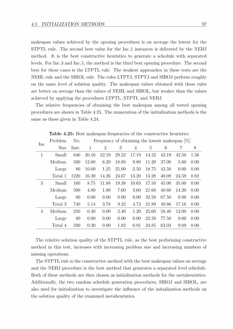
4.5 INITIALIZATION METHODS 97
makespan values achieved by the opening procedures is on average the lowest for the
STPTL rule. The second best value for the Inc 1 instances is delivered by the NEHJ
method. It is the best constructive heuristics to generate a schedule with separated
levels. For Inc 3 and Inc 5, the method is the third best opening procedure. The second
best for these cases is the LTPTL rule. The weakest approaches in these tests are the
NEHL rule and the SIROL rule. The rules LTPTJ, STPTJ and SIROJ perform roughly
on the same level of solution quality. The makespan values obtained with these rules
are better on average than the values of NEHL and SIROL, but weaker than the values
achieved by applying the procedures LTPTL, STPTL and NEHJ.
The relative frequencies of obtaining the best makespan among all tested opening
procedures are shown in Table 4.25. The numeration of the initialization methods is the
same as those given in Table 4.24.
Table 4.25: Best makespan frequencies of the constructive heuristics
IncProblem No. Frequency of obtaining the lowest makespan [%]
Size Inst. 1 2 3 4 5 6 7 8
1 Small 640 20.16 22.19 29.22 17.19 14.22 42.19 42.50 1.56
Medium 500 12.60 6.20 18.80 9.80 11.20 37.00 5.60 0.00
Large 80 10.00 1.25 25.00 2.50 18.75 42.50 0.00 0.00
Total 1 1220 16.39 14.26 24.67 13.20 13.28 40.08 24.59 0.82
3 Small 160 8.75 11.88 19.38 10.63 17.50 45.00 35.00 0.00
Medium 500 4.80 1.80 7.60 3.60 21.60 48.60 14.20 0.00
Large 80 0.00 0.00 0.00 0.00 32.50 67.50 0.00 0.00
Total 3 740 5.14 3.78 9.32 4.73 21.89 49.86 17.16 0.00
4 Medium 250 0.40 0.00 2.40 1.20 25.60 58.40 12.00 0.00
Large 80 0.00 0.00 0.00 0.00 22.50 77.50 0.00 0.00
Total 4 330 0.30 0.00 1.82 0.91 24.85 63.03 9.09 0.00
The relative solution quality of the STPTL rule, as the best performing constructive
method in this test, increases with increasing problem size and increasing numbers of
missing operations.
The STPTL rule is the constructive method with the best makespan values on average
and the NEHJ procedure is the best method that generates a separated level schedule.
Both of these methods are then chosen as initialization methods for the metaheuristics.
Additionally, the two random schedule generation procedures, SIROJ and SIROL, are
also used for initialization to investigate the influence of the initialization methods on
the solution quality of the examined metaheuristics.

4.6 NEIGHBORHOOD STRUCTURES IN RPFS 98
4.6 Neighborhood Structures in Re-entrant Permutation
Flow Shops
Two main neighborhoods are differentiated within this section: the swap neighborhood
and insertion neighborhood. These neighborhoods are examined in different stages:
1. Job stage,
2. Job level stage.
The number of neighbors in the lowest hierarchy stage, which represents changes in
particular members of the permutation, can be limited with so-called block neighbor-
hoods. Grabowski (1982) first mentioned the block structure in flow shops given
by the critical path.15 The block neighborhoods introduced by Nowicki/Smutnicki
(1996) are also based on the critical path of a solution, which defines the makespan of a
permutation.16
The levels l < L of each job i are not allowed to be processed before their succeeding
levels l+1. The levels l > 1 are not allowed to be scheduled before their preceding levels
l − 1.
4.6.1 Swap Moves
Swap moves imply that the sequence positions of two job levels are exchanged. A swap
between a level l of a job i and a level l′ of a job i′ is valid if the following limits to the
sequence position are not exceeded:
• jil < ji′,l′+1 if l′ < L,
• jil > ji′,l′−1 if l′ > 1,
• ji′l′ < ji,l+1 if l < L,
• ji′l′ > ji,l−1 if l > 1.
jil is the sequence position of the first swap partner (the position of job i’s level l). ji′l′
is the position of the second swap partner. Swaps between levels of the same job are
not possible, because they would violate the move limits. The sequence positions of all
other job levels stay the same.
Figure 4.22 illustrates the limits of a swap move of a single job level at position jil in
a given permutation.
15 See Grabowski (1982): Solving the Flow—Shop Problem, pp. 57–58.16 See Nowicki/Smutnicki (1996): Fast taboo search for the job shop problem, pp. 161–165.

4.6 NEIGHBORHOOD STRUCTURES IN RPFS 99
Figure 4.22: Illustration of the swap move limits of a level
b b b ji,l−1 jil ji,l+1 b b b
Considering the second swap partner ji′l′ a possible swap may become invalid because
of the additional move limits of level i′l′. An example is given by Figure 4.23.
Figure 4.23: Example of an invalid level swap
b b b ji,l−1 jil ji′,l′−1 ji′l′ ji,l+1 ji′,l′+1 b b b
Not all swap moves need to be evaluated to find the best neighbor, as Figure 4.24
shows. The dashed lines indicate irrelevant swap moves.
Figure 4.24: Illustration of relevant and irrelevant level swap moves
b b b ji,l−1 jil ji,l+1 b b b
The moves to the left can be omitted in the evaluation of neighbors since they are
equal to the moves to the right side by the corresponding swap partners between ji,l−1
and jil. Either all moves to the right or all moves to the left need to be evaluated. This
leads to a number of 12n · L (n · L− 1) possible swap moves if the move limits of single
levels are not considered. The original permutation on which the moves are performed
determines the specific number of possible swap moves, as seen in the example with two
jobs and L = 2 levels in Figures 4.25 and 4.26.
Two different swap moves can be applied to the permutation given in Figure 4.25.
Figure 4.25: Example of the number of possible level swap moves (I)
j11 j21 j12 j22
It is possible to apply only one swap move on the permutation shown in Figure 4.26.
Figure 4.26: Example of the number of possible level swap moves (II)
j11 j12 j21 j22

4.6 NEIGHBORHOOD STRUCTURES IN RPFS 100
A swap on the job stage needs all levels l = 1, . . . , L of two jobs i and i′ to be exchanged.
Move limits of levels do not need to be considered, as long as both jobs have the same
number of levels. An example is given in Figure 4.27. i = 2 and i′ = 4 are the swapped
jobs.
Figure 4.27: Example of a job swap
j11 j21 j31 j41 j12 j22 j32 j42 j13 j23 j33 j43
4.6.2 Insertion Moves
A job level at position j is picked to be placed at a new sequence position j′. The
conditions on j′ are:
ji,l−1 < j′ ∀i = 1, . . . , n, l = 2, . . . , L; (4.25)
j′ < ji,l+1 ∀i = 1, . . . , n, l = 1, . . . , L− 1. (4.26)
(n · L− 1)2 different insertion moves can be applied to a permutation of the length n ·L
if move limits are not considered.17 Therefore insertion neighborhoods are larger than
swap neighborhoods if n > 2 and L > 1 or n = 2 and L > 2; otherwise, the size of
the neighborhoods is equal. The position of the job levels j′′ = 1, . . . , j′ − 1 does not
change. The job levels on the positions j′′′ = j′ + 1, . . . , j − 1 are respectively shifted to
j′′′ + 1. The remaining levels stay on the same positions. Figure 4.28 shows the limits
of insertion moves. The earliest position for the job level il is right behind the position
of level i, l − 1. The latest position is the one before the level i, l + 1.
Figure 4.28: Illustration of the insertion move limits and valid moves of a level
b b b ji,l−1 jil ji,l+1 b b b
A job insertion move is depicted in Figure 4.29. Two jobs i = 2 and i′ = 4 are selected
for the move. It it necessary to define whether the levels of job i should be inserted in
the position of job i′, or vice versa, before the move is performed. Job i = 2 is inserted
in the positions of i′ = 4 in the given example.
17 See Taillard (1990): Heuristic methods for the flow shop sequencing problem, p. 61.

4.6 NEIGHBORHOOD STRUCTURES IN RPFS 101
Figure 4.29: Example of a job insertion move
j11 j21 j31 j41 j12 j22 j32 j42 j13 j23 j33 j43
The resulting permutation is shown in Figure 4.30. The levels of job i = 2 are now on
the previous sequence positions of the corresponding levels of job i′ = 4.
Figure 4.30: Resulting permutation after the job insertion move
j11 j31 j41 j21 j12 j32 j42 j22 j13 j33 j43 j23
4.6.3 Block Neighborhoods
Block neighborhoods refer to sections in a critical path of a schedule. The blocks are the
sequence positions between two different job levels that follow each other on a critical
path. The critical path of operations determines the makespan of a schedule. Members of
the same block are processed consecutively on the same machine according to Nowicki/
Smutnicki (1996).18
The procedure to identify the critical path is shown in algorithm 4.8.
The identification starts with the last operation of the schedule, which is finished
at the highest value silk + pilk. The sequence position of the corresponding job level is
added to the critical path. The following steps are repeated until the starting time of
an operation equals 0, i.e. the first operation of the schedule is reached. For the latest
identified operation on the critical path, it is determined whether there is an operation
on any k′ of the preceding machines k for the same job level il, which is finished right
before the operation on k starts (silk′ + pilk′ = silk). k is updated to k′ as long as such a
machine is found. If none of the preceding job levels match this requirement, then the
last operation of the preceding level l− 1 of the same job i is added to the critical path.
The last operation added is the first operation of the schedule with a starting time equal
to 0 and a processing time greater than zero.
18 See Nowicki/Smutnicki (1996): Fast taboo search for the job shop problem, p. 161.

4.6 NEIGHBORHOOD STRUCTURES IN RPFS 102
Algorithm 4.8 Identifying a critical path in a re-entrant flow shop
(1) Find the job level, which is finished last (highest value silk + pilk).(2) Add its sequence position j to the critical path.while silk 6= 0 or pilk = 0 do
if There is a machine k′ < k with silk′ + pilk′ = silk then
(3) k ← k′.else
if There is a job level i′l′ at sequence position j′ with si′
l′k + pi′
l′k = silk then
(4a) Add the sequence position j′ of this job level to the critical path.(4b) j ← j′.
else
(4c) Add the sequence position j′ of the job level i, l − 1 to the critical path.(4d) k ← k′, where k′ is the machine with the last operation in i, l − 1.(4e) j ← j′.
end if
end if
end while
(5) Add the sequence position j with silk = 0 and pilk > 0 to the critical path.(6) Reverse the created list.
Figure 4.31: Example of identifying the critical path of operations
k 1 2 3 4 5 6 7 Blockj i l
1 1 1
2 2 1
3 1 2
4 3 1
5 2 2
6 3 2
7 1 3
8 2 3
9 3 3
1
2
3
4
The members of the permutation are the job levels. Some of the job levels define the

4.6 NEIGHBORHOOD STRUCTURES IN RPFS 103
border of the blocks based on the critical path. They are labeled with ub = 0, . . . , B. The
critical path in the example shown in Figure 4.31 contains the job levels at the sequence
positions j = (1, 3, 5, 6, 9). The limits of critical blocks are identified as the positions
ub = (1, 3, 5, 6, 9) ∀b = 0, . . . , B, where B is the number of blocks on the critical path.
Between each pair of adjacent block limits, the operations defining the critical path are
performed on the same machine.
There are two types of moves connected to the block properties. The first type is called
intra block moves and the second type is called across block moves.19 There are different
definitions of intra and across block moves in related literature.20 The definitions are
explained in the following section for swaps and insertion moves. Equivalent moves
yielding to the same permutation are included only once in every neighborhood.
Intra block moves
The figures in this subsection show all possible insertion moves following the particular
block definition. No swap moves are omitted in the figures, despite the fact that some
swap moves are not necessary to obtain all possible solutions in a swap neighborhood,
as explained in subsection 4.6.1. The position of a job i’s level l is labeled with jil in the
following.
Intra block swaps exclude moves to the block border positions ub−1 and ub in the
definition of Nowicki/Smutnicki (1996), as shown in Figures 4.32 and 4.34.21 On the
other hand, the Figures 4.33 and 4.35 show the Chen/Pan/Wu (2007) definition of
intra block moves, which includes swaps to the block borders ub−1 and ub.22
Figure 4.32: Example of a Nowicki intra block swap if jil is not a block border
b b b
ub−2
ji,l−1
ub−1
jil
ub
ji,l+1
ub+1
b b b
Figure 4.33: Example of a Chen intra block swap if jil is not a block border
b b b
ub−2
ji,l−1
ub−1
jil
ub
ji,l+1
ub+1
b b b
19 See Shen/Buscher (2012): Serial batching in job shops , pp. 17–18.20 See Nowicki/Smutnicki (1996): Fast taboo search for the job shop problem, p. 164 and Chen/
Pan/Wu (2007): Reentrant flow-shops and hybrid tabu search, p. 355.21 See Nowicki/Smutnicki (1996): Fast taboo search for the job shop problem, p. 164.22 See Chen/Pan/Wu (2007): Reentrant flow-shops and hybrid tabu search, p. 356.

4.6 NEIGHBORHOOD STRUCTURES IN RPFS 104
A job level that is a block border ub is part of the two blocks, b−1 and b. The possible
intra block swaps for the members of the permutation are shown in Figures 4.34 and
4.35. The Nowicki intra block swaps again exclude moves to the block borders ub−1 and
ub+1, but these moves are included in the Chen intra block swaps.
Figure 4.34: Example of a Nowicki intra block swap if jil is a block border
b b b ji,l−1
ub−1
jil
ub ub+1
ji,l+1
ub+2
b b b
Figure 4.35: Example of a Chen intra block swap if jil is a block border
b b b ji,l−1
ub−1
jil
ub ub+1
ji,l+1
ub+2
b b b
The possible intra block insertion moves are illustrated in Figures 4.36 and 4.37, where
the permutation member is not a block border.
A Nowicki intra block neighborhood allows only moves between the two block borders
ub−1 and ub if the member to move is not on a block border position ub, as can be seen
in Figure 4.36.23
Figure 4.36: Example of a Nowicki intra block insertion if jil is not a block border
b b b
ub−2
ji,l−1
ub−1
jil
ub
ji,l+1
ub+1
b b b
The Chen intra block insertion shown in Figure 4.37, allows a job level to be moved to
the position before the lower block border ub−1 and behind the the upper block border
ub, as well as on all positions between ub−1 and ub.
Figure 4.37: Example of a Chen intra block insertion if jil is not part of the criticalpath
b b b
ub−2
ji,l−1
ub−1
jil
ub
ji,l+1
ub+1
b b b
23 See Nowicki/Smutnicki (1996): Fast taboo search for the job shop problem, p. 164.

4.6 NEIGHBORHOOD STRUCTURES IN RPFS 105
The intra block moves if the job level to move is a block border are displayed in Figures
4.38 and 4.39.
Nowicki moves do not allow changes in the positions of the lower and upper block borders
ub−1 and ub+1. In this case, insertion moves are only allowed between the mentioned block
borders.
Figure 4.38: Example of a Nowicki intra block insertion if jil is a block border
b b b ji,l−1
ub−1
jil
ub ub+1
ji,l+1
ub+2
b b b
Chen intra block insertion moves allow the sequence positions of the block borders
ub−1 and ub+1 to be change. Therefore, a job level that is a block border ub itself is
allowed to be inserted directly before ub−1 as well as directly behind ub+1, as shown in
Figure 4.39.
Figure 4.39: Example of a Chen intra block insertion if jil is a block border
b b b ji,l−1
ub−1
jil
ub ub+1
ji,l+1
ub+2
b b b
Across block moves
Figures 4.40, 4.41, 4.42 and 4.43 show the possible swap move of a permutation member
jil out of its block b. The possible Nowicki across block moves include swaps with
the sequence positions ub−1 and ub, defining the limits of the bth block, because these
positions are also part of the neighboring blocks b− 1 and b+ 1.
Figure 4.40: Example of a Nowicki across block swap if jil is not a block border
b b b
ub−2
ji,l−1
ub−1
jil
ub
ji,l+1
ub+1
b b b
The example in Figure 4.41 illustrates that Chen/Pan/Wu (2007) exclude moves
to ub−1 and ub from across block moves, since they are classified as intra block moves.24
This means that for swap moves, the job levels on the positions ub−1 and ub are not
allowed to be swap partners of jil (Figure 4.41).
24 See Chen/Pan/Wu (2007): Reentrant flow-shops and hybrid tabu search, p. 356.

4.6 NEIGHBORHOOD STRUCTURES IN RPFS 106
Figure 4.41: Example of a Chen across block swap if jil is not a block border
b b b
ub−2
ji,l−1
ub−1
jil
ub
ji,l+1
ub+1
b b b
Swaps to the adjacent block borders ub−1 and ub+1 are seen as across block moves by
Nowicki/Smutnicki (1996) if the permutation member at the jilth position is also a
block border ub, which will be swapped with a member at another position.25
To evaluate all across block swaps in the Nowicki definition of across block moves, not
all moves to the left can be omitted. The move to the left border of the block still needs
to be evaluated if the job level is not a block limit itself.
Figure 4.42: Example of a Nowicki across block swap if jil is a block border
b b b ji,l−1
ub−1
jil
ub ub+1
ji,l+1
ub+2
b b b
Figure 4.43 shows that swap partners of jil, if jil = ub, need to be before ub−1 and
behind ub+1 in the sequence of job levels.
Figure 4.43: Example of a Chen across block swap if jil is a block border
b b b ji,l−1
ub−1
jil
ub ub+1
ji,l+1
ub+2
b b b
The possible across block insertion moves are displayed in Figures 4.44, 4.45, 4.46 and
4.47. Nowicki across block insertion moves allow a job level to be inserted right before
ub−1 and directly behind ub.
Figure 4.44: Example of a Nowicki across block insertion if jil is not a block border
b b b
ub−2
ji,l−1
ub−1
jil
ub
ji,l+1
ub+1
b b b
Chen across block moves do not allow a level to overtake the positions of the border
job levels ub−1 and ub of its block, i.e. the insertion position needs to be lower than or
25 See Nowicki/Smutnicki (1996): Fast taboo search for the job shop problem, p. 164.
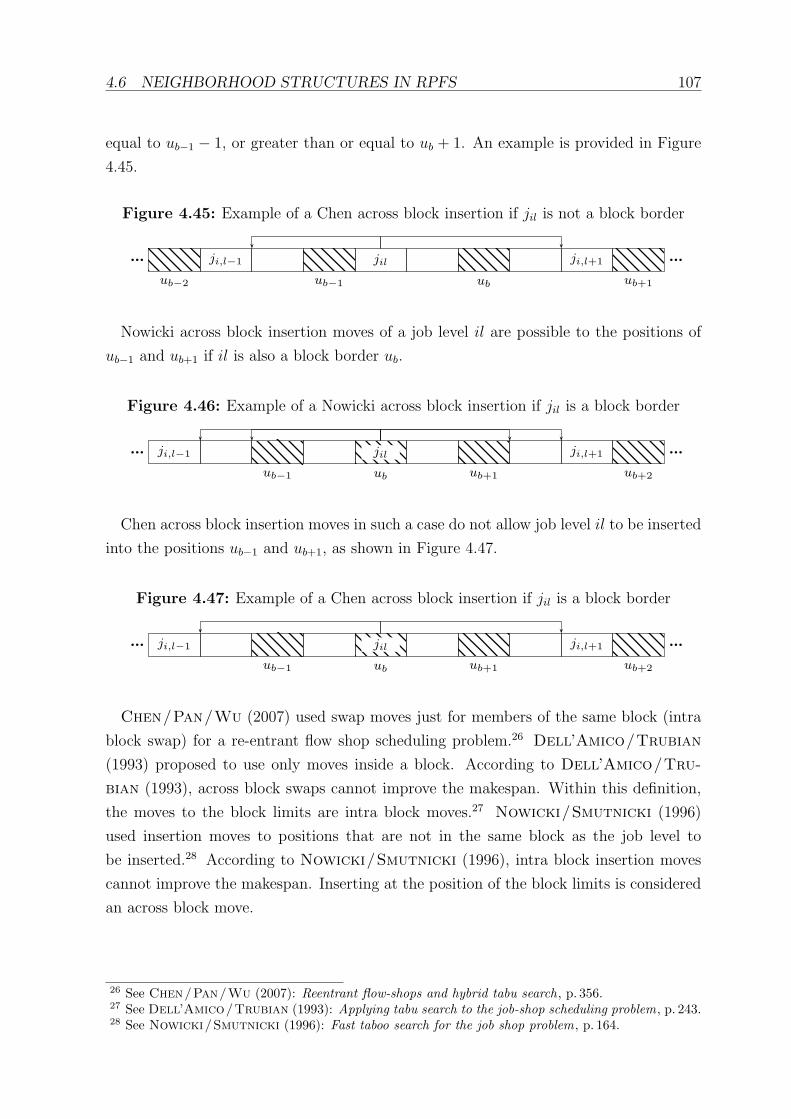
4.6 NEIGHBORHOOD STRUCTURES IN RPFS 107
equal to ub−1 − 1, or greater than or equal to ub + 1. An example is provided in Figure
4.45.
Figure 4.45: Example of a Chen across block insertion if jil is not a block border
b b b
ub−2
ji,l−1
ub−1
jil
ub
ji,l+1
ub+1
b b b
Nowicki across block insertion moves of a job level il are possible to the positions of
ub−1 and ub+1 if il is also a block border ub.
Figure 4.46: Example of a Nowicki across block insertion if jil is a block border
b b b ji,l−1
ub−1
jil
ub ub+1
ji,l+1
ub+2
b b b
Chen across block insertion moves in such a case do not allow job level il to be inserted
into the positions ub−1 and ub+1, as shown in Figure 4.47.
Figure 4.47: Example of a Chen across block insertion if jil is a block border
b b b ji,l−1
ub−1
jil
ub ub+1
ji,l+1
ub+2
b b b
Chen/Pan/Wu (2007) used swap moves just for members of the same block (intra
block swap) for a re-entrant flow shop scheduling problem.26 Dell’Amico/Trubian
(1993) proposed to use only moves inside a block. According to Dell’Amico/Tru-
bian (1993), across block swaps cannot improve the makespan. Within this definition,
the moves to the block limits are intra block moves.27 Nowicki/Smutnicki (1996)
used insertion moves to positions that are not in the same block as the job level to
be inserted.28 According to Nowicki/Smutnicki (1996), intra block insertion moves
cannot improve the makespan. Inserting at the position of the block limits is considered
an across block move.
26 See Chen/Pan/Wu (2007): Reentrant flow-shops and hybrid tabu search, p. 356.27 See Dell’Amico/Trubian (1993): Applying tabu search to the job-shop scheduling problem, p. 243.28 See Nowicki/Smutnicki (1996): Fast taboo search for the job shop problem, p. 164.

4.6 NEIGHBORHOOD STRUCTURES IN RPFS 108
4.6.4 Computational Experiments
The following enumeration is used in Tables 4.26 and 4.27 to evaluate the neighborhoods
presented in Section 4.6:
1 Level swap without considering blocks,
2 Chen intra block level swap,
3 Nowicki intra block level swap,
4 Chen across block level swap,
5 Nowicki across block level swap,
6 Level insertion without considering blocks,
7 Chen intra block level insertion,
8 Nowicki intra block level insertion,
9 Chen across block level insertion,
10 Nowicki across block level insertion,
J1 Job swap,
J2 Job insertion.
The neighborhoods are tested by applying the best neighbor algorithm to the SIROJ
and SIROL solutions on the test instance sets Inc 1, Inc 3 and Inc 4. The test results in
Table 4.26 show the results for small test problems with two to five jobs and levels per
job as well as m ∈ {2, 5, 6, 10} machines. The number of jobs and machines for large test
instances can take the values 10, 20, 30, 40 and 50, and the number of levels per job is
either 5 or 10.29 Ten instances are generated for each combination within the small and
large problems of the sets Inc 1, Inc 3 and Inc 4. Test set Inc 3 includes only problem
sizes with L ≥ 5, and set Inc 4 requires the number of levels L per job to be greater than
or equal to 10.30 The processing times greater than 0 are uniformly distributed random
numbers between 1 and 99. The relative makespan improvement of the initial solution
by applying the best neighbor algorithm is calculated by:
∆C initmax = 1−
Cmax (πBN)
Cmax (πinit).
Cmax (πBN) is the makespan value of the permutation, πBN , after applying the best
neighbor algorithm. Cmax (πinit) is the makespan of the initial solution. The average
values of ∆C initmax are displayed in Tables 4.26 and 4.27.
The mean relative makespan reduction by applying level swap moves is, in most cases,
lower than the improvement values of the corresponding insertion moves for small test
29 See Table B.2 in Appendix B (p. 204) for detailed information on the problem sizes.30 See Table B.1 in Appendix B (p. 203) for an overview of missing operations.

4.6 NEIGHBORHOOD STRUCTURES IN RPFS 109
problems, which is shown in Table 4.26. Swap moves only deliver better average results
for the level moves without block criteria (in test set Inc 1) and the Nowicki across
block moves (with SIROL initialization in Inc 1 and SIROJ initialization in Inc 3). Job
insertion moves also deliver better results on average than job swaps. In Chen block
neighborhoods, intra block moves lead to higher mean average makespan improvements
than across block moves and vice versa for the Nowicki block definition. The Nowicki
across block moves deliver better results than the Chen intra block moves for small
problems.
Table 4.26: Mean makespan deviations ∆C initmax [%] of best neighbors for small problems
NInc 1 Inc 3
SIROJ SIROL SIROJ SIROL
1 3.08 13.39 3.89 9.05
2 2.73 10.76 3.28 7.82
3 1.01 1.20 1.31 1.58
4 1.29 9.00 2.22 5.34
5 3.08 13.39 3.89 9.05
6 3.26 13.26 4.09 10.29
7 2.85 11.08 3.37 8.76
8 1.38 1.85 1.56 2.31
9 1.65 11.16 2.60 8.92
10 3.11 13.25 3.87 10.26
J1 5.09 4.89 3.57 3.41
J2 5.28 16.15 3.84 16.20
The results for large test instances are shown in Table 4.27. The relation between
Chen and Nowicki block moves is similar to the results for small test instances. Also,
here Nowicki across block moves are preferred over the other block criteria moves. The
highest rates of improvement are achieved by job moves. Job swaps are most effective if
the initial solution is based on separated levels. Job insertion moves perform better on
initial random solutions with mixed levels.

4.6 NEIGHBORHOOD STRUCTURES IN RPFS 110
Table 4.27: Mean makespan deviations ∆C initmax [%] of best neighbors for large problems
NInc 1 Inc 3 Inc 4
SIROJ SIROL SIROJ SIROL SIROJ SIROL
1 0.85 5.04 1.16 5.60 1.04 4.20
2 0.53 2.41 0.64 2.67 0.54 2.14
3 0.30 0.35 0.39 0.48 0.34 0.43
4 0.80 5.04 1.14 5.59 1.03 4.20
5 0.85 5.04 1.16 5.60 1.04 4.20
6 0.78 3.21 0.99 3.74 0.81 2.90
7 0.55 2.40 0.66 2.63 0.56 2.12
8 0.33 0.43 0.44 0.59 0.38 0.51
9 0.74 3.21 0.97 3.74 0.81 2.90
10 0.78 3.21 0.98 3.74 0.81 2.90
J1 1.63 1.42 1.80 1.59 1.59 1.40
J2 1.40 6.64 1.54 6.88 1.36 6.27
The computation times are given for the largest tested problem size, 50 jobs, 10 lev-
els and 50 machines, in Table 4.28. The differences in computation time between the
different neighborhoods are highest for this problem size. The computation times are
compared for swaps and insertion neighborhoods, not considering block criteria, Nowicki
across block moves and the two job neighborhoods. Chen block moves and Nowicki intra
block moves are not considered because they deliver weak average makespan results.
The computation times with the best neighbor algorithm are higher for insertion neigh-
borhoods than for the corresponding swap neighborhoods. A higher number of missing
operations leads to lower computation times for single level moves. The application of
the Nowicki block criteria leads to a reduction in the computation time for insertion
moves. The effect for swap moves is low and even increased computation times occur for
some cases.

4.7 IMPROVEMENT METHODS 111
Table 4.28: Average computation times [s] of best neighbor algorithms
NInc 1 Inc 3 Inc 4
SIROJ SIROL SIROJ SIROL SIROJ SIROL
1 54.50 24.10 39.50 24.90 34.00 21.10
5 41.30 32.60 41.40 27.10 39.80 28.00
6 248.70 183.80 249.70 183.00 135.60 177.60
10 91.90 130.20 91.20 93.00 81.50 91.70
J1 1.80 1.50 1.60 1.60 1.40 1.50
J2 32.00 40.80 31.60 40.80 31.60 37.10
The makespan reductions led to the decision to omit the Chen block neighborhoods.
The neighborhoods examined for the configuration of the VNS in section 4.7 are swaps
and insertions for complete jobs and single levels without block criteria, since they achieve
the highest values of makespan improvement. The effects of using Nowicki across block
moves instead of level swaps and insertions without block criteria in the preferred neigh-
borhood hierarchies of Section 4.7 are examined in subsection 4.7.6.
4.7 Improvement Methods
Improvement methods use an initial solution to search for better solutions in prede-
fined neighborhoods. The metaheuristic improvement methods examined are variable
neighborhood search, simulated annealing and tabu search.
4.7.1 Simple Local Search Algorithms
Two common local search algorithms are the first improvement and the best neighbor
algorithms.31 Both are often integrated in metaheuristic solution methods like GRASP32,
particle swarm optimization33 and simulated annealing34 for different flow shop problems.
Both are trajectory methods, applying neighborhood moves to an incumbent solution.
The first improvement algorithm evaluates neighbors in a predefined neighborhood N in
a random order. The first solution found, which improves the initial solution, is accepted
as the new solution. The procedure is shown in algorithm 4.9. The initial solution is
kept, if no improvement can be found. The improvement criterion for the RPFS is the
31 See Widmer/Hertz (1989): A new heuristic method for flow shops , p. 190.32 See Ruiz/Stutzle (2007): Iterated greedy algorithm, p. 2037.33 See Tseng/Liao (2008): Particle swarm optimization for lot-streaming , p. 3105.34 See Naderi/Zandieh/Roshanaei (2009): Scheduling hybrid flowshops with sequence dependent
setup times , p. 1189.

4.7 IMPROVEMENT METHODS 112
makespan of a schedule. The first improvement is considered to shorten the computation
time in local search phases of different algorithms.35
Recalling the method introduced in Chapter 2, the implementation of the first im-
provement algorithm is given by algorithm 4.9.
Algorithm 4.9 First improvement
Data: n, L, m and pilk ∀i = 1, . . . , n; l = 1, . . . , L; k = 1, . . . ,m.
(1) Initial solution: Result of a constructive heuristic πinit.
(2) Update solution: πbest ← πinit.
(3) Identify a list of all tmax valid moves in neighborhood N (πinit).
(4) t← 1.
while t ≤ tmax do
5) Update solution: πt ← πinit.
(6) Perform a random move from the list of moves.
if Cmax (πt) < Cmax (πbest) then
(7) πbest ← πt and t← tmax.
end if
(8) Delete the move from the list of valid moves.
(9) t← t+ 1.
end while
The best neighbor algorithm, shown in algorithm 4.10, evaluates all valid moves in
a predefined neighborhood N . The solution with the lowest makespan is accepted if it
improves the initial solution.
35 See Ishibuchi/Yoshida/Murata (2003): Memetic algorithms for permutation flowshops , p. 205.

4.7 IMPROVEMENT METHODS 113
Algorithm 4.10 Best neighbor
Data: n, L, m and pilk ∀i = 1, . . . , n; l = 1, . . . , L; k = 1, . . . ,m
(1) Initial solution: Result of a constructive heuristic πinit.
(2) Update solution: πbest ← πinit.
(3) Identify a list of all tmax valid moves in neighborhood N (πinit).
(4) t← 1
while t ≤ tmax do
(5) Update solution: πt ← πinit
(6) Perform move t in the list of moves
if Cmax (πt) < Cmax (πbest) then
(7) πbest ← πt
end if
(8) t← t+ 1
end while
Both local search mechanisms are tested in different calibrations of a VNS in Section
4.7.2.
4.7.2 Variable Neighborhood Search
The VNS applied to the RPFS is based on different neighborhood setups. The available
neighborhoods are:
• Swaps of job levels without block criteria,
• Insertion moves of single job levels without block criteria,
• Nowicki across block swaps of single job levels,
• Nowicki across block insertion moves of single job levels,
• Swaps of complete jobs,
• Insertion moves of complete jobs.
The block criteria do not apply to complete jobs, since they are multiply represented
by their levels within the permutation.
The various neighborhoods are used in different hierarchies. The criteria for selecting
the neighborhoods are:
1. Job moves or level moves first,
2. Swap moves or insertion moves first,

4.7 IMPROVEMENT METHODS 114
3. Level moves without considering block criteria or Nowicki across block moves.
The first two characteristics of neighborhood hierarchies are examined in subsection
4.7.5. The third point is investigated in subsection 4.7.6.
The VNS was described first by Mladenovic/Hansen (1997).36 and basically con-
sists of two alternating phases. One phase is called shaking and is used to escape local
optima in order to find another, better, local optimum or the global optimum. The other
phase applies a local search method to identify local optima. A basic overview of the
method is shown in Algorithm 4.11.
Algorithm 4.11 Variable neighborhood search
Data: n, L, m and pilk ∀i = 1, . . . , n; l = 1, . . . , L; k = 1, . . . ,m
(1) Initial solution: Result of a constructive heuristic πinit.
(2) Update solution: πbest ← πinit
(3) t← 1
while t ≤ tmax do
(4) Shaking:
Select random neighbor π ∈ Nt (πbest)
(5) Local Search:
First improvement algorithm or best neighbor algorithm in Nt (π) to obtain the
local search solution π′.
if Cmax (π′) < Cmax (πbest) then
(6a) πbest ← π′ and t← 1
else
(6b) t← t+ 1
end if
end while
Initial Solution
The initial solution for the VNS is generated by one of the suggested constructive heuris-
tics, i.e. NEHJ, SIROJ, STPTL or SIROL.
Shaking
The shaking phase provides the possibility to leave local optima in order to obtain an
even better solution than the current best in an additional local search phase. The
shaking applies if no improvement is found within a selected neighborhood. The next
neighborhood is selected, and a random valid move within this neighborhood is made.
36 See Mladenovic/Hansen (1997): Variable neighborhood search, pp. 1097–1098.

4.7 IMPROVEMENT METHODS 115
The different a = 1, . . . , 8 neighborhood hierarchies N at are presented in Table 4.29.
“J-swap” (neighborhood N = J1) and “J-insert” (N = J2) are neighborhood definitions
that require moves of all levels of the selected jobs. “L-swap” (neighborhood N = 1)
and “L-insert” (N = 6) are single level move neighborhoods. Block criteria are not
considered for the level moves for the tests in subsection 4.7.5.
Table 4.29: Examined neighborhood hierarchies
t N 1t N 2
t N 3t N 4
t N 5t N 6
t N 7t N 8
t
1 J-swap J-insert J-swap J-insert L-insert L-swap L-insert L-swap
2 J-insert J-swap L-swap L-insert L-swap J-swap J-insert J-swap
3 L-swap L-insert J-insert J-swap J-insert L-insert L-swap L-insert
4 L-insert L-swap L-insert L-swap J-swap J-insert J-swap J-insert
Hansen/Mladenovic (1997) preferred to start in neighborhoods that are defined
by relatively small changes in the current solution.37 It is disputable whether insertion
or swap moves imply larger changes in a given solution. Insertion moves change the
sequence position of a minimum of two job levels in the permutation, but may also affect
more than one sequence position since they can shift several members of the permutation
to the right or to the left. Swap moves of two permutation members, on the other hand,
are limited to two changes in the permutation position. Job moves define neighborhoods
that yield relatively large changes in the solution structure, since multiple job levels are
inserted or swapped. The issue of dividing a permutation into blocks and the resulting
neighborhoods of moves within a block or to another block are not directly linked to a
larger or smaller neighborhood. There can only be a small number of valid moves due
to tight technological move limits of a permutation member.
Integrated Local Search Algorithm
The shaking is followed by a local search phase. Two different methods are tested within
this local search phase:
• First improvement,
• Best neighbor.
One of the local search methods is applied on the shaking solution. There is no change
in the shaking solution if no improvement is found. In this case the VNS changes to the
37 See Hansen/Mladenovic (1997): Variable neighborhood search for the p-median, p. 211.

4.7 IMPROVEMENT METHODS 116
next neighborhood Nt+1 and repeats the shaking on the best solution, πbest, found at
that point.
Iterations and Termination
The algorithm terminates if the tmaxth neighborhood is reached and no better solution
compared to the current best is found.
4.7.3 Tabu Search
The tabu search looks for the best neighbor in each iteration. Neighbors that are part of
the tabu list are not accepted if they do not lead to large improvements in the objective
value. The tabu list stores forbidden moves to prevent the algorithm from becoming
stuck in local optima. The size of such tabu lists and the tabu tenure can be fixed
or variable. The calibration of the implemented tabu search is based on Nowicki/
Smutnicki (1996).38 The initial solutions are created with one of the constructive
heuristics NEHJ, SIROJ, STPTL or SIROL.
The maximum number of tabu search iterations is limited to tmax = 5000 for every
problem. The calibration of the tabu search, shown in Figure 4.12, is explained in the
following.
38 See Nowicki/Smutnicki (1996): Fast taboo search for the job shop problem, pp. 161–167.

4.7 IMPROVEMENT METHODS 117
Algorithm 4.12 Tabu search
Data: n, L, m, A and pilk ∀i = 1, . . . , n; l = 1, . . . , L; k = 1, . . . ,m.
(1) Initial solution: Result of a constructive heuristic πinit.
(2) Update solution: πbest ← πinit, π ← πinit.
(3) t← 1.
while t ≤ tmax do
(4) Create candidate list: All moves to the permutations π′ ∈ N (π) and evaluate
the candidates.
(5) Select Candidate: Choose the candidate πt with the minimum Cmax (πt) among
all candidates.
if Candidate is a tabu and Aspiration function value F asp ≤ Cmax (πt). then
if Tabu list size > 0 then
(6a) Cmax (πt)← A and go back to (5).
else
(6b) Remove tabu list row 1 and restore candidate list and the Cmax values.
end if
else
(7) π ← πt and t← t+ 1 and Add move to tabu list.
if Cmax (π) < Cmax (πbest) then
(8) πbest ← π.
end if
if Tabu list size > 8 then
(9) Remove tabu list row 1.
end if
end if
end while
Tabu list
The tabu list size is chosen to be static with eight rows. Nowicki/Smutnicki (1996)
used a static tabu list of the size eight.39 This leads to a tabu tenure for each row in the
tabu list of eight iterations. The tabu moves are recorded by the following scheme:
For insertion moves, the two items registered within the tabu list are:
1. The job or job level that has been moved,
2. The job or job level that took its position within the permutation.
39 See Nowicki/Smutnicki (1996): Fast taboo search for the job shop problem, p. 170.

4.7 IMPROVEMENT METHODS 118
An insertion move is tabu if it changes the sequence position of any of the recorded pairs
of job levels or jobs in the tabu list. The entry for job swaps is the two participating
jobs. The pair of participating job levels is added to the tabu list in case of a level
swap neighborhood. A move is tabu if there is a pair of jobs or job levels that change
their sequence position by applying the move and are identical to a pair of jobs or job
levels within the tabu list. Nowicki/Smutnicki (1996) used Nowicki across block
level insertion moves (neighborhood N = 10). These moves and job insertion moves
(N = J2) are the neighborhoods tested in subsection 4.7.5.
Aspiration function
Nevertheless, a tabu move can be accepted if a certain aspiration criterion is fulfilled. The
aspiration function within this implementation of tabu search compares the makespan,
Cmax (πt), of the tabu move in iteration t and the tabu permutation, with so-called
income and outcome values. Considering the tabu solution πt of an iteration t, the
income makespan value is defined as CImax (πt) = Cmax (πt−1), i.e. the makespan value
of the previous iteration. The outcome is defined as COmax (πt) = Cmax (πt+1), i.e. the
makespan value of the next iteration. Two values FI (Cmax (πt)) and FO (Cmax (πt)) are
necessary to decide whether or not a tabu move should be accepted via the aspiration
function. To determine the income value FI and the outcome value FO, the income and
outcome values of the relevant iterations resulting in a permutation with an objective
value of Cmax (πt′) = Cmax (πt) are compared. The maximum values of these incomes
CImax (πt′) ∀t
′ = t′ = 2, . . . , t and outcomes COmax (πt) ∀t
′ = 1, . . . , t − 1 are the values
FI (Cmax (πt)) and FO (Cmax (πt)). The aspiration function chooses the minimum of value
FI (Cmax (πt)) and FO (Cmax (πt)) by equation (4.31) and compares it to the objective
value Cmax (πt) of the tabu permutation. If the makespan value obtained by the tabu
move is lower than the aspiration value, then the tabu move is accepted and the iteration
counter t is increased by one, otherwise the next candidate will be chosen.
A summary of the calculations for the aspiration function value F asp is given by the
following equations (4.27)-(4.31).
CImax (πt′) = Cmax (πt′−1) , (4.27)
FI (Cmax (πt)) = mint′=2,...,t
{
CImax (πt′)
}
, (4.28)
COmax (πt′) = Cmax (πt′+1) , (4.29)
FO (Cmax (πt)) = mint′=1,...,t−1
{
COmax (πt′)
}
(4.30)
F asp = min {FI ;FO} . (4.31)

4.7 IMPROVEMENT METHODS 119
The implemented algorithm for finding the aspiration value F is shown with the pseudo
code 4.13.
Algorithm 4.13 Finding the value of the aspiration function
Data: current iteration number t, Cmax (πt) ∀t′
= 1, . . . , t, A.
(1) FI ← A, FO ← A
(2) t′ ≤ 1
while t′ ≤ t do
if Cmax (πt′) = Cmax (πt) then
if t′ > 1 and Cmax (πt′−1) < FI then
(3a) FI ← Cmax (πt′−1)
end if
if t′ < t and Cmax (πt′+1) < FO then
(3b) FO ← Cmax (πt′+1)
end if
end if
(4) t′ ← t′ + 1
end while
(5) F asp ← min {FI ;FO}
If a makespan value is lower than the aspiration value, then the tabu move is accepted
and the next iteration begins.
4.7.4 Simulated Annealing
Simulated annealing uses another scheme to avoid being stuck in a local optimum. Worse
objective values than in previous iterations are accepted with a certain probability. This
probability declines with the number of iterations. The chosen implementation of simu-
lated annealing is based on Osman/Potts (1989)40 and summarized in algorithm 4.14.
The initialization is done with one of the suggested constructive methods used also for
the VNS and the TS. The temperature in each iteration is T t.
40 See Osman/Potts (1989): Simulated annealing for permutation flow-shop scheduling , pp. 551–557.

4.7 IMPROVEMENT METHODS 120
Algorithm 4.14 Simulated annealing
Data: n, L, m, T 1, K and pilk ∀i = 1, . . . , n; l = 1, . . . , L; k = 1, . . . ,m.
(1) Initial solution: Result of a constructive heuristic πinit.
(2) Update solution: πbest ← πinit
while T t ≥ Tmin do
(3) Create random neighbor: π′ ∈ N (π).
if Cmax (π′) < Cmax (π) then
(4a) π ← π′.
if Cmax (π′) < Cmax (πbest) then
(4b) πbest ← π′
end if
else
(4c) Create random number 0 ≤ r ≤ 1.
if r ≤ P = e−Cmax(π)−Cmax(π′)
Tt then
(4d) π ← π′.
end if
end if
(5) T t+1 ← T t/(
1 +K · T t)
.
end while
Annealing scheme
The initial temperature is calculated by T 1 =∑n
i=1
∑Ll=1
∑mk=1 p
ilk/ (5 · n · L ·m). The
algorithm terminates when T t < Tmin = 1. The number of iterations per temperature
state is one. The annealing scheme by Osman/Potts (1989) is based on the number of
temperature states, which depends on the initial temperature. The annealing function
for the re-entrant permutation flow shop in this thesis is based on the calculation of
annealing parameters of Osman/Potts (1989), but its parameters K and K depend
on the neighborhood type. The first annealing parameter for level move neighborhoods
is calculated by:
K = max {3300 log (n · L− L+ 1) + 7500 logm− 18250; 2000} .
The calculation of the parameter is slightly different for job move neighborhoods:
K = max {3300 log n+ 7500 logm− 18250; 2000} .

4.7 IMPROVEMENT METHODS 121
The parameter K for job moves is calculated with log n because there are n different
positions in a job permutation and every job is allowed to change to every position
in every possible permutation. A level permutation consists of n · L positions, but
not every level is allowed to change its position arbitrarily. This limitation of moves
grows with a higher number of levels per job L. Therefore, L is subtracted from n · L
in log (n · L− L+ 1) if the neighborhood is a level move neighborhood. The second
annealing parameter is defined by:
K =T 1 − Tmin
(K − 1) · T init · Tmin
The annealing scheme for each iteration t is Tt+1 = T/(
1 +K · Tt
)
.
Probabilistic function
The probabilistic function generates a probability P , which is the probability of accepting
a worse value of the makespan compared to the previous solution:
P = e−Cmax(π)−Cmax(π′)
T .
Additionally, a uniformly distributed continuous random number 0 ≤ r ≤ 1 is gener-
ated. For r ≤ P , the new solution is accepted and the objective value updated. The
probabilistic function is suggested by Osman/Potts (1989), Ogbu/Smith (1990) and
Ogbu/Smith (1991) and for permutation flow shop problems.41
Neighborhoods
The neighborhoods used to generate new solutions for the experiments in subsection
4.7.5 are the level insertion (N = J2) and job insertion neighborhood (N = 6), because
Osman/Potts (1989) recommended insertion neighborhoods. Block criteria are not
considered.
4.7.5 Computational Experiments
This subsection compares different configurations of the variable neighborhood search,
tabu search and simulated annealing for the minimization of the makespan in re-entrant
permutation flow shops. The aim of the computational experiments is to find an ap-
propriate configuration for the VNS and to find out if it is superior to the TS and SA.
41 See Osman/Potts (1989): Simulated annealing for permutation flow-shop scheduling , p. 553,Ogbu/Smith (1990): Simulated annealing for the n/m/C max flowshop problem, p. 64 and Ogbu/Smith (1991): Simulated annealing for the permutation flowshop problem, p. 244.

4.7 IMPROVEMENT METHODS 122
The VNS configurations are denominated by “VNSa” and “BN” for a best neighbor local
search or “FI” for a first improvement local search. a stands for the number, suggested in
subsection 4.7.2, of the neighborhood hierarchies for the VNS. The tabu search is tested
with a job insertion (N = J2) and a Nowicki across block level insertion neighborhood
(N = 10). The simulated annealing approach uses a simple level insertion (N = 6) and
a job insertion neighborhood (N = J2). All metaheuristics are tested with four different
initialization methods (NEHJ, SIROJ, STPTL and SIROL).
Test instances
The parameters of the problem size are n ∈ {2, 3, 4, 5}, L ∈ {2, 3, 4, 5}, and m ∈
{2, 5, 6, 10} for small problems and n ∈ {20, 40}, L ∈ {5, 10}, and m ∈ {20, 40} for large
problems.42 The processing times are uniformly distributed random numbers between 1
and 99. Ten test instances are generated for each problem size. Missing operations are
generated about the Inc 1 and Inc 3 schemes.43
Results
Table 4.30 shows the average makespan deviations between all solutions calculated by
the metaheuristics and the MIP solutions for the small test instances. The aim of this
evaluation is to determine a method to use for small problem sizes, by taking into account
the deviation to the MIP solution. The MIP solutions are obtained with CPLEX 12.4
with a computation time limit of 1 hour. The makespan deviation is defined as:
∆CMIPmax =
Cmax (πmeta)
Cmax (πMIP )− 1.
Cmax (πMIP ) stands for the makespan value of a MIP solution. Cmax (πmeta) is the
makespan with the permutation πmeta calculated by a metaheuristic. The VNS4 BN
delivers the best results for the small instances of test set Inc 1 independently from the
initialization method used, and for the Inc 3 instances if the initial solution is created
with the SIROL rule. The VNS3 BN has three times the lowest average ∆CMIPmax for small
Inc 3 instances. These results imply the use of either the VNS3 BN or VNS4 BN for
small problem sizes. The computation times are negligible for these problem sizes. The
initialization with the STPTL rule delivers, on average, the best results for the VNS3
BN and VNS4 BN. There is a tendency of higher deviations to the MIP solutions in the
Inc 3 set than in the Inc 1 set. This means that a higher number of missing operations
makes it harder for the heuristic solution approaches to find a near optimal or optimal
42 See Table B.2 in Appendix B (p. 204) for detailed information on the problem sizes.43 See Table B.1 in Appendix B (p. 203) for an overview of missing operations.

4.7 IMPROVEMENT METHODS 123
solution.
Table 4.30: Average makespan deviation ∆CMIPmax [%] for small problems
Inc 1 Inc 3
NEHJ SIROJ STPTL SIROL NEHJ SIROJ STPTL SIROL
VNS1 BN 2.02 1.90 1.63 2.88 4.34 4.87 3.23 4.95
VNS2 BN 2.05 1.93 1.66 2.89 4.85 4.84 3.38 6.37
VNS3 BN 2.11 1.91 1.69 2.76 4.09 4.15 2.63 4.92
VNS4 BN 1.84 1.79 1.61 2.67 4.32 4.51 3.08 4.44
VNS5 BN 2.08 2.21 1.77 3.08 4.84 4.32 3.22 5.48
VNS6 BN 2.03 2.15 1.77 3.32 4.29 4.38 2.98 6.25
VNS7 BN 1.97 2.24 1.72 2.69 5.02 4.70 2.94 4.80
VNS8 BN 1.98 2.46 1.75 3.27 4.72 4.29 3.23 5.98
VNS1 FI 3.27 3.31 2.66 10.10 7.54 8.01 4.08 19.30
VNS2 FI 2.55 2.90 2.20 3.45 5.93 6.34 4.44 7.73
VNS3 FI 3.18 3.42 2.54 8.47 8.70 8.37 4.60 12.73
VNS4 FI 3.43 3.60 2.58 5.46 8.21 8.45 4.53 11.28
VNS5 FI 3.32 4.09 2.64 7.56 6.67 6.41 4.84 11.49
VNS6 FI 3.34 3.61 2.65 6.64 7.14 8.19 4.76 10.84
VNS7 FI 3.90 4.34 2.94 7.73 7.35 7.16 4.72 11.60
VNS8 FI 3.88 4.32 2.89 7.40 7.01 7.25 4.69 11.29
TS N = J2 4.63 4.98 3.18 29.53 10.35 10.62 5.79 36.03
TS N = 10 5.70 7.60 4.32 35.27 9.30 10.54 5.85 47.04
SA N = J2 6.63 7.69 4.97 35.01 11.61 12.02 7.21 37.52
SA N = 6 8.10 10.64 6.42 46.09 12.85 14.92 8.33 58.47
Best 1.84 1.79 1.61 2.67 4.09 4.15 2.63 4.44
The values of mean makespan reduction for large problem sizes are considered (Table
4.31) to get a pre-selection on the constructive methods used for initialization of the
metaheuristics. The table shows the average deviation of a solution obtained with a
certain method from the best solution over all methods. The values are calculated by:
∆Cbestmax =
Cmax (πmeta)
Cmax (πbest)− 1.
The lowest obtained makespan value for a problem instance is denoted with Cmax (πbest).
The mean deviations from the best achieved makespan, which are obtained with the
STPTL rule, an opening procedure for the metaheuristics, are the lowest for all meta-
heuristics in the test instance sets Inc 1 and Inc 3. The weakest results for every meta-

4.7 IMPROVEMENT METHODS 124
heuristic are obtained with the SIROL rule.
The values for the Inc 3 instances are slightly higher than the makespan deviations in
the Inc 1 instances.
Table 4.31: Average makespan deviation ∆Cbestmax [%] for large problems
Inc 1 Inc 3
NEHJ SIROJ STPTL SIROL NEHJ SIROJ STPTL SIROL
VNS1 BN 2.29 2.38 1.29 37.69 5.24 6.02 1.47 32.27
VNS2 BN 2.58 2.71 1.84 25.56 5.29 5.93 1.62 26.26
VNS3 BN 2.28 2.16 1.69 46.03 5.51 5.54 1.73 43.78
VNS4 BN 2.48 2.45 1.78 25.16 5.80 5.35 1.98 24.82
VNS5 BN 2.58 2.73 2.57 50.30 5.22 5.10 2.47 44.27
VNS6 BN 2.87 2.60 2.29 48.26 5.39 5.95 2.25 43.87
VNS7 BN 2.84 2.33 2.14 39.86 5.79 5.12 2.17 38.97
VNS8 BN 2.63 2.60 1.88 50.33 5.29 4.75 2.03 47.68
VNS1 FI 3.30 3.34 2.57 183.62 7.73 7.41 3.13 164.08
VNS2 FI 2.70 3.23 1.87 27.17 6.57 6.82 2.25 27.80
VNS3 FI 3.06 3.06 2.15 166.62 7.65 7.44 2.59 156.29
VNS4 FI 3.17 3.26 2.35 30.57 7.44 7.48 2.46 26.76
VNS5 FI 6.00 6.13 5.69 135.77 9.69 10.26 5.96 115.10
VNS6 FI 4.14 4.08 3.53 44.72 7.84 8.31 3.97 43.88
VNS7 FI 5.27 5.83 4.75 125.86 10.06 9.87 5.29 111.29
VNS8 FI 6.50 6.64 6.01 86.73 10.55 10.62 5.85 73.32
TS N = J2 6.05 6.28 5.07 259.68 11.20 11.79 5.33 234.45
TS N = 10 6.62 6.92 5.92 272.20 11.80 12.30 6.02 245.44
SA N = J2 3.86 4.28 3.07 122.42 8.89 9.36 3.74 117.31
SA N = 6 7.40 7.69 6.63 279.25 12.66 13.14 6.87 255.64
Best 2.28 2.16 1.29 25.16 5.24 4.75 1.47 24.82
The main area of application for heuristics contains large problem sizes; therefore, the
results for the large problem sizes are examined in the following. The average makespan
reductions are used to compare the different metaheuristic improvement methods and
their different configurations. The relative makespan reductions of the metaheuristic
solutions compared to the initial solutions are:
∆C initmax = 1−
Cmax (πmeta)
Cmax (πinit).

4.7 IMPROVEMENT METHODS 125
The mean values of the large instances are shown in Table 4.32.44 The VNS with neigh-
borhood hierarchy a = 1 in combination with a best neighbor local search delivers the
highest mean improvements in three cases: two times when the the initial solution is pro-
vided by the STPTL rule (for Inc 1 and Inc 3 instances), and once for a initial solution
with the NEHJ method for the Inc 3 instances. The other mean makespan reduction
values of the VNS1 BN are not far from the best achieved, except for the initializa-
tion with the SIROJ rule in test set Inc 3. All metaheuristics deliver the worst results
when they are initialized with the SIROL rule. If only VNS configurations with the
first improvement local search are considered, then neighborhood hierarchy a = 2, i.e.
VNS2 FI, is the most promising approach for large instances. The solutions achieved
with best neighbor local search are better than those obtained with first improvement.
Tabu search and simulated annealing deliver weak results compared to the VNS1 BN
and VNS2 FI. The tested job neighborhoods are superior to the level moves for tabu
search and simulated annealing.
44 The average makespan reductions, ∆Cinit
max, for small problems are provided by Table C.1 in Appendix
C (p. 206).

4.7 IMPROVEMENT METHODS 126
Table 4.32: Average makespan reductions ∆C initmax [%] for large problems
Inc 1 Inc 3
NEHJ SIROJ STPTL SIROL NEHJ SIROJ STPTL SIROL
VNS1 BN 4.79 4.96 5.05 63.43 6.61 6.38 5.13 62.04
VNS2 BN 4.52 4.66 4.54 66.51 6.53 6.45 4.98 63.58
VNS3 BN 4.80 5.16 4.69 61.30 6.35 6.77 4.90 58.94
VNS4 BN 4.61 4.87 4.60 66.52 6.08 6.94 4.65 64.11
VNS5 BN 4.51 4.62 3.85 60.15 6.57 7.12 4.21 58.76
VNS6 BN 4.23 4.74 4.13 60.72 6.42 6.39 4.41 58.96
VNS7 BN 4.27 4.98 4.26 62.93 6.07 7.09 4.47 60.32
VNS8 BN 4.47 4.75 4.51 60.19 6.53 7.42 4.62 57.88
VNS1 FI 3.86 4.07 3.88 25.59 4.46 5.18 3.60 25.88
VNS2 FI 4.41 4.18 4.52 66.12 5.43 5.69 4.40 63.12
VNS3 FI 4.08 4.35 4.27 30.04 4.53 5.18 4.09 28.29
VNS4 FI 3.99 4.15 4.06 65.10 4.68 5.12 4.21 63.42
VNS5 FI 1.36 1.50 0.99 38.26 2.69 2.65 0.97 39.50
VNS6 FI 3.09 3.38 2.97 61.52 4.31 4.38 2.81 58.86
VNS7 FI 2.04 1.78 1.85 40.77 2.40 3.03 1.58 40.07
VNS8 FI 0.90 1.02 0.68 50.74 1.94 2.31 1.07 51.00
TS N = J2 1.33 1.37 1.54 6.23 1.43 1.38 1.56 6.55
TS N = 10 0.79 0.78 0.77 2.98 0.90 0.94 0.92 3.55
SA N = J2 3.35 3.23 3.41 40.95 3.47 3.51 3.03 38.14
SA N = 6 0.08 0.07 0.11 1.10 0.15 0.20 0.14 0.60
Best 4.80 5.16 5.05 66.52 6.61 7.42 5.13 64.11
Further information on the solution quality of the tested metaheuristics is provided in
Figures 4.48 and 4.49. They compare how often a metaheuristic obtains the best solution
among all the tested methods. Additionally, the frequency of obtaining the best solution
is shown if only solutions based on an initial STPTL solution are compared. The best
solution is most often achieved by the VNS1 BN method. The VNS2 FI delivers most
frequently the best solutions among the procedures with short computation times.

4.7 IMPROVEMENT METHODS 127
Figure 4.48: Frequency of obtaining best solutions for large Inc 1 problems
VNS1 BN
VNS2 BN
VNS3 BN
VNS4 BN
VNS5 BN
VNS6 BN
VNS7 BN
VNS8 BN
VNS1 FI
VNS2 FI
VNS3 FI
VNS4 FI
SA N=J2
Other
0 5 10 15 20 25
Only with STPTL ruleOver all opening procedures
Figure 4.49: Frequency of obtaining best solutions for large Inc 3 problems
VNS1 BN
VNS2 BN
VNS3 BN
VNS4 BN
VNS5 BN
VNS6 BN
VNS7 BN
VNS8 BN
VNS1 FI
VNS2 FI
VNS3 FI
VNS4 FI
SA N=J2
Other
0 5 10 15 20 25
Only with STPTL ruleOver all opening procedures

4.7 IMPROVEMENT METHODS 128
Figures 4.50 and 4.51 provide an overview of the computation times of the different
improvement methods for Inc 1 instances. The computation times for problems with an
increased number of missing operations, i.e. Inc 3 instances, can be seen in Appendix C.
The value refers only to the time used to improve an initial solution and the computation
times for initialization are not included. The shortest computation times are achieved
with the first improvement VNS, tabu search in all configurations and the simulated
annealing with level moves. The computation times are higher if the opening procedure
is SIROL. This leads to values higher than 15000 seconds for the VNS5 BN and VNS7
BN.

4.7 IMPROVEMENT METHODS 129
Figure 4.50: Average computation times for large Inc 1 instances (I)
VNS1
Com
puta
tion t
ime
[s]
20520
40520
201020
401020
20540
40540
201040
401040
0
1000
2000
3000
4000
Problem size
mLn
BN NEHJBN SIROJBN STPTLBN SIROLFI NEHJFI SIROJFI STPTLFI SIROL
VNS2
Com
puta
tion t
ime
[s]
20520
40520
201020
401020
20540
40540
201040
401040
0
1000
2000
3000
4000
Problem size
mLn
BN NEHJBN SIROJBN STPTLBN SIROLFI NEHJFI SIROJFI STPTLFI SIROL
VNS3
Com
puta
tion
tim
e [s
]
20520
40520
201020
401020
20540
40540
201040
401040
0
1000
2000
3000
4000
Problem size
mLn
BN NEHJBN SIROJBN STPTLBN SIROLFI NEHJFI SIROJFI STPTLFI SIROL
VNS4
Com
puta
tion
tim
e [s
]
20520
40520
201020
401020
20540
40540
201040
401040
0
1000
2000
3000
4000
5000
Problem size
mLn
BN NEHJBN SIROJBN STPTLBN SIROLFI NEHJFI SIROJFI STPTLFI SIROL
VNS5
Com
puta
tion
tim
e [s
]
20520
40520
201020
401020
20540
40540
201040
401040
0
5000
10000
15000
20000
Problem size
mLn
BN NEHJBN SIROJBN STPTLBN SIROLFI NEHJFI SIROJFI STPTLFI SIROL
VNS6
Com
puta
tion
tim
e [s
]
20520
40520
201020
401020
20540
40540
201040
401040
0
1000
2000
3000
4000
5000
6000
7000
Problem size
mLn
BN NEHJBN SIROJBN STPTLBN SIROLFI NEHJFI SIROJFI STPTLFI SIROL

4.7 IMPROVEMENT METHODS 130
Figure 4.51: Average computation times for large Inc 1 instances (II)
VNS7
Com
puta
tion t
ime
[s]
20520
40520
201020
401020
20540
40540
201040
401040
0
5000
10000
15000
20000
Problem size
mLn
BN NEHJBN SIROJBN STPTLBN SIROLFI NEHJFI SIROJFI STPTLFI SIROL
VNS8
Com
puta
tion t
ime
[s]
20520
40520
201020
401020
20540
40540
201040
401040
0
1000
2000
3000
4000
5000
6000
Problem size
mLn
BN NEHJBN SIROJBN STPTLBN SIROLFI NEHJFI SIROJFI STPTLFI SIROL
TS
Com
puta
tion
tim
e [s
]
20520
40520
201020
401020
20540
40540
201040
401040
0
50
100
150
200
Problem size
mLn
N=J2 NEHJN=J2 SIROJN=J2 STPTLN=J2 SIROLN=10 NEHJN=10 SIROJN=10 STPTLN=10 SIROL
SA
Com
puta
tion
tim
e [s
]
20520
40520
201020
401020
20540
40540
201040
401040
0
100
200
300
400
500
Problem size
mLn
N=J2 NEHJN=J2 SIROJN=J2 STPTLN=J2 SIROLN=6 NEHJN=6 SIROJN=6 STPTLN=6 SIROL
The STPTL rule is suggested for further applications of the investigated metaheuristics
for re-entrant permutation flow shops with mixed levels and missing operations, because
of the results in this subsection. The VNS, especially its configurations VNS1 BN, is
superior in solution quality to the investigated tabu search and simulated annealing
configurations. The reason lies in the advanced exploitation of the solution space in
re-entrant permutation flow shops by applying job and level moves. The VNS1 BN is
further used in subsection 4.7.6 and Chapter 5 to minimize the makespan in re-entrant
permutation flow shops. An advantage of an integrated first improvement local search for
the VNS is its relatively short computation time. Hence, the VNS2 FI is also suggested
for the makespan minimization in re-entrant permutation flow shops and is used in
subsection 4.7.6 and Chapter 5.

4.7 IMPROVEMENT METHODS 131
Chen/Pan/Lin (2008), Chen/Pan/Wu (2008) and Qian et al. (2013b) ran tests
with other heuristic solution methods on similar problem sizes for re-entrant permuta-
tion flow shop problems. These authors published improvement rates over their NEHJ
solutions. Chen/Pan/Wu (2008) suggested a hybrid tabu search. The improvement
rates of makespan, ∆C initmax, over NEHJ solutions were between 2 and 4 % for test in-
stances similar to the here tested large problems.45 The hybrid genetic algorithm of
Chen/Pan/Lin (2008) delivered improvement rates between 1 and 4.5 % for small
problem sizes.46 Qian et al. (2013b) tested two differential evolution algorithms and the
hybrid genetic algorithm of Chen/Pan/Lin (2008) with medium and large problem
instances. The average value of ∆C initmax over the NEHJ solutions was 1.62 % for the
hybrid genetic algorithm, 4.39 % for the first differential evolution algorithm and 5.32
% for the second differential evolution algorithm if only problem instances with n ≥ 20
are considered.47 The suggested variable neighborhood search configurations, VNS1 BN
/ VNS2 FI, deliver average improvement values of 5.50 / 5.10 % (Inc 1) and 7.50 / 6.03
% (Inc 3) for small instances and 4.79 / 4.41 % (Inc 1) and 6.61 % / 5.43 % (Inc 3) for
large instances. The VNS configurations achieve obviously better makespan values. The
tests by Qian et al. (2013a) were performed on a similar computer system to the one
used for this thesis. The computation times of the differential equation algorithms for
the large problems sizes were regularly several hours. The suggested variable neighbor-
hood searches with only several hundred seconds are much faster than the approaches of
Qian et al. (2013a). The VNS is also superior to the iterated local search, which only
uses a level swap neighborhood, as proposed by Hinze/Sackmann (2016).48
4.7.6 Improvement of Metaheuristics
This subsection investigates the influence of exchanging the level moves without block
criteria with the corresponding Nowicki across block swap and insertion moves for the
VNS. The resulting VNS algorithms for the configurations suggested in subsection 4.7.5
are denoted with VNS1 BN* and VNS2 FI*. The tabu search with level moves uses
across block swaps (N = 5) instead of across block insertion moves, because of the
results on large instances in the neighborhood experiments. The same neighborhood
is also tested within the simulated annealing approach. Furthermore, neighborhoods
in the tabu search and simulated annealing only using job moves are changed to job
swaps (N = 11) instead of job insertion moves. All metaheuristics are initialized with
the STPTL rule. The target of the experiment is to find out how these changes in
45 See Chen/Pan/Wu (2008): Hybrid tabu search for re-entrant flow-shops , pp. 1928–1929.46 See Chen/Pan/Lin (2008): A hybrid genetic algorithm for re-entrant flow-shops , p. 575.47 See Qian et al. (2013b): Reentrant permutation flow-shops with different job reentrants , p. 25.48 See Hinze/Sackmann (2016): An Iterated Local Search for a Re-entrant Flow Shop, pp. 221–226.
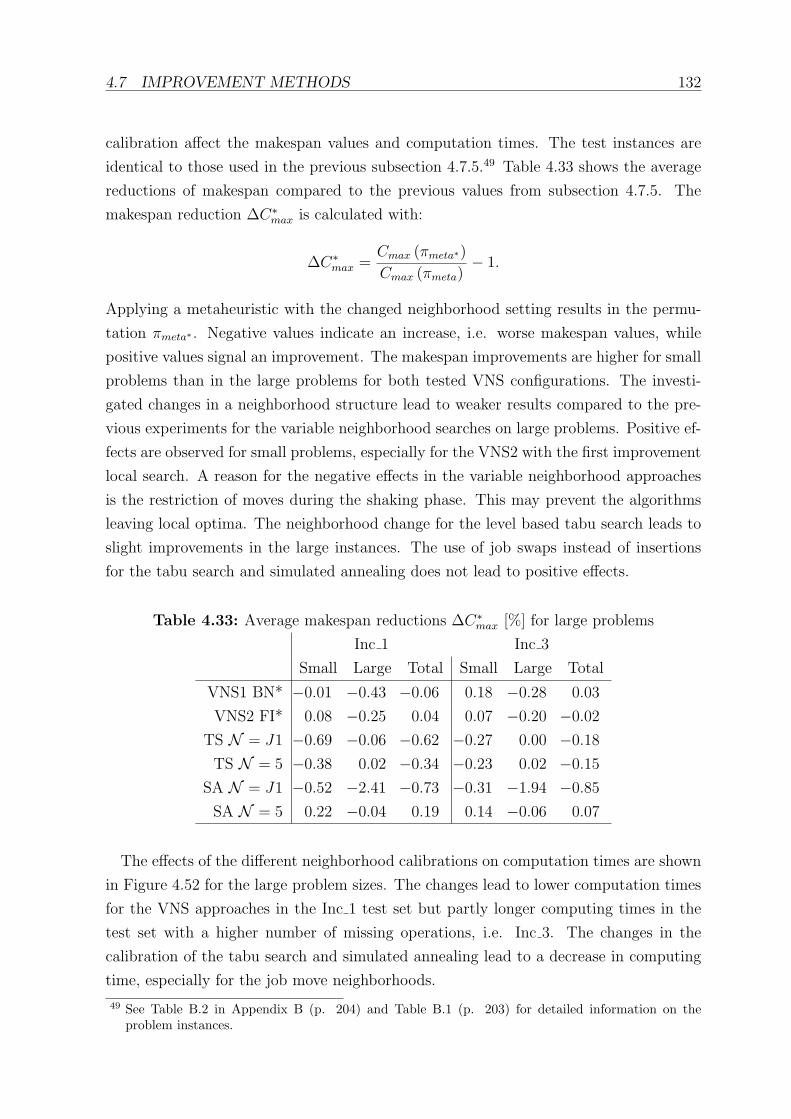
4.7 IMPROVEMENT METHODS 132
calibration affect the makespan values and computation times. The test instances are
identical to those used in the previous subsection 4.7.5.49 Table 4.33 shows the average
reductions of makespan compared to the previous values from subsection 4.7.5. The
makespan reduction ∆C∗max is calculated with:
∆C∗max =
Cmax (πmeta∗)
Cmax (πmeta)− 1.
Applying a metaheuristic with the changed neighborhood setting results in the permu-
tation πmeta∗ . Negative values indicate an increase, i.e. worse makespan values, while
positive values signal an improvement. The makespan improvements are higher for small
problems than in the large problems for both tested VNS configurations. The investi-
gated changes in a neighborhood structure lead to weaker results compared to the pre-
vious experiments for the variable neighborhood searches on large problems. Positive ef-
fects are observed for small problems, especially for the VNS2 with the first improvement
local search. A reason for the negative effects in the variable neighborhood approaches
is the restriction of moves during the shaking phase. This may prevent the algorithms
leaving local optima. The neighborhood change for the level based tabu search leads to
slight improvements in the large instances. The use of job swaps instead of insertions
for the tabu search and simulated annealing does not lead to positive effects.
Table 4.33: Average makespan reductions ∆C∗max [%] for large problems
Inc 1 Inc 3
Small Large Total Small Large Total
VNS1 BN* −0.01 −0.43 −0.06 0.18 −0.28 0.03
VNS2 FI* 0.08 −0.25 0.04 0.07 −0.20 −0.02
TS N = J1 −0.69 −0.06 −0.62 −0.27 0.00 −0.18
TS N = 5 −0.38 0.02 −0.34 −0.23 0.02 −0.15
SA N = J1 −0.52 −2.41 −0.73 −0.31 −1.94 −0.85
SA N = 5 0.22 −0.04 0.19 0.14 −0.06 0.07
The effects of the different neighborhood calibrations on computation times are shown
in Figure 4.52 for the large problem sizes. The changes lead to lower computation times
for the VNS approaches in the Inc 1 test set but partly longer computing times in the
test set with a higher number of missing operations, i.e. Inc 3. The changes in the
calibration of the tabu search and simulated annealing lead to a decrease in computing
time, especially for the job move neighborhoods.
49 See Table B.2 in Appendix B (p. 204) and Table B.1 (p. 203) for detailed information on theproblem instances.

4.7 IMPROVEMENT METHODS 133
Figure 4.52: Average computation times with changed neighborhood structures
VNS Inc 1
Com
puta
tion t
ime
[s]
20520
40520
201020
401020
20540
40540
201040
401040
0
100
200
300
400
500
600
Problem size
mLn
VNS1 BNVNS2 FIVNS1 BN*VNS2 FI*
VNS Inc 3
Com
puta
tion t
ime
[s]
20520
40520
201020
401020
20540
40540
201040
401040
0
100
200
300
400
500
600
Problem size
mLn
VNS1 BNVNS2 FIVNS1 BN*VNS2 FI*
TS Inc 1
Com
puta
tion
tim
e [s
]
20520
40520
201020
401020
20540
40540
201040
401040
0
20
40
60
80
100
120
Problem size
mLn
N=12N=10N=11N=5
TS Inc 3
Com
puta
tion
tim
e [s
]
20520
40520
201020
401020
20540
40540
201040
401040
0
20
40
60
80
100
120
Problem size
mLn
N=12N=10N=11N=5
SA Inc 1
Com
puta
tion
tim
e [s
]
20520
40520
201020
401020
20540
40540
201040
401040
0
50
100
150
200
250
300
350
Problem size
mLn
N=12N=6N=11N=5
SA Inc 3
Com
puta
tion
tim
e [s
]
20520
40520
201020
401020
20540
40540
201040
401040
0
50
100
150
200
250
300
350
Problem size
mLn
N=12N=6N=11N=5

4.8 APPLICATION ON JOB SHOP PROBLEMS 134
Considering the decreasing solution quality for the VNS and the low impact on com-
putation time, the examined changes of neighborhood structures are not recommended
for re-entrant permutation flow shop problems without lot streaming.
4.8 Application on Job Shop Problems
The RPFS models are also able to solve job shop scheduling problems optimally. This
section shows how missing operations can be used to represent a job shop problem.
A common job shop model50 and another formulation based on the model of Manne
(1960)51 are suggested. Afterwards, the computational performance of the job shop
model is compared to the performance of the re-entrant permutation flow shop model
with missing operations. The problem assumptions are:
1. All n jobs are available for processing at time zero.
2. There is a predetermined machine sequence for each job.
3. The machine sequence does not need to be identical for each job.
4. Each job may be processed on only one machine at a time, i.e., job splitting is not
permitted.
5. There is only one of each type of machine available.
6. Only one job at a time can be processed on an individual machine.
7. Processing times of all n jobs on each of the m machines are predetermined.
8. Set-up times are not considered.
9. Unlimited in-process inventory is allowed between consecutive machines in the
production system.
10. No preemption is allowed: once started, a task must be completed without inter-
ruption.
The job shop model from literature uses sig as the starting time variable for the start
of the gth operation of job i. pig is the processing time of the gth operation of job i. The
parameter wig indicates on which machine the gth operation of job i is performed.
50 See Domschke/Scholl/Voß (1997): Produktionsplanung , p. 403.51 See Manne (1960): On the job-shop scheduling problem, p. 220.

4.8 APPLICATION ON JOB SHOP PROBLEMS 135
The objective in the considered job shop problem is to minimize the makespan (4.32).
minCmax (4.32)
The makespan is measured by the inequalities 4.33.
sim + pim ≤ Cmax (4.33)
∀i = 1, . . . , n.
The inequalities 4.34 ensure the correct sequence of operations for every job i. The
gth operation needs to be finished before operation g + 1 is allowed to start.
sig + pig ≤ sig+1 (4.34)
∀i = 1, . . . , n; g = 1, . . . ,m− 1.
The constraints 4.35 and 4.36 prevent the machines k = 1, . . . ,m from being occupied
by more than one job at a point of time. The constraints apply to the gth operation
of job i and the g′th operation of job i′, if they both need to be performed on machine
wig = wi′
g′ = k. The binary variable yii′k equals 1 if job i is scheduled before job i′ on
machine k. Otherwise, it equals 0. The operation i′g′ is only allowed to start on machine
k, after operation ig is finished, if yii′k = 0 (4.35).
A (1− yii′k) + sig + pig ≤ si′
g′ (4.35)
∀i, i′ = 1, . . . , n; g, g′ = 1, . . . ,m; k = 1, . . . ,m; if(
wig = wi′
g′ = k)
.
In the case of yii′k = 0, operation i′g′ needs to completed before operation ig is allowed
to start (4.36).
Ayii′k + si′
g′ + pi′
g′ ≤ sig (4.36)
∀i, i′ = 1, . . . , n; g, g′ = 1, . . . ,m; k = 1, . . . ,m; if(
wig = wi′
g′ = k)
.
The non-negativity constraints (4.37) and binary constraints (4.37) apply to the start-
ing times and sequence variables.
sig ≥ 0 ∀i = 1, . . . , n; k = 1, . . . ,m. (4.37)
yii′k ∈ {0; 1} ∀i, i′ = 1, . . . , n; k = 1, . . . ,m. (4.38)

4.8 APPLICATION ON JOB SHOP PROBLEMS 136
The following example considers three jobs that need to be processed on three ma-
chines. The machine sequences are given by W :
W =
1 2 3
2 1 3
3 2 1
.
The processing times of the different operations are provided by the values of pig:
p1g =(
5 3 1)
, p2g =(
2 3 3)
, p3g =(
1 1 4)
The number of levels in the corresponding RPFS problem with missing operations is
L = m = 3. The processing time parameters are:
p1lk =
5 0 0
0 3 0
0 0 1
, p2lk =
0 2 0
3 0 0
0 0 3
, p3lk =
0 0 1
0 1 0
4 0 0
Both models lead to a result of Cmax = 12. The solution is shown in Figure 4.53.
Figure 4.53: Solution to the job shop example
Time
3
2
1
Machine
0 1 2 3 4 5 6 7 8 9 10 11 12 13 14 15 16 17 18
Job 1
Job 2
Job 3
Both models are tested on several job shop problem instances. The number of jobs in
the test instances is n = 5, . . . , 10, which are processed on m = 5, . . . , 10 machines with
n = m for all problem sizes. Ten different instances are generated and solved for each
problem size. The processing times are uniformly distributed random numbers between
1 and 99.52
The results on computational performance are shown in Figures 4.54 and 4.55. The
average number of iterations performed by the level model on the n = 10,m = 10
problems is lower than for the n = 9,m = 9 instances, because CPLEX runs out of
time and the iterations are more time consuming. The number of iterations is generally
52 See Table B.3 in Appendix B (p. 205) for detailed information on the problem sizes.

4.8 APPLICATION ON JOB SHOP PROBLEMS 137
higher for the level model compared to the job shop model.
Figure 4.54: Average number of CPLEX iterations for job shops
Num
ber
of iter
atio
ns
55
66
77
88
99
1010
0.0e+00
2.0e+06
4.0e+06
6.0e+06
8.0e+06
1.0e+07
1.2e+07
Problem size
mn
Job shop model
Level model
The computation times of the level model are higher compared to the pure job shop
model. The mean computation time of the level model reaches a limit of 1 hour for the
problem size n = 10,m = 10, while the job shop needs just several seconds to optimally
solve the problems.

4.8 APPLICATION ON JOB SHOP PROBLEMS 138
Figure 4.55: Average computation times for job shops
Com
puta
tion
tim
e [s
]
55
66
77
88
99
1010
0
1000
2000
3000
4000
Problem size
mn
Job shop model
Level model
The level model in this form and with this kind of input data does not seem to
be a suitable alternative to solve job shop problems. A possible improvement is the
reduction of levels by allowing multiple processing times greater than 0 within one job
level. This gives the representation a more flow shop-like appeal and may lead to a better
computational performance. Generally, the model is able to find the optimal solutions
for job shop problems.

5 Re-entrant Permutation Flow Shop
Problems with Mixed Levels, Missing
Operations and Lot Streaming
The term “lot streaming” for splitting up a production job into several sublots was ini-
tially used for a job shop problem.1 The basic condition for applying lot streaming is,
that the jobs can be divided, for example, if a job consists of a discrete number of parts.
The first part of this chapter investigates the impact of different sublot forms and pro-
cessing requirements on the makespan and computational performance by using different
MIP models to solve re-entrant lot streaming problems. A framework for metaheuristics
is discussed in section 5.4 based on the findings from the MIP models.
5.1 Introduction
It is possible to split the operations to process a job if the job is assumed to be a lot
consisting of multiple parts. Dividing the job into two sublots makes it possible to
transfer the first sublot earlier to the next processing step.
An example of the ability to reduce the makespan is given for one job with the pa-
rameters plk. The job is processed in two levels and on two machines.
plk =
4 4
4 4
.
The resulting starting times in a re-entrant flow shop without lot streaming are:
slk =
0 4
8 12
.
The job is finished after 16 time units.
1 Reiter (1966): A system for managing job-shop production, pp. 371–393.
139
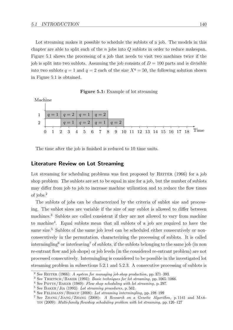
5.1 INTRODUCTION 140
Lot streaming makes it possible to schedule the sublots of a job. The models in this
chapter are able to split each of the n jobs into Q sublots in order to reduce makespan.
Figure 5.1 shows the processing of a job that needs to visit two machines twice if the
job is split into two sublots. Assuming the job consists of D = 100 parts and is divisible
into two sublots q = 1 and q = 2 each of the size Xq = 50, the following solution shown
in Figure 5.1 is obtained.
Figure 5.1: Example of lot streaming
Time
2
1
Machine
0 1 2 3 4 5 6 7 8 9 10 11 12 13 14 15 16 17 18
q = 1 q = 2 q = 1 q = 2
q = 1 q = 2 q = 1 q = 2
The time after the job is finished is reduced to 10 time units.
Literature Review on Lot Streaming
Lot streaming for scheduling problems was first proposed by Reiter (1966) for a job
shop problem. The sublots are set to be equal in size for a job, but the number of sublots
may differ from job to job to increase machine utilization and to reduce the flow times
of jobs.2
The sublots of jobs can be characterized by the criteria of sublot size and process-
ing. The sublot sizes are variable if the size of any sublot is allowed to differ between
machines.3 Sublots are called consistent if they are not allowed to vary from machine
to machine4. Equal sublots mean that all sublots of a job are required to have the
same size.5 Sublots of the same job level can be scheduled either consecutively or non-
consecutively in the permutation, characterizing the processing of sublots. It is called
intermingling6 or interleaving7 of sublots, if the sublots belonging to the same job (in non
re-entrant flow and job shops) or job levels (in the considered re-entrant problem) are not
processed consecutively. Intermingling is considered to be possible in the investigated lot
streaming problem in subsections 5.2.1 and 5.2.3. A consecutive processing of sublots is
2 See Reiter (1966): A system for managing job-shop production, pp. 371–393.3 See Trietsch/Baker (1993): Basic techniques for lot streaming , pp. 1065–1066.4 See Potts/Baker (1989): Flow shop scheduling with lot streaming , p. 297.5 See Baker/Jia (1993): Lot streaming procedures , p. 562.6 See Feldmann/Biskup (2008): Lot streaming intermingling , pp. 198–1997 See Zhang/Jiang/Zhang (2008): A Research on a Genetic Algorithm, p. 1141 and Mar-
tin (2009): Multi-family flowshop scheduling problem with lot streaming , pp. 126–127
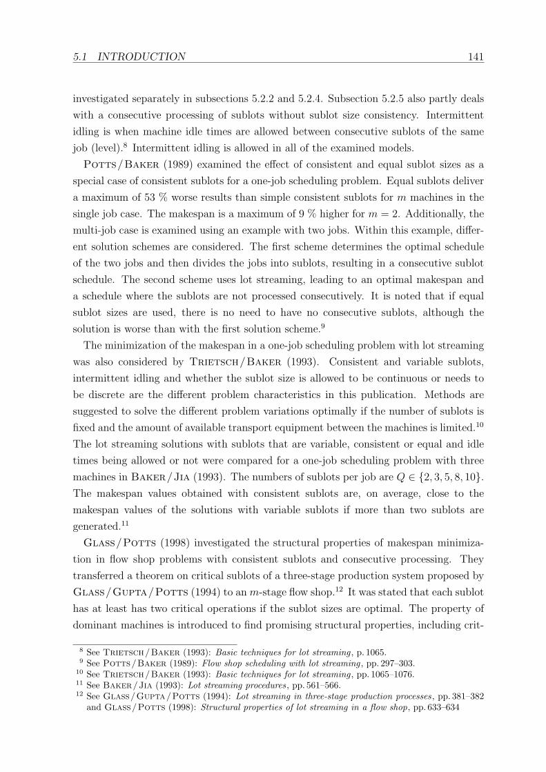
5.1 INTRODUCTION 141
investigated separately in subsections 5.2.2 and 5.2.4. Subsection 5.2.5 also partly deals
with a consecutive processing of sublots without sublot size consistency. Intermittent
idling is when machine idle times are allowed between consecutive sublots of the same
job (level).8 Intermittent idling is allowed in all of the examined models.
Potts/Baker (1989) examined the effect of consistent and equal sublot sizes as a
special case of consistent sublots for a one-job scheduling problem. Equal sublots deliver
a maximum of 53 % worse results than simple consistent sublots for m machines in the
single job case. The makespan is a maximum of 9 % higher for m = 2. Additionally, the
multi-job case is examined using an example with two jobs. Within this example, differ-
ent solution schemes are considered. The first scheme determines the optimal schedule
of the two jobs and then divides the jobs into sublots, resulting in a consecutive sublot
schedule. The second scheme uses lot streaming, leading to an optimal makespan and
a schedule where the sublots are not processed consecutively. It is noted that if equal
sublot sizes are used, there is no need to have no consecutive sublots, although the
solution is worse than with the first solution scheme.9
The minimization of the makespan in a one-job scheduling problem with lot streaming
was also considered by Trietsch/Baker (1993). Consistent and variable sublots,
intermittent idling and whether the sublot size is allowed to be continuous or needs to
be discrete are the different problem characteristics in this publication. Methods are
suggested to solve the different problem variations optimally if the number of sublots is
fixed and the amount of available transport equipment between the machines is limited.10
The lot streaming solutions with sublots that are variable, consistent or equal and idle
times being allowed or not were compared for a one-job scheduling problem with three
machines in Baker/Jia (1993). The numbers of sublots per job are Q ∈ {2, 3, 5, 8, 10}.
The makespan values obtained with consistent sublots are, on average, close to the
makespan values of the solutions with variable sublots if more than two sublots are
generated.11
Glass/Potts (1998) investigated the structural properties of makespan minimiza-
tion in flow shop problems with consistent sublots and consecutive processing. They
transferred a theorem on critical sublots of a three-stage production system proposed by
Glass/Gupta/Potts (1994) to anm-stage flow shop.12 It was stated that each sublot
has at least has two critical operations if the sublot sizes are optimal. The property of
dominant machines is introduced to find promising structural properties, including crit-
8 See Trietsch/Baker (1993): Basic techniques for lot streaming , p. 1065.9 See Potts/Baker (1989): Flow shop scheduling with lot streaming , pp. 297–303.
10 See Trietsch/Baker (1993): Basic techniques for lot streaming , pp. 1065–1076.11 See Baker/Jia (1993): Lot streaming procedures , pp. 561–566.12 See Glass/Gupta/Potts (1994): Lot streaming in three-stage production processes , pp. 381–382
and Glass/Potts (1998): Structural properties of lot streaming in a flow shop, pp. 633–634

5.1 INTRODUCTION 142
ical block structure and sublot sizes of a solution with minimal makespan.13 In a later
work, the structural properties were used within a relaxation algorithm to find the opti-
mal solutions for the flow shop problem with multiple jobs and consecutive sublots.14
Feldmann/Biskup (2008) considered a permutation flow shop with lot streaming.
The problem was stated as a lot streaming problem with intermingling, which means that
the sublots of a job do not need to form a consecutive sequence. The sublot sizes need
to be consistent between different machines. Also a model with consecutive sublots was
investigated. The model with consecutive sublots relies on a position-related variable,
assigning sequence positions to single sublots. The model with intermingling uses a
sequence-related binary variable to determine a permutation representing a predecessor-
successor relation between sublots. Both formulations have been tested for the case
of intermingling sublots with the LINGO solver software. The model using position-
related binary variables to determine a permutation required that more branch and
bound iterations occurred for every test instance to find the optimal solution regarding
the makespan. For one of the test instances, the position-related formulation required
173.6 % more iterations.15
Makespan minimization in permutation flow shops was also investigated by Pan et al.
(2010). The sublot sizes were determined to be equal and the setup times of the opera-
tions were sequence-dependent. The setup can be performed without the sublot present
on the machine. The setup is only necessary for the first sublot of a job, since also con-
secutive sublots are assumed. The solution method applied to the problem is a heuristic
called a discrete harmony search algorithm. The algorithm is compared to a hybrid
genetic algorithm, an ant colony optimization algorithm, and two threshold accepting
algorithm modifications, one with swap moves and the other with insertion moves. The
discrete harmony search algorithm outperformed the other comparative solution meth-
ods.16
A combined objective function of weighted tardiness and weighted earliness was sug-
gested byPan et al. (2011) to reduce the deviation of job completion time and job due
date in a permutation flow shop with equal sublots and consecutive processing of same
job sublots. An artificial bee colony algorithm was used to solve problem instances with
and without intermittent idling. The number of sublots per job was chosen randomly
between one and six sublots per job.17
Defersha (2011) proposed an MIP model for a hybrid flexible flow shop problem
with multiple unrelated parallel machines at each stage and sequence-dependent setup
13 See Glass/Potts (1998): Structural properties of lot streaming in a flow shop, pp. 624–639.14 See Glass/Possani (2011): Lot streaming multiple jobs in a flow shop, pp. 425–431.15 See Feldmann/Biskup (2008): Lot streaming intermingling , pp. 197–216.16 See Pan et al. (2010): Discrete harmony search for lot-streaming flow shops , pp. 1531–1536.17 See Pan et al. (2011): Artificial bee colony algorithm for lot-streaming , pp. 2455–2468.

5.1 INTRODUCTION 143
times. The flexible property is referred to as the possibility for jobs to skip stages. This
is formulated by using a precedence parameter defining the two succeeding stages for a
job. The sublots do not need to be consistent or consecutive. The formulation is tested
for multiple configurations of the maximal number of sublots per job. The reductions
of the makespan with increasing sublot numbers are lower for higher sublot numbers.
Generating more than five sublots per job is not appropriate for simple flow shops or for
hybrid flexible flow shops.18
The minimization of the makespan in job shops with lot streaming was tackled with
a combination of a tabu search and genetic algorithm by Buscher/Shen (2008). The
tabu search sequenced the sublots, while a genetic algorithm was applied to change
sublot sizes.19 Also Buscher/Shen (2009) used a tabu search mechanism to sequence
sublots in a job shop with lot streaming. The initially generated sublot sizes were gen-
erated randomly. The tabu search was applied repeatedly to the schedule, and every
time the size of selected sublots was recalculated by the suggested procedure. Both the
tabu search and the recalculation of sublot sizes, are based on the block structure sug-
gested by Nowicki/Smutnicki (1996).20 In Buscher/Shen (2011), a mixed integer
lot streaming model for job shops with consistent sublots and setup times is proposed.
The model is extended with no-wait and non-idling constraints. The objective is the
makespan. The computational experiments show that the benefit of lot streaming de-
creases if the setup times are increased per operation. Additionally the impact of raising
the number of sublots per job by one leads to a decreased benefit for higher numbers of
sublots per job.21
To the authors knowledge, lot streaming has not been investigated for the re-entrant
permutation flow shop problem, except by Hinze (2016).22 The publication of Reiter
(1966) considered re-entrant product flows in job shops without explicitly calling the
repeated processing of jobs on one or more machines “re-entrant”.23 Queries in the
databases mentioned in Section 3.2 did not deliver any relevant results regarding the
search terms “re-entrant” (“reentrant”) and “lot streaming”. Also, the review on lot
streaming by Chang/Chiu (2005), as well as the reviews on re-entrant scheduling,
do not show any information regarding the application of lot streaming on re-entrant
permutation flow shops.24
18 See Defersha (2011): Hybrid flexible flowshop lot streaming problem, pp. 283–294.19 See Buscher/Shen (2008): Lot Streaming in Job Shops , pp. 425-431.20 See Buscher/Shen (2009): Tabu search for the lot streaming problem in job shops , pp. 385–399.21 See Buscher/Shen (2011): An integer programming for lot streaming in a job shop, pp. 1343–1348.22 See Hinze (2016): Lot Streaming with Missing Operations , pp. 152–155.23 See Reiter (1966): A system for managing job-shop production, p. 378.24 See Chang/Chiu (2005): A comprehensive review of lot streaming , pp. 1515–1536.

5.2 MATHEMATICAL MODELS 144
5.2 Mathematical Models
The number of sublots per job, Q, is predetermined in the models of this section. It is
not considered as a solution variable. Contrary to the previous chapters, the symbol pilk
indicates the unit processing time, which refers to the processing time for one part of
job i in level l on machine k.
5.2.1 Consistent Sublots
The equations (5.1) ensure that the set of sublots contains all units of the complete job.
The sublots of the jobs are not variable, i.e. consistent during all operations. Therefore
the sublot size X iq has neither a level nor a machine index.
Q∑
q=1
X iq = Di (5.1)
∀i = 1, . . . , n.
The multiplication with the processing times in the constraint sets (5.2), (5.3) and
(5.4) enables the ability to skip missing operations, equivalent to the model without lot
streaming. Both sides of the constraints equal zero if one of the considered operations
is missing. The constraints (5.2) regulate the machine sequence for each of the sublots
q = 1, . . . , Q of a job i on level l. The sublots usually need to start on machine k = 1
and end the level on machine k = m. The operation on a machine k′, with k′ > k, can
only start after the operations on all machines k are finished. The constraints are not
relevant if an operation on either a machine k or k′ is left out.
The sublots of a job i should be processed in a sequence starting with sublot q = 1 on
each level l = 1, . . . , L and ending with sublot q = Q in (5.3). The level transitions of a
job’s sublots are regulated in (5.4). A level l + 1 of a job’s i sublot q is not allowed to
start before its level l is finished.
pilk′ ·(
siqlk + pilk ·Xiq)
· pilk ≤ pilk′ · siqlk′ · p
ilk (5.2)
∀i = 1, . . . , n; q = 1, . . . , Q; l = 1, . . . , L; k, k′ = 1, . . . ,m; (k < k′) ;(
siqlk + pilk ·Xiq)
· pilk ≤ si,q+1lk · pilk (5.3)
∀i = 1, . . . , n; q = 1, . . . , Q− 1; l = 1, . . . , L; k = 1, . . . ,m;
pil+1,k′ ·(
siqlk + pilk ·Xiq)
· pilk ≤ pil+1,k′ · siql+1,k′ · p
ilk (5.4)
∀i,= 1, . . . , n; q = 1, . . . , Q; l = 1, . . . , L− 1; k, k′ = 1, . . . ,m.
The constraint sets (5.5) and (5.6) prevent jobs from being scheduled on a machine k

5.2 MATHEMATICAL MODELS 145
when there is already another job on k at the same time. The constraints (5.5) consider
two sublots q and q′ of two different jobs i 6= i′ or the same job i = i′ on the levels l
and l′. If yi′q′l′
iql = 1, i.e. iql precedes i′q′l′, then i′q′l′ needs to wait for iql to be finished
before it can start on machine k. The inequalities (5.6) are applied for the case that i′q′l′
precedes iql, i.e. yi′q′l′
iql = 0.
A ·(
1− yiqli′q′l′
)
+ sl′ki′q′ − slkiq ≥ pilk ·X
iq (5.5)
∀i, i′ = 1, . . . , n; (i ≥ i′) ; l, l′ = 1, . . . , L; k = 1, . . . ,m; q, q′ = 1, . . . , Q; if (i = i′) {q 6= q′} ;
A · yiqli′q′l′ + slkiq − sl′ki′q′ ≥ pi
′
l′k ·Xi′q′ (5.6)
∀i, i′ = 1, . . . , n; (i ≥ i′) ; l, l′ = 1, . . . , L; k = 1, . . . ,m; q, q′ = 1, . . . , Q; if (i = i′) {q 6= q′} .
The job levels are kept in a basic sequence by the constraint set (5.7). Unless different
levels can be mixed, the job sequence within each level is the same. If a sublot q of job
i precedes a sublot q′ of a job i′ in level l, then it also precedes sublots q′ of job i′ on all
other levels l′ 6= l. These constraints are not included in the tested models, in order to
identify the full impact of lot streaming on the objective values.
yiqli′q′l = yiqLi′q′L (5.7)
∀i, i′ = 1, . . . , n; (i > i′) ; l = 1, . . . , L; q, q′ = 1, . . . , Q; if (i = i′) {q 6= q′} .
The equations (5.8) ensure the unambiguousness of sequence variables. Given two
sublots q and q′ of two different jobs i and i′ on any two levels l and l′, one of these
sublots needs to precede the other one, i.e. one of the variables yiqli′q′l′ and yi′q′l′
iql needs to
be 1. Then the other variable must be 0.
yiqli′q′l′ + yi′q′l′
iql = 1 (5.8)
∀i, i′ = 1, . . . , n; i ≥ i′; l, l′ = 1, . . . , L; q, q′ = 1, . . . , Q; if (i = i′) {q 6= q′} .
The makespan of the schedule is calculated by (5.10). It is necessary to check the end
of all operations to compute the makespan, since it is not known whether the operation
on the last machine has a processing time equal to 0.
minCmax; (5.9)
siqlk + pilk ·Xiq ≤ Cmax (5.10)
∀i = 1, . . . , n; q = 1, . . . , Q; l = 1, . . . , L; k = 1, . . . ,m.

5.2 MATHEMATICAL MODELS 146
An alternative objective function is the total flow time as the sum of completion times.
minn∑
i=1
Ci; (5.11)
siqlk + pilk ·Xiq ≤ Ci (5.12)
∀i = 1, . . . , n; q = 1, . . . , Q; l = 1, . . . , L; k = 1, . . . ,m.
The equations (5.12) measure the completion time of each job, which is only necessary
if the sum of completion times is the objective.
The constraints (5.13) are the binary constraints to the sequence variables. The non-
negativity constraints apply to the sublot size (5.14), and (5.15) to the starting times of
the sublots.
yiqli′q′l′ ∈ {0; 1} (5.13)
∀i, i′ = 1, . . . , n; i ≥ i′; l, l′ = 1, . . . , L; q, q′ = 1, . . . , Q; if (i = i′ANDl = l′) q 6= q′
siqlk ≥ 0 (5.14)
∀i = 1, . . . , n; q = 1, . . . , Q; l = 1, . . . , L; k = 1, . . . ,m;
X iq ≥ 0 (5.15)
∀i = 1, . . . , n; q = 1, . . . , Q.
There are n = 3 jobs to schedule in an RPFS example with m = 3 machines. All jobs
run L = 2 times through the production system. Missing operations are not considered
in the example, as it should show only the effects of different forms of sublots. Each job
consists of 100 parts:
D1 = D2 = D3 = 100.
The unit processing times pilk of each job are given with p1lk, p2lk and p3lk:
p1lk =
0.01 0.01
0.01 0.02
, p2lk =
0.04 0.04
0.03 0.01
, p3lk =
0.01 0.01
0.04 0.03
The maximum number of sublots per job is set to Q = 2.
The sublot sizes of the jobs are represented by the parameters X iq. The first job is
not divided into sublots, because the first sublot includes all of the job’s parts.
X1q =(
100 0)
, X2q =(
80 20)
, X3q =(
80 20)
.
The optimal schedule, if the sublots are consistent but not equal and not consecutive,

5.2 MATHEMATICAL MODELS 147
leads to the permutation provided by Table 5.1. The values in parentheses are for sublots
of size X iq = 0.
Table 5.1: Optimal permutation of the example with consistent sublots
Position 1 2 3 4 5 6 7 8 9 10 11 12
Job 1 3 3 1 2 (1) 3 2 (1) 2 3 2
Level 1 1 1 2 1 (1) 2 1 (2) 2 2 2
Sublot 1 1 2 1 1 (2) 1 2 (2) 1 2 2
The starting times of all operations of the i = 1, 2, 3 job’s sublots q = 1, 2 in the levels
l = 1, 2 on the machines k = 1, 2, 3 are given by the values of siqlk.
s11lk =
0 1
2 4.2
, s12lk =
6.2 9.4
9.4 11.8
,
s21lk =
3 6.2
10.2 12.6
, s22lk =
9.4 11.8
13.4 14
,
s31lk =
1 2
6.2 9.4
, s32lk =
1.8 2.8
12.6 13.4
.
The optimal schedule is shown in Figure 5.2. The resulting makespan is Cmax = 14.2.
The example is also presented in Section 4.2 without lot streaming. The makespan in
the solution without lot streaming is Cmax = 16.
Figure 5.2: Solution to the example with consistent sublots
Time
2
1
Machine
0 1 2 3 4 5 6 7 8 9 10 11 12 13 14 15 16 17 18
Job 1
Job 2
Job 3
Impact of Lot Streaming with Consistent Sublots
The test problem sizes are determined by the values of the number of jobs n ∈ {2, 3, 4},
the number of levels per job L ∈ {2, 3, 4}, the number of machines m ∈ {2, 5, 6, 10} and

5.2 MATHEMATICAL MODELS 148
the number of sublots per job Q ∈ {2, 3, 4}.25 Combining the different parameters results
in 108 different problem sizes. The same ten instances as in the experiments of Chapter
5 are tested for each problem size regardless of the number of sublots per job. Missing
operations are generated in ascending quantity for test instance sets Inc 1 and Inc 2.
The instance set Inc 2 requires a minimum of L = 4 levels per job.26 The processing
times of the operations in the tested problem instances in Chapter 5 are identical to the
tested problems in Chapter 4, i.e. uniformly distributed random numbers between 1 and
99 as suggested by Taillard (1993) for non-missing operations.27 The unit processing
times in this chapter are obtained by dividing the processing times generated for each
job by the number of parts / units of the job. The lot sizes are required to be divisible by
two and three for the tests with equal sublots in Sections 5.2.3 and 5.2.4. Additionally
the divisibility by four is secured for additional tests in section 5.4.2. This allows job lot
sizes of:
D ∈ {60, 72, 84, 96, 108, 120}
Figure 5.3 shows the mean relative values of makespan achieved by applying lot stream-
ing with consistent sublots compared to the makespan values of the simple re-entrant
permutation flow shop with missing operations for the Inc 1 instances. The relative
makespan values are calculated with the formula:
Cmax =CQ
max
C1max
.
CQmax is the makespan value of the solution if the jobs are each split into Q > 1 sublots.
The lot streaming problem with Q = 1 sublots, and the makespan values C1max, equal the
problem without lot streaming. The values for splitting each job level into Q = 2 sublots
are between 55.50 % (n = 2, L = 4, m = 10) and 79.93 % (n = 4, L = 4, m = 5) for every
problem size. 55.50 % relative makespan means, that the average makespan computed
for this problem size is 55.50 % of the makespan value if lot streaming is not applied.
The reduction of the makespan between applying lot streaming with two sublots and no
lot streaming is higher than the reduction from using three sublots instead of two and
four sublots instead of three. The lowest values are obtained by splitting the job levels
into Q = 4 sublots each. The mean values range from 37.44 % to 75.01 % compared
to the mean makespan values of the model without lot streaming. The reduction of the
makespan is generally higher for a larger number of machines, i.e. for problem sizes
25 See Table B.3 in Appendix B (p. 205) for detailed information on the problem sizes.26 See Table B.1 in Appendix B (p. 203) for an overview of missing operations.27 See Taillard (1993): Benchmarks for basic scheduling problems , pp. 279–280.

5.2 MATHEMATICAL MODELS 149
with m = 10. The advantage of using lot streaming increases with a higher number of
machines that need to be visited by the job levels. The number of sequence positions to
assign is n · L ·Q.
Figure 5.3: Average makespan of consistent sublots compared to using no sublots(Inc 1)
Cmax [%
]
522
1022
532
1032
542
1042
523
1023
533
1033
543
1043
524
1024
534
1034
544
1044
0
20
40
60
80
100
Problem size
mLn
2 Sublots3 Sublots4 Sublots
The results of the mean relative makespan for the Inc 2 instances are shown in Figure
5.4. The lowest mean relative makespan is again achieved by splitting the job levels
into four sublots. The average makespan for the instances of the problem size with ten
machines, four levels and two jobs drops to 37.67 % of the makespan value without
lot streaming. The lowest value for the three-sublot calculation appears for the same
problem size with 43.14 % using two sublots per job, compared to the solution obtained
if lot streaming is not allowed. The step from applying no lot streaming to lot streaming
with two sublots is the largest step in makespan reduction compared to the step of
increasing the number of sublots per job level from two to three and from three to four.
Nevertheless, the mean relative makespan values for lot streaming with two sublots are
higher than those for three and four sublots. The lowest value for the Inc 2 instances
and Q = 2 is 56.66 % (n = 2, L = 4, m = 10).

5.2 MATHEMATICAL MODELS 150
Figure 5.4: Average makespan of consistent sublots compared to using no sublots(Inc 2)
Cmax [%
]
542
1042
543
1043
544
1044
0
20
40
60
80
100
Problem size
mLn
2 Sublots3 Sublots4 Sublots
The symbols used in the evaluation tables in this subsection (5.2.1) are GQ, ∆CQ|Q−1max
and ItQ. GQ stands for the relative gap between the lower bound and best incumbent
solution after 3600 seconds if lot streaming with Q consistent sublots per job is applied.
It is 0 if the optimal solution is found. The makespan reduction by increasing the number
of sublots by one is given by the symbol ∆CQ|Q−1max and calculated by:
∆CQ|Q−1max =
CQmax
CQ−1max
− 1.
ItQ denotes the number of CPLEX iterations for the lot streaming model with Q sublots
per job.
Table 5.2 shows the average gaps for the the re-entrant permutation flow with missing
operations and lot streaming for solutions with one, two, three and four sublots for each
job depending on the number of machines. CPLEX comes closer to the optimal solution
or closer to approving the solution found as optimal for problems with m = 10 machines
compared to instances with m = 5 machines. Also the makespan reductions achieved
by increasing the number of lots by one are higher for the ten machine instances. The
makespan reductions are the highest for the step from one to two sublots per job. The
weakest improvements of the makespan within a computation time of 1 hour are the
ones for increasing Q from three to four. These facts apply for both test instance sets

5.2 MATHEMATICAL MODELS 151
Inc 1 and Inc 2.
Table 5.2: Influence of m on makespan if the sublots are consistent
Inc m G1 [%] G2 [%] G3 [%] G4 [%] ∆C2|1max [%] ∆C3|2
max [%] ∆C4|3max [%]
1 5 0.00 5.86 21.25 31.14 −27.98 −7.97 −3.41
10 0.00 1.66 12.12 21.14 −40.08 −17.57 −9.19
2 5 0.00 12.22 28.97 41.67 −27.55 −6.58 −2.56
10 0.00 4.17 17.55 29.69 −39.94 −17.06 −8.04
In Figure 5.3 and 5.4, a slight increase of the mean relative makespan values with an
increasing number of jobs n can be seen. The reason for the effect can be explained by
looking at Figures 5.5 and 5.6, which show the mean computation times for every problem
size in the instance sets Inc 1 and Inc 2. An increase in the number of jobs leads to the
largest increase of computation time compared to the influence of the number of levels.
An increase in the number of machines leads to a lower computation time similar to
the effect for the model without lot streaming. Solving the lot streaming problem with
four consistent sublots prevents CPLEX from closing the gap between the incumbent
solution and lower bound for most of the instances of the Inc 1 set. CPLEX either fails
to find the optimal solution or fails to confirm the solution found as optimal. These
problem sizes have an average computation time of 3600 seconds, which is the set limit
of computing time. The calculations for three sublots and three jobs and more also lead
to average computation time around 3600 seconds. The lot streaming problems with two
sublots for each job are mostly solved optimally in less than 1 hour. The computation
times without lot streaming, i.e. with just one sublot per job level, are around 1 second
for the considered Inc 1 instances.

5.2 MATHEMATICAL MODELS 152
Figure 5.5: Average computation time with consistent sublots (Inc 1)
Com
puta
tion
tim
e [s
]
522
1022
532
1032
542
1042
523
1023
533
1033
543
1043
524
1024
534
1034
544
1044
0
1000
2000
3000
4000
5000
Problem size
mLn
Without Sublots2 Sublots3 Sublots4 Sublots
Increasing the number of missing operations, as done by switching to the Inc 2 in-
stances, leads to higher computation times for the lot streaming problem with two sublots
per job. On the other hand, the computation times for the three sublot problem drop
slightly for the considered problems, as can be seen by comparing Figure 5.5 and 5.6.
The computational effort for the problem without lot streaming does not change. The
four-sublot problem is difficult to evaluate since the calculation times of the compara-
ble problem sizes are around 3600 seconds in the cases of lower and higher numbers of
missing operations.

5.2 MATHEMATICAL MODELS 153
Figure 5.6: Average computation time with consistent sublots (Inc 2)
Com
puta
tion
tim
e [s
]
542
1042
543
1043
544
1044
0
1000
2000
3000
4000
5000
Problem size
mLn
Without Sublots2 Sublots3 Sublots4 Sublots
Increasing the number of consistent sublots to values higher than two leads to greater
computational effort, without reaching the same reduction of the makespan compared
to the introduction of lot streaming.
The number of iterations also depends on the number of machines, as seen in Table
5.3. Problems with a higher number of machines need fewer iterations to be solved than
comparable problems with a lower number of machines and the same number of jobs and
levels per job. The calculated iterations for the problem without lot streaming and ten
machines need the lowest number of CPLEX iterations with, on average, 284.28 iterations
for the Inc 1 problem set and 3117.93 iterations for Inc 2 problems. The highest average
number of iterations is 11923622.61 for the Q = 4 problems in Inc 1. For problems that
are solved optimally or near optimally, i.e. mainly the calculation with Q = 1 and Q = 2,
the number of iterations is higher if more missing operations are included within the job
levels.
Table 5.3: Influence of m on CPLEX iterations if the sublots are consistent
Inc m It1 It2 It3 It4
1 5 3224.83 4,466,321.71 4,090,186.17 11,923,622.61
10 284.28 1,015,293.40 1,980,717.80 5,534,364.94
2 5 8056.43 3,560,833.63 4,000,401.57 10,279,038.53
10 3117.93 1,721,735.00 2,406,330.40 3,830,610.90

5.2 MATHEMATICAL MODELS 154
Table 5.4 shows the solution quality for different values of Q depending on the number
of levels L per job. The Inc 2 test set includes only problems with L = 4 levels per
job; therefore, a differentiation of the solution quality and number of CPLEX iterations
based on the number of levels is not possible for these instances. The values of gaps after
a maximum computation time of 1 hour increase with the increasing number of levels.
The higher the number of levels, the more permutations are possible, which increases the
computational effort necessary to solve the problem optimally. The values of makespan
reductions for a given step from Q − 1 to Q are almost unaffected by the number of
levels.
Table 5.4: Influence of L on makespan if the sublots are consistent
Inc L G1 [%] G2 [%] G3 [%] G4 [%] ∆C2|1max [%] ∆C3|2
max [%] ∆C4|3max [%]
1 2 0.00 0.67 11.48 19.45 −31.88 −11.78 −5.48
3 0.00 3.80 16.93 25.62 −34.85 −13.46 −7.10
4 0.00 6.82 21.65 33.35 −35.37 −13.07 −6.31
2 4 0.00 8.19 23.26 35.68 −33.74 −11.82 −5.30
The number of iterations distinguished by the number of levels and the number of
sublots per job is shown in Table 5.5. The higher the number of levels, the higher the
number of iterations performed by CPLEX. There are no large differences visible between
the L = 4 instances with a lower or higher number of missing operations.
Table 5.5: Influence of L on CPLEX iterations if the sublots are consistent
Inc L It1 It2 It3 It4
1 2 178.80 2,282,915.23 3,973,201.18 10,873,712.45
3 1829.28 2,625,889.20 2,661,204.70 8,827,528.18
4 3255.58 3,313,618.23 2,471,950.07 6,485,740.70
2 4 5587.18 2,641,284.32 3,203,365.98 7,054,824.72
The following Tables 5.6 and 5.7 evaluate the solution quality using gap values and
makespan reduction values as well as the computational effort (by the number of itera-
tions) for different numbers of jobs.

5.2 MATHEMATICAL MODELS 155
Table 5.6: Influence of n on makespan if the sublots are consistent
Inc n G1 [%] G2 [%] G3 [%] G4 [%] ∆C2|1max [%] ∆C3|2
max [%] ∆C4|3max [%]
1 2 0.00 0.00 1.06 6.52 −38.70 −18.28 −9.03
3 0.00 0.00 1.19 6.87 −38.48 −18.17 −9.01
4 0.00 0.00 1.58 7.52 −38.47 −18.05 −8.93
2 2 0.00 0.00 3.42 14.99 −39.68 −18.13 −8.69
3 0.00 5.32 25.90 39.69 −34.55 −10.75 −4.77
4 0.00 19.26 40.46 52.36 −27.00 −6.57 −2.44
The four-job four-sublot problem instances required more than 3600 seconds of com-
putation time on average for test sets Inc 1 and Inc 2. However, the number of iterations
performed for Inc 1 instances is almost twice as high as for Inc 2 instances. Thus, the
time for single CPLEX iterations increases with a higher number of missing operations.
Table 5.7: Influence of n on CPLEX iterations if the sublots are consistent
Inc n It1 It2 It3 It4
1 2 109.58 5927.38 919,157.70 7,637,007.68
3 230.97 2,754,148.20 4,168,759.72 10,487,879.42
4 4923.12 5,462,347.08 4,018,438.53 8,062,094.23
2 2 153.80 21,055.35 1,829,851.55 9,301,545.65
3 379.70 3,055,880.65 3,713,227.00 6,871,212.80
4 16,228.05 4,846,916.95 4,067,019.40 4,991,715.70
5.2.2 Consecutive Sublots
The equations (5.16) secure a consecutive processing of sublots that belong to the same
job level. In the following, this is called consecutive sublots. If a sublot q′ of a job level
i′, l′ does not precede sublot q′ of another job i’s level l (yiq′l
i′q′l′ = 0), then all other sublots
q = 1, . . . , Q precede sublot q′ of job i′ in level l′ (yi′q′l′
iql = 1).
yiqli′q′l′ + yi′q′l′
iq′l = 1 (5.16)
∀i, i′ = 1, . . . , n; i > i′; l, l′ = 1, . . . , L; q, q′ = 1, . . . , Q.
Considering the example from Section 5.2.1, the optimal makespan increases if con-
secutive processing is necessary. The new makespan is now Cmax = 14.25. The variables
of the solution are shown below.

5.2 MATHEMATICAL MODELS 156
Job one is split into two sublots, with 50 parts each. The sublots of job two are given
by X2q, with 75 parts in the first and 25 parts in the second sublot. The first sublot of
job three is smaller than its second sublot.
X1q =(
50 50)
, X2q =(
75 25)
, X3q =(
29 71)
.
The resulting permutation is represented in Table 5.8. Job i = 1 starts the permutation
with its first sublot in level l = 1. The last position in the sequence is occupied by the
second sublot of job i = 2 in level l = 2.
Table 5.8: Optimal permutation of the example with consecutive consistent sublots
Position 1 2 3 4 5 6 7 8 9 10 11 12
Job 1 1 3 3 1 1 2 2 3 3 2 2
Level 1 1 1 1 2 2 1 1 2 2 2 2
Sublot 1 2 1 2 1 2 1 2 1 1 2 2
The associated starting times sijlk are:
s11lk =
0 1.5
1.5 3.5
, s12lk =
0.5 2
2.5 4.5
,
s21lk =
3 6
11 13.25
, s22lk =
6 9
13.25 14
,
s31lk =
1 2
6.2 9.4
, s32lk =
1.8 2.8
12.6 13.4
.
The Gantt chart of the schedule is shown in Figure 5.7. The resulting makespan
is Cmax = 14.25, which is higher than the makespan without the consecutive sublot
constraints (5.16).

5.2 MATHEMATICAL MODELS 157
Figure 5.7: Solution to the example with consecutive sublots
Time
2
1
Machine
0 1 2 3 4 5 6 7 8 9 10 11 12 13 14 15 16 17 18
Job 1
Job 2
Job 3
Influence of Consecutive Sublots
The test instances are identical to the instances tested in Section 5.2.1, except for a
limitation of the number of sublots per job to Q ≤ 3.28
Figures 5.8 and 5.9 show the mean relative makespan deviation between the model
with consecutive consistent sublots and the previously introduced model with consistent
sublots. The values ∆CQmax in Table 5.9 are calculated by:
∆CQmax =
CQ, consecutivemax
CQ, consistentmax
− 1.
The mean relative makespan values are positive for all problem sizes of the Inc 1 problem
set. This means that the makespan is higher on average in the consecutive sublot model
than in the simple consistent case, even for the problem sizes that are not solved in time
if the simple consistent sublots model is used. The lowest increase in makespan for the
Inc 1 instances is 0.51 % for the Q = 2, n = 2, L = 4,m = 10 instances. The highest
deviation is 8.38 % for the problem size n = 2, L = 4,m = 5 and Q = 3 sublots per
job. The average makespan deviation of Q = 3 sublot lot streaming is higher for 11 of
18 problem sizes of Inc 1.
28 See also the Tables B.3 and B.1 in Appendix B (p. 205 and p. 203).

5.2 MATHEMATICAL MODELS 158
Figure 5.8: Average makespan deviations with consecutive sublots (Inc 1)
∆C
max [%
]
522
1022
532
1032
542
1042
523
1023
533
1033
543
1043
524
1024
534
1034
544
1044
0
2
4
6
8
10
Problem size
mLn
2 Sublots3 Sublots
The makespan deviations shown in Figure 5.9 represent the values for Inc 2 instances.
The value for instances of the problem size n = 4, L = 4,m = 10, Q = 3 is -0.02 %,
meaning that the makespan values achieved with the consecutive sublot model are on
average better for this problem size, which is due to the limited computation time. The
values for both two- and three-sublot problems in the Inc 2 set are lower for m = 5
problems than they are in the Inc 1 problem set. For m = 10 problems, the makespan
deviations are on the same level as those for Inc 1 instances.

5.2 MATHEMATICAL MODELS 159
Figure 5.9: Average makespan deviations with consecutive sublots (Inc 2)
∆C
max [%
]
542
1042
543
1043
544
1044
0
2
4
6
8
10
Problem size
mLn
2 Sublots3 Sublots
The average gap between the lower bound and incumbent solution after one hour of
computation time is mostly closed for the problems with Q = 2 consecutive sublots per
job, except for the n = 4 problem of Inc 2, as seen in Table 5.9. The gaps, GQ, for
Q = 3 consecutive sublots are higher than for Q = 2 problems and show an increase
with the increasing number of jobs. The gap values are equal or lower for consecutive
sublots than without consecutive sublots. The makespan deviation increases with the
number of jobs, if Q = 2. It decreases with the number of jobs, if Q = 3, since the gaps
for the formulation without consecutive sublots are relatively large for these instances
compared to the formulation with consecutive sublots.
Table 5.9: Solution quality of consistent (I) and consecutive (II) sublots
Inc n G2 I [%] G2 II [%] G3 I [%] G3 II [%] ∆C2max [%] ∆C3
max [%]
1 2 0.00 0.00 1.06 0.00 2.28 4.38
3 0.96 0.00 17.26 0.00 3.88 4.79
4 10.32 0.00 31.73 1.41 3.52 3.21
2 2 0.00 0.00 3.42 0.00 2.26 4.62
3 5.32 0.00 25.90 0.01 3.55 3.24
4 19.26 0.12 40.46 3.76 2.35 0.82
The computation time of the models with consistent and consecutive sublots for Inc 1

5.2 MATHEMATICAL MODELS 160
instances are shown in Figure 5.10. For most of the problem sizes, the average com-
putation time of CPLEX for solving the problems with consecutive sublots is only a
few seconds for the two- and three-sublot configuration. Except for the problem sizes
with four jobs and four levels, the computation times in this case are much higher for
Q = 3. The computation time reaches the limit of 3600 seconds in the case of m = 5
and is about 2300 seconds for m = 3, while the times for the same problems with the
Q = 2 configuration are 210 and 100 seconds, respectively. Despite reaching the limit
of computing time for one problem size, the computing times are generally lower for the
consecutive sublot model than the computation times of the consistent sublot model,
which does not prescribe a consecutive processing of sublots of the same job level.
Figure 5.10: Average computation times with consecutive sublots (Inc 1)
Com
puta
tion
tim
e [s
]
522
1022
532
1032
542
1042
523
1023
533
1033
543
1043
524
1024
534
1034
544
1044
0
1000
2000
3000
4000
5000
Problem size
mLn
2 Consecutive sublots3 Consecutive sublots2 Consistent sublots3 Consistent sublots
The same effect of lower computation times is also visible for Inc 2 instances in Figure
5.11. The computation times with the consecutive sublot formulation are lower than the
computing times without consecutive sublots. There is no pattern visible that describes
how the increased number of missing operations influences the computation time for the
consecutive sublot model.

5.2 MATHEMATICAL MODELS 161
Figure 5.11: Average computation times with consecutive sublots (Inc 2)
Com
puta
tion
tim
e [s
]
542
1042
543
1043
544
1044
0
1000
2000
3000
4000
Problem size
mLn
2 Consecutive sublots3 Consecutive sublots2 Consistent sublots3 Consistent sublots
The numbers of CPLEX iterations, ItQ, performed to solve the problems optimally or
until a computation time of 1 hour is reached are shown in Table 5.10. The consecutive
lot model requires more iterations than the consistent sublot model only for the n = 4
Inc 2 instances. In all other cases, the average numbers of iterations are lower.
Table 5.10: Influence of consecutive sublots on CPLEX iterations
Inc nConsistent Consecutive
It2 It3 It2 It3
1 2 5927.38 919,157.70 268.08 5201.80
3 2,754,148.20 4,168,759.72 11,629.53 188,970.62
4 5,462,347.08 4,018,438.53 516,747.68 3,416,716.17
2 2 21,055.35 1,829,851.55 587.50 15,446.85
3 3,055,880.65 3,713,227.00 50,285.45 616,849.80
4 4,846,916.95 4,067,019.40 3,135,292.20 8,353,501.75
5.2.3 Equal Sublots
The intention of testing equally sized sublots is to reduce computational efforts without
losing much of the solution quality. The size of the sublots is now solely predetermined by
the number of sublots Q and the number of parts per job Di. The results for equally sized

5.2 MATHEMATICAL MODELS 162
sublots are shown in Section 5.2.3. The model is similar to the simple consistent sublot
model introduced in Section 5.2.1. However, the only difference is that the constraints
(5.1) are replaced with the equations (5.17).
X iq =Di
Q(5.17)
∀i = 1, . . . , n; q = 1, . . . , Q.
The solution to the problem above is given in Table 5.11.
Table 5.11: Optimal permutation of the example with equal sublots
Position 1 2 3 4 5 6 7 8 9 10 11 12
Job 3 2 1 3 1 2 1 3 2 1 3 2
Level 1 1 1 1 1 1 2 2 2 2 2 2
Sublot 1 1 1 2 2 2 1 1 1 2 2 2
The equal sublot constraints lead to a size of 50 parts per sublot.
X1q =(
50 50)
, X2q =(
50 50)
, X3q =(
50 50)
.
The starting times are given below with the values siqlk. The starting time of the first
sublot of job i = 3 in level l = 1 on machine m = 1 is equal to 0 since it is the first
sublot in the sequence.
s11lk =
2.5 4.5
6 8
, s12lk =
3.5 5.5
8.5 10.5
,
s21lk =
0.5 2.5
9 11.5
, s22lk =
4 6
12.5 14
,
s31lk =
0 2
6.5 9
, s32lk =
3 5
10.5 12.5
.
The schedule with equally sized sublots for every job is shown in Figure 5.12. It
leads to a makespan of Cmax = 14.5. The value of the makespan is higher than that
without the restriction of having equal sublots. In this example, it is even higher than
the makespan of 14.25 achieved by the consecutive sublot model.
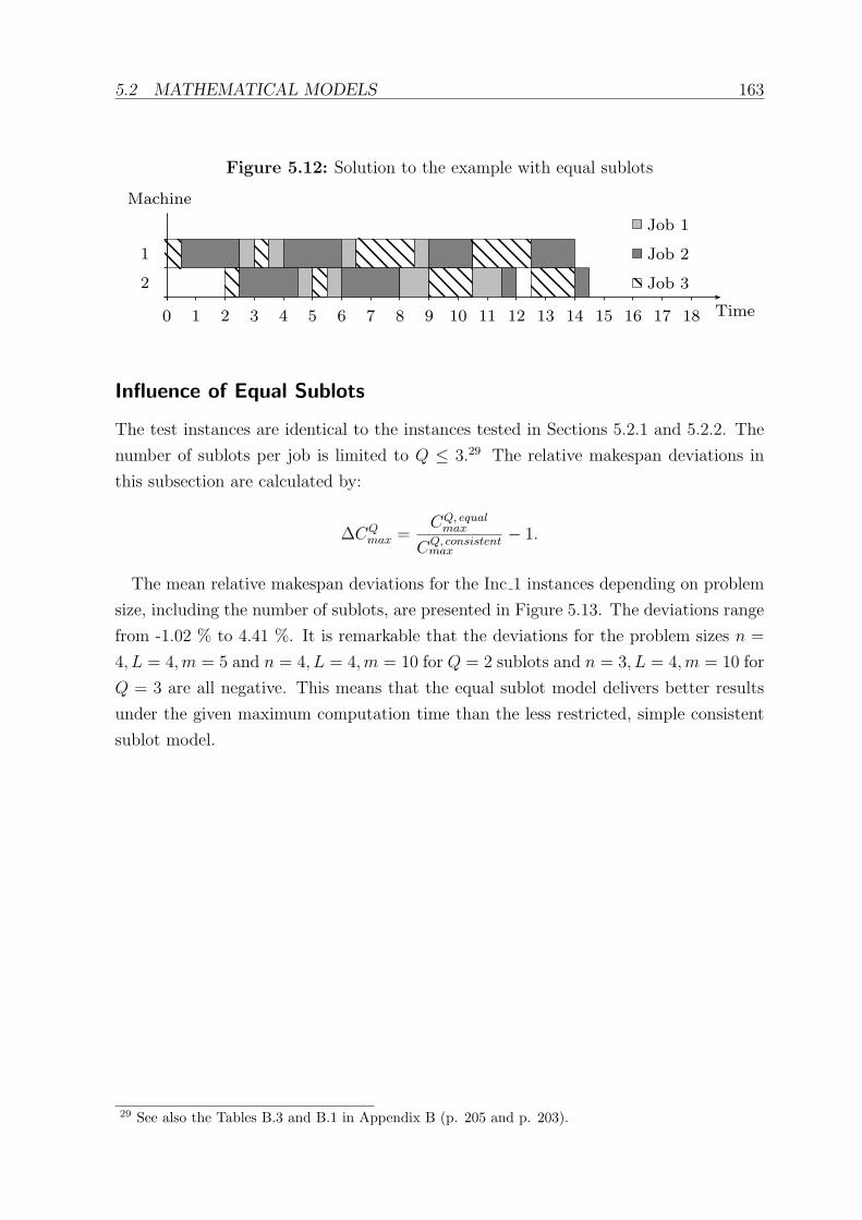
5.2 MATHEMATICAL MODELS 163
Figure 5.12: Solution to the example with equal sublots
Time
2
1
Machine
0 1 2 3 4 5 6 7 8 9 10 11 12 13 14 15 16 17 18
Job 1
Job 2
Job 3
Influence of Equal Sublots
The test instances are identical to the instances tested in Sections 5.2.1 and 5.2.2. The
number of sublots per job is limited to Q ≤ 3.29 The relative makespan deviations in
this subsection are calculated by:
∆CQmax =
CQ, equalmax
CQ, consistentmax
− 1.
The mean relative makespan deviations for the Inc 1 instances depending on problem
size, including the number of sublots, are presented in Figure 5.13. The deviations range
from -1.02 % to 4.41 %. It is remarkable that the deviations for the problem sizes n =
4, L = 4,m = 5 and n = 4, L = 4,m = 10 for Q = 2 sublots and n = 3, L = 4,m = 10 for
Q = 3 are all negative. This means that the equal sublot model delivers better results
under the given maximum computation time than the less restricted, simple consistent
sublot model.
29 See also the Tables B.3 and B.1 in Appendix B (p. 205 and p. 203).

5.2 MATHEMATICAL MODELS 164
Figure 5.13: Average makespan deviations with equal sublots (Inc 1)
∆C
max [%
]
522
1022
532
1032
542
1042
523
1023
533
1033
543
1043
524
1024
534
1034
544
1044
−1
0
1
2
3
4
5
6
Problem size
mLn
2 Sublots3 Sublots
The deviations of makespan shown for the Inc 2 instances in Figure 5.14 are all positive
but on a relatively low range between 0.40 % and 2.03 % for the two- and three-sublot
configurations.

5.2 MATHEMATICAL MODELS 165
Figure 5.14: Average makespan deviations with equal sublots (Inc 2)
∆C
max [%
]
542
1042
543
1043
544
1044
0
1
2
3
4
5
6
Problem size
mLn
2 Sublots3 Sublots
Further details on the solution quality of the equal sublot model compared to the
consistent sublot model are provided in Table 5.12. The gaps, GQ, after the maximum
computation time of 1 hour are all lower when the sublots are equally sized. Equal
sublots seem to be suitable for a higher number of jobs since the makespan deviations
of simple consistent sublots decrease if the number of jobs is increased. Five of the six
mean relative makespan deviations, depending on the number of jobs, are lower for the
Inc 2 instances. This means that a higher number of missing operations leads to a lower
deviation between the models with consistent and equal consistent sublot sizes.
Table 5.12: Solution quality of consistent (I) and equal (II) sublots
Inc n G2 I [%] G2 II [%] G3 I [%] G3 II [%] ∆C2max [%] ∆C3
max [%]
1 2 0.00 0.00 1.06 0.77 1.38 2.51
3 0.96 0.31 17.26 14.32 1.85 1.91
4 10.32 6.98 31.73 28.13 0.99 1.36
2 2 0.00 0.00 3.42 2.36 1.25 1.50
3 5.32 2.64 25.90 24.37 0.82 1.22
4 19.26 18.10 40.46 38.54 1.06 0.81
The computation times of the equal sublot model are compared to the consistent
sublot model in Figures 5.15 and 5.16. Both figures show that the average computation

5.2 MATHEMATICAL MODELS 166
times for equal sublots is slightly below those of the consistent sublot model or that both
models reach the limit of one hour. The single exception is the value for n = 2, L =
3,m = 5, Q = 3 in Figure 5.15 .
Figure 5.15: Average computation times with equal sublots (Inc 1)
Com
puta
tion
tim
e [s
]
522
1022
532
1032
542
1042
523
1023
533
1033
543
1043
524
1024
534
1034
544
1044
0
1000
2000
3000
4000
5000
Problem size
mLn
2 Equal sublots3 Equal sublots
2 Consistent sublots3 Consistent sublots
The average computation times for the same problem sizes do not differ relevantly.
Both show higher computation times for m = 5 problem sizes than for the corresponding
m = 10 problems.

5.2 MATHEMATICAL MODELS 167
Figure 5.16: Average computation times with equal sublots (Inc 2)
Com
puta
tion
tim
e [s
]
542
1042
543
1043
544
1044
0
1000
2000
3000
4000
5000
Problem size
mLn
2 Equal sublots3 Equal sublots
2 Consistent sublots3 Consistent sublots
The average numbers of iterations, ItQ, for the compared models are shown in Table
5.13. The instances with a number of jobs n = 2 are solved optimally for Q = 2. The
mean number of iterations for these instances is seven times higher for the consistent
sublot model than for the equal sublots. A similar relation can be observed for n = 2
instances with Q = 3 sublots, even if they are not all solved optimally by both models.
The average number of iterations for n = 4, which are mostly not solved optimally by
the consistent sublot model and the equal sublot model, are higher for the equal sublot
model, indicating a shorter computation time for single iterations performed on this
model.
Table 5.13: Influence of equal sublots on CPLEX iterations
Inc nConsistent Equal
It2 It3 It2 It3
1 2 5927.38 919,157.70 779.17 182,664.53
3 2,754,148.20 4,168,759.72 2,013,406.23 6,043,305.55
4 5,462,347.08 4,018,438.53 7,092,066.87 4,480,098.72
2 2 21,055.35 1,829,851.55 6458.70 593,835.70
3 3,055,880.65 3,713,227.00 4,817,891.50 2,302,744.60
4 4,846,916.95 4,067,019.40 4,256,979.85 6,387,377.10

5.2 MATHEMATICAL MODELS 168
5.2.4 Consecutive Equal Sublots
A consecutive processing of sublots is achieved by the constraints (5.18).
yiqli′q′l′ + yi′q′l′
iq′l = 1 (5.18)
∀i, i′ = 1, . . . , n; i > i′; l, l′ = 1, . . . , L; q, q′ = 1, . . . , Q.
The jobs are split into Q equal sublots of size Di/Q by the equations (5.19).
X iq =Di
Q(5.19)
∀i = 1, . . . , n; q = 1, . . . , Q.
The example from the previous sections is now solved with the consecutive and equal
sublot constraints. The optimal permutation is shown in Table 5.14.
Table 5.14: Optimal permutation of the example with consecutive equal sublots
Position 1 2 3 4 5 6 7 8 9 10 11 12
Job 3 3 1 1 2 2 1 1 3 3 2 2
Level 1 1 1 1 1 1 2 1 2 2 2 2
Sublot 1 2 1 2 1 2 1 2 1 2 1 2
The sublot sizes are all 50 units per sublot.
X1q =(
50 50)
, X2q =(
50 50)
, X3q =(
50 50)
.
The starting times are given by the values siqlk and visualized in Figure 5.17.
s11lk =
1 1.5
6 8
, s12lk =
1.5 2
6.5 9
,
s21lk =
2 4
11 13
, s22lk =
4 6
12.5 14
,
s31lk =
0 0.5
7 10
, s32lk =
0.5 1
9 11.5
.

5.2 MATHEMATICAL MODELS 169
Figure 5.17: Solution to the example with consecutive equal sublots
Time
2
1
Machine
0 1 2 3 4 5 6 7 8 9 10 11 12 13 14 15 16 17 18
Job 1
Job 2
Job 3
The resulting makespan is 14.5 time units, which is the worst value compared to
simple consistent sublots, equal sublots and simple consistent consecutive sublots. This
is reasonable, because the consecutive equal sublot model is the most restricted model
among the mentioned formulations.
Influence of Consecutive Equal Sublots
The test instances are identical to the instances tested in Sections 5.2.1, 5.2.2 and 5.2.3.
The number of sublots per job is limited to Q ≤ 3.30
The relative makespan deviations in the tables and figures of this section are calculated
with the formula:
∆CQmax =
CQ, consecutive equalmax
CQ, consistentmax
− 1.
Increases in the number of machines and levels lead to smaller mean relative makespan
deviations which are visible in Figure 5.18. Increasing the number of jobs from n = 2 to
n = 3 leads to higher deviations, i.e. to worse results for the consecutive equal sublot
model compared to the consistent sublot model. The highest deviation is 10.26 % and
occurs when each job level is split into three sublots. The value is 0.62 % for the Inc 1
instances and occurs for Q = 2. Therefore, the consecutive equal sublot model delivers
results that are on average weaker than the consistent sublot model for all tested problem
sizes in Inc 1.
30 See also the Tables B.3 and B.1 in Appendix B (p. 205 and p. 203).

5.2 MATHEMATICAL MODELS 170
Figure 5.18: Average makespan deviations with consecutive equal sublots (Inc 1)
∆C
max [%
]
522
1022
532
1032
542
1042
523
1023
533
1033
543
1043
524
1024
534
1034
544
1044
0
5
10
15
Problem size
mLn
2 Sublots3 Sublots
The results shown in Figure 5.19 represent the makespan deviations for the Inc 2
instances. The range of deviations for this problem set is between 0.60 % and 6.76 %,
which is similar to the same problem sizes in Inc 1.

5.2 MATHEMATICAL MODELS 171
Figure 5.19: Average makespan deviations with consecutive equal sublots (Inc 2)
∆C
max [%
]
542
1042
543
1043
544
1044
0
5
10
15
Problem size
mLn
2 Sublots3 Sublots
The gap values, GQ, of the consecutive equal sublot model shown in Table 5.15 are
all lower than or equal to the gaps obtained with the consistent sublot model after a
maximum computation time of 1 hour. Only three values are greater than zero, indicating
that just a few of the n = 4 problems in Inc 1 and Inc 2 were not solved optimally or the
incumbent was not approved as an optimal solution in time. The makespan deviations
for consecutive equal sublots are on average higher than those for consecutive but not
equal and equal but not consecutive sublots.
Table 5.15: Solution quality of consistent (I) and consecutive equal (II) sublots
Inc n G2 I [%] G2 II [%] G3 I [%] G3 II [%] ∆C2max [%] ∆C3
max [%]
1 2 0.00 0.00 1.06 0.00 3.49 6.69
3 0.96 0.00 17.26 0.00 4.89 6.79
4 10.32 0.00 31.73 0.05 4.43 4.50
2 2 0.00 0.00 3.42 0.00 2.95 6.18
3 5.32 0.00 25.90 0.00 4.26 4.54
4 19.26 0.19 40.46 0.94 2.96 1.64
Most of the average computation times of the model with consecutive equal sublots
shown in Figure 5.20 are less than 10 seconds for the Inc 1 problem set. Only the values
for the problem sizes with n = 4 and L = 4 are higher, between 18.50 and 640.90 seconds

5.2 MATHEMATICAL MODELS 172
for Q = 2 sublots per job. For Q = 3 sublots, the mean computing times reach up to
1820.40 seconds.
Figure 5.20: Average computation times with consecutive equal sublots (Inc 1)
Com
puta
tion
tim
e [s
]
522
1022
532
1032
542
1042
523
1023
533
1033
543
1043
524
1024
534
1034
544
1044
0
1000
2000
3000
4000
5000
Problem size
mLn
2 Consecutive equal sublots3 Consecutive equal sublots
2 Consistent sublots3 Consistent sublots
The corresponding computing times for Inc 2 presented in Figure 5.21 do not differ
remarkably from the mean values in Figure 5.20.

5.2 MATHEMATICAL MODELS 173
Figure 5.21: Average computation times with consecutive equal sublots (Inc 2)
Com
puta
tion
tim
e [s
]
542
1042
543
1043
544
1044
0
1000
2000
3000
4000
5000
Problem size
mLn
2 Consecutive equal sublots3 Consecutive equal sublots
2 Consistent sublots3 Consistent sublots
The average numbers of iterations, ItQ, depending on the number of jobs, are shown in
Table 5.16. All the mean numbers of iterations performed on the problems of Inc 1 and
Inc 2 with the consecutive equal sublot model are lower than those with the consistent
sublot model. More iterations are necessary to solve a problem if the number of earlier
exits from a level or of later re-entries is increased.
Table 5.16: Influence of consecutive equal sublots on CPLEX iterations
Inc nConsistent Consecutive equal
It2 It3 It2 It3
1 2 5927.38 919,157.70 139.48 448.77
3 2,754,148.20 4,168,759.72 1866.28 33,296.15
4 5,462,347.08 4,018,438.53 243,235.55 1,538,305.07
2 2 21,055.35 1,829,851.55 217.45 1428.30
3 3,055,880.65 3,713,227.00 12,754.10 136,345.25
4 4,846,916.95 4,067,019.40 1,166,911.50 3,318,295.40
5.2.5 Resizing Sublots
This section proposes models that allow a resizing of sublots after a level is finished and
the sublot re-enters the production system. The sublots are thus less strictly consistent.

5.2 MATHEMATICAL MODELS 174
Consistency remains within each level l, but not necessarily during re-entry.
To show the advantages of resizing, the following example is considered. n = 2 jobs
with a number of parts equal to 100 each need to be processed in L = 2 levels on m = 2
machines.
D1 = D2 = 100.
The processing times per part are given below:
p1lk =
0.02 0.03
0.03 0.01
, p2lk =
0.02 0.02
0.01 0.02
.
The solution without resizing leads to a permutation shown in Table 5.17.
Table 5.17: Optimal permutation of the example with consistent sublots
Position 1 2 3 4 5 6 7 8
Job 2 1 2 2 1 1 2 1
Level 1 1 2 1 1 2 2 2
Sublot 1 1 1 2 2 1 2 2
The sublot sizes remain the same for all operations. The job i = 1 is divided into
sublots of 39 and 61 parts. The second job, i = 2, is split into sublots with 28 and 72
parts.
X1q =(
39 61)
, X2q =(
28 72)
.
The starting times of each operation are given below. s11lk are the starting times of the
first sublot of job i = 1, and s12lk are the starting times of the second sublot. The starting
times s21lk and s22lk refer to job i = 2.
s11lk =
0 0.8
4.3 5.8
, s12lk =
1.04 2.24
6.8 8.3
,
s21lk =
0.8 2
5.8 6.3
, s22lk =
2.28 4.04
6.14 6.98
.
The schedule results in a makespan of Cmax = 8.78 for the processing of both jobs.
The permutation of sublots stays the same for the example concerning an enabled
resizing of sublots (see Table 5.18).

5.2 MATHEMATICAL MODELS 175
Figure 5.22: Solution to the example without resizing of sublots
Time
2
1
Machine
0 1 2 3 4 5 6 7 8 9 10 11 12 13 14 15 16 17 18
Job 1
Job 2
Table 5.18: Optimal permutation of the example with sublot resizing
Position 1 2 3 4 5 6 7 8
Job 2 1 2 2 1 1 2 1
Level 1 1 2 1 1 2 2 2
Sublot 1 1 1 2 2 1 2 2
The level index l is added to the sublot size variable X iq, changing it to X iql , to indicate
different lot sizes for the sublots q = 1, . . . , Q of the jobs i = 1, . . . , n dependent on the
levels l = 1, . . . , L. The calculated sublot sizes with the possibility of resizing are:
X11l =
(
36 36)
, X12l =
(
64 64)
,
X21l =
(
36 22)
, X22l =
(
64 78)
.
The corresponding starting times of the operations are:
s11lk =
0.72 1.44
4.24 6.16
, s12lk =
2.96 4.24
6.16 8.08
,
s21lk =
0 0.72
1.44 2.52
, s22lk =
1.68 2.96
5.38 6.52
.
The size of job i = 2’s sublot j = 1 decreases with the transition to level l = 2
from X211 = 36 to X21
2 = 22. The number of parts in the second sublot of job two
increases from X221 = 64 to X22
2 = 78. After 1.44 time units, 36 parts are ready to be
processed in level l = 2, since s2112 + p212 · X211 = 1.44. At this moment, the number of
available parts decreases by 22, since s2121 = 1.44 and X212 = 22. There are now 14 parts
available to be added to the second sublot. The second sublot finishes level l = 1 after
s2212+p212 ·X221 = 2.96 time units, making X22
1 = 64 parts available for forming the second

5.2 MATHEMATICAL MODELS 176
sublot in level l = 2. After 2.96 time units, 78 parts are waiting to be processed in level
l = 2, forming sublot two with X222 = 78. The second sublot starts at a time s2221 ≥ s2212,
resulting in a valid schedule regarding the starting times and numbers of ready parts.
Figure 5.23: Solution to the example with resizing of sublots
Time
2
1
Machine
0 1 2 3 4 5 6 7 8 9 10 11 12 13 14 15 16 17 18
Job 1
Job 2
The possibility of resizing sublots reduces the makespan of this example to Cmax =
8.72. The ∆Cmax to the compared model without sublot resizing is 0.68% for this small
example.
The following section introduces an MIP model to describe a valid schedule with a
resizing option in order to minimize the makespan. The computational experiments give
an overview of the effect of resizing for different problem sizes.
The models which feature sublot resizing before re-entering the production system do
not consider equal lot sizes, since this would make the resizing obsolete. The resizing
feature makes it necessary to modify the sublot size variables X iq and add a level index l,
resulting in a new variable X iql . This variable distinguishes between the sizes of the lots
in different levels. Also, a new binary variable Riqq′l ∈ {0; 1} is introduced to formulate
the resizing. Two sublot indices are given by q = 1, . . . , Q and q′ = 1, . . . , Q for every
single job level. Riqq′l equals 1 if a sublot q of a job starts being processed at level l + 1
before sublot q′ of the same job i has finished its level l; Riqq′l equals 0 otherwise.
The objective is the makespan:
minCmax. (5.20)
Every part of a job needs to be processed in the levels l = 1, . . . , L, i.e. the sum of
parts in the sublots per level needs to be equal to the parts contained by a job i. This
is ensured by the constraints (5.21). The constraints need to be valid for each job and
level since the size of a sublot is allowed to vary between levels.
Q∑
q=1
X iql = Di (5.21)
∀i = 1, . . . , n; l = 1, . . . , L.

5.2 MATHEMATICAL MODELS 177
The correct order of operations of each single sublot is defined by the constraints
(5.22). The equations (5.22) secure the correct machine order from machine 1 to m for
each sublot of any job in every level.
pilk′ ·(
siqlk + pilk ·Xiql
)
· pilk ≤ pilk′ · siqlk′ · p
ilk (5.22)
∀i = 1, . . . , n; q = 1, . . . , Q; l = 1, . . . , L; k, k′ = 1, . . . ,m; (k < k′) .
The constraints (5.23) ensure that a sublot q of a job i in level l is processed before
sublot q + 1 on every machine k = 1, . . . ,m.
(
siqlk + pilk ·Xiql
)
· pilk ≤ si,q+1lk · pilk (5.23)
∀i = 1, . . . , n; q = 1, . . . , Q− 1; l = 1, . . . , L; k = 1, . . . ,m.
The equations (5.24) and (5.25) avoid the processing of two or more sublots on a
machine at the same time. The cases for sublot q = q′ of the same job but in different
levels are controlled by the constraints (5.26) and (5.27).
A ·(
1− yiqli′q′l′
)
+ sl′ki′q′ − slkiq ≥ pilk ·X
iql (5.24)
∀i, i′ = 1, . . . , n; (i ≥ i′) ; l, l′ = 1, . . . , L; k = 1, . . . ,m; q, q′ = 1, . . . , Q; if (i = i′) {q 6= q′} ;
A · yiqli′q′l′ + slkiq − sl′ki′q′ ≥ pi
′
l′k ·Xi′q′l′ (5.25)
∀i, i′ = 1, . . . , n; (i ≥ i′) ; l, l′ = 1, . . . , L; k = 1, . . . ,m; q, q′ = 1, . . . , Q; if (i = i′) {q 6= q′} .
Equations (5.26) and (5.27) ensure that a sublot q of a job i is not processed simulta-
neously on a machine k in different levels l and l′.
A ·(
1− yiqliql′
)
+ sl′kiq − slkiq ≥ pilk ·X
iql (5.26)
∀i = 1, . . . , n; l, l′ = 1, . . . , L (l 6= l′) ; k = 1, . . . ,m; q = 1, . . . , Q;
A · yiqliql′ + slkiq − sl′kiq ≥ pil′k ·X
iql′ (5.27)
∀i = 1, . . . , n; l, l′ = 1, . . . , L (l 6= l′) ; k = 1, . . . ,m; q = 1, . . . , Q.
The resizing problem, i.e. providing a valid amount of parts for new sublot sizes, is
depicted by the constraint sets (5.31), (5.28), (5.29) and (5.30). The equations (5.28) are
time restrictions to the sublots q > 1 with respect to the ready times of parts forming
new sublots. The constraints force the binary variable Riqq′l to be 1 if a certain sublot
q′ has finished a level and is available for providing parts for a new sublot q. The values
of Riqq′l are regulated in the constraint set (5.28). If any starting time of a job i’s sublot
q on level l+1, siql+1,k, is lower than any of the times when an operation of a sublot q′ of

5.2 MATHEMATICAL MODELS 178
the same job on the previous level l ends, siq′
lk +X iq′
l+1 · piq′
lk , then Riqq′l equals 1.
pil+1,k′ ·(
siq′
lk + pilk ·Xiq′
l
)
· pilk ≤ pil+1,k′ ·(
A ·Riqq′l + siql+1,k′
)
· pilk (5.28)
∀i = 1, . . . , n; l = 1, . . . , L− 1; k, k′ = 1, . . . ,m; q, q′ = 1, . . . , Q.
The limitation of starting times during level transition is not sufficient for the sublots
q > 1 since the resizing of sublots can yield a situation where some parts of q = 1 are
left over after starting l + 1. These parts can, for instance form a sublot q = 2, which
starts into l + 1 before q = 2 is finished in l.
Another set of constraints (5.29) limits the level transition of all sublots q = 1, . . . , Q
via the binary variables Riq1l. All values of Riq1l need to be equal to 0 in order to prevent
the sublots from being processed in l + 1 before the first sublot has finished l.
Riq1l = 0 (5.29)
∀i = 1, . . . , n; l = 1, . . . , L; q = 1, . . . , Q.
The equations (5.30) secure a proper level transition of the last sublot of a job. The
last sublot q = Q of a job i is not allowed to start into level l + 1 before all sublots
q = 1, . . . , Q have finished level l.
RiQql = 0 (5.30)
∀i = 1, . . . , n; l = 1, . . . , L; q = 1, . . . , Q.
The equations (5.31) determine the number of parts available to increase and decrease
the number of parts of a sublot. Sublot q starts into level l+1 before sublot q′+1 finishes
level l and after sublot q′ finishes l, if∑q′+1
q′′=1 Riqq′′l = 1 and
∑q′
q′′=1 Riqq′′l = 0. This means
that the parts available for sublots q′′ = 1, . . . , q in level l + 1 are not allowed to exceed
the total number of parts provided by the sublots q′′ = 1, . . . , q′ in level l. But they are
allowed to include fewer parts, as long as the constraints (5.21) hold.
q∑
q′′=1
X iq′′
l+1 ≤q′∑
q′′=1
X iq′′
l + A ·
1−q′+1∑
q′′=1
Riqq′′l
+ A ·q′∑
q′′=1
Riqq′′l (5.31)
∀i = 1, . . . , n; l = 1, . . . , L− 1; q = 1, . . . , Q; q′ = 1, . . . , Q− 1.
The makespan and completion times can be measured with the inequalities (5.32) and

5.2 MATHEMATICAL MODELS 179
(5.33).
siqlk + pilk ·Xiql ≤ Cmax (5.32)
∀i = 1, . . . , n; q = 1, . . . , Q; l = 1, . . . , L; k = 1, . . . ,m;
siqlk + pilk ·Xiql ≤ Ci (5.33)
∀i = 1, . . . , n; q = 1, . . . , Q; l = 1, . . . , L; k = 1, . . . ,m.
The binary constraints on the variables yiqli′q′l′ and Rizz′l are provided by equations
(5.34) and (5.35).
yiqli′q′l′ ∈ {0; 1} (5.34)
∀i, i′ = 1, . . . , n; i ≥ i′; l, l′ = 1, . . . , L; q, q′ = 1, . . . , Q; if (i = i′ANDl = l′) q 6= q′
Riqq′l ∈ {0; 1} (5.35)
∀i = 1, . . . , n; q, q′ = 1, . . . , Q; l, l′ = 1, . . . , L.
The inequalities (5.36) and (5.37) are the non-negativity constraints for the starting
times siqlk and sublot sizes X iql .
siqlk ≥ 0 (5.36)
∀i = 1, . . . , n; q = 1, . . . , Q; l = 1, . . . , L; k = 1, . . . ,m;
X iql ≥ 0 (5.37)
∀i = 1, . . . , n; q = 1, . . . , Q; l = 1, . . . , L.
Additional constraints ((5.38)) can be added to tighten the formulation regarding the
unambiguousness of the sequence variables yiqli′q′l′ .
yiqli′q′l′ + yi′q′l′
iql = 1 (5.38)
∀i, i′ = 1, . . . , n; i > i′; l, l′ = 1, . . . , L; q, q′ = 1, . . . , Q.
Possible additional restrictions regarding lot sizes and sequence
Equal sublot sizes are not reasonable in the context of resizing, because equally sized
sublots do not allow differences between sublot sizes in the different levels. Nevertheless,
it is possible to add constraints for consecutive sublots and a basic sublot sequence.
Consecutive sublots can be obtained by adding the constraints (5.39) to the formula-

5.2 MATHEMATICAL MODELS 180
tion.
yiqli′q′l′ + yi′q′l′
iq′l = 1 (5.39)
∀i, i′ = 1, . . . , n; i > i′; l, l′ = 1, . . . , L; q, q′ = 1, . . . , Q.
A possible basic sequence similar to the case of a re-entrant permutation flow shop
without lot streaming can be achieved by adding the restrictions (5.40).
yiqli′q′l = yiqLi′q′L (5.40)
∀i, i′ = 1, . . . , n; i ≥ i′; l = 1, . . . , L; q, q′ = 1, . . . , Q; if (i = i′) {q 6= q′}
Influence of Resizing Sublots
The tested problem sizes in Section 5.2.5 are described by the parameters n ∈ {2, 3},
L ∈ {2, 3}, m ∈ {2, 5, 6, 10} and Q ∈ {2, 3}. Ten instances are generated for each
problem size. These instances are the same as those in Sections 5.2.1 - 5.2.4 for identical
problem size parameters.31 The tested problems are part of the Inc 1 set.32
The resizing of sublots at a level transition is tested with and without consecutive
processing of same level sublots. The makespan values are compared to the values ob-
tained with the consistent sublot model. The consecutive processing of resized sublots is
investigated to know whether the gain in solution space using sublot resizing still allows
improvement of the consistent solution, even if the resizing is connected with a consecu-
tive processing of sublots of the same job level. The average relative changes of makespan
per problem size are displayed in Figure 5.24. The relative makespan deviations for the
application of a sublot resizing option during level transition are calculated by:
∆CQmax =
CQ, resizemax
CQ, consistentmax
− 1,
and
∆CQmax =
CQ, resize consecutivemax
CQ, consistentmax
− 1.
The resizing leads to slight improvements if the same level sublots do not need to be
processed consecutively. The relative changes of makespan are slightly below 0 % if the
problems are solved optimally, which is mainly the case for Q = 2 sublots per job. The
mean relative changes in makespan are several times above 0 % for three sublots per job,
because CPLEX runs out of time for these problem sizes. The consecutive processing
31 See Table B.3 in Appendix B (p. 205) for detailed information on the problem sizes.32 See Table B.1 in Appendix B (p. 203) for an overview of missing operations.

5.2 MATHEMATICAL MODELS 181
of the sublots still delivers weaker results than the consistent model if the sublots are
allowed to be resized. The highest average makespan reduction of 0.43 % (- 0.43 %
makespan deviation) during a computation time of 3600 seconds is achieved for Q = 3
sublots per job.
Figure 5.24: Average makespan deviations with resizing of sublots (Inc 1)
∆C
max [%
]
522
1022
532
1032
523
1023
533
1033
−2
0
2
4
6
8
Problem size
mLn
Resizing 2 consecutive sublotsResizing 3 consecutive sublotsResizing 2 sublotsResizing 3 sublots
The computation times of the three different models, each with the two parameter
configurations Q = 2 and Q = 3, are shown in Figure 5.25. A consecutive processing
of sublots that are allowed to be resized, leads to low mean computation times under
170 seconds for the tested problem sizes. The resizing model without constraints for
consecutive processing reaches the maximum computation time of 1 hour for Q = 3
sublots per job for most problem instances with n = 3 jobs. The possibility of resizing
the sublots of a job during level transition leads to high computation times of more
than 2000 seconds, even if just two jobs are split into three sublots. The resizing model
requires computation times of only a few seconds for n = L = 3 instances on an average
of around 2000 seconds to calculate the optimal solution if the number of sublots per
job is Q = 2.

5.2 MATHEMATICAL MODELS 182
Figure 5.25: Average computation times with resizing of sublots (Inc 1)
Com
puta
tion
tim
e [s
]
522
1022
532
1032
523
1023
533
1033
0
1000
2000
3000
4000
5000
Problem size
mLn
Resizing 2 consecutive sublotsResizing 2 consecutive sublotsResizing 2 sublotsResizing 3 sublots
2 Consistent sublots3 Consistent sublots
5.2.6 Summary of Sublot Properties
This section gives an overview of the different lot streaming models for makespan min-
imization in re-entrant permutation flow shops. The consistent sublot model without
consecutive processing delivers better results than the equal sublot models and the con-
secutive sublot models, but requires high computation times. One approach to balance
the solution quality and computational requirements is to use equal sublots without a
prescribed consecutive sublot processing. The makespan values are close to the results
with a simple consistent model, but require less computation time. Although the con-
secutive processing of the sublots of the same job level reduces the computation time
drastically, it also leads to a relatively low solution quality. A consecutive processing
of sublots is not further pursued in Sections 5.3 and 5.4 due to the makespan values
obtained and the fact that neighborhood moves of single sublots in the permutation are
forbidden if consecutive processing is prescribed. The comparison between the consistent
sublot model and the model with a resizing option during the level transition of sublots
shows that the resizing option leads to much higher computational efforts, even for small
problem sizes, than the consistent sublot model. The makespan reductions achieved by
resizing the sublots is not high enough to compensate the increase in computational
efforts. Therefore a resizing of sublots is not considered for the application of a variable
neighborhood search for the lot streaming problem in Section 5.4.

5.2 MATHEMATICAL MODELS 183
Tables 5.19 and 5.20 summarize the number of constraints and variables for the differ-
ent sublot configurations. Allowing a resizing of sublots results in a much higher number
of constraints than without resizing.
Table 5.19: Number of constraints for lot streaming with consistent sublots
Constraints Number
(5.2) 12n · L ·m · (m− 1) ·Q
(5.3) n · L ·m · (Q− 1)
(5.4) n · (L− 1) ·m2 ·Q
(5.5) 12n · (n+ 1) · L2 ·m ·Q2 − n · L2 ·m ·Q
(5.6) 12n · (n+ 1) · L2 ·m ·Q2 − n · L2 ·m ·Q
Total n ·m ·(
L ·Q ·(
(n+ 1) · L ·Q− n · L+ 12m+ 3
2
)
− L−Q)
Consistent (5.1) n
Equal (5.17) n ·Q
Consecutive (5.16) 12n · (n− 1) · L2 ·Q2
Cmax n · L ·m ·Q
Ci n · L ·m ·Q
NNC n · L ·m + n ·Q
Binary n (n+ 1) · L2 ·Q2 − n · L ·Q
Basic Sequence (5.7) 12n · (n+ 1) · L ·Q2 − n · L ·Q

5.3 NEIGHBORHOODS IN RPFS WITH LOT STREAMING 184
Table 5.20: Number of constraints for lot streaming with sublot resizing
Constraints Number
(5.22) n · L · 12m · (m− 1) ·Q
(5.23) n · L ·m · (Q− 1)
(5.24) 12n · (n+ 1) · L2 ·m ·Q2 − n · L2 ·m ·Q
(5.25) 12n · (n+ 1) · L2 ·m ·Q2 − n · L2 ·m ·Q
(5.26) n · L · (L− 1) ·m ·Q
(5.27) n · L · (L− 1) ·m ·Q
(5.28) n · (L− 1) ·m2 ·Q2
(5.29) n · L ·Q
(5.30) n · L ·Q
(5.31) n · (L− 1) ·Q · (Q− 1)
Total n · L ·m ·Q ·(
12m+ (n+ 1) · L ·Q+ L+m ·Q− 3
2
)
+n · L ·m ·Q (Q+ 1)
+n · (−L ·m−m2 ·Q2 −Q · (Q− 1))
Consistent level (5.21) n · L
Consecutive (5.39) 12n · (n− 1) · L2 ·Q2
Cmax n · L ·m ·Q
Ci n · L ·m ·Q
NNC n · L ·m + n ·Q + Cmax (1)
Binary n (n+ 1) · L2 ·Q2 − n · L ·Q+ n · L ·Q2
Basic Sequence (5.40) 12n · (n+ 1) · L ·Q2 − n · L ·Q
5.3 Neighborhoods in Re-entrant Permutation Flow
Shops with Lot Streaming
The move limits of the sublots in the MIP are:
• For sublots q the position of the same sublot q in the previous level, if l 6= 1,
• The position of the previous sublot q − 1 of the same level l, if q 6= 1,
• The position of the next sublot q + 1 of the same level l, if q 6= Q,
• The position of the same sublot q in the next level l + 1, if l 6= L.
Since the number of possible permutations increases through the introduction of sublots
to (n · L ·Q)!/ ((L ·Q)!)n, the moves are limited more strictly to reduce the computa-
tional effort for large test instances. The stricter move limits are:

5.3 NEIGHBORHOODS IN RPFS WITH LOT STREAMING 185
• For sublots q = 1 the position of the last sublot q = Q of the previous level, if
l 6= 1,
• The position of the previous sublot q − 1 of the same level l, if q 6= 1,
• The position of the next sublot q + 1 of the same level l, if q 6= Q,
• The position of the first sublot q = 1 of the next level l + 1, if l 6= L.
The strict limits for any move of a sublot of a job i in level l in the sublot permutation
are given by the levels l − 1 and l + 1 and the sublots q − 1 and q + 1. These limits do
not consider the possibility that a sublot q can be processed before q− 1 of the same job
level.
Technological restrictions to resizing the sublots after entering a new level are given
by the number of available parts. There need to be enough parts available to reach
the wanted sublot size. However, resizing is not considered in the heuristic solution
approaches, since the experiments with the resizing models show that the effect on the
makespan and total completion time are quite low considering the effort of selecting the
new lot size.
Swap moves
Swap moves are also in the lot streaming problem, where the exchanges of sequence
positions occur between two different sequence members. The sequence members are
not the various job levels, but the single sublots of each job level. Without resizing of
sublots, a sublot can start a new level after finishing the previous level. The earliest
swap position is that of the same sublot in the preceding level. The latest swap position
is the position of the same sublot in the next level.
An example of a level swap is given in Figure 5.26. The sequence position of a sublot
q of job i in level l is given by jiql. All sublots of the job level il = 11 are exchanged with
the sublots of i′l′ = 31.
Figure 5.26: Example of a level swap of i = 1, l = 1 and i′ = 3, l′ = 1
j111 j211 j311 j121 j221 j321 j112 j212 j312 j122 j222 j322
A job swap is shown in Figure 5.27, where every sublot of job i = 1 swaps its sequence
position with the corresponding sublot of job i′ = 3.

5.4 A VNS FOR A RPFS WITH LOT STREAMING 186
Figure 5.27: Example of a job swap of i = 1 and i′ = 3
j111 j211 j311 j121 j221 j321 j112 j212 j312 j122 j222 j322
Insertion moves
The insertion moves select a member of the sequence, i.e. a sublot of a job in a specific
level, and place it into a new position. To be placed in a later position, the member
is inserted between the former jth and (j + 1)th position. Since the members of the
sequence between the old position j′ and new position j move forward in the sequence,
their sequence index is reduced by 1. If the member is inserted into a prior position, the
sequence position of the members in between the old and new position will be increased
by one because the number of the sublots is increased by 1.
Figures 5.28 and 5.29 give examples of level insertion and job insertion in a re-entrant
flow shop with lot streaming, considering the example sublot permutation from the
example for swap moves.
Figure 5.28: Example of a level insertion of i = 1, l = 1 to the positions of i′ = 3, l′ = 1
j111 j211 j311 j121 j221 j321 j112 j212 j312 j122 j222 j322
Figure 5.29: Example of a job insertion of i = 1 to the positions of i′ = 3
j111 j211 j311 j121 j221 j321 j112 j212 j312 j122 j222 j322
5.4 A Variable Neighborhood Search for a Re-entrant
Permutation Flow Shop with Lot Streaming
This section focuses on the adjustment and testing of variable neighborhood search
configurations for the re-entrant permutation flow shop with missing operations and lot
streaming. Other methods are not considered in this section, due to the relatively weak
results in Chapter 4. The first part of the section introduces the tested calibration in
a lot streaming framework, to define the sublot sizes for single job levels. The second

5.4 A VNS FOR A RPFS WITH LOT STREAMING 187
part presents the computational results to answer the research question concerning the
number of sublots per job that should be chosen in the considered problem and the
calibration of the VNS that obtains the best results.
5.4.1 Calibration
Consistent sublots are used for the heuristic solution methods in this section. The
number of sublots may vary from iteration to iteration. Due to the results presented in
Section 5.2.3, the sublots are considered to be equal but are not necessarily consecutive.
Equal sublots do not require intense effort in calculating lot sizes and do not result in
high losses of solution quality for makespan. The makespan values obtained by solving
the model with equal sublots lead to even lower makespan values for some problems with
four jobs to be scheduled with a maximum computation time of 1 hour.
The framework splits each job into Q = 2 sublots within the first main iteration. Then,
the improvement method is applied to the permutation. The resulting objective value is
compared to that of the previous iteration. The number of sublots Q is set to Q + 1 if
the resulting makespan value, CQmax, of the iteration is CQ
max ≤ 0.95CQ−1max . Otherwise, the
algorithm terminates. This lot streaming framework is chosen to determine the number
of sublots per job that is useful in the context of re-entrant permutation flow shops and
to quantify the improvement of metaheuristics for the problem with lot streaming. The
VNS is suggested as an improvement method for this problem, since it showed the best
results on the makespan with acceptable computational effort in Section 4.7.
Figure 5.30: Lot streaming framework with equal sublots
Start Input data
Initial solution
Split jobs in πinit into Q sublots Q+ 1
Metaheuristic
Improved < 5%
y
nQ = Qmax
n
y
Output
best solutionEnd

5.4 A VNS FOR A RPFS WITH LOT STREAMING 188
Initial solutions for an RPFS with missing operations and lot streaming
The initial solution for the re-entrant permutation flow shop with lot streaming can be
generated by applying the suggested constructive heuristics of section 4.5. The selected
method of initialization is the STPTL rule because of the achieved solution quality for
the RPFS without lot streaming and the performance of the VNS operating on the initial
solution generated by this procedure.
The mentioned constructive heuristic generates an initial sequence with mixed levels.
The job levels in this solution are then split into Q equal consecutive sublots. If there
is a remainder of parts of size X > 0 after a job is divided into Q sublots, then the X
parts are equally split between the X first sublots of the job. The improvement methods
are then able to update the solutions to permutations with non-consecutive sublots, as
presented by the neighborhood structures introduced in Section 5.3.
Neighborhood Structures for the RPFS with Lot Streaming
The neighborhood hierarchies 1 and 2 chosen in Section 4.7.5 are extended by two addi-
tional neighborhoods to sequence single sublots. The extended neighborhood hierarchies
are shown in Table 5.21. S-swaps are swaps of two sublots in the sequence. An S-insert
is an insertion move performed by a single sublot in the sequence.
Table 5.21: Neighborhood hierarchies with lot streaming
t N 1t N 2
t
1 J-swap J-insert
2 J-insert J-swap
3 L-swap L-insert
4 L-insert L-swap
5 S-swap S-insert
6 S-insert S-swap
The Nowicki across block moves are also tested for the re-entrant permutation flow
shop with lot streaming to investigate whether these improve their performance in the
extended problem setting. The Nowicki across block moves can only be used by single
sublots if lot streaming is applied.
Shaking
The shaking phase and the switch of neighborhoods follow the two preferred schemes in
Section 4.7.5, which are extended to the neighborhood hierarchies shown in Table 5.21.

5.4 A VNS FOR A RPFS WITH LOT STREAMING 189
Integrated Local Search Algorithm
Again, both local search procedures, best neighbor and first improvement, are separately
implemented within the local search phase.
5.4.2 Computational Experiments
This section examines what numbers of equally sized sublots per job are appropriate in a
VNS framework for a re-entant permutation flow shop with lot streaming and how they
affect the makespan and computation time. Furthermore, different calibrations of the
VNS are evaluated regarding their performance in the considered problem.
Experimental Setup
The parameters of the problem size are n ∈ {2, 3, 4, 5}, L ∈ {2, 3, 4, 5}, m ∈ {2, 5, 6, 10}
for small problems and n ∈ {20, 40}, L ∈ {5, 10}, m ∈ {20, 40} for large problems.33
The processing times of complete operations are uniformly distributed random numbers
between 1 and 99. Ten test instances are generated for each problem size. Missing
operations are generated about the Inc 1 and Inc 3 schemes.34
Results
The makespan deviations, ∆CMIPmax , of the VNS solutions from the MIP solutions with
equally sized sublots are used to identify if strict limits should be applied to single sublot
moves. The deviation is calculated via the equation:
∆CMIPmax =
Cmax
(
πQmeta
)
Cmax
(
πQMIP
) − 1.
The permutation obtained by the metaheuristics if each job is split into Q equally sized
sublots is denoted by πQmeta. The average values of ∆CMIP
max per problem size are shown
in Figure 5.31 for small problems. The deviations for strict and non-strict move limits of
sublots are very close for every tested VNS configuration. Therefore, strict sublot move
limits are used in all further tests with large instances to limit the computational effort.
33 See Table B.3 in Appendix B (p. 205) for detailed information on the problem sizes.34 See Table B.1 in Appendix B (p. 203) for an overview of missing operations.

5.4 A VNS FOR A RPFS WITH LOT STREAMING 190
Figure 5.31: Average makespan deviation to MIP solutions (Inc 1)
2 Sublots
∆C
max
MIP
[%
]
522
1022
532
1032
542
1042
523
1023
533
1033
543
1043
524
1024
534
1034
544
1044
0
2
4
6
8
10
Problem size
mLn
VNS2 BN strictVNS3 FI strictVNS2 BNVNS3 FI
2 Sublots with Nowicki moves
∆C
max
MIP
[%
]
522
1022
532
1032
542
1042
523
1023
533
1033
543
1043
524
1024
534
1034
544
1044
0
2
4
6
8
10
Problem size
mLn
VNS2 BN* strictVNS3 FI* strictVNS2 BN*VNS3 FI*
3 Sublots
∆C
max
MIP
[%
]
522
1022
532
1032
542
1042
523
1023
533
1033
543
1043
524
1024
534
1034
544
1044
0
2
4
6
8
10
Problem size
mLn
VNS2 BN strictVNS3 FI strictVNS2 BNVNS3 FI
3 Sublots with Nowicki moves
∆C
max
MIP
[%
]
522
1022
532
1032
542
1042
523
1023
533
1033
543
1043
524
1024
534
1034
544
1044
0
2
4
6
8
10
Problem size
mLn
VNS2 BN* strictVNS3 FI* strictVNS2 BN*VNS3 FI*
The following evaluation tables and figures all provide the results for the different VNS
approaches with strict sublot move limits.
Table 5.22 shows the mean makespan reductions of using lot streaming in different
VNS configurations if the number of sublots per job depends on the makespan reduction

5.4 A VNS FOR A RPFS WITH LOT STREAMING 191
that is achieved by an increase of Q by one. The makespan reductions are denoted with
∆CLSmax and calculated by:
∆CLSmax = 1−
Cmax
(
πLSmeta
)
Cmax (πmeta).
πLSmeta is a permutation obtained with the tested methods for the re-entrant permutation
flow shop problem with lot streaming. The number of sublots per job for each problem
instance is determined by the framework illustrated in Figure 5.30. The average values
of ∆CLSmax are about 30 % for all approaches for small problems and for large instances
the mean makespan reductions are about 20 %. The Inc 3 instances are only solved with
the first improvement variations of the VNS due to the high computation times with an
integrated best neighbor local search.
Table 5.22: Average makespan reductions ∆CLSmax [%] with lot streaming
Inc 1 Inc 3
Small Large Total Small Large Total
VNS1 BN 30.93 21.35 29.87 - - -
VNS2 FI 30.17 20.68 29.11 27.92 19.66 25.16
VNS1 BN* 30.84 21.54 29.81 - - -
VNS2 FI* 30.33 20.83 29.27 30.83 23.17 28.27
The number of sublots per job reaches Q = 7 as shown in Table 5.23. The most
frequently calculated sublots per job are Q = 3 and Q = 4.
Table 5.23: Number of sublots per job in the best solutions of small problems (Inc 1)
Q VNS1 BN VNS2 FI VNS1 BN* VNS2 FI*
2 64 73 67 70
3 210 222 204 208
4 202 197 208 201
5 109 100 98 107
6 41 32 49 43
7 13 15 12 9
The number of sublots per job in the solutions obtained by metaheuristics in large
instances are most frequently Q = 3 and Q = 4. Table 5.24 shows the frequencies
of different numbers of sublots per job for large instances in the test sets Inc 1 and
Inc 3. Q = 5 is the highest number of sublots per job calculated by the different VNS
calibrations.

5.4 A VNS FOR A RPFS WITH LOT STREAMING 192
Table 5.24: Number of sublots per job in the best solution of large problems (Inc 1)
Q VNS1 BN VNS2 FI VNS1 BN* VNS2 FI*
2 2 3 5 2
3 53 55 54 52
4 24 20 21 23
5 1 2 0 3
Due to the results shown in Tables 5.23 and 5.24, it is suggested that the VNS starts
with Q = 3 sublots per job and that the number of sublots per job should be limited to
a maximum of Qmax = 4.
Figure 5.32: Average number of sublots per job in best solution (Inc 1)
Num
ber
of su
blo
ts
20520
40520
201020
401020
20540
40540
201040
401040
2.5
3.0
3.5
4.0
4.5
Problem size
mLn
VNS1 BNVNS2 FIVNS1 BN*VNS2 FI*
The average improvement values, ∆C initmax, shown in Figure 5.3335 describe the relative
reductions of makespan if a variable neighborhood search is applied to an STPTL so-
lution, where jobs are each split into Q = 3 sublots. The following formula is used to
calculate the single improvement values:
∆C initmax =
Cmax (π3meta)
Cmax (π3init)
− 1.
35 Figure 5.33 provides the values for the Inc 1 test set. The corresponding values for the Inc 3 areshown in Figure D.1 in Appendix D (p. 210).

5.4 A VNS FOR A RPFS WITH LOT STREAMING 193
High improvements of between 6 and 10 % are realized if the number of levels is L = 5.
The mean makespan reductions for L = 10 instances are lower. The configurations with
a best neighbor local search deliver better results than when first improvement is used
as local search.
Figure 5.33: Average improvement of the Q = 3 STPTL solutions (Inc 1)
∆C
max
init [%
]
20520
40520
201020
401020
20540
40540
201040
401040
2
4
6
8
10
Problem size
mLn
VNS1 BNVNS2 FIVNS1 BN*VNS2 FI*
Figure 5.34 shows the average makespan reductions when lot streaming with Q = 3
sublots per job is applied to the Inc 1 test instances36, as compared to the solutions
obtained by the variable neighborhood searches without lot streaming. The makespan
reductions are up to 40 % for n = 20 instances and up to 20 % for n = 40 instances.
The values of reduction are calculated as follows:
∆C3|1max = 1−
Cmax (π3meta)
Cmax (πmeta).
36 The corresponding values for the Inc 3 are shown in Figure D.2 in Appendix D (p. 210).

5.4 A VNS FOR A RPFS WITH LOT STREAMING 194
Figure 5.34: Average makespan reductions compared to Q = 1 solutions (Inc 1)
∆C
max
3|1
[%
]
20520
40520
201020
401020
20540
40540
201040
401040
0
10
20
30
40
Problem size
mLn
VNS1 BNVNS2 FIVNS1 BN*VNS2 FI*
The mean computation times for the tested problem sizes are shown in Table 5.25. The
best neighbor variable neighborhood search based on the Nowicki block moves requires
longer computation times on average for the largest instances (n = 40 and L = 10) than
the equivalent VNS without block criteria. The VNS with a best neighbor local search
is not tested for Inc 3 instances due to the relatively long computation times.

5.4 A VNS FOR A RPFS WITH LOT STREAMING 195
Table 5.25: Average computation times [s] with Q = 3 sublots per job
Set n L m VNS1 BN VNS2 FI VNS1 BN* VNS2 FI*
Inc 1 20 5 20 500 119 128 82
40 324 76 287 76
10 20 941 398 526 270
40 1180 284 613 346
40 5 20 4320 650 2331 615
40 4438 1350 3775 678
10 20 9849 3978 11,163 1863
40 7500 7276 9485 2696
Inc 3 20 5 20 - 147 - 68
40 - 102 - 96
10 20 - 611 - 362
40 - 584 - 216
40 5 20 - 844 - 489
40 - 2154 - 987
10 20 - 4326 - 2913
40 - 3011 - 4014
The results of the test lead to the conclusion that the preferred algorithm configuration
is the VNS2 FI. It works with acceptable computation times, even for large problems
with about 1200 positions within a permutation, and delivers makespan reductions of
initial solutions for large problem sizes which are only 1 to 2 % points lower than the
reductions obtained with best neighbor variable neighborhood searches. Further, the
VNS2 FI* with the Nowicki across block moves is a good configuration of the VNS. It
delivers weaker results than the VNS2 FI but is up to around three times faster than
the VNS2 FI.

6 Conclusion
This thesis considers a re-entrant permutation flow shop with missing operations. The
permutation consists of job levels which represent the re-entries of jobs into a manufac-
turing system. The literature review showed the fields of application of the examined
problem and addressed different problem characteristics and solution methods. An MIP
model was suggested to solve small problem instances. Metaheuristic solution meth-
ods are developed for large problem instances. The main contributions of this work
are provided by the answers to the research questions in the previous chapters and are
summarized in the following.
Q1: What is the state of research for re-entrant permutation flow shops?
Current literature concerning re-entrant permutation flow shops only considers schedules
with separated levels. MIP models only represent missing operations by using an opera-
tion index on the sequence variables. The literature review found applications of various
metaheuristic solution approaches to the re-entrant scheduling problems. Evolutionary
algorithms are a widely used group of heuristics for re-entrant scheduling problems. Be-
side this, also the tabu search approach and variable neighborhood search are applied
on the problem in the literature. Simulated annealing has not been applied to a re-
entrant permutation flow shop before. Nevertheless, the special neighborhood structures
in re-entrant permutation flow shop problems have not been exploited extensively be-
fore. Additionally, no publication regarding lot streaming in re-entrant permutation flow
shops is known to the author of this thesis, except for the author’s earlier work Hinze
(2016).
Q2: How can missing operations and mixed levels be formulated in a mathematical
model and what are the effects on the optimal makespan of a schedule? What
problem sizes can be solved optimally?
Two approaches were examined for modeling a re-entrant permutation flow shop with
mixed levels without using a machine or operation index on the sequence variable. One
model uses sequence variables which define predecessor-successor relations for each possi-
ble pair of job levels. This formulation is superior to the approach that assigns sequence
196

6 CONCLUSION 197
positions directly to single job levels. Furthermore, the influence of missing operations
on the optimal makespan was examined. The preferred model was adjusted to deal
with missing operations without using an operation index on the sequence variable. The
proper management of missing operations leads to further makespan reductions. The
models were able to optimally solve problem sizes with up to either four jobs and five
levels or five jobs and four levels per job in an appropriate time.
Q3: How does the application of problem-specific constructive heuristics and adjusted
metaheuristics affect the solution quality and computational performance in re-
entrant permutation flow shop problems?
Eight different constructive heuristics were tested for the re-entrant permutation flow
shop problem. The first set of heuristics generated schedules with separated levels, while
the second set allowed mixed levels and considered the ready times of job levels. An
STPTL priority rule delivered better results than the other methods. The best method
for creating separated level schedules was the NEHJ algorithm. Both methods and
two random schedule generation procedures were tested regarding their influence on the
performance of various metaheuristics.
The suggested neighborhood structure for an application in metaheuristics contains
swap and insertion moves of single job levels and all levels of a certain job. Furthermore,
different definitions of block moves were examined. The block moves based on the
definition of Chen/Pan/Wu (2007) delivered weaker results than the block moves
based on the definition of Nowicki/Smutnicki (1996). Computation times were not
cut down remarkably and the makespan values were not improved compared to the VNS
configuration without block criteria.
Tabu search, simulated annealing and variable neighborhood search were examined
regarding the makespan values achieved and the computation times required. Each
metaheuristic was tested with different neighborhood settings based on the previous
results of the tested neighborhoods. The variable neighborhood search obtained the
best makespan values within a reasonable amount of computation time. Two different
neighborhood hierarchies deliver the best results for the VNS with best neighbor and
first improvement local search. The suggested neighborhood hierarchy for a VNS with a
best neighbor local search uses swap neighborhoods before the corresponding insertion
neighborhoods, and vice versa if a first improvement local search is integrated in the VNS.
Block criteria did not lead to a better performance of the variable neighborhood search.
The choice of the opening procedures affects the result of the VNS. The best results
are obtained with the STPTL rule. Initializing with the SIROL rule leads to extensive
computation times and weak makespan values. The VNS configurations delivered better
average improvement values of NEHJ solutions than the suggested algorithms of Chen/

6 CONCLUSION 198
Pan/Lin (2008), Chen/Pan/Wu (2008) and Qian et al. (2013b) for similar problem
sizes.
Q4: What is the impact of different forms of lot streaming on the makespan?
Applying lot streaming in re-entrant permutation flow shops led to large reductions of
the makespan. Equally sized non-consecutively processed sublots were determined as a
suitable form of sublots for a variable neighborhood search. Equal sublot sizes reduced
the effort in determining sublot sizes but still obtained good results compared to not
necessarily equal sublots. Schedules with a consecutive processing of sublots of the same
job level were solved quickly by commercial solver software but lacked solution quality.
A resizing of sublots during level transition did not lead to remarkable improvements of
the makespan.
Q5: What numbers of sublots per job dependent on the problem size are suitable for
metaheuristics?
Due to the weak results in the previous tests, tabu search and simulated annealing were
not pursued further for the problem with lot streaming. The preferred configurations of
the variable neighborhood search in the context of the problem without lot streaming
were extended to neighborhood hierarchies with limited insertion and swap moves of
single sublots. Splitting the jobs into three or four sublots was most appropriate for the
application of the VNS to large problem instances. First improvement is the preferred
integrated local search for the VNS due to the extended permutation if lot streaming
is considered. The replacement of single sublot neighborhoods with across block neigh-
borhoods for single sublots resulted in reduced computation times without a remarkable
decrease in solution quality.
Future Research
Further points of interest in the research field of re-entrant permutation flow shops
include in the following:
• Further neighborhood structures may lead to further improvements in solution
quality, e.g. moving levels without move limits and re-assigning level numbers
after invalid moves to repair the solution, or involving more than two levels in
swap moves.
• Especially, more sophisticated opening procedures may lead to a better perfor-
mance in computation time and solution quality. The final solutions of the tra-
jectory metaheuristics depend strongly on the initial solution of the re-entrant

6 CONCLUSION 199
permutation flow shop and tend to terminate earlier if they are performed on a
good initial solution.
• Different integrated local search methods in the framework of a variable neigh-
borhood search could be used to profit from the short computation times of a
first improvement search while maintaining the solution quality of a best neighbor
search.
• It is necessary to investigate the influence of setup times and to solve the lot
streaming problem in re-entrant permutation flow shops with setup times, either
sequence-dependent or independent, to get a complete impression of the impact of
lot streaming in re-entrant permutation flow shops.
• Lower bounds could be applied for the makespan to estimate the solution quality
and to decrease the computation time of metaheuristics.
• The model performance on job shops could be increased by editing the number of
necessary levels per job in a job shop representation.
• Different schemes to determine sublot sizes should be examined to get further
makespan reductions for the lot streaming problem.

A Literature Review Search
Methodology
This section shows the search methodology on different scientific search engines. The
queries searched for literature between the years 2010 and 2015.
Google Scholar
The used url was:
http://scholar.google.de/
The search terms for Google Scholar were “scheduling” or “flow shop / flowshop” OR
“job shop / jobshop” and “reentrant” or “re-entrant”, since there was no keyword or
abstract search available.
Web of Science or Web of Knowledge
The used url was:
http://apps.webofknowledge.com/UA_GeneralSearch_input.do?product=UA
&search_mode=GeneralSearch&SID=X1RfCdK6zgXWmjlqEds&preferencesSaved=
The dependencies between the search terms were:
TITLE: (Scheduling OR Flow Shop OR Job Shop OR Flowshop OR Jobshop) AND
TITLE: (re-entrant OR reentrant) OR TITLE: (Scheduling OR Flow Shop OR Job
Shop OR Flowshop OR Jobshop) AND TOPIC: (re-entrant OR reentrant) OR TOPIC:
(Scheduling OR Flow Shop OR Job Shop OR Flowshop OR Jobshop) AND TITLE:
(re-entrant OR reentrant) OR TOPIC: (Scheduling OR Flow Shop OR Job Shop OR
Flowshop OR Jobshop) AND TOPIC: (re-entrant OR reentrant).
200

A LITERATURE REVIEW SEARCH METHODOLOGY 201
Ebsco Academic Search Complete
The used urls were:
http://web.b.ebscohost.com/ehost/search/advanced?sid
=440abe82-9a15-4fc7-a3d7-5b57ac3ae5cb\%40sessionmgr115&vid=0&hid=124
and
http://wwwdb.dbod.de:2105/ehost/search/advanced?sid
=0242f8e0-6038-470e-87db-68f38ed704e2\%40sessionmgr4004&vid=0&hid=4104
The dependencies between the search terms were:
(TI (Flowshop) OR TI (Flow-shop) OR TI (Flow Shop) OR TI (Jobshop) OR TI (Job-
shop) OR TI (Job Shop) OR TI (Scheduling) OR SU (Flowshop) OR SU (Flow-shop)
OR SU (Flow Shop) OR SU (Jobshop) OR SU (Job-shop) OR SU (Job Shop) OR SU
(Scheduling) OR AB (Flowshop) OR AB (Flow-shop) OR AB (Flow Shop) OR AB (Job-
shop) OR AB (Job-shop) OR AB (Job Shop) OR AB (Scheduling)) AND (TI (reentrant)
OR TI (re-entrant) OR SU (reentrant) OR SU (re-entrant) OR AB (reentrant) OR AB
(re-entrant)).
Only peer reviewed journals have been included within the search.
ScienceDirect
The used url was:
http://www.sciencedirect.com/science/jrnlallbooks/a
The dependencies between the search terms were:
(TITLE-ABSTR-KEY(scheduling) OR (“flow shop”) OR (“flow-shop”) OR (flowshop)
OR (“job shop”) OR (“job-shop”) OR (jobshop)) AND (TITLE-ABSTR-KEY((“re-
entrant”) OR (reentrant))).
The search for journal articles in ScienceDirect was limited to the fields of computer
science and mathematics.
IEEE xplore
The used url was:
http://ieeexplore.ieee.org/Xplore/home.jsp

A LITERATURE REVIEW SEARCH METHODOLOGY 202
The dependencies between the search terms were:
(((“Abstract”:QT.: ((Flowshop) OR (Flow Shop) OR (Jobshop) OR (Job Shop) OR
(Scheduling))) OR “Document Title”:”: ((Flowshop) OR (Flow Shop) OR (Jobshop)
OR (Job Shop) OR (Scheduling))) OR “Author Keywords”:”: ((Flowshop) OR (Flow
Shop) OR (Jobshop) OR (Job Shop) OR (Scheduling))) AND ((((reentrant) OR (“re-
entrant”))) OR “Document Title”:”: ((reentrant) OR (“re-entrant”)) OR “Author Key-
words”:”: ((reentrant) OR (”re-entrant”))),
(((“Abstract”:Flowshop OR “Flow-Shop” OR “Job-Shop” OR Jobshop OR Scheduling)
OR “Document Title”:Flowshop OR “Flow-Shop” OR “Job-Shop” OR Jobshop OR
Scheduling) OR “Author Keywords”:Flowshop OR “Flow-Shop” OR “Job-Shop” OR
Jobshop OR Scheduling),
(((“Abstract”:Flowshop OR “Flow-Shop” OR “Job-Shop” OR Jobshop OR Scheduling)
OR “Document Title”:Flowshop OR “Flow-Shop” OR “Job-Shop” OR Jobshop OR
Scheduling) OR “Author Index Terms”:Flowshop OR “Flow-Shop” OR “Job-Shop” OR
Jobshop OR Scheduling).
The search querries were limited to “Journals & Magazines.”
Taylor and Francis
The used url was:
http://www.tandfonline.com/
The dependencies between the search terms were:
((scheduling) OR (“flow shop”) OR (“flow-shop”) OR (flowshop) OR (“job shop”) OR
(“job-shop”) OR (jobshop)) AND (reentrant OR “re-entrant”).

B Test Instances
The problem size depends on the number of jobs n, number of levels per job L, and the
number of machines m. The different settings for these three parameters are displayed
in the Tables B.2 and B.3. A job leaving the production system after a machine k < m
to re-enter the system on a new level or to be finished is one possible characteristic of
incomplete levels. Another possible characteristic can be an entrance to a new level on a
machine k > 1. The numbers of earlier exits or later entries in a new job level are given
by Table B.1.
Table B.1: Incomplete level scheme
Instance setLevels per job
Chapter / Section2 3 4 5 10 20 40
Complete 0 0 0 0 0 0 0 4.4.1, 4.4.2, 4.4.1
Inc 1 1 1 1 1 1 2 4 4.4.3, 4.5.3, 4.6.4, 4.7.5, 4.7.6, 5.2, 5.4
Inc 2 - - 2 2 4 7 12 4.4.3, 5.2
Inc 3 - - - 3 5 9 20 4.4.3, 4.5.3, 4.6.4, 4.7.5, 4.7.6, 5.4
Inc 4 - - - - 9 18 36 4.5.3, 4.6.4, 4.7.5, 4.7.6
The sizes of jobs in Chapter5 are required to be divisible by two and three for the
tests with equal sublots in sections 5.2.3 and 5.2.4. Additionally the divisibility by four
is secured for additional tests. So the lot sizes are allowed to take the values:
D ∈ {60, 72, 84, 96, 108, 120} .
203

BTEST
INSTANCES
204
All experiments are performed on a 64-bit Windows 10 system with a 2.5 GHz Intel i7-4710HQ quad core processor and 16 GB
RAM. IBM CPLEX 12.4 is used as MIP solver and the examined heuristics are coded in C++.
Table B.2: Parameter settings of the test instances without lot streaming
Test Size Missing Operations n L m
4.4.1 Sequence variable p. 72 - Complete 2, 3, 4, 5 2, 3, 4, 5 2, 5, 6, 10
4.4.1 Mixed Levels p. 78 - Complete 2, 3, 4, 5 2, 3, 4, 5 2, 5, 6, 10
4.4.2 Basic Sequence p. 80 - Complete 2, 3, 4, 5 2, 3, 4, 5 2, 5, 6, 10
4.4.3 Missing Operations p. 85 - Inc 1, Inc 2 (L ≥ 4), Inc 3 (L ≥ 5) 2, 3, 4, 5 2, 3, 4, 5 2, 5, 6, 10
4.5.3 Initialization p. 95 Small Inc 1, Inc 3 (L ≥ 5) 2, 3, 4, 5 2, 3, 4, 5 2, 5, 6, 10
4.5.3 Initialization p. 95 Medium Inc 1, Inc 3 (L ≥ 5), Inc 4 (L ≥ 10) 10, 20, 30, 40, 50 5, 10 10, 20, 30, 40, 50
4.5.3 Initialization p. 95 Large Inc 1, Inc 3 (L ≥ 5), Inc 4 (L ≥ 10) 50, 100 20, 40 50, 100
4.6.4 Neighborhoods p. 108 Small Inc 1, Inc 3 (L ≥ 5), Inc 4 (L ≥ 10) 2, 3, 4, 5 2, 3, 4, 5 2, 5, 6, 10
4.6.4 Neighborhoods p. 108 Large Inc 1, Inc 3 (L ≥ 5), Inc 4 (L ≥ 10) 10, 20, 30, 40, 50 5, 10 10, 20, 30, 40, 50
4.7.5 Meta heuristics p. 121 Small Inc 1, Inc 3 (L ≥ 5) 2, 3, 4, 5 2, 3, 4, 5 2, 5, 6, 10
4.7.5 Meta heuristics p. 121 Large Inc 1, Inc 3 (L ≥ 5) 20, 40 5, 10 20, 40
4.8 Job Shops p. 134 - - 5, 6, 7, 8, 9, 10, 15 - 5, 6, 7, 8, 9, 10, 15

BTEST
INSTANCES
205
All experiments are performed on a 64-bit Windows 10 system with a 2.5 GHz Intel i7-4710HQ quad core processor and 16 GB
RAM. IBM CPLEX 12.4 is used as MIP solver and the examined heuristics are coded in C++.
Table B.3: Parameter settings of the test instances with lot streaming
Test Size Missing Operations n L m Q
5.2.1 Consistent Sublots p. 144 - Inc 1, Inc 2 (L ≥ 4) 2, 3, 4, 5 2, 3, 4, 5 2, 5, 6, 10 2, 3, 4
5.2.2 Consecutive Sublots p. 155 - Inc 1, Inc 2 (L ≥ 4) 2, 3, 4, 5 2, 3, 4, 5 2, 5, 6, 10 2, 3
5.2.3 Equal Sublots p. 161 - Inc 1, Inc 2 (L ≥ 4) 2, 3, 4, 5 2, 3, 4, 5 2, 5, 6, 10 2, 3
5.2.4 Equal Consecutive Sublots p. 168 - Inc 1, Inc 2 (L ≥ 4) 2, 3, 4, 5 2, 3, 4, 5 2, 5, 6, 10 2, 3
5.2.5 Resizing Sublots p. 173 - Inc 1 2, 3 2, 3 2, 5, 6, 10 2, 3
5.4.2 VNS p. 189 Small Inc 1, Inc 3 (L ≥ 5) 2, 3, 4, 5 2, 3, 4, 5 2, 5, 6, 10 -
5.4.2 VNS p. 189 Large Inc 1, Inc 3 (L ≥ 5) 20, 40 5, 10 20, 40 -

C Additional Computational Results of
Metaheuristics
Table C.1: Average makespan deviations ∆C initmax for small problems
Inc 1 Inc 3
NEHJ SIROJ STPTL SIROL NEHJ SIROJ STPTL SIROL
VNS1 BN 5.55 7.86 4.56 30.83 7.40 8.54 4.73 33.52
VNS2 BN 5.52 7.84 4.52 30.72 6.93 8.56 4.59 32.62
VNS3 BN 5.47 7.86 4.50 30.89 7.60 9.13 5.27 33.54
VNS4 BN 5.71 7.96 4.57 30.84 7.40 8.83 4.86 33.83
VNS5 BN 5.50 7.61 4.42 30.68 6.95 9.00 4.73 33.19
VNS6 BN 5.55 7.65 4.43 30.55 7.41 8.91 4.93 32.84
VNS7 BN 5.59 7.57 4.47 30.92 6.77 8.63 4.98 33.59
VNS8 BN 5.59 7.37 4.45 30.61 7.04 9.02 4.70 32.96
VNS1 FI 4.46 6.66 3.64 26.88 4.67 5.96 4.00 25.77
VNS2 FI 5.10 7.03 4.05 30.42 6.03 7.37 3.66 31.80
VNS3 FI 4.55 6.57 3.75 27.44 3.74 5.68 3.56 29.03
VNS4 FI 4.34 6.43 3.72 29.03 4.13 5.62 3.61 29.73
VNS5 FI 4.44 6.00 3.67 28.13 5.43 7.23 3.32 29.90
VNS6 FI 4.40 6.40 3.65 28.64 4.99 5.78 3.40 30.06
VNS7 FI 3.90 5.75 3.40 28.11 4.79 6.61 3.43 29.73
VNS8 FI 3.92 5.78 3.42 28.35 5.08 6.46 3.44 29.85
TS N = J2 3.32 5.28 3.21 16.15 2.38 3.84 2.50 16.20
TS N = 10 2.36 3.02 2.20 13.20 3.29 3.87 2.46 10.24
SA N = J2 1.57 2.99 1.63 12.89 1.32 2.67 1.26 15.03
SA N = 6 0.28 0.46 0.33 6.11 0.27 0.21 0.28 3.17
Best 5.71 7.96 4.57 30.92 7.60 9.13 5.27 33.84
206

C ADDITIONAL COMPUTATIONAL RESULTS OF METAHEURISTICS 207
Figure C.1: Average computation times for large Inc 3 instances (I)
VNS1
Com
puta
tion t
ime
[s]
20520
40520
201020
401020
20540
40540
201040
401040
0
1000
2000
3000
4000
Problem size
mLn
BN NEHJBN SIROJBN STPTLBN SIROLFI NEHJFI SIROJFI STPTLFI SIROL
VNS2
Com
puta
tion t
ime
[s]
20520
40520
201020
401020
20540
40540
201040
401040
0
1000
2000
3000
4000
Problem size
mLn
BN NEHJBN SIROJBN STPTLBN SIROLFI NEHJFI SIROJFI STPTLFI SIROL
VNS3
Com
puta
tion
tim
e [s
]
20520
40520
201020
401020
20540
40540
201040
401040
0
1000
2000
3000
4000
Problem size
mLn
BN NEHJBN SIROJBN STPTLBN SIROLFI NEHJFI SIROJFI STPTLFI SIROL
VNS4
Com
puta
tion
tim
e [s
]
20520
40520
201020
401020
20540
40540
201040
401040
0
1000
2000
3000
4000
5000
6000
Problem size
mLn
BN NEHJBN SIROJBN STPTLBN SIROLFI NEHJFI SIROJFI STPTLFI SIROL
VNS5
Com
puta
tion
tim
e [s
]
20520
40520
201020
401020
20540
40540
201040
401040
0
10000
20000
30000
40000
50000
Problem size
mLn
BN NEHJBN SIROJBN STPTLBN SIROLFI NEHJFI SIROJFI STPTLFI SIROL
VNS6
Com
puta
tion
tim
e [s
]
20520
40520
201020
401020
20540
40540
201040
401040
0
1000
2000
3000
4000
5000
Problem size
mLn
BN NEHJBN SIROJBN STPTLBN SIROLFI NEHJFI SIROJFI STPTLFI SIROL

C ADDITIONAL COMPUTATIONAL RESULTS OF METAHEURISTICS 208
Figure C.2: Average computation times for large Inc 3 instances (II)
VNS7
Com
puta
tion t
ime
[s]
20520
40520
201020
401020
20540
40540
201040
401040
0
5000
10000
15000
Problem size
mLn
BN NEHJBN SIROJBN STPTLBN SIROLFI NEHJFI SIROJFI STPTLFI SIROL
VNS8
Com
puta
tion t
ime
[s]
20520
40520
201020
401020
20540
40540
201040
401040
0
1000
2000
3000
4000
5000
Problem size
mLn
BN NEHJBN SIROJBN STPTLBN SIROLFI NEHJFI SIROJFI STPTLFI SIROL
TS
Com
puta
tion
tim
e [s
]
20520
40520
201020
401020
20540
40540
201040
401040
0
50
100
150
200
Problem size
mLn
N=J2 NEHJN=J2 SIROJN=J2 STPTLN=J2 SIROLN=10 NEHJN=10 SIROJN=10 STPTLN=10 SIROL
SA
Com
puta
tion
tim
e [s
]
20520
40520
201020
401020
20540
40540
201040
401040
0
100
200
300
400
Problem size
mLn
N=J2 NEHJN=J2 SIROJN=J2 STPTLN=J2 SIROLN=6 NEHJN=6 SIROJN=6 STPTLN=6 SIROL

D Lot Streaming Results for Inc 3
Instances
Table D.1: Number of sublots per job in the best solutions of small problems (Inc 3)
Q VNS2 FI VNS2 FI*
2 17 18
3 62 66
4 57 46
5 17 22
6 7 6
7 0 2
Table D.2: Number of sublots per job in the best solutions of large problems (Inc 3)
Q VNS2 FI VNS2 FI*
2 8 7
3 49 50
4 16 20
5 6 3
6 1 0
209

D LOT STREAMING RESULTS FOR INC 3 INSTANCES 210
Figure D.1: Average improvement of the Q = 3 STPTL solutions (Inc 3)
∆C
max
init [%
]
20520
40520
201020
401020
20540
40540
201040
401040
2
4
6
8
10
Problem size
mLn
VNS2 FIVNS2 FI*
Figure D.2: Average makespan reductions compared to Q = 1 solutions (Inc 3)
∆C
max
3|1 [%
]
20520
40520
201020
401020
20540
40540
201040
401040
0
10
20
30
40
Problem size
mLn
VNS2 FIVNS2 FI*
Bibliography
1. Adams, J. / Balas, E. / Zawack, D. et al. (1988): The Shifting Bottle-
neck Procedure for Job Shop Scheduling. In: Management Science, Vol. 34, Nr. 3,
pp. 391–401.
2. Adenso-Dıaz, B. (1992): Restricted neighborhood in the tabu search for the
flowshop problem. In: European Journal of Operational Research, Vol. 62, Nr. 1,
pp. 27–37.
3. Arisha, A. / Young, P. / El Baradie, M. (2002): Flow shop scheduling
problem: A computational study. In: 6th International Conference on Production
Engineering and Design for Development., pp. 543–557.
4. Armentano, V. A. / Ronconi, D. P. (1999): Tabu search for total tardiness
minimization in flowshop scheduling problems. In: Computers & Operations Re-
search, Vol. 26, Nr. 3, pp. 219–235.
5. Baker, K. R. / Jia, D. (1993): A comparative study of lot streaming procedures.
In: Omega, Vol. 21, Nr. 5, pp. 561–566.
6. Bard, J. F. / Gao, Z. / Chacon, R. / Stuber, J. (2013): Daily schedul-
ing of multi-pass lots at assembly and test facilities. In: International Journal of
Production Research, Vol. 51, Nr. 23-24, pp. 7047–7070.
7. Bard, J. F. / Jia, S. / Chacon, R. / Stuber, J. (2015): Integrating optimisa-
tion and simulation approaches for daily scheduling of assembly and test operations.
In: International Journal of Production Research, Vol. 53, Nr. 9, pp. 2617–2632.
8. Bareduan, S. A. / Gani, I. M. (2014): Clustered Absolute Bottleneck Adja-
cent Matching Heuristic for Re-Entrant Flow Shop. In: Applied Mechanics and
Materials , Vol. 465, pp. 1138–1143.
9. Bareduan, S. A. / Hasan, S. (2010): Makespan Algorithms and Heuristic for
Internet-Based Collaborative Manufacturing Process Using Bottleneck Approach.
In: Journal of Software Engineering & Applications , Vol. 3, Nr. 1, pp. 91–97.
211

Bibliography 212
10. Bareduan, S. A. / Hasan, S. (2012): Methodology To Develop Heuristic For
Re-Entrant Flow Shop With Two Potential Dominant Machines Using Bottleneck
Approach. In: International Journal of Combinatorial Optimization Problems and
Informatics , Vol. 3, Nr. 3, pp. 81–93.
11. Barnhart, C. / Johnson, E. L. / Nemhauser, G. L. / Savelsbergh,
M. W. / Vance, P. H. (1998): Branch-and-price: Column generation for solving
huge integer programs. In: Operations Research, Vol. 46, Nr. 3, pp. 316–329.
12. Ben-Daya, M. / Al-Fawzan, M. (1998): A tabu search approach for the flow
shop scheduling problem. In: European Journal of Operational Research, Vol. 109,
Nr. 1, pp. 88–95.
13. B lazewicz, J. / Ecker, K. H. / Pesch, E. / Schmidt, G. / Weglarz,
J. (1996): Scheduling Computer and Manufacturing Processes. Berlin: Springer.
14. B lazewicz, J. / Ecker, K. H. / Pesch, E. / Schmidt, G. / Weglarz,
J. (2007): Handbook on Scheduling: From Theory to Applications. Berlin:
Springer.
15. B lazewicz, J. / Kobler, D. (2002): Review of properties of different precedence
graphs for scheduling problems. In: European Journal of Operational Research,
Vol. 142, Nr. 3, pp. 435–443.
16. Blum, C. / Roli, A. (2003): Metaheuristics in combinatorial optimization:
Overview and conceptual comparison. In: ACM Computing Surveys , Vol. 35, Nr. 3,
pp. 268–308.
17. Brucker, P. (1995): Scheduling algorithms. Berlin: Springer.
18. Buscher, U. / Shen, L. (2008): A Hybrid Metaheuristic for the Lot Stream-
ing Problem in Job Shops. In: Operations Research and Its Applications, The
Seventh International Symposium, ISORA’08. Volume Lecture Notes in Opera-
tions Research 8, World Publishing Corporation, Asia-Pacific Operations Research
Center, pp. 425–431.
19. Buscher, U. / Shen, L. (2009): An integrated tabu search algorithm for the lot
streaming problem in job shops. In: European Journal of Operational Research,
Vol. 199, Nr. 2, pp. 385–399.
20. Buscher, U. / Shen, L. (2011): An integer programming formulation for the lot
streaming problem in a job shop environment with setups. In: Proceedings of the

Bibliography 213
International MultiConference of Engineers and Computer Scientists. Volume 2,
Citeseer, pp. 1343–1348.
21. Campbell, H. G. / Dudek, R. A. / Smith, M. L. (1970): A heuristic algo-
rithm for the n job, m machine sequencing problem. In: Management Science,
Vol. 16, Nr. 10, pp. 630–637.
22. Cao, Z.-C. / Peng, Y.-Z. / Wu, Q.-D. (2010): Re-entrant manufacturing sys-
tem scheduling based on Drum-Buffer-Rope. In: Computer Integrated Manufactur-
ing Systems , Vol. 16, Nr. 12, pp. 2668–2673.
23. Censor, Y. (1977): Pareto optimality in multiobjective problems. In: Applied
Mathematics and Optimization, Vol. 4, Nr. 1, pp. 41–59.
24. Cerny, V. (1985): Thermodynamical approach to the traveling salesman prob-
lem: An efficient simulation algorithm. In: Journal of Optimization Theory and
Applications , Vol. 45, Nr. 1, pp. 41–51.
25. Chamnanlor, C. / Sethanan, K. / Chien, C. / Gen, M. (2012): Reentrant
flow-shop scheduling with time windows for hard-disk manufacturing by hybrid
genetic algorithms. In: Proceedings of the Asia Pacific Industrial Engineering &
Management Systems Conference 2012. APIEMS, pp. 896–907.
26. Chamnanlor, C. / Sethanan, K. / Chien, C.-F. / Gen, M. (2014): Re-
entrant flow shop scheduling problem with time windows using hybrid genetic
algorithm based on auto-tuning strategy. In: International Journal of Production
Research, Vol. 52, Nr. 9, pp. 2612–2629.
27. Chang, J. H. / Chiu, H. N. (2005): A comprehensive review of lot streaming.
In: International Journal of Production Research, Vol. 43, Nr. 8, pp. 1515–1536.
28. Chang, Y.-C. / Huang, W.-T. (2014): An enhanced model for SDBR in a
random reentrant flow shop environment. In: International Journal of Production
Research, Vol. 52, Nr. 6, pp. 1808–1826.
29. Chen, J. C. / Wu, C.-C. / Chen, C.-W. / Chen, K.-H. (2012): Flexible
job shop scheduling with parallel machines using Genetic Algorithm and Group-
ing Genetic Algorithm. In: Expert Systems with Applications , Vol. 39, Nr. 11,
pp. 10016–10021.
30. Chen, J.-S. / Chao-Hsien Pan, J. (2006): Integer programming models for the
re-entrant shop scheduling problems. In: Engineering Optimization, Vol. 38, Nr. 5,
pp. 577–592.

Bibliography 214
31. Chen, J.-S. / Pan, J. C.-H. / Lin, C.-M. (2008): A hybrid genetic algorithm for
the re-entrant flow-shop scheduling problem. In: Expert Systems with Applications ,
Vol. 34, Nr. 1, pp. 570–577.
32. Chen, J.-S. / Pan, J. C.-H. / Wu, C.-K. (2007): Minimizing makespan in
reentrant flow-shops using hybrid tabu search. In: The International Journal of
Advanced Manufacturing Technology , Vol. 34, Nr. 3-4, pp. 353–361.
33. Chen, J.-S. / Pan, J. C.-H. / Wu, C.-K. (2008): Hybrid tabu search for re-
entrant permutation flow-shop scheduling problem. In: Expert Systems with Ap-
plications , Vol. 34, Nr. 3, pp. 1924–1930.
34. Chen, T. / Wang, Y.-C. (2013): A Fuzzy Rule for Improving the Performance
of Multiobjective Job Dispatching in a Wafer Fabrication Factory. In: Journal of
Applied Mathematics , Vol. 2013, Special Issue, pp. 1–18.
35. Chiang, T.-C. (2013): Enhancing rule-based scheduling in wafer fabrication fa-
cilities by evolutionary algorithms: Review and opportunity. In: Computers &
Industrial Engineering , Vol. 64, Nr. 1, pp. 524–535.
36. Chiang, T.-C. / Fu, L.-C. (2012): Rule-based scheduling in wafer fabrication
with due date-based objectives. In: Computers & Operations Research, Vol. 39,
Nr. 11, pp. 2820–2835.
37. Cho, H.-M. / Bae, S.-J. / Kim, J. / Jeong, I.-J. (2011): Bi-objective schedul-
ing for reentrant hybrid flow shop using Pareto genetic algorithm. In: Computers
& Industrial Engineering , Vol. 61, Nr. 3, pp. 529–541.
38. Choi, H.-S. / Kim, H.-W. / Lee, D.-H. / Yoon, J. / Yun, C. Y. / Chae,
K. B. (2009): Scheduling algorithms for two-stage reentrant hybrid flow shops:
minimizing makespan under the maximum allowable due dates. In: The Interna-
tional Journal of Advanced Manufacturing Technology , Vol. 42, Nr. 9-10, pp. 963–
973.
39. Choi, H.-S. / Kim, J.-S. / Lee, D.-H. (2011): Real-time scheduling for reen-
trant hybrid flow shops: A decision tree based mechanism and its application to
a TFT-LCD line. In: Expert Systems with Applications , Vol. 38, Nr. 4, pp. 3514–
3521.
40. Choi, J. Y. (2015): Design and comparative performance analysis of a heuristic-
based parameterised Banker’s algorithm using the CRL scheduling problems. In:
International Journal of Production Research, Vol. 53, Nr. 9, pp. 2605–2616.

Bibliography 215
41. Choi, J. Y. / Kim, S. B. (2012): Computationally efficient neuro-dynamic
programming approximation method for the capacitated re-entrant line schedul-
ing problem. In: International Journal of Production Research, Vol. 50, Nr. 8,
pp. 2353–2362.
42. Chong, W. / Jingshan, L. (2010): Approximate Analysis of Reentrant Lines
With Bernoulli Reliability Model. In: IEEE Transactions on Automation Science
and Engineering , Vol. 7, Nr. 3, pp. 708–715.
43. Chu, F. / Chu, C. / Desprez, C. (2010): Series production in a basic re-
entrant shop to minimize makespan or total flow time. In: Computers & Industrial
Engineering , Vol. 58, Nr. 2, pp. 257–268, Scheduling in Healthcare and Industrial
Systems.
44. Danping, L. / Lee, C. K. (2011): A review of the research methodology for the
re-entrant scheduling problem. In: International Journal of Production Research,
Vol. 49, Nr. 8, pp. 2221–2242.
45. Defersha, F. M. (2011): A comprehensive mathematical model for hybrid flex-
ible flowshop lot streaming problem. In: International Journal of Industrial Engi-
neering Computations , Vol. 2, Nr. 2, pp. 283–294.
46. Dehghanian, N. / Homayouni, S. M. (2013): A fuzzy-genetic algorithm for a
re-entrant job shop scheduling problem with sequence-dependent setup times. In:
2013 13th Iranian Conference on Fuzzy Systems (IFSC). IEEE, pp. 1–5.
47. Dell’Amico, M. / Trubian, M. (1993): Applying tabu search to the job-shop
scheduling problem. In: Annals of Operations Research, Vol. 41, Nr. 3, pp. 231–
252.
48. Domschke, W. / Scholl, A. / Voß, S. (1997): Produktionsplanung. Berlin:
Springer.
49. Dong, M. / He, F. (2012): A new continuous model for multiple re-entrant
manufacturing systems. In: European Journal of Operational Research, Vol. 223,
Nr. 3, pp. 659–668.
50. Drießel, R. / Monch, L. (2012a): An integrated scheduling and material-
handling approach for complex job shops: a computational study. In: International
Journal of Production Research, Vol. 50, Nr. 20, pp. 5966–5985.

Bibliography 216
51. Drießel, R. / Honig, U. / Monch, L. / Schiffmann, W. (2010): A parallel
shifting bottleneck heuristic for scheduling complex job shops: architecture and
performance assessment. In: 2010 IEEE Conference on Automation Science and
Engineering (CASE). IEEE, pp. 81–86.
52. Drießel, R. / Monch, L. (2012b): An exploratory study of a decomposition
heuristic for complex shop scheduling with transportation. In: 2012 IEEE In-
ternational Conference on Automation Science and Engineering (CASE). IEEE,
pp. 413–418.
53. Drießel, R. / Monch, L. (2011): Variable neighborhood search approaches
for scheduling jobs on parallel machines with sequence-dependent setup times,
precedence constraints, and ready times. In: Computers & Industrial Engineering ,
Vol. 61, Nr. 2, pp. 336–345.
54. Dueck, G. / Scheuer, T. (1990): Threshold accepting: a general purpose op-
timization algorithm appearing superior to simulated annealing. In: Journal of
Computational Physics , Vol. 90, Nr. 1, pp. 161–175.
55. Dugardin, F. / Amodeo, L. / Yalaoui, F. (2010): FLC-archive to solve mul-
tiobjective reentrant hybride flowshop scheduling problem. In: 2010 International
Conference on Machine and Web Intelligence (ICMWI). IEEE, pp. 324–329.
56. Dugardin, F. / Amodeo, L. / Yalaoui, F. (2011): Fuzzy Lorenz Ant Colony
System to solve multiobjective reentrant hybride flowshop scheduling problem.
In: 2011 International Conference on Communications, Computing and Control
Applications (CCCA). IEEE, pp. 1–6.
57. Dugardin, F. / Yalaoui, F. / Amodeo, L. (2010): New multi-objective
method to solve reentrant hybrid flow shop scheduling problem. In: European
Journal of Operational Research, Vol. 203, Nr. 1, pp. 22–31.
58. Eberhart, R. / Kennedy, J. (1995): A new optimizer using particle swarm
theory. In: Micro Machine and Human Science, 1995. MHS’95., Proceedings of
the Sixth International Symposium on. IEEE, pp. 39–43.
59. Elmi, A. / Solimanpur, M. / Topaloglu, S. / Elmi, A. (2011): A simulated
annealing algorithm for the job shop cell scheduling problem with intercellular
moves and reentrant parts. In: Computers & Industrial Engineering , Vol. 61, Nr. 1,
pp. 171–178.

Bibliography 217
60. Emmons, H. / Vairaktarakis, G. (2013): Flow shop scheduling: Theoretical
results, algorithms, and applications. New York: Springer.
61. Eskandari, H. / Hosseinzadeh, A. (2014): A variable neighbourhood search
for hybrid flow-shop scheduling problem with rework and set-up times. In: Journal
of the Operational Research Society , Vol. 65, Nr. 8, pp. 1221–1231.
62. Fattahi, P. / Tavakoli, N. B. / Jalilvand-Nejad, A. / Jolai, F. (2010): A
hybrid algorithm to solve the problem of re-entrant manufacturing system schedul-
ing. In: CIRP Journal of Manufacturing Science and Technology , Vol. 3, Nr. 4,
pp. 268–278.
63. Feldmann, M. / Biskup, D. (2008): Lot streaming in a multiple product per-
mutation flow shop with intermingling. In: International Journal of Production
Research, Vol. 46, Nr. 1, pp. 197–216.
64. Feo, T. A. / Resende, M. G. (1995): Greedy randomized adaptive search
procedures. In: Journal of Global Optimization, Vol. 6, Nr. 2, pp. 109–133.
65. Foumani, M. / Jenab, K. (2012): Cycle time analysis in reentrant robotic cells
with swap ability. In: International Journal of Production Research, Vol. 50, Nr. 22,
pp. 6372–6387.
66. Framinan, J. / Leisten, R. (2003): An efficient constructive heuristic for flow-
time minimisation in permutation flow shops. In: Omega, Vol. 31, Nr. 4, pp. 311–
317.
67. Glass, C. / Gupta, J. / Potts, C. (1994): Lot streaming in three-stage pro-
duction processes. In: European Journal of Operational Research, Vol. 75, Nr. 2,
pp. 378–394.
68. Glass, C. / Potts, C. (1998): Structural properties of lot streaming in a flow
shop. In: Mathematics of Operations Research, Vol. 23, Nr. 3, pp. 624–639.
69. Glass, C. A. / Possani, E. (2011): Lot streaming multiple jobs in a flow shop.
In: International Journal of Production Research, Vol. 49, Nr. 9, pp. 2669–2681.
70. Glover, F. (1986): Future paths for integer programming and links to artificial
intelligence. In: Computers & Operations Research, Vol. 13, Nr. 5, pp. 533–549.
71. Gomes, M. C. / Barbosa-Povoa, A. P. / Novais, A. Q. (2013): Reac-
tive scheduling in a make-to-order flexible job shop with re-entrant process and
Bibliography 218
assembly: a mathematical programming approach. In: International Journal of
Production Research, Vol. 51, Nr. 17, pp. 5120–5141.
72. Gomory, R. E. (1958): Outline of an algorithm for integer solutions to lin-
ear programs. In: Bulletin of the American Mathematical Society , Vol. 64, Nr. 5,
pp. 275–278.
73. Gonzalez, T. / Sahni, S. (1976): Open Shop Scheduling to Minimize Finish
Time. In: Journal of the Association for Computing Machinery , Vol. 23, Nr. 4,
pp. 665–679.
74. Grabowski, J. (1982): A New Algorithm of Solving the Flow—Shop Problem.
In: Feichinger, G. / Kall, P., editors: Operations Research in Progress.
Dordrecht: Springer. – chapter 6, pp. 57–75.
75. Grabowski, J. / Pempera, J. (2001): New block properties for the permutation
flow shop problem with application in tabu search. In: Journal of the Operational
Research Society , Vol. 52, Nr. 2, pp. 210–220.
76. Grabowski, J. / Pempera, J. (2005): Some local search algorithms for no-wait
flow-shop problem with makespan criterion. In: Computers & Operations Research,
Vol. 32, Nr. 8, pp. 2197–2212.
77. Grabowski, J. / Wodecki, M. (2004): A very fast tabu search algorithm for
the permutation flow shop problem with makespan criterion. In: Computers &
Operations Research, Vol. 31, Nr. 11, pp. 1891–1909.
78. Graham, R. L. / Lawler, E. L. / Lenstra, J. K. / Kan, A. (1979): Opti-
mization and approximation in deterministic sequencing and scheduling: a survey.
In: Annals of Discrete Mathematics , Vol. 5, pp. 287–326.
79. Graves, S. C. (1981): A review of production scheduling. In: Operations Re-
search, Vol. 29, Nr. 4, pp. 646–675.
80. Graves, S. C. / Meal, H. C. / Stefek, D. / Zeghmi, A. H. (1983): Schedul-
ing of re-entrant flow shops. In: Journal of Operations Management , Vol. 3, Nr. 4,
pp. 197–207.
81. Guo, C. / Zhibin, J. / Zhang, H. / Li, N. (2012): Decomposition-based classi-
fied ant colony optimization algorithm for scheduling semiconductor wafer fabrica-
tion system. In: Computers & Industrial Engineering , Vol. 62, Nr. 1, pp. 141–151.

Bibliography 219
82. Gupta, J. N. / Stafford Jr, E. F. (2006): Flowshop scheduling research
after five decades. In: European Journal of Operational Research, Vol. 169, Nr. 3,
pp. 699–711.
83. Gutenberg, E. (1983): Grundlagend er Betriebswirtschaftslehre: Die Produk-
tion. Berlin: Springer-Verlag.
84. Han, Y.-H. / Choi, J. Y. (2010): A GSPN-based approach to stacked chips
scheduling problem. In: IEEE Transactions on Semiconductor Manufacturing ,
Vol. 23, Nr. 1, pp. 4–12.
85. Hanen, C. (1994): Study of a NP-hard cyclic scheduling problem: The recurrent
job-shop. In: European Journal of Operational Research, Vol. 72, Nr. 1, pp. 82–101.
86. Hansen, P. / Mladenovic, N. (1997): Variable neighborhood search for the
p-median. In: Location Science, Vol. 5, Nr. 4, pp. 207–226.
87. Hekmatfar, M. / Fatemi Ghomi, S. / Karimi, B. (2011): Two stage reentrant
hybrid flow shop with setup times and the criterion of minimizing makespan. In:
Applied Soft Computing , Vol. 11, Nr. 8, pp. 4530–4539.
88. Hinze, R. (2016): A Lot Streaming Model for a Re-entrant Flow Shop Schedul-
ing Problem with Missing Operations. In: Mattfeld, D. et al., editors:
Logistics Management. Cham: Springer, pp. 149–158.
89. Hinze, R. / Sackmann, D. (2016): An Iterated Local Search for a Re-entrant
Flow Shop Scheduling Problem. In: Lubbecke, M. et al., editors: Operations
Research Proceedings 2014. Cham: Springer, pp. 221–226.
90. Hinze, R. / Sackmann, D. / Buscher, U. / Aust, G. (2013): A Contribution
to the Reentrant Flow-Shop Scheduling Problem. In: Proceedings of IFAC Confer-
ence on Manufacturing Modelling, Management and Control. IFAC, pp. 718–723.
91. Hu, H. / Jiang, Z. / Guo, C. / Liu, R. (2010): A decomposition based al-
gorithm for the scheduling problem in wafer fabrication system. In: 2010 IEEE
International Conference on Industrial Engineering and Engineering Management
(IEEM). IEEE, pp. 2066–2070.
92. Hu, H. / Zhen, L. / Sun, Z. / Zhang, H. (2013): A multi-stage fluctuation
smoothing method for multiple bottlenecks in wafer fabrication. In: The Interna-
tional Journal of Advanced Manufacturing Technology , Vol. 67, Nr. 1-4, pp. 111–
120.

Bibliography 220
93. Huang, R.-H. / Yu, S.-C. / Kuo, C.-W. (2014): Reentrant two-stage multi-
processor flow shop scheduling with due windows. In: The International Journal
of Advanced Manufacturing Technology , Vol. 71, pp. 1–14.
94. Hunsucker, J. / Shah, J. (1994): Comparative performance analysis of priority
rules in a constrained flow shop with multiple processors environment. In: European
Journal of Operational Research, Vol. 72, Nr. 1, pp. 102–114.
95. IBM (2011): IBM ILOG CPLEX optimization studio CPLEX user’s manual. Ver-
sion 12, Release 4, 2011.
96. Ignall, E. / Schrage, L. (1965): Application of the branch and bound tech-
nique to some flow-shop scheduling problems. In: Operations Research, Vol. 13,
Nr. 3, pp. 400–412.
97. Ishibuchi, H. / Yoshida, T. / Murata, T. (2003): Balance between genetic
search and local search in memetic algorithms for multiobjective permutation flow-
shop scheduling. In: IEEE Transactions on Evolutionary Computation, Vol. 7,
Nr. 2, pp. 204–223.
98. Jampani, J. / Mason, S. J. (2010): A column generation heuristic for complex
job shop multiple orders per job scheduling. In: Computers & Industrial Engineer-
ing , Vol. 58, Nr. 1, pp. 108–118.
99. Jeong, B. / Kim, Y.-D. (2014): Minimizing total tardiness in a two-machine
re-entrant flowshop with sequence-dependent setup times. In: Computers & Oper-
ations Research, Vol. 47, pp. 72–80.
100. Jia, W. / Jiang, Z. / Li, Y. (2013): Closed loop control-based real-time dis-
patching heuristic on parallel batch machines with incompatible job families and
dynamic arrivals. In: International Journal of Production Research, Vol. 51, Nr. 15,
pp. 4570–4584.
101. Jia, W. / Jiang, Z. / Li, Y. (2015): Combined scheduling algorithm for re-
entrant batch-processing machines in semiconductor wafer manufacturing. In: In-
ternational Journal of Production Research, Vol. 53, Nr. 6, pp. 1866–1879.
102. Johnson, S. M. (1954): Optimal two-and three-stage production schedules with
setup times included. In: Naval Research Logistics Quarterly , Vol. 1, Nr. 1, pp. 61–
68.

Bibliography 221
103. Jung, C. / Lee, T.-E. (2012): An Efficient Mixed Integer Programming Model
Based on Timed Petri Nets for Diverse Complex Cluster Tool Scheduling Problems.
In: IEEE Transactions on Semiconductor Manufacturing , Vol. 25, Nr. 2, pp. 186–
199.
104. Kaihara, T. / Fujii, N. / Tsujibe, A. / Nonaka, Y. (2010): Proactive main-
tenance scheduling in a re-entrant flow shop using Lagrangian decomposition co-
ordination method. In: CIRP Annals - Manufacturing Technology , Vol. 59, Nr. 1,
pp. 453–456.
105. Kaihara, T. / Kurose, S. / Fujii, N. (2012): A proposal on optimized schedul-
ing methodology and its application to an actual-scale semiconductor manufac-
turing problem. In: CIRP Annals - Manufacturing Technology , Vol. 61, Nr. 1,
pp. 467–470.
106. Kang, K. / Lee, Y. (2007): Make-to-order scheduling in foundry semiconduc-
tor fabrication. In: International Journal of Production Research, Vol. 45, Nr. 3,
pp. 615–630.
107. Karaboga, D. / Akay, B. (2009): A comparative study of artificial bee colony
algorithm. In: Applied Mathematics and Optimization, Vol. 214, Nr. 1, pp. 108–
132.
108. Kim, S. / Cox, J. F. / Mabin, V. J. (2010): An exploratory study of protective
inventory in a re-entrant line with protective capacity. In: International Journal
of Production Research, Vol. 48, Nr. 14, pp. 4153–4178.
109. Kim, Y.-D. / Kang, J.-H. / Lee, G.-E. / Lim, S.-K. (2011): Scheduling al-
gorithms for minimizing tardiness of orders at the burn-in workstation in a semi-
conductor manufacturing system. In: IEEE Transactions on Semiconductor Man-
ufacturing , Vol. 24, Nr. 1, pp. 14–26.
110. Kirkpatrick, S. / Gelatt, C. / Vecchi, M. (1983): Optimization by Simu-
lated Annealing. In: Science, Vol. 220, pp. 671–680.
111. Korte, B. / Vygen, J. (2012): Kombinatorische Optimierung: Theorie und
Algorithmen. Berlin: Springer Spektrum.
112. Kumar, P. (1993): Re-entrant lines. In: Queueing Systems , Vol. 13, Nr. 1-3,
pp. 87–110.

Bibliography 222
113. Lee, C. / Lin, D. / Ho, W. / Wu, Z. (2011): Design of a genetic algorithm
for bi-objective flow shop scheduling problems with re-entrant jobs. In: The In-
ternational Journal of Advanced Manufacturing Technology , Vol. 56, Nr. 9–12,
pp. 1105–1113.
114. Lee, C. / Lin, D. (2010): Hybrid genetic algorithm for bi-objective flow shop
scheduling problems with re-entrant jobs. In: 2010 International Conference on
Industrial Engineering and Engineering Management (IEEM). IEEE, pp. 1240–
1245.
115. Li, L. / Linhao, P. / Yunfeng, L. (2012): Simulation-based optimization
method for release control of a reentrant manufacturing system. In: Proceedings
of the 2012 Winter Simulation Conference (WSC). IEEE, pp. 1–6.
116. Li, Z. C. / Qian, B. / Hu, R. / Zhu, X. H. (2013): A Hybrid Population-Based
Incremental Learning Algorithm for M-Machine Reentrant Permutation Flow-Shop
Scheduling. In: Advanced Materials Research, Vol. 655, pp. 1636–1641.
117. Lin, D. / Lee, C. (2012): A Multi-Level GA Search with Application to the
Resource-Constrained Re-Entrant Flow Shop Scheduling Problem. In: Proceedings
of World Academy of Science, Engineering and Technology. World Academy of
Science, Engineering and Technology.
118. Lin, D. / Lee, C. / Ho, W. (2013): Multi-level genetic algorithm for the
resource-constrained re-entrant scheduling problem in the flow shop. In: Engi-
neering Applications of Artificial Intelligence, Vol. 26, Nr. 4, pp. 1282–1290.
119. Lin, D. / Lee, C. / Wu, Z. (2011): Integrated GA and AHP for re-entrant flow
shop scheduling problem. In: 2011 IEEE International Conference on Quality and
Reliability (ICQR). IEEE, pp. 496–500.
120. Lin, D. / Lee, C. / Wu, Z. (2012): Integrating analytical hierarchy process to
genetic algorithm for re-entrant flow shop scheduling problem. In: International
Journal of Production Research, Vol. 50, Nr. 7, pp. 1813–1824.
121. Linn, R. / Zhang, W. (1999): Hybrid flow shop scheduling: a survey. In: Com-
puters & Industrial Engineering , Vol. 37, Nr. 1, pp. 57–61.
122. Liu, A. J. / Yang, Y. / Liang, X. D. / Zhu, M. H. / Yao, H. (2010): Dy-
namic reentrant scheduling simulation for assembly and test production line in
semiconductor industry. In: Advanced Materials Research, Vol. 97, pp. 2418–2422.

Bibliography 223
123. Liu, Y. / Li, J. / Chiang, S.-Y. (2010): Performance approximation of re-
entrant lines with unreliable exponential machines and finite buffers. In: The
International Journal of Advanced Manufacturing Technology , Vol. 49, Nr. 9-12,
pp. 1151–1159.
124. Liu, Y. / Li, J. / Chiang, S.-Y. (2012): Re-entrant lines with unreliable asyn-
chronous machines and finite buffers: performance approximation and bottleneck
identification. In: International Journal of Production Research, Vol. 50, Nr. 4,
pp. 977–990.
125. Manne, A. (1960): On the job-shop scheduling problem. In: Operations Research,
Vol. 8, Nr. 2, pp. 219–223.
126. Martin, C. H. (2009): A hybrid genetic algorithm/mathematical programming
approach to the multi-family flowshop scheduling problem with lot streaming. In:
Omega, Vol. 37, Nr. 1, pp. 126–137.
127. Mladenovic, N. / Hansen, P. (1997): Variable neighborhood search. In: Com-
puters & Operations Research, Vol. 24, Nr. 11, pp. 1097–1100.
128. Murata, T. (1989): Petri nets: Properties, analysis and applications. In: Pro-
ceedings of the IEEE , Vol. 77, Nr. 4, pp. 541–580.
129. Naderi, B. / Zandieh, M. / Roshanaei, V. (2009): Scheduling hybrid flow-
shops with sequence dependent setup times to minimize makespan and maximum
tardiness. In: The International Journal of Advanced Manufacturing Technology ,
Vol. 41, Nr. 11-12, pp. 1186–1198.
130. Nawaz, M. / Enscore, E. E. / Ham, I. (1983): A heuristic algorithm for the
m-machine, n-job flow-shop sequencing problem. In: Omega, Vol. 11, Nr. 1, pp. 91–
95.
131. Nowicki, E. / Smutnicki, C. (1996): A fast taboo search algorithm for the job
shop problem. In: Management Science, Vol. 42, Nr. 6, pp. 797–813.
132. Ogbu, F. / Smith, D. K. (1990): The application of the simulated annealing
algorithm to the solution of the n/m/C max flowshop problem. In: Computers &
Operations Research, Vol. 17, Nr. 3, pp. 243–253.
133. Ogbu, F. / Smith, D. (1991): Simulated annealing for the permutation flowshop
problem. In: Omega, Vol. 19, Nr. 1, pp. 64–67.

Bibliography 224
134. Osman, I. H. / Potts, C. (1989): Simulated annealing for permutation flow-
shop scheduling. In: Omega, Vol. 17, Nr. 6, pp. 551–557.
135. Ow, P. S. (1985): Focused scheduling in proportionate flowshops. In: Manage-
ment Science, Vol. 31, Nr. 7, pp. 852–869.
136. Pan, F. S. / Ye, C. M. / Zhou, J. H. (2011): Re-Entrant Production Schedul-
ing Problem under Uncertainty Based on QPSO Algorithm. In: Applied Mechanics
and Materials , Vol. 66, pp. 1061–1066.
137. Pan, J. C.-H. / Chen, J.-S. (2004): A comparative study of schedule-generation
procedures for the reentrant shops scheduling problem. In: International Journal of
Industrial Engineering: Theory, Applications and Practice, Vol. 11, Nr. 4, pp. 313–
321.
138. Pan, J. / Chen, J. (2003): Minimizing makespan in re-entrant permutation flow-
shops. In: Journal of the Operational Research Society , Vol. 54, Nr. 6, pp. 642–653.
139. Pan, Q.-k. / Duan, J.-H. / Liang, J. / Gao, K. / Li, J. (2010): A novel dis-
crete harmony search algorithm for scheduling lot-streaming flow shops. In: 2010
Chinese Control and Decision Conference. IEEE, pp. 1531–1536.
140. Pan, Q.-K. / Tasgetiren, M. F. / Suganthan, P. N. / Chua, T. J. (2011):
A discrete artificial bee colony algorithm for the lot-streaming flow shop scheduling
problem. In: Information Sciences , Vol. 181, Nr. 12, pp. 2455–2468.
141. Pinedo, M. (2002): Scheduling: theory, algorithms, and systems. New Jersey:
Prentice Hall, Prentice Hall international series in industrial and systems engineer-
ing.
142. Pinedo, M. L. (2005): Planning and Scheduling in Manufacturing and Services.
New York: Springer.
143. Potts, C. / Baker, K. (1989): Flow shop scheduling with lot streaming. In:
Operations Research Letters , Vol. 8, Nr. 6, pp. 297–303.
144. Prabhaharan, G. / Khan, B. S. H. / Rakesh, L. (2006): Implementation of
grasp in flow shop scheduling. In: The International Journal of Advanced Manu-
facturing Technology , Vol. 30, Nr. 11-12, pp. 1126–1131.
145. Qian, B. / Li, Z. / Hu, R. / Zhang, C. (2013a): A hybrid differential evolution
algorithm for the multi-objective reentrant job-shop scheduling problem. In: 2013

Bibliography 225
10th IEEE International Conference on Control and Automation (ICCA). IEEE,
pp. 485–489.
146. Qian, B. / Wan, J. / Liu, B. / Hu, R. / Che, G.-L. (2013b): A DE-based al-
gorithm for reentrant permutation flow-shop scheduling with different job reentrant
times. In: 2013 IEEE Symposium on Computational Intelligence in Scheduling
(SCIS). IEEE, pp. 22–27.
147. Qiao, F. / Ma, Y.-M. / Li, L. / Ding, X.-J. / Dai, Y.-N. (2010): Multi-
reentrant manufacturing system scheduling based on layered bottleneck analysis.
In: Computer Integrated Manufacturing Systems , Vol. 16, Nr. 4, pp. 855–860.
148. Qiao, F. / Wu, Q. (2013): Layered Drum-Buffer-Rope-Based Scheduling of
Reentrant Manufacturing Systems. In: IEEE Transactions on Semiconductor Man-
ufacturing , Vol. 26, Nr. 2, pp. 178–187.
149. Rajendran, C. / Ziegler, H. (2004): Ant-colony algorithms for permutation
flowshop scheduling to minimize makespan/total flowtime of jobs. In: European
Journal of Operational Research, Vol. 155, Nr. 2, pp. 426–438.
150. Reiter, S. (1966): A system for managing job-shop production. In: The Journal
of Business , Vol. 39, Nr. 3, pp. 371–393.
151. Rifai, A. P. / Nguyen, H.-T. / Dawal, S. Z. M. (2016): Multi-objective
adaptive large neighborhood search for distributed reentrant permutation flow shop
scheduling. In: Applied Soft Computing , Vol. 40, pp. 42–57.
152. Ruiz, R. / Maroto, C. (2005): A comprehensive review and evaluation of
permutation flowshop heuristics. In: European Journal of Operational Research,
Vol. 165, Nr. 2, pp. 479–494.
153. Ruiz, R. / Stutzle, T. (2007): A simple and effective iterated greedy algo-
rithm for the permutation flowshop scheduling problem. In: European Journal of
Operational Research, Vol. 177, Nr. 3, pp. 2033–2049.
154. Saaty, T. L. (1990): How to make a decision: the analytic hierarchy process. In:
European Journal of Operational Research, Vol. 48, Nr. 1, pp. 9–26.
155. Sangsawang, C. / Sethanan, K. / Fujimoto, T. / Gen, M. (2015): Meta-
heuristics optimization approaches for two-stage reentrant flexible flow shop with
blocking constraint. In: Expert Systems with Applications , Vol. 42, Nr. 5, pp. 2395–
2410.

Bibliography 226
156. Schragenheim, E. / Ronen, B. (1990): Drum-buffer-rope shop floor control.
In: Production and Inventory Management Journal , Vol. 31, Nr. 3, pp. 18–22.
157. Shen, L. / Buscher, U. (2012): Solving the serial batching problem in job shop
manufacturing systems. In: European Journal of Operational Research, Vol. 221,
Nr. 1, pp. 14–26.
158. Shin, H. (2015): A dispatching algorithm considering process quality and due
dates: an application for re-entrant production lines. In: The International Journal
of Advanced Manufacturing Technology , Vol. 77, Nr. 1-4, pp. 249–259.
159. Solimanpur, M. / Vrat, P. / Shankar, R. (2004): A neuro-tabu search
heuristic for the flow shop scheduling problem. In: Computers & Operations Re-
search, Vol. 31, Nr. 13, pp. 2151–2164.
160. Sriskandarajah, C. / Sethi, S. P. (1989): Scheduling algorithms for flexible
flowshops: worst and average case performance. In: European Journal of Opera-
tional Research, Vol. 43, Nr. 2, pp. 143–160.
161. Starkov, K. / Pogromsky, A. / Adan, I. / Rooda, J. (2013): Performance
analysis of re-entrant manufacturing networks under surplus-based production con-
trol. In: International Journal of Production Research, Vol. 51, Nr. 5, pp. 1563–
1586.
162. Tai, Y. / Pearn, W. / Lee, J. (2012): Cycle time estimation for semiconductor
final testing processes with Weibull-distributed waiting time. In: International
Journal of Production Research, Vol. 50, Nr. 2, pp. 581–592.
163. Taillard, E. (1993): Benchmarks for basic scheduling problems. In: European
Journal of Operational Research, Vol. 64, Nr. 2, pp. 278–285.
164. Taillard, E. (1990): Some efficient heuristic methods for the flow shop sequenc-
ing problem. In: European Journal of Operational Research, Vol. 47, Nr. 1, pp. 65–
74.
165. Topaloglu, S. / Kilincli, G. (2010): A modified shifting bottleneck heuristic
for the reentrant job shop scheduling problem with makespan minimization. In: The
International Journal of Advanced Manufacturing Technology , Vol. 44, Nr. 7/8,
pp. 781–794.
166. Trietsch, D. / Baker, K. R. (1993): Basic techniques for lot streaming. In:
Operations Research, Vol. 41, Nr. 6, pp. 1065–1076.

Bibliography 227
167. Tseng, C.-T. / Liao, C.-J. (2008): A discrete particle swarm optimization for
lot-streaming flowshop scheduling problem. In: European Journal of Operational
Research, Vol. 191, Nr. 2, pp. 360–373.
168. Uzsoy, R. / Lee, C.-Y. / Martin-Vega, L. A. (1992): A review of production
planning and scheduling models in the semiconductor industry part I: system char-
acteristics, performance evaluation and production planning. In: IIE Transactions ,
Vol. 24, Nr. 4, pp. 47–60.
169. Uzsoy, R. / Lee, C.-Y. / Martin-Vega, L. A. (1994): A review of production
planning and scheduling models in the semiconductor industry part II: shop-floor
control. In: IIE Transactions , Vol. 26, Nr. 5, pp. 44–55.
170. Wagner, H. (1959): An integer programming model for machine scheduling. In:
Naval Research Logistics Quarterly , Vol. 6, Nr. 2, pp. 131–140.
171. Wang, M. / Sethi, S. / Velde, S. van de (1997): Minimizing makespan in a
class of reentrant shops. In: Operations Research, Vol. 45, Nr. 5, pp. 702–712.
172. Widmer, M. / Hertz, A. (1989): A new heuristic method for the flow shop
sequencing problem. In: European Journal of Operational Research, Vol. 41, Nr. 2,
pp. 186–193.
173. Wikborg, U. / Lee, T.-E. (2013): Noncyclic scheduling for timed discrete-
event systems with application to single-armed cluster tools using Pareto-optimal
optimization. In: IEEE Transactions on Automation Science and Engineering ,
Vol. 10, Nr. 3, pp. 699–710.
174. Wilson, J. (1989): Alternative formulations of a flow-shop scheduling problem.
In: The Journal of the Operational Research Society , Vol. 40, Nr. 4, pp. 395–399.
175. Wu, N. / Chu, F. / Chu, C. / Zhou, M. (2011): Petri Net-Based Scheduling
of Single-Arm Cluster Tools With Reentrant Atomic Layer Deposition Processes.
In: IEEE Transactions on Automation Science and Engineering , Vol. 8, Nr. 1,
pp. 42–55.
176. Xie, X. / Tang, L. / Li, Y. (2011): Scheduling of a hub reentrant job shop
to minimize makespan. In: The International Journal of Advanced Manufacturing
Technology , Vol. 56, Nr. 5-8, pp. 743–753.
177. Xu, J. / Yin, Y. / Cheng, T. / Wu, C.-C. / Gu, S. (2014): A memetic
algorithm for the re-entrant permutation flowshop scheduling problem to minimize
the makespan. In: Applied Soft Computing , Vol. 24, Nr. 0, pp. 277–283.
Bibliography 228
178. Yalaoui, N. / Amodeo, L. / Yalaoui, F. / Mahdi, H. (2010): Particle swarm
optimization under fuzzy logic controller for solving a hybrid Reentrant Flow Shop
problem. In: 2010 IEEE International Symposium on Parallel & Distributed Pro-
cessing, Workshops and Phd Forum (IPDPSW). IEEE, pp. 1–6.
179. Yan, B. / Chen, H. Y. / Luh, P. B. / Wang, S. / Chang, J. (2013): Litho
Machine Scheduling With Convex Hull Analyses. In: IEEE Transactions on Au-
tomation Science and Engineering , Vol. 10, Nr. 4, pp. 928–937.
180. Yan, C.-B. / Hassoun, M. / Meerkov, S. M. (2012): Equilibria, stability,
and transients in re-entrant lines under FBFS and LBFS dispatch and constant
release. In: IEEE Transactions on Semiconductor Manufacturing , Vol. 25, Nr. 2,
pp. 211–229.
181. Yan, Y. / Wang, Z. (2012): A two-layer dynamic scheduling method for min-
imising the earliness and tardiness of a re-entrant production line. In: International
Journal of Production Research, Vol. 50, Nr. 2, pp. 499–515.
182. Yang, T. / Hsieh, C.-H. / Cheng, B.-Y. (2011): Lean-pull strategy in a re-
entrant manufacturing environment: a pilot study for TFT-LCD array manufac-
turing. In: International Journal of Production Research, Vol. 49, Nr. 6, pp. 1511–
1529.
183. Ye, W. H. / Li, J. / Chen, W. F. / Ma, W. T. / Leng, S. (2014): Study
on Scheduling Method for Reentrant Autoclave Moulding Operation of Composite
Materials. In: Applied Mechanics and Materials , Vol. 490, pp. 14–18.
184. Ying, K.-C. / Lin, S.-W. / Wan, S.-Y. (2014): Bi-objective reentrant hybrid
flowshop scheduling: an iterated Pareto greedy algorithm. In: International Jour-
nal of Production Research, Vol. 52, Nr. 19, pp. 5735–5747.
185. Yugma, C. / Dauzere-Peres, S. / Artigues, C. / Derreumaux, A. /
Sibille, O. (2012): A batching and scheduling algorithm for the diffusion area in
semiconductor manufacturing. In: International Journal of Production Research,
Vol. 50, Nr. 8, pp. 2118–2132.
186. Zadeh, L. A. (1965): Fuzzy sets. In: Information and Control , Vol. 8, Nr. 3,
pp. 338–353.
187. Zegordi, S. H. / Itoh, K. / Enkawa, T. (1995): Minimizing makespan for flow
shop scheduling by combining simulated annealing with sequencing knowledge. In:
European Journal of Operational Research, Vol. 85, Nr. 3, pp. 515–531.

Bibliography 229
188. Zhang, Z. / Zheng, L. / Hou, F. / Li, N. (2011): Semiconductor final test
scheduling with Sarsa(λ, k) algorithm. In: European Journal of Operational Re-
search, Vol. 215, Nr. 2, pp. 446–458.
189. Zhang, Z. / Jiang, L. / Zhang, Q. (2008): A Research on a Genetic Algorithm
for Hybrid Production Style. In: Xu, L. D. / Tjoa, A. M. / Chaudhry, S. S.,
editors: Research and Practical Issues of Enterprise Information Systems II.
Boston: Springer US, pp. 1413–1417.
190. Zitzler, E. / Laumanns, M. / Thiele, L. (2001): SPEA2: Improving the
Strength Pareto Evolutionary Algorithm. Computer Engineering and Networks
Lab (TIK), Swiss Federal Institute of Technology (ETH) Zurich (103). – Technical
report.