UNH-

Polari,zation of the Light from the

3 1P-2 1 S Transition in Proton

Beam Excited Helium

by

Martin S. WeinhousB.S., Renss-elaer Polytechnic Institute, 1966

M.S., University of-New Hampshire, 1970

(NASA-CR-139639) POLARIZATION OF THE N74-32177

LIGHT FROM THE 3P(1)-2S(1) TRANSITION IN

PROTON BEAM EXCITED HELIUM Ph.D. Thesis

(New Hampshire Univ.) 206 p HC $13.50 UnclasCSCL 20H G3/24 46877

Department of Physics

UNIVERSITY OF NEW HAMPSHIREDurham

POLARIZATION OF THE LIGHT FROMTHE 31P-2'S TRANSITION IN PROTON

BEAM EXCITED HELIUM

by

MARTIN S. WEINHOUS

B.S., Rensselaer Polytechnic Institute, 1966M.S., University of New Hampshire, 1970

A THESIS

Submitted to the University of New Hampshire

In Partial Fulfillment ofThe Requirements for the Degree of

Doctor of Philosophy

Graduate SchoolDepartment of Physics

December 1973

This Thesis has been examined and approved.

E. L. Chupp,c sis Chairman, Professor of Physics

J. F. Dawson, Assistant Professor of Physics

H. H. Hall ~ ofessor Emeritus of Physics

R. E. Houston, Jr., Pr essor of Physics

R. H. Lambert, Professor of Physics

Date

ACKNOWLF DGMFNTS

The author wishes to express his sincere thanks to

his advisor Dr. Edward L. Chupp for suqaestin a the re-

search topic and then providing support and advice.

Thanks are also given to Dr. Robert E. Houston, and

Dr. Robert H. Lambert for their critisisms, encourage-

rents and assistance.

Bill Dotchin was very helpful in and around the

Van De Graaff Accelerator.

Thanks finally go to Mrs. Mary Chupp for her faith

and encouragement.

This work was supported by the National Aeronautics

and Space Administration under Grant NGL 30-002-018,NGL-30-002-021, NGR-30-002-104 andNAS5-11054

iii

DEDICATION

The author would like to express his deep appre-

ciation and gratitude to his parents. It was their love,

devotion and support which made this work possible.

iv

TABLE OF CONTENTS

LIST OF TABLES ................................ viii

LIST OF FIGURES............................... x

ABSTRACT .........**...... . ............ xii

I. INTRODUCTION.................................. 1

1.1 Purpose of the Investigation............. 1

1.2 Polarization Measurements ................ 3

1.3 Astrophysical Interest................... 5

1.4 Previous Experimental Work............... 7

1.5 Previous Theoretical Work ............... 8

II. EXPERIMENTAL APPARATUS........................ 11

2.1 Introductory Description of the

Experimental Apparatus................... 11

2.2 The Van De Graaff Accelerator........... 12

2.3 The Accelerator System.................. 13

2.4 The Polarization Detection System ........ 27

III. EXPERIMENTAL METHOD........... .......... ..... 44

3.1 Introductory Description.................. 44

3.2 TheNeed for Normalization ................ 45

3.3 Setting the Detector System.............. 48

3.4 Taking Data ........ . .............. 51

IV. ANALYSIS .........**.......... ................ 55

4.1 Calculating 7T ....... ....... ......... ... 55

4.2 Polarization Measurement Error

Analysis ....... .... ........... ....... 59

4.3 Other Parameters......................... 80

4.4 Data Manipulation ........................ 84

V.. RESULTS AND CONCLUSIONS........................ 92

5.1 Summary of Results ............................ 92

5.2 Discussion of Results .................... .103

5.3 Conclusions .......** ....... ............ 116

REFERENCES.................................... 117

APPENDIX A. DESCRIPTION AND MEASUREMENT OF

POLARIZED LIGHT................................ 119

A.1 Polarized Radiation ..................... 119

A.2 Mathematical Descriptions of Polarized

Radiation .................... ............ 122

A.3 Polarized Light and Matter............... 133

A.4 Semiclassical and Quantum Mechanical

Aspects of Polarized Light .............. 141

A.5 Measurement Methods for Polarized

Light.0.0................ .............. 153

APPENDIX B. Theory ............ .... ................. 158

B.1 Collision Theory...................... 158

B.2 Cross Sections and Polarization.......... 165

APPENDIX C. COMPUTER PROGRAMS ....................... 170

C.1 LAM ...........*...... .. * ...* .. ......... 170

C.2 NEWPOL ......................... ..... 171

C.3 STP~'''''*'''''.. -.-.....-.* ... 173C . TTESL ...... . . . . . . . . . . . . . . . . . . 174

C.5 PUTPOL......... ....................... 175

C.6 PUTPOLR ............ ...... ........ .. . 177

vi

C.7 PUTPOLP .................................. 179

C.8 PUT ............ ........ ,...... . ..... 181

C.9 PUTPTEST................................. 182

APPENDIX D. QUALITATIVE CONSIDERATIONS OF THE

EFFECT OF HELIUM PRESSURE ON ................. 183

vii

LIST OF TABLES

1. HELIUM TRANSITIONS NEAR 5016 .................. 33

2. PROPERTIES OF THE INTERFERENCE FILTER .......... 37

3. SCALAR COUNTING RATES............... ....... 504. DATA FROM THE LAB NOTEBOOK..................... 54

5. OUTPUT OF THE PROGRAM NEWPOL ................... 58

6. T-TEST SIGNIFICANCE LEVELS.................... 66

7. TEST FOR SIGNIFICANCE OF DIFFERENCE

OF MEAN n ........ ........ ............ 68

8. TRAPPING CORRECTIONS.......................... 74

9. ESTIMATED UNPOLARIZED LIGHT CORRECTIONS ........ 76

10. NUMBER OF RUNS AT VARIOUS PARAMETERS ........... 86

11. DATA PROGRAM .............. 87

12. OUTPUT OF THE PROGRAM STAT............. 90

13. RESULTS FOR EACH RUN, CHRONOLOGICALLY ......... 93

14. RESULTS FOR EACH RUN, BY PARAMETER ............. 97

15. Vs BEAM ENERGY........................... 101

16. 7 Vs HELIUM PRESSUREE..................... ,**. 104

17. 7 Vs HELIUM PRESSURE....... ...... ............ 105

18. T Vs HELIUM PRESSURE.. .... * . *. . ...... ... 106

19. 7 Vs BEAM CURRENT...... os.****** ******** . ** 10820. APPROXIMATE BEAM CURRENT MAXIMUMS...........**** 110

21. COMPARISON WITH OTHER EXPERIMENTS... ...... 112

22. CORRECTED 7 Vs PRESSURE************************ 113Al. EXAMPLES OF THE STOKES AND JONES VECTORS... ... 132

A2. BEHAVIOR OF THE HN-32 POLAROID ANALYZER........ 155

viii

Bl. THEORETICAL EXCITATION CROSS SECTIONS......... 168

B2. THEORETICAL LINEAR POLARIZATION

FRACTIONS..................................... 169

D1. INTENSITY Vs HELIUM PRESSURE .................... 185

D2. INTENSITY Vs HELIUM PRESSURE ..................... 186

D3. INTENSITY Vs HELIUM PRESSURE .................. 187

ix

LIST OF FIGURES

1. SPECIFICATION OF DIRECTIONS.................... 4

2. MEASUREMENT OF LINEAR POLARIZATION............. 6

3. THE VAN DE GRAAFF ELECTROSTATIC ACCELERATOR.... 14

4. BEAM OPTICS OF THE VAN DE GRAAFF

ACCELERATOR...... .............................. 15

5. THE ACCELERATOR SYSTEM........................... 16

6. TARGET CHAMBER AND SLITS....................... 23

7. GAS AND PRESSURE SYSTEMS ....................... 25

8. TARGET CHAMBER DETECTOR ELECTRONICS............ 29

9. THE DETECTOR .................... *........ .. .. 30

10. THE INTERFERENCE FILTER ............ ,... ... 32

11. PARTIAL TERM DIAGRAM OF He ................. 34

12. PARTIAL HELIUM SPECTRAL SCAN................... 35

13. PHOTOMULTIPLIER BASE CIRCUIT................... 39

14. LIGHT NORMALIZATION SYSTEM............. 41

15. THE FARADAY CUP.................... . ..... 42

16. POLARIZATION Vs PROTON BEAM ENERGY............. 10217. POLARIZATION Vs HELIUM PRESSURE........... 107

Al. LINEARLY POLARIZED ELECTROMAGNETIC WAVE........ 121

A2. SECTIONAL PATTERNS.. ...... .... .. ..... ... .. . ... . 123

A3. THE POINCARE SPHERE.* ........ *..... . .. . .. 128A4. ELLIPTICALLY POLARIZED LIGHT•...... ........ 129

A5. SCATTERING OF LIGHT............................ 135

A6. POLARIZATION BY REFLECTION AND REFRACTION ..... 136

A7 BIREFRINGENCE............... ........ .... 138

x

A8. LINEAR ELECTRIC DIPOLE ....................... 142

A9. POLARIZATION OF ELECTRIC DIPOLE

RADIATION ............. ........................ 145

A10. NORMAL ZEEMAN EFFECT............................. 152

Bl. MOMENTUM TRANSFER ........ ...................... 162

Dl. INTENSITY Vs HELIUM PRESSURE @ 150 keV ......... 188

D2. INTENSITY Vs HELIUM PRESSURE @ 300 keV ......... 189

D3. INTENSITY Vs HELIUM PRESSURE @ 450 keV.......... 190

xi

ABSTRACT

POLARIZATION OF THE LIGHT FROM

THE 31P-21S TRANSITION IN PROTON BEAM-

EXCITED HELIUM

by

MARTIN S. WEINHOUS

Measurements of the polarization of the light from

the 31P-21S (A 5016 A) transition in proton beam excited

Helium have shown both a proton beam energy and Helium

target gas pressure dependence. Results for the linear

polarization fraction (at right angles to the proton beam

and at .2 mtorr He target pressure) range from +2.6% at

100 keV proton energy to -5.5% at 450 keV. The zero cross-

over occurs at approximately 225 keV. This is in good

agreement with other experimental work in the field, but

in poor agreement with theoretical predictions. The

other experimental workers have used .2 mtorr as their

lowest He target gas pressure, while in this work measure-

ments have been made at He target gas pressures as low

as .01 mtorr. The results have shown that the linear

polarization fraction is still pressure dependent at .01

mtorr.

xii

We also have found a pressure dependence of photons

per proton per He target atom. We then conclude that

experimental deteriminations of the linear polarization

fraction have not yet been made under conditions which

allow for strict comparison with theoretical predictions.

xiii

SECTION I

INTRODUCTION

1.1 Purpose of the Investigation

In the early 1900's it was known that spectral

lines could exhibit polarization when magnetic fields

were applied to the light source (the 7T and a components

in a Zeeman effect spectrum). However in about 1920

the yellow mercury lines, 5770 A and 5791 A created in a

gas discharge tube, were found to be weakly polarized

even in the absence of a magnetic field. The light was

polarized such that the maximum electric vector was par-

allel to the path of current in the discharge tube. This

fact led the investigators of the period., notably Skinner

(1926) to test the hypothesis that the polarization was

caused by the electron "beam" within the discharge tube.

The hypothesis proved to be correct and so began the

study of collisionally-produced polarized atomic line

radiation. Many such studies have been completed since

that time. Percival (1958) has published an extensive

article on electron excitation of polarized atomic line

radiation. Included in this article are Born approxima-

tion calculations for excitation of the various magnetic

substates of the target atom. More recently,

1

2

investigators have become interested in the polariza-

tion due to proton impact. Bell (1961) has calculated

theoretical excitation cross-sections for proton-

excited helium. He has used both the Born and Distorted

Wave Approximations for his calculations. The results

of these calculations can easily be converted into an

expected polarization of the light emitted after the

collision. Two independent research groups have done

just that. A Dutch group, Van Eck (1964) and Van Den Bos

(1968) were able to compare these theoretical polarization

values with experiments in the 5 to 35 keV and 1 to 150

key proton energy ranges respectively. A second group

working at the University of Giessen, Germany, has also

done an experimental check of Bell's work. Scharmann

(1967), (1969) has also investigated the polarization of

light emitted by He after proton impact in the energy

range 100 to 1000 keV. Unfortunately, there is little

overlap and only mediocre agreement between these two

groups.

It is the purpose of this thesis then to make a

detailed study of the polarization of the light emitted

by He which has been excited by proton impact; to provide

a confirmation of the work of either the Dutch or German

research groups; and to extend the work in the direction

of lower He target gas pressures in the hope of finding

the "free atom" value for the polarization. Only then

can one make a valid comparison with the theoretical

3

models which are available.

1.2 Polarization Measurements

The poiarization of linearly polarized light is

usually described by a quantity called the linear polari-

zation fraction, denoted by the symbol IT. Two quantities

are required to calculate 7, the light intensities with

the electric field vectors parallel to and perpendicular

to a "preferred" direction. The observation is made

along a line which meets the "preferred" direction line

at right angles. See Figure 1. Then

I/ - Ig

Tr= 1.2.1lII + I-

obviously f can range from -1 to +1.

To measure the polarization one must separate

and measure the intensities of I// and IL. This can be

done by a number of methods. In this work a glass

laminated polaroid-type HN 32 sheet polarizer was placed

on the observer's line of sight such that the light of

interest passed normally through the polarizer and such

that the polarizer could be rotated (about the line of

sight) by 90 0 . If one now replaces the observer by an

instrument capable of measuring intensities and then uses

the polarizer to pass first E/l light and then E_ light

for measurements of I/ and I, respectively, one can then

calculate ir.

.4

SPECIFICATION OF DIRECTIONS

Obs rver

900

"Preferred Directions"

FIGURE 1

In this experiment the "preferred" direction is

the proton beam direction; the light originates from a

He gas filled target chamber, an interference filter

selects the 5016 X line (of He), and a photomultiplier

measures the light intensity. See Figure 2.

A detailed discussion of polarized light and its

measurement is found in Appendix A.

1.3 Astrophysical Interest

Astronomy has its very roots in the observation

of the heavens via visible light. As the science matured

more and more information was extracted from that light.

Just as the intensity, wavelehgth, and phase of the

light convey information to the observer, so does the

polarization. In fact the magnetic field of some stars

has been determined from measurements of the polarization

of the Zeeman components of spectral lines. A similar,

analysis of light from the sunspots on our own sun lead to

a determination of the intensities and polarities of the

magnetic fields associated with those spots. The radial

polarization exhibited in the light from reflection

nebula can be used to calculate the average particle

size in the nebula. The correlation between the inter-

stellar reddening of starlight and the amount of polari-

zation of that light can be used to gain information about

the magnetic field of our galaxy. The light from the

6

MEASUREMENT OF LINEAR POLARIZATION

Photomultiplier

Interference Filter (5016 A)

Polarizer (Rotatable By 90")

E

90*

Target Proton BeamChamber

FIGURE 2

7

"jet" of material emanating from the giant galaxy M87

(in Virgo) is highly polarized and therefore is believed

to be generated by synchrotron radiation. The astro-

physicist thus needs to be informed as to what processes

create polarized light and to what degree they create

it. Only then can he successfully unfold his data.

This work investigates one non-magnetic process which

creates polarized light, a process which is certainly

active in space, a proton collision with an atom.

1.4 Previous Experimental Work

Van Eck (1964) provides us with the first experi-

mental determination of the polarization of the light

resulting from proton impact on ground-state Helium. He

used a Glann-Thompson prism as the polarization analyzer

and a Leiss monochromator to isolate light from the

transition being investigated. Since the intensity of

reflected light from the grating in the monochromator de-

pends upon the polarization of the light, Van Eck et al.

had to take great care to separate the polarization of

the light due to the atomic transition from that due to

the instrumental polarization. His measurements covered

a proton energy range of 5 to 35 keV (generated by a Von

Ardenne ion source) and a Helium target gas pressure

range of .2 to 1 m torr. A sensitive McLeod gauge was

used to determine the pressure of the Helium.

8

Van Den Bos (1968) essentially repeated Van Eck's

work (with some additions). He extended the proton energy

range up to 150 keV and added magnetic shielding to the

collision chamber. The agreement between Van Den Bos and

Van Eck is very good (5 to 35 keV).

Scharmann (1967, 1969) used a very different de-

tecting apparatus to find the polarization of the light

from Helium which had been excited by proton impact. His

detector used a sheet polarizer and interference filter

rather than the Glan-Thompson prism and monochromator of

the Dutch groups. He was also able to cover a very wide

proton energy range of 100 to 1000 keV. The Helium tar-

get gas pressure range in his study was .2 m torr to 5 m

torr.

1.5 Previous Theoretical Work

Percival's (1958) article on the "Polarization of

Atomic Line Radiation Excited by Electron Impact" dis-

cusses both the Oppenheimer-Penney Theory and Born approxi-

mation methods for calculating the polarization. The

Oppenheimer-Penney (O-P) theory is used to calculate the

polarization of atomic line radiation when the cross-

sect ons for exciting quantum states of the upper level

are known. These upper level quantum states have a defi-

nite orbital angular momentum component ML (the preferred

direction being that of the electron beam). Percival

pays particular attention to He and certain isotopes of

9

Hg for which the nuclear spin is zero. In fact one can

extract from his table of polarization formulae for the

He multiplets(SL-SL') the expression

where the parameters G, h0 and hi are determined by the

values of S and L', then for our case (31P-21S),

L'= 0; and from Percival's table G = 1, h0 = 1, h i 1.

Qo and Q are of course the cross-sections for exciting

the ML = 0, and Mj = ±1 substates. This result is in-

dependent of the exciting particle.

Percival goes on to actually calculate via the

Born approximation the Q ML for the excitation of the

3'D states of He. His results however were in poor

agreement with the experimental results available at the

time. Percival questions the suitability of the approxi-

mate wave functions used rather than the validity of the

Born approximation.

Bell's (1961) work uses both the Born and Distor-

ted Wave Approximation methods to calculate the cross-

sections for the process

H1 We (I S1_ l+ i e (I ShP

He used product wave functions for the ground state of

the target system and excited state wave functions pro-

portional to L (f,i i 'Yr,') 'f, (r~i

10

The actual forms of the gn contain "adjustable" param-

eters which are chosen so as to obtain particular oscil-

lator strengths. The calculations of the Q0m 's are

carried out by numerical methods on high speed computers.

Theoretical details are given in Appendix B.

SECTION II

EXPERIMENTAL APPARATUS

2.1 Introductory Description of theExperimental Apparatus-

In order to implement the polarization measure-

ment discussed in section 1.2, apparatus was assembled

which would provide a relatively stable proton beam,

a confined region of Helium target atoms, and a method

for measuring the intensity of the two linear polariza-

tion components of the X 5016 A line of Helium. This

apparatus was assembled in the physics department of

the University of New Hampshire. The three main com-

ponents of the experimental apparatus were a Van De Graaff

positive ion accelerator and associated beam tube optics,a

differentially pumped target chamber and vacuum system;

and the polarization detection system. The proton beam

is of course produced by the accelerator, the Helium

target atoms are isolated within the differentially

pumped target chamber, and the polarization detection

system will isolate and measure the intensity of the

linear polarization components of the He line. Each of

these systems is described in detail in the following

paragraphs.

12

2.2 The Van De Graaff Accelerator

Our accelerator is a model PN-400 manufactured

by High Voltage Engineering of Burlington, Massachusetts.

It is capable of producing positive ion beams within the

energy range of 100 to ,-450 keV. In our work we confine

ourselves to proton beams of '1 to '19 u A's current.

Within the accelerator, the protons are generated in a

radio-frequency source bottle. Hydrogen gas is continu-

ously leaked into the source bottle through a palladium

leak (maintaining very high purity), where it is ionized

by a radio-frequency discharge. This source bottle is

located at the high potential end of the accelerator tube.

A small canal (beryllium) connects the source bottle and

accelerator tube. The protons then enter the accelerator

tube at a rate dependent upon both the hydrogen gas

pressure in the source bottle, and the magnitude of the

positive probe voltage within the bottle. Once into the

accelerator tube, the protons are confronted with a

focusing electric field and then an accelerating electric

field. These fields are maintained by a focus plane

and a series of equipotential planes. The voltages with-

in the Van de Graaff are due to the relocation of charges

by the motor driven belt. So the potential difference

seen by the protons depends upon the amount of charge

carried by the belt, and is adjustable. The proton beam

energy then depends only on the potential difference

13

through which the proton accelerates.

In-fact, not only protons appear in the beam.

Any positive ions created in the source bottle will be

accelerated in the beam. One will therefore get at

least H , H2 ' and H3 . Any impurities found in the

bottle may ionize and produce accelerated positive ions.

Rough measurements have shown our H+ yield to be approxi-

mately 10-40 per cent of total beam current. Since this

beam is later magnetically analyzed, its content is not

important so long as sufficient H is present. Diagrams

of the accelerator are shown in figures 3 and 4.

2.3 The Accelerator System

A large number of accessory systems are requiredby the Van de Graaff. The accelerator tube and beam tubes

must be maintained at low pressures, and the ion beam

must be steered and focused as well as energy stabilized.

Our experiment also requires accessory systems to dif-

ferentially pump the target chamber, and to accurately

measure the pressure within the target chamber. The ac-

celerator is also used for another research project as

well as for teaching. Some of our equipment has there-

fore been designed around these other requirements.

The vacuum system and beam tube arrangement is

shown in fig. 5. Both the main pump and left port pump

No. 2 are NRC six inch diffusion pumps backed by Welch

mechanical pumps. Typical operating pressures are; at

14

THE VAN. DE GRAAFF ELECTROSTATIC ACCELERATOR

High voltcge Electronics for ion source

Charge extrcction - Ion sourcescreen

________Accelerating

column

Belt I_ _ I k<-- ( .4nsulators

Column __ I I I iresistors -I I I I I t II

Equipotenticl .:-planes II! i

--------___ I _,I i _

Power supply> -Beam tube

Chcrge feedon comb

Ion beamBelt drive motor

FIGURE 3

15

BEAM OPTICS OF THE VAN DE GRAAFFACCELERATOR

r.:--Anode (Extr-c:ion electrode)

--- lon source bottleR.F clips~

Terminalelectrodes. os

--IFocus electrode

S, -9 equipotential ringsColumnresistors ...

i ,7 1 <- Insulator

Beam tube

-. -Splash ring

' Il on beam

FIGURE 4

16

THE ACCELERATOR SYSTEM

Van De GraaffAccelerator

-Vacuum Pump (Main)

a.. - Steering Magnet

- Gate Valve

30 -Vacuum Pump #I

- Electrostatic FocusingSystem

-Energy StabilizationSlits

Electrostatic Deflection- -Vacuum GaugePlates --Vacuum Pump #2

Differential PumpingSlits -Target Chamber

-Vacuum Pump

Faraday Cup-

Vycor End Window

FIGURE 5

the main pump ,6-8x10 6 torr; and at the No. 2 pump

l 0xl0 - 6 torr. Left port pumps No. 1, and No. 3 are two

inch diffusion pumps again backed by mechanical pumps.

The center port beam tube has no pumps of its own, how-

ever, it is short enough not to need one. The only time

we use the center port is during the initial tune up of

the Van de Graaff. The right port beam tube (details not

shown in fig. 5) is used generally for teaching experi-

ments and not for research, and will hence be ignored.

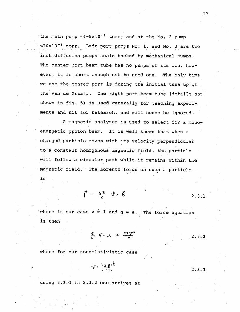
A magnetic analyzer is used to select for a mono-

energetic proton beam.. It is well known that when a

charged particle moves with its velocity perpendicular

to a constant homogenous magnetic field, the particle

will follow a circular path while it remains within the

magnetic field. The Lorentz force on such a particle

is

Yx 8 2.3.1

where in our case z = 1 and q = e. The force equation

is then

e mym-y- 2.3.2C r

where for our nonrelativistic case

l 2.3.3

using 2.3.3 in 2.3.2 one arrives at

18

- ECI - 2.3.4

eB

This last equation shows that for a constant magnetic

field B, and a constant beam energy E, the radius of

curvature for any ion depends upon the square root of

the ion's mass. The magnetic analyzer then can bend the

different ions in the beam into different paths and thus

isolate them. In practice, in our system, the accelerator

will be tuned to a specific energy and beam current in

the center port. The analyzing magnet will then be turned

on with a current known to be insufficient to bend pro-

tons (the most easily bent positive ion) into the left

port. The magnetic current will then be gently increased

until our various indicators show a beam in the left

port tube. The current supplied to the analyzing magnet

is regulated by an Atomic Laboratories Inc. power supply

and regulator (Model C). The regulator holds the current

(and hence magnetic field) constant to one part in 10s.

An Energy Stabilization System is used to prevent

changes in the ion beam energy. The energy of the ion

beam, as it exits from the Van de Graaff accelerator,

depends upon the difference in potential between the ion

source bottle and ground. This potential difference in

turn is controlled by the quantity of charge located at

the high voltage terminal of the accelerator. High

Voltage Engineering's design of the PN-400 accelerator

19

includes a corona probe extending inward from the pre-

sure tank wall toward the high voltage terminal. This

corona probe is tipped with an array of needle-like points,

which increase the probe's efficiency in draining charge

from the high voltage terminal to the pressure tank and,

therefore, ground. It is then clear that the beam energy

is a function of the rate of charge leakage through the

corona probe. The High Voltage Engineering Inc. Corona

Stabilizer takes advantage of the above. The corona

probe is not connected directly to tank ground, but

rather to the plate of a type 4-125A vacuum tube. One

can then control the charge drain from the high voltage

terminal by controlling the conduction of the 4-125A,

the corona stabilizer does exactly that and hence controls

the beam energy.

When a beam has been magnetically analyzed, and

directed down the left port, it encounters two probes

(an insulated vertical slit) within the beam tube. If

the beam energy drifts upward (due to drifts within the

accelerator), then the beam will be bent less by the

magnet and it will impact upon the center (or High energy)

probe more heavily than upon the outside (or low energy)

probe. This imbalance in probe currents is detected by

the High Voltage Engineering Corona Stabilizer Ampli-

fier, and this amplifier in turn sends a negative feed-

back signal to the (grid and cathode) 4-125A. This

signal changes the tube's conductance, so as to correct

20

the beam energy, i.e., to have equal impact on the

probes (this centers the correct energy beam in the tube).

Energy calibraticns of the Van de Graaff accelera-

tor are done with a High Voltage Engineering generating

voltameter. This instrument is used to measure and dis-

play (digitally) the potential of the high voltage

terminal (and, therefore, the beam energy). The unit

consists of a chopper (or rotor) and stator plate (both

eight sectioned). The unit is located within the Van

de Graaff pressure tank near the high voltage terminal.

As the chopper rotates, it alternately exposes and shields

the stator from the high voltage terminal. The voltage

induced on the stators is then a chopped D.C. or roughly

triangular A.C. which is proportional to the high vol-

tage terminal potential and, therefore, proportional to

the beam energy. The rectified output of the generating

voltameter is now connected to a digital voltameter for

a fast, easy, and accurate readout. We estimate an

instrumental accuracy of from 1 to 2 per cent. This,

however, assumes a linear response, a "good" calibration,

and a focus voltage setting which remains at its cali-

bration value.

In practice, the linearity has been verified for

a two point calibration, and the focus voltages used

do not vary more than \5 kV. The calibration procedure

for the generating voltameter involves the use of the

F1 9 (p,ay)0 IG6 nuclear resonance. The cross-section for

21

this reaction shows two distinct resonances, one at a

(laboratory) proton energy of 340 keV, and the second at

a proton energy of 484 keV. To perform the calibration

experiment, a small aluminum wafer is exposed to con-

centrated hydroflouric acid for 15 min. This provides

us with a thin target for use at the end of the beam tube.

A 2 inch Nal scintillation detector is used to detect

the 6 MeV y rays emitted from the fluorine. The pulses

from the detector were Amplified and sent to a single

channel analyzer and then to a scalar. The scalar is

generally set to repeat 10 second data acquisition periods

and I5 second display periods. One then impacts a pro-

ton beam on the fluorine target, adjusting the energy of

the beam to a value less than that required for a reso-

nance. The "background" on the scalar is then noted.

One then gradually increases the beam energy (by increas-

ing the magnetic current, and belt charge) until a peak

is reached, again the number of y-ray counts is noted.

The resonance occurs at that point in energy where the

number of counts on the scalar is just the average of the

background and peak va'lues. The Van de Graaff's energy

is adjusted so that t.. scalar is showing just that

average value, and the digital voltameter is set to the

resonance value. We will generally use the 340.5 KeV

value for our calibration and the higher energy resonance

for a linearity check. Using this calibration procedure,

an overall energy readout accuracy of ",8 KeV appears

22

appropriate.

An Electrostatic Focusing System was installed

as an improvement for the pulsing system used by Dotchin

et. al. for mean life studies. It has, however, become

useful in this work due to its ability to focus the.beam

through the differential pumping slits (to be discussed

later). The system was designed and constructed by

D. L. Keator as a course project. In operation, one

simply monitors the beam current (by means of a Farady

cup) and adjusts the voltages supplied to the electro-

static focusing system so as to maximize that current.

The differentially pumped target chamber, shown

in figure 6, is used to provide the relatively high

pressures of He (<2xlO'3torr) required for the experi-

ment without filling the beam tube with gas and adversely

influencing the operation of the accelerator. To main-

tain a pressure differential between the target chamber

and beam tube, one continually leaks the target gas into

the chamber which is then pumped through narrow slits

into the beam tubes. The slit size is a compromise be-

tween maximizing beam current, and minimizing the flow

of gas into the beam tube. In our case, the upstream

slits (nearer the accelerator) are also a part of the

pulsing system used by Dotchin et. al. There are three

slits in that group, each a horizontal opening L1 x %10 mm

separated by a distance of '5 mm. The downstream slit

is adjustable and set such that it will not intercept any

23

TARGET CHAMBER AND SLITS

/ HBeam

/ UpstreamSlits

ToPressure

Gauge.

Glass'Opaque Tape- Detetor

Detector

-Opaque Tape

Glass

ToDotchin'sDetector

FromHe Gas / BrassInlet -Downstream Slit

To FaradayCup

FIGURE 6

24

of the beam (typically 10 mm 45 mm). During operation,

the highest pressure used in the target chamber is

1l.5xl0-3torr, a simultaneous pressure measurement

"70 cm upstream from the triple slit will typically indi-

cate a pressure of 6xl0-6torr, a ratio of 250:1. The

lowest pressure used in the target chamber is ,10-storr

at which time the pressure in the beam tube is .3xl0 -6

torr giving a ratio of '3:1. Again, differential pump-

ing is required because the beam tube and accelerator

must be kept at pressures <l0- 5torr; and because we want

to spatially localize the beam gas collisions.

The target chamber is a brass cylinder with

5 cm I.D. and 17.7 cm length. Two glass rectangular

windows have been attached on opposite sides of the

cylinder walls with epoxy cement. The chamber is

oriented such that one may look horizontally through both

windows. See again figure 6. The window sizes are

both 13 cm x 2.3 cm. This target chamber is used both

for the mean life studies of Dotchin et. al. and for

our polarization studies, each group using one window

of the chamber. There are two vacuum couplings on the

top of the chamber, one connected through a series of

regulators and valves to the gas supply, and the other

through valves to our pressure gauge. See figure 7.

The gas supply system is quite conventional with

a two stage regulator reducing the tank pressure to a

value of 110 psig. The gas then flows through-a

25

GAS AND PRESSURE SYSTEMS

- CapacitanceManometer

H+Beam

VacIon TC Gaouge-Pump

Target Chamber-----

Shut Off Valves-

To Faradaycup

MeteringValve

VacuumRegulator

Two Stage-He Gas Regulator

FIGURE 7

26

flexible hose to another regulator. This second regu-

lator is a Matheson Co. vacuum type, capable of regula-

ting its output from '50 - 750 torr. We typically run

at 1300 torr. Next, the gas encounters a Hoke Micromite

fine metering valve, which is used to control its flow

into the evacuated target chamber. I would add that with-

out the vacuum regulator, we would only be able to use

the first ! turn of the 18 turn metering valve, whereas,

with the vacuum regulator's pressure reduction, we are

able to use \1-1/2 turns of the valve to achieve the

desired pressures within the target chamber.

The pressure measuring system consists of a num-

ber of vacuum pressure gauges spread about the beam tube

and target chamber, see figures 5 and 7. The gauges

located at the main pump, left port pump No. 1 and left

port pump No. 2 are the cold cathode type usable from

nlxl0- 6torr to 150xl0- 6torr. The vacuum gauge on left

port pump No. 3 is the ionization type usable from

\10 - 9 to n10-storr. The above gauges are used for general

maintenance of the system and not for data acquisition.

An extremely accurate and sensitive MKS Instruments Inc.

Baratron capacitance manometer is connected to the

target chamber for pressure data measurements. The

manufacturer claims a general accuracy of .1 per cent,

and repeatability of .005 per cent. The method employed

by the designers is to compare the unknown pressure

Px with a smaller known reference pressure Pr"* This

27

comparison is done in our model 77 H-I pressure head.

The head is divided by a highly stressed thin flat

metallic diaphragm into two chambers, one for reference

pressure, one for the unknown pressure. When the

reference and unknown sides differ in pressure, the

diaphragm is deformed, but the diaphragm is part of an

A.C. capacitance bridge. Therefore, any imbalance in

pressure will be transformed into an imbalance in the A.C.

bridge. Our type 77M-XR indicator translates this bridge

imbalance into a pressure reading. One great advantage of

this arrangement is the ability of the indicator to null

(or balance) out (digitally) the gross pressure difference

and to then use the full sensitivity of the instrument on

the finer levels of imbalance. One can then achieve five

significant digits in the readout.

In order to achieve high accuracy, one must know

the reference pressure Pr' or reduce P to a value lowr

enough to cause negligible error. Recall the pressure

indicated by the instrument is the difference in pressure

P - Pr. We are using a Varian VacIon pump (2k/sec.) to

maintain a very low P . We estimate from the currentr

drawn by the VacIon pump, Pr to be <10-6torr and would

therefore have <10 per cent error in our lowest pressure

data.

2.4 The Polarization Detection System

This system is used to detect the intensity of

28

both the vertically and horizontally linearly polarized

components of the 5016 A (31P - 21S transition) light

from-the helium target gas. The system is shown in

block diagram in figure 8 and in 1:1 scale in figure 9.

The polarization analyzer consists of a type

HN-32 polarizer which has been carefully mounted in a

holder and aligned such that it can be rotated from one

terminal position by 90 degrees to another terminal

position and then back, etc. This arrangement allows

the experimenter to set the analyzer (at one terminal

position) to pass light whose electric field vector is

vertical, and to then rotate the analyzer (blindly) to

its other terminal position where it will pass only

horizontally polarized light. These rotations are in

fact done by the experimenter in the darkened accelerator

room. Thus the need for the two (90 degrees apart)

terminal positions.

Reflections from the surfaces of the polarizer

are according to the manufacturer isotropic and <4 per

cent; they can therefore be ignored. As previously

stated, the ratio of transmissions for the desired:

undesired components is r1.5x10. This arrangement is

then quite suitable for alternate analysis of the

orthogonal components of linearly polarized light.

The 5016 A line of He is selected by an in-

terference filter. This type of filter is a device

which will transmit (by constructive interference)

TARGET CHAMBER 8 DETECTOR ELECTRONICSFrom He

Vacuum Gas TargetFaraday Cup Pump Supply Chamber

r To Pressure Gauge

: - Polaroid AnalyzerMrOpaque Tap Interference FilterAmmeter M.

TubeVoltage ToFreq. Conv. Amplifier

Inverter Pulser Spy ChannelAnalyzer

Scaler Gate Preset GateSignal Scaler Signal

FIGURE 8

30

THE DETECTOR SCALE 1:1

PhotomultiplierTube

Photocathode

Interference

OpaquePolaroid TapeAnalyzer / / Tape

Glass

To PressureGaugeo HBeam

Target Chamber Interior

Maximum acceptance angle at photocathode is -.70

FIGURE 9

31

only certain wavelengths of light. The transmission

is polarization form independent, and will therefore

not effect our measurement. This polarization form in-

dependence was tested and confirmed by a rotation of

the entire detector and a comparison of the polariza-

tion results for the two detector positions. This test-

ing and confirmation process is described in section IV.

The filter used for this work was manufactured by Spectra

Films Inc., Winchester, Mass. It has a peak transmittance0

of 60 per cent at 5018 A, and a full width at half maxi-0

mum of 18.8 A for normal incidence. The slight difference0

in wavelength between our line (5016 A) and peak is not

significant, it only reduces the percentage transmission

for our line to 58 per cent, a 2% loss. See figure 10.

The need for such a filter becomes apparent when

one examines the He spectrum. There are a large number

of prominent lines in the spectrum. Table 1 lists some0

of those lines near our 5016 A line. Also, a partial

energy diagram for He is shown in figure 11, and figure

12 shows a spectral scan in the region around 5016 A. The0 o o

lines nearest 5018 A are at 5047 A and 4922 A. It is

necessary that our interference filter not transmit these

or any other lines. We have no problem when the Helium

light is normally incident upon the filter, the 5047 A

line is attenuated by n99 per cent, and the 4922 A line

is attenuated by >99 per cent. However, all the light

incident upon the filter is not normally incident, and

32

THE INTERFERENCE FILTER

5018 1

60%Transmittance

18.8 A

4980 A 5060 A

FIGURE 10

33

TABLE 1

0

-EULI- 'T!RA1TIS WEARI 5016 A

0 0 0

Wavelength(A) Transition (5016 A - X)A

4713 43 S-2 3p 303

4859 (He II) 8-4 157

4922 41D421 p 94

5047 41 S-2 1 p -31

5411 (He II) 7-4 -395

34

PARTIAL TERM DIAGRAM OF He

SINGLETS TRIPLETSID Ip S 3S 3p 3D4S 4p

4d 4 4s s 4p d3d 3 3d2p s 2P

2sI /

i/

Is

I,

The 31P-21S transition is indicated by a heavy line

FIGURE 11

33

PARTIAL HELIUM SPECTRAL SCAN

5016 A

4922 A.5047 A

FIGURE 12

36

Xpeak is in fact, a function of the angle of incidence.

According to Baird-Atomic, a manufacturer of interference

filters, the wavelength of peak transmittance is lowered

as the angle of incidence increases, such that

where e is the angle of incidence, XA is the wavelength

of peak transmittance for the angle of incidence, A1 is

the wavelength of peak transmittance for normal incidence

and n is the effective index of refraction of the filter.

A short computer program was written to compute X0 as

a function of both e and n. The program is listed in

Appendix C.1, and the results are shown in Table 2.

In our detector (see again figure 9) the largest

possible incidence angle is '70. Referring to Table 2,

we then see that the worst possible case (n=l) has a0

Xpeak = 4980 A. This worst case is still quite good

since ,99 per cent attenuation is achieved at only

22 A from Apeak (see again Figure.10). Our interference0

filter is then quite sufficient to isolate the 5016 A

line of helium. \

A photomultiplier tube and associated electronics

are used to measure light intensity. We refer again to

Figures 8 and 9 where the tube, its housing and the

various electronics are shown. The tube is an EMI

6256S, n2 inch diameter, S(Q), SbCs photocathode, and

very low ('12x10-'A) dark current at the operating

37

TABLE 2

PROPERTIES OF THE INTERFERENCE FILTER

0

Index of Refraction Angle of Incidence (deg) x (A)

1.0 0 5018

4 5005

8 4969

1.4 0 5018

4 5011

8 4993

1.6 0 5018

4 5013

8 4998

38

voltage of -1850 volts. The tube is wrapped with black

tape and housed in an aluminum light-tight container

with a single aperture in front of the photocathode.

The tube base is wired as shown in Figure 13, and power

is supplied by a Power Designs Pacific Inc., Model 2k-10

high voltage power supply. The spectral response of the

photocathode is near its peak at 5000 A (10 per cent

quantumefficiency) and is well suited for measurements

on the 5016 A line. The tube was usually operated at

room temperature excepting very warm days when ice water

cooling was necessary to bring background count rates

back down to "normal."

Signal pulses from the tube were fed into a C.I.

1416 Amplifier, these amplified pulses were next passed

through a C.I. 1430 single channel analyzer which was

used as a discriminator to reject pulses of less than a

preset magnitude. The Scalar output of the single channel

analyzer was passed to a C.I. 1470 scalar for counting.

It was found that the discriminator setting had little

effect upon the final signal to noise ratio, therefore,

a setting was chosen to give a reasonable counting rate.

This same effect was noticed by Pegg (1970), who used

this same tube and similar electronics.

A second photomultiplier tube was used briefly

during this research, it was mounted directly on the

second window of the target chamber and monitored the

helium light output for normalization purposes. The

39

PHOTOMULTIPLIER BASE CIRCUIT

CathodeIM

Dp680 K

> D680K

->D

.Ol If 680K

>DI,.0Ip/f - 680K

IMS68KAnode

+H.V. SignalOut

FIGURE 13

40

tube was an RCA 8575 run at -2500 volts, at room tem-

perature. The arrangement is shown in figure 14. This

system was used only long enough to confirm that light

normalization and current normalization gave the same

value for the linear polarization fraction, it was then

abandoned so as to minimize the changeover time between

the experiment of Dotchin et. al. and this work.

Due to the fact that the proton beam from the

accelerator is not stable, we must use a Faraday cup

to determine just how much beam we have had in any counting

period. The cup is really just an extension of the beam

tube, of length 14.5 cm, with an oval entrance aperture

(10 mm x n20 mm). The downstream end is closed by a

double end window of Vycor glass. See figure 15. We

depend upon the length of the cup, and the entrance

aperture to contain secondary electrons. A comparison of

beam current measurements was made for two lengths of

the cup with and without the aperture, since the results

were essentially identical, we concluded that secondary

electrons were not escaping and that the cup was contain-

ing the proton beam. We therefore felt there was no

need for a suppression grid. The electronics for the

cup were shown in figure 8, and consist of Keithly Model

610 Microammeter, a homemade voltage to frequency con-

vertor, a C.I. invertor, and a Mechtronics 700 scalar.

In use, the microammeter is connected directly to the

Faraday cup, the D.C. chart recorder output of the

41

LIGHT NORMALIZATION SYSTEM

PolarizationTo Detector From HePressure Gas

Gauge Supply

H+Beaom

PM.Tube

ConstantSFraction

Discriminator

H.V.Supply Gate Signal From

Preset Scalar

FIGURE 14

42

THE FARADAY CUP

AluminumAperture Disk H+

Beam

VycorDoubleEndWindows

FIGURE 15

43

microammeter is sent to the voltage to frequency conver-

tor (built by L. W. Dotchin from plans in the General

Electric Transistor Manual, General Electric Co., Syracuse,

N. Y. 1964). The pulses from the convertor are inverted

to match the input requirements of the scalar where they

are counted. The number of counts appearing on this

scalar is directly proportional to the number of protons

passing through the target chamber, and can therefore be

used as a normalization base.

44

SECTION III

EXPERIMENTAL METHOD

3.1 Introductory Description

The methods used in this research have been

evolved so as to maximize the usefulness and effective-

ness of the apparatus with which we have worked. Methods

were evolved to deal with the irregularities in the proton

beam from the Van de Graaff accelerator. In fact two

methods were developed and used simultaneously and gave

the same value for the linear polarization fraction. The

need for these normalization methods and their implementa-

tion will be discussed in the next paragraph.

The actual data taking process is dependent upon

the type and settings of electronics used. One must re-

main within the useable limits of the electronics while

at the same time maximizing the signal to noise ratio.

Our methods for achieving this end are described in

paragraph 3.3.

Finally the actual step by step data taking pro-

cess is outlined in paragraph 3.4.

45

3.2 The Need for Normalization

The Van de Graaff accelerator, being mechanically

powered, is more susceptible to irregularities than most

other pieces of apparatus. The proton beam from the

accelerator typically undergoes three different types of

transition, irregular oscillations of beam current, long

term upward or downward drift of beam current, and

sudden "1/2 to 1 1/2 second complete cessations of beam.

The irregular oscillations in the beam current

are probably due to a number of factors including;

irregular transport of charge by the belt within the

accelerator; fluctuations in the probe voltage (the probe

voltage supply is powered by a generator driven by the

belt); and overcorrections in the negative feedback

loops of the energy stabilization system. In so far as

our experiment is concerned, high frequency oscillations

are of no importance, they would simply average over the

>1 second observation period used in taking data. Low

frequency oscillations must be accounted for in order to

correctly compare intensity measurements taken at differ-

ent times.

Long term upward or downward drifts of beam

current must be dealt with in the same manner as the low

frequency irregular oscillations, especially if these

drifts are noticeable within l second periods. These

long term drifts are most likely due to changes in the

46

rate of flow of H2 through the paladium leak.

The sudden cessations of beam are usually due to

sparks within the accelerator tube, sparks among the

equipotential planes, or a spark from the high voltage

terminal to the tank wall. Occasionally, the beam is lost

for a short time when the energy stabilization system is

unable to correct for an excess or lack of charge on the

high voltage terminal. The beam energy will then be too

high/low for the magnet to steer the beam into the left

port beam tube and the beam will be lost until the charge

situation corrects itself. In any case, whenever the

beam is interrupted, the data taken at that time is not

used, the machine is reset if necessary and new data is

taken. The problem is to determine when an interruption

has occurred. The problem is solved by making the experi-

menter a part of the apparatus. While taking data, the

experimenter stands at the end of the left port beam tube

and stares at the Vycor end window of the Faraday cup.

In striking the Vycor, the proton beam generates a dis-

tinct blue light. With practice, the experimenter can

spot beam interruptions (as an interruption of the blue

light) which last for as short a time as \1/10 second.

The data is then not used, the scalars are reset and

new data is taken.

Again, normalization is required so that one may

compare intensity measurements made at different times

even though the beam current is not constant in time.

47

Also, the experimenter is part of the apparatus not only

in the sense of making adjustments, but also as a sensor

using eyes and even ears to detect irregularities in the

Van de Graaff performance.

We have used two different normalization systems

to monitor beam current. In the first case, we monitored

the irregularities in the light output of the helium

target gas. This system was based upon the assumption

that the light output was directly proportional to the

number of excitations which had occurred within the tar-

get chamber. The second system was a bit more direct,

we used a Faraday cup to collect the beam after its

passage through the target chamber (assuming very little

loss) and integrated the beam current. The first system

then normalizes to the number-of excited helium atoms

(assuming no saturation occurs), while the second system

normalized to the number of protons passing through the

target chamber. We formulated the hypothesis that the

number of excitations should be directly proportional to

the number of protons passing through the chamber, i.e.

that calculations based upon data taken simultaneously

with both systems should give the same result. This

was in fact the case demonstrating that our two nor-

malizing systems were equivalent. Once we were satis-

fied as to that equivalence, the light normalization

system was deleted from the experiment. Its continued

use would have created large scale problems durin the

48

changeovers between this work and that of Dotchin et al.

All the data and results presented in this work are

based upon the current normalization system.

3.3 Setting the Detector System

The system is "set" by properly adjusting all

discriminators, amplifier gains, and miscellaneous other

parameters.

A very simple and direct method is used to time

the runs, in fact, all runs have the same duration. As

shown in Figure 8 , an Ortec 48.0 pulser drives a pre-

setable Mectronics 702 scalar/timer. Pulses are gen-

erated by the pulser in syncronization with the A.C. line

frequency, i.e. 60 pulses/second. The Mectronics scalar/

timer is preset to turn off at 80 counts, (or 80/60 of a

second = 1.3 second). When the scalar/timer shuts off,

it will simultaneously (i.e. in a time which is short

compared with the average time between data pulses to

the other scalers) shut off, via built-in gating cir-

cuits, the other two scalars. The counting time of 1.3

second was in part forced upon us by the data count rates,

and by the tendency of the Van de Graaff to spark quite

often. We wanted a counting time of the order of 1 to

1 1/2 seconds in order to get convenient count rates and

yet still be short enough so that the probability of a

spark (beam interruption) would be small, 1. second

49

was the best available compromise.

The amplifier gains, discriminators, and photo-

multiplier tube high voltage have been set for single

photon counting and zero dead time correction. Typical

count rates are shown in table 3.

The scalars used are capable of count rates on

the order of 104-10 s counts/second before dead time cor-

rections are needed.

The signal count rate for the normalization

scalar is controlled by the range switch on the Keithly

microammeter. The output of the Keithly is the same per.-

centage of 10 volts as is the indicator of full scale.

We limit, by choice of range, the percentage of full

scale such that the input voltage to the voltage to fre-

quency converted does not exceed 2 volts, which in turn

limits the count rate.

The criteria for the polarized light intensity

scalar is that the tube be operating in the single photon

counting mode and that extraneous noise not be counted.

The count rate is then controlled by tube voltage, am-

plifier gain, and the single channel analyzer's dis-

criminator.

The sources of background counts are noise pulses

(both thermal and light noise) in the case of the polar-

ized light intensity scalar; and zero offset of the

Keithly microammeter in the case of the normalization

scalar. To minimize background counts in the first case,

5C

TABLE 3

SCALAR COUNTING RATES

Signal +Scalar Background rate Background rate

Scalar/timer 60/sec 0

Light intensity 100 to 5000/sec 10 to 50/sec

Normalization \1300/sec "'7/sec

51

one darkens the accelerator room, uses lead bricks to

shield the tube from tank x-rays, and when necessary,

cools the tube. In the case of the normalization scalar,

one can "adjust" the background count rate by adjusting

the zero of the microammeter. We have always chosen to

carry a background rate of 2 to r8 counts/second so

that we were sure that the "zero" was not negative. A

negative zeroing of the microammeter would have given us

a false (low) value for the integrated beam current.

Our next problem is that of maximizing the sig-

nal to noise ratio. Only in the polarized light inten-

sity scalar is the S/N ratio low enough to merit concern.

The only option, after external noise sources have been

eliminated, is to try adjusting the discriminator of the

single channel analyzer. We have found no appreciable

changes in S/N over a wide range of discriminator set-

tings. (The S/N ratio is a function of the pressure and

ranges from "3 to "100.) We have therefore arbitrarily

chosen a discriminator setting which results in a con-

venient count rate. Again, see Pegg (1970) for further

discussion.

3.4 Taking Data

The steps followed in the actual data taking

are:

1. Warm up phototube and electronics for x12

hours.

52

2. Warm up accelerator for 1l hour

3. Turn on beam in center port, adjust current

and energy

4., Steer beam into left port, adjust current

and energy

5. Go downstairs and . . .

6. Start flow of He into target chamber, adjust

pressure

7. Assume data taking position at end of left

port beam tube

8. Reset all scalars

9. Switch beam off by remote switch

10. Start scalars for background count

11. Record values on scalars

12. Turn beam back on

13. Rotate polarizer (by hand) for passing E

vector vertical

14. Reset scalars

15. Start scalars

16. Record values

17. Rotate polarizer 900 (by hand)

18. Start scalars

19. Record values

20. Repeat 13-19 with occasional background

runs (beam off)

A normal data run will consist of first a back-

ground reading for the polarization and normalization

53

scalars; then 7 sets of "polarization vertical" -

normalization - "polarization horizontal" - normalization;

then a background run; then 6 sets of data; then a back-

ground run; then 7 sets of data; and finally a last back-

ground run. Typically, a data run (20 measurements +

4 backgrounds) will take .3/4 hour exclusive of tune up

time for the Van de Graaff (another 1/2 hour). Table 4

is an actual data page from the laboratory notebook.

54

TABLZ 4

DATA F O:: THE LB 3 N77BO& ,

'3 oo e *- v -/-- e-

2-

Y93 F

7 ? S 3 -S3 r __ _

7frS -/ / 2 .66 1. I/ -2 P /s 3

go S2 /'3 ,n . tr3

q61 7/ Y r ; r

gy; ,</30 79r /t

g'oy /2& fgrry

6E /[ / r3 ti9 7r 2./7

S ro g ,3 g /.rr 3

6y 2 / Cf 3 o 737 /FIgO Y / rk?~ ~g7 /s6

S7/ /10VD Eg[ /So&~

RL /4 09gy /o

S'b/ / V1 3 Y8o /V y'r

96 to 6 76 6o

i 6y 2

z /60?

4

55

SECTION IV

ANALYSIS

4.1 Calculating w

The linear polarization fraction 7 is defined

as . . .

7 + 4.1.1

where Io and I, are the intensities of the light with

electric field vectors respectively horizontal (parallel)

and vertical (perpendicular). These intensities are

determined from the number of counts showing on the

scalars at the end of each parallel and perpendicular

data acquisition period. We must of course subtract any

background counts which are included in the scalar dis-

play. Furthermore we must normalize these intensities

to integrated beam current (as discussed in section 3).

Therefore the intensities are expressed as . . .

C, - 82

I,4

4.1.2

cA- BA

56

where in both cases the numerator represents signal

counts, i.e. total counts (on the light intensity scalar)

minus background counts. The denominator in both cases

is proportional to the number of protons which have

passed through the target chamber, represented by total

counts (or the noxrmalization scalar..,minus background

counts. Thus It and 'l ~ie the intensities per proton,

and are-therefore independent of small fluctuations of

the proton beam current. We then have the following

definitions .

Cv, C, = The number of counts on the light in-

tensity scalar for the parallel and perpendicular data

acquisition periods.

B, = The average number of background counts

on the light intensity scalar.

N,, N, = The number of counts on the normaliza-

tion scalar for the parallel and perpendicular data

acquisition periods.

BN = The average number of background counts

on the normalization scalar.

At first glance a non zero BN is not expected, however we

purposely set the zero adjustment of the Keithly micro-

ammeter to give a small background on the normalization

scalar. This was done so that we could be assured (by

checking background counts) that the microammeter zero

adjustment was not set negative. Therefore we were

57

assured that no counts were lost.

We then do the actual calculation of the linear

polarization fraction 7 from . . .

7= C. -4.1.3

IV, -

Note that a calculation of w requires two data acquisition

periods, one for the parallel and one for the perpendicular

orientation of the polarization analyzer. A typical data

run then consisted of twenty measurements of I,, and IL,

and then the twenty calculations of 7. The average back-

grounds BI and BN were found from four measurements taken

before, during and after the data run. See again table 4.

The actual calculations are done on the University

of New Hampshire's IBM Call 360 time sharing computer

system.

The computer program which does this calculation

(called NEWPOL and listed in Appendix C.2) will print out

Cl, N,,, C_, N , and 7 all twenty times and will then print

a mean w, the standard deviation, and the standard error

of the mean, the beam energy, current, the He target pres-

sure, and the number of 7's deviating by more than two

standard deviations from the mean n. Table 5 shows the

program output created from the data of table 4.

5p

TABLE 5

OUTPUT OF THE PROG: " E.:POL

LINEAR POLARIZATION FRACTION# OF RUNS TO ANALYZE IS?lLIST ALL P?YES

V C H C P899 1467 818 1502 -0.06165902 1523 815 1533 -0.0568863 1533 852 1530 -0. 0'74782 1486 838 1524 0.02395792 1531 795 1546 -0 290

'809 1538 778 1553 -0 .2561809 1558 780. 1553 -0.01775847 1430 795 1514 -0.06218894 1559 784 1565 -0.07126804 1569 784 1546 -0.00594819 1549 802 1547. -0.01047824 1550 873 1553 0.02955900 1564 793 1567 -0.06777885 1633 883 1638 -0.00273952 1634 838 1557 -0.04292906 1587 878 1600 -0.02064871 1604 888 1606 0.900957892 1609 844 1607 -0.02P56936 .1606 927 1599 -0.00 288861 1421 880 1484 -0.01030

300 KEV, .20 U HE, 11.5 U A H+, 20 TRIALSST DV = .02991 0 PTS DV > 2 SIG S.E.= *00669(P-SE)=-.02849 MEAN P =-0.02180 (P+SE)=- 01511

59

4.2 Polarization Measurement Error Analysis

There are of course two types of error inherent

in this experiment. Random errors occur due to the nor-

mal variations (fluctuations) in counting rates; and

systematic errors occur if faulty equipment and/or

methodology is used. The random errors present a problem

only in that they limit the precision of the calculation

of n; any systematic error could reduce the accuracy of

the experimental result.

We will first discuss the random errors present

in this work. The linear polarization fraction 7 is

calculated from Eq. 4.1.3. The variables which.appear in

this equation are simply the numbers which are displayed

by the scalars at the conclusion of each of two 1 1/3

second intensity data acquisition periods, as well as

the average of four 1 1/3 seconds background count

acquisition periods. Every one of these scalar displayed

numbers is subject to normal statistical fluctuations,

thus when rr is calculated, the precision of a single cal-

culation is quite poor. We therefore repeat the measure-

ments from which n is calculated twenty times for each

"run," and take many runs for every "final" value of ~.

The i which we will report as a result is the average

of Nx20 values, (where N is the number of runs at some

particular pressure, beam current, and beam energy). Thus,

the precision of this work is enhanced by repeating our

60

measurement a multitude of times.

In order to analyze our random errors, we must

take care to distinguish between sample variables and

population variables. We will follow the notation of

Parratt (1971) and Wilson (1952) where the sample (run)

mean, standard deviation, and standard error are sym-

bolized by m,s, and sm; while the population mean, stan-

dard deviation, and standard error are symbolized by p,

a, and am. We are of course most interested in - and

am since we will report the linear polarization fraction

in terms of our best estimate of the parent population

mean, and its standard error. The procedure is outlined

in the following formulae where 7ij is the calculated 7

from one set of measurements for the jth run (i.e. 1/20

of a run) and n=20. All nij are equally weighed. For

each run, where j is the run index

S4.2.1

while for the best estimate of the parent population

mean . . .

NHn

At n 4.2.2

where N is the number of runs at some particular He target

gas pressure, beam current and energy. It now remains to

calculate and estimate the dispersions in the sample and

parent populations. The standard deviations s and a are

61

suitable dispersion indicies. For each run we have

4.2.3

while for the parent population we have

CT 4.2.4

However, u is never known exactly, only estimated as u'

from Eq. 4.2.2. The best estimate of a (see the appendix

of Bacon (1953) is then

0- - - ')J 4.2.5

Since in this work we take many runs and calculate

a mean T for each, it is useful to also calculate the stan-

dard error am (also called the standard deviation in the

mean). The experimental standard error S is

where is the grand mean, or mean of means.

. 4.2.7

Jzs7

where in our case n=20, the number of r's in one run. We

are in fact more interested in the standard error am cf

the parent distribution.

"u)4.2.8

and

U z4.2.9

Again V is unknowable exactly and we must estimate am.

Using 4.2.9 with 4.2.5, we arrive at the useful result

that

o:~7n (nN -) 4.2.10

According to statistical theory, the mean 7 of

any run has a probability of 68.3% of falling between the

values of pi am •

We calculate and report as follows . . . for

every run of n=20 iT's, we calculate the mean for the run

mj (Eq. 4.2.1); an estimate of the parent population

standard deviation for the run aj (Eq. 4.2.5, with N = 1)

and the estimated population standard error am (Eq. 4.2.10,

with N = i).

When sufficient runs at a particular He target

gas pressure, beam current and energy have been-

63

accumulated, the Nx20 7 values are combined to estimate

the population mean, ' (Eq. 4.2.2), usually written

simply as 7; the population standard deviation a

(Eq. 4.2.5); and the population standard error a

(Eq. 4.2.9).

In the first case where single runs are analyzed,

the computer program NEWPOL is used (Appendix C.2), for

calculation of the accumulated result the computer program

STAT is used (Appendix C.3).

When our results are given in the next section,

we will report the estimated population mean and the

standard error amm

We must now discuss possible systematic errors

since this type of error will reduce the accuracy of any

experiment. Some typical examples of systematic error

are .

1. Subconscious bias on the part of the

observer

2. Incorrectly calibrated instrument(s)

3. Misaligned apparatus

4. Lack of correction for changing

environmental conditions

5. False assumptions of independence of result

from an experimental parameter

6. .etc.

In this work, the greatest possibility for a

64

systematic error lies in whether or not our polarization

detector is biased. We evolved a simple method for

determining the existence of any bias. Our polarization

detector housing was modified such that it was possible

to rotate the entire detector, about its line of sight,

by 90 0 . When we then compared n results arrived at for

the detector normal (N) position and the results for the

detector rotated (R) position, we could unfold any de-

tector bias. We chose to do this procedure over a range

of proton beam energies with constant beam current and

He target gas pressure. Many runs were taken at each

energy with detector (N) and (R). The means N and TRwere calculated at each energy along with the estimated

population standard deviations aN and a c We are then

able to use the "student" t test for the significance of

the difference of means as described by Spiegel (1961).

The t test is derived from small sampling theory

(although, under conditions of large samples, it becomes

equivalent to the z statistic). Using our notation .

= ,4.2.11

nN, + nN

where n again is 20 and NN (NR) is the number of runs

with detector N(R). Also,

n+ S 4.2.12CT

65

where SN(SR) are the detector N(R) standard deviations

calculated from

4.2.13

Note that 5= j -- where a was defined in Eq. 4.2.5.

Having done these calculations, we are then faced

with the statistical decision making process. In order to

compare two means, we must do a two-tailed test on the t

statistic. Let us state the hypothesis H0 : there is no

significant difference in the means; and H,: there is a

significant difference in the means. It is customary to

make the test at both the .05 and .01 levels of signifi-

cance. The range of acceptable t values at the .01 and

.05 levels is shown in table 6 for various degrees of

freedom v= Nk, + -2 . If when we calculate t

from Eq. 4.2.11, t lies outside the range given by

table 6 (for a particular i? and level of significance),we would have to reject H0 at that level of significance..

A rejection at the .05 level means we have a 5 percent

probability of having made a "false" rejection, and a

rejection of Ho at the .01 level implies a probability of

1 percent of a "false" rejection. If we have a rejection

at .05, but not at .01 then HI is "probably" true, i.e.

there may be a significant difference in the means.

A computer program TTEST (Appendix C.4) was used

to calculate the t values from Eq. 4.2.11 for both N and

66

TABLE 6

T-TEST SIGNIFICANCE LEVELS

SIGNIFICANCE LEVEL

.01 .05

20 -2.84 < t < 2.84 -2.09 < t < 2.09

40 -2.70 < t < 2.70 -2.02 < t < 2.02

60 -2.66 < t < 2.66 -2.0 < t < 2.0

120 -2.62 < t < 2.62 -1.98 < t < 1.98

00 -2.58 < t < 2.58 -1.96 < t < 1.96

67

R orientations of the detector. The results are shown

in table 7. Only at 450 keV proton beam energy is there

any possible significant difference in the means. The

last entry in table 7 compares the mean of the (N+R)

results with the mean of the N results, and shows no

significant difference. We therefore conclude, that our

polarization detector has no inherent polarization form

bias and that said detector does not contribute any

systematic error to our experiment. We will henceforth

combine the results of N and R runs taken at the same

pressure, energy and current.

A second possible source of systematic error in

this work could be caused by any drift in our electronics

which was constant in sign for the greater part of a run.

In order to average out any such drifts, the order of

data taking was varied during a run. The linear polar-

ization fraction was always calculated for time adjacent

I, and I1 values. Our data taking order would be .

[(11N1:) (IlNL )] [(I_ N.) (II N i [(I, NI) (I N )] (. N )(IN,)]

etc. where the rectangular brackets denote a cal-

culated i7. It is our contention that any "constant"

drifts would be averaged out by this method of data

taking. Any random drifts would of course average them-

selves out of our calculations.

Another possible source of systematic error lies

in the fact that stray magnetic fields can cause preces-

sion of the atomic electrons and, therefore, depolarize

68

TABLE 7

TEST FOR SIGNIFICANCE OF DIFFERENCE OF MEAN r

FROM NORMAL AND ROTATED DETECTOR

BEAM t VALUE # of DEGREES DIFFERENCE IN MEANSENERGY N Vs R of FREEDOM SIGNIFICANT

.15 .01

(keV)

150 0.00 138 No No

200 1.75 118

250 .25 118

300 -.48 238

350 .96 118

400 1.76 118

450 2.48 138 YES

t VALUE(N+R) Vs N

450 -1.23 218 No No

69

the light from a collection of atoms. Feofilov (1961)

discusses this problem and gives the results of Breit

as follows

and 4.2.14

where e is the zero magnetic field linear polarization

fraction, w is the polarization fraction measured at

magnetic field strength H, T is the mean life of the

transition, g is the Lande g factor and 4 is the angle of

rotation of the plane of polarization. Using

e = 4.8x10- 0o stat cm = 9.1x10 -2 8 gmc = 3x1010 cm/sec

estimating T=2xl0- 9 seconds (from Dotchin et al.) and cal-

culating g for the 31p states from

+ +[t) + s(s+4 -(li) 4.2.15

where j=l, s=O0, and £=l so that g=l. We then have .

S7To f + .o3;>H 4.2.16

Measurements of the magnetic field strength H in

the vicinity of the target chamber were made using a

HeliFlux Magnetic Aspect Sensor type RAM-3. These measure-

ments were made with the Van De Graaff steering magnet

energized. In no case were we able to find a field in

excess of ,3/4 gauss. Using this in Equation 4.2.16, we

70

get

and conclude that the magnetic depolarization is negli-

gible when compared with the random error present. Simi-

larly we conclude that =0 and the plane of polarization

is not rotated by the magnetic field.

We must also concern ourselves with collisional

depolarization. Collisions between helium atoms in the

target chamber, as well as with the chamber wall, will

tend to equalize the magnetic substate populationsand,

therefore, reduce the polarization. Referring to a

mean free path calculation done in the next section

(4.3), we find the mean free path (using the geometric

cross-section) of the helium atoms to be = 47cm. The

rms velocity of the helium atoms is V = 3kT

which for room temperature helium works out to

S /.' /X /o~ cn/sec . Therefore the mean collision

time is = 3.3x10-4 sec. However, we must also account

for the chamber walls where the radius is n2.5cm. Thus,

we can expect a wall collision in t=1.8x10 - s seconds.

Since even this time is 4 orders of magnitude larger

than the mean life of the 31P state (1.8x10- 9 sec), we

can ignore the possibility of depolarizing collisions.

Another mechanism which could cause a systematic

error is that of cascading, where the 31P level is popu-

lated not only by direct proton excitation, but also by

73.

downward transitions from n'S and n'D levels (n>3). In

general, cascading into the 31P level from a number of

different upper levels will tend to equalize the mag-

netic substate populations and, therefore, reduce the

amount of polarization exhibited by the 31P --- 2's

transition. Heddle (1962) has shown that if the per-

centage of the 31P population due to cascading is C%

then the experimentally observed polarization must be

multiplied by the factor (1 + c/100) in order to correct

for the cascade depolarization. C is most easily cal-

culated following the method in appendix b of Van Eck's

(1964) paper, using the transition probabilities listed

in Gabriel (1960). However, in order to do this calcula-

tion, we need the values of various experimental emission

and excitation cross sections. All the necessary experi-

mental cross sections for this calculation are not yet

in the literature. Since the agreement between theoreti-

cal and experimental cross sections is so poor, we have

decided not to do the calculation with the theoretical

values, but to instead rely upon the experimental deter-

minations of cascade given by Van den Bos (1968) and by

Thomas (1967). In both of these works, the authors use

their own unpublished data to calculate the cascade per-

centage c, which they then report. Van den Bos reports

values for c of 8% at 100 keV and 6% at 150 keV; while

Thomas reports 4% over the energy range 150 - 1000 keV.

We will, therefore, correct for cascade as follows:

72

at 100 keV use 8%, at 150 keV use 5%, and above 150 keV

use 4% for the cascade correction.

We must next discuss the effect of resonance

trapping on the polarization of the emitted light.

Resonance trapping occurs when the beam excited 31P

level decays to the 1'S level and the resultant photon

is trapped by a ground state He atom. The ground state

atom is then of course excited to the 31P level and may

then undergo a 31P -- 21S transition. This event re-

sults in our detector seeing light from atoms which were

not space quantized by the proton beam, and, therefore,

results in an experimental polarization which is lower

than the free atom value. In order to estimate the

amount of trapping which occurs, we turn first to the

work of Lees (1932) and Lees et al. (1932). These works

used photographic techniques to determine the excitation

cross sections for various He levels excited by electron

impact. When Lees' photographs showed X 5016 A light

emanating from He gas which was not impacted upon by the

beam, he and Skinner concluded that 3'P-1'S radiation

from the beam area was being trapped and a portion of it

would then be emitted as 31P-21 S light. They showed that

the proportion of light absorbed = I- where n is

the number density, r is the target chamber radius, and

T is the atomic absorbtion coefficient.

Their values for Ta were 2.3x10- Is (experimental)

and q92xl0 -' 5 (theoretical). Once we know the

73

percentage trapped in the 31P level, the ratio of the

transition probabilities A(3lP-2 S)/A(3lP-1'S) = .023

will give us some indication of the percentage of

31P-1 1S which is first trapped and then radiated at

3'P-21S radiation. Of course, the reradiated 31P-1IS

radiation may be retrapped, etc. Table 8 shows the re-

sults of these estimations as a function of pressure.

This issue is obviously not resolvable with this data..

Recently more comprehensive work on the imprison-

ment of Resonance Radiation in gases has been done,

notably by Holstein (1951) and Phelps (1958). Holstein's

mathematics are not suited to our low pressure work, and

in fact are not useable. Phelps on the other hand using

Holstein's concept presents a transmission probability

graph from which the transmission of the 31P-11S radia-

tionof He (in terms of target chamber radius) can be

abstracted. This transmission probability is then con-

verted into % trapped (see table 8). We note that the

Phelps results fall between the two extremes of Lees'

work. Using Phelps' results in the worst possible case,

where 93% of the 31P-11S radiation is trapped, and

applying the factor of .023 from the ratio of transition

probabilities, we find a trapping correction T of 2.1%.

This has assumed single trapping events. In order to

account for multiple trapping we arbitrarily raise that

figure by (.023)x(.5)=.012 and estimate the trapping

correction T as 3.2%. Estimated trapping corrections

74

TABLE 8

TRAPPING CORRECTIONS

He % TRAPPED TRAPPINGPRESSURE LEE'S LEE 'S PHELPS CORRECTIONmtorr EXPERIMENTAL T THEORETICAL Ta RESULTS T in %a a

.01 .15 5.9 5 .17

.05 .75 26. 20 .69

.2 3.0 70 45 1.6

.6 8.7 97 80 2.8

1.0 14 99 90 3.1

1.5 20 99 93 3.2

75

are listed in table 8 for the various He pressures we

have used. We can then correct for resonance trapping

depolarization by multiplying our experimental n by

(1 + T/100). We will later discuss another type of

trapping which may cause error, namely trapping at the

21S level of a 31P-2 1S photon.

Since we are already making a cascade correction

of the form (1 + C/100), and rather than compound the cor-

rection, we define D = C + T as the unpolarized light

contribution to the 31P-21S radiation. Our correction

therefore takes the form n = r (1 + D/100). Table 9expshows D tabulated for various proton beam energies and

Helium gas pressures. Generally this correction is

smaller than the standard error of the mean of w.

We must also discuss the effect of the He gas

purity on the measured polarization. Since we work at

quite low pressures, 1.5 mtorr and below, the gas density

is quite low and as stated earlier the mean collision

time is roughly 3x10 -4 sec. However the 31P state has

a mean life of 1.8x10- 9 sec (Dotchin - private communica-

tion) and decays of that state should be extremely free

of effects from the very infrequent collisions with not

only other He atoms, but also with the rare impurity

atom. We have used two sources of He in taking data, the

first was standard grade '98% pure, and the second was

research grade 99.999% pure. The results obtained were

identical (within S.E.) and clearly impurities pose no

76

TABLE 9

ESTIMATED UNPOLARIZED LIGHT CORRECTIONS

He Pressure (m torr)

.01 .05 .2 .6 1.0 1.5

100 9.6

150 5.2 5.7 6.6 7.8 8.1 8.2

200 5.6

Proton 250 5.6

Energy(keV) 300 4.2 4.7 5.6 6.8 7.1 7.2

350 5.6

400 5.6

450 4.2 4.7 5.6 6.8 7.1 7.2

77

problem to this study.

A simple problem which could have caused a gross

systematic error was dust. Any substance which might

adhere to our HN-32 polaroid analyzer and scatter light,

could cause an artificial difference in the intensities

Il, and I, as the analyzer was rotated between its two

positions. We therefore took great care to keep the

polarization analyzer clean and dust free. To insure

that an error caused by dust would be reduced, we spread

our data taking over many days and many analyzer clean-

ings, assuming that in the long run unescapable small

errors would average out.

Another possible source of error is due to the

shape of.our proton beam. It is roughly rectangular in

cross-section, n2x10 mm. This is quite a large beam area

for an experiment of this type, and we need to be con-

cerned about those processes which might occur within the

beam region. We are forced to accept this unusual geom-

etry due to both the idiosyncrasies of our electrostatic

focusing system and the experimental needs of Dotchin

et al. The beam region in the target chamber is a plasma

region, and a Faraday rotation of the plane of polariza-

tion of light is conceivable. Faraday rotation occurs

due to birefringence in the plasma, the birefringence in

turn is due to a magnetic field (e.g. the earth's field).

The birefringence also means that the indices of refrac-

tion are different for right and left circularly

78

polarized light. Since a linearly polarized wave can be

considered to be the superposition of two counterrotating

circularly polarized waves, and since the indices of re-

fraction are different for each component (hence the phase

velocities are different), the plane of polarization of

the linearly polarized wave is rotated. The amount of

rotation depends upon the differences in the two indices

of refraction, and the thickness of plasma penetrated by

the wave. An outline of the Faraday effect is found in

a text by Marion (1965) and a very good generalized

treatment is available in the work of Larson (1967). The

two indices of refraction are found from

-- 4.2.17W(y teS)

where w0 is the plasma frequency O,= Ne

is the electron density; s is the gyrofrequency of the

electrons in the magnetic field S - , B is

the magnetic field component along the propagation direc-

tion; and w is the frequency of the light from the

31P-21 S transition. The rotation of the plane of polari-

zation is given by

! -c ( - /)4.2.18

79

where - is the rotation in radians/cm of penetration.

The important quantity is obviously (n+-n_) this in turn

depends upon w±s. For our work we have J c 7 74 /

and assuming B .5 gauss, s = 8.78x106 . Using formula

4.2.17 we find that the difference between n+ and n_ is

on the order of one part in 101 s or (n+-n_) =10- * and

therefore 6x10'1 radians/cm. We can therefore

state that any Faraday rotation of the plane of polariza-

tion of the light from the He atoms is totally and com-

pletely ignorable.

Another problem which could have caused a sys-

tematic error was caused by soft x-rays from the Van de

Graaff tank. These x-rays contributed to the background

count rate for our phototube. However to take a back-

ground count measurement, we shut off the belt charge

and therefore the beam and x-rays. Thus we had been get-

ting false (low) background count measurements. This

problem has been solved by shielding our phototube with

lead bricks so that essentially no x-ray counts are de-

tected.

We have taken pains to eliminate other sources

of systematic error. The detector has always been care-

fully aligned at 900 to the beam direction with the use

of a "square." We have checked our electronic's count-

ing rates by feeding a simultaneous pulsed signal to all

systems and observing identical numbers on all scalars.

80

We, therefore, conclude that systematic errors

in the polarization measurement have been reduced to

the extent that they are not significant in comparison

to the random errors present.

4.3 Other Parameters

Since it is our aim to find the linear polariza-

tion fraction as a function of Helium target gas pres-

sure, proton beam energy, and proton beam current, we

must both measure (and estimate the error in our measure-

ments of) these parameters.

We measure the Helium target gas pressure with an

instrument which, according to the manufacturers specifi-

cations is capable of five digit accuracy. This MKS

Barratron capacitance manometer will not in of itself

be a source of error. We could, however, have a pres-

sure error if there is "significant" outgassing in the

piping which connects the target chamber to the pressure

head. See figure 7. This piping is primarily 1/4" O.D.

copper tube soft soldered to brass and/or stainless

steel fittings. In our observations of the behavior of

this section of the vacuum system, we are able to state

that under various valve closed conditions, the pressure

indicators available have not shown excessive outgassing.

Another possible source of error in the pressure

measurement system is the fact that the pressure measure-

ment port of the target chamber is located '2.5 cm

81

"upstream" of the observation window, see figure 6. We

must then ask whether or not the He gas is undergoing

Laminar flow and exhibiting a relatively large pressure

gradient in the target chamber, or whether the He is

streaming through the chamber with little pressure

gradient. The latter case is of course the desirable

situation. We can decide between cases by doing a simple

mean free path calculation. We have for the mean free

path £, Young (1964) . . .

K TF- 4.3.1

where k is the Boltzman constant k=1.38x10-23J/Ok, T is

the temperature, estimated 300 0k; rr2 is the geometrical

cross section estimated as 3x10- 20 square meters; and P

is the pressure in N/m2 . We then have . . .

Oc .Oq 4.3.2

The largest pressure at which we work is 1.5x10,3 torr =

1.5xl0-3mm of Hg =.2 N/m 2. Therefore, the mean free path

for our highest pressure is £=.47m=47cm. We then con-

clude that the Helium gas is streaming through our cham-

ber and that no significant pressure gradient exists.

Therefore, the fact that our pressure measuring port is

upstream of the observation window will cause no signifi-

cant pressure error.

82

Our next concern is whether or not the proton

beam energy at the target chamber is the same as at the

accelerator. We have previously discussed, in

section 2.2, the accuracy of the beam energy readout of

the Van de Graaff accelerator system. Our estimate of

the accuracy of that readout was u8 keV. We must also,

however, ask whether or not the proton beam energy is

effected by the presence of the target gas, or "back-

ground" gases in the beam tube. We can use the

stopping power data compiled by Allison (1953) to cal-

culate dE/dZ, i.e. the proton beam energy loss/cm. In

the energy range of 100 to 500 keV, the greatest stopping

power of Helium for protons (occurring at 100 keV) is

7.3x10-5 evxcm 2/atom. We can easily calculate the num-

ber of atoms/cm 3 from the ideal gas law . . .

PV =nKT 4.3.3

where P=1.5xl-3numm of H =22 dynes/cm2 , K is the Boltzman

constant 1.38x10-1 6 erg/K; and T is estimated room

temperature 300 0 K. Therefore, the number density of He

atoms in our target chamber is ~2. _P ./c 3

Multiplying the stopping power by the number density, we

arrive at the energy loss/cm = 35x10- 2 ev/cm. Thus the

beam energy lost to the target gas is completely negli-

gible. Since the "background" gas pressure is -102 less

than the target pressure, we can estimate an Energy loss

to "background" gas of .0035 ev/cm, again totally

83

negligible. We, therefore, conclude that the systematic

error in the beam energy is not significant when com-

pared to the ,8 keV instrumental uncertainty.

The next important parameter is the proton beam

current, which is detected within our Faraday cup (dis-

cussed in section 2.3). We have avoided the common

secondary electron loss problem in the cup in two ways;the proton beam impacts on Vycor glass rather than onmetal thus producing fewer secondaries; and we havelengthened our cup and provided a small entrance aper-ture such that secondary electrons could only escape

through a very small solid angle. Considering otherfactors such as leakage through insulators, etc., weestimate an overall accuracy of \5 percent on the collec-tion of beam current by our Faraday cup.

The readout of the proton beam current measure-ment is then taken two ways for two purposes. TheKeithly microammeter meter readout is used to tune theVan de Graaff and to provide a number for the comparisonof the linear polarization fraction with beam current.We estimate an instrumental accuracy of %2 percent.

However, in practice, the beam current is a very un-stable quantity. If for example the Van de Graaff hasbeen tuned to give a lOA H+ beam in the left port, themicroammeter will show short term fluctuations in theworst case of from '9 to 'lluA. The reported beam cur-rent of %10Al is the observers best estimate of the time

84

averaged beam current, uncertainty ,5 percent. This

problem is further complicated by drifts in the Van de

Graaff's output current. During the course of a run

(45 minutes) the beam current may change, e.g. from 110

to %1212A. We will, therefore, state an overall average

beam current uncertainty, for any run of "'15 percent.

The second type of beam current readout is taken

from one of our scalars and used to normalize light in-

tensity to beam current. This scalar readout is in

arbitrary units since an absolute number is not required,

see Eq. 4.1.3. Our main concern here is repeatability,

i.e. a given number of protons impacting on the Vycor

end window of the Faraday cup should produce the same

number on the normalization scalar. We have no direct

way of confirming this repeatability, however, our ob-

servations of the performance of this equipment has en-

abled us to conclude that so long as the Keithly micro-

ammeter and other electronics have been warmed up for

\5 hours prior to a run, the repeatability will be quite

good. Once the electronics have warmed up, the random

errors on the normalization scalar far outweigh any re-

maining systematic error.

4.4 Data Manipulation

From the time data is first collected and written

in our lab notebook, until the time a "final" 71 is re-

ported, much computer manipulation occurs. We must

J

85

analyze each and every run prior to joining the results

of that run to previous results (to guard against major

systematic system error). We must maintain a separate

file for every target gas pressure, proton beam Energy,

proton beam current, and detector orientation (to en-

able us to separately analyze 7 as a function of each of

those parameters). Table 10 shows the number of (20

polarization measurements) runs taken at each beam en-

ergy and target gas pressure for both N and R detector

orientations and for normal and low beam currents, a

total of 116 runs. Due to the large amounts of data in-

volved, we have established a system whereby all of the

data and calculated 7's are stored in the University of

New Hampshire's computer (call 360 system).

All the data taken for one run (Table 4) will

be entered into the computer memory, as a program, using

the data statement. Table 11 shows the section of a

data program relevant to the data of Table 4. All of our

data is hand typed into the computer memory and onto

punched paper tape. We have used a consistent naming

system for these data programs. They are labeled as

DATAXXYY, where XX is a pair of numbers representing the

month, and YY is a pair of numbers representing the day

of the month. Any data program will include all the

runs done during one day. These data programs contain

nothing but data statements and are useless unless merged

with an operational program.

TABLE 10

NUMBER OF RUNS AT VARIOUS PARAMETERS

Helium Target Gas Pressure (m torr)

.01 .05 .2 .6 1.0. 1.5

100 2N

150 5N,3R 2N,3R 4N,3R 2R 2R 2R

200 4N,2R

H + 250 4N,2R

Energy(keV) 300 4N,3R 5N,2R 1H,6L,7N,3R 2N,1R 2N,1R 1N,1R

350 4N,2R

400 4N,2R

450 1N,3R 1N,4R 4N,3R 1N,2R 1N,2R 2R

where N = Normal, R = Rotated, L = Low Current, H = High Current

0co

TA:3LE 11

DATA P R 0O: -Ak

DATA0414i 9:36 AUtiUST 27p 1973

100 RiFh DATA0u14110 REMi ENERGY, PRESS .RE, CURRENT, Ii201,ACGRONDS.120 DATA130 RE 'M DATA***COUNTS V 'ERTANORM,HOR!?,NUORI,VERT,NORP.. ETC140 DATA 99.I6,)jS!,P1,5385,53-6AS3P2l3150 DATA 79 146*i8 l2 o9 j5 l75956PP9P13.7g l5160 DATA 9.15,8.15,4.13,7515,841597,56170 DATA 84 16o8*56~ ~ l4 .82 1/7o24o5')O7 .1,)180 DATA 9001564-793,I567,8851633o83,1638,952,1634,3rI5190 DATA 90 i.8 ,R8p6~~~.I04#8A.63.82 1(,.EL-.i?200 DATA 936.l6c36,927A1599,861,142, 880 1484

88

The first operational program used in NEWPOL

(appendix C.2). Its function is, when merged with

DATAXXYY; to separately and sequentially analyze each

run; to calculate all 20 w's for each run; to calculate

a mean r and the standard deviation and error; and to

print for each run the raw data and the calculated re-

sults. See again Table 5.

In order to combine runs, their individual results

have to be cumulatively stored. We have a series of pro-

grams which will analyze the runs within DATAXXYY and,

instead of printing the results, add to storage files the

20 r's from each run according to target gas pressure,

beam energy, and detector normalization. These programs

are labeled PUTPOL, PUTPOLR, and.PUTPOLP (appendicies

C.5,6 and 7). The files into which the results are placed

were created from the keyboard by user commands and ini-

tialized by using PUT (appendix C.8). PUTPOL is merged

with detector N data with Normal beam currents. It will

only analyze and file .2 m torr runs at energies from

100 to 450 keV (by 50 keV steps). These files are la-

beled PXXX where XXX is the beam energy in keV. PUTPOLR

resembles PUTPOL except that it is used on detector R

runs and the files are labeled PXXXR. Finally PUTPOLP

is used for.all beam energies and target gas pressures

excepting .2 m torr. This program was put into use

after we had concluded that our experimental result was

independent of detector orientation, therefore, the

89

output files were labeled only by beam energy and target

gas pressure. We selectively analyze and file only

normal beam current data with PUTPOLP. The output files

are labeled TI50PYY, T300PYY, and T450PYY; or TXXX where

YY represents the Helium target gas pressure:

01=.01 mmtorr, 05=.05 mmtorr, 2=.2 mtorr, 6= .6 mtorr,

1 = 1 mtorr, and 15 = 1.5 mtorr; and XXX represents beam

energy for.100, 200, 250, 350, and 400 keV where only .2

mtorr data was taken. See again, Table 10. Low beam+current (014A H ) data were analyzed and filed using

PUTPTEST (appendix C.9). The files were labeled T300LYY,

where YY is defined as above.

These files are all structured alike as a one

dimensional array of the form m,l,rr1 ,721 ,r3 1,... where m=

the total number of n's (nxN). This form was chosen so

that we might use IBM's statistical analysis program

STATPACK. Generally, we used our own programs since our

files contained too many entries for use by STATPACK.

We, therefore, have over 40 different files rep-

resenting different conditions of detector orientation,

beam current, beam energy, and Helium target gas pres-

sure. In order to analyze the cumulative contents of a

file, we use the program STAT (appendix C.3). This pro-

gram will find a mean , for a file as well as a standard

deviation, standard error of the mean, etc., see Table 12

for Typical Output.

Thus, we have the capability of individually

90

TABLE 12

OUTPUT OF THE PROGRAM STAT

STAT 9:40 AUGUST 27, 1973

FILE TO BE ANALYZED IS?T380P05140 P'S IN CALCULATIONST DV = .05651 8 PTS DV > 2 SIG S.E.= *00478(P-SE)= -0-01297 MEAN P = -(0c819 (P+SE)= -0,00342

91

analyzing runs using NEWPOL, or of cumulatively filing

data by parameter for later analysis by STAT.

92

SECTION V

RESULTS AND CONCLUSIONS

5.1 Summary of Results

In this work we have investigated the linear

polarization fraction of light (X 5016 A) from the

31P-21S transition in Helium as a function of proton beam

energy, He target gas pressure and proton beam current.

Because of the large random errors inherent in our experi-

ment, determinations of 7 were made in groups of twenty,

i.e. twenty measurements for each run. Each run of

course was done at some particular He pressure, beam cur-

rent and energy. Any number of runs would be taken on a

particular day depending upon the behavior of the equip-

ment and apparatus. The run by run results are listed in

table 13 in chronological order. Table 14 lists the run

by run results chronologically within each section of

beam energy and target pressure. In both of these tables

we havereported 7 in percent, rather than as a (decimal)

fraction, for the sake of easy readability.

Table 15 and figure 16 show our results for r

(in %) as a function of proton beam energy and for con-

stant He pressure and reasonably constant beam current.

The graph (fig. 16) uses the corrected T's. Tables 16,

TABLE 13

RESULTS FOR EACH RUN, CHRONOLOGICALLY

H+ HE H+ SE.EiNERGY PRESSURE CURREt.T IN ?FKEV MTORR MICRO-A 7 MEAN

DATA1216100 .20 4.5 2.760 0.569150 .20 8.0 1.921 0*443200 .20 8.0 1.57 0 .495250 .20 8.5 -0.308 0.580300 .20 8*5 -1.359 0.730350 .20 9-5 -2*350 0.407400 .20 9.5 -3.418 0.672450 -20 9*5 -3-815 0.585

DATA1217450 .20 9.5 -3.477 0.740460 .20 9.5 " -2.194 0.737350 .20 9*5 -3*142 0.640300 .20 8.0 -1.279 0.570250 .20 6.5 -0.883 0.795200 -20 7.5 0.675 0.766150 .20 4.0 2.624 1.205100 .20 5.0 2.538 0.900

DATA1224200 .20 10.0 1.097 0.505250 .20 10.0 -0.785 0.455300 .20 12.0 -2*451 0.527350 .20 10.5 -4.498 0.669400 .20 12.0 -4.513 0,529450 .20 11.0 -6.421 0.696

DATA1225450 .20 11.0 -5.832 0.886400 .20 10.0 -4.585 0.604350 .20 11.0 -3.304 0.569300 .20 11.0 -3.909 0*723300 *20 11.0 -2.224 0.451250 -20 10.5 -0.991 0.430200 .20 11.0 0.539 0.374150 .20 8.5 1.791 0.536300 .20 19.0 -3.221 0.300300 .20 4.5 , -3358 0,699300 .05 10.5 -1-321 1.240300 .20 10.5 -3.850 0.542300 .60 11.0 -4.766 0.175300 1.00 11.0 -4.049 0.302300 1.50 11.0 -2.896 0.157300 2.00 11.0 -2.196 0.107

94

TABLE 13 CONTINUED

H+ HE H+ S.E.ENERGY PRESSURE CURRENT IN OF

KEV MTORP. MICRO-A z MEAN

DATA1226300 *20 10*0 -2.967 0.693450 .20 10.0 -6.940 0.463150 .20 7.5 2.507 0.649

DATA1230150 .20 7.5 0.759 0.523200 .20 10.5 -0.320 0.605250 .20 11.0 -1.578 0.612300 .20 11.0 -3.054 0.439350 020 11.0 -4.815 0.620400 .20 12.0 -5.210 0.679450 .20 10.0 -6.472 0.454450 .05 10.0 -4.430 1.548450 .60 10.0 -7.218, 0.240

DATABI01150 *60 8.0 0.286 0.228150 .05 8.0 4.766 0.918150 .20 8.0 2.462 0.372200 .20 10.5 0.520 0.578250 .20 11.0 -0.153 0.550300 *20 11.0 -1.331 0.564350 '20 10.5 -2.836 0.557400 .20 10.5 -4.142 0.587450 20 11.0 -5.237 0.763

DATA0120300 1.00 11.5 -3.619 0.278300 .60 11;5 -2.705 0.486300 *05 10.0 1.493 1.086300 '01 10.5 0.614 1.692150 &01 6*0 -0.606 1.959150 05 6 0 5.387 1.934150 1.00 5.5 -0.084 0.148150 1.50 5.5 -0.519 0.137150 .01 5.5 -2.988 2.534

DATA0122150 1.50 6*5 -0.838 0.246150 1.00 6.0 0.800 0*13g150 .60 6.0 0*937 0.275150 .05 6.0 14952 0.846150 .01 6;0 0.857 1.568300 .01 11.5 1.058 1.692300 1S 11.5 -1*439 0*911

95

TABLE 13 CO:SI:'UED

H+ -HE .-- S.EENERGY PRESSURE CURRENT IN OFKEV MTORR M!ICRO-A MEN

300 1.50 11.5 -1.687 0.175300 .01 11.5 -2,373 1.31

DATA 124450 .01 12.0 -0.722 1.819450 .05 10.0 -0.083 0.770450 @60 11.0 -0.274 0.333450 1.00 11.0 -1.061 0.310450 1.50 11.0 -2*401 0.229450 *01 11.0 -2.336 1.484450 .05 10.0 -1.158 1.049450 1.00 10.0 -3.168 0.431450 1.50 10.0 -4.224 0.152450 .01 12.0 -2.661 1.153450 .05 11.0 -3.547 0.603

DATA0220300 .01 12.5 3.270 3.740300 -05 13.0 0.158 1.5F2300 .60 14.0 -3.103 0.227300 .01 14.0 2.700 3.462300 .05 13.0 -1.673 1.081

DATA0414300 .20 11.5 -2.180 0.669300 .05 11.0 -2*381 1.455300 .01 12.0 2.213 2.585300 I 10.5 -1.818 2.283300 .05 11.0 -0.571 1*345150 05 6.5 0.643 1.841150 .05 6.5 -0.085 2.194150 .20 6.5 1.308 0.862150 01 65 4*906 3.769150 .01 6.5 -0.239 3.161

DATA0415450 !,00 11.5 -6.377 0.172450 .60 11.0 -7.363 0.285450 .05 11.0 -20289 2.189450 .01 12.0 -2.676 2.646

DATA0513300 1.00 11.0 -1.112 0.228

DATA0519150 .01 4.5 -6.200 3.520

TA3BLE 13 CO'2;INr:ED

H+ HE H+ SeE.ENIERGY PRESSURE CURRENT IN OV

KEV TOR M ICR 0-A IEAN

150 *01 4.5 0.667 2.725150 .01 4.5 -3.759 2.625300 .20 I 0 -3.706 2.175300 .20 1.0 -4.333 2*.S9300 .20 1.0 -5.940 1.712

DATA0821300 .20 1.0 -0,994 2.696300 .20 1.0 -5.336 2.346300 .20 1.0 -2*316 2.074

16 DATA PROGRAMS 117 DATA RUNS

97

TABLE 14

RESULTS FOR EACH RUN, BY PA~A~~ TER

FROM H+ S.E.DATA CU0 ENT IN OFPROG MICRO-A X MEAN

100(. KEV BEAM .20 MTORR HEDATA1216 4.5 2.760 0.569DATA 1217 5.0 2.538 0.900

150 KEV BEArN 01 MTORR HEDF.TAO120 6.(1 -0.606 1.959D..ITA 0120 5.5 -2.988 2.534DA.TAo12 2 6.0 0.857 1.568DATAO414 6.5 4.906 3.769D'TA0414 6.5 -0.239 3.161DATA0519 4.5 -6.200 3.520DATA0519 4.5 0.667 2.725DAETA0519 4.5 -3*759 2.625

150 KEV BEAM .05 MTORR HED. TAO101 8.0 4.766 0,918D.''TA@ 120 6.0 5.387 1.934DA.TAO122 6.0 1*952 0.846DA. TA0414 6.5 0.643 1.841DATA0414 6.5 -0.085 2.194

150 KEV BEAM *20 MTORR HEDATA1216 8.0. 1.921 0*443DATAI217 4*0 2.624 1.205DA TAI225 8.5 1.791 0.536DATA1226 7.5 2.507 0 .649DATA1230 7o5 0.759 0*523DATAO 101 8.0 2*462 0*372DATA0414 6.5 1.308 0.862

150 KEV BEAM .60 MTORR HEDATAO10I 8.0 0.286 0.228DATA0122 6.0 0.937 0.275

150 KEV BEAM 1,00 MTORR HEDnTAO 20 5.5 -0.084 0*148DA.TA0122 6.0 0,800 0.130

150 KEV BEAM 1*50 MTORR HEDATAO 120 5.5 -0.519 0.137DAlTAO 122 6.5 -0.838 0.246

200 KEV BEAM .20 MTORR HEDATA 1216 80 I1S507 0.495DA'TA 217 7.5 0.675 0.766-DATA12.24 10.0 1.097 0.505

TABLE 14 CON'TINUED

FROM H+ S.E.DATA CURPENT IN OFPROG MICRO-A % MEAN

DATAI225 11.0 0-539 0.374DATA 1230 1005 -0.320 0.605DATAOI01 10.5 0.520 0.578

250 KEY BEAM .20 MTORR HEDATA1216 8.5 -0.308 0.580DATAI217 6.5 -0.883 0.795DATA1224 10.0 -0*785 0.455DATA1225 10.5 -0.991 0.430DATA1230 11.0 -1.578 0.612DATAO101 11.0 -0.153 0.550

300 KEV BEAM .01 MTORR HEDATAOI20 10.5 0.614 1.692DATA0122 11.5 1.058 1.692DATAOI22 11 5 -2.373 1.340..DATA0220 12.5 3.270 3.740DATA0220 14.0 2.700 3.462DATA0414 .12.0 2.213 2.585DATA0414 10 5 -1.818 2.283

300 KEV BEAM *05 MTORR HEDATA1225 10.5 -1-321 1.240DATA0120 10.0 1.493 1.086DATA0I22 11 5 -1.439 0.911DATAO220 13.0 0.158 1,582DATAO220 13.0 -1.673 1.081DATAV414 110 -2.381 1.455DATA0414 11*0 -0.571 1.345

300 KEV BEAM .20 MTORR HEDATAI216 8.5 -1*359 0.730DATAI217 80 -1.279 0.570DATA1224 12.0 -2.451 0.527DATA1225 11.0 -3.909 0.723DATA1225 1.*0 -2.224 0.451DATA1225 19.0 -3.221 0.300DATA1225 4.5 -3.358 0.699DATAI225 10.5 -3.850 0.542DATA1226 10.0 -2*967 0.693DATA1230 11.0 -3.054 0.439DATA01O1 11.0 -1.331 0.564DATA0414 11.5 -2*180 0.669DATA0519 1.0 -3.706 2.075DATAO519 1.0 -4.333 2,009DATA0519' .0 -5.940 1.712

TABLE 14 CONTIj UED

FROM H+ S*E.DATA CURRENT IN OFPROG MICRO-A M MEAN

DATA0821 1.0 -0.994 2.696DATAOFS21 1.0 -5.336 2.346DATA0821 I.0 -2.316 2.074

300 KEV BEAM *60 MTORR HEDATA1225 11.0 -4.766 0.175DATA0120 11.5 -2.705 0.486DATA0220 14.0 -3.103 0.227

300 KEV BEAM 1.00 MT?RR HEDATAI225 11.0 -4.049 0*302DATA0120 11.5 -3.619 0.278DATA0513 11.0 -1.112 0.228

300 KEV BEAM 1.50 MTORR HEDATAI225 11.0 -2*896 0.157DATA0122 11.5 -1'687 0.175

350 KEV BEAM .20 MTORR HEDATAI216 9,5 -2.350 0.407DATA1217 9.5 -3.142 0.640DATAI224 10.5 -4.498 0.669DATA1225 11'0 -3*304 0.569DATAI230 11.0 -4.815 0.620DATAOI01 10.5 -2.836 0.557

400 KEV BEAM *20 MTORR HEDATAI216 9,5 -3.418 0.672DATAI217 9.5 -2*194 0.737DATA1224, 12.0 -4.513 0.529DATAI225 10.0 -4.585 0.604DATAI230 12*0 -5.210 0.679DATAO101 10 5 -4*142 0.587

450 KEV BEAM .01 MTORR HEDATA0124 12.0 -0*722 1.819DATA0124 11.0 -2-336 1.484DATA0124 -12*0 -2.661 1.153DATA0415 12.0 -2.676 2.646

450 KEV BEAM .05 MTORR HEDATA1230 10.0 -4.430 1.548DATA0124, 10.0 -0.083 0770DATA0124 10.0 -10158 1.049DATAOI24 11.0 -3.547 0.603DATAO415 11.0 -2.289 2.189

TABLE 14 CON'TjIUED

FROM H+ S .E.DATA CURRENT IN OFPROG MICRO-A % MEAN

450 KEV BEAM .20 MTbRR HEDATAI216 9.5 -3.815 0.585DATAI217 9.5 -3.477 0.740DATAI224 11.0 -6.421 0.696DATAI225 11*0 -5.832 0.886DATA1226 .10.0 -6.940 0.463DATAI230 10.0 -6.472 0.454DATAO101 11*0 -5.237 0.763

450 KEV BEAM o60 IITORR HEDATA1230 10.0 -7.218 0.240DATA0124 11.0 -0.274 0.333DATA0415 11.0 -7.363 0.285

450-KEV BEAM .1.00 MT.RR HEDATAf124 .11.0 -1.061 0.310DATA0124 10.0 -3.168 0.431DATA0415 11.5 -6.377 0.172

450 KEV BEAM 1.50 MTORR HEDATA0124 11.0 -2,401 0.229DATA0124 10.0 -4.224 0.152

TABLE 15

n Vs BEAM ENERGY

AV.BEAM BEAM # OF 7T FOR % CORRECTED

ENERGY CURRENT # OF MEASUREMENTS 7 S.E. FOR(keV) iA RUNS OF T IN % OF MEAN OF r CASCADE AND TRAPPING

100 4.8 2 40 2.65 .53 2.90

150 7.1 7 140 1.91 .27 2.04

200 9.6 6 120 .67 .23 .71

250 9.6 6 120 - .78 .24 - .83

300 10.5 10 200 -2.46 .2 -2.60

350 10.3 6 120 -3.49 .25 -3.69

400 10.6 6 120 -4.01 .27 -4.23

450 10.3 7 140 -5.46 .27 -5.76

Helium target gas pressure = .2 mtorr

102

POLARIZATION Vs PROTON BEAM ENERGY(HELIUM TARGET GAS PRESSURE=.2mtorr)

+4

+2- x

Proton. 00 300 400 Beam

00 1200 Energy

2 (keV)

0

S-2 X

-4-

-6

-8 0

" this workScharmann(1967)

D Scharmann(1969)

FIGURE 16

103

17, 18 and figure 17 show our results for Tr (in %) as

a function of He gas pressure at constant beam currents

and at beam energies of 150, 300, and 450 keV respec-

tively. The graph (fig. 17) uses the corrected rr's.

Table 19 shows our results for n (in %) as a function of

beam current at 300 keV and .2 mtorr He pressure.

5.2 Discussion of Results

Let us first note from table 19 that a t-test of

the significance of the difference of the mean 7's for

the normal and low beam current runs shows no significant

difference. In other words the polarization is not a

function of beam current. As can be seen from the table,

this comparison was made at 300 keV beam energy and

.2 mtorr He pressure. We chose to do the comparison at

these values in order to obtain good statistics. The

beam current was lowered by a factor of ten in order to

make the comparison. The Van de Graaff accelerator is

not capable of sustained runs at higher currents, nor is

the Faraday cup capable of absorbing higher current runs,

therefore we were not able to compare our normal current

run with other than just the one 19.5VA run of

December 25, 1972. A t-test between the normal and high

current runs also implies no significant difference in

means. However we must realize that there was only one

19uA H+ run and we should be leery of this single result.

TABLE 16

7 Vs HELIUM PRESSURE

AV.He BEAM # OF T FOR % CORRECTED

PRESSURE CURRENT # OF MEASUREMENTS 7 S.E. FORmtorr -pA RUNS OF iT IN % OF MEAN OF n CASCADE AND TRAPPING

.01 5.5 8 160 - .92 1. - .97

.05 6.6 5 100 2.53 .75 2.67

.2 7.1 7 140 1.91 .27 2.04

.6 7. 2 40 .61 .8 .66

1.0 5.8 2 40 .36 .12 .39

1.5 6. 2 40 - .68 .14 - .74

Proton beam energy = 150 keV

TABLE 17

7 Vs HELIUM PRESSURE

AV.He BEAM # OF T FOR % CORRECTED

PRESSURE CURRENT # OF MEASUREMENTS T S.E. FORmtorr : IA RUNS OF ff IN % OF MEAN OF r CASCADE AND TRAPPING

.01 11.8 7 140 .81 .96 .84

.05 11.4 7 140 - .82 .48 - .86

.2 10.5 10 200 -2.46 .2 -2.6

.6 12.2 3 60 -3.53 .22 -3.76

1.0 11.2 3 60 -2.93 .23 -3.13

1.5 11.3 2 40 -2.29 .15 -2.46

Proton beam energy = 300 keV

ul

TABLE 18

7 Vs HELIUM PRESSURE

AV.He BEAM # OF rr IN % CORRECTED

PRESSURE CURRENT # OF MEASUREMENTS 7 S.E. FORmtorr pA RUNS OF r IN % CASCADE AND TRAPPING

.01 11.8 4 80 -2.1 .92 -2.19

.05 10.4 5 100 -2.3 .62 -2.41

.2 10.3 7 140 -5.46 .27 -5.76

.6 10.7 3 60 -4.95 .46 -5.29

1.0 10.8 3 60 -3.54 .34 -3.79

1.5 10.5 2 40 -3.31 .2 -3.55

Proton beam energy = 450 keV

107

POLARIZATION Vs HELIUM PRESSURE

4-

21

0 , Hein % .4 .8 1.2 1.6 Pressuremtorr

-4-

-6C -

a= 150 keV 300 keV a- 450 keV

7T- ,Hein% .1 .15 .2 Pressure

-2- mtorr

-4

-6-

Horizontal axis expanded for lower graph:

FIGURE 17

TABLE 19

7 Vs BEAM CURRENT

AV.BEAM # OF r IN % CORRECTED

CURRENT # OF MEASUREMENTS f S.E. FOR1A RUNS OF 7 IN % CASCADE AND TRAPPING

19.0 1 20 -3.22 .3 -3.4

10.5 10 200 -2.46 .2 -2.6

1.0 6 120 -3.77 .88 -3.98

t-test Comparisons

Low Vs. Normal t = 1.80 t= 318

High Vs. Normal t = 1.53 = 218

oODh

109

In any case we have shown that the polarization of the

light from the 31P-21 S transition in proton beam excited

He is independent of beam current (over the range 1l

to A201A H+). We are now able to compare measurements

of T made at different beam energies and unavoidable dif-

ferent beam currents. The accelerator is most efficient

at 300 keV, and less efficient at 150 and 450 keV. We

were therefore unable to run at the optimum of lO1pA for

all beam energies. The accelerator maximum currents are

shown in table 20. Ten micro amperes was chosen as an

optimum for several reasons; signal to noise ratios were

better with this high current;.and the Faraday cup

could tolerate this current for sustained periods of time.

When possible we ran at lOUA H+, otherwise (at 100, and

150 keV) we ran with as much current as we could get.

We may now compare polarization measurements made

at different beam currents having shown that the data

taken at these different beam currents are compatible.

The energy dependent results have been shown in table 15

and in figure 16 (Corrected 7r Vs Beam Energy). The large

error on the 100 keV point is due to the fact that we

were only able to get two runs at that energy and pres-

sure. The Van de Graaff accelerator, upon the installa-

tion of a new (and slightly larger) exit canal at the

source bottle, ceased to operate at 100 keV. It was

deemed impractical to attempt modification of the ac-

celerator in order to refine measurements of that one

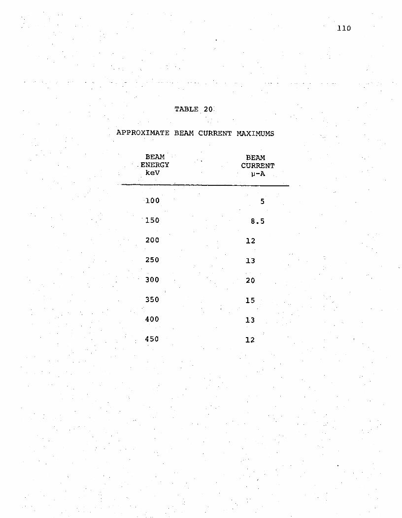
110

TABLE 20

APPROXIMATE BEAM CURRENT MAXIMUMS

BEAM BEAMENERGY CURRENTkeV li-A

100 5

150 8.5

200 12

250 13

300 20

350 15

400 13

450 12

point. The points in figure 16 generally form a smooth

gently curving line with the exception of the 400 keV

point. Theoretical predictions (Appendix B, Table B2)

from the work of Bell (1961) are, except for the distor-

tion approximation at 178 keV, in very poor agreement

with our results. Previous experimental work however is

in good agreement with ours. We have abstracted the re-

sults of Scharmann (1967), and Scharmann (1969), from

their graphical presentations (neither of these works

either tabularized their results or included error bars)

and reported the estimates in table 21 along with the

tabularized results of Van den Bos (1968). In the small

region of overlap (100-150 keV) we find ourselves in

much better agreement with Scharmann (especially con-

sidering the curve shapes which we have not shown).

Van den Bos' polarization measurements were done using a

monochrometer to select the X 5016 A line and he may not

have completely corrected for the polarizing influence

of the monochrometer. He also may have not taken care

with regard to He pressure. He implies that he used

.2 mtorr but does not explicitly say so.

All other previous experimental work on the

polarization of the X 5016 A line has been done at pres-

sures > .2 mtorr. This work is the first to extend that

measurement to lower pressures, see summary in table 22.

It has been difficult to do so since the signal to noise

ratios fall off rapidly as one lowers the He target gas

TABLE 21

COMPARISON WITH OTHER EXPERIMENTS

BEAM VAN DEN BOS SCHARMANN SCHARMANNENERGY THIS WORK NO PRESSURE (1967) (1969) THEORY-BELL(keV) .2 mtorr STATED .2 mtorr .2 mtorr DISTORTION

100 2.9 % -1. % 2.5 % 5.5 % 14 %

150 2.04 % 4. %

(178 keV) 2.6%200 .71 %

250 - .83 % -2 %

300 -2.6 %(316 keV) 13%

350 -3.69 %

400 -4.23 % -5.5 %

450 -5.76 % -6 % -8. % -22 %

113

TABLE 22

CORRECTED 7 Vs PRESSURE

PRESSURE 150 300 450mtorr keV BEAM keV BEAM keV BEAM

.01 - .97±1. .84±.96 -2.19±.92

.05 2.67± .75 - .86±.48 -2.41±.62

.2 2.04± .27 -2.6 ±.2 -5.76±.27

.6 .66± .8 -3.76±.22 -5.29±.46

1.0 .39± .12 -3.13±.23 -3.79±.34

1.5 - .74± .14 -2.46±.15 -3.55±.2

114

pressure. We consider our .05 mtorr measurements as suc-

cessful, but have less faith in our .01 mtorr results.

There is simply very little light reaching our detector

from the target chamber when the pressure is .01 mtorr.

We are therefore not surprised to find the .01 mtorr

points in f gurb'eq7 to ioe'of questionable value. The

.05 mtorr and higher pressure points do lie on relatively

smooth sensible curves and in fact a similar curve shape

was reported by Scharmann (1969). He graphically dis-

played results for w as a function of pressure over the

range .2 mtorr to \8. mtorr °(for beam energies of 100,

450, 600, and 835 keV). Each of his curves shows a

minimum (a most negative r), and as energy increases, the

minimum occurs at a lower pressure. We have observed the

same phenomena for our 300 and 450 keV curves. Our

150 keV curve does not show a minimum, however from

Scharmann's curves, we would expect the 150 keV minimum

to occur at \2 mtorr, a pressure which we do not reach.

Scharmann's results also showed the polarization (at

100 keV beam energy) changing sign as the pressure

changed. (Also for the 41P-21S line at 100 keV.) Our

results show a change in the sign of T (for 150 keV beam)

at %1.2 mtorr, and imply (at 300 keV) a change in sign at

^.015 mtorr. Scharmann does take notice of this change

in sign of rr, however he offers no explanation and in

fact states that he has no explanation for this phe-

nomena. We discuss this problem in Appendix D.

115

This work is limited in a number of ways. The

lowest pressure we are able to accurately measure is

.01 mtorr, we would have liked to have used lower pres-

sures. However we could just barely get data at

.01 mtorr as so little light was received by our detec-

tor. We are also limited by the heat dissipation ca-

pability of our Faraday cup, our Signal/Noise ratio

could have been improved by using higher beam currents.

(At some energies the beam current is limited by the

Van de Graaff accelerator rather than the Faraday cup.)

Improvements in this work could be made by .

1. Obtain a new pressure measuring system

capable of accurately measuring pressures

to 10- 3 or 10- mtorr.

2. Rebuild the Van de Graaff beam tube vacuum

system so that one could have a differen-

tially pumped target chamber at 10- 3 or 10- 4

mtorr while the beam tube was held at 10-5

mtorr. (Now the beam tube ,is generally held

at 10- 3 mtorr.)

3. Rebuild the target chamber electrostatic

focusing system and entrance slits such that

we get a beam of small cross section through

the axis of the chamber, and such that the

detector can be brought much closer to the

beam region of the chamber.

4. Modify the accelerator as so to be able to

116

obtain much higher beam currents especially

at low energies.

5. Devise a way to cool the Faraday cup while

still keeping if electrically insulated.

6. Use the PDP-8 or equivalent to automaet the

data taking.

7. Shield the target chamber with mu metal so as

to determine whether 7 is in fact effected by

stray magnetic fields. Note 7 should not be

so effected.

5.3 Conclusions

It is clear from this work that the polarization

of the light from the 31P-21S transition in proton beam

excited Helium is still pressure dependent even at pres-

sures as low as .05 or .01 mtorr. The results of

Scharmann, as far as they go, bear this out. We are

faced with a phenomena which exhibits poor agreement be-

tween theory and experiment, however we conclude that

even we have not yet reached low enough pressures to find

the natural value of the polarization. It remains for the

next worker in the field to extend the measurement to yet

lower pressures in search of a pressure independent value

for the linear polarization fraction.

117

REFERENCES

Allison, S. K., and Warshaw, S. D., Rev. Mod. Phys. 25,779 (1953).

Bacon, R. H., Am. J. Phys. 21, 428 (1953).

Bell, R. J., Proc. Phys. Soc. 78, 903 (1961).

Bethe, H. A., and Jackiw, R., Intermediate QuantumMechanics, Benjamin, New York (1968).

Condon, E. U., and Shortley, G. H., The Theory of AtomicSpectra, Cambridge University Press, Cambridge (1935).

Feofilov, P. P., The Physical Basis of PolarizedEmission, Consultants Bureau, New York (1961).

Gabriel, A.H., and Heddle, D. W. 0., Proc. Roy. Soc.A258, 124 (1960).

Hasted, J. B., Physics of Atomic Collisions, AmericanElsevier, New York (1972).

Heddle, D. W. 0., and Lucas, C. B., Proc. Roy. Soc.A271, 129 (1962).

Holstein, T., Phys. Rev. 83, 1159 (1951).

Jenkins, F. A., and White, H. E., Fundamentals of Optics,McGraw-Hill, New York (1950).

Land, E. H., J. Opt. Soc. Am. 41, 957 (1951).

Larson, L., Ph.D. Thesis University of New Hampshire,Durham, New Hampshire (1967).

Lees, J. H., Proc. Roy Soc. A137, 173 (1932).

Lees, J. H., and Skinner, H. W. B., Proc. Roy Soc. A137,186 (1932).

Marion, J. B., Classical Electromagnetic Radiation,Academic Press, New York (1965).

Merzbacher, E., Quantum Mechanics, John Wiley & Sons, Inc.,New York (1961).

118

Mitchell, A. C. G., and Zemansky, M. W., ResonanceRadiation and Excited Atoms, Cambridge UniversityPress, Cambridge (1961).

Mott, N. F., and Massey, H. S. W., The Theory of AtomicCollisions, Oxford, London (1965).

Parratt, L. G., Probability and Experimental Errors inScience, Dover, New York (1971).

Pegg, D. J., Ph.D. Thesis University of New Hampshire,Durham, New Hampshire (1970).

Percival, I. C., and Seaton, M. J., Phil. Trans. Roy. Soc.A251, 113 (1958).

Phelps, A. V., Phys. Rev. 110, 1362 (1958).

Scharmann, A., and Schartner, K. H., Phys. Let. 26A,51 (1967).

Scharmann, A., and Schartner, K. H., Z. Physik 219, 55(1969).

Skinner, H. W. B., Proc. Roy. Soc., All12, 642 (1926).

Shurcliff, W. A., Polarized Light, Harvard UniversityPress, Cambridge, Mass. (1966).

Spiegel, M. R., Theory and Problems of Statistics,Schaum, New York (1961).

Thomas, E. W., and Brent, G. W., Phys. Rev. 164, 143(1967).

Van den Bos, J., Winter, G. J., and DeHeer, F. J.,Physica 40, 357 (1968.).

Van den Bos, J., Physica 42, 245 (1969).

Van Eck, J., DeHeer, F. J., and Kistemaker, J., Physica30, 1171 (1964).

Wilson, E. B., Jr., An Introduction to Scientific Re-search, McGraw-Hill, New York (1952).

Young, H. D., Mechanics and Heat, McGraw-Hill, New York(1964).

119

APPENDIX A

DESCRIPTION AND MEASUREMENT OF POLARIZED LIGHT

A.1 Polarized Radiation

It is well known that electromagnetic radiation

behaves as a transverse wave. This means that the

directions of both the electronic and magnetic field

vectors of the wave are at all times perpendicular to the

direction of propagation of the wave, as well as perpen-

dicular to each other. Therefore, in order to completely

specify the nature of a wave, one must among the many

parameters, include those which describe the direction of

either the electric or magnetic field vector as a function

of time and position. Conventionally, one specifies the

direction of electric field vector. We will from this

point on use the term "light" in place of "electromagnetic

radiation." Of course it is understood that light (in-

cluding infrared, visable, and ultraviolet) is the name

applied to a very small section of the electromagnetic

spectrum. Furthermore comments made about polarized

light do usually apply to other electromagnetic radia-

tions.

Light can be described as either unpolarized or

polarized. Unpolarized light has no preferred direction

120

for its electric field vector, nor any preferred rota-

tion of its electric field vector about the propagation

direction. Conversely, polarized light does have pre-

ferred direction and/or rotation for its electric field

vector. As a matter of convenience, one can discuss

three types of polarized light: 1. linearly polarized,

2. circularly polarized, and 3. elliptically polarized.

1. Linearly polarized light. When the electric

field vector of a light beam maintains a fixed direction

in space, then the beam is called linearly polarized.

See Fig. A.l. This is by far the simplest case of polari-

zation and in fact is a type of polarization often produced

in nature.

2. Circularly polarized light. Light is said to

be circularly polarized when the magnitude of the electric

field vector appears constant while the vector itself

rotates about the propagation direction. There are of

course 2 types of circularly polarized radiation. The

conventional distinction is that if the locus of the "tip"

of the electric field vector describes a right-handed

helix (such as the thread of a typical machine screw),

then one has a wave of positive helicity (in optics

called a left circularly polarized wave). Conversely,

right circularly polarized light has the "tip" of its

electric field vector describing a left-handed helixi,

and possesses negative helicity.

3. Elliptically polarized light. This is the

121

LINEARLY POLARIZED ELECTROMAGNETIC WAVE

E

HH

R XE

HZ

FIGURE Al

122

more complicated of the three cases due to the fact that

both linear and circular components are present. To

describe elliptically polarized radiation one must specify

the handedness and magnitude of the circularly polarized

component as well as the direction and magnitude of the

linearly polarized component. Note that the major axis

of the ellipse lies in the same direction as that of the

linearly polarized component. An alternate equivalent

description of elliptically polarized light is that it

is made up to two linearly polarized components with

differing amplitudes and non-00 , 900, 1800.phase angle

differences. One must then specify each amplitude as

well as the phase angle difference.

For purposes of description one can draw sectional

patterns for a beam of light. These drawings represent

the electric field vector as seen by an observer located

on the z axis (assuming that the beam is traveling in the

+z direction) and looking toward the source of the radia-

tion. See fig. A.2. We might add at this point that a

monochromatic beam has been assumed for the sake of

simplicity.

A.2 Mathematical Descriptions ofPolarized radiation

There are numerous equivalent mathematical descrip-

tions of monochromatic waves, e.g.

123

SECTIONAL PATTERNS-

I)bd)

FIGURE A2

124

or in complex notation

or

where IEI is the magnitude of the electric field vector,

w is the 27 times the frequency of the wave, z is the

position along the axis of propagation, X is the wave-

length, and t is the time. The last equation is just an

abbreviated form of the second where

Let us also state that Ee is called the complex ampli-

tude, 4 is called the phase angle (at t and z) and that

the intensity of the wave is proportional to (E )2

The direction of the electric vector has not yet been

specified. Therefore the polarization of the wave has

not yet been specified.

At first glance one may easily arrange a system

to describe a linearly polarized beam by simply choosing

the x axis along the direction of the beam's electric

field vector. Then using the unit vector ,A

or E = Re E,.A e J

125

One can then in turn describe circularly polarized

light as the addition of two components of linearly polar-

ized light of equal Emax, directed along the x and y axis

respectively, with a phase angle difference of +900. By

convention if the difference in phase angles, called y

(Y = y-4x), is +900 the light is left-circularly polar-

ized. Conversely, if y = -900 the light is right-

circularly polarized.

When the x and y linearly polarized components

have different amplitudes, and when -1800 < y < 1800

(Y 0), the beam exhibits elliptical polarization. If

-1800 < y < 0o then the handedness is right, conversely

the wave is left-elliptically polarized if 0o < y < 1800.

If one considers elliptical polarization to be

the general case, then linear polarization results when

Y = 00, and circular polarization results when 1Yi = 900

and (E max) = (E max).

Strangely, it is very difficult to properly de-

scribe a beam of unpolarized light. One can demand that

no long term preference exist for handedness or linearity.

(This precludes a "pure" coherent monochromatic wave.)

Perhaps it is best to describe unpolarized light in terms

of what it will and will not do (i.e., and operational

definition). When a beam of unpolarized light is divided

into two completely polarized components (by an ideal

analyzer) the components will deliver equal power.

In the real worldlight is seldom either completely

126

polarized or unpolarized. One must in such a case specify

the degree of polarization. This is usually accomplished

by dividing the beam of light into orthogonal polarization

components (e.g. right and left circular; horizontal and

vertical linear, etc.), measuring the intensity of each

of these components, and then calculating the degree of

polarization V from

I - Ia bIa + Ib

where Ia and Ib are the maximum and minimum intensities

of the orthogonally polarized components respectively.

Note that if one is discussing linearly polarized light,

V reduces to T the linear polarization fraction.

A number of different mathematical models are in

use for the treatment of beams of polarized light. These

methods range from the geometrical methods of the Poincare

sphere to the matrix calculus of the Stokes vector and

Jones vector.

The Poincare Sphere model uses a mapping technique

to describe the polarization form of a completely polar-

ized beam. It is most useful for predicting the change

in polarization form as the beam passes through various

active polarizing devices (analyzers, retarders, etc.).

In this model, every point on the surface of a unit sphere

represents a 'ferent and specific polarization form.

By definition ihe "north "pole represents left-circularly

polarized light, and the "south" pole right. All points

127

on the equator represent linearly polarized light with

various inclination angles (to the equator). One loca-

tion on the equator (the prime meridian) is given the

designation H for linearly polarized light parallel to

the equator. Half way around the sphere (on the equator)

the light is linearly polarized perpendicular to the

equator, and given the designation V. At any location

away from the poles and equator, one has elliptically

polarized light. See Fig. A.3. To specify the form of

a completely polarized beam, one need only specify the

angles X and w (where 2X = longitude and 2 = latitude).

This is easily done since X is the azimuthal angle of

the polarization ellipse and tanlwi is the ellipticity

(b/a). See Fig. A.4. Furthermore the handedness is

defined as left for the northern hemisphere (w<0) and

right for the southern hemisphere (w>O).

When dealing with completely polarized beams and

various retarders one can use this Poincare sphere to

predict the change in the polarization form of the beam.

This model is limited however in that one must be dealing

with completely polarized beams.

The Stokes Vector model of polarized light is

perhaps the most versitle and useful. The Stokes vector

is a four parameter column vector

M

C

SL j

128

THE POINCARE SPHERE

N

IH2w

S

FIGURE A3

129

ELLIPTICALLY POLARIZED LIGHT

Y

(E max)y b

(Emax)x-,

FIGURE A4

130

where all four entries have the units of intensity.

Each of these parameters -is defined in terms of a

measurement made with a set of ideal polarizing filters.

This set of four ideal filters have the following proper-

ties. All filters have a transmittance of .5 for un-

polarized light. Then ... Fi , is a neutral isotropic

filter; F2 is a linearly (horizontally) polarizing filter;

F3 is a linearly (+450) polarizing filter; and F4 is a

right-circularly polarizing filter. A polarization form

independent detector is placed behind each of the filters

in succession and four measurements are taken. The re-

sult of each measurement is multiplied by 1/.5.and the

four values V1, V 2, V3 , and V4 are reported. The Stokes

column vector is then calculated as follows

I =V 1

M= V -V 12 1

S= 3 - 1

S = V4 - V1

An alternate and equivalent approach is to use

the parameters from the wave description of light. One

may then write (note time average < ).

M =v i - ho

C =

c = S .) ) c.>

It is also conventional to normalize the Stokes vectors.

131

This is accomplished by dividing all four entries by I

(which is-the -largest). The Stokes vectors are very use-

ful in that they can be applied to partially polarized

beams, monochromatic as well as polychromatic beams, and

incoherent beams. Furthermore, the Stokes vector can be

manipulated (by Mueller calculus to be discussed later)

so as to predict the behavior of a beam when passing

through retarders and polarizers.

The Jones Vector model is applicable to situations

in which the coherence and phase of the beam is important.

For a specific location along the propagation direction

(the z axis) the Jones vector is written as a two-element

column vector [E:or6 #t eF

where Ex and Ey are the phases of the x and y components

at t = 0. There is a normalized form of the Jones vector

2 2where m + n = 1. Conversion of this vector to a

recognizable form is a bit cumbersome and in general use

of the Jones vector is confined to problems in which

phase is important.

Table A.1 shows various polarization forms and

the corresponding Stokes and Jones vectors.

The Mueller Calc.: us methodology provides a

132

TABLE A.1

EXAMPLES OF THE STOKES AND JONES VECTORS

Polarization Normalized NormalizedForm Stokes Vector Jones Vector

LinearCS Co RLSIb J 5,; R

Left Circular [ 7

Right Circular . ]CosR e

I &

Elliptical .2 ICo , Re

S, , 2. _

Unpolarized none

133

means for manipulating the Stokes vectors so as to pre-

dict the behavior of a beam of light as it passes through

any series of retarders, and or polarizers. The method

itself is of a matrix-algebraic nature. For this work

it is sufficient to say that every retarder and or

polarizer at whatever orientation can be represented by

a 4 x 4 Mueller matrix. To determine the polarization

form and intensity of a beam exiting from an "active"

filter one multiplies the Stokes Vector for the incoming

beam by the Mueller matrix of the "active" filter. The

new Stokes vector then describes the exit beam. Using

the methods of matrix algebra one can easily predict the

result of any combination of "active" filters.

The Jones Calculus methodology is similar to.the

above except that a smaller (2 x 2) matrix is used. This

smaller matrix is usually made up of complex elements and

can preserve phase information.

Standardized Mueller and Jones matrices are

available in many works, notibly in Schurcliff (1966).

A.3 Polarized Light and Matter

When a beam of light (polarized or not) interacts

with matter, the result of the interaction depends upon

both the polarization of the initial beam, and the

specific nature of the matter involved.

Let us first consider (classically) the scattering

of an unpolarized light wave incident upon a molecule.

134

The electric charges in the molecule will try to "follow"

the incident electric fields. As a result, the molecule

will radiate, i.e. scatter the light. The polarization

of the scattered light will depend upon the location of

the observer. If the incoming light is linearly polar-

ized then the light is scattered anisotropically, and

again the polarization depends upon the location of the

observer. See fig. A.5.

Polarization can also be caused by reflection and

refraction. Again the electric field of the incoming

light will cause the charges within the material to os-

cillate, thus multiple scattering is observed. Consider

an unpolarized beam of light' (in air) incident upon a

more optically dense material (glass). Applying the

boundry conditions that the tangential electric and

magnetic fields at the surface are continuous, one arrives

at the situation shown in fig. A.6. The degree of polari-

zation depends upon the angle of incidence e.. When

6 + 8r = the polarization of the reflected and re-

fracted components is almost total. The incidence angle

for which this occurs is named Brewster's angle Oa, de-n

fined by Tan 8 = - . Where n 2 and nl are the indices

of refraction for the two media.

Certain materials exhibit the phenomena of

Birefringence (double refraction) when interacting with

light. Some crystalline solids fall into this category,

that is they are optically anisotropic. In such a crystal

135

SCATTERING OF LIGHT

1I

b)

a) unpolarized incident waveb) linearly polarized incident wave

FIGURE A5

136

POLARIZATION BY REFLECTION AND REFRACTION

AirGlass

FIGURE A6

137

(calcite or quartz for example) an incident ray of un-

polarized light will have two refracted rays (hence

double refraction) as well as the usual reflected ray.

One of the refracted rays will obey Snells Law...

This ray is then called the ordinary or 0 ray, while the

refracted component which does not obey Snells Law is

called the extraordinary or E ray. See fig. A.7. In

1678 Huygens-discovered that the E and 0 rays were

linearly polarized, and orthogonal. Birefringence is

basically due to the fact that the velocity of the 0 ray

is isotropic and therefore the material has the single

index of refraction no for the 0 ray. The velocity of

the E ray depends upon direction and therefore so does

the index of refraction ne for the E ray. The velocity

of the rays depends upon the orientation of the electric

field (the polarization) of the ray. This difference in

velocity between the 0 and E rays enables the experimenter

to selectively retard one of the linear polarization

components. (This use of a birefringent crystal requires

that the crystal be cut in a specific way... see Jenkins

(1950). A crystal arranged in this manner is called a

retarder and has the properties of resolving a beam into

two components, transmitting the components at different

velocities, and recombining them with a phase difference

that depends upon, among other parameters, the thickness

138

BIREFRINGENCE

ReflectedRay

IncidentRay

0Ray

Calcite Crystal

FIGURE A7.

139

of the retarder. One can then generate elliptically

polarized light by sending a beam of linearly polarized

light through a retarder whose fast direction is at some

angle 0 with respect to the initial plane of polarization,

and whose retardance (phase angle difference) is 6. The

results will be elliptically polarized unless 0 = + 450,

6 =+ 900 (circular); or 0 = + 90, 6 = + 90 (linear) or

if 6 = 00, 1800 (linear). A retarder then is just a

polarization form converter.

The most important interactions of light with

matter (for the practical use of polarized light) are

dichroic interactions. Materials which exhibit dichroism

will absorb one polarization form and transmit the

orthogonal form. Polaroid sunglasses are a typical ex-

ample of dichroic material. The lenses are oriented so

as to pass linearly-vertically polarized light, therefore

the horizontally polarized components are absorbed. But

glare from the surface of a road, or body of water, or

from many other horizontal reflecting surface is hori-

zontally polarized, and removed by the dichroism of the

sunglass lens. Although there are many materials which

can be made to exhibit dichroism, the most commonly

available is Polaroid Corporation's type H. This material

is manufactured by alligning iodine molecules in a stretched

sheet of polyvinyl alcohol. When a beam of light passes

through the sheet, the component of the beam whose electric

field lies along the long axis of the iodine mdlecules

140

will be absorbed. The orthogonal component is trans-

mitted (with some attenuation due simply to the optical

density of the sheet). Land (1951) has done a review of

the history of dichroic polarizers (He is the inventor

of the modern dichroic polarizer).

Optically active materials such as Turpentine,

Quartz crystals and sugars (to be optically active a

sample of the compound must contain a significant majority

of one of the mirror image versions of itself; either the

right or left handed version) can rotate the plane of

polarization of a beam of linearly polarized light.

Jenkins (1950) describes Fresnel's explanation for

optical rotations. Fresnel assumed that optically active

material treats the entering linearly polarized light as

two equal amplitude, zero phase difference, counter-

rotating circularly polarized components. He further

assumed that the propagation speed was different for the

Right and Left components; producing a non-zero phase

difference. Then because of the non-zero phase difference,

when the beam exits the material and the two counter-

rotating components recombine, we once again have linearly

polarized light, but the plane of polarization has been

rotated by an angle 6/2 (6 is the phase difference). It

is apparent then that the magnitude of the rotation

depends upon the amount of optically-active material the

beam passes through. Although Fresnel's explanation does

agree with experimental evidence it does not explain

141

the process on the molecular level. That explanation

was first put forth by Reusch; he suggested that the

molecules in an optically active substance are aligned

in a helical pattern. This was later verified in other

experiments.

A.4 Semiclassical and Quantum MechanicalAspects of Polarized Light

In the previous section we have discussed the

interaction of light with matter, without regard to how

the light was created. We will now rectify that omission

by discussing (both semi-classically and quantum mechani-

cally) the origins of light within the most elementary

radiating systems.

We begin with an electric dipole. Consider a

fixed positive charge with a negative charge in linear

periodic motion about it. Let us assume that our observa-

tion point is located a distance ro from the positive

charge with r = ro >> r. See fig. A.8. We can then

write the retarded scalar and vector potentials (for the

observer) of the moving negative charge as follows.

~-

Cr,

A.4.1

If we exand the above terms usin

If we expand the above terms using

142

LINEAR ELECTRIC DIPOLE

Observer

FIGURE A8FIGURE A8

143

-X- + + + O(x .

• 2and if we neglect terms of order (-) and higher...

then

A.4.2

If we now neglect the first term in the scalar potential

expression (at large r the -- is cancelled out by the

+Q or term from the fixed positive charge), and use the

o

facts that

Ca

S4 r. xE 'A.4.3

we arrive at

S ] A.4.4

where fl is the component of the negative charges ac-

celeration in a plane perpendicular to ro. The observer

(at sufficiently large ro, in the wave zone) sees a plane

polarized electromagnetic wave. Let us surround this

oscillating and radiating d. lie with an imaginary sphere

(radius re) such that the polar axis is along the dipole

moment, the observed polarization direction of the wave

will then depend upon where on the sphere the observer

144

is located. See fig. A.9. Since the dipole makes an

angle 8 with respect to ro, and since Qr = p = pb cos(t)z

... then

r, C

-7A.4.50 C'

and

I/( = A.4.6

where H is always parallel to the equator of our sphere

and E is always perpendicular to said equator. Thus the

wave is completely linearly polarized.

Let us now consider the electric rotor where

the negative charge travels about the fixed positive

charge in a circular path. Rather than repeat the calcu-

lations from the beginning, we can instead resolve the

circular motion into two linear harmonic components with

the same frequency and amplitude but with a phase dif-

ference of +n/2. If we again use our imaginary sphere,

this time with the polar axis along the symmetry axis

of the rotor, again the form of the polarization will

depend upon the location of the observer. For = 00,

1800 one observes a circularly polarized wave, at a = 900

one observes a linearly polarized wave, and anywhere in

between one observes an elliptically polarized wave.

There are of course higher order terms which we

POLARIZATION OF ELECTRIC DIPOLE RADIATION

Z

00

I

FIGURE A9

146

have neglected, a summary of the radiation from higher

electric multipoles as well as from magnetic radiators

is available in Feofilov (1961).

We can now discuss polarization in the normal

Zeeman effect. Let us place our linear dipole oscillator

in a magnetic field H not directed along the dipole

moment. The equation of motion of the negative charge is

" = - rnw ,F - -F A.4.7/7 w, r - [ ]

which can be written as the three scalar equations (choos-

ing the z direction to be along H)

m~y' : - LXS- A.4.8

' : - rlL4t

The z equation solves immediately the z = z cos w t. WeS O0

will try solutions of the form x = A e and y = Aye iwt

for the x and y equations. This procedure yields

w- ) - A.4.9

or

L T H A.4.10

therefore

SA.4.ll

147

However for magnetic fields, H, of realizable magnitude,

>> Q2. . and therefore dropping-terms of order (QH

we arrive at

A.4.12

and note Aw << o. We may now solve for the A and A0 x yby again using x = A e t and y = A e in A.4.8 andx ythen removing terms of order (A )2. We then find

0

AX x" A, A.4.13

and the full x and y solutions are

A.4.14

Therefore when w = mo + Aw, x leads'y by a phase angle of

r/2 and the radiation emitted by this oscillator (when

viewed from the z axis) is circularly polarized; and when

SW o -Aw, x lags y by a phase angle of T/2 and the

radiation is again circular butopposite in direction

(called a components).

In summary, when a linear dipole oscillator is

placed in a magnetic field one observes three frequencies

of oscillation w, wo + Aw, and - Aw. Both the in-

tensities and polarizations of these radiations depend

upon the location of the observer. If the observer is

148

on the z axis he will observe only circularly polarized

components of frequency w + Aw. (the linearly polarized

W radiation has zero intensity on the z axis). However,

if the observer is on a line perpendicular to the z axis,

in the plane containing the dipole, he will then observe

all three radiations w , w + Aw. Now however the a com-0 o-

ponents (w = w + Aw) will appear as linearly polarized

with the electric field vector perpendicular to the mag-

netic field direction. (Analogous to observing an electric

rotor edge on) the wo radiation (the i component) is of

course linearly polarized with its electric field vector

parallel to the magnetic field direction.

This classical description of the normal Zeeman

effect is limited to cases in which the source of radiation

can be considered a simple system of linear dipole os-

cillators.

We now turn to quantum mechanics for a description

of polarized light on an atomic scale. We will confine

our discussion to electric dipole transitions where

At = + 1, and Am = 0, + 1. These selection rules are

necessary for non zero matrix elements between the upper

and lower states. The transition probability is of course

proportional to the square of the matrix element. The

selection rules can be demonstrated as follows. The matrix

element

SA.4.15

149

(where p is the dipole moment of the atom electron system)

can be resolved into the cartesian elements

- A.4.16

assuming that the electron moves in a central force field,

we can then write

A.4.17

where a is the orbital angular momentum quantum number,

and m is the "z" component of k. There are 2£ + 1 values

of m, and m ranges by integers from -Z to +Z. Using

A.4.17 in A.4.16 and with the z axis as the polar axis we

arrive at ...7

+ ""A..

The first two integrals will be zero unless

(m' - m) = + 1 or Am = + 1. The last integral will be

zero unless (m' - m) = 0. Also note that when Am = + 1

we have in effect linear dipole oscillators in the x and

150

y directions and circularly polarized light, (as viewed

from a point on the z axis) these are again the a com-

ponents. When Am = 0 we again have the equivalent of a

linear dipole oscillator with the E vector parallel to

the z direction, which is the , component. Further note

that when viewed from position in the xy plane one sees

the a components as linearly polarized with E perpendicular

to z and the 7 component as linearly polarized with E

parallel to z. It can also be shown that for Am = 0, + 1,

At must be + 1. These selection rules can be generalized

to the set of quantum numbers rnjM. Where then Aj = + 1,

0 but j =0 + j = 0 is forbidden and AM = 0, + 1.

The above selection rules are appropriate in light

of the following arguments... the angular momentum of

linearly polarized light is zero, therefore when such

light is emitted, the change in the angular momentum com-

ponent along any axis (mrf) should not change, hence

Am = 0. Circularly polarized light carries angular

momentum + Y one would therefore expect Am = + 1.

We are now prepared to discuss the Zeeman effect

quantum mechanically. Let us choose the z axis along

the external magnetic field H. This problem has been

solved in many books (see Bethe (1956) pg 208) with the

following result...

E eA- E',j 9 A.4.19

where

151

.. . S) s - ( A.4.20

and M takes on (2j + 1) values. The energy E' therefore

takes on (2j + 1) values, one of which is still the zero

magnetic field value Enk j' The wavelengths of the radia-

tion are then

AA.4.21

The polarization rules are again, i7 component when AM = 0

(and therefore A = Xo), and a component when AM = + 1

(and therefore A = o + AX). The apparent polarization

of the r and a components will depend upon the location

of the observer. If the observer is located upon the z

axis then the intensity of the T component will be zero

and only the circularly polarized a components will appear

(at wavelengths A = o + AX). If the observer is located

in the xy plane, then both the i component (linearly

polarized with the E vector parallel to z, with wavelength

o), and the a component (appearing a linearly polarized

with the E vector perpendicular to the z axis at wave-

lengths X = o + AX) will appear. As a specific example

consider Helium with s = 0, therefore J = L and g = i.

See fig. A.10. It was also shown by Feojilov (1961) that

for this specific 'pl 's transition the ratio of

intensities for the ff and a components (observed in the

152

NORMAL ZEEMAN EFFECT

+1

P, M=O

S MO=0

M-O

S I I on Z Axis

Xo7 in XY Plane

The presence or absence of i or a radiationis indicated schematically in the lower twolines.

FIGURE A10

153

x, y plane) is 1:2:1 for a-_l::+1a.

The question now arises of what happens to the

7 and a components as the magnetic field H goes to zero.

Certainly the wavelength splitting decreases toward zero,

and in fact the magnetic sublevels become degenerate.

However (experimentally) the rr and a components do con-

tinue to exist even at zero field. Heisenberg (1925)

has stated the principle of spectroscopic stability...

(paraphased) the state of polarization does not change

when the external additional magnetic field, which is

superimposed on the system in such a way that 'its symmetry

remains unaltered, tends to zero.

The entire above discussion has concerned itself

with one elementary radiator (or one atom).. In general

for a macroscopic system of many radiators the polariza-

tion will average to zero unless some anisotropy is intro-

duced. In this work the anisotropy is introduced by the

energetic proton beam. The beam direction is chosen as

the z axis and observations are made from within the xy

plane. See figure 2.

A.5 Measurement Methods for Polarized Light

The devices which are used to analyze polarized

light in fact apply those phenomena which we have dis-

cussed in A.3. Some of these devices are; the linear

polarizer (dichroism); the polarizing prisms, Nicol,

Glan-Thompson etc. (birefringence); retarders (bire-

fringence); and the pile of plates polarizer (reflection

154

and refraction).

The linear polarizers are the invention of E. H.

Land and generally the product of polaroid Corporation

(Cambridge, Massachusetts). The so-called H-sheet is the

most common, and is covered by a number of patents. Dur-

ing manufacture a thin sheet of polyvinal alcohol is

heated, stretched and then for support purposes laminated

to a sheet of cellulose acetate butyrate. The polyvinal

alcohol face is then wet with an iodine rich solution which

will leave a residue of aligned iodine molecules within

the polyvinal alcohol. This sheet is then laminated be-

tween plates of glass to form the completed linear polar-

izer. These polarizers can be made in various colors and

transmittances. In this work a type HN-32 implies a peak

transmittance of 32% for unpolarized incident light. Thebehavior of this polarizer for normal incidence is cate-

gorized in table A.2. Note that Kl(the major principle

transmittance) is defined as the ratio of transmitted to

incident intensity when the linear polarizer is placed ina normally incident, linearly polarized beam of light

oriented to maximize the transmittance. The minor princi-

ple transmittance, K2' is obtained from the same ratio

during minimum transmitance. The principle transmittance

ratio Rt is defined as kl/k 2 . For one polarizer Rt is onthe order of 1.5 x 10 (at 5000 A). Reflection losses

do occur at the surfaces of linear polarizers, however

these losses (for normal incidence) are isotropic and

155

TABLE A.2

BEHAVIOR OF THE HN-32 POLAROID ANALYZER

Wavelength K1 K2

3750 .33 .001

4000 .47 .003

4500 .68 .0005

5000 .75 .00005

5500 .70 .00002

6000 .67 .00002

6500 .70 .00002

7000 .77 .00003

7500 .84 .0002

156

amount to typically <4%.

.There are of course many other dichroic linear

polarizers which do not immediately concern us. De-

tailed -information can be obtained from Polaroid Corpora-

tion, Cambridge, Massachusetts.

The linear polarizing prisms have been in large

measure replaced by the dichroic sheet polarizers. How-

ever one great advantage the birefringent polarizer has

over the dichroic type is that a polarizing prism can

separate and deliver both of the orthogonal linear com-

ponents, there is no significant absorbtion. Very few of

these prism polarizers however can be adjusted to leave

the path of the incident beam undeflected, this is the main

cause of their replacement by the linear dichroic polar-

izers.

Polarization form conversion is done with the use

of retarders. The most common retarders are quarter and

half-wave plates. The quarter-wave plate will convert a

beam of linearly polarized light into a beam of circularly

polarized light (when properly oriented). The half-wave

plate can be used to rotate the plane of polarization of

linearly polarized light. There are also circular and

elliptical retarders, so that in general with the proper

combinations and orientations of linear polarizers and

retarders one may convert from any one polarization form

to another.

The pile of plates polarizer is usually used for

157

production.and/or analysis of vacuum ultraviolet polarized

light. The polarizers previously mentioned generally are

unusable in the ultraviolet region of the spectrum. There-

fore the pile of plates reflection/refraction polarizer

arrangement, even though extremely cumbersome, is grudging-

ly used.

Given a beam of light of unknown polarization form,

one can use the devices previously discussed in order

to analyze the polarization form. Once the form has been

analyzed, specific polarizing analyzers can be used to

separate the orthogonal components for the purpose of

intensity measurements. The results of these intensity

measurements can be used to calculate the degree of

polarization. The beam is then completely analyzed. In

order to make the intensity measurements one needs a

detector which meets two general requirements. Many

different detector types can be used, the requirements

being that the detector be sufficiently sensitive and

also that the detector be completely polarization in-

sensitive.

In this research the HN-32 analyzer is used to

isolate the linear polarization components so that we

may use a photomultiplier detector system to measure

the intensities of the components. We are then able to

calculate the linear polarization fraction.

158

APPENDIX B

THEORY

B.1 Collison Theory

We must eventually use inelastic scattering

theory to describe our process...

H+ He + H+ + H*e e

However, let us first review elastic scattering.

We will assume the ideal case of a fixed scatter-

ing center at the origin impacted upon by a beam of

particles incident along the +z direction. We can re-

present the scattering center by a potential V(F) , and

let us assume that the incoming beam is monoenergetic.

If after the elastic scattering occurs, the particles

are detected far from the origin by a device which sub-

tends an angle dJL , then the differential scattering cross

section is

where N is the flux of particles in the beam, and dN is.

the flux counted by the detector. The total scattering

cross section a4 is then

5r(e1 ,4 A. JB.1.2

159

We can describe the monoenergetic beam of parti-

cles -by a plane wave with wave function.--

B.l.3

The wave function after the interaction will then be

B.1.4

where at large r, we must have

SKr

i.e. an outgoing spherical wave. The particle flux can be

calculated from the wavefunction by using the expression

for the probability current density...

B.1.6

When this is applied to B.1.5 and we further assume large

r, then

- r r' B.1.7

where - the classical velocity of the parti-

cle, and S is the scattered particle flux per unit area.

Since Jl S,;de and since an element of

area in spherical coordinates is do:-r's J~d we can

then write

__ B.1.8r-'

160

and therefore

r

but (I(19,) 2 .Al P Arej-re

At B.1.10

This is the scattered particle flux per unit area at

angles 8, and Q.

We can apply B.1.6 to B.1.3 to arrive at the

incident flux N

IF B.1.11

using B.1.11 in B.1.10 we get

JN v B.1.12

dA rL

a comparison of B.1.12 and B.1.7 yields the important

result that the differential scattering cross section is

equal to the square of the scattering amplitude, i.e.

(r (8, ): I , ,) B.i.13

The solution of many scattering problems is then

reduced to finding the scattering amplitude f () .

Recall the scattering amplitude is the coefficient

of the spherical outgoing wave in the asymptotic form

161

*, FAr e Ir jB.1.14

when this is used in the Schrodinger equation

(1+ 7 ) . Vl Y) B.1.15

one arrives at (see e.g. Merzbacher (1961))

(, &v; , V(v') ?P*(F) i B.1.16

As it stands, this result is not explicit and not useful.

The first Born approximation simply replaces y.')

a plane wave e so that

) S -k Ak..r'' JI B. 117

This approximation is generally valid for short range

weak potentials, or very high energy incident particle.

The scattering amplitude is often written as

;,ee 5 eA V(7) SZ B.1.18

where , 2 /=/ , i<, 9 and

Co's (see figure B.1) and therefore we have...

/( , T Ie ~()B.1.19

and

162

MOMENTUM TRANSFER

- +Z

K = incident proton momentumK' = final proton momentumq = momentum transfer

FIGURE B1

163

0, 0 L dce, g J0 -B. B.1.2o

Let us now go on to a discussion of inelastic

scattering. The vectors K and K' no longer have equal

magnitudes since energy is transferred to the target

atom. The total system Hamiltonian is H where

H= H + H + H B.1.21atom particle interaction

In general, the transition amplitude from a state a to

a state 8 is given by

T < , / > B.1.22

For our situation, the *'s are product wave functions

t B..23

where o and n represent the ground and excited states.

Conservation of energy requires

where E refers to the atom and W to the incident particle.

The momentum transfer relations are now Ao -

.(4 )+9kk, ' and Cos , k see

again B.1. Equation B.1.22 now becomes, (in the Born

approximation)...

164

B.1.25

where A is representative of the atomic electron coordin-

ates.

To obtain the differential and finally the total

cross sections for .the excitation, one must use B.1.25

in Fermi's golden rule...

2,171) - - / ( ) B.1.26

The density of states factor,., (bv) is equal to Li]' n

so

(rn 6910) r- B.1.27

and

-> ,on2 JE B.1.28

At lower energies (or with target atom potentials

of greater range), the Born approximation becomes less

accurate. One then turns to the Distorted Wave Approxi-

mation. The initial and final wave functions of the

particle are no longer the simple free particle wave

functions.

165

In fact, the Distorted Wave Approximation will

use the approach of Eqs. B.1.22 and B.1.27, but with wave

functions which have been distorted by the interaction

potential. Details are available from Bethe (1968),

from Mott (1965), and also from Hasted (1964).

B.2 Cross Sections and Polarization

The polarization of light emitted (in a particular

direction) by an impact excited gas will depend upon the

relative cross sections for excitation of the magnetic

substates of the upper level.

The methods of the preceding section can be

generalized to calculate the cross sections for excitation

to the various M levels. A conventional label for these

cross sections is where o& is the total orbital angular

momentum quantum number L, and M represents the magnetic

substate. Let us next define A, (x) ,) , and

AM 9) as the transition probabilities for emission of

light from the Mth substate with the light's electric

field vector aligned with the x,y, or z directions re-

spectively. Also, since our system is symmetric about

the z axis

{[A2' - A 2P )J3 B.2.1

The intensity of light emitted with its electric field

vector polarized parallel (perpendicular) to the z axis.

166

is then. 4P

'<OG a4 dB.2.2AM

We can then write the linear polarization fraction

A A- q B.2.3

Using the Zeeman intensity formula from Condon (1967) for

a J - J-1 transition we get

B.2.4

where A,( and (Y) T

then Eq. B.2.3 becomes (with use of B.2.4 and O- Q-, )

for a 'P -. S transition

7 i- B.2.5Q, +C,

The theoretical problem has been reduced to finding

the Q, and 0, for the 3'P state of Helium.

Both the Born and Distorted Wave Approximations

can be used to find the Ro and c, given a proper

choice of wave functions, i.e., wavefunctions in which

the M dependence has not been summed over. The matrix

167

elements must be taken between various M states so that

the transition probability will show any M dependence

they might have. Mott (1965) gives an example of this

type of procedure. Bell (1961) and others who have dohe

this type calculation have used multi-parameter wave-

functions whose parameters have in general been chosen

to satisfy calculations of oscillator strengths. The

cross sections arrived at by Bell (1961) are shown in

table B1 as abstracted by this author from Bell's (1961)

graphical results. Table B2 shows the values of r as

calculated from the cross sections of table B1 using

equation B.2.5

168

TABLE B1

THEORETICAL EXCITATION CROSS SECTIONS

H+ Energy Q in 7ra Q+ in a 2

in keV Born D.W.A. Born D.,W.A.100 .0238 .0198 .0271 .0150

178 .0166 .0175 .0238 .0166316 .0107 .0122 .0192 .0158450 .0080 .0093 .0163 .0144

Cross sections for the excitation of He to the31po and 3 P+1 states calculated by both the Born Ap-proximation and Distorted Wave Approximation (D.W.A.)methods. These numbers were abstracted from thegraphical results of Bell (1961).

169

TABLE B2

THEORETICAL LINEAR POLARIZATION FRACTIONS

H+ Energy Tr Theoretical T Theoreticalin keYV from Born from Distortion

100 - .065 + .138

178 - .178 + .026

316 - .284 - .129

450 - .342 - .215

The linear polarization fraction T calculatedfrom Bell's (1961) theoretical cross sections.

170

APLPNDIX C

CO.PUjT,R

C.1 LA:

This program is used to calculate the behavior -fthe interference filter.

LAM 9:19 FRIDAY AUG 24, 1973

100 PR I1NT 'INTERFERENCE FILTER LAI.1H8A VS ANGLE'110 FOR N=I TO 2 STEP .2120 PRINT USING 13g,w130 :AWGLE LANBDA N=##.###140 FOR A=O TO 10 STEP 2150 LET X=HAD(A)160 LET L=5018*SR(I-((SIN(x))**2/(N**2)))170 PRINT USING 180,A,L180 :### ##vg ,190 NlYT A200 PRINT210 NEXT i220 ELND

C. 2 E;W1;OL

This prog rai is useds to calculate i on a run by

run basis accordino to ecuation 4.1.3..

NEUPOL 0:22 FR IDAY AUG 24, 1973

100 DIM P(25)110 PRHIT 'LINEEAR POLARIZATION FRACTION'120 PRINT '# OF RUNS TO ANALYZE IS'130 INPUT NO140 PRINT 'LIST ALL P':150 INPUT AsIb FOR NI=l TO NO170 READ AlA2,A3,80,BI160 LET C,D=o190 FOi N2=1 TO B0200 READ B2,B3210 LET C=C+B2/B0220 LET D=D+83/80230 NEYT 1J2240 IF AS='YES' THEN 270250 LET Z=2260 GO TO 310270 LET Z=1.280 PRINT290 PRINT

300 PRINT ' V C H C P"310 LET F=0.320 FOR N3=1 TO BI330 READ V,N,H,M340 LET A=(H-C)/(I-DY350 LET B=(V-C)/(N-D)360 LET P(N3)=(A-B)/(A+B)370 LET F=F+P(N3)/BI380 GO TO 39o,410 ON Z390 PRINT USING 400,VNJ,H,M,P(N3)400 t u##v# ###g #### ##### ##,####

410 NEXT N3420 LET S=o430 FOR N4=1 TO .B440 LET S=S+(P(N4)-F)t2450 NEXT N4460 IF 81=1 THEN 490470 LET S=SQR(S/(BI-I))480 GO TO 50oo490 LET S=0

500 LET E=S/SRjHI)510.LET 1=0520 FOR N5=1 TO BI530 LET G=ABS(P(NS)-F)540 IF G<2*S THEN 560

172

550 LET I-+560 INXT L;:570 PRINT580, PRINT UISING 5 9 nAIl,A2A3,.3159$ :#: , N# U HE, ### U A H+., # TRIALS60 PRINT KSING 1 bIS,IE610 :ST DV PTS DV > 2 SIG S*E.=#C#####620 LET FP=F-E630 LLT FI=F+E640 PRINT i-?SING 6 50AFOFF I65 -EAN P #.# (+SE)=######660 PRINT670 NEXT NA680 END

C.3 S:AT

This program is used to calculate -, -or a

Collection of rane ( from results sored in a -ie ).

STAT 9:25 FRIDAY AUG 24, 10o73

100 DIM P(30(i)110 PRINT 'FILE TO BE ANALYZED IS';120 IN}PUT AS130 OPEN 1 ASINPUT140 GET 1,N150 LET F=o160 FOR 1=1 TO M170 GET P(I)186 LET F=F+P(I)/M190 NEXT I200 LET S=0210 FOR 0=1 TO M220 LET S=S+(P(d)-F) 2230 NEXT j24j0 LET S=So.(S/(M-I))250 LET K=R260 FOR L=1 TO M270 LET G=AHS(P(L)-F)280 IF G<2*S THEN 300290 LET K=K+I30 NEXT L310 LET E=S/SR(M)320 LET F0=F-E330 LET FI=F+E340 PRINT USING 350,1350 :### p'S IN CALCULATION360 PRINT tSING 3 7 0,S,KE370 :ST DV = 3.#### ## PTS DV > 2 SIG S.E.=#.#####380 PRINT IUSING 3 90,FOF,FI390 (P-SE)= EAN P = EtP (P+SE)=400 PRINT410 PRINT

420 GO TO 110430 EiLND

CA4 T7-1

This pro',ram is used to calculate tihe t Stati.~3cuseui-as -a test for the sir ificance of the di-ferece c

means.

TTEST 9:26 FRIDAY AUG 24, 1q73100 PRINT 'T TEST..IDI;T t:EAtHST DiYjr.110 INPUT PI,SlEAST .120 INPUT P 2 ,S2,rN2125 INPUT AS130 S3=((NI- )/tNI )*S 2140 =((N2-1)/t2) S2t2150 FNI1+N2-2160 Z=SOR((NI*S3+fJ2*S4)/F)170 T=(PI-p2)/( SR(/NI) (|/N2)))180 PRINT USING 190,F,T190 :#P# DEGREES OF FREEDOM T=###.#,200 PRINT210 GO TO 110220 END

C.5 PUTOL

This program is used to calculate the 20 v 'lv.ues

for each N run and to store the : i a..n a rr-pri ate ile.

PIJTPOL 9:29 FRIDAY AUG 24, 1973

10,I REM PUTPOL TO ANALY7E P AND FILE IT1 1 DI t! 0o(3o0),P(25)120 PRINT '# OF RUNS TO ANALYZE AND FILE IS';130 INPUT NO140 FOR NI=l TO NO150 READ I,JjK160 LET C,D=o170 READ BOT180 FOR N2=1 TO BO190 READ BlB2200 C=C+BI/BO210 D=D+B2/B0220 NEXT N2230 FOR N3=1 TO T240 READ V,NH,M250 A=(H-C)/(M-D)260 B=(V-C)/(N-D)270 P(N 3 )=(A-B)/(A+B)280 NEXT N3290 IF J=.2 THEN 330300 PRINT USING 310,J,I310 IPRESS=#,## ### KEV DATA NOT ADDED TO FILE320 GO TO 710330 AS='Plo0'340 IF I=100 THEN 510350 AS="PI'50360 IF 1=150 THEN 510370 A.='P200'380 IF 1=200 THEN 510390 A$='P250'400 IF 1=250 THEN 510410 A$='P300'420 IF I=300 THEN 510430 AS='P350'440 IF I=350 THEN 510450 AS='P400'460 IF I='400 THEN 510470 A$='PI450'480 IF 1=450 THEN 510490 PRINT 'UNACCEPTABLE ENERGY VALUE'500 GO TO 710510 OPEN I.A$,INPUT520 GET E,G

530 IF E=0 THEN 570540 FOR L=I TO E.

176

550 GET O(L)560 NEXT L570 CLOSE I580 G=590 OPEN 1,AS,OUTPUT600 Q=E+T610 PUT I:v,G620 FOP R=I TO E630 PUT 1:0(R)640 NEXT R650 FOR N4=1 TO T660 PUT I:P(N4)670 NEXT N4680 PRINT USING 690,I690 :#### KEV DATA ADDED TO FILE700 CLOSE I710 NEXT NI720 END

C.6 £UT PCLR

This program is used to calculate the 20 value-

for each R run an. to store them in a aupr)Jriate 'ile.

PUTPOLR 9:32 FRIDAY AUG 24, 1973

100 REM PUTPOL TO ANALYZE p AND FILE IT110 DIM O(300),P(25)120, PRINT '# OF RUNS TO ANALYZE AND FILE IS';130 INPUT NO140 FOR NI=1 TO NO150 HEAD I', K160 LET CD=o170 HEAD B0,T180 FOR N2=1 TO 8p190 READ BlB2200 C=C+81/80210 D=D+B2/80

220 NEYT N2230 FOR N3=1 TO T240 READ V,N,}IM250 A=(H-C)/(M-D)260 B=(V-C)/(N-D)270 P(N3)=(A-B)/(A+B)280 NEXT N3290 IF J=.2 THEN 330300 PRINT USING 3 10,*J,310 :PRESS= ## ### KEV DATA NOT ADDED TO FILE320 GO TO 710330 A$='PI0R'340 IF I=100 THEN 510

350 AS='PISOR'

36 IF 1I=150 THEN 510370 A$='P200R'380 IF i=200 THEN 510390 AS='P250R'400 IF 1=250 THEN 510410 AS='P30VR'

420 IF 1=300 THEN 510430 AS='P350R'

440 IF 1=350 THEN 510450 A$='P4aOR'460 IF I=40~ THEN 510470 A$='P450R'

480 IF I=450 THEN 510490 PRINT 'UNACCEPTABLE ENERGY VALUE'500 GO TO 710510 OPEN I,A$,INPUT520 GET E,G530 IF E=O THEN 570540 FOR L=1 TO E

179

550 GET 0(L)560 NEXT L570 CLOSE 1580 G=1590 OPEN IsA$,OUTPUT600 O=E+T

610 PUT 1:O,G620 FOP R=1 TO E630 PUT 1:0O(R)640 NEXT R650 FOR N4=1 TO T660 PUT 1:P(N4)670 NEXT N4680 PRINT USING 690,1I690 : .## KEV DATA ADDED TO FILE700 CLOSE I710 NEXT NI720 END

C. 7 .PU'POL:

This ,rogram is used to calcul ate the 20 valuesfor each run and to store the aCc~r..inc7 to pre, 5-ure an- er.er--

PUTPULP 9:35 FRIDAY AUG 24, 1973

100 Ri E PUTPOL TO ANALYZE P Al.D FILE ITI0 DIN 0(3 (; ).P(25)120 PHINT '# OF PUNS TO ANALYZE AND FILE IS':130 INPUT 1io,140 FOm NI=: TO Nj,150 RLAi I,J,K160 LET C..=0.170 READ bo,T180 FO4 N2=1 TO F30190 READ B1,B2200 C=C+BI/ y0210 DD+B2/B(220 NEXT N2230 FOR N3=1 TO T240 READ V,Wi,H,y250 A=(H-C)/(M-D)260 B=(V-C)/(N-D)270 P(N3)=(A-B)/(A+B)280 NEXT N3290 IF J=.01 THEN 380300 IF J=.05 THEN '470310 IF J=.2 THEN 540320 IF d=.6 THEN 570330 IF J=1.0 THEN 640340 IF" J=l.5 THEN 710350 PRINT USING 3 60,1,j360 :PRESS OUT OF BOUNDS ###, ##.#s370 GO TO 980380 AS='TI50P01'390 IF 1=150 THEN 780400 A$='T300PI '410 IF i=300 THEN 780420 AS='T45P01o'430 IF i=450 THEN 780440 PRINT USING 450,1,I450 :ENERGY OUT OF BOUNDS ###, #.#460 GO TO 980470 AS='T150P05'

480 IF i=150 THEN 780490 AS='T300Po5'500 IF I=300 THEN 780510 A$='T45PS'520 IF I=450 THEN 780530 GO TO 440540 PRINT USING 5 50,I,J

550 :USE PUTPOL ###, ##.#560 GO TO 980570 A$='T150P6'

580 IF I=150 THEN 780590 A$='T3 0oP6'600 IF l=300 THEN 780610 AS='T'50P6'620 IF 1=450 THEN 780630 GO TO 440640 AS='T15 IPlO'650 IF i=150 THEN 780660 A$='T300P10'670 IF 1=300 THEN 780680 A$='T450P10*.690 IF i1=450 THEN 780700 GO TO 440710 A$='TI50Pl5'720 IF I=150 THEN 780730 AS='T300Pl5'

740 IF 1=300 THEN 780750 A$='T450P15'760 IF 1=450 THEN 780770 GO TO 440780 OPEN 1,A$ INPUT790 GET EG800 IF E=0 THEN 840810 FOR L=I TO E820 GET 0(L)830 NEXT L840 CLOSE I850 G=1860 OPEN I1A$SOUTPUT870 Q=E+T880 PUT 1:QG890 FOR R=1 TO E900 PUT 110(R)910 NEXT R920 FOR N,4=1 TO T930 PUT 1:P(N4)940 NEXT N4950 PRINT USING 9 6 0 I,JAS960 to##.# KEV, w#.# U HE DATA ADDED TO ##e#gpp970 CLOSE I980 NEXT NI990 END

C. 3 PUTThis program is used to initialize storage files

Within .the computer for- later acceptance of calculatejvalues.

PUT 9:39 FRIDAY AUG 24, 1073

1(I0 PRINT 'FILE NAME'110 INPUT A$120 OPEN l.A$,OUTPUT130 M=o

140 N=I150 PUT I:M,N160 CLOSE I170 GO TO 100180 END

C.9 PUTP'TEST

This program is used to calculate tnd < tore : s

d irected by the user and was dsed for low current ruIn.

PUTPTEST 9:40 FRIDAY AUG 24, 1973

1~0 DIM 0(300),P(25)110 PRINT '# OF RUNS TO ANALYZE AND FILE IS';120 INPUT NO130 FOR NI=1 TO N.140 READ I•J,K150 LET C,D=o160 READ Bf0,T170 FOR N2=1 TO BO180 READ 81,H2190 C=C+BI/BO.200 D=D+B2/B0210 NEXT N2220. FOR N3=1 TO T230 READ VN,H,M240 A=(H-C)/(tI-D)250 B=(V-C)/(N-D)260 P(N3)=(A-B)/(A+B)

NEXT N32,80 IN USING 290'JFI

290 -FILE NAM'E FOR RUN. NO. ## IS,300 INPUT AST3'10 OPEN . . NPUT

330 IF E=0 TI N370340 FO =TO E

GET 0 tL)

360 O, A,$ OUTPUT"

i( O(4 10 1 -'0 -

S4 i3-0 POT I:0(R-)

4520 ENDXT

520 END+

13

APPENDIX D

QUALITATIVE CONSIDERATIONS OF THE

EFFECT OF HELIUM PRESSURE ON -

In previous experimental studies of the polariza-

tion of the light from the 31P-21 S transition in Helium,

the researchers have either claimed that their result was

independent of the pressure of Helium in the target cham-

ber below .2 mtorr (Van Eck (1964), and Van den Bos

(1969)), or they show a pressure dependence of 7 down to

their lowest pressure of .2 mtorr (Scharmann (1969)). We

have clearly shown that Tr is still pressure dependent

below .2 mtorr. The problem which remains however is to

explain that pressure dependence, and especially to ex-

plain the change in the sign of 7 as the He pressure is

lowered. Scharmann (1969) also observed a sign change,

but was not able to explain it.

In order to attempt to discover the reason for the

sign change in ,, we followed a suggestion made by Pro-

fessor R. H. Lambert. We reanalyzed our data so as to

show relative intensities of X 5016 A light as a function

of He gas pressure. Both the parallel and perpendicular

intensities were calculated by equation 4.1.2. We then

normalized these results to He pressure. The results of

these calculations are shown in Tables Dl, D2 and D3.

13 4

We have plotted the beam current and pressure normalized

results in Figures Dl, D2 and D3. These intensities are

proportional to the number of photons per proton per

target atom received at the detector.

We had intended to look into changes in the rela-

tive intensities of parallel and perpendicularly polarized

light (as a function of pressure) in order to attempt an

explanation of the change in sign of T. However the

relative changes in relative intensities are very small

compared to the average relative intensity changes (as afunction of pressure), therefore we were not able to find

a probable cause for the change in sign of T7.

The information gained however, has caused us to

realize that significant trapping in the metastable states

of He occurs within the target chamber. We have pre-

viously discussed (section 4.2) trapping at the 11S level

and how it would tend to depolarize the X 5016 A light.

We have also previously corrected for this effect. How-

ever capture at levels other than the ground state must

now be considered. Inspection of figure 11 shows three

states which do not connect (via electric dipole transi-

tions) with the 11S ground state. These three states

(which are long lived and called metastable) are the 21S,

2 S and the 23 p. The triplet states need not concern us

since.transitions between triplet states will not result

in light of wavelength 5016 R, and since the only inter-

system transition of note is 23P-11S which simply leaves

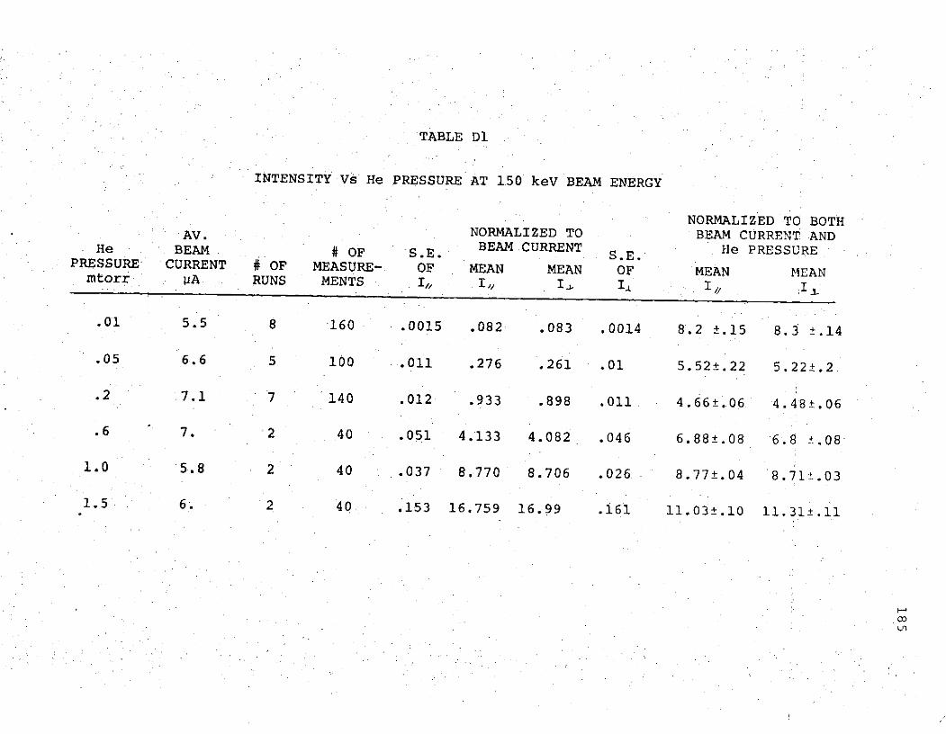
TABLE Dl

INTENSITY Vs He PRESSURE AT 150 keV BEAM ENERGY

NORMALIZED TO BOTHAV. NORMALIZED TO BEAM CURRENT AND

He BEAM # F S.E. BEAM CURRENT He PRESSUREPRESSURE CURRENT # OF MEASURE- OF MEAN MEAN OF MEAN MEANmtorr ijA RUNS MENTS I,, I,, I, I. I I

.01 5.5 8 160 .0015 .082 .083 .0014 8.2 ±.15 8.3 ±.14

.05 6.6 5 100 .011 .276 .261 .01 5.52±.22 5.22±.2

.2 7.1 7 140 .012 .933 .898 .011. 4.66±.06 4.48±.06

.6 7. 2 40 .051 4.133 4.082 .046 6.88±.08 6.8 ±.08

1.0 5.8 2 40 .037 8.770 8.706 .026 8.77±.04 8.71±.03

1.5 6. 2 40 .153 16.759 16.99 .161 11.03±.10 11.31+.11

•0

TABLE D2

INTENSITY Vs He PRESSURE AT 300 keV BEAM ENERGY

NORMALIZED TO BOTHAV. NORMALIZED TO BEAM CURRENT AND

He BEAM CURRENT He PRESSUREHe BEAM # OF S.E. S.E.PRESSURE CURRENT # OF MEASURE- OF MEAN MEAN OF MEAN MEANmtorr iA RUNS MENTS I, I, I. I I, I,

.01 11.8 7 140 .001 .0629 .0615 .0009 6.29±.1 6.15±.09

.05 11.4 7 140 .002 .159 .162 .002 3.19±.04 3.24±.04

.2 10.5 10 200 .004 .594 .624 .004 2.97±.02 3.12±.02

.6 12.2 3 60 .106 1.907 2.06 .118 3.18±.18 3.44±.2

1.0 11.2 3 60 .323 4.428 4.714 .353 4.43±.32 4.71±.35

1.5 11.3 2 40 .662 11.917 12.528 .717 7.95±.44 8.38±.48

co.

TABLE D3

INTENSITY Vs He PRESSURE AT 450 keV BEAM ENERGY

NORMALIZED TO BOTHAV. NORMALIZED TO BEAM CURRENT AND

He BEAM # OF S.E. BEAM CURRENT He PRESSUREHe BEAM #OF S.E. S.E.PRESSURE CURRENT # OF MEASURE- OF MEAN MEAN OF MEAN MEANmtorr IA RUNS MENTS I, I I I- I

.01 11.8 4 80 .0018 .0877 .0914 .0018 8.77±.18 9.14±.18

.05 10.4 5 100 .0029 .1741 .1813 .0023 3.48±.58 3.62±.46

.2 10.3 7 140 .004 .4821 .5387 .005 2.41±.02 2.69±.03

.6 10.7 3 60 .039 1.953 2.181 .058 3.26±.07 3.64±.1

1.0 10.8 3 60 .171 3.754 4.094 .211 3.75±.17 4.09±.21

1.5 10.5 2 40 .106 5.107 5.47 .129 3.41±.07 3.65±.09

CC

188

INTENSITY Vs HELIUM PRESSURE@ 150 keV BEAM ENERGY

2oo

o5-

C

00

I I ! I ,.

O .2 .6 1.0 1.5He Pressure mtorr

FIGURE Dl

189

INTENSITY Vs HELIUM PRESSURE( 300 keV BEAM ENERGY

10

0~c

D

4-

.2 .6 1.0 1.5He Pressure mtorr

FIGURE D2

190

INTENSITY Vs HELIUM PRESSUREod 450 keV BEAM ENERGY

10

Do

0

0

.2 .6 1.0 1.5He Pressure mtorr

FIGURE D3

191

a ground state atom. It is then the 21S state with which

we must concern ourselves. In order to estimate the

effect on X 5016 A photons by 21S state He atoms, we must

first discuss the presence of 215S atoms in the targetchamber. Referring to calculations done in sections 4.2

and 4.3, we have at our highest working pressure (1.5

mtorr) a mean free path of 47 cm, a mean collision time

of n.3 msec, and an estimated minimum wall collision timeof \.02 msec. Similar calculations for our lowest work-

ing pressure (.01 mtorr) yield a mean free path of

r7000 cm, a mean collision time of n50 msec, and an

estimated minimum wall collision time of \.02 msec.

Note that the wall collision times are minimum times and

in fact the "diffusion" times would be much longer.

Furthermore, we have from Hasted (1972) the fact that the

natural lifetime of the metastable state He 21S is

> 1 msec. We can then conclude that at our high pressure

runs the He 21S level will be collisionally quenched and

significant absorbtion of A 5016 A light will not occur.

However as we go to lower pressures, the number of sur-

viving He 21S atoms increases and we can expect some

absorbtion of the X 5016 1 light. Finally at very low

pressures one would expect a high percentage of He 21S

in the target chamber, but these metastables would be

spread so thinly that there would be lit e photon-

metastable interaction, and therefore an increase in the

amount of A 5016 . light detected.

192

The results which have been normalized to both

Beam Current and Gas Pressure are the relative intensi-

ties of A 5016 . light per proton per target atom. The

minimum observed in these curves is just what one would

expect (qualitatively) from our discussion of the exis-

tence of the metastable He 21S atoms. We thus conclude

that trapping by the metastable He 21S atoms is respon-

sible for the changes in relative intensity with pres-

sure.

In conclusion then, we are still unable to ex-

plain the cause of the change in the sign of 7 as the

He pressure changes. We have shown qualitatively that

trapping is occurring at the metastable 21S level. This

trapping provides yet another reason for the next experi-

menter to work at lower pressures. Only then will the

photon from a beam excited 31P-21S transition be directly

detected.