
university of london
411
UNIVERSITY OF LONDON IMPERIAL COLLEGE OF SCIENCE AND TECHNOLOGY' DEPARTMENT OF MECHANICAL ENGINEERING EFFECTS OF STRAIN RATE, FRICTION AND TEMPERATURE DISTRIBUTION IN HIGH SPEED AXISYRMETRIC UPSETTING M. MOHITPOUR B.Sc.(Eng.), Graduate Inst. Mech. Engrs. A thesis submitted for the degree of DOCTOR OF PHILOSOPHY of the University of London and also fOr the ( DIPLOMA OF IMPERIAL COLLEGE Sept 1972
-
Upload
khangminh22 -
Category
Documents
-
view
1 -
download
0
Transcript of university of london

UNIVERSITY OF LONDON
IMPERIAL COLLEGE OF SCIENCE AND TECHNOLOGY'
DEPARTMENT OF MECHANICAL ENGINEERING
EFFECTS OF STRAIN RATE, FRICTION
AND TEMPERATURE DISTRIBUTION IN HIGH SPEED
AXISYRMETRIC UPSETTING
M. MOHITPOUR B.Sc.(Eng.), Graduate Inst. Mech. Engrs.
A thesis submitted for the
degree of
DOCTOR OF PHILOSOPHY
of the University of London
and also fOr the (
DIPLOMA OF IMPERIAL COLLEGE
Sept 1972

2
RESUME
The literature is reviewed to sum up the best method of approach
to establish the dynamic mechanical behaviour of materials without
side effects. The review is further extended to cover the phenomena
of strain rate effects with particular reference to stress/strain
characteristics.
An incremental method of determining stress/strain curves to
large strains at high strain rate and sub-critical temperatures, is
described. Comparisons are made between the incrementally obtained
stress/strain curves and those obtained under continuously applied
loads to large deformations by means of a free flight type impact
device. The strain rate varied between wide limits in the continuous
tests. This variation and the adiabatic heat generated by the plastic
work are explained to be responsible for the different stress/strain
curves obtained in the two methods.
A step by step numerical method using a finite element technique
is presented along with the computer programme used to establish the
temperature field in high speed upsetting of axisymmetric billets.
Homogeneous deformation with constant end frictions is considered.
It is demonstrated that plastic work and friction are jointly
responsible for the adiabatic temperature rise. If deformation is
homogeneous, the bulk of the deforming material experiences almost
uniform temperature increase. When friction is present, the temperature
field is significantly influenced, particularly near the tooling/
material interface, which could influence tool life and the product
properties.
Some effects observed in high speed forming of materials are
explained in terms of adiabatic temperature rise.

CONTENTS
Page
RESUME
2
CONTENTS
3
LIST OF FIGURES
7
LIST OF TABLES
15
NOTATION
16
ACKNOWLEDGEMENTS
23
1. INTRODUCTION AND SCOPE OF WORK
24
2. A REVIEW OF HIGH STRAIN RATE PHENOMENA AND THEIR EFFECTS
29
ON MATERIAL BEHAVIOUR AND PROPERTIES
2.1 Introduction
29
2.2 Methods of obtaining and evaluating dynamic stress/
32
strain data
2.2.1 Dynamic compression (Hopkinson pressure bar
33
techniques)
2.2.2 Dynamic compression (other methods)
42
2.2.3 Torsional processes
51
2.2.4 Impact tension techniques
54
2.2.5 Other methods 58
2.2.6 Assessment of techniques
69 .
2.3 Incremental Approach
79
2.4 Material Behaviour and Properties under Dynamic
83
Loading
3. EXPERIMENTAL APPARATUS AND PROCEDURE
116
3.1 Introduction 116
3.2 Modified U.S. Industries Forging Press
116
3.2.1 Operation of the machine
123.
3

Page
3.2.2 Automatic Guard 126
3.3 Experimental Subpress 128
3.3.1 Dynamic incremental tests 128
3.3.2 Dynamic large deformation tests 133
3.3.3 Quasi-static tests 135
3.4 Instrumentation 135
3.4.1 Load measurement 135
3.4.2 Velocity and displacement measurement 140
3.4.3 Temperature measurement 153
3.4.4 Arrangement of instrumentation 158
3.5 material and Lubricant 160
4. THEORETICAL CONSIDERATIONS 165
4.1 Introduction 165
4.2 Analysis and Assessment of Experimental Data 165
4.2.1 Determination of dynamic material behaviour 165
4.2.2 Estimation of the limiting strain rate error, 166
the adiabatic temperature rise and work ratio
in incremental tests
4.2.3 Contribution of inertia forces and stress 168
wave propagation
4.3 Estimation of Temperatuie Field 170
4.3.1 Review of previous works 170
4.3.2 The finite element approach 173.
4.3.3 Governing equations 175
4.3.4 The finite element idealisation 178
4.3.5 Assembly of minimising equations 191
4.3.6 Recursive procedure 191
4.3.7 Heat generation due to deformation and work 195
of boundary friction

Page
5. COMPUTATION PROCEDURE AND COMPUTER PROGRAMMING 198
5.1 Procedure and Programming 198
5.1.1 Subroutine INPUT 202
5.1.2 Subroutine GEN (calling subroutines TINTL, 202
ZONE and BOUND)
5.1.3 Subroutine MODIFY 205
5.1.4 Subroutine CORCTN 205
5.1.5 Subroutine STRESS 208
5.1.6 Subroutine DTINTL 208
5.1.7 subroutine FRICTN 211
5.1.8 Subroutine STIFF 212
5.1.9 Subroutines SMOOTH and LINSOZ 213
5.1.10 Subroutine LININT 216
5.1.11 Miscellaneous 216
6. RESULTS AND DISCUSSIONS 218
6.1 Dynamic Incremental Stress/strain Characteristics 218
6.1.1 Limit of accuracy of results 225
6.2 Comparison of Dynamic Stress/strain Curves obtained 233
by the Incremental and Large Deformation Methods
6.3 Temperature Distribution in High Speed Axisymmetric 240
Upsetting with End Frictions
6.3.1 Testing of the computer programme 240
6.3.2 Temperature field 247
7. CONCLUSIONS AND RECOMMENDATIONS 283
7.1 Conclusions 283
7.2 Recommendations for future work 285
REFERENCES 287
APPENDIX A. Programming Symbols and Computer Programme 298
APPENDIX B. Mechanical and Thermal Properties for the 333
Computer Programme
5

6
Page
APPENDIX C. Results from computer programme
339
APPENDIX D. Published papers
371

7
LIST OF FIGURES
Page
CHAPTER 2
2.1 A modified (schematic) arrangement of split Hopkinson 35
pressure bar
2.2 Examples of modified split Hopkinson pressure bar 35
arrangements
2.3 Possible material testing arrangements 36
2.4 The terminology for the analysis of stress/strain data 36
2.5 Graphical Solution to equations 2.6-and 2.7 40
2.6 Experimental records and analyses for 1.01cm tubular 40
aluminium specimen with an applied stress of 140 MN/m2
2.7 Exploded view of the air gun and allied instrumentation 41
2.8 An example of drop forging apparatus and allied 41
instrumentation
2.9 Typical load recording trial using a short load cell 47
- 18:4:1 HSS steel - 1100°C
2.10 Typical variation of strain rate with strain using free 47
flight impact devices
2.11 Concept of mean strain rate - HSS steel : 1055°C 50
2.12 Typical deflection of longitudinal line marked on bore 50
of specimen
2.13 Diagramatic representation of an impact tensile 56
testing machine and instrumentation
2.14 Earliest tracing of typical velocity and load records 57
2.15 Typical load recording due to Chiang - En 3B cold drawn 57
2.16 Idealised orthogonal metal cutting 60
2.17 The expanding ring technique for the measurement of
62
plastic flow properties
2.18 The teminology of expanding ring technique 63

Page
2.19 . Three components of extrusion pressure and their
67
relation to flow stress as over a range of strain
rates
2.20 Schematic representation of set-up incorporating
67
a bar with a truncated cone
2.21 a) Flow stress/strain rate of aluminium showing
72
deviations because of stress gradients across
the specimen
b) Percentage deviation in flow stress versus
72
number of transients across specimen
2.22 strain rate /strain histories for pure lead at room
73
temperature using a drop hammer
2.23 Strain rate/strain characteristics for high speed
73
upsetting using free flight impact devices
2.24 Constant strain rate/strain history achieved with
75
free flight impact devices
2.25' Difference in shear stress/shear strain character- 75
istics for carbon steel
2.26 Experimental apparatus as used by Von Karman and 80
Duwez to stop impact after a given deformation of
specimen has been reached
2.27 Incremental dynamic compression set-up 80
2.28 Incremental stress/strain curves for copper 82
2.29 Arrangement of torsional incremental set-up as used 82
by Campbell and Dowling
2.30 Variation of flow stress with subgrain diameter , 94
2.31 surface representation of stress, log strain rate 94
and temperature
2.32 stress/strain rate characteristics of aluminium at
96
20% strain
8

Page
2.33 Dynamic stress/strain rate characteristics for 100
aluminium at 250°C
2.34 Yield stress/strain characteristics 2.25% C and 100
13% Cr Steel at 900°C
2.35 Temperature rise of specimen undergoing high speed 108
deformation
2.36 Temperature and strain rate effect on the behaviour 108
of mild steel
2.37 Dependence of strain rate effects on the homogeneous 110
temperature for 40% reduction
2.38 Dependence of strain rate sensitivity on temperature 110
as determined by several test methods
2.39 Effect of strain rate on transition temperature — 111
annealed aluminium
2.40 Variation of subgrain size with temperature in . 111
several materials for different modes of deformation
as measured by variety of techniques
2.41 Relation between maximum load, ratios of maximum 113
load with lubricant/maximum load without lubricant
and maximum load at low speed/maximum load at high
speed with percentage reduction — indicating the
variation in frctional restraints
Chapter 3
3.1 Schematic half section of the modified U.S.I.
forging press
117
3.2 U.S.I. forging press as previously used 119
3.3 Exploded view of valve and drive piston assembly 120
3.4 modified U.S.I. forging press and allied
instrumentation (as set up for an incremental test)
123
9

3.5 modified U.S.I. press, pneumatic circuit
3.6 modified U.S.I. press, hydraulic circuit
3.7 Automatic guard and safety mechanism
3.8 Experimental sub-press for incremental tests
3.9 Arrangement of incremental tooling in the press
3.10 Long load cell and allied parts
3.11 Experimental sub-press for large deformation tests
3.12 Load cells and their strain gauge arrangements
3.13 The ring load cell assembly
3.14 Calibration curves of load cells
10
Page
124
125
127
129
131
132
- 134
137
139
141
3.15 Typical load and velocity traces 142
3.16 Calibration of velocity transducers: equipment set-up 144
3.17 Calibration of velocity transducers: general layout 145
of tooling and instrumentation
3.18 Calibration of velocity transducers: motor circuit 147
3.19 Hysteresis loops of velocity transducers 148
3.20 Characteristic response of velocity transducers: 150
solenoid signal/velocity curves
3.21 Characteristic response of velocity transducers: 151
solenoid signal/L curves
3.22 Calibration curves of velocity transducers 151
3.23 A compressed specimen with thermocouple 155
3.24 A compressed specimen showing position of thermocouple 155
bead
3.25 Typical temperature and velocity records 156
3.26 Thermocouple set-up for temperature measurement in 157
hot tests
3.27 General layout of instrumentation for the U.S.I. press 159
3.28 Arrangement of velocity transducer and triggering
mechanism (incremental set-up)

11
Page
3.29 Typical specimens of aluminium subjected to incremental 164
and large deformation tests
Chapter 4
4.1 Specimen's geometry before and after an increment of 166
deformation
4.2 Axisymmetric body under compression and an arbitrary 176
triangular elemental ring
4.3 An arbitrary solid subjected to transient heat 177
conduction
4.4 The idealised body with triangular elements 179
4.5 Triangular element dimensions 181
4.6 A triangular element with one side convecting heat 184
4.7 An axisymmetric continuum with triangular elements 186
subjected to surface convective heat transfer
4.8 Typical element along the line of discontinuity 193
Chapter 5
5.1 Block diagram of computer programme 199-200
5.2 Numbering of the elements and nodal points in the 203
mesh
5.3 Labelling of the specimen and platen continua for 204
identification purposes
5.4 Overall mesh after 502 reduction in the specimen's 206
height
5.5 Movement of the nodal point in the platen continuum 207
5.6 Contribution of boundary heat flux to nodal points 211
5.7 Variation of iteration cycles with relaxation factors 214

Page
Chapter 6
6.1 Flow stress/strain rate curves for copper 219
6.2 Flow stress/strain rate curves for aluminium 220
6.3 Flow stress/strain rate curves for copper (indicating 223
power law behaviour)
6.4 Flow stress/strain rate curves for aluminium 224
(indicating power law behaviour)
6.5 Stress/strain curves for copper 226.
6.6 Stress/strain curves for aluminium 227
6.7 Estimation of incremental limiting strain rate error 229
for copper
6.8 Estimation of incremental limiting strain rate error 229
for aluminium 1
6.9 Estimation of incremental limiting temperature rise 229
for copper
6.10 Estimation of incremental limiting temperature rise 229
for aluminium
6.11 comparison of the stress/strain curves obtained by the 234
incremental ( ) and large deformation (- --) methods
for copper
6.12 Comparison of the stress/strain curves obtained by the 235
incremental ( ) and large deformation methods
for aluminium
6.13 strain rate/strain variation curves for large 236
deformation tests on copper
6.14 Strain rate/strain variation curves for large 237
deformation tests on aluminium
6.15 Temperature/strain variations for large deformation 239
tests
12
13
Page
6.16 Temperature distribution (°C) in upper right quadrant 242
of a steel cylinder cooled in water at 0°C for 4
seconds
6.17 Isotherms for cooling of a steel cylinder in water at 243
0°C after 4 seconds
6.18 Temperature distribution (°C) foi: cooling of a steel 244
cylinder in water at 0°C after 4 seconds - comparison
of results (fine mesh)
6.19 Temperature distribution (°C) for cooling of a steel 245
cylinder in water at 0°C after 4 seconds - comparison
of results (coarse mesh)
6.20 Cooling curves for the edge of a steel cylinder cooled 246
in water at 0°C
6.21 Velocity/time variation curves for copper at various 248
impact velocities
6.22 Strain rate/strain variation curves for copper at 249
various impact velocites
6.23 Temperature contours - Test A 251-253
6.24 Temperature contours - Test 8 254-256
6.25 Temperature contours - Test B 257-259
6.26 Temperature contours - Test C 260-261
6.27 Temperature contours - Test C 262-263
6.28 Temperature contours - Test 0 264-266
6.29 Effect of friction and strain on temperature 269-270
6.30 Variation of temperature with coefficient of friction 271-272
6.31 Effect of speed and friction on mean bulk temperatures 273
6.32 Effect of speed and friction on maximum localised 274.
temperature
6.33 Theoretical representation of the effect of impact 279
velocity on the centre point temperature for copper

6.34 Comparison of experimental and theoretical centre
point temperatures - vi = 4.5m/s, and vi = 10mis
6.35 Comparison of experimental and theoretical centre
poiritterverature _ vi .6.1 .8m/s
Appendix 8
B.1
Quasistatic stress/strain characteristics of 99.95%
copper
8.2
Flow stress/strain rate characteristics of high
conductivity copper
B.3
Thermal conductivity of copper
8.4
Specific heat of copper
8.5
Heat transfer film coefficient
14
Page
280
281
335
336
337
338
338

LIST OF TABLES
the dynamic behaviour
conditions
of
Page
85 2.1 Relationships describing
metals with testing
2.2 Values of o and n in the equation 0s = o oE n
es I T 91
- (Table 2.1a)
2.3 Values of ta BB and l in the equation 92
T .(tT-X) = a + 00 c - (Table 2.1d)
2.4 Values of a and m in equation os
= 0 o oc epT
92
- (Table 2.1j)
2.5 Values of the constants and the parameters of the 93
equations presented in Table 2.11.
2.6 Values of 0o and n in the equation as = oen
93 E Tt
- (Table 2.1o) Al :1100
2.7 Values of the slopes of the m/T curves (Fig. 2.37)
various reductions
for 110
3.1 Weight of machine components and toolings 122
3.2 Velocity transducer specifications 146
C.1Tempuraturedistributionforv.=10m/s 1 340-358
(a-s)
C.2Temperaturedistributionforv.=0.8m/s 1 359-361
(a-c)
C.3 Temperature distribution for vi= 6.4m/s 362-367 (a-f)
C.4 Temperature distribution for v= 4.5m/s 368-370 (a-c)
15

NOTATION
Each symbol is defined as it first appears in the text. General
symbols defining similar variables are grouped together. Other symbols
which are used frequently are defined separately.
A, Ab, Art As area, cross sectional area
Ai
initial cross sectional area of specimen
dA increment of area
aj, ak radial dimensions of nodes j and k
B dislocation damping constant
b, bo chip thickness, thickness of metal removed
bj, bk axial dimensions of nodes j and k
br chip length ratio
by
Berger's vector
IC] Cij total heat capacity matrix
[c]8, cije elemental heat capacity matrix.
C1,
C2
constants
c specific heat
cv, c
vb c
vs wave velocity, shear wave velocity
0, Dr indentor or projectile diameter, ram diameter
d, db indentation or specimen diameter
di
initial specimen diameter, inside diameter
dm mean indentation or specimen diameter
do
outside diameter of testpiece
dsg subgrain diameter
E, Em modulus of elasticity
Ed deformation energy
Eg discharge energy
16
17
ER extrusion ratio
e, e., et
engineering strain
mean engineering strain
of
final engineering strain
engineering yield strain
engineering strain rate
mean engineering strain rate
F,Fh,FstF IFNSforce, shear force
F average force or shear force, dynamic force d•
f frequency
GI Gt shear modulus
Hi hardness
pH activation energy
Ha adiabatic heating
Hc constant
[H]! Hid total convective heat matrix
[h]e, h11. .e elemental heat matrix
h specimen's length, height, gauge length, workplace
thickness
6h, 6h1, 6hIr displacement, depth of indentation, increment of
deformation, thickness of the zone of deformation
he effective gauge length, final specimen length or
height, final specimen gauge length
hF heat transfer film coefficient
hi initial specimen length or height, initial specimen
gauge length
specimen length or height after an increment of
deformation
hs shear length
J, k nodal points defining a triangular element

18
mechanical equivalent of heat
b polar moment of inertia
K aspect ratio
KE kinetic energy of platen or projectile
KEd
energy of deformation
KEi
kinetic energy of platen at impact
KEn kinetic energy of platen after an increment of
deformation
Ks stiffness, structural stiffness
[K] Kij total thermal heat matrix
[k]e, kije elemental thermal heat matrix
k thermal conductivity
kr, k
z radial and axial thermal conductivities
KK ratio 2Wh
L, 1 length, bar length, elemental side length
Lc inductance
LR relative position of electromagnet and solenoid
piston or platen mass, mass, ram or projectile mass
Mr mass ratio
strain rate sensitivity index
ms
specimen mass
Ems increment of specimen mass
N ratio L/R
n strain index
nb
normal to boundary
no an index
P normal pressure distribution, pressure
Py yield pressure
Q activation energy
q boundary heat flux

19
total boundary heat flux vector
elemental boundary heat flux vector
R, r radius, specimen or testpiece radius
universal gas. constant
Re resistance, equivalent resistance
R r
inside radius of testpiece, initial inside radius
Ro
Roi t ro outside radius of testpiece, initial outside radius
Rbr mean radial ordinates of two nodes of an element's
side parallel to r axis
nbz mean radial ordinates of two nodes of an element's
side parallel to z axis
R1
elemental side length with the side parallel to
r axis
R, f radial velocity
R, radial acceleration or deceleration
rte z polar co-ordinates
mean elemental radius = (ri+ rj+ rk)/3
S surface area
dS increment of surface area
T temperature
AT increment of temperature rise
Ti total temperature vector
iT} e elemental temperature vector
total transient (temperature/time) vector
4.1.1 e elemental transient (temperature/time) vector
TA absolute temperature
TB known boundary temperature
TH homologous temperature
Tf fluid or air temperature
Ti, Ti, Tk temperature of nodes i, j, k
Tm melting point temperature

20
Tq, Tqc, Tqe Tqs torque
t, tt, tb, tt, is time, deformation or contact time, time of propogation
At increment of time
6t thickness of tubular specimen
V, Vi, V2, Vt, Vr voltage
5V increment of bridge voltage
V volume, apparent activation volume
v, v velocity, extrusion velocity, particle velocity,
relative velocity
average velocity
✓ velocity of sound
✓ impact or initial velocity
✓ velocity after an increment of deformation ca
r rebound velocity
Wf frictional work
Xid(20(3,X4,X5 constants
x position
linear velocity
Amax maximum linear velocity
Z Zenor Holloman function
Z1 elemental side length with side parallel to z axis
A triangular elemental area
✓ angle, angle of twist
de increment of angle
rate of change of angle with time
angle of torsion at fracture
a, act, (313 constants
(3 proportion of plastic work converted to heat
shear strain
shear strain rate
average shear strain rate

21
natural strain
AE increment of strain
t strain rate
strain rate error error
mean strain rate
tm
integrated mean strain rate
• • rate of change of strain rate
constant
X constant
XX' XX1, ) gauge factor
coefficient of friction
v Poisson ratio
13' 138 Pmd density, billet density, mean dislocation density
0 0 Ott t
o oit
ar tt t o t
t 0z stress, measured or recorded stress
to increment of stress
GB stress to overcome barriers
C113 constant
flow stress at zero or unity strain rate
lateral inertia stress 4
flow stress Gs
os mean flow stress
ost static stress
°st mean static stress
a dynamic yield stress 1
ay mean dynamic yield stress
cyst static yield stress
°yst mean static yield stress
po sy increment of stress preceding yield
slope
22
S 1, S 2' g 39 g4
constants
T B
shear stress
angle of fracture, shear angle, angle lying in
the second quadrant -
X variational function
;:;.<1.1 e elemental minimised functional
4) , gis chip formation angle, die semi-angle
c, 1 , Ci2 p 3 c, 4 constant
chip force angle

ACKNOWLEDGEMENTS
My sincere thanks and gratitude to Ur. B. Lengyel for instigation
of the project, much encouragement and help in every way, which made the
completion of this work a reality. Thanks are due to Professor J.M.
Alexander to whom the author is truly grateful for support and
permission to use the facilities of the Metal Working Laboratory,
Mechanical Engineering Department.
The assistance given by all members of the staff and students
of the Metal Working Laboratory is also gratefully acknowledged. In
particular Messrs P.G. Ashford and M.G. Gutteridge for advice on the
experimental machine. Help given by Messrs J. Pooley, R. Baxter and
S.C. Pridham and in particular Mr. N. Keith for assistance in the
experimental work, is acknowledged.
Acknowledgements are due to Miss E.M. Archer and Mrs L.M. Ward,
the librarians of the Mechanical Engineering Department for every kind
effort they put forward in obtaining mauscripts and papers, etc.
useful to the author's work.
Many thanks are due to Mr. K. Palit and Dr. R.T. Fenner of the
Mechanical Engineering Department for stimulating discussions, help
and advice.
Financial support of the Science Research Council is gratefully
acknowledged.
Finally, and indeed, not the least, many thanks to my wife Carol
for all her help, courage and patience throughout the course. My thanks
are also due to her for typing of the thesis.
M. m.
September 1972
23

CHAPTER 1
INTRODUCTION AND SCOPE OF WORK
Material behaviour is influenced by strain, strain rate and
temperature. It is also affected by boundary and inertia restraints.
If the rate and amount of straining is high,heating of the deforming
material due to the work of deformation and possible friction becomes
inevitable resulting in the change of the working temperature.
Strain rate modifies material structures and behaviour by in-
fluencing the dislocation motions, densities and networks, loops,
tangles, intersection jogs, vacancies, etc.. An increase in strain
rate should cause a proportionate increase in the flow stress; but the
extent of the influence may become misrepresentative of the actual effect,
if other factors affecting the deformation are not isolated. A common
example is the upsetting of right cylindrical billets, a method widely
used to obtain stress/strain curves of materials to high strain rates.
In this case, if friction exists between the die/material interface,
the curves could take a different path than those which are free from
the restraint. The effect is to raise the flow stress. On the other
hand since an increase in the temperature lowers the flow stress, the
frictional work and the work due to the plastic deformation could lead
to temperature rise in the deforming material such that the flow stress
could experience a drop in'its level. Consequently the concommitant
effect of friction and adiabatic heating of the material could mask the
actual strain rate effects and lead to stress/strain data unrepresent-
ative of the billets' conditions at the commencement of the test, to
which they are usually related. Strain rate may vary during the deform-
24

25
ation and this could further alter the data.
It could therefore be inferred that it is of much interest in
the true determination of material properties, with particular reference
to stress/strain data, to isolate or minimise possible side effects by
suitable means, in order to be able to study a particular phenomenon.
An example of this is the procedure adopted by Cooke and Larke (1) for
minimising spurious frictional increases of the flow stress determined
from compression tests. Besides, it may also be decided that it is of
interest to know the actual conditions during a particular process of
deformation, such as material temperatures, strain rates, etc. as the
deformation proceeds, and relate the measured data to real rather than
initial or mean values, since the use of misrepresentative data in metal
working analysis could reflect on the vigour of any algebraic equations
proposed and the validity of the assumptions made.
The above collectively indicate that in order to obtain correct
dita useful forlbell application to metal working processes and
analyses, particularly those with large strain/high strain rate
applications, and further to study the true strain rate effect on
material properties, a test method must be adopted which bears the
following characteristics:
a) The test method must be suitable for the application of large
strains and high strain rates.
b) The magnitude of the testing temperature and strain rate must be •
known throughout the test, or preferably made to remain constant.
c) There must be no side effects reflecting on the data.
A suitable method in this context for the attainment of data to
large strains and at high strain rates (satisfying condition (a)) would
be the use of free flight compression devices. However these pose
several problems, namely in satisfying conditions (b) and (c). Firstly
materials show strain rate sensitivity at high strain rates even at

26
room tempetature; thus constant strain rates shoul be maintained during,
the tests, which is rarely feasible with these methods. Secondly in
continuously loading the material to large strains, a significant rise
in the level of the material's temperature is unavoidable. This combined
with the short duration of the test results in adiabatic heating.
Finally since data need to be obtained to large strains for their
application to large deformation metal working processes and analyses,
e.g. extrusions, end friction in compression tests could also become
significant. This may distort the results particularly at large
reductions. Prediction of correct data *are)therefore hardly possible
with these methods unless some alternative arrangements are incorporated.
These considerations lead to the conclusion that an incremental
method based on the same principle as quasi-static testing incorporating
a compression technique (l)(2), is a feasible solution to many difficul-
ties encountered in the dynamic testing of materials to obtain stress/
strain data. The method could include such factors as large strains,
controlled high strain rates and limited adiabatic temperature rises,
as well as reduced end frictions and inertia restraints. All the in-
fluencing elements can be made known, or their effects separated at
points along the stress/strain curves, such that data when obtained
could be interpreted in terms (of the effect) of a single variable. If
data are obtained in such a manner, it would then be interesting to
make a comparison of incrementally obtained isothermal dynamic stress/
strain curves with those achieved under the condition of continuous
loading, where the adiabatic heating effects due to the work of
deformation and possible friction are thought to be prevalent and the
variation in strain rate during the test unavoidable. Such a comparison
would provide quantitatively the extent of the influence of any
temperature rise of the testpiece during the process of continuous
deformation on the mechanical behaviour and the product properties. It

27
is of interest to know the influence as it could also affect high
speed forming processes for industrial applications.
Claims have been made as to the advantages of high speed forming,
in particular to the forgeability of difficult components, better
lubrication conditions and recently, to forming of brittle and hard
materials. Since in high speed upsetting the duration of deformation
is short, plastic work of deformation and frictional work could give
rise to and alter the material's testing temperature during the deform-
ation, it would be helpful to compute the extent of this temperature
rise, variation, and, in particular, its distribution, to explain this
pertinent factor which could influence material formability. It would
be of value to show effects caused by hioh speed forming of materials
in terms of localised heating prevalent in these processes. Examples
of these could be regarded as the decrease in the hardness value near
the product's surface layer, incipient melting as a result of high
speed extrusion (3) and the flaring of cylindrical specimen ends in
high velocity compression tests (4).
Under high speed forming, the work of friction along the
boundaries of contacts causes localised temperature rises. The latter,
if significant, could alter properties of lubricants, influence the
localised product properties and hardness distributian and further
could set up thermal stresses in the tool producing wear and fatigue.
On the other hand, adiabatic heating could be beneficial industriallYr .
since it could reduce the forming force. It could also be beneficial in
preventing the failure of forming dies in terms of erosive wear.
Similarly it could be the heating of cylindrical billets during deform-
ation in high speed compression tests which reduces barrelling effects.
It would consequently be of much benefit to compute the temperature
field in high speed upsetting with the intention of explaining the
causes and effects of high temperature rises, the pattern of the

23
temperature field and the changes occurring in material properties,
process and lubrication conditions during the deformation. Besides,
the knowledge of localised temperature will provide a comprehensive
picture of the deforming material and relating this property to a
single variable would help the understanding of the phenomena occurring
under high speed upsetting.
With the above ideas in mind the aim of the present work is to
review the literature extensively, to study critically the methods of
approach for the determination of dynamic mechanical behaviour of
metals and also to demonstrate the strain rate effects on material
properties as established by several disciplines.
The aim is also to establish and describe in detail experimental,
incremental and large deformation methods to obtain dynamic stress/strain
data to large strains by means of a free flight type impact device. This
is mainly to pursue the intentions set out above to establish the effects
on the mechanical behaviour of accumulative adiabatic heating due to
deformation and the variation in strain rate persistent in continuous
high speed upsetting, and further provide true isothermal dynamic
stress/strain curves free of side effects for use in metal working
analyses.
Further the aim of the work is to establish the temperature field
in high speed compression of right cylindrical billets experiencing
homogeneous deformation with constant end frictions by a suitable step
by step method. A finite element technique is thought of for this
purpose since this method is now commonly used a a powerful tool in
the solution of continuum mechanics problems and metal working processes.
It is then envisaged to explain effects observed in high speed formings
of materials, some of which are enumerated above in terms of temperature
rise of the deforming material, and the localised heating effects
present in these processes.
CHAPTER 2
A REVIEW OF HIGH STRAIN RATE PHENOMENA AND THEIR EFFECTS
ON MATERIAL BEHAVIOUR AND PROPERTIES
2.1 Introduction
Several disciplines - engineering, physics, metallurgy - are
concerned with strain rate effects on material behaviour during the
forming process of metals (with residual effects). The prime concern
is to evaluate and explain material behaviour under diverse modes and
rates of deformation. If there exist contrasts of approach between these
disciplines, they stem from the fact that each is primarily interested
in different problems.
From an engineering point of view, material properties are the
shape of stress/strain curves and the manner by which these inter-related
parameters vary by changing the factors of strain rate, temperature and
the mode of the deforming process. To achieve their objectives,
engineers have devised many testing techniques such as indentation (5),
impact extension (6), wave propogation effects (7), extrusion (8) etc.
On the other hand, metallurgists are concerned with the macro-
structural changes occurring in the upsetting process to establish the
rate controlling mechanisms operative during the deformation with their
eventual effects on the mechanical properties. Considering the role of
the motion of dislocation (9), (10), the activation energy Q is
evaluated for cold and hot working processes and hence the dominant
rate controlling mechanisms are determined. From the analysis of such
operative mechanisms, functional relationships having constants of some
physical significance are proposed to predict the dynamic behaviour.
29

30
Physicists approach the fundamental changes occurring in the
micro-structure and the formation of substructures as a result of
change in the rate or the mode of deformation. Using transmission
electron microscopy (11) the phenomenon of substructure strengthening,
by changing the strain rate v and its subsequent effect on the subgrain
size and misorientations produced, is discussed. On the basis of the
subgrain formations and substructure arrangements, the phenomena
occurring during the deformation process are explained and hence the
physical behaviour of the material described.
Although the engineeering and physical aspects of mechanical
properties are tackled through contrasting fields of interest, they
should provide a unique result in understanding the material behaviour.
This is possible if only common features are considered with no side
effects, under different rates and modes of upsetting.
The mechanism of deformation structurally or otherwise is dependent
upon the forms of upsetting. In any case the working material undergoes
a complex system of stresses controlled by loading rate, temperature,
boundary restraints and any other conditions. For instance, in
quasi-static forming, the metal is deformed by slip along a specific
lattice plane and in directions which are related to the structure of
the material (12). On the other hand for plastic working of metals
sustaining high rates of straining, the deformation is produced by glide
on a greater number of closely spaced slip bands which are affected by °
the magnitude of the deforming rate. /—
The complex system of stresses can in most cases be reduced to
three principal stresses and by applying Von Mises' or Tresca's 1
Criteria, then the flow or shear stresses sustained by the material
may be obtained. But in the manipulation of these criteria very close
approximations to stresses can only be achieved if realistic material
properties are considered. Such knowledge would then provide correct end
results from the solution of plasticity problems and in particular

31
establishes the actual potentials and capabilities of forming
techmiques. It also assesses correctly the factors which influence
the characteristic parameters of these forming techniques.
Strain rate effects are present in all forming techniques, but
the level of the effect is dependent upon relative molecular movements
within the material's structure during the particular upsetting process.
For instance if a sharp wave front is propogated through a material
subjected to explosive loading, the strain rate is so high that the
plastic process cannot operate and instead an elastic component sets
in. On the other hand at plastic wave fronts, the time of the propog-
ation is essentially longer so that a plastic strain wave of low strain
rate magnitude operates. material properties are accordingly affected
with the change in strain rate and the form of straining.
In high speed forming techniques in as much as the behaviour of
the metal undergoing deformation changes with strain rate, the extent
of the variation in the strain rate in the deformation zone influences
the terminal product properties. Even in conventional slow forming
processes such as rolling, extrusion etc., the element of the material
which passes through the deformation zone may experience high magnitudes
of strain rates. The extent of the deformation may also be different
for each element. Accordingly each element of the product may have
different properties.
These material properties which are influenced by the extent of
straining, strain rate and the working temperature would be further
altered with any temperature changes occurring during the defdrmation
process. In any dynamic forming techniques such as impact extrusion
(13),(14), the work of deformation contributes to the rise
in the temperature of the workpiece. If the level of adiabatic
temperature rise is significant then product properties are further
modified (3). Such a phenomenon a'so influences the dynamic behaviour in

32
such a way that the dominant operating mechanism might change.
It is therefore essential to obtain realistic material properties
under known conditions of strain rate, temperature etc., without any
side effects as invaluable aids for the designer of forming equipment
to evaluate the full use and the capabilities of such processes. This
also provides means of assisting metallurgists and physicists in their
work, since the extreme conditions generated by such processes intensify
the weaknesses of certain assumptions made about the bulk properties of
matter.
This chapter reviews the techniques available for the determination
of material properties with comments on their merits and shortcomings.
It also embodies the behaviour of materials as influenced by factors
discussed above and other considerations such as friction, inertia
restraints etc..
2.2 methods of obtaining and evaluating dynamic stress/strain data
The interest in the dynamic behaviour of metals started with
the advent of high energy rate forming processes which themselves
stemmed from the missile and ballistic testing rigs of the Convair
Division of the General Dynamic Corporation in 1955. A project was
started to convert the shock testing unit into the "Dynapak" forging
machine which was first demonstrated in 1958.
Accurate studies of the rate effect are essential in order to
complete the total picture of material behaviour. .Juch knowledge of
rate dependent behaviour over wide ranges of strain rate, not only
yields formulation of constitutive relationships, but determines the
predominant mechanism responsible for material behaviour for the
understanding of the basic plasticity problems.

33
It is not therefore surprising that the pressure of scientific
as well as practical interest has led to the evolvement of many schemes
to investigate the phenomenon of high strain rate effects and to measure
the stress and strain over wide ranges of ,strain rate and temperature
conditions.
Work on strain rate phenomena is reported as early as 1926 when
Hennecke (15) presented his results of dynamic and static deformation.
As instrumentation techniques were limited in those daysr no direct or
indirect measuements of strain rate are reported in his work. In 1940
Nadai and manjoine (6) reported work on high speed extension of metals
at constant strain rate. They also gave an excellent summary of the
literature existing on the subject at that time.
Seitz at al (16) in building a machine (1942) similar to that of
Nadai and Manjoine carried out tests on copper specimens but the rate
of compression speed attained in comparison, was small. Krafft (17)
and Kolsky (7) have given reviews of some earlier schemes of measuring
high strain rate properties of materials.
The method established by Taylor in 1946 (18), that of E.Volterra
in 1948 (19) and of Kolsky in 1949 (7) are real pioneers of stress-strain
measurement at high rates of straining. These methods are still used
in modified forms (20),(21),(22).
2.2.1 Dynamic compression (Hopkinson pressure bar technique)
Taylor and Volterra, (18),(19), by placing a cylindrical specimen
on the plane end of a cylindrical rod which hung as a ballistic pendulum,
and by freely suspending another bar, imposed compression on the short
cylindrical specimen when the latter force bar was swung against it.
Measurement of stress and strain was made by a photographic method of
recording.
A modified version of Volterra's technique using Davies' -pressure
bar (later known as the split Hopkinson pressure bar) is shown in

34
Fig. 2.1. One face of the specimen was placed against 'the firing end of
the bar, and a short cylindrical anvil was placed in contact with the
opposite face of the specimen. By firing a bullet at the exposed face
of the input anvil, a stress pulse was produced at the end of the bar
which communicated it to the specimen. The stress and displacement were
recorded by appropriate instrumentation.
Fig. 2.2 shows three latest arrangements of a modified split
Hopkinson bar for performing compression, double shearing and tension
tests on any arbitary material at high strain rates. In each case long
elastic input and output rods are used for stress pulse shaping and
measuring.
The basis differences in measurement of data between static,
quasi-static and dynamic testing are shown in Fig. 2.3. In Fig. 2.3a
the load and initial specimen area are known and thus the engineering
stress can easily be defined. Also as the initial gauge length is
known and its change can be readily measured as a function of time,
engineering strain rate and strain can be calculated by assuming uniform
strain distribution throughout the gauge section. Even the formation
of Luder's band can yield the assumption of Uniformity in strain and
stress distribution, but if under such static conditions the loading
rate is increased, then at any instant of time the load reading at the
load cell may be different from the load sustained within the specimen,
since the strain distribution within the gauge length becomes non-
uniform due to finite rate of stress and strain distribution.
In quasi-static testing, Fig. 2.3b, the loading rate achieved
is higher than that of static testing. Thus it is essential to avoid
the above adversities. To obtain useful data, the load cell is made
small and in intimate contact with the specimen. The specimen itself
is also machined to a smaller length to achieve uniform strain
distribution.

Parallel Plate Ern,drniscj Condenser
Microphone Microphone Inertia Switch
Rain
SHEAR
Transmitter bare
h
Input bar ."1"ronster
antimafia',
Fig.2.1- A modified (schematic) arrangement of split Hopkinson pressure bar (Kolsky 7 )
Ram
.specimen (Pscr
Input bar Output bar
ACub A i, ft 4,C„A,,i
Input gage I h
It IIoutput gage
COMPRESSION
TcNSION
Fig 2.2- Examples of modified split Hopkinson pressure
bar arrangement
35

36
Load cell Specimen Oscilloscope
Lower arrvil
Impact ram
Input bar
Stroin gages SA Specimen
Stroin gages 5B
Output bor 0
■■•••••■■•■■■■
I Specimen(ps A s II SA O
OUTPUT BAR( P C A ) b Vb b
[4-1 1-4h INPUT BAR
(?bCvbA.6) output
a. STATIC
b. QUASI-STATIC c: DYNAMIC
Fig. 2.3- Possible material testing arrangements.
Fig. 2.4 The terminology for the analysis of stress - s-urain
data.

37
These arrangements are found to have been modified and optimised
to obtain dynpmic results, up to strain rate E of about 100sec-1
At higher strain rates, special techniques and instrumentation,
taking into account the consideration of the stress wave reflection
in both the test piece and machine body components must be considered
if reliable data are desired. The arrangement shown in Fig. 2.3c avoids
such difficulties as the reflection of elastic stress waves across the
discontinuities, which cause stepwise loading rate, by considering the
theoretical solutions of wave propogation equations. This is a modified
arrangement of Kolsky'a split Hopkinson pressure bar technique and can
yield reliable dynamic data with the strain rate range of 100 to
100,000sec-1.
On release of the ram on the input bar a compression stress of
propogates down the input bar past the strain gauge SA, where its
magnitude can be measured. On reaching the specimen, part of the
wave (at) is transmitted through the specimen and partly reflected
back towards the ram. This is due to impedence mismatch at discontinuities.
The magnitude of the reflected wave or can be measured again at SA. The
input gauge then records (0 - or), As the specimen strain hardens a
higher stress can be supported and of increases while or decreases as
a function of time. The transmitted stress at in turn is partially
transmitted into the output bar and recorded at the output gauge as
at'. The part of or'which is reflected at the specimen/output bar
interface reflects back and forth within the specimen and soon reaches
the equilibrium condition.
making use of the knowledge of wave propogation theory and the
relevant mathematical analysis the stress, strain and strain rate data
may be obtained. A complete analysis provided by Hauser (23) extends
the theory put forward by Kolsky to account for the calculation of mean
strain rate from the analysis of strain time recording.

6hI = 0 'c f
(o - or)dt
s vs o
t i.e. 41.0011.( 2.3)
38
As shown in Fig. 2.4, by considering the equilibrium of forces,
the average flow stress os on the specimen is:-
Cis
= i( aI + o
II)
where
(2.1)
I• = stress at the specimen/input rod interface
II
•
= stress at specimen/output rod interface
•at + t °r1) (a- or) + ot Ab or,
as- = 2 = 2 'A '
(2.2)
where, Ab = cross sectional area of the input and output bars
As = cross sectional area of the specimen
and all the stresses are measured at SA and 58.
Using the equation of motion of particles in the bars, the specimen's
displacements 6h and 6hII near the ends of the input and output rods
can be'respectively computed:-
d(6h) = ,c dt " V
1 - tt
1 6h II pacv0 0
o dto
•
ps c vs jvc = at• dt ...(2.4)
where, cvs is the wave velocity in the specimen of gauge length h,
having density ps,
and 4 & to are the deformation time at any instant.
For very short specimens, as are used for Hopkinson type high
strain rate testing techniques, the lower time limit correction for
6hII becomes negligible. The mean engineering strain e in the specimen
is then:-
g 6h
I - 6h
II h
( 2.5 )
VS

t i t ( 0.1 - or )dt - )dt - of dt
.3 h/c vs
39
(2.6)
(2.7)
1 p c h s vs
and the engineering mean strain rate is:-
de (a
i - o
r) - o
f
u dt p c h s vs
Fig. 2.5 gives the procedure for the graphical solution of
equations (2.6) and (2.7), and Fig. 2.6 shows the typical experimental
record and analysis of data for aluminium.
The split Hopkinson pressure bar is used in a variety of forms
to study the rate effects in materials. The theory of wave propogation
to predict the stress, strain and strain rate sustained during the
deformation is also changed or simplified accordingly to suit the
specific application, an example of which may be cited in the paper by
Billington (24). For this work specimen dimensions were optimised by
means of the Davies Hunter Criterion,
h.1 = N/0.75 d.v (2.8) 1
v= poisson ratio, hi and di refer to the undeformed gauge
length and the diameter of the specimen respectively. Use of equation
(2.8) minimises restraint imposed by both radial and longitudinal
particle accelerations in the specimen.
Billington has also demonstrated the useful range of strain rate
and strain attained in the iopkinson pressure bar technique and shown
that,
= 2cvb(ei et)/h vi/h 2cvbet/h (2.9)
where ei and et refer to the recorded incident and reflected
strain on the pressure bars, cvb their elastic wave velocity and vi the
impact velocity. In plotting g versus et and setting g=0 a value for
et was obtained which gave the maximum permitted loading pulse as

0
40
Fig.2.5 — Graphical solution to equations 2.6 and 2.7
e= 1% = 560
2 CT. 93( MN! m E =2% e = 530 , cr.= i ea(
e= 4% E = 470 Cr=110(10/m )
2
0
20
— Cr r (INPUT BAR)
(OUTPUT BAR)
°)ove.
ti - I [f (CI dt -f dt A.c-gbh 0 h ic„s
E 15
ci to 10
I ( 6rr Pb~,,bh
60 80 100 120 TIME IN p SEC.
180 200 20
40 160 140
Fig 2.6 — Experimental records and analyses for 1.01 cm tubular aluminium spec imen with an applied stress of 140 MN/m2 (Hauser 23 )

Co bcrrol---
licrdchA ,
p;_to
(mQssM )
tliordoncd stool loco pinta
F--77-1 1.1 C.; z:cncinctor 6 6 —
Ampg..w.
Ocollioctcph vriaL plotos
Fig. 2.7-Exploded view of the air gun and allied instrumentation (Habib 4 )
OccIlIovoph vorticol Qmplifior
Lontp:t.
Copper Slit cpzoimon
I
—4-- ■iCA photocoll Typo 922
Guide rails for the tup
Tup mass
Upper platen
—Lower platen
Anvil
plate
Fig. 2.8 - An example of drop forging apparatus and tooling. (Samanta 32 )

42
determined by the above proportional limit. The upper limit of A was
then determined by setting et=0.'
After plotting 4 versus a curves, a rectangular pulse was then
impacted to provide a constant ei
A straight line was then drawn with
intercepts on the 4 and a axes which gave a maximum loading line for
a particular gauge length of the specimen tested.
It was then suggested that in the split hopkinson pressure bar the
smallest change in strain rate which can be resolved, consistent with
the limits of experimental accuracy, is therefore very much dependent
upon the proportional limit of the pressure bar's material and the
undeformed length of the testpiece.
2.2.2 Dynamic compression (other methods)
Research into strain rate effects in compression testing has
been undertaken using a number of other methods. Habib (4) (1948) in
an explanatory attempt to establish the flow stress characteristics of
oxygen free, high conductivity copper used an air gun apparatus (Fig. 2.7).
The air gun, in blowing a hardened steel piston on a copper specimen
located on a heavy anvil at the end of the gun barrel, caused the copper
specimen to undergo plastic deformation. Velocity measurement of the
hardened piston prior to impact was carried out by a photo-cell unit.
Since the gun barrel had holes along its length, the problem of air
pressure acting on the piston before the piston maximum velocity was
measured, was thus obviated.
Since Habib had no method of measuring the load during deformation
and displacement, he presented his results as the energy of deformation
versus deformation characteristics for several pistons of varying masses '
including a hollow piston. The energy of deformation KEd of the specimen
was calculated by considering the striking velocity vi and the rebound
velocity vr of a piston having mass m:-
KEd = im(v.2 v 2) r /

43
The mean strain rate was computed thus:-
hf vi
= hi . tf 2 tf • hi = = 2hi
(2.10.)
where, hf
= final height of specimen
v = average velocity of the piston taken as iv. 1
tf
= total deformation time
The above parameters were plotted for various average strain
rates and then the characteristics of flow stress versus natural strain
rate t , were derived from these curves by numerical differentiation.
The resulting curves were then replotted to show conventional stress
versus average strain rate. Points from the latter curves were then
used to plot curves of the flow stress versus natural strain where the
average strain rate was the same for all point on each individual curve.
The air gun apparatus for dynamic indentation has been widely used in
some modified form, and using refined instrumentations (25). Mahtab et
al (26) in studies concerned with the dynamic indentation of copper and
aluminium alloy at elevated temperatures, used a conical projectile of
mass m in conjunction with an air gun which was fitted co-axially at
one end of a vacuum tube. The latter was used effectively to reduce the
air pressure on the projectile as it struck the test piece. Since it
was established that the hardness of metal H diminishes exponentially
with the absolute temperature TA,
i.e. -aT
A H = Rce
(2.11)
where Hc = constant, the authors in conjunction with their
previous work (25) on impact indentation with a cylindro-conical
projectile, represented the following equations:-
2
d = aa( psV
( (2.12) st ps

-aTA • • *
as A
2 psvi ),-
T
(3.8
(2.15)
44 OW 2 (Is Psvi-7.% 1+3a = --s 0 °st aa st
(2.13)
where d = diameter of indentation
ps
= density of indentation material
as
= mean dynamic stress
°st = mean static stress
and ay.:2(a and S are constants and are dependent on frictional
behaviour between the projectile and the indented material.
Using equation (2.11) for static indentation, thus,
S t = 0c 8
where ac
is constant,
in conjunction with equations (2.12) and (2.13) the following equations
were proposed to investigate the dynamic characteristics of the metals
investigated:-
and
2 ( Psvi ,14.3a.
- TA
as
c.8 arA
(2.16)
aa3 a .e
The mean strain rate imparted to the material was calculated by
considering the time (tr) elapsed during the indentation, thus,
t = 6h f - 1/
(2.17)
where bh is the depth of indentation
V ep h
where er = final engineering strain

45
A similar method as that above but using a bouncing ball indentor
to study the dynamic behaviour of metals at elevated temperatures
was undertaken by flick and Duffy (5). Using an indentor of a particular
shape made of hardened tool steel which produced an indentation when
thrown onto a polished surface of a specimen, general behaviour of
metals was established.
In their work, flick and Duffy presented their experimental results
in terms of two dimensionless expressions
(431 M v
2 \ a/2
M- i‘EmD3i
and
2 t OE i MI1 f (222iNiMv2 In/2
F 2' E 3' M
M
where 0yst
= static yield stress,
which predict quite accurately for any given temperature, the dependence
of the indentation diameter (d) and the time of contact (t) during impact
by the mass (M), diameter (D), modulus of elasticity Em and the velocity
(v ) of the ball.
Since their experimental result did not substantiate the form of
vst v st the functions f1 E
° and f ° except that the numerical values of 2
M these functions vary little with temperature, and the above relations
only provided means of understanding the general behaviour of materials,
it was in their later work (28), that flick and Duffy interpreted their
results in terms of dynamic yield stress at various strain rates. They
interpreted the results of their dynamic indentation tests in terms of
yield pressure p Y:—
Pr = (2 a ---)(iMv 2O 0rd4/32. 1
(2.20)
Dynamic yield stress and yield strain were then computed from
the expression suggested by Tabor (29):—

G= constant
46
(2'.21)
and d
ey = 57
(2.22)
The corresponding change in the value of strain rate was measured
by:-
6 _ d 1 - 5D x tf
(2.23)
The work of Taylor (18) and that of Johnson and Travis (30) may
also be referred to as a study of the phenomena associated with high
speed impact of metals using methods employing projectile indentors.
Other methods which are universally used to institute the fund-
amentals of strain rate effect on material properties are by simple use
of instrumented drop forging hammers.
Drop hammers are often used to impart dynamic loads on test pieces
of materials to study their rate behaviour. Samanta (31)(32) in his
earlier works en the dynamic compression of metals at elevated temperatures
had used a drop forging apparatus (Fig. 2.8) suitably instrumented to
record the load sustained by specimens of ferrous and non-ferrous
materials and the displacement during deformation. Since the energy
KE imparted to the specimen by a mass In is proportional to the square
of the impact velocity vit
i.e. KE = iMvi2
then in drop hammers, by varying either the mass or the height from which
it is dropped, the energy imparted on a simple test piece is varied and
hence the dynamic behaviour studied. In such a study, using drop hammers,
experimenters (33) often employ short load cells to measure the load
sustained by the specimen during deformation and also use instrumentations
of some physical nature to record the displacement or the velocity as
the deformation proceeds. Typical of a load recording is shown in Fig. 2*9

TIME U)
a
a
0
0
0
Oscillations 0 due to stress wave transient
tn e•—•
(1) 0 T .„1
U) 0
0.8
0.6
0.4
0.2 q
1.0 strain rate
19.4 FT 4 FT \6 FT 9 FT - \12 FT \16 FT
0.55% CARBON STEEL
TUN MASS = 52.3 LB
TEMPERATURE =20°E
THEURE ncAL CURVES
U x • A • 4- EXPERIMENTAL VALUES
'(eq:2.28
Fig. 2.9 - Typical load recordin trial using a short
load cell - 18:4:1 H.S.S Steel- 1100°0 ( Sturgess and Bramley 33 )
47
0.1 0.2 0.3 0.4 0.5 0.6
Engineering strain e=(hi-h)/bi
Fig. 2.10 - Typical variation of strain rate with strain
using free flight impact devices(Aku et.al. 34 )

48
In most impact studies using free flight impact devices, it is
noted that experimenters are often concerned with the mean value of
strength or strain rate. From impact upsetting of cylindrical specimens
using drop hammers, Aku at al (34), using the principle of conservation
of momentum and assuming the condition of free flight, established that
the mean force r acting on the specimen was at any instant of time, t,
considered as:-
= My t
(2.25)
from which the mean dynamic yield stress was computed:-
F y Ah x
(2.26)
The mean natural strain rate was calculated from:-
h
= t t = Mr ln(—h )/2(h - h
f ) v f.
(2.27)
where E = natural strain
A = initial cross sectional area of specimen
h = instantaneous specimen height
v = deformation velocity
r = constant = mass ratio of moving parts.
Continuing on this work Slater et al (35) in their analysis of
variation of engineering strain rate (g) with engineering strain (e)
have shown that:-
1- e -2L. [1 (2-)] f e
f (2.28)
where of
= final engineering strain
This is compared in Fig. 2.10 with their experimental results.

hi
E = jidh In
h
h h h
(2.29).
Since Samanta in his work (32) on the resistance to dynamic
compression of steel and steel alloys at elevated temperatures and
at high strain rates, using an experimental drop hammer instrumented
with an accelerometer and capacitive type, displacement transducer,
could not attain constant strain rate with strain (Fig. 2.11), he
presented his results in terms of mean natural strain rate. The
instantaneous strain and strain rate were calculated from:-
49
de dh/h v E dt dt
• • # • • ####### • • • •• • • • • ( 2 • 3 0 )
Forging hammers basically achieving a condition of free flight
are also reported to have been used by Pugh and watkins (36), Baraya
et al (37) and Hawkyard and Potter (38). In the work of Pugh and Watkins
results are presented by considering a nominal mean strain rate. A
novel approach in the design of drop hammers is due.to Hawkyard and
Potter (38). The drop hammer pressure bar with artificially distributed
resilience and mass is designed to perform compression tests at an
approximately uniform straining velocity at low temperatures. Neverthless
the strain rate achieved in deforming a test piece using this apparatus
was not as smooth or as uniform as may be desired and hence the data
presented was in terms of mean strain rate values.
Stress/strain for large strain and strain rates is also obtained
by the compression of specimens of various shapes, usually right
cylindrical forms, in a cam-plastometer, which originally is due to
Orowan (39, 1950). When specimens are compressed between parallel
platens, the expression for strain rate often used is similar to
equation (2.28):-
• 1 dh V _
dt • h h
(2.31)

__Angle of fracture Original line of axis prior to deflection
Fracture surfa e
reflection
U U 400
ut
300 te
200
50
0 0-1 02 03 Oi 05 05 0-7
NATURAL STRAIN E
Fig. 2.11 - Concept of mean strain rate(Samanta 32) - HSS Steel : 1055 00
Deformation zone
Fig. 2.12- Typical deflection of longitudinal line
marked on bore of specimen.(Tsubouchi-Kudo 47)
51
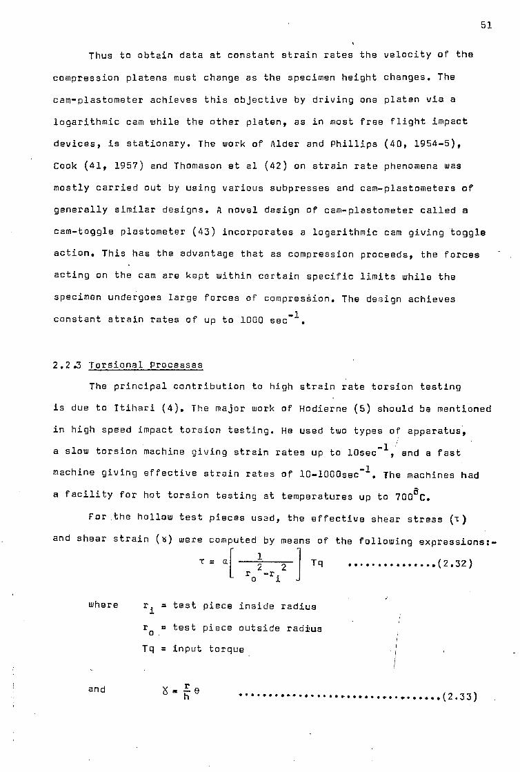
Thus to obtain data at constant strain rates the velocity of the
compression platens must change as the specimen height changes. The
cam-plastometer achieves this objective by driving one platen via a
logarithmic cam while the other platen, as in most free flight impact
devices, is stationary. The work of Alder and Phillips (40, 1954-5),
Cook (41, 1957) and Thomason at al (42) on strain rate phenomena was
mostly carried out by using various subpresses and cam-plastometers of
generally similar designs. A novel design of cam-plastometer called a
cam-toggle plastometer (43) incorporates a logarithmic cam giving toggle
action. This has the advantage that as compression proceeds, the forces
acting on the cam are kept within certain specific limits while the
specimen undergoes large forces of compresSion. The design achieves
constant strain rates of up to 1000 sec-1
2.2.3 Torsional Processes
The principal contribution to high strain rate torsion testing
is due to Itihari (4). The major work of Hodierne (5) should be mentioned
in high speed impact torsion testing. He used two types of apparatus,
a slow torsion machine giving strain rates up to l0sec-1 and a fast
machine giving effective strain rates of 10-1000sec-1. The machines had
a facility for hot torsion testing at temperatures up to 700aC.
For the hollow test pieces used, the effective shear stress (I)
and shear strain (1s) were computed by means of the following expressions:-
T = 1 Tq (2.32) 2 2 r -r. o 1
where ri = test piece inside radius
ro = test piece outside radius
Tq = input torque
and = e f • • • (2.33)

52
where r = test piece mean radius at any instant
0= instantaneous angle of twist
Since the effective shear strain is calculated as an average
using the mean radius of the specimen tested, the magnitude of the
shear strain rate upon which data was presented was therefore an
average quantity.
The work of Calvert (46) should also be mentioned. Using an
impact torsion machine, having a flywheel capable of being rotated up
to 40 rev/min, he studied of the upper and lower yield of several grades of
steel using hollow specimens. Results of yield stresses are presented
in terms of wheel speed. In the work of Tsubouchi and Kudo (47)(48)
and recently that of Duffy at al (49) torsional techniques were employed
to study rate effects in metals.
Shear strain rates achieved during the torsional dynamic studies
of Tsubouchi using cylindrical specimens were up to 240sec-1, with
the resulting shear strain of up to 1.5. The shear stress was then
calculated from the following expression:-
Tq ....(2.34) 2nr
2ot
where 6t = thickness of the tubular specimen
and ZS = 0 - tank') .- (2.35) n
where 11= angle of torsion at fratture
gyp = angle of fracture surfaces as shown in terminology,
Fig. 2.12.
The technique employed by Tsubouchi and Kudo is the first of its
kind yielding constant strain rate in torsion testing at large shear
strains, yet the calculation of shear stress was based on the mean
radius of the hollow specimen.

Duffy et. al. used a torsional technique in conjunction with a
tubular split Hopkinson pressure bar to study rate effects. Torsional
pulses, square in shape, were generated in a bar to deform thin-walled
tubular specimens at constant strain rates up to 800sec-1. The dynamic
stress/strain rate curves were obtained directly from the oscilloscope
recordings using the following expressions:-
53
Gtdo3(1-K
4) 2V
t I _
2cyb
dm 2V
r - hd
o XX2V2
8d 26t XX
11/.1 m
(2.37)
where C. = shear modulus of the transmitter tube
d = outside diameter of split Hopkinson tubes whose d
•
inside diameter to outside diameter ratio = d
= K a
(aspect ratio)
dm
= mean diameter of the specimen
cvb = elastic shear wave velocity of the Hopkinson tube
Vt = the output oscilloscope recording of the bridge
on the transmitter bar when the bridge voltage
= V1
and the gauge factor =XX1
Ur = bridge output oscilloscope recording during the
passage of a reflected pulse when the bridge voltage
is V2
and the gauge factor )A2.
Only small shear strains were achieved with Duffy's torsional
system.
A flywheel type torsional apparatus using a short thin-walled
tubular specimen was used by Bitans and Whitton (50) to obtain constant
shear strain rate, shear stress/shear strain data for oxygen free high

3 3 r -r
T = o Tq (2.38)
conductivity copper in the range of 1 - 1000S-1,
Expressions,
54
r.tr 1 a 6 = 0 2h
(2.39)
r.+r 1 0 2h e e= rate of change of 0 with time
11,
(2,40)
li/Sre, used respectively to evaluate shear stress, shear strain and
shear strain rate.
The mode of testing using a flywheel type torsion machine has
the advantage of allowing the specimen to attain large values of strain
before the original geometrical configuration alters appreciably.
Besides with their machine, Bitan and Whitton showed that they were
able to adapt rapid application of the chosen constant y to their
testpiece. This enabled them to study the effect of the formation of
shear bands as applied strain rate increased.
2%2.4 Impact tension techniques
The establishment of impact tension techniques to study strain
rate phenomena in materials is due to manjoine and Nadai (6 and 51,
1940), The maximum strain rate observed was of the order of 1000sec-1
with their methods. Constant rates of straining in tension were
achieved and in the calculation of stresses sustained, variation in
area as a result of necking in the tubular specimen was taken into
account. A comprehensive analysis of stress and strain distribution
in the deformation area was undertaken, and the authors presented the
first record of the adiabatic temperature rise during high speed
testing.
Impact tension methods have been widely used in varying forms
since then. Brookes and Reddaway (52) used a high speed tensile system

55
to find the energy absorbed in fracturing a tensile test specimen at
strain rates up to 2400in. sec-1. Fig. 2.13 shows diagrammatic
representation of their method and allied instrumentation,. A tensile
test specimen is accelerated along its longitudinal axis until the
kinetic energy of its forward end together with a suitable attached
mass is sufficient to break the specimen when its rear end is arrested.
In principle, the velocity of the forward mass is measured just before
the arrest of the rear end of the specimen and again just after fracture
when the forward end of the specimen is in free flight. Since Brookes
and Reddaway were concerned with the change in velocities and hence
the measurement of kinetic energies, they presented their results in
terms of the general dynamic behaviour of their tensile specimen,
rather than the shape of the stress/strain curve.
With their method they also used strain gauges to record the
load, and this seems to be the first case ever shown where strain
gauges were employed in dynamic tensile testing. Since the strain
gauges were fixed on the specimen, stress wave reflections within the
specimen appearing were superimposed on their load recording. The
recording of their load trace, Fig. 2.14, shows such oscillations with
this arrangement, and therefore only some order of the magnitude of the
load could have been measured. The velocity record also shows that
strain rates of constant magnitude could not have been achieved.
High speed tensile testing was extended by Chiang (53) using high
explosives to produce high tensile strain rates. The load was measured
by a strain gauged composite dynamometer system acting as an elastic
body when loaded. Since the moving end velocity of the test piece could
not be measured with sufficient accuracy during the measurement of
upper yield, the strain rate was calculated from the following relation:-
Ao,„ Elastic strain rate =
e E.At
(2.41)

7 f.
Q
AIAMMUKIMMACOMW,
M
\ 0 s'.:•■•••S‘ks.W..s:sX,'" It
T
A Head in flight. B Reflecting surface. C Lens. D Light source. E Slit. F Photo-multiplier. G Power supply for photo-multiplier. H Hole for high-speed photographs. 1 Inertia head engraved for high-velocity measurement. J Piston sealing ring.
K Notched bar for release. • L Compressed nitrogen inlet.
M Outlet for strain-gauge leads. O D.C. bridge. P Pre-amplifier. Q Force. R Roller support. S Specimen. T Double-beam oscillograph. ✓ Velocity.
Fig 2.13 Diagramatic representation of an impact tensile testing machine' and instrumentation (Brookes. and Reddaway 52 )

0-122 MILLISECOND
STRAINCALJGE TRACE
0.118 MILLISECOND
VELOCITY TRACE
Fig. 2.14
Earliest tracing of typical velocity
and load records. (Brookes and
Reddaway 52 )
57.
Oscillations due to
--transient stress wave
reflections.
Load
(x 9
KN
/ D
ivis
ion
)
TIME (0.2 ms/DIVISION)
Fig. 2.15 - Typical load recording due to Chiang (53) - En 3B cold drawn.

58
where nosy = increment of stress preceding yield with a
time interval At
E = modular of elasticity
Fig. 2.15 shows a typical example of their load recordings with
oscillations superimposed on them; the author attributed these oscill-
ations to the vibration of the load cell used owing to its fundamental
frequency.
The tensile strength data was presented by considering the maximum
load in drawing a mean line through the oscillations of the load
recording. Since the time at which this maximum load was reached was
uncertain, approximate strain rate values were determined from the
relation:-
v c = —
he (2.42)
where he
= effective gauge length
maximum strain rate achieved with this technique was of the order
of 250sec-1.
2.2.5 Other methods
Among techniques available for the determination of dynamic
behaviour are those concerned with metal cutting, metal shaping and
forming methods such as extrusion.
A way by which the dynamic behaviour of metals may be studied
in cutting is described by Wolak and Finnie (54). With their techilique
stress/strain relations are derived from orthogonal cutting of metals
at high strain rates. The strain rate was estimated by associating
with the zone of chip formation during cutting, a zone of micro-hardness
variation.

The conventional picture of idealised orthogonal metal cutting
is given in Fig. 2.16. Assuming continuous chip formation on the shear
plane by 1:esolved shear force Fs as a result of vertical (Fv
) and
horizontal (Fh) components of forces, Wolak and Finnie computed their
results from the following expressions:-
shear stress Fssing)
7- hb
(2.43)
where Fs = Fvcos F sin LP • . • • • •(2.44)
w= shear angle, qi= chip formation angle
tan W lbr - sink
b 0 where br = = chip length ratio
bo = thickness of metal removed
b = thickness of resulting chip
h = workpiece thickness
and from the geometry of the process,
shear strain tS = cos q) + tan(y -(1)) • .(2.45)
and the average shear strain rate,
lusiny (2.46) 6h
where v = relative tool velocity
6h = average thickness of the zone of deformation
If h o then the process takes place under essentially plane
strain conditions.
A technique which was developed by P.C. Johnson et al (55, 1962)
to allow the measurement to be made of plastic flow properties under
59
rcos LP

Fig. 2.16 - Idealised orthagonal metal cutting : FE is an
external force applied to the chip at angle7,\
( Wolak and Finnie 54 )
60

61
uniform uniaxiel stress conditions at strain rates of the order of
500.0sec-1
is that of an expanding ring technique. The technique depends
on high speed observation of the diameter of a freely expanding ring
having no external constraints, as shown in Fig. 2.17. Measurement of
the deceleration of the ring presented by the following expressions
provides tha data required to compute the hoop stress acting on the ring
as a function of time and strain:-
_ dr dt (2.47)
0 =-parrr
Or r 8
r Ps r it
(2.48)
(2.49)
where r = radial velocity of the ring = v
le = radial deceleration of the ring
r = internal radius of the ring at any instant ,
r-= 1 initial internal radius of the ring
rate of change of strain rate E s
Cine photography of the radial expansions of the ring provided
a means of measuring the strains and strain rate it had undergone.
If the physical description of the process is accurate then
equation (2.48) may be exact; yet with this technique only average
strain rates and flow stress data were attained.
This method of measurement of plastic flow properties at high
strain rates was further developed and applied by Hoggatt and Recht
(56)(57). Basing their calculations on the equation of motion of a
wall element of the ring having mass &m Fig. 2.18a, they calculated
the true hoop stress in terms of external radius from the following
expressions:-

DIRECT/ON Of OBSERVATION
/ EXPLOSIVE
CORE
Ring specimen
DETONATOR
exmAusr rue(
SUPPORT ROD
b) - Ring specimen and apparatus
a)- The expanding ring and its stress
system-ring density Ps
components.
Fig. 2.17 - The expanding ring technique for the measurement of plastic flow
properties ( Johnson et al 55 )

4ms = v rurms
1.010
1.000
0.990
70' 0.980 cc
0.970 —1.1 • 1.0 Rai R01
X 6.9 K N/m2
0 E
Steel 100,000 30 x106 .25 Aluminum 60,000 10 x 106 .33 Titanium 230,000 16.5 A106 .35
0.960 0 • A • 0 •
0.950
.95 .94 .96 .97 .100 .99 .98
R07
a)- Dynamic symmetrical expansion of thin ring specimen-Zero internal
pressure.
b)- Plot of f(r,q) )-equation 2.51as a fuotion
of ring thickness.
Fig. 2.18-The terminology of expanding ring technique ( Hoggat and Recht .5_1),54 )
CY%
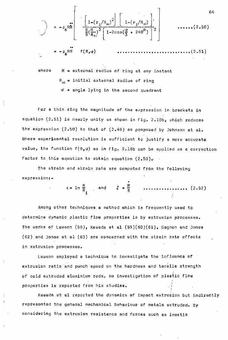
64
......(2.50) 1-(ri/Roi)2 L 1-(ri/R0)
[1-2cos(3 + 2400)1 2 )1 2N3 of
PeRk
O S
= -osRR f(11,49) (2.51)
where R = external radius of ring at any instant
R = initial external radius of ring
y = angle lying in the second quadrant
For a thin ring the magnitude of the expression in brackets in
equation (2.51) is nearly unity as shown in Fig. 2.18b, which reduces
the expression (2.50) to that of (2.48) as proposed by Johnson et al.
Where experimental resolution is sufficient to justify a more accurate
value, the function f(R,w) as in Fig. 2.18b can be applied as a correction
factor to this equation to obtain equation (2.50)..
The strain and strain rate are computed from the following
expression:-
c= In R — and ; = R . .. (2.52) Ri R
Among other techniques a method which is frequently used to
determine dynamic plastic flow properties is by extrusion processes.
The works of Lawson (58), Kawada at al (59)(60)(61), Gagnon and Jones
(62) and Jonas et al (63) are concerned with the strain rate effects
in extrusion processes.
Lawson employed a technique to investigate the influence of
extrusion ratio and punch speed on the hardness and tensile strength
of cold extruded aluminium rods. No investigation of plastic flow
properties is reported from his studies.
Kawada at al reported the dynamics of impact extrusion but indirectly
represented the general mechanical behaviour of metals extruded. By
considering the extrusion resistance and forces such as inertia
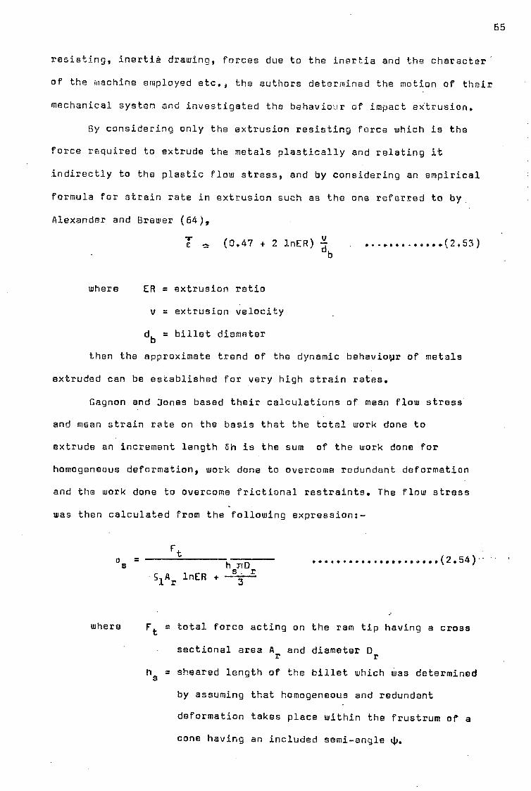
t os h IrD .
S1Ar lnER + s r
F (2 . 54 ) •
resisting, inertia drawing, forces due to the inertia and the character
of the machine employed etc., the authors determined the motion of their
mechanical system and investigated the behaviour of impact extrusion.
By considering only the extrusion resisting force which is the
force required to extrude the metals plastically and relating it
indirectly to the plastic flow stress, and by considering an empirical
formula for strain rate in extrusion such as the one referred to by
Alexander and Brewer (64),
— (0.47 + 2 lnER) .•..••••••••.(2.53) b
where ER = extrusion ratio
v = extrusion velocity
db
= billet diameter
then the approximate trend of the dynamic behaviour of metals
extruded can be established for very high strain rates.
Gagnon and Jones based their calculations of mean flow stress
and mean strain rate on the basis that the total work done to
extrude an increment length bh is the sum of the work done for
homogeneous deformation, work done to overcome redundant deformation
and the work done to overcome frictional restraints. The flow stress
was then calculated from the following expression:-
65
where Ft = total force acting on the ram tip having a cross
sectional area Ar and diameter Dr
hs
= sheared length of the billet which was determined
by assuming that homogeneous and redundant
deformation takes place within the frustrum of a
cone having an included semi-angle 44

The mean equivalent strain rate was calculated by evaluating the
time required to perform a strainc s equivalent to the homogeneous and
redundant strains. The evaluation of the time depends on the shape of
the deformation zone when it is assumed that this zone is the frustrum
of a cone having an included semi-angle LP then:-
S2 t = sec. ........... 0-(2.55)
and since
then
e = 53 inER
T = 54 v 1nER
(255)
(2.57)
51' S2 s3, S zt , are constants of the process parameters.
A similar approach but more simplified than that above was under-
taken by Jonas et al (63) to investigate the possible rate controlling
mechanisms under hot working extrusion of aluminium. With the technique
employed they converted the extrusion pressure into flow stress over
. a wide range of experimental conditions. Fig. 2.19 shows the extrusion
pressure as related to flow stress over a range of strain rates. This
assumes that the ratios of work done to overcome frictional restraints
and the work done to overcome the redundant work to the total work
done in extruding a billet of certain length is constant and is indep-
endent of strain rate and temperature for a given metal and geometry.
The figure also shows that the flow stress for the particular
strain sustained during the extrusion is extrapolated to ranges of
zero and creep strain rates. An interesting feature of this is that
the curve follows a single straight line for the creep strain rates
and the extrusion strain rates up to 105-1
66
Techniques used by Bell (65) and Suh (66) should also be mentioned.

STRAIN RATE, s-I I0.5 f0 z wove
Mwaredoldorew4 Mefoctica
Effect of iscegornecso noisrcrson--«
ER=40
Aluminium
• Extrusic• press.es d 400°C Eltruseon (ice stresses of 400.0
Exolcu1ofeel CI Creep stresses of 571°C (Sersi- oref--Croce)
I
I0 10° 101 102 105 W 1 106 STRAIN RATE S
SR-4 STRAIN GAGES
STATIC FORCE CONICAL
END
TRIGGER
V ■ •■•■•11...
HAMMER
Fig. 2.19 - Three components of extrusion pressure and their relations to flow stress os over a range of strain rates.
(Jonas et.al. 63)
Fig. 2.20 - Schematic representation of set up incorporating a bar with a truncated cone.(Suh 66)
67

68
Bell's defraction grating technique was based on a localised measurement
of strain and he showed that non-uniform finite strain distribution
and non-linear wave initiation, propagation and reflection and interaction
phenomena occur within a testpiece undergoing rapid deformation. Bell,
by using the theory of von Kerman for the finite amplitude wave theory,
showed that the defraction grating technique could yield accurate
determination of dynamic plastic strain at a point at any temperature.
The experimental method of Suh (Fig. 2.20) consisted of amplifying
an elastic compression stress wave by propagating it through a truncated
cone at one end of a bar and observing the change in the shape of the
wave reflected from the conical end which was in contact with a rigid
anvil. The stress wave amplitude was amplified, to varying degrees by
truncating the cone at different places. With his method he was
able to detect the lower and upper yield phenomena peculiar to a low
carbon steel and concluded that these phenomena as appear at low strain
rates do not exist at high strain rates and that the effect of intermittent
loading is addative. magnitudes of 123sec-1 in strain rate and very small
strains were achieved with their technique.
The method of high strain rate testing of small diameter ttibes
used by Al-Hassani and Johnson (67) is also of particular interest.
Their system consisted of expanding small diameter tubes by a
magneto-hydraulically activated system. Expansion of each tube was
carried out by the pressure of liquid inside it, which was brought about
by a piston when subjected to electro-magnetic impulsive loading,
produced by sudden discharge of a capacitor bank through a spiral coil
resting on the piston. The radial velocity and expansion of the tubes
were related to the energy equivalent of the electrical input and
properties of the coil and piston and to the strength and size of the
workpiece. The energy expansion of the tubes thus gave some idea of
the behaviour of the aluminium and steel specimens tested.

69
An equation of the following form for the average strain rate
experienced was proposed:—
dLc E 8MhRe °dx
(2.58)
where E = discharge energy
M = piston mass
h = length of the unrestricted portion of the tube
Re
= equivalent resistance
dLc = ratio of increment change of inductance with piston
dx
position
It is noted that a wide range of strain rates could be obtained
by changing the variable on the right hand side of equation (2.58).
2.2.6 Assessment of techniques
The above gives a general description of some widely used techniques
to obtain dynamic stress/strain characteristics the general dynamic
behaviour of materials. Other methods such as the impulsive loading
beam of Symonds (68) or the Scleroscopic method of Vincent et al (69)
of course exist. They are basically of the same nature as those methods
described above.
Since the history of the strain rate effect in metals is
controversial, it is essential to assess the limitations of these
techniques on their own merits or shortcomings and then draw a conclusion
against the background of these controversies. Such controversies are
between investigators, some of whom believe that not all metals are
strain rate dependent while others believe that all metals respond
differently to various rates of straining. An instance of this is the
extensive discussion of papers published by some authors on the subject
of rate dependency of aluminium given by Karnes (70).

70
With the split Hopkinson pressure bar technique; or its modified
version, the determination of many material characteristics in the
range of 100S-1 to 100,000S-1 (71) is permissible. There are nevertheless
certain inherent limitations in the method. As the analysis assumes
equilibrium conditions in the sample being deformed, and since these do
not exist during the first few microseconds of the test, the data
obtained at very low strain values are not reliable. This has been
avoided by Suh (66) using a modified Hopkinson bar incorporating a
truncated cone at one end for amplification of the incident and reflected
stress waves to detect the upper and lower yielding phenomena. This
was mainly due to the existence of an extremely thin plastic region at
yield. The upper limit of strain rate and stress is determined by the
yield strength of the input and output bars. If plastic deformation
takes place in these bars, the analysis described for the computation
of the stress, strain and strain rate data would no longer apply; as
the position of the interface between the specimen and the bar can no
longer be determined by an elastic equation when o= pee = particle
velocity).
With the data obtained by the Hopkinson pressure bar, stress
histories are introduced into a remarkably simple formula suggested by
Kolsky (7). From these the dynamic average stress/strain histories in
the specimen are then deducted and presented. With the use of the
Hopkinson pressure bar technique an extremely important parameter should
be taken into account and that is the specimen geometry as compared to
the length of pressure bar used. The specimen should be both short
compared to the length of the stress pulse and long compared to the
radius of the bar. The first restriction provides assurance of reasonable
stress uniformity along the specimen, while the second minimises'the
effect of restraints offered by the bar ends in contact with the specimen.
Ari adverse effect of this transient stress wave propogation in the

71
specimen on the flow stress determination of aluminium was demonstrated
by Oharan (72) and is shown in Fig. 2.21a. On the choice of the specimen
geometry to overcome and minimise the internal restraint in the specimen
Davies' and Hunter's Criterion (24) may be adapted.
On the use of the one dimensional wave theory of Kolsky, Jahsman
(73) has re-examined wave propogation analysis for average stress and
strain in a specimen exhibiting bilinear elastic plastic behaviour
when subjected to trapezoidal and triangular incident pulses. It is
concluded that when one dimensional wave effects dominate, by careful
selection of design parameters such as specimen length and pulse shape,
one may use the Koisky formulae with confidence in establishing the
presence (or absence) of a strain rate effect in elastic plastic
materials during plastic deformation. The analysis predicted some
separation of the specimen from the bars near the end of the unloading
process. Jahsman concluded that a specimen length giving at least four
complete reflections can yield reasonable data.
Impact compression techniques generally suffer from one main dis-
advntage,that the strain rate does not remain constant during the whole
process of deformation. This excludes testing of materials in compression
using a cam-plastometer. However this is the basic shortcoming of many
free flight impact indentation or compression methods so far mentioned.
The strain rate /strain histories of Slater at al (74) obtained for
pure lead at room temperature using a drop hammer should provide an
excellent example of this important factor (Fig. 2.22). Indeed metal's
response to strain rate/stress histories are different and for a
particular metal again these characteristics vary for various temperature
environments of the testing material. An example of this is shown in
Fig. 2.23, when compared to Fig. 2.10.
In the context of free flight impact devices, the method adopted
by Sturgess and Bramley (33) seems to be the only reported means by

(b),- Percentage deviation in flow stress vs. number of transients
at longitudinal wave velocity across specimen(At, least 8 transients are required for equilibrium to be reached)
E.0.105
80
60
40
20
Deviation in stress
osVo
s (%)
Flow Stress Gs(MN/m2)
280 0- Data t>tb
420 0 8 12 16 20
0
140 ■ NO
ts=Longitudinal stress
Os
wave duration in specimen
(a) - Flow stress/strain rate characteristic of aluminium showing deviations because of stress gradients across the specimen.
It It TI 11 If tI E =0.105
0
20 40 60 80 100 . Strain rate C.x103 sec-1 Fig. - 2.21 (Dharan 72)

2•0
PS
I-
z 1.0
0
0 0
z 0 z • 0.5
73
THEORETICAL. EG: 2.2 8 ICI A 0 X EXPERIMENTAL RESULTS
44.
CONSTANT TUP MASS 22.5 LB LEGEND DROP HEIGHT 5- eo. FT
0 2 105 0.145 4 I SO 0.237 6 183 0-290
0 9 224 0.363 X 12 258 0.427
X
\\\ ...........m...L....... ,..1........................... ................L...... x 0.1 0.2 0.3 0.4 COMPRESSIVE ENGINEERING STRAIN er.1hi-h)/hi
0.5
2.5
tz
20
Q 15
• a .6 z .w
a 10 0 0 z 2 05 O
Fig. 2.22 Strain rate/strain histories for pure lead
at room temperature-using a drop hammer. (Slater et al 74)
I MAIL. 18:4:1 HSS TEMPERATURE 1100°C LUB. FOLIAC A20
low A KAN
001 0
.0 iii
Fr 111111 I
1 I 1 0 05 1.0 1 5
NATURAL STRAIN E
THEORETICAL : EQ. 2.28 A A • EXPT. Et =482 sec-1 a • a EXPT. Et =376sec-1 • •• EXPT. .0
•
EXPT. 6i = 283sec-1
Fig.2.23- Strain rate/strain characteristics for high speed upsetting using free flight impact devices ( Sturgess and Bramley 33)
ZO

74
which virtually constant high strain rate data may be obtained. Following
Pugh and Watkins) (36) suggestion for the constancy of energy per unit
volume and strain rate, eturgess and Bramley utilised a modified Cook
and Larks test (1) employing different numbers of billets such that
when different impact velocities were carried out on different pre-
determined numbers of identical billets, virtually constant strain rates
were yielded. It is nevertheless reported, as seen in Fig. 2.24 that
only a small magnitude of strain could be achieved with this procedure.
This amount of straining is of course not comparable with the large
reductions obtained in most free flight and impact compression devices
(75), in impact extrusion processes (76)(77) or in high speed drawing
(76), where material behaviours are essentially to he determined from
the test, or to be used for obtaining characteristics of the high speed
forming techniques.
The maximum strain rates achieved in drop hammers are limited due
to the limit in the weight employed or the height it is dropped. In
cam-plastometers although constant strain rate data of up to a reasonably
large strain can be achieved, the maximum constant strain , rate
attainable is limited owing to the revolution of the cam and the
limitation imposed on the cam surface as a result of the creation of
high stresses.
many recent investigators using impact tension or compression
devices have employed short cells (53)(79) or have attached (52)
strain gauges on their specimen to record the loading history during
the deformation. The latter was used with some reservation on the limit
of straining achieved. 1
If the duration of the test is short, such that it would be
essential to record the load without the stress wave reflections in
the load cell affecting the recording, then the design of the cell and
its length should be carefully assessed.

0 271iLtiZilAinri511 • 1.4 ito
— THEORETICAL
EXPERIMENTAL
symbol
620 640
MEAN=1-05eo
1 •
1111 I' e. sec-1
billet height
iris
0-33 3 0 • 333 0-666 0.666 1 • 000 1-000 MEAN
" 710 630 620 6 50 645
0
• a •
MATL. 18:4:1 H SS TEMPERATURE 1100°C LUB. FOLIAC A20
MEAN NATURAL STRAIN RATE •T-• 680 seEl
r-r -rr-iiV 1 . -
17CI 120
120 s i
_J_i..L__1__J_._J.- L
350
300;
200
ce IOU
1-2 .4) .(L) uJ 10 CC
CC 0-8 0
cr
z
0.6
00,4
Ui X
YO2
0 z
0-2 04 06 0.8 1-0
NATURAL STRAIN 6
Fig. 2.24 - Constant strain rate/strain history achieved, with free flight impact devices(Sturgess and. Bramley 33)
SHEAR STRAIN, y
Fig. 2.25 - Difference in shear stress/ shear strain characteristics (a)-Tsubouchi and Kudo (47) (b)-Bitan and. Whitton (50)
c.n

76
At low strains which are achieved in short time intervals stress
wave reflection within the cell are of serious concern and if short load
cells are employed then some imposition of this adverse wave
propogation effect on the load recording may be expected. Fig. 2.9
clearly indicates that stress wave reflections are the cause of the
oscillations imposed on the initial stage of load recording before
the stage of stress equilibrium in the specimen is reached. In Chiang
(53), Fig. 2.15, Brook and Reddaway (52), Fig. 2.14, similar effects
are observed. While Chiang does not attribute the oscillation on ,
the recording to the stress wave reflection, the oscillations may be sug-
gested to bea result of waves moving up and down the short load cell
he employed. Considering the length of his load cell and the longer
length he had chosen as the gauge length of his specimen, it
may be verified that an elastic wave could have travelled in
the cell in a time to cause reflection to be superimposed on his load
recordings. It is clear from his load recording of shorter durations,
that more pronounced stress wave reflections were effective than in his
tests with longer duration for the deformation.
In general tension and compression testings have the undesirable
features of stress and strain states which involve both hydrostatic
and deviatoric components of the stress and strain (80), and complications
such as necking and barrelling which make data interpretation difficult.
In addition, radial inertia, transverse shear, boundary friction and
complex wave interactions are effects which make tests at very high
strain rates difficult to analyse. Obviously, as discussed above all
these considerations should be taken into account when interpreting
data. One last important consideration is the inertia effect even though
other factors can be satisfactorily separated. With the theory proposed
by Lippman (81) and extended by Dean (82), the possible inertia effect
with these techniques, and under high strain rate conditions, can to

77
some extent be obviated by a suitable choice of the specimen and
process parameters, or at least the approximate magnitude of the effect
known and calculated.
At least in torsional systems a more desirable way of eliminating
many of the difficulties enumerated is at hand. For instance, in using
a thin-walled tube specimen only one component of shear stress and strain
is present with no hydrostatic components. The devices, though
providing information for large strains at constant strain rate, suffer
from the lack of providing reliable data at very high strain rates. An
example of this latter effect is work carried out by Bitan and Whitton
(BO) on oxygen free high conductivity copper at shear strain rates of
up to 103S-1. The dynamic strain/strain rate data of Bitan and Whitton
was obtained by the rapid application of the chosen strain rate. It is
interesting to note'from this work that as a result of increasing the
applied shear strain rate, the flow stress dropped for a particular
value of strain. since the authors were of the, opinion that this behaviour
might have been peculiar to this kind of metal, they repeated the work
carried out by Tsubouchi and Kudo on low carbon steel. This is shown
in Fig. 2.25 for clarity. Although the work done by Tsubouchi and Kudo
shows a drop in flow strain for higher strain rates, but at relatively
large shear strain, they assumed this to be the result of the creation
of adiabatic heating affecting the flow stress and indeed make corrections
to obtain isothermal data. Bitan and Whitton used sleeved tubular specimens
with a very small gauge length of very thin thickness& They attributed
the fall in stress level with increasing strain to be due to the formation
of adiabatic shear bands and no fault of the very thin specimens of small
gauge length used. Of course they may be right in the suggestion of
adiabatic shear bands since extremely high temperatures are generated
in a localised region between the specimen gauge length and the larger
sleeve, but surely such localised high adiabatic heating had imparted

78
localised softening which has caused a larger recording of strain. This
can be the cause of discrepancies. seen in Fig. 2.25.
Some difficulties in the damping mechanisms employed in the works
of many experimenters are also reported. This was mainly experienced at
larger strains and strain rates.
No doubt with techniques such as orthogonal cutting and the
expanding ring, strains and strain rates of higher magnitudes than
those obtainable with other devices can be expected. With conventional
cutting, strain rates of magnitudes greater than 105S-1 are usually
achieved and the expanding ring technique provides sufficiently high
strain rate value data. But it is envisaged as reported (33),that the
heat generation due to high speed cutting is so great that the influence
of adiabatic heating can not be excluded. Variation in strain rate is
also significant in both methods. Similarly in extrusion processes,
variation of strain rate is unavoidable whether in the deformation zone
or in the product emerging from the die$ since each element of the upsetting
test piece undergoes different rates and amount of straining. Adiabatic
heat and variation in temperature distribution are also considerable.
Although many of the works referred to and the techniques devised
are of the highest calibre in giving the dynamic behaviour of materials,
it is seen that in almost all methods investigated, various averaging
techniques are present in the computation of the measured data. Although
in some techniques some side effects are excluded or their magnitude
controlled, it is not inferred that the adiabatic heating effect is
excluded. For this reason it is not surprising to see a drop in flow
stress with strain rate of oxygen free high conductivity copper in
Bitan and Whittonfs work (50) when, compared to the work of Habib(4)
at equivalent strains.Adiebatic heating is most effective in
influencing the working of softer materials of low critical temperature.
This influnce can have deleterious effect not only on the product propeties
79
but also on the true determination of the dynamic behaviour of these
materials,since the temperature rise would be prevalent during the
deformation,obscuring the actual strain rate effect.
With all the difficulties encountered and serious assumptions
made on the influence of some factors, such as adiabatic heating,
created under high strain rate conditions, it is not therefore
unexpected to note contrasts of opinion between investigators on the
subject of strain rate dependency and independency in metals.
In conclusion it is relevant to say that the common feature
shared by all techniques is the specimens temperature change during
the test as a result of adiabatic heating which affects the flow stress.
The latter property is a function of the initial temperature of the
specimen and of the temperature rise due to deformation; it also
depends on boundary conditions.
In the methods discussed, regardless of the process, adiabatic
heating of the test material is unavoidable even if other conditions
are satisfied. from these considerations therefore, it is reasonable
to suggest that an incremental method suitably d6signed to be incorp-
orated in any of the above techniques would provide better means of
accurately assessing the material behaviour on much the same principle
as the technique used in quasi-static testing,
2.3 Incremental Approach
The incremental approach in impact tension was first introduced
by von Karman and Duwez (84) to analyse the plastic strain wave at the
end of a cylindrical bar in the case where the impact veliocity was
large enough to produce constant plastic strain. They mounted, Fig. 2.26,
the specimen on a breaking plate designed to fracture when struck by
a subsidiary anvil after a predetermined extension of the workpiece

1- Distance travelled before imIact Specimen
I '',?. •
, 7,...
Anvil
Notched breaking plate
--Striking rod
BO
Fig. 2.26 _ Experimental apparatus as used by von Karman
and nuwez(34) to stop the impact after a given
deformation of specimen has been reached.
Deformation Impacting carriage and disc
Specimen and anvil
STOP
eCARRIAG
HOPKiNSON BAR
STOP
Fig. 2.27 - Incremental dynamic compression set up.
( Mok and Duffya8')

82.
was achieved. This method was later modified; with a similar set-up
(rig. 2.27) and applied to compression tests by Mok and Duffy (28).
They interpreted their results in terms of yield pressure (Section 2.2.2,
equation (2.20)) and presented the stress/strain characteristics of
steel, lead and aluminiuM as computed from equations (2.21) and (2.22)
to very large constant strain rates. Unfortunately. the result of their
work provided only average values of flow stress and strain. Only a
small percentage of strain however was achieved by either von Karman
and Duwez or by Mok and Duffy.
Studies of the behaviour of material subjected to dynamic
incremental shear loading were first undertaken by Campbell and
Dowling (85). With their method an incremental shear stress was applied
to a thin-walled tube in a very short time and the speed of the
resulting stress wave was measured. The apparatus was also used to
test short tubular specimens in pure shearing using the split Hopkinson
bar technique. Incremental dynamic characteristics were obtained from
a number of different specimens each yielding a curve of os versus e
for the appropriate shear strain rate considered. Each curve as rep-
resented in Fig. 2.28 was plotted with its starting point at the
appropriate position on the quasi-static stress/strain curve corresponding
to the level of pre-stress at which the dynamic test was performed.
The main shear stress/strain curve for each specimen was computed
from the following expressions which were obtained by considering the
equation of motion of loading and unloading torsional waves:-
Tqs = (2.59) 2nr261
he (2.60)
Tqs.r =
b obcvbh
,, (2.61 )

(NJ 0
rn •
>4
CD a) ;-1
a)
82
Shear strain y ,per cent
F.g. 2.28 - Incremental stress/strain curves
for copper ( Campbell and Dowlling85 )
A
1
Specimen
Drdynornic SD C ED SS
17.5in 6: 2'n 1.3541714:1
(o) Torsional clamp
X- Strain gauges
Output bar
/
17.5 in
B
Fig. 2.29 - Arrangement of torsional incremental
set up as used by Campbell and Dowlling (85)

83
(t where 0 11 7-77— I (Tq
v Tq,) dt
bPb-vb )0
and Tqc = Tqv Tqs
Tqc = clamping input torque
Tqv = unloading torque
Tqs = specimen torque
b = polar moment of inertia of the cross-section of the
Hopkinson bar
Tqv and Tqc were recorded directly on an oscilloscope screen
from the signal sent by the strain gauges (SD and SS) affixed on the
input and output bars as shown in Fig. 2.29.
With such a method the maximum limiting shear strain rate of the
order of only 270sec was reported by the authors. The data presented
was based on a shear strain rate of 100sec so that the strain increment
achieved during the period of release of a clamp, initiating the
transmission of torque in the specimen was not too. large to introduce
any error.
2.4 Material Behaviour and Properties under Dynamic Loading
Metal and alloy response is dependent on the rate of loading '
and since all undergo plastic deformation before becoming products,
it is of scientific as well as industrial importance to investigate
their behaviour under varying rates and conditions.
From the basic data obtained by experimenters on the dynamic
behaviour and properties of materials, functional relationships which
describe the deformation characteristics are presented. These relation-
ships at least provide suitable means of assessing the general dynamic

84
behaviour of metals as influenced by parameters of strain, strain rate,
environment, boundary conditions etc., From the test data, workers
assess the mechanism operating during deformation, with conclusions on
the mechanics of structural changes.
Table 2.1 briefly reviews some of these functional relationships
and mechanisms describing the dynamic behaviour of metals and alloys.
Constants of the functions not given in Table 2.1 are presented in
Tables 2.2 - 2.6. These are all for later comparison. strain rates
indicated span from 0 to over 4000sec-1 with maximum natural strain
of 0.8 except for extrusions where natural strains of the order of
2-4 are presented. Wide ranges of working temperature are covered and
the lubrication conditions and the extent of the performance of each
lubricant specified. The results of hot working experiments, analysed
in terms of thermally activated processes are also presented, with their
activation energy values determining the operative mechanisms,
For, higher strain rates the work of Hauser (23) and Dharan (72)
concerning the dynamic behaviour of aluminium at room temperature,
cover strain rates ranging from 4000 to 120,000sec Tn analysing the
data Dharan considered the specimen size effect, and thpt of lateral
inertia. In his work the maximum strain achieved was of the order of
20% engineering strain, and he used a modified version of Koisky's
thin wafer technique. NO other significant data was found in the
literature giving an account of the dynamic behaviour of material
at such high magnitudes of strain rate.
Dharan, in describing the mechanisms operative during the
deformation at those large strain rates, subdivided his stress/strain
curve into three regions - two approximately linear regions followed
by a non-linear rise in the stress at the highest strain rates. Since
his results are the only contribution at such high magnitudes of strain
rate, and since they take into account two important factors of
frictional restraints, and the transient wave propagation effect in the

r n pp a b c •
R,,f. (5) (28) (6), (51) (8)
Me'ho,d emclo ed Bouncing ball (cold)
Lead Al (6061) Al (C1100F) Steel (C1018)
Impact tension (hot) Stainless steel Al Cu (Commercially
pure) Pure Iron
Low carbon steel
Extrusion (hot)
Al (Commercially pure) • Materials
tested
Useful temperature range 0C
Room temperature, (RT) '
Al : RT-600 Cu : RT-100 Steel:RT-1200
255 - 616 (T > 0.55 T
m)
Tm . melting point temperature
ItPiqc(RAcr3L175in 0.001 - 100 (Ave.) 0.513 - 100 (const.) 0.1 - 10 (Ave.) ,,IX1::11 strain
e = 0.1 e = 10% e = 3.67
Functional relationship describing the mechanical behaviour
6 ' 6 cn k T s .o , (See table 2.2 for constants d
o and n)
P:,-
= constant
d = f (log e) 1 g •
J. = constant
, 1
= X [sinh (ccif)J -AH ) s exp ( R,7- c A ,..++ ,H or
-C. = exp sTiEr--) = X [sink (ads)ril e A
n' = 4.45 a = 3.58 psi 1 R,. Universal gas constant
Activationenergy and (dominant operating mechanism)
Not determined
..
Not determined
alnt alnt AH* = (81 (aln
/TA a
f) _ sinh (ads
)) TA " s =
) AH = 41 8 Kcal/mole at
aln sink (cols - t i=1sec ( n - as self diffusion
a(1/T ) in creep.
Lubrication No lubricant No lubricant No lubricant
Lui:-4 ---io% c..N-6iFir ,.. +4-
log Z vs lidS9-1 is linear. See Fig. 2.30 . d = am+00 • (ds ) - After Garofalo (86)
CoTment p7i- = Coefficient of friction
TABLE 2.1 - RELATIONSHIPS DESCRIBING THE DYNAMIC BEHAVIOUR OF METALS
WITH TESTING CONDITIONS.

Table 2 1. (cont. )
°PP1F Pl':F. d c f
,,2,>f (12) (21) (31), (32)
m=' od e-.io.ed Impact compression Impact com.ression Impact compression (hot and cold)++
Materials tested
Cu (99% pure) Al (Commercially
pure)
Al (Commercially pure)
Low carbon steel (SIS 1311) Construction steel (SIS 2244) High speed steel (SIS72722) Tool steel (SIS 2242) 18/9 ,--n q-f- ,li n1 $%5 -q.E.1 (STS 9'111)
Useful temperature range oc
Al Cu 30-550
SIS 1311 : RT-1055 SIS 2244 : 765-1055 SIS 2722 SIS 2242 I- 524-1055 SIS 2333
250-550 450-900
Pa;e o s,' r -r,,
g -I in
'110=260 155-600 300-2018 (Ave.) 350-545 (Ave.) f--„ximum s:rain
e_ 0.8 e = 0.3 e= 0,6
Functional T (CT-X) as =
app . 4 relationship C describing the for T > 0.55 T
m mechanical (For constants M, behaviour , pp, c and X see table 2.3) p. = constant
, X a
s = 1 + - lng — ao do or = .m as doe
(No values for constant were given)
d = d + X In 1 IeT s o • (This is only for SIS 2722 at 1055°C) For SIS 2722 at 1055°C d /d - 8 " " 2244 " 11 S nO - 4 H H 1311 H H " - 6
Activation energy and (dominant (Intersection of
operating glide and forest
mechoniJm) dislocations)
Not -determined Not determined (Thermally activated)
Lubrication Holub alloy No lubricant Teflon (RT) - NS
2(524°C) - also graphite sus-
pended in alcohool and glass suspended in alco-hol for high temperatures.
Lutricacion cerformance No barrelling" No barrelling up to 40% reduction
Comment ° up to 50% reduction
+ Sensitivity of Al increases with increase in I
++ (using drop hammer) +++ glass suspended in alcohol (unsatisfactory

Table 2 •1. (coat.)
E w • h i
P.,f. (33) (34) (35), (74)
Me'hod emPloved Impact compression (hot). Impact compression (cold) Impact compression (cold)"
tested 1:4:1 peed steel High speed
Materials
prismatic block of hot Plasticine to simulate
metals.
Medium carbon (0.55) steel Pure lead
Useful temperature range oc
1100 ,
Room Temperature Steel Lead RT RT
nrl'"(F -5Li In 300-680++(Ave.) 50-300 (Ave.) Up to 500 (Ave.)Up to 250 (Ave.)
t,ximum st.Idin e = 0.8 e = 2.0 e = 0.5 e = 0.4
Functional relationship describing the mechanical behaviour
Is = a-6 A I e,T
m = 0.17 fort 1 = 0.15 to 600 sec , n = 0 i.e.
1s = opc.t0.17
6 = a.A I Y le at room temperature. • a = 3.1 in = 0.78)(Ave.)
++ .111, n 6s = (do
+ .e ;X e 1
Steel Lead 3 -3
X = 10 X . 4x10 6o = 44 Tf/in2 6 = 1 Tf/in2 all = 1.41 Xo = 2.02 l average
1 m = 1.5 m1= 0.66 values. = 0.3 n = 0.44
Activation energy and (dominant operating mechanism)
Not determined (Thermally activated) .
Not determined Not determined
Lubrication Foliac A20, Colloidal suspension of graphite in alcohol (Copaslip)
French chalk P.T.F.E.
Luhr1=--,ion ”erroi-mance . .....„, Sli ht barrellin.+++ No barrelling* ------ No barrelling ..
Comment +Free flight ++Virt. Const. at 680 +++After 50% reduction.
up to 70% reduction drop hammer -1 1-4-0. =1.25 (Steel) at e=400sec )6.20.25 s o

Table 2.1 (cont. )
c : 1. ,r" k 1
••,f, (41) . (47), (418)
Ma'• ,-, emnlo ad -c
Impact compression Impact compression+
Impact torsion - cold and hot
Materials tested
Al (Commercially pure) Cu (Phosphorus - de-
oxidised) Steel (0.55C) •
Low, medium and High carbOn Steel-En:16-25,31,40,45,52 18/8 stainless steel 2.25%C+13%Cr steel 18:4:1 H.S.S.
0.15%C steel Brass •
Useful temperatUre range 0C
Al: -190-550 Cu: 18-900 Steel: 930-1200
900-1200 RT - 200
:F8's(S-:111.0 in 1-40 (Constant) 1.5-100 (Const.) 8.5x10²
1, xlmm strain = yo e = 0.7 Y' 2
Functional relationship describing the mechanical behaviour
6= 1 +X.lni I , s o 1 C J or /. = .m 1 ds doc Ie,T (preferred) (See table 2.4 for values of constants) m increase as T or e increase.
given)
Y= Y +X.ln e I., s o 1 e T
_ m I or Ys - Yol IZ,T
(Y X and m were not 0, .
• M
T = X. or T . x14 [
.6,T ,T (for 0.254.Ng4 240 or:
/T)+++
n .m T = X s .- exp(X3 A 2' 0
Activation energy and (dominant operating mechanism)
Not determined -
Not determined Not determined
Lubrication
Petroleum jelly (RT)- graphite (up to 450°C) and powdered glass (for T 450°C) -
Lead borate: 900-100°C Hard flint: 1100°C Pyrex: 1200°C
No lubricant
1,, 6r. ,, No barrelling No barrelling
Comment +Cam Plastometer n vs TH is linear for 7.'0.55,
+Cam Plastometer +++See table 2.5a and 2.5b for all constants. n=constontt smolt for TH<C55

Table 2.1 (cont.)
,trc (55) (62), (87)
Method emoloyed Expanding ring Impact extrusion
Materials tested
304 Stainless steel 7075-T6 Al T1-6A1-4V Alloy 99.99% pure Al . Tnrinf iron (ln14 high)
Room temperature
. Zinc (SHG) - containing 99.9963 to.99.9966% zinc. '
110 - 350
Useful ten..perature range oc
N7:.7(St-sLf in Up to 1500 (Ave.) 0.05-5 (Ave.)
e= 7% 7 . 3.4 Functional relationship describing the mechanical behaviour
+ 1s/0'0
.. -Q 1 = X Csinh(ads] exp(----)
i RT c A
3 a = 0.16x10,psi; n'... 5.6(neglecting a = 0.13x10'psi; n'= 4.7(considering
- V1 ds -Q or, e = X2 exp(7--).exp; ilik RT . A
.• • . 1'.. u
or Z = A exp(----) = X Pa-lh(ads RT 1 c A . adiabatic heating Ha) adiabatic heatingHa)
V d a Q deter- z =texp(---)=X exp(-1--=1). (For deter- cF, 2 PgA
chanisms ) Nit. . apparent activation volume
-3 Jr- = 3.9x10 to 0.6x10⁻³ PSI-1
1.7 : 304 steel 1.7 : 7075-T6 1.8 : T1-6A1-4V 2.1 : 99.99% Al 2.8 : Iron (low) 7.8 : Iron (hi h)
Activation energy and (dominant operating mechanism)
Not determined
clog sinh(a.ds)) Q = 2.3 n'T 1 1/TA) ' Q = 28+Kcal/mole (neglecting adiabatic Q = 23-2 Kcal/mole(considering
- on like rroep)
No lubricant used to result in
heating H ) adiabatic heatingaHa)
condition of sticking friction. T. ion Jbricat No lubricant
Lui..r a_ on reriorm. --e
Comment ++Only general dynamic behaviour was given.
++oc..X./2;c=Xexp(Xcl ), =X 1 - X=0.8x10
3 to 1.7x10³, n=15.3-6.4
(neglecting Ha)-X=0!5x10 -tos2.1x10, n'=9-4.5 (considering Ha).
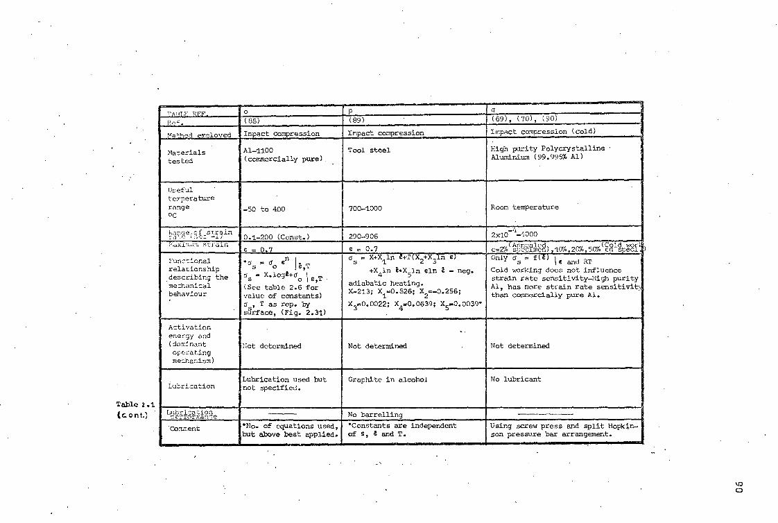
Table 2.1 (Gent.)
''PliLE REF. o P
r,f. (88) (89) (69), (70), (90)
Me'l'od employed Impact compression Impact compression Impact compression (cold)
Materials tested
Al-1100 (commercially pure).
Tool steel High purity Polycrystalline . Aluminium (99.995% Al)
Useful temperature range Pc
-50 to 400 • 700-1000 Room temperature
ra' 11:'..:eiq,-7.5t-iiin
0.1-200 (Comet.) 290-906 2x10 -4000
----. i..x.i.m strain e = 0.7 e = 0.7 (Annealed (Cold worir
e=2% soecimen),10% 2O% 50% ed s.eci.
Functionalrelationship describing the mechanical behaviour
"s ' 60 n
e,T as = X.logt+do l e,T ,
(See table 2.6 for value of constants) ds, T as rep. by surface, (Fig. 2.31)
s = X+X11n a+T(X2.)
+X,ln e)
+X in E+X5ln eln a - neg.
adiabatic heating. X=213; X1=0.826; X
2=-0.256;
3=0.0022; X4=0.0639; X5=0.0039'
Only as . f(t) 1 e and RT Cold working does not influence strain rate sensitivity-High purity Al, has more strain rate sensitivit) than commercially pure Al.
Activation energy and (dominant operating mechanism)
Not determined Not determined Not determined
Lubrication Lubrication used but not specified.
Graphite in alcohol No lubricant
LO-Fial,P. No barrelling
' Comment *No. of equations used, but above best applied.
*Constants are independent of e, a and T.
Using screw press and split Hopkin-son pressure bar arrangement. ........

Specimen material :itrain.
rate (80e-')
0; X6.9 M NI/ m2
Lead 0.001 2.12 0.256 150 5.50 0.432 1500 5.93 0.397
Aluminum (6061-T6) 0.001 36.2 0.100 200-1500 42.3 0.347
Steel (C1018) 0.001 58.4 0.214 150 55.0 0.0536 1300 65.2 ' 0.0536
Aluminum (1100?) 0.001 171 0.264 200 24.0 0.314 1500 25.3 0.294
Table 2.2 - Values of a0 and n in equation
os=00 E 11 -Table 2.1a
(Mok and Duffy 5,28)
91.

Metal Constants Values of constants for a compression of:
10% 20% 30% 40%
a 21.93 24.95 25.4 30.5
Al pp 0.99528 0.99525 0.99538 0.99491
0.000608 0.000656 0.000712 0.000736
A 0.0665 0.0687 0.069 0.0665
a 71.75 93.87 111.1 130.9
PP 0.99658 0.99656 0.99649 0.99631
Cu 0.00052 0.000503 0.0005046 0.00051
A 0.1045 0.11 0.104 0.115
Table 2.3 - Values of ,cc, (3(3, and k in the eq. _y_ ° oc RT
E (rT- A) -Table 2.1d
( Samanta 12 )
mew Temp., 'C.
TaMe of a for a Compression of: Value of mfor a Compression of :
10% 20% 30% 40% 10% 10% 20% 30% 40% 30%
Al 18 14.6 17.1 18.9 20.6 22.0 0.013 0.018 0.018 0.018 0.021) 150 11-4 13-5 15.0 16.1 17..0 0.022 0.022 0.021 0.024 0.026 250 9.1 10-5 11.4 , 11.9 12.3 0.026 0.031 0.035. 0-041 0.041 350 6.3 6.9 7.2 7.3 7.4 0.055 • 0.061 0.073 0.084 0.088 450 3.9 4.3 4.5 4.4 4.3 0.100 0.098 0.100 0.116 0-.13u 550 2.2 2.4 2.5 2.4 2.4 0.130 0.130 0.141 0.156 0-155
18 26.3 40.3 49.0 54.1 5.5-7 0.010 0.001 0.002 0.006 0-010 150 23-1 '42-4 37.8 " 41.5 43.5 0.014 0.016 0.020 0.023 0.020 300 20.2 26-5 30.2 32.2 34-4 0.016 0.018 0.017 0.025 0.024 450 17.0 22.5 25.1 26.6 26.8 0-010 0.004 0.008 0.014 0-031 600 12.7 16.8 18-9 19.4 19.0 0.050 0-043 0.041 0.056 0-07:.t 750 7.6 9.7 10.0 8.5 8.2 0.096 0.097 0.128 0.186 0.182 900 4.7 6.3 6.1 5.5 5.2 0.134 0.110 0.154 0.195 0.19u
- -- Fe 930 16.3 19.4 20.4 20-9 20.9 0.088 0.084 0.094 - 0.099 0.10,'
1000 13.0 15.6 17.3 18.0 16.9 0.108 0.100 0-090 0.093 0.122 1060 10.9 12.9 14.0 14-4 13.6 0.112 0-107 0.117 0.127 0-13.1 1135 9.1 10.5 11.2 11.0 9.9 0.123 0.129 0.138 0.159 0.19-_, 1200 7.6 8-6 8.8 8-3 7.6 0.116 0.122 0.141 0.173 0-190
Table 2.4 - Values of oo and in in
-12able, 2.11 (Alder and Phillips 40 )
eq. o £ m o ,
92
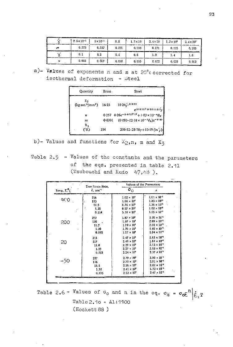
Quantity Brass. Steel
16.25 18.24i-"" c(0.055+0.00tts...iy
0.257 0.26e" 0.07271/2 + 1.03 x 10- 'OK.
0.0301 (0.093-12-18 x 10- 50K)e-
194 206-52-28.78y+ 13.19 (In
x2
(kg sec.'"inlm2)
.......---
4e0 216 113
1.02 x 10' 1.06 x 10⁴
1.01 x 10" 1.83 x 10"
11.5 8.76 x 10' 1.36 x 10" 1.25 6.57 x 10' 1.02 x 10" 0.114 5.18 x 10' 1.55 x 10"
212 1.87 x 10' 1.90 x 10" 200 116 , 1.87 x 10' 2.09 x 10⁴
11.7 1.79 x 10' 2.01 x 10⁴ 1.20 1.70 x 10⁴ 1.80 x 10⁴ 0.095 1.57 x 10' 1.94 x10⁴
213 2.47 x 10' 1.83 x 10⁴ 20 117 2.40 x 10' 1.84 x 10"
11.0 2.29 x 10' 2.13 x 10" 1.23 2.27 x 10' 2.03 x 10" 0.113 2.24 x 10' 2.37 x 10'''
227 2.79 x 10' 2.00 x 10" -50 116 2.71 x 10' 2.01 x 10"
11.1 2.56 x 10' 2.02 x 10" 1.32 2.41 x 10⁴ 1.72 x 10" 0.135 2.52 x 10' 2.47 x 10"
.......-........ ammearsan
Temp, r,ac True Strain Rate,
see' Values of the Parameters
Co n
2.5)(10-2 5x10⁻² 8.5 1.7x10 3.4x10 1.2x10² 2.0.102 in 0.273 0.257 0.221 0.208 0.171 0.125 0.105
0.1 0.2 0.4 0.6 1.0 1.4 1.6 vs 0.088 0.067 0.048 0:035 0.022 0.022 0.013
a)- Values of exponents n and m at 20°c corrected for isothermal deformation - steel
b)- Values and functions for X2,n, m and X3
Table 2.5 - Values of the constants and the parameters
of the eqs. presented in table 2.11 (Tsubouchi and hudo 47,48 ).
93
Table 2.6 - Values of co and n in the eq. (3., = ooEn T Table 2.10 - Al :1100
(Hackett 88 )

'0 •
•
10
5
1.0
° EXTRUSION SUBSRAINS
o
o 6 CONSTANT, T VARIABLE T CONSTANT, 6 VARIABLE
• CREEP. X RAY
A
nIr Si
ATE,,
20
TEI
STR
ESS, X
6 . 9 M
N/m
a
2 5 10 20 50 100 SUEIGRAIN DIAMETER ,dsg MICRONS
(0 s.moci-p(3 *1 (dsg) )
Fig. 2.30- Variation of flow stress with subgrain
diameter -Table2.1c (Mcqueen et al8 )
30 30 TRUE STRESS, s 6.9
2S zs x ilivm2
TRUE STRAIN, E* 0.5
94
Fig. 2.31 - surface representation of stress,log strain rate and temperature -Table 2.10 /
(Hackett 88)

95
specimen, as well as lateral inertia, an example of experimental data
obtained is shown in Fig. 2.32.
Considering the motion of moving dislocations and dislocation
damping:-
(1. -T8)b2pmd
8 = 2
= sbv pmd
(2.62)
T-1
where s= slope of applied stress vs strain rate
and B = dislocation damping constant
b = Bergers vector
T.-I8
= net applied shear stress on the moving dislocation
I = shear stress to overcome barriers
pmd
= density of mobile dislocation
The mechanism operating in the first linear region is related
to dislocation damping by phonon viscosity. The dislocation drag
coefficient .8 in this region ranges from 1.75x10⁻¹ to 2.66x10⁻¹ N.sec/m2.
The smaller slope in the second region is attributed to decrease in the
dislocation damping owing to phonon scattering and enharmonic radiation
effects. The dislocation drag coefficient varies from 0.45x10⁻¹ to
0,75x10⁻¹
N.sec/m2.
The rapid rise in stress with strain rate in the third region as
fitted by the following equation (2.63), by suitable choice of dislocation
density pmd, is considered to be due to the Lorentz contraction of the
core of the dislocation as its velocity approaches that of sound:-
0 WO o S
2
(1 - 3c
.r 2
Pmd bv2va2)
• • (2.63)

(S )I 3 (gN, 4830 N.Sec/m2
REGION I.- REGION I
£c=12,400 SEC"'
1 REGION
III
560 FLOW STRESS as MN/m2
A UNCORRECTED p, CORRECTED FOR LATERAL INERTIA 0 ANNULAR SPECIMENS
0
420
280
Ed 2.63 with d.2.01,z10/cm2
3(S))=;8228 . Se eim2
140. 10
0 20 40 60 3 80 TRUE STRAIN RATE, E xI0 SECT
100 120
A
Fig. 2.32 - Stress / strain rate characteristic of aluminiumaat 20% strain. at
(Dharan. 72)
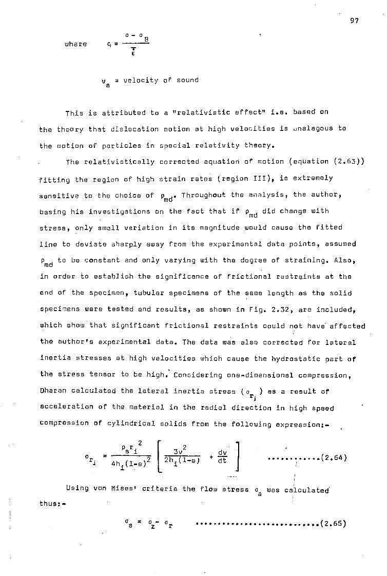
97
- where c,-
va = velocity of sound
This is attributed to a "relativistic effect" i.e. based on
the theory that dislocation motion at high velocities is enalagous to
the motion of particles in special relativity theory.
The relativistically corrected equation of motion (equation (2.63))
fitting the region of high strain rates (region III), is extremely
sensitive to the choice of pmd. Throughout the analysis, the author,
basing his investigations on the fact that if pmd did change with
stress, only small variation in its magnitude would cause the fitted
line to deviate sharply away from the experimental data points, assumed
pmd
to be constant and only varying with the degree of straining. Also,
in order to establish the significance of frictional restraints at the
end of the specimen, tubular specimens of the same length as the solid
specimens were tested and results, as shown in Fig. 2.32, are included,
which show that significant frictional restraints could not have affected
the author's experimental data. The data was also corrected for lateral
inertia stresses at high velocities which cause the hydrostatic part of
the stress tensor to be high. Considering one-dimensional compression,
Dharan calculated the lateral inertia stress (or.
) as a result of
acceleration of the material in the radial direction in high speed
compression of cylindrical solids from the following expression:-
or.
2 p S r. 3v2
dv dt .(2.64)
4h (1-e) 2 2hi(1-e)
Using von Mises' criteria the flow stress os was calculated
thus:-
CY = NMI or

98
where o = measured stress in compression z
An excellent review, covering strain rates up to 5000sec-1
and
the general effects of dynamic loading on the material properties is
given by Stamelos (91). Wide ranges of materials are considered and
their behaviour over their working temperature ranges discussed. The
principal deduction however is that most materials undergoing a particular
deformation mode change their characteristics as the rate at which the
energy is dissipated is altered. The author concludes that several
mechanisms of plastic flow are suggested by experimenters, but points
out that even if these mechanisms are accurately determined a single
clear cut mechanism of flow seldom takes place by itself. It follows
that the structure of the material responds differently to rates of
straining if the loading rate is varied. A hybrid of flow mechanisms
thus becomes operative depending on temperature and other conditions.
The mechanism of deformation under high speed hot working is
usually analysed in terms of dynamic recovery (63)(92) since this has
a great effect on the mechanical and structural properties of materials.
Recovery is a time dependent process and since mechanical behaviour of
materials is rate dependent, then recovery and material properties are
interrelated.
In the process of recovery, cross slip and climb of dislocations
occur, and when these two phenomena are operating both screw and edge
dislocations are able to surmount barriers and rearrange themselves
into low energy configuration, which means they lower the overall
dislocation density as well as the subgrain formation. When a material
is simply annealed and no external stress applied to it, the cross slip
or climb of each dislocation occurs in response to the stress field of
other dislocations in the material and is assisted by thermal activation.
Hence the static recovery process as referred to polygonisation, driven
by thermal stresses in conjunction with thermal activation, exists in

99
such a situation.
On the other hand, when a material is deformed dynamically the
polygonisation occurring is driven by external stresses as well as
internal stresses and thermal activation. An increase in the rate of
deformation increases the rate of cross slip and climb and hence enhances
more polygonisation by producing intersection jogs and vacancies which
promote climb. The dynamic recovery thus proceeds more quickly than the
static recovery due to the accelerating effect of shear stresses and
strain associated with the deformation.
The dynamic stress/strain characteristics of materials, particularly'
at elevated temperatures, as presented by experimenters, exhibit two
stages (41)(93) - the transient stage followed by a steady state and/or
a decline in stress level after the transition stage is terminated.
Typical of these examples are shown in Fig. 2.33 and 2.34. The transient
part is represented by the rising part of the stress/strain curve and
the steady state by the horizontal part as shown in Fig. 2.33. For some
metals, soon after the transition stage is terminated, a decline in
stress level is observed, Fig. 2.34.
The initial slope which is common to the behaviour of all materials
indicates the rate of work hardening at the beginning of deformation.
With increasing strain, the slope gradually decreases and when an
equilibrium is established between strain hardening and dynamic
softening, the flow stress level remains constant and hence - the
horizontal part appears. For other metals since the dynamic softening
supercedes work hardening to a greater extent, the stress/strain curve
exhibits a drop in the stress level soon after the transient stage is
reached.
In the region where a steady state stress level is attained, or
during the dynamic hot working of some materials, dynamic recovery
exhibits itself by setting an equilibrium between the rate of
annihilation and the generation of dislocation during deformation,

100
Natural Strain
Fig. 2.33- Dynamic stress strain characteristics of
aluminium at 250°C -(6amanta 73)
0.2 0.4
0.6 Natural Strain
Fig. 2.34 - Yield stress strain characteristics of 2.25% C
,13%Or steel at 900°C. (Cook 41)

101
so that the dislocation density remains constant. In hot working,
since flow stress is proportional to the working temperature, the
controlling mechanism is thermally activated and thus when the moving
dislocations meet stress fields of various types, they overcome these
fields by external thermal fluctuations as well as by applied stresses.
Stress fields which may be overcome by thermal activation include
"Peierlo-Nabarro" stresses, non-conservative motion of jogs resulting
in the creation of vacancies, intersection, cross slip and climb.
Other mechanisms, such as long range stress fields, or Suzuki locking
in alloys, are of such a magnitude that they cannot be overcome thermally
and when these effects are predominant the deformation is essentially
athermal and not rate sensitive.
Billington (24) explained the difference between the static and
dynamic stress to be due,
a) solely to stress enhancement by an amount Ao arising, possibly,
from some form of dynamic strengthening mechanism,
b) solely to strain retardation by and amount 6E arising from
one dimensional extension or dilation,
or c) to a combination of stress enhancement and strain retardation.
It is then explained that if the stress enhancement were the
cause of the difference between the static and dynamic mechanical
response, as a result of the existence of some possible strengthening
mechanism, then it can be expected that a particular mode of stress
loading could be identified which when varied would produce changes
in the level of stress enhancement i.e. a change in the level of the
dynamic stress relative to the static stress for a given value of
strain. It is further argued that established and accepted theories
of the dependance of the macroscopic mechanical response of metals or
their microstructure, in particular the theory of crystal dislocation
mechanics, defy the existence of one dimensional dilation in the plastic
region of deformation. Besides, no experimental evidence is cited to

102
suggest the existence of such a strain retardation arising from one
dimensional dilation. nowever it is pointed out that the existence
of one dimensional dilation was cited in the literature. The effect
known as Poynting was reported by way of static measurement in shear
such that the lengths of various steel, copper and brass wires were
increased in torsion. bince no evidence was reported to support this
poynting effect, Billington has argued that it is unlikely that strain
retardation is the cause of the difference between the dynamic and the
static response.
Billington and Tate (94) approached the non-linear mechanical
response of some materials from the physical point of view and considered
that there existed a marked similarity in the general shape of the
dynamic stress/strain curves for metals and the dynamic shear stress/
rate of deformation curves for liquids. On this basis Billington and
Tate, in distinguishing between the behaviour of real materials,
indicated that for non-work hardening materials such as hexagonal
metals (e.g. zinc) deformation is comparable to that of laminar flow,
while with cubic metals such as copper or aluminium, deformation takes
place in a "turbulent" manner resulting in rapid rise in work hardening.
By considering tentatively a material consisting of a regular
assembly of identical laminar layers, the thickness of each layer being
the same, the authors specified that the effect of shear stress is to
produce a relative displacement of the assembly of units, with no
movement occurring at the interface between adjacent layers i.e. at.the
slip planes. A non-linear response results if the thickness of the
laminar layers decreases with increasing stress. On the decrease in the
spacing or slip planes arising from an increase in the number of slip
planes per unit volume of the material, the authors suggested that the
spacing (6) of active slip planes is inversely proportional to the
applied stress, i.e. 6= a/os, a = constant.
It now may be said that since os is dependent upon t, then

103
6 must be proportional to l/e. On this basis the effect of strain rate
on the mechanical response of materials cen be explained physically
and the concept of saturation occurring at some critical value of
applied stress established.
On relative terminal characteristics of the metals formed by
high energy rates as opposed to more conventional techniques, Orava
and Otto (95) conducted a comprehensive review of literature and
concluded that little hesitation need be experienced in most cases
using high speed forming if the material properties of interest are
hardness,. strength, ductility, fatigue and stress corrosion. They do
however point out that care should be exercised in evaluating the
residual stress levels in formed parts if the service environment id
conducive to stress corrosion cracking. They were concerned with the
adverse differences in the properties of dynamically loaded ferrous
and non-ferrous metals and alloys as opposed to those statically
deformed. Since their sources of information on these materials were
limited no definite conclusion was drawn. The authors thereby indicate
that the variations in the forming conditions often preclude effective
comparison between different investigations. They further point out
that the literature on the subject still suffers from discrepancies
and inadequacied which lead to the adaptation of conflicting opinions,
and misconceptions due to lack of basic understanding of the subject.
It is shown that the dependence of microstructural changes such as
dislocation substructure, mechanical twins and strain induced transition
phases due to forming rate, can be quite significant, but the lack of
well documented data which considers all the factors influencing the
deforming process, does not provide reasonable correlations between
terminal structures and properties.
On the effect of strain rate and temperature on the fatigue life
and properties of metals, the work of Thiruvengandam and Conn (96) is
of interest. The authors investigated the effect of elevated temperature
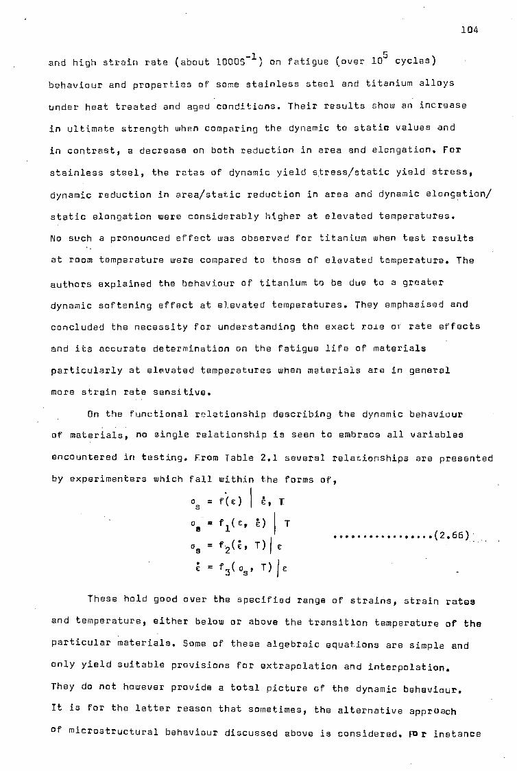
104
and high strain rate (about 10005 on fatigue (over 105
cycles)
behaviour and properties of some stainless steel and titanium alloys
under heat treated and aged conditions. Their results show an increase
in ultimate strength when comparing the dynamic to static values and
in contrast, a decrease on both reduction in area and elongation. For
stainless steel, the rates of dynamic yield stress/static yield stress,
dynamic reduction in area/static reduction in area and dynamic elongation/
static elongation were considerably higher at elevated temperatures.
No such a pronounced effect was observed for titanium when test results
at room temperature were compared to those of elevated temperature. The
authors explained the behaviour of titanium to be due to a greater
dynamic softening effect at elevated temperatures. They emphasised and
concluded the necessity for understanding the exact role Of rate effects
and its accurate determination on the fatigue life of materials
particularly at elevated temperatures when materials are in general
more strain rate sensitive.
On the functional relationship describing the dynamic behaviour
of materials, no single relationship is seen to embrace all variables
encountered in testing. From Table 2.1 several relationships are presented
by experimenters which fall within the forms of,
as
= f(E) I E, T
0s = f1(C 0 T
os = f2(e, T)le
= 3( os T) I
These hold good over the specified range of strains, strain rates
and temperature, either below or above the transition temperature of the
particular materials. Some of these algebraic equations are simple and
only yield suitable provisions for extrapolation and interpolation.
They do not however provide a total picture of the dynamic behaviour.
It is for the latter reason that sometimes, the alternative approach
of microstructural behaviour discussed above is considered. For instance
(2.66)i .

105
in hot working of many metals, the process of hot compression behaviour
like that of creep is taken as thermally activated and from the thermo-
dynamic and rate theory of this phenomenon, stress/strain rate relation-
ships are derived - Tables 2.1c and 2.1n..
Derivation of a function describing material dynamic behaviour
is an extremely difficult task, since it entails correct consideration
of variables affecting the deformation. Simple equations might give
some guidance as to the strength and mechanical properties, but are
of a very doubtful nature when applied to metal working analyses. One
of the conclusions drawn by Slater at al (74) on the pronounced error
encountered in the estimation of the deformation forces can be considered
as an example of this.
In the determination of true functional relationships, assessment
must be made of all factors influencing the upsetting process. Variation
in strain rate, boundary friction and restraints, radial and tangential
inertia forces, stresa wave propagation effect within the testpiece
and the machine components, and variation in the temperature environment •
including heating effect due to deformation, are all important factors.
These entail that their influence must be separately taken into account
if true behaviour and description are desirable.
Using free flight type impact devices, variation in strain rate
during the deformation is unavoidable (97)(98). If this variation is
of considerable magnitude, and only a mean value is taken into account;
then the assessment of strain rate effects would be grossly in error.
Attainment of constant strain rate in the test piece depends not only
on the velocity of compression but also on the machine components'
stiffness.
Under high speed compression, with a cross head tasting machine,
Atkins (99), by considering the structural stiffness (Ks) of machine
components showed,

v/h.
Asi do
expE exp(-c)day 's
S i
116.0.0J
106
(2.67)
where do
= slope of true stress/strain curve de
A= initial cross sectional area of the specimen, Si
gauge length hi
v st cross head velocity
For small strains, Et expression (2.67) reduces to:-
v/h.
= elastic strain rate ...... (2.68) A doe
+ • --0- K h. de s
dos - slope of engineering stress/strain curve for a material
de
having a non-linear behaviour
des or = E for a material obeying Hook's Law
i .
The term Kh -- considers both the machine component and the As
s specimen stiffness.
Expressions (2.67) and (2.68) indicate that high machine stiffness
allows higher strain rates since most of the deformation goes into
the machine. Clearly t = v/hi * would be exact for an infinitely stiff
machine.
If a small increment of strain is not chosen, even if the velocity
of compaction is constant, then the variation of strain rate due to
machine stiffness or unsuitable choice of specimen geometry is
unavoidable. Similar considerations also hold for tension.
Further increasing the speed of deformation causes the time of
duration of the test to diminish and become comparable to the time
of propogation and attenuation of stress wave in the solid. when these
conditions are approached, the stress/strain system in the specimen
is unsteady and non-uniform. Since conventional interpretation of

107
load-strain behaviour assumes uniform stress and strain distribution,
it is difficult to analyse data obtained above a certain limiting
deforming velocity or initial strain rate, unless allowance in time
is made for several stress wave reflections to occur within the specimen
to allow for uniform stress and strain distribution. No doubt if the
specimen's geometry is not carefully selected to avoid such undesirable
phenomena, the determination of material behaviour would be adversely
affected. The basic requirement (72)(73)(93) to overcome this, is to
choose a specimen of suitable gauge length h so that the time is taken
for a longitudinal elastic wave to traverse the specimen at the
longitudinal wave velocity cs becomes smaller than tb the time taken
to obtain a strain e at which point the stress/strain and strain rate
are measured. If such a condition exists for several reflection to
occur within the specimen then the stress and strain gradient between
the faces of the workpiece may be eliminated. For instance in compression,
as shown in Fig. 2.21a and 2.21b, Dharan (72) experimentally demonstrated
that for a suitable specimen geometry at least six to eight reflections
are essential to ascertain uniformity in stress and strain levels.
O inertia effects (81)(82)(100), if the velocity of deformation
is of considerable magnitude then the radial and tangential particle
velocities of the working material may achieve high value. This results
in acceleration which imposes high compressional stresses in all
directions. It is therefore essential to ascertain the magnitude of
these forces on the dynamic behaviour.
Adiabatic heating effects as a result of high speed deformation
are considerable particularly where high reductions are involved.
Nadai and Manjoine (51) showed (Figs. 2.35 and 2.36) that as the speed
of deformation is increased, or the time allowed for considerable
straining decreased, the creation of adiabatic heating with high magnitudes
becomes unavoidable. From these figures, the magnitude of working and
localised heating effects are obvious. The impact of localised temperature

Oscillations as result of stress wave reflection in the specimen/load cell 1
R
200
600 C6,-,600 ,
Ce* epc,
.000
.200
20 TIML 367LR CRACTIRL IN SEC01403
Fig. 2.35 - Temperature rise of specimen undergoing
high speed deformation .(Nadai and Manjoine 51.)
SWUM
Fig. 2.36 - Temperature and strain rate effects on the mechanical behaviour of mild steel
1-4 :E:=200 Seel
5k6 : " = 350 " 7 : " = 600 "
(Nadai and Manjoine 51 )
108

109
rises is so high that the working temperature would alter. This subseq-
uently alters the dynamic behaviour. If the working temperature is low,
under high strain rate conditions, substantial change in the magnitude
of this temperature should be expected. As a result of this alteration
the stress level reached would be modified with subsequent reflection
on the strain rate effect. On the other hand at elevated temperatures
since most materials are more strain rate sensitive, adiabatic heating,
although not so high as in a low temperature working environment,
would cause substantial modification.to the strain rate sensitivity.
The dependence of strain rate sensitivity on temperature is well
demonstrated by Alder and Phillips (40) and Jones et al (63) (Figs. 2.37,
and 2.38, Table 2,4). If the effect of adiabatic heating is not taken
into account the dependence of strain rate sensitivity, particularly
at high temperatures is not fully justified.
On the transition temperature of metals, Mahtab et al (26) showed
that an increase in the temperature would be expected with increase in
strain rate. As seen in Fig. 2.39 the significance of the adiabatic
heating effect on the transition temperature at very high strain rates
is prominent. The work of Gagnon and Jones (52), Table 2.1n, indicates
that if the temperature change as a result of adiabatic heat generation
is neglected, both power sinh stress dependence and the activation
energy are significantly increased. The resultant incorrect estimation
of these values indicates the assumption of isothermal conditions is
unwarranted.
At elevated working temperatures the rate of straining is controlled
by thermally activated mechanisms (101). The temperature dependence of
the strain rate in dynamic deformation is then expressed by Arrhenius
terms. Exclusion of the effect of adiabatic heating on the constants
of this function would no doubt produce underestimation of strain
rate effects.
For hot working of materials, it is suggested (102) that a

0.2
0•I
• • a
a X x ALUMINIUM
• COPPER a
a STEEL A X
•
it • X
0 •
0 op
0.2 04 04 04
HOMOLOGOUS TEMPERATURE
1.0
I I I
/o
/0 •---)
/ 1:1/
KLAv/. 0 0 / ely //a
e / v t. 0-0 4
0-I 0-2 --- 8 D °-../ 03 Cr 4 050 6 0-7 0.8 HOMOLOGOUS TEMPERATURE
0-25 r- , V Extrusion 13 Compression.
0-20 0 Compressionr Hot torsion
A Creep
I I I
0-IS E
Mumirrium 01
0.9 1.0
Fig. 2.37 -Dependence of strain rate effects
on the homologous temperature for 40% reduction -(Alder and Phillips 40)
Compression, % . 10 20 30 40 50
ml * . . . 0-045 0-050 0-055 0.060 0.065
mi t . . . 0.36 0.38 0-41 0.46 0-52
* m, is the slope for 0 < To < 055. ml is the slope for TH > 0-5.5.
Table 2.2 - Values of the slopes of the 11,/T curves (Fig 2.37) for
_ various r e du ci iwas
E
Fig. 2.38- Dependence of strain rate sensitivity
on temperature as determined by several
test methods. (Jonas et al )

9 Ex tru s ion SrOn riz 0SZC,..:.2 • Cu, tension, esscIrcn o Rotting, eiecsron cscss:acm rJ Torslon, poicrize-r„' Y Rolimq, phase cor-,,ast at Creep, X-ray • Ro!ling, X-rcy a Irons torsion, 02tscal
V
L.) V+ A
A a A A A
6 0 0$ 04 03 04 C5 06 07 08 0
HOMOLOGOUS TEMPERATURE T °W. °W.
8
7
6
IV 0 1
o 0
s
Ck....̂ 1 0
20 ----
10 —
5
w CONSTANT STRAIN 6e.r cant 1.P.
..., 2
0 20 00 . 600 IEMPERATURE ^
Fig. 2.39 Effect of strain rate on
transition temperature;ft
annealed aluminium.
(Mahtab et al 26 )
Fig. 2.40 - Variation of aubgrain size with temperature
in several materials for different modes of
deformation as measured by variety of techniques. (Jonas et al 63 )
111

112
fibrous structure would be formed composed of subgrains. It is also
shown (63), Fig. 2.40, that the subgrain size increases with temperature
and hence causes a decrease in hardness value. No doubt the adiabatic
heating contributes significantly to the formation of subgrains and
in this way causes variation in their density, size and hence the
movement of dislocations. The effect of the variation in subgrain
diameter on flow stress is shown in Fig. 2.40.
Since during any process of deformation, particularly at elevated
temperatures, several activated mechanisms are suggested to be present
(103) then if the factor of adiabatic heating or even other deformation
influencing factors such as friction is not carefully considered, a
misconception on the dominant operative mechanism and the dynamic
behaviour might result.
It is adiabatic heating which is suggested by Parsons et al (104)
and Dower (105) to be the influencing factor on the properties of
products extruded at high speed. It is implied by the authors that
although adiabatic temperature rise can only play a minor role in
influencing the deformation process because of the limited time avail-
able for temperature dependent recovery processes to operate, it
could however influence the properties of - products .Similar
conditions are to be regarded for high velocity powder compaction (106).
frictional effect and boundary restraints affect the flow stress.
These effects on the mechanical behaviour are more significant at
elevated temperatures and high strain rates. This is well explained'
by Jain and Bramley (107) who conducted simple compression tests on
solid and ring specimens at elevated temperatures. Their investigation
was concerned with varying the speed of forming from approximately
0.021m/s to approximately 12m/s and changing the type of lubricant.
As illustrated in Fig. 2.41, the load sustained during the deformation
varies considerably with lubrication conditions and speed. It can also
be observed that the maximum load at low speeds is higher at reductions

80 90 70
70 80 90 0 10 20 30 40 50 60 REDUCTION per cent
(a )
1111 1/11
/ A
10,+
4—T+
'41
E
cb) NM ,
• Colloidal graphite. ▪ Copaslip. O No lubricant.
• Colloidal + Copaslip o No lubricant
; graphite
I. I I
4e7 I - 1
+
) o,
0 o ii • ... •
- - .- -----1 ---
>7
0.4 0 10 20 30 40 50 - 60
REDUCTION—per cent
Fig. 2.41- Relations between maximum load,ratios of
of maximum load with lubricant/ maximum load without lubricant and maximum load
at low speed / maximum load at high
speed with percentage reduction -
indicating the variation in frictional
restraints.( Jain and Bramley 107)
200
180
160
• 140
120
0 100 z -
80
60
40
20
0
1.0
Tc „ 0 9 =
0.8 O
0.7
'80-6
0.5
2.4
' 20 LLJ
LD 1-6
a" 12
1.0 -J0.8
>7c04 <
0

114
greater than 45%, while the reverse is true for reductions up to 45%.
The authors suggest that this trend is due to the following phenomena:-
(1) The strain rate effect which causes an increase in the flow
stress as the impact speed is increased,
(2) The chilling effect causing the workpiece to lose heat to
the surrounding dies and thus increase its flow stress,
(3) The adiabatic heating effect which is related to the chilling
effect. During plastic work, about 90% of the plastic work is
converted into heat, and at high speeds this manifests itself
as a temperature rise in the workpiece, causing a reduction in
flow stress.
The authors then suggested that for low reductions the strain
rate *effect is the predominant influence, resulting in higher loads at
high speeds. For large reductions the chilling effect and the adiabatic
heating effect are significant at low and high speeds respectively and
result in lower loads at high speeds. These thprefore indicate how
frictional conditions at constrained boundaries are dependent upon
the speed of the deformation and may alter with the adiabatic heating
of the workpiece.
Further, Nicholas (108) has shown that the flow stress in metals
depends not only on atrain, strain rate and other effects but also on
the strain rate history of loading. For instance in mild steel, it
was shown that the flow stress in dynamic loading is higher after static
prestraining than in a constant strain rate test. In titanium the
reverse was found to be true.
The forgoing explanations clearly indicate that intrinsic behav-
iour of materials is complex and that realistic constitutive equations
must include not only strain rate, strain, strain history, but also
other factors influencing material behaviour. The complete stress,
strain, strain rate, actual temperature history of metals cannot be
determined solely from tests at constant strain rates and initial temperature,

115
but consideration must be made of the indirect effects such as stress
wave propagations, stress uniformity in the test piece, adiabatic
heating, boundary friction etc..
More realistic theories of dynamic plastic behaviour can be
approached if all factors influencing the deformation process are
carefully assessed. Perhaps the controversy between the strain rate
dependent and strain rate independent schools of thought in dynamic
plasticity can then be commented on effectively.

116
CHAPTER 3
EXPERIMENTAL APPARATUS AND PROCEDURE
3.1 Introduction
The experimental apparatus consisted mainly of a modified U.S.
Industries forging press, incremental and large deformation subpresses
with appropriate instrumentation. The tooling and instrumentation
incorporated suitable load cells and velocity transducers. These
provided recordings of the load and velocity histories on an oscilloscope.
A calibration set-up was used for calibrating the velocity transducers.
Various sot-ups were also organised to carry out hot incremental tests
and for the measurement of temperature rise during the continuous
loading process
3.2 Modified U.S. Industries Forging Press
A U.S. Industries Model 2008 high energy rate counterblow forging
hemmer has been extensively modified (109) mainly in order to extend
its speed range. The details of operation and calibration of this
machine prior to modification are described elsewhere (110).
The present arrangement, Fig. 3.1, incorporates drive pistons
consisting of heavily overlapping synthetic rubber seals./Formerly
the piston arrangement consisted of all metal seals (ill)/ causing the
machine to misfire, particularly at high precharge pressures. This was
a result of irreducible minute leaks between the hard steel valve seatings.
The new arrangement also ensures that an appreciable displacement

TOP FLOAT PISTON
117
TOP INCH & COUNTER BALANCE
CYLINDER
LARGE VOLUME GAS
ACCUMULATORS
PRECHARGE NITROGEN PRESSURE SUPPLY
DRIVE PISTON
NITROGEN COMPRESSION CHAM BER
BOTTOM PLATEN
NITROGEN BLEED HOLE
COPRESSION CYLINDER
BOTTOM INCH CYLINDER
MAIN FLOAT PISTON
MAI N HYDRAULIC
4-SUPPLY PUMP DELIVERY
FIG.3.1- SCHEMATIC HALF SECTION OF THE MODIFIED U.S.I. FORGING PRESS
LOWER FLOAT PISTON

118
of the bottom platen takes place before the top face of the drive piston
is exposed to high pressure nitrogen compressed into the gas chamber.
This makes it possible to reduce the oil pressure below the drive piston
(and consequently the precharge pressure)'to achieve smaller ram
velocities. For comparison purposes Fig. 3.2 illustrates the machine
schematically before modifications.
The relative velocity of the opposing rams can now be adjusted
between 1 and 21.4 m/s to cover compaction velocities of interest. By
using a single ram a minimum strain rate in the region of 2051 can be
achieved, while the maximum strain rate using both platens could exceed
2000S-1
Since the commisioning of the machine after modifications coincided
with the onset of experimental work, some difficulties were encountered
in carrying out a test series without the press breaking down. This was
due to failure or the valve seals, Fig. 3.3, which occurred after a
number of machine operations. During the primary stages of the experimen-
tal work, considerable effort was thus expended in establishing a seal
material which would resist tear, wear and abrasion when the valve seals
enter the drive cylinders.
Several seals were tried and the most successful one was the
special solid unreinforced hard polyurethane seal (R14082 in meth 02119)
provided by Hall & Hall Ltd.. The surface profile of the seal was
similar to a standard Hallprene seal and its characteristics consisted
of high tensile strength with high resistance to abrasion. The dynamic
fatigue failure life of the seals was found to extend over 200 machine
operations. No such a fatigue failure was observed for the piston seals.
This life of 200 machine operations is obviously comparable to the
maximum of 5-7 operations carried out before modifications. The machine
as instrumented is shown in rig. 3.4. Pneumatic and hydraulic circuit
diagrams which were prepared are illustrated in Fig. 3.5 and 3.6.

OIL C. BALANCE SCUPPER INCH
UNIT GAS
PRECHARGE GAS 'SUPPLY
MAIN VALVE SEATS
FLOAT PISTON
MAIN CYLINDER
LOWER I NCH PISTON
MAIN HYDRAULIC SUPPLY
OIL
119
FIG.32- US.I FORGING PRESS AS PREVIOUSLY USED (89)

Fixing flange 1 Vatve seal
Piston seat
Bleed hole
FIG. 3.3 EXPLODED VIEW OF VALVE AND DRIVE PISTON ASSEMBLY

121
Specifications of the weight of machine components and the toolings,
which influence the magnitude of the energy created by the press rams
are given in Table 3.1.
3.2.1 Operation of the machine
Since modifications, the operation of the machine goes through
a different sequence. For a particular setting of precharge, counter-
balance and main hydraulic supply pressures and for a typical cycle
of operation the sequence is as follows:-
1) With the piston seal assembly lifted out of its valve seat and
other parts placed in the standby position of Fig. 3.1, hydraulic
oil is supplied via the main pump delivery to under the main
float piston. The float piston is then pushed upwards to compress
the precharged nitrogen gas in the compression cylinder. This
is due to the compression ratio of the compression cylinder. The
gas in the compression chamber within the bottom platen is
compressed accordingly through the nitrogen bleed hole. After the
compression is over, the upper face of the main float piston
contacts the bottom face of the drive piston seal assembly.
2) A signal is sent to the bottom inch cylinder causing the bottom
platen to move down, this closes the valve by letting the valve
seal close and sit on the valve seat, after which there would
be no more connections between the gas in the compression
chamber and the gas in the compression cylinder.
3) The main hydraulic supply is signalled to close after which the
oil in the compression cylinder below the main float position
is drained. This drops the gas pressure within the compression
cylinder to a negligible magnitude.
4) A signal is again sent to the bottom inch cylinder causing it to
move the bottom platen sufficiently to expose the face of the drive

Table 3.1: WEIGHT OF MACHINE COMPONENTS AND TOOLINGS
1) ToR_platen Weight(lbs)
Weight of top platen
339
91
t1
" drive pistons 56
" fixing ring screws and sealing
parts 14
tt " piston head assemblies 4
Total weight of the top platen 413
2
Bottom platen
Weight of bottom platen 366
tt " drive cylinders 104
ft
" fixing rings for drive cylinders , 48
(+ screws)
Total weight of the bottom platen 518
3) Incremental tooling and instrumentation only
Weight of shroud tube and tooling fixed
on the top platen
30
Weight of the tooling assembly fixed on
the bottom platen
32
Weight of the electromagnet and fixture
fixed on the bottom platen
7
122

123
Storage drot osciltos
Line dete
Con cur
ING PRESS IED INSTRUMENTATION
(as set up for an incremental test)

Weight
Counter balance pressure control
Precharge pressure ----control
Control console
Automatic /guard
Storage oscilloscope
Guard ----control
Line fault detector
Constant' current source
D.C.Supplies (triggerring & load cell)
FIG. 3.4 MODIFIED U.S.I. FORGING PRESS AND ALLIED INSTRUMENTATION (as set up for an incremental test)
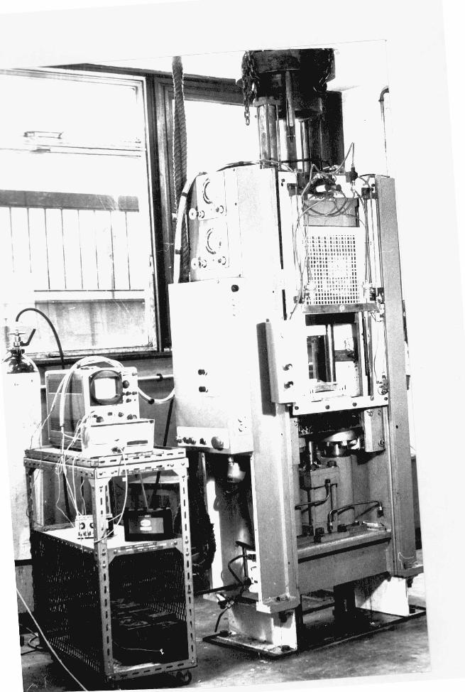

fis
To other ) accumulator
& c' balance cylinder
124
Large volume gas
6, accum fin/r/P "
cs) D
0
To drive cylinder=, Manual exhaust
Pressure guage
(-0
Manual shut off val.
TOP PLATEN
Bottom inch & trigger
Drain
Nitro
gen
bott
le p
FIG.3.5 : MODIFIED U.S.I. PRESS -
PNEUMATIC CIRCUIT

VALVE PANEL
of Sol ri A B .
-0- 2
To bottom inch cylinder
Psi ps 2
Sol B
To drive cylinders 1._
V1 Sol A
Sol A
To top inch cylinder
Sol [-- 13
0 V3
Supply
Exhaust
Unloader relief valve
Man exhaust
Electric. motor Pf
•■•■••••■•
s r
125
— 1 I -
1 I
I i II
1 F l
I I
_ 1 t I I oil
Tank
PUMP UNIT
FIG. 3.6-MODEFIED U.S.I. PRESS HYDRAULIC CIRCUIT

126
piston seal assembly which has up to now been in intimate contact
with the face of the valve seat. High pressure gas now acts on
these areas creating a sufficiently large force which causeS'a
machine to fire. As a consequence top and bottom rams are driven
towards one another in states of free flight.
5) After compression the rams are returned to their previous position
as in (1) and the machine is now ready far the next cycle of
operation. The time taken is about 7 seconds depending upon the
required speed.
The inching movement of the top and bottom platens are effected
by the top inch of the counterbalance and bottom inch cylinder-piston
assemblies.
uuring the course of the experimentation precharga pressures of
up to 800 P.S.I. with the main hydraulic supplies of 1500 to 2000 P.S.I.
were used to achieve a range of desirable impact velocities.
Counterbalnce pressures of a maximum of 140 P.S.I. and a minimum of
80 P.S.I. were also used. The maximum limit was due to the strength of
the rubber tubing connecting the large gas pressure reservoir to the
counterbalance assembly. The minimum gas pressure was to ensure that the
counterbalance piston never hit the counterbalance valve seat at the
end of compaction when the rams met. The setting of the counterbalance -
gas pressure also helped to control and regulate the velocity of the top
platen.
3.2.2 Automatic Guard
In order to safeguard human factors (particularly under hot
working conditions) and prevent the machine from undue misfiring an
automatic guard was designed which incorporated a safety prop, keeping
the platens apart until a moment before the machine fired. Schematically,
control circuitry of the guard and allied parts is shown in Fig. 17.
The guard can be used either independently or in connection with the

Pressure line Pilot
— Air supply Exhaust
A L Fire 1
E ---- - --1 Speed control
•■••■■■111.■ .0111•■■■••••••••■••
Reset
•••• MO Oft 1111111.,

128
firing sequence of the machine.
rig. 3.7 shows the safety prop and guard in the idling pcsitions
such that the prop is in between the platens, keeping them apart, and
the guard is up clearing the platens for loading purposes. Upon
sending a signal by pressing the fire button, the guard is activated
first, coming down to cover the platens and in turn sending a pneumatic
signal to operate the safety prop to come out from between the platens
prior to the machine firing and compression. This also sends en electical
signal to the machine via electrical switches placed on the side of the
prop arm to activate the firing stage of the machine as soon as the
guard has come down.
All takes place within a fraction of a second to ensure that the
machine is cleart particularly under hot working conditions for rapid
firing. Speed controls are incorporated with Ote mechanism and the
machine to vary the guard and the firing sequence velocities. The back
part of the press is guarded by manually operated covers. All parts of
the guard control mechanisms were supplied by mecman Ltd..
3,3 Experimental Subpress
3.3.1 Dynamic incremental tests
The basic principal of the incremental subpress and tooling has•
been described elsewhere (79). In the present arrangement, Fig. 3.8,
the specimen is supported in a holder and laterally located by a soft
rubazote rubber sleeve so that the axis of the specimen coincides with
that of the long load cell. The specimen projects above the holder by
the amount of preselected deformation. The load cell is fixed to the
press frame. As the bottom ram travels upwards, the specimen is
compressed under the dynamic load applied on impact by the long load

LOAD CELL (STATIONARY)
COM PRESSOR SPRING
DUCTILE TUBE
HOLDER
SPECIMEN D EFORMATION
129
STEEL SPACER
FIG. 33-EXPERIMENAL-SUB PRESS FOR INCREMENTAL TESTS

130
cell and is deformed by the amount of preselected increment. In this
arrangement only a single platen is used to achieve lower ranges of
strain rates.
When the incremental deformation is terminated, the load cell
resting on the specimen holder which is fixed on the shear pin assembly
unit crops the pins. The specimen with the holder then falls in the
cavity below the assembly and subsequently both platens are brought to
rest by a ductile tube which absorbs their excess kinetic energy. The
ductile tube is supported radially by a soft rubber sheet which is
strapped (Fig. 3.9) on the plate fixing the shear pin assembly on to
the bottom platen. Subsequent deformation steps are carried out using
holders of gradually reduced heights. Between each incremental step,
a steel spacer of suitable thickness is placed between the heavy weight
(Fig. 3.8) and the load cell, thus compressing the load cell down
further towards the specimen holder. This compensates for the reduced
height of the specimen holder, thus allowing the compression to be
carried out successsfully in each step. The purpose of the compression
spring was to allow for this movement. Fig. 3.10 illustrates the load
cell with the compression spring, the fixing plate and the steel tube.
The latter acted as the support for the load cell to prevent buckling.
This arrangement ensures that the amount of incremental strain
can be easily and accurately measured, and that friction is kept at a
much reduced value as the specimen end faces are relubricated between
each incremental compression. It also entails that the time of
deformation is short enough for the load measurement to-be free from
the effect of stress waves in the long load cell employed. Also, since
the energy of deformation is only a small fraction of the total kinetic
energy of the press, the velocity of the platen remains constant during
the deformation.
The diameter and the material of the shear pins in the shear pin

Shroud tube & flange
Safet prop y
Long load cell
uctile
Strap
Soft rubber sheet ft.̀441'
1
131
FIG. M- ARRANGEMENT OF INCREMENTAL TOOLING IN THE PRESS

31

Fixing plate Load cell Steel tube
Compression spring
FIG 3.10 LONG LOAD CELL AND ALLIED PARTS.

133
assembly unit was calculated from the consideration that for an
incremental equivalent strain, dynamic stress of the material undergoing
deformation is three times as much as its static stress. Three shear
pins were altogether used in the hole drilled in the assembly displaced
at 1200 apart. Three series of three holes were drilled to accomodate
pins of different diameters.
The diameter (d) of the pins were calculated by considering the
static shearing strength (T) of the pin material and the dynamic force
Fd
exerted by the load cell on the test piece, such that for 3 pins,
4Fd
---y 3nd
or d = /0.425 Fc4'.
(3.1)
. . pp 0000000 000000 w • • • • • • • ( 3•2 )
The dynamic force Fd for the pins used was calculated for a
1,27cm diameter test piece. This arrangement ensured that the testpiece
was fully loaded before the shear pins started to crop. Shear pin
materials of brass and silver steel were mainly used. The maximum length
of each pin was limited to 3.8cm due to the limited available space
and the length of the holes in the assembly unit. Each series of pins
were cropped three times before they were completely discarded.
3.3.2 Dynamic large deformation tests
The arrangement of the continuous deformation subpress and
instrumentation is shown in Fig. 3.11. The tooling consists of a top
anvil fixed on the top platen and a bottom die assembly incorporating
a ring load cell, die and base plate, fixed on the bottom platen. The
testpiece is compressed between the top anvil and the bottom die. The
top anvil and the bottom die faces were all ground and mirror polished.
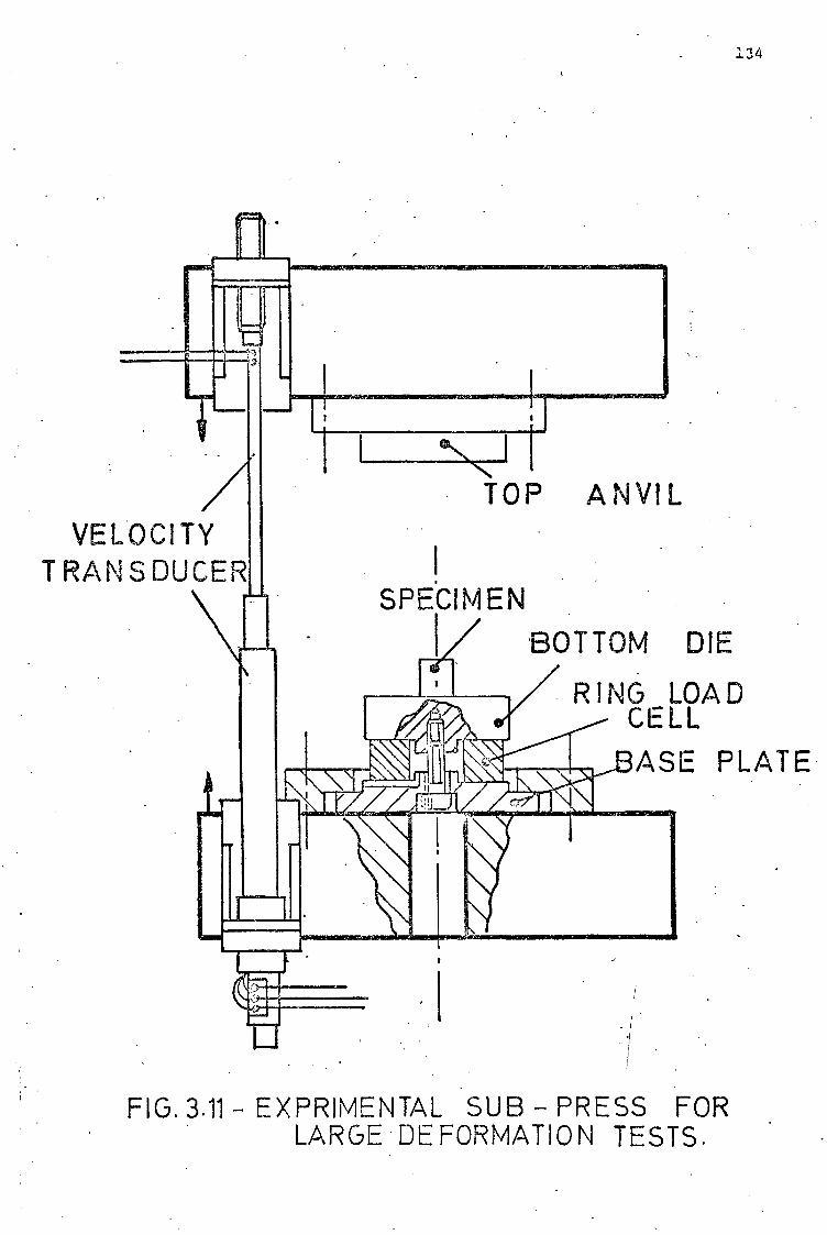
TOP ANVIL
.134
SPECIMEN BOTTOM DIE
R I NG LOAD CELL ASE PLATE
VELOCITY TRANSDUCEI
FIG. 3.11 EXPRIMENTAL SUB - PRESS FOR LARGE DE FORMATION TESTS. •

3.35
1.3.3 Quasi-static tests
For quasi-static tests, the test specimens were subjected to
incremental loading using a Tinius-Olsen (0 - 120,0001b0 machine.
The speed of compression was set at 0.000033m/8 (0.005in/min).
The method adopted (112) involved measuring the overall length,
diameter at centre and at both ends of each specimen and lubricating
the die/specimen interface between each incremental compression.
The specimen was placed in a special subpress assembly used for
Cook and Larke quasi-•static testing of materials. The subpress was
placed on the stationary platform of an Olsen screw testing machine.
A dial gauge was fixed between the platform and upper cross head of the
press so as to indicate the relative movement of the two parts and hence
the incremental compression steps. The load was applied to the specimen
via the hardened platen of the subpress. An increment of lmm was
chosen for the deformation steps.
The incremental compression was carried aut to about 50% reduction
in height, after which the specimen was remachined to retain its original
height to diameter ratio. Between each incremental compression,
measurements were made of the specimen's diameter at the top, centre
and bottom to ensure the homogeneity in the deformation. As soon as any
appreciable difference was observed in these measurements, the specimen
was further remachined to its original aspect ratio.
3.4 Instrumentation
3.4.1 Load measurement
The load sustained during the incremental testing was measured
by a long load cell which had four Micromeasurement (1000 + 15%)
type LA-06-250BK-10C (Temperature compensated) strain gauges. These

136
gauges were cemented in the form of a Wheatstone Bridge near the impact
end of the tool steel load cell. the gauges were connected in series and
supplied with 80 volts d.c. supply via a line fault detector. The signal
produced by the elastic stress was fed via an amplifier to the
oscilloscope. uuring the compression of the specimen, the strain gauges
experienced a stress wave of approximately constant stress level after
which and on completion of the incremental deformation, owing to the
shearing of the shear pins a large intensity stress wave was recorded.
The design and calibration of the load cell is described elsewhere
(91). Consideration of a design was based on the weakest signal obtain-
able when compressing an aluminium specimen of 1.27cm diameter by an
increment of --=cel.6mm for the first time. For this a dynamic stress of
1.5 times greater than the static stress was assumed.
The length of the bar was chosen such that under the highest
compression velocity and for the incremental step of 1.6mm, by the time
the wave travels to the end of the load cell and back again, the whole
incremental operation is over. This ensures that no oscillations are
superimposed on the load signal. Accordingly a length of about 1 meter
was decided for the load cell, Fig. 3.10.
Considering the change in resistance of strain gauges with suitable
lengths, all having a gauge factor XX(and all changing equally), the
weakest signal 61/ sent by the bar of poisson ratio v and the modulus of
elasticity Eb, with V volts supplied to the bridge was determined in terms
of the weakest incremental strain e,
bU e. C.41 (v + 1)E (3.3)
Consideration of this weakest incremental strain lead to choosing
a load cell of 3.05cm diameter. The present arrangement of the gauges
eod Wiring of the cell is shown in Fig. 3.12a. Static calibration of the

rerminal strip
137
000 nt 0.15%)
i . •Fj + Termincil strip Si. Rd. 01
( A ) LONG LOAD CELL
B ) RING LOAD CELL
X
FIG.3•12 LOAD CELLS AND THEIR STRAIN GAUGE ARRANGEMENT

138
load cell was carried out in the Tinius Olsen press.
For the purpose of the large deformation tests a ring load cell
of the type described by Jain and Amini (113) was designed. Eight strain
gauges in a full bridge form (four longitudinal and four circumferential),
all temperature compensated with particulars mentioned above were
cemented on the inside and outside of the ring. The arrangement is shown
in Fig. 3.12b and the ring forms the integral part of the bottom tooling
shown in Fig. 3..11.
The design of the short load cell was based on the approximate load
created by the press in a short time interval at the highest relative
velocity of the rams causing the onset of a plastic strain in the cell.
Basing on these factors, the load cell was designed to sustain at least
a load of ==8 MN. The ring load cell and the allied parte were all made
of KE 355 (EN308) steel having a 0.2% proof stress of 1235 mN/m2. All
parts were hardened and tempered to 50 Rockwell C. The ring has an
outside diameter of 11.43cm and an inside diameter of 3.9_1cm. With these
particulars it can sustain elasticelly, loads in excess of 11 MN.
A thickness to height ratio of unity was chosen for. the ring as
the best possible design (113), Two die inserts (Fly. 3.13) of 5.08cm
and 2.54cm - 12.7cm in diameter were made to study the best possible
behaviour and response of the cell and to obviate the inaccuracies due
to loading area and the location of the loading. In assembling the ring
load cell in the subpress, the cell was slightly strained by tightening
the central Screw. This assumed that all intimate faces of the die
insert, ring load cell and base plate were in close contact. The screw
was Locktited to avoid any vibration of the machine loosening the
assembly. The ring load cell as assembled and sandwiched between the
base plate and the die insert is presented in Fig. 3.13.;
After static calibration of the load cell in a 0-300 tonf type
TIA Denison hydraulic press, it was found that a die insert of 5.08cm

Ring toad cell
Die. inserts 7NN
FIG 3.13 THE RING LOAD CELL ASSEMBLY

140
in thickness responded best and provided a single calibration curve up
to 7.6cm diameter of the die insert. Calibration was carried out with
flat platens and with strong steel specimens of 1.27, 2.54, 3.81, 5.08,
7.6, and 10.16cm in diameter all having a thickness of 2.54cm. It was
Pound that the output of the cell was independent of the eccentricity
of loading. The gauges on the ring were connected to 160 volt d.c.
supply via the line fault detector and the output was fed to the
oscilloscope, as before.
Calibration curves for the two load cells and typical dynamic
load/time recordings are shown in Figs 3.14 and 3.15 respectively.
3.4.2 Velocity and displacement measurement
Two electromagnetic velocity transducers as described by Organ (114)
were used for recording ram velocity, one each for the incremental and
large deformation methods. The construction of these transducers with
the method used for their calibration is described in Ref.(111),
Briefly, the operation of the transducers was based on the known
phenomenon of voltage generation across the terminals of a wire wound
solenoid, when wire turns are linked with magnetic flux. The voltage is
generated while flux linkage varies with time.
Since the characteristic behaviour of the transducers was unknown,
an extensive calibration procedure was undertaken to establish their
velocity response over a wide range of excitation currents and differeht
relative positions of the electromagnet and the solenoid (el). These
interdependent variables were chosen from the earliest description of
the behaviour of the instruments (91) and mainly'in order,to establish
the optimum conditions for their operation.
The calibration procedure consisted of fixing the solenoid to
a stationary position-and attaching the electromagnet to the crank pin
of a flywheel of the motor via a connecting rod. As the flywheel is

20 60 40 80 100 120
400
a)Long load cell 300
Load cell output (mV)
z
D 200 a 0 -J
100
0 20 40 60 80 100 120 140
1200
1000
800
z 600
a 0
-o
400
200
Load cell output (mV )
141
FIG. 3.14-CALIBRATION CURVES OF LOAD-CELLS

LO
VELOCITY Noug
10'
ALOAD
1+4 , 4 ifil lif 1-4 1- 1 44
( a ) - I NCREMENAL TESTS (with long toad cell & larT velocity transducer )
142,
1
0.5 ms
( b )-LARGE DEFORMATION TESTS ( with ring loud cell & small velocity transducer )
FIG. 3.15 -TYPICAL LOAD AND • VELOCITY TRACES

143
rotated by the variable speed d.c. motor, the electromagnet would move
to and fro within the solenoid. From the geometry of the calibration
parts (Fig. 3.16), the maximum speed of the electromagnet for the
particular speed of the motor could be determined in terms of the
angular speed of the flywheel such that,
= R 6 (sin 4. 2sin20
N ) ..e ********** ........(3.4)
N R
e 4.6 for the particular set-up.
or x. max
= 1.0222R 5 rad/s • ****** • • • • • A ****** ( 3 .5 )
= 0.458f m/s (3.6)
where f = frequency of the flywheel.
For each transducer, conditions of the actual experimental setup
were assimilated during the investigation so as to attain minimal
error in data when in use. Since each transducer was designed for a
particular compression setup on the press, the length LA was chosen to
very accordingly either from the top or bottom extremes of respective
solenoids.
The calibration setup and allied instrumentation are illustrated
in Figs. 3.16 and 3.17. Transducer specifications are given in Table 3.2.
The motor circuit is .illustrated in Fig. 3.18.
Prior to calibration tests, two experiments were conducted to
obtain the hysteresis behaviour of the tranducers. This. was done to
establish the sensitivity level and errors expected if the excitation
current unduly altered r and also to obtain the saturation level of the
electromagnets for maximum output sensitivity and accuracy. The hysteresis
characteristics are shown in Fig. 3.19. From these it was inferred that
an excitation current of one ampere should provide all the required

Oscilloscope
Small Transducer Terminal
Large Transducer Terminal
Solonoid
Electromagnet
Weir Power Pack 0 - 1.5 Amp
U.V. Recorder Power Supply Type 1059 Series 863/101
6 channel U V recorder galvo input unit
U.V. Recorder Type 1050 (New Electronic Products Ltd.)
Series (863/101) 4. FIG. 3.16-CALIBRATION OF VELOCITY TRANSDUCERS : EQUIPMENT SET -UP

Velocity transducer 11 ,
current
Galvo unit
rder
S
FIG. 3.17-CALIBRATION OF VELOCITY TRANSDUCERS-GENERAL LAYOUT OF TOOLING AND INSTRUMENTATION

S

145
Table 3.2: VELOCITY TRANSDUCER SPECIFICATIONS
1
Large Velocity Transducer (L11
Electromagnet : resistance 252
length 48cm total
thread portion 2.54cm
effective wire wound length 28cm
core dia. (O.D.) 1.27cm
Solenoid : length 35.5cm
output lines 1-3' = 300051
2-3' = 40 C2
1-3' = 40S1
2
Small Velocity Transducer (ST)
Electromagnet : resistance 10.5C1
length 45.5cm total
thread portion 5.18cm
effective wire wound length 35.5cm •
Solenoid : output resistance = 7552
.length 30.5cm

«200 0 -200 400v D.C.
Supply Load switch
0 -475 n variable resistor
0-475Q field resistor
Spring switch L
D.C. Motor 6 H.P 1.5Amp 0-1500 R.P.M.
0-2 Amp
FIG. 33B- CALI BRATION OF VELOCITY TRANSDUCERS : MOTOR CIRCUIT

16
0
>02
-1.6 -1.2 -0.8 -0.4 0
Velocity signal= 1.72 m/s L =25.4 cms
-12
-16
Large velocity transducer 3 ci
3 0 0 .6 2
0.6 0.8 1.2 16 Excitation Current (A ) 0 u-)
Small velocity transducer
-4 -1-6 -1.2 -0.8 -0.4
12 0.4 0-8 1.2 1.6
Excitation Current (A)
Velocity signal = 2.25 m/s L = 19 cms
FIG:3.19-HYSTERESIS LOOPS OF VELOCITY TRANSDUCERS

149
responc,- .
Letibration procedures were then conducted on the transducers to
establish their other potentials. Typical examples of the solenoid
outputs versus velocity signals, for various excitation currents are
shown in Fig. 3.20, From this calibration data characteristics of
solenoid output/relative position of solenoid-electromagnet were
deducted. Typical examples are shown in Fig. 3.21.
From these it was established that the response of the transducers,
for a particular excitation current, was almost independent of the
relative position of the electromagnet and the solenoid. Further, an
excitation current of 0.75 ampere provided a better result. With this
current the maximum variation in the solenoid output was determined not
to exceed 7.5% and 5% over the useful length of the large and small
transducers respectively. On the other hand if the relative position of
the electromagnet and the solenoid was kept within + 5.08cm from the
centre line for. the large transducer, and within 3.81cm for the small
transducer, no significant error in the output could be expected. When
a suitable relative position of solenoid and electromagnet was established
this was used throughout the experimentation procedure.
Since it was proved that the transducers had a linear range and
the signals were quite accurate and free from undesirable oscillations,
the velocity signal thus obtained was integrated during the large
deformation trials to obtain displacement and reduction in height during
the upsetting process. The reduction thus obtained was checked against
the actual reduction after; the error in no case was more than 2% of the
final displacement. The displacement in the incremental method was
obtained by micrometer measurement of the initial and final specimen
heights for each increment of deformation.
Calibration characteristics of the velocity transducers are pross
ented in Fig. 3.22 and the typical velocity signals in Fig. 3.15a and
3.15b.

0
0
4
B.D.C.
SMALL TRANSDUCER D
0 3 0
ts -4)
L=12.5 cms
4 Velocity m/s )
6
FiG.:3.20-CHARACTERISTIC RESPONSE OF VELOCITY TRANSDUCERS: SOLENOID SIGNAL /VnOCITY CURVES
0 6 - 8 (m/s)
4 Velocity
32 MIIM • T. D.0
LARGE TRANSDUCER
0 cP
L= 15 cms

Relative position of solenoid & electromagnet L (cms)
43. a
° 16 o Large
transducer 0
24
32
25
a
O 4 0 0 C
2
5 15 10 20
- 0.0(A ) VELOCITY = 7 m/s
8
.75
025
Small transducer
( A )
VELOCITY= 7 m/s
0 5 10 1 20
Relative position of solenoid & electromagnet L (curs)
FIG: 3.21- CHARACTERISTIC RESPONSE OF VELOCITY TRANSDUCERS SOLENOID SIGNAL! L CURVES

Solenoid Output
10 20 30 CV) 40
FIG 3.22 CALIBRATION CURVES OF VELOCITY TRANSDUCERS

153
3.4.3 Temperature Measurement
In order to assess the validity of the theoretical temperature
distribution during the dynamic continuous deformation tests, chromel/
alumel thermocouples embedded in very thin stainless steel tubular
sheathing were used. The thermocouples of the type TO41HT7/NC-NA were
supplied by Pyrotenax Ltd. The tubular sheathing was filled with magnesium
oxide acting as an insulant and packing between the wires and the
stainless steel sheaths The protecting sheath was 0.062" in outside
diameter.
The thermocouple for each test of temperature measurement was
buried on the geometrical centre point of the specimen through a hole
drilled laterally halfway up the length of the specimen. The hole was
drilled to a depth just slightly in excess of the radius of the specimen
so that the thermocouple bead was at the centre. The hole diameter was
about 0.001" in excess of the protecting sheath outside diameter. This
was sufficient to embed the sheathed thermocouple at the centre of the
specimen.
For each test, only a length of about 7.5cm of the thermocouples
with the protecting case was used. The bead of the thermocouple was
formed by welding the wire ends together and ensuring that the junction
thus made was a small as possible for fast and accurate response. Wires
coming from the sheathing were soldered to ordinary thread wound
Chromel/Alumel wires. Each wire was soldered to its pairing match.
Identification of the wires was carried out by a Comark 'electronic
thermometer'. These wires were then directly connected to the oscilldscope
via an amplifier.
Calibration of each thermocouple was carried out separately prior
to testing and at two points, namely at 0°C and 100°C. Junctions between
the protected thermocouple and unsheathed wires were kept at room
temperature during the calibration and the test. The characteristics of

154
the thermocouples were such that a slight change in room temperature
did not affect these junctions causing the generation of any spurious
e.m.f. The junctions were thinly soldered together with a special
stainless steel solder and flux.
An example of a specimen after compression with the sheathed
thermocouple is given in Fig. 3.23. The diagram also illustrates the
protected thermocouple as prepared ready for embedding in the specimen.
In order to verify that the thermocouple was not dragged out from the
centre point if the compressed material gripped the sheathing and caused
it to move in the radial direction, the impacted specimens were sawn
off in half to see the location of the bead. A typical impacted specimen
as sawn off to show the location of the thermocouple is shown in Fig. 3.24.
Microscopic examination revealed that the bead almost remained at the
centre and that the powdered insulant acted well as packing in preserving
the thermocouple wires. A typical response of the thermocouple during
the temperature measurement is shown in Fig. 3.25.
On the experimental side, to substantiate that the difference
between the flow stress for a given strain under identical deformation
conditions in the continuous and incremental trials, was only due to
the accumulation of adiabatic heating effects of the continuously loaded
specimen, incremental tests were conducted to obtain equivalent points
along the selected large deformation curve by subjecting each strain
increment to the actual temperature and strain rate. It was assumed that
the strain rate remained constant in each incremental strain. These
tests were mainly to ascertain the absence of unpredicted effects such
as the elastic deflection of the tooling etc.. The temperature rise was
calculated by considering the area under the stress/strain curve and
assuming that the expended work was converted into the heat of deform-
ation such that,

PROTECTED THERMOCOUPLE
FIG. 3.23 A COMPRESSED SPECIMEN WITH THERMOCOUPLE
FIG. 3.24 A COMPRESSED SPECIMEN SHOWING POSITION OF THERMOCOUPLE BEAD
155

Temperatu-re
ms
6.24 °C
2 m/s
FIG 3.25 TYPICAL TEMPRATURE AND VELOCITY RE=CORDS

cold junction (iced water) hot junction
(specimen)
0-250 st
Variable resistor
U.V. Recorde
osAe AT = OCp
( 3. )
157
The heat parameters were assumed to remain unaltered with
temperature.
Prior to the conduction of the tests a series of experiments
was carried out to establish the cooling characteristics of the test.
specimen. After being heated in an all bath to the desired temperature,
each specimen was then taken out in the air and placed in the incremental
subprese. This was followed by the compaction procedure. Essentially
under the slowest condition about 15 seconds elapsed for the operation.
These cooling curves were necessary in order to know with close
approximation the temperature of the specimen at impact.
An ordinary Chromel/Alumel thermocouple forming hot and cold
junctions was prepared incorporating a variable resistor to control
the deflection of the signal in the U.V. recorder. The hot junction
was placed in .the geometric centre of the specimen through a hole drilled
as before. The cold junction was kept at 0°C in a mixture of ice and
water. The instrumentation setup is shown below in Fig. 3 .26. The
calibration of the thermcouple was carried out at 0°C and 100°C.
Fig. 3.25: Thermocouple set-up for temperature measurement
in hot tests

158
When the test piece was immersed in the oil bath already heated
to a uniform temperature sufficient time was then allowed for the bulk
of the material to attain this uniform temperature. This was noted
when the record of deflection on the recorder reached a constant value.
High flash point Veluta oil 45 supplied by Shell was used. The bath
oil was heated by an automatic coil heater fitted with an electric
stirrer and thermostat. The specimen was then removed from the bath
and simultaneous recording of the cooling temperature/time was carried
out. A similar procedure was undertaken to establish the surface
temperature of the specimen to see any possible gradient effects. No
appreciable difference in the cooling characteristics between the
centrepoint and surface temperatures were noted in all cases. The
temperature drop seen from the cooling curve of the specimen was also
minimal for the short duration considered. The film of oil covering
the whole specinon in leaving the bath must have therefore acted as
a good insulant for .a short period in keeping the specimen at an
almost constant temperature.
3.4.4 Arrangement o instrumentation
The instrumentation setup for a typical incremental dynamic run
is schematically shown in Fig.. 3.27. The setup of tooling and the
velocity transducer for a continuous loading is shown in Fig. 3.10.
In both testing arrangements, the velocity and load were recorded
simultaneously on a TEKTRONIX double beam storage oscilloscope. For
the temperature measurement trials, no load recording was carried out
and instead the temperature signal was fed to the oscilloscope. This
564 type TEKTRONIX oscilloscope was used in conjunction with type 3A6
Dual-Trace amplifier and type 384 time-base unit.
For temperature recordings, the amplifier was replaced by type
CA3 which provided greater amplifications of the recording.
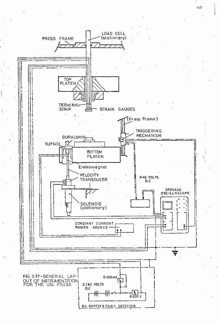
DURALUMINr
TUFNOL
BOTTOM PLATEN
Etetromagnet
VELOCITY TRANSDUCER
SOLENOID (stationary)
CONSTANT CURRENT POWER SOUR CE
159
LOAD CELL PRESS FRAME .„----- (stationary)
TERMINAL---r, STRIP STRAIN GAUGES
(Press Frame)
TRIGGERING MECHANISM
045 VOLTS D.0
STORAGE OSCILLOSCOPE
e
FIG.3.27-GENERAL LAY-1 0-100mA OUT OF INSTRUMENTATION FOR THE U.S. PRESS I 0-180 you's
D.0
4 D.C. SUPPLY & FAULT DETECTOR
0-200 V

160
The d.c. from the accumulators was fed via a line fault detector
to the load cells. The fault detector unit consisted of voltage and
ampere indicators with an on-off switch. The purpose of this fault
detector was to give visually an indication of any fault developed
within the supply or output lines to the load cells, during the course
of experimentation, besides indicating the correct voltage input to the
load cells.
The constant current to the velocity transducers, electromagnets
was supplied by a 0-1.5A Wier power Pack. The output from the load
cells and the velocity transducers or the e.m.f. generated from the
thermocouples for the temperature recording were fed to the amplifier.
The oscilloscope was triggered off in both types of tests, by a spring-
loaded-lever type microswitch just before impact. The microswitch was
fixed on the press frame with its junction connected to the triggering
connections of the 394 time-base unit in series-with a 60 volt battery.
When the bottom platen, in moving up, pressed the lever, a closed
circuit was set wbich caused the oscilloscope to trigger. Provision
was made to move the triggering mechanisms up and down the press frame
when required, but within certain limits. This was provided since during
the compaction the extent to which the bottom platen moved varied
according to the velocity or the increment of compression. Fig. 3,.28.,
illustrates the setup of the instrumentation and the positioning of the
triggering mechanism on the press for an incremental test*
3.5 Material and Lubricant
Specimens of commercially pure aluminium and high conductivity
copper were machined from cold drawn bars and each quantity of one
kind for a particular test series was heat treated in a single batch.
Heat treatment for aluminium consisted of annealing to 360°C for one

'14
Trigge ring mechanism
tocity nsducer
FIG. 3.28 ARRANGEMENT OF VELOCITY TRANSDUCER AND TRIGOE RI N MECHANISM ( incremental set up)
161

1 6 1

162
hour Followed by subsequent furnace cooling. The copper specimens
were annealed to 600°C for one hour duration and then furnace cooled.
Oxidation of the copper specimens during the annealing treatment was
partially avoided by wrapping the test pieces in thin copper foils.
Since during the experimentation a vacuum furnace became available,
further heat treatments were carried out in this furnace. Needless to
say the copper specimens in this case were heat treated without the
copper foils.
Molybdenum disulphide grease was used as a lubricant in all tests.
The lubrication was carried out before each test and between each
increment of compression.
In most cases specimens of 1.59cm diameter were used for the
dynamic incremental tests, usually with a length to diameter ratio of
unity. For some tests larger or smaller length/diameter ratios were
used to obtain data at higher or lower ranges of strain rates and for
particular ranges of strain. If however in such cases, buckling or
barrelling occurred, the data were discarded. The aspect ratio was also
chosen such that for a particular increment of deformation, elastic
stress wave propagation within the testpiece quickly reached the
equilibrium position after which the stress was measured,
For the quasi-static testing, only specimens of length/diameter
ratio of unity were used. Each specimen was 1.59cm in diameter.
Specimens for continuous large deformation tests had diameter of--
2.54cm with usually a length/diameter ratio of one. Large diameter
specimens were used since protection of the tooling and the machine
were essential particularly at high speeds. Specimens with larger
aspect ratios were mainly used to determine strain rate/strain histories
at lower ranges of compattion velocities.
For the temperature measurement during the continuous deformation
only specimens of 2.54cm diameter with length to diameter ratio of one

163
were considered. In all dynamic cases it was assumed that homogeneous
deformation without dispersion prevailed up to the strains considered,
or else the results were discarded. Fig. 3.29 shows typical specimens
of aluminium as subjected to incremental and large deformation trials.
Fig. 3.29(a) shows specimens prior to and after compaction. It is clear
that relubrication between each incremental step and the effect of high
speed on the lubrication condition, caused the homogeneity in deformation
to be a prevalent factor in all cases throughout the deformation
(Fig. 3.29(b)). Similarly up to reductions of 68% no pronounced
barrelling was observed in continuous deformation trials.

20 0/0
Compressed to^ 68°I°
42°10
Before compression
After compression
(a.)
I n cremental tests
b) Large deformation tests
FIG.3.29 TYPICAL SPECIMENS OF ALUMINIUM SUBJECTE D TO INCREMENTAL AND LARGE DEFORMATION TESTS

CHAPTER 4
THEORETICAL CONSIDERATIONS
4.1 Introduction
The theoretical work comprised of two parts; (a) the work
pertaining to the analysis and the assessment of the experimental
data for the determination of the material properties and (b) the
theoretical analysis using a finite element method and the computation
procedure (Chapter 5) adopted to establish the temperature field in
high speed axisymmetric upsetting with constant end frictions and
homogeneous deformations. Most of the work concentrated on the latter.
4.2 Analysis and Assessment of Experimental Data
4.2.1 Determination of dynamic material behaviour
From the load and velocity time recordings, the dynamic flow
stress/strain curves may be obtained by assuming a homogeneous strain
field such that: h
s load x
A (4.1)
.h i
6h /
If c= — the strain rate in the time t can be expressed as: h
165

1156
(4.2)
[ 2 ndt (")— 6h dt
h
as I5h --->dh then
Limit ; = dh/dt
h
or E=
(4.3)
At any instant the strain rate may therefore be evaluated from
the recorded velocity/time of the deformation. In the incremental trial
since the speed of the deformation (v) remains substantially unaltered
by virtue of choosing a small deformation step (oh), t in each incremental
step may then be evaluated by taking h as the, specimen height prior
to each compression step. Natural strain may simply be expressed as:
E = in —
4.2.2 Estimation of the limiting strain rate error,the adiabatic
temperature rise and work ratio in incremental tests
Since expression 4.3 introduces some error of small magnitude in
the estimation of strain rate in the incremental deformation tests, the
magnitude of the limiting error introduced should be established. This
may be predicted in two ways:
1) Assuming constant velocity and kinetic energy (K.E.) of compresion.
Referring to Fig. 4.1, the percentage of the error in strain rate
Fig. 4.1: Specimen's geometry before and after an increment
of deformation

167
(terror) may be defined as:
7 M
t X 100
error ti
0.4.4,0***0.......e000400 ,111;( 4,,5 )
where ii
= strain rate at the onset of deformation = hi
m = integrated mean value of the g during the compression
step from an initial length hi to a length hn.
If v = velocity of deformation in the deformation step Eh = hi-hn
then for hn< h<h1P
hi
m = dh
h. - hn
1
h n
h.
we
2)
at
ln hn
Tin as
hi
expressed above
h l -- 1 n
hn
platen before
x
into expression
100
and after impact
(4.6)
4.4
hi
hn
Substituting for T and
get,
error h
[
Considering the K.E. of
- h n
(lower)
rewritten Expression 4.4. may be
and'after impact such that,
in terms of the platen velocities
v vn
h.i hn
g error v
i hi
(4.7)
Since generally K.E. = -2-111v2. it would follow that,
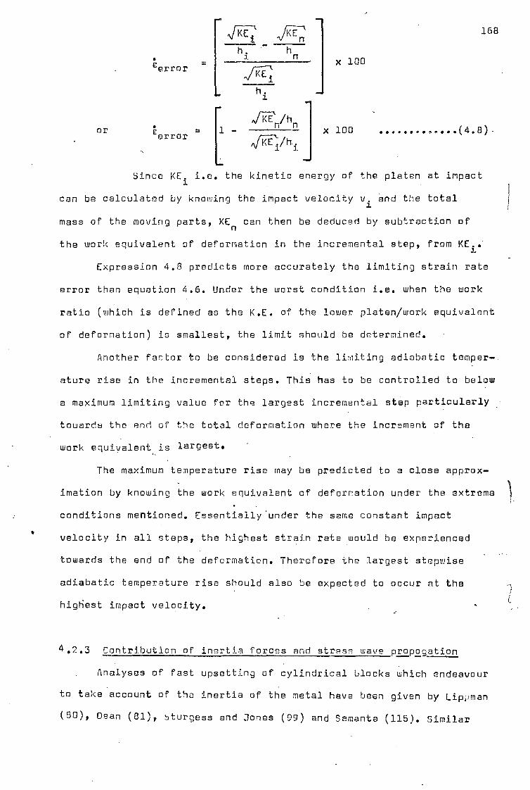
1
VKE KE 1
h. h J.
OOP
168
x 100
— ,IKen/h
n
A/KE1/45 x 100 ........ ,....(4.8)-
=MP
error
or error
Since KE. i.e. the kinetic energy of the platen at impact
can be calculated by knowing the impact velocity vi and the total
mass of the moving parts, KEn can then be deduced by subtraction of
the work equivalent of deformation in the incremental step, from KEi.
Expression 4.8 predicts more accurately the limiting strain rate
error than equation 4.6. Under the worst condition i.e. when the work
ratio (which is defined as the K.E. of the lower platen/work equivalent
of deformation) is smallest, the limit should be determined.
Another factor to be considered is the limiting adiabatic temper—.
ature rise in the incremental steps. This has to be controlled to below
a maximum limiting value for the largest incremental step particularly
towards the end of the total deformation where the increment of the
work equivalent is largest.
The maximum temperature rise may be predicted to a close approx-
imation by knowing the work equivalent of deformation under the extreme
conditions mentioned. Essentielly'under the same constant impact
velocity in all steps, the highest strain rate would be experienced
towards the end of the deformation. Therefore the largest stepwise
adiabatic temperature rise should also be expected to occur at the
highest impact velocity.
4.2.3 Contribution of inertia forces and stress wave propogation
Analyses of fast upsetting of cylindrical blocks which endeavour
to take account of the inertia of the metal have been given by Lippman
(80), Dean (81), bturgess and Jones (99) and Samanta (115). Similar

pv 2 2 pv C o e
y
and aCtn-.1 24 ye (4.9)
169
ine2tia effects have also been etudied by Dharan (72) who also considered
the wave propagation effects within the specimen, using one dimensional
wave theory. It is envisaged that below the compression speed of about
16m/s, or strain rates less than 1000sec-1
inertia nertia effects are usually
negligible. '
Lippman's analysis or Dharan's theory may be used to predict any
possibility of inertia effects and stress wave propagation within the
specimen.
Using Lippman's dimensionless quantities as and pp where,
Tr leak:10-2 and If3r31--- 10-2 then the error introduced by inertia
effectc would be of the order of 1%.
Using equation 2.64 of Dharan (72) the magnitude of radial
inertia stress may be estimated quantitatively; viz.
ps r.
2
3v2
dv —
2hi(1-e) dt
(4.10) r. - 4hi.(1-
In using von 'Mises' Criterion as before the flow stress may be
expressed as:
as =oz r -a a r = oe (4.11)
where or, o
z and a
6 are the components of stresses in the
coordinate axes r, z and 0 (Fig. 4.1). In our context,
o = stress calculated from the load records z
In the incremental test since the velocity of impact substantially
remains unaltered throughout the deformation step, the rate of change
in the deformation velocity with time, may be taken as zero, such that.

tb/t = time taken for a longitudinal elastic wave to traverse
the specimen length h at wave velocity c
time taken to attain a strain e at which point os and c
are measured
170
r. 0 =
1,2 ki2 r. "sh.' (1-e)
3
(4.12)
The geometry of the specimen affects both the inertia restraints.
and the transient elastic wave reflections within the testpiece gauge
length. It moreover affects the frictional restraints at the end faces
(116). This latter effect is of great importance in shorter specimens
resulting in high measured stresses.
As briefly mentioned in Chapter 2, the basic requirement to
satisfy the imposition of stress wave reflection is to choose a specimen
gauge length such that the ratio,
should be .:?.= 8 (4.13)
. A choice of h 3./d. equal to unity together with a suitable
lubricant should generally overcome inertia and frictional restraints
and barrelling effects to a satisfactory extent (116)(117). In increm-
ental tests since the specimen and faces are relubricated between each
incremental step, and therefore frictional and barrelling effects are
much reduced, specimens having other aspect ratios than unity may be
used providing other impositions are taken care of.
4.3 Estimation of Temperature Field
4.3.1 Review of previous works
In dynamic processes due to the limited' time available for heat
losses to occur, most of the deformation work appears as heat in the

171
testpiece(118). Several.attempts were made previously to measure and
predict the temperature change and distribution as a result of this
heat of upsetting in some metal working processes. As mentioned in
Chapter 2, Nadai and Manjoine (50) in predicting the dynamic behaviour-
of some steel specimens recorded the local surface temperature rises
under high speed extensions. As seen in Fig. 2.35 high temperatures,;
were recorded near the region where most plastic deformation takes place.
In the environs of this zone lower temperatures were measured indicating
short duration of the time available for heat transportation. In
extrusion and drawing processes similar pioneering investigations were
carried out by Siebel and Kobitzsch (119), Hirst and Ursell (120) and
others.
Siebel and Kobitzsch estimated the temperature gradient/ in the
material and the die in wire drawing by neglecting heat flow in the
axial direction by assuming uniform deformation and a constant coefficient
of friction. Hirst and Ursell used an empirical formula for determining
the extrusion pressure and hence estimated the average temperature
increase of products extruded through square dies. The early significant
contribution in the field of temperature changes occurring during
extrusion is due to Watkins et al (121). In this work, temperature
changes taking place in billets during the extrusion of several non-
ferrous metals and alloys at room and elevated temperatures were recorded
by means of inserted thermocouples. Pronounced rises in temperature
were recorded in the region of the die. Singer and Al—Samarrai (122),
Singer and Coakham (123) measured and predicted with same approximations
the emergent temperature of extruded products. They assumed a simple
model in which all the deformation takes place as the metal crosses
the die exit plane. No container friction was assumed and the heat
transportation was considered to take place only in the axial direction.
This work was further extended by Sauve (124) by assuming an average

.31.72
velocity and uniform deformation under the die. 5euve neglected the
die/billet interface friction but considered the heat transfer to the
tooling and established the temperature field in the axial direction.
Tanner and Johnsen (125) using the slip line theory for the velocity
field, considered some of the aspects of temperature, rise which occur
when a metal is rapidly plastically deformed perticularly under plane
strain conditions. Although references were made to flat punch indent-
ation of a semi-infinite medium, compression between a• perfectly smooth
plane and forging of a block of material with three equal sized
symmetrically inclined punchesl'the emphasis was mostly on plane strain
extrusion. Johnson and Ludo (126) extended this work and by neglecting
die/material friction and assuming an ideal plastic material established
the adiabatic temperature increase in axisymmetric extrusion processes,
using realistic upper bound solutions and an admissible velocity field.
A fast hot rolling process was also considered partly to justify the
use of the method employed. The result of their calculations also took
no account of such features as roll distortion, radiation losses,
conduction losses to dies or rolls, variation of yield stress with
temperature.
Kellow et al(127) assessed the die temperature transient in
axisymmetric hot forging operations. fly using encapsulated thermocouples
below a simple circular flet forging die, die and die/billet interface
temperatures during simple upsetting operations were measured. High
degrees of temperature rises were recorded both at low and high speed.
It was noted that in so far as high speed conditions were concerned,
surface temperature was higher due to higher friction work. The sub-
surface temperatures of the die were however dependent on forging speed
and were much higher at low speeds,
Peishop (126) pioneered the development of the principle of the
numerical incremental method and estimated the temperature distribution

173
in the deformation zone and product for the plane extrusion of a
plastic rigid material. He assumed no die/material interface friction
and used a simple slip line field to evaluate stress, strain and strain
rate and regarded the heat generation and deformation as occurring
simultaneously, followed by an interval in which conduction takes place
as for a stationary medium. Akeret (129) using Dusinberre's (130)
finite difference numerical approach estimated the temperature of the
extruded product in hot extrusion and attempted to predict the input
variables to generate a steady emergent product temperature.
Altan and Kobayashi (131) basing their method on Bishop's approach,-
by employing the visioplasticity method (132) for obtaining velocity
field and Dusinberre's finite difference solution of heat conduction
problems, calculated the temperature distribution in conventional
extrusion processes. Guha and Lengyel,(133)(134) on the other hand
considered the heat generation, transportation, conduction, convection
and radiation in high speed hydrostatic extrusion drawing and, using
a finite difference method, obtained the temperature field in the
billet, Product and tOol. Coulomb's friction with constant coefficient
of friction was assumed. Both Altan and Kobayashi and Guha and Lengyel
used temperature dependent thermal and mechanical properties. The latter
was also considered under varied dynamic conditions.
Recently Lange (135), by using a difference principle, evaluated
the energy field and temperature distribution in cold axisymmetric
upsetting. This work concerned only low magnitude compression velocities
and Lange verified experimentally his predicted temperature distribution
by using thermocouples embedded in the meridian plane of the.specimen.
4.3.2 The finite element approach
The finite element method is now widely used for the solution
of continuum mechanic problems (136)(137)(138), in particular the

174
analysis of some metal working processes (139)(140)(141)(142). The
generality of application of the method is given by Zienkiewicz and
Cheung (143). In brief, with a finite element approach the continuum
is replaced by an equivalent system comprising of discrete elements.
In the finite difference method a direct approximation is made to the
governing equation in terms of a finite number of values of the unknown
quantity selected at strategic mesh points. In the finite element
method the solution of the differential equation is transformed
(ex: by the variational principle (144)) to an equivalent problem of
minimizing a functional which is defined by a suitable integral of the
unknown functional and its derivatives. Other approaches such as a
direct equilibrium formulation are also possible. In any event if a
variational process allows a finite element formulation then (a) other
parameters than nodal known values could be included in the analysis
and (b) many alternative formulations of the same problem are possible
(145).
The real power of the finite element methods lies in their
ability to deal with non-homogeneous situations and the case where
element size and shapes may be altered and regarded to follow arbitary
boundaries and to allow for the region of rapid variation of the
unknown functional. Boundary conditions can simply be introduced. With
a method such as the present approach, time dependent functionals can be
incorporated with simplicity and with imposition of no restrictions
as to the magnitude of the time. High order elements may be included
to improve accuracy without complicating boundary conditions.
There is no record of anyone ever using the finite element
method for the determination of the temperature field in any metal
forming processes, although literature is cited for the transient field
problem of the type encountered in heat transmission topics. However
the general mathematical formulation as to the application of the method
to the determination of transient temperature distribution and thermal
175
deformation is due to Visser (146).
Works due to Wilson and Nickell (147) and Zienkiewicz and Parekh
(148)„ using a finite element approach, are concerned with time dependent
temperature distribution problems. Wilson and Nickell analysed the method
and applied it to the heat conduction analysis of complex solids of
arbitary shape with temperature and heat flux boundary conditions.
The method was developed in detail for two dimensional bodies which
were idealized by systems of triangular elements. Elements of various
shapes and the associated temperature field were discussed for one,
two or three dimensional bodies. A method of solution for the Euler's
equations of the Lagrangian form which are obtained by the variational
principle was introduced which provide stability and minimum computer
effort. A similar procedure is adopted in the present work. In a
similar manner, Zienkiewicz and Parekh applied the method to two and
three dimensional temperature transient field problems by using
isoparametric finite elements to establish the temperature field in
a turbine rotor blade.
Recently Soliman and Fakhroo (149) in using a finite element
method analysed in detail solidifications of steel ingots. They used
a two dimensional model and in their work took into account the variation
of thermal properties.
4.3.3 Governing equations
The present problem to be examined is that of time dependent heat
flow in an incompressible moving medium with heat generation due to
deformation and friction. A finite element method descibed below is
formulated to establish the transient temperature field,in axisymmetric
upsetting with tool/testpiece interface heat flux due tO the work of
friction. Although the problem is three dimensional, the symmetry of
the body (Fig. 4.2) allows the variables to be described as a two

1
compression
1 1 compression
FIG.4.2 AXISYMMETRIC BODY UNDER COMPRESSION & AN ARBITRARY TRIANGULAR ELEMENTAL RING
176

177
dimensional field. The governing differential equation of heat trans-
portation for the two dimensional field is thus:
6, b.T x '6T
ko k r --) -- kK r ) = p-- zr r ar bz z bz br
(4.14)
kr
and kz
are thermal conductivit:es in the r and z directions
respectively and p is the density.
Equation (4.14) together with the following conditions (Fig. 4.3)
satisfies the problem in a unique manner,
T = Tb' on the boundary with known T
dT k = -q on the boundary with heat, flux
dnb
having normal nb
(4.15)
and hF(T T
f) = k --_, on the boundary with convection
unb
where T > Tf
hF = heat transfer film coefficient
Tf •
Fig. 4.3: An arbitrary solid subjected to transient heat conduction
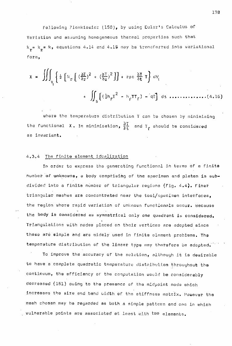
178
Following Zionkiewicz (150), by using Euler's Calculus of
Variation and assuming homogeneous thermal properties such that
k = kz
k, equations 4.14 and 4.15 may be transferred into variational
form,
X = fa, 1k 1 (.41-N2 /2.1\2]] 2).T. rpc at ' L rt. \ br 1 oz) vi
if ((111FT2 h
FTT
f
0 .0 0 . ********* (4.16)
whore the temperature distribution T can be chosen by minimising
the functional X. In minimisation, and Tr should be considered
as invariant.
4.3.4 The finite element idealization
In order to express the generating functional in terms of a finite
number'of unknowns, a body comprising of the specimen and platen is sub-
divided into a finite number of triangular regions (Fig. 4.4). Finer
triangular meshes are concentrated near the tool/specimen interfaces,
the region where rapid variation of unknown functionals occur. because
the body is considered as symmetrical only one quadrant is considered.
Triangulations with nodes placed on their vertices are adopted since
these are simple and are widely used in finite element problems. The
temperature distribution of the linear type may therefore be adopted.
To improve the accuracy of the solution, although it is desirable
to have a complete quadratic temperature distribution throughout tha
continuum, the efficiency of the computation would be considerably
decreased (151) owing to the presence of the midpoint node which
increases the size and band width of the stiffness matrix. However the
mesh chosen may be regarded as both a simple pattern and ono in which
vulnerable points are associated at least with two elements.

0.508cm
0.508 CM
r
Boundaries of Constant Temperature.
1.778cm
179
FALAWIALALIAIALAAIALI 141 111.61111114411 smardestomenermuomen BIERSBIVESMINEAVIIIMEIMMINIGLIME 11011111/11/1151.51 ALIMILIPAILWARINNINW
121115111111ffELMMINEMEMISIIII ISAMMEOLMEITIPAVEMOI a MENEMILUMOMEINEMEMILAII MILIPMERINERIAMM20/111111/ P
1111 1111111111 1111111111111 11111111111111
Q FIG. 4.4—THE IDEALISED BODY WITH
TRIANGULAR ELEMENTS.

aT az
where 2A = det
(b.- bk ) bk
bj Ti
T . > (4.20)
ik
a
b J.
= 2 (volume of element ijk) ak
bk
-ak
a.
I
{ T } e = .
T.
i J
and {-34) e =
( x Ti
ax
T.
ax k
Tk
(4.21)
180
The admissible temperature distribution rendering the functional
continuous throughout the discretized system is given as,
T = Ti + C 1r + C2z (4.17)
An element of the continuum as dimensioned is shown in Fig 4.5
such that in terms of the local coordinates,
Tj = T. + C
l a. + C
2 bj (4.18)
Tk i = T + Clak + C2bj
(4.19)
From the above simultaneous equations C1
and C2
can he expressed
in terms of nodal point temperatures. Since from equation 4.17,
Cl ar = 1-T- and C
2 = - ?-1-
' it could then follow that,
az
Since the unknown function T is defined element by element in
terms of nodal point parameters, then the approximate minimization has
to be carried out accordingly.
For an element ijk the following are defined,
The minimization of equation 4.16 would therefore take the
following form:

r FIG.4.5 TRIANGULAR ELEMENT DIMENSIONES

182
) e a rrr r r r 0 ttf/ )1) (M2]] rPc at T (NI
V az
js F T2 — hFTTf ) ds ....(4.22)
Consider the minimization of the function X term by term:
(a) Conduction only
22:I 217 DaT aT 2
D 2 + az' 1 rdrdd s.0000.9.0.(4,23)
The simplest approximation procedure is to consider
r = (r + rj + r
k)/3 • .(4,24)
for a centroidal point. Although a more elaborate numerical
integration scheme could be used, this method would however converge
to an exact answer within the limit of the elemental subdivisions
(150)
From 4.23 and 4.24 and since lidrdz = A it could follow,
tax I e aT D ( DT dT (a
= 2n
)
aT ]
7" f(ar ) TT '717 )\
DT az
For each nodal point,.
{D X = 23.Tr, k A I (a) (.aN fa) (..1).] DT. 'ar ) ai
l 'arl + 'az ) DT `az / 2. i
IP • • • •• . • • ••a ( 4 .25 )
** (4.20
From expression 4.20 it would follow that:
OT. (7.77) :1- 2A (bi bk)
(4.27)
aT 1 al-. az, - 2A (ak aj)

183
aT SubstitOtionbfecluations4.27andvalueso nd (—) from
`br' az
expression 4.20 into equation 4.27 gives,
Dx rk - 2n— (b.- b )
2
3T. 44 k ( "ak- ai)
2 T i + [ bk( b j- bk ) ak(ak- ai)
Similarly,
+ + a.(e as)] Tki j k J k
(4.28)
rk 2r 7 [b .
k 2
1. k(b j- b) ak(ak- aj) ]Ti I r
ak2
[ -bkbj aka, Tk
• *0 • • • • • • • • • • • i• • • ( 4 .29 )
and
TX Tk •
2r 47E I -b.(b - b ) +- a
k k - ai) J Ti -b.ba .a jk j k
T
b2+ a 2]
Tk (4.30)
For an element from equation 4.20 to 4.30 it can be concluded that,
(bj- b
k)2
+ (ak
a
bk(bj
bk)
-ak(ak- aj)
bk2+ a
k2
b j k)
+ a j .(a - a ) k j
b a a - kj jk
aX e = 2 rk n aT 4A
SYHIT
b.2 + a.2
J
..(4.31)

184
Minmization has to be carried out over the whole area thus:
_ s {
_ ().T 1 8 = 0 where from equation 4.31 4r) - 4-
e K.. = k . lj 1
(4.32)
(b) Free boundary surface heat transfer
The term If (1hFT2
- hFTTf )ds in equation 4.16 accounts for heat
losses from free surfaces owing to convection. Far boundary elements
this expression has to be minimized only for the discrete nodal points
experiencing heat transfer to the free surrounding environment.
For a triangular element ijk (Fig. 4.0 where'any side can convect
heat, T may be assumed to vary linearly between the two nodal points.
Fig. 4.6:
triangular element with one side convecting heat
For side jk (Fig. 4.6) convecting heat to the surrounding air,
I = Tj (1k- T.) 1/L . (4.33) j
Since the actual body is regarded as axisymmetric, the
following generalised functions are applicable depending on which side
of the triangle (Fig. 4.7) and along which coordinate axis it is
subjected to convective heat transfer.
Along the end face x = if(2hFT2- hFTTf ) rdrdO (4.34)
Along the side face x = 1j(12hFT2- hiTTf ) rdedz (4.35)

185
Now for the element (1), Fig. 4.7 whose side ik is subjected to
heat transfer by convection expression 4.34 is applicable such that
after substituting for T from the generalised expression 4.33 we get,
X= jiilh [T. + (Tk- Ti) r/R1 .1 2 - hF { Ti + (Tk- Ti)r/Ril T f rdrdO
• •
(4.36)
To evaluate expression 4.36 r may be approximated to ribr=(ri+rk )/2
such that,
x = 23111brhF JR' f -2 [T.2 + r2
r --.,(T
2- 2T.T + Tit ) + (T - Ti )T k 1 k
2 R k 1 i 1
1
TiTf - 7- (T- T.)Tf dr ,
(4.37)
which after integration gives,
X = 237Pbr hF R1 6
(1.(Ti 2+ Tki 2+ TT
k )
f(Ti + T
k )]
(4.30)
Minimizing the function with respect to nodal point parameters
would provide:
1 0
"
e
= h 0 0 0 1 - 2377 h 1 T
R1 e
aT br F 3 brF 2 'f
0 1
(4.39)
Similar expressions would be obtained if other boundaries of the
triangularelements were convecting heat. For example for element 2
(Fig. 4,7), if side ij is convecting heat only:

dA Az 211Rbz Z 1
I-bz---(' r1b+rk )/2
dA=rdrde A-2-TtRbrRl RbF I (r+ rk )/2
FIG. 4.7 AN AXISYMMETRIC CONTINUUM WITH TRIANGULAR ELEMENTS SUBJECTED TO SURFACE CONVECTIVE
HEAT TRANSFER

- 231R h T br 2 F f
1
Similarly for side jk:
2.)-( = arfi h aT br F 3
187
0
R1
= 2n11 aT br
h F 3
1 A 2
2 1
L 0
0
0
0
(T) R1
-h T br F 2 f
(4.40)
where n'br . )/2
where Flbr
= rk )/2
j
* • ************* o • • • • • • 4.41)
For this corner element since two sides are exposed to air,
the contribution of convection is therefore due to both expressions
4.40 and 4.41. The minimization with respect to the whole continuum
can be expressed as:
1+13 = hij (4.42)
(c) The transient
r
term
J )( The term I (pc -- T) dV
tconstitutes the non-stationary part
v 1 of the formulation. Therefore for an element ijk:
X= iff ( pc T) rdrdzde (4.43)
Using the approximation mentioned in (a):
x= 2rrr pc JJT drdz (4.44)
Substituting for C1
and c2
in equation 4.17 and the resulting

188
expression into equation 4.44 gives:
, DT X = 2nrpc jlf(Ti+ r
aT + z
aT az)
a 517kTi + r ar + z drdz .....(4.45)
From Zienkiewicz (150) the following integrations are applicable
drdz =
rdrdz = J1 zdrdz = 0
ff r2drdz = 12`aj2 ak
2 \
JI z2drdzA 2 h 2) = 12
i'Ljh j -k /
(4.46)
ff rz dr dz (ajbj+ a bk) = 12
Integration of expression 4.45 together with considerations shown
in 4.46 yields:
T. (a ;2+ 01(
2)
( aT) a ( aT \ X = 23-ISApc Ti (7-t1 + j 12 'ariar'arl +
(abj+ akb.) (b 2+ by 2 ) T
k ( al- ) a ( aT, + ,x) .) t ar) 12 ‘.ar'at'az / aziat'ar1 4. j 12 ''< (az a (4)) at az
• • • • •
(4.47)
From expression 4 1 20 we have:
DT _ ar 24 (b j- bk )Ti + bkT j bilk]
a oT DT. DT. DTk (
War/,
= 24 { (13j- bk )at -k at h - j at
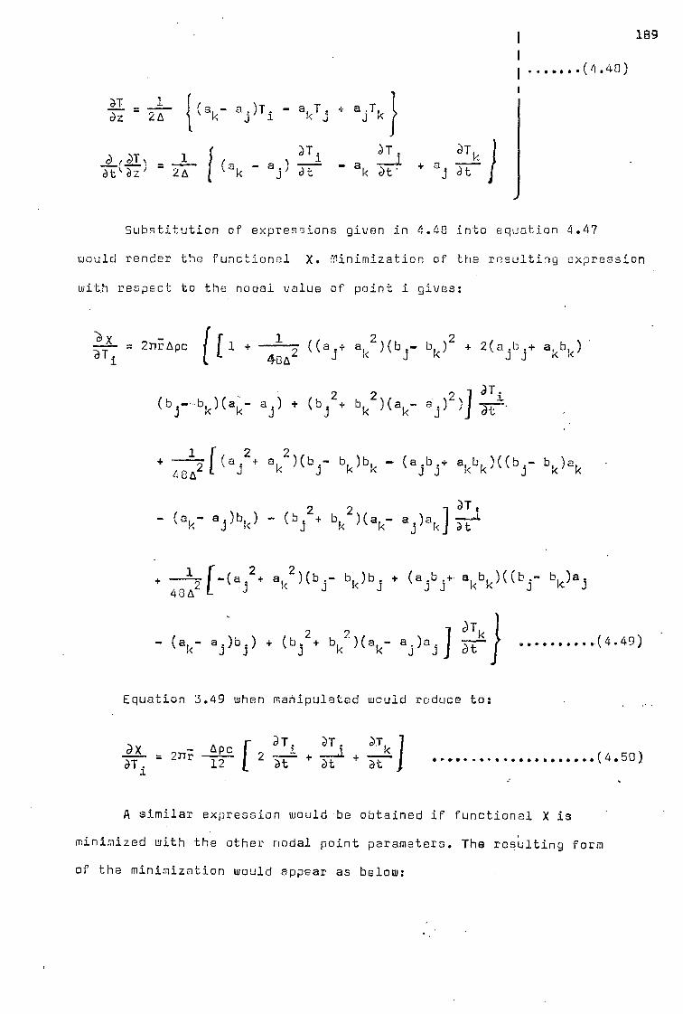
189
..... (4.48)
( a a , af T. + a .T, az - 2A kji x,3 Jr'
. a ( aT. 1 ( )
3T 1
t‘z ) - 2A `ak ajl at - a
3T 3Tk 4/ „
k at'
Substitution of expressions given in 4.48 into equation 4.47
would render the functional X. Tinimization of the resulting expression
with respect to the nodal value of point i gives:
1 —X -aTi
2317 Apc 48A2
j I 1 + ( (a + ak
2) ( b j
- bk )2
+ 2(a .1-3 j+ a
k b, )
j
(bj--b
k)(
aT. - a ) + (b
j
2+ b
k 2)(a
k j - a)
2)]
+ 1 1,a
j 2+ a
k ) 2.(0 .
---7 j bk)bk (ajbj+ akb )((bj. bk )ak 48A
al. 4 - (a
k- a
j)bk) - (bj
2+ b
k 2)(a
k - a
j )a
k ---J-
a.2+ akj 2)(3- b
k )b
j + (a j13
j .+ a b )((b
j bk )a.
K.)
aT
- (a,- ab.) + (b 2+ bk )(ak
2 - a.)a i at ...... (4.49)
J j
Equation 3.49 when manipulated would reduce to:
aT aT, aX APc 1- 2
T.
k 2.TT aT. 12
+ at + at
( 4.50)
A similar expression would be obtained if functional X is
minimized with the other nodal point parameters. The resulting form
of the minimization would appear as below:

190
f o
e
" = 211; pc 12
2 1 1
1 2 1
SYMT 2
fT1°
(4.51)
The resulting matrix can be checked against the similar matrix
obtained by Wilson and Nickell (147).
When minimization is carried over the whole continuum would
produce:
C.. = e 1.1
• -I • • * e • • • 0 fa • • a • • • • • • • • ,52)
(d) Boundary heat flux
In equation 4.16 term If qT ds applies to elementswhere any of the
boundaries are subjected to heat flux due to generated work of friction.
As in (b) (Fig. 4.6, equation 4.33) the temperatu're T may be assumed
to vary between two nodal points. Following a similar procedure as in
(b) (Fig. 4.7), for side ik:
R1
)0.12rii7,01,q x
1[1.+(T, - Ti) 11 — dr 1 0
which after minimization would result in the following equation:
,) ) 8
dT = 2TT:lbrcl . . (4.54).
where Pbr = (r.1+ r
k )/2
Similarly,
for side ij ax aT = 2nr. q br
.(4.55)
where Rbr = r.+ r.)/2
4 53

e
and far side it: ---- = 2rril, qZ
.1. ur 1
0
1
1
0 0 000 ***** 0 * **
191
(4.56)
where Pbr
= 1.1)/2
4.3.5 Assembly of minimizing equations
For a typical element ijk subjected to transient conduction,
boundary convection with heat flux, the total minimising equation
reads:
.0 . i)x) e
aT
iki e iT] a 4. HeiT e cj e e e
600000 (4.57)
in which the stiffness matrices [k] and fc] can be obtained
from expressions 4.31 and 4.51 respectively. For matrix [hi' any one
of the expressions given in equations 4.39, 4.40 or 4.41 is applicable
depending on the side of the triangle subjected to heat transfer by
convection. Similarly fq )e
accounts for the known boundary heat flux
to the element and for this any of the expressions 4.54 to 4.56 may
be adopted.
Assembly of the whole , set of minimizing equations follows the usual
finite element rules (150). Thus for the whole region:
ax aT = 0 (4.58).
such that,
[K.itT) H i TJ T = g I (4:59)
As only one variable is considered, scalar quantities only arise'
in the above.
4.3.6 Recursive procedure
Since initial values of T (where t=0) can be specified, a numerical

192
recurrence process (148) can be applied to find the solution at
subsequent times.
For the most accurate way of solving the transient thermal
problem, Wilson and Nickell's (147) recursive process may be followed.
c)T Using the Crank Nikolson formulation i.e. letting TE vary with time
over the time interval At we have:
IT] aT
= (r) + + t+At t 2 at
t+ At
It could follow that:
aT at f2
L [
t+At et
t+ At t T it] - dti
(4.61)
Substitution of equation 4.61 into equation 4.59 would provide
the temperature field at time t+At auch that:
( K] f H11 1
2
t+At t+At {i.I t+At
2 = (qi + [C] [ T) + c] T ....(4.62)
For a typical element (.S) shown in Fig. 4.8 with boundary ij
subjected to heat flux q and the side jk convecting heat, equation
4.62 when written in full appears as below:
4 60

PLATEN
Line of discontinuity R (s) I
AIR
r
193
FIG.4.8 TYPICAL ELEMENTS ALON G THE LINE OF DISCONTINUITY

(b -b2
k)
+(ak-a
j)2
b ) k j k
-a (a -a.) k k j
-bj(b.-b
k )
+a.(ak -a.)
194
rk 4A b
k
2+ak2
-b b.-a.a Jk
SYMT b.2
+9.2
J
0 0 0
0 1
0 2 1
t+ At
t+At e
2 1 1
2 1
6YMT 2
+ TRtyzhFR1
3 pc t
+ b At
a
t
22A
2
SYMT
1
2
1 ie T.
T.
Tk
6At =
1
PL Z,c1[ 2
plcA
2
SYMT
Rbz
=
1 1
2 1
2
(r.+rk )/2
1.
t
Rbr
= (r.+rk )/2
OT.
4. 12
where
at
aTk
at
and
(4.63)
Thus { T j can be known by solving the above system of
t+ At simultaneous equations namely (4.61) and (4.62) provided that the
values of i T] and NI are initially known.
At time t=0, { TI is known. Following Zienkiewicz and Cheung
(151), substitution of nodal point temperatures T into equation 4.59
would then render the determination of 7 at the initiation of
conduction such that:

t=o q
t=o
195
4.3.7 Peat generation due to deformation and work of boundary_friction
The temperature of the deforming material rises due to two
factors, (a) plastic work of deformation and (b) generation of heat
due to the generation of friction created along intimate surfaces.
Temperature rise due to deformation is proportional to the plastic
work done on the material. Therefore adiabatic temperature rise in
the time interval At is given by:
ustAt os
AT = 0-57 . oJpG
.(4.65)
whore as = f(e, T), c=c(T) and p= p(T)
Addition or this temperature rise to discretizod nodal points
constitute the temperature field prior to conduction.
]The vector { q which constitutes the boundary heat flux repo
. resents the work due to friction (w
f) generated between tool/testpiece
intimate surfaces and may only be considered for the elements on the
sides of the line of discontinuity. Nodal points of these elements
lying on this interface therefore experience the friction work and
heat flUx should beassigned to them only.
Considering sliding Coulomb friction, the friction shear stress
acting on the die/specimen interface is given by
T = 11P ..w..... ..(4.66)
In the absence of reliable theory of lubrication the friction
coefficient maybe expressed as constant and the pressure disttibution
of the type expressed by Avitzur (152) may be assumed sUch that':
211 (R a— P = a
s e (4.67)
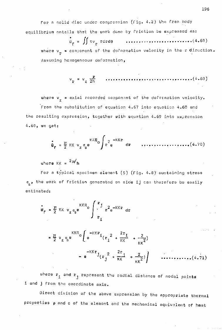
—KKr. 2
KK
2r
j — e 3(r + -a + 2
)I
KK (4.71)
196
For a solid disc under compression (Fig. 4.2) the free body
equilibrium entails that the work done by friction be expressed as:
1:1 f, = filvr rdrde
where vr
= component of the deformation velocity in the r
Assuming homogeneous deformation,
(4.68)
v = v -- r z 2h
• • • • 0 • • • 0- • • • • fir
(4.69)
where vz
= axial recorded component of the deformation velocity.
From the substitution of equation 4.67 into equation 4.68 and
the resulting expression, together with equation 4.69 into expression
4.68, we get:
• KKR 2 —KKr
f 2 = KK v
z os
o e e dr • 0 ********* • • • • • • • • (4 • 70 )
where KK = 2P/h
For a typical specimen element (S) (Fig. 4.8) sustaining stress
s the work of friction generated on side ij can therefore be easily
estimated:
f = KK v 2 z
0 se o
r
KKRf r i
r
' - 2 e —KKr dr
.
KKRo [ —KKr. 2 2r
2
1 = 2 vz ose a (r. + KK +
KK
where r. and rj represent the radial distance of nodal points
i and j from the coordinate axis.
Direct division of the above expression by the appropriate thermal
properties p and c of the element and the mechanical equivalent of heat

197
3, would provide the boundary heat flux q.
Inclusion of friction work as boundary heat flux in the heat
conduction equation has the advantage that the size of the relevant
elemental volume or area would not reflect on the magnitude of the
heat flux.
In compression tests frictional forces present on the die/work-
piece interface cause extra work. This work due to friction is dependent
upon surface conditions, aspect ratio and is a function of pressure
distribution over the faces of the specimen in contact with the compress-
ion dies. High velocity of deformation however,as shown above contribute&
greater friction work. If the velocity of deformation is high, then
work due to friction can attain considerable magnitude. This causes high
localised temperatures in the vicinity of the boundaries of contact.
If local work hardening effects are offset by this temperature rise
which causes localised thermal softening, then frictional conditions
would he altered. Therefore, the inclusion of friction work may provide
answers with regards to some phenomena observed under high speed upsetting.

CHAPTER 5
COPTUTATICN PROCEDURE AND'COMPUTER PROGRAnlING
5.1 Procedure and Programming
A similar approach to that of Rishop's (128) has been adopted
to determine the temperature field in high speed axisymmetric upsetting.
In essence, the deformation of the specimen is considered to occur
as a series of compression steps. Each step takes place in an interval
At. The heat generation in each step is followed by conduction to
the tooling and surrounding free air, as for a stationary medium,
in the same time interval At. The deformation is-assumed to be
homogeneous with constant platen/specimen interface friction. The
platen is assumed to make perfect contact with the specimen at all
times throughout the compression.
A computer programme was then developed.in FORTRAN IV language
to simulate the upsetting process where the compression of the
specimen and simultaneous generation of heat in a small time increment •
is considered to be followed by static heat conduction within the
same time interval. The principal block diagram of the incremental
computation procedure is illustrated in Fig. 5.1
Briefly the programme goes through the following cycles;
Thermal properties and flow stress data as a function of temper-
ature and the velocity time characteristics are read in and stored in
the computer memory. Friction coefficient p is chosen and the
triangular overall mesh pattern covering the specimen and platen
continua is then generated. The ordinates of the nodal points together
with their arrangements are established. Initial temperatures are
assigned to all nodal points. The elements in the specimen and the
198

START
Calculate displacement
199
Read and Store
Heat Parameters
Flow stress data
Velocity/time characteristics
of compaction
Set friction coefficient
COFMEU
Yes COFMEU > a max
Natue
Generate the triangular mesh system, -
establish nodal points and their
ordinates.
: Assign initial temperatures to all
nodal points
Establish platen specimen zones
Discern boundaries of convection &
fixed temperatures & the one boundary
subjected to heat flux
COFMEU.LOFMEU
+11 Choose increment of time TIMINC
Establish total deformation time TIMMAX
Set deformation time TIMDEFaTIMINC
TI,' DEF2> TIMMAY
FIG 5.1 BLOCK DIAGRAM OF COMPUTER PROGRAMME

Recompute' nodal point ordinates
&elemental areas.
make corrections to nodal point
temperatures within the platen
continum due to their movement
in r direction
Calculate• strain,strain rate experienced
by all nodal points
Compute the increment rise in temperature
AT and assign to the state of previous
temperature field
Calculate the temperature/time derivatives
prior to conduction steps
Calculate the temperature aistribution
in time intervalAtt smooth out and write
the temperature field
TIMOEF=OEFTIM+TIMINC
To A.
From the previous states of temperature
compute the stresses sustained in the
deformation zone
FIG 5.1 (continued )
200

201
platen together with boundaries of fixed temperature, convection,
and the one boundary subjected to heat flux, are discerned. Elemental
areas are computed.
An interval of time At is chosen and from the velocity/time
characteristics of the deformation, the increment of displacement
and hence deformation is calculated. Accordingly the nodal point
ordinates are modified and the elemental areas are recomputed.
Actually only nodal points covering the specimen continuum would
alter position, but the nodal points within the platen continuum are
also made to move artificially and only in the r direction. This is
essential in order to maintain the continuous mesh pattern for the
conduction part of the programmer Corrections to the nodal point
temperatures within the platen body except those lying on the specimen/
die line of discontinuity are accordingly made.
.train, strain rate and the stresses sustained in the deformation
zone are computed. Calculation of the heat equivalent of deformation
then follows, after which the temperature rise is assigned to nodal
points and added to the previous state of the temperature field.
Properties essential for these calculations are considered from the
previous state of the temperature distribution.
The gradient of temperature with tine prior to heat conduction
for all nodal points is established. CondUction and simultaneous
convection with heat flux due to the work of friction along the
specimen/platen interface are simulated for the same time increment
At. The new temperature field at the end of At is established and
the procesS outlined above is repeated until the deformation is
complete. A new friction coefficient is selected and all cycles of
the computation process similarly repeated. The programme stops any
time a particular procedure or declaration is not satisfied.
The computer programming thus developed comprised of sixteen
subroutines, four of which fulfill only minor operations. A complete

202
listing of the programme along with the name list of variables is
given in endix A. A commentary on subroutines is given below,
5.1.1 Subroutine INPUT
With subroutine INPUT, all heat parameters as functions of
temperature, flow stress data, i.e. the quasi-static stress curves,
with respect to strain and temperature and the velocity/time character-
istics of the compression are read in and stored in the computer
memory. Once these input variables are set, the sequential running
of the programme with different friction conditions can be achieved
without referring to any more external information.
Normally all input data are expressed in SI units except for
heat units which are expressed for convenience as 'kcal'.
5.1.2 Subroutine EON (calling subroutines TINTL, ZONE and 00UND)
Considering the geometry of the two bodies, i.e. the specimen
and the platen as one continuumIsubroutine GEN when called from
the main programme, subdivided the system into a number of 'triangular
regions with nodal points placed on their vertices. In practice,
firstly the elements covering a rectangular body (i.e. in our case,
the specimen and part of the platen) are generated, and then the
elements in the rest of the platen are added, completing the pattern.
The elements and nodal points are generated and numbered in a regular
manner, as shown in Fig. 5.2. A finer concentration of elements is
generated in the region of rapid variation in the functional i.e. near
the die/specimen interface. The distribution of points and the number-
ing of the elements are in accordance with standard finite element
programming in particular the type programmed by Palit and Fenner
(153)(154). This is for ease in the computation of nodal point var-
iables. Accordingly the technique of solution of these authors was
used for nodal point variables.
FIG. 5.2 NUMBERING OF THE ELEMENTS & NODAL POINTS IN THE MESH
IFAMIMIkii595 9
INEINEMP - MENEWIRM kiniairaUM MENIMMIkiLl
MARRIEMPr- SIMEM10116;.- EMBEM
Milla■._ INEMANNISEMBIIMh.- _..;7■0111ifts■- MiliiiiiIWINIVAGElliNELMILSW
ffil■FALIBIENERVEraik■
1111P"rilliwmi..---- Ibill■ IIIPwr"" Nima■L 95 1
Iiiii ltil... 1PMEIGNMINFAIENMIP
ill ibm... MEIMINEWAINIVAILIVah■
IIIIP__.•=1111ft395
3i4
IIIIPP"7- ■
111011Mit2'15
IIV•artillft_
IIPP"-7-
11110,Millimb,
Ili ntiliffin01516111§6141Pr IMINNIABEENEMIE
IPP■ognillraPnirEINEMENIMIP7 klIENI71411EELEMEINglib:-
INIRSIMEENNffillita MNTsIMZL_RLAIEPANMKINIEFBTtMV7
-
IPP"7-
- 2 72
i._....Prifillift■ Iiiii■. 111■Wrillift
199
libia■_ 111W11111ft■-_
iolliro _
PIALo' ■ inVIIMIIMMEMENTLEMILVI
Plellib■MMEMEMEMENIkv■ INNEFIEMEMENIENIMIP
11 111116110411VAILIMERIardliko: ligionliMILVIEMENSIMILEMIPF7
MIMINELMENTAMMilkb: wegrairahr o
■ .011111111■ IIIPP"
MINSIMENEVAIVar" MINIMELPIE RWA R
1'ij lirlir M IL-'4111P" 74111111 lir

in rig. 5.3.
Boundaries of free convection
specimen zone Line of discontinuity
Boundaries of fixed temperature
204
The areas of the elements thus generated are computed and
subroutines TINTL, ZONE and BOUND are respectively called tocarry
out the following specific operations:
(a) Subroutine TINTL is called to assign initially known temperatures
to all nodal points and to initialise the gradients with respect
to time of these temperatures.
(b) The purpose of subroutine ZONE is to distinguish between the
elements of the specimen and those of the platen. Since each
element is defined by its nodal points i,j and k, numbers are
assigned to all nodal points to discern the identity cf the
elements lying in either continuum.
(c) Subroutine ROUND, in a similar manner as subroutine ZONE,
discerns the boundaries of convection for elements placed near
the free surfaces in the specimen and platen zones. It also
sets the boundaries of fixed temperatures. Accordingly known
temperatures and their gradients with respect to time are assigned
to all nodal points lying along these boundaries. This is
essential in order to prevent the relevant total stiffness
matrix becoming singular (155).
Specimen and platen zones and boundaries subject to'heat transfer
by convection are identified by the numbering labels illustrated below
Fig, 5.3 Labelling of the specimen and platen continua
for identification purposes

205
5.1.3 Subroutine rODIFY
After each increment of compression of the specimen, elements
in the deformation zone change geometry as a result of which their
nodal point ordinates are altered. Assuming homogeneous deformation
and the knowledge of the increment of deformation (DEFINC), all nodal
point ordinates in the axial direction are chang-ed by this subroutine.
The spacing of the nodal points in the z direction are changed
accordingly except for the nodal points covering the platen zone,
Since it is essential to maintain the continuous mesh pattern
for the conduction part of the problem, it was decided to move the
nodal points of the platen body in the r direction by exactly the same
magnitude as those in the specimen continuum. With the constancy of
volume in mind for the specimen elements, all nodal points in the
r direction are accordingly altered.
For a solid disc under compression having an initial height
ZORDI and and radius RCRDI the ordinates of the nodal points in the
r direction (RORD), after being subjected to an increment of compression
DEFINC, are simply corrected in terms of this deformation step, i.e.,
RORD = RORDI * RFACT
where RFACT = 1/SCST(ZFACT)
and .'_FACT = 1 DEFINC/ZO9DI
An example of the shape of the overall mesh after,505 reduction
of the specimen is given in'Fig. 5.4. The subroutine recomputas the •
elemental areas after the modification of their ordinates.
5.1.4 Subroutine CORCTN
Since each step in the deformation entails the nodal points in
the platen continuum moving in the.r direction, corrections are nec-
essary to their temperatures. This subroutine by considering a general
linear interpolation method corrects all the nodal point temperatures
covering the platen except those on the line of discontinuity along

AIALALALALAIALA LALA ALA impolopumpumilimapormwm PICAMOVJAMMIAIMEN AMMAINNIMEMILI ■1101EPATOMMILMEMERIMEALWFWIF"NAMIRY Amissmorassmomosigsgm& MIKIM... 11WIPREPrIzIrMONSINIONEWINAOP ANIV11/
-""1-..■.-1.V.A0P.OU■ ---tmr....-■=_Wi: smam limm„,m,sumg wass molharadMiterirahlpt EUMENINIMMIINIMAINWEWSIA11 /1/1/1/1/111/10/1/1
r 11411111.1111111111 , FIG. 5.4 - OVERALL MESH AF TER 50% REDUCTION
IN THE SPE SIMENS HEIGHT

207
the specimen/platen interface. These latter points are excluded since
the specimen is assumed to make perfect contact with the platen at
all times during the compression.
Fig. 5.5 ; movement of a nodal point in the platen continuum
As illustrated in Fig. 5.5,
T(N) = T(N-1) ((T(N+1)-T(N-1))*((RORD(N)-RORDI(N))/(RORD(N+1)
-riORD(N-1)))'
The condition to satisfy the subroutine for correct assessment
of the nodal point temperature is that,
RORD(N)-RORDI(N)‹ RORD(N+1)-ROR0(N-1)

208
After the operation of interpolation the current radial nodal
point ordinates are stored as previous values for the next cycle in
the increment of deformation.
5.1.5 Subroutine STRESS
Considering the previous state of the temperature distribution
and the strain sustained in the deformation zone, this subroutine
calculates the flow stresses for all nodal points of the specimen.
This operation is carried out by a two dimensional linear interpolation
and by considering a linear relationship between the intervals. The
effect of strain rate on the flow stress is taken into account by
a relationship expressing the strain rate, dependency of flow stress
for a particular strain and temperature. The relationship incorporated
is of the following form:.
a =0 4-mt (5.1) 0
The strain rate sensitivity m is considered to remain unaltered
with temperature. For the copper specimens used m was assumed to
remain unaltered up to 400°C.
5.1.6 Subroutine DTINTL
In this major subroutine the temperature/time gradients for
all nodal points, except those along the boundaries of the fixed
temperature defined in subroutine BOUND, are determined after each
compression step and prior to initiation of the interval of heat
conduction. In praOtice this subroutine carries out the computation
of equation 4.64 (Cbaptbr 4).
In entering the subroutine all terms of the total stiffness
matrix [SZZlfor all the nodal points and their connections to any
adjacent nodes, together with known part [CU] are zeroed. (SZZ] and
[CZZ] represent the left hand and right hand side part of the
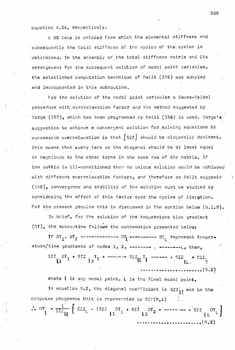
209
equation 4.64, respectively.
A DO loop is entered from which the elemental stiffness and
subsequently the total stiffness of the system of.the system is
determined. In the assembly of the total stiffness matrix and its
arrangement for the subsequent solution of nodal point variables,
the established computation technique of Palit (156) was adopted
and incorporated in this subroutine.
For the solution of the nodal point variables a Gauss-Seidel
procedure with overrelaxation factor and the method suggested by
Varga (157), which has been programmed by Palit (156) is used. Varga's
suggestion to achieve a convergent solution for solving equations by
successive overrelaxation is that [SZZ] should be diagonally dominant.
This means that every term on the diagonal should be at least equal
in magnitude to the other terms in the same row of the matrix. If
the matrix is ill-conditioned then no unique solution would be achieved
with different overrelaxation factors, and therefore as Palit suggests
(156),, convergence and stability of the solution must be studied by
considering the effect of this factor over the cycles of itergtion.
For 'the present problem this is discussed in the section below (5.1.3).
In brief, for the solution of the temperature tame gradient
(DT), the subroutine follows the mathematics presented below:
If DTI, DT2 .s DT represent temper.
ature/time gradients of nodes 1, 2, Lt then,
SZZ DT + SZZ T + (3. 1 l2
SZZ IL It
+ SZZ = CZZ -
(5.2)
where 1 is any nodal point, L is the final nodal point.
In equation 5.2, the diagonal coefficient is Sllit and in the
computer programme this is represented by SZ7(M,1)
.6. DT - CZZ (SZZ DT + SZZ DT„, + +SZZ DT, SZZ It 11 1 12 - L
(5.3)

210
It would follow that for each cycle of iteration:
ADT czzi. (szz DT, szz DT2 Ii 1 2
3ZZ DTL
L
— DTL
(5.4)
CT for a subsequent cycle is;
DT = DT' XFACT ACT (5,5)
where UT = the current value of temperature
DT' = t:-le previous value of DT
XFACT = the overrelaxetion factor .
and ADT = TemperatOre difference between DT obtained for two
successive iterations.
The convergence criterion followed to obtain a unique solution
is:
=1
IADTI r 10
-6 (5.6)
This is incorporated in the subroutine as SUT
—r----- \TOLER SUMU
.... ..(5.7)
Convergence and stability of solution is very much dependent
on the geometry of the elements (159). For the present problem this
is satisfied providing that, in generation, the elements remain acute
and right—angled triangles (153). As seen from Fig. 5.4, after 50%
reduction, this condition holds and it can further be envisaged that
for higher reductions this convergence limitation is also satisfied.
The convergence criterion however can not satisfy the oscillation
in the solution as this is dependent on the orientation of the
elements (159). Since from the outset of the deformation, the orient-
ation of triangles changes, some oscillation to the solution of nodal
point variables is inevitable.
In this subroutine calculation of relevant elemental stiffness
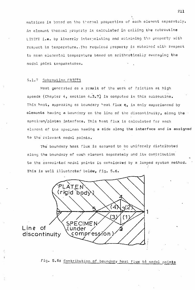
Line of discontinuity
2.1.1
matrices is based on the thermal properties of each element separately.
An element thermal property is calculated in calling the subroutine
LININT i.e. by linearly interpolating and obtaining the property with
respect to temperature.—The required property is obtained with respect
to mean elemental temperature based on arithmetically averaging the
nodal point temperatures.
5.1.7 Subroutine FRTCTN
Heat generated as a result of the work of friction at high
speeds (Chapter 4, section 4.3.7) is computed in this subroutine.
This heat, appearing as boundary heat flux qo is only experienced by
elements having a boundary on the line of the discontinuity, along the
specimen/platen interface. This heat flux is calculated for each
element of the specimen havihg a side along the interface and is assigned
to the relevant nodal points.
The boundary heat flux is assumed to be uniformly distributed
along the boundary of each element separately and its contribution
to the associated nodal points is considered by a lumped system method.
This is well illustrated below? Fig. 5.6.
Fig. 5.6: Contribution of boundary heat Flux t6 nodal points

212
If q12 and q3, are the boundary heat fluxes due to friction work
generated between elements (1)-(2) and (3)-(4) respectively, then by
definition of the lumped method:
for node 1 q12
el ..-.■•••••••••• '11 2
and for node 3 (q12+ q34)
(13 - 2
The method is accurate providing the mesh in the region of the
interface is fine. For the present problem this is satisfactory, but
if a more exact solution is required, then an integration procedure
similar to the method outlined by Kamyab (160) may be adopted.
This subroutine is called from subroutines DTINTL and STIFF
when required.
Since the computation of friction work to obtain q already
takes into account the elemental boundary surface area, q appearing
as QF in subroutine DTINTL or subroutine HEAT called from subroutine
STIFF, is not multiplied by Z1br
(which calculates area) as seen in
equation 4.63, Chapter 4.
5.1.8 Subroutine STIFF
The principal operation of this subroutine is identical to
subroutine DTINTL. Hera computation is carried out on equation 4.62.
(chapter 4) to achieve solutions of nodal point temperatures. The
solution is carried out by subroutine SOLN using a similar Gauss-Seidel
and convergence procedure outlined above in section 5.1.6. Nodal
points along the boundaries of fixed temperatures are excluded as
before. [SZZ] and [CZZ] in this subroutine include all terms appearing
on the left and right hand sides of equation 4.62. For a typical
element, the terms of the matrices are computed from expression 4.63.
In this subroutine, subroutine HEAT is called element by element to

213
compute the terms appearing on the right hand side of this expression.
To ensure that the diagonal of [5Z21 never became ill-conditioned,
the effect of changing the relaxation factor or the cycles of iteration
to converge a solution of nodal point variables, was examined in
detail. Fie. 5.7 illustrates in general the effect of the relaxation
factor on the cycles of iteration (NCYCM) for a case with no platen/
specimen interface friction. From this it is clear that a solution
with a relaxation factor of unity can only be achieved after about
ten cycles of iteration to convergence. However with different
relaxation factors uniquely identical solutions were obtained.
When boundary heat flux was present, however, a slight over-
relaxation was essential. Therefore XFACT r. 1.475 was chosen, which
according to Fig. 5.7, still gives a minimum of cycles of iteration
to convergence. As discussed in Section 6.1.6 to achieve a unique
solution with minimum cycles of operation is very much dependent on
the geometry and on the solution of the type of nodal point variables
required. For. .instance to solve for the temperature/time gradients of
nodal points,' it was found that a different optimum XFACT is essential
to achieve a solution with minimum cycles of iteration. However the
full extent of the changes occurring in the solution of some finite
element problems, as a result of changing the relaxation factor and
the geometry of the elements, is given by Palit (156). For the present
problem the chosen XFACT provided satisfactory answers to convergence'
with minimum cycles of iteration in all cases.
The temperature field is printed out in subroutine SUN for
each increment of deformation and after smoothing operations. r
5.1.9 Subroutines 9700TH and LINSOZ
As discussed above, since the orientation and the geometry of
the elements change continuously due to deformation, some oscillations
in the nodal point temperatures were observed. These oscillations of

. rn Region of minimum' /iteration/ cycles
Ater 1.0 2_0
Relaxation Factor (X FAC
I TERATION CYCLES' 50 (NCYCM) FIG 5.7- VARIATION OF ITERATION
CYCLES. WITH RELAXATION FACTOR
100 tolerance= 0.000001
1,1-0.0
50

215
the temperature distributions were more pronounced for cases where
friction was present along the specimen/platen interface. Frictional
work caused an extra constraint as boundary heat flux to the elconts
having a side on this line of interface. Since only some of the elements
in a row near the specimen/platen interface experienced this boundary
heat flux, the oscillations may be regarded as partly inherent in the
method of mesh generation. Of course these oscillations con be reduced
by concentration of a finer mesh in this region. of discontinuity..
In addition the transient nature of the problem also renders
some oscillations in the temperature field (159). On the basis of
the time dependent nature of the problem, the effect of increasing
the time interval At (DELTI) for conduction was investigated prior to
the inclusion of these subroutines. For time intervals greeter than
ions and 50ms for pesos with and without end frictions respectively,
it was established that no severe oscillations in the temperature
field occurred. Some oscillations which were present were concluded
to be duo to the chenging fineness of the mesh and the changing
geometry and orientation of the elements. However on the basis of
this conclusion„ since the duration of the deformation was expected
to be considerably less than 10ma, subroutines LINSOZ and SMOOTH were
included to clear out any oscillations after each increment in the
establishment of the temperature field.
When no friction is present on the interface, subroutine LIMSOZ
is called to average out the line temperature distribution in the
radial direction only. This is carried out in each increment of the
deformation after the determination of the temperature field. Since
nodal points are equidistant in the r direction, the averaging of
the nodal point temperatures is carried out by considering three
successive nodes and taking the arithmetic mean value of their
temperatures. This mean value is then assigned to the middle point.

216
Nodal points along all boundaries, including the z axis (which
is an artificial boundary) are excluded from this procedure. Their
temperature values remain unaltered.
Men friction is present, oscillations are more severe. Sub-
routine SMOOTH is'therefore called to smooth out the oscillations
appearing both in the axial and radial directions. Elemental temper-
atures are calculated by considering the mean Values of nodal point
temperatures. This is carried out for all elements and thence, when
the elemental temperature field is established, it is extrapolated
back to obtain the nodal point temperature field, The procedure for
this is to average the elemental temperatures around a particular
node and assign the result to that node. Subroutine LINSOZ is again
called after this subroutine to clear out any line oscillations. Both
subroutines were tested against a known temperature field with no
oscillations such as the temperature distribution obtained after
cooling a steel billet in water at 0°C (dis,cussed in Chapter 6). This
Was necessary in order to avoid any significant distortiOn of the
temperature field due to the smoothing procedure adopted.
5.1.10 Subroutine LININT
This is a simple one dimensional linear interpolation subroutine
and is used for calculating heat constants corresponding to the required
temperatures or the velocity of the deformation at a particular deform-
ation time. It has also a check characteristic to see whether the
independent variable at which point the interpolation is sought, lies
within the range supplied. If the interpolation falls /outside the
range, the programme will stop.
5.1.11 Miscellaneous
Coefficient. g (CCFMEU) and the time increment of deformation

217
(TIMING) are set in the main routine. The state of strain, strain
rate and the temperature rise due to an increment of deformation are
all set initially to zero.
The increment of temperature rise due to the increment of
deformation is calculated after computing the strain and strain rate
experienced within the deformation time increment by specimen nodes
Since deformation is homogeneous, the strain and strain rate field
would be homogeneous. The increment of the temperature rise is assigned
to specimen nodal points after which the conduction follows.
It was found that due to the transient nature of the problem
(discussed above) the temperature of some nodal points in the platen
continuum fells slightly below the initialised temperature. To avoid
this, temperature/time gradients for these nodes were made to take
absolute values, meaning that the temperature of the platen is . 4
considered as constantly rising during the deformation although in
actual fact, this is not always true, since convection from the platen
to the air takes place. Since the duration of deformation in all cases
is very short, the effect on the nodal point temperatures of the platen
was insignificant, and this fact was demonstrated by comparing two
identical outputs', one with and the other one without the above
consideration. The operation of making the temperature/time gradient
of nodal points within the platen absolute, is carried out by
statements 32 to 37 appearing in the main routine of the computer
programme (Appendix A). If the duration of the deformation is longer
than 10ms, the operation should be excluded.

CHAPTER 6
RESULTS AND DISCUSSIONS
6.1 Dynamic Incremental Stress/Strain Characteristics
Since it was established that it was not possible to control very
closely the precharge and counterbalance pressures of the experimental
machine to produce data at exactly the same strain rate throughout the
steps of an incremental test series, recourse had to be made to an
alternative arrangement. This was to plot the flow stress versus strain
rate curves first, for a given number of strains and then obtain stress/
strain curves at constant strain rates by cross plotting.
Incrementally obtained dynamic stress/strain rate plots for copper
and aluminium at room temperature are presented in Figs. 6,1 and 6.2
.respectively. The plots, which represent the recorded data, were prepared
from sets of tabulated results as followss
For a particular precharge and counterbalance pressure and machine
setting, an incremental series of tests was carried out on a testpiece
up to the maximum permissible reduction. For each step of compression
and from the stored oscilloscope records, load and the velocity of
deformation were noted. Similarly notes were made of the specimen's
heights prior to and after the incremental compressions. The test
procedure was then repeated on other specimens of the same kind but
with different precharge and counterbalance pressures, providing varied
ranges of impact velocities. In all. cases notes were made of the
incremental load, velocity and the specimen's heights in each step of
deformation as before. Recordings of loads and velocities on the
218

• E =0.07 600 —0 —E=0.13
—E = 0.25 — A E = 0.43 —o—E= 0.63
A E 0 8 6
OW, 0111., Rm. IM MO OM" mama ■1111 WM.
WOMINI ONNI• 01•11110 ■■•■• 1•00.10 Wale)
OMR mini. 01•1111• Min 04101111 Mob MEND Iasi
gnaw/ Immo NMI.* •■• ./INEWII MOO -
"E
io 0400
Cr
tn
0 -3200 U-
A
OM. ImINW M.11 GM. MO
art...■■•••■••r. 0
n
0 * A e e A
04...• MM.. 0 ••■•■........0
mamma, a • CI ...N....8
OSIIMON1.11•1•=10.e.
100 200 400 600 1000 - STRAIN RATE 51
FIG.6.1- FLOW STRESS /STRAIN--RATE CURVES FOR COPPER
1
mama& am.• ORM
•

200 r4E
0
100
O
V
=0.125 0.175
E= 0.215 E= 0.35
—E=0.065 1
-- -- ---
ttral
A
•
.
--- A— A--- A
—E --0—E=
• • II
1:3 .......... A
............osw
--- --------.0- 0-0 -Os A .......A........... A ............ ZXN.......76, ■.:
0 la c:F......■...--ci 0 0 Ve M. 12.'0
— ° --- --- . 0 0 IS IS
SIM............... 113 k 6
. .
-4,-- co
55
A
.
—
la
ps ....... it' a........ 0.-- ®........ f I
.......r Illi 0...... ES if liTa . A------A
Mt 1.1•101. •••■■■ ••••••
INPNIO MOMS .00.1.. ...I.
wawa. a;sawr ••■•••
_ -- — E = 0.54
=0. 925 E = 1•165
—A—E,0.75 °
—0 —E . A
2 20 50 100 —1 STRAIN RATE S1 500 1000
FIG. 6.2 FLOW STRESS / STRAIN-RATE CURVES FOR ALUMINIUM

221
oscilloscope (typical of which is shown in Fig. 3.15a) were in almost
all cases well defined and reasonably free from any interference. In
each case the velocity remained constant during the deformation.
From the recorded data, strain, stress and strain rate) sustained
in each increment of deformation were calculated and the results for each
specimen were separately tabulated. The stress and strain were computed
from expressions 4.1 and 4.4 respectively. The strain rate experienced
during each increment was calculated by dividing the velocity of
compression by the height of the specimen prior to the step of the
deformation. The strain rate calculated in this way was then assumed
to remain unaltered in each step. From the tabulation of results, it
was then possible to observe a series of stresses and strain rates
particular to a value of strain and then conveniently plot the flow
stress/strain rate characteristics.
The incremental steps of deformation providing rationalised
results were of the order of 1.6mm. Sometimes slightly smaller or
larger steps of deformation were considered, to protect the tooling
or arrive at desired ranges of strain rate for a particular strain. The
latter was considered mainly to fill in the gaps in the extremities of
stress/strain rate plots. In any case it was not possible to obtain
many results to large strains and lower strain rates. As the increment
of deformation proceeded and larger strains were achieved, it was found
that the energy provided by the machine was not sufficient to affect
the incremental deformation at the lower ranges of compression velocity.
To overcome this, since it was established that the incremental method
entailed homogeneous deformation owing to the relubrication of the
specimen end faces after each compression step, some specimens having
length to diameter ratios other than unity were used to provide data
to fill in the required gaps. In all these cases homogeneity in the
deformation was observed, as illustrated in Fig. 3.29a, and care was

222
taken to obtain data free from any other side effects. Only in one
instance specimens of copper and aluminium having respectively length/
diameter ratios of 2 and 2.5 were used. This was aimed at achieving
strain rate data below 200S-1 to large strains. The operation was
unsuccessful since after three incremental steps shearing over effects
appeared in the specimen. The resultant product looked 00-shaped. Tests
were discontinued and results discarded. The data at unity strain rate
are those obtained from quasistatic testings.
The flow stress/strain rate relationships for a giverrstrain, as
appear in Figs. 6.1 and 6.2 may reasonably be approximated by the semi-
logarithmic formula of Cidwick (161) used by Alder and Phillips (40):
as
= (ao 4. Xln;)I cIT (6.1)
X = constant
It may also be approximated by a power law (12)(40)(88)(162) as
illustrated in Figs. 603 and 6.4. (These figures show only parts of
the plot for convenience;)
.m = S 0£,T
. i (6.2 )
m = strain rate sensitivity
As appear in Figs. 6.1 to 6.4, both X and m are dependent on the
levels of strain. However, for all strains, X or m may be assumed as ti
almost identical in.magnitude.
The values of X and m in general not only depend on the level of
strain, but also on the working temperature and the material (l2)(40).
It is also asserted (163)(164) that the flow stress of metals and alloys
are more susceptible to strain rate sensitivity above recrystallisation
temperatures than below. Since only cold tests were carried out and the
incremental method entailed the determination of flow stress/strain rate
characteristics virtually isothermally, parameters m and X if determined

1000
(NI 600
j 400
U) Lu
U)
E= 0.07 E = 0.13 E = 0.25 E = 0.43 E = .63 E =0.86
0
STRAIN ATE E.(Se l
100 200 400 600 1000
FIG 6.3 — FLOW STRESS 1 ST RAIN RATE CURVES FOR • COPPER ( Indicating pow er law behaviour )

1000
500 .1011•11.
E 2 2
Cl) 100
50 0 -J LL
10
0.065 0.175
) 0 OM
OW A —00-c0-6 Cr' 44-AA---Ada .,f1.,," "..-1..„.cy,---)
0 •
E 0.750 -- 0— = --E = 1 .065
...---.....6
. .
0 ---------IVG
........ .0........ ......-
•
STRAIN RATE E ( Seel ) 10 50 100 500 1000
FIG 6.4 FLOW ST ESS / STRAIN RATE CURVES FOR ALUMlN1UM(Indicating power law behaviour )

225
may be regarded as true isothermal values and hardly affected by the
small rise of the testpiece temperature due to the work of small
incremental deformation.
The flow stress/strain rate characteristics may be further
approximated (72)(165) by the following formula:
0 = (0 + m E) I 8 1 o E,T
(6.3)
The isothermal stress/strain characteristics at constant strain
rate as obtained by cross plotting of Figs. 6.1 and 6.2 appear in
Figs. 6.5 and 6.6 for copper and aluminium respectively. The results
clearly indicate that the flow stress increases with strain rate.
Furthermore the stress/strain curves show no plateaux up to the maximum
strains and strain rates attained in these experiments. When the general
shape and path of the stress/strain curves are examined and compared
with those shown by others (4)(23)(166) for similar materials, the
strain rate effect seems to be more significant because of the absence
of any accumulative adiabatic temperature rise. The strain rate effect
is more marked in aluminium, and copper only shows a moderate trend.
similar effects were observed by Alder and Phillips (40).
6.1.1 Limit of accuracy 'results
The magnitude of the error introduced in assuming constant strain
rate data in the deformation steps of the incremental tests may be
assumed from equations 4.6 amd 4.8. It is also essential to express the
work ratio (defined in Section 4.2.2) to ascertain the amount of energy
imparted to the specimen at impact in relation to the incremental
deformation work. The larger the work ratio, the higher would be the
energy at impact to effect a deformation step. This also means that the
more is the likelihood for the deformation velocity to remain constant
and equal to the impact velocity. If this is true, equation 4.6 would

1.2 1.0 0.2 06 0.8 0.4 - 100
FIG. 6.5 STRESS/STRAIN CURVES. FOR COPPER

FLOW STRESS Os MN /m2
150
100
50
0 0 0.2 OA 0.6 0.8 1.0 1.2
FIG 6.6 -- STRESS/STRAIN CURVES FOR ALUMINIUM

228
give an almost exact estimation of the limiting strain rate error. The
limiting adiabatic temperature rise can be estimated by considering the
heat equivalent of deformation for the largest incremental step-considered.
Similarly the order of magnitude of any inertia restraints can be
estimated either from expression 4.9 as derived by Lippmann (81) or
from equation 4.12 of Dharan (72). Estimation of these limiting para-
meters, which would reflect the accuracy of the data, are to be considered
in extreme cases.
Under the most extreme conditions the maximum error introduced in
assuming constant incremental strain rate data and the smallest work
ratio achieved, would be due to the slowest impact velocity effecting
the largest increment of deformation. The strain rate error would be
more significant if the largest step is taken near the end of the
deformation where the specimen height is smallest and the resistance
of the material is highest. The results for the most extreme case
encountered during the course of the experimentation are presented in
Figs. 6.7 and 6.8. These are for a series of incremental tests which
were carried out at the slowest range of impact velocities on copper
and aluminium specimens respectively. Only points towards the ends of
the deformations are plotted.
Since from Table 3,1, the total mass of the lower platen's moving
parts including toolings, amounted to 5571bs, the kinetic energy of the
lower platen at impact can be expressed as:
KE = 11.7vi2
Nm (6,4)
With the lowest impact velocities of 3m/s and 1.5m/s imparted
to copper and aluminium specimens respectively, the energy at impact
would accordingly amount to 105Nm and 26.3Nm. Referring to Figs. 6.7
and 6.8 for the work equivalent of deformation and other particeilars
of the deformation steps, it would then follow that:

FLOW STRESS Os (MN/m2)
,) 761
685 Et
—570 /
100 work equivalent of deformation = 9.9 Nm
0.2 I . I I r
0.4 0.6 0.8 1.0 FIG.6.9 ESTIMATION OF INCREMENTAL
LIMITING TEMPERATURE RISE FOR COPPER
FLOW STRESS .., Os (MN! rn- ) 389
250
/37 .400-
350
300- O
co
E
KE of platen at impact =10 5 Nm h.=1.92 cm , d,=1.11 cm rn .9. 200
t. v..3 m is
E
o.
400
119
200
100-
p= 8940 kg 1m3 (Ns2 !m4) c•=0.092 kcal /kg c
vi :6.85 m/s
Os AE 45 MN! m2 7
AT=13-5 I/
Natural Strain E
0.2 0.4 0.6 0.8 FIG.6.7 ESTIMATION OF INCREMENTAL
LIMITING STRAIN RATE ERROR FOR COPPER
Natural Strain c 0 0 1.0
7
FLOW STRESS Os (MN /m2 )
84
77 • .t.a'6c" ‘'s 00(15
owasi_st atiC
0.8 . 0.2 OA 0.6 FIG 6.8 ESTIMATION OF INCREMENTAL
LIMITING STRAIN RATE ERROR FOR ALUMINIUM
FLOW STRESS Os (MN/ m2 )
---- i-1 •- 7 1(S 150 ____-------7/59 6
) --- E(S1
793
0 0 0.4 0.6 0.8 1 0 FIG.6.10. ESTIMATION OF INCREMENTAL
LIMITING TEMPERATURE RISE FOR ALUMINIUM
P=2800 kg/m3 (Ns2 /m4 ) c 2 0.23 kcal/ kg-c
Natural Strain C
1.0 1.2
150-
100-
50-
100
50
asAE:21.25 MN/m
AT=7 8 5°C
m /s
K.E. of platen at =Pact =26.3 Nm hi = .7cm d. =1-59cm v1 .1.5 rri is
a work equivalent of deforination =10.85
Nm
Natural Strain E
21.9

For copper
K.E. after impact = 105 - 9.9 = 95.1Nm
0 155 Work ratio = . 57 - 10.6
230
From expression 4.6
From expression 4.8
error = 0.B1 7
0.81 - 1 x 100 0.81 - 0.2 In
c-T-7ff
= 5%
error = ....21121.9222 x 100 105/0.81
6%
For aluminium
K.E. after impact = 15.45Nm
Work ratio = 2.42
From expression 4.6 error = 7.5%
From expression 4.8 ierror = 12.5%
Since expression 4.8 is derived from the actual change in the
kinetic energy, values of 6% and 12.5% represent more accurately the
actual limiting strain rate error than those obtained from expression
4.6 for copper and aluminium respectively. It may be pointed out that
these maximum errors occurred at the lower ranges of strain rate. At
the other end of the scale where the speed is highest and hence the
work ratio largest, the errors would be less. This is paticularly so-
for smaller increments of deformation. However at high velocities, where
the work ratio is large, expression 4.6 may be used with confidence in
predicting any strain rate error without recourse to energy calculations.
This is well demonstrated in comparing the values obtained from both
expressions 4.6 and 4.8 for copper.

231
The maximum limiting incremental adiabatic temperature rise
would be expected to occur at the highest impact velocity, effecting
the largest deformation step. This would be more significant if the
step is considered near the end of deformation as before, when the
resistance of the material is highest and the plastic work due to
the increment of deformation largest. The results for the limiting
case are presented in Figs. 6.9 and 6.10. By dividing the incremental
area of deformation, eAc, by the appropriate thermal properties, also
presented in Figs. 6.9 and 6.10, and the mechanical equivalent of heat,
the emerging values would become 13.5°C for copper and 7.85°C for
aluminium. To obtain these values it was considered that all the work
of incremental deformation appeared as heat. For the lower ranges of
impact velocity, or the smallest incremental step, the maximum tempera-
ture rise would be smaller than these quantities. This is specifically
relevant to the onset of the deformation where the heat equivalent of
deformation is smallest. From these it is clear that the increment of
temperature rise has had negligible effects on the results. Besides
since considerable time has been allowed to elapse (about 30 minutes)
between each incremental step due to the loading and reloading of the
subpress and the machine, no accumulative temperature rise could have
accrued to influence the mechanical properties.
Inertia restraints have also had negligible effects on the results.
Using expression 4.9 of Lippmann and considering the parameters presented
in Figs. 6.9 and 6.10, it would be concluded that even for a velocity
of compression equal to 15m/s, the uniaxial yield stress would be almost
equal to twice the quasistatic stress at the highest strain (c= 600MN/m2
for copper, and :=300MN/m2 for aluminium) and the incremental
engineering strain of 0.1, the magnitude of inertia effects are
negligible, such that:
for copper, f aal 8940 x (15)2 -- 0.15 X 10- 2
24 x 600 x 105

232
2 -- 0.95 x 10⁻²
and for aluminium last == 0.088 x 10⁻² and 1"/ 0.264 x 10⁻² 2
Comparison of these values to those expressed in Section 4.2.3
would indicate that the inertia effects are negligible.
Similarly under the most extreme condition Dharan's expression
(equation 4.12) would render the presence of inertia restraints as
quantitatively negligible; such that for a typical specimen having
unity length/diameter ratio and for the same impact velocity and
incremental strain considered above,
for copper, o = 3 x 8940 x (1)2 x 15 2
ri 8 (1 - 0.1)2
• == 0.84 MN/m
2
and for aluminium or -- 0.263 MN/m2
While in the practical situation the high impact velocity
considered above for the calculation of inertia restraints was never
attempted, it is clear that even under extreme conditions for the
experimentation, inertia effects were negligible.
It may also be ascertained that stress equilibria (72)(73)(93),
Fig. 2.21, were reached in the specimen prior to the recording of the
data. Expression 4.13 indicates that for each incremental step the
ratio tbits can be expressed as,
tb
6h/ vi
is hi
vs
6h vi
hi/4277 pe .1
Such that for an impact velocity of 15m/s with a specimen having
hi/di = 1, d. = 1.57cm and a typical incremental step 6h = 1.6mm,

233
for copper, bits
106/4.25 25
and for aluminium tb/t
= 106/2.8
== 38 s
E for copper and aluminium in these calculations was taken as
86000 MN/m2 and 124000 MN/m2 respectively.
Since at least 6 to 8 reflections (72) are required to satisfy
the stress transient condition, the above indicates that under -extreme
conditions the requirement has been met. The oscilloscope load records
were observed in almost all cases to be free from almost any undesirable
stress wave reflections.
The data thus plotted may be considered as free from the imposition
of any side effects.
6.2 Comparison of Dynamic Stressistrain Curves obtained by the
Incremental and Large Deformation Methods
Incrementally obtained dynamic stress/strain curves and those
obtained under the continuous deformation tests are compared in Figs.
6.11 and 6.12 for copper and aluminium respectively. Data for the plot
of the continuous curves were obtained by directly analysing the
load-velocity/time records. In all cases homogeneous deformation was
prevalent up to the strains considered. This is shown in Fig. 3.29b.
The strain rate variations in the large deformation tests are
shown in Figs 6.13 and 6.14. The mean strain rates have been obtained
by integrating the strain rate/strain curves (97)(167). It is clear'
that while at low values the mean strain rate represents relatively
well the actual strain rate during a significant part of the test, at
higher strain rates, no mean value would represent the actual variation
with any accuracy. Comparison of the strain rate/strain histories for

=700
8,=700 51 •
—ma"' qo ° X 851 \ • 600 S
Ai .
4 6355 59°Ct I =600 it'. 612 S1
X -Incrementally obtained at actual temperatures and
• strain rates •
FLOW STRESS 400 0 MN/ m2 s
• -:7- 600 §1
200
100 _ . 0.2 Oh • 0.6 0.8. 1.0 12•
FIG 6.11 COMPARISON OF. THE STESS/STRAIN CURVES OBTAINED BY THE INCREMENTAL(—) LARGE-DEFORMATION(---) METHOD
FOR -COPPER

66°C 43551
150
FLOW STRESS 65 MN/m2 475 S1
1111.1■011101•
....510.711111.10 011X2121.1■10
100- /
23°C 32B5
\\54̀); X-,„4 2C1 - ")., ./.1)
479S 3° C.1 71
4325 t=475 51
X -incrementally obtained at actual temperatures and strain rates
NATURAL STRAIN E 0 0 . 0.2 0.4 0.6 0.8 1.0 1.2
FIG.6.12 COMPARISON OF THE. STRESS/STRAIN CURVES OBTAINED BY
THE INCREMENTAL( ) & LARGE-DEFORMATION (---) ME THOD FOR • ALUMINIUM

.1.k) 600 W
400
0.2. 0.4 0.,6 0.8 1.0
1.2
1.4 NATURAL STRAIN E
FIG 6.13 -STRAIN-RATE /STRAIN -VARIATION CURVES FOR LARGE • DEFORMATION TESTS ON COPPER

E -77551 A /
1000
800
600
uJ
cc
z 400 :Tc cc
200 —1
Er...125 S
0.4 0.8 1.2 1.6 2.0 2.4 NATURAL STRAIN E
FIG. 6.14 - STRAIN-RATE./ STRAIN-VARIATION CURVES FOR LARGE DEFORMATION TESTS. ON ALUMINIUM

238
the two materials further illustrates that the variation paths are
different even for the same value of mean strain rate. These collectively
indicate that in continuously loading the material in free flight impact
devices, constant strain rate data would hardly be achieved and that
the path of strain rate variation is dependent on the test material and
the conditions at impact. Also the concept of mean strain rate may
misrepresent the actual strain rate effect if the strain rate varies
extensively during the test.
Figs. 6.11 and 6.12 indicate that for large strains the stress/
strain curves obtained by the large deformation method lie well below
the results of the incremental tests. The reason for this, as already
mentioned, is partly that mean strain rates are not representative of
the true strain rates in large deformation tests, and predominantly
because the temperature rise becomes significant at larger strains. It
is of course true that at the later stages of these tests, the actual
strain rates are often larger than the mean values, an effect which
would tend to raise the flow stress. It is therefore not unreasonable
to suggest that the stress/strain curves in the large deformation
test would drop even further if the strain rate effects were
absent.
It is evident from the forgoing that each point on the stress/
strain curve obtained in the large deformation tests represents data
far a particular temperature and strain rate, which are different for '—
each point along the curves. The actual values of strain rate can be
obtained by comparing Figs.- 6:11 and 6.13 for copper and 6.12 and 6.14
for aluminium, and the actual temperature by referring to Fig. 6.15.
The temperature plots were obtained by calculating the heat equivalent
of deformation in assuming that all the plastic work was converted into
heat and that there were no heat losses during the test.
To confirm that no other side effects e.g. the elastic deflection
of the tooling were responsible for the difference in the dynamic

120
Actual Temperature oc
0 0.2 0.4 0.6 0.8 1.0
HG. 6.15 TEMPERATURE / STRAIN VARIATIONS FOR LARGE DEFORMATION TESTS

240
behaviour, a few points along the continuous deformation curve were
obtained isothermally. The results are indicated in Figs. 6.11 and 6.12.
These points were obtained by preheating the specimen to the calculated
temperatures and compressing it incrementally at almost the actual
strain rate obtained in the large deformation tests.
Since the present argument is justified, it may therefore be
concluded, that it would be possible to obtain points on the large
deformation curves by the incremental method and vice versa. The in-
crementally obtained points on the large deformation curves reasonably
agree with this. In a similar manner Kudo and Tsubouchi (48)
obtained isothermal stress/strain curves for steel and brass tubes in
fast torsion to shear strains up to 2 and shear strain rates up to
about 115S-1. Similarly Okamura'and Nakanishi (168) obtained the dynamic
isothermal stress/strain characteristics for the upsetting of solid
cylindrical billets of polycrystalline copper and aluminium to 100S-1
and et:: 0.7. The trend of the present results follows well the work
of these authors.
6.3 Temperature Distribution in High Speed Axisymmetric Upsetting
with End Frictions
6.3.1 Testing of the computer programme
Prior to the application of the programme to the problem of
determining the temperature field in high speed axisymmetric upsetting,
a shorter version of the programme was developed to check the accuracy
of the finite element numerical solution of the transient heat equations.
The listing of this programme is not included with the present work
for the sake of brevity. Temperature distribution was determined for
cooling of a steel cylinder (10cm long x 2.5cm radius) in water at
zero degrees Centigrade after 4 seconds, for which the analytical

241
solution of Berger in the form of an infinite series of Bessel's functions
of the first kind and zero order was available. Half of the meridian
plane of the cylinder •5 divided into 400 triangular, nearly equal
sided, elements and 246 nodal points.
The finite element mesh together with the temperature field
assigned to nodal points for a quarter of the continuum appears in
Fig. 6.16. Figures appearing in each element indicate the element
number. The isotherm plot is presented in Fig. 6.17. Comparison between
the analytical solution obtained by Berger and the present work can
be seen in Fig. 6.18. From the latter it can be deduced that the maximum
difference between the two solutions of the temperature field is of the
order of 1%.
As seen in Fig. 6.16 there are some oscillations in the temperature
field. The kinks in the isotherm plot are due to these fluctuations.
However the oscillations are minor and as discussed in Chapter 5 are
inherent in finite element problems of a transient nature. They are also
due to the geometry and the orientation of the triangulations. The
accuracy of the solution is dependent upon the fineness of the mesh
and this is well illustrated in Fig. 6,19 where the temperature field
is presented for the continuum divided into 100 elements and 66 nodal
points, and compared with Berger's results and those obtained by
Altan and Kobayashi (131). The latter authors used a finite difference
method.
However it is clear that if the continuum is discretized into
fine triangulations, near exact solutions for the nodal point temper-
atures would be achieved,' Due to the recursive procedure used, it was
also found that solutions at subsequent times could be obtained with
relatively large time intervals, without much affecting the convergence
and stabilty of the problem. Cooling curves for the edge of the cylinder
are shown in Fig. 6.20 for time intervals of 100 milliseconds and
o.5 seconds. It is clear that the time interval has little effect on

Q
Bitters initial temperature r= 600°C P=7B60 kg/m3, c =0.12 kcal /k g*c hF 2: 2000 kcal/m2hr °C
Nodal. Point Temperatures
" :3 73 37 2'56 751
351
321
30
41-, .,., 1
111111r , 35
1, ,7
30. 37.
',I7
37' 37
,
37'
1 7
33.
,, -7.
33 33
4 1 1
3 '5''
33
1 I
33
'3
33 3 ')
;
3.
3:: ' 35
"...3 .:
3'
3 ':-
35 4 5
'.. 25 25 ' 2:-., • 3.31 337 30 30"
. 1,
2
-'4 5
- 2f," , 3' + 3"'
20 20 20— 2 ' 22 , 22 02 22' 23; 23 23" 24
20 2 --' Z• 21r2 2: 2, 2Z 2 =', 22 Z• i 2 ' ,.... ,. 23 2..,
45 .-i , 4,";
/ 1? 1 =2 12 1 30 1 .3' , 1/31' .1 .3'. 1 1-' 14 ' 14 + 14" 1
' 12 1 ' . 1.(_ -- 1..2. 1 '3 1- - 1 ,' 1 ,, ' 14; 1,-+ 1 ct i . 1.0.
4. ^ 47^ /^ a '.7. ':1-7, ' l '-', •
r 5755 . ; + 73 76 77 52, Alkihh.11111 i
15
p liVr5 15'3 5 4 1
5 -., .60 6,_: 5€, .: 5 '7 0 7 1 74
FIG. 6.16 TEMPERATURE DISTRIBUTION CC ) IN UPPER RIGHT QUADRANT OF A STEEL CYLINDER COOLED IN WATER AT FOR
4 SECONDS
"4 17 272
33r)
321
537
3 45
z

o
312----122-----t-L----1—ls,— i}1, ...—ti‹ .111 2 2 2 1 ,,,',. 3c1,2 9 .?. 9 3a2 '3 0? 1 .', ID 9
41? 422 Ai:2_
412 . 419 422
4:21_z_412 44:: 4 1 2 40?
402 419
4Q11---- ----4_
42 --___ 1F-------
4 ry, 402 402 402
22
_432_ 49' 49.1 497 497 4'39 -________
._4,--315------- 442 442 412 4'42__iLt2 4A2 I. 4 ' 4 2 92 452 452
62
6 .̀
Billets initial 4emperature=600 °C p= 7860 kg/m') , c =0.12 kcalikg*c hF 2000 kcal/m2hr °C
ISOTHERMS Fm COOLING OF A STEEL CYLINDER IN WATER AT 0 OCRFTER 4 SEC
FIG-617

360 Temperature
•C
temperature profile on top side face
390
330 — PRESENT INVESTIGATION — -- BERGER (169) Initial billet temperature = 600 °C
300
By Berger r
(377) (377) (377) (374) (3 51) 376 376 376 373 351
270
244
(273) 272
FIG. 6.18 TEMPERATURE DISTRIBUTION ( ° C) FOR COOLING OF A STEEL CYLINDER IN WATER AT °0 C AFTER 4 SECONDS— COMPARISON OF RESULTS (FINE MESH )
temperature profile along the axis of symmetry ( z axis)
Mir /4
ik
4) ) FOrt 441r°01\
AILAIL.All■ —
38•)
385
51 111%4 Ni 0
10111111...1,1111.1■1111111111,111.1%
461 4 r Ar 1
133 .4 J.0\ 4.2 434 ra
488 488 48.4 456 (482) (482) (478) (45 0)
(299) 300
321321)
33336)
7
z 347
(349)
(414) 414 (443) 443 (46 466

245
300
270
(414 413
(443 44
(465) 465 480
..11.10■••■■■
Temperature profile along the axis of symmetry (z axis )
460 Temperature
°C
'490
400
430
390
360 Temperature
°C
Temperature- profile on top side faces"---
330 Finite Element (present work) _ Analytical Berger 169)
-- Finite difference (Alta n & Kobayashi 131) initial billet temperature = 600 °C
Berger [346]
351)
------__(47 41---- 14) 1--
-- ---------------( 413
4 -4
1. 0)-------
_------- (3 6)
414 3 8 ____- - -
443 -(466)---
4 , _ - -4, , (465) •• - _----------- 6_0-) (4 3) ---------
-_______ — - - :4 6- 6 - ---- - - - - - - - -____
4180 . ..--,•-•
4'65___------ --- ----- •
— -
• .
66 .
4.6
..onc•
----______________ - -
77) (377) (3377) 1377 77
Altan & Kobayashi [369] [365]
(374) 7
299) 302 321) 323 (336) 342 351
[27 - (273)
2
357 (349) [366]
482) 340 [495]
(482) [495]
(482 ) [494 ]
488 (478) [489]
456 (450)
• [463 ]
FIG. G.19- TEMPERATURE . DISTRIBUTION (°C )FORCOOLING 370 OF A STEEL SYLINDER IN WATER AT °O C //
AFTER 4 SECONDS — COMPARISON OF RESULTS // (COARSE MESH ) i/
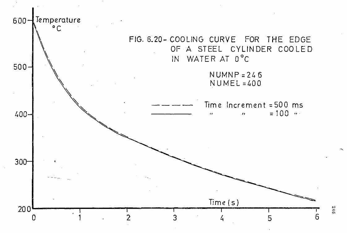
6 5
FIG. 6.20- COOLING CURVE FOR THE EDGE OF A STEEL CYLINDER COOLED IN WATER AT 0°C
500
400
300
200 0
NUMNP =24 6 NUMEL =400
Time Increment =500 ms =100 8 ,
Time (s
4
Temperature °C
600

247
the accuracy of the solution, although it should be said, as discussed
in Chapter 5, that it has some hearing on the oscillations. The latter
is envisaged to be more due to the element's boundary condition, geometry
and orientation and moreover to the fineness of the overall mesh.
Unlike the finite difference approach to the,solution of transient
temperature fields (131)(133)(165), which requires small time increments
of the order of 2-5 milliseconds to achieve conditions of stability and
convergence, the present method can be successfully applied to establish
the temperature field over extended time intervals, which therefore .
reduces the computation time and effort (170).
63.2 Temperature field
Thermal properties and flow stress data as a function of temper-
ature (Appendix 8) and the charactersitic velocity of compaction
constitute the input values to the computer programme. The temperature
dependence of the flow stress for quesistatc conditions (163)(165)
t?gether with the strain rate effect on the flow stress, determined
from equation 6.3 (Appendix 8), and assumed to hold up to 400°C,
provided the necessary mechanical properties. Heat parameters for copper
(171) and for steel (172) taken from the literature provided the thermal
properties. Copper materials having similar composition to those whose
mechanical properties are presented in Appendix B were used to obtain
the velocity/time characteristics of compression. Billets having unity
height/diameter ratios with diameter of 2.54cm were used. The velocity/
time characteristics of the billets under free flight compression far
various impact velocities are given in Fig. 6.21. From these the strain
rate/strain curves presented in Fig. 6.22 are determined, which shows
the strain rate variation during the upsetting process. Each step in
the computation of the temperature distribution accounts for this
variation in strain rate. Initially the specimen and platen were

0.5 1.0 1.5 2.0 2.5
248
h; /d1 =1 di .2.54 cms
vi 4.5 mis
400 ( TESTA )
200
Deformation time t(ms)
3.0
F1G.6.21 -VELOCITY/ TIME VARIATION CURVES FOR COPPER AT VARIOUS
IMPACT VELOCITIES

249
hi/di = 1 di= 2.54 crim
1.6 0.8
vi = 4.5 m/s
0
•
0
0.4 Natural strain
1.2
FIG 6222 STRAIN-RATE/STRAIN VARIATION CURVES FOR COPPER AT VARIOUS
IMPACT VELOCITIES

250
assumed to be at room temperature, taken as 20°C uniformly throughout.
In the estimation of the temperature field, it was assumed that all
plastic work of deformation in each increment is converted into heat.
The value of the mechanical equivalent of heat, J, is also given in
Appendix B.
Results of the temperature distribution were printed out at periodic
intervals. Each time interval equalled the time increment of deformation.
The nodal point temperatures constituting the temperature fields at
selected intervals of strain, and various impact velocities are given
in Appendix C. Tables C.1 present the temperature field for the impact
velocity of 10m/s for various platen/specimen interface friction cond-
itions. For each coefficient of friction results are printed out at
selected intervals to give the overall picture of the temperature field
and, moreover, the development of the region of intensive heating.*Tables
C.2, C.3 and C.4 respectively present the results for impact velocities
of 8.8m/s, 6.4m/s and 4.5m/s. The temperature fields are given at or
near the end of the deformation under various frictional conditions.
Comparison of tables C.1 to C*.11 shows clearly-the temperature distrib-
ution throughout the platen and specimen with various compression
parameters. It is clear that when friction is present the zone near the
platen/specimen interface is mostly affected by the generation of heat
due to the work of friction at high speed along these intimate surfaces.
This is further substantiated by the isotherms given in Figs. 6.23 to
6.28, to complete the picture. Isotherms are presented under varied
conditions to provide all information regarding the effects of speed,, fric-
tion and reduction on the temperature distribution. The four impact
velocities considered are sufficient to indicate.the time effects in
the conduction of heat.
An examination of the results reveals that even for small strains,
the temperature rise can be very high depending on the coefficient of

61
57
20 20
20
Platen 23
36 50
Specimen
CIL
20 20
L
TEST A
4v. = .5 m/s
C 0.5 ev
F IG, 6.23-Temperature . cOntours after 0.0032 sec

Platen 23
36 50
90 ero
60
57
CIL 20 20
20
TEST A
v i z 4.5 m/s
E.: 0.5
FIG 6.23—Temperature - contours. after 0.0032 sec
1.1 :0.3 d )
57°C
Specimen

20 20
20 20
p. 0 . 4 e )
Platen
TEST A
v. z 4.5 m/s
E- 0.5
FIG, 6.23-Temperature contours after 0.0032 sec
p. z 0.5 f
20 Platen --- 23
20
90 80
______----- 70
57
Specimen 57°C
- L
CL
C--105
36 50
C L.

20
Platen 20
20
72 74
74 °C
Specimen C L
23 --
20
20 20
CL
TEST B
vi = 6.4 m/s
C 0.65
FIG 6.24 — Temperature co rt.-tours after 0.002 sec
Platen
Specimen

platen 20
20
23
50
160 1 3 0
100
0
74
74 °C
Specimen
20
20
c L L
20
20
50
160 _100
80
74
74°C
20
Platen
23
80
Specimen
= 0.2 p.= 0.3
c ) TEST B ( d )
6.4 mis
C r. 0.65
6.24 —Temperature contours after 0.002 sec

20
20
Platen
20
20
L
p. = 0.4 ( c ) TEST 8
vi - - 6.4 m/s
c = 0.65
p. = 0.5 ( f )
NG 6.24 --Temperature contours after 0.002sec

.4 rni s
0.902 (at max reduction)
20
20 20
98 °C
Specimen
IL )
20 Platen
20
96
TEST ta-
20
27
98°C
Specimen
L
C L
FIG. 6.25-Temperature contours after 0.0032 sec

20
do
contours after 0.0032 sec F IG 6.2S —Temperature
20 20
TEST 13
vi r. 6.4 mis
0.902 (at max reduction)
(d)
20 20 20
Platen 27
50
_L--- L • L
100
98
Specimen
10
Platen 27
50
120

20 20
TEST H
v i = 6.4 m/s E= 0.902 (at max reduction)
20 20
FIG sa 5—Temperature contours after 0.0032 sec
12d
100
Specimen 98°C
98
98 °C Specimen
-24 200 ------
140 120
11 0.--------------
100'
98
. IL
20

C L 20
20
20
90 °C
CIL
TEST C
vi = 8.8 m/s
= 0,782
Specimen
20
Platen 20
89
FIG 6.26—Temperature contours , atter 0.0016sec
23
88
90
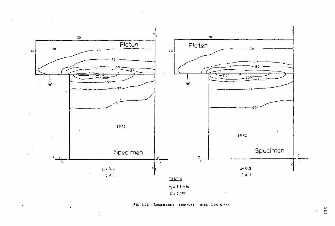
20
C L II'. 0.3
( 4 )
p.= 0. 2
(c )
90 °C
L L
Specimen
20 20
90°C
Specimen
TEST C
v1 = 8.8 m/s
E 1. 0.782
FIG. 6.26 — Temperature contours at ter 0.0016 sec

20 Platen ZO 20
20
30 135 141
145 146
146 °C
Specimen
20
20
20 Platen
0.0 a )
FIG. 6.27—Temperature contour s (in °C) after 0.0028 sec
T EST C
v. =5.8 m/s
E = 1.345

Ft- G. 6.27
20 Platen
25
—146
L we 0.2
c-1.345
20 1,0
20
210
180
165
30 50
100 f 6 5
c -Temperature contour s of ter 0.0028 sec
20
1"-- 0.3
E w 1.14 S S
d-Temperature contours of ter 0.0022 sec
TEST C
8.8 m/s
Specimen
146 °C

20 20
.20 Platen
20
20
- 23
az
93
93 °C
Specimen
IL
c1.58
20
E-0.79
( a ) Temperature ' contours after 0.0014 sec b )Temperature contours . after 0.0026 sec TEST 0
p.= 0.0 .
v. = 10 mis 1.
FIG, 6.1B

20 20
20
c L
e =1.5 8
TEST 0- c ) Temperature contours after 0.0014 sec ( b ) Temperature cont ours after 0.0026 sec
p.=0,1
10 mis
FIG-6.28
--179
Specimen • 179°C
Platen 23
50 100
27 —2 5
218 --200
--------19
E =0.79

20
TEST D
0.2
tv. 7.: 0 mls
FIG, 6.28
f )Temperature contours after 0 002sec c ) Temperature contours after 0.0014 sec
20
Platen
--- 98
93
93°C
Specimen
20
E = 0.7 9
20
148 °C
Specimen L
CL
1 . 3

267
friction which plays a major part in high speed upsetting. It may also
be deduced that the conduction to the die is slower at high speeds.
Nevertheless when friction is present, the layers near the platen
surface experience high intensity temperature rise particularly towards
the end of the deformation whore reduction is high. This may tentatively
explain the wearing of the forming dies in high speed forming processes
(13)(173). The wear is suggested by Rooks et al (173) to be partly due
to the temperature gradients in the die surface causing thermal fatigue
cracking and a reduction in the material's resistance. As the forming
speed is increased the bulk temperature of the die is lowered due to
the reduction of the time available for conduction. This however increases
the temperature gradient on the die surface. The authors, on the basis
that the higher the temperature, the more significant would be the wear,
in dynamically compressing cylindrical billets of steel between par-
allel, steel dies, concluded that the greater wear on their subpresp.
top die than the bottom one was due to higher temperature gradients.
They also showed that under various lubrication conditions the extent
and the depth of the wear was higher near the initial radius of the
billet. Isotherms given in Figs.6.23 to 6.28 show that when friction
is present the zone of intensive heating is in the region near the die
surface towards the outer radius. Considering the findings of Rooks at al
for the region of maximum wear, and the present investigation of the
region of intensive heating, it may be inferred as concluded experimentally
by those authors, that the region of maximum temperature and maximum
erosive wear seem to be virtually coincidental. In other words intensive
localised heating may be the cause of thermal fatigue failure and wear
in the toolings of high speed forming machines. On the other hand it
may also be said that it is these high localised temperatures which are
beneficial in preventing the die failure in terms of erosive wear as
suggested by Kellow et al (127).

268
From the temperature field and isotherms it can also be noticed
that in all cases if friction is absent the bulk of the material even
at the slowest speed considered, experienced almost uniform temperature
rise, the latter being only due to the plastic work of deformation.
Since heat flow to the die is slow, the assumption of uniform adiabatic
heating of the specimen is applicable, a point of argument which was
considered by Okamura and Nakanishi (168) in predicting the dynamic
isothermal behaviour of materials.
The mean bulk temperature of the specimen was also determined
in every increment of deformation. This is also presented in Table C,
below each temperature field. From the temperature distributions, the
maximum localised temperatures were determined, and these together with
the mean bulk temperature of the specimen are presented in Fig. 6.29.
This covers the four impact velocities, various platen/specimen
frictional conditions and reductions. From Fig. 6.29, the effect of
friction, speed and the extent of deformation, influencing the specimens'
bulk and localised temperatures can be deduced. Fig. 6.30 is accordingly•
produced by replotting Fig. 6.29. From the two figures it is clear that
speed and friction play a minor part in the deformation, but the extent
of their influence on the localised state of temperature is significant.
On this basis it is evident that the structure and the properties of
the deforming material are much influenced by the adiabatic heat of
deformation and more by friction. This is well substantiated further
by Figs. 6.31 and 6.32 which respectively indicate the effect of impact
velocity on the specimen's mean temperature and the maximum localised
temperature for various frictional conditions. The extent of the work
of friction in some instances at high speeds was so significant that
localised temperatures of limiting values (...--. 400EtC) were reached before
the end of the deformation. This limit was set ao as to avoid the
variations in the strain rate sensitivity usually experienced by copper
at high temperatures (40). The example given in Table C.18 for impact

'FIG 629 EFFECT OF FRICTION AND STRAIN ON TEMPERATURE
0 0.4 0,8 k2
Natural Strain
1.6
/1*
( a ) v = :10m/s
Natural train 0.4 048 1.2 1.6
300
MEAN BULK TEMPERATUV --MAX LOCALISED
(Material : copper) /
0
o
/ ti
fz;
100

0.3 0.4 0,5
300
MEAN BULK TEMPERATURE
MAX. LOCALISED TEMPERATURE
(Material : copper)
200 0
j E5 CL E
10
si/i/ V
/// _ 0 \
/ 'N /
/ V OZ
d )vi=4.5m/s
Natural Strain 0.2 0.4 0.6 0.8 1.0 0 0.1 0.2
Natural strain
MP,
FIG 6.29—EFFECT OF FRICTION AND STRAIN ON TEMPERATURE

I 7
0.1 0.2 0.3
Coefficient of friction II Coefficient of friction 0.1 0.2
z — MEAN BULK TEMPERATURE
— —MAX LOCALISED TEMPERATURE cMaterial copper)
( b )vi = 8.8m/s p
/
.6
- 0.4
0.2
100
FIG. 6.30-VARIATION OF TEMPERATURE WITH COEFFICIENT OF FRICTION

300-
MEAN BULK TEMPERATURE
MAX LOCALISED TEMPERATURE
(Material : copper)
200-1
Actu
al tem
pera
ture
°C
100
0.5
0.4
0 0.3 0.2
E_0.1
( d ) vi = 4.5 m/s
Coefficient of friction µ Coefficient of friction 1.1 yommaiwimmi■rwriast• 0.1 0.2 0.3 0.4 0t5 0 0.1 0.2 0.3 0.4 0.5
FIG, 6.30-VARIATION OF TEMPERATURE WITH COEFFICIENT OF FRICTION
11 te
mf
300
(c )vi = 6.4 m/s
20
1 0.6
100
E = 0.2

0.8
11=0.1 11.;0.2
ti =0.3
(Material : copper)
.4 •-■
• 0 . 2
mpact velocity (m/s)
8 9 10
273
20 mpe
ratu
re °
C
FIG. 6.31 -EFFECT OF SPEED AND FRICTION ON MEAN BULK TEMPERATURE

emp
erat
ure
°C Olifi•••••• z
p.=0.1
v=0.2
(Material : copper)
E: 0.8
z
274
m act velocit m/s)
8 9 10 3
FIG. 632 EFFECT OF SPEED AND FRICTION ON MAXIMUM LOCALISED
TEMPERATURE

275
velocity of 10m/s, clearly indicates this limiting temperature rise
The programme stopped for p= 0.2, at e=f=1.3 prior to the end of the
deformation. If however higher friction coefficients were attempted,
the limiting temperature would have been reached earlier in the deform-
ation.
From the results it is clear that the plastic work and friction
are jointly responsible for rise in the temperature and the latter has
a very pronounced role near the die/material interface. This influences
both the properties of the deforming material and frictional conditions.
Since stress and temperature are interdependent, and increasing, the
latter reduces the former, the high localised temperatures reduce the
yield stress locally. As seen from the isothermal plots, where friction
is present high temperatures are concentrated near the die/material
interface. This concentration is more radial than axial and has out-
flowing effects. Accordingly it may be inferred that shear stress
sustained by the specimen is lower in the region of high temperature
concentration than in the rest of the body. The anomaly of the flanging
effect observed by Habib (4) in dry compression of cylindrical high
conductivity copper billets at high velocities may be attributed to
this effect of localised intensive heating. The heat generation due
to the work of friction may have been so high as to prevent the temp-
erature dependent recovery processes operating. This therefore has
influenced the localised material properties and let the deforming
material flow more in the radial direction near the die/material
interface.
It is the high localised temperature rise which may be the cause
of incipient melting and recrystallisation of materials in high speed
extrusion processes (3)(13)(174). Aggrawal (3) and Lengyel and
Aggrawal (174) observed that in extruding copper rods, surface hardness
of the product decreased with increasing extrusion speed. Recrystallised

276
structures were observed on the product surface indicating high localised
temperature rises. eimilar recrystallisation of the structure of the
extruded products of copper at high speeds were also observed by Dower
(13). Aggrawal both quantitatively and experimentally showed the temp-
erature rise of the product's surface as a function of reduction and
equivalent mean strain rate. Although the product's temperature was
measured after some delay, high temperature rises were recorded. Since
friction along the surface of the die varies (160), and this also
changes with speed (107), the incipient melting may be attributed to
possible variation in the speed or friction, which in turn causes
changes in temperature locally by altering the magnitude of the work
of friction.
On the other hand it might be the adiabatic heating and the
localised temperature rise which are the beneficial factors in the
forming of difficult materials. An example of this is the high speed
impact extrusion of brittle materials given by Parsons et al (104).
The authors' preliminary results indicate that, generally, tensile
strength is lower while the residual ductility is higher for products
of high speed impact extrusion than for extrusion by true cold working
at slow speeds. On the basis that the limited time for heat losses
in high speed processes causes the work of deformation to appear as
heat in the workpiece, the present investigation may underline these
authors' suggestion that this adiabatic heating could have influenced
the mechanical properties and hence has been partly beneficial in the
forming of brittle materials.
Although at high speeds, strain rate effects should be predominant.
in increasing the yield stress, the accumulative adiabatic heating
could become prevalent in reducing it, so that at some stage the thermal
softening supercedes the work hardening and the strain rate effects (175).
The lowering of the extrusion force with the increase in speed found
by Whitely (176) might be the result of this. Whitely also attributes

277
the lowering of yield stress distribution with speed in the deformation
zone to be the result of increasing adiabatic heating in this region,
and moreover to the intensive localised heating effect persistent near
the die/material interface. Similar effects were observed by Davies and
Ohawan (177) who attributed the improvement in blanking characteristics
at high speeds to a thermoplastic instability in which deformation
became confined to a very narrow zone of high temperature material.
The present investigation similarly indicates the narrow region to
which high temperature is confined. This demonstrates that not only
would yield stress of the deforming material be lowered more extensively
in this region, a result of which may be the better product form due
to a possible reduction of the boundary friction, but also there would
be a reduction in the overall forming force, both of which were observed
by the above authors. These therefore explain that in general the
material's temperature rise can to some extent be beneficial in the
industrial application of forging and other large strain/high speed
metal working processes.
Results of the present findings and those of Lengyel and Aggrawal
(174) and Lengyel and Culver (178) signify that no typical material
properties may be expected from a particular deformation process.
Specifically, in high speed processes the heating of the workpiece and
the temperature distribution and variation can become significant and
the properties of each element of the deforming material and the
product may therefore be different depending on how much each is
influenced by heating.
The present results also show the significant contribution of
friction heat and point out the complex interaction between lubrication
conditions and temperatures, where neither could be understood unless
the process is followed step by step. Although the high temperature
rise at the billet/die interface in some forming processes may be
regarded as being due to poor lubrication conditions which could

278
develop partly due to the thinned down lubricant layer over the
interface, it may be that the reverse is also true and that the
lubrication breakdown is caused by the high localised temperature
rise. In other words lubrication conditions and temperature interact
with each other in a complex manner.
On the basis of the results of the present work, more homogeneity
in the deformation to larger strains in high speed compressions than in
slow speed compressions (77)(107), which is thought to be due to less
friction at the die/material interface and therefore better lubrication
conditions at high speeds, can be commented upon,. At high speeds higher
temperatures near the billet/platen interface could, as already indicated,
influence the strain distribution in this region. Owing to the reduced
flow stress, the end faces of the specimen could move more freely than
would be the case at slow speeds under otherwise identical conditions.
This might load to the reduction or complete elimination of barrelling
(attributed to friction at slow speeds), which in turn might be assumed
to represent a reduction in friction; in fact the reduction of friction
may be partly or entirely due to thermal effects. Indeed since temper-
atures and the drop in flow stress become greater as friction increases,
the elimination orany inhomogeneous deformation may, far from indic-
ating better lubrication and frictional conditions, imply the contrary
- more heat generation at the interface due to lubrication breakdown.
In order to verify that the results of the theoretical invest-•
igation were conclusive the actual temperature rises during the tests
were measured. Fig. 6.33 shows the effect of impact velocity on the
theoretical centre point temperatures. Figs. 6.34 and 6.35 provide
comparisons between the experimental and theoretical results and it is
clear that their agreement is generally reasonable. The discrepancies
could be attributed to the possible differences in the thermal properties
and the flow stress data of the experimented material and those used

0.4 0.8 1.2 1.6
Natural strain
15
•
279
F 10,6.33-THEORETICAL REPRESENTATION OF THE
EFFECT OF IMPACT VELOCITY ON THE CENTRE POINT TEMPERATURE
FOR COPPER

Vi ; 10 m/s
150—
Actu
al t
empe
ratu
re °
C
100—
280
•A 0 Experimental
Theoretical
(Material : copper)
vi _- 4.5 m/s
50—
I I I
0 0.2 0.4 0.6 0.8 vsuressintir
1.0
Natural strain ) ,.., 1.2 1.4 1.6
F1G. 6.34-COMPARISON OF EXPERIMENTAL AND THEORETICAL CENTRE POINT
TEMPERATURE

0 0.2 0.4 0.6 0.8 1.0 1.2 1.4
va c 8.8 m/s
Natural strain
A--® Experimental
Theoretical
(Material : copper)
Actu
al t
emp e
ratu
r e °
C
FIG.6.35 COMPARISON OF EXPERIMENTAL AND THEORETICAL CENTRE POINT.
TEMPERATURE
281

282
in the calculations, and also due to the heat generated by the billet
material in flowing over the thermocouple junction, an effect which is
not included in the computation.
The investigation however confirmed that in high strain rate
upsetting the adiabatic heat can alter material properties. It is
also substantiated that if homogeneous deformation is persistent
during the upsetting process, the bulk of the deforming material
experiences almost uniform temperature rise. It also ascertains the
complexity of interaction between a number of parameters persistent
in high speed metal forming which significantly influences the material
properties.

CHAPTER 7
CONCLUSIONS AND RECOMMENDATIONS
7.1 Conclusions
It is clear from the study that in previous investigations the
effects of variables influencing the dynamic material properties are
not always isolated. Moreover properties are either indirectly related
to the heat generation during the upsetting or are determined without
taking into account the influence of this additional heating effect. It
is suggested that this treatment often masks the accurate determination
of material behaviour as influenced by strain, strain rate and temper-
ature.
Examples are given of the variation in strain rate and its
associated effects, with the accumulation of temperature rise, on the
flow stress/strain-characteristics when compressing a cylindrical
specimen under free flight impact conditions. It is shown that in
continuously loading the specimen under dynamic conditions, the strain
rate changes considerably during the deformation. The material prop
erties which are represented in terms of the average values of this
variation are believed to misrepresent the actual behaviour since this
is an average of a substantial range over which the flow stress varies
significantly. Of similar effect is the material's temperature change
during the deformation, which is shown to influence the material
properties. Although the effect may be taken as unconnected with the
basic material properties, it is nevertheless seen to depend on
boundary conditions etc.; it is therefore considered undesirable since
283

284
it masks the required basic data.
The investigation reaffirms that the stress/strain curves obtained
by large deformation tests using free flight impact devices constitute
an assembly of data which correspond, in each test, to varioue temp-
eratures
and strain rate. Such data are thought to be quite satisfactory
in giving the general dynamic behaviour and in approximate metal working
analyses, but are of little help for a more realistic analysis where
the true properties at specific strains, strain rates and temperatures
are required, i.e. when mean values are no longer satisfactory.
The study indicates that more accurate stress/strain data can be ,
obtained by an incremental method, based on much the same priciple as
the techniques used in quasistatic testing. The incremental test method
used in the experimentation is found to be suitable for the application
to large strains, and high strain rate. With this method the magnitude
of the testing temperature and the strain rate could be made to remain
almost constant. The results obtained are shown to be free from any
possible side effects and represent the true dynamic behaviour.
From the theoretical work, it can be concluded that plastic work
and the heat generation due to end frictions in high speed compression
of axisymmetric billets have concommitant effects on the adiabatic
temperature rise. When friction is present the temperature field,
otherwise almost uniform, is much affected and the temperature rise
becomes significantly higher near the specimen/tooling interface. The
results also indicate that the stress distribution in the billet could
be different from that at slow speeds and that barrelling could be
decreased or completely eliminated by decreased stress due to reduced
flow stress at the billet ends.
The speed, friction and strain, and their contribution all have
pronounced influence on the adiabatic heating of the deforming material,
in as far as they alter the material's localised properties and structures.
It is shown that it is detrimental to the correct determination of the

285
dynamic behaviour if these effects are not isolated. Some effects
observed in high speed forming processes are interpreted tentatively
in terms of localised heating. Forming of difficult materials at high
speed and the improvement in their products and the process character-
istics are discussed. Lubrication conditions, the interaction between
this and temperature, on the tool life are accordingly explained.
The step by step method using the finite element technique was
found to be helpful and accurate in predicting the temperature field
by taking into account all variables influencing the deformation process.
Although homogeneous deformation, with constant tool/material frictions,
was assumed, the temperature fields obtained helped in describing
material properties in terms of single variables, and to some extent
demonstrated some adverse or beneficial effects of high speed formings.
7.2 Recommendations for Future Work
Arising out of the present study, the following approaches are
suggested for any possible future work:
1) Dynamic isothermal stress/strain characteristics may be determined
through obtaining data under continuous deformation tests. This
requires some initial extensive experimentation to obtain data
corresponding to various strain rates and temperatures. However
this has to be confined to ranges of temperature away from the
critical temperatures of the materials. Assembly of data correspond-
ing to a particular strain rate and temperature rise which would
include the temperature rise due to deformation, could then con-
stitute isothermal dynamic behaviour. Some possible constitutive
relationships describing the material behaviour might arise out of
out of these experimentations.
2) With the present computer programme which only considers homogeneous

286
deformation with constant specimen/platen interface friction, the
solutions of the temperature field may be used to work back and
find the strain distributions. It may then be possible substan-
tiate the extent of the flow of material near the die, ,aerial
interface.
3) Some realistic velocity field may be introduced in the computer
programme to account for the variation of strain and strain rate
due to any possible non-homogeneous deformation. For this purpose
some form of the visioplasticity method may be adopted. An example
of this is to use a specimen having fine holes in the longitudinal
and diametrical directions on its meridian plane; such that after
an increment of compression the movement of the intersection of
holes can be studied. Otherwise the procedure adopted by Metzler
(179) may be considered.
4) Arising out of (2) and (3), it may be possible to explain the
extent of barrelling and flaring effects in non-homogeneous deform-
ation in high speed upsetting and therefore study the possibility
of the distribution of any end frictions for the material.
5) The experimental and theoretical work may be further extended to
investigate thermal effects at high initial temperatures. The process
of dynamic recovery and dynamic recrystallisation (180) both being
time dependent and the hardness distribution as affected by temper-
ature and strain rate may then be explained.
6) The present computer programme may be modified to obtain temperature
distribution in other high speed metal working processes.

287
REFERENCES
1. COOK, M. and LARKE, E.C. J. Inst. Metals, 1945, 17, 371.
2. WATTS, A.B. and FORD, H. Proc. Inst. Mech. Eng., 1955, 169,
1141.
3. AGGRAWAL, R.N. "Material Properties in Hydrostatic Extrusion",
1970, M.Sc. Thesis, University of London.
4. HABIB, E.T. Symposium on "Flow and Fracture of Metals", ASME,
1968, 248.
b. MOK, C.H. and DUFFY, J. Int. J. mech. Sci., 1964, 6, 161.
6. MANJOINE, M. and NADAI, A. Pro. Am. Soc. Testing Materials.
1940, 40, 882.
7. KOLSKY, H. "Stress waves in Solids", 1963, New York.
8. McgUEEN,H.J., WONG, W.A. and JONAS, J.J. Canadian J. Phys.,
1967, 45, 1225.
9. ROSEN, A. and DORN, J.E. J. Inst. metals, 1964-5, 93, 387.
10. JONAS, J.J. and IMMARTGEON, J.P. "Zeitschrift feir Metallkunde",
1969, 60, 3, 227.
11. JONAS, J.J., AXELRAD, D..R. and UVIRA, J.L. Trans. Japan. Inst.
Met., 1968, 9, 257.
;12, SAMANTA, S.K. Int. J. Mech. Science, 1969, 11, 433.
13. DOWER, R.J. N.E.L. Report 188, 1965.
14. COLE, B.N., DAVIES, R., AUSTIN, E.R. and BAKHTAR, F. Pro. I.M.E.,
1965-6, 180, 1.
15. HENNECKE, H. "Warmstauchversuche mit Perlitischen, Martensit-
ischen and Austenitischen SeAhlen", 1926, Dr,' Ing.
Dissertation, Aachen Technichen Hochschule.
16. SEITZ, F., LAWSON, A.W. and MILLER, P. N.D.R.C. Report
A41-0SRD 495, 1942, U.S.A.

288
17. KRAFFT, V.N. "Instrumentation for High Speed Strain Measurement"
Responses of Metals to High Velocity Deformation, 1961,
9, Interscience Pub., New York,
18. TAYLOR, G.I. J. Inst. Civil Engrs., 1946, 26, 486,
19, VOLTERRA, E. Nuovo Cimento, 1948, 4, 1.
20, LINDHOLM, U.S. J. Mech. Phys. Solids, 1964, 12, 317.
21, MALVERN, L.E. "Behaviour of Material under Dynamic Loading",
1965, ASME Pub., New York, 81.
22. SAMANTA, S.K. and MAGI, J. Annals of the C.I.R.P., 1969,
XVII, 463.
23. HAUSER, F.E. Experimental Mechanics, 1966, 6, 395.
24. BILLINGTON, E.U. R.A.R.D.E. memorandum 8/72, 1972.
25, DILLION, W. "Mechanical Behaviour of Materials under Dynamic
Loads", 1967, Springer, Verlagen, New York, 21.
26. MAHTAB, F.U., JOHNSON, W. and SLATER, R.A.C. Proc. I.M.E.,
1965-6, 180, 1.
27. MAHTAB, F.U., JOHNSON, W. and SLATER, R.A.C. Int. 3. Mech.
Sci., 1965, 7, 685.
28. MOK, C.H. and DUFFY, J. Int. 3. mech. Sol., 19651 7, 355.
29. TABOR, D.
"The Hardness of Metals", 1951, Oxford University
Press.
30. JOHNSON, W. and TRAVIS, F.W. "High Speed Blanking of Steel",
in "Engineering Plasticity", 1968, Cambridge University
Press, 385.
31. SAMANTA, S.K. Int. J. Mech. Sci., 1967, 9, 485,
32. SAMANTA, S.K. Int. J. Mech. Sci., 1968, 10, 613.
33. STURGESS, C.E.N. and BRAMLEY, A.N. Adv. mach. Tool Des. Res.,
1970, B, 803.'
34. AKU, S.Y.', SLATER, R.A.C., and JOHNSON, W. Int. J. Mech. Sci.,
1967, 9, 495.

289
35. SLATER, R.A.C., JOHNSON, W. and AKU., S.Y. Adv. Mach. Tool
Des. Res., 1968, 1 , 115.
36. PUGH, H.L1.0. and WATKINS, M.T. "Properties of Materials at
High Rates of Strain", Pro..Inst. Mech. Engrs., 1957,
122.
37. BARAYA, G.L., JOWISON, W. and SLATER, R.A.C. Int. 3. mech. Sci.,
1965, 7, 621.
38. HAWKYARD, J.B. and POTTER, T.B. Int. J. Mech. Sci., 1971,
13, 2, 171.
39. OROWAN, E. B.I.S.R.A. Restricted Report, MW/F/22/50, 1950.
40. ALDER, J.F. and PHILLIPS, V.A. J. Inst. metals, 1954-5, 83, 80.
41. COOK, P.M. "Properties of materials at High Rates of Strain",
Pro. Inst. Mech. Engrs., 1957, 86.
42. THOMASON, P.F., FOGG, B. and CHISHOLM, A.W.J. Adv. Mach.
Tool Des. Res.., 1968, It 287.
43, PORTER, R. and 00101, A. "Cam-toggle Plastometer", B.Sc. Project,
Imperial College, London, 1969.
44. ITIHARI, M. metallurgist, 1935-6, 10, 141.
45. HODIERNE, F.A. J. Inst. metals, 1963, 91, 8, 267.
46. CALVERT, G. Pro. Inst. Mech. Engra., 1955, 169, 897.
47. TSUBOUCHI, M. and KUDO,.H. J. Japan Soc. for Tech. of Palsticity,
1968, 9, 88, 322.
48. KUDO, H. and TSUBOUCHI, M. Annals of C.I.R.P., 1971, XVIV„ 225, ,
49. DUFFY, J., CAMPBELL, J.D. and HAWLEY, R.H. J. App. Mech.,
Trans. ASME, 1971, 38, Series E, 83.
50. OrTANS, K. and WHITTON, P.W. Pro. Inst. Mech. Engrs, 1971,
185, 1149.
51. NADAI, A. and MANJOINE, M. J. App. Mech., Trans. AME, 1941,
63, A77.
52, BROOKES, A.M.P. and REDDAWAY, J.L. "Properties of materials at
High Rates of Strain", Pro. Inst. Mech. Engrs., 1957, 31.

290
53. CHIANG, C.H. J. Inst. Metals, 1970, 98, 78.
54. WOLAK, J. and FINNIE, I. Adv. Mach. Tool Des. Res.,
1967, 1, 233.
55. JOHNSON, P.C., STEIN, B.A. and DAVIS, R.S. "Symposium on
Dynamic Behaviour of Materials", 1962, Pub. American
Society for Testing and Materials, ASTM-Material Science,
Series E, 195.
56. HOGGATT, C.R. and RECHT, R.F. Pro. Int. Conf. on the Center for
High Energy Forming, June 1969.
57. HOGGATT, C.R. and RECHT, R.F. Experimental Mechanics, October 1969.
58. LAWsON, G.S. N.E.L. Report No. 51, 1962.
59. KUWADA, T., TAKEUCHI, T. and KUMASI, T. Trans. Nat. Res. Inst.
for Metals, 1964, 6, 6, 14.
60. KAWADA, T., TAKEUCHI, T., IKEDA, S. and KUMABI, T. Trans. Nat.
Res. Inst. for Metals, 1964, 6, 6, 14.
61. KAWADA, T., SUZUKI, M., TAKEUCHI, T., IKEDA, S., KUMABI, T. and
DENDO, T. Annals of the C.I.R.P., 1966, XIV, 35.
62. GAGNON, G. and JONAS, J.J. Trans. Metallurgical Society of
AIME, 1969, 245, 2581.
63. JONAS, J.J., McQUEEN„ H.J. and WONG, W.A. "Deformation under
Hot Working Conditions", 1968, Iron and Steel Inst.
Report Mo. 108, 49.
64. ALEXANDER, J.M.and BREWER, R.C. "Manufacturing Properties of
Metals", 1963, Van Norstrand„ London.
65. BELL, J.F. "Behaviour of Materials under Dynamic Loading",
1966, ASME Pub., New York, 19.
66. SUN, N.P. .Int. J. Mech. Sol., 1967, 9 415.
1
67. AL-HASSANI, S.T.S. and JOHNSON, W. "Advances in Machine Tool
Design and Research", 1970, B, 855.
68. SYMONDS, P.S. "Behaviour of Materials under Dynamic Loading",
1966, ASME Pub., 107.

291
69. VINCENT, B.J., GEE, R. and HUNTER, S.C. "Properties of Materials
at High Rates of Strain", Pro. Inst. Mech. Engrs., 1957,
51.
70. KARNES, C.H. "Strain Rate Effects in Cold Worked High Purity
Aluminium", 1963, Ph.D. Thesis, University of Texas,
U.S.A..
71. DHARAN, C.K.H. and HAUSER, F.E. Experimental Mechanics, 1970,
10, 9, 370.
72. DHARAN, C.K.H. "The Dynamic Behaviour of Aluminium at High
Strain Rates", 1968, Lawrence Radiation Laboratory,
University of California-Berkeley, U.S.A..
73. JAHSMAN, W.E. J. App. Mech., Trans. ASME, 1971, 38, E l (1), 75.
74, SLATER, R.A.C., JOHNSON, W. and AKU, S.Y. Int. J. Mech. Sci.,
1968, 10, 169.
75. THOMASON, P.F., FOGG, B. and CHISHOLM, A.W.J. "The Effect of
Temperature on the Yield Stress/Strain Relationships for
Alloy Steels", 1969, Res. Rept. No. 69/33, Dept of Mech.
Eng., University of Salford.
76, AUSTIN, E.R., DAVIES, R. and BAKHTAR, F. Pro. Inst. Mech.
Engrs., 1967-8, 182, 1, (9), 175.
77. JAIN, S.C. and BRAMLEY,.A.N. Adv. mach. Tool Des. Res., 1968,
1, 95.
78, PARSON, B., TAYLOR, R. and COLE, B.N. Pro. Inst. Mech. Engrs.,
1965-6, 180, 32.
79. KROK, T.V. "Development of a Technique for obtaining Stress/Strain
Curves of Metals at High Strain Rates on the U.S.I.
High Energy Rate Forging Machine", 1967, M.Sc. Thesis,
University of London.
80. HILL, R. "The Mathematical Theory of Plasticity", 1950,
Clarendon Press, Oxford.
81. LIPPMANN, H. Adv. Mach. Tool Des. Hes" 1966, 53.
292
82. DEAN, T.A. "Advances in machine Tool Design and Research",
1970, 0, 761,
83. CROOKALL, J.R. Private Communications, Imperial College, London.
84. VON KARMAN, T. and DUWEZ, P. J. App. Phys.r 1950, 21, 987.
85. CAMPBELL, J.D. and DOWLING, A.R. J. Mech. Phys. Solids, 19701
18, 43.
86. GAROFALO, F. "Fundamentals of Creep and Rupture in metals",
1965, Macmillan, Now York.
87. GAGNON, G. "Extrusion of Zinc at High Temperatures and Strain
Rates", 1968, Ph.D. Thesis, McGill University, Montreal,
Canada.
88. HACKETT, J.E. Trans. metallurgical Soc. AIME, 1967, 239, 969.
89. SAMANTA, S.K. "Deformation under Hot Working Conditions", 1968,
Iron and Steel Inst. Rept. No. 108, 121.
90. KARNES, C.H. and RIPPERGER, E.A. J. mech. Phys. Solids, 1966,
14, 75.
91. STAMELOS, D.C. "Effects of Strain Rates on Material.Properties",
1968, M.Sc. Thesis, Imperial College, University of London.
92. SARANTA, S.K. "Dynamic Deformation of Aluminium and Copper as
a Thermally Activated Process", 1970, Rept. No. M.E.49,
• Acta Polytechnica, Scandinavia.
93. SAMANTA S.K. 3. mech. Phys. Solids, 1971, 19, (3), 117.
94. BILLINGTON, E.W. and TATE, A. R.A.R.D.E. memorandum 30/71, 1971..
95. ORAVA, R.N. and OTTO, H.E. J. metals, 1970, 72, 2, 17.
96. THIRUVENGANDAM, A. and CONN, A.F. Experimental mechanics,
July 1971, 315.
97. SAMANTA, S.K. "Strain Rate Variation and Temperature Rise during
High Speed Testing of materials", Jernkontorets Annaler,
1971.
98. SLATER, R.A.C., AKU, S.Y. and JOHNSON, W. Annals of the C.I.R.P.,
19, (3), 513.

293
99. ATKINS, A.G. J. btrain Analysis, 1970, 5, 4, 269.
100. STURGESS, C.E.N. and JONES, M.G. Int. J. Mech. Sci., 1971,
13, 309.
101. SAMANTA, S.K. Annals of the C.I.R.P., 1971, 19, 755.
102. HARDY, H.K. Metallurgia, 1944, 30, 240.
103. SAMANTA, S.K. Adv. mach. Tool. Des. Res., 1970, B, 827.
104. PARSONS, B., LAYCOCK, 0.8. and COLE, B.N. Adv. mach. Tool Des.
Res., 1967, 2, 1003.
105. DOWER, R.J. Adv. mach. Tool Des. Res., 1966, 41.
106. DOWER, R.J., MILES, G.I. and BURGESS, I. N.E.L. Report 481, 1971.
107. JAIN, S.C. and BRAMLEY, A.N. Pro. Inst. Mech. Engra., 1967-68,
182, 1.
108. NICHOLAS, T. Exp. Mech., 1971, 11, 8, 370.
109. ASHFORD, P.G. D.I.C. Thesis, To be published.
110. LENGYEL, B. and KROK, T.V. Metal Forming, 1969, 36, (6), 172.
ill. LENGYEL, B. and STAMELOS, D.C. Annals of C.I.R.P., 1971, 19,
225
112. WHITFIELD, W. N.E.L. Report 325, 1967.
113. JAIN, S.C. and AMINI, E. Advs. Mach. Tool Des. Res., 1968, 2,
229
114. ORGAM, A.J. Int. J:Mach, Tool Des. Res., 1967, 7, 325.
115. SAMANTA, S.K. Int. J. Mech. Sci., 1970, 12, 793.
116. NAGAMATSU, A., mUROTA, T. and JIMMA, T. Bul. Japan. Soc. Mech.'
Engrs., 1971, 14, (70), 331.
117. KULKRANI, K.N. and KALPAKJIAN, S. Trans ASME, J. Eng. Inds.,
1969, 91, (B), 743.
118. FARREN. W.S. and TAYLOR, G.I. Proc. Royal Society, 1925,
Series A, 107, 422,
119. SIEBEL, E. and KOBITZSCH, R. Stahl and Eisen, 1943, 63, 110.

294
120. HIRST, S. and URSELL, D.H. "Proceedings of the Conference on
the Technology of Engineering Manufacture", 1958,
Paper 32, metal Treatment, 1958, 25, 409.
121. WATKINS, M.T., ASHCROFT, K. and McKENZIE, J. MERL Plasticity
Repts., 102(1955) and 111(1956).
122, SINGER, A.R.E. and AL-SAMARRAI, S.H.K J. Inst. Metals, 1960-61,
89, 225.
123. SINGER, A.R.E. and COAKHAM, J.W. ibid, 1960-61, 89, 177.
124. SAUVE, Ch.. "Phgnomenes Calorifiques Associes au Filage"„
Mem. Sci. Rev. Metallurgy, 1962, 59, 189.
125. TANNER, R.I. and JOHNSON, W. Int. J. Mech. Sci., 1960, 1, 28.
126. JOHNSON, W. and KUDO, H. ibid, 1960, 1, 175.
127. KELLOW, M.A., BRAMLEY, A.N. and BANNISTER, F.K. Int. J. mach.
Tool Des. Res., 1969, 9, 9.
128. BISHOP, J.F.N Quart. J. Mach Appl. Math., 1956, 9, (2), 236.
129. AKERET, R. J. Inst. Metals., 1967, 95, 204.
130. DUSINBERRE, G.M. "Heat Transfer Calculations by Finite Difference",
1961, International Textbook.
131. ALTAN, T. and KOBAYASHI, S. Trans. ASME„ J. Eng. Inds., 1968,
90, (B), 107.
132. THOMSEN, E.G., YOUNG, C.T. and KOBAYASHI, S., "Mechanics of
Plastic Deformation in Metal Processing", 1965, Macmillan,
New York.
133. GUHA, R.M. and LENGYEL, 8. Pro. Annals C.I.R.P., 1972, 20.
134. GUHA, R.M. and LENGYEL, B. "Temperaturuerteilung bei kobin-
ierter hydrostatischer Strangpressung and Zeihung",
Industrie-Anzeiger, To be published.
135. LANGE, K. Industrie-Anzeiger, 1972, 94, (20), 399.
136. YAMADA, Y., YOSHIMURA, N.,and SAKURAI, T. Int. J. Mech, Sol.,
1968, 10, 343.

295
137. MILES, G.A. and WHITE, D.J. J. Sci. Tech., 1970, 37, (3), 127.
138. ALEXANDER, J.M. and GUNUAKERA, J.S. Proc. Royal Society, 1972,
Series A, 326, 361.
139. LEE, C.H. and KOBAYAsHI, S. Int. J. Mech. sci., 1970, 12, 349.
140. LEE, C.H. and KOBAYASHI, S. Trans ASME, J. Eng. Inds., 1971,
93, Series 8, (2), 445.
141. NAGAMATSU, A., MUROTA, T. and JIMMA, T., Bul. Japan. Soc.
Mech. Engrs., 1971, 14, (70),,339.
142. IWATA, K., OSAKADA, K. and FUJINO, S. Trans ASME, 1972, 94,
Series B, (2), 697.
143. ZIENKIEWICZ, 0.C. and CHEUNG, Y.K. The Engineer, Sept 1965, 507.
144. SCHECHTER, R.S. "The Variational Method in Engineering", 1967,
McGraw Hill, New York.
145. ZIENKIEWICZ, 0.C. App. Mech. Rev., 1970, 23, pt.3, (1), 249.
146. VISSER, W. Pro. Conf. on Matrix Method in Structural Mechanics,
1965, Air Force Inst., bf Tech., Wright Patterson A.F.
Base, Ohio, U.S.A..
147. WILSON, E.L. and NICKELL, R.E. Nuc. Eng. Des., 1966, 4, 276.
148. ZIENKIEWICZ, O.C. and PAREKH, C.J. Int. J. Num. Meth. Eng.,
1970, 2, 61.
149. sOLIMAN, J.I. and FAKiiR00, E.A. J. Mech. Eng. sci., 1972, 14,
(1), 19.
150. ZIENKIEWICZ, O.C. "The finite element method in Engineering
Science", 1971, McGraw Hill, London.
151. ZIENKIEWICZ, O.C. and CHEUNG, Y.K. "The Finite Element Method
in Structural and Continuum Mechanics", 1967, McGraw 1
Hill, New York.
152. AVITZUR, B. "Metal Forming: Processes and-Analy'ses", 1968,
McGraw Hill, New York.
153. PALIT, K. and FENNER, R.T. J. A.I.Ch. Eng., 1972, 18, (3),
628.

296
154. PALIT, K. and FENNER, R.T. "Two Dimensional Slow non-Newtonian
flows", J. A.I.Ch. Eng., To be published.
155. FENNER, R.T. Private Communication, 1971, Imperial College,
London.
156. PALIT, K. "melt Flow in Polymer Processing Equipments", 1972,
Ph.D. Thesis, University of London.
157. VARGA, R.S. "Matrix Iterative Analysis", 1962, Prentice Hall,
London.
158. PALIT, K. Private Communication, 1971, Imperial College,
London.
159. BLOMFIELD, J. Private Communication, 1971, Imperial College,
London.
160. KAMYAB-TEHRANI, S. "On Pressure and Frictional Conditions in
Hydrostatic Extrusion Dies", 1972, Ph.D. Thesis, University
of London.
161. LUDWICK, P. "Elements der Technologischen Mechanik"„ 1909,
Springer, Berlin.
162. BITANS, K. and WHITTON, P.W. Int. met. Rev., 1972, 17, 66,
163. SUZUKI, H., HASHIZUME, S., YABUKI, Y., ICHIHARA, Y., NAKAJIMA, S.
and KOMMOCHI, K. Rept. Inst. ind. Sci., Tokyo Univ.,
1968, 18, (2)'t 139.
164. KENDALL, D.P. Trans ASME, J. Basic Eng., 1972, 94, (0), 207.
165. GUHA, R.M. "Temperature Distribution in Hydrostatic Extrusion",
1971, M.Sc. Thesis, University of London.
166. LINDHOLM, U.S. "BehaViour of Materials under Dynamic Loading",
1965, ASME Pub., New York, 62.
167. LENGYEL, B. and MOHITPOUR, M. J. Inst. Metals, 1972, 100, 1.
168. OKAMURA, S. and NAKANISHI, K. Japan Soc. Tech. Plas., 1971,
12, (128), 653.
169. BERGER, F. Zeitschrift fur math. u. Mech., 1931, 11, (1), 45.

297
170. EMERY, A.F. and CARSON, W.W. Trans ASME., J. Heat Trans.*
1971, 93, (2), C, 136.
171. Handbook of Thermophysical Properites of Solid materials, 1955,
1, Pergamon Press, New York.
172. TOULOUKIAN, Y.S. "Thermophysical Properites of High Temperature
Solids", 1967, 3, Macmillan Co., New York.
173. ROOKS, 8.W., TOBIAS, S.A. and ALI, S.M. Advs. mach. Tool Des.
Res., 197.0, 8, 745.
174. LENGYEL, B. and AGGRAWAL, B. "Further Results on material
Properties in HydrOstatic Extrusion", To be published.
175. LENGYEL, B. "Properties of Hydrostatically Extruded Products"
Post Experience Course in Hydrostatic Extrusion, 196B,
Imperial College, London.
176. WHITELY, A. M.Sc. Thesis, 1972, Imperial College, University of
London.
177. DAVIES, R. and DHAWAN, S.M. Advs. Mach. Tool Des. Res., 1968,
2, 135.
178. LENGYEL, B. and CULVER, L.E. J. Inst. metals, 1969, 97, 97.
179. METZLER, H.J. Industrie-Anzeiger, 1970, 92, (57), 1373.
180, McQUEEN, H.J. and JONAS, J.J. metal Sci. J., 1972. 6, 25.

298
APPENDIX A
PROGRATTING SYMIROLS AND COMPUTER PROGRAMTE
A.1 Name List of Major Variables
A.1.I Main Routines
BETA (3 r Constant; proportion of deformation work
appearing as heat (Eq. 4.64)
COFMEU Coefficient of friction p
DELTI Increment of time for heat transportation hr
HITEQU O - Mechanical equivalent of heat kbar m3/kcal
NUMNPS Total number of billets nodal points
*NUP Nodal point
RMAXSP Maximum radius of billet cm
SPLNGT Billet's initial length cm
TIMING Time increment for deformation S
A.1.2 Subroutine GEN
NCYCM No. of cycles of iteration
NRPT No. of nodal points in r direction in an overall
rectangular continuum
NRPTPL No. of points added in r direction to cover
additional nodes for a reversed L-shaped (J) body
I *NUP 4... refers to a particular nodal point and-is used abundantly
throughout the programme.

299
NZPT No. of nodal points in z direction in an overall
rectangular continuum
NZPTSP No. of points along the specimen's side in z
direction
NUMBC Total number of nodal points along boundaries
where variables are fixed or known
NU11EL Total number of elements
NUMNP Total number of nodal points
NUP Nodal point
RN Largest distance between two nodal points in r
direction cm
TOLER Tolerance
XFACT Relaxation factor
7N Largest distance between two nodal points in z
direction
A.1.3 Subroutine INPUT
CDC(NUCDC) Billet's density kg/m3
CKC(NUCKC) Billet's thermal conductivity kcal
hr m oC
CPC(NUCPC) Billet's specific heat kcal/kg
CDS(NUCDS) Platen's density kg/m3
CKS(NUCKS) Platen's thermal conductivity kcal
CPS(NUCPS) Platen's specific heat kcal/kg
DEFVEL(NUVEL) Deformation velocity m/s
DEFTIM(NUVEL) Deformation time
HFA(NUHFA) Heat transfer film coefficient for air kcal
INTENT Error Signal parameter
hr m oC
m2 hr oC

300
NUCOC
NUCKC
NUCPC
NUCOS
NUCKS
NUCPS
NUHF1
NUSTRS
NUSTRN
NUVEL
Number of intervals at which various data
are read in
STRNST(NUSTRN) Strains (natural) at which flow stresses are read
in
STS(NUSTRS, NUSTRN) Flow stress data input kbar
TEMCDC(NUCDC)
TEMCKC(NUCKC)
TEMCPC(NUCPC) Temperatures corresponding to thermal
TEMCDS(NUCDS) parameters
oC
TEMCKS(NUCKS)
TEMCPS(NUCPS)
TSTRS(NUSTRS) Temperature corresponding to flow stress
input data 0C
A.2 Other General Symbols
AREA Elemental area A cm2
AA(N) Area of element N cm2
AO(N), AK(N) Dimension ail ak of element N (see text Fig. 5.5)
AVSTRN Mean strain (Actual strain for homogeneous
deformation)

301
AVSTRT Mean strain rate (actual strain rate for
homogeneous deformation)
AVTEMP Specimen's mean bulk temperature °C
BDMNT Boundary temperature oC
BJ(N), OK(N) Dimension bj'
bk
of element N (see text
Fig. 5.5)
BRAKT 1
ORAKT 2
ODSTRS
2 2r 2/
r / KK KK"
Boundary stress MN/m2
— equation 4.71
CD Elemental density p kg/m2
CK Elemental conductivity k kcal/hr m °C
CP Elemental specific heat c kcal/kg
CZZ(L) Contribution of terms appearing on the right
hand side of expressions 4.63 or 4.64,
(L=1, NUMNP)
D(IN,3N), DZ(IN,JN) Elemental heat capacity matrices [c ]e
DY(IN,JN) (INIJN= 3x3)
DEFINC - Increment of deformation cm
DEFVLI Deformation velocity at the outset of impact
or prior to each step of deformation
DT(L) Gradient of temperature with respect to
time for nodal point, numbered L °C/hr
ELMNT Mean elemental temperature
= (T(I) + T(J) + T(K))/3 °C
ELTEMP(N)
EXPCON
EXPVR1
EXPVR2
F(L)
Temperature of element N
Exponential constant eKKR
o (equation 4.71)"
Exponential variable (1/6KKr) (equation 4.71)
Elemental contribution of terms on the right
hand side of expression 4.63 or 4.62 L=1,3

302
FACTOR Constant KK = --8 (equation 4.70)
FICWRK Work done due to friction Wf
MN m/hr
H(IN,JN), HXX(IN,JN) Elemental convection heat matrix h
- contribution appearing on the left hand
side of equation 4.63 (IN,3N = 3 x 3)
HITRIS Elemental boundary heat flux due to the work
of friction kcal/hr
HF Elemental boundary heat transfer film
coefficient (hF ) kcal/hr m2 (IC
HX(L), HXXX(L) Elemental contribution of heat transfer
appearing on the right hand side of equation
4.63 (L = 1,3)
INTENT Error signal parameter
MP(L) Array defining nodal point in a zone L=1, NUMNP
NAP(L) Nodal point numbered L
NNPI(M) Nodal point i of a regular rectangle M
NNP3(M) tf 11 j n 11 11 n /I
NNPK(M) ft n k 11 ft 11 tt
NNPL(M) ft 1 " 11 11 ft If
NOD(L,LL) Array describing the connection of nodal
point numbered L to LL number of adjacent
nodes
NPB(L) Boundary node numbered L having a fixed
and known value
NPI(N) Nodal point i of a triangular element N
NP3(N) j 11 1I If
NPKtN)- k " " u
NREL No. of regular rectangled'in r directibn
(for a rectangular continuum
NPNUM(L) Nodal point numbered L
NUME(N) Element numbered N

303
NUMELI Total number of elements in a rectangular continuum
NUMNPI Total number of nodal points in a rectangular
continuum
NUP Nodal point
NZEL No. of rectangles in a row in z direction
NZPL Number of nodal points in a row in z direction
in the platen continuum
NZST Number of nodal points in a row in z direction
in the platen continuum except the rone on the
line of discontinuity
Q(N) Heat generation in element N (if included) kcal/hr
QF(L) Boundary heat flux assigned to node L kcal/hr
RBR, RBZ Mean value of two nodal point ordinates in r
and z directions respectively
RFACT A factor by which nodal point ordinates in r
direction would increase as a result of a reduction
of the ordinates of these points in z direction
RL Right angled side length of an element in r
direction cm
RM mean elemental radius cm
RORD(M) Ordinate of node M in r direction
S(IN,IJ) Elemental conduction heat metrix k 8,
(IN,JN = 3 x 3) - and also contribution of all -
terms appearing on the left hand side of equation
4.63 or 4.64 for the whole body to give the
continuum stiffness
SPLGTF Billet length at any instant cm
SPLGTI Billet length prior to each step of deformation

304
STRATE(N) Strain rate sustained by node N
STRN(N) Strain sustained by node N
STRNI(N) Initial strain sustained by node N
STRNIC(N) Increment of strain sustained by node N
STRS(N) Stress sustained by node N
SZZ(L,LL) Nodal point L stiffness with respect to LL
number of adjacent nodes
SZZ(L,l) Diagonals of total stiffness matrix
(L=1, NUMNP) (see text, equation 5.3)
O T(M), TEMNOD(M) Temperature of nodal point M C
TF Fluid or air temperature
TI(M) Initial temperature of nodal point M 0C
TINCDF Increment of temperature rise due to increment
of deformation = p x os x AE/(DpC) °C
(equation 4.65)
TIME Duration of deformation from the outset of
compression t.
TIMMAX Maximum actual permissible duration for
compression
VELDEF
Velocity at any instant during the deformation
cm/s
ZL Right angled side length of an element in
z direction cm
ZORD(M) Ordinate of node M in z direction cm

305
A.3-COMPUTER PROGRAMME
PROGRAM TEMPS (INPUT.OUTPUT, TAPE5=INPUTe TAPE6=OUTPUT) C C JOB NO. UMEM 237 M.MOHITPOUR C
COMMON NUMEL. NUmNP. NUMBC, NUZPT. NZPT, ZN, NPI(696), NPJ(696), 1 NPK(696), AA(696) 9NZEL,NZ COMMON /LCl/XFACT.NCYCM.TOLER.NPNUM(392)/LC2/AJ(696).AK(696)$ 18,1(696).BK(696)/Lc3/ZORD(392).RORD(392)/LC4/C4Z(392),SZZ(392,9)* 2ZLOAD(392)/LC5/NP(392,10),NAP(392)/LC6/ T (392)/LC7/NPb(035) COMMON/LC9/RORDI(392)/LC10/MP(392)/LC11/DT(392)/LC14/T1(392) CoMMON/LC15/STRN(392).STRATE(392),STRS(392) COMMON/LC17/CPC(050),TEMCPC(050)+NUCPC.CDC(050),TEMCDC(050),NUCDC COMMON/LC21/DEFVEL(050),DEFTIM(050),NUVEL DIMENSION OTI(392),TNODAL(392),TINCDF(392)+STRNI(392),STRNIC(392)
CALL INPUT
COFMEU=0.0 GO TO 4
3 COFMEU=COFMEU+0.1 IF(COFMEU.GT.0.51) GO TO 130
4 CALL GEN (NUMNPI.NZPL,NZST ) C C *************** INITIALISE THE NECESSARY COMPONENTS **************
DO 5 N=10NUMNP STRS(N)=0.0 STRN(N)=0.0 STRATE(N)=0.0 STRNI(N)=0.0 STRNIC(N)=0.0 TINCDF(N)=0.0
5 CONTINUE C
NPLEFT=1 NUP1=NPLEFT NPRIT=NZPT—NZST NUP321=NUMNPI—(NZPT-1) NUP330=NUMNPI—NZST SPLNGT=2.0*(ZORD(NPRIT)—ZORD(NPLEFT)) SPLGTI=SPLNGT RMAXSP=RORD(NUP330) ZNNEW=ZN
C C *****************************************************************
START OF DEFORMATION C *****************************************************************
TIMINC=0.0002 TIME=TIMINC T/MMAX=DEFTIM(NUVEL) DEFVLI=DEFVEL(1)
8 IF(TIME.GE.TIMMAX) GO TO 3 CALL LININT (DEFVELIDEFTIM,NUVEL.TIME eVELDEF;INTENT ) IF(INTENT.NE.10) GO TO 15 WRITE(6.10) TIME
10 FORMAT(1X,22H DEFORMATION VELOCITY // 20H DEFORMATION TIME = 9F10. X7) STOP
15 DEFINC=(DEFVLI+VELDEF)/2.0*TIMINC DEFINC=DEFINC*100,0
C
C

ZFACT=1.0—DEFINC/((ZORD(NPRIT)—ZORD(NPLEFT))*2o0) RFACT=1•0/SORT(ZFACT) CALL MODIFY(ZNNEW,DEFINC,RFACToNUMNPIoNZPLoNZST,COFMEU) SPLGTF=SPLGTI—DEFINC RMAXSP=RORD(NUP330)
C C ** MAKE CORRECTIONS TO TEMPERATURE DISTRIBUTION WITHIN PLATENS ***
CALL CORCTN (NZPToNZSTIINUMNPIoNZPLoNUMNP ) C C ** EVALUATE STRESSES AND STRAIN SUSTAINED IN THE DEFORMATION ZONE**
AVSTRN=0,0 AVSTRT=0.0 NUMNPS=210 DO 20 II=NUPloNUP321INZPT JJ=II KK=JJ+(NZPT—NZPL) DO 20 NN=JJoKK STRN(NN)=ALOG(SPLNGT/SPLGTF) STRNIC(NN)=STRN(NN)—STRNI(NN) STRATE(NN)=VELDEF/SPLGTF*1004,0
C AVSTRN=AVSTRN+STRN(NN) AVSTRT=AVSTRT+STRATE(NN)
C 20 CONTINUE
AVSTRN=AVSTRN/FLOAT(NUMNPS) AVSTRT=AVSTRT/FLOAT(NUMNPS)
C C ***** CALCULATE STRESSES SUSTAINED IN THE DEFORMATION ZONE *******
CALL STRESS (NUMNPloNZPToNZPL) C C ****** EVALUATE TEMPERATURE RISE IN THE DEFORMATION ZONE *********
DO 61 III=NUP1oNUP321oNZPT JJJ=Ill KKK=JJJ+(NZPT—NZPL) DO 61 NNN=JJJ,KKK TEMNOD=T(NNN) CALL LININT (CPCoTEMCPC•NUCPCoTEMNODvCPCNODvINTENT) IF(INTENT.NE.10) GO TO 40 WRITE(6.30) TEMNOD.NNN
30 FORMAT(1X,31H SPECIFIC HEAT OF SPECIMEN // 29H NODAL POINT• XTEMPERATURE = ,F10.5/14H NODAL POINT = .14) STOP
40 CALL LININT(CDC.TEMCDC.NUCDCoTEMNODoCOCNOD.INTENT ) IF(INTENToNE.10) GO TO 60 WRITE(6450) TEMNOD'NNN
50 FORMAT(IX.21H DENSITY OF SPECIMEN // 26H NODAL POINT TEMPERATURE.= X oF10.5/ 14H NODAL POINT = 0I4) STOP
60 BETA=1.0 HITEW=0.0042 TiNCDF(NNN)=CBETA*STRS(NNN)*STRNIC(NNN))/(HITECIV*CPCNOD*CDCNOD)
61 CONTINUE C
DO 65 N=loNUMNP TNOOAL(N)=T(N)+TINCDF(N) T(N)=TNODAL(N) TI(N)=T(N)
306

307
65 CONTINUE C C ************* START OF TRANSIENT HEAT TRANSPORTATION ************* C TEMPERATURE TIME DERIVATIVE INITIALISATION
81 CALL DTINTL(NZST.NUmNPI,C0FmEueHITEov,RmAXSP+VELDEF, XSpLGTF,INTENT) 1F(INTENT.EQ.10) STOP
C IF1C0FMEU) 82482,87
82 NuP11=NZPT—(NZST-1) NUP331=NUMNPI—(NZST-1) NUP337=NUMNP1 NUP386=NUMNP—NZST DO 85 M=NUPIleNUP3314NZPT JsM K=J+(NZST-1) DO 85 L=JoK DICL)=ABSIDT(L))
85 CONTINUE DO 86 M=NUP337+NUP386+NZPL J=M K=J+NZST DO 86 L=J,K DT(L)=ABS(DT(L))
86 CONTINUE C
87 DELTI=2.0/36000000.0 CALL STIFF (NZST+NUMNPI,COFMEU•HITEQV+RMAXSP+VELDEF•SPLGTF, XDELTI•INTENT) IF(INTENToE0.10) STOP CALL SOLN(TIME,AVSTRN+AVSTRT+COFMEU•NLST,NZPL•NUMNPI•NUMNPS)
C C ******************* END OF HEAT TRANSPORTATION ******************* C -
****************************************************************** C PROGRESSION OF DEFORMATION C ****************************************************************** .
TIME=TIME+TIMINC DEFVLI=VELDEF SPLGTI=SPLGTF DO 120 IV=NUP10,NUP321.NZPT JV=IV Kv=JV-4-(NZPT—NZPL) DO 120 NV=JV,KV STRNI(NV)=STRN(NV)
120 CONTINUE GO TO 8
C C ***********************END OF DEFORMAT/ON************************* - - 130 STOP
END
SUBROUTINE INPUT C
COMMON/LC16/STS(5,15)+TSTRS(5)•STRNST(15)+NUSTRS+NUSTRN COMMoN/LC17/Cpc(050).TEMCpc(050)+NuCPC,CDC(050).TEMCDC(050).NUCDC

308
COMMON/LC18/CPS(050),TEMCPS(050).NUCPS,CDS(050),TEMCDS(050),NOCDS COMMON/LC19/HFA(050),TEMHFA(050),NUHFA COMMON/LC20/CKC(050),TEMCKC(050).NUCKCIICKS(050),TEMCKS(050),NUCKS COMMON/LC21/DEFVEL(050),DEFTIM(050),NUVEL
C ******************************************************************
C READ STRESS CURVES C ******************************************************************
READ(5.10) NUSTRSoNUSTRN READ(5,15) (TSTRS(1),I=1,NUSTRS) READ(5.15)(STRNST(J).J=1,NUSTRN) DO 5 J=1,NUSTRN
5 READ(5,15)(STS(I.J)01=1.11NUSTRS) 10 FORMAT(215) 15 FORMAT(7F10.0)
C C ******************************************************************
C READ HEAT CONSTANTS ******************************************************************
READ(5,18) NUCPC.NUCDC.NUCKC•NUCPS,NUCDS,NUCKS+NUHFA.NUVEL READ(5.20)(TEMCPC(I)+CPC(I)+I=1,NUCPC) READ(5,20)(TEMCDC(I),CDC(I)+1=1 ,NUCDC) READ(5,20)(TEMCKC(I).CKC(I),I=1 ,NUCKC) READ(5,20) (TEMCPS(I),CPS(I),I=1,NUCPS) READ(5,20)(TEMCDS(I)+CDS(1),I=1 ,NUCDS) READ(5.20)(TEMCKS(1).CKS(I),I=1 ,NUCKS) READ(5,20) (TEMHFA(I),HFA(I) .1=1,NUHFA)
18 FORMAT(8I5) 20 FORMAT(8F10.0)
C ******************************************************************
C READ DEFORMATION VELOCITY ****************************************************************##
READ(5,25) (DEFVEL(1),DEFTIM(I).1.7.1,NUVEL) 25 FORMAT(8F10.7) '
C RETURN END
SUBROUTINE GEN(NUMNPI,NZPLoNZST) C
COMMON NUMEL. NUMNP, NUMBC. NUZPT, NZPTo 2N, NPI(696), NPJ(696), 1 NPK(696). AA(696)•NZEL•NZ COMMON /LC1/XFACTIINCYCM.TOLER,NPNUM(392) COMMON/LC2/AJ(696),AK(696).8J(696),BK(696)/LC3/ZORD(392)+RORD(392) 1/LC6/ T (392)/LC7/NPB(035)/LC8/2(392),R(392) COMMON/LC9/RORDI(392) COMMON/LC1O/MP(392) COMMON/LC11/ DT(392) COMMON/LC14/TI(392) DIMENSION NNPI(348).NNPJ(348).NNPK(348),NNPL(348),NUME(696)
C C ******************************************************************
C TO GENERATE A RECTANGULAR OVERALL MESH PATTREN C ******************************************************************
NZPT=16 NRPT=21

NCYCM=1000 XFACT=1.475 TPLER=0.000001 NZEL=NZPT — 1 NPEL=NRPT-1 ZN=0.254 RN=04,0635 NUMEL = 2*NZEL*NREL NUMELI=NUMEL NUMNP = NZPT*NRPT NUM8C=NRPT NUZPT=NUMNP NZEL NUMELN=NUMEL/2 NUZEL=NUMELH NZEL + 1 NZELM1=NZEL — 1 NZ=NUZPT—NZPT
DO 50 J=1*NUZPTe NZPT
DO 50 I=1•NZPT M=I + K IF(I.LE.4) GO TO 42 IF(I.E©.5.OR .I.EQ,6•OR•I.E0.15.0R.I.EQ•16) GO TO 44 IFfI.GE.7.AN0.I•LE•14) GO TO 46
42 L=I—.1 ZORD(M)=ZN*FLOAT(L) GO TO 50
44 ZORDM=ZORD(M-1)+ZN/24,0 GO TO 50
46 ZORD(M)=ZORD(M-1)+ZN/4.0 50 CONTINUE .
DO 60 J=1,NZPT
DO 60 I=1•NUZPT. NZPT M=I + K L=(I-1)/NZPT RORD(M)=RN*FLOAT(L)
60 RORDI(M)=RORD(M)
MM=O KL=0 DO 90 K=1.NUZELt NZEL N=K-1 DO 80 M=IeNZEL I=M + N KM=I+MM+KL KN=KM/2 L=2*1 — 1 J=2*I NNPI( I )=M+N+MM NNPJ( I )=NNPI( I ) +1 NNPK( I )=NNPJ( 1 ) +NZPT NNPL( I )=NNPI( I ) +NZPT IF(KN*2 .NE. KM) GO TO 91 IF(KN*2 .EQ. KM) GO TO 92
91 NPI(L)=NNPI(I) NPJ(L)=NNPK(I) NPK(L)=NNPL(I)
309
C
C

310
NpI(J)=NNPI(I) NpJ(J)=NNPJ(I) NpK(J)=NNPK(I) GO TO 80
92 NpI(L)=NNPI(I) NpJ(L)=NNPJ(I) NpK(L)=NNPL(I) NpI(J)=NNPJ(I) NpJ(J)=NNPK(I) NpK(J)=NNPL(I)
80 CONTINUE Mm=MM + 1 KL=KL+1
90 CONTINUE C
C
****************************************************************** TO INCLUDE ADDITIONAL ELEMENTS FOR A REVERSED L SHAPED CONTINUM
C ******************************************************************
C NuMNPI=NUMNP NuMNP1= NUMNP+1 NzPTSP=I0 NRPTPL=8 NuMNP=NUMNP+NRPTPL*(NRPTPL-1) NuMEL=NUMEL+(NZEL-(NZPTSP-1))*NRPTPL*2 NZST=NZPT-NZPTSP NzPL=NRPTPL-1 NuP386=NUMNP-(NZPL-1)
C DO 105 NP=NUMNPI•NUP386.NZPL NpEND=NP+NZST DO 105 M=NP,NPEND ZoRD(M)=ZORD(M-NZPL) RORD(M)=RORD(M-NZPL)+RN
105 RoRDI(M)=RORD(M) . C
NuMBC=NUMBC+NZELM1 C
NN=NZPL NzEBOT=NUMELH+I NZETOP=NZEBOT+NZST*NZPL Mm=2*NZEL-1 DO 1000 K=NZEBOT,NZETOP. NZST N=K-1 DO 940 M=1,NZST I=M + N KM=I+MM KN=KM/2 L=2*I - 1 J=2*I NNPI( I )=M+N+MM NNPJ( I )=NNPI( I ) +1 NNPK(I)=NNPJ(I)+NN NNPL(I)=NNPI(I)+NN IF(KN*2 •NE. KM) GO TO 920 IF(KN*2 .EQ. KM) GO TO 930
920 NPI(L)=NNPI(I) NpJ(L)=NNPK(I) NpK(L)=NNPL(I)

311
N13/(j)=NNPI(I) NpJ(J)=NNPJ(I) NpK(J)=NNPK(I) GO TO 940
930 NPI(L)=NNPI(I) NpJ(L)=NNPJ(I) NpK(L)=NNPL(I) NPI(J)=NNPJ(I) NpJ(J)=NNPK(I) NpK(J)=NNPL(I)
940 CONTINUE MM=MM+1
1000 CONTINUE C C *****************COMPUTE THE ELEMENTAL AREA **********************
DO 1010 N=1.NUMEL IF(N.LE.696) GO TO 1006 WRITE(6.1005) N
1005 FORMAT(10X+24H UNRECOGNISABLE ELEMENT /10X.14H ELEMENT NO = +18) STOP
1006 I=NPI(N) J = NPJ(N) K = NPK(N) Aj(N) = ZORD(J) ZORD(I) AK(N) = ZORD(K) — ZORD(I) Bj(N) = RORD(J) RORD(I) BK(N) = RORD(K) — RORD(I) AREA = (AJ(N)*BK(N) — BJ(N)*AK(N))/2. AA(N)=AREA IF(AREA) 1020,1020.1010
1010 CONTINUE GO TO 1031
1020 WRITE(6+1030) N 1030 FORMAT(I8) 1031 CONTINUE C C ***** ASSIGN KNOWN INIT1AL,TEMPERATURES TO ALL NODAL POINTS ******
CALL TINTL(NUMNP) C
DO 71 K=1:NUMNP NpNUM(K)=K MP(K)=0
71 CONTINUE C C *********** IDENTIFY SUBDIVISIONS OF THE OVERALL MESH ************
CALL ZONE (NZPTIINZST,NUMNPIeNZPL,NUMNP ) C
***********CONVECTING OR NONCONVECTING BOUNDARIES *************** CALL BOUND (NZPT,NUMNPI,NZPLsNZST,NUMNP )
C DO 75 L=1,NUMEL NuME(L)=L
75 CONTINUE
RETURN END

SUBROUTINE TINTL (NUMNP)
COMMON /LCl/XFACTeNCYCM,TOLER,NPNUM(392)/LC6/T(392)/ 1LC14/TI(392)/LC11/01-(351)
DO 70 I=1sNUMNP NPNUM(I)=I T(I)=204.0 DT(I)=0.0 T1(1)=T(I)
70 CONTINUE
RETURN END
SUBROUTINE ZONE (NZPT,NZSTIINUMNPIoNZPL.NUMNP )
COMMON /LC1/XFACTeNCYCM,TOLER+NPNUM(392)/LCIO/MP(392)
NUP10=NZPT—NZST NuP330=NUMNPI—NZST, DO 65 M=NUP104NUP330.NZPT DO 65 MM=I.NZPL L=M+MM-1 NpNUM(L)=L K=NPNUM(L) MP(K)=5
65 CONTINUE NUP337=NUMNPI+1 NuMNPI=NUP337 NUP386=NUMNP—NZST DO 66 M=NUP337eNUP386,NZPL DO 66 MM=1,NZPL L=M+MM-1 NPNUM(L)=L K=NPNUM(L) MP(K)=5
66 CONTINUE C
RETURN END
SUBROUTINE BOUND (NZPT.NUMNPI,NZPL,NZST.NUMNP ) C
COMMON /LC1/XFACT,NCYCM+TOLER.NPNUM(392)/LC6/1-(392)/LC7 I/NPB(035)/LC10/MP(392)/LC11/DT(392)
C C **************(A)—NONCONDUCTING AND CONVECTING- BOUNDARIES ******# C
MM=1 DO 55 L=1,21 NpB(L)=MM*NZPT K=NPB(L) T(K)=20.0 DT(K)=0.0
312
C
C
C
C
C

MM=MM+1 55 CONTINUE
MM =1 DO 56 L=22.28 NpB(L)=NUMNPI+MM*NZPL K=NPWL) T(K)=20.0 DT(K)=0.0 Mm=MM+1
56 CONTINUE C
NuP386=NUMNP—NZST MM=0 DO 57 L=29.35 NPB(L)=NUP386+MM K=NPB(L) T(K)=20.0 DT(K)=0,k0 MM=MM+1
57 CONTINUE C C ***************(B)— CONVECTING BOUNDARIES ************************
C NUP337=NUMNPI+1 NuMNP1=NUP337 DO 61 L=NUP337,NUP386.NZPL NPNUM(L)=L K=NPNUM(L) MP(K)=3
61 CONTINUE C
NuP321=NUMNPI—(NZpT-1) NUP330=NUMNPI—NZST DO 62 L=NUP321.NUP330 NpNUM(L)=L K=NPNUM(L) MP(K)=1
62 CONTINUE C
RETURN END
SUBROUTINE LININT(F.A.N.X.R.INTENT )
DIMENSION F (N).A(N) C
INTENT=0 IF(X.LT.A(1).0R.X.GTeA(N)) GO TO 15 DO 5 I=1.N IF(X.LT.A(I)) GO TO 10
S CONTINUE
10 R=F(I-1)+(F(I)—F(1-1))*(X—A(I-1))/(A(I)—A(I-1)) GO TO 25
15 WRITE(6.20) 20 FORMAT(1HO•56H LINEAR INTERPOLATION SOUGHT OUTSIDE SUPPLIED RANGE
XFOR )
313

314
INTENT=10
25 RETURN END
SUBROUTINE MODIFY(ZNNEWIDEFINC,RFACT.NUMNPI$NZPL,NZST.COFMEU)
COMMON NUMEL, NUMNP+ NUMBC. NUZPTs NZPT' ZN, NPI(696), NPJ(696), 1 NPK(696)• AA(696),NZELONZ COMMON/LC2/AJ(696),AK(696).BJ(696)*BK(696) COMMON /LC3/ZORD(392),RORD(392) COMMON/LC9/RORDI(392)
C DEFACT=DEFINC/5.0 DEFACT=DEFACT/2.0 ZNNEW=ZNNEW—DEFACT
C DO 110 J=1,NUZPT,NZPT K=J—I DO 110 I=1.NZPT M=I+K IF(IoLE.4) GO TO 60 IF(IoEU.5.0R.l.E0.6) GO TO 70 IF(I.GE.7oAND.I.LE•10 ) GO TO 80 IF(I.GE.11.AND.I.LE•14) GO TO 90 IF(I.EQ.15.OR.I.EO.16) GO TO 100
60 L=I-1 ZORD(M)=ZNNEW*FLOAT(L) GO TO 110
70 ZORD(M)=ZORD(M-1)+ZNNEW/2.0 GO TO 110
80 ZORD(M)=ZORD(M-1)+ZNNEW/4.0 GO TO 110
90 ZORD(M)=ZORD(M—I)+ZN/4.0 GO TO 110
100 ZORD(M)=ZORD(M-1)+ZN/2.0 110 CONTINUE
C NUMNP1=NUMNPI+1 NUP386=NUMNP—(NZPL-1) DO 120 NP=NUMNP1,NOP386sNZPL NPEND=NP+NZST DO 120 M=NP.NPEND ZORD(M)=ZORD(M—NZPL)
120 CONTINUE C
DO 130 I=1*NUMNP RORD(I)=RORD(I)*PFACT
130 CONTINUE C C ************** RECOMPUTE THE ELEMENTAL AREA **********************
DO 1010 N=loNUMEL IF(N.LE.696) GO TO 1006 WRITE(61.1005) N
1005 FORMAT(10Xs24H UNRECOGNISABLE ELEMENT /10Xs14H ELEMENT NO = +18) STOP
1006 I=NPI(N)
C
C

J = NPJ(N) K = NPK(N) Aj(N) = ZORD(J) — ZORD(I) AK(N) = ZORD(K) — ZORD(I) 8j(N) = RORD(J) — RORD(I) BK(N) = RORD(K) — RORD(I) AREA = (AJ(N)*BK(N) BJ(N)*AK(N))/2. AA(N)=AREA IF(AREA) 1020,102001010
1010 CONTINUE C
GO TO 1031 1020 WRITE(6,1030) N 1030 FORMAT(18) 1031 CONTINUE
C RETURN END
SUBROUTINE CORCTN (NZPT,NZST+NUMNPI,NZPL,NUMNP )
COMMON/LC3/ZORD(392)*RORD(392)/LC6/T(392) COMMON/LC9/RORDI(392)
NUP27=2*NZPT—(NZST-1) NUP331=NUMNPI+1—NZST DO 100 M=NUP27.NUP331eNZPT J=M K=J+(NZST-2) DO 100 L=JoK LL=L+NZPT IF(L.GE.NUP331) LL=L+NZPL RL=RORD(L)—RORDI(L) RLI=RORDI(LL)—RORDI(L) IF(RL.GT.RLI) RL=RLI T(L)=T(L)-1-(T(LL)—T(L))*RL/RLI
100 CONTINUE
NUP337=NUMNPI+1 NUP386=NUMNP—NZST DO 200 M=NUP337,NUP3869NZPL J=M K=J+(NZST-1) DO 200 L=JoK IF(L.LT.NUP386) GO TO 150 GO TO 200
150 LL=L+NZPL RL=RORD(L)—RORDI(L) RLI=RORDI(LL)—RORDI(L) IF(RL.GT.RLI) RL=RLI T(L)=T(L)+(T(LL)—T(L))*RL/RLI
200 CONTINUE C
DO 400 N=1.NUMNP RORDI(N)=RORD(N)
400 CONTINUE
315
C
C
C
C

RETURN END
SUBROUTINE STRESS (NUMNPI,NZPIoNZPL)
COMMON/LC6/T(392) COMMON/LC15/STRN(392),STRATE(392)*STRS(392) COMMON/LCl6/STS(5.15)+TSTRS(5)•STRNS'T(15)+NUSTRS oNUSTRN DIMENSION TEMP(330) oSTRSPT(330)
NUP1=1 NUP321=NUMNPI—(NZPT-1) DO 5 L=NUPloNUP321*NZPT
K=L+(NZPT—NZPL) DO 5 M=JoK TEMP(M)=T(M).
5 CONTINUE
DO 30 LL=NUP1eNUP3211NZPT Jj=LL. KK=LL+(NZPT—NZPL) DO 30 N=JJ,KK IF( TEMP(N).GEo400.0) I=NUSTRS IF(TEMP(N).GE46400.0) GO TO 15 DO 10 I=1oNUSTRS IF(TSTRS(I).GT.TEMP(N))GO TO 15
10 CONTINUE C
15 DO 20 J=loNUSTRN IF(STRNST(J).GT*STRN(N))GO TO 25
20 CONTINUE C
25 STRSPT(N)=STS(1-1...)-1)+(STS(1,J-1)—STS(I-1*J-1))*(TEMP(N).— XTSTRS(I-1))/(TSTRS(I)—TSTRS(1-1)) STRS(N)=SIRSPI(N)+(STS(I,J)—STS(Iej-1))*(STRN(N)—STRNST(J....1)) X/(STRNST(J)—STRNST(J-1)) STRS(N)=STRS(N)+0.00053*STRATE(N) STRS(N)=STRS(N)*100.0
30 CONTINUE C
RETURN END
SUBROUTINE DTINTL(NZSToNUMNPIICOFMEU*HITEQVoRMAXSPoVELDEF, XSPLGTFoINTENT) •
COMMON NUMB...* NUMNP* NUMBC, NUZPTo NZPI, ZNo NPI(696). NPJ(696), 1 NPK(696), AA(696),NZELoNZ COMMON A.C1/XFACTINCYCM ,TOLER*NPNUM(392) COMMON/LC2/AJ(696),AK(696)*BJ(696)*BK(696)/LC3/ZORD(392)*RORD(392) I/LC4/CZZ(392),SZZ(392,09) oZLOAD(392)/LCB/NP(392,10)*NAP(392) 2/LC6/I(392)/LC7/NPU(035)/LCI0/MP(392) COMMON/LC11/DT(392),LC13/F(3) COMMON/LC17/CPC(050).TEMCPC(050),NUCPC,CDC(050)*TEMCDC(050)*NUCDC
316
C
C
C

317
CoMmON/LC18/CPS(050),TEmCPS(050),NUCPS.CDS(050).TEMCDS(050).NUCDS COMMON/LC19/HFA(O50)•TEMHFA(O50)•NUHFA CoMmON/LC20/CKC(050).TEmCKc(050),NUCKC,CKS(050).TEMCKS(050).NUcKS CoMMON/LC22/0(696) CoMMON/LC23/0F(392) DIMENSION B(3,3)• LM(3)• S(3.3) •C(3•3)•H(3.3)•D(3•3)•FF(3)•HX(3), 1HXx(3.3).HXXx(3),FT(3.3)
C C ************* INITIATISATION OF NECESSARY COMPONENTS *************
TF=I8.0 DO 1 N=1.NUMEL 0(N)=0.0
1 CONTINUE DO 175 L=1. NUMNP CZZ(L)• = 0.0 DO 170 M=1. 9 SZZ(L,M) = 0.0
170 NP(L.M)=O Np(L,10) = 0
175 NP(L,1) = L C
C COMPUTATION OF ELEMENTS STIFFNESS MATRICES C ******************************************************************
C TO INCLUDE HEAT FLUX DUE TO FRICTION WORK IF(COFMEU) 2.8.4
2 WRITE(6.3) COFMEU 3 FORmAT(IOX.638H INCONSISTENT COEFFICIENT OF FRICTION /10X.10H COFME XU = ,F6.3) STOP
4 CALL FRICTN(NZST,NUMNPI,COFMEU.HITEGV,RMAXSP.VELDEF•SPLGTF) C
8 DO 200 N=1,NUmEL IF(N.LE.696) GO TO 7 WRITE(6•6) N
6 F0RMAT(10X.24H UNRECOGNISABLE ELEMENT /10X.14H ELEMENT NO = .18) STOP
7 I=NPI(N) J = NPJ(N) K = NPK(N)
C DO 14 IN=1.3 DO 14 JN=1.3 H(IN.JN)=.0.0 HXX(IN.JN)=0.0 D(IN.JN) = 0.0
14 CONTINUE DO 15 L=1.3 FF(L)=0.0 HX(L)=0.0 HXXX(L)=0.0
15 CONTINUE C
RM = (RORD(I) + RORD(J) + RORD(K))/3.0 B(1.1)=C(BJ(N)-BK(N))**2)/(4.*AAIN1)*T(I) C(1.1)=I(AK(N)-AJ(N))**2)/(4.*AA(N))*T(1) B(1.2)= (CBJ(N)-BK(N))* BK(N))/(4.*AA(N))*T(J) C(1.2)= ((AK(N)-AJ(N))*(-AK(N)))/(4•*AA(N))*T(J) B(1.3)=((BJ(N)-BK(N))*(-BJ(N)))/(4.*AA(N))*T(K)

C(1,3)=((AK(N)—AJ(N))*( AJ(N)))/(4.*AA(N))*T(K) B(2,1)= BK(N)*(BJ(N)-5K(N))/(4.*AA(N))*T(I) C(291)=—AK(N)*(AK(N)—AJ(N))/(4.*AA(N))*T(I) 5(292)=(BK(N)**2)/(409AA(N))*T(J) C(292)=(AK(N)**2)/(4.*AA(N))*T(J) B(293)=( BK(N)*(-6J(N)))/(44.*AA(N))*T(K) C(293)=(—AK(N)*( AJ(N)))/(4.*AA(N))*T(K) 0(391)=—BJ(N)*(6J(N)—BX(N))/(4.*AA(N))*T(I) C(391)= AJ(N)*(AK(N)—AJ(N))/(4.*AA(N))*T(I) B(302)=BK(N)*(—BJ(N))/(4.*AA(N))*T(J) C(3,2)=AJ(N)*(..-AK(N))/(4.*AA(N))*T(J) B(393)=(BJ(N)**2)/(4.*AA(N))*T(K) C(393)=(AJ(N)**2)/(4.*AA(N))*T(X)
ELMNT=(T(I)+T(J)+T(K))/3.0 BDMNT2=(T(J)+T(K))12.0 BDMNT3=IT(K)+T(I))/2.0
C C. C
**TO IDENTIFY CONDUCTING AND CONDUCTING PLUS CONVECTING ELEMENTS** ZONE WITH ELEMENTS COVERING SPECIMEN (DEFORMATION ZONE ) IF(MP(I).EG).04.ANDoMP(J).E0e0.AND.MP(K).EO.0) GO TO 50 IF(MP(I).EQ.0.AND.MP(J).EQ.0.AND.MP(K).EQ.1) GO TO 50 IF(MP(1)4DEQ.O.AND.MP(J).EQ*5.ANDoMP(K).EQ.5) GO TO 50 IF(MP(I)*E0.0•AND.MP(J).E0.5.AND.MP(K).EQ.0) GO TO 50 IF(MP(I).EQ.5.ANDoMP(J).E0.5.ANDoMP(K)eE0e0) GO TO 50 IF(MP(1).EQ.OsAND,MP(J).E0.5.AND.MP(K).E0.1) GO TO 50 IF(MP(1).E0.06AND,MP(J).E0.1.ANDI,MP(K),EQ.1) GO TO 60 IF(MP(1).ECI.5•ANO.MP(J).E0.1.AND.MP(K).E0.4) GO TO 60
C C ZONE WITH ELEMENTS COVERING PLATEN
IF(MP(I).E0.5.ANDoMP(J).E0.5.ANDoMP(K).EQ*5) GO TO 20 IF(MP(1).EQ.5.ANDoMP(J).E0.5.AND.MP(K).EQ.1) GO TO 20 IF(MP(1).EQ.5.AND.MP(J).E0.5.ANDeMP(K).EQ.3) GO TO 20 IF(MP(I).EQ.3.ANDsMP(J).E(1.5.ANDoMP(K).E0.5) GO TO 20 IF(MP(I).EGI.I.AND.MP(J).E0.5.ANDoMP(K).E(1.3) GO TO 70 IF(MP(I)*EQ.3.ANDoMP(J).E0.54DANDoMP(K).EQ.3) GO TO 70
C WRITE(6919) N,MP(I) ,MP(J),MP(K)
19 FORMAT(10X.41H ELEMENT NOT COVERED BY THE IF STATEMENTS/ 10)(914H E XLEMENT NO = 914,8H MP(I) =sI298H MP(J) = 9129 8H MP(K)= +12) STOP
C 20 CALL LININT(CPS,TEMCPS+NUCPS9ELMNT9CP,INTENT)
IF(INTENT.NE.10) GO TO 22 WRITE(6+21) ELMNT.N
21 FORMAT(IX.25H SPECIFIC HEAT OF PLATEN // 22H ELEMENT TEMPERATURE = X,F10.5/ 14H ELEMENT NO = .14) RETURN
22 CALL LININT(CDS,TEMCDSeNUCDS,ELMNT9CD,INTENT) IF(INTENTeNE.10) GO TO 24 WRITE(6,23) ELMNT.N
23 FORMAT()X+19H DENSITY OF PLATEN // 22H ELEMENT TEMPERATURE = +F10. X5 / 14H ELEMENT NO = ,I4 ) RETURN
24 CALL LININT(CKS,TEMCKSIINUCKS,ELMNT,CK,INTENT) IF(INTENT.NE.1O) GO TO 26 WRITE(6925) ELMNTIN
25 FORMAT(1X924H CONDUCTIVITY OF PLATEN //22H ELEMENT TEMPERATURE = 9 XF10.5/ 14H ELEMENT NO = 914 )
318

319
RETURN 26 GO TO 100
50 CALL LININT(CPC'TEMCPCoNUCPC"ELMNToCP"/NTENT) IF(INTENT.NE.10) GO TO 52 WRITE(6.51) ELMNT,N
51 FORMAT(1X•26H SPECIFIC HEAT OF SPECIMEN//22H ELEMENT TEMPERATURE = X,F10.51 14H ELEMENT NO = .14) RETURN
52 CALL LININT(CDC"TEMCDC+NUCDCtELMNT,CO+INTENT) IF(INTENT.NE.10) GO TO 54 WRITE(6,53) ELMNT,N
53 FORMAT(IX,20H DENSITY OF SPECIMEN//22H ELEMENT TEMPERATURE = 'F10. X5 / 14H ELEMENT NO = '14 ) RETURN
54 CALL LININT(CKC'TEMCKC'NUCKC'ELMNT,CKtINTENT) IF(INTENT►NE.10) GO TO 56 WRITE(6,55) ELMNT,N
55 FORMAT(1X*25H CONDUCTIVITY OF SPECIMEN//22HELEMENT TEMPERATURE = • XF10$5/ 14H ELEMENT NO = +14 ) RETURN
56 GO TO 100
C
C 60 CALL LININT(CPC1TEMCPC.NUCPC'ELMNT,CP,INTENT)
IF(INTENT.NE.1O) GO TO 62 WRITE(6o61) ELMNT.N
61 FORMAT(1X,26H SPECIFIC HEAT OF SPECIMEN//22H ELEMENT TEMPERATURE = X"F10o5/ 14H ELEMENT NO = ,14) RETURN
62 CALL LININT(CDC,TEMCDC'NUCDCIELMNT,CD,INTENT) IF(INTENT.NE.1O) GO TO 64 WRITE(6463) ELMNT,N
63 FORMAT(1X,20H DENSITY OF SPECIMEN//22H ELEMENT TEMPERATURE = *F10. X5 / 14H ELEMENT NO = '14 ) RETURN
64 CALL LININT(CKCITEMCKC9NUCKC,ELMNT,CK+INTENT) IF(INTENT.NE.10) GO TO 66 ' WRITE(6,65) ELMNT,N
65 FORMAT(1X•25H CONDUCTIVITY OF SPECIMEN//22HELEMENT TEMPERATURE = o XF1O.5/ 14H ELEMENT NO = .14 ) RETURN
66 CALL LININT (HFA,TEMHFA'NUHFA,BOMNT2,HF+INTENT ) IF(INTENT.NE.1O) GO TO 68 WRITE(6'67) BDMNT2oN
67 FORMAT(1X,32H HEAT COEFFICIENT ALONG SPECIMEN/124H BOUNDARY TEMPER XATURE = oF10.5/ 14H ELEMENT NO = '14 ) RETURN
68 GO TO 115
70 CALL LININT(CPS,TEMCPS"NUCPS,ELMNT"CP*INTENT) IF(INTENT.NE.10) GO TO 72 WRITE(6,71) ELMNT,N
71 FORMAT(1X,25H SPECIFIC HEAT OF PLATEN // 22H ELEMENT TEMPERATURE = X.F10.5/ 14H ELEMENT NO = 014) RETURN
72 CALL LININT(CDS.TEMCDS.NUCDS*ELMNT,CD+INTENT) IF(INTENT.NE.10) GO TO 74 WRITE(6.73) ELMNT,N
73 FORMAT(00119H DENSITY OF PLATEN // 22H ELEMENT TEMPERATURE = 9F10.
C

320
X5 / 14H ELEMENT NO = .14 ) RETURN
74 CALL LININT(CKS.TEMCKS.NUCKS.ELMNT.CK.INTENT) IF(INTENT.NE.10) GO TO 76 WRITE(6,75) ELMNT.N
75 FORMAT(1X.24H CONDUCTIVITY OF PLATEN //22H ELEMENT TEMPERATURE = XF10.5/ 14H ELEMENT NO = '14 ) RETURN
76 CALL LININT (NFA.TEMNFA.NUNFA+BOMNT3+HF+INTENT ) IF(INTENT.NE.10) GO TO 78 WRITE(6.77) BDMNT34N
77 FORMAT(1X.31H HEAT COEFFICIENT ALONG PLATEN // 24H BOUNDARY TEMPER XATURE = .F10.5/ 14H ELEMENT NO = .14 ) RETURN
78 GO TO 120
100 CD=CD/1000000.0 CK=CK/100.0 HX(1)=0.0 HX(2)=HX(1) HX(3)=HX(1) GO TO 145
C C
C 115 ZL=ZORD(J)-ZORD(K)
RBZ=(RORD(J)+RORD(K))/8.0 cD=CD/1000000,0 CK=CK/100.0 HF=HF/10000.0 Hx(1)=0.0 HX(2)=RBZ*ZL*HF*TF/2.0 HX(3)=HX(2) H(1.1)=0.0 H(1.2)=H(1,1) H(1,3)=H(1.1) H(2,1)=H(1.1) H(2.2)=RBZ*ZL*HF/3.0*T(J) H(2.3)=RBZ*ZL*HF/6.0*T(K) H(3.1)=1.1(1.1) H(3.2)=H(2.2)/2,0 H(3.3)=RBZ*ZL*HF/3.0*T(K) GO TO 145
120 RL=RORD(K)-RORD(I) REIR=(RORD(K)+RORD(I))/2.0 CD=CD/1000000.0 CK=CK/100.0 HF=HF/10000.0 HX(1)=RBR*RL*HF*TF/2.0 Hx(2)=0.0 NX(3)=HX(1) H(1.1)=RBR*RL*HF/3.0*T(I) H(1,2)=0.0 H(1,3)=RBR*RL*HF/8.0*T(K) H(211)=H(1.2) H(2.2)=H(1.2) H(2,3)=H(1.2) H(3.1)=H(1,1)/2.0 H(3.2)=H(1.2)
C

H(393)=RBR*RL*HF/390*T(K)
145 DO 150 IN=193 DO 150 JN=193 FT(IN.JN)=B(IN*JN)+C(IN.JN)
150 CONTINUE DO 160 JN=193 FF(1)=FF(1)—CK*RM*FT(19JN)—H(1*JN)—HXX(1*JN) FF(2)=FF(2)—CK*RM*FT(2.JN)—H(2.JN)—HXX(2•JN) FF(3)=FF(3)—CK*RM*FT(39JN)—H(30JN)—HXX(39JN)
160 CONTINUE C4F(1)=0F(I) OF(2)=GF(J) CW(3)=GIF(K) F(1)=FF(1)+0(N)/3.0+OF(1)/2.0+HX(1)+HXXX(1) F(2)=FF(2)+0(N)/3.0+QF(2)/2.0+HX(2)+HXXX(2) F(3)=FF(3)+Q(N)/3.0+QF(3)/2.0+HX(3)+HXXX(3)
CC=CP*CD*AA(N)/12.0 D(1,1)=2.0*CC D(I.2)=CC D(1*3)=CC D(211)=CC D(292)=2910*CC D(293)=CC D(3.1)=CC D(3.2)=CC
C C
D(3.3)=200*CC
************ STIFFNESS MATRIX ASSEMBLY DO 500 IN=1.3 DO 500 JN=1113 5(INoJN)=RM*D(IN9jN)
***************************
500 CONTINUE C
LM(1) = NPI(N) LM(2) = NPJ(N) LM(3) = NPK(N) DO 200 L=193 LX = LM(L) CZZ(LX) = CZZ(LX) + F(L) DO 200 M=1.3 MX = 0.0
185 MX = MX + 1 IF (NP(LX. MX) — LM(M)) 190* 1959 190
190 IF (NP(LX, MX)) 185* 195* 185 195 NP(LX. MX) = LM(M)
IF (MX — 10) 1969 702. 702 196 SZZ(LX• MX) = SZZ(LX. MX) + S(L,M) 200 CONTINUE
C ******************************* END ***************************
C DO 206 M =1. NUMNP MX = 1
205 MX = MX 1 IF (NP(M9MX)) 2069 206. 205
206 NAP(M) = MX — 1 DO 210 M=1,NUMNP
210 SZZ(M91)=1./SZZ(M91)
321
C
C

322
C C *****BOUNDARY NODAL POINTS WHERE GRADIENT REMAINS CONSTANT *******
DO 240 L=1,NUMBC M=NPB(L) NP(MeI)=0 SZZ(M.1)=0.0
240 CONTINUE C
DO 250 I = 1.NUMNP ZLOAD(I) = CZZ(1)
250 CONTINUE C
****************************************************************** TO OBTAIN SOLUTION FOR THE GRADIENTS
C ******************************************************************
C NCYCLE = 0
244 SUM=O.O SUMD=0.0 DO 290 M=1,NUMNP NUM=NAP(M) IF(SZZ(M.1)) 275,290,275
275 FRZ=ZLOAD(M) DO 280 L=2.NUM N=NP(M,L)
280 FRZ=FRZ—SZZ(M.L)*DT(N) DTZ=SZZ(M.1)*FRZ—DT(M) DT(M)=DT(M)+XFACT*UTZ SUMD=SUMD + ABS( DT(M)) IF(NP(M,1)) 285,290,285
285 SUM=SUM + ABS(DTZ) 290 CONTINUE
C SUM=SUM/SUMD NCYCLE=NCYCLE + 1 IF(NCYCM NCYCLE) 400,400.390
390 IF(SUM — TOLER) 400.400,244 400 CONTINUE
C GO TO 10000
702 WRITE(6.703)LX 703 FORMAT(418)
10000 RETURN END
SUBROUTINE FRICTN(NZSTeNUMNPI.COFMEU•HITEOV,RMAXSP,VELDEF•SPLGTF) C
COMMON NUMEL. NUMNP, NUMBC. NUZPT, NZPT, ZN, NPI(696). NPJ(696)9 1 NPK(696), AA(696),NZEL,NZ COMMON/LC3/ZORD(392)+RORD(392) COMMON/LC15/STRN(392),STRATE(392).STRS(392) COMMON/LC23/OF(392)
C DO 50 N=1.NUMNP OF(N)=0•0
50 CONTINUE

323
NUP1O=NZPT—NZST NUP314=NUMNPI—(NZPT+NZST) DO 200 M=NUP10,NUP314eNZPT N=M BDSTRS=iSTRS(N)+STRS(N+NZPT))/24,0 FACTOR=2.0*COFMEU/SPLGTF EXPCON=EXP(FACTOR*RMAXSP) EXPVR1=1.0/EXP(FACTOR*RORD(N+NZPT)) EXPVR2=1.0/EXP(FACTOR*RORD(N)) BRAKT1=RORD(N+NZPT)**2.0+2.0*RORD(N+NZPT)/FACTOR+2.0/(FACTOR**2.0) BRAKT2=RORD(N)**2.0+2.0*RORD(N)/FACTOR+2.0/(FACTOR**2.0) FTCWRK=VELDEF/4.0*BDSTRS*EXPCON*(EXPVR2*BRAKT2 X—EXPVR1*BRAKT1) HITRIS=FICWRK/HITEQV HITRIS=HITRIS*3600.0/10000.0 QF(N)=0F(N)+HITRIS/2.0 OF(N+NZPT)=0F(N+NZPT)+HITRIS/2.0
200 CONTINUE
RETURN END
SUBROUTINE STIFF (NZST.NUMNPI+COFMEWHITEQV,RMAXSPtVELDEFIPSPLGTF, XDELTItINTENT)
COMMON NUMEL, NUMNP1 NUMBC, NUZPT, NZPT, ZN+ NPI(696), NPJ(696)+ I NPK(696)* AA(696),NZELtNZ CoMMON/LC2/AJ(696),AK(696),BJ(696),BK(696)/LC3/ZORD(392),RORD(392) . 1/LC4/CZZ(392)*SZZ(392+9),ZLOAD(392)/LC5/NP(392,10),NAP(392) 2/LC6/T(392)/LC7/NPB(035)/LC10/MP(392) COMMON/LCII/DT(392),LC13/F(3) COMMON/LC17/CPC(050),TEMCPC(050),NUCPC,CDC(050),TEMCDC(050),NUCDC COMMON/LC18/CPS(050),TEMCPS(050),NUCPSICOS(050),TEMCDS(050),NUCDS COMMON/LC19/HFA(050)•TEMHFA(050)+NUHFA COMMON/LC20/CKC(050),TEMCKC(050)1NUCKC,CKS(050),TEMCKS(050),NUCKS COMMON/LC22/Q(696) COMMON/LC23/0F(392) DIMENSION B(3*3). LM(3). S(303) tC(3,3),H(3,3)+D(313),FF(3),HX(3). 1HXX(3,3),HXXX(3)
TF=18.0 DO 1 N=ltNUMEL Q(N)=0.0
1 CONTINUE DO 175 L=1, NUMNP CZZ(L) = 0.0 DO 170 M=1, 9 SZZ(LtM) = 0.0
170 NP(L,M)=0 NP(L.10) = 0
175 NP(L•1) = L
DO 200 N=1,NUMEL IF(NaLE+696) GO TO 7 WRITE(6.6) N
6 FORMAT(10X,24H UNRECOGNISABLE ELEMENT /10X$14H ELEMENT NO = .18) STOP
C
C
C
C

7 I=NPI(N) J = NPJ(N) K = NPJ(N)
DO 14 IN=1.3 DO 14 JN=1,3 H(INIJN)=0.0 HXX(IN,JN)=0.0 D(IN,JN) = 0.0
14 CONTINUE
DO 15 L=103 FF(L)=0*0 HX(L)=0.0 HXXX(1.:)=0.0
15 CONTINUE
RM = (RORD(I) + RORD(J) + RORD(K))/3.0 B(1,1)=((BJ(N)—BK(N))**2)/(4.*AA(N)) C(111)=((AK(N)—AJ(N))**2)/(4.*AA(N)) B(1.2)= ((BJ(N)—BION))* BK(N))/(4.*AA(N)) C(1,2)= (CAK(N)—AJ(N))*(—AK(N)))/(4e*AA(N)) B(1,3)=((BJ(N)-6K(N))*(—BJ(N)))/(4.*AA(N)) C(1,3)=((AK(N)—AJ(N))*( AJ(N)))/(4**AA(N)) B(2,1)= BK(N)*(8J(N)—BK(N))/(4.*AA(N)) C(291)=—AK(N)*(AK(N)—Aj(N))/(4e*AA(N)) B(2,2)=(BK(N)**2)/(4e*AA(N)) C(2e2)=(AK(N)**2)/(4.*AA(N)) B(2/3)=( BK(N)*(....BJ(N)))/(4.*AA(N)) C(2,3)=(—AK(N)*( AJ(N)))/(4.*AA(N)) B(3111)=—BJ(N)*(8J(N)—BK(N))/(4.*AA(N)) C(3,1)= AJ(N)*(AK(N)—AJ(N))/(4.*AA(N)) B(3,2)=BK(N)*(—BJ(N))/(4**AA(N)) C(3i2)=AJ(N)*(—AK(N))/(4**AA(N)) B(3.3)=(BJ(N)**2)/(4.*AA(N)) C(3,3)=(AJ(N)**2)/(4.*AA(N))
ELMNT=(T(I)+T(J)+T(K))/3.0 BDMNT2=(T (J)+T(K))/2.0 BDMNT3=( T(K )+T ( I ) )/2.0
C IF(MP(1).EG.O.AND.MP(J).E0.0.AND.MP(K).EQ4,0) GO TO 50 IF(MP(I).EQ.O.AND.MP(J).EO.O.ANDeMP(K).EQ.1) GO TO 50 IF(MP(I).EQ.O.AND.MP(J).EQ.5.AND.MP(K).EQ.5) GO TO 50 IF(MP(I).EQ.O.AND.MP(J).E0.5.AND.MP(K).EQ.0) GO TO 50 IF(MP(I).EQ.5.AND.MP(J).E0.5.ANDoMP(K).E0.0) GO TO 50 1F(MP(I).EQ.O.ANDoMP(J).EQ.5.AND.MP(K).E(:).1) GO TO 50 IF(MP(I).E0.0.AND,MP(J).EQ.1.AND.MP(K).EQ.1) GO TO 60 IF(MP(1).E04.5.ANDo MP(J).EQ.I.ANDoMP(K).E0.1) GO TO 60
C IF(MP(I).EQ.5.AND.MP(J).EQ.5.AND.MP(K).EQ.5) GO T0. 20 IF(MP(I).EG11.5.ANDo MP(J).E0.5.ANDoMP(K).E0.1) GO TO 20 IF(MP(1)0EQ.54AND,MP(J).E0.5.AND.MP(K).EG.3) GO TO 20 IF(MP(I).EQ.34,ANDo MP(J).EQ.54,AND.MP(K).E0s5) GO TO 20 IF(MP(I).EQ.1.AND.MP(J)•EQ.5•AND•MP(K).EQ•3) GO TO 70 IF(MP(I).E0.34,ANDe MP(J).EQ.51bANDoMP(K).EGe3) GO TO 70
C
324
C
C
C
WRITE(6119) N,MP(I) eMP(J),MP(K) 19 FORMAT(10X*41H ELEMENT NOT COVERED BY THE IF STATEMENTS/ 10)(914H E

XLEMENT NO = '14.8H MP(I) =oI208H MP(J) = 012o 8H MP(K)= ,I2) STOP
20 CALL LININT(CPSoTEMCPS+NUCPS,ELMNT+CP,INTENT) IF(INTENT.NE.10) GO TO 22 WRITE(6.21) ELMNT$N
21 FORMAT(1Xo25H SPECIFIC HEAT OF PLATEN // 22H ELEMENT TEMPERATURE = XoF10o5/ 14H ELEMENT NO = oI4) RETURN
22 CALL LININT(CDS+TEMCDS,NUCDSoELMNTsCDoINTENT) IF(INTENT.NE.1O) GO TO 24 WRITE(6,23) ELMNT$N
23 FORMAT(1X+19H DENSITY OF PLATEN // 22H ELEMENT TEMPERATURE = 0FlOo X5 / 14H ELEMENT NO = .14 ) RETURN
24 CALL LININT(CKSITEMCKS$NUCKS,ELMNTICK,INTENT) IF(INTENT.NE.10) GO TO 26 WRITE(6,25) ELMNT$N
25 FORMAT(1X,24H CONDUCTIVITY OF PLATEN //22H ELEMENT TEMPERATURE = • XF)0$5/ 14H ELEMENT NO = .14 ) RETURN
26 GO TO 100
325
C
C 50 CALL LININT(CPCoTEMCPCINUCPCoELMNT.CP,INTENT)
IF(INTENT.NE.10) GO TO 52 WRITE(6,51) ELMNTIDN
51 FORMAT(1X$26H SPECIFIC HEAT OF SPECIMEN//22H ELEMENT TEMPERATURE = X,F104$5/ 14H ELEMENT NO = o14) RETURN
52 CALL LININT(CDCoTEMCDCoNUCDCsELMNToCDoINTENT) IF(INTENT.NE.10) GO TO 54 WRITE(64153) ELMNT$N
53 FORMAT(1)0120H DENSITY OF SPECIMEN//22H ELEMENT TEMPERATURE = oFlOo X5 / 14H ELEMENT NO = .14 ) RETURN
54 CALL LININT(CKC.TEMCKC,NUCKC,ELMNToCK,INTENT) IF(INTENT.NE.10) GO TO 56 WRITE(6,155) ELMNToN
55 FORMAT(IX,25H CONDUCTIVITY OF SPECIMEN//22HELEMENT TEMPERATURE = o XF1O.5/ 14H ELEMENT NO = 914 ) RETURN
56 GO TO 100
60 CALL LININT(CPC,TEMCPC+NUCPC,ELMNT,CP+INTENT) IF(INTENT.NE.10) GO TO 62 WRITE(6,61) ELMNToN
61 FORMAT(1Xo26H SPECIFIC HEAT OF SPECIMEN//22H ELEMENT TEMPERATURE = XoF10.5/ 14H ELEMENT NO = 014) RETURN
62 CALL LININT(CDC,TEMCDCoNUCDCoELMNTICDoINTENT) IF(INTENT.NE.10) GO TO 64 ' WRITE(6,63) ELMNT$N
63 FORMAT(IXo20H DENSITY OF SPECIMEN//22H ELEMENT TEMPERATURE = eFlOo X5 / 14H ELEMENT NO = .14 ) RETURN
64 CALL LININT(CKC,TEMCPC+NUCKC•ELMNToCK,INTENT) IF(INTENT.NE.10) GO TO 66 WRITE(6,65) ELMNT$N
65 FORMAT(IX,25H CONDUCTIVITY OF SPECIMEN//22HELEMENT TEMPERATURE = •
C

326
XF10,5/ I4H ELEMENT NO = +14 ) RETURN
66 CALL LININT (HFA,TEMHFAINUHFA9BDMNT2,HF9INTENT ) IF(INTENT.NE.10) GO TO 68 WRITE(6.67) BDMNT2eN
67 FORMAT(1X,32H HEAT COEFFICIENT ALONG SPECIMEN//24H BOUNDARY TEMPER XATURE = ,F1065/ 14H ELEMENT NO = +14 ) RETURN
68 GO TO 115 C
70 CALL LININT(CPS,TEMCPS,NUCPS+ELMNT+CP,INTENT) IF(INTENT.NE.10) GO TO 72 WRITE(6+71) ELMNT,N
71 FORMAT(1X.25H SPECIFIC HEAT OF PLATEN // 22H ELEMENT TEMPERATURE X+F10.5/ 14H ELEMENT NO = +IA) RETURN
72 CALL LININT(CDS.TEMCDS+NUCDS+ELMNT+CD+INTENT) IF(INTENT.NE.10) GO TO 74 WRITE(6+73) ELMNTIN
73 FORMAT(1X+19H DENSITY OF PLATEN // 22H ELEMENT TEMPERATURE = +F10. X5 / 14H ELEMENT NO = +14 ) RETURN
74 CALL LININT(CKSIITEMCKSIINUCKS+ELMNT,CK,INTENT) IF(INTENT.NEolO) GO TO 76 WRITE(6975) ELMNT,N
75 FORMAT(1X,24H CONDUCTIVITY OF PLATEN //22H ELEMENT TEMPERATURE = + XF10e5/ 14H ELEMENT NO = +14 ) RETURN
76 CALL LININT (HFA,TEMHFA9NUHFAtBDMNT3sHFsINTENT ) IF(INTENT.NEolO) GO TO 78 WRITE(6+77) BDMNT3oN
77 FORMAT(IX*31H HEAT COEFFICIENT ALONG PLATEN // 24H BOUNDARY TEMPER XATURE = 9F10.5/ 14H ELEMENT NO = .14 ) RETURN
78 GO TO 120 C
C
100 CD=CD/1000000.0 CK=CK/100.0 HX(1)=0,0 HX(2)=HX(1) HX(3)=HX(1) CALL HEAT ( GO TO 145
DELTI,N+I.J.K.RMIIFF+HX,HXXX,CD+CP )
115 ZL=ZORD(J)—ZORD(K) RBZ=(RORD(J)+RORD(K))/200 CD=CD/1000000.0 CK=CK/100.0 HF=HF/10000.0 Hx(1)=04,0 HX(2)=RBZ*ZL*HF*TF/24,0 II HX(3)=HX(2) CALL HEAT ( DELTI0N+11J+K+RM.FF.HX+HXXX.CD+CP ) GO TO 135
C 120 RL=RORD(K)—RORD(I)
RBR=(RORD(K)+RORD(I))/24,0 CD=CD/1000000.0 CK=CK/100.0

HF=HF/10000.0 HX(1)=REIR*RL*HF*TF/2.0 HX(2)=0.0 HX(3)=HX(1) CALL HEAT ( DELTI,N*I9J+KoRM.FF9HX9HXXX,CD9CP ) GO TO 140
C 135 H(191)=0.0
H(192)=H(1.1) H(193)=H(191) H(2.1)=H(191) H(292)=RBZ*ZL*HF/3.0 H(293)=H(2412)/2.0 H(391)=H(1.1) H(342)=H(2.2)/2.0 H(393)=H(292) GO TO 145
C 140 H(1.1)=RBR*RL*HF/3.0
H(192)=0.0 H(1•3)=H(1+1)/2.0 H(2.1)=H(192) H(292)=H(192) H(2.3)=H(192) H(3.1)=H(1.1)12.0 H(3+2)=H(1•2) H(3.3)=H(191)
C 145 CC=(CD*CP*AA(N)*2.0)/(12.0*DELT1)
D(191)=2.0*CC D(192)=CC D(193)=CC D(2.1)=CC D(2.92)=2.0*CC D(2.3)=CC D(391)=CC D(3.2)=CC D(393)=2.0#CC
C DO 500 IN=1.3 DO 500 JN=1.3 S(IN,JN)=B(IN.JN) +C(IN,JN) S(IN9JN)=CK*RM*S(IN,JN)+H(IN,JN)+HXX(INtJN)+RM*D(IN9JN)
500 CONTINUE C
LM(1) = NPI(N) LM(2) = NPJ(N) LM(3) = NPK(N) DO 200 L=1.3 LX = LM(L) CZZ(LX) = CZZ(LX) + F(L) DO 200 M=1.3 MX = 0.0
185 MX = MX + 1 IF (NP(LX, MX) — LM(M)) 190. 195. 190
190 IF (NP(LX, MX)) 1859 1959 185 195 Np(LX, MX) = LM(M)
IF (MX — 10) 196. 7029 702 196 SZZ(LX. MX) = SZZ(LX. MX) + S(L9M)
327

200 CONTINUE C
DO 206 M =1, NUMNP MX = 1
205 MX = MX 1 IF (NP(MsMX)) 206, 2060 205
206 NAP(M) = MX — 1 00 210 M=1,NUMNP
210 SZZ(M,1)=1./SZZ(M,1)
DO 240 L=1INUMBC M=NPB(L) NP(Me1)=0 SZZ(M.11)=0.0
240 CONTINUE C
DO 250 I = leNUMNP ZLOAD(I) = CZZ(I)
250 CONTINUE C C
GO TO 704 702 WRITE(6,703) LX 703 FORMAT(4I8) 704 RETURN
END
SUBROUTINE HEAT ( DELTI.N.IejsKIPRM,FFIHX,HXXX sCD,CP) C
COMMON NUMEL, NUMNP' NUMBC• NUZPT, NZPT, ZN' NPI(696), NPJ(696)' 1 NPK(696), AA(696),NZEL,NZ COMMON/LC6/T(392)/LC11/0T(392) 1/LC13/F(3)/LC22/Q(696) COMMON/LC23/OF(392) DIMENSION DZ(3,3) • DY(393),FF(3)1HX(3),HXXX(3)
C DX=(CD*CP*AA(N)*2e0)/( 12.O*DELTI) DZ(1,1)=2.0*DX*T(I) DZ(1,2)=DX*T(J) DZ(1.3)=DX*T(K) DZ(2,1)=DX*T(I) DZ(2,2)=2*0*DX*T(J) DZ(2+3)=DX#T(K) DZ(391)=DX*T(I) DZ(3.2)=DX*T(J) DZ(3,3)=2.0*DX#T(X)
C DXX=(CD*CP*AA(N))/12.0' DY(191)=2.0*DXX*DT(I) DY(1e2)=DXX*DT(J) DY(1.3)=DXX*DT(K) DY(2111)=DXX*DT(1) DY(2,2)=2.0*DXX*OT(J) DY(2,3)=DXX*DT(K) DY(3•1)=DXX*DT(I) DY(342)=DXX*DT(J) DY(3,3)=2.0*DXX*DT(K)
328

DO 31 JN=1.3 FF(1)=FF(1)+RM*DZ(1...)N)+RM*DY(1.JN) FF(2)=FF(2)+RM*DZ(20JN)+RM*DY(2.JN) FF(3)=FF(3)+RM*DZ(3.JN)+RM*DY(3.JN)
31 CONTINUE OF(1)=0F(I) OF(2)=OF(J) OF(3)=0F(K) F(1)=FF(1)+Q(N)/3.0+0F(1)/2.0+HX(1)+HXXX(1) F(2)=FF(2)+Q(N) /3.0+OF(2)/2.0+HX(2)+HXXX(2) F(3)=FF(3)+Q(N)/3.0+0F(3)/2.04-HX(3)+HXXX(3)
RETURN . END
SUBROUTINE SOLN(TIME+AVSTRN+AVSTRT+COFMEU+NZST•NZPL•NUMNPI+NUMNPS)
COMMON NUMEL, NUMNP, NUMBC, NUZPT. NZPT. ZN, NPI(696)9 NPJ(696)9 1 NPK(696)• AA(696),NZEL.NZ COMMON/LC4/CZZ(392),SZZ(39299),ZLOAO(392)/LC5/NP(392910).NAP(392) 1/LC1/XFACTeNCYCM,TOLER,NPNUM(392)/LC3/ZORO(392),RORO(392)/ 2LC6/T(392)
NuMNP1=NUMNPI+1 NCYCLE = 0
244 SUM=0.0 SUMD=O.0
DO 290 M=1.NUMNP NUM=NAP(M) IF(SZZ(M.1)) 2759290,275
275 FRZ=ZLOAD(M) DO 280 L=2.NUM N=NP(M.L)
280 FRZ=FRZ—SZZ(M.L)* I (N) TZ=SZZ(Mol)*FRZ T (M) T(M)=T(M)+XFACT*TZ sump=sump + ABS( T (M)) IF(NP(M.1)) 285+2909285
285 SUM=SUM + ABS(TZ) 290 CONTINUE
SUM=SUM/SUMD NCYCLE=NCYCLE + 1 IF(NCYCM NCYCLE) 400.400.390
390 IF(SUM — TOLER) 400,400.244 400 IF(COFMEU)415.4150410 410 CALL SMOOTH(NZST•NUMNPI) 415 CALL LINSOZ(NUMNPI,NUMNP.NZST,NZPTeNZPL)
C ***************************** OUTPUTS ****************************
WpITE(6,420) 420 FORMAT(IH1.////)
WRITE(6o425)TIME 425 FORMAT(52X•31H TEMPERATURE DISTRIBUTION AFTER fF8.611)(96H (SEC))
WRITE(6,450) 450 FORMA7(47X,55(1H—)+/)
329
C
C
C
C

330
WRITE(6,500) AVSTRN.AVSTRT9COFMEU 500 FORMAT(35X+17H NATURAL STRAIN = $F705.1X+14H STRAIN RATE = •F7.2+7
XH (/SEC).1X,23H FRICTION COEFFICIENT = ,F4.2,/) WRITE(6,600)(T(M),M= 1,NUMNPI)
600 FORMAT(20X+4F8.1,2F74,1.8F6s1.2F7.1) WRITE(6,700)(T(M),M=NUMNP1,NUMNP)
700 FORMAT(20Xv64X,5F64.192F7401) C C *** TO COMPUTE THE BULK TEMPERATURE WITHIN THE DEFORMATION ZONE***
NUP1=1 NUP321=NUMNPI—NZPT TOTALT=O.O DO 1000 L=NUP1sNUP321eNZPT J=1.. K=L+(NZPT—NZPL) DO 1000 M=J,K TOTALT=TOTALT+T(M)
1000 CONTINUE AVTEMP=TOTALT/FLOAT(NUMNPS)
C WRITE(6,1010) AVTEMP
1010 FORMAT(//.52X+29H SPECIMENS MEAN TEMPERATURE = e1F6.1,X95H (0C) ) C
RETURN END
SUBROUTINE SMOOTH(NZSToNUMNPI) C
COMMON NUMEL, NUMNP, NUMBC. NUZPT, NZPT. ZN. NPI(696)' NPJ(696)+ 1 NPK(696), AA(696),NZELoNZ COMMON/LC6/T(392) COMMON/LC10/MP(392) DIMENSION ELTEMP(696)0NOD(392,10).JCOUNT(392)
C DO 10 N=1.NUMEL I=NPI (N) J=NPJ(N). K=NPK(N) ELTEMP(N)=(T(I)+T(J)+T(K))/3.0
10 CONTINUE C
DO 20 I=1,NUMNP DO 20 J=1+10 NOD(I,J)=0
20 CONTINUE DO 40 I=1,NUMNP J=0 DO 35 N=1,NUMEL IF(141E0*NPI(N):OR.I.EQ.NPJ(N).0R.I.E0.NPK(N)) GO TO 30 IF(N.EO.NUMEL) GO TO 40 GO TO 35
30 J=J+1 JCOUNT(I)=J NgD(I,J)=N
35 CONTINUE 40 CONTINUE

MM=1 DO 60 I=1,NUMNPI IF(I.E0oNUMNPI) GO TO 60 KBOUND=NZPT*MM 1F(IoEO.KBOUND) GO TO 55 ELTEM=04,0 M=JCOUNT(I) DO 50 J=104 MAP=NOD(I.J) ELTEM=ELTEM+ELTEMP(MAP)
50 CONTINUE GO TO 58
55 MM=MM+1 GO TO 60
58 T(1)=ELTEM/FLOAT(M) 60 CONTINUE
NUMNP1=NUMNPI+1 NUP386=NUMNP—NZST KK=1 DO 80 I=NUMNPI.NUMNP IF(I.GE.NUP386) GO TO 80 KBOUND=NUMNP14-(NZST+1)*KK IF(IeEQ*K8OUND) GO TO 75 ELTEM=O.O M=JCOUNT(I) DO 70 J=1.M M4P=NOD(I,J) ELTEM=ELTEM+ELTEMP(MAP)
70 CONTINUE GO TO 78
75 KK=KK4-1 GO TO 80
78 T(1)=ELTEM/FLOAT(M) 80 CONTINUE
331
C
C RETURN END
SUBROUTINE LINSOZ(NUMNPISNUMNP,NZST4NZPT.NZPL)
COMMON/LC6/T(392)
MM=I DO 40 I=1,NUMNPI IF(1.1—TeNZPT) GO TO 40 IF(I.E0.(NZPT*MM) ) GO TO 30 IF(I.GE.(NUMNPI—NZPT+1).AND.I.LE.(NUMNPI—NZST)) GO TO 40 IF(I.GE*(NUMNPI—NZST+1).AND.I.LE.(NUMNP1-1)) GO TO 20 T(1)=(T(1)+T(I—NZPT)+T(I+NZPT))/3.0 GO TO 40
20 T(I)=(T(I)+T(I—NZPT)+T(I+NZPL))/3.0 GO TO 40
30 MM=MM+1 40 CONTINUE
NUMNP1=NUMNPI+1
C
C
C

KK=1 NN=O DO 80 1=NUMNPI,NUMNP IF(I,E04.(NUMNPI+NZPL*NN)) GO TO 50 IF(I.E0.(NUMNPI+NZPL*KK)) GO TO 60 IF(IeGE.(NUMNP—NZ8T)) GO TO 80 T(1)=(T(I)+Tt1—NZPL)+T(I+NZPL))/3.0 GO TO 80
50 NN=NN+1 GO TO 80
60 KK=KK+1 80 CONTINUE
RETURN END
332

APPENDIX B
EU.HANICAL AND THERMAL PROPERTIES FOR THE COMPUTER PROGRAMME
8.1 Flow stress strain-temperature characteristics
Fig. 8.1 represents temperature dependent quasistatic stress/strain
characteristics for 99.95% copper (163)(165). Stress, strain and
temperatures were directly read in and stored in the computer. The
dynamic flow stress os was then determined in the programme according
to the equation 6.3
o = o me s o
m is taken as the average slope of the line in Fig. 8.2 (165)
which numerically is equal to 0.0053MN/m2 s or 0.000053kbar s. The flow
stress data were read in the programme in kbar units for convenience.
8.2 Heat parameters
Figs 8.3 and B.4 represent the thermal conductivity and specific
heat respectively of copper in terms of temperature (171). The density
of copper was taken as 8940kg/m3 over the temperature range 18-430°C.
For steel used for the platen the heat parameters are given below
(172):-
Thermal conductivity,
at 18°C 39 kcal/m hr°C
100°C 37.8 kcal/m hr °C
430°C 33.3 kcal/m hr °C
and is linear over the range.
333

Specific heat,
at 180C
0.1055 kcal/kg °C
60°C
0.11 U
430oC
0.15
and is linear over the range.
Density of steel = 7850 kg/m3
over the temperature range
18-43QoC.
Film coefficient of heat transfer for the surfaces exposed
to air is presented in Fig. 8.5.
334

Natural Strain
J 0.2 0.4 0.6 0.8 1.0 1.2
335
FIG:B.1 QUASISTATIC STRESS/STRAIN CHARACTERISTICS OF
99.95°/0 COPPER

sec -1 Strain rate
4001N'E
0 (no
380
u_
360
340
320
300 100 200 300 400 500 600 700 800
FIG: B.2 FLOW STRESS /STRAIN RATE CHARACTERISTICS OF
HIGH CONDUCTIVITY COPPER
0

Temperature °C
•
337
400
375
>, 4-, 350
" .5 "C
E a c 325 Ci
v
0 300
275
1.0 200 300 400 500 600
FIG :13.3 THERMAL CONDUCTIVITY OF COPPER
0 200 400 600 800
FIG:B.4 SPECIFIC HEAT OF COPPER

( kca
l /m
2 h
r °C
)
FIG: B.5 HEAT TRANSFER FILM COEFFICIENT
30
20
10
0 Temperature °C
100 200 300 400

APPENDIX C
RESULTS FROM COMPUTER PROGRAMME
Since it would be voluminous to reproduce results
for the entire investigation only the temperature fields
at selected intervals for various platen/specimen inter-
face frictions are presented in TablesC.1. These cover
the entire duration of the deformation at an impact
velocity of 10m/s. Tables C.2, C.3 and C.4 respectively
present the result at, or near, the end of the compaction
under various frictional conditions for impact velocities
of 8.8m/s, 6.4m/s and 4.5m/s
339

NATURAL STRAIN =
TEMPERATURE OISTRIRUTION AFTER .000400 (SEC)
.17136 STRAIN RATE = 467429 (/SEC) FRICTION COEFFICIENT =0.00
30.3 30.3 30.3 30.3 30.3 30.3 30.3 30.3 30.4 30.1 20.1 20.0 20.0 20.0 20.0 20.0 30.3 30.3 30.3 30.3 30.3 30.3 30.3 30.3 30.4 30,2 20.2 20.0 20.0 20.0 20.0 20.0 30.3 30.3 30,3 30,3 30.3 30.3 30.3 30.3 30.4 30.2 20.2 20.0 20.0 20.0 20.0 20.0 30.3 30.3 30.3 30,3 30.3 30.3 30.3 30.3 30.4 30.2 20.2 20.3 20.0 20.0 20.0 20.0 30.3 30.3 30.3 30,3 30,3 30,3 30.3 30.3 30.4 30.2 20.2 20.0 20.0 20.0 20,0 20.0 30.3 30.3 30.3 30.3 30.3 30.3 30.3 30.3 30.4 3362 2062 20.0 20.0 20.0 20.0 20.0 30.3 30.3 30.3 30.3 30.3 30.3 30.3 30.3 30.4 30.2 20.2 20.0 20.0 20.0 20.0 20.0 30.3 30.3 30.3 30.3 30.3 30.3 30.3 30.3 30.4 30.2 20,2 20.0 20.0 20.0. 20.0 20.0 30,3 30.3 30.3 30.3 30.3 30.3 30,3 30,3 30.4 30.2 20.2 20.0 20.0 20.0 20.0 20,0 30.3 30.3 30.3 30.3 30.3 30.3 30.3 30.3 30.4 30.2 20.2 20.0 20.0 20.0 20.0 20.0 30.3 30.3 30.3 30.3 30.3 30.3 30.3 30.3 30.4 30.2 20.2 20.0 20.0 20.0 20.0 20.0 30.3 30.3 30.3 30,3 30.3 30.3 30.3 30.3 30,4 30.2 20.2 20.0 20.0 20,0 20,0 20.0 30.3 30.3 30.3 30.3 30.3 30.3 30.3 30.3 3064 30.2 20.2 20.0 20.0 20.0 20.0 20.0 30.3 30.3 3063 30.3 30.3 30.3 30.3 30.3 30.4 30.2 20.2 20.0 20.0 20.0 20.0 20.0 30.3 30.3 30.3 30,3 30.3 30.3 30.3 30.3 30.4 30.2 20.2 20.0 20.0 20.0 20.0 20,0 30.3 30.3 30.3 30.3 30.3 30.3 30.3 30.3 30.4 30.2 20.2 20,0 20.0 20.0 20.0 20.0 30.3 30.3 30.3 30.3 30.3 30.3 30.3 30.3 30.4 30.2 20.2 20.0 20.0 20.0 20.0 20.0 30.3 33.3 30.3 30.3 30.3 30.3 30.3 30.3 30.4 30.2 20.2 20.0 20.0 20.0 20.0 20.0 30.3 30.3 30.3 30.3 30.3 30.3 30.3 30.3 30.4 30.2 2062 20.0 20.0 20.0 20.0 20.0 30.3 30.3 30.3 30.3 30.3 30.3 30.3 30.3 30.4 30.1 20.2 20.0 20.0 20.0 20.0 20.0 30.3 30.3 30.3 30.3 30.3 30.3 30.3 30.3 30.4 29.8 20.1 20.0 20.0 20.0 20.0 20.0
20.1 20.0 20.0 20.0 20.0 20.0 2000 20.0 20.0 20,0 20.0 20.0 20.0 20.0 20.0 20.0 20.0 20.0 2060 20.0 20.0 20.0 20.0 20.0 20.0 20.0 20.0 20.0 20.0 20.0 20.0 20.0 20.0 20.8 20.0 20.0 20.0 20.0 20.0 20.0 20.0 2060 20.0 20.0 20.0 20.0 20.0 20.0 20.0 20.0 20.0 20.0 20.0 20,0 20.0 20.0
SPECIMENS MEAN TEMPERATURE = 30.3 (0C) Vi .=10 M/S
TABIAL CAE,'

TEMPERATURE DISTRIBUTION AFTER .000800 (SEC)
NATURAL STRAIN = .37828 STRAIN RATE = 574.71 (fSEC) FRICTION COEFFICIENT =0.00
49.2 49.2 49.2 49.2 49.2 49.2 49.2 49.2 49.3 48.4 20.3 20.1 20.1 20.0 20.0 20.0 49.2 49.2 49.2 49.2 49.2 49.2 49.2 49.2 49.2 48.4 20.6 20.0 20.1 20.0 20.0 20.0 49.2 49.2 49.2 49.2 49.2 49.2 49.2 49.2 49.1 48.4 20.8 20.0 20.1 20.0 20.0 20.0 49.2 49.2 49.2 49.2 49.2 49.2 49.2 49.2 49.1 48.4 20.8 20.0 20.1 20.0 20.0 20.0 49.2 49,2 49.2 49.2 49.2 49.2 49.2 49.2 49.1 48.4 20.8 20.0 20.1 20.0 20.0 20.0 49.2 49.2 49,2 49.2 49,2 49.2 49.2 49.2 49.1 48.4 20.8 20.0 20.1 20.0 20.0 20,0 49.2 49.2 49.2 49.2 49.2 49.2 49.2 49.2 49.1 48.4 20.8 20.0 20,1 20.0 20.0 20.0. 49.2 49.2 49.2 49.2 49.2 49.2 49.2 49.2 49.1 48.4 20.9 20.0 20.1 20.0 20.0 20.0 49.2 49.2 49.2 49.2 49,2 49.2 49.2 49.2 49.1 48.4 20.9 20.0 20.1 20.0 20.0 20.0 49.2 49.2 49.2 49.2 49.2 49.2 49.2 49.2 49.1 48.4 20.9 20.0 20.1 20.0 20.0 20.0 49.2 49.2 49.2 49.2 49.2 49.2 49.2 49.2 49.1 48.4 20.9 20.0 20.1 20.0 20.0 20.0 49.2 49.2 49.2 49.2 49,2 49.2 49.2 49.2 49.1 48.4 20.9 20.0 20.1 20.0 20.0 20.0 41,2 49.2 49.2 49.2 49.2 49.2 49.2 49.2 49,1 48.4 20.9 20.0 20.1 20.0 20.0 20.0 49.2 49.2 49.2 49.2 49.2 49.2 49.2 49.2 49.1 48.4 20.9 20.0 20.1 20.0 20.0 20.0 49.2 49.2 49.2 49.2 49.2 49.2 49.2 49,2 49.1 48.4 20.9 20.0 20.1 20.0 20.0 20.0 49.2 49.2 49.2 49.2 49.2 49,2 49.2 49.2 49.1 48.4 20.8 20.0 20.1 20,0 20.0 20.0 49.2 49.2 49.2 49.2 49.2 49.2 49.2 49.2 49.1 48.4 20.8 20.0 20.1 20.0 20.0 20.0 49.2 49.2 49.2 49.2 49.2 49.2 49.2 49.2 49,1 48.4 20.8 20.0 20.1 20.0 20.0 20.0 49.2 49.2 49.2 49.2 49.2 49.2 49.2 49.2 49.1 48.3 20.7 20.0 20.0 20.0 20.0 20.0 49.2 49.2 49.2 49.2 49.2 49.2 49.2 49.2 49.1 48.0 20.6 20.0 20.0 20.0 20.0 20.0 49.2 49.2 49.2 49.2 49.2 49.2 49.2 49.2 49.1 47.3 20.4 20.0 20.0 20.0 20.0 20.0
20.2 20.1 20.0 20.0 20.0 20.0 20.0 20.0 23.1 20.0 20.0 20.0 20.0 20.0 20,0 20.0 20.0 20.0 20.0 20.0 20.0 20.0 20.0 20,0 20.0 20.0 20.0 20.0 20.0 20.0 20.0 20.0 20.0 20.0 20.0 20.0 20.0 20.0 20.0 20.0 20.0 20.0 20.0 20.0 20.0 20.0 20.0 20.0 20.0 20.0 20.0 20.0 20.0 20.0 20.0 20.0
;SPECIMENS MEAN TEMPERATURE = 49.1 (00) 0° M/S
1
TABLE C.lb

NATURAL STRAIN =
TEMPERATURE DISTRIBUTION AFTER .001200 (SEC)
.63771 STRAIN RATE = 727.06 (/SEC) FRICTION COEFFICIENT =0.00
76.2 76.2 76.2 76.2 76.2 76.2 76.2 76.3 76.3 74.6 20.8 20.1 20.1 20.0 20.0 20.0 76.2 76.2 76.2 76.2 76.2 76.2 76.2 76.2 76.1 74.5 21.5 20.1 20.1 20,0 20.0 20.0 76.2 76.2 76.2 76.2 76.2 76.2 76.2 76.2 76.0 74.5 21.9 20.1 20.1 20.0 20.0 20.0 76,2 76.2 76.2 76.2 76.2 76.2 76.2 76.2 75.9 74.5 22.0 20.0 20.1 20.0 20.0 20.0 76.2 76.2 76.2 76.2 76.2 76.2 76.2 76,2 75.9 74.5 22.1 20.0 20.1 20,0 20.0 20.0 76,2 76.2 76.2 76.2 76.2 76.2 76.2 76.2 75.9 74.5 22,1 20.0 20.1 20.0 20.0 20.0 76.2 76.2 76.2 76.2 76.2 76.2 76.2 76.2 75.9 74.5 22.1 20.0 20.1 20.0 20.0 20.0 76.2 76.2 76.2 76.2 76.2 76.2 76.2 76.2 75.9 74.5 22.1 20.0 20.1 20,0 20.0 20.0 76.2 76.2 76.2 76.2 76.2 76.2 76.2 76.2 75.9 74.5 22.1 20.0 20.1 20.0 20.0 20.0 76.2 76.2 76.2 76.2 76.2 76.2 76.2 76.2 75.9 74.5 22.1 20.0 20.1 20.0 20.0 20.0 76.2 76.2 76.2 76.2 76.2 76.2 76.2 76.2 75.9 74.5 22.1 20.0 20.1 20.0 20.0 20.0 76.2 76.2 76.2 76.2 76.2 76.2 76.2 76.2 75.9 74.5 22.1 20.0 20.1 20.0 20.0 20.0 76.2 76.2 76.2 76.2 76.2 76.? 76.2 76.2 75.9 74.5 22.1 20.0 20.1 20.0 20.0 20.0 76.2 76.2 76.2 76.2 76.2 76.2 76.2 76.2 75.9 74.5 22.1 20.0 20.1 20.0 20.0 20.0 76.2 76.2 76.2 76.2 76.2 76.2 76.2 76.2 75.9 74.5 22.1 20.0 20.1 20.0 20.0 20.0 7602 76.2 76.2 76.2 76.2 76.2 76.2 76.2 75.9 74.5 22.0 20.0 20.1 20.0 20.0 20.0 76.2 76.2 76.2 76,2 76.2 76.2 76.2 76.2 75.9 74.5 21.9 20.0 20.1 20.0 20.0 20.0 76.2 76.2 76.2 76.2 76.2 76.2 76.2 76.2 75.9 74.4 21.8 20.0 20.1 20.0 20.0 20.0 76.2 76.2 76.2 76.2 76.2 76,2 76.2 76.2 75.8 74.3 21.5 20.0 20.1 20.0 20.0 20.0 76,2 76.2 76.2 76.2 76,2 76.2 76.2 76.2 75.7 73.5 21.3 20.0 20.1 20.0 20.0 20.0 76.2 76.2 76.2 76.2 76.2 76,2 76.2 76.1 75.6 72.1 20.7 20.0 20.0 20.0 20.0 20.0
20.3 20.3 20.0 20.0 20.0 20.0 20.0 20.0 20.1 20,0 20.0 20.0 20.0 20.0 20.0 20.0 20.0 20.0 20.0 20.0 20.0 20,0 20,0 20.0 20.0 20.0 20.0 20.0 20.0 20.0 20.0 20.0 20.0 20.0 20.0 20.0 20.0 20.0 20.0 20.0 20.0 20.0 20.0 20.0 20.0 20.0 20.0 20.0 20.0 20.0 20.0 20.0 20.0 20.0 20.0 20.0
SPECIMENS MEAN TEMPERATURE = 76.0 (0C) Ir.= 10 M/S
TABLE C.1c

NATURAL STRAIN =
TEMPERATURE OISTRI9UTION AFTER .001600 (SEC)
.95769 STRAIN RATE = 865.-82 (/SEC) FRICTION COEFFICIENT =0.00
110.0 110.0 110.0 110.0 110.0 110.0 110.0 110.0 109.7 107.3 21.5 20.3 20.3 20.0 20.0 20.0 110.0 110.0 110.0 110.0 110.0 110.0 110.0 109.9 109.2 107.1 22.9 20.2 20.3 20.0 20.0 20.0 110.0 110.0 110.0 110.0 110.0 110.0 110.0 109.8 109.1 107.0 23.6 20.1 20,3 20.0 20.0 20.0 110.0 110.0 110.0 110.0 110.0 110.0 110.0 109.8 109.0 106.9 23.9 20.1 20.3 20.0 20.0 20.0 110.0 110.0 110.0 110.0 110.0 110.0 110.0 109.7 109.0 106.9 24.0 20.1 20.3 20.0 20.0 20.0 116.0 110.0 110.0 110.0. 110.0 110.0 110.0 109.7 109.0 106.9 24.1 20.1 2003 20.0 20.0 20.0 113.0 110.0 110.0 110.0 110.3 110.0 110.0 109.7 108.9 106.9 24.1 20.1 20.3 20.0 20.0 20.0 110.0 110.0 110.0 110.0 110.0 110.0 110.0 109.7 108.9 106.9 24.1 20.1 20.3 20.0 20.0 20.0 110.0 1111s0 110.0 110.0 110.0 110.0.110.0 109.7 108.9 106.9 24.1 20.1 20.3 20.0 20.0 20.0 110.0 110.0 110.0 110.0 110.0 110.0 110.0 109.7 108.9 106.9 24.1 20.1 20.3 20.0 20,0 20.0 -110.0 110.0 110.0 110.0 110.0 110.0 110.0 109.7 108.9 106.9 24.1 20.1 20.3 20.0 20,0 20.0 110.0 110.0 110.0 110.0 110.0 110.0 110.0 109.7 108.9 106.9 24.1 20.1 20.3 20.0 20.0 20.0 110.0 110.0 110.0 110.0 110.0 110.0 110.0 109.7 108,9 106.9 24.1 20.1 20.3 20.0 20.0 20.0 110.0 110.0 110.0. 110.0 110.0 110.0 110.0 109.7 108.9 106.9 24.0 20.1 20.2 20.0 20.0 20.0 110.0 110.0 110.0 110.0 110.0 110.0 110.0 109.7 108,9 106.9 23.9 20.1 20.2 20.0 20.0 20.0 110.0 110.0 110.0 110.0 110.0 110.0 110.0 109.7 108.9 106.9 23.0 20.1 20.2 20.0 20.0 20.0 110.0 110.0 110.0 110.0 110.0 110.0 110.0 109.7 108.9 106.9 23.5 20.1 20.2 20.0 20.0 20.0 110.0 110.3 110.0 110.0 110.0 110,0 109.9 1.09.7 108,8 106.7 23.2 20.1 20.2 20.0 20.0 20.0 110.0 110.0 110.0 110.0 110.0 110.0 109.9 109.6 108.6 106.4 22.6 20.0 20.2 20.0 20.0 20.0 110.0 110.0 110.0 110.0 110.0 110.0 109.9 109.5 108.2 105.1 22.1 20.0 20.1 20.0 20.0 20.0 110.0 110.0 110,0 110.0 110.0 110.0 109.9 109.2 107.7 103.0 21.2 20.0 20.1 20.0 20.0 20.0
20.4 20.5 20.0 20.0 20.0 20.0 20.0 20.0 20.2 20.0 20.0 20.0 20.0 20.0 20.0 20.1 20.0 20.0 20.0 20.0 20.0 20.0 20.0 20.0 20.0 20.0 20.0 20.0 20.0 20.0 20.0 20.0 20.0 20.0 20.0 20,0 20,0 20.0 20.0 20.0 20.0 20,0 20.0 20.0 20,0 20.0 20.0 20.0 20.0 20.0 2000 20.0 20.0 20.0 20.0 20.0
SPECIMENS MEAN TEMPERATURE = 109.5 (0C)
V .= 10 M/S
TABLE C.id

NATURAL
TEMPERATURE DISTRIBUTION AFTER .002000 (SEC)
STRAIN =1.30875 STRAIN RATE = 859x81 (/SEC) FRICTION COEFFICIENT =0.00
147.7 147.7 147.7 147.7 147.7 1.47.7 147.7 147.2 146.4 143,8 22.5 20.5 20.4 20.0 20.0 20.0 147.7 147.7 147.7 147.7 147.7 147.6 147.5 146.9 145.7 143.3 24.7 20.3 20.4 20.0 20.0 20.0 147.7 147.7 147.7 147.7 147.7 147.6 147.4 146.7 145.9 143.1 2.5.9 20.2 20.4 20.0 20.0 20.0 147.7 147.7 147.7 147,7 147.7 147.6 147.3 146.7 145.3 143.0 26,4 20.2 20,4 20.0 20.0 20.0 147.7 147.7 147.7 147.7 147.7 147.6 147.3 146.6 145.3 142.9 26.7 20.2 20.4 20.0 20.0 20.0 147.7 147.7 147.7 147.7 147.7 147.6 147.3 146.6 145.2 142.9 26.8 20.2 20.4 20.0 20.0 20.0 147.7 147.7 147.7 147.7 147.7 147.6 147.3 146.6 145.2 142.9 26.9 20.2 20.4 20.0 20.0 20.0. 147.7 147.7 147.7 147.7 147.7 247.6 147.3 146.6 145.2 142.9 26,9 20.2 20.4 20.0 20.0 20.0 147,7 147.7 147.7 147.7 147.7 147.6 147.3 146.6 145.2 142.9 26.9 20,2 2074 20.0 20.0 20.0 147.7 147.7 147.7 147.7 147.7 147.6 147.3 146.6 145.2 142.9 26.9 20.2 20.4 20.0 20.0 20.0 147.7 147.7 147.7 147.7 147.7 147.5 147.3 146.6 145.2 142.9 26.9 20.2 20.4 20.0 20.0 20.0 147.7 147.7 147.7 147.7 147.7 147.5 147.3 146.6 145.2 142.9 26.8 20.2 20.4 20.0 20.0 20.0 147.7 147.7 147.7 147.7 147.7 147.5 147.3 146.6 145.2 142.9 26.7 20.2 20.4 20.0 20.0 20.0 147.7 147.7 147.7 147.7 147.7 147.5 147.3 146.6 145.2 142.9 26.5 20.1 20.4 20.0 20.0 20.0 147.7 147.7 147.7 147.7 147.7 147.5 147.3 146.6 145.2 142.8 26.2 20.1 20.4 20.0 20.0 20.0 147.7 147.7 147,7 14747 147.7 147.5 147.3 146.6 145.2 142.8 25.9 20.1 20.4 20.0 20.0 20.0 147.7 147.7 147.7 147.7 147.7 147.5 147.2 146.5 145.1 142.7 25.4 20.1 20.3 20.0 20.0 20.0 147.7 1.47.7 147.7 147.7 147.7 147.5 147.2 146.4 145.0 142.5 24.8 20.1 20.3 20.0 20.0 20.0 147.7 147.7 147.7 147.7 147.7 147.5 147.1 146.3 144.6 142.0 23.9 20.1 20.2 20.0 20.0 20.0 147.7 147,7 147.7 14717 147.7 147.4 146.9 145.8 143.6 140.1 23.0 20.1 20.2 20.0 20.0 20.0 147.7 147.7 147.7 147.7 147.7 147.3 146.7 145.0 142.3 137.3 21.7 20.0 20.1 20.0 20.0 20.0 20.4 20.7 20.0 20.1 20.0 20.0 20.0 20.0 20.3 20.0 20.0 20.0 20.0 20.0 20.0 20.1 20.0 20.0 20.0 20.0 20.0 20.0 20.0 20.0 20.0 20.0 20.0 20.0 20.0 20.0 20.0 20.0 20.0 20.0 20.0 20.0 20.0 20.0 20.0 20.0 20.0 20.0 20.0 20.0 20.0 20.0 20.0 20.0 20.0 20,0 20.0 20.0 20.0 20.0 20.0 2000
SPECIMENS MEAN TEMPERATURE = 146.7 (0C) V.=1° M/S
TABLE C.le

TEMPERATURE DISTRIgUTION AFTER .002400 (SEC)
NATURAL STRAIN =1.55169 STRAIN RATE = 323.30 (/SEC) FRICTION COEFFICIENT =0.00
175.0 175.0 175.0 175.1 175.1 174.9 174.7 173.8 172.5 170.0 23.6 20.8 20.7 20.0 20.0 20.0 175.0 175.0 175.0 175.0 175.0 174.7 174.2 173.2 171.6 169.2 26.8 20.6 20.6 20.0 20.0 20.0 175.0 175.0 175.0 175.0 175.0 174.5 173.9 172.9 171.2 168.8 28.5 20.4 20.6 20.0 20.0 20.0 175.0 175.0 175.0 175.0 174.9 174.5 173.8 172.7 171.0 168.6 29.4 20.4 20,6 20.0 20.0 20.0 175.0 175.0 175.0 175.0 174.9 174.4 173.8 172.6 170.9 168.5 29.9 20.3 20.6 20.0 20.0 20.0 175.0 175.0 175.0 175.0 174.9 174.4 173.7 172.6 170.9 368.4 30.1 20,3 20.6 20.0 20.0 20.0 175.0 175.0 175.0 175.0 174.9 174.4 173.7 172.6 170.8 168.4 30.2 20.3 20.6 20.0. 20.0 20.0. 175.0 175.0 175.0 175.0 174.9 174.4 173.7 172.6 170.8 168.4 30.2 20.3 20.6 20.0 20.0 20.0 175.0 175.0 175.0 175.0 174.9 174.4 173.7 172.6 170.8 168.4 30.2 20.3 20.6 20.0 20.0 20.0 175.0 175.0 175.0 175.0 174.9 174.4 173.7 172.6 170.8 168.4 30.2 20.3 20.6 20.0 20.0 20.0 175.0 175.0 175.0 175.0 174.9 174.4 173.7 172.6 170.8 168.4 30.1 20.3 20.6 20.0 20.0 20.0 175.0 175.0 175.0 175.0 174.9 174.4 173.7 172.6 170.8 168.3 29.9 20.3 20.6 20.0 20.0 20.0 175.0 175.0 175.0 175.0 174.9 174.4 173,7 172.6 170,8 168.3 29.6 20.3 20.6 20.0 20.0 20.0 175.0 175.0 175.0 175.0 174.9 174.4 173.7 172.5 170.8 168.3 29.3 20.3 20.5 20.0 20.0 20.0 175.0 175.0 175.0 175.0 174.9 174.4 173.7 172.5 170.8 168.3 28.8 20.2 20.5 20.0 20.0 20.0 175.0 175.0 175.0 175.0 174.9 174.4 173.7 172.5 170.7 168.2 28.2 20.2 20.5 20.0 20.0 20.0 175.0 175.0 175.0 175.0 174.9 174.3 173.6 172.4 170.6 168.1 27.4 20.2 20.4 20.0 20.0 20.0 175.0 175.0 175.0 175.0 174.9 174.3 173.5 172.2 170.3 167.7 26.4 20.1 20.4 20.0 20.0 20.0 175.0 175.0 175.0 175.0 174,9 174.1 173.2 171.8 169.7 166.9 25.2 20.1 20.3 20.0 20.0 20.0 175.0 175.0 175.0 175.0 174.8 173.8 172.6 170.8 168.0 164.4 24.0 20.1 20.2 20.0 20.0 20.0 175.0 175.0 175.0 175.0 174.8. 173.2 171.9 169.3 165.9 160.8 22.2 20.0 20.1 20.0 20.0 20.0
20.3 20.9 20.0 20.1 20.0 20.0 20.0 20.0 20.4 20.0 20.0 20.0 20.0 20.0 20.0 20.2 20.0 20.0 20.0 20.0 20.0 20.0 20.1 20.0 20.0 20.0 20.0 20.0 20.0 20.0 20,0 20.0 20.0 20.0 20.0 20.0 20.0 20.0 20.0 20.0 20.0 20.0 20.0 20.0 20.0 20.0 20.0 20.0 20.0 20.0 20.0 20.0 20.0 20.0 20.0 20.0
SPECIMENS MEAN TEMPERATURE = 173.4 (0C) 7,10 m/s
TABLE C.lf

TEMPERATURE DISTRIBUTION AFTER .002600 (SEC)
NATURAL STRAIN =1.58455 STRAIN RATE = .00 USEC) FRICTION COEFFICIENT =040
178.6 178.6 178.6 178.6 178.7 178.3 177.9 176.8 175.4 172.9 24.2 21.0 20.8 20.0 20.0 20.0 178.6 178.6 178.6 178.6 178.5 177.9 177.3 176.1 174,5 171.9 27.7 20.7 20.7 20.0 20.0 20.0 178.6 178.6 178.6 178.6 178.4 177.7 177.0 175.7 174.0 171.5 29.7 20.6 20.7 20.0 20.0 20.0 178.6 178.6 178.6 178.5 178.3 177.6 176.8 175.5 173.7 171.2 30.8 20.5 20.7 20.0 20.0 20.0 178.6 178.6 178.6 178.5 178.3 177.5 176.7 175.4 173.6 171.1 3164 20.4 20.7 20.0 20.0 20.0 178.6 178.6 178.6 178.5 178.3 177.5 176.7 175.4 173.5 171.0 31.7 20.4 20.7 20.0 20.0 20.0 178.6 178.6 178.6 178.5, 178.3 177.5 176.7 175.4 173.5 171.0 31.8 20.4 20.7 20.0 20.0 20.0 178.6 178.6 178.6 178.5 178.3 177.5 176.6 175.3 173.5 171.0 31.9 20.4 20.7 20.0 20.0 20.0 178.6 178.6 178.6 178.5 178.3 177.5 176.6 175.3 173.5 171.0 31.8 20.4 20.7 20.0 20.0 20.0 178.6 178.6 178.6 178.5 178.3 177.5 176.6 175.3 173.5 171.0 31.8 20.4 20.7 20.0 20.0 20.0 178.6 178.6 178.6 178.5 178.3 177.5 176.6 175.3 173.5 171.0 31.7 20.4 20.7 20.0 20.0 20.0 178.6 178.6 178.6 178.5 178.3 177.5 176.6 175.3 173.5 170.9 31.5 20.4 20.6 20.0 20.0 20.0 178.6 178.6 178.6 178.5 178.3 177.5 176.6 175.3 173.5 170.9 31.2 20.4 20.6 20.0 20.0 20.0 178.6 178.6 178.6 178.5 178.3 177.5 176.6 175.3 173.4 170.9 30.8 20.3 20.6 20.0 20.0 20.0 178.6 178.6 178.6 178.5 178.3 177.5 176.6 175.3 173.4 170.9 30.3 20.3 20.6 20.0 20.0 20.0 178.6 178.6 178.6 178.5 178.3 177.5 176.6 175.3 173.3 170.8 29.7 20.3 20.6 20.0 20.0 20.0 178.6 178.6 178,6 178.5 178.3 177.4 176.5 175.1 173.2 170.6 28.8 20.2 20.5 20.0 20.0 20.0 178.6 173.6 178.6 178.5 178.2 177.3 i76.3 174.9 172.8 170.2 27.7 20.2 20.5 20.0 20.0 20.0 178.6 178.6 178.6 178.5 178.2 177.1 175.9 174.3 172.0 169.1 26.4 20.1 20.4 20.0 20.0 20.0 178.6 178.6 178.6 178.5 178.0 176.6 175.1 173.0 170.1 165.3 25.1 20.1 20.3 20.0 20.0 20.0 178.6 178.6 178.6 178.4 178.0 175.8 174.1 171.2 167.6 162.4 23.0 20.1 20.2 20.0 20.0 20.0
20.5 21.4 20.0 20.1 20.0 20.0 20.0 20.0 20.6 20.0 20.1 20.0 20.0 20.0 20.0 20.3 20.0 20.0 20.0 20.0 20.0 20.0 20.1 20.0 20.0 20.0 20.0 20.0 20.0 20.0 20.0 20.0 20.0 20.0 20.0 20.0 20.0 20.0 20.0 20.0 20.0 20.0 20.0 20-.0 20.0 20.0 20.0 20.0 20.0 20.0 20.0 20.0 20.0 20.0 20.0 20.0
SPECIMENS MEAN TEMPERATURE = 176.5 (0C) OV.1=1 M/S
TABLE O.1g

TEMPERATURE DISTRIBUTION AFTER .000400 (SEC)
NATURAL STRAIN = .17136 STRAIN RATE = 467.29 (/SEC) FRICTION COEFFICIENT = .10
30.3 30.3 30.3 30.3 30.3 30.3 30.4 30.3 30.8 29.7 23.5 20.2 20.0 20.0 20.0 20.0 30.3 30.3 30.3 30.3 30.3 30.3 30.4 30.3 30.9 30.1 23.3 20.1 20.0 20.0 20.0 20.0 30.3 30.3 30.3 30.3 30.3 30.3 30.4 30.3 31.2 30.8 23.4 20.1 20.0 20.0 20.0 20.0 30.3 30.3 30.3 30.3 30.3 30.3 30.4 30.2 31.6 32.0 23.7 20.0 „20.0 20.0 20.0 20.0 30.3 30.3 30.3 30.3 30.3 30.3 30.4 30.2 32.0 33.1 23.9 20.0 20.1 20.0 20.0 20.0 30.3 30.3 30.3 30.3 30.3 30.3 30.4 30.2 32.9 34.4 24.3 19.9 20.1 20.0 20.0 20.0 30.3 30.3 30.3 30.3 30.3 30.3 30.4 30.1 32.9 35.5 24.6 19.9 20.i 20.0 20,0 20.0 30.3 30.3 30.3 30.3 30.3 30.3 30.4 30.1 33.3 36.8 24.9 19.8 20.1 20.0 20.0 20.0 30.3 33.3 30.3 30.3 30.3 30.3 30.4 30.1 33.7 37.9 25.2 19.8 20.1 19.9 20.0 20.0 30.3 30.3 30.3 30.3 30.3 30.3 30.4 30.1 34.2 39.1 25.6 19.8 20.1 19.9 20.0 20.0 30.3 33.3 30.3 30.3 30.3 30.3 30.4 30.0 34.6 40.2 25.8 19.7 20.1 19.9 20.0 20.0 3(3.3 30.3 30.3 30.3 30.3 30.3 30.4 30.0 35.0 41.4 26.2 19.7 20.1 19.9 20.0 20.0 30.3 30.3 30.3 . 30.3. 30.3 30.3 30.5 30.0 35.4 42.5 26.5 19.6 20.1 19.9 20.0 20.0 30.3 30.3 30.3 30.3 30.3 30.3 30.5 30.0 35.8 43.6 26.8 19.6 20.2 19.9 20.0 20.0 30.3 30.3 30.3 30.3 30.3 30.3 30.5 29.9 36.2 44.7 27.1 19.5 20.2 19.9 20.0 20.0 30.3 30.3 30.3 30.3 30.3 30.3 30.5 29.9 36.6 45.8 27.4 19.5 20.2 19.9 20.0 20.0 30.3 30.3 30.3 30.3 30.3 30.3 30.5 29.9 37.0 46.8 27.6 19.5 20.2 19.9 20.0 20.0 30.3 30.3 30.3 30.3 30.3 30.3 30.5 29.9 37.3 47.8 27.8 19.4 20.2 19.9 20.0 20.0 30.3 30.3 30.3 30.3 30.3 30.3 30.5 29.8 37.6 48.2 27.9 19.4 20.2 19.9 20.0 20.0 30.3 30.3 30.3 30.3 30.4 30.3 30.5 29.9 37.3 44.6 26.4 19.4 20.2 19.9 20.0 20.0 30.3 30.3 30.3 30.3 30.4 30.3 30.5 29.9 37.8 40.8 23.7 19.7 20.1 19.9 20.0 20.0
21.4 21.1 19.8 20.0 20.0 20.0 20.0 20.0 20.4 19.9 20.0 20.0 20.0 20.0 20.0 20.1 20.0 20.0 20.0 20.0 20.0 20.0 20.0 20.0 20.0 20.0 20.0 20.0 20.0 20.0 20.0 20.0 20.0 20.0 20.0 20.0 20.0 20.0 20.0 20.0 20.0 20.0 20.0 20.0 20.0 20.0 20.0 20.0 20.0 20.0 20.0 20.0 20.0 20.0 20.0 20.0
SPECIMENS MEAN TEMPERATURE = 31.6 (00) v =10 m/s 1
TABLE 0.1h

NATURAL STRAIN =
TEMPERATURE OISTRIBUTION AFTER .000800
.37828 STRAIN RATE = 574.71 USEC)
(SEC)
FRICTION COEFFICIENT = .10
49.2 49.2 49.2 49.2 49.2 49.1 49.3 49.2 49.9 46.6 31.3 21,6 20.3 20.0 20.0 20.0 49.2 49.2 49.2 49.2 49.2 49.1 49.3 49.2 50.5 47.6 31.1 21.6 20.3 20.0 20.0 20.0 49.2 49.2 49.2 49.2 49.2 49.1 49.3 49.3 51.1 49.6 31.5 21.6 20.3 20.0 20.0 20.0 49.2 49.2 49.2 49.2 49.2 49.1 49.3 49,4 52.8 52.5 32.5 21.6 20.3 20.0 20.0 20.0 49.2 49.2 49.2 49.2 49.2 49.1 49.4 49.6 54.2 55.4 33,4 21.6 20.3 19.9 20.0 20.0 49.2 49.2 49.2 49.2 49.2 49.1. 49.4 49.8 55.7 58.6 34.6 21.7 20.3 19.9 20.0 20.0 49.2 49.2 49.2 49.1 49.2 49,1 49.5 49.9 57.2 61.5 35,6 21.7 20.•4 19.9 20.0 20.0 49.2 49.2 49.2 49.1 49.2 49.1 49.5 50.1 58.7 64.8 36.9 21.8 20.4 19.9 20.0 20.0 49.2 49.2 49.2 49.1 49.2 49.1 . 49.6 50.3 60.1 67.6 37.9 21.8 20.4 19.9 20.0 20.0 49.2 49.2 49.2 49.1 49.1 49.1 49.6 50.5 61.6 70.7 39.0 21.9 20.4 19.9 20.0 20.0
- 49.2 49.2 49.2 49.1 49.1 49.1 49.7 50.7 62.9 73.4 40.0 21.9 20.5 19.9 20.0 20.0 49.2 49.2 49.2 49.1 49.1 49.1 49.7 50.8 64.3 76.4 41.2 21.9 20.5 19.8 20.0 20.0 49.2 . 49.2 49.2 49.1 49.1 49.1 49.8 51.0 65.6 79.0 42.1 22.0 20.5 19.8 20.0 20.0 49.2 49.2 49.2 49.1 49.1 49.1 49.8 51,2 67.0 81.8 43.2 22.0 20,5 19.8 20.0 20.0 49.2 49.2 49.2 49,1 49,1 49.1 49.9 51.3 68.2 84,3 44.0 22.0 20.6 19.8 20.0 20.0 49.2 49.2 49.2 49.1 49.1 49.1 49.9 51.5 69.5 86.9 44.9 22.0 20.6 19.8 20.0 20.0 49,2 49.2 49.2 49.1 49.1 49.1 49.9 51.6 70.6 88,9 45.2 21.8 20.6 19.8 20.0 20.0 49.2 49.2 49.2 49.1 49,1 49,0 50.0 51.7 71.4 90.5 44.8 21.3 20.5 19.8 20,0 20.0 49,2 49.2 49.2 49.1 49.1 49.0 50.0 51.6 71.9 90,1 43.3 20.6 20.5 19.8 20.0 20.0 49.2 49.2 49.2 49.1 49.1 49.1 50.0 51.5 70.5 81.0 38.2 20.1 20.4 19.8 20.0 20.0 49.2 49.2 49.2 49.1 49.2 49.0 50.1 51.0 70.2 70.6 30.5 19.9 20.2 19.9 20.0 20.0
24.4 23.5 20.0 20.1 19.9 20.0 20.0 20.1 21.3 20.0 20.1 20.0 20.0 20.0 20.0 20.5 20.0 20.0 20.0 20.0 20.0 20.0 20.2 20.0 20.0 20.0 20.0 20.0 20.0 20.1 20.0 20.0 20.0 20.0 20.0 20.0 20.0 20.0 20.0 20.0 20.0 20.0 20.0 20.0 20.0 20.0 20.0 20.0 20.0 20.0 20.0 20.0 20,0 20.0 20.0 20.0
SPECIMENS MEAN TEMPERATURE = 52.8 (00) v.=10 m/s
TABLE C.1i

NATURAL STRAIN =
TEMPERATURE DISTRIBUTION AFTER .001200 (SEC)
.63771 STRAIN RATE = 727.06 (/SEC) FRICTION COEFFICIENT = .10
76.2 76.2 76.2 76.2 76.2 76.2 76.5 76.3 77.5 71.6 44.0 25.0 21.3 20.1 20.0 20.0 76.2 76.2 76.2 76.2 76.2 76.2 76,6 76.5 78.9 73.7 44.0 25.2 21.2 20.1 20.0 20.0 76.2 76.2 76.2 76.2 76.2 76.3 76.7 77.0 81.3 77.7 45,1 25.3 21.2 20.1 20.0 20,0 76.2 76.2 76.2 76.2 76.2 76.3 76.9 77.6 84.3 83.4 47.2 25.5 ,21.3 20.0 20.0 20.0 76.2 76.2 76.2 76.2 76.2 76.3 77.1 78.3 87.5 89.0 49.3 25.8 21.4 20.0 20.0 20.0 76.2 76.2 76.2 76.2 76.3 76.3 77.4 79.0 90.9 95.1 51.9 26.1 21.5 20.0 20.0 20.0 76,2 76.2 76.2 76.2 76.3 76.4 77.7 79.8 94.1 100.8 54.2 26.5 21.6 20.0 20.0 20.0 76.2 76.2 76.2 76.2 76.3 76.4 77.9 80.6 97.4 106.7 56.7 26.8 21.7 20.0 20.0 20.0 76.2 76.2 76.2 76,2 76.3 76.4 78,2 81.4 100.5 112.0 59.0 27.2 21.8 19.9 20.0 20.0 76.2 76.2 76.2 76.2 76.3 76.5 78.4 82.1 103.6 117.5 61.4 27.5 21.9 19.9 20.0 20.0 76.2 76.2 76.2 76.2 76.3 76.5 78.7 82.9 106.5 122.3 63.5 27.9 22.0 19.9 20.0 20.0 76.2 76.2 76.2 76.2 76.3 76.5 78.9 83.5 109.4 127.5 65,7 28.2 22.1 19.9 20.0 20.0 76.2 76.2 76.2 76.2 76.3 76.6 79.1 84.3 112.1 132.0 67.6 28.4 22.2 19.9 20.0 20.0 76.2 76.2 76.2 76,2 76.3 76.6 79.4 84.9 114.9 136.8 69.5 28.5 22.2 19.9 20.0 20.0 76.2 76.2 76.2 76.2 76.3 76.6 79.6 85.6 117.3 140.8 70.7 28.4 22.1 19.8 20.0 20.0 76.2 76.2 76.2 76.2 76.3 76.6 79,5 86.1 119.7 144.8 71.6 27.9. 22.0 19.8 20.0 20.0 76.2 76.2 76.2 76.2 76.3 76.7 80.0 86.5 121.6 147.5 71.1 26.9 21.8 19.8 20.0 20.0 76.2 76.2 76.2 76.2 76.3 76.7 80.0 86.6 122.7 149.2 69.1 25.3 21.5 19.7 20.0 20.0 76.2 76.2 76.2 76.2 76.3 76.7 80.1 86.2 122.4 147.3 64.8 23.2 21.2 19.7 20.0 20.0 76.2 76.2 76.2 76.2 76.3 76.6 80.0 85.4 119.6 130,3 54.6 21.5 20.8 19.8 20.0 20.0 76.2 76.2 76.2 76.2 76.3 76.5 80.1 83.6 117.1 110.2 39.9 20.6 20.5 19.8 20.0 20.0
28.3 26.9 20.3 20.2 19.9 20.0 20.0 20.2 22.6 20.2 20.1 2000 20.0 20.0 20.1 21,0 20.1 20.0 20.0 20.0 20.0 20.0 20.4 20.0 20.0 20.0 20.0 20.0 20.0 20,1 20.0 20.0 20.0 20.0 20.0 20.0 20.0 20.0 20.0 20,0 20.0 20.0 20.0 20.0 20.0 20.0 20.0 20.0 20.0 20.0 20.0 20.0 20.0 20.0 20.0 20.0
SPECIMENS MEAN TEMPERATURE = 83.7 (00) °IV.
1= 0 M/S
TABLE C .1 j

NATURAL STRAIN =
TEMPERATURE DISTRIBUTION AFTER .001600 (SEC)
.95769 STRAIN RATE = 865.82 (/SEC) FRICTION COEFFICIENT = .10
110.0 110.0 110.0 110.0 110.0 110.0 110.5 110.0 112.7 104.3 62.2 31.0 23.4 20.5 20.1 20.0 110.0 110.0 110.0 110.0 110.1 110.1 110.9 111.0 115.7 108.3 62.6 31.5 23.3 20.5 20.1 20.0 110.0 110.0 110.0 110.0 110.1 110.3 111.5 112.6 120.7 115.6 64.9 32.0 23.4 20.5 20.1 20.0 110.0 110.0 110.0 110.0 110.1 110.5 112.2 114.4 126.7 125.3 68.8 32.7 23.6 20.5 20.1 20.0 110.0 110.0 110.0 110.0 110.2 110.7 113.0 116.5 133.1 134.9 72.9 33.5 k23.9 20.5 20.1 20.0 110.0 110.0 110.0 110.0 110.2 110.9 113.9 118.5 139.6 145.2 77.4 34.4 24.2 20.5 20.1 20.0 110.0 110.0 110.0 110.0 110.2 111.1 114.7 120.7 145.9 154.5 81.7 35.3 24.5 20.5 20.1 20.0 110.0 110.0 110.0 110.0 110.3 111.3 115.6 122.7 151.9 164.0 86.1 36.3 24.8 20.5 20.1 20.0 110.0 110.0 110.0 110.0 110.3 111.6 116.5 124.8 157.7 172.5 90.1 37.2 25.1 20.5 20.1 20.0 110.0 110.0 110.0 110.0 110.4 111.8 117.3 126.7 163.2 181.0 94.1 38.0 25.4 20.5 20.1 20.0 110.0 110.0 110.0 110.0 110.4 112.0 118.1 128.7 168.4 188.6 97.6 38.8 25.6 20.5 20.1 20.0 110.0 110.0 110.0 110.0 110.5 112.2 118.9 130.5 173.4 196.1 101.0 39.4 25.7 20.5 20.1 20.0 110.0 110.0 110.0 110.0 110.5 112.4 119.6 132.3 178.1 202.6 103.6 39.6 25.7 20.4 20.0 20.0 110.0 110.0 110.0 110.0 110.5 112.6 120.3 133.9 182.4 209.0 105.9 39.4 25.5 20.3 20.0 20.0 110.0 110.0 110.0 110.0 110.6 112.8 121.0 135.4 186.4 214.1 106.9 38.6 25.1 20.2 20.0 20.0 110.0 110.0 110.0 110.0 110.6 112.9 121.5 136.6 189.9 218.9 107.1 37.2 24.5 20.0 2000 20.0 110.0 110.0 110.0 110.0 110.6 113.0 121.9 137.4 192.6 221.8 104.9 34.7' 23.8 19.9 20.0 20.0 110.0 110.0 110.0 110.0 110.6 113.0 122.0 137.5 193.8 222.8 100.4 31.4 23.0 19.8 20.0 20.0 110.0 110.0 110.0 110.0 110.6 112.9 121.8 136.1 192.1 218.4 92.1 27.2 22.3 19.7 20.0 20.0 110.0 110.0 110.0 110.0 110.6• 112.7 121.2 133.3 186.1 191.2 75.0 23.7 21.6 19.7 20.0 20.0 110.0 110.0 110.0 110.0 110.7 112.2 120.7 128.4 178.7 158.1 51.5 21.6 21.0 19.8 20.0 20.0
33.2 31.2 20.8 20.5 19.9 20.0 20.0 20.5 24.3 20.5 20.2 20.0 20.0 20.0 20.3 21.6 20.2 20.1 20.0 20.0 20.0 20.1 20.6 20.1 20.0 20.0 20.0 20.0 20.0 20.2 20.0 20.0 20.0 20.0 20.0 20.0 20.1 20.0 20.0 20.0 20.0 20.0 20.0 20.0 20.0 20.0 20.0 20.0 20.0 20.0 20.0 20.0 20.0 20.0 20.0 20.0
SPECIMENS MEAN TEMPERATURE = 124.1 (0C) V.=1° M/S
TABLE C.1k

NATURAL
TEMPERATURE DISTRIBUTION AFTER .002000
STRAIN =1.30875 STRAIN RATE = 859;81 (/SEC)
(SEC)
FRICTION COEFFICIENT = .10
147.7 147,7 147.7 147.7 147.9 147.8 149.1 148.2 154.4 144.3 85.0 40.0 27.1 21,4 20.3 20.0 147.7 147.7 147.7 147.7 148.0 148.4 150.4 151.4 161.0 152.2 87.4 41.0 27.0 21.4 20.3 20.0 147.7 147.7 147.7 147.7 148.2 149.2 152.4 155.8 171.1 165.0 91.7 42.1 27.3 21.5 20.3 20.0 147,7 147,7 147.7 147.7 148.4 150,0 154.8 160.5 182.5 181.0 98.4 43.6 27.8 21.5 20.3 20.0 147.7 147.7 147.7 147.8 148.7 151.0 157.4 165.7 194.3 196.5 105.2 45.4 28.5 21.6 20.3 20.0 147.7 147.7 147.7 147.8 149.0 152.0 160.0 170.7 205.7 212.1 112.6 47.3 29.2 21.7 20.3 20.0 147.7 147.7 147.7 147.8 149.2 153.0 162.6 175,7 216.3 225.8 119,4 49.2 29.8 21,8 20.4 20.0 147.7 147.7 147.7 147.9 149,5 153.9 165.0 180.2 225.7 238.3 125.9 51.1 30.5 21.9 20.4 20.0 147.7 147.7 147.7 147.9 149.8 154.9 167.3 184,5 234.0 248,9 131.5 52.8 31.0 21.9 20.4 20.0 147.7 147,7 147.7 147.9 150.0 155.8 169.4 188.4 241.8 259.2 136.9 54.2 31.4 21.9 20.4 20.0 147,7 147.7 147.7 148.0 150.3 156.6 171.5 192.2 249.3 268.4 141.4 55.3 31.6 21.9 20.3 20.0 147.7 147.7 147.7 148.0 150.5 157.4 173.4 195.7 256.1 277.2 145.3 55.8 31.5 21.8 20.3 20.0 147.7 147.7 147.7 148.0 150.8 158.2 175.2 198.9 262,3 28406 148.0 55.7 31.2 21.6 20.3 20.0 147.7 147.7 147.7 148.1 151.0 158.9 176.8 201.8 267.9 291.4 149.9 54.8 30.5 21.3 20.2 20.0 147.7 147.7 147.7 148.1 151.1 159.5 178.2 204.4 272.7 296.5 149.9 52.9 29.5 21.0 20.1 20.0 147.7 147.7 147.7 148.1 151.3 160.0 179.4 206.3 276.7 300.7 148.5 49.8 28.1 20.6 20.1 20.0 147.7 147.7 147.7 148.1 151,4 160.2 180,0 207.4 279.4 302.1 143.5 45.3 26.7 20,3 20.1 20.0 147.7 147.7 147.7 148.1 151.4 160.1 179.9 207.0 279.7 301.0 135.2 39.6 25.1 20.0 20,0 20.0 147.7 147.7 147.7 148.1 151.3 159.5 178.8 203.6 275.2 292,6 121.8 32.7 23.7 19.8 20.0 20.0 147.7 147.7 147.7 148.1 151.1 158.4 176.6 196.7 264.2 254.6 97.0 26.9 22.5 19.8 20,0 20.0 147.7 147,7 147.7 148.0 151.1 156.6 173.8 186.0 249.5 207.2 64.1 23.2 21.5 19.8 20.0 20.0
38.5 35.9 21.6 20.7 19.9 20.0 20.0 20.8 26.1 20.9 20.3 20.0 20.0 20.0 20.5 22.3 20.4 20.1 20.0 20.0 20.0 20.1 20.9 20.2 20.0 20.0 20.0 20.0 20.1 20.3 20,1 20.0 20.0 20.0 20.0 20.0 20.1 20.0 20.0 20.0 20.0 20.0 20.0 20.0 20.0 20.0 20.0 20.0 20.0 20.0 20.0 20.0 20.0 20.0 20.0 20.0
SPECIMENS MEAN TEMPERATURE = 172.6 (00) .0=10 Mis
TABLE C.11

.
NATURAL
TEMPERATURE IISTRIBUTION AFTER .002400
STRAIN =1.55169 STRAIN RATE = 323..30 (/SEC)
(SEC)
FRICTION COEFFICIENT "= .10
175.0 175.0 175.1 175.1 175.9 176.7 179.2 179.7 183.5 171.2 108.3 52.5 32.4 23.1 20.8 20.0 175.0 175.0 175.1 175.3 176.5 178.5 182.1 184.8 190.6 178.3 111.2 54.8 32.4 23.3 20.8 20.0 175.0 175.0 175.1 175.5 177.3 181.0 186.6 191.9 201.5 190.0 117.2 57.3 33.0 23.5 20.8 20.0 175.0 175.0 175.2 175.8 178.3 183.7 191.6 199.8 2/3.6 204.3 125.2 60.2 33.9 23.8 20.9 20.0 175.0 175.0 175.2 176.0 179.4 186.5 196.9 207.9 226.1 218.5 133.7 63.5 34.9 24.0 20.9 20.0 175.0 175.0 1.75.3 176.3 180.5 189.3 202.0 215.8 238.1 232.6 142.3 66.8 36.1 24.3 21.0 20.0 175.0 175.0 175.3 176.6 181,6 192.0 206.7 223.3 249.2 245.3 150.4 70.0 37.1 24.6 21.0 20.0 175.0 175.0 175.4 176.8 182.6 194.5 211.2 230.1 259.3 257.2 157.8 72.9 38.1 24.8. 21.0 20.0. 175.0 175.0 175.4 177.1 183.5 196.9 215.4 236.4 268.6 267.6 164.4 75.5 38.9 24.9 21.1 20.0 175.0 175.0 175.4 177.4 184.4 199.0 219.2 242.1 276.8 277.1 170.2 77.4 39.3 24.9 21.0 20.0 175.0 175.1 175.5 177.6 185.2 201.0 222.7 247.2 284.1 285.1 174.9 78.8 39.4 24.8 21.0 20.0 175.1 175.1 175.5 177.8 186.0 202.8 225.8 251.8 290.5 292.3 178.5 79.2 39.1 24.5 20.8 20.0 175.1 175.1 175.6 178.0 186.7 204.4 228.6 255.8 296.1 297.8 180.6 78.7 38.2 24.0 20.7 20.0 175.1 175.1 175.6 178.2 187.3 205.1 231.0 259.2 300.7 302.4 181.2 76.9 36.8 23.5 20.6 20.0 175.1 175.1 175.6 178.3 187.8 207.0 233.0 261.9 304.2 304.9 179.4 73.7 35.0 22.8 20.4 20.0 175.1 175.1 175.7 178.5 138.2 207.8 234.3 263.6 30603 305.9 175.3 68.8 32.6 22.1 20.3 20.0 175.1 175.1 175.7 178.5 188.3 208.0 234.6 263.7 306.3 303.2 166.6 61.8 30.0 2/.4 20.2 20.0 175.1 175.1 175.7 178.4 188.1 207.3 233.2 261.3 302.4 296.0 153.5 53.3 27.2 20.9 20.1 20.0 175.1 175.1 175.6 178.3 137.5 265.3 229.4 254.0 291.0 279.6 133.1 43.2 24.9 20.5 20.0 20.0 175.1 175.1 175.6 178.1 136.7 202.3 224.2 242.7 274.7 239.8 103.4 34.0 23.0 20.2 20.0 20.0 175.1 175.1 175.7 177.6 186.3 199.1 219.0 230.1 257.9 193.6 67.6 27.1 21.7 20.1 20.0 20.0
41.9 38.2 23.6 20.8 20.0 20.0 20.0 21.2 27.0 21.7 20.4 20.0 20.0 20.0
. 20.7 22.7 20.8 20.2 20.0 20.0 20.0 20.2 21.0 20.3 20.1 20.0 20.0 20.0 20.1 20.4 20.1 20.0 20.0 20.0 20.0 20.0 20.2 20.1 20,0 20.0 20.0 20.0 20.0 20.1 20.0 20.0 20.0 20.0 20.0 20,0 20.0 20,0 20.0 20.0 20.0 20.0
SPECIMENS MEAN TEMPERATURE = 204.9 (00) Vi=10 M/S
TABLE C .IM

NATURAL
TEMPERATURE DISTRIBUTION AFTER .002600 (SEC)
STRAIN =1.58455 STRAIN RATE = .00 (/SEC) FRICTION COEFFICIENT = .10
178.6 178.6 178.7 178.9 180.2 181.8 183.8 184.4 183,0 169.7 113.7 59.4 35,6 24.4 21.2 20.0 178.6 178.6 178.7 179.3 181.0 183,9 186.7 188.4 187.4 173.1 116.7 62.2 35.8 24.7 21.2 20.0 178.6 178.6 178.8 179,7 182,3 186.9 191.3 194.6 195.0 180.6 122.5 65.4 36.5 25.0 21.2 20.0 178.6 178.6 178.9 180.2 183.9 190.3 196.8 202.2 204.4 190.8 129.8 68.9 37.6 25.3 21.3 20,0 178.6 178.6 179.0 180.7 185,5 193.9 202.5 210.3 214.5 201.5 138.0 72.8 38.9 25.7 21.4 20.0 178.6 178.6 179.1 181.3 187.1 197.5 208.3 218.3 224.5 212.6 146.2 76.6 40.2 26.1 21.5 20.0 178.6 178.6 179.2 181.8 188.7 201.0 213.7 225.9 234.1 222.9 154.0 80.4 41.5 26.5 21.5 20.0 178.6 178.6 179.4 182.3 190.2 204.3 218.9 233.0 243.0 232.6 161.2 83.7 42.7 26.8 21.6 20.0 178.6 178.6 179.5 182.8 /91,6 207.3 223.5 239.4 251.1 241.2 167.7 86.7 43.6 27.0 21.6 20.0 178.6 178.7 179.6 183.2 192,9 210.0 227.8 245.2 258.3 249,0 173.2 89.0 44.2 27.0 21.6 20.0 178.6 173.7 179.7 183.6 194.0 212.5 231.5 250.4 264.7 255.6 177.7 90.6 44.3 26.9 21.5 20.0 178.6 178.7 179.8 184.0 195.1 214.7 234.9 254.9 270.2 261.3 181.0 91.3 44.0 26.6 21.4 20.0 178.6 178.7 179.8 184.4 196.0 216.6 237,8 258.8 274.8 265.6 182.9 90.9 43.2 26.1 . 21.2 20.0 178.6 178.7 179.9 184.7 196.9 218.3 240.3 261.9 278.4 268.9 183.2 89.2 41.7 25.4 21.0 20.0 178.6 178.7 180.0 184.9 197.5 219.6 242.1 264.1 280.8 270.1 181.2 86.0 39.6 24,6 20.8 20.0 178.6 178.7 180.0 185.1 197.9 220.3 243.0 265.0 281.3 269.4 176.7 80.,9 36.9 23.7 20.6 20.0 178.6 178.7 180.0 185.1 198.0 220.2 242.6 263.9 279.2 264.7 167.9 73.8 33.8 22.8 20.4 20.0 178.6 178.7 180.0 185.0 197.4 218.8 239.9 259.6 272.4 254.8 154.6 64.9 30.4 22.0 20.2 20.0 178.6 178,7 180.0 184.7 196.3 215.9 234.5 250,5 258.0 236.2 134.3 54.1 27.3 21.3 20.1 20.0 178.6 178.7 179.9 184.3 195.1 212.1 225.3 238.6 241.2 202.4 106.4 43.3 24.6 20.8 20.1 20.0 178.5 178.7 180.0 183.7 194.5 208.8 222.8 227.9 227.0 165.5 72.8 33.6 22.7 20.4 20.0 20.0
50.0 44.1 27.4 21.4 20.2 2003 20.0 24.6 30.3 23.5 20.7 20.1 20.0 20.0 21.7 24.3 21.6 20.3 20.0 20.0 20.0 20.4 21.7 2007 20.1 20.0 20.0 20.0 20.2 20.7 20.3 20.1 20.0 20.0 20.0 20.1 20.3 20.1 20.0 20.0 20.0 20.0 20.0 20.1 20,0 20.0 20.0 20.0 20.0 20.0 20.0 20.0 20.0 20.0 20.0 20.0
SPECIMENS MEAN TEMPERATURE = 204.6 (00) vl ...10 m/s
TABLE C.ln

NATURAL STRAIN =
TEMPERATURE DISTRIBUTION AFTER .000400 (SEC)
.17136 STRAIN RATE = 467.29 (/SEC) FRICTION COEFFICIENT = .20
30.3 30.3 30.3 30.3 30.3 30.3 30.4 30.3 31.6 31.4 24.2 20.2 20.1 20.0 20.0 20.0 30.3 30.3 30.3 3.0.3 30.3 30.3 30.4 30.2 31.9 32.5 24.1 20.1 20.1 20.0 20.0 20.0 30.3 30.3 30.3 30.3 30.3 30.3 30.4 30.2 32.5 34.4 24.4 19.9 20.1 20.0 20.0 20.0 30.3 30.3 30.3 30.3 30.3 30.3 30.4 30.1 33.4 36.9 25.0 19.8 '20.1 19.9 20.0 20.0 30.3 30.3 30.3 30.3 30.3 30.3 30.4 30.0 34.2 39.3 25.6 19.7 20.1 19.9 20.0 20.0 30.3 30.3 30.3 30.3 30.3 30.3 30.5 30.0 35.2 42.0 26.4 19.6 -20.1 19.9 20.0 20.0 30.3 30.3 30.3 30.3 30.3 30.3 30.5 29.9 36.1 44.4 26.9 19.5 20.2 19.9 20.0 20.0 30.3 30.3 30.3 30.3 30.3 30.3 30.5 29.9 37.0 47.0 27.7 19.5 20.2 19.9 20.0 20.0 30.3 30.3 30.3 30.3 30.3 30.3 30.5 29.8 37.8 49.2 28.3 19.4 20.2 19.9 20.0 20.0 30.3 30.3 30.3 30.3 30.4 30.3 30.5 29.7 38.7 51.7 29.0 19.3 20.2 19.9 20.0 20.0 30.3 30.3 30.3 30.3 30.4 30.3 30.5 29.7 39.5 53.9 29.5 19.2 20.3 19.9 20.0 20.0 30.3 30.3 30.3 30.3 30.4 30.3 30.6 29.6 40.4 56.2 30.2 19.1 20.3 19.8 20.0 20.0 30.3 , 30.3 30.3 30,3 30,4 30.3 30.6 29.6 41.1 58.2 30.7 19.0 20.3 19.8 20.0 20.0 36.3 30.3 30.3 30.3 30.4 30.2 30.6 29.6 41.9 60.4 31.4 19.0 20.3 19.8 20.0 20.0 30.3 30.3 30.3 30.3 30.4 30.2 30.6 29.5 42.6 62.3 31.8 18.9 20.3 19.8 20.0 20.0 30.3 30.3 30.3 30.3 30.4 30.2 30.6 29.5 43.3 64.4 32.4 18.8 20.4 19.8 20.0 20.0 30.3 30.3 30.3 30.3 30.4 30.2 30.6 29.4 44,0 66.1 32.9 18.7 20.4 19.8 20.0 20.0 30.3 30.3 30.3 30.3 30.4 30.2 30.6 29.4 44.6 67.9 33.2 18.7 20.4 19.8 20.0 20.0 30.3 30.3 30.3 30.3 30.4 30.2 30.7 29,3 45.0 68.5 33.4 18.6 20.4 19.8 20.0 20.0 30.3 30.3 30.3 30.3 30.4 30.2 30.7 29.4 44.9 62.0 30.7 18.8 20.3 19.8 20.0 20.0 30.3 30.3 30.3 30.3 30.4 30.2 30.7 29.5 45.6 55.1 26.2 19.3 20.2 19.9 20.0 20.0
22.1 21.8 19.6 20.1 19.9 20.0 20.0 19.9 20.7 19.9 20.0 20.0 20.0 20.0 20,0 20.2 20.0 20.0 20.0 20.0 20.0 20.0 20.1 20.0 20.0 20.0 20.0 20.0 20.0 20.0 20.0 20.0 20.0 20.0 20.0 20.0 20.0 20.0 20.0 20.0 20.0 20.0 20.0 20.0 20.0 20.0 20.0 20.0 20.0 20.0 20.0 20.0 20.0 20.0 20.0 20.0
SPECIMENS MEAN TEMPERATURE = 33,3 (0C) -7,.10 m/s 1
TABLE C.lo

NATURAL STRAIN =
TEMPERATURE DISTRIBUTION AFTER .000800 (SEC)
.37828 STRAIN RATE = 574.71 (/SEC) FRICTION COEFFICIENT = .20
49.2 49.2 49.2 49.2 49.2 49.1 49.4 49.5 52.9 52.0 34.0 21.9 20.4 20.0 20.0 20.0 49.2 49.2 49.2 49.2 49.2 49.1 49.4 49.6 54.2 55.0 34.2 21.8 20.4 19.9 20.0 20.0 49.2 49.2 49..2 49.1 49.2 49.1 49.5 49.9 56.4 59.7 35.3 21.8 20.4 19.9 20.0 20.0 49.2 49.2 49.2 49.1 49.2 49.1 49.6 50.1 59.4 66.2 37.5 21.8 20.4 19.9 20.0 20.0 49.2 49.2 49.2 49.1 49.1 49.1 49.6 50.5 62.3 72.3 39.6 21.8 20.5 19.9 20.0 20.0 49.2 49.2. 49.2 49.1 49.1 49.1 49.8 50.8 65.5 79.1 42.1 21.9 20.5 19.8 20.0 20.0 49.2 49.2 49.2 49.1 49.1 49.1 49,9 51.2 68.5 85.1 44.2 22.0 20.6 19.8 20.0 20.0 49.2 49.2 49.2 49.1 49.1 49.0 50.0 51.6 71.5 91.5 464;6 22.1 20.6 19.8. 20.0 20.0- 49.2 49.2 49.2 49.1 49.1 49.0 50.1 52.0 74.3 97.0 48.6. 22.2 20.7 19.7 20.0 20.0 49.2 49.2 49.2 49.1 49.1 49.0 50.2 52.3 77.1 102.9 50.9 22.3 20.7 19.7 20.0 20.0 49.2 49.2 49.2 49.1 49.1 49.0 50.3 52.7 79.6 107.9 52.7 22.4 20.8 19.7 20.0 20.0 49.2 49.2 49.2 49.1 49.1 49.0 50.4 53.0 82.2 113.2 54.8 22.5 20.8 19.7 26.0 20.0 49.2 49.2 49.2 49.1 49.1 494,0 50.4 53414 84.5 117.8 56.5 22.6 20.9 19.7 20.0 20.0 49.2 49.2 49.2 49.1 49.1 49.0 50.5 53.7 86.9 122.6 58.3 22.7 20.9 19.6 20.0 20.0 49.2 49.2 49.2 49.1 49.1 49.0 50.6 54.0 89.0 126.7 59.8 22.8 21.0 19.6 20.0 20.0 49.2 49.2 49.2 49.1 49.1 49.0 50.7 54.3 91.2 131.1 61.3 22.7 21.0 19.6 20.0 20.0 49.2 49.2 49.2 49.1 49.1 49.0 50.8 54.5 93.1 134.8 61.9 22.3 21.0 19.6 20.0 20.0 49.2 49.2 49.2 49,1 49.1 49.0 50.8 54.6 94.5 137.6 61.2 21.6 20.9 19.6 20.0 20.0 49.2 49.2 49.2 49.1 49.1 49.0 50.9 54.5 94.7 136.8 58.7 20.5 20.9 19.6 20.0 20.0 49.2. 49.2 49.2 49.1 49.1 49.0 50.9 54.3 92.7 120.7 50.0 19.6 20.7 19.7 20.0 20.0 49.2 49.2 49.2 49.1 491.1 48.9 51.2 53.4 92.4 102.9 37.2 19.6 20.4 19.8 20.0 20.0
26.7 25.7 19.8 20.2 19.9 20.0 20.0 20.1 22.1 20.0 20.1 20.0 20.0 20.0 20.1 20.8 20.0 20.0 20.0 20.0 20.0 20,0 20.3 20.0 20.0 20.0 20.0 20.0 20,0 20.1 20.0 20.0 20.0 20.0 20.0 20.0 20.0 20.0 20.0 20.0 20.0 20.0 20.0 20.0 20:0 20.0 20.0 20.0 20.0 20.0 20.0 20.0 20,0 20.0 20.0 20.0
SPECIMENS MEAN TEMPERATURE 22 57.5 (DC) Va. ..10 M/S
TABLE C.lp

NATURAL STRAIN =
TEMPERATURE DISTRIBUTION AFTER .001200 (SEC) .11*
.63771 STRAIN RATE = 727.06 (tSEC) FRICTION COEFFICIENT = .20
76.2 76.2 76.2 76.2 76.3 .76.3 77.2 77.7 85.0 83.7 50.5 26.1 21.7 20.1 20.0 20.0 76.2 76.2 76.2 76.2 76.3 76.3 77.4 78.5 88.4 90.0 51.5 26.3 21.7 20.0 20.0 20.0 76.2 76.2 76.2 76.2 76.3 76.4 77.7 79.7 93.8 99.8 54.3 26.5 21,7 20.0 20.0 20.0 76.2 76.2 76.2 76.2 76.3 76.4 78.2 81.0 100.5 112.4 59.0 27.0 21.9 19.9 20.0 20.0 76.2 76.2 76.2 76.2 76.3 76.5 78.6 82,6 107.2 124.2 63.7 27.6 22.0 19.9 20.0 20.0 76.2 76.2 76.2 76.2 76.3 76.5 79.2 84.1 114.1 136.8 68.9 28.2 22.3 19.9 20.0 20.0 76.2 76.2 76.2 76.2 76.3 76.6 79.7 85.7 120.5 147.8 73.5 29.0 22.5 19.8 20.0 20.0 76.2 76.2 76.2 76.2 76.3 76.7 80.2 87.2 126.8 159.0 78.3 29.6 22.7 19.8 20.0 20.0 76.2 76.2 76.2 76.2 76.3 76,7 80.7 88.7 132.5 168.6 82.5 30.4 22.9 19.8 20.0 20.0 76.2 76.2 76.2 76.2 76.3 76.8 81.2 90.1 138.0 178.3 86.8 31.0 23.1 19.8 20.0 20.0 76.2 76.2 76.2 76.2 76.3 76.9 81.6 91.5 143.1 186.7 90.4 31.7 23.3 19.7 20.0 20.0 76.2 76.2 76,2 76,2 76.3 76.9 82.1 92.7 147.9 195.0 94.2 32.3 23.5 19.7 19.9 20.0 76.2 76.2 76.2 76.2 76.3 77.0 82.5 94.0 152.3 202.2 97.3 32.8 23.6 19.7 19.9 20.0 76.2 76.2 76.2 76.2 76.3 77.0 82.9 95.2 156.5 209.3 100.2 33.0 23.6 19.7 19.9 20.0 76.2 76.2 76.2 76.2 76.3 77.1 83.3 96.3 160.3 215.1 102.1 32.8 23.5 19.6 19.9 20.0 76.2 76.2 76.2 76.2 76.3 77.2 83.6 97.3 163.8 220.6 103.3 32.1 23.3 19.6 19.9 20.0 76.2 75.2 76.2 76.2 76.3 77.2 83.9 98.0 166.6 224.2 102,2 30.4 22.9 19.5 20.0 20.0 76.2 76.2 76.2 76.2 76.3 77.2 84.0 98.1 168.1 226.3 98.7 27.9 22.4 19.5 20.0 20.0 76.2 76.2 76.2 76.2 76.4 77.2 84.0 97.4 167.4 223.0 91.7 24.5 22.0 19.5 20.0 20.0 76.2 76.2 76.2 76,2 76.4 77.2 83.9 96.0 162,6 195.0 75.0 21.8 21.4 19.6 20.0 20.0 76.2 76.2 76.2 76.2 76.4 76.9 84.1 92.8 158.6 162.5 51.4 20.5 20.9 19.7 20,0 20.0
32.4 30.9 20.3 20.4 19.8 20.0 20.0 20.3 24.1 20.2 20.2 19.9 20.0 20.0 20.2 21.5 20.1 20.1 20.0 20.0 20.0 20.1 20.6 20.1 20.0 20.0 20.0 20.0 20.0 20.2 20.0 20.0 20.0 20.0 20.0 20.0 20.1 20.0 20.0 20.0 20.0 20.0 20.0 20.0 20.0 20.0 20.0 20.0 20.0 20.0 20.0 20.0 20.0 20.0 20.0 20.0
SPECIMENS MEAN TEMPERATURE = 93.4 (0C)
1V . =- 0 m/S ON
TABLE C.1q__

NATURAL STRAIN =
TEMPERATURE DISTRIBUTION AFTER .001600 (SEC)
.95769 STRAIN RATE = 865.82 (/SEC) FRICTION COEFFICIENT = .20
110.0 110.0 110.0 110.0 110.2 110.4 112,9 114.2 129.4 129.2 76.0 33.8 24.6 20.5 20.1 20.0 110.0 110.0 110.0 110.0 110.2 110.7 113.8 117.2 137.6 142.1 78.6 34.5 24.6 20.5 20.1 20.0 110.0 110.0 110.0 110.0 110.3 111.1 115.1 121.2 149.8 160.8 84.5 35.4 24.8 20.5 20.1 2000 110.0 110.0 110.0 110.0 110.3 111.5 116.8 125.2 163.6 183.3 93.3 36.8 25.3 20.4 20.1 20.0 110.0 110.0 110.0 110.0 110.4 112.0 118.5 129.7 177.2 204.0 102.0 38.5 25.8 20.4 20.1 20.0 110.0 110.0 110.0 110.0 110.5 112.4 120.3 133.9 190.2 224.4 111.1 40.3 26.5 20.4 20.1 20.0 110.0 110.0 110.0 110.0 120.6 112,9 122.0 138.2 201.9 241,7 119.1 42.2 27.0 20.5 20.1 20.0 110.0 110.0 110.0 110.0 110.7 113,3 123.7 142.0 212.7 258.2 127.0 44.0 27.7 20.5 20.1 20.0 110.0 110.0 110.0 110.0 1100 113.5 125.2 145.7 222.3 272.1 133.8 45.7 28.2 20.5 20.1 20.0 110.0 110.0 110.0 110.0 110.9 114.2 126.7 149.1 231.1 285.3 140.2 47.3 28.7 20.6 2041 20.0 110.0 113.0 110.0 110.0 110.9 114.6 128.0 152.2 238.9 296.3 145.6 48.6 29.0 20.6 20.1 20.0 110.0 110.0 110.0 110.0 111.0 115.0 129.3 155.1 245.8 306.5 150.5 49.6 29.3 20.5 20.1 20.0 110.0 118.0 110.0 110.0 111.1 115.3 130.5 157.7 252.0 314.8 154.0 50.0 29.2 20.4 20.0 20.0 110.0 110.0 110.0 110.0 111.2 115.7 131.6 160.1 257.5 322,5 156.8 49.7 28.9 20.3 20.0 20.0 110.0 110.0 110.0 110.0 111.2 116.0 132.6 162.2 262.4 328.2 157.6 48.5 28.3 20.1 20.0 20.0 110.0 110.0 110.0 110.0 111.3 116.2 133.4 164.0 266.4 333.1 157.0 46.1 27.3 19.9 20.0 20.0 110.0 110.0 110.0 110.0 111.3 116.3 133.9 165.0 269.2 335.1 152.8 42.2 26.2 19.7 20.0 20.0 110.0 110.0 110.0 110.0 111.3 116.3 134.0 164.9 270.0 334.8 145.0 37.0 24.9 19.5 20.0 20.0 110.0 110.0 110.0 110.0 111.3 116.2 233.6 162.6 266.8 326.9 131.8 30.4 23.8 19.4 20.0 20.0 110.0 110.0 110.0 110.0 111.3 115.8 132.7 158.1 257.0 283.6 105.0 25.1 22.6 19.5 20.0 20.0 110.0 110.0 110.0 110.9 111.5 115.0 131.9 150.0 245.3 231.7 68.4 22.1 21.6 19.6 20.0 20.0
39.3 37.1 21.1 20.7 19.8 20.0 20.0 20.7 26.6 20.7 20.4 19.9 20.0 20,0 20.4 22.4 20,3 20.1 20.0 20.0 20.0 20.1 20.9 20.2 20.0 20.0 20.0 20.0 20.1 20.3 20.1 20.0 20.0 20.0 20.0 20.0 20.1 23.0 20.0 20.0 20.0 20.0 20.0 20.0 20.0 20.0 20.0 20.0 20.0 20.0 20.0 20.0 20.0 20.0 20.0 20.0
SPECIMENS MEAN TEMPERATURE = 142.1 (0C) 17.=10 m/s
TABLE C.1r

NATURAL
TEMPERATURE DISTRIBUTION AFTER .002000
STRAIN =1.30875 STRAIN RATE = 859.81 (/SEC)
(SEC)
FRICTION COEFFICIENT = .20
147.7 147.7 147.7 147.7 148.7 149.7 157.0 160.4 194.3 198.8 115.7 46.3 30.1 21.6 20.4 20.0 147.7 147.7 147.7 147.7 149.0 151.5 160.8 170.3 213.7 224.7 120.9 47.8 30.1 21.7 20.4 20.0 147.7 147.7 147.7 147.8 149.4 153.5 165.8 181.9 239.7 258.9 131.7 49.9 30.8 21.7 20.4 20.0 147.7 147.7 147.7 147.9 150.0 155.5 171.2 192.8 266.2 296.2 146.6 52.9, 31.9 21.8 20.4 20.0 147.7 147.7 147.7 147.9 150.5 157.6 176.6 203.6 290.6 328.5 160.7 56.4 33.1 21.9 20.4 20,0 147,7 147.7 147.7 148.0 151.1 159.6 181.7 213.2 311.9 357.8 174.6 60.0 34.5 22.1 20.5 20.0 147.7 147.7 147.7 148.1 151.6 161.5 18603 222.0 329.9 381.1 186.4 63.6 35.7 22.3 20.5 20.0 147.7 147.7 147.7 148.1 152.2 163.2 190.4 229.7 345.0 401.0 197.0 66.9 36.9 22.5 20.5 20.0 147.7 147.7 147.8 148.2 152.6 164.8 194.1 236.5 357.5 416.5 205.7 69.9 37.7 22.6 20.5 20.0 147.7 147.7 147.8 148.3 153.1 166.3 197.4 242.4 367.7 429.3 213.1 72.2 38.4 22.7 20.5 20.0 147.7 147.7 147,8 148.4 153.5 167.6 200.3 247.5 376.0 439.0 218.7 73.9 38.7 22.6 20.5 20.0 147.7 147.7 147.8 148,4 153.9 168.6 202.8 251.8 382.6 446.7 222.7 74.6 38.5 22.5 20.4 20.0 147.7 147.7 147,8 148.5 154.2 169.9 204.9 255.5 387.8 451,9 225.0 74.3 37.9 22.2 20.4 20.0 147.7 147.7 147.8 148.5 154.5 170.8 206.8 258.6 391.8 455,6 225.4 72.7 36.7 21.8 20.3 20.0 147,7 147.7 147.8 148.6 154.8 171.6 208.3 261.0 394.6 457.0 223.4 69.7 35.0 21.3 20.2 20.0 147.7 147.7 147.8 148.6 155.0 172.2 209.4 262.7 396.2 456.9 218.8 64,8 32.9 20.8 20.1 20.0 147.7 147.7 147.8 148.6 155.1 172.4 209.9 263.0 396.2 453.3 209.5 57,8 30.5 20.2 20.1 20.0 147.7 147.7 147.8 148.6 155.0 172.1 209.2 261.3 393.5 447.0 195.2 49.0 28.0 19.9 20.0 20.0 147.7 147.7 147.8 148.6 154.9 171.1 207.2 25564 384.9 431.5 173.9 38.5 25.9 19.6 20.0 20.0 147.7 147.7 147.8 148.6 154.6 169.4 203.8 244.4 366.8 371.4 135.8 29.7 23.9 19.5 20,0 20.0 147.7 147.7 147.8 148.4 154.8 166.6 199.6 227.3 343.0 298,0 85.8 24.4 22.3 19.6 20.0 20.0
46.6 43.7 22.2 21.1 19.8 20.0 20.0 21.2 29.2 21.2 20.6 19.9 20.0 20.0 20.7 23.4 20.6 20.2 20.0 20.0 20.0 20.2 21.3 20.3 20.0 20.0 20.0 20.0 20.1 20.5 20.1 20.0 20.0 20.0 20.0 20.0 20.2 20.1 20.0 20.0 20.0 20.0 20.0 20.1 20.0 20.0 20.0 20.0 20.0 20.0 20.0 20.0 20.0 20.0 20.0 20.0
programme sloped here due some nodes exceeding limiting temperature
of about 400 °C
SPECIMENS MEAN TEMPERATURE = 205.2 (0C)
Vi=10 m/s
TABLE C.is

TEMPERATURE OISTRI9UTION AFTER
NATURAL-STRAIN =1.34526 STRAIN RATE
.G02860 (SEC)
T-(/SEC) FRICTION OOEFFICIET _ . = .23
146.2 146.3-- 146.6- 147.3 150.5 155.6- 163.4 -171.1--- 175- 0-- 17a.4 120.2 - 39.3 -25.9 21.5 "--- 20.0 146.2 146.3 146.6 /47.7 151.4 158.3 167.3 177.5 165.4 177.7 125.9 69.4 39.9 26.4 21.8 23.0 146.3 146.3 - 146.7 - 148.1 152.7 161.8 173.3- 166.5 197.3 190.1 135.1 74.2 41.1 27.4 21.9 20.0 146.3 146.3 146.8 14'8.6 154.3 165.8 180.2 197.0 211.2 2u5.6 146.2 79.4 43.4 27.6 22.0 20.0 146.3 146.3-146.9 149.1 156.0 169.5' 187:3 207.8 225.6 221.2 157.9 85.1 45.2J -:23.3 22.2 20.0 146.3 146.3 147.4 149.6 157.7 173.9 194.1 218.1 239.2 236.4 169.2 90.6' 47.2 29.0 22.3 20.0
-146.3 146.3 - 147.1 154.2 159.3 177.6 200.4 227.5 251.6'254.4 179.6 95.9 - 49.1 -- 29.6 22.5 20.4 146.3 146.4 147.2 150.7 163.8 181.0 2u6.1 235.8 262.4 262.0 186.6 1U0.5 54.9 30.2 22.6 20.0 146.3 146.4 - 147.3 - 151.1 162.2 184.1 211.1 242.9 271.7 272.0 196.3 104.4 52.3 34.6 22.7 20.0 146.3 146.4 147.4 151.5 1b3.4 186.3 215.4 249.1 279.6 280.5 2L2.5 107.2 53.2 34.7 22.7 24.0 146,3 146.4- 147.5 : 151.9 164.5 189.1 219.1 254.2 286.0 287.2 217.1 109.0 -- 53.5 -3u.6 22.6 20.0 146.3 146.4 147.6, 152.3 165.5 191.2 222.2 258.4 291.0 292.3 20.9 149.4 53.1 34.2 22.4 211.0 146.3 146.4 -= 147.7 - 152.6 =166.3 192.3 224.7 261.6 294.8- 295.5 21J.8 108.4 51.8 - 29.5 22.2 20.4 146.3 146.4 147.8 152.9 167.0 194.1 226.5 263.9 297.1 297.1 209.5 105.6 49.6 28.5 21.8 20.0 146.3 146.4 147.8 - -153.0 167.5 195.0 227.6 264.9 297.6.296.2 205.5 141.4 46.7 ' 27.2 • 21.5 20.0 146.3 146.5 147.9 153.1 167.7 195.2 227.7 264.5 296.5 293.0 198.6 94.2 42.9 25.8 21.1 26.0 146.3 146.5 147.9 153.1 -157.6 194.6 226.5 262.0 292.3 285.7 187.3 65.2- 38.8 - 24.4 2'4.8 28.0 146.3 14b.5 147.9 153.1 167.0 193.1 223.3 256.6 283.3 272.8 171.5 74.5 34.3 23.2 24.5 20.0 146.3 146.5 147.8 -152.9 166.2 190.5 218.1 247.1 267.3 251.3 148.4 61.7 30.2-- 22.1 , 2'0.3 --- 20.0 146.3 146.5 147.8 152.7 165.4 187.b 212.6 235.6 249.6 214.5 i17.5 49.1 26.5 21.3 20.2 20.0 146.3 146.5 148.0 152.2-165.3 185.1 208.1 225.6 234.5 174.7 80.5 37.5- 24.0 24.7 20.1 :20.0
55.2 48.8 29.8 22.2 24.4 24.0 20.4 26.7- 32.8 24.8 - 21.2 ' 20.2 - 20.0 20.0 22.4 25.4 22.3 23.5 2u.1 20.0 20.4 2u.6 22.2 21.5 20.2 24.0 -23.0 - 20.G 20.3 20.9 20.4 2u.1 20.0 20.0 20.0
- 20.1 20.4 20.2 23.0- 20.0 20.0 - 20.0 20.6 20.1 24.1 20.0 2u.11 20.0 20.0 20.0 20.0 24.4 23.0 24.0 20.J 20.0
SPECIMENS MEANTEMPERATURC- = 188.1 AOC)
m/s 73.
TABLE C.2a

- _
=1
TEMPERATURE r)ISTRIBUTION
.34526 STRAIN RATE
AFTER 311280111
- - .II0 (iSEC) FRICTION
(SEC)
.10 -NATURAL -STRAIN COEFFICIEITT=
146. 2-- 146.2 - 146. 3 146.4 146.8 /47;2 147.5 146.6 143.9 132.4 - 91.7 52. 6 34. t,I 24.4- 21.3 - 20. 0 1.46.2 246.2 146.3 146.5 147.2 148.1 148.9 148.8 146.4 134.2 93.5 54.5 34.2 24.7 21.3 20.0 146.2 -- 146.2-- 146.3 146.7 147.7 149.5 151.3 152.3 - 151.0 138.8 - 97.2 56.7 - 34.7 24.9 21.4 20.0 146.2 146.3 146.4 146.9 148.4 151.2 154.3 156.9 157.1. 145.5 112.1 59.2 35.6 25.2 21.4 20.0 146.2 146.3 146.4 147.2 -149.2 153.2 157.7 152.1- 163.9 152.9- 107.8 62.0 - 36.6 - 25.6 21.5 - 20.0 146.2 146,3 146.5 147.4 1511.1 1.55.2 161.3 167.4 170.9 160.7 113,7 64.9 37.8 26.6 21.6 23.0 146.2 146.3- . -146.6 147.7 151.0 157.3 164.8. 172.6 177.8 168.2- 119.5 67.9= 38.8 - 26.3 21.7 20.0 146.2 146.3 146.6 148.u. 151.8 159.3 168.1 177.6 134.3 175.4 124.9 7u.5 3.9.9 26.6 21.7 20. 13 1.46.2 146.3 146.7 148.2 152.7 161.2 171.3 182.1 -190.2 181.3 129.9 73.0 46.7 26.8 21.8 • 20.0 146.3 146.3 146.7 148.5 153.5 153.0 174.2 186.3 19t.5 187.7 134.2 74.9 41.3 26.9 21.8 23.0 146.3 146.3 146.8 148.7 154.2 164.6.176.9 190.1- 260.4 192.8 137.8 76.3 41.5 26.8 21.7 20.0 146.3 146.3 146.9 149.4 154.9 166.2 179.3 193.6 204.8 197.4 140.5 76.9 41.3 26.6 21.6 20.0 146.3 146.3 146.9 - 149.2 155.5 167.5 131.5 196.7 2-‘1 8. 6 2u 1. 0 142.1 76.6-46.5 26.1 21.4 .20.0 146.3 146.3 147.0 149.4 156.0 168.7 183.3 199.2 211.6 2u3.7 142.4 75.2 39.3 25.5 21.2 20.0 146.3-, 146.3 -- 147.0 149.5 155.4 169.5 184.7 201,0 213.6 204.8 140.9 72.6 37.4 24.7 21.0 20.0 146.3 146.3 147.0 149.6 156.7 17u,0 185.4 201.8 214.2 204.4 137.5 b6.5 35.1 23.8 20.7 20.0 146.3 146.3 147.0 149.6 156.7 169.9 185.1 231.1 212.8 2,01.1" "131.0 63.0 32.4 22.9 - 211.5 26.0 146.3 146.3 147.0 149.6 156.4 169.2 183.5 198.4 208.2 194.1 121.4 56.1 29.5 22.1 20.3 2u.0 146.3 146.3."'147.0 149.4 155.9 167.6 180.5 132.8 198.6 181.o 106.7 47.8- 26.8 21.4 -- 20.2 - 20.0 146.3 146.3 147.0 149,3 155.4 165.8 177.1 1.85.6 187.6 156.7 86.4 39.4 24.4 20.9 20.1 20.0 146.3 14b.3 -147.1 149.1 155.3 164.2 174.2 179.3 178.0 129.6 61.3 31.8 22.7 2u.5 20.1 26.0
44.3-39.6 26.6 21.5 20.3 2u.0 20.0 - 24.5 - 28.7 - 23.2 a- 20.8 26.1 26.11 - 20.0
21.6 23.7 21.5 20.4 20.1 20.0 26.6 20.4 - 21.5 26.7 20.1 2u,0 20.0 20.0 20.2 20.6 20.3 20.1 23.4.1 20.0 20.0
--- 20.1 20.3 20.1. 20.3 20.0 20.0 - 20.0 20.0 23.1 2U.0 20.0 20.0 20.0 20.0 211.0 20.0 --20.0- 20.0 -20.6 - 23.0 - 20.0
SPEC IMENS-MEAN -TEMPERATURE = 1.6/.4 (0C) v1=8.8 m/s
TABLE C.2b

TEMPERATURE DISTRIBUTION
STRAIN =1..34526
AFTER .032803 (SEC)
RATE = .00 (/SEC) FRICTION COEFFICIE4T NATURAL -STRAIN =0-.00
146.2 146.21 146.2 146.3 146.3 146.1 145.9 145.0"-143.8 -141.2 23.7 20.9 20.7 20.-0 20.0 20.0 146.2 146.2 146.2 146.2 146.2 /45.9 145.4 144.5 142.9140.4 26.7 20.7 23.6 20.0 21.:.0 2u.6 146.2 146.2 146.2 146.2 145.2 145.8 145.2 144.2 -142.5-140.0" 28.4 20.5 20.6 -20.0 20.3-20.0 146.2 146.2 146.2 146.2 146.2 145.7 145.1 144.0 142.3 139.8 29.4 2u.5 20.6 23.0 2L.0 20.0 145.2 146.2 146.2 146.2 146.1 145.6 145.0 143.9 142.2 139.7 29.9 20.4 20.6 23.0 20.(1 20.6 146.2 146.2 146.2 146.2 146.1 145.5 145.3 143.9 142.1 139.7 33.2 20.4 20.6 2u.G 2o.3 20.0 /46.2 146.2. 146.2 - 146.2 146.1 145.6 145.0 143.811+2.1 139.6 33.3 23.4 20.6 - 2 4.1.3 21/.0 20.0 146.2 146.2 146.2 146.2 146.1 145.6 145.3 143.8 142.1 139.6 33.4 23.4 20.6 20.0 2L.0 20.0 146.2 146.2 146.2 146.e 146.1 145.5 144.9 143.8 142.1- 139.6 30.4 2u.4 20.5 23.0 26.0 20.0 145.2 146.2 146.2 146.2 146.1 145.5 144.9 143.8142.1 139.6 23.3 20.4 20.6 20.0 20.0 20.0. 146.2 146.2 - 145.2 - - 145.2 146.1 145.6 144.9 143.8 142.1 139.6 30.2 20.4 20.6 23.0 2c.0 20.3 146.2 146.2 14b.2 146.2 146.1 145.6 144.9 143.8 142.1 139.6 33.1 20.4 20.6 23.11 20.0 20.0 146.2 146.2 14'6.2 T146.2 146.1 145.6 144.9 143.8 142.1 139.6 29.8 23.3 20.5 20.0 23.0 20.0 146.2 146.2 146.2 146.2 146.1 145.6 144.9 143.8 142.0 139.5 29.4 2u.3 20.5 20.0 2u.0 20.0 146.2 146.2 --- 146.2 - 146.2 146.1 145.6 144.9 143.8 142.0 139.5 29.0 2u.3 20.5 20.0 20.0 - 20.0 146.2 145.2 146.2 145.2 146.1 145.6 144.9 143.7 141.9 139.4 28.3 20.3 2u.5 2u.d 20.0 20.0 1.46.2 146.2 146.2 146.2 146.1 145.5 144.8 143.6 141.8 139.2 27.6 211.2 20.4 23.0 20.3 20.0 146.2 146.2 146.2 146.2 146.1 145.4 144.7 143.4 141.4 138.8 26.6 2u.2 2u.4 20.0 2u.0 20.0 146.2 146.2 - 146.2 146.2 146.1 145.3 144.4 142.9 140.7 137.8 -25.5 20.1 23.3 20.0 20.0 20.0 146.2 146.2 146.2 146.2 146.0 145.0 143.3 141.9 139.1 135.3 24.4 20.1 2u.3 20.3 20.0 20.0 146.2 146.2 146.2 - - 146.2 146.0 144.6 143.2 140.6 137.1 131.8 22.6 20.1 20.2 20.3 20.0 -20.0
23.6 21.2 2u.0 20.1 2u.0 20.0 20.6 20.0 -- 20.6 20.0- 20.0 20.0 20.0 -. 26.0 20.0 20.2 20.0 20.0 20.0 2u.0 20.0 20.0 -
• 20.0 20.1 2u.0
20.0 20.0
20.0 23.6
23.0 20.0
20.3-20.0 20.0 20.6
20.0 20.0 20.3 -- 20.0 20.0 20.0 20.0 - 20.0 23.0 20.0 20.0 23.0 20.0 20.0
• • 20.07- 20.0 20.0 2L.ti - 20.0 20.0 20.0
SPECIMENS MEAN TEMPERATURE = (00) ..8.8 za/s
tA
TABLE C .2c

TEMPERATURE
.90196
DISTRIBUTION
STRAIN RATE-
AFTER .303200 (SEC)
&SEC). -FRICTION NATURAL- STRAIN--=- COEFFICIE'4T =0.30 97.9 97.9 97.9 97.9 97.9 97.9 97.8 97.3 96.5 94.0 22,7 23.7 23.5 26-.Li 20.0 77-20.0 97.9 97.9 97.9 97.9 97.9 97.8 97.6 97.0 95.9 93.6 24.7 20.5 23.4 20.3 20.0 20.0 97.9 97,9 97,9 97.9 97.9 97.8 - 97.5 96.9 95.7 93.4 25.9 20.4 2u.4 2U.0 2t.1.0 23.0 97.9 97.9 97.9 97.9 97.9 97.7 97.5 96.8 95,5 93.2 26.6 26.4 7 0.4 20.3 2u.0 20.0 97.9 97.9 97.9 97.9 97.9 97.7 97.4 96.7 95.4 93.2- 27.0 20.4- 23.4:23.0 - 26.0 - 97.9 97.9 97.9 97.9 97.9 97.7 97.4 96.7 95.4 93.1 27.3 20.4, 26.4 26.J 2,./.0 20.0 97.9 97.9 97.9 97.9 97.9 97.7 97.4 96.7 95.4 93.1 27.4 20.3- 20.4 - 26.i-v 2U.t. - 20.3 97.9 97.9 97.9 97.9 97.9 97.7 97.4 96.7 96.3 - 93.1 - 27.5 2u.3 2u.4 2u.0 26.6 20.0 97.9 97.9 97.9 97.9 97.9 97.7 97.41 96.7 95.3 93.1 27.5 26.3_ 2 1:;.4 26.0 2J.3 26.3 97.9 97.9 97.9 97.9 97.9 97.7 97.4 96.7 95.3 93.1 27.5 20.3 23.4 23.0 23.3 23.3 97.9 97.9 97.9 -97.9 97.9 97.7 97.4 95.7 - 95.3 93.1 27.5 20.3 26.4 2O.0 - 26.0 20.0 97.9 97.9 97.9 97.9 97.9 97.7 97.4 96.7 95.3 93.1 27.4 20.3 20.4 23.3 20.3 20.0 97.9 97.9 97.9 97.9 97.9 97.7 97.4 96.7- 95.3 93.1 27.3 20.3 20.4 2u.0 26.6 20.0 97.9 97.9 97.9 97.9 97.9 97.7 97.4 96.7 95.3 93.1 27.2 23.3 20.4 20.3 20.0 97.9 97.9 97.9 - 97.9 - 97.9 97.7 97.4 96.6 95.3 93.0 26.9 25.3 - 23.4 26.0 . 2u.0 24..G 97.9 97.9 97.9 97.9 97.9 97.7 97.3 96.6 95.2 92.9 26.6 2u.3 20.4 2u.0 23.3 2u.0 97.9 97.9 97.9 97.9 97.9 97.7 97.3 96.5 95.1 92.7 26.1 23.2 -- 23.3 2...i 2..3 - 23,0 97.9 97.9 97.9 97.9 97.9 97.6 97.2 96.3 94.8 92.3 25.5 20.Z 20.3 2u.0 23.0 -20.0 97.9 97.9 97.9 97.9 97.3 97.6 97.1 96.1 94.2 91.5 24.7 23.2 23.3 23.0 20.0 20.0 97.9 97.9 97.9 97.9 97.8 97.5 96.9 95.6 93.2 89.6 23.8 20.1 23.2 23.3 26.3 20.0 97.9 97.9 97.9 97.9 97.9 97.4 96.7 95.4 92.2 87.0 22.4
23.9-21.3 23.1 23.0
-23.1 - 2U.1 23.0 20.6
23.3 2u.3
20.0 20.0
• 20.0 20.7 20.3 20.0 20.3 26.0 20.0 _ 20.0 21).3 23.0 23.0 23.3 20.3 20.0 20.0- 23.2 23.6 23.0 2,1.3 2u.3 20.3 20.4.1 2u.1 20.0 23.0 20.3 2u.0 20.0 20.0- 23.3 2u.0 23.0 23.3 20.0 20.3 2.1.0 2u.0 23.0 2u.0 2u.3 20.0 20.0-- 20.0 26.3 .213.3 20.3 2u.0 20.0
SPECIMENS MEAN TEMPERATURE = 95.9 (00)
- v.=6.4-mis
TABLE C.3a
- -
rn
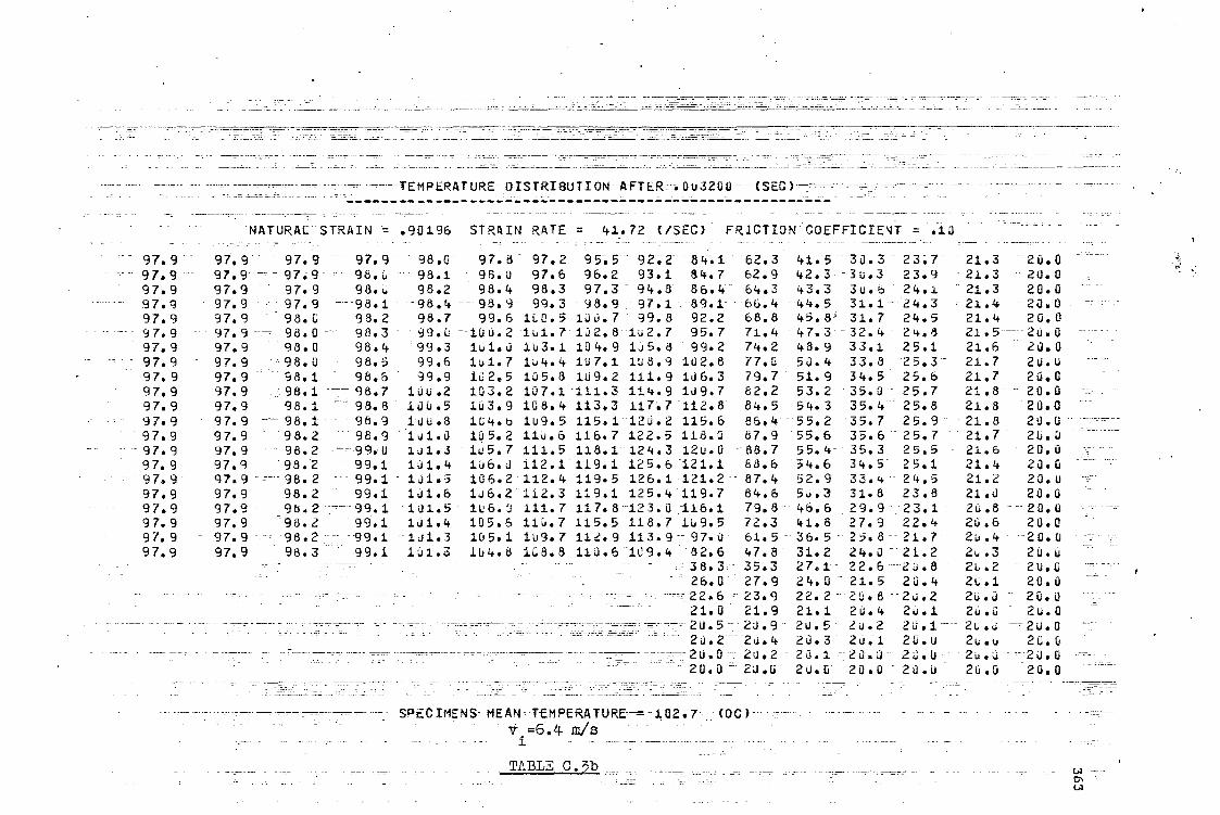
-
STRAIN = .90196
- --TEMPERATURE-DISTRIBUTION AFTER .0-u3200 (SEC)-
STRAIN RATE = 41.72 USEC) FRICTION
_
NATURAL COEFFICIENT = .10
97.9 97.9 97.9 97.9 98.0 97.8 - 97.2 95.5- 92.2 84.1 62.3 41.5 30.3 23.7 21.3 23.0 97,9 97.9 97.9 98"3 -'98"1 98.0 97.6 96.2 93.1 34.7 62.9 42.3- 3u.3 23.9 - 21.3 - 20.0 97.9 97.9 97.9 98.0 98.2 98.4 99.3 97.3 94.8 86.4 64.3 43.3 3u.6 24.1 -- 21.3 20.0 97.9 97.9 97.9 98.1 98.4 98.9 99.3 98.9 97.1 89.1 66.4 44.5 31..1 - 24.3 21.4 20.0 97.9 97.9 98.0 98.2 98.7 99.6 100.5 130.7 99.8 92.2 68.8 45.8,' 31.7 24.5 21.4 20.0 97.9 97.9 98.0 98.3 99.i: 130.2 101.7 102.8 102.7 95.7 71.4 47.3. 32.4 - 2°"0 21.5 - - 20.0 97.9 97.9
97.9 97.9
98.0 - 798.0
98.4 - 98.5
99.3 -99.6
161.0 131.7
133.1
104.9 135.8 99.2 74.2
107.1 108.9 102.8 77.1.1
48.9 33.1 25.1 -1G4.4 50.4 33.8 - 25.3-
21.6 21.7
20.0 20.0
97.9 97.9 98.1 98.5 - 99.9 132.5 135.8 1019.2 /11^91J6^3 79.7 51.9 34.5 25.6 21.7 20,0 97.9 97.9 :if-_98.1 --- 98.7 10u.2 103.2 107.1 -111.3 114.9 109.7 82.2 53.2 35.0 - 25.7 2:1.8 -- 20.0 97.9 97.9 98.1 98.8 183.5 1U3.9 108.4 113.3 117.7112"8 84.5 54.3 35.4 25.8 21.8 20.0 97.9 97.9
97.9 97.9
---98.1 98.2
-7 -96.9 98.9
130.8 131.8
134.6 135.2
1u9.5 110.6
115.1 123.2 115.6 -- 86.4
116.7 122.5 - 118.3 87.9
- 55.2 '35"7'25"9'
55.6 35.6 - 25.7 -- 21.8 21.7
20.0 23.3
97.9 97.9 • 98.2 131.3 1u5,7 111.5 110.1- 1a4,3 128.0 - 88.7 95.4 35.3 25.5 • 21.6 20.0 97.9 97.9 - 98.2 99.1 131.4 136.J 112.1 119.1 125.6 121.1 83.6 54.6 34.5- 25.1 21.4 20.0 97.9 97.9 ----- 98. 2 - 99.1 - 131.5 106.2 112.4 119.5 126.1 121.2 - 87.4 52.9 33.4 24.5 21.2 20.0 97.9 97.9 98.2 - 99.1 131.6 136.2 112.3 119.1 125.4'119.7 84.6 53.3 31.8 23.8 21.8 20.0 97.9 97.9 - 96.2 .-'99^1 131.5 1U6.0 111.7 117.8-123.0 116.1 79.8- 46.6 29.9-23.1 213.8 --- 20.0 97.9 97.9 -98.2 99.1 131.4 105.6 113.7 115.5 118.7 109.5 72.3 41.8 27.9 22.4 2G.6 20.0 97.9 97.9 -^ 98.2 -99.1 -131.3 105.1 1u9.7 112.9 11s.9-97.0 61.5 - 36.5 25.8-21.7 2G.4 20.0 97.9 97.9 98.3 99.1 131.3 134.8 108.8 110.6 -109.4 - 82.6 47.8 31.2 24.0 -21.2 26.3 20.0
38.3- 35.3 27,1 - 22.6-23.8 20.2 - 2U.1; 26.0 27.9 24.0 - 21.5 20.4 20.1 20.3
- 23.9 22.2 - 23.8 -23.2 23.0 21.0 21.9 21.1 213.4 2u.1 26.0 - 2u.0
- - - 23.5 2u.2 23.1-- 20.3 --2U.0 _ 211.5-28.9 - 20.2 - 23.4 23.3 23.1 26.0 20.3 20.0
==- 23.1 20.0 2U.0 2G.;3 -28.0 - 2U.0 20.2
8.3 23.0' 20.0 20.0 23.8 20.0 -
SPECIMENS i4EAN TEMPERATURE-=-102.7 (0C) v =6.4 m/s
TABLE C
-

• :
0 1.1.1 CL ct)
! • 364
H
f2c3coce c7 c.* Ca Ca CI c3 •.• • • • • • • • • • • • • • • • • • • • • • • • • • • Ca Ca CO C2 0 CO CO 0 0 CO CO 0 CO 1.1:2 0 ¶3 CO 2 C2 C2 ca C, cn ca c] za OJ Co Oki ed C4 ed 04 CO OJ OJ N CO CO C4 CV OJ N CO CO ra N 04 eU Od 00 04 0.1 00
j • ! aD CP cn 0,1 NI UN 0 N. N. N. Un UN OJ CP OD N1 CD N. 4t CO .4 .4 CO cn cn :n Ca • • • • • • • • • • • • • • • • • • • • • • • • • • • • •
.4 .4 OJ Od OJ 0,1 OJ OJ 04 04 04 ri .4 .o CO La CD 2 L2 CV NJ co 0.1 NOJOJOJOJ OJ DJ OJ CJ CJ OJ c1/4/ OJ PJ PO no N Cj NJ CO co co Pd
I Cn CO LA LA c, UN CO UN OD CO .4 cn UN CM '11 C3 OD N. N. aD CO 40 ND N r4 .4 CD C2 • • • • • • • • • • • • • • • • • • • • • • • • • • • a •
• 4r UN UN UD ps Ps on on OD Cn aD 00 P. 0D 4p op cxj .4 co -.7,o co c7o 1
N N N N N N N N N N N N cu N N CO N N CU N N Ni N N N N N Ni N 1 p
op UN 0 CO co un cp .4 ....I 01N N) NJ N. UN Ns ND OD cn CO CN 4t CV JD NI N •A ca , • • • • • • • • • • S • • • • • • • • . • • * . • • • • •
pl ND ,r uN 0 op CD a. N ND ND 4N CD pj ca on UN 04 In 01 NI VJ T4 .a cn CO CO CO NI N) N) P/ DD Do P1 4t .4.t 4t pn CD PI NJ NJ co Ni N NJ Nd NJ NO PJ
65 ur uo TA CD cr :4 cm 0 cn 0'N cm oD r) 4) st N V4 N. .4 a/ (Ni rn • • • • • • • • . 0 • • • • • • • • • • • • • • • • • • • p. CO •4 ,r r- cm N1 UN 00. CD CO 4h .4. -.1" ND cn 'JD a P1 UN Ps In .4 CO CO CO
Si UN LA LA IA V3 %JD N. N. N. N. N. N.N. UN 4 PI NI CO CO NJ Ni Ni NJ CO
UN UD no OD .4 UP c2 eV .4 UN PD 4. up N. rp PO UD CO JO wi UO tZ CD CD OD NI up 0.1 c/ • • • a • • • • • • • • • • • • • • • • • • • • • • • • • N) LA CP N) cn -t U'. 72 .i. on v4 Na) .1' 4V Ni N. D CO N .4 N1 ,4 UN NJ .4 L2 -2 hs IN hs OD OD CD L) Z.) .-4 vl T4 04 CO N N N v4 r4 (7' 00 0 .4,1- NI NJ Ni NJ NO OJ CO
1 1 4' . CJ OD UN CO, N. CD C3 on CO OP C., UN .4 CD NJ c,0 4h 0 LA OD N. ,4 Ti m UN LA N IO CO ' • • • • • • • • • • • • • • • • • • • • • • • • • • • • • CO cO UN .4 CO 0 ND CO 0 T4 N. v4 UN N. CP CP Qn -a cn .4 CD N. CD Si' v4 CD CO .3 CD 131 C2 M .4 .4 CJ PI to) J• UN UN 0 UD UD 0 0 0 0 UN ND v4 ,S, NJ NJ nj oj pj 0J pJ
' . .
. I..Iit UP .4 hr.) hs 0 on CD Ps NJ P1 Cn ca UN .7-1 OM PP CP CQ UN vi PI ;11 ; • • • • • • • • • • • • • • . • • • • • • • i ; ,, 41- r.. .4 QD CU aD 4P ca UD .4 UN ".'D ND JD N. on ,0 CI Q1 cn N I • :• 1
;
L7 47 1.1 .4 VJ OU P/ 1 42- UN UN 4.4) QD OD QD uD %ID LID UN zr .1' . , , : . • : I
1 1 1: CO CD CD 4t UN N. t:2 .4 C2 OD CD en UN UN CD NI UD UN CD gr 1 ,11 1 , • 3 • •• • • • • • • •• ••••0• • •
••1 -7 UD ID OU OD '17, uN cn PI ,..0 CD Pa UN Ps an CD aD 'UD DD CD LIN CO 13 cn .4 v4 NJ CU N N) NI N) Si- ..11 4' .1- .1. 4' .1* .1- r■I ND
1 .4 TA v4 v4 .4 .4 IA .4 .4 vi T4 Ti 7-4 .4 v4 vA v4 .4 .4 vA v4
OD cm 010 *5 Oj 61 UN .4 '.o o'. .4 p- v4 .4 Ls NJ NJ OD .4 CD • • • • • • • • • • •.• •••• • • • •
: ou PI UN ps CO CU UN OD CO eV IA Ns eD CD .4 v4 .4 -2 aD p. UN CO CO CO .4) el .4 v4 •4 Ni N CJ CJ NJ Cl pn pn N) N) Ni CU NJ .4 T4 .4 v4 .4 v4 v4 .4 .-4 .4 .4 .4 .4 .i v4 v4 .4 v4 1-1 v4 .4
OD 4t -tt UN 00 N) N. ,.4 UN OD .4 N NJ rn UD a0 aD 1' on v4 UN • • • • • • • • • • • • * ••••• • • o C2 .4 CO N1 -2' 0 N. CD CO v4 NI .1" UN JD UD 0 LID 0 UN UN 4N cn .::a CD 3 C2 ,:a ..a ca .4 .4 .4 .4 ...I .4 .4 vA .4 v4 .4 v4 a-i .4 .4 v4 .4 .4 ..4 v4 .4 .4 v4 v4 v4 .4 .4 .4 .4 .4 .4 .4 .4 .4
UD N1 UN CD NO Cn UN v4 N. N7 CD .1. CD NI N. c, .4 TA .n Cn an Cr ,
CP • • • • • • • . • • • • • • . • . • • • • •1 CO Cn cn ,-,. ,:, .4 NJ 04 P/ P9 .41- .1- UN UN UN .J0 UD Or UN UN UN
C2 CD Cn Cm Cn '-a ':2 CD Cn ,2 CI .9 ¶3 fa :n CO 7.D CO L2 en ea en I
0' .4 .4 T4 .4 .4 .4 .1 v4 v4 .4 .4 .4 vA .4 .4 .4 .4 .4 , .
1 Al NI 4' OD N. cn .4 NI LA T... as CO Al J• IA V3 .0 CO P.,- CO Na LA • • • • voloo* die.. • •••• "et • • OD on. on ao (3 0' CD CD CD CD u/ :.) ur .= un .C.1 CO ,-...) Za
' I-I en cn cm cn cn cn cn cn co CO t2 L2 ea c:2 en ,..ro ea .2 Cn ,:a ,a :. • ( 1 1 cX i . CY I , ! !t; • . .•
.4 .4 v4 1-1 v4 .4 .4 .4 ri 1.4 v4
. , •, , I. t: • •
, . • 1
. , • . 1 , . .
i GI . : CO CD .4 .4 .4 N CO PI 41•1 4 UN LA LA JD UD OD UD r- r N. r-
!
. ;
....1 • 0 • • • • • • • • • 0 • • • • • • . • • 1 cr co ao ao co OD m7 DO 03 a3 c0 c0 on on 03 on on an on on an ora I toe cn co co cn co cn cn cn cn cn co cn CP Cm CP cn OD CP CP CD CP
. :,
1, i., i . . : I tt 1: ::, 1,
. , :, . 1 z . ' . cn Cn cn Cn Cn Cn CP ca Ca cn Cn ca Ca ca Ca ca CD C2 f2 CO I'1 • • • e • • • • • ••••••••• • . • . .
hs IN N. hs Ps N. h. a) OP on On CO on OP On CO OP CO OD a, aD 1 1 Cn Cn cm cn cn co co cn co cn cn cn cn CD CP CD CD CP CD CO CP
• CP CP CP CD ON CD CP CP CP CP CP CP 137 CD CD 07 07 CP CP .07 CP ' !• • • • • • • • • • • • • • • o • • • • •
cn cn Cn CP CD CP CP CD CO CD CD CP CD CP CP CP 0P CP CP CP CD
I
t J :!!! !!,
1! 1.
I
, I
I • •:: ,
•
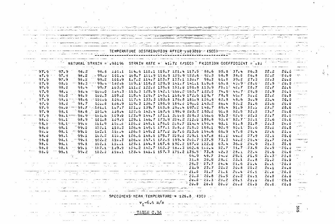
STRAIN RATE = 41;72 USEC) FRICTION
TEMPERAT-URE-OISTRIBUTION-AFTER-.-003201-7,-(SEC)-----------
COEFFICIENT
-
= NATURAL STRAIN ='"9O196
97.9 97.9 98.2 98.8 1J1.1 104.6 110.1 1/5.7 121.4 117.5 88.6 55.8 37.4 26.3 - 22.2 28.0 97.9 97.9 98.2 =99.0- 101.4 105.7 111.9 118.9 125.9 122.6 92.3 58.5- 38.0 26.8 22.2 20.0 97.9 97.9 98.2 99.2 101.9 107.2 114.7 123.7 133.1 130.7 98.3 51.8 39.2 27.3 22.3 20.0 97.9 98.0 98.3 - 99.4 -182.6 109.1 118.2 129.5 141.7 141.1 1G5.8 55.8 *y.9 - 28.0 22.5 20.0 97.9 98.0 98.4 - 99.7 103.5 111.2 122.8 135.8 151.8 151.8 113.9 70.1' 42.7 28.7 22.7 28.6 97.9 98.0 98.4 180.0 184.3 113.3 125.9 142.1 -16u.2 162.7 122.0 74.5 44.7 - 29.5 22.9 20.0 97.9 98.0 98.5 iuti.3 105.2 115.4 129.7 148.1 158.9 172.6 129.7 78.8 46.7 30.2 23.2 20.0 97.9 98.0 98.6 -100.6 106.1 117.4 133.3 153.8 176.8 181.9 136.8 82.8 48.6 31.149 23.4 20.0 97.9 98.0 - 98.7 131J.8 106.9 119.3 /36.7 158.9 184.8 190.0 143.2 86.4 58.2 31.6 23.6 20.0 97.9 98.0 -- 98.7 101.1 107.7 121.J 139.7 163.5 19u.4 197.2 148.7 89.4 51.5 32.0 23.7 20.0 97.9 98.1 98.8 101.4 108.4 122.6 142.4 167.6 195.9 283.2 153.2 91.8 52.5 32.3 23.7 20.0 97.9 98.1 98.9 1u1.6 109.0 123.9 144.7 171.1 2u0.5 208.3 156.6 93.3 52.9 32.3 23.7 20.0 98.6 93.1 - 98.9 101.8 .189.5 125.1 146.7 173.9 204.2 212.8 158.8 98.0 98.1- 99.12 101.9 - 110.8 126.8 148.1 176.0 206.7 214.4 159.4 98.0 98.1 - 99.0 102.1 110.3 126.6 149.1 177.1 - 2u8.J 215.0 158.1 98.0 98.1 - 99.0 -102.1 116.4 126.8 149.2 177.2 207.6 213.6 154.6 98.0 98.1 99.1 102.2 110.4 126.6 148.6 175.7 285.0 239.1 147.8 98.0 98.1 _ 99.1 102.2 11u.3 126.0 147.1 172.5 199.4 200.7 137.5 98.G 98.1 99.1 102.1 125.1 144.8 167.6 190.2 187.0 122.0 98.0 98.1 '-99.1- 102.1 189.9 124.2 142.7 162.2 180.3 162.6 1t.,0.4 98.8 98.1 ~-99°2 102.8 110.1 123.4 /41.1 157.3 171.2 135.5 73.8
- 54.9 49.7 31.8 35.5 25.2 27.7
- 21.9 - 23.7 - 21.0 -- 21.7 _ _~~-2J°3 -20.3 20.8
2o.8 - 23.3 20.0 - 28.0
- _ SPECIMENS MEAN TEMPERATURE- = 126.8 (0C)
v.=6.4 mis J.
TABLE C.3d cn.

TEMPERATURE DISTRIBUTION AFTER - .0332010 - (SEC.')
NATURAL STRAIN = .90196 STRAIN RATE = 41.72 COEFFICIENT = .43 ( /SEC) FRICTION
97.9 98.0 98.4 99.4 1.03.2 109.4 - 119.4 133.4 143,4 143.1-108.1 66.0 42-.3 28.0 - 22.T - 20.0 97.9 98.0 98.4 99.7 103.6 111.3 122.3 135,3 150.2 153i9 113.7 69.7 43.1 -28.7 - 22.8 20.0 97.9 98.3 98.4 103.3 104.3 113.2 126.0 142.2 160.5 162.8 122.3 74.4 44.8 29.4 22.9 20.0 97.9 98.0 98.5 133.3 105.3 115.7 133.8 150.2 172.6 177.4 132.6 79.7 - 47.0 30.3 23.2 - 20.0 97.9 98.0 98.6 100.6 1;06.4 118.5 135.9 158.6 185.1 192.0 143.4 85.4 49.5 31.2 23.5 20.0 97.9 98.0 - 98.7 101.0 137.6 121.2 141.0 156.8 197.1 236.1 153.9 91.1 52.1 - 32,2 23.8-20.0 97.9 98.1 98.8 101.4 /08.7 123.9 145.8 174.5 2u 8.6 218.6 163.6 96.5 54.5 33.2 24.0 20.0 97.9 98.1 98.9 101.8 109.8 126.4 15u.2 181.3 217.7 229.7 172.1 101.3 56.8 34.0 24.3 23.0 98.0 98.1 99.3 102.1 /10.8 128.7 154.1 187.3 225.9 239.0 179.5 135.5 58.7 34.8 24.5 23.0 98.3 93.1 - 99.1 102.4 111.7 130.7 157.5 192.5 232.8 246.7 185.4 108.9 6u.2 - 35.3 24.7 20.0 98.0 98.1 99.2 102.7 1.02.5 132.4 163.5 196.8 238.5 252.7 1910.0 111.3 61.2 35.6 24.7 23.0 98.0 98.2 99,3 163.0 113.2 133.9 162.9 200.2"242.8 257.3 193.0 112.6 61.5 35.5 24.7 20.0 98.6 98.2 99.3 1u3.2 113.8 135.1 164.7 202.8 245.9 260.1 194.4 112.6 61.0 35.1 24.5 20.0 98.0 98.2 - 99.4 103.4 114.2 135.9 166.0 234.4 247.5 261.3 194.0 111.1 59.6 34.4 24.2 -- 20.0 98.0 98.2 99.4 103.5 114.5 135.4 166.6 234.8 247.6 263.2 191.1 137.9 57.3 33.2 23.7 20.0 98.6 98.2 - -99.4 -1133.6 114.6 136.4 106.3 204.0 245,7"256,8 185.6 132.5 - 54.0 31.6 23.2 20.0 98.0 98.2 99.5 - 103.6 114.5 135.9 165.1 201.4 241.3 249.9 176.4 95.0 49.8 29.8 22.7 23.0 93.0 98.2 - 99.5 103.5 114.2 134.9 162.3 196.8 233.4 238.4 163.0 85.1 - 44.8 27.9 22.1 20.0 98.0 98.2 99.5 133.5 113.9 133.7 159.3 193.3 221.3 2201.7 143.6 72.9 39.5 26.3 21.5 20.0 98.0 98.2 99.5 1u3.5 113.? 132.5 156.9 183.4 208.8 19u.7 117.1 59.7 - 34.3 - 24.3 21.1 20.0 98.3 98.2 " 99.6 103.3 114.0 131.4 154.9 177.2 197.4 157.7" 84.8 - 47.0 -"29.9 22.9 23.7 20.0
61.9 55.9 37.3_ 26.2 -21.9 23.4 20.0 34.3 38.7 29.7 23.8 21.0 21:..2 20.0 26.3 - 29.3 25.3 . 22.6 2u.5 23.1 - 20.0 22.3 24.4 22.7 21.0 20.3 26.1 20.0
22.1 21.3 -- 23.5 - 23.2 - 23.0 20.3 - 21.2- 23.4- 21.3 26.6 23.3" 23.1 23.0 20.0 20.0- 20.4 20.3 - 20.1-23.0 - 23.0 ":- 20.0 20.0 23.3 20.3 20.0 20.0 20.3 - 20.0
- SPECIMENS-MEAN:TEMPERATURE--

NATURAL STRAIN =
TEMPERATURE DISTRIBUTION AFTER .003230 (SEC)
.90196 STRAIN RATE = 41.72 &SEC) FRICTION COEFFICIENT = .53
97.9 98.3 98.6 1,r,.2 1,5.7 115.2 13..8 148.9 171.3 175.7 132.8 78.6 48.3 30.0 23.4 21.6 97.9 98.. 98.6 101.5 1,6.2 117.3 134.2 155.5 184.5 186.6 140.3 83.4 49.3 36.9 23,5 2u.. 97.9 98.3 98.7 1r.3 117.2 120.2 139.4 164.6 194.4 202.8 151.6 89.3 51.3 31.8 23.7 20.0 97.9 98.1 93.8 141.2 103.5 123.5 145.6 175.0 216.2 221.9 164.8 96.. 54.1 32.8 24. 97.9 98.1 98.9 141.7 109.1 126.9 152.9 185.5 225.9 24..1 178.3 123.1. 57.1 34.1 24.3 2u.0 98.1 98.1 99.1 1 2.2 111.3 13u.3 158.1 195.4 240.2 257.. 19-.8 1 9.9 64.2 35.2 24.7 2..1 98.. 98.1 99.1 1'2.6 112.6 133.4 163.7 2,,4.2 252.7 271.2 21.9 u 116.2 63.1 36.3 25. 20.0 93.14 98.1 99.3 103.1 113.9 136.3 168.7 211.8 263.1 283.1 211.2 121.5 65.7 37.3 25.3 29.4 98. 98.2 99.4 143.5 115.0 138.0 172.9 213.1 271.5 292.4 218.7 126.0 67.8 38.1 25.5 20.0 98.3 98.2 99.5 1u3.8 116.1 140.9 176.5 223.2 278.1 299.5 224.4 i29.3 69.3 38.7 25.7 2... 98.4 98.2 99.6 104.2 116.8 142.7 179.3 227.2 282.9 3,4.4 228.2 131.5 70.2 38.9 25.7 20.0 91.0 98.2 99.7 104.4 117.6 144.1 181.5 23,.1 286.2 3.47.5 234.2 132.3 70.3 38.8 25.6 20.0 98.3 98.3 99.7 1,4.7 118.1 145.2 183.4 231.9 287.9 3,8.6 23..3 131.6 69.4 33.2 25.4 22.0 98.0 98.3 99.8 11.4.3 113.5 145.8 183.5 232.6 283.1 3.7.7 228.1 129., 67.5 37.2 25.0 2u.0 98.9 98.3 99.8 104.9 113.7 146.0 183.9 232.. 286.4 3‘4.4 223.3 124.5 64.5 35.7 24.5 20.. 98.0 98.3 99.9 11F.) 113.7 145.7 182.9 236.0 282.5 298,4 215.6 117.7 61:.3 33.8 23.8 20.0 98.4 98.3 99.9 105.3 111.5 144.9 1817.9 225.9 275.9 283.7 2443.6 1,8.3 55.2 31.6 23.2 24.. 9iS.i s 98.3 99.9 1i 4.9 118.) 143.5 177.3 219.9 265.5 273.9 187.1 96.3 49.2 29.4 22.5 2..0 98., 98.3 99.9 104.1 11/.6 141.9 173.) 211.7 253.6 252,3 163.8 81.8 42.9 27.1 21.8 23..4 98., 98.3 99.9 144.1 117.3 1413.4 17,4.4 2 13.2 215.4 216.8 132.7 66.3 36.8 25.1 21.3 20.0 98.1 98.3 100.0 134.5 117.7 139.0 167.9 195.7 221.8 178.3 95.1 51.5 31.5 23.4 2o.8 20.o
68.4 61.6 39.8 27.3 22.2 2t.5 24.0 3u.5 41.6 31.3 24.4 21.2 20.2 20.0 27.3 34.7 26.2 22.3 .6 24.1 20.4 22:7 25.1 23.1 21.1 20.3 20.1 20.0 21.4 22.5 41.5 2,.6 2..2 20.0 26.0 2 .4 21.1 24.7 2J.3 2..1 20.0 20.J 2,.0 21..4 2u.3 21,1 2..G 20.0 2-.0 2L.0 2..0 29.. 20., 21.14 24.0
SPECIMENS MEAN TEMPERATURE = 153.3 (0C)
v=6.4 m/s
TABLE C.3f

NATURAL STRAIN =
TEMPERATURE DISTRI8UTION AFTER .6032J0 (SEC)
.90196 STRAIN RATE = 41.72 (&SEC) FRICTION COEFFICIENT = .50
97.9 98.0 98.6 10P.2 15.7 115.2 13:j.d 148.9 171.3 175.7 132.8 78.6 48.3 30.0 23.4 20.0 97.9 98..3 98.6 10.5 136.2 117.3 134.2 155.5 181.5 186.6 14U.3 83.4 49.3 30.9 23.5 20.4 97.9 98.0 98.7 1n.3 107.2 120.2 139.4 164.6 194.4 202.8 151.6 89.3 51.3 31.8 23.7 20.0 97.9 98.9 98.8 161.2 103.5 123.5 145.6 175.0 210.2 221.9 164.8 96.0 54.1 32.8 24.2. 2J.6 97.9 98.1 93.9 111.7 109.8 126.9 152.0 185.5 225.9 24J.1 178.3 113.1 57.1 34.1.: 24.3 24.6 98.1. 98.1 99.) 1L2.2 111.3 130.3 158.1 195.4 240.2 257.6 19.8 1_9.9 60.2 35.2 24.7 26.3 98.6 98.1 99.1 1C, 2.6 112.6 133.4 163.7 244.2 252.7 271.2 21.1.9 11.6.2 63.1 36.3 25.0 20.0 93.0 98.1 99.3 103.1 113.9 136.3 168.7 211.8 263.1 287.1 211.2 121.5 65.7 37.3 25.3 20.0 98.0 98.2 99.4 1.3.5 115."1 138.b 172.9 211.1 271.5 294.4 218.7 126.6 67.8 38.1 25.5 20.0 98.0 98.2 99.5 1L3.81 116.J 140.9 178.5 223.2 273.i 499.5 224.4 129.3 69.3 38.7 25.7 2..0 98.4 98.2 99.6 104.2 116.8 142.7 179.3 227.2 282.9 3,4.4 228.2 131.5 70.2 38.9 25.7 20.0 98.0 98.2 99.7 104.4 117.6 144.1 181.5 230.1 286.2 307.5 23:..2 132.3 70.3 38.8 25.6 20.0 98.0 98.3 99.7 104.7 113.1 145.2 183.J 231.9 287.9 3j8.6 23i.3 131.6 69.4 38.2 45.4 20.0 98.0 98.3 99.8 114.3 118.5 145.8 183.8 232.6 283.1 387.7 228.1 129.i. 67.5 37.2 25.6 28.0 98.0 98.3 99.8 104.9 113.7 146.0 183.9 232.0 286.4 304.4 223.3 144.5 64.5 35.7 24.5 20.0 98.0 98,3 99.9 105.) 113.7 145.7 182.9 230.0 282.5 293.4 215.6 117.7 60.3 33.8 23.8 20.0 98.6 98.3 99.9 105.0 118.5 144.9 18C.9 225.9 275.9 288.7 2 1J3.6 11.8.3 55;2 31.6 23.2 2u..i 98. 98.3 99.9 11'4.9 118.) 143.5 177.3 219.9 265.5 273.9 187.1 96.3 49.2 29.4 22.5 26.6 98.0 98.3 99.9 104.3 117.8 141.9 173.9 211.7 250.6 252.3 163.8 81.8 42.9 27.1 21.8 2C.0 98.J 93.3 99.9 1u4.8 117.3 140.4 17...4 2J3.2 235.4 216.8 132.7 66.3 36.8 25.1 21.3 26.0 98.1 98.3 160.0 104.5 117.7 139.6 167.9 195.7 221.8 178.3 95.1 51.5 31.5 23.4 20.8 20.0
68.4 61.6 39.8 27.3 22.2 2i..5 20.0 38.5 41.6 31.3 24.4 21.2 20.2 20.0 27.3 3-0.7 26.2 22.3 2.6 26.1 20.0 22.7 25.1 23.1 21.1 20.3 20.1 20.0 21.4 22.5 21.5 26.6 2:J.2 2t..0 20.0 2.4 21.1 20.7 20.3 2..1 20.0 20.0 2J.0 20.4 26.3 20.1 2..0 211.r 20.0 2.;.0 2L.0 2U.0 20.0 20.0 20.0 21.0
SPECIMENS MEAN TEMPERATURE = 153.3 (0C)
vi.6.4 m/s
TABLE C.3f

--V
NATURAL
-
STRAIN =
TEMPERATURE" ISTRI1UTTON AFTER .003200 ---(SEC)-
.50012 STRAIN RATE = ;CO (SEC) FRICTION COEFFICIENT =0.00
56.7 56.7 56.7 56.7 56.7 56.7 56.7 56.6 56.3 54.5 21.4 20.3 20.2 20.0 20.0 20.0 56.7 56.7 56.7 56.7 56.7 56.7 56.7 56.5 56.0 54.4 22.3 20.3 20.2 20.0 20.0 20.0 56.7 56.7 56.7 56.7 56.7 56.7 56.7 56.5 55.8 54.3 22.9 20.2 20.2 20.0 20.0 20.0 56.7 56.7 56.7 56.7 56.7 56.1 56.6 56.4 55.8 54.3 23.3 20.2 i 20.2 20.0 20.0 20.0 56.7 56.7 56.7 56.7 56.7 56.7 56.6 56.4 55.7 54.3 23.5 20.2 20.2 20.0 20.0 20.0 56,7 56.7 56.7 56.7 56.7 56.7 56.6 56.4 55.7 54.2 23.6 20.2 20.2 20.0 20.0 20.0 56.7 56.7 56.7 56.7 56.7 56.7 56.6 56.4 55.7 54.2 23.7 20.2 20.2 20.0 20.0 20.0 56.7 56.7 56.7 56.7 56.7 56.7 56.6 56.4 55.7 54.2 23.7 20.2 20.2 20.0 20.0 20.0 56.7 56.7 56.7 56.7 56.7 56.7 56.6 56.4 55.7 54.2 23.8 20.2 20.2 20.0 20.0 20.0 56.7 56.7 56.7 56.7 56.7 56.7 56.6 56.4 55.7 54.2 23.8 20.2 20.2 20.0 20.1 20.0 56.7 56.7 56.7 56.7 56.7 56.7 56.6 56.4 55.7 54.2 23.8 20.2 20.2 20.0 20.0 20.0 56.7 56.7 56.7 56.7 56.7 56.7 56.6 56.4 55.7 54.2 23.8 20.2 20.2 20.0 20.0 20.0 56.7 56.7 56.7 56.7 56.7 56.7 56.6 56.4 55.7 54.2 23.8 20.2 20.2 20.0 20.0 20.0 56.7 56.7 56.7 56.7 56.7 56.7 56.6 56.4 55.7 54.2 23.7 20.2 20.2 20.0 20.0 20.0 56.7 96.7 56.7 56.7 56.7 56.7 56.6 56.4 55.7 54.2 23.7 20.2 20.2 20.0 20.0 20.0 56.7 56.7 56.7 56.7 56.7 56.7 56.6 56.3 55.6 54.1 23.6 20.2 20.2 20.0 20.0 20.0 56.7 56.7 56.7 56.7 56.7 56.7 56.6 56.3 55.5 54.0 23.4 20.1 20.2 20.0 20.0 20.0 56.7 56.7 56.7 56.7 56.7 56.7 56.6 56.2 55.4 53.8 23.2 20.1 20.2 20.0 20.0 20.0 56.7 56.7 56.7 56.7 56.7 56.7 56.6 56.2 55.1 53.3 22.8 20.1 20.1 20.0 20.0 20.0 56.7 56.7 56.7 56.7 56.7 56.7 56.5 56.0 54.7 52.2 22.3 20.1 20.1 20.0 20.0 20.0 56.7 56.7 56.7 56.7 56.7 56.7 56.5 55.8 54.4 50.8 21.6 20.0 20.1 20.0 20.0 20.0
21.0 20,9 20.0 20.1 20.0 20.0 20.0 20.0 20.5 20.0 20.0 20.0 20.0 20.0 20.0 20.3 20.0 20.0 20.0 20.0 20.0 20.0 20.2 20.0 20.0 20.0 20.0 20.0 20.0 20.1 20.0 20.0 20.0 20.0 20.0 20.0 20.0 20.0 20.0 20.0 20.0 20.0
- 20.0 20.0 20.0 20.0 20.0 20.0 20.0 20.0 20.0 20.0 20.0 20.0 20.0 20.0
SPECIMENS MEAN TEMPERATURE = 56.3 (00) v.=4.5 m/s
-TABLE C.4a

TEMPERATURE OISTRIBUTI ON AFTER-:003200 (SEC) ---
NATURAL STRAIN = .50012 STRAIN RATE = .00 ( /SEC ) FRICTION COEFFICIENT = .20
56.7 56.7 56.8 56.9 57.2 57.6 58.2 58.2 57.2 53.2 43.1 32.6 26.3 22.4 20.8 20.0 56.7 56.7 56.8 56.9 57.2 57.8 58.5 58.8 57.9 53.9 43.8 33.3 26.4 22.5 20.8 20.0 56.7 56.7 56.8 56.9 57.3 58.1 59.0 59.7 59,2 55.2 45.0 34.1 26.7 22.7 20.9 20.0 56.7 56.7 56.8 57.0 57.5 58.4 59.7 60.8 60.9 57.2 46.5 35.0 27.2 22.9 20.9 20.0 56.7 56.7 56.8 . 57.0 57.6 58.8 60.5 62.2 62.8 59.4 48.4 36.2 27.7 23.1 21.0 20.0 56.7 56.7 56.8 57.1 57.8 59.3 61.4 63.7 65.0 61.9 50.4 37.4 28.3 23.3 21.0 20.0 56.7 56.7 56.8 57,2 58.0 59.8 62.3 65.3 67.3 64.4 52.6 38.7 28.9 23.5 21.1 20.0 56.7 56.7 56.9 57.2 58.2 63.3 63.3 66.9 69.5 67.0 54.7 40.0 29.5 23.8 21.2 20.0 56.7 56.8 56.9 57.3 58.4 60.8 64.2 68.5 71.8 69.5 56.8 41.3 30.1 24.0 21.3 20. 0 56.7 56.8 56.9 57.3 58.6 61.3 65.2 73.0 73.9 72.0 58.8 42.5 30.7 24.3 21.3 20.0 56.7 56.8 56.9 57.4 58.8 61.7 66.1 71.5 76.0 74.3 60,7 43.6 31.2 24.5 21.4 20.0 56.7 56.8 56.9 57.5 - 59.0 62.2 66.9 72.8 77.9 76.5 62.4 44, 6 31.7 24.6 21.4 20.0 56.7 56.8 56.9 57.5 5962 62.6 67.6 74.1. 79.8 78.3 63.9 45.3 32.0 24.7 21.5 20.0 56.7 56.8 57.0 - 57.6 59.3 62.9 68.3 75.1 81.0 79.8 64.9 45.8 32.1 24.7 21.4 20.0 56.7 56.8 57.0 57.6 59.4 63.2 68.8 75.8 82.0 80.8 65.4 45.8 32.0 24.6 21.4 20.0 56.7 56,8 57.0 57.6 59.5 63.3 69.0 76.2 82.4 - 81.1 65.2 45.3 31.5 24.4 21.3 20.0 56.7 56.8 57.0 57,7 59.5 63.4 69.1 76.1 82,1 80.3 63.9 44.1 30.8 24.0 21.2 20.0 56.7 56.8 57.0 57.7 59.5 63.4 68.9 75.5 80.8 78.1 61.3 42.0 29.6 23.5 21.0 20.0 56.7 56.8 57.0 57.7 59.5 63.3 68.5 74.5 78.5 74.3 56.8 39.0 28.2 23.0 20.9 20.0 56.7 56.8 57.0 57.7 59.5 63.2 68.2 73.4 76.0 67.5 50.4 35.4 26.6 22.4 20.7 20.0 56.7 56.8 57.0 57.7 59.6 63.0 67.9 72.5 73.7 59.7 42.1 31.5 25.0 21.8 20.5 20.0
36.5 34.1 28.0 23.5 21.3 20.4 20.0 27.8 28.4 25.1 22.4 20.9 20.3 20.0 24.1. 24.8 23.i 21.5 20.6 20.2 20.0 21.9 22.6 21.8 20.9 20.4 20,1 20.0 21.0 - 21.4 21.0 20.5 20.2 20.1 20.0 20.4 20.7 20.5 20.3 20.1 20.0 20.0 20.2 20.3 20.2 20.1 20.1 20.0 20.0 20.0 20.0 20.0 20.0 20.0 20.0 20.0
SPECIMENS 'MEAN - TEMPERATURE =---62.- 2 ( OC ) 1r1=4.5 VS -
TABLE C.4b

TEMPERATURE - nrs-TRisun ON -AFT ER • 003200 (SEC)
.50012 STRAIN RATE = .00 f/SEC) FRICTION = .40 COEFFICIENT NATURAL STRAIN =
56.7 56.8 56.9 57.2 58.4 60.3 63.4 66.6 69.0 66.6 54.1 39.3 29.8 23.7 21.3 20.0 56.7 56.8 56.9 57.3 58.5 60.7 64.1 68.0 70.9 68.6 55.9 40.7 30.1 24.3 21.3 20.0 56.7 56.8 56.9 57.4 58.7 61.3 65.3 70.1 73.9 71.8 58.7 42.4 30.8 24.3 21.4 20.0 56.7 56.8 56.9 57.5 59.0 62.1 66.8 72.7 77.7 76.2 62.2 44.6 31.8 24.7 21.5 20.0 56.7 56.8 57.0 57.6 59.3 63.0 68.5 75.6 81.9 81.0 66.3 47.0 1 32.9 25.2 21.6 20.0 56.7 56.8 57.0 57.7 59.7 63.9 - 70.4 78.7 -86.3 86.1 73.4 49.5 34.1 25.7 21.8 20.0 56.7 56.8 57.0 57.8 60.1 64.9 72.3 81.8 90.8 " 91.2 74.7 52.1 35.4 26.2 21.9 20.0 56.7 56.8 57.1 57.9 60.5 65.9 74.1 - 84.9 -- 95.1- 96.1 78.7 54.6 36.6 26.6 22.1 20.0 56.7 56.8 57.1 58.1 60.9 66.8 75.9 87.8 99.2 100.7 82.6 56.9 37.7 27.1 22.2 20.0 56.8 56.8 - 57.1 58.2 61.2 67.7 77.6 90.6 103.1 105.1 86.2 59.1 38.8 27.5 22.4 20.0 56.8 56.8** 57.2 58.3 61.6 68.5 79.1 93.1 136.'5 108.9 89.3 61.0 39.7 27.9 22.5 20.0 56.8 56.8 57.2 58.4 61.9 69.3 - 80.5 95.3 109.6 112.3 92.1 62.6 40.4 28.1 22.5 20.0 56.8 56.8 57.2 58.5 62.2 69.9 81.7 97.2 112.2 115.1 94.2 63.7 40.9 28.3 22.6 20.0 56.8 56.8 57.2 58.6 62.4 70.4 82. 6 -- 98.7 114.2 117.2" 95.6 64.2 41.0 28.2 22.5 20.0 56.8 56.8 57.2 58.7 62.6 70.8 83.3 99.6 115.4 118,3 96.0 64.0 40.6 28.0 22.4 20.0 56.8 56.8 57.3 58.7 62.7 71.0 83.5 99.9 115.6 118.1 95.1 62.9 39.8 27.6 22.3 20.0 56.8 56.8 57.3 58.7 62.7 71.0 83.4 99.4 114.5 116.2 92.4 60.5' 38.4 26.9 22.1 20.0 56.8 56.8 57.3 58.7 62.7 70.9 82.9 98.1 111.8 112.1 87.7 56.9 36.3 26.1 21.8 20.0 56.8 56.9 57.3 58.8 62.7 70.7 82.2 96.2 107.7 105.3 80.0 51.7 33.9 25.1 21.5 20.0 56.8 56.9 57.3 58.8 62.7 70.5 81.5 94.2 103.4 94.4 69.4 45.6 31.1 24.1 21.2 20.0 56.8 56.8 57.3 - 58.7 62.9 70.2 81.1 92.6 99.4 82.1 55.9 39.0 28.4 23.1 20.9 20.0
46.7 43.0 33.2 25.9 22.2 20.6 20.0 - 32.9 33.8 28.5 24,0 21.5 20.4 20.0
26.8- 27.9 25.2 22.6 21.0 20.3 20.0 - 23.2 24.4 23.1 21.6 20.6 20.2 20.0 21.7 22.3 21.7 20.9 20.4 20.1 20.0
-- 20.7 - 21.2 20.9 20.5 20.2 20.1 20.0 20.3 - 20.5 20.4 20.2 20.1 20.0 20.0
- 20.0 23.0 20.0 20.0 20.0 20.0 20.0
SPECIMENS MEAN TEMPERATURE-= 71.6 IOC) v1=4.5 m/s
TABLE C.4c
APPENDIX D
PUBLISHED PAPERS
, D.1 - Dynamic stress strain data to large strains
D.2 - Temperature rise in high speed upsetting with
end frictions (To be published)
371

DUCTILE TUBE
HOLDER
SPECIMEN DEFORMATION
SHEAR PI NS
WEIGHT
COMPRESSION SPRING
PRESS FRAME
A
91
LOAD CELL (STATIONARY)
SHROUD TUBE
TOP PLATEN
2665 Dynamic Stress/Strain Data to Large Strains B. Lengyel and M. Mohitpour
An incremental method of determining stress/strain curves to large strains at high strain rates and sub-critical temperatures is described. Comparisons are made between the results incre-mentally obtained and those obtained under continuously applied loads to large deformations by means of a free-flight-type impact device. The strain rate varied between wide limits in the (continuous) large-deformation tests. This variation and the heat generated by the plastic work are responsible for the different stress/strain paths obtained in the two methods.
Considerable efforts have been made in the past to obtain the true stress/strain curves of materials to large strains, for use in metalworking analyses. For low strain rates and room temperature incremental methods have been developed and are now widely used.1'2 With the introduction of high-speed " cold " metalworking processes, such as cold rolling and wire drawing, or hydrostatic extrusion at large reductions, it is becoming increasingly important to record stress/strain curves at high (constant) strain rates and constant temperatures. With the development of step-by-step methods of analysis in metalworking, the use of true stress/strain data for a given temperature, strain, and strain rate is required at each point of the material, in each step. There would be little point in adopting a more realistic numerical approach, as distinct from mathematical solutions developed for " ideal " materials and conditions, if the stress/strain data would not be truly relevant for the computed conditions of the deforming material.
The usual large-deformation testing techniques3.4 using free-flight impact devices pose several problems. First, materials exhibit strain-rate-sensitivity at high strain rates even at room temperature;5 thus constant strain rates should be maintained during the test, which is rarely feasible with this method. Secondly, if testing is carried out continuously to large strain rates at high speed, the specimen temperature could rise to a level where its effect could no longer be neglected. Finally, since compression tests need to be used to obtain data to large strains, end friction could also become significant in the large-deformation test and might distort the results. The experiments described in this paper show that strain rate and temperature could vary significantly in large-deformation tests and, consequently, the stress/strain paths are different from those obtained in the incremental method, where strain rate and temperature can be held practically constant and end friction is small. Specimen configurations indicate that the deformation was essentially homogeneous in both types of test.
Experimental Apparatus A modified US Industries high-energy-rate forging machine
was used in the experiments. Its two opposing rams have relative velocities adjustable between 1 and 24 m/s. The significant constructional details and operation of the machine have been described elsewhere.6 In the incremental method the work required to deform the specimens to the preselected small strains was only a fraction of the kinetic energy of the platen;
Manuscript received 20 July 1971; in revised form 1 October 1971. B. Lengyel, Dipl.Ing., DIC, PhD, and M. Mohitpour, BSc, are in the Department of Mechanical Engineering, Imperial College of Science and Technology, London.
BOTTOM PLATEN
Fig. 1 Experimental sub-press for incremen al tests.
ANVIL
SPECIMEN BOTTOM DIE
R I N2E W7ME COIN ASE PLATE ‘1210.,•' see L-.1/A,:age
Fig. 2 Experimental sub-press for large-deformation tests.
VELOCITY T RA N S DUCE
JOURNAL OF THE INSTITUTE OF METALS 1972, Vol. 100 1

2 Lengyel and Mohitpour: Dynamic Stress/Strain Data to Large Strains
I— 0.2 m s
1 • 2 5 Tri /5
(a) Ilti 1 M 11111 I'll
•
_ 1 5 kN
--I 0.5 m s
5m / s
(b)
130 kN -7
Fig. 3 Typical load and velocity traces: (a) incremental tests; (b) large-deformation tests.
thus, the change in strain rate was small during each incre-mental test. The platens are in free flight by the time impact occurs. The results are, therefore, representative of those obtainable on this type of device generally, regardless of the source of energy.
The experimental sub-press for the incremental test is shown in Fig. 1. The specimen is located by a rubber sleeve in the holder and projects above the top surface of the holder by the amount of preselected deformation. As the bottom ram travels upwards, the specimen is compressed under the dynamic load applied on impact by the long load cell, fixed to the machine frame. This strain-gauged load cell is con-nected to an 80 V battery supply and, via an amplifier, to a Tektronix double-beam storage oscilloscope. After a small specimen deformation has been attained, the shear pins fracture when the load cell hits the holder, thus unloading the specimen. The remaining kinetic energy is absorbed by the work expended on deforming the ductile tube.?
The sub-press for the large-deformation test is fixed to the top and bottom platens (Fig. 2). A load cell of the type described in Ref. (8) forms part of the bottom tooling. It is connected to a 160 V battery supply and to the oscilloscope. The oscilloscope is triggered-off, in both types of test, by a micro-switch somewhat before impact. A typical oscilloscope trace for the incremental method is shown in Fig. 3(a) and for the large-deformation method in Fig. 3(b). The first jump in the load trace in Fig. 3(a) occurs on specimen impact, and the second when the load cell contacts the holder and the speci-men is unloaded. The small initial peak in the load trace in Fig. 3(b), caused by reflected stress waves, has no effect on the results. Both load cells have been calibrated statically in a compression testing machine.
Two electromagnetic transducers were used to record ram velocity, one each for the incremental and large-deformation methods. The construction of these transducers and their calibration have been described elsewhere.6 Typical velocity traces are also shown in Fig. 3. It is clear from Fig. 3(a) that the ram velocity is constant during the deformation of the specimen in the incremental method, while it is evident from Fig. 3(b) that the velocity of the ram falls to zero during the large-deformation tests.
The strain in the incremental method was obtained by micrometer measurements of the initial and final specimen heights, while in the large-deformation tests strain was calculated by the graphical integration of the velocity trace.
The accuracy of the latter method was checked in each case by comparing the final strain determined in this manner with the difference between the initial and final specimen heights. The error has never exceeded 2 %.
For quasi-static tests, the test specimens were subjected to incremental loading. The method adopted9 involved lubri-cating the platen/specimen interface between each compres-sion and remachining the specimen, after 5Q% reduction, to its original height : dia. ratio.
Materials Specimens of El C 99-grade aluminium to BS 1476 and
C101 electrolytic tough-pitch high-conductivity copper to BS 2874 were machined from cold-drawn bars and each quality heat-treated in a single batch. Annealing tempera-tures were 360 and 6000 C (633 and 873 K) for aluminium and copper, respectively, followed by furnace cooling. During annealing the copper specimens were wrapped in copper foil to reduce oxidation.
Molybdenum disulphide grease was used as a lubricant. The lubrication was carried out before each test and between each incremental compression. No pronounced barrelling of the specimens occurred in either method up to the strains considered; the deformation was reasonably uniform along the length of the specimens, indicating that end friction was small.
Mostly 1.59 cm-dia specimens were used in the incremental tests, usually with a length : dia. ratio of 1. Occasionally, larger or smaller length : dia. ratios were included to obtain lower or higher strain rates for particular values of strain. If, in such cases, buckling or barrelling occurred, the data were discarded. The specimens for large-deformation tests were normally made to a length : dia. ratio of 1, but with a larger dia. (2.55 cm), to provide sufficient protection for the machine and tooling.
Results and Discussion In the incremental tests the specimen length was reduced
by 1.54 mm in each step; thus, the calculated temperature rise never exceeded 8 and 13.5 degC (K) for aluminium and copper, respectively, in each increment. The kinetic energy of the platen was at least 2.5 times the plastic work expended in each step for the aluminium specimens. The relevant mini-mum was 10.6 for copper. Owing to the small change in specimen height (h) and deformation velocity (v) the strain

Fig. 6 Stress/strain curves for copper. Fig. 7 Stress/strain curves for aluminium.
Lengyel and Mohitpour: Dynamic Stress/Strain Data to Large Strains 3
0 p0
A
0 0--0 -8 -
'A----Z- 0
A A
0 0
A-Th A A-A-AA A
0 /--• •
• •
600 E z
bN n 400 w
—so = 0-07 —E.., 0-13
—o —E = 0.25 _.-C.0.86
0 200
•
0
00 200 400 STRAIN RATE, 51
Fig. 4 Flow-stress/strain-rate curves for copper.
600 1000
200 NE
z 7
U)
cc 100 N
0
0
— • --E 0.065 A —E= 0-215
—0 —E= 0.54 — • E= 1.065
2 k 20
A—A
00 cb_o _-0 —0 Iscrzoo—o- A A A
• • •
50 100 1 500 1000 STRAIN RATE, 5
4-•
Fig. 5 Flow-stress/strain-rate curves for aluminium.
150
100

...--
_...A•""".4. A .......,A i =700 S-1 _
A./.. < ....--, A./....1
• -
,......--o,..--- E =600 S ----- o \ ._ t-•"--..-o----0.....—o—o --0—__
7 -to, _ ........-t".--- •
\s,
S
• • "••••
E. 2 ov". 25
\ I I \I I 1 1e i l o 1 •
•
X =Incrementally obtained at actual temperatures and strain rates
I I I NATURAL STRAIN (E)
E =700S-I = 600 Si
FLOW STRESS _.(55),MN/ m2
Ej700 S-I
,/,..:::57 59°C-I I =600 SH XJ614°°CS1 j~49°C 1 6355 ' E=6005 \
Lengyel and Mohitpour: Dynamic Stress] Strain Data to Large Strains
Fig. 8 Strain-rate/strain-variation curves for large-deformation tests on copper.
4
1000
800
ti 600 La
— 400 cc
200
0 0
1000
800
1.4 0.2 0.4 0.6 0.8 1.0 12 NATURAL STRAIN (6)
400
300
200
100 ,, 0 0.2 0.4 0.8 0.6 1.0 1-2
2.4 Fig. 10 Comparison of the stress !strain curves obtained by the incremental (—) and large-deformation (- - -) method for copper.
0 0 0-4 0.8 1.2 1.6 2.0
NATURAL STRAIN (6) Fig. 9 Strain-rate/strain-variation curves for large-deformation tests
on aluminium. I ' I 1 ' I ' 1 FLOW STRESS
(Crs),MN / m2 L475 6=7" — ---
--- \-----1(= -- x,,.7,
\54°C, 66C -7.....-- - ----X,42°C_, _ 47951 4355
...X 432g.
0, 420 5 • E7= 75S1
_ E=475S1
23°C 328 S1 X - Incrementally obtained at
actual temperatures and strain rates
50
NATURAL STRAIN (£)
rate 6 = v jh in each incremental step remained constant 150 within 12.5 and 6 %, or less, for aluminium and copper, respectively. From the recorded data it was convenient to plot flow-stress vs. strain-rate curves first, as shown in Figs. 4 and 5, and to obtain Figs. 6 and 7 by cross-plotting.
The results clearly indicate that the flow stress increases 100 with strain rate. Furthermore, the stress/strain curves exhibit no plateau up to the maximum strain rate attained in these experiments.
The strain-rate variation in the large-deformation tests is shown in Figs. 8 and 9 for copper and aluminium, respec- tively. The mean strain rates, e, have been obtained by integrating the strain-rate/strain curves. It is clear that, while at low values the mean strain rate represents relatively well the actual strain rates during a significant part of the test, at higher strain rates no mean value would represent the actual variation with any accuracy.
Figs. 10 and 11 indicate that, for large strains, the stress/ strain curves determined by the large-deformation method
1.0 1.2 0.8 0.6 00 0.2
Fig. 11 Comparison of the stress/strain curves obtained by the incremental (—) and large-deformation (- - -) method for aluminium.

Lengyel and Mohitpour: Dynamic StressIStrain Data to Large Strains 5 lie well below the results of the incremental tests. The reason for this is partly that mean strain rates are not representative of the true strain rate in the large-deformation tests, and predominantly because the temperature rise becomes signifi-cant at larger strains. It is of course true that, in the later stages of these tests, the actual strain rates are often greater than the mean values, an effect that would tend to raise the flow stress. It is, therefore, not unreasonable to suggest that the stress/strain path in the large-deformation test would drop even further if this strain-rate effect were absent.
It is evident from the foregoing that each point on the stress/strain curves in the large-deformation tests represents data for a particular temperature and strain rate, which are different for each point along the curves. The actual values of strain rates can be obtained by comparing Figs. 8 and 10 for copper and Figs. 9 and 11 for aluminium, and the tempera-tures can be calculated by assuming that all plastic work is converted into heat and that there were no heat losses during the test.
If this line of argument is true, it should be possible to record points on the large-deformation curves by the incre-mental method and vice versa. The former has been achieved in a few cases by preheating the specimen to the calculated temperature and compressing it incrementally at the actual strain rate obtained in the large-deformation test. The
results, indicated in Figs. 10 and 11, are reasonably good considering that the method needs a number of refinements.
Conclusions The present investigation reaffirms the well-known, but
often contested, evidence that the stress/strain curves ob-tained, by large-deformation tests, using a free-flight device, constitute an assembly of data which correspond, in each test, to various temperatures and strain rates. Such data might be quite satisfactory in approximate analyses but are of little help when, for a more realistic analysis, the properties of a material at specific strains, strain rates, and temperatures are required, i.e. when mean values are no longer satisfactory.
The initial results described in this work indicate that more accurate stress/strain data can be obtained by an incremental method, based on much the same principles as the techniques used in quasi-static testing.
Acknowledgements The financial assistance of the Science Research Council in
this work is gratefully acknowledged. The authors thank Professor J. M. Alexander for permission to use facilities in the Metalworking Laboratory of the Mechanical Engineering Department, Imperial College, and Mr. P. G. Ashford for his assistance with the experimental machine.
References
I. M. Cook and E. C. Larke, J. Inst. Metals, 1945, 71, 371. 2. A. B. Watts and H. Ford, Proc. Inst. Mech. Eng., 1955, 169,
1141. 3. C. E. N. Sturgess and A. N. Bramley, "Proceedings of the 11th
International Machine Tool Design and Research Conference" Vol. B, p.803. 1970: Oxford, &c. (Pergamon Press).
4. S. K. Samanta, J. Mechanics Physics Solids, 1971, 19, 117. 5. H. Suzuki, S. Hasizuma, Y. Yabuki, Y. Ichihara, S. Nakajima,
and K. Kenmochi, Proc. Inst. Indust. Sci., Univ. Tokyo, 1968, 18, 3.
6. B. Lengyel and D. C. Stamelos, Ann. CIRP Conf., 1971, 19, (2), 2.
7. B. Lengyel and T. V. Krok, Metal Forming, 1969, 36, (6), 370. 8. S. C. Jain and E. Amini, "Proceedings of the 9th International
Machine Tool Design and Research Conference", p. 229. 1968: Oxford, &c. (Pergamon Press).
9. W. Whitfield, NEL Rep. (325), 1967.
The Institute of Metals. 1972.

TEMPERATURE RISE IN HIGH SPEED
UPSETTING WITH END FRICTION
M. MOHITPOUR* and B. LENGYEL*
Summary
A numerical method using a finite element technique is described
to establish the temperature field in the upsetting of right cylind-
rical billets at high rates of strain. The initial billet temperature
is 20°C and the temperature rise due to homogeeous deformation and
end friction is considered.
For the frictionless case the temperature distribution is almost
uniform across the billet. Friction raises the temperature of both the
billet and tooling near their interface, which could influence the
process, tool life and the product properties.
* The authors are in the Department of Mechanical Engineering,
Imperial College of Science and Technology, London.

Introduction
In metal working the work of deformation and friction is
converted into heat, which raises the temperature of the material
often significantly, particularly at large strains and high strain
rates. Computations and experiments show that, at high extrusion
speeds and large reductions, thermal softening could partly or
completely outweigh work hardening effects (1,2). At high speeds the
process becomes adiabatic when the temperature of the outer layers
is raised even higher than the bulk temperature, resulting in a relative
drop in surface hardness, quite contrary to that experienced in slow
speed cold extrusion (3,4).
In forging, like in extrusion, large strains are often applied
at high speeds..The simplest and most common example is the upsetting
of right cylindrical billets, a method widely used in production and
also in laboratory tests aimed at obtaining the stress/strain curves
of materials to high strains. In this case not only product properties
could be affected by the rise in the deforming material's temperature
but forging loads could also be influenced. This in turn could lead to
stress/strain data unrepresentative of billet conditions at the
commencement of the test, to which they are usually related (5). It
is clearly of great interest to know the actual conditions during the
deformation, such as the material temperatures as deformation proceeds
and relate the measured flow stress data to these real rather than to
the initial values. The temperature rise could also affect frictional
conditions and tool life.
In the following a finite element analysis of heat flow during the
upsettino of right cylindrical billets is described for the homogeneous
deformation of an isotropic material. The platens are assumed to make

perfect contact with the billet ends at all times. A computer programme
has been developed in the FORTRAN IV language to simulate the process, i.
wher.4 the upsetting of the specimen and simultaneous heat generation
during a small time interval At is followed by static heat transport-
ation during an equal increment of time, a method applied repeatedly
until the specimen is reduced to the desired height. The results of
computations for billets of high conductivity copper of 25.4mm height
and the same diameter- are presented. Initially the billet and
tooling are assumed to be at room temperature (20°C) and, as deformation
proceeds, the computed temperatures after given time intervals and
corresponding strains are indicated and some conclusions drawn.
Theoretical Background
The general problem to be examined is that of time dependent
heat flow in an incompressible moving medium with heat generation.
Although the problem is three dimensional, the symmetry of the body
(Fig. 1) allows the variables to be described in a two dimensional
field. The governing differential equation of heat transportation
then becomes (6):
r ii) + rk r II) _ dT ar r ar az' z az/ "ar • *
Equation (1) and the following boundary conditions describe
the problem in a unique manner.
T = Tb
on boundaries with known temperatures,
( 1 )
(2)

dr k -n- q
on boundaries with heat flux, and
dT h(T T f ) = k dn
on boundaries with heat convection.
Following Zienkiewicz (7) and by assuming homogeneous thermal
properties these equations could be transferred into variational
form:
X = 277' [kr [ A ‘c)z)i 7t- T dA (fi) 2 fill21]
r pc
+ PhT2 — hTTf) -iqT:IdS (5)
Here the desired temperature distribution must be so chosen as
to minimise the value of x in the region of interest.
Because the specimen and platen are symmetrical, in the finite
element formulation only one quadrant needs to be considered (Fig. 2).
To improve the accuracy of the solution it would be desirable to obtain
a quadratic temperature distribution but this would decrease the
efficiency of the computations considerably by increasing the size
and bandwidth of the stiffness matrix (8). For this reason a linear
temperature distribution is considered and triangular elements with
nodes placed at their vertices are adopted.
For the function X to remain continuous throughout the discretized
system, the admissible temperature field must take the form (8):
T' = Ti +C1
r+C2z
and for an element (Fig. 1),
T. =T + C1a +C b~j i lj 2 j
(3)
(4)
(6)

Tk = Ti
+ Clak
+ C2bk
Differentiation of equation (6) with respect to r and z gives:
C = 11 and 2 az
Solving equations (7) and (8) for C1 and C2 would satisfy the
conductional term of the functional X in equation (5), (9). Similarly
the transient, convection and boundary flux terms may be formulated
(10). In all cases the functional X must be minimised with respect
to the nodal point temperatures Ti, T.j and Tk.
Considering the equations for each element and merging them for
all elements which constitute the body, the following equations are
obtained:
[id {T} + iH]{T}+{ci A {r} = {q}
was followed. Using the Crank Nikolson formula (8) i.e. letting aT -5T
vary linearly with time over the time interval At we have:
{T} a 1 { ()-1-
t+At = {T }t + 2 .t t + l',Tt } t+At
A similar recursive procedure was adopted by Zienkiewicz and
Parekh (12). The substitution of equation (11) into equation (10)
yields the following equations:
( 8 )
( 9 )
( 1 0 )
where {T} is the column vector of nodal point temperatures
Ti, Tj and Tk.
In solving this problem the approach of Wilson and Nickell (11)

!••
2 1 1
pcL 2 1 12
SYMT 2
(13)
{ T t+ At + [ I-1]{ T1 t+ t + [ C] {T}
= 2 { cif T1 t ci *{T} t
For a typical element (s) shown in Fig. 3 with boundary i,j
subjected to heat flux q and the side j,k convecting heat, equation
(12) when written in full appears as:
(12)
bk(bj- bk) -b.(b.- b )
j j k
-ak(ak- aj) +aj(ak- aj)
bk2+ a
k2
-b b.- aj a
kJ k
aJ
2 b 24.
(b j- bk)2
+(ak- aj)2
rk 4A
S Y !YET
+ abzhR1
0
1
0
e
0
1
+
011Tile
1 Tk
13-bzhR_T f
t+
0
if
1
At
e
scA 6At
+ 2.91 6
2
At
SYMT
1
2
2
s YMT
1 2
1
21 I I
1
11
2
T.
T j
Tk
1 T.
Tk
t+At
t
brZ1q 2

1 = 2(area of triangle ijk) where 2A = det
1 Eli
bj
ak
ak
r = (ri+ rj+ rk)/3 Rbx = (ri+ r3)/2 and ribz = (rj+ rk)/2
For each side a. linear temperature distribution may be assumed
between the nodal points such that for ij:
T = T + (T - T.)1/
j Z1
For elements not experiencing the heat flux and/or not convecting
heat, the appropriate parts of equation (13) disappear.
Thus { T} t+At
can be found by solving the above system of
simultaneous equations (10) and (11) provided the values of { T} and
{Id are initially known before each step. In our case { T/ is known after each increment of deformation prior to heat transportation.
aT -5-7-t at the initiation of conduction can be determined (13) by
substituting the nodal point temperature into equation (10).
The temperature rise due to plastic work in time interval At
is given by:
AT = 13 oAE
= (3
J p c J pc
where p was assumed to be unity
and
0 = 0(c, e, T), c = c(T) and
P= P(T)
The temperature field prior to conduction is obtained by adding
this temperature rise to the nodal point temperatures.
The vector(q)in equation (12) is the boundary heat flux which
represents the heat generated by friction along the platen/specimen
interface, and is assigned to nodal points of the elements (for
(14)
( 15 )

example, P and s in Fig. 3) along this interface. This treatment
ensures that the size of the element has no effect on the results.
Assuming Coulomb friction and the type of normal stress di8trib-
ution derived by means of the free-body equilibrium approach (14),
the frictional work becomes (10):
Wf
= 2r I µP v rdr z 2H
where p =e (R s H o
The integral must be taken between radii of nodal points along the
side of elements subjected to friction. The frictional work generated
along side J,i of element s, Fig. 3, becomes (110)
KRo -Kr .
i 2
2r 2 -Kr j(r.2 __ 2r.
2 W 1 N
K = —
f v
2 z o s e e (ri +
K -2/ K 2) e
p. where 2
= /14
Results and Discussion
The heat parameters as functions of temperaiture were obtained
from standard references (15,16). The temperature dependence of the
flow stress under quasi-static conditions was taken from ref.(17) and
the strain rate effect at room temperature (5) was assumed to hold
up to 400°C, the limit set in the computations. The velocity/time
characteristics of high speed upsetting were determined experimentally
for each particular impact velocity, with the platen in free flight (10).
The block diagram of the computer programme is given in Fig. 4
which indicates that, after the triangular mesh is generated, nodal
( 1 6 )
( 1 7 )

point initial temperatures and boundary conditions are established,
the time increment At (TIMINC) and coefficient of friction µ (COFMEU)
are chosen, the incremental displacement corresponding to At is
calculated. As the billet is reduced in height and increases in
diameter all nodal points are made to move radially outwards, so that
the full billet meridional surface remains divided into triangular
elements in mesh with those mapping the platen. The new nodal point
co-ordinates and thence strain, strain rate and flow stress, and the
temperature rise AT sustained at each nodal point in the specimen,
are computed. Temperature rise AT is calculated from equation (15).
Now the temperature/time derivatives prior to heat transfer are
established by _technique similar to that described in reference (16).
Conduction, convection and boundary heat flux are calculated during
time interval At and the new temperature field is determined. The
whole process is repeated until the sum of the time increments (TIMDEF)
reaches the preselected total time of deformation (TIMMAX). The
boundaries indicated in Fig. 3 are assumed to remain at the initial
20°C,temperature throughout the deformation.
To check the accuracy of the finite element numerical solution
of the heat equations, the relevant part of the programme was tested
by calculating the cooling (in water at 0°C) of a 100mm lond and 50mm
diameter steel cylinder during a time interval of 4 seconds, for which
an analytical solution was available (19). Half of the meridian plane
of the cylinder was divided into 400 triangular elements with 246
nodal points. The maximum difference between the analytical and
numerical solutions was of the order of 1% (10).
An experimental check on the result of calculations was also
carried out. A chromel-alumel thermocouple was inserted into a small
diameter radial hole at mid-point in the specimen, protected by a thin
stainless steel sheath, to record temperature rise as deformation

proceeds. The thermocouple remained in position and undamaged during
deformation (Fig. 5). A typical temperature/time recording, obtained
by an oscilloscope and polaroid camera, is shown in Fig. 6. The
agreement between the experimental and computed results is generally
reasonable (Fig. 7). The discrepancies could be attributed to possible
differences in the thermal properties and flow stress data of the
experimental material and those used in the calculations and also to
the heat generated by the billet material flowing over the thermocouple ,
junction, an effect not included in the computations.
The computed isotherms are shown in Fig. 8 for an impact velocity
of 10m/s at 0.002 and 0.0026 seconds after impact for the frictionless
case'and for p= 0.1 and 0.2. Fig. 8a indicates almost uniform
temperature distribution, as one would expect for homogeneous deformation
without end friCtion. There are slight heat losses on the outside
diameter of the specimen and at the end faces and some increase in the
platen temperature close to the billet/platen interface.
The temperature pattern becomes vastly different if a reasonably
small coefficient of friction p= 0.1 is assumed, for otherwise
identical conditions, Fig. 8b. While the temperature away from the
platen remains unaltered at 179°C, it jumps to a maximum of 270°C both
in the billet and platen at their interface, indicating the important
contribution of frictional work to the temperature rise at high speeds,
when the generated heat could not be dissipated to any extent during
the short time of deformation. This point is even more emphasised by
Fig. 8c where, at a coefficient of friction of 0.2, and for a smaller
strain, temperatures at the billet/platen interface exceed 400°C.
From similar results at 6.4m/s impact velocity, the computed
maximum and aean bulk temperatures are shown in Fig. 9, which once
more illustrates the very significant influence of frictional work
— 10 —

on the maximum temperatures.
The effect of billet temperature on the stress/strain curve needs
no emphasis since at 400°C the flow stress drops by up to 60%"from
the room temperature value for this material (101;17). This reduction
in the :flow stress could become significant in the industrial applic-
ations of forging and other large strain/high speed metal working
processes. For example, engineering steel components are often made
by cold forging (a term which in this case includes extrusion and other
- processes besides forging) in a number of consecutive operations. If
such a sequence of operations is carried out in quick succession on
high speed transfer machinesl .the flow stress of the deforming material
could drop and its ductility increase in the later stages. As a result,
operations which would be difficult or impossible to carry out on
single station slower presses, when the heat generated by plastic work
and friction is dissipated to the environment between each stage, could
become feasible on high speed transfer machines.
The effect of temperature rise on material properties in "cold"
hydrostatic extrusion was adequately demonstrated (2,3,4). Similar
results could be expected in the cold forging of steel components
where work hardening, which often represents important economies
against other processes, could be reduced or completely eliminated
by thermal softening, particularly in the outer layers where its
absence would be most undesirable.
The temperature rise at the billet/platen interface is much
higher than the mean value, where the contribution of the frictional
heat is significant.. Poor lubrication conditions enhance this effect,
which could develop partly due to the thinned down lubricant layer
over the interface of extended area and also because temperature rise
could cause lubrication breakdown. Thus a complex inter—relation
— 11 —

develops between temperature and lubrication conditions, when neither
could be understood unless the process is followed step by step.
Higher temperatures near the billet/platen interface could
influence the strain distribution in this region. Owing to the reduced
flow stress the end faces could expand to a greater extent than would
be the case at slow speeds under otherwise identical conditions. This
might lead to the reduction or complete elimination of barrelling
(attributed to friction at slow ppeeds) which in turn might be assumed
to represent a reduction in friction, while it could be partly or
entirely a thermal effect. Indeed, since temperature and the drop in
flow stress become larger as friction increases, the elimination of
barrelling in this case, far from indicating better frictional conditions,
could imply quite the contrary: more heat generation at the interface
due to lubrication breakdown. A further industrially important effect
would then be increased tool wear.
Conclusions
A numerical method has been developed to calculate temperatures
during the upsetting of right cylindrical billets. Temperature rise
due to plastic work and friction has been considered and heat flow
_within the billet and to the environment taken into account.
The results indicate several important effects of the temperature
rise in general and the temperature distribution in particular. A drop
in the flow stress of the deforming material could reduce forging
loads. The strain distribution in the billet could be different from
that at slow speeds and barrelling could be decreased or completely
eliminated-by increased strains due to reduced flow stress at the billet
ends. The temperature rise could affect lubrication conditions and
12 —

tool wear. Finally, when large strains and high speeds are applied
simultaneously, thermal softening could intervene and the result
would then be a product of different properties from those obtained
at slow speeds.
Acknowledgements
The authors are grateful to Professor J.M. Alexander for the use
of experimental facilities in the metalworking Laboratory of the
Department of Mechanical Engineering, Imperial College. This work
was supported by a grant from the Science Research Council.

REFERENCES
1. J.M. ALEXANDER and B. LENGYEL "Hydrostatic Extrusion",
Mills & Boon Ltd., (1971).
2. B. LENGYEL and L.E. CULVER J. Inst. metals, 97, 97, (1969)
3. R.N. AGGRAWAL M.Sc. Thesis, University of London, (1970).
4. R.N. GUHA and B. LENGYEL Annals CIRP, Stockholm, (1972).
5. B. LENGYEL and M. MOHITPOUR J. Inst. Metals, 100, 1, (1972).
6. H.S. CARSLAW and J.C. JAEGER "Conduction of Heat in Solids",
Oxford & Clarendon Press, 2nd ed., (1959).
7. O.C. ZIENKIEWICZ "The Finite Element method in Engineering
Science", McGraw Hill, London, (1971).
A.F. EMERY, and W.W. CARSON ASME J. Heat Trans., 93, (2), C,
136, (1971).
9. K. PALIT Ph.D. Thesis, University of London, (1972).
10. M. MOHITPOUR Ph.D. Thesis, University of London, (1972).
11. E.L. WILSON and R.E. NICKELL Nuc. Eng. Des., 4, 276, (1966).
12. O.C. ZIENKIEWICZ and C.J. PAREKH In. J. Num. Meth. Eng.,
2, 61, (1970).
13. O.C. ZIENKIEWICZ and Y.K. CHEUNG "The Finite Element Method
in Structural and Contiuum Mechanics", McGraw
Hill, New York, (1967).
14. B. AVITZUR "Metal Forming: Processes and Analyses", mcGraw
Hill, New York, (1968).
15. "Handbook of Thermophysical Properties of Solid Material",
1, Pergamon Press, New York, (1955).
16. Y.S. TOULOUKIAN "Thermophysical Properties of High Temperature
Solid Materials", 3, Macmillan Co., New York,
(1967)
- 14 -

17. H. SUZUKI, S. HASHIZUME, Y. YOBUKI, Y. ICHIHARA, S. NAKAJIMA
and K. KENMOCHI Rept. Inst. Ind. Sci., Tokyo
I University, 18, (3), (1968).
18. 1 K. PALIT and R.T. FENNER J. A.I.Ch.E, 18, (3), 628, (1972).
19. F. BERGER Zeitschrift Kir Math. U. Mech., 11, (1), 45, (1931).
- 15 -

List of Illustrations
Fig.II l. The axisymmetric body and triangular elemental ring.
" 12. The idealised body with triangular elements.
3: Typical elements on either side of the line of discontinuity.
4. Block diagram of the computer programme.
5. A compressed copper specimen with thermocouple.
6. Typical temperature and velocity recordings.
7. Comparison of theoretical and experimental mid-point
temperatures for copper at an impact velocity of 8.8m/s.
8. Isotherms in the specimen and platen for an impact velocity
of 10m/s
a) 0.0026sec after impact, p= 0.0, E.= 1.58
b) 0;0026sec after impact p= 0.1, c = 1.58
c) 0.002sec after impact p= 0.2, c= 1.3
9. Typical temperature/strain characteristics for copper at
various friction coefficients, for impact velocity of 6.4m/s;
) mean bulk temperature, ( ----) maximum localised
temperature.
- 16 -

Notation
area
dA increment of area
aj, ak radial dimansions of nodes j and k
by bk axial dimensions of nodes j and k
[C] heat capacity matrix
C1, C2 constants
C specific heat
H specimen height
{1-1] convection heat matrix
h heat transfer film coefficient
mechanical equivalent of heat
ratio 2p/H
[K] thermal heat matrix
k thermal conductivity
k kZ radial and axial thermal conductivities
1 distance from a datum
n normal to a boundary
p
stress distribution normal to surface =se
H(Ro- r)
q
boundary heat flux
{
boundary heat flux vector
Ro specimen's outside radius
Rbr mean radial ordinates of two nodes of an element's side
parallel to r axis=(r + rk)/2
Rbz mean radial ordinates of two nodes of an element's side
parallel to z axis= (rj+ rk)/2
R1 elemental side length with the side parallel to r axis
- 17 -
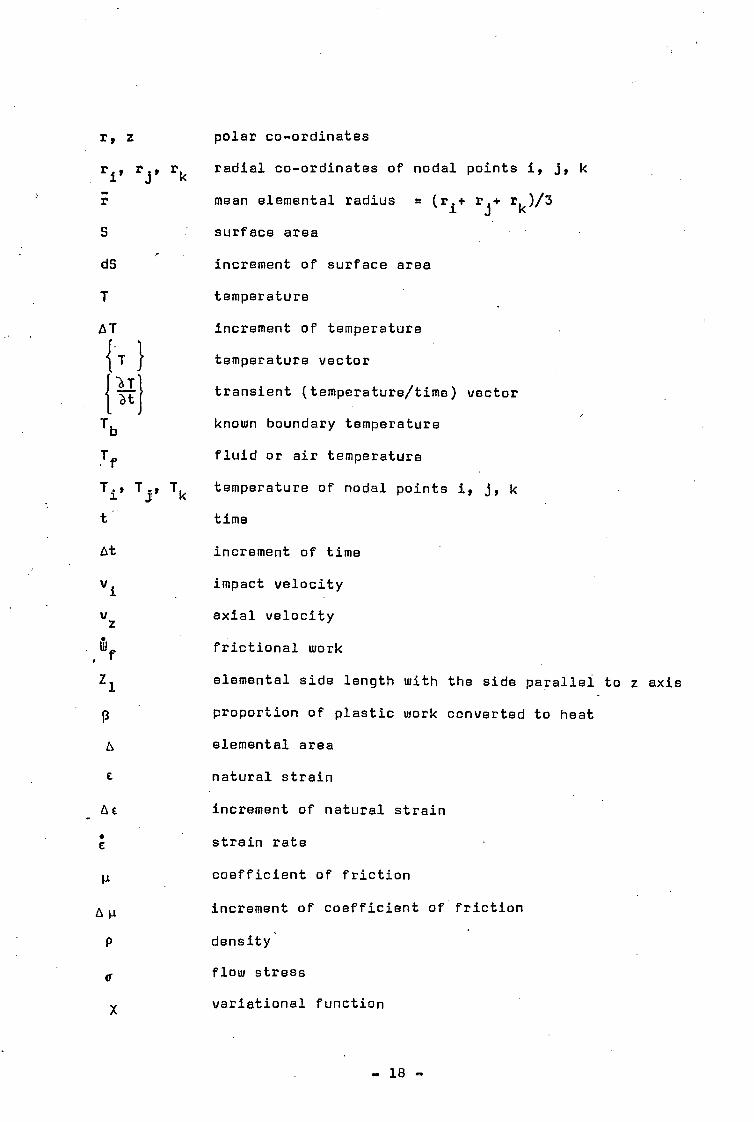
Ty z polar co-ordinates
radial co-ordinates of nodal points i, j, k
r mean elemental radius = (r.+ rj + r
k )/3
S
surface area
dS
increment of surface area
T
temperature
AT increment of temperature
tT } temperature vector
cat transient (temperature/time) vector
Tb known boundary temperature
Tf fluid or air temperature
Tip Ts, Tk temperature of nodal points i, JI k
t time
At increment of time
v impact velocity
vz
axial velocity
tllf
frictional work
Z1 elemental side length with the side parallel to z axis
P proportion of plastic work converted to heat
A elemental area
natural strain
Q E increment of natural strain
strain rate
coefficient of friction
A u increment of coefficient of friction
density
flow stress
X variational function
- 18 -

#A z 25.4mm
25.4 mm
FIG. 1

BOUNDARIES OF CONSTANT TEMPERATURE 17.78mm
ASIN111/111/1/1/1/151/1 /11411111/11/1i1STAVAIiiiii
MPAWIPMERISIMINIBV LIMINMEMPRIE
ITIRCELI MEM 11 M 'EATEN m enes enne PAINGERMILOWN■ Ah AardablrardB 1111/211/4111112111/EMEMINISIMMISIIIESIVIKIE
EMILMINEMEMS111/119"Alanna 11•1111111/1115111211.601011.61MIS AIMMEMBIIIMINIMILIEMPATEME 15111111111■111EIGLINLIMMUME /111/111157111/1141/1/1 1/4111111111/1/111/41/11
MR11111111 12.7mm
E E
r
FIG. 2
1=111•01.1

FIG. 3

i
Set friction coefficient
COFMEU
Read and Store
Heat Parameters
Flow stress data
Velocity/time characteristics
of compaction
COFMEU=LOFMEU
+,6,4
No Calculate displacement
:Choose increment of time TIMINC
Establish total deformation time TIIIITAX
Set deformation time TIMDEF4ITIMINC
START
: Generate the triangular mesh system,
establish nodal points and their
oidinates.
Assign initial temperatures to all
nodal points
Establish platen specimen zones
Uiscern boundaries of convection &
fixed temperatures & the one boundary
subjected to heat flux
FIG, 4

t Recompute nodal point ordinates &elemental areas.
rake corrections to nodal point
temperatures within the platen
continum due to their movement
in r direction
Calculate strain,strain rate experienced
by all nodal points
1
1.
From the previous states of temperature
compute the stresses sustained in the
deformation zone
Compute the increment rise in temperature
AT and assign to the state of previous
temperature field
.1 Calculate the temperature/time deriv,atives
prior to conduction steps
Calculate the temperature distribution
in time intervalAt, smooth out and write
the temperature field
TIMDEF=DEFTIM+TIMINC 1 To A
FIG. 4 (Cont.)

?e, • s, ',4,4144},,(4.1;4,4+4,1,1,500,,,,,,,,4,4;"+■44,41:tili,444 ta.;
g

1 m s
Temperature Velocity
6.24 °C
2 m / s
FIG. 6

0.5 1.0 1.5 0
150
100
50
FIG. 7
Temperature °C
Experimental-"A
Theoretical
Natural Strain
INEM•110

( b ) ( a )
20
20 20
20
FIG. 8

F IG.. 8 (Cont. )
20
(c)
20

0
0.5
10
F IG. 9