university of kwazulu-natal the financial and economic ...

UNIVERSITY OF KWAZULU-NATAL

THE FINANCIAL AND ECONOMIC FEASIBILITY OF

BIODIGESTER USE AND BIOGAS PRODUCTION FOR

RURAL HOUSEHOLDS

Michael T. Smith

Submitted in partial fulfilment of the requirements for the degree of

Master of Commerce

School of Economics and Finance

Faculty of Management Studies

Supervisor: Ms. Jessica Schroenn Goebel

Co-Supervisor: Prof. James N. Blignaut

2011

i

ACKNOWLEDGEMENTS

A great number of people were involved in supportive roles during the completion of this

project. My sincerest thanks must go to my supervisor, Jessica Schroenn Goebel, whose wise

advice and knowledgeable guidance was always willingly given. Thank you for your

generosity of time, effort and support, Jessica!

Thank you also to my co-supervisor, Prof. James Blignaut, whose experience as a resource

economist was a valuable asset to the project. Dr. Terry Everson and Prof. Colin Everson

went well beyond the call of duty as project leaders and I am extremely grateful for their

time, support and guidance along the way.

The research in this project was funded by the Water Research Commission (WRC - Project

Number K5/1955). The National Research Foundation (NRF) provided support funding. I am

sincerely grateful to the WRC for making this project a possibility and to the NRF for their

assistance.

Thanks must also be given to the Okhombe Community for their cooperation and willingness

to be involved in the project.

To my parents, Brian and Di, and brother, Pete, thanks for your patience and support during

the lengthy process. The assistance you gave with editing my work was extremely valuable

and generous. Thanks for the continuous brain storming sessions and all the love.

Lauren, thanks for your support, encouragement and love during a challenging and

demanding time. Your love and support kept me enthusiastic about the project and has

always kept me happy. Thank you also to Pat and Rich for the continuous support and

interest.

ii

TABLE OF CONTENTS

Acknowledgements i

List of Figures vii

List of Tables viii

Acronyms and Abbreviations i

Abstract iv

Chapter 1: Introduction 1

1.1. Background to Study 1

1.2. Rationale and Problem Statement 2

1.3. Aims and Objectives 4

1.4. Hypothesis 5

1.5. Research Methods and Data Sources 5

1.6. Potential Limitations 8

1.7. Structure 8

Chapter 2: Study Area and Project Specifics 10

2.1. The Study Area 10

2.1.1. Location 10

2.1.2. Geographical Setting 11

2.1.3. Socio-Economic Profile 11

2.1.4. Site Selection 15

2.2. Biodigester and Rain Water Harvesting 16

2.2.1. Introduction to Biodigesters 16

2.2.2. Biogas 16

2.2.3. Bioslurry 17

2.2.4. The BiogasPro 17

2.2.5. Household Suitability Requirements 20

2.2.6. Water and Water Harvesting Systems 20

2.3. Introduction to Potential Costs and Benefits of the System 20

2.3.1. Financial Costs and Benefits 21

2.3.2. Economic Costs and Benefits 22

2.3.3. Distinction between Categories of Costs and Benefits 22

2.4. Hypothesised Programme Size and Time Horizon 23

Chapter 3: Literature Review 25

3.1. Introduction to Cost-Benefit Analysis (CBA) 25

3.1.1. Introduction 25

iii

3.1.2. A Brief History of CBA 25

3.1.3. The Distinction between Financial and Economic CBA 26

3.2. Theoretical Foundations of CBA 27

3.2.1. Welfare Foundations of CBA 27

3.2.2. Economic Efficiency 30

3.2.3. Sources of Inefficiency and Market Failure 35

3.2.4. Shadow Pricing 39

3.2.5. Risk and Uncertainty 40

3.2.6. Income Distribution 42

3.2.7. Conclusion 44

3.3. CBA Procedure 44

3.3.1. Identify and Define the Project 45

3.3.2. Identify Economically Relevant Impacts 47

3.3.3. Identify Requirements of the CBA 47

3.3.4. Physical Quantification of Impacts 48

3.3.5. Monetary Valuation 49

3.3.6. Discount the Flow of Costs and Benefits 49

3.3.7. Decision Rules 51

3.3.8. Sensitivity Analysis 56

3.3.9. Conclusion 58

3.4. Monetary Valuation Methodology 59

3.4.1. The Importance of Monetary Valuation 59

3.4.2. Environmental Valuation Methodology 60

3.4.3. The Economic Valuation of Time 69

3.4.4. The Economic Valuation of Health 71

3.4.5. Cost Estimation 77

3.4.6. The Use of Existing Case Studies 79

3.5. Conclusion 81

Chapter 4: Methodology 82

4.1. Introduction 82

4.2. Data Sources 82

4.3. Questionnaire Design and Survey Process 83

4.3.1. Questionnaire Design 83

4.3.2. Survey Procedure 84

4.4. Data Analysis 88

4.4.1. Data Structuring and Software Use 88

4.4.2. Identified Problem Areas 89

iv

4.4.3. Use of External Study Data 92

4.5. Appraisal of Costs and Benefits 93

4.5.1. General Assumptions 93

4.6. Cost Appraisal 94

4.6.1. Financial Costs 94

4.6.2. Economic Costs 97

4.7. Benefit Appraisal 100

4.7.1. Financial Benefits 100

4.7.2. Economic Benefits 111

4.8. Comparison of Costs and Benefits 120

4.8.1. Conducting the CBA 120

4.8.2. Analysis 121

4.8.3. The Choice of a Discount Rate 122

4.9. Sensitivity Analysis 123

4.10. Conclusion 126

Chapter 5: Results 127


5.2. Demographics 127

5.2.1. Respondents to the Questionnaire 127

5.2.2. Sample Group Demographic 127

5.3. Energy Use Profile 128

5.3.1. Electrification of Households 129

5.3.2. Energy Forms Used for Household Lighting 129

5.3.3. Energy Forms Used for Cooking 129

5.3.4. Energy Forms Used for Thermal Heating in Households. 130

5.4. Water Source and Collection 131

5.4.1. Source of Collection 131

5.4.2. Details of Water Collection 132

5.5. Farming Practices 132

5.6. Suitable Households for Biodigester Installation 133

5.7. Cost Appraisal 134

5.7.1. Financial Costs 134

5.7.2. Economic Costs 137

5.8. Benefit Appraisal 138

5.8.1. Financial Benefits 138

5.8.2. Economic Benefits 140

5.9. Cost-Benefit Analysis (Base Case Results) 141

v

5.10. Sensitivity Analysis Results 144

5.11. Conclusion 145

Chapter 6: Discussion and Recommendations 146


6.2. Financial Analysis 146

6.2.1. Discussion of Base Case Scenario Results 146


6.2.3. Comparison with Existing Studies 152

6.3. Economic Analysis 153

6.3.1. Discussion of Base Case Scenario Results 153


6.3.3. Comparison with Existing Studies 157

6.4. Limitations of the Study 157

6.4.1. The Aggregation of Individuals to Society 157

6.4.2. Limitation of the Biodigester Range Assessed 158

6.4.3. Availability of Data 158

6.4.4. Area Specific Analysis 159

6.5. The Argument for Government Subsidisation 159

6.6. A Discussion of Cost and Benefit Flows 160

6.6.1. Discussion of Benefit Flows 160

6.6.2. Discussion of Cost Flows 165

6.7. Scale of Analysis 168

6.7.1. A Biodigester as a Household Investment 168

6.7.2. A Biodigester as a Rural Development Project 170

6.7.3. A Biodigester as a Community Job Creation Project 171

6.8. Conclusion 172

CHAPTER 7: Conclusion 173

List of References 175

Personal Communications 194

Appendix 196

Appendix I: Household Questionnaire Conducted in Okhombe. 197

Appendix II: Biodigester Explanation for Household Questionnaire Respondents. 209

Appendix III: Okhahlamba Local Municipality Map. 212

Appendix IV: CO2 Emission Calculations 213

Appendix V: Time Taken to Dig a Hole for a BiogasPro. 215

vi

Appendix VI: Calculation of the Value of Time 216

Appendix VII: Distribution of Surveyed Households in Okhombe. 219

Appendix VIII: Calculation of Avoided Fuel Costs 220

Appendix IIX: Calculation of Time Saving Due to a Biodigester 223

Appendix IX: Calculation of Financial and Economic Health Benefits 225

Appendix X: Financial and Economic Sensitivity Analysis 228

Appendix XI: Ethical Clearance 230

vii

LIST OF FIGURES

Figure 1. Map showing the location of Okhombe. 10

Figure 2. Okhombe traditional and traditional/formal dwellings. 12

Figure 3. Cross-sectional diagram of an underground biodigester system 16

Figure 4. Biodigester cycle. 17

Figure 5. AGAMA BiogasPro 18

Figure 6. Biogas output relating to manure input. 19

Figure 7. Edgeworth box showing consumption efficiency. 32

Figure 8. Edgeworth box showing production efficiency 33

Figure 9. External cost and inefficient market outcomes. 37

Figure 10. Diagram of Total Economic Value. 61

Figure 11. Total economic value and valuation techniques. 64

Figure 12. Relative pollutant emissions per meal. 72

Figure 13. Google Earth map representing the study area and sample distribution. 87

Figure 14. Flow diagram showing health-related productivity gains calculation process. 115

Figure 15. The distribution of stated monthly household income in Okhombe. 128

Figure 16. Percentage of households using different energy forms for lighting. 129

Figure 17. Percentage of households using different energy forms for cooking. 130

Figure 18. Percentage of households using different energy forms for thermal heating. 131

Figure 19. Percentage of households collecting water at different sources. 132

Figure 20. Flow diagram showing suitable households for biodigester use. 134

Figure 21. Financial sensitivity analyses - Benefit-Cost Ratio 151

Figure 22. Financial sensitivity analyses: Internal Rate of Return 151

Figure 23. Economic sensitivity analyses - Benefit-Cost Ratio 156

Figure 24. Economic sensitivity analyses - Internal Rate of Return 156

Figure 25. Crude oil price history 1981 - 2011. 161

viii

LIST OF TABLES

Table 1. Objectives and methodology for completion 6

Table 2. General living standard statistics of OLM in relation to South Africa national

average. 14

Table 3. Costs and benefits of a biodigester system. 21

Table 4. Potential health-damaging products from incomplete combustion of wood. 71

Table 5. Factors affecting the quantification of biodigester related CO2 emissions. 119

Table 6.Sensitivity analyses and critical variable changes. 124

Table 7. Percentage of households using different energy forms for lighting. 129

Table 8. Percentage of households using different energy forms for cooking. 130

Table 9. Percentage of households using different energy forms for thermal heating. 130

Table 10. Percentage of households collecting water at different sources. 131

Table 11. Details of water collection. 132

Table 12. Details of standard farming activity and practice 133

Table 13. Rural biodigester installation costs. 135

Table 14. Financial costs of a biodigester installation in Okhombe. 137

Table 15. The total time taken to feed a biodigester per day. 138

Table 16. Break down of average household total avoided fuel costs. 139

Table 17. Avoided fertiliser costs. 139

Table 18. Total time saving due to biogas use in place of traditional cooking fuels and

methods (per household). 140

Table 19. Base case cost-benefit analysis for household biodigesters in Okhombe (all data is

per household and in 2011 ZAR unless otherwise stated) 142

Table 20. Combined sensitivity analysis. 144

Table 21. Combined sensitivity analysis with 20.0% variation. 144

Table 22. Discount rate sensitivity analysis 147

Table 23. Combined financial sensitivity analysis (including all variations made in the 14

sensitivity analyses). 149

Table 24. Combined financial sensitivity analysis (using 20.0% variation in all final costs and

benefits). 149

Table 25. Combined economic sensitivity analysis (including all variations made in the 14

sensitivity analyses). 155

Table 26. Combined economic sensitivity analysis (using 20.0% variation in all final costs

and benefits). 155

ix

Table 27. Monthly repayments in ZAR. 169

Table 28. Effects of various levels of government subsidy on monthly repayment and FIRR.

169

Table 29. Model of a hypothesised roll-out of biodigester installations to all suitable

households in Okhombe. 171

Table 30. Average fuel economy and CO2 emission of diesel. 213

Table 31. Average number of days taken to dig a hole for the BiogasPro. 215

Table 32. South African minimum labour wage rate. 216

Table 33. Stated use of time in the event of having more free time as a result of using a

biodigester system. 216

Table 34. Weighted value of time, by activity. 217

Table 35. Calculation of the cost of purchased firewood per average household. 220

Table 36. Calculation of cost of paraffin per average household. 221

Table 37. Calculation of average cost of LPG per average household. 221

Table 38. Calculation of average expenditure on cooking electricity per average household.

222

Table 39. Total monthly expenditure on energy. 222

Table 40. Time saving due to reduced firewood collection. 223

Table 41. Time saved in cooking practices. 224

Table 42. Calculation of medical expenditure saving from reduced IAP. 225

Table 43. Calculation of health related productivity gains. 226

Table 44. Financial and economic valuation of saved lives. 227

Table 45. Financial sensitivity analysis 228

Table 46. Economic senitivity analysis. 229

i

ACRONYMS AND ABBREVIATIONS

ADB Asian Development Bank

ALRI Acute Lower Respiratory Infections

Approx. Approximately

AsgiSA Accelerated Shared Growth Initiative of South Africa

BCR Benefit-Cost Ratio

CAD Canadian Dollar

CBA Cost Benefit Analysis

CDE Commonwealth Department for the Environment

CEAS Central Economic Advisory Service

CFR Case Fatality Rate

CH4 Methane

CIC Center for International Comparisons

CO Carbon Monoxide

CO2 Carbon Dioxide

CO2e Carbon Dioxide Equivalent

COPD Chronic Obstructive Pulmonary Disease

CPIX Consumer Price Index

CV Compensating Variation

CVM Contingent Valuation Method

DALY Disability Adjusted Life Year

DAP Diammonium Phosphate

DECC Department of Energy and Climate Change

e.g. Example

EBCR Economic Benefit-Cost Ratio

EIA Environmental Impact Assessment

EIRR Economic Internal Rate of Return

ENPV Economic Net Present Value

EPA Environmental Protection Agency

ETC Action Group on Erosion, Technology and Concentration

EV Equivalent Variation

excl. Excluding

FBCR Financial Benefit-Cost Ratio

ii

FEE Forum for Economics and Environment

FIRR Financial Internal Rate of Return

FNPV Financial Net Present Value

GBP Great British Pound

GDP Gross Domestic Product

GHG Green House Gasses

GPS Global Positioning System

HDV Heavy Duty Vehicle

HH Households

HST Health Systems Trust

i.e. That Is

IAP Indoor Air Pollution

IES Isikhungusethu Environmental Services

IMF International Monetary Fund

incl. Including

IRR Internal Rate of Return

KZN KwaZulu-Natal

LPG Liquefied Petroleum Gas

LPG-SASA Liquefied Petroleum Gas Safety Association of Southern Africa

MEC Marginal External Cost

mil. Million

MPI Multidimensional Poverty Index

MRS Marginal Rate of Substitution

MRT Marginal Rate of Transformation

MRTS Marginal Rate of Technical Substitution

N2O Nitrogen Dioxide

NERSA National Energy Regulator of South Africa

NOAA National Oceanic and Atmospheric Administration

NPK Nitrogen Phosphorus Potassium

NPV Net Present Value

NRF National Research Foundation

OBPR Office of Best Practice Regulation

OLM Okhahlamba Local Municipality

PASASA Paraffin Safety Association of Southern Africa

iii

Pers. com. Personal Communication

Pers. obs. Personal Observation

PES Payment for Ecosystem Services

PIC Products of Incomplete Combustion

PM Particulate Matter

PPF Production Possibility Frontier

PPP Purchasing Power Parity

Prep. Preparation

Prof. Professor

RNC Restoration of Natural Capital

SCC Social Cost of Carbon

SNV Netherlands Development Organisation

SPSS Statistical Package for Social Sciences

SSA Sub-Saharan Africa

STPR Social Time Preference Rate

TCM Travel Cost Method

TEV Total Economic Value

TLB Tractor-Loader-Backhoe

UNDP United Nations Development Programme

UN-ECA United Nations – Economic Commission for Africa

UNSD United Nations Statistical Division

US United States

US$ United States Dollar

USA United States of America

VAT Value Added Tax

VOSL Value of a Statistical Life

WACC Weighted Average Cost of Capital

WHO World Health Organization

WRC Water Research Commission

WTA Willingness to Accept

WTP Willingness to Pay

YLD Years Lived with Disability

YLL Years of Life Lost

ZAR South African Rand

iv

ABSTRACT

In South Africa, sustainable development is set in the context of two separate economies. The second of these economies consists of the rural population and is characterised by poverty and stagnant development. Sustainable development is an increasingly topical concept which

highlights the need for development to proceed in a manner that does not deplete natural resources. In addition to narrowing the gaps between the various classes (layers) in an

economy, the key ‘ingredients’ of sustainable economic development include “natural resource management, food, water, and energy access, provision and security” (Blignaut, 2009: cited in Blignaut and van der Elst, 2009: 14).

A biodigester is a potential solution to some of the difficulties faced by remote rural

populations. Biodigester systems are submerged tanks capable of producing a nutrient rich fertiliser and combustible gas when consistently fed with organic matter and water. A biodigester may be one simple answer to the key ingredient needs of sustainable development

– reducing the depletion of natural resources, providing clean burning energy for cooking and fertiliser for growing food.

The potential is clear for biodigesters to aid in the process of sustainable development. The question to be analysed is whether this technology would be financially and economically

feasible for installation and use in rural households.

This thesis focuses on a typically remote and rural community in KwaZulu-Natal, South Africa, in order to assess the potential feasibility of a biodigester system. The appraisal takes the form of a Cost Benefit Analysis (CBA) and aims to establish whether or not this

technology is financially feasible for individual rural households and/or economically beneficial to society.

1

CHAPTER 1: INTRODUCTION

1.1. BACKGROUND TO STUDY

Sustainable development is defined by Todaro and Smith (2009: 839) as a “pattern of

development that permits future generations to live at least as well as current generations”.

This definition highlights the need for development to proceed in a manner that does not

deplete the earth’s finite resources.

Blignaut and van der Elst (2009: 13) introduce three pathways to sustainable development,

namely:

- Sustainability through technological change, allowing resources and energy to be used

conservatively.

- Sustainability through a change of society’s preferences, value systems and subsequent

behavioural patterns.

- Sustainability through restoration of natural capital (RNC), replenishing natural capital

stocks and improving the flows of goods and services that ecosystems provide

(ecosystem services) (Aronson et al, 2007: cited in Blignaut and van der Elst, 2009).

One of the aims of development is to reduce income inequality (measured by the Gini

coefficient) and economic disparity among members of a population (The Presidency, 2009:

25). In addition to narrowing the inequality between the various classes in an economy, the

key ‘ingredients’ of a sustainable economic development package include “natural resource

management, food, water, and energy access, provision and security” (Blignaut, 2009: cited

in Blignaut and van der Elst, 2009: 14).

In South Africa, sustainable development is set in the context of the presence of separate yet

concurrently existing economies. Blignaut and van der Elst (2009) extend this further by

explaining South Africa’s economy as consisting of three layers. The top and middle layers

of the economy – comprising educated, affluent and employed people, and blue-collar semi-

skilled workers respectively – make up South Africa’s formal and structured ‘first economy’;

the bottom layer, which contains more than half the population, consists mainly of rural

people living in poverty with little access to the formal economy. Similarly, du Toit and van

Tonder (2009: 15) describe the ‘second economy’ as characterised by “extreme poverty…

high and structural unemployment as well as poor socio-economic conditions”.

2

Challenged with the difficulties of poverty and stagnant development, this second economy

encompasses rural communities throughout South Africa which lack basic amenities and face

the difficulties of a harsh lifestyle and survival. While much is being done for development,

there is still a great need for programmes to assist in the progression, the improvement of

basic living standards and upliftment in these areas. A recent report for Accelerated Shared

Growth Initiative of South Africa (AsgiSA) identified that a greater focus was needed on

South Africa’s second economy. The need for shared growth among all layers of the

economy was highlighted (Trade and Industry Policy Strategies (TIPS), 2009).

Of major concern in these rural areas is the general health of people and their livestock, as

well as their basic standard of living. Of specific relevance to this project is the fact that the

preparation of a simple meal in a rural household requires people (usually women and girl

children) to walk great distances to collect cooking fuel. This potentially contributes to

deforestation as they harvest local timber and hamper the health of their families by cooking

with ‘non-clean’ burning woods and fuels in poorly ventilated homes. Those households

which can afford other fuels for cooking (for example, paraffin) spend large percentages of

their monthly income on potentially hazardous and ‘non-clean’ burning fuels. In addition to

this, rural livestock suffer a harsh existence without sufficient grazing or supplementary

fodder during winter months (pers. com. Prof. Colin Everson, March 2010). Salomon (2009)

noted in a cattle-keeping study from the Okhombe area, that overgrazing is one of the factors

that may lead to erosion and land degradation.

1.2. RATIONALE AND PROBLEM STATEMENT

A recent South African National Household Biogas Feasibility Study was conducted by

Austin and Blignaut (2008). The study highlighted some of the social, economic and

environmental benefits associated with a national programme for implementation of a rural

biodigester plan in South Africa. The feasibility study found a potential for household

biodigesters in 310 000 households in the study area (six provinces in South Africa). Using

conservative assumptions the study calculated financial and economic internal rates of return

(IRR) to be 15% and 67% respectively across the study area with a capital subsidy of 30%

(Austin and Blignaut, 2008: 4). In addition to the output benefits of the system, some of the

benefits that were included in the economic analysis were:

3

avoiding deforestation by replacing firewood as a household thermal fuel;

saving time by not having to collect this firewood;

improving soil fertility by using bioslurry as a fertiliser;

reducing health care costs as a result of replacing solid fuels and open cooking fires

(which impact on indoor air quality and cause health problems) with biogas.

(Austin and Blignaut, 2008: 9)

In addition to this and in the context of sustainable development, a biogas programme has the

ability to tackle development in South Africa’s second economy with the key ‘ingredients’ of

sustainable development identified by Blignaut (2009: cited in Blignaut and van der Elst,

2009: 14). A biodigester system has the potential to reduce the depletion of natural forests,

provide food security by sustaining the lands and livestock with the use of bio-fertilisers,

provide clean energy, and thus fulfil the sustainable development package of: “natural

resource management, food, water, and energy access, provision and security” proposed by

Blignaut (2009: cited in Blignaut and van der Elst, 2009: 14).

The proposed financial and economic feasibility study aims to consider a hypothetical roll-

out of biodigesters to all suitable households in the Okhombe community in northern

KwaZulu-Natal, and develop a better understanding of the potential for biodigesters as a form

of renewable energy and development means for rural communities in South Africa. The

feasibility study will consist of a cost-benefit analysis. The costs derived from the technical

comparison component will be evaluated against the array of potential benefits, namely:

direct outputs of biogas for cooking, and fertiliser for food and cattle fodder production;

reduced time involved in collecting firewood and traditional cooking practices; health

benefits of using ‘clean’ burning biogas for cooking in place of traditional solid fuels (wood

and cattle manure); environmental benefits of reduced deforestation, erosion and CO2

emission reduction. Some of the costs to be considered are the construction and maintenance

of the biodigester plant. Included in these costs are the time cost of running the system as

well as a consideration of the carbon ‘footprint’ attached to the construction of the plant.

The study will use survey data, case study data output, as well as pre-existing studies to

develop monetary values for the identified benefits. The benefits will be considered against

the costs, to calculate financial and economic feasibility indicators. The feasibility appraisal

4

should assist in assessing the financial and economic viability of biodigester systems as a

means to combat some of the hardships of rural poverty through ‘clean energy’ production

and use.

In terms of environmental impact, the project will assess the potential for quantifying and

monetising reduced deforestation, erosion and CO2 emission in rural areas. The use of biogas

for cooking reduces the need for firewood to be sourced from local surrounds. Erosion as a

result of overgrazing is expected to be reduced as biodigester effluent is used to produce

livestock fodder and supplement livestock feed. CO2 production is expected to decrease as a

result of using ‘clean’ burning and efficient biogas in place of firewood, cattle dung and other

fuels for cooking.

The beneficiaries of the programme are firstly the rural households who will use biodigester

systems, and more generally, the greater public who gain the benefit of environmental

preservation. The biogas programme has the potential to benefit women in particular, who

usually undertake the tasks of fuel collection and cooking (Legros et al, 2009: 22; Banik,

2010: 210). Reduced time spent on these duties may allow women to partake in economically

beneficial activities, or simply enhance their quality of life.

The project will build on the 5-year Water Research Commission (WRC) project1 being

undertaken by AGAMA Energy and the University of KwaZulu-Natal (UKZN), which

focuses on assessing the impacts on rural livelihoods, grasslands and animal health related to

the use of biodigester and rainwater harvesting systems in rural communities. This project

commenced in April 2010. Within this 5-year project, AGAMA Energy will assist in

installing 10 biodigesters for selected households in Limpopo, Eastern Cape and KwaZulu-

Natal (including the Okhombe community). UKZN will be the leading institute for research

involved with the project and along with shared resources will begin by identifying suitable

case study sites and households.

1.3. AIMS AND OBJECTIVES

The aim of this project is to use survey data and existing studies to quantify and monetise the

potential impacts of a biodigester system on an average rural household in the Okhombe

1 WRC Project number K5/1955.

5

community. Following this, the corresponding aim is to use this information in a cost-benefit

analysis to identify the financial and economic feasibility of a biodigester for a rural

household in the Okhombe community. In achieving these aims, the objectives of the

research project include:

1. Analysis of internal and external costs of installation and implementation of a

biodigester.

2. Identification of costs and benefits likely to arise from the biodigester system.

3. Quantification and monetary valuation of key costs and benefits.

4. Cost-benefit analysis and the calculation of feasibility indicators including, net

present value (NPV), benefit-cost ratio (BCR) and internal rate of return (IRR).

5. The presentation of a hypothesised roll-out model of biodigester installations at

village-level – a need identified by the WRC Project reference committee.

6. A consideration of the alternative financing models for household biodigester

systems.

1.4. HYPOTHESIS

The null hypothesis is that the biodigester system and related elements will not be financially

and economically feasible in meeting the food and energy security requirements of a rural

household.

The alternative hypothesis is that a biodigester system and related outputs will meet basic

energy requirements of a rural household and will contribute to food security. The system

will be financially and economically feasible with the capital investment being paid off over

n number years. The economic IRR is expected to be greater than the financial IRR. The

system may reveal economic but not financial feasibility when taken over a limited period of

time, x years.

1.5. RESEARCH METHODS AND DATA SOURCES

The initial phase of this project followed the general course of a literature review. Current

literature (journal articles, case studies, pre-existing reports from South Africa and other

countries) formed the basis for theoretical understanding of the economic terms and

procedures required in completing the financial and economic analysis.

6

A survey was compiled and conducted in the Okhombe community to identify the number of

suitable households for biodigester installation, as well as determining various aspects of

their daily activity that would aid in identifying the impacts of biodigester use. Key data

included the current usage of cooking fuels, the time taken collecting water and fuels for

cooking, and ability of a household to meet the basic requirements for successful running of a

biodigester. A questionnaire was designed by the researcher and reviewed for suitability by

the WRC Project team. Specific questions relating to the economic feasibility study were

defined and included in the questionnaire.

The biodigesters installed in the Okhombe community will be used by the selected

households and their use and productive ability monitored by the UKZN project team. In

addition to the monitoring of biogas production and use, the WRC project will include the

implementation of cattle fodder production using the bioslurry effluent from the biodigesters

as a nutrient rich fertiliser. Data on levels of fodder production and cattle health will be

monitored by project personnel and captured for use in, amongst other studies, further

economic analysis of biodigester benefits.

The data captured from the community survey and the case study will be used in conjunction

with pre-existing studies to quantify potential costs and benefits and conduct a household

level cost-benefit analysis. The information will also assist in the formulation of a model

hypothesising a roll-out of biodigesters to all suitable households in the Okhombe

community.

Table 1 shows the process of methodology in achieving objectives and the party that will

carry out each stage of the process.

Table 1. Objectives and methodology for completion

Objective Necessary Steps To be carried out

by:

Literature review - Review available literature

including pre-existing biodigester feasibility studies (South African and other)

M Smith

Survey Okhombe - Compile questions necessary for M Smith

7

community feasibility study

- Integrate questions with project community survey

- Conduct survey in Okhombe

M Smith + WRC Project team

WRC Project team

Analysis of biodigester

installation and

implementation costs.

- Record all costs involved in the

construction and implementation of biodigesters in Okhombe

- Analyse costs of biodigesters

recorded in pre-existing case

studies - Take into account economies of

scale and purchasing power parity (PPP) between countries

AGAMA Energy

M Smith

M Smith

Identification of costs and

benefits likely to arise

from using a rural

biodigester system.

- Analysis of pre-existing case

studies and reported results - Analysis of available literature

- Recognition of costs/benefits identified during the course of the

case study.

M Smith

M Smith

WRC Project team (Interviews and

progress reports captured by the Team)

Results captured from

case study (Okhombe).

- Progress results (including how the biodigesters perform and are used)

will be captured

WRC Project team

Monetary valuation of key

costs and benefits.

- Literature review will reveal most suitable methods of valuation

- Results from case study, in conjunction with pre-existing case

study findings will be used to apply monetary valuation

- Results from pre-existing studies to

be used where applicable

M Smith

M Smith

M Smith

CBA and projected

internal rates of return.

- Results from monetary valuation will be applied to steps involved in

CBA procedure (identified during literature review)

M Smith

Preparation of financing

models for rural

household biodigesters.

- Financing models will be

considered in relation to the results found from CBA analysis

M Smith

8

1.6. POTENTIAL LIMITATIONS

From a project perspective, the fundamental limitation is that the case study relies on the

active and continued participation of households that are chosen as sites for biodigesters. The

reality that many rural inhabitants are uneducated could be a potentially detrimental aspect to

the successful reporting and capture of case study data, as well as the effective running of a

biodigester system. The absence of education in the study area is also likely to pose potential

difficulties in the study survey process.

Case study site selection is also a point of concern as it is necessary to attain community

acceptance when selecting individual households to partake in a community project. The

potential difficulties of this concern will be limited to the greatest extent possible as the WRC

project team will conduct community selection processes to insure that the community selects

the households. This process needs to be weighed against the reality that a household needs to

be suitable for biodigester use.

In relation to the greater outlay of biodigester systems, as proposed by the hypothetical study,

it is recognised that the education element may pose potential problems. Extensive education

may be required to explain the technology of the system and to ensure that it is used to its full

potential.

It is understood that this thesis is a financial and economic feasibility study and should be

limited to those confines. The task of assessing the social acceptability and technological

viability of the project will be considered where appropriate and necessary, but will not be

discussed in detail. Such elements of biodigester use will be assessed by the WRC project

team.

1.7. STRUCTURE

In this thesis:

- Chapter two will introduce the area of study (Okhombe) and the specifics of the

project; including details of biodigester and rain water harvesting technology and their

potential costs and benefits.

9

- Chapter three will comprise of a literature review. Points of analysis will include; the

economic foundations of cost-benefit analysis (CBA), the procedure of CBA, the

monetary valuation of potential costs and benefits.

- Chapter four will outline the methods and procedures to be used in the analysis of

data.

- Chapter five will present the data findings. Included in this will be the results from a

survey conducted in the Okhombe area and the application of existing study findings

to the current study.

- Chapter six will include an analysis of the results, a discussion and recommendations

for the project.

- Chapter seven will conclude the study.

10

CHAPTER 2: STUDY AREA AND PROJECT SPECIFICS

2.1. THE STUDY AREA

2.1.1. Location

Situated in the province of KwaZulu-Natal, South Africa, Okhombe is a rural community of

the Upper Thukela catchment area. Figure 1 shows the position of Okhombe (28° 42’ S; 29°

05’ E) at the base of the northern Drakensberg Mountains. The Okhombe area is located in

Ward 7 of the Okhahlamba Local Municipality (Van Niekerk GIS, 2009). Within this area,

there are 6 sub-wards and the community falls under the jurisdiction of the Amazizi

Traditional Administrative Council (Bangamwabo, 2009). Okhombe is surrounded by a

horseshoe shaped range of mountains and its land forms part of the Ingonyama tribal trust

land, administered through tribal authorities under trusteeship of the state (Chellan, 2002).

Figure 1. Map showing the location of Okhombe.

(Salomon, 2009: 1)

11

2.1.2. Geographical Setting

The Okhombe Valley forms part of the catchment area for the Thukela River. The valley is

drained by the Khombe River and feeds the nearby Woodstock Dam. With an altitude

ranging from 1000-1800m (Everson et al, 2007: 3) the area receives between 800mm and

1265mm of rain per annum, 82% of which falls during the summer rainfall months of

October to March (Kollar & Goudy, 1999: cited in Everson et al, 2007). According to

Everson et al (2007) the heavy precipitation during these periods has led to a loss of nutrient

soils and extensive erosion along the slopes. The vegetation of the area is predominantly

Southern Tall Grassland and Highland Sourveld (Acocks, 1988) with areas of shrub and

forest in the higher regions. Sourveld grasses are only palatable in the summer months

(Chellan, 2002). According to Professor Colin Everson (pers. com. March 2010) the

‘Sourveld’ native to the area makes livestock survival a challenge without supplementary

fodder in the winter months as the nutrients of grasses retreat into their roots and the grass’s

nitrogen to carbon ratios are too low for digestion by ruminants (Chellan, 2002). In addition

to this, grazing cattle put more pressure on the grasslands under these winter conditions and

cause further erosion.

2.1.3. Socio-Economic Profile

Okhahlamba Local Municipality (OLM), of which the Okhombe community is a part, is a

predominantly rural area by the largely accepted definition of ‘rural’ being, “sparsely

populated areas in which people farm or depend on natural resources, including villages and

small towns that are dispersed throughout these areas … [and]… large settlements in the

former homelands” (Department of Land Affairs, 1997).

Land in the OLM area is predominantly used for primary sector commercial farming and

subsistence farming, with some areas (mainly the Cathkin Park Reserve and surrounds) being

used for tourism and recreational activity. The primary sector is the largest employer in the

area (22%), followed by the community/social/personal services sector (which includes

subsistence farming and community industry) at 19% (OLM, 2010: 23).

The Okhombe community is situated within the Amazizi Tribal Authority which, under

apartheid South Africa, was part of the non-independent homeland, KwaZulu (Chellan, 2002:

46). Historically the area is a tribal one, and from personal observation is still made up almost

12

exclusively of traditional and traditional/formal dwellings surrounded by communal grazing

lands and subsistence agriculture (pers. obs. August 2010; Chellan, 2002).

Figure 2. Okhombe traditional and traditional/formal dwellings.

(Smith, 2010)

The Okhombe community (Okhombe Ward 7 in the Okhahlamba Local Municipality) had a

recorded population in the South African 2001 Census of approximately 5 760 people (IES,

2001). This population is estimated to have increased by 10.12% to 6 3432 as of 2007, based

on the 2007 Community Survey (Stats SA, 2007). Although United Nations (UNSD, 2011)

and Unicef (2010) reports suggest a decline in rural populations across South Africa, what is

considered to be ‘rural’ may differ in definition and it does appear that this particular area has

increased in population since the 2001 Census (Councillor Dhadhla, pers. com. January

2011).

The Okhombe area is separated into six sub-wards or villages, namely: Mahlabathini,

Sigodiphola, Enhlanokhombe, Empamemi, Oqolweni and Ingubhela (Sookraj, 2002). It is

estimated that there are approximately 1 160 households cumulatively in these sub-wards3.

In the economic sense of the word, poverty is defined as a relative measure that describes the

state of being unable to maintain what are considered by society to be minimum standards of

2 The OLM increased from 137 525 (2001 Census) to 151 441 (2007 community survey) (Stats SA, 2007: p14).

The population increased 10.12% from 2001 to 2007. Applying this increase to the 2001 population of

Okhombe Ward 7, we arrive at a population estimate of 6 343 people. 3 Based on data from IES (2001) and Statistics South Africa (1996) revealing a person per household figure of

5.47.

13

living: “in absolute terms, having income and/or wealth too low to maintain life and health at

a subsistence level” (Barron’s Educational Series, 2000). There are a number of economic

measures, qualitative and quantitative, used to assess whether a population may be considered

poor or not. The Presidency of the Republic of South Africa (2009) uses a variety of

quantitative methods to assess levels of poverty. One of these measures of poverty is similar

to the World Bank Group’s recognised ‘$1 a day poverty line’ which has been updated to the

$1.25 dollar a day poverty line (Ravallion et al, 2008). In South Africa, the R238 per month

income line is one measure used to assess the level of poverty. In addition to examining how

many people survive on less than R238 per month, the ‘depth of poverty’ index measures

how far below (in percentage terms) the R238 mark the average poor person’s (person below

the R238 income line) income is (The Presidency, 2009). The Multidimensional Poverty

Index (MPI) is also a useful metric which may be applied, albeit indirectly, to the Okhombe

area. The MPI examines three key deprivations relating to education, health and living

standards (including access to electricity, drinking water and sanitation) (Alkire and Santos,

2010: 7).

It is generally agreed that the Okhombe community is a poor one in terms of income and

general living standards (Sookraj, 2002: 67). In relation to income levels, the 2007

Community Survey (Statistics South Africa) revealed that 82% of people in the OLM do “not

receive any form of income”, while the next poorest group (14%) receive between R1 and

R800 per month (OLM, 2010: 25). In consideration of the fact that the Okhahlamba

Municipality includes two relatively affluent towns and the Cathkin Park Reserve (including

golf and recreational resorts), it is clear that the Okhombe population is likely to have even

lower income levels. Although much of the community will be supported by social grants, the

majority of peoples’ income will fall below the R238 poverty line. In relation to the

population of South Africa, 22% of whom live below the R238 poverty line (The Presidency,

2009) Okhombe suffers greater levels of poverty with reference to the national norm.

While the MPI may not be applied directly, as recent and specific data are not currently

available, it is possible to draw some links between indicators of the MPI and the available

statistics. Education levels in the OLM are minimal. Only 4% of the OLM population over 20

years old have ‘higher education’ qualifications (degree/diploma), 10% having matriculated

and 38% having had no formal schooling (OLM, 2010: 20). 44.7% of the OLM population

have access to piped water. This figure is significantly lower than the South African statistic

14

of 88.6% who have access to piped water. In addition to this, only 5.9% of the OLM

population have access to piped water in their homes (OLM, 2010: 17; Stats SA, 2007).

Qualitative measures of poverty are subjective, but are useful in allowing us to describe the

deprivations in an area. Some of the aspects that we assess qualitatively are general living

standards, including dwelling type, sanitation facilities, service provision and access to water.

Many of these items may be noted by observation of an area, but it is also possible to identify

their significance by quantitative examination and many of these measures are correlative to

the MPI. Table 2 identifies some of these ‘general living standards’ and compares them to

South African national statistics.

Table 2. General living standard statistics of OLM in relation to South Africa national average.

GENERAL LIVING STANDARD STATISTICS (OLM)

Deprivation

or measure Description OLM South Africa

Dwelling type Percentage of population living in ‘formal’

dwellings 35.1% 70.6%

Electricity Households without access 37.7% 24.5%

Sanitation Households using pit latrine systems as

toilets 52.0% 27.3%

Sanitation Households with no toilets 14.5% 8.3%

Service

provision

Refuse removed by local authority or private

company 6.8% 61.6%

Water access Households with access to piped water 47.1% 70.8%

(The Presidency, 2009; Stats SA, 2007; OLM, 2010)

If the above measures of deprivation may be considered as an indication of general living

standards (and poverty), it is clear that OLM has significantly lower levels of living standards

than South Africa as a whole. Furthermore, the OLM includes Winterton and Bergville

(developed and relatively affluent towns) as well as a series of golfing and recreational

resorts in the Cathkin Park Reserve. The Okhombe community, coming from a historical

background as a tribal trust land and former non-independent homeland (Chellan, 2002: 46),

is solely rural and with considerably lower levels of general living standards (pers. obs.

August 2010). In addition to this, a survey conducted by Chellan (2002) revealed further

15

indications of Okhombe’s rural and under-provisioned existence. Chellan found that the

majority of people dwell in ‘mud-brick’ constructed homes (72.4%), use wood and candles as

their main fuels for energy (cooking, heating, lighting), and only 3.1% of people have a

private tap as a source of water (Chellan, 2002). According to Chellan’s findings (2002: 67)

86.3% of surveyed individuals were unemployed.

IsiZulu is the predominant language in OLM (96%) with African people comprising the

largest ethnic group. The gender profile of the area reveals a bias of woman (53%) to men

(47%) which is likely linked to the tendency of South African rural males to seek work in

major cities and mining areas (migrant labour). The OLM is considered to have a relatively

young population with 75% of people being under the age of 34 years. The young age profile

is likely to result in future population growth, although it is recognised that this population is

vulnerable to HIV and AIDS (OLM, 2010).

2.1.4. Site Selection

The Okhombe community was selected for this case study for a number of reasons. The

community is a rural one situated some distance from any town or major centre with many

households lacking adequate food, water and energy security (Sookraj, 2002). It is thus one

that would benefit greatly from the outputs of biodigester systems that could provide a source

of energy and a means for aiding food production. The community has also been involved

with numerous land care and other studies conducted by the University of KwaZulu-Natal

and associated organisations. The community has been actively involved in these projects and

has shared success with the researching institutions. The nature of this project includes the

need for active participation of households and community members. It is thus valuable that

there is an established relationship between the community and researchers and this is likely

to facilitate further involvement.

A recent survey showed that in one of the sub-wards, Enhlanokhombe, approximately one

third of the households (51 of 148) own cattle in varying quantities (Salomon, 2009: 8).

Based on the manure requirements for the operation of the biodigesters, a survey will be

needed to gather information regarding cattle ownership in the remainder of the community.

This will allow for households to be assessed, based on the household biodigester suitability

requirements to be outlined in section 2.2.5.

16

2.2. BIODIGESTER AND RAIN WATER HARVESTING

2.2.1. Introduction to Biodigesters

A biodigester is a construction of varying size in which organic matter may be fed and

allowed to decompose in the absence of oxygen (anaerobic digestion) to produce a gas and

liquid digested slurry (Riuji, 2005).

There are two main design categories of biodigesters available, a fixed dome digester and a

floating digester (Khan and Khan, 2009; Flynn, 2010). As shown in Figure 3, a fixed dome

biodigester is a dome shaped (often submerged) construction which has an inlet area, a

digestion chamber, and an outlet. Animal manure, human waste and other organic matter

(‘green waste’) may be fed into the biodigester through the inlet (Riuji, 2005: 12). In the

digester chamber anaerobic digestion takes place as a composite of water and waste material

decomposes in the absence of oxygen (Fulford, 1988: 30). As the decomposition takes place,

gas (biogas) is released and the waste material decomposes into a nutrient rich liquid

(bioslurry).

Figure 3. Cross-sectional diagram of an underground biodigester system

(International Workshop on Domestic Biogas, 2009)

2.2.2. Biogas

Biogas is formed in the process of decomposition that takes place in the digestion chamber as

microorganisms break down organic compounds (Wu et al, 2009: 8.1). Biogas is

predominantly a composition of Methane (CH4 – 55-60%), Carbon Dioxide (CO2 – 35-40%)

17

and Hydrogen Sulphide (H2S – <2%) (Mata-Alvarez, 2003). The biogas, which is methane

rich, may be siphoned from the chamber and used. Biogas with a methane content of 45%

and above is combustible and thus, using a slightly modified gas burner, methane can be used

for cooking, lighting and/or heating in a rural household (Riuji, 2005: 14).

2.2.3. Bioslurry

The anaerobic digestion process not only decomposes organic waste into biogas, but also

produces an effluent slurry. The digestion process results in nitrogen, potassium and

phosphorus plant nutrients being released and converted into a form that may effectively be

absorbed by plants (Fulford, 1988: 39). The removal of biogas elements (methane, carbon

dioxide and hydrogen sulphide) is said to improve the concentration of plant nutrients in the

remaining bioslurry (Fulford, 1988: 39). The bioslurry is thus a good replacement for

chemical fertilisers and a high quality fertiliser for rural agriculture (Pandey et al, 2005: 3;

Khan and Khan, 2009: 468). Bioslurry may be used as a nutrient rich fertiliser to grow food

gardens or fodder for animals (Pandey et al, 2005: 3). Excess bioslurry is not considered to be

an environmental problem as it poses no greater threat than uncollected cattle manure.

Figure 4. Biodigester cycle.

(Sasse et al, 1991: 7)

2.2.4. The BiogasPro

The biodigesters that will be used in this case study are the “BiogasPro” prefabricated

biodigesters designed by AGAMA Energy Pty (Ltd)4. The BiogasPro is based on the

4 www.agama.co.za

18

hydraulic functionality of the 6m3 Nepalese digester GGC 2047 designed to support the

energy needs of an eight person rural household (Greg Austin, pers. com. April 2010).

Successful running of the Nepalese digester requires 20kg of cow manure and the equivalent

amount of liquid (20 litres) per day. It has been concluded that four cattle are sufficient to

provide this quantity of manure (Austin and Blignaut, 2008), on the premise that the dung is

conveniently accessible from cattle that free-range during the day and are kraaled5 overnight

(Greg Austin, pers. com. May 2010). The liquid requirement may comprise of cattle urine

and re-used household water, alternatively it is assumed that access to water less than 1km

from the household meets suitability requirements.

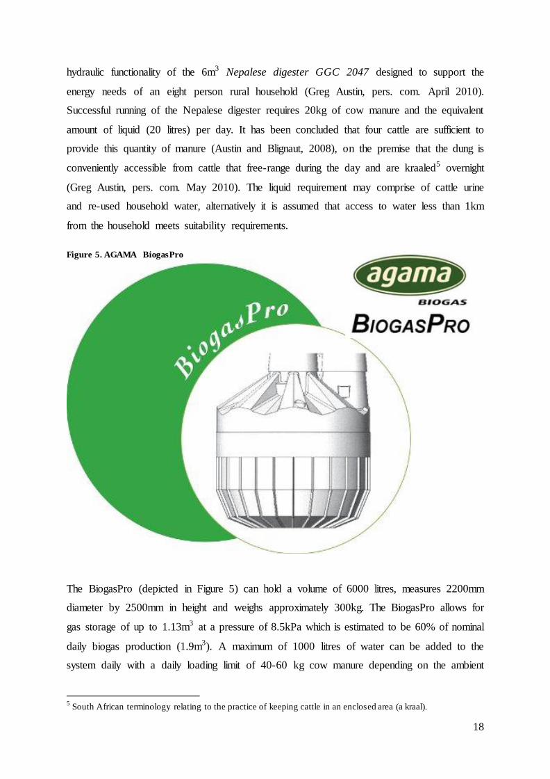
Figure 5. AGAMA BiogasPro

The BiogasPro (depicted in Figure 5) can hold a volume of 6000 litres, measures 2200mm

diameter by 2500mm in height and weighs approximately 300kg. The BiogasPro allows for

gas storage of up to 1.13m3 at a pressure of 8.5kPa which is estimated to be 60% of nominal

daily biogas production (1.9m3). A maximum of 1000 litres of water can be added to the

system daily with a daily loading limit of 40-60 kg cow manure depending on the ambient

5 South African terminology relating to the practice of keeping cattle in an enclosed area (a kraal).

19

temperature. The optimal ratio of water to feedstock is 1:1. An input of 20kg of cow manure

and an equivalent amount of water would produce 1.2 – 1.9 hours of burn time on a large

single-plate gas burner (AGAMA Energy, 2010).

Figure 6 displays the ability of the BiogasPro to produce biogas for cooking (AGAMA

Energy, 2010). The Y-axis shows the number of hours a ‘large single-plate gas burner’ may

be used (i.e. how much useable biogas has been produced) in relation to the amount of cow

manure that is added to the system (X-axis). The variable in this experiment was the ambient

air temperature. As can be seen in Figure 6, the higher the ambient temperature, the greater

the volume of gas that may be produced within a day. Depending on the ambient temperature,

1.2 to 1.9 hours of biogas burn time will be available to a user who inputs 20kg of cow

manure. According to Guidotti (2002: 12) 1m3 of biogas is sufficient to provide enough

energy for cooking three meals for a five to six person household per day.

Figure 6. Biogas output relating to manure input.

(AGAMA Energy, 2010)

20

2.2.5. Household Suitability Requirements

There are certain requirements which are necessary for a household to be deemed suitable for

the installation and running of a biodigester. In rural areas like Okhombe, it is most common

practice to allow cattle to roam freely during the day and to be kept in an enclosure (a kraal)

near the household at night. Four cows are able to produce 20kg of dung overnight and are

thus the minimum requirement for the purposes of this study (Austin and Blignaut, 2008: 24).

The suitability requirements for a household to be deemed technically viable for biodigester

use are as follows:

Must have four or more cattle.

Must kraal these cattle overnight.

Must be happy to use biogas for cooking purposes.

Must want to have and use a biodigester at their household.

Must be willing and able to provide 20l of water and 20kg of cow dung every day, to

be fed into the biodigester.

Must have space in their garden/yard for a BiogasPro to be installed.

2.2.6. Water and Water Harvesting Systems

Water is a critical ingredient in the digestion process of the biodigester system, as well as

being a necessity for cooking, drinking and the production of food/fodder. Thus, a water

harvesting system is an extended part of this household project, which makes the access to

the required water feasible in a rural setting. The standalone benefits derived from clean

water access will not be considered expressly, but will be recognised in so far as they relate to

the running/feeding of the biodigester.

2.3. INTRODUCTION TO POTENTIAL COSTS AND BENEFITS OF THE

SYSTEM

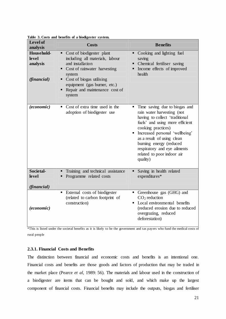
For purposes of the literature review to follow, the potential costs and benefits of the project

will be introduced. Table 3 is adapted from Biogas for Better Life: An African Initiative

(Renwick et al, 2007: 12) and serves to outline some of the costs and benefits associated with

a biodigester system.

21

Table 3. Costs and benefits of a biodigester system.

Level of

analysis Costs Benefits

Household-

level

analysis

(financial)

Cost of biodigester plant

including all materials, labour and installation

Cost of rainwater harvesting

system Cost of biogas utilising

equipment (gas burner, etc.) Repair and maintenance cost of

system

Cooking and lighting fuel

saving Chemical fertiliser saving Income effects of improved

health

(economic) Cost of extra time used in the

adoption of biodigester use

Time saving due to biogas and

rain water harvesting (not having to collect ‘traditional fuels’ and using more efficient

cooking practices) Increased personal ‘wellbeing’

as a result of using clean burning energy (reduced respiratory and eye ailments

related to poor indoor air quality)

Societal-

level

(financial)

Training and technical assistance Programme related costs

Saving in health related expenditures*

(economic)

External costs of biodigester (related to carbon footprint of

construction)

Greenhouse gas (GHG) and CO2 reduction

Local environmental benefits (reduced erosion due to reduced overgrazing, reduced

deforestation)

*This is listed under the societal benefits as it is likely to be the government and tax payers who fund the medical costs of

rural people

2.3.1. Financial Costs and Benefits

The distinction between financial and economic costs and benefits is an intentional one.

Financial costs and benefits are those goods and factors of production that may be traded in

the market place (Pearce et al, 1989: 56). The materials and labour used in the construction of

a biodigester are items that can be bought and sold, and which make up the largest

component of financial costs. Financial benefits may include the outputs, biogas and fertiliser

22

which replace items that previously may have been purchased – including fuels for cooking

and fertiliser for agriculture (Renwick et al, 2007: 23). The process of valuing these outputs

involves the identification of: percentage of fuel/fertiliser users; amount of each product used;

amount purchased versus amount collected of each product; cost of products and the expected

reduction in product purchased/collected by using the outputs of the biodigester (Renwick et

al, 2007: 23).

2.3.2. Economic Costs and Benefits

Economic costs and benefits include financial costs and benefits as well as those which relate

more to societal values and values which cannot be bought and sold in the market place. “In-

kind contributions” (Renwick et al, 2007) are material or labour contributions which are

made by households and/or communities and are considered economic costs as they “do not

involve cash outlays” (Renwick et al, 2007). Time saving and environmental benefits are not

items that may be bought and sold in the market place, but do translate to benefits and are

thus categorised as economic values. One method of calculating the monetary value of time is

to value it as a “shadow price” of labour (Austin and Blignaut, 2008: 29). Environmental

valuation involves the use of a range of different methods which will be investigated and

selected based on the relevant elements of each environmental factor.

2.3.3. Distinction between Categories of Costs and Benefits

The distinction between financial and economic costs and benefits, as well as private

(household level) and public (societal level), is important for the decision making process.

From a household perspective, net private cost or benefit is likely to hold more weight than

public (predominantly economic) costs and benefits. In addition to this, the financial aspect

of private costs/benefits is likely to be more conclusive for decision makers of households.

People are “readily used to the meaning of gains and losses that are expressed in pounds or

dollars” (Pearce et al, 1989: 56). A household is likely to make their decision not only on

expressed monetary value, but also on the direct financial impact that a biodigester may have

on their expendable income. Although economic costs and benefits are arguably as important,

they are often values that affect society as a whole and should thus be considered by

government, whose purpose it is to maximise societal welfare (Leiman and Tuomi, 2004: 10).

Although economic considerations tend to add significant value, they are often not given the

same recognition by households as financial value reflects positively or negatively on

stakeholder assets, and may more accurately be measured.

23

While it is recognised that the end user of a biodigester system will be the beneficiary of the

financial benefits, it is argued that economic benefits (with the exception of a households

‘time-saving’) accrue to a greater range of beneficiaries (Renwick et al, 2007: 3). While the

end user and community members may benefit from many economic benefits, outsiders may

potentially be beneficiaries as well. For example, the establishment of fodder species using

rainwater harvesting techniques may reduce erosion, while using clean burning biogas may

result in a reduction of CO2 emissions and local deforestation which will potentially benefit

society as a whole. Reduced health care costs as a result of using clean burning fuels is also

an economic benefit (Austin and Blignaut, 2008) that is likely to assist government and tax

payers responsible for funding health care services. It is the purpose of an economist to assess

all relevant values “from the standpoint of society as a whole” (Bateman, 1995).

2.4. HYPOTHESISED PROGRAMME SIZE AND TIME HORIZON

The programme size and time horizon must also be considered (Renwick et al, 2007: 13).

The CBA will be calculated at individual household level. Costs and benefits will be

considered as aggregated values across the Okhombe community and applied to the CBA. In

addition to this analysis, a hypothesised roll-out model will also be considered. Although the

project case study will only consist of between 5 to 10 biodigesters in the Okhombe

community, the feasibility study will assume a hypothesised roll-out of biodigesters to all

suitable households in the Okhombe area. It is necessary to do this so as to realise the

potential effects that reduced firewood usage and increased use of cattle fodder will have on

the local environment. It is also necessary to do so in order to determine the effects

economies of scale will have on costs associated with increased levels of biodigester

installation and implementation.

The time horizon for CBA will be assumed to be 15 years. Although the biodigester is

expected to have a life span of at least 40 years, costs and benefits after a 15 year period will

have increasingly less value and little effect on feasibility indicators (Austin and Blignaut,

2008: 28). The reasoning for evaluating the systems costs and benefits over a period of 15

years is predominantly a practical one. The system needs to prove a level of financial and

economic viability within 15 years for potential users to be interested in and committed to it.

24

Behavioural change is unlikely to be induced by net benefits accrued after 15 years (Prof.

James Blignaut notes, pers. com. May 2010).

Chapter three aims to continue the study by analysing existing literature that will shed light

on CBA, methods of valuation and how they relate to a rural household biodigester study.

25

CHAPTER 3: LITERATURE REVIEW

This chapter aims to introduce the concepts, procedures and theories that will be used during

the course of this study. An in depth analysis of the cost-benefit analysis (CBA) will form the

greater part of this literature review. The process of CBA involves the undertaking of various

steps. These steps are not mutually exclusive, and the specific steps and the order in which

they are presented are not unanimously agreed upon. The economic foundations on which

CBA is founded will be discussed but, prior to this discussion and the introduction of the

procedures of CBA, it is important to introduce CBA, its history and foundation in welfare

economics.

3.1. INTRODUCTION TO COST-BENEFIT ANALYSIS (CBA)

3.1.1. Introduction

CBA is a project appraisal procedure that includes the identification, assessment and

valuation of the various costs and benefits involved in a project. CBA is an established and

versatile procedure and in terms of sustainable development, it holds great merit as it offers

the capacity for all-encompassing feasibility assessment, especially where social and

environmental impacts need to be assessed simultaneously. CBA is supported by a substantial

body of theoretical and empirical work. This thesis is intended to build on and contribute to

this knowledge by reviewing the purpose, procedures and outcomes of CBA in the context of

a rural development project in South Africa.

3.1.2. A Brief History of CBA

The first known recognition of CBA came in 1808 with the recommendations of Albert

Gallatin, the United States of America’s (USA) Secretary of the Treasury, to compare costs

and benefits in the assessment of water related projects (Hanley and Spash, 1993: 4). The

United States (US) federal water agencies and the US Army Corps of Engineers were some

of the first agencies to use CBA methods and preceded French engineer, Jules Dupuit’s

writings on cost-benefit models in the 1840s (Hanley and Spash, 1993: 4). CBA used in the

US Army Corps was recognised as a means to reach agreement and specifically to avoid

bureaucratic conflict which arose from ad-hoc allocation of investments (Zerbe, 2006: 1).

CBA began to develop as research and interest in the field of study increased. In 1936 the US

Flood Control Act (1936) stated that all costs and benefits of water resource projects were to

26

be evaluated fully. This gave rise to further study on the topic of CBA and in 1950 the

Proposed Practises for Economic Analysis of River Basin Projects, dubbed ‘the Green Book’,

a guide to CBA procedure was formulated by a subcommittee of the US Federal Interagency

River Basin Committee (Hanley and Spash, 1993: 5). In 1955 the Harvard University Water

Programme was instigated and further computer aided analysis at the university led to the

publication of Arthur Maass and associates’ Design of Water-Resource Systems, in 1962

(Hanley and Spash, 1993: 5).

CBA is currently used extensively in project analysis, especially with regard to

environmental concerns. Zerbe (2006) contends that although US Congress has not yet

legislated the formal use of CBA, it is very apparent in all levels of government decision

making in the USA and President Bill Clinton’s Executive Order issued in 1994 confirmed

the USA government’s support of CBA in regulatory decision making (Zerbe, 2006: 3).

Research and literature on CBA has developed greatly over the past few decades and it is

considered one of the most widely used economic tools for policy evaluation (Chichilnisky,

1997: 202; Kocabaş and Kopurlu, 2010: 1279).

3.1.3. The Distinction between Financial and Economic CBA

There are two distinct types of CBA that are used both in the private and public sectors.

Financial CBA is one that is usually found in the private domain and is conducted in order to

answer the question of whether or not a project will be commercially profitable (Perkins,

1994: 8). Financial CBAs are also conducted by government and international organisations

where the output of a project is likely to be traded on the market. Economic CBA is more

commonly conducted by governments in order to assess the social welfare implications of a

proposed project. Although the distinction is made between financial and economic analysis,

financial analysis is an integral component of economic CBA.

As stated, financial and economic components of CBA are often used at two levels, private

and social respectively (Leiman and Tuomi, 2004: 4). Financial analysis is arguably the

simpler component of this process as costs and benefits can be measured accurately and in

monetary terms by assessing market activity and market pricing. While financial CBA is

often used in the private sector, economic analysis stretches further into those aspects of an

activity which pose benefits or costs for society as a whole and is commonly used to

“appraise the social merit” of a proposed project (Leiman and Tuomi, 2004: 4). Cutting down

27

a forest, for example, may only cost a company so many Rand in labour and consumables

used, but its societal costs may extend into the reduction of carbon dioxide (CO2) conversion,

compromised natural water management systems and even aesthetic appeal lost to a local

neighbourhood. The costs of this activity (or alternatively benefits of the forest) are obviously

non-market goods whose values must first be ascertained before they can be included in an

overall assessment of economic CBA.

An economic CBA, such as that to be undertaken in this project, is thus a comprehensive

procedure which aims not only to assess the monetary costs incurred and benefits gained by

individuals, but also to assess effects on the environment and overall societal impact – the

‘social merit’ of the project (Leiman and Tuomi, 2004: 4). One of the major difficulties of

CBA is assigning monetary value to non-market goods, for example, environmental quality

or human life (Heinzerling and Ackerman, 2002: 1). For this reason, accurate and efficient

valuation techniques are required.

3.2. THEORETICAL FOUNDATIONS OF CBA

3.2.1. Welfare Foundations of CBA

The underlying foundation of CBA is welfare theory. The rationale for this is that

governments and agencies conducting economic analysis should normatively be concerned

with the overall well-being of a community or country and not merely the potential profits

revealed by financial analysis of market prices (Perkins, 1994: 95). Economic analysis (and

CBA) considers the overall picture of a project and reveals all costs and benefits irrespective

of whether they are found in the market place or not. In addition, CBA discounts and

aggregates costs and benefits in such a way that price distortions are compensated for. The

welfare of communities cannot be gauged on distorted market pricing and often shadow

prices must be used for valuation.

3.2.1.1. Welfare, well-being and utility

Welfare, well-being and utility are all expressions used to explain the economic foundations

of CBA. Welfare and well-being refer to a person or group of people’s general health,

happiness and contentedness. Utility is an economic measure used to describe people’s

relative satisfaction. It is a measure given in arbitrary units which are used to rank people’s

preferences. Utility maximisation is based on the assumption that an individual will always

28

choose the most preferred bundle of goods under the conditions of completeness, transitivity

and reflexivity (Hanley and Spash, 1993: 26). Completeness states that for every bundle of

goods A and B, either the preference of A ≥ B or B ≥ A exists. Transitivity acknowledges that

given the consumption possibilities A, B and C; if A is preferred to bundle B and B is

preferred to bundle C then A must be preferred to C. Reflexivity notates that bundles are

asymptotically equivalent to themselves (symbolised by A A in Hanley and Spash, 1993:

26).

The concepts of welfare, well-being and utility can all be used to describe how a change from

one state to the next affects a person or society as a whole. They are in effect a change in

overall happiness.

3.2.1.2. Preferences

Essentially the underlying assumption of welfare, well-being and utility is human preference

and in this regard, preference is an assumption behind CBA. “Choices have to be made in the

context of scarce resources” (Pearce et al, 1989: 54) and the basis for these choices is

preference. Preference states whether a person regards option A above B or B above A.

Pearce et al (2006) explain that CBA regulates the aggregation of human preferences and

provides the standing to “speak of a ‘social’ preference for or against something” (2006: 41).

Preferences of individuals are also said to be taken as the source of value. Considering that an

individual’s welfare, well-being or utility is higher in one state than another is analogous to

saying that they prefer that state (Pearce et al, 2006: 42).

3.2.1.3. The measurement of preference

The measurement of preference, in practice, is based on the willingness to pay (WTP) and

willingness to accept (WTA) criteria, which provide a means to monetise the differences in

an individual’s utility under different circumstances. Considering a foreseeable change in the

environment, or simply from one state of well-being to another, the measurement of

preference is gauged on a person’s willingness to pay for a beneficial situation or their

willingness to accept compensation for a costly one. WTP could also be derived from a

situation where a person reveals the monetary sum they would be willing to pay to avoid a

situation. The WTA and WTP are correspondent to the theories of equivalent and

compensating variation introduced by John H. Hicks (in 1943) to monetize a welfare change

for a consumer (Weber, 2010: 171).

29

Zerbe (2006) uses the example of an individual who will be affected by a move from one

state A to another state B, to explain the concepts of compensating variation (CV) and

equivalent variation (EV). If she were required to move from state A to B, her CV would be

the income adjustment in state B necessary to make her indifferent between state A and the

income-adjusted state B (Zerbe, 2006: 8). Her monetary willingness to accept a move from A

to B would be revealed by the absolute value of a negative CV if she preferred state A to B.

The amount she would be willing to pay to move from A to B would be revealed by a

positive CV, if she preferred state B to A. In the same example, the individual’s EV would be

seen as the income adjustment in state A necessary to make her indifferent between B and

income-adjusted A where she was required to move from state A to B. A positive EV would

display the minimum amount she would be willing to accept for a move from B to A where

she preferred B above A. If her EV is negative, it is evident that she prefers A to B and that

the absolute value of the EV would show her maximum monetary willingness to pay for a

move from B to A, or to remain at state A (Zerbe, 2006: 8).

3.2.1.4. Aggregation

It is assumed that the aggregation of individual preferences will assimilate to societal

preference and hence an expression of welfare changes. The sum of all individuals’ costs and

all individuals’ benefits is representative of social cost and social benefit respectively (Pearce

et al, 2006: 42). The measurement of such social preference has stemmed from the early use

of the Pareto criterion.

One of the first benchmarks used by economists for measuring the welfare effects of a

particular situation change was the Pareto ‘unanimity’ criterion (compensation principle)

(Perkins, 1994: 10). Vilfredo Pareto introduced a welfare criterion in 1896 which became

known as the Pareto-optimum or Pareto-efficiency (Zerbe, 2006: 3). The Pareto-optimum

was a situation of resource allocation in which no one could be made better off without

making someone else worse off (Tietenberg and Lewis, 2010: 27). It followed that a Pareto

improvement could be achieved in the economy in a situation where someone could be made

better off by a change of resource allocation, without making anyone else worse off (i.e.

creating a Pareto superior state) (Varian, 2006: 17). Practically, the Pareto unanimity criterion

was not useful in most situations (Zerbe, 2007: 13). It provided an extremely unlikely

situation and in reality the Pareto criterion made it difficult for any projects to be accepted on

30

a basis of actual Pareto improvement. With the development of welfare economics came the

potential Pareto criterion (or the Kaldor-Hicks criterion) which was a more practical

substitute for the Pareto criterion (Zerbe, 2006: 4).

One of the problems with the Pareto criterion was its assumption that utility levels could be

directly compared across individuals. Kaldor (in 1939) recognised that interpersonal utility

comparisons could be avoided by assessing aggregate real income and accepting policies or

projects where aggregate real income was increased (Zerbe, 2006: 5). Kaldor posited that a

project, whose monetary gain exceeded its monetary losses, would be a desirable one. Hicks

accepted the findings of Kaldor and the Kaldor-Hicks criterion, or potential Pareto welfare

improvement also became known as the ‘compensation principle’. The principle showed that

if those who benefited from a welfare change could potentially compensate those who lost,

and still have increased well-being, then an overall improvement in welfare could be effected

(Perkins, 1994: 10). The Kaldor-Hicks criterion is the standard for CBA and central to the

process (Zerbe, 2006: 4; Perkins, 1994: 10).

A problem with the Kaldor-Hicks criterion is that it makes no consideration of who loses and

who gains in a project (Perkins, 1994: 10). The ethical difficulty here is that gains could be

given to the wealthy to the detriment of the poor. Kaldor believed that the discussion of

equity was “outside the purview of CBA” (Zerbe, 2006: 6) and that the focus of CBA should

be on efficiency. Consequently, efficiency and increasing welfare gains is the central concern

of CBA according to Kaldor and Hicks, and it is thus useful to further discuss the

requirements for efficiency.

3.2.2. Economic Efficiency

Leiman and Tuomi (2004: 11) state that conventional CBA operates on the principle that

economic efficiency (also referred to as social efficiency) can be measured by market

efficiency where market failures and price distortions can be ascertained and corrected

accurately. In a perfectly efficient economy, where no externalities, price distortions or

market failure existed, it would hold true that a market efficient allocation of resources would

also be a socially efficient allocation of resources (bearing in mind the negation of an equity

argument or the consideration of what society considers to be an equitable allocation of

resources).

31

Economic efficiency, also known as Pareto-efficiency, is defined as a situation in which no

one can be made better off, without making someone else worse off (Tietenberg and Lewis,

2010: 27); and a state in which we are unable to produce more of one good without producing

less of a more desirable good (Parkin et al, 2005: 37, 99). Allocative efficiency is found in

the presence of a perfectly efficient economy; founded on the existence of perfect

competition, an efficient property rights regime and the absence of price distortion and

externalities. Pareto-efficiency requires certain conditions for efficient trade, which in turn

rest on the existence of a comprehensively defined and protected property rights regime

(Bennett, 2004: 1; Cooper, 2001: 7).

3.2.2.1. Conditions for Pareto-efficiency

Pareto-efficient resource allocation is underpinned by a sequence of conditions known as the

Pareto-efficiency or optimality conditions: efficiency in consumption, efficiency in

production, efficiency in product mix and general competitive equilibrium (Eaton et al,

2005). It is suggested that if these conditions are in place, then the first welfare theorem of

economics states that a competitive equilibrium results in a Pareto-efficient resource

allocation. In this circumstance, price mechanisms and free market allocations theoretically

result in socially efficient allocation of resources.

1. Efficiency in consumption

Efficiency in consumption requires that the marginal rate of substitution (MRS) – the rate at

which one good will be sacrificed for another good – between any two commodities is

identical for all consumers (Eaton et al, 2005: 451). In the example, for any commodities x

and y, and any consumers A and B, the Edgeworth box (Figure 7) reflects the scenario of

consumer efficiency where the two respective indifference curves are tangent. A non-efficient

resource allocation is displayed by point A and the potential for a Pareto improvement exists.

32

Figure 7. Edgeworth box showing consumption efficiency.

(Adapted from Low, 2008)

2. Efficiency in production

Efficiency in production, or efficient resource allocation, occurs where the marginal rate of

technical substitution (MRTS) is identical for all firms in an economy (Eaton et al, 2005:

453). The MRTS is the rate at which one factor of labour (or materials) can be substituted

with another, without any change in output. It follows that efficient resource allocation

(production efficiency) is reached at a point where no reallocation of factors of production

will increase production of one good while keeping the output yield of all other goods stable

(Denzau, 1992: 473). In Figure 8, MRTS of firm x is equal to MRTS of firm y at the point

where the isoquants are tangent to each other. Point A shows an inefficient allocation of

resources where the MRTS of the two firms are not equivalent and Pareto improvement is

possible.

33

Figure 8. Edgeworth box showing production efficiency

(Adapted from Low, 2008)

3. Efficiency in product mix

The absolute value of the slope at any point along a production possibility frontier (PPF) is

representative of the marginal rate of transformation (MRT) (Eaton et al, 2005: 455). The

MRT may also be described as the rate at which the production of one good must be forgone

for an increase in production of another good, or the opportunity cost of producing more of

the first good (Denzau, 1992: 481).

Efficient product mix is realised where the MRT for any two goods in an economy is

identical for any two producing firms.

4. General competitive equilibrium

General competitive equilibrium refers to a state in which production and consumption

factors are coordinated. The clearing of markets can only take place where production

matches consumers’ preferences, and thus general equilibrium is a requirement for Pareto-

efficiency. General equilibrium occurs where the marginal rate of substitution is equal to the

marginal rate of transformation (Varian, 2006; Low, 2008).

34

The conditions described above are expected in a world of perfect competition, where many

buyers and sellers exist with perfect information and no barriers to entry. In this idealised

world, ‘the invisible hand’ [of competitive market forces] that Adam Smith spoke of in The

Wealth of Nations (1776), is at work and resources are efficiently allocated (cited in Parkin et

al, 2005: 105). Where perfect competition and the conditions of Pareto-efficiency are met, the

market will set prices where marginal cost is equivalent to marginal social cost and equal to

marginal benefit. Under these conditions, and only these conditions, market prices and

market allocation of resources will be representative of economic value and an efficient

societal allocation of resources (Eaton et al, 2005: 461; Cooper, 2001: 9).

In reality, there are many obstacles to efficiency which distort market prices and result in an

inefficient allocation of resources that is not representative of society’s needs and wants.

Price regulation, taxes, uncompetitive markets, externalities and public goods are all

actualities which result in price distortions and inefficient allocation of resources (Parkin et

al, 2005: 105).

3.2.2.2. Characteristics of an efficient property rights structure

The use of resources and efficiency with which they are allocated by producers and

consumers is largely reliant on the powerful incentives created by a property rights structure

(Tietenberg and Lewis, 2010: 65). It stands to reason that the property rights that are in place

have valuable importance in a discussion of efficient use of resources. Tietenberg and Lewis

(2010: 65) propose three of the main characteristics necessary for an efficient property rights

structure:

1. Exclusivity

All benefits and costs that accrue from a resource are entitled to the owner. These resources

are only entitled to the owner and may be received directly or indirectly if sold to another

party.

2. Transferability

All property rights should be transferable from one owner to another by voluntary transaction

in various forms. The confidence of transferability of rights creates the incentive for owners

to conduct sustainable resource management and invest in resource improvements as the

certainty of capturing future benefit exists (FEE, 2003).

35

3. Enforceability

Property rights should be secure and protected from any encroachment or exploitation by

others. Where enforcement cannot be assured, the incentive to invest in resource

improvement and conservation is diminished by the threat of expropriation by others (FEE,

2003).

A well-defined and enforceable property rights structure with the characteristics of

exclusivity, transferability and enforceability has immense strength in creating the incentive

for owners to use resources efficiently (Tietenberg, 1998: 37).

Similarly to the case of the Pareto-efficiency conditions, the real world is not always

characterised by an efficient and well-defined property rights system. Poorly defined property

rights structures with the effects of public ownership, externalities and common property or

open-access resources result in the misallocation of resources (Tietenberg and Lewis, 2010:

74). In the reality of poorly structured property rights regimes and non-complete Pareto-

efficiency conditions, it is possible for reallocation of resources to benefit some individual

without the reduction of any other individual’s welfare (i.e. a non-Pareto-efficient allocation

of resources) (Perloff, 2004: 340). It thus follows that a consideration of the sources of

inefficiency, which hamper the efficient and sustainable allocation of resources, would prove

useful to a discussion of market efficiency.

3.2.3. Sources of Inefficiency and Market Failure

There are a number of obstacles to efficiency which result in the failure of markets,

distortions in market pricing and inefficient allocation of resources. The main obstacles to

efficiency, according to Parkin et al (2005: 105), are: price regulation, taxes and subsidies,

monopoly, externalities and public goods.

1. Price regulation

Price regulation, in the form of price ceilings and price floors, can constrain the market from

reaching efficient quantities demanded and supplied (Krugman et al, 2007: 85). For

example, a minimum wage, despite its arguable ethical merits, can result in an excess supply

of labour (unemployment), if set above the market-clearing level. The result of this would be

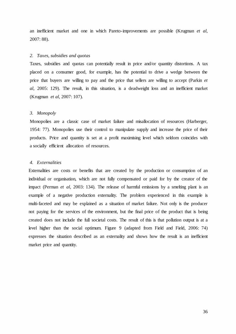
36

an inefficient market and one in which Pareto-improvements are possible (Krugman et al,

2007: 88).

2. Taxes, subsidies and quotas

Taxes, subsidies and quotas can potentially result in price and/or quantity distortions. A tax

placed on a consumer good, for example, has the potential to drive a wedge between the

price that buyers are willing to pay and the price that sellers are willing to accept (Parkin et

al, 2005: 129). The result, in this situation, is a deadweight loss and an inefficient market

(Krugman et al, 2007: 107).

3. Monopoly

Monopolies are a classic case of market failure and misallocation of resources (Harberger,

1954: 77). Monopolies use their control to manipulate supply and increase the price of their

products. Price and quantity is set at a profit maximising level which seldom coincides with

a socially efficient allocation of resources.

4. Externalities

Externalities are costs or benefits that are created by the production or consumption of an

individual or organisation, which are not fully compensated or paid for by the creator of the

impact (Perman et al, 2003: 134). The release of harmful emissions by a smelting plant is an

example of a negative production externality. The problem experienced in this example is

multi-faceted and may be explained as a situation of market failure. Not only is the producer

not paying for the services of the environment, but the final price of the product that is being

created does not include the full societal costs. The result of this is that pollution output is at a

level higher than the social optimum. Figure 9 (adapted from Field and Field, 2006: 74)

expresses the situation described as an externality and shows how the result is an inefficient

market price and quantity.

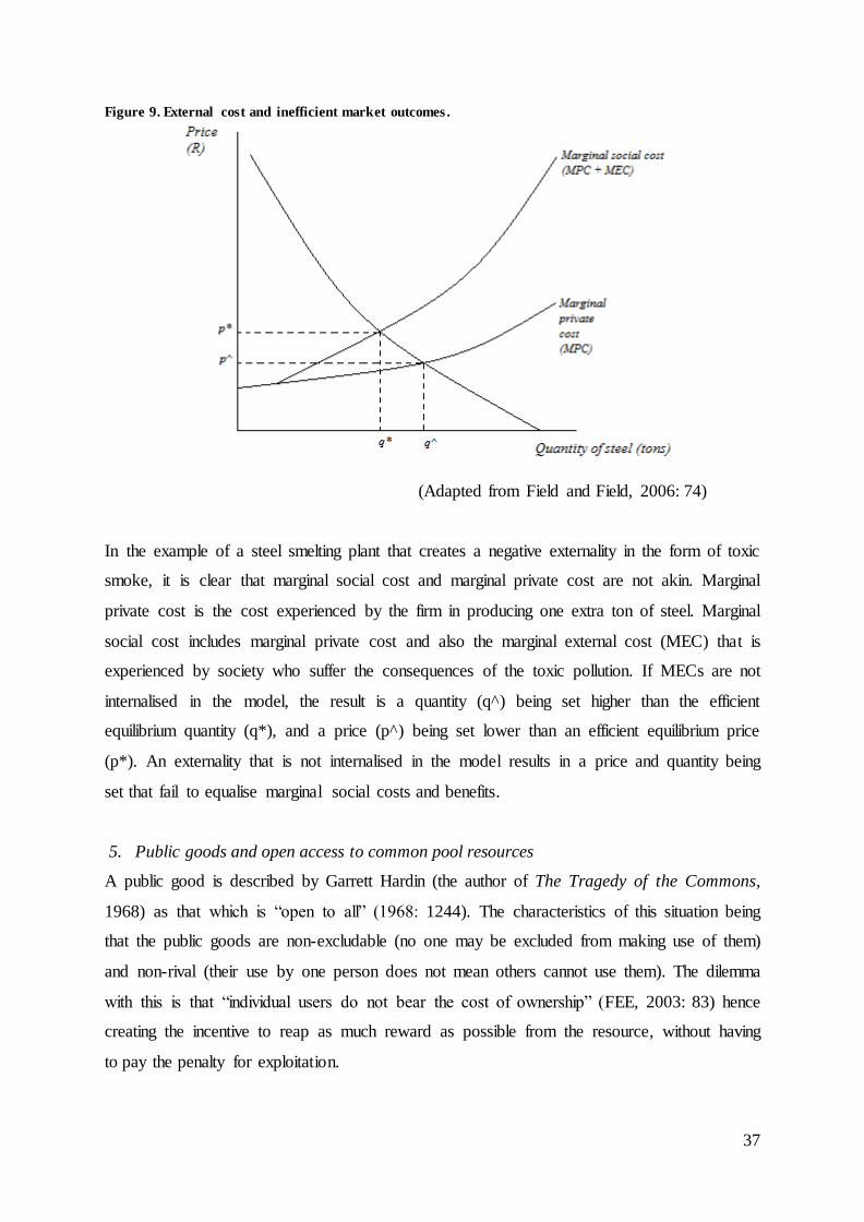
37

Figure 9. External cost and inefficient market outcomes.

(Adapted from Field and Field, 2006: 74)

In the example of a steel smelting plant that creates a negative externality in the form of toxic

smoke, it is clear that marginal social cost and marginal private cost are not akin. Marginal

private cost is the cost experienced by the firm in producing one extra ton of steel. Marginal

social cost includes marginal private cost and also the marginal external cost (MEC) that is

experienced by society who suffer the consequences of the toxic pollution. If MECs are not

internalised in the model, the result is a quantity (q^) being set higher than the efficient

equilibrium quantity (q*), and a price (p^) being set lower than an efficient equilibrium price

(p*). An externality that is not internalised in the model results in a price and quantity being

set that fail to equalise marginal social costs and benefits.

5. Public goods and open access to common pool resources

A public good is described by Garrett Hardin (the author of The Tragedy of the Commons,

1968) as that which is “open to all” (1968: 1244). The characteristics of this situation being

that the public goods are non-excludable (no one may be excluded from making use of them)

and non-rival (their use by one person does not mean others cannot use them). The dilemma

with this is that “individual users do not bear the cost of ownership” (FEE, 2003: 83) hence

creating the incentive to reap as much reward as possible from the resource, without having

to pay the penalty for exploitation.

38

In a similar vein, Ostrom (2008) uses the term ‘common pool resources’ as a description for

many environmental resources. Common pool resources are considered to be large enough to

preclude the option of excluding consumptive or non-consumptive users, but use by one

individual reduces the available resource to others (Ostrom, 2008: 24). The open-access to

common pool resources, like water, often results in over-harvesting and damage to valuable

resources (Ostrom, 2008: 24).

The open-access (public property) regime used by the Fisheries of the Southern African West

Coast (FEE, 2003) serves as a useful example for the potential market failure of open-access

to common pool resources. With no individual incentive to limit fishing to a sustainable level

and an absence of institutions to manage the ocean resources, individual’s self-interest is

guided by an incentive structure that favours harvesting as much as possible. The ‘free-for-

all’ situation results in people exceeding a sustainable catch limit as they try to catch more

fish than the next person – who will ultimately practise the same ethic.

Bromley (1991: 32) describes public goods and open-access property regimes as resulting in

people taking possession over goods, but not property rights. Using the example of air

pollution, where the polluter ‘takes possession’ of clean air, and fisheries, where the catcher

takes possession of a fish simply because he caught it first, Bromley explains that the

property right, “a social contract that defines an individual and an object of value vis-à-vis all

other individuals” (Bromley, 1991: 32), does not exist. It is also clear that the incentive to

allocate resources efficiently is non-existent where public goods prevail. Naturally, where a

small population’s survival depended on a particular resource it would be in their best interest

to preserve that resource and use it efficiently. In today’s world and in the face of scarcity,

heightened population growth, profit maximisation and self-interest; incentive creating

institutions are key to sustainable resource use. Ostrom (2008: 26) explains an institution

used in New Zealand to manage endangered fisheries as a suitable example. By supplying

individual transferable quotas to a select number of trawlers and instituting a quota

management system, market-based fishery regulation is allowed to control and manage a

sustainable catch of endangered fish.

There are a number of sources of inefficiency which result in misallocation of resources. In

the presence of inefficiency, it is clear that market prices are not representative of society’s

needs and the market allocation of resources does not coincide with an efficient societal

39

allocation of resources. When conducting CBA in the light of market distortions, it is

necessary to use shadow prices to reflect the true value of impacts that effect societal efficient

allocation of resources.

3.2.4. Shadow Pricing

Following a discussion of inefficiency in markets and resource allocation, it is clear that there

is a need for a price that reflects the true value society places on resources. Shadow prices are

defined as the ‘social opportunity cost’ of resources (Drèze and Stern, 1994: 59). Shadow

prices are used for economic calculation where existing prices are distorted by market

inefficiencies, where market prices are not considered to be reflective of true economic value

or where a price does not exist at all (Mishan, 1982: 83; Tallec and Bockel, 2005: 7). As

described in the discussion of efficiency (section 3.2.2), it is often the case that market

pricing is distorted due to externalities and other present obstacles to Pareto-optimality.

Shadow prices, also referred to as ‘efficiency prices’, are the social value in terms of net loss

(or gain) in welfare as a result of having one unit less (or more) of that resource (Drèze and

Stern, 1994: 61). Shadow prices thus reflect prices that would exist in perfectly competitive

markets where Pareto-efficient conditions are in place (Pearce et al, 2006: 31). The aim of

CBA is to assess the true societal value of a project and not simply its market value. To this

end, shadow prices are a useful tool in the CBA procedure.

Mishan (1982: 83) introduces three key situations in which shadow prices may be used:

1. In mathematical programming where the value of an objective function, at given

prices, is maximised subject to the inputs and technologically feasible factor-

combinations. A ‘dual’ problem is derived and using a minimised corresponding

objective function the ‘correct’ input prices may be interpreted as shadow or

accounting prices (Mishan and Quah, 2007: 61).

2. In the case above, market failure and inefficient resource allocation result in distorted

or inefficient pricing of resources. Shadow prices may be used in these circumstances

and in the case of absent resource pricing to reflect the true social value (price) of a

resource whose price does not exist or is not accurately measured by the markets.

3. In the case of imports and exports, usually in poorer developing countries, where the

prices of imports and exports do not accurately reflect the social value of these goods.

40

In this thesis, shadow prices will be used to assist in pricing resources that are either not

priced or whose prices are not reflective of true social costs and benefits. The shadow pricing

of labour and time is commonly used in cases of high unemployment (Pearce et al, 2006: 84)

and will be discussed further under valuation techniques (section 3.4).

3.2.5. Risk and Uncertainty

One of the controversial challenges that CBA faces is that of risk and uncertainty, and the

manner in which they should be incorporated in project appraisal. It is important to draw a

distinction between risk and uncertainty – two terms which are often and incorrectly used

interchangeably. Certainty refers to the outcome of a situation being fully known and to the

contrary, uncertainty (to varying degrees) refers to the inability to predict future occurrences.

Risk on the other hand has been defined as ‘quantifiable uncertainty’ (Irvin, 1978: 44) in

which the probability distribution of future happenings is known. While risk is naturally an

unwanted anomaly, it is a more favourable scenario than that of uncertainty, as probability

weighting may be used to establish a relationship between the potential value and the

preferences of risk averse (or loving) individuals. The key task in managing uncertainty is to

define certain and uncertain, as extremities of a continuum, and predict the most plausible

outcomes. The management of uncertainty may include quantifying it through research,

analysis of comparable scenarios, applying statistical techniques and conducting sensitivity

analysis (Irvin, 1978: 44).

Uncertainty in CBA is related to two major sources. Internal uncertainty is regarded as

doubtfulness about the potential for a project to produce the estimated level of outputs or its

ability to contain costs as predicted (Perkins, 1994: 348). External sources of uncertainty are

arguably less controllable and result from unpredictable price levels, market demand,

technology and changes in the critical characteristic of markets (Perkins, 1994: 348). The

difficulty of valuing certain impacts of a project may also present itself as an uncertainty in

the appraisal itself.

Uncertainty may apply to many CBA project appraisals and needs to be removed or

quantified to the greatest degree possible. All potential costs and benefits whose actual values

are not completely assured are open to uncertainty. There are many writings and various

opinions on how uncertainty should be dealt with. Depending on the particular resource or

situation of uncertainty, there are various economic tools available to the appraiser. It has

41

been suggested that uncertainty should be ignored in some scenarios, where random events

are the creators of uncertainty and no meaningful probabilities can be derived (Nas, 1996:

127). It would, however, be more appropriate to conduct sensitivity analysis in all cases

where uncertainty hampers the accuracy of appraisals.

Uncertainty is one of the elements that has led to the use of discount rates in projects whose

costs and benefits extend over a period of time. Time horizons of projects, uncertainty and

appropriate discount rates are a point of much debate in CBA practice and theory. Discount

rates are used to discount the value of future benefits, not only because they occur in a

different time period, but also because they do not hold the same certainty as current benefits

(Brent, 2006: 240). The choice of appropriate discount rates to be used will be discussed in

section 4.8.3, however, it is suggested that discount rates should be higher in cases of high

risk and/or uncertainty. The degree to which this should remain true is dependent on the

period at which uncertainty is higher (Staehr, 2006: 20).

Uncertainty and risk have much to do with the choice of discount rates, but also with the

accuracy with which values for costs and benefits may be derived. Sensitivity analysis is used

in response to the uncertainty of various elements in a CBA. Sensitivity analysis will be

discussed further as a stage in the CBA procedure (section 3.3.8). When uncertainty is

present, some of the elements that are subject to sensitivity analysis are:

1. The discount rate

2. Physical quantities and qualities of inputs and outputs

3. Shadow prices of impacts

4. Project life span.

(Hanley and Spash, 1993: 20)

Uncertainty is an unavoidable reality of most project appraisals. Although it is considered

unavoidable, it can and should be managed to the greatest degree possible. Sensitivity

analysis is the most widely used method of controlling levels of uncertainty and presenting

possible outcomes in the results of project appraisal. Sensitivity analysis will be discussed

further as a stage of CBA procedure (section 3.3).

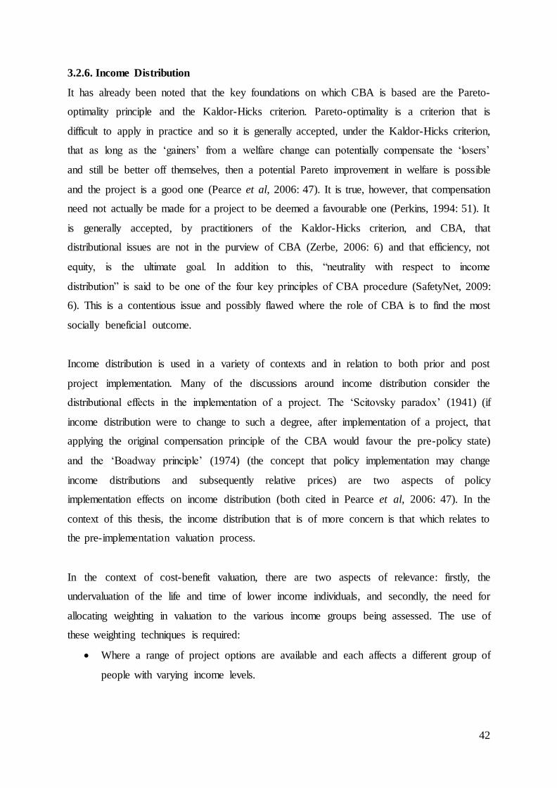
42

3.2.6. Income Distribution

It has already been noted that the key foundations on which CBA is based are the Pareto-

optimality principle and the Kaldor-Hicks criterion. Pareto-optimality is a criterion that is

difficult to apply in practice and so it is generally accepted, under the Kaldor-Hicks criterion,

that as long as the ‘gainers’ from a welfare change can potentially compensate the ‘losers’

and still be better off themselves, then a potential Pareto improvement in welfare is possible

and the project is a good one (Pearce et al, 2006: 47). It is true, however, that compensation

need not actually be made for a project to be deemed a favourable one (Perkins, 1994: 51). It

is generally accepted, by practitioners of the Kaldor-Hicks criterion, and CBA, that

distributional issues are not in the purview of CBA (Zerbe, 2006: 6) and that efficiency, not

equity, is the ultimate goal. In addition to this, “neutrality with respect to income

distribution” is said to be one of the four key principles of CBA procedure (SafetyNet, 2009:

6). This is a contentious issue and possibly flawed where the role of CBA is to find the most

socially beneficial outcome.

Income distribution is used in a variety of contexts and in relation to both prior and post

project implementation. Many of the discussions around income distribution consider the

distributional effects in the implementation of a project. The ‘Scitovsky paradox’ (1941) (if

income distribution were to change to such a degree, after implementation of a project, that

applying the original compensation principle of the CBA would favour the pre-policy state)

and the ‘Boadway principle’ (1974) (the concept that policy implementation may change

income distributions and subsequently relative prices) are two aspects of policy

implementation effects on income distribution (both cited in Pearce et al, 2006: 47). In the

context of this thesis, the income distribution that is of more concern is that which relates to

the pre-implementation valuation process.

In the context of cost-benefit valuation, there are two aspects of relevance: firstly, the

undervaluation of the life and time of lower income individuals, and secondly, the need for

allocating weighting in valuation to the various income groups being assessed. The use of

these weighting techniques is required:

Where a range of project options are available and each affects a different group of

people with varying income levels.

43

Where people of varying income ranges are subject to the impacts of a project and

hence are involved in the valuation of that particular project.

These situations are not synonymous with the CBA being conducted in Okhombe. It is,

however, useful to discuss the first and second aspects of relevance to cost-benefit valuation.

In the first scenario, the valuation of time and life give us some insight into the argument for

adjusted weighting in the valuation procedure. One common method of valuing time is to

value its opportunity cost – the value of gained or lost production (Edwards, 2008: 22). In this

case, it is clear that some individuals’ time would be valued more highly than others’ and

especially in the case of the unemployed, whose time value may be near to zero when valued

in this manner. This valuation procedure may arguably be acceptable in many circumstances,

but the valuation of life should be more objective. Human life may be valued by the value of

future production lost, resulting in a highly paid person’s life being valued more highly than

that of a lower paid individual (Edwards, 2008: 22). This is quite clearly morally and

ethically improper. In these circumstances it may be worthwhile to attach compensatory

weighting to the income of the poor (Edwards, 2008: 22).

The second scenario suggests that potential additional income to a lower earning individual

should be relatively more important than additional income being distributed to higher

earning individuals (Mullins et al, 2007: 45). The example of a project involving the building

of one dam in only one of two sites is used by Leiman and Tuomi (2004: 10). In this

example, there is sufficient capital to build only one dam, either on a site which will benefit a

rich and productive farming community, or on a site that will benefit a poor community.

From one point of view, it is suggested that the weighting of value should be in favour of the

poor. The other point of view favours the productive farmers, and using the Kaldor-Hicks

criterion as its defence, insists that efficiency and not distributional equity should be the

concern of CBA appraisers, and that redistributive instruments of the state should be used to

correct social disparities (Leiman and Tuomi, 2004: 10).

There are many methods of weighting and discounting that can be used to correct income

distribution distortions in the valuation of projects. Mullins et al (2007) suggest a simple

income weighting formula that is of worthwhile interest and argued as the “best known form

of weighting” (2007: 47). This simple income weighting formula has two parameters; a

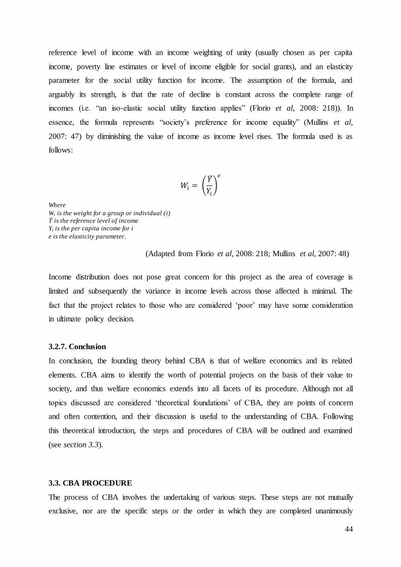
44

reference level of income with an income weighting of unity (usually chosen as per capita

income, poverty line estimates or level of income eligible for social grants), and an elasticity

parameter for the social utility function for income. The assumption of the formula, and

arguably its strength, is that the rate of decline is constant across the complete range of

incomes (i.e. “an iso-elastic social utility function applies” (Florio et al, 2008: 218)). In

essence, the formula represents “society’s preference for income equality” (Mullins et al,

2007: 47) by diminishing the value of income as income level rises. The formula used is as

follows:

( ̅

)

Where

Wi is the weight for a group or individual (i)

Ῡ is the reference level of income

Yi is the per capita income for i

e is the elasticity parameter.

(Adapted from Florio et al, 2008: 218; Mullins et al, 2007: 48)

Income distribution does not pose great concern for this project as the area of coverage is

limited and subsequently the variance in income levels across those affected is minimal. The

fact that the project relates to those who are considered ‘poor’ may have some consideration

in ultimate policy decision.

3.2.7. Conclusion

In conclusion, the founding theory behind CBA is that of welfare economics and its related

elements. CBA aims to identify the worth of potential projects on the basis of their value to

society, and thus welfare economics extends into all facets of its procedure. Although not all

topics discussed are considered ‘theoretical foundations’ of CBA, they are points of concern

and often contention, and their discussion is useful to the understanding of CBA. Following

this theoretical introduction, the steps and procedures of CBA will be outlined and examined

(see section 3.3).

3.3. CBA PROCEDURE

The process of CBA involves the undertaking of various steps. These steps are not mutually

exclusive, nor are the specific steps or the order in which they are completed unanimously

45

agreed upon. Various authors propose different degrees of importance in each step of the

procedure, as well as combining various stages. This literature review will break the CBA

procedure into an eight stage process under the headings of:

1. Identify and define the project

2. Identify economically relevant impacts

3. Identify requirements of the CBA

4. Physical quantification of impacts

5. Monetary valuation of costs and benefits

6. Discount the flow of costs and benefits

7. Apply a decision rule

8. Sensitivity analysis.

3.3.1. Identify and Define the Project

The first of the stages involved in the CBA procedure is that of identifying and defining the

potential projects to the greatest degree of accuracy possible. Included in this stage are two

major objectives; i) defining the project and potential reallocation of resources, ii) defining

the population which will experience the impacts of the proposed project (Hanley and Spash,

1993: 8).

i) Defining the project to be appraised may sound like a basic necessity, but it is a very

important one and one that requires detailed investigation. CBA may be conducted ex ante, to

determine if a potential project is a worthwhile one; or ex post, to examine an already

completed project and assess if it was worthy of instigation (Pearce et al, 2006: 52). It also

needs to be established whether there are a variety of options available to a decision maker or

if it is just one potential project that is being appraised. In the case of this thesis, there is just

one option being assessed – whether or not the use of biodigesters and related elements

would be financially and economically feasible for rural households in the Okhombe

community. In other cases it may be necessary to present the findings of a variety of projects,

allowing the decision maker to choose the most beneficial one (presumably the project with

the highest net present value (NPV)).

This stage of the process is also a critical one as it is necessary to set the boundaries of the

proposed project and related appraisal (Hanley and Spash, 1993: 8). The quality and accuracy

of a CBA may be compromised where the appraisers include potentially inadmissible

46

evidence and extend the analysis beyond what is necessary. The Treasury Board of Canada

(1998: 10) suggests that the definitional stage should include the definition of the appraisal’s

constraints, objectives and targets. In addition to these requirements, it is suggested that a

‘reference scenario’ (a ‘do-nothing’ alternative or description of the current state of affairs)

be described for decision makers to understand potential changes (SafetyNet, 2009: 4). This

is likely to be of use in the project of this thesis and comparable projects as it is often useful

to describe the reference scenario for living standard improvement proposals to potentially

uninformed decision makers.

ii) The ‘point of view’ (Treasury Board of Canada, 1998), ‘relevant population affected’

(Hanley and Spash, 1993) and the ‘issue of standing’ (Pearce et al, 2006) are all terms used to

express the need for defining who is going to be affected by the proposed project and whose

costs and benefits are of relevance. This question can sometimes be prescribed by law, but in

most cases there is some degree of discretion permitted (Hanley and Spash, 1993). Pearce et

al (2006: 55) consider the general rule in assessing the standing of a project, to consider all

nationals, but not non-nationals, unless the project relates to an international context or an

accepted ethical reason binds the appraiser to including non-nationals.

This is an important stage in CBA as it defines who is of ultimate importance to the project

and in some cases may have an effect on distributional concerns. Stringent environmental

policies and growing environmental concern have led to the importance of national and supra

national effects being recognised in project appraisal (Hanley and Spash, 1993: 8), but it is

still important to address the welfare of those closely affected by a project. In the current

study it is clear that the interests of rural people who may be able to use biodigesters are of

utmost concern, but it is also relevant to consider the point of view of the government –

which may be involved in the financing of such projects. The Treasury Board of Canada

(1998: 9) asserts that CBA is not restricted to a single point of view and it should be noted

that the standings are not mutually exclusive.

It is argued by some authors that the definition and identification stage of the project should

include a finalisation of parameters (including discount rates, growth rates and inflation rates)

and discussion of the optimal scale of a project. For the purposes of this thesis, and in

agreement with those authors who do not complicate this level of the study with such

47

inclusions, considerations outside what has been mentioned will find their place in the

relevant stages to follow.

3.3.2. Identify Economically Relevant Impacts

Identifying the relevant impacts of the project is the next major step in the CBA process and

is a very important precursory step to the quantification and valuation of impacts. Pearce et al

(2006: 55) express the importance of CBA’s strong presumption that individuals’ preferences

are of relevance and not the preferences of experts and politicians when identifying relevant

impacts.

In this stage of the process it is vital to consider all potential levels of impact. In many cases

‘impact pathways’ are likely to be very complex (Pearce et al, 2006: 56), and especially so in

the case of environmental impacts. Considering the CBA being conducted in this thesis, it

would be important to recognise all levels of impact. As an example, it may be true that the

use of efficient biogas in place of traditional cooking methods could result in reduced carbon

dioxide emissions. This is a difficult benefit to quantify, let alone value, but it is important to

recognise it and state its being in this stage of the process.

Hanley and Spash (1993: 9) recognise two important concepts in the identification process,

additionality and displacement. Additionality denotes that net impacts of a project should be

measured. It is important to only consider net impacts in the case of project changes

coinciding with other changes which could have similar impacts (for example, the reduction

in indoor air pollution (IAP) as a result of ventilating homes and not using biogas for

cooking). Displacement is an important concept to consider where the introduction of a

policy or project could have displacement effects on other areas of the economy. For

example, it is plausible that the development of a new factory (with beneficial impacts) could

have detrimental effects on another factory – resulting in the benefits being crowded out by

the costs (Hanley and Spash, 1993: 9).

3.3.3. Identify Requirements of the CBA

There are two main objectives in identifying the requirements of the CBA: first, to identify

what type of CBA (economic and/or financial) will be relevant to the project (Leiman and

Tuomi, 2004: 5); and second, the time horizon over which the appraisal will apply.

48

Understanding what type of CBA should be used is a simple task which can be done by

assessing some of the impacts of the project. In the unlikely event that it is possible to use

current market prices for the entire appraisal of costs and benefits, without having to correct

for any distortions, then a financial CBA would be appropriate. An economic, social or

extended CBA would be necessary in any situation of price distortion, missing prices and

social and environmental impact assessment (Leiman and Tuomi, 2004: 5).

The time horizon of a project is the period over which costs and benefits will be assessed.

Selecting a time horizon is dependent on a number of factors and is a decision over which

there is much debate. The general rule for investment projects is to set the time horizon to the

life expectancy of the investment (Pearce et al, 2006: 56). CBA is often used for assessing the

value of projects and policies relating to environmental assets and in this case it is clear that

the ‘goal’ would be a long term one, often beyond 100 years. Other arguments suggest that

the time horizon should be based on the degree of uncertainty relating to future benefits

(costs) or the level to which discounting makes future benefits and costs irrelevant (Pearce et

al, 2006: 57). There may even be practical motivation for the setting of a time horizon, for

example, where the period of cost benefit assimilation is based on a period of years that the

decision makers and people involved in the project will relate to. The inclusion of costs and

benefits beyond 15 years is said to be excessive for the installation of a biodigester as the

home users are unable to relate to what benefits (or costs) they might receive beyond that

point (Prof. James Blignaut, pers. com. May 2010). Cesarone (1999) furthers this concept

saying that appraisers may warrant the setting of a time horizon that is shorter than necessary

where the objective may be to prove that a project can be profitable over a relatively short

period of time.

3.3.4. Physical Quantification of Impacts

The physical quantification of impacts is the process of enumerating the flows of costs and

benefits involved in a project. A key element in this process is the identification of when

and/or over what period of time these impacts will occur (Hanley and Spash, 1993: 11). In the

case of environmental impacts, it is often necessary to use or conduct environmental impact

assessments (EIA). In the circumstance that impacts cannot be assessed directly, it is useful to

use proxies or relevant tools and techniques in their estimation (Mullins et al, 2007: 62).

Mullins (2007: 62) also proposes that impacts that cannot be quantified should be recorded in

qualitative terms and ranked in order of importance.

49

Hanley and Spash (1993: 11) note that all calculations at this point in the CBA are made

under varying degrees of uncertainty. Where levels of probability are known for an impact

stream, it is possible to internalise the uncertainty in these calculations by factoring the

probabilities into the equation. In the case of probabilities being known, an expected value

can be equated for impacts that are subject to uncertainty (Hanley and Spash, 1993: 11).

3.3.5. Monetary Valuation

Effective and accurate monetary valuation forms an important and significant part of the

CBA procedure. Due to the scale, complexities and importance of this topic, it will be

discussed in detail under section 3.4. Monetary valuation is the fifth stage of the CBA process

and refers to the quantification of impacts into a common unit of value, money. Some of the

complexities of the process involve having to predict value flows which extend into the

future, correct for distortions in market pricing and estimate the value of impacts where no

price exists (Hanley and Spash, 1993: 11).

3.3.6. Discount the Flow of Costs and Benefits

Immediate costs and benefits are not valued synonymously with costs and benefits which

occur at a later time period or over a period of time. It is generally accepted that present

income (or money) is valued higher than income that will be received at some point in the

future. Thus, the discount rate effectively acts in a manner opposite to an interest rate –

devaluing income (or cost flows) that will be received in the future, so that it may be directly

compared to immediate costs and benefits. The motivation behind discounting is the time

preference of money. People prefer money today to money received at some point in the

future, and similarly they prefer costs experienced in the future to those incurred

immediately. It is commonplace for costs and benefits to occur at different time periods and it

is therefore necessary to discount these values so that systematic comparison of costs and

benefits may be done by calculating their net present value (i.e. the present value of all

discounted future benefits minus all discounted future costs) (Jenkins and Kuo, 2007: 41).

3.3.6.1. Financial discount rate versus social discount rate

A distinction must be made between the financial discount rate and the social discount rate.

The financial discount rate is considered to be the opportunity cost of capital (Florio et al,

2008: 207). The use of capital in one project precludes its use in any other project and we

50

value this opportunity cost as the potential return forgone. Florio et al (2008: 207) present

three main approaches to identifying a financial discount rate.

1. To estimate the actual weighted average cost of capital (WACC). In this approach,

real return on government bonds and long term real interest rate of commercial loans,

the cost of public (government) and private funding respectively, are considered in

isolation or by the weighted average of their rates.

2. To consider a “maximum limit value for the discount rate” (Florio et al, 2008: 207) by

recognising the potential of an appropriate financial portfolio to give return on the

same investment.

3. Finally to consider a cut-off rate as a parameter in the planning process. This rate may

be pragmatically identified by consulting a well-established issuer or securities rate of

return and applying a multiplier to the minimum benchmark (Florio et al, 2008: 207).

In contrast, the social discount rate is based on a social view (rather than financial view) of

how present benefits and costs are valued against those which will be experienced at some

point in the future. The social discount rate puts society’s time preferences first and is thus

usefully utilised in the economic appraisal of projects. Mullins et al (2007: 40) discuss three

distinct points of departure in identifying a social discount rate.

1. The discount rate should represent the marginal return on capital, which is the

opportunity cost of capital (Mullins et al, 2007: 40). The rationale behind this

argument is that public investment has the potential to displace private investment

(Florio et al, 2008: 208).

2. The long-term real interest rate should be used to derive a social discount rate as it

represents the cost of state funding.

3. The social time preference rate (STPR) should be used as the social discount rate.

Florio et al (2008: 208) suggest a fourth (third in their case) approach, as the use of varying

rates in appraisal of projects whose costs and benefits may occur over a long-term period.

The argument for this method is furthered where costs may be experienced immediately but

benefits occur repeatedly and into the distant future, or vice versa. It is also argued that future

generations should not be discriminated against by excessive discounting of the value of

future costs and benefits.

51

It is assumed that a social discount rate would be of greater value for the purposes of this

study, namely due to its nature as an economic assessment and not a purely financial one.

Although financial analysis will be conducted, it seems appropriate to use the same discount

rate (social discount rate) throughout the course of the study and especially in consideration

of the economic methods by which many ‘financial’ values may be determined. The effects

of various discount rates will be assessed in the sensitivity analysis.

3.3.7. Decision Rules

The ultimate objective of CBA is to assess the social benefit (or cost) of a proposed or

existing change. CBA provides significant information on which a decision maker might

formulate policy and it is the responsibility of the appraiser to provide suitable means on

which decisions can be made. Decision rules are designed to reveal the net effect of a project

on society and determine whether a project should be accepted or rejected (Pearce et al, 2006:

68). As has been discussed in the prior steps and theoretical foundations of CBA, CBA is

designed from the outset to assess the social gain or loss of any situational change. The

careful and accurate implementation of each step, especially the identification and valuation

of economic benefits and costs, is vital to provide accurate data for the application of decision

rules. The efficacy of a decision rule is directly reliant on the accuracy of the data provided

for its application.

There are a number of decision rules available for the appraiser and decision maker to assist

in making the decision of whether to accept or reject a project. The decision rules which will

be discussed and are of most relevance to this project are: net present value (NPV), internal

rate of return (IRR) and benefit-cost ratio (BCR).

3.3.7.1. Net present value (NPV)

The net present value of an investment is the present value of all future value from net

benefits (benefits minus costs) (Parkin et al, 2005: 378). An investment (such as a rural

household biodigester) is associated with costs and benefits which occur at differing time

periods. The costs of a biodigester including installation and cost of materials are likely to be

incurred immediately. The benefits are expected to assimilate over a period of time extending

into years beyond the installation date. As discussed under section 3.3.6, benefits and costs

that are experienced at later time periods are not valued as highly as those which are

experienced immediately (Jenkins and Kuo, 2007: 41). For this reason, it is important to

52

choose an appropriate discount rate for the discounting of benefits/costs which will occur at

differing time periods.

Discounting benefits and costs which occur at later time periods allows for all impacts to be

measured in the same ‘units’ and consequently an absolute magnitude of present value can be

identified (Pearce et al, 2006: 68). Essentially, the NPV procedure allows the appraiser to

calculate the present value of a rural household biodigester (or any other investment) which

includes all of its future costs and benefits, discounting them from the period of time at which

they occur.

In calculating the NPV of a project or regulation, the present value (discounted value) of

costs is subtracted from the present value of benefits (OBPR, 2009: 2). Mathematically, the

equation is represented as:

∑( )

( )

Where

NPV is the net present value of a project or regulation

Bt is the benefit in year t

Ct is the cost in year t

r is the discount rate

t is the year at which benefits and costs occur

n is the number of years over which the benefits and costs will accrue starting at year t = 1.

The general decision criterion when using the NPV assessment is to accept a project whose

NPV is greater than zero (NPV > 0), and when deciding between various alternatives, to

accept the project with the highest NPV (OBPR, 2009: 2; Florio et al, 2008: 211).

Although the NPV rule is the most favoured decision criterion by most authors, it is not

without fault. Pearce et al (2006: 69) use an example of ranking independent projects to

reveal one of these short-comings. Considering the available projects X, Y and Z with cost of

100, 50 and 50; net benefit of 100, 60 and 70 respectively – if the expenditure budget were

limited to 100 and the NPV rule were used for project selection, project X with a cost of 100

and NPV of 100 would be chosen. The mistake in this selection is the use of the NPV rule

without consideration of expenditure budget. If the budget could be exhausted by

implementing project Y and Z of cost 50 each, then the combined NPV would be 130. In this

53

situation the budget should be considered in conjunction with the NPV rule, or the benefit-

cost ratio rule could be used to select projects with the highest benefit-cost ratio until the

budget is exhausted (Pearce et al, 2006: 69).

3.3.7.2. Internal rate of return (IRR)

The internal rate of return (IRR) of a project is the rate of discount at which net present value

over the specified time period is equal to zero (Jenkins and Kuo, 2007: 31; European

Commission, 2006: 13). Mathematically the calculation of IRR is similar to that of NPV

calculation.

∑( ) ( )

Where



(B– C)t is cash flow (or net flow of benefits) for year t

IRR is the discount rate at which NPV = 0

n is the number of years over which the benefits and costs will accrue starting at year t = 1 .

Florio et al (2008: 212) note that IRR is indicative of relative efficiency in a project and

accordingly, should be used with circumspection. In situations where net benefits vacillate

from being positive to negative from year to year, a ‘multiple IRR’ occurs and it is not

possible to use the IRR as a decision rule. This situation is not likely to be experienced in this

study.

The acceptance criterion when using the IRR decision rule is to accept the project where the

IRR is greater than the applicable discount rate (IRR > r) (Hosking and du Preez, 2004: 144).

Naturally it is possible to separate the IRR into a financial internal rate of return (FIRR) and

an economic internal rate of return (EIRR), with the former including only financial costs and

benefits and the latter assessing all economic impacts of a project. The IRR criteria serves a

valuable purpose in many decision making scenarios and especially financial decisions where

it is possible to gauge the return on investment (represented by IRR) in relation to the cost of

capital (the interest rate of borrowing). The IRR decision rule is, however, not highly

favoured in CBA as it faces the following shortfalls:

54

Since IRR is a function of time and capital outlay, it tends to overstate the value of a

project with a short life span and does not give useful guidance to social welfare

(Florio et al, 2008: 213).

IRR cannot be used in cases of time-varying discount rates or where net benefits

fluctuate between being negative and positive from year to year, as described above

(Florio et al, 2008: 213).

IRR is unsystematically sensitive to the length of a project’s life and cash flows being

discounted, and it provides unreliable results related to the scale of activity (Jenkins

and Kuo, 2007: 31). IRR tends to understate the value of a project whose benefits are

experienced at later periods in the project’s life cycle (Jenkins and Kuo, 2007: 32).

Although IRR is generally considered to be unreliable for decision making (Jenkins and Kuo,

2007: 32; OBPR, 2009: 2; Perman et al, 2003: 367) it is commonly used for assessing

investments and does serve some purpose in CBA if used in conjunction with appropriate

decision rules.

3.3.7.3. Benefit-cost ratio (BCR)

Benefit-cost ratio (BCR) is one of the most widely used decision rules in CBA (Pearce et al,

2006: 70). The BCR of a project is expressed as the discounted value of benefits (present

value) divided by the discounted value of estimated costs. Mathematically the BCR equation

is represented as follows:

∑( )

( )

∑( )

( )

⁄

Where

BCR is the benefit-cost ratio of a project or regulation


Bt is the benefit in period t

Ct is the cost in period t


n is the number of years over which the benefits and costs will accrue starting at year t = 1.

The general criteria to be applied to the BCR decision rule are that:

A project should be accepted where BCR > 1.

When faced with various project options, projects should be ranked in order of highest

to lowest BCR.

55

In the case of mutually exclusive projects, the project with the highest BCR should be

selected.

Although commonly used, the BCR decision rule is not favoured by many authors as it is

subject to many complications and flaws. Pearce et al (2006: 70) note a fundamental problem

in that no decision rule should be sensitive to the classification of impacts as cost or benefits,

negative benefits or negative costs. Using a simple example with benefits 10, 20 and 30 and

costs 10 and 20, Pearce et al (2006: 70) reveal this inequity – the BCR ratio is 2.0 and the

NPV is 30 units; if the cost of 10 were to be considered as a negative benefit – as may be the

case in some situations and especially in those of environmental changes – then the BCR will

change to 2.5 and the NPV will correctly remain the same at 30 units. Jenkins and Kuo

(2007: 31) also note that the BCR decision rule is flawed in that it favours projects with lower

expenditure that have more productivity per unit of money spent, but may not have as much

overall benefit surplus as larger expenditure projects whose productivity per unit of money is

lower.

3.3.7.4. Conclusion

The use of decision rules in isolation without consideration of expenditure budgets and cross

examination is subject to some level of difficulty and inaccuracy. Depending on the specific

situation and needs for analysis of a single project, various budget spend options on different

projects or mutually exclusive projects, each decision rule serves some level of purpose. In

summary, a project is deemed worthy of acceptance where its NPV is greater than zero, or the

IRR is greater than an applicable discount rate, or the BCR is greater than one (Hosking and

du Preez, 2004: 144). In terms of the current research, it seems appropriate to calculate all of

these indicators to assess the feasibility of the project. It is also likely that a pragmatic

approach might be necessary for households to make decisions of their own. If the project life

span is assumed to be 15 years, then the amount payable per month over this (or another)

period for the initial capital cost would be a useful and a practical indicator for such rural

households. This amount payable may be presented in relation to fuel and fertiliser

expenditure saving per month (financial benefits). Similarly, Habermehl (2007: 13) proposes

the assessment of annual avoided fuel costs in relation to mean annual income for rural

people using an improved stove for cooking.

56

3.3.8. Sensitivity Analysis

The distinction between risk and uncertainty is that risk is a situation in which the probability

distribution of future outcomes is known, whereas the probability distribution of uncertain

events is unknown. Uncertainty is a problem associated with CBA, but it may be managed to

some degree by sensitivity analysis (Hosking and du Preez, 2004: 150). This process entails

varying parameter values (variables), both independently and in combination, and assessing

the impact on a project’s net present value (or other feasibility indicators) (Perkins, 1994:

359). A project whose NPV were to become negative with minimal adjustments on key

parameters would be a marginal project, while one whose NPV remains constant with large

alterations on key parameters would be a robust project (Perkins, 1994: 360).

3.3.8.1. Selecting Critical Variables

The immediate purpose of sensitivity analysis is to identify the ‘critical variables’ which are

defined as variables whose positive or negative variation has the most significant impact on

the performance of a project (Florio et al, 2008: 60). Florio et al (2008: 60) consider the

general rule for identifying critical variables to be the consideration of variables whose

variation of 1% (absolute value) around the base value is estimated to result in a variation of

NPV by 1% or higher. This would essentially display an impact elasticity of unity or greater

than unity.

Florio et al (2008: 61) consider the following steps in the procedure of conducting a

sensitivity analysis to identify critical variables:

1. Identification of variables – Identify all variables involved in the CBA. This involves

listing all input and output variables which contribute to the cost estimation and

impact analysis of the project in question.

2. Elimination of deterministically dependent variables – This process involves the

removal of redundant variables and the inclusion of those which appear to be of most

significance. Deterministically dependent variables include those which are internally

dependent on each other and those which result in double-counting. The aim should

be to have independent variables or variables that are disaggregated from each other.

Florio et al (2008: 61) use revenue being disaggregated into quantity and price as an

example.

3. Elasticity analysis – Qualitative analysis is suggested as the first step in identifying

variables whose elasticity is likely to be marginal. This process can be conducted by

57

using the appraiser’s knowledge and expert advice to rank variables in order of high,

intermediate and low potential elasticity on NPV (Florio et al, 2008: 62) or rank the

confidence estimates of variables from 1-10 (Cooper, 2001: 112). The variables with

low confidence estimates or alternatively with high/intermediate potential impact

elasticity on NPV should be subjected to further quantitative analysis. Quantitative

analysis involves taking the significant variables independently, assigning higher and

lower values to them, recalculating NPV and noting the absolute and percentage

differences to the base case scenario (Florio et al, 2008: 61). Florio et al (2008: 61)

note that elasticities are not likely to always be linear functions and it may be prudent

to repeat calculations with arbitrary deviations.

4. Choose critical variables – Having completed the calculations of impact elasticity, the

general rule in choosing critical variables, as mentioned previously, would be to

consider variables with impact elasticities on NPV of unity or higher. It is noted that

there should be very few variables in most cases, unless variables are considered to be

critical at very low performance (impact) elasticity (Florio et al, 2008: 61).

3.3.8.2. Scenario Analysis

Scenario analysis, or simply the variation of a combination of key variables, may also be used

to assess the robustness of a project in the context of uncertain conditions. Also referred to as

worst/best case analysis, pessimistic and optimistic values in the plausible range are assigned

to each of the key variables and new NPVs are calculated for each of the scenarios. Naturally,

there would be cause for concern if the worst/pessimistic case scenario were to reveal a

negative NPV in relation to a positive one found under the base case scenario. Worst/best

case analysis has been proposed as a preliminary step before furthering the sensitivity

analysis to understand significant NPV changes from worst/base/best case scenarios

(Australian Government, 2007: 122).

3.3.8.3. Switching Value

An approach to sensitivity analysis known as ‘switching value’ is also used to assess the

sensitivity of key variables. The switching value approach calculates the level at which a

critical variable will just change a project’s NPV to zero (Perkins, 1994: 360). The analyst is

then responsible for considering whether the value of the critical variable is likely to ever

occur and what conditions would result in this occurrence (Perkins, 1994: 360; Florio et al,

2008: 62).

58

3.3.8.4. Probability distributions and Monte Carlo simulation

Florio et al (2008: 63), supported by Jenkins and Kuo (2007: 26), note that sensitivity and

scenario analysis are greatly limited by not assigning probability distribution to various

outcomes. It is noted that the arbitrary variation of critical parameters is in no way related to

the probability of those variables actually varying and it is proposed that probability

distributions for each variable be identified (Florio et al, 2008: 63). Once probability

distributions for individual key parameters have been identified through consultation of

expert literature and experimental data, Monte Carlo simulations are proposed as a suitable

means of developing probability distributions and conducting risk analysis for NPV and IRR

(Florio et al, 2008: 63).

Monte Carlo simulations can be done by computer analysis software which simulates the re-

calculation of CBA data repeatedly, using randomly selected value sets for each key

parameter. By simulating all plausible combinations of parameter values and the response of

the performance indices (NPV, IRR) for each combination, the software is able to produce a

probability distribution of NPV and IRR (Mullins et al, 2007: 45; Florio et al, 2008: 63). It is

noted that a significant sample size, “generally no more than a few hundred” (Florio et al,

2008: 63), is required for this process.

3.3.8.5. Conclusion

Uncertainty is an unavoidable challenge of most project appraisals. Sensitivity analysis is a

means of managing uncertainty and is a vital stage in the CBA process as it allows the

appraiser to present descriptive and comprehensive results to decision makers. Essentially,

sensitivity analysis allows the appraiser to cover all bases with regard to the potential

uncertainties in a project’s future.

3.3.9. Conclusion

Eight steps involved in the CBA procedure have been discussed. It should be noted again that

these steps are not mutually exclusive and that there is no conclusive agreement on their

order of application other than that which is logical. Each of the stages in the CBA process is

important in producing an accurate end result and it is clear that inaccuracies at any point will

tarnish the integrity of the final product. Monetary valuation is arguably the most technical

59

aspect of this process and a stage which requires great accuracy. Monetary valuation

methodology is thus continued in the discussion to follow.

3.4. MONETARY VALUATION METHODOLOGY

Monetary valuation forms step number five of the CBA procedure and is a fundamental part

of the process. Effective and accurate valuation of costs and benefits is integral to the

accuracy of the appraisal process and errors or imprecision at this stage can affect the

integrity of the final outcome. In this section, the importance of monetary valuation as well as

the methodology for valuing various costs and benefits will be discussed.

3.4.1. The Importance of Monetary Valuation

In this section, a range of potential impacts and the methodology for valuing them is to be

discussed. A large part of this discussion will centre on environmental resources, human

health and life and the value of time. These costs and benefits do not have specifically agreed

upon or standard values attached to them and in most cases tend to be intangible elements.

The fact that they hold no tangible or standard value is, however, no indication of their

importance to humanity and the following reasons are most commonly argued for the

importance of assigning monetary value to them:

The absence of a unilateral understanding for the value of un-priced benefits reveals

the need for a single unitary measure that is understood by all. Although money is

considered by some to be an ‘imperfect measure’ of value (Menger, 2005: 245), it is

one that is unilaterally understood and serves a purpose as a common yardstick

(Pearce and Özdemiroglu, 2002: 10).

‘Decision makers’ tend to understand and respond to values expressed in monetary

terms. Pearce et al (1989) state that, “voters, politicians and civil servants are readily

used to the meaning of gains and losses that are expressed in pounds or dollars”

(1989: 56). Monetary value provides a foundation for making rational choices

between available options (Tietenberg and Lewis, 2010: 31).

In terms of market failure, which is described as a situation where the price

mechanism of a market breaks down, the absence of accurate monetary values for

impacts on the environment, human health, human life and time can result in markets

representing incorrect pricing for goods and services. In a situation where impacts are

60

not fully represented in market pricing, the market actions of demand and supply are

not likely to be in accordance with society’s needs – resulting in market failure.

The importance of life, health, the environment and biodiversity is testament to the

need for its valuation and inclusion in economic appraisals. While some argue that the

process of valuing these ‘priceless’ impacts is inherently flawed (Heinzerling and

Ackerman, 2002: 1), it is generally accepted that despite the difficulties, it is

necessary to at least attempt valuing all impacts in the need for a comprehensive

economic appraisal.

The accuracy of a CBA is fundamentally dependant on the accuracy of the monetary

values to which it relates. An economic CBA requires that all elements of impact be

included and to this end it is vital that all impacts (economic and financial) be valued

and included.

3.4.2. Environmental Valuation Methodology

Environmental valuation is an attempt to identify monetary values for environmental

resources. The difficulty with valuing environmental goods and services is that they are often

not sold in markets or even related to market goods and services. The need for the valuation

of environmental resources is becoming more prevalent as human activity infringes on

natural resources. Although considerable debate exists between those who perceive

environmental valuation to be moral or immoral, possible or impossible, it is generally

motivated by economists that it is a necessity to include environmental impacts in

comprehensive project appraisals and environmental valuation is thus required (Perman et al,

2003: 399). There are a variety of techniques available for the satisfactory valuation of

environmental resources. Total economic value (TEV) will serve as the point of departure for

discussing these.

3.4.2.1. Total economic value (TEV)

Economics provides that, “choices have to be made in the context of scarce resources”

(Pearce et al, 1989: 54) and such choices must be made on the grounds of preference, be it

personal or within a greater social context. The valuation of the environment is based on

human preference, for or against something. As has been discussed, preference is measured in

either the willingness to pay (WTP) for the preservation of the environment or alternately the

compensation expected (willingness to accept - WTA) for its degradation or loss (Pearce et

61

al, 1989: 54). The task of the economist is to take the qualities that are instilled within the

environment, or a particular aspect of the environment, and assign as accurately as possible a

monetary figure that may represent that ‘worth’. The worth and value within the environment

is multi-faceted, and the grounds on which people’s preferences may be based is explained

more fully in the discussion of total economic value (TEV).

The intricacies of environmental valuation are clearly revealed in the discussion of TEV. The

value of the environment is comprised of two distinct values: use values refer to those

benefits that are gained from the environment through tangible and actual use of its services,

and non-use values, are considered to be the value of the environment’s existence

independent of any actual or potential use by any individual (Perman et al, 2003: 402).

Figure 10 (adapted from FEE, 2002) serves a lucid purpose in furthering the discussion and

explanation of the various aspects of value inherent in the TEV model.

Figure 10. Diagram of Total Economic Value.

(Adapted from FEE, 2002: 391)

62

As Figure 10 displays, use and non-use values are further disseminated into various

categories. Pearce and Özdemiroglu (2002: 24) separate the actual use values into two

categories, direct and indirect use. Direct use values are those benefits man is actually able to

reap from the environment itself, in a tangible form. Firewood from an indigenous forest or

pastures that are grazed by cattle are examples of direct use values and can aid in assigning a

monetary worth to the environment. In addition to this, use may also be non-consumptive and

may include recreational activities. Indirect use values are usually more difficult to monetize

or even to identify in some cases. The services of an ecosystem are examples of indirect use

value. Although we are often unaware of the services that our environment provides us, it is

possible that we would suffer great loss without these. A forest that acts as a watershed or

barrier in the aid of flood control is an example of an indirect use value. The sequestration of

carbon dioxide by the same forest could also be considered as a provision of an ecosystem

service and indirect use value (Pearce and Özdemiroglu, 2002: 23).

While option values are included by FEE (2002) and Pearce and Özdemiroglu (2002) in their

models of TEV as use values, there is some debate about whether they should rather be

viewed as a division of non-use value. In consideration of use values, option values refer to

the opportunity of having the direct and indirect use values that are yet to be realised. The

option denotes that although a particular ecosystem service may not have been utilized, its

potential for future use still exists. The option value subset assures that an economist does not

neglect particular values that are available, but are yet to be used to their full potential. Pearce

et al (1989) further the definition of option value by stating that it is a combination of “value

in use (by the individual) + value in use by future individuals (descendants and future

generations) + value in use by others (vicarious value to the individual)” (1989: 62). It

follows that these values are even more difficult to assign a specific monetary value to.

The non-use values that form the next category of total economic value are even more

challenging to assign monetary value to. Figure 10 shows bequest and existence values as

being part of the non-use value segment of total economic value. Binning et al (1995) explain

non-use values further; classifying them into five types.

1. Existence value is described by Pearce et al (1989: 61) as “fuzzy values” in that

they are particularly difficult to define. They are based on the acceptance that value

is gained simply by the knowledge that an environmental resource exists (Binning

et al, 1995). As Pearce et al (1989) describe, the existence of a whale may provide

63

great value to people, not due to a direct use of it and given that they may never

personally see it, but simply because there is an option of seeing one and that it is in

existence.

2. Vicarious value is the indirect value of an environmental resource, obtained through

the experiences of other people, books, videos and other media.

3. Option value, as described previously is the potential future opportunity of making

use of an environmental resource, even where it is not being used at present.

4. Quasi-option value is the value gained by the delay in a decision to irreversibly

damage an environmental resource and allowing for the development of better

information. The resource may prove to be of greater use as new technologies or

knowledge augment its value.

5. Bequest value is the value of the preserved natural environment for the use of future

generations.

(Binning et al, 1995)

The accurate assignment of monetary worth to the natural environment is a difficult task.

Non-use values are important and are integral to the environmental valuation process. Figure

10 shows that as one moves to the right hand side of the TEV diagram, tangibility decreases

and it becomes more difficult to value goods and services of the environment. It is difficult to

develop a process of valuation that includes each one of these integral aspects of value. With

regard to intangibles, the two main valuation approaches are the use of shadow pricing and

preference valuation methods (Brent, 2006: 184).

The principal purpose of economic valuation is to quantify the total economic value of an

impact, be it environmental or any other (Pearce and Özdemiroglu, 2002: 17). The TEV

diagram considers use and non-use attributes to provide an all-encompassing, economic view

of impacts. By decomposing value into use and non-use, it is possible to identify methods of

valuation associated with the human preference for each level of sub-categorised value

(Pearce et al, 2006: 19).

3.4.2.2. Methods of environmental valuation

There are two main categories of environmental valuation techniques which stem from the

TEV model. Both of these approaches are modelled on the recurring concept of human

preference and expression of that preference in willingness to pay (WTP) for something, or

64

willingness to accept (WTA) its degradation or loss. The value inherent in human preference

is quantified into monetary terms by the assessment of revealed preferences and/or stated

preferences. Figure 11 (adapted from Pearce and Özdemiroglu, 2002: 30) assists in the

explanation of valuation techniques and their link to the TEV model.

Figure 11. Total economic value and valuation techniques.

(Adapted from Pearce and Özdemiroglu, 2002: 30)

Revealed preferences methods of valuation refer to valuation of impacts based on the actual

behaviour of individuals and the link this has to their preference for or against some

observable environmental impact (Spash, 2000: 9). The ideology behind this technique is that

preference and value may be identified in the relationship between the environment and

market activity. If a link can be drawn between markets and surrogate or proxy markets then

it is possible to identify the value attributed to an environmental resource by observing the

actual behaviour of individuals. It is suggested that the motive for behaviour should be

carefully considered in this technique as the link between observational data and underlying

motives of direct behaviour may tend to be weak or even speculative (Spash, 2000: 9). Stated

preference methods approach valuation by eliciting a willingness to pay (or accept) response

from surveyed individuals. In this approach surveys are used to assess people’s preferences

65

for specific changes in environmental assets by constructing hypothetical markets (Atkinson,

2010: 9).

Revealed preference methods of valuation use conventional and/or surrogate markets to

assess people’s behaviour and the value shown by their observed actions. Some of the

revealed preference methods of valuation are as follows:

Discrete Choice/Random Utility Models – The discrete choice model, which

ascertains utility as a reflection of people’s choice for a specific option, is linked to

the random utility model which models these choices in a probabilistic form (Pearce

and Özdemiroglu, 2002: 30). The random utility model assesses the discrete choice of

one option over others to reveal preferences associated with varying characteristics of

the option (Parsons, 2001: 2). Used in conjunction with the travel cost method of

valuation (to be discussed) the model offers the ability of measuring the preference

for certain characteristics of recreational sites in relation to the cost of travel. The

model is thus able to identify the trade-off between money and specific environmental

characteristics associated with the sites (Parsons, 2001: 2).

Travel Cost Method (TCM) – In its most basic form, the TCM uses the surrogate

market of travel costs to infer people’s willingness to pay to visit a particular site. In

practice there are two basic assumptions made by the TCM. The first of these

recognises the visit function: ( ), in which the cost of a visit

(V) from a specified origin (i) is a function of travel cost (Ci) and any number of other

variables (Xn). The second of these assumptions recognises that the cost of a visit is a

combination of a varying cost of travel (dependent on the location of origin) and a

constant admission price for the site, and further that the visitor considers these to be

the combined cost of a visit (Perman et al, 2003: 411). Taking into account the costs

of travel, on-site expenditure and expenses related to and necessary for consumption,

it is then possible to determine a value of the environmental asset to the composite of

all visitors’ costs (Hanley and Spash, 1993: 83). It would also be possible, using this

method, to assess the changes in that composite value related to a specific change in

the environmental asset (for example, if an estuary were to become polluted). This

change in perceived value could then be extrapolated to valuing relevant scenarios

and defined assets.

66

A weakness of TCM is that it is unable to assign non-use value to an environmental

asset. It is also at risk of being affected by increased travel expenditure. If travel were

to become too expensive for any person to visit a particular area, the marginal social

cost of a loss of any part of that environmental asset would be considered to be zero if

the TCM were used for appraisal (Hanley and Spash, 1993: 83).

Hedonic pricing – is a valuation technique that uses surrogate or proxy markets to

assess the value of specific changes in environmental quality. The hedonic pricing

hypothesis assumes that the total price of the surrogate good is a composition of

prices that consumers assign to the specific characteristics of that good (Rivenbark,

2003: 41). The price of housing is most commonly used as a surrogate market in the

valuation of associated environmental assets and/or quality. By regressing the variable

characteristics of houses and the change in items of environmental quality against the

price of houses (Rivenbark, 2003: 41), it is possible to isolate the value associated to

the environmental asset in question. Hedonic pricing is a useful technique where no

actual market for the environment in question is available. As Spash (2000: 9)

recognised in the discussion of revealed preference methods, the link between the

environmental asset and the surrogate market (or motive for behaviour) should not be

weak or speculative.

Averting behaviour method – assesses value by observing the relationship between

changes in the quality of the environment and individuals’ behavioural response

(Jenkins and Kuo, 2007: 21). The behavioural response to a negative change in

environment, health or safety is likely to be in the form of averting or defensive

expenditure. The inference of value for the impact in question is taken from what

individuals are willing to pay to avoid it. A concern with this method of valuation is

that the averting behaviour often provides other benefits in addition to reducing the

damage caused by the change and thus overstates a person’s willingness to pay

(Jenkins and Kuo, 2007: 21).

Market prices – If environmental changes or effects are directly visible in markets,

then it is possible to use market prices for valuation. As examples, the cost of

67

pollution on crops or the market value of firewood may be useful in the valuation of

clean air/water and an indigenous forest respectively (Pearce and Özdemiroglu, 2002:

31). In order for market prices to be reflective of the actual benefit (or cost) they need

to be economically competitive and unaffected by distortions from taxes and subsidies

(Jenkins and Kuo, 2007: 17). If relevant market prices are available they can often

provide the most reliable estimates of value (Jenkins and Kuo, 2007: 17).

It is often the case that there are neither actual markets nor surrogate markets available to

reveal the preferences of the public for environmental goods. In these cases and when non-

market approaches are more appropriate, it is possible to use stated preference methods of

valuation. The two most commonly used stated preference techniques are contingent

valuation and choice modelling.

Contingent valuation method (CVM) – has been widely used and its process and

intricacies explored in academic literature. The main advantage of CVM is its ability

to capture society’s preference for non-use values, specifically existence and bequest

values, as well as the direct use values attributed to an asset (Spash, 2000: 10). CVM

uses a survey-based approach to present a sample group of people with hypothetical

scenarios of changes in environmental quality and directly asks them what they would

either be willing to pay for the preservation of the environment, or accept for its

degradation or loss (NOAA, 1999: 5). Various payment vehicles (taxes, entrance fees,

donations) are proposed to respondents as a means of payment for the environmental

resource or asset. There is much controversy around the choice of willingness to pay

(WTP) or willingness to accept (WTA) and it is generally noted that the use of WTP

measures tends to produce significantly lower values than WTA (Spash, 2000: 10). It

is agreed that care should be taken in the design and implementation of surveys as

protest votes and other potential biases can significantly distort the values attributed to

environmental assets (Pearce and Özdemiroglu, 2002; Spash, 2000; Bateman and

Turner, 1995: 146)

Choice modelling – similar to hedonic pricing, choice modelling is based on the

concept that goods are a composite of various attributes or characteristics (Perman et

al, 2003: 436; Pearce and Özdemiroglu, 2002: 54). Choice modelling uses

hypothetical scenarios in which the attributes of the environment are altered to

68

provide differing environmental ‘good’ options. In contrast to contingent valuation,

people are not asked to provide values for hypothetical scenarios, but rather to rank or

rate the varying options given to them. Monetary indicators for the various

alternatives given to the surveyed individuals are, however, still used in the choice

modelling process. The method of providing various alternatives in conjunction with a

monetary indicator allows for a range of information to be gathered relating to the

importance of certain environmental attributes, their respective ranking to one another

and the total economic value associated with the environmental good in question

(Pearce and Özdemiroglu, 2002: 54).

The various types of choice modelling methods are:

Choice experiments – which offer the respondent a status quo option in relation to

other alternatives.

Contingent ranking – where a respondent is required to rank various alternatives.

Contingent rating – in which the respondent rates the given alternatives on a scale

of 1 – 10.

Paired comparisons – where respondents are required to rate paired scenarios on a

given scale.

3.4.2.3. Choosing a method of valuation

Choosing a preferred method of valuation for the environment is essentially a practical

question about what is available to the valuator. Stated preference methods may be used for

the measurement of both use values and non-use values. Revealed preference methods can

only be used in a situation where appropriate proxy markets or actual markets are available,

and therefore they are restricted to valuing use values.

It is quite legitimate to use both stated and revealed preference techniques in unison,

especially as a form of ‘checks and balance’ to assess convergent validity (Pearce and

Özdemiroglu, 2002: 32). As described, non-use values cannot be measured by revealed

preference. It is critical that valuators pre-emptively determine whether the non-use value of

an asset is important. Pearce and Özdemiroglu (2002: 31) propose the consultation of experts

who are familiar with empirical literature in assessing the importance of non-use values. It is

also recognised that unique assets or those with heritage ties, are likely to hold an important

69

existence or bequest value. Caution should be taken in the practical application of stated

preference techniques as respondents’ cognitive limitations can hamper the reliability of

results. Small changes in risk and assets like biodiversity (with highly complex attributes) are

open to misunderstanding by respondents (Pearce and Özdemiroglu, 2002: 32).

3.4.3. The Economic Valuation of Time

On the assumption that a biodigester system may result in a net time saving (or loss) then it is

necessary to assign the value of time saved or lost as an economic benefit or cost. Although

there is much debate and apparently many differing methods of measuring the non-market

value of time, it appears that the opportunity cost of time is the most commonly used method

to value time (Edwards, 2008: 22). Opportunity cost is defined as being the best alternative

forgone and in relation to time would be the best alternative use of time (Florio et al, 2008:

250). In rural scenarios with high unemployment levels, such as that of the Okhombe

community, the best alternative for time is arguably to be working and earning an income

from that work.

Although it is subject to ethical debate, the economic approach to valuing time in rural

settings is to use the unskilled minimum wage rate as a shadow price for time (ADB, 1999:

13). Casey et al’s (1995: 7) paper on the economic valuation of leisure activities showed that,

with regard to certain uses of time, revealed value of time was a more appropriate form of

valuation than a wage rate which displays trade-offs between work and leisure. Although a

contingent valuation process could possibly reveal a stated preference for time in a rural

community, it is noted that calculating a precise value for time would require a considerable

amount of resources and data (ADB, 1999: 149). It also seems plausible that this ‘precise’

value is likely to vary greatly across different rural communities or even differing sample

groups. With this in mind, the Asian Development Bank (1999), along with numerous other

publications, propose that the value of time should be “calculated on the basis of local

minimum wage rate for unskilled labour” (ADB, 1999: 149; Austin and Blignaut, 2008: 29;

World Bank, 1996: 39).

In most rural scenarios it is empirically improbable that an extra hour or more available in a

day (or lost in a day) would be directly used for income generating economic activity. This

especially seems the case in areas of high unemployment, and notably in the study site with a

formal employment rate of less than 14% (Chellan, 2002: 67). This does not, however, negate

70

the potential value of this time to individuals. Austin and Blignaut (2008: 29) refer to this

time as having ‘societal value’, and in acknowledging that the time is not likely to be purely

used for money-making activities, Habermehl (2007) states that it is potentially used for

“other highly valued productive activities” (2007: 19) including farming, child care, income

generation and activities which improve the living conditions of a household (Habermehl,

2007: 19). It is generally agreed that although the local minimum wage rate is the appropriate

value for time in rural areas, it is not appropriate to assume full value of each hour at

minimum hourly wage rate. Some of the differing approaches to weighting the value of time

in a rural context are:

Austin and Blignaut (2008: 29) conservatively consider the shadow cost of rural

labour to be 35% of minimum hourly wage.

Habermehl (2007: 19), in contrast to other literature, uses 50% of the study area’s

mean monthly household income instead of the unskilled labour wage rate.

The Asian Development Bank values time at 50% of the unskilled labour market

wage rate (ADB, 1999: 149).

Whittington et al (1990: cited in ADB, 1999: 149) consider the value of time to be

near or possibly above the unskilled labour market wage rate.

In relation to a study on rural water supply and sanitation in Nepal, The World

Bank (1996) based their valuation of time on how the time to be valued would be

used in the rural areas. A study revealed that 30% of time would be used for

economic activities, 16% for household activities including child-care and

housekeeping, and the remainder to socializing, sleeping and other activities. The

time spent on these respective activities was valued at 100% (economic activity),

50% (household activity) and 25% (other activity) of rural market wage (World

Bank, 1996: 39). The weighted average value of time under this method is 51.5%

of rural market wage for the study area in question (ADB, 1999: 149).

If one were to follow the processes of the World Bank (1996), it would be necessary to

ascertain what time saved (or lost) would be used for in the study area. It is generally agreed

that even in the case of very high unemployment levels and the likelihood that time will not

be used solely for economic activity, time still holds societal value and should not go un-

monetized.

71

3.4.4. The Economic Valuation of Health

It is generally recognised that indoor air pollution (IAP) resulting from the burning of wood,

biomass and other solid fuels in poorly ventilated environments presents a major health

concern for rural households (ETC UK, 2007: 7; Dekelver et al, 2005: 6; ter Heegde and

Sonder, 2007: 3). Among the many IAP related illnesses, respiratory diseases and eye

ailments are commonly recorded (ter Heegde and Sonder, 2007: 3). The use of biogas and

other clean burning fuels, such as liquefied petroleum gas (LPG), for cooking is documented

to have a positive effect on health and general quality of life (Dekelver et al, 2005: 6, 39). In

rural areas, like Okhombe, where 78.2% of people are said to use wood and 9.4% to use

paraffin for cooking (Chellan, 2002: 79), the use of biogas for cooking may have a significant

positive effect on inhabitants health.

3.4.4.1. Indoor air pollution – health-damaging products

Wood and other forms of biomass are understood to have very few harmful contaminants;

however, in small scale combustion devices or open fires they do not burn completely,

leaving partially burnt particles or products of incomplete combustion (PIC) (Smith et al,

2005: 22). Table 4 shows some of the health-damaging products resulting from incomplete

combustion in wood smoke (Smith et al, 2005: 22).

Table 4. Potential health-damaging products from incomplete combustion of wood.

(Smith et al, 2005: 22)

Of the products of incomplete combustion found in wood smoke, carbon monoxide (CO) is

the largest component (Smith et al, 2005: 22) and is a toxic gas with many potential health

impacts where concentration levels are high and exposure extended (Raub and Benignus,

72

2002). The remainder of the PIC and most commonly measured pollutants is made up of a

range of different simple and complex hydrocarbons as well as elemental carbon (commonly

known as soot) in small particulate matter (PM) form (Legros et al, 2009: 22). The PM

chemical composition is said to vary greatly with differing conditions. The danger of their

presence in unventilated environments is that they are minute and able to penetrate deep into

the human lung when inhaled. Although the above mentioned PICs are only a few of the

emissions involved in burning wood, they have become common indicators for the relative

risk to health of combustion smokes (Smith et al, 2005: 22).

Figure 12. Relative pollutant emissions per meal.

(Smith et al, 2005: 23)

Figure 12, from Smith et al (2005: 23), displays the relative pollutant emission of the

different cooking fuels as grams per mega joule delivered per cooking pot. The results reveal

a significantly lower CO, hydrocarbon and PM ratio for biogas in relation to other

combustible energy forms.

3.4.4.2. Disease and health implications related to indoor air pollution (IAP)

Indoor air pollution has been categorised as one of the leading environmental factors for

disease (Prüss-Üstün and Corvalán, 2006: 10). Extensive academic literature and research

point to a number of health problems and diseases related to IAP from the burning of solid

fuels and other non-clean burning combustibles. Of the most notable and recognised diseases,

the following are regarded as the most common and severe health concerns:

73

Acute lower respiratory infections (ALRI), including tuberculosis and pneumonia can

be directly related to IAP from the use of solid fuels (Prüss-Üstün and Corvalán,

2006: 9; Banik, 2010: 210).

Chronic obstructive pulmonary disease (COPD) is linked to smoke created by solid

fuel use (Legros et al, 2009: 22).

Lung cancer, although most notably linked to coal smoke, has also been noted as one

of the diseases resulting from indoor air pollution (Hutton and Rehfuess, 2006: 36).

The above mentioned diseases are of the worst related directly to IAP. There are many other

health implications of IAP with the most commonly mentioned being respiratory diseases,

eye disease and low birth weight (Banik, 2010: 210; Habermehl, 2007: 22). Also included in

the list of health risks are the potential for burns from open fires and poisoning of people

from drinking harmful fuels (e.g. kerosene/paraffin) (Legros et al, 2009: 22).

Listed as a top 10 burden of disease risk factors in Sub-Saharan Africa (including South

Africa), IAP from solid fuels is ranked 8th (Smith et al, 2005: 16). Globally 1 961 000 deaths

in 2004 were attributed to IAP from solid fuel use and more than one quarter of these

occurred in Sub-Saharan Africa (Legros et al, 2009: 23). It should further be mentioned that

those most affected by the aforementioned health hazards are women and children who spend

much of their time cooking for their families (Legros et al, 2009: 22; Banik, 2010: 210,

Hutton and Rehfuess, 2006: 39; Dekelver et al, 2005: 39).

3.4.4.3. Methods of valuing health and life

The valuation of health and the change in environmental burdens to health has a number of

different approaches. The approaches that will be discussed and potentially serve the purpose

of health valuation in the context of this research are: health expenditure saving, health-

related productivity gains and value of saved lives. In varying contexts, it may be appropriate

to use these valuation methods in isolation, however, for a comprehensive economic appraisal

it would be suitable to use them conjunctively. It is also clear that a distinction can be made

between financial and economic implications and these will be considered in the discussion

to follow.

74

3.4.4.3.1. Health-related expenditure saving

Indoor air pollution has been noted as being one of the most significant environmental

burdens to human health (Prüss-Üstün and Corvalán, 2006). Changes to household energy

use have been directly linked to the changes in expenditure related to the prevention and

treatment of disease (Hutton and Rehfuess, 2006: 36). The burden of health expenditure is

dependent largely on institutional arrangements and circumstantially specific settings of

communities or regions. Some of the recognised expenditures are those which are carried by

the government where a subsidised public health system is in place; those which a patient

pays for medical treatment as well as non-medical related costs (e.g. transport); or the cost

incurred by a ‘medical aid’ insurer of the patient or patient’s employer (Hutton and Rehfuess,

2006: 36).

Essentially the value of being healthy, under this valuation method, is the avoided costs of

health related expenditure. The complexity of this process is the great need for specific data

relating to the incidence of illness, the cause of the illness and the cost of that illness. Hutton

and Rehfuess (2006: 36) note that only health outcomes with strong scientific evidence

linking them to the relevant causation should be included.

Financial benefits are considered to be those avoided by the patient’s household themselves.

If patients are expected to pay for medical treatment and are required to cover other costs of a

visit to a clinic, including transport, then these would be considered financial (out-of-pocket)

costs (or benefits in the case of avoidance). In many countries, as in South Africa, state

provided health care is free of charge and the burden of costs is reflected onto tax payers.

These costs are considered to be economic costs (or benefits) (Renwick et al, 2007: 31).

3.4.4.3.2. Health-related productivity gains

In addition to expenditure on health care, it is also assumed that morbidity conditions result in

households losing productive time that could be used for income earning activity as well as

productive household activities (Habermehl, 2007: 22; Renwick et al, 2007: 32). Hutton and

Rehfuess (2006: 37) note that the realisation of impacts due to time lost from daily activity

can be immediate (loss of income) or distant (impact of forgone educational days). The

financial implications of time lost to illness may be recognised in time spent away from work

(income earning jobs) (Renwick et al, 2007: 32). The value of income earning time lost can

be weighted based on the employment statistics of the study area in question. Economic

75

implications of illness include the loss of time for productive activities. As has been noted

under the discussion of the value of time, although these activities are not necessarily

income-earing, they are still considered important and are economically relevant (Habermehl,

2007: 19). Time lost for child-caring, household activity and subsistence farming should be

considered in an economic discussion of time lost to illness. The valuation of time lost to

morbidity conditions can be approached in the same manner as described above under section

3.4.3.

3.4.4.3.3. Value of saved lives

As has been noted, IAP is considered not only to be a high risk factor in the cases of related

disease, but also in subsequent death. The value of human life is a highly contentious debate

with significant ethical and moral considerations. The reduction in lives lost due to reduced

incidence of IAP related disease has financial and economic implications (Renwick et al,

2007: 33).

The financial implications of a lost life are the burden created for a deceased individual’s

household and may be considered as the cost of a funeral and the loss of future income

(Renwick et al, 2007: 33). The loss of potential future income is a questionable item of value

in areas of high unemployment. In addition to the common difficulties of proving causation

and incidence of death related to IAP, only the working age population and the potentially

employed (less than 14% of people in the Okhombe area (Chellan, 2002: 67)) are included in

this calculation. In addition, it is recalled that the prominent incidence of IAP related disease

is likely to affect women and children who are involved with cooking (Hutton and Rehfuess,

2006: 39). Women and children tend not to be in income-earning positions and this further

negates the value of future earnings lost. Renwick et al (2007: 34) excludes income losses

from their benefit assessment.

The economic valuation of life is an area of much debate and contention. Although there is

considerable ethical and moral opposition toward the idea of attempting to value human life,

Schelling (1968: cited in Brent, 2006) gives wise perspective to the economist’s predicament.

Schelling argued that, when valuing death (or life), it is statistical death that is being valued

and most definitely not certain death, for which value would certainly be infinite (Brent,

2006: 191). In reality a CBA evaluator is faced with little choice other than placing a value on

human life (Brent, 2006: 191). The evaluator is tasked with assessing costs and benefits for

76

an array of different possibilities and the need to allocate scarce resources. It is thus

imperative that human life be recognised in these assessments.

Due to the difficulties, technicalities and vast amounts of data and research required, it seems

appropriate that the economic valuation of life be extrapolated from specific existing studies

relating to the value of human life. Some of the methods used to value human life are:

Traditional methods – the traditional methods use varying approaches to assess the

loss of human capital to society. The first human capital approach values life by a

person’s contribution to the economy. This value is calculated from present value of

future earnings and is dependent on the average age of lost life, retirement age and

national average earnings. The second human capital approach uses the same format

of calculation, but considers a person’s consumption not to be a loss to society and

subsequently deducts the average consumption from predicted future earnings (Brent,

2006: 187).

The value of a statistical life – there is some argument that the human capital

approach ignores society’s preference for life (Brent, 2006: 190). The value of a

statistical life (VOSL) approach estimates the value of life by drawing links between

aggregate expenditure and wage rates related to different occupations with varying

levels of risk. The analyst is able to link the willingness to accept monetary

compensation for potential risk of losing a life. The VOSL approach tends to be

highly setting-specific and is affected by many contextual factors of human behaviour

(Hutton and Rehfuess, 2006: 49).

Life as a period of time – Although there are strong arguments for the necessity of

assigning monetary value to human life, there is still significant resistance toward the

idea. An approach which does not use money but time as a numeraire is potentially a

manner of valuing life in specific situations (Brent, 2006: 191). If the proposed project

or regulation will result in a time cost, then this may be juxtaposed against the

potential time saving resulting from saving human life. Naturally the use of this

means of ‘valuation’ is case specific, and is not likely to work as proficiently in all

CBAs.

The difficulty with these valuation methods is that they require great amounts of research and

specific data. Especially in the hypothesised scenario of a biodigester roll-out to the relatively

77

small Okhombe community, it appears that specific environmental conditions may have a

dramatic effect on the changes in health and the value of health conditions. In this setting, it

is plausibly necessary to extrapolate the extensive research of IAP health specific studies and

to make use of national statistics in estimating values.

3.4.5. Cost Estimation

The process of estimating costs is largely in line with the discussion of valuing all other

impacts. There are, however, some specific intricacies that require further discussion.

3.4.5.1. Methods of cost estimation

As stated, the methods involved in cost estimation are the same as those used for monetary

valuation of benefits. The additional approaches that are required specifically for cost

estimation relate to the challenges involved in gathering potentially sensitive information

about costs.

The first point to note in the cost estimation process is not one that is necessitated by these

challenges, but rather a reminder of the importance of understanding all costs involved in a

potential project. The US Army (2011: 31) refer to total costs being a composite of first,

second and third-order costs. First-order costs are considered to be those directly related to

the instigation of a project and include direct and indirect costs. A biodigester may be

considered a direct first-order cost and the indirect costs are those that are less easily traced

(US Army, 2011: 32) to the cost of the biodigester (for example the salaries of biodigester

design personnel and rental of office space). In the case of a biodigester and other marketable

goods, these items are most likely to be included in the cost of the product. Second and third-

order costs relate to those which come about as a result of the initial investment. For example,

if the installation of a biodigester required that a road be constructed for workman to deliver

the product, this could be included as a second-order cost.

The specific challenge of cost estimation, which has been referred to, relates to the sensitive

nature of a good/service provider’s cost inputs (Tietenberg and Lewis, 2010: 51). Firms

involved in future projects are unlikely to want to divulge too much information about the

costs they incur in a future project as this information may become available to competitors

or other interested stakeholders. The general approaches to cost estimation proposed by

Tietenberg and Lewis (2010: 51) are:

78

The survey approach – the survey approach involves asking those who bear the costs

to divulge information about the details of their costs. The problem associated with

this technique is that it may be in the firm’s interest to overinflate their costs,

depending on the project or regulation in question (Tietenberg and Lewis, 2010: 51).

The engineering approach – the engineering approach uses general engineering

information to create an understanding of the materials and technologies involved in a

proposed project and to assign cost estimates to the purchase and implementation of

these inputs. The estimates that are created tend to assume that a service providing

firm is ‘well-informed’ and seeks the lowest possible costs. This assumption may tend

to deliver under-estimates of cost, as not all firms are likely to achieve minimum costs

at all levels of input (Tietenberg and Lewis, 2010: 51).

The combined approach – it is also proposed that a combination of the engineering

and survey approaches be used in the formulation of cost estimates. Surveys are

utilised to gain greater understanding of the special circumstances faced by service

providing firms and the engineering approach is applied with the knowledge of these

finer details (Tietenberg and Lewis, 2010: 51).

Some of the challenges posed above were experienced in the course of this study and are

discussed in section 4.4.2. It was clear that biodigester producers were cautious about

divulging too much information relating to precise costs of their products and the potential

for variation in these costs. It should also be kept in mind that the final cost of a product in

the case of a biodigester, will be the consumer retail price and service providers are unlikely

to over-inflate these prices.

3.4.5.2. Economies of scale

Another intricacy associated with cost estimation is the potential for economies of scale to be

present, depending on the size of the project to be carried out. In the case of this thesis, and as

has been seen in other case studies, it is likely that the cost of each biodigester and

installation will potentially be significantly reduced as the scale of biodigester installation

increases (Pandey et al, 2007: 52).

Economies of scale refer to the reduction in unit cost as the scale of production increases. The

sources of economies of scale are usually related to the specialisation of labour and capital

79

(Parkin et al, 2005: 214). It has been noted in previously completed feasibility studies relating

to biodigesters, that commercialisation and extended research along with design efficiency

and optimisation are likely to be responsible for reducing input costs and providing greater

potential for economies of scale (Pandey et al, 2007: 16; Austin and Blignaut, 2008: 22).

The calculation of economies of scale follow from the gathering of information about the

fixed and variable costs involved in a project or particular product. Variable costs are those

which will remain constant per unit output, regardless of the scale of the project. Fixed costs

exist regardless of the number of product units that are manufactured and their cost may

hence be spread across all units as the scale of a project increases. In the case of biodigester

construction and installation, transport of materials (where greater numbers of digesters are

loaded onto a single vehicle) is an example of an expense responsible for the decrease in unit

cost as the scale of the project increases.

3.4.6. The Use of Existing Case Studies

3.4.6.1. Extrapolation from existing case studies

Although the use of extrapolation and benefit transfer methods, especially with regard to

stated preference results, is generally not favoured (Pearce and Özdemiroglu, 2002: 35) – in

the case of this research, where time and resources are not without limits, it appears to be

acceptable to make provision for extrapolation and use of aggregate regional data where site

specific details are not available (European Commission, 2006: 11).

Benefit transfer is described as the process of borrowing values (costs or benefits) from

suitable case studies and altering them to the context of the study being conducted (Pearce

and Özdemiroglu, 2002: 35). Pearce and Özdemiroglu (2002: 35) describe the need for

certain conditions to be met before existing study values can be used appropriately and state

that these conditions are seldom met in entirety. Pearce and Özdemiroglu (2002: 37) propose

six (three of which apply to this discussion) conditions necessary for benefit transfer to be

acceptable:

1. The existing study data must itself be considered sound.

2. The existing and current study sites must be similar. Population and demographic

characteristic differences should be adjusted for.

3. Any other site characteristics should be alike and accounted for where they are

differing.

80

It is noted that these conditions relate to the transferring of stated preference benefits, and that

less strict observance may be acceptable where aggregate national data and revealed

preference valuation is used for application to impact analysis.

Caulkins (1987) confirms the findings of Pearce and Özdemiroglu (2002) stating that

representativeness is important for the extrapolation of data from existing case studies. It is

clear that although it is not the most favourable process, it is acceptable to extrapolate

information – for example, using regional unemployment figures where local ones are not

available (European Commission, 2006: 11) – but that this should be done with caution and

the results should be read with an appropriate degree of circumspection (Caulkins, 1987: 69).

3.4.6.2. Purchasing power parity and exchange rates

The use of case study data from countries outside of that of the study site requires that prices

be converted into domestic currency. Purchasing power parity (PPP) and the law of one price

states that in a perfectly competitive global market, freely traded commodities should be the

same price in each country once they have been converted into the same currency (Pugel,

2007: 425). It is clear, however, that the law of one price does not hold true for most products

due to a number of distortions in spatial trade and in market exchange rates. Simply using

market exchange rates to convert commodity prices for international comparisons is likely to

result in great inaccuracy and thus, PPP-adjusted exchange rates are required for the

adjustment of commodity prices in international comparisons. PPP-adjusted exchange rates

make international comparisons possible by converting commodity prices into currency that

has the same purchasing power in the countries of comparison.

Heston, Summers and Aten have developed international comparisons of gross domestic

product (GDP) and PPP from the years 1950 to date, in what is known as the Penn World

Table (CIC, 2006; CIC, 2011a). The Penn World Table provides a list of some 189 countries

for which international comparisons can be made (CIC, 2006). The International Monetary

Fund (IMF) and the World Bank have applied similar methods to those used in the

development of the Penn World Table, and have developed PPP-adjusted exchange rates that

may be used in the conversion of international commodity prices (Parkin et al, 2010: 487). It

is advised that in making international comparisons and extrapolating data from countries

81

outside that of the study site, one should consult the Penn World Table, IMF and World Bank

for PPP-adjusted exchange rates (Parkin et al, 2010: 487).

3.5. CONCLUSION

It is clear that there is an abundance of academic literature surrounding the processes and

practice of CBA. With welfare economics as CBA’s foundation, it is evident that the process

is structured around the aim of identifying society’s preferences and applying them to the

decision of whether to accept or reject a project. The foundations, processes and valuation

methods applied to CBA have been discussed. The task hereafter is to conduct a CBA study

with these elements in mind and as an underpinning to each of the stages to be conducted.

With the continuation of this study, reference will be made to this literature review and items

of discussion will be noted in the choice of specific methods.

82

CHAPTER 4: METHODOLOGY

4.1. INTRODUCTION

The nature of this research project and of rural development projects in general is

characterised by a diverse range of potential implications. Sustainable development, in the

context of the key ingredients referred to in section 1.1.1, is especially denoted by the need

for comprehensive appraisal of financial, environmental, economic and social consequences.

The versatility of cost-benefit analysis (CBA) was required in addition to various valuation

methods in the process of quantifying potential project implications. The scope of the project

was defined as the Okhombe community (Ward 7, Okhahlamba Municipality) in KwaZulu-

Natal South Africa for a number of reasons (section 2.1.4) in addition to the practicality of

conducting a comprehensive survey and CBA which could reflect on similar remote and rural

communities throughout KwaZulu-Natal and South Africa. The assessment of impacts was

done on a largely quantitative basis, with the need for qualitative elements on occasion.

Technical difficulties with the survey process resulted in a limited reliance on external study

data and the incorporation of external and case specific data to mitigate potential imbalances.

This chapter will present the methodology used in quantifying impacts as well as an

explanation of the processes utilised and some of the difficulties encountered.

4.2. DATA SOURCES

The information and data presented in this thesis were obtained from a variety of sources.

The literature review relied on the findings of journal articles, previously conducted

feasibility assessments and a wide array of literature on the economic foundations of CBA.

Literature provided the foundations on which valuation methodology and CBA procedures

could be formulated for the research project.

The case study conducted in the Okhombe community relied on a survey process and the

administration of questionnaires to a predefined number of households. The detail pertaining

to the development of these questionnaires and the manner in which the survey was

conducted will be further discussed under section 4.3. The questionnaire aimed to gather

information about the community and household characteristics which would assist in the

appraisal of costs and benefits relating to biodigester use.

83

In addition to the literature and the conducted surveys, the advice of professionals was

frequently enlisted throughout the course of the study. Expert opinion, assistance and

suggestions were elicited through the form of personal communications and these have been

acknowledged where necessary.

Due to the nature of surveys conducted in rural communities and some technical difficulties,

the data analysis revealed some potentially unrealistic findings. The details of these

difficulties will be outlined in section 4.3.2.4 and the manner in which each problem was

combatted will be thoroughly clarified through the course of this chapter. In cases of

unrealistic and untrustworthy data, the input of external studies was required to complement

existing findings. The source of these data was found in an array of existing studies relating

to the specific requirement of each element. It has been noted in section 3.4.6 that the

extrapolation of external data is not a favoured practice, but it should be stated that in a study

of this nature, where time and resources are limited and the potential project implications are

complex, appropriately adjusted external data serves a necessary purpose (Pearce and

Özdemiroglu, 2002: 35). The details of external study data extrapolation and incorporation

will be disclosed through the course of this chapter.

4.3. QUESTIONNAIRE DESIGN AND SURVEY PROCESS

In order to conduct a comprehensive feasibility study of the potential benefits of rural

household biodigester use, it was first necessary to elicit information about the current

characteristics and energy demands of rural households in the study area. For this purpose a

questionnaire was designed to gather detailed information about the households, their energy

requirements, their livestock keeping practice, water usage and the production of crops and

vegetables at their homesteads. The questionnaire design, survey and analysis process will be

discussed.

4.3.1. Questionnaire Design

The questionnaire (appendix I) used in this research project was based on and adapted from

previously used questionnaires: a questionnaire used in a biomass energy audit conducted by

Rhodes University (Grahamstown South Africa) and a biogas perception and behaviour

84

questionnaire conducted by AGAMA Energy6 and Jabenzi7 in development of the South

African National Biogas Feasibility Study (Austin and Blignaut, 2008). The questionnaires

were used as a basis for this research project as they had been tried and tested in the field and

had contributed to some meaningful studies.

The questionnaire used in this study comprised of 12 pages in which 12 sections investigated

various aspects of rural household daily practice. The questionnaire was designed with the

greater Water Research Commission (WRC) funded Biogas Project8 in mind and thus

included many aspects that would not be directly used in this research project. The

questionnaire was designed with the intention of analysing predominantly quantitative results

using IBM’s Statistical Package for Social Sciences (SPSS). The use of this analysis

programme required that most questions be designed as closed questions with identifiable

coded options or scale answers. The questionnaire will thus be seen with numbered options in

each response box which relate to the relevant coded answer.

In final preparation of the questionnaire design, the services of Mr Oliver Bodhlyera, a

professional statistician at the School of Statistics and Actuarial Science (University of

KwaZulu-Natal) were employed to assess the efficacy of the questionnaire for administration

and application of statistical software. On advice of the statistician, open-ended questions

were kept to a bare minimum and questions that offered an array of options were classified as

far as possible (Oliver Bodhlyera, pers. com. April 2011).

In addition to the questionnaire a descriptive biodigester system brochure was produced to

accompany the questionnaire. The descriptive brochure (appendix II) was designed to simply

and graphically introduce the concept of a biodigester, biogas and bioslurry to all

interviewees irrespective of whether they were knowledgeable about the technology or not.

4.3.2. Survey Procedure

4.3.2.1. Selection of an interviewer

Due to language barriers and resource constraints it made sense to employ a third party

interviewer who was familiar with the rural area, cultural intricacies and local language. The

6www.agama.co.za.

7www.jabenzi.co.za

8WRC Project number K5/1955.

http://www.agama.co.za/

85

interviewer who was selected, Mr Mxolisi Fulumente, was employed on a part-time basis by

the Wildlands Conservation Trust9 at the time of the survey and had extensive knowledge of

the area through his work with the University of KwaZulu-Natal’s Farmers Support Group10

which has conducted many workshops and activities in the study site region. Mr Fulumente

was identified as a suitable individual as he not only had an understanding of isiZulu and

English, but was not directly affiliated to the study site as he originated from the Eastern

Cape (South Africa). Having knowledge and experience in the Okhahlamba area, Mr

Fulumente was also able to negotiate the necessary permission from the tribal authorities of

the area. Although the option of using an interpreter and conducting the interviews personally

was considered, it became clear in the initial process of the survey that the presence of the

researcher (a white male) had a noticeable effect on the interviewees, who were likely to be

unsettled by the researcher’s presence and their answers or co-operation affected (pers. obs.

April 2011); for this reason and the belief that the researchers presence (as someone who

does not understand isiZulu) was not useful to the project, this option was thus rejected.

4.3.2.2. Interviewer training and interaction

Personal interactions were conducted with the interviewer in order to thoroughly educate him

on the process to be conducted and the design of the questionnaire. A day was spent on site

with the interviewer to train him and conduct pilot questionnaires. Further to this, the

interviewer spent a number of days conducting the survey alone before the researcher met

again to review and fine-tune the process. A lengthy pilot survey was not considered

necessary as the questionnaire was based on two existing questionnaires which had been used

in a similar context. The survey process was conducted over one month with 135

questionnaires being administered to households within the boundaries of the study area.

Throughout this process, constant communication was maintained with the interviewer and

queries were dealt with on a case-by-case basis.

4.3.2.3. Questionnaire administration and sampling

The questionnaire, as included as appendix I, was conducted within individual households

and administered as a one-on-one interview. The interviewer approached individual

households and requested an individual member’s participation in the process. To begin the

process and in accordance with ethical clearance regulations (see ethical clearance acceptance

9www.wildlands.co.za.

10http://caes.ukzn.ac.za/Researchgroupsandcentres.aspx.

http://www.wildlands.co.za/

86

appendix XI) the interviewee was asked for their informed consent and presented with the

details of this agreement (refer to appendix I).

After the completion of question H3 (appendix I) a detailed explanation of biodigester

systems and related outputs was presented to interviewees using a biodigester explanatory

pamphlet (appendix II). The questionnaire was then completed on the assumption that

interviewees understood the concept of a biodigester and what it was capable of providing.

The biogas perceptions and behavioural questionnaire used in the South African National

Biogas Feasibility Study (Austin and Blignaut, 2008) was used as a guide in preparation of

the biodigester explanation pamphlet and an attempt to present the biodigester technology

accurately and objectively was maintained.

The interviewer was instructed to administer questionnaires to a representative sample of

households throughout the defined boundaries of the study area. Selecting differing

households is a subjective process and required the interviewer to use intuition as to the

varrying characteristics of the households. The results (section 5.2.1) display a representative

sample group with the possible exception of interviewees being predominantly female. It is

proposed that the bias of female to male interviewees poses no threat to the accuracy of data

as the females of rural populations tend to have more experience with the daily chores that

require energy use in rural households (Matsika et al, 2011: 11). The results also indicate that

interviewees of varying ages were consulted and as expected, the respondent sample was

exclusively isiZulu speaking individuals (refer to section 5.2.1).

Instruction was given for the questionnaires to be administered to 135 households throughout

the study area and within all of the various sub-wards. 135 households were interviewed as

this represented a statistical sample size of over 10% of all households in the Okhombe

community, leaving some margin for removing spoilt questionnaires and remaining above

10% of all households. The location of 119 of the sampled households was recorded using a

Global Positioning System (GPS) device, the remaining 16 were not recorded due to

technical difficulties. Using the GPS co-ordinates, the sample locations have been

superimposed on a Google Earth map, as seen in Figure 13. The green, numbered pins

represent the location of sampled households who’s GPS co-ordinates were recorded and the

red lines indicate the approximate boundaries of Okhombe, Ward 7 which were estimated

using a map of the Okhahlamba Local Municipality (appendix III). Figure 13 indicates that

87

the sample distribution across the study area was representative and well-spread. A larger

version of Figure 13 is included as appendix VII.

Figure 13. Google Earth map representing the study area and sample distribution.

(Adapted from Google Earth imagery dated 08-08-2010, Google©)

4.3.2.4. Difficulties experienced with survey results

In the analysis of questionnaire results it became evident that, in some cases, individual data

appeared to be highly unrealistic and in others, responses to specific questions were deemed

unreliable. It must be noted that surveys conducted in rural communities are predictably

fraught with potential difficulties. The surveyed population were largely uneducated and it is

possible that information, strategic and interviewer/respondent biases may have affected

some sample cases. Information bias arises where interviewees are pressured to provide

values for items with which they have “little or no experience” (King and Mazzotta, 2000).

Strategic bias is described as being the result of an interviewer or interviewee believing their

88

response may in some way effect future action or policy (Bateman and Turner, 2005; King

and Mazzotta, 2000). Interviewer/respondent bias is created by a leading manner in which

questions are posed by the interviewer to respondents. It is strongly believed that the

interviewer was not biased in his questioning nor recording of data, but rather that

information bias and to a lesser extent, strategic bias, is responsible for some of the

questionable data. As a case relevant example of strategic bias, if a respondent presupposed

that inflated energy costs would favour the potential for biodigester technologies to be

implemented in rural communities, then they may have a vested interest in exaggerating

household costs. While this scenario is not considered to be likely, this type of bias may have

played a role in the result of low values for question H6 (appendix I) as interviewees wished

not to overstate their willingness to pay for the outputs of a biodigester. Information bias is

most likely to be responsible for some of the unlikely quantities stated, as interviewees may

not have had direct experience with, for example, buying liquefied petroleum gas (LPG) or

accurately reporting the precise amount of wood they may use on a daily basis. It is also

noted that the lack of education in the area would contribute to the misconception of

distances and quantities which led to some of the unrealistic data. The details of actions taken

to correct for data deemed unrealistic will be outlined in the explanation of data analysis

(section 4.4).

4.4. DATA ANALYSIS

4.4.1. Data Structuring and Software Use

Once the data was captured in questionnaire format, Microsoft Excel spread sheets were used

to capture the information from each questionnaire. The data was structured in a way that

made it possible to analyse data on a question-by-question basis and identify problematic

results (and entire cases of unreliability in some instances).

Both SPSS and Microsoft Excel were used in the analysis of the data. Predominantly

frequency analysis and descriptive statistics were used in the analysis of question responses

and the results were applied to the valuation models that will be outlined further in the course

of this chapter.

89

4.4.2. Identified Problem Areas

In the course of the data review and analysis process there were specific sample cases and

specific questions that were identified as being potentially unrealistic and/or unreliable. It is

suggested that the occurrence of problematic data is to be expected in wide-scale survey

processes, perhaps especially so in the case of rural studies. Caution was taken not to

manipulate any data in the data review phase of the process, but it was decided that some

cases should be withdrawn from the data pool as it was clear that this data would contaminate

sample reliability.

15 cases of the 135 samples were considered spoilt due to reliability issues throughout their

response. The specific reason for these unreliable cases is not clear, but it is believed that

their inaccuracy may have been a result of an uninterested interviewee, an uninformed

interviewee and possibly a rushed or hurried interview. On the advice of a consulted

statistician, it was decided that unreliable cases would potentially tarnish overall sample

reliability and it would be acceptable to remove these cases from the study sample (pers.

com. Oliver Bodhlyera, November 2011).

The potentially unreliable data appeared largely to be in questions relating to the scale of

average household energy usage. The following problems were of greatest concern:

Firewood usage: the amount of firewood used per household, per day (kg) appeared to be

inaccurately measured. It was identified that the most common quantity of wood used per

day, 14kg, was quoted in 40 out of the 120 cases while 69% of the valid responses were a

multiple of 7kg. The interviewer acknowledged that the process of requesting individuals to

set aside the amount of wood they used in a day and then weighing this wood, had been

highly difficult to do accurately or at all. In retrospect, it was not always realistic for an

interviewee to accurately set aside the amount of wood the household were likely to use in a

day. In the event that they are able to do this, the discrepancies between type of wood,

moisture content of wood and actual quantity were likely to affect accuracy of the data. On

advice of the researcher, the interviewer requested that households estimate the amount they

were likely to use based on a standard unit (a 20 litre bucket which was displayed to each

household). Although this system appeared plausible, it resulted in the interviewer recording

a standard weight (7kg) for each bucket of wood. This weight cannot be considered to be

accurate.

90

Further to this, a significant challenge in the valuation process was that the quantity of

firewood used by a household was not necessarily the specific quantity of wood used for

cooking purposes (the only wood that can directly be replaced by biogas use). Although this

was not considered in the original design of the questionnaire, it is recognised that it would

have taken significant time and resources to accurately define and measure these specific

details and was not within the feasible scope of this research project. For this reason, it seems

acceptable to use external study data and case study data to draw suitable assumptions on

specific firewood usage data for the purposes of this research project. The details of this

process will be presented in section 4.7.1.1.1.

Paraffin usage: details relating to the specific quantity usage of paraffin were mistakenly

omitted from the questionnaire by the researcher. The average usage of paraffin was thus

gleaned from external studies and weighted according to differing sample group

characteristics.

Liquefied Petroleum Gas (LPG) usage: the usage of LPG appeared to be excessive for rural

households often only using single gas burners and seldom as their primary source of energy

(only 1.7% of households sampled used gas as their primary energy source for cooking, see

section 5.3.3). The noticeably large stated quantity of LPG used per household is most likely

a result of interviewees not having direct experience with their households’ LPG purchases or

simply not comprehending the length of time that a gas cylinder lasted. Although the LPG

usage statistics appear to be inflated, it was decided that they were not unusable and that

sensitivity analysis would be the best process of correction.

Electricity usage: it was immediately noted that stated electricity costs were characterised by

rounded-off units and that there was no discrepancy between summer and winter usage.

These findings led to some doubt about the accuracy of these stated figures but were later

accepted as accurate given a better understanding of the system of electricity usage in rural

communities. Differing costs of electricity usage were expected in winter and summer since it

was assumed that electricity would be used to heat homes in winter. Results revealed that

only 9.1% (section 5.3.4) of households used electricity for the heating of their homes, and

thus it is accepted that stated winter and summer costs would reveal differences in few

91

homes. In addition to this, it is noted that all households in the study area use pre-paid

electricity services. All respondents seemed to have a clear understanding of specifically how

much electricity they used per month and it is understood that this would be a pre-allocated

amount that would not likely be increased when it expired nor would it differ from summer to

winter. All households in the sample group used a variety of energy sources to meet their

daily needs and it is assumed that other energy sources would substitute for the use of

electricity when the prepaid purchase expired. In summary, the stated figures of electricity

usage were deemed reliable.

Cost estimation: as discussed in the literature review (section 3.4.5.1), the sensitive nature of

service providers’ input costs often translates to a difficulty in developing accurate cost

estimates (Tietenberg and Lewis, 2010: 51). The most commonly used approaches to cost

estimation are the survey approach, in which goods/service providers are questioned about

the details of costs, and the engineering approach which bases estimates of project costs on

general engineering systems and information, or a combination of these methods (Tietenberg

and Lewis, 2010: 51). Unfortunately, the nature of this project results in the potential for both

of these methods to be affected by sensitive cost information partially due to the fact that the

service provider (AGAMA Energy) is the supplier of services (the biodigester and

installation) to the funding party of this research (WRC Project) and partially due to the

sensitivity of information relating to a relatively new technology. It was understood and duly

accepted that potential conflicts of interest might preclude the attainment of complete

information in this case.

As this research project relies on one service provider and one type of biodigester (produced

only by that service provider) it was necessary to request information on cost estimates and

engineering detail. The service provider was helpful and willing to provide rough costing

estimates, but was unable to reveal the details of specific fixed and variable input costs that

would be required to calculate economies of scale. The reason for this was that installation

costs were difficult to predict as they are household specific and the fixed and variable cost

information of biodigester manufacturing was protected, sensitive information.

The engineering approach of cost estimation would seemingly be the most appropriate

method in assessing the labour and material costs of installing a biodigester. Again, difficulty

was experienced as the service provider was relied upon for details of this process. The

92

BiogasPro that is to be used in this project is a relatively new and unique technology and its

costs, relating to construction and installation, are not directly comparable with other

technologies. Due to this fact, it was again necessary to rely on the service provider for

details of the materials and labour needed for installation purposes. The service provider was

justifiably unable to give detailed, specific data which would make the engineering approach

possible. The service provider explained that the installation costs would be highly case

dependent and reliant on a number of differences in each site, for example: the ground and

sand conditions, distance from the house and difficulty of access to the property (pers. com.

Greg Austin, November 2011).

It was thus necessary to rely on the service provider for details of all costs, with the exception

of transport costs, and the justifiable sensitivity of this information made it difficult to

estimate precise costs. The next best option, which was adopted for this study was to request

a “most likely” cost per household, as well as an upper and lower estimate of the maximum

and minimum potential costs which could be applied in the sensitivity analysis.

The most identifiable challenges to data reliability have been presented above. Although

there were a number of challenges experienced, it is believed that the overall reliability of the

data, and the research study, is intact. Specific actions taken to improve reliability will be

presented on a variable by variable basis. The use of external study data played a role in the

data analysis process, either to substitute for unusable data or to augment existing data. The

use of external studies will be discussed briefly.

4.4.3. Use of External Study Data

Due to some specific difficulties experienced with gathering information in the study site, it

has been noted that external study data was used in the analysis process. The acceptability of

using external studies has been explored in section 3.4.6.1 and some methodological

procedure will be added briefly. Details of the specific data to be used in each case will be

discussed where necessary; however, some general rules did apply to the selection of such

data. These criteria have been noted previously and include:

The existing study data must itself be considered sound.

The existing and current study sites must be similar. Population and demographic

characteristic differences should be adjusted for.

93

Any other site characteristics should be alike and accounted for where they are

differing.

(Pearce and Özdemiroglu, 2002: 37)

Further to the literature review of external study data use in section 3.4.6.1, expert advice was

sought from Professor Geoff Harris, a CBA specialist in the School of Economics and

Finance at the University of KwaZulu-Natal. Prof. Harris’s opinion on the matter was that the

use of external study data was acceptable at this level of research and would be preferable to

using existing and unreliable data. He cautioned that it was critical to remain transparent

about the source of all data used and to use sensitivity analysis to correct for potential

imbalances (pers. com. Prof. Geoff Harris, November 2011). This was accordingly done. The

most important criterion of using external data was accepted as being the representativeness

and similarity of the study samples. Special attention was drawn to this in each of the

applicable cases and weighting was used where necessary. It is thus held that the use of

external study data in this research does not significantly detract from the reliability and

representativeness of results.

4.5. APPRAISAL OF COSTS AND BENEFITS

The appraisal of costs and benefits for a rural household biodigester (BiogasPro) and the

hypothetical roll-out of biodigesters to all suitable households in the Okhombe community

was conducted using data from the survey of the area (section 4.3) as well as external study

data. The details of the procedure followed to quantify and value costs and benefits will be

discussed.

4.5.1. General Assumptions

To remain consistent throughout the appraisal of costs and benefits, it is necessary to follow

certain assumptions:

All prices are stated in year 2011 prices and in South African Rand (ZAR)11, unless

otherwise stated.

An exchange rate of the US Dollar to ZAR, US$ 1 = ZAR 7.9612.

11

2011 values are calculated using the Consumer Price Index (CPIX) year on year average inflation rate used by

the Reserve Bank of South Africa and calculated by Statistics South Africa (Stats SA, 2011a).

94

An exchange rate of the Great British Pound, GBP = ZAR 12.69.

An exchange rate of the Canadian Dollar, CAD = ZAR 7.85.

1 month is taken as 30.42 days (365 days in a year, divided by 12 months)

‘Suitable household’ refers to all households that meet the suitability requirements for

the use of a biodigester stated in section 2.2.5 (see also section 5.6).

The time horizon over which costs and benefits will be appraised is taken as 15 years

(see section 2.4).

It is assumed that the BiogasPro, fed with 20kg of dung and 20 litres of water per day

will provide sufficient amounts of biogas for the cooking needs of the average rural

household in the study area and provide enough bioslurry to replace the average rural

households’ purchased fertiliser13.

4.6. COST APPRAISAL

The quantification and valuation of costs relies predominantly on the information supplied by

service providers. It has been noted in sections 3.4.5.1 and 4.4.2 that the reliance on service

provider information has potential for inaccuracy. This was, however, unavoidable and stated

costs were ratified where possible.

4.6.1. Financial Costs

4.6.1.1. Cost of digester

The cost of the BiogasPro digester had to be requested from the supplier (AGAMA Energy);

the details of fixed and variable costs that would be required to make inferences about

economies of scale, were not available. Nonetheless, it is clear that economies of scale would

not be relevant in a project of this size. A study conducted by AGAMA Energy revealed that

economies of scale may become evident at a point where 1200 BiogasPro units are installed

within the period of one year (pers. com. Greg Austin, November 2011) – a figure which

would not be approached in the current research study, as the strict suitability requirements

would only permit the installation of 411 biodigesters (see section 5.6).

12

Asian Development Bank suggests using “the official exchange rate at appraisal” (ADB, 1999: 123).

Exchange rates are the official rate stated by South African Reserve Bank on 11/11/2011. PPP-adjustments are

made on the basis of these stated exchange rates. 13

The average rural household of the sample group (Okhombe) was found to have 5.39 inhabitants. Austin and

Blignaut (2008: 21) found that a 6 m3 digester (similar to the size of the BiogasPro) was sufficient for the

cooking and lighting needs of a 4-5 people household. It is not being suggested that lighting be replaced in this

study. See also section 2.2.4.

95

4.6.1.2. Cost of biodigester transport

The most cost effective transport would be the most suitable choice. The supplier revealed

that they had a cross-subsidised cost model that would allow them to transport nine digesters

on an 18m heavy duty vehicle to any major centre (Pietermaritzburg in this case) at a cost of

ZAR 2 000.00 per digester excluding VAT (pers. com. Greg Austin, November 2011).

Further investigation was done to confirm that this would be the most suitable option. Three

major transport companies were contacted for quotations for the same transport requirement.

Two companies responded with quotes which were in excess of those advised by the

biodigester supplier. A further request of transport from Pietermaritzburg (a major centre) to

Okhombe was made to a major Pietermaritzburg based transport company in order to

compare the transport of the supplier to that of the outsourced agents. The service providers

transport was concluded as the most cost effective method of transport.

4.6.1.3. Cost of biodigester installation

4.6.1.3.1. Preparation of hole

An initial cost involved with the installation of a biodigester is the preparation of a hole in the

earth in which the digester may be sunken. In the WRC Biogas Project14 it was agreed that

community members would organise the digging and preparation of their own holes. The

same system is proposed for this research project. Three households who were involved in

the KwaZulu-Natal (KZN) study area were asked for the details of their work. The average

number of days (one day equals 8 work hours) was taken and valued using the minimum

labour wage rate for farm workers15 as a shadow wage for time (see appendix IIX). The farm

worker wage was used as this is the most similar form of labour involved.

4.6.1.3.2. Installation costs

The cost of installation was based on the information provided by the installation service

provider (RenEn Energy Solutions (Pty) Ltd). RenEn Energy Solutions is the only accredited

dealer and installer for the BiogasPro in KwaZulu-Natal and therefore was the only surveyed

party. A detailed breakdown of the costs was supplied and is presented in the results (section

5.7.1.1). At the level of investment proposed by the project, the service provider saw little

14

WRC Project number K5/1955. 15

ZAR 7.04 (appendix IIX).

96

scope for economies of scale other than those relating to transport and the shared services of a

mechanised digger (Tractor-Loader-Backhoe – TLB).

Based on the information given and assumptions made by the researcher, it is believed that

two digester installations may be completed within one day (and therefore 10 digesters per

working week). Calculations of cost reduction (or economies of scale) were calculated on an

assumed accommodation price of ZAR 1 000.00 per night for all staff and the assumption

that cost of backfilling around the digester could be halved if two digesters were installed in

one day (shared labour and/or machinery costs). In the case of 10 digesters being installed per

week, transport and accommodation costs would be spread across all installations.

Due the transport constraints making it most cost effective to transport nine digesters at a

time, the calculation of installation costs is spread across nine biodigesters and not 10.

4.6.1.3.3. Cost of biodigester utilising equipment

In order to cook with biogas, a gas burner is required. AGAMA Energy is the supplier of the

gas burners in this research project and supplied an estimate of the cost (including all

transport and taxes). The origin of the gas burners is Tanzania, which is relevant in the

consideration of societal transport costs. All piping and connections for the gas burner are

considered to be a part of the installation costs (section 4.6.1.3.2).

4.6.1.4. Repair and maintenance costs

On expert advice, it is assumed that there are no repair and maintenance costs for the

BiogasPro (pers. com. Greg Austin, November 2011). The expectation of zero maintenance

costs is based on the assumption that users abide by the general guidelines of use. Training is

a necessary element to realise this zero maintenance cost and is therefore included in the cost

appraisal.

4.6.1.5. Training and technical assistance

The training system used by the biodigester suppliers is used for assessment of training costs

and is based on a repeated engagement process. The biodigester supplier provides the

technical training at a cost of ZAR 3 000 excluding VAT per day plus transport. It is assumed

that this project will employ the services of a local inhabitant (already identified) to conduct

the training process and for this reason transport is considered insignificant and is not

97

considered in the cost appraisal. The training process to be used is; one day at installation,

one day after three months, one day after six months and one day after 12 months, with the

training given to a representative from each user household. It is accepted that approximately

10 people may participate in the training; however, in consistency with the transport and

installation costs being spread across nine digesters, the training cost is also calculated with

respect to nine user households.

Where

Ct is the net cost of training per household (ZAR)

pt is the price of training (ZAR/day)

dt is the number of days training required per user household

4.6.2. Economic Costs

4.6.2.1. Social cost of transport

In addition to the financial costs of transporting the biodigesters, there are externality costs

which impact on the environment and society as a whole. Valuing the precise external

impacts involved in transport would require extensive research and would involve the

necessity to consider the societal cost (or marginal external cost - MEC) of congestion and of

producing vehicles, tyres and the roads on which they travel. For the purposes of this study,

and in consideration of its limits, the only external economic cost that will be included is the

cost to society of emitted carbon dioxide (CO2). It is recognised that even this inclusion is

limited in that CO2 is not the only or the most destructive emission of transport. The inclusion

of CO2 costs is, however, the most feasible for this research project.

The external cost of transport (Ct) will be calculated as follows:

( [ ])

Where

Ct is the external cost of transport (ZAR)

x is the average amount of CO2 released per litre of diesel burned (kg/l)

D is the total round trip distance travelled (km)

e is the fuel economy of an average HDV (l/km)

SCC is the predefined social cost of carbon (ZAR/tonne).

98

The average round trip was taken in two segments as the distance from the supplier’s

premises to Pietermaritzburg and back to the supplier’s premises, and from Pietermaritzburg

to Okhombe (using the Okhombe Primary School as a central location) and back to

Pietermaritzburg. This route was used as it was calculated to be the most cost effective

financial transport option. The average amount of CO2 released per litre of diesel burned and

the fuel economy of an average heavy duty vehicle (HDV – an 18 metre long truck is

considered to be a class 8 HDV vehicle) was calculated by aggregating the standards used by

four different sources (appendix IV). The standard deviation for the average stated fuel

consumption and stated CO2 emission per litre of diesel burned was 0.188 (km/l) and 27.285

(g/litre) which was considered to be negligible. The choice of a social cost of carbon (SCC)

standard rate for the impacts caused by CO2 was done via an assessment of literature and

existing studies (appendix IV). The process used is explained further in appendix IV.

4.6.2.2. Time spent on the feeding of a biodigester

The production of biogas and bioslurry is reliant on the constant feeding of a biodigester. In

order to supply enough biogas for the average rural household’s cooking needs, it is

necessary for the household to collect 20kg of cow dung, 20l of water and mix the two before

pouring them into a biodigester daily. The time taken (T) to feed a biodigester is calculated

using the following equation:

(∑ ∑

) (∑ )

Where

T is the total time taken in feeding a biodigester (minutes/day)

∑tw is the sum of all respondents stated time spent collecting water in one day (minutes)

∑qw is the quantity of all respondents stated water collected in one day (l)

∑td is the stated time (by suitable households) taken to collect 20kg of dung (minutes)

tx is the time taken to mix dung/water and pour into the biodigester (minutes)

n is the number of respondents who met all suitability requirements for the use of a biodigester.

Survey data was used for the calculation of time used in feeding a biodigester. Households

stated how long they spent collecting water in one day and how much water they collected

per day. The time spent collecting water was thus calculated as the average time taken to

collect one litre of water across the sample group. The time taken to collect one litre of water

was then multiplied by 20, the amount required in feeding a biodigester per day. It is

recognized that in some cases an additional, time consuming trip may be required to collect

99

an extra bucket of water, and in others the extra time may be negligible (for example, where

individuals simply add another bucket of water for transport to the household). It was not

possible to calculate these differences accurately and thus the aggregate method used was

considered the best approach.

The questionnaire asked households how long it would take them (in their experience) to

collect one 20 litre bucket (approximately 20kg) of cow dung. This was considered to be the

best available method in calculating time taken to collect cow dung as all suitable households

had direct experience with collecting and using cow dung.

The time taken to mix the cow dung and water, and then pour it into the biodigester is taken

as a standard 10 minutes per day. This value is assumed on the basis of expert opinion from

an experienced rural biodigester practitioner. The opinion of the expert was that this process

would not take more than 10 minutes per day (pers. com. Jotte van Ierland, November 2011).

4.6.2.3. The economic valuation of time

The literature review proposed that the opportunity cost of time was the best method of

valuation for time (section 3.4.3). Further to this, The World Bank (1996: 39) considered time

to be a weighted value of the unskilled labour wage rate where:

Productive economic activity is taken as 100% of the unskilled labour wage rate

Household activity is taken as 50% of the unskilled labour wage rate

Other activity (including leisure and socialising) is taken as 25% of the unskilled

labour wage rate.

South Africa has a number of differing minimum wage rates across different sectors and

areas. The ‘unskilled minimum wage rate’ was taken as an average of the relevant sectors

wage rates in the appropriate region (see appendix IIX). Using the weightings proposed by

The World Bank (1996: 39), a weighted wage rate for productive economic activity (we),

household activity (wh) and for other activity (wo) were calculated. Further to this, the

questionnaire asked respondents what they would be most likely to do with their time – if

using a biodigester, instead of other cooking related time consuming activities, saved them

time (appendix I, question J3). It was thus possible to calculate a standard value for one hour

100

of time based on the percentage of people who would partake in the three weighted activities.

The following equation displays this method of calculation:

( ) ( ) ( )

Where:

Vt is the economic value of time (ZAR/ hour)

e is the percentage of people who will seek or partake in economic activity (%)

we is the weighted hourly wage rate for economic activity (ZAR)

h is the percentage of people who will use time for household activities (%)

wh is the weighted hourly shadow wage rate for household activities (ZAR)

o is the percentage of people who will spend time on other activities (%)

wo is the weighted hourly shadow wage rate for other activities (ZAR).

4.7. BENEFIT APPRAISAL

The appraisal of financial and economic benefits required diverse sources of information and

techniques of valuation. Section 3.4 of the literature review provides the foundation for

valuation methodology. Analysis of the survey results as well as external study data were

used in conjunction to provide the most accurate available valuations.

4.7.1. Financial Benefits

4.7.1.1. Avoided fuel costs

Using biogas in place of traditional cooking fuels is assumed to result in a saving on fuel cost

expenditure. This benefit is valued as the amount of money saved on avoided fuel costs.

Rural households tend to use a range of different fuels in their cooking activity (section 5.3.3;

Hughes et al, 2009: 4; Chirwa et al, 2010: 27). An aspect of difficulty in valuing the avoided

fuel costs is the necessity to disaggregate fuels used for cooking and all other purposes. This

is necessary as it is proposed, in this research project, that biogas will only replace fuels used

for cooking. The combination of fuels used in daily cooking activity is represented as the

final step in the total avoided fuel cost valuation:

Where

Ct is the total avoided fuel costs per household (ZAR/month)

Cf is the average amount spent on purchased* firewood (ZAR)

Cp is the average amount spent on purchased paraffin (ZAR)

Cg is the average amount spent on purchased LPG (ZAR)

Ce is the average amount spent on electricity (ZAR).

Note: All values are per average household.

All values relate to cooking fuel expenditure only.

101

* represents only purchased firewood. The opportunity cost of time spent collecting firewood will be

analysed in the assessment of economic benefits.

The assumption is made that all cooking fuels will be replaced by the use of biogas, where a

biodigester is installed in a household. The term cooking is used in reference to all cooking

and water heating activity.

4.7.1.1.1. Quantifying and valuing firewood usage

The amount of firewood used for cooking was difficult to quantify. Firewood is used for

cooking, space heating inside the house and heating outside. In addition to this, firewood is

often used as a dual purpose fuel – households can thermally heat their dwellings if they cook

inside (i.e. they do not cook in an external cooking shelter or outside). This study was limited

in that it did not ask respondents to specify (and it was not technically feasible to identify) the

precise disaggregated amount of firewood used solely for cooking purposes. A search of

existing studies for useable information regarding the specific quantity of firewood used for

defined activities revealed that very little information was available (Madubansi and

Shackleton, 2007: 416).

After analysing the difference in firewood use for distinct seasons, noted in an existing study

which focused specifically on firewood usage (Matsika et al, 2011), it was decided to assume

that a conservative proportion of 65% of firewood (bought and collected) would be used

solely for cooking purposes. The study by Matsika, Twine and Erasmus (2011) was

conducted in Bushbuckridge, Mpumalanga, South Africa. Although 95% of households were

electrified in the study area, the primary energy choice was firewood (Matsika et al, 2011: 5;

Madubansi and Shackleton, 2007: 423). The assumptions made about firewood used solely

for cooking purposes are based on the seasonal differences in firewood use. The study area in

question is said to have “hot, humid summers” (Madubansi and Shackleton, 2007: 417) in

which it is assumed that households seldom use firewood to heat their homes. Matsika et al

(2011: 21) reported that approximately 7.8kg, 10.5kg and 10.2kg of firewood per household

per day were used in the summer, winter and the rainy seasons respectively. The assumption

was made that firewood would only be needed for heating in the winter and the rainy season

and thus an analysis of the difference between summer and a combination of winter and rainy

seasons would reveal how much firewood was used solely for cooking purposes. An analysis

of the three seasons revealed that 32.69% more fuel was used during the ‘colder periods’

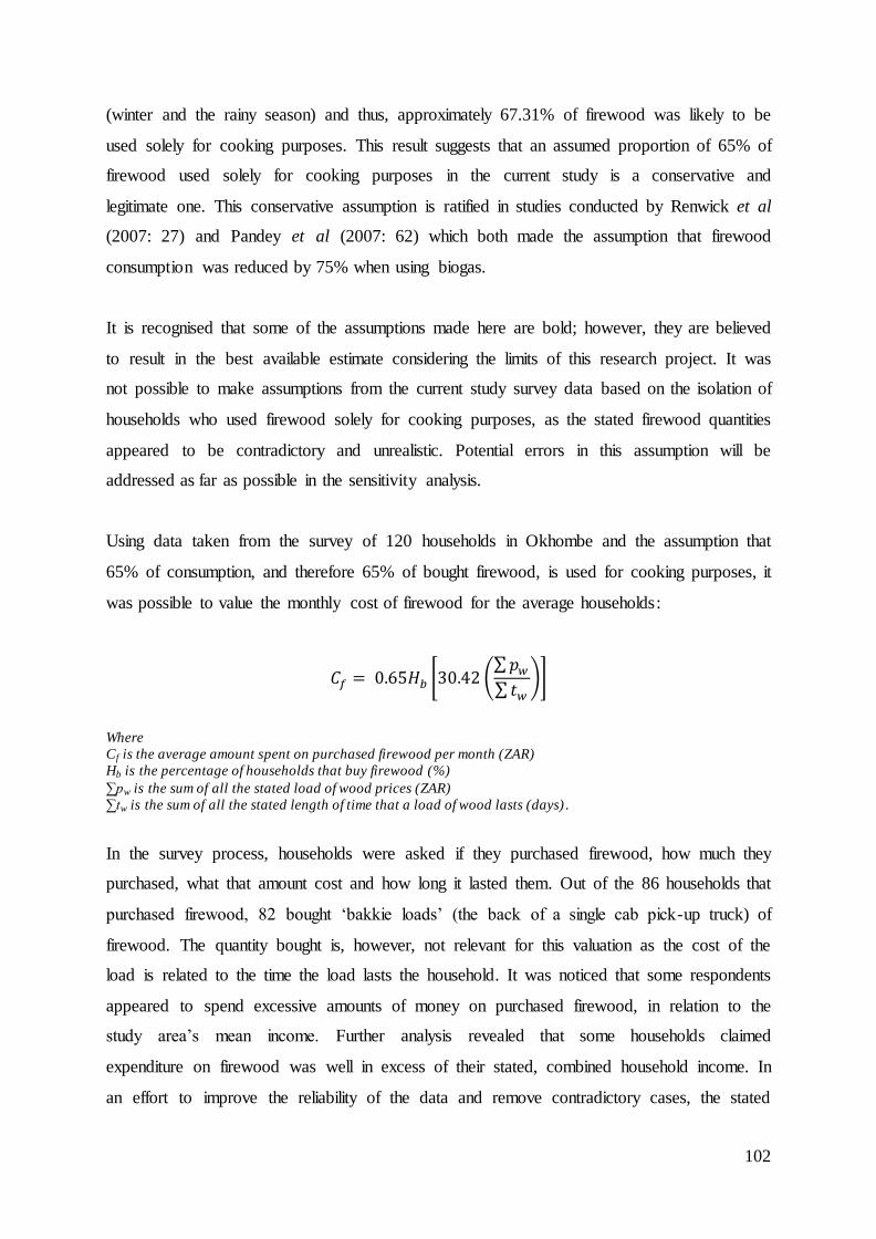
102

(winter and the rainy season) and thus, approximately 67.31% of firewood was likely to be

used solely for cooking purposes. This result suggests that an assumed proportion of 65% of

firewood used solely for cooking purposes in the current study is a conservative and

legitimate one. This conservative assumption is ratified in studies conducted by Renwick et al

(2007: 27) and Pandey et al (2007: 62) which both made the assumption that firewood

consumption was reduced by 75% when using biogas.

It is recognised that some of the assumptions made here are bold; however, they are believed

to result in the best available estimate considering the limits of this research project. It was

not possible to make assumptions from the current study survey data based on the isolation of

households who used firewood solely for cooking purposes, as the stated firewood quantities

appeared to be contradictory and unrealistic. Potential errors in this assumption will be

addressed as far as possible in the sensitivity analysis.

Using data taken from the survey of 120 households in Okhombe and the assumption that

65% of consumption, and therefore 65% of bought firewood, is used for cooking purposes, it

was possible to value the monthly cost of firewood for the average households:

[ (∑ ∑

)]

Where

Cf is the average amount spent on purchased firewood per month (ZAR)

Hb is the percentage of households that buy firewood (%)

∑pw is the sum of all the stated load of wood prices (ZAR)

∑tw is the sum of all the stated length of time that a load of wood lasts (days) .

In the survey process, households were asked if they purchased firewood, how much they

purchased, what that amount cost and how long it lasted them. Out of the 86 households that

purchased firewood, 82 bought ‘bakkie loads’ (the back of a single cab pick-up truck) of

firewood. The quantity bought is, however, not relevant for this valuation as the cost of the

load is related to the time the load lasts the household. It was noticed that some respondents

appeared to spend excessive amounts of money on purchased firewood, in relation to the

study area’s mean income. Further analysis revealed that some households claimed

expenditure on firewood was well in excess of their stated, combined household income. In

an effort to improve the reliability of the data and remove contradictory cases, the stated

103

amount of money spent on firewood per month was calculated as a percentage of stated

monthly income for each household and those households whose stated firewood purchases

exceeded 50% of monthly income were removed from the sample group. The total sample

size was reduced by the number of removed cases for calculation of sample aggregate

purchased firewood costs. The removal of sample cases that stated over 50% of monthly

income is considered to be reasonable and conservative. In a wide ranging rural energy use

survey, Paulsen et al (2010: 23) found that the greatest amount spent on all fuel costs (i.e. not

just purchased firewood) was 26% of income.

In the equation, 30.42 is the number of days in a month and 0.65 represents the proportion of

firewood that is used for cooking purposes (65%).

4.7.1.1.2. Quantifying and valuing paraffin usage

In the absence of study area paraffin consumption data, six study samples were considered

for extrapolation. A study conducted by Paulsen et al (2010) (hereafter referred to as the

Paulsen study) was used as it appeared to be the most recent and representative study

available. The Paulsen study was conducted in 18 rural areas throughout South Africa,

including two sites of sample size 251 households each in KwaZulu-Natal. 67% of household

incomes were below ZAR 1 500.00 per month and only 1% were in excess of ZAR 5 500.00,

which is not dissimilar from the current study area with proportions of 78% and 0.83%

respectively.

The Paulsen study found that on average, rural households in their study sample used 5.1

litres of paraffin per week (20.4 litres per month) (Paulsen et al, 2010: 28). It is assumed in

this study that only 50% of this quantity (10.2 litres per month) is used for cooking. This was

the assumption made in a study conducted by AGAMA Energy and used in the South Africa

National Household Biogas Feasibility Study (Austin and Blignaut, 2008).

A major difference between the study samples was that only 34% of paraffin users in the

Okhombe study area used paraffin as their primary cooking energy, as opposed to the Paulsen

104

study, in which 61% used paraffin as their primary16 source of cooking energy. The

calculation of study area paraffin use was weighted accordingly to rectify this disparity.

Considering that 96% of households in the Paulsen study sample are paraffin users, the

average consumption of paraffin is considered reasonably representative of the average

paraffin using household’s paraffin consumption. It was, therefore, assumed that primary

users of paraffin would use 100% of this quantity, secondary users would use 50% of this

quantity and tertiary users would use 12.5% of this quantity.

Although it is recognised that prices vary across regions and places of purchase (Paulsen et

al, 2010: 24), the information regarding the distribution of purchases is not known for the

study area. In addition to this knowledge, research would be needed to gather distribution of

prices across different access points. The price of paraffin (pp) is, therefore, taken as ZAR

7.35 per litre (incl. VAT), which is the standard price within rural areas in KwaZulu-Natal

South Africa, as at November 2011 (Department of Energy, 2011a).

[( ( ) ( ) ( )

)]

Where

Cp is the average amount spent on purchased paraffin (ZAR/month)

pp is the price of paraffin (ZAR/litre)

Hp is the number of households that use paraffin as their primary energy source for cooking

Hs is the number of households that use paraffin as their secondary energy source for cooking

Ht is the number of households that use paraffin as their tertiary energy source for cooking.

qp is the quantity of paraffin used by the average household for cooking, as extrapolated from the Paulsen study

(10.2 litres/month).

4.7.1.1.3. Quantifying and valuing liquefied petroleum gas (LPG) usage

It was recognised in the survey process that that households were unable to provide an

accurate response as to how much LPG they used in one month. Similar to the approach used

in Heltberg (2003), they were therefore asked to state what size gas cylinder they used, and

how long this would last them. The answer was then converted into quantity (kg) per month.

After analysing the survey data, it was found that the stated quantities of LPG use were

higher than expected for a poor rural community, but were not considered to be excessive

16

Primary, secondary and tertiary sources of energy refer to the households first, second and third most

commonly used source of energy.

105

(section 5.8.1.1). Results were compared to existing study data and contradictions are

accordingly dealt with in the sensitivity analysis.

It was recognised that some households used LPG for a range of purposes including cooking,

heating and refrigeration. In order to disaggregate the use of cooking from other activities, the

quantities stated by those who only used LPG for cooking purposes17 (51% of LPG users)

were calculated first. Once the average quantity of gas used by households who only cooked

with LPG was calculated, this average was used for all LPG using households who cooked

with LPG and used it for other purposes. The calculation of value used per month was simply

calculated on a price (pg)18 multiplied by quantity (qg) basis.

( )

Where

Cg is the average amount spent on purchased LPG (ZAR/month)

Hg is the number of households who use LPG for cooking

qg is the average quantity of LPG used by households that only cook with LPG (kg)

pg is the price of LPG (ZAR)

n is the number of households in the sample group.

4.7.1.1.4. Quantifying and valuing electricity usage

As with the other energy forms, electricity was used for a number of different purposes and it

was necessary to disaggregate that amount used for cooking. The results displayed that all

electrified households used electricity for lighting, with 80% using it for cooking and 27.5%

using it for heating (section 5.3). The same method as used in disaggregating LPG usage

could not be utilised as there were no households who used electricity solely for cooking. As

there were 15% of households who used electricity solely for lighting, it was possible to

calculate an average expenditure on lighting. Once this was completed, the amount of

electricity expenditure on cooking was calculated by taking the average expenditure on

electricity for those households who only cooked and illuminated with electricity (55% of

electrified households) and subtracting the average expenditure on lighting (shown by those

who only lighted with electricity). It was then assumed that this calculated expenditure for

17

This includes households who used LPG for water heating purposes. Water heating is an activity that c an be

replaced by biogas use. 18

The price of LPG is taken as a standard regulated price of ZAR 20.65 per kg incl. VAT for Magisterial District

Zone 6C – Bergville, as at November 2, 2011 (Department of Energy (RSA), 2011b).

106

cooking applied to all households who cooked with electricity19. This approach was used with

confidence as there was a clear difference in electricity expenditure for households who used

electricity for one, two or three purposes (appendix VIII).

The average expenditure for electricity across the sample group was then calculated by

multiplying the average cooking expenditure on electricity by the proportion of the sample

group that used electricity for cooking.

( )

Where

Ce is the average amount spent on electricity (ZAR/month)

Hc is the number of households that cook with electricity

qe is the average cost of electricity used for cooking (ZAR/month)


4.7.1.2. Avoided fertiliser costs

The bioslurry that is a by-product of the decomposition of cow dung and water in the

biodigester is considered to be a good replacement for chemical fertilisers and a high quality

fertiliser for rural agriculture (Pandey et al, 2005: 3; Khan and Khan, 2009: 468). It is

assumed that bioslurry can replace all purchased fertiliser requirements of the average rural

household.

The study survey asked respondents how much fertiliser they used in a year, what type of

fertiliser they used and how much this cost them for a year. The results appeared to be very

consistent, with all but three respondents purchasing amounts in factors of 50kg, with precise

stated costs. As it is proposed that all fertiliser requirements may be replaced by bioslurry, it

was possible to calculate the average cost of fertiliser per household, per year and convert this

into a monthly cost.

19

Including those households who also heated with electricity.

107

(∑

)

Where

Cfs is the cost of fertiliser for the average household (ZAR/month)

∑qf is the quantity of fertiliser used per year stated in monetary terms (ZAR)


4.7.1.3. Financial benefit of improved health

The use of biogas is expected to reduce indoor air pollution (IAP) and thus make a notable

improvement to people’s health (Dekelver et al, 2005: 6), especially the health of those

involved with cooking practices – usually woman and children (Legros et al, 2009: 22;

Banik, 2010: 210). The details and reasons for this health improvement are discussed

thoroughly in section 3.4.4 of the literature review. The valuation of health is categorised into

financial and economic benefits and further into three sub-categories: health expenditure

saving, health-related productivity gains and the value of saved lives. The inclusion of these

categories is based on an assumption that reduction in IAP is expected to have a positive

effect on medical expenditure costs, productivity losses and the number of deaths related to

IAP.

4.7.1.3.1. Financial value of avoided medical expenditure

At household level:

The household level financial impact of reduced expenditure on medical costs is not

considered in this valuation. In South Africa, state medical treatment is provided free of

charge and is subsequently a cost to the government (or society). In a poor rural area, as is the

study site, it is unlikely that households will seek medical care other than that provided by the

government. Medical expenditure saving is thus expected to be a benefit to society. Other

costs of seeking medical care, including transport, were also not considered in this study due

to the extensive and specific research required to accurately assess these, and the expectation

that they would be of insignificant value.

At societal level:

The saving on health care as a result of reduced IAP related incidence of disease is

considered to be a benefit to society as the government (and society) pay for the medical

costs of those who cannot afford them. There are a number of methods of valuing the

potential decrease in health-related expenditure saving. Some methods consider the incidence

108

of disease in relation to the incidence of treatment seeking, number of treatment days

required, and the cost of treatment. Although it was not a recognised method, an attempt was

made to use disability adjusted life year (DALY) indicators to deduce an estimate of the

percentage of aggregate per capita spending on health care that is spent on IAP related

diseases.

Disability adjusted life years (DALY) is an indicator used by the World Health Organization,

which combines the years of life lost (YLL) and years lived with a disability (YLD) as a

measure of the burden of disease (WHO, 2011). The World Health Organization lists the

DALYs lost for all burdens of disease, including those which result from IAP. The method

that was used to gauge a value for societal expenditure on health care for IAP made use of the

World Health Organization’s DALY stated statistics for South Africa (WHO, 2004a).

The societal expenditure (government expenditure) on IAP related disease was calculated by

assuming the percentage of DALYs that are lost due to IAP (i.e. the percentage of DALYs

lost to IAP out of the total DALYs lost in South Africa per year) is directly proportionate

with the percentage of government expenditure on health care. It is recognised that this is a

potentially flawed assumption in that actual treatment costs are not considered and DALYs

include years of life lost (or premature deaths) which do not account for government

expenditure on health care. Although it is recognised as being a crude estimate, the

presumption is made that aggregating across DALYs lost to all burdens of disease results in a

useable estimate of the percentage of total per capita expenditure on medical treatment. This

method is not expected to be precisely accurate and the results will be treated with

circumspection.

The procedure followed in this method of calculation was as follows:

The per capita government expenditure in purchasing power parity (PPP) international

dollars was taken from the WHO data repository and converted to ZAR using the

Penn World Table PPP-adjusted exchange rate for the year 2009 (WHO, 2009; CIC,

2011b). The 2009 expenditure on government health care was then converted to 2011

ZAR (Stats SA, 2011a).

109

The number of DALYs attributable to IAP (IAP DALYs) was calculated as a

percentage of all DALYs lost in South Africa within one year (WHO, 2004a; WHO,

2004d).

The percentage of IAP DALYs was multiplied by the government expenditure on

health care per capita and this resulted in a ZAR value for health-related expenditure

on IAP related diseases.

Finally, only those households who use solid fuels (firewood, cow dung and coal) as a

primary or secondary cooking energy source are expected to gain from using biogas

and only 65% of IAP20 is considered to be reduced by using biogas. These elements

were included by reducing the health-related expenditure savings by the percentage of

households who do not use firewood or cow dung, and then reducing this value

further by 35% (the percentage of IAP that is not expected to be reduced by biogas

use).

After analysing the results produced by this method of valuation (presented and calculated in

appendix IX), it was recognised that the values estimated (ZAR 18.39 per household per year)

were significantly lower than the estimates of existing studies including Austin and Blignaut

(2008: 29) and Pandey et al (2007: 74) who calculated ZAR 1000.00 (2008 ZAR) and

US$34.02 (2007 US$) per household per year respectively. In response, a similar method to

that described above was attempted using annual incidence of IAP related diseases

(calculated from quoted percentages of ALRI, COPD and lung cancers attributed to IAP

(Prüss-Üstün and Corvalán, 2006)) as a percentage of annual incidence of all disease. Again,

the results were extremely low and contradictory to the findings of existing studies.

The methods proposed by existing studies could not be applied to the research project due to

the lack of area specific (and even region specific) information required. In addition to this,

the attempt to apply new valuation methods (described above) was not successful. It was thus

decided to extrapolate the findings of existing studies to the research project. The health-

related expenditure savings were taken from a Ugandan study and converted to 2011 ZAR

using the Penn World Table PPP-adjusted exchange rates (Pandey et al, 2007; Renwick et al,

2007; CIC, 2011b).

20

It is assumed that the use of biogas will reduce 65% of IAP, on the basis that the use of biogas reduces

firewood consumption by 65%.

110

4.7.1.3.2. Financial value of health-related productivity gains

The reduction of IAP is expected to reduce morbidity conditions that result in individuals not

being able to take part in economic activity (see section 3.4.4.3.2).

In this study, this value is considered unlikely to be significant for a number of reasons. The

study area is said to have an employment rate of only 13.7%; moreover, those who are mostly

affected by the IAP health hazards are women and children who are involved with the

cooking of meals (ETC UK, 2007) – these groups are even less likely to be involved in

income generating economic activity than the population as a whole. Further to this,

information as to the provision of paid sick-leave among those who are employed is not

known.

Considering all these factors as well as the extensive data that would be required to attempt a

valuation, it was decided that the effect of improved health on earnings would be excluded

from this research project. It is noted that Renwick et al (2007: 32), in a comparable study to

the current one, also excluded earning benefits of increased health (related to IAP) for similar

reasons.

4.7.1.3.3. Financial value of saved lives

The total number of IAP related deaths in the study area was calculated using environmental

health burden of disease data from the World Health Organization (WHO, 2004a; WHO,

2007). IAP is considered to be a result of solid fuel use in households and thus, all IAP

related diseases were considered to be from only those households that used solid fuels as an

energy source (17.3% of the South African population) (WHO, 2007). Using this

information, it was possible to calculate the number of IAP related deaths per 100 solid fuel

users, per year in South Africa. Once this figure was calculated, it was possible to determine

the number of deaths per year in the study area that would be as a result of IAP.

It was assumed that only those households in the study site that cooked with solid fuels would

benefit from a reduction in IAP21 and thus the calculation of IAP related deaths for the study

site was based on the number of households that used firewood, cow dung or coal as their

primary and/or secondary cooking fuel. It is assumed that the use of biogas will reduce 65%

21

Biogas will only replace cooking fuels.

111

of IAP, on the basis that the use of biogas reduces firewood consumption by 65% (as

calculated in section 4.7.1.1.1). The supposition here is that 65% of IAP related deaths will be

reduced by the use of biogas in place of traditional solid fuels.

Once the number of avoided deaths had been deduced, it was possible to assign a monetary

value to this statistic. The loss of future income and cost of death are relevant financial costs.

Due to the high unemployment rates and the fact that women and children, who are most

likely to be affected by IAP related diseases (Legros et al, 2009: 22; Banik, 2010: 210) are

often not in income earning positions, it is common place to consider the cost of death and

not loss of future income (Renwick et al, 2007: 34). The cost of death is considered to be the

cost of an average funeral in a rural area of South Africa (section 3.4.4.3.3). The average cost

of a funeral is conservatively taken as one third of the average, annual household income for

the study area, as found in a study by the United Nations Economic Commission for Africa

(UN-ECA, 2011: 18). Although another study suggested that funeral costs amounted to two

months of mean monthly income, the former assumption is considered to be legitimate and

conservative with reference to a study by Collins and Leibbrandt (2007: 75) in which funerals

were said to cost up to the equivalent of seven months of income.

4.7.2. Economic Benefits

4.7.2.1. Time saving due to using biogas in place of traditional cooking fuels and methods

The time saved by using biogas in place of traditional cooking fuels and methods includes

reduced time collecting firewood and reduced time spent on traditional cooking practices.

Firewood collection time is expected to be reduced, as firewood for cooking is replaced by

biogas use. Cooking and cooking related activity times are expected to decline as individuals

do not need to prepare and maintain cooking fires, wait while food is cooked slowly, or spend

extra time cleaning utensils that were dirtied by solid fuel fires.

4.7.2.1.1. Quantifying reduced firewood collection time

Similarly to the financial benefit of reduced purchased firewood, it is assumed that only 65%

of firewood is used for cooking purposes (section 4.7.1.1). This is assumed to translate into a

reduction of 65% of purchased firewood and 65% of collection time (Pandey et al, 2007: 65;

Renwick et al, 2007: 26). Surveyed respondents were asked to state how much time they

spent on an average trip to collect firewood and how many trips they made to collect

firewood per week in summer and winter (appendix I, section C). It was assumed that winter

112

and summer were equal length periods in a year and thus the number of trips per week was

averaged across the two periods. The average number of trips to collect firewood per week

was converted to an average number of trips per month and multiplied by the average time

spent collecting firewood per day trip. The average time spent collecting firewood was then

multiplied by the proportion of firewood used for cooking (65% of firewood is assumed to be

used for cooking purposes) and added to the cooking time savings before converting into a

monetary value.

(∑ )

Where

Tf is the time spent collecting firewood for cooking purposes per average household ( hours/month)

∑tf is the sum of all time spent collecting firewood (hours)


4.7.2.1.2. Quantifying reduced cooking time

Reduction of cooking time is not something that could be gauged by the primary research of

this study. At the time of appraisal, the case study biodigesters had been installed at the study

households, but were not yet in full and efficient working order. The amount of time saved in

cooking practices was thus reliant on the stated figures of existing studies. These studies were

believed to be more accurate than a calculated assumption as the households had actual

experience with working biodigesters.

After an extensive effort to review over 20 biodigester related studies it became apparent that

in all, but one, relevant cases, researchers had estimated these values in combination with the

time saving of collecting cooking fuels. An extensive cost-benefit analysis for biogas and

sanitation systems in Sub-Saharan Africa by Renwick et al (2007) provided suitable data for

the time saved on cooking practices. Renwick et al (2007: 27) explained in detail that biogas

had been proven to be 1.07, 1.22, 4.63, 6.52 times more efficient than LPG, kerosene

(paraffin), agricultural residue and dung-burning stoves respectively, in relation to the output

of heat (Renwick et al, 2007: 27). A Nepalese study quoted by Renwick et al (2007: 27)

showed that on average, biogas users save 96 minutes in cooking time and an estimated 39

minutes in cooking utensil washing time per day per household. An Ethiopian field survey

revealed on average that biogas users had also saved 96 minutes in cooking time and 37

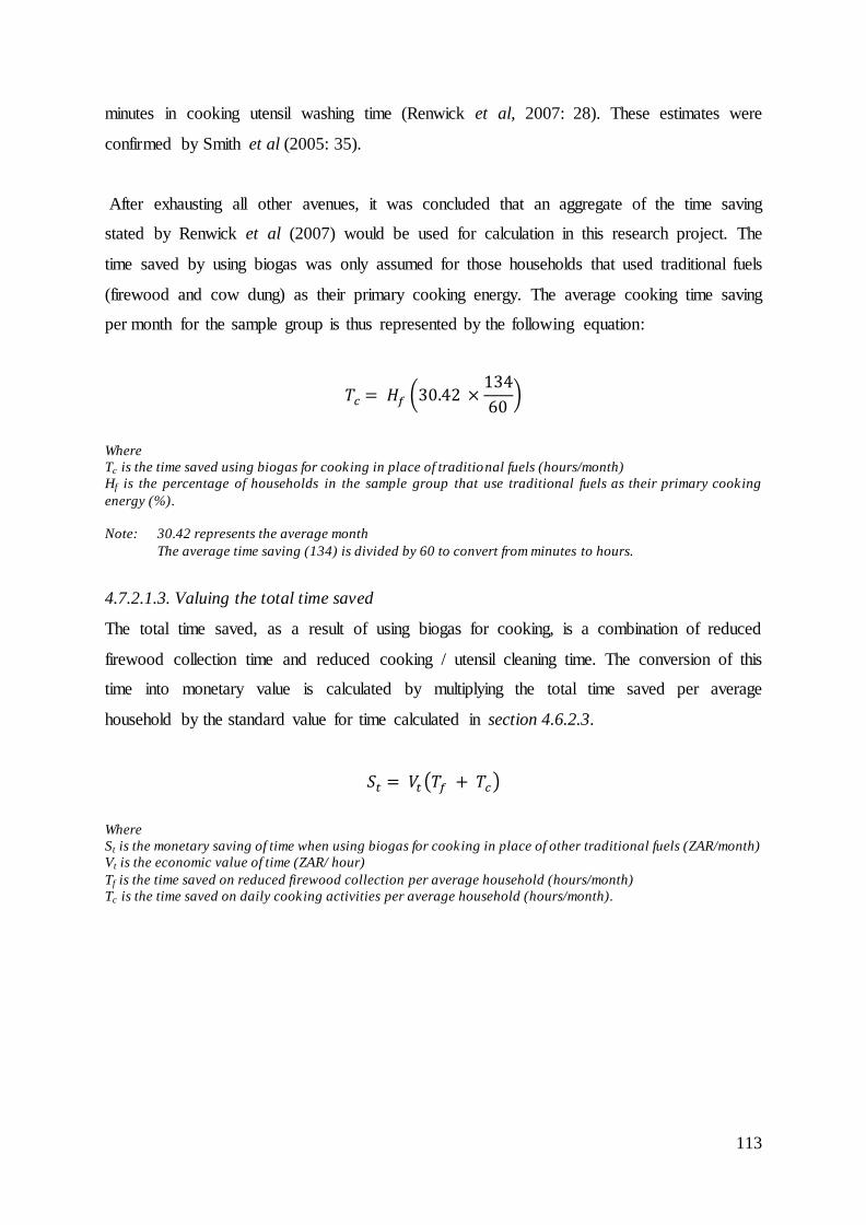
113

minutes in cooking utensil washing time (Renwick et al, 2007: 28). These estimates were

confirmed by Smith et al (2005: 35).

After exhausting all other avenues, it was concluded that an aggregate of the time saving

stated by Renwick et al (2007) would be used for calculation in this research project. The

time saved by using biogas was only assumed for those households that used traditional fuels

(firewood and cow dung) as their primary cooking energy. The average cooking time saving

per month for the sample group is thus represented by the following equation:

(

)

Where

Tc is the time saved using biogas for cooking in place of traditional fuels (hours/month)

Hf is the percentage of households in the sample group that use traditional fuels as their primary cooking

energy (%).

Note: 30.42 represents the average month

The average time saving (134) is divided by 60 to convert from minutes to hours.

4.7.2.1.3. Valuing the total time saved

The total time saved, as a result of using biogas for cooking, is a combination of reduced

firewood collection time and reduced cooking / utensil cleaning time. The conversion of this

time into monetary value is calculated by multiplying the total time saved per average

household by the standard value for time calculated in section 4.6.2.3.

( )

Where

St is the monetary saving of time when using biogas for cooking in place of other traditional fuels (ZAR/month)


Tf is the time saved on reduced firewood collection per average household (hours/month)

Tc is the time saved on daily cooking activities per average household (hours/month).

114

4.7.2.2. Economic benefit of improved health

The economic benefit of improved health conditions relating to reductions in IAP follows the

same categorisation as explained in section 4.7.1.3 with the exclusion of health-related

medical expenditure. The economic valuation of health-related productivity gains and value

of saved lives will be discussed.

4.7.2.2.1. The economic value of health-related productivity gains

Improved indoor air quality is expected to result in a reduction of incapacity due to IAP

related diseases. For the calculation of IAP related productivity gains, only acute lower

respiratory infections are considered as they appear to be the most notable and prevalent

diseases caused by IAP (Renwick et al, 2007: 31). Due to an absence of area specific and

national data, incidence of disease data from Sub-Saharan Africa (SSA), compiled by the

World Health Organization, is used (WHO, 2004c). The researcher is comfortable with the

use of SSA data, as the percentage of solid fuel using households is closely matched with that

of the study area22 and does therefore not require correction, as was needed in section

4.7.1.3.3.

The process used in calculating the number of productivity hours gained by using biogas is

best explained through the use of a flow diagram (Figure 14).

22

80.00% of the sample group were calculated to use solid fuels for cooking. The UNDP (2009: 11) reported

that 81% of households in SSA used solid cooking fuels (including 1% coal, 11% dung, 69% firewood).

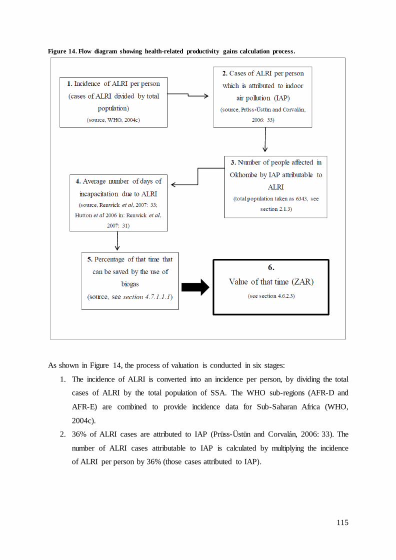
115

Figure 14. Flow diagram showing health-related productivity gains calculation process.

As shown in Figure 14, the process of valuation is conducted in six stages:

1. The incidence of ALRI is converted into an incidence per person, by dividing the total

cases of ALRI by the total population of SSA. The WHO sub-regions (AFR-D and

AFR-E) are combined to provide incidence data for Sub-Saharan Africa (WHO,

2004c).

2. 36% of ALRI cases are attributed to IAP (Prüss-Üstün and Corvalán, 2006: 33). The

number of ALRI cases attributable to IAP is calculated by multiplying the incidence

of ALRI per person by 36% (those cases attributed to IAP).

116

3. The number of people affected in the study area (Okhombe) is calculated by

multiplying the Okhombe population23 by the incidence rate. Solid fuel using

households are not separated from those who do not use solid fuels as the percentage

of solid fuel using households in SSA is closely correlated with the percentage of

solid fuel using households in Okhombe (see footnote 22).

4. The average number of days of incapacitation due to ALRI is calculated using

assumptions made by Renwick et al (2007: 33). All cases of ALRI are conservatively

assumed to be non-severe with an average recovery of five days if treated and 10 days

if not treated (Renwick et al, 2007: 33). 44.4% of people are expected to seek

treatment for ALRI in SSA, and thus the average number of days of incapacity is

calculated to be 8.88 days24.

5. 65% of solid fuel use is expected to be reduced by the use of biogas for cooking (see

section 4.7.1.1.1). It is assumed that this reduces the exposure to IAP by 65% and

consequently reduces the health-related productivity loss due to IAP by 65%.

6. The value of time is calculated using the same method as proposed in section 4.6.2.3.

In the calculation of a standard value for the opportunity cost of time, differing

proportions for time spent on various activities are used. The employment rate for

Okhombe is taken as 13.7% (Chellan, 2002: 67) and therefore only 13.7% of time

spent on economic activity is expected to be lost. The remainder of time is expected to

be spent on an equal proportion of household activity and other activity. The same

equation for calculating an opportunity cost of time is used as in section 4.6.2.3, and

as explained the proportions for economic activity (e), household activity (h) and

other activity (o) are taken as 13.7%, 43.15% and 43.15% respectively.

( ) ( ) ( )

Where


e is the percentage of people who will use time for economic activity (%)






23

6 343 people, as calculated in section 2.1.3. 24

Calculated with the probability of 44.4% of people seeing treatment: Average incapacity days = (44.4% * 5) +

(66.6% * 10).

117

4.7.2.2.2. The economic value of saved lives

The potential number of lives saved by the use of biogas and subsequent reduction in IAP is

calculated in section 4.7.1.3.3. In assessing the economic impact of this potentially avoided

mortality, the value of a statistical life (VOSL) is used (see section 3.4.4.3.3). A value of US$

9.1 million (2011 US$) is used by the Environmental Protection Agency (EPA) of the United

States of America and appeared to be the most widely recognised value with considerable

attempts made by the EPA to use scientifically sound methods of calculation (Sinha et al,

201025: 121; Appelbaum, 2011). The value used by the EPA was calculated as a mean of 26

contingent valuation and labour market studies published between 1974 and 1991, and

adjusted to 2010 US$ (Sinha et al, 2010: 121). The value used by the EPA appeared to be

legitimate considering that a great number of implemented regulations have cost well in

excess of US$ 9.1 million per life saved (Tietenberg and Lewis, 2010: 49). Although the

value used by the EPA appeared to be the most widely used VOSL, it is calculated with

respect to the labour markets of a first world developed country. VOSL studies relating to

developing and emerging economic countries are very rare and thus it was decided to use a

conservative mean estimate of US$ 2 million (adjusted to 2011 ZAR) used by Renwick et al

(2007: 34). The VOSL used by Renwick et al (2007) is based on estimates made for North

America and Western European countries. The value of US$ 9.1 million, used by the EPA,

will be used as an optimistic case scenario in the sensitivity analysis.

The VOSL value, stated in US$, is converted to ZAR using a PPP-adjusted exchange rate.

The PPP-adjusted exchange rate is calculated using reported statistics on South African GDP

and PPP-adjusted GDP (World Bank, 2011; IMF, 2011b). PPP-adjusted GDP is divided by

nominal GDP and then divided by the market exchange rate.

4.7.2.3. Local environmental benefits

4.7.2.3.1. The preservation of indigenous trees

The preservation of indigenous trees is expected to be a value to society. In rural areas

firewood is often collected from natural indigenous forests, and thus the reduction of this

occurrence would be expected to be a societal benefit which would hold value. In this project,

it was found that approximately 35.3% of the collected firewood was collected from natural

wood stocks, while the remainder of collected wood (64.7%) was alien tree species.

25

Report published in 2010 but VOSL is still used in 2011 as US$ 9.1 million.

118

According to expert knowledge, the wood that is purchased in Okhombe originates mostly

from the Royal Natal National Park and is taken from alien plant removal projects (pers. com.

Steve McKean November 2011, pers. com. Mxolisi Fulumente, August 2011). In contrast to

the removal of indigenous tree species, the removal of alien trees is considered to increase

stream flow and thus be economically beneficial (Cooper, 2001).

Although it would be technically correct to value both the benefits and costs of alien and

indigenous tree removal respectively, the extensive research required to quantify these two

offsetting impacts was not feasible. The quantification of these impacts was therefore omitted

from this research project.

4.7.2.3.2. Reduction of erosion

One of the most notable potential environmental benefits for a biodigester system is to reduce

the movement of cattle and subsequent erosion that it causes. Erosion poses a great threat to

the siltation of the Woodstock dam which is fed by the Okhombe River. The siltation of this

dam affects its holding capacity and its ability to be used for electricity generation (pers. com.

Dr Terry Everson, October 2010). Both these impacts are economically relevant and are

being assessed by payment for ecosystem services (PES) studies in the area.

A reduction of erosion would be expected to result from less movement of cattle and

overgrazing of pastures. This reduction in grazing and cattle movement would be assisted by

a zero grazing system where cattle dung feeds a biodigester system, the bioslurry output is

used to grow fodder for the cattle and the kraaled cattle are fed with the fodder and

consequently do not need to graze in the natural rangeland.

This benefit was not considered in this research project as this system of zero grazing was not

proposed. Further research would be necessary to deduce the feasibility of changed cattle-

keeping practices before this system could be implemented. While considering environmental

protection, the ethics of keeping cattle penned continuously must also be called into question.

4.7.2.4. Economic valuation of GHG and CO2 reductions

The general assumption, made by studies relating to biodigester use, is that there is a net

saving of GHG and CO2 emissions if a biodigester is used correctly and traditional fuels are

exchanged for biogas (Halter, 2005; Hellen, 2010; Trade plus aid, 2009). The specific amount

119

of CO2 equivalent26 (CO2e) reduction is, however, not agreed upon and is highly case

specific. Although it is recognised that deforestation and CO2 reductions may be combated

greatly by the use of biodigesters, it was decided to exclude this aspect of valuation based on

the volume of untested assumptions and methodology that would be implicit. Some of the

CO2e emission impacts and their complexities are included in Table 5.

Table 5. Factors affecting the quantification of biodigester related CO2 emissions.

Point of

emission change

Reduction

or Increase Quantification and complexities

Biodigester Construction

Increased emissions

Production of the BiogasPro is likely to result in GHG emissions.

The BiogasPro is a reasonably new technology and the manufactures were/are not able to provide details of the ‘carbon footprint’

27 of production.

Transport of biodigester

Increased emissions

The CO2 emissions of transport were included in this study; however, all related CO2e emissions were not.

The true cost of transport to the environment is exceedingly difficult to quantify and was not included in this study.

Biodigester installation and related biogas utilising equipment

Increased emissions

The carbon footprint of all items used in the installation of a biodigester (cement, stone, sand, pipes and fittings) would be difficult to quantify precisely and would be highly specific on each of their points of origin.

The carbon footprint of biogas utilising equipment (gas burner) is highly specific on method of production and point of origin.

Biodigester leakages

Increased emissions

Most biodigesters are expected to have some form of GHG leakages, with assumptions being made for feasibility assessments.

The design of the BiogasPro is expected to reduce potential leakages, but this has not been proven or quantified.

Manure management practices

Decreased emissions

Cow dung naturally ferments and releases GHG28

emissions into the atmosphere (Halter, 2005: 14).

Placing cow dung into a digester, then burning the methane that it produced results in CO2 and water vapour emissions, which are less damaging (in terms of global warming potential (Hellen, 2010: 5)) than the GHG emissions of fermenting cow dung (most notably methane).

Using bioslurry in place of chemical

Decreased emissions

Use of bioslurry in place of chemical fertilisers may have an overall reduction of GHG emissions.

The application of chemical fertilisers may result in GHG emissions.

26

A GHG equivalent, or CO2 equivalent (CO2e) is calculated by multiplying the mass of an emitted gas by the

relevant Global Warming Potential (standardised for each GHG), to provide a unit of greenhouse gas emission

equivalent to CO2 for the purpose of valuation and comparison (Northern Territory Government, 2009: 4). 27The term ‘carbon footprint’ is used to describe the combination of all CO2e emissions relating to a specific

item or impact. 28

Including NH3, CH4, CO2 and N2O (Halter, 2005: 14).

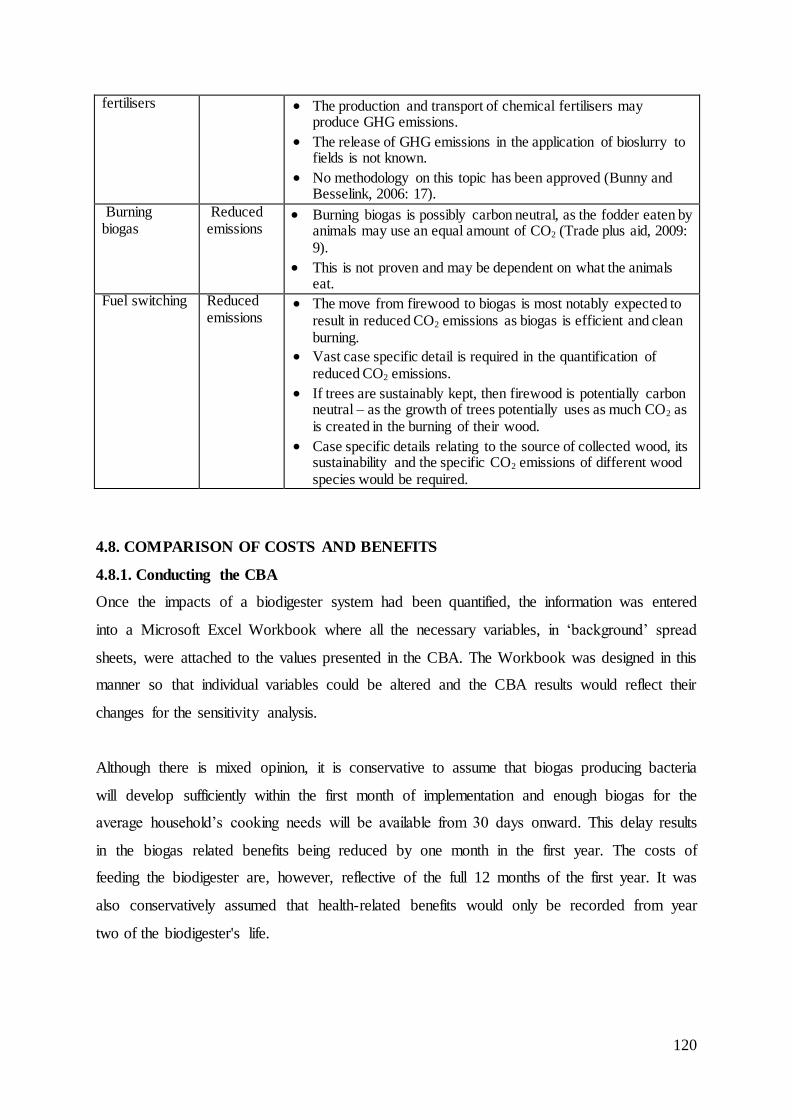
120

fertilisers The production and transport of chemical fertilisers may produce GHG emissions.

The release of GHG emissions in the application of bioslurry to fields is not known.

No methodology on this topic has been approved (Bunny and Besselink, 2006: 17).

Burning biogas

Reduced emissions

Burning biogas is possibly carbon neutral, as the fodder eaten by animals may use an equal amount of CO2 (Trade plus aid, 2009: 9).

This is not proven and may be dependent on what the animals eat.

Fuel switching Reduced emissions

The move from firewood to biogas is most notably expected to result in reduced CO2 emissions as biogas is efficient and clean burning.

Vast case specific detail is required in the quantification of reduced CO2 emissions.

If trees are sustainably kept, then firewood is potentially carbon neutral – as the growth of trees potentially uses as much CO2 as is created in the burning of their wood.

Case specific details relating to the source of collected wood, its sustainability and the specific CO2 emissions of different wood species would be required.

4.8. COMPARISON OF COSTS AND BENEFITS

4.8.1. Conducting the CBA

Once the impacts of a biodigester system had been quantified, the information was entered

into a Microsoft Excel Workbook where all the necessary variables, in ‘background’ spread

sheets, were attached to the values presented in the CBA. The Workbook was designed in this

manner so that individual variables could be altered and the CBA results would reflect their

changes for the sensitivity analysis.

Although there is mixed opinion, it is conservative to assume that biogas producing bacteria

will develop sufficiently within the first month of implementation and enough biogas for the

average household’s cooking needs will be available from 30 days onward. This delay results

in the biogas related benefits being reduced by one month in the first year. The costs of

feeding the biodigester are, however, reflective of the full 12 months of the first year. It was

also conservatively assumed that health-related benefits would only be recorded from year

two of the biodigester's life.

121

The values of LPG and paraffin (both Brent crude oil based commodities) as well as

electricity were assumed to increase in real value every year. Experience from the past 15

years (and beyond) has shown a dramatic increase in crude oil prices (IMF, 2011c) and a

noteworthy increase in electricity prices (Eskom Holdings, 2011a), both beyond aggregate

annual inflation (Stats SA, 2011a). Predictions (to be discussed in Chapter six) suggest that

these commodities will continue to increase above inflation over the next 15 years. Crude oil

based commodities, paraffin and LPG, were increased yearly by the past 15 year aggregate

crude oil price increase (IMF, 2011c) minus the past 15 year aggregate annual inflation rate

(Stats SA, 2011a), in the base case scenario CBA. Electricity yearly increases were based on

the past 15 year aggregate price increases of electricity (Eskom Holdings, 2011a) minus the

past 15 year aggregate annual inflation rate (Stats SA, 2011a). These increases were believed

to be conservative assumptions given the discussion in section 6.6.1.1, and in the interest of

caution, were tested with varying rates of increase in the sensitivity analysis (see section

4.10).

4.8.2. Analysis

The Net Present Value (NPV), internal rate of return (IRR) and benefit-cost ratio (BCR)

techniques were used in this research project to compare costs and benefits and consider the

overall feasibility of the project. As discussed in section 3.3.7, in calculating the NPV of a

project or regulation, the present value (discounted value) of costs is subtracted from the

present value of benefits (OBPR, 2009: 2). Mathematically, the equation is represented as:

∑( )

( )

Where:


Bt is the benefit in year t

Ct is the cost in year t



n is the number of years over which the benefits and costs will accrue start ing at year t = 1.

The internal rate of return (IRR) is the discount rate, r (in the NPV equation), that results in

the NPV equalling zero. The IRR was calculated using Microsoft Excel statistical software.

The BCR was calculated as the present value of benefits divided by the present value of

costs, as described in section 3.3.7.

122

As costs and benefits of a biodigester are experienced in differing time periods, the choice of

a discount rate is important to the project appraisal.

4.8.3. The Choice of a Discount Rate

A social discount rate (as opposed to a financial discount rate) is used for calculation in this

study (as explained in section 3.3.6.1). Although there is no formal consensus on what

method should be used to determine the precise social discount rate (Mullins et al, 2007: 40),

it is agreed that the choice of discount rate should remain consistent as far as possible in the

appraisal of projects in a region or country (Florio et al, 2008: 57). Mullins et al (2007: 40,

127) feel strongly that time and resources should not be spent on extensive research into the

true social discount rate, but rather that the intricacies be understood and that the applicable

rates applied in various countries and by various international institutions should be

considered.

In accordance with these assertions, it is noted that the European Commission (EC) (2006:

11) has recommended the use of 5.5% and 3.5% as the social discount rate in ‘cohesion

countries’29 and all other countries respectively during the period from 2007-2013. Statistics

South Africa (Stats SA, 2011b: 19), noted as South Africa’s leading statistics authority, are

known to use 3%, 5% and 11.7% in sensitivity analyses as the social discount rate in

resources rent calculations. A study (relating to Telecommunication Cables Disposal in South

Africa) done by Lottering in 2008 used a statistical approach to arrive at a real social discount

rate of 6.72% (Lottering, 2008: 97).

Mullins et al (2007: 127) noted that the ratio of Gross Domestic Saving to Gross Domestic

Product (GDP) diminished from 15.8% to 13.7% in South Africa from the years 2000 to 2005

and recognised that this should lead to a higher discount rate. It is noted that a decreased

savings rate has the subsequent effect of tighter supply of capital in the market which leads to

the need for capital to be used as efficiently and productively as possible, hence leading to the

suggestion of a higher discount rate.

29

Cohesion countries are defined by the European Union (EU) (2002) as countries who share

economic/technological characteristics, a GDP per capita lower than 90% of the EU average, a large portion of

the country having the ‘Less Favoured Region status’, high primary industry employment, traditional

manufacturing structures and low productivity (European Commission, 2002).

123

Mullins et al (2007: 127) proposed a rate of 8% to be used in the South African context,

citing the Central Economic Advisory Service (CEAS) (1989) and Water Research

Commission (2002) as recommending these rates in their manuals for cost-benefit analysis.

Mullins et al (2007: 127) also suggested that the figure of 8% is in-line with the

recommendations of the World Bank to use 10% as the social discount rate for investment

projects in South Africa. The figure of 8% is recognised as being higher than the

recommendations of Lottering (2008) and Stats SA (2011b), but it should be acknowledged

that it is in light of the discussion of using higher interest rates where capital supply

restrictions are notable (Mullins et al, 2007: 127).

In consideration of the propositions by Mullins et al (2007), EC (2006), Lottering (2008),

Stats SA (2011b) and in light of the fact that South Africa’s Gross Domestic Saving to GDP

ratio has increased to 15.6% in 2009 and nearly 20% in 2010 (IMF, 2011a), it is suggested

that a social discount rate of 6% would be appropriate for the current study. In recognition of

the controversy surrounding the use of a specific discount rate, it also seems appropriate to

conduct a sensitivity analysis with respect to a variation of discount rates. The rates of 2%,

6% and 10% will be used with 6% representing the base case discount rate.

4.9. SENSITIVITY ANALYSIS

There was a degree of uncertainty with regard to the accuracy of some cost and benefit

quantifications. In addition to this, the discount rate used in cost/benefit comparison was

chosen with some degree of circumspection and a wide degree of possibilities proposed by

various studies and institutions. For these reasons, a sensitivity analysis was used to correct

for potential imbalances in the feasibility indicator30 calculations.

The method of sensitivity analysis used in this research project and as used by Florio et al

(2008), Renwick et al (2007) and proposed by Pearce et al (2006), is a process by which an

upper and a lower estimate is given to a range of variables in the cost benefit appraisal. The

upper and lower, or optimistic and conservative, values were assigned to all uncertain

variables and the NPV, IRR and BCR were recalculated (Florio et al, 2008: 61).

30

Feasibility indicators refer to net present value (NPV), internal rate of return (IRR) and benefit -cost ratio

(BCR) calculations.

124

This process was conducted in a tabulated form where all uncertain variables were given an

optimistic, pessimistic and base value. The base value was that which was calculated in the

research study and the optimistic and pessimistic values were chosen on consideration of

existing studies, literature, expert opinion and pragmatic assumptions. The reasons for the

choice of upper and lower estimates were explained where necessary.

The results of the sensitivity analysis were separated into financial and economic groups,

presented as data in Chapter five, but graphically presented and discussed in Chapter six

along with the financial and economic analysis. Table 6 displays the various sensitivity

analyses that were conducted and the critical variables that were altered in each case.

Table 6.Sensitivity analyses and critical variable changes.

SENSITIVITY

ANALYSIS VARIABLE Conservative Base Optimistic

Digester cost

SENSITIVITY ANALYSIS 1

BiogasPro price 125% 100% 75%

Installation costs


Hole prep. (hours to dig hole) 174 hours 116.67 hours 58 hours

Backfill (price) 150% 100% 50%

Plumbing (price) 125% 100% 50% Accommodation – installation team (price) 150% 100% 50% Accommodation - gas (price) 150% 100% 50%

Plumbing (gas) 125% 100% 50%

Maintenance


Maintenance (as a percentage of digester cost per year) 1.50% 0% 0%

Training of biodigester users


Number of participants per days training 4 people 9 people 15 people

Social cost of transportation


Social cost of carbon price (ZAR/tonne) 250% 100% 0%

Biodigester feeding time


Water collection time 200% 100% 20%

Cow dung collection time 200% 100% 50%

Time to mix dung and water 200% 100% 50%

125

Quantity of cooking fuel


Per cent reduction in firewood use (when using biogas) 50%

65% (reduction)

80%

Quantity of paraffin used (normally) 50% 100% 150%

Quantity of LPG used (normally) 50% 100% 120%

Increase in fuel price (over 15 years)


Percentage increase per year in crude oil based fuels (real price, inflation excluded)

0% 14.88% (less

inflation) 20% (less inflation)

Electricity price (tariff increase per year) 0%

8.28% (less inflation)

13% (less inflation

Avoided medical expenditure


Value of avoided medical expenditure (ZAR) 0% 100% 200%

Avoided fertiliser cost


Cost of fertiliser 50% 100% 150%

Value of time


Shadow wage for labour (relating to health-related prod. and net time saving) ZAR 2.58 ZAR 5.44 ZAR 10.31

Value of saved lives


VOSL value 0 US$ 2.6 mil. US$ 9.1 mil.

Health related to IAP


Percentage of IAP (and thus IAP disease burden) reduced by biogas use 40% 65% 90%

Discounting


Discount rate 1% 6% 10%

In addition to the 14 sensitivity analyses, a combined result was produced for all conservative

and all optimistic assumptions. It was also noted in sensitivity analysis 14 that the discount

rate had a significant effect on the CBA results and it was thus decided that a separate

sensitivity analysis would be conducted with respect to the discount rate. In this analysis, the

discount rate was varied from 0% to 10% and the NPV, IRR and BCR were recalculated in

each case. The results of this analysis were discussed in section 6.2.2.

126

4.10. CONCLUSION

The methods used for impact quantification and project appraisal have been outlined in this

chapter. It has been explained that the questionnaire survey was used to provide information

for the valuation process and existing study data was extrapolated where current information

was unavailable or deemed unreliable. Due to the use of existing study data and a degree of

uncertainty in the quantified impacts, a comprehensive sensitivity analysis was conducted to

reveal potential inaccuracies. Based on the findings of the CBA, recommendations were

established and a conclusion prepared.

127

CHAPTER 5: RESULTS

5.1. INTRODUCTION

This chapter presents the results of this research project. The manner in which these results

were calculated is described in Chapter four and will be referred to when applicable. The

costs and benefits of a rural household biodigester are thoroughly presented in this chapter

and rely on the analysis of information sourced from the survey conducted in the study area,

existing studies and relevant literature. The presentation of results is designed to be strictly

factual, with all relevant explanation and calculations found in the methodology chapter

(Chapter four) and appendices.

5.2. DEMOGRAPHICS

5.2.1. Respondents to the Questionnaire

135 individuals, each representing different households in the Okhombe area (Ward 7,

Okhahlamba Municipality), were interviewed. 15 interviews were removed from the sample

on the basis of unreliable and contradictory data, leaving a sample group of 120 individuals

which represented 120 separate households and a collective number of 647 people living in

those households. The sample group thus represents 10.2% of the estimated population of the

study area31.

The average age of the respondents was 45 years with an age range from 16 to 83 years.

25.8% of the respondents were male and 74.2% were female. All respondents were black

Africans and all spoke isiZulu as their home language.

5.2.2. Sample Group Demographic

Of the 120 valid households that made up the sample group the minimum household size was

one person, the maximum was 14 people and the mode was four people. The average

household size was 5.39 people which correlated closely with information from IES (2001)

and Statistics South Africa statistics (1996) which revealed a person per household figure of

5.47 and was used for calculating population size in section 2.1.3.

31

Okhombe population was estimated at 6 343 people (see section 2.1.3).

128

The range of combined household stated monthly incomes was ZAR 25 to ZAR 7 000.00

with a mean monthly income of ZAR 1 089.63. This mean stated monthly income indicates

that the average per capita income was ZAR 202.10 which is substantially below the ZAR

235 poverty line used by The Presidency of South Africa as an indicator of relative poverty in

2009 (The Presidency, 2009).

The distribution of stated monthly household income revealed that the majority of households

(33.3%) received an income between ZAR 1 001.00 and ZAR 1 500.00 per month. 96% of

the sample population received a stated monthly household income of less than ZAR

2 501.00, with the remainder (only 4.2%) earning above ZAR 2 501.00. Figure 15 graphically

displays the distribution of income across the sample population (R is used interchangeably

to represent ZAR – South African Rands).

Figure 15. The distribution of stated monthly household income in Okhombe.

Note: HH represents ‘households’.

5.3. ENERGY USE PROFILE

The energy use profile for the sample group is important in the valuation of costs and

benefits. Where households used multiple fuels for specific activities, they were asked to

state the order of fuel use, from fuel used most often to least often. The top three ranking

fuels were classified as primary (most used) followed by secondary and tertiary. The potential

saving from fuel switching (using biogas in place of other energy forms) is dependent on the

cooking fuels that are originally used by a household.

27.5%

20.0%

33.3%

15.0%

4.2%

0.0%

5.0%

10.0%

15.0%

20.0%

25.0%

30.0%

35.0%

R0 - R500 R501 - R 1000 R1 001 - R1 500 R1 501 - R2 500 R2 501 +

HH

(% )

Income Group

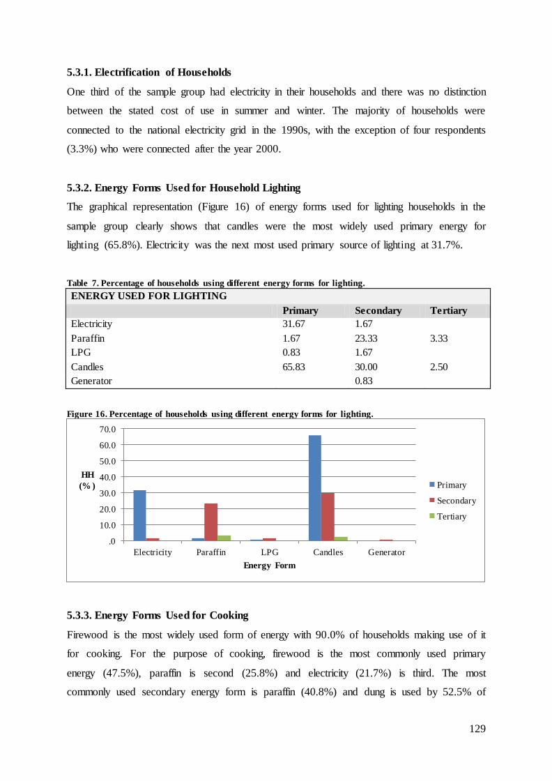
129

5.3.1. Electrification of Households

One third of the sample group had electricity in their households and there was no distinction

between the stated cost of use in summer and winter. The majority of households were

connected to the national electricity grid in the 1990s, with the exception of four respondents

(3.3%) who were connected after the year 2000.

5.3.2. Energy Forms Used for Household Lighting

The graphical representation (Figure 16) of energy forms used for lighting households in the

sample group clearly shows that candles were the most widely used primary energy for

lighting (65.8%). Electricity was the next most used primary source of lighting at 31.7%.

Table 7. Percentage of households using different energy forms for lighting.

ENERGY USED FOR LIGHTING

Primary Secondary Tertiary

Electricity 31.67 1.67

Paraffin 1.67 23.33 3.33

LPG 0.83 1.67

Candles 65.83 30.00 2.50

Generator 0.83

Figure 16. Percentage of households using different energy forms for lighting.

5.3.3. Energy Forms Used for Cooking

Firewood is the most widely used form of energy with 90.0% of households making use of it

for cooking. For the purpose of cooking, firewood is the most commonly used primary

energy (47.5%), paraffin is second (25.8%) and electricity (21.7%) is third. The most

commonly used secondary energy form is paraffin (40.8%) and dung is used by 52.5% of

.0

10.0

20.0

30.0

40.0

50.0

60.0

70.0

Electricity Paraffin LPG Candles Generator

HH

(% )

Energy Form

Primary

Secondary

Tertiary

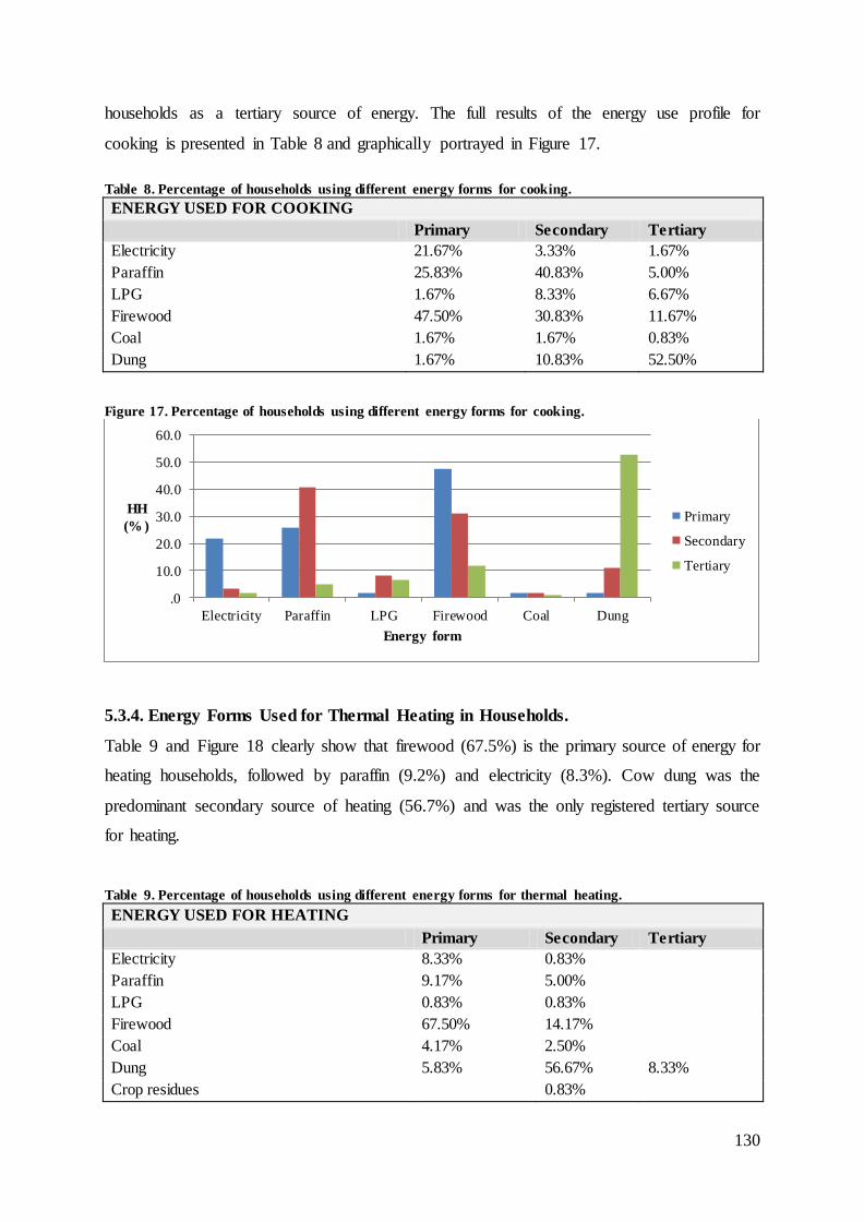
130

households as a tertiary source of energy. The full results of the energy use profile for

cooking is presented in Table 8 and graphically portrayed in Figure 17.

Table 8. Percentage of households using different energy forms for cooking.

ENERGY USED FOR COOKING


Electricity 21.67% 3.33% 1.67%

Paraffin 25.83% 40.83% 5.00%

LPG 1.67% 8.33% 6.67%

Firewood 47.50% 30.83% 11.67%

Coal 1.67% 1.67% 0.83%

Dung 1.67% 10.83% 52.50%

Figure 17. Percentage of households using different energy forms for cooking.

5.3.4. Energy Forms Used for Thermal Heating in Households.

Table 9 and Figure 18 clearly show that firewood (67.5%) is the primary source of energy for

heating households, followed by paraffin (9.2%) and electricity (8.3%). Cow dung was the

predominant secondary source of heating (56.7%) and was the only registered tertiary source

for heating.

Table 9. Percentage of households using different energy forms for thermal heating.

ENERGY USED FOR HEATING


Electricity 8.33% 0.83%

Paraffin 9.17% 5.00%

LPG 0.83% 0.83%

Firewood 67.50% 14.17%

Coal 4.17% 2.50%

Dung 5.83% 56.67% 8.33%

Crop residues 0.83%

.0

10.0

20.0

30.0

40.0

50.0

60.0

Electricity Paraffin LPG Firewood Coal Dung

HH

(% )

Energy form

Primary

Secondary

Tertiary

131

Figure 18. Percentage of households using different energy forms for thermal heating.

5.4. WATER SOURCE AND COLLECTION

5.4.1. Source of Collection

Municipal community stand taps and boreholes were the most common sources of water with

34.2% and 30.0% of households collecting at each source respectively. River or streams were

the next most used source of primary collection as well as being the most used secondary

source of water collection. No households had municipal water inside their houses and 13.3%

of households had a municipal tap directly outside their households.

Table 10. Percentage of households collecting water at different sources.

WATER SOURCES


River/Stream 22.50% 20.83% 0.83%

Municipal Tap (directly outside house) 12.50% 0.83%

Borehole 30.00% 10.83%

Community Stand (municipal) 34.17% 7.50%

Rainwater Tank 0.83%

.0

10.0

20.0

30.0

40.0

50.0

60.0

70.0

80.0

Electricity Paraffin LPG Firewood Coal Dung Crop

residues

HH

(% )

Energy form

Primary

Secondary

Tertiary

132

Figure 19. Percentage of households collecting water at different sources.

5.4.2. Details of Water Collection

The source of collection ranged from being 2 metres to 1km away from the respondents’

homes, with a mean distance of 309 metres. The average amount of time spent collecting

water was 25 minutes per day and the average quantity used per household was 62 litres per

day. The average time spent collecting a 20 litre bucket of water is relevant to the assessment

of time spent feeding a biodigester and was calculated at 8 minutes and 6 seconds.

Table 11. Details of water collection.

DETAILS OF WATER COLLECTION

Minimum Maximum Mean Std. Deviation

Source distance (m) 2 1000 308.61 289.793

Time spent collecting per day (minutes) 1 120 25.29 20.324

Quantity used per day (litres) 10 140 61.93 22.960

Average time taken to collect 20 litres of water 8.1 minutes

5.5. FARMING PRACTICES

The results of the survey, summarised in Table 12, showed that over 84% of households grew

their own vegetables, but only 3.3% of households grew fodder for cattle with, “not being

able to afford it” being the most commonly quoted (36.7%) reason for not growing fodder for

cattle. The use of fertiliser was prevalent, with all households that grew vegetables using

.0

5.0

10.0

15.0

20.0

25.0

30.0

35.0

40.0

River/Stream Municipal Tap

(directly

outside house)

Borehole Community

Stand

(municipal)

Rainwater

Tank

HH

(% )

Water Source

Primary

Secondary

Tertiary

133

some form of fertiliser and with 79.2%32 of households buying chemical fertilisers. The most

frequently used chemical fertiliser was NPK (321)33 which was used by 84.2% of fertiliser

buyers and DAP34 which was purchased by 12.6% of buyers. The average quantity of

fertiliser used across the sample group was 83.17 kg and the average cost of fertiliser used

per year was ZAR 365.98.

Table 12. Details of standard farming activity and practice

STANDARD FARMING PRACTICE

Households that grow own vegetables (%) 84.17

Households that grow fodder for cattle (%) 3.33

Households that use fertiliser for growing crops (%) 84.17

Households that purchase fertiliser (%) 79.17

Mean quantity of fertiliser used per year (kg) 83.17

Mean cost of fertiliser per year (ZAR) 365.98

5.6. SUITABLE HOUSEHOLDS FOR BIODIGESTER INSTALLATION

The strict suitability requirements for a household to be deemed worthy of having a

biodigester are listed in section 2.2.5. The adjusted suitability requirements are included in

the results to display the number of potential biodigester using households in the area, if they

are not required to own four or more cattle. These households are included for later

discussion as it became clear in the survey process that even those households who do not

have cattle, tend to collect cow dung on a regular basis.

Figure 20 indicates that 35% of the sample group is considered suitable for having and using

a biodigester under the strict suitability requirements and 79% of the sample group are

considered suitable households under the adjusted requirements. When extrapolated to the

total area population35 (Okhombe community), 411 households meet the strict suitability

requirements and 931 households meet the adjusted suitability requirements.

32

One household bought ‘compost’, which is not considered a chemical fertiliser. 33

Nitrogen Phosphorus Potassium in the ration 3:2:1. 34

Diammonium phosphate. 35

Population of Okhombe community is calculated as 6 343 people (section 2.1.3) and 1 176 households

(population divided by average number of people per household, see section 5.2.2).

134

Figure 20. Flow diagram showing suitable households for biodigester use.

5.7. COST APPRAISAL

5.7.1. Financial Costs

5.7.1.1. Biodigester and installation cost

The cost of a BiogasPro is set at ZAR 19 950.00 excluding VAT and economies of scale did

not appear possible (at the proposed level of investment) for the reduction of this price (see

section 4.6.1.1). The installation costs of a BiogasPro in the Okhombe area are presented in

Table 13. The price of a single digester installation is 45.1% higher than the unit price of

installation when nine biodigesters are installed in the period of one week. The cost factors

that drive the price down significantly are the service provider’s transport and the assumption

135

that services required to backfill a biodigester hole can be spread across two digesters

installed in the course of one day.

The total cost of installing a single biodigester is ZAR 15 916.78 and the cost of installing a

biodigester where nine biodigesters are installed in the same area within the period of one

week is ZAR 10 971.56. Although 10 digesters could be installed by the same team within

one week, digesters are transported in quantities of nine and thus it is pragmatic to calculate

installation costs across nine digesters.

Table 13. Rural biodigester installation costs.

INSTALLATION COSTS

Item Quantity Unit Rate

Price per

digester

(single

installation)

(ZAR)

% of single

installation price (9

installations)

Price per

digester (9

installations

within one

week) (ZAR)

Civil Construction (Rural area) 10088.78 6425.63

Hole excavation 116.67 hours 7.04 821.36 100% 821.36

Backfill 1 each 6053.97 6053.97 56% 3363.32

Plumbing (18m from household) 1 each 1869.39 1869.39 100% 1869.39

Transport 262 km 5.13 1344.06 11% 149.34

Accommodation 4 night 500.00 0.00

222.22

Gas installation 5828.00 4545.93

Ground preparation 1 each 696.54 696.54 56% 386.97

Plumbing (18m from household) 1 each 3787.40 3787.40 100% 3787.40

Transport 262 km 5.13 1344.06 11% 149.34

Accommodation 4 km 500.00 0.00

222.22

Total ZAR 15 916.78 ZAR 10 971.56

Note: It should be noted that the rounded-off figures found in tables do not necessarily sum to the presented

totals as figures are not rounded off in the calculation process.

5.7.1.2. Biogas utilising equipment

Based on information from the product supplier, the final cost of a single plate biogas specific

burner is ZAR 150.00 inclusive of VAT and transport to the site.

136

5.7.1.3. Cost of transporting biodigester tanks

The cross-subsidised transport model used by the biodigester suppliers allows for transport

from Cape Town to any major centre in South Africa at a cost of ZAR 2 000.00 excluding

VAT, assuming that nine biodigesters are transported on the same truck. Pietermaritzburg is

the nearest ‘major centre’ to Okhombe and therefore the transport of digesters to Okhombe is

separated into two sections, from Cape Town to Pietermaritzburg and from Pietermaritzburg

to Okhombe. The cost of transporting nine digesters to Pietermaritzburg is ZAR 20 520.00

including VAT. The cost of transporting nine biodigesters on a truck to Okhombe is ZAR

7 809.00. The total financial cost of transport is thus ZAR 28 329.00 (ZAR 3 147.67 per

digester, assuming nine digesters are transported on a single truck). The supplier’s quotation

for transport was ZAR 3 591.00 cheaper than the next best of two quotations sourced.

In the case of only one digester being installed in the Okhombe area, the cost of transport is

assumed to be the cost of transporting one digester on a standard pick-up truck at a cost of

ZAR 5.13 per km (i.e. the standard cost of travel ZAR 4.5 plus VAT). The cost amounts to

ZAR 16 159.5036

5.7.1.4. Cost of training and technical assistance

Based on the service provider’s recommended four days of training within the period of one

year from installation date (section 4.6.1.5), the cost of ZAR 3 420.00 per day and the

assumption that 9 user households37 may participate (see section 4.6.1.5) – the cost of

training for one installation is ZAR 1 520.00. If a single biodigester was installed in the area,

the cost of training would be ZAR 13 680.00 plus the transport costs of the training

consultant, on the assumption that having a locally trained consultant would not be feasible.

5.7.1.5. Total financial cost of a biodigester system

The total financial cost of installing a biodigester system in Okhombe is ZAR 38 532.23 and

is detailed in Table 14. The difference between a single installation and multiple installations

(installations in multiples of nine – referred to as multiple installations)38 is demonstrated.

36

The distance from Cape Town to Okhombe, and return, is approximately 3 150 km. 37

Although it was stated by the service provider that 10 users may participate in training, installations are

proposed to occur in multiples of 9 due to the transport and installation implications on total cost. Cost is equal

to the cost of training for a year (ZAR 13 680.00) divided by nine. 38

Factors of nine biodigesters are required to assure that economies of scale for transportation are realised to the

full potential.

137

The costs in Table 14 are not subject to discounting as they are all experienced in the first

year of appraisal.

Table 14. Financial costs of a biodigester installation in Okhombe.

TOTAL FINANCIAL COST

Item Cost (single installation)

ZAR Cost (multiple installations)

ZAR

BiogasPro biodigester 22 743.00 22 743.00

Installation cost 15 916.78 10 971.56

Biogas utilising equipment 150.00 150.00

Transport 16 159.50 3 147.67

Maintenance 0.00 0.00

Training 13 680.00 1 520.00

Total ZAR 68 649.28 ZAR 38 532.23

In the CBA, the cost of a biodigester will be considered as a multiple installation option. The

cost of a single installation is not cost effective and it will be assumed that all installations

referred to in this project are those described as a multiple installation (nine biodigesters

transported on one truck and installed in the study area over the period of one working week).

5.7.2. Economic Costs

5.7.2.1. The social cost of transport

The social cost of transport is based on the average fuel economy of a heavy duty vehicle

(HDV – as prescribed for transporting nine biodigesters) and the stated CO2 emissions of

various reviewed sources (as presented in appendix IV). The standard rate at which CO2

emissions were valued (the SCC), was discussed and chosen on the basis of literature review

as presented in appendix IV. The total travel distance for the transport of goods includes the

return trip of transport vehicles and was equal to 3 558 km39. Using the methods prescribed in

the methodology (section 4.6.2.1) and a social cost of carbon (SCC) of ZAR 180.81, the total

cost of one truck load (nine digesters) is ZAR 550.60.

On the assumption that nine biodigesters are transported on the same vehicle, the social cost

of transport per biodigester is ZAR 61.18.

39

Cape Town (where the BiogasPro is produced) to Pietermaritzburg and return (approx. 3 150 km),

Pietermaritzburg to Okhombe and return (approx. 408 km).

138

5.7.2.2. The economic cost of time taken in feeding a biodigester

The total time spent feeding a biodigester is a composite of time spent collecting 20 litres of

water, collecting 20kg of cow dung and mixing the two before pouring the mix into a

biodigester. The respective times are indicated in Table 15.

Table 15. The total time taken to feed a biodigester per day.

BIODIGESTER FEEDING TIME

Total time for biodigester feeding Minutes/day Hours/day

Time per 20l bucket of water 8.11 0.14

Time per 20kg dung 6.19 0.10

Time to mix and pour into biodigester 10.00 0.17

Total time 24.30 0.40

The weighted opportunity cost value of time, as calculated in appendix IIX, is ZAR 5.44 per

hour. In total the amount of time spent feeding a biodigester per month is 12.32 hours and

amounts to an economic value of ZAR 67.04 per month. It should be noted again that the

figures displayed in tables do not always correlate with stated totals (in the tables and/or text)

as rounding-off is not done until the final result.

5.8. BENEFIT APPRAISAL

5.8.1. Financial Benefits

5.8.1.1. Avoided fuel costs

The avoided fuel costs are a composite of the purchase of paraffin, purchased firewood, LPG

and electricity for cooking activities. The methods of calculation for each energy form are

presented in section 4.7.1.1 and calculated in appendix VIII. Table 16 displays the results of

these calculated values.

Purchased firewood was the greatest cost to households (39.3% of total avoided fuel cost),

which was not surprising considering that 47.5% of households used firewood as their

primary cooking energy. LPG (29.4%) was second and paraffin third (19.5%) in average

household expenditure on energy for cooking. Electricity (11.9%) was the lowest contributor

to average cooking energy expenditure. The total avoided fuel cost from switching to biogas

is ZAR 180.57 per month per average household.

139

Table 16. Break down of average household total avoided fuel costs.

TOTAL AVOIDED FUEL COSTS

Energy form Percentage of total cooking energy expenditure

Monthly expenditure (ZAR)

Purchased firewood 39.27% 70.92

Paraffin 19.45% 35.12

LPG 29.42% 53.12

Electricity 11.86% 21.42

Total 100.00% ZAR 180.57

5.8.1.2. Avoided fertiliser costs

Section 5.5 showed that 84.2% of households used fertiliser in their standard farming practice

and that 80.0% of households purchased fertilisers. Table 17 illustrates that total saving as a

result of replacing purchased fertiliser with bioslurry is ZAR 30.82 per month for the average

sample group household.

Table 17. Avoided fertiliser costs.

AVOIDED FERTILISER COST

Percentage of

households Quantity

used (kg) Cost per year

(ZAR) Cost per month

(ZAR)

Average (for

fertiliser buyers) 100.00% 105.05 462.29 38.52

Average (for all

households) 80.00% 84.04 ZAR 369.84 ZAR 30.82

5.8.1.3. Financial benefit of improved health

5.8.1.3.1. Financial value of avoided medical expenditure

As described in section 4.7.1.3.1, the financial value of avoided medical costs is considered at

societal level and not at household level. The method for calculating avoided medical

expenditure, discussed in section 4.7.1.3.1 and presented in appendix IX, proved to be

unreliable and thus the estimates from existing studies were extrapolated for this research

project. The average avoided medical expenditure, for a household using biogas, is ZAR

167.54 per household per year (calculated using information from Pandey et al, 2007: 74;

Renwick et al, 2007: 32). The value proposed by Pandey et al (2007) was converted to ZAR

using PPP-adjusted exchange rates and annual average inflation figures (CIC, 2011b; Stats

SA, 2011a).

140

5.8.1.3.2. Financial value of saved lives

The method of calculating avoided deaths is discussed in section 4.7.1.3.3 and applied in

appendix IX. The average number of avoided deaths in Okhombe was calculated to be 1.3 per

annum as a result of reduced IAP from using biogas for cooking (see appendix IX). The

financial value of a saved life is considered to be ZAR 4358.50, which is the equivalent of

one third of mean annual income (see section 4.7.1.3.3). The potential financial saving for a

biogas using household is aggregated at ZAR 4.95 per annum per household.

5.8.2. Economic Benefits

5.8.2.1. Economic value of time saving due to using biogas in place of traditional cooking

fuels and methods

The total time saving due to cooking with biogas is a composite of time saved on wood

collection activities, cooking with traditional solid fuels and cleaning cooking utensils. The

methods of calculation for each item of time saving are presented in section 4.7.2.1 and

applied in appendix IIX. Table 18 displays the results of these calculations.

Table 18. Total time saving due to biogas use in place of traditional cooking fuels and methods (per

household).

TOTAL TIME SAVING

Time saving activity Percentage of total time

saved Monthly saving (ZAR)

Wood collection time (65% reduced) 41.48% 132.21

Cooking activities 42.24% 134.63

Cleaning cooking utensils 16.28% 51.89

TOTAL 100.00% ZAR 318.72

Table 18 shows that the monthly time saving of wood collection was 41.5% and cooking

activities was 42.2% of the total time saved. The total economic value of time saving, due to

using a biodigester system in place of traditional cooking fuels and collection of firewood, is

calculated as ZAR 318.72 per month.

5.8.2.2. Economic benefit of improved health

5.8.2.2.1. The economic value of health-related productivity gains

Using information from a variety of sources and methods described in section 4.7.2.2.1, the

total incapacity time attributed to IAP was calculated at 46 867.31 hours per year for the

141

Okhombe community (see appendix IX). On the assumption that using biogas reduces 65% of

IAP and using a calculated value of time of ZAR 4.75 per hour (see section 4.7.2.2.1 and

appendix IIX), the total health-related productivity gains per biodigester using household was

calculated as ZAR 123.02 per annum.

5.8.2.2.2. Economic value of saved lives

The potential number of saved lives, from using biogas, is calculated in appendix IX using

methods described in section 4.7.1.3.3. The value of a statistical life (VOSL) is taken as the

value of US$ 2 million40 used by Renwick et al (2007: 34). The VOSL value is converted

into ZAR using a calculated PPP-adjusted exchange rate which correlated closely with the

PPP-adjusted exchange rate proposed by the Center for International Comparisons of

Production, Income and Prices (CIC) in the Penn World Table (appendix IX; CIC, 2011b).

The economic value of saved lives per biodigester using household is ZAR 16 331.21 per

year.

5.9. COST-BENEFIT ANALYSIS (BASE CASE RESULTS)

Table 19 presents the base case scenario results for a biodigester installed in the Okhombe

community and evaluated over a period of 15 years. The results represent the valuation of a

single biodigester for one user household. The impact appraisal was calculated using

community aggregation and thus the results are representative of a biodigester installed in an

average household in the Okhombe community. A financial and economic analysis of the

results will be conducted along with sensitivity analyses in Chapter six. The financial net

present value (FNPV) is negative ZAR 651.85 and the economic net present value (ENPV) is

positive ZAR 178 783.29 per household, using a discount rate of six per cent in the CBA. The

financial and economic internal rates of return (FIRR and EIRR) are -0.25% and 57.68%

respectively. The financial and economic benefit-cost ratios (FBCR and EBCR) are 0.98 and

4.83 respectively. The negative financial indicators (FNPV and FIRR) and FBCR value

below unity indicates that a biodigester is not a financially feasible investment in Okhombe.

The economic indicators, however, indicate that a biodigester is an economically feasible

investment in Okhombe. The details of this analysis and implications are discussed in

Chapter six.

40

Converted to 2011 ZAR using the calculated PPP-adjusted exchange rate (World Bank, 2011; IMF, 2011b)

and annual inflation figures (Stats SA, 2011a).

142

Table 19. Base case cost-benefit analysis for household biodigesters in Okhombe (all data is per household and in 2011 ZAR unless otherwise stated)

COST-BENEFIT ANALYSIS

at 6% discount rate, 2011 ZAR values

Year

Item 1 2 3 4 5 6 7 8 9 10 11 12 13 14 15

FINANCIAL COSTS

BIOGASPRO 22743

INSTALLATION

Hole preparation 821.4

Backfill 3363.3

Plumbing 1869.4

Transport 149.3

Accommodation 222.2

Ground prep (gas) 387.0

Plumbing (gas) 3787.4

Transport (gas) 149.3

Accommodation (gas) 222.2

BIOGAS EQUIPMENT 150.0

DIGESTER TRANSPORT 3147.7

MAINTENANCE 0.0

TRAINING 1520.0

TOTAL 38532.2 0.0 0.0 0.0 0.0 0.0 0.0 0.0 0.0 0.0 0.0 0.0 0.0 0.0 0.0

ECONOMIC COST

SOCIAL COST TRANSPORT 61.2

BIODIGESTER FEEDING

Water collection 268.8 252.7 237.5 223.3 209.9 197.3 185.4 174.3 163.9 154.0 144.8 136.1 127.9 120.3 113.0

Dung Collection 204.9 192.6 181.1 170.2 160.0 150.4 141.4 132.9 124.9 117.4 110.4 103.8 97.5 91.7 86.2

Water/dung mix 331.1 311.2 292.5 275.0 258.5 243.0 228.4 214.7 201.8 189.7 178.3 167.6 157.6 148.1 139.2

TOTAL 866.0 756.5 711.1 668.4 628.3 590.6 555.2 521.9 490.6 461.1 433.5 407.5 383.0 360.0 338.4

143

FINANCIAL BENEFIT

AVOIDED FUEL COST

Purchased firewood 780.1 800.0 752.0 706.8 664.4 624.6 587.1 551.9 518.8 487.6 458.4 430.9 405.0 380.7 357.9

Paraffin 386.3 433.0 445.0 457.2 469.8 482.8 496.1 509.8 523.8 538.3 553.1 568.4 584.0 600.1 616.7

Liquefied petroleum gas 584.3 655.0 673.0 691.6 710.6 730.2 750.4 771.0 792.3 814.1 836.6 859.6 883.3 907.7 932.7

Electricity 390.7 409.8 394.1 378.9 364.3 350.3 336.9 323.9 311.5 299.5 288.0 276.9 266.3 256.1 246.2

AVOIDED FERTILISER COST 335.5 344.0 323.4 304.0 285.7 268.6 252.5 237.3 223.1 209.7 197.1 185.3 174.2 163.7 153.9

AVOIDED MEDICAL EXP. 0.0 157.5 148.0 139.2 130.8 123.0 115.6 108.6 102.1 96.0 90.2 84.8 79.7 74.9 70.5

SAVED LIVES 0.0 4.6 4.4 4.1 3.9 3.6 3.4 3.2 3.0 2.8 2.7 2.5 2.4 2.2 2.1

TOTAL 2476.8 2803.9 2739.8 2681.8 2629.7 2583.1 2541.9 2505.8 2474.6 2448.1 2426.1 2408.4 2394.9 2385.5 2379.9

ECONOMIC BENEFIT

TIME SAVING

Reduced wood collection 1454.3 1491.3 1401.8 1317.7 1238.6 1164.3 1094.5 1028.8 967.1 909.0 854.5 803.2 755.0 709.7 667.2

Reduced cooking time 2051.7 2103.9 1977.7 1859.0 1747.5 1642.6 1544.1 1451.4 1364.3 1282.5 1205.5 1133.2 1065.2 1001.3 941.2

HEALTH PROD. GAINS 0.0 115.6 108.7 102.2 96.0 90.3 84.9 79.8 75.0 70.5 66.3 62.3 58.5 55.0 51.7

SAVED LIVES 0.0 15351.3 14430.3 13564.4 12750.6 11985.5 11266.4 10590.4 9955.0 9357.7 8796.2 8268.5 7772.4 7306.0 6867.7

TOTAL 3505.9 19062.2 17918.4 16843.3 15832.7 14882.8 13989.8 13150.4 12361.4 11619.7 10922.5 10267.2 9651.1 9072.1 8527.7

GOVERNMENT SUBSIDY

Capital investment subsidy 0.0

COST-BENEFIT ANALYSIS

TOTAL FINANCIAL COST ZAR 38 532.23 TOTAL ECONOMIC COST ZAR 46 704.43

TOTAL FINANCIAL BENEFIT ZAR 37 880.37

TOTAL ECONOMIC BENEFIT ZAR 225 487.72

FINANCIAL NPV -ZAR 651.85 ECONOMIC NPV ZAR 178 783.29

FINANCIAL IRR -0.25% ECONOMIC IRR 57.68%

FINANCIAL B/C RATIO 0.98 ECONOMIC B/C RATIO 4.83

144

5.10. SENSITIVITY ANALYSIS RESULTS

The results of 14 separate sensitivity analyses are presented in appendix X. In addition to the

separate sensitivity analyses, all conservative, base and optimistic assumptions were

combined in sensitivity analyses to gauge the collective result of the varied assumptions. The

results of the combined analyses are presented in Table 20. The combination of these

assumptions was highly amplified and the subsequent result believed to be excessive. The

excessive result was also likely to be partially due to deterministically dependent variables

resulting in double counting (Florio et al, 2008: 61). It was thus decided that a separate

combined sensitivity analysis would be conducted where all final variables were increased or

decreased by a margin of 20.0%. The conservative sensitivity analysis was conducted by

decreasing benefits by 20.0% and increasing costs by 20.0%, and vice versa for the optimistic

sensitivity analysis. The results of this 20.0% variation sensitivity analysis are presented in

Table 21. The results of the various sensitivity analyses are presented graphically for

discussion along with the financial and economic analysis in Chapter six.

Table 20. Combined sensitivity analysis.

COMBINED SENSITIVITY ANALYSIS (Financial)

FNPV FBCR FIRR

CONSERVATIVE -ZAR 36 069 0.28 -16.98%

BASE -ZAR 652 0.98 -0.25%

OPTIMISTIC ZAR 58 262.61 3.15 18.83%

COMBINED SENSITIVITY ANALYSIS (Economic)

ENPV EBCR EIRR


BASE ZAR 178 783 4.83 57.68%

OPTIMISTIC ZAR 1 099 821.77 32.37 489.07%

Table 21. Combined sensitivity analysis with 20.0% variation.

COMBINED SENSITIVITY ANALYSIS (20.0% VARIATION) (Financial)

FNPV FBCR FIRR

CONSERVATIVE -ZAR 16 955.05 0.63 -6.19%

BASE -ZAR 652 0.98 -0.25%

OPTIMISTIC ZAR 14 630.67 1.47 6.42%

COMBINED SENSITIVITY ANALYSIS (20.0% VARIATION) (Economic)

ENPV EBCR EIRR

CONSERVATIVE ZAR 112 378.84 3.03 32.07%

BASE ZAR 178 783 4.83 57.68%

OPTIMISTIC ZAR 233 221.72 7.24 99.84%

145

5.11. CONCLUSION

The results of the CBA reveal that a biodigester is not a financially feasible investment in

Okhombe. The positive ENPV and EIRR as well as an EBCR above unity indicate that a

biodigester is a feasible investment on economic grounds. The results of the research study in

Okhombe have been presented factually and without analysis. The analysis of these results

and discussion of specific findings will follow in Chapter six.

146

CHAPTER 6: DISCUSSION AND RECOMMENDATIONS

6.1. INTRODUCTION

Although the results from this study indicate that a household biodigester installed in the

Okhombe community is not financially feasible but is economically feasible, this

conclusion requires further discussion. This chapter presents an analysis of the financial

and economic results as well as a discussion of critical variable changes and their

potential impact on the feasibility of the project. In addition to a discussion of the cost

and benefit flows, the discount rate is analysed closely as this appears to have a

noteworthy effect on the feasibility of the project.

6.2. FINANCIAL ANALYSIS

6.2.1. Discussion of Base Case Scenario Results

The base case scenario CBA shows that a BiogasPro installed for a single user

household in the Okhombe community is not financially feasible. Where a BiogasPro

biodigester and a discount rate of six per cent are used in the base case scenario; the

financial NPV per household is negative ZAR 651.85, the FBCR is 0.98 and the FIRR is

negative 0.25%. Table 19 illustrates a breakdown of the costs and benefits.

The greatest financial cost is the cost of a BiogasPro biodigester which represents 59.0%

of all financial costs and the cost of installation is a further 28.5% of the financial costs.

The most costly subsets of installation are the cost of backfilling the digester into its

hole and the cost of gas plumbing at 8.7% and 9.8% of total financial cost respectively.

The most significant financial benefit is avoided fuel costs which represents 86.2% of

total financial benefit. A breakdown of the avoided fuel costs revealed that LPG is the

greatest contributor to this saving at 30.6% of total financial benefit, followed by

purchased firewood at 22.5%. Purchased firewood was expected to be, and was

previously stated as the biggest contributor to this sector. Further analysis revealed that

the higher value of avoided LPG costs was driven by the assumption of increasing LPG

price (i.e. LPG was assumed to increase at the conservative rate of 14.88%, less inflation

(6.12%), per year – based on information from IMF (2011c) and Stats SA (2011a) and

the methodology as described in section 4.8.1. Had these increasing price assumptions

147

not been included in the analysis, purchased firewood (as predicted) would be the largest

contributor to avoided fuel costs at 29.8% of total financial benefits. Under these

assumptions, LPG would contribute 22.3% to total financial benefits.


A sensitivity analysis is conducted to assess what impact changes in critical variables

will have on the overall outcome of the appraisal. A variation in nine key variables

displayed that in all but two instances, the optimistic assumption changes the results

from a negative to a positive (feasible) outcome. Changes to the user training and

maintenance variables do not result in a financially feasible outcome. The results of the

nine sensitivity analyses are summarised in Table 45 (appendix X) and displayed

graphically in Figure 21 and Figure 22.

Changes to the discount rate result in the most pronounced effect on the financial

outcome. Using a discount rate of 2% and 10% in the optimistic and conservative

scenarios respectively results in a BCR of 1.31 and 0.75, and an IRR of 3.78% and

negative 4.28% respectively. The choice of a discount rate is a hotly debated concept

(section 4.8.3) and further analysis is conducted to determine the switching value (the

point at which NPV changes from a negative to a positive value, or vice versa). Table 22

exhibits the effects of various discount rates on the financial outcomes.

Table 22. Discount rate sensitivity analysis

DISCOUNT RATE

Discount Rate FNPV FBCR FIRR

0% ZAR 19 866.12 1.52 5.80%

1% ZAR 15 662.33 1.41 4.79%

2% ZAR 11 809.69 1.31 3.78%

3% ZAR 8 278.28 1.21 2.77%

4% ZAR 5 040.64 1.13 1.77%

5% ZAR 2 071.61 1.05 0.76%

6% -ZAR 651.85 0.98 -0.25%

7% -ZAR 3 150.86 0.92 -1.26%

8% -ZAR 5 444.73 0.86 -2.26%

9% -ZAR 7 551.17 0.80 -3.27%

10% -ZAR 9 486.33 0.75 -4.28%

Table 22 indicates that the choice of a discount rate has a notable effect on the financial

results. The switching point is between a five and six per cent discount rate. Further

148

calculation reveals that the switching point is approximately at a 5.75% discount rate. It

is evident that a minor decrease in the discount rate results in a change from a negative

to a positive NPV. With reference to the discussion in section 4.8.3, the lowest

suggested discount rate for use was 3.5% (European Commission, 2006: 11). Literature

(section 4.8.3) provides a convincing argument for the discount rate not to be lowered to

this level; however, if this rate were to be used, the financial NPV would be ZAR

6 624.36, the FIRR would be 2.27% and the FBCR would be 1.17. This result is a

positive one, but not one of great significance. If an interest rate of 9% were to be used

in calculation of a biodigester capital investment repayment, the financial returns would

not be sufficient to cover the cost of the investment (see section 6.7.1).

Potential changes to the annual energy price increase revealed the next most significant

result. In the optimistic case scenario an assumption is made of a 20% price increase in

LPG and paraffin, and an increase of 13% in electricity price – year on year, less

inflation (see section 4.8.1). The optimistic assumptions reveal a change to a feasible

outcome where BCR is 1.27 and IRR is 3.33%. If the assumptions of increased price

were to become a reality, there would be a case for feasibility of the project. In the

conservative assumption, fuel prices are assumed not to increase year on year and the

result is a BCR of 0.74 and an IRR of -4.59%. These are significant decreases; however,

it is strongly believed that fuel prices will increase at least by the same rate at which

they have over the past 15 years (see section 6.6.1.1).

The variable change that reveals the greatest decline in BCR and IRR under the

conservative assumptions is that of fuel usage quantities. Results indicate that under a

conservative scenario, firewood consumption reduced by biogas use is decreased by

15% and the quantities of paraffin and LPG usage (to be replaced by biogas) are both

halved. These changes result in a decrease in the BCR and the IRR to 0.68 and -5.23%

respectively. Although the quantified fuel usage is expected to be accurate at an

aggregated level, this result does suggest that a poorer than average household (one that

would use less cooking fuel per month), would not save money by switching to a

biodigester (and biogas).

As indicated, the costs of the biodigester and its installation are the largest financial

costs. In an optimistic scenario, the digester cost is assumed to drop by 25% and further

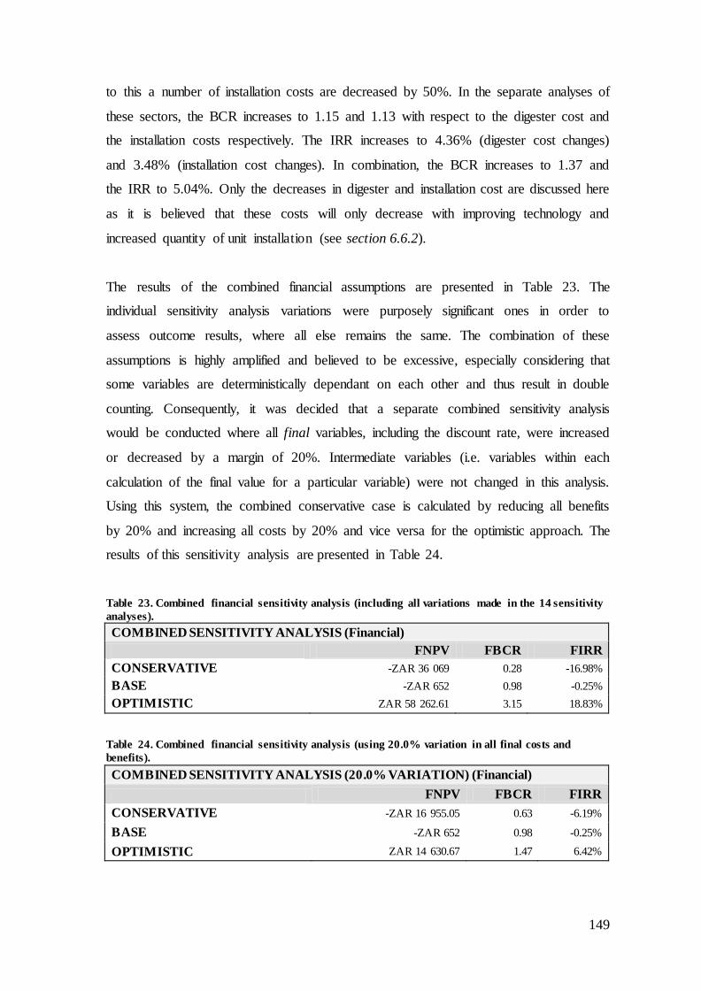
149

to this a number of installation costs are decreased by 50%. In the separate analyses of

these sectors, the BCR increases to 1.15 and 1.13 with respect to the digester cost and

the installation costs respectively. The IRR increases to 4.36% (digester cost changes)

and 3.48% (installation cost changes). In combination, the BCR increases to 1.37 and

the IRR to 5.04%. Only the decreases in digester and installation cost are discussed here

as it is believed that these costs will only decrease with improving technology and

increased quantity of unit installation (see section 6.6.2).

The results of the combined financial assumptions are presented in Table 23. The

individual sensitivity analysis variations were purposely significant ones in order to

assess outcome results, where all else remains the same. The combination of these

assumptions is highly amplified and believed to be excessive, especially considering that

some variables are deterministically dependant on each other and thus result in double

counting. Consequently, it was decided that a separate combined sensitivity analysis

would be conducted where all final variables, including the discount rate, were increased

or decreased by a margin of 20%. Intermediate variables (i.e. variables within each

calculation of the final value for a particular variable) were not changed in this analysis.

Using this system, the combined conservative case is calculated by reducing all benefits

by 20% and increasing all costs by 20% and vice versa for the optimistic approach. The

results of this sensitivity analysis are presented in Table 24.

Table 23. Combined financial sensitivity analysis (including all variations made in the 14 sensitivity

analyses).

COMBINED SENSITIVITY ANALYSIS (Financial)

FNPV FBCR FIRR


BASE -ZAR 652 0.98 -0.25%

OPTIMISTIC ZAR 58 262.61 3.15 18.83%

Table 24. Combined financial sensitivity analysis (using 20.0% variation in all final costs and

benefits).

COMBINED SENSITIVITY ANALYSIS (20.0% VARIATION) (Financial)

FNPV FBCR FIRR

CONSERVATIVE -ZAR 16 955.05 0.63 -6.19%

BASE -ZAR 652 0.98 -0.25%

OPTIMISTIC ZAR 14 630.67 1.47 6.42%

150

As with all the conservative and base case sensitivity analyses conducted, the 20.0%

variation results in a BCR and IRR which do not support financial feasibility. The

optimistic case of 20.0% variation reveals a BCR of 1.47 and an IRR of 6.42% (Table

24), a positive outcome which supports potential feasibility. The result is not, however, a

resoundingly significant one, considering the substantial optimism inherent in a 20.0%

increase in all benefits, and a 20.0% decrease in all costs. As will be discussed in section

6.2.3, the positive outcomes of the 20.0% optimistic variation are not significant in

comparison with existing studies.

The financial results, even in the case of the 20.0% variation, suggest that a biodigester

is not financially feasible for installation in the Okhombe community. The potential for

feasibility through reductions in financial cost and/or the impact of a government

subsidy will be discussed in section 6.6.2 and section 6.5 respectively.

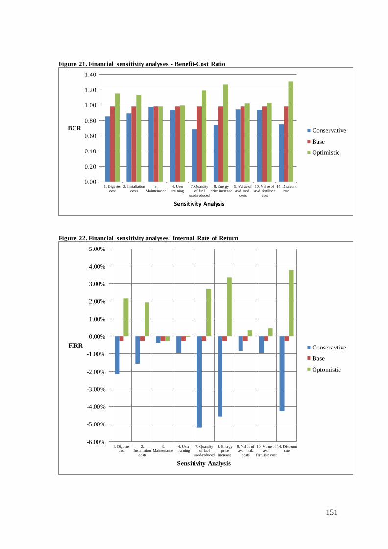
151

Figure 21. Financial sensitivity analyses - Benefit-Cost Ratio

Figure 22. Financial sensitivity analyses: Internal Rate of Return

0.00

0.20

0.40

0.60

0.80

1.00

1.20

1.40

1. Digestercost

2. Installationcosts

3.Maintenance

4. Usertraining

7. Quantityof fuel

used/reduced

8. Energyprice increase

9. Value ofavd. med.

costs

10. Value ofavd. fert iliser

cost

14. Discountrate

BCR

Sensitivity Analysis

Conservative

Base

Optimistic

-6.00%

-5.00%

-4.00%

-3.00%

-2.00%

-1.00%

0.00%

1.00%

2.00%

3.00%

4.00%

5.00%

1. Digestercost

2.Installation

costs

3.Maintenance

4. Usertraining

7. Quantityof fuel

used/reduced

8. Energyprice

increase

9. Value ofavd. med.

costs

10. Value ofavd.

fertil iser cost

14. Discountrate

FIRR


Conseravtive

Base

Optomistic

152

6.2.3. Comparison with Existing Studies

Direct comparison with studies involving the BiogasPro, and specific installation

requirements, cannot be made as these do not yet exist. It is, however, possible to

compare the results to existing studies conducted on the feasibility of biodigester

systems. Renwick et al (2007) conducted a feasibility study considering the installation

of biodigester and latrine systems in Uganda, Rwanda, Ethiopia and Sub-Saharan Africa

(SSA). Renwick et al (2007: 40) calculated FIRRs for Uganda (8%), Rwanda (9.5%),

Ethiopia (10.3%) and SSA (7.5%). Austin and Blignaut (2008) conducted the South

African National Biogas Feasibility Study, which assessed the potential for biodigester

systems in three provinces of South Africa (the Eastern Cape, KwaZulu-Natal and

Limpopo provinces). Austin and Blignaut (2008: 28) calculated a cumulative 16% FIRR

for the three provinces in South Africa, at a 0% subsidy level.

The most notable difference in these project appraisals is in the capital cost of the

biodigester and its installation. The cost of a 6 m3 biogas plant in the Austin and

Blignaut (2008: 27) study was ZAR 8 050.00 (2008 value) and the average capital cost

for the Ethiopian area, the highest FIRR in Renwick et al’s (2007: 47) study, is ZAR 5

402.18 (2007 value). These costs are extremely low in contrast to a biodigester cost of

ZAR 22 743.00 and a total financial cost of ZAR 38 532.20 in the current study, which

predictably produce a negative FIRR of -0.25%. If the biodigester and installation costs

in the current study were assumed to be (ZAR 9405. 9241) with all other costs remaining

the same, the FIRR would be 17.93%. This result displays the significance of capital

costs and opens the dialogue for discussion on this point to follow in section 6.6.2.

It is also noted that the discount rate used in Renwick el al’s (2007) study is 3% as

opposed to the base case 6% used in this research project. Altering the discount rate to

3% in this project would produce a FIRR of 2.77%; a positive result, but still

significantly lower than the lowest rate of 7.5% (SSA) found in Renwick et al’s study.

41

The cost of a biogas plant used in the Austin and Blignaut (2008) study, adjusted for annual inflation

(Stats SA, 2011a). Transport and accommodation of service providers are kept unchanged, as is the cost of

gas plumbing.

153

6.3. ECONOMIC ANALYSIS

6.3.1. Discussion of Base Case Scenario Results

Under the base case scenario for Okhombe, with the use of a BiogasPro as the digester

and a discount rate of six per cent; the economic NPV is ZAR 178 783.29, the EBCR is

4.83 and the EIRR is 57.68%. The results of the economic analysis (Table 19) displayed

a significantly feasible outcome in contrast to a non-feasible financial analysis result.

With regard to the economic costs, the biodigester cost is the greatest contributor to total

cost at 48.7% of total economic cost. Similarly to the financial analysis, installation

costs are the second highest contributor at 23.49%. The economic cost of time taken to

feed and run the biodigester is the next highest contributor at 17.3% of total economic

cost.

The substantial economic benefits were driven up considerably by the value of saved

lives which represented 65.8% of the total economic benefit. The next highest

contributor was the economic value of time saving related to biogas use and the benefit

of avoided fuel costs; 17.0% and 14.5% of total economic benefit respectively.

The base case scenario is significantly in favour of feasibility for a biodigester system

installed in Okhombe. A sensitivity analysis is conducted to assess the impact of key

variable changes and to test the robustness of this strong case of economic feasibility.


The results of the 14 sensitivity analyses are summarised in Table 46 (appendix X) and a

graphical representation of these results is presented in Figure 23 and Figure 24. In both

Figure 23 and Figure 24, it is clear that the changes to the value of a statistical life

(VOSL) have the greatest impact. The optimistic case VOSL is US$ 9.1 million which is

the standard rate used by the Environmental Protection Association (EPA) of the United

States and is arguably one of the most scientifically sound values for developed

countries (Sinha et al, 2010: 121). A zero value is used in the conservative approach, not

because the value of life is being disregarded, but rather in an effort to test the

significance of all other economic variables where the value of saved lives clearly

overwhelms other benefits in the base case (65.8% of total economic benefit). Under a

154

zero VOSL assumption, the BCR and IRR remained positive with values of 1.65 and

11.19% respectively – still strong evidence of economic feasibility.

The only other variables that appear to make a noteworthy effect on the EBCR and

EIRR are the reduction of indoor air pollution (IAP) and the change in the discount rate.

A change of 25% reduction in IAP, either side of the base case, results in the BCR

ranging from 3.59 to 6.07 and the IRR ranging from 39.9% to 75.5%. These significant

changes are not surprising as they relate directly to the value of saved lives which

contributes 65.8% to total economic benefit. Changing the discount rate by 4% either

side of the base case of 6% results in the BCR ranging from 6.08 to 3.85, and the IRR

ranging from 64.4% to 51.01% in the optimistic and conservative cases respectively.

These results are significant, but in contrast to the case of financial analysis, the BCR

and IRRs remain positive in all variations of discount rate.

As discussed in the financial analysis (section 6.2.2), the combined results of all

individual variations (Table 25) are considered to be excessive and thus a combined

20.0% variation sensitivity analysis is included for discussion (Table 26).

The combined 14 individual sensitivity analyses displays a highly amplified result of

489.1% (IRR) and a BCR of 32.37 (Table 25). The conservative 14 individual sensitivity

analysis combination reveals the first negative BCR and IRR of the economic analysis;

however, the result of 0.51 (BCR) and -11.81% (IRR) are insignificant in comparison to

both the base case and optimistic case scenarios.

The result of the 20.0% variation sensitivity analysis (Table 26) displays valuable

outcomes. The conservative assumption, where all final benefits are decreased by 20.0%

and costs increased by 20.0%, still remains significantly positive with a BCR of 3.03

and an IRR of 32.07%. Of even greater interest is that the BCR and IRR remain positive

at 1.06 and 1.08% respectively where the value of saved lives is devalued to zero.

Again, it is not suggested that the value of life be disregarded, but rather that the

robustness of all other variables be tested in this sensitivity analysis. The values of BCR

and IRR in this instance are not high, but do remain positive.

155

Table 25. Combined economic sensitivity analysis (including all variations made in the 14 sensitivity

analyses).

COMBINED SENSITIVITY ANALYSIS (Economic)

ENPV EBCR EIRR


BASE ZAR 178 783 4.83 57.68%

OPTIMISTIC ZAR 1 099 821.77 32.37 489.07%

Table 26. Combined economic sensitivity analysis (using 20.0% variation in all final costs and

benefits).

COMBINED SENSITIVITY ANALYSIS (20.0% VARIATION) (Economic)

ENPV EBCR EIRR

CONSERVATIVE ZAR 112 378.84 3.03 32.07%

BASE ZAR 178 783 4.83 57.68%

OPTIMISTIC ZAR 233 221.72 7.24 99.84%

The result of the economic sensitivity analysis strongly supports the finding of economic

feasibility, even when significant changes are made to a range of variables. The finding

of economic feasibility is also robust to a conservative sensitivity analysis of 20.0%

reduction to all final benefit variables and an increase of 20.0% to all final cost

variables. These findings argue strongly for the potential value contribution to society

through biodigester installation in the Okhombe community. Further to this, this result

might provide compelling motivation for the merits of a government subsidy to

strengthen financial feasibility and desirability. The potential for this outcome will be

discussed further in section 6.5.

156

Figure 23. Economic sensitivity analyses - Benefit-Cost Ratio

Figure 24. Economic sensitivity analyses - Internal Rate of Return

0.00

2.00

4.00

6.00

8.00

10.00

12.00

14.00

BCR


Conservative

Base

Optimistic

0.00%

20.00%

40.00%

60.00%

80.00%

100.00%

120.00%

140.00%

160.00%

180.00%

200.00%

EIRR


Conservative

Base

Optimistic

157

6.3.3. Comparison with Existing Studies

As noted in the comparison of financial results (section 6.2.3), a direct comparison to a

precisely similar study is not possible. Again, the findings of Renwick et al (2007) and

Austin and Blignaut (2008) are considered in the comparison of economic results.

The economic IRR calculated by Austin and Blignaut (2008: 29) for the South African

National Biogas Feasibility Study, was 52% (CO2 emission benefits are excluded in this

estimation, as is the case in the current study). This EIRR is not dissimilar from the

EIRR of 57.7% calculated in the current study. On further analysis, it is noted that

Austin and Blignaut (2008) did not include the value of life in their calculations. The

value of life is a considerable contributor to the EIRR calculated in this study and with

its exclusion the EIRR is recalculated to be 11.2%. The corresponding difference

between the two studies is of no major surprise, considering the significant financial cost

differences which have been highlighted in section 6.2.3.

In comparison with the Renwick et al (2007) study, the current study findings are

markedly lower. In the Renwick et al (2007: 52) study, EIRRs of 166% (Uganda), 161%

(Rwanda), 78% (Ethiopia) and 178% (Sub Saharan Africa) were found. The value of life

is not a distinguishing variable in this case as the VOSL used by Renwick et al (2007:

34) was extrapolated for the purpose of the current study. Again, the substantially lower

financial costs in the Renwick et al study are most likely to be responsible for the higher

EIRR findings, and it is noted that the study conducted by Renwick et al (2007) is made

in reference to very large scale projects where economies of scale are of great

significance. The number of biodigesters proposed for installation in SSA, for example,

is 2 002 800 and the corresponding economic cost per digester installation is ZAR

13 970.65 (PPP-adjusted 2011 ZAR). Using this financial cost of a biodigester

installation, the EIRR of the current project is recalculated at 195.1% which is not

dissimilar from the value of 178% calculated for SSA (Renwick et al, 2007: 52).

6.4. LIMITATIONS OF THE STUDY

6.4.1. The Aggregation of Individuals to Society

One of the limiting aspects of a CBA of this nature is that impacts are quantified on the

basis of an average household. This process is an inescapable one, as it would not be

158

possible to access all households' specific characteristics and recalculate the CBA for

each individual household. As an example of the limitation of this method of

quantification, the benefit of avoided fuel costs is calculated on the average fuel usage of

the average household in Okhombe. In reality, it is probable that some households use

significantly more purchased fuel than others. Those who spend more on energy for

cooking (potentially the relatively higher income households) are more likely to benefit

financially from a biodigester than the poorer, or those who use less purchased fuel for

cooking. Financial desirability of a rural household biodigester is calculated on the basis

of aggregate data and thus cannot be directly translated to each household. Kopp et al

(1997: 6) note a fault in this system of measurement being the potential of favouring a

specific category of people (potentially the more affluent in this case) and in doing so,

neglecting distributional considerations. A suggestion for further study would be to

segment the population under specific categories (Renwick et al, 2007: 10). Given this

practice, it would be possible to more accurately distinguish benefits between those who

collect firewood, those who purchase firewood and those who use different primary

energies for cooking.

6.4.2. Limitation of the Biodigester Range Assessed

This CBA assessed the feasibility of only one type of biodigester, the BiogasPro. The

results clearly indicated that the cost of this product is significantly higher than the

technology used in other biodigester feasibility studies (sections 6.2.3 and 6.3.3). The

BiogasPro, albeit expensive, is reputed to be a technologically advanced product with

many benefits as well as being the only known prefabricated biodigester in South Africa.

Further research on this topic would be enhanced by an inclusion of different biodigester

systems, possibly including internationally produced technologies and digesters

constructed on site.

6.4.3. Availability of Data

The availability of data presented some constraint to the accuracy of impact

quantification and limited some assessments from being made.

Specific health statistics were not accessible for the area in question and it was thus

necessary to extrapolate both national and regional data for the quantification of

impacts. Although this might be acceptable where localised data is not available

159

(European Commission, 2006: 11), the accuracy of these results must be treated with

circumspection (Caulkins, 1987: 69). An accurate assessment of the health-related

impacts of a biodigester installation would require detailed area specific information.

The degree to which this would be possible or feasible, considering the scale of

resources required, is questionable.

The quantification of energy fuels used for cooking was limited by the availability of

data relating to the specific disaggregated consumption of fuels for cooking. It appeared

that information relating to the specific proportions of fuel used for cooking are not

available and research relating to this topic would be useful to perform accurate impact

assessment. The degree to which it would be possible, and again resource efficient, to

determine these fuel usage proportions is potentially limited itself.

The specific environmental impacts (including potential reductions in CO2 emissions,

reduced indigenous plant deforestation and other local environmental benefits) were

excluded from this analysis based on an absence of case specific information and a

reluctance to use existing studies whose methods are yet to be fully accepted. This topic

will be discussed further in section 6.6.1.3.

6.4.4. Area Specific Analysis

The costs and benefits in this research project are calculated for the average household

in the Okhombe community. Although the Okhombe community is believed to be

representative of many rural communities in South Africa, the energy use profiles

amongst other household characteristics are not interchangeable with all rural

communities. For this reason, the results of this analysis should be extrapolated for other

rural areas with great caution.

6.5. THE ARGUMENT FOR GOVERNMENT SUBSIDISATION

The financial analysis shows that a biodigester is not financially feasible for installation

in an average household in Okhombe. It is understood that very few, if any, households

in Okhombe would be able to pay for the capital outlay of a biodigester system and thus

an FIRR of magnitude greater than the interest rate on a loan (to be discussed in section

6.7.1) would be required for actual financial feasibility.

160

Although the results display a non-feasible financial investment, a significantly feasible

economic result is evident by the EIRR of 57.68%. The economic CBA result is

descriptive of the social desirability of a project. The EIRR of 57.68% and EBCR of

4.83 clearly indicate economic benefit (and benefit to society) well beyond economic

costs. If government’s position is to improve the social welfare of its people, then such a

resounding societal benefit of a project is a strong argument for a government subsidy at

least up until a point where the project becomes financially feasible and desirable for

individual households.

Referring back to the introductory discussion of sustainable development and a

sustainable development ‘package’ of “natural resource management, food, water, and

energy access, provision and security” (Blignaut, 2009: cited in Blignaut and van der

Elst, 2009: 14), an economically desirable biodigester has great merit in meeting social

welfare objectives. A well designed and orchestrated biodigester project has the

potential to:

Provide energy access, provision and security in the form of biogas.

Provide the potential for food security through the use of bioslurry as a fertiliser

to grow food.

Assist in natural resource management through: the reduction of deforestation;

the potential to use bioslurry to grow fodder for cattle and improve the

sustainability of cattle management practices; and the potential for a biodigester

and biogas use to reduce CO2 and GHG emissions.

6.6. A DISCUSSION OF COST AND BENEFIT FLOWS

6.6.1. Discussion of Benefit Flows

6.6.1.1. The increasing price of energy for cooking

An assumption, believed to be conservative, was made that the price of paraffin and

LPG (whose price is related to the price of Brent crude oil) would increase at the

aggregate annual real rate (nominal rate less inflation) of crude oil price increases that

had been experienced over the prior 15 years. On further analysis of this topic, it was

found that crude oil price forecasts tend to be highly varied with one analyst predicting a

nominal price of US$ 300 by 2020 (Kedrosky, 2011; Christian Broadcasting Network,

161

2011) and another, albeit potentially unreliable, forecasting a price per barrel of less than

US$ 20 – due to advancements in alternative energy sources and a decreased demand for

oil (Alternative Energy Today, 2008). Although both of these predictions are hotly

contested, the range illustrates the difficulty in making predictions about fuel energy

pricing. This discussion will venture no further on the available literature regarding

future predictions; however, the recent history of crude oil price increases is of interest.

Figure 25. Crude oil price history 1981 - 2011.

(Data source: IMF, 2011c)

Figure 25 shows the past 30 year crude oil price history (IMF, 2011c), where it becomes

clear that the past 10 years have revealed the most dramatic rise in crude oil price. From

1981 to date (2011) the price of crude oil has increased by 203.2%. Further analysis

reveals that while the price of crude oil decreased from 1981 to 1990, it increased by

25.6% from 1991 to 2001 and by 324% from 2001 to 2011.

The potential price increase of paraffin and LPG are noted to have a significant effect on

the financial (and economic) returns of a biodigester. The result of sensitivity analysis

eight (Table 45 ,appendix X) show that an increase of 5.2% in the annual real LPG and

paraffin price (and an increase in the real electricity price of 4.7% per annum) resulted in

a movement from a negative base case IRR of -0.25% to a positive 3.33%. This result is

significant and if the exponential increases in the fuel price of the last 10 years were to

continue over the 15 year project life cycle, the financial returns would be substantially

increased.

0

20

40

60

80

100

120

198

11

98

2

198

3

198

41

98

5

198

6

198

71

98

8

198

9

199

0

199

1

199

2

199

31

99

4

199

5

199

61

99

7

199

8

199

92

00

0

200

1

200

22

00

3

200

4

200

52

00

6

200

7

200

82

00

9

201

0

201

1

Price per barrel (US$)

Year

162

While the forecast price of oil is uncertain, the probability of electricity prices increasing

in South Africa is more predictable. The base case feasibility assessment assumed an

annual real price increase in electricity of just over 2%, based on the average increase

over the past 15 years (Eskom Holdings, 2011a). The National Energy Regulator of

South Africa (NERSA) has granted Eskom Holdings (the sole electricity supplier to

South Africa) permission to increase electricity prices by 24.8% (2010/2011), 25.8%

(2011/2012) and 25.9% (2012/2013) (Eskom Holdings, 2011b: 1). Even in the case

where electricity price follows a 15 year average increase after the 2013 price increase,

the average annual price increase for the next 15 years will be higher than that assumed

in the CBA base case scenario.

In addition to these set price increases, the National Integrated Resource Plan (2010) for

electricity concluded a projection of “annual increases well above inflation up to 2021”

(Rycroft et al, 2011; Muller, 2011). A one per cent increase in real electricity price per

year (all else remaining the same) results in a 0.23% increase in the FIRR. Although this

appears to be minor, a substantial rise in electricity price (as is being predicted) will

make a notable effect on the financial feasibility and subsequent desirability of a

biodigester.

6.6.1.2. Further potential for farming productivity

The benefit of a biodigester (and the output of bioslurry) to farming practice was

quantified as the avoided cost of purchased fertilisers. A well designed biodigester

system, with the inclusion of rain water harvesting systems and fodder cultivation (as is

being investigated in the Water Research Commission Biogas Project42), has the

potential to provide benefits well beyond the mere replacement of purchased fertilisers.

A project in which biodigester household members are trained to use harvested water

and bioslurry to grow food and fodder for their cattle, has significant potential to

improve the health of both cattle and people as well as instigating improved cattle

management practice which will, in turn, contribute to the preservation of natural

resources. Further study on these topics is required, but it is believed that a suitable

42

WRC Project number K5/1955.

163

fodder feeding programme will benefit the health of cattle greatly and reduce grazing

pressures on the land – resulting in reduced erosion. These outcomes have great

potential in terms of food supply and resource management for sustainable development.

The increased economic benefit inherent in these outcomes is likely to further increase

the societal desirability of the project.

6.6.1.3. Environmental benefits

Local and societal environmental benefits were excluded from this study based on an

absence of current research and the reluctance to use existing research whose

methodology and applicability to the current study is questionable. Although these

impacts were omitted from the current study, it is strongly believed that their benefit is

potentially immense and would improve the economic desirability of the project.

In addition to the local environmental benefits that were described as improved farming

practices and sustainable resource management in section 6.6.1.2, the use of biogas for

cooking does have the potential to reduce deforestation of indigenous plants. As noted in

section 4.7.2.3 these benefits were not quantified due to the lack of specific knowledge

and the uncertainty of whether the deforestation of alien tree species (as a result of

household use) would actually be a benefit to society (and consequently a cost, if biogas

resulted in a reduction of this process).

A reduction of CO2 and GHGs is a significant potential impact with the use of biogas

reducing solid fuel use for cooking and improved manure management practices

resulting in reduced methane (CH4) and nitrogen dioxide (N2O) emissions (Tao et al,

2007: 3). Reduced emission of CO2 was precluded from the benefit assessment based on

a reluctance to use information that did not relate directly to the system in question. Of

interest, AGAMA Energy is currently researching the potential for the BiogasPro to

reduce GHG emissions (pers. com. Greg Austin, November 2011) and this information

will benefit future biodigester impact assessments.

A biodigester has the potential to provide clean energy as well as many related impacts

that may benefit preservation of environmental resources. Further studies should be

aimed at assessing some of these impacts and including them in impact appraisals.

164

6.6.1.4. Calculated energy usage in relation to existing studies

The quantified energy costs of this study are compared with those calculated in Paulsen

et al (2010) as this study appeared to be extensive and representative of rural areas in

KwaZulu-Natal and South Africa as a whole. The Paulsen study covered a sample size

of 4 427 households throughout South Africa and 502 households in rural areas of

KwaZulu-Natal (Paulsen et al, 2010: 17). The study sample areas are largely comparable

and the similarities of the Paulsen study sample areas characteristics to the current study

have been noted in section 4.7.1.1.2.

Paulsen et al (2010: 23) found that household expenditure on energy (cooking, heating

and lighting energy) were similar across all income groups and ranged from ZAR 200 to

ZAR 268 per month. It was noted, however, that the monthly energy expenditure as a

percentage of household income did range greatly with the highest expenditure as a

percentage of income being 26%, in the lowest income bracket (ZAR 0 to ZAR 1 500).

The cost of candles (the primary source of lighting for households in Okhombe) was not

estimated in the current study. Extrapolating the aggregate expenditure of candles found

in the Paulsen et al study (2010: 23) to the current study, the aggregate monthly

expenditure on energy for lighting, heating and cooking is ZAR 336.47. This value is

representative of 30.9% of the average Okhombe household’s monthly income and is

approximately 5% higher than the highest expenditure percentage of monthly income

quoted by Paulsen et al (2010: 23). The finding of this result is of no surprise to the

researcher. Considering only the cost of paraffin (not LPG and candles43, for which the

price increase is likely to be similar), the price of paraffin has increased by 44.0% since

the Paulsen study was conducted in January 2010 – an increase which is well beyond the

inflation rate (LPG-SASA, 2011; Stats SA, 2011a). It is recognised that price increases

are likely to translate to reduced consumption; however, these dramatic price increases

(also evident in the increased price of LPG) are likely to affect the percentage of

monthly income spent on energy, especially where price changes occur over a relatively

short period of time (the price of paraffin increased by 29.3% in the year prior to the

date interviews were conducted in Okhombe).

43

A key ingredient in the production of candles is paraffin.

165

It is therefore concluded that the quantification of energy expenditure used in the current

study is not dissimilar to that found in the Paulsen et al (2010) study. This finding is

quoted with confidence.

6.6.1.5. Realisation of benefits

A final comment with regard to benefit flows should be made. The benefits described in

this project, arising from biodigester and biogas use, are all dependent on rural

households acting to take advantage of these benefits. A biodigester does not provide a

constant flow of benefits without the input of household members in feeding the

biodigester regularly, and acting to realise benefit flows – by replacing household use of

purchased energy fuels and fertiliser with biodigester by-products. The CBA was based

on the assumption that all user households act in such a manner that all biodigester

benefits are effectively realised.

6.6.2. Discussion of Cost Flows

6.6.2.1. Capital cost of the biodigester and potential for economies of scale

In this study, the cost of a biodigester (the BiogasPro) contributes 59.02% of the

financial costs in the CBA. The financial analysis (section 6.2) revealed a negative

investment net present value (NPV) and it is clear that the potential for the biodigester

system to become financially desirable would depend on a significant reduction of the

financial costs and/or a viable government subsidy.

Although the BiogasPro supplier was unable to provide specific details on the potential

for economies of scale with anticipated reduction of the cost of a biodigester (see section

4.6.1.1), the potential for these to exist appears logical. A brief analysis of prefabricated

plastic water tanks in comparison with the BiogasPro provides some evidence for this.

While it is noted that a BiogasPro is not directly comparable to a plastic water tank, the

comparison is believed to provide interesting insight given that both products are based

on plastic mould construction. A 4 500 litre Build-it Water Tank was advertised in a

marketing supplement at a price of ZAR 2 699.95 (Build-it, 2011: 5). A comparable

water tank to that advertised is said to weigh in the region of 80 kg (pers. com. Richard

Jardine, December 2011). It is understood that a BiogasPro requires specific design

technology to improve strength and pressure holding capacity and in contrast to these

tanks, weighs in the region of 300 kg (AGAMA Energy, 2010). This information cannot

166

be applied directly to formulate an understanding of potential economies of scale in the

production of biodigester tanks; however, if material costs were taken alone (assuming

the same material is used for the construction of water and biodigester tanks44) then a

biodigester could potentially cost in the region of ZAR 10 124.8145. While these

calculations are far from precise, they do provide food for thought. The transport cost of

a BiogasPro to the Pietermaritzburg area (the area in which the Build-it water tank is

being sold at a final value of ZAR 2 699.95) is ZAR 2 280.00, some 85% of the final

cost of a Build- it water tank.

The evidence is noted to be highly assumptive and not directly comparable, but is

certainly interesting in terms of the potential of economies of scale and vast reductions

in financial cost where increased biodigester tank production becomes a reality. Further

research is needed on the topic of economies of scale. Accurate predictions of reduced

financial cost have significant potential to promote rural development projects involving

the installation of biodigesters in rural households.

6.6.2.2. Potential for reduction in installation costs

The cumulative cost of installation of the BiogasPro amounts to 28.47% of total

financial cost and is the next highest financial cost after the cost of a digester. A

reduction in installation costs will have a marked effect on the financial feasibility of a

biodigester system (as noted in the financial sensitivity analysis, section 6.2.2) and again

it appears pragmatic that an increased number of installations in a specific area has the

potential to reduce costs.

If 411 biodigesters were to be installed in the Okhombe community (based on the

number of strictly suitable households, see section 5.6) and potentially even more than

this in the surrounding areas, then it appears likely that most, if not all, costs involved in

the installation process would be reduced. If the adjusted suitability requirements (see

5.6) were permitted, it would be possible that even more households would qualify for

biodigester installation in Okhombe and the surrounding rural communities, providing

the possibility for further economies of scale.

44

Noting also that a BiogasPro has a capacity of 6 000 litres and not 4 500 litres. 45

Based on the material weight of each tank, a biodigester weighs 3.75 times more than a comparable

water tank and is thus taken as 3.75 multiplied by the cost of a comparable water tank.

167

Analysing the costs involved in the installation process briefly, it is noted that

accommodation and transport of service providers amounts to nearly 7% of installation

costs. A wide scale installation programme in the area would be likely to reduce most of

these costs on the assumption that a project of this scale would take a number of years to

complete and it is likely that local labour would be used for the installation of digesters.

The backfilling and ground preparation costs of installation contribute to 41.7% of

installation cost and it seems reasonable to assume that these costs would be greatly

reduced by mechanisation within a localised area. The plumbing of the digester system

(gas and water plumbing) makes up 51.6% of the digester installation costs. Improved

technological understanding and expertise on these specific systems will undoubtedly

result in decreases in the cost of plumbing the biodigester systems.

The financial feasibility of the biodigester systems described in this research is largely

dependent on reduced financial costs, and potential for government subsidisation. The

argument presented in this section suggests there is a potential for costs to be reduced

with increased unit production/installation and these assumptions will be elaborated on

in a hypothetical example in section 6.7.2.

6.6.2.3. The cost of transporting a biodigester

6.6.2.3.1. Financial cost of transport and potential for reductions

The cost of transporting a BiogasPro to Pietermaritzburg (from Cape Town) is

representative of 8.2% of total financial costs.

If a large scale roll-out of biodigester systems to rural areas of KwaZulu-Natal were to

be instigated, it would be advisable to use local industry to produce biodigester tanks in

an effort to reduce transportation, and ultimately financial, costs.

6.6.2.3.2. The social cost of transportation

The social cost of carbon (SCC) approach was used to calculate an estimate of the cost

to society of transporting biodigesters from Cape Town to Okhombe (see appendix IV).

The approach used considered the cost of transport to be the cost of increased CO2

equivalent emissions into the atmosphere. In reality, the cost to society of transport is a

combination of increased road congestion, CO2 equivalent emissions, the cost of road

168

maintenance, the environmental externalities inherent in production of transportation

vehicles and by-products and even the use of land on which roads are built (Tietenberg

and Lewis, 2010: 370). Arguably, the transport costs of one biodigester are well beyond

the assumptions made in the approach used for the current study. The valuation of this

impact would require specific and in-depth knowledge of the transport and was not

feasible within the parameters of this research project. Further research on this topic

should examine these potential costs and it is noted that, given the multiple potential

impacts of transport costs, both financial and economic, the argument for localised

biodigester production is compelling.

6.7. SCALE OF ANALYSIS

The appraisal of a household biodigester has been presented thus far as a household unit

expressed in per household values. The extension of this process is to consider the

biodigester as a household investment. In addition to this, a brief discussion of a

hypothetical roll-out of biodigester systems to all suitable households in the Okhombe

community and surrounding rural areas is considered valuable.

6.7.1. A Biodigester as a Household Investment

Based on the findings of the CBA presented in Table 19 (section 5.9), a biodigester is

not a financially feasible investment for a rural household. Further to this, the direct

financial benefits accruing to user households are exaggerated in the finding of a

financial IRR of -0.25% as avoided medical costs are considered a benefit to society (a

reduction in government health care costs) and not a financial benefit to the household

itself. If these benefits are removed from the analysis of household financial benefits, the

FIRR is -0.84%.

Although a substantial economic IRR represents a desirable investment in terms of

social welfare benefits, it is unlikely that a rural household would invest in a biodigester

and suffer a potential financial loss. It is also not likely, even considering the potential

health-benefiting and time saving implications of a biodigester, that a household would

make this investment. Based on a loan at current South African prime interest rate of

9.0% (as of December 2011), a zero per cent deposit and various payback periods

expressed in Table 27, it is clear that even over a 15 year repayment period the monthly

169

instalments would be well in excess of an average household's potential monthly savings

of ZAR 211.3946 in 2011 (saving on avoided fuel and fertiliser costs47) (see section

5.8.1).

Table 27. Monthly repayments in ZAR.

MONTHLY REPAYMENTS IN ZAR

Capital investment ZAR 38 532.23 Interest rate 9.0%

Terms in months Monthly repayment Total repayment

60 ZAR 799.87 ZAR 47 991.94

120 ZAR 488.11 ZAR 58 573.20

180 ZAR 390.82 ZAR 70 347.52

As proposed in section 6.5, the case for a government subsidy is compelling given the

significant economic and societal welfare benefit shown by the economic results (see

section 6.3). It is proposed that government subsidisation, at least to a point where

financial desirability becomes evident, would be worthy of consideration. Financial

desirability would be at a point where the financial IRR of household benefits (as

discussed above) is in excess of the rate of interest of a loan.

Calculations reveal that a capital subsidy of ZAR 16 953.79 would be required in order

to produce a household specific financial IRR of 9.00%. This amount would thus, under

the base case scenario, be the minimum capital subsidy required to make a biodigester

financially feasible for the average household in Okhombe. Table 28 displays the effect

of various subsidy levels on the FIRR and monthly repayment.

Table 28. Effects of various levels of government subsidy on monthly repayment and FIRR.

EFFECTS OF VARIOUS GOVERNMENT SUBSIDIES ON MONTHLY REPAYMENT AND

FIRR

Capital investment ZAR 38

532.23 Interest rate 9.0%

Terms in months

ZAR 10 000 Subsidy ZAR 16 593.79

Subsidy ZAR 20 000 Subsidy

FIRR Monthly

Repayment FIRR

Monthly

Repayment FIRR

Monthly

Repayment

180 3.79% ZAR 289.39 9.00% ZAR 218.86 12.35% ZAR 187.97

46

The value of life is also omitted from this discussion for logical reasons. It is expected that the value of

life as a probability of death and expenditure on funeral costs would be difficult to explain to rural

households. 47

This value is an undiscounted value and represents average household expenditure on cooking energy.

170

Based on the information provided in Table 28, the recommendation for a subsidy of

ZAR 20 000.00 is made. A subsidy of this amount would result in an FIRR of 12.35%

and would provide a financial incentive for the average household to invest in a

biodigester system repaid over a period of 15 years (180 months). A household’s

investment in a biodigester system would consequently secure the societal welfare gains

inherent in the substantial economic benefit. At an interest rate of 9%, the repayment of

this investment would be ZAR 187.97 per month, which is less than the monthly

monetary saving in avoided fuel and fertiliser costs, and would thus be a desirable

investment. It is also possible for various financial options to be investigated in which

various interest rate options are offered to households, at differing subsidy levels.

Regardless of the specific financial plan, it is believed that a financial incentive would

be required for households to invest in a biodigester system and so secure the

community economic and welfare benefits.

6.7.2. A Biodigester as a Rural Development Project

There is compelling evidence for a biodigester to be a valuable asset to the process of

sustainable development in rural areas. Biodigesters have the ability to contribute to the

energy needs of rural people as well as the potential to aid in food security development

and natural resource management. If a wide scale roll-out of biodigesters to suitable

households became a reality, it is probable that the cumulative benefits would result in

worthy benefit to society and the environment.

In this rural development project model, it is hypothesised that biodigesters are to be

installed in all suitable households in Okhombe (411 suitable households – see section

5.6) and to all suitable households in the local municipality region (Okhahlamba Local

Municipality). This model is based purely on assumptions and is presented as an

interesting scenario only. In this model, the assumption is made that sufficient

installations in the area are possible to reduce biodigester and installation costs

dramatically; however, it should be noted that the model is generated with respect to the

Okhombe community specifically48.

48

The Okhombe community is not expected to be large enough to result in economies of scale alone (see

section 4.6.1.1).

171

Table 29. Model of a hypothesised roll-out of biodigester installations to all suitable households in

Okhombe.

MODEL OF HYPOTHES IS ED ROLL-OUT

Number of installations 411 Government subsidy ZAR

5000

Interest

rate 9.00%

Cost of single installation ZAR 23 119.34

FINANCIAL NPV ZAR 8 121 786.24 ECONOMIC NPV ZAR 81 869 629.40

FINANCIAL IRR 13.93% ECONOMIC IRR 156.87%

FINANCIAL BCR 2.09 ECONOMIC BCR 8.58

Monthly terms of

repayment Monthly repayment

180 ZAR 183.78

In the CBA model presented in Table 29, the unproven assumption is made that all

financial costs are reduced by 40% due to economies of scale present in a large scale

roll-out of biodigester installation in a localised area. A government capital subsidy of

ZAR 5000.00 is assumed, the interest rate on the investment repayment is 9.00% per

annum and the repayment period is 15 years (180 months).

Under these assumptions, the financial and economic NPVs of the project are

approximately ZAR 8.1 million and ZAR 81.9 million respectively. The economic and

financial IRRs are 13.93% and 156.87%, and the BCRs are 2.09 and 8.58 respectively.

The calculation of these results does not include any environmental benefits and it is

believed that these would contribute significantly to the calculated economic returns.

The presented model is one based on assumption and extrapolation from the findings in

the study of the Okhombe population. Under these methods, it is clear that there is great

potential for a rural development project of this magnitude to contribute to the

sustainable development needs of rural areas like that of Okhombe. Further research into

the potential for large scale biodigester projects is required to clarify the potential of

economies of scale to reduce financial costs and the potential for biodigesters to have a

quantifiable impact on the environment.

6.7.3. A Biodigester as a Community Job Creation Project

It was presented in section 6.6.2.2 that installation costs of a biodigester could be

reduced by mechanised installations in a localised area. While it is clear that the

172

potential for economies of scale may be present in this process, an equally compelling

case could be made for the engagement of local communities in a biodigester project.

Rather than using service provider’s labour and mechanisation, local community

members themselves could be trained and enrolled in the excavation, backfilling and

construction tasks of a biodigester installation – potentially minimising the costs

involved in these processes. Possibly of greater benefit, is that such a system could

provide opportunity for skills development and employment. Such a model is also

expected to be of benefit in securing a sense of community ownership and

empowerment.

6.8. CONCLUSION

Financial and economic analyses of the current study have been presented in this

chapter. The results of these analyses indicate that the installation of a biodigester for

single rural households (at present financial cost) is not a financially feasible investment,

but is considered viable with respect to economic appraisal. It is clear that there is

latitude for significant reduction of financial costs and these reductions would be

necessary to generate potential financial feasibility. It was also suggested that the

quantification of environmental impact should be analysed further and additional

understanding of these impacts would be valuable to a more comprehensive appraisal of

biodigesters. As a household investment, it is suggested that a government subsidy in the

order of ZAR 20 000.00 would be required to encourage household acceptance. An up-

scaled model of biodigester installations to a significant number of households is

considered to present great merit for sustainable development.

173

CHAPTER 7: CONCLUSION

This study represents an effort to explore the practice and procedure of cost-benefit

analysis (CBA) as applied to a rural development project. A literature review outlined

the economic foundations of CBA and presented the real world difficulties CBA is

designed to manage. The procedure of CBA was defined and it was concluded that

successful and accurate project appraisal is largely dependent on effective quantification

and valuation of impacts.

A household questionnaire was designed and interviews were conducted in the study

area producing a valid sample size of 120 households representing approximately 10.2%

of the study area population. Methodology, informed by the literature review, was

applied to the study and the financial and economic impacts of biodigester installation in

a rural household in Okhombe were quantified and valued. Where current study data

was not available, existing study findings were weighted and extrapolated to the current

case. Along with community specific characteristics relating to energy usage and

farming practice, a comprehensive CBA and sensitivity analysis were presented.

The study reveals that further academic investigation would be of great value to future

project appraisals relating to biodigester use in rural communities. Specifically, further

studies relating to local and global environmental benefits, as well as the potential for

increased biodigester unit production and installation to give rise to economies of scale,

would be of particular value.

The final results revealed that a household biodigester, installed in the Okhombe

community, is not a financially feasible investment. For financial feasibility to be

achieved, it was concluded that significant capital cost reductions would be required. A

hypothesised biodigester roll-out model gives some indication of the potential for large

scale biodigester installation to contribute to sustainable development initiatives.

While the results indicate non-feasibility with respect to financial outcomes, it was

resoundingly clear that a household biodigester, installed in the Okhombe community,

would be an economically beneficial investment. Significant economic feasibility was

identified and this provides a convincing argument for the social value of biodigester

174

systems in rural households. Considering a governmental imperative to uplift the social

wellbeing of its people, the economic result is compelling evidence for government

support to make financial desirability of biodigester systems a reality.

175

LIST OF REFERENCES

Ackerman F, Stanton E. 2010. The Social Cost of Carbon. Economics for Equity and

Environment: Portland.

Acocks JPH. 1988. Veld types of South Africa. Memoir of the Botanical Survey of South

Africa. 57: 146.

AGAMA Energy. 2010. AGAMA BiogasPro – Product Datasheet. [AGAMA Biogas].

Available at:

[http://www.biogaspro.com/resources/Marketing/BiogasPro%20Product%20Datash

eet%20final.pdf] (Accessed 30 October 2010).

Alkire S, Santos ME. 2010. Acute Multidimensional Poverty: A New Index for

Developing Countries. Oxford Poverty and Human Development Initiative (OPHI):

Oxford.

Alternative Energy Today. 2008. Prediction: Oil Under $20 a Barrel by 2020.

[Alternative Energy Today]. Available at [http://alt-

energystocks.com/blog/2008/06/18/prediction-oil-under-20-a-barrel-by-2020/]

(Accessed 5 December 2011).

Appelbaum B. 2011. As U.S. Agencies Put More Value on Life, Businesses Fret . [The

New York Times]. Available at:

[http://www.nytimes.com/2011/02/17/business/economy/17regulation.html?_r=1&s

cp=1&sq=value%20life&st=cse] (Accessed 19 November 2011).

Asian Development Bank (ADB). 1999. Handbook for the Economic Analysis of Water

Supply Projects. ADB: Mandaluyong City.

Atkinson G. 2010. Environmental Valuation and Greening the National Accounts. The

World Bank: Washington DC.

Austin G, Blignaut J. 2008. South African National Rural Domestic Biogas Feasibility

assessment: Prepared for Ministry for Development Co-operation, The State of

Netherlands. AGAMA Energy: Cape Town.

176

Australian Government. 2007. Best Practice Regulation Handbook . Office of Best

Practice Regulation: Canberra.

Bangamwabo VM. 2009. Spatial and temporal extent of land degradation in a communal

landscape of KwaZulu-Natal, South Africa. Master of Science Thesis, University of

KwaZulu-Natal, South Africa.

Banik BK. 2010. Female perceptions on health hazards associated with indoor air

pollution in Bangladesh. International Journal of Sociology and Anthropology. 2(9)

206-212.

Barron’s Educational Series, Inc. 2000. Barron’s banking Dictionary: Poverty.

[Barron’s Educational Series] Available at:

[http://www.answers.com/topic/poverty#ixzz1Dv9DdC3N] (Accessed 19 February).

Bateman I. 1995. Environmental and economic appraisal, In: O’Riordan, T (ed). 1995.

Environmental Science for Environmental Management . Harlow: Longman.

Bateman IJ, Turner RK. 1995. Chapter 5: Valuation of the Environment, Methods and

Techniques: The Contingent Valuation Method, In: Turner RK (ed). 1995.

Sustainable Environmental Economics and Management. John Wiley: Chichester.

Bennett J. 2004. Realising Environmental Demands in Water Markets. Paper presented

at the Institute for Public Affairs Symposium “Establishing Australian Water

Markets”, Melbourne 9 August 2004.

Binning C, Commonwealth Department of the Environment (CDE), Sport and

Territories, Australian Department of Finance, Australian Resource Assessment

Commission. 1995. Techniques to Value Environmental Resources: an

Introductory Handbook. [Commonwealth Department of the Environment].

Available at:

[http://www.environment.gov.au/about/publications/economics/value/chapter2.ht

ml#concept] (Accessed 19 March 2009).

Blignaut J, van der Elst L. 2009. South Africa and Sustainable development: a

reflection. Perspectives: Political analysis and commentary from Southern Africa.

3: 13-18.

http://www.environment.gov.au/about/publications/economics/value/chapter2.html#concept

http://www.environment.gov.au/about/publications/economics/value/chapter2.html#concept

177

Blignaut J. 2009. Fixing both the symptoms and the causes of degradation: The need for

an integrated approach to economic development and restoration. Journal of Arid

Environments. 73(6-7): 696-698.

Brent RJ. 2006. Applied Cost-Benefit Analysis. (2nd Edition). Edward Elgar Publishing

Limited: Cheltenham.

Bromley DW. 1991. Environment and Economy: Property rights and public policy.

Blackwell: Cambridge USA.

Build-it. 2011. Build-it marketing supplement. The Witness 25 November, supplement,

p.5.

Bunny H, Besselink I. 2006.The National Biodigester Programme in Cambodia in

Relation to the Clean Development Mechanism, presented at National Workshop on

the integrated Capacity Strengthening for the Clean Development Mechanism in

Cambodia. [Clean Development Mechanism]. Available at:

[http://www.iges.or.jp/en/cdm/pdf/cambodia/activity03/F.pdf] (Accessed 20

November 2011).

Casey JF, Vukina T, Danielson LE. 1995. The Economic Value of Hiking: Further

Considerations of Opportunity Cost of Time in Recreational Demand Models.

Journal of Agriculture and Applied Economics. 27 (2): 658-668.

Caulkins P. 1987. A summary of the benefit-cost analysis of the final effluent limitation

guidelines for the organic chemicals, plastics, and synthetic fibers [sic] industry.

U.S. Environmental Protection Agency: Washington DC.

Christian Broadcasting Network. 2011. Analyst’s Prediction: Oil to Hit $300 by 2020.

[CBN News]. Available at:

[http://www.cbn.com/cbnnews/finance/2011/February/Analysts-Prediction-Oil-to-

Hit-300-by-2020/] (Accessed 5 December 2011).

Center for International Comparisons of Production, Income and Prices (CIC). 2006.

Penn World Table. [University of Pennsylvania] Available at:

[http://pwt.econ.upenn.edu/aboutpwt2.html] (Accessed 17 August 2011).

178

Center for International Comparisons of Production, Income and Prices (CIC). 2011a.

PWT Index Page. [University of Pennsylvania] Available at:

[http://pwt.econ.upenn.edu/php_site/pwt_index.php] (Accessed 14 December

2011).

Center for International Comparisons of Production, Income and Prices (CIC). 2011b.

PWT 7.0. [University of Pennsylvania] Available at:

[http://pwt.econ.upenn.edu/php_site/pwt70/pwt70_form.php] (Accessed 22

November 2011).

Cesarone J. 1999. Sell Your Product. IIE Solution: December: 32-37.

Chellan N. 2002. An assessment of tourism potential in the Okhombe area, KwaZulu-

Natal. Master of Arts Thesis. University of KwaZulu-Natal South Africa.

Chichilnisky G. 1997. The costs and benefits of benefit-cost analysis. Environment and

Development Economics. 2: 195-221.

Chirwa PW, Ham C, Maphiri S, Balmer M. 2010. Bioenergy use and food preparation

practices of two communities in the Eastern Cape Province of South Africa. Journal

of Energy in Southern Africa. 21 (4): 26-31.

Clive Van Niekerk GIS Office. 2009. KZ235 Ward Map. [Uthukela District

Municipality]. Available at:

[http://www.uthukeladm.co.za/uthukela/index.php?option=com_docman&task=doc

_download&gid=41&Itemid=202] (Accessed 28 November 2010).

Collins DL, Leibbrandt M. 2007. The financial impact of HIV/AIDS on poor households

in South Africa. AIDS. 21(7): 75-81.

Comcar. 2011. Kg CO2 per litre. [Comcar]. Available at:

[http://www.comcar.co.uk/newcar/companycar/poolresults/co2litre.cfm] (Accessed

11 November 2011).

Cooper J. 2001. Costs and Benefits of Eradication Alien Invasive Vegetation from the

Upper Reaches of the Mhlatuze Catchment. Master of Social Science Thesis.

University of KwaZulu-Natal, South Africa.

179

Damm O, Triebel R. 2008. A Synthesis Report on Biomass Energy Consumption and

Availability in South Africa. Programme for Basic Energy and Conservation in

Southern Africa (ProBEC): Pretoria.

Davies T. 2004. Calculation of CO2 emissions. [University of Exeter]. Available at:

[http://people.exeter.ac.uk/TWDavies/energy_conversion/Calculation%20of%20CO

2%20emissions%20from%20fuels.htm] (Accessed 11 November 2011).

Dekelver G, Ruzigana S, Lam J. 2005. Report on the Feasibility Study for a Biogas

Support Programme in the Republic of Rwanda. SNV: Rwanda.

Denzau A. 1992. Microeconomic Analysis. Richard D Irwin: Boston.

Department of Energy (Republic of South Africa). 2011a. Fuel Price History: 2011.

[Department of Energy]. Available at:

[http://www.energy.gov.za/files/esources/petroleum/Nov%202011/Fuel%20Price%

20History.pdf] (Accessed 23 November 2011).

Department of Energy (Republic of South Africa). 2011b. LPG Regulation. [Department

of Energy]. Available at:

[http://www.energy.gov.za/files/esources/petroleum/Nov%202011/LPG%20Regulat

ions.pdf] (Accessed 16 November 2011).

Department of Energy and Climate Change (DECC). 2011a. Social Cost of Carbon.

[DECC]. Available at:

[http://www.decc.gov.uk/en/content/cms/emissions/valuation/valuation.aspx]

(Accessed 11 November 2011).

Department of Energy and Climate Change (DECC). 2011b. Carbon values used in

DECC’s energy modelling. [DECC]. Available at:

[http://www.decc.gov.uk/assets/decc/11/cutting-emissions/carbon-valuation/3138-

carbon-values-decc-energy-modelling.pdf] (Accessed 11 November 2011).

Department of Labour (Republic of South Africa). 2011. Useful Documents.

[Department of Labour]. Available at: [http://www.labour.gov.za/documents/useful-

documents/basic-conditions-of-employment/useful-documents] (Accessed 11

November 2011).

180

Department of Land Affairs. 1997. Rural Development Framework. CTP Books:

Pretoria.

Drèze J, Stern N. 1994. Shadow prices and markets: Policy reform, shadow prices and

market prices. In: Layard R, Glaister S (eds). 1994. Cost-Benefit Analysis. (2nd

Edition). Cambridge University Press: Cambridge. pp. 59-99.

du Toit C, van Tonder J. 2009. Africa’s economic performance since 1994: can we do

better?. In: Parsons R (ed), Zumanomics. Jacana Media: Auckland Park.

Eaton BC, Eaton DF, Allen DW. 2005. Microeconomics theory with application. (6th

Edition). Pearson Prentice Hall: Toronto.

Edwards C. 2008. Social Cost-Benefit Analysis – the available evidence on drinking

water. In: Pond K, Pedley S, Edwards C. 2008. Valuing water – valuing well-being:

a guide to understanding the costs and benefits of water interventions. [World

Health Organization]. Available at:

[http://www.who.int/water_sanitation_health/economic/cb_interventions/en/index.h

tml] (Accessed 29 April 2011).

Environmental Protection Agency (EPA). 2005. Emission Facts: Average Carbon

Dioxide Emissions Resulting from Gasoline and Diesel Fuel. [EPA]. Available at:

[http://www.epa.gov/otaq/climate/420f05001.pdf] (Accessed 11 November 2011).

Eskom Holdings. 2011a. Average price increases. [Eskom Holdings]. Available at:

[http://www.eskom.co.za/c/article/143/average-price- increases/] (Accessed 27

November 2011).

Eskom Holdings. 2011b. Eskom Retail Tariff Adjustment for 2011/12. [Eskom

Holdings]. Available at: [http://www.eskom.co.za/content/priceincrease2011.pdf]

(Accessed 5 December 2011).

ETC UK. 2007. Promoting Biogas Systems in Kenya: A feasibility study. ETC Group:

Ottawa.

181

European Commission (EC). 2006. Guidance on the Methodology for Carrying out

Cost-Benefit Analysis – Working document No. 4. European Commission Director

General Regional Policy: Brussels.

European Commission (EC). 2002. Regional Foresight in the Cohesion Countries:

Experiences, concepts and lessons learned. European Commission Research

Director General: Brussels.

Everson TM, Everson CS, Zuma KD. 2007. Community based research on the influence

of rehabilitation techniques on the management of degraded catchments. WRC

Report No.1316/1/07. Water Research Commission: Pretoria.

Field BC, Field MK. 2006. Environmental Economics. 4th ed. McGraw-Hill: New York.

Florio M, Maffii S, Atkinson K, de Rus G, Evans D, Ponti M, Genco M, Parolin R,

Vignetti S, Bollati J, Giglio M, Panza G, Sartori D. 2008. Guide to Cost Benefit

Analysis of Investment Projects. European Commission: Brussels.

Flynn H. 2010. Digester Biogas and Energy Security. BioCycle. 51 (6): 33-34.

Forum for Economics and Environment (FEE). 2002. Environmental Economics and

Natural Resource Policy Analysis. [Forum for Economics and Environment

(FEE)]. Available at: [http://www.econ4env.co.za/training/MODULE9.pdf]

(Accessed 2 September 2009).

Forum for Economics and Environment (FEE). 2003. Training manual (draft 1) –

Module 4. [Forum for Economics and Environment] Available at:

[http://www.econ4env.co.za/training/MODULE4C.pdf] (Accessed 20 February

2008).

Franzese O, Knee HE, Slezak L. 2009. Effect of Tires on Class-8 Heavy Truck Fuel

Efficiency. Center for Transportation Analysis: Knoxville.

Fulford D. 1988. Running a Biogas Programme – A handbook. Intermediate Technology

Publications: London.

Gregory K. 2011. FOS Response to Environment Canada’s CO2 Emissions Reduction

Plan. Friends of Science Society: Connaught.

http://www.econ4env.co.za/training/MODULE9.pdf

182

Guidotti G. 2002. Biogas from Excreta – treatment of faecal sludge in developing

countries. SANDEC: Dübendorf.

Habermehl H. 2007. Economic evaluation of improved household cooking stove

dissemination programme in Uganda. German Agency for Technical Cooperation

(GTZ): Eschborn.

Hardin G. 1968. Tragedy of the Commons. Science. 162 (3859): 1243-1248.

Halter S. 2005. Biodigester Development in Saskatchewan. University of Saskatchewan:

Saskatoon.

Hanley N, Spash CL. 1993. Cost-Benefit Analysis and the Environment. Edward Elgar

Publishing: Brookfield.

Harberger AC. 1954. Monopoly and Resource Allocation. The American Economic

Review. 44 (2): 77-87.

Healey J. 2003. House of Commons – Environment, Food and Rural Affairs – Minutes of

Evidence. [Parliament UK]. Available at:

[http://www.publications.parliament.uk/pa/cm200203/cmselect/cmenvfru/929/3091

706.htm] (Accessed 11 November 2011).

Heinzerling L, Ackerman F. 2002. Pricing the Priceless. Georgetown University:

Georgetown.

Hellen M. 2010. Climate change mitigation in Agroindustries: the case of Mexico, paper

presented at FAO-CP/World Bank Workshop. Rome, 19-20 April.

Heltberg R. 2003. Household fuel and energy use in developing countries – A

Multicountry Study. The World Bank: Washington DC.

Hosking SG, du Preez M. 2004.A cost-benefit analysis of the Working for Water

Programme on selected sites in South Africa. Water SA. 30 (2): 143-152.

Hughes AG, Matsika R, Prasad G, Twine W. 2009. A model methodology representing

woodfuel supply and demand dynamics, paper presented at Domestic Use of Energy

(DUE) Conference. n.d. April.

183

Hutton G, Rehfuess E. 2006. Guidelines for conducting cost-benefit analysis of

household energy and health interventions. World Health Organization: Geneva.

International Monetary Fund (IMF). 2011a. AFR Regional Economic Outlook. [IMF].

Available at:

[http://www.imf.org/external/datamapper/?lang=EN&tab=mapView&chart=linecha

rtView&maximize=chartView&interactive=1&db=AFRREO&indicator=NGS_GD

P&indicatorx=NGDPD&indicatory=LP&year=2011&speed=1&geoitems=AGO,B

WA,COD,LSO,MDG,MWI,MUS,MOZ,NAM,SYC,ZAF,SWZ,TZA,ZMB,Z]

(Accessed 14 May 2011).

International Monetary Fund (IMF). 2011b. World Economic Outlook Database. [IMF].

Available at: [www.imf.org/external/pubs/ft/weo/2011/02/weodata/weoselagr.aspx]


International Monetary Fund (IMF). 2011c. IMF Primary Commodity Prices. [IMF].

Available at: [http://www.imf.org/external/np/res/commod/index.aspx] (Accessed

27 November 2011).

International Workshop on Domestic Biogas. 2009. Workshop report: How to improve

and scale up practices?. SNV Nepal: Kathmandu.

Irvin G. 1978. Modern Cost-Benefit Methods. MacMillan Press: London.

Isikhungusethu Environmental Services (IES). 2001. Okhahlamba Local Municipality

Integrated Development Plan, Phase 1: Report 1 Municipal Analysis. Okhahlamba

Local Municipality: Bergville.

Jenkins GP, Kuo C. 2007. Canadian Regulatory Cost-Benefit Analysis Guide. Treasury

Board of Canada: Ottawa.

Kedrosky P. 2011. Maxwell: Oil to $300 by 2020. [Infectious Greed]. Available at:

[http://paul.kedrosky.com/archives/2011/02/maxwell_oil_to.html] (Accessed 5

December 2011).

184

Khan KA, Khan A. 2009. Improved Bio-gas Plant – an Environmental Friendly

Renewable Energy. Proceedings of World Academy of Science: Engineering &

Technology. 51: 468-473.

King DM, Mazzotta JM. 2000. Ecosystem Valuation – Contingent Valuation Method.

[US Department of Agriculture, Natural Resources, Conservation Services].

Available at: [http://www.ecosystemvaluation.org/contingent_valuation.htm]

(Accessed 25 March 2009).

Kocabaş G, Kopurlu BS. 2010. An Ex-Post Cost-Benefit Analysis of Bolu Mountain

Tunnel Project. Ege Academic Review. 10 (4): 1279-1287.

Kopp RJ, Krupnick AJ, Toman M. 1997. Cost-Benefit Analysis and Regulatory Reform:

An Assessment of the Science and the Art – Discussion Paper 97-19. Resources for

the Future: Washington DC.

Krugman P, Wells R, Graddy K. 2007. Economics – European Edition. Worth

Publishers: Richmond.

Labour Research Service. 2011. MyWage – Minimum Wages in South Africa. [Labour

Research Services]. Available at: [http://www.mywage.co.za/main/minimum-

wages] (Accessed 11 November 2011).

Legros G, Havet I, Bruce N, Bonjour S. 2009. The Energy Access Situation in

Developing Countries. World Health Organization: New York.

Leiman T, Tuomi K. 2004. Cost Benefit Analysis, Integrated Environmental

Management. Information Series 8. Department of Environmental Affairs and

Tourism (DEAT): Pretoria.

Lottering T. 2008. An Economic Evaluation of Waste Telecommunication Cables

Disposal in South Africa. Master of Commerce Thesis. Nelson Mandela

Metropolitan University.

Low H. 2008. Part 11a: Paper 1 General Equilibrium and Welfare Economics – Lecture

6. [Cambridge University]. Available at:

185

[www.econ.cam.ac.uk/faculty/low/p2ap1/GWLecture6.pps] (Accessed 24 April

2011).

Lowell D, Balon T. 2009. Setting the Stage for Regulations of Heavy-Duty Vehicle Fuel

Economy & GHG Emission: Issues and Opportunities. M.J. Bradley & Associates

LLC: Concord.

LPG Safety Association of Southern Africa (LPG-SASA). 2011. LPG Retail Prices –

Petrol Price Archive. [LPG-SASA]. Available at:

[http://www.lpgas.co.za/page34/page34.html] (Accessed 23 November 2011).

Madubansi M, Shackleton CM. 2007. Changes in fuelwood use and selection following

electrification in the Bushbuckridge lowveld, South Africa. Journal of

Environmental Management. 83: 416-426.

Mata-Alvarez J. 2003. Biomethanization of the organic fraction of municipal solid

Wastes. IWA Publishing: Cornwall.

Matsika R, Twine WC, Erasmus BFN. 2011. Double Jeopardy: the dichotomy of

fuelwood use in rural South Africa. Submitted for publication to Energy Policy.

University of the Witwatersrand: Acornhoek.

Menger C. 2005. Money as a measure of value. History of Political Economy. 37(2):

245-261.

Millikin M (ed). 2009. Study Concludes That Class 8 Truck Fuel Consumption Could Be

Reduced By Up to 50% By 2017 Using Existing and Emerging Technologies;

Current Payback Requirements Could Forestall Implementation. [Green Car

Congress]. Available at: [http://www.greencarcongress.com/2009/11/icct-

20091120.html] (Accessed 11 November 2011).

Mishan EJ, Quah E. 2007. Cost-Benefit Analysis. (5th Edition). Routledge: Oxon.

Mishan EJ. 1982. Cost-Benefit Analysis. (3rd Edition). George Allen & Unwin: London.

Muller R. 2011. Yikes! More electricity price increases. [MyBroadband]. Available at

[http://mybroadband.co.za/news/business/19437-yikes-more-electricity-price-

increases.html] (Accessed 5 December 2011).

186

Mullins D, Mosaka DD, Green AB, Downing R, Mapekula PG. 2007. A Manual for

Cost Benefit Analysis in South Africa with Specific Reference to Water Resource

Development. WRC Report No.TT 305/07. Water research commission: Pretoria.

Nas TF. 1996. Cost Benefit Analysis – Theory and Application. Sage Publications:

California.

NOAA Coastal Services Center. 1999. Environmental valuation: Principal, Techniques

and Application. [National Oceanic and Atmospheric Administration (NOAA)].

Available at: [http://www.csc.noaa.gov/coastal/economics/envvaluation.htm]

(Accessed 16 August 2009).

Northern Territory Government. 2009. NT Environmental Impact Assessment Guide:

Greenhouse Gas Emissions and Climate Change. Australia Northern Territory

Government – Department of Natural Resources, Environment, the Arts and Sport:

Darwin.

Office of Best Practice Regulation (OBPR). 2009. Best Practice Regulation Guidance

Note - Decision Rules in regulatory cost-benefit analysis. [Australian Government].

Available at: [http://www.finance.gov.au/obpr/docs/Decision-Rules.pdf]. (Accessed

9 August 2011).

Okhahlamba Local Municipality (OLM) - Office of the Municipal Manager. 2010.

Okhahlamba Local Municipality IDP Review 2010/2011. Okhahlamba Local

Municipality: Bergville.

Ostrom E. 2008. The Economic Analysis of Institutions and the Environment: Journal

Compilation, Institute of Economic Affairs. Blackwell Publishing: Oxford.

Pandey BR, Partin JG, Subedi PS, Sharma M, Dhakal S. 2005. Financing Biogas: A

Reference manual for Microfinance Institutions in Nepal. Winrock International:

Brussels.

Pandey BR, Subedi PS, Sengendo M, Monroe I. 2007. Report on the Feasibility for a

National Household Commercialization Program in Uganda. Winrock

International: Brussels.

187

Parkin M, Kohler M, Lakay L, Rhodes B, Saayman A, Schoer V, Scholtz F, Thompson

K. 2010. Economics. (8th Edition). Pearson Education South Africa: Cape Town.

Parkin M, Powell M, Matthews K. 2005. Economics. (6th Edition). Harlow: Pearson

Education Limited.

Parry ML, Canziani OF, Palutikof JP, van der Linden PJ, Hanson CE (eds). 2007.

Contribution of Working Group II to the Fourth Assessment Report of the

Intergovernmental Panel on Climate Change. [Cambridge University Press].

Available at: [http://www.ipcc.ch/publications_and_data/ar4/wg2/en/contents.html]


Parsons GR. 2001.The Random Utility Model for Valuing Recreational Uses of the

Environment. University of Delaware: Newark.

Paulsen R, Truran G, Swart D. 2010. A study on the market potential of paraffin

appliances in South Africa. The Paraffin Safety Association of Southern Africa

(PASSA): Cape Town.

Pearce DW, Atkinson G, Mourato S. 2006. Cost-Benefit Analysis and the Environment:

Recent Developments. OECD: Paris.

Pearce DW, Markandya A, Barbier E. 1989. Blueprint for a Green Economy. London:

Earthscan Publications Ltd.

Pearce DW, Özdemiroglu E (eds). 2002. Economic Valuation with Stated Preference

Techniques. Department of Transport, Local Government and the Regions: London.

Perkins F. 1994. Practical Cost Benefit Analysis. MacMillan Education Australia:

Melbourne.

Perloff JM. 2004. Microeconomics. (3rd Edition). Pearson Addison Wesley: Boston.

Perman R, Ma Y, McGillivray J, Common M. 2003. Natural Resource and

Environmental Economics. (3rd Edition). Pearson Addison Wesley: Harlow.

188

Prüss-Üstün A, Corvalán C. 2006. Preventing Disease Through Healthy Environments

– Towards an estimate of the environmental burden of disease. World Health

Organization: Geneva.

Raub JA, Benignus VA. 2002. Carbon Monoxide and the Nervous System.

Neuroscience and Biobehavioral Reviews. 26 (8): 925-940.

Ravallion M, Chen S, Sanqraula P. 2008. Dollar a day Revisited: Summary. [The World

Bank Group]

[http://econ.worldbank.org/external/default/main?pagePK=64165259&piPK=64165

421&theSitePK=469372&menuPK=64216926&entityID=000158349_2008090209

5754] (Accessed 19 February 2011).

Renwick M, Subedi PS, Hutton G. 2007. Biogas for better life: An African Initiative - A

Cost-Benefit Analysis of National and Regional Integrated Biogas and Sanitation

Programmes in Sub-Saharan Africa: Prepared for the Dutch Ministry of Foreign

Affairs. Winrock International: Arkansas.

Riuji LC. 2005. Research on Anaerobic Digestion of Organic Solid Waste at Household

Level in Dar es Salaam, Tanzania. Bachelor of Science Thesis. Zurich University.

Rivenbark AE. 2003. A Hedonic Price Comparisons of Manufactured and Site-Built

Homes. Master of Science Thesis. University of Georgia.

Rycroft M, Botha M, Yelland C. 2011. Eskom carry on hiking. [EE Publishers].

Available at [http://www.citizen.co.za/citizen/content/en/citizen/business-

news?oid=175462&sn=Detail&pid=146848&Eskom-carry-on-hiking] (Accessed 5

December 2011).

SafetyNet. 2009. Cost-Benefit Analysis. [European Commission, Directorate-General

Transport and Energy]. Available at:

[http://ec.europa.eu/transport/road_safety/specialist/knowledge/pdf/cost_benefit_an

alysis.pdf] (Accessed 28 April 2011).

Salomon M. 2009.Research into keeping cattle in a changing rural landscape. Centre for

Environment, Agriculture and Development (CEAD): Pietermaritzburg.

189

Sasse L, Kellner C, Kimaro, A. 1991. Improved Biogas Unit for Developing Countries.

Prepared for: Deutsche Gesellschaftfür Technische Zusammenarbeit (GTZ):

Eschborn.

Sinha P, Depro B, Braun F. 2010. Regulatory Impact Analysis (RIA) for Existing

Stationary Compression Ignition Engines NESHAP. Environmental Protection

Agency (EPA): Washington DC.

Smith KR, Rogers J, Cowlin SC. 2005. Household Fuels and Ill-Health in Developing

Countries: What improvements can be brought by LP Gas?. World LP Gas

Association: Paris.

Sookraj A. 2002. The provision of services in rural areas –with special reference to

health and education: A case study of Okhombe Village in the North-West

Drakensberg, KwaZulu-Natal. Master of Arts Thesis. University of KwaZulu-Natal

South Africa.

Spash CL. 2000. The Concerted Action on Environmental Valuation in Europe (EVE):

An Introduction. Cambridge Research for the Environment: Cambridge.

Staehr K. 2006. Risk and Uncertainty in Cost Benefit Analysis. Environmental

Assessment Institute: Copenhagen.

Statistics South Africa (Stats SA). 2011a. Consumer Price Index (CPI). [StatsSA].

Available at: [http://www.statssa.gov.za/keyindicators/cpi.asp] (Accessed 12

November 2011).

Statistics South Africa (Stats SA). 2011b. Mineral accounts for South Africa 1980-2008

– Discussion document – D0405.2. Statistics South Africa: Pretoria.

Statistics South Africa (Stats SA). 1996. Okhahlamba [KZ235] Census 96. [StatsSA].

Available at: [www.statssa.gov.za/census01/Census96/Wards/catb/KZ235.htm]


Statistics South Africa (Stats SA). 2007. Community Survey 2007 (Statistical release:

P0301.1). Statistics South Africa: Pretoria.

190

Tallec F, Bockel L. 2005. Commodity Chain Analysis – Impact Analysis Using Shadow

Prices. Food and Agriculture Organization of the United Nations (FAO): Rome.

Tao F, Li Z, Azizova Z. 2007. CDM Potential in Animal Manure Management and

Estimation of Emission Reduction. [Clean Development Mechanism]. Available at:

[http://siteresources.worldbank.org/EXTECAREGTOPENVIRONMENT/Resources

/511432-1179513928596/Animal_Manure_Management.ppt] (Accessed 6

December 2011).

ter Heegde F, Sonder K. 2007. Biogas for Better Life: An African Initiative - Domestic

biogas in Africa; a first assessment of the potential and need. SNV: Netherlands.

The Presidency: Republic of South Africa. 2009. Development Indicators. [The

Presidency]. Available at:

[http://www.thepresidency.gov.za/learning/me/indicators/2009/indicators.pdf]

(Accessed 17 January 2011).

Tietenberg T, Lewis L. 2010. Environmental Economics and Policy. (6th Edition).

Pearson Education: Boston.

Tietenberg T. 1998. Environmental Economics and Policy. (2nd Edition). Addison

Wesley: Boston.

Todaro MP, Smith SC. 2009. Economic Development. (10th Edition). Pearson Education

Limited: Harlow.

Trade and Industry Policy Strategies (TIPS). 2009. Second Economy Strategy Project.

[TIPS]. Available at: [http://www.tips.org.za/programme/2nd-economy-strategy-

project] (Accessed 4 May 2010).

Trade plus aid Africa. 2009. A proposal that unlocks South Africa’s biogas potential

through the selling of carbon credits and linking the first (commercial) and second

(informal & mostly rural) economies of the country. Trade plus aid Africa:

Johannesburg.

Treasury Board of Canada. 1998. Benefit-Cost Analysis Guide – Draft. [Treasury Board

of Canada Secretariat]. Available at:

191

[http://classwebs.spea.indiana.edu/krutilla/v541/Benfit-Cost%20Guide.pdf]

(Accessed 2 May 2011).

US Department of Energy. 2005. Fact #372: Truck Fuel Economy by Size Class. [U.S.

Department of Energy]. Available at:

[http://www1.eere.energy.gov/vehiclesandfuels/facts/2005/fcvt_fotw372.html]


Unicef. 2010. Unicef – South Africa – Statistics. [Unicef]. Available at:

[http://www.unicef.org/infobycountry/southafrica_statistics.html] (Accessed 17

January 2011).

United Nations Economic Commission for Africa (UN- ECA). 2011. The Impacts of

HIV/AIDS on Families and Communities in Africa. Economic Commission for

Africa: Addis Ababa.

United Nations Development Programme (UNDP). 2009. The Energy Access Situation

in Developing Countries. United Nations Development Programme: New York.

United Nations Statistics Division (UNSD). 2011. UNData – Country Profile – South

Africa. [United Nations]. Available at:

[http://data.un.org/CountryProfile.aspx?crName=SOUTH%20AFRICA] (Accessed

17 January 2011).

United States Army (US Army). 2011. US Army Cost Benefit Analysis Guide. Office of

the Deputy Assistant Secretary of the Army (Cost and Economics): Washington

DC.

Varian HR. 2006. Intermediate Micro Economics (7th Edition). W.W. Norton &

Company: New York.

Weber TA. 2010. Hicksian Welfare Measures and the Normative Endowment Effect.

American Economic Journal: Microeconomics. 2: 171-194.

World Bank. 1996. Staff Appraisal Report – Nepal – Rural Water Supply and Sanitation

Project. World Bank Report No. 15232-NEP. The World Bank: Washington DC.

192

World Bank. 2011. World dataBank: World Development Indicators & Global

Development Finance. [World Bank]. Available at:

[http://databank.worldbank.org/ddp/home.do] (Accessed 22 November 2011).

World Health Organization (WHO). 2004a. Global Health Observatory Data Repository

– Environmental Health – Household Air Pollution. [WHO]. Available at:

[http://apps.who.int/ghodata/?vid=61540] (Accessed 18 November 2011).

World Health Organization (WHO). 2004b. Global Health Observatory Data Repository

– Environmental Health – Total environment, Burden of disease. [WHO]. Available

at: [http://apps.who.int/ghodata/cache/global/xls/vid.35600.xls] (Accessed 18

November 2011).

World Health Organization (WHO). 2004c. Annual incidence for selected causes,

countries grouped by WHO subregion. [WHO]. Available at:

[http://www.who.int/healthinfo/global_burden_disease/INC14%202004.xls]


World Health Organization (WHO). 2004d. Death and DALY Estimates for 2004 by

Cause for WHO Member States > Persons, all ages. [WHO]. Available at:

[http://www.who.int/healthinfo/global_burden_disease/gbddeathdalycountryestimat

es2004.xls] (Accessed 24 November 2011).

World Health Organization (WHO). 2007. Global Health Observatory Data Repository

– Environmental Health – Exposure – Households using solid cooking fuels.

[WHO]. Available at: [http://apps.who.int/ghodata/?vid=61540] (Accessed 18

November 2011).

World Health Organization (WHO). 2009. Health financing, Health Expenditure per

capita. [WHO]. Available at:

[http://apps.who.int/ghodata/cache/global/xls/vid.1921.xls] (Accessed 25 November

2011).

World Health Organization (WHO). 2011. Metrics: Disability-Adjusted Life Year

(DALY). [WHO]. Available at:

193

[http://www.who.int/healthinfo/global_burden_disease/metrics_daly/en/] (Accessed

18 November 2011).

Wu B, Bibeau EL, Gebremedhin KG. 2009. Three-dimensional numerical simulation

model of biogas production for anaerobic digesters. Canadian Biosystems

Engineering. 51: p8.1-8.7.

Zerbe R. 2006. History of Benefit-Cost Analysis, paper presented at Cost Benefit and

Cost Effectiveness Analysis: Theory and Practice Conference. The American

Statistical Association Chicago Chapter. Chicago, 5th May.

Zerbe R. 2007. An Ethical Benefit-Cost Analysis. Northwestern University School of

Law: Chicago.

194

PERSONAL COMMUNICATIONS

Austin, Greg (08/04/10)

AGAMA Energy Cape Town


AGAMA Energy Electronic


AGAMA Energy

Electronic Austin, Greg (11/11/11)

AGAMA Energy Electronic

Blignaut, James (20/05/10)

Jabenzi

Electronic

Blignaut, James (27/08/10)

Jabenzi Electronic

Bodhlyera, Oliver (13/04/11)

University of KwaZulu-Natal Pietermaritzburg

Bodhlyera, Oliver (03/11/11) University of KwaZulu-Natal

Electronic

Dhadhla, Councillor (20/01/11)

Okhahlamba Local Municipality Telephonic

Everson, Colin (12/03/10)

CSIR

Pietermaritzburg

Everson, Terry (23/08/10) University of KwaZulu-Natal Okhombe

Fulumente, Mxolisi (15/08/11)

Wildlands Education Trust Telephonic

195

Harris, Geoff (26/10/11)

University of KwaZulu-Natal, School of Economics and Finance

Telephonic

Jardine, Richard (6/12/11)

Underberg Forge Telephonic

McKean, Steve (26/10/11)

KZN Wildlife Telephonic and Electronic

van Ierland, Jotte (03/11/11)

Mpfuneko

Electronic

196

APPENDIX

Appendix I: Household Questionnaire Conducted in Okhombe. 197

Appendix II: Biodigester Explanation for Household Questionnaire Respondents. 209

Appendix III: Okhahlamba Local Municipality Map. 212

Appendix IV: CO2 Emission Calculations 213

Appendix V: Time Taken to Dig a Hole for a BiogasPro. 215

Appendix VI: Calculation of the Value of Time 216

Appendix VII: Distribution of Surveyed Households in Okhombe. 219

Appendix VIII: Calculation of Avoided Fuel Costs 220

Appendix IIX: Calculation of Time Saving Due to a Biodigester 223

Appendix IX: Calculation of Financial and Economic Health Benefits 225

Appendix X: Financial and Economic Sensitivity Analysis 228

Appendix XI: Ethical Clearance 230

197

Appendix I: Household Questionnaire Conducted in Okhombe.

Researcher: Michael Trevor Smith (M.Com. Student, School of Economics & Finance, University of KwaZulu-Natal) Tel. 082 822 4688 E-mail: [email protected] Project Leader: Dr. Terry Everson (School of Biological and Conservation Sciences, UKZN) Tel. 033 2605509 E-mail: [email protected] Supervisor: Ms. Jessica Schroenn Goebel (Senior Lecturer, School of Economics & Finance, UKZN) Tel. 033 260 5520 E-mail: [email protected]

The financial and economic feasibility of biodigester use and biogas production for rural households.

INFORMED CONSENT A team from the University of KwaZulu-Natal is doing a study on the implementation of biodigesters in South Africa. We would like you to contribute to this research by answering our questionnaire on your household’s use of energy, what livestock you keep and what food you grow. Your answers are very important for our research; we therefore value your answers and thank you for your help and taking the time to assist us in the survey!

You do not have to fill in your name

All questions are for research purposes only.

Participation is voluntary, and you are free to withdraw from the study at any time.

In terms of the University’s policies governing research you are requested to sign the following statement indicating your willingness to participate in this research project.

I………………………………………..…………(full names of participant) hereby confirm that I understand the contents of this document and the nature of the research project, and I

consent to participating in the research project.

I understand that I am at liberty to withdraw from the project at any time, should I so desire.

SIGNATURE OF PARTICIPANT …………………………………

DATE ……………

198

Questionnaire on energy sources, use and views on household biogas

BIOMASS ENERGY AUDIT QUESTIONNAIRE

Date: __________ Interviewer: ____________________ Translator: _____________________

Town/area _____________________ Street: _______________ Household number: ________

Sub-ward __________________

Sample no.: _____ GPS Co-ordinates: ______________________________________________

SECTION A: ENERGY USE PROFILE

A1. Which of the following energy forms does this household use? (*write the rank 1-3 of the most to least used energy forms, where a combination is used in the household).

Energy Use Energy Use

a)

Lighting b)

Cooking c)

Heating a)

Lighting b)

Cooking c)

Heating

Electricity 1 1 1 Fire wood 7 7 7

Paraffin 2 2 2 Coal 8 8 8

Gas 3 3 3 Charcoal 9 9 9

Candles 4 4 4 Dung 10 10 10

Dry cell batteries 5 5 5 Crop residues 11 11 11

12 V car batteries 6 6 6 Generator 12 12 12

A2. Which of the above energy forms are most important for your household?

Lighting 1 Cooking 2 Heating 3

199

SECTION B: USE OF FIREWOOD

B1. Does your household ever use firewood? Yes [ 1 ] No [ 2 ]

(*If No, continue to Section E)

B2. If yes, for what purposes? (*write the rank 1-3 of the most to least important use, where firewood

is used for a variety of needs in the household).

Cooking 1 Heating inside the home

2 Heating when outside 3

Other (please specify):

B3. If you use an inside fire, do you make an open fire, or burn the wood in a stove?

Open [ 1 ] Stove [ 2 ]

B4. If you cook on an open fire, where do you make the fire?

- a) In summer: In the house 1 In an external cooking shelter

2 Outdoors 3

- b) In winter: In the house 1 In an external cooking shelter

2 Outdoors 3

B5. Can you please show me how much wood you use in a day (*weigh the bundle)

____________________ kg

SECTION C: COLLECTION OF FIREWOOD (only complete this section if answer to Q B1 is

yes)

C1. a) How do you usually obtain the firewood that you use?

Buy only 1 Collect only 2 Buy and Collect

3

b) If you ‘buy and collect’, do you?

Buy More 1

Equal 2

Collect More 3

200

C2. If you hardly ever collect firewood, why is that so?

Not enough available

1 Don’t have time

2 We prefer to buy it 3 Too far away 4

C3. Who in the household collects the firewood?

a) Who is the main person?

Men 1 Women 2 Boy child 3 Girl child 4

b) Who helps?


C4. From where do they collect the firewood?

a) ___________________

b) Distance? _____________km

C5. How long does each trip to collect firewood take you? ____________________hours, minutes

C6. How often do you/they go to collect wood? a) In summer _____________trips per week

b) In winter _____________trips per week

C7. What tree species do you use for firewood?

(for a) write the rank 1-3 of the most to least used tree species, where a combination is used in the

household).

Tree Species a)

Used for

firewood

b) Used for firewood

most often

c) Most preferred

as a firewood Sazimane 1 1 1 Wattle 2 2 2 Pine Tree 3 3 3 Gum Tree 4 4 4 Uqayi 5 5 5 Isiqalaba (Proteacaffra) 6 6 6 uSondeza (Scutiamyrtina) 7 7 7 uSiphahluka (Hippobromuspaucifino) 8 8 8 uKhamba (Acacia sieberana) 9 9 9

Other (please specify)

201

SECTION D: BUYING FIREWOOD (only complete if answer to Question C1 is yes to buy)

D1. How often do you buy firewood a) In summer ________________________times per month

b) In winter __________________________times per month

D2. How much do you generally buy each time? (* remember to record unit- ask to be shown the

bundle and weigh it) _________________kg

D3. What is the cost? (* remember to record the unit) ____________________ per bundle/kg?

D4. How long does that amount usually last? ______________________days

SECTION E: USE OF GAS/BUYING OF GAS

E1. Does your household ever use gas? Yes [ 1 ] No [ 2 ]

(*if No, go to Section F)

E2. If yes, for what purposes (*rank 1-3 from most to least used, where gas is used for more than one purpose)?

Cooking 1 Heating water (for tea)

2 Heating inside the home

3 Heating outside the home

4

Other (please specify):

E3. How many days a week do you use gas? a) In summer: _____________________ per week

b) In winter: ______________________ per week

E4. What gas appliances do you have? (*rank 1-3 from most used to least used appliance, where more

than one item are used in the household)

Small LPG gas burner

1 Gas Stove 2 Heater 3 Lamp 4

Other

E5. Can you please tell me how much gas you use in a month? (*record unit) ______________kg

202

SECTION F: USE OF DUNG/COLLECTION OF DUNG

F1. Does your household ever use cow dung? Yes [ 1 ] No [ 2 ]

(*if No, go to Question F4)

F2. How much cow dung do you use per month for? (*use the 20l bucket to estimate kg, if they say

how much they use per YEAR, divide by 12)

a)

Cooking

b) Construction

c)

Heating inside the home

d)

Heating when outside

e)

Fertilizer for crops

kg kg kg kg kg

F3. How do you usually obtain the dung that you use?

Collect from our own livestock

1 Collect from the livestock of others

2 Buy it 3

F4. How many livestock do you own?

a) Cattle b) Goats c) Pigs d) Donkeys

e) Horses f) Sheep g) Chickens h) Duck/Goose

F5. Do you keep your cattle in a kraal overnight? Yes [ 1 ] No [ 2 ]

F6. Where is the dung collected from? a) _______________________

b) Distance? _______________km

F7. How long does it take to collect the dung? _________________hours, minutes

F8. How often do you/they go to collect dung: a) In summer ____________ trips per week

b) In winter ____________ trips per week

203

SECTION G: WATER & FOOD SUPPLY

G1. Where do you get your water from? (*rank 1-3 from most to least used source, where water is

obtained from more than one source)

River/Stream 1 Municipal tap inside house

2 Municipal tap directly outside house

3

Borehole 4 Rainwater Tank

5 Community stand/municipal tap

6

Tap from runoff water (captured from mountain)

7 Other (Please specify)

G2. How far from the household is your water source, distance? _____________________ km

G3. How much time do you spend a day collecting water? _________________ hours, minutes

G4. How much water do you use per day? ____________________ litres (*show 20l bucket)

G5. Who in the household collects the water?

a) Main person


b) Helpers (if any)


G6. Do you grow your own vegetables? Yes [ 1 ] No [ 2 ]

G7. Do you grow fodder for your cattle?

a) Yes [ 1 ] No [ 2 ]

b) If yes, what fodder do you grow?

Kikuyu Eragrostis hay (bought)

Lucerne hay (bought)

Home grown legumes

1 2 3 4

Other

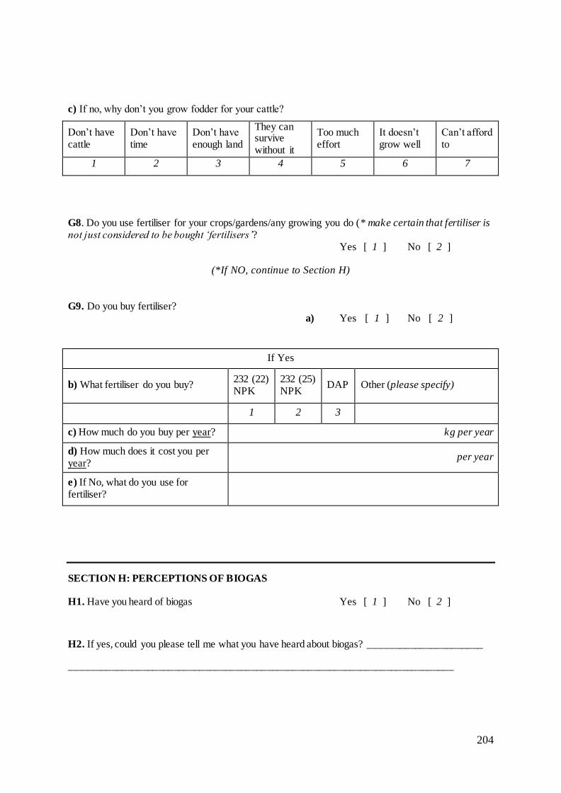
204

c) If no, why don’t you grow fodder for your cattle?

Don’t have cattle

Don’t have time

Don’t have enough land

They can survive without it

Too much effort

It doesn’t grow well

Can’t afford to

1 2 3 4 5 6 7

G8. Do you use fertiliser for your crops/gardens/any growing you do (* make certain that fertiliser is not just considered to be bought ‘fertilisers’? Yes [ 1 ] No [ 2 ]

(*If NO, continue to Section H) G9. Do you buy fertiliser? a) Yes [ 1 ] No [ 2 ]

If Yes

b) What fertiliser do you buy? 232 (22) NPK

232 (25) NPK

DAP Other (please specify)

1 2 3

c) How much do you buy per year? kg per year

d) How much does it cost you per year?

per year

e) If No, what do you use for fertiliser?

SECTION H: PERCEPTIONS OF BIOGAS

H1. Have you heard of biogas Yes [ 1 ] No [ 2 ]

H2. If yes, could you please tell me what you have heard about biogas? ______________________

__________________________________________________________________________

205

H3. What experiences have you had with biogas as a fuel? (*ask only if the response of H1 is Yes)

a) Advantages/good aspects b) Disadvantages/problems

(* If insufficient space in table continue writing on back of page)

(*A detailed explanation must be given about biogas at this point – see supplementary information & pictures.)

H4. Assuming equal prices, which energy source would you rather buy to satisfy your household

cooking needs?

H5.Would you be happy to use biogas for cooking? Yes [ 1 ] No [ 2 ]

H6. If a biogas system is installed at your house how much would you be willing to pay for the gas (and fertiliser) if sufficient gas is provided to replace ALL your cooking needs and you get fertiliser from the digester to use on your food garden and fodder crops? (*this is hypothetical, make sure they know that this will not influence how much they may be charged if a biodigester is given to them in

the future)

R _________________ per month

SECTION I: PERCEPTION OF HOUSEHOLD BIODIGESTERS AND SUITABILITY

REQUIREMENTS

It is possible to have a biodigester for each household. The household needs to feed the biodigester with 20kg of dung and 20l of water every day. They will be able to use the biogas (for cooking/heating) and the fertiliser from the biodigester (for growing vegetables and fodder to feed livestock). If you use gas for cooking, you would not have to buy it and travel to collect it. If you use firewood, you would not have to collect it and make fires for cooking.

I1. If your household could run a biodigester that can give you biogas for cooking and fertiliser, would you want to have one? Yes [ 1 ] No [ 2 ]

Firewood 1 Dung 2 Gas 3 Biogas 4 Paraffin 5

Other (please specify)

206

To run a biodigester and get biogas, it is required that you feed it with 20kg (two 20l buckets [*show

bucket]) of dung and 20l of water every day.

I2. Would your household be willing to do this? Yes [ 1 ] No [ 2 ] I3. Where would you get the 20kg of dung from?

I4. Who will collect this dung?

a) Main person


b) Helpers (if any)


I5. From where will they collect this dung?

a)______________________

b) Distance? _____________ km

I6. How long will it take to collect this dung? ______________________________hours, minutes

I7. Will your household be able to get 20l of water for the biodigester every day? Yes [ 1 ] No [ 2 ]

I8. Who will collect this water?

a) Main person


b) Helpers (if any)


I9. Do you have a space in your garden to dig a 6m X 6m hole for a biodigester? Yes [ 1 ] No [ 2 ]

Collect from our own livestock

1 Collect from the livestock of others 2 Buy it 3

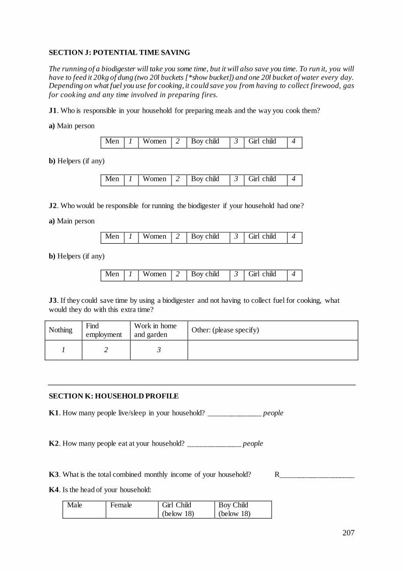
207

SECTION J: POTENTIAL TIME SAVING

The running of a biodigester will take you some time, but it will also save you time. To run it, you will have to feed it 20kg of dung (two 20l buckets [*show bucket]) and one 20l bucket of water every day. Depending on what fuel you use for cooking, it could save you from having to collect firewood, gas

for cooking and any time involved in preparing fires.

J1. Who is responsible in your household for preparing meals and the way you cook them?

a) Main person


b) Helpers (if any)


J2. Who would be responsible for running the biodigester if your household had one?

a) Main person


b) Helpers (if any)


J3. If they could save time by using a biodigester and not having to collect fuel for cooking, what

would they do with this extra time?

Nothing Find employment

Work in home and garden

Other: (please specify)

1 2 3

SECTION K: HOUSEHOLD PROFILE

K1. How many people live/sleep in your household? ______________ people

K2. How many people eat at your household? ______________ people

K3. What is the total combined monthly income of your household? R____________________

K4. Is the head of your household:

Male Female Girl Child (below 18)

Boy Child (below 18)

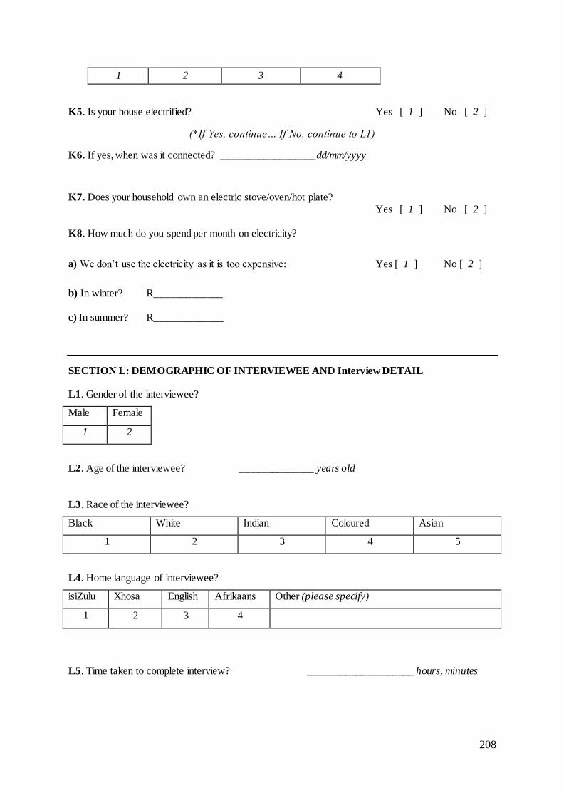
208

1 2 3 4

K5. Is your house electrified? Yes [ 1 ] No [ 2 ]

(*If Yes, continue… If No, continue to L1)

K6. If yes, when was it connected? __________________dd/mm/yyyy

K7. Does your household own an electric stove/oven/hot plate? Yes [ 1 ] No [ 2 ]

K8. How much do you spend per month on electricity?

a) We don’t use the electricity as it is too expensive: Yes [ 1 ] No [ 2 ]

b) In winter? R_____________ c) In summer? R_____________

SECTION L: DEMOGRAPHIC OF INTERVIEWEE AND Interview DETAIL

L1. Gender of the interviewee?

Male Female

1 2

L2. Age of the interviewee? ______________ years old

L3. Race of the interviewee?

Black White Indian Coloured Asian

1 2 3 4 5

L4. Home language of interviewee?

isiZulu Xhosa English Afrikaans Other (please specify)

1 2 3 4

L5. Time taken to complete interview? ____________________ hours, minutes

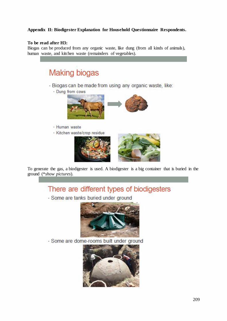
209

Appendix II: Biodigester Explanation for Household Questionnaire Respondents.

To be read after H3:

Biogas can be produced from any organic waste, like dung (from all kinds of animals),

human waste, and kitchen waste (remainders of vegetables).

To generate the gas, a biodigester is used. A biodigester is a big container that is buried in the ground (*show pictures).

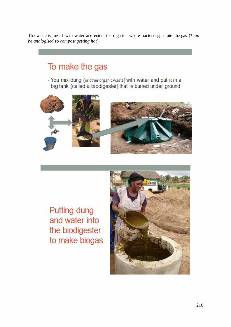
210

The waste is mixed with water and enters the digester where bacteria generate the gas (*can

be analogised to compost getting hot).

211

The gas is piped from the top of the digester and can be used for cooking (*show pictures).

At the one side of the digester the waste goes into the digester, and at the other side the

residue (bioslurry) comes out. This bio-slurry can be used as a fertiliser to grow food for yourself and your animals. Many people around the world and in Africa are already using biogas for cooking and the bioslurry for fertiliser.

Requirements to run a biodigester:

If you have a biogas digester at your home, you will have to fill the digester each day with 20kg of dung (*show bucket), and/or other organic waste, and 20l of water (*show bucket). The dung might be collected from a kraal where the cattle (or any other livestock) sleep at

night.

If you have access to this gas, you will not have to use any other sources of energy for

your cooking needs. If you have sufficient animal dung and install a biogas digester, then

you will not have to search for firewood, buy paraffin or gas for cooking.

ADVANTAGES OF BIOGAS

1. It will give you energy for cooking. 2. Biogas will save you time that you spend collecting firewood. This time can be used

for any other activity, such as agriculture and/or leisure. 3. When you cook on biogas, you help to protect the environment because you will cut

fewer trees for wood. 4. Cooking with biogas is also good for your health because you do not have to inhale

the smoke if you cooked on an open fire.

5. You will get fertiliser, for free. 6. Building the digester may create a small number of jobs.

212

Appendix III: Okhahlamba Local Municipality Map.

(Clive Van Niekerk GIS Office, 2009)

213

Appendix IV: CO2 Emission Calculations

Table 30. Average fuel economy and CO2 emission of diesel.

Stated Average

Fuel Consumption

(km/litre)

Source

Stated CO2

Emission per litre

Diesel burned

(g/litre)

Source

3.244639 (Millikin, 2009) 2680 (Davies, 2004)

2.975370 (US Department of Energy, 2005)

2639.1 (Comcar, 2011)

3.272907 (Franzese et al, 2009: 13)

2668.1 (EPA, 2005)

2.900510 (Lowell and

Balon, 2009: 7) 2620 (Healey, 2003)

Mean 3.098357 2651.8

IV.1. Choice of a Standard Cost for CO2 Emissions

The valuation of Carbon Dioxide (CO2) detrimental impacts on the environment and society

is a highly contentious topic. One of the most commonly used methods of valuing the effects

of CO2 is the social cost of carbon (SCC) approach which values the full cost to society of a

unit of CO2 or the GHG equivalent (DECC, 2011a). A GHG equivalent, or CO2 equivalent

(CO2e) is calculated by multiplying the mass of an emitted gas by the relevant Global

Warming Potential (standardised for each GHG), to provide a unit of greenhouse gas

emission equivalent to CO2 for the purpose of valuation and comparison (Northern Territory

Government, 2009: 4).

While the SCC approach is the most common method of valuing CO2e emission impacts,

there is great variance in the proposed values for the actual social cost of emissions. Parry et

al (2007) conducted a study in which 100 estimates of SCC values were compared. The

sample of values varied from -US$ 10 to US$ 350 with a mean value of US$ 43 per tonne of

CO2 (2007 US Dollars). The Interagency Working Group of America “has endorsed a

‘central’ estimate of US$ 21 per ton of CO2 in 2010” (ZAR 174.85 in 2011 ZAR) (Ackerman

and Stanton, 2010: 1), while the United Kingdom Department of Energy and Climate Change

(DECC) use a ‘central’ value of GBP 13.5 (ZAR 171.32/tonne of CO2) for policy modelling

(DECC, 2011b: 3). This also appears to be approximately in line with the Canadian

Government who uses a value of CAD 25 (ZAR 196.25/tonne of CO2) (Gregory, 2011: 18).

214

Although the values used by America (Interagency Working Group), the United Kingdom

(DECC) and Canada are significantly lower than some of the values stated by Parry et al’s

(2007) peer review, it seems most appropriate to use the value of ZAR 180.81/tonne of CO2,

which is an aggregate of the aforementioned governments values used for policy making.

215

Appendix V: Time Taken to Dig a Hole for a BiogasPro.

Table 31. Average number of days taken to dig a hole for the BiogasPro.

Household Days taken Time spent digging per

day Number of people

digging Total time taken Days (8hr day)

Khumalo 13 5 1 65 8.125

Mdakana 20 6 1 120 15

Khumalo (2) 9 9 2 165* 20.25

Average 14 6.67 116.67 14.46

*Total time is calculated as man hours (i.e. (9 days x 9 hours digging time) multiplied by 2 people)

216

Appendix VI: Calculation of the Value of Time

VI.1. Calculation of a Minimum Wage Rate

An average of the minimum wage rates for different sectors is used in the assessment of the

economic value of time (section 4.6.2.3).

Table 32. South African minimum labour wage rate.

Employment Sector Minimum wage (ZAR/hour)

Civil Engineering R 20.49

Contract Cleaning R 11.27

Domestic Worker R 6.44

Farm Worker R 7.04

Forestry R 6.55

Hospitality R 10.70

Taxi Services R 9.69

Average R 10.31

(Source: Labour Research Services, 2011; Department of Labour, 2011).

VI.2. Valuation of Time Relating to Biodigester Use and Operation

The questionnaire asked respondents to state what activities they would do if they were to

save time by using a biodigester (appendix I, Question J3).

Table 33. Stated use of time in the event of having more free time as a result of using a biodigester system.

Option Percentage of

households Activity grouping (section 3.4.3)

Find employment 6.06% Productive economic activity

Work in home or garden 92.93% Household activity

Nothing 1.01% Other activity

Using the World Bank (1996) methods as described in section 4.6.2.3, time is valued as a

weighted proportion of the minimum wage rate depending on the use of that time (gauged by

stated activity). The minimum wage rate is taken as ZAR 10.31, as calculated in section VI.1.

217

Table 34. Weighted value of time, by activity.

Activity grouping (section 3.4.3) Weighting (as a percentage of

average minimum wage) Symbol

ZAR

Value

Productive economic activity 100 We 10.31

Household activity 50 Wh 5.16

Other activity 25 Wo 2.58

The standard value for time, with respect to biodigester use and running is ZAR 5.44 per

hour:

( ) ( ) ( ) ( ) ( ) ( )

Where:


e is the percentage of people who will seek or partake in economic activity (%)






218

VI.3. Valuation of Time Relating to Productivity Loss

The same weighting technique and weighted wage rates for economic, household and other

activity are used as presented in section VI.2. The employment rate is used as an indication of

how much ‘productive economic activity’ time will be lost in the event of incapacity. The

remainder of time is assumed to be an equal division between household activity and other

activity (including socialising and leisure). The employment rate in Okhombe is taken as

13.7% (section 2.1.3; Chellan, 2002: 67).

The value of time relating to health-related productivity losses for the study area is calculated

to be ZAR 4.75 per hour. The following equation displays this calculation:

( ) ( ) ( ) ( ) ( ) ( )

Where:


e is the percentage of people who will use time for economic activity (%)






219

Appendix VII: Distribution of Surveyed Households in Okhombe.

(Adapted from Google Earth imagery dated 08-08-2010, Google©)

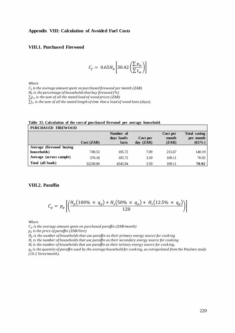
220

Appendix VIII: Calculation of Avoided Fuel Costs

VIII.1. Purchased Firewood

[ (∑ ∑

)]

Where

Cf is the average amount spent on purchased firewood per month (ZAR)

Hb is the percentage of households that buy firewood (%)

∑pw is the sum of all the stated load of wood prices (ZAR)

∑tw is the sum of all the stated length of time that a load of wood lasts (days).

Table 35. Calculation of the cost of purchased firewood per average household.

PURCHAS ED FIREWOOD

Cost (ZAR)

Number of

days load/s

lasts

Cost per

day (ZAR)

Cost per

month

(ZAR)

Total saving

per month

(65% )

Average (firewood buying

households) 749.53 105.72 7.09 215.67 140.19

Average (across sample) 379.18 105.72 3.59 109.11 70.92

Total (all loads) 32230.00 4545.94 3.59 109.11 70.92

VIII.2. Paraffin

[( ( ) ( ) ( )

)]

Where

Cp is the average amount spent on purchased paraffin (ZAR/month)

pp is the price of paraffin (ZAR/litre)

Hp is the number of households that use paraffin as their primary energy source for cooking

Hs is the number of households that use paraffin as their secondary energy source for cooking

Ht is the number of households that use paraffin as their tertiary energy source for cooking.

qp is the quantity of paraffin used by the average household for cooking, as extrapolated from the Paulsen study

(10.2 litres/month).

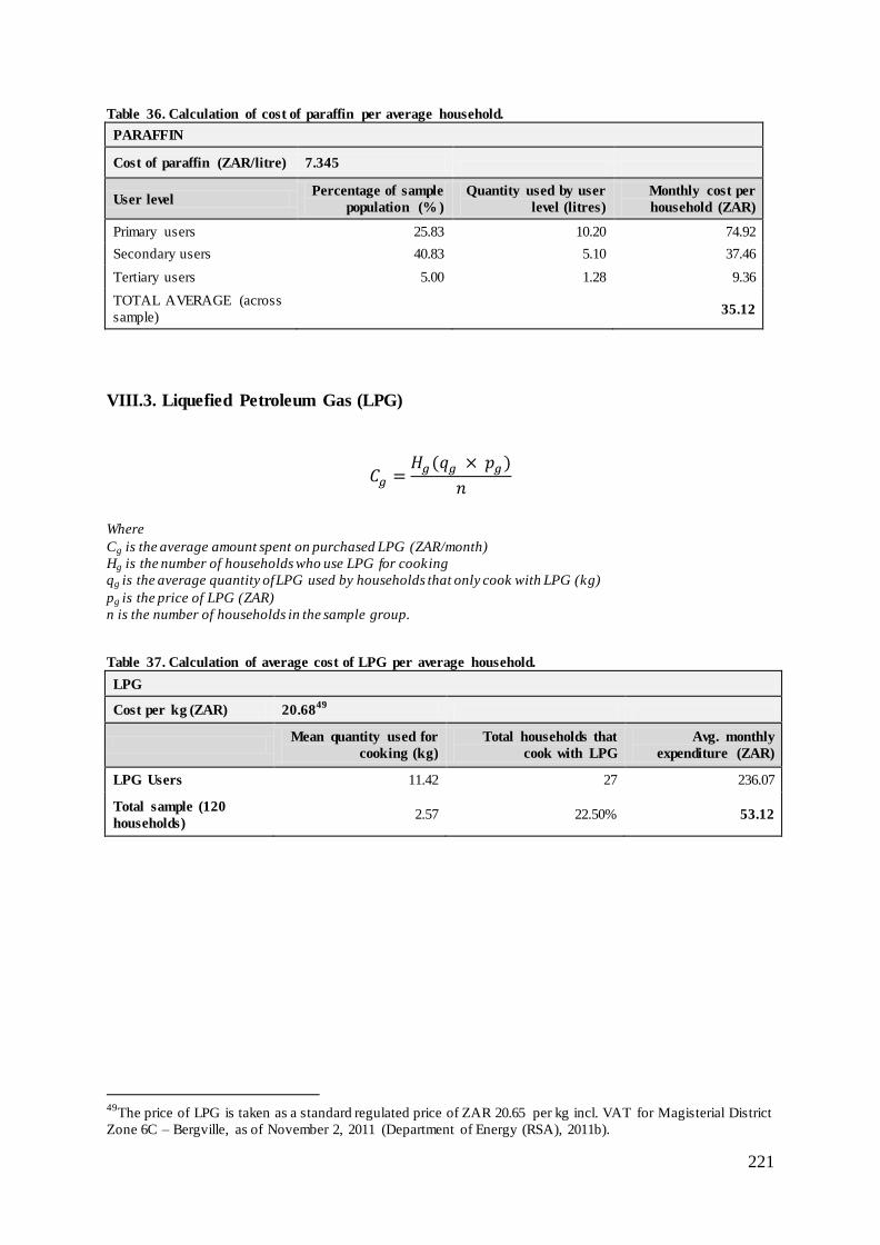
221

Table 36. Calculation of cost of paraffin per average household.

PARAFFIN

Cost of paraffin (ZAR/litre) 7.345

User level Percentage of sample

population (% )

Quantity used by user

level (litres)

Monthly cost per

household (ZAR)

Primary users 25.83 10.20 74.92

Secondary users 40.83 5.10 37.46

Tertiary users 5.00 1.28 9.36

TOTAL AVERAGE (across

sample) 35.12

VIII.3. Liquefied Petroleum Gas (LPG)

( )

Where

Cg is the average amount spent on purchased LPG (ZAR/month)

Hg is the number of households who use LPG for cooking

qg is the average quantity of LPG used by households that only cook with LPG (kg)

pg is the price of LPG (ZAR)


Table 37. Calculation of average cost of LPG per average household.

LPG

Cost per kg (ZAR) 20.6849

Mean quantity used for

cooking (kg)

Total households that

cook with LPG

Avg. monthly

expenditure (ZAR)

LPG Users 11.42 27 236.07

Total sample (120

households) 2.57 22.50% 53.12

49

The price of LPG is taken as a standard regulated price of ZAR 20.65 per kg incl. VAT for Magisterial District

Zone 6C – Bergville, as of November 2, 2011 (Department of Energy (RSA), 2011b).

222

VIII.4. Electricity

( )

Where

Ce is the average amount spent on electricity (ZAR/month)

HC is the number of households that cook with electricity

qe is the average cost of electricity used for cooking (ZAR/month)


Table 38. Calculation of average expenditure on cooking electricity per average household.

ELECTRICITY

Lighted

only

Cooked and

lighted

Lighted, cooked and

heated

Lighted and

heated

Number of households 7 22 10 1

% of electrified

households 17.50 55.00 25.00 2.50

Average expenditure

(ZAR) 52.86 133.18 194.44 60

Avg. expenditure on

cooking (ZAR) 80.32

Number of households that

cook with electricity 32

Avg. expenditure on

cooking across sample

group (ZAR)

21.42

VIII.5. Total Expenditure on All Energy

Table 39. Total monthly expenditure on energy.

TOTAL ENERGY EXPENDITURE

Energy form Percentage of total energy

expenditure Monthly expenditure (ZAR)

Purchased firewood 36.49% 109.11

Paraffin 23.49% 70.24

LPG 25.55% 76.37

Electricity 14.47% 43.25

TOTAL 298.97

Note: it should be noted that candles were not included in this assessment and that candles are of significant

importance in household lighting. The average cost of candles is extrapolated from Paulsen et al (2010: 23).

223

Appendix IIX: Calculation of Time Saving Due to a Biodigester

IIX.1. Reduced wood collection time

(∑ )

Where

Tfis the time spent collecting firewood for cooking purposes per average household (hours/month)

∑tf is the sum of all time spent collecting firewood (hours)


Table 40. Time saving due to reduced firewood collection.

COLLECTED FIREWOOD Value of time

(ZAR/hour) 5.44

50

Collecting

households

Collection

time

(hours)

Number of

collection

days per

month

Total

collection

time

(hours)

Value of time

(ZAR/month)

Total

saving per

month

(65% )

(ZAR)

Average (collecting

households) 100.00% 4.90 10.39 50.87 276.82 179.94

Average (across

sample) 42.50% 2.12 17.67 37.38 203.40 132.21

50

Calculated as the economic value of time in appendix IIX.

224

IIX.2. Reduced Cooking Time

(

)

Where

Tc is the time saved using biogas for cooking in place of traditional fuels (hours/month)

Hf is the percentage of households in the sample group that use traditional fuels as their primary cooking

energy (%).

Note: 30.42 represents the average month

The average time saving (134) is divided by 60 to convert from minutes to hours.

Table 41. Time saved in cooking practices.

Cooking practices

Value of time

(ZAR/hour) 5.44

Time saved per

primary fuel cooking

household per day

(hours)

Time saved per

average sample

group

household51

Time saved

per

household

per month

(hours)

Value of time

saved per

month (ZAR)

Cooking activities 1.60 0.81 24.74 134.63

Cleaning cooking utensils 0.62 0.31 9.54 51.89

TOTAL 186.52

51

50.8% of households use solid fuels (firewood, dung and coal) as primary sources of cooking. Only these

households are considered to save time by cooking with biogas.

225

Appendix IX: Calculation of Financial and Economic Health Benefits

IX.1. Financial Value of Avoided Medical Expenditure

As described in section 4.7.1.3.1 the following method was used for estimating the financial value of reduced medical expenditure, but was

deemed inaccurate and the results were therefore disregarded.

Table 42. Calculation of medical expenditure saving from reduced IAP.

SAVING ON IAP RELATED HEALTH EXPENDITURE

Per capita government expenditure

on health care (2011 ZAR)a 2159.18

d

Total DALYs lost

per year (South

Africa)b

Total IAP

attributable

DALYs per

yearc

Percentage of

total DALYs

caused by IAP

Percentage of

households using solid

fuels as primary and/or

secondary cooking fuel

Potential saving in

health care costs per

person (assuming 65%

reduced IAP for solid

fuel users)

Potential saving in

health care costs per

household (assuming

65% reduced IAP for

solid fuel users)

20988180 63791 0.30% 80.00%

Value as a % of

Govt. exp. on per

capita health care

costs per year

(ZAR) 2159.18 6.56 5.25 3.41 18.39

(Source of information, WHO, 2009a; WHO, 2004db; WHO, 2004ac; CIC, 2011bd).

226

IX.2. Valuation of Health-Related Productivity Gains

The valuation of health-related productivity gains is presented in Table 43 and follows the methodology described in section 4.7.2.2.1.

Table 43. Calculation of health related productivity gains.

HEALTH-RELATED PRODUCTIVITY GAINS

Value of time (ZAR)a

4.75

Incidence of

ALRI per

personb

Percentage of

ALRI

attributable to

IAPc

Incidence of

IAP

attributable

ALRI per

person

Average number of

days of incapacity

per cased

Average number of

hours of incapacity

per case (assuming

12 waking hours per

day)

SSA 0.192609906 36% 0.069339566 8.88 106.56

Incidence of

IAP

attributable

ALRI per

person

Number of

people affected

per year in

Okhombe

(population

6343e)

Total incapacity

time attributed

to IAP (hours)

Value of incapacity

time attributable to

IAP (ZAR)

Percentage of

reduced IAP and

thus assumed IAP

attributable ALRI

Total health-related

productivity saving

attributed to fuel

switching in

Okhombe

(ZAR/year)

Total health-

related

productivity saving

per household

(ZAR/year)

Okhombe 0.069339566 439.82 46867.31 222574.91 65.00% 144673.69 123.02

(Source of information, appendix IIXa; WHO, 2004cb; Prüss-Üstün and Corvalán, 2006: 33c; Renwick et al, 2007: 31d; section 2.1.3e).

IX.3. Financial and Economic Valuation of Saved Lives

The method used to calculate potential reduction of IAP related deaths is described in section 4.7.1.3.3 and presented in Table 44. The financial

value of saved lives is based on the cost of an average funeral in South African rural context. The economic value of saved lives is based on the

value of a statistical life (VOSL) used by Renwick et al (2007). The VOSL value of US$2 million is converted to ZAR using a PPP-adjusted

exchange rate (calculated by dividing South African PPP-adjusted GDP (international dollars) by South African Nominal GDP (in US$) and

dividing this by the standard ZAR to USD exchange rate used in this research project, see section 4.5.1). It is further converted to 2011 ZAR

using annual inflation figures quoted by Stats SA (2011a).

227

Table 44. Financial and economic valuation of saved lives.

VALUE OF SAVED LIVES (financial and economic)

Indoor air pollution

attributable deaths per

100 000 capitaa

Population using

solid fuels (% )b

Number of households

using solid fuels per

100 000

Percentage of solid fuel users

dying from IAP attributable

disease per year (% )

South Africa 7 17.3 17300 0.040462428

Percentage of solid fuel

users dying from IAP

attributable diseases

per year (% )

Population using

solid fuels for

primary and/or

secondary cooking

(% )

Number of individuals in

households that use solid

fuels (total population =

6343)

Number of IAP attributable

deaths per year (in Okhombe)

Potential number of reduced

IAP related deaths per year

(assumed 65% reduced IAP)

Okhombe 0.040462428 80.00 5074.4 2.053225434 1.33460

Average monthly

income (ZAR)

Average annual

income (ZAR)

Average cost of a funeral

(one third of mean

annual income) (ZAR)c

Potential financial saving from

IAP reduced deaths per year

(Okhombe) (ZAR)

Potential financial saving from

IAP reduced deaths per year

per household (ZAR)

Okhombe

Financial 1089.6250 13075.50 4358.50 5816.84 4.95

Value of a statistical

life (US$)d

PPP-adjusted

exchange rate (ZAR

per US$)e

Potential number of

reduced IAP attributable

deaths per year (in

Okhombe)

Potential economic saving

from reduced IAP attributable

deaths per year (Okhombe)

(ZAR)

Potential economic saving from

reduced IAP attributable deaths

per year per household (ZAR)

Okhombe

Economic 2605615 0.18107 1.33460 19205500.21 16331.20

(Source of information, WHO, 2004aa; WHO, 2007b; Collins and Leibbrandt, 2007:75c; Renwick et al, 2007: 34d; Stats SA, 2011ad;World Bank,

2011e; IMF, 2011be).

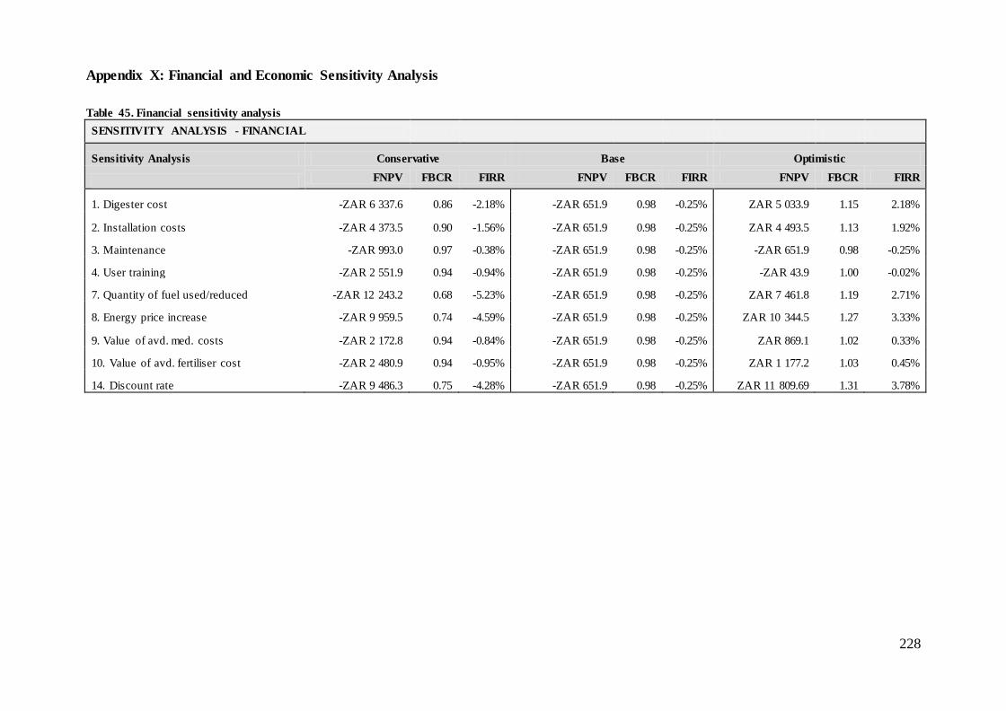
228

Appendix X: Financial and Economic Sensitivity Analysis

Table 45. Financial sensitivity analysis

SENSITIVITY ANALYSIS - FINANCIAL

Sensitivity Analysis Conservative Base Optimistic

FNPV FBCR FIRR FNPV FBCR FIRR FNPV FBCR FIRR

1. Digester cost -ZAR 6 337.6 0.86 -2.18% -ZAR 651.9 0.98 -0.25% ZAR 5 033.9 1.15 2.18%

2. Installation costs -ZAR 4 373.5 0.90 -1.56% -ZAR 651.9 0.98 -0.25% ZAR 4 493.5 1.13 1.92%

3. Maintenance -ZAR 993.0 0.97 -0.38% -ZAR 651.9 0.98 -0.25% -ZAR 651.9 0.98 -0.25%

4. User training -ZAR 2 551.9 0.94 -0.94% -ZAR 651.9 0.98 -0.25% -ZAR 43.9 1.00 -0.02%

7. Quantity of fuel used/reduced -ZAR 12 243.2 0.68 -5.23% -ZAR 651.9 0.98 -0.25% ZAR 7 461.8 1.19 2.71%

8. Energy price increase -ZAR 9 959.5 0.74 -4.59% -ZAR 651.9 0.98 -0.25% ZAR 10 344.5 1.27 3.33%

9. Value of avd. med. costs -ZAR 2 172.8 0.94 -0.84% -ZAR 651.9 0.98 -0.25% ZAR 869.1 1.02 0.33%

10. Value of avd. fertiliser cost -ZAR 2 480.9 0.94 -0.95% -ZAR 651.9 0.98 -0.25% ZAR 1 177.2 1.03 0.45%

14. Discount rate -ZAR 9 486.3 0.75 -4.28% -ZAR 651.9 0.98 -0.25% ZAR 11 809.69 1.31 3.78%

229

Table 46. Economic senitivity analysis.

SENSITIVITY ANALYSIS - ECONOMIC

Sensitivity Analysis Conservative Base Optimistic

ENPV EBCR EIRR ENPV EBCR EIRR ENPV EBCR EIRR

1. Digester cost ZAR 173 097.5 4.30 48.46% ZAR 178 783.3 4.83 57.68% ZAR 184 469.0 5.50 70.65%

2. Installation costs ZAR 175 061.6 4.47 51.33% ZAR 178 783.3 4.83 57.68% ZAR 183 928.6 5.43 69.20%

3. Maintenance ZAR 178 442.1 4.79 57.04% ZAR 178 783.3 4.83 57.68% ZAR 178 783.3 4.83 57.68%

4. User training ZAR 176 883.3 4.64 54.27% ZAR 178 783.3 4.83 57.68% ZAR 179 391.3 4.89 58.86%

5. Social cost of transport ZAR 178 691.5 4.82 57.51% ZAR 178 783.3 4.83 57.68% ZAR 178 844.5 4.83 57.80%

6. Biodigester running time ZAR 170 672.3 4.11 54.00% ZAR 178 783.3 4.83 57.68% ZAR 183 651.6 5.39 59.98%

7. Quantity of fuel used/reduced ZAR 167 191.9 4.58 54.05% ZAR 178 783.3 4.83 57.68% ZAR 186 896.9 5.00 60.39%

8. Energy price increase ZAR 169 475.7 4.63 56.82% ZAR 178 783.3 4.83 57.68% ZAR 189 779.7 5.06 58.43%

9. Value of avd. med. costs ZAR 177 262.3 4.80 57.21% ZAR 178 783.3 4.83 57.68% ZAR 180 304.3 4.86 58.15%

10. Value of avd. fertiliser cost ZAR 176 954.3 4.79 56.86% ZAR 178 783.3 4.83 57.68% ZAR 180 612.3 4.87 58.52%

11. Value of shadow wage ZAR 162 946.1 4.84 50.84% ZAR 178 783.3 4.83 57.68% ZAR 205 730.5 4.81 70.76%

12. VOSL ZAR 30 520.9 1.65 11.19% ZAR 178 783.3 4.83 57.68% ZAR 548 321.0 12.74 171.86%

13. IAP reductions ZAR 121 084.3 3.59 39.91% ZAR 178 783.3 4.83 57.68% ZAR 236 634.4 6.07 75.51%

14. Discount rate ZAR 128 325.2 3.85 51.01% ZAR 178 783.3 4.83 57.68% ZAR 249 532.32 6.08 64.35%

230

Appendix XI: Ethical Clearance

university of kwazulu-natal the financial and economic ...

Documents

Transcript of university of kwazulu-natal the financial and economic ...