University of Iowa Bayesian inference in dynamic discrete choice models

University of IowaIowa Research Online

Theses and Dissertations

2007

Bayesian inference in dynamic discrete choicemodelsAndriy NoretsUniversity of Iowa

This dissertation is available at Iowa Research Online: http://ir.uiowa.edu/etd/148

Recommended CitationNorets, Andriy. "Bayesian inference in dynamic discrete choice models." dissertation, University of Iowa, 2007.http://ir.uiowa.edu/etd/148.

http://ir.uiowa.edu

http://ir.uiowa.edu/etd

BAYESIAN INFERENCE IN DYNAMIC DISCRETE CHOICE MODELS

by

Andriy Norets

An Abstract

Of a thesis submitted in partial fulfillment of therequirements for the Doctor of Philosophy

degree in Economicsin the Graduate College of

The University of Iowa

July 2007

Thesis Supervisor: Professor John Geweke

1

ABSTRACT

In this dissertation, I develop methods for Bayesian inference in dynamic dis-

crete choice models (DDCMs.) Chapter 1 proposes a reliable method for Bayesian

estimation of DDCMs with serially correlated unobserved state variables. Inference

in these models involves computing high-dimensional integrals that are present in the

solution to the dynamic program (DP) and in the likelihood function. First, the chap-

ter shows that Markov chain Monte Carlo (MCMC) methods can handle the problem

of multidimensional integration in the likelihood, which was previously considered

infeasible for DDCMs with serially correlated unobservables. Second, the chapter

presents an efficient algorithm for solving the DP suitable for use in conjunction with

the MCMC estimation procedure. The algorithm utilizing random grids and nearest

neighbor approximations iterates the Bellman equation only once for each parame-

ter draw. The chapter evaluates the method’s performance on two different DDCMs

using real and artificial datasets. The experiments demonstrate that ignoring serial

correlation in unobservables of DDCMs can lead to serious misspecification errors.

Experiments on dynamic multinomial logit models, for which analytical integration

is also possible, show that the estimation accuracy of the proposed method is good.

Chapter 2 presents a proof of the complete (and thus a.s.) uniform convergence

of the DP solution approximations proposed in Chapter 1 to the true values under

mild assumptions on the primitives of DDCMs. It also establishes the complete

convergence of the corresponding approximated posterior expectations.

2

Chapter 3 proposes a method for inference in DDCMs that combines MCMC

and artificial neural networks (ANN.) MCMC is intended to handle high dimensional

integration in the likelihood function of richly specified DDCMs. ANNs approximate

the DP solution as a function of the parameters and state variables beforehand of

the estimation procedure to reduce the computational burden. Potential applications

of the proposed methodology include inference in DDCMs with random coefficients,

serially correlated unbservables, and dependent observations. The chapter discusses

MCMC estimation of DDCMs, provides relevant background on ANNs, and derives

a theoretical justification of the method. Experiments suggest that application of

ANNs in the MCMC estimation of DDCMs is a promising approach.

Abstract Approved:

Thesis Supervisor

Title and Department

Date

BAYESIAN INFERENCE IN DYNAMIC DISCRETE CHOICE MODELS

by

Andriy Norets

A thesis submitted in partial fulfillment of therequirements for the Doctor of Philosophy

degree in Economicsin the Graduate College of

The University of Iowa

July 2007

Thesis Supervisor: Professor John Geweke

Graduate CollegeThe University of Iowa

Iowa City, Iowa

CERTIFICATE OF APPROVAL

PH.D. THESIS

This is to certify that the Ph.D. thesis of

Andriy Norets

has been approved by the Examining Committee for thethesis requirement for the Doctor of Philosophy degreein Economics at the July 2007 graduation.

Thesis Committee:

John Geweke, Thesis Supervisor

Charles Whiteman

Beth Ingram

Elena Pastorino

Luke Tierney

To my parents.

ii

ACKNOWLEDGEMENTS

I am grateful to my committee members Charles Whiteman, Elena Pastorino,

Beth Ingram, Luke Tierney, and especially my advisor, John Geweke, for guidance and

helpful suggestions. Each stage of this research benefited from invaluable comments

of John Geweke. My understanding of econometrics and economics were influenced by

him to a great extent. Many faculty members and fellow students at the University

of Iowa contributed to my learning and research. I would like to thank Marianna

Kudlyak, Yaroslav Litus, Maksym Obrizan, and Latchezar Popov for their friendship,

help, and encouragement throughout the years at the PhD program. I also would like

to acknowledge financial support from the Economics Department graduate fellowship

and the Seashore Dissertation fellowship at the University of Iowa. Finally, I am

grateful to my parents and my wife, Keiko, for their love and support.

iii

ABSTRACT

In this dissertation, I develop methods for Bayesian inference in dynamic dis-

crete choice models (DDCMs.) Chapter 1 proposes a reliable method for Bayesian

estimation of DDCMs with serially correlated unobserved state variables. Inference

in these models involves computing high-dimensional integrals that are present in the

solution to the dynamic program (DP) and in the likelihood function. First, the chap-

ter shows that Markov chain Monte Carlo (MCMC) methods can handle the problem

of multidimensional integration in the likelihood, which was previously considered

infeasible for DDCMs with serially correlated unobservables. Second, the chapter

presents an efficient algorithm for solving the DP suitable for use in conjunction with

the MCMC estimation procedure. The algorithm utilizing random grids and nearest

neighbor approximations iterates the Bellman equation only once for each parame-

ter draw. The chapter evaluates the method’s performance on two different DDCMs

using real and artificial datasets. The experiments demonstrate that ignoring serial

correlation in unobservables of DDCMs can lead to serious misspecification errors.

Experiments on dynamic multinomial logit models, for which analytical integration

is also possible, show that the estimation accuracy of the proposed method is good.

Chapter 2 presents a proof of the complete (and thus a.s.) uniform convergence

of the DP solution approximations proposed in Chapter 1 to the true values under

mild assumptions on the primitives of DDCMs. It also establishes the complete

convergence of the corresponding approximated posterior expectations.

iv

Chapter 3 proposes a method for inference in DDCMs that combines MCMC

and artificial neural networks (ANN.) MCMC is intended to handle high dimensional

integration in the likelihood function of richly specified DDCMs. ANNs approximate

the DP solution as a function of the parameters and state variables beforehand of

the estimation procedure to reduce the computational burden. Potential applications

of the proposed methodology include inference in DDCMs with random coefficients,

serially correlated unbservables, and dependent observations. The chapter discusses

MCMC estimation of DDCMs, provides relevant background on ANNs, and derives

a theoretical justification of the method. Experiments suggest that application of

ANNs in the MCMC estimation of DDCMs is a promising approach.

v

TABLE OF CONTENTS

LIST OF TABLES . . . . . . . . . . . . . . . . . . . . . . . . . . . . . . . . . viii

LIST OF FIGURES . . . . . . . . . . . . . . . . . . . . . . . . . . . . . . . . ix

CHAPTER

1 INFERENCE IN DYNAMIC DISCRETE CHOICE MODELS WITHSERIALLY CORRELATED UNOBSERVED STATE VARIABLES . 1

1.1 Introduction . . . . . . . . . . . . . . . . . . . . . . . . . . . . . 11.2 Setup and estimation of DDCMs . . . . . . . . . . . . . . . . . . 61.3 Algorithm for solving the DP . . . . . . . . . . . . . . . . . . . . 14

1.3.1 Algorithm description . . . . . . . . . . . . . . . . . . . . 141.3.2 Comparison with Imai et al. (2005) . . . . . . . . . . . . 181.3.3 Theoretical results . . . . . . . . . . . . . . . . . . . . . . 19

1.4 Convergence of posterior expectations . . . . . . . . . . . . . . . 241.5 Experiments . . . . . . . . . . . . . . . . . . . . . . . . . . . . . 27

1.5.1 Gilleskie’s (1998) model . . . . . . . . . . . . . . . . . . 271.5.2 Rust’s (1987) model . . . . . . . . . . . . . . . . . . . . 49

1.6 Conclusion and future work . . . . . . . . . . . . . . . . . . . . . 74

2 PROOFS OF THE THEORETICAL RESULTS . . . . . . . . . . . . 78

2.1 Lemmas . . . . . . . . . . . . . . . . . . . . . . . . . . . . . . . . 782.2 Extension to the uniform convergence . . . . . . . . . . . . . . . 852.3 Convergence of posterior expectations

and ergodicity of the Gibbs sampler . . . . . . . . . . . . . . . . 892.4 Auxiliary results . . . . . . . . . . . . . . . . . . . . . . . . . . . 98

3 ESTIMATION OF DYNAMIC DISCRETE CHOICE MODELS WITHDP SOLUTION APPROXIMATED BY ARTIFICIAL NEURAL NET-WORKS . . . . . . . . . . . . . . . . . . . . . . . . . . . . . . . . . . 113

3.1 Introduction . . . . . . . . . . . . . . . . . . . . . . . . . . . . . 1133.2 DDCM and MCMC . . . . . . . . . . . . . . . . . . . . . . . . . 1163.3 Feedforward ANN . . . . . . . . . . . . . . . . . . . . . . . . . . 120

3.3.1 Definition of feedforward ANN . . . . . . . . . . . . . . . 1203.3.2 Consistency of FFANN approximations . . . . . . . . . . 124

3.4 Experiments . . . . . . . . . . . . . . . . . . . . . . . . . . . . . 1273.4.1 Evaluating approximation quality . . . . . . . . . . . . . 127

vi

3.4.2 Estimation results . . . . . . . . . . . . . . . . . . . . . . 134

REFERENCES . . . . . . . . . . . . . . . . . . . . . . . . . . . . . . . . . . . 138

vii

LIST OF TABLES

Table

1.1 Estimation results for artificial data . . . . . . . . . . . . . . . . . . . . . 42

1.2 Joint distribution test . . . . . . . . . . . . . . . . . . . . . . . . . . . . 48

1.3 Estimation results for artificial data . . . . . . . . . . . . . . . . . . . . . 61

1.4 Exact and approximate estimation results. . . . . . . . . . . . . . . . . . 64

1.5 Estimation results for the dynamic logit model and the model with Gaus-sian serially correlated unobservables. . . . . . . . . . . . . . . . . . . . . 67

1.6 Estimation results for data from Rust’s paper, group 4. . . . . . . . . . . 70

viii

LIST OF FIGURES

Figure

1.1 Flowchart of a direct search procedure for finding a fixed point. . . . . . 36

1.2 Estimated densities of Vw. The tightest density corresponds to N = 1000,the most widespread to N = 100. The dashed lines are fitted normaldensities. . . . . . . . . . . . . . . . . . . . . . . . . . . . . . . . . . . . 38

1.3 Estimated densities of E(m)[V (s′; θ)|s, d1; θ] − E(m)[V (s′; θ)|s, d2; θ]. Thetightest density corresponds to N = 1000, the most widespread to N =100. The dashed lines are fitted normal densities. . . . . . . . . . . . . . 39

1.4 Estimated posterior densities of (a) α1, (b) α2, (c) α3, (d) α4, (e) ρ, (f) η1,

(g) η2, (h) η3, (k) η4, (l) h−1/2ε . The dashed lines are prior densities. The

vertical lines show the actual parameter values. . . . . . . . . . . . . . . 43

1.5 Posterior densities of η: (a) η1, (b) η2, (c) η3, (d) η4. The solid lines showthe densities estimated by probit, the dotted lines by the full model. Thevertical lines show the actual parameter values. . . . . . . . . . . . . . . 45

1.6 Posterior densities of α, ρ, and h−1/2ε : (a) α1, (b) α2, (c) α3, (d) α4, (e) ρ,

(f) h−1/2ε . The solid lines show the densities estimated with fixed η (two

simulator runs,) the dotted lines by the full model. The vertical lines showthe actual parameter values. . . . . . . . . . . . . . . . . . . . . . . . . . 46

1.7 Joint distribution tests: (a) α1, (b) α2, (c) α3, (d) α4, (e) ρ, (f) η1, (g) η2,

(h) η3, (k) η4, (l) h−1/2ε . . . . . . . . . . . . . . . . . . . . . . . . . . . . . 49

1.8 Estimated posterior densities: solid lines for I = 500, dotted lines forI = 50. (a) α1, (b) α2, (c) ρ, (d) η1, (e) η2, (f) η3. The dashed lines areprior densities. The vertical lines show the actual parameter values. . . . 62

1.9 Comparison with exact and approximate estimation algorithms. Esti-mated posterior densities: (a) α1, (b) α2, (c) η1, (d) η2, (e) η3. Thevertical lines show the actual parameter values.The solid line shows theposterior for exact estimation procedure, the dashed line – approximateestimation procedure . . . . . . . . . . . . . . . . . . . . . . . . . . . . . 66

ix

1.10 The posterior means of the hazard functions. Panel (a)—the data gen-erated from the model with the serially correlated unobservables, panel(b)—the data generated from the dynamic logit model. The vertical axisis for the probability of engine replacement, the horizontal axis is for themileage interval. The solid line is for the model with serially correlated un-observables. The dashed line—for dynamic multinomial logit, the dottedline—data hazard. . . . . . . . . . . . . . . . . . . . . . . . . . . . . . . 68

1.11 Estimated posterior densities for different grids: (a) α1, (b) α2, (c) ρ, (d)η1, (e) η2, (f) η3. The dashed lines are prior densities. The solid lines areposterior densities averaged over all simulator runs. The dotted lines showposterior densities averaged for runs 1–2, 3–4, and 5–6. . . . . . . . . . 72

2.1 Nearest neighbors. . . . . . . . . . . . . . . . . . . . . . . . . . . . . . . 100

3.1 Multi-layer feed-forward neural network . . . . . . . . . . . . . . . . . . 121

3.2 Densities of the difference between the exact solution and the solutionon random grids. The model with extreme value iid unobservables. Thedashed line - the density of [F (xji, θj)−F ji

1,100], the dotted line - the density

of [F (xji, θj) − F ji10,100], and the solid line - the density of [F (xji, θj) −

F ji100,100]. . . . . . . . . . . . . . . . . . . . . . . . . . . . . . . . . . . . 129

3.3 Densities of residuals eji (the dotted line is for the validation part of thesample. . . . . . . . . . . . . . . . . . . . . . . . . . . . . . . . . . . . . 130

3.4 Fitted values F (xji, εj, θj; w) (the dotted lines) and F ji100,100 (the solid lines)

as functions of one input component. The model with serially correlatedunobservables. The horizontal axes: (a) α1, (b) α2, (c) ρ, and (d) ε. . . 131

3.5 Densities of the approximation error for FFANNs and DP solutions onrandom grids. The model with extreme value iid unobservables. Thedashed line - for a FFANN trained on exact data, the dotted line - for aFFANN trained on F ji

100,100, the solid line - for F ji100,100. . . . . . . . . . . 132

3.6 Densities of e from neural network (the dotted line) and from DP solutionon a random grid (the solid line.) The model with serially correlatedunobservables. . . . . . . . . . . . . . . . . . . . . . . . . . . . . . . . . 133

3.7 Estimated posterior densities: (a) α1, (b) α2, (c) η1, (d) η2. The solidlines for the algorithm using the exact DP solutions, the dashed for thealgorithm using the FFANN. . . . . . . . . . . . . . . . . . . . . . . . . 136

x

3.8 Estimated posterior densities: (a) α1, (b) α2. The solid lines - the simu-lator using the exact DP solutions, the other lines - the simulators usingDP solutions on different random grids. . . . . . . . . . . . . . . . . . . . 136

xi

1

CHAPTER 1INFERENCE IN DYNAMIC DISCRETE CHOICE MODELS WITHSERIALLY CORRELATED UNOBSERVED STATE VARIABLES

1.1 Introduction

Dynamic discrete choice models (DDCMs) describe the behavior of a forward-

looking economic agent who chooses between several available alternatives repeatedly

over time. Estimation of the deep structural parameters of such decision problem is

a theoretically appealing and promising area in empirical economics. In contrast to

conventional statistical modeling of discrete data, it does not fall under the Lucas

critique and often produces better behavior forecasts. Structural estimation of dy-

namic models though, is very complex computationally. This fact substantially limits

the ability of estimable models to capture essential features of the real world. One

such important feature that had mainly to be assumed away in the literature is the

presence of serial correlation in unobserved state variables. Although introducing se-

rial dependence in modelled productivity, health status, or taste idiosyncrasies would

improve the credibility of obtained quantitative results, general feasible estimation

methods for dealing with serially correlated unobservables in dynamic discrete choice

models are yet to be developed, according to Rust (1994). This chapter attempts to

develop such a feasible general method.

Advances in simulation methods and computing speed over the last two decades

made the Bayesian approach to statistical inference practical. Bayesian methods are

now applied to many problems in statistics and econometrics that could not be tack-

2

led by the classical approach. Static discrete choice models, and more generally,

models with latent variables, are one of those areas where the Bayesian approach was

extremely fruitful, see for example McCulloch and Rossi (1994) and Geweke et al.

(1994). In these models, the likelihood function is often an intractable integral over

the latent variables. In Bayesian inference, the posterior distribution of the model

parameters is usually explored by simulating a sequence of parameter draws that rep-

resents the posterior distribution. A simulation technique called the Gibbs sampler

is particularly convenient for exploring posterior distributions in models with latent

variables. This sampler simulates the parameters conditional on the data and the

latent variables, and then simulates the latent variables conditional on the data and

the parameters. The resulting sequence of the simulated parameters and latent vari-

ables is a Markov chain with the stationary distribution equal to the joint posterior

distribution of the parameters and the latent variables. Thus, the high-dimensional

integration required at each step of classical likelihood maximization can be replaced

with sequential simulation from low-dimensional distributions in the Bayesian ap-

proach. In DDCMs, the likelihood function is an integral over the unobserved state

variables. If the unobserved state variables are serially correlated, computing this in-

tegral is generally infeasible. Standard tools of Bayesian inference—the Gibbs sampler

and the Metropolis-Hastings algorithm—are employed in this chapter to successfully

handle this issue.

One of the main obstacles for Bayesian estimation of dynamic discrete choice

models is the computational burden of solving the dynamic program at each iteration

3

of the estimation procedure. Imai et al. (2005) were the first to attack this prob-

lem and consider application of Bayesian methods for estimation of dynamic discrete

choice models with iid unobserved state variables. Their method uses a Markov chain

Monte Carlo (MCMC) algorithm that solves the DP and estimates the parameters

at the same time. The Bellman equation is iterated only once for each draw of the

parameters. To obtain the approximations of the expected value functions for the

current MCMC draw of the parameters, the authors use kernel smoothing over the

approximations of the value functions from the previous MCMC iterations. The au-

thors also provide a proof that for discrete observed state variables and deterministic

observed state transitions their approximations of the value functions converge in

probability to the true values.

This chapter extends the work of Imai et al. (2005) in several dimensions. First,

it introduces a different parameterization of the Gibbs sampler and Metropolis-within-

Gibbs steps to account for the effect of change in parameters on the expected value

functions. Second, it allows for serial correlation in unobservables. Third, instead

of kernel smoothing it uses nearest neighbors from previously generated parameter

draws for approximating the expected value functions for the current parameter draw.

The complete (and thus a.s., see Hsu and Robbins (1947)) uniform convergence of

these nearest neighbor approximations is established for a more general model setup:

a compact state space, random state transitions and less restrictive assumptions on

the Gibbs sampler transition density. In addition to the wider theoretical applica-

bility of this proposed DP solution method, there might be a substantial practical

4

advantage since kernel smoothing does not work well in many dimensions: e.g., Scott

(1992), pp. 189–190, shows that the nearest neighbor algorithm outperforms the usual

kernel smoothing method in density estimation for Gaussian data if the number of

dimensions exceeds four.

The proposed Gibbs sampler estimation procedure uses the approximations

described above instead of the actual DP solutions. How this might affect infer-

ence results is an important issue. In Bayesian analysis, most inference exercises

involve computing posterior expectations of some functions. For example, the poste-

rior mean and the posterior standard deviation of a parameter can be expressed in

terms of posterior expectations. Moreover, the answers to the policy questions that

DDCMs address also take this form. Using the uniform complete convergence of the

approximations of the expected value functions, I prove the complete convergence of

the approximated posterior expectations under weak assumptions on a kernel of the

joint posterior distribution of the parameters and the latent variables in the Gibbs

sampler.

The estimation method is experimentally evaluated on two different DDCMs:

the Rust (1987) binary choice model of optimal bus engine replacement and the

Gilleskie (1998) model of medical care use and work absence. Serially correlated unob-

served state variables are introduced into these models instead of the original extreme

value iid unobservables. Model simplicity and availability of the data1 make Rust’s

model very attractive for computational experiments. Experiments on Gilleskie’s

1http://gemini.econ.umd.edu/jrust/nfxp.html

5

model in turn show that the method works when the number of alternatives exceeds

two.

Estimation experiments presented in the chapter are meant to demonstrate the

utility of the proposed method. Experiments on data from Rust (1987) confirm Rust’s

conclusion of weak evidence of the presence of serial correlation in unobservables

for his model and dataset. However, experiments on artificial data show that the

estimated choice probabilities implied by a dynamic logit model and a model with

serially correlated unobservables can behave quite differently. More generally, the

experiments demonstrate that ignoring serial correlation in unobservables of DDCMs

can lead to serious misspecification errors.

The proposed theoretical framework is flexible and leaves room for experi-

mentation. Experiments with the algorithm for solving the DP led to a discovery

of modifications that provided increases in speed and precision beyond those antici-

pated directly by the theory. First, iterating the Bellman equation on several smaller

random grids and combining the results turns out to be a very efficient alternative to

iterating the Bellman equation on one larger random grid. Second, the approxima-

tion error for a difference of expected value functions is considerably smaller than the

error for an expected value function by itself (this can be taken into account in the

construction of the Gibbs sampler.) Finally, iterating the Bellman equation several

times for each parameter draw, using the Gauss-Seidel method and a direct search

procedure, also produces significant performance improvement.

A verification of the algorithm implementation is provided in the chapter. For

6

example, to assess the accuracy of the proposed DP solving algorithm I apply it to a

dynamic multinomial logit model, in which unobservables are extreme value iid and

the exact DP solution can be quickly computed. The design and implementation of

the posterior, prior, and data simulators are checked by joint distribution tests (see

Geweke (2004).) Multiple posterior simulator runs are used to check the convergence

of the MCMC estimation procedure. The proposed estimation algorithm can be

applied to dynamic multinomial logit models, for which an exact algorithm is also

available. A comparison of the estimation results for the proposed algorithm and the

exact algorithm suggests that the estimation accuracy is excellent.

Section 1.2 of the chapter sets up a general dynamic discrete choice model,

constructs its likelihood function, and outlines classical and Bayesian estimation pro-

cedures. The algorithm for solving the DP and corresponding convergence results are

presented in Section 1.3. Section 1.4 states the convergence result for the approxi-

mated posterior expectations. The proofs are given in Chapter 2. The models used in

experiments are described in Section 1.5. This section also provides a verification of

the method and implementation details. The last section concludes with a summary

of findings and directions for future work.

1.2 Setup and estimation of DDCMs

Eckstein and Wolpin (1989) and Rust (1994) survey the literature on the classi-

cal estimation of dynamic discrete choice models. Below, I briefly introduce a general

model setup and emphasize possible advantages of the Bayesian approach to the esti-

7

mation of these models, especially in treating the time dependence in unobservables.

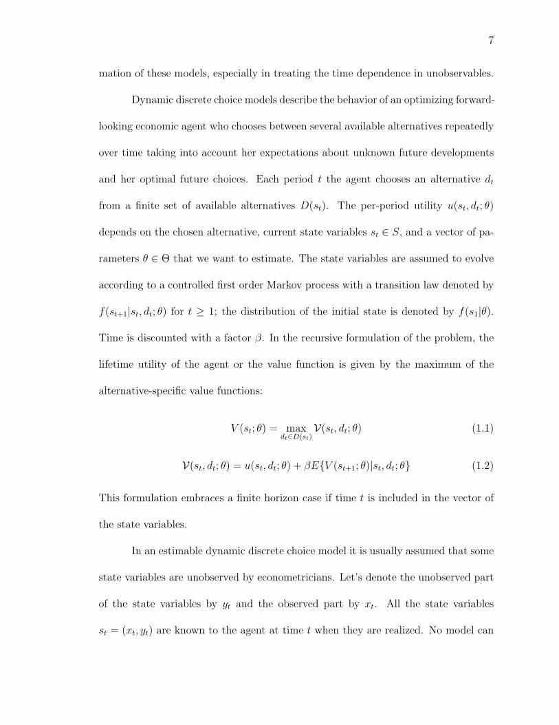
Dynamic discrete choice models describe the behavior of an optimizing forward-

looking economic agent who chooses between several available alternatives repeatedly

over time taking into account her expectations about unknown future developments

and her optimal future choices. Each period t the agent chooses an alternative dt

from a finite set of available alternatives D(st). The per-period utility u(st, dt; θ)

depends on the chosen alternative, current state variables st ∈ S, and a vector of pa-

rameters θ ∈ Θ that we want to estimate. The state variables are assumed to evolve

according to a controlled first order Markov process with a transition law denoted by

f(st+1|st, dt; θ) for t ≥ 1; the distribution of the initial state is denoted by f(s1|θ).

Time is discounted with a factor β. In the recursive formulation of the problem, the

lifetime utility of the agent or the value function is given by the maximum of the

alternative-specific value functions:

V (st; θ) = maxdt∈D(st)

V(st, dt; θ) (1.1)

V(st, dt; θ) = u(st, dt; θ) + βEV (st+1; θ)|st, dt; θ (1.2)

This formulation embraces a finite horizon case if time t is included in the vector of

the state variables.

In an estimable dynamic discrete choice model it is usually assumed that some

state variables are unobserved by econometricians. Let’s denote the unobserved part

of the state variables by yt and the observed part by xt. All the state variables

st = (xt, yt) are known to the agent at time t when they are realized. No model can

8

perfectly predict human behavior. Using the unobserved state variables is an attrac-

tive way to structurally incorporate random errors in the model. The unobserved

state variables can be interpreted as shocks, taste idiosyncrasy, unobserved hetero-

geneity, or measurement errors. They may also be more specific: e.g. health status or

returns to patents. The unobservables play an important role in the estimation. The

likelihood function of a DDCM is an integral over the unobservables. In a static case,

as few as n unobservables can be used in a model with 2n alternatives to produce

non-zero choice probabilities for all the alternatives and for any parameter vector in

Θ given that the support of the distribution for the unobservables is sufficiently large

relative to Θ. It would happen, for example, if a distinct combination of the compo-

nents of n-dimensional yt additively enters the utility function for each alternative.

However, it is often more convenient to assume a larger number of the unobservables,

e.g., a dynamic multinomial logit model has one unobservable for each alternative.

The set of the available alternatives D(st) is assumed to depend only on the

observed state variables. Hereafter, it will be denoted by D to simplify the nota-

tion. This is without loss of generality since we could set D = ∪xt∈XD(xt) and the

alternatives unavailable at state xt could be assigned a low per-period utility value.

A data set that is usually used for the estimation of a dynamic discrete choice

model consists of a panel of I individuals. The observed part of the state and the

decisions are known for each individual i ∈ 1, . . . , I for Ti periods: xt,i, dt,iTit=1.

Assuming that the state variables are independent for the individuals in the sample,

9

the likelihood for the model can be written as

p(xt,i, dt,iTit=1, i ∈ 1, . . . , I|θ) =

I∏i=1

p(xTi,i, dTi,i, . . . , x1,i, d1,i|θ) = (1.3)

I∏i=1

∫p(yTi,i, xTi,i, dTi,i, . . . , y1,i, x1,i, d1,i|θ)dyTi,i, . . . , dy1,i

The joint density p(yTi,i, xTi,i, dTi,i, . . . , y1,i, x1,i, d1,i|θ) could be decomposed as follows

p(yTi,i, xt,i, dt,i, . . . , y1,i, x1,i, d1,i|θ) =

Ti∏t=1

p(dt,i|yt,i, xt,i; θ)f(xt,i, yt,i|xt−1,i, yt−1,i, dt−1,i; θ)

(1.4)

where f(.|.; θ) is the state transition density, x0,i, y0,i, d0,i = ∅, and p(dt,i|yt,i, xt,i; θ)

is an indicator function:

p(dt,i|yt,i, xt,i; θ) = 1V(yt,i,xt,i,dt,i;θ)≥V(yt,i,xt,i,d;θ),∀d∈D(yt,i, xt,i, dt,i; θ) (1.5)

In general, evaluation of the likelihood function in (1.3) involves computing

multidimensional integrals of an order equal to Ti times the number of components

in yt, which becomes infeasible for large Ti and/or multi-dimensional unobservables

yt. That is why in previous literature the unobservables were mainly assumed to be

iid. In a series of papers, John Rust developed a dynamic multinomial logit model,

where he assumed that the utility function of the agents is additively separable in

the unobservables and that the unobservables are extreme value iid. In this case, the

integration in (1.3) can be performed analytically. Pakes (1986) used Monte Carlo

simulations to approximate the likelihood function in a model of binary choice with

a serially correlated one-dimensional unobservable.

In a Bayesian framework, the high dimensional integration over yt for each

parameter value can be circumvented by employing Gibbs sampling and data aug-

10

mentation. In models with latent variables, the Gibbs sampler typically has two types

of blocks: (a) parameters conditional on other parameters, latent variables and the

data; (b) latent variables conditional on other latent variables, parameters and the

data (this step is sometimes called data augmentation.) The draws simulated from

this Gibbs sampler form a Markov chain with the stationary distribution equal to the

joint distribution of the parameters and the latent variables conditional on the data.

The densities for both types of the blocks are proportional to the joint density of the

data, the latent variables, and the parameters. Therefore, in order to construct the

Gibbs sampler in our case, we need to obtain an analytical expression for the joint

density of the data, the latent variables, and the parameters.

By a parameterization of the Gibbs sampler I mean a set of parameters and

latent variables used in constructing the sampler. One parameterization is obtained

from another by a change of variables. The number of the variables does not have to

be the same for different parameterizations: some variables could just have degenerate

distributions given other variables in the parameterization. This section illustrates

that although any parameterization validly describes the econometric model, the pa-

rameterization choice could be crucial for the Gibbs sampler performance. For a

simple example, consider parameterizing a multinomial probit model by the error

terms and the parameters instead of the latent utilities and the parameters.

It is straightforward to obtain an analytical expression for the joint density of

the data, the latent variables, and the parameters under the parameterization of the

Gibbs sampler in which the unobserved state variables are directly used as the latent

11

variables in the sampler:

p(θ; dt,i; yt,i; xt,iTit=1; i = 1, . . . , I) =

p(θ)I∏

i=1

Ti∏t=1

p(dt,i|xt,i, yt,i; θ)f(xt,i, yt,i|xt−1,i, yt−1,i, dt−1,i; θ) (1.6)

where p(θ) is a prior density for the parameters and p(dt,i|xt,i, yt,i; θ) is an indicator

function defined in (1.5). It is evident from (1.6) that in this Gibbs sampler, the

parameter blocks will be drawn subject to the observed choice optimality constraints:

V(yt,i, xt,i, dt,i; θ) ≥ V(yt,i, xt,i, d; θ),∀d ∈ D, ∀t ∈ 1, . . . , Ti,∀i ∈ 1, . . . , I (1.7)

For realistic sample sizes, the number of these constraints is very large and the algo-

rithm becomes impractical. The same situation occurs under the parameterization in

which ut,d,i = u(yt,i, xt,i, dt,i; θ) are used as the latent variables in the sampler instead

of some or all of the components of yt,i2.

The complicated truncation region (1.7) in drawing the parameter blocks could

be avoided if we use Vt,i = Vt,d,i = V(st,i, d; θ), d ∈ D as latent variables in the

sampler. However, then some extra assumptions on the unobserved state variables are

needed so that the joint density of the data, the latent variables, and the parameters

could be specified analytically. A way to achieve this when an analytical solution

to the DP is not available is to assume that the unobserved part of the state vector

includes some serially conditionally independent components that do not affect the

distribution of the future state. Let’s denote them by νt and the other (possibly

2Imai et al. (2005) seem to use this parameterization, but they omit the observed choiceoptimality constraints (1.7) in drawing the parameters. From my communication withProfessor Imai, I understand that it will be changed in the next version of their paper.

12

serially correlated) ones by εt; so, yt = (νt, εt) and

f(xt+1, νt+1, εt+1|xt, νt, εt, d; θ) = p(νt+1|xt+1, εt+1; θ)p(xt+1, εt+1|xt, εt, d; θ) (1.8)

Then, the expected value function EV (st+1; θ)|st, d; θ) will not depend on the un-

observables νt. The alternative specific value functions Vt,i = u(νt,i, εt,i, xt,i, d; θ) +

βE[V (st+1; θ)|εt,i, xt,i, d; θ)], d ∈ D will have analytical expressions as functions of

νt. Thus, the density of the distribution of Vt,i|θ, xt,i, εt,i could have an analytical

expression in contrast to the case when νt are serially conditionally dependent and

the expectation term depends on them.

A simple example of an analytical expression for the density p(Vt,i|θ, xt,i, εt,i) is

obtained for normal iid νt = νt,dd∈D and u(νt,i, εt,i, xt,i, d; θ) = u(εt,i, xt,i, d; θ)+νt,d,i.

The serially correlated unobservables εt,i could follow an AR(1) process and also enter

the utility function additively:

u(yt,i, xt,i, d; θ) = u(xt,i, d; θ) + νt,d,i + εt,d,i (1.9)

This formulation could be seen as a simple way of introducing time persistent unob-

served heterogeneity in the model. The serially correlated unobservables could also

have a more meaningful economic interpretation, e.g. health status, and enter the

utility function differently. In general, the number of components in νt and εt does

not have to be the same and they do not have to enter the utility additively.

The requirement of the presence of the serially conditionally independent un-

observables and the existence of a convenient analytical expression for p(Vt,i|θ, xt,i, εt,i)

does restrict the class of the DDCMs that can be estimated by the proposed method.

13

However, this restriction does not seem to be strong since the process for the unob-

servables can still be made quite flexible.

Assuming that a convenient analytical expression for p(Vt,i|θ, xt,i, εt,i) exists,

the joint distribution of the data, the parameters and the latent variables can be

decomposed into parts with known analytical expressions:

p(θ; dt,i;Vt,i; xt,i; εt,iTit=1; i = 1, . . . , I) =

p(θ)I∏

i=1

Ti∏t=1

p(dt,i|Vt,i)p(Vt,i|xt,i, εt,i; θ)p(xt,i, εt,i|xt−1,i, εt−1,i, dt−1,i; θ) (1.10)

Under this parameterization, the observed choice optimality constraints

p(dt,i|Vt,i; θ; xt,i; εt,i) = p(dt,i|Vt,i) = 1Vt,dt,i,i≥Vt,d,i,d∈D(dt,i,Vt,i) (1.11)

will not depend on the parameters and will be present only in the blocks for Vt,d,i| . . ..

This could be easily handled since there will be only one constraint for each block

Vt,d,i| . . .. Complete specifications of the Gibbs sampler constructed along these lines

are given in Section 1.5 for the models used in experiments.

Further simplification of the Gibbs sampler is possible if we assume that the

per-period utility function is given by (1.9) and that the unobservables νt,d,i are ex-

treme value iid. Then, Vt,i can be integrated out analytically as in dynamic multino-

mial logit models. This slight simplification is not pursued here.

The Gibbs sampler outlined above requires computing the expected value func-

tions for each new parameter draw θm from the MCMC iteration m and each obser-

vation in the sample:

E[V (st+1; θm)|xt,i, ε

mt,i, d; θm)],∀i, t, d

14

The following section describes how the approximations of the expected value func-

tions are obtained.

1.3 Algorithm for solving the DP

For a discussion of methods for solving the DP in (1.1) and (1.2) for a given

parameter vector θ, see the literature surveys by Eckstein and Wolpin (1989) and

Rust (1994). Models used in the previous literature were mostly amenable to a sig-

nificant analytical simplification. For example, in Rust’s dynamic multinomial logit

model, the integration in computing expected value functions could be performed an-

alytically. Below, I introduce a method of solving the dynamic program suitable for

use in conjunction with the Bayesian estimation of a general dynamic discrete choice

model. This method uses an idea from Imai et al. (2005) of iterating the Bellman

equation only once at each step of the estimation procedure and using information

from previous steps to approximate the expectations in the Bellman equation. How-

ever, the way the previous information is used differs for the two methods. A detailed

comparison is given in Section 1.3.2.

1.3.1 Algorithm description

In contrast to conventional value function iteration, this algorithm iterates the

Bellman equation only once for each parameter draw. First, I will describe how the

DP solving algorithm works and then how the output of the DP solving algorithm is

used to approximate the expected value functions in the Gibbs sampler.

The DP solving algorithm takes a sequence of parameter draws θm, m =

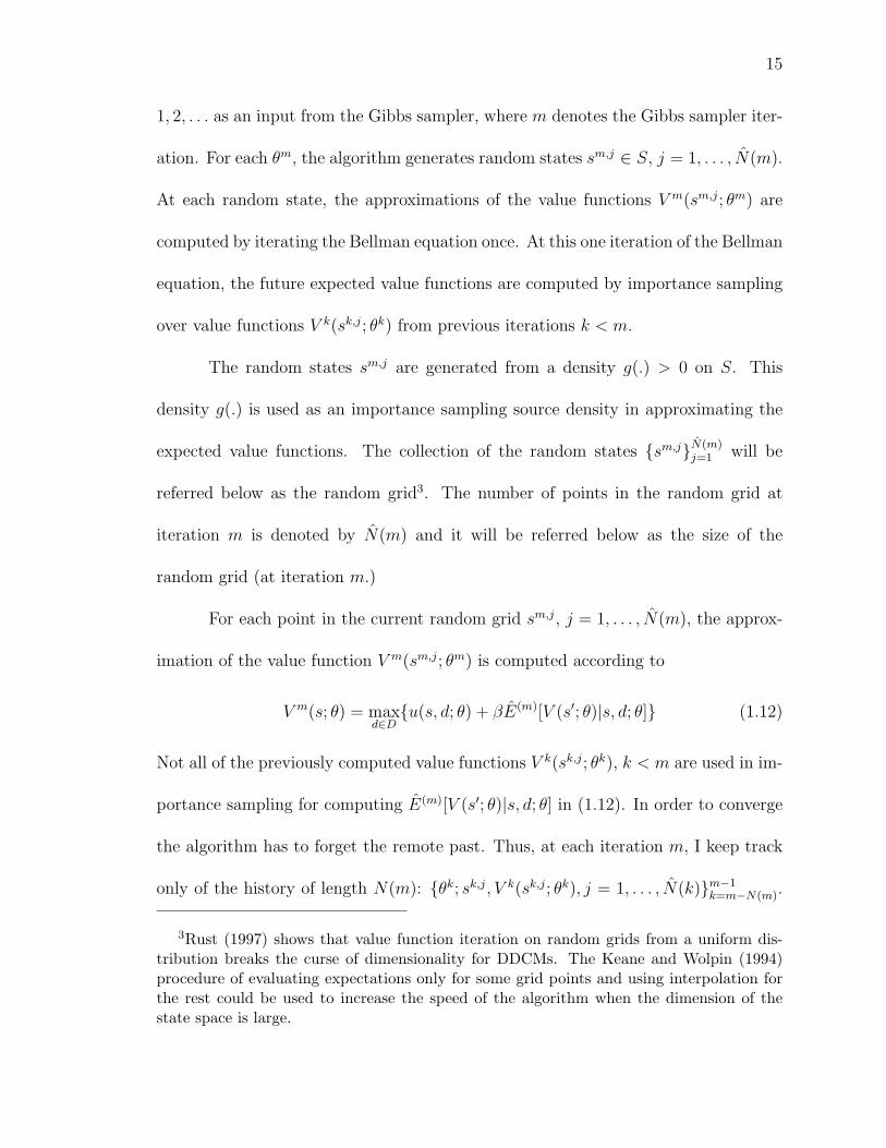
15

1, 2, . . . as an input from the Gibbs sampler, where m denotes the Gibbs sampler iter-

ation. For each θm, the algorithm generates random states sm,j ∈ S, j = 1, . . . , N(m).

At each random state, the approximations of the value functions V m(sm,j; θm) are

computed by iterating the Bellman equation once. At this one iteration of the Bellman

equation, the future expected value functions are computed by importance sampling

over value functions V k(sk,j; θk) from previous iterations k < m.

The random states sm,j are generated from a density g(.) > 0 on S. This

density g(.) is used as an importance sampling source density in approximating the

expected value functions. The collection of the random states sm,jN(m)j=1 will be

referred below as the random grid3. The number of points in the random grid at

iteration m is denoted by N(m) and it will be referred below as the size of the

random grid (at iteration m.)

For each point in the current random grid sm,j, j = 1, . . . , N(m), the approx-

imation of the value function V m(sm,j; θm) is computed according to

V m(s; θ) = maxd∈D

u(s, d; θ) + βE(m)[V (s′; θ)|s, d; θ] (1.12)

Not all of the previously computed value functions V k(sk,j; θk), k < m are used in im-

portance sampling for computing E(m)[V (s′; θ)|s, d; θ] in (1.12). In order to converge

the algorithm has to forget the remote past. Thus, at each iteration m, I keep track

only of the history of length N(m): θk; sk,j, V k(sk,j; θk), j = 1, . . . , N(k)m−1k=m−N(m).

3Rust (1997) shows that value function iteration on random grids from a uniform dis-tribution breaks the curse of dimensionality for DDCMs. The Keane and Wolpin (1994)procedure of evaluating expectations only for some grid points and using interpolation forthe rest could be used to increase the speed of the algorithm when the dimension of thestate space is large.

16

In this history, I find N(m) closest to θ parameter draws. Only the value functions

corresponding to these nearest neighbors are used in importance sampling. Formally,

let k1, . . . , kN(m) be the iteration numbers of the nearest neighbors of θ in the cur-

rent history:

k1 = arg mini∈m−N(m),...,m−1∣∣∣∣θ − θi

∣∣∣∣kj = arg mini∈m−N(m),...,m−1\k1,...,kj−1

∣∣∣∣θ − θi∣∣∣∣ , j = 2, . . . , N(m) (1.13)

If the arg min returns a multivalued result, I use the lexicographic order for (θi − θ)

to decide which θi is chosen first. If the result of the lexicographic selection is also

multivalued: θi = θj, then I choose θi over θj if i > j. This particular way of

resolving the multivaluedness of the arg min might seem irrelevant for implementing

the method in practice; however, it is important for the proof of the measurability

of the supremum of the approximation error, which is necessary for the uniform

convergence results. A reasonable choice for the norm would be ||θ|| =√

θT Hθθ,

where Hθ is the prior precision for the parameters. Importance sampling is performed

as follows:

E(m)[V (s′; θ)|s, d; θ]

=

N(m)∑i=1

N(ki)∑j=1

V ki(ski,j; θki)f(ski,j | s, d; θ)/g(ski,j)∑N(m)

r=1

∑N(kr)q=1 f(skr,q | s, d; θ)/g(skr,q)

(1.14)

=

N(m)∑i=1

N(ki)∑j=1

V ki(ski,j; θki)Wki,j,m(s, d, θ) (1.15)

The target density for importance sampling is the state transition density f(.|s, d; θ).

The source density is the density g(.) from which the random grid on the state space

17

is generated. The computation of the weights Wki,j,m(s, d, θ) could be simplified if a

part of the state vector is serially independent and its distribution does not depend

on the parameters and the other state variables. Both models used for experiments

contain examples of that: the unobservables νt are Gaussian iid with zero mean and

the variance fixed for normalization. In this case the source density for νt could be the

same as the density according to which νt are distributed in the model. Then, the part

of the weight Wki,j,m(s, d, θ) corresponding to νt would be equal to 1. In general, g(.)

should give reasonably high probabilities to all parts of the state space that are likely

under f(.|s, d; θ) with reasonable values of the parameter θ. To reduce the variance

of the approximation of expectations produced by importance sampling4, one should

make g(.) relatively high for the states that result in larger value functions.

To obtain the convergence of the DP solution approximations as m →∞, we

have to impose some obvious restrictions on the size of the random grid N(m), the

length of the tracked history N(m), and the number of the nearest neighbors N(m).

The length of the tracked history N(m) has to go to infinity so that when we pick

the nearest neighbors from this history they get very close to the current parame-

ter. For the same reason the number of the nearest neighbors N(m) has to be small

relative to N(m). The length of the forgotten history m − N(m) has to go to infin-

ity so that early imprecise approximations would not contaminate the future ones.

A lower bound on the number of the random states used in importance sampling

4Importance sampling is used as a variance reduction technique for Monte Carlo simu-lations

18

[N(m) ·mini∈m−N(m),...,m−1 N(i)] should go to infinity so that the importance sam-

pling approximations of the integrals converge. More specific assumptions on N(m),

N(m), and N(m) are made in the current version of the algorithm convergence proof.

They are described along with the assumptions on the model primitives in Section

1.3.3, which formally presents convergence results.

After V m(sm,j; θm) are computed, formula (1.14) is used to obtain the ap-

proximations of the expectations E[V (st+1; θm)|xt,i, ε

mt,i, d; θm)] ∀i, t, d in the Gibbs

sampler.

1.3.2 Comparison with Imai et al. (2005)

Imai et al. (2005) use kernel smoothing over all N(m) previously computed

value functions to approximate the expected value functions. They do not need

the importance sampling for the iid unobserved states; they also generate only one

new state at each iteration, N(m) = 1,∀m. In contrast, I use the nearest neighbor

(NN) algorithm instead of kernel smoothing. The advantage of the NN algorithm

seems to be twofold. First, it was shown to outperform kernel smoothing in density

estimation when the number of dimensions exceeds four. Thus, it might work better

in practice for the DP solving algorithm as well. Second, the NNs seem to be easier

to deal with mathematically. First of all, to prove the convergence of the DP solution

approximations I do not have to impose the requirement of a uniform upper bound on

the Gibbs sampler transition density (used by Imai et al. (2005) in their Lemma 2),

which I have not managed to establish for the actual Gibbs sampler. Second, the Imai

19

et al. (2005) assumption of finiteness of the observed states space X can be substituted

by compactness. Third, Imai et al. (2005) assumed deterministic transition for the

observed states in the proof and iid unobserved states. With NN approximations,

random state transitions can be used. Imai et al. (2005) proved the convergence in

probability for their DP solution approximations with bounds on the probabilities

that are uniform over the parameter space. For the NN algorithm, I establish a much

stronger type of convergence: the complete uniform convergence. Most importantly,

the strong convergence results for the NN approximations of the DP solutions are

shown to imply the convergence of the approximated posterior expectations, which

provides a complete theoretical justification for the proposed Bayesian estimation

algorithm.

1.3.3 Theoretical results

The following assumptions on the model primitives and the algorithm param-

eters are made:

Assumption 1.1. Θ ⊂ RJΘ and S ⊂ RJS are bounded rectangles.

Assumption 1.2. u(s, d; θ) is bounded, β ∈ (0, 1) is known.

Assumption 1.3. V (s; θ) is continuous in (θ, s).

Assumption 1.3 will hold, for example, under the following set of restrictions

on the primitives of the model: Θ and S are compact, u(s, d; θ) is continuous in (s, θ),

and f(s′ | s, d; θ) is continuous in (θ, s, s′) (for a proof see Proposition 2.4.)

20

Assumption 1.4. The density of the state transition f(.|.) and the source importance

density g(.) are bounded above and away from zero, which gives:

infθ,s′,s,d

f(s′|s, d; θ)/g(s′) = f > 0

supθ,s′,s,d

f(s′|s, d; θ)/g(s′) = f < ∞

Assumption 1.5. ∃δ > 0 such that P (θm+1 ∈ A|ωm) ≥ δλ(A) for any Borel mea-

surable A ⊂ Θ, any m, and any feasible history ωm = ω1, . . . , ωm where λ is the

Lebesgue measure. The history includes all the parameter and latent variable draws

from the Gibbs sampler and all the random grids from the DP solving algorithm:

ωt = θt, ∆V t, εt; st,j, j = 1, . . . , N(t).

Assumption 1.5 means that at each iteration of the algorithm, the parame-

ter draw can get into any part of Θ. This assumption should be verified for each

specific DDCM and the corresponding parameterization of the Gibbs sampler. The

assumption is only a little stronger than standard conditions for convergence of the

Gibbs sampler, see Corollary 4.5.1 in Geweke (2005). Since a careful practitioner

of MCMC would have to establish convergence of the Gibbs sampler, a verification

of Assumption 1.5 should not require much extra effort. Even if the assumption is

not satisfied for the Gibbs sampler, the DP solving algorithm can be theoretically

justified if the parameter draws from the Gibbs sampler are mixed with parameter

draws from a positive on Θ density for creating the input sequence θ1, θ2, . . . for the

DP solving algorithm.

21

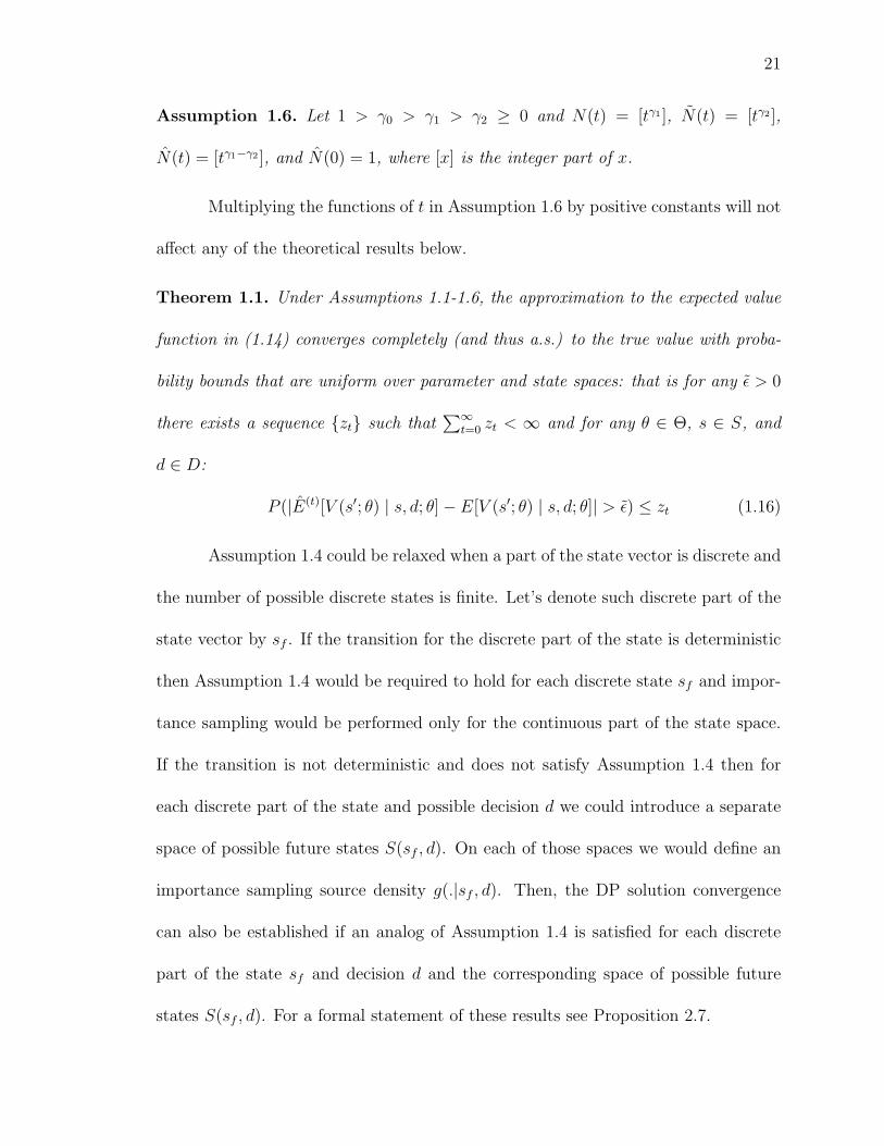
Assumption 1.6. Let 1 > γ0 > γ1 > γ2 ≥ 0 and N(t) = [tγ1 ], N(t) = [tγ2 ],

N(t) = [tγ1−γ2 ], and N(0) = 1, where [x] is the integer part of x.

Multiplying the functions of t in Assumption 1.6 by positive constants will not

affect any of the theoretical results below.

Theorem 1.1. Under Assumptions 1.1-1.6, the approximation to the expected value

function in (1.14) converges completely (and thus a.s.) to the true value with proba-

bility bounds that are uniform over parameter and state spaces: that is for any ε > 0

there exists a sequence zt such that∑∞

t=0 zt < ∞ and for any θ ∈ Θ, s ∈ S, and

d ∈ D:

P (|E(t)[V (s′; θ) | s, d; θ]− E[V (s′; θ) | s, d; θ]| > ε) ≤ zt (1.16)

Assumption 1.4 could be relaxed when a part of the state vector is discrete and

the number of possible discrete states is finite. Let’s denote such discrete part of the

state vector by sf . If the transition for the discrete part of the state is deterministic

then Assumption 1.4 would be required to hold for each discrete state sf and impor-

tance sampling would be performed only for the continuous part of the state space.

If the transition is not deterministic and does not satisfy Assumption 1.4 then for

each discrete part of the state and possible decision d we could introduce a separate

space of possible future states S(sf , d). On each of those spaces we would define an

importance sampling source density g(.|sf , d). Then, the DP solution convergence

can also be established if an analog of Assumption 1.4 is satisfied for each discrete

part of the state sf and decision d and the corresponding space of possible future

states S(sf , d). For a formal statement of these results see Proposition 2.7.

22

Theorem 1.1 gives uniform bounds on the probabilities that the approximation

error for fixed (θ, s) exceeds some positive number. However, the uniform convergence

for random functions, which seems to be easier to apply but harder to establish,

is defined differently in the literature (see Bierens (1994)). A uniform version of

Theorem 1.1 can be obtained given an extra assumption:

Assumption 1.7. Fix a combination m = m1, . . . ,mN(t) from t−N(t), . . . , t−1.

Let

X(ωt−1, θ, s, d,m) = (1.17)∣∣∣∣∣∣N(t)∑i=1

N(mi)∑j=1

(V (smi,j; θ)− E[V (s′; θ) | s, d; θ]))f(smi,j | s, d; θ)/g(smi,j)∑N(t)r=1

∑N(mr)q=1 f(smr,q | s, d; θ)/g(smr,q)

∣∣∣∣∣∣Assume that family of functions X(ωt−1, θ, s, d,m)ωt−1 is equicontinuous in (θ, s).

This assumption will be satisfied, for example, if u(s, d; θ) is continuous in

(θ, s) on the compact set Θ×S and f(s′ | s, d; θ) and g(s′) are continuous in (θ, s, s′)

and satisfy Assumption 1.4 (for a proof see Propositions 2.4 and 2.5.)

Theorem 1.2. Under Assumptions 1.1-1.7, the approximation to the expected value

function in (1.14) converges uniformly and completely to the true value: that is

(i) sups,θ,d |E(t)[V (s′; θ) | s, d; θ]− E[V (s′; θ) | s, d; θ]| is measurable,

(ii) for any ε > 0 there exists a sequence zt such that∑∞

t=0 zt < ∞ and

P (sups,θ,d

|E(t)[V (s′; θ) | s, d; θ]− E[V (s′; θ) | s, d; θ]| > ε) ≤ zt (1.18)

The proof of Theorem 1.2 is given in Chapter 2, Section 2.2. It is a modification

of the proof of Theorem 1.1, the main steps of which are given below.

23

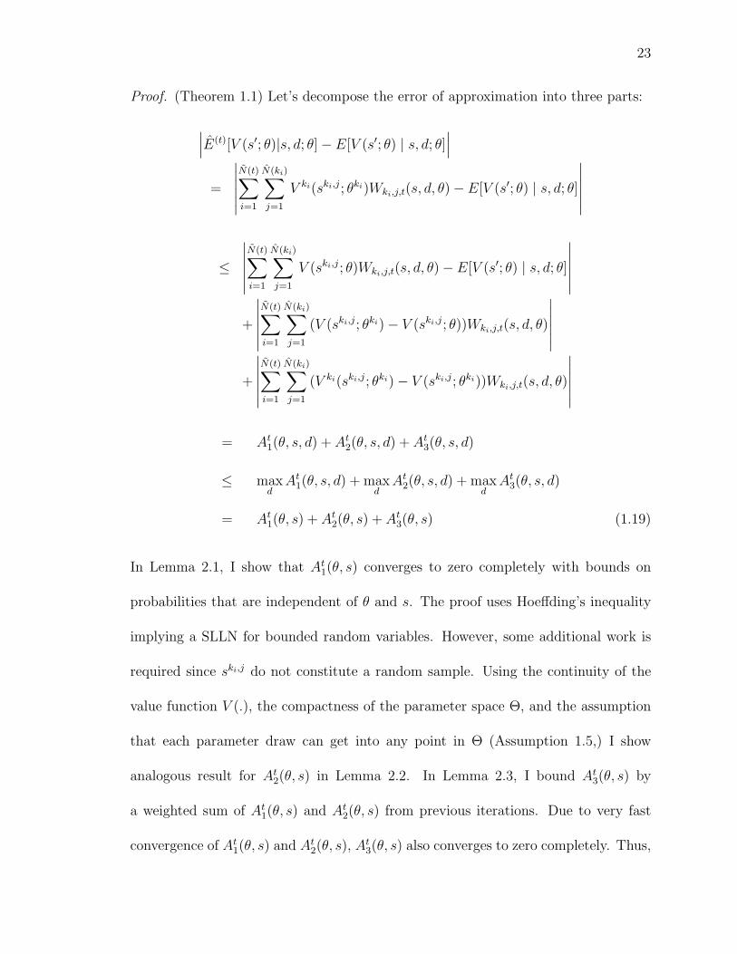
Proof. (Theorem 1.1) Let’s decompose the error of approximation into three parts:

∣∣∣E(t)[V (s′; θ)|s, d; θ]− E[V (s′; θ) | s, d; θ]∣∣∣

=

∣∣∣∣∣∣N(t)∑i=1

N(ki)∑j=1

V ki(ski,j; θki)Wki,j,t(s, d, θ)− E[V (s′; θ) | s, d; θ]

∣∣∣∣∣∣≤

∣∣∣∣∣∣N(t)∑i=1

N(ki)∑j=1

V (ski,j; θ)Wki,j,t(s, d, θ)− E[V (s′; θ) | s, d; θ]

∣∣∣∣∣∣+

∣∣∣∣∣∣N(t)∑i=1

N(ki)∑j=1

(V (ski,j; θki)− V (ski,j; θ))Wki,j,t(s, d, θ)

∣∣∣∣∣∣+

∣∣∣∣∣∣N(t)∑i=1

N(ki)∑j=1

(V ki(ski,j; θki)− V (ski,j; θki))Wki,j,t(s, d, θ)

∣∣∣∣∣∣= At

1(θ, s, d) + At2(θ, s, d) + At

3(θ, s, d)

≤ maxd

At1(θ, s, d) + max

dAt

2(θ, s, d) + maxd

At3(θ, s, d)

= At1(θ, s) + At

2(θ, s) + At3(θ, s) (1.19)

In Lemma 2.1, I show that At1(θ, s) converges to zero completely with bounds on

probabilities that are independent of θ and s. The proof uses Hoeffding’s inequality

implying a SLLN for bounded random variables. However, some additional work is

required since ski,j do not constitute a random sample. Using the continuity of the

value function V (.), the compactness of the parameter space Θ, and the assumption

that each parameter draw can get into any point in Θ (Assumption 1.5,) I show

analogous result for At2(θ, s) in Lemma 2.2. In Lemma 2.3, I bound At

3(θ, s) by

a weighted sum of At1(θ, s) and At

2(θ, s) from previous iterations. Due to very fast

convergence of At1(θ, s) and At

2(θ, s), At3(θ, s) also converges to zero completely. Thus,

24

from the three Lemmas the result follows. Formally, according to Lemmas 2.1, 2.2,

2.3, there exist δ1 > 0, δ2 > 0, δ3 > 0 and T such that ∀θ ∈ Θ, ∀s ∈ S, and ∀t > T :

P (|At1(θ, s)| > ε/3) ≤ e−0.5δ1tγ1

P (|At2(θ, s)| > ε/3) ≤ e−0.5δ2tγ1

P (|At3(θ, s)| > ε/3) ≤ e−δ3tγ0γ1

Combining the above equations gives:

P (|E(t)[V (s′; θ) | s, d; θ]− E[V (s′; θ) | s, d; θ]| > ε)

≤ P (At1(θ, s) + At

2(θ, s) + At3(θ, s) > ε)

≤ P (|At1(θ, s)| > ε/3) + P (|At

2(θ, s)| > ε/3) + P (|At3(θ, s)| > ε/3)

≤ e−0.5δ1tγ1 + e−0.5δ2tγ1 + e−δ3tγ0γ1 , ∀t > T

= zt, ∀t > T (1.20)

For t ≤ T set zt = 1. Proposition 2.10 shows that∑∞

t=0 zt < ∞. The Lemmas are

stated and proved in Chapter 2.

1.4 Convergence of posterior expectations

In Bayesian analysis, most inference exercises involve computing posterior ex-

pectations of some functions. For example, the posterior mean and the posterior

standard deviation of a parameter and the posterior probability that a parameter

belongs to a set can all be expressed in terms of posterior expectations. More im-

portantly, the answers to the policy questions that DDCMs address also take this

25

form. Examples of such policy questions for the models I use in experiments in-

clude: (i) in Gilleskie’s model, investigators might be interested in how the average

number of doctor visits and/or work absences would be affected by changes in the

coinsurance rates and in the proportion of the wage that sick leave replaces; (ii) in

Rust’s model, investigators could care about how the annual number of bus engine

replacements would be affected by a change in the engine replacement cost. Using the

uniform complete convergence of the approximations of the expected value functions,

I prove the complete convergence of the approximated posterior expectations under

mild assumptions on a kernel of the posterior distribution.

Assumption 1.8. Assume that εt,i ∈ E, θ ∈ Θ, and νt,k,i ∈ [−ν, ν], where νt,k,i

denotes the kth component of νt,i. Let the joint posterior distribution of the parameters

and the latent variables be proportional to a product of a continuous function and

indicator functions:

p(θ,V , ε; F |d, x) ∝ r(θ,V , ε; F (θ, ε)) · 1Θ(θ) ·

(∏i,t

1E(εt,i)p(dt,i|Vt,i)

)

·

(∏i,t,k

1[−ν,ν](qk(θ,Vt,i, εt,i, Ft,i(θ, εt,i)))

)(1.21)

where r(θ,V , ε; F ) and qk(θ,Vt,i, εt,i, Ft,i) are continuous in (θ,V , ε, F ), F = Ft,d,i,∀i, t, d

stands for a vector of the expected value functions, and Ft,i are the corresponding sub-

vectors. Also, assume that the level curves of qk(θ,Vt,i, εt,i, Ft,i) corresponding to ν

and −ν have zero Lebesgue measure:

λ[(θ,V , ε) : qk(θ,Vt,i, εt,i, Ft,i) = ν] = λ[(θ,V , ε) : qk(θ,Vt,i, εt,i, Ft,i) = −ν] = 0 (1.22)

26

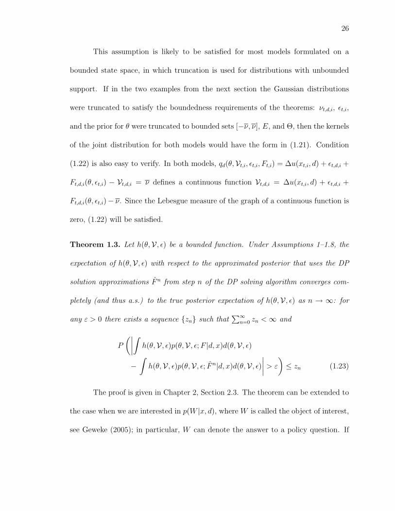
This assumption is likely to be satisfied for most models formulated on a

bounded state space, in which truncation is used for distributions with unbounded

support. If in the two examples from the next section the Gaussian distributions

were truncated to satisfy the boundedness requirements of the theorems: νt,d,i, εt,i,

and the prior for θ were truncated to bounded sets [−ν, ν], E, and Θ, then the kernels

of the joint distribution for both models would have the form in (1.21). Condition

(1.22) is also easy to verify. In both models, qd(θ,Vt,i, εt,i, Ft,i) = ∆u(xt,i, d) + εt,d,i +

Ft,d,i(θ, εt,i) − Vt,d,i = ν defines a continuous function Vt,d,i = ∆u(xt,i, d) + εt,d,i +

Ft,d,i(θ, εt,i)− ν. Since the Lebesgue measure of the graph of a continuous function is

zero, (1.22) will be satisfied.

Theorem 1.3. Let h(θ,V , ε) be a bounded function. Under Assumptions 1–1.8, the

expectation of h(θ,V , ε) with respect to the approximated posterior that uses the DP

solution approximations F n from step n of the DP solving algorithm converges com-

pletely (and thus a.s.) to the true posterior expectation of h(θ,V , ε) as n → ∞: for

any ε > 0 there exists a sequence zn such that∑∞

n=0 zn < ∞ and

P

(∣∣∣∣∫ h(θ,V , ε)p(θ,V , ε; F |d, x)d(θ,V , ε)

−∫

h(θ,V , ε)p(θ,V , ε; F n|d, x)d(θ,V , ε)

∣∣∣∣ > ε

)≤ zn (1.23)

The proof is given in Chapter 2, Section 2.3. The theorem can be extended to

the case when we are interested in p(W |x, d), where W is called the object of interest,

see Geweke (2005); in particular, W can denote the answer to a policy question. If

27

the implications of the model for W are specified by a density p(W |θ,V , ε, d, x), then

p(W |d, x) =

∫p(W |θ,V , ε, d, x)p(θ,V , ε; F |d, x)d(θ,V , ε) (1.24)

If p(W |θ,V , ε, d, x) has the same properties as the kernel of p(θ,V , ε; F |d, x) in As-

sumption 1.8, then the theorem holds for p(W |x, d).

1.5 Experiments

To implement the algorithm I wrote a program in C. The program uses BACC5

interface to libraries LAPACK, BLAS, and RANLIB for performing matrix operations

and random variates generation. Higher level interpreted languages like Matlab would

not provide necessary computation speed since the algorithm cannot be sufficiently

vectorized. As a matter of future work, the algorithm could be easily parallelized

with very significant gains in speed (this is is not necessarily possible or easy for

an arbitrary algorithm.) A short discussion of algorithm parallelization is given in

Section 1.5.2.5.

1.5.1 Gilleskie’s (1998) model

1.5.1.1 Setup

For experiments, I used a simplified version of Gilleskie’s model. Only one

type of sickness was included and some parameters were fixed. For the extreme value

iid process for taste shocks in the original model I substituted a serially correlated

process.

5BACC is an open source software for Bayesian Analysis, Computation, and Communi-cation available at www2.cirano.qc.ca/bacc

28

In the model, an agent can be sick or well. If sick, every period she has the

following alternatives to choose from: d = 1 – work and do not visit a doctor, d = 2

– work and visit a doctor, d = 3 – do not work and do not visit a doctor, d = 4 –

do not work and visit a doctor. The observed state x for a sick agent includes: t –

the time since the illness started, vt – the number of doctor visits since the illness

started, and at – the number of work absences accumulated since the illness started.

For a well agent x = (0, 0, 0).

The per-period utility function of a well agent is equal to her income Y , which

is known; so, the marginal utility of consumption when well is fixed to 1. The per-

period utility function of an ill agent is additively separable in the unobserved state

variables yt = yt,d, d ∈ D and linear in parameters:

u(xt, yt, d) = z(xt, d) · α + yt,d

where α = (α1, α2, α3, α4), α1 is the disutility of illness, α2 is the direct utility of

doctor visit, α3 is the direct utility of attending work when ill, and α4 is the marginal

utility of consumption when ill. As a function of the observed state and the decision,

the 1× 4 matrix z(xt, d) is given by

z(xt, 1) = (1, 0, 1, Y ), z(xt, 2) = (1, 1, 1, Y − C)

z(xt, 3) = (1, 0, 0, Y φ(at + 1)), z(xt, 4) = (1, 1, 0, Y φ(at + 1)− C)

where C is a known out-of-pocket cost of a doctor visit; φ(at) is a proportion of the

daily wage that sick leave replaces for the accumulated number of absences at. In the

original model φ(at) depends on some parameters; here, I just fix those.

29

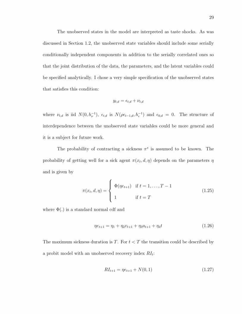
The unobserved states in the model are interpreted as taste shocks. As was

discussed in Section 1.2, the unobserved state variables should include some serially

conditionally independent components in addition to the serially correlated ones so

that the joint distribution of the data, the parameters, and the latent variables could

be specified analytically. I chose a very simple specification of the unobserved states

that satisfies this condition:

yt,d = εt,d + νt,d

where νt,d is iid N(0, h−1ν ), εt,d is N(ρεt−1,d, h

−1ε ) and ε0,d = 0. The structure of

interdependence between the unobserved state variables could be more general and

it is a subject for future work.

The probability of contracting a sickness πs is assumed to be known. The

probability of getting well for a sick agent π(xt, d, η) depends on the parameters η

and is given by

π(xt, d, η) =

Φ(ηet+1) if t = 1, . . . , T − 1

1 if t = T

(1.25)

where Φ(.) is a standard normal cdf and

ηet+1 = η1 + η2vt+1 + η3at+1 + η4t (1.26)

The maximum sickness duration is T . For t < T the transition could be described by

a probit model with an unobserved recovery index RIt:

RIt+1 = ηet+1 + N(0, 1) (1.27)

30

Conditional on RIt+1 the transition for xt is deterministic:

xt+1|xt, d, RIt+1 =

(0, 0, 0), if RIt+1 > 0 or t = T

x′(xt, d) = (t + 1, at + 13,4(d), vt + 12,4(d)), otherwise

(1.28)

where x′(.) denotes the future state as a deterministic function of the current state

and the decision given that the agent remains sick.

The life-time value of being well is

Vw = Y + β(1− πs)Vw + βπsEV (x1, y1) (1.29)

where x1 = (1, 0, 0).

The lifetime value of being sick is

V (xt, yt) = maxd∈D

V(xt, yt, d) (1.30)

V(xt, yt, d) = u(xt, yt, d) + βπ(xt, d, η)Vw

+ β(1− π(xt, d, η))E[V (x′(xt, d), yt+1)|εt; θ] (1.31)

1.5.1.2 Gibbs sampler

In the model formulation above, the assumed distributions for the unobserved

states have unbounded support. It is also more convenient to use distributions with

unbounded support in constructing the Gibbs sampler. To reconcile this with the

theory, which requires the parameters and the states to be in bounded spaces, we

could assume the existence of bounds for all the parameters and the states. If these

bounds are large enough, then the Gibbs sampler that takes them into account would

31

produce the same results as the Gibbs sampler that does not. Thus, not to clutter

the notation I present the Gibbs sampler assuming no bounds. For an example of the

Gibbs sampler that imposes the bounds see the Gibbs sampler for Rust’s model in

Section 1.5.2.3.

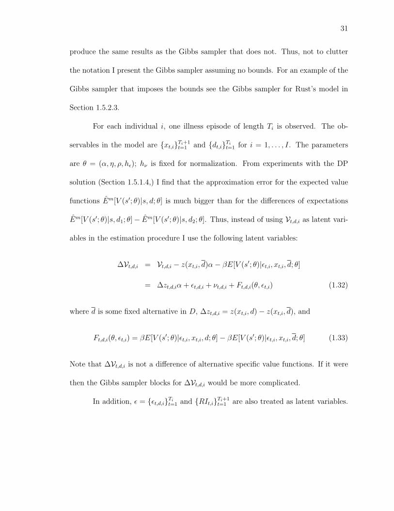
For each individual i, one illness episode of length Ti is observed. The ob-

servables in the model are xt,iTi+1t=1 and dt,iTi

t=1 for i = 1, . . . , I. The parameters

are θ = (α, η, ρ, hε); hν is fixed for normalization. From experiments with the DP

solution (Section 1.5.1.4,) I find that the approximation error for the expected value

functions Em[V (s′; θ)|s, d; θ] is much bigger than for the differences of expectations

Em[V (s′; θ)|s, d1; θ]− Em[V (s′; θ)|s, d2; θ]. Thus, instead of using Vt,d,i as latent vari-

ables in the estimation procedure I use the following latent variables:

∆Vt,d,i = Vt,d,i − z(xt,i, d)α− βE[V (s′; θ)|εt,i, xt,i, d; θ]

= ∆zt,d,iα + εt,d,i + νt,d,i + Ft,d,i(θ, εt,i) (1.32)

where d is some fixed alternative in D, ∆zt,d,i = z(xt,i, d)− z(xt,i, d), and

Ft,d,i(θ, εt,i) = βE[V (s′; θ)|εt,i, xt,i, d; θ]− βE[V (s′; θ)|εt,i, xt,i, d; θ] (1.33)

Note that ∆Vt,d,i is not a difference of alternative specific value functions. If it were

then the Gibbs sampler blocks for ∆Vt,d,i would be more complicated.

In addition, ε = εt,d,iTit=1 and RIt,iTi+1

t=1 are also treated as latent variables.

32

The joint distribution of the data, the parameters, and the latent variables is

p(θ; dt,i; ∆Vt,1,i, . . . , ∆Vt,D,i; εt,1,i, . . . , εt,D,iTit=1; xt,i; RIt,iTi+1

t=1 ; i = 1, . . . , I) =

p(θ)I∏

i=1

Ti∏t=1

[p(xt+1,i|xt,i; dt,i; RIt+1,i)p(RIt+1,i|xt,i; dt,i; η)

p(dt,i|∆Vt,1,i, . . . , ∆Vt,D,i)D∏

d=1

p(∆Vt,d,i|xt,i, εt,i; θ)p(εt,d,i|εt−1,d,i, ρ, hε)] (1.34)

where p(θ) is a prior density for parameters; x0,i = ∅; p(dt,i|∆Vt,1,i, . . . ,Vt,D,i) is an

indicator function, which is equal to 1 when ∆Vt,dt,i,i ≥ ∆Vt,d,i,∀d.

p(∆Vt,d,i|xt,i, εt,i; θ) ∝ exp −0.5hν(∆Vt,d,i −∆zt,d,iα− εt,d,i − Ft,d,i(θ, εt,i))2

p(εt,d,i|εt−1,d,i, θ) ∝ h−1/2ε exp −0.5hε(εt,d,i − ρεt−1,d,i)

2

Gibbs sampler blocks

The block for ∆Vt,d,i| . . . is N(∆zt,d,iα + εt,d,i + Ft,d,i(θ, εt,i), hν) truncated to

∆Vt,dt,i,i ≥ ∆Vt,d,i∀d ∈ D. The block for RIt+1,i| . . . is N(et+1,iη, 1) truncated to

(0,∞) if xt+1,i = (0, 0, 0) and to (−∞, 0) otherwise, where et+1,i is a vector depending

on xt,i and dt,i that was defined in (1.26). The density for εt,d,i| . . . block:

p(εt,d,i| . . .) ∝ exp −0.5hν(∆Vt,d,i − Ft,d,i(θ, εt,i)−∆zt,d,iα− εt,d,i)2 (1.35)

× exp −0.5hν

∑d6=d

(∆Vt,d,i − Ft,d,i(θ, εt,i)−∆zt,d,iα− εt,d,i)2(1.36)

× exp−0.5hε(εt+1,d,i − ρεt,d,i)2 − 0.5hε(εt,d,i − ρεt−1,d,i)

2 (1.37)

To draw from this density I use a Metropolis step with a normal transition density

proportional to (1.37). Blocks for εt,d,i with t = 0 and t = Ti will be similar. Blocks

for α| . . ., η| . . ., ρ| . . ., hε| . . . are drawn by the Metropolis-Hastings (MH) random

33

walk algorithm since an analytical expression for the difference in expected value

functions Ft,d,i(θ, ε) is unknown and it could only be approximated numerically. The

proposal density of the MH random walk algorithm is normal with mean equal to the

current parameter draw and a fixed variance. The variances are chosen so that the

acceptance probability would be between 0.2−0.8. If a vector of parameters is drawn

as one block by the MH random walk it is important to make the variances for all the

components of the vector as large as possible keeping the acceptance rate reasonable.

Nevertheless, reasonable acceptance rates do not guarantee fast convergence. While

drawing vector α by the MH as one block worked well, drawing η as one block resulted

in too slow mixing of the chain. Thus, on every other iteration the components of η

are drawn one at a time. This significantly accelerated convergence. For larger sample

sizes (I = 1000,) acceptance rates in the range 0.2-0.3 worked the best. For Rust’s

model, I explore an alternative to the random walk chain, in which the MH transition

densities are proportional to the familiar parts of the posterior. This alternative

seems to work remarkably well for the state transition parameters that are strongly

identified by the data (see Section 1.5.2.)

1.5.1.3 Approximating the value functions

The sequential structure of the model was exploited in computing the ap-

proximations of the value functions. In experiments, only one nearest neighbor

was picked for approximating the expectations: N(m) = 1. First, a random grid

ym,j = (νm,j, εm,j)N(m)j=1 is generated on the continuous part of the state space:

34

νm,jd ∼ N(0, h−1

ν ) and εm,j ∼ g(.), where g(.) is normal with zero mean and the pre-

cision equal to the prior mean of hε. The approximations of the value functions for

each x ∈ X and ym,j, j = 1, . . . , N(m) are computed as follows:

V m(x, ym,j; θm) = maxd∈D

u(x, ym,j, d, αm)

+ βπ(x, d, ηm)V k1w + β(1− π(x, d, ηm))× (1.38)

×N(m)∑i=1

V m(x′(x, d), ym,i; θm)f(εm,i | εm,j; θm)/g(εm,i)∑N(m)

r=1 f(εm,r | εm,j; θm)/g(εm,r)

where f(.|ε; θ) is a N(ρε, h−1ε ) density. Note that νm,j

d have the same distribution

as νt,d in the model. Thus, the corresponding density values cancel each other in

the numerator and denominator of the importance sampling weight. The approxima-

tions of the value functions with larger t are computed first. That is why only the

value functions already updated at the current iteration m, V m(.; θm) (as opposed

to V k1(.; θk1),) are used for approximating the expectations in (1.38). Note, that for

x with t = T , the recovery is certain, π(x, d, ηm) = 1, and only V k1w is required for

computing the expectation. This procedure is similar to the backward induction or

the Gauss-Seidel method.

After (1.38), the approximation of the value of being well is computed.

V mw = [1/(1− β(1− πs))][Y +

+ βπs

N(m)∑i=1

V m((1, 0, 0), ym,i; θm)f(εm,i|0; θm)/g(εm,i)∑N(m)

r=1 f(εm,r|0; θm)/g(εm,r)] (1.39)

Experiments with a sequence of θm, which was drawn from a prior distribution one

component of θ at a time, showed that performing only one Bellman equation iter-

ation might not provide a sufficient approximation precision for feasible run times.

35

For N(m) = 1000 and N(m) = 100 the average approximation error for Ft,d,i(θ, ε)

was three times as large as the standard deviation of the taste shocks h−.5ε . The

approximation error for the kernel smoothing algorithm of Imai et al. (2005) was on

average twice as large as for the nearest neighbors algorithm6.

The approximation precision could be improved by repeating (1.38) and (1.39)

several times. For that purpose we can separate iterations of the Gibbs sampler and

the DP solving algorithm. For each iteration m of the Gibbs sampler we perform

several iterations of the DP solving algorithm keeping the parameter vector fixed at

θm. Only the approximations of the value functions obtained on the last repetition are

used for approximating the expectations in the Gibbs sampler at iteration m. Note

that for N(m) = 1 this procedure could still fit the proposed theoretical framework

with the modification that at each iteration of the DP solving algorithm the parameter

vector is drawn with a small probability p from a density p(θ) > 0 on Θ or, otherwise,

taken to be the current Gibbs sampler draw θm with a probability 1 − p. This

augmentation would guarantee that Assumption 1.5 holds.

The value function iteration algorithm has linear convergence rates and con-

vergence may slow down significantly near the fixed point. That is why employing

the following non-linear optimization procedure might help in obtaining a good ap-

proximation precision at reduced computational costs. Performing one iteration of

the DP solving algorithm (computations in (1.38) and (1.39)) for the fixed parameter

6Imai et al. (2005) do not provide numerical results characterizing the accuracy of theirDP solution approximations. It might be possible to improve the results obtained here forthe kernel smoothing algorithm by varying the kernel smoothing band width.

36

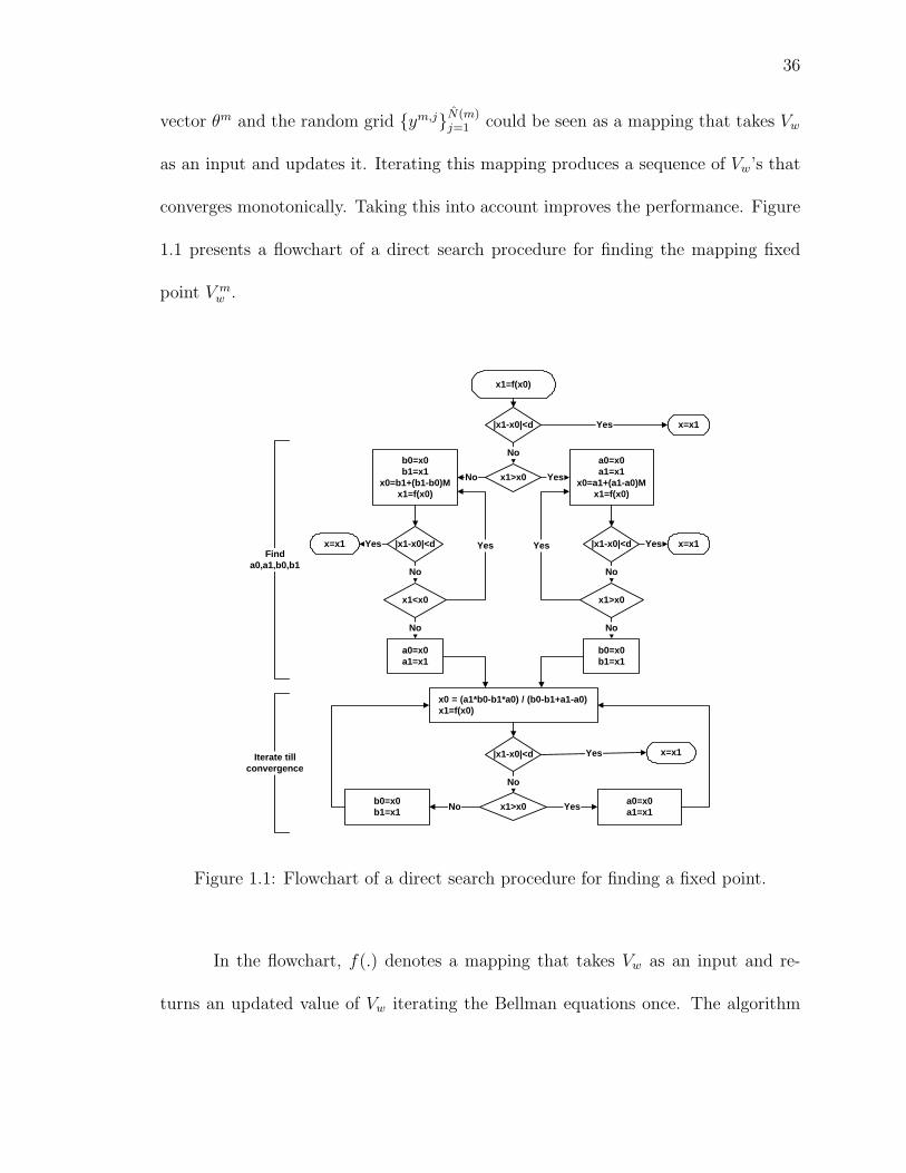
vector θm and the random grid ym,jN(m)j=1 could be seen as a mapping that takes Vw

as an input and updates it. Iterating this mapping produces a sequence of Vw’s that

converges monotonically. Taking this into account improves the performance. Figure

1.1 presents a flowchart of a direct search procedure for finding the mapping fixed

point V mw .

x1=f(x0)

|x1-x0|<d Yes x=x1

No

x1>x0 YesNo

a0=x0a1=x1

x0=a1+(a1-a0)Mx1=f(x0)

|x1-x0|<d Yes x=x1

x1>x0

No

Yes

No

b0=x0b1=x1

x0 = (a1*b0-b1*a0) / (b0-b1+a1-a0)x1=f(x0)

|x1-x0|<d x=x1Yes

No

x1>x0 Yes a0=x0a1=x1Nob0=x0

b1=x1

b0=x0b1=x1

x0=b1+(b1-b0)Mx1=f(x0)

|x1-x0|<dYesx=x1

x1<x0

No

Yes

No

a0=x0a1=x1

Finda0,a1,b0,b1

Iterate tillconvergence

Figure 1.1: Flowchart of a direct search procedure for finding a fixed point.

In the flowchart, f(.) denotes a mapping that takes Vw as an input and re-

turns an updated value of Vw iterating the Bellman equations once. The algorithm

37

searches for a fixed point x = f(x). First, the algorithm finds bounds a0, a1, b0, b1:

a0 < a1 = f(a0) ≤ x ≤ b1 = f(b0) < b0 starting with x0. A scaling factor M is cho-

sen experimentally. Updated x is obtained by cutting interval [a1, b1] in proportions

(a1 − a0) : (b0 − b1). After each iteration the difference f(x0) − x0 is compared to

a tolerance parameter d. If the convergence has not been achieved a0, a1, b0, b1 are

updated and the procedure is repeated. This procedure is used in the estimation ex-

periments presented below. In these experiments, starting from the nearest neighbor,

the procedure required only 2-4 passages over (1.38) and (1.39) to find the fixed point

V mw or, equivalently, to solve the DP for θm on the random grid ym,jN(m)

j=1 .

Since the Gibbs sampler changes only one or few components of the parame-

ter vector at a time, the previous parameter draw θm−1 turned out to be the nearest

neighbor of the current parameter θm in most cases. Taking advantage of this obser-

vation and keeping track only of one previous iteration saves a significant amount of

computer memory.

In the Gibbs sampler, the approximations of the differences in the expectations

are computed as follows:

Ft,d,i(θm, εm

t,i) =

β(π(xt,i, d, ηm)− π(xt,i, d, ηm))V mw

+ β(1− π(xt,i, d, ηm))

N(m)∑i=1

V m(x′(xt,i, d), ym,i; θm)f(εm,i | εm

t,i; θm)/g(εm,i)∑N(m)

r=1 f(εm,r | εmt,i; θ

m)/g(εm,r)

− β(1− π(xt,i, d, ηm))

N(m)∑i=1

V m(x′(xt,i, d), ym,i; θm)f(εm,i|εm

t,i; θm)/g(εm,i)∑N(m)

r=1 f(εm,r|εmt,i; θ

m)/g(εm,r)

38

1.5.1.4 Experiments with DP solution

A simulation study was conducted to assess the quality of the DP solution

approximations. The study explores how the randomness of the grid affects the ap-

proximations for fixed parameters and how these effects change with the random

grid size. The parameter values for this experiment are the same as for the es-

timation experiments described below in Section 1.5.1.5. First, I generated 1000

random grids ym,jNj=1, m = 1, . . . , 1000. Then, for each random grid m, I solved

the DP as described in the previous section and computed the approximation of

the value of being well V mw and the approximation of the difference in expectations

E(m)[V (s′; θ)|s, d1; θ]− E(m)[V (s′; θ)|s, d2; θ].

Figure 1.2: Estimated densities of Vw. The tightest density corresponds to N = 1000,the most widespread to N = 100. The dashed lines are fitted normal densities.

The approximation V mw is a measurable function of the random grid realization

ym,jNj=1 and thus itself is a random variable. Using kernel smoothing, I estimated

39

densities of those approximations. The estimated densities for N = 100, 500, 1000 are

presented in Figures 1.2 and 1.3.

Figure 1.3: Estimated densities of E(m)[V (s′; θ)|s, d1; θ] − E(m)[V (s′; θ)|s, d2; θ]. Thetightest density corresponds to N = 1000, the most widespread to N = 100. Thedashed lines are fitted normal densities.

Visual inspection of the figures suggests that the approximations converge as

the number of the points in the random grid increases. The mean of the distribution

seems to be the same for N = 100, 500, 1000. The variances are roughly proportional

to N−1. The densities are close to the fitted normal densities. All this hints that an

analog to a CLT might hold for this problem. Comparison of the two figures shows

that the maximal approximation error for the expected value function is larger by two

orders of magnitude than the maximal approximation error for the difference in the

expected value functions. This result seems to have a simple intuitive explanation.

An approximal DP solution computed on a random grid could be far from the actual

solution. However, the errors resulting from discretization and numerical integration

40

very similarly affect the approximations of the future expected value functions for the

same current state but different decisions. It probably happens because numerical

integration over the future states is performed on the same random grid no matter

which alternative is chosen in the current period. Thus, the approximations of the

expected value functions have very high positive correlation and their variances are of

similar magnitude. This results in a small variance for their difference. As I mentioned

earlier, these findings motivate the choice of the Gibbs sampler parameterization, in

which only the differences of the expected value functions are used.

Comparing the approximation precision with the magnitude of the taste shocks

in the model seems to be a reasonable way of judging the approximation quality. The

maximal approximation error for the differences in the expected value functions for

N = 100 was smaller than the standard deviation of the taste shocks h−1ν = 10 by a

factor of 15− 30.

To further verify that the method is implemented correctly I conducted a

similar simulation study using the extreme value iid unobservables instead of the

serially correlated unobservables. The results were analogous to the ones reported

in the figures. The actual DP solution for the iid extreme value unobservables can

be easily computed with a high precision as described in Rust (1994). As expected,

the exact solutions were right at the means of the distributions obtained from the

simulation study.

These experiments also suggest an improvement in the algorithm performance.

Solving the DP on several small random grids and combining the results seems to

41

be a very efficient alternative to using one large grid. I separate the series of the

approximations of Vw for N = 100 into batches of size 10. For each batch I compute

the mean and then use these means in kernel smoothing to obtain the estimated

density for such approximations of Vw. The resulting density practically coincide

with the density obtained for N = 1000 and no batching. Thus, the approximation

precision for these procedures is about the same. The time of iterating the Bellman

equation on a grid of size N is proportional to N2. Therefore, the time required for

iterating the Bellman equation on a grid of size N = 100 for ten different grids will be

smaller by a factor of 10 than the time required for iterating the Bellman equation on

one grid of size N = 1000. These experimental results are intriguing. Investigating

theoretical properties of this improved procedure, e.g. deriving complexity bounds,

seems to be of great interest and is a subject of future work. This improvement has not

been incorporated into the estimation experiments in this chapter. However, I employ

it in Chapter 3 that uses artificial neural networks to approximate the expected value

function as a function of the parameters θ and the state variables.

1.5.1.5 Estimation for artificial datasets

The generated sample contained I = 100 observations. The maximal length

of an illness episode was T = 5, the standard deviation of the uncorrelated taste

shocks was h−0.5ν = 10, and the time discount factor was β = 0.9997. The size of the

random grid for solving the DP was equal to N = 100, and the number of the picked

nearest neighbors was equal to N = 1. Data generation and each iteration of the

42

estimation procedure use the same random grid for solving the DP (Proposition 2.6

justifies using the same random grid at each iteration of the algorithm if the number

of the nearest neighbors is constant.) Experiments with different grids are conducted

on real data for the Rust (1987)’s model. The approximation error for the differences

in the expected value functions was smaller than the standard deviation of the taste

shocks by a factor of 15 − 30. Under these settings, it takes about 30 seconds to

produce 100 draws from the posterior on a 2002 vintage PC. The priors are specified

together with estimation results in Table 1.1.

Table 1.1: Estimation results for artificial data

Param- True Posterior Prior

eter value Mean SD NSE

α1 -1000 -1225.1 458.26 14.931 N(−1000, 3333.32)

α2 -50 -0.5944 174.96 5.6386 N(−50, 333.32)

α3 90 87.298 120.52 5.0465 N(90, 333.32)

α4 0.2 1.939 5.8549 0.1924 N(0.2, 16.72)

ρ 0.7 0.66199 0.1368 0.0068 N(0.5, 10002), s.t.[0, 0.99]

η1 -4.5 -4.5983 0.3107 0.0479 N(−4.5, 0.672)

η2 0.1 0.09767 0.0192 0.0036 N(0.1, 0.0672)

η3 0.1 0.13571 0.0348 0.0101 N(0.1, 0.0672)

η4 1.5 1.4872 0.1112 0.0187 N(1.5, 0.672)

h−0.5ε 20 19.4959 5.2168 0.67 800χ2

2, mean=sd=20

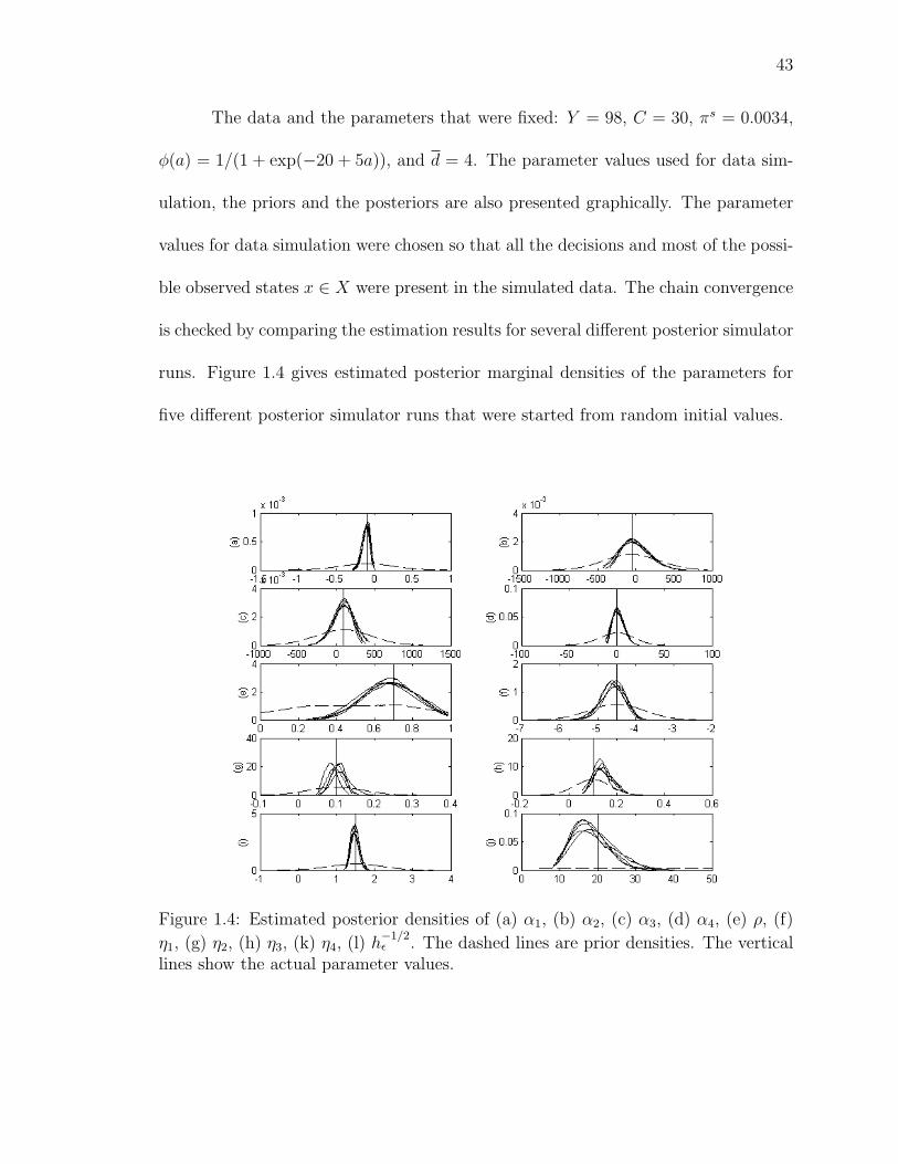
43

The data and the parameters that were fixed: Y = 98, C = 30, πs = 0.0034,

φ(a) = 1/(1 + exp(−20 + 5a)), and d = 4. The parameter values used for data sim-

ulation, the priors and the posteriors are also presented graphically. The parameter

values for data simulation were chosen so that all the decisions and most of the possi-

ble observed states x ∈ X were present in the simulated data. The chain convergence

is checked by comparing the estimation results for several different posterior simulator

runs. Figure 1.4 gives estimated posterior marginal densities of the parameters for

five different posterior simulator runs that were started from random initial values.

Figure 1.4: Estimated posterior densities of (a) α1, (b) α2, (c) α3, (d) α4, (e) ρ, (f)

η1, (g) η2, (h) η3, (k) η4, (l) h−1/2ε . The dashed lines are prior densities. The vertical

lines show the actual parameter values.

44

The length of the runs was 300000 − 1000000 draws. The posterior densities

estimated by kernel smoothing seem to converge to the same stationary distributions

for different posterior runs.

As can be seen from the figure, α and ρ converge much faster than η and hε.

Overall, the amount of serial correlation in the sampler draws is quite large. This is

typical for the Metropolis-Hastings random walk algorithm. The situation might be

complicated here by the presence of a lot of latent variables and by the sensitivity of

the expected value functions to changes in parameters. Thus, long simulator runs are

necessary to estimate the posterior distributions with sufficient precision. Also, some

experimental work is required for choosing the variance of the transition densities for

the MH random walk.

Another apparent feature of the estimation results is that the uncertainty

about the parameter values is huge. One reason being that the model is not very

parsimonious and the parameters are weakly identified. Changes in different param-

eters might lead to similar changes in the observables. This also creates difficulties

for classical maximum likelihood estimation of dynamic discrete choice models. The

standard errors of the parameter estimates are often large and difficult to compute

precisely. In contrast to the classical approach, Bayesian inference takes into account

the uncertainty about the parameters and this advantage seems to be important for

dynamic discrete choice models. As will be seen in the experiments with Rust’s

model, an increase in the sample size does not necessarily cure the problem of weak

identification.

45

1.5.1.6 Two stage estimation

The following experiment is motivated by the two stage classical estimation

procedure in which the state transition parameters η are estimated first from the

partial likelihood and then these estimates are used in the estimation of the rest

of the parameters. The experiment below could give some clues on how the full

maximum likelihood estimation results would differ from the ones of the two stage

procedure. Using the priors and the artificial dataset from the experiments in the

previous section, I estimate η by a standard probit model with the assumption that xt,i

are fixed. The results of this procedure are contrasted with the full model estimation

results in Figure 1.5.

Figure 1.5: Posterior densities of η: (a) η1, (b) η2, (c) η3, (d) η4. The solid lines showthe densities estimated by probit, the dotted lines by the full model. The verticallines show the actual parameter values.

Then, fixing η at the posterior mean from the probit estimation, I estimate

46

the rest of the parameters. The results are compared with the full model in Figure

1.6. As can be seen from Figure 1.5, the posterior standard deviations for η are

significantly smaller for the full model estimation. Thus, there seem to be significant

efficiency gains from the full model estimation. Surprisingly, the estimation results

for the rest of the parameters are only slightly affected by fixing η. The “second stage

posteriors”, depicted in Figure 1.6, noticeably differ from the full model posteriors

only for α1 and h−1/2ε .

Overall, this experiment does not seem to suggest that the two stage classical

estimation procedure would produce unreasonable results for this model and sample

size. However, the standard errors of the parameters might be considerably affected.

Figure 1.6: Posterior densities of α, ρ, and h−1/2ε : (a) α1, (b) α2, (c) α3, (d) α4, (e)

ρ, (f) h−1/2ε . The solid lines show the densities estimated with fixed η (two simulator

runs,) the dotted lines by the full model. The vertical lines show the actual parametervalues.

47

1.5.1.7 Joint distribution tests

To verify that the Gibbs sampler is implemented correctly I employ joint dis-

tribution tests developed in Geweke (2004). The test works as follows. First, start

from the joint prior distribution for the observables and the unobservables: θ0 ∼ p(θ)

and ∆V0, ε0, x0, RI0, d0 ∼ p(data|θ0). Then, generate a draw from the posterior sim-

ulator ∆V1, ε1, RI1, θ1 and generate the observed and the augmented data from the

data simulator ∆V1, ε1, x1, RI1, d1 ∼ p(data|θ1) and continue repeating these two

steps. The invariant stationary distribution of this Markov chain is the joint prior

distribution of the observables and the unobservables. This successive conditional

simulator uses the posterior and data simulators. If the posterior and data simulators

are derived and implemented correctly, then, for example, the sample mean of θm

converges to the prior mean of θ, which could be tested formally using a central limit

theorem.

Using smaller size of the artificial dataset results in better mixing of the chain

in the successive conditional simulator. In this experiment I = 2. Tighter priors also

increase the speed of convergence. Some experimental work was required to choose

the variances for the Metropolis-Hastings transition densities. The acceptance rates

were in 0.2-0.7 interval.

The test uses 10000 draws from the prior simulator and 75000 draws from the

successive conditional simulator. The hypothesis of means equality was not rejected

by the standard means equality test performed for the parameters and their squares.

The test p-values are reported in Table 1.2. The numerical standard errors were

48

computed by batching with a first order time series correction.7

Table 1.2: Joint distribution test

Parameter Prior simulator Successive conditional Means equality

mean simulator mean p-value

α1 -999.99 -1000 0.25

α2 -49.997 -50.03 0.42

α3 90.009 89.946 0.10

α4 0.20014 0.19997 0.67

ρ 0.50209 0.50122 0.60

η1 -4.5033 -4.4989 0.24

η2 0.099921 0.099911 0.99

η3 0.099814 0.10013 0.63

η4 1.4989 1.5034 0.72

h−.5ε 20.306 20.296 0.73

These tests are useful not only at the program debugging stage, but also help

to catch some conceptual errors in the posterior simulator implementation: e.g., in

drawing ρ by the MH random walk a truncation constant was not taken into account

in computing the acceptance probability (prior for ρ is truncated to [0, 0.99].) The

7The sequence of the draws is divided into batches. It is assumed that the means of thebatches follow an AR(1) process and the corresponding standard error is computed.

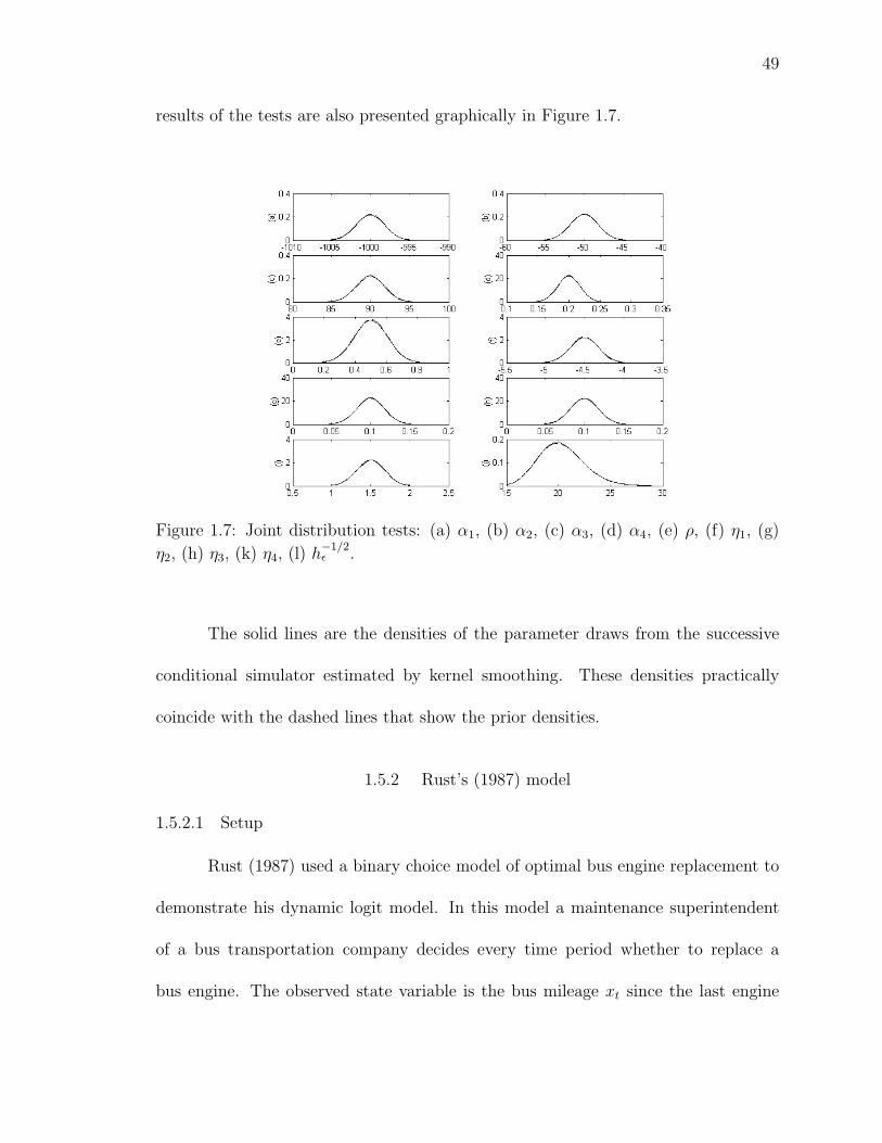
49

results of the tests are also presented graphically in Figure 1.7.

Figure 1.7: Joint distribution tests: (a) α1, (b) α2, (c) α3, (d) α4, (e) ρ, (f) η1, (g)

η2, (h) η3, (k) η4, (l) h−1/2ε .

The solid lines are the densities of the parameter draws from the successive

conditional simulator estimated by kernel smoothing. These densities practically

coincide with the dashed lines that show the prior densities.

1.5.2 Rust’s (1987) model

1.5.2.1 Setup

Rust (1987) used a binary choice model of optimal bus engine replacement to

demonstrate his dynamic logit model. In this model a maintenance superintendent

of a bus transportation company decides every time period whether to replace a

bus engine. The observed state variable is the bus mileage xt since the last engine

50

replacement. The control variable dt takes on two values: 2 if the engine is replaced

at t and 1 otherwise. The per-period utility function of the superintendent is the

negative of per-period costs:

u(xt, εt, νt, dt; α) =

α1xt + εt if dt = 1

α2 + νt if dt = 2

(1.40)

where εt and νt are the unobserved state variables, α1 is the negative of per-period

maintenance costs per unit of mileage, α2 is the negative of the costs of engine replace-

ment. Rust assumes that εt and νt are extreme value iid. I assume νt is iid N(0, h−1ν )

truncated to [−ν, ν], εt is N(ρεt−1, h−1ε ) truncated to E = [−ε, ε], and ε0 = 0. The bus

mileage since the last replacement is discretized into M intervals X = 1, . . . ,M.

The observed state xt evolves according to

P (xt+1|xt, dt; η) =

π(xt+1 − xt; η) if dt = 1

π(xt+1 − 1; η) if dt = 2

(1.41)

and

π(∆x; η) =

η1 if ∆x = 0

η2 if ∆x = 1

η3 if ∆x = 2

0 if ∆x ≥ 3

(1.42)

Rust assumes that if the mileage reaches the state M it stays in this state with

probability 1. I instead assume that the engine is replaced at t if xt exceeds M − 1,

which slightly simplifies the DP solution. In the recursive formulation, the life-time

51

utility for xt < M is given by

V (xt, εt, νt; θ) = max α1xt + εt + β3∑

k=1

ηkE[V (xt + k − 1, ε′, ν ′; θ)|εt; θ],

α2 + νt + βEV2(θ) (1.43)

where

EV2(θ) =3∑

k=1

ηkE[V (k, ε′, ν ′; θ)|0; θ] (1.44)

E[V (xt+1, ε′, ν ′; θ)|εt; θ] =

∫V (xt+1, ε

′, ν ′; θ)dP (ε′, ν ′|εt; θ) (1.45)

For xt ≥ M :

V (xt, εt, νt; θ) = α2 + νt + βEV2(θ) (1.46)

1.5.2.2 Approximating value functions

The algorithm of approximating the value functions is similar to the one for

Gilleskie’s model, where the role of Vw is played by EV2. Only one nearest neighbor

is used, N(m) = 1. The random grid ym,j = (νm,j, εm,j)N(m)j=1 is generated from

a normal distribution: νm,jd ∼ N(0, h−1

ν ) and εm,j ∼ g(.), where g(.) is a normal

density. First, one iteration of the DP solving algorithm is described as it should be

performed according to the theory. Then, improvements in the algorithm performance

are discussed.

An iteration of the DP solving algorithm is performed as follows. For a given

initial EV k12 (θk1) corresponding to the nearest neighbor, Bellman equations (1.43) are

52

iterated for x in descending order and j = 1, . . . , N(m):

V m(x, ym,j; θm) = max αm1 x + εm,j + β

3∑k=1

ηkEm[V (x + k − 1, y′; θm)|ym,j; θm],

αm2 + νm,j + βEV k1

2 (θk1) (1.47)

where

Em[V (x + k − 1, y′; θm)|ym,j; θm] =

N(k1)∑r=1

V k1(x + k − 1, yk1,r; θk1)W (εk1,r, εk1,j, θk1)

(1.48)

Note that for k > 1 the value functions V m(x + k − 1, ym,r; θm) have already been

computed. Thus, for k > 1, k1 will be equal to m in (1.48). Next, EV m2 (θm) is

computed:

EV m2 (θm) =

3∑k=1

ηk

N(m)∑r=1

V m(k, ym,r; θm)W (εm,r, 0, θm) (1.49)

In practice, iterating (1.47) several times in a row for one x before going to the

next significantly improves the convergence speed. It happens because the expression

for the value function at the mileage x includes the expected value function at the

same x. If Bellman equation (1.47) is iterated several times the approximation error

in V m(x, ym,j; θm) becomes smaller and affects the value functions for 1, . . . , x− 1

much less. Using only already updated V m(x, ym,j; θm) in computing the expectations

further improves the performance. Thus, when (1.47) is iterated first time for a given

x the expectations for k = 1 are approximated as follows:

Em[V (x + k − 1, y′; θm)|ym,j; θm] =

j−1∑r=1

V (x, ym,r; θm)W (ym,r, ym,j, θm) (1.50)

53

For j = 1, Em[V (x + 0, y′; θm)|ym,1; θm] is a solution of the following equation:

Em[V (x + 0, y′; θm)|ym,1; θm] = maxαm2 + βEV k1

2 (θk1),

αm1 x + β(ηm

1 Em[V (x + 0, y′; θm)|ym,1; θm] (1.51)

+ηm2 Em[V (x + 1, y′; θm)|ym,1; θm] + ηm

3 Em[V (x + 2, y′; θm)|ym,1; θm])(1.52)

This equation is obtained by interchanging the places of the expectation and the max

in the Bellman equation. After the first iteration on (1.47) for a given x, all the

expectations are computed according to (1.48) on the subsequent iterations. This

procedure can be seen as a mapping taking EV2 as an input and updating it. The

fixed point of this mapping can be found by a direct search procedure similar to the

one described in Section 1.5.1.3.

1.5.2.3 Gibbs sampler

Each bus i is observed over Ti time periods: xt,i, dt,iTit=1 for i = 1, . . . , I. The

parameters are θ = (α, η, ρ, hε); hν is fixed for normalization. The latent variables

are ∆Vt,i, εt,iTit=1 i = 1, . . . , I.

∆Vt,i = xt,iα1 − α2 + εt,i − νt,i + Ft,i(θ, εt,i)

where

Ft,i(θ, ε) = β

3∑j=1

ηj(E[V (xt,i + j − 1, ε′, ν ′; θ)|ε; θ]− EV2(θ))

The compact space for parameters Θ is defined as follows: αi ∈ [−α, α], ρ ∈ [−ρ, ρ],

hε ∈ [hlε, h

rε ], and η belongs to a three dimensional simplex. The joint distribution of

54

the data, the parameters, and the latent variables is

p(θ; xt,i, dt,i; ∆Vt,i, εt,iTit=1; i = 1, . . . , I) =

p(θ)I∏

i=1

Ti∏t=1

[p(dt,i|∆Vt,i)p(∆Vt,i|xt,i, εt,i; θ)p(xt,i|xt−1,i; dt−1,i; η)p(εt,i|εt−1,i, ρ, hε)]

where p(θ) is a prior density for the parameters; p(xt,i|xt−1,i; dt−1,i; η) is given in (1.41)

and p(x1,i|x0,i; d0,i; η) = 11(x1,i)—all the buses start with a new engine;

p(dt,i|∆Vt,i) =

1, if dt,i = 1, ∆Vt,i ≥ 0 or dt,i = 2, ∆Vt,i ≤ 0

0, if dt,i = 1, ∆Vt,i < 0 or dt,i = 2, ∆Vt,i > 0

(1.53)

p(∆Vt,i|xt,i, εt,i; θ) = exp −0.5hν(∆Vt,i − [xt,iα1 − α2 + εt,i + Ft,i(θ, εt,i)])2(1.54)

·1[−ν,ν](∆Vt,i − [xt,iα1 − α2 + εt,i + Ft,i(θ, εt,i)]) (1.55)

· h0.5ν√

2π[Φ(νh0.5ν )− Φ(−νh0.5

ν )]

p(εt,i|εt−1,i, θ) =h

1/2ε exp −0.5hε(εt,i − ρεt−1,i)

2√2π[Φ([ε− ρεt−1,i]h0.5

ε )− Φ([−ε− ρεt−1,i]h0.5ε )]

1E(εt,i) (1.56)

Gibbs sampler blocks

The Gibbs sampler blocks for ∆Vt,i| . . . will have a normal truncated distri-

bution proportional to (1.54) and (1.55), and also truncated to R+ if dt,i = 1 or to

R− otherwise. An algorithm from Geweke (1991) is used to simulate efficiently from

the normal distribution truncated to R+ (or R−.) Acceptance sampling handles the

truncation in (1.55).

55

The density for εt,i| . . . is proportional to

p(εt,i| . . .) ∝ exp −0.5hν(∆Vt,i − [xt,iα1 − α2 + εt,i + Ft,i(θ, εt,i)])2

Φ([ε− ρεt−1,i]h0.5ε )− Φ([−ε− ρεt−1,i]h0.5

ε )

· 1[−ν,ν](∆Vt,i − [xt,iα1 − α2 + εt,i + Ft,i(θ, εt,i)])

· exp−0.5hε(εt+1,i − ρεt,i)2 − 0.5hε(εt,i − ρεt−1,i)

2 · 1E(εt,i)(1.57)

Draws from this density are obtained from a Metropolis step with a normal truncated

transition density proportional to (1.57). The blocks for εt,i with t = 0 and t = Ti

will be similar.

Assuming a normal prior N(ρ, hρ) truncated to [−ρ, ρ],

p(ρ| . . .) ∝exp −0.5hν

∑i,t(∆Vt,i − [xt,iα1 − α2 + εt,i + Ft,i(θ, εt,i)])

2∏i,t Φ([ε− ρεt−1,i]h0.5

ε )− Φ([−ε− ρεt−1,i]h0.5ε )

·∏i,t

1[−ν,ν](∆Vt,i − [xt,iα1 − α2 + εt,i + Ft,i(θ, εt,i)])

· exp−0.5hρ(ρ− ρ)2 · 1[−ρ,ρ](ρ) (1.58)

where hρ = hρ +∑

i

∑Ti

t=2 ε2t−1,i and ρ = h

−1

ρ (hρρ + hε

∑i

∑Ti

t=2 εt,iεt−1,i). To draw

from this density I use a Metropolis step with a normal truncated transition density

proportional to (1.58).

Assuming a gamma prior s2hε ∼ χ2(df), truncated to [hlε, h

rε ],

p(hε| . . .) ∝exp −0.5hν

∑i,t(∆Vt,i − [xt,iα1 − α2 + εt,i + Ft,i(θ, εt,i)])

2∏i,t Φ([ε− ρεt−1,i]h0.5

ε )− Φ([−ε− ρεt−1,i]h0.5ε )

·∏i,t


· h(df−2)/2ε exp −0.5s2hε · 1[hl

ε,hrε ](hε) (1.59)

where df = df +∑

i Ti and s2 = s2 +∑

i

(∑Ti

t=2(εt,i − ρεt−1,i)2 + ε2

1,i

). For this block,

I employ a Metropolis step with a truncated gamma transition density proportional

56

to (1.59); draws from this density are obtained by acceptance sampling.

Assuming a Dirichlet prior with parameters (a1, a2, a3),

p(η| . . .) ∝ exp −0.5hν

∑i,t

(∆Vt,i − [xt,iα1 − α2 + εt,i + Ft,i(θ, εt,i)])2

·∏i,t


·3∏

j=1

ηnj+aj−1j (1.60)

where nj =∑

i

∑Ti

t=2 1j−1(xt,i−xt−1,i). A Metropolis step with a Dirichlet transition

density proportional to (1.60) is used in this block.

p(α| . . .) ∝ p(α) exp −0.5hν

∑i,t

(∆Vt,i − [xt,iα1 − α2 + εt,i + Ft,i(θ, εt,i)])2

· 1[−α,α]×[−α,α](α) ·∏i,t


To draw from this density I use the Metropolis-Hastings random walk algorithm. The

proposal density is normal truncated to [−α, α] × [−α, α] with a mean equal to the

current parameter draw and a fixed variance. The variance matrix is chosen so that

the acceptance probability would be between 0.2− 0.3.

1.5.2.4 Uniform ergodicity

The draws from the Gibbs sampler are used for approximating posterior expec-

tations by sample averages. Under certain conditions, the sample averages converge

almost surely to the posterior expectations and a corresponding central limit theo-

rem holds. Uniform ergodicity of the Gibbs sampler—a sufficient condition for these

results (see Tierney (1994))—is established by the following theorem.

57

Theorem 1.4. Consider the Gibbs sampler with the following order of blocks at each

iteration: 1) (∆Vm+1t,i |θm, εm, d, x), ∀t, i; 2) (ρm+1|θm, εm, ∆Vm+1, d, x), (αm+1| . . .),

(ηm+1| . . .), (hm+1ε | . . .); 3) (εm+1

t,i |εm, θm+1, ∆Vm+1), ∀t, i; 4) (∆Vm+1t,i |θm+1, εm+1, d, x),

∀t, i; where the blocks were described above. Block 4) is redundant but simplifies the

proof. Assume that the support of νt,i is sufficiently large relative to the support of

ε and θ: Φ(−h0.5ν ν) < 0.25 and ν > 2(u + ε + βEV ), where u is an upper bound on

the absolute value of the deterministic part of the per-period utility function, ε is an

upper bound on the absolute value of εt,i, and EV = [u + ε + 1 + 2h−1ε ]/(1 − β) is

an upper bound on the absolute value of the expected value function (see the proof.)

Then, the Gibbs sampler is uniformly ergodic. Thus, by Theorems 3 and 5 in Tierney

(1994), for any integrable (w.r.t. posterior) function z(∆V , θ, ε) the sample average

zn = 1/n∑

m z(∆Vm, θm, εm) converges a.s. to the posterior expectation E(z|d, x). If

E(z2|d, x) < ∞ then there exists a real number σ2(z) such that√

n(zn − E(z|d, x))

converges in distribution to N(0, σ2(z)).

The theorem is proven in Chapter 2, Section 2.3. For the Gibbs sampler that

uses the approximations instead of the actual value functions the uniform ergodicity

holds in probabilistic sense. Suppose that the DP solving algorithm stops at iteration

n and that the Gibbs sampler uses the output from the DP solving algorithm up to

iteration n for approximating the value functions on all the subsequent iterations.

Then, this Gibbs sampler is uniformly ergodic with a probability that converges to

1 very fast as n goes to infinity. That is it becomes uniformly ergodic a.s. This

statement follows from the proof of Theorem 1.4 and the fact that the approximated

58

expected value functions will be bounded by EV plus a small positive number with

a probability that converges to 1.

Most of the distributions in the described Gibbs sampler are truncated dis-

tributions. In practice, it is easier to use distributions with unbounded support and

ignore the truncation. To reconcile this with the theory, we could assume that the

truncation bounds are very large. Then, the Gibbs sampler that takes them into

account would produce the same results as the Gibbs sampler that does not: e.g.

simulating N(0, 1) (or N(106, 106)) truncated to (−1.7 · 10308, 1.7 · 10308) will give the

same results as simulating N(0, 1) (or N(106, 106).) Therefore, in the experiments

below, the truncation to the bounded parameter and state spaces is not enforced.

1.5.2.5 Algorithm parallelization

Opportunities for algorithm parallelization are abundant and it is a possible

subject for future work. Approximating the expectations of the value functions either

in the DP solving algorithm or in the Gibbs sampler is a very frequent and time con-

suming task. The computations of the expected value functions for different current

states are not interrelated. Thus, they could be computed simultaneously on differ-

ent computers/processors in the cluster. In designing a parallel implementation of

an algorithm, it is crucial to take into account the time required for communication

and data transfer between computers. As was indicated in Section 1.5.1.4 solving

the DP on several smaller random grids and combining the results is a very efficient

alternative to using one big random grid. If, in addition, different processors are used

59

for solving the DP on each random grid, the performance would be increased consid-

erably since the need for data transfer between processors will be decreased relative

to just computing expectations simultaneously. In the Gibbs sampler, the volume

of data exchange between machines in the cluster could also be minimized. Each

processor in the cluster could be assigned to a part of the dataset. Then, simulating

latent variables pertaining to these parts of the dataset could be performed simulta-

neously by different processors and no data exchange is needed given that the current

parameters and the results of the DP solving algorithm are copied to the memory of

each computer in the cluster. In drawing parameters there is no need for transferring

all the latent variables and the corresponding expectations between computers. A

computer assigned to a part of the dataset could compute aggregates corresponding

to its part of the dataset and transfer only these aggregates to the computer that

performs drawing the parameters: e.g. in drawing ρ| . . . parts of the sum in (1.58)

could be computed by the computers to which the corresponding part of the sample

is assigned. The proposed parallelization scheme is relatively easy to implement, and

the potential gains in performance seem to be considerable.

1.5.2.6 Estimation for artificial datasets

Estimation was performed for two different artificial datasets. One artificial

sample consisted of I = 500 observations, the other one of I = 50. Each bus i is

observed Ti ∈ 1, . . . , 200 months until the engine is replaced (if the engine is not

replaced at t = 200 the observation i is censored, there were no such observations in

60

simulated data.) As in Rust’s paper, the mileage is divided into 90 discrete intervals

corresponding to [0, 5000], . . . , [445000, 450000] miles. The parameter values used for

data generation were taken from Rust’s paper. The precision for the correlated unob-

served state variables hε was fixed: hε = hν = 0.6, which roughly corresponds to the

precision of the extreme value distributed errors in Rust’s paper. The time discount

factor was equal to β = 0.999. Joint distribution tests did not reject the hypothesis

of correct implementation of the prior, the data, and the posterior simulators.

Table 1.3 shows the estimation results for six posterior simulator runs. The

first three runs (1-3) were produced for the sample of size I = 500, the other three

runs (4-6) for the sample of size I = 50. The length of each run was equal to 1000000.

Figure 1.8 illustrates the estimation results graphically. As can be seen from the fig-

ure and the table, the posterior distributions are tighter for the larger sample size.

This expected behavior is more pronounced for η than for the rest of the parameters.

There are some other respects in which the results are different for η. First, the

uncertainty about η seems to be much smaller than for the rest of the parameters.

Second, the acceptance rate for η was about 90%, which is quite high compared to

10-20% for ρ (for alpha it was about 27%, but it should not be compared with the

other two since it is affected by the preset variance of the MH transition density.)

Third, the amount of serial correlation in draws of η was insignificant, which resulted

in very fast convergence for η. For the rest of the parameters the observations made

for Gilleskie’s model, such as large uncertainty about parameters and slow conver-

gence are unchanged. The most important reason for this difference seems to be a

61

Table 1.3: Estimation results for artificial data

Run α1 α2 ρ η1 η2 η3

1 -.0026 -9.65 .683 0.33925 0.63972 0.021033

2 -.0027 -10.36 .703 0.33926 0.63971 0.021032

Post 3 -.0029 -10.35 .699 0.33927 0.6397 0.021032

mean 4 -.0035 -9.82 .649 0.34686 0.63296 0.020176

5 -.0036 -11.1 .684 0.34692 0.6329 0.020182

6 -.003 -8.69 .599 0.34681 0.63302 0.020176

1 .00099 1.56 .049 0.003814 0.003869 0.001156

2 .00095 1.66 .043 0.003813 0.003868 0.001155

Post 3 .00101 1.68 .051 0.003816 0.003869 0.001156

SD 4 .00146 2.17 .103 0.011592 0.011751 0.003421

5 .0015 2.89 .104 0.011585 0.011734 0.003424

6 .00129 2.07 .126 0.011589 0.011731 0.003423

1 .00026 .774 .022 5.00E-06 4.92E-06 1.19E-06

NSE 2 .00024 .903 .021 4.85E-06 4.81E-06 1.31E-06

for 3 .00026 .792 .024 4.54E-06 4.48E-06 1.27E-06

post 4 .00022 .466 .019 1.85E-05 1.87E-05 3.78E-06

mean 5 .00025 .817 .024 1.79E-05 1.78E-05 4.36E-06

6 .00017 .392 .020 1.75E-05 1.79E-05 3.80E-06

True -.003 -10 .7 .34 .64 .02

Prior N(-.0035, N(−12, 52) N(.5, 106) Dirichlet prior for η:

.00172) s.t.[0,.99] a1 = 34 a2 = 64 a3 = 2

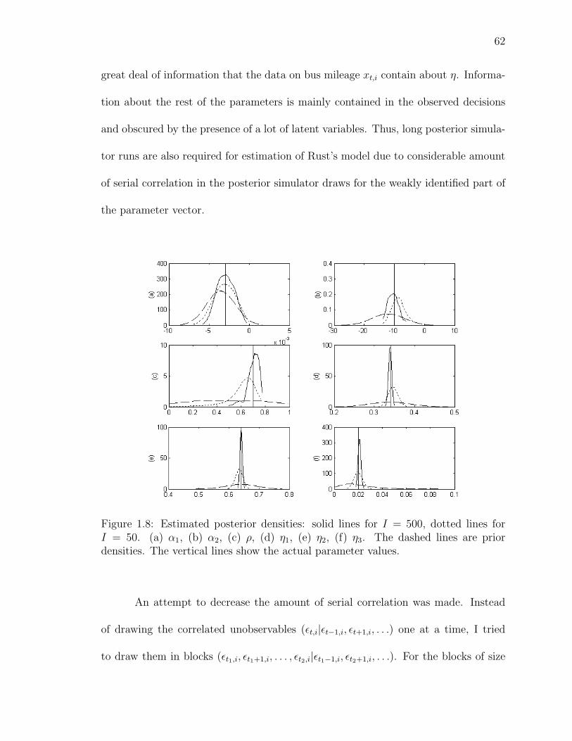
62

great deal of information that the data on bus mileage xt,i contain about η. Informa-

tion about the rest of the parameters is mainly contained in the observed decisions

and obscured by the presence of a lot of latent variables. Thus, long posterior simula-

tor runs are also required for estimation of Rust’s model due to considerable amount

of serial correlation in the posterior simulator draws for the weakly identified part of

the parameter vector.

Figure 1.8: Estimated posterior densities: solid lines for I = 500, dotted lines forI = 50. (a) α1, (b) α2, (c) ρ, (d) η1, (e) η2, (f) η3. The dashed lines are priordensities. The vertical lines show the actual parameter values.

An attempt to decrease the amount of serial correlation was made. Instead

of drawing the correlated unobservables (εt,i|εt−1,i, εt+1,i, . . .) one at a time, I tried

to draw them in blocks (εt1,i, εt1+1,i, . . . , εt2,i|εt1−1,i, εt2+1,i, . . .). For the blocks of size

63

t2 − t1 + 1 = 2 the acceptance rate for the correlated unobservables dropped from

0.6 to 0.4 and the amount of serial correlation in the sampler did not seem to change

much. For the blocks of size t2− t1 +1 = 5 the acceptance rate for the correlated un-

observables and ρ decreased to less than 0.001. Thus, grouping parameters in larger

Gibbs sampler blocks does not seem to work as a technique of decreasing the amount

of serial correlation in posterior simulator draws for this problem. Looking for other

techniques is a subject of future work.

1.5.2.7 Exact and approximate estimation

To evaluate the quality of the estimation results I conduct experiments on

the model with extreme value unobservables—the dynamic logit model. For this

model, the integration over the unobservables in solving the DP and in the likelihood

function can be performed analytically. The estimation method that integrates the

unobservables analytically in the likelihood and in the DP solution will be referred

below as the exact algorithm. The posterior simulator for this method also uses the

Metropolis-Hastings algorithm since the logit-like choice probabilities comprising the

likelihood function contain the expected value functions that can only be computed

numerically. The approximate algorithm will refer to the algorithm proposed in this

chapter. The Gibbs sampler for the approximate algorithm is the same as the one

for the Gaussian unobservables described in Section 1.5.2.3; except here the Gaussian

probability densities are replaced by the densities for the extreme value distribution.

Table 1.4 gives the estimation results for the exact and approximate algorithms.

64

Table 1.4: Exact and approximate estimation results.

Run α1 α2 η1 η2 η3

1 -.00228 -9.0721 0.34433 0.63394 0.021736

2 -.00247 -9.4999 0.34435 0.63392 0.021731

3 -.00203 -9.1815 0.3443 0.63397 0.021733

Post 4 -.00207 -9.2569 0.34433 0.63394 0.021732

mean 5 -.00229 -8.7955 0.34435 0.63393 0.021727

6 -.00241 -9.0610 0.34435 0.63392 0.021733

7 -.00229 -9.0519 0.34434 0.63392 0.02174

8 -.00231 -9.0797 0.34432 0.63395 0.021733

1 .00044 0.8538 0.006311 0.006399 0.001939

2 .00049 0.9795 0.006315 0.006403 0.001938

3 .00046 0.9681 0.006314 0.0064 0.00194

Post 4 .00047 0.9655 0.00631 0.006394 0.001932

SD 5 .00042 0.7790 0.006302 0.006396 0.001938

6 .00051 0.9789 0.006298 0.006395 0.001938

7 .00051 1.0028 0.006327 0.006412 0.001941

8 .00049 0.9680 0.006306 0.006396 0.001941

65

Table 1.4 – Continued

1 .00015 0.3444 7.42E-06 7.31E-06 2.23E-06

2 .00019 0.4404 8.48E-06 8.12E-06 2.11E-06

NSE 3 .00007 0.1892 2.27E-05 2.10E-05 4.16E-06

for 4 .00007 0.2015 2.63E-05 2.36E-05 4.61E-06

post 5 .00005 0.1196 1.90E-05 1.74E-05 3.95E-06

mean 6 .00007 0.1957 1.82E-05 1.71E-05 3.88E-06

7 .00007 0.1926 2.11E-05 1.97E-05 3.93E-06

8 .00006 0.1776 2.04E-05 1.88E-05 3.81E-06

Prior N(-.003,.0017) N(-10, 5) Dirichlet prior

a1 = 34 a2 = 64 a3 = 2

Actual param -.003 -10 .34 .64 .02

The experiments use an artificial dataset consisting of observations on I = 70

buses. Runs 1–2 in the table are the runs of the exact posterior simulator started

from different random initial values for the parameters. The length of runs 1–2 was

1000000. For the approximate algorithm three different realization of the random grid

for solving the DP were used. Each grid realization corresponds to a pair of simulator

runs: 3–4, 5–6, and 7–8. The random number generator was initialized differently for

each run. The length of runs 3–8 was about 500000.

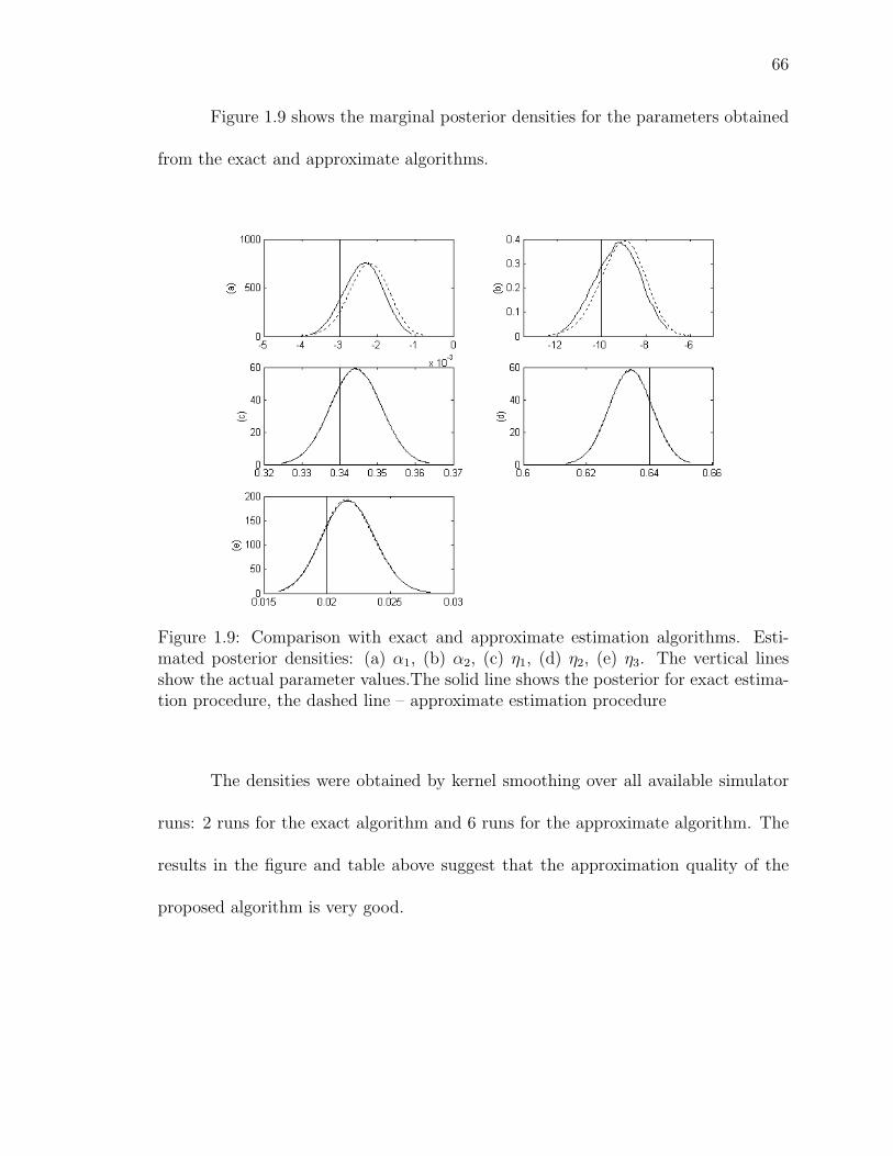
66

Figure 1.9 shows the marginal posterior densities for the parameters obtained

from the exact and approximate algorithms.

Figure 1.9: Comparison with exact and approximate estimation algorithms. Esti-mated posterior densities: (a) α1, (b) α2, (c) η1, (d) η2, (e) η3. The vertical linesshow the actual parameter values.The solid line shows the posterior for exact estima-tion procedure, the dashed line – approximate estimation procedure

The densities were obtained by kernel smoothing over all available simulator

runs: 2 runs for the exact algorithm and 6 runs for the approximate algorithm. The

results in the figure and table above suggest that the approximation quality of the

proposed algorithm is very good.

67

1.5.2.8 The role of serial correlation

In this section, I show how the presence of serial correlation in unobservables in

the data generation process affects the estimation results for the dynamic logit model.

For this purpose I use an artificial dataset simulated from the model with Gaussian

serially correlated unobservables described in this chapter (it will be referred in this

section as the true model.) Then, I use this data in estimation of the dynamic logit

model and the true model. The results are shown in the table below.

Table 1.5: Estimation results for the dynamic logit model and the model with Gaus-sian serially correlated unobservables.


Post logit -.0009 -3.1431 .35883 .6273 .0138

mean true -.0028 -10.7342 .843 .35887 .6273 .0138

Post logit .00065 0.2275 .012606 .012703 .003

SD true .00098 1.3262 .061 .012607 .012719 .003

NSE post logit .00001 .005 1.4E-05 1.4E-05 3.2E-06

mean true .00006 0.1848 .019 2.0E-05 2.0E-05 3.8E-06

Actual -.003 -10.0 .85 .34 .64 .02

Prior N(-.003, N(-10,52) N(0.5,106) Dirichlet prior

.00172) s.t.[-.99,.99] a1 = 34 a2 = 64 a3 = 2

From this table, it might seem that the presence of serial correlation in unob-

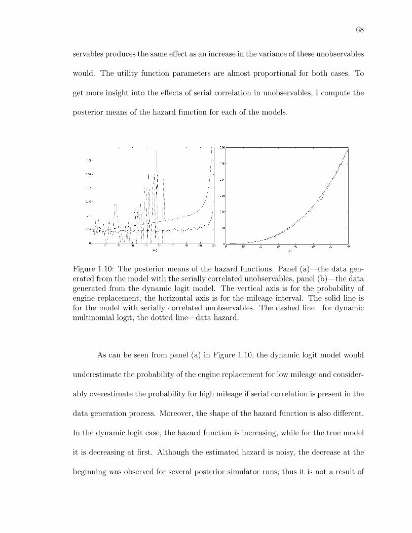
68

servables produces the same effect as an increase in the variance of these unobservables

would. The utility function parameters are almost proportional for both cases. To

get more insight into the effects of serial correlation in unobservables, I compute the

posterior means of the hazard function for each of the models.

Figure 1.10: The posterior means of the hazard functions. Panel (a)—the data gen-erated from the model with the serially correlated unobservables, panel (b)—the datagenerated from the dynamic logit model. The vertical axis is for the probability ofengine replacement, the horizontal axis is for the mileage interval. The solid line isfor the model with serially correlated unobservables. The dashed line—for dynamicmultinomial logit, the dotted line—data hazard.

As can be seen from panel (a) in Figure 1.10, the dynamic logit model would

underestimate the probability of the engine replacement for low mileage and consider-

ably overestimate the probability for high mileage if serial correlation is present in the

data generation process. Moreover, the shape of the hazard function is also different.

In the dynamic logit case, the hazard function is increasing, while for the true model

it is decreasing at first. Although the estimated hazard is noisy, the decrease at the

beginning was observed for several posterior simulator runs; thus it is not a result of

69

the noise. For comparison, panel (b) shows the posterior means of the hazard func-

tions estimated from the artificial data that were simulated from the dynamic logit

model. In this case, the hazards for the dynamic logit model and for the model with

Gaussian serially correlated unobservables seem to be very close and have the same

shape. These results support the claim that the disparities in the hazards observed

in panel (a) are driven by the presence of serial correlation in the data but not by the

different distributional assumptions on unobservables: Gaussian vs. extreme value.

These experiment demonstrate that ignoring serial correlation in unobservables might

lead to serious misspecification errors.

1.5.2.9 Estimation for a real dataset

The data set is group 4 from Rust’s paper. It contains observations on 37

buses that could be divided into I = 70 individual spells containing one engine

replacement (or censored at the last observed xt), which gives∑

i Ti = 4329 monthly

mileage/decision points. It takes about 50 seconds to produce 100 draws from the

posterior on a 2002 vintage PC.

To start the Gibbs sampler I used the parameter estimates from Rust’s paper.

The algorithm also works if the Gibbs sampler is started from a draw from the prior

distribution or from the zero vector for the utility function parameters α and the data

frequencies for the state transition probabilities η. The initial values for the latent

variables are adjusted so that the observed decisions are optimal. In particular, given

the parameter values, the serially correlated unobservables εt,i are simulated from

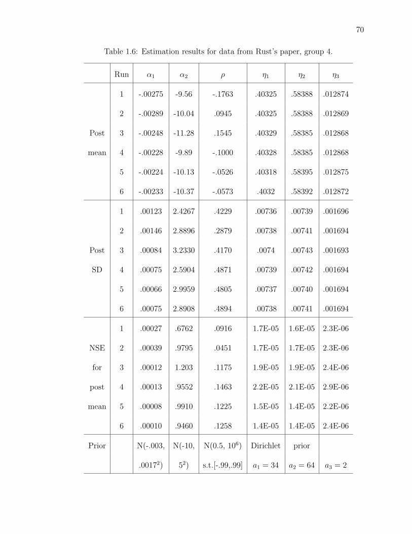
70

Table 1.6: Estimation results for data from Rust’s paper, group 4.


1 -.00275 -9.56 -.1763 .40325 .58388 .012874

2 -.00289 -10.04 .0945 .40325 .58388 .012869

Post 3 -.00248 -11.28 .1545 .40329 .58385 .012868

mean 4 -.00228 -9.89 -.1000 .40328 .58385 .012868

5 -.00224 -10.13 -.0526 .40318 .58395 .012875

6 -.00233 -10.37 -.0573 .4032 .58392 .012872

1 .00123 2.4267 .4229 .00736 .00739 .001696

2 .00146 2.8896 .2879 .00738 .00741 .001694

Post 3 .00084 3.2330 .4170 .0074 .00743 .001693

SD 4 .00075 2.5904 .4871 .00739 .00742 .001694

5 .00066 2.9959 .4805 .00737 .00740 .001694

6 .00075 2.8908 .4894 .00738 .00741 .001694

1 .00027 .6762 .0916 1.7E-05 1.6E-05 2.3E-06

NSE 2 .00039 .9795 .0451 1.7E-05 1.7E-05 2.3E-06

for 3 .00012 1.203 .1175 1.9E-05 1.9E-05 2.4E-06

post 4 .00013 .9552 .1463 2.2E-05 2.1E-05 2.9E-06

mean 5 .00008 .9910 .1225 1.5E-05 1.4E-05 2.2E-06

6 .00010 .9460 .1258 1.4E-05 1.4E-05 2.4E-06

Prior N(-.003, N(-10, N(0.5, 106) Dirichlet prior

.00172) 52) s.t.[-.99,.99] a1 = 34 a2 = 64 a3 = 2

71

the corresponding AR(1) process. Then, ∆Vt,i are adjusted to satisfy the observed

choice optimality constraints with a small margin. It is also possible to adjust εt,i

together with ∆Vt,i. If the initial values for εt,i are not simulated from the AR(1)

process or if the starting value for ρ is far in the tail of the posterior, a procedure

similar to the simulated annealing might be helpful in starting the Gibbs sampler with

high acceptance rates: the acceptance probabilities for the parameters are multiplied

by a decreasing quantity on the first hundred iterations.

Estimation results for 6 posterior simulator runs are presented in Table 1.6

and Figure 1.11. The number of draws for each simulator run was equal to 1000000.

Three different random grids for solving the DP were used in these experiments (the

random grid is generated before the estimation procedure starts and it stays fixed

through the simulator run, Proposition 2.6 justifies using the same random grid at

each iteration of the algorithm if the number of the nearest neighbors is constant.)

One grid was used for runs 1–2, another one for runs 3–4, and the last one for runs

5–6. The random number generator was initialized differently for each run.

Convergence of the Gibbs sampler draws to the stationary distribution could

be judged by comparing the posteriors obtained for the same realizations of the ran-

dom grid. For all the parameters but ρ convergence was attained in all the runs.

Convergence for ρ was clearly attained only for runs 5–6. To reduce the role of the

MCMC slow convergence for ρ in evaluating the effects of the random grid on the

estimation results I combine the draws from the simulator runs corresponding to the

same realizations of the random grid. The three posterior densities corresponding

72

to runs 1–2, 3–4, and 5–6 are presented in Figure 1.11. The figure and table above

suggest that only the estimation results for ρ are significantly affected by the random

grid realization. The results for strongly identified η are not affected at all.

Figure 1.11: Estimated posterior densities for different grids: (a) α1, (b) α2, (c) ρ, (d)η1, (e) η2, (f) η3. The dashed lines are prior densities. The solid lines are posteriordensities averaged over all simulator runs. The dotted lines show posterior densitiesaveraged for runs 1–2, 3–4, and 5–6.

The qualitative results for ρ do not seem to depend on the grid realization.

The posterior distribution for ρ is bimodal. The higher mode is positive and located

at about 0.2, the lower mode is at about -0.6. The posterior mean is close to 0. The

posterior probability of ρ > 0 is in 0.54–0.66 range. Overall, there seems to be no

strong evidence that Rust’s assumption of no serial correlation in the unobservables

73

is invalid.

A more objective criterion for studying the effects of the grid realization on

the estimation results would be to check how it affects conditional choice probabilities

or results of some policy changes. If the effects are still present then there are several

alternative ways to reduce them. The first one is to estimate the posterior densities

from several posterior simulator runs corresponding to different grids. This was done

for the experiment above and the resulting densities are shown by the solid lines in

Figure 1.11.

Increasing the size of the grid seems to be a more attractive way to obtain

better approximations for the posterior distribution. However, it would increase the

computational burden of solving the DP and approximating the expectations in the

Gibbs sampler. In both cases this burden can be ameliorated. As was described

in Section 1.5.1.4, solving the DP on several small random grids and combining the

results produces about the same approximation precision as solving the DP on one

big random grid. However, using several smaller grids requires much less time. To

speed up the approximation of the expectations in the Gibbs sampler a strategy

proposed by Keane and Wolpin (1994) could be used. In solving the DP, the authors

compute expectations using Monte Carlo integration only for a subset of states in

the discretized state space. For the rest of the states the expectations are computed

by interpolation. Such an interpolation function could be used for approximating the

expectations in the Gibbs sampler.

Chapter 3 presents another approach to estimation of dynamic discrete choice

74

models that avoids the problem of estimation results dependence on the random grid

realization. The future expected value function can be seen as a function of the pa-

rameters, the current state, and the chosen alternative. Experiments in this chapter

showed that kernel smoothing does not provide sufficiently good approximations of

this function. It turns out that artificial neural networks do. The DP solving algo-

rithm presented in this chapter can produce very precise approximations of the value

functions as described in Section 1.5.1.4. It is not feasible to get such precision for a

million of parameter draws required to reasonably approximate the posterior distri-

butions. However, it is feasible for several thousand draws from a prior distribution.

These precise approximations can be used to train an artificial neural network before-

hand of the estimation procedure. Then this neural network can be used in the Gibbs

sampler for approximating the expectations of the value functions. Experiments in

Chapter 3 suggest that this indeed is a promising alternative.

1.6 Conclusion and future work

This chapter presents a method for Bayesian inference in dynamic discrete

choice models with serially correlated unobserved state variables. It constructs the

Gibbs sampler, employing data augmentation and Metropolis steps, that can success-

fully handle multidimensional integration in the likelihood function of these models.

The computational burden of solving the DP at each iteration of the estimation

algorithm can be reduced by efficient use of the information obtained on previous

iterations. A proof of the complete uniform convergence of the proposed DP solution

75

approximations to the true values is obtained under mild assumptions on the prim-

itives of the model. In Bayesian analysis, inference results are often represented in

terms of posterior expectations. The chapter establishes the complete convergence of

the posterior expectations approximated by the proposed method.

Serially correlated unobservables are not the only possible source of intractable

integrals in the likelihood function of DDCMs. The Gibbs sampler algorithm can be

extended to tackle other cases as well. First, missing observations could be handled

by data augmentation in this framework. An example of that is different observation

frequencies for different variables in a dataset, e.g. HRS interviews are conducted

biannually but the attached data from the Social Security Administration and Medi-

care records are available monthly or even daily. Also, adding a macro shock or a

cohort effect into a model is equally easy. It would amount to adding another block

in the Gibbs sampler.

The method is experimentally evaluated on two different dynamic discrete

choice models. First of all, estimation experiments show that ignoring serial correla-

tion in unobservables can lead to serious misspecification errors. Second, parameters

in DDCMs are often weakly identified. In Bayesian inference, uncertainty about pa-

rameters is treated explicitly. This advantage of Bayesian methods seems to be very

important for DDCMs. Since the proposed estimation method allows for serial corre-

lation in unobservables and accounts for uncertainty about parameters, its application

is likely to improve the reliability of the answers to the policy questions that a DDCM

can provide.

76

There are several directions in which the method could be improved. First,

the amount of serial correlation in posterior simulator draws is very large. Thus,

long posterior simulator runs are required for exploring the posterior distributions.

Developing strategies for decreasing the amount of serial correlation in the Gibbs

sampler draws is an important area for future research. Due to the high computational

demand the method is implemented in C. Application of parallel computing seems to

be a fruitful way to achieve higher performance of the method in the future.

Experiments with the DP solving algorithm led to a discovery of several sig-

nificant practical improvements in the algorithm. First, the approximations of the

expected value function obtained for fixed parameters and different realizations of the

random grid behave as if an analog of a CLT with respect to the size of the random

grid holds. This suggests that solving the DP on several small random grids and

combining the results is a very efficient alternative to using one large grid. Theoret-

ical justification of this observed improvement in the algorithm performance could

be a subject of future work. Second, a difference of expected value functions can

be approximated by the DP solving algorithm with a much higher precision than an

expected value function by itself. This is taken into account in the construction of

the Gibbs sampler. As a result, the realization of the random grid on which the DP

is solved does not seem to seriously alter the results of estimation even for small grid

sizes.

The flexibility of the framework and extensive experimentation were crucial

for making the proposed approach successful. Nevertheless, combined with efficient

77

DP solution strategies, standard tools of Bayesian analysis—Gibbs sampling, data

augmentation, and the Metropolis-Hastings algorithm—seem to be very promising in

making more elaborate dynamic discrete choice models estimable.

78

CHAPTER 2PROOFS OF THE THEORETICAL RESULTS

2.1 Lemmas

Lemma 2.1. Given ε > 0, there exist δ > 0 and T such that for any θ ∈ Θ, s ∈ S,

and t > T :

P (|At1(θ, s)| > ε) ≤ e−δN(t)N(t−N(t)) ≤ e−0.5δtγ1 (2.1)

Proof. Fix a combination m = m1, . . . ,mN(t) from t−N(t), . . . , t−1. Assumption

1.7 defines X(ωt−1, θ, s, d,m). Since the importance sampling weights are bounded

away from zero by f > 0 (see Assumption 1.4),

[X(ωt−1, θ, s, d,m) > ε]

⊂

| N(t)∑i=1

N(mi)∑j=1

(V (smi,j; θ)− E[V (s′; θ) | s, d; θ])f(smi,j | s, d; θ)/g(smi,j)∑N(t)r=1 N(mr) infθ,s,s′,d f(s′|s, d; θ)/g(s′)

| > ε

=

| N(t)∑i=1

N(mi)∑j=1

(V (smi,j; θ)− E[V (s′; θ) | s, d; θ])f(smi,j | s, d; θ)/g(smi,j)| >

εf

N(t)∑i=1

N(mi)

(2.2)

Using (2.2) and then applying Hoeffding (1963)’s inequality we get

P (X(ωt−1, θ, s, d,m) > ε)

≤ P

| N(t)∑i=1

N(mi)∑j=1

(V (smi,j; θ)− E[V (s′; θ) | s, d; θ])f(smi,j | s, d; θ)/g(smi,j)| >

εf

N(t)∑i=1

N(mi)

≤ 2 exp

−2f 2ε2

(b− a)2

N(t)∑r=1

N(mr)

(2.3)

where a and b are correspondingly the lower and upper bounds on

(V (smi,j; θ)− E[V (s′; θ) | s; θ])f(smi,j | s, d; θ)/g(smi,j). Hoeffding’s inequality applies

79

since smi,j are independent, the summands have expectations equal to zero:

∫(V (smi,j; θ)− E[V (s′; θ) | s; θ])f(smi,j | s, d; θ)

g(smi,j)g(smi,j)dsmi,j = 0 (2.4)

and a and b are finite by Assumptions 1.1, 1.3, and 1.4.

Since N(.) is non-decreasing, (2.3) implies

P (X(ωt−1, θ, s, d,m) > ε) ≤ 2 exp

−2f 2ε2

(b− a)2N(t)N(t−N(t))

= 2 exp

−4δN(t)N(t−N(t))

(2.5)

where the last equality defines δ > 0.

Since |At1(θ, s, d)| < maxm X(ωt−1, θ, s, d,m):

P (|At1(θ, s, d)| > ε) ≤ P [max

mX(ωt−1, θ, s, d, m) > ε]

= P (∪m[X(ωt−1, θ, s, d, m) > ε]) ≤∑m

P [X(ωt−1, θ, s, d,m) > ε]

≤ 2 exp−4δN(t)N(t−N(t))

N(t)!

(N(t)− N(t))!N(t)!(2.6)

where the summation, the maximization, and the union are taken over all possi-

ble combinations m and N(t)!/((N(t) − N(t))!N(t)!) is the number of the possible

combinations.

Assumption 1.6 and Proposition 2.8 show that ∃T1 such that ∀t > T1,

exp−4δN(t)N(t−N(t))

N(t)!

(N(t)− N(t))!N(t)!≤ exp


(2.7)

80

Finally,

P (|At1(θ, s)| > ε) = P (max

d∈D|At

1(θ, s, d)| > ε) = P (∪d∈D[|At1(θ, s, d)| > ε])

≤ card(D)2 exp−2δN(t)N(t−N(t)),∀t > T1

≤ exp−δN(t)N(t−N(t)),∀t > T2 ≥ T1 (2.8)

where such T2 exists since card(D)2 exp−δN(t)N(t−N(t)) → 0. The last inequality

in (2.1) follows since N(t)N(t − N(t)) ≥ tγ1 − tγ1−γ2 ≥ 0.5tγ1 for any t larger than

some T ≥ T2.

Lemma 2.2. Given ε > 0, there exist δ > 0 and T such that for any θ ∈ Θ, s ∈ S,

and t > T :

P (|At2(θ, s)| > ε) ≤ e−δ(N(t)−N(t)) ≤ e−0.5δtγ1 (2.9)

Proof.

[∣∣At2(θ, s, d)

∣∣ > ε]

=

∣∣∣∣∣∣N(t)∑i=1

N(t)∑j=1

(V (ski,j; θki)− V (ski,j; θ))Wki,j,t(s, d, θ)

∣∣∣∣∣∣ > ε

⊂

N(t)∑i=1

N(t)∑j=1

|V (ski,j; θki)− V (ski,j; θ)|Wki,j,t(s, d, θ) > ε

⊂

[∃ki, j : |V (ski,j; θki)− V (ski,j; θ)| > ε

](2.10)

Since V (s; θ) is continuous, and Θ × S is a compact, ∃δε > 0 such that ||(s1, θ1) −

(s2, θ2)|| ≤ δε implies |V (s1; θ1)− V (s2; θ2)| ≤ ε. Therefore,

[∃ki, j : |V (ski,j; θki)− V (ski,j; θ)| > ε

]⊂ [∃ki, j : ||(ski,j, θki)− (ski,j, θ)|| > δε] = [∃ki : ||θki − θ|| > δε] (2.11)

81

Because ki are the indices of the parameters from the previous iterations that are the

closest to θ:

[∃ki : ||θki − θ|| > δε]

⊂ [∀j ∈ t−N(t), . . . , t− 1 \ k1, . . . , kN(t) : ||θj − θ|| > δε]

⊂⋃

(j1,...,jN(t)−N(t)):jm∈t−N(t),...,t−1,m 6=l⇒jm 6=jl

N(t)−N(t)⋂m=1

[||θjm − θ|| > δε

](2.12)

Fix some (j1, . . . , jN(t)−N(t)), then by Assumption 1.5:

P ([||θjm − θ|| > δε]|ωjm−1)

= 1− P ([||θjm − θ|| < δε]|ωjm−1) ≤ 1− δλ[Bδε(θ) ∩Θ]

≤ 1− δ[δε/J0.5Θ ]J = exp−4(−0.25 log(1− δ[δε/J

0.5Θ ]J)) = e−4δ (2.13)

where the last equality defines δ > 0, JΘ is the dimensionality of rectangle Θ, B.(.)

is a ball in RJΘ . It holds for any history ωjm−1; thus for fixed (j1, . . . , jN(t)−N(t))

P

N(t)−N(t)⋂m=1

[||θjm − θ|| > δε

] ≤ e−4δ(N(t)−N(t)) (2.14)

Since the union in (2.12) is taken over N(t)!/(N(t)!(N(t)− N(t))!) events

P[∣∣At

2(x, θ, ε)∣∣ > ε

]≤ e−4δ(N(t)−N(t)) N(t)!

N(t)!(N(t)− N(t))!

≤ e−2δ(N(t)−N(t)),∀t > T2 (2.15)

where the second inequality and existence of T2 follows from Assumption 1.6 and

Proposition 2.8. Finally,

P (|At2(θ, s)| > ε) = P (max

d∈D|At

2(θ, s, d)| > ε) = P (∪d∈D[|At2(θ, s, d)| > ε])

≤ card(D)e−2δ(N(t)−N(t)),∀t > T2

≤ e−δ(N(t)−N(t)),∀t > T3 ≥ T2 (2.16)

82

where such T3 exists since card(D)e−δ(N(t)−N(t)) → 0. The last inequality in (2.9)

follows since N(t) − N(t) ≥ [tγ1 − [tγ2 ] ≥ tγ1 − 1 − tγ2 ≥ 0.5tγ1 for any t larger than

some T ≥ T3.

Lemma 2.3. Given ε > 0, there exist δ > 0 and T such that ∀θ ∈ Θ, ∀s ∈ S, and

∀t > T :

P (|At3(θ, s)| > ε) ≤ e−δtγ0γ1 (2.17)

Proof. First let’s show that for any positive integer m, ∀θ ∈ Θ, and ∀s ∈ S

At3(θ, s) ≤

β

1− β

[max

i=t−mN(t),t−1

(max

j=1,N(i)Ai

1(θi, si,j)

)+ (2.18)

maxi=t−mN(t),t−1

(max

j=1,N(i)Ai

2(θi, si,j)

)]+ βm max

i=t−mN(t),t−1

(max

j=1,N(i)Ai

3(θi, si,j)

)By definition

At3(θ, s, d) =

∣∣∣∣∣∣N(t)∑i=1

N(ki)∑j=1

(V ki(ski,j; θki)− V (ski,j; θki))Wki,j,t(s, d, θ)

∣∣∣∣∣∣ (2.19)

Since maxd a(d)−maxd b(d) ≤ maxda(d)− b(d)

|V ki(ski,j; θki)− V (ski,j; θki)|

= |maxd∈D

u(ski,j, d) + βE(ki)[V (s′; θki) | ski,j, d; θki ]

−max

d∈D

u(ski,j, d) + βE[V (s′; θki) | ski,j, d; θki ]

|

≤ |maxd∈D

βE(ki)[V (s′; θki) | ski,j, dθki ]]− βE[V (s′; θki) | ski,j, d; θki ]

| (2.20)

From (2.20) and definition of Atl(.) given in Theorem 1.1,

|V ki(ski,j; θki)− V (ski,j; θki)|

≤ β maxd∈D

(Aki

1 (θki , ski,j, d) + Aki2 (θki , ski,j, d) + Aki

3 (θki , ski,j, d))

≤ β(Aki

1 (θki , ski,j) + Aki2 (θki , ski,j) + Aki

3 (θki , ski,j))

(2.21)

83

Combining (2.19) and (2.21) gives:

At3(θ, s, d) ≤ β

N(t)∑i=1

N(ki)∑j=1

(Aki

1 (θki , ski,j) + Aki2 (θki , ski,j) + Aki

3 (θki , ski,j))Wki,j,t(s, d, θ)

≤ β maxi=t−N(t),t−1

(max

j=1,N(i)Ai

1(θi, si,j)

)+ β max

i=t−N(t),t−1

(max

j=1,N(i)Ai

2(θi, si,j)

)+β max

i=t−N(t),t−1

(max

j=1,N(i)Ai

3(θi, si,j)

)(2.22)

where the second inequality follows from the fact that ∀i ∈ 1, . . . , N(t), ki ∈ t −

N(t), . . . , t−1 and the weights sum to one. Since the r.h.s. of (2.22) does not depend

on d:

At3(θ, s) ≤ β max

i=t−N(t),t−1

(max

j=1,N(i)Ai

1(θi, si,j)

)+ (2.23)

β maxi=t−N(t),t−1

(max

j=1,N(i)Ai

2(θi, si,j)

)+ β max

i=t−N(t),t−1

(max

j=1,N(i)Ai

3(θi, si,j)

)

To facilitate the description of the iterative process on (2.23) that will lead to (2.18)

let M(t, 0) = t and M(t, i) = M(t, i− 1)−N(M(t, i− 1)), then

At3(θ, s) ≤ β max

i=t−N(t),t−1

(max

j=1,N(i)Ai

1(θi, si,j)

)+ β max

i=t−N(t),t−1

(max

j=1,N(i)Ai

2(θi, si,j)

)+β2 max

i=t−N(t)−N [t−N(t)],t−2

(max

j=1,N(i)Ai

1(θi, si,j)

)+β2 max

i=t−N(t)−N [t−N(t)],t−2

(max

j=1,N(i)Ai

2(θi, si,j)

)+β2 max

i=t−N(t)−N [t−N(t)],t−2

(max

j=1,N(i)Ai

3(θi, si,j)

)

≤m∑

k=1

βk

[max

i=M(t,k),t−k

(max

j=1,N(i)Ai

1(θi, si,j)

)+ max

i=M(t,k),t−k

(max

j=1,N(i)Ai

2(θi, si,j)

)]+βm max

i=M(t,m),t−m

(max

j=1,N(i)Ai

3(θi, si,j)

)(2.24)

from which (2.18) follows since∑m

k=1 βk < β/(1− β), and M(t,m) ≥ t−mN(t) ∀m.

84

Inequality in (2.18) is shown to hold for any m. Let m(t) = [(t − tγ0)/N(t)]

([x] is the integer part of x.) and notice that M(t,m(t)) ≥ t − m(t)N(t) ≥ tγ0 .

Since Ai3(θ

i, si,j) is bounded above by some A3 < ∞ (utility function and state and

parameter spaces are bounded):

P [|At3(θ, s)| > ε]

≤ P [β

1− β

max

i=t−m(t)N(t),t−1

(max

j=1,N(i)Ai

1(θi, si,j)

)+

maxi=t−m(t)N(t),t−1

(max

j=1,N(i)Ai

2(θi, si,j)

)+βm(t) max


(max

j=1,N(i)Ai

3(θi, si,j)

)> ε]

≤ P

[max


(max

j=1,N(i)Ai

1(θi, si,j)

)>

ε(1− β)

3β

]+P

[max


(max

j=1,N(i)Ai

2(θi, si,j)

)>

ε(1− β)

3β

]+P

[βm(t)A3 >

ε

3

]

≤t−1∑

i=t−m(t)N(t)

N(i)∑j=1

P

[Ai

1(θi, si,j) >

ε(1− β)

3β

]+ P

[Ai

2(θi, si,j) >

ε(1− β)

3β

]The last inequality holds for t > T3, where T3 satisfies P (βm(t)A3 > ε/3) = 0, ∀t > T3.

Such T3 exists since m(t) →∞.

Since t−m(t)N(t) →∞, by Lemma 2.1 and Lemma 2.2, exist δ1 > 0, δ2 > 0,

T1, and T2, such that for ∀t > max(T1, T2, T3):

P (|At3(θ, s)| > ε) ≤

t−1∑i=t−m(t)N(t)

N(i)[e−δ1N(i)N(i−N(i)) + e−δ2(N(i)−N(i))

](2.25)

Proposition 2.9 shows that exist δ > 0 and T4 such that the r.h.s of (2.25) is no

larger than exp(−δtγ0γ1),∀t > T4. Thus, setting T = max(T1, T2, T3, T4) completes

the proof.

85

2.2 Extension to the uniform convergence

First, note that the approximation error is not a continuous function of (θ, s).

Thus, we cannot apply the standard results to show the measurability of the supre-

mum of the approximation error over the state and parameter spaces. Proposition 2.1

and Proposition 2.3 can be used to establish the measurability in this case. Below,

Lemma 2.4 shows that a uniform version of Lemma 2.1 holds given extra Assumption

1.7. Lemma 2.5 shows that a uniform version of Lemma 2.2 also holds. A uniform

version of Lemma 2.3 holds trivially since the right hand side of the key inequality

(2.18) does not depend on (θ, s). Theorem 1.2 follows from the uniform versions of

the Lemmas in the same way as Theorem 1.1 follows from Lemmas 2.1-2.3.

Proposition 2.1. Let f(ω, θ) be a measurable function on (Ω × Θ, σ(A × B)) with

values in R. Assume that Θ has a countable subset Θ and that for any ω ∈ Ω and

any θ ∈ Θ there exists a sequence in Θ, θn such that f(ω, θn) → f(ω, θ). Then,

supθ∈Θ f(ω, θ) is measurable w.r.t. (Ω,A) (the proposition can be used to show that

the supremum of a random function with some simple discontinuities, e.g. jumps, on

a separable space is measurable.)

To apply the proposition for establishing the measurability of the supremum

of the approximation errors, let the set of rational numbers contained in Θ× S play

the role of the countable subset Θ. Proposition 2.3 shows that for any given history

ωt−1 and any (θ, s) it is always possible to find a sequence with rational coordinates

(θn) → θ such that for all n, (θn) and θ have the same iteration indices for the nearest

neighbors. For a given history ωt−1, the approximation error is continuous in (θ, s)

86

on the subsets of Θ×S that give the same iteration indices of the nearest neighbors.

Using any rational sequence sn → s gives f(ω, ˜(θ, s)n) → f(ω, (θ, s)) required in the

proposition. Thus, the supremum of the approximation error is measurable.

Proof. First, let’s show that for an arbitrary t

∪θ∈Θ[f(ω, θ) > t] = ∪θ∈Θ[f(ω, θ) > t] (2.26)

Assume ω1 ∈ ∪θ∈Θ[f(ω, θ) > t]. It means there exists θ1 ∈ Θ such that f(ω1, θ1) > t.

By the theorem’s assumption ∃θn such that f(ω1, θn) → f(ω1, θ1). Then, ∃n,

f(ω1, θn) > t. Thus, ω1 ∈ ∪θ∈Θ[f(ω, θ) > t] and (2.26) is proven.

Note that [supθ∈Θ f(ω, θ) > t] = ∪θ∈Θ[f(ω, θ) > t] = ∪θ∈Θ[f(ω, θ) > t] is a

countable union of sets from A and thus also belongs to A.

Lemma 2.4. Given ε > 0, there exist δ > 0 and T such that ∀t > T :

P ( supθ∈Θ,s∈S

|At1(θ, s)| > ε) ≤ e−δN(t)N(t−N(t)) ≤ e−0.5δtγ1 (2.27)

Proof. Fix a combination m = m1, . . . ,mN(t) from t−N(t), . . . , t− 1. Assump-

tion 1.7 defines X(ωt−1, θ, s, d,m). By Assumption 1.7, X(ωt−1, θ, s, d,m)ωt−1 are

equicontinuous on Θ×S: there exists δ(ε) > 0 such that ||(θ1, s1)− ((θ2, s2))|| < δ(ε)

implies |X(ωt−1, θ1, s1, d, m)−X(ωt−1, θ2, s2, d, m)| < ε/2. Since Θ× S is a compact

set it can be covered by M balls: Θ × S ⊂ ∪Mi=1Bi with radius δ(ε) and centers at

(θi, si), where M < ∞ depends only on ε. It follows that

[supθ,s

X(ωt−1, θ, s, d, m) > ε] = ∪θ,s[X(ωt−1, θ, s, d,m) > ε] =

∪Mi=1 ∪(θ,s)∈Bi

[X(ωt−1, θ, s, d, m) > ε] (2.28)

87

Let’s show that

∪(θ,s)∈Bi[X(ωt−1, θ, s, d,m) > ε] ⊂ [X(ωt−1, θi, si, d, m) >

ε

2] (2.29)

If ωt−1∗ ∈ ∪(θ,s)∈Bi

[X(ωt−1, θ, s, d,m) > ε], then ∃(θ∗, s∗) ∈ Bi(θi, si) such that

X(ωt−1∗ , θ∗, s∗, d, m) > ε. Since ||(θ∗, s∗) − (θi, si)|| ≤ δ(ε), X(ωt−1

∗ , θi, si, d, m) ≥

X(ωt−1∗ , θ∗, s∗, d, m)− ε/2. This implies ωt−1

∗ ∈ [X(ωt−1, θi, si, d, m) > ε2].

Since supθ,s |At1(θ, s, d)| < maxm supθ,s X(ωt−1, θ, s, d,m):

P (supθ,s|At

1(θ, s, d)| > ε)

≤ P [maxm

supθ,s

X(ωt−1, θ, s, d, m) > ε] (max is over all possible combinations m)

≤ P (∪m[supθ,s

X(ωt−1, θ, s, d,m) > ε]

≤∑m

P [supθ,s

X(ωt−1, θ, s, d,m) > ε]

≤∑m

P (∪Mi=1[X(ωt−1, θi, si, d, m) >

ε

2]) (by (2.28) and (2.29) )

≤ MN(t)!

(N(t)− N(t))!N(t)!2 exp


(2.30)

where N(t)!/((N(t) − N(t))!N(t)!) is the number of different combinations m and

2 exp−4δN(t)N(t − N(t)) is the bound from (2.5) in Lemma 2.1. From the last

inequality, the proof follows steps of the argument starting after (2.6) in the proof of

Lemma 2.1.

Lemma 2.5. Given ε > 0, there exist δ > 0 and T such that ∀t > T :

P (supθ,s|At

2(θ, s)| > ε) ≤ e−δ(N(t)−N(t)) ≤ e−0.5δtγ1 (2.31)

88

Proof. From Lemma 2.2

[∣∣At2(θ, s, d)

∣∣ > ε]

⊂⋃

(j1,...,jN(t)−N(t)):jm∈t−N(t),...,t−1,m 6=l⇒jm 6=jl

N(t)−N(t)⋂m=1

[||θjm − θ|| > δε

](2.32)

This implies that[supθ,s

∣∣At2(θ, s, d)

∣∣ > ε

]=⋃θ,s

[∣∣At2(θ, s, d)

∣∣ > ε]

(2.33)

⊂⋃θ∈Θ

⋃(j1,...,jN(t)−N(t)):jm∈t−N(t),...,t−1,m 6=l⇒jm 6=jl

N(t)−N(t)⋂m=1

[||θjm − θ|| > δε

]Since Θ is a rectangle in RJΘ it can be covered by a finite number of balls with radius

δε

2:

Θ ⊂ ∪Mi=1B(θi), M = const · (δε/2)−JΘ (2.34)

Let’s prove the following fact:

⋃θ∈B(θi)

N(t)−N(t)⋂m=1

[||θjm − θ|| > δε

]⊂

N(t)−N(t)⋂m=1

[θjm /∈ B(θi)] (2.35)

Assume ωt−1 ∈(⋂N(t)−N(t)

m=1 [θjm /∈ B(θi)])c

. Then ∃m such that θjm ∈ B(θi).

It follows that ∀θ ∈ B(θi),∃θjm : ||θjm − θ|| ≤ δε. Thus, ωt−1 belongs to the following

set:

⋂θ∈B(θi)

N(t)−N(t)⋃m=1

[||θjm − θ|| ≤ δε

]=

⋃θ∈B(θi)

N(t)−N(t)⋂m=1

[||θjm − θ|| > δε

]c

(2.36)

Therefore, the claim in (2.35) is proven.

By the same argument as for (2.14) from Lemma 2.2, we can establish that

P

N(t)−N(t)⋂m=1

[θjm /∈ B(θi)

] ≤ e−4δ(N(t)−N(t)) (2.37)

89

for some positive δ.

From (2.33), (2.34) and (2.35)[supθ,s

∣∣At2(θ, s, d)

∣∣ > ε

]

⊂⋃

(j1,...,jN(t)−N(t)):jm∈t−N(t),...,t−1,m6=l⇒jm 6=jl

M⋃i=1

N(t)−N(t)⋂m=1

[θjm /∈ B(θi)]

(2.38)

Using (2.37) and (2.38) gives

P

[supθ,s

∣∣At2(θ, s, d)

∣∣ > ε

]≤ N(t)!

N(t)!(N(t)− N(t))!Me−4δ(N(t)−N(t)) (2.39)

The rest of the proof follows the corresponding steps in Lemma 2.2.

2.3 Convergence of posterior expectations

and ergodicity of the Gibbs sampler

Proof. (Theorem 1.3.) First, let’s introduce some notation shortcuts:

r = r(θ,V , ε; F (θ, ε))

r = r(θ,V , ε; F n(θ, ε))

1 = 1Θ(θ) ·

(∏i,t


)·

(∏i,t,k

1[−ν,ν](q(θ,Vt,i, εt,i, Ft,i(θ, εt,i)))

)

1 = 1Θ(θ) ·

(∏i,t


)·

(∏i,t,k

1[−ν,ν](q(θ,Vt,i, εt,i, Fnt,i(θ, εt,i)))

)∫

h(θ,V , ε)d(θ,V , ε) =

∫h

p = p(θ,V , ε; F |d, x) =r · 1∫r · 1

90

p = p(θ,V , ε; F n|d, x) =r · 1∫r · 1

The probability that the approximation error exceeds ε > 0 can be bounded by the

sum of two terms:

P

[∣∣∣∣∫ h · p−∫

h · p∣∣∣∣ > ε

]≤ P (||F − F || > δF ) (2.40)

+P

([

∣∣∣∣∫ h · p−∫

h · p∣∣∣∣ > ε] ∩ [||F − F || ≤ δF ]

)(2.41)

where ||F − F || = sups,θ,d |F (s, θ, d)− F (s, θ, d)| and F (s, θ, d) is the expected value

function (or the difference of expected value functions, depending on the parameter-

ization of the Gibbs sampler) and F is the approximation to F from the DP solving

algorithm on its iteration n (fixed in this proof.) I will show that for a sufficiently

small δF > 0, the set in (2.41) is empty. Then, by Theorem 1.2, the term in (2.40)

can be bounded by zn corresponding to δF .

[

∣∣∣∣∫ h · p−∫

h · p∣∣∣∣ > ε] ∩ [||F − F || ≤ δF ]

⊂[∫

|p− p| > ε/||h||]∩ [||F − F || ≤ δF ]

⊂

([∫1=1

|p− p| > ε/(2||h||)

]∩ [||F − F || ≤ δF ]

)(2.42)

∪

([∫1 6=1

|p− p| > ε/(2||h||)

]∩ [||F − F || ≤ δF ]

)(2.43)

Let’s start with (2.42):([∫1=1

|p− p| > ε/(2||h||)

]∩ [||F − F || ≤ δF ]

)

=

[∫1=1

| r∫r · 1

− r∫r · 1

| > ε

2||h||

]∩ [||F − F || ≤ δF ]

⊂

[|| r∫

r · 1− r∫

r · 1|| > ε

2||h||λ

]∩ [||F − F || ≤ δF ] (2.44)

91

where λ < ∞ is the Lebesgue measure of the space for the parameters and the latent

variables. For δSp ∈ (0,∫

r · 1):[|| r∫

r · 1− r∫

r · 1|| > ε

2||h||λ

]∩ [||F − F || ≤ δF ] =([

|| r∫r · 1

− r∫r · 1

|| > ε

2||h||λ

]∩ [||F − F || ≤ δF ]

∩[∣∣∣∣∫ r · 1 −

∫r · 1

∣∣∣∣ > δSp

])(2.45)

⋃([|| r∫

r · 1− r∫

r · 1|| > ε

2||h||λ

]∩ [||F − F || ≤ δF ]

∩[∣∣∣∣∫ r · 1 −

∫r · 1

∣∣∣∣ ≤ δSp

])(2.46)

By Proposition 2.2 for δSp there exists δ1F > 0 such that [

∣∣∫ r · 1 −∫

r · 1∣∣ > δSp] =

∅. Thus, (2.45) (the whole two-line expression in parentheses) is the empty set for

any δF < δ1F . Now, let’s work with (2.46) (again, both lines in parentheses.)

|| r∫r · 1

− r∫r · 1

|| ≤||r|| · |

∫r · 1 −

∫r · 1|∫

r · 1 ·∫

r · 1+||r − r||∫

r · 1

≤||r|| · |

∫r · 1 −

∫r · 1|∫

r · 1 · (∫

r · 1 − δSp)+

||r − r||∫r · 1 − δSp

(2.47)

This inequality shows that (2.46) is a subset of the union of the following two sets:[||r|| · |

∫r · 1 −

∫r · 1|∫

r · 1 · (∫ ∫

r · 1 − δSp)>

ε

4||h||λ

]∩[||F−F || ≤ δF ]∩

[∣∣∣∣∫ r · 1 −∫

r · 1∣∣∣∣ ≤ δSp

](2.48)

and

[||r − r||∫

r · 1 − δSp

>ε

4||h||λ

]∩ [||F − F || ≤ δF ]∩

[∣∣∣∣∫ r · 1 −∫

r · 1∣∣∣∣ ≤ δSp

](2.49)

92

I will show that both of them are empty for sufficiently small δF . By Proposition 2.2

there exists δ2F > 0 such that

[∣∣∣∣∫ r · 1 −∫

r · 1∣∣∣∣ > ε ·

∫r · 1 · (

∫r · 1 − δSp)

4||h||λ||r||

]= ∅

whenever ||F − F || ≤ δ2F . Therefore, (2.48) is equal to the empty set for δF ≤ δ2

F .

Since r is continuous in components of F , there exists δ3F > 0 such that

||r − r|| <ε · (∫

r · 1 − δSp)

4||h||λ||r||

whenever ||F − F || ≤ δ3F . Therefore, for δF ≤ δ3

F , (2.49) is equal to the empty set

and so is (2.46). Thus, so far we showed that (2.42) is equal to the empty set for

δF ≤ mini=1,2,3(δiF ).

Now, let’s work with (2.43). Note that

∫1 6=1

|p−p| ≤ (||r||∫r · 1

+||r||∫r · 1

)

∫1 6=1

1 ≤ (||r||∫r · 1

+||r||∫

r · 1 − δSp

)

∫1 6=1

1

Thus, (2.43) is a subset of the following set:([∫1 6=1

|p− p| > ε/(2||h||)

]∩ [||F − F || ≤ δF ]

)

⊂

∫1 6=1

1 >ε

2||h||( ||r||Rr·1

+ ||r||Rr·1−δSp

)

∩ [||F − F || ≤ δF ]

(2.50)

Using the same argument as the one starting from (2.54) in Proposition 2.2, I can

show that there exists δ4F > 0 such that ∀δF < δ4

F , (2.43) will be the empty set.

Setting δF = mini=1,2,3,4δiF completes the proof of the theorem.

93

Proposition 2.2. For any ε > 0 there exists δF > 0 such that

[||F − F || < δF

]∩[∣∣∣∣∫ r · 1 −

∫r · 1

∣∣∣∣ > ε

]= ∅ (2.51)

Proof.

[∣∣∣∣∫ r · 1 −∫

r · 1∣∣∣∣ > ε

]⊂

[∫|r · 1 − r · 1| > ε

]⊂

[∫1=1

|r · 1 − r · 1| > ε/2

](2.52)

∪

[∫1 6=1

|r · 1 − r · 1| > ε/2

](2.53)

Let’s show that the intersection of (2.52) and [||F − F || < δF ] is the empty set for a

sufficiently small δF .[∫1=1

|r · 1 − r · 1| > ε/2

]⊂

[∫1=1

|r − r| > ε/2

]⊂[||r − r|| > ε/(2λ)

]where λ < ∞ is the Lebesgue measure of the bounded space for the parameters and

the latent variables on which the integration is performed: Θ×E×. . .×E×V×. . .×V,

where V ⊂ R is the space for the alternative specific value functions Vt,d,i. By

Assumption 1.8, r is continuous in components of F . Thus, ∃δ1F > 0 such that

||F − F || < δ1F implies ||r− r|| < ε/(2λ), which means that the intersection of (2.52)

and [||F − F || < δF ] is the empty set for ∀δF < δ1F .

Let’s show that the intersection of (2.53) and [||F − F || < δF ] is the empty set

for a sufficiently small δF . First, note that

∫1 6=1

|r · 1 − r · 1| ≤ (||r||+ ||r||)∫

1 6=·11 (2.54)

94

where ||r|| < ∞ and ||r|| < r < ∞ for any F (everything is bounded in the model.)

Thus,

[||F − F || < δF ] ∩

[∫1 6=1

|r · 1 − r · 1| > ε/2

]

⊂ [||F − F || < δF ] ∩

[∫1 6=1

1 > ε/(2(||r||+ ||r||))

]= [||F − F || < δF ] ∩

[λ[1 6= 1] > ε/(2(||r||+ ||r||))

](2.55)

where λ(.) is the Lebesgue measure on the space of the parameters and the latent

variables.

By Assumption 1.8, qk is continuous in components of F . Thus, for any δq > 0

there exists δF (δq) > 0 such that ||F − F || < δF (δq) implies maxk ||qk − qk|| < δq.

On the space of the parameters and the latent variables (these are not subsets of the

underlying probability space):

[(θ,V , ε) : 1 6= 1] ⊂⋃i,t,k

[(θ,V , ε) : qk(θ,Vt,i, εt,i, Ft,i) ∈ Bδq(ν) ∪Bδq(−ν)] (2.56)

if ||F − F || < δF (δq). To prove this claim assume ∀i, t, k qk(θ,Vt,i, εt,i, Ft,i) /∈ Bδq(ν)∪

Bδq(−ν). So, the distance between qk and the truncation region edges −ν and ν is

larger than δq for all i, t, k. But then, since ||qk − qk|| < δq, 1 = 1 and the claim

(2.56) is proven.

Note that

limδq→0

λ

(⋃i,t,k

[(θ,V , ε) : qk(θ,Vt,i, εt,i, Ft,i) ∈ Bδq(ν) ∪Bδq(−ν)]

)(2.57)

≤∑i,t,k

limδq→0

λ[(θ,V , ε) : qk(θ,Vt,i, εt,i, Ft,i) ∈ Bδq(ν) ∪Bδq(−ν)]

=∑i,t,k

λ[(θ,V , ε) : qk(θ,Vt,i, εt,i, Ft,i) ∈ ν,−ν]

95

where the last equality holds by the monotone property of measures (the Lebesgue

measure in this case) and by the fact that ∩δq>0[qk ∈ Bδq(ν)] = [qk = ν].

By Assumption 1.8, λ[(θ,V , ε) : qk = ν] = λ[(θ,V , ε) : qk = −ν] = 0.

Therefore, the limit in (2.57) is equal to zero and there exists δ∗q > 0 such that if

||F − F || < δF (δ∗q ) then

λ[1 6= 1] < ε/(2(||r||+ ||r||))

So, ∀δF ∈ (0, δF (δ∗q )] the intersection of (2.53) and [||F − F || < δF ] is the empty set.

Setting δF = minδF (δ∗q ), δ1F completes the proof of the proposition.

Proof. (Theorem 1.4)

Consider the following uniform probability density:

q(∆V , θ, ε) = c · 1Θ(θ)∏i,t

[1E(εt,i) · p(dt,i|∆Vt,i)

·1[−ν,ν](∆Vt,i − [xt,iα1 − α2 + εt,i + Ft,i(θ, εt,i)])] (2.58)

where c is a normalization constant. The corresponding probability measure is de-

noted by Q(.).

Let’s show that the transition probability measure for the Gibbs sampler sat-

isfies the marginalization condition w.r.t. Q(.):

P ((Vm+1, θm+1, εm+1) ∈ A|Vm, θm, εm, d, x) ≥ bQ(A),∀Vm, θm, εm

where b > 0 is a constant. Then, the uniform ergodicity follows from Proposition 2

in Tierney (1994).

96

P ((Vm+1, θm+1, εm+1) ∈ A|Vm, θm, εm, d, x) (2.59)

=

∫R×...×R

∫A

∏t,i

p(∆Vm+1t,i |θm, εm, d, x)

p(ρm+1|θm, εm, ∆Vm+1, d, x) · p(αm+1|ρm+1ηm, hmε , αm, εm, ∆Vm+1, d, x)

p(ηm+1| . . .) · p(hm+1ε | . . .)

∏t,i

p(εm+1t,i | . . .)∏

t,i

p(∆Vm+1t,i |θm+1, εm+1, d, x) d(∆V , θm+1, εm+1, ∆Vm+1)

where p(.|.) are the densities for the Gibbs sampler blocks. Even though the Metropolis-

Hastings is used in the blocks, the densities can be expressed by using the Dirac delta

function (see, for example, chapter 4 in Geweke (2005).)

Given the assumptions on the support of νt,i let’s show that there exist δ1 > 0

such that ∆Vt,i ∈ [−δ1, δ1] implies (∆Vt,i − [xt,iα1 − α2 + εt,i + Ft,i(θ, εt,i)]) ∈ [−ν, ν],

∀θ, ε. It was stated in the formulation of the theorem that EV is an upper bound on

the absolute value of the expected value function. Note that an upper bound on the

expected value function EVub exists. Let’s show that it is no greater than EV .

E[|V (s′; θ)|; ‖s, d; θ] = E[|maxα1x + ε + βE[V (s′′; θ)|s′, d1; θ],

α2 + ν + βE[V (s′′; θ)|s′, d2; θ]|]

≤ u + ε + E[|ν|] + βEVub (2.60)

It was also assumed in the theorem that Φ(−ν) < 0.25, which implies E[|ν|] ≤

1 + E[ν2] ≤ 1 + 2h−1ν . Since (2.60) holds for any (s, d, θ):

EVub ≤ u + ε + (1 + 2h−1ε )

1− β= EV

97

Therefore,

|[xt,iα1 − α2 + εt,i + Ft,i(θ, εt,i)]| ≤ 2(u + ε + βEV )

Let δ1 = ν − 2(u + ε + βEV ), which is positive by the assumption of the theorem.

Thus, for |∆Vt,i| ≤ δ1,

|∆Vt,i − [xt,iα1 − α2 + εt,i + Ft,i(θ, εt,i)]| ≤ δ1 + 2(u + ε + βEV ) = ν

To find a lower bound on the integral in (2.59), let’s restrict the integration over

∆Vm+1t,i to |∆Vm+1

t,i | ≤ δ1 and use only the parts of the block densities corresponding

to the accepted draws. The parts of the block densities for the accepted draws are

equal to the MH transition densities multiplied by the acceptance probabilities. For

(∆Vt,i − [xt,iα1 − α2 + εt,i + Ft,i(θ, εt,i)]) ∈ [−ν, ν], these densities for the accepted

draws are positive and continuous on Θ, E, and [∆Vt,i ≥ 0] (or [∆Vt,i < 0] depending

on dt,i) for all blocks, and thus bounded away from zero. Let’s denote the common

bound by δ > 0. Then,

P ((Vm+1, θm+1, εm+1) ∈ A|Vm, θm, εm, d, x) ≥ (∏t,i

δ1δ)

·∫

A

1Θ(θm+1) · δ4 ·∏t,i

[δ · 1E(εt,i)] ·∏t,i

δ · p(dt,i|∆Vt,i)

·1[−ν,ν](∆Vt,i − [xt,iα1 − α2 + εt,i + Ft,i(θ, εt,i)])

d(θm+1, εm+1, ∆Vm+1) =1

c(∏t,i

δ)2 · δ4 ·∏t,i

δ1 ·Q(A) (2.61)

Also, since Q(.) is absolutely continuous w.r.t. the posterior probability measure, the

transition probability measure for the Gibbs sampler is irreducible w.r.t. the posterior

probability measure. This completes the proof of the uniform ergodicity of the Gibbs

sampler.

98

2.4 Auxiliary results

Proposition 2.3. For any θ1, . . . , θN and θ in Rn and any N ≤ N , there exists a

sequence of rational numbers qm → θ such that for any m, qm and θ have the same

set of indices for the nearest neighbors: k1, . . . , kN defined by (1.13).

Proof. The outcomes of selecting the nearest neighbors can be classified into two

cases. The trivial one occurs when there exists a ball around θ with radius r such

that ||θki − θ|| < r and ||θj − θ|| > r + d for d > 0 and j 6= ki. Then, applying the

triangle inequality twice we get ∀q ∈ Bd/4(θ), ||θki − q|| < r +d/2 < ||θj − q|| ∀j 6= ki.

For this case the proposition holds trivially.

The other case occurs when there exists a ball at θ with radius r1 such that

the closure of the ball includes all the nearest neighbors and the boundary of the ball

includes one or more θj that are not included in the set of the nearest neighbors.

For this case, I will construct a ball in the vicinity of θ such that it can be made as

close to θ as needed and such that for any point inside this ball the set of the nearest

neighbors is the same as for θ.

As described in the paper body (see (1.13)), the selection of the nearest neigh-

bors on the boundary of Br1(θ) is conducted by the lexicographic comparison of

(θj − θ). Let’s denote vectors (θj − θ) such that θj is on the boundary of Br1(θ):

||θj − θ|| = r1 by x0,i, i = 1, . . . ,M0x . The results of the lexicographic selection

99

process can be represented as follows:

zk,i = (r1 − a1, . . . , rk−1 − ak−1, zk,ik , . . . , zk,i

n )

xk,i = (r1 − a1, . . . , rk−1 − ak−1, rk − ak , xk,ik+1, . . . , x

k,in ) (2.62)

yk,i = (r1 − a1, . . . , rk−1 − ak−1, yk,ik , . . . , yk,i

n )

where a geometric interpretation of variables rk and ak is given in the figure below,

zk,ik > rk − ak > yk,i

k (2.63)

and k = 1, . . . , K for some K ≤ n. Vectors zk,i, i = 1, . . . ,Mkz are those vectors

included in the set of the nearest neighbors for which the decision of the inclusion

was obtained from the lexicographic comparison for the coordinate k. Vectors xk,i, i =

1, . . . ,Mkx are the vectors for which the decision has not yet been made after comparing

coordinates k. Vectors yk,i, i = 1, . . . ,Mky are the vectors for which the decision of

not including them in the set of the nearest neighbors was obtained from comparing

coordinate k. Vectors xk+1,i, yk+1,i, zk+1,i are all selected from xk,i. The lexicographic

selection will end at some coordinate K with unique xK . This vector is denoted by x

not by z to emphasize the fact that if there are multiple repetitions of θ + xK = θi =

θj, i 6= j in the history, then not all the repetitions have to be selected for the set of

the nearest neighbors (the ones with larger iteration number will be selected first.)

Of course, this is true only for the last selected nearest neighbor, for all the previous

ones all the repetitions are included. Note that vectors zk,i, xk,i, yk,i are constructed

in the system of coordinates with the origin at θ; so, we should add θ to all of them

to get back to the original coordinate system.

100

A graphical illustration might be helpful for understanding the idea of the

proof (the proof was actually constructed from similar graphical examples in R2 and

R3.)

Figure 2.1: Nearest neighbors.

The figure shows an example, in which 2 nearest neighbors have to be chosen for point

O. Since the required number of the nearest neighbors is smaller than the number of

the points on the circle, we can always find a1 such that all the points with the first

coordinate strictly above r1 − a1 will be included in the set of the nearest neighbors

and all the points with the first coordinate strictly below r1 − a1 will not be. For

the points with the coordinate equal to r1− a1, the selection process continues to the

next dimension.

If we did not use the lexicographic comparison and just resolved the multival-

uedness of arg min by choosing vectors with larger iteration numbers first, than the

proposition would not hold (a counterexample could be easily found in R2.)

If the following conditions hold than the same nearest neighbors from the

101

surface of Br1(θ) will be chosen for (θ + b) and θ:

||b− yk,i|| > ||b− xK || > ||b− zk,i||,∀k, i (2.64)

The condition says that (xK + θ), which is the last nearest neighbor selected for θ,

also has to be selected last for (θ + b) and that vectors on the boundary of Br1(θ)

that are not the selected nearest neighbors for θ (yk,i,∀k, i) should not be the selected

nearest neighbors for (θ + b). Since ||yk,i|| = ||xK || = ||zk,i|| = r1, these conditions

are equivalent to the following:

bT (xK − yk,i) > 0 and bT (zk,i − xK) > 0 (2.65)

Define

d = mink=1,K

minmini

[zk,ik − (rk − ak)], min

i[(rk − ak)− yk,i

k ], d > 0 by construction.

For given ε1 > 0, let

εk+1 = minεk, εkd/(4nr1), ε(ε1) = (ε1, . . . , εn)

δ(ε1) = εnd/(8nr1) (2.66)

Let b ∈ Bδ(ε1)(ε(ε1)) and l = b− ε(ε1). Let’s show that (2.65) holds for any such b.

bT (xK − yk,i) = (rk − ak − yk,ik )εk +

n∑m=k+1

(xKm − yk,i

m )εm +n∑

m=k

(xKm − yk,i

m )lm (2.67)

Note that |lk| ≤ δ(ε1) and |xKm − yk,i

m | ≤ 2r1:

bT (xK − yk,i) ≥ (rk − ak − yk,ik )εk − n2r1 max

m=k+1,nεm − n2r1δ(ε1)

≥ dεk − n2r1εkd

4nr1

− n2r1εkd

8nr1

= dεk/4 > 0 (2.68)

102

Analogously,

bT (zk,i − xK) ≥ [zk,ik − (rk − ak)]εk +

n∑m=k+1

(zk,im − xK

m)εm +n∑

m=k

(zk,im − xK

m)lm

≥ dεk − n2r1 maxm=k+1,n

εm − n2r1δ(ε1) ≥ dεk/4 > 0 (2.69)

Thus, the order of selecting the nearest neighbors on the surface of Br1(θ) is the

same for θ and any θ + b if b ∈ Bδ(ε1)(ε(ε1)) for any ε1 > 0. Making ε1 sufficiently

small, we can guarantee that all θj satisfying ||θj − θ|| < r1 will be chosen as the

nearest neighbors for θ + b before the vectors on the surface of Br1(θ) and that θj

satisfying ||θj− θ|| > r1 will not be chosen at all. For any ε1 > 0, Bδ(ε1)(θ + ε(ε1)) will

contain rational numbers. Letting a positive sequence εm1 go to zero and choosing

qm ∈ Bδ(θ + εm) ∩Q will give the sought sequence qm.

Proposition 2.4. If Θ and S are compact, u(s, d; θ) is continuous in (s, θ), and

f(s′ | s, d; θ) is continuous in (θ, s, s′), then V (s; θ) and

EV (s′; θ)|s, d; θ are continuous in (θ, s).

Proof. The proof of the proposition follows closely the standard proof of the continuity

of value functions with respect to the state variables (see, for example, chapters 3 and

4 of Stokey and Lucas (1989).) Let’s consider the Bellman operator Γ on the Banach

space of bounded functions B with sup norm: V : Θ×S → X, where X is a bounded

subset of R:

Γ(V )(s; θ) = maxdu(s, d; θ) + β

∫V (s′; θ)f(s′|s, d; θ)ds′

Blackwell’s sufficient conditions for contraction are satisfied for this operator; so, Γ is

a contraction mapping on B. The set of continuous functions C is a closed subset in

103

B. Thus, it suffices show that Γ(C) ⊂ C (this trivially implies that the fixed point

of Γ is a continuous function.)

Let V (s; θ) be a continuous function in B (V ∈ C). Let’s show that Γ(V ) is

also continuous.

|Γ(V )(s1; θ1)− Γ(V )(s2; θ2)| ≤ maxd|u(s1, d; θ1)− u(s2, d; θ2)

+β

∫V (s′; θ1)f(s′|s1, d; θ1)ds′ − β

∫V (s′; θ2)f(s′|s2, d; θ2)ds′|

≤ maxd|u(s1, d; θ1)− u(s2, d; θ2)|

+β maxd|∫

[V (s′; θ1)f(s′|s1, d; θ1)− V (s′; θ2)f(s′|s2, d; θ2)]ds′| (2.70)

Given ε > 0 there exists δ1 > 0 such that ||(s1; θ1)− (s2; θ2)|| < δ1 implies

maxd |u(s1, d; θ1)− u(s2, d; θ2)| < ε/2.

|∫

[V (s′; θ1)f(s′|s1, d; θ1)− V (s′; θ2)f(s′|s2, d; θ2)]ds′|

≤ maxd

sups′|V (s′; θ1)f(s′|s1, d; θ1)− V (s′; θ2)f(s′|s2, d; θ2)| · λ(S) (2.71)

Since V (s′; θ)f(s′|s, d; θ) is continuous on compact Θ× S × S, for ε > 0 there exists

δd2 > 0 such that ||(s1, s

′; θ1)− (s2, s′; θ2)|| = ||(s1; θ1)− (s2; θ2)|| < δd

2 implies

sups′|V (s′; θ1)f(s′|s1, d; θ1)− V (s′; θ2)f(s′|s2, d; θ2)| <

ε

2λ(S)

Thus, for δ = minδ1, mind δd2, ||(s1; θ1) − (s2; θ2)|| < δ implies |Γ(V )(s1; θ1) −

Γ(V )(s2; θ2)| < ε. So, Γ(V ) is a continuous function. The continuity of

EV (s′; θ)|s, d; θ follows from the continuity of V (s′; θ) by an analogous argument.

104

Proposition 2.5. Assumption 1.7 holds if Θ and S are compacts, V (s; θ) and

E[V (s′; θ) | s, d; θ] are continuous in (θ, s), and f(s′ | s, d; θ)/g(s′) is continuous in

(θ, s, s′) and satisfies Assumption 1.4.

Proof. Let’s introduce the following notation shortcuts. T will denote the number of

terms in the sum defining X(ωt−1, θ, s, d,m). Consider two arbitrary points: (θ1, s1)

and (θ2, s2), let V ij = V (sj; θi)− EV (θi, si) and

W ij =

f ij/g

ij∑

f ik/g

ik

=f(sj | si, d; θi)/g(sj)∑f(sk | si, d; θi)/g(sk)

Then,

|X(ωt−1, θ1, s1, d, m)−X(ωt−1, θ2, s2, d, m)| = |T∑

j=1

V 1j W 1

j −T∑

j=1

V 2j W 2

j ±T∑

j=1

V 2j W 1

j |

≤ |T∑

j=1

(V 1j − V 2

j )W 1j | (2.72)

+|T∑

j=1

V 2j (W 1

j −W 2j )| (2.73)

By the proposition’s hypothesis, V (s; θ) and E[V (s′; θ) | s, d; θ] are continuous in

(θ, s) on a compact set. Thus, given ε > 0 ∃δ1 > 0 such that

||(θ1, s1, sj)− (θ2, s2, s

j)|| = ||(θ1, s1)− (θ2, s2)|| < δ1

implies |V (sj; θ1) − EV (θ1, s1) − (V (sj; θ2) − EV (θ2, s2))| < ε/2 . Since the weights

105

sum to one, (2.72) is bounded above by ε/2. Let’s similarly bound (2.73):

|T∑

j=1

V 2j (W 1

j −W 2j )| =

∣∣∣∣∣T∑

j=1

V 2j (

f 1j /g1

j∑f 1

k/g1k

−f 2

j /g2j∑

f 2k/g2

k

)

∣∣∣∣∣=

∣∣∣∣∣(∑

f 2k/g2

k)[∑

V 2j (f 1

j /g1j − f 2

j /g2j )]+ [∑

f 2k/g2

k −∑

f 1k/g1

k](∑

V 2j f 2

j /g2j

)∑f 1

k/g1k ·∑

f 2k/g2

k

∣∣∣∣∣≤

V ·maxj |f 1j /g1

j − f 2j /g2

j | · TfT

+T ·maxj |f 1

j /g1j − f 2

j /g2j | · V · f · T

f 2T 2

≤ maxj|f 1

j /g1j − f 2

j /g2j | · V (

1

f+

f

f 2 ) (2.74)

where f and f are the upper and lower bounds on f/g introduced in Assumption 1.4;

V < ∞ is an upper bound on V ij . Since f(s′ | s, d; θ)/g(s′) is continuous in (θ, s, s′)

on compact Θ × S × S, for any ε > 0 there exists δ2 > 0 such that ||(θ1, s1, sj) −

(θ2, s2, sj)|| = ||(θ1, s1)− (θ2, s2)|| < δ2 implies

|f(sj | s1, d; θ1)/g(sj)− f(sj | s2, d; θ2)/g(sj)| < ε/2

||V ||( 1f

+ ff2 )

, ∀j

Thus, (2.73) is also bounded above by ε/2. For given ε > 0, let δ = minδ1, δ2.

Then, ||(θ1, s1) − (θ2, s2)|| < δ implies |X(ωt−1, θ1, s1, d, m) −X(ωt−1, θ1, s1, d, m)| <

ε/2 + ε/2 = ε

Proposition 2.6. Assume, that in the DP solving algorithm, the same random grid

over the state space is used at each iteration: sm1,j = sm2,j = sj for any m1, m2,

and j, where sj iid∼ g(.). If the number of the nearest neighbors is constant: γ2 in

Assumption 1.6 is equal to zero and N(t) = N , then all the theoretical results proven

in the paper will hold.

Proof. Only the proof of Lemma 2.1 is affected by the change since in the other parts

106

I use only one fact about the weights in the importance sampling: the weights are in

[0, 1]. Thus let’s show that Lemma 2.1 holds.

In Lemma 2.1 the terms in the sum (2.2) corresponding to the same sj should

be grouped into one term multiplied by the number of such terms:

P (X(ωt−1, θ, s, d,m) > ε) (2.75)

= P

| N(maxmi)∑j=1

Mj(t,m)(V (sj; θ)− E[V (s′; θ) | s, d; θ])f(sj | s, d; θ)/g(sj)∑N(maxmr)r=1 Mr(t,m)f(sr | s, d; θ)/g(sr)

| > ε

≤ P

| N(maxmi)∑j=1

Mj(t,m)(V (sj; θ)− E[V (s′; θ) | s, d; θ])f(sj | s, d; θ)/g(sj)|

> εfN(maxmi))

where Mj(t,m) ∈ 1, . . . , N(t) denotes the number of the terms corresponding to sj

and N(maxmr) is the largest grid size. The inequality above follows since

N(maxmi)∑j=1

Mj(t,m)f(sj | s, d; θ)/g(sj) ≥ fN(maxmi)

The summands in (2.75) are bounded by (Na, Nb), where a and b where

defined in Lemma 2.1. Application of Hoeffding’s inequality to (2.75) gives

P (X(ωt−1, θ, s, d, m) > ε)

≤ 2 exp−4δNN(maxmi

≤ 2 exp

−4δNN(t−N(t))

(2.76)

where 0 < δ = ε2f 2/(2(b − a)2N3). The rest of the argument follows the steps in

Lemma 2.1 starting after (2.5).

Proposition 2.7. This proposition shows how to relax Assumption 1.4 for the state

transition density and correspondingly change the DP solving algorithm so that the

107

theoretical results proved in the paper would hold. Let the state space be a product of

a finite set and a bounded rectangle in RJSc S = Sf × Sc. Let f(s′f , s′c|sf , sc; θ) be

the state transition density with respect to the product of the counting measure on Sf

and the Lebesgue measure on Sc. Assume for any sf ∈ Sf and d ∈ D we can define

S(sf , d) ⊂ S such that f(s′f , s′c|sf , sc, d; θ) > 0 for any (s′f , s

′c) ∈ S(sf , d) and any

sc ∈ Sc and for any (s′f , s′c) /∈ S(sf , d) and any sc ∈ Sc f(s′f , s

′c|sf , sc, d; θ) = 0. For

each sf ∈ Sf let density gsf(.) be such that for any sf ∈ Sf

infθ∈Θ,s′f ,s′c∈S(sf ),sc∈Sc

f(s′f , s′c|sf , sc, d; θ)/gsf ,d(s

′f , s

′c) = f > 0

supθ∈Θ,s′f ,s′c∈S(sf ),sc∈Sc,d∈D

f(s′f , s′c|sf , sc, d; θ)/gsf ,d(s

′f , s

′c) = f < ∞

In the DP solving algorithm generate the random grid over the state space for each

discrete state sf ∈ Sf and decision d ∈ D : sm,jsf ,d ∼ gsf ,d(.) and use these grids in

computing the approximations of the expectations E(V (s′; θ)|sf , sc, d; θ). Then, all the

theoretical results stated in the paper hold.

If the transition for the discrete states is independent from the the other states,

then a more efficient alternative would also work. Let’s denote the transition proba-

bility for the discrete states by f(s′f |sf , d; θ). Suppose that for f(s′c|sc, d; θ) and some

g(.) defined on Sc Assumption 1.4 holds, and the random grid sm,jc is generated only

on Sc from g(.). Consider the following approximation of the expectations in the DP

solving algorithm:

E(m)[V (s′; θ)|sf , sc, d; θ] (2.77)

=∑

s′f∈Sf (sf ,d)

f(s′f |sf , d; θ)

N(m)∑i=1

N(ki)∑j=1

V ki(s′f , ski,j; θki)f(ski,j | s, d; θ)/g(ski,j)∑N(m)

r=1

∑N(kr)q=1 f(skr,q | s, d; θ)/g(skr,q)

108

where Sf (sf , d) denotes the set of possible future discrete states given the current state

sf and decision d. Then, all the theoretical results stated in the paper hold.

Proof. Given the assumptions made in the first part of this proposition, the proofs

of Lemma 2.1 and its uniform extension Lemma 2.4 apply without any changes. The

rest of the results are not affected at all.

If (2.77) is used for approximating the expectations then in the proof of Lem-

mas 2.1 and 2.4 let’s separate the expression for X(.) into K = card(Sf (sf , d)) terms

corresponding to each possible future discrete state:

X(ωt−1, θ, s, d,m) =

f(s′f,1|sf , d; θ) N(m)∑i=1

N(ki)∑j=1

V ki(s′f,1, ski,j; θki)f(ski,j|sc, d; θ)/g(ski,j)∑N(m)

r=1

∑N(kr)q=1 f(skr,q|sc; θ)/g(skr,q)

−E[V (s′; θ)|s′f = s′f,1, sc, d; θ]

+ . . . (2.78)

+ f(s′f,K |sf , d; θ) N(m)∑i=1

N(ki)∑j=1

V ki(s′f,K , ski,j; θki)f(ski,j|sc, d; θ)/g(ski,j)∑N(m)r=1


−E[V (s′; θ)|s′f = s′f,K , sc, d; θ]

Then, applying the argument from Lemmas 2.1 and 2.4 we can bound the following

probabilities for k = 1, . . . , K:

P [|f(s′f,k|sf , d; θ)

N(m)∑i=1

N(ki)∑j=1

V ki(s′f,k, ski,j; θki)f(ski,j|sc, d; θ)/g(ski,j)∑N(m)

r=1


(2.79)

−E[V (s′; θ)|s′f = s′f,k, sc, d; θ]| > ε

K] (2.80)

and Lemmas 2.1 and 2.4 will hold. The proofs of the other Lemmas are not affected

at all since the weights on the value functions in expectation approximations are still

109

non-negative and sum to 1.

Proposition 2.8. If xt, zt, and yt are integer sequences with limt→∞ yt/zt = 0,

limt→∞ zt = ∞, and lim supt→∞ zt/xt < ∞ then ∀δ > 0 ∃T such that ∀t > T

e−δxtzt!

(zt − yt)!yt!≤ e−0.5δxt

Proof.

log

[e−δxt

zt!

(zt − yt)!yt!

]= −δxt +

zt∑i=zt−yt+1

log(i)−yt∑

i=1

log(i)

≤ −δxt +

∫ zt+1

zt−yt+1

log(i)di−∫ yt

1

log(i)di

= −δxt + (zt + 1) log(zt + 1)− (zt − yt + 1) log(zt − yt + 1)−

[(zt + 1)− (zt − yt + 1)]− yt log(yt)− 1 log(1)− [yt − 1]

= −δxt + zt[log(zt + 1)− log(zt − yt + 1)] + yt[log(zt − yt + 1)− log(yt)]

+ log(zt + 1)− log(zt − yt + 1)− yt log(yt)− 1

≤ −δxt + zt logzt + 1

zt − yt + 1+ yt log

zt − yt + 1

yt

+ logzt + 1

zt − yt + 1= xt

[− δ +

+zt

xt

logzt + 1

zt − yt + 1+

(zt − yt + 1)yt

xt(zt − yt + 1)log

zt − yt + 1

yt

+1

xt

logzt + 1

zt − yt + 1

](2.81)

≤ −0.5δxt,∀t > T

There exists such T that the last inequality holds since all the terms in (2.81) converge

to zero. Exponentiating the obtained inequality completes the proof.

Proposition 2.9. For any δ1 > 0 and δ2 > 0 there exist δ > 0 and T such that

∀t > T :



]≤ exp−δtγ0γ1 (2.82)

110

Proof. The following inequalities will be used below:

t−m(t)N(t) ≥ t− t− tγ0

N(t)N(t) = tγ0 (2.83)

t−m(t)N(t) ≤ t− (t− tγ0

N(t)− 1)N(t) ≤ tγ0 + tγ1 < 2tγ0 (2.84)

N(t−m(t)N(t)) = [(t−m(t)N(t))γ2 ] ≥ [tγ0γ2 ] ≥ tγ0γ2−1 ≥ 0.5tγ0γ2 , ∀t > T1 = 21/(γ0γ2)

(2.85)

N(t−m(t)N(t)) = [(t−m(t)N(t))γ1 ] ≤ (2tγ0)γ1 ≤ 2γ1tγ0γ1 (2.86)

N(t−m(t)N(t)−N(t−m(t)N(t))) = [(t−m(t)N(t)−N(t−m(t)N(t)))γ1−γ2 ]

≥ (tγ0 − 2γ1tγ0γ1)γ1−γ2 − 1, by (2.83) and (2.86)

≥ tγ0(γ1−γ2)

2γ1−γ2− 1, ∀t > 2(1+γ1/(γ0(1−γ1))

≥ tγ0(γ1−γ2)

21+γ1−γ2, ∀t > T2 = max2(1+γ1−γ2/(γ0(γ1−γ2)), 2(1+γ1/(γ0(1−γ1)) (2.87)

Combining (2.85) and (2.87) gives:

exp−δ1N(t−m(t)N(t))N(t−m(t)N(t)−N(t−m(t)N(t)))

≤ exp− δ1tγ0γ1

22+γ1−γ2 = exp−δ1t

γ0γ1 (2.88)

where the last equality defines δ1 > 0.

N(t−m(t)N(t))− N(t−m(t)N(t)) = [(t−m(t)N(t))γ1 ]− [(t−m(t)N(t))γ2 ]

≥ [tγ0γ1 ]− [2γ2tγ0γ2 ], by (2.83) and (2.84)

≥ tγ0γ1 − 1− 2γ2tγ0γ2

≥ 0.5tγ0γ1 , for t larger than some T3 (2.89)

111

where such T3 exists since (0.5tγ0γ1 − 1− 2γ2tγ0γ2) →∞.

Taking an upper bound on summands in (2.82) and multiplying it by the

number of terms in the sum gives the following upper bound on the sum:



]≤ ((t− 1)− (t−m(t)N(t)) + 1)× N(t− 1)×

×[e−δ1N(t−m(t)N(t))N(t−m(t)N(t)−N(t−m(t)N(t)))

+e−δ2(N(t−m(t)N(t))−N(t−m(t)N(t)))]

(2.90)

Inequalities in (2.88), (2.89), and (2.90) imply:



]≤ t1+γ1−γ2(exp−δ1t

γ0γ1+ exp−0.5δ2tγ0γ1)

≤ 2t1+γ1−γ2 exp−min(δ1, 0.5δ2)tγ0γ1 (2.91)

where δ1 was defined in (2.88).

Note that (2t1+γ1−γ2 exp−0.5 min(δ1, 0.5δ2)tγ0γ1) → ∞ and therefore ∃T ≥

max(T1, T2, T3) such that ∀t > T

2t1+γ1−γ2 exp−min(δ1, 0.5δ2)tγ0γ1 ≤ exp−δtγ0γ1 (2.92)

where δ = 0.5 min(δ1, 0.5δ2). This completes the proof.

Proposition 2.10. For any a > 0 and δ > 0,∑∞

t=1 exp−δta < ∞

Proof. Sketch. The sum above is a lower sum for the following improper inte-

gral∫∞

0exp−δtadt. One way to show that it is finite is to do a transformation

112

of variables y = ta, then bound the obtained integral by an integral of the form∫∞0

yn exp−δydy, where n is an integer. It follows by induction and integration by

parts that this integral is finite.

113

CHAPTER 3ESTIMATION OF DYNAMIC DISCRETE CHOICE MODELS WITH

DP SOLUTION APPROXIMATED BY ARTIFICIAL NEURALNETWORKS

3.1 Introduction

The dynamic discrete choice model (DDCM) is a dynamic program (DP) with

discrete controls. Estimation of these models is a growing area in econometrics

with a wide range of applications. Labor economists employed DDCMs in mod-

eling job search and occupational choice (Miller (1984), Wolpin (1987), Keane and

Wolpin (1997)), retirement decisions (Stock and Wise (1990), Rust and Phelan (1997),

French (2005)), fertility (Wolpin (1984), Hotz and Miller (1993)), and crime (Imai

and Krishna (2004).) Health economists estimated DDCMs of medical care utiliza-

tion (Gilleskie (1998)), health and financial decisions of elderly (Davis (1998)), and

smoking addiction (Choo (2000).) In industrial organization DDCMs were used for

studying optimal investment replacement (Rust (1987), Das (1992), Kennet (1994),

Cho (2000).) Pakes (1986) estimated a DDCM of patent renewals. There is a grow-

ing interest to DDCMs in marketing literature (Erdem and Keane (1996), Osborne

(2006).)

DDCMs are attractive for empirical research since they are grounded in eco-

nomic theory. However, estimation of these models is very computationally expen-

sive. The DP has to be solved at each iteration of an estimation procedure and the

likelihood function of a richly specified DDCM contains high-dimensional integrals.

114

Chapter 1 shows that Markov chain Monte Carlo (MCMC) methods can handle the

high dimensional integration in the likelihood function for DDCMs with serially corre-

lated unobservables. In this chapter, I describe how to apply MCMC for dealing with

such desirable features of DDCMs as random coefficients and dependent observations

that were avoided in the literature because of the high computational burden. A pos-

terior simulator for dynamic discrete choice models proposed in Chapter 1 produces

a large amount of serial correlation in parameter draws. Thus, long simulator runs

are required to estimate posterior densities with sufficient precision. The solution

of the dynamic program that has to be obtained at each iteration of the estimation

procedure constitutes a considerable part of the algorithm’s computational burden.

Algorithms for solving the DP that use information from the previous MCMC iter-

ations to speed up the DP solution on the current iteration were proposed in Imai

et al. (2005) and Chapter 1. However, even if the DP solution on a grid over the state

space is available, computing the expected value functions by importance sampling

for each observation in the dataset still requires a lot of time. The approach based

on artificial neural networks (ANN) proposed here can ameliorate this problem.

The expected value function can be seen as a function of the parameters and

the current state. Instead of obtaining the DP solution at each iteration of the

estimation procedure one could beforehand approximate it by a function of the pa-

rameters and state variables and then use this function in the estimation procedure.

Under this approach, there is no need to solve the DP at each iteration of a long

posterior simulator run. Moreover, if the approximations can be computed faster

115

than the importance sampling integration of the value functions then there will ad-

ditional performance gains. The DP solving algorithm presented in Chapter 1 can

produce precise solutions to the DP as described in Section 5.1.4. It is not feasible

to get a very high precision for millions of parameter draws required to reasonably

approximate the posterior distributions. However, it is feasible for several thousand

draws from a prior distribution. These precise DP solutions on a randomly generated

collection of parameters and states can be used to approximate the expected value

function.

Approximating a function of several variables is a formidable task. Kernel

smoothing did not perform well in experiments, see Chapter 1, Section 5.1.3. ANNs

seem to be a method of choice for that. An intuitive explanation for excellent per-

formance of ANNs in theory and practice might be that the basis functions in the

ANN case can be tuned, which provides additional flexibility relative to many other

approximation methods, e.g., approximation by polynomials, in which the basis func-

tions are fixed. The theoretical properties of ANNs are very attractive: the number

of neural network parameters required to obtain an approximation of functions in

certain smooth classes grows only polynomially fast in the function argument dimen-

sion (Barron (1994).) This theoretical result suggests that relatively small neural

networks might provide sufficient approximation precision and at the same time pro-

duce approximations faster than the importance sampling integration algorithm from

Chapter 1. A word of caution is in order here. Although in experiments ANNs do

perform very well it has not been proven that DDCM’s expected value functions have

116

the smoothness properties required for the Barron’s results.

An important issue is whether we can use ANN function approximation proper-

ties to show that the estimation results, e.g., posterior expectations, that are obtained

with approximated DP solutions converge to the true ones as the approximation preci-

sion improves. Although there are lot of different results available for the consistency

and convergence rates for ANN function approximation, the result we could use to

show the consistency of the estimated posterior expectations does not seem to be

available in the ready-to-use form. In this chapter, I derive such a result from the

contributions of White (1990), Hornik et al. (1989), and Chen (2005).

Section 3.2 of this chapter sets up a DDCM and outlines an MCMC estima-

tion procedure. Section 3.3 introduces ANNs and derives necessary theoretical results.

Experiments are conducted on the model from Rust (1987). The model and the cor-

responding MCMC algorithm are is described in Chapter 1. The ANN approximation

quality is evaluated in Section 3.4.1. Section 3.4.2 presents estimation results.

3.2 DDCM and MCMC

A DDCM is a single agent model. Each time period t the agent chooses an

alternative dt from a finite set of available alternatives D(st). The per-period utility

u(st, dt; θ) depends on the chosen alternative, current state variables st ∈ S, and a

vector of parameters θ ∈ Θ. The state variables are assumed to evolve according to a

controlled first order Markov process with a transition law denoted by f(st+1|st, dt; θ)

for t ≥ 1; the distribution of the initial state is denoted by f(s1|θ). Time is discounted

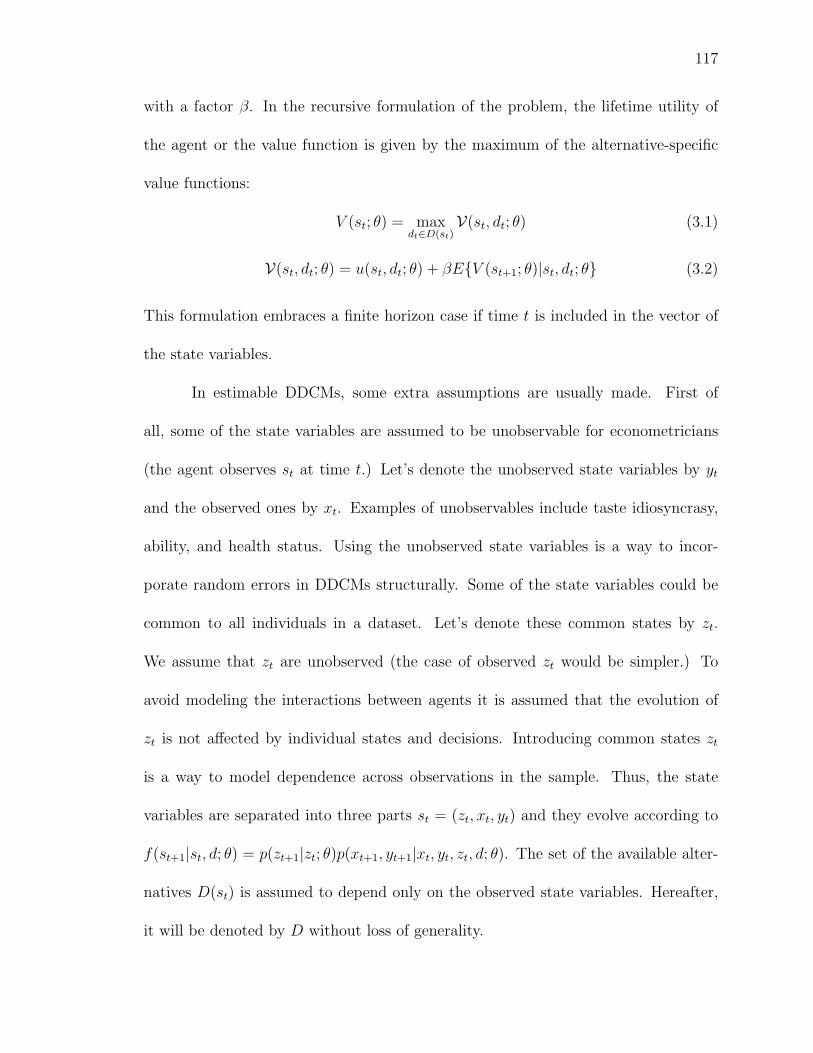
117

with a factor β. In the recursive formulation of the problem, the lifetime utility of

the agent or the value function is given by the maximum of the alternative-specific

value functions:

V (st; θ) = maxdt∈D(st)

V(st, dt; θ) (3.1)

V(st, dt; θ) = u(st, dt; θ) + βEV (st+1; θ)|st, dt; θ (3.2)

This formulation embraces a finite horizon case if time t is included in the vector of

the state variables.

In estimable DDCMs, some extra assumptions are usually made. First of

all, some of the state variables are assumed to be unobservable for econometricians

(the agent observes st at time t.) Let’s denote the unobserved state variables by yt

and the observed ones by xt. Examples of unobservables include taste idiosyncrasy,

ability, and health status. Using the unobserved state variables is a way to incor-

porate random errors in DDCMs structurally. Some of the state variables could be

common to all individuals in a dataset. Let’s denote these common states by zt.

We assume that zt are unobserved (the case of observed zt would be simpler.) To

avoid modeling the interactions between agents it is assumed that the evolution of

zt is not affected by individual states and decisions. Introducing common states zt

is a way to model dependence across observations in the sample. Thus, the state

variables are separated into three parts st = (zt, xt, yt) and they evolve according to

f(st+1|st, d; θ) = p(zt+1|zt; θ)p(xt+1, yt+1|xt, yt, zt, d; θ). The set of the available alter-

natives D(st) is assumed to depend only on the observed state variables. Hereafter,

it will be denoted by D without loss of generality.

118

There is a consensus in the literature that it is desirable to allow for individual

heterogeneity in panel data models. Examples of individual heterogeneity in DDCMs

include individual specific time discount rates and individual specific intercepts or

coefficients in the per period utility function that would represent taste idiosyncrasies.

To allow for that let’s assume that the parameter vector θ contains individual specific

components θi1 and common components θ2 and the prior p(θi

1|θ2)p(θ2) is specified.

The common parameters θ2 may include components that define p(θ1|θ2) and do not

affect the DP.

A data set that is usually used for the estimation of a dynamic discrete choice

model consists of a panel of I individuals. The observed part of the state and the deci-

sions are known for each individual i ∈ 1, . . . , I for T periods: (x, d) = xt,i, dt,i; t =

1, . . . , T ; i = 1, . . . , I. The likelihood function is given by the integral over the latent

variables:

p(x, d|θ2) =

∫p(x, d, y, θ1, z|θ2)d(y, θ1, z) (3.3)

where y = yt,i; t = 1, . . . , T ; i = 1, . . . , I, z = zt; t = 1, . . . , T, and θ1 = θi1; i =

1, . . . , I. Because of the high dimensionality of the integral computing the likelihood

function is infeasible for richly specified DDCMs.

In a Bayesian framework, the high dimensional integration over the latent

variables can be handled by employing MCMC for exploring the joint posterior dis-

tribution of the latent variables and parameters. As was shown in Chapter 1, it is

119

convenient to use the differences in alternative specific value functions

∆V = ∆Vt,d,i = u(st,i, d; θ)+βE[V (st+1; θ)|st,i, d; θ)]−E[V (st+1; θ)|st,i, d; θ)],∀i, t, d

(3.4)

as the latent variables in the MCMC algorithm instead of a part of yt,i, where d is

a chosen base alternative. Let’s denote the part of yt,i substituted with ∆Vt,i by νt,i

and the remaining part by εt,i; thus yt,i = (νt,i, εt,i). To save space it is assumed below

that p(νt,i|zt, xt,i, εt,i, zt−1, xt−1,i, εt−1,i, dt−1,i; θi) = p(νt,i|zt, xt,i, εt,i; θ

i). However, this

assumption is not necessary.

The joint posterior distribution of the parameters and latent variables will

be proportional to the joint distribution of the data, the parameters and the latent

variables:

p(θ1, θ2, ∆V , ε, z|x, d) ∝ p(d, ∆V , θ1, θ2, ε, z, x)

which in turn can be decomposed into the product of marginals and conditionals:

p(d, ∆V , θ1, θ2, ε, z, x) =T∏

t=1

[I∏

i=1

(p(dt,i|∆Vt,i)p(∆Vt,i|xt,i, εt,i, zt; θ

i1, θ2) (3.5)

·p(xt,i, εt,i|xt−1,i, εt−1,i, zt−1, dt−1,i; θi1, θ2)

)·p(zt|zt−1, θ2)

]·

[I∏

i=1

p(θi1|θ2)

]· p(θ2)

The Gibbs sampler can be used to simulate a Markov chain which would have the sta-

tionary distribution equal to the posterior. The densities of the Gibbs sampler blocks:

p(θi1|∆Vi, θ2, εi, z, di, xi), p(θ2|∆V , ε, z, d, x), p(∆Vt,i|θi

1, θ2, εt,i, zt,i, dt,i, xt,i),

p(εt,i|∆Vt,i, θi1, θ2, εt−1,i, εt+1,i, zt,i, dt,i, xt,i), and p(zt|∆Vt, θ1, θ2, εt, zt+1, zt−1, dt, xt) are

proportional to (3.5). If p(∆Vt,i|θ, xt,i, εt,i, zt) can be quickly computed then (3.5)

(and, thus, the kernels of the densities of the Gibbs sampler blocks) can be quickly

120

computed as well. Therefore, it is possible to use the Metropolis-within-Gibbs algo-

rithm to simulate the chain.

As evident from (3.4), computing the value of the joint density (3.5) will require

computing the differences in expected value functions F (s, d, θ) = E[V (st+1; θ)|s, d; θ)]−

E[V (st+1; θ)|s, d; θ)]. Let F (s, θ) = F (s, d, θ), d ∈ D be a vector of the differences in

expected value functions corresponding to all available alternatives, the same current

state s, and the parameter vector θ. Solving the DP and computing F (s, θi1, θ2) for

each observation i = 1, . . . , I at each MCMC iteration would be infeasible. Instead,

one could approximate F (.) beforehand of the estimation procedure by ANNs. The

following section gives a relevant background on ANNs.

3.3 Feedforward ANN

3.3.1 Definition of feedforward ANN

It is beyond the scope of this chapter to survey the literature on artificial neu-

ral networks and their (potential) applications in economics. For general information,

history, and econometric perspective on ANN the reader is referred to the work by

Kuan and White (1994). Rust (1996) discusses the application of neural networks

to function approximation problems in the context of numerical dynamic program-

ming. Cho and Sargent (1996) consider applications of neural networks in dynamic

economics and game theory.

The purpose of this section is to provide information on artificial neural net-

works relevant to applications in DDCM estimation. The section describes a par-

121

ticular type of artificial neural networks, feedforward networks (FFANN), that are

well suited for function approximation problems. Figure 3.1 shows the structure of a

multi-layer FFANN that transforms the input vector x ∈ Rn into the output vector

y ∈ Rm.

y11

...

...

...

...

y21 yN1

1

. . . . . . . . . . . . . . .

y12 y2

2=f(w22y1) yN22

...

...

y1k-1 y2

k-1 yNk-1k-1

...

...

Inputs

Layer 1

Layer 2

Layer k

Outputs

w11 w12 w1N1

w21 w22 w2N2

wk1 wk2 wkNk

y1=y1k y2=y2

k ym=yNkk

y10=x1 y2

0=x2 yN00=xn

Figure 3.1: Multi-layer feed-forward neural network

The network consists from a number of nodes called neurons. The neurons are

grouped into layers. The outputs of the neurons on the layer i − 1 are used as the

inputs for each neuron on the next layer i. The inputs for the first level are the net-

work inputs x. The outputs of the last layer are the network outputs. The neuron j

on the level i multiplies the inputs yi−1 = (yi−11 , . . . , yi−1

Ni−1) by the connection weights

wij = (wijl , . . . , wij

Ni−1)T and transforms the sum of the weighted inputs into a scalar

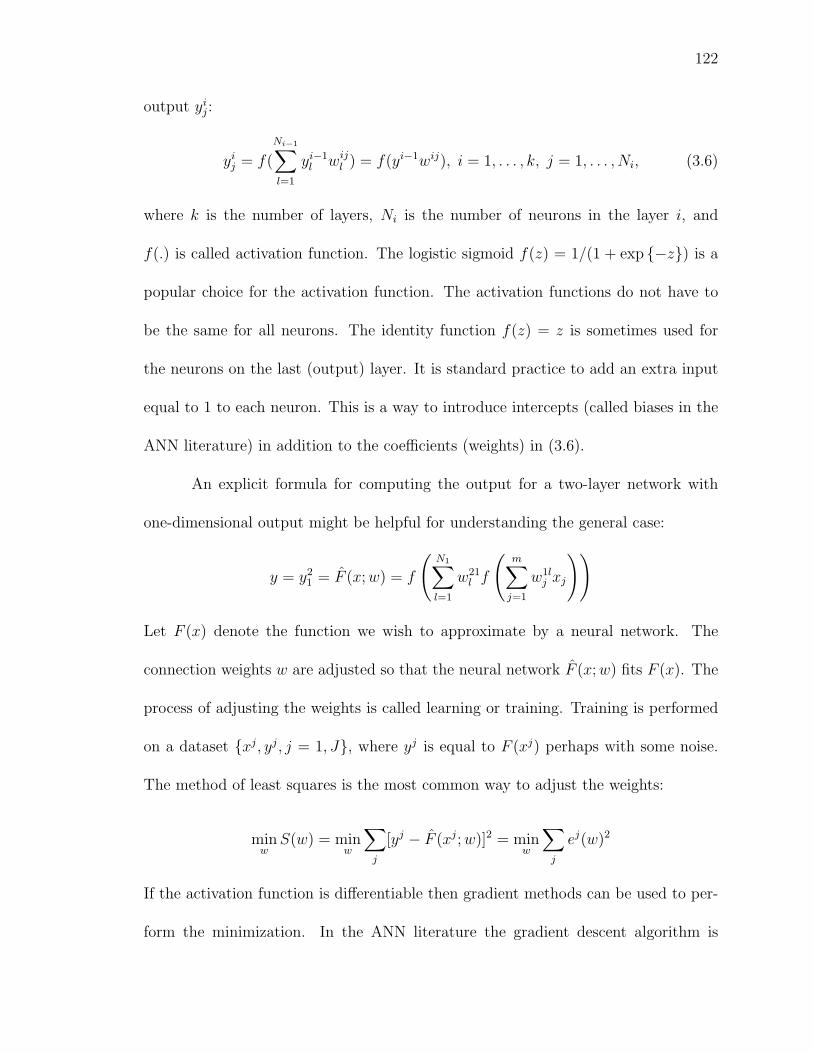
122

output yij:

yij = f(

Ni−1∑l=1

yi−1l wij

l ) = f(yi−1wij), i = 1, . . . , k, j = 1, . . . , Ni, (3.6)

where k is the number of layers, Ni is the number of neurons in the layer i, and

f(.) is called activation function. The logistic sigmoid f(z) = 1/(1 + exp −z) is a

popular choice for the activation function. The activation functions do not have to

be the same for all neurons. The identity function f(z) = z is sometimes used for

the neurons on the last (output) layer. It is standard practice to add an extra input

equal to 1 to each neuron. This is a way to introduce intercepts (called biases in the

ANN literature) in addition to the coefficients (weights) in (3.6).

An explicit formula for computing the output for a two-layer network with

one-dimensional output might be helpful for understanding the general case:

y = y21 = F (x; w) = f

(N1∑l=1

w21l f

(m∑

j=1

w1lj xj

))

Let F (x) denote the function we wish to approximate by a neural network. The

connection weights w are adjusted so that the neural network F (x; w) fits F (x). The

process of adjusting the weights is called learning or training. Training is performed

on a dataset xj, yj, j = 1, J, where yj is equal to F (xj) perhaps with some noise.

The method of least squares is the most common way to adjust the weights:

minw

S(w) = minw

∑j

[yj − F (xj; w)]2 = minw

∑j

ej(w)2

If the activation function is differentiable then gradient methods can be used to per-

form the minimization. In the ANN literature the gradient descent algorithm is

123

referred to as the back error propagation. The derivatives are computed by the

chain rule: S ′(w) = 2e′(w)T e(w). More sophisticated optimization methods, such as

conjugate gradient algorithms and quasi-Newton methods, can be used to increase

the training speed. According to the Matlab manual, the Levenberg-Marquardt al-

gorithm is the fastest method for training moderate-sized FFANN (up to several

hundred weights). My experiments with a few other algorithms (not implemented in

Matlab) confirm this claim. The Levenberg-Marquardt algorithm iteratively updates

the weights according to

wq+1 = wq − [e′(wq)T e′(wq) + µI]−1e′(wq)T e(wq)

If the scalar µ is small then the method works as a quasi-Newton method with the

Hessian approximated by e′(w)T e′(w) (computing actual Hessian would be very time

consuming.) If µ is large then the method works as the gradient descent algorithm

with a small step. The Newton method performs considerably better than the gradient

descent algorithm near the optimum. Thus, after successful iterations (the ones that

decrease S(w)) µ is decreased; otherwise it is increased. For large FFANNs conjugate

gradient methods might perform better than the Levenberg-Marquardt algorithm.

The training methods mentioned above are local optimization methods. There

is no guarantee that they will find the global minimum. The theoretical results on the

consistency of ANN approximations do require finding the global minimum. There-

fore, running training algorithms for several initial values is advisable. In experiments

on approximating the expected value function by a FFANN the Matlab implementa-

tion of the Levenberg-Marquardt algorithm performed very well. No cases of getting

124

stuck in a very bad local minimum were detected.

3.3.2 Consistency of FFANN approximations

The consistency and convergence rates for ANN function approximation were

examined by a number of authors. However, the result we would need for approx-

imation of the DDCM solutions does not seem to be available in the literature in

the ready-to-use form. In this section we deduce the necessary result building on the

existing theory of ANN approximation.

In Section 1.4 I show that the uniform (in sup norm) convergence in proba-

bility of the expected value function approximation would imply the consistency of

the approximated posterior expectations (see Theorem 1.3 and its proof.) It was

also shown that the expected value function is continuous in the state variables and

parameters under suitable continuity and compactness assumptions on the primitives

of DDCMs (see Section 1.3.3.) At the same time the differentiability of the expected

value function with respect to the state variables and parameters does not seem to

have been established for a general DDCM. Therefore, it would be desirable to have

the consistency of the ANN approximations in sup norm for continuous functions on

compact spaces. However, the consistency results in the ANN literature are avail-

able for convergence in Lp norm and/or for smooth functions (White (1990), Barron

(1994), and Chen and White (1999).)

Following White (1990) let’s consider a FFANN sieve estimator. For a survey

of sieve estimation see Chen (2005). Let F denote a set of continuous functions on a

125

compact space X with sup norm ||.||. Let (X, Y ) be random variables defined on a

complete probability space. Assume that X has a positive density on X , E(Y |X =

x) = F (x), and F ∈ F . Let xj, yjnj=1 denote an i.i.d. sample of (X, Y ). The

consistency results are proven below for randomly generated xjnj=1. Experiments

show that using low discrepancy sequences on X instead of randomly generated ones

does not improve the approximation quality.

A FFANN with one hidden layer consisting of q neurons and a linear activation

function for the neuron on the output layer is described by

F (x; w, q) = w210 +

q∑k=1

w21k f

(w1k

0 +∑

j

w1kj xj

)

Let

T (q, ∆) = F (.; w, q) :

q∑k=0

|w21k | < ∆ and

q∑k=1

∑j

|w1kj | < q∆

be a set of FFANNs with q neurons on the hidden layer and the weights satisfying a

restriction on their sum norm. For specified sequences qn and ∆n, T (qn, ∆n) is

called a sieve. The sieve estimator Fn(.) is defined as the solution to the least squares

problem:

minF∈T (qn,∆n)

1

n

n∑j=1

[yj − F (xj)]2 (3.7)

The parameters qn and ∆n determine the flexibility of approximating functions F ∈

T (qn, ∆n). As they increase to infinity the set T (qn, ∆n) will become dense in F . The

flexibility of approximating functions should depend on the number of observations n

in such a way that overfitting and underfitting are avoided at the same time. Specific

restrictions on qn and ∆n that achieve this are given below. Also, introducing a finite

126

bound on the weights ∆n makes T (qn, ∆n) compact. White (1990) proves a version

of the following theorem for Lp norm. Here, I present a proof for sup norm.

Theorem 3.1. Assume that the activation function f is Lipschitz continuous and it

is a squashing function (f is non-decreasing, limx→−∞ f(x) = 0, limx→+∞ f(x) = 1).

Also assume that qn, ∆n ∞, ∆n = o(n1/4), and ∆4nqn log(∆nqn) = o(n). Under

these conditions there exists a measurable sieve estimator Fn(.) defined by (3.7) and

for any ε > 0

limn→∞

P (||F − Fn|| > ε) = 0

Proof. Theorem 3.1 in Chen (2005) specifies five conditions under which an abstract

extremum sieve estimator will be consistent. Let’s show that these five conditions are

satisfied.

Condition 3.1: E[Y −g(X)]2 is uniquely minimized over g ∈ F at F and E[Y −

F (X)]2 < ∞. This identification condition is satisfied in our case because F (x) ≡

E(Y |X = x) is a minimizer and it is unique since functions in F are continuous and

the density of X is positive on X .

Condition 3.2: the sequence of sieves is increasing (T (qn, ∆n) ⊂ T (qn+1, ∆n+1))

and ∪∞n=1T (qn, ∆n) is dense in F . The denseness of the set of one hidden layer

FFANNs with unconstrained weights ∪∞n=1T (n,∞) in the set of continuous functions

on compacts is proven in Hornik et al. (1989), Theorem 2.4. The condition is satisfied

since ∪∞n=1T (qn, ∆n) = ∪∞n=1T (qn,∞) for qn, ∆n →∞.

Condition 3.3: −E[Y − g(X)]2 is upper semicontinuous in g w.r.t ||.||. The

condition is trivially satisfied since E[Y − g(X)]2 is continuous.

127

Condition 3.4: T (qn, ∆n) is compact under ||.||. Since any element in T (qn, ∆n)

is defined by a vector of weights belonging to a compact set and the activation function

f is continuous, any sequence in T (qn, ∆n) will have a convergent subsequence with

the limit in T (qn, ∆n), thus T (qn, ∆n) is compact.

Condition 3.5: (uniform convergence over sieves) plimn→∞ supg∈T (qn,∆n) | 1n∑n

j=1[yj−

g(xj)]2 − E[Y − g(X)]2| = 0. This condition is proven in White (1990), pp.543-544.

That is where the Lipschitz continuity of f and the specific conditions on qn and ∆n

are used.

3.4 Experiments

Experiments in this section demonstrate how well FFANNs can approximate

expected value functions and what the performance gains of using FFANNs in MCMC

estimation of DDCMs can be. The Rust (1987) model of optimal bus engine replace-

ment is used for experiments.

3.4.1 Evaluating approximation quality

The posterior simulator for Rust’s model described in Section 1.5.2.3 requires

computing the differences in expected value functions F (xt,i, εmt,i, θ

m) defined in (1.5.2.3)

for each parameter draw θm and each observation (i, t) in the sample. This section

shows how FFANNs can be used for approximating F (.). A FFANN is trained and

validated beforehand of the estimation procedure on a set of inputs and outputs. The

inputs include parameters and states: xji, εj, αj1, α

j2, ρ

j, ηj1, η

j2, η

j3; i = 1, . . . , 90; j =

1, . . . , 2200. In the experiments described below, the inputs are generated from

128

the following distributions: αj1 ∼ U [−.006, 0], αj

2 ∼ U [−25,−5], ρj ∼ U [0, .99],

εj ∼ U [−3.8, 3.8], η ∼ Dirichlet(34, 64, 2), and xji = i. For large and complicated

models, more involved inputs could be used, e.g., some functions of states and pa-

rameters and the value functions for the DP in which shocks are replaced by zeros.

The latter could also be subtracted from the difference in expected value function to

obtain a better behaved output. Since the exact DP solution is not available for the

model with serially correlated unobservables the following approximations are used

as etalon outputs. For each θj the DP is solved on N = 100 different random grids.

Each grid consists of N = 100 randomly generated points on the space for ν and ε.

The differences in the expected value functions is computed for each random grid.

The average over the grids, denoted by F ji

N ,N, is used as the output. This procedure

efficiently produces good approximations of F (.). Let’s illustrate this for the model

with extreme value iid unobservables εt and νt.

Under the extreme value iid assumption, the integration over the unobserv-

ables can be performed analytically (see Rust (1994),) the exact DP solution can be

quickly computed, and solutions on the random grids can be compared with the exact

solution. Figure 3.2 shows densities of the difference between the exact solution and

the solution on random grids [F (xji, θj)− F ji

N ,N] (for iid unobservables F (.) does not

depend on ε.) The densities were estimated by kernel smoothing.

The precision of the DP solution obtained by averaging the results over 100

random grids with 100 points in each grid is about the same as for the solution ob-

tained on one random grid with 10000 points. However, the former algorithm works

129

about 100 times faster since the number of operations performed for one Bellman

equation iteration is roughly proportional to the square of the number of points in

the grid. See Section 1.5.1.4 of Chapter 1 for further discussion of this issue. The

maximal approximation error for F ji100,100 does not exceed 3% of the standard devia-

tion of the iid shocks in the model.

Figure 3.2: Densities of the difference between the exact solution and the solution onrandom grids. The model with extreme value iid unobservables. The dashed line -the density of [F (xji, θj)−F ji

1,100], the dotted line - the density of [F (xji, θj)−F ji10,100],

and the solid line - the density of [F (xji, θj)− F ji100,100].

A three layer FFANN was trained in Matlab by the Levenberg-Marquardt al-

gorithm for the data from the model with normal serially correlated unobservables.

The network layers contained 8, 10, and 1 neurons correspondingly (it will be re-

ferred below as the 8-10-1 FFANN.) First 1500 points in the data were used for

training, the remaining data were used for validation. Figure 3.3 shows the distribu-

130

tions of the residuals scaled by the standard deviation of the iid shocks in the model

eji = (F ij100,100− F (xji, εj, θj; w))h0.5

ν for the training and validation parts of the data.

Scaling is performed to facilitate the comparison of the approximation error and the

magnitude of the random shocks in the model. As can be seen from the figure, the

approximation quality for the validation part of the data is the same as for the train-

ing part. This suggest that no overfitting occurred.

Figure 3.3: Densities of residuals eji (the dotted line is for the validation part of thesample.

In addition to the randomly generated validation part of the sample, F ji100,100

were computed for inputs with one component changing over a relevant range and the

other components fixed at (x, ε, α1, α2, ρ, η1, η2, η3) = (55, 0,−.003,−10, .5, .34, .64, .02).

Figure 3.4 shows these F ji100,100 and the corresponding fitted values.

As Figure 3.4 and Figure 3.2 demonstrate, the values F ji100,100 used for neural

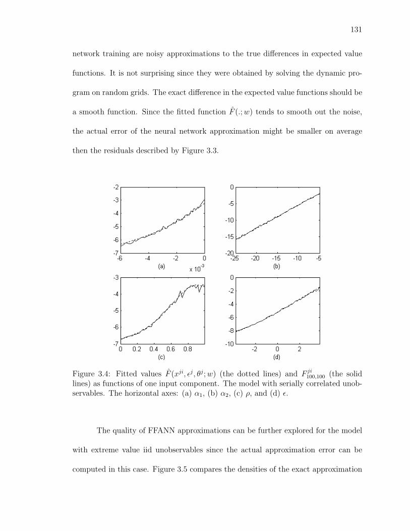
131

network training are noisy approximations to the true differences in expected value

functions. It is not surprising since they were obtained by solving the dynamic pro-

gram on random grids. The exact difference in the expected value functions should be

a smooth function. Since the fitted function F (.; w) tends to smooth out the noise,

the actual error of the neural network approximation might be smaller on average

then the residuals described by Figure 3.3.

Figure 3.4: Fitted values F (xji, εj, θj; w) (the dotted lines) and F ji100,100 (the solid

lines) as functions of one input component. The model with serially correlated unob-servables. The horizontal axes: (a) α1, (b) α2, (c) ρ, and (d) ε.

The quality of FFANN approximations can be further explored for the model

with extreme value iid unobservables since the actual approximation error can be

computed in this case. Figure 3.5 compares the densities of the exact approximation

132

error for FFANNs and DP solutions on random grids.

In this particular example, the noise in the training data does not affect the

FFANN approximation quality as evidenced by similar results for FFANNs trained

on exact and noisy data.

Figure 3.5: Densities of the approximation error for FFANNs and DP solutions onrandom grids. The model with extreme value iid unobservables. The dashed line - fora FFANN trained on exact data, the dotted line - for a FFANN trained on F ji

100,100,

the solid line - for F ji100,100.

Figure 3.6 compares the FFANN and random grid DP solution approximations

for the model with serially correlated unobservables. Unfortunately, the exact DP so-

lution and, thus, the exact approximation errors are not available for this model.

Therefore, the figure shows the densities of the scaled residuals eji = (F ji100,100 −

F (xji, εj, θj; w))h0.5ν for an 8-10-1 FFANN and the scaled differences [F ji

100,100−F ji10,100]h

0.5ν .

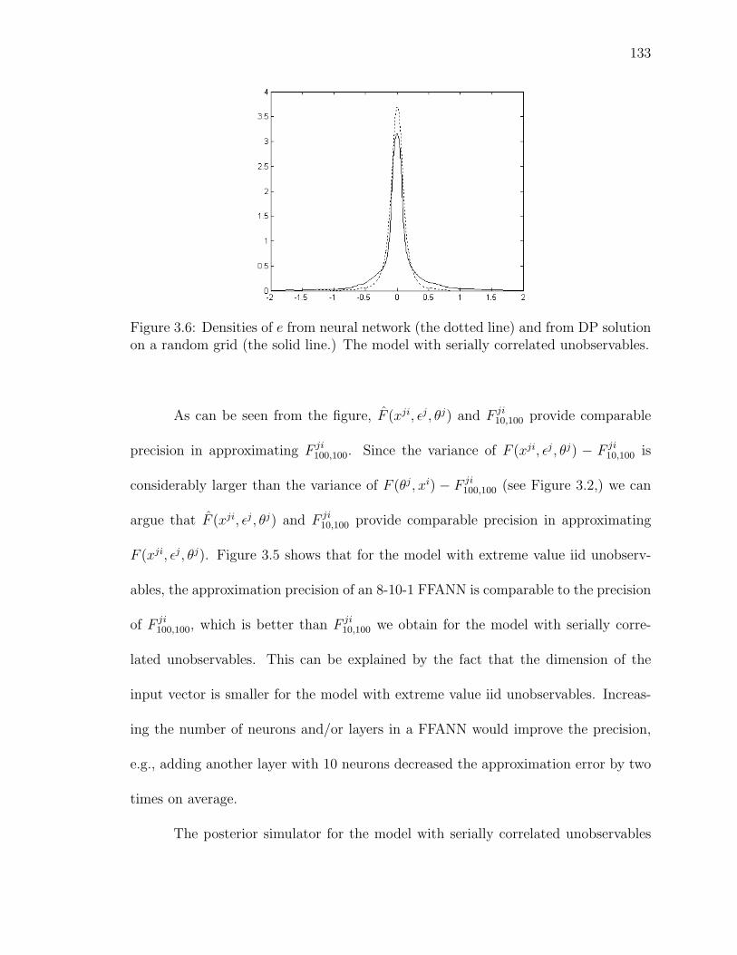
133

Figure 3.6: Densities of e from neural network (the dotted line) and from DP solutionon a random grid (the solid line.) The model with serially correlated unobservables.

As can be seen from the figure, F (xji, εj, θj) and F ji10,100 provide comparable

precision in approximating F ji100,100. Since the variance of F (xji, εj, θj) − F ji

10,100 is

considerably larger than the variance of F (θj, xi) − F ji100,100 (see Figure 3.2,) we can

argue that F (xji, εj, θj) and F ji10,100 provide comparable precision in approximating

F (xji, εj, θj). Figure 3.5 shows that for the model with extreme value iid unobserv-

ables, the approximation precision of an 8-10-1 FFANN is comparable to the precision

of F ji100,100, which is better than F ji

10,100 we obtain for the model with serially corre-

lated unobservables. This can be explained by the fact that the dimension of the

input vector is smaller for the model with extreme value iid unobservables. Increas-

ing the number of neurons and/or layers in a FFANN would improve the precision,

e.g., adding another layer with 10 neurons decreased the approximation error by two

times on average.

The posterior simulator for the model with serially correlated unobservables

134

that uses the 8-10-1 FFANN works 4-5 times faster than the posterior simulator that

uses DP solutions on one random grid with 100 points. Averaging DP solutions over

10 random grids (which would provide precision comparable to the 8-10-1 FFANN as

we argued above) will increase the execution time by 10 times. Thus, for this partic-

ular example, the performance gains from using FFANNs in the posterior simulator

could amount to about 40-50 times. In experiments, the MCMC estimation algorithm

required at least 1 million draws to converge. The time required for preparing FFANN

training data is less than 2% of the time required for solving the DP on 10 random

grids for 1 million parameter draws. The time required for training an 8-10-1 FFANN

is also of similar magnitude. Thus the overall time saving from using FFANN approx-

imations in DDCM estimation seems considerable. This claim is confirmed by the

performance comparison for the model with extreme value iid unobservables, which

is presented with the estimation results in the next section.

3.4.2 Estimation results

This section presents estimation results for the model with extreme value iid

unobservables. The advantage of using this model relative to the model with serially

correlated unobservables is that we can characterize the true posterior distributions

of parameters with a high precision. The integration over the unobservables in solv-

ing the DP and in the likelihood function can be performed analytically. Thus it

would be easier to evaluate the quality of the posterior simulator that uses FFANNs.

The posterior simulator for this model also uses the Metropolis-Hastings algorithm

135

since the logit-like choice probabilities comprising the likelihood function contain the

expected value functions that do not have an analytical representation.

Figure 3.7 shows the estimated posterior densities for the simulators that use

the exact DP solutions and the 8-10-1 FFANN approximations. The experiments

use an artificial dataset consisting of observations on I = 70 buses (about 4000

mileage/decision points.) The posterior densities were estimated by kernel smoothing

over several simulator runs. The length of the runs was 3 million draws. The simulator

using the 8-10-1 FFANN takes about 1.2 second to produce 1000 draws from the

posterior on a 2002 vintage PC. The simulator that uses the exact DP solutions works

10 times slower. The estimated densities from both simulators are very similar.

The model with extreme value iid unobservables could also be estimated by

the algorithm that performs integration numerically as in the case of the model with

serially correlated unobservables. The Gibbs sampler for this algorithm is the same

as the one for the Gaussian unobservables described in Section 1.5.2.3; except here

the Gaussian probability densities are replaced by the densities for the extreme value

distribution. Figure 3.8 compares the estimation results for the exact posterior simu-

lator and the simulator that integrates unobservables numerically and solves the DP

on a random grid with 100 points. The posteriors for η are not shown in the fig-

ure since they are identical for all simulators. For some random grids the estimated

density can be far off as the figure demonstrates. The simulator that integrates un-

observables numerically and solves the DP on a random grid with 100 points produce

1000 parameter draws in 102 seconds. The same task takes 14 seconds for the same

136

simulator if it uses an 8-10-1 FFANN instead of DP solutions on a random grid. As

Figure 3.5 from the previous section demonstrates, the approximation precision of an

8-10-1 FFANN is comparable to the average over 100 DP solutions on random grids

Figure 3.7: Estimated posterior densities: (a) α1, (b) α2, (c) η1, (d) η2. The solidlines for the algorithm using the exact DP solutions, the dashed for the algorithmusing the FFANN.

Figure 3.8: Estimated posterior densities: (a) α1, (b) α2. The solid lines - thesimulator using the exact DP solutions, the other lines - the simulators using DPsolutions on different random grids.

with 100 points. If the simulator uses averages of the DP solutions over several

137

random grids the computing time will increase proportionally to the number of the

random grids used. Thus, the performance gains from using FFANNs in this exam-

ple can reach 729 = (102 · 100/14) times. Similar estimation experiments in Section

1.5.2.7 of Chapter 1 suggest that averaging the posterior distributions estimated with

the DP solved on different random grids improves estimation precision. Nevertheless,

this posterior averaging strategy does not have a rigorous theoretical justification and

it is still considerably outperformed by a simulator using FFANNs.

In summary, the experiments suggest that application of ANNs in the MCMC

estimation of DDCMs is indeed a promising approach. It is fast and precise. It can

also provide a feasible way to estimate rich DDCMs with different forms of individ-

ual heterogeneity, e.g., serially correlated unobserved state variables and individual

specific parameters.

138

REFERENCES

Barron, A. Approximation and estimation bounds for artificial neural networks.Machine Learning, 14, 1994.

Bierens, H. Topics in Advanced Econometrics. Cambridge University Press, 1994.

Chen, X. Large sample sieve estimation of semi-nonparametric models, 2005.

Chen, X. and White, H. Improved rates and asymptotic normality for nonparametricneural network estimators. IEEE Transactions on Information Theory, (45), 1999.

Cho, I.-K. and Sargent, T. Neural networks for encoding and adapting in dynamiceconomies. In H. Amman, D. K. and Rust, J., editors, Handbook of ComputationalEconomics. North Holland, 1996.

Cho, S.-J. An empirical model of mainframe computer replacement, 2000.

Choo, E. Rational addiction and rational cessation: A dynamic structural model ofcigarette consumption, 2000.

Das, M. A micro-econometric model of capital utilization and retirement: The caseof the cement industry. Review of Economic Studies, 59:277–297, 1992.

Davis, M. A. The Health and Financial Decisions of the Elderly. Ph.D. thesis,University of Pennsylvania, 1998.

Eckstein, Z. and Wolpin, K. The specification and estimation of dynamic stochasticdiscrete choice models: A survey. Journal of Human Resources, 24(58):562–598,1989.

Erdem, T. and Keane, M. Decision-making under uncertainty: Capturing dynamicbrand choice processes in turbulent consumer goods markets. Marketing Science,15(1):1–20, 1996.

French, E. The effects of health, wealth, and wages on labour supply and retirementbehaviour. Review of Economic Studies, 72:395–427, 2005.

Geweke, J. Efficient simulation from the multivariate normal and student-t distri-butions subject to linear constraints and the evaluation of constraint probabilities,1991.

Geweke, J. Getting it right: Joint distribution tests of posterior simulators. Journalof the American Statsitical Association, 99:799–804, 2004.

Geweke, J. Contemporary Bayesian Econometrics and Statistics. Wiley-Interscience,2005.

139

Geweke, J., Keane, M., and Runkle, D. Alternative computational approaches toinference in the multinomial probit model. The review of economics and statistics,76(4):609–632, 1994.

Gilleskie, D. A dynamic stochastic model of medical care use and work absence.Econometrica, 6(1):1–45, 1998.

Hoeffding, W. Probability inequalities for sums of bounded random variables. Journalof the American Statistical Association, (58):13–30, 1963.

Hornik, K., Stinchcombe, M., and White, H. Multilayer feedforward networks areuniversal approximators. Neural Networks, (2):359–366, 1989.

Hotz, J. and Miller, R. Conditional choice probabilities and the estimation of dynamicmodels. Re-view of Economic Studies, 60(3):497–530, 1993.

Hsu, P. L. and Robbins, H. Complete convergence and the law of large numbers. InProc. Natl. Acad. Sci., February, 33(2), pages 25–31. USA, 1947.

Imai, S., Jain, N., and Ching, A. Bayesian estimation of dynamic discrete choicemodels, 2005.

Imai, S. and Krishna, K. Employment, deterrence, and crime in a dynamic model.International Economic Review, 45(3):845–872, 2004.

Keane, M. and Wolpin, K. The solution and estimation of discrete choice dynamicprogramming models by simulation and interpolation: Monte carlo evidence. Re-view of Economics and Statistics, 76(4):648–672, 1994.

Keane, M. and Wolpin, K. The career decisions of young men. Journal of PoliticalEconomy, 1997.

Kennet, M. A structural model of aircraft engine maintenance. Journal of AppliedEconometrics, 9:351–368, 1994.

Kuan, C.-M. and White, H. Artificial neural networks: An econometric perspective.Econometric Reviews, (13):1–92, 1994.

McCulloch, R. and Rossi, P. An exact likelihood analysis of the multinomial probitmodel. Journal of Econometrics, 64(1-2):207–240, 1994.

Miller, R. Job matching and occupational choice. Journal of Political Economy,(92):1086–1120, 1984.

Osborne, M. Consumer learning, habit formation, and heterogeneity: A structuralexamination, 2006.

Pakes, A. Patents as options: Some estimates of the value of holding european patentstocks. Econometrica, 54(4):755–84, 1986.

140

Rust, J. Optimal replacement of gmc bus engines: an empirical model of haroldzurcher. Econometrica, 55(5):999–1033, 1987.

Rust, J. Structural estimation of markov decision processes. In Engle, R. and Mc-Fadden, D., editors, Handbook of Econometrics. North Holland, 1994.

Rust, J. Numerical dynamic programming in economics. In H. Amman, D. K. andRust, J., editors, Handbook of Computational Economics. North Holland, Availableonline at http://gemini.econ.umd.edu/jrust/sdp/ndp.pdf, 1996.

Rust, J. Using randomization to break the curse of dimensionality. Econometrica,65(3):487–516, 1997.

Rust, J. and Phelan, C. How social security and medicare affect retirement behaviorin a world of incomplete markets. Econometrica, 65(4):781–831, 1997.

Scott, D. Multivariate Density Estimation. Wiley-Interscience, 1992.

Stock, J. and Wise, D. The pension inducement to retire: An option value analysis.NBER Working Papers, (2660), 1990.

Stokey, N. and Lucas, R. Recursive Methods in Economic Dynamics. Harvard Uni-versity Press, 1989. With Edward Prescott.

Tierney, L. Markov chains for exploring posterior distributions. The Annals of Statis-tics, Vol. 22, No. 4, 1758-1762, 22(4):1758–1762, 1994.

White, H. Connectionist nonparametric regression: Multilayer feedforward networkscan learn arbitrary mappings. Neural Networks, (3):535–549, 1990.

Wolpin, K. An estimable dynamic stochastic model of fertility and child mortality.Journal of Political Economy, 1984.

Wolpin, K. Estimating a structural search model: The transition from school to work.Econometrica, 1987.

University of Iowa Bayesian inference in dynamic discrete choice models

Documents

Transcript of University of Iowa Bayesian inference in dynamic discrete choice models