
Universidad Católica de Santa María Facultad de Ciencias e ...
620
Universidad Católica de Santa María Facultad de Ciencias e Ingenierías Físicas y Formales Escuela Profesional de Ingeniería Mecánica, Mecánica Eléctrica y Mecatrónica “ANÁLISIS MEDIANTE ELEMENTOS DISCRETOS (MED) Y EVALUACIÓN EXPERIMENTAL BAJO LA NORMA ASTM G-99 DEL DESGASTE EN REVESTIMIENTOS DUROS APLICADOS POR PROCESOS DE SOLDADURA EN UÑAS DE ACERO 32MnCrMo6-4-3 DE UNA EXCAVADORA HIDRÁULICA CAT 336D2 L” Tesis presentada por el Bachiller: Purca Justo, Ruben Rodrigo Para optar el Título Profesional de: Ingeniero Mecánico Asesor: Ing. Chire Ramirez, Emilio AREQUIPA-PERÚ 2019
-
Upload
khangminh22 -
Category
Documents
-
view
0 -
download
0
Transcript of Universidad Católica de Santa María Facultad de Ciencias e ...

Universidad Católica de Santa María
Facultad de Ciencias e Ingenierías Físicas y Formales
Escuela Profesional de Ingeniería Mecánica, Mecánica Eléctrica
y Mecatrónica
“ANÁLISIS MEDIANTE ELEMENTOS DISCRETOS (MED) Y EVALUACIÓN
EXPERIMENTAL BAJO LA NORMA ASTM G-99 DEL DESGASTE EN
REVESTIMIENTOS DUROS APLICADOS POR PROCESOS DE SOLDADURA
EN UÑAS DE ACERO 32MnCrMo6-4-3 DE UNA EXCAVADORA
HIDRÁULICA CAT 336D2 L”
Tesis presentada por el Bachiller:
Purca Justo, Ruben Rodrigo
Para optar el Título Profesional de:
Ingeniero Mecánico
Asesor:
Ing. Chire Ramirez, Emilio
AREQUIPA-PERÚ
2019

ii
"Hay una fuerza motriz más poderosa que el vapor, la electricidad y la energía atómica:
La voluntad” - Albert Einstein.
El presente trabajo se lo dedico principalmente a Dios por ser mi guía y acompañarme en el
transcurso de mi vida, brindándome sabiduría y fuerza para continuar en este proceso de obtener
uno de los anhelos más deseados.
A mis padres: Benigno y Agripina, por ser los principales promotores de mis sueños, por confiar
y creer en mis expectativas, por los consejos, valores y principios que me han inculcado. Por ser
mi pilar fundamental y haberme apoyado incondicionalmente, pese a las adversidades e
inconvenientes que se presentaron.
A todas las personas que ayudaron en la realización de esta investigación, en especial a Christian,
David, Laura y Milagros, que siempre estuvieron dispuestos a brindarme todo su apoyo para
alcanzar los objetivos trazados.
A los Ingenieros Manuel Donayre, Emilio Chire y Sergio Mestas, por su valiosa orientación y
apoyo a la conclusión de esta investigación.
A la Universidad Católica de Santa María por ser la sede de todo el conocimiento adquirido en
estos años.
iii
ÍNDICE
RESUMEN ..................................................................................................................................................xv
ABSTRACT ................................................................................................................................................ xvi
CAPÍTULO I ............................................................................................................................................... 1
1. FUNDAMENTACIÓN DEL PROYECTO .............................................................................. 2
1.1. Descripción del Problema ............................................................................................................. 2
1.2. Justificación .................................................................................................................................. 3
1.3. Delimitación del Proyecto ............................................................................................................. 4
1.4.2. Específicos .................................................................................................................................... 5
CAPÍTULO II ............................................................................................................................................. 7
2. MARCO TEÓRICO ................................................................................................................... 8
2.1. Aceros ........................................................................................................................................... 8
2.2. Efectos de los elementos de aleación .......................................................................................... 10
2.3. Aceros utilizados en elementos de desgaste................................................................................ 11
2.4. Tribología .................................................................................................................................... 13
2.5. Desgaste ...................................................................................................................................... 17
2.6. Contexto operacional .................................................................................................................. 26
2.7. Hardfacing ................................................................................................................................... 31
2.8. Ensayos ....................................................................................................................................... 47
2.9. Descripción de la Excavadora Hidráulica CAT 336D2L ............................................................ 65
2.10. Elementos discretos (EDEM) ...................................................................................................... 72
CAPÍTULO III .......................................................................................................................................... 75
3. INGENIERÍA DE PROYECTO .............................................................................................. 76
3.1. Análisis mediante elementos discretos al desgaste de las uñas 32MnCrMo6-4-3 y sus
Revestimientos aplicados mediante Elementos Discretos. ......................................................................... 76
3.2. Evaluación experimental. ............................................................................................................ 96
3.2.1. Fabricación de las probetas ....................................................................................................... 100
3.2.2. Selección del metal base y el material de aporte probetas y elaboración de procedimiento de
soldadura. .................................................................................................................................................. 106
3.2.3. Análisis Químico - Composición Química ............................................................................... 128
3.2.4. Análisis Metalográfico .............................................................................................................. 131
3.2.5. Ensayo de dureza ...................................................................................................................... 135

iv
3.2.6. Ensayo de Tracción ................................................................................................................... 136
3.2.7. Ensayo de desgaste ................................................................................................................... 139
CAPÍTULO IV ........................................................................................................................................ 146
4. RESULTADOS Y DISCUSIÓN ............................................................................................ 147
4.1. Análisis de composición química ............................................................................................. 147
4.2. Análisis metalográfico .............................................................................................................. 152
4.3. Ensayo de dureza ...................................................................................................................... 171
4.4. Ensayo de tracción .................................................................................................................... 178
4.5. Ensayo de desgaste ................................................................................................................... 193
4.6. Análisis de Desgaste mediante Software EDEM ...................................................................... 208
CAPÍTULO V.......................................................................................................................................... 217
5. EVALUACIÓN ECÓNOMICA............................................................................................. 218
5.1. Análisis de costo ....................................................................................................................... 218
5.2. Impacto económico por parada ................................................................................................. 222
CONCLUSIONES................................................................................................................................... 223
RECOMENDACIONES ......................................................................................................................... 225
REFERENCIAS ...................................................................................................................................... 226

v
Índice de Tablas
Tabla 2-1 - Efectos de elementos de aleación [2] ....................................................................................... 11
Tabla 3-1 - Tasa de desgaste ensayos de desgaste [1] ................................................................................ 92
Tabla 3-2 - Medidas de la probeta de desgaste según la norma ASTM G65-16 [23] ............................... 100
Tabla 3-3 - Medidas de la probeta de tracción según la norma ASTM A370 – 18 [16] ........................... 103
Tabla 3-4 - Medidas de la probeta según la norma ASTM G99-17 [17] .................................................. 106
Tabla 3-5 - Material Saarstahl - 32MnCrMo6-4-3 [22] ............................................................................ 106
Tabla 3-6 - Saarstahl - 32MnCrMo6-4-3 - Composición química [22] .................................................... 107
Tabla 3-7 - Conformado en caliente y tratamiento térmico [22] .............................................................. 107
Tabla 3-8 - Propiedades mecánicas del acero 32MnCrMo6-4-3 [22] ....................................................... 107
Tabla 3-9 - Clasificación de electrodo Citodur 1000 [10] ........................................................................ 108
Tabla 3-10 - Análisis Químico Citodur 1000 [10] .................................................................................... 108
Tabla 3-11 - Propiedades Mecánicas Citodur 1000 [10] .......................................................................... 109
Tabla 3-12 - Clasificación de electrodo Citomangan [10] ........................................................................ 109
Tabla 3-13 - Análisis Químico Citomangan [10] ...................................................................................... 109
Tabla 3-14 - Propiedades Mecánicas Citomangan [10] ............................................................................ 109
Tabla 3-15 - Clasificación de electrodo Exadur – 43 [10] ........................................................................ 110
Tabla 3-16 - Análisis Químico Exadur – 43 [10] ...................................................................................... 110
Tabla 3-17 - Propiedades Mecánicas Exadur – 43 [10] ............................................................................ 110
Tabla 3-18 - Especificación del procedimiento de soldadura (Desgaste - Citodur 1000) [1] ................... 112
Tabla 3-19 - Especificación del procedimiento de soldadura (Desgaste -Citomangan) [1] ...................... 113
Tabla 3-20 - Especificación del procedimiento de soldadura (Desgaste - Exadur 43) [1] ........................ 114
Tabla 3-21 - Especificación del procedimiento de soldadura (Tracción - Citodur 1000) [1] ................... 116
Tabla 3-22 - Especificación del procedimiento de soldadura (Tracción - Citomangan) [1] ..................... 117
Tabla 3-23 - Especificación del procedimiento de soldadura (Tracción – Exadur-43) [1] ....................... 118
Tabla 3-24 - Parámetro de soldeo Recomendado – Citodur 1000 [10] ..................................................... 118
Tabla 3-25 - Parámetro de soldeo Recomendado – Citomangan [10] ...................................................... 119
Tabla 3-26 - Parámetro de soldeo Recomendado – Exadur 43 [10] ......................................................... 120
Tabla 3-27 - Preparación método 2 para materiales duros ≥ 45 (450 HV) [24] ....................................... 131
Tabla 3-28 - Reactivos utilizados para la metalografía [25] ..................................................................... 133
Tabla 3-29 - Valores obtenidos de las muestras de tracción [1] ............................................................... 137
Tabla 3-30 - Variables de ensayo de desgaste [1] ..................................................................................... 140
Tabla 4-1 - Resumen de Resultados de Micrografías [1] .......................................................................... 152
Tabla 4-2 - Resultados de Barrido de dureza [1] ...................................................................................... 171
Tabla 4-3 - Barrido de dureza probeta sin Recargue [1] ........................................................................... 172
Tabla 4-4 - Barrido de dureza probeta con Recargue C-1000. [1] ............................................................ 172
Tabla 4-5 - Barrido de dureza probeta con Recargue CITOMANGAN [1] .............................................. 173
Tabla 4-6 - Barrido de dureza probeta con Recargue EXADUR – 43 [1] ................................................ 173
Tabla 4-7 - Datos iniciales probetas de tracción [1] ................................................................................. 191
Tabla 4-8 - Datos finales probetas de tracción [1] .................................................................................... 191
Tabla 4-9 - Datos finales probetas de tracción [1] .................................................................................... 191

vi
Tabla 4-10 - Resultados Fuerza Máxima y Resistencia a la tracción [1] .................................................. 192
Tabla 4-11 - Resultados Modulo de Young y Coeficiente de Poisson [1] ................................................ 192
Tabla 4-12 - Resultados de pesaje inicial y final de probetas de desgaste [1] .......................................... 196
Tabla 4-13 - Resultados de pesaje inicial y final de billas de WC [1] ...................................................... 196
Tabla 4-14 - Resultados de coeficiente de desgaste [1] ............................................................................ 197
Tabla 4-15 - Resultados de coeficiente de desgaste InstrumX – Anton Paar Tribometro [1] ................... 207
Tabla 4-16 - Resultado de desgaste EDEM [1] ......................................................................................... 212
Tabla 4-17 - Frecuencia de cambio de Uñas de Acero 32MnCrMo6-4-3 en Barrick Lagunas Norte [1] . 215
Tabla 4-18 - Frecuencia de cambio de uñas de acero 32MnCrMo6-4-3 [1] ............................................. 216
Tabla 4-19 - Resultado de duración de material [1] .................................................................................. 216
Tabla 5-1 - Costos de electrodos de Recubrimiento [1] ............................................................................ 218
Tabla 5-2 - Costos de electrodos de Recubrimiento [1] ............................................................................ 219
Tabla 5-3 – Costo laboral Soldador [1] ..................................................................................................... 220
Tabla 5-4 - Costos de general de recubrimiento [1] .................................................................................. 220
Tabla 5-5 - Costo de juego de uña de acero 32MnCrMo6-4-3 [1] ............................................................ 220
Tabla 5-6 - Costo de estimación de vida útil [1] ....................................................................................... 220
Tabla 5-7 - Costo total por juego de uñas de acero 32MnCrMo6-4-3 [1] ................................................ 221
Tabla 5-8 - Costo hora x maquina [1] ....................................................................................................... 222
Tabla 5-9 - Costos equipos parados y vida útil de uñas de acero 32MnCrMo6-4-3 [1] ........................... 222
vii
Índice de Figuras
Figura 1-1 - Excavadora Hidráulica Cat 336 D2 L en operación [1] ............................................................ 4
Figura 1-2 - Zona de trabajo Alexa Sur [1] ................................................................................................... 4
Figura 2-1 - Efecto de los elementos de aleación sobre la dureza de la martensita templada para 1 h a 482◦C.
[3] ................................................................................................................................................................ 12
Figura 2-2 - Esquema tribológico [4] .......................................................................................................... 14
Figura 2-3 - Diferentes Ensayos de Tribológicos [4] .................................................................................. 15
Figura 2-4 - Tribo – pérdidas económicas [4] ............................................................................................. 15
Figura 2-5 - Pérdidas económicas por Industria [4] .................................................................................... 16
Figura 2-6 - Investigación del desgaste [4] ................................................................................................. 16
Figura 2-7 - Microestructura de desgaste de Material [5] ........................................................................... 18
Figura 2-8 - Partícula abrasiva en movimiento [6] ..................................................................................... 18
Figura 2-9 - Impacto de Metal con roca a baja velocidad [6] ..................................................................... 19
Figura 2-10 - Partícula abrasiva en Hopper [6] ........................................................................................... 20
Figura 2-11 - Partícula abrasiva en movimiento [6] ................................................................................... 20
Figura 2-12 - Desgarro de material con partícula abrasiva [6] ................................................................... 21
Figura 2-13 - Cucharon de excavadora desgarrado con material abrasivo [1] ............................................ 21
Figura 2-14 - Pulsos de tensión repetitivos bajo el desgaste por impacto [7] ............................................. 22
Figura 2-15 - Desgaste por impacto en un cincel [6] .................................................................................. 23
Figura 2-16 - Posibles mecanismos de erosión; a) abrasión en ángulos de bajo impacto, b) fatiga superficial
durante un impacto de baja velocidad y alto ángulo de impacto, c) fractura frágil o deformación plástica
múltiple, d) fusión de superficie a altas velocidades de impacto, e) erosión macroscópica con efectos
secundarios [7] ............................................................................................................................................ 24
Figura 2-17 - Desgaste producto de la fricción no lubricada entre piezas metálicas [6] ............................ 25
Figura 2-18 - Ubicación y accesibilidad Mina Lagunas Norte [8] .............................................................. 26
Figura 2-19 - Ubicación y accesibilidad Mina Lagunas Norte [8] .............................................................. 27
Figura 2-20 - Clasificación de materiales para polígonos y estacas de campo [8] ..................................... 27
Figura 2-21 - Mineral M2-M2A [8] ............................................................................................................ 28
Figura 2-22 - Mineral M3 [8] ...................................................................................................................... 28
Figura 2-23 - Muestras superficiales [9] ..................................................................................................... 29
Figura 2-24 - Resultados de módulo de elasticidad [9] ............................................................................... 30
Figura 2-25 - Resultados de coeficiente de Poissson [9] ............................................................................ 30
Figura 2-26 - Resultados a la resistencia a la compresión [9] ..................................................................... 30
Figura 2-27 - Resultados de ensayo de abrasión [9] ................................................................................... 31
Figura 2-28 - Resultados de ensayo de abrasión [9] ................................................................................... 31
Figura 2-29 - Composición quimica de electrodos de revestimientos [11]................................................. 36
Figura 2-30 - Microestructura de Martensita (x100) [10] ........................................................................... 42
Figura 2-31 - Microestructura de Austenita [10] ........................................................................................ 43
Figura 2-32 - Fotomicrografía Carburos en Red [10] ................................................................................. 44
Figura 2-33 - Fotomicrografía carburos dispersos [10] .............................................................................. 44
Figura 2-34 - Recargue de soldadura en uña de excavadora hidráulica [6] ................................................ 45
viii
Figura 2-35 - Recalce de cantonera de tractor Cat - D8T [6] ...................................................................... 45
Figura 2-36 - Recargue de soldadura en hoja de cucharon de cargador frontal de bajo perfil - Scoop Cat
1300G [1] .................................................................................................................................................... 46
Figura 2-37 - Reforzamiento de nariz de adaptador de una pala hidráulica Cat - 6060S [1] ...................... 46
Figura 2-38 - Cortadora metalográfica [13] ................................................................................................ 47
Figura 2-39 - Incluidora metalográfica [13] ............................................................................................... 48
Figura 2-40 - Pulidora metalográfica [13] .................................................................................................. 49
Figura 2-41 - Penetradores para las pruebas de dureza Brinell y Rockwell [14] ........................................ 51
Figura 2-42 - Comparación de durezas [14] ............................................................................................... 53
Figura 2-43 - Se aplica una fuerza unidireccional a una muestra en la prueba de tracción por medio de la
cruceta móvil. El movimiento de la cruceta puede ser realizado con tornillos o un mecanismo hidráulico
[14] .............................................................................................................................................................. 56
Figura 2-44 - Curvas de esfuerzo y deformación para diferentes materiales. Tenga en cuenta que estos son
cualitativos. Las magnitudes de las tensiones y las tensiones no deben ser comparadas [14] .................... 57
Figura 2-45 - Muestras de prueba de tensión rectangular [16] ................................................................... 58
Figura 2-46 - Estándar de 0.500 pulg. (12.5 mm) Muestra de prueba de tensión redonda con 2 pulg. (50
mm) de longitud de calibre y ejemplos de muestras de tamaño pequeño [16] ........................................... 58
Figura 2-47 - Características de las muestras de prueba de desgaste entre laboratorios [17] ..................... 59
Figura 2-48 - Resultados de la prueba Inter laboratorio [17] ...................................................................... 60
Figura 2-49 - Parámetros de prueba utilizados para pruebas Inter laboratorios [17] .................................. 61
Figura 2-50 - Sistema de prueba de desgaste pin-on-disk [17] ................................................................... 62
Figura 2-51 - Excavadora Hidráulica Cat 336D2 L [19] ............................................................................ 66
Figura 2-52 - Especificaciones de la Excavadora Hidráulica 336D2/D2 L [19] ........................................ 66
Figura 2-53 - Especificaciones de la Excavadora Hidráulica 336D2/D2 L [19] ........................................ 67
Figura 2-54 - Partes de la excavadora Hidráulica 336D2/D2 L [1] ............................................................ 68
Figura 2-55 - Cucharon 3.2 yd3 de excavadora hidráulica Cat 336D2 L [20] ............................................ 69
Figura 2-56 - Conjuntos de piezas de cucharon [20] .................................................................................. 70
Figura 2-57 - Uña K-130 (32MnCrMo6-4-3) de excavadora hidráulica Cat 336D2 L [20] ....................... 71
Figura 2-58 - Método continuo [21] ........................................................................................................... 72
Figura 2-59 - Método discreto [21] ............................................................................................................. 73
Figura 2-60 - Simulación DEM-MBD de una cuchara de arrastre (Cortesía de VR Steel), modelo DEM-
CFD de dinámica de flotación de partículas (Cortesía de la Universidad de Utah) y acoplamiento DEM-
FEA utilizado para analizar las cargas de la cuchara del camión volquete (Cortesía de Austin Engineering)
[21] .............................................................................................................................................................. 74
Figura 3-1 - Creación de mineral a simular [1] ........................................................................................... 76
Figura 3-2 - Dimensiones de partícula de mineral [1] ................................................................................ 77
Figura 3-3 - Propiedades de partícula de mineral [1] .................................................................................. 77
Figura 3-4 - Propiedades Material base – 32MnCrMo6-4-3 [1] ................................................................. 78
Figura 3-5 - Propiedades Físicas del Material base – 32MnCrMo6-4-3 [22] ............................................. 79
Figura 3-6 - Resultados ensayo de desgaste – Base 32MnCrMo6-4-3 [1].................................................. 79
Figura 3-7 - Coeficiente de fricción a la roladura [15] ............................................................................... 80
Figura 3-8 - Propiedades Material base – Citomangan [1] ......................................................................... 80
Figura 3-9 - Propiedades Físicas del Material base – 32MnCrMo6-4-3 [22] ............................................. 81
Figura 3-10 - Resultados ensayo de desgaste – Base Citomangan [1] ........................................................ 82
ix
Figura 3-11 - Coeficiente de fricción a la roladura [15] ............................................................................. 82
Figura 3-12 - Propiedades Material base – Exadur 43 [1] .......................................................................... 83
Figura 3-13 - Propiedades Físicas del Material base – 32MnCrMo6-4-3 [22] ........................................... 83
Figura 3-14 - Resultados ensayo de desgaste – Base Exadur 43 [1] ........................................................... 84
Figura 3-15 - Coeficiente de fricción a la roladura [15] ............................................................................. 84
Figura 3-16 - Propiedades Material base – Citodur 1000 [1] ...................................................................... 85
Figura 3-17 - Propiedades Físicas del Material base – 32MnCrMo6-4-3 [22] ........................................... 85
Figura 3-18 - Resultados ensayo de desgaste – Base Exadur 43 [1] ........................................................... 86
Figura 3-19 - Coeficiente de fricción a la roladura [15] ............................................................................. 86
Figura 3-20 - Importación de geometría [1] ................................................................................................ 87
Figura 3-21 - Importación de geometría – uña y adaptador [1] .................................................................. 87
Figura 3-22 - Creación de geometría virtual [1] ......................................................................................... 88
Figura 3-23 - Parámetros de geometría virtual [1] ...................................................................................... 88
Figura 3-24 - Parámetros de fábrica de partículas [1] ................................................................................. 89
Figura 3-25 - Interacción - modelo de contacto de partícula a geometría [1] ............................................. 90
Figura 3-26 - Modelo de contacto [1] ......................................................................................................... 90
Figura 3-27 - Coeficiente de Archard Material Base – EDEM [1] ............................................................. 92
Figura 3-28 - Coeficiente de Archard Citomangan – EDEM [1] ................................................................ 93
Figura 3-29 - Coeficiente de Archard Exadur - 43 – EDEM [1] ................................................................ 93
Figura 3-30 - Coeficiente de Archard Citodur 1000– EDEM [1] ............................................................... 94
Figura 3-31 - Simulador de Edem [1] ......................................................................................................... 94
Figura 3-32 - Analista EDEM [1] ............................................................................................................... 95
Figura 3-33 - Esquema del Procedimiento Experimental [1] ...................................................................... 99
Figura 3-34 - Diagrama esquemático del aparato de prueba [23] ............................................................. 100
Figura 3-35 - Uña de acero 32MnCrMo6-4-3 [1] ..................................................................................... 101
Figura 3-36 - Corte con disco Manual [1] ................................................................................................. 101
Figura 3-37 - Fresado de Probetas de desgate [1] ..................................................................................... 102
Figura 3-38 - Probetas de desgaste de Acero 32MnCrMo6-4-3 culminadas según la norma ASTM G65-16
[1] .............................................................................................................................................................. 102
Figura 3-39 - Muestra de prueba de tensión redonda estándar de 0,500 pulgadas (12,5 mm) con una longitud
de calibre de 2 pulgadas (50 mm) y ejemplos de muestras de tamaño pequeño. Proporcional a las muestras
estándar [16].............................................................................................................................................. 103
Figura 3-40 - Probetas de Tracción de Acero 32MnCrMo6-4-3 listos para la aplicación de soldadura [1]
.................................................................................................................................................................. 104
Figura 3-41 - Torneado de Probetas de Tracción de Acero 32MnCrMo6-4-3 después de la aplicación unión
de la soldadura de Recargue [1] ................................................................................................................ 104
Figura 3-42 - Probetas de Tracción de Acero 32MnCrMo6-4-3 culminadas según la norma ASTM A370 –
18 [1] ......................................................................................................................................................... 105
Figura 3-43 - Esquema del sistema de prueba de desgaste Pin-on-Disk [17] ........................................... 105
Figura 3-44 - Probetas de Desgaste de Acero 32MnCrMo6-4-3 después del recargue de Soladura Según la
norma ASTM G-99 -17 [1] ....................................................................................................................... 106
Figura 3-45 - Cucharon de excavadora 336D2 L con 04 uñas de Acero 32MnCrMo6-4-3 [1] ................ 108
Figura 3-46 - Máquina de soldar multiproceso Miller XMT 425 SERIES, alimentación trifásica, de 5 a 425
A a 10 - 38 VCD [1] ................................................................................................................................. 111

x
Figura 3-47 - Especificaciones de Maquina de soldar Miller XMT 425 SERIES [1]............................... 111
Figura 3-48 - Máquina de soldar multiproceso Miller XMT 425 SERIES – 160 A [1] ........................... 119
Figura 3-49 - Máquina de soldar multiproceso Miller XMT 425 SERIES – 220 A [1] ........................... 120
Figura 3-50 - Máquina de soldar multiproceso Miller XMT 425 SERIES – 122 A [1] ........................... 121
Figura 3-51 - Precalentamiento del metal base (Desgaste), utilizando un equipo de Oxiacetileno [1] .... 122
Figura 3-52 - Monitoreo del precalentamiento del metal base (Desgaste), utilizando pirómetro SKF modelo
TKTL 10 [1] .............................................................................................................................................. 123
Figura 3-53 - Precalentamiento del metal base (Tracción), utilizando un equipo de Oxiacetileno [1] ..... 123
Figura 3-54 - Monitoreo del precalentamiento del metal base (Tracción), utilizando pirómetro SKF modelo
TKTL 10 [1] .............................................................................................................................................. 124
Figura 3-55 - Aplicación de soldadura de Recargue sobre el material base (Desgaste) [1] ...................... 124
Figura 3-56 - Monitoreo de la soldadura de Recargue sobre el material base (Desgaste), utilizando pirómetro
SKF modelo TKTL 10 [1] ....................................................................................................................... 125
Figura 3-57 - Aplicación de la soldadura de Recargue sobre el material base (Tracción) [1] .................. 125
Figura 3-58 - Monitoreo de la soldadura de Recargue sobre el material base (Tracción), utilizando pirómetro
SKF modelo TKTL 10 [1] ........................................................................................................................ 126
Figura 3-59 - Probetas de Desgaste con soldadura de Recargue [1] ......................................................... 126
Figura 3-60 - Probeta de Tracción unido con soldadura de Recargue [1]................................................. 127
Figura 3-61 - Probeta de desgaste con recargue en recipiente con cal industrial [1] ................................ 127
Figura 3-62 - Probetas de tracción con recargue en recipiente con cal industrial [1] ............................... 128
Figura 3-63 - Uña de acero Excavadora hidráulica Cat 336 D2 L [1] ...................................................... 129
Figura 3-64 - Probeta con soldadura de recargue Exadur 43 (P1) [1] ...................................................... 129
Figura 3-65 - Probeta con soldadura de recargue Citomangan (P2) [1].................................................... 130
Figura 3-66 - Probeta con soldadura de recargue Citodur 1000 (P3) [1] .................................................. 130
Figura 3-67 - Desbaste grueso de probetas para ensayo metalográfico [1] .............................................. 132
Figura 3-68 - Pulido de probetas para ensayo metalográficos [1] ............................................................ 132
Figura 3-69 - Probeta con pulido final [1] ................................................................................................ 133
Figura 3-70 - Preparación del Reactivo químico [1] ................................................................................. 134
Figura 3-71 - Visualización de las microestructuras con el microscopio Metalúrgico Invertido Óptico, Time
Group INC, DX40TV con una resolución 20x/100x [1]........................................................................... 134
Figura 3-72 - Línea de Barrido de Dureza [1] .......................................................................................... 135
Figura 3-73 - Durómetro dureza Rockwell C, marca Time Group INC modelo HRC -150 [1] ............... 136
Figura 3-74 - Demarcación de longitud inicial [1].................................................................................... 137
Figura 3-75 - Máquina de tracción INSTRON modelo 23-100 [1] .......................................................... 138
Figura 3-76 - Software Bluehill® [1]........................................................................................................ 138
Figura 3-77 - Muestras de tracción ensayadas [1] .................................................................................... 139
Figura 3-78 - Tribómetro marca ANTON PAAR modelo TRB3 [1] ........................................................ 139
Figura 3-79 - Indentador (billa) carburo de wolframio (WC) con radio de 6 mm y dureza de 75 HRC [1]
.................................................................................................................................................................. 140
Figura 3-80 - Probetas de ensayo de desgaste pulidas [1] ........................................................................ 141
Figura 3-81 - Pesaje en balanza de probetas de desgaste [1] .................................................................... 141
Figura 3-82 - Pesaje en balanza de billas de contacto [1] ......................................................................... 142
Figura 3-83 - Montaje de la probeta de desgaste en el porta-muestra del tribómetro [1] ......................... 142
Figura 3-84 - Ensayo de desgate ASTM G-99 [1] .................................................................................... 143
xi
Figura 3-85 - Parámetros de ensayo de desgate ASTM G-99 [1] ............................................................. 143
Figura 3-86 - Probeta de desgaste ensayada [1] ........................................................................................ 144
Figura 3-87 - Pesaje en balanza de probetas de desgaste ensayadas [1] ................................................... 144
Figura 3-88 - Pesaje en balanza de billas de contacto ensayadas [1] ........................................................ 145
Figura 3-89 - Medición de Wear Track de probeta de desgaste ensayada [1] .......................................... 145
Figura 4-1 - Composición química del material Base (CERT-DCM-2018-086) [1] ................................ 147
Figura 4-2 - Composición química del recargue duro Exadur 43 sobre el material base (CERT-DCM-2018-
169-P1) [1] ................................................................................................................................................ 148
Figura 4-3 - Composición química del recargue duro (CITOMANGAN) sobre el material base (CERT-
DCM-2018-169-P2) [1] ............................................................................................................................ 149
Figura 4-4 - Composición química del recargue duro (CITODUR 1000) sobre el material base (CERT-
DCM-2018-169-P3) [1] ............................................................................................................................ 150
Figura 4-5 - Representación de los valores de dureza de cada recargue [1] ............................................. 176
Figura 4-6 - Modelización de pista de desgaste – Material Base [1] ........................................................ 199
Figura 4-7 - Modelización de pista de desgaste – Citomangan [1] ........................................................... 199
Figura 4-8 - Modelización de pista de desgaste – Exadur – 43 [1] ........................................................... 200
Figura 4-9 - Modelización de pista de desgaste – Citodur – 1000 [1] ...................................................... 200
Figura 4-10 - Medida de pista de desgaste – Material Base [1] ................................................................ 201
Figura 4-11 - Medida de desgaste Billa de WC con Material Base [1] .................................................... 201
Figura 4-12 - Medida de pista de desgaste – Citomangan [1] ................................................................... 202
Figura 4-13 - Medida de desgaste Billa de WC con Citomangan [1] ....................................................... 202
Figura 4-14 - Medida de pista de desgaste – Exadur – 43 [1] ................................................................... 203
Figura 4-15 - Medida de desgaste Billa de WC con Exadur – 43 [1] ....................................................... 203
Figura 4-16 - Medida de pista de desgaste – Citodur – 1000 [1] .............................................................. 204
Figura 4-17 - Medida de desgaste Billa de WC con Citodur – 1000 [1] .................................................. 204
Figura 4-18 - Resultado coeficiente de desgaste Material Base [1] .......................................................... 205
Figura 4-19 - Resultado coeficiente de desgaste Citomangan [1] ............................................................. 206
Figura 4-20 - Resultado coeficiente de desgaste Exadur – 43 [1] ............................................................. 206
Figura 4-21 - Resultado coeficiente de desgaste Citodur – 1000 [1] ........................................................ 207
Figura 4-22 - Simulación de desgaste EDEM – Material Base 32MnCrMo6-4-3 [1] .............................. 208
Figura 4-23 - Simulación de desgaste EDEM – Material Base 32MnCrMo6-4-3 [1] .............................. 208
Figura 4-24 - Simulación de desgaste EDEM – Material Citomangan [1] ............................................... 209
Figura 4-25 - Simulación de desgaste EDEM – Material Citomangan [1] ............................................... 209
Figura 4-26 - Simulación de desgaste EDEM – Material Exadur – 43 [1] ............................................... 210
Figura 4-27 - Simulación de desgaste EDEM – Material Exadur – 43 [1] ............................................... 210
Figura 4-28 - Simulación de desgaste EDEM – Material Citodur – 1000 [1] .......................................... 211
Figura 4-29 - Simulación de desgaste EDEM – Material Citodur – 1000 [1] .......................................... 211
Figura 4-30 - Longitud inicial de una uña de acero 32MnCrMo6-4-3 [1] ................................................ 212
Figura 4-31 - Longitud final de una uña de acero 32MnCrMo6-4-3 [1] ................................................... 213
xii
Índice de Fichas
Ficha 4-1 - Reporte Resumen de composición química por Espectrometría - voestalpine High Performance
Metals del Perú S.A [1] ............................................................................................................................. 151
Ficha 4-2 - Análisis metalográfico (Micrografía 1) [1] ............................................................................ 153
Ficha 4-3 - Análisis metalográfico (Micrografías 2,3,4) [1] ..................................................................... 154
Ficha 4-4 - Análisis metalográfico (Micrografías 5,6,7) [1] ..................................................................... 155
Ficha 4-5 - Análisis metalográfico (Micrografías 8,9,10) [1] ................................................................... 156
Ficha 4-6 - Análisis metalográfico (Micrografías 11) [1] ......................................................................... 157
Ficha 4-7 - Análisis metalográfico (Micrografías 12,13,14) [1] ............................................................... 158
Ficha 4-8 - Análisis metalográfico (Micrografías 15,16,17) [1] ............................................................... 159
Ficha 4-9 - Análisis metalográfico (Micrografías 18,19,20) [1] ............................................................... 160
Ficha 4-10 - Evaluación micrografía 1 [1] ................................................................................................ 161
Ficha 4-11 - Evaluación micrografía 2 [1] ................................................................................................ 161
Ficha 4-12 - Evaluación micrografía 3 [1] ................................................................................................ 162
Ficha 4-13 - Evaluación micrografía 4 [1] ................................................................................................ 162
Ficha 4-14 - Evaluación micrografía 5 [1] ................................................................................................ 163
Ficha 4-15 - Evaluación micrografía 6 [1] ................................................................................................ 163
Ficha 4-16 - Evaluación micrografía 7 [1] ................................................................................................ 164
Ficha 4-17 - Evaluación micrografía 8 [1] ................................................................................................ 164
Ficha 4-18 - Evaluación micrografía 9 [1] ................................................................................................ 165
Ficha 4-19 - Evaluación micrografía 10 [1] .............................................................................................. 165
Ficha 4-20 - Evaluación micrografía 11 [1] .............................................................................................. 166
Ficha 4-21 - Evaluación micrografía 12 [1] .............................................................................................. 166
Ficha 4-22 - Evaluación micrografía 13 [1] .............................................................................................. 167
Ficha 4-23 - Evaluación micrografía 14 [1] .............................................................................................. 167
Ficha 4-24 - Evaluación micrografía 15 [1] .............................................................................................. 168
Ficha 4-25 - Evaluación micrografía 16 [1] .............................................................................................. 168
Ficha 4-26 - Evaluación micrografía 17 [1] .............................................................................................. 169
Ficha 4-27 - Evaluación micrografía 18 [1] .............................................................................................. 169
Ficha 4-28 - Evaluación micrografía 19 [1] .............................................................................................. 170
Ficha 4-29 - Evaluación micrografía 20 [1] .............................................................................................. 170
Ficha 4-30 - Parámetros generales del ensayo - P-1 - EXADUR-43 [1] .................................................. 178
Ficha 4-31 - Parámetros generales del ensayo - P-2 – CITOMANGAN [1] ............................................ 179
Ficha 4-32 - Parámetros generales del ensayo - P-3 - CITODUR 1000 [1] .............................................. 179
Ficha 4-33 - Parámetros generales del ensayo - P-4 - MATERIAL BASE [1] ........................................ 180
Ficha 4-34 - Resultado del ensayo de Tracción - P-1 - EXADUR-43 [1] ................................................ 181
Ficha 4-35 - Resultado del ensayo de Tracción - P-2 – CITOMANGAN [1] .......................................... 182
Ficha 4-36 - Resultado del ensayo de Tracción - P-3 - CITODUR 1000 [1] ............................................ 183
Ficha 4-37 - Resultado del ensayo de Tracción - P-4 - MATERIAL BASE [1] ....................................... 184
xiii
Índice de Gráficas
Gráfica 4-1 - Perfil de dureza de la probeta C-1000 [1] ........................................................................... 174
Gráfica 4-2 - Perfil de dureza de la probeta CITOMANGAN [1] ............................................................ 174
Gráfica 4-3 - Perfil de dureza de la probeta EXADUR 43 [1] .................................................................. 175
Gráfica 4-4 - Comparación de perfiles de Dureza [1] ............................................................................... 176
Gráfica 4-5 - Esfuerzo – Deformación P1 – P3 [1] ................................................................................... 185
Gráfica 4-6 - Curva de esfuerzo - % elongación P1 - EXADUR – 43 [1] ................................................ 186
Gráfica 4-7 - Curva de esfuerzo - % elongación P2 – CITOMANGAN [1] ............................................. 187
Gráfica 4-8 - Curva de esfuerzo - % elongación P3 – CITODUR – 1000 [1] .......................................... 188
Gráfica 4-9 - Curva de esfuerzo - % elongación P4 – MATERIAL BASE [1] ........................................ 189
Gráfica 4-10 - Curva de esfuerzo - % elongación P1-P2-P3-P4 [1] ......................................................... 190
Gráfica 4-11 - Coeficiente de fricción en función a la distancia recorrida – Material Base [1] ............... 190
Gráfica 4-12 - Coeficiente de fricción en función a la distancia recorrida – Citomangan [1] .................. 190
Gráfica 4-13 - Coeficiente de fricción en función a la distancia recorrida – Exadur – 43 [1] .................. 190
Gráfica 4-14 - Coeficiente de fricción en función a la distancia recorrida – Citodur 1000 [1] ................ 190
Gráfica 4-15 - Resultados de ensayos de desgaste [1] .............................................................................. 198
xiv
Índice de Ecuaciones
Ec 2-1 - Dureza Brinell ............................................................................................................................... 51
Ec 2-2 - Dureza RockWell para un indentador de diamante esférico cónico ............................................. 54
Ec 2-3 - Dureza Superficial de RockWell para un indentador de diamante esférico cónico ...................... 54
Ec 2-4 - Dureza RockWell para un indentador de bola .............................................................................. 54
Ec 2-5 - Dureza Superficial de RockWell para un indentador de bola ....................................................... 54
Ec 2-6 - Promedio de las mediciones de dureza ......................................................................................... 54
Ec 2-7 - Error de promedio de las mediciones de dureza ........................................................................... 54
Ec 2-8 - Esfuerzo Ingenieril ........................................................................................................................ 56
Ec 2-9 - Deformación Ingenieril ................................................................................................................. 56
Ec 2-10 - Pérdida de volumen en milímetros cúbicos................................................................................. 64
Ec 2-11 - Pérdida de volumen en milímetros cúbicos................................................................................. 64
Ec 2-12 - Conversión de masa pérdida a pérdida de volumen .................................................................... 65
Ec 3-1 - Ecuación de Archard ..................................................................................................................... 91
Ec 3-2 - Constante de desgate ..................................................................................................................... 91
Ec 3-3 - Predicción de un volumen de material .......................................................................................... 91
Ec 4-1 - Coeficiente de desgaste ............................................................................................................... 197
Ec 4-2 - Cálculo de vida útil de una uña de acero 32MnCrMo6-4-3 ........................................................ 213
Ec 4-3 - Cálculo de vida útil de una uña de acero 32MnCrMo6-4-3 ........................................................ 213
Ec 4-4 - Cálculo de vida útil de una uña de acero 32MnCrMo6-4-3 ........................................................ 213
Ec 4-5 - Cálculo de vida útil de una uña de acero 32MnCrMo6-4-3 - Citomangan ................................. 213
Ec 4-6 - Cálculo de vida útil de una uña de acero 32MnCrMo6-4-3 - Citomangan ................................. 214
Ec 4-7 - Cálculo de vida útil de una uña de acero 32MnCrMo6-4-3 - Exadur - 43 .................................. 214
Ec 4-8 - Cálculo de vida útil de una uña de acero 32MnCrMo6-4-3 - Exadur - 43 ................................. 214
Ec 4-9 - Cálculo de vida útil de una uña de acero 32MnCrMo6-4-3 - Citodur - 1000 ............................. 214
Ec 4-10 - Cálculo de vida útil de una uña de acero 32MnCrMo6-4-3 - Citodur - 1000 ........................... 214
Ec 5-1 - Costo dia Moto Soldadora ........................................................................................................... 219
Ec 5-2 - Costo dia de combustible ............................................................................................................ 219

xv
RESUMEN
El desgaste de materiales es un fenómeno que afecta a todo tipo de industrias, debido a este gran
problema, diferentes investigadores vienen desarrollando estudios para minimizar los efectos del
desgaste.
La presente tesis abarca el estudio de 3 recubrimientos duros aplicado en el acero de las uñas de
Acero 32MnCrMo6-4-3 (K-130), utilizado en las excavadoras hidráulicas 336D2 L CAT y su
incidencia en el desgaste presentado en la mina Barrick – Lagunas norte.
Durante la elaboración de este proyecto se realizarán estudios y pruebas respecto a la resistencia
al desgaste de los materiales anteriormente mencionados, mediante la norma ASTM G99 y
elementos discretos (MED). Teniendo en cuenta factores como tenacidad, dureza, estructura,
corrosión presente, modo y tipo de carga, composición química, rugosidad de la superficie,
distancia recorrida, frecuencia de cambio, etc. Expresándolos mediante un marco conceptual y de
referencia, la metodología con la cual se procedió en este proyecto y las actividades desarrolladas.
Palabras claves: desgaste, uñas de acero, recubrimiento, excavadora hidráulica, elementos
discretos, tenacidad, dureza, composición química

xvi
ABSTRACT
The wear of materials is a phenomenon that affects all types of industries, due to this major
problem, different researchers are developing studies to minimize the effects of wear.
The present thesis covers the study of 3 hard coatings applied in the steel of the steel nails
32MnCrMo6-4-3 (K-130), used in the hydraulic excavators 336D2 L CAT and its incidence in the
wear presented in the mine Barrick - Lagunas Norte.
During the elaboration of this project, studies and tests will be carried out with respect to the wear
resistance of the aforementioned materials, by means of the ASTM G99 standard and discrete
elements (MED). Taking into account factors such as toughness, hardness, structure, present
corrosion, mode and type of load, chemical composition, surface roughness, distance travelled,
frequency of change, etc. Expressing them through a conceptual and reference framework, the
methodology used in this project and the activities developed.
Keywords: wear, steel nails, coating, hydraulic excavator, discrete elements, toughness, hardness,
chemical composition

1
CAPÍTULO I
2
1. FUNDAMENTACIÓN DEL PROYECTO
1.1.Descripción del Problema
De manera general, se define al desgaste como: el daño a una superficie sólida, que implica
la pérdida progresiva de material, causada por el movimiento relativo entre la superficie y
una sustancia de contacto o sustancias.
En casi todas las empresas relacionadas a la minería hay desgaste de piezas y maquinaria,
por lo cual se requiere de minimizar este desgaste y aumentar el ciclo de vida útil de estas
piezas obteniendo una mayor relación costo – beneficio. Además de aumentar las horas de
producción y la utilidad de los equipos.
Para hacer una buena selección del tipo de revestimiento protector y su aplicación, se
necesita saber los tipos de desgaste a los que puede estar sometido la pieza que se quiere
proteger.
En este contexto, en el presente tema de tesis, se busca evaluar el efecto en el revestimiento
de electrodos duro sobre la microestructura, dureza y resistencia al desgaste de depósitos
obtenidos mediante proceso SMAW sobre el acero (32MnCrMo6-4-3) de las uñas K-130
de una excavadora hidráulica CAT 336D2 L, finalmente se determinará cuál de los
electrodos proporciona un recargue con mayor resistencia al desgaste.

3
1.2.Justificación
Se ha observado que uno de los problemas que más afecta al área de mantenimiento y
oficina técnica es el desgaste prematuro de los elementos de desgaste (Uñas de Acero
32MnCrMo6-4-3) de las excavadoras hidráulicas 336D2 L, y su incidencia en los altos
costos por la alta rotación de estas, al no cumplir con el ciclo de vida útil.
Por tal motivo el presente trabajo de investigación se centra en el análisis de revestimientos
duros aplicados por procesos de soldadura en las uñas de acero 32MnCrMo6-4-3 (K-130)
de una excavadora hidráulica 336D2 L y su incidencia en el desgaste.
Por lo antes expuesto, desde el punto de vista económico, se considera que este estudio es
de utilidad tanto para las diferentes empresas del sector minero, por la optimización de
costos en compra, cambio de uñas desgastadas, fisuradas, fracturadas con pocas horas de
trabajo y paradas no programadas por mantenimiento. Así también optimización de costos
por la utilización de los equipos y evitar pérdidas por hora de alquiler no trabajada.
4
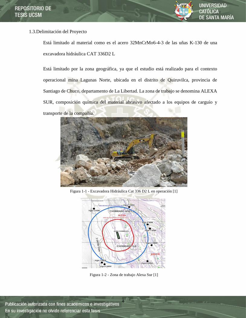
1.3.Delimitación del Proyecto
Está limitado al material como es el acero 32MnCrMo6-4-3 de las uñas K-130 de una
excavadora hidráulica CAT 336D2 L
Está limitado por la zona geográfica, ya que el estudio está realizado para el contexto
operacional mina Lagunas Norte, ubicada en el distrito de Quiruvilca, provincia de
Santiago de Chuco, departamento de La Libertad. La zona de trabajo se denomina ALEXA
SUR, composición química del material abrasivo afectado a los equipos de carguío y
transporte de la compañía.
Figura 1-1 - Excavadora Hidráulica Cat 336 D2 L en operación [1]
Figura 1-2 - Zona de trabajo Alexa Sur [1]
5
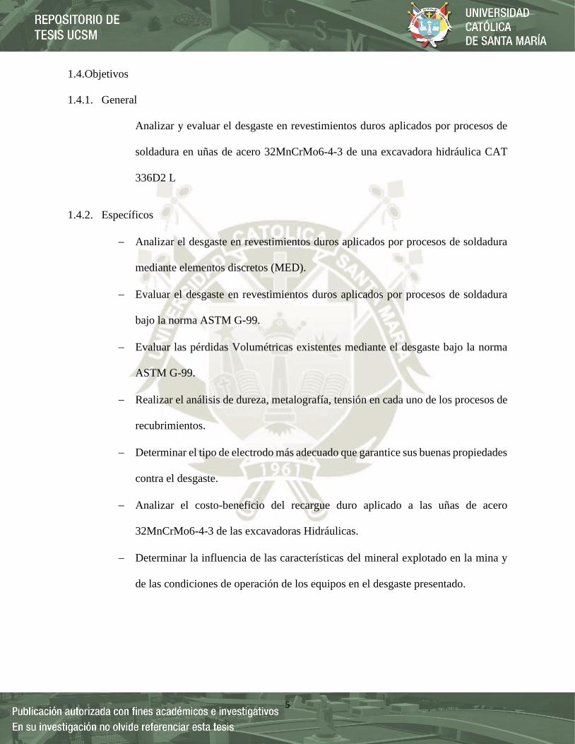
1.4.Objetivos
1.4.1. General
Analizar y evaluar el desgaste en revestimientos duros aplicados por procesos de
soldadura en uñas de acero 32MnCrMo6-4-3 de una excavadora hidráulica CAT
336D2 L
1.4.2. Específicos
Analizar el desgaste en revestimientos duros aplicados por procesos de soldadura
mediante elementos discretos (MED).
Evaluar el desgaste en revestimientos duros aplicados por procesos de soldadura
bajo la norma ASTM G-99.
Evaluar las pérdidas Volumétricas existentes mediante el desgaste bajo la norma
ASTM G-99.
Realizar el análisis de dureza, metalografía, tensión en cada uno de los procesos de
recubrimientos.
Determinar el tipo de electrodo más adecuado que garantice sus buenas propiedades
contra el desgaste.
Analizar el costo-beneficio del recargue duro aplicado a las uñas de acero
32MnCrMo6-4-3 de las excavadoras Hidráulicas.
Determinar la influencia de las características del mineral explotado en la mina y
de las condiciones de operación de los equipos en el desgaste presentado.

6
1.5.Hipótesis
1.5.1. Hipótesis General
Analizando los revestimientos duros aplicados por procesos de soldadura en las
uñas de acero 32MnCrMo6-4-3 (K-130) de una excavadora CAT 336D2 L,
podemos aumentar la relación costo-beneficio y reducir la compra de elementos
de desgaste de las excavadoras debido a la alta rotación de esta.

7
CAPÍTULO II

8
2. MARCO TEÓRICO
2.1.Aceros
2.1.1. ¿Qué es el Acero?
El Acero es básicamente una aleación o combinación de hierro y carbono (alrededor de
0,05% hasta menos de un 2%). Algunas veces otros elementos de aleación específicos tales
como el Cr (Cromo) o Ni (Níquel) se agregan con propósitos determinados.
Ya que el acero es básicamente hierro altamente refinado (más de un 98%), su fabricación
comienza con la reducción de hierro (producción de arrabio) el cual se convierte más tarde
en acero [2].
El hierro puro es uno de los elementos del acero, por lo tanto, consiste solamente de un tipo
de átomos. No se encuentra libre en la naturaleza ya que químicamente reacciona con
facilidad con el oxígeno del aire para formar óxido de hierro - herrumbre. El óxido se
encuentra en cantidades significativas en el mineral de hierro, el cual es una concentración
de óxido de hierro con impurezas y materiales térreos [2].
2.1.2. Clasificación de los aceros.
Los diferentes tipos de acero se clasifican de acuerdo con los elementos de aleación que
producen distintos efectos en el Acero [26]:
2.1.2.1.Aceros al Carbono
Más del 90% de todos los aceros son aceros al carbono. Estos aceros contienen diversas
cantidades de carbono y menos del 1,65% de manganeso, el 0,60% de silicio y el 0,60%
de cobre. Entre los productos fabricados con aceros al carbono figuran máquinas,
carrocerías de automóvil, la mayor parte de las estructuras de construcción de acero, cascos
de buques, somieres y horquillas [26].
9
2.1.2.2.Aceros Aleados
Estos aceros contienen una proporción determinada de vanadio, molibdeno y otros
elementos, además de cantidades mayores de manganeso, silicio y cobre que los aceros al
carbono normales. Estos aceros de aleación se pueden subclasificar en [26]:
2.1.2.2.1. Estructurales
Son aquellos aceros que se emplean para diversas partes de máquinas, tales como
engranajes, ejes y palancas. Además, se utilizan en las estructuras de edificios,
construcción de chasis de automóviles, puentes, barcos y semejantes. El contenido de
la aleación varía desde 0,25% a un 6% [26].
2.1.2.2.2. Para Herramientas
Aceros de alta calidad que se emplean en herramientas para cortar y modelar metales y
no metales. Por lo tanto, son materiales empleados para cortar y construir herramientas
tales como taladros, escariadores, fresas, terrajas y machos de roscar [26].
2.1.2.2.3. Especiales
Los Aceros de Aleación especiales son los aceros inoxidables y aquellos con un
contenido de cromo generalmente superior al 12%. Estos aceros de gran dureza y alta
resistencia a las altas temperaturas y a la corrosión se emplean en turbinas de vapor,
engranajes, ejes y rodamientos [26].
2.1.2.2.4. Aceros de baja aleación ultrarresistentes
Esta familia es la más reciente de las cuatro grandes clases de acero. Los aceros de baja
aleación son más baratos que los aceros aleados convencionales ya que contienen
cantidades menores de los costosos elementos de aleación. Sin embargo, reciben un
tratamiento especial que les da una resistencia mucho mayor que la del acero al
10
carbono. Por ejemplo, los vagones de mercancías fabricados con aceros de baja
aleación pueden transportar cargas más grandes porque sus paredes son más delgadas
que lo que sería necesario en caso de emplear acero al carbono. Además, como los
vagones de acero de baja aleación pesan menos, las cargas pueden ser más pesadas. En
la actualidad se construyen muchos edificios con estructuras de aceros de baja aleación.
Las vigas pueden ser más delgadas sin disminuir su resistencia, logrando un mayor
espacio interior en los edificios [26].
2.1.2.2.5. Aceros Inoxidables
Los aceros inoxidables contienen cromo, níquel y otros elementos de aleación, que los
mantienen brillantes y resistentes a la herrumbre y oxidación a pesar de la acción de la
humedad o de ácidos y gases corrosivos. Algunos aceros inoxidables son muy duros;
otros son muy resistentes y mantienen esa resistencia durante largos periodos a
temperaturas extremas. Debido a sus superficies brillantes, en arquitectura se emplean
muchas veces con fines decorativos. El acero inoxidable se utiliza para las tuberías y
tanques de refinerías de petróleo o plantas químicas, para los fuselajes de los aviones o
para cápsulas espaciales [26].
2.2.Efectos de los elementos de aleación
Los elementos de aleación específicos y sus cantidades determinan el tipo de acero de aleación
y sus propiedades particulares [26].
Se puede apreciar en la Tabla 2-1 los efectos principales de algunos de los elementos más
comunes.

11
Tabla 2-1 - Efectos de elementos de aleación [2]
2.3.Aceros utilizados en elementos de desgaste
2.3.1. Acero 32MnCrMo6-4-3 – Aceros Aleados
Efectos de los elementos de aleación.
Las aleaciones se utilizan principalmente para aumentar la templabilidad de los aceros. No
tienen ningún comportamiento durante el temple. Los formadores de carburo de tungsteno
tienden a para aumentar la dureza de la martensita templada, como se muestra en la Figura
2-1 [3].
ELEMENTO APORTACIÓN
ALUMINIO Empleado en pequeñas cantidades, actúa como un desoxidante para el acero
fundido y produce un Acero de Grano Fino.
BORO Aumenta la templabilidad (la profundidad a la cual un acero puede ser
endurecido).
CROMO
Aumenta la profundidad del endurecimiento y mejora la resistencia al desgaste y
corrosión. COBRE Mejora significativamente la resistencia a la corrosión
atmosférica.
MANGANESO
Elemento básico en todos los aceros comerciales. Actúa como un desoxidante y
también neutraliza los efectos nocivos del azufre, facilitando la laminación,
moldeo y otras operaciones de trabajo en caliente. Aumenta también la penetración
de temple y contribuye a su resistencia y dureza.
MOLIBDENO Mediante el aumento de la penetración de temple, mejora las propiedades del
tratamiento térmico. Aumenta también la dureza y resistencia a altas temperaturas.
NIQUEL
Mejora las propiedades del tratamiento térmico reduciendo la temperatura de
endurecimiento y distorsión al ser templado. Al emplearse conjuntamente con el
Cromo, aumenta la dureza y la resistencia al desgaste.
SILICIO Se emplea como desoxidante y actúa como endurecedor en el acero de aleación.
AZUFRE
Normalmente es una impureza y se mantiene a un bajo nivel. Sin embargo, alguna
vez se agrega intencionalmente en grandes cantidades (0,06 a 0,30%) para
aumentar la maquinabilidad (habilidad para ser trabajado mediante cortes) de los
aceros de aleación y al carbono.
TITANIO Se emplea como un desoxidante y para inhibir el crecimiento granular. Aumenta
también la resistencia a altas temperaturas.
TUNGSTENO Se emplea en muchos aceros de aleación para herramientas, impartiéndoles una
gran resistencia al desgaste y dureza a altas temperaturas.
VANADIO
Imparte dureza y ayuda en la formación de granos de tamaño fino. Aumenta la
resistencia a los impactos (resistencia a las fracturas por impacto) y también la
resistencia a la fatiga.

12
Figura 2-1 - Efecto de los elementos de aleación sobre la dureza de la martensita templada para 1 h a 482◦C. [3]
El efecto neto de las aleaciones sobre la dureza Vickers es la suma de las contribuciones
de cada elemento. El molibdeno aumenta el tiempo para formar perlita mucho más que el
tiempo para formar bainita, por lo que se utiliza en aceros en los que la bainita es un
producto deseado. Elementos de aleación aumenta el tiempo necesario para el revenido.
Mn, Ni, Cr y Si tienden a promueven la fragilidad del temperamento; Mo, Ti y Zr la retrasan
[3].
2.3.2. Aplicaciones
Las aleaciones bajas en carbono (0.10-0.25%C) se utilizan principalmente para carburizado
partes. Estos incluyen 4023, 4118 y 5015. Partes intrincadas que contienen más del 0,40%
C debe ser templado con aceite para evitar que se agriete. El 52100 se utiliza
exclusivamente para rodamientos de bolas. Los resortes se fabrican normalmente de las
aleaciones 5155 y 5160 [3].

13
2.4.Tribología
La palabra “tribología” viene de la palabra griega tribos que significa fricción, traduciendo la
palabra literalmente como la “ciencia de la fricción”. Mientras que el estudio del concepto se
remonta a Leonardo da Vinci y sus estudios sobre las leyes de la fricción, la palabra
“Tribología” no se había utilizado ampliamente hasta que Peter H. Jost, un ingeniero mecánico
británico, acuñó el término en el Reporte Jost del 9 de marzo de 1966 [12].
Jost es considerado el fundador de la disciplina de la tribología, y a partir de su reporte, se puso
una mayor atención sobre el tema. Solicitó el establecimiento de Institutos de Tribología, junto
con la publicación de un manual sobre tribodiseño e ingeniería [12].
En una entrevista realizada por Jim Fitch, fundador de Noria Corporation, se le pidió a Jost
que describiera el momento en que concibió la tribología, señalando que fue en septiembre de
1964 en la Conferencia sobre Lubricación en Trabajos de Hierro y Acero en Cardiff (Reino
Unido) del Instituto del Hierro y del Acero/Grupo de Lubricación y Desgaste del ImechE [12].
Fue en esta conferencia donde se discutieron las fallas, particularmente en la maquinaria y
equipos dañados en acerías. Después de esto, se le pidió a Jost que formara un comité para
“investigar lo relacionado con la educación sobre lubricación, la investigación y las
necesidades de la industria” (vea el artículo de Jim Fitch, “Interview with Luminary Professor
H. Peter Jost – The Man who Gave Birth to the Word ‘Tribology”) [12].
Poco después de la publicación del Reporte Jost, el 26 de septiembre de 1966 se estableció
formalmente la Comisión de Tribología y fue encargada de varias tareas, incluyendo [12]:

14
Asesorar al ministro de tecnología para medir el efecto del progreso tecnológico y los
ahorros en el ámbito de la tribología [12].
Asesorar a los departamentos gubernamentales y otros organismos en asuntos
relacionados con la tribología [12].
Examinar y recomendar a la industria las últimas técnicas en tribología [12].
Informar anualmente al ministro de tecnología sobre sus propias actividades y sobre las
tendencias y desarrollos en tribología que se consideran de importancia tecnológica o
económica para la nación [12]
Desde entonces, la tribología se ha convertido en un área interdisciplinaria relacionada con la
biología, la química, la ingeniería, las ciencias de los materiales, las matemáticas y la física
[4].
Figura 2-2 - Esquema tribológico [4]
15
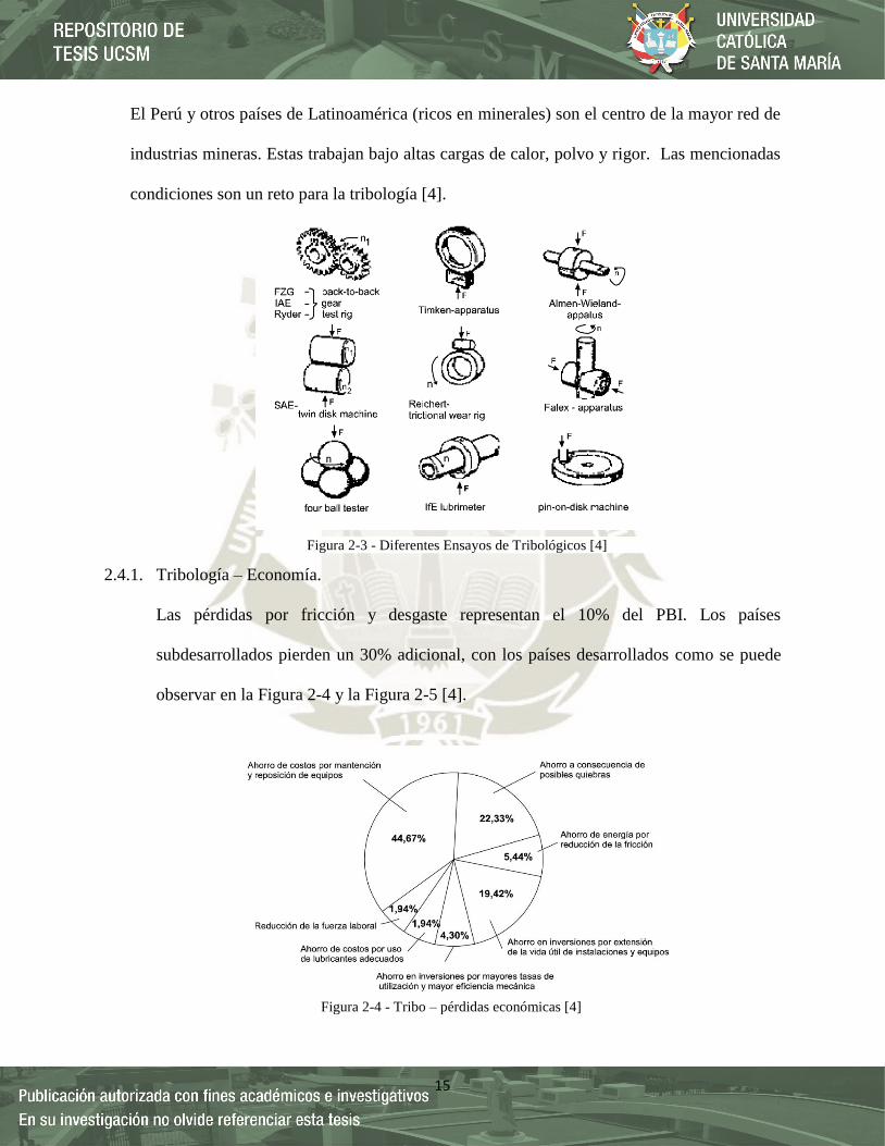
El Perú y otros países de Latinoamérica (ricos en minerales) son el centro de la mayor red de
industrias mineras. Estas trabajan bajo altas cargas de calor, polvo y rigor. Las mencionadas
condiciones son un reto para la tribología [4].
2.4.1. Tribología – Economía.
Las pérdidas por fricción y desgaste representan el 10% del PBI. Los países
subdesarrollados pierden un 30% adicional, con los países desarrollados como se puede
observar en la Figura 2-4 y la Figura 2-5 [4].
Figura 2-3 - Diferentes Ensayos de Tribológicos [4]
Figura 2-4 - Tribo – pérdidas económicas [4]

16
Figura 2-5 - Pérdidas económicas por Industria [4]
Figura 2-6 - Investigación del desgaste [4]
17
2.5.Desgaste
El desgaste es una de las causas principales de los daños en los componentes y de las
consiguientes averías de máquinas y aparatos. Su mitigación mediante la elección del material
apropiado, el revestimiento, el diseño de la superficie o la lubricación lo es, por lo tanto, de
gran importancia económica [5].
Aunque la fricción y el desgaste siempre aparecen juntos, en la práctica son fenómenos
cualitativamente diferentes. Esto ya se puede ver en el hecho de que uno puede imaginar la
fricción sin desgaste, al menos en un modelo. Por ejemplo, hay fricción, pero no hay desgaste
en el modelo Prandtl-Tomlinson. Incluso se puede prever un desgaste sin fricción: el desgaste
ya puede ser causado por un contacto normal sin movimiento tangencial [5].
Los mecanismos físicos de fricción y desgaste, a menudo diferentes, se hacen visibles en el
hecho de que la tasa de desgaste de varios pares de fricción (en condiciones idénticas) puede
variar en varios órdenes de magnitud [5].
Al mismo tiempo puede observarse que en situaciones específicas, los procesos que conducen
a la fricción también causan que el desgaste ocurra al mismo tiempo, por ejemplo, la
deformación plástica de los microcontactos. En estos casos, la fricción y el desgaste pueden
tener una estrecha correlación [5].
En la mayoría de los casos, la fricción se considera un fenómeno no deseado. Sin embargo, el
desgaste también puede ser la base de varios procesos tecnológicos, como el esmerilado, el
pulido o el chorro de arena [5].
Es común diferenciar los siguientes tipos fundamentales de desgaste según sus mecanismos
físicos [5]:
18
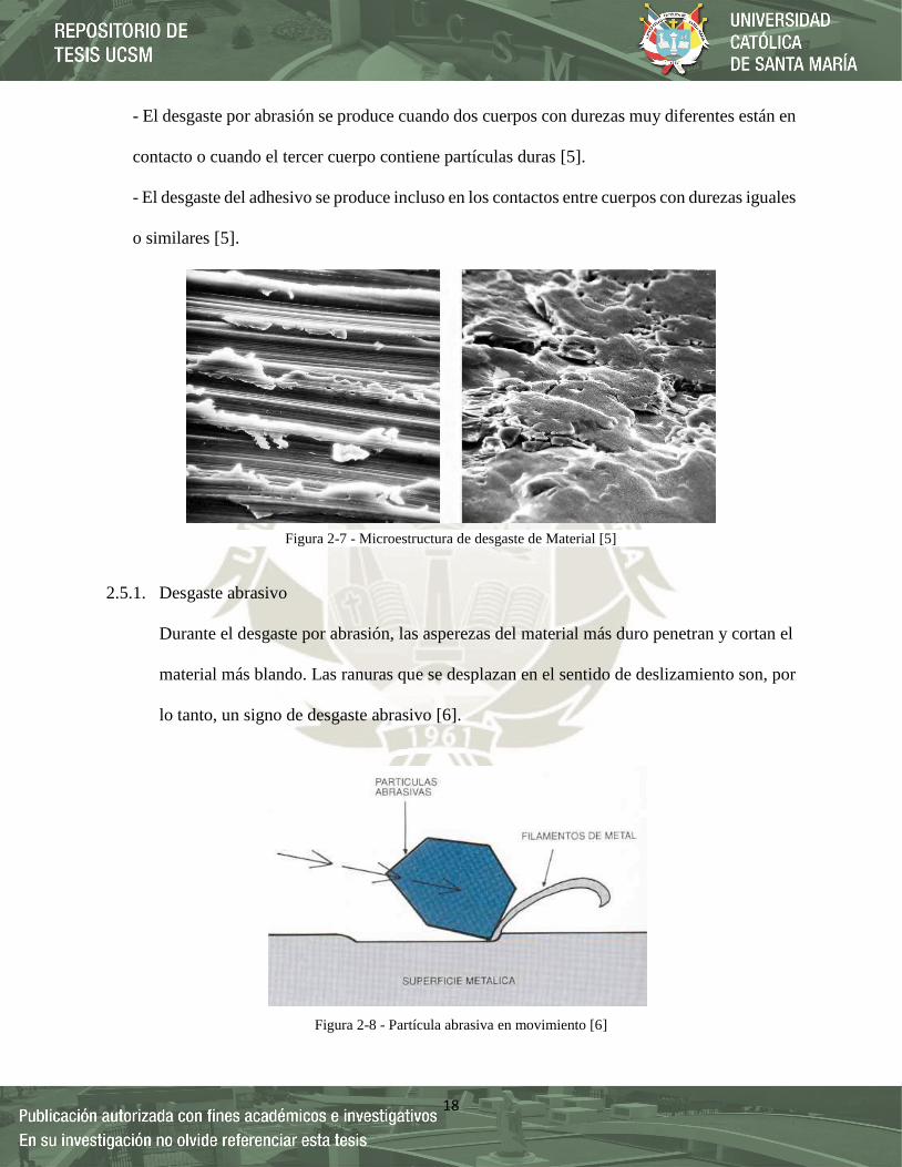
- El desgaste por abrasión se produce cuando dos cuerpos con durezas muy diferentes están en
contacto o cuando el tercer cuerpo contiene partículas duras [5].
- El desgaste del adhesivo se produce incluso en los contactos entre cuerpos con durezas iguales
o similares [5].
2.5.1. Desgaste abrasivo
Durante el desgaste por abrasión, las asperezas del material más duro penetran y cortan el
material más blando. Las ranuras que se desplazan en el sentido de deslizamiento son, por
lo tanto, un signo de desgaste abrasivo [6].
Figura 2-7 - Microestructura de desgaste de Material [5]
Figura 2-8 - Partícula abrasiva en movimiento [6]
19
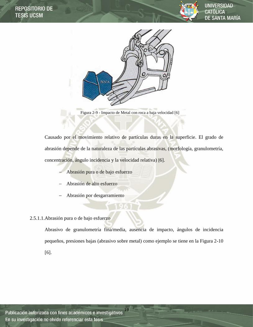
Causado por el movimiento relativo de partículas duras en la superficie. El grado de
abrasión depende de la naturaleza de las partículas abrasivas, (morfología, granulometría,
concentración, ángulo incidencia y la velocidad relativa) [6].
Abrasión pura o de bajo esfuerzo
Abrasión de alto esfuerzo
Abrasión por desgarramiento
2.5.1.1.Abrasión pura o de bajo esfuerzo
Abrasivo de granulometría fina/media, ausencia de impacto, ángulos de incidencia
pequeños, presiones bajas (abrasivo sobre metal) como ejemplo se tiene en la Figura 2-10
[6].
Figura 2-9 - Impacto de Metal con roca a baja velocidad [6]

20
2.5.1.2.Abrasión de alto esfuerzo
Constituido por partículas pequeñas y que no impactan sobre la superficie de desgaste [6].
2.5.1.3.Abrasión por desgarramiento
Difiere al anterior en cuanto a que el elemento abrasivo es de mayor tamaño y muchas
veces existe impacto [6].
Figura 2-10 - Partícula abrasiva en Hopper [6]
Figura 2-11 - Partícula abrasiva en movimiento [6]

21
Figura 2-12 - Desgarro de material con partícula abrasiva [6]
Figura 2-13 - Cucharon de excavadora desgarrado con material abrasivo [1]
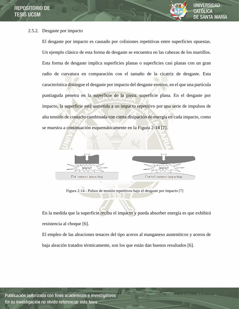
22
2.5.2. Desgaste por impacto
El desgaste por impacto es causado por colisiones repetitivas entre superficies opuestas.
Un ejemplo clásico de esta forma de desgaste se encuentra en las cabezas de los martillos.
Esta forma de desgaste implica superficies planas o superficies casi planas con un gran
radio de curvatura en comparación con el tamaño de la cicatriz de desgaste. Esta
característica distingue el desgaste por impacto del desgaste erosivo, en el que una partícula
puntiaguda penetra en la superficie de la pieza. superficie plana. En el desgaste por
impacto, la superficie está sometida a un impacto repetitivo por una serie de impulsos de
alta tensión de contacto combinada con cierta disipación de energía en cada impacto, como
se muestra a continuación esquemáticamente en la Figura 2-14 [7].
En la medida que la superficie reciba el impacto y pueda absorber energía es que exhibirá
resistencia al choque [6].
El empleo de las aleaciones tenaces del tipo aceros al manganeso austeniticos y aceros de
baja aleación tratados térmicamente, son los que están dan buenos resultados [6].
Figura 2-14 - Pulsos de tensión repetitivos bajo el desgaste por impacto [7]

23
2.5.3. Desgaste erosivo
El desgaste erosivo es causado por el impacto de partículas sólidas o líquidas contra la
superficie de un objeto. El desgaste erosivo se produce en una gran variedad de maquinaria
y los ejemplos típicos como los siguiente: daños en los álabes de las turbinas de gas cuando
una aeronave vuela a través de nubes de polvo, y el desgaste de impulsores de bombas en
sistemas de procesamiento de lodos minerales. En común con otras formas de desgaste, la
resistencia mecánica no garantiza la resistencia al desgaste y un estudio detallado del
material se requieren para minimizar el desgaste. Las propiedades de la partícula que se
erosiona son también son importantes y se reconocen cada vez más como un parámetro
relevante en el control de este tipo de desgaste [7].
El desgaste erosivo implica varios mecanismos de desgaste que son controlados en gran
medida por el material de las partículas, el ángulo de impacto, la velocidad de impacto y el
tamaño de las partículas. Si la partícula es dura y sólida, es posible que se produzca un
proceso similar al desgaste abrasivo. Cuando las partículas líquidas son el erodente, la
Figura 2-15 - Desgaste por impacto en un cincel [6]

24
abrasión no tiene lugar y los mecanismos de desgaste involucrados son el resultado de
esfuerzos repetitivos en el impacto [7].
El término "desgaste erosivo" se refiere a un número indeterminado de mecanismos de
desgaste que se producen cuando partículas relativamente pequeñas impactan contra
componentes mecánicos. Esta definición es empírica por naturaleza y se relaciona más con
consideraciones prácticas que con cualquier comprensión fundamental del desgaste. Los
mecanismos conocidos de desgaste erosivo se ilustran en la Figura 2-16 [7].
Figura 2-16 - Posibles mecanismos de erosión; a) abrasión en ángulos de bajo impacto, b) fatiga
superficial durante un impacto de baja velocidad y alto ángulo de impacto, c) fractura frágil o
deformación plástica múltiple, d) fusión de superficie a altas velocidades de impacto, e) erosión
macroscópica con efectos secundarios [7]

25
2.5.4. Desgaste adhesivo
Si los elementos de fricción tienen durezas comparables, entonces otro tipo de desgaste
comienza a jugar un papel primordial: el desgaste adhesivo. El desgaste del adhesivo es lo
más importante tipo de desgaste en aplicaciones tribológicas en las que se debe minimizar
el desgaste y, por lo tanto, deben evitarse las condiciones en las que se produce el desgaste
por abrasión [5].
El mecanismo de desgaste adhesivo puede ser imaginado como la soldadura de microfibras
de las asperezas seguidas de los elementos de volumen (partículas de desgaste) cerca de la
superficie siendo arrancada. Investigamos las condiciones para la soldadura y el desgarro
de una partícula según este mecanismo [5].
La propiedad fundamental de los materiales metálicos es que se deforman plásticamente
después de superar una tensión crítica. Si el material se carga en tensión, después de una
deformación crítica, se produce un fallo. Por el contrario, si se sobrepasa el límite elástico
bajo presión, los dos socios se sueldan entre sí. Aunque este efecto no sea perceptible
macroscópicamente (similar al caso de la adhesión), es válido para micro contactos
individuales, este se puede observar en la Figura 2-17 [5].
Figura 2-17 - Desgaste producto de la fricción no lubricada entre piezas metálicas [6]
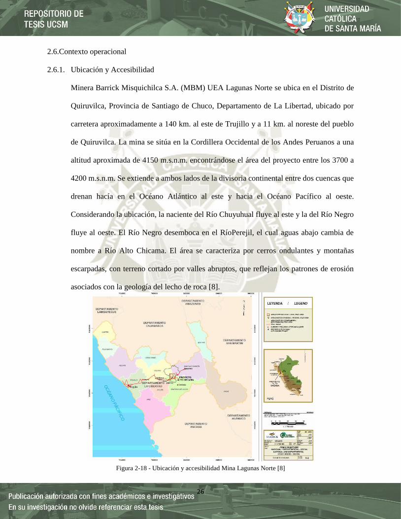
26
2.6.Contexto operacional
2.6.1. Ubicación y Accesibilidad
Minera Barrick Misquichilca S.A. (MBM) UEA Lagunas Norte se ubica en el Distrito de
Quiruvilca, Provincia de Santiago de Chuco, Departamento de La Libertad, ubicado por
carretera aproximadamente a 140 km. al este de Trujillo y a 11 km. al noreste del pueblo
de Quiruvilca. La mina se sitúa en la Cordillera Occidental de los Andes Peruanos a una
altitud aproximada de 4150 m.s.n.m. encontrándose el área del proyecto entre los 3700 a
4200 m.s.n.m. Se extiende a ambos lados de la divisoria continental entre dos cuencas que
drenan hacía en el Océano Atlántico al este y hacia el Océano Pacífico al oeste.
Considerando la ubicación, la naciente del Río Chuyuhual fluye al este y la del Río Negro
fluye al oeste. El Río Negro desemboca en el RíoPerejil, el cual aguas abajo cambia de
nombre a Río Alto Chicama. El área se caracteriza por cerros ondulantes y montañas
escarpadas, con terreno cortado por valles abruptos, que reflejan los patrones de erosión
asociados con la geología del lecho de roca [8].
Figura 2-18 - Ubicación y accesibilidad Mina Lagunas Norte [8]

27
2.6.2. Clasificación de materiales para polígonos y estacas de campo.
Figura 2-19 - Ubicación y accesibilidad Mina Lagunas Norte [8]
Figura 2-20 - Clasificación de materiales para polígonos y estacas de campo [8]
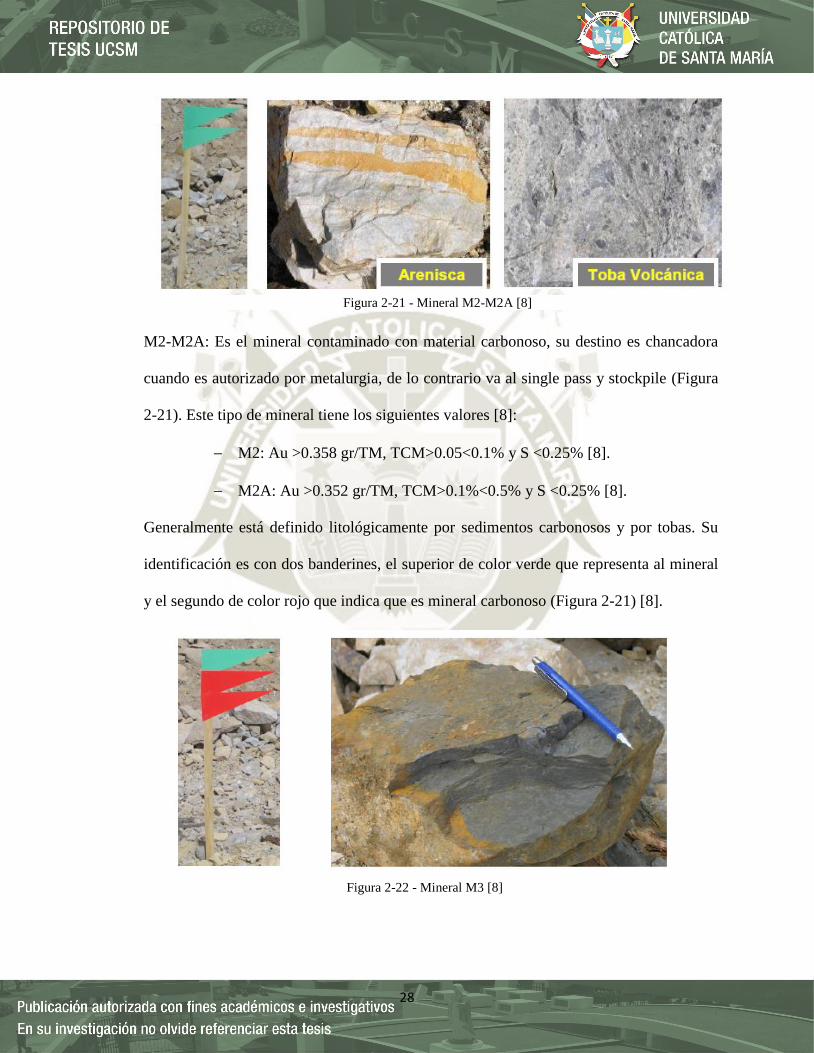
28
M2-M2A: Es el mineral contaminado con material carbonoso, su destino es chancadora
cuando es autorizado por metalurgia, de lo contrario va al single pass y stockpile (Figura
2-21). Este tipo de mineral tiene los siguientes valores [8]:
M2: Au >0.358 gr/TM, TCM>0.05<0.1% y S <0.25% [8].
M2A: Au >0.352 gr/TM, TCM>0.1%<0.5% y S <0.25% [8].
Generalmente está definido litológicamente por sedimentos carbonosos y por tobas. Su
identificación es con dos banderines, el superior de color verde que representa al mineral
y el segundo de color rojo que indica que es mineral carbonoso (Figura 2-21) [8].
Figura 2-21 - Mineral M2-M2A [8]
Figura 2-22 - Mineral M3 [8]

29
M3: Este mineral es con sulfuro, su destino es single pass chancado (Figura 2-22). Solo en
casos extremos será enviado a Stockpile. Este tipo de mineral tiene los siguientes valores
[8]:
M3: Au >0.339 gr/TM, TCM<0.05% y S >0.40% [8].
Generalmente está definido litológicamente por brechas y tobas volcánicas con sulfuro. Su
identificación es con dos banderines, el superior de color verde que representa al mineral
y el siguiente de color amarillo que indica que es mineral con sulfuro [8].
Figura 2-23- Muestras superficiales [9]
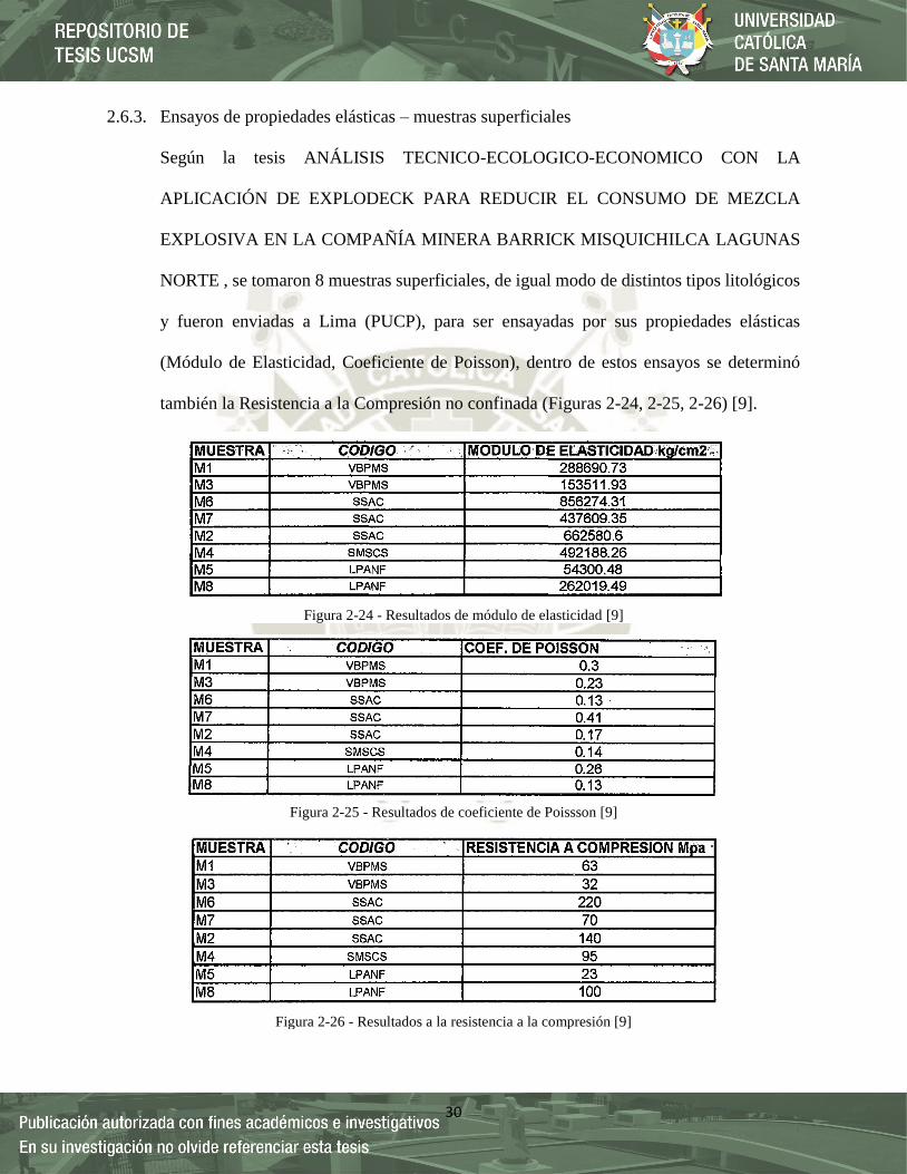
30
2.6.3. Ensayos de propiedades elásticas – muestras superficiales
Según la tesis ANÁLISIS TECNICO-ECOLOGICO-ECONOMICO CON LA
APLICACIÓN DE EXPLODECK PARA REDUCIR EL CONSUMO DE MEZCLA
EXPLOSIVA EN LA COMPAÑÍA MINERA BARRICK MISQUICHILCA LAGUNAS
NORTE , se tomaron 8 muestras superficiales, de igual modo de distintos tipos litológicos
y fueron enviadas a Lima (PUCP), para ser ensayadas por sus propiedades elásticas
(Módulo de Elasticidad, Coeficiente de Poisson), dentro de estos ensayos se determinó
también la Resistencia a la Compresión no confinada (Figuras 2-24, 2-25, 2-26) [9].
Figura 2-24 - Resultados de módulo de elasticidad [9]
Figura 2-25 - Resultados de coeficiente de Poissson [9]
Figura 2-26 - Resultados a la resistencia a la compresión [9]
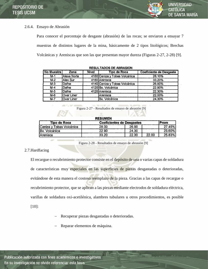
31
2.6.4. Ensayo de Abrasión
Para conocer el porcentaje de desgaste (abrasión) de las rocas; se enviaron a ensayar 7
muestras de distintos lugares de la mina, básicamente de 2 tipos litológicos; Brechas
Volcánicas y Areniscas que son las que presentan mayor dureza (Figuras 2-27, 2-28) [9].
2.7.Hardfacing
El recargue o recubrimiento protector consiste en el depósito de una o varias capas de soldadura
de características muy especiales en las superficies de piezas desgastadas o deterioradas,
evitándose de esta manera el costoso reemplazo de la pieza. Gracias a las capas de recargue o
recubrimiento protector, que se aplican a las piezas mediante electrodos de soldadura eléctrica,
varillas de soldadura oxi-acetilénica, alambres tubulares u otros procedimientos, es posible
[10]:
Recuperar piezas desgastadas o deterioradas.
Reparar elementos de máquina.
Figura 2-27 - Resultados de ensayo de abrasión [9]
Figura 2-28 - Resultados de ensayo de abrasión [9]
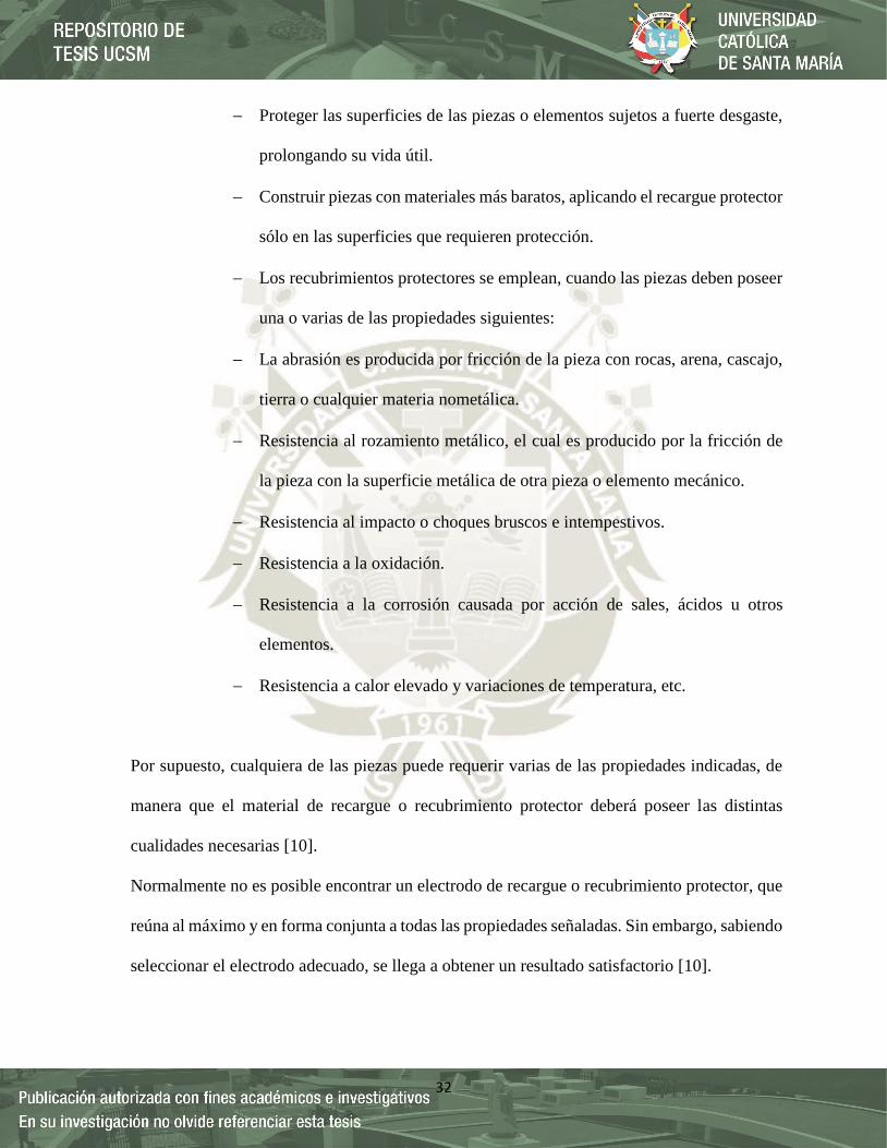
32
Proteger las superficies de las piezas o elementos sujetos a fuerte desgaste,
prolongando su vida útil.
Construir piezas con materiales más baratos, aplicando el recargue protector
sólo en las superficies que requieren protección.
Los recubrimientos protectores se emplean, cuando las piezas deben poseer
una o varias de las propiedades siguientes:
La abrasión es producida por fricción de la pieza con rocas, arena, cascajo,
tierra o cualquier materia nometálica.
Resistencia al rozamiento metálico, el cual es producido por la fricción de
la pieza con la superficie metálica de otra pieza o elemento mecánico.
Resistencia al impacto o choques bruscos e intempestivos.
Resistencia a la oxidación.
Resistencia a la corrosión causada por acción de sales, ácidos u otros
elementos.
Resistencia a calor elevado y variaciones de temperatura, etc.
Por supuesto, cualquiera de las piezas puede requerir varias de las propiedades indicadas, de
manera que el material de recargue o recubrimiento protector deberá poseer las distintas
cualidades necesarias [10].
Normalmente no es posible encontrar un electrodo de recargue o recubrimiento protector, que
reúna al máximo y en forma conjunta a todas las propiedades señaladas. Sin embargo, sabiendo
seleccionar el electrodo adecuado, se llega a obtener un resultado satisfactorio [10].

33
La dureza (Rockwell o Brinell) del metal depositado por un electrodo de recubrimiento
protector es la, que generalmente se toma como indicación de las cualidades de resistencia al
desgaste. Sin embargo, lo que el grado de dureza realmente nos proporciona es una orientación
sobre las propiedades del material depositado, ya que materiales diferentes con el mismo grado
de dureza pueden tener reacciones completamente distintas al someterlos a las diferentes
condiciones de desgaste o de servicio [10].
Muchos de los recubrimientos protectores poseen efectivamente una gran dureza; de allí la
expresión ”recubrimiento duro”. Este término se ha hecho muy común; sin embargo, no es
correcta la expresión en todos los casos. Lo importante en una capa de recubrimiento es que
tenga las propiedades necesarias, las cuales muchas veces no coinciden con valores de dureza
particularmente elevados [10].
2.7.1. Normas AWS A5.13, A5.21
Esta especificación prescribe los requisitos para la clasificación de los electrodos de
revestimiento para la soldadura por arco metálico blindado. La clasificación se basa en la
composición química del metal de soldadura depositado, excepto en el caso de los
electrodos de carburo de tungsteno, donde la clasificación se basa en el rango de malla,
cantidad y composición de los gránulos de carburo de tungsteno. Una guía se adjunta al
pliego de condiciones como fuente de información sobre las características y aplicaciones
del producto clasificado electrodos [11].

34
2.7.2. Especificaciones para electrodos y varillas utilizadas en recubrimientos duros
Esta especificación prescribe los requisitos para la clasificación de los electrodos de
revestimiento para la soldadura por arco metálico blindado.
Los electrodos y varillas desnudos sólidos para superficies se clasifican en AWS
A5.13:2010, Especificación para electrodos desnudos y varillas para superficies y Varillas
para el acabado de superficies [11].
2.7.2.1.Utilidad
Para demostrar la utilidad de los electrodos, con el fin de ser clasificados en esta
especificación, los electrodos deberán ser capaces de producir los siguientes resultados en
las pruebas requeridas [11]:
a. Para varillas de soldadura, el metal fluirá libremente y sin problemas
sobre la superficie de la placa sin escurrir.
b. Los electrodos deberán funcionar sin problemas y sin salpicaduras
excesivas cuando se use dentro de los rangos de corriente recomendado
por el fabricante.
c. La escoria se elimina fácilmente con herramientas de mano.
d. La superficie de la plataforma de prueba después de ser esmerilado,
estarán libres de defectos visibles al ojo desnudo.
35
2.7.2.2.Fabricación
Los electrodos y varillas pueden ser utilizados por cualquier método para piezas o
productos que cumpla los requisitos de esta especificación.
La selección del material o electrodos de aporte depende básicamente de tres factores, que
son [11]:
a. Metal base
b. Tipo de desgaste
c. Elección de proceso de soldeo
2.7.2.3.Clasificación [11]:
a. Excepto los electrodos de carburo de tungsteno, los electrodos de
superficie cubiertos por esta especificación A5.13/A5.13M son
clasificados de acuerdo con la composición química del metal de
aportación no diluido [11].
b. Los electrodos de carburo de tungsteno se clasifican en función del
tamaño y la composición química del tungsteno de carburo [11].
c. Los electrodos clasificados en una clasificación no se clasificarán en
ninguna otra clasificación de la presente especificación [11].
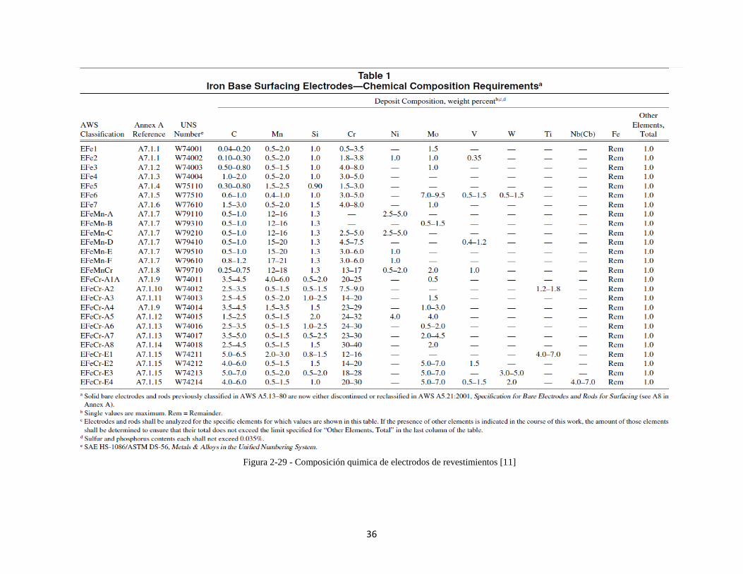
36
Figura 2-29 - Composición quimica de electrodos de revestimientos [11]

37
2.7.3. Selección de material de aporte
La selección del electrodo adecuado se inicia con el reconocimiento de los factores que
actúan en el desgaste a que está sujeta la pieza, así como de las exigencias de trabajo a que
estará sometida [10].
Esta determinación inicial se complementa con el estudio de los aspectos siguientes [10]:
Influencia de la abrasión, rozamiento, corrosión etc. en el desgaste o deterioro que
sufre la pieza, es decir las causas secundarias o paralelas [10].
Necesidad de maquinado o forjado del depósito de soldadura [10].
Composición y condición de la pieza a recubrir [10].
Si las características físicas de la pieza a recubrir no se alteran fuertemente por el
calentamiento y/o enfriamiento brusco [10].
Si la pieza resiste cambios de temperatura violentos y localizados, sin agrietarse
o romperse [10].
Espesor del metal a depositar, ya que debe evitarse la deposición de demasiadas
capas con determinados electrodos; en general nunca depositar más de 3 capas de
cualquier recargue o recubrimiento protector [10].
2.7.3.1.Materiales de aporte para recubrimientos protectores de piezas sujetas a desgaste.
En el campo de los electrodos para recubrimientos protectores, SOLDEXA fabrica una
gran variedad de tipos, tanto convencionales como especiales [10].
Naturalmente existen electrodos SOLDEXA, que cubren dos o más tipos de desgaste, pero
jamás se pretenderá que un solo electrodo cubra todas las diversas formas de desgaste o
exigencias que se presentan [10].
38
Por tal motivo, debe analizarse cuál es el factor de desgaste más importante que debemos
evitar, a fin de hacer la selección más correcta del electrodo. En algunos casos habrá que
sacrificar algunas de las características de resistencia. Por ejemplo, cuando el material está
sujeto a impacto combinado con abrasión como es el caso en las uñas de las palas,
pondremos un electrodo que, aunque no resista tanto la abrasión, tampoco sea quebradizo
y pueda resistir el impacto [10].
Cada uno de los recubrimientos descritos en la Figura 2-29 presentan una microestructura
característica principalmente dependiente de su composición química, esto define sus
propiedades mecánicas y su aplicación [10].
2.7.3.1.1. Citodur 1000
Electrodo para recargue de gran resistencia a la corrosión oxidación y abrasión severa.
El material depositado es una fundición blanca con alto contenido de cromo (36%), por
lo que, se recomienda aplicar 2 pases para que el relleno no se desprenda. En la mayoría
de los casos, para obtener las características deseadas, es recomendable usar una cama
cojín apropiada en función a las características del material base o los desgastes
presentes. Gracias a su alto contenido de carburos de cromo, el depósito conserva la
resistencia a la abrasión severa aún a temperaturas elevadas (hasta 1000°C). Los
cordones que deposita son perfectamente lisos, libres de poros, sin salpicaduras ni
inclusiones de escoria. El material de aporte es no maquinable, pero puede ser forjado
y templado [10].
39
Aplicaciones:
Para recuperar y recubrir piezas que están expuestas a desgaste por
abrasión severa y bajo impacto [10].
Usado en la industria minera, siderúrgica, construcción, ladrillera,
cementera, agrícola y todos aquellos sectores donde los materiales
están expuestos a desgaste abrasivo severo [10].
Ideal para la recuperación y protección de dientes, cucharas, baldes
y cubos de draga, sinfines de transporte, paletas de mezcladoras,
uñas de palas, bombas de arena, aletas de ventiladores, etc [10].
Para ollas, moldes y bordes de cucharas de fundición, que sufren
desgaste por abrasión o erosión de escorias o metal líquido a
temperaturas elevadas [10].
2.7.3.1.2. Citomangan
Electrodo que deposita un acero al manganeso con 12,0 – 14,0% Mn. Presenta
excelente comportamiento frente a abrasión e impacto severo. El material depositado
posee una estructura austenítica de gran tenacidad, que le permite absorber los golpes
durante el trabajo. Por las características del CITOMANGAN, requiere estar expuesto
a impacto severo para que la superficie se autoendurezca y llegue a una dureza final de
55 HRC. Usar una técnica de soldadura que garantice el mínimo aporte de calor y cuidar
que la pieza no sobrepase los 250°C (riesgo de cristalización). Es susceptible al
fisuramiento en caliente, riesgo que se incrementa por las elevadas contracciones que
presenta este material. Cuando se trata de rellenos considerables, es necesario el empleo
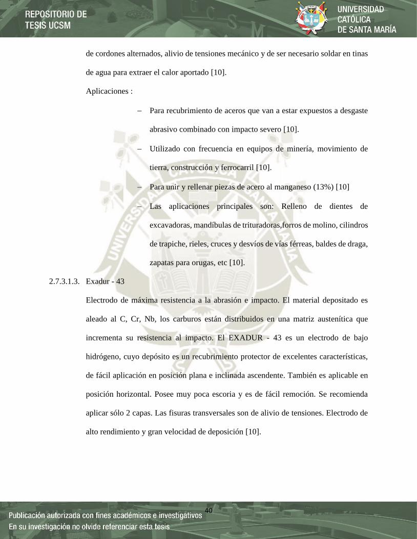
40
de cordones alternados, alivio de tensiones mecánico y de ser necesario soldar en tinas
de agua para extraer el calor aportado [10].
Aplicaciones :
Para recubrimiento de aceros que van a estar expuestos a desgaste
abrasivo combinado con impacto severo [10].
Utilizado con frecuencia en equipos de minería, movimiento de
tierra, construcción y ferrocarril [10].
Para unir y rellenar piezas de acero al manganeso (13%) [10]
Las aplicaciones principales son: Relleno de dientes de
excavadoras, mandíbulas de trituradoras,forros de molino, cilindros
de trapiche, rieles, cruces y desvíos de vías férreas, baldes de draga,
zapatas para orugas, etc [10].
2.7.3.1.3. Exadur - 43
Electrodo de máxima resistencia a la abrasión e impacto. El material depositado es
aleado al C, Cr, Nb, los carburos están distribuidos en una matriz austenítica que
incrementa su resistencia al impacto. El EXADUR - 43 es un electrodo de bajo
hidrógeno, cuyo depósito es un recubrimiento protector de excelentes características,
de fácil aplicación en posición plana e inclinada ascendente. También es aplicable en
posición horizontal. Posee muy poca escoria y es de fácil remoción. Se recomienda
aplicar sólo 2 capas. Las fisuras transversales son de alivio de tensiones. Electrodo de
alto rendimiento y gran velocidad de deposición [10].
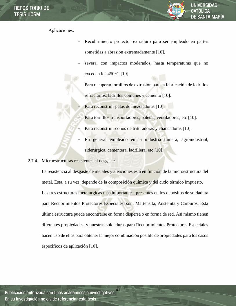
41
Aplicaciones:
Recubrimiento protector extraduro para ser empleado en partes
sometidas a abrasión extremadamente [10].
severa, con impactos moderados, hasta temperaturas que no
excedan los 450°C [10].
Para recuperar tornillos de extrusión para la fabricación de ladrillos
refractarios, ladrillos comunes y cemento [10].
Para reconstruir palas de mezcladoras [10].
Para tornillos transportadores, paletas, ventiladores, etc [10].
Para reconstruir conos de trituradoras y chancadoras [10].
En general empleado en la industria minera, agroindustrial,
siderúrgica, cementera, ladrillera, etc [10].
2.7.4. Microestructuras resistentes al desgaste
La resistencia al desgaste de metales y aleaciones está en función de la microestructura del
metal. Esta, a su vez, depende de la composición química y del ciclo térmico impuesto.
Las tres estructuras metalúrgicas más importantes, presentes en los depósitos de soldadura
para Recubrimientos Protectores Especiales, son: Martensita, Austenita y Carburos. Esta
última estructura puede encontrarse en forma dispersa o en forma de red. Así mismo tienen
diferentes propiedades, y nuestras soldaduras para Recubrimientos Protectores Especiales
hacen uso de ellas para obtener la mejor combinación posible de propiedades para los casos
específicos de aplicación [10].

42
2.7.4.1.Martensita
Es la estructura más común y más ampliamente usada en los depósitos de Recubrimientos
Protectores; es resistente a todos los tipos de condiciones suavemente abrasivas y algunos
ambientes severamente abrasivos.
La martensita tiene una alta dureza, que aumenta con el incremento del carbono. Los
depósitos martensíticos tienen moderada ductilidad y mediana resistencia al impacto. La
martensita ofrece ventajas al ser usada contra medios de abrasión por rayado, condición
que puede considerarse moderada. Las martensitas con más alto porcentaje de carbono
presentan excelente resistencia a la abrasión por esmerilado (Figura 2-30) [10].
2.7.4.2.Austenita
La austenita es blanda y dúctil; se autoendurece rápidamente durante el trabajo con impacto
y posee buenas cualidades de resistencia a la abrasión por raspado. Los depósitos
austeníticos tienen un núcleo tenaz y dúctil, que soporta una capa superficial que se
endurece durante el trabajo [10].
Figura 2-30 - Microestructura de Martensita (x100) [10]
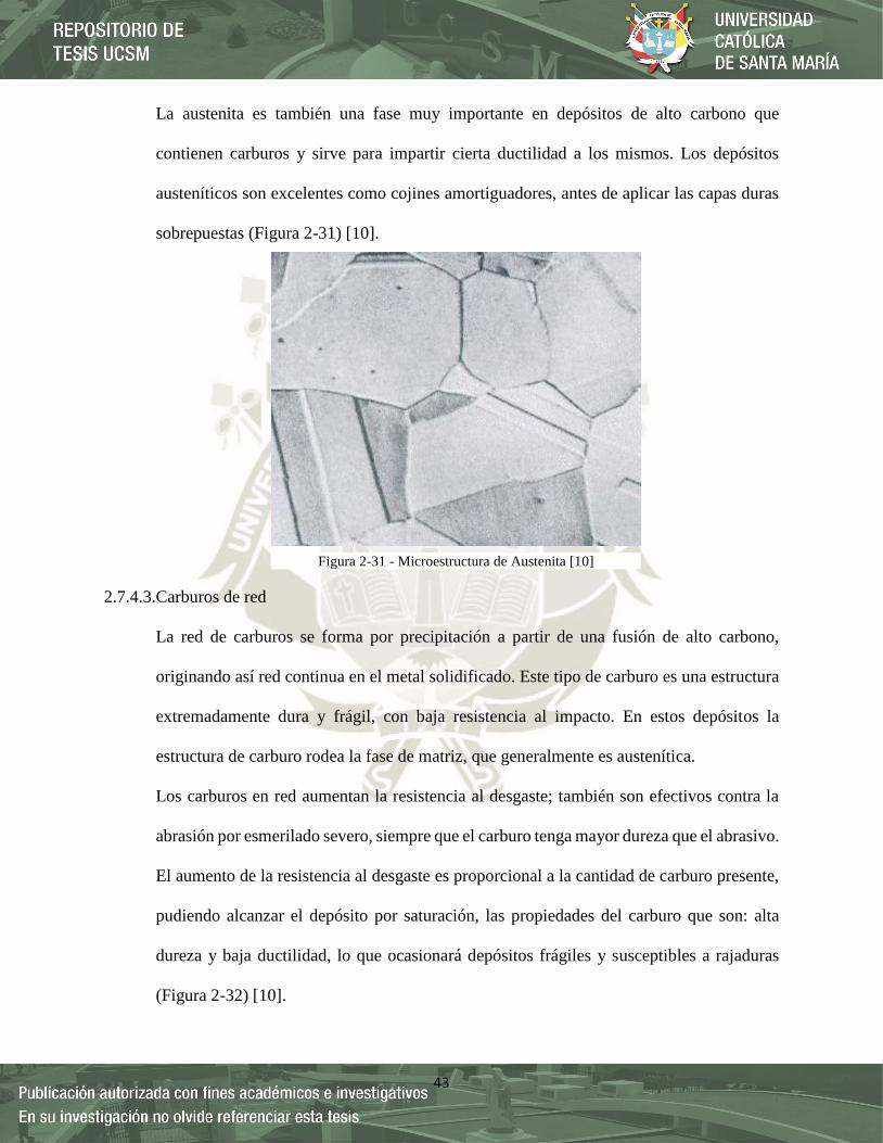
43
La austenita es también una fase muy importante en depósitos de alto carbono que
contienen carburos y sirve para impartir cierta ductilidad a los mismos. Los depósitos
austeníticos son excelentes como cojines amortiguadores, antes de aplicar las capas duras
sobrepuestas (Figura 2-31) [10].
2.7.4.3.Carburos de red
La red de carburos se forma por precipitación a partir de una fusión de alto carbono,
originando así red continua en el metal solidificado. Este tipo de carburo es una estructura
extremadamente dura y frágil, con baja resistencia al impacto. En estos depósitos la
estructura de carburo rodea la fase de matriz, que generalmente es austenítica.
Los carburos en red aumentan la resistencia al desgaste; también son efectivos contra la
abrasión por esmerilado severo, siempre que el carburo tenga mayor dureza que el abrasivo.
El aumento de la resistencia al desgaste es proporcional a la cantidad de carburo presente,
pudiendo alcanzar el depósito por saturación, las propiedades del carburo que son: alta
dureza y baja ductilidad, lo que ocasionará depósitos frágiles y susceptibles a rajaduras
(Figura 2-32) [10].
Figura 2-31 - Microestructura de Austenita [10]
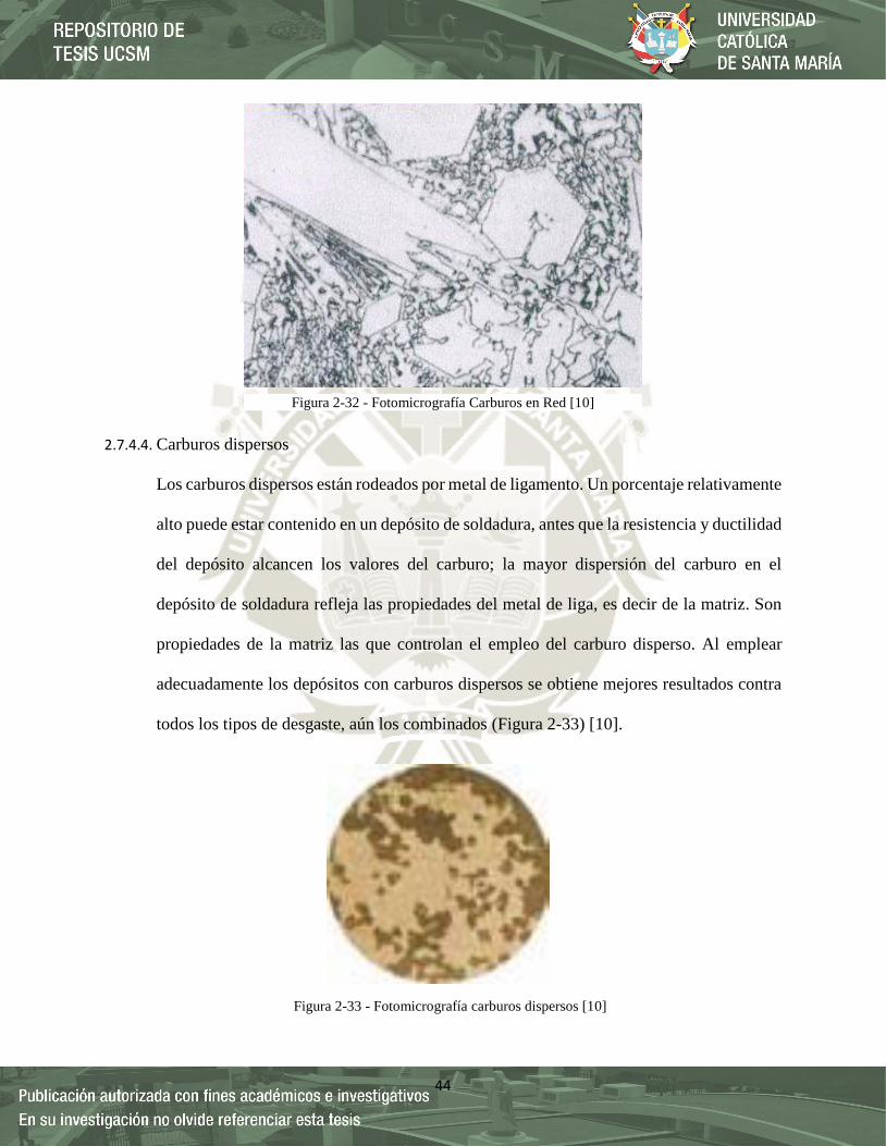
44
2.7.4.4. Carburos dispersos
Los carburos dispersos están rodeados por metal de ligamento. Un porcentaje relativamente
alto puede estar contenido en un depósito de soldadura, antes que la resistencia y ductilidad
del depósito alcancen los valores del carburo; la mayor dispersión del carburo en el
depósito de soldadura refleja las propiedades del metal de liga, es decir de la matriz. Son
propiedades de la matriz las que controlan el empleo del carburo disperso. Al emplear
adecuadamente los depósitos con carburos dispersos se obtiene mejores resultados contra
todos los tipos de desgaste, aún los combinados (Figura 2-33) [10].
Figura 2-32 - Fotomicrografía Carburos en Red [10]
Figura 2-33 - Fotomicrografía carburos dispersos [10]
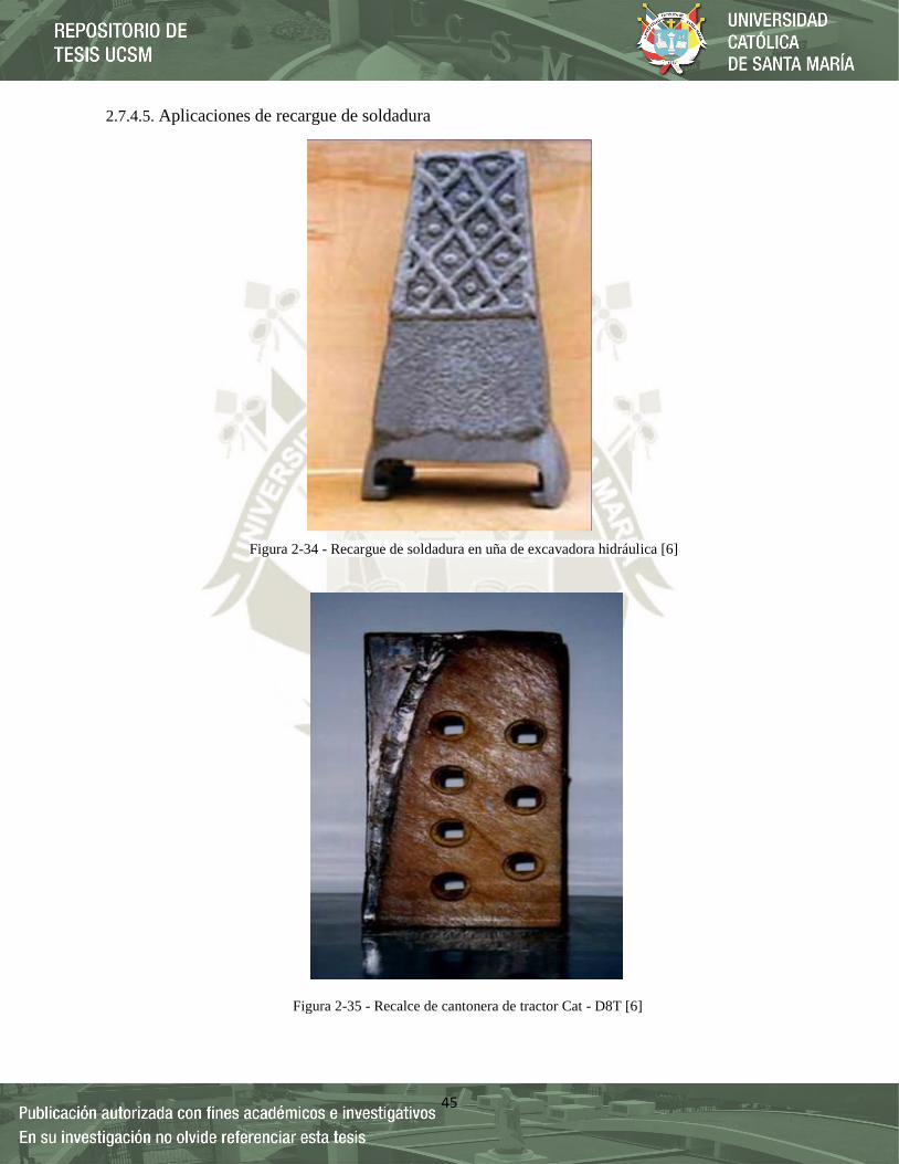
45
2.7.4.5. Aplicaciones de recargue de soldadura
Figura 2-34 - Recargue de soldadura en uña de excavadora hidráulica [6]
Figura 2-35 - Recalce de cantonera de tractor Cat - D8T [6]
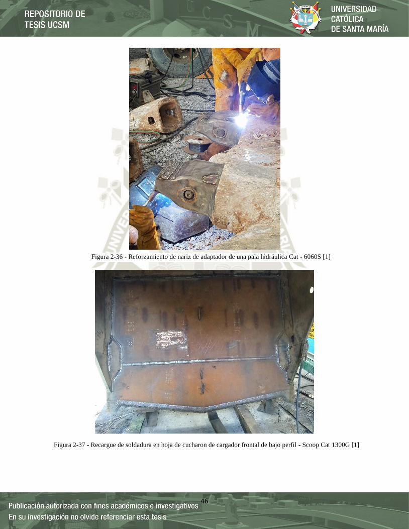
46
Figura 2-36 - Reforzamiento de nariz de adaptador de una pala hidráulica Cat - 6060S [1]
Figura 2-37 - Recargue de soldadura en hoja de cucharon de cargador frontal de bajo perfil - Scoop Cat 1300G [1]
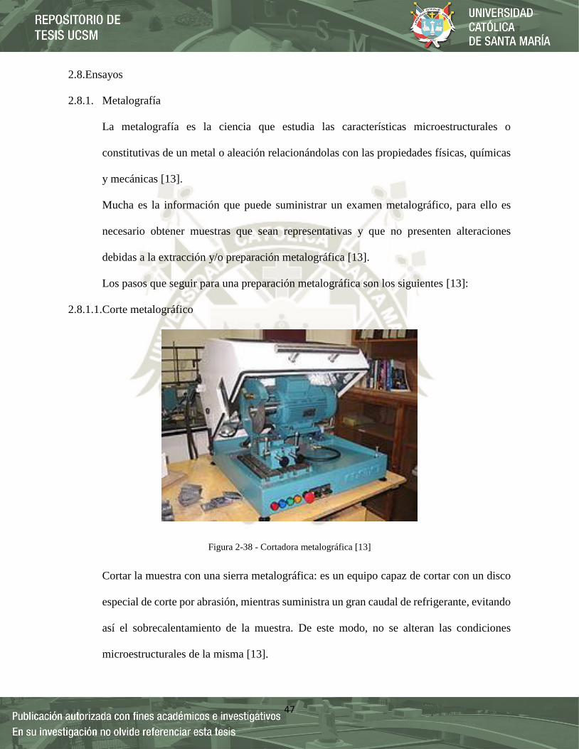
47
2.8.Ensayos
2.8.1. Metalografía
La metalografía es la ciencia que estudia las características microestructurales o
constitutivas de un metal o aleación relacionándolas con las propiedades físicas, químicas
y mecánicas [13].
Mucha es la información que puede suministrar un examen metalográfico, para ello es
necesario obtener muestras que sean representativas y que no presenten alteraciones
debidas a la extracción y/o preparación metalográfica [13].
Los pasos que seguir para una preparación metalográfica son los siguientes [13]:
2.8.1.1.Corte metalográfico
Cortar la muestra con una sierra metalográfica: es un equipo capaz de cortar con un disco
especial de corte por abrasión, mientras suministra un gran caudal de refrigerante, evitando
así el sobrecalentamiento de la muestra. De este modo, no se alteran las condiciones
microestructurales de la misma [13].
Figura 2-38 - Cortadora metalográfica [13]
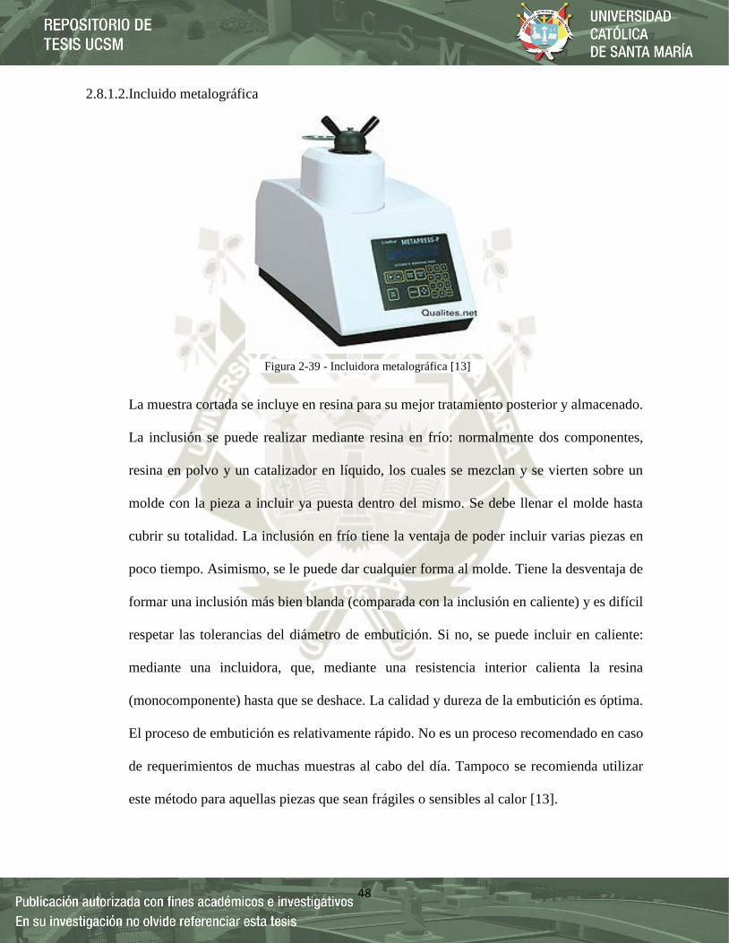
48
2.8.1.2.Incluido metalográfica
La muestra cortada se incluye en resina para su mejor tratamiento posterior y almacenado.
La inclusión se puede realizar mediante resina en frío: normalmente dos componentes,
resina en polvo y un catalizador en líquido, los cuales se mezclan y se vierten sobre un
molde con la pieza a incluir ya puesta dentro del mismo. Se debe llenar el molde hasta
cubrir su totalidad. La inclusión en frío tiene la ventaja de poder incluir varias piezas en
poco tiempo. Asimismo, se le puede dar cualquier forma al molde. Tiene la desventaja de
formar una inclusión más bien blanda (comparada con la inclusión en caliente) y es difícil
respetar las tolerancias del diámetro de embutición. Si no, se puede incluir en caliente:
mediante una incluidora, que, mediante una resistencia interior calienta la resina
(monocomponente) hasta que se deshace. La calidad y dureza de la embutición es óptima.
El proceso de embutición es relativamente rápido. No es un proceso recomendado en caso
de requerimientos de muchas muestras al cabo del día. Tampoco se recomienda utilizar
este método para aquellas piezas que sean frágiles o sensibles al calor [13].
Figura 2-39 - Incluidora metalográfica [13]
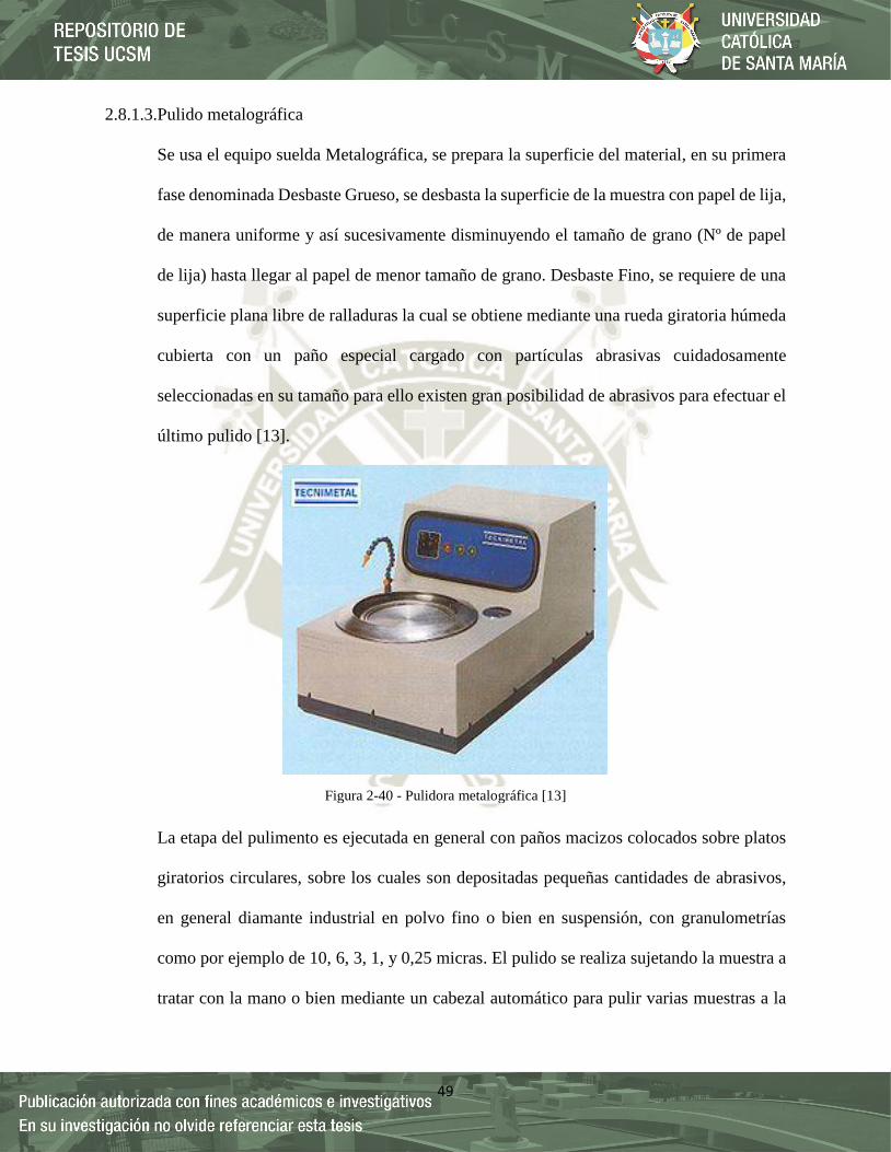
49
2.8.1.3.Pulido metalográfica
Se usa el equipo suelda Metalográfica, se prepara la superficie del material, en su primera
fase denominada Desbaste Grueso, se desbasta la superficie de la muestra con papel de lija,
de manera uniforme y así sucesivamente disminuyendo el tamaño de grano (Nº de papel
de lija) hasta llegar al papel de menor tamaño de grano. Desbaste Fino, se requiere de una
superficie plana libre de ralladuras la cual se obtiene mediante una rueda giratoria húmeda
cubierta con un paño especial cargado con partículas abrasivas cuidadosamente
seleccionadas en su tamaño para ello existen gran posibilidad de abrasivos para efectuar el
último pulido [13].
La etapa del pulimento es ejecutada en general con paños macizos colocados sobre platos
giratorios circulares, sobre los cuales son depositadas pequeñas cantidades de abrasivos,
en general diamante industrial en polvo fino o bien en suspensión, con granulometrías
como por ejemplo de 10, 6, 3, 1, y 0,25 micras. El pulido se realiza sujetando la muestra a
tratar con la mano o bien mediante un cabezal automático para pulir varias muestras a la
Figura 2-40 - Pulidora metalográfica [13]

50
vez. Este ejerce una presión pre-configurada hacia el disco o paño de desbaste o pulido
durante un tiempo concreto. Estos parámetros deben ser configurados según el tipo de
material (dureza, estado del pulido, etc.) [13].
2.8.1.4.Ataque químico
Hay una enormidad de ataques químicos, para diferentes tipos de metales y situaciones. En
general, el ataque es hecho por inmersión o fregado con algodón embebido en el líquido
escogido por la región a ser observada, durante algunos segundos hasta que la estructura o
defecto sea revelada. Uno de los más usados es el nital, (ácido nítrico y alcohol), para la
gran mayoría de los metales ferrosos. Una guía de los ataques químicos utilizados para
revelar las fases y microconstituyentes de metales y aleaciones se pueden ver en la norma
ASTM E407 - 07 Standard Practice for Microetching Metals and Alloys [13].
2.8.1.5.Microscopio
Utilización de lupas estereoscópicas (que favorecen la profundidad de foco y permiten, por
tanto, visión tridimensional del área observada) con aumentos que pueden variar de 5x a
64X [13].
El principal instrumento para la realización de un examen metalográfico lo constituye el
microscopio metalográfico, con el cual es posible examinar una muestra con aumentos que
varían entre 50x y 2000x [13].
El microscopio metalográfico, debido a la opacidad de los metales y aleaciones, opera con
la luz reflejada por el metal. Por lo que para poder observar la muestra es necesario preparar
una probeta y pulir a espejo la superficie. Existe una norma internacional ASTM E3-11
Standard Practice for Preparation of Metallographic Specimens que trata sobre las correctas
técnicas de preparación de muestras metalográficas [13].
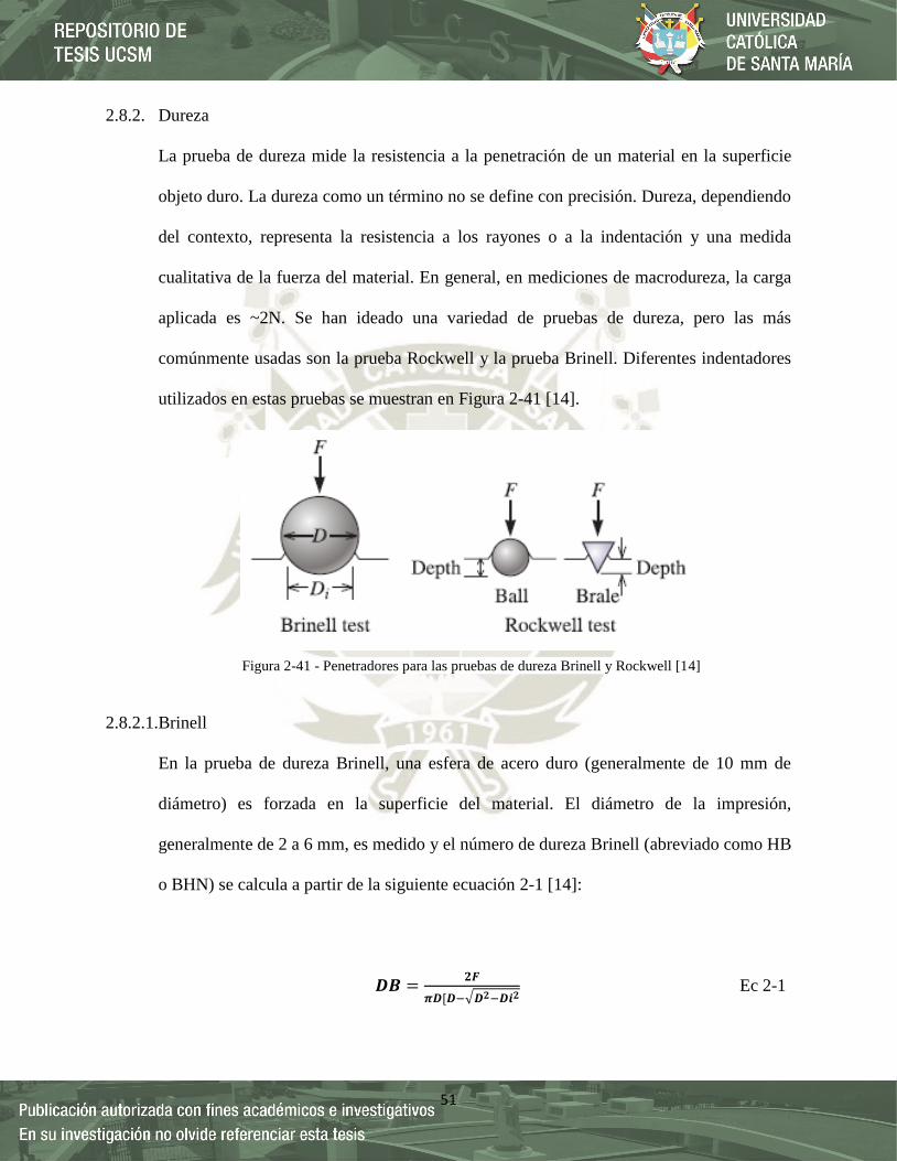
51
2.8.2. Dureza
La prueba de dureza mide la resistencia a la penetración de un material en la superficie
objeto duro. La dureza como un término no se define con precisión. Dureza, dependiendo
del contexto, representa la resistencia a los rayones o a la indentación y una medida
cualitativa de la fuerza del material. En general, en mediciones de macrodureza, la carga
aplicada es ~2N. Se han ideado una variedad de pruebas de dureza, pero las más
comúnmente usadas son la prueba Rockwell y la prueba Brinell. Diferentes indentadores
utilizados en estas pruebas se muestran en Figura 2-41 [14].
2.8.2.1.Brinell
En la prueba de dureza Brinell, una esfera de acero duro (generalmente de 10 mm de
diámetro) es forzada en la superficie del material. El diámetro de la impresión,
generalmente de 2 a 6 mm, es medido y el número de dureza Brinell (abreviado como HB
o BHN) se calcula a partir de la siguiente ecuación 2-1 [14]:
𝑫𝑩 =𝟐𝑭
𝝅𝑫[𝑫−√𝑫𝟐−𝑫𝒊𝟐 Ec 2-1
Figura 2-41 - Penetradores para las pruebas de dureza Brinell y Rockwell [14]

52
donde F es la carga aplicada en kilogramos, D es el diámetro del penetrador en milímetros,
y Di es el diámetro de la impresión en milímetros. La dureza Brinell tiene unidades de
kg/mm2 [14] .
2.8.2.2.RockWell
La prueba de dureza Rockwell utiliza una bola de acero de pequeño diámetro para
materiales blandos y un cono de diamante, o Brale, para materiales más duros. La
profundidad de penetración del indentador es medido automáticamente por la máquina de
prueba y convertido a una dureza Rockwell número (HR). Ya que no es necesaria una
medición óptica de las dimensiones de la hendidura, la prueba de Rockwell tiende a ser
más popular que la de Brinell. Varias variaciones de la Se utiliza la prueba de Rockwell,
incluidas las descritas en la Tabla 6-5. Una prueba Rockwell C (HRC) se utiliza para aceros
duros, mientras que para el aluminio se puede seleccionar una prueba Rockwell F (HRF).
Las pruebas de Rockwell proporcionan un número de dureza que no tiene unidades [14].
Los números de dureza se utilizan principalmente como base cualitativa para la
comparación de materiales (Figura 2-42), las especificaciones de fabricación y tratamiento
térmico, el control de calidad y la correlación con otras propiedades de los materiales. Por
ejemplo, la dureza Brinell está relacionada a la resistencia a la tracción del acero por la
aproximación [14]:
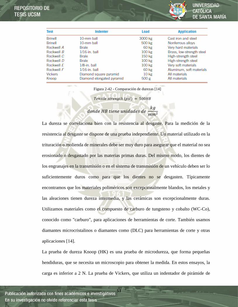
53
𝑇𝑒𝑛𝑠𝑖𝑙𝑒 𝑠𝑡𝑟𝑒𝑛𝑔𝑡ℎ (𝑝𝑠𝑖) = 500𝐻𝐵
𝑑𝑜𝑛𝑑𝑒 𝐻𝐵 𝑡𝑖𝑒𝑛𝑒 𝑢𝑛𝑖𝑑𝑎𝑑𝑒𝑠 𝑑𝑒 𝑘𝑔
𝑚𝑚2
La dureza se correlaciona bien con la resistencia al desgaste. Para la medición de la
resistencia al desgaste se dispone de una prueba independiente. Un material utilizado en la
trituración o molienda de minerales debe ser muy duro para asegurar que el material no sea
erosionado o desgastado por las materias primas duras. Del mismo modo, los dientes de
los engranajes en la transmisión o en el sistema de transmisión de un vehículo deben ser lo
suficientemente duros como para que los dientes no se desgasten. Típicamente
encontramos que los materiales poliméricos son excepcionalmente blandos, los metales y
las aleaciones tienen dureza intermedia, y las cerámicas son excepcionalmente duras.
Utilizamos materiales como el compuesto de carburo de tungsteno y cobalto (WC-Co),
conocido como "carburo", para aplicaciones de herramientas de corte. También usamos
diamantes microcristalinos o diamantes como (DLC) para herramientas de corte y otras
aplicaciones [14].
La prueba de dureza Knoop (HK) es una prueba de microdureza, que forma pequeñas
hendiduras, que se necesita un microscopio para obtener la medida. En estos ensayos, la
carga es inferior a 2 N. La prueba de Vickers, que utiliza un indentador de pirámide de
Figura 2-42 - Comparación de durezas [14]
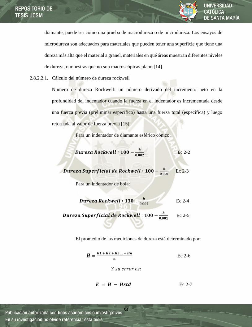
54
diamante, puede ser como una prueba de macrodureza o de microdureza. Los ensayos de
microdureza son adecuados para materiales que pueden tener una superficie que tiene una
dureza más alta que el material a granel, materiales en qué áreas muestran diferentes niveles
de dureza, o muestras que no son macroscópicas plano [14].
2.8.2.2.1. Cálculo del número de dureza rockwell
Numero de dureza Rockwell: un número derivado del incremento neto en la
profundidad del indentador cuando la fuerza en el indentador es incrementada desde
una fuerza previa (preliminar específico) hasta una fuerza total (específica) y luego
retornada al valor de fuerza previa [15].
Para un indentador de diamante esférico cónico:
𝑫𝒖𝒓𝒆𝒛𝒂 𝑹𝒐𝒄𝒌𝒘𝒆𝒍𝒍 ∶ 𝟏𝟎𝟎 −𝒉
𝟎.𝟎𝟎𝟐 Ec 2-2
𝑫𝒖𝒓𝒆𝒛𝒂 𝑺𝒖𝒑𝒆𝒓𝒇𝒊𝒄𝒊𝒂𝒍 𝒅𝒆 𝑹𝒐𝒄𝒌𝒘𝒆𝒍𝒍 ∶ 𝟏𝟎𝟎 −𝒉
𝟎.𝟎𝟎𝟏 Ec 2-3
Para un indentador de bola:
𝑫𝒖𝒓𝒆𝒛𝒂 𝑹𝒐𝒄𝒌𝒘𝒆𝒍𝒍 ∶ 𝟏𝟑𝟎 −𝒉
𝟎.𝟎𝟎𝟐 Ec 2-4
𝑫𝒖𝒓𝒆𝒛𝒂 𝑺𝒖𝒑𝒆𝒓𝒇𝒊𝒄𝒊𝒂𝒍 𝒅𝒆 𝑹𝒐𝒄𝒌𝒘𝒆𝒍𝒍 ∶ 𝟏𝟎𝟎 −𝒉
𝟎.𝟎𝟎𝟏 Ec 2-5
El promedio de las mediciones de dureza está determinado por:
�� =𝑯𝟏 + 𝑯𝟐 + 𝑯𝟑 … + 𝑯𝒏
𝒏 Ec 2-6
𝑌 𝑠𝑢 𝑒𝑟𝑟𝑜𝑟 𝑒𝑠:
𝑬 = 𝑯 − 𝑯𝒔𝒕𝒅 Ec 2-7

55
Donde Hstd es un promedio de dureza certificada, estandarizado según el material utilizado
[15].
2.8.3. Tracción
La prueba de tracción es popular ya que las propiedades obtenidas se pueden aplicar al
diseño diferente componentes. La prueba de tracción mide la resistencia de un material a
una carga estática o lentamente fuerza aplicada. Las tasas de deformación en una prueba
de tracción son típicamente pequeñas (10-4 a 10-2 s-1). Una prueba la configuración se
muestra en la Figura 2-43; una muestra típica tiene un diámetro de 0,505 pulgadas y un
instrumento longitud de 2 pulg. La muestra se coloca en la máquina de prueba y una fuerza
F, llamada carga, Está aplicado. Una máquina de prueba universal en la que las pruebas de
tracción y compresión pueden ser realizado a menudo se utiliza. Un medidor de tensión o
extensómetro se utiliza para medir la cantidad que la muestra se estira entre las marcas del
medidor cuando se aplica la fuerza. Por lo tanto, el cambio en longitud de la muestra (Δl)
se mide con respecto a la longitud original (l0). La información sobre la resistencia, el
módulo de Young y la ductilidad de un material puede ser obtenido a partir de dicha prueba
de tracción. Por lo general, se realiza una prueba de tracción en metales, aleaciones, y
plásticos. Las pruebas de tracción se pueden usar para cerámica; sin embargo, estos no son
muy populares porque la muestra puede fracturarse mientras se alinea. La siguiente
discusión principalmente se aplica a las pruebas de tracción de metales y aleaciones [14].

56
2.8.3.1.Esfuerzo y deformación Ingenieril
Se aplican los resultados de una prueba única a todos los tamaños y secciones transversales
de especímenes para un material dado si convertimos la fuerza en esfuerzo y la distancia
entre las marcas de calibración para deformar. El esfuerzo ingenieril y la deformación
ingenieril se definen por las siguientes ecuaciones 2-8 y 2-9 [14]:
Esfuerzo Ingenieril = 𝑺 =𝑭
𝑨𝟎 Ec 2-8
Deformación Ingenieril = 𝒆 =𝜟𝒍
𝒍𝟎 Ec 2-9
donde A0 es el área de sección transversal original de la muestra antes de que comience la
prueba, l0 es la distancia original entre las marcas del medidor, y Δl es el cambio en la
longitud después de que la fuerza F es aplicado [14].
Figura 2-43 - Se aplica una fuerza unidireccional a una muestra en la prueba de tracción
por medio de la cruceta móvil. El movimiento de la cruceta puede ser realizado con
tornillos o un mecanismo hidráulico [14]

57
La Figura 2-44 muestra cualitativamente las curvas de tensión y deformación para un metal
típico (a), (b) material termoplástico, (c) elastómero, y (d) cerámica (o vidrio) en
condiciones relativamente pequeñas tasas de deformación Las escalas en esta figura son
cualitativas y diferentes para cada material [14].
2.8.3.2.Medición de las dimensiones de las muestras de ensayo:
Probetas estándar para la prueba de tensión rectangular - Estas formas de probetas se
muestran en la Figura 2-45. Para determinar el área de la sección transversal, la dimensión
de la anchura central se medirá con una precisión de 0,005 pulg. (0,13 mm) para el modelo
de 8 pulgadas (200 mm) de longitud de calibre y 0,001 pulg. (0,025 mm) para la muestra
de longitud de calibre 2" (50 mm) en la Figura 2-45. La dimensión del espesor central se
medirá con una precisión de 0,001 pulgadas para ambas muestras [16].
Figura 2-44 - Curvas de esfuerzo y deformación para diferentes materiales. Tenga en cuenta que
estos son cualitativos. Las magnitudes de las tensiones y las tensiones no deben ser comparadas [14]

58
Probetas de prueba de tensión redondas estándar: estas Las formas de las muestras se
muestran en las Figura 2-46. Para determinar el área de la sección transversal, el diámetro
deberá ser medida en el centro de la longitud del gálibo con precisión 0,001 pulg. (0,025
mm) [16].
Figura 2-45 - Muestras de prueba de tensión rectangular [16]
Figura 2-46 - Estándar de 0.500 pulg. (12.5 mm) Muestra de prueba de tensión redonda con 2 pulg. (50
mm) de longitud de calibre y ejemplos de muestras de tamaño pequeño [16]

59
2.8.4. Desgaste
2.8.4.1.Ensayo de tribología– Norma ASTM G99
Este método de ensayo abarca un procedimiento de laboratorio para determinar el desgaste
de los materiales durante el deslizamiento mediante un aparato pin-on-disk. Los materiales
se prueban en pares bajo condiciones nominalmente no abrasivas. Las principales áreas de
atención experimental en el uso de este tipo de aparatos para se describen las medidas de
desgaste. El coeficiente de fricción puede también ser determinado [17].
Este método de prueba estándar utiliza un conjunto específico de pruebas parámetros
(carga, velocidad de deslizamiento, materiales, etc.) que fueron entonces utilizado en un
estudio interlaboratorios (ILS), cuyos resultados son los siguientes (Figura 2-47 y 2-48).
(Esto satisface la forma ASTM en que "Las instrucciones para realizar la prueba deben
incluir todas de los detalles esenciales en cuanto a aparatos, muestras de prueba, y los
cálculos necesarios para lograr un resultado satisfactorio. precisión y sesgo.") Cualquier
usuario debe informar de que "siguió los requisitos de la norma ASTM G99", cuando esto
sea cierto [17].
Figura 2-47 - Características de las muestras de prueba de desgaste entre laboratorios [17]

60
Para el ensayo de desgaste pin-on-disk se necesitan dos probetas. Uno de ellos, un pasador
con una punta de radio está posicionado perpendicularmente a la otra, normalmente un
disco circular plano. Una pelota, rígidamente se utiliza a menudo como espécimen de
alfiler. La máquina de prueba hace que la probeta de disco o la probeta de pasador giren
sobre el centro del disco. En cualquier caso, la trayectoria de deslizamiento es un círculo
en la superficie del disco. El plano del plato ya sea horizontal o verticalmente [17].
La probeta se presiona contra el disco a una distancia de carga especificada, normalmente
por medio de un brazo o una palanca y pesos adjuntos. Se han utilizado otros métodos de
carga, tales como hidráulico o neumático [17].
Los resultados de desgaste se informan como pérdida de volumen en milímetros cúbicos
para el pasador y el disco por separado. Cuando se prueban dos materiales diferentes, se
recomienda que cada material se pruebe tanto en la posición del pasador como en la del
disco [17].
Figura 2-48 - Resultados de la prueba Inter laboratorio [17]

61
La cantidad de desgaste se determina mediante la medición de dimensiones lineales de
ambas muestras antes y después del ensayo, o bien pesando ambas muestras antes y
después del ensayo. Si se utilizan medidas lineales de desgaste, el cambio de longitud o de
forma cambio del perno, y el cambio de profundidad o forma del disco de desgaste (en
milímetros) están determinadas por cualquier técnica metrológica, como la medición
electrónica de distancia o el perfilado del palpador. Las medidas lineales de desgaste se
convierten en desgaste volumen (en milímetros cúbicos) utilizando la geometría apropiada
relaciones. Las medidas lineales de desgaste se utilizan con frecuencia en ya que la pérdida
de masa es a menudo demasiado pequeña para medirla con precisión. Si se mide la pérdida
de masa, el valor de pérdida de masa se convierte a pérdida de volumen (en milímetros
cúbicos) utilizando un valor apropiado para la densidad del espécimen [17].
Los resultados de desgaste suelen obtenerse mediante la realización de una prueba para una
distancia de deslizamiento seleccionada y para valores de carga seleccionados y velocidad.
En la Figura 2-49 se presenta un conjunto de condiciones de prueba que se utilizaron en
una serie de mediciones inter-laboratorios. Se pueden seleccionar otras condiciones de
prueba dependiendo del propósito de la prueba. En tales casos, el usuario debe reportar sus
resultados como "siguiendo el procedimiento de ASTM G99" [17].
Figura 2-49 - Parámetros de prueba utilizados para pruebas Inter laboratorios [17]
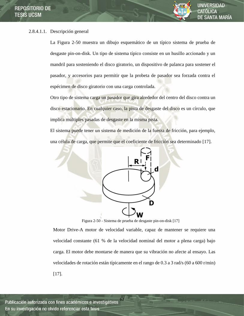
62
2.8.4.1.1. Descripción general
La Figura 2-50 muestra un dibujo esquemático de un típico sistema de prueba de
desgaste pin-on-disk. Un tipo de sistema típico consiste en un husillo accionado y un
mandril para sosteniendo el disco giratorio, un dispositivo de palanca para sostener el
pasador, y accesorios para permitir que la probeta de pasador sea forzada contra el
espécimen de disco giratorio con una carga controlada.
Otro tipo de sistema carga un pasador que gira alrededor del centro del disco contra un
disco estacionario. En cualquier caso, la pista de desgaste del disco es un círculo, que
implica múltiples pasadas de desgaste en la misma pista.
El sistema puede tener un sistema de medición de la fuerza de fricción, para ejemplo,
una célula de carga, que permite que el coeficiente de fricción sea determinado [17].
Motor Drive-A motor de velocidad variable, capaz de mantener se requiere una
velocidad constante (61 % de la velocidad nominal del motor a plena carga) bajo
carga. El motor debe montarse de manera que su vibración no afecte al ensayo. Las
velocidades de rotación están típicamente en el rango de 0.3 a 3 rad/s (60 a 600 r/min)
[17].
Figura 2-50 - Sistema de prueba de desgaste pin-on-disk [17]
63
Contador de revoluciones-La máquina debe estar equipada con un contador de
revoluciones o su equivalente que registre el número de revoluciones del disco, y
preferiblemente tenga la capacidad de apagar la máquina después de un número
preseleccionado de revoluciones [17].
Portamuestras y brazo de palanca - En un sistema típico, el portamuestras estacionario
se fija a un brazo de palanca que tiene un pivote. La adición de pesas, como una
opción de carga, produce una fuerza de prueba proporcional a la masa de las pesas
aplicadas. Lo ideal es que el pivote del brazo esté situado en el plano del contacto de
desgaste para evitar fuerzas de carga extrañas debidas a la fricción de deslizamiento
[17]. El soporte del pasador y el brazo deben ser de construcción sustancial para
reducir el movimiento vibratorio durante la prueba [17].
Sistemas de medición de desgaste: los instrumentos para obtener medidas lineales de
desgaste deben tener una sensibilidad de 2,5 μm o superior [17].
Cualquier balanza utilizada para medir la pérdida de masa de la muestra de ensayo
deberá tener una sensibilidad de 0,1 mg o superior; en situaciones de bajo desgaste
puede ser necesaria una sensibilidad mayor [17].
2.8.4.1.2. Cálculo y elaboración de informes
Las medidas de desgaste deben ser reportadas como la pérdida de volumen en
milímetros cúbicos para el pasador y el disco, por separado [17].
Utilice las siguientes ecuaciones 2-10, 2-11 para calcular el volumen pérdidas cuando
el pasador tiene inicialmente una forma de extremo esférica de radio R y el disco es
inicialmente plano, bajo las condiciones que sólo uno de los dos miembros lleva un
desgaste significativo [17]:
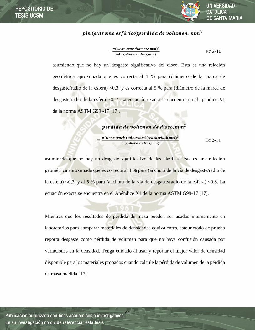
64
𝒑𝒊𝒏 (𝒆𝒙𝒕𝒓𝒆𝒎𝒐 𝒆𝒔𝒇é𝒓𝒊𝒄𝒐)𝒑é𝒓𝒅𝒊𝒅𝒂 𝒅𝒆 𝒗𝒐𝒍𝒖𝒎𝒆𝒏, 𝒎𝒎𝟑
=𝝅(𝒘𝒆𝒂𝒓 𝒔𝒄𝒂𝒓 𝒅𝒊𝒂𝒎𝒆𝒕𝒆,𝒎𝒎)𝟒
𝟔𝟒 (𝒔𝒑𝒉𝒆𝒓𝒆 𝒓𝒂𝒅𝒊𝒖𝒔,𝒎𝒎) Ec 2-10
asumiendo que no hay un desgaste significativo del disco. Esta es una relación
geométrica aproximada que es correcta al 1 % para (diámetro de la marca de
desgaste/radio de la esfera) <0,3, y es correcta al 5 % para (diámetro de la marca de
desgaste/radio de la esfera) <0,7. La ecuación exacta se encuentra en el apéndice X1
de la norma ASTM G99 -17 [17].
𝒑é𝒓𝒅𝒊𝒅𝒂 𝒅𝒆 𝒗𝒐𝒍𝒖𝒎𝒆𝒏 𝒅𝒆 𝒅𝒊𝒔𝒄𝒐,𝒎𝒎𝟑
=𝝅(𝒘𝒆𝒂𝒓 𝒕𝒓𝒂𝒄𝒌 𝒓𝒂𝒅𝒊𝒖𝒔,𝒎𝒎)(𝒕𝒓𝒂𝒄𝒌 𝒘𝒊𝒅𝒕𝒉,𝒎𝒎)𝟑
𝟔 (𝒔𝒑𝒉𝒆𝒓𝒆 𝒓𝒂𝒅𝒊𝒖𝒔,𝒎𝒎) Ec 2-11
asumiendo que no hay un desgaste significativo de las clavijas. Esta es una relación
geométrica aproximada que es correcta al 1 % para (anchura de la vía de desgaste/radio de
la esfera) <0,3, y al 5 % para (anchura de la vía de desgaste/radio de la esfera) <0,8. La
ecuación exacta se encuentra en el Apéndice X1 de la norma ASTM G99-17 [17].
Mientras que los resultados de pérdida de masa pueden ser usados internamente en
laboratorios para comparar materiales de densidades equivalentes, este método de prueba
reporta desgaste como pérdida de volumen para que no haya confusión causada por
variaciones en la densidad. Tenga cuidado al usar y reportar el mejor valor de densidad
disponible para los materiales probados cuando calcule la pérdida de volumen de la pérdida
de masa medida [17].

65
Utilice la siguiente ecuación 2-12 para la conversión de masa pérdida a pérdida de volumen
[17].
𝒗𝒐𝒍𝒖𝒎𝒆 𝒍𝒐𝒔𝒔,𝒎𝒎𝟑 =𝒎𝒂𝒔𝒔 𝒍𝒐𝒔𝒔,𝒈
𝒅𝒆𝒏𝒔𝒊𝒕𝒚,𝒈/𝒄𝒎𝟑∗ 𝟏𝟎𝟎𝟎 Ec 2-12
2.9.Descripción de la Excavadora Hidráulica CAT 336D2L
Es una unidad mecánica hidráulica que está compuesta por dos bastidores. Un bastidor
principal en cual están montados los bastidores del tren de rodamiento con motores de
propulsión y el bastidor superior. Un bastidor superior o de rotación en cual está montado la
cabina, el motor, bombas hidráulicas, motores de rotación, cojinetes de rotación, la pluma, el
brazo y la cuchara. El accionamiento obtenido en la excavadora está basado en la hidráulica,
la fuerza necesaria para mover estas bombas lo proporciona el motor Diésel con que está
equipado [18].
Funciones de Equipo
Carga de camiones en excavaciones de corte
Carga de materiales para planta de agregados y asfalto
Carga de material sub-base para carreteras
Alcantarillado y postura de tubería
Grandes movimientos de tierra

66
2.9.1. Especificaciones de la Excavadora Hidráulica CAT 336D2/D2 L
Figura 2-51 - Excavadora Hidráulica Cat 336D2 L [19]
Figura 2-52 - Especificaciones de la Excavadora Hidráulica 336D2/D2 L [19]

67
Figura 2-53 - Especificaciones de la Excavadora Hidráulica 336D2/D2 L [19]

68
2.9.2. Partes de la excavadora Hidráulica CAT 336D2/D2 L
1. Punto de Unión entre brazo y pluma
2. Cilindro hidráulico del cucharon
3. Brazo
4. Eslabón de articulación
5. Cucharon
6. Trenes de Rodaje
7. Chasis o Bastidor
8. Compartimiento del motor
9. Cabina de operador
10. Cilindro hidráulico de Pluma
11. Pluma o Boom
12. Cilindro hidráulico del brazo
Figura 2-54 - Partes de la excavadora Hidráulica 336D2/D2 L [1]

69
2.9.2.1.Cucharon 3.2 yd3
Figura 2-55 - Cucharon 3.2 yd3 de excavadora hidráulica Cat 336D2 L [20]

70
2.9.2.1.1. Conjunto de piezas del Cucharon
Figura 2-56 - Conjuntos de piezas de cucharon [20]

71
2.9.2.1.2. Uña K-130 (32MnCrMo6-4-3)
Figura 2-57 - Uña K-130 (32MnCrMo6-4-3) de excavadora hidráulica Cat 336D2 L [20]
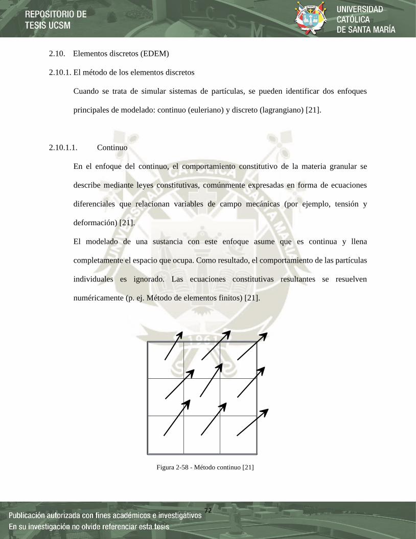
72
2.10. Elementos discretos (EDEM)
2.10.1. El método de los elementos discretos
Cuando se trata de simular sistemas de partículas, se pueden identificar dos enfoques
principales de modelado: continuo (euleriano) y discreto (lagrangiano) [21].
2.10.1.1. Continuo
En el enfoque del continuo, el comportamiento constitutivo de la materia granular se
describe mediante leyes constitutivas, comúnmente expresadas en forma de ecuaciones
diferenciales que relacionan variables de campo mecánicas (por ejemplo, tensión y
deformación) [21].
El modelado de una sustancia con este enfoque asume que es continua y llena
completamente el espacio que ocupa. Como resultado, el comportamiento de las partículas
individuales es ignorado. Las ecuaciones constitutivas resultantes se resuelven
numéricamente (p. ej. Método de elementos finitos) [21].
Figura 2-58 - Método continuo [21]

73
2.10.1.2. Discreto
En contraste con el enfoque continuo, los enfoques discretos modelan cada partícula como
una entidad distinta y representan el material granular como un conjunto idealizado de
partículas. El comportamiento general del sistema (macroscópico) resulta de las
interacciones individuales de las partículas [21].
Esto hace que el enfoque discreto sea muy bueno para investigar fenómenos que ocurren
en la escala de longitud del diámetro de las partículas y para simular el comportamiento a
granel de las partículas [21].
2.10.1.3. Acoplamiento dem y cosimulaciones
2.10.1.3.1. DEM-MBD
El acoplamiento DEM con paquetes de dinámica multicuerpo (MBD) permite a los
usuarios realizar simulaciones con control programático del movimiento de la
geometría y la física, lo que permite la implementación de movimientos de cuerpos
rígidos y complejos [21].
Figura 2-59 - Método discreto [21]

74
Las fuerzas de materiales a granel que actúan sobre las superficies de los equipos
calculadas por el software DEM pueden ser recuperadas por el código acoplado para
obtener una cinemática de equipo realista [21].
2.10.1.3.2. DEM-CFD
DEM también puede utilizarse en combinación con la dinámica de fluidos
computacional (CFD) para investigar el comportamiento de las partículas en fase
fluida. El movimiento sólido y fluido se resuelve mediante las ecuaciones de
movimiento de Newton para partículas discretas y las ecuaciones de Navier-Stokes para
el fluido continuo [21].
El acoplamiento se basa en el intercambio continuo de información entre el software
DEM y CFD. Se pueden utilizar varios modelos de arrastre para la interacción
partícula-fluido [21].
2.10.1.3.3. DEM-FEA
El software DEM puede proporcionar fuerzas y distribuciones de presión realistas del
material que actúa sobre el equipo. Estas cargas pueden ser utilizadas como insumos
en el análisis estructural o de fatiga en cualquier software de análisis de elementos
finitos (FEA) [21].
Figura 2-60 - Simulación DEM-MBD de una cuchara de arrastre (Cortesía de VR Steel), modelo DEM-
CFD de dinámica de flotación de partículas (Cortesía de la Universidad de Utah) y acoplamiento DEM-
FEA utilizado para analizar las cargas de la cuchara del camión volquete (Cortesía de Austin Engineering)
[21]

75
.
CAPÍTULO III

76
3. INGENIERÍA DE PROYECTO
3.1.Análisis mediante elementos discretos al desgaste de las uñas 32MnCrMo6-4-3 y sus
Revestimientos aplicados mediante Elementos Discretos.
En este capítulo se realizó una simulación del desgaste del cucharon en general, uñas de Acero
32MnCrMo6-4-3 y los revestimientos aplicados a las uñas (Citomangan, Exadur 43, Citodur –
1000) en el orden descrito. Para verificar el desgaste, se utilizó el Software de Elementos
Discretos EDEM.
3.1.1. Secuencia de Simulación EDEM
Los pasos por seguir fueron los siguientes:
3.1.1.1.EDEM Creator: creando materiales
Acá la principal interacción que tendrá será el mineral será con el Acero 32MnCrMo6-4-
3.
Figura 3-1 - Creación de mineral a simular [1]
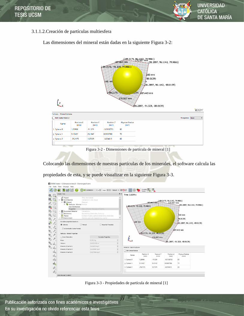
77
3.1.1.2.Creación de partículas multiesfera
Las dimensiones del mineral están dadas en la siguiente Figura 3-2:
Colocando las dimensiones de nuestras partículas de los minerales, el software calcula las
propiedades de esta, y se puede visualizar en la siguiente Figura 3-3.
Figura 3-2 - Dimensiones de partícula de mineral [1]
Figura 3-3 - Propiedades de partícula de mineral [1]
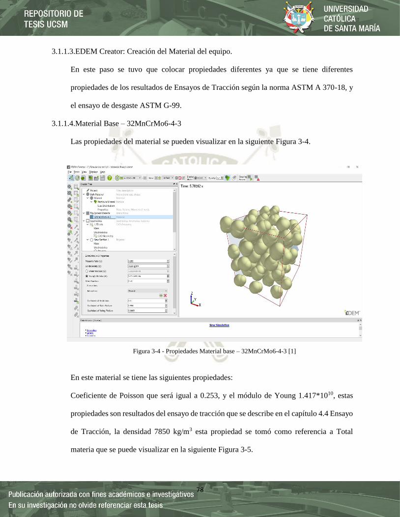
78
3.1.1.3.EDEM Creator: Creación del Material del equipo.
En este paso se tuvo que colocar propiedades diferentes ya que se tiene diferentes
propiedades de los resultados de Ensayos de Tracción según la norma ASTM A 370-18, y
el ensayo de desgaste ASTM G-99.
3.1.1.4.Material Base – 32MnCrMo6-4-3
Las propiedades del material se pueden visualizar en la siguiente Figura 3-4.
En este material se tiene las siguientes propiedades:
Coeficiente de Poisson que será igual a 0.253, y el módulo de Young 1.417*1010, estas
propiedades son resultados del ensayo de tracción que se describe en el capítulo 4.4 Ensayo
de Tracción, la densidad 7850 kg/m3 esta propiedad se tomó como referencia a Total
materia que se puede visualizar en la siguiente Figura 3-5.
Figura 3-4 - Propiedades Material base – 32MnCrMo6-4-3 [1]

79
Para el coeficiente de restitución se pondrá un valor aproximado de 0.5 ya que este valor
comprende entre 0 y 1 indica en un choque inelástico.
El coeficiente de fricción es igual 0.594 y es el resultado del ensayo de desgaste realizado
en el capítulo 4.5, se puede visualizar en la siguiente Figura 3-6.
Figura 3-5 - Propiedades Físicas del Material base – 32MnCrMo6-4-3 [22]
Figura 3-6 - Resultados ensayo de desgaste – Base 32MnCrMo6-4-3 [1]

80
El coeficiente por fricción será igual a 0.0005 a la rodadura, según la Figura 3-7 a
continuación en el que tomamos como referencia un contacto acero con acero.
3.1.1.5.Material Base – Citomangan
Las propiedades del material fueron obtenidas se puede visualizar en la siguiente Figura 3-
8.
Figura 3-7 - Coeficiente de fricción a la roladura [15]
Figura 3-8 - Propiedades Material base – Citomangan [1]
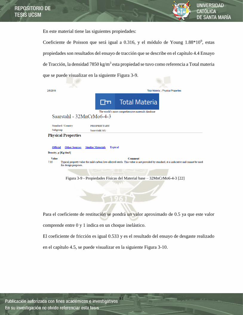
81
En este material tiene las siguientes propiedades:
Coeficiente de Poisson que será igual a 0.316, y el módulo de Young 1.88*109, estas
propiedades son resultados del ensayo de tracción que se describe en el capítulo 4.4 Ensayo
de Tracción, la densidad 7850 kg/m3 esta propiedad se tuvo como referencia a Total materia
que se puede visualizar en la siguiente Figura 3-9.
Para el coeficiente de restitución se pondrá un valor aproximado de 0.5 ya que este valor
comprende entre 0 y 1 indica en un choque inelástico.
El coeficiente de fricción es igual 0.533 y es el resultado del ensayo de desgaste realizado
en el capítulo 4.5, se puede visualizar en la siguiente Figura 3-10.
Figura 3-9 - Propiedades Físicas del Material base – 32MnCrMo6-4-3 [22]
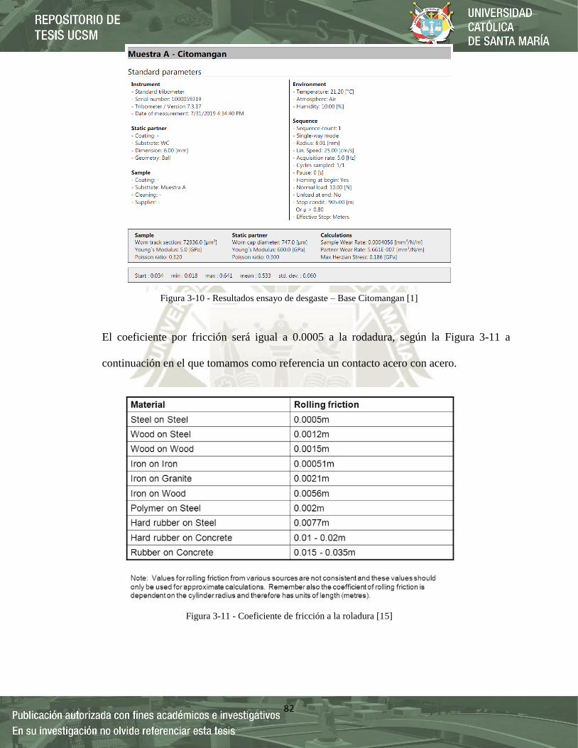
82
El coeficiente por fricción será igual a 0.0005 a la rodadura, según la Figura 3-11 a
continuación en el que tomamos como referencia un contacto acero con acero.
Figura 3-10 - Resultados ensayo de desgaste – Base Citomangan [1]
Figura 3-11 - Coeficiente de fricción a la roladura [15]

83
3.1.1.6.Material Base – Exadur – 43
Las propiedades del material fueron obtenidas se puede visualizar en la siguiente Figura
3-12.
En este material tiene las siguientes propiedades:
Coeficiente de Poisson que será igual a 0.262 y el módulo de Young 4.55*109, estas
propiedades son resultados del ensayo de tracción que se describe en el capítulo 4.4 Ensayo
de Tracción, a densidad 7850 kg/m3 esta propiedad se tuvo como referencia a Total materia
que se puede visualizar en la siguiente Figura 3-13.
Figura 3-12 - Propiedades Material base – Exadur 43 [1]
Figura 3-13 - Propiedades Físicas del Material base – 32MnCrMo6-4-3 [22]
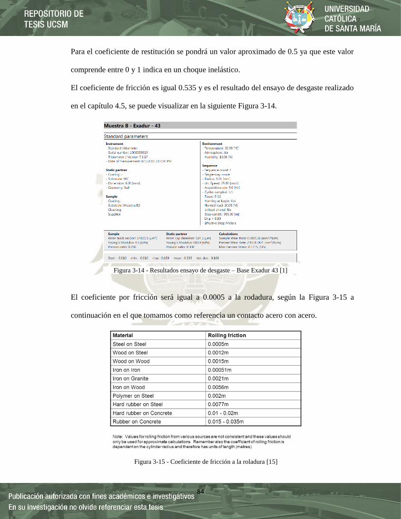
84
Para el coeficiente de restitución se pondrá un valor aproximado de 0.5 ya que este valor
comprende entre 0 y 1 indica en un choque inelástico.
El coeficiente de fricción es igual 0.535 y es el resultado del ensayo de desgaste realizado
en el capítulo 4.5, se puede visualizar en la siguiente Figura 3-14.
El coeficiente por fricción será igual a 0.0005 a la rodadura, según la Figura 3-15 a
continuación en el que tomamos como referencia un contacto acero con acero.
Figura 3-14 - Resultados ensayo de desgaste – Base Exadur 43 [1]
Figura 3-15 - Coeficiente de fricción a la roladura [15]

85
3.1.1.7. Material Base – Citodur 1000
Las propiedades del material fueron obtenidas se puede visualizar en la siguiente Figura 3-
16.
En este material tiene las siguientes propiedades:
Coeficiente de Poisson que será igual a 0.262 y el módulo de Young 4.065*109, estas
propiedades son resultados del ensayo de tracción que se describe en el capítulo 4.4 Ensayo
de Tracción, la densidad 7850 kg/m3 esta propiedad se tuvo como referencia a Total materia
que se puede visualizar en la siguiente Figura 3-17.
Figura 3-16 - Propiedades Material base – Citodur 1000 [1]
Figura 3-17 - Propiedades Físicas del Material base – 32MnCrMo6-4-3 [22]

86
Para el coeficiente de restitución se pondrá un valor aproximado de 0.5 ya que este valor
comprende entre 0 y 1 indica en un choque inelástico.
El coeficiente de fricción es igual 0.534 y es el resultado del ensayo de desgaste realizado
en el capítulo 4.5, se puede visualizar en la siguiente Figura 3-18.
El coeficiente por fricción será igual a 0.0005 a la rodadura, según la Figura 3-19 a
continuación en el que tomamos como referencia un contacto acero con acero.
Figura 3-18 - Resultados ensayo de desgaste – Base Exadur 43 [1]
Figura 3-19 - Coeficiente de fricción a la roladura [15]

87
3.1.1.8.EDEM Creator: sección de geometrías
Las secciones de geometría se utilizan para crear el entorno en el que actúa el Mineral. En
este paso se procedió a importar dos Geometrías, el cucharon con todas las piezas, esto
para poder visualizar las partes más afectadas (Desgaste), y el adaptador con la uña K -130.
Cabe recalcar que se trabajó en mm y se unió todas las piezas en una sola geometría. Se
pueden visualizar en las siguientes Figuras 3-20 y 3-21
Figura 3-20 - Importación de geometría [1]
Figura 3-21 - Importación de geometría – uña y adaptador [1]

88
3.1.1.9.Creación de piezas de geometría incorporada
En este paso se procede a crear una geometría virtual, 500 mm x 200 mm de color rojo
transparente. Esta geometría nos servirá para la creación del mineral y la interacción con
el material Acero. Se puede observar en las siguientes Figuras 3-22 y 3-23.
Figura 3-23 - Parámetros de geometría virtual [1]
Figura 3-22 - Creación de geometría virtual [1]
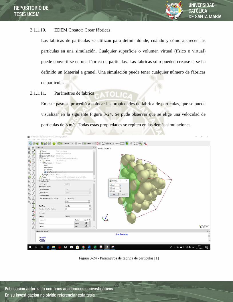
89
3.1.1.10. EDEM Creator: Crear fábricas
Las fábricas de partículas se utilizan para definir dónde, cuándo y cómo aparecen las
partículas en una simulación. Cualquier superficie o volumen virtual (físico o virtual)
puede convertirse en una fábrica de partículas. Las fábricas sólo pueden crearse si se ha
definido un Material a granel. Una simulación puede tener cualquier número de fábricas
de partículas.
3.1.1.11. Parámetros de fabrica
En este paso se procedió a colocar las propiedades de fábrica de partículas, que se puede
visualizar en la siguiente Figura 3-24. Se pude observar que se elige una velocidad de
partículas de 3 m/s. Todas estas propiedades se repiten en las demás simulaciones.
Figura 3-24 - Parámetros de fábrica de partículas [1]
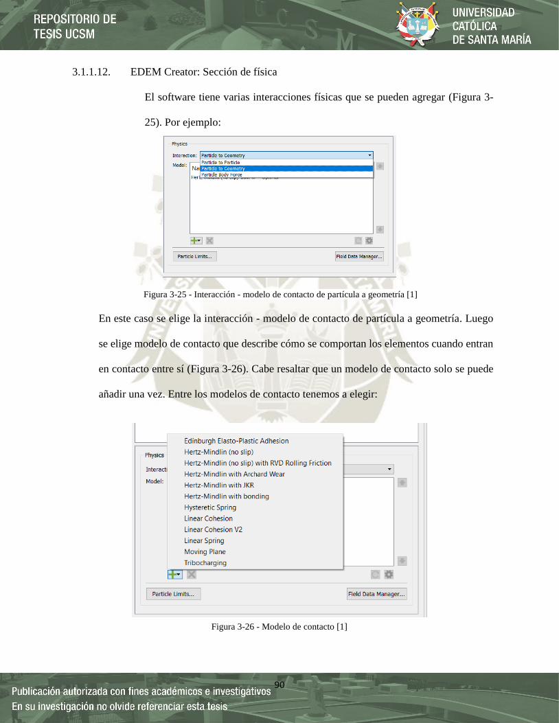
90
3.1.1.12. EDEM Creator: Sección de física
El software tiene varias interacciones físicas que se pueden agregar (Figura 3-
25). Por ejemplo:
En este caso se elige la interacción - modelo de contacto de partícula a geometría. Luego
se elige modelo de contacto que describe cómo se comportan los elementos cuando entran
en contacto entre sí (Figura 3-26). Cabe resaltar que un modelo de contacto solo se puede
añadir una vez. Entre los modelos de contacto tenemos a elegir:
Figura 3-25 - Interacción - modelo de contacto de partícula a geometría [1]
Figura 3-26 - Modelo de contacto [1]
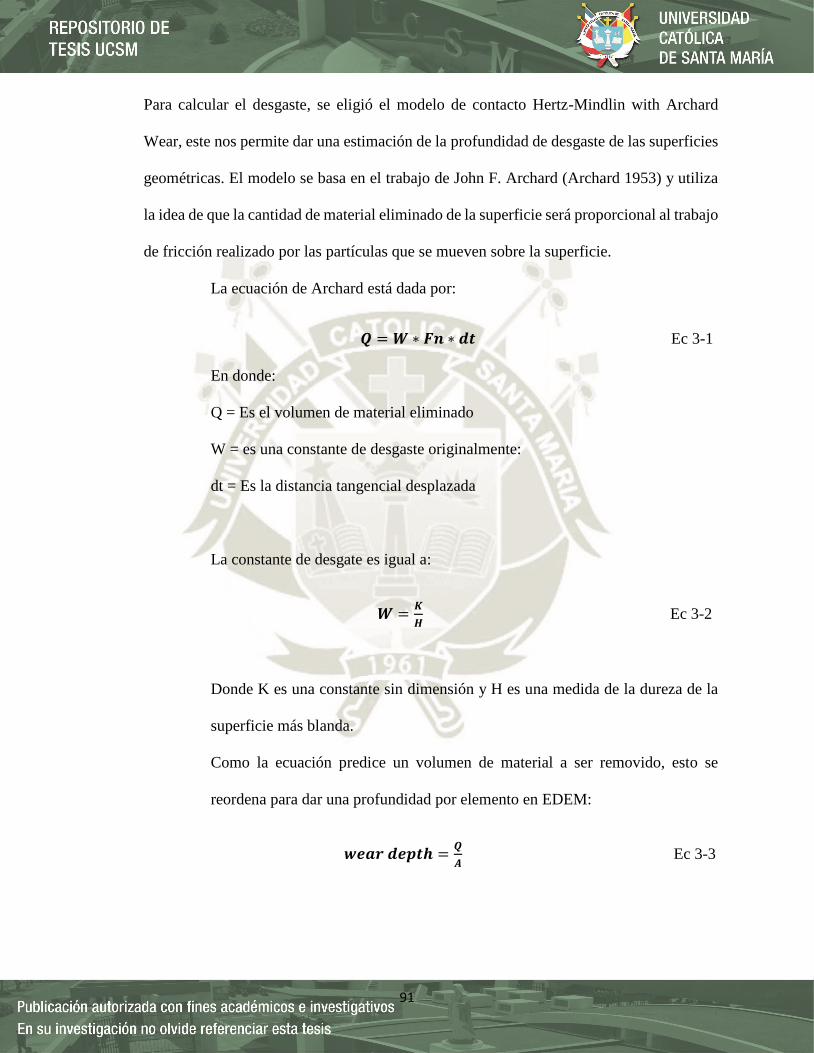
91
Para calcular el desgaste, se eligió el modelo de contacto Hertz-Mindlin with Archard
Wear, este nos permite dar una estimación de la profundidad de desgaste de las superficies
geométricas. El modelo se basa en el trabajo de John F. Archard (Archard 1953) y utiliza
la idea de que la cantidad de material eliminado de la superficie será proporcional al trabajo
de fricción realizado por las partículas que se mueven sobre la superficie.
La ecuación de Archard está dada por:
𝑸 = 𝑾 ∗ 𝑭𝒏 ∗ 𝒅𝒕 Ec 3-1
En donde:
Q = Es el volumen de material eliminado
W = es una constante de desgaste originalmente:
dt = Es la distancia tangencial desplazada
La constante de desgate es igual a:
𝑾 =𝑲
𝑯 Ec 3-2
Donde K es una constante sin dimensión y H es una medida de la dureza de la
superficie más blanda.
Como la ecuación predice un volumen de material a ser removido, esto se
reordena para dar una profundidad por elemento en EDEM:
𝒘𝒆𝒂𝒓 𝒅𝒆𝒑𝒕𝒉 =𝑸
𝑨 Ec 3-3
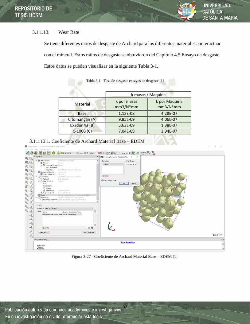
92
3.1.1.13. Wear Rate
Se tiene diferentes ratios de desgaste de Archard para los diferentes materiales a interactuar
con el mineral. Estos ratios de desgaste se obtuvieron del Capítulo 4.5 Ensayo de desgaste.
Estos datos se pueden visualizar en la siguiente Tabla 3-1.
Tabla 3-1 - Tasa de desgaste ensayos de desgaste [1]
3.1.1.13.1. Coeficiente de Archard Material Base – EDEM
k masas / Maquina
Material k por masas mm3/N*mm
k por Maquina mm3/N*mm
Base 1.13E-08 4.28E-07
Citomangan (A) 9.85E-09 4.06E-07
Exadur 43 (B) 5.63E-09 1.38E-07
C-1000 (C) 7.04E-09 2.94E-07
Figura 3-27 - Coeficiente de Archard Material Base – EDEM [1]
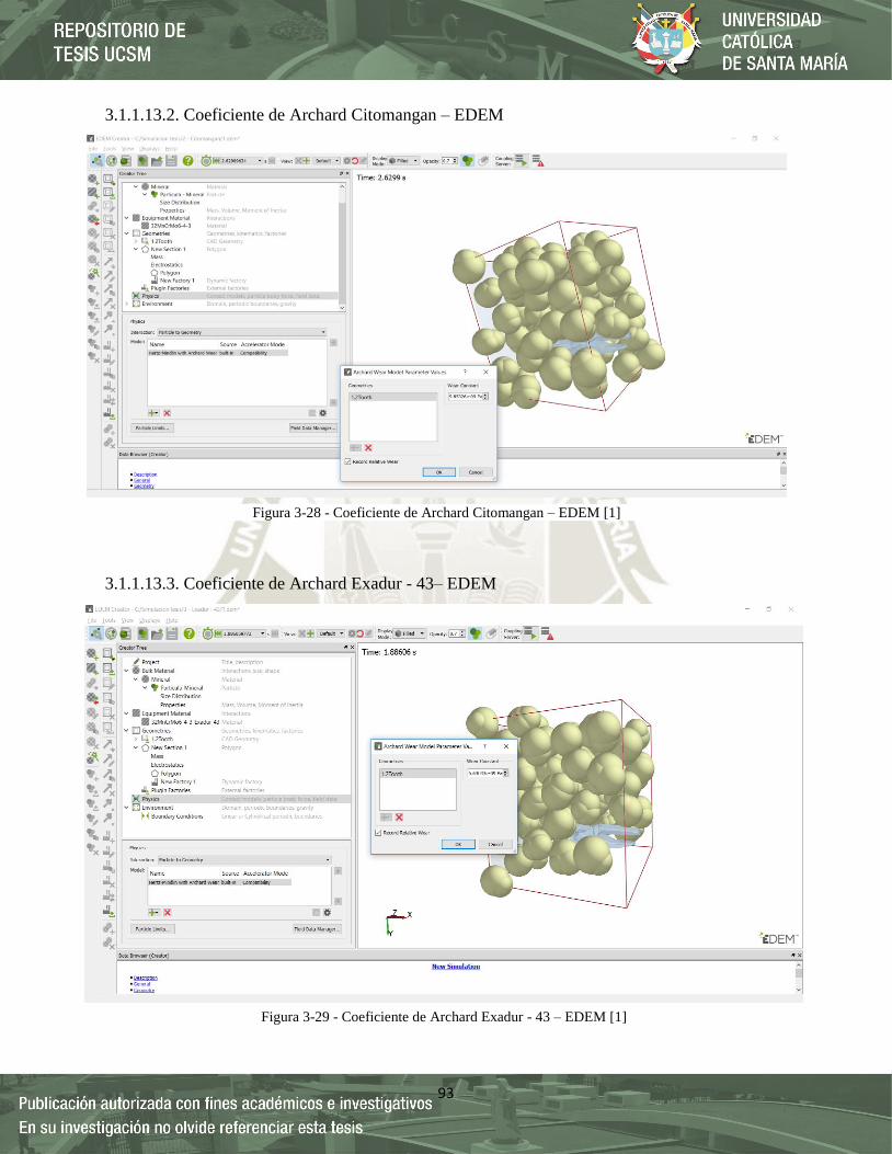
93
3.1.1.13.2. Coeficiente de Archard Citomangan – EDEM
3.1.1.13.3. Coeficiente de Archard Exadur - 43– EDEM
Figura 3-28 - Coeficiente de Archard Citomangan – EDEM [1]
Figura 3-29 - Coeficiente de Archard Exadur - 43 – EDEM [1]
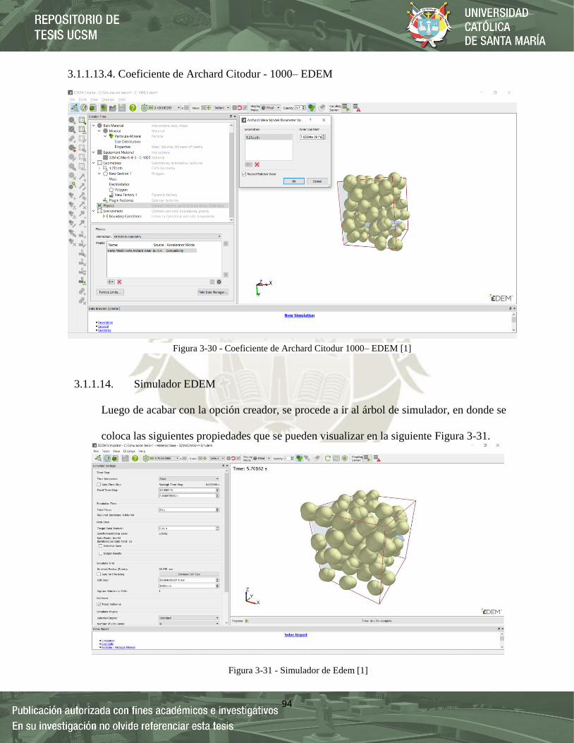
94
3.1.1.13.4. Coeficiente de Archard Citodur - 1000– EDEM
3.1.1.14. Simulador EDEM
Luego de acabar con la opción creador, se procede a ir al árbol de simulador, en donde se
coloca las siguientes propiedades que se pueden visualizar en la siguiente Figura 3-31.
Figura 3-30 - Coeficiente de Archard Citodur 1000– EDEM [1]
Figura 3-31 - Simulador de Edem [1]

95
En donde se elige un fixed time Step del 20%. El time Step es la cantidad de tiempo entre
iteraciones (cálculos) en el Simulador. La simulación se coloca 60 s para poder obtener el
desgaste total.
3.1.1.15. Descripción general del analista del EDEM
Luego de colocar los parámetros del Simulador, se procede a ir al árbol del analista, El
árbol de analistas se muestra en el lado izquierdo de la ventana EDEM. Tiene cinco
secciones: Visualización, configuración de selecciones, herramientas, recorte y campo
(opcional, dependiendo de la licencia). Se tiene como ejemplo en la siguiente Figura 3-32.
En donde se coloca Archard Wear para la geometría y se pincha en el cuadro de Auto
Update para que calcule el desgaste total en el tiempo propuesto. Se puede colocar los
colores de desgaste según corresponda. Este modelo de se aplico para todas las
simulaciones.
Figura 3-32 - Analista EDEM [1]

96
3.2.Evaluación experimental.
Lo objetivo de este punto es describir la metodología realizada en la evaluación de las muestras
preparadas de esta tesis. Los resultados de cada ensayo se mostrarán en el siguiente capítulo.
La Figura 3-33 se presenta un esquema de las actividades y ensayos realizados en las probetas.
Materiales y equipos utilizados:
Electrodos de Recargue (Citodur 1000, Exadur – 43, Citomangan) donde la
composición química se describe en la Tabla 3-6
Fuente de poder para proceso SMAW y parámetros de soldeo (figura 3-49)
Probetas de ensayo (9 probetas para los ensayos de Dureza, Metalografía, 4
probetas para los ensayos de tracción, 4 probetas para los ensayos de desgaste)
Equipo de dureza Rockwell C (carga desde 60kgf hasta 150 kgf) Marca Time
Group INC modelo HRC -150 con rango de medición de 20-88HRA, 20-100HRB,
20-70HRC.
Microscopio Metalúrgico Invertido Óptico, Time Group INC, DX40TV con
resolución 20x/100x.
Equipos de desbaste y set de lijas para preparación de muestras metalográficas.
Equipo de tracción INSTRON modelo 23-100.
Tribómetro pin-on-disk - Anton Paar (TRB3) de 0.2 rpm to 2000 rpm, segun la
norma ASTM G-99, ASTM G-133, DIN 50324.
Balanza con una precisión de 0.0001 gramos . Marca Mettler Toledo y Modelo –
ML-T.
Microscopio compuesto de binoculares, Motic, BA310POL con resolución 4x/60x
Equipo de pulidora Metalográfica.
97
Los ensayos de Metalografía y dureza se realizaron en las instalaciones del laboratorio de
Materiales de la universidad Católica de Santa María, y los ensayos de tracción y desgaste se
realizaron en las instalaciones del laboratorio de materiales de la Universidad Nacional de San
Agustín. Los pasos se describen a continuación:
Se realizó el corte y mecanizado de las probetas a ensayar según la norma
ASTM G65 en la empresa TALLER LÍDER S.A, se produjeron en total 14
probetas.
Se realizo la preparación de los cupones de soldadura en la empresa Taller
Lider S.A. Se agrupo en series (C-1000, E-43 y CITOMANGAN) según el
elemento aleante a evaluar tal como se puede observar en la Figura 3-38.
Se realizó el análisis de composición químico a una muestra de cada serie,
esta se llevó a cabo en la empresa VOESTALPINE HIGH
PERFORMANCE METALS DEL PERÚ S.A. El objetivo de la realización
de la composición química de cada muestra fue tener una mayor exactitud
del porcentaje de elementos químicos que poseen y corroborarlo con la Data
Sheet de cada soldadura. Se puede observar en la Ficha 4-1.
Se realizó la preparación para el análisis metalográfico a todas las muestras,
la superficie evaluada fue la transversal respecto al cordón de soldadura. La
preparación metalográfica se hizo según la norma ASTM E3-11. Se puede
observar en la Figura 3-69.

98
Se realizo la preparación para el ensayo de dureza a todas las muestras, la
superficie evaluada fue la transversal respecto al cordón de soldadura. El
ensayo de dureza se realizó según la norma ASTM E18-15. Se puede
observar en la Figura 3-69.
Se realizo el corte y mecanizado para la unión de soldadura de 04 muestras,
una de cada serie, en la empresa TALLER LÍDER S.A. Luego se precedió
al mecanizado de estas muestras para la realización del ensayo de tracción
según la norma ASTM A370 – 18. Se pude observar en la Figura 3-41.
Se realizo el corte y mecanizado de 04 muestras en la empresa TALLER
LÍDER S.A. para el ensayo de desgaste según la norma ASTM G99-17. Se
pude observar en la Figura 3-44.
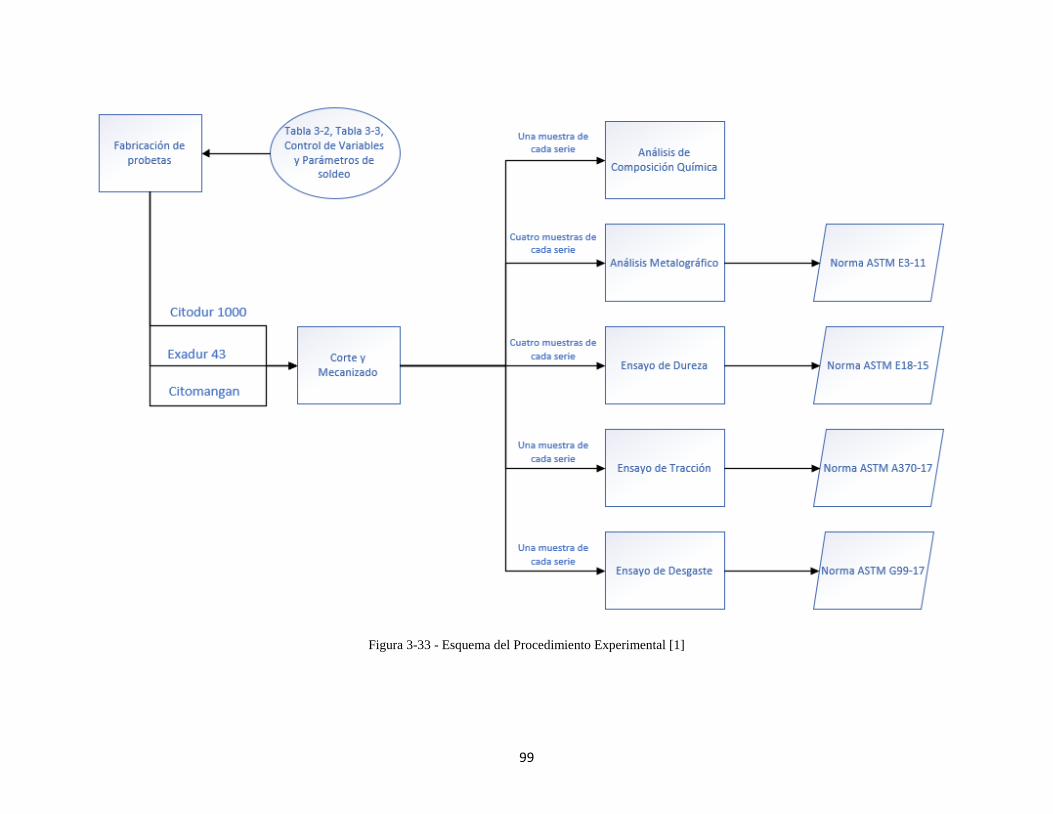
99
Figura 3-33 - Esquema del Procedimiento Experimental [1]

100
3.2.1. Fabricación de las probetas
3.2.1.1.Probetas de Desgaste según la norma ASTM G65-16, metalografía y dureza
Las probetas se obtuvieron de una uña de acero 32MnCrMo6-4-3 (Figura 3-35), se realizó
mediante Corte con Disco (Figura 3-36) y fresado (Figura 3-37) para obtener el correcto
dimensionamiento, paralelepípedos con sus lados rectificados (Tabla 3-2). Según la norma
ASTM G-65 (Figura 3-34).
Tabla 3-2 - Medidas de la probeta de desgaste según la norma ASTM G65-16 [23]
Medidas in mm
Largo 3 76.2
Ancho 1 25.4
Espesor 0.5 12.7
Figura 3-34 - Diagrama esquemático del aparato de prueba [23]

101
.
Figura 3-35 - Uña de acero 32MnCrMo6-4-3 [1]
Figura 3-36 - Corte con disco Manual [1]
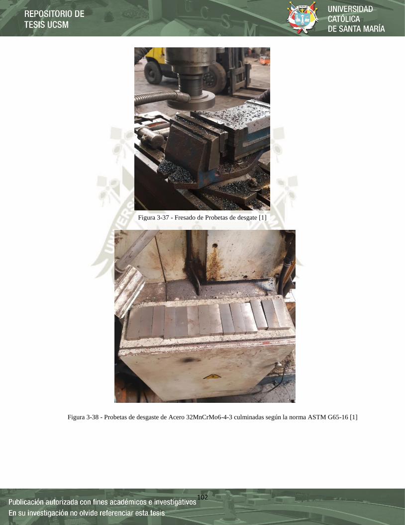
102
Figura 3-37 - Fresado de Probetas de desgate [1]
Figura 3-38 - Probetas de desgaste de Acero 32MnCrMo6-4-3 culminadas según la norma ASTM G65-16 [1]
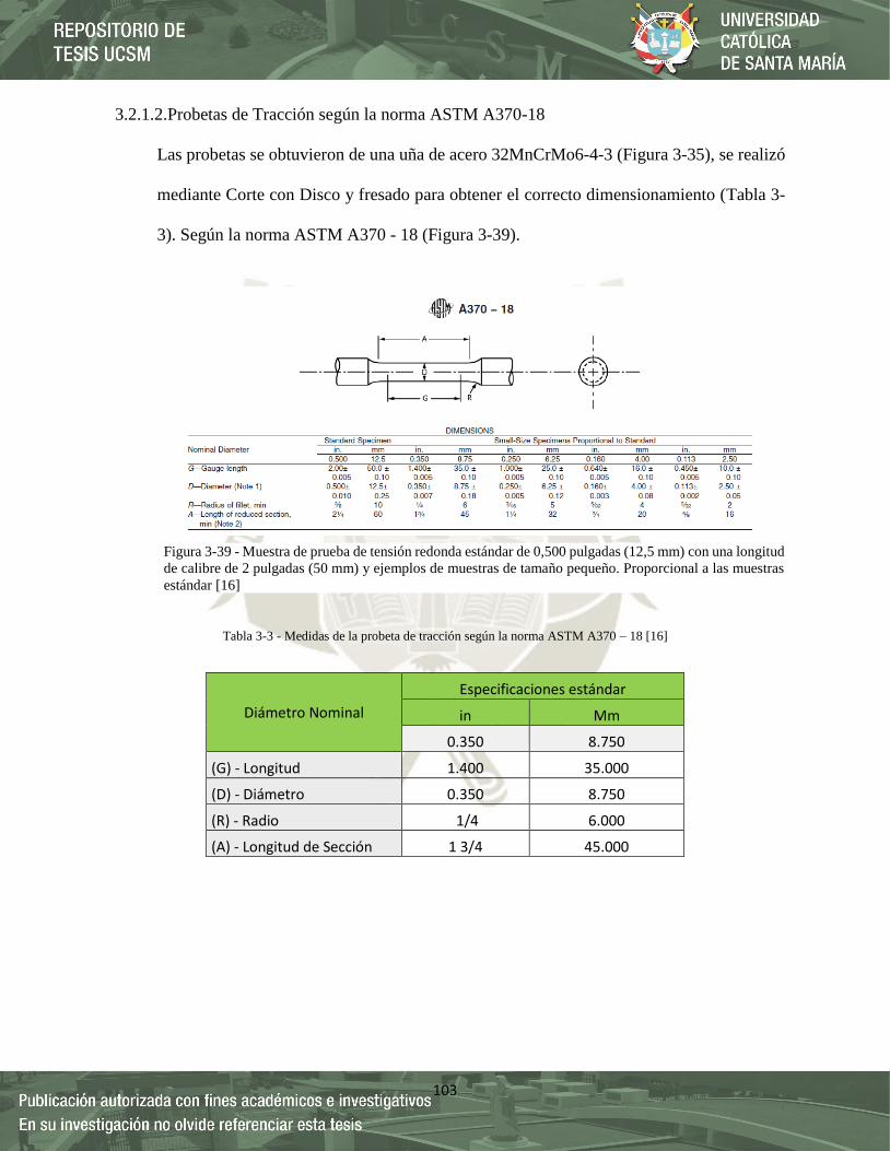
103
3.2.1.2.Probetas de Tracción según la norma ASTM A370-18
Las probetas se obtuvieron de una uña de acero 32MnCrMo6-4-3 (Figura 3-35), se realizó
mediante Corte con Disco y fresado para obtener el correcto dimensionamiento (Tabla 3-
3). Según la norma ASTM A370 - 18 (Figura 3-39).
Tabla 3-3 - Medidas de la probeta de tracción según la norma ASTM A370 – 18 [16]
Diámetro Nominal
Especificaciones estándar
in Mm
0.350 8.750
(G) - Longitud 1.400 35.000
(D) - Diámetro 0.350 8.750
(R) - Radio 1/4 6.000
(A) - Longitud de Sección 1 3/4 45.000
Figura 3-39 - Muestra de prueba de tensión redonda estándar de 0,500 pulgadas (12,5 mm) con una longitud
de calibre de 2 pulgadas (50 mm) y ejemplos de muestras de tamaño pequeño. Proporcional a las muestras
estándar [16]
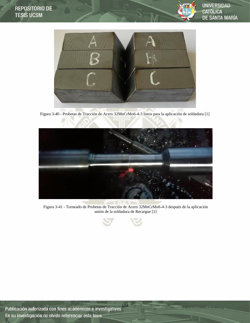
104
Figura 3-40 - Probetas de Tracción de Acero 32MnCrMo6-4-3 listos para la aplicación de soldadura [1]
Figura 3-41 - Torneado de Probetas de Tracción de Acero 32MnCrMo6-4-3 después de la aplicación
unión de la soldadura de Recargue [1]
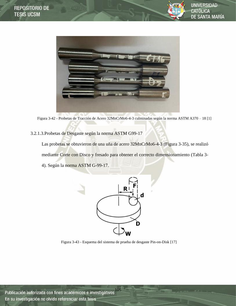
105
3.2.1.3.Probetas de Desgaste según la norma ASTM G99-17
Las probetas se obtuvieron de una uña de acero 32MnCrMo6-4-3 (Figura 3-35), se realizó
mediante Corte con Disco y fresado para obtener el correcto dimensionamiento (Tabla 3-
4). Según la norma ASTM G-99-17.
Figura 3-42 - Probetas de Tracción de Acero 32MnCrMo6-4-3 culminadas según la norma ASTM A370 – 18 [1]
Figura 3-43 - Esquema del sistema de prueba de desgaste Pin-on-Disk [17]
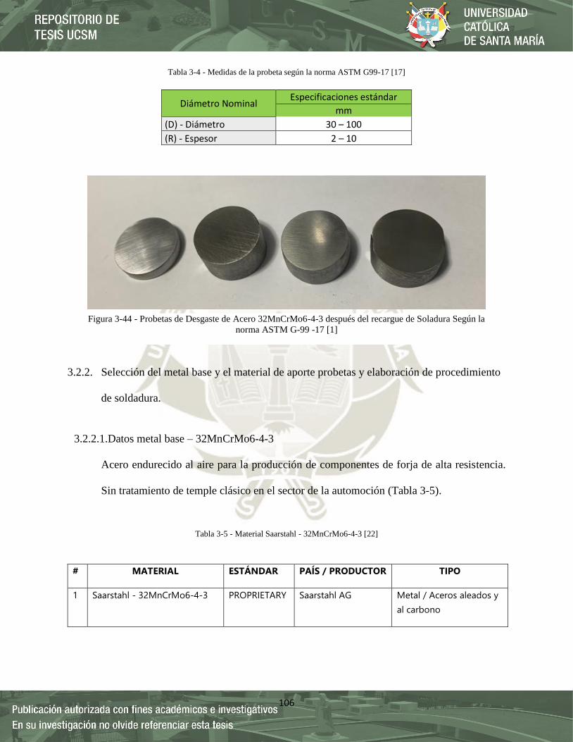
106
Tabla 3-4 - Medidas de la probeta según la norma ASTM G99-17 [17]
3.2.2. Selección del metal base y el material de aporte probetas y elaboración de procedimiento
de soldadura.
3.2.2.1.Datos metal base – 32MnCrMo6-4-3
Acero endurecido al aire para la producción de componentes de forja de alta resistencia.
Sin tratamiento de temple clásico en el sector de la automoción (Tabla 3-5).
Tabla 3-5 - Material Saarstahl - 32MnCrMo6-4-3 [22]
Diámetro Nominal Especificaciones estándar
mm
(D) - Diámetro 30 – 100
(R) - Espesor 2 – 10
# MATERIAL ESTÁNDAR PAÍS / PRODUCTOR TIPO
1 Saarstahl - 32MnCrMo6-4-3 PROPRIETARY Saarstahl AG Metal / Aceros aleados y
al carbono
Figura 3-44 - Probetas de Desgaste de Acero 32MnCrMo6-4-3 después del recargue de Soladura Según la
norma ASTM G-99 -17 [1]
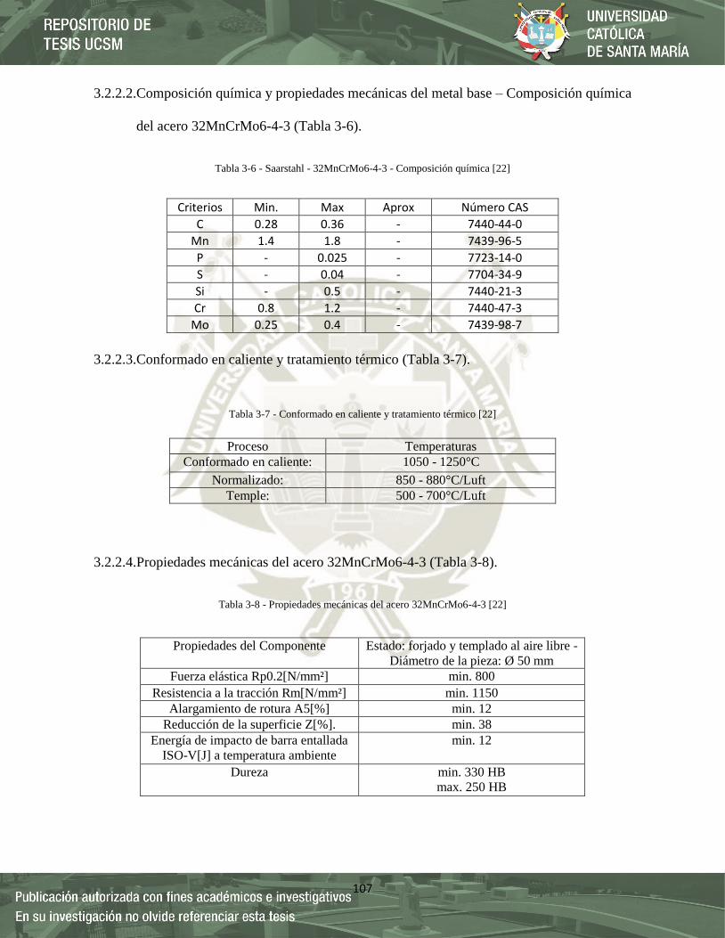
107
3.2.2.2.Composición química y propiedades mecánicas del metal base – Composición química
del acero 32MnCrMo6-4-3 (Tabla 3-6).
Tabla 3-6 - Saarstahl - 32MnCrMo6-4-3 - Composición química [22]
3.2.2.3.Conformado en caliente y tratamiento térmico (Tabla 3-7).
Tabla 3-7 - Conformado en caliente y tratamiento térmico [22]
3.2.2.4.Propiedades mecánicas del acero 32MnCrMo6-4-3 (Tabla 3-8).
Tabla 3-8 - Propiedades mecánicas del acero 32MnCrMo6-4-3 [22]
Criterios Min. Max Aprox Número CAS
C 0.28 0.36 - 7440-44-0
Mn 1.4 1.8 - 7439-96-5
P - 0.025 - 7723-14-0
S - 0.04 - 7704-34-9
Si - 0.5 - 7440-21-3
Cr 0.8 1.2 - 7440-47-3
Mo 0.25 0.4 - 7439-98-7
Proceso Temperaturas
Conformado en caliente: 1050 - 1250°C
Normalizado: 850 - 880°C/Luft
Temple: 500 - 700°C/Luft
Propiedades del Componente Estado: forjado y templado al aire libre -
Diámetro de la pieza: Ø 50 mm
Fuerza elástica Rp0.2[N/mm²] min. 800
Resistencia a la tracción Rm[N/mm²] min. 1150
Alargamiento de rotura A5[%] min. 12
Reducción de la superficie Z[%]. min. 38
Energía de impacto de barra entallada
ISO-V[J] a temperatura ambiente
min. 12
Dureza min. 330 HB
max. 250 HB

108
3.2.2.5.Composición química, propiedades mecánicas y aplicaciones de material de aporte
3.2.2.5.1. Electrodos de Recubrimiento Protector – Citodur 1000
Tabla 3-9 - Clasificación de electrodo Citodur 1000 [10]
Tabla 3-10 - Análisis Químico Citodur 1000 [10]
Clasificación AWS A5.13 / ASME SFA-5.13 DIN 8555 E10
EFeCr-A8 UM 60 CGRZ
C Mn Si P S Mo Ni Cr Cu Otros
4.00 1.10 0.60 máx. 0.020
máx. 0.020
- - 36.00 - -
Figura 3-45 - Cucharon de excavadora 336D2 L con 04 uñas de Acero 32MnCrMo6-4-3 [1]

109
Tabla 3-11 - Propiedades Mecánicas Citodur 1000 [10]
3.2.2.5.2. Electrodos de Recubrimiento Protector – Citomangan
Tabla 3-12 - Clasificación de electrodo Citomangan [10]
Tabla 3-13 - Análisis Químico Citomangan [10]
Tabla 3-14 - Propiedades Mecánicas Citomangan [10]
Tratamiento Térmico
Resistencia a la Tracción [MPa (psi)]
Límite de Fluencia
[MPa (psi)]
Elongación en 2'' [%]
Energía Absorbida
ISO-V [°C (°F)] [J (Ft-Lbf)]
Dureza
Sin tratamiento - - - - 58 - 62 HRC
Clasificación AWS A5.13 / ASME SFA-5.13 DIN 8555 E10
EFe Mn-B E 7 - UM - 200 KP
C Mn Si P S Mo Ni Cr Cu Otros
1.00 12.00 – 14.00
0.60 máx. 0.020
máx. 0.020
- - - - -
Tratamiento Térmico
Resistencia a la Tracción [MPa (psi)]
Límite de Fluencia
[MPa (psi)]
Elongación en 2'' [%]
Energía Absorbida
ISO-V [°C (°F)] [J (Ft-Lbf)]
Dureza
Sin tratamiento Auto endurecido
- - - - 19 - 28 HRC 50 - 60 HRC

110
3.2.2.5.3. Electrodos de Recubrimiento Protector – Exadur – 43
Tabla 3-15 - Clasificación de electrodo Exadur – 43 [10]
Tabla 3-16 - Análisis Químico Exadur – 43 [10]
Tabla 3-17 - Propiedades Mecánicas Exadur – 43 [10]
3.2.2.6.Selección de la máquina de soldar
Para el proceso de soldadura se utilizó la máquina de soldar multiproceso Miller XMT 425
SERIES, alimentación trifásica, con salida nominal (con ciclo de trabajo al 100%) de 5 a
425 A a 10 - 38 VCD (Figura 3-46).
Clasificación AWS A5.13 / ASME SFA-5.13 DIN 8555 E10
E Fe Cr-A2 E 10-UM-65-GRZ
C Mn Si P S Mo Ni Cr Cu Otros
3.40 1.10 0.60 máx. 0.020
máx. 0.020
- - 22.00 - 8%Nb
Tratamiento Térmico
Resistencia a la Tracción [MPa (psi)]
Límite de Fluencia
[MPa (psi)]
Elongación en 2'' [%]
Energía Absorbida
ISO-V [°C (°F)] [J (Ft-Lbf)]
Dureza
Sin tratamiento - - - - 60 - 62 HRC
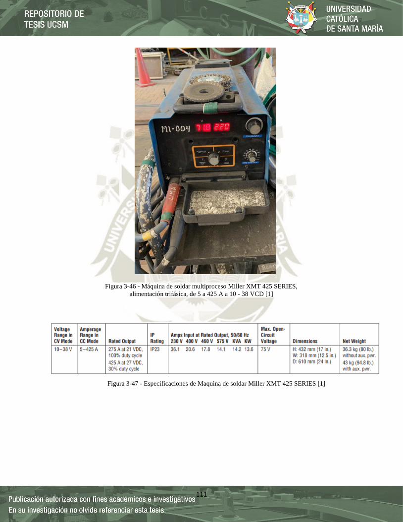
111
Figura 3-46 - Máquina de soldar multiproceso Miller XMT 425 SERIES,
alimentación trifásica, de 5 a 425 A a 10 - 38 VCD [1]
Figura 3-47 - Especificaciones de Maquina de soldar Miller XMT 425 SERIES [1]

112
3.2.2.7.Procedimiento de Soldadura
3.2.2.7.1. Especificación del procedimiento de soldadura - Ensayo de desgaste (AWS
D1.1/D1.1M:2008)
Tabla 3-18 - Especificación del procedimiento de soldadura (Desgaste - Citodur 1000) [1]
Nombre de la Compañía
“ANÁLISIS MEDIANTE ELEMENTOS DISCRETOS (MED) Y EVALUACIÓN EXPERIMENTAL BAJO LA NORMA ASTM G-65 DEL DESGASTE ABRASIVO EN REVESTIMIENTOS DUROS APLICADOS POR PROCESOS DE SOLDADURA EN UÑAS DE ACERO 32MnCrMo6-4-3 DE
UNA EXCAVADORA HIDRÁULICA CAT 336D2 L”
Proceso de Soldadura SMAW
Material Base Especificación del material: 32MnCrMo6-4-3
Espesor: 0.5 in
Material de Aporte
Especificación AWS: Clasificación AWS A5.13 / ASME SFA-
5.13
Clasificación AWS: EFeCr-A8
Especificación DIN: DIN 8555 E10
Clasificación DIN: UM 60 CGRZ
Diámetro y longitud del electrodo:
Ø 4 mm (5/32 in) x 35 cm
Precalentamiento T° Precalentamiento: 100 a 120 °C
T° Interpase: 150 °C - 350 °C. Las repeticiones sin
precalentamiento
Posición Plana 1G
Características Eléctricas Amperaje: 150 - 160 A
CCEP (corriente continua con electrodo positivo)
Técnica
Arrastre sin oscilación
Pasadas múltiples por cara, de 1 y 3 capas. Las repeticiones de 2 - 3 capas
La limpieza entre pasadas se hará con escobilla metálica y picota. Si es necesario se utilizará esmeril.
Tratamiento Térmico Post Soldadura
Enfriamiento lento utilizando cal industrial que cubrirá la probeta.
PROCEDIMIENTO DE SOLDADURA
Pase o Capa
Proceso
Metal de Aporte Corriente
Voltaje (V)
Velocidad de avance
Clase (cm/min)
Detalles de la junta
Clase Diámetro
(in) Tipo y
polaridad Amperaje
(A)
1 SMAW EFeCr-A8 5/32 CCEP 150 - 160 A 20 - 30 25-30 cm/min
2 SMAW EFeCr-A8 5/32 CCEP 150 - 160 A 20 - 30 25-30 cm/min
3 SMAW EFeCr-A8 5/32 CCEP 150 - 160 A 20 - 30 25-30 cm/min

113
Tabla 3-19 - Especificación del procedimiento de soldadura (Desgaste -Citomangan) [1]
Nombre de la Compañía
“ANÁLISIS MEDIANTE ELEMENTOS DISCRETOS (MED) Y EVALUACIÓN EXPERIMENTAL BAJO LA NORMA ASTM G-65 DEL DESGASTE ABRASIVO EN REVESTIMIENTOS DUROS APLICADOS POR PROCESOS DE SOLDADURA EN UÑAS DE ACERO 32MnCrMo6-4-3 DE
UNA EXCAVADORA HIDRÁULICA CAT 336D2 L”
Proceso de Soldadura SMAW
Material Base Especificación del material: 32MnCrMo6-4-3
Espesor: 0.5 in
Material de Aporte
Especificación AWS: Clasificación AWS A5.13 / ASME SFA-
5.13
Clasificación AWS: EFe Mn-B
Especificación DIN: DIN 8555 E10
Clasificación DIN: E 7 - UM - 200 KP
Diámetro y longitud del electrodo:
Ø 5 mm (3/16 in) x 35 cm
Precalentamiento T° Precalentamiento: 100 a 120 °C
T° Interpase: 150 °C - 350 °C. Las repeticiones sin
precalentamiento
Posición Plana 1G
Características Eléctricas Amperaje: 170 - 220 A
CCEP (corriente continua con electrodo positivo)
Técnica
Arrastre sin oscilación
Pasadas múltiples por cara, de 1 y 3 capas. Las repeticiones de 2 - 3 capas
La limpieza entre pasadas se hará con escobilla metálica y picota. Si es necesario se utilizará esmeril.
Tratamiento Térmico Post Soldadura
Enfriamiento lento utilizando cal industrial que cubrirá la probeta.
PROCEDIMIENTO DE SOLDADURA
Pase o Capa Proceso
Metal de Aporte Corriente
Voltaje (V)
Velocidad de avance
Clase (cm/min)
Detalles de la junta
Clase Diámetro
(in) Tipo y
polaridad Amperaje (A)
1 SMAW EFe Mn-B 3/16 CCEP 170 - 220 A 20 - 30 25-30 cm/min
2 SMAW EFe Mn-B 3/16 CCEP 170 - 220 A 20 - 30 25-30 cm/min
3 SMAW EFe Mn-B 3/16 CCEP 170 - 220 A 20 - 30 25-30 cm/min

114
Nombre de la Compañía
“ANÁLISIS MEDIANTE ELEMENTOS DISCRETOS (MED) Y EVALUACIÓN EXPERIMENTAL BAJO LA NORMA ASTM G-65 DEL DESGASTE ABRASIVO EN REVESTIMIENTOS DUROS APLICADOS POR PROCESOS DE SOLDADURA EN UÑAS DE ACERO 32MnCrMo6-4-3 DE
UNA EXCAVADORA HIDRÁULICA CAT 336D2 L”
Proceso de Soldadura SMAW
Material Base Especificación del material: 32MnCrMo6-4-3
Espesor: 0.5 in
Material de Aporte
Especificación AWS: Clasificación AWS A5.13 / ASME SFA-
5.13
Clasificación AWS: E Fe Cr-A2
Especificación DIN: DIN 8555 E10
Clasificación DIN : E 10-UM-65-GRZ
Diámetro y longitud del electrodo:
Ø 3.25 mm (1/8 in) x 35 cm
Precalentamiento
T° Precalentamiento: 100 a 120 °C
T° Interpase: 150 °C - 350 °C. Las repeticiones sin
precalentamiento
Posición Plana 1G
Características Eléctricas Amperaje: 90 - 130 A
CCEP (corriente continua con electrodo positivo)
Técnica
Arrastre sin oscilación
Pasadas múltiples por cara, de 1 y 3 capas. Las repeticiones de 2 - 3 capas
La limpieza entre pasadas se hará con escobilla metálica y picota. Si es necesario se utilizará esmeril.
Tratamiento Térmico Post Soldadura
Enfriamiento lento utilizando cal industrial que cubrirá la probeta.
Tabla 3-20 - Especificación del procedimiento de soldadura (Desgaste - Exadur 43) [1]
PROCEDIMIENTO DE SOLDADURA
Pase o Capa
Proceso
Metal de Aporte Corriente
Voltaje (V)
Velocidad de avance
Clase (cm/min)
Detalles de la junta
Clase Diámetro
(in) Tipo y
polaridad Amperaje
(A)
1 SMAW EFe Cr-A2 1/8 CCEP 90 - 130 A 20 - 30 25-30 cm/min
2 SMAW EFe Cr-A2 1/8 CCEP 90 - 130 A 20 - 30 25-30 cm/min
3 SMAW EFe Cr-A2 1/8 CCEP 90 - 130 A 20 - 30 25-30 cm/min
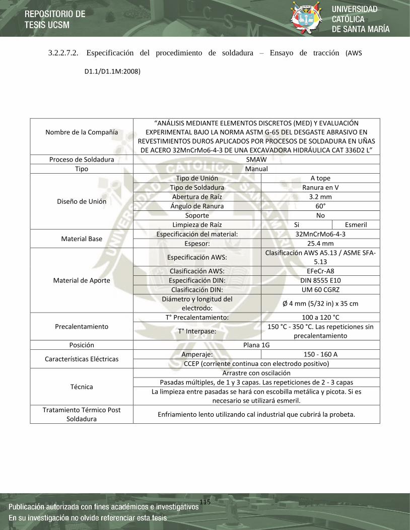
115
3.2.2.7.2. Especificación del procedimiento de soldadura – Ensayo de tracción (AWS
D1.1/D1.1M:2008)
Nombre de la Compañía
“ANÁLISIS MEDIANTE ELEMENTOS DISCRETOS (MED) Y EVALUACIÓN EXPERIMENTAL BAJO LA NORMA ASTM G-65 DEL DESGASTE ABRASIVO EN
REVESTIMIENTOS DUROS APLICADOS POR PROCESOS DE SOLDADURA EN UÑAS DE ACERO 32MnCrMo6-4-3 DE UNA EXCAVADORA HIDRÁULICA CAT 336D2 L”
Proceso de Soldadura SMAW
Tipo Manual
Diseño de Unión
Tipo de Unión A tope
Tipo de Soldadura Ranura en V
Abertura de Raíz 3.2 mm
Ángulo de Ranura 60°
Soporte No
Limpieza de Raíz Si Esmeril
Material Base Especificación del material: 32MnCrMo6-4-3
Espesor: 25.4 mm
Material de Aporte
Especificación AWS: Clasificación AWS A5.13 / ASME SFA-
5.13
Clasificación AWS: EFeCr-A8
Especificación DIN: DIN 8555 E10
Clasificación DIN: UM 60 CGRZ
Diámetro y longitud del electrodo:
Ø 4 mm (5/32 in) x 35 cm
Precalentamiento T° Precalentamiento: 100 a 120 °C
T° Interpase: 150 °C - 350 °C. Las repeticiones sin
precalentamiento
Posición Plana 1G
Características Eléctricas Amperaje: 150 - 160 A
CCEP (corriente continua con electrodo positivo)
Técnica
Arrastre con oscilación
Pasadas múltiples, de 1 y 3 capas. Las repeticiones de 2 - 3 capas
La limpieza entre pasadas se hará con escobilla metálica y picota. Si es necesario se utilizará esmeril.
Tratamiento Térmico Post Soldadura
Enfriamiento lento utilizando cal industrial que cubrirá la probeta.
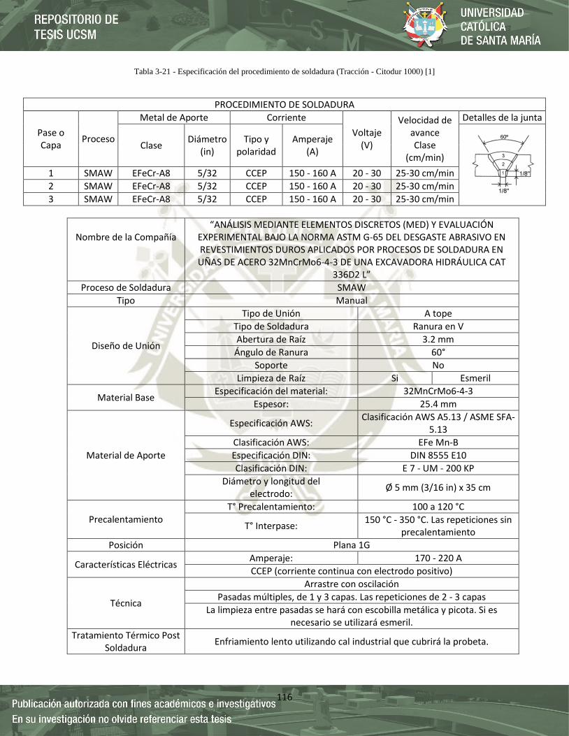
116
Tabla 3-21 - Especificación del procedimiento de soldadura (Tracción - Citodur 1000) [1]
PROCEDIMIENTO DE SOLDADURA
Pase o Capa
Proceso
Metal de Aporte Corriente
Voltaje (V)
Velocidad de avance Clase
(cm/min)
Detalles de la junta
Clase Diámetro
(in) Tipo y
polaridad Amperaje
(A)
1 SMAW EFeCr-A8 5/32 CCEP 150 - 160 A 20 - 30 25-30 cm/min
2 SMAW EFeCr-A8 5/32 CCEP 150 - 160 A 20 - 30 25-30 cm/min
3 SMAW EFeCr-A8 5/32 CCEP 150 - 160 A 20 - 30 25-30 cm/min
Nombre de la Compañía
“ANÁLISIS MEDIANTE ELEMENTOS DISCRETOS (MED) Y EVALUACIÓN EXPERIMENTAL BAJO LA NORMA ASTM G-65 DEL DESGASTE ABRASIVO EN REVESTIMIENTOS DUROS APLICADOS POR PROCESOS DE SOLDADURA EN UÑAS DE ACERO 32MnCrMo6-4-3 DE UNA EXCAVADORA HIDRÁULICA CAT
336D2 L”
Proceso de Soldadura SMAW
Tipo Manual
Diseño de Unión
Tipo de Unión A tope
Tipo de Soldadura Ranura en V
Abertura de Raíz 3.2 mm
Ángulo de Ranura 60°
Soporte No
Limpieza de Raíz Si Esmeril
Material Base Especificación del material: 32MnCrMo6-4-3
Espesor: 25.4 mm
Material de Aporte
Especificación AWS: Clasificación AWS A5.13 / ASME SFA-
5.13
Clasificación AWS: EFe Mn-B
Especificación DIN: DIN 8555 E10
Clasificación DIN: E 7 - UM - 200 KP
Diámetro y longitud del electrodo:
Ø 5 mm (3/16 in) x 35 cm
Precalentamiento T° Precalentamiento: 100 a 120 °C
T° Interpase: 150 °C - 350 °C. Las repeticiones sin
precalentamiento
Posición Plana 1G
Características Eléctricas Amperaje: 170 - 220 A
CCEP (corriente continua con electrodo positivo)
Técnica
Arrastre con oscilación
Pasadas múltiples, de 1 y 3 capas. Las repeticiones de 2 - 3 capas
La limpieza entre pasadas se hará con escobilla metálica y picota. Si es necesario se utilizará esmeril.
Tratamiento Térmico Post Soldadura
Enfriamiento lento utilizando cal industrial que cubrirá la probeta.
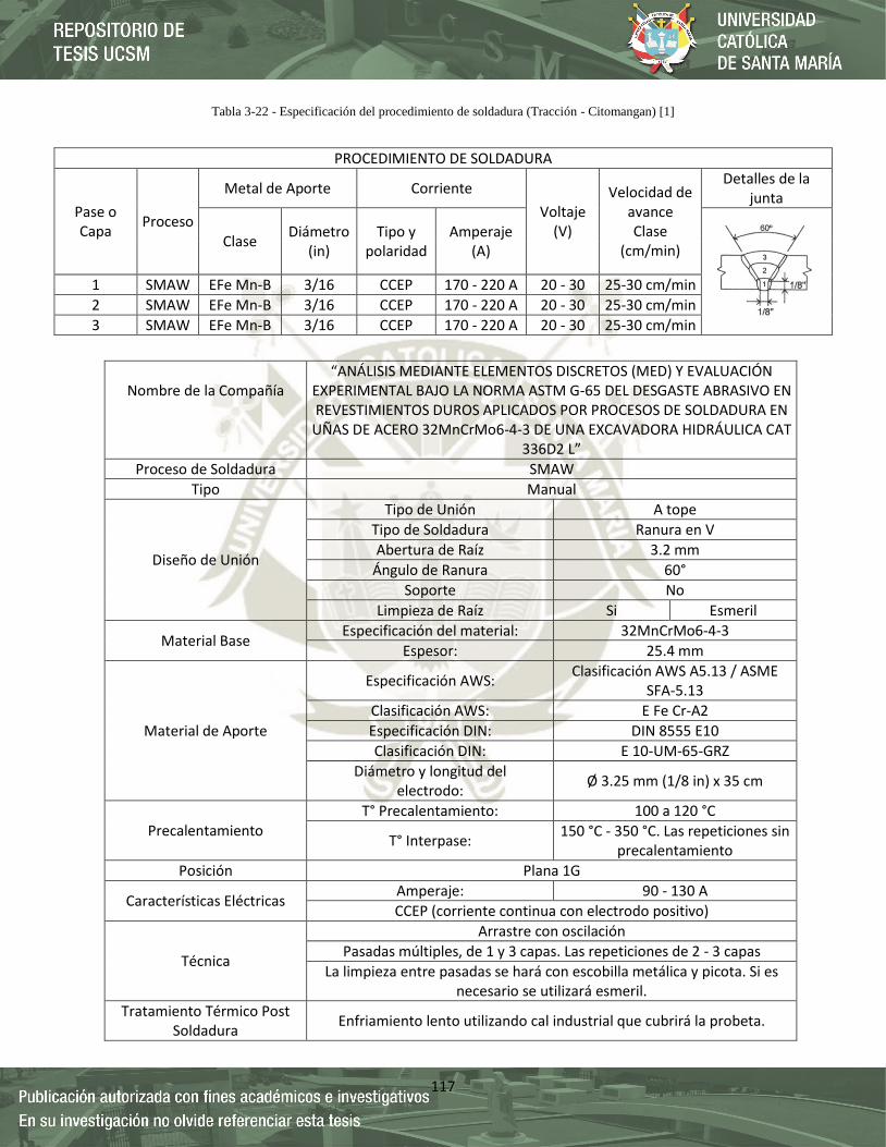
117
Tabla 3-22 - Especificación del procedimiento de soldadura (Tracción - Citomangan) [1]
PROCEDIMIENTO DE SOLDADURA
Pase o Capa
Proceso
Metal de Aporte Corriente
Voltaje (V)
Velocidad de avance Clase
(cm/min)
Detalles de la junta
Clase Diámetro
(in) Tipo y
polaridad Amperaje
(A)
1 SMAW EFe Mn-B 3/16 CCEP 170 - 220 A 20 - 30 25-30 cm/min
2 SMAW EFe Mn-B 3/16 CCEP 170 - 220 A 20 - 30 25-30 cm/min
3 SMAW EFe Mn-B 3/16 CCEP 170 - 220 A 20 - 30 25-30 cm/min
Nombre de la Compañía
“ANÁLISIS MEDIANTE ELEMENTOS DISCRETOS (MED) Y EVALUACIÓN EXPERIMENTAL BAJO LA NORMA ASTM G-65 DEL DESGASTE ABRASIVO EN REVESTIMIENTOS DUROS APLICADOS POR PROCESOS DE SOLDADURA EN
UÑAS DE ACERO 32MnCrMo6-4-3 DE UNA EXCAVADORA HIDRÁULICA CAT 336D2 L”
Proceso de Soldadura SMAW
Tipo Manual
Diseño de Unión
Tipo de Unión A tope
Tipo de Soldadura Ranura en V
Abertura de Raíz 3.2 mm
Ángulo de Ranura 60°
Soporte No
Limpieza de Raíz Si Esmeril
Material Base Especificación del material: 32MnCrMo6-4-3
Espesor: 25.4 mm
Material de Aporte
Especificación AWS: Clasificación AWS A5.13 / ASME
SFA-5.13
Clasificación AWS: E Fe Cr-A2
Especificación DIN: DIN 8555 E10
Clasificación DIN: E 10-UM-65-GRZ
Diámetro y longitud del electrodo:
Ø 3.25 mm (1/8 in) x 35 cm
Precalentamiento T° Precalentamiento: 100 a 120 °C
T° Interpase: 150 °C - 350 °C. Las repeticiones sin
precalentamiento
Posición Plana 1G
Características Eléctricas Amperaje: 90 - 130 A
CCEP (corriente continua con electrodo positivo)
Técnica
Arrastre con oscilación
Pasadas múltiples, de 1 y 3 capas. Las repeticiones de 2 - 3 capas
La limpieza entre pasadas se hará con escobilla metálica y picota. Si es necesario se utilizará esmeril.
Tratamiento Térmico Post Soldadura
Enfriamiento lento utilizando cal industrial que cubrirá la probeta.

118
Tabla 3-23 - Especificación del procedimiento de soldadura (Tracción – Exadur-43) [1]
3.2.2.7.3. Especificación del procedimiento de soldadura – Ensayo de tracción (AWS
D1.1/D1.1M:2008)
Para la aplicación del recubrimiento, se seleccionó el mínimo y el máximo amperaje
recomendado en la ficha técnica del fabricante. Para conocer la influencia de este
parámetro en el depósito final del recubrimiento, que definirá la microestructura, el
valor de dureza y el comportamiento de resistencia al desgaste abrasivo.
El mínimo y máximo valor de amperaje para la aplicación de recubrimiento y la unión
de tope del electrodo Citodur 1000 fue de 150 a 160 A para un diámetro de 5/32 (Tabla
3-24).
PROCEDIMIENTO DE SOLDADURA
Pase o Capa
Proceso
Metal de Aporte Corriente
Voltaje (V)
Velocidad de avance Clase
(cm/min)
Detalles de la junta
Clase Diámetro
(in) Tipo y
polaridad Amperaje
(A)
1 SMAW E Fe Cr-A2 1/8 CCEP 90 - 130 A 20 - 30 25-30 cm/min
2 SMAW E Fe Cr-A2 1/8 CCEP 90 - 130 A 20 - 30 25-30 cm/min
3 SMAW E Fe Cr-A2 1/8 CCEP 90 - 130 A 20 - 30 25-30 cm/min
Tabla 3-24 - Parámetro de soldeo Recomendado – Citodur 1000 [10]

119
El mínimo y máximo valor de amperaje para la aplicación de recubrimiento y la unión
de tope del electrodo Citomangan fue de 170 a 220 A para un diámetro de 3/16 (Tabla
3-25).
Tabla 3-25 - Parámetro de soldeo Recomendado – Citomangan [10]
Figura 3-48 - Máquina de soldar multiproceso Miller XMT 425 SERIES – 160
A [1]
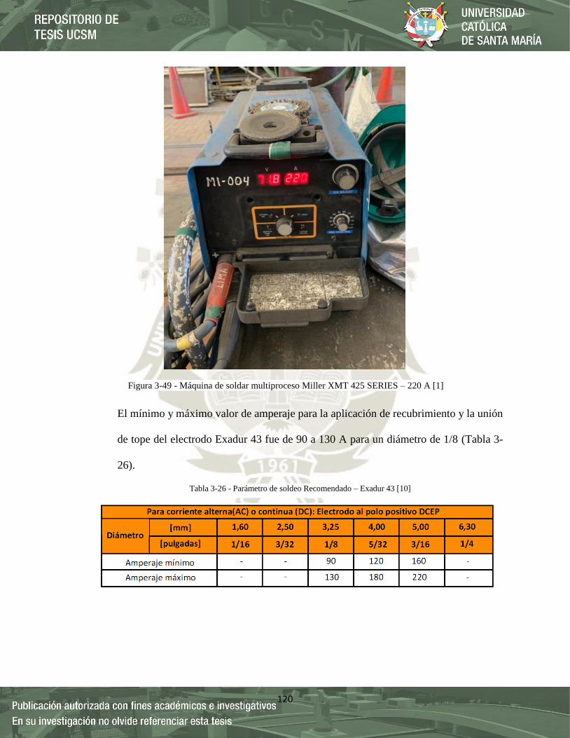
120
El mínimo y máximo valor de amperaje para la aplicación de recubrimiento y la unión
de tope del electrodo Exadur 43 fue de 90 a 130 A para un diámetro de 1/8 (Tabla 3-
26).
Tabla 3-26 - Parámetro de soldeo Recomendado – Exadur 43 [10]
Figura 3-49 - Máquina de soldar multiproceso Miller XMT 425 SERIES – 220 A [1]
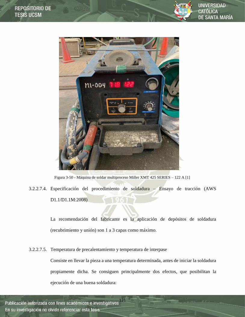
121
3.2.2.7.4. Especificación del procedimiento de soldadura – Ensayo de tracción (AWS
D1.1/D1.1M:2008)
La recomendación del fabricante es la aplicación de depósitos de soldadura
(recubrimiento y unión) son 1 a 3 capas como máximo.
3.2.2.7.5. Temperatura de precalentamiento y temperatura de interpase
Consiste en llevar la pieza a una temperatura determinada, antes de iniciar la soldadura
propiamente dicha. Se consiguen principalmente dos efectos, que posibilitan la
ejecución de una buena soldadura:
Figura 3-50 - Máquina de soldar multiproceso Miller XMT 425 SERIES – 122 A [1]
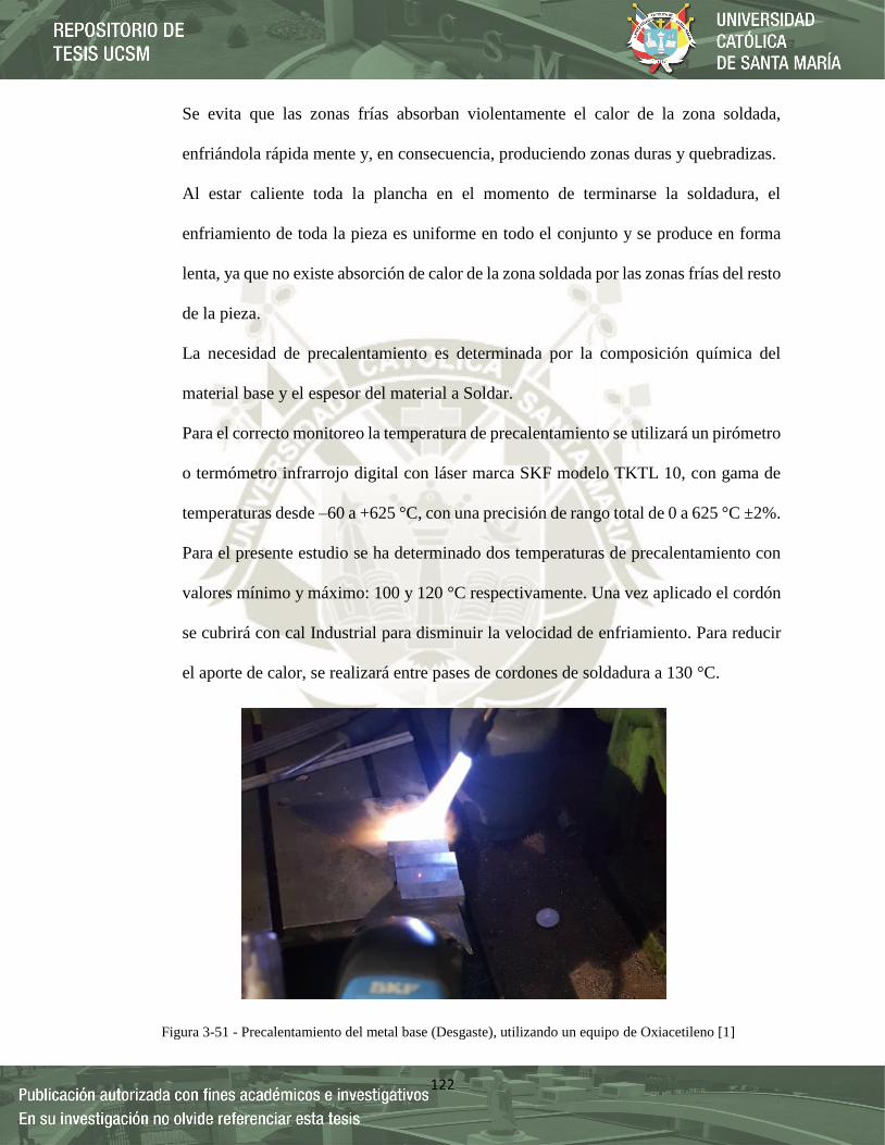
122
Se evita que las zonas frías absorban violentamente el calor de la zona soldada,
enfriándola rápida mente y, en consecuencia, produciendo zonas duras y quebradizas.
Al estar caliente toda la plancha en el momento de terminarse la soldadura, el
enfriamiento de toda la pieza es uniforme en todo el conjunto y se produce en forma
lenta, ya que no existe absorción de calor de la zona soldada por las zonas frías del resto
de la pieza.
La necesidad de precalentamiento es determinada por la composición química del
material base y el espesor del material a Soldar.
Para el correcto monitoreo la temperatura de precalentamiento se utilizará un pirómetro
o termómetro infrarrojo digital con láser marca SKF modelo TKTL 10, con gama de
temperaturas desde –60 a +625 °C, con una precisión de rango total de 0 a 625 °C ±2%.
Para el presente estudio se ha determinado dos temperaturas de precalentamiento con
valores mínimo y máximo: 100 y 120 °C respectivamente. Una vez aplicado el cordón
se cubrirá con cal Industrial para disminuir la velocidad de enfriamiento. Para reducir
el aporte de calor, se realizará entre pases de cordones de soldadura a 130 °C.
Figura 3-51 - Precalentamiento del metal base (Desgaste), utilizando un equipo de Oxiacetileno [1]
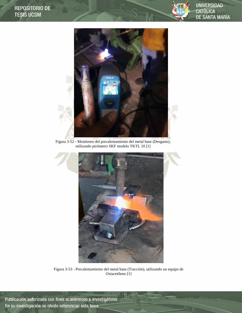
123
Figura 3-52 - Monitoreo del precalentamiento del metal base (Desgaste),
utilizando pirómetro SKF modelo TKTL 10 [1]
Figura 3-53 - Precalentamiento del metal base (Tracción), utilizando un equipo de
Oxiacetileno [1]
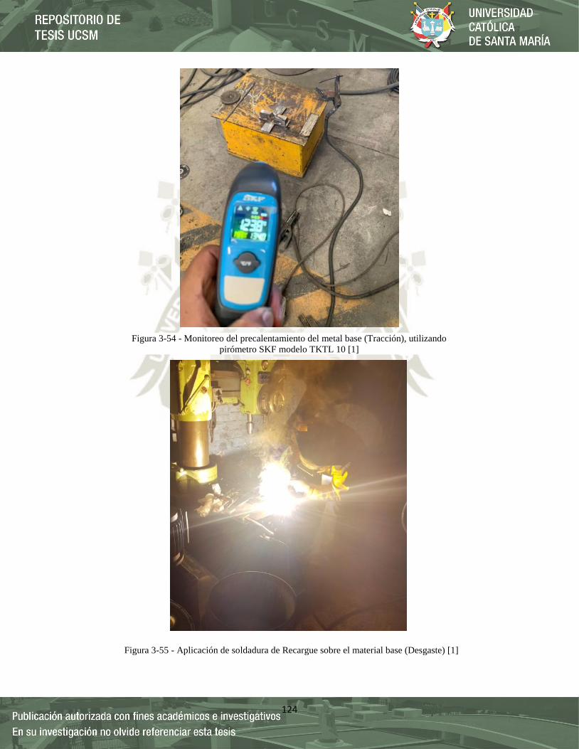
124
Figura 3-54 - Monitoreo del precalentamiento del metal base (Tracción), utilizando
pirómetro SKF modelo TKTL 10 [1]
Figura 3-55 - Aplicación de soldadura de Recargue sobre el material base (Desgaste) [1]

125
Figura 3-56 - Monitoreo de la soldadura de Recargue sobre el material base
(Desgaste), utilizando pirómetro SKF modelo TKTL 10 [1]
Figura 3-57 - Aplicación de la soldadura de Recargue sobre el material base
(Tracción) [1]
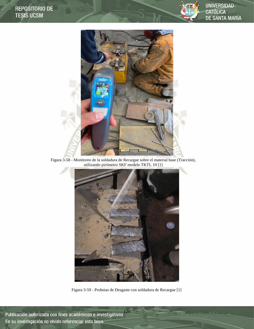
126
Figura 3-58 - Monitoreo de la soldadura de Recargue sobre el material base (Tracción),
utilizando pirómetro SKF modelo TKTL 10 [1]
Figura 3-59 - Probetas de Desgaste con soldadura de Recargue [1]

127
Figura 3-60 - Probeta de Tracción unido con soldadura de Recargue [1]
Figura 3-61 - Probeta de desgaste con recargue en recipiente con cal industrial [1]
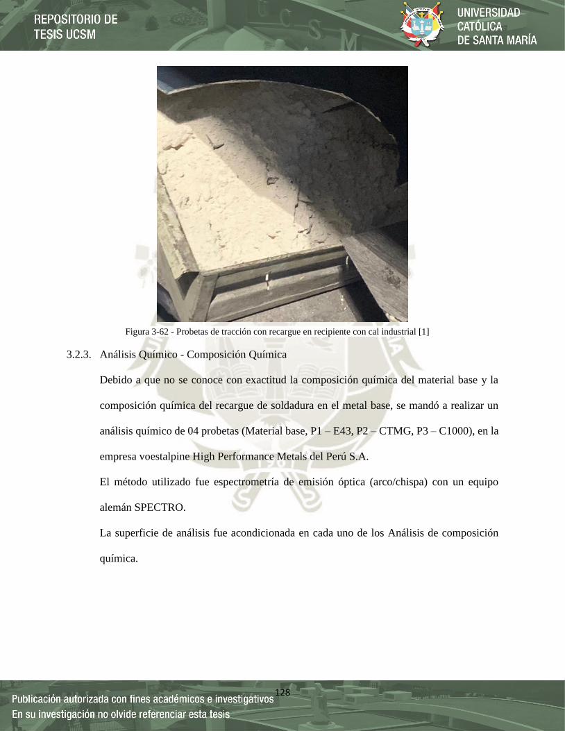
128
3.2.3. Análisis Químico - Composición Química
Debido a que no se conoce con exactitud la composición química del material base y la
composición química del recargue de soldadura en el metal base, se mandó a realizar un
análisis químico de 04 probetas (Material base, P1 – E43, P2 – CTMG, P3 – C1000), en la
empresa voestalpine High Performance Metals del Perú S.A.
El método utilizado fue espectrometría de emisión óptica (arco/chispa) con un equipo
alemán SPECTRO.
La superficie de análisis fue acondicionada en cada uno de los Análisis de composición
química.
Figura 3-62 - Probetas de tracción con recargue en recipiente con cal industrial [1]

129
3.2.3.1.Material base
3.2.3.2.Recubrimiento - Exadur - 43
Figura 3-63 - Uña de acero Excavadora hidráulica Cat 336 D2 L [1]
Figura 3-64 - Probeta con soldadura de recargue Exadur 43 (P1) [1]
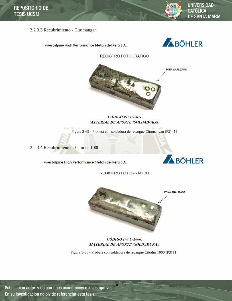
130
3.2.3.3.Recubrimiento - Citomangan
3.2.3.4.Recubrimiento – Citodur 1000
Figura 3-65 - Probeta con soldadura de recargue Citomangan (P2) [1]
Figura 3-66 - Probeta con soldadura de recargue Citodur 1000 (P3) [1]

131
3.2.4. Análisis Metalográfico
Se preparó las muestras la evaluación metalográfica, según la norma ASTM E3-11
“Standard Practice for Preparation of Metallographic Specimens” que se describe en la
siguiente Tabla 3-27. Se dividió en las siguientes etapas:
3.2.4.1.Desbaste grueso: Se trabajó papel lijar al agua, marca ABRALIT:
Lijar #100
Lijar #220
Lijar #400
Lijar #600
3.2.4.2.Desbaste fino: Se trabajó con papel lijar al agua:
Lijar #1000, marca ABRALIT
Lijar #1200, marca ABRALIT
Lijar #2000, marca ASALITE
3.2.4.3.Pulido fino: En una pulidora de disco con paño de pulido, con pasta de alúmina 0,5
micrones.
Tabla 3-27 - Preparación método 2 para materiales duros ≥ 45 (450 HV) [24]
Superficie Lubricante Tipo de Abrasivo
Tiempo (s) Fuerza N(lbf)A
Plato RPMB
Rotación Tamaño ANSI
Papel/piedra lija plano Agua 120-320
(P120-400) Polvo SiC/Al2O3
15 - 45 20-30 (5-8) 200-300C COD
Disco rígido de lija fina Lubricante compatible 6-15 μm diamante 180 - 300 20-30 (5-8) 100-150 CO
Pulido áspero bajo Lubricante compatible 3-6 μm diamante 120 - 300 20-30 (5-8) 100-150 CO
Pulido final Lubricante compatible 1 μm diamante 60 - 120 10-20 (3-5) 100-150 CO
Gamuza sinteticaE Agua 0.04 μm
silice coloidal 0.05 μm alumina
30 - 60 10-20 (3-5) 100-150 CONTRAF
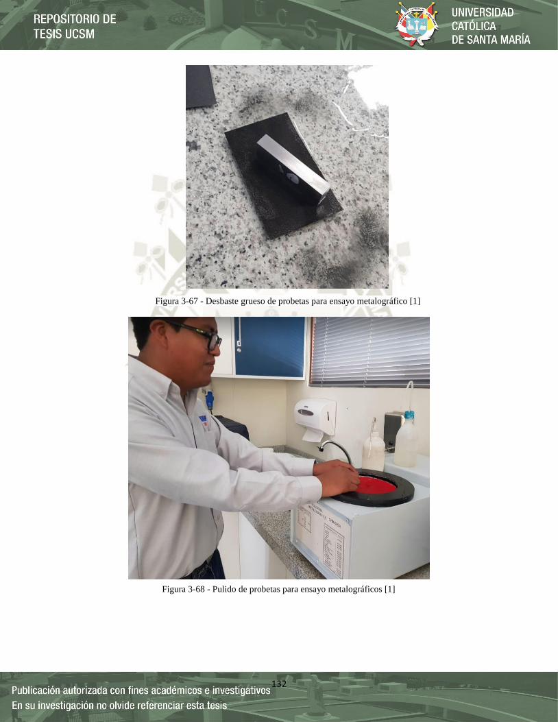
132
Figura 3-67 - Desbaste grueso de probetas para ensayo metalográfico [1]
Figura 3-68 - Pulido de probetas para ensayo metalográficos [1]
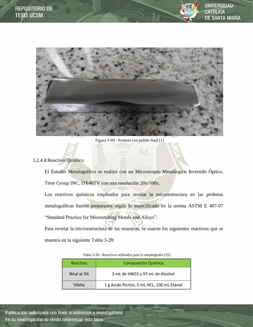
133
3.2.4.4.Reactivo Químico
El Estudio Metalográfico se realizó con un Microscopio Metalúrgico Invertido Óptico,
Time Group INC, DX40TV con una resolución 20x/100x.
Los reactivos químicos empleados para revelar la microestructura en las probetas
metalográficas fueron preparados según lo especificado en la norma ASTM E 407-07
“Standard Practice for Microetching Metals and Alloys”.
Para revelar la microestructura de las muestras, se usaron los siguientes reactivos que se
muestra en la siguiente Tabla 3-28:
Tabla 3-28 - Reactivos utilizados para la metalografía [25]
Reactivo Composición Química
Nital al 3% 3 mL de HNO3 y 97 mL de Alcohol
Vilella 1 g Acido Picrico, 5 mL HCL, 100 mL Etanol
Figura 3-69 - Probeta con pulido final [1]
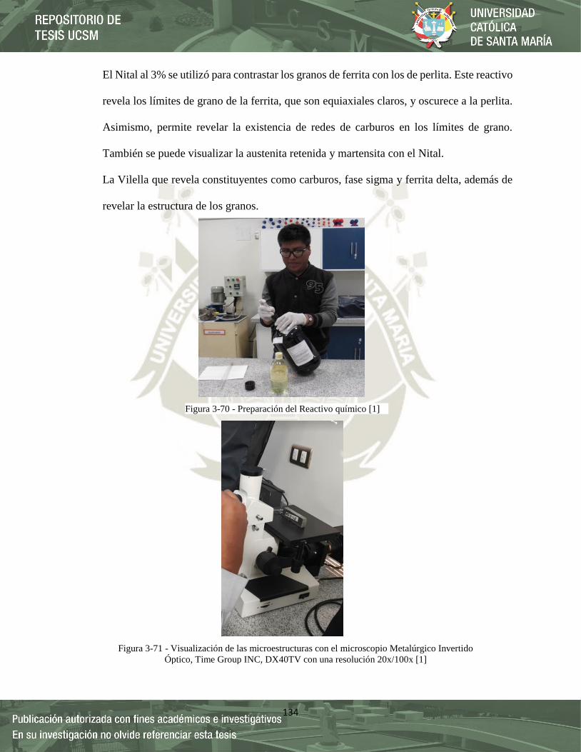
134
El Nital al 3% se utilizó para contrastar los granos de ferrita con los de perlita. Este reactivo
revela los límites de grano de la ferrita, que son equiaxiales claros, y oscurece a la perlita.
Asimismo, permite revelar la existencia de redes de carburos en los límites de grano.
También se puede visualizar la austenita retenida y martensita con el Nital.
La Vilella que revela constituyentes como carburos, fase sigma y ferrita delta, además de
revelar la estructura de los granos.
Figura 3-70 - Preparación del Reactivo químico [1]
Figura 3-71 - Visualización de las microestructuras con el microscopio Metalúrgico Invertido
Óptico, Time Group INC, DX40TV con una resolución 20x/100x [1]
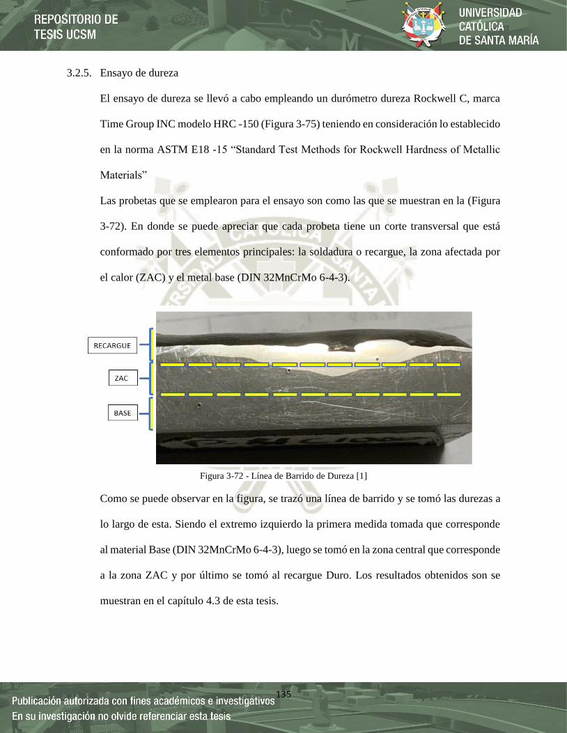
135
3.2.5. Ensayo de dureza
El ensayo de dureza se llevó a cabo empleando un durómetro dureza Rockwell C, marca
Time Group INC modelo HRC -150 (Figura 3-75) teniendo en consideración lo establecido
en la norma ASTM E18 -15 “Standard Test Methods for Rockwell Hardness of Metallic
Materials”
Las probetas que se emplearon para el ensayo son como las que se muestran en la (Figura
3-72). En donde se puede apreciar que cada probeta tiene un corte transversal que está
conformado por tres elementos principales: la soldadura o recargue, la zona afectada por
el calor (ZAC) y el metal base (DIN 32MnCrMo 6-4-3).
Como se puede observar en la figura, se trazó una línea de barrido y se tomó las durezas a
lo largo de esta. Siendo el extremo izquierdo la primera medida tomada que corresponde
al material Base (DIN 32MnCrMo 6-4-3), luego se tomó en la zona central que corresponde
a la zona ZAC y por último se tomó al recargue Duro. Los resultados obtenidos son se
muestran en el capítulo 4.3 de esta tesis.
Figura 3-72 - Línea de Barrido de Dureza [1]
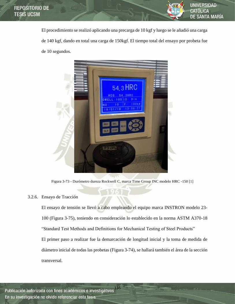
136
El procedimiento se realizó aplicando una precarga de 10 kgf y luego se le añadió una carga
de 140 kgf, dando en total una carga de 150kgf. El tiempo total del ensayo por probeta fue
de 10 segundos.
3.2.6. Ensayo de Tracción
El ensayo de tensión se llevó a cabo empleando el equipo marca INSTRON modelo 23-
100 (Figura 3-75), teniendo en consideración lo establecido en la norma ASTM A370-18
“Standard Test Methods and Definitions for Mechanical Testing of Steel Products”
El primer paso a realizar fue la demarcación de longitud inicial y la toma de medida de
diámetro inicial de todas las probetas (Figura 3-74), se hallará también el área de la sección
transversal.
Figura 3-73 - Durómetro dureza Rockwell C, marca Time Group INC modelo HRC -150 [1]
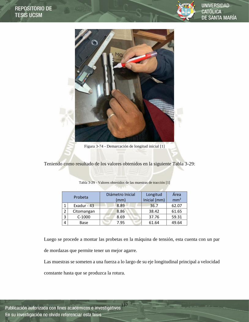
137
Teniendo como resultado de los valores obtenidos en la siguiente Tabla 3-29:
Tabla 3-29 - Valores obtenidos de las muestras de tracción [1]
Luego se procede a montar las probetas en la máquina de tensión, esta cuenta con un par
de mordazas que permite tener un mejor agarre.
Las muestras se someten a una fuerza a lo largo de su eje longitudinal principal a velocidad
constante hasta que se produzca la rotura.
Probeta Diámetro Inicial
(mm) Longitud
Inicial (mm) Área mm2
1 Exadur - 43 8.89 36.7 62.07
2 Citomangan 8.86 38.42 61.65
3 C-1000 8.69 37.76 59.31
4 Base 7.95 61.64 49.64
Figura 3-74 - Demarcación de longitud inicial [1]

138
El equipo de tracción cuenta con el software Bluehill® instalado, este permite registrar las
fuerzas y los valores de incrementos entre las mordazas (Figura 3-76).
En total se realizaron 04 ensayos de tracción, 03 de unión de soldadura y 01 de material
base (Figura 3-77).
Figura 3-75 - Máquina de tracción INSTRON modelo 23-100 [1]
Figura 3-76 - Software Bluehill® [1]
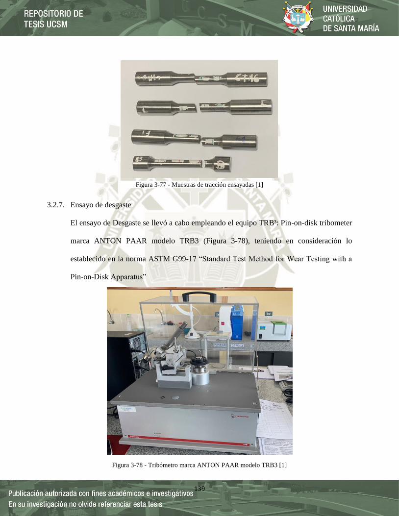
139
3.2.7. Ensayo de desgaste
El ensayo de Desgaste se llevó a cabo empleando el equipo TRB³: Pin-on-disk tribometer
marca ANTON PAAR modelo TRB3 (Figura 3-78), teniendo en consideración lo
establecido en la norma ASTM G99-17 “Standard Test Method for Wear Testing with a
Pin-on-Disk Apparatus”
Figura 3-77 - Muestras de tracción ensayadas [1]
Figura 3-78 - Tribómetro marca ANTON PAAR modelo TRB3 [1]
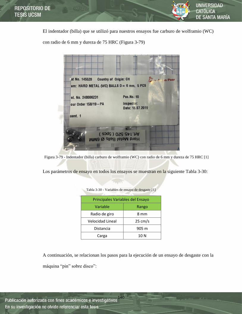
140
El indentador (billa) que se utilizó para nuestros ensayos fue carburo de wolframio (WC)
con radio de 6 mm y dureza de 75 HRC (Figura 3-79)
Los parámetros de ensayo en todos los ensayos se muestran en la siguiente Tabla 3-30:
Tabla 3-30 - Variables de ensayo de desgaste [1]
A continuación, se relacionan los pasos para la ejecución de un ensayo de desgaste con la
máquina “pin” sobre disco”:
Principales Variables del Ensayo
Variable Rango
Radio de giro 8 mm
Velocidad Lineal 25 cm/s
Distancia 905 m
Carga 10 N
Figura 3-79 - Indentador (billa) carburo de wolframio (WC) con radio de 6 mm y dureza de 75 HRC [1]
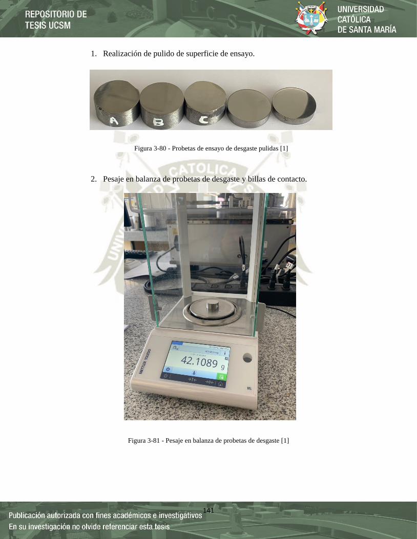
141
1. Realización de pulido de superficie de ensayo.
2. Pesaje en balanza de probetas de desgaste y billas de contacto.
Figura 3-80 - Probetas de ensayo de desgaste pulidas [1]
Figura 3-81 - Pesaje en balanza de probetas de desgaste [1]

142
3. Montaje de la probeta de desgaste en el porta-muestras del equipo para el ensayo
de desgaste.
Figura 3-82 - Pesaje en balanza de billas de contacto [1]
Figura 3-83 - Montaje de la probeta de desgaste en el porta-muestra del
tribómetro [1]

143
4. Selección del radio desde el centro del disco hasta el apoyo de la probeta de
ensayo, distancia del ensayo, fuerza de aplicación y velocidad lineal.
5. Realización del ensayo de desgaste, durante el tiempo calculado de la distancia
total.
Figura 3-84 - Ensayo de desgate ASTM G-99 [1]
Figura 3-85 - Parámetros de ensayo de desgate ASTM G-99 [1]
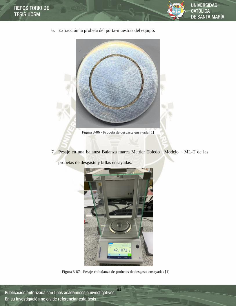
144
6. Extracción la probeta del porta-muestras del equipo.
7. Pesaje en una balanza Balanza marca Mettler Toledo , Modelo – ML-T de las
probetas de desgaste y billas ensayadas.
Figura 3-86 - Probeta de desgaste ensayada [1]
Figura 3-87 - Pesaje en balanza de probetas de desgaste ensayadas [1]
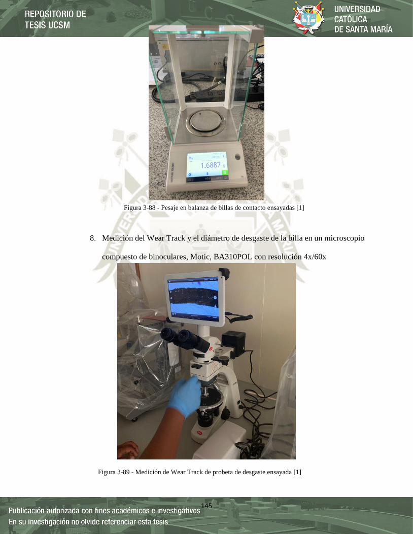
145
8. Medición del Wear Track y el diámetro de desgaste de la billa en un microscopio
compuesto de binoculares, Motic, BA310POL con resolución 4x/60x
Figura 3-88 - Pesaje en balanza de billas de contacto ensayadas [1]
Figura 3-89 - Medición de Wear Track de probeta de desgaste ensayada [1]

146
CAPÍTULO IV
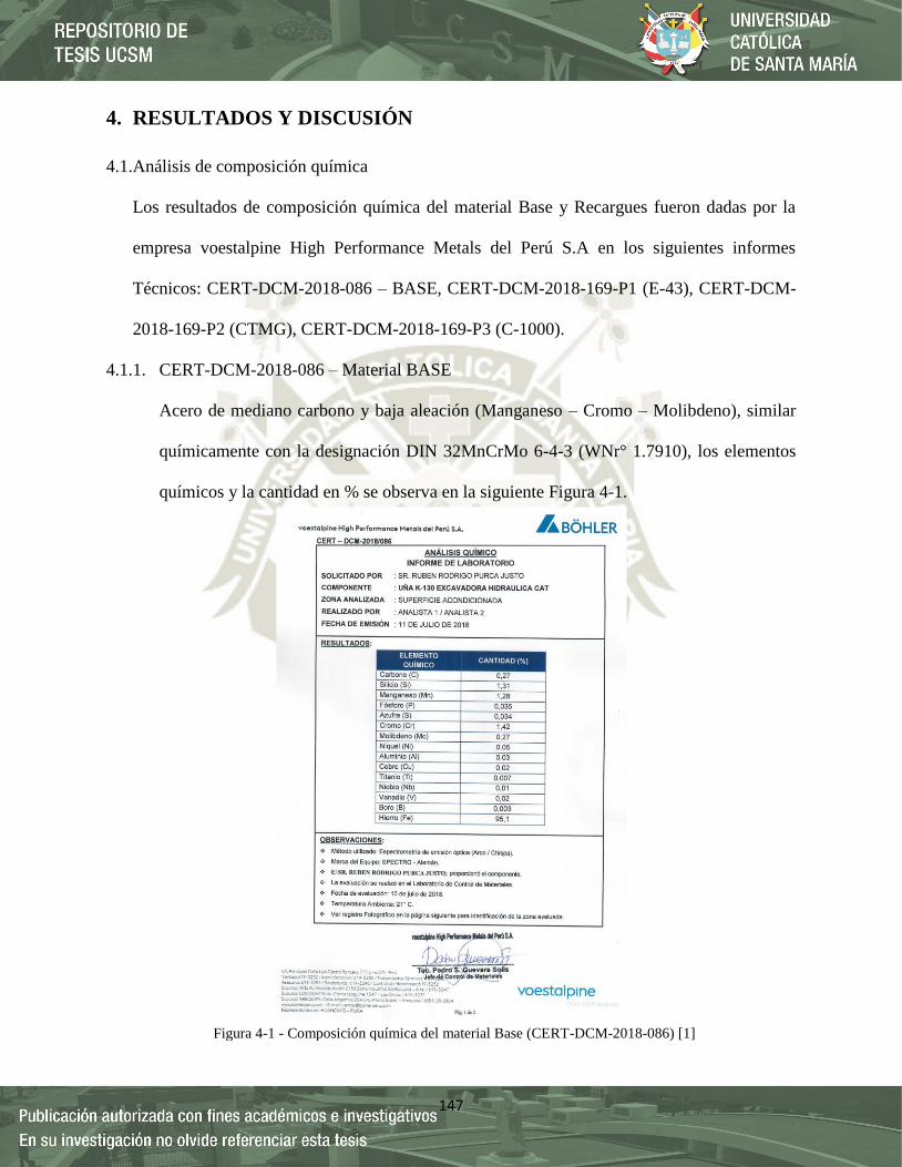
147
4. RESULTADOS Y DISCUSIÓN
4.1.Análisis de composición química
Los resultados de composición química del material Base y Recargues fueron dadas por la
empresa voestalpine High Performance Metals del Perú S.A en los siguientes informes
Técnicos: CERT-DCM-2018-086 – BASE, CERT-DCM-2018-169-P1 (E-43), CERT-DCM-
2018-169-P2 (CTMG), CERT-DCM-2018-169-P3 (C-1000).
4.1.1. CERT-DCM-2018-086 – Material BASE
Acero de mediano carbono y baja aleación (Manganeso – Cromo – Molibdeno), similar
químicamente con la designación DIN 32MnCrMo 6-4-3 (WNr° 1.7910), los elementos
químicos y la cantidad en % se observa en la siguiente Figura 4-1.
Figura 4-1 - Composición química del material Base (CERT-DCM-2018-086) [1]

148
4.1.2. CERT-DCM-2018-169-P1 (E-43)
Material de alto carbono y alta aleación (Cromo – Niobio), similar químicamente con la
designación EXADUR 43, los elementos químicos y la cantidad en % se observa en la
siguiente Figura 4-2.
Figura 4-2 - Composición química del recargue duro Exadur 43 sobre el material base (CERT-DCM-
2018-169-P1) [1]
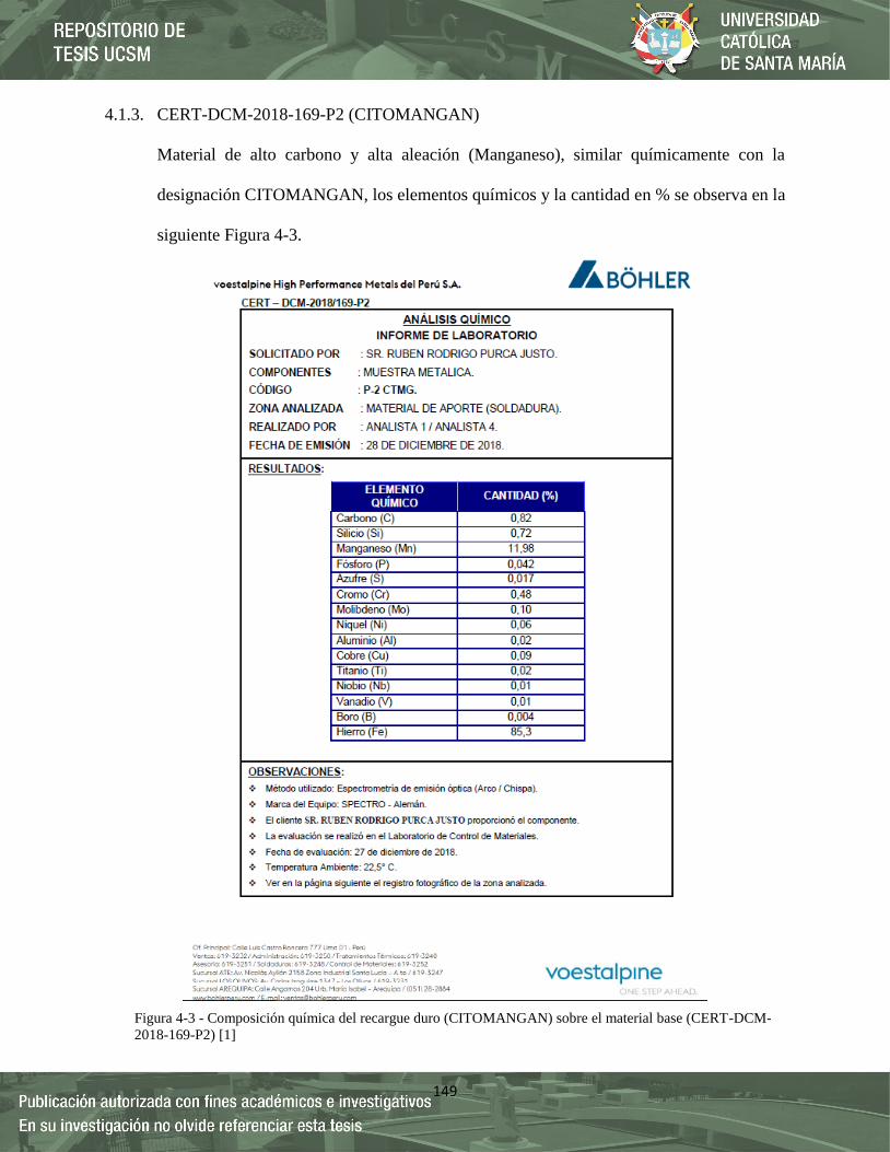
149
4.1.3. CERT-DCM-2018-169-P2 (CITOMANGAN)
Material de alto carbono y alta aleación (Manganeso), similar químicamente con la
designación CITOMANGAN, los elementos químicos y la cantidad en % se observa en la
siguiente Figura 4-3.
Figura 4-3 - Composición química del recargue duro (CITOMANGAN) sobre el material base (CERT-DCM-
2018-169-P2) [1]
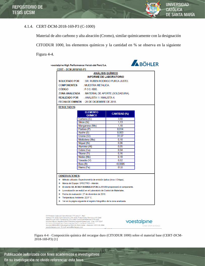
150
4.1.4. CERT-DCM-2018-169-P3 (C-1000)
Material de alto carbono y alta aleación (Cromo), similar químicamente con la designación
CITODUR 1000, los elementos químicos y la cantidad en % se observa en la siguiente
Figura 4-4.
Figura 4-4 - Composición química del recargue duro (CITODUR 1000) sobre el material base (CERT-DCM-
2018-169-P3) [1]

151
UNIVERSIDAD CATÓLICA DE SANTA MARIA, ESCUELA PROFESIONAL DE INGENIERIA
MECÁNICA, MECÁNICA ELÉTRICA Y MECÁTRONICA
REPORTE DE COMPOSICIÓN QUÍMICA POR - Espectrometría de emisión óptica (Arco / Chispa) Tipo de Estudio De laboratorio Ensayo N⁰ 1, 2 ,3 , 4
Fecha: 28 DE DICIEMBRE DE 2018 Probeta N⁰ Base, P-1, P-2, P-3
Parte Especificada: Material Base y aporte Revestimientos Duros
Solicitado Por: Ruben Purca Dirección Asoc. De Viv Los Olmos Arequipa, Peru
Centro de estudios y análisis: Laboratorio de Control de Materiales - voestalpine High Performance Metals del Perú S.A
Realizado Por: Analista 1/ Analista 2 Revisado Por: Pedro Guevara Solis
PARÁMETROS DEL ENSAYO DE ESPECTROMETRÍA
Tipo de Ensayo:
Espectrometría de emisión óptica (Arco /
Chispa). Equipo utilizado: SPECTRO - Alemán.
Temperatura del Ensayo:
22,5° C.
BASE P1-E43
P-2 CTMG P-3 C-1000
RESULTADOS
Probeta Tipo de Recargue C Si Mn P S Cr Mo Ni Al Cu Ti Nb V B Fe
P-0 BASE Sin Recargue 0.27 1.31 1.28 0.035 0.034 1.42 0.27 0.05 0.03 0.02 0.007 0.01 0.02 0.003 95.1
P-1 (E-43) Exadur 43 3.96 1.59 1.24 0.028 0.013 20.3 0.1 0.15 0.05 0.07 0.08 4.2 0.04 0.0005 67.8
P-2 (CTMG) Citomangan 0.82 0.72 11.98 0.042 0.017 0.48 0.1 0.06 0.02 0.09 0.02 0.01 0.01 0.004 85.3
P-3 (C-1000) Citodur 1000 3.6 1.13 1.1 0.014 0.003 31.57 0.1 0.06 0.05 0.04 0.16 0.1 0.02 0.0005 61.6
Ficha 4-1 - Reporte Resumen de composición química por Espectrometría - voestalpine High Performance Metals del Perú S.A [1]
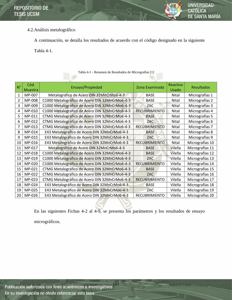
152
4.2.Análisis metalográfico
A continuación, se detalla los resultados de acuerdo con el código designado en la siguiente
Tabla 4-1.
Tabla 4-1 - Resumen de Resultados de Micrografías [1]
En las siguientes Fichas 4-2 al 4-9, se presenta los parámetros y los resultados de ensayo
micrográficos.
N° Cód.
Muestra Ensayo/Propiedad Zona Examinada
Reactivo Usado
Resultados
1 MP-007 Metalográfico de Acero DIN 32MnCrMo6-4-3 BASE Nital Micrografías 1
2 MP-008 C1000 Metalográfico de Acero DIN 32MnCrMo6-4-3 BASE Nital Micrografías 2
3 MP-009 C1000 Metalográfico de Acero DIN 32MnCrMo6-4-3 ZAC Nital Micrografías 3
4 MP-010 C1000 Metalográfico de Acero DIN 32MnCrMo6-4-3 RECUBRIMIENTO Nital Micrografías 4
5 MP-011 CTMG Metalográfico de Acero DIN 32MnCrMo6-4-3 BASE Nital Micrografías 5
6 MP-012 CTMG Metalográfico de Acero DIN 32MnCrMo6-4-3 ZAC Nital Micrografías 6
7 MP-013 CTMG Metalográfico de Acero DIN 32MnCrMo6-4-3 RECUBRIMIENTO Nital Micrografías 7
8 MP-014 E43 Metalográfico de Acero DIN 32MnCrMo6-4-3 BASE Nital Micrografías 8
9 MP-015 E43 Metalográfico de Acero DIN 32MnCrMo6-4-3 ZAC Nital Micrografías 9
10 MP-016 E43 Metalográfico de Acero DIN 32MnCrMo6-4-3 RECUBRIMIENTO Nital Micrografías 10
11 MP-017 Metalográfico de Acero DIN 32MnCrMo6-4-3 BASE Vilella Micrografías 11
12 MP-018 C1000 Metalográfico de Acero DIN 32MnCrMo6-4-3 BASE Vilella Micrografías 12
13 MP-019 C1000 Metalográfico de Acero DIN 32MnCrMo6-4-3 ZAC Vilella Micrografías 13
14 MP-020 C1000 Metalográfico de Acero DIN 32MnCrMo6-4-3 RECUBRIMIENTO Vilella Micrografías 14
15 MP-021 CTMG Metalográfico de Acero DIN 32MnCrMo6-4-3 BASE Vilella Micrografías 15
16 MP-022 CTMG Metalográfico de Acero DIN 32MnCrMo6-4-3 ZAC Vilella Micrografías 16
17 MP-023 CTMG Metalográfico de Acero DIN 32MnCrMo6-4-3 RECUBRIMIENTO Vilella Micrografías 17
18 MP-024 E43 Metalográfico de Acero DIN 32MnCrMo6-4-3 BASE Vilella Micrografías 18
19 MP-025 E43 Metalográfico de Acero DIN 32MnCrMo6-4-3 ZAC Vilella Micrografías 19
20 MP-026 E43 Metalográfico de Acero DIN 32MnCrMo6-4-3 RECUBRIMIENTO Vilella Micrografías 20

153
Ficha 4-2 - Análisis metalográfico (Micrografía 1) [1]
UNIVERSIDAD CATÓLICA DE SANTA MARIA, ESCUELA PROFESIONAL DE INGENIERIA
MECÁNICA, MECÁNICA ELÉTRICA Y MECÁTRONICA
ENSAYO METALOGRÁFICO Tipo de Estudio De laboratorio Ensayo N⁰ Micrografías 1
Fecha: 17/01/2019 Probeta N⁰ Acero DIN 32MnCrMo
6-4-3
Parte Especificada: PROBETA MATERIAL BASE - DIN 32MnCrMo 6-4-3 (WNr°
1.7910)
Solicitado Por: Ruben Purca Dirección Asoc. De Viv Los Olmos Arequipa, Perú
Centro de estudios y análisis: Laboratorio de Ingeniería de Materiales de la Universidad
Católica de Santa María
Realizado Por: Ruben Purca Revisado Por: Ing. Emilio Chire
PARAMETROS AMBIENTALES DEL LUGAR DURANTE EL ENSAYO
Tipo de Ensayo: Ensayo
Metalográfico Iluminación: Buena
Temperatura del Ensayo: 22,5° C.
Tipo de probeta: Rectangular
Espec. del material:
Acero de mediano carbono y baja aleación (Manganeso – Cromo – Molibdeno)
PARÁMETROS DEL ENSAYO METALOGRÁFICO
Preparación de la superficie: Lijar #100; Lijar #220; Lijar #400 ,Lijar #600, Lijar #1000, Lijar
#1200, Lijar #2000
Tiempo de ataque: 10 segundos Ataque
químico: Nital
RESULTADO 1- 20X 1 - 100X

154
UNIVERSIDAD CATÓLICA DE SANTA MARIA, ESCUELA PROFESIONAL DE INGENIERIA
MECÁNICA, MECÁNICA ELÉTRICA Y MECÁTRONICA
ENSAYO METALOGRÁFICO Tipo de Estudio De laboratorio Ensayo N⁰ Micrografías 2,3,4
Fecha: 17/01/2019 Probeta N⁰ C1000 Metalográfico de Acero DIN 32MnCrMo6-
4-3
Parte Especificada: PROBETA CON UNION DE RECARGUE CITODUR - 1000
Solicitado Por: Ruben Purca Dirección Asoc. De Viv Los Olmos Arequipa, Perú
Centro de estudios y análisis: Laboratorio de Ingeniería de Materiales de la Universidad
Católica de Santa María
Realizado Por: Ruben Purca Revisado Por: Ing. Emilio Chire
PARAMETROS AMBIENTALES DEL LUGAR DURANTE EL ENSAYO
Tipo de Ensayo: Ensayo
Metalográfico Iluminación: Buena
Temperatura del Ensayo: 22,5° C.
Tipo de probeta: Rectangular
Espec. del material:
Unión de Acero de mediano carbono y baja aleación (Manganeso – Cromo – Molibdeno)
con Soldadura CITODUR - 1000
PARÁMETROS DEL ENSAYO METALOGRÁFICO
Preparación de la superficie: Lijar #100; Lijar #220; Lijar #400, Lijar #600, Lijar #1000, Lijar
#1200, Lijar #2000
Tiempo de ataque: 10 segundos Ataque
químico: Nital
RESULTADO 2 4
3
La figura 2 corresponde al material Base
La figura 3 corresponde a la zona ZAC
La figura 4 corresponde a la zona de Recargue
Ficha 4-3 - Análisis metalográfico (Micrografías 2,3,4) [1]

155
UNIVERSIDAD CATÓLICA DE SANTA MARIA, ESCUELA PROFESIONAL DE INGENIERIA
MECÁNICA, MECÁNICA ELÉTRICA Y MECÁTRONICA
ENSAYO METALOGRÁFICO Tipo de Estudio De laboratorio Ensayo N⁰ Micrografías 5,6,7
Fecha: 17/01/2019 Probeta N⁰ CTMG Metalográfico de Acero DIN 32MnCrMo6-
4-3
Parte Especificada: PROBETA CON UNIÓN DE RECARGUE CITOMANGAN
Solicitado Por: Ruben Purca Dirección Asoc. De Viv Los Olmos Arequipa, Perú
Centro de estudios y análisis: Laboratorio de Ingeniería de Materiales de la Universidad
Católica de Santa María
Realizado Por: Ruben Purca Revisado Por: Ing. Emilio Chire
PARAMETROS AMBIENTALES DEL LUGAR DURANTE EL ENSAYO
Tipo de Ensayo: Ensayo
Metalográfico Iluminación: Buena
Temperatura del Ensayo: 22,5° C.
Tipo de probeta: Rectangular
Espec. del material:
Unión de Acero de mediano carbono y baja aleación (Manganeso – Cromo – Molibdeno)
con Soldadura CITOMANGAN
PARÁMETROS DEL ENSAYO METALOGRÁFICO
Preparación de la superficie: Lijar #100; Lijar #220; Lijar #400, Lijar #600, Lijar #1000, Lijar
#1200, Lijar #2000
Tiempo de ataque: 10 segundos Ataque
químico: Nital
RESULTADO 5 7
6
La figura 5 corresponde al material Base
La figura 6 corresponde a la zona ZAC
La figura 7 corresponde a la zona de Recargue
Ficha 4-4 - Análisis metalográfico (Micrografías 5,6,7) [1]
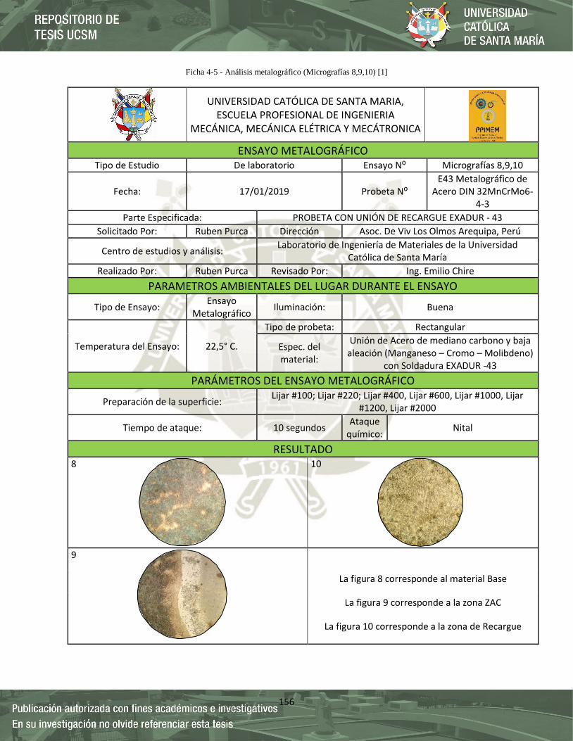
156
Ficha 4-5 - Análisis metalográfico (Micrografías 8,9,10) [1]
UNIVERSIDAD CATÓLICA DE SANTA MARIA, ESCUELA PROFESIONAL DE INGENIERIA
MECÁNICA, MECÁNICA ELÉTRICA Y MECÁTRONICA
ENSAYO METALOGRÁFICO Tipo de Estudio De laboratorio Ensayo N⁰ Micrografías 8,9,10
Fecha: 17/01/2019 Probeta N⁰ E43 Metalográfico de
Acero DIN 32MnCrMo6-4-3
Parte Especificada: PROBETA CON UNIÓN DE RECARGUE EXADUR - 43
Solicitado Por: Ruben Purca Dirección Asoc. De Viv Los Olmos Arequipa, Perú
Centro de estudios y análisis: Laboratorio de Ingeniería de Materiales de la Universidad
Católica de Santa María
Realizado Por: Ruben Purca Revisado Por: Ing. Emilio Chire
PARAMETROS AMBIENTALES DEL LUGAR DURANTE EL ENSAYO
Tipo de Ensayo: Ensayo
Metalográfico Iluminación: Buena
Temperatura del Ensayo: 22,5° C.
Tipo de probeta: Rectangular
Espec. del material:
Unión de Acero de mediano carbono y baja aleación (Manganeso – Cromo – Molibdeno)
con Soldadura EXADUR -43
PARÁMETROS DEL ENSAYO METALOGRÁFICO
Preparación de la superficie: Lijar #100; Lijar #220; Lijar #400, Lijar #600, Lijar #1000, Lijar
#1200, Lijar #2000
Tiempo de ataque: 10 segundos Ataque
químico: Nital
RESULTADO 8 10
9
La figura 8 corresponde al material Base
La figura 9 corresponde a la zona ZAC
La figura 10 corresponde a la zona de Recargue

157
Ficha 4-6 - Análisis metalográfico (Micrografías 11) [1]
UNIVERSIDAD CATÓLICA DE SANTA MARIA, ESCUELA PROFESIONAL DE INGENIERIA
MECÁNICA, MECÁNICA ELÉTRICA Y MECÁTRONICA
ENSAYO METALOGRÁFICO Tipo de Estudio De laboratorio Ensayo N⁰ Micrografías 11
Fecha: 17/01/2019 Probeta N⁰ BASE
Parte Especificada: PROBETA MATERIAL BASE - DIN 32MnCrMo6-4-3 (WNr°
1.7910)
Solicitado Por: Ruben Purca Dirección Asoc. De Viv Los Olmos Arequipa, Perú
Centro de estudios y análisis: Laboratorio de Ingeniería de Materiales de la Universidad
Católica de Santa María
Realizado Por: Ruben Purca Revisado Por: Ing. Emilio Chire
PARAMETROS AMBIENTALES DEL LUGAR DURANTE EL ENSAYO
Tipo de Ensayo: Ensayo
Metalográfico Iluminación: Buena
Temperatura del Ensayo: 22,5° C.
Tipo de probeta: Rectangular
Espec. del material:
Acero de mediano carbono y baja aleación (Manganeso – Cromo – Molibdeno)
PARÁMETROS DEL ENSAYO METALOGRÁFICO
Preparación de la superficie: Lijar #100; Lijar #220; Lijar #400 ,Lijar #600, Lijar #1000, Lijar
#1200, Lijar #2000
Tiempo de ataque: 10 segundos Ataque
químico: Vilella
RESULTADO 11 - 20X 11 -100X
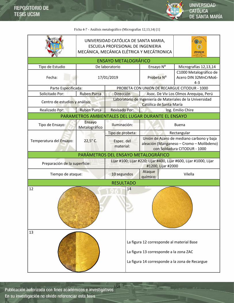
158
Ficha 4-7 - Análisis metalográfico (Micrografías 12,13,14) [1]
UNIVERSIDAD CATÓLICA DE SANTA MARIA, ESCUELA PROFESIONAL DE INGENIERIA
MECÁNICA, MECÁNICA ELÉTRICA Y MECÁTRONICA
ENSAYO METALOGRÁFICO Tipo de Estudio De laboratorio Ensayo N⁰ Micrografías 12,13,14
Fecha: 17/01/2019 Probeta N⁰ C1000 Metalográfico de Acero DIN 32MnCrMo6-
4-3
Parte Especificada: PROBETA CON UNION DE RECARGUE CITODUR - 1000
Solicitado Por: Ruben Purca Dirección Asoc. De Viv Los Olmos Arequipa, Perú
Centro de estudios y análisis: Laboratorio de Ingeniería de Materiales de la Universidad
Católica de Santa María
Realizado Por: Ruben Purca Revisado Por: Ing. Emilio Chire
PARAMETROS AMBIENTALES DEL LUGAR DURANTE EL ENSAYO
Tipo de Ensayo: Ensayo
Metalográfico Iluminación: Buena
Temperatura del Ensayo: 22,5° C.
Tipo de probeta: Rectangular
Espec. del material:
Unión de Acero de mediano carbono y baja aleación (Manganeso – Cromo – Molibdeno)
con Soldadura CITODUR - 1000
PARÁMETROS DEL ENSAYO METALOGRÁFICO
Preparación de la superficie: Lijar #100; Lijar #220; Lijar #400, Lijar #600, Lijar #1000, Lijar
#1200, Lijar #2000
Tiempo de ataque: 10 segundos Ataque
químico: Vilella
RESULTADO 12 14
13
La figura 12 corresponde al material Base
La figura 13 corresponde a la zona ZAC
La figura 14 corresponde a la zona de Recargue

159
Ficha 4-8 - Análisis metalográfico (Micrografías 15,16,17) [1]
UNIVERSIDAD CATÓLICA DE SANTA MARIA, ESCUELA PROFESIONAL DE INGENIERIA
MECÁNICA, MECÁNICA ELÉTRICA Y MECÁTRONICA
ENSAYO METALOGRÁFICO Tipo de Estudio De laboratorio Ensayo N⁰ Micrografías 15,16,17
Fecha: 17/01/2019 Probeta N⁰ CTMG Metalográfico de Acero DIN 32MnCrMo6-
4-3
Parte Especificada: PROBETA CON UNIÓN DE RECARGUE CITOMANGAN
Solicitado Por: Ruben Purca Dirección Asoc. De Viv Los Olmos Arequipa, Perú
Centro de estudios y análisis: Laboratorio de Ingeniería de Materiales de la Universidad
Católica de Santa María
Realizado Por: Ruben Purca Revisado Por: Ing. Emilio Chire
PARAMETROS AMBIENTALES DEL LUGAR DURANTE EL ENSAYO
Tipo de Ensayo: Ensayo
Metalográfico Iluminación: Buena
Temperatura del Ensayo: 22,5° C.
Tipo de probeta: Rectangular
Espec. del material:
Unión de Acero de mediano carbono y baja aleación (Manganeso – Cromo – Molibdeno)
con Soldadura CITOMANGAN
PARÁMETROS DEL ENSAYO METALOGRÁFICO
Preparación de la superficie: Lijar #100; Lijar #220; Lijar #400, Lijar #600, Lijar #1000, Lijar
#1200, Lijar #2000
Tiempo de ataque: 10 segundos Ataque
químico: Villela
RESULTADO 15 17
16
La figura 15 corresponde al material Base
La figura 16 corresponde a la zona ZAC
La figura 17 corresponde a la zona de Recargue
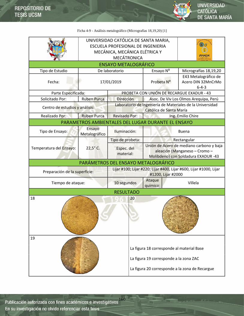
160
Ficha 4-9 - Análisis metalográfico (Micrografías 18,19,20) [1]
UNIVERSIDAD CATÓLICA DE SANTA MARIA, ESCUELA PROFESIONAL DE INGENIERIA
MECÁNICA, MECÁNICA ELÉTRICA Y MECÁTRONICA
ENSAYO METALOGRÁFICO Tipo de Estudio De laboratorio Ensayo N⁰ Micrografías 18,19,20
Fecha: 17/01/2019 Probeta N⁰ E43 Metalográfico de Acero DIN 32MnCrMo
6-4-3
Parte Especificada: PROBETA CON UNIÓN DE RECARGUE EXADUR - 43
Solicitado Por: Ruben Purca Dirección Asoc. De Viv Los Olmos Arequipa, Perú
Centro de estudios y análisis: Laboratorio de Ingeniería de Materiales de la Universidad
Católica de Santa María
Realizado Por: Ruben Purca Revisado Por: Ing. Emilio Chire
PARAMETROS AMBIENTALES DEL LUGAR DURANTE EL ENSAYO
Tipo de Ensayo: Ensayo
Metalográfico Iluminación: Buena
Temperatura del Ensayo: 22,5° C.
Tipo de probeta: Rectangular
Espec. del material:
Unión de Acero de mediano carbono y baja aleación (Manganeso – Cromo –
Molibdeno) con Soldadura EXADUR -43
PARÁMETROS DEL ENSAYO METALOGRÁFICO
Preparación de la superficie: Lijar #100; Lijar #220; Lijar #400, Lijar #600, Lijar #1000, Lijar
#1200, Lijar #2000
Tiempo de ataque: 10 segundos Ataque
químico: Villela
RESULTADO 18 20
19
La figura 18 corresponde al material Base
La figura 19 corresponde a la zona ZAC
La figura 20 corresponde a la zona de Recargue
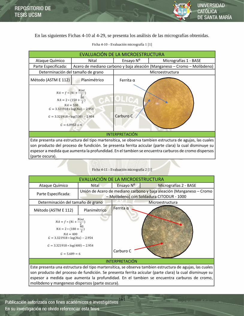
161
En las siguientes Fichas 4-10 al 4-29, se presenta los análisis de las micrografías obtenidas.
Ficha 4-10 - Evaluación micrografía 1 [1]
Ficha 4-11 - Evaluación micrografía 2 [1]
EVALUACIÓN DE LA MICROESTRUCTURA Ataque Químico Nital Ensayo N⁰ Micrografías 1 - BASE
Parte Especificada: Acero de mediano carbono y baja aleación (Manganeso – Cromo – Molibdeno)
Determinación del tamaño de grano Microestructura
Método (ASTM E 112) Planimétrico Ferrita α
Carburo C
𝑁𝐴 = 𝑓 ∗ (𝑁𝑖 +𝑁𝑖𝑛𝑡
2)
𝑁𝐴 = 2 ∗ (150 +80
2)
𝑁𝐴 = 530 𝐺 = 3.321918 ∗ log(𝑁𝑎) − 2.954
𝐺 = 3.321918 ∗ log(530) − 2.954
𝐺 = 6.0952 = 6
INTERPRETACIÓN
Este presenta una estructura del tipo martensítica, se observa tambien estructura de agujas, las cuales son producto del proceso de fundición. Se presenta ferrita acicular (parte clara) la cual disminuye su espesor a medida que aumenta la profundidad. En el tambien se encuentra carburos de cromo dispersos (parte oscura).
EVALUACIÓN DE LA MICROESTRUCTURA Ataque Químico Nital Ensayo N⁰ Micrografías 2 - BASE
Parte Especificada: Unión de Acero de mediano carbono y baja aleación (Manganeso – Cromo
– Molibdeno) con Soldadura CITODUR - 1000
Determinación del tamaño de grano Microestructura
Método (ASTM E 112) Planimétrico Ferrita α Carburo C
𝑁𝐴 = 𝑓 ∗ (𝑁𝑖 +𝑁𝑖𝑛𝑡
2)
𝑁𝐴 = 2 ∗ (180 +40
2)
𝑁𝐴 = 400 𝐺 = 3.321918 ∗ log(𝑁𝑎) − 2.954
𝐺 = 3.321918 ∗ log(400) − 2.954
𝐺 = 5.689 = 6
INTERPRETACIÓN
Este presenta una estructura del tipo martensítica, se observa tambien estructura de agujas, las cuales son producto del proceso de fundición. Se presenta ferrita acicular (parte clara) la cual disminuye su espesor a medida que aumenta la profundidad. En el tambien se encuentra carburos de cromo, molibdeno y mangeneso dispersos (parte oscura).

162
Ficha 4-12 - Evaluación micrografía 3 [1]
Ficha 4-13 - Evaluación micrografía 4 [1]
EVALUACIÓN DE LA MICROESTRUCTURA Ataque Químico Nital Ensayo N⁰ Micrografías 3 - ZAC
Parte Especificada: Unión de Acero de mediano carbono y baja aleación (Manganeso – Cromo
– Molibdeno) con Soldadura CITODUR - 1000
Determinación del tamaño de grano Microestructura
Método (ASTM E 112) Planimétrico
𝑁𝐴 = 𝑓 ∗ (𝑁𝑖 +𝑁𝑖𝑛𝑡
2)
𝑁𝐴 = 2 ∗ (370 +40
2)
𝑁𝐴 = 780 𝐺 = 3.321918 ∗ log(𝑁𝑎) − 2.954
𝐺 = 3.321918 ∗ log(780) − 2.954
𝐺 = 6.6533 = 7
INTERPRETACIÓN
Cerca de la intercara metal base-recubrimiento, se observa una estructura con crecimiento dendrítico ocasionada por el rápido enfriamiento característico del proceso de soldadura eléctrica.
EVALUACIÓN DE LA MICROESTRUCTURA Ataque Químico Nital Ensayo N⁰ Micrografías 4 - RECUBRIMIENTO
Parte Especificada: Unión de Acero de mediano carbono y baja aleación (Manganeso – Cromo
– Molibdeno) con Soldadura CITODUR - 1000
Determinación del tamaño de grano Microestructura
Método (ASTM E 112) Planimétrico
𝑁𝐴 = 𝑓 ∗ (𝑁𝑖 +𝑁𝑖𝑛𝑡
2)
𝑁𝐴 = 2 ∗ (450 +120
2)
𝑁𝐴 = 1020 𝐺 = 3.321918 ∗ log(𝑁𝑎) − 2.954
𝐺 = 3.321918 ∗ log(1020) − 2.954
𝐺 = 7.0403 = 7
INTERPRETACIÓN
Se aprecia una zona en donde se encuentran carburos alargados (carburos primarios) inmersos en una matriz martensítica. Los cuales no presentan una orientación preferente respecto a la intercara o a la superficie

163
Ficha 4-14 - Evaluación micrografía 5 [1]
Ficha 4-15 - Evaluación micrografía 6 [1]
EVALUACIÓN DE LA MICROESTRUCTURA Ataque Químico Nital Ensayo N⁰ Micrografías 5 - BASE
Parte Especificada: Unión de Acero de mediano carbono y baja aleación (Manganeso – Cromo
– Molibdeno) con Soldadura CITOMANGAN
Determinación del tamaño de grano Microestructura
Método (ASTM E 112) Planimétrico Ferrita α
Carburo C
𝑁𝐴 = 𝑓 ∗ (𝑁𝑖 +𝑁𝑖𝑛𝑡
2)
𝑁𝐴 = 2 ∗ (240 +130
2)
𝑁𝐴 = 610 𝐺 = 3.321918 ∗ log(𝑁𝑎) − 2.954
𝐺 = 3.321918 ∗ log(610) − 2.954
𝐺 = 6.2986 = 6
INTERPRETACIÓN
Este presenta una estructura del tipo martensítica, se observa tambien estructura de agujas, las cuales son producto del proceso de fundición. Se presenta ferrita acicular (parte clara) la cual disminuye su espesor a medida que aumenta la profundidad. En el tambien se encuentra carburos de cromo, molibdeno y mangeneso dispersos (parte oscura).
EVALUACIÓN DE LA MICROESTRUCTURA Ataque Químico Nital Ensayo N⁰ Micrografías 6 - ZAC
Parte Especificada: Unión de Acero de mediano carbono y baja aleación (Manganeso – Cromo –
Molibdeno) con Soldadura CITOMANGAN
Determinación del tamaño de grano Microestructura
Método (ASTM E 112) Planimétrico
𝑁𝐴 = 𝑓 ∗ (𝑁𝑖 +𝑁𝑖𝑛𝑡
2)
𝑁𝐴 = 2 ∗ (380 +120
2)
𝑁𝐴 = 880 𝐺 = 3.321918 ∗ log(𝑁𝑎) − 2.954
𝐺 = 3.321918 ∗ log(880) − 2.954
𝐺 = 6.8273 = 7
INTERPRETACIÓN
Cerca de la intercara metal base-recubrimiento, se observa una estructura con crecimiento de perlita, el carbono tiende a difundirse al carburo y dejar a la ferrita.
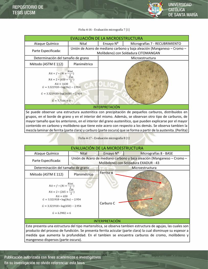
164
Ficha 4-16 - Evaluación micrografía 7 [1]
Ficha 4-17 - Evaluación micrografía 8 [1]
EVALUACIÓN DE LA MICROESTRUCTURA Ataque Químico Nital Ensayo N⁰ Micrografías 7 - RECUBRIMIENTO
Parte Especificada: Unión de Acero de mediano carbono y baja aleación (Manganeso – Cromo –
Molibdeno) con Soldadura CITOMANGAN
Determinación del tamaño de grano Microestructura
Método (ASTM E 112) Planimétrico
𝑁𝐴 = 𝑓 ∗ (𝑁𝑖 +𝑁𝑖𝑛𝑡
2)
𝑁𝐴 = 2 ∗ (650 +330
2)
𝑁𝐴 = 1630 𝐺 = 3.321918 ∗ log(𝑁𝑎) − 2.954
𝐺 = 3.321918 ∗ log(1630) − 2.954
𝐺 = 7.7166 = 8
INTERPRETACIÓN
Se puede observar una estructura austenítica con precipitación de pequeños carburos, distribuidos en grupos, en el borde de grano y en el interior del mismo. Además, se observan otro tipo de carburos, de mayor tamaño que los anteriores, en el interior del grano austenítico, que pueden explicarse por el mayor contenido en carbono y molibdeno que tiene este acero con respecto a los demás. Se observa tambien la mezcla laminar de ferrita (parte clara) y carburo (parte oscura) que se forma a partir de la austenita. (Perlita)
EVALUACIÓN DE LA MICROESTRUCTURA Ataque Químico Nital Ensayo N⁰ Micrografías 8 - BASE
Parte Especificada: Unión de Acero de mediano carbono y baja aleación (Manganeso – Cromo –
Molibdeno) con Soldadura EXADUR - 43
Determinación del tamaño de grano Microestructura
Método (ASTM E 112) Planimétrico Ferrita α
Carburo C
𝑁𝐴 = 𝑓 ∗ (𝑁𝑖 +𝑁𝑖𝑛𝑡
2)
𝑁𝐴 = 2 ∗ (265 +120
2)
𝑁𝐴 = 650 𝐺 = 3.321918 ∗ log(𝑁𝑎) − 2.954
𝐺 = 3.321918 ∗ log(650) − 2.954
𝐺 = 6.3902 = 6
INTERPRETACIÓN
Este presenta una estructura del tipo martensítica, se observa tambien estructura de agujas, las cuales son producto del proceso de fundición. Se presenta ferrita acicular (parte clara) la cual disminuye su espesor a medida que aumenta la profundidad. En el tambien se encuentra carburos de cromo, molibdeno y mangeneso dispersos (parte oscura).
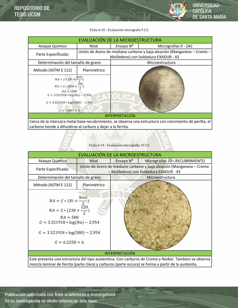
165
Ficha 4-18 - Evaluación micrografía 9 [1]
Ficha 4-19 - Evaluación micrografía 10 [1]
EVALUACIÓN DE LA MICROESTRUCTURA Ataque Químico Nital Ensayo N⁰ Micrografías 9 - ZAC
Parte Especificada: Unión de Acero de mediano carbono y baja aleación (Manganeso – Cromo –
Molibdeno) con Soldadura EXADUR - 43
Determinación del tamaño de grano Microestructura
Método (ASTM E 112) Planimétrico
𝑁𝐴 = 𝑓 ∗ (𝑁𝑖 +𝑁𝑖𝑛𝑡
2)
𝑁𝐴 = 2 ∗ (590 +320
2)
𝑁𝐴 = 1500 𝐺 = 3.321918 ∗ log(𝑁𝑎) − 2.954
𝐺 = 3.321918 ∗ log(1500) − 2.954
𝐺 = 7.5967 = 8
INTERPRETACIÓN
Cerca de la intercara metal base-recubrimiento, se observa una estructura con crecimiento de perlita, el carbono tiende a difundirse al carburo y dejar a la ferrita.
EVALUACIÓN DE LA MICROESTRUCTURA Ataque Químico Nital Ensayo N⁰ Micrografías 10 - RECUBRIMIENTO
Parte Especificada: Unión de Acero de mediano carbono y baja aleación (Manganeso – Cromo
– Molibdeno) con Soldadura EXADUR - 43
Determinación del tamaño de grano Microestructura
Método (ASTM E 112) Planimétrico
𝑁𝐴 = 𝑓 ∗ (𝑁𝑖 +𝑁𝑖𝑛𝑡
2)
𝑁𝐴 = 2 ∗ (230 +120
2)
𝑁𝐴 = 580 𝐺 = 3.321918 ∗ log(𝑁𝑎) − 2.954
𝐺 = 3.321918 ∗ log(580) − 2.954
𝐺 = 6.2258 = 6
INTERPRETACIÓN
Este presenta una estructura del tipo austenitica. Con carburos de Cromo y Niobio. Tambien se observa mezcla laminar de ferrita (parte clara) y carburos (parte oscura) se forma a partir de la austenita.

166
Ficha 4-20 - Evaluación micrografía 11 [1]
Ficha 4-21 - Evaluación micrografía 12 [1]
EVALUACIÓN DE LA MICROESTRUCTURA Ataque Químico Vilella Ensayo N⁰ Micrografías 11 - BASE
Parte Especificada: PROBETA MATERIAL BASE - DIN 32MnCrMo 6-4-3 (WNr° 1.7910)
Determinación del tamaño de grano Microestructura
Método (ASTM E 112) Planimétrico
Ferrita α
Carburo C
𝑁𝐴 = 𝑓 ∗ (𝑁𝑖 +𝑁𝑖𝑛𝑡
2)
𝑁𝐴 = 2 ∗ (230 +120
2)
𝑁𝐴 = 580 𝐺 = 3.321918 ∗ log(𝑁𝑎) − 2.954
𝐺 = 3.321918 ∗ log(580) − 2.954
𝐺 = 6.2258 = 6
INTERPRETACIÓN
Este presenta una estructura del tipo martensítica, se observa tambien estructura de agujas, las cuales son producto del proceso de fundición. Se presenta ferrita acicular (parte clara) la cual disminuye su espesor a medida que aumenta la profundidad. En el tambien se encuentra carburos de cromo, molibdeno y mangeneso dispersos (parte oscura).
EVALUACIÓN DE LA MICROESTRUCTURA Ataque Químico Vilella Ensayo N⁰ Micrografías 12 - BASE
Parte Especificada: Unión de Acero de mediano carbono y baja aleación (Manganeso – Cromo –
Molibdeno) con Soldadura CITODUR - 1000
Determinación del tamaño de grano Microestructura
Método (ASTM E 112) Planimétrico Ferrita α
Carburo C
𝑁𝐴 = 𝑓 ∗ (𝑁𝑖 +𝑁𝑖𝑛𝑡
2)
𝑁𝐴 = 2 ∗ (230 +110
2)
𝑁𝐴 = 570 𝐺 = 3.321918 ∗ log(𝑁𝑎) − 2.954
𝐺 = 3.321918 ∗ log(570) − 2.954
𝐺 = 6.2007 = 6
INTERPRETACIÓN
Este presenta una estructura del tipo martensítica, se observa tambien estructura de agujas, las cuales son producto del proceso de fundición. Se presenta ferrita acicular (parte clara) la cual disminuye su espesor a medida que aumenta la profundidad. En el tambien se encuentra carburos de cromo, molibdeno y mangeneso dispersos (parte oscura).

167
Ficha 4-22 - Evaluación micrografía 13 [1]
Ficha 4-23 - Evaluación micrografía 14 [1]
EVALUACIÓN DE LA MICROESTRUCTURA Ataque Químico Vilella Ensayo N⁰ Micrografías 13 - ZAC
Parte Especificada: Unión de Acero de mediano carbono y baja aleación (Manganeso – Cromo –
Molibdeno) con Soldadura CITODUR - 1000
Determinación del tamaño de grano Microestructura
Método (ASTM E 112) Planimétrico
𝑁𝐴 = 𝑓 ∗ (𝑁𝑖 +𝑁𝑖𝑛𝑡
2)
𝑁𝐴 = 2 ∗ (345 +190
2)
𝑁𝐴 = 880 𝐺 = 3.321918 ∗ log(𝑁𝑎) − 2.954
𝐺 = 3.321918 ∗ log(880) − 2.954
𝐺 = 6.8273 = 7
INTERPRETACIÓN
Cerca de la intercara metal base-recubrimiento, se observa una estructura con crecimiento dendrítico ocasionada por el rápido enfriamiento característico del proceso de soldadura eléctrica.
EVALUACIÓN DE LA MICROESTRUCTURA Ataque Químico Vilella Ensayo N⁰ Micrografías 14 - RECUBRIMIENTO
Parte Especificada: Unión de Acero de mediano carbono y baja aleación (Manganeso – Cromo –
Molibdeno) con Soldadura CITODUR - 1000
Determinación del tamaño de grano Microestructura
Método (ASTM E 112) Planimétrico
𝑁𝐴 = 𝑓 ∗ (𝑁𝑖 +𝑁𝑖𝑛𝑡
2)
𝑁𝐴 = 2 ∗ (550 +340
2)
𝑁𝐴 = 1440 𝐺 = 3.321918 ∗ log(𝑁𝑎) − 2.954
𝐺 = 3.321918 ∗ log(1440) − 2.954
𝐺 = 7.5378 = 8
INTERPRETACIÓN
Se aprecia una zona en donde se encuentran carburos alargados (carburos primarios) inmersos en una matriz martensítica. Los cuales no presentan una orientación preferente respecto a la intercara o a la superficie
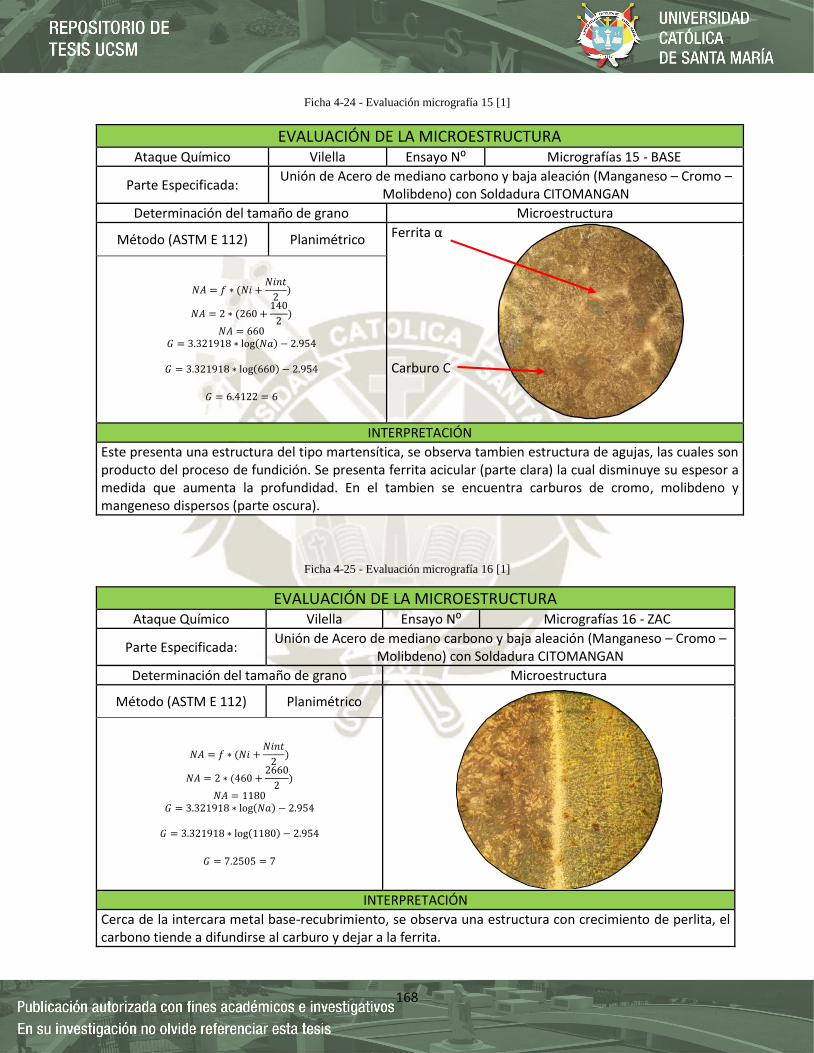
168
Ficha 4-24 - Evaluación micrografía 15 [1]
Ficha 4-25 - Evaluación micrografía 16 [1]
EVALUACIÓN DE LA MICROESTRUCTURA Ataque Químico Vilella Ensayo N⁰ Micrografías 15 - BASE
Parte Especificada: Unión de Acero de mediano carbono y baja aleación (Manganeso – Cromo –
Molibdeno) con Soldadura CITOMANGAN
Determinación del tamaño de grano Microestructura
Método (ASTM E 112) Planimétrico Ferrita α
Carburo C
𝑁𝐴 = 𝑓 ∗ (𝑁𝑖 +𝑁𝑖𝑛𝑡
2)
𝑁𝐴 = 2 ∗ (260 +140
2)
𝑁𝐴 = 660 𝐺 = 3.321918 ∗ log(𝑁𝑎) − 2.954
𝐺 = 3.321918 ∗ log(660) − 2.954
𝐺 = 6.4122 = 6
INTERPRETACIÓN
Este presenta una estructura del tipo martensítica, se observa tambien estructura de agujas, las cuales son producto del proceso de fundición. Se presenta ferrita acicular (parte clara) la cual disminuye su espesor a medida que aumenta la profundidad. En el tambien se encuentra carburos de cromo, molibdeno y mangeneso dispersos (parte oscura).
EVALUACIÓN DE LA MICROESTRUCTURA Ataque Químico Vilella Ensayo N⁰ Micrografías 16 - ZAC
Parte Especificada: Unión de Acero de mediano carbono y baja aleación (Manganeso – Cromo –
Molibdeno) con Soldadura CITOMANGAN
Determinación del tamaño de grano Microestructura
Método (ASTM E 112) Planimétrico
𝑁𝐴 = 𝑓 ∗ (𝑁𝑖 +𝑁𝑖𝑛𝑡
2)
𝑁𝐴 = 2 ∗ (460 +2660
2)
𝑁𝐴 = 1180 𝐺 = 3.321918 ∗ log(𝑁𝑎) − 2.954
𝐺 = 3.321918 ∗ log(1180) − 2.954
𝐺 = 7.2505 = 7
INTERPRETACIÓN
Cerca de la intercara metal base-recubrimiento, se observa una estructura con crecimiento de perlita, el carbono tiende a difundirse al carburo y dejar a la ferrita.
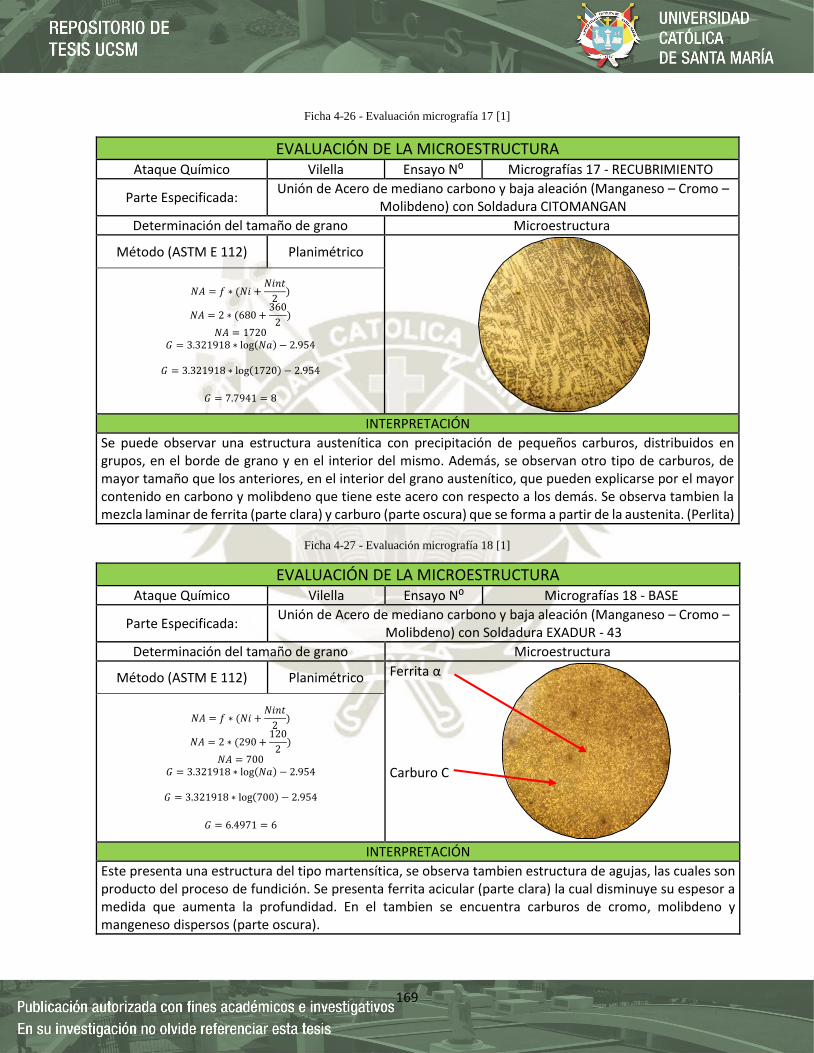
169
Ficha 4-26 - Evaluación micrografía 17 [1]
Ficha 4-27 - Evaluación micrografía 18 [1]
EVALUACIÓN DE LA MICROESTRUCTURA Ataque Químico Vilella Ensayo N⁰ Micrografías 17 - RECUBRIMIENTO
Parte Especificada: Unión de Acero de mediano carbono y baja aleación (Manganeso – Cromo –
Molibdeno) con Soldadura CITOMANGAN
Determinación del tamaño de grano Microestructura
Método (ASTM E 112) Planimétrico
𝑁𝐴 = 𝑓 ∗ (𝑁𝑖 +𝑁𝑖𝑛𝑡
2)
𝑁𝐴 = 2 ∗ (680 +360
2)
𝑁𝐴 = 1720 𝐺 = 3.321918 ∗ log(𝑁𝑎) − 2.954
𝐺 = 3.321918 ∗ log(1720) − 2.954
𝐺 = 7.7941 = 8
INTERPRETACIÓN
Se puede observar una estructura austenítica con precipitación de pequeños carburos, distribuidos en grupos, en el borde de grano y en el interior del mismo. Además, se observan otro tipo de carburos, de mayor tamaño que los anteriores, en el interior del grano austenítico, que pueden explicarse por el mayor contenido en carbono y molibdeno que tiene este acero con respecto a los demás. Se observa tambien la mezcla laminar de ferrita (parte clara) y carburo (parte oscura) que se forma a partir de la austenita. (Perlita)
EVALUACIÓN DE LA MICROESTRUCTURA Ataque Químico Vilella Ensayo N⁰ Micrografías 18 - BASE
Parte Especificada: Unión de Acero de mediano carbono y baja aleación (Manganeso – Cromo –
Molibdeno) con Soldadura EXADUR - 43
Determinación del tamaño de grano Microestructura
Método (ASTM E 112) Planimétrico Ferrita α
Carburo C
𝑁𝐴 = 𝑓 ∗ (𝑁𝑖 +𝑁𝑖𝑛𝑡
2)
𝑁𝐴 = 2 ∗ (290 +120
2)
𝑁𝐴 = 700 𝐺 = 3.321918 ∗ log(𝑁𝑎) − 2.954
𝐺 = 3.321918 ∗ log(700) − 2.954
𝐺 = 6.4971 = 6
INTERPRETACIÓN
Este presenta una estructura del tipo martensítica, se observa tambien estructura de agujas, las cuales son producto del proceso de fundición. Se presenta ferrita acicular (parte clara) la cual disminuye su espesor a medida que aumenta la profundidad. En el tambien se encuentra carburos de cromo, molibdeno y mangeneso dispersos (parte oscura).

170
Ficha 4-28 - Evaluación micrografía 19 [1]
Ficha 4-29 - Evaluación micrografía 20 [1]
EVALUACIÓN DE LA MICROESTRUCTURA Ataque Químico Vilella Ensayo N⁰ Micrografías 19 - ZAC
Parte Especificada: Unión de Acero de mediano carbono y baja aleación (Manganeso – Cromo –
Molibdeno) con Soldadura EXADUR - 43
Determinación del tamaño de grano Microestructura
Método (ASTM E 112) Planimétrico
𝑁𝐴 = 𝑓 ∗ (𝑁𝑖 +𝑁𝑖𝑛𝑡
2)
𝑁𝐴 = 2 ∗ (390 +230
2)
𝑁𝐴 = 1010 𝐺 = 3.321918 ∗ log(𝑁𝑎) − 2.954
𝐺 = 3.321918 ∗ log(1010) − 2.954
𝐺 = 7.0261 = 7
INTERPRETACIÓN
Cerca de la intercara metal base-recubrimiento, se observa una estructura con crecimiento de perlita, el carbono tiende a difundirse al carburo y dejar a la ferrita.
EVALUACIÓN DE LA MICROESTRUCTURA Ataque Químico Vilella Ensayo N⁰ Micrografías 20 - RECUBRIMIENTO
Parte Especificada: Unión de Acero de mediano carbono y baja aleación (Manganeso – Cromo
– Molibdeno) con Soldadura EXADUR - 43
Determinación del tamaño de grano Microestructura
Método (ASTM E 112) Planimétrico
𝑁𝐴 = 𝑓 ∗ (𝑁𝑖 +𝑁𝑖𝑛𝑡
2)
𝑁𝐴 = 2 ∗ (620 +210
2)
𝑁𝐴 = 1450 𝐺 = 3.321918 ∗ log(𝑁𝑎) − 2.954
𝐺 = 3.321918 ∗ log(1450) − 2.954
𝐺 = 7.5478 = 8
INTERPRETACIÓN
Este presenta una estructura del tipo austenitica. Con carburos de Cromo y Niobio. Tambien se observa mezcla laminar de ferrita (parte clara) y carburos (parte oscura) se forma a partir de la austenita.
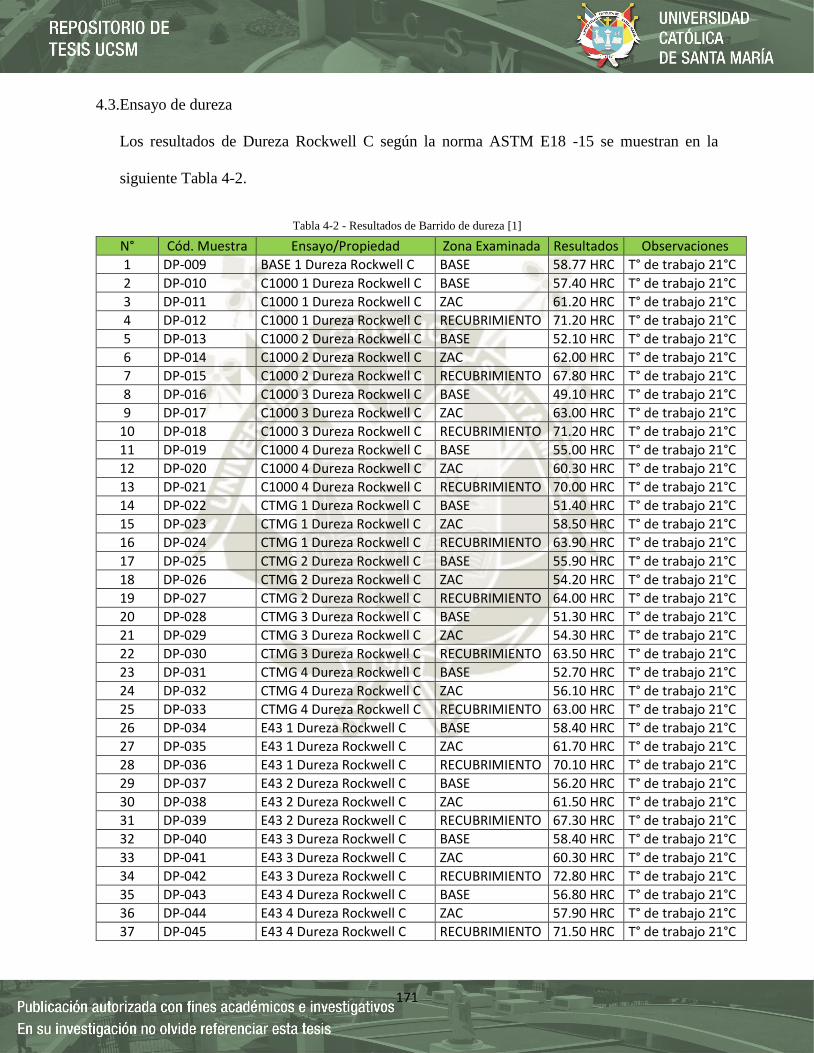
171
4.3.Ensayo de dureza
Los resultados de Dureza Rockwell C según la norma ASTM E18 -15 se muestran en la
siguiente Tabla 4-2.
Tabla 4-2 - Resultados de Barrido de dureza [1]
N° Cód. Muestra Ensayo/Propiedad Zona Examinada Resultados Observaciones
1 DP-009 BASE 1 Dureza Rockwell C BASE 58.77 HRC T° de trabajo 21°C
2 DP-010 C1000 1 Dureza Rockwell C BASE 57.40 HRC T° de trabajo 21°C
3 DP-011 C1000 1 Dureza Rockwell C ZAC 61.20 HRC T° de trabajo 21°C
4 DP-012 C1000 1 Dureza Rockwell C RECUBRIMIENTO 71.20 HRC T° de trabajo 21°C
5 DP-013 C1000 2 Dureza Rockwell C BASE 52.10 HRC T° de trabajo 21°C
6 DP-014 C1000 2 Dureza Rockwell C ZAC 62.00 HRC T° de trabajo 21°C
7 DP-015 C1000 2 Dureza Rockwell C RECUBRIMIENTO 67.80 HRC T° de trabajo 21°C
8 DP-016 C1000 3 Dureza Rockwell C BASE 49.10 HRC T° de trabajo 21°C
9 DP-017 C1000 3 Dureza Rockwell C ZAC 63.00 HRC T° de trabajo 21°C
10 DP-018 C1000 3 Dureza Rockwell C RECUBRIMIENTO 71.20 HRC T° de trabajo 21°C
11 DP-019 C1000 4 Dureza Rockwell C BASE 55.00 HRC T° de trabajo 21°C
12 DP-020 C1000 4 Dureza Rockwell C ZAC 60.30 HRC T° de trabajo 21°C
13 DP-021 C1000 4 Dureza Rockwell C RECUBRIMIENTO 70.00 HRC T° de trabajo 21°C
14 DP-022 CTMG 1 Dureza Rockwell C BASE 51.40 HRC T° de trabajo 21°C
15 DP-023 CTMG 1 Dureza Rockwell C ZAC 58.50 HRC T° de trabajo 21°C
16 DP-024 CTMG 1 Dureza Rockwell C RECUBRIMIENTO 63.90 HRC T° de trabajo 21°C
17 DP-025 CTMG 2 Dureza Rockwell C BASE 55.90 HRC T° de trabajo 21°C
18 DP-026 CTMG 2 Dureza Rockwell C ZAC 54.20 HRC T° de trabajo 21°C
19 DP-027 CTMG 2 Dureza Rockwell C RECUBRIMIENTO 64.00 HRC T° de trabajo 21°C
20 DP-028 CTMG 3 Dureza Rockwell C BASE 51.30 HRC T° de trabajo 21°C
21 DP-029 CTMG 3 Dureza Rockwell C ZAC 54.30 HRC T° de trabajo 21°C
22 DP-030 CTMG 3 Dureza Rockwell C RECUBRIMIENTO 63.50 HRC T° de trabajo 21°C
23 DP-031 CTMG 4 Dureza Rockwell C BASE 52.70 HRC T° de trabajo 21°C
24 DP-032 CTMG 4 Dureza Rockwell C ZAC 56.10 HRC T° de trabajo 21°C
25 DP-033 CTMG 4 Dureza Rockwell C RECUBRIMIENTO 63.00 HRC T° de trabajo 21°C
26 DP-034 E43 1 Dureza Rockwell C BASE 58.40 HRC T° de trabajo 21°C
27 DP-035 E43 1 Dureza Rockwell C ZAC 61.70 HRC T° de trabajo 21°C
28 DP-036 E43 1 Dureza Rockwell C RECUBRIMIENTO 70.10 HRC T° de trabajo 21°C
29 DP-037 E43 2 Dureza Rockwell C BASE 56.20 HRC T° de trabajo 21°C
30 DP-038 E43 2 Dureza Rockwell C ZAC 61.50 HRC T° de trabajo 21°C
31 DP-039 E43 2 Dureza Rockwell C RECUBRIMIENTO 67.30 HRC T° de trabajo 21°C
32 DP-040 E43 3 Dureza Rockwell C BASE 58.40 HRC T° de trabajo 21°C
33 DP-041 E43 3 Dureza Rockwell C ZAC 60.30 HRC T° de trabajo 21°C
34 DP-042 E43 3 Dureza Rockwell C RECUBRIMIENTO 72.80 HRC T° de trabajo 21°C
35 DP-043 E43 4 Dureza Rockwell C BASE 56.80 HRC T° de trabajo 21°C
36 DP-044 E43 4 Dureza Rockwell C ZAC 57.90 HRC T° de trabajo 21°C
37 DP-045 E43 4 Dureza Rockwell C RECUBRIMIENTO 71.50 HRC T° de trabajo 21°C

172
En la Tablas 4-3, 4-4, 4-5 y 4-6 se pueden apreciar los resultados de los barridos dureza de las
probetas Material Base, (Citodur 1000), Citomangan y Exadur 43 respectivamente.
Tabla 4-3 - Barrido de dureza probeta sin Recargue [1]
Tabla 4-4 - Barrido de dureza probeta con Recargue C-1000. [1]
PROBETA SIN RECARGUE
N° Cód.
Muestra Ensayo/Propiedad
Zona Examinada
Resultados Promedio
(HRC) Observaciones
1 DP-009 BASE 1 Dureza Rockwell C BASE 58.77 58.77 T° de trabajo
21°C
PROBETA CON RECARGUE CITODUR – 1000
N° Cód.
Muestra Ensayo/Propiedad Zona Examinada Resultados
(HRC) Promedio
(HRC) Observaciones
1 DP-010 C1000 1 Dureza Rockwell C BASE 57.4
53.4
T° de trabajo 21°C
2 DP-013 C1000 2 Dureza Rockwell C BASE 52.1 T° de trabajo 21°C
3 DP-016 C1000 3 Dureza Rockwell C BASE 49.1 T° de trabajo 21°C
4 DP-019 C1000 4 Dureza Rockwell C BASE 55 T° de trabajo 21°C
5 DP-011 C1000 1 Dureza Rockwell C ZAC 61.2
61.6
T° de trabajo 21°C
6 DP-014 C1000 2 Dureza Rockwell C ZAC 62 T° de trabajo 21°C
7 DP-017 C1000 3 Dureza Rockwell C ZAC 63 T° de trabajo 21°C
8 DP-020 C1000 4 Dureza Rockwell C ZAC 60.3 T° de trabajo 21°C
9 DP-012 C1000 1 Dureza Rockwell C RECUBRIMIENTO 71.2
70.1
T° de trabajo 21°C
10 DP-015 C1000 2 Dureza Rockwell C RECUBRIMIENTO 67.8 T° de trabajo 21°C
11 DP-018 C1000 3 Dureza Rockwell C RECUBRIMIENTO 71.2 T° de trabajo 21°C
12 DP-021 C1000 4 Dureza Rockwell C RECUBRIMIENTO 70 T° de trabajo 21°C

173
Tabla 4-5 - Barrido de dureza probeta con Recargue CITOMANGAN [1]
Tabla 4-6 - Barrido de dureza probeta con Recargue EXADUR – 43 [1]
PROBETA CON RECARGUE CITOMANGAN
N° Cód.
Muestra Ensayo/Propiedad Zona Examinada Resultados
(HRC) Promedio
(HRC) Observaciones
1 DP-022 CTMG 1 Dureza Rockwell C BASE 51.4
52.8
T° de trabajo 21°C
2 DP-025 CTMG 2 Dureza Rockwell C BASE 55.9 T° de trabajo 21°C
3 DP-028 CTMG 3 Dureza Rockwell C BASE 51.3 T° de trabajo 21°C
4 DP-031 CTMG 4 Dureza Rockwell C BASE 52.7 T° de trabajo 21°C
5 DP-023 CTMG 1 Dureza Rockwell C ZAC 58.5
55.8
T° de trabajo 21°C
6 DP-026 CTMG 2 Dureza Rockwell C ZAC 54.2 T° de trabajo 21°C
7 DP-029 CTMG 3 Dureza Rockwell C ZAC 54.3 T° de trabajo 21°C
8 DP-032 CTMG 4 Dureza Rockwell C ZAC 56.1 T° de trabajo 21°C
9 DP-024 CTMG 1 Dureza Rockwell C RECUBRIMIENTO 63.9
63.6
T° de trabajo 21°C
10 DP-027 CTMG 2 Dureza Rockwell C RECUBRIMIENTO 64 T° de trabajo 21°C
11 DP-030 CTMG 3 Dureza Rockwell C RECUBRIMIENTO 63.5 T° de trabajo 21°C
12 DP-033 CTMG 4 Dureza Rockwell C RECUBRIMIENTO 63 T° de trabajo 21°C
PROBETA CON RECARGUE EXADUR - 43
N° Cód.
Muestra Ensayo/Propiedad Zona Examinada Resultados
(HRC) Promedio
(HRC) Observaciones
1 DP-034 E43 1 Dureza Rockwell C BASE 58.4
57.5
T° de trabajo 21°C
2 DP-037 E43 2 Dureza Rockwell C BASE 56.2 T° de trabajo 21°C
3 DP-040 E43 3 Dureza Rockwell C BASE 58.4 T° de trabajo 21°C
4 DP-043 E43 4 Dureza Rockwell C BASE 56.8 T° de trabajo 21°C
5 DP-035 E43 1 Dureza Rockwell C ZAC 61.7
60.4
T° de trabajo 21°C
6 DP-038 E43 2 Dureza Rockwell C ZAC 61.5 T° de trabajo 21°C
7 DP-041 E43 3 Dureza Rockwell C ZAC 60.3 T° de trabajo 21°C
8 DP-044 E43 4 Dureza Rockwell C ZAC 57.9 T° de trabajo 21°C
9 DP-036 E43 1 Dureza Rockwell C RECUBRIMIENTO 70.1
70.4
T° de trabajo 21°C
10 DP-039 E43 2 Dureza Rockwell C RECUBRIMIENTO 67.3 T° de trabajo 21°C
11 DP-042 E43 3 Dureza Rockwell C RECUBRIMIENTO 72.8 T° de trabajo 21°C
12 DP-045 E43 4 Dureza Rockwell C RECUBRIMIENTO 71.5 T° de trabajo 21°C

174
Con los datos obtenidos de los barridos de dureza, se pueden obtener los perfiles de dureza que
muestran las Gráficas 4-1, 4-2 y 4-3 para las diferentes probetas.
Gráfica 4-1 - Perfil de dureza de la probeta C-1000 [1]
Gráfica 4-2 - Perfil de dureza de la probeta CITOMANGAN [1]
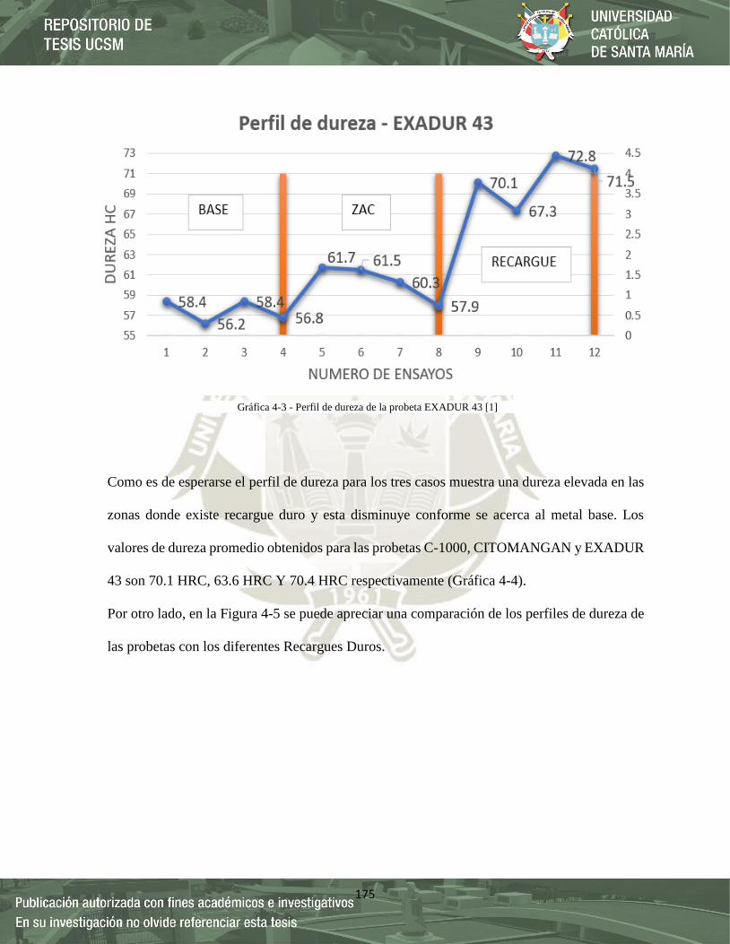
175
Como es de esperarse el perfil de dureza para los tres casos muestra una dureza elevada en las
zonas donde existe recargue duro y esta disminuye conforme se acerca al metal base. Los
valores de dureza promedio obtenidos para las probetas C-1000, CITOMANGAN y EXADUR
43 son 70.1 HRC, 63.6 HRC Y 70.4 HRC respectivamente (Gráfica 4-4).
Por otro lado, en la Figura 4-5 se puede apreciar una comparación de los perfiles de dureza de
las probetas con los diferentes Recargues Duros.
Gráfica 4-3 - Perfil de dureza de la probeta EXADUR 43 [1]
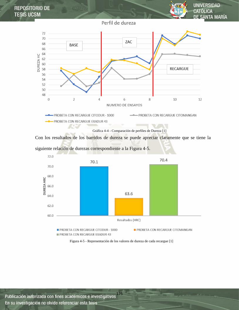
176
Con los resultados de los barridos de dureza se puede apreciar claramente que se tiene la
siguiente relación de durezas correspondiente a la Figura 4-5.
Gráfica 4-4 - Comparación de perfiles de Dureza [1]
Figura 4-5 - Representación de los valores de dureza de cada recargue [1]

177
Se puede observar que los valores promedio de dureza son elevados en la zona de recargue,
pero se tiene que recalcar que estos están afectados por la dilución del metal base y efectos de
revenido entre pases. Los resultados de dureza varían de acuerdo a la composición química de
los recubrimientos y su microestructura. Por ejemplo, se tiene a la probeta con Recargue
EXADUR 43 con una dureza promedio de 70.4 HRC, esto se debe a que posee una estructura
austenítica con carburos de Cr, Nb. Los carburos están distribuidos en una matriz austenítica
que incrementa su resistencia al impacto. En la composición química dio como resultado que
tiene un 20.3% de Cromo, este componente el cromo provee resistencia a la corrosión
atmosférica y al desgaste, sin embargo, el efecto no siempre es consistente y depende de
aplicaciones individuales. Se tiene a la probeta con Recargue C-1000 con una dureza de
promedio de 70.1 HRC, esto se debe a que posee una estructura austenítica con carburos de C
Mn Si Cr, se tiene también que esta composición contiene un 31.57 % de Cromo. Cabe resaltar
que ambas probetas Exadur 43 y Citodur 1000 contienen un valor similar de % Carbono, que
son 3.96 % y 3.6 % (ficha 4-1), con el incremento en el porcentaje de carbono se aumenta la
resistencia al desgaste del acero austenítico. Por último se tiene se tiene a la probeta con
Recargue CITOMANGAN con una dureza de promedio de 63.6 HRC, material depositado
posee una estructura austenítica de gran tenacidad, que le permite absorber los golpes durante
el trabajo, se tiene en el resultado de composición química que contiene 11.98% de Manganeso,
esta estabiliza la austenita retardando la transformación martensítica, incrementa la resistencia
a la tracción, el límite elástico, la resistencia a la fatiga y a la fluencia lenta, la forjabilidad, la
resistencia al desgaste, En cambio, disminuye la maquinabilidad, la embutibilidad, las
conductividades térmica y eléctrica y la sensibilidad a la fractura frágil.

178
4.4.Ensayo de tracción
Las Fichas 4-30 al 4-37 que se presentan a continuación son los parámetros y resultados de los
ensayos de tracción realizados a las probetas P1-EXADUR – 42, P2 – CITOMANGAN, P3 –
C – 1000 y P-4 MATERIAL BASE según la norma ASTM E370 – 18 “Standard Test Methods
and Definitions for Mechanical Testing of Steel Products”.
Ficha 4-30 - Parámetros generales del ensayo - P-1 - EXADUR-43 [1]
UNIVERSIDAD CATÓLICA DE SANTA MARIA, ESCUELA PROFESIONAL DE INGENIERIA MECÁNICA, MECÁNICA
ELÉTRICA Y MECÁTRONICA
ENSAYO DE TRACCIÓN Tipo de Estudio De laboratorio Ensayo N⁰ 1
Fecha: 03 DE JULIO DEL 2019 Probeta N⁰ P-1 - EXADUR-43
Parte Especificada: PROBETA CON UNIÓN DE RECARGUE EXADUR - 43
Solicitado Por: Ruben Purca Dirección Asoc. De Viv Los Olmos Arequipa, Perú
Centro de estudios y análisis: Laboratorio de Ingeniería de Materiales de la Universidad Nacional de San
Agustín
Realizado Por: Ruben Purca Revisado Por: Ing. Guido Quispe Ampuero
PARÁMETROS DEL ENSAYO DE TRACCIÓN
Tipo de Ensayo: Ensayo de Tracción
Equipo utilizado: Marca INSTRON modelo 23-100
Temperatura del Ensayo:
22,5° C.
Tipo de probeta: Cilíndrica Norma: ASTM E370 - 18
Espec. del material: Unión de Acero de mediano carbono y baja
aleación (Manganeso – Cromo – Molibdeno) con Soldadura EXADUR -43
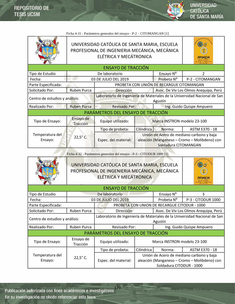
179
Ficha 4-31 - Parámetros generales del ensayo - P-2 – CITOMANGAN [1]
Ficha 4-32 - Parámetros generales del ensayo - P-3 - CITODUR 1000 [1]
UNIVERSIDAD CATÓLICA DE SANTA MARIA, ESCUELA PROFESIONAL DE INGENIERIA MECÁNICA, MECÁNICA
ELÉTRICA Y MECÁTRONICA
ENSAYO DE TRACCIÓN Tipo de Estudio De laboratorio Ensayo N⁰ 2
Fecha: 03 DE JULIO DEL 2019 Probeta N⁰ P-2 - CITOMANGAN
Parte Especificada: PROBETA CON UNIÓN DE RECARGUE CITOMANGAN
Solicitado Por: Ruben Purca Dirección Asoc. De Viv Los Olmos Arequipa, Perú
Centro de estudios y análisis: Laboratorio de Ingeniería de Materiales de la Universidad Nacional de San
Agustín
Realizado Por: Ruben Purca Revisado Por: Ing. Guido Quispe Ampuero
PARÁMETROS DEL ENSAYO DE TRACCIÓN
Tipo de Ensayo: Ensayo de Tracción
Equipo utilizado: Marca INSTRON modelo 23-100
Temperatura del Ensayo:
22,5° C.
Tipo de probeta: Cilíndrica Norma: ASTM E370 - 18
Espec. del material: Unión de Acero de mediano carbono y baja
aleación (Manganeso – Cromo – Molibdeno) con Soldadura CITOMANGAN
UNIVERSIDAD CATÓLICA DE SANTA MARIA, ESCUELA PROFESIONAL DE INGENIERIA MECÁNICA, MECÁNICA
ELÉTRICA Y MECÁTRONICA
ENSAYO DE TRACCIÓN Tipo de Estudio De laboratorio Ensayo N⁰ 3
Fecha: 03 DE JULIO DEL 2019 Probeta N⁰ P-3 - CITODUR 1000
Parte Especificada: PROBETA CON UNION DE RECARGUE CITODUR - 1000
Solicitado Por: Ruben Purca Dirección Asoc. De Viv Los Olmos Arequipa, Perú
Centro de estudios y análisis: Laboratorio de Ingeniería de Materiales de la Universidad Nacional de San
Agustín
Realizado Por: Ruben Purca Revisado Por: Ing. Guido Quispe Ampuero
PARÁMETROS DEL ENSAYO DE TRACCIÓN
Tipo de Ensayo: Ensayo de Tracción
Equipo utilizado: Marca INSTRON modelo 23-100
Temperatura del Ensayo:
22,5° C.
Tipo de probeta: Cilíndrica Norma: ASTM E370 - 18
Espec. del material: Unión de Acero de mediano carbono y baja
aleación (Manganeso – Cromo – Molibdeno) con Soldadura CITODUR - 1000
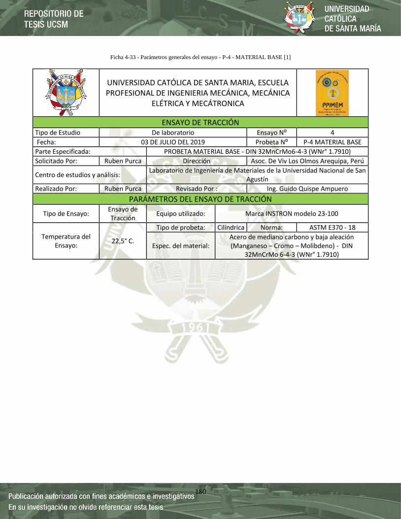
180
Ficha 4-33 - Parámetros generales del ensayo - P-4 - MATERIAL BASE [1]
UNIVERSIDAD CATÓLICA DE SANTA MARIA, ESCUELA PROFESIONAL DE INGENIERIA MECÁNICA, MECÁNICA
ELÉTRICA Y MECÁTRONICA
ENSAYO DE TRACCIÓN Tipo de Estudio De laboratorio Ensayo N⁰ 4
Fecha: 03 DE JULIO DEL 2019 Probeta N⁰ P-4 MATERIAL BASE
Parte Especificada: PROBETA MATERIAL BASE - DIN 32MnCrMo6-4-3 (WNr° 1.7910)
Solicitado Por: Ruben Purca Dirección Asoc. De Viv Los Olmos Arequipa, Perú
Centro de estudios y análisis: Laboratorio de Ingeniería de Materiales de la Universidad Nacional de San
Agustín
Realizado Por: Ruben Purca Revisado Por : Ing. Guido Quispe Ampuero
PARÁMETROS DEL ENSAYO DE TRACCIÓN
Tipo de Ensayo: Ensayo de Tracción
Equipo utilizado: Marca INSTRON modelo 23-100
Temperatura del Ensayo:
22,5° C.
Tipo de probeta: Cilíndrica Norma: ASTM E370 - 18
Espec. del material: Acero de mediano carbono y baja aleación (Manganeso – Cromo – Molibdeno) - DIN
32MnCrMo 6-4-3 (WNr° 1.7910)
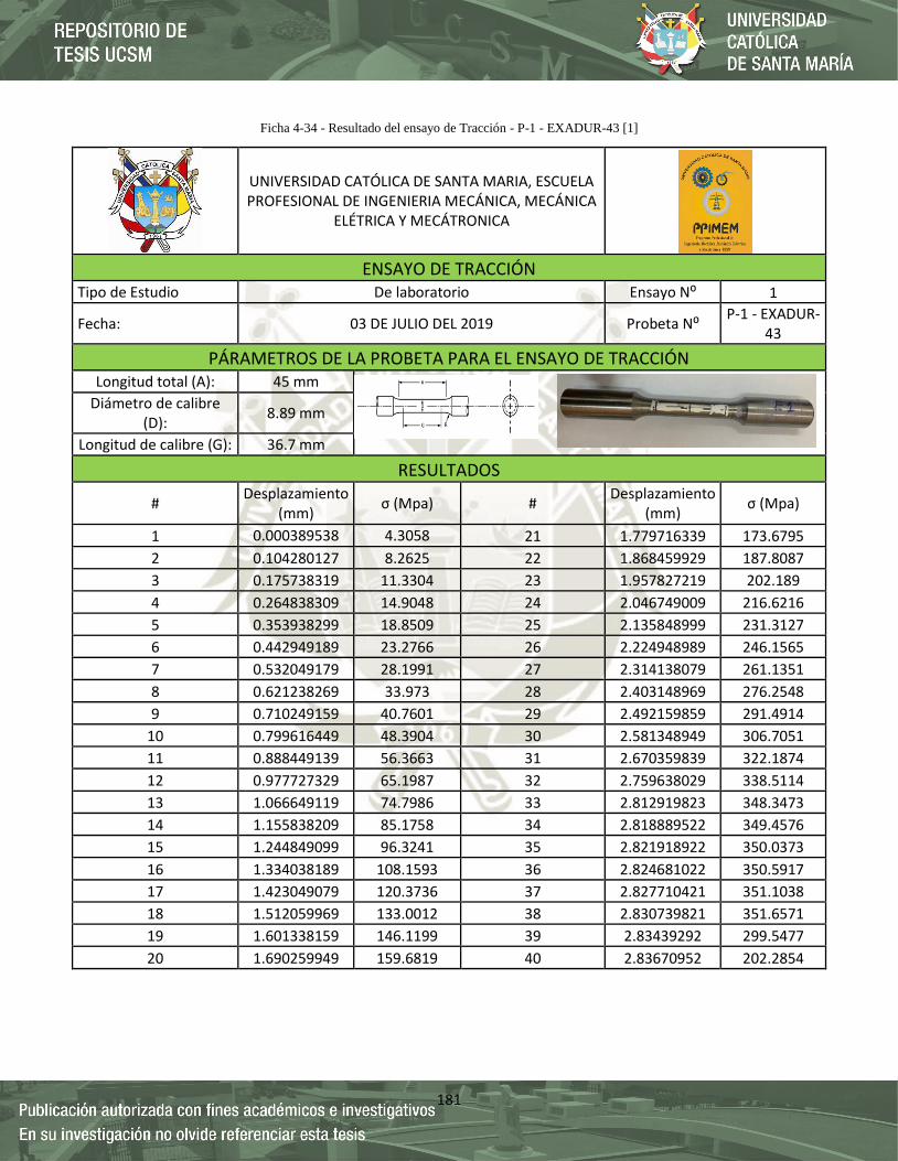
181
Ficha 4-34 - Resultado del ensayo de Tracción - P-1 - EXADUR-43 [1]
UNIVERSIDAD CATÓLICA DE SANTA MARIA, ESCUELA PROFESIONAL DE INGENIERIA MECÁNICA, MECÁNICA
ELÉTRICA Y MECÁTRONICA
ENSAYO DE TRACCIÓN
Tipo de Estudio De laboratorio Ensayo N⁰ 1
Fecha: 03 DE JULIO DEL 2019 Probeta N⁰ P-1 - EXADUR-
43
PÁRAMETROS DE LA PROBETA PARA EL ENSAYO DE TRACCIÓN Longitud total (A): 45 mm
Diámetro de calibre (D):
8.89 mm
Longitud de calibre (G): 36.7 mm
RESULTADOS
# Desplazamiento
(mm) σ (Mpa) #
Desplazamiento (mm)
σ (Mpa)
1 0.000389538 4.3058 21 1.779716339 173.6795
2 0.104280127 8.2625 22 1.868459929 187.8087
3 0.175738319 11.3304 23 1.957827219 202.189
4 0.264838309 14.9048 24 2.046749009 216.6216
5 0.353938299 18.8509 25 2.135848999 231.3127
6 0.442949189 23.2766 26 2.224948989 246.1565
7 0.532049179 28.1991 27 2.314138079 261.1351
8 0.621238269 33.973 28 2.403148969 276.2548
9 0.710249159 40.7601 29 2.492159859 291.4914
10 0.799616449 48.3904 30 2.581348949 306.7051
11 0.888449139 56.3663 31 2.670359839 322.1874
12 0.977727329 65.1987 32 2.759638029 338.5114
13 1.066649119 74.7986 33 2.812919823 348.3473
14 1.155838209 85.1758 34 2.818889522 349.4576
15 1.244849099 96.3241 35 2.821918922 350.0373
16 1.334038189 108.1593 36 2.824681022 350.5917
17 1.423049079 120.3736 37 2.827710421 351.1038
18 1.512059969 133.0012 38 2.830739821 351.6571
19 1.601338159 146.1199 39 2.83439292 299.5477
20 1.690259949 159.6819 40 2.83670952 202.2854

182
Ficha 4-35 - Resultado del ensayo de Tracción - P-2 – CITOMANGAN [1]
UNIVERSIDAD CATÓLICA DE SANTA MARIA, ESCUELA PROFESIONAL DE INGENIERIA MECÁNICA, MECÁNICA
ELÉTRICA Y MECÁTRONICA
ENSAYO DE TRACCIÓN
Tipo de Estudio De laboratorio Ensayo N⁰ 2
Fecha: 03 DE JULIO DEL 2019 Probeta N⁰ P-2 -
CITOMANGAN
PÁRAMETROS DE LA PROBETA PARA EL ENSAYO DE TRACCIÓN Longitud total (A): 45 mm
Diámetro de calibre (D):
8.86 mm
Longitud de calibre (G): 38.42 mm
RESULTADOS
# Desplazamiento
(mm) σ (Mpa) #
Desplazamiento (mm)
σ (Mpa)
1 0.004247365 4.1526 21 1.544990965 151.3078
2 0.078764565 7.6294 22 1.622445565 164.7109
3 0.156219165 10.3336 23 1.699668265 178.5085
4 0.233519165 13.2295 24 1.776968265 192.5607
5 0.310973765 16.6005 25 1.854190965 206.7741
6 0.388119165 20.6841 26 1.931413665 221.2058
7 0.465573765 25.1537 27 2.008868265 235.8133
8 0.542641865 30.0953 28 2.086090965 250.5839
9 0.620096465 35.6549 29 2.163622865 265.4256
10 0.697241865 42.0011 30 2.240690965 280.3265
11 0.772145565 48.9231 31 2.318068265 295.6841
12 0.849368265 56.5448 32 2.395290965 311.0801
13 0.926668265 64.5538 33 2.472668265 326.5033
14 1.003890965 73.1756 34 2.575709165 346.8155
15 1.083741865 82.9885 35 2.872077365 399.8094
16 1.158568265 92.8919 36 2.977669165 415.076
17 1.235790965 103.637 37 3.070351865 423.9267
18 1.313322865 114.7922 38 3.084111265 322.5679
19 1.390390965 126.4836 39 3.130104765 287.8999
20 1.467768265 138.6266 40 3.292357465 144.2063
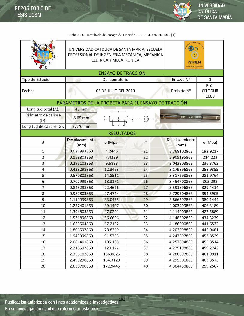
183
Ficha 4-36 - Resultado del ensayo de Tracción - P-3 - CITODUR 1000 [1]
UNIVERSIDAD CATÓLICA DE SANTA MARIA, ESCUELA PROFESIONAL DE INGENIERIA MECÁNICA, MECÁNICA
ELÉTRICA Y MECÁTRONICA
ENSAYO DE TRACCIÓN
Tipo de Estudio De laboratorio Ensayo N⁰ 3
Fecha: 03 DE JULIO DEL 2019 Probeta N⁰ P-3 -
CITODUR 1000
PÁRAMETROS DE LA PROBETA PARA EL ENSAYO DE TRACCIÓN Longitud total (A): 45 mm
Diámetro de calibre (D):
8.69 mm
Longitud de calibre (G): 37.76 mm
RESULTADOS
# Desplazamiento
(mm) σ (Mpa) #
Desplazamiento (mm)
σ (Mpa)
1 0.027993863 4.2445 21 2.768102863 192.9217
2 0.158803863 7.4239 22 2.905195863 214.223
3 0.296102863 9.6883 23 3.042803863 236.3763
4 0.433298863 12.3463 24 3.179896863 258.9355
5 0.570803863 14.8511 25 3.317298863 281.9764
6 0.707999863 18.3171 26 3.454700863 305.298
7 0.845298863 22.4626 27 3.591896863 329.4414
8 0.982803863 27.4744 28 3.729504863 354.5905
9 1.119999863 33.0435 29 3.866597863 380.1444
10 1.257401863 39.1407 30 4.003999863 406.3189
11 1.394803863 47.0201 31 4.114003863 427.5889
12 1.531896863 56.6606 32 4.148302863 434.3239
13 1.669504863 67.2162 33 4.186000863 441.6532
14 1.806597863 78.8359 34 4.203098863 445.0481
15 1.943999863 91.5793 35 4.247697863 453.8529
16 2.081401863 105.185 36 4.257894863 455.8514
17 2.218597863 120.172 37 4.275198863 459.2742
18 2.356102863 136.8826 38 4.288897863 461.9911
19 2.493298863 154.3128 39 4.295901863 463.3573
20 2.630700863 172.9446 40 4.304450863 259.2567
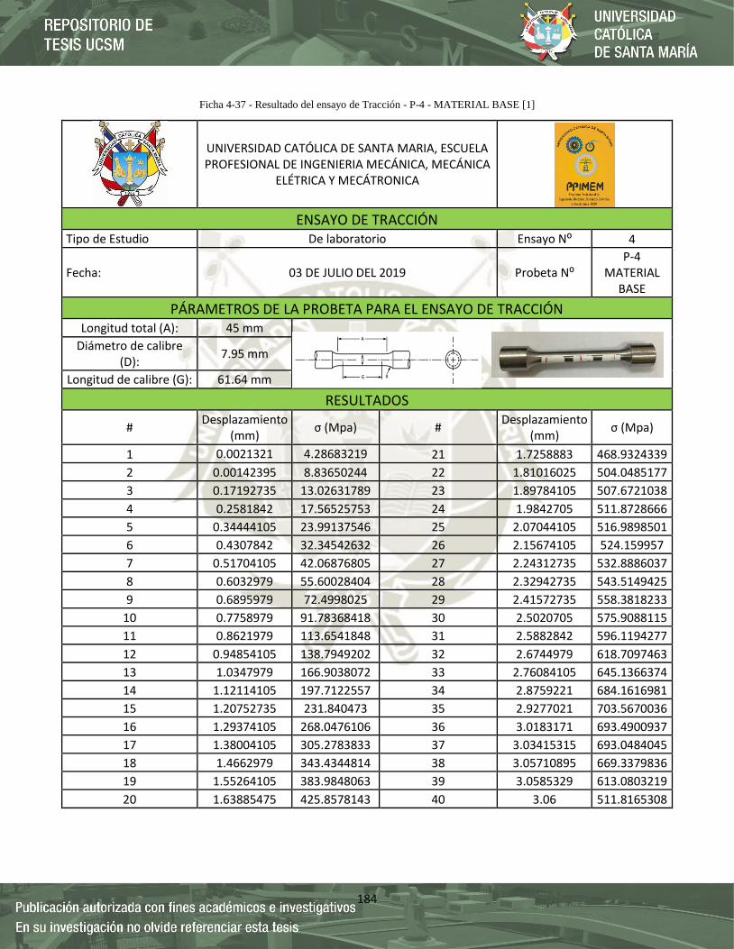
184
Ficha 4-37 - Resultado del ensayo de Tracción - P-4 - MATERIAL BASE [1]
UNIVERSIDAD CATÓLICA DE SANTA MARIA, ESCUELA PROFESIONAL DE INGENIERIA MECÁNICA, MECÁNICA
ELÉTRICA Y MECÁTRONICA
ENSAYO DE TRACCIÓN
Tipo de Estudio De laboratorio Ensayo N⁰ 4
Fecha: 03 DE JULIO DEL 2019 Probeta N⁰ P-4
MATERIAL BASE
PÁRAMETROS DE LA PROBETA PARA EL ENSAYO DE TRACCIÓN Longitud total (A): 45 mm
Diámetro de calibre (D):
7.95 mm
Longitud de calibre (G): 61.64 mm
RESULTADOS
# Desplazamiento
(mm) σ (Mpa) #
Desplazamiento (mm)
σ (Mpa)
1 0.0021321 4.28683219 21 1.7258883 468.9324339
2 0.00142395 8.83650244 22 1.81016025 504.0485177
3 0.17192735 13.02631789 23 1.89784105 507.6721038
4 0.2581842 17.56525753 24 1.9842705 511.8728666
5 0.34444105 23.99137546 25 2.07044105 516.9898501
6 0.4307842 32.34542632 26 2.15674105 524.159957
7 0.51704105 42.06876805 27 2.24312735 532.8886037
8 0.6032979 55.60028404 28 2.32942735 543.5149425
9 0.6895979 72.4998025 29 2.41572735 558.3818233
10 0.7758979 91.78368418 30 2.5020705 575.9088115
11 0.8621979 113.6541848 31 2.5882842 596.1194277
12 0.94854105 138.7949202 32 2.6744979 618.7097463
13 1.0347979 166.9038072 33 2.76084105 645.1366374
14 1.12114105 197.7122557 34 2.8759221 684.1616981
15 1.20752735 231.840473 35 2.9277021 703.5670036
16 1.29374105 268.0476106 36 3.0183171 693.4900937
17 1.38004105 305.2783833 37 3.03415315 693.0484045
18 1.4662979 343.4344814 38 3.05710895 669.3379836
19 1.55264105 383.9848063 39 3.0585329 613.0803219
20 1.63885475 425.8578143 40 3.06 511.8165308
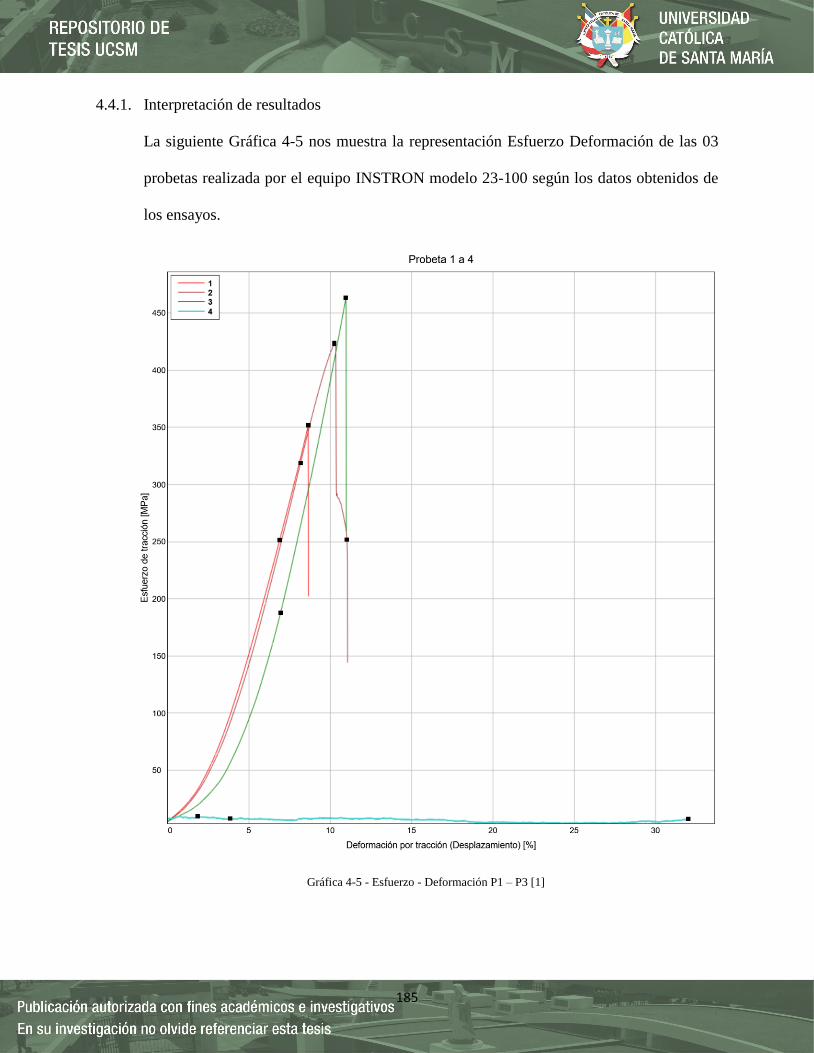
185
4.4.1. Interpretación de resultados
La siguiente Gráfica 4-5 nos muestra la representación Esfuerzo Deformación de las 03
probetas realizada por el equipo INSTRON modelo 23-100 según los datos obtenidos de
los ensayos.
Gráfica 4-5 - Esfuerzo - Deformación P1 – P3 [1]
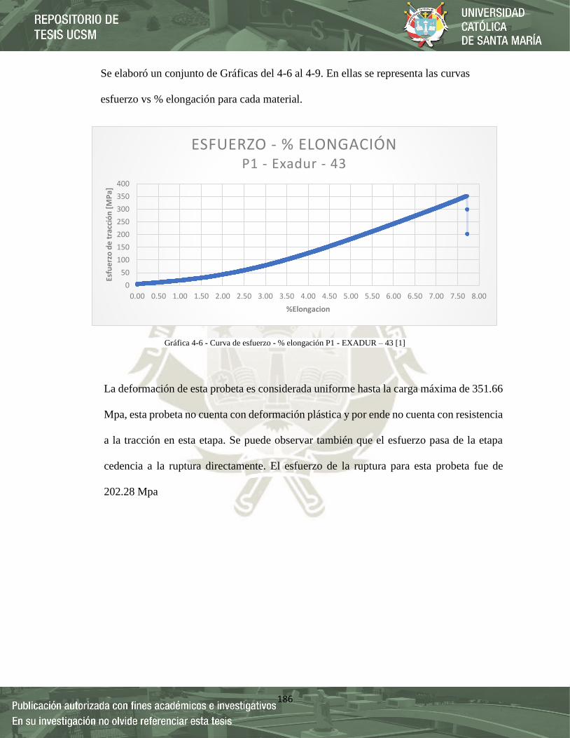
186
Se elaboró un conjunto de Gráficas del 4-6 al 4-9. En ellas se representa las curvas
esfuerzo vs % elongación para cada material.
La deformación de esta probeta es considerada uniforme hasta la carga máxima de 351.66
Mpa, esta probeta no cuenta con deformación plástica y por ende no cuenta con resistencia
a la tracción en esta etapa. Se puede observar también que el esfuerzo pasa de la etapa
cedencia a la ruptura directamente. El esfuerzo de la ruptura para esta probeta fue de
202.28 Mpa
0
50
100
150
200
250
300
350
400
0.00 0.50 1.00 1.50 2.00 2.50 3.00 3.50 4.00 4.50 5.00 5.50 6.00 6.50 7.00 7.50 8.00
Esfu
erz
o d
e t
racc
ión
[M
Pa]
%Elongacion
ESFUERZO - % ELONGACIÓN P1 - Exadur - 43
Gráfica 4-6 - Curva de esfuerzo - % elongación P1 - EXADUR – 43 [1]

187
La deformación de esta probeta es considerada uniforme hasta la carga máxima de 424.00
Mpa, esta probeta no cuenta con fluencia, pero cuenta con alargamiento homogéneo hasta
el esfuerzo 228.39 Mpa, el esfuerzo donde se produce la ruptura para esta probeta fue de
144.20 Mpa
0
50
100
150
200
250
300
350
400
450
0 0.5 1 1.5 2 2.5 3 3.5 4 4.5 5 5.5 6 6.5 7 7.5 8 8.5 9
Esfu
erz
o d
e t
racc
ión
[M
Pa]
%Elongacion
ESFUERZO - % ELONGACIÓN P2 - CITOMANGAN
Gráfica 4-7 - Curva de esfuerzo - % elongación P2 – CITOMANGAN [1]
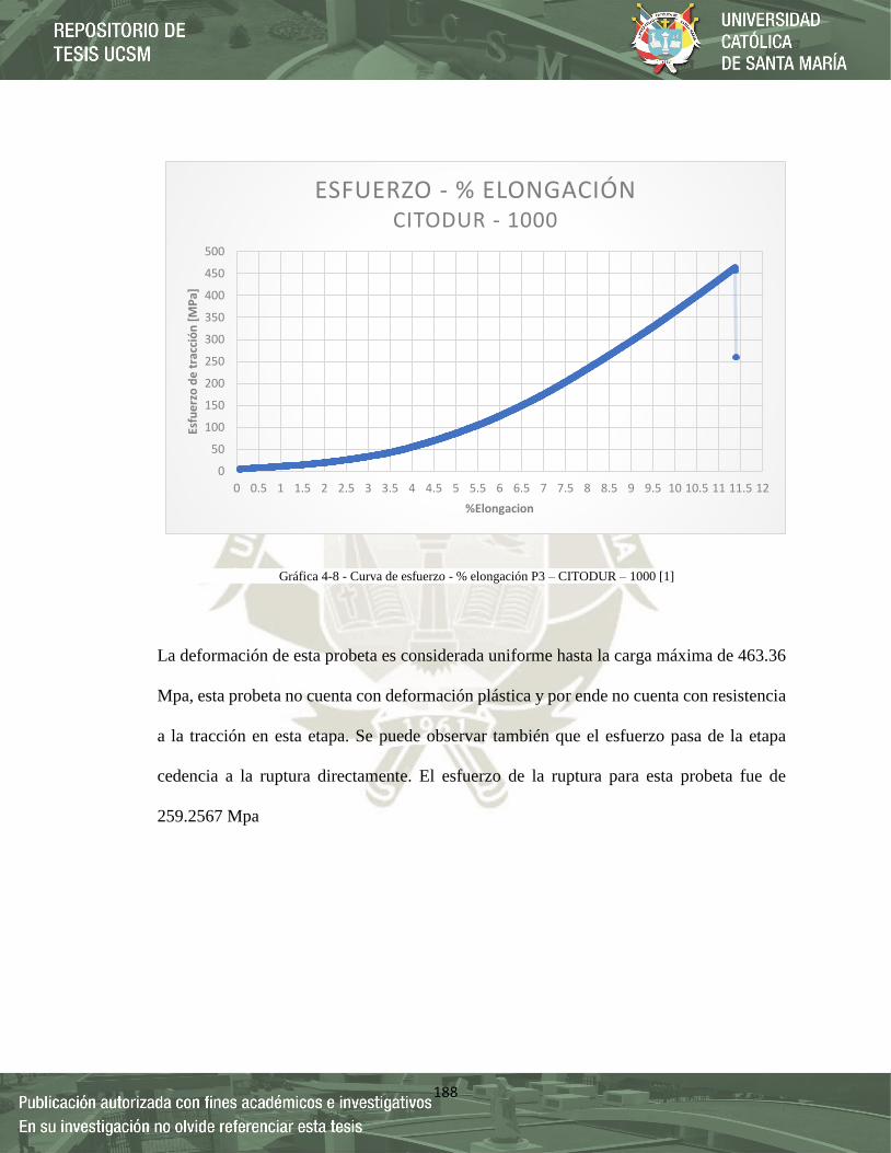
188
La deformación de esta probeta es considerada uniforme hasta la carga máxima de 463.36
Mpa, esta probeta no cuenta con deformación plástica y por ende no cuenta con resistencia
a la tracción en esta etapa. Se puede observar también que el esfuerzo pasa de la etapa
cedencia a la ruptura directamente. El esfuerzo de la ruptura para esta probeta fue de
259.2567 Mpa
0
50
100
150
200
250
300
350
400
450
500
0 0.5 1 1.5 2 2.5 3 3.5 4 4.5 5 5.5 6 6.5 7 7.5 8 8.5 9 9.5 10 10.5 11 11.5 12
Esfu
erz
o d
e t
racc
ión
[M
Pa]
%Elongacion
ESFUERZO - % ELONGACIÓN CITODUR - 1000
Gráfica 4-8 - Curva de esfuerzo - % elongación P3 – CITODUR – 1000 [1]

189
La deformación de esta probeta es considerada uniforme hasta la carga máxima de 502.42
Mpa, esta probeta cuenta con zona de fluencia hasta el esfuerzo 703.56 Mpa, también
cuenta con alargamiento homogéneo hasta el esfuerzo 613.08 Mpa, el esfuerzo donde se
produce la ruptura para esta probeta fue de 511.8165 Mpa.
0.0050.00
100.00150.00200.00250.00300.00350.00400.00450.00500.00550.00600.00650.00700.00750.00
0 0.5 1 1.5 2 2.5 3 3.5 4 4.5 5
Esfu
erz
o d
e t
racc
ión
[M
Pa]
%Elongacion
ESFUERZO - % ELONGACIÓN P4 - MATERIAL BASE
Gráfica 4-9 - Curva de esfuerzo - % elongación P4 – MATERIAL BASE [1]

190
Se elaboró la Gráfica 4-10, que representa las curvas esfuerzo vs % elongación de los
materiales ensayados.
Se puede observar en la Gráfica 4-10 que la probeta P4 Material Base presenta el mayor
esfuerzo a la tracción con 703.56 Mpa, seguido de P3 C-1000 con 463.36 Mpa, seguido de
la probeta P2 – Citomangan con 424.00 Mpa y por último se tiene a la probeta P1 –
EXADUR 43 con 351.66 Mpa. Se observa también que la probeta que mas sufrió de
Elongación fue la probeta P3 C – 1000 con un % 11.40 y la que menos sufrió de elongación
fue la probeta P4 – Material Base con % 4.96 de elongación.
050
100150200250300350400450500550600650700750
0.00 0.50 1.00 1.50 2.00 2.50 3.00 3.50 4.00 4.50 5.00 5.50 6.00 6.50 7.00 7.50 8.00 8.50 9.00 9.5010.0010.5011.0011.50
Esfu
erz
o d
e t
racc
ión
[M
Pa]
%Elongacion
ESFUERZO - % ELONGACIÓN
Exadur - 43 CITOMANGAN CITODUR - 1000 MATERIAL BASE
Gráfica 4-10 - Curva de esfuerzo - % elongación P1-P2-P3-P4 [1]

191
En la siguiente Tabla 4-7 se muestra los datos iniciales de las probetas ensayadas a
tracción.
Tabla 4-7 - Datos iniciales probetas de tracción [1]
Culminado los ensayos de tracción, se midió las probetas y se obtuvo los siguientes datos
de la siguiente Tabla 4-8.
Tabla 4-8 - Datos finales probetas de tracción [1]
Con los datos de la Tabla 4-8, se obtiene la Porcentaje de alargamiento o Deformación
porcentual total y el % Reducción área (estricción) en la siguiente Tabla 4-9.
Tabla 4-9 - Datos finales probetas de tracción [1]
Probeta Diámetro Inicial
(mm) Longitud
Inicial (mm) Área (mm2) Inicial
1 Exadur 43 8.89 36.7 62.07
2 Citomangan 8.86 38.42 61.65
3 C 1000 8.69 37.76 59.31
4 Material Base 7.95 61.64 49.64
Probeta Diámetro Final (mm) Longitud Final (mm)
1 Exadur 43 8.71 39.54
2 Citomangan 8.62 41.71
3 C 1000 8.47 42.1
4 Material Base 7.85 64.7
Probeta Elongación Estricción
% %
1 Exadur 43 7.73 2.02
2 Citomangan 8.57 2.71
3 C 1000 11.4 2.53
4 Material Base 4.96 1.26

192
Los Resultados de la Fuerza Máxima y Resistencia a la tracción del ensayo a la tracción
se muestra en la siguiente Tabla 4-10.
Tabla 4-10 - Resultados Fuerza Máxima y Resistencia a la tracción [1]
Con los resultados de la Fuerza Máxima, Resistencia a la tracción, el % de Elongación y
el % Reducción área. Se obtuvo el Módulo de Young E y Coeficiente de Poisson ʋ para
cada Probeta en la siguiente Tabla 4-11.
Tabla 4-11 - Resultados Modulo de Young y Coeficiente de Poisson [1]
Probeta Fuerza Máxima
N Resistencia a la Tracción
MPA
1 Exadur 43 21827.94 351.67
2 Citomangan 26140.48 424.01
3 C 1000 27481.82 463.36
4 Material Base 34923.6 703.55
Probeta Módulo de Young
E
Coeficiente de Poisson
ʋ
1 Exadur 43 4549.683 0.262
2 Citomangan 4947.858 0.316
3 C 1000 4064.816 0.222
4 Material Base 14172.51 0.253

193
4.5.Ensayo de desgaste
Los ensayos de resistencia al desgaste se han realizado mediante el metodo Pin on disk, bajo
la norma “Standard Test Method for Wear Testing with a Pin-on-Disk Apparatus”,
determinándose el coeficiente de desgaste a partir de la pérdida de masa experimentada por la
muestra. También, se obtuvo el coeficiente de fricción desarrollado a lo largo de los ensayos
que se muestra en la Gráfica 4-11 a la Gráfica 4-14.
Gráfica 4-11 - Coeficiente de fricción en función a la distancia recorrida – Material Base [1]

194
Gráfica 4-12 - Coeficiente de fricción en función a la distancia recorrida – Citomangan [1]
Gráfica 4-13 - Coeficiente de fricción en función a la distancia recorrida – Exadur – 43 [1]

195
La Gráfica 4-11 representa el coeficiente de fricción realizado en el ensayo del Material Base
sin recubrimiento. Puede observarse cómo el valor del coeficiente de fricción tiene un
comportamiento ascendente hasta la distancia 120 m aproximadamente, en donde también
llega al punto más alto de coeficiente de fricción, a partir de la distancia 150 m permanece
constante a lo largo del ensayo. El valor medio que nos da el equipo fue de µ = 0.594
La Gráfica 4-12 representa el coeficiente de fricción realizado en el ensayo del recubrimiento
con Recargue Citomangan. Puede observarse cómo el valor del coeficiente de fricción fluctúa
entre los valores 0.60 y 0.45 durante todo el ensayo. El valor medio que nos da el equipo fue
de µ = 0.533
Gráfica 4-14 - Coeficiente de fricción en función a la distancia recorrida – Citodur 1000 [1]
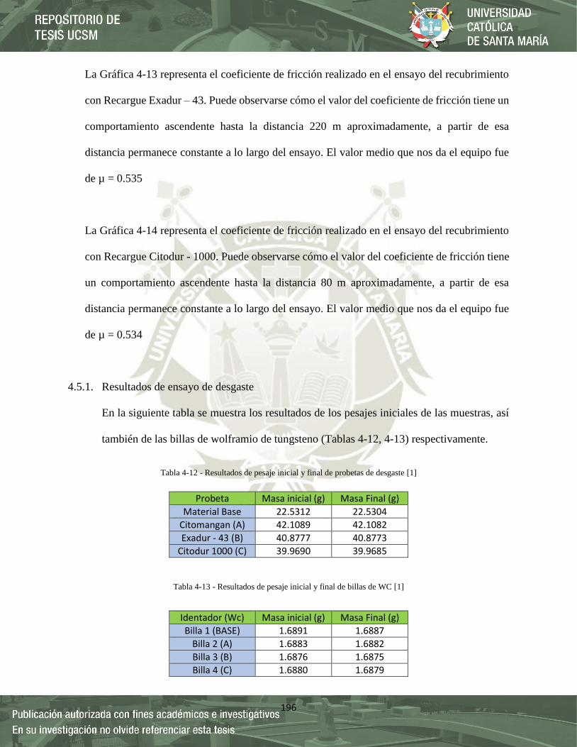
196
La Gráfica 4-13 representa el coeficiente de fricción realizado en el ensayo del recubrimiento
con Recargue Exadur – 43. Puede observarse cómo el valor del coeficiente de fricción tiene un
comportamiento ascendente hasta la distancia 220 m aproximadamente, a partir de esa
distancia permanece constante a lo largo del ensayo. El valor medio que nos da el equipo fue
de µ = 0.535
La Gráfica 4-14 representa el coeficiente de fricción realizado en el ensayo del recubrimiento
con Recargue Citodur - 1000. Puede observarse cómo el valor del coeficiente de fricción tiene
un comportamiento ascendente hasta la distancia 80 m aproximadamente, a partir de esa
distancia permanece constante a lo largo del ensayo. El valor medio que nos da el equipo fue
de µ = 0.534
4.5.1. Resultados de ensayo de desgaste
En la siguiente tabla se muestra los resultados de los pesajes iniciales de las muestras, así
también de las billas de wolframio de tungsteno (Tablas 4-12, 4-13) respectivamente.
Tabla 4-12 - Resultados de pesaje inicial y final de probetas de desgaste [1]
Tabla 4-13 - Resultados de pesaje inicial y final de billas de WC [1]
Probeta Masa inicial (g) Masa Final (g)
Material Base 22.5312 22.5304
Citomangan (A) 42.1089 42.1082
Exadur - 43 (B) 40.8777 40.8773
Citodur 1000 (C) 39.9690 39.9685
Identador (Wc) Masa inicial (g) Masa Final (g)
Billa 1 (BASE) 1.6891 1.6887
Billa 2 (A) 1.6883 1.6882
Billa 3 (B) 1.6876 1.6875
Billa 4 (C) 1.6880 1.6879

197
Teniendo las masas, se procede a calcular el coeficiente de desgaste utilizando la siguiente
ecuación 4-1.
𝒌 =𝑾
𝑭𝑵∗𝑺 Ec 4-1
Donde:
k = El coeficiente de desgaste
W = Volumen desgastado.
FN = Es la fuerza normal
S = Es la distancia lineal Total
Los resultados de coeficiente de desgaste a partir de la pérdida de peso se muestran en la
siguiente Tabla 4-14:
Tabla 4-14 - Resultados de coeficiente de desgaste [1]
En la siguiente Gráfica 4-15 se muestran los resultados obtenidos de los ensayos de
desgaste de todas las probetas, en función del coeficiente de desgaste calculado, junto con
el resultado del valor medio del coeficiente de fricción y la dureza Rockwell de cada una
Probeta Masa inicial
Masa Final
Diff Masa volume
loss, mm3 por Masa
k mm3/N*mm
Material Base 22.5312 22.5304 0.0008 0.1019108 1.12609E-08
Citomangan 42.1089 42.1082 0.0007 0.089172 9.85326E-09
Exadur 43 40.8777 40.8773 0.0004 0.0509554 5.63043E-09
Citodur 1000 39.969 39.9685 0.0005 0.0636943 7.03804E-09

198
de las probetas ensayados. Los datos representados gráficamente son los valores medios
obtenidos en cada ensayo.
Se puede observar en la gráfica que la probeta con menos desgaste fue el que tuvo recargue
de soldadura con 5.63*10-9, cabe resalta que esta probeta posee la mayor dureza de todas,
con 70.4 HRC en promedio. La probeta con más desgaste con recargue fue la de
Citomangan con 9.85*10-9, esta probeta posee la menor dureza de las probetas con
recargue con 63.6 HRC. La probeta sin recargue obtuvo un desgaste de 11.26*10-9, esta
probeta obtuvo la menor dureza de todas las probetas con 58.77 HRC.
También se puede observar que no hay mucha variación en el coeficiente de fricción entre
todas las probetas, siendo el valor más alto 0.594 que corresponde a la probeta de Material
Base, y el menor 0.533 que corresponde a la probeta con recargue de Citomangan.
11.126
9.85326
5.6304
7.038
0.594 0.533 0.5350.534
58.77
63.6
70.4
70.1
52
54
56
58
60
62
64
66
68
70
72
00.5
11.5
22.5
33.5
44.5
55.5
66.5
77.5
88.5
99.510
10.511
11.512
Material Base Citomangan Exadur - 43 Citodur 1000
Du
reza
HR
C
Co
efic
ien
te d
e d
esga
ste
(m
m3
/Nm
m)*
10
^-9
Co
efic
ien
te d
e fr
icci
ón
Coeficiente de Desgaste (k) Coeficiente de Fricción (u) Dureza (HRC)
Gráfica 4-15 - Resultados de ensayos de desgaste [1]

199
4.5.2. Perfil de Huella de Wear Track
Se tiene las siguientes Figuras 4-6 al 4-9, donde se puede observar las modelizaciones de
profundidad de la pista de desgaste de las probetas de desgaste ensayadas.
Figura 4-6 - Modelización de pista de desgaste – Material Base [1]
Figura 4-7 - Modelización de pista de desgaste – Citomangan [1]

200
Figura 4-9 - Modelización de pista de desgaste – Citodur – 1000 [1]
Figura 4-8 - Modelización de pista de desgaste – Exadur – 43 [1]
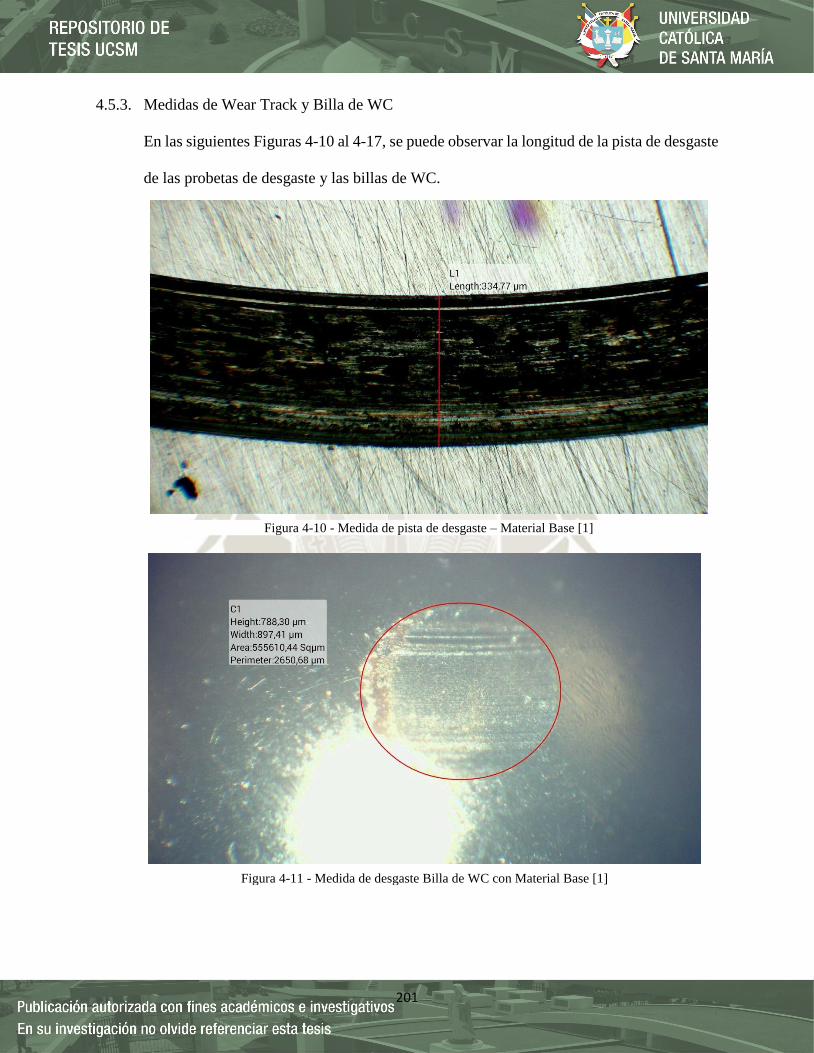
201
4.5.3. Medidas de Wear Track y Billa de WC
En las siguientes Figuras 4-10 al 4-17, se puede observar la longitud de la pista de desgaste
de las probetas de desgaste y las billas de WC.
Figura 4-10 - Medida de pista de desgaste – Material Base [1]
Figura 4-11 - Medida de desgaste Billa de WC con Material Base [1]
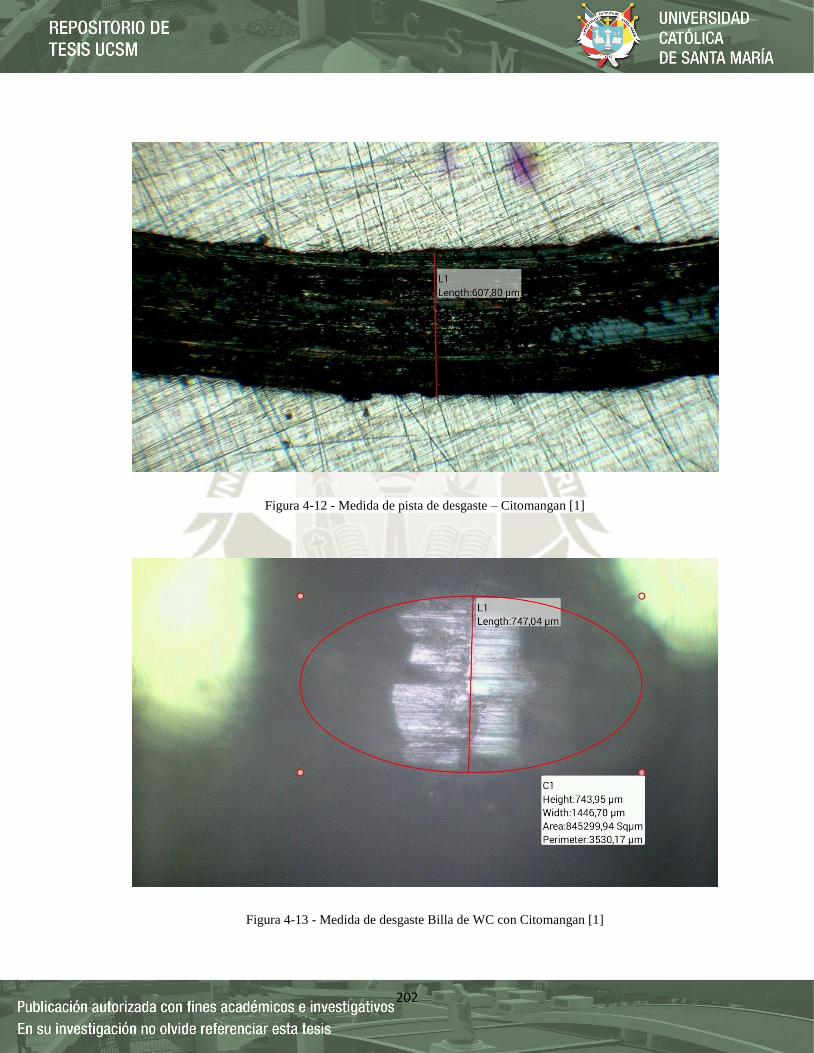
202
Figura 4-12 - Medida de pista de desgaste – Citomangan [1]
Figura 4-13 - Medida de desgaste Billa de WC con Citomangan [1]

203
Figura 4-14 - Medida de pista de desgaste – Exadur – 43 [1]
Figura 4-15 - Medida de desgaste Billa de WC con Exadur – 43 [1]

204
Figura 4-16 - Medida de pista de desgaste – Citodur – 1000 [1]
Figura 4-17 - Medida de desgaste Billa de WC con Citodur – 1000 [1]
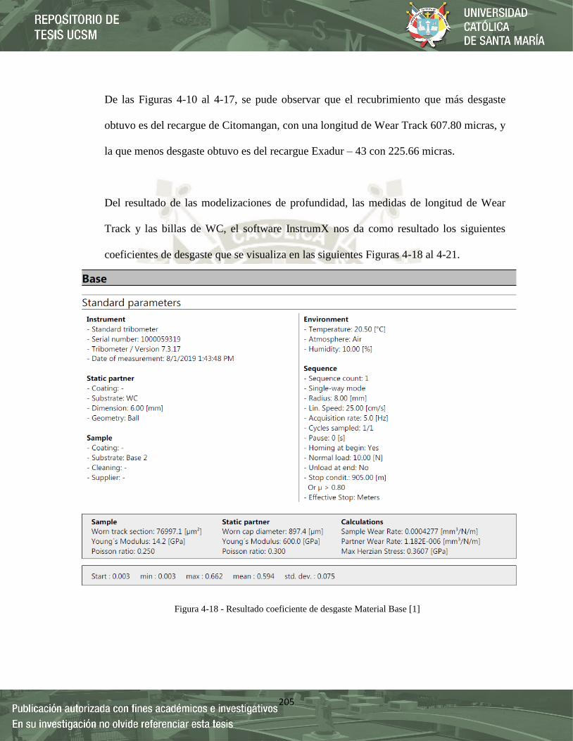
205
De las Figuras 4-10 al 4-17, se pude observar que el recubrimiento que más desgaste
obtuvo es del recargue de Citomangan, con una longitud de Wear Track 607.80 micras, y
la que menos desgaste obtuvo es del recargue Exadur – 43 con 225.66 micras.
Del resultado de las modelizaciones de profundidad, las medidas de longitud de Wear
Track y las billas de WC, el software InstrumX nos da como resultado los siguientes
coeficientes de desgaste que se visualiza en las siguientes Figuras 4-18 al 4-21.
Figura 4-18 - Resultado coeficiente de desgaste Material Base [1]

206
Figura 4-20 - Resultado coeficiente de desgaste Exadur – 43 [1]
Figura 4-19 - Resultado coeficiente de desgaste Citomangan [1]
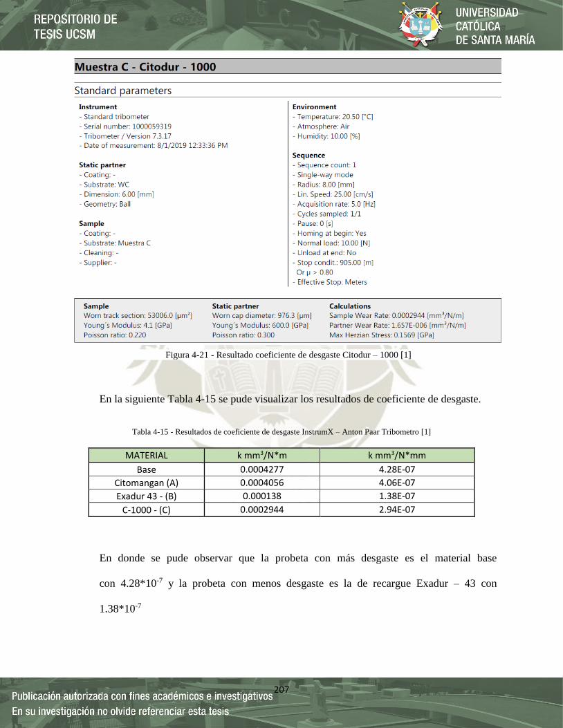
207
En la siguiente Tabla 4-15 se pude visualizar los resultados de coeficiente de desgaste.
Tabla 4-15 - Resultados de coeficiente de desgaste InstrumX – Anton Paar Tribometro [1]
En donde se pude observar que la probeta con más desgaste es el material base
con 4.28*10-7 y la probeta con menos desgaste es la de recargue Exadur – 43 con
1.38*10-7
MATERIAL k mm3/N*m k mm3/N*mm
Base 0.0004277 4.28E-07
Citomangan (A) 0.0004056 4.06E-07
Exadur 43 - (B) 0.000138 1.38E-07
C-1000 - (C) 0.0002944 2.94E-07
Figura 4-21 - Resultado coeficiente de desgaste Citodur – 1000 [1]
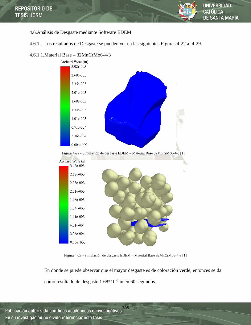
208
4.6.Análisis de Desgaste mediante Software EDEM
4.6.1. Los resultados de Desgaste se pueden ver en las siguientes Figuras 4-22 al 4-29.
4.6.1.1.Material Base – 32MnCrMo6-4-3
En donde se puede observar que el mayor desgaste es de coloración verde, entonces se da
como resultado de desgaste 1.68*10-3 in en 60 segundos.
Figura 4-22 - Simulación de desgaste EDEM – Material Base 32MnCrMo6-4-3 [1]
Figura 4-23 - Simulación de desgaste EDEM – Material Base 32MnCrMo6-4-3 [1]
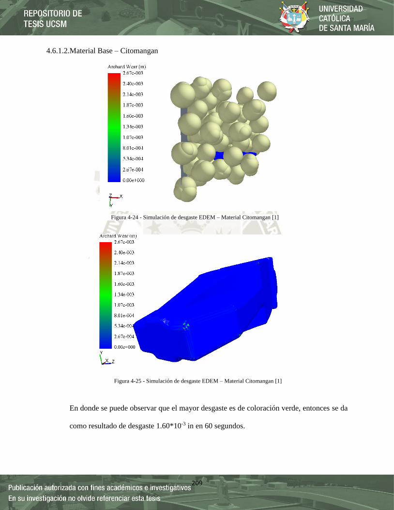
209
4.6.1.2.Material Base – Citomangan
En donde se puede observar que el mayor desgaste es de coloración verde, entonces se da
como resultado de desgaste 1.60*10-3 in en 60 segundos.
Figura 4-24 - Simulación de desgaste EDEM – Material Citomangan [1]
Figura 4-25 - Simulación de desgaste EDEM – Material Citomangan [1]

210
4.6.1.3.Material Base – Exadur 43
En donde se puede observar que el mayor desgaste es de coloración verde, entonces se da
como resultado de desgaste 5.43*10-4 in en 60 segundos.
Figura 4-26 - Simulación de desgaste EDEM – Material Exadur – 43 [1]
Figura 4-27 - Simulación de desgaste EDEM – Material Exadur – 43 [1]
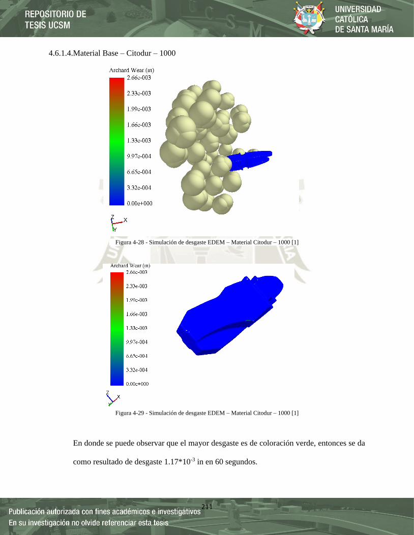
211
4.6.1.4.Material Base – Citodur – 1000
En donde se puede observar que el mayor desgaste es de coloración verde, entonces se da
como resultado de desgaste 1.17*10-3 in en 60 segundos.
Figura 4-28 - Simulación de desgaste EDEM – Material Citodur – 1000 [1]
Figura 4-29 - Simulación de desgaste EDEM – Material Citodur – 1000 [1]
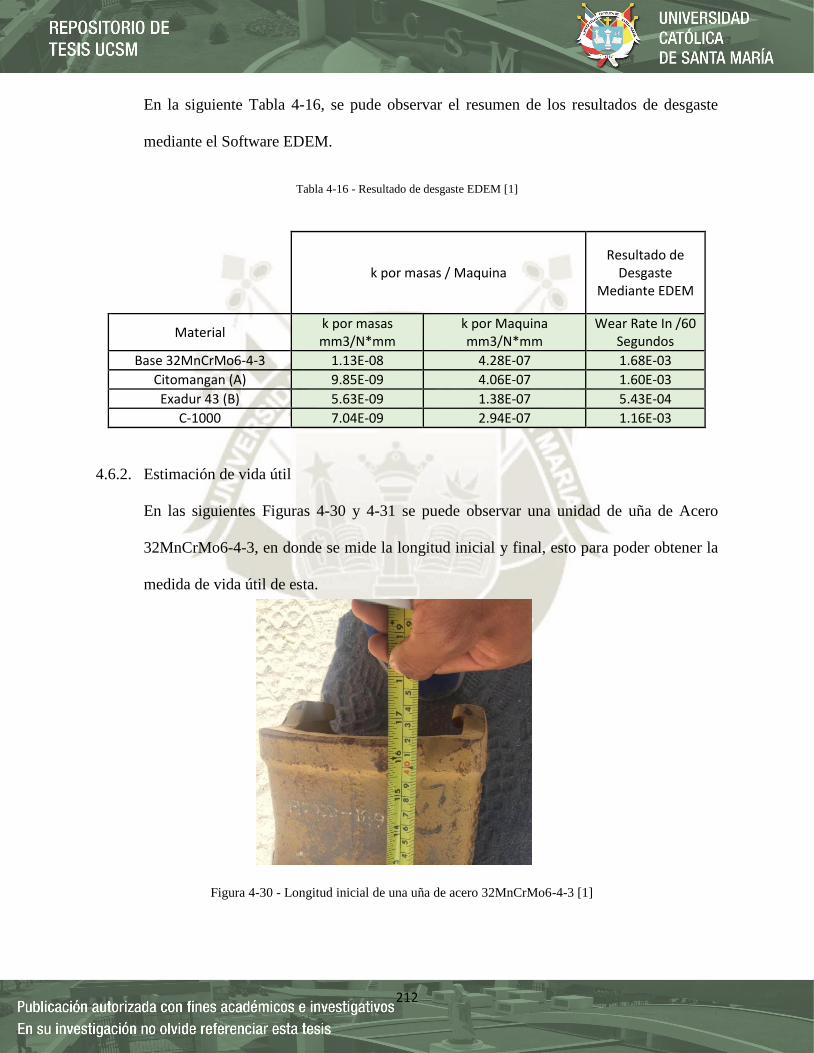
212
En la siguiente Tabla 4-16, se pude observar el resumen de los resultados de desgaste
mediante el Software EDEM.
Tabla 4-16 - Resultado de desgaste EDEM [1]
4.6.2. Estimación de vida útil
En las siguientes Figuras 4-30 y 4-31 se puede observar una unidad de uña de Acero
32MnCrMo6-4-3, en donde se mide la longitud inicial y final, esto para poder obtener la
medida de vida útil de esta.
k por masas / Maquina Resultado de
Desgaste Mediante EDEM
Material k por masas mm3/N*mm
k por Maquina mm3/N*mm
Wear Rate In /60 Segundos
Base 32MnCrMo6-4-3 1.13E-08 4.28E-07 1.68E-03
Citomangan (A) 9.85E-09 4.06E-07 1.60E-03
Exadur 43 (B) 5.63E-09 1.38E-07 5.43E-04
C-1000 7.04E-09 2.94E-07 1.16E-03
Figura 4-30 - Longitud inicial de una uña de acero 32MnCrMo6-4-3 [1]

213
Teniendo los resultados de ensayo de desgaste mediante la norma ASTM G-99 y el
Software se deduce la cantidad de días que duraría la uñas mediante las siguientes formulas:
Según las mediciones, se tiene la vida útil con la siguiente ecuación 4-2:
𝟏𝟔. 𝟓 𝒊𝒏 (𝒍𝒂𝒓𝒈𝒐) − 𝟔. 𝟓 (𝒄𝒐𝒓𝒕𝒐) = 𝟏𝟎 𝒊𝒏 Ec 4-2
Pero por precaución y no dañar los adaptadores se cambia cuando esta tiene un desgaste de
8 in.
4.6.2.1.Material Base 32MnCrMo6-4-3
𝟏.𝟔𝟖∗𝟏𝟎−𝟑
𝟏 𝒎𝒊𝒏∗𝟔𝟎 𝒎𝒊𝒏
𝟏 𝒉∗
𝟐𝟒 𝒉
𝟏 𝒅𝒊𝒂= 𝟐. 𝟒𝟐𝟒𝟕
𝒊𝒏
𝒅𝒊𝒂 Ec 4-3
Teniendo un desgaste máximo de 8 in, entonces la uña durara:
𝟐.𝟒𝟐𝟒𝟕
𝒊𝒏
𝒅𝒊𝒂
𝟖 𝒊𝒏 = 𝟑. 𝟐𝟗𝟐𝟑 𝒅𝒊𝒂𝒔 Ec 4-4
4.6.2.2.Material Base – Citomangan
𝟏.𝟔𝟎∗𝟏𝟎−𝟑
𝟏 𝒎𝒊𝒏∗𝟔𝟎 𝒎𝒊𝒏
𝟏 𝒉∗
𝟐𝟒 𝒉
𝟏 𝒅𝒊𝒂= 𝟐. 𝟐𝟗𝟗𝟒
𝒊𝒏
𝒅𝒊𝒂 Ec 4-5
Figura 4-31 - Longitud final de una uña de acero 32MnCrMo6-4-3 [1]

214
Teniendo un desgaste máximo de 8 in, entonces la uña durara:
𝟐.𝟐𝟗𝟗𝟒
𝒊𝒏
𝒅𝒊𝒂
𝟖 𝒊𝒏 = 𝟑. 𝟒𝟕𝟗𝟎 𝒅𝒊𝒂𝒔 Ec 4-6
4.6.2.3.Material Base - Exadur – 43
𝟓.𝟒𝟑∗𝟏𝟎−𝟒
𝟏 𝒎𝒊𝒏∗𝟔𝟎 𝒎𝒊𝒏
𝟏 𝒉∗
𝟐𝟒 𝒉
𝟏 𝒅𝒊𝒂= 𝟎. 𝟕𝟖𝟐𝟑
𝒊𝒏
𝒅𝒊𝒂 Ec 4-7
Teniendo un desgaste máximo de 8 in, entonces la uña durara:
𝟎.𝟕𝟖𝟐𝟑
𝒊𝒏
𝒅𝒊𝒂
𝟖 𝒊𝒏 = 𝟏𝟎. 𝟐𝟐𝟓𝟒 𝒅𝒊𝒂𝒔 Ec 4-8
4.6.2.4.Material Base – Citodur – 1000
𝟏.𝟏𝟔∗𝟏𝟎−𝟑
𝟏 𝒎𝒊𝒏∗𝟔𝟎 𝒎𝒊𝒏
𝟏 𝒉∗
𝟐𝟒 𝒉
𝟏 𝒅𝒊𝒂= 𝟏. 𝟔𝟔𝟗𝟎
𝒊𝒏
𝒅𝒊𝒂 Ec 4-9
Teniendo un desgaste máximo de 8 in, entonces la uña durara:
𝟏.𝟔𝟔𝟗𝟎
𝒊𝒏
𝒅𝒊𝒂
𝟖 𝒊𝒏 = 𝟒. 𝟕𝟗𝟑𝟏 𝒅𝒊𝒂𝒔 Ec 4-10
Se recopilo la frecuencia de cambio de las uñas de Acero 32MnCrMo6-4-3 sin
recubrimiento en las OTS. Se pude observar en la siguiente Tabla 4-17:

215
Tabla 4-17 - Frecuencia de cambio de Uñas de Acero 32MnCrMo6-4-3 en Barrick Lagunas Norte [1]
FECHA INICIO HOROMETRO INICIO FECHA DE FIN HOROMETRO DE FIN DURACION EN HORAS
DESCRIPCION DE EDD
1 JUEGO DE UÑAS ALTERNATIVOS 11/05/2017 4249 21/05/2017 4340 91 2 JUEGO DE UÑAS ALTERNATIVOS 21/05/2017 4340 28/05/2017 4417 77 3 JUEGO DE UÑAS ALTERNATIVOS 28/05/2017 4417 17/06/2017 4494 77 4 JUEGO DE UÑAS ALTERNATIVOS 17/06/2017 4494 27/06/2017 4568 74 5 JUEGO DE UÑAS ALTERNATIVOS 27/06/2017 4568 30/06/2017 4623 55 6 JUEGO DE UÑAS ALTERNATIVOS 30/06/2017 4623 28/07/2017 4723 100 7 JUEGO DE UÑAS ALTERNATIVOS 28/07/2017 4723 30/07/2017 4752 29 8 JUEGO DE UÑAS ALTERNATIVOS 30/07/2017 4752 07/08/2017 4842 90 9 JUEGO DE UÑAS ALTERNATIVOS 07/08/2017 4842 16/08/2017 4925 83
10 JUEGO DE UÑAS ALTERNATIVOS 16/08/2017 4925 22/08/2017 5025 100 11 JUEGO DE UÑAS ALTERNATIVOS 22/08/2017 5025 27/08/2017 5115 90 12 JUEGO DE UÑAS ALTERNATIVOS 27/08/2017 5115 03/09/2017 5202 87 13 JUEGO DE UÑAS ALTERNATIVOS 03/09/2017 5202 08/09/2017 5281 79 14 JUEGO DE UÑAS ALTERNATIVOS 08/09/2017 5281 16/09/2017 5361 80 15 JUEGO DE UÑAS ALTERNATIVOS 16/09/2017 5361 20/09/2017 5440 79 16 JUEGO DE UÑAS ALTERNATIVOS 20/09/2017 5440 27/09/2017 5512 72 17 JUEGO DE UÑAS ALTERNATIVOS 27/09/2017 5512 04/10/2017 5632 120 18 JUEGO DE UÑAS ALTERNATIVOS 04/10/2017 5632 15/10/2017 5771 139 19 JUEGO DE UÑAS ALTERNATIVOS 15/10/2017 5771 18/10/2017 5823 52 20 JUEGO DE UÑAS ALTERNATIVOS 18/10/2017 5823 21/10/2017 5877 54 21 JUEGO DE UÑAS ALTERNATIVOS 21/10/2017 5877 05/11/2017 5985 108 22 JUEGO DE UÑAS ALTERNATIVOS 05/11/2017 5985 10/11/2017 6069 84 23 JUEGO DE UÑAS ALTERNATIVOS 10/11/2017 6069 14/11/2017 6136 67 24 JUEGO DE UÑAS ALTERNATIVOS 14/11/2017 6136 17/11/2017 6180 44 25 JUEGO DE UÑAS ALTERNATIVOS 17/11/2017 6180 22/11/2017 6262 82 26 JUEGO DE UÑAS ALTERNATIVOS 22/11/2017 6262 25/11/2017 6311 49 27 JUEGO DE UÑAS ALTERNATIVOS 25/11/2017 6311 30/11/2017 6401 90 28 JUEGO DE UÑAS ALTERNATIVOS 30/11/2017 6401 05/12/2017 6495 94 29 JUEGO DE UÑAS ALTERNATIVOS 05/12/2017 6495 08/12/2017 6538 43 30 JUEGO DE UÑAS ALTERNATIVOS 08/12/2017 6538 10/12/2017 6561 23 31 JUEGO DE UÑAS ALTERNATIVOS 10/12/2017 6561 13/12/2017 6611 50

216
De las Ots se tiene los siguientes resultados que se muestra en la siguiente Tabla 4-18:
Tabla 4-18 - Frecuencia de cambio de uñas de acero 32MnCrMo6-4-3 [1]
En donde la frecuencia de cambio para el Contexto Operacional es 3.463 días para uñas de
acero 32MnCrMo6-4-3 sin recubrimiento, similar al resultado que salió mediante el
Software EDEM que dio como resultado 3.2923 días para el mismo material.
Tabla 4-19 – Resultado de duración de material [1]
Se concluye de la tabla 4-19, que las soldaduras de recubrimiento más efectivas al desgaste
son:
Exadur – 43 con una duración de 10.2254 días
Citodur – 1000 con una duración de 4.7931 días
Ahora se realiza el análisis de costos en el Capítulo 5 – Evaluación Económica, para ver si
es viable la aplicación de estos recubrimientos en el contexto Operacional (Mina Barrick
Lagunas Norte).
* COSTO DE JUEGO DE EDD
$ 500.00
RATIO PROM. (HRS/EDD)
RATIO PROM. TRAB (HRS/DIA)
FRECUENCIA DE CAMBIO (DIA/EDD)
RATIO PROM. MENSUAL ( EDD/MES)
COSTO MES
76.19354839 22 3.463 9 $ 1,731.67
Material Duración (Días)
Base 32MnCrMo6-4-3 (OT) 3.46
Base 32MnCrMo6-4-3 3.29
Citomangan (A) 3.48
Exadur 43 (B) 10.23
C-1000 4.79

217
CAPÍTULO V
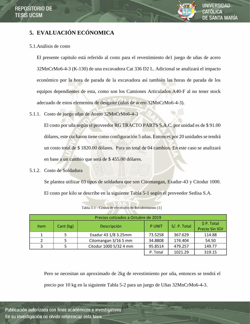
218
5. EVALUACIÓN ECÓNOMICA
5.1.Análisis de costo
El presente capitulo está referido al costo para el revestimiento de1 juego de uñas de acero
32MnCrMo6-4-3 (K-130) de una excavadora Cat 336 D2 L. Adicional se analizará el impacto
económico por la hora de parada de la excavadora así también las horas de parada de los
equipos dependientes de esta, como son los Camiones Articulados A40-F al no tener stock
adecuado de estos elementos de desgaste (uñas de acero 32MnCrMo6-4-3).
5.1.1. Costo de juego uñas de Acero 32MnCrMo6-4-3
El costo por uña según el proveedor RG TRACTO PARTS S.A.C. por unidad es de $ 91.00
dólares, este cucharon tiene como configuración 5 uñas. Entonces por 20 unidades se tendrá
un costo total de $ 1820.00 dólares. Para un total de 04 cambios. En este caso se analizará
en base a un cambio que será de $ 455.00 dólares.
5.1.2. Costo de Soldadura
Se plantea utilizar 03 tipos de soldadura que son Citomangan, Exadur-43 y Citodur 1000.
El costo por kilo se describe en la siguiente Tabla 5-1 según el proveedor Sedisa S.A.
Tabla 5-1 - Costos de electrodos de Recubrimiento [1]
Pero se necesitan un aproximado de 2kg de revestimiento por uña, entonces se tendrá el
precio por 10 kg en la siguiente Tabla 5-2 para un juego de Uñas 32MnCrMo6-4-3.
Precios cotizados a Octubre de 2019
Item Cant (kg) Descripción P UNIT S/. P. Total $ P. Total
Precio Sin IGV
1 5 Exadur 43 1/8 3.25mm 73.5258 367.629 114.88
2 5 Citomangan 3/16 5 mm 34.8808 174.404 54.50
3 5 Citodur 1000 5/32 4 mm 95.8514 479.257 149.77
P. Total 1021.29 319.15

219
Tabla 5-2 - Costos de electrodos de Recubrimiento [1]
5.1.3. Costo de Hora-Hombre
Para el recubrimiento de las uñas 32MnCrMo6-4-3 se necesitarán 2.4 H-H por uña, para
un juego completo se necesitará 12 H-H.
Se puede observar el costo laboral de un soldador en la siguiente Tabla 5-3.
Tabla 5-3 – Costo laboral Soldador [1]
Entonces el costo laboral de un soldador es 78 $/día
5.1.4. Costo de Moto soldadora
El costo de la moto soldadora mensual es de $ 1200.00 por mes.
$𝟏𝟐𝟎𝟎
𝟏 𝒎𝒆𝒔∗
𝟏𝒎𝒆𝒔
𝟑𝟎 𝒅𝒊𝒂𝒔= 𝟒𝟎
$
𝒅𝒊𝒂 Ec 5-1
De la ecuación 5-1, nos da como resultado 40 $/día, por Revestimiento.
Se tiene que la moto soldadora consume promedio 15 gal/día, entonces se tiene el costo del
combustible en la siguiente ecuación 5-2
Precios cotizados a Octubre de 2019
Item Cant (kg) Descripción P UNIT S/. P. Total $ P. Total
Precio Sin IGV
1 10 Exadur 43 1/8 3.25mm 73.5258 735.258 229.77
2 10 Citomangan 3/16 5 mm 34.8808 348.808 109.00
3 10 Citodur 1000 5/32 4 mm 95.8514 958.514 299.54
P. Total 2042.58 638.31
Item Cantidad Descripción $ Base $ Anual
1 12 Remuneración Básica 1500 18000.00
2 2 Gratificación 1500 3000.00
3 1 Vacaciones 1500 1500.00
4 2 CTS 1500 3000.00
5 2 Bonificación 500 1000.00
6 12 Seguro Social 100 1200.00
7 12 SCTR 25 300.00
Total $ 28000.00
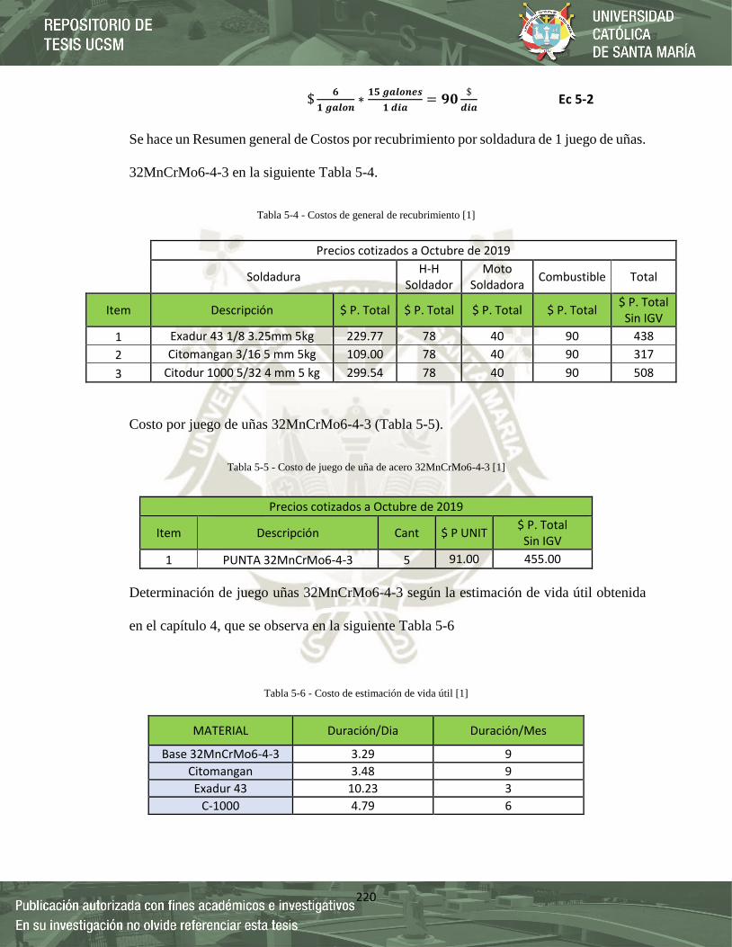
220
$𝟔
𝟏 𝒈𝒂𝒍𝒐𝒏∗𝟏𝟓 𝒈𝒂𝒍𝒐𝒏𝒆𝒔
𝟏 𝒅𝒊𝒂= 𝟗𝟎
$
𝒅𝒊𝒂 Ec 5-2
Se hace un Resumen general de Costos por recubrimiento por soldadura de 1 juego de uñas.
32MnCrMo6-4-3 en la siguiente Tabla 5-4.
Tabla 5-4 - Costos de general de recubrimiento [1]
Costo por juego de uñas 32MnCrMo6-4-3 (Tabla 5-5).
Tabla 5-5 - Costo de juego de uña de acero 32MnCrMo6-4-3 [1]
Determinación de juego uñas 32MnCrMo6-4-3 según la estimación de vida útil obtenida
en el capítulo 4, que se observa en la siguiente Tabla 5-6
Tabla 5-6 - Costo de estimación de vida útil [1]
Precios cotizados a Octubre de 2019
Soldadura
H-H Soldador
Moto Soldadora
Combustible Total
Item Descripción $ P. Total $ P. Total $ P. Total $ P. Total $ P. Total
Sin IGV
1 Exadur 43 1/8 3.25mm 5kg 229.77 78 40 90 438
2 Citomangan 3/16 5 mm 5kg 109.00 78 40 90 317
3 Citodur 1000 5/32 4 mm 5 kg 299.54 78 40 90 508
Precios cotizados a Octubre de 2019
Item Descripción Cant $ P UNIT $ P. Total
Sin IGV
1 PUNTA 32MnCrMo6-4-3 5 91.00 455.00
MATERIAL Duración/Dia Duración/Mes
Base 32MnCrMo6-4-3 3.29 9
Citomangan 3.48 9
Exadur 43 10.23 3
C-1000 4.79 6

221
En la siguiente Tabla 5-7 se determina los costos totales por juego de uña en 1 mes y 1 año,
de acuerdo con la vida útil y los costos por adquisición de uñas y recubrimiento de uñas.
Tabla 5-7 - Costo total por juego de uñas de acero 32MnCrMo6-4-3 [1]
Se puede Observar que el costo Anual del juego con recubrimiento de Soldadura Exadur –
43 es $ 16992.0 más bajo que el juego sin recubrimiento, en porcentaje se educe que es un
% 34.58 menos costoso.
Este análisis es para solo 01 excavadora, el proyecto cuenta con 04 excavadoras con la
misma configuración de cucharon. Entonces se podría ahorrar un promedio de $ 67968.0
dólares por el recubrimiento de estas uñas con Soldadura Exadur – 43.
No sale a cuenta recubrir las uñas 32MnCrMo6-4-3 con los demás Soldaduras. Si se aplica
estos recubrimientos, nos podríamos asegurar un stock adecuado de Gets (Elementos de
desgaste en Almacén).
Precios cotizados a Octubre de 2019
MATERIAL Duración/
Dia Duración
/Mes
Costo de Recubrim
iento $
Costo x Juego $
Costo x Juego $ + Recubrimiento $
Costo x Mes Total
$
Costo x Anual Total $
Sin IGV
Base 32MnCrMo6-4-3
3.29 9 0 455 455 4095 49140
Citomangan 3.48 9 317 455 772 6948 83376
Exadur - 43 10.23 3 438 455 893 2679 32148
C-1000 4.79 6 508 455 963 5778 69336

222
5.2.Impacto económico por parada
Al parar una excavadora por falta de Elementos de desgaste, este acarrea a dos articulados más,
el impacto económico por falta (Gets) en Almacén en la siguiente Tabla 5-8:
Tabla 5-8 - Costo hora x maquina [1]
En el proyecto se observó que cada mes para una excavadora por falta de Gets (Uñas de Acero
32MnCrMo6-4-3), entonces se pude deducir que se pierde un total de $ 118.080.00 dólares
anuales.
Los ahorros anuales por evitar equipos parados y aumento de vida útil de los GETS se observan
en la siguiente Tabla 5-9.
Tabla 5-9 - Costos equipos parados y vida útil de uñas de acero 32MnCrMo6-4-3 [1]
Se puede observar que se puede obtener un ahorro de $186048.0 dólares si se tiene una correcta
estrategia de Mantenimiento (Recubrimiento de uñas 32MnCrMo6-4-3, stock adecuado en
Almacén) anualmente.
Precios cotizados a Octubre de 2019
1 ALQUILERES DE EQUIPOS PARA EL SERVICIO MOVIMIENTO DE TIERRAS
1.1 Tarifa horaria por equipo H DIA AÑO
1.1.2 Alquiler de Excavadora hidráulico (01 und) 336 D2 L $130.00 $3,120.00 $37,440.00
1.1.3 Alquiler de Camiones articulados de 24 m3 (02 und) $140.00 $6,720.00 $80,640.00
Total $ $9,840.00 $118,080.00
Precios cotizados a Octubre de 2019
Item Impacto Económico $ Total
1 Costo por parada de 01 Excavadora 336D2 L y 02 Articulados A-40F $118,080.00
2 Costo ahorro por Recubrimiento de Uñas 32MnCrMo6-4-3 $67,968.00
$186,048.00

223
CONCLUSIONES
1. Se analizó y evaluó el desgaste en revestimientos duros aplicados por procesos de
soldadura en uñas de acero 32MnCrMo 6-4-3 de una excavadora hidráulica Cat 336D2 L.
2. Se analizó el desgaste en revestimientos duros aplicados por procesos de soldadura
mediante elementos discretos (MED). En donde se concluye que la uña de acero sin
recubrimiento es la más afectada al desgaste, con un promedio de 1.68x10⁻³ in por minuto.
Se concluye que la uña con recubrimiento Exadur – 43 posee un menor desgaste con
5.43x10⁻⁴ in por minuto.
3. Se evaluó el desgaste en revestimientos duros aplicados por procesos de soldadura bajo la
norma ASTM G-99, en donde se demostró que la probeta con menos desgaste fue Exadur
– 43, con un coeficiente de fricción 0.563 y un coeficiente de desgaste de 5.6304x10⁻⁹,
seguido de la probeta con recargue Citodur – 1000, con un coeficiente de fricción de 0.534
y un coeficiente de desgaste de 7.0380x10⁻⁹, seguido de la probeta con recargue
Citomangan, con un coeficiente de fricción de 0.533 y un coeficiente de desgaste de
9.8532x10⁻⁹. Teniendo como la probeta con más desgaste sin recubrimiento con un
coeficiente de fricción de 0.594 y un coeficiente de desgaste de 1.1260 x10⁻⁸.
4. Se evaluó las pérdidas Volumétricas existentes bajo la norma ASTM G-99. En donde se
observa que la probeta sin revestimiento tiene una perdida volumétrica de 0.1019 mm3,
seguido de la probeta recubierta con Citomangan con 0.0892 mm3, seguido de la probeta
recubierta con Citodur - 1000 con 0.0636 mm3. Teniendo como la probeta con menos
perdidas Volumétricas la recubierta con Exadur – 43 con una pérdida de 0.0509 mm3.
5. Se observa que la estructura más resistente al desgaste es la Austenítica, con carburos de
Cromo y Niobio, esta estructura corresponde al recubrimiento con soldadura Exadur – 43.

224
6. Se realizó el análisis de dureza en cada uno de los procesos de recubrimientos. En donde
se observó que la probeta con más dureza obtenida fue el recargue de Exadur – 43, este
obtuvo como promedio 70.4 HRC. Esto también puede deberse al alto contenido de %
Cromo (20.3) y % Niobio (4.3).
7. Se determinó el tipo de electrodo más adecuado que garantice sus buenas propiedades
contra el desgaste es el recubrimiento Exadur – 43, ya que posee un coeficiente de desgaste
más bajo, tiene la mayor dureza y posee el menor desgaste por minuto que los demás
recubrimientos.
8. Se determinó la influencia de las características del mineral explotado en la mina y de las
condiciones de operación de los equipos en el desgaste presentado, al ser un contexto
Operacional duro. Se determinó que afecto en los resultados al desgaste mediante la
simulación MED (Elementos Discretos).
9. Se Analizó el costo-beneficio del recargue duro aplicado a las uñas de las excavadoras. En
donde puede concluir que es factible el recubrimiento de las uñas con soldadura Exadur –
43, pudiendo ahorrar anualmente $186,048.00 mil dólares anualmente aumentando el ciclo
de vida útil de esta por excavadora y evitando roturas de Stock de Almacén.
225
RECOMENDACIONES
1. Se debe simular también los esfuerzos que interactúan el material acero con el mineral, ya
que el software EDEM permite exportar los valores de presiones y fuerzas en rangos
determinados de tiempo. Esto para poder tener un mejor análisis de costo beneficio de
recargue de los materiales a estudiar.
2. Se debe realizar el estudio de desgaste de electrodos de recargue de otras marcas de similar
composición química, esto para poder tener un mejor análisis de rendimiento y costo
beneficio.
3. Las superficies de desgaste y las virutas deberán ser analizados por MEB y espectroscopia
de energías de rayos X dispersados (EDX).
4. Se debe realizar el costo beneficio por disponibilidad operacional de equipos y cantidad de
mineral procesado en planta.

226
REFERENCIAS
[1] PURCA JUSTO, R. R. (2019). Análisis mediante elementos discretos (MED) y evaluación
experimental bajo la norma ASTM G-99 del desgaste en revestimientos duros aplicados
por procesos de soldadura en uñas de acero 32MnCrMo6-4-3 de una excavadora hidráulica
Cat 336D2 L. AREQUIPA: UCSM.
[2] CUESTA CASTRO, E.J/LAGUNAS MOYA, J.C (2010). El cuchillo militar.ESPAÑA
[3] WILLIAM F, Iron and Steel - Hosford, Universidad de Michigan
[4] Dr RODRIGO BULNES AGUILAR. (2018), Análisis de tribología – Camiper,
[5] Professor Dr. VALENTIN L. POPOV (auth.). (2010). Contact Mechanics and Friction_
Physical Principles and Applications-Springer-Verlag Berlin Heidelberg
[6] CORRALES, JOSE. (2010). Soldadura de Mantenimiento, Soldexa
[7] GWIDON STACHOWIAK, A W BATCHELOR. (2000). Engineering Tribology, Second
Edition -Butterworth-Heinemann
[8] MIGUEL ANGEL, WILFREDO LANATA ROSPIGLIOSI. (2004) Modelamiento de
Vibraciones en el campo cercano aplicado a Lagunas Norte, U.N.I
[9] MANUEL ANGEL CHANDUVI GAMARRA. (2010). ANALISIS TECNICO-
ECOLOGICO-ECONOMICO CON LA APLICACIÓN DE EXPLODECK PARA
REDUCIR EL CONSUMO DE MEZCLA EXPLOSIVA EN LA COMPAÑÍA MINERA
BARRICK MISQUICHILCALAGUNAS NORTE, U.N.I
[10] SOLDEXA. (2010). Manual de Soldadura y Catálogo de Productos – 7 Edición
[11] AWS A5.13/A5.13M:2010, Specification for Surfacing Electrodes for Shielded
Metal Arc Welding

227
[12] NORIA. (11 de ENERO de 2019). NORIA. Obtenido de NORIA:
http://noria.mx/lublearn/que-es-la-tribologia/
[13] FLORIAN CAMACHO, ANALIVIA PRISCILA. (2017). SÁNCHEZ SÁNCHEZ,
Sandro Fabrizzio. (2017). INFLUENCIA DEL TIEMPO DE NITRURACIÓN IÓNICA
SOBRE EL PERFIL DE DUREZA Y VARIACIÓN MICROESTRUCTURAL DEL
ACERO AISI 4340. Trujillo. Universidad Nacional de Trujillo
[14] DONALD ASKELAND. (2012). Ciencia e Ingeniería de los Materiales. - 6 Edición
[15] LÓPEZ PÉREZ, CHRISTOPHER CESAR AUGUSTO, NINACONDOR
NARVÁEZ, CHRISTIAN RICARDO. (2017). MEJORA EN LA RECUPERACION
PARA LA OPTIMIZACIÓN DE LA VIDA ÚTIL DE CUCHARON DE 74YD3 DE UNA
PALA P&H 4100XPC. U.C.S.M
[16] ASTM A370 – 18, Standard Test Methods and Definitions for Mechanical Testing
of Steel Products.
[17] ASTM G99 – 17, Standard Test Method for Wear Testing with a Pin-on-Disk
Apparatus
[18] CHILLITUPA, ALEXANDER - Manual de Formación Técnica Excavadora
Hidráulica - Mecatec
[19] Brochure Excavadora Hidráulica 336D2/D2 L
[20] CATERPILLAR. (2017). Manual de piezas Excavadora 336 D2 L.
[21] EDEM. (2018). WHAT IS DEM - Theoretical background behind the Discrete
Element Method (DEM)
[22] TOTAL MATERIA. (2019). The world’s most comprehensive materials database
228
[23] ASTM G65 – 16, Standard Test Method for Measuring Abrasion Using the Dry
Sand/Rubber Wheel Apparatus.
[24] ASTM E3-11, Standard Practice for Preparation of Metallographic Specimens
[25] ASTM E407-07, Standard Practice for Microetching Metals and Alloys
[26] CAP S.A. (04 de OCTUBRE de 2000). INFO ACERO. Obtenido de INFO ACERO:
https://www.infoacero.cl/acero/que_es.htm

ANEXOS

ANEXO 1
PROPIEDADES
ACERO
32MnCrMo6-4-3
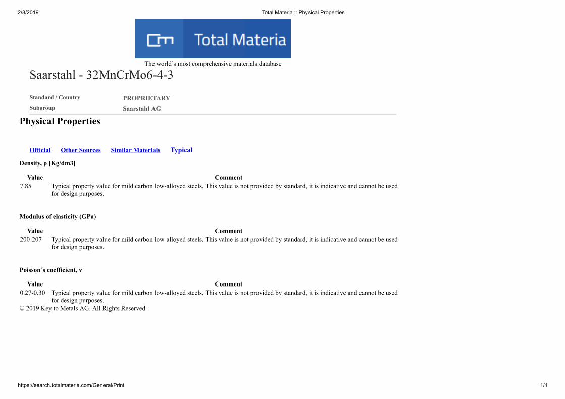
2/8/2019 Total Materia :: Physical Properties
https://search.totalmateria.com/General/Print 1/1
Saarstahl - 32MnCrMo6-4-3The world’s most comprehensive materials database
Standard / Country PROPRIETARYSubgroup Saarstahl AG
Physical Properties
Density, ρ [Kg/dm3]
Value Comment7.85
Typical property value for mild carbon low-alloyed steels. This value is not provided by standard, it is indicative and cannot be usedfor design purposes.
Modulus of elasticity (GPa)
Value Comment200-207
Typical property value for mild carbon low-alloyed steels. This value is not provided by standard, it is indicative and cannot be usedfor design purposes.
Poisson´s coefficient, ν
Value Comment0.27-0.30
Typical property value for mild carbon low-alloyed steels. This value is not provided by standard, it is indicative and cannot be usedfor design purposes.
© 2019 Key to Metals AG. All Rights Reserved.
Official Other Sources Similar Materials Typical

ANEXO 2
COMPOSICIÓN
QUÍMICA ACERO
32MnCrMo6-4-3

2/8/2019 Total Materia :: Chemical Composition
https://search.totalmateria.com/General/Print 1/2
Saarstahl - 32MnCrMo6-4-3The world’s most comprehensive materials database
Standard / Country PROPRIETARYSubgroup Saarstahl AG
Chemical Composition
Chemical Composition (%)
Criteria Min. Max. Approx CAS NumberC 0.2800 0.3600 - 7440-44-0Mn 1.4000 1.8000 - 7439-96-5P - 0.0250 - 7723-14-0S - 0.0400 - 7704-34-9Si - 0.5000 - 7440-21-3Cr 0.8000 1.2000 - 7440-47-3Mo 0.2500 0.4000 - 7439-98-7
Carbon EquivalentCeq 1 = 0.85PCM = 0.48
FormulasCeq 1 = C + Mn/6 + Cr/5 + Mo/5 + V/5 + Cu/15 + Ni/15PCM = C + Si/30 + (Mn + Cu + Cr)/20 + Ni/60 + Mo/15 + V/10 + 5*B
Comment: Middle carbon steel
Precautions for the steel C>0.25% and thicknesses of welded materials t>12 mm- preheating treatment required- apply constant cooling rate e.g. limitation max and min welding interpass temperature- apply both base coated electrodes and powder materials- apply shielding gas protect zone of welding without presence of moisture- low content of diffusions line, etc.The value of C eq is by its nature approximative. Please review these results with welding specialists, especially if there issignificant difference among results obtained by different formulas and/or with values recommended by standards.

2/8/2019 Total Materia :: Chemical Composition
https://search.totalmateria.com/General/Print 2/2
© 2019 Key to Metals AG. All Rights Reserved.
ANEXO 3
NORMA AWS
A5.13/A5.13M:2010
Specification forSurfacingElectrodes forShielded MetalArc Welding
AWS A5.13/A5.13M:2010An American National Standard
AWS_Cover.qxp 7/21/10 6:24 PM Page C

AWS A5.13/A5.13M:2010An American National Standard
Approved by theAmerican National Standards Institute
March 24, 2010
Specification for Surfacing Electrodes for Shielded Metal Arc Welding
55tthh EEddiittiioonn
SSuuppeerrsseeddeess AAWWSS AA55..1133::22000000
Prepared by theAmerican Welding Society (AWS) A5 Committee on Filler Metals and Allied Materials
Under the Direction of theAWS Technical Activities Committee
Approved by theAWS Board of Directors
Abstract
This specification prescribes the requirements for classification of surfacing electrodes for shielded metal arc welding.Classification is based upon the chemical composition of the deposited weld metal except for tungsten carbide electrodeswhere classification is based on the mesh range, quantity, and composition of the tungsten carbide granules. A guide is appended to the specification as a source of information as to the characteristics and applications of the classified electrodes.
AWS_A5.13.qxp 7/21/10 1:26 PM Page i

International Standard Book Number: 978-0-87171-773-3American Welding Society
550 N.W. LeJeune Road, Miami, FL 33126© 2010 by American Welding Society
All rights reservedPrinted in the United States of America
PPhhoottooccooppyy RRiigghhttss.. No portion of this standard may be reproduced, stored in a retrieval system, or transmitted in anyform, including mechanical, photocopying, recording, or otherwise, without the prior written permission of the copyrightowner.
Authorization to photocopy items for internal, personal, or educational classroom use only or the internal, personal, or edu-cational classroom use only of specific clients is granted by the American Welding Society provided that the appropriatefee is paid to the Copyright Clearance Center, 222 Rosewood Drive, Danvers, MA 01923, tel: (978) 750-8400; Internet:<www.copyright.com>.
AWS A5.13/A5.13M:2010
ii
AWS_A5.13.qxp 7/21/10 1:26 PM Page ii
--`,`,`,,`,,`,```,```,`,,,,,````-`-`,,`,,`,`,,`---
AWS A5.13/A5.13M:2010
iii
Statement on the Use of American Welding Society Standards
All standards (codes, specifications, recommended practices, methods, classifications, and guides) of the AmericanWelding Society (AWS) are voluntary consensus standards that have been developed in accordance with the rules of theAmerican National Standards Institute (ANSI). When AWS American National Standards are either incorporated in, ormade part of, documents that are included in federal or state laws and regulations, or the regulations of other governmen-tal bodies, their provisions carry the full legal authority of the statute. In such cases, any changes in those AWS standardsmust be approved by the governmental body having statutory jurisdiction before they can become a part of those laws andregulations. In all cases, these standards carry the full legal authority of the contract or other document that invokes theAWS standards. When this contractual relationship exists, changes in or deviations from requirements of an AWS stan-dard must be by agreement between the contracting parties.
AWS American National Standards are developed through a consensus standards development process that bringstogether volunteers representing varied viewpoints and interests to achieve consensus. While the AWS administers theprocess and establishes rules to promote fairness in the development of consensus, it does not independently test, evalu-ate, or verify the accuracy of any information or the soundness of any judgments contained in its standards.
AWS disclaims liability for any injury to persons or to property, or other damages of any nature whatsoever, whether special, indirect, consequential, or compensatory, directly or indirectly resulting from the publication, use of, or relianceon this standard. AWS also makes no guarantee or warranty as to the accuracy or completeness of any information published herein.
In issuing and making this standard available, AWS is neither undertaking to render professional or other services for oron behalf of any person or entity, nor is AWS undertaking to perform any duty owed by any person or entity to someoneelse. Anyone using these documents should rely on his or her own independent judgment or, as appropriate, seek theadvice of a competent professional in determining the exercise of reasonable care in any given circumstances. It isassumed that the use of this standard and its provisions are entrusted to appropriately qualified and competent personnel.
This standard may be superseded by the issuance of new editions. Users should ensure that they have the latest edition.
Publication of this standard does not authorize infringement of any patent or trade name. Users of this standard accept anyand all liabilities for infringement of any patent or trade name items. AWS disclaims liability for the infringement of anypatent or product trade name resulting from the use of this standard.
Finally, the AWS does not monitor, police, or enforce compliance with this standard, nor does it have the power to do so.
On occasion, text, tables, or figures are printed incorrectly, constituting errata. Such errata, when discovered, are postedon the AWS web page (www.aws.org).
Official interpretations of any of the technical requirements of this standard may only be obtained by sending a request,in writing, to the appropriate technical committee. Such requests should be addressed to the American Welding Society,Attention: Managing Director, Technical Services Division, 550 N.W. LeJeune Road, Miami, FL 33126 (see Annex B).With regard to technical inquiries made concerning AWS standards, oral opinions on AWS standards may be rendered.These opinions are offered solely as a convenience to users of this standard, and they do not constitute professionaladvice. Such opinions represent only the personal opinions of the particular individuals giving them. These individualsdo not speak on behalf of AWS, nor do these oral opinions constitute official or unofficial opinions or interpretations ofAWS. In addition, oral opinions are informal and should not be used as a substitute for an official interpretation.
This standard is subject to revision at any time by the AWS A5 Committee on Filler Metals and Allied Materials. It mustbe reviewed every five years, and if not revised, it must be either reaffirmed or withdrawn. Comments (recommendations,additions, or deletions) and any pertinent data that may be of use in improving this standard are required and should beaddressed to AWS Headquarters. Such comments will receive careful consideration by the AWS A5 Committee on FillerMetals and Allied Materials and the author of the comments will be informed of the Committee’s response to the com-ments. Guests are invited to attend all meetings of the AWS A5 Committee on Filler Metals and Allied Materials toexpress their comments verbally. Procedures for appeal of an adverse decision concerning all such comments are pro-vided in the Rules of Operation of the Technical Activities Committee. A copy of these Rules can be obtained from theAmerican Welding Society, 550 N.W. LeJeune Road, Miami, FL 33126.
AWS_A5.13.qxp 7/21/10 1:26 PM Page iii

AWS A5.13/A5.13M:2010
iv
This page is intentionally blank.
AWS_A5.13.qxp 7/21/10 1:26 PM Page iv

AWS A5.13/A5.13M:2010
v
Personnel
AAWWSS AA55 CCoommmmiitttteeee oonn FFiilllleerr MMeettaallss aanndd AAlllliieedd MMaatteerriiaallssJ. S. Lee, Chair Chevron
H. D. Wehr, 1st Vice-Chair Arcos Industries, LLCJ. J. DeLoach, Jr., 2nd Vice-Chair Naval Surface Warfare Center
R. Gupta, Secretary American Welding SocietyT. Anderson ESAB Welding & Cutting Products
J. M. Blackburn Naval Sea Systems CommandR. Brown RSB Alloy Applications, LLC
J. C. Bundy Hobart Brothers CompanyD. D. Crockett The Lincoln Electric Company
R.V. Decker WeldstarD. A. DelSignore Consultant
J. DeVito ESAB Welding & Cutting ProductsH. W. Ebert ConsultantD. M. Fedor The Lincoln Electric Company
J. G. Feldstein Foster Wheeler North AmericaS. E. Ferree ESAB Welding & Cutting ProductsD. A. Fink The Lincoln Electric Company
G. L. Franke Naval Surface Warfare CenterR. D. Fuchs Bohler Welding Group USA, Incorporated
R. M. Henson J.W. Harris Company, IncorporatedS. D. Kiser Special Metals
P. J. Konkol Concurrent Technologies CorporationD. J. Kotecki Damian Kotecki Welding Consultants
L. Kvidahl Northrop Grumman Ship SystemsA. Y. Lau Canadian Welding Bureau
A. S. Laurenson ConsultantW. A. Marttila Chrysler LLC
T. Melfi The Lincoln Electric CompanyR. Menon Stoody Company
M. T. Merlo HyperTech Research, IncorporatedB. Mosier Polymet Corporation
A. K. Mukherjee Siemens Power Generation IncorporatedC. L. Null Consultant
R. L. Peaslee Wall Colmonoy CorporationK.C. Pruden Hydril Company
S. D. Reynolds, Jr. ConsultantP. K. Salvesen Det Norske Veritas (DNV)
K. Sampath ConsultantW. S. Severance ESAB Welding & Cutting Products
M. J. Sullivan NASSCO-Natl Steel & ShipbuildingR. Sutherlin ATI Wah ChangR. A. Swain Euroweld, Limited
K. P. Thornberry Care Medical, IncorporatedM. D. Tumuluru US Steel Corporation
AAddvviissoorrss ttoo tthhee AAWWSS AA55 CCoommmmiitttteeee oonn FFiilllleerr MMeettaallss aanndd AAlllliieedd MMaatteerriiaallss
R. L. Bateman Electromanufacturas, S. A.R. A. Daemen Consultant
C. E. Fuerstenau Lucas-Milhaupt, IncorporatedJ. P. Hunt ConsultantS. Imaoka Kobe Steel Limited
M. P. Parekh ConsultantM. A. Quintana The Lincoln Electric Company
E. R. Stevens Stevens Welding Consulting
AWS_A5.13.qxp 7/21/10 1:26 PM Page v
--`,`,`,,`,,`,```,```,`,,,,,````-`-`,,`,,`,`,,`---
E. S. Surian National University of Lomas de Zamora
AAWWSS AA55GG SSuubbccoommmmiitttteeee oonn HHaarrddffaacciinngg FFiilllleerr MMeettaallss
R. Menon, Chair Stoody CompanyR. K. Gupta, SEC American Welding Society
F. Broshjeit Farrel CorporationJ. Dezelle Kennametal Energy Mining
G. L. Fillion Wall Colmonoy CorporationS. P. Iyer Weartech International, Incorporated
W. E. Layo MidalloyJ. G. Postle Postle Industries, IncorporatedV. B. Rajan The Lincoln Electric Company
G. C. Schmid Bechtel Bettis, IncorporatedA. P. Yelistratov Caterpillar, Incorporated
AAddvviissoorrss ttoo tthhee AAWWSS AA55GG SSuubbccoommmmiitttteeee oonn HHaarrddffaacciinngg FFiilllleerr MMeettaallss
J. B. C. Wu Deloro Stellite Group
AWS A5.13/A5.13M:2010
vi
AWS_A5.13.qxp 7/21/10 1:26 PM Page vi
AWS A5.13/A5.13M:2010
vii
ForewordThis foreword is not part of AWS A5.13/A5.13M:2010, Specification for Surfacing Electrodes for
Shielded Metal Arc Welding, but is included for informational purposes only.
The first AWS specification for surfacing filler metals was published in 1956 as a joint ASTM/AWS specification. It wasthe first of what would later become a two-set series, A5.13 and A5.21.
The composite electrodes and rods classifications were removed from the 1970 revision of A5.13 and placed into a newspecification, A5.21. A5.13–70 specification contained requirements for both covered and bare electrodes or rodsemploying solid core only. This distinction was maintained for the 1980 revision of A5.13.
The revisions of both A5.13:2000 and A5.21:2001 incorporated a totally different scope. The method of manufacture ofthe core of the electrode or rod was no longer a factor in determining placement of a classification. Instead, the coveredelectrode products were classified under AWS A5.13:2000 and the bare electrode products under AWS A5.21:2001.
This document is the first of the A5.13 specifications which makes use of both U.S. Customary Units and the InternationalSystem of Units (SI). The measurements are not exact equivalents; therefore each system must be used independently ofthe other, without combining values in any way. In selecting rational metric units, ANSI/AWS A1.1, Metric PracticeGuide for the Welding Industry, and ISO 544 Welding consumables – Technical delivery conditions for welding fillermaterials – Type of product, dimensions, tolerances and marking, are used where suitable. Tables and figures make useof both the U.S. Customary and SI Units, which, with the application of the specified tolerances, provides for interchange-ability of products in both the U.S. Customary and SI Units.
Rounding-off Procedure has been revised in this edition. Detailed general safety information in Clause A9 has beenreplaced by Safety and Health Fact Sheets. Such substantive changes are shown in Italic font in this specification.
The historical evolution of the specification is:
ASTM A 399-56T Tentative Specification for Surfacing Welding Rods and ElectrodesAWS A5.13-56T
AWS A5.13-70 Specification for Surfacing Welding Rods and ElectrodesANSI W3.13-73
ANSI/AWS A5.13-80 Specification for Solid Surfacing Welding Rods and ElectrodesAWS A5.13:2000 Specification for Surfacing Electrodes for Shielded Metal Arc Welding
Comments and suggestions for the improvement of this standard are welcome. They should be sent to the Secretary, AWS A5 Committee on Filler Metals and Allied Materials, American Welding Society, 550 N.W. LeJeuneRoad, Miami, FL 33126.
AWS_A5.13.qxp 7/21/10 1:26 PM Page vii

AWS A5.13/A5.13M:2010
viii
This page is intentionally blank.
AWS_A5.13.qxp 7/21/10 1:26 PM Page viii
AWS A5.13/A5.13M:2010
ix
Table of Contents
Page No.
Personnel . . . . . . . . . . . . . . . . . . . . . . . . . . . . . . . . . . . . . . . . . . . . . . . . . . . . . . . . . . . . . . . . . . . . . . . . . . . . . . . . . . . . vForeword . . . . . . . . . . . . . . . . . . . . . . . . . . . . . . . . . . . . . . . . . . . . . . . . . . . . . . . . . . . . . . . . . . . . . . . . . . . . . . . . . . . viiList of Tables . . . . . . . . . . . . . . . . . . . . . . . . . . . . . . . . . . . . . . . . . . . . . . . . . . . . . . . . . . . . . . . . . . . . . . . . . . . . . . . . . xList of Figures . . . . . . . . . . . . . . . . . . . . . . . . . . . . . . . . . . . . . . . . . . . . . . . . . . . . . . . . . . . . . . . . . . . . . . . . . . . . . . . . x
11.. SSccooppee . . . . . . . . . . . . . . . . . . . . . . . . . . . . . . . . . . . . . . . . . . . . . . . . . . . . . . . . . . . . . . . . . . . . . . . . . . . . . . . . . . 1
22.. RReeffeerreenncceedd DDooccuummeennttss. . . . . . . . . . . . . . . . . . . . . . . . . . . . . . . . . . . . . . . . . . . . . . . . . . . . . . . . . . . . . . . . . . . . 1
33.. CCllaassssiifificcaattiioonn . . . . . . . . . . . . . . . . . . . . . . . . . . . . . . . . . . . . . . . . . . . . . . . . . . . . . . . . . . . . . . . . . . . . . . . . . . . . 2
44.. AAcccceeppttaannccee. . . . . . . . . . . . . . . . . . . . . . . . . . . . . . . . . . . . . . . . . . . . . . . . . . . . . . . . . . . . . . . . . . . . . . . . . . . . . . 2
55.. CCeerrttiifificcaattiioonn. . . . . . . . . . . . . . . . . . . . . . . . . . . . . . . . . . . . . . . . . . . . . . . . . . . . . . . . . . . . . . . . . . . . . . . . . . . . . 2
66.. RRoouunnddiinngg--OOffff PPrroocceedduurree . . . . . . . . . . . . . . . . . . . . . . . . . . . . . . . . . . . . . . . . . . . . . . . . . . . . . . . . . . . . . . . . . . 2
77.. SSuummmmaarryy ooff TTeessttss . . . . . . . . . . . . . . . . . . . . . . . . . . . . . . . . . . . . . . . . . . . . . . . . . . . . . . . . . . . . . . . . . . . . . . . . 2
88.. RReetteesstt . . . . . . . . . . . . . . . . . . . . . . . . . . . . . . . . . . . . . . . . . . . . . . . . . . . . . . . . . . . . . . . . . . . . . . . . . . . . . . . . . . 6
99.. WWeelldd TTeesstt AAsssseemmbbllyy . . . . . . . . . . . . . . . . . . . . . . . . . . . . . . . . . . . . . . . . . . . . . . . . . . . . . . . . . . . . . . . . . . . . . . 7
1100.. CChheemmiiccaall AAnnaallyyssiiss . . . . . . . . . . . . . . . . . . . . . . . . . . . . . . . . . . . . . . . . . . . . . . . . . . . . . . . . . . . . . . . . . . . . . . . 7
1100..11 FFoorr AAllll EExxcceepptt CCoovveerreedd TTuunnggsstteenn CCaarrbbiiddee EElleeccttrrooddeess . . . . . . . . . . . . . . . . . . . . . . . . . . . . . . . . . . . . 7
1100..22 FFoorr TTuunnggsstteenn CCaarrbbiiddee EElleeccttrrooddeess . . . . . . . . . . . . . . . . . . . . . . . . . . . . . . . . . . . . . . . . . . . . . . . . . . . . . 7
1111.. MMeetthhoodd ooff MMaannuuffaaccttuurree . . . . . . . . . . . . . . . . . . . . . . . . . . . . . . . . . . . . . . . . . . . . . . . . . . . . . . . . . . . . . . . . . . . 9
1122.. SSttaannddaarrdd SSiizzeess aanndd LLeennggtthhss . . . . . . . . . . . . . . . . . . . . . . . . . . . . . . . . . . . . . . . . . . . . . . . . . . . . . . . . . . . . . . . 9
1133.. CCoorree WWiirree aanndd CCoovveerriinngg . . . . . . . . . . . . . . . . . . . . . . . . . . . . . . . . . . . . . . . . . . . . . . . . . . . . . . . . . . . . . . . . . 10
1144.. EExxppoosseedd CCoorree . . . . . . . . . . . . . . . . . . . . . . . . . . . . . . . . . . . . . . . . . . . . . . . . . . . . . . . . . . . . . . . . . . . . . . . . . . 10
1155.. EElleeccttrrooddee IIddeennttiifificcaattiioonn . . . . . . . . . . . . . . . . . . . . . . . . . . . . . . . . . . . . . . . . . . . . . . . . . . . . . . . . . . . . . . . . . . 10
1166.. PPaacckkaaggiinngg . . . . . . . . . . . . . . . . . . . . . . . . . . . . . . . . . . . . . . . . . . . . . . . . . . . . . . . . . . . . . . . . . . . . . . . . . . . . . 11
1177.. MMaarrkkiinngg ooff PPaacckkaaggeess . . . . . . . . . . . . . . . . . . . . . . . . . . . . . . . . . . . . . . . . . . . . . . . . . . . . . . . . . . . . . . . . . . . . 11
Annex A (Informative)—Guide to AWS Specification for Surfacing Electrodes for Shielded Metal Arc Welding. . . . . . . . . . . . . . . . . . . . . . . . . . . . . . . . . . . . . . . . . . . . . . . . 13
Annex B (Informative)—Guidelines for the Preparation of Technical Inquiries . . . . . . . . . . . . . . . . . . . . . . . . . . . . 27
AWS Filler Metal Specifications by Material and Welding Process . . . . . . . . . . . . . . . . . . . . . . . . . . . . . . . . . . . . . . 29AWS Filler Metal Specifications and Related Documents . . . . . . . . . . . . . . . . . . . . . . . . . . . . . . . . . . . . . . . . . . . . . 31
AWS_A5.13.qxp 7/21/10 1:26 PM Page ix

AWS A5.13/A5.13M:2010
x
List of Tables
Table Page No.
1 Iron Base Surfacing Electrodes—Chemical Composition Requirements. . . . . . . . . . . . . . . . . . . . . . . . . . . 32 Nickel and Cobalt Base Surfacing Electrodes—Chemical Composition Requirements . . . . . . . . . . . . . . . 43 Copper Base Surfacing Electrodes—Chemical Composition Requirements . . . . . . . . . . . . . . . . . . . . . . . . 54 Mesh Size and Quantity of Tungsten Carbide (WC) Granules in the Core of
Tungsten Carbide Electrodes. . . . . . . . . . . . . . . . . . . . . . . . . . . . . . . . . . . . . . . . . . . . . . . . . . . . . . . . . . . . . 65 Chemical Composition of Tungsten Carbide (WC) Granules . . . . . . . . . . . . . . . . . . . . . . . . . . . . . . . . . . . 66 Standard Sizes and Lengths of Covered Electrodes Using Solid Drawn Core Wire . . . . . . . . . . . . . . . . . . 97 Standard Sizes and Lengths for Covered Cast and Composite Tubular Electrodes . . . . . . . . . . . . . . . . . . . 98 Standard Sizes and Lengths for Covered Tungsten Carbide (WC) Electrodes. . . . . . . . . . . . . . . . . . . . . . 10
A.1 Comparison of Classifications. . . . . . . . . . . . . . . . . . . . . . . . . . . . . . . . . . . . . . . . . . . . . . . . . . . . . . . . . . . 14A.2 Effect of Shielded Metal Arc Variables on the Three Most Important Characteristics of Surfacing . . . . . . . 17A.3 Approximate Weld Deposit Hardness (SMAW). . . . . . . . . . . . . . . . . . . . . . . . . . . . . . . . . . . . . . . . . . . . . 22A.4 Discontinued Electrode and Rod Classifications . . . . . . . . . . . . . . . . . . . . . . . . . . . . . . . . . . . . . . . . . . . . 24
List of Figures
Figure Page No.
1 Pad for Chemical Analysis of Undiluted Weld Metal. . . . . . . . . . . . . . . . . . . . . . . . . . . . . . . . . . . . . . . . . . 8
AWS_A5.13.qxp 7/21/10 1:26 PM Page x

AWS A5.13/A5.13M:2010
1
Specification for Surfacing Electrodes for Shielded Metal Arc Welding
11.. SSccooppee
11..11 This specification prescribes requirements for the classification of surfacing electrodes for shielded metal arc welding.Solid bare electrodes and rods for surfacing are classified in AWS A5.21:2001, Specification for Bare Electrodes andRods for Surfacing (see Clause A8 in Annex A).
11..22 Safety and health issues and concerns are beyond the scope of this standard and, therefore, are not fully addressedherein. Some safety and health information can be found in Clauses A5 and A9 in Annex A. Safety and healthinformation is available from other sources, including, but not limited to ANSI Z49.1, Safety in Welding, Cutting, andAllied Processes, and applicable federal and state regulations.
11..33 This specification makes use of both U.S. Customary Units and the International System of Units (SI). Themeasurements are not exact equivalents; therefore, each system must be used independently of the other withoutcombining in any way when referring to material properties. The specification with the designation A5.13 uses the U.S.Customary Units. The specification A5.13M uses the SI Units. The latter are shown within brackets [ ] or in appropriatecolumns in tables and figures. Standard dimensions based on either system may be used for sizing of filler metal orpackaging or both under A5.13 or A5.13M specifications.
22.. RReeffeerreenncceedd DDooccuummeennttssThe following documents are referenced within this publication. For undated references, the latest edition of the referencedstandard shall apply. For dated references, subsequent amendments to, or revisions of, any of these publications do not apply.
22..11 AWS standards1
(1) AWS A5.01M/A5.01(ISO 14344), Procurement Guidelines for Consumables – Welding and Allied Processes –Flux and Gas Shielded Electrical Welding Processes
(2) AWS A3.0, Standard Welding Terms and Definitions(3) AWS F3.2, Ventilation Guide for Weld Fume
22..22 ANSI standard2
(1) ANSI Z49.1, Safety in Welding, Cutting, and Allied Processes
22..33 ASTM standards3
(1) ASTM A 36/A 36M, Standard Specification for Carbon Structural Steels(2) ASTM A 285/A 285M, Standard Specification for Pressure Vessel Plates, Carbon Steel, Low-and Intermediate-
Tensile Strength
1 AWS Standards are published by the American Welding Society, 550 N.W. LeJeune Road, Miami, FL 33126.2 ANSI Z49.1 is published by the American Welding Society, 550 N.W. LeJeune Road, Miami, FL 33126.3 ASTM Standards are published by the American Society for Testing and Materials, 100 Barr Harbor Drive, West Conshohocken,
PA 19428-2959.
AWS_A5.13.qxp 7/21/10 1:26 PM Page 1
--`,`,`,,`,,`,```,```,`,,,,,````-`-`,,`,,`,`,,`---

(3) ASTM B 214, Standard Test Method for Sieve Analysis of Metal Powders(4) ASTM E 29, Standard Practice for Using Significant Digits in Test Data to Determine Conformance with
Specifications
22..44 ISO standards4
(1) ISO 80 000-1, Quantities and units – Part 1: General(2) ISO 544, Welding Consumables – Technical delivery conditions for welding filler materials – Type of product,
dimensions, tolerances, and marking
33.. CCllaassssiifificcaattiioonn
33..11 Except for tungsten carbide electrodes, the surfacing electrodes covered by this A5.13/A5.13M specification areclassified according to the chemical composition of the undiluted weld metal, as specified in Tables 1, 2, and 3.
33..22 Tungsten carbide surfacing electrodes are classified on the basis of size and chemical composition of the tungstencarbide granules (see Tables 4 and 5).
33..33 Electrodes classified under one classification shall not be classified under any other classification in this specification.
44.. AAcccceeppttaanncceeAcceptance5 of the electrodes shall be in accordance with the provisions of AWS A5.01M/A5.01 (ISO 14344).
55.. CCeerrttiifificcaattiioonnBy affixing the AWS specification and classification designations to the package, or the classification to the product, themanufacturer certifies that the product meets the requirements of this specification.6
66.. RRoouunnddiinngg--OOffff PPrroocceedduurreeFor purposes of determining compliance with the requirements of this standard, the actual test values obtained shall besubjected to the rounding-off rules of ASTM E 29 or ISO 80000-1, Annex B, Rule A (the results are the same). If the mea-sured values are obtained by equipment calibrated in units other than those of the specified limit, the measured valuesshall be converted to the units of the specified limit before rounding off. If an average value is to be compared to the spec-ified limit, rounding off shall be done only after calculating the average. An observed or calculated value shall berounded to the nearest 1 000 psi for yield strength for U.S. Customary Unit standard to the nearest 10 MPa for yieldstrength for SI unit standard and to the nearest unit in the last right-hand place of figures used in expressing the limitingvalues for other quantities. The rounded-off results shall fulfil the requirements for the classification under test.
77.. SSuummmmaarryy ooff TTeessttss
77..11 Except for tungsten carbide electrodes, chemical composition of undiluted weld metal is the only test required forclassification of a product under this specification (see Tables 1, 2, and 3).
AWS A5.13/A5.13M:2010
2
4 ISO standards are published by the International Organization for Standardization, 1, rue de Varembé, Case postale 56, CH-1211Geneva 20, Switzerland.
5 See Clause A3, Acceptance (in Annex A), for further information concerning acceptance, testing of material shipped, and AWSA5.01M/A5.01.
6 See Clause A4, Certification (in Annex A), for further information concerning certification and the testing called for to meet thisrequirement.
AWS_A5.13.qxp 7/21/10 1:26 PM Page 2
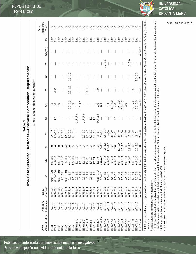
AWS A5.13/A5.13M:2010
3
Tab
le 1
Iro
n B
ase
Su
rfac
ing
Ele
ctro
des
—C
hem
ical
Co
mp
osi
tio
n R
equ
irem
ents
a
Dep
osit
Com
posi
tion,
wei
ght p
erce
ntb,
c,d
Oth
erA
WS
Ann
ex A
UN
SE
lem
ents
,C
lass
ifica
tion
Ref
eren
ceN
umbe
reC
Mn
SiC
rN
iM
oV
WT
iN
b(C
b)Fe
Tot
al
EFe
1A
7.1.
1W
7400
10.
04–0
.20
0.5–
2.0
1.0
0.5–
3.5
—1.
5—
——
—R
em1.
0E
Fe2
A7.
1.1
W74
002
0.10
–0.3
00.
5–2.
01.
01.
8–3.
81.
01.
00.
35—
——
Rem
1.0
EFe
3A
7.1.
2W
7400
30.
50–0
.80
0.5–
1.5
1.0
4.0–
8.0
—1.
0—
——
—R
em1.
0E
Fe4
A7.
1.3
W74
004
1.0–
2.0
0.5–
2.0
1.0
3.0–
5.0
——
——
——
Rem
1.0
EFe
5A
7.1.
4W
7511
00.
30–0
.80
1.5–
2.5
0.90
1.5–
3.0
——
——
——
Rem
1.0
EFe
6A
7.1.
5W
7751
00.
6–1.
00.
4–1.
01.
03.
0–5.
0—
7.0–
9.5
0.5–
1.5
0.5–
1.5
——
Rem
1.0
EFe
7A
7.1.
6W
7761
01.
5–3.
00.
5–2.
01.
54.
0–8.
0—
1.0
——
——
Rem
1.0
EFe
Mn-
AA
7.1.
7W
7911
00.
5–1.
012
–16
1.3
—2.
5–5.
0—
——
——
Rem
1.0
EFe
Mn-
BA
7.1.
7W
7931
00.
5–1.
012
–16
1.3
——
0.5–
1.5
——
——
Rem
1.0
EFe
Mn-
CA
7.1.
7W
7921
00.
5–1.
012
–16
1.3
2.5–
5.0
2.5–
5.0
——
——
—R
em1.
0E
FeM
n-D
A7.
1.7
W79
410
0.5–
1.0
15–2
01.
34.
5–7.
5—
—0.
4–1.
2—
——
Rem
1.0
EFe
Mn-
EA
7.1.
7W
7951
00.
5–1.
015
–20
1.3
3.0–
6.0
1.0
——
——
—R
em1.
0E
FeM
n-F
A7.
1.7
W79
610
0.8–
1.2
17–2
11.
33.
0–6.
01.
0—
——
——
Rem
1.0
EFe
MnC
rA
7.1.
8W
7971
00.
25–0
.75
12–1
81.
313
–17
0.5–
2.0
2.0
1.0
——
—R
em1.
0E
FeC
r-A
1AA
7.1.
9W
7401
13.
5–4.
54.
0–6.
00.
5–2.
020
–25
—0.
5—
——
—R
em1.
0E
FeC
r-A
2A
7.1.
10W
7401
22.
5–3.
50.
5–1.
50.
5–1.
57.
5–9.
0—
——
—1.
2–1.
8—
Rem
1.0
EFe
Cr-
A3
A7.
1.11
W74
013
2.5–
4.5
0.5–
2.0
1.0–
2.5
14–2
0—
1.5
——
——
Rem
1.0
EFe
Cr-
A4
A7.
1.9
W74
014
3.5–
4.5
1.5–
3.5
1.5
23–2
9—
1.0–
3.0
——
——
Rem
1.0
EFe
Cr-
A5
A7.
1.12
W74
015
1.5–
2.5
0.5–
1.5
2.0
24–3
24.
04.
0—
——
—R
em1.
0E
FeC
r-A
6A
7.1.
13W
7401
62.
5–3.
50.
5–1.
51.
0–2.
524
–30
—0.
5–2.
0—
——
—R
em1.
0E
FeC
r-A
7A
7.1.
13W
7401
73.
5–5.
00.
5–1.
50.
5–2.
523
–30
—2.
0–4.
5—
——
—R
em1.
0E
FeC
r-A
8A
7.1.
14W
7401
82.
5–4.
50.
5–1.
51.
530
–40
—2.
0—
——
—R
em1.
0E
FeC
r-E
1A
7.1.
15W
7421
15.
0–6.
52.
0–3.
00.
8–1.
512
–16
——
——
4.0–
7.0
—R
em1.
0E
FeC
r-E
2A
7.1.
15W
7421
24.
0–6.
00.
5–1.
51.
514
–20
—5.
0–7.
01.
5—
——
Rem
1.0
EFe
Cr-
E3
A7.
1.15
W74
213
5.0–
7.0
0.5–
2.0
0.5–
2.0
18–2
8—
5.0–
7.0
—3.
0–5.
0—
—R
em1.
0E
FeC
r-E
4A
7.1.
15W
7421
44.
0–6.
00.
5–1.
51.
020
–30
—5.
0–7.
00.
5–1.
52.
0—
4.0–
7.0
Rem
1.0
aSo
lid b
are
elec
trod
es a
nd r
ods
prev
ious
ly c
lass
ified
in A
WS
A5.
13–8
0 ar
e no
w e
ither
dis
cont
inue
d or
rec
lass
ified
in A
WS
A5.
21:2
001,
Spe
cific
atio
n fo
r B
are
Ele
ctro
des
and
Rod
s fo
r Su
rfac
ing
(see
A8
inA
nnex
A).
bSi
ngle
val
ues
are
max
imum
. Rem
= R
emai
nder
.c
Ele
ctro
des
and
rods
sha
ll be
ana
lyze
d fo
r the
spe
cific
ele
men
ts fo
r whi
ch v
alue
s ar
e sh
own
in th
is ta
ble.
If th
e pr
esen
ce o
f oth
er e
lem
ents
is in
dica
ted
in th
e co
urse
of t
his
wor
k, th
e am
ount
of t
hose
ele
men
tssh
all b
e de
term
ined
to e
nsur
e th
at th
eir
tota
l doe
s no
t exc
eed
the
limit
spec
ified
for
“O
ther
Ele
men
ts, T
otal
” in
the
last
col
umn
of th
e ta
ble.
dSu
lfur
and
pho
spho
rus
cont
ents
eac
h sh
all n
ot e
xcee
d 0.
035%
.e
SAE
HS-
1086
/AST
M D
S-56
, Met
als
& A
lloys
in th
e U
nifie
d N
umbe
ring
Sys
tem
.
AWS_A5.13.qxp 7/21/10 1:26 PM Page 3
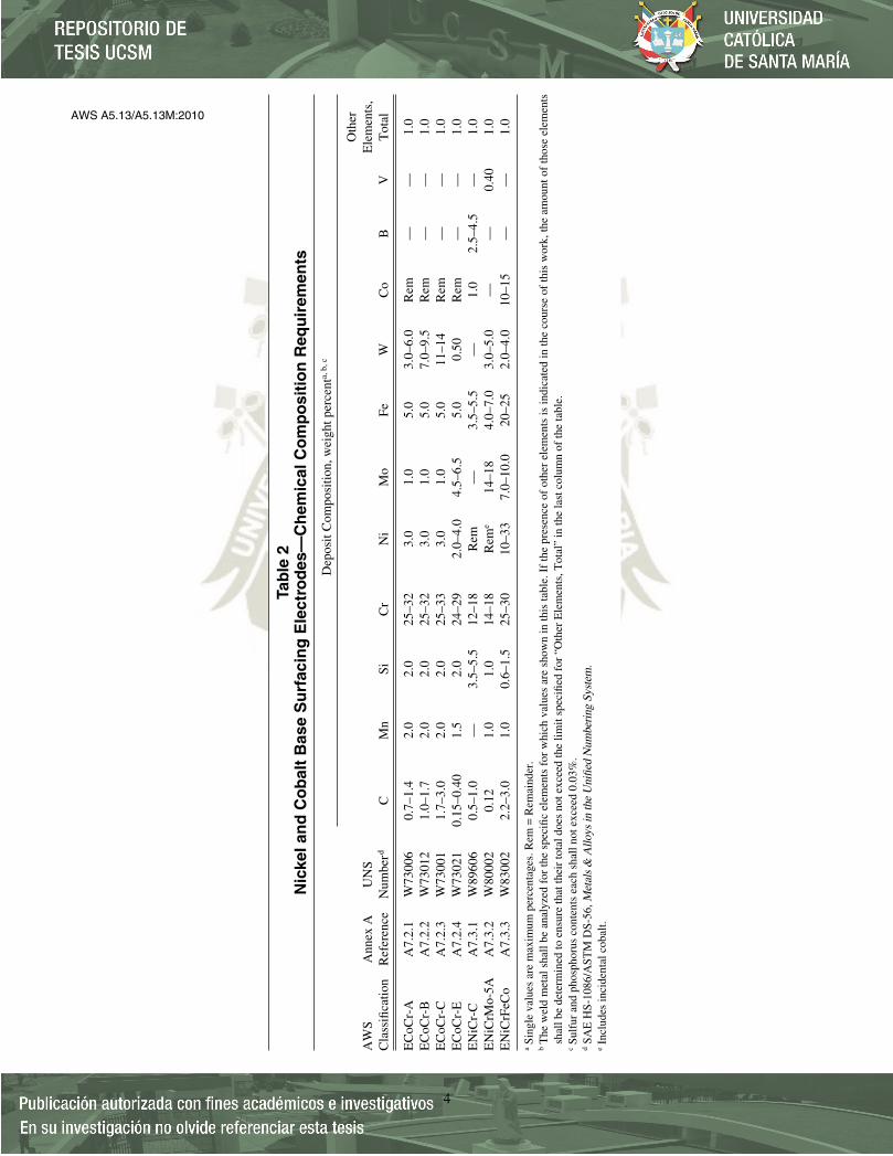
AWS A5.13/A5.13M:2010
4
Tab
le 2
Nic
kel a
nd
Co
bal
t B
ase
Su
rfac
ing
Ele
ctro
des
—C
hem
ical
Co
mp
osi
tio
n R
equ
irem
ents
Dep
osit
Com
posi
tion,
wei
ght p
erce
nta,
b, c
Oth
erA
WS
Ann
ex A
UN
SE
lem
ents
, C
lass
ifica
tion
Ref
eren
ceN
umbe
rdC
Mn
SiC
rN
iM
oFe
WC
oB
VT
otal
EC
oCr-
AA
7.2.
1W
7300
60.
7–1.
42.
02.
025
–32
3.0
1.0
5.0
3.0–
6.0
Rem
——
1.0
EC
oCr-
BA
7.2.
2W
7301
21.
0–1.
72.
02.
025
–32
3.0
1.0
5.0
7.0–
9.5
Rem
——
1.0
EC
oCr-
CA
7.2.
3W
7300
11.
7–3.
02.
02.
025
–33
3.0
1.0
5.0
11–1
4R
em—
—1.
0E
CoC
r-E
A7.
2.4
W73
021
0.15
–0.4
01.
52.
024
–29
2.0–
4.0
4.5–
6.5
5.0
0.50
Rem
——
1.0
EN
iCr-
CA
7.3.
1W
8960
60.
5–1.
0—
3.5–
5.5
12–1
8R
em—
3.5–
5.5
—1.
02.
5–4.
5—
1.0
EN
iCrM
o-5A
A7.
3.2
W80
002
0.12
1.0
1.0
14–1
8R
eme
14–1
84.
0–7.
03.
0–5.
0—
—0.
401.
0E
NiC
rFeC
oA
7.3.
3W
8300
22.
2–3.
01.
00.
6–1.
525
–30
10–3
37.
0–10
.020
–25
2.0–
4.0
10–1
5—
—1.
0
aSi
ngle
val
ues
are
max
imum
per
cent
ages
. Rem
= R
emai
nder
.b
The
wel
d m
etal
sha
ll be
ana
lyze
d fo
r th
e sp
ecifi
c el
emen
ts f
or w
hich
val
ues
are
show
n in
this
tabl
e. I
f th
e pr
esen
ce o
f ot
her
elem
ents
is in
dica
ted
in th
e co
urse
of
this
wor
k, th
e am
ount
of
thos
e el
emen
tssh
all b
e de
term
ined
to e
nsur
e th
at th
eir
tota
l doe
s no
t exc
eed
the
limit
spec
ified
for
“O
ther
Ele
men
ts, T
otal
” in
the
last
col
umn
of th
e ta
ble.
cSu
lfur
and
pho
spho
rus
cont
ents
eac
h sh
all n
ot e
xcee
d 0.
03%
.d
SAE
HS-
1086
/AST
M D
S-56
, Met
als
& A
lloys
in th
e U
nifie
d N
umbe
ring
Sys
tem
.e
Incl
udes
inci
dent
al c
obal
t.
AWS_A5.13.qxp 7/21/10 1:26 PM Page 4

AWS A5.13/A5.13M:2010
5
Tab
le 3
Co
pp
er B
ase
Su
rfac
ing
Ele
ctro
des
—C
hem
ical
Co
mp
osi
tio
n R
equ
irem
ents
Dep
osit
Com
posi
tion,
wei
ght p
erce
nta,
b
Oth
er
AW
S A
nnex
AU
NS
Ele
men
ts,
Cla
ssifi
catio
nR
efer
ence
Num
berc
Cu
Mn
PSi
FeA
lZ
nN
idPb
SnT
iT
otal
EC
uAl-
A2f
A7.
4.1.
1W
6061
7R
emg
—1.
50.
5–5.
08.
5–11
.0g
g0.
02g
—0.
50E
CuA
l-B
fA
7.4.
1.2
W60
619
Rem
g—
1.5
2.5–
5.0
11–1
2g
g0.
02g
—0.
50E
CuA
l-C
A7.
4.1.
2W
6062
5R
em—
—1.
03.
0–5.
012
–13
0.02
—0.
02—
—0.
50E
CuA
l-D
A7.
4.1.
3W
6162
5R
em—
—1.
03.
0–5.
013
–14
0.02
—0.
02—
—0.
50E
CuA
l-E
A7.
4.1.
3W
6262
5R
em—
—1.
03.
0–5.
014
–15
0.02
—0.
02—
—0.
50E
CuS
ifA
7.4.
1.4
W60
656
Rem
1.5
g2.
4–4.
00.
500.
01g
g0.
021.
5—
0.50
EC
uSn-
Af
A7.
4.1.
5W
6051
8R
emg
0.05
–0.3
5g
0.25
0.01
gg
0.02
4.0–
6.0
—0.
50E
CuS
n-C
fA
7.4.
1.5
W60
521
Rem
g0.
05–0
.35
g0.
250.
01g
g0.
027.
0–9.
0—
0.50
EC
uNie,
fA
7.4.
1.6
W60
715
Rem
1.0–
2.5
0.02
0.50
0.40
–0.7
5—
g29
–33
0.02
g0.
500.
50E
CuN
iAlf
A7.
4.1.
7W
6063
2R
em0.
5–3.
5—
1.5
3.0–
6.0
8.5–
9.5
g4.
0–6.
00.
02g
—0.
50E
CuM
nNiA
lfA
7.4.
1.8
W60
633
Rem
11–1
4—
1.5
2.0–
4.0
7.0–
8.5
g1.
5–3.
00.
02g
—0.
50
aSi
ngle
val
ues
show
n ar
e m
axim
um p
erce
ntag
es. R
em =
Rem
aind
er.
bT
he w
eld
met
al s
hall
be a
naly
zed
for
the
spec
ific
elem
ents
for
whi
ch v
alue
s, o
r a
“g,”
are
sho
wn
in th
is ta
ble.
If
the
pres
ence
of
othe
r el
emen
ts is
indi
cate
d in
the
cour
se o
f th
is w
ork,
the
amou
nt o
f th
ose
elem
ents
sha
ll be
det
erm
ined
to e
nsur
e th
at th
eir
tota
l doe
s no
t exc
eed
the
limit
spec
ified
for
“O
ther
Ele
men
ts, T
otal
” in
the
last
col
umn
of th
e ta
ble.
cSA
E H
S-10
86/A
STM
DS-
56, M
etal
s &
Allo
ys in
the
Uni
fied
Num
beri
ng S
yste
m.
dIn
clud
es c
obal
t.e
Sulf
ur is
res
tric
ted
to 0
.015
% m
axim
um.
fT
his
AW
S cl
assi
ficat
ion
is i
nten
ded
to c
orre
spon
d to
the
sam
e cl
assi
ficat
ion
that
app
ears
in
AW
S A
5.6,
Spe
cific
atio
n fo
r C
oppe
r an
d C
oppe
r-A
lloy
Cov
ered
Ele
ctro
des.
Bec
ause
of
revi
sion
dat
es t
he
com
posi
tion
rang
es m
ay n
ot b
e id
entic
al.
gT
hese
ele
men
ts m
ust b
e in
clud
ed in
“O
ther
Ele
men
ts, T
otal
.”
AWS_A5.13.qxp 7/21/10 1:26 PM Page 5
--`,`,`,,`,,`,```,```,`,,,,,````-`-`,,`,,`,`,,`---
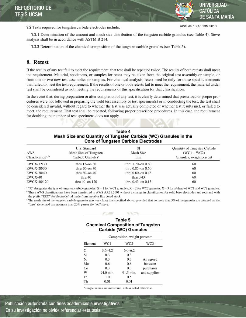
77..22 Tests required for tungsten carbide electrodes include:
77..22..11 Determination of the amount and mesh size distribution of the tungsten carbide granules (see Table 4). Sieveanalysis shall be in accordance with ASTM B 214.
77..22..22 Determination of the chemical composition of the tungsten carbide granules (see Table 5).
88.. RReetteessttIf the results of any test fail to meet the requirement, that test shall be repeated twice. The results of both retests shall meetthe requirement. Material, specimens, or samples for retest may be taken from the original test assembly or sample, orfrom one or two new test assemblies or samples. For chemical analysis, retest need be only for those specific elementsthat failed to meet the test requirement. If the results of one or both retests fail to meet the requirement, the material undertest shall be considered as not meeting the requirements of this specification for that classification.
In the event that, during preparation or after completion of any test, it is clearly determined that prescribed or proper pro-cedures were not followed in preparing the weld test assembly or test specimen(s) or in conducting the test, the test shallbe considered invalid, without regard to whether the test was actually completed or whether test results met, or failed tomeet, the requirement. That test shall be repeated, following proper prescribed procedures. In this case, the requirementfor doubling the number of test specimens does not apply.
AWS A5.13/A5.13M:2010
6
Table 4Mesh Size and Quantity of Tungsten Carbide (WC) Granules in the
Core of Tungsten Carbide Electrodes
U.S. Standard SI Quantity of Tungsten CarbideAWS Mesh Size of Tungsten Mesh Size (WC1 + WC2)Classificationa, b Carbide Granulesc mm Granules, weight percent
EWCX-12/30 thru 12–on 30 thru 1.70–on 0.60 60EWCX-20/30 thru 20–on 30 thru 0.85–on 0.60 60EWCX-30/40 thru 30–on 40 thru 0.60–on 0.43 60EWCX-40 thru 40 thru 0.43 60EWCX-40/120 thru 40–on 120 thru 0.43–on 0.13 60
a “X” designates the type of tungsten carbide granules; X = 1 for WC1 granules, X = 2 for WC2 granules, X = 3 for a blend of WC1 and WC2 granules.b These AWS classifications have been transferred to AWS A5.21:2001 without a change in classification for solid bare electrodes and rods and with
the prefix “ERC” for electrode/rod made from metal or flux cored stock.c The mesh size of the tungsten carbide granules may vary from that specified above, provided that no more than 5% of the granules are retained on the
“thru” sieve, and that no more than 20% passes the “on” sieve.
Table 5Chemical Composition of Tungsten
Carbide (WC) Granules
Composition, weight percenta
Element WC1 WC2 WC3
C 3.6–4.2 6.0–6.2Si 0.3 0.3Ni 0.3 0.3 As agreed Mo 0.6 0.6 between Co 0.3 0.3 purchaser W 94.0 min. 91.5 min. and supplierFe 1.0 0.5Th 0.01 0.01
a Single values are maximum, unless noted otherwise.
AWS_A5.13.qxp 7/21/10 1:26 PM Page 6

99.. WWeelldd TTeesstt AAsssseemmbbllyy
99..11 A sample for chemical analysis is the only test assembly required. The sample may be prepared by any methodproducing undiluted weld metal. In case of dispute, the weld pad described in 9.2 shall be the referee method.
99..22 The dimensions of the completed pad shall be as shown in Figure 1 for each size of electrode. Testing of this assemblyshall be as specified in Clause 10, Chemical Analysis.
99..22..11 Welding shall be done in the flat position using welding conditions specified by the manufacturer.
99..22..22 Postweld heat treatment may be used to facilitate subsequent sampling.
99..33 The base metal shall conform to one of the following specifications or its equivalent:
99..33..11 ASTM A 285/A 285M Grade A (UNS K01700).
99..33..22 ASTM A 36/A 36M (UNS K02600).
1100.. CChheemmiiccaall AAnnaallyyssiiss
1100..11 FFoorr AAllll EExxcceepptt CCoovveerreedd TTuunnggsstteenn CCaarrbbiiddee EElleeccttrrooddeess
1100..11..11 Shielded metal arc welding surfacing electrodes shall be analyzed in the form of undiluted weld metal. Thesample shall come from a weld metal pad.
1100..11..22 The top surface of the pad, as described in Clause 9 and shown in Figure 1, shall be removed and discarded, anda sample for analysis shall be obtained from the underlying metal by any appropriate mechanical means. The sample shallbe free of slag.
For electrodes 3/32 in [2.5 mm] in diameter and smaller, the sample shall be taken at least 1/2 in [13 mm] from thenearest surface of the base metal.
For electrodes 1/8–3/16 in [3.2–5.0 mm] in diameter, the sample shall be taken at least 5/8 in [16 mm] from the near-est surface of the base metal.
For electrodes larger than 3/16 in [5.0 mm] in diameter, the sample shall be taken at least 3/4 in [19 mm] from the nearest surface of the base metal.
1100..11..33 The sample may be removed from an undiluted weld metal pad by any convenient method.
1100..11..44 The sample shall be analyzed by accepted analytical methods as agreed upon between the purchaser andsupplier. The referee method shall be the appropriate ASTM method for the element being determined.
1100..11..55 The results of the analysis shall meet the requirements of Tables 1, 2, or 3 for the classification of electrodeunder test.
1100..22 FFoorr TTuunnggsstteenn CCaarrbbiiddee EElleeccttrrooddeess
1100..22..11 Chemical composition of tungsten carbide granules shall conform to the requirements of Table 5. Chemicalanalysis may be made by any suitable method as agreed upon between the purchaser and supplier.
1100..22..22 Tungsten carbide granules for chemical analysis shall be free of any surface contaminant.
1100..22..33 The percentage by weight of the tungsten carbide, as specified in Table 4, can be determined by the followingsteps:
(1) Record the weight of the tungsten carbide welding electrode after removing any covering present.(2) Remove the tungsten carbide from the tube and clean it by washing with water and treating with 1-1 hydrochlo-
ric acid, as required, to remove any flux, powdered iron, graphite, etc. Heating of the acid may be required. Ahot or cold 1-1 hydrochloric acid will not appreciably attack cast tungsten carbide in less than an hour. Whenhandling any acids appropriate safety precautions should be followed.
AWS A5.13/A5.13M:2010
7
AWS_A5.13.qxp 7/21/10 1:26 PM Page 7

(3) Dry tungsten carbide for a minimum period of two hours by holding in an oven at 250°F ± 25°F [120°C ± 15°C].(4) Weigh the cleaned and dried tungsten carbide granules. Calculate the percentage of tungsten carbide from the
initial weight of the tube using the following formula:
Tungsten carbide % = × 100
Weight of clean and dry tungsten carbide granules
Weight of electrode after removal of covering
AWS A5.13/A5.13M:2010
8
Electrode Size Weld Pad Size, minimum
in mm in mm
5/64 (0.078) 2.0 L = 1-1/2 383/32 (0.094) 2.4 W = 1/2 13
(0.097) 2.5 H = 1/2 13
1/8 (0.125) 3.2 L = 2 505/32 (0.156) 4.0 W = 1/2 133/16 (0.187) 4.8 H = 5/8 16
(0.197) 5.0
7/32 (0.219) L = 2-1/2 64(0.236) 6.0 W = 1/2 13
1/4 (0.250) 6.4 H = 3/4 195/16 (0.312) 8.0
Source: AWS A5.13:2000, Figure 1.
FFiigguurree 11——PPaadd ffoorr CChheemmiiccaall AAnnaallyyssiiss ooff UUnnddiilluutteedd WWeelldd MMeettaall
AWS_A5.13.qxp 7/21/10 1:26 PM Page 8

Table 6Standard Sizes and Lengths of Covered
Electrodes Using Solid Drawn Core Wirea
Electrode Sizes, Diameter of Solid Drawn Core Wireb Standard Lengths
in mm in mm
5/64 (0.078) 2.0 9 ± 1/4 230 ± 10
3/32 (0.094) 2.4 9 ± 1/4 230 ± 10(0.097) 2.5 12 ± 1/4 300 ± 10
1/8 (0.125) 3.2 14 ± 1/4 350 ± 105/32 (0.156) 4.0 14 ± 1/4 350 ± 10
3/16 (0.187) 4.8c 14 ± 1/4 350 ± 10(0.197) 5.0 18 ± 1/4 450 ± 10
(0.236) 6.0 14 ± 1/4 350 ± 101/4 (0.250) 6.4c 18 ± 1/4 450 ± 10
5/16 (0.312) 8.0 14 ± 1/4 350 ± 1018 ± 1/4 450 ± 10
a Other electrode diameters and lengths may be supplied as agreed between themanufacturer and purchaser.
b Tolerance on the diameter shall be ± 0.002 in [± 0.05 mm]c These metric sizes are not shown in ISO 544.
AWS A5.13/A5.13M:2010
9
Table 7Standard Sizes and Lengths for Covered Cast and Composite Tubular Electrodesa
Electrode Sizes, Nominal Standard LengthsDiameter of Core Wireb For Cast Electrodes For Composite Tubular Electrodes
in mm in mm in mm
1/8 (0.125) 3.25/32 (0.156) 4.03/16 (0.187) 4.8c 9 to 14 ± 3/8 230 to 350 ± 10 9 to 14 ± 3/8 230 to 350 ± 10
(0.197) 5.0
(0.236) 6.0 14 ± 3/8 350 ± 10(0.236) 6.0 18 ± 3/8 450 ± 10
1/4 (0.250) 6.4c 12 to 14 ± 3/8 300 to 350 ± 10 14 ± 3/8 350 ± 101/4 (0.250) 6.4c 18 ± 3/8 450 ± 10
5/16 (0.312) 8.0 12 to 14 ± 3/8 300 to 350 ± 10 14 ± 3/8 350 ± 105/16 (0.312) 8.0 18 ± 3/8 450 ± 10
a Other diameter and lengths of electrodes may be supplied as agreed between the manufacturer and the purchaser.b Diameter tolerance shall be ± 0.02 in [± 0.5 mm] from the nominal diameter.c These metric sizes are not shown in ISO 544.
}}}}
1111.. MMeetthhoodd ooff MMaannuuffaaccttuurreeThe electrodes classified according to this specification may be manufactured by any method that will produce materialthat meets the requirements of this specification. For tungsten carbide electrodes, any carbon steel sheath material (typi-cally C1008) that will not alter the matrix significantly may be used.
1122.. SSttaannddaarrdd SSiizzeess aanndd LLeennggtthhss
1122..11 Standard sizes (diameter of core wire) and lengths of electrodes and applicable tolerances shall be as shown inTables 6, 7, and 8.
AWS_A5.13.qxp 7/21/10 1:26 PM Page 9
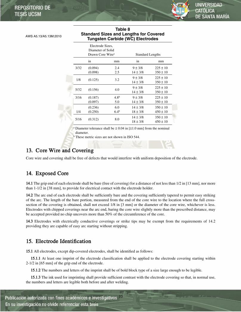
1133.. CCoorree WWiirree aanndd CCoovveerriinnggCore wire and covering shall be free of defects that would interfere with uniform deposition of the electrode.
1144.. EExxppoosseedd CCoorree
1144..11 The grip end of each electrode shall be bare (free of covering) for a distance of not less than 1/2 in [13 mm], nor morethan 1-1/2 in [38 mm], to provide for electrical contact with the electrode holder.
1144..22 The arc end of each electrode shall be sufficiently bare and the covering sufficiently tapered to permit easy strikingof the arc. The length of the bare portion, measured from the end of the core wire to the location where the full cross-section of the covering is obtained, shall not exceed 1/8 in [3 mm] or the diameter of the core wire, whichever is less.Electrodes with chipped coverings near the arc end, baring the core wire slightly more than the prescribed distance, maybe accepted provided no chip uncovers more than 50% of the circumference of the core.
1144..33 Electrodes with electrically conductive coverings or strike tips may be exempt from the requirements of 14.2providing they are capable of easy arc starting without stripping.
1155.. EElleeccttrrooddee IIddeennttiifificcaattiioonn
1155..11 All electrodes, except dip-covered electrodes, shall be identified as follows:
1155..11..11 At least one imprint of the electrode classification shall be applied to the electrode covering starting within 2-1/2 in [65 mm] of the grip end of the electrode.
1155..11..22 The numbers and letters of the imprint shall be of bold block type of a size large enough to be legible.
1155..11..33 The ink used for imprinting shall provide sufficient contrast with the electrode covering so that, in normal use,the numbers and letters are legible both before and after welding.
AWS A5.13/A5.13M:2010
10
Table 8Standard Sizes and Lengths for Covered
Tungsten Carbide (WC) Electrodes
Electrode Sizes, Diameter of Solid Drawn Core Wirea Standard Lengths
in mm in mm
3/32 (0.094) 2.4 9 ± 3/8 225 ± 10(0.098) 2.5 14 ± 3/8 350 ± 10
9 ± 3/8 225 ± 101/8 (0.125) 3.214 ± 3/8 350 ± 10
9 ± 3/8 225 ± 105/32 (0.156) 4.014 ± 3/8 350 ± 10
3/16 (0.187) 4.8b 9 ± 3/8 225 ± 10(0.097) 5.0 14 ± 3/8 350 ± 10
(0.236) 6.0 14 ± 3/8 350 ± 101/4 (0.250) 6.4b 18 ± 3/8 450 ± 10
14 ± 3/8 350 ± 105/16 (0.312) 8.018 ± 3/8 450 ± 10
a Diameter tolerance shall be ± 0.04 in [±1.0 mm] from the nominaldiameter.
b These metric sizes are not shown in ISO 544.
AWS_A5.13.qxp 7/21/10 1:26 PM Page 10

1155..11..44 The prefix letter E in the electrode classification may be omitted from the imprint.
1155..22 Identification of dip-covered electrodes shall be as agreed upon between the purchaser and supplier. Imprinting isnot mandatory.
1166.. PPaacckkaaggiinngg
1166..11 Electrodes shall be suitably packaged to protect them against damage during shipment and storage under normalconditions.
1166..22 Standard package weights shall be as agreed between purchaser and supplier.
1177.. MMaarrkkiinngg ooff PPaacckkaaggeess
1177..11 The following product information (as a minimum) shall be legibly marked on the outside of each unit package:
(1) AWS specification and classification designations (year of issue may be excluded)
(2) Supplier’s name and trade designation
(3) Size and net weight
(4) Lot, control, or heat number
1177..22 The appropriate precautionary information7 as given in ANSI Z49.1,8 latest edition (as a minimum) or its equivalent,shall be prominently displayed in legible print on all packages of electrodes, including individual unit packages enclosedwithin a larger package.
AWS A5.13/A5.13M:2010
11
7 Typical examples of “warning labels” are shown in figures in ANSI Z49.1 for some common or specific consumables used withcertain processes.
8 ANSI Z49.1 is published by the American Welding Society, 550 N.W. LeJeune Road, Miami, FL 33126.
AWS_A5.13.qxp 7/21/10 1:26 PM Page 11

AWS A5.13/A5.13M:2010
12
This page is intentionally blank.
AWS_A5.13.qxp 7/21/10 1:26 PM Page 12

AWS A5.13/A5.13M:2010
13
Annex A (Informative)Guide to AWS Specification for Surfacing Electrodes
for Shielded Metal Arc Welding
This annex is not part of AWS A5.13/A5.13M:2010, Specification for Surfacing Electrodes for Shielded Metal Arc Welding, but is included for informational purposes only.
AA11.. IInnttrroodduuccttiioonnThis guide has been prepared as an aid to prospective users of the electrodes covered by the specification in determiningthe classification of filler metal best suited for a particular application, with due consideration to the particular require-ments for that application.
AA22.. CCllaassssiifificcaattiioonn SSyysstteemm
AA22..11 The system for identifying the electrode classifications in this specification follows the standard pattern used inother AWS filler metal specifications. The letter E at the beginning of each classification designation stands for electrode.The letters immediately after the E are the chemical symbols for the principal elements in the classification. Thus, CoCris a cobalt–chromium alloy, CuAl is a copper–aluminum alloy, etc. Where more than one classification is included in abasic group, the individual classifications in the group are identified by the letters A, B, C, etc., as in ECuSn-A. Furthersubdivision is done by using a 1, 2, etc., after the last letter, as the 2 in ECuAl-A2. An additional letter or number has beenadded to some designations if the composition requirements in this specification differ somewhat from those of the earlierversions for electrodes of the same basic classification.
AA22..22 From an application point of view, many classifications in this specification have a corresponding classification inAWS A5.21 Specification for Bare Electrodes and Rods for Surfacing (see Table A.1).
AA22..33 An international system for designating welding filler metals is under development by the International Institute ofWelding (IIW) for possible adoption as an ISO specification. The latest proposal for designating welding filler metalsappears in AWS IFS:2002, International Index of Welding Filler Metal Classifications9. Table A.1 shows the proposedISO designations applicable to filler metal classifications included in this specification.
AA22..44 RReeqquueesstt ffoorr FFiilllleerr MMeettaall CCllaassssiifificcaattiioonn
(1) When a surfacing electrode or rod cannot be classified as given in this specification, the manufacturer may request that a classification be established for that welding electrode. The manufacturer may do this by following the proceduregiven here.
(2) A request to establish a new electrode or rod classification must be in writing, and it needs to provide sufficientdetail to permit the AWS A5 Committee on Filler Metals and Allied Materials or the subcommittee to determine whetherthe new classification or the modification of an existing classification is more appropriate, and whether either is necessaryto satisfy the need. The request needs to state the variables and their limits, for such a classification or modification. The
9 This publication is published by the American Welding Society, 550 N.W. LeJeune Rd, Miami, FL 33126, in an electronic format(CDROM).
AWS_A5.13.qxp 7/21/10 1:26 PM Page 13
--`,`,`,,`,,`,```,```,`,,,,,````-`-`,,`,,`,`,,`---
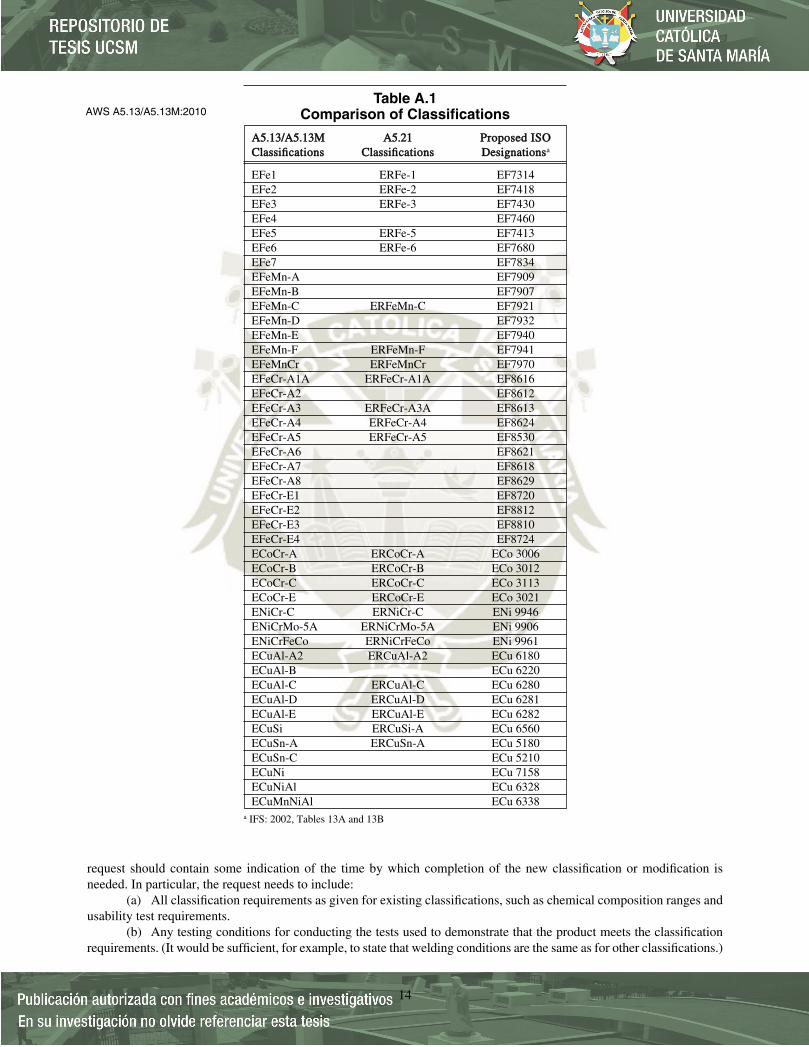
AWS A5.13/A5.13M:2010
14
Table A.1Comparison of Classifications
AA55..1133//AA55..1133MM AA55..2211 PPrrooppoosseedd IISSOO CCllaassssiifificcaattiioonnss CCllaassssiifificcaattiioonnss DDeessiiggnnaattiioonnssa
EFe1 ERFe-1 EF7314EFe2 ERFe-2 EF7418EFe3 ERFe-3 EF7430EFe4 EF7460EFe5 ERFe-5 EF7413EFe6 ERFe-6 EF7680EFe7 EF7834EFeMn-A EF7909EFeMn-B EF7907EFeMn-C ERFeMn-C EF7921EFeMn-D EF7932EFeMn-E EF7940EFeMn-F ERFeMn-F EF7941EFeMnCr ERFeMnCr EF7970EFeCr-A1A ERFeCr-A1A EF8616EFeCr-A2 EF8612EFeCr-A3 ERFeCr-A3A EF8613EFeCr-A4 ERFeCr-A4 EF8624EFeCr-A5 ERFeCr-A5 EF8530EFeCr-A6 EF8621EFeCr-A7 EF8618EFeCr-A8 EF8629EFeCr-E1 EF8720EFeCr-E2 EF8812EFeCr-E3 EF8810EFeCr-E4 EF8724ECoCr-A ERCoCr-A ECo 3006ECoCr-B ERCoCr-B ECo 3012ECoCr-C ERCoCr-C ECo 3113ECoCr-E ERCoCr-E ECo 3021ENiCr-C ERNiCr-C ENi 9946ENiCrMo-5A ERNiCrMo-5A ENi 9906ENiCrFeCo ERNiCrFeCo ENi 9961ECuAl-A2 ERCuAl-A2 ECu 6180ECuAl-B ECu 6220ECuAl-C ERCuAl-C ECu 6280ECuAl-D ERCuAl-D ECu 6281ECuAl-E ERCuAl-E ECu 6282ECuSi ERCuSi-A ECu 6560ECuSn-A ERCuSn-A ECu 5180ECuSn-C ECu 5210ECuNi ECu 7158ECuNiAl ECu 6328ECuMnNiAl ECu 6338
a IFS: 2002, Tables 13A and 13B
request should contain some indication of the time by which completion of the new classification or modification isneeded. In particular, the request needs to include:
(a) All classification requirements as given for existing classifications, such as chemical composition ranges andusability test requirements.
(b) Any testing conditions for conducting the tests used to demonstrate that the product meets the classificationrequirements. (It would be sufficient, for example, to state that welding conditions are the same as for other classifications.)
AWS_A5.13.qxp 7/21/10 1:26 PM Page 14
(c) Information on Descriptions and intended Use, which parallels that for existing classifications, for that section of the Annex.
(d) A request for a new classification without the above information will be considered incomplete. TheSecretary will return the request to the requestor for further information.
(3) The request should be sent to the Secretary of the AWS A5 Committee on Filler Metals and Allied Materials atAWS Headquarters. Upon receipt of the request, the Secretary will:
(a) Assign an identifying number to the request. This number will include the date the request was received.(b) Confirm receipt of the request and give the identification number to the person who made the request.(c) Send a copy of the request to the Chair of the AWS A5 Committee on Filler Metals and Allied Materials, and
the Chair of the particular Subcommittee involved.(d) File the original request.(e) Add the request to the log of outstanding requests.
(4) All necessary action on each request will be completed as soon as possible. If more than 12 months lapse, the Secretaryshall inform the requestor of the status of the request, with copies to the Chairs of the Committee and of the Subcommittee.Requests still outstanding after 18 months shall be considered not to have been answered in a “timely manner” and theSecretary shall report these to the Chair of the AWS A5 Committee on Filler Metals and Allied Materials, for action.
(5) The Secretary shall include a copy of the log of all requests pending and those completed during the precedingyear with the agenda for each AWS A5 Committee on Filler Metals and Allied Materials meeting. Any other publicationof requests that have been completed will be at the option of the American Welding Society, as deemed appropriate.
AA33.. AAcccceeppttaanncceeAcceptance of all welding materials classified under this specification is in accordance with AWS A5.01M/A5.01 (ISO14344) as the specification states. Any testing a purchaser requires of the supplier, for material shipped in accordancewith this specification, shall be clearly stated in the purchase order, according to the provisions of AWS A5.01M/A5.01(ISO 14344). In the absence of any such statement in the purchase order, the supplier may ship the material with what-ever testing he normally conducts on material of that classification, as specified in Schedule 1 or F, Table 1, of the AWSA5.01M/A5.01 (ISO 14344). Testing in accordance with any other schedule in that table must be specifically required bythe purchase order. In such cases, acceptance of the material shipped will be in accordance with those requirements.
AA44.. CCeerrttiifificcaattiioonnThe act of placing the AWS specification and classification designations on the packaging enclosing the product, or theclassification on the product itself, constitutes the supplier’s (manufacturer’s) certification that the product meets all ofthe requirements of the specification.
The only testing requirement implicit in this certification is that the manufacturer has actually conducted the tests requiredby the specification on material that is representative of that being shipped and that the material met the requirements ofthe specification. Representative material, in this case, is any production run of that classification using the same formu-lation. “Certification” is not to be construed to mean that tests of any kind were necessarily conducted on samples of thespecific material shipped. Tests on such material may or may not have been made. The basis for the certification requiredby the specification is the classification test of “representative material” cited above, and the “Manufacturer’s QualityAssurance System” in AWS A5.01M/A5.01 (ISO 14344).
AA55.. VVeennttiillaattiioonn DDuurriinngg WWeellddiinngg
AA55..11 Five major factors govern the quantity of fume in the atmosphere to which welders and welding operators areexposed during welding:
(1) Dimensions of the space in which welding is done (with special regard to the height of the ceiling)
(2) Number of welders and welding operators working in that space
AWS A5.13/A5.13M:2010
15
AWS_A5.13.qxp 7/21/10 1:26 PM Page 15
--`,`,`,,`,,`,```,```,`,,,,,````-`-`,,`,,`,`,,`---
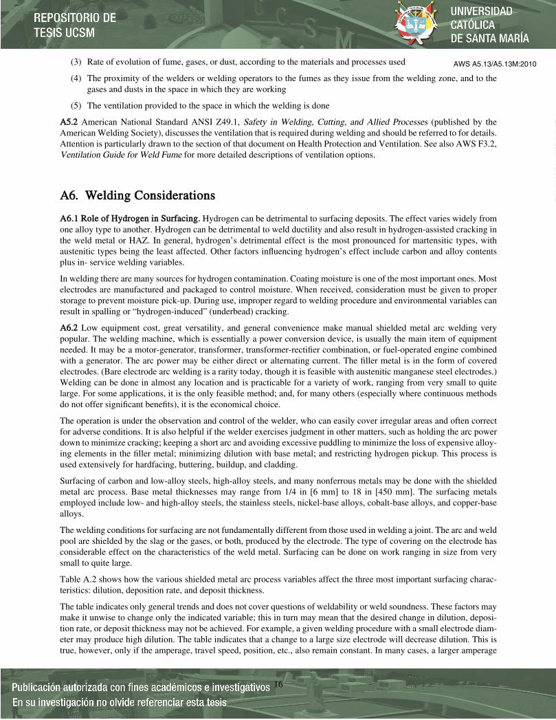
(3) Rate of evolution of fume, gases, or dust, according to the materials and processes used
(4) The proximity of the welders or welding operators to the fumes as they issue from the welding zone, and to thegases and dusts in the space in which they are working
(5) The ventilation provided to the space in which the welding is done
AA55..22 American National Standard ANSI Z49.1, Safety in Welding, Cutting, and Allied Processes (published by theAmerican Welding Society), discusses the ventilation that is required during welding and should be referred to for details.Attention is particularly drawn to the section of that document on Health Protection and Ventilation. See also AWS F3.2,Ventilation Guide for Weld Fume for more detailed descriptions of ventilation options.
AA66.. WWeellddiinngg CCoonnssiiddeerraattiioonnss
AA66..11 RRoollee ooff HHyyddrrooggeenn iinn SSuurrffaacciinngg.. Hydrogen can be detrimental to surfacing deposits. The effect varies widely fromone alloy type to another. Hydrogen can be detrimental to weld ductility and also result in hydrogen-assisted cracking inthe weld metal or HAZ. In general, hydrogen’s detrimental effect is the most pronounced for martensitic types, withaustenitic types being the least affected. Other factors influencing hydrogen’s effect include carbon and alloy contentsplus in- service welding variables.
In welding there are many sources for hydrogen contamination. Coating moisture is one of the most important ones. Mostelectrodes are manufactured and packaged to control moisture. When received, consideration must be given to properstorage to prevent moisture pick-up. During use, improper regard to welding procedure and environmental variables canresult in spalling or “hydrogen-induced” (underbead) cracking.
AA66..22 Low equipment cost, great versatility, and general convenience make manual shielded metal arc welding verypopular. The welding machine, which is essentially a power conversion device, is usually the main item of equipmentneeded. It may be a motor-generator, transformer, transformer-rectifier combination, or fuel-operated engine combinedwith a generator. The arc power may be either direct or alternating current. The filler metal is in the form of coveredelectrodes. (Bare electrode arc welding is a rarity today, though it is feasible with austenitic manganese steel electrodes.)Welding can be done in almost any location and is practicable for a variety of work, ranging from very small to quitelarge. For some applications, it is the only feasible method; and, for many others (especially where continuous methodsdo not offer significant benefits), it is the economical choice.
The operation is under the observation and control of the welder, who can easily cover irregular areas and often correctfor adverse conditions. It is also helpful if the welder exercises judgment in other matters, such as holding the arc powerdown to minimize cracking; keeping a short arc and avoiding excessive puddling to minimize the loss of expensive alloy-ing elements in the filler metal; minimizing dilution with base metal; and restricting hydrogen pickup. This process isused extensively for hardfacing, buttering, buildup, and cladding.
Surfacing of carbon and low-alloy steels, high-alloy steels, and many nonferrous metals may be done with the shieldedmetal arc process. Base metal thicknesses may range from 1/4 in [6 mm] to 18 in [450 mm]. The surfacing metalsemployed include low- and high-alloy steels, the stainless steels, nickel-base alloys, cobalt-base alloys, and copper-basealloys.
The welding conditions for surfacing are not fundamentally different from those used in welding a joint. The arc and weldpool are shielded by the slag or the gases, or both, produced by the electrode. The type of covering on the electrode hasconsiderable effect on the characteristics of the weld metal. Surfacing can be done on work ranging in size from verysmall to quite large.
Table A.2 shows how the various shielded metal arc process variables affect the three most important surfacing charac-teristics: dilution, deposition rate, and deposit thickness.
The table indicates only general trends and does not cover questions of weldability or weld soundness. These factors maymake it unwise to change only the indicated variable; this in turn may mean that the desired change in dilution, deposi-tion rate, or deposit thickness may not be achieved. For example, a given welding procedure with a small electrode diam-eter may produce high dilution. The table indicates that a change to a large size electrode will decrease dilution. This istrue, however, only if the amperage, travel speed, position, etc., also remain constant. In many cases, a larger amperage
AWS A5.13/A5.13M:2010
16
AWS_A5.13.qxp 7/21/10 1:26 PM Page 16
--`,`,`,,`,,`,```,```,`,,,,,````-`-`,,`,,`,`,,`---

value must be used with the larger electrode size to obtain acceptable weld quality. In this case, the dilution may remainconstant or even increase with the change to the larger electrode size.
The process usually achieves a deposition rate from 1–4 lb [0.5–2 kg] per hour at dilution levels from 30%–50%.
AA77.. DDeessccrriippttiioonn aanndd IInntteennddeedd UUssee ooff SSuurrffaacciinngg EElleeccttrrooddeess
AA77..11 IIrroonn--BBaassee EElleeccttrrooddeess
AA77..11..11 EEFFee11 aanndd EEFFee22 EElleeccttrrooddeess
AA77..11..11..11 CChhaarraacctteerriissttiiccss.. Deposits made with these electrodes are a machinery grade steel suitable for applicationon carbon and alloy steels. With care, they can be applied crack-free. Deposits are machinable with carbide-tipped tools.Deposit hardness generally is in the range of 25–50 HRC with EFe2 electrodes providing weld metal with the higherhardness. These deposits contain sufficient alloy to attain full hardness without the need of heat treatment. Abrasionresistance is comparable to heat-treated steels of equal hardness.
AA77..11..11..22 AApppplliiccaattiioonnss.. These electrodes are used to restore worn machinery parts to their original dimensions.Deposit surfaces are suitable for metal-to-metal rolling and sliding contact, such as occurs on large, low-speed gear teeth,shafts, etc. High compressive strength makes these materials suitable as a base for more abrasion-resistant materials.
AA77..11..22 EEFFee33 EElleeccttrrooddeess
AA77..11..22..11 CChhaarraacctteerriissttiiccss.. Weld metal deposited by these electrodes is an air-hardening tool steel type with highroom temperature hardness (55–60 HRC). Deposits can be applied crack-free with careful procedures. The depositscannot be machined and generally are ground when finishing is required.
AA77..11..22..22 AApppplliiccaattiioonnss.. EFe3 electrodes are used to overlay surfaces and edges requiring high hardness and crack-free deposits, such as the edges of tools and dies. Deposits are compatible with many tool steels. Although generally used
AWS A5.13/A5.13M:2010
17
Table A.2Effect of Shielded Metal Arc Variables on the Three Most Important
Characteristics of Surfacing
Influence of Change on
Variable Change of Variablea Dilution Deposition Rate Deposit Thickness
AC Intermediate Intermediate IntermediatePolarity DCEP High Low Thin
DCEN Low High Thick
AmperageHigh High High ThickLow Low Low Thin
TechniqueStringer High No effect ThickWeave Low No effect Thin
Bead spacingNarrow Low No effect ThickWide High No effect Thin
Electrode diameterSmall High High ThickLarge Low Low Thin
Arc lengthLong Low No effect ThinShort High No effect Thick
Travel speedFast High No effect ThinSlow Low No effect Thick
a This table assumes that only one variable at a time is changed. However, for acceptable surfacing conditions, a change in one variable may require achange in one or more other variables.
AWS_A5.13.qxp 7/21/10 1:26 PM Page 17

for metal-to-metal applications, EFe3 weld metal performs well in earth abrasion applications where high impact isencountered.
AA77..11..33 EEFFee44 EElleeccttrrooddeess
AA77..11..33..11 CChhaarraacctteerriissttiiccss.. These electrodes will have a graphitic (black) coating and are suitable for application oncast iron. Although the deposited metal is relatively brittle, crack-free deposits can be made with controlled procedures.Deposits can be machined providing they are slow cooled from an annealing temperature.
AA77..11..33..22 AApppplliiccaattiioonnss.. EFe4 weld metal is used to rebuild worn cast iron machinery parts subject to metal-to-metalrolling or sliding contact. Although EFe4 weld deposits are compatible with carbon and low-alloy steel, EFe2 electrodesgenerally are preferred for such applications.
AA77..11..44 EEFFee55 EElleeccttrrooddeess
AA77..11..44..11 CChhaarraacctteerriissttiiccss.. EFe5 electrodes deposit a cold work type of tool steel. Hardness as-deposited should be inthe range of 50–55 HRC. Weld metal deposited by EFe5 electrodes is air-hardening and machinable only after annealing.
AA77..11..44..22 AApppplliiccaattiioonnss.. Typical applications include those requiring high compressive strength with moderateabrasion and metal-to-metal wear, such as machine components, shafts, and brake drums.
AA77..11..55 EEFFee66 EElleeccttrrooddeess
AA77..11..55..11 CChhaarraacctteerriissttiiccss.. Weld metal deposited by EFe6 electrodes is a high-speed tool steel with a hardness inrange of 60 HRC or higher. The deposit maintains a high degree of hardness to 1100°F [600°C]. Weld metal depositedby EFe6 electrodes is air-hardening and is machinable only after annealing.
AA77..11..55..22 AApppplliiccaattiioonnss.. Weld deposits may be used for metal-to-metal wear applications at temperatures up to1100°F [600°C]. Typical applications combine high temperature service with severe abrasion and metal-to-metal wearand include shear blades, trimming dies, and punching dies.
AA77..11..66 EEFFee77 EElleeccttrrooddeess
AA77..11..66..11 CChhaarraacctteerriissttiiccss.. EFe7 series electrodes are essentially a higher carbon modification of EFe3 electrodes.Abrasion resistance of the weld deposit is improved with some sacrifice in resistance to impact. Deposits air harden, anda two-layer deposit can be expected to have a hardness of 60 HRC or higher. Stress-relief cracks (checks) typically occurthrough the overlay. Deposits cannot be machined.
AA77..11..66..22 AApppplliiccaattiioonnss.. EFe7 electrodes are used for overlaying surfaces that require good low-stress abrasionresistance. Applications include cement chutes, fan blades, bulldozer blades, and other parts and equipment used forearthmoving or construction. Carbon and alloy steels, tool steels, and stainless steels are compatible base metals.
AA77..11..77 EEFFeeMMnn SSeerriieess EElleeccttrrooddeess (EFeMn-A through EFeMn-F)
AA77..11..77..11 CChhaarraacctteerriissttiiccss.. Deposits made with EFeMn series electrodes nominally contain 14% manganese,although they may vary from 12% to 21%. This is an amount sufficient to yield austenitic weld deposits. Austenite is a nonmagnetic, tough form of steel. To preserve the toughness, excessive heat must be avoided during welding. Stringer beads and a block sequence are recommended. The additions of other elements, such as 4% nickel, are made to give more stability to the austenite; chromium, molybdenum, and vanadium are also added singly or in combination of 0.5%–8% to increase the yield strength. Abrasion resistance is only a little better than that of low-carbon steel unless there has been sufficient impact to cause work hardening. As-deposited surfaces generally are no harder than HRC 20, but can work harden to HRC 55. Since deposits are difficult to machine, grinding is preferred for finishing.
AA77..11..77..22 AApppplliiccaattiioonnss.. These electrodes are used for the rebuilding, repair, and joining of Hadfield austeniticmanganese steel. Ability to absorb high impact makes such deposits ideal for the rebuilding of worn rock crushingequipment and parts subject to impact loading, such as railroad frogs.
AA77..11..88 EEFFeeMMnnCCrr EElleeccttrrooddeess
AA77..11..88..11 CChhaarraacctteerriissttiiccss.. Weld metal deposited by EFeMnCr electrodes have characteristics similar to austeniticmanganese deposits. The high chromium content imparts stainless steel qualities. These deposits cannot be flame cut.Although care must be taken in application to avoid heat build-up, deposits are more stable than FeMn series electrodes.
AWS A5.13/A5.13M:2010
18
AWS_A5.13.qxp 7/21/10 1:26 PM Page 18
AA77..11..88..22 AApppplliiccaattiioonnss.. Like EFeMn type electrodes, EFeMnCr electrodes are used for rebuilding, repair, andjoining of equipment made of Hadfield austenitic manganese steel. EFeMnCr electrodes offer the added advantage ofbeing usable for joining austenitic manganese steel both to itself and to carbon steel. EFeMnCr weld metals often are usedas a base for surfacing with EFeCr types for parts subject to both wear and impact.
AA77..11..99 EEFFeeCCrr--AA11AA aanndd EEFFeeCCrr--AA44 EElleeccttrrooddeess
AA77..11..99..11 CChhaarraacctteerriissttiiccss.. Weld metal deposited by these electrodes will contain massive chromium carbides in anaustenitic matrix providing excellent wear resistance and toughness. Surface checks are typical and give some degree ofstress relief. Deposits cannot be machined and must be ground when finishing is required. To ensure the desired depositcomposition, two layers are recommended. Additional layers invite spalling and must be applied with caution. Electrodesare suitable for welding on carbon, alloy, and austenitic steels as well as cast irons. The weld metal deposited by EFeCr-A1A electrodes generally provides greater resistance to impact but slightly less abrasion resistance than weld metaldeposited by EFeCr-A4 electrodes.
AA77..11..99..22 AApppplliiccaattiioonnss.. Deposits frequently are used to surface parts and equipment involved in sliding andcrushing of rock, ore, etc., such as bucket lips and teeth, impact hammers, and conveyors. Very low coefficients offriction develop as a result of scouring by earth products.
AA77..11..1100 EEFFeeCCrr--AA22 EElleeccttrrooddeess
AA77..11..1100..11 CChhaarraacctteerriissttiiccss.. The weld metal deposit contains titanium carbide in an austenitic matrix. It ismachinable only by grinding. Build-up should be limited to three layers to minimize relief check cracking.
AA77..11..1100..22 AApppplliiccaattiioonnss.. This weld metal group may be applied to both carbon steel and austenitic manganese basemetal. Deposits frequently are used to hardface mining, construction, earth moving, and quarrying equipment subject toabrasion and moderate impact.
AA77..11..1111 EEFFeeCCrr--AA33 EElleeccttrrooddeess
AA77..11..1111..11 CChhaarraacctteerriissttiiccss.. Filler metal deposited by EFeCr-A3 electrodes is similar to a deposit made usingEFeCr-A1A electrodes except, due to the lower manganese content, a martensitic matrix is present, rendering the depositsomewhat brittle. These deposits are not machinable but may be finished by grinding where necessary.
AA77..11..1111..22 AApppplliiccaattiioonnss.. This weld metal is a general purpose hardfacing alloy for earth abrasion applications andis suitable for low stress scratching abrasion with low impact.
AA77..11..1122 EEFFeeCCrr--AA55 EElleeccttrrooddeess
AA77..11..1122..11 CChhaarraacctteerriissttiiccss.. The weld deposit contains chromium carbide in an austenitic matrix. The nonmagneticweld metal has fair machinability. Build-up should be restricted to three layers to minimize stress-relief checking.
AA77..11..1122..22 AApppplliiccaattiioonnss.. Surfaced components frequently are used for applications involving frictional metal-to-metal wear or earth scouring under low stress abrasion.
AA77..11..1133 EEFFeeCCrr--AA66 aanndd EEFFeeCCrr--AA77 EElleeccttrrooddeess
AA77..11..1133..11 CChhaarraacctteerriissttiiccss.. These are a higher carbon version of EFeCr-A5 electrodes. The deposit containshexagonal chromium carbides in an austenitic carbide matrix and has a hardness of 50–60 HRC. Deposits develop stress-relief checks. The addition of molybdenum increases wear resistance to high stress abrasion. The weld metal may beapplied on carbon, alloy, or austenitic manganese steel base metal.
AA77..11..1133..22 AApppplliiccaattiioonnss.. Weld metal is frequently used for applications involving low stress abrasive wearcombined with moderate impact.
AA77..11..1144 EEFFeeCCrr--AA88 EElleeccttrrooddeess
AA77..11..1144..11 CChhaarraacctteerriissttiiccss.. EFeCr-A8 is a higher chromium version of EFeCr-A3. The deposit contains hexagonalchromium carbides in an austenitic matrix and has a hardness of 50–60 HRC. The increased chromium content tends todecrease the toughness while increasing the abrasion resistance. Maximum relief checking can be expected. The weldmetal may be applied to carbon, alloy, or austenitic manganese base metals.
AA77..11..1144..22 AApppplliiccaattiioonnss.. Weld metal is frequently used for applications involving low stress abrasion combinedwith minimum impact.
AWS A5.13/A5.13M:2010
19
AWS_A5.13.qxp 7/21/10 1:26 PM Page 19

AA77..11..1155 EEFFeeCCrr--EEXX SSeerriieess EElleeccttrrooddeess
AA77..11..1155..11 CChhaarraacctteerriissttiiccss.. This family of electrodes deposits weld metal containing finely dispersed chromiumcarbides plus one or more metallic carbides (vanadium, niobium [columbium], tungsten, or titanium). The resultantdeposits are not machinable, and maintain their hot hardness and abrasion resistance to 1200°F [650°C]. Deposits stress-relief check readily.
AA77..11..1155..22 AApppplliiccaattiioonnss.. Equipment subjected to severe high stress abrasion combined with moderate impact maybe surfaced with one of the specific grades. Selection of the specific grade will be dependent on local service conditionsand the specific application.
AA77..22 CCoobbaalltt--BBaassee SSuurrffaacciinngg EElleeccttrrooddeess
AA77..22..11 EECCooCCrr--AA EElleeccttrrooddeess
AA77..22..11..11 CChhaarraacctteerriissttiiccss.. Weld metal deposited by ECoCr-A electrodes is characterized by a hypoeutecticstructure consisting of a network of about 13% eutectic chromium carbides distributed in a cobalt-chromium-tungstensolid solution matrix. The result is a material with a combination of overall resistance to low stress abrasive wear coupledwith the necessary toughness to resist some degree of impact. Cobalt alloys also are inherently good for resisting metal-to-metal wear, particularly in high load situations that are prone to galling. The high alloy content of the matrix alsoaffords excellent resistance to corrosion, oxidation, and elevated temperature retention of hot hardness up to a maximumof 1200°F [650°C]. These alloys are not subject to allotropic transformation and therefore do not lose their properties ifthe base metal subsequently is heat treated.
AA77..22..11..22 AApppplliiccaattiioonnss.. The alloy is recommended for cases where wear is accompanied by elevated temperaturesand where corrosion is involved, or both. Typical applications include automotive and fluid flow valves, chain sawguides, hot punches, shear blades, extruder screws, etc.
AA77..22..22 EECCooCCrr--BB EElleeccttrrooddeess
AA77..22..22..11 CChhaarraacctteerriissttiiccss.. Weld metal deposited by ECoCr-B electrodes is similar in composition to ECoCr-Adeposits except for a slightly higher carbide content (approximately 16%). The alloy also has a slightly higher hardnesscoupled with better abrasive and metal-to-metal wear resistance. Impact and corrosion resistance are lowered slightly.Deposits can be machined with carbide tools.
AA77..22..22..22 AApppplliiccaattiioonnss.. ECoCr-B electrodes are used interchangeably with ECoCr-A. Choice will depend on thespecific application.
AA77..22..33 EECCooCCrr--CC EElleeccttrrooddeess
AA77..22..33..11 CChhaarraacctteerriissttiiccss.. This alloy’s deposits have a higher carbide content (19%) than those made using eitherECoCr-A or ECoCr-B electrodes. In fact, the composition is such that primary hypereutectic carbides are found in themicrostructure. This characteristic gives the alloy higher wear resistance, accompanied by reductions in the impact andcorrosion resistance. The higher hardness also means a greater tendency to stress crack during cooling. The crackingtendency may be minimized by closely monitoring preheating, interpass temperature, and postheating techniques.
While the cobalt–chromium deposits soften somewhat at elevated temperatures, they normally are considered immune totempering.
AA77..22..33..22 AApppplliiccaattiioonnss.. Weld metal deposited by ECoCr-C electrodes is used to build up mixer rotors and itemsthat encounter severe abrasion and low impact.
AA77..22..44 EECCooCCrr--EE EElleeccttrrooddeess
AA77..22..44..11 CChhaarraacctteerriissttiiccss.. Welds made using ECoCr-E electrodes have very good strength and ductility attemperatures up to 1600°F [870°C]. Deposits are resistant to thermal shock, and oxidizing and reducing atmospheres.Early applications of these types of alloys were found in jet engine components such as turbine blades and vanes.
The deposit is a solid-solution-strengthened alloy with a relatively low weight-percent carbide phase in the microstruc-ture. Hence, the alloy is very tough and will work harden. Deposits possess excellent self-mated galling resistance andalso are very resistant to cavitation erosion.
AA77..22..44..22 AApppplliiccaattiioonnss.. Welds made using ECoCr-E electrodes are used where resistance to thermal shock isimportant. Typical applications, similar to those of ECoCr-A deposits, include guide rolls, hot extrusion and forging dies,hot shear blades, tong bits, and valve trim.
AWS A5.13/A5.13M:2010
20
AWS_A5.13.qxp 7/21/10 1:26 PM Page 20

AA77..22..55 Typical hardness values for multilayer welds made using the cobalt-base electrodes are:
ECoCr-A 23–47 HRCECoCr-B 34–47 HRCECoCr-C 43–58 HRCECoCr-E 20–32 HRC
Hardness values for single layer deposits will be lower because of dilution from the base metal.
AA77..33 NNiicckkeell--BBaassee SSuurrffaacciinngg EElleeccttrrooddeess
AA77..33..11 EENNiiCCrr--CC EElleeccttrrooddeess
AA77..33..11..11 CChhaarraacctteerriissttiiccss.. Undiluted weld metal of this composition exhibits a structure consisting of chromiumcarbides and chromium borides in a nickel-rich matrix. The nickel base and high chromium content give these depositsgood heat and corrosion resistance. Care should be taken when cooling hardfacing deposits because of a tendency tostress crack. This alloy possesses excellent resistance to low stress abrasion.
AA77..33..11..22 AApppplliiccaattiioonnss.. ENiCr-C weld metal flows very easily, has very high abrasion resistance, and normallytakes on a high polish. Typical applications include cultivator sweeps, plow shares, extrusion screws, pump sleeves,pistons, and impellers, capstan rings, glass mold faces, centrifuge filters, sucker pump rods, etc. The deposits have highcorrosion resistance and normally require grinding for finishing. Single layer deposits typically have a hardness of 35–45HRC. Multilayer deposits typically have a hardness of 49–56 HRC.
AA77..33..22 EENNiiCCrrMMoo--55AA EElleeccttrrooddeess
AA77..33..22..11 CChhaarraacctteerriissttiiccss.. Undiluted weld metal deposited by ENiCrMo-5A electrodes is a solid-solution-strengthenedalloy with relatively low weight-percent carbide phase produced through secondary hardening. The resultant deposit is toughand work hardenable.
Deposits have the ability to retain hardness up to 1400°F [760°C]. Deposits are machinable with high-speed tool bits andhave excellent resistance to high-temperature wear and impact.
AA77..33..22..22 AApppplliiccaattiioonnss.. These electrodes are used to rebuild and repair hot extrusion dies, hot forging dies, sizingpunches, hot shear blades, guide rolls, tong bits, blast furnace bells, etc.
AA77..33..33 EENNiiCCrrFFeeCCoo EElleeccttrrooddeess
AA77..33..33..11 CChhaarraacctteerriissttiiccss.. Weld metal deposited by these electrodes contain a fairly large volume fraction ofhypereutectic chromium carbides distributed throughout the microstructure. The alloy offers many of the same high-performance characteristics of deposits made using ECoCr-C or ENiCr-C electrodes in terms of abrasive wear resistance.The reduced nickel or cobalt content, or both, lowers corrosion properties and galling resistance. The high volumefraction of carbides makes this alloy sensitive to cracking during cooling.
AA77..33..33..22 AApppplliiccaattiioonnss.. Welds made using ENiCrFeCo electrodes are preferred where high abrasion (low impact)is a major factor. Typical applications are feed screws, slurry pumps, and mixer components.
AA77..44 CCooppppeerr--BBaassee AAllllooyy EElleeccttrrooddeess
AA77..44..11 IInnttrroodduuccttiioonn.. The copper-base alloy electrodes classified by this specification are used to deposit overlays andinlays for bearing, corrosion-resistant, or wear-resistant surfaces.
AA77..44..11..11 ECuAl-A2 electrodes are used for surfacing bearing surfaces, requiring the hardness in the ranges of130–150 HB, as well as corrosion-resistant surfaces.
AA77..44..11..22 ECuAl-B and ECuAl-C electrodes are used primarily for surfacing bearing surfaces requiring hardness inthe range of 140–220 HB. These alloys are not recommended for applications that require resistance to corrosion.
AA77..44..11..33 ECuAl-D and ECuAl-E electrodes are used to surface bearing and wear-resistant surfaces requiringhardness in the range of 230–320 HB, such as gears, cams, sheaves, wear plates, dies, etc. These alloys are also used tosurface dies that form or draw titanium, low-carbon and stainless steels. These alloys are not recommended forapplications that require resistance to corrosion.
AA77..44..11..44 The ECuSi electrodes are used primarily for surfacing corrosion-resistant surfaces. Copper–silicondeposits generally are not recommended for bearing service.
AWS A5.13/A5.13M:2010
21
AWS_A5.13.qxp 7/21/10 1:26 PM Page 21
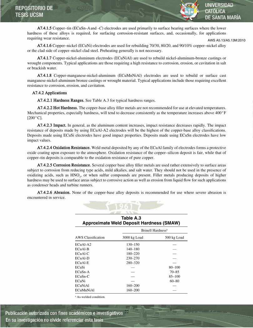
AA77..44..11..55 Copper–tin (ECuSn-A and -C) electrodes are used primarily to surface bearing surfaces where the lowerhardness of these alloys is required, for surfacing corrosion-resistant surfaces, and, occasionally, for applicationsrequiring wear resistance.
AA77..44..11..66 Copper–nickel (ECuNi) electrodes are used for rebuilding 70/30, 80/20, and 90/10% copper–nickel alloyor the clad side of copper–nickel clad steel. Preheating generally is not necessary.
AA77..44..11..77 Copper-nickel-aluminum electrodes (ECuNiAl) are used to rebuild nickel-aluminum-bronze castings orwrought components. Typical applications are those requiring a high resistance to corrosion, erosion, or cavitation in saltor brackish water.
AA77..44..11..88 Copper-manganese-nickel-aluminum (ECuMnNiAl) electrodes are used to rebuild or surface castmanganese-nickel-aluminum bronze castings or wrought material. Typical applications include those requiring excellentresistance to corrosion, erosion, and cavitation.
AA77..44..22 AApppplliiccaattiioonnss
AA77..44..22..11 HHaarrddnneessss RRaannggeess.. See Table A.3 for typical hardness ranges.
AA77..44..22..22 HHoott HHaarrddnneessss.. The copper-base alloy filler metals are not recommended for use at elevated temperatures.Mechanical properties, especially hardness, will tend to decrease consistently as the temperature increases above 400°F[200°C].
AA77..44..22..33 IImmppaacctt.. In general, as the aluminum content increases, impact resistance decreases rapidly. The impactresistance of deposits made by using ECuAl-A2 electrodes will be the highest of the copper-base alloy classifications.Deposits made using ECuSi electrodes have good impact properties. Deposits made using ECuSn electrodes have lowimpact values.
AA77..44..22..44 OOxxiiddaattiioonn RReessiissttaannccee.. Weld metal deposited by any of the ECuAl family of electrodes forms a protectiveoxide coating upon exposure to the atmosphere. Oxidation resistance of the copper–silicon deposit is fair, while that ofcopper–tin deposits is comparable to the oxidation resistance of pure copper.
AA77..44..22..55 CCoorrrroossiioonn RReessiissttaannccee.. Several copper base alloy filler metals are used rather extensively to surface areassubject to corrosion from reducing type acids, mild alkalies, and salt water. They should not be used in the presence ofoxidizing acids, such as HNO3, or when sulfur compounds are present. Filler metals producing deposits of higherhardness may be used to surface areas subject to corrosive action as well as erosion from liquid flow for such applicationsas condenser heads and turbine runners.
AA77..44..22..66 AAbbrraassiioonn.. None of the copper-base alloy deposits is recommended for use where severe abrasion isencountered in service.
AWS A5.13/A5.13M:2010
22
Table A.3Approximate Weld Deposit Hardness (SMAW)
Brinell Hardnessa
AWS Classification 3000 kg Load 500 kg Load
ECuAl-A2 130–150 —ECuAl-B 140–180 —ECuAl-C 180–220 —ECuAl-D 230–270 —ECuAl-E 280–320 —ECuSi — 80–100ECuSn-A — 70–85ECuSn-C — 85–100ECuNi — 60–80ECuNiAl 160–200 —ECuMnNiAl 160–200 —
a As-welded condition.
AWS_A5.13.qxp 7/21/10 1:26 PM Page 22
--`,`,`,,`,,`,```,```,`,,,,,````-`-`,,`,,`,`,,`---
AA77..44..22..77 MMeettaall--ttoo--MMeettaall WWeeaarr.. Copper–aluminum deposits with hardnesses of 130 to approximately 320 HB areused to overlay surfaces subjected to excessive wear from metal-to-metal contact. For example, ECuAl-E electrodes are used to surface dies, and to draw and form stainless and carbon steels and aluminum.
All of the copper-base alloy filler metals classified by this specification are used to deposit overlays and inlays for bear-ing surfaces, with the exception of the CuSi filler metals. Silicon bronzes are considered poor bearing alloys. Copper-basealloy filler metals selected for a bearing surface should produce a deposit of 50–75 HB under that of the mating part.Equipment should be designed so that the bearing will wear in preference to the mating part.
AA77..44..22..88 MMeecchhaanniiccaall PPrrooppeerrttiieess iinn CCoommpprreessssiioonn.. Deposits of the ECuAl filler metals have high elastic limits andultimate strengths in compression ranging between 25 000–65 000 psi [170–450 MPa] and 120 000–171 000 psi[825–1180 MPa], respectively. The elastic limit of ECuSi deposits is around 22 000 psi [150 MPa] with an ultimatestrength in compression of 60 000 psi [415 MPa]. The ECuSn deposits will have an elastic limit of 11 000 psi [75 MPa]and an ultimate strength of 32 000 psi [220 MPa].
AA77..44..22..99 MMaacchhiinnaabbiilliittyy.. All of these copper-base alloy deposits are machinable.
AA77..44..22..1100 HHeeaatt TTrreeaattmmeenntt.. Ordinarily, no heat treatment is needed in surfacing with copper-base alloy fillermetals.
AA77..44..22..1111 WWeellddiinngg CChhaarraacctteerriissttiiccss.. To minimize dilution from the base metal when surfacing with copper-baseelectrodes, the first layer should be deposited using as low an amperage as practical. Excessive base metal dilution canresult in reduced machinability and service performance. The manufacturer should be consulted for specific weldingparameters.
AA77..44..22..1122 PPrreehheeaatt.. Generally, a preheat is not necessary unless the part is exceptionally large; in this case, a 200°F[100°C] preheat may be desirable to facilitate the smooth flow of the weld metal. At no time should the preheattemperature be above 400°F [200°C] when applying the first layer. On subsequent layers, an interpass temperature ofapproximately 200°F–600°F [100°C–300°C] will simplify deposition of the weld metal.
AA77..55 TTuunnggsstteenn CCaarrbbiiddee EElleeccttrrooddeess
AA77..55..11 CChhaarraacctteerriissttiiccss.. Tungsten carbide covered electrodes contain 60% by weight tungsten carbide granules. TheWC1 carbide is a mixture of WC and W2C. The WC2 carbide is macrocrystalline WC. Hardness of the matrix of thedeposit can be varied from 30 HRC to 60 HRC depending on welding technique. Hardness of individual carbide particlestypically is about 2400 HV20. The abrasion resistance of tungsten carbide deposits is outstanding.
AA77..55..22 AApppplliiccaattiioonnss.. Tungsten carbide deposits are applied on surfaces subjected to sliding abrasion combined withlimited impact. Such applications are encountered in earth drilling, digging, and farming. Specific tools that may requirethis type of surfacing overlay include oil drill bits and tool joints, earth handling augers, excavator teeth, farm fertilizerapplicator knives, and cultivator shares.
AA88.. DDiissccoonnttiinnuueedd CCllaassssiifificcaattiioonnssSome classifications have been discontinued from one revision of this specification to another. This results either fromchanges in commercial practice or changes in the classification system used in the specification. The classifications thathave been discontinued are listed in Table A.4, along with the year in which they were last included in the specification.
AA99.. GGeenneerraall SSaaffeettyy CCoonnssiiddeerraattiioonnss
AA99..11 Safety and health issues and concerns are beyond the scope of this standard and, therefore, are not fully addressedherein. Some safety and health information can be found in Clause A5 and below. Safety and health information isavailable from other sources, including but not limited to ANSI Z49.1, Safety in Welding, Cutting, and Allied Processes,and applicable federal and state regulations.
AA99..22 SSaaffeettyy aanndd HHeeaalltthh FFaacctt SShheeeettss.. The Safety and Health Fact Sheets listed below are published by the AmericanWelding Society (AWS). They may be downloaded and printed directly from the AWS website at http://www.aws.org.The Safety and health Fact Sheets are revised and additional sheeets added periodically.
AWS A5.13/A5.13M:2010
23
AWS_A5.13.qxp 7/21/10 1:26 PM Page 23
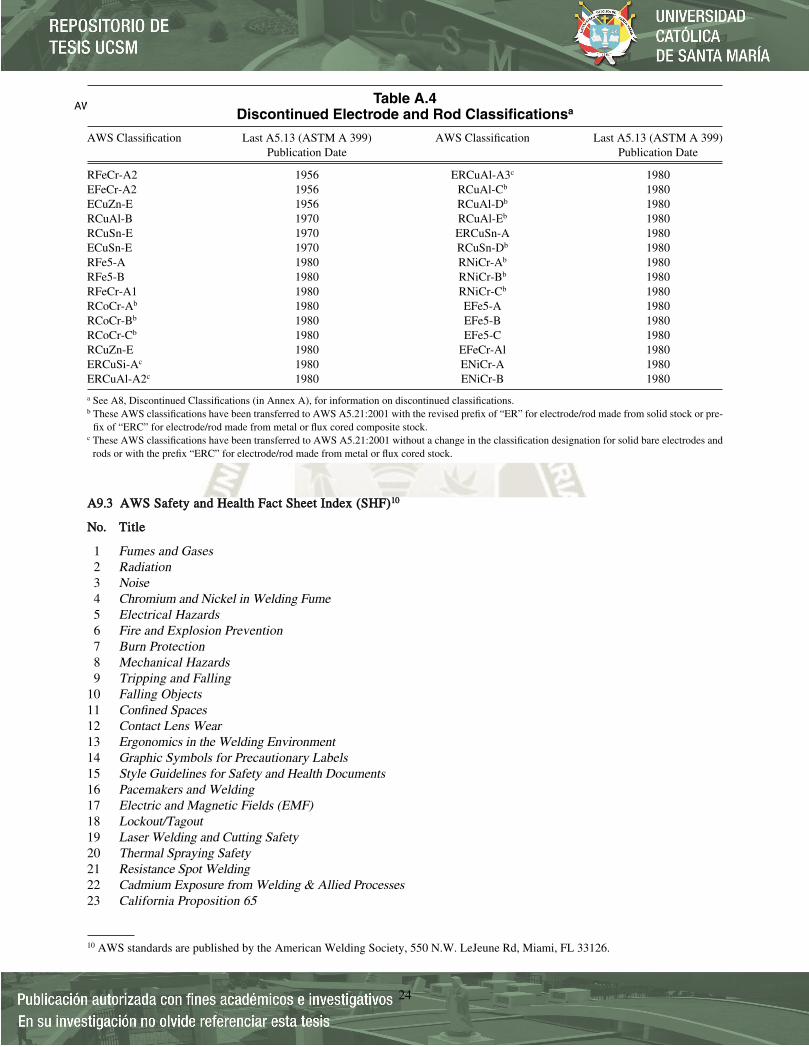
AA99..33 AAWWSS SSaaffeettyy aanndd HHeeaalltthh FFaacctt SShheeeett IInnddeexx ((SSHHFF))1100
NNoo.. TTiittllee
1 Fumes and Gases2 Radiation3 Noise4 Chromium and Nickel in Welding Fume5 Electrical Hazards6 Fire and Explosion Prevention7 Burn Protection8 Mechanical Hazards9 Tripping and Falling
10 Falling Objects11 Confined Spaces12 Contact Lens Wear13 Ergonomics in the Welding Environment14 Graphic Symbols for Precautionary Labels15 Style Guidelines for Safety and Health Documents16 Pacemakers and Welding17 Electric and Magnetic Fields (EMF)18 Lockout/Tagout19 Laser Welding and Cutting Safety20 Thermal Spraying Safety21 Resistance Spot Welding22 Cadmium Exposure from Welding & Allied Processes23 California Proposition 65
AWS A5.13/A5.13M:2010
24
Table A.4Discontinued Electrode and Rod Classificationsa
AWS Classification Last A5.13 (ASTM A 399) AWS Classification Last A5.13 (ASTM A 399) Publication Date Publication Date
RFeCr-A2 1956 ERCuAl-A3c 1980EFeCr-A2 1956 RCuAl-Cb 1980ECuZn-E 1956 RCuAl-Db 1980RCuAl-B 1970 RCuAl-Eb 1980RCuSn-E 1970 ERCuSn-A 1980ECuSn-E 1970 RCuSn-Db 1980RFe5-A 1980 RNiCr-Ab 1980RFe5-B 1980 RNiCr-Bb 1980RFeCr-A1 1980 RNiCr-Cb 1980RCoCr-Ab 1980 EFe5-A 1980RCoCr-Bb 1980 EFe5-B 1980RCoCr-Cb 1980 EFe5-C 1980RCuZn-E 1980 EFeCr-Al 1980ERCuSi-Ac 1980 ENiCr-A 1980ERCuAl-A2c 1980 ENiCr-B 1980
a See A8, Discontinued Classifications (in Annex A), for information on discontinued classifications.b These AWS classifications have been transferred to AWS A5.21:2001 with the revised prefix of “ER” for electrode/rod made from solid stock or pre-
fix of “ERC” for electrode/rod made from metal or flux cored composite stock.c These AWS classifications have been transferred to AWS A5.21:2001 without a change in the classification designation for solid bare electrodes and
rods or with the prefix “ERC” for electrode/rod made from metal or flux cored stock.
10 AWS standards are published by the American Welding Society, 550 N.W. LeJeune Rd, Miami, FL 33126.
AWS_A5.13.qxp 7/21/10 1:26 PM Page 24

24 Fluxes for Arc Welding and Brazing: Safe Handling and Use25 Metal Fume Fever26 Arc Welding Distance27 Thoriated Tungsten Electrodes28 Oxyfuel Safety: Check Valves and Flashback Arrestors29 Grounding of Portable and Vehicle Mounted Welding Generators30 Cylinders: Safe Storage, Handling, and Use31 Eye and Face Protection for Welding and Cutting Operations33 Personal Protective Equipment (PPE) for Welding & Cutting34 Coated Steels: Welding and Cutting Safety Concerns36 Ventilation for Welding & Cutting37 Selecting Gloves for Welding & Cutting
AWS A5.13/A5.13M:2010
25
AWS_A5.13.qxp 7/21/10 1:26 PM Page 25

AWS A5.13/A5.13M:2010
26
This page is intentionally blank.
AWS_A5.13.qxp 7/21/10 1:26 PM Page 26
--`,`,`,,`,,`,```,```,`,,,,,````-`-`,,`,,`,`,,`---

AWS A5.13/A5.13M:2010
27
Annex B (Informative)Guidelines for the Preparation of Technical Inquiries
This annex is not part of AWS A5.13/A5.13M:2010, Specification for Surfacing Electrodes for Shielded Metal Arc Welding, but is included for informational purposes only.
BB11.. IInnttrroodduuccttiioonnThe American Welding Society (AWS) Board of Directors has adopted a policy whereby all official interpretations ofAWS standards are handled in a formal manner. Under this policy, all interpretations are made by the committee that isresponsible for the standard. Official communication concerning an interpretation is directed through the AWS staffmember who works with that committee. The policy requires that all requests for an interpretation be submitted in writ-ing. Such requests will be handled as expeditiously as possible, but due to the complexity of the work and the proceduresthat must be followed, some interpretations may require considerable time.
BB22.. PP rroocceedduurreeAll inquiries shall be directed to:
Managing DirectorTechnical Services DivisionAmerican Welding Society550 N.W. LeJeune RoadMiami, FL 33126
All inquiries shall contain the name, address, and affiliation of the inquirer, and they shall provide enough informationfor the committee to understand the point of concern in the inquiry. When the point is not clearly defined, the inquiry willbe returned for clarification. For efficient handling, all inquiries should be typewritten and in the format specified below.
BB22..11 SSccooppee.. Each inquiry shall address one single provision of the standard unless the point of the inquiry involves twoor more interrelated provisions. The provision(s) shall be identified in the scope of the inquiry along with the edition ofthe standard that contains the provision(s) the inquirer is addressing.
BB22..22 PPuurrppoossee ooff tthhee IInnqquuiirryy.. The purpose of the inquiry shall be stated in this portion of the inquiry. The purpose can beto obtain an interpretation of a standard’s requirement or to request the revision of a particular provision in the standard.
BB22..33 CCoonntteenntt ooff tthhee IInnqquuiirryy.. The inquiry should be concise, yet complete, to enable the committee to understand thepoint of the inquiry. Sketches should be used whenever appropriate, and all paragraphs, figures, and tables (or annex) thatbear on the inquiry shall be cited. If the point of the inquiry is to obtain a revision of the standard, the inquiry shall providetechnical justification for that revision.
BB22..44 PPrrooppoosseedd RReeppllyy.. The inquirer should, as a proposed reply, state an interpretation of the provision that is the pointof the inquiry or provide the wording for a proposed revision, if this is what the inquirer seeks.
BB33.. IInntteerrpp rreettaattiioonn ooff PPrroovviissiioonnss ooff tthhee SSttaannddaarrddInterpretations of provisions of the standard are made by the relevant AWS technical committee. The secretary of thecommittee refers all inquiries to the chair of the particular subcommittee that has jurisdiction over the portion of the
AWS_A5.13.qxp 7/21/10 1:26 PM Page 27
standard addressed by the inquiry. The subcommittee reviews the inquiry and the proposed reply to determine what theresponse to the inquiry should be. Following the subcommittee’s development of the response, the inquiry and theresponse are presented to the entire committee for review and approval. Upon approval by the committee, the interpreta-tion is an official interpretation of the Society, and the secretary transmits the response to the inquirer and to the WeldingJournal for publication.
BB44.. PPuubblliiccaattiioonn ooff IInntteerrpp rreettaattiioonnssAll official interpretations will appear in the Welding Journal and will be posted on the AWS web site.
BB55.. TTeelleepphhoonnee IInnqquuiirriieessTelephone inquiries to AWS Headquarters concerning AWS standards should be limited to questions of a general natureor to matters directly related to the use of the standard. The AWS Board Policy Manual requires that all AWS staff mem-bers respond to a telephone request for an official interpretation of any AWS standard with the information that such aninterpretation can be obtained only through a written request. Headquarters staff cannot provide consulting services.However, the staff can refer a caller to any of those consultants whose names are on file at AWS Headquarters.
BB66.. AAWWSS TTeecchhnniiccaall CCoommmmiitttteeeessThe activities of AWS technical committees regarding interpretations are limited strictly to the interpretation of provi-sions of standards prepared by the committees or to consideration of revisions to existing provisions on the basis of newdata or technology. Neither AWS staff nor the committees are in a position to offer interpretive or consulting services on(1) specific engineering problems, (2) requirements of standards applied to fabrications outside the scope of the docu-ment, or (3) points not specifically covered by the standard. In such cases, the inquirer should seek assistance from a com-petent engineer experienced in the particular field of interest.
AWS A5.13/A5.13M:2010
28
AWS_A5.13.qxp 7/21/10 1:26 PM Page 28
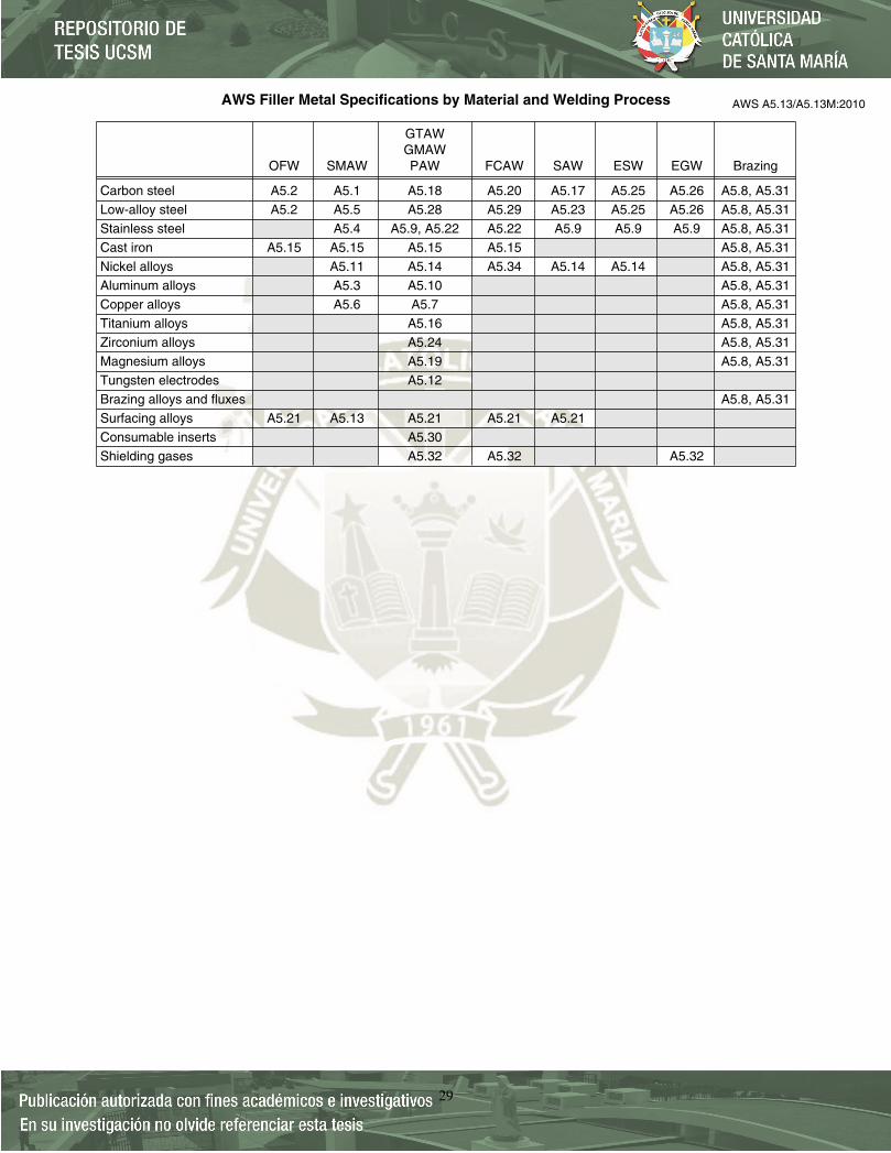
AWS A5.13/A5.13M:2010
29
AWS Filler Metal Specifications by Material and Welding Process
GTAWGMAW
OFW SMAW PAW FCAW SAW ESW EGW Brazing
Carbon steel A5.2 A5.1 A5.18 A5.20 A5.17 A5.25 A5.26 A5.8, A5.31Low-alloy steel A5.2 A5.5 A5.28 A5.29 A5.23 A5.25 A5.26 A5.8, A5.31Stainless steel A5.4 A5.9, A5.22 A5.22 A5.9 A5.9 A5.9 A5.8, A5.31Cast iron A5.15 A5.15 A5.15 A5.15 A5.8, A5.31Nickel alloys A5.11 A5.14 A5.34 A5.14 A5.14 A5.8, A5.31Aluminum alloys A5.3 A5.10 A5.8, A5.31Copper alloys A5.6 A5.7 A5.8, A5.31Titanium alloys A5.16 A5.8, A5.31Zirconium alloys A5.24 A5.8, A5.31Magnesium alloys A5.19 A5.8, A5.31Tungsten electrodes A5.12Brazing alloys and fluxes A5.8, A5.31Surfacing alloys A5.21 A5.13 A5.21 A5.21 A5.21Consumable inserts A5.30Shielding gases A5.32 A5.32 A5.32
AWS_A5.13.qxp 7/21/10 1:26 PM Page 29
--`,`,`,,`,,`,```,```,`,,,,,````-`-`,,`,,`,`,,`---

AWS A5.13/A5.13M:2010
30
This page is intentionally blank.
AWS_A5.13.qxp 7/21/10 1:26 PM Page 30

AWS A5.13/A5.13M:2010
31
AWS Filler Metal Specifications and Related Documents
Designation Title
FMC Filler Metal Comparison Charts
IFS International Index of Welding Filler Metal Classifications
UGFM User’s Guide to Filler Metals
A4.2M (ISO 8249) Standard Procedures for Calibrating Magnetic Instruments to Measure the Delta Ferrite Content ofAustenitic and Duplex Ferritic-Austenitic Stainless Steel Weld Metal
A4.3 Standard Methods for Determination of the Diffusible Hydrogen Content of Martensitic, Bainitic,and Ferritic Steel Weld Metal Produced by Arc Welding
A4.4M Standard Procedures for Determination of Moisture Content of Welding Fluxes and WeldingElectrode Flux Coverings
A5.01M/A5.01 Procurement guidelines for consumables – Welding and allied processes – Flux and Gas Shielded (ISO 14344) Electrical Welding Processes
A5.02/A5.02M Specification for Filler Metal Standard Sizes, Packaging, and Physical Attributes
A5.1/A5.1M Specification for Carbon Steel Electrodes for Shielded Metal Arc Welding
A5.2/A5.2M Specification for Carbon and Low Alloy Steel Rods for Oxyfuel Gas Welding
A5.3/A5.3M Specification for Aluminum-Alloy Electrodes for Shielded Metal Arc Welding
A5.4/A5.4M Specification for Stainless Steel Welding Electrodes for Shielded Metal Arc Welding
A5.5/A5.5M Specification for Low Alloy Steel Electrodes for Shielded Metal Arc Welding
A5.6/A5.6M Specification for Covered Copper and Copper-Alloy Arc Welding Electrodes
A5.7/A5.7M Specification for Copper and Copper Alloy Bare Welding Rods and Electrodes
A5.8/A5.8M Specification for Filler Metals for Brazing and Braze Welding
A5.9/A5.9M Specification for Bare Stainless Steel Welding Electrodes and Rods
A5.10/A5.10M Specification for Bare Aluminum and Aluminum-Alloy Welding Electrodes and Rods
A5.11/A5.11M Specification for Nickel and Nickel-Alloy Welding Electrodes for Shielded Metal Arc Welding
A5.12/A5.12M Specification for Tungsten and Tungsten-Alloy Electrodes for Arc Welding and Cutting
A5.13/A5.13M Specification for Surfacing Electrodes for Shielded Metal Arc Welding
A5.14/A5.14M Specification for Nickel and Nickel-Alloy Bare Welding Electrodes and Rods
A5.15 Specification for Welding Electrodes and Rods for Cast Iron
A5.16/A5.16M Specification for Titanium and Titanium Alloy Welding Electrodes and Rods
A5.17/A5.17M Specification for Carbon Steel Electrodes and Fluxes for Submerged Arc Welding
A5.18/A5.18M Specification for Carbon Steel Electrodes and Rods for Gas Shielded Arc Welding
A5.19 Specification for Magnesium Alloy Welding Electrodes and Rods
A5.20/A5.20M Specification for Carbon Steel Electrodes for Flux Cored Arc Welding
A5.21 Specification for Bare Electrodes and Rods for Surfacing
A5.22/A5.22M Specification for Stainless Steel Flux Cored and Metal Cored Welding Electrodes and Rods
A5.23/A5.23M Specification for Low-Alloy Steel Electrodes and Fluxes for Submerged Arc Welding
A5.24/A5.24M Specification for Zirconium and Zirconium Alloy Welding Electrodes and Rods
A5.25/A5.25M Specification for Carbon and Low-Alloy Steel Electrodes and Fluxes for Electroslag Welding
AWS_A5.13.qxp 7/21/10 1:26 PM Page 31

AWS A5.13/A5.13M:2010
32
Designation Title
A5.26/A5.26M Specification for Carbon and Low-Alloy Steel Electrodes for Electrogas Welding
A5.28/A5.28M Specification for Low-Alloy Steel Electrodes and Rods for Gas Shielded Arc Welding
A5.29/A5.29M Specification for Low-Alloy Steel Electrodes for Flux Cored Arc Welding
A5.30/A5.30M Specification for Consumable Inserts
A5.31 Specification for Fluxes for Brazing and Braze Welding
A5.32/A5.32M Specification for Welding Shielding Gases
A5.34/A5.34M Specification for Nickel-Alloy Electrodes for Flux Cored Arc Welding
AWS_A5.13.qxp 7/21/10 1:26 PM Page 32

AWS_Back Cover.qxp 7/21/10 6:25 PM Page 33
ANEXO 4
PROPIEDADES
CITODUR – 1000
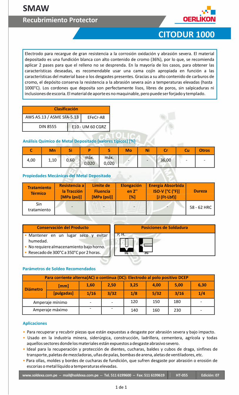
1 de 1
SMAW
Recubrimiento Protector
CITODUR 1000
Electrodo para recargue de gran resistencia a la corrosión oxidación y abrasión severa. El material
depositado es una fundición blanca con alto contenido de cromo (36%), por lo que, se recomienda
aplicar 2 pases para que el relleno no se desprenda. En la mayoría de los casos, para obtener las
características deseadas, es recomendable usar una cama cojín apropiada en función a las
características del material base o los desgastes presentes. Gracias a su alto contenido de carburos de
cromo, el depósito conserva la resistencia a la abrasión severa aún a temperaturas elevadas (hasta
1000°C). Los cordones que deposita son perfectamente lisos, libres de poros, sin salpicaduras ni
inclusiones de escoria. El material de aporte es no maquinable, pero puede ser forjado y templado.
Clasificación
AWS A5.13 / ASME SFA-5.13 EFeCr-A8
DIN 8555 E10 - UM 60 CGRZ
Análisis Químico de Metal Depositado (valores típicos) [%]
C Mn Si P S Mo Ni Cr Cu Otros
4,00 1,10 0,60 máx.
0,020 máx.
0,020 - - 36,00 - -
Propiedades Mecánicas del Metal Depositado
Tratamiento
Térmico
Resistencia a
la Tracción
[MPa (psi)]
Límite de
Fluencia
[MPa (psi)]
Elongación
en 2''
[%]
Energía Absorbida
ISO-V [°C (°F)]
[J (Ft-Lbf)]
Dureza
Sin
tratamiento - - - -
58 - 62 HRC
Conservación del Producto Posiciones de Soldadura
• Mantener en un lugar seco y evitar
humedad.
• No requiere almacenamiento bajo horno.
• Resecado de 300°C a 350°C por 2 horas.
P, H.
1G 2G
Parámetros de Soldeo Recomendados
Para corriente alterna(AC) o continua (DC): Electrodo al polo positivo DCEP
[mm] 1,60 2,50 3,25 4,00 5,00 6,30
Diámetro [pulgadas] 1/16 3/32 1/8 5/32 3/16 1/4
Amperaje mínimo - - 120 150 180 -
Amperaje máximo - - 140 160 230 -
Aplicaciones
• Para recuperar y recubrir piezas que están expuestas a desgaste por abrasión severa y bajo impacto.
• Usado en la industria minera, siderúrgica, construcción, ladrillera, cementera, agrícola y todas
aquellos sectores donde los materiales están expuestos a desgaste abrasivo severo.
• Ideal para la recuperación y protección de dientes, cucharas, baldes y cubos de draga, sinfines de
transporte, paletas de mezcladoras, uñas de palas, bombas de arena, aletas de ventiladores, etc.
• Para ollas, moldes y bordes de cucharas de fundición, que sufren desgaste por abrasión o erosión de
escorias o metal líquido a temperaturas elevadas.
www.soldexa.com.pe -- [email protected] -- Tel. 511 6199600 -- Fax: 511 6199619 HT-055 Edición: 07

ANEXO 5
PROPIEDADES
CITOMANGAN

1 de 1
SMAW
Recubrimiento Protector
CITOMANGAN
Electrodo que deposita un acero al manganeso con 12,0 – 14,0% Mn. Presenta excelente comportamiento
frente a abrasión e impacto severo. El material depositado posee una estructura austenítica de gran
tenacidad, que le permite absorber los golpes durante el trabajo. Por las características del CITOMANGAN,
requiere estar expuesto a impacto severo para que la superficie se autoendurezca y llegue a una dureza final
de 55 HRC. Usar una técnica de soldadura que garantice el mínimo aporte de calor y cuidar que la pieza no
sobrepase los 250°C (riesgo de cristalización). Es susceptible al fisuramiento en caliente, riesgo que se
incrementa por las elevadas contracciones que presenta este material. Cuando se trata de rellenos
considerables, es necesario el empleo de cordones alternados, alivio de tensiones mecánico y de ser
necesario soldar en tinas de agua para extraer el calor aportado.
Clasificación
AWS : A5.13 EFe Mn-B
DIN 8555 E 7 - UM - 200 KP
Análisis Químico de Metal Depositado (valores típicos) [%]
C Mn Si P S Mo Ni Cr Cu Otros
1,00 12,00
14,00 0,50 máx.
0,020 máx.
0,020 - - - - -
Propiedades Mecánicas del Metal Depositado
Tratamiento
Térmico
Resistencia a
la Tracción
[MPa (psi)]
Límite de
Fluencia
[MPa (psi)]
Elongación
en 2''
[%]
Energía Absorbida
ISO-V [°C (°F)]
[J (Ft-Lbf)]
Dureza
Sin tratamiento
Auto endurecido - - - - 19 - 28 HRC
50 - 60 HRC
Conservación del Producto Posiciones de Soldadura
• Mantener en un lugar seco y evitar
humedad.
• No requiere almacenamiento bajo horno.
• Resecado de 300°C a 350°C por 2 horas.
P, H.
1G 2G
Parámetros de Soldeo Recomendados
Para corriente alterna(AC) o continua (DC): Electrodo al polo positivo DCEP
[mm] 1,60 2,50 3,25 4,00 5,00 6,30 Diámetro
[pulgadas] 1/16 3/32 1/8 5/32 3/16 1/4
Amperaje mínimo - - 110 140 170 -
Amperaje máximo - - 135 175 220 -
Aplicaciones
• Para recubrimiento de aceros que van a estar expuestos a desgaste abrasivo combinado con impacto
severo.
• Utilizado con frecuencia en equipos de minería, movimiento de tierra, construcción y ferrocarril.
• Para unir y rellenar piezas de acero al manganeso (13%)
• Las aplicaciones principales son: Relleno de dientes de excavadoras, mandíbulas de trituradoras,
forros de molino, cilindros de trapiche, rieles, cruces y desvíos de vías férreas, baldes de draga, zapatas
para orugas, etc.
Observaciones: El éxito de la aplicación dependerá de la técnica de soldadura seguida, para lo cual,
comuníquense con SOLDEXA para que le brindemos asesoramiento técnico.
www.soldexa.com.pe -- [email protected] -- Tel. 511 6199600 -- Fax: 511 6199619 HT-056 Edición: 07

ANEXO 6
PROPIEDADES
EXADUR – 43
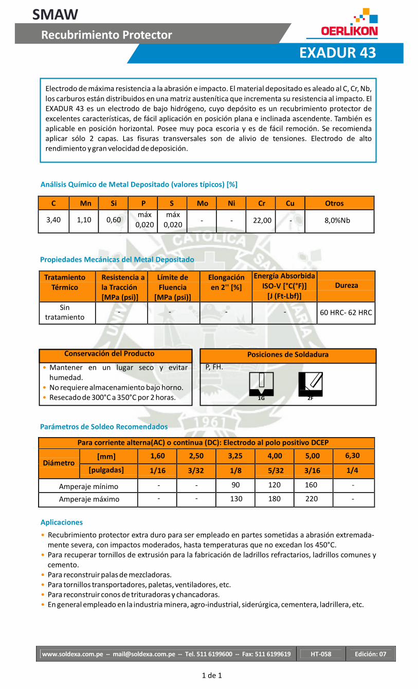
1 de 1
SMAW
Recubrimiento Protector
EXADUR 43
Electrodo de máxima resistencia a la abrasión e impacto. El material depositado es aleado al C, Cr, Nb,
los carburos están distribuidos en una matriz austenítica que incrementa su resistencia al impacto. El
EXADUR 43 es un electrodo de bajo hidrógeno, cuyo depósito es un recubrimiento protector de
excelentes características, de fácil aplicación en posición plana e inclinada ascendente. También es
aplicable en posición horizontal. Posee muy poca escoria y es de fácil remoción. Se recomienda
aplicar sólo 2 capas. Las fisuras transversales son de alivio de tensiones. Electrodo de alto
rendimiento y gran velocidad de deposición.
Análisis Químico de Metal Depositado (valores típicos) [%]
C Mn Si P S Mo Ni Cr Cu Otros
3,40 1,10 0,60 máx
0,020 máx
0,020 - - 22,00 - 8,0%Nb
Propiedades Mecánicas del Metal Depositado
Tratamiento
Térmico Resistencia a
la Tracción
[MPa (psi)]
Límite de
Fluencia
[MPa (psi)]
Elongación
en 2'' [%]
Energía Absorbida
ISO-V [°C(°F)]
[J (Ft-Lbf)]
Dureza
Sin
tratamiento - - - - 60 HRC- 62 HRC
Conservación del Producto
• Mantener en un lugar seco y evitar
humedad.
• No requiere almacenamiento bajo horno.
• Resecado de 300°C a 350°C por 2 horas.
P, FH.
Posiciones de Soldadura
1G 2F
Parámetros de Soldeo Recomendados
Para corriente alterna(AC) o continua (DC): Electrodo al polo positivo DCEP
[mm] 1,60 2,50 3,25 4,00 5,00 6,30
Diámetro [pulgadas] 1/16 3/32 1/8 5/32 3/16 1/4
Amperaje mínimo - - 90 120 160 -
Amperaje máximo - - 130 180 220 -
Aplicaciones
• Recubrimiento protector extra duro para ser empleado en partes sometidas a abrasión extremada-
mente severa, con impactos moderados, hasta temperaturas que no excedan los 450°C.
• Para recuperar tornillos de extrusión para la fabricación de ladrillos refractarios, ladrillos comunes y
cemento.
• Para reconstruir palas de mezcladoras.
• Para tornillos transportadores, paletas, ventiladores, etc.
• Para reconstruir conos de trituradoras y chancadoras.
• En general empleado en la industria minera, agro-industrial, siderúrgica, cementera, ladrillera, etc.
www.soldexa.com.pe -- [email protected] -- Tel. 511 6199600 -- Fax: 511 6199619 HT-058 Edición: 07
ANEXO 7
CASOS DE ESTUDIO
EDEM – FEA
for Handling Bulk Materials
Optimizing

Contents
Challenges of designing bulk material handling equipment
The importance of including the impact of materials
Traditional approaches for calculating material loads
Simulating bulk material behavior with theDiscrete Element Method
Introducing realistic material loads inFinite Element Analysis and Multi-body Dynamics
Case study: Austin Engineering OptimizeCustom Truck Body Performance
Case study: Dragline Bucket Design at VR Steel
Optimizing Heavy Equipment Designfor Handling Bulk Materials
3
5
7
8
9
11
13

Optimizing Heavy Equipment Designfor Handling Bulk Materials
When designing heavy equipment in the construction, off-
highway or mining industries such as truck bodies,
diggers, grab buckets and excavators, engineers are
faced with many challenges. Machines need to be reliable
and efficient, being able to perform well under extreme
conditions, there is constant pressure to increase payload
capacity but at the same time equipment needs to be
lightweight and use fuel efficiently to keep costs down.
To address those challenges, the use of CAE tools such as Finite element analysis (FEA)
and Multi-body dynamics (MBD) are well established in the engineering toolkit for the
design of structures and mechanical equipment. The benefits of simulation driven
product development are numerous and include shorter design cycles, reduced
product development time and costs, product innovation and the need for fewer
physical prototypes resulting in significant cost reduction.
But there is one thing missing in such analysis:
the material itself that the machine is supposed to handle!
Can you spot the difference?
Challenges of Designing Bulk Material Handling Equipment

4

The importance of including the impact of materials
Let’s think about a bucket moving a material like
sand. It can be free-flowing one day but after a
heavy rain shower it becomes highly cohesive and
very difficult to handle.
When in operation, nearly every aspect of equipment
performance – stresses on load arms, hydraulic forces,
traction of tyres, delivery of power, etc. – is dependent to
some degree on the bulk material being handled.
Real bulk materials such as rocks, coal, iron ores, gravel,
soil and grains are complex in their behaviors. They can
vary widely in shape and size. This variability means it is
very difficult for engineers to predict how they will behave
with their equipment.
Bulk materials exist in different form –free-flowing, sticky, cohesive,dry,large lumps, sandy…
Engineers could be dealing with heavy duty, large quarry
rocks that are generating high force impacts; or perhaps a
fine but highly abrasive material such as sand; or even
cohesive clay-like materials that can be difficult to handle
and stick to the equipment.
Optimizing Heavy Equipment Designfor Handling Bulk Materials
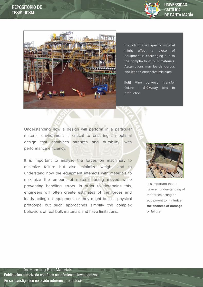
It is important to analyze the forces on machinery to
minimize failure but also minimize weight, and to
understand how the equipment interacts with materials to
maximize the amount of material being moved while
preventing handling errors. In order to determine this,
engineers will often create estimates of the forces and
loads acting on equipment, or they might build a physical
prototype but such approaches simplify the complex
behaviors of real bulk materials and have limitations.
It is important that to
have an understanding of
the forces acting on
equipment to minimize
the chances of damage
or failure.
Understanding how a design will perform in a particular
material environment is critical to ensuring an optimal
design that combines strength and durability, with
performance efficiency.
Optimizing Heavy Equipment Designfor Handling Bulk Materials
Predicting how a specific material
might affect a piece of
equipment is challenging due to
the complexity of bulk materials.
Assumptions may be dangerous
and lead to expensive mistakes.
[left] Mine conveyor transfer
failure - $10M/day loss in
production.
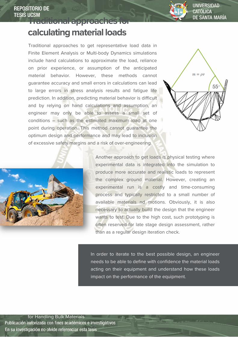
Traditional approaches to get representative load data in
Finite Element Analysis or Multi-body Dynamics simulations
include hand calculations to approximate the load, reliance
on prior experience, or assumption of the anticipated
material behavior. However, these methods cannot
guarantee accuracy and small errors in calculations can lead
to large errors in stress analysis results and fatigue life
prediction. In addition, predicting material behavior is difficult
and by relying on hand calculations and assumption, an
engineer may only be able to assess a small set of
conditions – such as the estimated maximum load at one
point during operation. This method cannot guarantee the
optimum design and performance and may lead to inclusion
of excessive safety margins and a risk of over-engineering.
Another approach to get loads is physical testing where
experimental data is integrated into the simulation to
produce more accurate and realistic loads to represent
the complex ground material. However, creating an
experimental run is a costly and time-consuming
process and typically restricted to a small number of
available materials nd motions. Obviously, it is also
necessary to actually build the design that the engineer
wants to test. Due to the high cost, such prototyping is
often reserved for late stage design assessment, rather
than as a regular design iteration check.
Traditional approaches for calculating material loads
Optimizing Heavy Equipment Designfor Handling Bulk Materials
In order to iterate to the best possible design, an engineer
needs to be able to define with confidence the material loads
acting on their equipment and understand how these loads
impact on the performance of the equipment.

Simulating bulk material behaviorwith the Discrete Element Method
The Discrete Element Method (DEM) is a particle-scale
numerical method for modeling the bulk behavior of
granular materials and geomaterials such as iron ores,
rocks, pellets, tablets, grains, soils, gravel and more.
Using a software powered by DEM technology means
engineers can recreate the behavior of real materials of any
size and shape in a virtual environment and get crucial
insight into how such materials will interact with equipment
during a range of operation and process conditions.
By adding DEM in the design process, engineers can
perform virtual testing of buckets, excavators, bulldozers,
truck bodies and any other piece of equipment with an
accurate representation of the bulk material they are
intended to handle. DEM Simulation of large boulders/ rocks, fine and
cohesive materials
Optimizing Heavy Equipment Designfor Handling Bulk Materials

Optimizing Heavy Equipment Designfor Handling Bulk Materials
Why include the insight of DEM? Get an accurate representation of loads and forces acting on equipment – this
means more accuracy, no more hand calculations, approximations or assumptions
Examine how various movements and conditions as well as different types of
materials will affect the overall design
Reduce the need for physical prototyping – hence reducing costs significantly!
Increase confidence that a design will perform as planned in real conditions
Gain greater insight into equipment performance
When combined with other CAE tools such as FEA and MBD, Discrete
Element Method (DEM) simulation can provide key insight into equipment
designs. It allows engineers to reduce the reliance on hand calculation and
assumption when designing heavy equipment and addresses the challenges
of how their equipment will perform when dealing with bulk materials.
Introducing realistic material loadsin Finite Element Analysis (FEA)and Multi-body Dynamics (MBD)
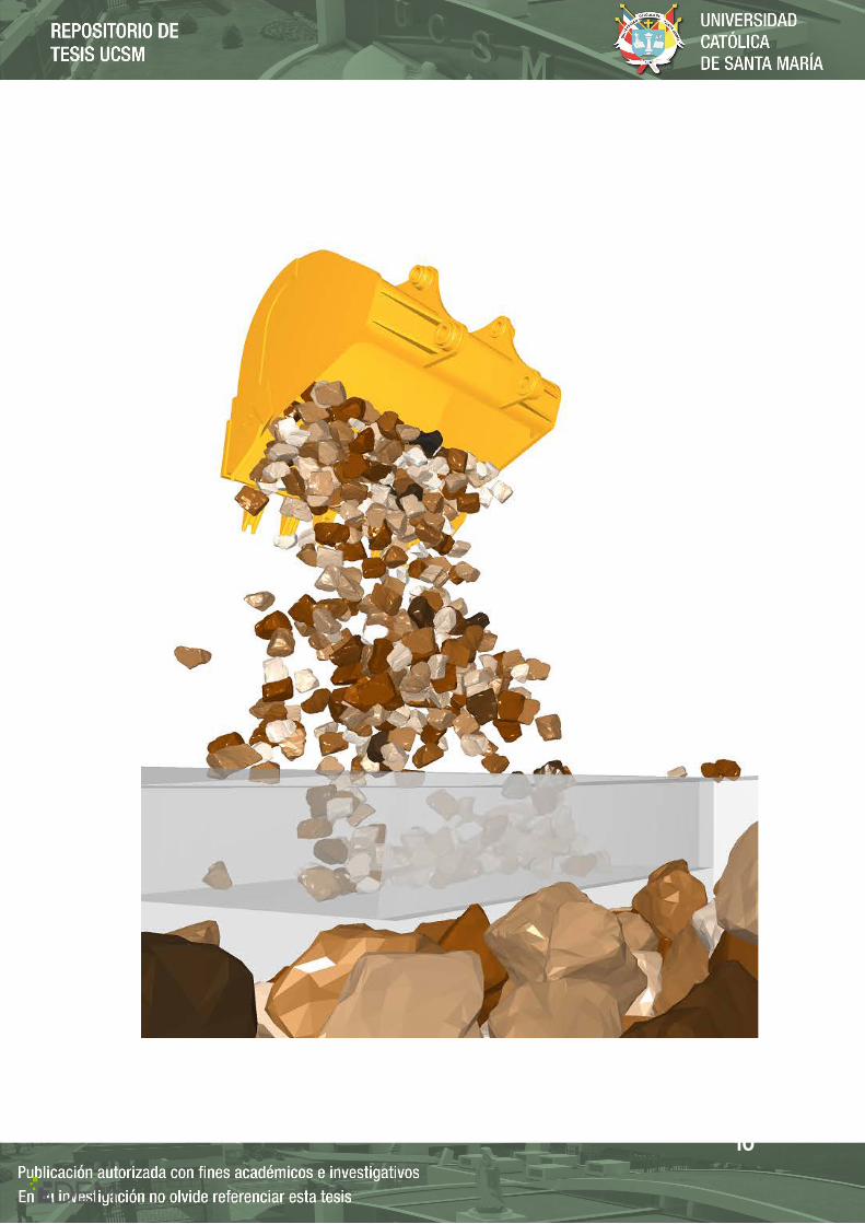
10
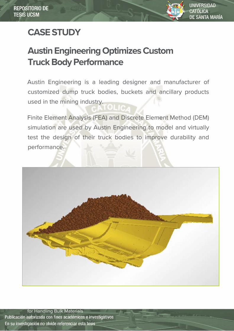
CASE STUDY
Austin Engineering Optimizes Custom Truck Body Performance
Austin Engineering is a leading designer and manufacturer of
customized dump truck bodies, buckets and ancillary products
used in the mining industry.
Finite Element Analysis (FEA) and Discrete Element Method (DEM)
simulation are used by Austin Engineering to model and virtually
test the design of their truck bodies to improve durability and
performance.
Optimizing Heavy Equipment Designfor Handling Bulk Materials
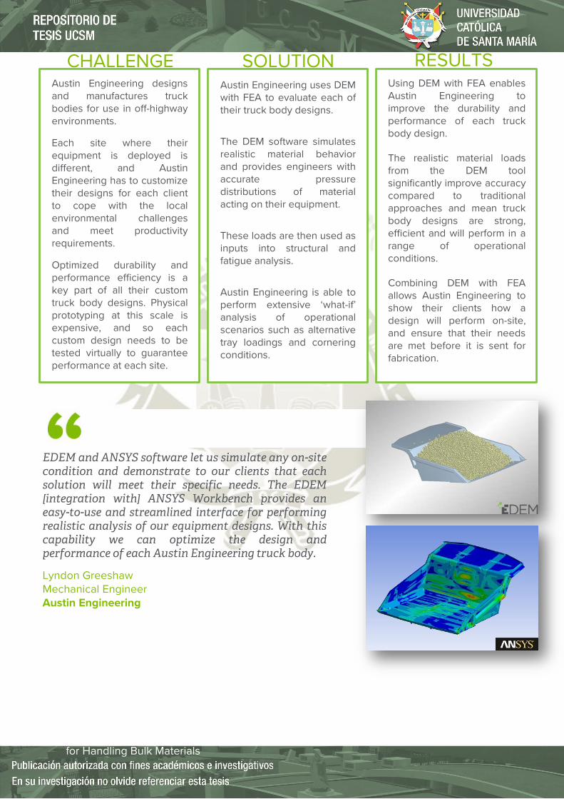
Austin Engineering designsand manufactures truckbodies for use in off-highwayenvironments.
Each site where theirequipment is deployed isdifferent, and AustinEngineering has to customizetheir designs for each clientto cope with the localenvironmental challengesand meet productivityrequirements.
Optimized durability andperformance efficiency is akey part of all their customtruck body designs. Physicalprototyping at this scale isexpensive, and so eachcustom design needs to betested virtually to guaranteeperformance at each site.
EDEM and ANSYS software let us simulate any on-sitecondition and demonstrate to our clients that eachsolution will meet their specific needs. The EDEM[integration with] ANSYS Workbench provides aneasy-to-use and streamlined interface for performingrealistic analysis of our equipment designs. With thiscapability we can optimize the design andperformance of each Austin Engineering truck body.
Lyndon GreeshawMechanical EngineerAustin Engineering
Austin Engineering uses DEMwith FEA to evaluate each oftheir truck body designs.
The DEM software simulatesrealistic material behaviorand provides engineers withaccurate pressuredistributions of materialacting on their equipment.
These loads are then used asinputs into structural andfatigue analysis.
Austin Engineering is able toperform extensive ‘what-if’analysis of operationalscenarios such as alternativetray loadings and corneringconditions.
Using DEM with FEA enablesAustin Engineering toimprove the durability andperformance of each truckbody design.
The realistic material loadsfrom the DEM toolsignificantly improve accuracycompared to traditionalapproaches and mean truckbody designs are strong,efficient and will perform in arange of operationalconditions.
Combining DEM with FEAallows Austin Engineering toshow their clients how adesign will perform on-site,and ensure that their needsare met before it is sent forfabrication.
CHALLENGE SOLUTION RESULTS
Optimizing Heavy Equipment Designfor Handling Bulk Materials

CASE STUDY
Dragline Bucket Design at VR Steel
VR Steel (Pty) Ltd designs, builds, and repairs fabricated mining
equipment attachments.
VR Steel uses Multi-body Dynamics (MBD) and Discrete Element
Method (DEM) software to field-test new design options, custom
designs for specific users, build fewer physical prototypes, shorten
the design cycle and increase customers’ productivity.
Optimizing Heavy Equipment Designfor Handling Bulk Materials
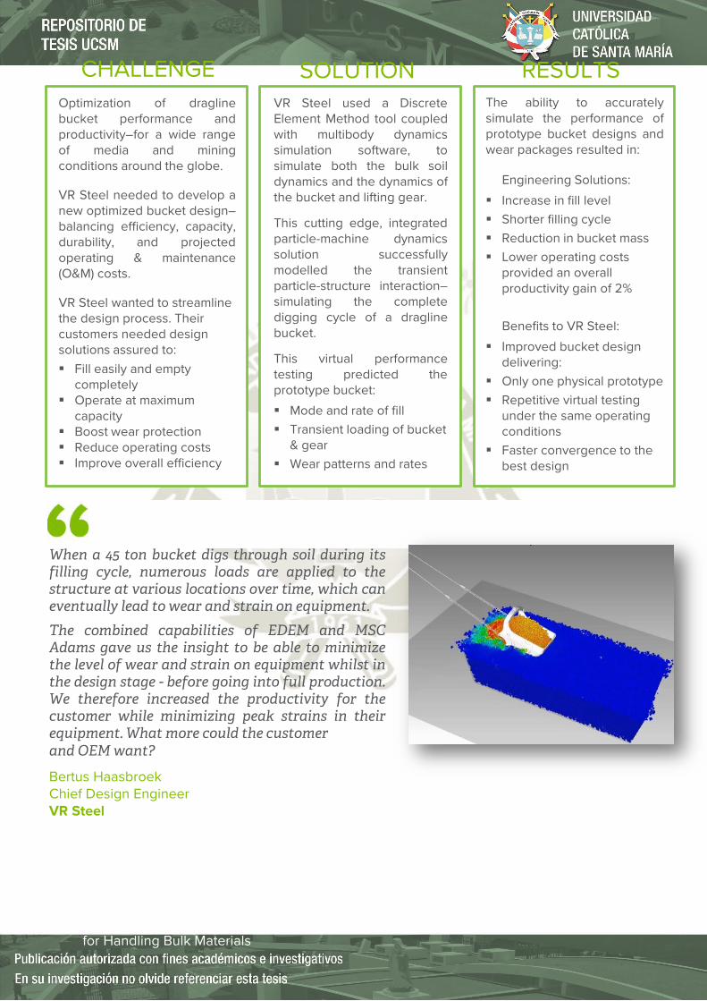
Optimization of draglinebucket performance andproductivity–for a wide rangeof media and miningconditions around the globe.
VR Steel needed to develop anew optimized bucket design–balancing efficiency, capacity,durability, and projectedoperating & maintenance(O&M) costs.
VR Steel wanted to streamline the design process. Their customers needed design solutions assured to: Fill easily and empty
completely Operate at maximum
capacity Boost wear protection Reduce operating costs Improve overall efficiency
When a 45 ton bucket digs through soil during itsfilling cycle, numerous loads are applied to thestructure at various locations over time, which caneventually lead to wear and strain on equipment.The combined capabilities of EDEM and MSCAdams gave us the insight to be able to minimizethe level of wear and strain on equipment whilst inthe design stage - before going into full production.We therefore increased the productivity for thecustomer while minimizing peak strains in theirequipment. What more could the customerand OEM want?
Bertus HaasbroekChief Design EngineerVR Steel
VR Steel used a DiscreteElement Method tool coupledwith multibody dynamicssimulation software, tosimulate both the bulk soildynamics and the dynamics ofthe bucket and lifting gear.
This cutting edge, integratedparticle-machine dynamicssolution successfullymodelled the transientparticle-structure interaction–simulating the completedigging cycle of a draglinebucket.
This virtual performancetesting predicted theprototype bucket:
Mode and rate of fill Transient loading of bucket
& gear Wear patterns and rates
The ability to accuratelysimulate the performance ofprototype bucket designs andwear packages resulted in:
Engineering Solutions:
Increase in fill level Shorter filling cycle Reduction in bucket mass Lower operating costs
provided an overall productivity gain of 2%
Benefits to VR Steel:
Improved bucket design delivering:
Only one physical prototype Repetitive virtual testing
under the same operating conditions
Faster convergence to the best design
CHALLENGE SOLUTION RESULTS
Optimizing Heavy Equipment Designfor Handling Bulk Materials

Interested in bulk material simulation?
Find out more about EDEM –Discrete Element Method (DEM) software
Optimizing Heavy Equipment Designfor Handling Bulk Materials
Want to include realistic material loads in your FEA or MBD tool?
Discover EDEM for CAE –no bulk material simulation knowledge needed

16
EDEM is the market-leading Discrete Element Method (DEM)software for bulk material simulation.
EDEM is used for ‘virtual testing’ of equipment that handles orprocesses bulk materials in the manufacturing of mining,construction, off-highway and agricultural machinery, as well as inthe mining and process industries.
Blue-chip companies around the world use EDEM to optimizeequipment design, increase productivity, reduce costs of operations,shorten product development cycles and drive product innovation.
www.edemsimulation.com© 2017 DEM Solutions Ltd. All Rights Reserved
ANEXO 8
ESPECIFICACIÓN
DEL
PROCEDIMIENTO DE
SOLDADURA (WPS)

ANNEX N AWS D1.1/D1.1M:2008
348
WELDING PROCEDURE SPECIFICATION (WPS) Yes PREQUALIFIED QUALIFIED BY TESTING
or PROCEDURE QUALIFICATION RECORDS (PQR) Yes
Identification #
Revision Date By
Company Name Authorized by Date
Welding Process(es)
Supporting PQR No.(s)
Type—Manual Semiautomatic
Machine Automatic
JOINT DESIGN USED POSITION
Type: Position of Groove:
Single Double Weld Vertical Progression: Up Down
Backing: Yes No
Backing Material: ELECTRICAL CHARACTERISTICS
Fillet:
Root Opening Root Face Dimension
Groove Angle: Radius (J–U) Transfer Mode (GMAW) Short-Circuiting
Back Gouging: Yes No Method Globular Spray
Current: AC DCEP DCEN Pulsed
BASE METALS Power Source: CC CV
Material Spec.
Type or Grade
Other
Tungsten Electrode (GTAW)
Thickness: Groove Fillet Size:
Diameter (Pipe) Type:
FILLER METALS TECHNIQUE
AWS Specification
AWS Classification
Stringer or Weave Bead:
Multi-pass or Single
Pass (per side) Number of
Electrodes
Electrode Spacing Longitudinal
SHIELDING Lateral
Flux
Electrode-Flux (Class)
Gas
Composition
Flow Rate
Angle
Contact Tube to Work Distance
Peening
Gas Cup Size Interpass Cleaning:
PREHEAT POSTWELD HEAT TREATMENT
Preheat Temp., Min. Temp.
Interpass Temp., Min. Max. Time
WELDING PROCEDURE
Pass or
Weld
Layer(s)
Process
Filler Metals Current
Volts
Travel
Speed
Joint Details
Class
Diam.
Type &
Polarity
Amps or Wire
Feed Speed
Form N-1 (Front)

ANNEX N AWS D1.1/D1.1M:2008
352
Procedure Qualification Record (PQR) # Test Results
TENSILE TEST
Specimen
No.
Width
Thickness
Area Ultimate Tensile
Load, lb
Ultimate Unit
Stress, psi
Character of Failure
and Location
GUIDED BEND TEST
Specimen
No.
Type of Bend
Result
Remarks
VISUAL INSPECTION
Appearance
Radiographic-ultrasonic examination
Undercut
Piping porosity
RT report no.:
UT report no.:
Result
Result
Convexity
Test date
Witnessed by
FILLET WELD TEST RESULTS
Minimum size multiple pass Maximum size single pass
Macroetch Macroetch
1.
2.
3. 1.
2.
3.
Other Tests All-weld-metal tension test
Tensile strength, psi
Yield point/strength, psi
Elongation in 2 in, %
Laboratory test no.
Welder’s name Clock no. Stamp no.
Tests conducted by Laboratory
Test number
Per
We, the undersigned, certify that the statements in this record are correct and that the test welds were prepared, welded, and tested in conformance with the requirements of Clause 4 of AWS D1.1/D1.1M, ( ) Structural Welding Code—Steel.
(year)
Signed
Manufacturer or Contractor
By
Title
Date
Form N-1 (Back)

ANEXO 9
NORMA
ASTM E-11
Designation: E3 − 11
Standard Guide forPreparation of Metallographic Specimens1
This standard is issued under the fixed designation E3; the number immediately following the designation indicates the year of originaladoption or, in the case of revision, the year of last revision. A number in parentheses indicates the year of last reapproval. A superscriptepsilon (´) indicates an editorial change since the last revision or reapproval.
This standard has been approved for use by agencies of the Department of Defense.
1. Scope
1.1 The primary objective of metallographic examinationsis to reveal the constituents and structure of metals and theiralloys by means of a light optical or scanning electronmicroscope. In special cases, the objective of the examinationmay require the development of less detail than in other casesbut, under nearly all conditions, the proper selection andpreparation of the specimen is of major importance. Because ofthe diversity in available equipment and the wide variety ofproblems encountered, the following text presents for theguidance of the metallographer only those practices whichexperience has shown are generally satisfactory; it cannot anddoes not describe the variations in technique required to solveindividual specimen preparation problems.
NOTE 1—For a more extensive description of various metallographictechniques, refer to Samuels, L. E., Metallographic Polishing by Mechani-cal Methods, American Society for Metals (ASM) Metals Park, OH, 3rdEd., 1982; Petzow, G., Metallographic Etching, ASM, 1978; andVanderVoort, G., Metallography: Principles and Practice, McGraw Hill,NY, 2nd Ed., 1999.
1.2 This standard does not purport to address all of thesafety concerns, if any, associated with its use. It is theresponsibility of the user of this standard to establish appro-priate safety and health practices and determine the applica-bility of regulatory limitations prior to use.
2. Referenced Documents
2.1 ASTM Standards:A90/A90M Test Method for Weight [Mass] of Coating on
Iron and Steel Articles with Zinc or Zinc-Alloy Coatings2
E7 Terminology Relating to MetallographyE45 Test Methods for Determining the Inclusion Content of
Steel
E768 Guide for Preparing and Evaluating Specimens forAutomatic Inclusion Assessment of Steel
E1077 Test Methods for Estimating the Depth of Decarbur-ization of Steel Specimens
E1122 Practice for Obtaining JK Inclusion Ratings UsingAutomatic Image Analysis (Withdrawn 2006)3
E1245 Practice for Determining the Inclusion or Second-Phase Constituent Content of Metals by Automatic ImageAnalysis
E1268 Practice for Assessing the Degree of Banding orOrientation of Microstructures
E1558 Guide for Electrolytic Polishing of MetallographicSpecimens
E1920 Guide for Metallographic Preparation of ThermalSprayed Coatings
3. Terminology
3.1 Definitions:3.1.1 For definitions used in this practice, refer to Termi-
nology E7.
3.2 Definitions of Terms Specific to This Standard:3.2.1 castable mount—a metallographic mount generally
made from a two component castable plastic. One componentis the resin and the other hardener. Both components can heliquid or one liquid and a powder. Castable mounts generallydo not require heat and pressure to cure.
3.2.2 compression mount—a metallographic mount madeusing plastic that requires both heat and pressure for curing.
3.2.3 planar grinding—is the first grinding step in a prepa-ration procedure used to bring all specimens into the sameplane of polish. It is unique to semi or fully automaticpreparation equipment that utilize specimen holders.
3.2.4 rigid grinding disc—a non-fabric support surface,such as a composite of metal/ceramic or metal/polymercharged with an abrasive (usually 6 to 15µm diamondparticles), and used as the fine grinding operation in a metal-lographic preparation procedure.
1 This guide is under the jurisdiction of ASTM Committee E04 on Metallographyand is the direct responsibility of Subcommittee E04.01 on Specimen Preparation.
Current edition approved May 1, 2011. Published June 2011. Originallyapproved in 1921. Last previous edition approved in 2007 as E3– 01(2007)´1. DOI:10.1520/E0003-11.
2 For referenced ASTM standards, visit the ASTM website, www.astm.org, orcontact ASTM Customer Service at [email protected]. For Annual Book of ASTMStandards volume information, refer to the standard’s Document Summary page onthe ASTM website.
3 The last approved version of this historical standard is referenced onwww.astm.org.
Copyright © ASTM International, 100 Barr Harbor Drive, PO Box C700, West Conshohocken, PA 19428-2959. United States
1
Copyright by ASTM Int'l (all rights reserved); Thu Sep 20 10:13:22 EDT 2012Downloaded/printed byMC MASTER UNIVERSITY pursuant to License Agreement. No further reproductions authorized.
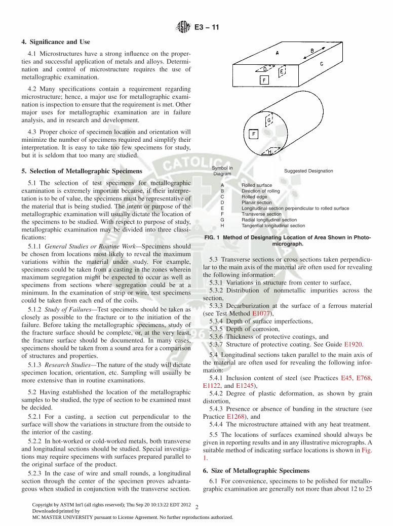
4. Significance and Use
4.1 Microstructures have a strong influence on the proper-ties and successful application of metals and alloys. Determi-nation and control of microstructure requires the use ofmetallographic examination.
4.2 Many specifications contain a requirement regardingmicrostructure; hence, a major use for metallographic exami-nation is inspection to ensure that the requirement is met. Othermajor uses for metallographic examination are in failureanalysis, and in research and development.
4.3 Proper choice of specimen location and orientation willminimize the number of specimens required and simplify theirinterpretation. It is easy to take too few specimens for study,but it is seldom that too many are studied.
5. Selection of Metallographic Specimens
5.1 The selection of test specimens for metallographicexamination is extremely important because, if their interpre-tation is to be of value, the specimens must be representative ofthe material that is being studied. The intent or purpose of themetallographic examination will usually dictate the location ofthe specimens to be studied. With respect to purpose of study,metallographic examination may be divided into three classi-fications:
5.1.1 General Studies or Routine Work—Specimens shouldbe chosen from locations most likely to reveal the maximumvariations within the material under study. For example,specimens could be taken from a casting in the zones whereinmaximum segregation might be expected to occur as well asspecimens from sections where segregation could be at aminimum. In the examination of strip or wire, test specimenscould be taken from each end of the coils.
5.1.2 Study of Failures—Test specimens should be taken asclosely as possible to the fracture or to the initiation of thefailure. Before taking the metallographic specimens, study ofthe fracture surface should be complete, or, at the very least,the fracture surface should be documented. In many cases,specimens should be taken from a sound area for a comparisonof structures and properties.
5.1.3 Research Studies—The nature of the study will dictatespecimen location, orientation, etc. Sampling will usually bemore extensive than in routine examinations.
5.2 Having established the location of the metallographicsamples to be studied, the type of section to be examined mustbe decided.
5.2.1 For a casting, a section cut perpendicular to thesurface will show the variations in structure from the outside tothe interior of the casting.
5.2.2 In hot-worked or cold-worked metals, both transverseand longitudinal sections should be studied. Special investiga-tions may require specimens with surfaces prepared parallel tothe original surface of the product.
5.2.3 In the case of wire and small rounds, a longitudinalsection through the center of the specimen proves advanta-geous when studied in conjunction with the transverse section.
5.3 Transverse sections or cross sections taken perpendicu-lar to the main axis of the material are often used for revealingthe following information:
5.3.1 Variations in structure from center to surface,5.3.2 Distribution of nonmetallic impurities across the
section,5.3.3 Decarburization at the surface of a ferrous material
(see Test Method E1077),5.3.4 Depth of surface imperfections,5.3.5 Depth of corrosion,5.3.6 Thickness of protective coatings, and5.3.7 Structure of protective coating. See Guide E1920.
5.4 Longitudinal sections taken parallel to the main axis ofthe material are often used for revealing the following infor-mation:
5.4.1 Inclusion content of steel (see Practices E45, E768,E1122, and E1245),
5.4.2 Degree of plastic deformation, as shown by graindistortion,
5.4.3 Presence or absence of banding in the structure (seePractice E1268), and
5.4.4 The microstructure attained with any heat treatment.
5.5 The locations of surfaces examined should always begiven in reporting results and in any illustrative micrographs. Asuitable method of indicating surface locations is shown in Fig.1.
6. Size of Metallographic Specimens
6.1 For convenience, specimens to be polished for metallo-graphic examination are generally not more than about 12 to 25
Symbol inDiagram
Suggested Designation
A Rolled surfaceB Direction of rollingC Rolled edgeD Planar sectionE Longitudinal section perpendicular to rolled surfaceF Transverse sectionG Radial longitudinal sectionH Tangential longitudinal section
FIG. 1 Method of Designating Location of Area Shown in Photo-micrograph.
E3 − 11
2
Copyright by ASTM Int'l (all rights reserved); Thu Sep 20 10:13:22 EDT 2012Downloaded/printed byMC MASTER UNIVERSITY pursuant to License Agreement. No further reproductions authorized.

mm (0.5 to 1.0 in.) square, or approximately 12 to 25 mm indiameter if the material is cylindrical. The height of thespecimen should be no greater than necessary for convenienthandling during polishing.
6.1.1 Larger specimens are generally more difficult to pre-pare.
6.1.2 Specimens that are, fragile, oddly shaped or too smallto be handled readily during polishing should be mounted toensure a surface satisfactory for microscopical study. Thereare, based on technique used, three fundamental methods ofmounting specimens (see Section 9).
7. Cutting of Metallographic Specimens
7.1 In cutting the metallographic specimen from the mainbody of the material, care must be exercised to minimizealtering the structure of the metal. Three common types ofsectioning are as follows:
7.1.1 Sawing, whether by hand or machine with lubrication,is easy, fast, and relatively cool. It can be used on all materialswith hardnesses below approximately 350 HV. It does producea rough surface containing extensive plastic flow that must beremoved in subsequent preparation.
7.1.2 An abrasive cut-off blade will produce a smoothsurface often ready for fine grinding. This method of sectioningis normally faster than sawing. The choice of cut-off blade,lubricant, cooling conditions, and the grade and hardness ofmetal being cut will influence the quality of the cut. A poorchoice of cutting conditions can easily damage the specimen,producing an alteration of the microstructure. Generally, softmaterials are cut with a hard bond blade and hard materialswith a soft bond blade. Aluminum oxide abrasive blades arepreferred for ferrous metals and silicon carbide blades arepreferred for nonferrous alloys. Abrasive cut-off blades areessential for sectioning metals with hardness above about 350HV. Extremely hard metallic materials and ceramics may bemore effectively cut using diamond-impregnated cuttingblades. Manufacturer’s instructions should be followed as tothe choice of blade. Table 1 lists the suggested cutoff blades formaterials with various Vickers (HV) hardness values.
7.1.3 A shear is a type of cutting tool with which a materialin the form of wire, sheet, plate or rod is cut between twoopposing blades.
7.2 Other methods of sectioning are permitted provided theydo not alter the microstructure at the plane of polishing. Allcutting operations produce some depth of damage, which willhave to be removed in subsequent preparation steps.
8. Cleanliness
8.1 Cleanliness (see Appendix X1) during specimen prepa-ration is essential. All greases, oils, coolants and residue fromcutoff blades on the specimen should be removed by somesuitable organic solvent. Failure to clean thoroughly canprevent cold mounting resins from adhering to the specimensurface. Ultrasonic cleaning may be effective in removing thelast traces of residues on a specimen surface.
8.2 Any coating metal that will interfere with the subse-quent etching of the base metal should be removed beforepolishing, if possible. If etching is required, when studying theunderlying steel in a galvanized specimen, the zinc coatingshould be removed before mounting to prevent galvanic effectsduring etching. The coating can be removed by dissolving incold nitric acid (HNO3, sp gr 1.42), in dilute sulfuric acid(H2SO4) or in dilute hydrochloric acid (HCl). The HNO3
method requires care to prevent overheating, since largesamples will generate considerable heat. By placing the clean-ing container in cold water during the stripping of the zinc,attack on the underlying steel will be minimized. Moreinformation may be found in Test Method A90/A90M.
NOTE 2—Picral etchant produces little or no galvanic etching effectswhen used on galvanized steel.
NOTE 3—The addition of an inhibitor during the stripping of Zn fromgalvanized coatings will minimize the attack of the steel substrate. NEP(polethylinepolyamine) or SbCl3 are two useful inhibitors.
8.3 Oxidized or corroded surfaces may be cleaned asdescribed in Appendix X1.
9. Mounting of Specimens
9.1 There are many instances where it will be advantageousto mount the specimen prior to grinding and polishing. Mount-ing of the specimen is usually performed on small, fragile, oroddly shaped specimens, fractures, or in instances where thespecimen edges are to be examined.
9.2 Specimens may be either mechanically mounted,mounted in plastic, or a combination of the two.
9.3 Mechanical Mounting:9.3.1 Strip and sheet specimens may be mounted by binding
or clamping several specimens into a pack held together by twoend pieces and two bolts.
9.3.2 The specimens should be tightly bound together toprevent absorption and subsequent exudation of polishingmaterials or etchants.
9.3.3 The use of filler sheets of a softer material alternatedwith the specimen may be used in order to minimize theseepage of polishing materials and etchants. Use of fillermaterial is especially advantageous if the specimens have ahigh degree of surface irregularities.
9.3.4 Filler material must be chosen so as not to reactelectrolytically with the specimen during etching. Thin piecesof plastic, lead, or copper are typical materials that are used.
TABLE 1 Cutoff Blade Selection
HardnessHV
Materials Abrasive BondBond
Hardness
up to 300 non-ferrous (Al, Cu) SiC P or R hardup to 400 non-ferrous (Ti) SiC P or R med.
hardup to 400 soft ferrous Al2O3 P or R hardup to 500 medium soft ferrous Al2O3 P or R med.
hardup to 600 medium hard ferrous Al2O3 P or R mediumup to 700 hard ferrous Al2O3 P or R&R med. softup to 800 very hard ferrous Al2O3 P or R&R soft
> 800 extremely hard ferrous CBN P or M hardmore brittle ceramics diamond P or M very hard
tougher ceramics diamond M ext. hard
P—phenolicR—rubberR&R—resin and rubberM—metal
E3 − 11
3
Copyright by ASTM Int'l (all rights reserved); Thu Sep 20 10:13:22 EDT 2012Downloaded/printed byMC MASTER UNIVERSITY pursuant to License Agreement. No further reproductions authorized.
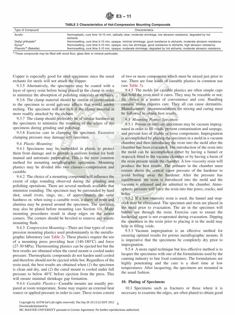
Copper is especially good for steel specimens since the usualetchants for steels will not attack the copper.
9.3.5 Alternatively, the specimens may be coated with alayer of epoxy resin before being placed in the clamp in orderto minimize the absorption of polishing materials or etchants.
9.3.6 The clamp material should be similar in compositionto the specimen to avoid galvanic effects that would inhibitetching. The specimen will not etch if the clamp material ismore readily attacked by the etchant.
9.3.7 The clamp should preferably be of similar hardness asthe specimens to minimize the rounding of the edges of thespecimens during grinding and polishing.
9.3.8 Exercise care in clamping the specimen. Excessiveclamping pressure may damage soft specimen.
9.4 Plastic Mounting:9.4.1 Specimens may be embedded in plastic to protect
them from damage and to provide a uniform format for bothmanual and automatic preparation. This is the most commonmethod for mounting metallographic specimens. Mountingplastics may be divided into two classes—compression andcastable.
9.4.2 The choice of a mounting compound will influence theextent of edge rounding observed during the grinding andpolishing operations. There are several methods available thatminimize rounding. The specimen may be surrounded by hardshot, small rivets, rings, etc., of approximately the samehardness or, when using a castable resin, a slurry of resin andalumina may be poured around the specimen. The specimenmay also be plated before mounting (see Section 10). Manymounting procedures result in sharp edges on the mountcorners. The corners should be beveled to remove any plasticmounting flash.
9.4.3 Compression Mounting—There are four types of com-pression mounting plastics used predominantly in the metallo-graphic laboratory (see Table 2). These plastics require the useof a mounting press providing heat (140-180°C) and force(27-30 MPa). Thermosetting plastics can be ejected hot but thebest results are obtained when the cured mount is cooled underpressure. Thermoplastic compounds do not harden until cooledand therefore should not be ejected while hot. Regardless of theresin used, the best results are obtained when (1) the specimenis clean and dry, and (2) the cured mount is cooled under fullpressure to below 40°C before ejection from the press. Thiswill ensure minimal shrinkage gap formation.
9.4.4 Castable Plastics—Castable mounts are usually pre-pared at room temperature. Some may require an external heatsource or applied pressure in order to cure. These resins consist
of two or more components which must be mixed just prior touse. There are four kinds of castable plastics in common use(see Table 3).
9.4.5 The molds for castable plastics are often simple cupsthat hold the resin until it cures. They may be reusable or not;the choice is a matter of convenience and cost. Handlingcastable resins requires care. They all can cause dermatitis.Manufacturers’ recommendations for mixing and curing mustbe followed to obtain best results.
9.5 Mounting Porous Specimen:9.5.1 Porous or intricate specimens may be vacuum impreg-
nated in order to fill voids, prevent contamination and seepage,and prevent loss of friable or loose components. Impregnationis accomplished by placing the specimen in a mold in a vacuumchamber and then introducing the resin into the mold after thechamber has been evacuated. The introduction of the resin intothe mold can be accomplished either by having a funnel orstopcock fitted to the vacuum chamber or by having a basin ofthe resin present inside the chamber. A low-viscosity resin willproduce the best results. The pressure in the chamber mustremain above the critical vapor pressure of the hardener toavoid boiling away the hardener. After the pressure hasequilibrated, the resin is introduced into the mold and thevacuum is released and air admitted to the chamber. Atmo-spheric pressure will force the resin into fine pores, cracks, andholes.
9.5.2 If a low-viscosity resin is used, the funnel and stop-cock may be eliminated. The specimen and resin are placed inthe mold prior to evacuation. The air in the specimen willbubble out through the resin. Exercise care to ensure thehardening agent is not evaporated during evacuation. Dippingthe specimen in the resin prior to placing it in the mold mayhelp in filling voids.
9.5.3 Vacuum impregnation is an effective method forensuring optimal results for porous metallographic mounts. Itis imperative that the specimens be completely dry prior toimpregnation.
9.5.4 A more rapid technique but less effective method is tolacquer the specimens with one of the formulations used by thecanning industry to line food containers. The formulations arehighly penetrating and the cure is a short time at lowtemperatures. After lacquering, the specimens are mounted inthe usual fashion.
10. Plating of Specimens
10.1 Specimens such as fractures or those where it isnecessary to examine the edges, are often plated to obtain good
TABLE 2 Characteristics of Hot-Compression Mounting Compounds
Type of Compound Characteristics
Acrylic thermoplastic, cure time 10-15 min, optically clear, moderate shrinkage, low abrasion resistance, degraded by hotetchants
Diallyl phthalateA thermosetting, cure time 5-10 min, opaque, minimal shrinkage, good resistance to etchants, moderate abrasion resistanceEpoxyA thermosetting, cure time 5-10 min, opaque, very low shrinkage, good resistance to etchants, high abrasion resistancePhenolicA (Bakelite) thermosetting, cure time 5-10 min, opaque, moderate shrinkage, degraded by hot etchants, moderate abrasion resistance
A These compounds may be filled with wood flour, glass fiber or mineral particulate.
E3 − 11
4
Copyright by ASTM Int'l (all rights reserved); Thu Sep 20 10:13:22 EDT 2012Downloaded/printed byMC MASTER UNIVERSITY pursuant to License Agreement. No further reproductions authorized.
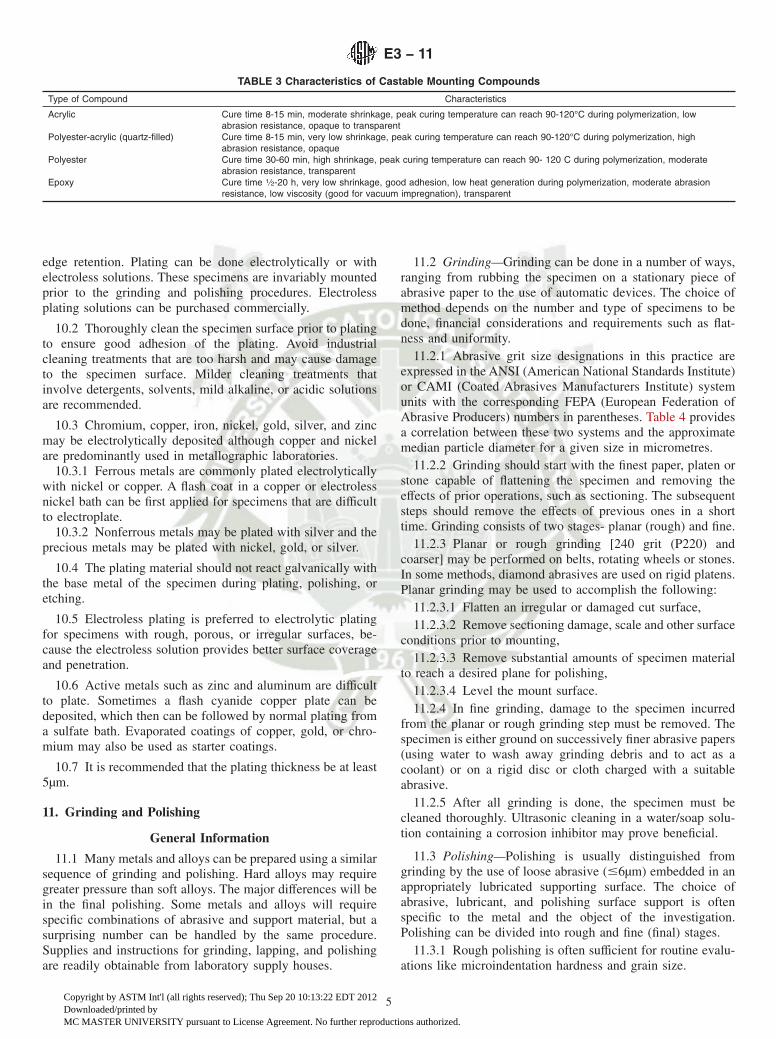
edge retention. Plating can be done electrolytically or withelectroless solutions. These specimens are invariably mountedprior to the grinding and polishing procedures. Electrolessplating solutions can be purchased commercially.
10.2 Thoroughly clean the specimen surface prior to platingto ensure good adhesion of the plating. Avoid industrialcleaning treatments that are too harsh and may cause damageto the specimen surface. Milder cleaning treatments thatinvolve detergents, solvents, mild alkaline, or acidic solutionsare recommended.
10.3 Chromium, copper, iron, nickel, gold, silver, and zincmay be electrolytically deposited although copper and nickelare predominantly used in metallographic laboratories.
10.3.1 Ferrous metals are commonly plated electrolyticallywith nickel or copper. A flash coat in a copper or electrolessnickel bath can be first applied for specimens that are difficultto electroplate.
10.3.2 Nonferrous metals may be plated with silver and theprecious metals may be plated with nickel, gold, or silver.
10.4 The plating material should not react galvanically withthe base metal of the specimen during plating, polishing, oretching.
10.5 Electroless plating is preferred to electrolytic platingfor specimens with rough, porous, or irregular surfaces, be-cause the electroless solution provides better surface coverageand penetration.
10.6 Active metals such as zinc and aluminum are difficultto plate. Sometimes a flash cyanide copper plate can bedeposited, which then can be followed by normal plating froma sulfate bath. Evaporated coatings of copper, gold, or chro-mium may also be used as starter coatings.
10.7 It is recommended that the plating thickness be at least5µm.
11. Grinding and Polishing
General Information
11.1 Many metals and alloys can be prepared using a similarsequence of grinding and polishing. Hard alloys may requiregreater pressure than soft alloys. The major differences will bein the final polishing. Some metals and alloys will requirespecific combinations of abrasive and support material, but asurprising number can be handled by the same procedure.Supplies and instructions for grinding, lapping, and polishingare readily obtainable from laboratory supply houses.
11.2 Grinding—Grinding can be done in a number of ways,ranging from rubbing the specimen on a stationary piece ofabrasive paper to the use of automatic devices. The choice ofmethod depends on the number and type of specimens to bedone, financial considerations and requirements such as flat-ness and uniformity.
11.2.1 Abrasive grit size designations in this practice areexpressed in the ANSI (American National Standards Institute)or CAMI (Coated Abrasives Manufacturers Institute) systemunits with the corresponding FEPA (European Federation ofAbrasive Producers) numbers in parentheses. Table 4 providesa correlation between these two systems and the approximatemedian particle diameter for a given size in micrometres.
11.2.2 Grinding should start with the finest paper, platen orstone capable of flattening the specimen and removing theeffects of prior operations, such as sectioning. The subsequentsteps should remove the effects of previous ones in a shorttime. Grinding consists of two stages- planar (rough) and fine.
11.2.3 Planar or rough grinding [240 grit (P220) andcoarser] may be performed on belts, rotating wheels or stones.In some methods, diamond abrasives are used on rigid platens.Planar grinding may be used to accomplish the following:
11.2.3.1 Flatten an irregular or damaged cut surface,11.2.3.2 Remove sectioning damage, scale and other surface
conditions prior to mounting,11.2.3.3 Remove substantial amounts of specimen material
to reach a desired plane for polishing,11.2.3.4 Level the mount surface.11.2.4 In fine grinding, damage to the specimen incurred
from the planar or rough grinding step must be removed. Thespecimen is either ground on successively finer abrasive papers(using water to wash away grinding debris and to act as acoolant) or on a rigid disc or cloth charged with a suitableabrasive.
11.2.5 After all grinding is done, the specimen must becleaned thoroughly. Ultrasonic cleaning in a water/soap solu-tion containing a corrosion inhibitor may prove beneficial.
11.3 Polishing—Polishing is usually distinguished fromgrinding by the use of loose abrasive (#6µm) embedded in anappropriately lubricated supporting surface. The choice ofabrasive, lubricant, and polishing surface support is oftenspecific to the metal and the object of the investigation.Polishing can be divided into rough and fine (final) stages.
11.3.1 Rough polishing is often sufficient for routine evalu-ations like microindentation hardness and grain size.
TABLE 3 Characteristics of Castable Mounting Compounds
Type of Compound Characteristics
Acrylic Cure time 8-15 min, moderate shrinkage, peak curing temperature can reach 90-120°C during polymerization, lowabrasion resistance, opaque to transparent
Polyester-acrylic (quartz-filled) Cure time 8-15 min, very low shrinkage, peak curing temperature can reach 90-120°C during polymerization, highabrasion resistance, opaque
Polyester Cure time 30-60 min, high shrinkage, peak curing temperature can reach 90- 120 C during polymerization, moderateabrasion resistance, transparent
Epoxy Cure time 1⁄2-20 h, very low shrinkage, good adhesion, low heat generation during polymerization, moderate abrasionresistance, low viscosity (good for vacuum impregnation), transparent
E3 − 11
5
Copyright by ASTM Int'l (all rights reserved); Thu Sep 20 10:13:22 EDT 2012Downloaded/printed byMC MASTER UNIVERSITY pursuant to License Agreement. No further reproductions authorized.
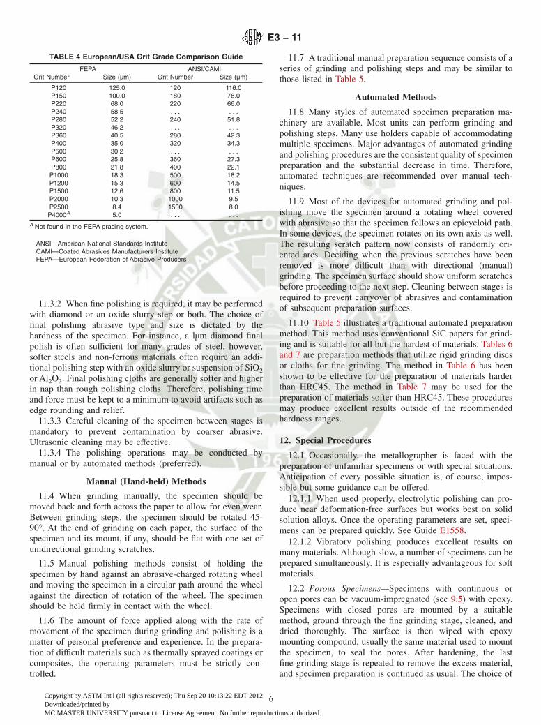
11.3.2 When fine polishing is required, it may be performedwith diamond or an oxide slurry step or both. The choice offinal polishing abrasive type and size is dictated by thehardness of the specimen. For instance, a lµm diamond finalpolish is often sufficient for many grades of steel, however,softer steels and non-ferrous materials often require an addi-tional polishing step with an oxide slurry or suspension of SiO2
or Al2O3. Final polishing cloths are generally softer and higherin nap than rough polishing cloths. Therefore, polishing timeand force must be kept to a minimum to avoid artifacts such asedge rounding and relief.
11.3.3 Careful cleaning of the specimen between stages ismandatory to prevent contamination by coarser abrasive.Ultrasonic cleaning may be effective.
11.3.4 The polishing operations may be conducted bymanual or by automated methods (preferred).
Manual (Hand-held) Methods
11.4 When grinding manually, the specimen should bemoved back and forth across the paper to allow for even wear.Between grinding steps, the specimen should be rotated 45-90°. At the end of grinding on each paper, the surface of thespecimen and its mount, if any, should be flat with one set ofunidirectional grinding scratches.
11.5 Manual polishing methods consist of holding thespecimen by hand against an abrasive-charged rotating wheeland moving the specimen in a circular path around the wheelagainst the direction of rotation of the wheel. The specimenshould be held firmly in contact with the wheel.
11.6 The amount of force applied along with the rate ofmovement of the specimen during grinding and polishing is amatter of personal preference and experience. In the prepara-tion of difficult materials such as thermally sprayed coatings orcomposites, the operating parameters must be strictly con-trolled.
11.7 A traditional manual preparation sequence consists of aseries of grinding and polishing steps and may be similar tothose listed in Table 5.
Automated Methods
11.8 Many styles of automated specimen preparation ma-chinery are available. Most units can perform grinding andpolishing steps. Many use holders capable of accommodatingmultiple specimens. Major advantages of automated grindingand polishing procedures are the consistent quality of specimenpreparation and the substantial decrease in time. Therefore,automated techniques are recommended over manual tech-niques.
11.9 Most of the devices for automated grinding and pol-ishing move the specimen around a rotating wheel coveredwith abrasive so that the specimen follows an epicycloid path.In some devices, the specimen rotates on its own axis as well.The resulting scratch pattern now consists of randomly ori-ented arcs. Deciding when the previous scratches have beenremoved is more difficult than with directional (manual)grinding. The specimen surface should show uniform scratchesbefore proceeding to the next step. Cleaning between stages isrequired to prevent carryover of abrasives and contaminationof subsequent preparation surfaces.
11.10 Table 5 illustrates a traditional automated preparationmethod. This method uses conventional SiC papers for grind-ing and is suitable for all but the hardest of materials. Tables 6and 7 are preparation methods that utilize rigid grinding discsor cloths for fine grinding. The method in Table 6 has beenshown to be effective for the preparation of materials harderthan HRC45. The method in Table 7 may be used for thepreparation of materials softer than HRC45. These proceduresmay produce excellent results outside of the recommendedhardness ranges.
12. Special Procedures
12.1 Occasionally, the metallographer is faced with thepreparation of unfamiliar specimens or with special situations.Anticipation of every possible situation is, of course, impos-sible but some guidance can be offered.
12.1.1 When used properly, electrolytic polishing can pro-duce near deformation-free surfaces but works best on solidsolution alloys. Once the operating parameters are set, speci-mens can be prepared quickly. See Guide E1558.
12.1.2 Vibratory polishing produces excellent results onmany materials. Although slow, a number of specimens can beprepared simultaneously. It is especially advantageous for softmaterials.
12.2 Porous Specimens—Specimens with continuous oropen pores can be vacuum-impregnated (see 9.5) with epoxy.Specimens with closed pores are mounted by a suitablemethod, ground through the fine grinding stage, cleaned, anddried thoroughly. The surface is then wiped with epoxymounting compound, usually the same material used to mountthe specimen, to seal the pores. After hardening, the lastfine-grinding stage is repeated to remove the excess material,and specimen preparation is continued as usual. The choice of
TABLE 4 European/USA Grit Grade Comparison Guide
FEPA ANSI/CAMIGrit Number Size (µm) Grit Number Size (µm)
P120 125.0 120 116.0P150 100.0 180 78.0P220 68.0 220 66.0P240 58.5 . . . . . .P280 52.2 240 51.8P320 46.2 . . . . . .P360 40.5 280 42.3P400 35.0 320 34.3P500 30.2 . . . . . .P600 25.8 360 27.3P800 21.8 400 22.1P1000 18.3 500 18.2P1200 15.3 600 14.5P1500 12.6 800 11.5P2000 10.3 1000 9.5P2500 8.4 1500 8.0P4000A 5.0 . . . . . .
A Not found in the FEPA grading system.
ANSI—American National Standards InstituteCAMI—Coated Abrasives Manufacturers InstituteFEPA—European Federation of Abrasive Producers
E3 − 11
6
Copyright by ASTM Int'l (all rights reserved); Thu Sep 20 10:13:22 EDT 2012Downloaded/printed byMC MASTER UNIVERSITY pursuant to License Agreement. No further reproductions authorized.
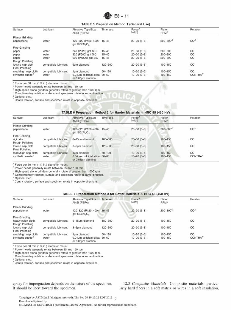
epoxy for impregnation depends on the nature of the specimen.It should be inert toward the specimen.
12.3 Composite Materials—Composite materials, particu-larly hard fibers in a soft matrix or wires in a soft insulation,
TABLE 5 Preparation Method 1 (General Use)
Surface Lubricant Abrasive Type/SizeANSI (FEPA)
Time sec. ForceA
N(lbf)PlatenRPMB
Rotation
Planar Grindingpaper/stone water 120–320 (P120–400)
grit SiC/Al2O3
15–45 20–30 (5–8) 200–300C COD
Fine Grindingpaper water 240 (P220) grit SiC 15–45 20–30 (5–8) 200–300 COpaper water 320 (P500) grit SiC 15–45 20–30 (5–8) 200–300 COpaper water 600 (P1200) grit SiC 15–45 20–30 (5–8) 200–300 CORough Polishinglow/no nap cloth compatible lubricant 6µm diamond 120–300 20–30 (5–8) 100–150 COFinal Polishingmed./high nap cloth compatible lubricant 1µm diamond 60–120 10–20 (3–5) 100–150 COsynthetic suedeE water 0.04µm colloidal silica
or 0.05µm alumina30–60 10–20 (3–5) 100–150 CONTRAF
A Force per 30 mm (11⁄4 in.) diameter mount.B Power heads generally rotate between 25 and 150 rpm.C High-speed stone grinders generally rotate at greater than 1000 rpm.D Complimentary rotation, surface and specimen rotate in same direction.E Optional step.F Contra rotation, surface and specimen rotate in opposite directions.
TABLE 6 Preparation Method 2 for Harder Materials $ HRC 45 (450 HV)
Surface Lubricant Abrasive Type/SizeANSI (FEPA)
Time sec. ForceA
N(lbf)PlatenRPMB
Rotation
Planar Grindingpaper/stone water 120–320 (P120–400)
grit SiC/Al2O3
15–45 20–30 (5–8) 200–300C COD
Fine Grindingrigid disc compatible lubricant 6–15µm diamond 180–300 20–30 (5–8) 100–150 CORough Polishinglow/no nap cloth compatible lubricant 3–6µm diamond 120–300 20–30 (5–8) 100–150 COFinal Polishingmed./high nap cloth compatible lubricant 1µm diamond 60–120 10–20 (3–5) 100–150 COsynthetic suedeE water 0.04µm colloidal silica
or 0.05µm alumina30–60 10–20 (3–5) 100–150 CONTRAF
A Force per 30 mm (11⁄4 in.) diameter mount.B Power heads generally rotate between 25 and 150 rpm.C High-speed stone grinders generally rotate at greater than 1000 rpm.D Complimentary rotation, surface and specimen rotate in same direction.E Optional step.F Contra rotation, surface and specimen rotate in opposite directions.
TABLE 7 Preparation Method 3 for Softer Materials # HRC 45 (450 HV)
Surface Lubricant Abrasive Type/SizeANSI (FEPA)
Time sec. ForceA
N(lbf)PlatenRPMB
Rotation
Planar Grindingpaper/stone water 120–320 (P120–400)
grit SiC/Al2O3
15–45 20–30 (5–8) 200–300C COD
Fine Grindingheavy nylon cloth compatible lubricant 6–15µm diamond 180–300 20–30 (5–8) 100–150 CORough Polishinglow/no nap cloth compatible lubricant 3–6µm diamond 120–300 20–30 (5–8) 100–150 COFinal Polishingmed./high nap cloth compatible lubricant 1µm diamond 60–120 10–20 (3–5) 100–150 COsynthetic suedeE water 0.04µm colloidal silica
or 0.05µm alumina30–60 10–20 (3–5) 100–150 CONTRAF
A Force per 30 mm (11⁄4 in.) diameter mount.B Power heads generally rotate between 25 and 150 rpm.C High-speed stone grinders generally rotate at greater than 1000 rpm.D Complimentary rotation, surface and specimen rotate in same direction.E Optional step.F Contra rotation, surface and specimen rotate in opposite directions.
E3 − 11
7
Copyright by ASTM Int'l (all rights reserved); Thu Sep 20 10:13:22 EDT 2012Downloaded/printed byMC MASTER UNIVERSITY pursuant to License Agreement. No further reproductions authorized.
can be particularly difficult to prepare. The best approach is tofirst seal or impregnate pores or holes. Then grind carefully,using copious lubrication. The grinding surface must be keptflat and firm. In the polishing stages, the substrate should haveno nap and should be fairly hard. Diamond abrasive isrecommended. Both will minimize rounding of the hardcomponents. Sometimes, a compromise will have to be madebetween accepting a few artifacts such as scratches or roundededges.
12.4 Coated Materials:12.4.1 Coated metals, such as galvanized steel, electro-
plated metal, enamel ware, and so forth, can be considered avariety of composite materials. They present problems of theirown, such as flaking, chipping, and rounding. For example,some coatings are so thin as to be unresolvable on simple crosssections (tinplate). Other problems are the presence of a softcoating on a harder substrate (galvanized steel) or a hard brittlecoating on a soft substrate (porcelain enamel on aluminum).
12.4.1.1 The problem of thin coatings can be handled byusing a taper mount. In this method, the specimen is mountedso that the plane of polish is at a small angle to the plane of thesurface. For example, a tapered plug is inserted in the mountingpress with the taper up. A blank tapered mount is prepared.Masking tape is wrapped around the circumference of themount to make a well on the tapered end. A small amount ofepoxy mounting compound is mixed. The specimen, cut to fitinside the well, is wetted with the epoxy and laid on the face ofthe tapered mount, coated side up. Using a probe, the specimenis pressed down firmly onto the tapered face. The balance ofthe epoxy compound is added and allowed to harden. Themounted specimen is ground and polished on the epoxy face inthe conventional manner exercising care that the plane of
polish is perpendicular to the cylindrical axis of the mount.This is easily done with most automatic grinding machines.
12.4.1.2 The problem of soft coatings can be solved by theuse of a suitable backup. A piece of spring steel is useful tohold the backup in place, or the backup may be cemented to thespecimen. The cement can act as an insulation to minimizegalvanic effects. Caution: some cements will dissolve in epoxymounting compounds. A particularly suitable backup is anotherpiece of the same material, with the coating sandwiched in.Another solution is to add another coating, for example,electroplate. However, this may introduce undesirable galvaniceffects during etching. Galvanic problems may arise also fromthe interaction of the coating and its substrate. The mountingprocedure used must result in excellent adhesion to the coatedsurface to minimize edge rounding. If edge rounding persists,the polishing time and applied force may have to be decreased.
12.4.1.3 Hard coatings on softer substrates can be mountedwith a backup piece or a hard-filled mounting compound.Diamond abrasives on a napless cloth will minimize surfacerelief during polishing.
12.5 Fragile specimens should be mounted in one of thecastable mounting formulations. Vacuum impregnation willensure filling of holes and cavities (see 9.5). Thin walls can bereinforced by electroless nickel plating, which will alleviate therounding problem.
12.6 Likewise, friable specimens can be bound together byimpregnation with plastic or by electroless nickel plating, orboth. Further guidance can be found in texts on preparation ofmineralogical specimens.
13. Keywords
13.1 alloys; grinding; metallography; metals; mounting;polishing; sectioning; specimen preparation (metallographic)
APPENDIXES
(Nonmandatory Information)
X1. CLEANING SPECIMENS
X1.1 Metallographers frequently need to clean specimens.In some instances, the adherent debris, oxidation, or corrosionproduct must be collected for analysis, for example, by X-raydiffraction. In other cases, the adherent matter is of no interest,it merely needs to be removed. If the underlying surface is ofno interest, the surface can be shot blasted, wire brushed, orground. However, if the underlying surface is important, forexample, a fracture surface, then the cleaning operation mustdo as little damage as possible. These different aims of thecleaning operation must be kept in mind before formulating thecleaning program.
X1.2 When the adherent material is to be analyzed, a varietyof procedures may be applied depending upon whether or notthe underlying surface can or cannot be damaged.
X1.2.1 In the case of debris or corrosion product on thesurface of a part, a stylus, scalpel, or other sharp object can be
used to scrape off or pry off enough material for analysis. Thiswill do some damage to the surface, but it will be localized.
X1.2.2 As an alternative, use cellulose acetate replicatingtape to remove surface debris by the extraction replica ap-proach. A number of approaches have been developed and aredescribed in STP 5474 as well as in many textbooks on electronmicroscopy. Generally, thick (0.127 mm or 0.005 in.) tape isemployed. One surface is moistened with acetone and thenpressed against the debris-coated surface. After it dries, stripoff the tape in the same way as you would remove adhesivetape. The debris will adhere to the tape.
X1.3 When the surface is to be examined, but the adherentdebris will not be analyzed, several approaches can be used.
4 “Manual Electron Metallography Techniques,” 1973. Available from ASTMHeadquarters. Request STP 547.
E3 − 11
8
Copyright by ASTM Int'l (all rights reserved); Thu Sep 20 10:13:22 EDT 2012Downloaded/printed byMC MASTER UNIVERSITY pursuant to License Agreement. No further reproductions authorized.

Always try the simplest, safest methods first. For example, usea blast of compressed air to remove any loosely adherentmaterial. A soft camel-hair brush or a soft toothbrush may alsobe useful for removing loosely adherent matter.
X1.3.1 If the techniques in X1.3 do not suffice, try aqueoussolutions, organic solvents, or alcohol with an ultrasoniccleaner. Aqueous solutions (8 g of Alconox per litre of warmwater) containing Alconox5, a detergent, have been found (1, 2)to be effective. Follow the Alconox bath with rinsing underrunning water, then dry. Organic solvents, such as acetone,ethyl methyl ketone, toluene, xylene, or alcohol (ethanol ispreferable to methanol because of potential health problemswith the latter) are also very effective. Before choosing one ofthese solutions, be sure that it will not adversely affect thematerial being cleaned. Avoid use of chlorinated organicsolvents (such as trichlorethylene or carbon tetrachloride) dueto their carcinogenic nature. Repeated replication, as describedin X1.2.2, is an effective method for cleaning fractures (3, 4).
X1.3.2 When the procedures in X1.3 and X1.3.1 areunsuccessful, more drastic methods are required. Electrolyticcleaning solutions (Table X1.1), have been found to be quiteuseful. An inert material (stainless steel, graphite, or platinum,for example) is used as an anode, while the specimen is thecathode in the electrolytic cell. Some of these solutions cangenerate dangerous fumes, hence they should be used under ahood with care. Endox 2146 has been found (1) to be useful forcleaning heavily rusted steel fractures.
X1.3.3 Cathodic cleaning solutions or acid-inhibited bathshave also been employed to clean fractures (3, 5). However, asthe degree of corrosion or oxidation increases, fracture featureswill be destroyed to a greater extent and cleaning, while it canremove the surface deposits, cannot restore damaged fracturefeatures.
X1.3.4 A number of proprietary rust removal solutions havebeen developed. These are premixed and used directly out ofthe container. Two such products are described in Refs 6 and 7.
5 The sole source of supply of Alconox known to the committee at this time isAlconox, Inc., New York, NY 10003. If you are aware of alternative suppliers,please provide this information to ASTM International Headquarters. Your com-ments will receive careful consideration at a meeting of the responsible technicalcommittee,1 which you may attend.
6 The sole source of supply of Endox 214 known to the committee at this timeis Enthone, Inc., West Haven, CT 06516.. If you are aware of alternative suppliers,please provide this information to ASTM International Headquarters. Your com-ments will receive careful consideration at a meeting of the responsible technicalcommittee,1 which you may attend.
TABLE X1.1 Cleaning Solutions for Use When Standard Methods Are Inadequate
6N HCl plus 2 g/LHexamethylene tetramineA
Immerse specimen in solution for 1 to 15 min. Good for steels. Cleaning action can be enhanced bylight brushing or by brief (5 s) periods in an ultrasonic cleaner.
3 mL HCl4 mL 2-Butyne-1, 4 diol inhibitor50 mL waterB
Use a fresh solution at room temperature. Use in an ultrasonic cleaner for about 30 s.
49 mL water49 mL HCl2 mL Rodine-50 inhibitorC
Wash specimen in alcohol for 2 min in an ultrasonic cleaner before and after a 2-min ultrasoniccleaning period with the inhibited acid bath.
6 g sodium cyanide6 g sodium sulphite100 mL distilled waterDEF
Electrolytic rust removal solution. Use under a hood with care. Use 100-mA/cm2 current density for upto 15 min.
10 g ammonium citrate100 mL distilled waterG
Use solution heated to 30°C (86°F).
70 mL orthophosphoric acid32 g chromic acid130 mL waterH
Recommended for removing oxides from aluminum alloy fractures (some sources claim that only organicsolvents should be used).
8 oz endox 214 powder1000 mL cold water (add small amountof Photo-Flo)I,J
Use electrolytically at 250-mA/cm2 current density for 1 min with a Pt cathode to remove oxidationproducts. Wash in an ultrasonic cleaner with the solution for 1 min. Repeat this cycle several timesif necessary. Use under a hood.
A deLeiris, H., et al, “Techniques for Removing Rust from Fractures of Steel Parts that are to be Examined by Electron Microfractography,” Mem. Sci. Rev. Met., Vol 63,No. 5, May 1966, pp. 463–472.B Dahlberg, E. P., “Techniques for Cleaning Service Failures in Preparation for Scanning Electron Microscope and Microprobe Analysis,” Scanning Electron Microscopy,1974, Part IV, pp. 911–918.C Brooks, C. E., and Lundin, C. D., “Rust Removal from Steel Fractures—Effect on Fractographic Evaluation,” Microstructural Science, Vol 3A, Elsevier, NY, 1975, pp.21–33.D deLeiris, H., et al, “Techniques for Removing Rust from Fractures of Steel Parts That Are to be Estimated by Electron Microfractography,” Mem. Sci. Rev. Met., Vol 63,No. 5, May 1966, pp. 463–472.E Russ, J. C., and Miller, G. A.,“ Effect of Oxidization on the Electron Fractographic Interpretation of Fractures in Steel,” JISI, December 1969, pp. 1635–1638.F Pickwick, K. M., and Smith, E., “The Effect of Surface Contamination in SEM Fractographic Investigations,” Micron, Vol 3, No. 2, 1972, pp. 224–237.G Interrante, C. G., and Hicho, G. E., “Removal of Iron-Sulfide Deposits from Fracture Surfaces,” ASTM STP 610, 1976, pp. 349–365.H Beachem, C. D., The Interpretation of Electron Microscope Fractographs, NRL Report 6360, U.S. Government Printing Office, Jan. 21, 1966.I Yuzawich, P. M., and Hughes, C. W., “An Improved Technique for Removal of Oxide Scale from Fractured Surfaces of Ferrous Materials,” Prakt. Met., Vol 15, April 1978,pp. 184–195.J Goubau, B., and Werner, H., “Microfractographic Investigation of Fracture Surfaces Coated With Magnetite,” Prakt. Met., Vol 17, No. 5, May 1980, pp. 209–219.
E3 − 11
9
Copyright by ASTM Int'l (all rights reserved); Thu Sep 20 10:13:22 EDT 2012Downloaded/printed byMC MASTER UNIVERSITY pursuant to License Agreement. No further reproductions authorized.

X1.3.5 Cleaning can also be accomplished by argon-ionbombardment (6) or by use of a glow-discharge method (7, 8).These methods require specialized equipment.
X2. PRESERVING PREPARED SPECIMENS
X2.1 After specimens have been polished and possiblyetched, there is usually a need to preserve that surface forothers to examine, either to confirm an observation, to viewproblems reported, or in litigations, for the opposing experts toview the same details. If the detail to be examined may be atthe origin of a failure, or may be small, it may be lost if thespecimen is re-prepared. This is not a problem usually whenthe general microstructural conditions are to be examined.
X2.2 For short term preservation, the prepared specimencan be placed in a vacuum dessicator. Specimens that haveinherent corrosion resistance can be observed without difficultyafter some time in a dessicator, depending upon how frequentlyit is opened and room humidity. Storage in a dessicator for along time may not be practical if a great many specimens mustbe stored.
X2.3 For longer term preservation, there are several options.First, one can coat the surface with a clear lacquer and thenplace the specimen within a closed polymeric container orwrap it up carefully with tissue and place it in a protective boxor drawer. The microstructure can be seen through the lacquer,or the lacquer can be removed with the appropriate solvent.Another solution is to place a protective “cap plug” polymericclosure tightly over the polished or etched surface, or both, andthen store the specimen in an appropriately marked box ordrawer. A somewhat less satisfactory long-term solution is totape a large piece of cotton over the polished and/or etched faceand then place that specimen in an appropriate box or drawer.
X3. APPLIED LOAD CONVERSIONS
X3.1 Automated preparation machines commonly displayforce in either pound-force (lbf) or newtons (N). The ability toconvert from one unit to the other may be necessary whentrying to interpret a documented procedure.
X3.1.1 To convert from pound-force to newton multiply thepound-force value by 4.5.
X3.1.2 To convert from newton to pound-force multiply thenewton value by 0.225.
X3.2 When multiple specimens of equal contact area areheld in a holder, the applied force must be divided by thenumber of specimens in the holder to determine the load perspecimen.
X3.2.1 Some automated machines apply force individuallyto each specimen. In this case it is necessary to divide the forceby the contact area to determine the load per specimen.
X3.3 Caution should be taken when using automated ma-chines that display pressure in pound-force per square inch(psi). Typically, the machine is displaying the air pressurewithin the loading cylinder and not the actual pressure appliedto either the specimen holder or individual specimen.
X3.4 When converting from a force to a pressure, thesurface area of the specimen(s) must be determined. The valueof force is then divided by the contact area to determine therequired pressure.
X4. PROCEDURE IMPROVEMENT
X4.1 To improve the preparation of a particular material, tryone of the preparation methods described in Table 5, Table 6,or Table 7. Following are general guidelines that may helpimprove results.
X4.2 If a material is being prepared for the first time, thesurface should be microscopically examined after every step.
X4.3 Before proceeding to the next step, be sure that alldeformation and artifacts from the previous step, such asscratches, pull-outs or embedded grains, are completely re-moved. It is difficult to identify when an artifact was intro-duced if the specimen is not examined prior to the final step.
You must know when the artifact was introduced in order toimprove the method.
X4.4 Keep the preparation times as short as possible.Excessive preparation wastes consumables and may introduceartifacts such as relief and edge rounding.
X4.5 New consumables such as polishing cloths or diamondgrinding products may need to be “broken in” for a short periodprior to use.
X4.6 The following section lists common preparation arti-facts and prevention measures.
E3 − 11
10
Copyright by ASTM Int'l (all rights reserved); Thu Sep 20 10:13:22 EDT 2012Downloaded/printed byMC MASTER UNIVERSITY pursuant to License Agreement. No further reproductions authorized.
X4.7 Scratches—Scratches are grooves in the surface of thespecimen produced by the points of abrasive particles.
X4.7.1 Make sure that after planar grinding the surface ofall of the specimens in the holder exhibit the same uniformscratch pattern over the entire specimen. Repeat the planargrinding step if necessary.
X4.7.2 Clean the specimens and holder carefully after eachstep to avoid contamination.
X4.7.3 If there are still scratches left over from the previousstep after finishing the current step, increase the preparationtime by 25 to 50 %. If this does not work then you shouldconsider altering the method by inserting an intermediate step.
X4.8 Deformation—Deformation can be classified by twotypes, elastic and plastic. Elastic deformation disappears whenthe applied load is removed. Plastic deformation, often calledcold work, can be induced during sectioning, mounting,grinding, lapping or polishing. Residual plastic deformationcan first be seen after etching. Only deformation that wasintroduced during metallographic preparation can be elimi-nated with procedure modification. Deformation from manu-facturing operations such as bending, drawing and stretchingare not considered because they cannot be removed by alteringthe preparation method.
X4.8.1 If the deformation is visible in brightfield in theunetched condition, please see X4.7.3 Scratches, for tips onhow to improve the preparation.
X4.8.2 If after etching, the deformation is restricted tosingle or a few grains then it is minimal and may be removedby repeating the previous step.
X4.8.3 If after etching, the deformation is well definedcovering several grains or even the whole specimen, then itmay have been recently introduced. Check and clean thepolishing cloth for possible contamination. Replace the cloth ifresults do not improve (see X4.14). Repeat the previous step.
X4.8.4 If after etching, the deformation is in the form oflong, blunt lines covering several grains (with possible inter-ruptions) then it may have been introduced from an earlierstage. Repeat the procedure starting from the fine grindingstage.
X4.9 Smearing—Smearing is the flow of material at thesurface of the specimen. It is the result of material being“pushed” across the surface instead of being cut.
X4.9.1 Check the amount of lubricant. Smearing most oftenoccurs when lubrication levels are too low. Increase or changethe lubricant to eliminate smearing.
X4.9.2 Check the applied load. Excessive loads can result insmearing. Reduce the load to eliminate smearing.
X4.9.3 Check the abrasive size. Abrasives grains that aretoo small may not be effective in material removal. Increase theabrasive grain size.
X4.10 Edge Rounding—Edge rounding results when theedge of the specimen abrades at a greater rate than the body ofthe specimen.
X4.10.1 Mount the specimen. Unmounted specimens al-ways exhibit greater edge rounding than mounted specimens.
X4.10.2 Use the correct mounting compound. There shouldbe minimal shrinkage of the mounting compound away fromthe specimen. Try to match the abrasion resistance of themounting compound closely to that of the specimen. SeeSection 9.
X4.10.3 If the edge rounding first occurred during grinding,consider changing the grinding substrate to a less resilientform. Also consider changing the abrasive type. Diamondabrasive is often more effective than SiC at cutting hardmaterials.
X4.10.4 Reduce polishing times as much as possible. Longpolishing procedures often result in excessive edge rounding.
X4.10.5 Reduce applied load. Normally lower loads resultin less edge rounding.
X4.10.6 Change the polishing lubricant. Oil or water/oiltype lubricants may help preserve edges.
X4.10.7 Change the polishing cloth. Less resilient clothsproduce better edges.
X4.10.8 If the preceding steps are ineffective then considerplating the specimen. See Section 10.
X4.11 Relief—Relief results when material from differentphases is removed at different rates due to varying hardness orwear rate of individual phases.
X4.11.1 Relief normally first occurs during polishing.However, if there are extreme differences in the hardnessbetween phases it may occur during grinding. If this is the casethen an alternative grinding method should be considered. SeeTables 5 and 6.
X4.11.2 Polishing time should be kept to a minimum.
X4.11.3 Polishing cloths that have less resiliency produceless relief (see Edge Rounding in X4.10).
X4.11.4 The polishing abrasive should be at least 2.5 timesharder (on the Vickers scale) than the hardest phase beingpolished.
X4.12 Pull-outs—Pullouts are the cavities left in the surfaceafter grains or particles are torn out during preparation.
X4.12.1 Avoid high loads during grinding and polishing.
X4.12.2 Do not use coarse abrasives for Planar or Finegrinding steps.
X4.12.3 Do not make large abrasive size jumps betweenpreparation steps. Insert an intermediate step if necessary.
X4.12.4 Napless polishing cloths produce less pull-out thannapped cloths.
X4.12.5 Every step has to remove the damage from theprevious step, and has to introduce as little damage as possible.
X4.12.6 Check the specimen after every step in order to findout when the pull-out occurs.
E3 − 11
11
Copyright by ASTM Int'l (all rights reserved); Thu Sep 20 10:13:22 EDT 2012Downloaded/printed byMC MASTER UNIVERSITY pursuant to License Agreement. No further reproductions authorized.

X4.13 Gaps—Gaps are the voids between the mountingcompound and the specimen. Gaps can result in a variety ofpreparation artifacts such as edge rounding, contamination andstaining.
X4.13.1 Clean and dry the specimen thoroughly prior tomounting.
X4.13.2 Select a mounting compound with low shrinkage(see Section 9).
X4.13.3 For hot compression mounting, cool the specimenunder pressure.
X4.13.4 For castable mounting compounds, avoid highcuring temperatures. It may be necessary to cool the specimenduring the curing.
X4.13.5 Specimen height should be kept as low as practicalto minimize gaps when using hot compression mounting.
X4.14 Contamination—Contamination is material from asource other than the specimen itself which is deposited on thespecimen surface during grinding or polishing.
X4.14.1 Thoroughly clean the specimen between prepara-tion steps (see 11.2.5, 11.3.3).
X4.14.2 Store grinding and polishing discs in a clean,dust-free environment.
X4.14.3 Change grinding or polishing substrate/abrasive ifnecessary.
X4.15 Embedded Abrasive—Embedded abrasive resultswhen loose grinding, lapping, or polishing abrasive sticks intothe surface of the specimen.
X4.15.1 Embedded abrasive is most common with softnon-ferrous materials.
X4.15.2 Change to a more resilient grinding substrate.
X4.15.3 Use a block of paraffin or candle to “pick up” looseSiC particles on fine grit papers. This is done by lightly passingthe paraffin block across the paper.
X4.15.4 Change to a more resilient polishing substratewhen using diamond abrasives that are less than 3µm indiameter.
X4.15.5 Change to an oil or water/oil-based polishinglubricant.
X4.16 Lapping Tracks—Lapping tracks are indentations onthe specimen surface made by abrasive particles moving freely(rolling) on a hard surface. Lapping tracks can be producedduring both grinding and polishing.
X4.16.1 Change to a more resilient grinding or polishingsubstrate.
X4.16.2 Increase the applied load in 10 % increments untilthe lapping tracks disappear.
X4.16.3 Employ optimal dynamics.
REFERENCES
(1) Yuzawich, P. M., and Hughes, C. W.,“ An Improved Technique forRemoval of Oxide Scale from Fractured Surfaces of FerrousMaterials,” Practical Metallography, Vol 15, April 1978, pp.184–195.
(2) Zipp, R. D., “Preservation and Cleaning of Fracture forFractography,” Scanning Electron Microscopy, Part I, 1979, pp.355–362.
(3) Russ, J. C., and Miller, G. A., “Effect of Oxidation on the ElectronFractographic Interpretation of Fractures in Steel,” Journal, Iron andSteel Institute, Vol 207, December 1969, pp. 1635–1638.
(4) Pickwick, K. M., and Smith, E., “The Effect of Surface Contaminationin SEM Fractographic Investigations,” Micron, Vol 3, No. 2, 1972, pp.224–237.
(5) Lane, G. S., and Ellis, J., “The Examination of Corroded FractureSurfaces in the Scanning Electron Microscope,” Corrosion Science,Vol 11, September 1971, pp. 661–663.
(6) Macmillan, J. W., and Flewitt, P. E. J., “Assessment of Methods forCleaning Oxide from Fracture Surfaces for Examination in a ScanningElectron Microscope,” Micron, Vol 6, No. 3/4, 1975, pp. 141–146.
(7) ASTM Task Group E24.02, “Clean Surfaces for Fractography,”ASTM STP 600, ASTM, Philadelphia, PA, 1976, pp. 251–253.
(8) Hajicek, D. J., et al, “Development of a Cleaning Method for SEMFractographic Analysis of Impulsively Loaded Cylinders,” Micro-structural Science, Vol 5, Elsevier, NY, 1977, pp. 413–421.
ASTM International takes no position respecting the validity of any patent rights asserted in connection with any item mentionedin this standard. Users of this standard are expressly advised that determination of the validity of any such patent rights, and the riskof infringement of such rights, are entirely their own responsibility.
This standard is subject to revision at any time by the responsible technical committee and must be reviewed every five years andif not revised, either reapproved or withdrawn. Your comments are invited either for revision of this standard or for additional standardsand should be addressed to ASTM International Headquarters. Your comments will receive careful consideration at a meeting of theresponsible technical committee, which you may attend. If you feel that your comments have not received a fair hearing you shouldmake your views known to the ASTM Committee on Standards, at the address shown below.
This standard is copyrighted by ASTM International, 100 Barr Harbor Drive, PO Box C700, West Conshohocken, PA 19428-2959,United States. Individual reprints (single or multiple copies) of this standard may be obtained by contacting ASTM at the aboveaddress or at 610-832-9585 (phone), 610-832-9555 (fax), or [email protected] (e-mail); or through the ASTM website(www.astm.org). Permission rights to photocopy the standard may also be secured from the ASTM website (www.astm.org/COPYRIGHT/).
E3 − 11
12
Copyright by ASTM Int'l (all rights reserved); Thu Sep 20 10:13:22 EDT 2012Downloaded/printed byMC MASTER UNIVERSITY pursuant to License Agreement. No further reproductions authorized.

ANEXO 10
NORMA
ASTM E407 – 07

Designation: E407 − 07 (Reapproved 2015)´1
Standard Practice forMicroetching Metals and Alloys1
This standard is issued under the fixed designation E407; the number immediately following the designation indicates the year oforiginal adoption or, in the case of revision, the year of last revision. A number in parentheses indicates the year of last reapproval. Asuperscript epsilon (´) indicates an editorial change since the last revision or reapproval.
This standard has been approved for use by agencies of the U.S. Department of Defense.
ε1 NOTE—Originally approved date was editorially corrected to 1970 in footnote 1 in January 2016.
1. Scope
1.1 This practice covers chemical solutions and proceduresto be used in etching metals and alloys for microscopicexamination. Safety precautions and miscellaneous informa-tion are also included.
1.2 This standard does not purport to address all of thesafety concerns, if any, associated with its use. It is theresponsibility of the user of this standard to establish appro-priate safety and health practices and determine the applica-bility of regulatory limitations prior to use. For specificcautionary statements, see 6.1 and Table 2.
2. Referenced Documents
2.1 ASTM Standards:2
D1193 Specification for Reagent WaterE7 Terminology Relating to MetallographyE2014 Guide on Metallographic Laboratory Safety
3. Terminology
3.1 Definitions:3.1.1 For definition of terms used in this standard, see
Terminology E7.3.2 Definitions of Terms Specific to This Standard:3.2.1 tint etch—an immersion etchant that produces color
contrast, often selective to a particular constituent in themicrostructure, due to a thin oxide, sulfide, molybdate, chro-mate or elemental selenium film on the polished surface thatreveals the structure due to variations in light interferenceeffects as a function of the film thickness (also called a ''stainetch”).
3.2.2 vapor-deposition interference layer method— a tech-nique for producing enhanced contrast between microstructuralconstituents, usually in color, by thin films formed by vacuumdeposition of a dielectric compound (such as ZnTe, ZnSe,TiO2, ZnS or ZnO) with a known index of refraction, generallydue to light interference effects (also known as the “Pepperhoffmethod”).
4. Summary of Practice
4.1 Table 1 is an alphabetical listing of the metals (includ-ing rare earths) and their alloys for which etching informationis available. For each metal and alloy, one or more etchantnumbers and their corresponding use is indicated. Alloys arelisted as a group or series when one or more etchants arecommon to the group or series. Specific alloys are listed onlywhen necessary. When more than one etchant number is givenfor a particular use, they are usually given in order ofpreference. The numbers of electrolytic etchants are italicizedto differentiate them from nonelectrolytic etchants.
4.2 Table 2 is a numerical listing of all the etchants refer-enced in Table 1and includes the composition and generalprocedure to be followed for each etchant.
4.3 To use the tables, look up the metal or alloy of interestin Table 1 and note the etchant numbers corresponding to theresults desired. The etchant composition and procedure is thenlocated in Table 2corresponding to the etchant number.
4.4 If the common name of an etchant is known (Marble’s,Vilella’s, etc.), and it is desired to know the composition,Table 3contains an alphabetical listing of etchant names, eachcoded with a number corresponding to the etchant compositiongiven in Table 2.
5. Significance and Use
5.1 This practice lists recommended methods and solutionsfor the etching of specimens for metallographic examination.Solutions are listed to highlight phases present in most majoralloy systems.
6. Safety Precautions
6.1 Before using or mixing any chemicals, all product labelsand pertinent Material Safety Data Sheets (MSDS) should be
1 This practice is under the jurisdiction of ASTM Committee E04 on Metallog-raphy and is the direct responsibility of Subcommittee E04.01 on SpecimenPreparation.
Current edition approved June 1, 2015. Published September 2015. Originallyapproved in 1970. Last previous edition approved in 2007 as E407–07ɛ1. DOI:10.1520/E0407-07R15E01.
2 For referenced ASTM standards, visit the ASTM website, www.astm.org, orcontact ASTM Customer Service at [email protected]. For Annual Book of ASTMStandards volume information, refer to the standard’s Document Summary page onthe ASTM website.
Copyright © ASTM International, 100 Barr Harbor Drive, PO Box C700, West Conshohocken, PA 19428-2959. United States
1
Copyright by ASTM Int'l (all rights reserved); Fri Sep 30 13:53:40 EDT 2016Downloaded/printed by(UFSC) Universidade Federal de Santa Catarina ((UFSC) Universidade Federal de Santa Catarina) pursuant to License Agreement. No further reproductions authorized.

read and understood concerning all of the hazards and safetyprecautions to be observed. Users should be aware of the typeof hazards involved in the use of all chemicals used, includingthose hazards that are immediate, long-term, visible, invisible,and with or without odors. See Guide E2014 on MetallographicLaboratory Safety for additional information on; ChemicalSafety, Electrolytic Polishing/Etching and LaboratoryVentilation/Fume Hoods.
6.1.1 Consult the product labels and MSDSs for recommen-dations concerning proper protective clothing.
6.1.2 All chemicals are potentially dangerous. All personsusing any etchants should be thoroughly familiar with all of thechemicals involved and the proper procedure for handling,mixing, and disposing of each chemical, as well as anycombinations of those chemicals. This includes being familiarwith the federal, state, and local regulations governing thehandling, storage, and disposal of these chemical etchants.
6.2 Some basic suggestions for the handling and disposingof etchants and their ingredients are as follows:
6.2.1 When pouring, mixing, or etching, always use theproper protective equipment, (glasses, gloves, apron, etc.) andit is strongly recommended to always work under a certifiedand tested fume hood. This is imperative with etchants thatgive off noxious odors or toxic vapors that may accumulate orbecome explosive. In particular, note that solutions containingperchloric acid must be used in an exclusive hood equippedwith a wash down feature to avoid accumulation of explosiveperchlorates. See Guide E2014 on Metallographic LaboratorySafety for additional information on safety precautions forelectrolytes containing perchloric acid..
6.2.2 No single type of glove will protect against allpossible hazards. Therefore, a glove must be carefully selectedand used to ensure that it will provide the needed protection forthe specific etchant being used. In some instances it may benecessary to wear more than one pair of gloves to provideproper protection. Information describing the appropriate glovemay be obtained by consulting the MSDS for the chemicalbeing used. If that does not provide enough detailedinformation, contact the chemical manufacturer directly.Additionally, one can contact the glove manufacturer or, ifavailable, consult the manufacturers glove chart. If the chemi-cal is not listed or if chemical mixtures are being used, contactthe glove manufacturer for a recommendation.
6.2.3 Use proper devices (glass or plastic) for weighing,mixing, containing, and storage of solutions. A number ofetchants generate fumes or vapors and should only be stored inproperly vented containers. Storage of fuming etchants insealed or non-vented containers may create an explosionhazard.
6.2.4 When mixing etchants, always add reagents to thesolvent unless specific instructions indicate otherwise.
6.2.5 When etching, always avoid direct physical contactwith the etchant and specimen; use devices such as tongs tohold the specimen (and tufts of cotton, if used).
6.2.6 Methanol is a cumulative poison hazard. Where etha-nol or methanol, or both are listed as alternates, ethanol is thepreferred solvent. Methanol should be used in a properlydesigned chemical fume hood.
6.2.7 When working with HF always be sure to wear theappropriate gloves, eye protection and apron. Buying HF at thelowest useable concentration will significantly reduce risk.Additionally, it is recommended that a calcium gluconatecream or other appropriate HF neutralizing agent be availablefor use if direct skin contact of the etchant occurs.
6.2.8 The EPA states that human studies have clearlyestablished that inhaled chromium (VI) is a human carcinogen,resulting in an increased risk of lung cancer. Animal studieshave shown chromium (VI) to cause lung tumors via inhalationexposure. Therefore, when working with Cr(VI) compoundssuch as K2Cr2O7 and CrO3 always use a certified and testedfume hood. Additional information can be obtained at the EPAwebsite3.
6.2.9 For safety in transportation, picric acid is distributedby the manufacturer wet with greater than 30% water. Caremust be taken to keep it moist because dry picric acid is shocksensitive and highly explosive especially when it is combinedwith metals such as copper, lead, zinc, and iron. It will alsoreact with alkaline materials including plaster and concrete toform explosive compounds. It should be purchased in smallquantities suitable for use in six to twelve months and checkedperiodically for lack of hydration. Distilled water may beadded to maintain hydration, It must only be stored in plastic orglass bottles with nonmetallic lids. If dried particles are notedon or near the lid, submerge the bottle in water to re-hydratethem before opening. It is recommended that any bottle ofpicric acid that appears dry or is of unknown vintage not beopened and that proper emergency personnel be notified.
6.2.10 Wipe up or flush any and all spills, no matter howminute in nature.
6.2.11 Properly dispose of all solutions that are not identi-fied by composition and concentration.
6.2.12 Store, handle and dispose of chemicals according tothe manufacturer’s recommendations. Observe printed cau-tions on reagent bottles.
6.2.13 Information pertaining to the toxicity, hazards, andworking precautions of the chemicals, solvents, acids, bases,etc. being used (such as material safety data sheets, MSDS)should be available for rapid consultation. A selection of usefulbooks on this subject is given in Refs. (1-11)4.
6.2.14 Facilities which routinely use chemical etchantsshould have an employee safety training program to insure theemployees have the knowledge to properly handle chemicaletchants.
6.2.15 When working with etchants always know where thenearest safety shower, eye-wash station, and emergency tele-phone are located.
7. Miscellaneous Information
7.1 If you know the trade name of an alloy and need toknow the composition to facilitate the use of Table 1, refer toa compilation such as Ref (12).
7.2 Reagent grade chemicals shall be used for all etchants.Unless otherwise indicated, it is intended that all reagents
3 http://www.epa.gov/ttn/atw/hlthef/chromium.html4 The boldface numbers in parentheses refer to the list of references at the end
of this standard.
E407 − 07 (2015)´1
2
Copyright by ASTM Int'l (all rights reserved); Fri Sep 30 13:53:40 EDT 2016Downloaded/printed by(UFSC) Universidade Federal de Santa Catarina ((UFSC) Universidade Federal de Santa Catarina) pursuant to License Agreement. No further reproductions authorized.

conform to specifications of the Committee on AnalyticalReagents of the American Chemical Society where suchspecifications are available. Other grades, such as United StatesPharmacopeia (USP), may be used, provided it is first ascer-tained that the reagent is of sufficiently high purity to permit itsuse without detrimental effect.
7.2.1 Unless otherwise indicated, references to water shallbe understood to mean reagent water as defined by Type IV ofspecification D1193. Experience has shown that the quality oftap water varies significantly and can adversely affect someetchants.
7.3 Methanol is usually available only as absolute methanol.When using this alcohol it is imperative that approximately 5volume % of water is added whenever an etchant compositioncalls for 95 % methanol. Some of these etchants will not workat all if water is not present.
7.4 For conversion of small liquid measurements, there areapproximately 20 drops/mL.
7.5 Etching should be carried out on a freshly polishedspecimen.
7.6 Gentle agitation of the specimen or solution duringimmersion etching will result in a more uniform etch.
7.7 The etching times given are only suggested startingranges and not absolute limits.
7.8 In electrolytic etching, d-c current is implied unlessindicated otherwise.
7.9 A good economical source of d-c current for small scaleelectrolytic etching is the standard 6-V lantern battery.
7.10 In electrolytic etching, the specimen is the anodeunless indicated otherwise.
7.11 Do not overlook the possibility of multiple etchingwith more than one solution in order to fully develop thestructure of the specimen.
7.12 Microscope objectives can be ruined by exposure tohydrofluoric acid fumes from etchant residue inadvertently lefton the specimen. This problem is very common when thespecimen or mounting media contain porosity and when themounting material (such as Bakelite) does not bond tightly tothe specimen resulting in seepage along the edges of thespecimen. In all cases, extreme care should be taken to removeall traces of the etchant by thorough washing and completedrying of the specimen before placing it on the microscopestage.
7.13 Tint etchants (13, 14-16) are always used byimmersion, never by swabbing, as this would inhibit filmformation. An extremely high quality polish is required as tintetchants will reveal remaining polishing damage even if it isnot visible with bright field illumination. After polishing, thesurface must be carefully cleaned. Use a polyethylene beakerto contain the etchant if it contains fluorine ions (for example,etchants containing ammonium bifluoride, NH4 FHF). Thespecimen is placed in the solution using tongs, polished faceup. Gently agitate the solution while observing the polishedsurface. After coloration begins, allow the solution to settle andremain motionless. Remove the specimen from the etchantwhen the surface is colored violet, rinse and dry. A lightpre-etch with a general-purpose chemical etchant may lead tosharper delineation of the structure after tint etching.
7.14 Specimens should be carefully cleaned before use of avapor-deposition interference film (“Pepperhoff”) method (13,14-17). A light pre-etch, or a slight amount of polishing relief,may lead to sharper delination of the constituents after vapordeposition. The deposition is conducted inside a vacuumevaporator of the type used to prepare replicas for electronmicroscopy. One or several small lumps of a suitable dielectriccompound with the desired index of refraction is heated undera vacuum until it evaporates. A vacuum level of 1.3 to 0.013 Pa(10−3 to 10−5 mm Hg) is adequate and the polished surfaceshould be about 10–15 cm beneath the device that holds thedielectric compound. Slowly evaporate the lumps and observethe surface of the specimen. It may be helpful to place thespecimen on a small piece of white paper. As the film thicknessincreases, the surface (and the paper) will become colored withthe color sequence changing in the order yellow, green, red,purple, violet, blue, silvery blue. Stop the evaporation when thecolor is purple to violet, although in some cases, thinner filmswith green or red colors have produced good results.
7.15 Metals Handbook (18) provides additional advice onetching solutions and techniques for various alloys.
8. Precision and Bias
8.1 It is not possible to specify the precision or bias of thispractice since quantitative measurements are not made.
9. Keywords
9.1 etch; etchant; interference method; metallography; met-als; microetch; microscope; microstructure; Pepperhoffmethod; tint etch
E407 − 07 (2015)´1
3
Copyright by ASTM Int'l (all rights reserved); Fri Sep 30 13:53:40 EDT 2016Downloaded/printed by(UFSC) Universidade Federal de Santa Catarina ((UFSC) Universidade Federal de Santa Catarina) pursuant to License Agreement. No further reproductions authorized.
TABLE 1 Etchants for Metals
NOTE 1—It is strongly recommended to always mix and use etchants under a certified and tested fume hood.
NOTE 2—Electrolytic etchants are italicized.Metal Etchants Uses
Aluminum Base:Pure Al 1a, 2, 3 general structure
4, 5 grain structure under polarized light1b grain boundaries and slip lines
1000 series 1a, 3, 2 general structure4, 5 grain structure under polarized light6, 7 phase identifications
2000 series 3, 2, 1a general structure8a, 6, 7 phase identifications
3000 series 3, 1a general structure4, 5 grain structure under polarized light
8a, 6, 7 phase identifications
4000 series 3, 1a general structure
5000 series 3, 1a, 2, 6, 8a general structure4, 5 grain structure under polarized light
6000 series 3, 1a, 2, 6, 8a, 222 general structure4, 5 grain structure under polarized light
1a, 2, 7, 6, 8a phase identifications
7000 series 3, 1a, 2 general structure4, 5 grain structure under polarized light3b, 6 phase identifications
Beryllium Base:Pure Be 9, 10 general structure via polarized lightBe alloys 11 general structure
Chromium Base: 12, 13c general structure
Cobalt Base:Pure Co 14, 15, 16, 17 general structure
Hard-facing and tool metals 18, 19, 20 general structureHigh-temperature alloys 20, 18, 16, 21, 22b, 24, 25 general structure
19 phase identification
Columbium Base (see niobium base)
Copper Base:Pure Cu 26, 27, 28, 29, 30, 31d, 32, 33, 34b, 35, general structure
36, 37, 38, 39, 40, 41, 42, 8b, 210, 21543, 28 chemical polish and etch
Cu-Al (aluminum bronze) 44, 31d, 34b, 35, 36, 37, 38, 39, 40, general structure45, 215
Cu-Be 46, 41, 45 general structureCu-Cr 41 general structureCu-Mn 41 general structureCu-Ni 34, 47, 48, 40, 49, 50 general structureCu-Si 41 general structure
Cu-Sn (tin bronze) 51, 52 general structure
Admiralty metal 8b general structureGilding metal
Cartridge brassFree-cutting brass
Nickel silver 31d, 32, 33, 41, 42, 49 general structure
Cu alloys 26, 27, 28, 29, 30, 44, 41, 31d, 32, 33, general structure34b, 35, 36, 37, 38, 39, 210, 215
53, 43, 28, 49 chemical polish and etch42, 49, 210 darkens beta in alpha-beta brass
54 etching of cold worked brass
Dysprosium Base: 55, 56 general structure
E407 − 07 (2015)´1
4
Copyright by ASTM Int'l (all rights reserved); Fri Sep 30 13:53:40 EDT 2016Downloaded/printed by(UFSC) Universidade Federal de Santa Catarina ((UFSC) Universidade Federal de Santa Catarina) pursuant to License Agreement. No further reproductions authorized.
TABLE 1 Continued
Metal Etchants Uses
Erbium Base: 55, 56 general structureGadolinium Base: 55, 56, 57 general structureGermanium Base: 58, 59, 60 general structure
Gold Base:Pure Au 61, 62 general structure
63 chemical polish and etchAu alloys 64b, 62 general structure
63 chemical polish and etch>90 % noble metals 61 general structure
<90 % noble metals 65 general structure
Hafnium base: 66, 67, 68, 69, 70 general structure71 grain structure under polarized light72 chemical polish and etch
Holmium Base: 55, 56 general structureIridium Base: 73c general structure
Iron Base:Pure Fe 74a grain boundaries
75 substructure210 colors ferrite grains
Fe + C 76, 74a, 77, 78, 79 general structureand 74a, 77, 31a, 223 ferrite grain boundaries
Fe + <1C + <4 % additions 80, 81, 82 prior austenitic grain boundaries in martensitic andbainitic steels
78, 222a untempered martensite31b, 78 carbides and phosphides (matrix darkened, carbides
and phosphides remain bright)83 cementite attacked rapidly, sustenite less, ferrite and
iron phosphide least84 overheating and burning85 stains carbides86 chemical polish-etch
210, 211 colors ferrite213, 214 colors carbides
216 colors lath martensite in low-carbon high-alloy grades222b for dual phase steels; reveals pearlite, darkens
martensite and outlines austenite
Fe + 4–12 Cr 80, 87, 88, 89, 90, 91, 79, 210 general structure86 chemical polish-etch
Fe + 12–30 Cr + <6 Ni (400 Series) 80, 87, 88, 89, 34, 40, 92, 93, 94, 95, 91, 226 general structure96, 97, 98 signs phase
31c carbides86 chemical polish-etch
219 grain boundary etch220 darkens delta ferrite
Fe + 12–20 Cr + 4–10 Ni + <7 % 80, 31c, 89, 99, 100, 91 general structureother elements (controlled trans- 31c carbidesformation, precipitation harden- 86 chemical polish-etching, stainless maraging alloys) 220 darkens delta ferrite
Fe + 15–30 Cr + 6–40 Ni + <5 % 13b, 89, 87, 88, 83a, 80, 94, 95, 91, general structureother elements (300 Series) 101, 212, 221, 226
13a, 102, 31c, 48c, 213 carbides and sensitizationand 48, 96, 97, 98 stains sigma phase
Fe + 16–25 Cr + 3–6 Ni + 5–10 103, 104, 98 delineates sigma phase andMn (200 series) 103, 104 welds of dissimilar metals
86 chemical polish-etch219 grain boundary etch (no twins)220 darkens delta ferrite
High temperature 89, 25, 105, 106, 97, 212, 221 general structure107, 108, 213 γ' precipitate
86 chemical polish-etchNonstainless maraging steels 109, 89, 99, 100, 221 general structure
83b grain boundaries86 chemical polish-etch
E407 − 07 (2015)´1
5
Copyright by ASTM Int'l (all rights reserved); Fri Sep 30 13:53:40 EDT 2016Downloaded/printed by(UFSC) Universidade Federal de Santa Catarina ((UFSC) Universidade Federal de Santa Catarina) pursuant to License Agreement. No further reproductions authorized.
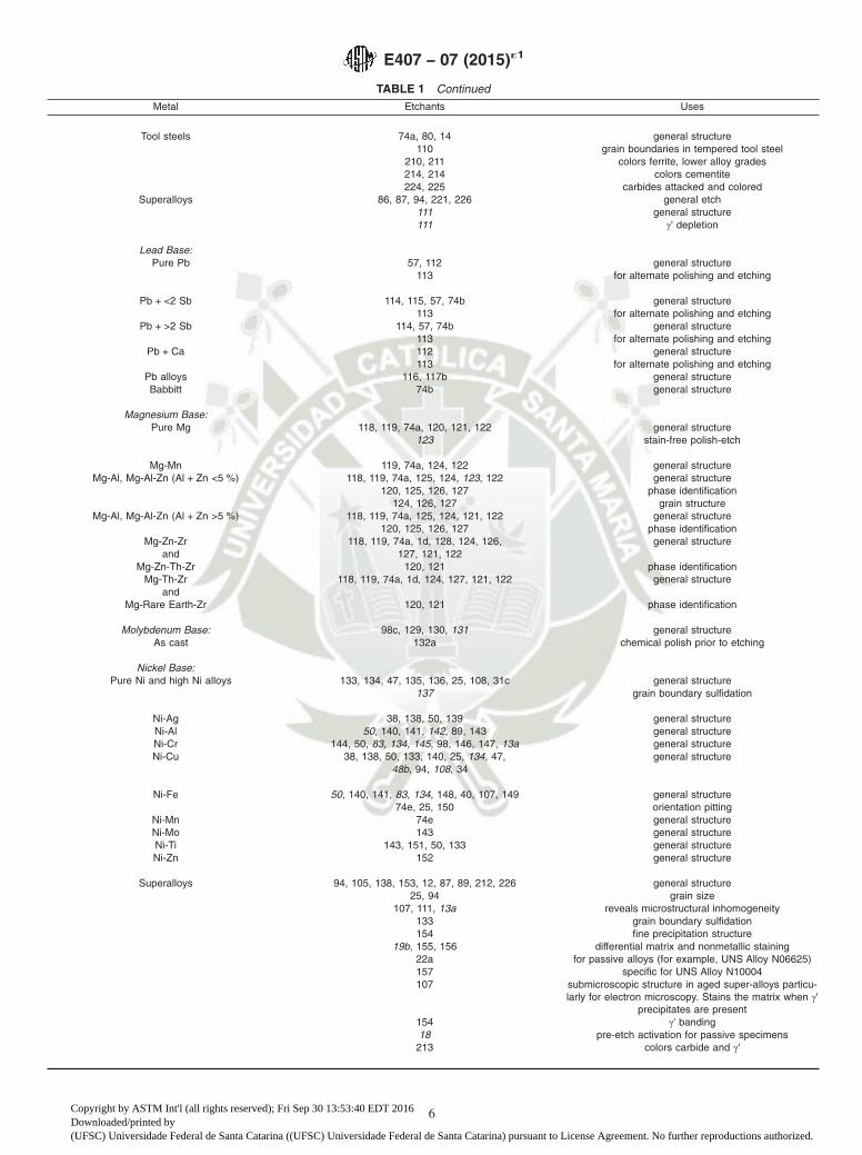
TABLE 1 Continued
Metal Etchants Uses
Tool steels 74a, 80, 14 general structure110 grain boundaries in tempered tool steel
210, 211 colors ferrite, lower alloy grades214, 214 colors cementite224, 225 carbides attacked and colored
Superalloys 86, 87, 94, 221, 226 general etch111 general structure111 γ' depletion
Lead Base:Pure Pb 57, 112 general structure
113 for alternate polishing and etching
Pb + <2 Sb 114, 115, 57, 74b general structure113 for alternate polishing and etching
Pb + >2 Sb 114, 57, 74b general structure113 for alternate polishing and etching
Pb + Ca 112 general structure113 for alternate polishing and etching
Pb alloys 116, 117b general structureBabbitt 74b general structure
Magnesium Base:Pure Mg 118, 119, 74a, 120, 121, 122 general structure
123 stain-free polish-etch
Mg-Mn 119, 74a, 124, 122 general structureMg-Al, Mg-Al-Zn (Al + Zn <5 %) 118, 119, 74a, 125, 124, 123, 122 general structure
120, 125, 126, 127 phase identification124, 126, 127 grain structure
Mg-Al, Mg-Al-Zn (Al + Zn >5 %) 118, 119, 74a, 125, 124, 121, 122 general structure120, 125, 126, 127 phase identification
Mg-Zn-Zr 118, 119, 74a, 1d, 128, 124, 126, general structureand 127, 121, 122
Mg-Zn-Th-Zr 120, 121 phase identificationMg-Th-Zr 118, 119, 74a, 1d, 124, 127, 121, 122 general structure
andMg-Rare Earth-Zr 120, 121 phase identification
Molybdenum Base: 98c, 129, 130, 131 general structureAs cast 132a chemical polish prior to etching
Nickel Base:Pure Ni and high Ni alloys 133, 134, 47, 135, 136, 25, 108, 31c general structure
137 grain boundary sulfidation
Ni-Ag 38, 138, 50, 139 general structureNi-Al 50, 140, 141, 142, 89, 143 general structureNi-Cr 144, 50, 83, 134, 145, 98, 146, 147, 13a general structureNi-Cu 38, 138, 50, 133, 140, 25, 134, 47, general structure
48b, 94, 108, 34
Ni-Fe 50, 140, 141, 83, 134, 148, 40, 107, 149 general structure74e, 25, 150 orientation pitting
Ni-Mn 74e general structureNi-Mo 143 general structureNi-Ti 143, 151, 50, 133 general structureNi-Zn 152 general structure
Superalloys 94, 105, 138, 153, 12, 87, 89, 212, 226 general structure25, 94 grain size
107, 111, 13a reveals microstructural inhomogeneity133 grain boundary sulfidation154 fine precipitation structure
19b, 155, 156 differential matrix and nonmetallic staining22a for passive alloys (for example, UNS Alloy N06625)157 specific for UNS Alloy N10004107 submicroscopic structure in aged super-alloys particu-
larly for electron microscopy. Stains the matrix when γ'precipitates are present
154 γ' banding18 pre-etch activation for passive specimens213 colors carbide and γ'
E407 − 07 (2015)´1
6
Copyright by ASTM Int'l (all rights reserved); Fri Sep 30 13:53:40 EDT 2016Downloaded/printed by(UFSC) Universidade Federal de Santa Catarina ((UFSC) Universidade Federal de Santa Catarina) pursuant to License Agreement. No further reproductions authorized.
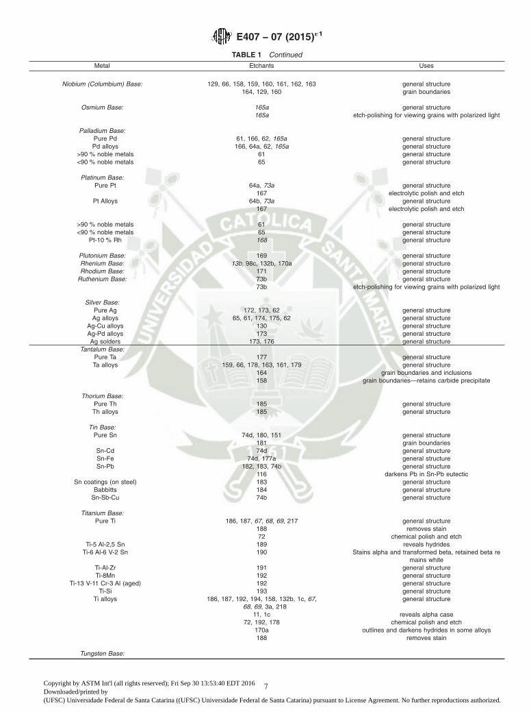
TABLE 1 Continued
Metal Etchants Uses
Niobium (Columbium) Base: 129, 66, 158, 159, 160, 161, 162, 163 general structure164, 129, 160 grain boundaries
Osmium Base: 165a general structure165a etch-polishing for viewing grains with polarized light
Palladium Base:Pure Pd 61, 166, 62, 165a general structurePd alloys 166, 64a, 62, 165a general structure
>90 % noble metals 61 general structure<90 % noble metals 65 general structure
Platinum Base:Pure Pt 64a, 73a general structure
167 electrolytic polish and etchPt Alloys 64b, 73a general structure
167 electrolytic polish and etch
>90 % noble metals 61 general structure<90 % noble metals 65 general structure
Pt-10 % Rh 168 general structure
Plutonium Base: 169 general structureRhenium Base: 13b, 98c, 132b, 170a general structureRhodium Base: 171 general structure
Ruthenium Base: 73b general structure73b etch-polishing for viewing grains with polarized light
Silver Base:Pure Ag 172, 173, 62 general structureAg alloys 65, 61, 174, 175, 62 general structure
Ag-Cu alloys 130 general structureAg-Pd alloys 173 general structureAg solders 173, 176 general structure
Tantalum Base:Pure Ta 177 general structureTa alloys 159, 66, 178, 163, 161, 179 general structure
164 grain boundaries and inclusions158 grain boundaries—retains carbide precipitate
Thorium Base:Pure Th 185 general structureTh alloys 185 general structure
Tin Base:Pure Sn 74d, 180, 151 general structure
181 grain boundariesSn-Cd 74d general structureSn-Fe 74d, 177a general structureSn-Pb 182, 183, 74b general structure
116 darkens Pb in Sn-Pb eutecticSn coatings (on steel) 183 general structure
Babbitts 184 general structureSn-Sb-Cu 74b general structure
Titanium Base:Pure Ti 186, 187, 67, 68, 69, 217 general structure
188 removes stain72 chemical polish and etch
Ti-5 Al-2,5 Sn 189 reveals hydridesTi-6 Al-6 V-2 Sn 190 Stains alpha and transformed beta, retained beta re
mains whiteTi-Al-Zr 191 general structureTi-8Mn 192 general structure
Ti-13 V-11 Cr-3 Al (aged) 192 general structureTi-Si 193 general structure
Ti alloys 186, 187, 192, 194, 158, 132b, 1c, 67,68, 69, 3a, 218
general structure
11, 1c reveals alpha case72, 192, 178 chemical polish and etch
170a outlines and darkens hydrides in some alloys188 removes stain
Tungsten Base:
E407 − 07 (2015)´1
7
Copyright by ASTM Int'l (all rights reserved); Fri Sep 30 13:53:40 EDT 2016Downloaded/printed by(UFSC) Universidade Federal de Santa Catarina ((UFSC) Universidade Federal de Santa Catarina) pursuant to License Agreement. No further reproductions authorized.

TABLE 1 Continued
Metal Etchants Uses
Pure W 98c, 131 general structureAs cast 132a chemical polish prior to etchingW-Th 209 general structure
Uranium Base:Pure U 67, 69, 195, 196 general structureU + Zr 68 general structure
U beryllides 170a general structureU alloys 67, 69, 195, 96 general structure
207 carbides
Vanadium Base:Pure V 170b, 165b general structure
197, 198 grain boundariesV alloys 199, 198 general structure
Zinc Base:Pure Zn 200a general structureZn-Co 177 general structureZn-Cu 201 general structure
203 distinguishes gamma (γ) and epsilon (ε)Zn-Fe 74a structure of galvanized sheet
Die castings 202 general structure
Zirconium Base: 66, 67, 204, 68, 69, 205 general structure206 electrolytic polish and etch71 grain structure under polarized light72 chemical polish and etch
E407 − 07 (2015)´1
8
Copyright by ASTM Int'l (all rights reserved); Fri Sep 30 13:53:40 EDT 2016Downloaded/printed by(UFSC) Universidade Federal de Santa Catarina ((UFSC) Universidade Federal de Santa Catarina) pursuant to License Agreement. No further reproductions authorized.
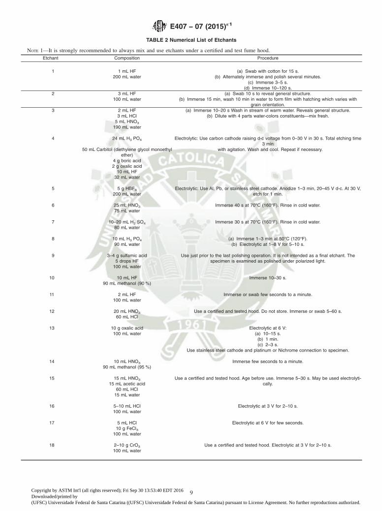
TABLE 2 Numerical List of Etchants
NOTE 1—It is strongly recommended to always mix and use etchants under a certified and test fume hood.Etchant Composition Procedure
1 1 mL HF (a) Swab with cotton for 15 s.200 mL water (b) Alternately immerse and polish several minutes.
(c) Immerse 3–5 s.(d) Immerse 10–120 s.
2 3 mL HF (a) Swab 10 s to reveal general structure.100 mL water (b) Immerse 15 min, wash 10 min in water to form film with hatching which varies with
grain orientation.3 2 mL HF (a) Immerse 10–20 s Wash in stream of warm water. Reveals general structure.
3 mL HCl (b) Dilute with 4 parts water-colors constituents—mix fresh.5 mL HNO3
190 mL water
4 24 mL H3 PO4 Electrolytic: Use carbon cathode raising d-c voltage from 0–30 V in 30 s. Total etching time3 min
50 mL Carbitol (diethylene glycol monoethylether)
with agitation. Wash and cool. Repeat if necessary.
4 g boric acid2 g oxalic acid
10 mL HF32 mL water
5 5 g HBF4
200 mL waterElectrolytic: Use Al, Pb, or stainless steel cathode. Anodize 1–3 min, 20–45 V d-c. At 30 V,
etch for 1 min.
6 25 mL HNO3
75 mL waterImmerse 40 s at 70°C (160°F). Rinse in cold water.
7 10–20 mL H2 SO4
80 mL waterImmerse 30 s at 70°C (160°F). Rinse in cold water.
8 10 mL H3 PO4 (a) Immerse 1–3 min at 50°C (120°F).90 mL water (b) Electrolytic at 1–8 V for 5–10 s.
9 3–4 g sulfamic acid5 drops HF
100 mL water
Use just prior to the last polishing operation. It is not intended as a final etchant. Thespecimen is examined as polished under polarized light.
10 10 mL HF90 mL methanol (90 %)
Immerse 10–30 s.
11 2 mL HF100 mL water
Immerse or swab few seconds to a minute.
12 20 mL HNO3
60 mL HClUse a certified and tested hood. Do not store. Immerse or swab 5–60 s.
13 10 g oxalic acid100 mL water
Electrolytic at 6 V:(a) 10–15 s.
(b) 1 min.(c) 2–3 s.
Use stainless steel cathode and platinum or Nichrome connection to specimen.
14 10 mL HNO3
90 mL methanol (95 %)Immerse few seconds to a minute.
15 15 mL HNO3
15 mL acetic acid60 mL HCl
15 mL water
Use a certified and tested hood. Age before use. Immerse 5–30 s. May be used electrolyti-cally.
16 5–10 mL HCl100 mL water
Electrolytic at 3 V for 2–10 s.
17 5 mL HCl10 g FeCl3
100 mL water
Electrolytic at 6 V for few seconds.
18 2–10 g CrO3
100 mL waterUse a certified and tested hood. Electrolytic at 3 V for 2–10 s.
E407 − 07 (2015)´1
9
Copyright by ASTM Int'l (all rights reserved); Fri Sep 30 13:53:40 EDT 2016Downloaded/printed by(UFSC) Universidade Federal de Santa Catarina ((UFSC) Universidade Federal de Santa Catarina) pursuant to License Agreement. No further reproductions authorized.
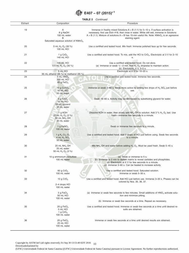
TABLE 2 Continued
Etchant Composition Procedure
19 A8 g NaOH
100 mL waterB
Saturated aqueous solution of KMnO4
Immerse in freshly mixed Solutions A + B (1:1) for 5–10 s. If surface activation isnecessary, first use Etch #18, then rinse in water. While still wet, immerse in Solutions
A + B (1:1). Mixture of solutions A + B has 15-min useful life. Note: KMnO4 is an agressivestaining agent.
20 5 mL H2 O2 (30 %)100 mL HCl
Use a certified and tested hood. Mix fresh. Immerse polished face up for few seconds.
21 1 g CrO3
140 mL HClUse a certified and tested hood. To mix, add the HCl to CrO3. Electrolytic at 3 V for 2–10
s.
22 100 mL HCl0.5 mL H2 O2 (30 %)
Use a certified and tested hood. Do not store.(a) Immerse or swab 1⁄2 –3 min. Add H2 O2 dropwise to maintain action.
(b) Electrolytic, 4 V, 3–5 s.23 5 mL HCl Electrolytic at 6 V for 10–20 s.
95 mL ethanol (95 %) or methanol (95 %)24 5 mL HNO3
200 mL HCl65 g FeCl3
Use a certified and tested hood. Immerse few seconds.
25 10 g CuSO4
50 mL HCl50 mL water
Immerse or swab 5–60 s. Made more active by adding few drops of H2 SO4 just beforeuse.
26 5 g FeCl310 mL HCl
50 mL glycerol30 mL water
Swab 16–60 s. Activity may be decreased by substituting glycerol for water.
27 1 g KOH20 mL H2 O2 (3 %)
50 mL NH4 OH30 mL water
Dissolve KOH in water, then slowly add NH4 OH to solution. Add 3 % H2 O2 last. Usefresh—immerse few seconds to a minute.
28 1 g FeNO3
100 mL waterSwab or immerse few seconds to a minute.
29 1 g K2 Cr2 O7
4 mL H2 SO4
50 mL water
Use a certified and tested hood. Add 2 drops of HCl just before using. Swab few secondsto a minute.
30 25 mL NH4 OH25 mL water
50 mL H2 O2 (3 %)
Mix NH4 OH and water before adding H2 O2. Must be used fresh. Swab 5–45 s.
31 10 g ammonium persulfate (a) Swab or immerse to 5 s.100 mL water (b) Immerse to 2 min to darken matrix to reveal carbides and phosphides.
(c) Electrolytic at 6 V for few seconds to a minute.(d) Immerse 3–60 s. Can be heated to increase activity.
32 60 g CrO3
100 mL waterUse a certified and tested hood. Saturated solution.
Immerse or swab 5–30 s.
33 10 g CrO3 Use a certified and tested hood. Add HCl just before use. Immerse 3–30 s. Phases can becolored by Nos. 35, 36, 37.
2–4 drops HCl100 mL water
34 5 g FeCl350 mL HCl
100 mL water
(a) Immerse or swab few seconds to few minutes. Small additions of HNO3 activate solu-tion and minimize pitting.
(b) Immerse or swab few seconds at a time. Repeat as necessary.
35 20 g FeCl35 mL HCl1 g CrO3
100 mL water
Use a certified and tested hood. Immerse or swab few seconds at a time until desired re-sults are obtained.
36 25 g FeCl325 mL HCl
100 mL water
Immerse or swab few seconds at a time until desired results are obtained.
E407 − 07 (2015)´1
10
Copyright by ASTM Int'l (all rights reserved); Fri Sep 30 13:53:40 EDT 2016Downloaded/printed by(UFSC) Universidade Federal de Santa Catarina ((UFSC) Universidade Federal de Santa Catarina) pursuant to License Agreement. No further reproductions authorized.

TABLE 2 Continued
Etchant Composition Procedure
37 1 g FeCl310 mL HCl
100 mL water
Immerse or swab few seconds at a time until desired results are obtained
38 8 g FeCl325 mL HCl
100 mL water
Swab 5–30 s.
39 5 g FeCl310 mL HCl1 g CuCl2
0.1 g SnCl2100 mL water
Immerse or swab few seconds at a time until desired results are obtained.
40 5 g FeCl316 mL HCl
Immerse or swab few seconds to few minutes.
60 mL ethanol (95 %) or methanol (95 %)
41 2 g K2 Cr2 O7
8 mL H2 SO4
4 drops HCl100 mL water
Use a certified and tested hood. Add the HCl just before using. Immerse 3–60 s.
42 10 g cupric ammonium chloride Add NH4 OH to solution until neutral or slightly alkaline. Immerse 5–60 s.100 mL water
NH4 OH43 20 mL NH4 OH
1 g ammonium persulfate60 mL water
Immerse 5–30 s.
44 50 mL NH4 OH20–50 mL H2 O2 (3 %)
0–50 mL water
Use fresh. Peroxide content varies directly with copper content of alloy to be etched. Im-merse or swab to 1 min. Film on etched aluminum bronze removed by No. 82.
45 1 g CrO3
100 mL waterUse a certified and tested hood. Electrolytic at 6 V for 3–6 s. Use aluminum cathode.
46 15 mL NH4 OH15 mL H2 O2 (3 %)
15 mL water4 pellets NaOH
When mixing, add NaOH pellets last. For best results use before pellets have dissolved.
47 5 g NaCN or KCN5 g (NH4)2 S2 O2
100 mL water
Use a certified and tested hood—Can give off extremely poisonous hydrogen cyanide.Precaution—Also poisonous by ingestion as well as skin contact.
48 10 g NaCN100 mL water
Use a certified and tested hood—Can give off extremely poisonous hydrogen cyanide.Precaution—Also poisonous by ingestion as well as skin contact. Electrolytic at 6 V:
(a) 5 s for sigma.(b) 30 s for ferrite and general structure.
(c) to 5 min for carbides.
49 3 g FeSO4
0.4 g NaOH10 mL H2 SO4
190 mL water
Electrolytic at 8–10 V (0.1 A) for 5–15 s.
50 5 mL acetic acid10 mL HNO3
85 mL water
Use a certified and tested hood. Do not store. Electrolytic at 1.5 V for 20 to 60 s. Use plati-num wires.
51 2 g FeCl35 mL HCl
30 mL water60 mL ethanol or methanol
Immerse few minutes.
52 1 g sodium dichromate1 g NaCl
4 mL H2 SO4
250 mL water
Swab few seconds.
53 1–5 mL NH4 OH100 mL water
Immerse 5–60 s.
E407 − 07 (2015)´1
11
Copyright by ASTM Int'l (all rights reserved); Fri Sep 30 13:53:40 EDT 2016Downloaded/printed by(UFSC) Universidade Federal de Santa Catarina ((UFSC) Universidade Federal de Santa Catarina) pursuant to License Agreement. No further reproductions authorized.
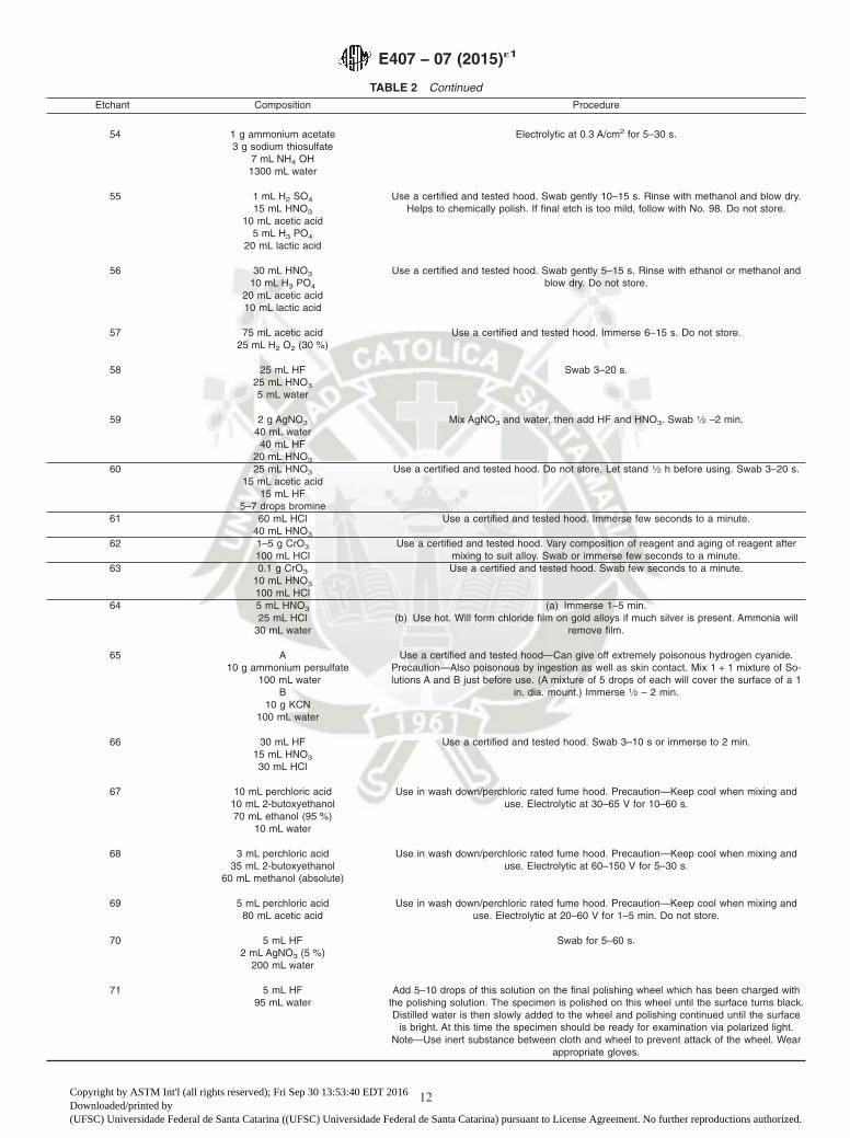
TABLE 2 Continued
Etchant Composition Procedure
54 1 g ammonium acetate3 g sodium thiosulfate
7 mL NH4 OH1300 mL water
Electrolytic at 0.3 A/cm2 for 5–30 s.
55 1 mL H2 SO4
15 mL HNO3
10 mL acetic acid5 mL H3 PO4
20 mL lactic acid
Use a certified and tested hood. Swab gently 10–15 s. Rinse with methanol and blow dry.Helps to chemically polish. If final etch is too mild, follow with No. 98. Do not store.
56 30 mL HNO3
10 mL H3 PO4
20 mL acetic acid10 mL lactic acid
Use a certified and tested hood. Swab gently 5–15 s. Rinse with ethanol or methanol andblow dry. Do not store.
57 75 mL acetic acid25 mL H2 O2 (30 %)
Use a certified and tested hood. Immerse 6–15 s. Do not store.
58 25 mL HF25 mL HNO3
5 mL water
Swab 3–20 s.
59 2 g AgNO3
40 mL water40 mL HF
20 mL HNO3
Mix AgNO3 and water, then add HF and HNO3. Swab 1⁄2 –2 min.
60 25 mL HNO3
15 mL acetic acid15 mL HF
5–7 drops bromine
Use a certified and tested hood. Do not store. Let stand 1⁄2 h before using. Swab 3–20 s.
61 60 mL HCl40 mL HNO3
Use a certified and tested hood. Immerse few seconds to a minute.
62 1–5 g CrO3
100 mL HClUse a certified and tested hood. Vary composition of reagent and aging of reagent after
mixing to suit alloy. Swab or immerse few seconds to a minute.63 0.1 g CrO3
10 mL HNO3
100 mL HCl
Use a certified and tested hood. Swab few seconds to a minute.
64 5 mL HNO3 (a) Immerse 1–5 min.25 mL HCl
30 mL water(b) Use hot. Will form chloride film on gold alloys if much silver is present. Ammonia will
remove film.
65 A10 g ammonium persulfate
100 mL waterB
10 g KCN100 mL water
Use a certified and tested hood—Can give off extremely poisonous hydrogen cyanide.Precaution—Also poisonous by ingestion as well as skin contact. Mix 1 + 1 mixture of So-lutions A and B just before use. (A mixture of 5 drops of each will cover the surface of a 1
in. dia. mount.) Immerse 1⁄2 – 2 min.
66 30 mL HF15 mL HNO3
30 mL HCl
Use a certified and tested hood. Swab 3–10 s or immerse to 2 min.
67 10 mL perchloric acid10 mL 2-butoxyethanol70 mL ethanol (95 %)
10 mL water
Use in wash down/perchloric rated fume hood. Precaution—Keep cool when mixing anduse. Electrolytic at 30–65 V for 10–60 s.
68 3 mL perchloric acid35 mL 2-butoxyethanol
60 mL methanol (absolute)
Use in wash down/perchloric rated fume hood. Precaution—Keep cool when mixing anduse. Electrolytic at 60–150 V for 5–30 s.
69 5 mL perchloric acid80 mL acetic acid
Use in wash down/perchloric rated fume hood. Precaution—Keep cool when mixing anduse. Electrolytic at 20–60 V for 1–5 min. Do not store.
70 5 mL HF2 mL AgNO3 (5 %)
200 mL water
Swab for 5–60 s.
71 5 mL HF95 mL water
Add 5–10 drops of this solution on the final polishing wheel which has been charged withthe polishing solution. The specimen is polished on this wheel until the surface turns black.Distilled water is then slowly added to the wheel and polishing continued until the surface
is bright. At this time the specimen should be ready for examination via polarized light.Note—Use inert substance between cloth and wheel to prevent attack of the wheel. Wear
appropriate gloves.
E407 − 07 (2015)´1
12
Copyright by ASTM Int'l (all rights reserved); Fri Sep 30 13:53:40 EDT 2016Downloaded/printed by(UFSC) Universidade Federal de Santa Catarina ((UFSC) Universidade Federal de Santa Catarina) pursuant to License Agreement. No further reproductions authorized.
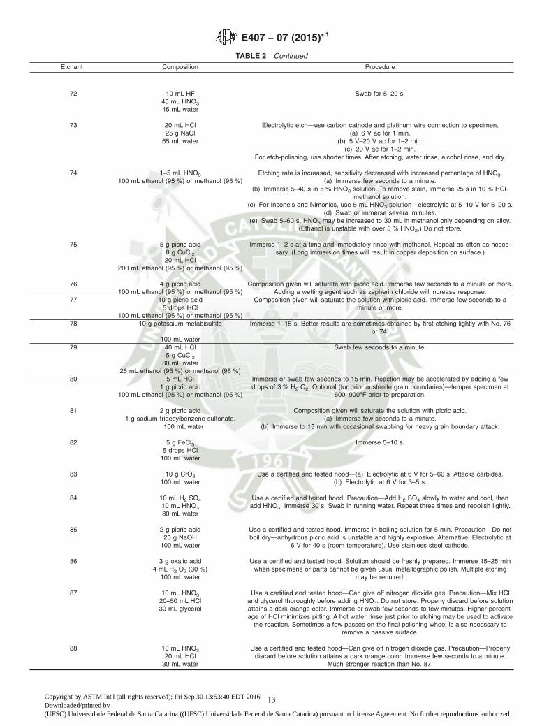
TABLE 2 Continued
Etchant Composition Procedure
72 10 mL HF45 mL HNO3
45 mL water
Swab for 5–20 s.
73 20 mL HCl Electrolytic etch—use carbon cathode and platinum wire connection to specimen.25 g NaCl (a) 6 V ac for 1 min.
65 mL water (b) 5 V–20 V ac for 1–2 min.(c) 20 V ac for 1–2 min.
For etch-polishing, use shorter times. After etching, water rinse, alcohol rinse, and dry.
74 1–5 mL HNO3 Etching rate is increased, sensitivity decreased with increased percentage of HNO3.100 mL ethanol (95 %) or methanol (95 %) (a) Immerse few seconds to a minute.
(b) Immerse 5–40 s in 5 % HNO3 solution. To remove stain, immerse 25 s in 10 % HCl-methanol solution.
(c) For Inconels and Nimonics, use 5 mL HNO3 solution—electrolytic at 5–10 V for 5–20 s.(d) Swab or immerse several minutes.
(e) Swab 5–60 s. HNO3 may be increased to 30 mL in methanol only depending on alloy.(Ethanol is unstable with over 5 % HNO3.) Do not store.
75 5 g picric acid8 g CuCl220 mL HCl
200 mL ethanol (95 %) or methanol (95 %)
Immerse 1–2 s at a time and immediately rinse with methanol. Repeat as often as neces-sary. (Long immersion times will result in copper deposition on surface.)
76 4 g picric acid100 mL ethanol (95 %) or methanol (95 %)
Composition given will saturate with picric acid. Immerse few seconds to a minute or more.Adding a wetting agent such as zepherin chloride will increase response.
77 10 g picric acid5 drops HCl
100 mL ethanol (95 %) or methanol (95 %)
Composition given will saturate the solution with picric acid. Immerse few seconds to aminute or more.
78 10 g potassium metabisulfite Immerse 1–15 s. Better results are sometimes obtained by first etching lightly with No. 76or 74.
100 mL water79 40 mL HCl
5 g CuCl230 mL water
25 mL ethanol (95 %) or methanol (95 %)
Swab few seconds to a minute.
80 5 mL HCl1 g picric acid
100 mL ethanol (95 %) or methanol (95 %)
Immerse or swab few seconds to 15 min. Reaction may be accelerated by adding a fewdrops of 3 % H2 O2. Optional (for prior austenite grain boundaries)—temper specimen at
600–900°F prior to preparation.
81 2 g picric acid Composition given will saturate the solution with picric acid.1 g sodium tridecylbenzene sulfonate. (a) Immerse few seconds to a minute.
100 mL water (b) Immerse to 15 min with occasional swabbing for heavy grain boundary attack.
82 5 g FeCl35 drops HCl
100 mL water
Immerse 5–10 s.
83 10 g CrO3
100 mL waterUse a certified and tested hood—(a) Electrolytic at 6 V for 5–60 s. Attacks carbides.
(b) Electrolytic at 6 V for 3–5 s.
84 10 mL H2 SO4
10 mL HNO3
80 mL water
Use a certified and tested hood. Precaution—Add H2 SO4 slowly to water and cool, thenadd HNO3. Immerse 30 s. Swab in running water. Repeat three times and repolish lightly.
85 2 g picric acid25 g NaOH
100 mL water
Use a certified and tested hood. Immerse in boiling solution for 5 min. Precaution—Do notboil dry—anhydrous picric acid is unstable and highly explosive. Alternative: Electrolytic at
6 V for 40 s (room temperature). Use stainless steel cathode.
86 3 g oxalic acid4 mL H2 O2 (30 %)
100 mL water
Use a certified and tested hood. Solution should be freshly prepared. Immerse 15–25 minwhen specimens or parts cannot be given usual metallographic polish. Multiple etching
may be required.
87 10 mL HNO3
20–50 mL HCl30 mL glycerol
Use a certified and tested hood—Can give off nitrogen dioxide gas. Precaution—Mix HCland glycerol thoroughly before adding HNO3. Do not store. Properly discard before solutionattains a dark orange color. Immerse or swab few seconds to few minutes. Higher percent-age of HCl minimizes pitting. A hot water rinse just prior to etching may be used to activate
the reaction. Sometimes a few passes on the final polishing wheel is also necessary toremove a passive surface.
88 10 mL HNO3
20 mL HCl30 mL water
Use a certified and tested hood—Can give off nitrogen dioxide gas. Precaution—Properlydiscard before solution attains a dark orange color. Immerse few seconds to a minute.
Much stronger reaction than No. 87.
E407 − 07 (2015)´1
13
Copyright by ASTM Int'l (all rights reserved); Fri Sep 30 13:53:40 EDT 2016Downloaded/printed by(UFSC) Universidade Federal de Santa Catarina ((UFSC) Universidade Federal de Santa Catarina) pursuant to License Agreement. No further reproductions authorized.
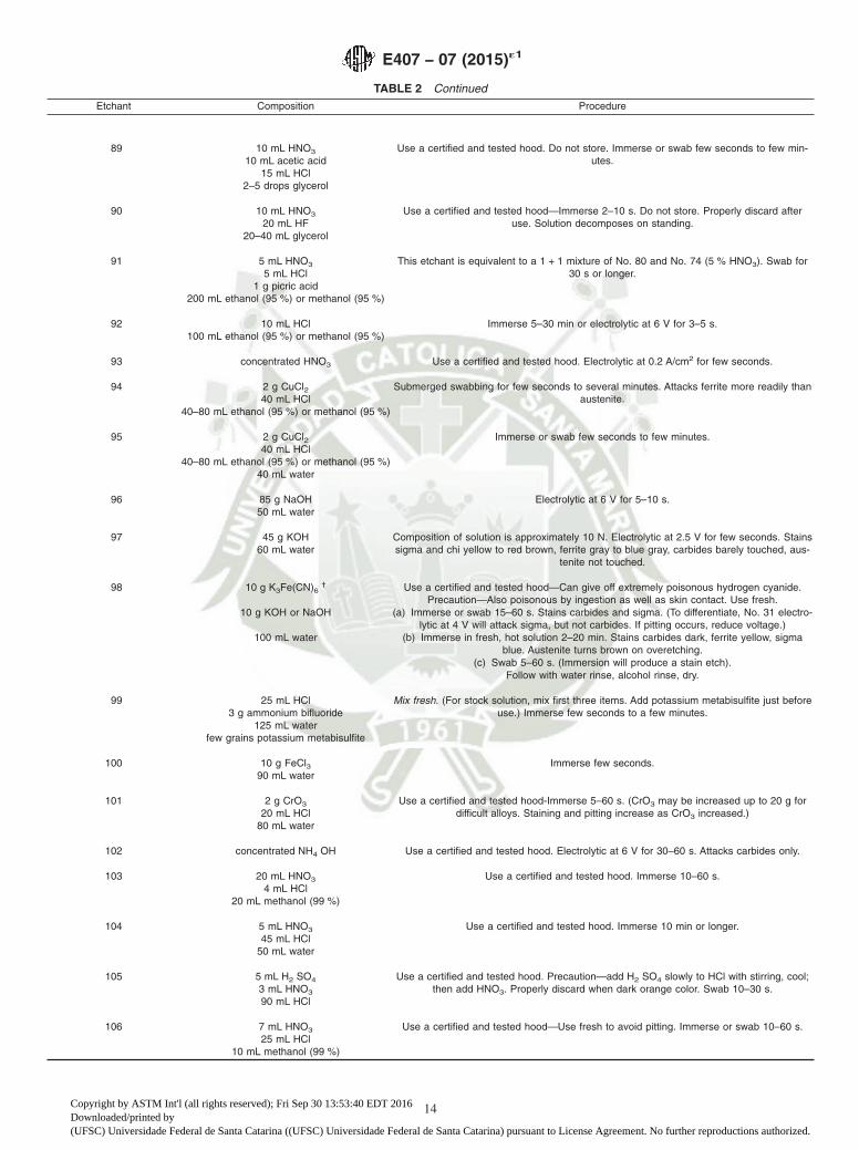
TABLE 2 Continued
Etchant Composition Procedure
89 10 mL HNO3
10 mL acetic acid15 mL HCl
2–5 drops glycerol
Use a certified and tested hood. Do not store. Immerse or swab few seconds to few min-utes.
90 10 mL HNO3
20 mL HF20–40 mL glycerol
Use a certified and tested hood—Immerse 2–10 s. Do not store. Properly discard afteruse. Solution decomposes on standing.
91 5 mL HNO3
5 mL HCl1 g picric acid
200 mL ethanol (95 %) or methanol (95 %)
This etchant is equivalent to a 1 + 1 mixture of No. 80 and No. 74 (5 % HNO3). Swab for30 s or longer.
92 10 mL HCl100 mL ethanol (95 %) or methanol (95 %)
Immerse 5–30 min or electrolytic at 6 V for 3–5 s.
93 concentrated HNO3 Use a certified and tested hood. Electrolytic at 0.2 A/cm2 for few seconds.
94 2 g CuCl240 mL HCl
40–80 mL ethanol (95 %) or methanol (95 %)
Submerged swabbing for few seconds to several minutes. Attacks ferrite more readily thanaustenite.
95 2 g CuCl240 mL HCl
40–80 mL ethanol (95 %) or methanol (95 %)40 mL water
Immerse or swab few seconds to few minutes.
96 85 g NaOH50 mL water
Electrolytic at 6 V for 5–10 s.
97 45 g KOH60 mL water
Composition of solution is approximately 10 N. Electrolytic at 2.5 V for few seconds. Stainssigma and chi yellow to red brown, ferrite gray to blue gray, carbides barely touched, aus-
tenite not touched.
98 10 g K3Fe(CN)6† Use a certified and tested hood—Can give off extremely poisonous hydrogen cyanide.
Precaution—Also poisonous by ingestion as well as skin contact. Use fresh.10 g KOH or NaOH (a) Immerse or swab 15–60 s. Stains carbides and sigma. (To differentiate, No. 31 electro-
lytic at 4 V will attack sigma, but not carbides. If pitting occurs, reduce voltage.)100 mL water (b) Immerse in fresh, hot solution 2–20 min. Stains carbides dark, ferrite yellow, sigma
blue. Austenite turns brown on overetching.(c) Swab 5–60 s. (Immersion will produce a stain etch).
Follow with water rinse, alcohol rinse, dry.
99 25 mL HCl3 g ammonium bifluoride
125 mL waterfew grains potassium metabisulfite
Mix fresh. (For stock solution, mix first three items. Add potassium metabisulfite just beforeuse.) Immerse few seconds to a few minutes.
100 10 g FeCl390 mL water
Immerse few seconds.
101 2 g CrO3
20 mL HCl80 mL water
Use a certified and tested hood-Immerse 5–60 s. (CrO3 may be increased up to 20 g fordifficult alloys. Staining and pitting increase as CrO3 increased.)
102 concentrated NH4 OH Use a certified and tested hood. Electrolytic at 6 V for 30–60 s. Attacks carbides only.
103 20 mL HNO3
4 mL HCl20 mL methanol (99 %)
Use a certified and tested hood. Immerse 10–60 s.
104 5 mL HNO3
45 mL HCl50 mL water
Use a certified and tested hood. Immerse 10 min or longer.
105 5 mL H2 SO4
3 mL HNO3
90 mL HCl
Use a certified and tested hood. Precaution—add H2 SO4 slowly to HCl with stirring, cool;then add HNO3. Properly discard when dark orange color. Swab 10–30 s.
106 7 mL HNO3
25 mL HCl10 mL methanol (99 %)
Use a certified and tested hood—Use fresh to avoid pitting. Immerse or swab 10–60 s.
E407 − 07 (2015)´1
14
Copyright by ASTM Int'l (all rights reserved); Fri Sep 30 13:53:40 EDT 2016Downloaded/printed by(UFSC) Universidade Federal de Santa Catarina ((UFSC) Universidade Federal de Santa Catarina) pursuant to License Agreement. No further reproductions authorized.
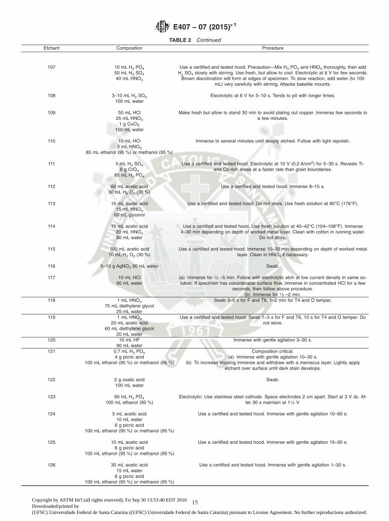
TABLE 2 Continued
Etchant Composition Procedure
107 10 mL H3 PO4
50 mL H2 SO4
40 mL HNO3
Use a certified and tested hood. Precaution—Mix H3 PO4 and HNO3 thoroughly, then addH
2SO4 slowly with stirring. Use fresh, but allow to cool. Electrolytic at 6 V for few seconds.
Brown discoloration will form at edges of specimen. To slow reaction, add water (to 100mL) very carefully with stirring. Attacks bakelite mounts.
108 3–10 mL H2 SO4
100 mL waterElectrolytic at 6 V for 5–10 s. Tends to pit with longer times.
109 50 mL HCl25 mL HNO3
1 g CuCl2150 mL water
Make fresh but allow to stand 30 min to avoid plating out copper. Immerse few seconds toa few minutes.
110 10 mL HCl5 mL HNO3
85 mL ethanol (95 %) or methanol (95 %)
Immerse to several minutes until deeply etched. Follow with light repolish.
111 5 mL H2 SO4
8 g CrO3
85 mL H3 PO4
Use a certified and tested hood. Electrolytic at 10 V (0.2 A/cm2) for 5–30 s. Reveals Ti-and Cb-rich areas at a faster rate than grain boundaries.
112 60 mL acetic acid30 mL H2 O2 (30 %)
Use a certified and tested hood. Immerse 8–15 s.
113 15 mL acetic acid15 mL HNO3
60 mL glycerol
Use a certified and tested hood. Do not store. Use fresh solution at 80°C (176°F).
114 15 mL acetic acid20 mL HNO3
80 mL water
Use a certified and tested hood. Use fresh solution at 40–42°C (104–108°F). Immerse4–30 min depending on depth of worked metal layer. Clean with cotton in running water.
Do not store.
115 100 mL acetic acid10 mL H2 O2 (30 %)
Use a certified and tested hood. Immerse 10–30 min depending on depth of worked metallayer. Clean in HNO3 if necessary.
116 5–10 g AgNO3 90 mL water Swab.
117 10 mL HCl90 mL water
(a) Immerse for 1⁄2 –5 min. Follow with electrolytic etch at low current density in same so-lution. If specimen has considerable surface flow, immerse in concentrated HCl for a few
seconds, then follow above procedure.(b) Immerse for 1⁄2 –2 min.
118 1 mL HNO3
75 mL diethylene glycol25 mL water
Swab 3–5 s for F and T6, 1–2 min for T4 and O temper.
119 1 mL HNO3
20 mL acetic acid60 mL diethylene glycol
20 mL water
Use a certified and tested hood. Swab 1–3 s for F and T6, 10 s for T4 and O temper. Donot store.
120 10 mL HF90 mL water
Immerse with gentle agitation 3–30 s.
121 0.7 mL H3 PO4
4 g picric acid100 mL ethanol (95 %) or methanol (95 %)
Composition critical.(a) Immerse with gentle agitation 10–30 s.
(b) To increase staining immerse and withdraw with a meniscus layer. Lightly applyetchant over surface until dark stain develops.
122 2 g oxalic acid100 mL water
Swab.
123 60 mL H3 PO4
100 mL ethanol (95 %)Electrolytic: Use stainless steel cathode. Space electrodes 2 cm apart. Start at 3 V dc. Af-
ter 30 s maintain at 11⁄2 V.
124 5 mL acetic acid10 mL water
6 g picric acid100 mL ethanol (95 %) or methanol (95 %)
Use a certified and tested hood. Immerse with gentle agitation 10–60 s.
125 10 mL acetic acid6 g picric acid
100 mL ethanol (95 %) or methanol (95 %)
Use a certified and tested hood. Immerse with gentle agitation 15–30 s.
126 30 mL acetic acid15 mL water
6 g picric acid100 mL ethanol (95 %) or methanol (95 %)
Use a certified and tested hood. Immerse with gentle agitation 1–30 s.
E407 − 07 (2015)´1
15
Copyright by ASTM Int'l (all rights reserved); Fri Sep 30 13:53:40 EDT 2016Downloaded/printed by(UFSC) Universidade Federal de Santa Catarina ((UFSC) Universidade Federal de Santa Catarina) pursuant to License Agreement. No further reproductions authorized.

TABLE 2 Continued
Etchant Composition Procedure
127 20 mL acetic acid20 mL water
3 g picric acid50 mL ethanol (95 %) or methanol (95 %)
Use a certified and tested hood. Immerse with gentle agitation 5–30 s.
128 8 mL HF5 mL HNO3
200 mL water
Use a certified and tested hood. Immerse with gentle agitation 5–15 s.
129 10 mL HF30 mL HNO3
60 mL lactic acid
Swab 10–20 s. Vary HF to increase or decrease activity.
130 25 mL HCl75 mL methanol
Caution—Keep below 24°C (75°F). Electrolytic at 30 V for 30 s.
131 5 mL H2 SO4
1 mL HF100 mL methanol (95 %)
Use a certified and tested hood. Electrolytic at 50–60 V for 10–20 s.
132 5 mL HF10 mL HNO3
50 mL lactic acid
Use fresh.(a) Swab with heavy pressure for 5–10 s. Water rinse, alcohol rinse, dry, then etch with
No. 98c.(b) Swab for 5–30 s.
133 50 mL HNO3
50 mL acetic acidUse a certified and tested hood. Do not store. Mix fresh. Immerse or swab 5 to 30 s. Will
chemically polish with longer times. Sulfidized grain boundaries etched before normal grainboundaries. Do not store.
134 70 mL H3 PO4
30 mL waterElectrolytic 5–10 V for 5–60 s. (Polishes at high currents.)
135 80 mL HNO3
3 mL HFUse a certified and tested hood. Warm specimen in boiling water prior to immersion for 10
to 120 s.
136 20 mL H3 PO4
80 mL waterElectrolytic at 10–20 V for 10–15 s.
137 10 g NaNO3
100 mL waterElectrolytic, 0.2 A/cm2, 1 min.
138 5 g FeCl32 mL HCl
100 mL ethanol (95 %) or methanol (95 %)
Swab 10–60 s.
139 5 g KCN100 mL water
0.5 mL H2 O2 (3 %)
Use a certified and tested hood—Can give off extremely poisonous hydrogen cyanide.Precaution—Also poisonous by ingestion as well as skin contact. Immerse 10–100 s.
140 50 mL acetic acid50 mL HNO3
50 mL acetone
Use a certified and tested hood. Do not store. Decomposes with possible explosion onstanding. Immerse 10–30 s.
141 3 g NH4 Cl3 g CrO3
10 mL HNO3
90 mL water
Use a certified and tested hood-Swab 5–30 s. Do not store.
142 5 mL HF10 mL glycerol85 mL water
Electrolytic at 2–3 V for 2–10 s.
144 A10 g sodium thiosulfate
100 mL waterB
10 mL HCl90 mL water
Electrolytic in Solution A: specimen is cathode, 10 V, 5–10 s. Then electrolytic in SolutionB: specimen is anode, 10 V, 5–10 s.
145 2 mL H2 SO4
100 mL waterElectrolytic at 3–10 V for 5–15 s. Use platinum wires. H2 SO4 may be increased to 20 mL
for deeper attack.
146 10 mL HF100 mL HNO3
Immerse 30 s–3 min.
147 20 mL HNO3
80 mL HClImmerse 5–30 s.
E407 − 07 (2015)´1
16
Copyright by ASTM Int'l (all rights reserved); Fri Sep 30 13:53:40 EDT 2016Downloaded/printed by(UFSC) Universidade Federal de Santa Catarina ((UFSC) Universidade Federal de Santa Catarina) pursuant to License Agreement. No further reproductions authorized.
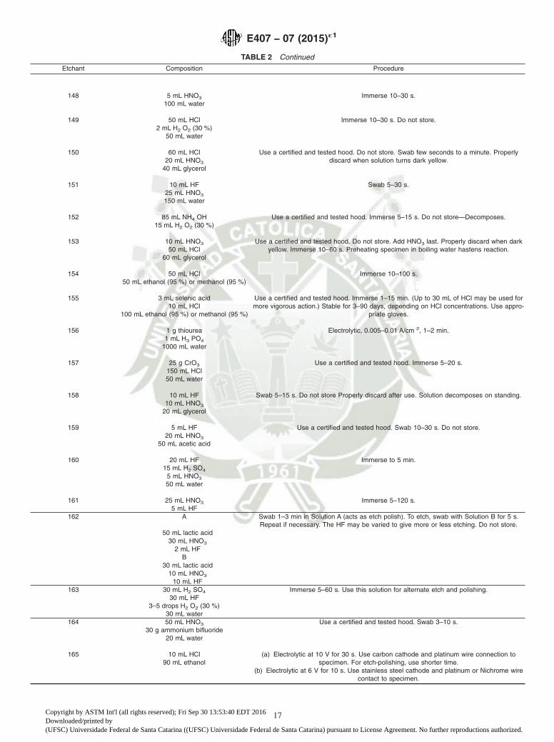
TABLE 2 Continued
Etchant Composition Procedure
148 5 mL HNO3
100 mL waterImmerse 10–30 s.
149 50 mL HCl2 mL H2 O2 (30 %)
50 mL water
Immerse 10–30 s. Do not store.
150 60 mL HCl20 mL HNO3
40 mL glycerol
Use a certified and tested hood. Do not store. Swab few seconds to a minute. Properlydiscard when solution turns dark yellow.
151 10 mL HF25 mL HNO3
150 mL water
Swab 5–30 s.
152 85 mL NH4 OH15 mL H2 O2 (30 %)
Use a certified and tested hood. Immerse 5–15 s. Do not store—Decomposes.
153 10 mL HNO3
50 mL HCl60 mL glycerol
Use a certified and tested hood. Do not store. Add HNO3 last. Properly discard when darkyellow. Immerse 10–60 s. Preheating specimen in boiling water hastens reaction.
154 50 mL HCl50 mL ethanol (95 %) or methanol (95 %)
Immerse 10–100 s.
155 3 mL selenic acid10 mL HCl
100 mL ethanol (95 %) or methanol (95 %)
Use a certified and tested hood. Immerse 1–15 min. (Up to 30 mL of HCl may be used formore vigorous action.) Stable for 3–90 days, depending on HCl concentrations. Use appro-
priate gloves.
156 1 g thiourea1 mL H3 PO4
1000 mL water
Electrolytic, 0.005–0.01 A/cm 2, 1–2 min.
157 25 g CrO3
150 mL HCl50 mL water
Use a certified and tested hood. Immerse 5–20 s.
158 10 mL HF10 mL HNO3
20 mL glycerol
Swab 5–15 s. Do not store Properly discard after use. Solution decomposes on standing.
159 5 mL HF20 mL HNO3
50 mL acetic acid
Use a certified and tested hood. Swab 10–30 s. Do not store.
160 20 mL HF15 mL H2 SO4
5 mL HNO3
50 mL water
Immerse to 5 min.
161 25 mL HNO3
5 mL HFImmerse 5–120 s.
162 A Swab 1–3 min in Solution A (acts as etch polish). To etch, swab with Solution B for 5 s.Repeat if necessary. The HF may be varied to give more or less etching. Do not store.
50 mL lactic acid30 mL HNO3
2 mL HFB
30 mL lactic acid10 mL HNO3
10 mL HF163 30 mL H2 SO4
30 mL HF3–5 drops H2 O2 (30 %)
30 mL water
Immerse 5–60 s. Use this solution for alternate etch and polishing.
164 50 mL HNO3
30 g ammonium bifluoride20 mL water
Use a certified and tested hood. Swab 3–10 s.
165 10 mL HCl90 mL ethanol
(a) Electrolytic at 10 V for 30 s. Use carbon cathode and platinum wire connection tospecimen. For etch-polishing, use shorter time.
(b) Electrolytic at 6 V for 10 s. Use stainless steel cathode and platinum or Nichrome wirecontact to specimen.
E407 − 07 (2015)´1
17
Copyright by ASTM Int'l (all rights reserved); Fri Sep 30 13:53:40 EDT 2016Downloaded/printed by(UFSC) Universidade Federal de Santa Catarina ((UFSC) Universidade Federal de Santa Catarina) pursuant to License Agreement. No further reproductions authorized.

TABLE 2 Continued
Etchant Composition Procedure
166 A20 g ammonium persulfate
90 mL waterB
20 g KCN90 mL water
Use a certified and tested hood—Can give off extremely poisonous hydrogen cyanide.Precaution—Also poisonous by ingestion as well as skin contact. Mix 1 + 1 ratio of Solu-
tion A and B just before use. (A mixture of 5 drops of each will cover the surface of a 1 in.dia mount.) Immerse to several minutes.
167 5 g NaCN100 mL water
Use a certified and tested hood—Can give off extremely poisonous hydrogen cyanide.Precaution—Also poisonous by ingestion as well as skin contact. Electrolytic at 1–5 V ac
for 1–2 min. Use platinum cathode.
168 20 mL HCl35 g NaCl
80 mL water
Composition given will saturate the solution with NaCl. Electrolytic at 11⁄2 V ac for 1 min.
169 5 mL HNO3
50 mL ethylene glycol20 mL ethanol (95 %) or methanol (95 %)
Electrolytic at 0.05 A/cm2 for 2 min. Use stainless steel cathode.
170 1 mL HF (a) Swab 5–30 s. Follow with water rinse, alcohol rinse, dry.30 mL HNO3
30 mL lactic acid(b) Swab for 10 s intervals. Increase HF to exaggerate grain boundaries.
171 concentrated HCl Use a certified and tested hood. Electrolytic at 5 V ac for 1–2 min. For etch-polishing, useshorter times. Follow with water rinse, alcohol rinse, and dry.
172 A5 g ammonium persulfate
100 mL waterB
5 g KCN100 mL water
Use a certified and tested hood—Can give off extremely poisonous hydrogen cyanide.Precaution—Also poisonous by ingestion as well as skin contact. Prepare 1 + 1 mixture ofSolutions A and B just before use. (A mixture of 5 drops of each will cover the surface of a
1 in. dia mount.) Immerse 1–2 min.
173 50 mL NH4 OH10–30 mL H2 O2 (50 %)
Immerse few seconds to a minute.
174 A Use a certified and tested hood. Prepare 1 + 1 mixture of Solutions A and B. Apply withcamel’s hair brush. Nonadherent film of silver chromate should form. If film adheres, add
more of Solution A, if none forms, add Solution B.25 mL HNO3
1 g K2 Cr2 O7
1000 mL waterB
40 g CrO3
3 g Na2 SO4
200 mL water
175 1 g CrO3
1 mL H2 SO4
1000 mL water
Use a certified and tested hood. Immerse to 1 min.
176 2 g FeCl3100 mL water
Immerse 5–30 s.
177 10 g NaOH100 mL water
Swab or immerse 5–15 s.
178 20 mL HF20 mL HNO3
60 mL lactic acid
Swab for 5–20 s. Do not store.
179 A Use a certified and tested hood—Mix Solution B very slowly. Solution A is used as achemical polish, though some etching will occur. Swab 2 or more minutes for desired sur-
face. If surface is insufficiently etched use Solution B electrolytically at 1⁄2 –1 A/in.2 ofspecimen. Use carbon cathode and platinum wire connection to specimen. Properly dis-
card Solution B after 1 hr. Do not store.10 mL HF
10 mL HNO3
30 mL lactic acidB
10 mL HF90 mL H2 SO4
E407 − 07 (2015)´1
18
Copyright by ASTM Int'l (all rights reserved); Fri Sep 30 13:53:40 EDT 2016Downloaded/printed by(UFSC) Universidade Federal de Santa Catarina ((UFSC) Universidade Federal de Santa Catarina) pursuant to License Agreement. No further reproductions authorized.
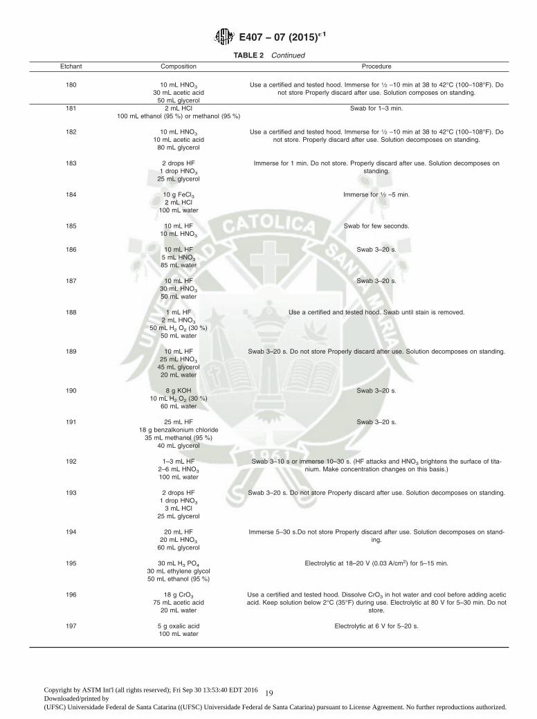
TABLE 2 Continued
Etchant Composition Procedure
180 10 mL HNO3
30 mL acetic acid50 mL glycerol
Use a certified and tested hood. Immerse for 1⁄2 –10 min at 38 to 42°C (100–108°F). Donot store Properly discard after use. Solution composes on standing.
181 2 mL HCl100 mL ethanol (95 %) or methanol (95 %)
Swab for 1–3 min.
182 10 mL HNO3
10 mL acetic acid80 mL glycerol
Use a certified and tested hood. Immerse for 1⁄2 –10 min at 38 to 42°C (100–108°F). Donot store. Properly discard after use. Solution decomposes on standing.
183 2 drops HF1 drop HNO3
25 mL glycerol
Immerse for 1 min. Do not store. Properly discard after use. Solution decomposes onstanding.
184 10 g FeCl32 mL HCl
100 mL water
Immerse for 1⁄2 –5 min.
185 10 mL HF10 mL HNO3
Swab for few seconds.
186 10 mL HF5 mL HNO3
85 mL water
Swab 3–20 s.
187 10 mL HF30 mL HNO3
50 mL water
Swab 3–20 s.
188 1 mL HF2 mL HNO3
50 mL H2 O2 (30 %)50 mL water
Use a certified and tested hood. Swab until stain is removed.
189 10 mL HF25 mL HNO3
45 mL glycerol20 mL water
Swab 3–20 s. Do not store Properly discard after use. Solution decomposes on standing.
190 8 g KOH10 mL H2 O2 (30 %)
60 mL water
Swab 3–20 s.
191 25 mL HF Swab 3–20 s.18 g benzalkonium chloride
35 mL methanol (95 %)40 mL glycerol
192 1–3 mL HF2–6 mL HNO3
100 mL water
Swab 3–10 s or immerse 10–30 s. (HF attacks and HNO3 brightens the surface of tita-nium. Make concentration changes on this basis.)
193 2 drops HF1 drop HNO3
3 mL HCl25 mL glycerol
Swab 3–20 s. Do not store Properly discard after use. Solution decomposes on standing.
194 20 mL HF20 mL HNO3
60 mL glycerol
Immerse 5–30 s.Do not store Properly discard after use. Solution decomposes on stand-ing.
195 30 mL H3 PO4
30 mL ethylene glycol50 mL ethanol (95 %)
Electrolytic at 18–20 V (0.03 A/cm2) for 5–15 min.
196 18 g CrO3
75 mL acetic acid20 mL water
Use a certified and tested hood. Dissolve CrO3 in hot water and cool before adding aceticacid. Keep solution below 2°C (35°F) during use. Electrolytic at 80 V for 5–30 min. Do not
store.
197 5 g oxalic acid100 mL water
Electrolytic at 6 V for 5–20 s.
E407 − 07 (2015)´1
19
Copyright by ASTM Int'l (all rights reserved); Fri Sep 30 13:53:40 EDT 2016Downloaded/printed by(UFSC) Universidade Federal de Santa Catarina ((UFSC) Universidade Federal de Santa Catarina) pursuant to License Agreement. No further reproductions authorized.
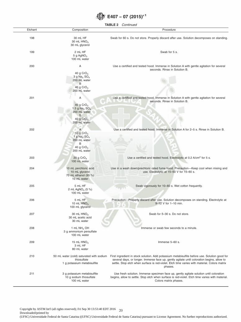
TABLE 2 Continued
Etchant Composition Procedure
198 30 mL HF30 mL HNO3
30 mL glycerol
Swab for 60 s. Do not store. Properly discard after use. Solution decomposes on standing.
199 2 mL HF5 g AgNO3
100 mL water
Swab for 5 s.
200 A Use a certified and tested hood. Immerse in Solution A with gentle agitation for severalseconds. Rinse in Solution B.
40 g CrO3
3 g Na2 SO4
200 mL waterB
40 g CrO3
200 mL water
201 A Use a certified and tested hood. Immerse in Solution A with gentle agitation for severalseconds. Rinse in Solution B.
40 g CrO3
1.5 g Na2 SO4
200 mL waterB
40 g CrO3
200 mL water
202 A Use a certified and tested hood. Immerse in Solution A for 2–5 s. Rinse in Solution B.10 g CrO3
1 g Na2 SO4
200 mL waterB
40 g CrO3
200 mL water
203 20 g CrO3
100 mL waterUse a certified and tested hood. Electrolytic at 0.2 A/cm2 for 5 s.
204 10 mL perchloric acid10 mL glycerol
70 mL ethanol (95 %)10 mL water
Use in a wash down/prechloric rated fume hood. Precaution—Keep cool when mixing anduse. Electrolytic at 15–50 V for 15–60 s.
205 5 mL HF2 mL AgNO3 (5 %)
100 mL water
Swab vigorously for 10–60 s. Wet cotton frequently.
206 5 mL HF10 mL HNO3
100 mL glycerol
Precaution—Properly discard after use. Solution decomposes on standing. Electrolytic at9–12 V for 1–10 min.
207 30 mL HNO3
30 mL acetic acid30 mL water
Swab for 5–30 s. Do not store.
208 1 mL NH4 OH3 g ammonium persulfate
100 mL water
Immerse or swab few seconds to a minute.
209 15 mL HNO3
3 mL HF80 mL water
Immerse 5–60 s.
210 50 mL water (cold) saturated with sodiumthiosulfate
1 g potassium metabisulfite
First ingredient in stock solution. Add potassium metabisulfite before use. Solution good forseveral days, or longer. Immerse face up, gently agitate until coloration begins, allow tosettle. Stop etch when surface is red-violet. Etch time varies with material. Colors matrix
phases.
211 3 g potassium metabisulfite10 g sodium thiosulfate
100 mL water
Use fresh solution. Immerse specimen face up, gently agitate solution until colorationbegins, allow to settle. Stop etch when surface is red-violet. Etch time varies with material.
Colors matrix phases.
E407 − 07 (2015)´1
20
Copyright by ASTM Int'l (all rights reserved); Fri Sep 30 13:53:40 EDT 2016Downloaded/printed by(UFSC) Universidade Federal de Santa Catarina ((UFSC) Universidade Federal de Santa Catarina) pursuant to License Agreement. No further reproductions authorized.

TABLE 2 Continued
Etchant Composition Procedure
212 10–50 % HCl in water0.5–1.0 g potassium metabisulfite per 100
mL of aqueous HCl solutionOptional: 1 g CuCl2
1–3 g FeCl32–10 g ammonium bifluoride
For more corrosion resistant alloys. Increase the HCl and potassium metabisulfite con-tents. Use optional ingredients to improve coloration, if needed. Colors matrix phases. Use
by immersion only.
213 2–10 mL HCl0.5–3 mL selenic acid
100 mL ethyl alcohol (95 %)
For more corrosion resistant alloys, increase the HCl and selenic acid content. For highlycorrosion-resistant alloys, use 20–30 mL HCl. Colors second phase constituents. Use by
immersion only.
214 1 g sodium molybdate100 mL water
Add nitric acid to lower the pH to 2.5–3. Add 0.1–0.5 g ammonium bifluoride for carbonsteels. Use by immersion only. Colors carbides. Immerse about 15 s.
215 240 g sodium thiosulfate30 g citric acid
24 g lead acetate1000 mL water
Mix in order given. Store in a dark bottle at least 24 h before use at 20°C. Lightly pre-etchspecimen before use. Use small portion of stock solution for 4 h max. Pre-etch steel speci-mens with nital before tinting the MnS (add 0.2 g sodium nitrite to 100 mL of etch) white.
Colors phosphides in cast iron. Colors matrix of Cu alloys.216 8–15 g sodium metabisulfite
100 mL waterDo not store. Mix fresh. Immerse specimen face up. Agitate solution gently until colorationbegins, allow to settle. Stop when surface is dark. Use crossed polarized light and sensi-
tive tint to improve coloration.217 5 g ammonium bifluoride
100 mL waterMix fresh, use plastic coated tongs and polyethylene beaker. Immerse until surface is col-
ored.218 3 g ammonium bifluoride
4 mL HCl100 mL water
Mix fresh, use plastic coated tongs and polyethylene beaker. Immerse until surface is col-ored. Works best with attack-polished specimens.
219 60 mL HNO3
40 mL waterElectrolytic etch, does not reveal twins in γ stainless steel. Excellent grain boundary etch
for ferritic stainless steels. Use at 1 V dc, 120 s, with stainless cathode; 0.6 V dc with plati-num cathode.
220 20 g NaOH100 mL water
Electrolytic etch, colors δ-ferrite in stainless steels. Use at 2–20 V dc, 5–20 s, stainlesssteel cathode. If δ is not colored, increase NaOH to 40 g.
221 50 mL water Use by immersion. Will not attack sulfides in stainless steels.50 mL ethyl alcohol
50 mL methyl alcohol50 mL HCl1 g CuCl2
2.5 g FeCl32.5 mL HNO3
222 8 g Na2 SO4 (a) Few seconds to 1 minute.100 mL water (b) Pre-etch 2 s in No. 74, rinse, and etch 20 s.
223 A8 g oxalic acid5 mL H2 SO4
100 mL waterB
H2 O2 (30 %)
Mix equal volumes of Solutions A and B just before use. Etch 2–3 s; 3 s pre-etch in No. 74may be needed.
224 10 mL H2 O2 (30 %)20 mL 10 % aqueous NaOH
Immerse 10 s at 20°C (68°F).
225 4 g NaOH100 mL saturated aqueous KMnO4
Immerse 10 s at 20°C (68°F).
226 15 mL HCl10 mL acetic acid
5 mL HNO3
2 drops glycerol
Use a certified and tested hood.—Can give off nitrogen dioxide gas. Precaution—MixHCl and glycerol thoroughly before adding HNO3. Do not store. Properly discard beforesolution attains a dark orange color. Use fresh or age up to 1 min. Immerse or swab few
seconds to few minutes. Can increase HNO3 to increase strength. Sometimes a fewpasses on the final polishing wheel is also necessary to remove a passive surface.
† Editorially corrected in May 2011.
E407 − 07 (2015)´1
21
Copyright by ASTM Int'l (all rights reserved); Fri Sep 30 13:53:40 EDT 2016Downloaded/printed by(UFSC) Universidade Federal de Santa Catarina ((UFSC) Universidade Federal de Santa Catarina) pursuant to License Agreement. No further reproductions authorized.

REFERENCES
(1) Lewis, R.J., Sax’s Dangerous Properties of Industrial Materials, 11thed. John Wiley and Sons., Inc., Hoboken, New Jersey, 2004.
(2) Prudent Practices for Handling Hazardous Chemicals inLaboratories, National Resource Council, National Academy Press,Washington, DC, 1995.
(3) Furr, A.K., CRC Handbook of Laboratory Safety, 5th ed. CRC Press,Boca Raton, Florida, 2000.
(4) .Wesenberg, G., Proctor, N., Proctor and Hughes’ Chemical Hazardsin the Workplace, 5th edition, edited by Gloria J. Hathaway and NickH, ProctorWiley-Interscience, Hoboken, New Jersey, 2004.
(5) OSHA Lab Safety Standard 29 CFR 1910.1450, Occupational Expo-sures to Hazardous Chemicals in the Laboratory.
(6) Prudent practices in the laboratory : handling and disposal ofchemicals, Committee on Prudent Practices for Handling, Storage,and Disposal of Chemicals in Laboratories, Board on ChemicalSciences and Technology, Commission on Physical Sciences,Mathematics, and Applications, National ResearchCouncil.Washington, D.C. : National Academy Press, 1995 .
(7) Lefevre, M. J., and Conibear, S., First Aid Manual for ChemicalAccidents, 2nd ed., Van Nostrand Reinhold Co., Inc., New York, 1989.
(8) Lewis, R. J., Rapid Guide to Hazardous Chemicals in the Workplace,4th ed.,John Wiley and Sons., Inc., New York, 2000.
(9) Anderson, R. L., “Safety in the Metallography Laboratory,” Westing-
house Research Lab, Pittsburgh, PA, Scientific Paper 65-1P30-METLL-P2, 1965 .
(10) Urben, P. and Bretherick, L., Bretherick’s Handbook of ReactiveChemical Hazards, 6th ed., Butterworth-Heinemann, , 1999.
(11) NFPA Haz-Mat Quick Guide, 1997.(12) Woldman’s Engineering Alloys, 9th ed., J. P. Frick, ed., ASM
International, Metals Park, Ohio, 2000.(13) Vander Voort, G. F., Metallography: Principles and Practice, ASM
International, Materials Park, Ohio, 1999.(14) Beraha, E., and Shpigler, B., Color Metallography, ASM, Metals
Park, OH, 1977.(15) Vander Voort, G. F., “Tint Etching,” Metal Progress, Vol 127, March
1985, pp. 31–33, 36–38, 41.(16) Weck, E., and Leistner, E., Metallographic Instructions for Colour
Etching by Immersion, Parts I, II and II, Deutscher Verlag, FürSchweisstechnik GmbH, Düsseldorf, West Germany, 1982, 1983,and 1986.
(17) Bühler, H. E., and Hougardy, H. P., Atlas of Interference LayerMetallography , Deutsche Gesellschaft für Metallkunde, Oberursel1, West Germany, 1980.
(18) Metals Handbook, Metallography and Microstructures, 10th ed., Vol9, ASM International, Metals Park, Ohio, 2004.
ASTM International takes no position respecting the validity of any patent rights asserted in connection with any item mentionedin this standard. Users of this standard are expressly advised that determination of the validity of any such patent rights, and the riskof infringement of such rights, are entirely their own responsibility.
This standard is subject to revision at any time by the responsible technical committee and must be reviewed every five years andif not revised, either reapproved or withdrawn. Your comments are invited either for revision of this standard or for additional standardsand should be addressed to ASTM International Headquarters. Your comments will receive careful consideration at a meeting of theresponsible technical committee, which you may attend. If you feel that your comments have not received a fair hearing you shouldmake your views known to the ASTM Committee on Standards, at the address shown below.
This standard is copyrighted by ASTM International, 100 Barr Harbor Drive, PO Box C700, West Conshohocken, PA 19428-2959,United States. Individual reprints (single or multiple copies) of this standard may be obtained by contacting ASTM at the aboveaddress or at 610-832-9585 (phone), 610-832-9555 (fax), or [email protected] (e-mail); or through the ASTM website(www.astm.org). Permission rights to photocopy the standard may also be secured from the Copyright Clearance Center, 222Rosewood Drive, Danvers, MA 01923, Tel: (978) 646-2600; http://www.copyright.com/
TABLE 3 Etchant Names
Common Name No. Common Name No.
Acetic glyceregia 89, 226 Groesbeck’s 19Alkaline Sodium Picrate 85 Hatch 2
Aqua regia 12 Howarth’s 84Barker’s 5 Kalling’s 1 95Beraha’s 99, 155, 211–215 Kalling’s 2 94Carapella 138 Keller’s 3
Chrome regia 101 Klemm’s 210Contrast 141 Kroll’s 192, 187
CP 4 60 Marble’s 25El-1R 107 Marshall’s 223Flat 133 Murakami’s 98
Flouregia 90, 158 Nital 74Frank’s 104 Palmerton 200
Fry’s 79 Phoschromic 111G 107 Picral 76
Glyceregia 87 Ralph’s 221Gorsuch 75 Super Picral 77
Grard’s No. 1 35 Vilella’s 80Green contrast 94 92-5-3 105
E407 − 07 (2015)´1
22
Copyright by ASTM Int'l (all rights reserved); Fri Sep 30 13:53:40 EDT 2016Downloaded/printed by(UFSC) Universidade Federal de Santa Catarina ((UFSC) Universidade Federal de Santa Catarina) pursuant to License Agreement. No further reproductions authorized.

ANEXO 11
NORMA
ASTM E112 – 12

Designation: E112 − 12
Standard Test Methods forDetermining Average Grain Size1
This standard is issued under the fixed designation E112; the number immediately following the designation indicates the year oforiginal adoption or, in the case of revision, the year of last revision. A number in parentheses indicates the year of last reapproval. Asuperscript epsilon (´) indicates an editorial change since the last revision or reapproval.
This standard has been approved for use by agencies of the Department of Defense.
INTRODUCTION
These test methods of determination of average grain size in metallic materials are primarilymeasuring procedures and, because of their purely geometric basis, are independent of the metal oralloy concerned. In fact, the basic procedures may also be used for the estimation of average grain,crystal, or cell size in nonmetallic materials. The comparison method may be used if the structure ofthe material approaches the appearance of one of the standard comparison charts. The intercept andplanimetric methods are always applicable for determining average grain size. However, thecomparison charts cannot be used for measurement of individual grains.
1. Scope
1.1 These test methods cover the measurement of averagegrain size and include the comparison procedure, the planim-etric (or Jeffries) procedure, and the intercept procedures.These test methods may also be applied to nonmetallicmaterials with structures having appearances similar to those ofthe metallic structures shown in the comparison charts. Thesetest methods apply chiefly to single phase grain structures butthey can be applied to determine the average size of a particulartype of grain structure in a multiphase or multiconstituentspecimen.
1.2 These test methods are used to determine the averagegrain size of specimens with a unimodal distribution of grainareas, diameters, or intercept lengths. These distributions areapproximately log normal. These test methods do not covermethods to characterize the nature of these distributions.Characterization of grain size in specimens with duplex grainsize distributions is described in Test Methods E1181. Mea-surement of individual, very coarse grains in a fine grainedmatrix is described in Test Methods E930.
1.3 These test methods deal only with determination ofplanar grain size, that is, characterization of the two-dimensional grain sections revealed by the sectioning plane.Determination of spatial grain size, that is, measurement of thesize of the three-dimensional grains in the specimen volume, isbeyond the scope of these test methods.
1.4 These test methods describe techniques performedmanually using either a standard series of graded chart imagesfor the comparison method or simple templates for the manualcounting methods. Utilization of semi-automatic digitizingtablets or automatic image analyzers to measure grain size isdescribed in Test Methods E1382.
1.5 These test methods deal only with the recommended testmethods and nothing in them should be construed as definingor establishing limits of acceptability or fitness of purpose ofthe materials tested.
1.6 The measured values are stated in SI units, which areregarded as standard. Equivalent inch-pound values, whenlisted, are in parentheses and may be approximate.
1.7 This standard does not purport to address all of thesafety concerns, if any, associated with its use. It is theresponsibility of the user of this standard to establish appro-priate safety and health practices and determine the applica-bility of regulatory limitations prior to use.
1.8 The paragraphs appear in the following order:Section Number
Scope 1Referenced Documents 2Terminology 3Significance and Use 4Generalities of Application 5Sampling 6Test Specimens 7Calibration 8Preparation of Photomicrographs 9Comparison Procedure 10Planimetric (Jeffries) Procedure 11General Intercept Procedures 12Heyn Linear Intercept Procedure 13Circular Intercept Procedures 14Hilliard Single-Circle Procedure 14.2
1 These test methods are under the jurisdiction of ASTM Committee E04 onMetallography and are the direct responsibility of Subcommittee E04.08 on GrainSize.
Current edition approved Nov. 15, 2012. Published January 2013. Originallyapproved in 1955. Last previous edition approved 2010 as E112 – 10. DOI:10.1520/E0112-12.
Copyright © ASTM International, 100 Barr Harbor Drive, PO Box C700, West Conshohocken, PA 19428-2959. United States
1
Copyright by ASTM Int'l (all rights reserved); Tue Sep 3 16:40:18 EDT 2013Downloaded/printed byCenter For Library Initiatives pursuant to License Agreement. No further reproductions authorized.
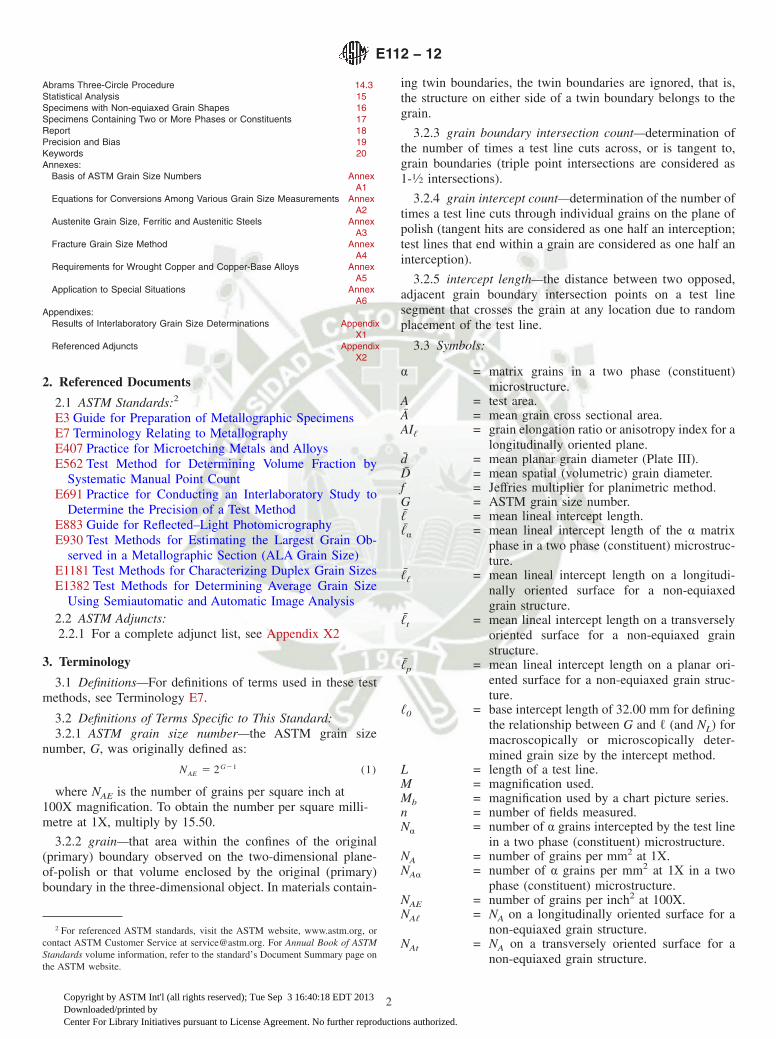
Abrams Three-Circle Procedure 14.3Statistical Analysis 15Specimens with Non-equiaxed Grain Shapes 16Specimens Containing Two or More Phases or Constituents 17Report 18Precision and Bias 19Keywords 20Annexes:
Basis of ASTM Grain Size Numbers AnnexA1
Equations for Conversions Among Various Grain Size Measurements AnnexA2
Austenite Grain Size, Ferritic and Austenitic Steels AnnexA3
Fracture Grain Size Method AnnexA4
Requirements for Wrought Copper and Copper-Base Alloys AnnexA5
Application to Special Situations AnnexA6
Appendixes:Results of Interlaboratory Grain Size Determinations Appendix
X1Referenced Adjuncts Appendix
X2
2. Referenced Documents
2.1 ASTM Standards:2
E3 Guide for Preparation of Metallographic SpecimensE7 Terminology Relating to MetallographyE407 Practice for Microetching Metals and AlloysE562 Test Method for Determining Volume Fraction by
Systematic Manual Point CountE691 Practice for Conducting an Interlaboratory Study to
Determine the Precision of a Test MethodE883 Guide for Reflected–Light PhotomicrographyE930 Test Methods for Estimating the Largest Grain Ob-
served in a Metallographic Section (ALA Grain Size)E1181 Test Methods for Characterizing Duplex Grain SizesE1382 Test Methods for Determining Average Grain Size
Using Semiautomatic and Automatic Image Analysis2.2 ASTM Adjuncts:2.2.1 For a complete adjunct list, see Appendix X2
3. Terminology
3.1 Definitions—For definitions of terms used in these testmethods, see Terminology E7.
3.2 Definitions of Terms Specific to This Standard:3.2.1 ASTM grain size number—the ASTM grain size
number, G, was originally defined as:
NAE 5 2G21 (1)
where NAE is the number of grains per square inch at100X magnification. To obtain the number per square milli-metre at 1X, multiply by 15.50.
3.2.2 grain—that area within the confines of the original(primary) boundary observed on the two-dimensional plane-of-polish or that volume enclosed by the original (primary)boundary in the three-dimensional object. In materials contain-
ing twin boundaries, the twin boundaries are ignored, that is,the structure on either side of a twin boundary belongs to thegrain.
3.2.3 grain boundary intersection count—determination ofthe number of times a test line cuts across, or is tangent to,grain boundaries (triple point intersections are considered as1-1⁄2 intersections).
3.2.4 grain intercept count—determination of the number oftimes a test line cuts through individual grains on the plane ofpolish (tangent hits are considered as one half an interception;test lines that end within a grain are considered as one half aninterception).
3.2.5 intercept length—the distance between two opposed,adjacent grain boundary intersection points on a test linesegment that crosses the grain at any location due to randomplacement of the test line.
3.3 Symbols:
α = matrix grains in a two phase (constituent)microstructure.
A = test area.A = mean grain cross sectional area.AIℓ = grain elongation ratio or anisotropy index for a
longitudinally oriented plane.d = mean planar grain diameter (Plate III).D = mean spatial (volumetric) grain diameter.f = Jeffries multiplier for planimetric method.G = ASTM grain size number.ℓ = mean lineal intercept length.ℓα = mean lineal intercept length of the α matrix
phase in a two phase (constituent) microstruc-ture.
ℓℓ = mean lineal intercept length on a longitudi-nally oriented surface for a non-equiaxedgrain structure.
ℓt = mean lineal intercept length on a transverselyoriented surface for a non-equiaxed grainstructure.
ℓp = mean lineal intercept length on a planar ori-ented surface for a non-equiaxed grain struc-ture.
ℓ0 = base intercept length of 32.00 mm for definingthe relationship between G and ℓ (and NL) formacroscopically or microscopically deter-mined grain size by the intercept method.
L = length of a test line.M = magnification used.Mb = magnification used by a chart picture series.n = number of fields measured.Nα = number of α grains intercepted by the test line
in a two phase (constituent) microstructure.NA = number of grains per mm2 at 1X.NAα = number of α grains per mm2 at 1X in a two
phase (constituent) microstructure.NAE = number of grains per inch2 at 100X.NAℓ = NA on a longitudinally oriented surface for a
non-equiaxed grain structure.NAt = NA on a transversely oriented surface for a
non-equiaxed grain structure.
2 For referenced ASTM standards, visit the ASTM website, www.astm.org, orcontact ASTM Customer Service at [email protected]. For Annual Book of ASTMStandards volume information, refer to the standard’s Document Summary page onthe ASTM website.
E112 − 12
2
Copyright by ASTM Int'l (all rights reserved); Tue Sep 3 16:40:18 EDT 2013Downloaded/printed byCenter For Library Initiatives pursuant to License Agreement. No further reproductions authorized.

NAp = NA on a planar oriented surface for a non-equiaxed grain structure.
NI = number of intercepts with a test line.NInside = number of grains completely within a test
circle.N Intercepted = number of grains intercepted by the test circle.NL = number of intercepts per unit length of test
line.NLℓ = NL on a longitudinally oriented surface for a
non-equiaxed grain structure.NLt = NL on a transversely oriented surface for a
non-equiaxed grain structure.NLp = NL on a planar oriented surface for a non-
equiaxed grain structure.PI = number of grain boundary intersections with a
test line.PL = number of grain boundary intersections per
unit length of test line.PLℓ = PL on a longitudinally oriented surface for a
non-equiaxed grain structure.PLt = PL on a transversely oriented surface for a
non-equiaxed grain structure.PLp = PL on a planar oriented surface for a non-
equiaxed grain structure.Q = correction factor for comparison chart ratings
using a non-standard magnification for micro-scopically determined grain sizes.
Qm = correction factor for comparison chart ratingsusing a non-standard magnification for mac-roscopically determined grain sizes.
s = standard deviation.SV = grain boundary surface area to volume ratio
for a single phase structure.SVα = grain boundary surface area to volume ratio
for a two phase (constituent) structure.t = students’ t multiplier for determination of the
confidence interval.VVα = volume fraction of the α phase in a two phase
(constituent) microstructure.95 %CI = 95 % confidence interval.%RA = percent relative accuracy.
4. Significance and Use
4.1 These test methods cover procedures for estimating andrules for expressing the average grain size of all metalsconsisting entirely, or principally, of a single phase. The testmethods may also be used for any structures having appear-ances similar to those of the metallic structures shown in thecomparison charts. The three basic procedures for grain sizeestimation are:
4.1.1 Comparison Procedure—The comparison proceduredoes not require counting of either grains, intercepts, orintersections but, as the name suggests, involves comparison ofthe grain structure to a series of graded images, either in theform of a wall chart, clear plastic overlays, or an eyepiecereticle. There appears to be a general bias in that comparisongrain size ratings claim that the grain size is somewhat coarser(1⁄2 to 1 G number lower) than it actually is (see X1.3.5).Repeatability and reproducibility of comparison chart ratingsare generally 61 grain size number.
4.1.2 Planimetric Procedure—The planimetric method in-volves an actual count of the number of grains within a knownarea. The number of grains per unit area, NA , is used todetermine the ASTM grain size number, G. The precision ofthe method is a function of the number of grains counted. Aprecision of 60.25 grain size units can be attained with areasonable amount of effort. Results are free of bias andrepeatability and reproducibility are less than 60.5 grain sizeunits. An accurate count does require marking off of the grainsas they are counted.
4.1.3 Intercept Procedure—The intercept method involvesan actual count of the number of grains intercepted by a testline or the number of grain boundary intersections with a testline, per unit length of test line, used to calculate the meanlineal intercept length, ℓ. ℓ is used to determine the ASTMgrain size number, G. The precision of the method is a functionof the number of intercepts or intersections counted. A preci-sion of better than 60.25 grain size units can be attained witha reasonable amount of effort. Results are free of bias;repeatability and reproducibility are less than 60.5 grain sizeunits. Because an accurate count can be made without need ofmarking off intercepts or intersections, the intercept method isfaster than the planimetric method for the same level ofprecision.
4.2 For specimens consisting of equiaxed grains, themethod of comparing the specimen with a standard chart ismost convenient and is sufficiently accurate for most commer-cial purposes. For higher degrees of accuracy in determiningaverage grain size, the intercept or planimetric procedures maybe used. The intercept procedure is particularly useful forstructures consisting of elongated grains.
4.3 In case of dispute, the intercept procedure shall be thereferee procedure in all cases.
4.4 No attempt should be made to estimate the average grainsize of heavily cold-worked material. Partially recrystallizedwrought alloys and lightly to moderately cold-worked materialmay be considered as consisting of non-equiaxed grains, if agrain size measurement is necessary.
4.5 Individual grain measurements should not be madebased on the standard comparison charts. These charts wereconstructed to reflect the typical log-normal distribution ofgrain sizes that result when a plane is passed through athree-dimensional array of grains. Because they show a distri-bution of grain dimensions, ranging from very small to verylarge, depending on the relationship of the planar section andthe three-dimensional array of grains, the charts are notapplicable to measurement of individual grains.
5. Generalities of Application
5.1 It is important, in using these test methods, to recognizethat the estimation of average grain size is not a precisemeasurement. A metal structure is an aggregate of three-dimensional crystals of varying sizes and shapes. Even if allthese crystals were identical in size and shape, the grain crosssections, produced by a random plane (surface of observation)through such a structure, would have a distribution of areasvarying from a maximum value to zero, depending upon where
E112 − 12
3
Copyright by ASTM Int'l (all rights reserved); Tue Sep 3 16:40:18 EDT 2013Downloaded/printed byCenter For Library Initiatives pursuant to License Agreement. No further reproductions authorized.
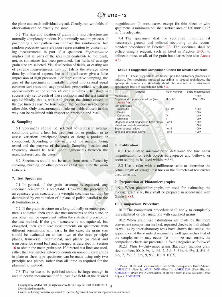
the plane cuts each individual crystal. Clearly, no two fields ofobservation can be exactly the same.
5.2 The size and location of grains in a microstructure arenormally completely random. No nominally random process ofpositioning a test pattern can improve this randomness, butrandom processes can yield poor representation by concentrat-ing measurements in part of a specimen. Representativeimplies that all parts of the specimen contribute to the result,not, as sometimes has been presumed, that fields of averagegrain size are selected. Visual selection of fields, or casting outof extreme measurements, may not falsify the average whendone by unbiased experts, but will in all cases give a falseimpression of high precision. For representative sampling, thearea of the specimen is mentally divided into several equalcoherent sub-areas and stage positions prespecified, which areapproximately at the center of each sub-area. The stage issuccessively set to each of these positions and the test patternapplied blindly, that is, with the light out, the shutter closed, orthe eye turned away. No touch-up of the position so selected isallowable. Only measurements made on fields chosen in thisway can be validated with respect to precision and bias.
6. Sampling
6.1 Specimens should be selected to represent averageconditions within a heat lot, treatment lot, or product, or toassess variations anticipated across or along a product orcomponent, depending on the nature of the material beingtested and the purpose of the study. Sampling location andfrequency should be based upon agreements between themanufacturers and the users.
6.2 Specimens should not be taken from areas affected byshearing, burning, or other processes that will alter the grainstructure.
7. Test Specimens
7.1 In general, if the grain structure is equiaxed, anyspecimen orientation is acceptable. However, the presence ofan equiaxed grain structure in a wrought specimen can only bedetermined by examination of a plane of polish parallel to thedeformation axis.
7.2 If the grain structure on a longitudinally oriented speci-men is equiaxed, then grain size measurements on this plane, orany other, will be equivalent within the statistical precision ofthe test method. If the grain structure is not equiaxed, butelongated, then grain size measurements on specimens withdifferent orientations will vary. In this case, the grain sizeshould be evaluated on at least two of the three principleplanes, transverse, longitudinal, and planar (or radial andtransverse for round bar) and averaged as described in Section16 to obtain the mean grain size. If directed test lines are used,rather than test circles, intercept counts on non-equiaxed grainsin plate or sheet type specimens can be made using only twoprinciple test planes, rather than all three as required for theplanimetric method.
7.3 The surface to be polished should be large enough inarea to permit measurement of at least five fields at the desired
magnification. In most cases, except for thin sheet or wirespecimens, a minimum polished surface area of 160 mm2 (0.25in.2) is adequate.
7.4 The specimen shall be sectioned, mounted (ifnecessary), ground, and polished according to the recom-mended procedures in Practice E3. The specimen shall beetched using a reagent, such as listed in Practice E407, todelineate most, or all, of the grain boundaries (see also AnnexA3).
8. Calibration
8.1 Use a stage micrometer to determine the true linearmagnification for each objective, eyepiece and bellows, orzoom setting to be used within 62 %.
8.2 Use a ruler with a millimetre scale to determine theactual length of straight test lines or the diameter of test circlesused as grids.
9. Preparation of Photomicrographs
9.1 When photomicrographs are used for estimating theaverage grain size, they shall be prepared in accordance withGuide E883.
10. Comparison Procedure
10.1 The comparison procedure shall apply to completelyrecrystallized or cast materials with equiaxed grains.
10.2 When grain size estimations are made by the moreconvenient comparison method, repeated checks by individualsas well as by interlaboratory tests have shown that unless theappearance of the standard reasonably well approaches that ofthe sample, errors may occur. To minimize such errors, thecomparison charts are presented in four categories as follows:3
10.2.1 Plate I—Untwinned grains (flat etch). Includes grainsize numbers 00, 0, 1⁄2, 1, 11⁄2, 2, 21⁄2, 3, 31⁄2, 4, 41⁄2, 5, 51⁄2, 6,61⁄2, 7, 71⁄2, 8, 81⁄2, 9, 91⁄2, 10, at 100X.
3 Plates I, II, III, and IV are available from ASTM Headquarters. Order Adjunct:ADJE11201P (Plate I), ADJE11202P (Plate II), ADJE11203P (Plate III), andADJE11204P (Plate IV). A combination of all four plates is also available. OrderAdjunct: ADJE112PS.
TABLE 1 Suggested Comparison Charts for Metallic Materials
NOTE 1—These suggestions are based upon the customary practices inindustry. For specimens prepared according to special techniques, theappropriate comparison standards should be selected on a structural-appearance basis in accordance with 8.2.
Material Plate Number Basic Magnification
Aluminum I 100XCopper and copper-base alloys (see
Annex A4)III or IV 75X, 100X
Iron and steel:Austenitic II or IV 100XFerritic I 100XCarburized IV 100XStainless II 100X
Magnesium and magnesium-base alloys I or II 100XNickel and nickel-base alloys II 100XSuper-strength alloys I or II 100XZinc and zinc-base alloys I or II 100X
E112 − 12
4
Copyright by ASTM Int'l (all rights reserved); Tue Sep 3 16:40:18 EDT 2013Downloaded/printed byCenter For Library Initiatives pursuant to License Agreement. No further reproductions authorized.

10.2.2 Plate II—Twinned grains (flat etch). Includes grainsize numbers, 1, 2, 3, 4, 5, 6, 7, 8, at 100X.
10.2.3 Plate III—Twinned grains (contrast etch). Includesnominal grain diameters of 0.200, 0.150, 0.120, 0.090, 0.070,0.060, 0.050, 0.045, 0.035, 0.025, 0.020, 0.015, 0.010, 0.005mm at 75X.
10.2.4 Plate IV—Austenite grains in steel (McQuaid-Ehn).Includes grain size numbers 1, 2, 3, 4, 5, 6, 7, 8, at 100X.
10.3 Table 1 lists a number of materials and the comparisoncharts that are suggested for use in estimating their averagegrain sizes. For example, for twinned copper and brass with acontrast etch, use Plate III.
NOTE 1—Examples of grain-size standards from Plates I, II, III, and IVare shown in Fig. 1, Fig. 2, Fig. 3, and Fig. 4.
10.4 The estimation of microscopically-determined grainsize should usually be made by direct comparison at the samemagnification as the appropriate chart. Accomplish this bycomparing a projected image or a photomicrograph of arepresentative field of the test specimen with the photomicro-graphs of the appropriate standard grain-size series, or withsuitable reproductions or transparencies of them, and select thephotomicrograph which most nearly matches the image of thetest specimen or interpolate between two standards. Report thisestimated grain size as the ASTM grain size number, or graindiameter, of the chart picture that most closely matches theimage of the test specimen or as an interpolated value betweentwo standard chart pictures.
10.5 Good judgment on the part of the observer is necessaryto select the magnification to be used, the proper size of area(number of grains), and the number and location in thespecimen of representative sections and fields for estimating
the characteristic or average grain size. It is not sufficient tovisually select what appear to be areas of average grain size.Recommendations for choosing appropriate areas for all pro-cedures have been noted in 5.2.
10.6 Grain size estimations shall be made on three or morerepresentative areas of each specimen section.
FIG. 1 Example of Untwinned Grains (Flat Etch) from Plate I.Grain Size No. 3 at 100X
FIG. 2 Example of Twin Grains (Flat Etch) from Plate II. GrainSize No. 3 at 100X
FIG. 3 Example of Twin Grains (Contrast Etch) from Plate III.Grain Size 0.090 mm at 75X
E112 − 12
5
Copyright by ASTM Int'l (all rights reserved); Tue Sep 3 16:40:18 EDT 2013Downloaded/printed byCenter For Library Initiatives pursuant to License Agreement. No further reproductions authorized.

10.7 When the grains are of a size outside the range coveredby the standard photographs, or when magnifications of 75X or100X are not satisfactory, other magnifications may be em-ployed for comparison by using the relationships given in Note2 and Table 2. It may be noted that alternative magnificationsare usually simple multiples of the basic magnifications.
NOTE 2—If the grain size is reported in ASTM numbers, it is convenientto use the relationship:
Q 5 2 log2 ~M/Mb! (2)
56.64 log10 ~M/Mb!where Q is a correction factor that is added to the apparent micro-grain
size of the specimen, as viewed at the magnification, M, instead of at thebasic magnification, Mb (75X or 100X), to yield the true ASTM grain-size
number. Thus, for a magnification of 25X, the true ASTM grain-sizenumber is four numbers lower than that of the corresponding photomi-crograph at 100X (Q = −4). Likewise, for 400X, the true ASTM grain-sizenumber is four numbers higher (Q = +4) than that of the correspondingphotomicrograph at 100X. Similarly, for 300X, the true ASTM grain-sizenumber is four numbers higher than that of the corresponding photomi-crograph at 75X.
10.8 The small number of grains per field at the coarse endof the chart series, that is, size 00, and the very small size of thegrains at the fine end make accurate comparison ratingsdifficult. When the specimen grain size falls at either end of thechart range, a more meaningful comparison can be made bychanging the magnification so that the grain size lies closer tothe center of the range.
FIG. 4 Example of Austenite Grains in Steel from Plate IV. GrainSize No. 3 at 100X
TABLE 2 Microscopically Determined Grain Size Relationships Using Plate III at Various Magnifications
NOTE 1—First line—mean grain diameter, d, in mm; in parentheses—equivalent ASTM grain size number, G.
NOTE 2—Magnification for Plate III is 75X (row 3 data).
MagnificationChart Picture Number (Plate III)
1 2 3 4 5 6 7 8 9 10 11 12 13 14
25X 0.015(9.2)
0.030(7.2)
0.045(6.0)
0.060(5.2)
0.075(4.5)
0.105(3.6)
0.135(2.8)
0.150(2.5)
0.180(2.0)
0.210(1.6)
0.270(0.8)
0.360(0)
0.451(0/00)
0.600(00 + )
50X 0.0075(11.2)
0.015(9.2)
0.0225(8.0)
0.030(7.2)
0.0375(6.5)
0.053(5.6)
0.0675(4.8)
0.075(4.5)
0.090(4.0)
0.105(3.6)
0.135(2.8)
0.180(2.0)
0.225(1.4)
0.300(0.5)
75X 0.005(12.3)
0.010(10.3)
0.015(9.2)
0.020(8.3)
0.025(7.7)
0.035(6.7)
0.045(6.0)
0.050(5.7)
0.060(5.2)
0.070(4.7)
0.090(4.0)
0.120(3.2)
0.150(2.5)
0.200(1.7)
100X 0.00375(13.2)
0.0075(11.2)
0.0112(10.0)
0.015(9.2)
0.019(8.5)
0.026(7.6)
0.034(6.8)
0.0375(6.5)
0.045(6.0)
0.053(5.6)
0.067(4.8)
0.090(4.0)
0.113(3.4)
0.150(2.5)
200X 0.0019(15.2)
0.00375(13.2)
0.0056(12.0)
0.0075(11.2)
0.009(10.5)
0.013(9.6)
0.017(8.8)
0.019(8.5)
0.0225(8.0)
0.026(7.6)
0.034(6.8)
0.045(6.0)
0.056(5.4)
0.075(4.5)
400X — 0.0019(15.1)
0.0028(14.0)
0.0038(13.1)
0.0047(12.5)
0.0067(11.5)
0.0084(10.8)
0.009(10.5)
0.0012(10.0)
0.0133(9.5)
0.0168(8.8)
0.0225(8.0)
0.028(7.3)
0.0375(6.5)
500X — — 0.0022(14.6)
0.003(13.7)
0.00375(13.1)
0.00525(12.1)
0.0067(11.5)
0.0075(11.1)
0.009(10.6)
0.010(10.3)
0.0133(9.5)
0.018(8.7)
0.0225(8.0)
0.03(7.1)
E112 − 12
6
Copyright by ASTM Int'l (all rights reserved); Tue Sep 3 16:40:18 EDT 2013Downloaded/printed byCenter For Library Initiatives pursuant to License Agreement. No further reproductions authorized.
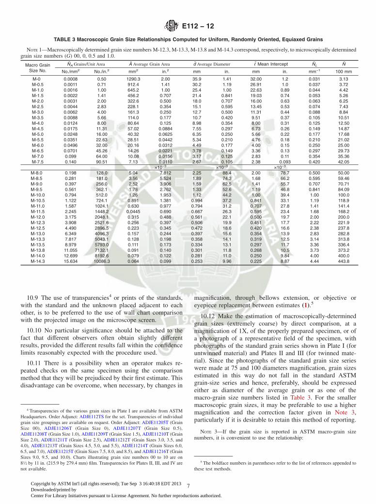
10.9 The use of transparencies4 or prints of the standards,with the standard and the unknown placed adjacent to eachother, is to be preferred to the use of wall chart comparisonwith the projected image on the microscope screen.
10.10 No particular significance should be attached to thefact that different observers often obtain slightly differentresults, provided the different results fall within the confidencelimits reasonably expected with the procedure used.
10.11 There is a possibility when an operator makes re-peated checks on the same specimen using the comparisonmethod that they will be prejudiced by their first estimate. Thisdisadvantage can be overcome, when necessary, by changes in
magnification, through bellows extension, or objective oreyepiece replacement between estimates (1).5
10.12 Make the estimation of macroscopically-determinedgrain sizes (extremely coarse) by direct comparison, at amagnification of 1X, of the properly prepared specimen, or ofa photograph of a representative field of the specimen, withphotographs of the standard grain series shown in Plate I (foruntwinned material) and Plates II and III (for twinned mate-rial). Since the photographs of the standard grain size serieswere made at 75 and 100 diameters magnification, grain sizesestimated in this way do not fall in the standard ASTMgrain-size series and hence, preferably, should be expressedeither as diameter of the average grain or as one of themacro-grain size numbers listed in Table 3. For the smallermacroscopic grain sizes, it may be preferable to use a highermagnification and the correction factor given in Note 3,particularly if it is desirable to retain this method of reporting.
NOTE 3—If the grain size is reported in ASTM macro-grain sizenumbers, it is convenient to use the relationship:
4 Transparencies of the various grain sizes in Plate I are available from ASTMHeadquarters. Order Adjunct: ADJE112TS for the set. Transparencies of individualgrain size groupings are available on request. Order Adjunct: ADJE11205T (GrainSize 00), ADJE11206T (Grain Size 0), ADJE11207T (Grain Size 0.5),ADJE11208T (Grain Size 1.0), ADJE11209T (Grain Size 1.5), ADJE11210T (GrainSize 2.0), ADJE11211T (Grain Size 2.5), ADJE11212T (Grain Sizes 3.0, 3.5, and4.0), ADJE11213T (Grain Sizes 4.5, 5.0, and 5.5), ADJE11214T (Grain Sizes 6.0,6.5, and 7.0), ADJE11215T (Grain Sizes 7.5, 8.0, and 8.5), and ADJE11216T (GrainSizes 9.0, 9.5, and 10.0). Charts illustrating grain size numbers 00 to 10 are on81⁄2 by 11 in. (215.9 by 279.4 mm) film. Transparencies for Plates II, III, and IV arenot available.
5 The boldface numbers in parentheses refer to the list of references appended tothese test methods.
TABLE 3 Macroscopic Grain Size Relationships Computed for Uniform, Randomly Oriented, Equiaxed Grains
NOTE 1—Macroscopically determined grain size numbers M-12.3, M-13.3, M-13.8 and M-14.3 correspond, respectively, to microscopically determinedgrain size numbers (G) 00, 0, 0.5 and 1.0.
Macro GrainSize No.
NA Grains/Unit Area A Average Grain Area d Average Diameter ! Mean Intercept NL N
No./mm2 No./in.2 mm2 in.2 mm in. mm in. mm−1 100 mm
M-0 0.0008 0.50 1290.3 2.00 35.9 1.41 32.00 1.2 0.031 3.13M-0.5 0.0011 0.71 912.4 1.41 30.2 1.19 26.91 1.0 0.037 3.72M-1.0 0.0016 1.00 645.2 1.00 25.4 1.00 22.63 0.89 0.044 4.42M-1.5 0.0022 1.41 456.2 0.707 21.4 0.841 19.03 0.74 0.053 5.26M-2.0 0.0031 2.00 322.6 0.500 18.0 0.707 16.00 0.63 0.063 6.25M-2.5 0.0044 2.83 228.1 0.354 15.1 0.595 13.45 0.53 0.074 7.43M-3.0 0.0062 4.00 161.3 0.250 12.7 0.500 11.31 0.44 0.088 8.84M-3.5 0.0088 5.66 114.0 0.177 10.7 0.420 9.51 0.37 0.105 10.51M-4.0 0.0124 8.00 80.64 0.125 8.98 0.354 8.00 0.31 0.125 12.50M-4.5 0.0175 11.31 57.02 0.0884 7.55 0.297 6.73 0.26 0.149 14.87M-5.0 0.0248 16.00 40.32 0.0625 6.35 0.250 5.66 0.22 0.177 17.68M-5.5 0.0351 22.63 28.51 0.0442 5.34 0.210 4.76 0.18 0.210 21.02M-6.0 0.0496 32.00 20.16 0.0312 4.49 0.177 4.00 0.15 0.250 25.00M-6.5 0.0701 45.26 14.26 0.0221 3.78 0.149 3.36 0.13 0.297 29.73M-7.0 0.099 64.00 10.08 0.0156 3.17 0.125 2.83 0.11 0.354 35.36M-7.5 0.140 90.51 7.13 0.0110 2.67 0.105 2.38 0.093 0.420 42.05
×10−3 ×10−3 ×10⁻³
M-8.0 0.198 128.0 5.04 7.812 2.25 88.4 2.00 78.7 0.500 50.00M-8.5 0.281 181.0 3.56 5.524 1.89 74.3 1.68 66.2 0.595 59.46M-9.0 0.397 256.0 2.52 3.906 1.59 62.5 1.41 55.7 0.707 70.71M-9.5 0.561 362.1 1.78 2.762 1.33 52.6 1.19 46.8 0.841 84.09M-10.0 0.794 512.0 1.26 1.953 1.12 44.2 1.00 39.4 1.00 100.0M-10.5 1.122 724.1 0.891 1.381 0.994 37.2 0.841 33.1 1.19 118.9M-11.0 1.587 1024.1 0.630 0.977 0.794 31.2 0.707 27.8 1.41 141.4M-11.5 2.245 1448.2 0.0445 0.690 0.667 26.3 0.595 23.4 1.68 168.2M-12.0 3.175 2048.1 0.315 0.488 0.561 22.1 0.500 19.7 2.00 200.0M-12.3 3.908 2521.6 0.256 0.397 0.506 19.9 0.451 17.7 2.22 221.9M-12.5 4.490 2896.5 0.223 0.345 0.472 18.6 0.420 16.6 2.38 237.8M-13.0 6.349 4096.3 0.157 0.244 0.397 15.6 0.354 13.9 2.83 282.8M-13.3 7.817 5043.1 0.128 0.198 0.358 14.1 0.319 12.5 3.14 313.8M-13.5 8.979 5793.0 0.111 0.173 0.334 13.1 0.297 11.7 3.36 336.4M-13.8 11.055 7132.1 0.091 0.140 0.301 11.8 0.268 10.5 3.73 373.2M-14.0 12.699 8192.6 0.079 0.122 0.281 11.0 0.250 9.84 4.00 400.0M-14.3 15.634 10086.3 0.064 0.099 0.253 9.96 0.225 8.87 4.44 443.8
E112 − 12
7
Copyright by ASTM Int'l (all rights reserved); Tue Sep 3 16:40:18 EDT 2013Downloaded/printed byCenter For Library Initiatives pursuant to License Agreement. No further reproductions authorized.
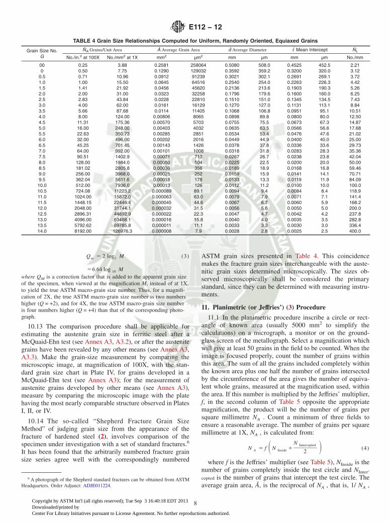
Qm 5 2 log2 M (3)
56.64 log 10 Mwhere QM is a correction factor that is added to the apparent grain sizeof the specimen, when viewed at the magnification M, instead of at 1X,to yield the true ASTM macro-grain size number. Thus, for a magnifi-cation of 2X, the true ASTM macro-grain size number is two numbershigher (Q = +2), and for 4X, the true ASTM macro-grain size numberis four numbers higher (Q = +4) than that of the corresponding photo-graph.
10.13 The comparison procedure shall be applicable forestimating the austenite grain size in ferritic steel after aMcQuaid-Ehn test (see Annex A3, A3.2), or after the austenitegrains have been revealed by any other means (see Annex A3,A3.3). Make the grain-size measurement by comparing themicroscopic image, at magnification of 100X, with the stan-dard grain size chart in Plate IV, for grains developed in aMcQuaid-Ehn test (see Annex A3); for the measurement ofaustenite grains developed by other means (see Annex A3),measure by comparing the microscopic image with the platehaving the most nearly comparable structure observed in PlatesI, II, or IV.
10.14 The so-called “Shepherd Fracture Grain SizeMethod” of judging grain size from the appearance of thefracture of hardened steel (2), involves comparison of thespecimen under investigation with a set of standard fractures.6
It has been found that the arbitrarily numbered fracture grainsize series agree well with the correspondingly numbered
ASTM grain sizes presented in Table 4. This coincidencemakes the fracture grain sizes interchangeable with the auste-nitic grain sizes determined microscopically. The sizes ob-served microscopically shall be considered the primarystandard, since they can be determined with measuring instru-ments.
11. Planimetric (or Jeffries’) (3) Procedure
11.1 In the planimetric procedure inscribe a circle or rect-angle of known area (usually 5000 mm2 to simplify thecalculations) on a micrograph, a monitor or on the ground-glass screen of the metallograph. Select a magnification whichwill give at least 50 grains in the field to be counted. When theimage is focused properly, count the number of grains withinthis area. The sum of all the grains included completely withinthe known area plus one half the number of grains intersectedby the circumference of the area gives the number of equiva-lent whole grains, measured at the magnification used, withinthe area. If this number is multiplied by the Jeffries’ multiplier,f, in the second column of Table 5 opposite the appropriatemagnification, the product will be the number of grains persquare millimetre NA . Count a minimum of three fields toensure a reasonable average. The number of grains per squaremillimetre at 1X, NA , is calculated from:
N A 5 f SN Inside 1N Intercepted
2 D (4)
where f is the Jeffries’ multiplier (see Table 5), NInside is thenumber of grains completely inside the test circle and NInter-
cepted is the number of grains that intercept the test circle. Theaverage grain area, A, is the reciprocal of NA , that is, 1/ NA ,
6 A photograph of the Shepherd standard fractures can be obtained from ASTMHeadquarters. Order Adjunct: ADJE011224.
TABLE 4 Grain Size Relationships Computed for Uniform, Randomly Oriented, Equiaxed Grains
Grain Size No.G
NA Grains/Unit Area A Average Grain Area d Average Diameter ! Mean Intercept NL
No./in.2 at 100X No./mm2 at 1X mm2 µm2 mm µm mm µm No./mm
00 0.25 3.88 0.2581 258064 0.5080 508.0 0.4525 452.5 2.210 0.50 7.75 0.1290 129032 0.3592 359.2 0.3200 320.0 3.12
0.5 0.71 10.96 0.0912 91239 0.3021 302.1 0.2691 269.1 3.721.0 1.00 15.50 0.0645 64516 0.2540 254.0 0.2263 226.3 4.421.5 1.41 21.92 0.0456 45620 0.2136 213.6 0.1903 190.3 5.262.0 2.00 31.00 0.0323 32258 0.1796 179.6 0.1600 160.0 6.252.5 2.83 43.84 0.0228 22810 0.1510 151.0 0.1345 134.5 7.433.0 4.00 62.00 0.0161 16129 0.1270 127.0 0.1131 113.1 8.843.5 5.66 87.68 0.0114 11405 0.1068 106.8 0.0951 95.1 10.514.0 8.00 124.00 0.00806 8065 0.0898 89.8 0.0800 80.0 12.504.5 11.31 175.36 0.00570 5703 0.0755 75.5 0.0673 67.3 14.875.0 16.00 248.00 0.00403 4032 0.0635 63.5 0.0566 56.6 17.685.5 22.63 350.73 0.00285 2851 0.0534 53.4 0.0476 47.6 21.026.0 32.00 496.00 0.00202 2016 0.0449 44.9 0.0400 40.0 25.006.5 45.25 701.45 0.00143 1426 0.0378 37.8 0.0336 33.6 29.737.0 64.00 992.00 0.00101 1008 0.0318 31.8 0.0283 28.3 35.367.5 90.51 1402.9 0.00071 713 0.0267 26.7 0.0238 23.8 42.048.0 128.00 1984.0 0.00050 504 0.0225 22.5 0.0200 20.0 50.008.5 181.02 2805.8 0.00036 356 0.0189 18.9 0.0168 16.8 59.469.0 256.00 3968.0 0.00025 252 0.0159 15.9 0.0141 14.1 70.719.5 362.04 5611.6 0.00018 178 0.0133 13.3 0.0119 11.9 84.0910.0 512.00 7936.0 0.00013 126 0.0112 11.2 0.0100 10.0 100.010.5 724.08 11223.2 0.000089 89.1 0.0094 9.4 0.0084 8.4 118.911.0 1024.00 15872.0 0.000063 63.0 0.0079 7.9 0.0071 7.1 141.411.5 1448.15 22446.4 0.000045 44.6 0.0067 6.7 0.0060 5.9 168.212.0 2048.00 31744.1 0.000032 31.5 0.0056 5.6 0.0050 5.0 200.012.5 2896.31 44892.9 0.000022 22.3 0.0047 4.7 0.0042 4.2 237.813.0 4096.00 63488.1 0.000016 15.8 0.0040 4.0 0.0035 3.5 282.813.5 5792.62 89785.8 0.000011 11.1 0.0033 3.3 0.0030 3.0 336.414.0 8192.00 126976.3 0.000008 7.9 0.0028 2.8 0.0025 2.5 400.0
E112 − 12
8
Copyright by ASTM Int'l (all rights reserved); Tue Sep 3 16:40:18 EDT 2013Downloaded/printed byCenter For Library Initiatives pursuant to License Agreement. No further reproductions authorized.

while the mean grain diameter, d, as listed on Plate III (see10.2.3), is the square root of A. This grain diameter has nophysical significance because it represents the side of a squaregrain of area A, and grain cross sections are not square.
11.2 To obtain an accurate count of the number of grainscompletely within the test circle and the number of grainsintersecting the circle, it is necessary to mark off the grains onthe template, for example, with a grease pencil or felt tip pen.The precision of the planimetric method is a function of thenumber of grains counted (see Section 19). The number ofgrains within the test circle, however, should not exceed about100 as counting becomes tedious and inaccurate. Experiencesuggests that a magnification that produces about 50 grainswithin the test circle is about optimum as to counting accuracyper field. Because of the need to mark off the grains to obtainan accurate count, the planimetric method is less efficient thanthe intercept method (see Section 12).
11.3 Fields should be chosen at random, without bias, asdescribed in 5.2. Do not attempt to choose fields that appear tobe typical. Choose the fields blindly and select them fromdifferent locations on the plane of polish.
11.4 By original definition, a microscopically-determinedgrain size of No. 1 has 1.000 grains/in.2 at 100X, hence 15.500grains/mm2 at 1X. For areas other than the standard circle,determine the actual number of grains per square millimetre,N
A, and find the nearest size from Table 4. The ASTM grain
size number, G, can be calculated from NA (number of grainsper mm2 at 1X) using (Eq 1) in Table 6.
11.5 This approach assumes that, on average, half of thegrains intersecting the test circle are within the circle while halfare outside the circle. This assumption is valid for a straightline through a grain structure, but not necessarily for a curvedline. The bias created by this assumption increases as thenumber of grains inside the test circle decreases. If the numberof grains within the test circle is at least 50, the bias is about2%.
11.5.1 There is a simple way (4) to avoid this bias, irrespec-tive of the number of grains inside the test figure - use a squareor rectangulat test area. However, the counting procedure mustbe modified slightly. First, it is assumed that the grains
intersecting each of the four corners are, on average, one fourthwithin the figures and three-fourths outside. These four cornergrains together equal one grain within the test box.
11.5.2 Ignoring the four corner grains, a count is made ofNInside, the grains completely within the box, and of NIntercepted,the grains intersected by the four sides of the box. Eq 4 nowbecomes:
NA 5 (M2⁄A) (N Inside10.5N Intercepted11) (5)
where M is the magnification, A is the test figure area in mm2
and NA is the number of grains per square millimeter at 1×.Select the fields at random, as described in 11.3. It is recom-mended that enough fields should be evaluated so that a total of~700 grains are counted which will usually provide a 10%relative accuracy (see Appendix X1, paragraph X1.3.2).
11.5.3 The average grain area, A, is the reciprocal of NA andthe mean grain diameter, d, is the square root of A, as describedin 11.1. The ASTM grain size number, G, can be estimatedusing the data in Table 4, or can be calculated from NA usingEq (1) in Table 6.
12. General Intercept Procedures
12.1 Intercept procedures are more convenient to use thanthe planimetric procedure. These procedures are amenable touse with various types of machine aids. It is strongly recom-mended that at least a manual tally counter be used with allintercept procedures in order to prevent normal errors incounting and to eliminate bias which may occur when countsappear to be running higher or lower than anticipated.
12.2 Intercept procedures are recommended particularly forall structures that depart from the uniform equiaxed form. Foranisotropic structures, procedures are available either to makeseparate size estimates in each of the three principal directions,or to rationally estimate the average size, as may be appropri-ate.
12.3 There is no direct mathematical relationship betweenthe ASTM grain size number, G, and the mean lineal intercept,unlike the exact relationship between G, NAE , NA and A (Eq 1)for the planimetric method. The relationship
ℓ 5 S π4
AD ½
(6)
TABLE 5 Relationship Between Magnification Used and Jeffries’Multiplier, f, for an Area of 5000 mm2 (a Circle of 79.8-mm
Diameter) (f = 0.0002 M2)
Magnification Used, M Jeffries’ Multiplier, f, to Obtain Grains/mm2
1 0.000210 0.0225 0.12550 0.575A 1.125
100 2.0150 4.5200 8.0250 12.5300 18.0500 50.0750 112.5
1000 200.0A At 75 diameters magnification, Jeffries’ multiplier, f, becomes unity if the areaused is 5625 mm2 (a circle of 84.5-mm diameter).
TABLE 6 Grain Size Equations Relating Measured Parameters tothe Microscopically Determined ASTM Grain Size, G
NOTE 1—Determine the ASTM Grain Size, G, using the followingequations:
NOTE 2—The second and third equations are for single phase grainstructures.
NOTE 3—To convert micrometres to millimetres, divide by 1000.
NOTE 4—A calculated G value of − 1 corresponds to ASTM G = 00.
Equation Units
G = (3.321928 log10 NA ) − 2.954 NA in mm−2
G = (6.643856 log10 NL ) − 3.288 NL in mm−1
G = (6.643856 log10 PL ) − 3.288 PL in mm−1
G = (−6.643856 log10 !) − 3.288 ! in mm
E112 − 12
9
Copyright by ASTM Int'l (all rights reserved); Tue Sep 3 16:40:18 EDT 2013Downloaded/printed byCenter For Library Initiatives pursuant to License Agreement. No further reproductions authorized.
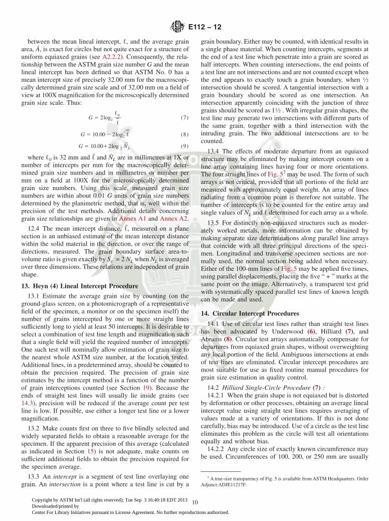
between the mean lineal intercept, ℓ, and the average grainarea, A, is exact for circles but not quite exact for a structure ofuniform equiaxed grains (see A2.2.2). Consequently, the rela-tionship between the ASTM grain size number G and the meanlineal intercept has been defined so that ASTM No. 0 has amean intercept size of precisely 32.00 mm for the macroscopi-cally determined grain size scale and of 32.00 mm on a field ofview at 100X magnification for the microscopically determinedgrain size scale. Thus:
G 5 2log2
ℓ0
ℓH(7)
G 5 10.00 2 2log2 ℓH (8)
G 5 10.0012log 2 NL (9)
where ℓ0 is 32 mm and ℓ and NL are in millimetres at 1X ornumber of intercepts per mm for the macroscopically deter-mined grain size numbers and in millimetres or number permm on a field at 100X for the microscopically determinedgrain size numbers. Using this scale, measured grain sizenumbers are within about 0.01 G units of grain size numbersdetermined by the planimetric method, that is, well within theprecision of the test methods. Additional details concerninggrain size relationships are given in Annex A1 and Annex A2.
12.4 The mean intercept distance, ℓ, measured on a planesection is an unbiased estimate of the mean intercept distancewithin the solid material in the direction, or over the range ofdirections, measured. The grain boundary surface area-to-volume ratio is given exactly by Sv = 2 NL when NL is averagedover three dimensions. These relations are independent of grainshape.
13. Heyn (4) Lineal Intercept Procedure
13.1 Estimate the average grain size by counting (on theground-glass screen, on a photomicrograph of a representativefield of the specimen, a monitor or on the specimen itself) thenumber of grains intercepted by one or more straight linessufficiently long to yield at least 50 intercepts. It is desirable toselect a combination of test line length and magnification suchthat a single field will yield the required number of intercepts.One such test will nominally allow estimation of grain size tothe nearest whole ASTM size number, at the location tested.Additional lines, in a predetermined array, should be counted toobtain the precision required. The precision of grain sizeestimates by the intercept method is a function of the numberof grain interceptions counted (see Section 19). Because theends of straight test lines will usually lie inside grains (see14.3), precision will be reduced if the average count per testline is low. If possible, use either a longer test line or a lowermagnification.
13.2 Make counts first on three to five blindly selected andwidely separated fields to obtain a reasonable average for thespecimen. If the apparent precision of this average (calculatedas indicated in Section 15) is not adequate, make counts onsufficient additional fields to obtain the precision required forthe specimen average.
13.3 An intercept is a segment of test line overlaying onegrain. An intersection is a point where a test line is cut by a
grain boundary. Either may be counted, with identical results ina single phase material. When counting intercepts, segments atthe end of a test line which penetrate into a grain are scored ashalf intercepts. When counting intersections, the end points ofa test line are not intersections and are not counted except whenthe end appears to exactly touch a grain boundary, when 1⁄2intersection should be scored. A tangential intersection with agrain boundary should be scored as one intersection. Anintersection apparently coinciding with the junction of threegrains should be scored as 11⁄2 . With irregular grain shapes, thetest line may generate two intersections with different parts ofthe same grain, together with a third intersection with theintruding grain. The two additional intersections are to becounted.
13.4 The effects of moderate departure from an equiaxedstructure may be eliminated by making intercept counts on aline array containing lines having four or more orientations.The four straight lines of Fig. 57 may be used. The form of sucharrays is not critical, provided that all portions of the field aremeasured with approximately equal weight. An array of linesradiating from a common point is therefore not suitable. Thenumber of intercepts is to be counted for the entire array andsingle values of NL and ℓ determined for each array as a whole.
13.5 For distinctly non-equiaxed structures such as moder-ately worked metals, more information can be obtained bymaking separate size determinations along parallel line arraysthat coincide with all three principal directions of the speci-men. Longitudinal and transverse specimen sections are nor-mally used, the normal section being added when necessary.Either of the 100-mm lines of Fig. 5 may be applied five times,using parallel displacements, placing the five “ + ” marks at thesame point on the image. Alternatively, a transparent test gridwith systematically spaced parallel test lines of known lengthcan be made and used.
14. Circular Intercept Procedures
14.1 Use of circular test lines rather than straight test lineshas been advocated by Underwood (6), Hilliard (7), andAbrams (8). Circular test arrays automatically compensate fordepartures from equiaxed grain shapes, without overweightingany local portion of the field. Ambiguous intersections at endsof test lines are eliminated. Circular intercept procedures aremost suitable for use as fixed routine manual procedures forgrain size estimation in quality control.
14.2 Hilliard Single-Circle Procedure (7) :14.2.1 When the grain shape is not equiaxed but is distorted
by deformation or other processes, obtaining an average linealintercept value using straight test lines requires averaging ofvalues made at a variety of orientations. If this is not donecarefully, bias may be introduced. Use of a circle as the test lineeliminates this problem as the circle will test all orientationsequally and without bias.
14.2.2 Any circle size of exactly known circumference maybe used. Circumferences of 100, 200, or 250 mm are usually
7 A true-size transparency of Fig. 5 is available from ASTM Headquarters. OrderAdjunct:ADJE11217F.
E112 − 12
10
Copyright by ASTM Int'l (all rights reserved); Tue Sep 3 16:40:18 EDT 2013Downloaded/printed byCenter For Library Initiatives pursuant to License Agreement. No further reproductions authorized.

convenient. The test circle diameter should never be smallerthan the largest observed grains. If the test circle is smaller thanabout three times the mean lineal intercept, the distribution ofthe number of intercepts or intersections per field will not beGaussian. Also, use of small test circles is rather inefficient asa great many fields must be evaluated to obtain a high degreeof precision. A small reference mark is usually placed at the topof the circle to indicate the place to start and stop the count.Blindly apply the selected circle to the microscope image at aconvenient known magnification and count the number of grainboundaries intersecting the circle for each application. Applythe circle only once to each field of view, adding fields in arepresentative manner, until sufficient counts are obtained toyield the required precision. The variation in counts per testcircle application decreases as the circle size increases and, ofcourse, is affected by the uniformity of the grain size distribu-tion.
14.2.3 As with all intercept procedures, the precision of themeasurement increases as the number of counts increases (seeSection 19). The precision is based on the standard deviation ofthe counts of the number of intercepts or intersections per field.In general, for a given grain structure, the standard deviation isimproved as the count per circle application and the total count(that is, the number of applications) increase. Hilliard recom-mended test conditions that produce about 35 counts per circlewith the test circle applied blindly over as large a specimenarea as feasible until the desired total number of counts isobtained.
14.3 Abrams Three-Circle Procedure (8) :
14.3.1 Based on an experimental finding that a total of 500counts per specimen normally yields acceptable precision,Abrams developed a specific procedure for routine averagegrain size rating of commercial steels. Use of the chi-square
NOTE 1—If reproduced to make straight lines marked length:Straight lines total: 500 mm
Circles are: Circumference, mm, Diameter, mm250.0 79.58166.7 53.05
83.3 26.53Total 500.0
NOTE 2—See Footnote 9.FIG. 5 Test Pattern for Intercept Counting
E112 − 12
11
Copyright by ASTM Int'l (all rights reserved); Tue Sep 3 16:40:18 EDT 2013Downloaded/printed byCenter For Library Initiatives pursuant to License Agreement. No further reproductions authorized.

test on real data demonstrated that the variation of interceptcounts is close to normal, allowing the observations to betreated by the statistics of normal distributions. Thus both ameasure of variability and the confidence limit of the result arecomputed for each average grain size determination.
14.3.2 The test pattern consists of three concentric andequally spaced circles having a total circumference of 500 mm,as shown in Fig. 5. Successively apply this pattern to at leastfive blindly selected and widely spaced fields, separatelyrecording the count of intersections per pattern for each of thetests. Then, determine the mean lineal intercept, its standarddeviation, 95 % confidence limit, and percent relative accuracy.For most work, a relative accuracy of 10 % or less representsan acceptable degree of precision. If the calculated relativeaccuracy is unacceptable for the application, count additionalfields until the calculated percent relative accuracy is accept-able. The specific procedure is as follows:
14.3.2.1 Examine the grain structure and select a magnifi-cation that will yield from 40 to 100 intercepts or intersectioncounts per placement of the three circle test grid. Because ourgoal is to obtain a total of about 400 to 500 counts, the idealmagnification is that which yields about 100 counts perplacement. However, as the count per placement increasesfrom 40 to 100, errors in counting become more likely.Because the grain structure will vary somewhat from field tofield, at least five widely spaced fields should be selected.Some metallographers feel more comfortable counting 10fields with about 40 to 50 counts per field. For most grainstructures, a total count of 400 to 500 intercepts or intersectionsover 5 to 10 fields produces better than 10 % relative accuracy.Fig. 6 shows the relationship between the average interceptcount and the microscopically determined ASTM grain sizenumber as a function of magnification.
14.3.2.2 Blindly select one field for measurement and applythe test pattern to the image. A transparency of the pattern maybe applied directly to the ground glass, or to a photomicrographwhen permanent records are desired. Direct counting using aproperly sized reticle in the eyepiece is allowable, but it mayhere be expected that some operators will find difficulty in
counting correctly at the count density recommended. Com-pletely count each circle in turn, using a manually operatedcounter to accumulate the total number of grain boundaryintersections with the test pattern. The manual counter isnecessary to avoid bias toward unreal agreement betweenapplications or toward a desired result, and to minimizememory errors. The operator should avoid keeping a mentalscore. When a tally counter is used, score any intersection ofthe circle with the junction of three grains as two rather thanthe correct value of 11⁄2 ; the error introduced is very small.
14.3.3 For each field count, calculate NL or PL according to:
NL 5Ni
L/M(10)
PL 5Pi
L/M(11)
where Ni and Pi are the number of intercepts or intersectionscounted on the field, L is the total test line length (500 mm) andM is the magnification.
14.3.4 Calculate the mean lineal intercept value for eachfield, ℓ by:
ℓH 51
NL
51
PL
(12)
The average value of n determinations of NL , PL , or ℓ isused to determine the microscopically measured ASTM grainsize using the equations in Table 6, the data shown graphicallyin Fig. 6, or the data in Table 4.
15. Statistical Analysis
15.1 No determination of average grain size can be an exactmeasurement. Thus, no determination is complete without alsocalculating the precision within which the determined sizemay, with normal confidence, be considered to represent theactual average grain size of the specimen examined. Inaccordance with common engineering practice, this sectionassumes normal confidence to represent the expectation thatthe actual error will be within the stated uncertainty 95 % ofthe time.
15.1.1 Many specimens vary measurably in grain size fromone field of view to another, this variation being responsible fora major portion of the uncertainty. Minimum effort in manualmethods, to obtain a required precision, justifies individualcounts whose precision is comparable to this natural variability(7). The high local precision that may be obtained by machinemethods often will yield only a small increase in overallprecision unless many fields also are measured, but does helpdistinguish natural variability from inaccuracies of counting.
15.2 After the desired number of fields have been measured,calculate the mean value of NA or ℓ from the individual fieldvalues according to:
X 5(Xi
n(13)
where Xi represents an individual value, X is the mean and nis the number of measurements.
15.3 Calculate the standard deviation of the individualmeasurements according to the usual equation:
FIG. 6 Average Intercept Counts on 500 mm Test Pattern
E112 − 12
12
Copyright by ASTM Int'l (all rights reserved); Tue Sep 3 16:40:18 EDT 2013Downloaded/printed byCenter For Library Initiatives pursuant to License Agreement. No further reproductions authorized.
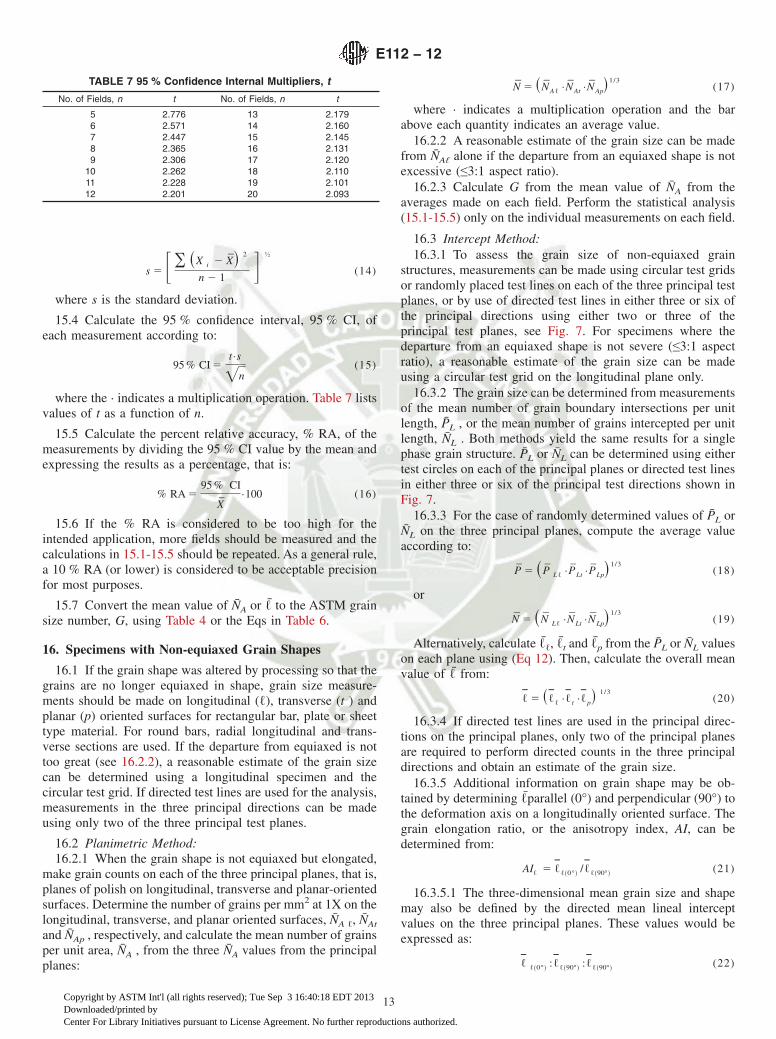
s 5 F ( ~X i 2 X!2
n 2 1G ½
(14)
where s is the standard deviation.
15.4 Calculate the 95 % confidence interval, 95 % CI, ofeach measurement according to:
95 % CI 5t ·s
=n(15)
where the · indicates a multiplication operation. Table 7 listsvalues of t as a function of n.
15.5 Calculate the percent relative accuracy, % RA, of themeasurements by dividing the 95 % CI value by the mean andexpressing the results as a percentage, that is:
% RA 595 % CI
X·100 (16)
15.6 If the % RA is considered to be too high for theintended application, more fields should be measured and thecalculations in 15.1-15.5 should be repeated. As a general rule,a 10 % RA (or lower) is considered to be acceptable precisionfor most purposes.
15.7 Convert the mean value of NA or ℓ to the ASTM grainsize number, G, using Table 4 or the Eqs in Table 6.
16. Specimens with Non-equiaxed Grain Shapes
16.1 If the grain shape was altered by processing so that thegrains are no longer equiaxed in shape, grain size measure-ments should be made on longitudinal (ℓ), transverse (t ) andplanar (p) oriented surfaces for rectangular bar, plate or sheettype material. For round bars, radial longitudinal and trans-verse sections are used. If the departure from equiaxed is nottoo great (see 16.2.2), a reasonable estimate of the grain sizecan be determined using a longitudinal specimen and thecircular test grid. If directed test lines are used for the analysis,measurements in the three principal directions can be madeusing only two of the three principal test planes.
16.2 Planimetric Method:16.2.1 When the grain shape is not equiaxed but elongated,
make grain counts on each of the three principal planes, that is,planes of polish on longitudinal, transverse and planar-orientedsurfaces. Determine the number of grains per mm2 at 1X on thelongitudinal, transverse, and planar oriented surfaces, NA ℓ, NAt
and NAp , respectively, and calculate the mean number of grainsper unit area, NA , from the three NA values from the principalplanes:
N 5 ~NAℓ ·NAt ·NAp!1/3
(17)
where · indicates a multiplication operation and the barabove each quantity indicates an average value.
16.2.2 A reasonable estimate of the grain size can be madefrom NAℓ alone if the departure from an equiaxed shape is notexcessive (≤3:1 aspect ratio).
16.2.3 Calculate G from the mean value of NA from theaverages made on each field. Perform the statistical analysis(15.1-15.5) only on the individual measurements on each field.
16.3 Intercept Method:16.3.1 To assess the grain size of non-equiaxed grain
structures, measurements can be made using circular test gridsor randomly placed test lines on each of the three principal testplanes, or by use of directed test lines in either three or six ofthe principal directions using either two or three of theprincipal test planes, see Fig. 7. For specimens where thedeparture from an equiaxed shape is not severe (≤3:1 aspectratio), a reasonable estimate of the grain size can be madeusing a circular test grid on the longitudinal plane only.
16.3.2 The grain size can be determined from measurementsof the mean number of grain boundary intersections per unitlength, PL , or the mean number of grains intercepted per unitlength, NL . Both methods yield the same results for a singlephase grain structure. PL or NL can be determined using eithertest circles on each of the principal planes or directed test linesin either three or six of the principal test directions shown inFig. 7.
16.3.3 For the case of randomly determined values of PL orNL on the three principal planes, compute the average valueaccording to:
P 5 ~ P Lℓ ·PLt ·PLp!1/3
(18)
or
N 5 ~ N Lℓ ·NLt ·NLp!1/3
(19)
Alternatively, calculate ℓℓ, ℓt and ℓp from the PL or NL valueson each plane using (Eq 12). Then, calculate the overall meanvalue of ℓ from:
ℓH 5 ~ℓHℓ ·ℓH t ·ℓHp!1/3
(20)
16.3.4 If directed test lines are used in the principal direc-tions on the principal planes, only two of the principal planesare required to perform directed counts in the three principaldirections and obtain an estimate of the grain size.
16.3.5 Additional information on grain shape may be ob-tained by determining ℓparallel (0°) and perpendicular (90°) tothe deformation axis on a longitudinally oriented surface. Thegrain elongation ratio, or the anisotropy index, AI, can bedetermined from:
AIℓ 5 ℓHℓ~0°!/ℓHℓ~90°!
(21)
16.3.5.1 The three-dimensional mean grain size and shapemay also be defined by the directed mean lineal interceptvalues on the three principal planes. These values would beexpressed as:
ℓH ℓ~0°!:ℓHℓ~90°!
:ℓHℓ~90°!(22)
TABLE 7 95 % Confidence Internal Multipliers, t
No. of Fields, n t No. of Fields, n t
5 2.776 13 2.1796 2.571 14 2.1607 2.447 15 2.1458 2.365 16 2.1319 2.306 17 2.120
10 2.262 18 2.11011 2.228 19 2.10112 2.201 20 2.093
E112 − 12
13
Copyright by ASTM Int'l (all rights reserved); Tue Sep 3 16:40:18 EDT 2013Downloaded/printed byCenter For Library Initiatives pursuant to License Agreement. No further reproductions authorized.
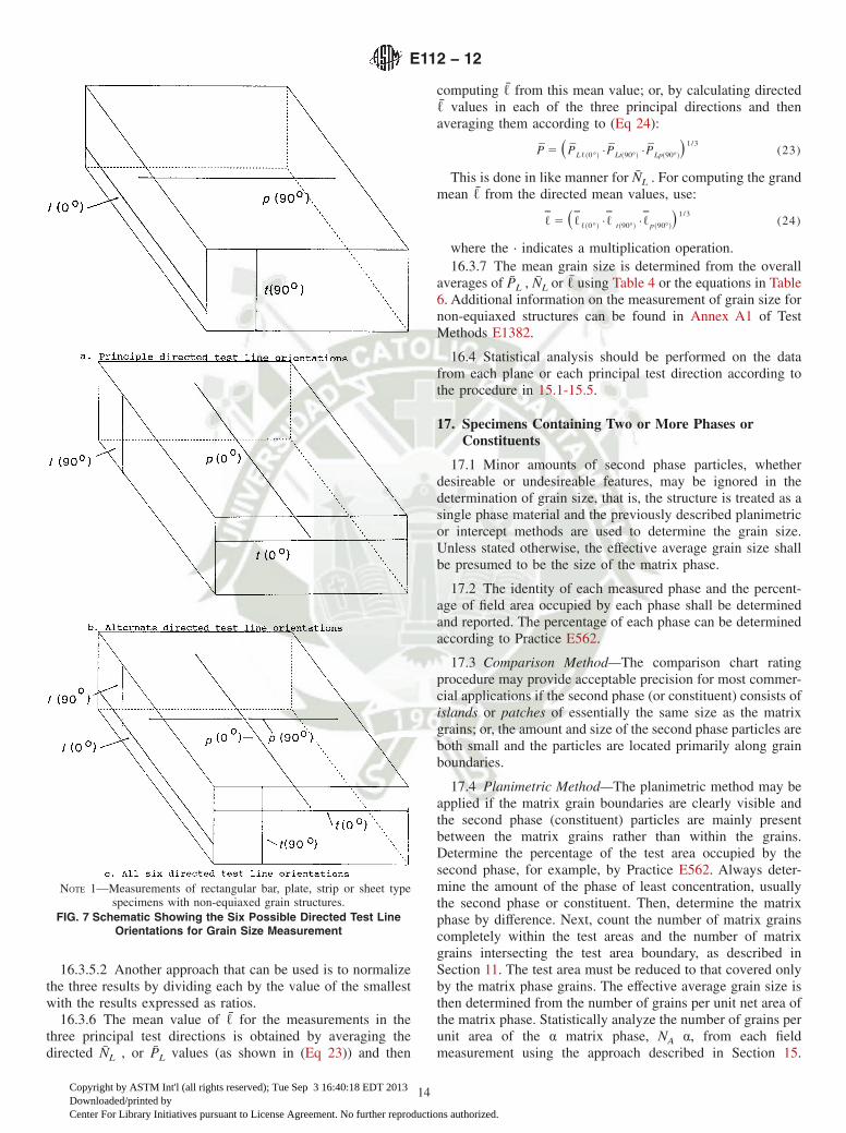
16.3.5.2 Another approach that can be used is to normalizethe three results by dividing each by the value of the smallestwith the results expressed as ratios.
16.3.6 The mean value of ℓ for the measurements in thethree principal test directions is obtained by averaging thedirected NL , or PL values (as shown in (Eq 23)) and then
computing ℓ from this mean value; or, by calculating directedℓ values in each of the three principal directions and thenaveraging them according to (Eq 24):
P 5 ~ PLℓ~0°!·PLt~90°!
·PLp~90°!!1/3
(23)
This is done in like manner for NL . For computing the grandmean ℓ from the directed mean values, use:
ℓH 5 ~ℓHℓ~0°!·ℓH t~90°!
·ℓHp~90°!!1/3
(24)
where the · indicates a multiplication operation.16.3.7 The mean grain size is determined from the overall
averages of PL , NL or ℓ using Table 4 or the equations in Table6. Additional information on the measurement of grain size fornon-equiaxed structures can be found in Annex A1 of TestMethods E1382.
16.4 Statistical analysis should be performed on the datafrom each plane or each principal test direction according tothe procedure in 15.1-15.5.
17. Specimens Containing Two or More Phases orConstituents
17.1 Minor amounts of second phase particles, whetherdesireable or undesireable features, may be ignored in thedetermination of grain size, that is, the structure is treated as asingle phase material and the previously described planimetricor intercept methods are used to determine the grain size.Unless stated otherwise, the effective average grain size shallbe presumed to be the size of the matrix phase.
17.2 The identity of each measured phase and the percent-age of field area occupied by each phase shall be determinedand reported. The percentage of each phase can be determinedaccording to Practice E562.
17.3 Comparison Method—The comparison chart ratingprocedure may provide acceptable precision for most commer-cial applications if the second phase (or constituent) consists ofislands or patches of essentially the same size as the matrixgrains; or, the amount and size of the second phase particles areboth small and the particles are located primarily along grainboundaries.
17.4 Planimetric Method—The planimetric method may beapplied if the matrix grain boundaries are clearly visible andthe second phase (constituent) particles are mainly presentbetween the matrix grains rather than within the grains.Determine the percentage of the test area occupied by thesecond phase, for example, by Practice E562. Always deter-mine the amount of the phase of least concentration, usuallythe second phase or constituent. Then, determine the matrixphase by difference. Next, count the number of matrix grainscompletely within the test areas and the number of matrixgrains intersecting the test area boundary, as described inSection 11. The test area must be reduced to that covered onlyby the matrix phase grains. The effective average grain size isthen determined from the number of grains per unit net area ofthe matrix phase. Statistically analyze the number of grains perunit area of the α matrix phase, NA α, from each fieldmeasurement using the approach described in Section 15.
NOTE 1—Measurements of rectangular bar, plate, strip or sheet typespecimens with non-equiaxed grain structures.
FIG. 7 Schematic Showing the Six Possible Directed Test LineOrientations for Grain Size Measurement
E112 − 12
14
Copyright by ASTM Int'l (all rights reserved); Tue Sep 3 16:40:18 EDT 2013Downloaded/printed byCenter For Library Initiatives pursuant to License Agreement. No further reproductions authorized.
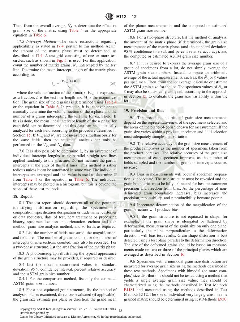
Then, from the overall average, NA α, determine the effectivegrain size of the matrix using Table 4 or the appropriateequation in Table 6.
17.5 Intercept Method—The same restrictions regardingapplicability, as stated in 17.4, pertain to this method. Again,the amount of the matrix phase must be determined, asdescribed in 17.4. A test grid consisting of one or more testcircles, such as shown in Fig. 5, is used. For this application,count the number of matrix grains, Nα, intercepted by the testline. Determine the mean intercept length of the matrix phaseaccording to:
ℓHα 5~VVα!~L/M!
Nα(25)
where the volume fraction of the α matrix, VVα , is expressedas a fraction, L is the test line length and M is the magnifica-tion. The grain size of the α grains is determined using Table 4or the equation in Table 6. In practice, it is inconvenient tomanually determine the volume fraction of the α phase and thenumber of α grains intercepting the test line for each field. Ifthis is done, the mean lineal intercept length of the α phase foreach field can be determined and this data can be statisticallyanalyzed for each field according to the procedure described inSection 15. If VVα and Nα are not measured simultaneously forthe same fields, then the statistical analysis can only beperformed on the VVα and Nα data.
17.6 It is also possible to determine ℓα by measurement ofindividual intercept lengths using parallel straight test linesapplied randomly to the structure. Do not measure the partialintercepts at the ends of the test lines. This method is rathertedious unless it can be automated in some way. The individualintercepts are averaged and this value is used to determine Gfrom Table 4 or the equation in Table 6. The individualintercepts may be plotted in a histogram, but this is beyond thescope of these test methods.
18. Report
18.1 The test report should document all of the pertinentidentifying information regarding the specimen, itscomposition, specification designation or trade name, customeror data requester, date of test, heat treatment or processinghistory, specimen location and orientation, etchant and etchmethod, grain size analysis method, and so forth, as required.
18.2 List the number of fields measured, the magnification,and field area. The number of grains counted or the number ofintercepts or intersections counted, may also be recorded. Fora two-phase structure, list the area fraction of the matrix phase.
18.3 A photomicrograph illustrating the typical appearanceof the grain structure may be provided, if required or desired.
18.4 List the mean measurement value, its standarddeviation, 95 % confidence interval, percent relative accuracy,and the ASTM grain size number.
18.4.1 For the comparison method, list only the estimatedASTM grain size number.
18.5 For a non-equiaxed grain structure, list the method ofanalysis, planes examined, directions evaluated (if applicable),the grain size estimate per plane or direction, the grand mean
of the planar measurements, and the computed or estimatedASTM grain size number.
18.6 For a two-phase structure, list the method of analysis,the amount of the matrix phase (if determined), the grain sizemeasurement of the matrix phase (and the standard deviation,95 % confidence interval, and percent relative accuracy), andthe computed or estimated ASTM grain size number.
18.7 If it is desired to express the average grain size of agroup of specimens from a lot, do not simply average theASTM grain size numbers. Instead, compute an arithmeticaverage of the actual measurements, such as, the NA or ℓ valuesper specimen. Then, from the lot average, calculate or estimatethe ASTM grain size for the lot. The specimen values of NA orℓ may also be statistically analyzed, according to the approachin Section 15, to evaluate the grain size variability within thelot.
19. Precision and Bias
19.1 The precision and bias of grain size measurementsdepend on the representativeness of the specimens selected andthe areas on the plane-of-polish chosen for measurement. If thegrain size varies within a product, specimen and field selectionmust adequately sample this variation.
19.2 The relative accuracy of the grain size measurement ofthe product improves as the number of specimens taken fromthe product increases. The relative accuracy of the grain sizemeasurement of each specimen improves as the number offields sampled and the number of grains or intercepts countedincrease.
19.3 Bias in measurements will occur if specimen prepara-tion is inadequate. The true structure must be revealed and thegrain boundaries must be fully delineated for best measurementprecision and freedom from bias. As the percentage of non-delineated grain boundaries increases, bias increases andprecision, repeatability, and reproducibility become poorer.
19.4 Inaccurate determination of the magnification of thegrain structure will produce bias.
19.5 If the grain structure is not equiaxed in shape, forexample, if the grain shape is elongated or flattened bydeformation, measurement of the grain size on only one plane,particularly the plane perpendicular to the deformationdirection, will bias test results. Grain shape distortion is bestdetected using a test plane parallel to the deformation direction.The size of the deformed grains should be based on measure-ments made on two or three of the principal planes which areaveraged as described in Section 16.
19.6 Specimens with a unimodal grain size distribution aremeasured for average grain size using the methods described inthese test methods. Specimens with bimodal (or more com-plex) size distributions should not be tested using a method thatyields a single average grain size value; they should becharacterized using the methods described in Test MethodsE1181 and measured using the methods described in TestMethods E112. The size of individual very large grains in a finegrained matrix should be determined using Test Methods E930.
E112 − 12
15
Copyright by ASTM Int'l (all rights reserved); Tue Sep 3 16:40:18 EDT 2013Downloaded/printed byCenter For Library Initiatives pursuant to License Agreement. No further reproductions authorized.

19.7 When using the comparison chart method, the chartselected should be consistent with the nature of the grains (thatis, twinned or non-twinned, or carburized and slow cooled) andthe etch (that is, flat etch or grain contrast etch) for bestprecision.
19.8 Grain size ratings using the comparison chart methodby an individual metallographer will vary within 60.5 G units.When a number of individuals rate the same specimen, thespread in ratings may be as great as 1.5 to 2.5 G units.
19.9 The fracture grain size method is only applicable tohardened, relatively brittle, tool steels. Specimens should be inthe as-quenched or lightly tempered condition so that thefracture surface is quite flat. An experienced metallographercan rate the prior-austenite grain size of a tool steel within60.5 G units by the Shepherd fracture grain size method.
19.10 A round robin test program (see Appendix X1),analyzed according to Practice E691, revealed a rather consis-tent bias between comparison chart ratings using Plate I andgrain size measurements using both the planimetric and inter-cept methods. Chart ratings were 0.5 to 1 G unit coarser, thatis, lower G numbers, than the measured values.
19.11 Grain sizes determined by either the planimetric orintercept methods produced similar results with no observedbias.
19.12 The relative accuracy of grain size measurementsimproved as the number of grains or intercepts countedincreased. For a similar number of counts, the relative accuracyof intercept measurements was better than that of planimetricmeasurements of grain size. For the intercept method, 10 %RA (or less) was obtained with about 400 intercept or inter-section counts while for the planimetric method, to obtain 10 %RA, or less, about 700 grains had to be counted. Repeatability
and reproducibility of measurements improved as the numberof grains or intercepts counted increased and was better for theintercept method than for the planimetric method for the samecount.
19.13 The planimetric method requires a marking off of thegrains during counting in order to obtain an accurate count. Theintercept method does not require marking in order to get anaccurate count. Hence, the intercept method is easier to use andfaster. Further, the round robin test showed that the interceptmethod provides better statistical precision for the samenumber of counts and is, therefore, the preferred measurementmethod.
19.14 An individual metallographer can usually repeat pla-nimetric or intercept grain size measurements within 60.1 Gunits. When a number of metallographers measure the samespecimen, the spread of grain sizes is usually well within 60.5G units.
19.15 If the number of grains completely within a test circledecreases below 50, the grain size estimate using the planim-etric method will be biased, with the degree of bias increasingas Ninside decreases from 50. To avoid this problem, select themagnification so that Ninside is ≥ 50, or use a rectangular orsquare test figure and the counting method described in 11.5.Magnifications that yield Ninside of ~100 and above lead toimprecision due to counting errors. A 10% relative accuracy inG will be obtained when at least 700 total grains are countedusing multiple fields selected at random.
20. Keywords
20.1 ALA grain size; anisotropy index; area fraction; ASTMgrain size number; calibration; equiaxed grains; etchant; grainboundary; grains; grain size; intercept count; intercept length;intersection count; non-equiaxed grains; twin boundaries
ANNEXES
(Mandatory Information)
A1. BASIS OF ASTM GRAIN SIZE NUMBERS
A1.1 Descriptions of Terms and Symbols
A1.1.1 The general term grain size is commonly used todesignate size estimates or measurements made in severalways, employing various units of length, area, or volume. Ofthe various systems, only the ASTM grain size number, G, isessentially independent of the estimating system and measure-ment units used. The equations used to determine G fromrecommended measurements, as illustrated in Fig. 6 and Table2 and Table 4, are given in A1.2 and A1.3. The nominalrelationships between commonly used measurements are givenin Annex A2. Measurements that appear in these equations, orin equations in the text, are as follows:
A1.1.1.1 N = Number of grain sections counted on a knowntest area, A, or number of intercepts counted on a known testarray of length = L, at some stated magnification, M. Theaverage of counts on several fields is designated as N.
A1.1.1.2 After correction for magnification, NA is the num-ber of grain sections per unit test area (mm2) at 1X; NL is thenumber of grains intercepted per unit length (mm) of test linesat 1X; and PL is the number of grain boundary intersections perunit length (mm) of test line at 1X.
A1.1.1.3 ℓ = 1/NL = 1/PL where ℓ is the mean lineal inter-cept length in mm at 1X.
E112 − 12
16
Copyright by ASTM Int'l (all rights reserved); Tue Sep 3 16:40:18 EDT 2013Downloaded/printed byCenter For Library Initiatives pursuant to License Agreement. No further reproductions authorized.
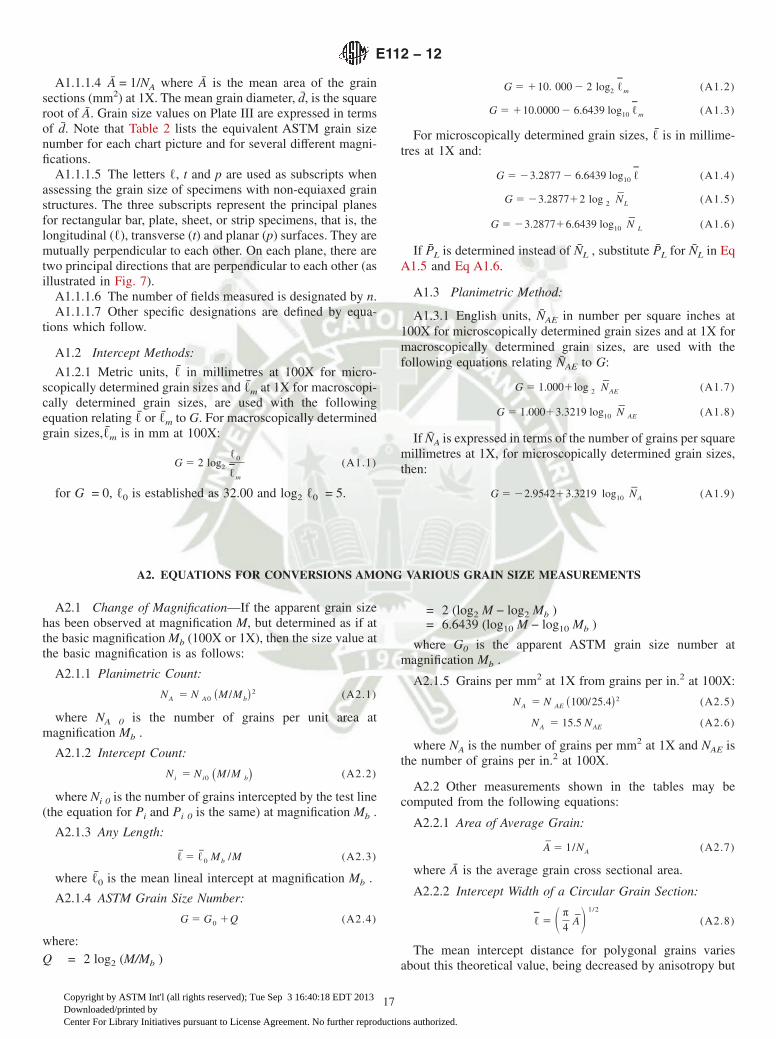
A1.1.1.4 A = 1/NA where A is the mean area of the grainsections (mm2) at 1X. The mean grain diameter, d, is the squareroot of A. Grain size values on Plate III are expressed in termsof d. Note that Table 2 lists the equivalent ASTM grain sizenumber for each chart picture and for several different magni-fications.
A1.1.1.5 The letters ℓ, t and p are used as subscripts whenassessing the grain size of specimens with non-equiaxed grainstructures. The three subscripts represent the principal planesfor rectangular bar, plate, sheet, or strip specimens, that is, thelongitudinal (ℓ), transverse (t) and planar (p) surfaces. They aremutually perpendicular to each other. On each plane, there aretwo principal directions that are perpendicular to each other (asillustrated in Fig. 7).
A1.1.1.6 The number of fields measured is designated by n.A1.1.1.7 Other specific designations are defined by equa-
tions which follow.
A1.2 Intercept Methods:
A1.2.1 Metric units, ℓ in millimetres at 100X for micro-scopically determined grain sizes and ℓm at 1X for macroscopi-cally determined grain sizes, are used with the followingequation relating ℓ or ℓm to G. For macroscopically determinedgrain sizes,ℓm is in mm at 100X:
G 5 2 log2
ℓ0
ℓHm
(A1.1)
for G = 0, ℓ0 is established as 32.00 and log2 ℓ0 = 5.
G 5 110. 000 2 2 log2 ℓHm (A1.2)
G 5 110.0000 2 6.6439 log10 ℓHm (A1.3)
For microscopically determined grain sizes, ℓ is in millime-tres at 1X and:
G 5 23.2877 2 6.6439 log10 ℓH (A1.4)
G 5 23.287712 log 2 NL (A1.5)
G 5 23.287716.6439 log10 N L (A1.6)
If PL is determined instead of NL , substitute PL for NL in EqA1.5 and Eq A1.6.
A1.3 Planimetric Method:
A1.3.1 English units, NAE in number per square inches at100X for microscopically determined grain sizes and at 1X formacroscopically determined grain sizes, are used with thefollowing equations relating NAE to G:
G 5 1.0001log 2 NAE (A1.7)
G 5 1.00013.3219 log10 N AE (A1.8)
If NA is expressed in terms of the number of grains per squaremillimetres at 1X, for microscopically determined grain sizes,then:
G 5 22.954213.3219 log10 NA (A1.9)
A2. EQUATIONS FOR CONVERSIONS AMONG VARIOUS GRAIN SIZE MEASUREMENTS
A2.1 Change of Magnification—If the apparent grain sizehas been observed at magnification M, but determined as if atthe basic magnification Mb (100X or 1X), then the size value atthe basic magnification is as follows:
A2.1.1 Planimetric Count:
NA 5 N A0 ~M/Mb!2 (A2.1)
where NA 0 is the number of grains per unit area atmagnification Mb .
A2.1.2 Intercept Count:
Ni 5 Ni0 ~M/M b! (A2.2)
where Ni 0 is the number of grains intercepted by the test line(the equation for Pi and Pi 0 is the same) at magnification Mb .
A2.1.3 Any Length:
ℓ 5 ℓ0 Mb /M (A2.3)
where ℓ0 is the mean lineal intercept at magnification Mb .
A2.1.4 ASTM Grain Size Number:
G 5 G0 1Q (A2.4)
where:Q = 2 log2 (M/Mb )
= 2 (log2 M − log2 Mb )= 6.6439 (log10 M − log10 Mb )
where G0 is the apparent ASTM grain size number atmagnification Mb .
A2.1.5 Grains per mm2 at 1X from grains per in.2 at 100X:
NA 5 N AE ~100/25.4!2 (A2.5)
NA 5 15.5 NAE (A2.6)
where NA is the number of grains per mm2 at 1X and NAE isthe number of grains per in.2 at 100X.
A2.2 Other measurements shown in the tables may becomputed from the following equations:
A2.2.1 Area of Average Grain:
A 5 1/NA (A2.7)
where A is the average grain cross sectional area.
A2.2.2 Intercept Width of a Circular Grain Section:
ℓH 5 S π4
AD 1/2
(A2.8)
The mean intercept distance for polygonal grains variesabout this theoretical value, being decreased by anisotropy but
E112 − 12
17
Copyright by ASTM Int'l (all rights reserved); Tue Sep 3 16:40:18 EDT 2013Downloaded/printed byCenter For Library Initiatives pursuant to License Agreement. No further reproductions authorized.
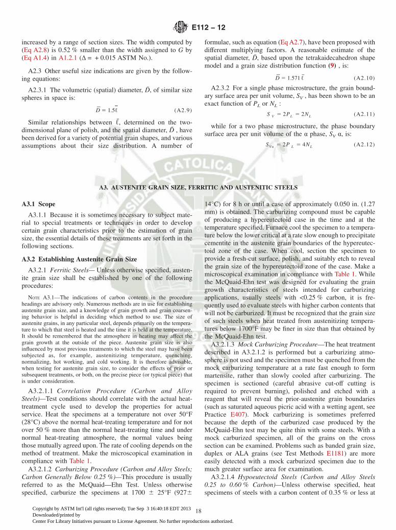
increased by a range of section sizes. The width computed by(Eq A2.8) is 0.52 % smaller than the width assigned to G by(Eq A1.4) in A1.2.1 (∆ = + 0.015 ASTM No.).
A2.3 Other useful size indications are given by the follow-ing equations:
A2.3.1 The volumetric (spatial) diameter, D, of similar sizespheres in space is:
D 5 1.5ℓH (A2.9)
Similar relationships between ℓ, determined on the two-dimensional plane of polish, and the spatial diameter, D , havebeen derived for a variety of potential grain shapes, and variousassumptions about their size distribution. A number of
formulae, such as equation (Eq A2.7), have been proposed withdifferent multiplying factors. A reasonable estimate of thespatial diameter, D, based upon the tetrakaidecahedron shapemodel and a grain size distribution function (9) , is:
D 5 1.571 ℓ (A2.10)
A2.3.2 For a single phase microstructure, the grain bound-ary surface area per unit volume, SV , has been shown to be anexact function of PL or NL :
S V 5 2PL 5 2NL (A2.11)
while for a two phase microstructure, the phase boundarysurface area per unit volume of the α phase, SV α, is:
SVα 5 2P L 5 4NL (A2.12)
A3. AUSTENITE GRAIN SIZE, FERRITIC AND AUSTENITIC STEELS
A3.1 Scope
A3.1.1 Because it is sometimes necessary to subject mate-rial to special treatments or techniques in order to developcertain grain characteristics prior to the estimation of grainsize, the essential details of these treatments are set forth in thefollowing sections.
A3.2 Establishing Austenite Grain Size
A3.2.1 Ferritic Steels— Unless otherwise specified, austen-ite grain size shall be established by one of the followingprocedures:
NOTE A3.1—The indications of carbon contents in the procedureheadings are advisory only. Numerous methods are in use for establishingaustenite grain size, and a knowledge of grain growth and grain coarsen-ing behavior is helpful in deciding which method to use. The size ofaustenite grains, in any particular steel, depends primarily on the tempera-ture to which that steel is heated and the time it is held at the temperature.It should be remembered that the atmosphere in heating may affect thegrain growth at the outside of the piece. Austenite grain size is alsoinfluenced by most previous treatments to which the steel may have beensubjected as, for example, austenitizing temperature, quenching,normalizing, hot working, and cold working. It is therefore advisable,when testing for austenite grain size, to consider the effects of prior orsubsequent treatments, or both, on the precise piece (or typical piece) thatis under consideration.
A3.2.1.1 Correlation Procedure (Carbon and AlloySteels)—Test conditions should correlate with the actual heat-treatment cycle used to develop the properties for actualservice. Heat the specimens at a temperature not over 50°F(28°C) above the normal heat-treating temperature and for notover 50 % more than the normal heat-treating time and undernormal heat-treating atmosphere, the normal values beingthose mutually agreed upon. The rate of cooling depends on themethod of treatment. Make the microscopical examination incompliance with Table 1.
A3.2.1.2 Carburizing Procedure (Carbon and Alloy Steels;Carbon Generally Below 0.25 %)—This procedure is usuallyreferred to as the McQuaid—Ehn Test. Unless otherwisespecified, carburize the specimens at 1700 6 25°F (9276
14°C) for 8 h or until a case of approximately 0.050 in. (1.27mm) is obtained. The carburizing compound must be capableof producing a hypereutectoid case in the time and at thetemperature specified. Furnace cool the specimen to a tempera-ture below the lower critical at a rate slow enough to precipitatecementite in the austenite grain boundaries of the hypereutec-toid zone of the case. When cool, section the specimen toprovide a fresh-cut surface, polish, and suitably etch to revealthe grain size of the hypereutectoid zone of the case. Make amicroscopical examination in compliance with Table 1. Whilethe McQuaid-Ehn test was designed for evaluating the graingrowth characteristics of steels intended for carburizingapplications, usually steels with <0.25 % carbon, it is fre-quently used to evaluate steels with higher carbon contents thatwill not be carburized. It must be recognized that the grain sizeof such steels when heat treated from austenitizing tempera-tures below 1700°F may be finer in size than that obtained bythe McQuaid-Ehn test.
A3.2.1.3 Mock Carburizing Procedure—The heat treatmentdescribed in A3.2.1.2 is performed but a carburizing atmo-sphere is not used and the specimen must be quenched from themock carburizing temperature at a rate fast enough to formmartensite, rather than slowly cooled after carburizing. Thespecimen is sectioned (careful abrasive cut-off cutting isrequired to prevent burning), polished and etched with areagent that will reveal the prior-austenite grain boundaries(such as saturated aqueous picric acid with a wetting agent, seePractice E407). Mock carburizing is sometimes preferredbecause the depth of the carburized case produced by theMcQuaid-Ehn test may be quite thin with some steels. With amock carburized specimen, all of the grains on the crosssection can be examined. Problems such as banded grain size,duplex or ALA grains (see Test Methods E1181) are moreeasily detected with a mock carburized specimen due to themuch greater surface area for examination.
A3.2.1.4 Hypoeutectoid Steels (Carbon and Alloy Steels0.25 to 0.60 % Carbon)—Unless otherwise specified, heatspecimens of steels with a carbon content of 0.35 % or less at
E112 − 12
18
Copyright by ASTM Int'l (all rights reserved); Tue Sep 3 16:40:18 EDT 2013Downloaded/printed byCenter For Library Initiatives pursuant to License Agreement. No further reproductions authorized.

1625 6 25°F (8856 14°C); heat specimens of steel with acarbon content of over 0.35 % at 1575 6 25°F (857 6 14°C)for a minimum of 30 min and cool in air or quench in water.The higher carbon steels in this range and alloy steels overapproximately 0.40 % carbon may require an adjustment incooling practice to outline clearly the austenite grain boundar-ies with ferrite. In such cases it is recommended that afterholding the specimen for the required time at a hardeningtemperature, the temperature be reduced to approximately1340 6 25°F (727 6 14°C) for 10 min, followed by water oroil quench. When cool, section the specimen to provide afresh-cut surface, polish, and suitably etch to reveal theaustenite grain size as outlined by precipitated ferrite in thegrain boundaries. Make the microscopical examination incompliance with Table 1.
A3.2.1.5 Oxidation Procedure (Carbon and Alloy Steels0.25 to 0.60 % Carbon)—Polish one of the surfaces of thespecimen (approximately 400-grit or 15-µm abrasive). Placethe specimen with the polished side up in a furnace, and, unlessotherwise specified, heat at 1575 6 25°F (857 6 14°C) for 1h and quench in cold water or brine. Polish the quenchedspecimen to reveal the austenite grain size as developed in theoxidized surface. Make the microscopical examination incompliance with Table 1.
A3.2.1.6 Direct Hardening Steels (Carbon and Alloy Steels;Carbon Generally Below 1.00 %)—Unless otherwise specified,heat specimens of steels with a carbon content of 0.35 % or lessat 16256 25°F (885 6 14°C); heat specimens of steels with acarbon content of over 0.35 % at 1575 6 25°F (857 6 14°C)for sufficient time and quench at a rate to produce fullhardening. Polish the quenched specimen and etch to reveal themartensitic structure. Tempering for 15 min at 450 6 25°F(232 6 14°C) prior to etching improves the contrast. Make themicroscopical examination in compliance with Table 1.
A3.2.1.7 Hypereutectoid Steels (Carbon and Alloy Steels;Carbon Generally Over 1.00 %)—Use a specimen approxi-mately 1 in. (25.4 mm) in diameter or 1 in. square for this test.Unless otherwise specified, heat the specimen at 1500 6 25°F(816 6 14°C) for a minimum of 30 min, and furnace cool to atemperature below the lower critical temperature at a rate slowenough to precipitate cementite in the austenite grain bound-aries. When cool, section the specimen to provide a fresh-cutsurface, polish, and suitably etch to reveal the austenite grainsize as outlined by precipitated cementite in the grain bound-aries. Make the microscopical examination in compliance withTable 1.
A3.2.2 Austenitic Steels—With austenitic materials, the ac-tual grain size of the metal has been established by priorheat-treatment.
A3.3 Revealing the Grain Size
A3.3.1 Ferritic Steels— For revealing austenite grain sizethe following methods (see Note A3.1) are generally used:
A3.3.1.1 Outlining the Grains with Cementite—In the hy-pereutectoid zone of a carburizing (McQuaid—Ehn test) pro-cedure or in hypereutectoid steels cooled from the austeniticcondition, the austenite grain size is outlined by the cementitewhich precipitated in the grain boundaries. It is therefore
possible to rate the grain size by etching the micrographicspecimen with a suitable etchant, such as nital, picral, oralkaline sodium picrate. (See Practice E407.)
A3.3.1.2 Outlining the Grains with Ferrite—In the hypoeu-tectoid zone of a carburized specimen, the austenite grain sizeis outlined by the ferrite that precipitated in the grain bound-aries. Ferrite similarly outlines the former austenite grains in amedium-carbon steel (approximately 0.50 % carbon), when ithas been cooled slowly from the austenite range. In low-carbonsteels (approximately 0.20 % carbon), cooling slowly from theaustenite range to room temperature, the amount of ferrite is solarge that the former austenite grain size is masked; in this case,the steel may be cooled slowly to an intermediate temperature,to allow only a small amount of ferrite to precipitate, followedby quenching in water; an example would be a piece previouslyheated to 1675°F (913°C), transferred to a furnace at between1350 to 1450°F (732 to 788°C), held at this temperature forperhaps 3 to 5 min, and then quenched in water; the austenitegrain size would be revealed by small ferrite grains outlininglow-carbon martensite grains.
A3.3.1.3 Outlining the Grains by Oxidation—The oxidationmethod depends on the fact that when steels are heated in anoxidizing atmosphere, oxidation takes place in part preferen-tially along the grain boundaries. A common procedure,therefore, is to polish the test specimen to a metallographicpolish, heat it in air at the desired temperature for the desiredlength of time, and then repolish the specimen lightly so asmerely to remove scale; whereupon the austenite grain bound-aries are visible as outlined by oxide.
A3.3.1.4 Outlining Martensite Grains with FinePearlite—A method applicable particularly to eutectoid steels,which cannot be judged so readily by some other methods, iseither to harden a bar of such a size that it is fully hardened atthe outside but not quite fully hardened in the interior, or toemploy a gradient quench in which the heated piece is for aportion of its length immersed in water and therefore fullyhardened, the remainder of the piece projecting above thequenching bath, being therefore not hardened. With eithermethod there will be a small zone which is almost but not quitefully hardened. In this zone, the former austenite grains willconsist of martensite grains surrounded by small amounts offine pearlite, thus revealing the grain size. These methods arealso applicable to steels somewhat lower and higher than theeutectoid composition.
A3.3.1.5 Etching of Martensite Grains—The former austen-ite grain size may be revealed in steels fully hardened tomartensite by using an etching reagent that develops contrastbetween the martensite grains. Tempering for 15 min at 450°F(232°C) prior to etching distinctly improves the contrast. Areagent that has been recommended is 1 g of picric acid, 5 mLof HCl (sp gr 1.19), and 95 mL of ethyl alcohol. An alternateapproach is to use an etchant that reveals the prior-austenitegrain boundaries preferentially. Many etchants have beendeveloped for this purpose (see Practice E407 and standard textbooks). The most successful consists of saturated aqueouspicric acid containing a wetting agent, usually sodium tride-cylbenzene sulfonate (the dodecyl version also works well).Specimens should be in the as-quenched condition or tempered
E112 − 12
19
Copyright by ASTM Int'l (all rights reserved); Tue Sep 3 16:40:18 EDT 2013Downloaded/printed byCenter For Library Initiatives pursuant to License Agreement. No further reproductions authorized.

not above about 1000°F. Success with this etchant dependsupon the presence of phosphorus in the alloy (≥0.005 % Prequired). Results may be enhanced by tempering the steelbetween 850 and 900°F for 8 h or more to drive phosphorus tothe grain boundaries. For steels with substantial alloyadditions, it may be necessary to add a few drops of hydro-chloric acid to the etchant (per 100 mL of etchant). Etchingusually takes at least 5 min. The etchant will attack sulfideinclusions. Lightly re-polishing the specimen on a stationarywheel to remove some of the unimportant background detailmay make it easier to see the grain boundaries.
A3.3.2 Austenitic Steels—For revealing the grain size inaustenitic materials, a suitable etching technique shall be usedto develop grain size. Recognizing that twinning tends toconfuse reading of grain size, the etching should be such thata minimum amount of twinning is evident.
A3.3.2.1 Stabilized Material—The specimen, as the anode,may be electrolytically etched in a water solution composed of60 % concentrated nitric acid by volume, at ambient tempera-ture. To minimize the appearance of twinning, a low voltage (1to 11⁄2 V) should be used. This etchant is also recommended forrevealing ferrite grain boundaries in ferritic stainless steels andis used identically.
A3.3.2.2 Unstabilized Material—The grain boundary maybe developed through precipitation of carbides by heatingwithin the sensitizing temperature range, 482 to 704°C (900 to1300°F). Any suitable carbide-revealing etchant should beused.
A3.4 Reporting the Grain Size
A3.4.1 Ferritic Steels— Duplex, or mixed grain-sized struc-ture (see Test Methods E1181) when observed, shall bereported with two representative ranges of grain size numbers.Whenever heat-treatments other than the carburizing(McQuaid—Ehn test) procedure are employed to developaustenite grain size, a complete report shall be made whichincludes:
A3.4.1.1 Temperature used in establishing the grain size,A3.4.1.2 Time at temperature used in establishing the grain
size,A3.4.1.3 Method of revealing grain size, andA3.4.1.4 Grain size.
A3.4.2 Austenitic Steels—In determining the size of auste-nitic grains, the twin boundaries within a grain shall not becounted.
A4. FRACTURE GRAIN SIZE METHOD8
A4.1 The fracture grain size method, developed by Arpi(10), and Shepherd (2), employs a graded series of tenfractured specimens to estimate the prior-austenite grain size ofsteel specimens (see Footnote 11 for applicable materials) bycomparison. Carburized cases of carbon and alloy steels mayalso be evaluated for prior-austenite grain size by this method(but not the low-carbon core).
A4.2 The ten fractured specimens are numbered from one toten where the numbers correspond to ASTM grain sizenumbers. The sample to be rated is fractured, usually trans-verse to the hot working direction, and the fracture is comparedto the ten test fractures of the Shepherd series.9 The fractureappearance of the specimen is rated to the nearest wholenumber of the standard, but interpolation to one-half numbersis permitted. It is also possible to rate duplex conditions whenthe fracture exhibits two different fracture patterns.
A4.3 Specimens can be fractured by striking the free end,while restraining the other end, or by three-point bending usinga press, or a tensile machine (loaded in compression) or anyother suitable method. Notching of specimens or refrigeration
prior to fracturing, or both, helps to ensure a flat fracture. Forfurther information see Vander Voort (11).
A4.4 The specimen to be rated must be predominantlymartensitic, although large amounts of retained austenite donot invalidate the results. Appreciable amounts of residualcarbide are also permitted. However, diffusion controlledtransformation products, such as bainite, pearlite, or ferrite, ifpresent in amounts more than a few percent, change the natureof the fracture appearance and invalidate fracture grain sizeratings. Excessive tempering of martensitic tool steel structuresalso alters the fracture appearance and invalidates fracturegrain size ratings. Ratings are most accurate for as-quenched orlightly tempered specimens. Flat, brittle fractures are desired toobtain the best accuracy.
A4.5 Studies have shown that fracture grain size ratings offully hardened, as-quenched tool steels correlate well withmicroscopically measured prior-austenite grain size ratings.For most tool steels, the fracture grain size rating will be within61 unit of the microscopically determined prior-austenitegrain size number, G.
A4.6 The fracture grain size method cannot be used to rategrain sizes finer than ten. Fractures of specimens with prior-austenite grain sizes finer than ten cannot be discriminated byeye and will be rated as if they were a ten grain size. Fracturescoarser than a grain size number of one will appear to becoarser than one but cannot be accurately rated by this method.
8 This method is applicable only to high-hardness, brittle steels with a predomi-nantly martensite microstructure, such as tool steels, high-carbon steels andmartensitic stainless steels, and should be done with the specimen in the as-quenched or lightly tempered condition.
9 For those individuals who do not possess a Shepherd standard series, aphotographic reproduction is available from ASTM Headquarters. OrderADJE011224.
E112 − 12
20
Copyright by ASTM Int'l (all rights reserved); Tue Sep 3 16:40:18 EDT 2013Downloaded/printed byCenter For Library Initiatives pursuant to License Agreement. No further reproductions authorized.

A5. REQUIREMENTS FOR WROUGHT COPPER AND COPPER ALLOYS
A5.1 For wrought copper and copper alloy products underthe jurisdiction of Committee B05 on Copper and CopperAlloys, it is mandatory that the following procedures be used:
A5.1.1 The specimen shall be prepared in accordance withPractice E3.
A5.1.2 The specimen used for the comparison method shallbe contrast etched, and compared with Plate III, or, if given aflat etch, compared with Plate II.
A5.1.3 The grain size shall be expressed as the averagegrain diameter in mm; for example, 0.025 mm average graindiameter. The meaning of this expression is the diameter of theaverage cross section of grains lying in the plane of the metalbeing examined.
A5.1.4 Mixed grain sizes (see Test Methods E1181) aresometimes encountered, particularly in hot-worked metal.These shall be expressed by giving the estimated area percent-ages occupied by the two ranges of sizes. For example, 50 % of0.015 mm; and 50 % of 0.070 mm; or, if a range exists, 40 %of 0.010 to 0.020 mm; and 60 % of 0.090 to 0.120 mm.
A5.1.5 For determining compliance of requirements forgrain size with the specified limits, the estimated value shall berounded in accordance with:
Grain Size Calculated or Observed Value to Which Grain SizeShould be Rounded
Up to 0.055 mm, incl to the nearest multiple of 0.005 mmOver 0.055 mm to the nearest 0.010 mm
A6. APPLICATION TO SPECIAL SITUATIONS
A6.1 Numerous specific practices for grain size measure-ment have become established in various segments of themetals and materials industries. The present listing of standardmethods is not intended to imply that any such specific practiceshould be abandoned when experience has shown that practiceto be adequate for the intended application. It is, however,strongly recommended that the statistical procedure of Section15 be applied to the data from these traditional practices inorder to ensure that they yield a confidence limit that isadequate for current requirements.
A6.2 It is characteristic of many special practices that theyreport a numerical result that is not conveniently related tocommonly used size scales such as are shown in Table 4.Continued usage of the customary numbers is justified on thegrounds that either they have inherent meaning in their owncommunity, or that they have acquired meaning through longusage. It is, however, strongly recommended that such mea-surements be made comprehensible to a wider audience first byreexpression on one of the preferred metric scales (as used inTable 4), and then by conversion to the corresponding ASTMgrain size numbers. Where the original measurements repre-sent some form of intercept or planimetric count it may be saidthat the ASTM grain size number has in fact been determined.Where the original data are of a different nature, it should bestated that the measurement is equivalent to ASTM grain size
No. “x”. Conversions may be made either through Table 4 orthrough the relations shown in Annex A1 and Annex A2.
A6.3 Examples:
A6.3.1 Example 1—The Snyder and Graff procedure (12)remains in general usage for estimating the austenitic grain sizeof tool steels. This is a specific version of the Heyn interceptmethod (see 13.1) in which the reported number is the averagenumber of intercepts with a 5-in. (127-mm) test line applied toan image at 1000X. This count is more immediately useful thanthe ASTM grain size number itself, as important changes ofquality are associated with a change of about two ASTM sizenumbers, which difference is not well resolved on the logarith-mic size scale or by comparison or planimetric methods. TheSnyder and Graff size number will become meaningful toothers by multiplying by the factor 7.874 to yield NL permillimetre, after which Table 4 will indicate, for example, thatS&G No. 15 is ASTM grain size No. 10.5. Furthermore, as theprecision of this practice does not attain 2 % of the count, the5-in. (127-mm) test line could be replaced by a 125-mm testline without invalidating past records, making the multiplier8.0, whereupon the total intercept count on eight test linesequals NL directly. The confidence limit evaluation in Section15 can be applied to single test lines, or to totals on fixednumbers of lines in each local area.
E112 − 12
21
Copyright by ASTM Int'l (all rights reserved); Tue Sep 3 16:40:18 EDT 2013Downloaded/printed byCenter For Library Initiatives pursuant to License Agreement. No further reproductions authorized.

APPENDIXES
(Nonmandatory Information)
X1. RESULTS OF INTERLABORATORY GRAIN SIZE DETERMINATIONS10
X1.1 This interlaboratory test program was conducted todevelop precision and bias estimates for the measurement ofgrain size by the chart comparison method, by the planimetricmethod, and by the intercept method (13).
X1.2 Procedure
X1.2.1 Photomicrographs (8 by 10 in.) of two differentferritic stainless steels, four of one specimen at differentmagnifications and three of the other specimen at differentmagnifications, were rated for grain size using the chartmethod with Plate I and by the planimetric and interceptmethods. A drawing of the grain boundaries of a specimen ofaustenitic Hadfield’s manganese steel, with a grain contrastetch, was also evaluated by all three methods. A number ofother micrographs were rated only by the comparison method.In each case, the grain boundaries were clearly and fullydelineated.
X1.2.2 For the planimetric method, each rater was given an8 by 10 in. clear plastic template with five 79.8 mm diametertest circles and a grease pencil. For the intercept method, eachrater was given a single three-circle template.
X1.2.3 For the planimetric method, the template wasdropped onto the photograph and taped down to preventmovement. Because the circles grid and the micrograph werenearly the same size, grid placement should be rather consis-tent between raters. For the intercept method, the ratersdropped their grid onto the micrograph five times at random. Itwas assumed that this difference in placement method wouldreduce the variability of the planimetric method relative to theintercept method.
X1.3 Results
X1.3.1 Figs. X1.1 and X1.2 show the grain size ratings forthe two ferritic stainless steels, identified as Series A and B, asa function of the magnification of the micrographs, for theplanimetric and intercept methods. Three people also madeimage analysis measurements of the images. As can be seen,the tightest spread occurred, for both sets of micrographs, at a
magnification of about 400X where the average grain count perplanimetric measurement was about 30 to 35 and the averagenumber of intercepts or intercepts was about 40 to 50 perthree-circle application.
X1.3.2 Figs. X1.3 and X1.4 show how the percent relativeaccuracy of the measurements varied with the number of grainscounted, Fig. X1.3, and with the number of intercepts orintersections counted, Fig. X1.4. All of the measurement dataare included. Note that a percent RA of 10 %, or less, isobtained when about 700 or more grains are counted by theplanimetric method and when about 400 grain boundaryintersections or grain intercepts are counted for the interceptmethod. Because the grains must be marked off on the templateas they are counted to ensure counting accuracy in theplanimetric method, while marking is not needed for theintercept method, it is clear that the intercept method is a moreefficient method.
X1.3.3 Tables X1.1 and X1.2 list the results of the analysisof repeatability and reproducibility according to Practice E691.In general, the intercept method outperformed the planimetricmethod in this study.
X1.3.4 Fig. X1.5 shows a plot of the planimetric versus theintercept grain size rating for each micrograph by each rater.Note that the data are scattered at random around the one-to-one trend line. This indicates that there was no bias in the grainsize measurements by either method.
X1.3.5 Each micrograph that was rated for grain size couldbe considered in two ways, first as a rating for the truemagnification of the micrograph and second for a rating as ifthe micrograph was at 100X. For evaluation of the comparisonmethod, it was assumed that each micrograph was at 100X.The intercept and planimetric data were also computed usingthis assumption. Figs. X1.6 and X1.7 show plots of the chartcomparison ratings versus the planimetric and intercept ratings,assuming all micrographs were at 100X. Note that the data arenot scattered at random around the one-to-one trend line. Thisclearly shows that bias is occurring in the chart comparisonratings, which were typically 0.5 to 1 G unit lower, that is,coarser, than the planimetric or intercept measurements. Thesource of this bias is under study.10 Supporting data have been filed at ASTM International Headquarters and may
be obtained by requesting Research Report RR:E04-1005.
E112 − 12
22
Copyright by ASTM Int'l (all rights reserved); Tue Sep 3 16:40:18 EDT 2013Downloaded/printed byCenter For Library Initiatives pursuant to License Agreement. No further reproductions authorized.
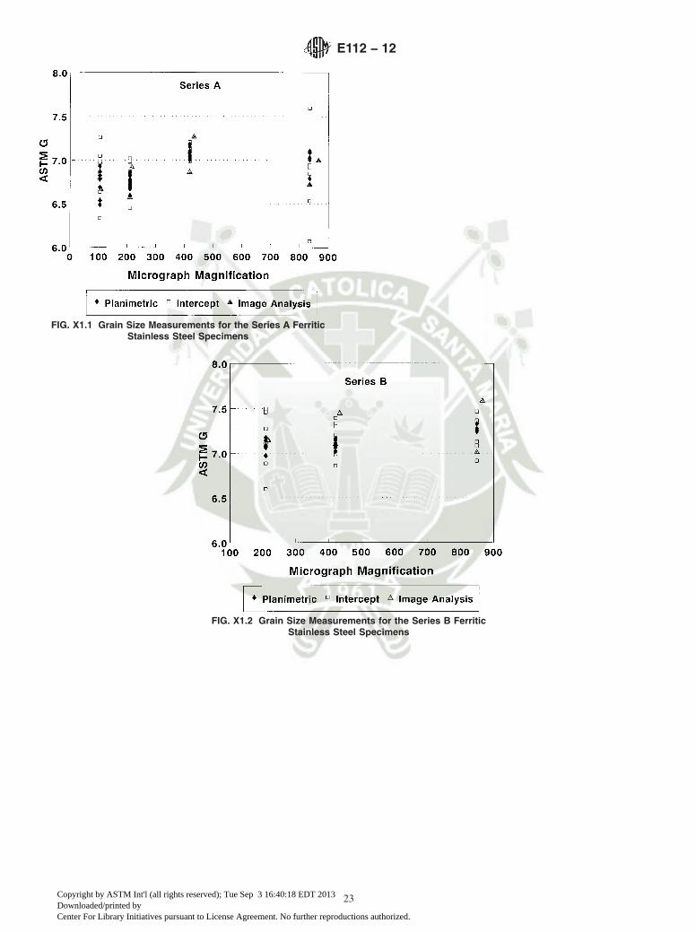
FIG. X1.1 Grain Size Measurements for the Series A FerriticStainless Steel Specimens
FIG. X1.2 Grain Size Measurements for the Series B FerriticStainless Steel Specimens
E112 − 12
23
Copyright by ASTM Int'l (all rights reserved); Tue Sep 3 16:40:18 EDT 2013Downloaded/printed byCenter For Library Initiatives pursuant to License Agreement. No further reproductions authorized.

NOTE 1—The image analysis results for the same micrographs.
FIG. X1.3 Relationship Between the Number of Grains Countedand the Percent Relative Accuracy for the Planimetric Method
NOTE 1—The image analysis results for the same micrographs.
FIG. X1.4 Relationship Between the Number of Intercepts or In-tersections Counted and the Percent Relative Accuracy for the
Intercept Method
TABLE X1.1 Results of ASTM Grain Size Round Robin (Planimetric Method)
Image No./sq. mm ASTM G Average No.Repeatability
95 % CLReproducibility
95 % CLRepeatability
% RAReproducibility
% RA
A1 846.64 6.77 1918.0 106.11 266.56 12.53 31.49A2 831.61 6.75 474.5 209.68 239.88 25.21 28.85A3 1046.98 7.08 150.5 499.42 489.10 47.70 46.72A4 978.49 6.98 35.5 785.07 765.18 80.23 78.20B1 1054.12 7.09 608.5 342.21 344.35 32.46 32.67B2 1069.41 7.11 152.5 464.60 452.27 43.44 42.29B3 1184.01 7.26 41.5 435.21 403.98 36.76 34.12
E112 − 12
24
Copyright by ASTM Int'l (all rights reserved); Tue Sep 3 16:40:18 EDT 2013Downloaded/printed byCenter For Library Initiatives pursuant to License Agreement. No further reproductions authorized.
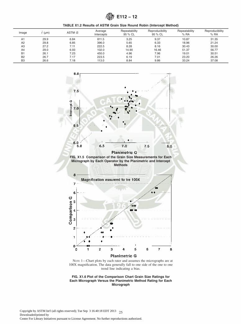
TABLE X1.2 Results of ASTM Grain Size Round Robin (Intercept Method)
Image ! (µm) ASTM GAverage
InterceptsRepeatability
95 % CLReproducibility
95 % CLRepeatability
% RAReproducibility
% RA
A1 29.9 6.84 811.5 3.25 9.37 10.87 31.35A2 29.8 6.85 396.0 5.65 6.33 18.96 21.24A3 27.2 7.11 222.5 8.28 8.16 30.43 30.00A4 29.0 6.93 102.0 14.90 16.46 51.37 56.77B1 26.1 7.23 450.0 4.96 7.96 19.01 30.51B2 26.7 7.17 223.5 6.19 7.01 23.20 26.26B3 26.6 7.18 113.0 8.84 9.86 33.24 37.08
FIG. X1.5 Comparison of the Grain Size Measurements for EachMicrograph by Each Operator by the Planimetric and Intercept
Methods
NOTE 1—Chart plots by each rater and assumes the micrographs are at100X magnification. The data generally fall to one side of the one to one
trend line indicating a bias.
FIG. X1.6 Plot of the Comparison Chart Grain Size Ratings forEach Micrograph Versus the Planimetric Method Rating for Each
Micrograph
E112 − 12
25
Copyright by ASTM Int'l (all rights reserved); Tue Sep 3 16:40:18 EDT 2013Downloaded/printed byCenter For Library Initiatives pursuant to License Agreement. No further reproductions authorized.

X2. REFERENCED ADJUNCTS
X2.1 The following is a complete and updated list ofadjuncts referenced in Test Methods E112. All adjuncts areavailable from ASTM.
Adjunct: Order Adjunct:Combination of 18 Components ADJE112CSCombination of Plates I, II, III, and IV ADJE112PSPlate I only ADJE11201PPlate II only ADJE11202PPlate III only ADJE11203PPlate IV only ADJE11204PCombination Transparencies, (Plate I) 00 through 10 ADJE112TSTransparency, Grain Size 00 ADJE11205TTransparency, Grain Size 0 ADJE11206TTransparency, Grain Size 0.5 ADJE11207T
Adjunct: Order Adjunct:Transparency, Grain Size 1.0 ADJE11208TTransparency, Grain Size 1.5 ADJE11209TTransparency, Grain Size 2.0 ADJE11210TTransparency, Grain Size 2.5 ADJE11211TTransparency, Grain Sizes 3.0, 3.5, and 4.0 ADJE11212TTransparency, Grain Sizes 4.5, 5.0, and 5.5 ADJE11213TTransparency, Grain Sizes 6.0, 6.5, and 7.0 ADJE11214TTransparency, Grain Sizes 7.5, 8.0, and 8.5 ADJE11215TTransparency, Grain Sizes 9.0, 9.5, and 10.0 ADJE11216T
Adjunct: Order ADJ:Fig. 5 only E11217F
Adjunct: Order ADJ:Shepherd Series Reproduction ADJE011224
REFERENCES
(1) Hull, F. C., Transactions, “A New Method for Making Rapid andAccurate Estimates of Grain Size,” American Institute of Mining andMetallurgical Engineers, Vol 172, 1947, p. 439–451.
(2) Shepherd, B. F., “The P-F Characteristic of Steel,” Transactions ,Transactions of the American Society of Metals, Vol 22, December1934 , pp. 979–1016.
(3) Jeffries, Z., Kline, A. H., and Zimmer, E. B., “The Determination ofthe Average Grain Size in Metals,” Transactions, American Instituteof Mining and Metallurgical Engineers, Vol 54, 1916, pp. 594–607.
(4) Saltykov, S.A., Steremetricheskaya Metallograpfiya (SterometricMetallography), 2nd revised and supplemented edition,Metallurgizdat, Moscow, 1958, 444 pgs.
(5) Heyn, E., “Short Reports from the Metallurgical Laboratory of theRoyal Mechanical and Testing Institute of Charlottenburg,” Metallog-raphist , Vol 5, 1903, pp. 37–64.
(6) Underwood, E. E., and Coons, W. C., “The Role of QuantitativeStereology in Deformation Twinning,” Deformation Twinning, Gor-
don and Breach, New York, 1965, pp. 405–429.(7) Hilliard, J., “Estimating Grain Size by the Intercept Method,” Metal
Progress, Vol 85, May 1964.(8) Abrams, H., “Grain Size Measurement by the Intercept Method,”
Metallography , Vol 4, 1971, pp. 59–78.(9) Mendelson, M. I., “Average Grain Size in Polycrystalline Ceramics,”
J. American Ceramic Society, Vol 52, August 1969, pp. 443–446.(10) Arpi, R., “The Fracture Test as Used for Tool Steel in Sweden,”
Metallurgia , Vol 11, No. 65, March 1935, pp. 123–127.(11) Vander Voort, G. F., “Grain Size Measurement,” Practical Applica-
tions of Quantitative Metallography, ASTM STP 839, 1984, pp.85–181.
(12) Snyder, R. W., and Graff, H. F., “Study of Grain Size in HardenedHigh Speed,” Metal Progress, Vol 33, 1938, pp. 377–380.
(13) Vander Voort, G. F., “Precision and Reproducibility of QuantitativeMeasurements,” Quantitative Microscopy and Image Analysis, ASMInternational, Materials Park, Ohio, 1994, pp. 21-34.
FIG. X1.7 Plot of the Comparison Chart Grain Size Ratings forEach Micrograph Versus the Intercept Method Rating for Each
Micrograph
E112 − 12
26
Copyright by ASTM Int'l (all rights reserved); Tue Sep 3 16:40:18 EDT 2013Downloaded/printed byCenter For Library Initiatives pursuant to License Agreement. No further reproductions authorized.

ASTM International takes no position respecting the validity of any patent rights asserted in connection with any item mentionedin this standard. Users of this standard are expressly advised that determination of the validity of any such patent rights, and the riskof infringement of such rights, are entirely their own responsibility.
This standard is subject to revision at any time by the responsible technical committee and must be reviewed every five years andif not revised, either reapproved or withdrawn. Your comments are invited either for revision of this standard or for additional standardsand should be addressed to ASTM International Headquarters. Your comments will receive careful consideration at a meeting of theresponsible technical committee, which you may attend. If you feel that your comments have not received a fair hearing you shouldmake your views known to the ASTM Committee on Standards, at the address shown below.
This standard is copyrighted by ASTM International, 100 Barr Harbor Drive, PO Box C700, West Conshohocken, PA 19428-2959,United States. Individual reprints (single or multiple copies) of this standard may be obtained by contacting ASTM at the aboveaddress or at 610-832-9585 (phone), 610-832-9555 (fax), or [email protected] (e-mail); or through the ASTM website(www.astm.org). Permission rights to photocopy the standard may also be secured from the ASTM website (www.astm.org/COPYRIGHT/).
E112 − 12
27
Copyright by ASTM Int'l (all rights reserved); Tue Sep 3 16:40:18 EDT 2013Downloaded/printed byCenter For Library Initiatives pursuant to License Agreement. No further reproductions authorized.

ANEXO 12
NORMA
ASTM E18 – 15
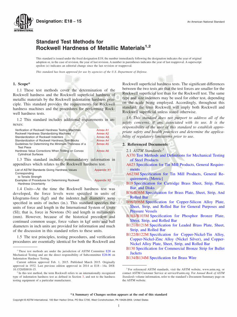
Designation: E18 − 15 An American National Standard
Standard Test Methods forRockwell Hardness of Metallic Materials1,2
This standard is issued under the fixed designation E18; the number immediately following the designation indicates the year of originaladoption or, in the case of revision, the year of last revision. A number in parentheses indicates the year of last reapproval. A superscriptepsilon (´) indicates an editorial change since the last revision or reapproval.
This standard has been approved for use by agencies of the U.S. Department of Defense.
1. Scope*
1.1 These test methods cover the determination of theRockwell hardness and the Rockwell superficial hardness ofmetallic materials by the Rockwell indentation hardness prin-ciple. This standard provides the requirements for Rockwellhardness machines and the procedures for performing Rock-well hardness tests.
1.2 This standard includes additional requirements in an-nexes:
Verification of Rockwell Hardness Testing Machines Annex A1Rockwell Hardness Standardizing Machines Annex A2Standardization of Rockwell Indenters Annex A3Standardization of Rockwell Hardness Test Blocks Annex A4Guidelines for Determining the Minimum Thickness of a
Test PieceAnnex A5
Hardness Value Corrections When Testing on ConvexCylindrical Surfaces
Annex A6
1.3 This standard includes nonmandatory information inappendixes which relates to the Rockwell hardness test.
List of ASTM Standards Giving Hardness ValuesCorresponding
to Tensile Strength
Appendix X1
Examples of Procedures for Determining RockwellHardness Uncertainty
Appendix X2
1.4 Units—At the time the Rockwell hardness test wasdeveloped, the force levels were specified in units ofkilograms-force (kgf) and the indenter ball diameters werespecified in units of inches (in.). This standard specifies theunits of force and length in the International System of Units(SI); that is, force in Newtons (N) and length in millimeters(mm). However, because of the historical precedent andcontinued common usage, force values in kgf units and balldiameters in inch units are provided for information and muchof the discussion in this standard refers to these units.
1.5 The test principles, testing procedures, and verificationprocedures are essentially identical for both the Rockwell and
Rockwell superficial hardness tests. The significant differencesbetween the two tests are that the test forces are smaller for theRockwell superficial test than for the Rockwell test. The sametype and size indenters may be used for either test, dependingon the scale being employed. Accordingly, throughout thisstandard, the term Rockwell will imply both Rockwell andRockwell superficial unless stated otherwise.
1.6 This standard does not purport to address all of thesafety concerns, if any, associated with its use. It is theresponsibility of the user of this standard to establish appro-priate safety and health practices and determine the applica-bility of regulatory limitations prior to use.
2. Referenced Documents
2.1 ASTM Standards:3
A370 Test Methods and Definitions for Mechanical Testingof Steel Products
A623 Specification for Tin Mill Products, General Require-ments
A623M Specification for Tin Mill Products, General Re-quirements [Metric]
B19 Specification for Cartridge Brass Sheet, Strip, Plate,Bar, and Disks
B36/B36M Specification for Brass Plate, Sheet, Strip, AndRolled Bar
B96/B96M Specification for Copper-Silicon Alloy Plate,Sheet, Strip, and Rolled Bar for General Purposes andPressure Vessels
B103/B103M Specification for Phosphor Bronze Plate,Sheet, Strip, and Rolled Bar
B121/B121M Specification for Leaded Brass Plate, Sheet,Strip, and Rolled Bar
B122/B122M Specification for Copper-Nickel-Tin Alloy,Copper-Nickel-Zinc Alloy (Nickel Silver), and Copper-Nickel Alloy Plate, Sheet, Strip, and Rolled Bar
B130 Specification for Commercial Bronze Strip for BulletJackets
B134/B134M Specification for Brass Wire
1 These test methods are under the jurisdiction of ASTM Committee E28 onMechanical Testing and are the direct responsibility of Subcommittee E28.06 onIndentation Hardness Testing.
Current edition approved Feb. 1, 2015. Published March 2015. Originallyapproved in 1932. Last previous edition approved in 2014 as E18 – 14a. DOI:10.1520/E0018-15.
2 In this test method, the term Rockwell refers to an internationally recognizedtype of indentation hardness test as defined in Section 3, and not to the hardnesstesting equipment of a particular manufacturer.
3 For referenced ASTM standards, visit the ASTM website, www.astm.org, orcontact ASTM Customer Service at [email protected]. For Annual Book of ASTMStandards volume information, refer to the standard’s Document Summary page onthe ASTM website.
*A Summary of Changes section appears at the end of this standard
Copyright © ASTM International, 100 Barr Harbor Drive, PO Box C700, West Conshohocken, PA 19428-2959. United States
1
B152/B152M Specification for Copper Sheet, Strip, Plate,and Rolled Bar
B370 Specification for Copper Sheet and Strip for BuildingConstruction
E29 Practice for Using Significant Digits in Test Data toDetermine Conformance with Specifications
E92 Test Method for Vickers Hardness of Metallic Materials(Withdrawn 2010)4
E140 Hardness Conversion Tables for Metals RelationshipAmong Brinell Hardness, Vickers Hardness, RockwellHardness, Superficial Hardness, Knoop Hardness, Sclero-scope Hardness, and Leeb Hardness
E384 Test Method for Knoop and Vickers Hardness ofMaterials
E691 Practice for Conducting an Interlaboratory Study toDetermine the Precision of a Test Method
2.2 American Bearings Manufacturer Association Stan-dard:
ABMA 10-1989 Metal Balls5
2.3 ISO Standards:ISO 6508-1 Metallic Materials—Rockwell Hardness Test—
Part 1: Test Method (scales A, B, C, D, E, F, G, H, K, N,T)6
ISO/IEC 17011 Conformity Assessment—General Require-ments for Accreditation Bodies Accrediting ConformityAssessment Bodies6
ISO/IEC 17025 General Requirements for the Competenceof Testing and Calibration Laboratories6
2.4 Society of Automotive Engineers (SAE) Standard:SAE J417 Hardness Tests and Hardness Number Conver-
sions7
3. Terminology and Equations
3.1 Definitions:3.1.1 calibration—determination of the values of the sig-
nificant parameters by comparison with values indicated by areference instrument or by a set of reference standards.
3.1.2 verification—checking or testing to assure confor-mance with the specification.
3.1.3 standardization—to bring in conformance to a knownstandard through verification or calibration.
3.1.4 Rockwell hardness test—an indentation hardness testusing a verified machine to force a diamond spheroconicalindenter or tungsten carbide (or steel) ball indenter, underspecified conditions, into the surface of the material under test,and to measure the difference in depth of the indentation as theforce on the indenter is increased from a specified preliminarytest force to a specified total test force and then returned to thepreliminary test force.
3.1.5 Rockwell superficial hardness test—same as the Rock-well hardness test except that smaller preliminary and total testforces are used with a shorter depth scale.
3.1.6 Rockwell hardness number—a number derived fromthe net increase in the depth of indentation as the force on anindenter is increased from a specified preliminary test force toa specified total test force and then returned to the preliminarytest force.
3.1.7 Rockwell hardness machine—a machine capable ofperforming a Rockwell hardness test and/or a Rockwell super-ficial hardness test and displaying the resulting Rockwellhardness number.
3.1.7.1 Rockwell hardness testing machine—a Rockwellhardness machine used for general testing purposes.
3.1.7.2 Rockwell hardness standardizing machine—a Rock-well hardness machine used for the standardization of Rock-well hardness indenters, and for the standardization of Rock-well hardness test blocks. The standardizing machine differsfrom a regular Rockwell hardness testing machine by havingtighter tolerances on certain parameters.
3.2 Equations:3.2.1 The average H of a set of n hardness measurements
H1, H2, …, Hn is calculated as:
H 5H11H21…1Hn
n(1)
3.2.2 The error E in the performance of a Rockwell hard-ness machine at each hardness level, relative to a standardizedscale, is determined as:
E 5 H 2 HSTD (2)
where:
H = average of n hardness measurements H1, H2, …, Hn
made on a standardized test block as part of aperformance verification, and
HSTD = certified average hardness value of the standardizedtest block.
3.2.3 The repeatability R in the performance of a Rockwellhardness machine at each hardness level, under the particularverification conditions, is estimated by the range of n hardnessmeasurements made on a standardized test block as part of aperformance verification, defined as:
R 5 Hmax 2 Hmin (3)
where:Hmax = highest hardness value, andHmin = lowest hardness value.
4. Significance and Use
4.1 The Rockwell hardness test is an empirical indentationhardness test that can provide useful information about metallicmaterials. This information may correlate to tensile strength,wear resistance, ductility, and other physical characteristics ofmetallic materials, and may be useful in quality control andselection of materials.
4 The last approved version of this historical standard is referenced onwww.astm.org.
5 Available from American Bearing Manufacturers Association (ABMA), 2025M Street, NW, Suite 800, Washington, DC 20036.
6 Available from American National Standards Institute (ANSI), 25 W. 43rd St.,4th Floor, New York, NY 10036, http://www.ansi.org.
7 Available from Society of Automotive Engineers (SAE), 400 CommonwealthDr., Warrendale, PA 15096-0001, http://www.sae.org.
E18 − 15
2

4.2 Rockwell hardness tests are considered satisfactory foracceptance testing of commercial shipments, and have beenused extensively in industry for this purpose.
4.3 Rockwell hardness testing at a specific location on a partmay not represent the physical characteristics of the whole partor end product.
4.4 Adherence to this standard test method provides trace-ability to national Rockwell hardness standards except as statedotherwise.
5. Principles of Test and Apparatus
5.1 Rockwell Hardness Test Principle—The general prin-ciple of the Rockwell indentation hardness test is illustrated inFig. 1. The test is divided into three steps of force applicationand removal.
Step 1—The indenter is brought into contact with the testspecimen, and the preliminary test force F0 is applied. Afterholding the preliminary test force for a specified dwell time,the baseline depth of indentation is measured.
Step 2—The force on the indenter is increased at acontrolled rate by the additional test force F1 to achieve thetotal test force F. The total test force is held for a specifieddwell time.
Step 3—The additional test force is removed, returning tothe preliminary test force. After holding the preliminary testforce for a specified dwell time, the final depth of indentationis measured. The Rockwell hardness value is derived from thedifference h in the final and baseline indentation depths whileunder the preliminary test force. The preliminary test force isremoved and the indenter is removed from the test specimen.
5.1.1 There are two general classifications of the Rockwelltest: the Rockwell hardness test and the Rockwell superficialhardness test. The significant difference between the two testclassifications is in the test forces that are used. For theRockwell hardness test, the preliminary test force is 10 kgf (98N) and the total test forces are 60 kgf (589 N), 100 kgf (981 N),and 150 kgf (1471 N). For the Rockwell superficial hardnesstest, the preliminary test force is 3 kgf (29 N) and the total testforces are 15 kgf (147 N), 30 kgf (294 N), and 45 kgf (441 N).
5.1.2 Indenters for the Rockwell hardness test include adiamond spheroconical indenter and tungsten carbide ballindenters of specified diameters.
5.1.2.1 Steel indenter balls may be used only for testing thinsheet tin mill products specified in Specifications A623 andA623M using the HR15T and HR30T scales with a diamondspot anvil. Testing of this product may give significantlydiffering results using a tungsten carbide ball as compared tohistorical test data using a steel ball.
NOTE 1—Previous editions of this standard have stated that the steelball was the standard type of Rockwell indenter ball. The tungsten carbideball is considered the standard type of Rockwell indenter ball. The use oftungsten carbide balls provide an improvement to the Rockwell hardnesstest because of the tendency of steel balls to flatten with use, which resultsin an erroneously elevated hardness value. The user is cautioned thatRockwell hardness tests comparing the use of steel and tungsten carbideballs have been shown to give different results. For example, depending onthe material tested and its hardness level, Rockwell B scale tests using atungsten carbide ball indenter have given results approximately oneRockwell point lower than when a steel ball indenter is used.
5.1.3 The Rockwell hardness scales are defined by thecombinations of indenter and test forces that may be used. Thestandard Rockwell hardness scales and typical applications ofthe scales are given in Tables 1 and 2. Rockwell hardnessvalues shall be determined and reported in accordance with oneof these standard scales.
5.2 Calculation of the Rockwell Hardness Number—Duringa Rockwell test, the force on the indenter is increased from apreliminary test force to a total test force, and then returned tothe preliminary test force. The difference in the two indentationdepth measurements, while under the preliminary test force, ismeasured as h (see Fig. 1).
5.2.1 The unit measurement for h is mm. From the value ofh, the Rockwell hardness number is derived. The Rockwellhardness number is calculated as:
5.2.1.1 For scales using a diamond spheroconical indenter(see Tables 1 and 2):
Rockwell Hardness 5 100 2h
0.002(4)
Rockwell Superficial Hardness 5 100 2h
0.001(5)
where h is in mm.5.2.1.2 For scales using a ball indenter (see Tables 1 and 2):
Rockwell Hardness 5 130 2h
0.002(6)
Rockwell Superficial Hardness 5 100 2h
0.001(7)
where h is in mm.5.2.2 The Rockwell hardness number is an arbitrary
number, which, by method of calculation, results in a highernumber for harder material.
5.2.3 Rockwell hardness values shall not be designated by anumber alone because it is necessary to indicate which indenterand forces have been employed in making the test (see Tables1 and 2). Rockwell hardness numbers shall be quoted with ascale symbol representing the indenter and forces used. Thehardness number is followed by the symbol HR and the scaledesignation. When a ball indenter is used, the scale designationFIG. 1 Rockwell Hardness Test Method (Schematic Diagram)
E18 − 15
3

is followed by the letter “W” to indicate the use of a tungstencarbide ball or the letter “S” to indicate the use of a steel ball(see 5.1.2.1).
5.2.3.1 Examples:64 HRC = Rockwell hardness number of 64 on Rockwell C scale
81 HR30N = Rockwell superficial hardness number of 81 on the Rockwell30N scale
72 HRBW = Rockwell hardness number of 72 on the Rockwell B scaleusing a tungsten carbide ball indenter
5.2.4 A reported Rockwell hardness number or the averagevalue of Rockwell hardness measurements shall be rounded inaccordance with Practice E29 with a resolution no greater thanthe resolution of the hardness value display of the testingmachine. Typically, the resolution of a Rockwell hardnessnumber should not be greater than 0.1 Rockwell units.
NOTE 2—When the Rockwell hardness test is used for the acceptancetesting of commercial products and materials, the user should take intoaccount the potential measurement differences between hardness testingmachines allowed by this standard (see Section 10, Precision and Bias).Because of the allowable ranges in the tolerances for the repeatability anderror of a testing machine, as specified in the verification requirements ofAnnex A1, one testing machine may have a test result that is one or morehardness points different than another testing machine, yet both machinescan be within verification tolerances (see Table A1.3). Commonly foracceptance testing, Rockwell hardness values are rounded to wholenumbers following Practice E29. Users are encouraged to address round-ing practices with regards to acceptance testing within their qualitymanagement system, and make any special requirements known duringcontract review.
5.3 Rockwell Testing Machine—The Rockwell testing ma-chine shall make Rockwell hardness determinations by apply-ing the test forces and measuring the depth of indentation inaccordance with the Rockwell hardness test principle.
5.3.1 See the Equipment Manufacturer’s Instruction Manualfor a description of the machine’s characteristics, limitations,and respective operating procedures.
5.3.2 The Rockwell testing machine shall automaticallyconvert the depth measurements to a Rockwell hardnessnumber and indicate the hardness number and Rockwell scaleby an electronic device or by a mechanical indicator.
5.4 Indenters—The standard Rockwell indenters are eitherdiamond spheroconical indenters or tungsten carbide balls of1.588 mm (1⁄16 in.), 3.175 mm (1⁄8 in.), 6.350 mm (1⁄4 in.), or12.70 mm (1⁄2 in.) in diameter. Indenters shall meet therequirements defined in Annex A3. Steel ball indenters may beused in certain circumstances (see 5.1.2.1).
5.4.1 Dust, dirt, or other foreign materials shall not beallowed to accumulate on the indenter, as this will affect thetest results.
NOTE 3—Indenters certified to revision E18-07 or later meet therequirements of this standard.
5.5 Specimen Support—A specimen support or “anvil” shallbe used that is suitable for supporting the specimen to betested. The seating and supporting surfaces of all anvils shall beclean and smooth and shall be free from pits, deep scratches,and foreign material. Damage to the anvil may occur fromtesting too thin material or accidental contact of the anvil bythe indenter. If the anvil is damaged from any cause, it shall berepaired or replaced. Anvils showing the least visibly percep-tible damage may give inaccurate results, particularly on thinmaterial.
5.5.1 Common specimen support anvils should have aminimum hardness of 58 HRC. Some specialty support anvilsrequire a lower material hardness.
TABLE 1 Rockwell Hardness Scales
ScaleSymbol
IndenterTotal TestForce, kgf
DialFigures
Typical Applications of Scales
B 1⁄16-in. (1.588-mm) ball 100 red Copper alloys, soft steels, aluminum alloys, malleable iron, etc.C diamond 150 black Steel, hard cast irons, pearlitic malleable iron, titanium, deep case hardened steel, and other
materials harder than B100.A diamond 60 black Cemented carbides, thin steel, and shallow case-hardened steel.D diamond 100 black Thin steel and medium case hardened steel, and pearlitic malleable iron.E 1⁄8-in. (3.175-mm) ball 100 red Cast iron, aluminum and magnesium alloys, bearing metals.F 1⁄16-in. (1.588-mm) ball 60 red Annealed copper alloys, thin soft sheet metals.G 1⁄16-in. (1.588-mm) ball 150 red Malleable irons, copper-nickel-zinc and cupro-nickel alloys. Upper limit G92 to avoid possible
flattening of ball.H 1⁄8-in. (3.175-mm) ball 60 red Aluminum, zinc, lead.K 1⁄8-in. (3.175-mm) ball 150 red
6L 1⁄4-in. (6.350-mm) ball 60 redM 1⁄4-in. (6.350-mm) ball 100 red Bearing metals and other very soft or thin materials. Use smallest ball and heaviest load that doesP 1⁄4-in. (6.350-mm) ball 150 red not give anvil effect.R 1⁄2-in. (12.70-mm) ball 60 redS 1⁄2-in. (12.70-mm) ball 100 redV 1⁄2-in. (12.70-mm) ball 150 red
TABLE 2 Rockwell Superficial Hardness Scales
Total Test Force,kgf (N)
Scale SymbolsN Scale, Diamond
IndenterT Scale, 1⁄16-in.(1.588-mm) Ball
W Scale, 1⁄8-in.(3.175-mm) Ball
X Scale, 1⁄4-in.(6.350-mm) Ball
Y Scale, 1⁄2-in.(12.70-mm) Ball
15 (147) 15N 15T 15W 15X 15Y30 (294) 30N 30T 30W 30X 30Y45 (441) 45N 45T 45W 45X 45Y
E18 − 15
4
5.5.2 Flat pieces should be tested on a flat anvil that has asmooth, flat bearing surface whose plane is perpendicular tothe axis of the indenter.
5.5.3 Small diameter cylindrical pieces shall be tested witha hard V-grooved anvil with the axis of the V-groove directlyunder the indenter, or on hard, parallel, twin cylinders properlypositioned and clamped in their base. These types of specimensupports shall support the specimen with the apex of thecylinder directly under the indenter.
5.5.4 For thin materials or specimens that are not perfectlyflat, an anvil having an elevated, flat “spot” 3 mm (1⁄8 in.) to12.5 mm (1⁄2 in.) in diameter should be used. This spot shall bepolished smooth and flat. Very soft material should not betested on the “spot” anvil because the applied force may causethe penetration of the anvil into the under side of the specimenregardless of its thickness.
5.5.5 When testing thin sheet metal with a ball indenter, it isrecommended that a diamond spot anvil be used. The highlypolished diamond surface shall have a diameter between 4.0mm (0.157 in.) and 7.0 mm (0.2875 in.) and be centered within0.5 mm (0.02 in.) of the test point.
5.5.5.1 CAUTION: A diamond spot anvil should only beused with a maximum total test force of 45 kgf (441 N) and aball indenter. This recommendation should be followed exceptwhen directed otherwise by material specification.
5.5.6 Special anvils or fixtures, including clamping fixtures,may be required for testing pieces or parts that cannot besupported by standard anvils. Auxiliary support may be usedfor testing long pieces with so much overhang that the piece isnot firmly seated by the preliminary force.
5.6 Verification—Rockwell testing machines shall be veri-fied periodically in accordance with Annex A1.
5.7 Test Blocks—Test blocks meeting the requirements ofAnnex A4 shall be used to verify the testing machine inaccordance with Annex A1.
NOTE 4—Test blocks certified to revision E18-07 or later meet therequirements of this standard.
NOTE 5—It is recognized that appropriate standardized test blocks arenot available for all geometric shapes, or materials, or both.
6. Test Piece
6.1 For best results, both the test surface and the bottomsurface of the test piece should be smooth, even and free fromoxide scale, foreign matter, and lubricants. An exception ismade for certain materials such as reactive metals that mayadhere to the indenter. In such situations, a suitable lubricantsuch as kerosene may be used. The use of a lubricant shall bedefined on the test report.
6.2 Preparation shall be carried out in such a way that anyalteration of the surface hardness of the test surface (forexample, due to heat or cold-working) is minimized.
6.3 The thickness of the test piece or of the layer under testshould be as defined in tables and presented graphically inAnnex A5. These tables were determined from studies on stripsof carbon steel and have proven to give reliable results. For allother materials, it is recommended that the thickness shouldexceed 10 times the depth of indentation. In general, no
deformation should be visible on the back of the test piece afterthe test, although not all such marking is indicative of a badtest.
6.3.1 Special consideration should be made when testingparts that exhibit hardness gradients; for example, parts thatwere case-hardened by processes such as carburizing,carbonitriding, nitriding, induction, etc. The minimum thick-ness guidelines given in Annex A5 only apply to materials ofuniform hardness, and should not be used to determine theappropriate scale for measuring parts with hardness gradients.The selection of an appropriate Rockwell scale for parts withhardness gradients should be made by special agreement.
NOTE 6—A table listing the minimum effective case depth needed fordifferent Rockwell scales is given in SAE J417.
6.4 When testing on convex cylindrical surfaces, the resultmay not accurately indicate the true Rockwell hardness;therefore, the corrections given in Annex A6 shall be applied.For diameters between those given in the tables, correctionfactors may be derived by linear interpolation. Tests performedon diameters smaller than those given in Annex A6 are notacceptable. Corrections for tests on spherical and concavesurfaces should be the subject of special agreement.
NOTE 7—A table of correction values to be applied to test results madeon spherical surfaces is given in ISO 6508-1.
6.5 When testing small diameter specimens, the accuracy ofthe test will be seriously affected by alignment between theindenter and the test piece, by surface finish, and by thestraightness of the cylinder.
7. Test Procedure
7.1 A daily verification of the testing machine shall beperformed in accordance with A1.5 prior to making hardnesstests. Hardness measurements shall be made only on thecalibrated surface of the test block.
7.2 Rockwell hardness tests should be carried out at ambienttemperature within the limits of 10 to 35°C (50 to 95°F). Usersof the Rockwell hardness test are cautioned that the tempera-ture of the test material and the temperature of the hardnesstester may affect test results. Consequently, users should ensurethat the test temperature does not adversely affect the hardnessmeasurement.
7.3 The test piece shall be supported rigidly so that displace-ment of the test surface is minimized (see 5.5).
7.4 Test Cycle—This standard specifies the Rockwell testcycle by stating recommendations or requirements for fiveseparate parts of the cycle. These parts are illustrated for aRockwell C scale test in Fig. 2, and defined as follows:
(1) Contact Velocity, vA—The velocity of the indenter at thepoint of contact with the test material.
(2) Preliminary Force Dwell Time, tPF—The dwell timebeginning when the preliminary force is fully applied andending when the first baseline depth of indentation ismeasured, (also see 7.4.1.3).
(3) Additional Force Application Time, tTA—The time forapplying the additional force to obtain the full total force.
(4) Total Force Dwell Time, tTF—The dwell time while thetotal force is fully applied.
E18 − 15
5
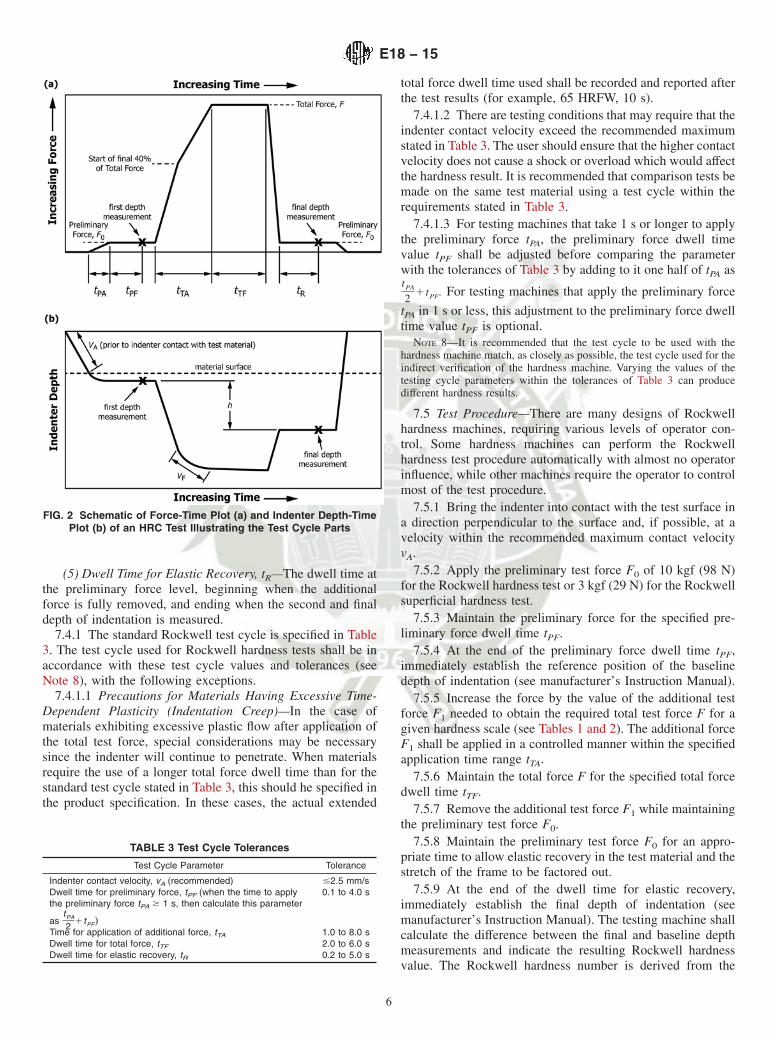
(5) Dwell Time for Elastic Recovery, tR—The dwell time atthe preliminary force level, beginning when the additionalforce is fully removed, and ending when the second and finaldepth of indentation is measured.
7.4.1 The standard Rockwell test cycle is specified in Table3. The test cycle used for Rockwell hardness tests shall be inaccordance with these test cycle values and tolerances (seeNote 8), with the following exceptions.
7.4.1.1 Precautions for Materials Having Excessive Time-Dependent Plasticity (Indentation Creep)—In the case ofmaterials exhibiting excessive plastic flow after application ofthe total test force, special considerations may be necessarysince the indenter will continue to penetrate. When materialsrequire the use of a longer total force dwell time than for thestandard test cycle stated in Table 3, this should he specified inthe product specification. In these cases, the actual extended
total force dwell time used shall be recorded and reported afterthe test results (for example, 65 HRFW, 10 s).
7.4.1.2 There are testing conditions that may require that theindenter contact velocity exceed the recommended maximumstated in Table 3. The user should ensure that the higher contactvelocity does not cause a shock or overload which would affectthe hardness result. It is recommended that comparison tests bemade on the same test material using a test cycle within therequirements stated in Table 3.
7.4.1.3 For testing machines that take 1 s or longer to applythe preliminary force tPA, the preliminary force dwell timevalue tPF shall be adjusted before comparing the parameterwith the tolerances of Table 3 by adding to it one half of tPA astPA
21tPF. For testing machines that apply the preliminary force
tPA in 1 s or less, this adjustment to the preliminary force dwelltime value tPF is optional.
NOTE 8—It is recommended that the test cycle to be used with thehardness machine match, as closely as possible, the test cycle used for theindirect verification of the hardness machine. Varying the values of thetesting cycle parameters within the tolerances of Table 3 can producedifferent hardness results.
7.5 Test Procedure—There are many designs of Rockwellhardness machines, requiring various levels of operator con-trol. Some hardness machines can perform the Rockwellhardness test procedure automatically with almost no operatorinfluence, while other machines require the operator to controlmost of the test procedure.
7.5.1 Bring the indenter into contact with the test surface ina direction perpendicular to the surface and, if possible, at avelocity within the recommended maximum contact velocityvA.
7.5.2 Apply the preliminary test force F0 of 10 kgf (98 N)for the Rockwell hardness test or 3 kgf (29 N) for the Rockwellsuperficial hardness test.
7.5.3 Maintain the preliminary force for the specified pre-liminary force dwell time tPF.
7.5.4 At the end of the preliminary force dwell time tPF,immediately establish the reference position of the baselinedepth of indentation (see manufacturer’s Instruction Manual).
7.5.5 Increase the force by the value of the additional testforce F1 needed to obtain the required total test force F for agiven hardness scale (see Tables 1 and 2). The additional forceF1 shall be applied in a controlled manner within the specifiedapplication time range tTA.
7.5.6 Maintain the total force F for the specified total forcedwell time tTF.
7.5.7 Remove the additional test force F1 while maintainingthe preliminary test force F0.
7.5.8 Maintain the preliminary test force F0 for an appro-priate time to allow elastic recovery in the test material and thestretch of the frame to be factored out.
7.5.9 At the end of the dwell time for elastic recovery,immediately establish the final depth of indentation (seemanufacturer’s Instruction Manual). The testing machine shallcalculate the difference between the final and baseline depthmeasurements and indicate the resulting Rockwell hardnessvalue. The Rockwell hardness number is derived from the
FIG. 2 Schematic of Force-Time Plot (a) and Indenter Depth-TimePlot (b) of an HRC Test Illustrating the Test Cycle Parts
TABLE 3 Test Cycle Tolerances
Test Cycle Parameter Tolerance
Indenter contact velocity, vA (recommended) #2.5 mm/sDwell time for preliminary force, tPF (when the time to applythe preliminary force tPA $ 1 s, then calculate this parameter
astPA
21tPF)
0.1 to 4.0 s
Time for application of additional force, tTA 1.0 to 8.0 sDwell time for total force, tTF 2.0 to 6.0 sDwell time for elastic recovery, tR 0.2 to 5.0 s
E18 − 15
6
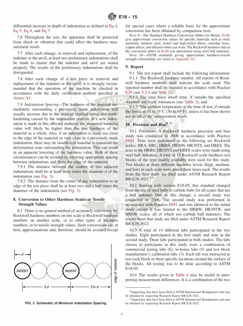
differential increase in depth of indentation as defined in Eq 4,Eq 5, Eq 6, and Eq 7.
7.6 Throughout the test, the apparatus shall be protectedfrom shock or vibration that could affect the hardness mea-surement result.
7.7 After each change, or removal and replacement, of theindenter or the anvil, at least two preliminary indentations shallbe made to ensure that the indenter and anvil are seatedproperly. The results of the preliminary indentations shall bedisregarded.
7.8 After each change of a test force or removal andreplacement of the indenter or the anvil, it is strongly recom-mended that the operation of the machine be checked inaccordance with the daily verification method specified inAnnex A1.
7.9 Indentation Spacing—The hardness of the material im-mediately surrounding a previously made indentation willusually increase due to the induced residual stress and work-hardening caused by the indentation process. If a new inden-tation is made in this affected material, the measured hardnessvalue will likely be higher than the true hardness of thematerial as a whole. Also, if an indentation is made too closeto the edge of the material or very close to a previously madeindentation, there may be insufficient material to constrain thedeformation zone surrounding the indentation. This can resultin an apparent lowering of the hardness value. Both of thesecircumstances can be avoided by allowing appropriate spacingbetween indentations and from the edge of the material.
7.9.1 The distance between the centers of two adjacentindentations shall be at least three times the diameter d of theindentation (see Fig. 3).
7.9.2 The distance from the center of any indentation to anedge of the test piece shall be at least two and a half times thediameter of the indentation (see Fig. 3).
8. Conversion to Other Hardness Scales or TensileStrength Values
8.1 There is no general method of accurately converting theRockwell hardness numbers on one scale to Rockwell hardnessnumbers on another scale, or to other types of hardnessnumbers, or to tensile strength values. Such conversions are, atbest, approximations and, therefore, should be avoided except
for special cases where a reliable basis for the approximateconversion has been obtained by comparison tests.
NOTE 9—The Standard Hardness Conversion Tables for Metals, E140,give approximate conversion values for specific materials such as steel,austenitic stainless steel, nickel and high-nickel alloys, cartridge brass,copper alloys, and alloyed white cast irons. The Rockwell hardness data inthe conversion tables of E140 was determined using steel ball indenters.
NOTE 10—ASTM standards giving approximate hardness-tensilestrength relationships are listed in Appendix X1.
9. Report
9.1 The test report shall include the following information:9.1.1 The Rockwell hardness number. All reports of Rock-
well hardness numbers shall indicate the scale used. Thereported number shall be rounded in accordance with PracticeE29 (see 5.2.4 and Note 2),
9.1.2 The total force dwell time, if outside the specifiedstandard test cycle tolerances (see Table 3), and
9.1.3 The ambient temperature at the time of test, if outsidethe limits of 10 to 35°C (50 to 95°F), unless it has been shownnot to affect the measurement result.
10. Precision and Bias8, 9
10.1 Precision—A Rockwell hardness precision and biasstudy was conducted in 2000 in accordance with PracticeE691. Tests were performed in the following six Rockwellscales: HRA, HRC, HRBS, HR30N, HR30TS, and HRES. Thetests in the HRBS, HR30TS and HRES scales were made usingsteel ball indenters. A total of 18 Rockwell scale hardness testblocks of the type readily available were used for this study.Test blocks at three different hardness levels (high, medium,and low) in each scale were tested three times each. The resultsfrom the first study are filed under ASTM Research ReportRR:E28-1021.8,9
10.2 Starting with version E18-05, this standard changedfrom the use of steel balls to carbide balls for all scales that usea ball indenter. Due to this change, a second study wasconducted in 2006. The second study was performed inaccordance with Practice E691 and was identical to the initialstudy except it was limited to the HRBW, HR30TW, andHREW scales, all of which use carbide ball indenters. Theresults from that study are filed under ASTM Research ReportRR:E28-1022.
10.3 A total of 14 different labs participated in the twostudies. Eight participated in the first study and nine in thesecond study. Three labs participated in both studies. The labschosen to participate in this study were a combination ofcommercial testing labs (6), in-house labs (5) and test blockmanufacturer’s calibration labs (3). Each lab was instructed totest each block in three specific locations around the surface ofthe blocks. All testing was to be done according to ASTME18-05.
10.4 The results given in Table 4 may be useful in inter-preting measurement differences. It is a combination of the two
8 Supporting data have been filed at ASTM International Headquarters and maybe obtained by requesting Research Report RR:E28-1021.
9 Supporting data have been filed at ASTM International Headquarters and maybe obtained by requesting Research Report RR:E28-1022.FIG. 3 Schematic of Minimum Indentation Spacing
E18 − 15
7

studies. The diamond scales, HRC, HRA, and HR30N are fromthe first study and the ball scales, HRBW, HREW, andHR30TW are from the second study. This combination reflectsthe testing that is being done currently.
10.5 The value of rPB indicates the typical amount ofvariation that can be expected between test results obtained forthe same material by the same operator using the samehardness tester on the same day. When comparing two testresults made under these conditions, a measurement differenceof less than the rPB value for that Rockwell scale is anindication that the results may be equivalent.
10.6 The value of RPB indicates the typical amount ofvariation that can be expected between test results obtained for
the same material by different operators using different hard-ness testers on different days. When comparing two test resultsmade under these conditions, a measurement difference of lessthan the RPB value for that Rockwell scale is an indication thatthe results may be equivalent.
10.7 Any judgments based on 10.5 and 10.6 would have anapproximately 95 % probability of being correct.
10.8 This precision and bias study was conducted on aselected number of the most commonly used Rockwell scales.For Rockwell scales not listed, the rPB and RPB values may beestimated using the conversion tables of E140 to determine acorresponding increment of hardness for the scale of interest atthe hardness level of interest. The user is cautioned thatestimating the rPB and RPB values in this way, decreases theprobability of them being correct.
10.9 Although the precision values given in Table 4 provideguidance on interpreting differences in Rockwell hardnessmeasurement results, a complete evaluation of measurementuncertainty will provide a more definitive interpretation of theresults for the specific testing conditions.
10.10 The data generally indicated reasonable precisionexcept for the 45.9 HR30N scale. In that scale the SR and RPB
values are very high compared to all of the other scales. Anexamination of the raw data reveled that one lab’s results weremuch higher than the others, significantly affecting the overallresults in that scale. The results from all of the other scalesseem to be reasonable.
10.11 Bias—There are no recognized standards by which tofully estimate the bias of this test method.
11. Keywords
11.1 hardness; mechanical test; metals; Rockwell
ANNEXES
(Mandatory Information)
A1. VERIFICATION OF ROCKWELL HARDNESS TESTING MACHINES
A1.1 Scope
A1.1.1 Annex A1 specifies three types of procedures forverifying Rockwell hardness testing machines: directverification, indirect verification, and daily verification.
A1.1.2 Direct verification is a process for verifying thatcritical components of the hardness testing machine are withinallowable tolerances by directly measuring the test forces,depth measuring system, machine hysteresis, and testing cycle.
A1.1.3 Indirect verification is a process for periodicallyverifying the performance of the testing machine by means ofstandardized test blocks and indenters.
A1.1.4 The daily verification is a process for monitoring theperformance of the testing machine between indirect verifica-tions by means of standardized test blocks.
A1.1.5 Adherence to this standard and annex providestraceability to national standards, except as stated otherwise.
A1.2 General Requirements
A1.2.1 The testing machine shall be verified at specificinstances and at periodic intervals as specified in Table A1.1,and when circumstances occur that may affect the performanceof the testing machine.
A1.2.2 The temperature at the verification site shall bemeasured with an instrument having an accuracy of at least62.0°C or 63.6°F. It is recommended that the temperature bemonitored throughout the verification period, and significanttemperature variations be recorded and reported. The tempera-ture at the verification site does not need to be measured for a
TABLE 4 Results of the Precision and Bias Study
Test BlockAverage
HardnessSr SR rPB RPB
Data from 2000 study62.8 HRA 62.50 0.164 0.538 0.459 1.50673.1 HRA 73.04 0.138 0.358 0.387 1.00283.9 HRA 84.54 0.085 0.468 0.238 1.30925.0 HRC 24.99 0.335 0.440 0.937 1.23245.0 HRC 45.35 0.156 0.259 0.438 0.72565.0 HRC 65.78 0.153 0.389 0.427 1.08945.9 HR30N 46.75 0.299 2.489 0.837 6.96964.0 HR30N 64.74 0.248 0.651 0.694 1.82281.9 HR30N 82.52 0.195 0.499 0.547 1.396
Data from 2006 study40 HRBW 43.90 0.492 0.668 1.378 1.87160 HRBW 61.77 0.663 0.697 1.855 1.95395 HRBW 91.09 0.250 0.292 0.701 0.81762 HREW 64.07 0.346 0.675 0.970 1.89081 HREW 81.61 0.232 0.406 0.649 1.136100 HREW 96.22 0.177 0.322 0.497 0.90122 HR30TW 18.33 0.702 0.901 1.965 2.52256 HR30TW 58.0 0.476 0.517 1.333 1.44779 HR30TW 81.0 0.610 0.851 1.709 2.382
E18 − 15
8

daily verification or when qualifying additional user’s indent-ers in accordance with A1.4.10.
A1.2.3 All instruments used to make measurements re-quired by this Annex shall be calibrated traceable to nationalstandards when a system of traceability exists, except as notedotherwise.
A1.2.4 Direct verification of newly manufactured or rebuilttesting machines shall be performed at the place ofmanufacture, rebuild or repair. Direct verification may also beperformed at the location of use.
A1.2.5 Indirect verification of the testing machine shall beperformed at the location where it will be used.
NOTE A1.1—It is recommended that the calibration agency that is usedto conduct the verifications of Rockwell hardness testing machines beaccredited to the requirements of ISO 17025 (or an equivalent) by anaccrediting body recognized by the International Laboratory AccreditationCooperation (ILAC) as operating to the requirements of ISO/IEC 17011.
A1.3 Direct Verification
A1.3.1 A direct verification of the testing machine shall beperformed at specific instances in accordance with Table A1.1.The test forces, depth-measuring system, machine hysteresis,and testing cycle shall be verified as follows.
NOTE A1.2—Direct verification is a useful tool for determining thesources of error in a Rockwell hardness testing machine. It is recom-mended that testing machines undergo direct verification periodically tomake certain that errors in one component of the machine are not beingoffset by errors in another component.
A1.3.2 Verification of the Test Forces—For each Rockwellscale that will be used, the corresponding test forces (prelimi-nary test force at loading, total test force, and preliminary testforce during elastic recovery) shall be measured. The testforces shall be measured by means of a Class A elastic forcemeasuring instrument having an accuracy of at least 0.25 %, asdescribed in ASTM E74.
A1.3.2.1 Make three measurements of each force. Theforces shall be measured as they are applied during testing.
A1.3.2.2 Each preliminary test force F0 and each total testforce F shall be accurate to within the tolerances given in TableA1.2, and the range of the three force measurements (highestminus lowest) shall be within 75 % of the tolerances of TableA1.2.
A1.3.3 Verification of the Depth Measuring System—Thedepth measuring system shall be verified by means of aninstrument, device or standard having an accuracy of at least0.0002 mm.
A1.3.3.1 Verify the testing machine’s depth measurementsystem at not less than four evenly spaced increments coveringthe full range of the normal working depth measured by thetesting machine. The normal working depth range shall corre-spond to the lowest and highest hardness values for theRockwell scales that will be tested.
A1.3.3.2 The indentation-depth measuring device shall beaccurate within 60.001 mm for the regular Rockwell hardnessscales and 60.0005 mm for the Rockwell superficial hardnessscales. These accuracies correspond to 0.5 hardness units.
A1.3.3.3 Some testing machines have a long-stroke depthmeasuring system where the location of the working range ofthe depth measuring system varies depending on the thicknessof the test material. This type of testing machine shall have asystem to electronically verify that the depth measuring deviceis continuous over its full range and free from dirt or otherdiscontinuities that could affect its accuracy. These types oftesters shall be verified using the following steps.
(1) At the approximate top, mid point, and bottom of thetotal stroke of the measuring device, verify the accuracy of thedevice at no less than four evenly spaced increments ofapproximately 0.05 mm at each of the three locations. Theaccuracy shall be within the tolerances defined above.
(2) Operate the actuator over its full range of travel andmonitor the electronic continuity detection system. The systemshall indicate continuity over the full range.
A1.3.4 Verification of Machine Hysteresis—Each time aRockwell hardness test is made, the testing machine willundergo flexure in some of the machine components and themachine frame. If the flexure is not entirely elastic during theapplication and removal of the additional force F1, the testingmachine may exhibit hysteresis in the indenter-depth measure-ment system, resulting in an offset or bias in the test result. Thegoal of the hysteresis verification is to perform a purely elastic
TABLE A1.1 Verification Schedule for a RockwellTesting Machine
VerificationProcedure
Schedule
Directverification
When a testing machine is new, or when adjustments,modifications or repairs are made that could affect theapplication of the test forces, the depth measuring system, orthe machine hysteresis.When a testing machine fails an indirect verification (seeA1.4.9.4).
Indirectverification
Recommended every 12 months, or more often if needed.Shall be no longer than every 18 months.When a testing machine is installed or moved, [only a partialindirect verification is performed by following the proceduregiven in A1.4.7 for verifying the as-found condition]. This doesnot apply to machines that are designed to be moved or thatmove prior to each test, when it has been previouslydemonstrated that such a move will not affect the hardnessresult.Following a direct verification.To qualify an indenter that was not verified in the last indirectverification, (only a partial indirect verification is performed,see A1.4.10).
Dailyverification
Required each day that hardness tests are to be made.Recommended whenever the indenter, anvil, or test force ischanged.
TABLE A1.2 Tolerances on Applied Force for a RockwellTesting Machine
Force Tolerance
kgf N kgf N
10 98.07 0.20 1.9660 588.4 0.45 4.41
100 980.7 0.65 6.37150 1471 0.90 8.83
3 29.42 0.060 0.58915 147.1 0.100 0.98130 294.2 0.200 1.96145 441.3 0.300 2.963
E18 − 15
9
test that results in no permanent indentation. In this way, thelevel of hysteresis in the flexure of the testing machine can bedetermined.
A1.3.4.1 Perform repeated Rockwell tests using a bluntindenter (or the indenter holder surface) acting directly onto theanvil or a very hard test piece. The tests shall be conductedusing the highest test force that is used during normal testing
A1.3.4.2 Repeat the hysteresis verification procedure for amaximum of ten measurements and average the last three tests.The average measurement shall indicate a hardness number of130 6 1.0 Rockwell units when Rockwell ball scales B, E, F,G, H and K are used, or within 100 6 1.0 Rockwell units whenany other Rockwell scale is used.
A1.3.5 Verification of the Testing Cycle—Section 7 specifiesthe Rockwell testing cycle by stating requirements and recom-mendations for five separate parameters of the cycle. Thetesting machine shall be verified to be capable of meeting thetolerances specified in Table 3 for the following four test cycleparameters: the dwell time for preliminary force, the time forapplication of additional force, the dwell time for total forceand the dwell time for elastic recovery. The tolerance for theindenter contact velocity is a recommendation. Direct verifi-cation of the testing cycle is to be verified by the testingmachine manufacturer at the time of manufacture, and whenthe testing machine is returned to the manufacturer for repairwhen a problem with the testing cycle is suspected. Verificationof the testing cycle is not required as part of the directverification at other times.
A1.3.5.1 Rockwell hardness testing machines manufacturedbefore the implementation of E18–07 may not have undergonethe direct verification of the machine’s testing cycle. Since thisverification often must be performed at the manufacturer’s site,the test cycle verification requirement does not apply to testingmachines manufactured before the implementation of E18–07,unless the testing machine is returned to the manufacturer forrepair.
A1.3.6 Direct Verification Failure—If any of the directverifications fail the specified requirements, the testing ma-chine shall not be used until it is adjusted or repaired. If the testforces, depth measuring system, machine hysteresis, or testingcycle may have been affected by an adjustment or repair, theaffected components shall be verified again by direct verifica-tion.
A1.3.7 An indirect verification shall follow a successfuldirect verification.
A1.4 Indirect Verification
A1.4.1 An indirect verification of the testing machine shallbe performed, at a minimum, in accordance with the schedulegiven in Table A1.1. The frequency of indirect verificationsshould be based on the usage of the testing machine.
A1.4.2 The testing machine shall be verified for eachRockwell scale that will be used prior to the next indirectverification. Hardness tests made using Rockwell scales thathave not been verified within the schedule given in Table A1.1do not meet this standard.
A1.4.3 Standardized test blocks meeting the requirementsof Annex A4 (see Note 4) shall be used in the appropriatehardness ranges for each scale to be verified. These ranges aregiven in Table A1.3. Hardness measurements shall be madeonly on the calibrated surface of the test block.
A1.4.4 The indenters to be used for the indirect verificationshall meet the requirements of Annex A3 (see Note 3).
A1.4.5 The testing cycle to be used for the indirect verifi-cation shall be the same as is typically used by the user.
A1.4.6 Prior to performing the indirect verification, ensurethat the testing machine is working freely, and that the indenterand anvil are seated adequately. Make at least two hardnessmeasurements on a suitable test piece to seat the indenter andanvil. The results of these measurements need not be recorded.
A1.4.7 As-found Condition:A1.4.7.1 It is recommended that the as-found condition of
the testing machine be assessed as part of an indirect verifica-tion. This is important for documenting the historical perfor-mance of the machine in the scales used since the last indirectverification. This procedure should be conducted prior to anycleaning, maintenance, adjustments, or repairs.
A1.4.7.2 When the as-found condition of the testing ma-chine is assessed, it shall be determined with the user’sindenter(s) that are normally used with the testing machine. Atleast two standardized test blocks, each from a differenthardness range as defined in Table A1.3, should be tested foreach Rockwell scale that will undergo indirect verification. Thedifference in hardness between any of the standardized testblocks shall be at least 5 hardness points for each Rockwellscale.
A1.4.7.3 On each standardized test block, make at least twomeasurements distributed uniformly over the test surface.
A1.4.7.4 Determine the repeatability R and the error E (Eq2 and Eq 3) in the performance of the testing machine for eachstandardized test block that is measured.
A1.4.7.5 The error E and the repeatability R should bewithin the tolerances of Table A1.3. If the calculated values oferror E or repeatability R fall outside of the specifiedtolerances, this is an indication that the hardness tests madesince the last indirect verification may be suspect.
A1.4.8 Cleaning and Maintenance—Perform cleaning androutine maintenance of the testing machine (when required) inaccordance with the manufacturer’s specifications and instruc-tions.
A1.4.9 Indirect Verification Procedure—The indirect verifi-cation procedure requires that the testing machine be verifiedusing one or more of the user’s indenters.
A1.4.9.1 One standardized test block shall be tested fromeach of the hardness ranges (usually three ranges) for eachRockwell scale to be verified, as given in Table A1.3. Thedifference in hardness between any of the standardized testblocks shall be at least 5 hardness points for each Rockwellscale. The user may find that high, medium and low range testblocks are unavailable commercially for some scales. In thesecases, one of the following two procedures shall be followed.
E18 − 15
10
(1) Alternative Procedure 1—The testing machine shall beverified using the standardized blocks from the one or tworanges that are available. Also, the testing machine shall be
verified on another Rockwell scale which uses the same testforces and for which three blocks are available. In this case, thetesting machine is considered verified for the entire Rockwellscale.
(2) Alternative Procedure 2—This procedure may be usedwhen standardized blocks from two ranges are available. Thetesting machine shall be verified using the standardized blocksfrom the two available ranges. In this case, the testing machineis considered verified for only the part of the scale bracketed bythe levels of the blocks.
A1.4.9.2 On each standardized test block, make five mea-surements distributed uniformly over the test surface. Deter-mine the error E and the repeatability R in the performance ofthe testing machine using Eq 2 and Eq 3 for each hardness levelof each Rockwell scale to be verified.
A1.4.9.3 The error E and the repeatability R shall be withinthe tolerances of Table A1.3. The indirect verification shall beapproved only when the testing machine measurements ofrepeatability and error meet the specified tolerances using atleast one of the user’s indenters.
A1.4.9.4 In the case that the testing machine cannot pass therepeatability and error verifications with the user’s indenter, anumber of corrective actions may be attempted to bring thetesting machine within tolerances. These actions include clean-ing and maintenance, replacing the anvil or using another ofthe user’s indenters. The indirect verification procedures shallbe repeated after making the allowed corrective actions.
NOTE A1.3—When a testing machine fails indirect verification, it isrecommended that the testing machine be verified again using a Class A(or better) indenter for those scales and hardness levels that failed theindirect verification with the user’s indenter. If the testing machine passesthe repeatability and error tests with a Class A indenter, it is an indicationthat the user’s indenter is out of tolerance. A new indenter may be acquiredby the user as a corrective action (see A1.4.9.4) allowing the indirectverification procedures to be repeated without having to perform a directverification. If the testing machine continues to fail the repeatability orerror tests of an indirect verification with the Class A indenter, it is anindication that there is a problem with the machine and not the user’sindenter.
A1.4.9.5 If the testing machine continues to fail the repeat-ability or error tests following corrective actions, the testingmachine shall undergo adjustment and/or repair followed by adirect verification.
A1.4.10 Qualifying Additional User’s Indenters—In caseswhere the testing machine passes indirect verification usingonly one of the user’s indenters, only that one indenter isconsidered verified for use with the specific testing machine forthe Rockwell scales that were indirectly verified using thatindenter. Before any other indenter may be used for testing thesame Rockwell scales, it must be verified for use with thespecific verified testing machine. This requirement does notapply to changing an indenter ball. The indenter verificationsmay be made at any time after the indirect verification, andmay be performed by the user as follows.
A1.4.10.1 The testing machine and indenter shall be verifiedtogether using the indirect verification procedures of A1.4.9with the following exception. The verification shall be per-formed on at least two standardized test blocks (high and lowranges) for each Rockwell scale that the indenter will be used.
TABLE A1.3 Maximum Allowable Repeatability and Error ofTesting Machines for Ranges of Standardized Test Blocks
Range of StandardizedTest BlocksA
MaximumRepeatability, R
(HR units)
MaximumError, E
(HR units)
HRA < 70$ 70 and < 80$ 80
2.01.51.0
± 1.0± 1.0± 0.5
HRBW < 60$ 60 and < 80$ 80
2.01.51.5
± 1.5± 1.0± 1.0
HRC < 35$ 35 and < 60$ 60
2.01.51.0
± 1.0± 1.0± 0.5
HRD < 51$ 51 and < 71$ 71
2.01.51.0
± 1.0± 1.0± 0.5
HREW < 84$ 84 and < 93$ 93
1.51.51.0
± 1.0± 1.0± 1.0
HRFW < 80$ 80 and < 94$ 94
1.51.51.0
± 1.0± 1.0± 1.0
HRGW < 55$ 55 and < 80$ 80
2.02.02.0
± 1.0± 1.0± 1.0
HRHW < 96$ 96
2.02.0
± 1.0± 1.0
HRKW < 65$ 65 and < 85$ 85
1.51.01.0
± 1.0± 1.0± 1.0
HRLWB 2.0 ± 1.0HRMWB 2.0 ± 1.0HRPWB 2.0 ± 1.0HRRWB 2.0 ± 1.0HRSWB 2.0 ± 1.0HRVWB 2.0 ± 1.0HR15N < 78
$ 78 and < 90$ 90
2.01.51.0
± 1.0± 1.0± 0.7
HR30N < 55$ 55 and < 77$ 77
2.01.51.0
± 1.0± 1.0± 0.7
HR45N < 37$ 37 and < 66$ 66
2.01.51.0
± 1.0± 1.0± 0.7
HR15TW < 81$ 81 and < 87$ 87
2.01.51.5
± 1.5± 1.0± 1.0
HR30TW < 57$ 57 and < 70$ 70
2.01.51.5
± 1.5± 1.0± 1.0
HR45TW < 33$ 33 and < 53$ 53
2.01.51.5
± 1.5± 1.0± 1.0
HR15WWB 2.0 ± 1.0HR30WWB 2.0 ± 1.0HR45WWB 2.0 ± 1.0HR15XWB 2.0 ± 1.0HR30XWB 2.0 ± 1.0HR45XWB 2.0 ± 1.0HR15YWB 2.0 ± 1.0HR30YWB 2.0 ± 1.0HR45YWB 2.0 ± 1.0
A The user may find that high, medium and low range test blocks are unavailablecommercially for some scales. In these cases one or two standardized blockswhere available may be used. It is recommended that all high range test blocks forRockwell scales using a ball indenter should be less than 100 HR units.B Appropriate ranges of standardized test blocks for the L, M, P, R, S, V, W, X, andY scales shall be determined by dividing the usable range of the scale into tworanges, if possible.
E18 − 15
11
A1.4.10.2 The indenter may be used with the specificverified testing machine only when the verification measure-ments of repeatability and error meet the specified tolerances.
A1.4.11 The user shall identify and keep track of theindenters verified for use with the testing machine.
A1.5 Daily Verification
A1.5.1 The daily verification is intended for the user tomonitor the performance of the testing machine betweenindirect verifications. At a minimum, the daily verification shallbe performed in accordance with the schedule given in TableA1.1 for each Rockwell scale that will be used.
A1.5.2 It is recommended that the daily verification proce-dures be performed whenever the indenter, anvil, or test forceis changed.
A1.5.3 Daily Verification Procedures—The procedures touse when performing a daily verification are as follows.
A1.5.3.1 Daily verification shall use standardized testblock(s) that meet the requirements of Annex A4 (see Note 4).Daily verification shall be done for each Rockwell scale that isto be used that day. At least one test block shall be used, andwhen commercially available, the hardness range of the testblock shall be chosen to be within 15 Rockwell points of thehardness value that the testing machine is expected to measure.Alternatively, two test blocks can be used, (when commerciallyavailable), one higher and one lower than the hardness rangethat the testing machine is expected to measure. In cases wherethe configuration of the anvil to be used is not suitable for thetesting of blocks, a suitable anvil or adapter for testing a testblock must be used temporarily.
A1.5.3.2 The indenter to be used for the daily verificationshall be the indenter that is normally used for testing.
A1.5.3.3 Before performing the daily verification tests,ensure that the testing machine is working freely, and that theindenter and anvil are seated adequately. Make at least twohardness measurements on a suitable test piece. The results ofthese measurements need not be recorded.
A1.5.3.4 Make at least two hardness measurements on eachof the daily verification test blocks adhering to the spacingrequirements given in 7.9.
A1.5.3.5 For each test block, calculate the error E (see Eq 2)and the repeatability R (see Eq 3) from the measured hardnessvalues. The testing machine with the indenter is regarded asperforming satisfactorily if both E and R for all test blocks arewithin the maximum tolerances given in Table A1.3. Note thatif the differences between the individual hardness values andthe certified value for a test block are all within the maximumerror E tolerances marked on the test block and given in TableA1.3, the above criteria will be met for that block and it is notnecessary to calculate E and R.
A1.5.3.6 If the daily verification measurements for any ofthe test blocks do not meet the criteria of A1.5.3.5, the dailyverification may be repeated with a different indenter or aftercleaning the tester, or both (see the manufacturer’s instruc-tions). If any of the test block measurements continue to notmeet the criteria of A1.5.3.5, an indirect verification shall beperformed. Whenever a testing machine fails a daily
verification, the hardness tests made since the last valid dailyverification may be suspect.
A1.5.3.7 If the anvil to be used for testing is different thanthe anvil used for the daily verification, it is recommended thatthe daily verification be repeated on an appropriate part ofknown hardness.
NOTE A1.4—It is highly recommended that the results obtained fromthe daily verification testing be recorded using accepted Statistical ProcessControl techniques, such as, but not limited to, X-bar (measurementaverages) and R-charts (measurement ranges), and histograms.
A1.6 Verification Report
A1.6.1 The verification report shall include the followinginformation as a result of the type of verification performed.
A1.6.2 Direct Verification:A1.6.2.1 Reference to this ASTM test method.A1.6.2.2 Identification of the hardness testing machine,
including the serial number, manufacturer and model number.A1.6.2.3 Identification of all devices (elastic proving
devices, etc.) used for the verification, including serial numbersand identification of standards to which traceability is made.
A1.6.2.4 Test temperature at the time of verification (seeA1.2.2).
A1.6.2.5 The individual measurement values and calculatedresults used to determine whether the testing machine meetsthe requirements of the verification performed. It is recom-mended that the uncertainty in the calculated results used todetermine whether the testing machine meets the requirementsof the verification performed also be reported.
A1.6.2.6 Description of adjustments or maintenance done tothe testing machine, when applicable.
A1.6.2.7 Date of verification and reference to the verifyingagency or department.
A1.6.2.8 Signature of the person performing the verifica-tion.
A1.6.3 Indirect Verification:A1.6.3.1 Reference to this ASTM test method.A1.6.3.2 Identification of the hardness testing machine,
including the serial number, manufacturer and model number.A1.6.3.3 Identification of all devices (test blocks, indenters,
etc.) used for the verification, including serial numbers andidentification of standards to which traceability is made.
A1.6.3.4 Test temperature at the time of verification (seeA1.2.2).
A1.6.3.5 The Rockwell hardness scale(s) verified.A1.6.3.6 The individual measurement values and calculated
results used to determine whether the testing machine meetsthe requirements of the verification performed. Measurementsmade to determine the as-found condition of the testingmachine shall be included whenever they are made. It isrecommended that the uncertainty in the calculated results usedto determine whether the testing machine meets the require-ments of the verification performed also be reported.
A1.6.3.7 Description of maintenance done to the testingmachine, when applicable.
A1.6.3.8 Date of verification and reference to the verifyingagency or department.
E18 − 15
12

A1.6.3.9 Signature of the person performing the verifica-tion.
A1.6.4 Daily Verification:A1.6.4.1 No verification report is required; however, it is
recommended that records be kept of the daily verification
results, including the verification date, measurement results,certified value of the test block, test block identification, andthe name of the person that performed the verification, etc. (seealso Note A1.4). These records can be used to evaluate theperformance of the hardness machine over time.
A2. ROCKWELL HARDNESS STANDARDIZING MACHINES
A2.1 Scope
A2.1.1 Annex A2 specifies the requirements for thecapabilities, usage, periodic verification, and monitoring of aRockwell hardness standardizing machine. The Rockwell hard-ness standardizing machine differs from a Rockwell hardnesstesting machine by having tighter tolerances on certain perfor-mance attributes such as force application and machine hys-teresis. A Rockwell standardizing machine is used for thestandardization of Rockwell hardness indenters as described inAnnex A3, and for the standardization of Rockwell test blocksas described in Annex A4.
A2.1.2 Adherence to this standard and annex provide trace-ability to national standards, except as stated otherwise.
A2.2 Accreditation
A2.2.1 The agency conducting direct and/or indirect verifi-cations of Rockwell hardness standardizing machines shall beaccredited to the requirements of ISO 17025 (or an equivalent)by an accrediting body recognized by the International Labo-ratory Accreditation Cooperation (ILAC) as operating to therequirements of ISO/IEC 17011. An agency accredited toperform verifications of Rockwell hardness standardizing ma-chines may perform the verifications of its own standardizingmachines. The standardizing laboratory shall have a certificate/scope of accreditation stating the types of verifications (directand/or indirect) and the Rockwell scales that are covered by theaccreditation.
NOTE A2.1—Accreditation is a new requirement starting with thisedition of the standard.
A2.3 Apparatus
A2.3.1 The standardizing machine shall satisfy the require-ments of Section 5 for a Rockwell hardness testing machinewith the following additional requirements.
A2.3.1.1 The standardizing machine shall be designed sothat: (1) each test force can be selected by the operator, and (2)adjustments to test forces cannot be made by the operator.
A2.3.1.2 The system for displaying the hardness measure-ment value shall be digital with a resolution of 0.1 Rockwellunits or better.
A2.3.1.3 Deviation in parallelism between the indentermounting surface and the anvil mounting surface shall not begreater than 0.002 mm/mm (0.002 in./in.). This characteristicof the standardizing machine is not likely to vary with time. Assuch, the accuracy of this dimension shall only be certified by
the machine manufacturer and need not be periodically verifiedby direct verification unless the components have beenchanged.
A2.3.1.4 Indenters—Class A ball indenters and Class A orReference diamond indenters as described in Annex A3 (seeNote 3) shall be used.
A2.3.1.5 Testing Cycle—The standardizing machine shall becapable of meeting each part of the testing cycle within thetolerances specified in Table A2.1. The manufacturer of thestandardizing machine shall verify each of the five componentsof the testing cycle at the time of manufacture, or when thetesting machine is returned to the manufacturer for repair.
A2.3.1.6 It is important that the final portion of the addi-tional force application be controlled. Two recommendedprocedures for properly applying the additional force are asfollows: (1) the average indenter velocity vF (see Fig. 2) duringthe final 40 % of additional force application should bebetween 0.020 mm/s and 0.040 mm/s, or (2) the amount offorce applied during the final 10 % of the additional forceapplication time should be less than 5 % of the additional force.
A2.3.1.7 During the period between verifications, no adjust-ments may be made to the force application system, the forcemeasurement system, the indenter depth measurement system,or the test cycle that is used for each Rockwell scale.
A2.4 Laboratory Environment
A2.4.1 The standardizing machine shall be located in atemperature and relative-humidity controlled room with toler-ances for these conditions given in Table A2.2. The accuracy ofthe temperature and relative-humidity measuring instrumentsshall be as given in Table A2.2. The display of the temperaturemeasuring device shall have a resolution of at least 1°C.
A2.4.2 The temperature and relative-humidity of the stan-dardizing laboratory shall be monitored beginning at least onehour prior to standardization and throughout the standardizingprocedure.
TABLE A2.1 Testing Cycle Requirements
Test Cycle Parameter Tolerance
Indenter contact velocity, vA #1.0 mm/sDwell time for preliminary force, tPF (when the time to applythe preliminary force tPA $ 1 s, then calculate this parameter
astPA
21tPF)
3.0 ± 1.0 s
Additional force application, tTA (see A2.3.1.6) 1.0 to 8.0 sDwell time for total force, tTF 5.0 ± 1.0 sDwell time for elastic recovery, tR 4.0 ± 1.0 s
E18 − 15
13

A2.4.3 The standardizing machine, indenter(s), and testblocks to be standardized must be in an environment meetingthe tolerances of Table A2.2 for at least one hour prior tostandardization.
A2.4.4 During the standardization process, the standardiz-ing machine shall be isolated from any vibration that mayaffect the measurements.
A2.4.5 The power supply to the standardizing machine shallbe isolated from any electrical surges that could affect itsperformance.
A2.5 Verifications
A2.5.1 The standardizing machine shall undergo direct andindirect verifications at periodic intervals and when circum-stances occur that may affect the performance of the standard-izing machine, according to the schedule given in Table A2.3.
NOTE A2.2—Periodic direct verification (every 12 months) is a newrequirement starting with this edition of the standard. In previous editionsof this standard, direct verification was required only when a standardizingmachine was new, moved, or when adjustments, modifications or repairswere made that could affect the application of the test forces, the depthmeasuring system, or the machine hysteresis.
A2.5.2 A standardizing machine used for the standardiza-tion of test blocks shall undergo monitoring verifications eachday that standardizations are made, according to the schedulegiven in Table A2.3.
A2.5.3 All instruments used to make measurements re-quired by this Annex shall be calibrated traceable to nationalstandards where a system of traceability exists, except as notedotherwise.
A2.5.4 The standardizing machine shall be directly andindirectly verified at the location where it will be used.
A2.6 Periodic Verification Procedures
A2.6.1 Perform Cleaning and Maintenance—If required,cleaning and routine maintenance of the standardizing machineshall be made before conducting direct or indirect verificationsin accordance with the manufacturer’s specifications and in-structions.
A2.6.2 Direct Verification—Perform a direct verification ofthe standardizing machine in accordance with the schedulegiven in Table A2.3. The test forces, depth measuring system,and machine hysteresis shall be verified.
A2.6.2.1 Verification of the Test Forces—For each Rockwellscale that will be used, the associated forces (preliminary testforce, total test force, and test force during elastic recovery)shall be measured. The test forces shall be measured by meansof a Class AA elastic force measuring instrument having anaccuracy of at least 0.05 %, as described in ASTM E74.
A2.6.2.2 Make three measurements of each force. Theforces shall be measured as they are applied during testing.
A2.6.2.3 Each preliminary test force F0 and each total testforce F shall be accurate to within 0.25 % in accordance withTable A2.4.
A2.6.2.4 Verification of the Depth Measuring System—Thedepth measuring system shall be verified by means of aninstrument having an accuracy of at least 0.0001 mm.
A2.6.2.5 Verify the standardizing machine’s measurementof depth at not less than four evenly spaced increments ofapproximately 0.05 mm at the range of the normal workingdepth of the standardizing machine. The normal working depthrange shall correspond to the lowest and highest hardnessvalues for the Rockwell scales that will be standardized or thatwill be used for indenter calibrations.
A2.6.2.6 For testing machines with long stroke actuatorsand fixed anvils, the depth measurement verification shall berepeated at positions corresponding to each thickness of testblock that will be standardized or that will be used for indentercalibrations.
A2.6.2.7 The indentation depth measuring device shall havean accuracy of at least 0.0002 mm over the normal workingdepth range which corresponds to 0.1 regular Rockwell hard-ness units and 0.2 Rockwell Superficial hardness units.
A2.6.2.8 Verification of Machine Hysteresis—Most Rock-well hardness machines will undergo flexure in the machineframe and some machine components each time a test is made.If the flexure is not entirely elastic during the application andremoval of the additional force F1, the testing machine mayexhibit hysteresis in the indenter depth measuring system,resulting in an offset or bias in the test result. The goal of the
TABLE A2.2 Standardization Laboratory EnvironmentalRequirements
EnvironmentalParameter
ToleranceAccuracy of
Measuring Instrument
Temperature 23.0 ± 3.0°C(73.4 ± 5.4°F)
±1.0°C(1.8°F)
Relative humidity #70 % ±10 %
TABLE A2.3 Verification Schedule for a Rockwell HardnessStandardizing Machine
VerificationProcedure
Schedule
Directverification
Shall be every 12 months.When a standardizing machine is new, moved, or whenadjustments, modifications or repairs are made that couldaffect the application of the test forces, the depth measuringsystem, or the machine hysteresis.
Indirectverification
Shall be within 12 months prior to standardization testing.Following a direct verification(limited number of scales).
Monitoringverification
Shall be before and after each lot is standardized, and at theend of each day and the start of the following day when asingle lot is standardized over multiple days.
TABLE A2.4 Tolerances on Applied Force for theStandardizing Machine
Force, kgf (N) Tolerance, kgf (N)
10 (98.07) 0.025 (0.245)60 (588.4) 0.150 (1.471)
100 (980.7) 0.250 (2.452)150 (1471) 0.375 (3.678)
3 (29.42) 0.008 (0.074)15 (147.1) 0.038 (0.368)30 (294.2) 0.075 (0.736)45 (441.3) 0.113 (1.103)
E18 − 15
14

hysteresis verification is to perform a purely elastic test thatresults in no permanent indentation. In this way, the level ofhysteresis in the flexure of the testing machine can be deter-mined.
A2.6.2.9 Perform repeated Rockwell tests using a bluntindenter (or the indenter holder surface) acting directly onto theanvil or a very hard test piece. The tests shall be conducted ona Rockwell scale having the highest test force that is used fornormal standardizations.
A2.6.2.10 Repeat the hysteresis tests for a maximum of tenmeasurements and average the last three tests. The averagemeasurement shall indicate a hardness number within130 6 0.3 Rockwell units when Rockwell ball scales B, E, F,G, H and K are used, or within 100 6 0.3 Rockwell units whenany other Rockwell scale is used.
A2.6.2.11 Direct Verification Failure—If any of the directverifications fail the specified requirements, the standardizingmachine shall not be used until it is adjusted or repaired. Anyparameter that may have been affected by an adjustment orrepair shall be verified again by direct verification.
A2.6.3 Indirect Verification—Indirect verification involvesverifying the performance of the standardizing machine bymeans of standardized test blocks and indenters. Prior toperforming standardizations for any Rockwell scale, an indi-rect verification of the standardizing machine for that scaleshall be made within the time period given in Table A2.3. Aselected number of Rockwell scales shall be indirectly verifiedat the time of the direct verification as described below. Theindirect verification of all other Rockwell scales may be madeat any time as long as it occurs within the time period given inTable A2.3 prior to standardization.
A2.6.3.1 Immediately following the direct verification, in-direct verifications of a selected number of scales shall beperformed to determine the performance of the standardizingmachine at each force level that the standardizing machine iscapable of applying. An example of an indirect verification fora standardizing machine capable of applying all force levels isgiven in Table A2.5. It is recommended that Rockwell scales bechosen that will also verify each indenter that will be used.When national primary standardized test blocks (see NoteA2.3) are available, they should be used for the periodicindirect verification.
NOTE A2.3—Primary standardized test blocks are certified at thenational standardizing laboratory level. In the United States, the nationalRockwell hardness standardizing laboratory is the National Institute ofStandards and Technology (NIST), Gaithersburg, MD 20899.
A2.6.3.2 Standardized test blocks shall be used in theappropriate hardness ranges for each scale to be verified. Theseranges are given in Table A2.6. The standardizing testingmachine shall not be adjusted during the indirect verificationprocedures.
TABLE A2.5 Suggested Rockwell Scales for the IndirectVerification of Machines Capable of Performing Both Regular and
Superficial Scale Tests and that Will Use Only Diamond and1/16 in. (1.588 mm) Diameter Carbide Ball Indenters
Preliminary Forcekgf (N)
Total Forcekgf (N)
IndenterType
RockwellScale
10 (98.07) 60 (588.4) diamond HRA10 (98.07) 100 (980.7) 1⁄16 in. ball HRB10 (98.07) 150 (1471) diamond HRC3 (29.42) 15 (147.1) diamond HR15N3 (29.42) 30 (294.2) 1⁄16 in. ball HR30T3 (29.42) 45 (441.3) diamond HR45N
TABLE A2.6 Maximum Allowable Repeatability and Error ofStandardizing Machines
Range of StandardizedTest Blocks
MaximumRepeatability, R
(HR units)
MaximumError, E
(HR units)
HRA 20 to 6570 to 7880 to 84
1.00.70.5
± 0.5± 0.5± 0.3
HRBW 40 to 5960 to 7980 to 100
1.00.70.7
± 0.7± 0.5± 0.5
HRC 20 to 3035 to 5560 to 65
1.00.70.5
± 0.5± 0.5± 0.3
HRD 40 to 4851 to 6771 to 75
1.00.70.5
± 0.5± 0.5± 0.3
HREW 70 to 7984 to 9093 to 100
0.70.70.5
± 0.5± 0.5± 0.5
HRFW 60 to 7580 to 9094 to 100
0.70.70.5
± 0.5± 0.5± 0.5
HRGW 30 to 5055 to 7580 to 94
1.01.01.0
± 0.5± 0.5± 0.5
HRHW 80 to 9496 to 100
1.01.0
± 0.5± 0.5
HRKW 40 to 6065 to 8085 to 100
0.70.50.5
± 0.5± 0.5± 0.5
HRLWA 1.0 ± 0.5HRMWA 1.0 ± 0.5HRPWA 1.0 ± 0.5HRRWA 1.0 ± 0.5HRSWA 1.0 ± 0.5HRVWA 1.0 ± 0.5HR15N 70 to 77
78 to 8890 to 92
1.00.70.5
± 0.5± 0.5± 0.4
HR30N 42 to 5055 to 7377 to 82
1.00.70.5
± 0.5± 0.5± 0.4
HR45N 20 to 3137 to 6166 to 72
1.00.70.5
± 0.5± 0.5± 0.4
HR15TW 74 to 8081 to 8687 to 93
1.00.70.7
± 0.7± 0.5± 0.5
HR30TW 43 to 5657 to 6970 to 83
1.00.70.7
± 0.7± 0.5± 0.5
HR45TW 13 to 3233 to 5253 to 73
1.00.70.7
± 0.7± 0.5± 0.5
HR15WWA 1.0 ± 0.5HR30WWA 1.0 ± 0.5HR45WWA 1.0 ± 0.5HR15XWA 1.0 ± 0.5HR30XWA 1.0 ± 0.5HR45XWA 1.0 ± 0.5HR15YWA 1.0 ± 0.5HR30YWA 1.0 ± 0.5HR45YWA 1.0 ± 0.5
A Appropriate ranges of standardized test blocks for the L, M, P, R, S, V, W, X, andY scales shall be determined by dividing the usable range of the scale into tworanges, high and low. Standardized test blocks for the R and S scales may beavailable at only one hardness level.
E18 − 15
15

A2.6.3.3 The indenter(s) to be used for the indirect verifi-cation shall be the same indenter(s) that will be used for futurestandardizations. If more than one indenter will be used for thesame hardness scale, an additional verification shall be madefor each indenter.
A2.6.3.4 The test cycle to be used for the indirect verifica-tion should be the same as the test cycle used by thestandardizing laboratory when calibrating the standardized testblocks.
A2.6.3.5 Prior to testing the standardized test blocks, ensurethat the testing machine is working freely, and that the indenterand anvil are seated adequately. Make at least two hardnessmeasurements on a uniform test piece for the scale to beverified. The results of these measurements need not berecorded.
A2.6.3.6 On each standardized block, make at least fivehardness measurements distributed uniformly over the surfaceof the block.
A2.6.3.7 Error—Using Eq 2, determine the error E in theperformance of the standardizing machine for each standard-ized test block that is measured. The error E shall be within thetolerances of Table A2.6.
A2.6.3.8 Repeatability—Using Eq 3, determine the repeat-ability R in the performance of the standardizing machine foreach standardized test block that is measured. The repeatabilityR shall be within the tolerances of Table A2.6. If the calculatedrepeatability is outside the tolerances of Table A2.6, it may bedue to the non-uniformity of the test block. The repeatability Rmay be determined again by making an additional five mea-surements on each standardized block in close proximity toeach other adhering to indentation spacing restrictions (see Fig.3). A pattern such as illustrated in Fig. A2.1 is recommended.The close proximity of the measurements will reduce the effectof test block non-uniformity.
A2.6.3.9 If any of the error E or repeatability R measure-ments fall outside of the specified tolerances, the standardizingmachine shall not be considered to have passed the indirectverification. A number of corrective actions may be attemptedto bring the standardizing machine within tolerances. Theseactions include cleaning and maintenance or replacing theanvil. No adjustments to the force application system, force
measurement system, or depth measuring system may be made.The indirect verification procedures may be repeated aftermaking the allowed corrective actions. If the standardizingmachine continues to fail the repeatability or error testsfollowing corrective actions, the standardizing machine mustundergo adjustment and/or repair followed by a direct verifi-cation.
A2.6.3.10 It is recommended that immediately followingthe successful completion of an indirect verification, user testblocks are calibrated for use as monitoring blocks as outlinedin A2.7.
A2.7 Monitoring Verification
A2.7.1 This section describes the monitoring procedures fora standardizing hardness machine used for the standardizationof test blocks, and the calibration and use of monitoring testblocks.
A2.7.2 The standardizing laboratory shall monitor the per-formance of a standardizing machine used for the standardiza-tion of test blocks between periodic direct and indirect verifi-cations by performing monitoring verifications each day thatstandardizations are made, according to the schedule given inTable A2.3. Monitoring verifications are indirect verificationsperformed with monitoring test blocks that bracket the stan-dardization hardness level.
A2.7.3 The standardizing laboratory should track the per-formance of the standardizing machine using control-chartingtechniques or other comparable methods. The control chartsare intended to indicate whether there is a loss of measurementcontrol in the performance of the standardizing machine
A2.7.4 Monitoring Test Blocks—Test blocks that meet thephysical requirements (see Table A4.1) and the uniformityrequirements (see Table A4.2) of Annex A4 shall be used. Themonitoring test blocks shall be at each of the appropriatehardness ranges of each hardness scale that will be used. Theseranges are given in Table A2.6. It is to the advantage of thelaboratory to use test blocks that exhibit high uniformity inhardness across the test surface. The laboratory may, in allcases, perform the monitoring tests using primary standardizedtest blocks.
A2.7.5 Procedure for Calibrating Monitoring Test Blocks—Monitoring test blocks for a specific Rockwell scale shall becalibrated by the standardizing laboratory following an indirectverification of the scales for which monitoring blocks will becalibrated. An adequate number of monitoring blocks shouldbe calibrated for each hardness scale and hardness level. Thenumber of blocks required is dependent on each laboratory’sneeds and experience.
A2.7.5.1 Prior to calibrating the monitoring test blocks,ensure that the testing machine is working freely, and that theindenter and anvil are seated adequately. Each time thehardness scale is changed, make at least two hardness mea-surements on a uniform test piece for the scale to be verified.The results of these measurements need not be recorded.FIG. A2.1 Suggested Pattern for Repeatability Measurements
E18 − 15
16
A2.7.5.2 Make at least five measurements distributed uni-formly over the surface of one of the monitoring test blocks.Repeat this procedure, as required, for the quantity of blocksneeded at the appropriate ranges of each Rockwell scale.
A2.7.5.3 For each of the monitoring test blocks, let HM bethe average of the calibration values as measured by thestandardizing machine. The value of HM may be corrected forthe error E that was determined for that Rockwell scale andhardness level as a result of the indirect verification.
A2.7.6 For each monitoring block, the following informa-tion shall be recorded and retained for at least the time periodduring which the monitoring block calibration is valid.
A2.7.6.1 Serial number.A2.7.6.2 Calibrated hardness value, HM.
A2.7.6.3 Date of calibration.
A2.7.7 Monitoring Methods—It is recommended that con-trol charts or other comparable methods be used to monitor theperformance of the standardizing machine between verifica-tions. Control charts provide a method for detecting lack ofstatistical control. There are many publications available thatdiscuss the design and use of control charts, such as the ASTM“Manual on Presentation of Data and Control Chart Analysis:6th Edition,” prepared by Committee E11 on Quality andStatistics. The standardizing laboratory should develop and usecontrol charts that best apply to their specific needs.
A2.7.8 Monitoring Procedures—The following monitoringprocedures shall be performed before and after each lot of testblocks is standardized. When standardizations of a single lot oftest blocks spans multiple days, the monitoring proceduresshall be performed at the end of the work day and at the startof the following day during the period that the lot is standard-ized. In addition, the monitoring procedures shall be performedwhenever the indenter, anvil, or test force is changed.
A2.7.8.1 At least two monitoring test blocks shall be used inthe appropriate hardness ranges that bracket the hardness levelto be standardized. These ranges are given in Table A2.6. Forsome Rockwell scales (for example, HRR and HRS) there maybe only one monitoring test block that can be used.
A2.7.8.2 Prior to testing the monitoring test blocks, ensurethat the testing machine is working freely, and that the indenterand anvil are seated adequately. Make at least two hardnessmeasurements on a uniform test piece for the scale to beverified. The results of these measurements need not berecorded. Repeat this procedure each time the hardness scale ischanged.
A2.7.8.3 On each monitoring test block, make at least fourmeasurements distributed uniformly over the surface of theblock.
A2.7.8.4 Error—Determine the error E (Eq 2) in the perfor-mance of the standardizing machine for each monitoring testblock that is measured. The error E shall be within thetolerances of Table A2.6.
A2.7.8.5 Repeatability—Determine the repeatability R inthe performance of the standardizing machine (Eq 3) for eachstandardized test block that is measured. The repeatability Rshall be within the tolerances of Table A2.6.
A2.7.8.6 If any of the error E measurements or the repeat-ability R measurements fall outside of the specified tolerances,the standardizing machine shall not be considered to havepassed the monitoring verification, and shall not be used forstandardizations. A number of corrective actions may beattempted to bring the standardizing machine within toler-ances. These actions include cleaning and maintenance orreplacing the anvil. No adjustments to the force applicationsystem, force measurement system, or depth measuring systemmay be made. The monitoring verification procedures may berepeated after making the allowed corrective actions. If thestandardizing machine continues to fail the error tests follow-ing corrective actions, the standardizing machine must undergoadjustment and/or repair followed by a direct verification.
A2.7.8.7 Whenever a standardizing machine fails a moni-toring verification, the standardizations made since the lastvalid monitoring verification may be suspect.
A2.7.8.8 Examine the measurement data using controlcharts or other monitoring systems that are being used (seeNote A2.4). If the monitoring verification data indicates thatthe standardizing machine is within control parameters, stan-dardizations are considered to be valid.
NOTE A2.4—Control chart data should be interpreted by the laboratorybased on past experience. The need for corrective action does not dependsolely on data falling outside the control limits, but also on the prior dataleading to this occurrence. As a general rule, however, once the standard-izing machine is determined to be in control, a single occurrence of datafalling outside the control limits should alert the laboratory to a possibleproblem. The level of action that is required depends on the history of themachine performance. It may be precautionary such as increasing themonitoring frequency, or corrective such as performing new direct andindirect verifications.
A2.8 Verification Report
A2.8.1 Direct Verification:A2.8.1.1 Reference to this ASTM test method.A2.8.1.2 Identification of the hardness standardizing
machine, including the serial number, manufacturer and modelnumber.
A2.8.1.3 Identification of all devices (elastic provingdevices, etc.) used for the verification, including serial numbersand identification of standards to which traceability is made.
A2.8.1.4 Test temperature at the time of verification re-ported to a resolution of at least 1°C.
A2.8.1.5 The individual measurement values and calculatedresults used to determine whether the standardizing machinemeets the requirements of the verification performed. It isrecommended that the uncertainty in the calculated results usedto determine whether the standardizing machine meets therequirements of the verification performed also be reported.
A2.8.1.6 Description of adjustments or maintenance done tothe standardizing machine, when applicable.
A2.8.1.7 Date of verification and reference to the verifyingagency or department.
A2.8.1.8 Signature of the person performing the verifica-tion.
A2.8.1.9 Accreditation certification number.
A2.8.2 Indirect Verification:A2.8.2.1 Reference to this ASTM test method.
E18 − 15
17
A2.8.2.2 Identification of the standardizing machine, in-cluding the serial number, manufacturer and model number.
A2.8.2.3 Identification of all devices (test blocks, indenters,etc.) used for the verification, including serial numbers andidentification of standards to which traceability is made.
A2.8.2.4 Test temperature at the time of verification re-ported to a resolution of at least 1°C.
A2.8.2.5 The Rockwell hardness scale(s) verified.A2.8.2.6 The individual measurement values and calculated
results used to determine whether the standardizing machinemeets the requirements of the verification performed. Measure-ments made to determine the as-found condition of thestandardizing machine shall be included whenever they aremade. It is recommended that the uncertainty in the calculated
results used to determine whether the standardizing machinemeets the requirements of the verification performed also bereported.
A2.8.2.7 Description of maintenance done to the standard-izing machine, when applicable.
A2.8.2.8 Date of verification and reference to the verifyingagency or department.
A2.8.2.9 Signature of the person performing the verifica-tion.
A2.8.2.10 Accreditation certification number.
A2.8.3 Monitoring Verification:A2.8.3.1 No verification report is required; however, it is
required that records be kept of the monitoring verificationresults, see A2.7.8.8.
A3. STANDARDIZATION OF ROCKWELL INDENTERS
A3.1 Scope
A3.1.1 Annex A3 specifies the requirements and proceduresto manufacture and standardize the Rockwell diamond sphero-conical indenter and Rockwell ball indenters for use with allRockwell scales.
NOTE A3.1—Previous versions of this standard specified that diamondindenters used for calibrations meet the following geometrical require-ments:
included angle of 120 6 0.1°;mean radius of 0.200 6 0.005 mm; andradius in each measured section of 0.200 6 0.007 mm.
It is believed that diamond indenters meeting these tolerances are notreliably available on the world market at this time. Consequently, for thisrevision, the tolerances for the geometric features of the Class A andReference diamond indenters have been temporarily widened to the levelsof Class B indenters until such time as indenters having tighter tolerancesbecome reliably available.
A3.1.2 The Annex covers two levels of ball indenters,designated by this standard as Class B, and Class A. Class Bindenters are intended for every day use with Rockwellhardness testing machines and for the indirect verification ofRockwell hardness testing machines in accordance with AnnexA1. Class A indenters are intended for the indirect verificationof Rockwell standardizing machines in accordance with AnnexA2, and for the standardization of test blocks in accordancewith Annex A4.
A3.1.3 The Annex covers three levels of diamond indenters,designated by this standard as Class B, Class A and Referenceindenters. Class B indenters are intended for every day usewith Rockwell hardness testing machines. Class A indentersare intended for the standardization of Class B indenters inaccordance with this Annex, and for the standardization of testblocks in accordance with Annex A4. Reference indenters areintended for the standardization of Class A indenters.
A3.1.4 This Annex also provides the schedule for verifyingindenters.
A3.1.5 Adherence to this standard and annex providestraceability to national standards, except as stated otherwise.
A3.2 Accreditation
A3.2.1 The agency conducting the standardizations of in-denters shall be accredited to the requirements of ISO 17025(or an equivalent) by an accrediting body recognized by theInternational Laboratory Accreditation Cooperation (ILAC) asoperating to the requirements of ISO/IEC 17011. The standard-izing laboratory shall have a certificate of accreditation statingthe class and types of indenters that are covered by theaccreditation. Only indenters of the class and types within thelaboratory’s scope of accreditation are considered to meet thisstandard, except as stated below.
NOTE A3.2—Accreditation is a new requirement starting with thisedition of the standard.
A3.3 General Requirements
A3.3.1 The standard Rockwell hardness indenters are thediamond spheroconical indenter, and tungsten carbide (WC)ball indenters with diameters of 1⁄16 in. (1.588 mm), 1⁄8 in.(3.175 mm), 1⁄4 in. (6.350 mm), and 1⁄2 in. (12.70 mm) to beused for the Rockwell hardness scales as given in Table A3.1.Steel ball indenters may be used in special circumstances (see5.1.2.1).
A3.3.2 The standardizing laboratory environment, the stan-dardizing machine, and the standardizing test cycle shallsatisfy the requirements of Annex A2.
A3.3.3 All instruments used to make measurements re-quired by this Annex shall be calibrated traceable to nationalstandards where a system of traceability exists, except as notedotherwise.
A3.3.4 All classes of diamond indenters and ball indentersshall be verified for correct geometry and performance inaccordance with the schedule specified in Table A3.2.
A3.4 Ball Indenters
A3.4.1 Ball indenters frequently consist of a holder, a capand a ball. The standardization process defined in this section
E18 − 15
18
involves the assembled unit. The ball may be changed withoutaffecting the assembly’s verification provided the ball con-forms to all the requirements in this section.
A3.4.2 One-piece fixed-ball indenters are allowed providedthe indenter meets the same requirements as removable ballindenters. The manufacturer shall ensure that the method usedto affix the ball to the holder does not affect the dimensions orproperties of the ball.
A3.4.3 Indenter Balls—The balls shall meet the followingrequirements:
A3.4.3.1 The mean surface roughness of the ball shall notexceed 0.00005 mm (2 µin.).
A3.4.3.2 The diameter of Class B balls, when measured atnot less than three positions, shall not differ from the nominaldiameter by more than 0.0025 mm (0.0001 in.).
A3.4.3.3 The diameter of Class A balls, when measured atnot less than three positions, shall not differ from the nominaldiameter by more than 0.0010 mm (0.00004 in.).
NOTE A3.3—Balls that conform to ABMA Grade 24 satisfy therequirements for size and finish for Class A and Class B as specified inABMA Standard 10-1989.
A3.4.3.4 The hardness of a tungsten carbide ball shall not beless than 1500 HV1 in accordance with Test Method E92 orE384.
A3.4.3.5 The material of tungsten carbide balls shall have adensity of 14.8 6 0.2 g/cm3, and the following chemicalcomposition:
Total other carbides 2.0 % maximumCobalt (Co) 5.0 to 7.0 %Tungsten carbide (WC) balance
A3.4.3.6 The surface hardness of a steel ball shall not beless than 746 HV1 in accordance with Test Method E92 orE384.
A3.4.3.7 For the purpose of verifying the requirements ofthe ball given in A3.4.3, it is considered sufficient to test asample set of balls selected at random from a batch inaccordance with the schedule specified in Table A3.2. The ballsverified for hardness shall be discarded.
A3.4.3.8 To meet the above requirements for indenter balls,the indenter standardizing laboratory may either verify that theballs meet the requirements, or obtain a certificate of verifica-tion from the ball manufacturer.
A3.4.4 Ball Holder—The ball holder shall meet the follow-ing requirements:
A3.4.4.1 The material used to manufacture the portion ofthe ball holder that supports the test force should have aminimum hardness of 25 HRC.
A3.4.4.2 The ball shall protrude outside the holder a mini-mum of 0.3 mm. This requirement may be verified by directmeasurement or by performing the appropriate Rockwell scaletest on a standardized test block that has an equivalent hardnessof 10 HRBW or softer. The protrusion is sufficient if thehardness result is within 6 1.5 of the certified value of theblock.
A3.4.5 Performance Verification of Ball Indenter Holders—The influence of the ball indenter on the hardness value is notdue solely to the previously specified features of the ball, butalso on characteristics of the ball holder that may vary due tomanufacturing procedures. To examine these influences, theperformance of each new Class B and Class A ball holder shallbe verified in accordance with the schedule specified in TableA3.2.
A3.4.5.1 The performance verification is accomplished bymaking hardness measurements on test blocks meeting themanufacturing requirements of A4.3 and having been standard-ized using a standardizing machine which successfully passeddirect verification in accordance with A2.6.2. At least one testblock shall be tested for the Rockwell hardness scale andhardness range given in Table A3.3, corresponding to the ballsize being verified. Some specially designed 1⁄16 in. (1.588 mm)Class B indenters may not be able to perform tests using theRockwell scales required for verification of normal indenters in
TABLE A3.1 Indenter Types for Specific Rockwell Scales
ScaleSymbol
Indenter Type
HRA Diamond SpheroconicalHRBW WC Ball - 1⁄16 in. (1.588 mm)HRC Diamond SpheroconicalHRD Diamond SpheroconicalHREW WC Ball - 1⁄8 in. (3.175 mm)HRFW WC Ball - 1⁄16 in. (1.588 mm)HRGW WC Ball - 1⁄16 in. (1.588 mm)HRHW WC Ball - 1⁄8 in. (3.175 mm)HRKW WC Ball - 1⁄8 in. (3.175 mm)HRLW WC Ball - 1⁄4 in. (6.350 mm)HRMW WC Ball - 1⁄4 in. (6.350 mm)HRPW WC Ball - 1⁄4 in. (6.350 mm)HRRW WC Ball - 1⁄2 in. (12.70 mm)HRSW WC Ball - 1⁄2 in. (12.70 mm)HRVW WC Ball - 1⁄2 in. (12.70 mm)HR15N Diamond SpheroconicalHR30N Diamond SpheroconicalHR45N Diamond SpheroconicalHR15TW WC Ball - 1⁄16 in. (1.588 mm)HR30TW WC Ball - 1⁄16 in. (1.588 mm)HR45TW WC Ball - 1⁄16 in. (1.588 mm)HR15WW WC Ball - 1⁄8 in. (3.175 mm)HR30WW WC Ball - 1⁄8 in. (3.175 mm)HR45WW WC Ball - 1⁄8 in. (3.175 mm)HR15XW WC Ball - 1⁄4 in. (6.350 mm)HR30XW WC Ball - 1⁄4 in. (6.350 mm)HR45XW WC Ball - 1⁄4 in. (6.350 mm)HR15YW WC Ball - 1⁄2 in. (12.70 mm)HR30YW WC Ball - 1⁄2 in. (12.70 mm)HR45YW WC Ball - 1⁄2 in. (12.70 mm)
TABLE A3.2 Indenter Verification Schedule
IndenterType
Geometrical Features Performance
Class Bdiamond
When an indenter is new. When an indenter is new, andwhen suspected damage hasoccurred.
Class Adiamond
When an indenter is new. Shall be within 12 months priorto standardization testing andwhen suspected damage hasoccurred.
Referencediamond
When an indenter is new. When an indenter is new, andwhen suspected damage hasoccurred.
Class AandClass Bball
Balls shall be verified fordimensions when new.Ball holders shall be verified forball protrusion when new.
Ball holders shall be verifiedwhen new, and when suspecteddamage has occurred. (Thisrequirement does not applywhen simply replacing a ball.)
E18 − 15
19
Table A3.3. For example, this applies to thin-tip 1⁄16 in. (1.588mm) ball indenters that cannot support HRB scale test forces.These limited scale indenters may be used provided they arecertified for the scale or scales they are designed to perform byusing the test block or blocks for those scales as defined inTable A3.4. In all cases the test report shall define the scale orscales the indenter is certified to perform.
A3.4.5.2 Prior to the performance verification, ensure thatthe testing machine is working freely, and that the indenter tobe verified and anvil are seated adequately. Make at least twohardness measurements on a uniform test piece. The results ofthese measurements need not be recorded.
A3.4.5.3 On the standardized test block, make at least threemeasurements distributed uniformly over the test surface.Determine the difference between the average of the three ormore measurements and the calibrated value of the test block.
A3.4.5.4 For acceptability, the difference shall be within thetolerances specified in Table A3.3 for the class of indenterbeing verified or Table A3.4 for the singular or limited scaleindenter being verified.
A3.4.6 Ball indenters frequently consist of a holder and aremovable cap that allows periodic changing of the ball.Indenter caps can be damaged during use and therefore mayhave to be replaced. When the cap is replaced with a new cap,the ball indenter assembly shall be performance tested beforeuse by performing a daily verification according to A1.5.3.1.The test block used should have a hardness equal to or softerthan the softest material that is expected to be tested using theindenter. The verification may be performed by the indenterowner or a calibration agency. A testing machine that meets therequirements of Annex A1 shall be used for this verification.
A3.5 Class B Diamond Indenters
A3.5.1 Class B diamond indenters are intended for everyday use to perform Rockwell hardness measurements. Theyshall be verified for correct geometry and performance inaccordance with the schedule specified in Table A3.2.
A3.5.2 Geometric Requirements of Class B Diamond In-denters:
A3.5.2.1 The polished portion of the diamond indenter shallbe free from surface defects (cracks, chips, pits, etc.) whenobserved under a 20× magnification. The indenter shall bepolished to such an extent that no unpolished part of its surfacemakes contact with the test piece when the indenter penetratesto a depth of 0.3 mm.
A3.5.2.2 Verification of the following geometric featuresshall be made at not less than four approximately equallyspaced full cross-section profiles. For example, four profileswould be spaced at approximately 45° intervals.
A3.5.2.3 The diamond shall have an included angle of120 6 0.35° (see Fig. A3.1).
A3.5.2.4 The tip of the diamond shall be spherical with amean radius of 0.200 6 0.010 mm (see Fig. A3.1). In eachmeasured section, the radius shall be within 0.200 6 0.015mm, and local deviations from a true radius shall not exceed0.002 mm.
A3.5.2.5 The surfaces of the cone and spherical tip shallblend in a tangential manner.
A3.5.2.6 The instrument(s) used to verify the geometricalfeatures shall be capable of measuring to the accuracies givenin Table A3.5.
A3.5.2.7 The verification of the geometrical features of thediamond may be made by direct measurement or by measure-ment of it’s projection on a screen provided the accuracyrequirements are met.
A3.5.2.8 When the projection on a screen method is used,the contour of the diamond projection is compared to lines onthe screen that indicate the dimensional tolerance limits. In thiscase, measurement values for the geometrical features are notrequired. It is sufficient to state that the features are withintolerances.
A3.5.3 Performance Verification of Class B Diamond In-denters:
A3.5.3.1 The influence of the diamond indenter on thehardness value is not due solely to the previously specifiedfeatures of the indenter, but also on other characteristics thatvary due to manufacturing procedures. To examine theseinfluences, the performance of each Class B indenter shall be
TABLE A3.3 Test Blocks to be Used for Class A and Class B BallIndenter Performance Verifications and the Maximum Tolerance
on the Performance with Respect to StandardizedReference Blocks
Ball Sizein. (mm)
Ranges ofRequired Test
Blocks
Class ATolerance
Class BTolerance
1⁄16 (1.588) 20 to 100 HRBW ± 0.4 HRBW ± 0.8 HRBW1⁄8 (3.175) 68 to 92 HREW ± 0.4 HREW ± 0.8 HREW1⁄4 (6.350) HRLW, HRMW, or
HRPW (any level)± 0.4 HR ± 0.8 HR
1⁄2 (12.70) HRRW, HRSW, orHRVW (any level)
± 0.4 HR ± 0.8 HR
TABLE A3.4 Test Blocks to be used for Singular or Limited ScaleBall Indenter Performance Verifications and the Maximum
Tolerance on the Performance with Respect to StandardizedReference Blocks
Ball Sizein. (mm)
Ranges ofRequired Test
BlocksTolerance
1⁄16 (1.588)HR15TW scale
67 to 90 HR15TW ± 0.8 HR15TW
1⁄16 (1.588)HR30TW scale
30 to 77 HR30TW ± 0.8 HR30TWFIG. A3.1 Diagram of Cross-Sectional View of Spheroconical Dia-
mond Indenter Tip
E18 − 15
20

verified by comparison to the performance of a qualifyingClass A or Reference indenter.
A3.5.3.2 Diamond indenters may be verified for use onlimited Rockwell scales as follows: regular Rockwell scalesonly; superficial Rockwell scales only; or both regular andsuperficial Rockwell scales. Special diamond indenters in-tended for single or limited scale use and indenters, such asside cut diamond indenters, that because of their geometriescannot support the heavier loads of some Rockwell scales arealso allowed. In all cases the test report shall define the scale orscales the indenter is certified to perform.
A3.5.3.3 The performance verification is accomplished bymaking hardness measurements on test blocks meeting themanufacturing requirements of A4.3.
A3.5.3.4 Prior to the performance verification, ensure thatthe testing machine is working freely, and that the indenter andanvil are seated adequately. Make at least two hardnessmeasurements on a uniform test piece using a total force of 150kgf, or the greatest test force that the indenter can support. Theresults of these measurements need not be recorded. Thisprocedure shall be repeated each time the indenter is changed.
A3.5.3.5 Using the qualifying indenter, perform the dailyverification procedures of A1.5.3 for the scales and hardnesslevels that will be used for the indenter performance verifica-tion. If any of the error E measurements or the repeatability Rmeasurements fall outside of the specified tolerances, thestandardizing machine shall not be considered to have passedthe verification, and shall not be used for standardization untilthe problem is determined and corrections have been made.Once corrections have been made, the verification procedureshall be repeated. This verification procedure is required onlyat the start of the indenter performance verification.
A3.5.3.6 The following procedures for performance verifi-cation involve making qualifying hardness tests on test blockswith a Class A or Reference indenter, then performing verifi-cation tests on the same blocks with the Class B indenters to beverified.
A3.5.3.7 Using the qualifying indenter, perform one set of atleast three qualifying tests on each test block from each rangedefined in Table A3.6 for the type of indenter to be verified.Special singular or limited scale indenters (see A3.5.3.2) shallbe certified for use on singular or limited scales using the testblocks defined in Table A3.7. For example, if an HRA scaleonly diamond indenter is desired, the two HRA scale testblocks defined in the table would be used. If an indenter to beused in the 15N and 30N scales only is desired, then 4 test
blocks would be used, 2 in the 15N scale and 2 in the 30N scaleas defined in the table. Record each test result and the locationof the indentation. Let HQ be the average of the qualifyingmeasurements.
A3.5.3.8 Using the Class B indenter to be verified, performverification tests on the test blocks previously tested with theClass A or Reference indenter. One verification test shall bemade within 6 mm of each qualifying indent. Let HV be theaverage of the verifying measurements.
A3.5.3.9 The number of verifying tests that can be madeadjacent to each qualifying test is limited by the requirementsto be within 6 mm of the qualifying indent while adhering tothe indent to indent spacing requirements given in 7.9. To makeadditional verifying tests, perform additional qualifying testswith the Class A or Reference indenter, and repeat the aboveverifying procedure. This process may be repeated until thereis no longer space on the test block.
A3.5.3.10 For acceptability, the difference between thequalifying and verifying averages, HQ2HV, shall be within thetolerances for Class B indenters of Table A3.6 or Table A3.7for the singular or limited scale indenter being verified.
TABLE A3.5 Minimum Measuring Instrument Accuracies forVerifying the Geometrical Features of Class B, Class A and
Reference Diamond Indenters
Geometrical FeatureMinimumAccuracy
Angles 0.1°Radius 0.001 mm
Straightness of the generatric lineof the cone
(Class A and Reference indentersonly)
0.001 mm
TABLE A3.6 Test Blocks to be Used Class B Diamond IndenterPerformance Verifications and the Maximum Tolerance on the
Performance Relative to the Class A or Reference Indenter
Indenter TypeRanges of
Required TestBlocks
Class BTolerance
as Comparedto
Class A orReferenceIndenterHQ2HV
Regular Scales Diamond 22 to 28 HRC60 to 65 HRC
± 0.8 HRC± 0.4 HRC
Superficial Scales Diamond 88 to 94 HR15N60 to 69 HR30N22 to 29 HR45N
± 0.5 HR15N± 0.5 HR30N± 0.8 HR45N
Combination Regular andSuperficial Scales Diamond
22 to 28 HRC60 to 65 HRC88 to 94 HR15N60 to 69 HR30N
± 0.8 HRC± 0.5 HRC± 0.5 HR15N± 0.5 HR15N
TABLE A3.7 Test Blocks to be Used for Singular or Limited ScaleDiamond Indenter Performance Verifications and the Maximum
Tolerance on the Performance Relative to the Class A orReference Indenter
Indenter TypeRanges of
Required TestBlocks
Toleranceas Compared to
Class A orReference Indenter
HQ2HV
HRA Scale 61 to 65 HRA81 to 84 HRA
± 0.8 HRA± 0.5 HRA
HRD Scale 41 to 46 HRD70 to 75 HRD
± 0.8 HRD± 0.5 HRD
HR15N Scale 70 to 74 HR15N88 to 94 HR15N
± 0.8 HR15N± 0.5 HR15N
HR30N Scale 43 to 49 HR30N77 to 82 HR30N
± 0.8 HR30N± 0.5 HR30N
E18 − 15
21

A3.6 Class A Diamond Indenters
A3.6.1 Class A indenters are intended to be used for thestandardization of Class B indenters in accordance with thisAnnex; the standardization of Rockwell hardness test blocks asdescribed in Annex A4, and as a troubleshooting tool duringthe indirect verification of Rockwell hardness testing machinesin accordance with Annex A1. They are verified for correctgeometry and performance in accordance with the schedulespecified in Table A3.2.
A3.6.1.1 The instrument(s) used to verify the geometricalfeatures shall be capable of measuring to the accuracies givenin Table A3.5.
A3.6.2 A Class A diamond indenter shall meet all of themanufacture and geometric requirements for a Class B dia-mond indenter given in A3.5.2 with the following additionalrequirements. See also Note A3.1.
A3.6.2.1 The deviation from straightness of the generatricline of the diamond cone adjacent to the blend shall not exceed0.002 mm over a minimum length of 0.40 mm.
A3.6.2.2 The angle between the axis of the indenter and theaxis normal to the seating surface of the indenter shall notexceed 0.5°.
A3.6.3 Class A diamond indenters have tighter performancetolerances than Class B diamond indenters. The performanceof each Class A indenter shall be verified by comparison to theperformance of a Reference indenter.
A3.6.4 Perform the qualifying and verifying measurementsas described in A3.5.3 for a Class B diamond indenter, exceptthat the qualifying measurements shall be made using aReference diamond indenter on each test block from eachrange defined in Table A3.8 for the type of indenter to beverified.
A3.6.4.1 For acceptability, the difference of the average ofthe three qualifying measurements and the average of the threeverifying measurements, HQ2HV, shall be within the tolerancespecified for Class A diamond indenters in Table A3.8.
A3.7 Reference Diamond Indenters
A3.7.1 Reference diamond indenters are intended for thestandardization of Class A diamond indenters. The referenceindenter shall have tighter performance tolerances than Class Aand Class B indenters and shall be verified for performance bycomparison to an indenter recognized as the national referenceindenter(s) of a national Rockwell hardness standardizinglaboratory (see Note A3.4).
NOTE A3.4—In the United States, the national Rockwell hardnessstandardizing laboratory is the National Institute of Standards andTechnology (NIST).
A3.7.2 Geometric Requirements of Reference Diamond In-denters:
A3.7.2.1 Verification of the following geometric features ofa Reference diamond spheroconical indenter shall be made atnot less than eight approximately equally spaced full cross-section profiles. For example, eight profiles would be spaced atapproximately 22.5 degree intervals.
A3.7.3 A Reference diamond indenter shall meet all of themanufacture and geometric requirements for a Class A dia-mond indenter given in A3.6.2. See also Note A3.1.
A3.7.4 Performance Verification of Reference Diamond In-denters:
A3.7.4.1 The performance comparison shall be performedby a national Rockwell hardness standardizing laboratory, andshall meet the performance tolerances of Table A3.9.
A3.7.4.2 Perform the qualifying and verifying measure-ments as described in A3.5.3 for a Class B indenter, except thatat least four qualifying measurements shall be made using anational reference indenter (see A3.7.1) on each test blockfrom each range defined in Table A3.9 for the type of indenterto be verified.
A3.7.4.3 For acceptability, the difference of the average ofthe five qualifying measurements and the average of the fiveverifying measurements, HQ2HV, shall be within the tolerancespecified for Reference indenters in Table A3.9 for each testblock used in the verification.
TABLE A3.8 Test Blocks to be Used for Class A DiamondIndenter Performance Verifications and the Maximum Tolerance
on the Performance Relative to the Reference Indenter
Indenter TypeRanges of
Required TestBlocks
Class ATolerance
as Comparedto
ReferenceIndenterHQ2HV
Regular Scales Diamond 80 to 83 HRA22 to 28 HRC42 to 50 HRC60 to 65 HRC
± 0.3 HRA± 0.4 HRC± 0.4 HRC± 0.3 HRC
Superficial Scales Diamond 88 to 94 HR15N60 to 69 HR30N42 to 50 HR30N22 to 29 HR45N
± 0.3 HR15N± 0.3 HR30N± 0.4 HR45N± 0.4 HR45N
Combination Regular andSuperficial Scales Diamond
22 to 28 HRC60 to 65 HRC88 to 94 HR15N60 to 69 HR30N
± 0.4 HRC± 0.3 HRC± 0.3 HR15N± 0.3 HR30N
TABLE A3.9 Test Blocks to be Used for Reference IndenterPerformance Verifications and the Maximum Tolerance on the
Performance Relative to a National Reference Indenter
Indenter TypeRanges of
Required TestBlocks
ReferenceIndenter
Tolerance asCompared
to a NationalReferenceIndenterHQ2HV
Regular Scales Diamond 22 to 28 HRC62 to 65 HRC
± 0.3 HRC± 0.3 HRC
Superficial Scales Diamond 88 to 94 HR15N40 to 48 HR45N
± 0.3 HR15N± 0.3 HR45N
Combination Regular andSuperficial Scales Diamond
20 to 28 HRC62 to 65 HRC88 to 94 HR15N40 to 48 HR45N
± 0.3 HRC± 0.3 HRC± 0.3 HR15N± 0.3 HR45N
E18 − 15
22

A3.8 Marking
A3.8.1 All indenters shall be serialized. When it is notpractical to mark the serial number on the indenter due to sizelimitations, the serial number shall be marked on the container.
A3.8.2 Diamond indenters should be marked to indicate thescales that they are certified to perform. For example, regularscale diamond indenters may be marked with a “C” andsuperficial scale diamond indenters may be marked with an“N”. Combination indenters may be marked with both a “C”and an “N”.
A3.8.3 Single or limited scale indenters shall be marked toindicate the scale(s) they are certified to perform. When it is notpractical to mark the scale on the indenter due to sizelimitations, the scale shall be marked on the container.
A3.9 Certificate
A3.9.1 Ball Indenters—Each Class B and Class A ballindenter holder shall have a calibration certificate with thefollowing information:
A3.9.1.1 Reference to this ASTM test method.A3.9.1.2 Serial number of the indenter.A3.9.1.3 Date of standardization.A3.9.1.4 A statement declaring that the indenter meets all of
the material hardness, ball protrusion and performance require-ments for the particular Class of Rockwell ball indenter.
A3.9.1.5 Accreditation agency certification number.A3.9.1.6 The scale(s) that the indenter is certified to per-
form when certified for singular or limited scales.
A3.9.2 Indenter balls for Class B and Class A indenters shallhave a report, applicable to one or more balls, with thefollowing information:
A3.9.2.1 Reference to this ASTM test method.A3.9.2.2 Identification of the lot or batch.A3.9.2.3 A statement declaring that the ball meets all of the
geometrical, density, chemical composition and hardness re-quirements for the particular Class of Rockwell ball indenter.
A3.9.3 Class B Diamond Indenters—Each Class B diamondindenter shall have a calibration certificate with the followinginformation:
A3.9.3.1 Reference to this ASTM test method.A3.9.3.2 Serial number of the indenter.A3.9.3.3 Date of standardization.A3.9.3.4 A statement declaring that the indenter meets all of
the geometrical and performance requirements for a Class Bindenter.
A3.9.3.5 Accreditation agency certification number.A3.9.3.6 The scale(s) that the indenter is certified to per-
form when certified for singular or limited scales.
A3.9.4 Class A Diamond Indenters—Each Class A diamondindenter shall have a calibration certificate with the followinginformation:
A3.9.4.1 Reference to this ASTM test method.A3.9.4.2 Serial number of the indenter.A3.9.4.3 Date of standardization.A3.9.4.4 The results of all geometrical verifications.A3.9.4.5 All qualifying and verifying performance mea-
surements with the hardness levels of the test blocks used.A3.9.4.6 The performance differences between the Refer-
ence standardizing indenter and the verified Class A indenterHQ2HV for each test block used.
A3.9.4.7 A statement declaring that the indenter meets all ofthe geometrical and performance requirements for a Class Aindenter.
A3.9.4.8 Accreditation agency certification number.
A3.9.5 Reference Diamond Indenters—Each Reference dia-mond indenter shall have a calibration certificate or report withthe following information:
A3.9.5.1 Serial number of the indenter.A3.9.5.2 Date of standardization.A3.9.5.3 The results of all geometrical verifications.A3.9.5.4 Serial number of the reference indenter.A3.9.5.5 All qualifying and verifying performance mea-
surements with the hardness levels of the test blocks used.A3.9.5.6 The performance differences between the refer-
ence indenter and the verified Reference indenter HQ2HV foreach test block used.
A4. STANDARDIZATION OF ROCKWELL HARDNESS TEST BLOCKS
A4.1 Scope
A4.1.1 Annex A4 specifies the requirements and proceduresfor the standardization of Rockwell hardness test blocks thatare traceable to specific Rockwell hardness standards. Thesestandardized test blocks are to be used for the verification ofthe performance of Rockwell and Rockwell superficial hard-ness testing machines by way of daily verifications and indirectverifications as described in Annex A1. The standardized testblocks are also to be used for the monitoring verifications ofRockwell standardizing machines as described in Annex A2.
A4.1.2 Adherence to this standard and annex providestraceability to national standards, except as stated otherwise.
A4.2 Accreditation
A4.2.1 The agency conducting the standardizations of testblocks shall be accredited to the requirements of ISO 17025 (oran equivalent) by an accrediting body recognized by theInternational Laboratory Accreditation Cooperation (ILAC) asoperating to the requirements of ISO/IEC 17011. The standard-izing agency shall have a certificate/scope of accreditation
E18 − 15
23
stating the Rockwell hardness scales that are covered by theaccreditation, and the standards to which the test blockstandardizations are traceable.
NOTE A4.1—Accreditation is a new requirement starting with thisedition of the standard.
A4.3 Manufacture
A4.3.1 The attention of the manufacturer of test blocks isdrawn to the need to use material and a manufacturing processwhich will give the necessary homogeneity, stability ofstructure, and uniformity of surface hardness. For qualitycontrol purposes, test blocks should be examined for homoge-neity and uniformity of surface hardness in accordance with astatistically acceptable sampling procedure.
A4.3.2 The test blocks, if of steel, shall be demagnetized atthe end of the manufacturing process.
A4.3.3 To assure that material is not removed from the testsurface after standardization, an identifying mark shall bemade on the test surface. The mark shall be such that it can notbe removed by any method other than removal of test blockmaterial.
A4.3.4 The standardized test block shall meet the physicalrequirements of Table A4.1.
A4.4 General Requirements
A4.4.1 The standardizing laboratory environment, the stan-dardizing machine, and the standardizing test cycle shallsatisfy the requirements of Annex A2.
A4.4.2 All instruments used to make measurements re-quired by this Annex shall have been calibrated traceable tonational standards where a system of traceability exists, exceptas noted otherwise.
A4.5 Standardization Procedure
A4.5.1 A test block is standardized by calibrating theaverage hardness of the test surface to a specific Rockwellhardness standard. Only one surface of the test block shall becalibrated. When possible, the test blocks should be calibratedtraceable to national Rockwell standards (see Note A4.2). TheRockwell standard to which the test blocks are traceable shallbe stated in the certification.
NOTE A4.2—In the United States, the national Rockwell hardnessstandardizing laboratory is the National Institute of Standards andTechnology (NIST), Gaithersburg, MD 20899.
NOTE A4.3—Primary standardized test blocks are available as StandardReference Material from NIST, Gaithersburg, MD 20899.
A4.5.2 Class A ball indenters and Class A or Referencediamond indenters as described in Annex A3 (see Note 3) shallbe used for the standardization of test blocks.
A4.5.3 The standardization procedure involves makinghardness measurements on the test block surface using theforces and type of indenter that are appropriate for the hardnessscale.
A4.5.3.1 Make at least five measurements distributed uni-formly over the test surface.
A4.5.4 Determine the nonuniformity range HR of the mea-surements as:
HR 5 Hmax 2 Hmin (A4.1)
where:Hmax = highest hardness value, andHmin = lowest hardness value.
A4.5.4.1 The nonuniformity range HR of the standardizingmeasurements provides an indication of the non-uniformity ofthe test block hardness. For acceptability, the nonuniformityrange HR shall be within the tolerances of Table A4.2.
A4.5.5 The standardized value of the test block is defined asthe average of the standardization measurements H .
A4.5.6 In some cases, a more accurate standardized valuefor the test block may be obtained by correcting the measuredaverage hardness value by a performance offset value for thestandardizing machine. The offset value may be based on theerror E values measured during the last indirect verification ofthe standardizing machine. For example, an appropriate offsetcorrection curve for each standardizing machine may becalculated for a specific Rockwell scale by fitting a linear lineto the error values measured during the indirect verification.
TABLE A4.1 Physical Requirements of Standardized Test Blocks
Test Block Parameter Tolerance
Thickness $6.0 mm (0.236 in.)#16.0 mm (0.630 in.)
Test surface area #2600 mm2 (4 in.2)Deviation from surface flatness(test & bottom)
#0.005 mm (0.0002 in.)
Deviation from surface parallelism(test & bottom)
#0.0002 mm per mm(0.0002 in. per in.)
Mean surface roughness(test & bottom)
Ra # 0.003 mm (12 µin.)center line average
TABLE A4.2 Maximum Nonuniformity for StandardizedTest Blocks
Nominal Hardness ofStandardized Test Block
Max.Nonuniformity
Range,HR
(HRunits)
HRA $20 and <80$80 and <92
1.00.5
HRBW $0 and <45$45 and <100
1.51.0
HRC $20 and <60$60 and <70
1.00.5
HRD $40 and <60$60 and <87
1.00.5
HREW, HRFW, HRGW, HRHW,HRKW, HRLW, HRMW, HRPW,HRRW, HRSW, HRVW
1.0
HR15N $69 and <90$90 and <97
1.00.7
HR30N $41 and <77$77 and <92
1.00.7
HR45N $19 and <66$66 and <87
1.00.7
HR15TW, HR30TW, HR45TW 1.0HR15WW, HR30WW, HR45WW,HR15XW, HR30XW, HR45XW,HR15YW, HR30YW, HR45YW
1.0
E18 − 15
24
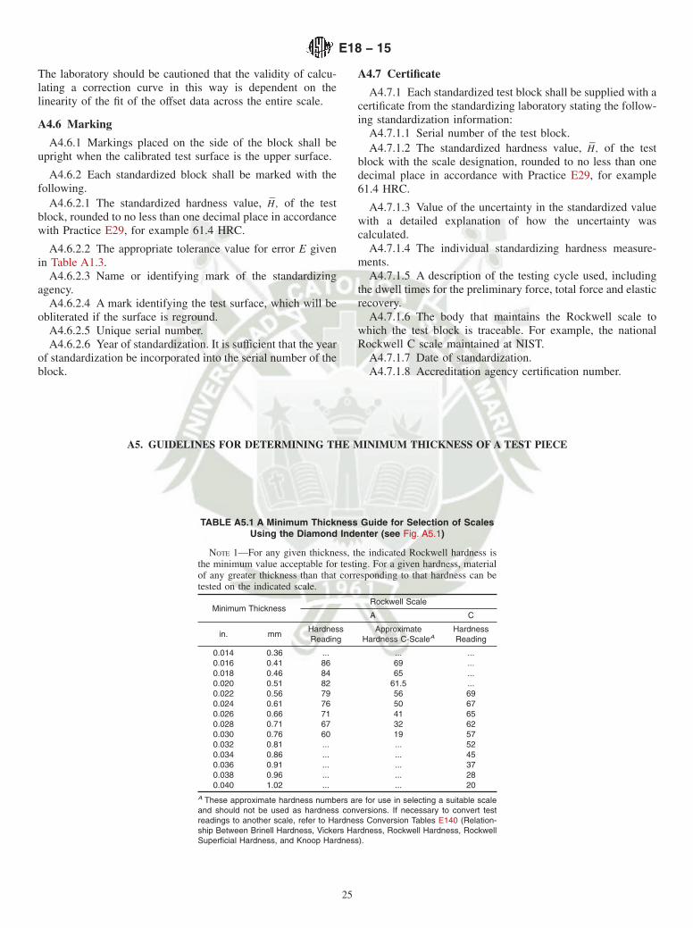
The laboratory should be cautioned that the validity of calcu-lating a correction curve in this way is dependent on thelinearity of the fit of the offset data across the entire scale.
A4.6 Marking
A4.6.1 Markings placed on the side of the block shall beupright when the calibrated test surface is the upper surface.
A4.6.2 Each standardized block shall be marked with thefollowing.
A4.6.2.1 The standardized hardness value, H , of the testblock, rounded to no less than one decimal place in accordancewith Practice E29, for example 61.4 HRC.
A4.6.2.2 The appropriate tolerance value for error E givenin Table A1.3.
A4.6.2.3 Name or identifying mark of the standardizingagency.
A4.6.2.4 A mark identifying the test surface, which will beobliterated if the surface is reground.
A4.6.2.5 Unique serial number.A4.6.2.6 Year of standardization. It is sufficient that the year
of standardization be incorporated into the serial number of theblock.
A4.7 Certificate
A4.7.1 Each standardized test block shall be supplied with acertificate from the standardizing laboratory stating the follow-ing standardization information:
A4.7.1.1 Serial number of the test block.A4.7.1.2 The standardized hardness value, H , of the test
block with the scale designation, rounded to no less than onedecimal place in accordance with Practice E29, for example61.4 HRC.
A4.7.1.3 Value of the uncertainty in the standardized valuewith a detailed explanation of how the uncertainty wascalculated.
A4.7.1.4 The individual standardizing hardness measure-ments.
A4.7.1.5 A description of the testing cycle used, includingthe dwell times for the preliminary force, total force and elasticrecovery.
A4.7.1.6 The body that maintains the Rockwell scale towhich the test block is traceable. For example, the nationalRockwell C scale maintained at NIST.
A4.7.1.7 Date of standardization.A4.7.1.8 Accreditation agency certification number.
A5. GUIDELINES FOR DETERMINING THE MINIMUM THICKNESS OF A TEST PIECE
TABLE A5.1 A Minimum Thickness Guide for Selection of ScalesUsing the Diamond Indenter (see Fig. A5.1)
NOTE 1—For any given thickness, the indicated Rockwell hardness isthe minimum value acceptable for testing. For a given hardness, materialof any greater thickness than that corresponding to that hardness can betested on the indicated scale.
Minimum ThicknessRockwell Scale
A C
in. mmHardnessReading
ApproximateHardness C-ScaleA
HardnessReading
0.014 0.36 ... ... ...0.016 0.41 86 69 ...0.018 0.46 84 65 ...0.020 0.51 82 61.5 ...0.022 0.56 79 56 690.024 0.61 76 50 670.026 0.66 71 41 650.028 0.71 67 32 620.030 0.76 60 19 570.032 0.81 ... ... 520.034 0.86 ... ... 450.036 0.91 ... ... 370.038 0.96 ... ... 280.040 1.02 ... ... 20
A These approximate hardness numbers are for use in selecting a suitable scaleand should not be used as hardness conversions. If necessary to convert testreadings to another scale, refer to Hardness Conversion Tables E140 (Relation-ship Between Brinell Hardness, Vickers Hardness, Rockwell Hardness, RockwellSuperficial Hardness, and Knoop Hardness).
E18 − 15
25

TABLE A5.2 A Minimum Thickness Guide for Selection of ScalesUsing the 1/16 in. (1.588 mm) Diameter Ball Indenter
(see Fig. A5.2)
NOTE 1—For any given thickness, the indicated Rockwell hardness isthe minimum value acceptable for testing. For a given hardness, materialof any greater thickness than that corresponding to that hardness can betested on the indicated scale.
Minimum ThicknessRockwell Scale
F B
in. mmHardnessReading
ApproximateHardness B-ScaleA
HardnessReading
0.022 0.56 ... ... ...0.024 0.61 98 72 940.026 0.66 91 60 870.028 0.71 85 49 800.030 0.76 77 35 710.032 0.81 69 21 620.034 0.86 ... ... 520.036 0.91 ... ... 400.038 0.96 ... ... 280.040 1.02 ... ... ...
A These approximate hardness numbers are for use in selecting a suitable scaleand should not be used as hardness conversions. If necessary to convert testreadings to another scale refer to Hardness Conversion Tables E140 (RelationshipBetween Brinell Hardness, Vickers Hardness, Rockwell Hardness, RockwellSuperficial Hardness and Knoop Hardness).
TABLE A5.3 A Minimum Thickness Guide for Selection of Scales Using the Diamond Indenter (see Fig. A5.1)
NOTE 1—For any given thickness, the indicated Rockwell hardness is the minimum value acceptable for testing. For a given hardness, material of anygreater thickness than that corresponding to that hardness can be tested on the indicated scale.
Minimum ThicknessRockwell Superficial Scale
15N 30N 45N
in. mmHardnessReading
ApproximateHardnessC-ScaleA
HardnessReading
ApproximateHardnessC-ScaleA
HardnessReading
ApproximateHardnessC-ScaleA
0.006 0.15 92 65 ... ... . .. ...0.008 0.20 90 60 ... ... ... ...0.010 0.25 88 55 ... ... ... ...0.012 0.30 83 45 82 65 77 69.50.014 0.36 76 32 78.5 61 74 670.016 0.41 68 18 74 56 72 650.018 0.46 ... ... 66 47 68 610.020 0.51 ... ... 57 37 63 570.022 0.56 ... ... 47 26 58 52.50.024 0.61 ... ... ... ... 51 470.026 0.66 ... ... ... ... 37 350.028 0.71 ... ... ... ... 20 20.50.030 0.76 ... ... ... ... ... ...
A These approximate hardness numbers are for use in selecting a suitable scale, and should not be used as hardness conversions. If necessary to convert test readingsto another scale, refer to Hardness Conversion Tables E140 (Relationship Between Brinell Hardness, Vickers Hardness, Rockwell Hardness, Rockwell SuperficialHardness and Knoop Hardness).
E18 − 15
26
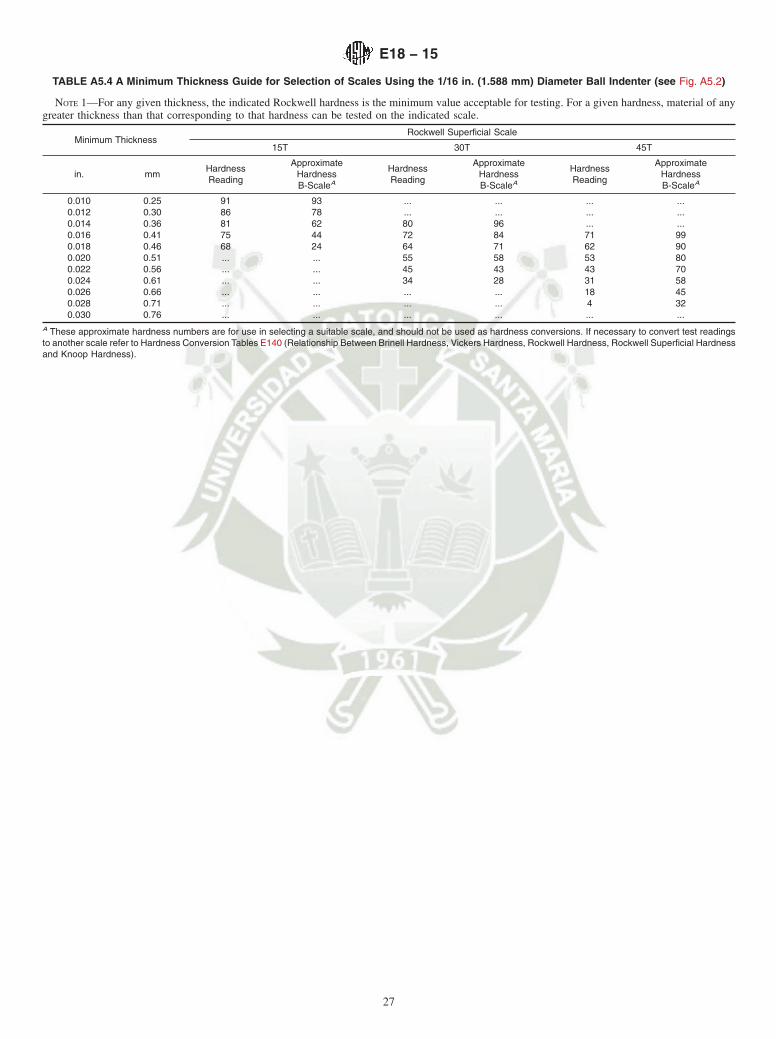
TABLE A5.4 A Minimum Thickness Guide for Selection of Scales Using the 1/16 in. (1.588 mm) Diameter Ball Indenter (see Fig. A5.2)
NOTE 1—For any given thickness, the indicated Rockwell hardness is the minimum value acceptable for testing. For a given hardness, material of anygreater thickness than that corresponding to that hardness can be tested on the indicated scale.
Minimum ThicknessRockwell Superficial Scale
15T 30T 45T
in. mmHardnessReading
ApproximateHardnessB-ScaleA
HardnessReading
ApproximateHardnessB-ScaleA
HardnessReading
ApproximateHardnessB-ScaleA
0.010 0.25 91 93 ... ... ... ...0.012 0.30 86 78 ... ... ... ...0.014 0.36 81 62 80 96 ... ...0.016 0.41 75 44 72 84 71 990.018 0.46 68 24 64 71 62 900.020 0.51 ... ... 55 58 53 800.022 0.56 ... ... 45 43 43 700.024 0.61 ... ... 34 28 31 580.026 0.66 ... ... ... ... 18 450.028 0.71 ... ... ... ... 4 320.030 0.76 ... ... ... ... ... ...
A These approximate hardness numbers are for use in selecting a suitable scale, and should not be used as hardness conversions. If necessary to convert test readingsto another scale refer to Hardness Conversion Tables E140 (Relationship Between Brinell Hardness, Vickers Hardness, Rockwell Hardness, Rockwell Superficial Hardnessand Knoop Hardness).
E18 − 15
27
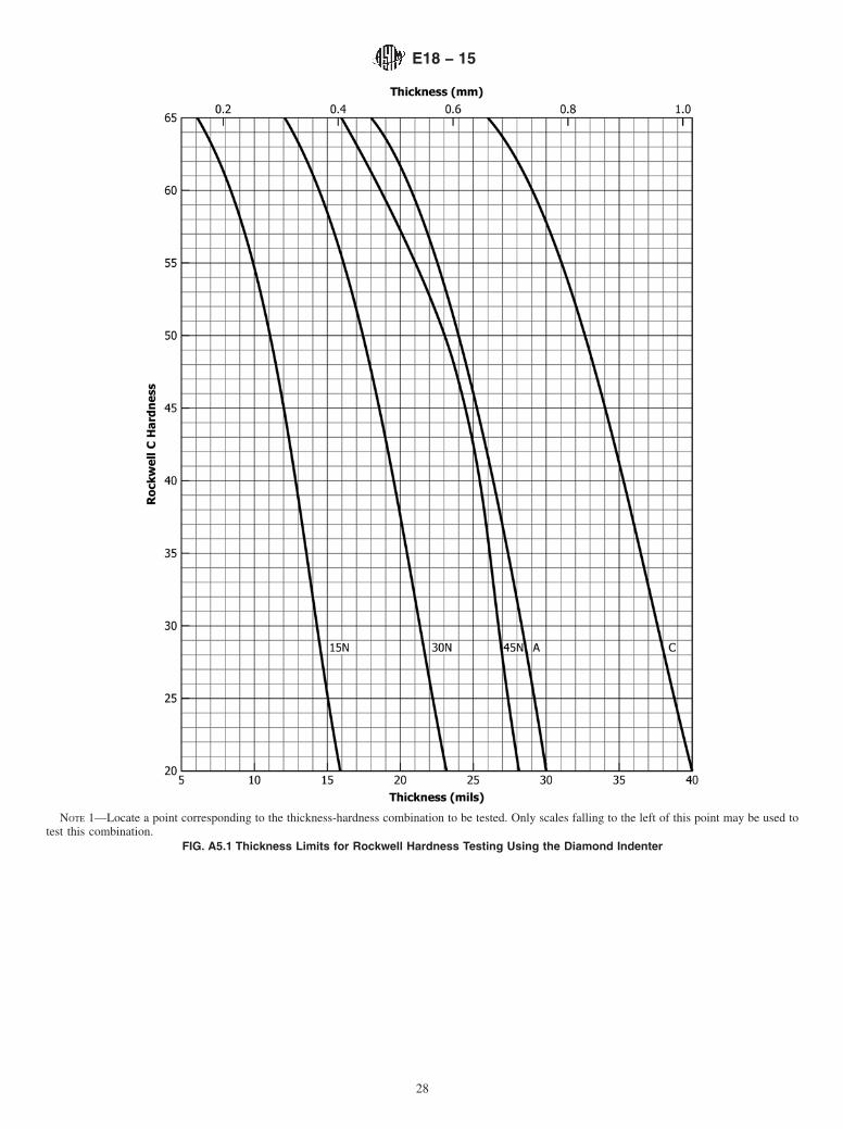
NOTE 1—Locate a point corresponding to the thickness-hardness combination to be tested. Only scales falling to the left of this point may be used totest this combination.
FIG. A5.1 Thickness Limits for Rockwell Hardness Testing Using the Diamond Indenter
E18 − 15
28
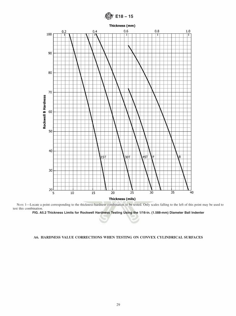
A6. HARDNESS VALUE CORRECTIONS WHEN TESTING ON CONVEX CYLINDRICAL SURFACES
NOTE 1—Locate a point corresponding to the thickness-hardness combination to be tested. Only scales falling to the left of this point may be used totest this combination.
FIG. A5.2 Thickness Limits for Rockwell Hardness Testing Using the 1/16-in. (1.588-mm) Diameter Ball Indenter
E18 − 15
29

TABLE A6.1 Corrections to be Added to Rockwell C, A, and D Values Obtained on Convex Cylindrical Surfaces of Various DiametersA
DialReading
Diameters of Convex Cylindrical Surfaces1⁄4 in.
(6.4 mm)
3⁄8 in.(10 mm)
1⁄2 in.(13 mm)
5⁄8 in.(16 mm)
3⁄4 in.(19 mm)
7⁄8 in.(22 mm)
1 in.(25 mm)
11⁄4 in.(32 mm)
11⁄2 in.(38 mm)
Corrections to be Added to Rockwell C, A, and D ValuesB
20 6.0 4.5 3.5 2.5 2.0 1.5 1.5 1.0 1.025 5.5 4.0 3.0 2.5 2.0 1.5 1.0 1.0 1.030 5.0 3.5 2.5 2.0 1.5 1.5 1.0 1.0 0.535 4.0 3.0 2.0 1.5 1.5 1.0 1.0 0.5 0.540 3.5 2.5 2.0 1.5 1.0 1.0 1.0 0.5 0.545 3.0 2.0 1.5 1.0 1.0 1.0 0.5 0.5 0.550 2.5 2.0 1.5 1.0 1.0 0.5 0.5 0.5 0.555 2.0 1.5 1.0 1.0 0.5 0.5 0.5 0.5 060 1.5 1.0 1.0 0.5 0.5 0.5 0.5 0 065 1.5 1.0 1.0 0.5 0.5 0.5 0.5 0 070 1.0 1.0 0.5 0.5 0.5 0.5 0.5 0 075 1.0 0.5 0.5 0.5 0.5 0.5 0 0 080 0.5 0.5 0.5 0.5 0.5 0 0 0 085 0.5 0.5 0.5 0 0 0 0 0 090 0.5 0 0 0 0 0 0 0 0
A When testing cylindrical specimens, the accuracy of the test will be seriously affected by alignment of elevating screw, V-anvil, indenters, surface finish, and thestraightness of the cylinder.B These corrections are approximate only and represent the averages to the nearest 0.5 Rockwell number, of numerous actual observations.
TABLE A6.2 Corrections to be Added to Rockwell B, F, and G Values Obtained on Convex Cylindrical Surfaces of Various DiametersA
HardnessReading
Diameters of Convex Cylindrical Surfaces1⁄4 in.
(6.4 mm)
3⁄8 in.(10 mm)
1⁄2 in.(13 mm)
5⁄8 in.(16 mm)
3⁄4 in.(19 mm)
7⁄8 in.(22 mm)
1 in.(25 mm)
Corrections to be Added to Rockwell B, F, and G ValuesB
0 12.5 8.5 6.5 5.5 4.5 3.5 3.010 12.0 8.0 6.0 5.0 4.0 3.5 3.020 11.0 7.5 5.5 4.5 4.0 3.5 3.030 10.0 6.5 5.0 4.5 3.5 3.0 2.540 9.0 6.0 4.5 4.0 3.0 2.5 2.550 8.0 5.5 4.0 3.5 3.0 2.5 2.060 7.0 5.0 3.5 3.0 2.5 2.0 2.070 6.0 4.0 3.0 2.5 2.0 2.0 1.580 5.0 3.5 2.5 2.0 1.5 1.5 1.590 4.0 3.0 2.0 1.5 1.5 1.5 1.0
100 3.5 2.5 1.5 1.5 1.0 1.0 0.5A When testing cylindrical specimens, the accuracy of the test will be seriously affected by alignment of elevating screw, V-anvil, indenters, surface finish, and thestraightness of the cylinder.B These corrections are approximate only and represent the averages to the nearest 0.5 Rockwell number, of numerous actual observations.
TABLE A6.3 Corrections to be Added to Rockwell Superficial 15N, 30N, and 45N Values Obtained on Convex Cylindrical Surfaces ofVarious DiametersA
HardnessReading
Diameters of Convex Cylindrical Surfaces1⁄8 in.
(3.2 mm)
1⁄4 in.(6.4 mm)
3⁄8 in.(10 mm)
1⁄2 in.(13 mm)
3⁄4 in.(19 mm)
1 in.(25 mm)
Corrections to be Added to Rockwell Superficial 15N, 30N, and 45N ValuesB
20 6.0 3.0 2.0 1.5 1.5 1.525 5.5 3.0 2.0 1.5 1.5 1.030 5.5 3.0 2.0 1.5 1.0 1.035 5.0 2.5 2.0 1.5 1.0 1.040 4.5 2.5 1.5 1.5 1.0 1.045 4.0 2.0 1.5 1.0 1.0 1.050 3.5 2.0 1.5 1.0 1.0 0.555 3.5 2.0 1.5 1.0 0.5 0.560 3.0 1.5 1.0 1.0 0.5 0.565 2.5 1.5 1.0 0.5 0.5 0.570 2.0 1.0 1.0 0.5 0.5 0.575 1.5 1.0 0.5 0.5 0.5 080 1.0 0.5 0.5 0.5 0 085 0.5 0.5 0.5 0.5 0 090 0 0 0 0 0 0
A When testing cylindrical specimens the accuracy of the test will be seriously affected by alignment of elevating screw, V-anvil, indenters, surface finish, and thestraightness of the cylinder.B These corrections are approximate only and represent the averages, to the nearest 0.5 Rockwell superficial number, of numerous actual observations.
E18 − 15
30
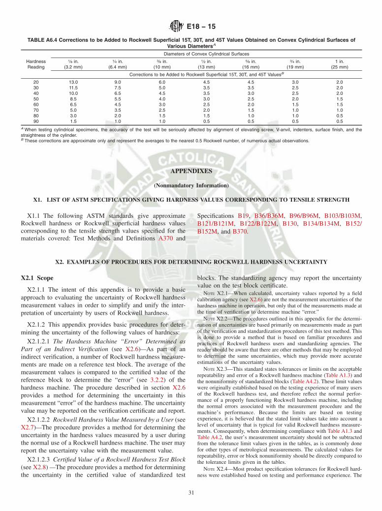
APPENDIXES
(Nonmandatory Information)
X1. LIST OF ASTM SPECIFICATIONS GIVING HARDNESS VALUES CORRESPONDING TO TENSILE STRENGTH
X1.1 The following ASTM standards give approximateRockwell hardness or Rockwell superficial hardness valuescorresponding to the tensile strength values specified for thematerials covered: Test Methods and Definitions A370 and
Specifications B19, B36/B36M, B96/B96M, B103/B103M,B121/B121M, B122/B122M, B130, B134/B134M, B152/B152M, and B370.
X2. EXAMPLES OF PROCEDURES FOR DETERMINING ROCKWELL HARDNESS UNCERTAINTY
X2.1 Scope
X2.1.1 The intent of this appendix is to provide a basicapproach to evaluating the uncertainty of Rockwell hardnessmeasurement values in order to simplify and unify the inter-pretation of uncertainty by users of Rockwell hardness.
X2.1.2 This appendix provides basic procedures for deter-mining the uncertainty of the following values of hardness:
X2.1.2.1 The Hardness Machine “Error” Determined asPart of an Indirect Verification (see X2.6)—As part of anindirect verification, a number of Rockwell hardness measure-ments are made on a reference test block. The average of themeasurement values is compared to the certified value of thereference block to determine the “error” (see 3.2.2) of thehardness machine. The procedure described in section X2.6provides a method for determining the uncertainty in thismeasurement “error” of the hardness machine. The uncertaintyvalue may be reported on the verification certificate and report.
X2.1.2.2 Rockwell Hardness Value Measured by a User (seeX2.7)—The procedure provides a method for determining theuncertainty in the hardness values measured by a user duringthe normal use of a Rockwell hardness machine. The user mayreport the uncertainty value with the measurement value.
X2.1.2.3 Certified Value of a Rockwell Hardness Test Block(see X2.8) —The procedure provides a method for determiningthe uncertainty in the certified value of standardized test
blocks. The standardizing agency may report the uncertaintyvalue on the test block certificate.
NOTE X2.1—When calculated, uncertainty values reported by a fieldcalibration agency (see X2.6) are not the measurement uncertainties of thehardness machine in operation, but only that of the measurements made atthe time of verification to determine machine “error.”
NOTE X2.2—The procedures outlined in this appendix for the determi-nation of uncertainties are based primarily on measurements made as partof the verification and standardization procedures of this test method. Thisis done to provide a method that is based on familiar procedures andpractices of Rockwell hardness users and standardizing agencies. Thereader should be aware that there are other methods that may be employedto determine the same uncertainties, which may provide more accurateestimations of the uncertainty values.
NOTE X2.3—This standard states tolerances or limits on the acceptablerepeatability and error of a Rockwell hardness machine (Table A1.3) andthe nonuniformity of standardized blocks (Table A4.2). These limit valueswere originally established based on the testing experience of many usersof the Rockwell hardness test, and therefore reflect the normal perfor-mance of a properly functioning Rockwell hardness machine, includingthe normal errors associated with the measurement procedure and themachine’s performance. Because the limits are based on testingexperience, it is believed that the stated limit values take into account alevel of uncertainty that is typical for valid Rockwell hardness measure-ments. Consequently, when determining compliance with Table A1.3 andTable A4.2, the user’s measurement uncertainty should not be subtractedfrom the tolerance limit values given in the tables, as is commonly donefor other types of metrological measurements. The calculated values forrepeatability, error or block nonuniformity should be directly compared tothe tolerance limits given in the tables.
NOTE X2.4—Most product specification tolerances for Rockwell hard-ness were established based on testing and performance experience. The
TABLE A6.4 Corrections to be Added to Rockwell Superficial 15T, 30T, and 45T Values Obtained on Convex Cylindrical Surfaces ofVarious DiametersA
HardnessReading
Diameters of Convex Cylindrical Surfaces1⁄8 in.
(3.2 mm)
1⁄4 in.(6.4 mm)
3⁄8 in.(10 mm)
1⁄2 in.(13 mm)
5⁄8 in.(16 mm)
3⁄4 in.(19 mm)
1 in.(25 mm)
Corrections to be Added to Rockwell Superficial 15T, 30T, and 45T ValuesB
20 13.0 9.0 6.0 4.5 4.5 3.0 2.030 11.5 7.5 5.0 3.5 3.5 2.5 2.040 10.0 6.5 4.5 3.5 3.0 2.5 2.050 8.5 5.5 4.0 3.0 2.5 2.0 1.560 6.5 4.5 3.0 2.5 2.0 1.5 1.570 5.0 3.5 2.5 2.0 1.5 1.0 1.080 3.0 2.0 1.5 1.5 1.0 1.0 0.590 1.5 1.0 1.0 0.5 0.5 0.5 0.5
A When testing cylindrical specimens, the accuracy of the test will be seriously affected by alignment of elevating screw, V-anvil, indenters, surface finish, and thestraightness of the cylinder.B These corrections are approximate only and represent the averages to the nearest 0.5 Rockwell number, of numerous actual observations.
E18 − 15
31

tolerance values reflect the normal performance of a properly functioningRockwell hardness machine, including the normal acceptable errorsassociated with the hardness measurement process. For these products, thestated tolerance limits take into account a level of uncertainty that istypical for valid Rockwell hardness measurements. Consequently, whenacceptance testing most products for Rockwell hardness, the user’smeasurement uncertainty should not be subtracted from the tolerance limitvalues given in the specification. The measured hardness values should bedirectly compared to the tolerances. There may be exceptional circum-stances where the hardness of a product must fall within determinedranges to a high level of confidence. In these rare occasions, specialagreement between the parties involved should be obtained before thehardness measurement uncertainty is subtracted from the tolerance limits.Before such an agreement is made, it is recommended that the productdesign take into consideration the anticipated influence of material andmetallurgical factors on the product variation as well as typical industryhardness uncertainty values.
X2.1.3 This appendix does not address uncertainties at theprimary reference standardizing level.
X2.2 Equations
X2.2.1 The average (AVG), H, of a set of n hardnessmeasurements H1, H2, …, Hn is calculated as:
AVG~H1, H2, … , H! 5 HH 5H11H21…1Hn
n(X2.1)
X2.2.2 The standard deviation (STDEV ) of a set of nhardness measurements H1, H2, …, Hn is calculated as:
STDEV~H1, H2, … , Hn! 5Œ~H1 2 HH! 21…1~Hn 2 HH! 2
n 2 1
(X2.2)
where H is the average of the set of n hardness measure-ments H1, H2, …, Hn as defined in Eq X2.1.
X2.2.3 The absolute value (ABS) of a number is the mag-nitude of the value irrespective of the sign, for example:
ABS~0.12! 5 0.12and
ABS~20.12! 5 0.12
X2.3 General Requirements
X2.3.1 The approach for determining uncertainty presentedin this appendix considers only those uncertainties associatedwith the overall measurement performance of the Rockwellhardness machine with respect to reference standards. Theseperformance uncertainties reflect the combined effect of theseparate uncertainties associated with the numerous individualcomponents of the machine, such as the force applicationsystem and indentation depth measuring system. Therefore, theuncertainties associated with the individual components of themachine are not included in the calculations. Because of thisapproach, it is important that the individual machine compo-nents are operating within tolerances. It is strongly recom-mended that this procedure be applied only after successfullypassing a direct verification.
X2.3.2 The procedures given in this appendix are appropri-ate only when the Rockwell hardness machine has passed anindirect verification in accordance with the procedures andschedules of this test method standard.
X2.3.3 The procedures for calculating the uncertainty ofRockwell hardness measurement values are similar for both astandardizing machine and testing machine. The principaldifference is in the hierarchy level of the reference test blocksnormally used for the indirect verification. Generally, standard-izing machines are verified using primary reference standards,and testing machines are standardized using secondary refer-ence standards.
X2.3.4 To estimate the overall uncertainty of Rockwellhardness measurement values, contributing components ofuncertainty must be determined. Because many of the uncer-tainties may vary depending on the specific hardness scale andhardness level, an individual measurement uncertainty shouldbe determined for each hardness scale and hardness level ofinterest. In many cases, a single uncertainty value may beapplied to a range of hardness levels based on the laboratory’sexperience and knowledge of the operation of the hardnessmachine.
X2.3.5 Uncertainty should be determined with respect to acountry’s highest level of reference standard or the nationalreference standard of another country. In some cases, thehighest level of reference standard may be a commercialreference standard.
X2.4 General Procedure
X2.4.1 This procedure calculates a combined standard un-certainty uc by combining the contributing components ofuncertainty u1, u2, …, un, such that:
uc 5 =u121u2
21…1un2 (X2.3)
X2.4.2 Measurement uncertainty is usually expressed as anexpanded uncertainty U which is calculated by multiplying thecombined standard uncertainty uc by a numerical coveragefactor k, such that:
U 5 k 3 uc (X2.4)
X2.4.3 A coverage factor is chosen that depends on howwell the standard uncertainty was estimated (number ofmeasurements), and the level of uncertainty that is desired. Forthis analysis, a coverage factor of k = 2 should be used. Thiscoverage factor provides a confidence level of approximately95 %.
X2.4.4 The measurement bias B of the hardness machine isthe difference between the expected hardness measurementvalues as displayed by the hardness machine and the “true”hardness of a material. Ideally, measurement biases should becorrected. When test systems are not corrected for measure-ment bias, as often occurs in Rockwell hardness testing, thebias then contributes to the overall uncertainty in a measure-ment. There are a number of possible methods for incorporat-ing biases into an uncertainty calculation, each of which hasboth advantages and disadvantages. A simple and conservativemethod is to combine the bias with the calculation of theexpanded uncertainty as:
U 5 kuc1ABS~B! (X2.5)
where ABS(B) is the absolute value of the bias.
E18 − 15
32

X2.4.5 Because several approaches may be used to evaluateand express measurement uncertainty, a brief description ofwhat the reported uncertainty values represent should beincluded with the reported uncertainty value.
X2.5 Sources of Uncertainty
X2.5.1 This section describes the most significant sourcesof uncertainty in a Rockwell hardness measurement andprovides procedures and formulas for calculating the totaluncertainty in the hardness value. In later sections, it will beshown how these sources of uncertainty contribute to the totalmeasurement uncertainty for the three measurement circum-stances described in X2.1.2.
X2.5.2 The sources of uncertainty to be discussed are (1) thehardness machine’s lack of repeatability, (2) the non-uniformity in hardness of the material under test, (3) thehardness machine’s lack of reproducibility, (4) the resolutionof the hardness machine’s measurement display, and (5) theuncertainty in the certified value of the reference test blockstandards. An estimation of the measurement bias and itsinclusion into the expanded uncertainty will also be discussed.
X2.5.3 Uncertainty Due to Lack of Repeatability (uRepeat)and when Combined with Non-uniformity (uRep& NU)—Therepeatability of a hardness machine is an indication of howwell it can continually produce the same hardness value eachtime a measurement is made. Imagine there is a material, whichis perfectly uniform in hardness over its entire surface. Alsoimagine that hardness measurements are made repeatedly onthis uniform material over a short period of time withoutvarying the testing conditions (including the operator). Eventhough the actual hardness of every test location is exactly thesame, it would be found that due to random errors eachmeasurement value would differ from all other measurementvalues (assuming sufficient measurement resolution).Therefore, lack of repeatability prevents the hardness machinefrom being able to always measure the true hardness of thematerial, and hence contributes to the uncertainty in themeasurement.
X2.5.3.1 The contribution that a hardness machine’s lack ofrepeatability makes to the overall measurement uncertainty isdetermined differently depending on whether a single measure-ment value or an average of multiple measurements is to bereported. Additionally, in cases where the reported averagemeasurement value is intended to be an estimate of the averagehardness of the material tested, the uncertainty contributionsdue to the machine’s lack of repeatability and the non-uniformity in the hardness of the test material are difficult toseparate and must be determined together. The uncertaintycontributions for each of these circumstances may be estimatedas follows.
X2.5.3.2 Single Hardness Measurement—For a futuresingle hardness measurement, the standard uncertainty contri-bution uRepeat, due to the lack of repeatability, may be esti-mated by the standard deviation of the values from a number ofhardness measurements made on a uniform test sample as:
uRepeat 5 STDEV~H1, H2, … , Hn! (X2.6)
where H1, H2, ..., Hn are the n hardness values. In general,the estimate of repeatability is improved as the number ofhardness measurements is increased. Usually, the hardnessvalues measured during an indirect verification will provide anadequate estimate of uRepeat; however, the caution given inNote X2.6 should be considered. It may be more appropriatefor the user to determine a value of uRepeat by making hardnessmeasurements close together (within spacing limitations) on auniform material, such as a test block.
NOTE X2.5—The uncertainty uRepeat, due to the lack of repeatability ofa hardness machine as discussed above, should not be confused with thehistorically defined “repeatability” that is a requirement to be met as partof an indirect verification (see 3.2.3). The calculations of the uncertaintyuRepeat and of the historically defined repeatability do not produce thesame value. The uncertainty uRepeat is the contribution to the overalluncertainty of a hardness measurement value due to a machine’s lack ofrepeatability, while the historically defined repeatability is the range ofhardness values measured during an indirect verification.
NOTE X2.6—All materials exhibit some degree of hardness non-uniformity across the test surface. Therefore, the above evaluation of theuncertainty contribution due to the lack of repeatability will also includea contribution due to the hardness non-uniformity of the measuredmaterial. When evaluating repeatability as discussed above, any uncer-tainty contribution due to the hardness non-uniformity should be mini-mized as much as possible. The laboratory should be cautioned that if themeasurements of repeatability are based on tests made across the surfaceof the material, then the repeatability value will likely include a significantuncertainty contribution due to the material’s non-uniformity. A machine’srepeatability is better evaluated by making hardness measurements closetogether (within spacing limitations).
X2.5.3.3 Average of Multiple Measurements—When theaverage of multiple hardness test values is to be reported, thestandard uncertainty contribution uRepeatH , due to the lack ofrepeatability of the hardness machine, may be estimated bydividing the standard uncertainty contribution uRepeat (previ-ously calculated from a number of hardness measurementsmade on a uniform test sample, see X2.5.3.1) by the square-root of the number of hardness test values being averaged, as:
uRepeatH 5uRepeat
=nT
(X2.7)
where uRepeat is calculated by Eq X2.6 and nT is the numberof individual hardness test values being averaged.
X2.5.3.4 Estimate of the Material Hardness—Hardnessmeasurements are often made at several locations and thevalues averaged in order to estimate the average hardness ofthe material as a whole. For example, this may be done whenmaking quality control measurements during the manufactureof many types of products; when determining the machine“error” as part of an indirect verification; and when calibratinga test block. Because all materials exhibit some degree ofhardness non-uniformity across the test surface, the extent of amaterial’s non-uniformity also contributes to the uncertainty inthis estimate of the average hardness of the material. When theaverage of multiple hardness measurement values is calculatedas an estimate of the average material or product hardness, itmay be desired to state the uncertainty in this value withrespect to the true hardness of the material. In this case, thecombined uncertainty contributions due to the lack of repeat-ability in the hardness machine and the non-uniformity in thetest material may be estimated from the “standard deviation of
E18 − 15
33

the mean” of the hardness measurement values. This iscalculated as the standard deviation of the hardness values,divided by the square-root of the number of measurements as:
uRep& NU 5STDEV~HT1, HT2, … , HTn!
=nT
(X2.8)
where HT1, HT2, ..., HTn are the nT measurement values.
X2.5.4 Uncertainty Due to Lack of Reproducibility(uReprod)—The day-to-day variation in the performance of thehardness machine is known as its level of reproducibility.Variations such as different machine operators and changes inthe test environment often influence the performance of thehardness machine. The level of reproducibility is best deter-mined by monitoring the performance of the hardness machineover an extended period of time during which the hardnessmachine is subjected to the extremes of variations in the testingvariables. It is very important that the test machine be incontrol during the assessment of reproducibility. If the machineis in need of maintenance or is operated incorrectly, the lack ofreproducibility will be over estimated.
X2.5.5 An assessment of a hardness machine’s lack ofreproducibility should be based on periodic monitoring mea-surements of the hardness machine, such as daily verificationmeasurements made on the same test block over time. Theuncertainty contribution may be estimated by the standarddeviation of the average of each set of monitoring values, as:
uReprod 5 STDEV~M1, M2, … , Mn! (X2.9)
where M1, M2, ..., Mn are individual averages of each of then sets of multiple monitoring measurement values.
NOTE X2.7—The uncertainty contribution due to the lack ofreproducibility, as calculated in Eq X2.10, also includes a contribution dueto the machine’s lack of repeatability and the non-uniformity of themonitoring test block; however, these contributions are based on theaverage of multiple measurements and should not significantly over-estimate the reproducibility uncertainty.
X2.5.6 Uncertainty Due to the Resolution of the HardnessMeasurement Display (uResol)—The finite resolution of thehardness value display prevents the hardness machine fromproviding an absolutely accurate hardness value. However, theinfluence of the display resolution on the measurement uncer-tainty is usually only significant when the hardness displayresolution is no better than 0.5 Rockwell hardness units, suchas for some dial displays. The uncertainty contribution uResol,due to the influence of the display resolution, may be describedby a rectangular distribution and estimated as:
uResol 5r/2
=35
r
=12(X2.10)
where r is the resolution limit that a hardness value can beestimated from the measurement display in Rockwell hardnessunits.
X2.5.7 Standard Uncertainty in the Certified Average Hard-ness Value of the Reference Test Block (uRefBlk)—Reference testblocks provide the link to the Rockwell standard to whichtraceability is claimed. The certificate accompanying referencetest blocks should provide an uncertainty in the stated certifiedvalue, and should state to which Rockwell standard the
reference test block value is traceable. This uncertainty con-tributes to the measurement uncertainty of hardness machinescalibrated or verified with the reference test blocks. Note thatthe uncertainty reported on reference test block certificates istypically stated as an expanded uncertainty. As indicated by EqX2.4, the expanded uncertainty is calculated by multiplying thestandard uncertainty by a coverage factor (often 2). Thisanalysis uses the standard uncertainty and not the expandeduncertainty value. Thus, the uncertainty value due to theuncertainty in the certified value of the reference test blockusually may be calculated as:
uRefBlk 5URefBlk
kRefBlk
(X2.11)
where URefBlk is the reported expanded uncertainty of thecertified value of the reference test block, and kRefBlk is thecoverage factor used to calculate the uncertainty in the certifiedvalue of the reference standard (usually 2).
X2.5.8 Measurement Bias (B)—The measurement bias isthe difference between the hardness measurement values asdisplayed by the hardness machine and the “true” hardness ofa material. The measurement bias B may be estimated by the“error” determined as part of the indirect verification as:
B 5 HH 2 HHRefBlk (X2.12)
where H is the mean hardness value as measured by thehardness machine during the indirect verification, and HRefBlk isthe certified average hardness value of the reference test blockstandard used for the indirect verification.
X2.6 Procedure for Calculating Uncertainty: IndirectVerification
X2.6.1 As part of an indirect verification, the “error” of thehardness machine is determined from the average value ofmeasurements made on a reference test block (see 3.2.2). Thisvalue provides an indication of how well the hardness machinecan measure the “true” hardness of a material. Since there isalways uncertainty in a hardness measurement, it follows thatthere must be uncertainty in the determination of the averagevalue of the measurements, and thus the determination of themachine “error.” This section provides a procedure that can beused, for example by a field calibration agency, to estimate theuncertainty UMach in the measurement “error” of the hardnessmachine determined as the difference between the average ofthe measurement values and the certified value of the referenceblock used for the verification.
X2.6.2 The contributions to the standard uncertainty of themeasurement “error,” uMach, are (1) uRep& NU (Ref. Block), theuncertainty due to the lack of repeatability of the hardnessmachine combined with the uncertainty due to the non-uniformity in the reference test block (Eq X2.9), which isdetermined from the hardness measurements made on a refer-ence test block to determine the “error” of the hardnessmachine, (2) uResol, the uncertainty due to the resolution of thehardness machine measurement display (Eq X2.11), and (3)uRefBlk, the standard uncertainty in the certified value of thereference test block (Eq X2.12). The notation (Ref. Block) isadded to the term uRep& NU to clarify that the uncertainty is
E18 − 15
34
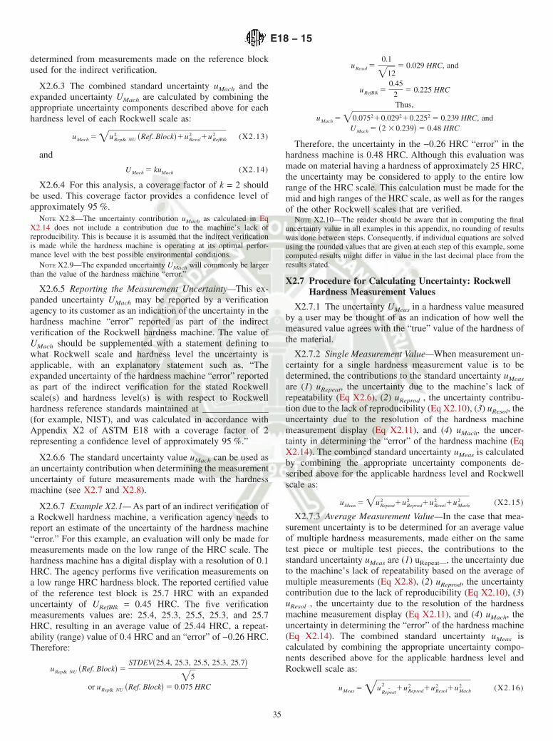
determined from measurements made on the reference blockused for the indirect verification.
X2.6.3 The combined standard uncertainty uMach and theexpanded uncertainty UMach are calculated by combining theappropriate uncertainty components described above for eachhardness level of each Rockwell scale as:
uMach 5 =uRep& NU2 ~Ref. Block!1uResol
2 1uRefBlk2 (X2.13)
and
UMach 5 kuMach (X2.14)
X2.6.4 For this analysis, a coverage factor of k = 2 shouldbe used. This coverage factor provides a confidence level ofapproximately 95 %.
NOTE X2.8—The uncertainty contribution uMach as calculated in EqX2.14 does not include a contribution due to the machine’s lack ofreproducibility. This is because it is assumed that the indirect verificationis made while the hardness machine is operating at its optimal perfor-mance level with the best possible environmental conditions.
NOTE X2.9—The expanded uncertainty UMach will commonly be largerthan the value of the hardness machine “error.”
X2.6.5 Reporting the Measurement Uncertainty—This ex-panded uncertainty UMach may be reported by a verificationagency to its customer as an indication of the uncertainty in thehardness machine “error” reported as part of the indirectverification of the Rockwell hardness machine. The value ofUMach should be supplemented with a statement defining towhat Rockwell scale and hardness level the uncertainty isapplicable, with an explanatory statement such as, “Theexpanded uncertainty of the hardness machine “error” reportedas part of the indirect verification for the stated Rockwellscale(s) and hardness level(s) is with respect to Rockwellhardness reference standards maintained at ______________(for example, NIST), and was calculated in accordance withAppendix X2 of ASTM E18 with a coverage factor of 2representing a confidence level of approximately 95 %.”
X2.6.6 The standard uncertainty value uMach can be used asan uncertainty contribution when determining the measurementuncertainty of future measurements made with the hardnessmachine (see X2.7 and X2.8).
X2.6.7 Example X2.1— As part of an indirect verification ofa Rockwell hardness machine, a verification agency needs toreport an estimate of the uncertainty of the hardness machine“error.” For this example, an evaluation will only be made formeasurements made on the low range of the HRC scale. Thehardness machine has a digital display with a resolution of 0.1HRC. The agency performs five verification measurements ona low range HRC hardness block. The reported certified valueof the reference test block is 25.7 HRC with an expandeduncertainty of URefBlk = 0.45 HRC. The five verificationmeasurements values are: 25.4, 25.3, 25.5, 25.3, and 25.7HRC, resulting in an average value of 25.44 HRC, a repeat-ability (range) value of 0.4 HRC and an “error” of −0.26 HRC.Therefore:
uRep& NU ~Ref. Block! 5STDEV~25.4, 25.3, 25.5, 25.3, 25.7!
=5or uRep& NU ~Ref. Block! 5 0.075 HRC
uResol 50.1
=125 0.029 HRC, and
uRefBlk 50.45
25 0.225 HRC
Thus,
uMach 5 =0.075210.029210.2252 5 0.239 HRC, andUMach 5 ~2 3 0.239! 5 0.48 HRC
Therefore, the uncertainty in the −0.26 HRC “error” in thehardness machine is 0.48 HRC. Although this evaluation wasmade on material having a hardness of approximately 25 HRC,the uncertainty may be considered to apply to the entire lowrange of the HRC scale. This calculation must be made for themid and high ranges of the HRC scale, as well as for the rangesof the other Rockwell scales that are verified.
NOTE X2.10—The reader should be aware that in computing the finaluncertainty value in all examples in this appendix, no rounding of resultswas done between steps. Consequently, if individual equations are solvedusing the rounded values that are given at each step of this example, somecomputed results might differ in value in the last decimal place from theresults stated.
X2.7 Procedure for Calculating Uncertainty: RockwellHardness Measurement Values
X2.7.1 The uncertainty UMeas in a hardness value measuredby a user may be thought of as an indication of how well themeasured value agrees with the “true” value of the hardness ofthe material.
X2.7.2 Single Measurement Value—When measurement un-certainty for a single hardness measurement value is to bedetermined, the contributions to the standard uncertainty uMeas
are (1) uRepeat, the uncertainty due to the machine’s lack ofrepeatability (Eq X2.6), (2) uReprod , the uncertainty contribu-tion due to the lack of reproducibility (Eq X2.10), (3) uResol, theuncertainty due to the resolution of the hardness machinemeasurement display (Eq X2.11), and (4) uMach, the uncer-tainty in determining the “error” of the hardness machine (EqX2.14). The combined standard uncertainty uMeas is calculatedby combining the appropriate uncertainty components de-scribed above for the applicable hardness level and Rockwellscale as:
uMeas 5 =uRepeat2 1uReprod
2 1uResol2 1uMach
2 (X2.15)
X2.7.3 Average Measurement Value—In the case that mea-surement uncertainty is to be determined for an average valueof multiple hardness measurements, made either on the sametest piece or multiple test pieces, the contributions to thestandard uncertainty uMeas are (1) uRepeat—, the uncertainty dueto the machine’s lack of repeatability based on the average ofmultiple measurements (Eq X2.8), (2) uReprod, the uncertaintycontribution due to the lack of reproducibility (Eq X2.10), (3)uResol , the uncertainty due to the resolution of the hardnessmachine measurement display (Eq X2.11), and (4) uMach, theuncertainty in determining the “error” of the hardness machine(Eq X2.14). The combined standard uncertainty uMeas iscalculated by combining the appropriate uncertainty compo-nents described above for the applicable hardness level andRockwell scale as:
uMeas 5 =uRepeat¯2
1uReprod2 1uResol
2 1uMach2 (X2.16)
E18 − 15
35

X2.7.4 The measurement uncertainty discussed above forthe single and average hardness values only represents theuncertainties of the measurement process and are independentof any test material non-uniformity.
X2.7.5 Average Measurement Value as an Estimate of theAverage Material Hardness—Measurement laboratories andmanufacturing facilities often measure the Rockwell hardnessof a test sample or product for the purpose of estimating theaverage hardness of the test material. Usually, multiple hard-ness measurements are made across the surface of the testpiece, and then the average of the hardness values is reportedas an estimation of the average hardness of the material. If it isdesired to report the uncertainty as an indication of how wellthe average measurement value represents the true averagehardness of the material, then the contributions to the standarduncertainty uMeas are (1) uRep& NU (Material), the uncertaintydue to the machine’s lack of repeatability combined with theuncertainty due to the material’s non-uniformity (Eq X2.9),which is determined from the hardness measurements made onthe test material, (2) uReprod, the uncertainty contribution due tothe lack of reproducibility (Eq X2.10), (3) uResol, the uncer-tainty due to the resolution of the hardness machine measure-ment display (Eq X2.11), and (4) uMach, the uncertainty indetermining the “error” of the hardness machine (Eq X2.14).The notation (Material ) is added to the term uRep& NU to clarifythat the uncertainty is determined from measurements made onthe material under test. The combined standard uncertaintyuMeas is calculated by combining the appropriate uncertaintycomponents described above for the applicable hardness leveland Rockwell scale as:
uMeas 5 =uRep& NU2 ~Material!1uReprod
2 1uResol2 1uMach
2 (X2.17)
X2.7.6 When reporting uncertainty as an indication of howwell the average measurement value represents the true aver-age hardness of the material, it is important to assure that asufficient number of measurements are made at the appropriatetest locations to provide an appropriate sampling of anyvariations in the hardness of the material.
X2.7.7 The expanded uncertainty UMeas is calculated for thethree cases discussed above as:
UMeas 5 kuMeas1ABS~B! (X2.18)
For this analysis, a coverage factor of k = 2 should be used.This coverage factor provides a confidence level of approxi-mately 95 %.
X2.7.8 Reporting Measurement Uncertainty:X2.7.8.1 Single and Average Measurement Values—When
the reported measurement value is for a single hardness test orthe average of multiple hardness tests, then the value of UMeas
should be supplemented with an explanatory statement such as,“The expanded measurement uncertainty of the reported hard-ness value (or average hardness value) is with respect toRockwell hardness reference standards maintained at ______________ [for example, NIST], and was calculated in accor-dance with Appendix X2 of ASTM E18 with a coverage factorof 2 representing a confidence level of approximately 95 %.”
X2.7.8.2 Average Measurement Value as an Estimate of theAverage Material Hardness—When it is desired to report the
uncertainty as an indication of how well the average measure-ment value represents the true average hardness of the material,then the value of UMeas should be supplemented with anexplanatory statement such as, “The expanded uncertainty ofthe reported average hardness of the material under test isbased on uncertainty contributions from the measurementprocess and from the hardness non-uniformity of the material.The uncertainty is with respect to Rockwell hardness referencestandards maintained at ______________ [for example,NIST], and was calculated in accordance with Appendix X2 ofASTM E18 with a coverage factor of 2 representing aconfidence level of approximately 95 %.” If the test report doesnot state the number of measurements that were averaged andthe locations that the measurements were made, then thisinformation should also be included as part of the briefexplanation of how the uncertainty was calculated.
X2.7.8.3 Example X2.2— For this example, a company testsits product by making six Rockwell hardness measurementsacross its surface as an estimate of the product hardness. Thehardness machine has a dial display that is judged to have areading resolution of 0.5 HRC. The values of the hardnessmeasurements of the product were 33, 31.5, 31.5, 32, 31, 32.5,resulting in an average value of 31.92 HRC. The testing facilitywould like to determine the measurement uncertainty in theaverage hardness value. A hardness of 31.92 HRC is closest tothe low range of the HRC scale (see Table A1.3). The lastindirect verification of the low range of the HRC scale reportedUMach = 0.8 HRC and an “error” of −0.3 HRC. Therefore:
uRep& NU ~Material! 5STDEV~33, 31.5, 31.5, 32, 31, 32.5!
=6or
uRep& NU ~Material! 5 0.300 HRC
For this example, assume the hardness machine has beenmonitored for an extended period of time, and from Eq X2.10,it was determined that uReprod = 0.21 HRC for the low range ofthe HRC scale. Other uncertainty contributions are calculatedas:
uResol 50.5
=125 0.144 HRC and
uMach 50.82
5 0.4 HRC, therefore
uMeas 5 =0.300210.21210.144210.42 5 0.561 HRC
and since B = −0.3 HRC, UMeas = (2 × 0.561) + ABS(−0.3),or UMeas = 1.42 HRC for the average value of the hardnessmeasurements made on the single product item.
X2.8 Procedure for Calculating Uncertainty: CertifiedValue of Standardized Test Blocks
X2.8.1 Standardizing laboratories engaged in the calibrationof reference test blocks must determine the uncertainty in thereported certified value. This uncertainty UCert provides anindication of how well the certified value would agree with the“true” average hardness of the test block.
X2.8.2 Test blocks are certified as having an averagehardness value based on calibration measurements made acrossthe surface of the test block. This analysis is essentiallyidentical to the analysis given in 5.3.1 for measuring the
E18 − 15
36

average hardness of a product. In this case, the product is acalibrated reference test block. The contributions to the stan-dard uncertainty uCert of the certified average value of the testblock are (1) uRep& NU (Calib. Block), the uncertainty due to thestandardizing machine’s lack of repeatability combined withthe uncertainty due to the calibrated block’s non-uniformity(Eq X2.9), which is determined from the calibration measure-ments made on the test block, (2) uReprod, the uncertaintycontribution due to the lack of reproducibility (Eq X2.10), (3)uResol, the uncertainty due to the resolution of the standardizingmachine’s measurement display (Eq X2.11), and (4) uMach, theuncertainty in determining the “error” of the standardizingmachine (Eq X2.14). The notation (Calib.Block) is added to theterm uRep& NU to clarify that the uncertainty is determined fromcalibration measurements made on the calibrated block.
X2.8.3 The combined standard uncertainty uCert and theexpanded uncertainty uCert are calculated by combining theappropriate uncertainty components described above for eachhardness level of each Rockwell scale as:
uCert 5 =uRep& NU2 ~Calib. Block!1uReprod
2 1uResol2 1uMach
2
(X2.19)
and
UCert 5 kuCert1ABS~B! (X2.20)
X2.8.4 For this analysis, a coverage factor of k = 2 shouldbe used. This coverage factor provides a confidence level ofapproximately 95 %.
X2.8.5 Reporting the Measurement Uncertainty—The valueof UCert is an estimate of the uncertainty in the reportedcertified average hardness value of a reference test block. Thereported value should be supplemented with a statementdefining to what Rockwell scale and hardness level theuncertainty is applicable, with an explanatory statement suchas, “The expanded uncertainty in the certified value of the testblock is with respect to Rockwell hardness reference standards
maintained at ______________ [for example, NIST], and wascalculated in accordance with Appendix X2 of ASTM E18 witha coverage factor of 2 representing a confidence level ofapproximately 95 %.”
X2.8.6 Example X2.3— A secondary level test-block stan-dardizing laboratory has completed the calibration of a testblock in the hardness range of 40 HRC. The values of thecalibration measurements of the block were 40.61, 40.72,40.65, 40.61, and 40.55 HRC, resulting in an average value of40.63 HRC and an E18 repeatability range of 0.17 HRC. Thelaboratory must determine the uncertainty in the certifiedaverage hardness value of the block. A hardness of 40 HRC isconsidered within the mid-range of the HRC scale (see TableA1.3). The last indirect verification of the mid range of theHRC scale reported UMach = 0.16 HRC and an “error” of +0.11HRC. The standardizing machine has a digital display with aresolution of 0.01 HRC. Therefore:
uRep& NU ~Calib. Block! 5STDEV~40.61, 40.72, 40.65, 40.61, 40.55!
=5or
uRep& NU ~Calib. Block! 5 0.028 HRC
For this example, let’s assume that the standardizing ma-chine has been monitored for an extended period of time, andfrom Eq X2.10, it was determined that uReprod = 0.125 HRC forthe mid range of the HRC scale. Other uncertainty contribu-tions are calculated as:
uResol 50.01
=125 0.003 HRC and
uMach 50.16
25 0.08 HRC therefore,
uCert 5 =0.028210.125210.003210.082 5 0.151 HRC
and, since B = +0.11 HRC, UCert = (2 × 0.151) + ABS(+0.11),or UCert = 0.41 HRC for the certified hardness value of thesingle calibrated test block.
SUMMARY OF CHANGES
Committee E28 has identified the location of selected changes to this standard since the last issue (E18–14a)that may impact the use of this standard. (Approved February 1, 2015.)
(1) A1.5.3.4 was revised.
Committee E28 has identified the location of selected changes to this standard since the last issue (E18–14)that may impact the use of this standard. (Approved Oct. 1, 2014.)
(1) A3.9.1.6 was revised. (2) A3.9.3.6 was revised.
Committee E28 has identified the location of selected changes to this standard since the last issue (E18–12)that may impact the use of this standard. (Approved Jan. 1, 2014.)
(1) A3.4.5.1 was revised.(2) A3.4.5.4 was revised.
(3) A3.5.3.2 was revised.(4) A3.5.3.7 was revised.
E18 − 15
37

(5) A3.8.2 was added.(6) A3.8.3 was added.(7) A3.9.1.6 was added.
(8) A3.9.3.6 was added.(9) New Table A3.4 was added.(10) New Table A3.7 was added.
ASTM International takes no position respecting the validity of any patent rights asserted in connection with any item mentionedin this standard. Users of this standard are expressly advised that determination of the validity of any such patent rights, and the riskof infringement of such rights, are entirely their own responsibility.
This standard is subject to revision at any time by the responsible technical committee and must be reviewed every five years andif not revised, either reapproved or withdrawn. Your comments are invited either for revision of this standard or for additional standardsand should be addressed to ASTM International Headquarters. Your comments will receive careful consideration at a meeting of theresponsible technical committee, which you may attend. If you feel that your comments have not received a fair hearing you shouldmake your views known to the ASTM Committee on Standards, at the address shown below.
This standard is copyrighted by ASTM International, 100 Barr Harbor Drive, PO Box C700, West Conshohocken, PA 19428-2959,United States. Individual reprints (single or multiple copies) of this standard may be obtained by contacting ASTM at the aboveaddress or at 610-832-9585 (phone), 610-832-9555 (fax), or [email protected] (e-mail); or through the ASTM website(www.astm.org). Permission rights to photocopy the standard may also be secured from the Copyright Clearance Center, 222Rosewood Drive, Danvers, MA 01923, Tel: (978) 646-2600; http://www.copyright.com/
E18 − 15
38

ANEXO 13
NORMA
ASTM A370 – 18
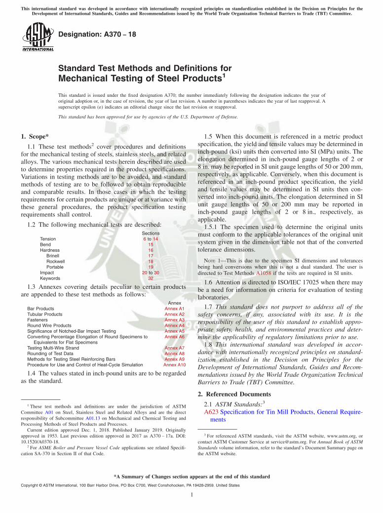
Designation: A370 − 18
Standard Test Methods and Definitions forMechanical Testing of Steel Products1
This standard is issued under the fixed designation A370; the number immediately following the designation indicates the year oforiginal adoption or, in the case of revision, the year of last revision. A number in parentheses indicates the year of last reapproval. Asuperscript epsilon (´) indicates an editorial change since the last revision or reapproval.
This standard has been approved for use by agencies of the U.S. Department of Defense.
1. Scope*
1.1 These test methods2 cover procedures and definitionsfor the mechanical testing of steels, stainless steels, and relatedalloys. The various mechanical tests herein described are usedto determine properties required in the product specifications.Variations in testing methods are to be avoided, and standardmethods of testing are to be followed to obtain reproducibleand comparable results. In those cases in which the testingrequirements for certain products are unique or at variance withthese general procedures, the product specification testingrequirements shall control.
1.2 The following mechanical tests are described:Sections
Tension 6 to 14Bend 15Hardness 16
Brinell 17Rockwell 18Portable 19
Impact 20 to 30Keywords 32
1.3 Annexes covering details peculiar to certain productsare appended to these test methods as follows:
AnnexBar Products Annex A1Tubular Products Annex A2Fasteners Annex A3Round Wire Products Annex A4Significance of Notched-Bar Impact Testing Annex A5Converting Percentage Elongation of Round Specimens to
Equivalents for Flat SpecimensAnnex A6
Testing Multi-Wire Strand Annex A7Rounding of Test Data Annex A8Methods for Testing Steel Reinforcing Bars Annex A9Procedure for Use and Control of Heat-Cycle Simulation Annex A10
1.4 The values stated in inch-pound units are to be regardedas the standard.
1.5 When this document is referenced in a metric productspecification, the yield and tensile values may be determined ininch-pound (ksi) units then converted into SI (MPa) units. Theelongation determined in inch-pound gauge lengths of 2 or8 in. may be reported in SI unit gauge lengths of 50 or 200 mm,respectively, as applicable. Conversely, when this document isreferenced in an inch-pound product specification, the yieldand tensile values may be determined in SI units then con-verted into inch-pound units. The elongation determined in SIunit gauge lengths of 50 or 200 mm may be reported ininch-pound gauge lengths of 2 or 8 in., respectively, asapplicable.
1.5.1 The specimen used to determine the original unitsmust conform to the applicable tolerances of the original unitsystem given in the dimension table not that of the convertedtolerance dimensions.
NOTE 1—This is due to the specimen SI dimensions and tolerancesbeing hard conversions when this is not a dual standard. The user isdirected to Test Methods A1058 if the tests are required in SI units.
1.6 Attention is directed to ISO/IEC 17025 when there maybe a need for information on criteria for evaluation of testinglaboratories.
1.7 This standard does not purport to address all of thesafety concerns, if any, associated with its use. It is theresponsibility of the user of this standard to establish appro-priate safety, health, and environmental practices and deter-mine the applicability of regulatory limitations prior to use.
1.8 This international standard was developed in accor-dance with internationally recognized principles on standard-ization established in the Decision on Principles for theDevelopment of International Standards, Guides and Recom-mendations issued by the World Trade Organization TechnicalBarriers to Trade (TBT) Committee.
2. Referenced Documents
2.1 ASTM Standards:3
A623 Specification for Tin Mill Products, General Require-ments
1 These test methods and definitions are under the jurisdiction of ASTMCommittee A01 on Steel, Stainless Steel and Related Alloys and are the directresponsibility of Subcommittee A01.13 on Mechanical and Chemical Testing andProcessing Methods of Steel Products and Processes.
Current edition approved Dec. 1, 2018. Published January 2019. Originallyapproved in 1953. Last previous edition approved in 2017 as A370 – 17a. DOI:10.1520/A0370-18.
2 For ASME Boiler and Pressure Vessel Code applications see related Specifi-cation SA-370 in Section II of that Code.
3 For referenced ASTM standards, visit the ASTM website, www.astm.org, orcontact ASTM Customer Service at [email protected]. For Annual Book of ASTMStandards volume information, refer to the standard’s Document Summary page onthe ASTM website.
*A Summary of Changes section appears at the end of this standard
Copyright © ASTM International, 100 Barr Harbor Drive, PO Box C700, West Conshohocken, PA 19428-2959. United States
This international standard was developed in accordance with internationally recognized principles on standardization established in the Decision on Principles for theDevelopment of International Standards, Guides and Recommendations issued by the World Trade Organization Technical Barriers to Trade (TBT) Committee.
1

A623M Specification for Tin Mill Products, General Re-quirements [Metric]
A833 Test Method for Indentation Hardness of MetallicMaterials by Comparison Hardness Testers
A956/A956M Test Method for Leeb Hardness Testing ofSteel Products
A1038 Test Method for Portable Hardness Testing by theUltrasonic Contact Impedance Method
A1058 Test Methods for Mechanical Testing of SteelProducts—Metric
A1061/A1061M Test Methods for Testing Multi-Wire SteelPrestressing Strand
E4 Practices for Force Verification of Testing MachinesE6 Terminology Relating to Methods of Mechanical TestingE8/E8M Test Methods for Tension Testing of Metallic Ma-
terialsE10 Test Method for Brinell Hardness of Metallic MaterialsE18 Test Methods for Rockwell Hardness of Metallic Ma-
terialsE23 Test Methods for Notched Bar Impact Testing of Me-
tallic MaterialsE29 Practice for Using Significant Digits in Test Data to
Determine Conformance with SpecificationsE83 Practice for Verification and Classification of Exten-
someter SystemsE110 Test Method for Rockwell and Brinell Hardness of
Metallic Materials by Portable Hardness TestersE190 Test Method for Guided Bend Test for Ductility of
WeldsE290 Test Methods for Bend Testing of Material for Ductil-
ity2.2 ASME Document:4
ASME Boiler and Pressure Vessel Code, Section VIII,Division I, Part UG-8
2.3 ISO Standard:5
ISO/IEC 17025 General Requirements for the Competenceof Testing and Calibration Laboratories
3. Significance and Use
3.1 The primary use of these test methods is testing todetermine the specified mechanical properties of steel, stainlesssteel, and related alloy products for the evaluation of confor-mance of such products to a material specification under thejurisdiction of ASTM Committee A01 and its subcommitteesas designated by a purchaser in a purchase order or contract.
3.1.1 These test methods may be and are used by otherASTM Committees and other standards writing bodies for thepurpose of conformance testing.
3.1.2 The material condition at the time of testing, samplingfrequency, specimen location and orientation, reportingrequirements, and other test parameters are contained in thepertinent material specification or in a General RequirementSpecification for the particular product form.
3.1.3 Some material specifications require the use of addi-tional test methods not described herein; in such cases, therequired test method is described in that material specificationor by reference to another appropriate test method standard.
3.2 These test methods are also suitable to be used fortesting of steel, stainless steel and related alloy materials forother purposes, such as incoming material acceptance testingby the purchaser or evaluation of components after serviceexposure.
3.2.1 As with any mechanical testing, deviations from eitherspecification limits or expected as-manufactured properties canoccur for valid reasons besides deficiency of the originalas-fabricated product. These reasons include, but are notlimited to: subsequent service degradation from environmentalexposure (for example, temperature, corrosion); static or cyclicservice stress effects, mechanically-induced damage, materialinhomogeneity, anisotropic structure, natural aging of selectalloys, further processing not included in the specification,sampling limitations, and measuring equipment calibrationuncertainty. There is statistical variation in all aspects ofmechanical testing and variations in test results from prior testsare expected. An understanding of possible reasons for devia-tion from specified or expected test values should be applied ininterpretation of test results.
4. General Precautions
4.1 Certain methods of fabrication, such as bending,forming, and welding, or operations involving heating, mayaffect the properties of the material under test. Therefore, theproduct specifications cover the stage of manufacture at whichmechanical testing is to be performed. The properties shown bytesting prior to fabrication may not necessarily be representa-tive of the product after it has been completely fabricated.
4.2 Improperly machined specimens should be discardedand other specimens substituted.
4.3 Flaws in the specimen may also affect results. If any testspecimen develops flaws, the retest provision of the applicableproduct specification shall govern.
4.4 If any test specimen fails because of mechanical reasonssuch as failure of testing equipment or improper specimenpreparation, it may be discarded and another specimen taken.
5. Orientation of Test Specimens
5.1 The terms “longitudinal test” and “transverse test” areused only in material specifications for wrought products andare not applicable to castings. When such reference is made toa test coupon or test specimen, the following definitions apply:
5.1.1 Longitudinal Test, unless specifically definedotherwise, signifies that the lengthwise axis of the specimen isparallel to the direction of the greatest extension of the steelduring rolling or forging. The stress applied to a longitudinaltension test specimen is in the direction of the greatestextension, and the axis of the fold of a longitudinal bend testspecimen is at right angles to the direction of greatest extension(Fig. 1, Fig. 2a, and Fig. 2b).
5.1.2 Transverse Test, unless specifically defined otherwise,signifies that the lengthwise axis of the specimen is at right
4 Available from American Society of Mechanical Engineers (ASME), ASMEInternational Headquarters, Two Park Ave., New York, NY 10016-5990, http://www.asme.org.
5 Available from American National Standards Institute (ANSI), 25 W. 43rd St.,4th Floor, New York, NY 10036, http://www.ansi.org.
A370 − 18
2

angles to the direction of the greatest extension of the steelduring rolling or forging. The stress applied to a transversetension test specimen is at right angles to the greatestextension, and the axis of the fold of a transverse bend testspecimen is parallel to the greatest extension (Fig. 1).
5.2 The terms “radial test” and “tangential test” are used inmaterial specifications for some wrought circular products andare not applicable to castings. When such reference is made toa test coupon or test specimen, the following definitions apply:
5.2.1 Radial Test, unless specifically defined otherwise,signifies that the lengthwise axis of the specimen is perpen-dicular to the axis of the product and coincident with one of theradii of a circle drawn with a point on the axis of the productas a center (Fig. 2a).
5.2.2 Tangential Test, unless specifically defined otherwise,signifies that the lengthwise axis of the specimen is perpen-dicular to a plane containing the axis of the product and tangentto a circle drawn with a point on the axis of the product as acenter (Fig. 2a, Fig. 2b, Fig. 2c, and Fig. 2d).
TENSION TEST
6. Description
6.1 The tension test related to the mechanical testing of steelproducts subjects a machined or full-section specimen of thematerial under examination to a measured load sufficient tocause rupture. The resulting properties sought are defined inTerminology E6.
6.2 In general, the testing equipment and methods are givenin Test Methods E8/E8M. However, there are certain excep-tions to Test Methods E8/E8M practices in the testing of steel,and these are covered in these test methods.
7. Terminology
7.1 For definitions of terms pertaining to tension testing,including tensile strength, yield point, yield strength,elongation, and reduction of area, reference should be made toTerminology E6.
8. Testing Apparatus and Operations
8.1 Loading Systems—There are two general types of load-ing systems, mechanical (screw power) and hydraulic. Thesediffer chiefly in the variability of the rate of load application.The older screw power machines are limited to a small numberof fixed free running crosshead speeds. Some modern screwpower machines, and all hydraulic machines permit steplessvariation throughout the range of speeds.
8.2 The tension testing machine shall be maintained in goodoperating condition, used only in the proper loading range, andcalibrated periodically in accordance with the latest revision ofPractices E4.
NOTE 2—Many machines are equipped with stress-strain recorders forautographic plotting of stress-strain curves. It should be noted that somerecorders have a load measuring component entirely separate from theload indicator of the testing machine. Such recorders are calibratedseparately.
8.3 Loading—It is the function of the gripping or holdingdevice of the testing machine to transmit the load from theheads of the machine to the specimen under test. The essentialrequirement is that the load shall be transmitted axially. Thisimplies that the centers of the action of the grips shall be inalignment, insofar as practicable, with the axis of the specimenat the beginning and during the test and that bending ortwisting be held to a minimum. For specimens with a reducedsection, gripping of the specimen shall be restricted to the gripsection. In the case of certain sections tested in full size,nonaxial loading is unavoidable and in such cases shall bepermissible.
8.4 Speed of Testing—The speed of testing shall not begreater than that at which load and strain readings can be madeaccurately. In production testing, speed of testing is commonlyexpressed: (1) in terms of free running crosshead speed (rate ofmovement of the crosshead of the testing machine when notunder load), (2) in terms of rate of separation of the two headsof the testing machine under load, (3) in terms of rate ofstressing the specimen, or (4) in terms of rate of straining thespecimen. The following limitations on the speed of testing arerecommended as adequate for most steel products:
NOTE 3—Tension tests using closed-loop machines (with feedbackcontrol of rate) should not be performed using load control, as this modeof testing will result in acceleration of the crosshead upon yielding andelevation of the measured yield strength.
8.4.1 Any convenient speed of testing may be used up toone half the specified yield point or yield strength. When thispoint is reached, the free-running rate of separation of thecrossheads shall be adjusted so as not to exceed 1⁄16 in. per minper inch of reduced section, or the distance between the gripsfor test specimens not having reduced sections. This speedshall be maintained through the yield point or yield strength. Indetermining the tensile strength, the free-running rate of
FIG. 1 Relation of Test Coupons and Test Specimens to RollingDirection or Extension (Applicable to General Wrought Products)
A370 − 18
3
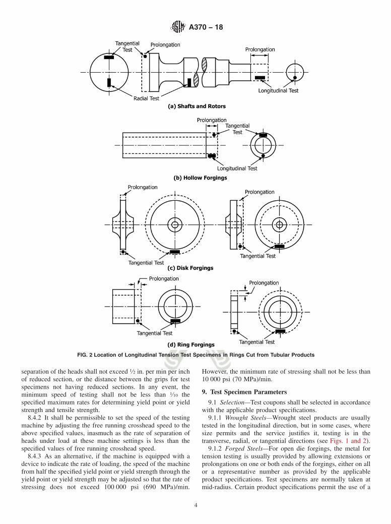
separation of the heads shall not exceed 1⁄2 in. per min per inchof reduced section, or the distance between the grips for testspecimens not having reduced sections. In any event, theminimum speed of testing shall not be less than 1⁄10 thespecified maximum rates for determining yield point or yieldstrength and tensile strength.
8.4.2 It shall be permissible to set the speed of the testingmachine by adjusting the free running crosshead speed to theabove specified values, inasmuch as the rate of separation ofheads under load at these machine settings is less than thespecified values of free running crosshead speed.
8.4.3 As an alternative, if the machine is equipped with adevice to indicate the rate of loading, the speed of the machinefrom half the specified yield point or yield strength through theyield point or yield strength may be adjusted so that the rate ofstressing does not exceed 100 000 psi (690 MPa)/min.
However, the minimum rate of stressing shall not be less than10 000 psi (70 MPa)/min.
9. Test Specimen Parameters
9.1 Selection—Test coupons shall be selected in accordancewith the applicable product specifications.
9.1.1 Wrought Steels—Wrought steel products are usuallytested in the longitudinal direction, but in some cases, wheresize permits and the service justifies it, testing is in thetransverse, radial, or tangential directions (see Figs. 1 and 2).
9.1.2 Forged Steels—For open die forgings, the metal fortension testing is usually provided by allowing extensions orprolongations on one or both ends of the forgings, either on allor a representative number as provided by the applicableproduct specifications. Test specimens are normally taken atmid-radius. Certain product specifications permit the use of a
FIG. 2 Location of Longitudinal Tension Test Specimens in Rings Cut from Tubular Products
A370 − 18
4

representative bar or the destruction of a production part fortest purposes. For ring or disk-like forgings test metal isprovided by increasing the diameter, thickness, or length of theforging. Upset disk or ring forgings, which are worked orextended by forging in a direction perpendicular to the axis ofthe forging, usually have their principal extension alongconcentric circles and for such forgings tangential tensionspecimens are obtained from extra metal on the periphery orend of the forging. For some forgings, such as rotors, radialtension tests are required. In such cases the specimens are cutor trepanned from specified locations.
9.2 Size and Tolerances—Test specimens shall be (1) thefull cross section of material, or (2) machined to the form anddimensions shown in Figs. 3-6. The selection of size and typeof specimen is prescribed by the applicable product specifica-tion. Full cross section specimens shall be tested in 8-in.(200-mm) gauge length unless otherwise specified in theproduct specification.
9.3 Procurement of Test Specimens—Specimens shall beextracted by any convenient method taking care to remove alldistorted, cold-worked, or heat-affected areas from the edges ofthe section used in evaluating the material. Specimens usuallyhave a reduced cross section at mid-length to ensure uniformdistribution of the stress over the cross section and localize thezone of fracture.
9.4 Aging of Test Specimens—Unless otherwise specified, itshall be permissible to age tension test specimens. The time-temperature cycle employed must be such that the effects ofprevious processing will not be materially changed. It may beaccomplished by aging at room temperature 24 to 48 h, or inshorter time at moderately elevated temperatures by boiling inwater, heating in oil or in an oven.
9.5 Measurement of Dimensions of Test Specimens:9.5.1 Standard Rectangular Tension Test Specimens—These
forms of specimens are shown in Fig. 3. To determine thecross-sectional area, the center width dimension shall bemeasured to the nearest 0.005 in. (0.13 mm) for the 8-in.(200-mm) gauge length specimen and 0.001 in. (0.025 mm) forthe 2-in. (50-mm) gauge length specimen in Fig. 3. The centerthickness dimension shall be measured to the nearest 0.001 in.for both specimens.
9.5.2 Standard Round Tension Test Specimens—Theseforms of specimens are shown in Fig. 4 and Fig. 5. Todetermine the cross-sectional area, the diameter shall bemeasured at the center of the gauge length to the nearest0.001 in. (0.025 mm) (see Table 1).
9.6 General—Test specimens shall be either substantiallyfull size or machined, as prescribed in the product specifica-tions for the material being tested.
9.6.1 It is desirable to have the cross-sectional area of thespecimen smallest at the center of the gauge length to ensurefracture within the gauge length. This is provided for by thetaper in the gauge length permitted for each of the specimensdescribed in the following sections.
9.6.2 For brittle materials it is desirable to have fillets oflarge radius at the ends of the gauge length.
10. Plate-Type Specimens
10.1 The standard plate-type test specimens are shown inFig. 3. Such specimens are used for testing metallic materialsin the form of plate, structural and bar-size shapes, and flatmaterial having a nominal thickness of 3⁄16 in. (5 mm) or over.When product specifications so permit, other types of speci-mens may be used.
NOTE 4—When called for in the product specification, the 8-in.(200-mm) gauge length specimen of Fig. 3 may be used for sheet and stripmaterial.
11. Sheet-Type Specimen
11.1 The standard sheet-type test specimen is shown in Fig.3. This specimen is used for testing metallic materials in theform of sheet, plate, flat wire, strip, band, and hoop ranging innominal thickness from 0.005 to 1 in. (0.13 to 25 mm). Whenproduct specifications so permit, other types of specimens maybe used, as provided in Section 10 (see Note 4).
12. Round Specimens
12.1 The standard 0.500-in. (12.5-mm) diameter round testspecimen shown in Fig. 4 is frequently used for testing metallicmaterials.
12.2 Fig. 4 also shows small size specimens proportional tothe standard specimen. These may be used when it is necessaryto test material from which the standard specimen or specimensshown in Fig. 3 cannot be prepared. Other sizes of small roundspecimens may be used. In any such small size specimen it isimportant that the gauge length for measurement of elongationbe four times the diameter of the specimen (see Note 5, Fig. 4).
12.3 The type of specimen ends outside of the gauge lengthshall accommodate the shape of the product tested, and shallproperly fit the holders or grips of the testing machine so thataxial loads are applied with a minimum of load eccentricity andslippage. Fig. 5 shows specimens with various types of endsthat have given satisfactory results.
13. Gauge Marks
13.1 The specimens shown in Figs. 3-6 shall be gaugemarked with a center punch, scribe marks, multiple device, ordrawn with ink. The purpose of these gauge marks is todetermine the percent elongation. Punch marks shall be light,sharp, and accurately spaced. The localization of stress at themarks makes a hard specimen susceptible to starting fracture atthe punch marks. The gauge marks for measuring elongationafter fracture shall be made on the flat or on the edge of the flattension test specimen and within the parallel section; for the8-in. gauge length specimen, Fig. 3, one or more sets of 8-in.gauge marks may be used, intermediate marks within the gaugelength being optional. Rectangular 2-in. gauge lengthspecimens, Fig. 3, and round specimens, Fig. 4, are gaugemarked with a double-pointed center punch or scribe marks.One or more sets of gauge marks may be used; however, oneset must be approximately centered in the reduced section.These same precautions shall be observed when the testspecimen is full section.
A370 − 18
5

DIMENSIONS
Standard Specimens Subsize Specimen
Plate-Type,11⁄2-in. (40-mm) Wide
8-in. (200-mm)Gauge Length
2-in. (50-mm)Gauge Length
Sheet-Type, 1⁄2in. (12.5-mm) Wide
1⁄4-in. (6-mm) Wide
in. mm in. mm in. mm in. mm
G—Gauge length(Notes 1 and 2)
8.00 ± 0.01 200 ± 0.25 2.000 ± 0.005 50.0 ± 0.10 2.000 ± 0.005 50.0 ± 0.10 1.000 ± 0.003 25.0 ± 0.08
W—Width(Notes 3, 5, and 6)
11⁄2 + 1⁄8− 1⁄4
40 + 3− 6
11⁄2 + 1⁄8− 1⁄4
40 + 3− 6
0.500 ± 0.010 12.5 ± 0.25 0.250 ± 0.002 6.25 ± 0.05
T—Thickness(Note 7)
Thickness of Material
R—Radius of fillet, min(Note 4)
1⁄2 13 1⁄2 13 1⁄2 13 1⁄4 6
L—Overall length, min(Notes 2 and 8)
18 450 8 200 8 200 4 100
A—Length ofreduced section, min
9 225 21⁄4 60 21⁄4 60 11⁄4 32
B—Length of grip section, min(Note 9)
3 75 2 50 2 50 11⁄4 32
C—Width of grip section, approxi-mate
(Notes 4, 10, and 11)
2 50 2 50 3⁄4 20 3⁄8 10
NOTE 1—For the 11⁄2-in. (40-mm) wide specimens, punch marks for measuring elongation after fracture shall be made on the flat or on the edge ofthe specimen and within the reduced section. For the 8-in. (200-mm) gauge length specimen, a set of nine or more punch marks 1 in. (25 mm) apart,or one or more pairs of punch marks 8 in. (200 mm) apart may be used. For the 2-in. (50-mm) gauge length specimen, a set of three or more punch marks1 in. (25 mm) apart, or one or more pairs of punch marks 2 in. (50 mm) apart may be used.
NOTE 2—For the 1⁄2-in. (12.5-mm) wide specimen, punch marks for measuring the elongation after fracture shall be made on the flat or on the edgeof the specimen and within the reduced section. Either a set of three or more punch marks 1 in. (25 mm) apart or one or more pairs of punch marks 2 in.(50 mm) apart may be used.
NOTE 3—For the four sizes of specimens, the ends of the reduced section shall not differ in width by more than 0.004, 0.004, 0.002, or 0.001 in. (0.10,0.10, 0.05, or 0.025 mm), respectively. Also, there may be a gradual decrease in width from the ends to the center, but the width at either end shall notbe more than 0.015 in., 0.015 in., 0.005 in., or 0.003 in. (0.40, 0.40, 0.10, or 0.08 mm), respectively, larger than the width at the center.
NOTE 4—For each specimen type, the radii of all fillets shall be equal to each other with a tolerance of 0.05 in. (1.25 mm), and the centers of curvatureof the two fillets at a particular end shall be located across from each other (on a line perpendicular to the centerline) within a tolerance of 0.10 in.(2.5 mm).
NOTE 5—For each of the four sizes of specimens, narrower widths (W and C) may be used when necessary. In such cases, the width of the reducedsection should be as large as the width of the material being tested permits; however, unless stated specifically, the requirements for elongation in a productspecification shall not apply when these narrower specimens are used. If the width of the material is less than W, the sides may be parallel throughoutthe length of the specimen.
NOTE 6—The specimen may be modified by making the sides parallel throughout the length of the specimen, the width and tolerances being the sameas those specified above. When necessary, a narrower specimen may be used, in which case the width should be as great as the width of the material beingtested permits. If the width is 11⁄2 in. (38 mm) or less, the sides may be parallel throughout the length of the specimen.
NOTE 7—The dimension T is the thickness of the test specimen as provided for in the applicable product specification. Minimum nominal thicknessof 1 to 11⁄2-in. (40-mm) wide specimens shall be 3⁄16 in. (5 mm), except as permitted by the product specification. Maximum nominal thickness of 1⁄2-in.(12.5-mm) and 1⁄4-in. (6-mm) wide specimens shall be 1 in. (25 mm) and 1⁄4 in. (6 mm), respectively.
NOTE 8—To aid in obtaining axial loading during testing of 1⁄4-in. (6-mm) wide specimens, the overall length should be as large as the material willpermit.
NOTE 9—It is desirable, if possible, to make the length of the grip section large enough to allow the specimen to extend into the grips a distance equalto two thirds or more of the length of the grips. If the thickness of 1⁄2-in. (13-mm) wide specimens is over 3⁄8 in. (10 mm), longer grips and correspondinglylonger grip sections of the specimen may be necessary to prevent failure in the grip section.
NOTE 10—For standard sheet-type specimens and subsize specimens, the ends of the specimen shall be symmetrical with the center line of the reducedsection within 0.01 and 0.005 in. (0.25 and 0.13 mm), respectively, except that for steel if the ends of the 1⁄2-in. (12.5-mm) wide specimen are symmetricalwithin 0.05 in. (1.0 mm), a specimen may be considered satisfactory for all but referee testing.
NOTE 11—For standard plate-type specimens, the ends of the specimen shall be symmetrical with the center line of the reduced section within 0.25 in.(6.35 mm), except for referee testing in which case the ends of the specimen shall be symmetrical with the center line of the reduced section within 0.10 in.(2.5 mm).
FIG. 3 Rectangular Tension Test Specimens
A370 − 18
6
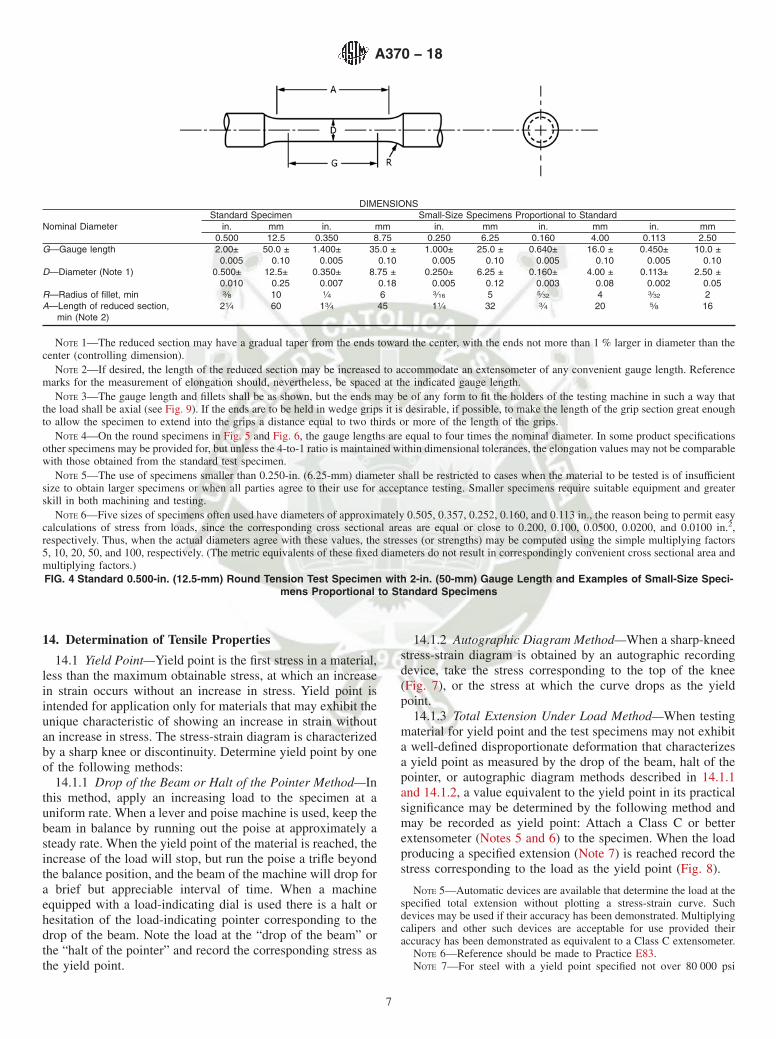
14. Determination of Tensile Properties
14.1 Yield Point—Yield point is the first stress in a material,less than the maximum obtainable stress, at which an increasein strain occurs without an increase in stress. Yield point isintended for application only for materials that may exhibit theunique characteristic of showing an increase in strain withoutan increase in stress. The stress-strain diagram is characterizedby a sharp knee or discontinuity. Determine yield point by oneof the following methods:
14.1.1 Drop of the Beam or Halt of the Pointer Method—Inthis method, apply an increasing load to the specimen at auniform rate. When a lever and poise machine is used, keep thebeam in balance by running out the poise at approximately asteady rate. When the yield point of the material is reached, theincrease of the load will stop, but run the poise a trifle beyondthe balance position, and the beam of the machine will drop fora brief but appreciable interval of time. When a machineequipped with a load-indicating dial is used there is a halt orhesitation of the load-indicating pointer corresponding to thedrop of the beam. Note the load at the “drop of the beam” orthe “halt of the pointer” and record the corresponding stress asthe yield point.
14.1.2 Autographic Diagram Method—When a sharp-kneedstress-strain diagram is obtained by an autographic recordingdevice, take the stress corresponding to the top of the knee(Fig. 7), or the stress at which the curve drops as the yieldpoint.
14.1.3 Total Extension Under Load Method—When testingmaterial for yield point and the test specimens may not exhibita well-defined disproportionate deformation that characterizesa yield point as measured by the drop of the beam, halt of thepointer, or autographic diagram methods described in 14.1.1and 14.1.2, a value equivalent to the yield point in its practicalsignificance may be determined by the following method andmay be recorded as yield point: Attach a Class C or betterextensometer (Notes 5 and 6) to the specimen. When the loadproducing a specified extension (Note 7) is reached record thestress corresponding to the load as the yield point (Fig. 8).
NOTE 5—Automatic devices are available that determine the load at thespecified total extension without plotting a stress-strain curve. Suchdevices may be used if their accuracy has been demonstrated. Multiplyingcalipers and other such devices are acceptable for use provided theiraccuracy has been demonstrated as equivalent to a Class C extensometer.
NOTE 6—Reference should be made to Practice E83.NOTE 7—For steel with a yield point specified not over 80 000 psi
DIMENSIONS
Nominal DiameterStandard Specimen Small-Size Specimens Proportional to Standard
in. mm in. mm in. mm in. mm in. mm0.500 12.5 0.350 8.75 0.250 6.25 0.160 4.00 0.113 2.50
G—Gauge length 2.00±0.005
50.0 ±0.10
1.400±0.005
35.0 ±0.10
1.000±0.005
25.0 ±0.10
0.640±0.005
16.0 ±0.10
0.450±0.005
10.0 ±0.10
D—Diameter (Note 1) 0.500±0.010
12.5±0.25
0.350±0.007
8.75 ±0.18
0.250±0.005
6.25 ±0.12
0.160±0.003
4.00 ±0.08
0.113±0.002
2.50 ±0.05
R—Radius of fillet, min 3⁄8 10 1⁄4 6 3⁄16 5 5⁄32 4 3⁄32 2A—Length of reduced section,
min (Note 2)21⁄4 60 13⁄4 45 11⁄4 32 3⁄4 20 5⁄8 16
NOTE 1—The reduced section may have a gradual taper from the ends toward the center, with the ends not more than 1 % larger in diameter than thecenter (controlling dimension).
NOTE 2—If desired, the length of the reduced section may be increased to accommodate an extensometer of any convenient gauge length. Referencemarks for the measurement of elongation should, nevertheless, be spaced at the indicated gauge length.
NOTE 3—The gauge length and fillets shall be as shown, but the ends may be of any form to fit the holders of the testing machine in such a way thatthe load shall be axial (see Fig. 9). If the ends are to be held in wedge grips it is desirable, if possible, to make the length of the grip section great enoughto allow the specimen to extend into the grips a distance equal to two thirds or more of the length of the grips.
NOTE 4—On the round specimens in Fig. 5 and Fig. 6, the gauge lengths are equal to four times the nominal diameter. In some product specificationsother specimens may be provided for, but unless the 4-to-1 ratio is maintained within dimensional tolerances, the elongation values may not be comparablewith those obtained from the standard test specimen.
NOTE 5—The use of specimens smaller than 0.250-in. (6.25-mm) diameter shall be restricted to cases when the material to be tested is of insufficientsize to obtain larger specimens or when all parties agree to their use for acceptance testing. Smaller specimens require suitable equipment and greaterskill in both machining and testing.
NOTE 6—Five sizes of specimens often used have diameters of approximately 0.505, 0.357, 0.252, 0.160, and 0.113 in., the reason being to permit easycalculations of stress from loads, since the corresponding cross sectional areas are equal or close to 0.200, 0.100, 0.0500, 0.0200, and 0.0100 in.2,respectively. Thus, when the actual diameters agree with these values, the stresses (or strengths) may be computed using the simple multiplying factors5, 10, 20, 50, and 100, respectively. (The metric equivalents of these fixed diameters do not result in correspondingly convenient cross sectional area andmultiplying factors.)FIG. 4 Standard 0.500-in. (12.5-mm) Round Tension Test Specimen with 2-in. (50-mm) Gauge Length and Examples of Small-Size Speci-
mens Proportional to Standard Specimens
A370 − 18
7
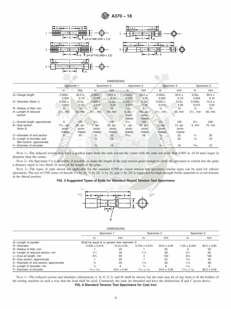
DIMENSIONS
Specimen 1 Specimen 2 Specimen 3 Specimen 4 Specimen 5
in. mm in. mm in. mm in. mm in. mm
G—Gauge length 2.000±0.005
50.0 ±0.10
2.000±0.005
50.0 ±0.10
2.000±0.005
50.0 ±0.10
2.000±0.005
50.0 ±0.10
2.00±0.005
50.0 ±0.10
D—Diameter (Note 1) 0.500 ±0.010
12.5±0.25
0.500 ±0.010
12.5±0.25
0.500 ±0.010
12.5±0.25
0.500 ±0.010
12.5±0.25
0.500±0.010
12.5 ±0.25
R—Radius of fillet, min 3⁄8 10 3⁄8 10 1⁄16 2 3⁄8 10 3⁄8 10A—Length of reduced
section21⁄4 , min 60, min 21⁄4 , min 60, min 4, ap-
proxi-mately
100, ap-proxi-mately
21⁄4 , min 60, min 21⁄4 , min 60, min
L—Overall length, approximate 5 125 51⁄2 140 51⁄2 140 43⁄4 120 91⁄2 240B—Grip section
(Note 2)13⁄8 , ap-
proxi-mately
35, ap-proxi-mately
1, ap-proxi-mately
25, ap-proxi-mately
3⁄4 , ap-proxi-mately
20, ap-proxi-mately
1⁄2 , ap-proxi-mately
13, ap-proxi-mately
3, min 75, min
C—Diameter of end section 3⁄4 20 3⁄4 20 23⁄32 18 7⁄8 22 3⁄4 20E—Length of shoulder and
fillet section, approximate. . . . . . 5⁄8 16 . . . . . . 3⁄4 20 5⁄8 16
F—Diameter of shoulder . . . . . . 5⁄8 16 . . . . . . 5⁄8 16 19⁄32 15
NOTE 1—The reduced section may have a gradual taper from the ends toward the center with the ends not more than 0.005 in. (0.10 mm) larger indiameter than the center.
NOTE 2—On Specimen 5 it is desirable, if possible, to make the length of the grip section great enough to allow the specimen to extend into the gripsa distance equal to two thirds or more of the length of the grips.
NOTE 3—The types of ends shown are applicable for the standard 0.500-in. round tension test specimen; similar types can be used for subsizespecimens. The use of UNF series of threads (3⁄4 by 16, 1⁄2 by 20, 3⁄8 by 24, and 1⁄4 by 28) is suggested for high-strength brittle materials to avoid fracturein the thread portion.
FIG. 5 Suggested Types of Ends for Standard Round Tension Test Specimens
DIMENSIONS
Specimen 1 Specimen 2 Specimen 3
in. mm in. mm in. mm
G—Length of parallel Shall be equal to or greater than diameter DD—Diameter 0.500 ± 0.010 12.5± 0.25 0.750 ± 0.015 20.0 ± 0.40 1.25 ± 0.025 30.0 ± 0.60R—Radius of fillet, min 1 25 1 25 2 50A—Length of reduced section, min 11⁄4 32 11⁄2 38 21⁄4 60L—Over-all length, min 33⁄4 95 4 100 63⁄8 160B—Grip section, approximate 1 25 1 25 13⁄4 45C—Diameter of end section, approximate 3⁄4 20 11⁄8 30 17⁄8 48E—Length of shoulder, min 1⁄4 6 1⁄4 6 5⁄16 8F—Diameter of shoulder 5⁄8 ± 1⁄64 16.0 ± 0.40 15⁄16 ± 1⁄64 24.0 ± 0.40 17⁄16 ± 1⁄64 36.5 ± 0.40
NOTE 1—The reduced section and shoulders (dimensions A, D, E, F, G, and R) shall be shown, but the ends may be of any form to fit the holders ofthe testing machine in such a way that the load shall be axial. Commonly the ends are threaded and have the dimensions B and C given above.
FIG. 6 Standard Tension Test Specimens for Cast Iron
A370 − 18
8
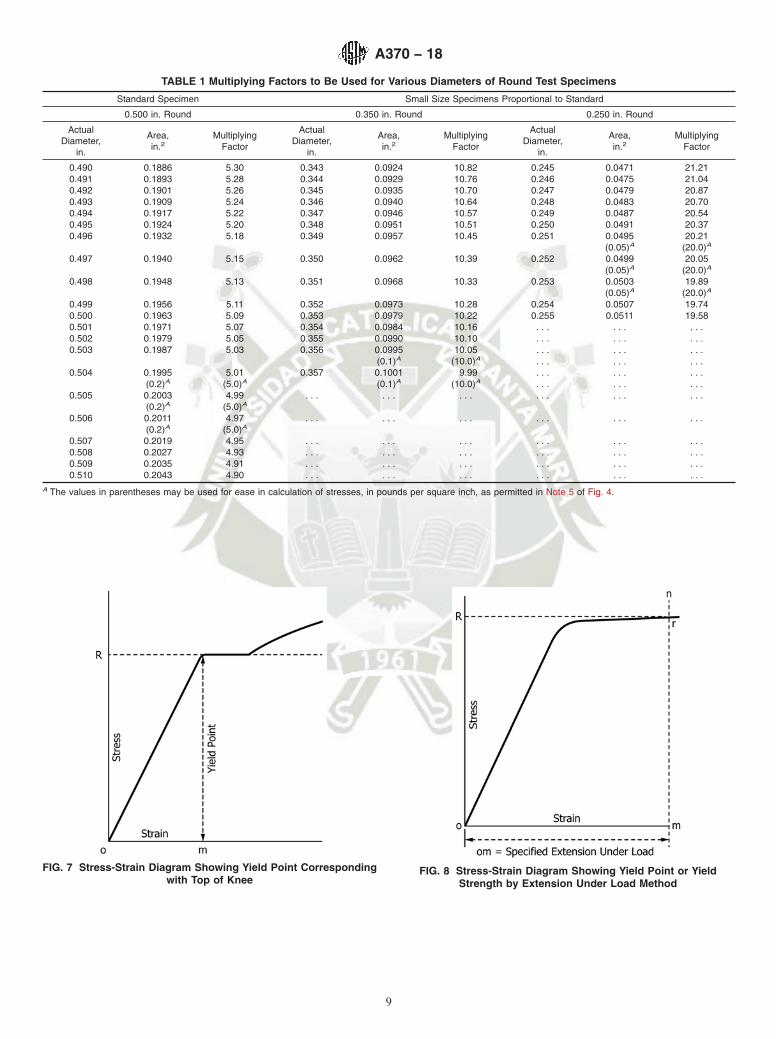
TABLE 1 Multiplying Factors to Be Used for Various Diameters of Round Test Specimens
Standard Specimen Small Size Specimens Proportional to Standard
0.500 in. Round 0.350 in. Round 0.250 in. Round
ActualDiameter,
in.
Area,in.2
MultiplyingFactor
ActualDiameter,
in.
Area,in.2
MultiplyingFactor
ActualDiameter,
in.
Area,in.2
MultiplyingFactor
0.490 0.1886 5.30 0.343 0.0924 10.82 0.245 0.0471 21.210.491 0.1893 5.28 0.344 0.0929 10.76 0.246 0.0475 21.040.492 0.1901 5.26 0.345 0.0935 10.70 0.247 0.0479 20.870.493 0.1909 5.24 0.346 0.0940 10.64 0.248 0.0483 20.700.494 0.1917 5.22 0.347 0.0946 10.57 0.249 0.0487 20.540.495 0.1924 5.20 0.348 0.0951 10.51 0.250 0.0491 20.370.496 0.1932 5.18 0.349 0.0957 10.45 0.251 0.0495 20.21
(0.05)A (20.0)A
0.497 0.1940 5.15 0.350 0.0962 10.39 0.252 0.0499 20.05(0.05)A (20.0)A
0.498 0.1948 5.13 0.351 0.0968 10.33 0.253 0.0503 19.89(0.05)A (20.0)A
0.499 0.1956 5.11 0.352 0.0973 10.28 0.254 0.0507 19.740.500 0.1963 5.09 0.353 0.0979 10.22 0.255 0.0511 19.580.501 0.1971 5.07 0.354 0.0984 10.16 . . . . . . . . .0.502 0.1979 5.05 0.355 0.0990 10.10 . . . . . . . . .0.503 0.1987 5.03 0.356 0.0995 10.05 . . . . . . . . .
(0.1)A (10.0)A . . . . . . . . .0.504 0.1995 5.01 0.357 0.1001 9.99 . . . . . . . . .
(0.2)A (5.0)A (0.1)A (10.0)A . . . . . . . . .0.505 0.2003 4.99 . . . . . . . . . . . . . . . . . .
(0.2)A (5.0)A
0.506 0.2011 4.97 . . . . . . . . . . . . . . . . . .(0.2)A (5.0)A
0.507 0.2019 4.95 . . . . . . . . . . . . . . . . . .0.508 0.2027 4.93 . . . . . . . . . . . . . . . . . .0.509 0.2035 4.91 . . . . . . . . . . . . . . . . . .0.510 0.2043 4.90 . . . . . . . . . . . . . . . . . .
A The values in parentheses may be used for ease in calculation of stresses, in pounds per square inch, as permitted in Note 5 of Fig. 4.
FIG. 7 Stress-Strain Diagram Showing Yield Point Correspondingwith Top of Knee
FIG. 8 Stress-Strain Diagram Showing Yield Point or YieldStrength by Extension Under Load Method
A370 − 18
9
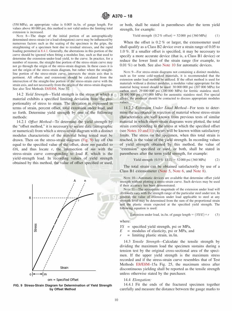
(550 MPa), an appropriate value is 0.005 in./in. of gauge length. Forvalues above 80 000 psi, this method is not valid unless the limiting totalextension is increased.
NOTE 8—The shape of the initial portion of an autographicallydetermined stress-strain (or a load-elongation) curve may be influenced bynumerous factors such as the seating of the specimen in the grips, thestraightening of a specimen bent due to residual stresses, and the rapidloading permitted in 8.4.1. Generally, the aberrations in this portion of thecurve should be ignored when fitting a modulus line, such as that used todetermine the extension-under-load yield, to the curve. In practice, for anumber of reasons, the straight-line portion of the stress-strain curve maynot go through the origin of the stress-strain diagram. In these cases it isnot the origin of the stress-strain diagram, but rather where the straight-line portion of the stress-strain curve, intersects the strain axis that ispertinent. All offsets and extensions should be calculated from theintersection of the straight-line portion of the stress-strain curve with thestrain axis, and not necessarily from the origin of the stress-strain diagram.See also Test Methods E8/E8M, Note 32.
14.2 Yield Strength—Yield strength is the stress at which amaterial exhibits a specified limiting deviation from the pro-portionality of stress to strain. The deviation is expressed interms of strain, percent offset, total extension under load, andso forth. Determine yield strength by one of the followingmethods:
14.2.1 Offset Method—To determine the yield strength bythe “offset method,” it is necessary to secure data (autographicor numerical) from which a stress-strain diagram with a distinctmodulus characteristic of the material being tested may bedrawn. Then on the stress-strain diagram (Fig. 9) lay off Omequal to the specified value of the offset, draw mn parallel toOA, and thus locate r, the intersection of mn with thestress-strain curve corresponding to load R, which is theyield-strength load. In recording values of yield strengthobtained by this method, the value of offset specified or used,
or both, shall be stated in parentheses after the term yieldstrength, for example:
Yield strength ~0.2 % offset! 5 52 000 psi ~360 MPa! (1)
When the offset is 0.2 % or larger, the extensometer usedshall qualify as a Class B2 device over a strain range of 0.05 to1.0 %. If a smaller offset is specified, it may be necessary tospecify a more accurate device (that is, a Class B1 device) orreduce the lower limit of the strain range (for example, to0.01 %) or both. See also Note 10 for automatic devices.
NOTE 9—For stress-strain diagrams not containing a distinct modulus,such as for some cold-worked materials, it is recommended that theextension under load method be utilized. If the offset method is used formaterials without a distinct modulus, a modulus value appropriate for thematerial being tested should be used: 30 000 000 psi (207 000 MPa) forcarbon steel; 29 000 000 psi (200 000 MPa) for ferritic stainless steel;28 000 000 psi (193 000 MPa) for austenitic stainless steel. For specialalloys, the producer should be contacted to discuss appropriate modulusvalues.
14.2.2 Extension Under Load Method—For tests to deter-mine the acceptance or rejection of material whose stress-straincharacteristics are well known from previous tests of similarmaterial in which stress-strain diagrams were plotted, the totalstrain corresponding to the stress at which the specified offset(see Notes 10 and 11) occurs will be known within satisfactorylimits. The stress on the specimen, when this total strain isreached, is the value of the yield strength. In recording valuesof yield strength obtained by this method, the value of“extension” specified or used, or both, shall be stated inparentheses after the term yield strength, for example:
Yield strength ~0.5 % EUL! 5 52 000 psi ~360 MPa! (2)
The total strain can be obtained satisfactorily by use of aClass B1 extensometer (Note 5, Note 6, and Note 8).
NOTE 10—Automatic devices are available that determine offset yieldstrength without plotting a stress-strain curve. Such devices may be usedif their accuracy has been demonstrated.
NOTE 11—The appropriate magnitude of the extension under load willobviously vary with the strength range of the particular steel under test. Ingeneral, the value of extension under load applicable to steel at anystrength level may be determined from the sum of the proportional strainand the plastic strain expected at the specified yield strength. Thefollowing equation is used:
Extension under load, in./in. of gauge length 5 ~YS/E!1r (3)
where:YS = specified yield strength, psi or MPa,E = modulus of elasticity, psi or MPa, andr = limiting plastic strain, in./in.
14.3 Tensile Strength—Calculate the tensile strength bydividing the maximum load the specimen sustains during atension test by the original cross-sectional area of the speci-men. If the upper yield strength is the maximum stressrecorded and if the stress-strain curve resembles that of TestMethods E8/E8M–15a Fig. 25, the maximum stress afterdiscontinuous yielding shall be reported as the tensile strengthunless otherwise stated by the purchaser.
14.4 Elongation:14.4.1 Fit the ends of the fractured specimen together
carefully and measure the distance between the gauge marks toFIG. 9 Stress-Strain Diagram for Determination of Yield Strength
by Offset Method
A370 − 18
10

the nearest 0.01 in. (0.25 mm) for gauge lengths of 2 in. andunder, and to the nearest 0.5 % of the gauge length for gaugelengths over 2 in. A percentage scale reading to 0.5 % of thegauge length may be used. The elongation is the increase inlength of the gauge length, expressed as a percentage of theoriginal gauge length. In recording elongation values, give boththe percentage increase and the original gauge length.
14.4.2 If any part of the fracture takes place outside of themiddle half of the gauge length or in a punched or scribed markwithin the reduced section, the elongation value obtained maynot be representative of the material. If the elongation someasured meets the minimum requirements specified, nofurther testing is indicated, but if the elongation is less than theminimum requirements, discard the test and retest.
14.4.3 Automated tensile testing methods using extensom-eters allow for the measurement of elongation in a methoddescribed below. Elongation may be measured and reportedeither this way, or as in the method described above, fitting thebroken ends together. Either result is valid.
14.4.4 Elongation at fracture is defined as the elongationmeasured just prior to the sudden decrease in force associatedwith fracture. For many ductile materials not exhibiting asudden decrease in force, the elongation at fracture can betaken as the strain measured just prior to when the force fallsbelow 10 % of the maximum force encountered during the test.
14.4.4.1 Elongation at fracture shall include elastic andplastic elongation and may be determined with autographic orautomated methods using extensometers verified over thestrain range of interest. Use a class B2 or better extensometerfor materials having less than 5 % elongation; a class C orbetter extensometer for materials having elongation greaterthan or equal to 5 % but less than 50 %; and a class D or betterextensometer for materials having 50 % or greater elongation.In all cases, the extensometer gauge length shall be the nominalgauge length required for the specimen being tested. Due to thelack of precision in fitting fractured ends together, the elonga-tion after fracture using the manual methods of the precedingparagraphs may differ from the elongation at fracture deter-mined with extensometers.
14.4.4.2 Percent elongation at fracture may be calculateddirectly from elongation at fracture data and be reportedinstead of percent elongation as calculated in 14.4.1. However,these two parameters are not interchangeable. Use of theelongation at fracture method generally provides more repeat-able results.
14.5 Reduction of Area—Fit the ends of the fracturedspecimen together and measure the mean diameter or the widthand thickness at the smallest cross section to the same accuracyas the original dimensions. The difference between the areathus found and the area of the original cross section expressedas a percentage of the original area is the reduction of area.
BEND TEST
15. Description
15.1 The bend test is one method for evaluating ductility,but it cannot be considered as a quantitative means of predict-ing service performance in all bending operations. The severity
of the bend test is primarily a function of the angle of bend ofthe inside diameter to which the specimen is bent, and of thecross section of the specimen. These conditions are variedaccording to location and orientation of the test specimen andthe chemical composition, tensile properties, hardness, type,and quality of the steel specified. Test Methods E190 and E290may be consulted for methods of performing the test.
15.2 Unless otherwise specified, it shall be permissible toage bend test specimens. The time-temperature cycle employedmust be such that the effects of previous processing will not bematerially changed. It may be accomplished by aging at roomtemperature 24 to 48 h, or in shorter time at moderatelyelevated temperatures by boiling in water or by heating in oilor in an oven.
15.3 Bend the test specimen at room temperature to aninside diameter, as designated by the applicable productspecifications, to the extent specified. The speed of bending isordinarily not an important factor.
HARDNESS TEST
16. General
16.1 A hardness test is a means of determining resistance topenetration and is occasionally employed to obtain a quickapproximation of tensile strength. Tables 2-5 are for theconversion of hardness measurements from one scale toanother or to approximate tensile strength. These conversionvalues have been obtained from computer-generated curvesand are presented to the nearest 0.1 point to permit accuratereproduction of those curves. All converted hardness valuesmust be considered approximate. All converted Rockwell andVickers hardness numbers shall be rounded to the nearestwhole number.
16.2 Hardness Testing:
16.2.1 If the product specification permits alternative hard-ness testing to determine conformance to a specified hardnessrequirement, the conversions listed in Tables 2-5 shall be used.
16.2.2 When recording converted hardness numbers, themeasured hardness and test scale shall be indicated inparentheses, for example: 353 HBW (38 HRC). This meansthat a hardness value of 38 was obtained using the Rockwell Cscale and converted to a Brinell hardness of 353.
17. Brinell Test
17.1 Description:
17.1.1 A specified load is applied to a flat surface of thespecimen to be tested, through a tungsten carbide ball ofspecified diameter. The average diameter of the indentation isused as a basis for calculation of the Brinell hardness number.The quotient of the applied load divided by the area of thesurface of the indentation, which is assumed to be spherical, istermed the Brinell hardness number (HBW) in accordance withthe following equation:
HBW 5 P/@~πD/2!~D 2 =D2 2 d2!# (4)
A370 − 18
11
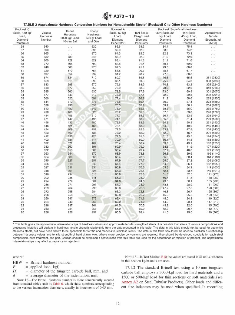
where:HBW = Brinell hardness number,P = applied load, kgf,D = diameter of the tungsten carbide ball, mm, andd = average diameter of the indentation, mm.
NOTE 12—The Brinell hardness number is more conveniently securedfrom standard tables such as Table 6, which show numbers correspondingto the various indentation diameters, usually in increments of 0.05 mm.
NOTE 13—In Test Method E10 the values are stated in SI units, whereasin this section kg/m units are used.
17.1.2 The standard Brinell test using a 10-mm tungstencarbide ball employs a 3000-kgf load for hard materials and a1500 or 500-kgf load for thin sections or soft materials (seeAnnex A2 on Steel Tubular Products). Other loads and differ-ent size indentors may be used when specified. In recording
TABLE 2 Approximate Hardness Conversion Numbers for Nonaustenitic SteelsA (Rockwell C to Other Hardness Numbers)Rockwell C
Scale, 150-kgfLoad,
DiamondPenetrator
VickersHardnessNumber
BrinellHardness
3000-kgf Load,10-mm Ball
KnoopHardness,
500-gf Loadand Over
Rockwell AScale, 60-kgf
Load,Diamond
Penetrator
Rockwell Superficial Hardness15N Scale,
15-kgf Load,Diamond
Penetrator
30N Scale 30-kgf Load,Diamond
Penetrator
45N Scale,45-kgf Load,
DiamondPenetrator
ApproximateTensile
Strength, ksi(MPa)
68 940 . . . 920 85.6 93.2 84.4 75.4 . . .67 900 . . . 895 85.0 92.9 83.6 74.2 . . .66 865 . . . 870 84.5 92.5 82.8 73.3 . . .65 832 739 846 83.9 92.2 81.9 72.0 . . .64 800 722 822 83.4 91.8 81.1 71.0 . . .63 772 706 799 82.8 91.4 80.1 69.9 . . .62 746 688 776 82.3 91.1 79.3 68.8 . . .61 720 670 754 81.8 90.7 78.4 67.7 . . .60 697 654 732 81.2 90.2 77.5 66.6 . . .59 674 634 710 80.7 89.8 76.6 65.5 351 (2420)58 653 615 690 80.1 89.3 75.7 64.3 338 (2330)57 633 595 670 79.6 88.9 74.8 63.2 325 (2240)56 613 577 650 79.0 88.3 73.9 62.0 313 (2160)55 595 560 630 78.5 87.9 73.0 60.9 301 (2070)54 577 543 612 78.0 87.4 72.0 59.8 292 (2010)53 560 525 594 77.4 86.9 71.2 58.6 283 (1950)52 544 512 576 76.8 86.4 70.2 57.4 273 (1880)51 528 496 558 76.3 85.9 69.4 56.1 264 (1820)50 513 482 542 75.9 85.5 68.5 55.0 255 (1760)49 498 468 526 75.2 85.0 67.6 53.8 246 (1700)48 484 455 510 74.7 84.5 66.7 52.5 238 (1640)47 471 442 495 74.1 83.9 65.8 51.4 229 (1580)46 458 432 480 73.6 83.5 64.8 50.3 221 (1520)45 446 421 466 73.1 83.0 64.0 49.0 215 (1480)44 434 409 452 72.5 82.5 63.1 47.8 208 (1430)43 423 400 438 72.0 82.0 62.2 46.7 201 (1390)42 412 390 426 71.5 81.5 61.3 45.5 194 (1340)41 402 381 414 70.9 80.9 60.4 44.3 188 (1300)40 392 371 402 70.4 80.4 59.5 43.1 182 (1250)39 382 362 391 69.9 79.9 58.6 41.9 177 (1220)38 372 353 380 69.4 79.4 57.7 40.8 171 (1180)37 363 344 370 68.9 78.8 56.8 39.6 166 (1140)36 354 336 360 68.4 78.3 55.9 38.4 161 (1110)35 345 327 351 67.9 77.7 55.0 37.2 156 (1080)34 336 319 342 67.4 77.2 54.2 36.1 152 (1050)33 327 311 334 66.8 76.6 53.3 34.9 149 (1030)32 318 301 326 66.3 76.1 52.1 33.7 146 (1010)31 310 294 318 65.8 75.6 51.3 32.5 141 (970)30 302 286 311 65.3 75.0 50.4 31.3 138 (950)29 294 279 304 64.6 74.5 49.5 30.1 135 (930)28 286 271 297 64.3 73.9 48.6 28.9 131 (900)27 279 264 290 63.8 73.3 47.7 27.8 128 (880)26 272 258 284 63.3 72.8 46.8 26.7 125 (860)25 266 253 278 62.8 72.2 45.9 25.5 123 (850)24 260 247 272 62.4 71.6 45.0 24.3 119 (820)23 254 243 266 62.0 71.0 44.0 23.1 117 (810)22 248 237 261 61.5 70.5 43.2 22.0 115 (790)21 243 231 256 61.0 69.9 42.3 20.7 112 (770)20 238 226 251 60.5 69.4 41.5 19.6 110 (760)
A This table gives the approximate interrelationships of hardness values and approximate tensile strength of steels. It is possible that steels of various compositions andprocessing histories will deviate in hardness-tensile strength relationship from the data presented in this table. The data in this table should not be used for austeniticstainless steels, but have been shown to be applicable for ferritic and martensitic stainless steels. The data in this table should not be used to establish a relationshipbetween hardness values and tensile strength of hard drawn wire. Where more precise conversions are required, they should be developed specially for each steelcomposition, heat treatment, and part. Caution should be exercised if conversions from this table are used for the acceptance or rejection of product. The approximateinterrelationships may affect acceptance or rejection.
A370 − 18
12

TABLE 3 Approximate Hardness Conversion Numbers for Nonaustenitic SteelsA (Rockwell B to Other Hardness Numbers)
Rockwell BScale, 100-
kgf Load 1⁄16-in. (1.588-mm) Ball
VickersHardnessNumber
BrinellHardness,
3000-kgf Load,10-mm Ball
KnoopHardness,
500-gf Load &Over
Rockwell AScale, 60-kgf
Load, DiamondPenetrator
Rockwell FScale, 60-kgfLoad, 1⁄16-in.
(1.588-mm) Ball
Rockwell Superficial HardnessApproximate
TensileStrength ksi
(MPa)
15T Scale,15-kgf
Load, 1⁄16-in. (1.588-mm) Ball
30T Scale,30-kgf
Load, 1⁄16-in. (1.588-mm) Ball
45T Scale,45-kgf
Load, 1⁄16-in. (1.588-mm) Ball
100 240 240 251 61.5 . . . 93.1 83.1 72.9 116 (800)99 234 234 246 60.9 . . . 92.8 82.5 71.9 114 (785)98 228 228 241 60.2 . . . 92.5 81.8 70.9 109 (750)97 222 222 236 59.5 . . . 92.1 81.1 69.9 104 (715)96 216 216 231 58.9 . . . 91.8 80.4 68.9 102 (705)95 210 210 226 58.3 . . . 91.5 79.8 67.9 100 (690)94 205 205 221 57.6 . . . 91.2 79.1 66.9 98 (675)93 200 200 216 57.0 . . . 90.8 78.4 65.9 94 (650)92 195 195 211 56.4 . . . 90.5 77.8 64.8 92 (635)91 190 190 206 55.8 . . . 90.2 77.1 63.8 90 (620)90 185 185 201 55.2 . . . 89.9 76.4 62.8 89 (615)89 180 180 196 54.6 . . . 89.5 75.8 61.8 88 (605)88 176 176 192 54.0 . . . 89.2 75.1 60.8 86 (590)87 172 172 188 53.4 . . . 88.9 74.4 59.8 84 (580)86 169 169 184 52.8 . . . 88.6 73.8 58.8 83 (570)85 165 165 180 52.3 . . . 88.2 73.1 57.8 82 (565)84 162 162 176 51.7 . . . 87.9 72.4 56.8 81 (560)83 159 159 173 51.1 . . . 87.6 71.8 55.8 80 (550)82 156 156 170 50.6 . . . 87.3 71.1 54.8 77 (530)81 153 153 167 50.0 . . . 86.9 70.4 53.8 73 (505)80 150 150 164 49.5 . . . 86.6 69.7 52.8 72 (495)79 147 147 161 48.9 . . . 86.3 69.1 51.8 70 (485)78 144 144 158 48.4 . . . 86.0 68.4 50.8 69 (475)77 141 141 155 47.9 . . . 85.6 67.7 49.8 68 (470)76 139 139 152 47.3 . . . 85.3 67.1 48.8 67 (460)75 137 137 150 46.8 99.6 85.0 66.4 47.8 66 (455)74 135 135 147 46.3 99.1 84.7 65.7 46.8 65 (450)73 132 132 145 45.8 98.5 84.3 65.1 45.8 64 (440)72 130 130 143 45.3 98.0 84.0 64.4 44.8 63 (435)71 127 127 141 44.8 97.4 83.7 63.7 43.8 62 (425)70 125 125 139 44.3 96.8 83.4 63.1 42.8 61 (420)69 123 123 137 43.8 96.2 83.0 62.4 41.8 60 (415)68 121 121 135 43.3 95.6 82.7 61.7 40.8 59 (405)67 119 119 133 42.8 95.1 82.4 61.0 39.8 58 (400)66 117 117 131 42.3 94.5 82.1 60.4 38.7 57 (395)65 116 116 129 41.8 93.9 81.8 59.7 37.7 56 (385)64 114 114 127 41.4 93.4 81.4 59.0 36.7 . . .63 112 112 125 40.9 92.8 81.1 58.4 35.7 . . .62 110 110 124 40.4 92.2 80.8 57.7 34.7 . . .61 108 108 122 40.0 91.7 80.5 57.0 33.7 . . .60 107 107 120 39.5 91.1 80.1 56.4 32.7 . . .59 106 106 118 39.0 90.5 79.8 55.7 31.7 . . .58 104 104 117 38.6 90.0 79.5 55.0 30.7 . . .57 103 103 115 38.1 89.4 79.2 54.4 29.7 . . .56 101 101 114 37.7 88.8 78.8 53.7 28.7 . . .55 100 100 112 37.2 88.2 78.5 53.0 27.7 . . .54 . . . . . . 111 36.8 87.7 78.2 52.4 26.7 . . .53 . . . . . . 110 36.3 87.1 77.9 51.7 25.7 . . .52 . . . . . . 109 35.9 86.5 77.5 51.0 24.7 . . .51 . . . . . . 108 35.5 86.0 77.2 50.3 23.7 . . .50 . . . . . . 107 35.0 85.4 76.9 49.7 22.7 . . .49 . . . . . . 106 34.6 84.8 76.6 49.0 21.7 . . .48 . . . . . . 105 34.1 84.3 76.2 48.3 20.7 . . .47 . . . . . . 104 33.7 83.7 75.9 47.7 19.7 . . .46 . . . . . . 103 33.3 83.1 75.6 47.0 18.7 . . .45 . . . . . . 102 32.9 82.6 75.3 46.3 17.7 . . .44 . . . . . . 101 32.4 82.0 74.9 45.7 16.7 . . .43 . . . . . . 100 32.0 81.4 74.6 45.0 15.7 . . .42 . . . . . . 99 31.6 80.8 74.3 44.3 14.7 . . .41 . . . . . . 98 31.2 80.3 74.0 43.7 13.6 . . .40 . . . . . . 97 30.7 79.7 73.6 43.0 12.6 . . .39 . . . . . . 96 30.3 79.1 73.3 42.3 11.6 . . .38 . . . . . . 95 29.9 78.6 73.0 41.6 10.6 . . .37 . . . . . . 94 29.5 78.0 72.7 41.0 9.6 . . .36 . . . . . . 93 29.1 77.4 72.3 40.3 8.6 . . .35 . . . . . . 92 28.7 76.9 72.0 39.6 7.6 . . .34 . . . . . . 91 28.2 76.3 71.7 39.0 6.6 . . .33 . . . . . . 90 27.8 75.7 71.4 38.3 5.6 . . .32 . . . . . . 89 27.4 75.2 71.0 37.6 4.6 . . .31 . . . . . . 88 27.0 74.6 70.7 37.0 3.6 . . .
A370 − 18
13
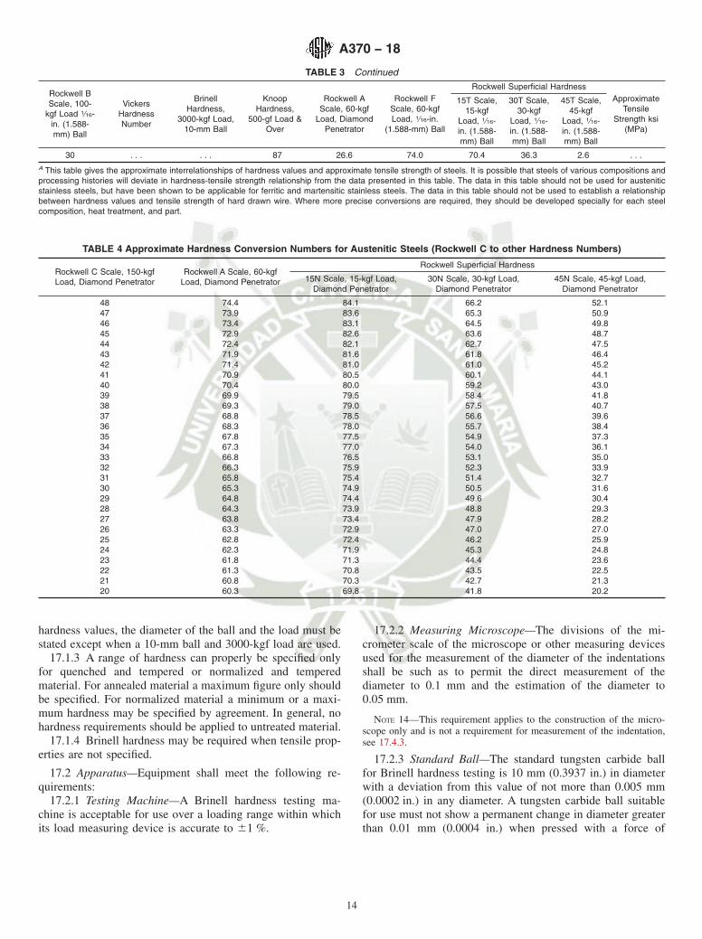
hardness values, the diameter of the ball and the load must bestated except when a 10-mm ball and 3000-kgf load are used.
17.1.3 A range of hardness can properly be specified onlyfor quenched and tempered or normalized and temperedmaterial. For annealed material a maximum figure only shouldbe specified. For normalized material a minimum or a maxi-mum hardness may be specified by agreement. In general, nohardness requirements should be applied to untreated material.
17.1.4 Brinell hardness may be required when tensile prop-erties are not specified.
17.2 Apparatus—Equipment shall meet the following re-quirements:
17.2.1 Testing Machine—A Brinell hardness testing ma-chine is acceptable for use over a loading range within whichits load measuring device is accurate to 61 %.
17.2.2 Measuring Microscope—The divisions of the mi-crometer scale of the microscope or other measuring devicesused for the measurement of the diameter of the indentationsshall be such as to permit the direct measurement of thediameter to 0.1 mm and the estimation of the diameter to0.05 mm.
NOTE 14—This requirement applies to the construction of the micro-scope only and is not a requirement for measurement of the indentation,see 17.4.3.
17.2.3 Standard Ball—The standard tungsten carbide ballfor Brinell hardness testing is 10 mm (0.3937 in.) in diameterwith a deviation from this value of not more than 0.005 mm(0.0002 in.) in any diameter. A tungsten carbide ball suitablefor use must not show a permanent change in diameter greaterthan 0.01 mm (0.0004 in.) when pressed with a force of
TABLE 3 Continued
Rockwell BScale, 100-
kgf Load 1⁄16-in. (1.588-mm) Ball
VickersHardnessNumber
BrinellHardness,
3000-kgf Load,10-mm Ball
KnoopHardness,
500-gf Load &Over
Rockwell AScale, 60-kgf
Load, DiamondPenetrator
Rockwell FScale, 60-kgfLoad, 1⁄16-in.
(1.588-mm) Ball
Rockwell Superficial HardnessApproximate
TensileStrength ksi
(MPa)
15T Scale,15-kgf
Load, 1⁄16-in. (1.588-mm) Ball
30T Scale,30-kgf
Load, 1⁄16-in. (1.588-mm) Ball
45T Scale,45-kgf
Load, 1⁄16-in. (1.588-mm) Ball
30 . . . . . . 87 26.6 74.0 70.4 36.3 2.6 . . .A This table gives the approximate interrelationships of hardness values and approximate tensile strength of steels. It is possible that steels of various compositions andprocessing histories will deviate in hardness-tensile strength relationship from the data presented in this table. The data in this table should not be used for austeniticstainless steels, but have been shown to be applicable for ferritic and martensitic stainless steels. The data in this table should not be used to establish a relationshipbetween hardness values and tensile strength of hard drawn wire. Where more precise conversions are required, they should be developed specially for each steelcomposition, heat treatment, and part.
TABLE 4 Approximate Hardness Conversion Numbers for Austenitic Steels (Rockwell C to other Hardness Numbers)
Rockwell C Scale, 150-kgfLoad, Diamond Penetrator
Rockwell A Scale, 60-kgfLoad, Diamond Penetrator
Rockwell Superficial Hardness
15N Scale, 15-kgf Load,Diamond Penetrator
30N Scale, 30-kgf Load,Diamond Penetrator
45N Scale, 45-kgf Load,Diamond Penetrator
48 74.4 84.1 66.2 52.147 73.9 83.6 65.3 50.946 73.4 83.1 64.5 49.845 72.9 82.6 63.6 48.744 72.4 82.1 62.7 47.543 71.9 81.6 61.8 46.442 71.4 81.0 61.0 45.241 70.9 80.5 60.1 44.140 70.4 80.0 59.2 43.039 69.9 79.5 58.4 41.838 69.3 79.0 57.5 40.737 68.8 78.5 56.6 39.636 68.3 78.0 55.7 38.435 67.8 77.5 54.9 37.334 67.3 77.0 54.0 36.133 66.8 76.5 53.1 35.032 66.3 75.9 52.3 33.931 65.8 75.4 51.4 32.730 65.3 74.9 50.5 31.629 64.8 74.4 49.6 30.428 64.3 73.9 48.8 29.327 63.8 73.4 47.9 28.226 63.3 72.9 47.0 27.025 62.8 72.4 46.2 25.924 62.3 71.9 45.3 24.823 61.8 71.3 44.4 23.622 61.3 70.8 43.5 22.521 60.8 70.3 42.7 21.320 60.3 69.8 41.8 20.2
A370 − 18
14

3000 kgf against the test specimen. Steel ball indentors are nolonger permitted for use in Brinell hardness testing in accor-dance with these test methods.
17.3 Test Specimen—Brinell hardness tests are made onprepared areas and sufficient metal must be removed from thesurface to eliminate decarburized metal and other surfaceirregularities. The thickness of the piece tested must be suchthat no bulge or other marking showing the effect of the loadappears on the side of the piece opposite the indentation.
17.4 Procedure:17.4.1 It is essential that the applicable product specifica-
tions state clearly the position at which Brinell hardnessindentations are to be made and the number of such indenta-tions required. The distance of the center of the indentationfrom the edge of the specimen or edge of another indentationmust be at least two and one-half times the diameter of theindentation.
17.4.2 Apply the load for 10 to 15 s.17.4.3 Measure diameters of the indentation in accordance
with Test Method E10.17.4.4 The Brinell hardness test is not recommended for
materials above 650 HBW.17.4.4.1 If a ball is used in a test of a specimen which shows
a Brinell hardness number greater than the limit for the ball asdetailed in 17.4.4, the ball shall be either discarded andreplaced with a new ball or remeasured to ensure conformancewith the requirements of Test Method E10.
17.5 Brinell Hardness Values:17.5.1 Brinell hardness values shall not be designated by a
number alone because it is necessary to indicate which indenterand which force has been employed in making the test. Brinellhardness numbers shall be followed by the symbol HBW, andbe supplemented by an index indicating the test conditions inthe following order:
17.5.1.1 Diameter of the ball, mm,17.5.1.2 A value representing the applied load, kgf, and,17.5.1.3 The applied force dwell time, s, if other than 10 to
15 s.17.5.1.4 The only exception to the above requirement is for
the HBW 10/3000 scale when a 10 to 15 s dwell time is used.Only in the case of this one Brinell hardness scale may thedesignation be reported simply as HBW.
17.5.1.5 Examples: 220 HBW = Brinell hardness of 220determined with a ball of 10 mm diameter and with a test forceof 3000 kgf applied for 10 to 15 s; 350 HBW 5/1500 = Brinellhardness of 350 determined with a ball of 5 mm diameter andwith a test force of 1500 kgf applied for 10 to 15 s.
17.6 Detailed Procedure—For detailed requirements of thistest, reference shall be made to the latest revision of TestMethod E10.
18. Rockwell Test
18.1 Description:18.1.1 In this test a hardness value is obtained by determin-
ing the depth of penetration of a diamond point or a tungstencarbide ball into the specimen under certain arbitrarily fixedconditions. A minor load of 10 kgf is first applied which causesan initial penetration, sets the penetrator on the material andholds it in position. A major load which depends on the scalebeing used is applied increasing the depth of indentation. Themajor load is removed and, with the minor load still acting, theRockwell number, which is proportional to the difference inpenetration between the major and minor loads is determined;this is usually done by the machine and shows on a dial, digitaldisplay, printer, or other device. This is an arbitrary numberwhich increases with increasing hardness. The scales mostfrequently used are as follows:
TABLE 5 Approximate Hardness Conversion Numbers for Austenitic Steels (Rockwell B to other Hardness Numbers)
Rockwell BScale, 100-
kgf Load, 1⁄16-in. (1.588-mm) Ball
Brinell IndentationDiameter, mm
Brinell Hardness,3000-kgf Load,
10-mm Ball
Rockwell A Scale,60-kgf Load,
Diamond Penetrator
Rockwell Superficial Hardness
15T Scale,15-kgf Load,
1⁄16-in. (1.588-mm) Ball
30T Scale,30-kgf Load,
1⁄16-in. (1.588-mm) Ball
45T Scale,45-kgf Load,
1⁄16-in. (1.588-mm) Ball
100 3.79 256 61.5 91.5 80.4 70.299 3.85 248 60.9 91.2 79.7 69.298 3.91 240 60.3 90.8 79.0 68.297 3.96 233 59.7 90.4 78.3 67.296 4.02 226 59.1 90.1 77.7 66.195 4.08 219 58.5 89.7 77.0 65.194 4.14 213 58.0 89.3 76.3 64.193 4.20 207 57.4 88.9 75.6 63.192 4.24 202 56.8 88.6 74.9 62.191 4.30 197 56.2 88.2 74.2 61.190 4.35 192 55.6 87.8 73.5 60.189 4.40 187 55.0 87.5 72.8 59.088 4.45 183 54.5 87.1 72.1 58.087 4.51 178 53.9 86.7 71.4 57.086 4.55 174 53.3 86.4 70.7 56.085 4.60 170 52.7 86.0 70.0 55.084 4.65 167 52.1 85.6 69.3 54.083 4.70 163 51.5 85.2 68.6 52.982 4.74 160 50.9 84.9 67.9 51.981 4.79 156 50.4 84.5 67.2 50.980 4.84 153 49.8 84.1 66.5 49.9
A370 − 18
15

TABLE 6 Brinell Hardness NumbersA
(Ball 10 mm in Diameter, Applied Loads of 500, 1500, and 3000 kgf)
Diameterof Indenta-tion, mm
Brinell HardnessNumber Diameter
ofIndenta-tion, mm
Brinell HardnessNumber Diameter
ofIndenta-tion, mm
Brinell HardnessNumber Diameter
ofIndenta-tion, mm
Brinell HardnessNumber
500-kgf
Load
1500-kgf
Load
3000-kgf
Load
500-kgf
Load
1500-kgf
Load
3000-kgf
Load
500-kgf
Load
1500-kgf
Load
3000-kgf
Load
500-kgf
Load
1500-kgf
Load
3000-kgf
Load
2.00 158 473 945 3.25 58.6 176 352 4.50 29.8 89.3 179 5.75 17.5 52.5 1052.01 156 468 936 3.26 58.3 175 350 4.51 29.6 88.8 178 5.76 17.4 52.3 1052.02 154 463 926 3.27 57.9 174 347 4.52 29.5 88.4 177 5.77 17.4 52.1 1042.03 153 459 917 3.28 57.5 173 345 4.53 29.3 88.0 176 5.78 17.3 51.9 1042.04 151 454 908 3.29 57.2 172 343 4.54 29.2 87.6 175 5.79 17.2 51.7 1032.05 150 450 899 3.30 56.8 170 341 4.55 29.1 87.2 174 5.80 17.2 51.5 1032.06 148 445 890 3.31 56.5 169 339 4.56 28.9 86.8 174 5.81 17.1 51.3 1032.07 147 441 882 3.32 56.1 168 337 4.57 28.8 86.4 173 5.82 17.0 51.1 1022.08 146 437 873 3.33 55.8 167 335 4.58 28.7 86.0 172 5.83 17.0 50.9 1022.09 144 432 865 3.34 55.4 166 333 4.59 28.5 85.6 171 5.84 16.9 50.7 1012.10 143 428 856 3.35 55.1 165 331 4.60 28.4 85.4 170 5.85 16.8 50.5 1012.11 141 424 848 3.36 54.8 164 329 4.61 28.3 84.8 170 5.86 16.8 50.3 1012.12 140 420 840 3.37 54.4 163 326 4.62 28.1 84.4 169 5.87 16.7 50.2 1002.13 139 416 832 3.38 54.1 162 325 4.63 28.0 84.0 168 5.88 16.7 50.0 99.92.14 137 412 824 3.39 53.8 161 323 4.64 27.9 83.6 167 5.89 16.6 49.8 99.52.15 136 408 817 3.40 53.4 160 321 4.65 27.8 83.3 167 5.90 16.5 49.6 99.22.16 135 404 809 3.41 53.1 159 319 4.66 27.6 82.9 166 5.91 16.5 49.4 98.82.17 134 401 802 3.42 52.8 158 317 4.67 27.5 82.5 165 5.92 16.4 49.2 98.42.18 132 397 794 3.43 52.5 157 315 4.68 27.4 82.1 164 5.93 16.3 49.0 98.02.19 131 393 787 3.44 52.2 156 313 4.69 27.3 81.8 164 5.94 16.3 48.8 97.72.20 130 390 780 3.45 51.8 156 311 4.70 27.1 81.4 163 5.95 16.2 48.7 97.32.21 129 386 772 3.46 51.5 155 309 4.71 27.0 81.0 162 5.96 16.2 48.5 96.92.22 128 383 765 3.47 51.2 154 307 4.72 26.9 80.7 161 5.97 16.1 48.3 96.62.23 126 379 758 3.48 50.9 153 306 4.73 26.8 80.3 161 5.98 16.0 48.1 96.22.24 125 376 752 3.49 50.6 152 304 4.74 26.6 79.9 160 5.99 16.0 47.9 95.92.25 124 372 745 3.50 50.3 151 302 4.75 26.5 79.6 159 6.00 15.9 47.7 95.52.26 123 369 738 3.51 50.0 150 300 4.76 26.4 79.2 158 6.01 15.9 47.6 95.12.27 122 366 732 3.52 49.7 149 298 4.77 26.3 78.9 158 6.02 15.8 47.4 94.82.28 121 363 725 3.53 49.4 148 297 4.78 26.2 78.5 157 6.03 15.7 47.2 94.42.29 120 359 719 3.54 49.2 147 295 4.79 26.1 78.2 156 6.04 15.7 47.0 94.12.30 119 356 712 3.55 48.9 147 293 4.80 25.9 77.8 156 6.05 15.6 46.8 93.72.31 118 353 706 3.56 48.6 146 292 4.81 25.8 77.5 155 6.06 15.6 46.7 93.42.32 117 350 700 3.57 48.3 145 290 4.82 25.7 77.1 154 6.07 15.5 46.5 93.02.33 116 347 694 3.58 48.0 144 288 4.83 25.6 76.8 154 6.08 15.4 46.3 92.72.34 115 344 688 3.59 47.7 143 286 4.84 25.5 76.4 153 6.09 15.4 46.2 92.32.35 114 341 682 3.60 47.5 142 285 4.85 25.4 76.1 152 6.10 15.3 46.0 92.02.36 113 338 676 3.61 47.2 142 283 4.86 25.3 75.8 152 6.11 15.3 45.8 91.72.37 112 335 670 3.62 46.9 141 282 4.87 25.1 75.4 151 6.12 15.2 45.7 91.32.38 111 332 665 3.63 46.7 140 280 4.88 25.0 75.1 150 6.13 15.2 45.5 91.02.39 110 330 659 3.64 46.4 139 278 4.89 24.9 74.8 150 6.14 15.1 45.3 90.62.40 109 327 653 3.65 46.1 138 277 4.90 24.8 74.4 149 6.15 15.1 45.2 90.32.41 108 324 648 3.66 45.9 138 275 4.91 24.7 74.1 148 6.16 15.0 45.0 90.02.42 107 322 643 3.67 45.6 137 274 4.92 24.6 73.8 148 6.17 14.9 44.8 89.62.43 106 319 637 3.68 45.4 136 272 4.93 24.5 73.5 147 6.18 14.9 44.7 89.32.44 105 316 632 3.69 45.1 135 271 4.94 24.4 73.2 146 6.19 14.8 44.5 89.02.45 104 313 627 3.70 44.9 135 269 4.95 24.3 72.8 146 6.20 14.7 44.3 88.72.46 104 311 621 3.71 44.6 134 268 4.96 24.2 72.5 145 6.21 14.7 44.2 88.32.47 103 308 616 3.72 44.4 133 266 4.97 24.1 72.2 144 6.22 14.7 44.0 88.02.48 102 306 611 3.73 44.1 132 265 4.98 24.0 71.9 144 6.23 14.6 43.8 87.72.49 101 303 606 3.74 43.9 132 263 4.99 23.9 71.6 143 6.24 14.6 43.7 87.42.50 100 301 601 3.75 43.6 131 262 5.00 23.8 71.3 143 6.25 14.5 43.5 87.12.51 99.4 298 597 3.76 43.4 130 260 5.01 23.7 71.0 142 6.26 14.5 43.4 86.72.52 98.6 296 592 3.77 43.1 129 259 5.02 23.6 70.7 141 6.27 14.4 43.2 86.42.53 97.8 294 587 3.78 42.9 129 257 5.03 23.5 70.4 141 6.28 14.4 43.1 86.12.54 97.1 291 582 3.79 42.7 128 256 5.04 23.4 70.1 140 6.29 14.3 42.9 85.82.55 96.3 289 578 3.80 42.4 127 255 5.05 23.3 69.8 140 6.30 14.2 42.7 85.52.56 95.5 287 573 3.81 42.2 127 253 5.06 23.2 69.5 139 6.31 14.2 42.6 85.22.57 94.8 284 569 3.82 42.0 126 252 5.07 23.1 69.2 138 6.32 14.1 42.4 84.92.58 94.0 282 564 3.83 41.7 125 250 5.08 23.0 68.9 138 6.33 14.1 42.3 84.62.59 93.3 280 560 3.84 41.5 125 249 5.09 22.9 68.6 137 6.34 14.0 42.1 84.32.60 92.6 278 555 3.85 41.3 124 248 5.10 22.8 68.3 137 6.35 14.0 42.0 84.02.61 91.8 276 551 3.86 41.1 123 246 5.11 22.7 68.0 136 6.36 13.9 41.8 83.72.62 91.1 273 547 3.87 40.9 123 245 5.12 22.6 67.7 135 6.37 13.9 41.7 83.42.63 90.4 271 543 3.88 40.6 122 244 5.13 22.5 67.4 135 6.38 13.8 41.5 83.12.64 89.7 269 538 3.89 40.4 121 242 5.14 22.4 67.1 134 6.39 13.8 41.4 82.82.65 89.0 267 534 3.90 40.2 121 241 5.15 22.3 66.9 134 6.40 13.7 41.2 82.52.66 88.4 265 530 3.91 40.0 120 240 5.16 22.2 66.6 133 6.41 13.7 41.1 82.22.67 87.7 263 526 3.92 39.8 119 239 5.17 22.1 66.3 133 6.42 13.6 40.9 81.92.68 87.0 261 522 3.93 39.6 119 237 5.18 22.0 66.0 132 6.43 13.6 40.8 81.62.69 86.4 259 518 3.94 39.4 118 236 5.19 21.9 65.8 132 6.44 13.5 40.6 81.3
A370 − 18
16

TABLE 6 Continued
Diameterof Indenta-tion, mm
Brinell HardnessNumber Diameter
ofIndenta-tion, mm
Brinell HardnessNumber Diameter
ofIndenta-tion, mm
Brinell HardnessNumber Diameter
ofIndenta-tion, mm
Brinell HardnessNumber
500-kgf
Load
1500-kgf
Load
3000-kgf
Load
500-kgf
Load
1500-kgf
Load
3000-kgf
Load
500-kgf
Load
1500-kgf
Load
3000-kgf
Load
500-kgf
Load
1500-kgf
Load
3000-kgf
Load
2.70 85.7 257 514 3.95 39.1 117 235 5.20 21.8 65.5 131 6.45 13.5 40.5 81.02.71 85.1 255 510 3.96 38.9 117 234 5.21 21.7 65.2 130 6.46 13.4 40.4 80.72.72 84.4 253 507 3.97 38.7 116 232 5.22 21.6 64.9 130 6.47 13.4 40.2 80.42.73 83.8 251 503 3.98 38.5 116 231 5.23 21.6 64.7 129 6.48 13.4 40.1 80.12.74 83.2 250 499 3.99 38.3 115 230 5.24 21.5 64.4 129 6.49 13.3 39.9 79.82.75 82.6 248 495 4.00 38.1 114 229 5.25 21.4 64.1 128 6.50 13.3 39.8 79.62.76 81.9 246 492 4.01 37.9 114 228 5.26 21.3 63.9 128 6.51 13.2 39.6 79.32.77 81.3 244 488 4.02 37.7 113 226 5.27 21.2 63.6 127 6.52 13.2 39.5 79.02.78 80.8 242 485 4.03 37.5 113 225 5.28 21.1 63.3 127 6.53 13.1 39.4 78.72.79 80.2 240 481 4.04 37.3 112 224 5.29 21.0 63.1 126 6.54 13.1 39.2 78.42.80 79.6 239 477 4.05 37.1 111 223 5.30 20.9 62.8 126 6.55 13.0 39.1 78.22.81 79.0 237 474 4.06 37.0 111 222 5.31 20.9 62.6 125 6.56 13.0 38.9 78.02.82 78.4 235 471 4.07 36.8 110 221 5.32 20.8 62.3 125 6.57 12.9 38.8 77.62.83 77.9 234 467 4.08 36.6 110 219 5.33 20.7 62.1 124 6.58 12.9 38.7 77.32.84 77.3 232 464 4.09 36.4 109 218 5.34 20.6 61.8 124 6.59 12.8 38.5 77.12.85 76.8 230 461 4.10 36.2 109 217 5.35 20.5 61.5 123 6.60 12.8 38.4 76.82.86 76.2 229 457 4.11 36.0 108 216 5.36 20.4 61.3 123 6.61 12.8 38.3 76.52.87 75.7 227 454 4.12 35.8 108 215 5.37 20.3 61.0 122 6.62 12.7 38.1 76.22.88 75.1 225 451 4.13 35.7 107 214 5.38 20.3 60.8 122 6.63 12.7 38.0 76.02.89 74.6 224 448 4.14 35.5 106 213 5.39 20.2 60.6 121 6.64 12.6 37.9 75.72.90 74.1 222 444 4.15 35.3 106 212 5.40 20.1 60.3 121 6.65 12.6 37.7 75.42.91 73.6 221 441 4.16 35.1 105 211 5.41 20.0 60.1 120 6.66 12.5 37.6 75.22.92 73.0 219 438 4.17 34.9 105 210 5.42 19.9 59.8 120 6.67 12.5 37.5 74.92.93 72.5 218 435 4.18 34.8 104 209 5.43 19.9 59.6 119 6.68 12.4 37.3 74.72.94 72.0 216 432 4.19 34.6 104 208 5.44 19.8 59.3 119 6.69 12.4 37.2 74.42.95 71.5 215 429 4.20 34.4 103 207 5.45 19.7 59.1 118 6.70 12.4 37.1 74.12.96 71.0 213 426 4.21 34.2 103 205 5.46 19.6 58.9 118 6.71 12.3 36.9 73.92.97 70.5 212 423 4.22 34.1 102 204 5.47 19.5 58.6 117 6.72 12.3 36.8 73.62.98 70.1 210 420 4.23 33.9 102 203 5.48 19.5 58.4 117 6.73 12.2 36.7 73.42.99 69.6 209 417 4.24 33.7 101 202 5.49 19.4 58.2 116 6.74 12.2 36.6 73.13.00 69.1 207 415 4.25 33.6 101 201 5.50 19.3 57.9 116 6.75 12.1 36.4 72.83.01 68.6 206 412 4.26 33.4 100 200 5.51 19.2 57.7 115 6.76 12.1 36.3 72.63.02 68.2 205 409 4.27 33.2 99.7 199 5.52 19.2 57.5 115 6.77 12.1 36.2 72.33.03 67.7 203 406 4.28 33.1 99.2 198 5.53 19.1 57.2 114 6.78 12.0 36.0 72.13.04 67.3 202 404 4.29 32.9 98.8 198 5.54 19.0 57.0 114 6.79 12.0 35.9 71.83.05 66.8 200 401 4.30 32.8 98.3 197 5.55 18.9 56.8 114 6.80 11.9 35.8 71.63.06 66.4 199 398 4.31 32.6 97.8 196 5.56 18.9 56.6 113 6.81 11.9 35.7 71.33.07 65.9 198 395 4.32 32.4 97.3 195 5.57 18.8 56.3 113 6.82 11.8 35.5 71.13.08 65.5 196 393 4.33 32.3 96.8 194 5.58 18.7 56.1 112 6.83 11.8 35.4 70.83.09 65.0 195 390 4.34 32.1 96.4 193 5.59 18.6 55.9 112 6.84 11.8 35.3 70.63.10 64.6 194 388 4.35 32.0 95.9 192 5.60 18.6 55.7 111 6.85 11.7 35.2 70.43.11 64.2 193 385 4.36 31.8 95.5 191 5.61 18.5 55.5 111 6.86 11.7 35.1 70.13.12 63.8 191 383 4.37 31.7 95.0 190 5.62 18.4 55.2 110 6.87 11.6 34.9 69.93.13 63.3 190 380 4.38 31.5 94.5 189 5.63 18.3 55.0 110 6.88 11.6 34.8 69.63.14 62.9 189 378 4.39 31.4 94.1 188 5.64 18.3 54.8 110 6.89 11.6 34.7 69.43.15 62.5 188 375 4.40 31.2 93.6 187 5.65 18.2 54.6 109 6.90 11.5 34.6 69.23.16 62.1 186 373 4.41 31.1 93.2 186 5.66 18.1 54.4 109 6.91 11.5 34.5 68.93.17 61.7 185 370 4.42 30.9 92.7 185 5.67 18.1 54.2 108 6.92 11.4 34.3 68.73.18 61.3 184 368 4.43 30.8 92.3 185 5.68 18.0 54.0 108 6.93 11.4 34.2 68.43.19 60.9 183 366 4.44 30.6 91.8 184 5.69 17.9 53.7 107 6.94 11.4 34.1 68.23.20 60.5 182 363 4.45 30.5 91.4 183 5.70 17.8 53.5 107 6.95 11.3 34.0 68.03.21 60.1 180 361 4.46 30.3 91.0 182 5.71 17.8 53.3 107 6.96 11.3 33.9 67.73.22 59.8 179 359 4.47 30.2 90.5 181 5.72 17.7 53.1 106 6.97 11.3 33.8 67.53.23 59.4 178 356 4.48 30.0 90.1 180 5.73 17.6 52.9 106 6.98 11.2 33.6 67.33.24 59.0 177 354 4.49 29.9 89.7 179 5.74 17.6 52.7 105 6.99 11.2 33.5 67.0
A Prepared by the Engineering Mechanics Section, Institute for Standards Technology.
A370 − 18
17

ScaleSymbol Penetrator
MajorLoad, kgf
MinorLoad, kgf
B 1⁄16-in. tungsten carbide ball 100 10C Diamond brale 150 10
18.1.2 Rockwell superficial hardness machines are used forthe testing of very thin steel or thin surface layers. Loads of 15,30, or 45 kgf are applied on a tungsten carbide (or a hardenedsteel) ball or diamond penetrator, to cover the same range ofhardness values as for the heavier loads. Use of a hardenedsteel ball is permitted only for testing thin sheet tin millproducts as found in Specifications A623 and A623M usingHR15T and HR30T scales with a diamond spot anvil. (Testingof this product using a tungsten carbide indenter may givesignificantly different results as compared to historical test dataobtained using a hardened steel ball.) The superficial hardnessscales are as follows:
ScaleSymbol Penetrator
MajorLoad, kgf
MinorLoad, kgf
15T 1⁄16-in. tungsten carbide or steel ball 15 330T 1⁄16-in. tungsten carbide or steel ball 30 345T 1⁄16-in. tungsten carbide ball 45 315N Diamond brale 15 330N Diamond brale 30 345N Diamond brale 45 3
18.2 Reporting Hardness—In recording hardness values, thehardness number shall always precede the scale symbol, forexample: 96 HRBW, 40 HRC, 75 HR15N, 56 HR30TS, or 77HR30TW. The suffix W indicates use of a tungsten carbide ball.The suffix S indicates use of a hardened steel ball as permittedin 18.1.2.
18.3 Test Blocks—Machines should be checked to makecertain they are in good order by means of standardizedRockwell test blocks.
18.4 Detailed Procedure—For detailed requirements of thistest, reference shall be made to the latest revision of TestMethods E18.
19. Portable Hardness Test
19.1 Although this standard generally prefers the use offixed-location Brinell or Rockwell hardness test methods, it isnot always possible to perform the hardness test using suchequipment due to the part size, location, or other logisticalreasons. In this event, hardness testing using portable equip-ment as described in Test Methods A956/A956M, A1038, andE110 shall be used with strict compliance for reporting the testresults in accordance with the selected standard (see examplesbelow).
19.1.1 Practice A833—The measured hardness numbershall be reported in accordance with the standard methods andgiven the HBC designation followed by the comparative testbar hardness to indicate that it was determined by a portablecomparative hardness tester, as in the following example:
19.1.1.1 232 HBC/240 where 232 is the hardness test resultusing the portable comparative test method (HBC) and 240 isthe Brinell hardness of the comparative test bar.
19.1.2 Test Method A956/A956M:19.1.2.1 The measured hardness number shall be reported in
accordance with the standard methods and appended with a
Leeb impact device in parenthesis to indicate that it wasdetermined by a portable hardness tester, as in the followingexample:
(1) 350 HLD where 350 is the hardness test result using theportable Leeb hardness test method with the HLD impactdevice.
19.1.2.2 When hardness values converted from the Leebnumber are reported, the portable instrument used shall bereported in parentheses, for example:
(1) 350 HB (HLD) where the original hardness test wasperformed using the portable Leeb hardness test method withthe HLD impact device and converted to the Brinell hardnessvalue (HB)
19.1.3 Test Method A1038—The measured hardness numbershall be reported in accordance with the standard methods andappended with UCI in parenthesis to indicate that it wasdetermined by a portable hardness tester, as in the followingexample:
19.1.3.1 446 HV (UCI) 10 where 446 is the hardness testresult using the portable UCI test method under a force of10 kgf.
19.1.4 Test Method E110—The measured hardness numbershall be reported in accordance with the standard methods andappended with a /P to indicate that it was determined by aportable hardness tester, as follows:
19.1.4.1 Rockwell Hardness Examples:(1) 40 HRC/P where 40 is the hardness test result using the
Rockwell C portable test method.(2) 72 HRBW/P where 72 is the hardness test result using
the Rockwell B portable test method using a tungsten carbideball indenter.
19.1.4.2 Brinell Hardness Examples:(1) 220 HBW/P 10/3000 where 220 is the hardness test
result using the Brinell portable test method with a ball of10 mm diameter and with a test force of 3000 kgf (29.42 kN)applied for 10 s to 15 s.
(2) 350 HBW/P 5/750 where 350 is the hardness test resultusing the Brinell portable test method with a ball of 5 mmdiameter and with a test force of 750 kgf (7.355 kN) applied for10 s to 15 s.
CHARPY IMPACT TESTING
20. Summary
20.1 A Charpy V-notch impact test is a dynamic test inwhich a notched specimen is struck and broken by a singleblow in a specially designed testing machine. The measuredtest values may be the energy absorbed, the percentage shearfracture, the lateral expansion opposite the notch, or a combi-nation thereof.
20.2 Testing temperatures other than room (ambient) tem-perature often are specified in product or general requirementspecifications (hereinafter referred to as the specification).Although the testing temperature is sometimes related to theexpected service temperature, the two temperatures need not beidentical.
A370 − 18
18
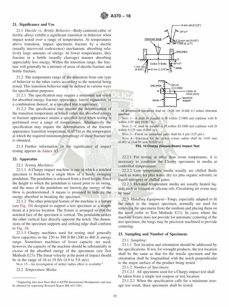
21. Significance and Use
21.1 Ductile vs. Brittle Behavior—Body-centered-cubic orferritic alloys exhibit a significant transition in behavior whenimpact tested over a range of temperatures. At temperaturesabove transition, impact specimens fracture by a ductile(usually microvoid coalescence) mechanism, absorbing rela-tively large amounts of energy. At lower temperatures, theyfracture in a brittle (usually cleavage) manner absorbingappreciably less energy. Within the transition range, the frac-ture will generally be a mixture of areas of ductile fracture andbrittle fracture.
21.2 The temperature range of the transition from one typeof behavior to the other varies according to the material beingtested. This transition behavior may be defined in various waysfor specification purposes.
21.2.1 The specification may require a minimum test resultfor absorbed energy, fracture appearance, lateral expansion, ora combination thereof, at a specified test temperature.
21.2.2 The specification may require the determination ofthe transition temperature at which either the absorbed energyor fracture appearance attains a specified level when testing isperformed over a range of temperatures. Alternatively thespecification may require the determination of the fractureappearance transition temperature (FATTn) as the temperatureat which the required minimum percentage of shear fracture (n)is obtained.
21.3 Further information on the significance of impacttesting appears in Annex A5.
22. Apparatus
22.1 Testing Machines:22.1.1 A Charpy impact machine is one in which a notched
specimen is broken by a single blow of a freely swingingpendulum. The pendulum is released from a fixed height. Sincethe height to which the pendulum is raised prior to its swing,and the mass of the pendulum are known, the energy of theblow is predetermined. A means is provided to indicate theenergy absorbed in breaking the specimen.
22.1.2 The other principal feature of the machine is a fixture(see Fig. 10) designed to support a test specimen as a simplebeam at a precise location. The fixture is arranged so that thenotched face of the specimen is vertical. The pendulum strikesthe other vertical face directly opposite the notch. The dimen-sions of the specimen supports and striking edge shall conformto Fig. 10.
22.1.3 Charpy machines used for testing steel generallyhave capacities in the 220 to 300 ft·lbf (300 to 400 J) energyrange. Sometimes machines of lesser capacity are used;however, the capacity of the machine should be substantially inexcess of the absorbed energy of the specimens (see TestMethods E23). The linear velocity at the point of impact shouldbe in the range of 16 to 19 ft/s (4.9 to 5.8 m/s).
NOTE 15—An investigation of striker radius effect is available.6
22.2 Temperature Media:
22.2.1 For testing at other than room temperature, it isnecessary to condition the Charpy specimens in media atcontrolled temperatures.
22.2.2 Low temperature media usually are chilled fluids(such as water, ice plus water, dry ice plus organic solvents, orliquid nitrogen) or chilled gases.
22.2.3 Elevated temperature media are usually heated liq-uids such as mineral or silicone oils. Circulating air ovens maybe used.
22.3 Handling Equipment—Tongs, especially adapted to fitthe notch in the impact specimen, normally are used forremoving the specimens from the medium and placing them onthe anvil (refer to Test Methods E23). In cases where themachine fixture does not provide for automatic centering of thetest specimen, the tongs may be precision machined to providecentering.
23. Sampling and Number of Specimens
23.1 Sampling:23.1.1 Test location and orientation should be addressed by
the specifications. If not, for wrought products, the test locationshall be the same as that for the tensile specimen and theorientation shall be longitudinal with the notch perpendicularto the major surface of the product being tested.
23.1.2 Number of Specimens.23.1.2.1 All specimens used for a Charpy impact test shall
be taken from a single test coupon or test location.23.1.2.2 When the specification calls for a minimum aver-
age test result, three specimens shall be tested.6 Supporting data have been filed at ASTM International Headquarters and may
be obtained by requesting Research Report RR:A01-1001.
All dimensional tolerances shall be 60.05 mm (0.002 in.) unless otherwisespecified.
NOTE 1—A shall be parallel to B within 2:1000 and coplanar with Bwithin 0.05 mm (0.002 in.).
NOTE 2—C shall be parallel to D within 20:1000 and coplanar with Dwithin 0.125 mm (0.005 in.).
NOTE 3—Finish on unmarked parts shall be 4 µm (125 µin.).NOTE 4—Tolerance for the striker corner radius shall be -0.05 mm
(0.002 in.) ⁄+0.50 mm (0.020 in.)FIG. 10 Charpy (Simple-Beam) Impact Test
A370 − 18
19

23.1.2.3 When the specification requires determination of atransition temperature, eight to twelve specimens are usuallyneeded.
23.2 Type and Size:23.2.1 Use a standard full size Charpy V-notch specimen as
shown in Fig. 11, except as allowed in 23.2.2.23.2.2 Subsized Specimens.23.2.2.1 For flat material less than 7⁄16 in. (11 mm) thick, or
when the absorbed energy is expected to exceed 80 % of fullscale, use standard subsize test specimens.
23.2.2.2 For tubular materials tested in the transversedirection, where the relationship between diameter and wallthickness does not permit a standard full size specimen, usestandard subsize test specimens or standard size specimenscontaining outer diameter (OD) curvature as follows:
(1) Standard size specimens and subsize specimens maycontain the original OD surface of the tubular product as shownin Fig. 12. All other dimensions shall comply with therequirements of Fig. 11.
NOTE 16—For materials with toughness levels in excess of about50 ft-lbs, specimens containing the original OD surface may yield valuesin excess of those resulting from the use of conventional Charpyspecimens.
23.2.2.3 If a standard full-size specimen cannot be prepared,the largest feasible standard subsize specimen shall be pre-pared. The specimens shall be machined so that the specimendoes not include material nearer to the surface than 0.020 in.(0.5 mm).
23.2.2.4 Tolerances for standard subsize specimens areshown in Fig. 11. Standard subsize test specimen sizes are:10 × 7.5 mm, 10 × 6.7 mm, 10 × 5 mm, 10 × 3.3 mm, and10 × 2.5 mm.
23.2.2.5 Notch the narrow face of the standard subsizespecimens so that the notch is perpendicular to the 10 mm wideface.
23.3 Notch Preparation—The machining (for example,milling, broaching, or grinding) of the notch is critical, asminor deviations in both notch radius and profile, or tool marksat the bottom of the notch may result in variations in test data,particularly in materials with low-impact energy absorption.(see Annex A5).
24. Calibration
24.1 Accuracy and Sensitivity—Calibrate and adjust Charpyimpact machines in accordance with the requirements of TestMethods E23.
25. Conditioning—Temperature Control
25.1 When a specific test temperature is required by thespecification or purchaser, control the temperature of theheating or cooling medium within 62°F (1°C).
NOTE 17—For some steels there may not be a need for this restrictedtemperature, for example, austenitic steels.
NOTE 18—Because the temperature of a testing laboratory often variesfrom 60 to 90°F (15 to 32°C) a test conducted at “room temperature”might be conducted at any temperature in this range.
26. Procedure
26.1 Temperature:26.1.1 Condition the specimens to be broken by holding
them in the medium at test temperature for at least 5 min inliquid media and 30 min in gaseous media.
26.1.2 Prior to each test, maintain the tongs for handling testspecimens at the same temperature as the specimen so as not toaffect the temperature at the notch.
26.2 Positioning and Breaking Specimens:26.2.1 Carefully center the test specimen in the anvil and
release the pendulum to break the specimen.26.2.2 If the pendulum is not released within 5 s after
removing the specimen from the conditioning medium, do notbreak the specimen. Return the specimen to the conditioningmedium for the period required in 26.1.1.
26.3 Recovering Specimens—In the event that fracture ap-pearance or lateral expansion must be determined, recover thematched pieces of each broken specimen before breaking thenext specimen.
26.4 Individual Test Values:26.4.1 Impact energy—Record the impact energy absorbed
to the nearest ft·lbf (J).26.4.2 Fracture Appearance:
NOTE 1—Permissible variations shall be as follows:
Notch length to edge 90 ±2°Adjacent sides shall be at 90° ± 10 minCross-section dimensions ±0.075 mm (±0.003 in.)Length of specimen (L) + 0, − 2.5 mm ( + 0, − 0.100 in.)Centering of notch (L/2) ±1 mm (±0.039 in.)Angle of notch ±1°Radius of notch ±0.025 mm (±0.001 in.)Notch depth ±0.025 mm (±0.001 in.)Finish requirements 2 µm (63 µin.) on notched surface and
oppositeface; 4 µm (125 µin.) on other two
surfaces(a) Standard Full Size Specimen
NOTE 2—On subsize specimens, all dimensions and tolerances of thestandard specimen remain constant with the exception of the width, whichvaries as shown above and for which the tolerance shall be 61 %.
(b) Standard Subsize Specimens
FIG. 11 Charpy (Simple Beam) Impact Test Specimens
A370 − 18
20

26.4.2.1 Determine the percentage of shear fracture area byany of the following methods:
(1) Measure the length and width of the brittle portion ofthe fracture surface, as shown in Fig. 13 and determine thepercent shear area from either Table 7 or Table 8 depending onthe units of measurement.
(2) Compare the appearance of the fracture of the specimenwith a fracture appearance chart as shown in Fig. 14.
(3) Magnify the fracture surface and compare it to aprecalibrated overlay chart or measure the percent shearfracture area by means of a planimeter.
(4) Photograph the fractured surface at a suitable magnifi-cation and measure the percent shear fracture area by means ofa planimeter.
26.4.2.2 Determine the individual fracture appearance val-ues to the nearest 5 % shear fracture and record the value.
26.4.3 Lateral Expansion:26.4.3.1 Lateral expansion is the increase in specimen
width, measured in thousandths of an inch (mils), on thecompression side, opposite the notch of the fractured CharpyV-notch specimen as shown in Fig. 15.
26.4.3.2 Examine each specimen half to ascertain that theprotrusions have not been damaged by contacting the anvil,machine mounting surface, and so forth. Discard such samplessince they may cause erroneous readings.
26.4.3.3 Check the sides of the specimens perpendicular tothe notch to ensure that no burrs were formed on the sidesduring impact testing. If burrs exist, remove them carefully byrubbing on emery cloth or similar abrasive surface, making
sure that the protrusions being measured are not rubbed duringthe removal of the burr.
26.4.3.4 Measure the amount of expansion on each side ofeach half relative to the plane defined by the undeformedportion of the side of the specimen using a gauge similar to thatshown in Figs. 16 and 17.
26.4.3.5 Since the fracture path seldom bisects the point ofmaximum expansion on both sides of a specimen, the sum ofthe larger values measured for each side is the value of the test.Arrange the halves of one specimen so that compression sidesare facing each other. Using the gauge, measure the protrusionon each half specimen, ensuring that the same side of thespecimen is measured. Measure the two broken halves indi-vidually. Repeat the procedure to measure the protrusions onthe opposite side of the specimen halves. The larger of the twovalues for each side is the expansion of that side of thespecimen.
26.4.3.6 Measure the individual lateral expansion values tothe nearest mil (0.025 mm) and record the values.
26.4.3.7 With the exception described as follows, any speci-men that does not separate into two pieces when struck by asingle blow shall be reported as unbroken. The lateral expan-sion of an unbroken specimen can be reported as broken if thespecimen can be separated by pushing the hinged halvestogether once and then pulling them apart without furtherfatiguing the specimen, and the lateral expansion measured forthe unbroken specimen (prior to bending) is equal to or greaterthan that measured for the separated halves. In the case wherea specimen cannot be separated into two halves, the lateral
FIG. 12 Tubular Impact Specimen Containing Original OD Surface
NOTE 1—Measure average dimensions A and B to the nearest 0.02 in. or 0.5 mm.NOTE 2—Determine the percent shear fracture using Table 7 or Table 8.
FIG. 13 Determination of Percent Shear Fracture
A370 − 18
21
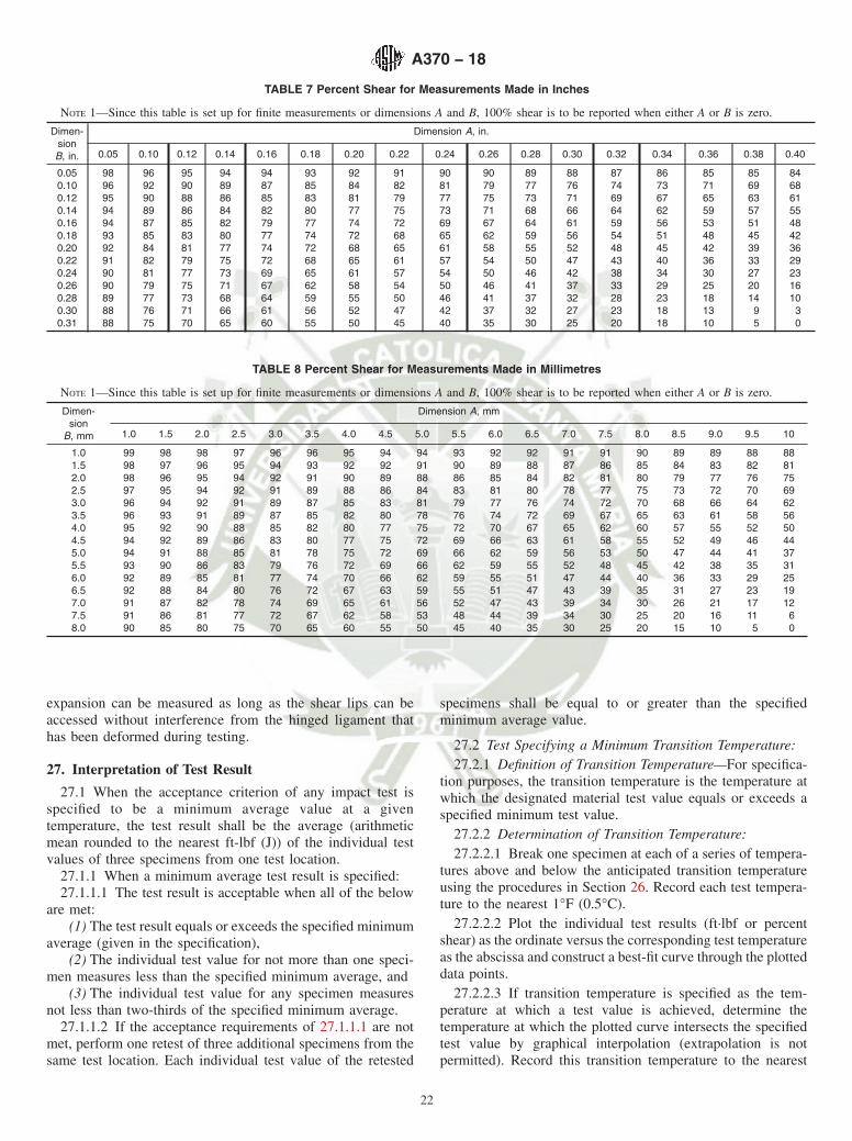
expansion can be measured as long as the shear lips can beaccessed without interference from the hinged ligament thathas been deformed during testing.
27. Interpretation of Test Result
27.1 When the acceptance criterion of any impact test isspecified to be a minimum average value at a giventemperature, the test result shall be the average (arithmeticmean rounded to the nearest ft-lbf (J)) of the individual testvalues of three specimens from one test location.
27.1.1 When a minimum average test result is specified:27.1.1.1 The test result is acceptable when all of the below
are met:(1) The test result equals or exceeds the specified minimum
average (given in the specification),(2) The individual test value for not more than one speci-
men measures less than the specified minimum average, and(3) The individual test value for any specimen measures
not less than two-thirds of the specified minimum average.27.1.1.2 If the acceptance requirements of 27.1.1.1 are not
met, perform one retest of three additional specimens from thesame test location. Each individual test value of the retested
specimens shall be equal to or greater than the specifiedminimum average value.
27.2 Test Specifying a Minimum Transition Temperature:27.2.1 Definition of Transition Temperature—For specifica-
tion purposes, the transition temperature is the temperature atwhich the designated material test value equals or exceeds aspecified minimum test value.
27.2.2 Determination of Transition Temperature:27.2.2.1 Break one specimen at each of a series of tempera-
tures above and below the anticipated transition temperatureusing the procedures in Section 26. Record each test tempera-ture to the nearest 1°F (0.5°C).
27.2.2.2 Plot the individual test results (ft·lbf or percentshear) as the ordinate versus the corresponding test temperatureas the abscissa and construct a best-fit curve through the plotteddata points.
27.2.2.3 If transition temperature is specified as the tem-perature at which a test value is achieved, determine thetemperature at which the plotted curve intersects the specifiedtest value by graphical interpolation (extrapolation is notpermitted). Record this transition temperature to the nearest
TABLE 7 Percent Shear for Measurements Made in Inches
NOTE 1—Since this table is set up for finite measurements or dimensions A and B, 100% shear is to be reported when either A or B is zero.
Dimen-sionB, in.
Dimension A, in.
0.05 0.10 0.12 0.14 0.16 0.18 0.20 0.22 0.24 0.26 0.28 0.30 0.32 0.34 0.36 0.38 0.40
0.05 98 96 95 94 94 93 92 91 90 90 89 88 87 86 85 85 840.10 96 92 90 89 87 85 84 82 81 79 77 76 74 73 71 69 680.12 95 90 88 86 85 83 81 79 77 75 73 71 69 67 65 63 610.14 94 89 86 84 82 80 77 75 73 71 68 66 64 62 59 57 550.16 94 87 85 82 79 77 74 72 69 67 64 61 59 56 53 51 480.18 93 85 83 80 77 74 72 68 65 62 59 56 54 51 48 45 420.20 92 84 81 77 74 72 68 65 61 58 55 52 48 45 42 39 360.22 91 82 79 75 72 68 65 61 57 54 50 47 43 40 36 33 290.24 90 81 77 73 69 65 61 57 54 50 46 42 38 34 30 27 230.26 90 79 75 71 67 62 58 54 50 46 41 37 33 29 25 20 160.28 89 77 73 68 64 59 55 50 46 41 37 32 28 23 18 14 100.30 88 76 71 66 61 56 52 47 42 37 32 27 23 18 13 9 30.31 88 75 70 65 60 55 50 45 40 35 30 25 20 18 10 5 0
TABLE 8 Percent Shear for Measurements Made in Millimetres
NOTE 1—Since this table is set up for finite measurements or dimensions A and B, 100% shear is to be reported when either A or B is zero.
Dimen-sion
B, mm
Dimension A, mm
1.0 1.5 2.0 2.5 3.0 3.5 4.0 4.5 5.0 5.5 6.0 6.5 7.0 7.5 8.0 8.5 9.0 9.5 10
1.0 99 98 98 97 96 96 95 94 94 93 92 92 91 91 90 89 89 88 881.5 98 97 96 95 94 93 92 92 91 90 89 88 87 86 85 84 83 82 812.0 98 96 95 94 92 91 90 89 88 86 85 84 82 81 80 79 77 76 752.5 97 95 94 92 91 89 88 86 84 83 81 80 78 77 75 73 72 70 693.0 96 94 92 91 89 87 85 83 81 79 77 76 74 72 70 68 66 64 623.5 96 93 91 89 87 85 82 80 78 76 74 72 69 67 65 63 61 58 564.0 95 92 90 88 85 82 80 77 75 72 70 67 65 62 60 57 55 52 504.5 94 92 89 86 83 80 77 75 72 69 66 63 61 58 55 52 49 46 445.0 94 91 88 85 81 78 75 72 69 66 62 59 56 53 50 47 44 41 375.5 93 90 86 83 79 76 72 69 66 62 59 55 52 48 45 42 38 35 316.0 92 89 85 81 77 74 70 66 62 59 55 51 47 44 40 36 33 29 256.5 92 88 84 80 76 72 67 63 59 55 51 47 43 39 35 31 27 23 197.0 91 87 82 78 74 69 65 61 56 52 47 43 39 34 30 26 21 17 127.5 91 86 81 77 72 67 62 58 53 48 44 39 34 30 25 20 16 11 68.0 90 85 80 75 70 65 60 55 50 45 40 35 30 25 20 15 10 5 0
A370 − 18
22

FIG. 14 Fracture Appearance Charts and Percent Shear Fracture Comparator
FIG. 15 Halves of Broken Charpy V-Notch Impact Specimen Joined for Measurement of Lateral Expansion, Dimension A
A370 − 18
23
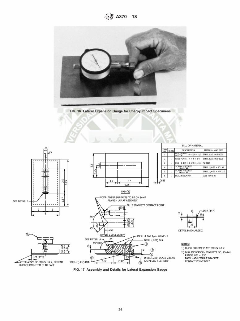
FIG. 16 Lateral Expansion Gauge for Charpy Impact Specimens
FIG. 17 Assembly and Details for Lateral Expansion Gauge
A370 − 18
24

5°F (3°C). If the tabulated test results clearly indicate atransition temperature lower than specified, it is not necessaryto plot the data. Report the lowest test temperature for whichtest value exceeds the specified value.
27.2.2.4 Accept the test result if the determined transitiontemperature is equal to or lower than the specified value.
27.2.2.5 If the determined transition temperature is higherthan the specified value, but not more than 20°F (12°C) higherthan the specified value, test sufficient samples in accordancewith Section 26 to plot two additional curves. Accept the testresults if the temperatures determined from both additionaltests are equal to or lower than the specified value.
27.3 When subsize specimens are permitted or necessary, orboth, modify the specified test requirement according to Table
9 or test temperature according to ASME Boiler and PressureVessel Code, Table UG-84.2, or both. Greater energies or lowertest temperatures may be agreed upon by purchaser andsupplier.
28. Records
28.1 The test record should contain the following informa-tion as appropriate:
28.1.1 Full description of material tested (that is, specifica-tion number, grade, class or type, size, heat number).
28.1.2 Specimen orientation with respect to the materialaxis.
28.1.3 Specimen size.
28.1.4 Test temperature and individual test value for eachspecimen broken, including initial tests and retests.
28.1.5 Test results.28.1.6 Transition temperature and criterion for its
determination, including initial tests and retests.
29. Report
29.1 The specification should designate the information tobe reported.
IZOD IMPACT TEST
30. Procedure
30.1 Testing equipment and methods are given in TestMethods E23.
31. Precision and Bias
31.1 The precision and bias of these test methods formeasuring mechanical properties are essentially as specified inTest Methods E8/E8M, E10, E18, and E23.
32. Keywords
32.1 bend test; Brinell hardness; Charpy impact test; elon-gation; FATT (Fracture Appearance Transition Temperature);hardness test; Izod impact test; portable hardness; reduction ofarea; Rockwell hardness; tensile strength; tension test; yieldstrength
TABLE 9 Charpy V-Notch Test Acceptance Criteria for Various Sub-Size SpecimensA,B,C
Full Size,10 by 10 mm
3⁄4 Size,10 by 7.5 mm
2⁄3 Size,10 by 6.7 mm
1⁄2 Size,10 by 5 mm
1⁄3 Size,10 by 3.3 mm
1⁄4 Size,10 by 2.5 mm
ft·lbf [J] ft·lbf [J] ft·lbf [J] ft·lbf [J] ft·lbf [J] ft·lbf [J]
75 [102] 56 [76] 50 [68] 38 [52] 25 [34] 19 [26]70 [95] 53 [72] 47 [64] 35 [48] 23 [31] 18 [24]65 [88] 49 [67] 44 [60] 33 [45] 21 [29] 16 [22]60 [82] 45 [61] 40 [54] 30 [41] 20 [27] 15 [20]55 [75] 41 [56] 37 [50] 28 [38] 18 [24] 14 [19]50 [68] 38 [52] 34 [46] 25 [34] 17 [23] 13 [18]45 [61] 34 [46] 30 [41] 23 [31] 15 [20] 11 [15]
40 [54] 30 [41] 27 [37] 20 [27] 13 [18] 10 [14]35 [48] 26 [35] 23 [31] 18 [24] 12 [16] 9 [12]30 [41] 22 [30] 20 [27] 15 [20] 10 [14] 8 [11]25 [34] 19 [26] 17 [23] 12 [16] 8 [11] 6 [8]20 [27] 15 [20] 13 [18] 10 [14] 7 [10] 5 [7]16 [22] 12 [16] 11 [15] 8 [11] 5 [7] 4 [5]15 [20] 11 [15] 10 [14] 8 [11] 5 [7] 4 [5]13 [18] 10 [14] 9 [12] 6 [8] 4 [5] 3 [4]12 [16] 9 [12] 8 [11] 6 [8] 4 [5] 3 [4]10 [14] 8 [11] 7 [10] 5 [7] 3 [4] 2 [3]7 [10] 5 [7] 5 [7] 4 [5] 2 [3] 2 [3]
A Care must be taken when using Table 9 for the conversion of subsize specimen absorbed energy results to those values that may be expected from full size Charpyspecimens. The use of conversion values should only be applied when both specimens types (full-size and sub-size) are in the same fracture regime (in other words. alower shelf, transition, or upper shelf) at the test temperature for the material under investigation. In particular test specimens <5 mm can exhibit variable absorbed energyvalues (NIST Technical Note 1858). (1)B Limit based upon presentation by Kim Wallin, VTT, “Sub-sized CVN Specimen Conversion Methodology 4, Slide #10,” which shows a common relationship for sub-sizedspecimens up to 75 ft·lbf (102J). (2)C Analysis of Data from NIST Note 1858 by J. A. Griffin, UAB, ASTM A01.13 Task Group meeting, San Antonio, TX 5.4.16. (1)
A370 − 18
25

ANNEXES
(Mandatory Information)
A1. STEEL BAR PRODUCTS
A1.1 Scope
A1.1.1 This annex contains testing requirements for SteelBar Products that are specific to the product. The requirementscontained in this annex are supplementary to those found in thegeneral section of this specification. In the case of conflictbetween requirements provided in this annex and those foundin the general section of this specification, the requirements ofthis annex shall prevail. In the case of conflict betweenrequirements provided in this annex and requirements found inproduct specifications, the requirements found in the productspecification shall prevail.
A1.2 Orientation of Test Specimens
A1.2.1 Carbon and alloy steel bars and bar-size shapes, dueto their relatively small cross-sectional dimensions, are cus-tomarily tested in the longitudinal direction. In special caseswhere size permits and the fabrication or service of a partjustifies testing in a transverse direction, the selection andlocation of test or tests are a matter of agreement between themanufacturer and the purchaser.
A1.3 Tension Test
A1.3.1 Carbon Steel Bars—Carbon steel bars are not com-monly specified to tensile requirements in the as-rolled condi-
tion for sizes of rounds, squares, hexagons, and octagons under1⁄2 in. (13 mm) in diameter or distance between parallel facesnor for other bar-size sections, other than flats, less than 1 in.2
(645 mm2) in cross-sectional area.
A1.3.2 Alloy Steel Bars—Alloy steel bars are usually nottested in the as-rolled condition.
A1.3.3 When tension tests are specified, the practice forselecting test specimens for hot-rolled and cold-finished steelbars of various sizes shall be in accordance with Table A1.1,unless otherwise specified in the product specification.
A1.4 Bend Test
A1.4.1 When bend tests are specified, the recommendedpractice for hot-rolled and cold-finished steel bars shall be inaccordance with Table A1.2.
A1.5 Hardness Test
A1.5.1 Hardness Tests on Bar Products—flats, rounds,squares, hexagons and octagons—is conducted on the surfaceafter a minimum removal of 0.015 in. to provide for accuratehardness penetration.
A370 − 18
26

TABLE A1.1 Practices for Selecting Tension Test Specimens for Steel Bar Products
NOTE 1—For bar sections where it is difficult to determine the cross-sectional area by simple measurement, the area in square inches may be calculatedby dividing the weight per linear inch of specimen in pounds by 0.2833 (weight of 1 in.3 of steel) or by dividing the weight per linear foot of specimenby 3.4 (weight of steel 1 in. square and 1 ft long).
Thickness, in. (mm) Width, in. (mm) Hot-Rolled Bars Cold-Finished Bars
FlatsUnder 5⁄8 (16) Up to 11⁄2 (38), incl Full section by 8-in. (200-mm) gauge
length (Fig. 3).Mill reduced section to 2-in. (50-mm)gauge length and approximately 25% lessthan test specimen width.
Over 11⁄2 (38) Full section, or mill to 11⁄2 in. (38 mm)wide by 8-in. (200-mm) gauge length (Fig.3).
Mill reduced section to 2-in. gauge lengthand 11⁄2 in. wide.
5⁄8 to 11⁄2 (16 to 38),excl
Up to 11⁄2 (38), incl Full section by 8-in. gauge length or ma-chine standard 1⁄2 by 2-in. (13 by 50-mm)gauge length specimen from center ofsection (Fig. 4).
Mill reduced section to 2-in. (50-mm)gauge length and approximately 25% lessthan test specimen width or machine stan-dard 1⁄2 by 2-in. (13 by 50-mm) gaugelength specimen from center of section(Fig. 4).
Over 11⁄2 (38) Full section, or mill 11⁄2 in. (38 mm) widthby 8-in. (200-mm) gauge length (Fig. 3) ormachine standard 1⁄2 by 2-in. gauge (13by 50-mm) gauge length specimen frommidway between edge and center of sec-tion (Fig. 4).
Mill reduced section to 2-in. gauge lengthand 11⁄2 in. wide or machine standard 1⁄2by 2-in. gauge length specimen from mid-way between edge and center of section(Fig. 4).
11⁄2 (38) and over Full section by 8-in. (200-mm) gaugelength, or machine standard 1⁄2 by 2-in.(13 by 50-mm) gauge length specimenfrom midway between surface and center(Fig. 4).
Machine standard 1⁄2 by 2-in. (13 by 50-mm) gauge length specimen from midwaybetween surface and center (Fig. 4).
Rounds, Squares, Hexagons, and Octagons
Diameter or Distance BetweenParallel Faces, in. (mm)
Hot-Rolled Bars Cold-Finished Bars
Under 5⁄8 Full section by 8-in. (200-mm) gauge length or ma-chine to subsize specimen (Fig. 4).
Machine to sub-size specimen (Fig. 4).
5⁄8 to 11⁄2 (16 to 38), excl Full section by 8-in. (200-mm) gauge length or ma-chine standard 1⁄2 in. by 2-in. (13 by 50-mm) gaugelength specimen from center of section (Fig. 4).
Machine standard 1⁄2 in. by 2-in. gauge length specimenfrom center of section (Fig. 4).
11⁄2 (38) and over Full section by 8-in. (200-mm) gauge length or ma-chine standard 1⁄2 in. by 2-in. (13 by 50-mm) gaugelength specimen from midway between surface andcenter of section (Fig. 4).
Machine standard 1⁄2 in. by 2-in. (13 by 50-mm gauge lengthspecimen from midway between surface and center of sec-tion (Fig. 4)).
Other Bar-Size SectionsAll sizes Full section by 8-in. (200-mm) gauge length or pre-
pare test specimen 11⁄2 in. (38 mm) wide (if possible)by 8-in. (200-mm) gauge length.
Mill reduced section to 2-in. (50-mm) gauge length and ap-proximately 25% less than test specimen width.
TABLE A1.2 Recommended Practice for Selecting Bend Test Specimens for Steel Bar Products
NOTE 1—The length of all specimens is to be not less than 6 in. (150 mm).
NOTE 2—The edges of the specimen may be rounded to a radius not exceeding 1⁄16 in. (1.6 mm).
FlatsThickness, in. (mm) Width, in. (mm) Recommended Size
Up to 1⁄2 (13), incl Up to 3⁄4 (19), incl Full section.
Over 3⁄4 (19) Full section or machine to not less than ot less than3⁄4 in. (19 mm) in width by thickness of specimen.
Over 1⁄2 (13) All Full section or machine to 1 by 1⁄2 in. (25 by 13 mm)specimen from midway between center and surface.
Rounds, Squares, Hexagons, and OctagonsDiameter or Distance Between Parallel Faces, in. (mm) Recommended SizeUp to 11⁄2 (38), incl Full section.
Over 11⁄2 (38) Machine to 1 by 1⁄2-in. (25 by 13-mm) specimen from midway between centerand surface.
A370 − 18
27
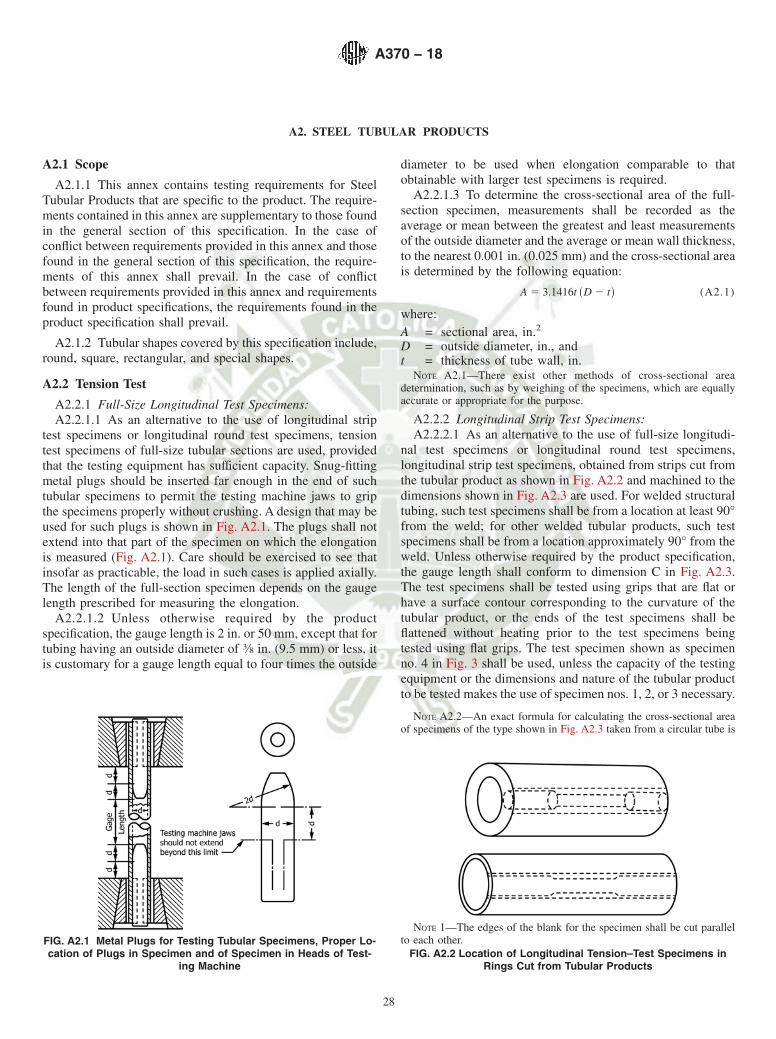
A2. STEEL TUBULAR PRODUCTS
A2.1 Scope
A2.1.1 This annex contains testing requirements for SteelTubular Products that are specific to the product. The require-ments contained in this annex are supplementary to those foundin the general section of this specification. In the case ofconflict between requirements provided in this annex and thosefound in the general section of this specification, the require-ments of this annex shall prevail. In the case of conflictbetween requirements provided in this annex and requirementsfound in product specifications, the requirements found in theproduct specification shall prevail.
A2.1.2 Tubular shapes covered by this specification include,round, square, rectangular, and special shapes.
A2.2 Tension Test
A2.2.1 Full-Size Longitudinal Test Specimens:A2.2.1.1 As an alternative to the use of longitudinal strip
test specimens or longitudinal round test specimens, tensiontest specimens of full-size tubular sections are used, providedthat the testing equipment has sufficient capacity. Snug-fittingmetal plugs should be inserted far enough in the end of suchtubular specimens to permit the testing machine jaws to gripthe specimens properly without crushing. A design that may beused for such plugs is shown in Fig. A2.1. The plugs shall notextend into that part of the specimen on which the elongationis measured (Fig. A2.1). Care should be exercised to see thatinsofar as practicable, the load in such cases is applied axially.The length of the full-section specimen depends on the gaugelength prescribed for measuring the elongation.
A2.2.1.2 Unless otherwise required by the productspecification, the gauge length is 2 in. or 50 mm, except that fortubing having an outside diameter of 3⁄8 in. (9.5 mm) or less, itis customary for a gauge length equal to four times the outside
diameter to be used when elongation comparable to thatobtainable with larger test specimens is required.
A2.2.1.3 To determine the cross-sectional area of the full-section specimen, measurements shall be recorded as theaverage or mean between the greatest and least measurementsof the outside diameter and the average or mean wall thickness,to the nearest 0.001 in. (0.025 mm) and the cross-sectional areais determined by the following equation:
A 5 3.1416t ~D 2 t! (A2.1)
where:A = sectional area, in.2
D = outside diameter, in., andt = thickness of tube wall, in.
NOTE A2.1—There exist other methods of cross-sectional areadetermination, such as by weighing of the specimens, which are equallyaccurate or appropriate for the purpose.
A2.2.2 Longitudinal Strip Test Specimens:A2.2.2.1 As an alternative to the use of full-size longitudi-
nal test specimens or longitudinal round test specimens,longitudinal strip test specimens, obtained from strips cut fromthe tubular product as shown in Fig. A2.2 and machined to thedimensions shown in Fig. A2.3 are used. For welded structuraltubing, such test specimens shall be from a location at least 90°from the weld; for other welded tubular products, such testspecimens shall be from a location approximately 90° from theweld. Unless otherwise required by the product specification,the gauge length shall conform to dimension C in Fig. A2.3.The test specimens shall be tested using grips that are flat orhave a surface contour corresponding to the curvature of thetubular product, or the ends of the test specimens shall beflattened without heating prior to the test specimens beingtested using flat grips. The test specimen shown as specimenno. 4 in Fig. 3 shall be used, unless the capacity of the testingequipment or the dimensions and nature of the tubular productto be tested makes the use of specimen nos. 1, 2, or 3 necessary.
NOTE A2.2—An exact formula for calculating the cross-sectional areaof specimens of the type shown in Fig. A2.3 taken from a circular tube is
FIG. A2.1 Metal Plugs for Testing Tubular Specimens, Proper Lo-cation of Plugs in Specimen and of Specimen in Heads of Test-
ing Machine
NOTE 1—The edges of the blank for the specimen shall be cut parallelto each other.
FIG. A2.2 Location of Longitudinal Tension–Test Specimens inRings Cut from Tubular Products
A370 − 18
28
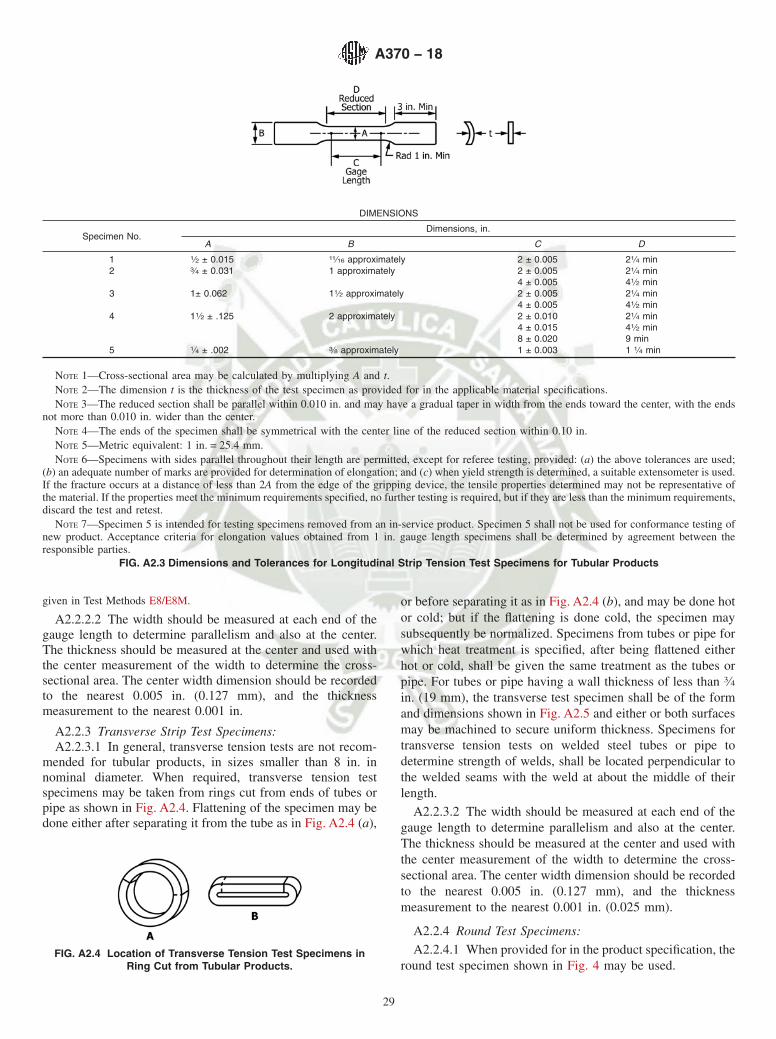
given in Test Methods E8/E8M.
A2.2.2.2 The width should be measured at each end of thegauge length to determine parallelism and also at the center.The thickness should be measured at the center and used withthe center measurement of the width to determine the cross-sectional area. The center width dimension should be recordedto the nearest 0.005 in. (0.127 mm), and the thicknessmeasurement to the nearest 0.001 in.
A2.2.3 Transverse Strip Test Specimens:A2.2.3.1 In general, transverse tension tests are not recom-
mended for tubular products, in sizes smaller than 8 in. innominal diameter. When required, transverse tension testspecimens may be taken from rings cut from ends of tubes orpipe as shown in Fig. A2.4. Flattening of the specimen may bedone either after separating it from the tube as in Fig. A2.4 (a),
or before separating it as in Fig. A2.4 (b), and may be done hotor cold; but if the flattening is done cold, the specimen maysubsequently be normalized. Specimens from tubes or pipe forwhich heat treatment is specified, after being flattened eitherhot or cold, shall be given the same treatment as the tubes orpipe. For tubes or pipe having a wall thickness of less than 3⁄4in. (19 mm), the transverse test specimen shall be of the formand dimensions shown in Fig. A2.5 and either or both surfacesmay be machined to secure uniform thickness. Specimens fortransverse tension tests on welded steel tubes or pipe todetermine strength of welds, shall be located perpendicular tothe welded seams with the weld at about the middle of theirlength.
A2.2.3.2 The width should be measured at each end of thegauge length to determine parallelism and also at the center.The thickness should be measured at the center and used withthe center measurement of the width to determine the cross-sectional area. The center width dimension should be recordedto the nearest 0.005 in. (0.127 mm), and the thicknessmeasurement to the nearest 0.001 in. (0.025 mm).
A2.2.4 Round Test Specimens:
A2.2.4.1 When provided for in the product specification, theround test specimen shown in Fig. 4 may be used.
DIMENSIONS
Specimen No.Dimensions, in.
A B C D
1 1⁄2 ± 0.015 11⁄16 approximately 2 ± 0.005 21⁄4 min2 3⁄4 ± 0.031 1 approximately 2 ± 0.005
4 ± 0.00521⁄4 min41⁄2 min
3 1± 0.062 11⁄2 approximately 2 ± 0.0054 ± 0.005
21⁄4 min41⁄2 min
4 11⁄2 ± .125 2 approximately 2 ± 0.0104 ± 0.0158 ± 0.020
21⁄4 min41⁄2 min9 min
5 1⁄4 ± .002 3⁄8 approximately 1 ± 0.003 1 1⁄4 min
NOTE 1—Cross-sectional area may be calculated by multiplying A and t.NOTE 2—The dimension t is the thickness of the test specimen as provided for in the applicable material specifications.NOTE 3—The reduced section shall be parallel within 0.010 in. and may have a gradual taper in width from the ends toward the center, with the ends
not more than 0.010 in. wider than the center.NOTE 4—The ends of the specimen shall be symmetrical with the center line of the reduced section within 0.10 in.NOTE 5—Metric equivalent: 1 in. = 25.4 mm.NOTE 6—Specimens with sides parallel throughout their length are permitted, except for referee testing, provided: (a) the above tolerances are used;
(b) an adequate number of marks are provided for determination of elongation; and (c) when yield strength is determined, a suitable extensometer is used.If the fracture occurs at a distance of less than 2A from the edge of the gripping device, the tensile properties determined may not be representative ofthe material. If the properties meet the minimum requirements specified, no further testing is required, but if they are less than the minimum requirements,discard the test and retest.
NOTE 7—Specimen 5 is intended for testing specimens removed from an in-service product. Specimen 5 shall not be used for conformance testing ofnew product. Acceptance criteria for elongation values obtained from 1 in. gauge length specimens shall be determined by agreement between theresponsible parties.
FIG. A2.3 Dimensions and Tolerances for Longitudinal Strip Tension Test Specimens for Tubular Products
FIG. A2.4 Location of Transverse Tension Test Specimens inRing Cut from Tubular Products.
A370 − 18
29

A2.2.4.2 The diameter of the round test specimen is mea-sured at the center of the specimen to the nearest 0.001 in.(0.025 mm).
A2.2.4.3 Small-size specimens proportional to standard, asshown in Fig. 4, may be used when it is necessary to testmaterial from which the standard specimen cannot be prepared.Other sizes of small-size specimens may be used. In any suchsmall-size specimen, it is important that the gauge length formeasurement of elongation be four times the diameter of thespecimen (see Note 5, Fig. 4). The elongation requirements forthe round specimen 2-in. gauge length in the product specifi-cation shall apply to the small-size specimens.
A2.2.4.4 For transverse specimens, the section from whichthe specimen is taken shall not be flattened or otherwisedeformed.
A2.2.4.5 Longitudinal test specimens are obtained fromstrips cut from the tubular product as shown in Fig. A2.2.
A2.3 Determination of Transverse Yield Strength, Hydrau-lic Ring-Expansion Method
A2.3.1 Hardness tests are made on the outside surface,inside surface, or wall cross-section depending upon product-specification limitation. Surface preparation may be necessaryto obtain accurate hardness values.
A2.3.2 A testing machine and method for determining thetransverse yield strength from an annular ring specimen, havebeen developed and described in A2.3.3 – 9.1.2.
A2.3.3 A diagrammatic vertical cross-sectional sketch ofthe testing machine is shown in Fig. A2.6.
A2.3.4 In determining the transverse yield strength on thismachine, a short ring (commonly 3 in. (76 mm) in length) testspecimen is used. After the large circular nut is removed fromthe machine, the wall thickness of the ring specimen isdetermined and the specimen is telescoped over the oil resistantrubber gasket. The nut is then replaced, but is not turned downtight against the specimen. A slight clearance is left betweenthe nut and specimen for the purpose of permitting free radialmovement of the specimen as it is being tested. Oil underpressure is then admitted to the interior of the rubber gasketthrough the pressure line under the control of a suitable valve.An accurately calibrated pressure gauge serves to measure oilpressure. Any air in the system is removed through the bleederline. As the oil pressure is increased, the rubber gasket expandswhich in turn stresses the specimen circumferentially. As thepressure builds up, the lips of the rubber gasket act as a seal toprevent oil leakage. With continued increase in pressure, thering specimen is subjected to a tension stress and elongatesaccordingly. The entire outside circumference of the ringspecimen is considered as the gauge length and the strain ismeasured with a suitable extensometer which will be describedlater. When the desired total strain or extension under load isreached on the extensometer, the oil pressure in pounds persquare inch is read and by employing Barlow’s formula, theunit yield strength is calculated. The yield strength, thusdetermined, is a true result since the test specimen has not beencold worked by flattening and closely approximates the samecondition as the tubular section from which it is cut. Further,the test closely simulates service conditions in pipe lines. Onetesting machine unit may be used for several different sizes ofpipe by the use of suitable rubber gaskets and adapters.
NOTE A2.3—Barlow’s formula may be stated two ways:
~1! P 5 2St/D (A2.2)
~2! S 5 PD/2t (A2.3)
where:P = internal hydrostatic pressure, psi,S = unit circumferential stress in the wall of the tube
produced by the internal hydrostatic pressure, psi,t = thickness of the tube wall, in., andD = outside diameter of the tube, in.
A2.3.5 A roller chain type extensometer which has beenfound satisfactory for measuring the elongation of the ringspecimen is shown in Figs. A2.7 and A2.8. Fig. A2.7 shows theextensometer in position, but unclamped, on a ring specimen.A small pin, through which the strain is transmitted to andmeasured by the dial gauge, extends through the hollowthreaded stud. When the extensometer is clamped, as shown inFig. A2.8, the desired tension which is necessary to hold theinstrument in place and to remove any slack, is exerted on theroller chain by the spring. Tension on the spring may beregulated as desired by the knurled thumb screw. By removingor adding rollers, the roller chain may be adapted for differentsizes of tubular sections.
A2.4 Hardness Tests
A2.4.1 Hardness tests are made either on the outside or theinside surfaces on the end of the tube as appropriate.
NOTE 1—The dimension t is the thickness of the test specimen asprovided for in the applicable material specifications.
NOTE 2—The reduced section shall be parallel within 0.010 in. and mayhave a gradual taper in width from the ends toward the center, with theends not more than 0.010 in. wider than the center.
NOTE 3—The ends of the specimen shall be symmetrical with the centerline of the reduced section within 0.10 in.
NOTE 4—Metric equivalent: 1 in. = 25.6 mm.FIG. A2.5 Transverse Tension Test Specimen Machined from Ring
Cut from Tubular Products
FIG. A2.6 Testing Machine for Determination of Transverse YieldStrength from Annular Ring Specimens
A370 − 18
30
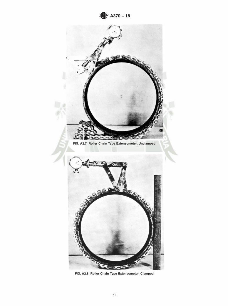
FIG. A2.7 Roller Chain Type Extensometer, Unclamped
FIG. A2.8 Roller Chain Type Extensometer, Clamped
A370 − 18
31
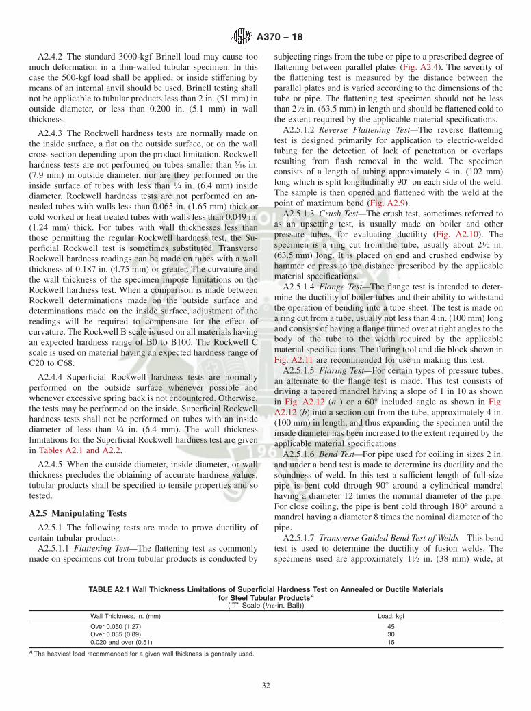
A2.4.2 The standard 3000-kgf Brinell load may cause toomuch deformation in a thin-walled tubular specimen. In thiscase the 500-kgf load shall be applied, or inside stiffening bymeans of an internal anvil should be used. Brinell testing shallnot be applicable to tubular products less than 2 in. (51 mm) inoutside diameter, or less than 0.200 in. (5.1 mm) in wallthickness.
A2.4.3 The Rockwell hardness tests are normally made onthe inside surface, a flat on the outside surface, or on the wallcross-section depending upon the product limitation. Rockwellhardness tests are not performed on tubes smaller than 5⁄16 in.(7.9 mm) in outside diameter, nor are they performed on theinside surface of tubes with less than 1⁄4 in. (6.4 mm) insidediameter. Rockwell hardness tests are not performed on an-nealed tubes with walls less than 0.065 in. (1.65 mm) thick orcold worked or heat treated tubes with walls less than 0.049 in.(1.24 mm) thick. For tubes with wall thicknesses less thanthose permitting the regular Rockwell hardness test, the Su-perficial Rockwell test is sometimes substituted. TransverseRockwell hardness readings can be made on tubes with a wallthickness of 0.187 in. (4.75 mm) or greater. The curvature andthe wall thickness of the specimen impose limitations on theRockwell hardness test. When a comparison is made betweenRockwell determinations made on the outside surface anddeterminations made on the inside surface, adjustment of thereadings will be required to compensate for the effect ofcurvature. The Rockwell B scale is used on all materials havingan expected hardness range of B0 to B100. The Rockwell Cscale is used on material having an expected hardness range ofC20 to C68.
A2.4.4 Superficial Rockwell hardness tests are normallyperformed on the outside surface whenever possible andwhenever excessive spring back is not encountered. Otherwise,the tests may be performed on the inside. Superficial Rockwellhardness tests shall not be performed on tubes with an insidediameter of less than 1⁄4 in. (6.4 mm). The wall thicknesslimitations for the Superficial Rockwell hardness test are givenin Tables A2.1 and A2.2.
A2.4.5 When the outside diameter, inside diameter, or wallthickness precludes the obtaining of accurate hardness values,tubular products shall be specified to tensile properties and sotested.
A2.5 Manipulating Tests
A2.5.1 The following tests are made to prove ductility ofcertain tubular products:
A2.5.1.1 Flattening Test—The flattening test as commonlymade on specimens cut from tubular products is conducted by
subjecting rings from the tube or pipe to a prescribed degree offlattening between parallel plates (Fig. A2.4). The severity ofthe flattening test is measured by the distance between theparallel plates and is varied according to the dimensions of thetube or pipe. The flattening test specimen should not be lessthan 21⁄2 in. (63.5 mm) in length and should be flattened cold tothe extent required by the applicable material specifications.
A2.5.1.2 Reverse Flattening Test—The reverse flatteningtest is designed primarily for application to electric-weldedtubing for the detection of lack of penetration or overlapsresulting from flash removal in the weld. The specimenconsists of a length of tubing approximately 4 in. (102 mm)long which is split longitudinally 90° on each side of the weld.The sample is then opened and flattened with the weld at thepoint of maximum bend (Fig. A2.9).
A2.5.1.3 Crush Test—The crush test, sometimes referred toas an upsetting test, is usually made on boiler and otherpressure tubes, for evaluating ductility (Fig. A2.10). Thespecimen is a ring cut from the tube, usually about 21⁄2 in.(63.5 mm) long. It is placed on end and crushed endwise byhammer or press to the distance prescribed by the applicablematerial specifications.
A2.5.1.4 Flange Test—The flange test is intended to deter-mine the ductility of boiler tubes and their ability to withstandthe operation of bending into a tube sheet. The test is made ona ring cut from a tube, usually not less than 4 in. (100 mm) longand consists of having a flange turned over at right angles to thebody of the tube to the width required by the applicablematerial specifications. The flaring tool and die block shown inFig. A2.11 are recommended for use in making this test.
A2.5.1.5 Flaring Test—For certain types of pressure tubes,an alternate to the flange test is made. This test consists ofdriving a tapered mandrel having a slope of 1 in 10 as shownin Fig. A2.12 (a ) or a 60° included angle as shown in Fig.A2.12 (b) into a section cut from the tube, approximately 4 in.(100 mm) in length, and thus expanding the specimen until theinside diameter has been increased to the extent required by theapplicable material specifications.
A2.5.1.6 Bend Test—For pipe used for coiling in sizes 2 in.and under a bend test is made to determine its ductility and thesoundness of weld. In this test a sufficient length of full-sizepipe is bent cold through 90° around a cylindrical mandrelhaving a diameter 12 times the nominal diameter of the pipe.For close coiling, the pipe is bent cold through 180° around amandrel having a diameter 8 times the nominal diameter of thepipe.
A2.5.1.7 Transverse Guided Bend Test of Welds—This bendtest is used to determine the ductility of fusion welds. Thespecimens used are approximately 11⁄2 in. (38 mm) wide, at
TABLE A2.1 Wall Thickness Limitations of Superficial Hardness Test on Annealed or Ductile Materialsfor Steel Tubular ProductsA
(“T” Scale (1⁄16-in. Ball))Wall Thickness, in. (mm) Load, kgf
Over 0.050 (1.27) 45Over 0.035 (0.89) 300.020 and over (0.51) 15
A The heaviest load recommended for a given wall thickness is generally used.
A370 − 18
32

least 6 in. (152 mm) in length with the weld at the center, andare machined in accordance with Fig. A2.13 for face and rootbend tests and in accordance with Fig. A2.14 for side bendtests. The dimensions of the plunger shall be as shown in Fig.A2.15 and the other dimensions of the bending jig shall besubstantially as given in this same figure. A test shall consist ofa face bend specimen and a root bend specimen or two sidebend specimens. A face bend test requires bending with the
inside surface of the pipe against the plunger; a root bend testrequires bending with the outside surface of the pipe againstthe plunger; and a side bend test requires bending so that oneof the side surfaces becomes the convex surface of the bendspecimen.
(a) Failure of the bend test depends upon the appearance ofcracks in the area of the bend, of the nature and extentdescribed in the product specifications.
TABLE A2.2 Wall Thickness Limitations of Superficial Hardness Test on Cold Worked or Heat Treated Materialfor Steel Tubular ProductsA
(“N” Scale (Diamond Penetrator))Wall Thickness, in. (mm) Load, kgf
Over 0.035 (0.89) 45Over 0.025 (0.51) 300.015 and over (0.38) 15
A The heaviest load recommended for a given wall thickness is generally used.
FIG. A2.9 Reverse Flattening Test
FIG. A2.10 Crush Test Specimen
A370 − 18
33

NOTE 1—Metric equivalent: 1 in. = 25.4 mm.FIG. A2.11 Flaring Tool and Die Block for Flange Test
FIG. A2.12 Tapered Mandrels for Flaring Test
NOTE 1—Metric equivalent: 1 in. = 25.4 mm.
Pipe Wall Thickness (t), in. Test Specimen Thickness, in.Up to 3⁄8, incl tOver 3⁄8 3⁄8
FIG. A2.13 Transverse Face- and Root-Bend Test Specimens
A370 − 18
34
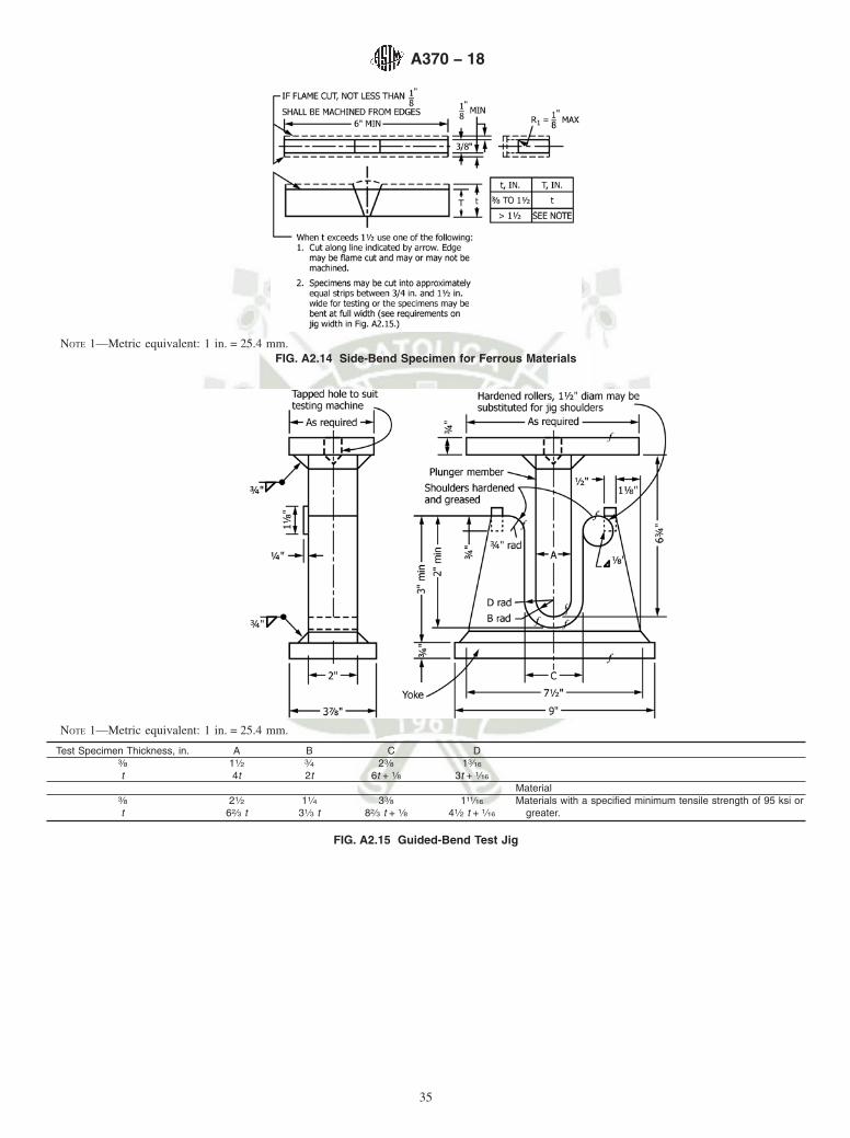
NOTE 1—Metric equivalent: 1 in. = 25.4 mm.FIG. A2.14 Side-Bend Specimen for Ferrous Materials
NOTE 1—Metric equivalent: 1 in. = 25.4 mm.
Test Specimen Thickness, in. A B C D3⁄8t
11⁄24t
3⁄42t
23⁄86t + 1⁄8
13⁄16
3t + 1⁄16
Material3⁄8t
21⁄262⁄3 t
11⁄431⁄3 t
33⁄882⁄3 t + 1⁄8
111⁄16
41⁄2 t + 1⁄16
Materials with a specified minimum tensile strength of 95 ksi orgreater.
FIG. A2.15 Guided-Bend Test Jig
A370 − 18
35
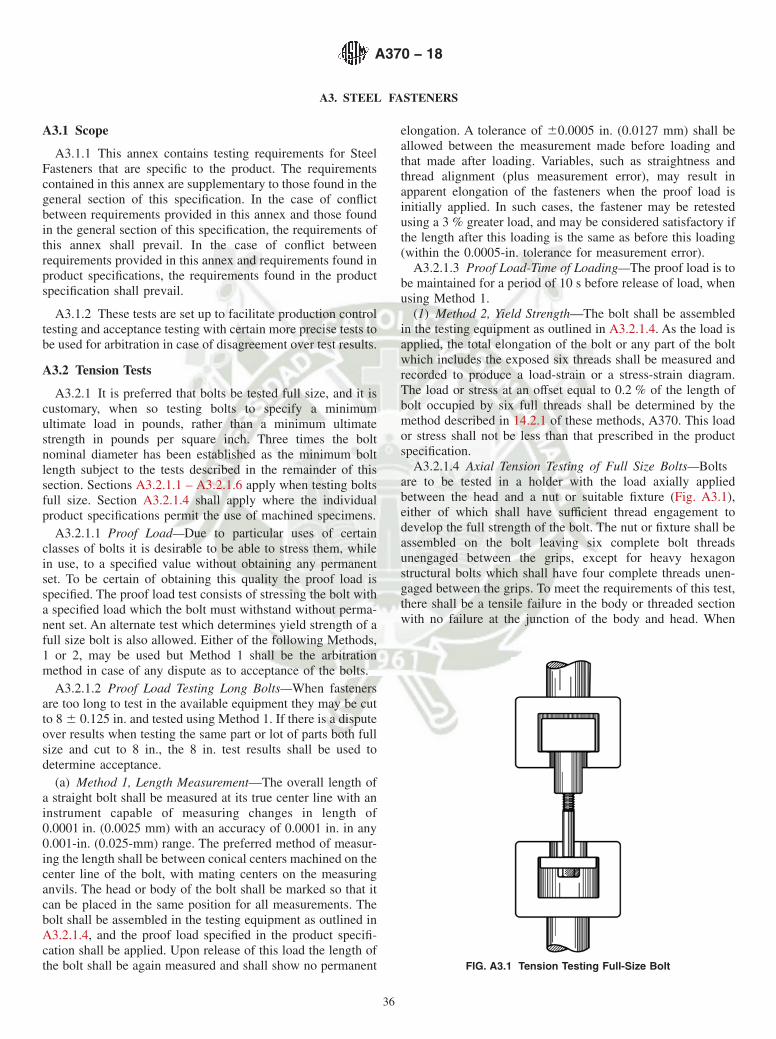
A3. STEEL FASTENERS
A3.1 Scope
A3.1.1 This annex contains testing requirements for SteelFasteners that are specific to the product. The requirementscontained in this annex are supplementary to those found in thegeneral section of this specification. In the case of conflictbetween requirements provided in this annex and those foundin the general section of this specification, the requirements ofthis annex shall prevail. In the case of conflict betweenrequirements provided in this annex and requirements found inproduct specifications, the requirements found in the productspecification shall prevail.
A3.1.2 These tests are set up to facilitate production controltesting and acceptance testing with certain more precise tests tobe used for arbitration in case of disagreement over test results.
A3.2 Tension Tests
A3.2.1 It is preferred that bolts be tested full size, and it iscustomary, when so testing bolts to specify a minimumultimate load in pounds, rather than a minimum ultimatestrength in pounds per square inch. Three times the boltnominal diameter has been established as the minimum boltlength subject to the tests described in the remainder of thissection. Sections A3.2.1.1 – A3.2.1.6 apply when testing boltsfull size. Section A3.2.1.4 shall apply where the individualproduct specifications permit the use of machined specimens.
A3.2.1.1 Proof Load—Due to particular uses of certainclasses of bolts it is desirable to be able to stress them, whilein use, to a specified value without obtaining any permanentset. To be certain of obtaining this quality the proof load isspecified. The proof load test consists of stressing the bolt witha specified load which the bolt must withstand without perma-nent set. An alternate test which determines yield strength of afull size bolt is also allowed. Either of the following Methods,1 or 2, may be used but Method 1 shall be the arbitrationmethod in case of any dispute as to acceptance of the bolts.
A3.2.1.2 Proof Load Testing Long Bolts—When fastenersare too long to test in the available equipment they may be cutto 8 6 0.125 in. and tested using Method 1. If there is a disputeover results when testing the same part or lot of parts both fullsize and cut to 8 in., the 8 in. test results shall be used todetermine acceptance.
(a) Method 1, Length Measurement—The overall length ofa straight bolt shall be measured at its true center line with aninstrument capable of measuring changes in length of0.0001 in. (0.0025 mm) with an accuracy of 0.0001 in. in any0.001-in. (0.025-mm) range. The preferred method of measur-ing the length shall be between conical centers machined on thecenter line of the bolt, with mating centers on the measuringanvils. The head or body of the bolt shall be marked so that itcan be placed in the same position for all measurements. Thebolt shall be assembled in the testing equipment as outlined inA3.2.1.4, and the proof load specified in the product specifi-cation shall be applied. Upon release of this load the length ofthe bolt shall be again measured and shall show no permanent
elongation. A tolerance of 60.0005 in. (0.0127 mm) shall beallowed between the measurement made before loading andthat made after loading. Variables, such as straightness andthread alignment (plus measurement error), may result inapparent elongation of the fasteners when the proof load isinitially applied. In such cases, the fastener may be retestedusing a 3 % greater load, and may be considered satisfactory ifthe length after this loading is the same as before this loading(within the 0.0005-in. tolerance for measurement error).
A3.2.1.3 Proof Load-Time of Loading—The proof load is tobe maintained for a period of 10 s before release of load, whenusing Method 1.
(1) Method 2, Yield Strength—The bolt shall be assembledin the testing equipment as outlined in A3.2.1.4. As the load isapplied, the total elongation of the bolt or any part of the boltwhich includes the exposed six threads shall be measured andrecorded to produce a load-strain or a stress-strain diagram.The load or stress at an offset equal to 0.2 % of the length ofbolt occupied by six full threads shall be determined by themethod described in 14.2.1 of these methods, A370. This loador stress shall not be less than that prescribed in the productspecification.
A3.2.1.4 Axial Tension Testing of Full Size Bolts—Boltsare to be tested in a holder with the load axially appliedbetween the head and a nut or suitable fixture (Fig. A3.1),either of which shall have sufficient thread engagement todevelop the full strength of the bolt. The nut or fixture shall beassembled on the bolt leaving six complete bolt threadsunengaged between the grips, except for heavy hexagonstructural bolts which shall have four complete threads unen-gaged between the grips. To meet the requirements of this test,there shall be a tensile failure in the body or threaded sectionwith no failure at the junction of the body and head. When
FIG. A3.1 Tension Testing Full-Size Bolt
A370 − 18
36

tensile testing externally threaded fasteners made of austeniticstainless steel and the test fastener’s thread pulls out of theinternally threaded test fixture after the minimum tensilestrength requirement has been reached, the fasteners shall beconsidered conforming to the tensile strength requirement and,in addition to the tensile strength, the failure mode shall bereported to the purchaser. If it is necessary to record or reportthe tensile strength of bolts as psi values, the stress area shallbe calculated from the mean of the mean root and pitchdiameters of Class 3 external threads as follows:
As 5 0.7854 @D 2 ~0.9743/n!#2 (A3.1)
where:As = stress area, in.2,D = nominal diameter, in., andn = number of threads per inch.
A3.2.1.5 Tension Testing of Full-Size Bolts with a Wedge—The purpose of this test is to obtain the tensile strength anddemonstrate the “head quality” and ductility of a bolt with a
standard head by subjecting it to eccentric loading. Theultimate load on the bolt shall be determined as described inA3.2.1.4, except that a 10° wedge shall be placed under thesame bolt previously tested for the proof load (see A3.2.1.1).The bolt head shall be so placed that no corner of the hexagonor square takes a bearing load, that is, a flat of the head shallbe aligned with the direction of uniform thickness of the wedge(Fig. A3.2). The wedge shall have an included angle betweenits faces as shown in Table A3.1 and shall have a thickness ofone-half of the nominal bolt diameter at the short side of thehole. The hole in the wedge shall have the following clearanceover the nominal size of the bolt, and its edges, top and bottom,shall be rounded to the following radius:
Nominal Bolt Size, in.Clearance in Hole, in.
(mm)Radius on Corners of
Hole, in. (mm)1⁄4 to 1⁄2 0.030 (0.76) 0.030 (0.76)9⁄16 to 3⁄4 0.050 (1.3) 0.060 (1.5)7⁄8 to 1 0.063 (1.5) 0.060 (1.5)
11⁄8 to 11⁄4 0.063 (1.5) 0.125 (3.2)13⁄8 to 11⁄2 0.094 (2.4) 0.125 (3.2)
c = Clearance of wedge holed = Diameter of boltR = RadiusT = Thickness of wedge at short side of hole equal to one-half diameter of bolt
FIG. A3.2 Wedge Test Detail
A370 − 18
37
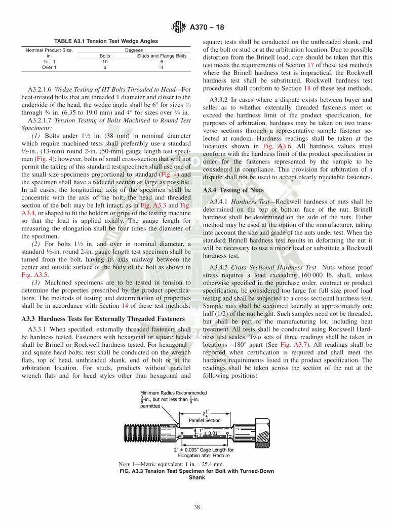
A3.2.1.6 Wedge Testing of HT Bolts Threaded to Head—Forheat-treated bolts that are threaded 1 diameter and closer to theunderside of the head, the wedge angle shall be 6° for sizes 1⁄4through 3⁄4 in. (6.35 to 19.0 mm) and 4° for sizes over 3⁄4 in.
A3.2.1.7 Tension Testing of Bolts Machined to Round TestSpecimens:
(1) Bolts under 11⁄2 in. (38 mm) in nominal diameterwhich require machined tests shall preferably use a standard1⁄2-in., (13-mm) round 2-in. (50-mm) gauge length test speci-men (Fig. 4); however, bolts of small cross-section that will notpermit the taking of this standard test specimen shall use one ofthe small-size-specimens-proportional-to-standard (Fig. 4) andthe specimen shall have a reduced section as large as possible.In all cases, the longitudinal axis of the specimen shall beconcentric with the axis of the bolt; the head and threadedsection of the bolt may be left intact, as in Fig. A3.3 and Fig.A3.4, or shaped to fit the holders or grips of the testing machineso that the load is applied axially. The gauge length formeasuring the elongation shall be four times the diameter ofthe specimen.
(2) For bolts 11⁄2 in. and over in nominal diameter, astandard 1⁄2-in. round 2-in. gauge length test specimen shall beturned from the bolt, having its axis midway between thecenter and outside surface of the body of the bolt as shown inFig. A3.5.
(3) Machined specimens are to be tested in tension todetermine the properties prescribed by the product specifica-tions. The methods of testing and determination of propertiesshall be in accordance with Section 14 of these test methods.
A3.3 Hardness Tests for Externally Threaded Fasteners
A3.3.1 When specified, externally threaded fasteners shallbe hardness tested. Fasteners with hexagonal or square headsshall be Brinell or Rockwell hardness tested. For hexagonaland square head bolts; test shall be conducted on the wrenchflats, top of head, unthreaded shank, end of bolt or at thearbitration location. For studs, products without parallelwrench flats and for head styles other than hexagonal and
square; tests shall be conducted on the unthreaded shank, endof the bolt or stud or at the arbitration location. Due to possibledistortion from the Brinell load, care should be taken that thistest meets the requirements of Section 17 of these test methodswhere the Brinell hardness test is impractical, the Rockwellhardness test shall be substituted. Rockwell hardness testprocedures shall conform to Section 18 of these test methods.
A3.3.2 In cases where a dispute exists between buyer andseller as to whether externally threaded fasteners meet orexceed the hardness limit of the product specification, forpurposes of arbitration, hardness may be taken on two trans-verse sections through a representative sample fastener se-lected at random. Hardness readings shall be taken at thelocations shown in Fig. A3.6. All hardness values mustconform with the hardness limit of the product specification inorder for the fasteners represented by the sample to beconsidered in compliance. This provision for arbitration of adispute shall not be used to accept clearly rejectable fasteners.
A3.4 Testing of Nuts
A3.4.1 Hardness Test—Rockwell hardness of nuts shall bedetermined on the top or bottom face of the nut. Brinellhardness shall be determined on the side of the nuts. Eithermethod may be used at the option of the manufacturer, takinginto account the size and grade of the nuts under test. When thestandard Brinell hardness test results in deforming the nut itwill be necessary to use a minor load or substitute a Rockwellhardness test.
A3.4.2 Cross Sectional Hardness Test—Nuts whose proofstress requires a load exceeding 160 000 lb. shall, unlessotherwise specified in the purchase order, contract or productspecification, be considered too large for full size proof loadtesting and shall be subjected to a cross sectional hardness test.Sample nuts shall be sectioned laterally at approximately onehalf (1/2) of the nut height. Such samples need not be threaded,but shall be part of the manufacturing lot, including heattreatment. All tests shall be conducted using Rockwell Hard-ness test scales. Two sets of three readings shall be taken inlocations ~180° apart (See Fig. A3.7). All readings shall bereported when certification is required and shall meet thehardness requirements listed in the product specification. Thereadings shall be taken across the section of the nut at thefollowing positions:
TABLE A3.1 Tension Test Wedge Angles
Nominal Product Size,in.
DegreesBolts Studs and Flange Bolts
1⁄4 – 1 10 6Over 1 6 4
NOTE 1—Metric equivalent: 1 in. = 25.4 mm.FIG. A3.3 Tension Test Specimen for Bolt with Turned-Down
Shank
A370 − 18
38
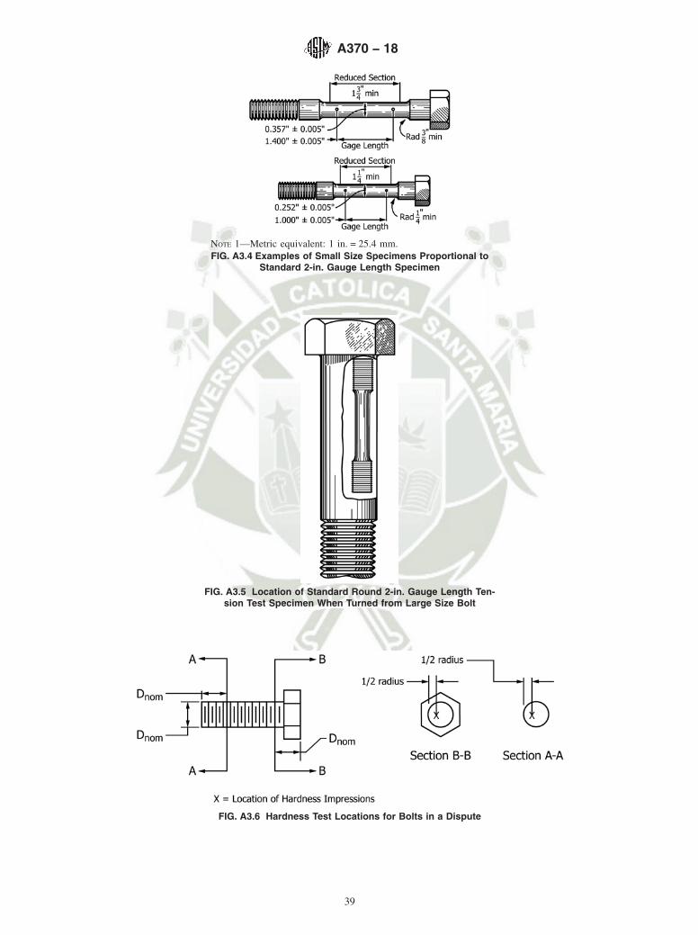
NOTE 1—Metric equivalent: 1 in. = 25.4 mm.FIG. A3.4 Examples of Small Size Specimens Proportional to
Standard 2-in. Gauge Length Specimen
FIG. A3.5 Location of Standard Round 2-in. Gauge Length Ten-sion Test Specimen When Turned from Large Size Bolt
FIG. A3.6 Hardness Test Locations for Bolts in a Dispute
A370 − 18
39

Position 1—as close as practical to the major diameter (ifthreaded) or hole side wall (if blank), but no closer than 2-1/2times the diameter of the indenter.
Position 2—at the core (halfway between the major diameter(if threaded) or hole side wall, if blank) and a corner of the nut.
Position 3—as close as practical to the corner of the nut, butno closer than 2-1/2 times the diameter of the indenter.
A4. STEEL ROUND WIRE PRODUCTS
A4.1 Scope
A4.1.1 This annex contains testing requirements for RoundWire Products that are specific to the product. The require-ments contained in this annex are supplementary to those foundin the general section of this specification. In the case ofconflict between requirements provided in this annex and thosefound in the general section of this specification, the require-ments of this annex shall prevail. In the case of conflictbetween requirements provided in this annex and requirementsfound in product specifications, the requirements found in theproduct specification shall prevail.
A4.2 Apparatus
A4.2.1 Gripping Devices—Grips of either the wedge orsnubbing types as shown in Figs. A4.1 and A4.2 shall be used(Note A4.1). When using grips of either type, care shall betaken that the axis of the test specimen is located approxi-mately at the center line of the head of the testing machine(Note A4.2). When using wedge grips the liners used behindthe grips shall be of the proper thickness.
NOTE A4.1—Testing machines usually are equipped with wedge grips.These wedge grips, irrespective of the type of testing machine, may bereferred to as the “usual type” of wedge grips. The use of fine (180 or 240)grit abrasive cloth in the “usual” wedge type grips, with the abrasivecontacting the wire specimen, can be helpful in reducing specimen
slipping and breakage at the grip edges at tensile loads up to about 1000pounds. For tests of specimens of wire which are liable to be cut at theedges by the “usual type” of wedge grips, the snubbing type grippingdevice has proved satisfactory.
For testing round wire, the use of cylindrical seat in the wedge grippingdevice is optional.
NOTE A4.2—Any defect in a testing machine which may cause nonaxialapplication of load should be corrected.
A4.2.2 Pointed Micrometer—A micrometer with a pointedspindle and anvil suitable for reading the dimensions of thewire specimen at the fractured ends to the nearest 0.001 in.(0.025 mm) after breaking the specimen in the testing machineshall be used.
A4.3 Test Specimens
A4.3.1 Test specimens having the full cross-sectional areaof the wire they represent shall be used. The standard gaugelength of the specimens shall be 10 in. (254 mm). However, ifthe determination of elongation values is not required, anyconvenient gauge length is permissible. The total length of thespecimens shall be at least equal to the gauge length (10 in.)plus twice the length of wire required for the full use of the gripemployed. For example, depending upon the type of testingmachine and grips used, the minimum total length of specimenmay vary from 14 to 24 in. (360 to 610 mm) for a 10-in. gaugelength specimen.
A4.3.2 Any specimen breaking in the grips shall be dis-carded and a new specimen tested.
FIG. A3.7 Hardness Test Locations
FIG. A4.1 Wedge-Type Gripping Device
FIG. A4.2 Snubbing-Type Gripping Device
A370 − 18
40
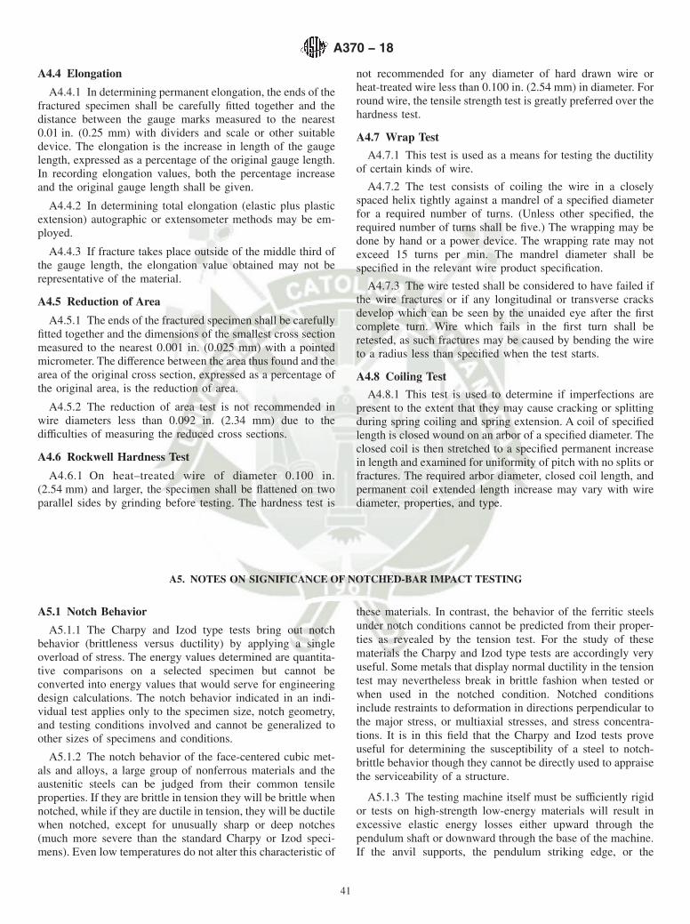
A4.4 Elongation
A4.4.1 In determining permanent elongation, the ends of thefractured specimen shall be carefully fitted together and thedistance between the gauge marks measured to the nearest0.01 in. (0.25 mm) with dividers and scale or other suitabledevice. The elongation is the increase in length of the gaugelength, expressed as a percentage of the original gauge length.In recording elongation values, both the percentage increaseand the original gauge length shall be given.
A4.4.2 In determining total elongation (elastic plus plasticextension) autographic or extensometer methods may be em-ployed.
A4.4.3 If fracture takes place outside of the middle third ofthe gauge length, the elongation value obtained may not berepresentative of the material.
A4.5 Reduction of Area
A4.5.1 The ends of the fractured specimen shall be carefullyfitted together and the dimensions of the smallest cross sectionmeasured to the nearest 0.001 in. (0.025 mm) with a pointedmicrometer. The difference between the area thus found and thearea of the original cross section, expressed as a percentage ofthe original area, is the reduction of area.
A4.5.2 The reduction of area test is not recommended inwire diameters less than 0.092 in. (2.34 mm) due to thedifficulties of measuring the reduced cross sections.
A4.6 Rockwell Hardness Test
A4.6.1 On heat–treated wire of diameter 0.100 in.(2.54 mm) and larger, the specimen shall be flattened on twoparallel sides by grinding before testing. The hardness test is
not recommended for any diameter of hard drawn wire orheat-treated wire less than 0.100 in. (2.54 mm) in diameter. Forround wire, the tensile strength test is greatly preferred over thehardness test.
A4.7 Wrap Test
A4.7.1 This test is used as a means for testing the ductilityof certain kinds of wire.
A4.7.2 The test consists of coiling the wire in a closelyspaced helix tightly against a mandrel of a specified diameterfor a required number of turns. (Unless other specified, therequired number of turns shall be five.) The wrapping may bedone by hand or a power device. The wrapping rate may notexceed 15 turns per min. The mandrel diameter shall bespecified in the relevant wire product specification.
A4.7.3 The wire tested shall be considered to have failed ifthe wire fractures or if any longitudinal or transverse cracksdevelop which can be seen by the unaided eye after the firstcomplete turn. Wire which fails in the first turn shall beretested, as such fractures may be caused by bending the wireto a radius less than specified when the test starts.
A4.8 Coiling Test
A4.8.1 This test is used to determine if imperfections arepresent to the extent that they may cause cracking or splittingduring spring coiling and spring extension. A coil of specifiedlength is closed wound on an arbor of a specified diameter. Theclosed coil is then stretched to a specified permanent increasein length and examined for uniformity of pitch with no splits orfractures. The required arbor diameter, closed coil length, andpermanent coil extended length increase may vary with wirediameter, properties, and type.
A5. NOTES ON SIGNIFICANCE OF NOTCHED-BAR IMPACT TESTING
A5.1 Notch Behavior
A5.1.1 The Charpy and Izod type tests bring out notchbehavior (brittleness versus ductility) by applying a singleoverload of stress. The energy values determined are quantita-tive comparisons on a selected specimen but cannot beconverted into energy values that would serve for engineeringdesign calculations. The notch behavior indicated in an indi-vidual test applies only to the specimen size, notch geometry,and testing conditions involved and cannot be generalized toother sizes of specimens and conditions.
A5.1.2 The notch behavior of the face-centered cubic met-als and alloys, a large group of nonferrous materials and theaustenitic steels can be judged from their common tensileproperties. If they are brittle in tension they will be brittle whennotched, while if they are ductile in tension, they will be ductilewhen notched, except for unusually sharp or deep notches(much more severe than the standard Charpy or Izod speci-mens). Even low temperatures do not alter this characteristic of
these materials. In contrast, the behavior of the ferritic steelsunder notch conditions cannot be predicted from their proper-ties as revealed by the tension test. For the study of thesematerials the Charpy and Izod type tests are accordingly veryuseful. Some metals that display normal ductility in the tensiontest may nevertheless break in brittle fashion when tested orwhen used in the notched condition. Notched conditionsinclude restraints to deformation in directions perpendicular tothe major stress, or multiaxial stresses, and stress concentra-tions. It is in this field that the Charpy and Izod tests proveuseful for determining the susceptibility of a steel to notch-brittle behavior though they cannot be directly used to appraisethe serviceability of a structure.
A5.1.3 The testing machine itself must be sufficiently rigidor tests on high-strength low-energy materials will result inexcessive elastic energy losses either upward through thependulum shaft or downward through the base of the machine.If the anvil supports, the pendulum striking edge, or the
A370 − 18
41
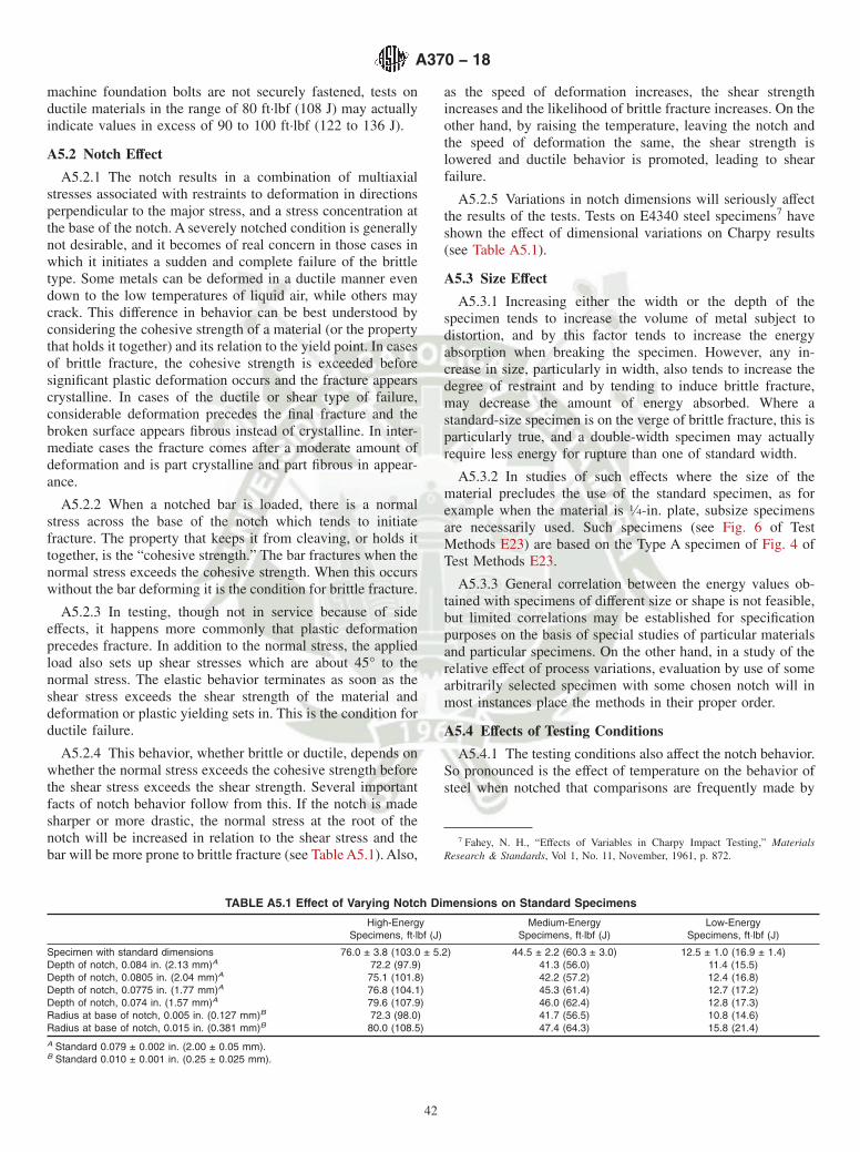
machine foundation bolts are not securely fastened, tests onductile materials in the range of 80 ft·lbf (108 J) may actuallyindicate values in excess of 90 to 100 ft·lbf (122 to 136 J).
A5.2 Notch Effect
A5.2.1 The notch results in a combination of multiaxialstresses associated with restraints to deformation in directionsperpendicular to the major stress, and a stress concentration atthe base of the notch. A severely notched condition is generallynot desirable, and it becomes of real concern in those cases inwhich it initiates a sudden and complete failure of the brittletype. Some metals can be deformed in a ductile manner evendown to the low temperatures of liquid air, while others maycrack. This difference in behavior can be best understood byconsidering the cohesive strength of a material (or the propertythat holds it together) and its relation to the yield point. In casesof brittle fracture, the cohesive strength is exceeded beforesignificant plastic deformation occurs and the fracture appearscrystalline. In cases of the ductile or shear type of failure,considerable deformation precedes the final fracture and thebroken surface appears fibrous instead of crystalline. In inter-mediate cases the fracture comes after a moderate amount ofdeformation and is part crystalline and part fibrous in appear-ance.
A5.2.2 When a notched bar is loaded, there is a normalstress across the base of the notch which tends to initiatefracture. The property that keeps it from cleaving, or holds ittogether, is the “cohesive strength.” The bar fractures when thenormal stress exceeds the cohesive strength. When this occurswithout the bar deforming it is the condition for brittle fracture.
A5.2.3 In testing, though not in service because of sideeffects, it happens more commonly that plastic deformationprecedes fracture. In addition to the normal stress, the appliedload also sets up shear stresses which are about 45° to thenormal stress. The elastic behavior terminates as soon as theshear stress exceeds the shear strength of the material anddeformation or plastic yielding sets in. This is the condition forductile failure.
A5.2.4 This behavior, whether brittle or ductile, depends onwhether the normal stress exceeds the cohesive strength beforethe shear stress exceeds the shear strength. Several importantfacts of notch behavior follow from this. If the notch is madesharper or more drastic, the normal stress at the root of thenotch will be increased in relation to the shear stress and thebar will be more prone to brittle fracture (see Table A5.1). Also,
as the speed of deformation increases, the shear strengthincreases and the likelihood of brittle fracture increases. On theother hand, by raising the temperature, leaving the notch andthe speed of deformation the same, the shear strength islowered and ductile behavior is promoted, leading to shearfailure.
A5.2.5 Variations in notch dimensions will seriously affectthe results of the tests. Tests on E4340 steel specimens7 haveshown the effect of dimensional variations on Charpy results(see Table A5.1).
A5.3 Size Effect
A5.3.1 Increasing either the width or the depth of thespecimen tends to increase the volume of metal subject todistortion, and by this factor tends to increase the energyabsorption when breaking the specimen. However, any in-crease in size, particularly in width, also tends to increase thedegree of restraint and by tending to induce brittle fracture,may decrease the amount of energy absorbed. Where astandard-size specimen is on the verge of brittle fracture, this isparticularly true, and a double-width specimen may actuallyrequire less energy for rupture than one of standard width.
A5.3.2 In studies of such effects where the size of thematerial precludes the use of the standard specimen, as forexample when the material is 1⁄4-in. plate, subsize specimensare necessarily used. Such specimens (see Fig. 6 of TestMethods E23) are based on the Type A specimen of Fig. 4 ofTest Methods E23.
A5.3.3 General correlation between the energy values ob-tained with specimens of different size or shape is not feasible,but limited correlations may be established for specificationpurposes on the basis of special studies of particular materialsand particular specimens. On the other hand, in a study of therelative effect of process variations, evaluation by use of somearbitrarily selected specimen with some chosen notch will inmost instances place the methods in their proper order.
A5.4 Effects of Testing Conditions
A5.4.1 The testing conditions also affect the notch behavior.So pronounced is the effect of temperature on the behavior ofsteel when notched that comparisons are frequently made by
7 Fahey, N. H., “Effects of Variables in Charpy Impact Testing,” MaterialsResearch & Standards, Vol 1, No. 11, November, 1961, p. 872.
TABLE A5.1 Effect of Varying Notch Dimensions on Standard Specimens
High-EnergySpecimens, ft·lbf (J)
Medium-EnergySpecimens, ft·lbf (J)
Low-EnergySpecimens, ft·lbf (J)
Specimen with standard dimensions 76.0 ± 3.8 (103.0 ± 5.2) 44.5 ± 2.2 (60.3 ± 3.0) 12.5 ± 1.0 (16.9 ± 1.4)Depth of notch, 0.084 in. (2.13 mm)A 72.2 (97.9) 41.3 (56.0) 11.4 (15.5)Depth of notch, 0.0805 in. (2.04 mm)A 75.1 (101.8) 42.2 (57.2) 12.4 (16.8)Depth of notch, 0.0775 in. (1.77 mm)A 76.8 (104.1) 45.3 (61.4) 12.7 (17.2)Depth of notch, 0.074 in. (1.57 mm)A 79.6 (107.9) 46.0 (62.4) 12.8 (17.3)Radius at base of notch, 0.005 in. (0.127 mm)B 72.3 (98.0) 41.7 (56.5) 10.8 (14.6)Radius at base of notch, 0.015 in. (0.381 mm)B 80.0 (108.5) 47.4 (64.3) 15.8 (21.4)A Standard 0.079 ± 0.002 in. (2.00 ± 0.05 mm).B Standard 0.010 ± 0.001 in. (0.25 ± 0.025 mm).
A370 − 18
42

examining specimen fractures and by plotting energy value andfracture appearance versus temperature from tests of notchedbars at a series of temperatures. When the test temperature hasbeen carried low enough to start cleavage fracture, there maybe an extremely sharp drop in impact value or there may be arelatively gradual falling off toward the lower temperatures.This drop in energy value starts when a specimen begins toexhibit some crystalline appearance in the fracture. The tran-sition temperature at which this embrittling effect takes placevaries considerably with the size of the part or test specimenand with the notch geometry.
A5.4.2 Some of the many definitions of transition tempera-ture currently being used are: (1) the lowest temperature atwhich the specimen exhibits 100 % fibrous fracture, (2) thetemperature where the fracture shows a 50 % crystalline and a50 % fibrous appearance, (3) the temperature corresponding tothe energy value 50 % of the difference between valuesobtained at 100 % and 0 % fibrous fracture, and (4) thetemperature corresponding to a specific energy value.
A5.4.3 A problem peculiar to Charpy-type tests occurswhen high-strength, low-energy specimens are tested at lowtemperatures. These specimens may not leave the machine inthe direction of the pendulum swing but rather in a sidewisedirection. To ensure that the broken halves of the specimens donot rebound off some component of the machine and contactthe pendulum before it completes its swing, modifications maybe necessary in older model machines. These modificationsdiffer with machine design. Nevertheless the basic problem isthe same in that provisions must be made to prevent rebound-ing of the fractured specimens into any part of the swingingpendulum. Where design permits, the broken specimens maybe deflected out of the sides of the machine and yet in otherdesigns it may be necessary to contain the broken specimenswithin a certain area until the pendulum passes through theanvils. Some low-energy high-strength steel specimens leaveimpact machines at speeds in excess of 50 ft (15.3 m) ⁄s
although they were struck by a pendulum traveling at speedsapproximately 17 ft (5.2 m)/s. If the force exerted on thependulum by the broken specimens is sufficient, the pendulumwill slow down and erroneously high energy values will berecorded. This problem accounts for many of the inconsisten-cies in Charpy results reported by various investigators withinthe 10 to 25-ft·lbf (14 to 34 J) range. The Apparatus Section(the paragraph regarding Specimen Clearance) of Test MethodsE23 discusses the two basic machine designs and a modifica-tion found to be satisfactory in minimizing jamming.
A5.5 Velocity of Straining
A5.5.1 Velocity of straining is likewise a variable thataffects the notch behavior of steel. The impact test showssomewhat higher energy absorption values than the static testsabove the transition temperature and yet, in some instances, thereverse is true below the transition temperature.
A5.6 Correlation with Service
A5.6.1 While Charpy or Izod tests may not directly predictthe ductile or brittle behavior of steel as commonly used inlarge masses or as components of large structures, these testscan be used as acceptance tests of identity for different lots ofthe same steel or in choosing between different steels, whencorrelation with reliable service behavior has been established.It may be necessary to make the tests at properly chosentemperatures other than room temperature. In this, the servicetemperature or the transition temperature of full-scale speci-mens does not give the desired transition temperatures forCharpy or Izod tests since the size and notch geometry may beso different. Chemical analysis, tension, and hardness tests maynot indicate the influence of some of the important processingfactors that affect susceptibility to brittle fracture nor do theycomprehend the effect of low temperatures in inducing brittlebehavior.
A370 − 18
43
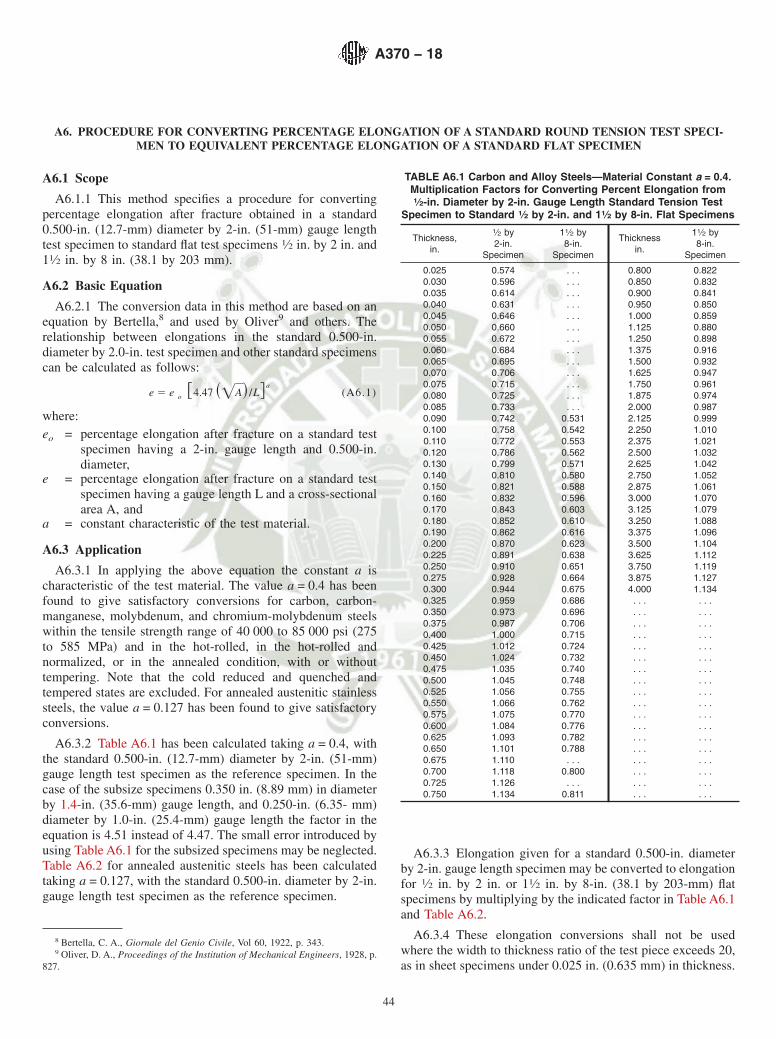
A6. PROCEDURE FOR CONVERTING PERCENTAGE ELONGATION OF A STANDARD ROUND TENSION TEST SPECI-MEN TO EQUIVALENT PERCENTAGE ELONGATION OF A STANDARD FLAT SPECIMEN
A6.1 Scope
A6.1.1 This method specifies a procedure for convertingpercentage elongation after fracture obtained in a standard0.500-in. (12.7-mm) diameter by 2-in. (51-mm) gauge lengthtest specimen to standard flat test specimens 1⁄2 in. by 2 in. and11⁄2 in. by 8 in. (38.1 by 203 mm).
A6.2 Basic Equation
A6.2.1 The conversion data in this method are based on anequation by Bertella,8 and used by Oliver9 and others. Therelationship between elongations in the standard 0.500-in.diameter by 2.0-in. test specimen and other standard specimenscan be calculated as follows:
e 5 e o @4.47 ~=A! /L#a
(A6.1)
where:eo = percentage elongation after fracture on a standard test
specimen having a 2-in. gauge length and 0.500-in.diameter,
e = percentage elongation after fracture on a standard testspecimen having a gauge length L and a cross-sectionalarea A, and
a = constant characteristic of the test material.
A6.3 Application
A6.3.1 In applying the above equation the constant a ischaracteristic of the test material. The value a = 0.4 has beenfound to give satisfactory conversions for carbon, carbon-manganese, molybdenum, and chromium-molybdenum steelswithin the tensile strength range of 40 000 to 85 000 psi (275to 585 MPa) and in the hot-rolled, in the hot-rolled andnormalized, or in the annealed condition, with or withouttempering. Note that the cold reduced and quenched andtempered states are excluded. For annealed austenitic stainlesssteels, the value a = 0.127 has been found to give satisfactoryconversions.
A6.3.2 Table A6.1 has been calculated taking a = 0.4, withthe standard 0.500-in. (12.7-mm) diameter by 2-in. (51-mm)gauge length test specimen as the reference specimen. In thecase of the subsize specimens 0.350 in. (8.89 mm) in diameterby 1.4-in. (35.6-mm) gauge length, and 0.250-in. (6.35- mm)diameter by 1.0-in. (25.4-mm) gauge length the factor in theequation is 4.51 instead of 4.47. The small error introduced byusing Table A6.1 for the subsized specimens may be neglected.Table A6.2 for annealed austenitic steels has been calculatedtaking a = 0.127, with the standard 0.500-in. diameter by 2-in.gauge length test specimen as the reference specimen.
A6.3.3 Elongation given for a standard 0.500-in. diameterby 2-in. gauge length specimen may be converted to elongationfor 1⁄2 in. by 2 in. or 11⁄2 in. by 8-in. (38.1 by 203-mm) flatspecimens by multiplying by the indicated factor in Table A6.1and Table A6.2.
A6.3.4 These elongation conversions shall not be usedwhere the width to thickness ratio of the test piece exceeds 20,as in sheet specimens under 0.025 in. (0.635 mm) in thickness.
8 Bertella, C. A., Giornale del Genio Civile, Vol 60, 1922, p. 343.9 Oliver, D. A., Proceedings of the Institution of Mechanical Engineers, 1928, p.
827.
TABLE A6.1 Carbon and Alloy Steels—Material Constant a = 0.4.Multiplication Factors for Converting Percent Elongation from1⁄2-in. Diameter by 2-in. Gauge Length Standard Tension Test
Specimen to Standard 1⁄2 by 2-in. and 11⁄2 by 8-in. Flat Specimens
Thickness,in.
1⁄2 by2-in.
Specimen
11⁄2 by8-in.
Specimen
Thicknessin.
11⁄2 by8-in.
Specimen
0.025 0.574 . . . 0.800 0.8220.030 0.596 . . . 0.850 0.8320.035 0.614 . . . 0.900 0.8410.040 0.631 . . . 0.950 0.8500.045 0.646 . . . 1.000 0.8590.050 0.660 . . . 1.125 0.8800.055 0.672 . . . 1.250 0.8980.060 0.684 . . . 1.375 0.9160.065 0.695 . . . 1.500 0.9320.070 0.706 . . . 1.625 0.9470.075 0.715 . . . 1.750 0.9610.080 0.725 . . . 1.875 0.9740.085 0.733 . . . 2.000 0.9870.090 0.742 0.531 2.125 0.9990.100 0.758 0.542 2.250 1.0100.110 0.772 0.553 2.375 1.0210.120 0.786 0.562 2.500 1.0320.130 0.799 0.571 2.625 1.0420.140 0.810 0.580 2.750 1.0520.150 0.821 0.588 2.875 1.0610.160 0.832 0.596 3.000 1.0700.170 0.843 0.603 3.125 1.0790.180 0.852 0.610 3.250 1.0880.190 0.862 0.616 3.375 1.0960.200 0.870 0.623 3.500 1.1040.225 0.891 0.638 3.625 1.1120.250 0.910 0.651 3.750 1.1190.275 0.928 0.664 3.875 1.1270.300 0.944 0.675 4.000 1.1340.325 0.959 0.686 . . . . . .0.350 0.973 0.696 . . . . . .0.375 0.987 0.706 . . . . . .0.400 1.000 0.715 . . . . . .0.425 1.012 0.724 . . . . . .0.450 1.024 0.732 . . . . . .0.475 1.035 0.740 . . . . . .0.500 1.045 0.748 . . . . . .0.525 1.056 0.755 . . . . . .0.550 1.066 0.762 . . . . . .0.575 1.075 0.770 . . . . . .0.600 1.084 0.776 . . . . . .0.625 1.093 0.782 . . . . . .0.650 1.101 0.788 . . . . . .0.675 1.110 . . . . . . . . .0.700 1.118 0.800 . . . . . .0.725 1.126 . . . . . . . . .0.750 1.134 0.811 . . . . . .
A370 − 18
44

A6.3.5 While the conversions are considered to be reliablewithin the stated limitations and may generally be used inspecification writing where it is desirable to show equivalentelongation requirements for the several standard ASTM tensionspecimens covered in Test Methods A370, consideration mustbe given to the metallurgical effects dependent on the thicknessof the material as processed.
TABLE A6.2 Annealed Austenitic Stainless Steels—MaterialConstant a = 0.127. Multiplication Factors for Converting PercentElongation from 1⁄2-in. Diameter by 2-in. Gauge Length StandardTension Test Specimen to Standard 1⁄2 by 2-in. and 11⁄2 by 8-in.
Flat Specimens
Thickness,in.
1⁄2 by2-in.
Specimen
11⁄2 by8-in.
Specimen
Thickness,in.
11⁄2 by8-in.
Specimen
0.025 0.839 . . . 0.800 0.9400.030 0.848 . . . 0.850 0.9430.035 0.857 . . . 0.900 0.9470.040 0.864 . . . 0.950 0.9500.045 0.870 . . . 1.000 0.9530.050 0.876 . . . 1.125 0.9600.055 0.882 . . . 1.250 0.9660.060 0.886 . . . 1.375 0.9720.065 0.891 . . . 1.500 0.9780.070 0.895 . . . 1.625 0.9830.075 0.899 . . . 1.750 0.9870.080 0.903 . . . 1.875 0.9920.085 0.906 . . . 2.000 0.9960.090 0.909 0.818 2.125 1.0000.095 0.913 0.821 2.250 1.0030.100 0.916 0.823 2.375 1.0070.110 0.921 0.828 2.500 1.0100.120 0.926 0.833 2.625 1.0130.130 0.931 0.837 2.750 1.0160.140 0.935 0.841 2.875 1.0190.150 0.940 0.845 3.000 1.0220.160 0.943 0.848 3.125 1.0240.170 0.947 0.852 3.250 1.0270.180 0.950 0.855 3.375 1.0290.190 0.954 0.858 3.500 1.0320.200 0.957 0.860 3.625 1.0340.225 0.964 0.867 3.750 1.0360.250 0.970 0.873 3.875 1.0380.275 0.976 0.878 4.000 1.0410.300 0.982 0.883 . . . . . .0.325 0.987 0.887 . . . . . .0.350 0.991 0.892 . . . . . .0.375 0.996 0.895 . . . . . .0.400 1.000 0.899 . . . . . .0.425 1.004 0.903 . . . . . .0.450 1.007 0.906 . . . . . .0.475 1.011 0.909 . . . . . .0.500 1.014 0.912 . . . . . .0.525 1.017 0.915 . . . . . .0.550 1.020 0.917 . . . . . .0.575 1.023 0.920 . . . . . .0.600 1.026 0.922 . . . . . .0.625 1.029 0.925 . . . . . .0.650 1.031 0.927 . . . . . .0.675 1.034 . . . . . . . . .0.700 1.036 0.932 . . . . . .0.725 1.038 . . . . . . . . .0.750 1.041 0.936 . . . . . .
A370 − 18
45

A7. TESTING MULTI-WIRE STRAND
This annex has been replaced by Test Methods A1061/A1061M, and procedures for the tension testing of multi-wirestrand for prestressed concrete have been integrated into the relevant product specifications.
A8. ROUNDING OF TEST DATA
A8.1 Rounding
A8.1.1 An observed value or a calculated value shall berounded off in accordance with the applicable product specifi-cation. In the absence of a specified procedure, the rounding-off method of Practice E29 shall be used.
A8.1.1.1 Values shall be rounded up or rounded down asdetermined by the rules of Practice E29.
A8.1.1.2 In the special case of rounding the number “5”when no additional numbers other than “0” follow the “5,”rounding shall be done in the direction of the specificationlimits if following Practice E29 would cause rejection ofmaterial.
A8.1.2 Recommended levels for rounding reported valuesof test data are given in Table A8.1. These values are designedto provide uniformity in reporting and data storage, and shouldbe used in all cases except where they conflict with specificrequirements of a product specification.
NOTE A8.1—To minimize cumulative errors, whenever possible, valuesshould be carried to at least one figure beyond that of the final (rounded)value during intervening calculations (such as calculation of stress fromload and area measurements) with rounding occurring as the finaloperation. The precision may be less than that implied by the number ofsignificant figures.
TABLE A8.1 Recommended Values for Rounding Test Data
Test Quantity Test Data Range Rounded ValueA
Yield Point up to 50 000 psi, excl (up to 50 ksi) 100 psi (0.1 ksi)Yield Strength 50 000 to 100 000 psi, excl (50 to 100 ksi) 500 psi (0.5 ksi)Tensile Strength 100 000 psi and above (100 ksi and above) 1000 psi (1.0 ksi)
up to 500 MPa, excl 1 MPa500 to 1000 MPa, excl 5 MPa1000 MPa and above 10 MPa
Elongation 0 to 10 %, excl 0.5 %10 % and above 1 %
Reduction of Area 0 to 10 %, excl 0.5 %10 % and above 1 %
Impact Energy 0 to 240 ft·lbf (or 0 to 325 J) 1 ft·lbf (or 1 J)B
Brinell Hardness all values tabular valueC
Rockwell Hardness all scales 1 Rockwell NumberA Round test data to the nearest integral multiple of the values in this column. If the data value is exactly midway between two rounded values, round in accordance withA8.1.1.2.B These units are not equivalent but the rounding occurs in the same numerical ranges for each (1 ft·lbf = 1.356 J).C Round the mean diameter of the Brinell impression to the nearest 0.05 mm and report the corresponding Brinell hardness number read from the table without furtherrounding.
A370 − 18
46

A9. METHODS FOR TESTING STEEL REINFORCING BARS
The testing requirements for steel reinforcing bars contained in this annex have been integrated into the relevant prod-uct specifications.
A10. PROCEDURE FOR USE AND CONTROL OF HEAT-CYCLE SIMULATION
A10.1 Purpose
A10.1.1 To ensure consistent and reproducible heat treat-ments of production forgings and the test specimens thatrepresent them when the practice of heat-cycle simulation isused.
A10.2 Scope
A10.2.1 Generation and documentation of actual productiontime—temperature curves (MASTER CHARTS).
A10.2.2 Controls for duplicating the master cycle duringheat treatment of production forgings. (Heat treating within theessential variables established during A1.2.1).
A10.2.3 Preparation of program charts for the simulatorunit.
A10.2.4 Monitoring and inspection of the simulated cyclewithin the limits established by the ASME Code.
A10.2.5 Documentation and storage of all controls,inspections, charts, and curves.
A10.3 Referenced Documents
A10.3.1 ASME Standards:4ASME Boiler and Pressure Ves-sel Code Section III, latest edition.
ASME Boiler and Pressure Vessel Code Section VIII,Division 2, latest edition.
A10.4 Terminology
A10.4.1 Definitions:A10.4.1.1 master chart—a record of the heat treatment
received from a forging essentially identical to the productionforgings that it will represent. It is a chart of time andtemperature showing the output from thermocouples imbeddedin the forging at the designated test immersion and test locationor locations.
A10.4.1.2 program chart—the metallized sheet used toprogram the simulator unit. Time-temperature data from themaster chart are manually transferred to the program chart.
A10.4.1.3 simulator chart—a record of the heat treatmentthat a test specimen had received in the simulator unit. It is achart of time and temperature and can be compared directly tothe master chart for accuracy of duplication.
A10.4.1.4 simulator cycle—one continuous heat treatmentof a set of specimens in the simulator unit. The cycle includesheating from ambient, holding at temperature, and cooling. Forexample, a simulated austenitize and quench of a set ofspecimens would be one cycle; a simulated temper of the samespecimens would be another cycle.
A10.5 Procedure
A10.5.1 Production Master Charts:A10.5.1.1 Thermocouples shall be imbedded in each forg-
ing from which a master chart is obtained. Temperature shall bemonitored by a recorder with resolution sufficient to clearlydefine all aspects of the heating, holding, and cooling process.All charts are to be clearly identified with all pertinentinformation and identification required for maintaining perma-nent records.
A10.5.1.2 Thermocouples shall be imbedded 180° apart ifthe material specification requires test locations 180° apart.
A10.5.1.3 One master chart (or two if required in accor-dance with A10.5.3.1) shall be produced to represent essen-tially identical forgings (same size and shape). Any change insize or geometry (exceeding rough machining tolerances) of aforging will necessitate that a new master cooling curve bedeveloped.
A10.5.1.4 If more than one curve is required per masterforging (180° apart) and a difference in cooling rate isachieved, then the most conservative curve shall be used as themaster curve.
A10.5.2 Reproducibility of Heat Treatment Parameters onProduction Forgings:
A10.5.2.1 All information pertaining to the quench andtemper of the master forging shall be recorded on an appro-priate permanent record, similar to the one shown in TableA10.1.
A10.5.2.2 All information pertaining to the quench andtemper of the production forgings shall be appropriatelyrecorded, preferably on a form similar to that used inA10.5.2.1. Quench records of production forgings shall beretained for future reference. The quench and temper record ofthe master forging shall be retained as a permanent record.
A10.5.2.3 A copy of the master forging record shall bestored with the heat treatment record of the production forging.
A10.5.2.4 The essential variables, as set forth on the heattreat record, shall be controlled within the given parameters onthe production forging.
A10.5.2.5 The temperature of the quenching medium priorto quenching each production forging shall be equal to or lowerthan the temperature of the quenching medium prior toquenching the master forging.
A10.5.2.6 The time elapsed from opening the furnace doorto quench for the production forging shall not exceed thatelapsed for the master forging.
A370 − 18
47

A10.5.2.7 If the time parameter is exceeded in opening thefurnace door to beginning of quench, the forging shall beplaced back into the furnace and brought back up to equaliza-tion temperature.
A10.5.2.8 All forgings represented by the same masterforging shall be quenched with like orientation to the surface ofthe quench bath.
A10.5.2.9 All production forgings shall be quenched in thesame quench tank, with the same agitation as the masterforging.
A10.5.2.10 Uniformity of Heat Treat Parameters—(1) Thedifference in actual heat treating temperature between produc-tion forgings and the master forging used to establish thesimulator cycle for them shall not exceed 625°F (614°C) forthe quench cycle. (2) The tempering temperature of theproduction forgings shall not fall below the actual temperingtemperature of the master forging. (3) At least one contactsurface thermocouple shall be placed on each forging in aproduction load. Temperature shall be recorded for all surfacethermocouples on a Time Temperature Recorder and suchrecords shall be retained as permanent documentation.
A10.5.3 Heat-Cycle Simulation:A10.5.3.1 Program charts shall be made from the data
recorded on the master chart. All test specimens shall be giventhe same heating rate above, the AC1, the same holding timeand the same cooling rate as the production forgings.
A10.5.3.2 The heating cycle above the AC1, a portion of theholding cycle, and the cooling portion of the master chart shallbe duplicated and the allowable limits on temperature and time,as specified in (a)–(c), shall be established for verification ofthe adequacy of the simulated heat treatment.
(a) Heat Cycle Simulation of Test Coupon Heat Treatmentfor Quenched and Tempered Forgings and Bars—If coolingrate data for the forgings and bars and cooling rate controldevices for the test specimens are available, the test specimensmay be heat-treated in the device.
(b) The test coupons shall be heated to substantially thesame maximum temperature as the forgings or bars. The test
coupons shall be cooled at a rate similar to and no faster thanthe cooling rate representative of the test locations and shall bewithin 25°F (14°C) and 20 s at all temperatures after coolingbegins. The test coupons shall be subsequently heat treated inaccordance with the thermal treatments below the criticaltemperature including tempering and simulated post weld heattreatment.
(c) Simulated Post Weld Heat Treatment of Test Specimens(for ferritic steel forgings and bars)—Except for carbon steel (PNumber 1, Section IX of the Code) forgings and bars with anominal thickness or diameter of 2 in. (51 mm) or less, the testspecimens shall be given a heat treatment to simulate anythermal treatments below the critical temperature that theforgings and bars may receive during fabrication. The simu-lated heat treatment shall utilize temperatures, times, andcooling rates as specified on the order. The total time attemperature(s) for the test material shall be at least 80 % of thetotal time at temperature(s) to which the forgings and bars aresubjected during postweld heat treatment. The total time attemperature(s) for the test specimens may be performed in asingle cycle.
A10.5.3.3 Prior to heat treatment in the simulator unit, testspecimens shall be machined to standard sizes that have beendetermined to allow adequately for subsequent removal ofdecarb and oxidation.
A10.5.3.4 At least one thermocouple per specimen shall beused for continuous recording of temperature on an indepen-dent external temperature-monitoring source. Due to the sen-sitivity and design peculiarities of the heating chamber ofcertain equipment, it is mandatory that the hot junctions ofcontrol and monitoring thermocouples always be placed in thesame relative position with respect to the heating source(generally infrared lamps).
A10.5.3.5 Each individual specimen shall be identified, andsuch identification shall be clearly shown on the simulatorchart and simulator cycle record.
A10.5.3.6 The simulator chart shall be compared to themaster chart for accurate reproduction of simulated quench in
TABLE A10.1 Heat-Treat Record-Essential Variables
MasterForging
ProductionForging 1
ProductionForging 2
ProductionForging 3
ProductionForging 4
ProductionForging 5
Program chart numberTime at temperature and actual temperature of heat treatmentMethod of coolingForging thicknessThermocouple immersionBeneath buffer (yes/no)Forging numberProductMaterialThermocouple location—0 degThermocouple location—180 degQuench tank No.Date of heat treatmentFurnace numberCycle numberHeat treaterStarting quench medium temperatureTime from furnace to quenchHeating rate above 1000°F (538°C)Temperature upon removal from quench after 5 minOrientation of forging in quench
A370 − 18
48
accordance with A10.5.3.2(a). If any one specimen is not heattreated within the acceptable limits of temperature and time,such specimen shall be discarded and replaced by a newlymachined specimen. Documentation of such action and reasonsfor deviation from the master chart shall be shown on thesimulator chart, and on the corresponding nonconformancereport.
A10.5.4 Reheat Treatment and Retesting:A10.5.4.1 In the event of a test failure, retesting shall be
handled in accordance with rules set forth by the materialspecification.
A10.5.4.2 If retesting is permissible, a new test specimenshall be heat treated the same as previously. The productionforging that it represents will have received the same heattreatment. If the test passes, the forging shall be acceptable. Ifit fails, the forging shall be rejected or shall be subject to reheattreatment if permissible.
A10.5.4.3 If reheat treatment is permissible, proceed asfollows: (1) Reheat treatment same as original heat treatment
(time, temperature, cooling rate): Using new test specimensfrom an area as close as possible to the original specimens,repeat the austenitize and quench cycles twice, followed by thetempering cycle (double quench and temper). The productionforging shall be given the identical double quench and temperas its test specimens above. (2) Reheat treatment using a newheat treatment practice. Any change in time, temperature, orcooling rate shall constitute a new heat treatment practice. Anew master curve shall be produced and the simulation andtesting shall proceed as originally set forth.
A10.5.4.4 In summation, each test specimen and its corre-sponding forging shall receive identical heat treatment or heattreatment; otherwise the testing shall be invalid.
A10.5.5 Storage, Recall, and Documentation of Heat-CycleSimulation Data—All records pertaining to heat-cycle simula-tion shall be maintained and held for a period of ten years or asdesigned by the customer. Information shall be so organizedthat all practices can be verified by adequate documentedrecords.
REFERENCES
(1) Griffin J.A., “Analysis of Data From Nist Technical Note 1858, ASTMA01.13,” Task Group meeting, San Antonio, TX, 5.4.16.https://www.sfsa.org/misc/A370refs/1_Griffin_Analysis%20of%20Data%20from%20NIST%20TEchnical%20Note%201858.pdf
(2) Wallin K., Powerpoint presentation “Sub-sized Cvn Specimen Con-version Methodology, ASTM A01.13,” Task Group meeting, Tampa,FL, 11.18.15. https://www.sfsa.org/misc/A370refs/2_Wallin%20Powerpoint%20Sub-size%20CVN%20Specimen%20Conversion%20Methodology.pdf
(3) Griffin, J.A., “A Literature Review to Assess the Reliability of theConversion Factors for Sub-Size Specimens Shown in ASTM A370
Table 9.” https://www.sfsa.org/publications/misc/Report%20to%20ASTM%20Table%209%20TG%20Table%209%20only%20version%202.pdf
(4) Lucon E., McCowan C.N., and Santoyo R.L. “Impact Chararacteriza-tion of 4340 and T200 Steels by Means of Standard, Sub-size andMiniaturized Charpy Specimens,” NIST Technical Note 1858. http://nvlpubs.nist.gov/nistpubs/TechnicalNotes/NIST.TN.1858.pdf.
(5) Lucon E., McCowan C.N., Santoyo R.L. “Impact Chararacterizationof Line Pipe Steels by Means of Standard, Sub-size and MiniaturizedCharpy Specimens,” NIST Technical Note 1865. http://nvlpubs.nist.gov/nistpubs/TechnicalNotes/NIST.TN.1865.pdf.
SUMMARY OF CHANGES
Committee A01 has identified the location of selected changes to this standard since the last issue(A370 – 17a) that may impact the use of this standard. (Approved Dec. 1, 2018.)
(1) Added “nominal” to better define diameter in Annex A3.(2) Deleted statement in 19.1 that Test Method A833 lacks aprecision and bias statement.
Committee A01 has identified the location of selected changes to this standard since the last issue (A370 – 17)that may impact the use of this standard. (Approved Nov. 15, 2017.)
(1) Increased range of values in Table 9 to 75 ft.lbf [102 J].(2) Replaced previous footnote A in Table 9 with new footnoteA.
(3) Added footnotes B and C to Table 9.(4) Added references (1) and (2) to References section.
Committee A01 has identified the location of selected changes to this standard since the last issue (A370 – 16)that may impact the use of this standard. (Approved Jan. 1, 2017.)
(1) Added Section 30. (2) Revised Section 32.
A370 − 18
49

Committee A01 has identified the location of selected changes to this standard since the last issue (A370 – 15)that may impact the use of this standard. (Approved May 1, 2016.)
(1) Removed previous Annex A7 and A9.(2) Added Precision and Bias statement (Section 31).
(3) Revised Annex A3 to permit testing of parts grater than8 inches in length using Method 1.
Committee A01 has identified the location of selected changes to this standard since the last issue (A370 – 14)that may impact the use of this standard. (Approved Nov. 1, 2015.)
(1) Revised 27.1, 14.3.(2) Revised Footnote A of Table 9.(3) Added References section.
(4) Added A1058 to Section 2.(5) Added 1.5.1.
ASTM International takes no position respecting the validity of any patent rights asserted in connection with any item mentionedin this standard. Users of this standard are expressly advised that determination of the validity of any such patent rights, and the riskof infringement of such rights, are entirely their own responsibility.
This standard is subject to revision at any time by the responsible technical committee and must be reviewed every five years andif not revised, either reapproved or withdrawn. Your comments are invited either for revision of this standard or for additional standardsand should be addressed to ASTM International Headquarters. Your comments will receive careful consideration at a meeting of theresponsible technical committee, which you may attend. If you feel that your comments have not received a fair hearing you shouldmake your views known to the ASTM Committee on Standards, at the address shown below.
This standard is copyrighted by ASTM International, 100 Barr Harbor Drive, PO Box C700, West Conshohocken, PA 19428-2959,United States. Individual reprints (single or multiple copies) of this standard may be obtained by contacting ASTM at the aboveaddress or at 610-832-9585 (phone), 610-832-9555 (fax), or [email protected] (e-mail); or through the ASTM website(www.astm.org). Permission rights to photocopy the standard may also be secured from the Copyright Clearance Center, 222Rosewood Drive, Danvers, MA 01923, Tel: (978) 646-2600; http://www.copyright.com/
A370 − 18
50

ANEXO 14
NORMA
ASTM G65 – 16


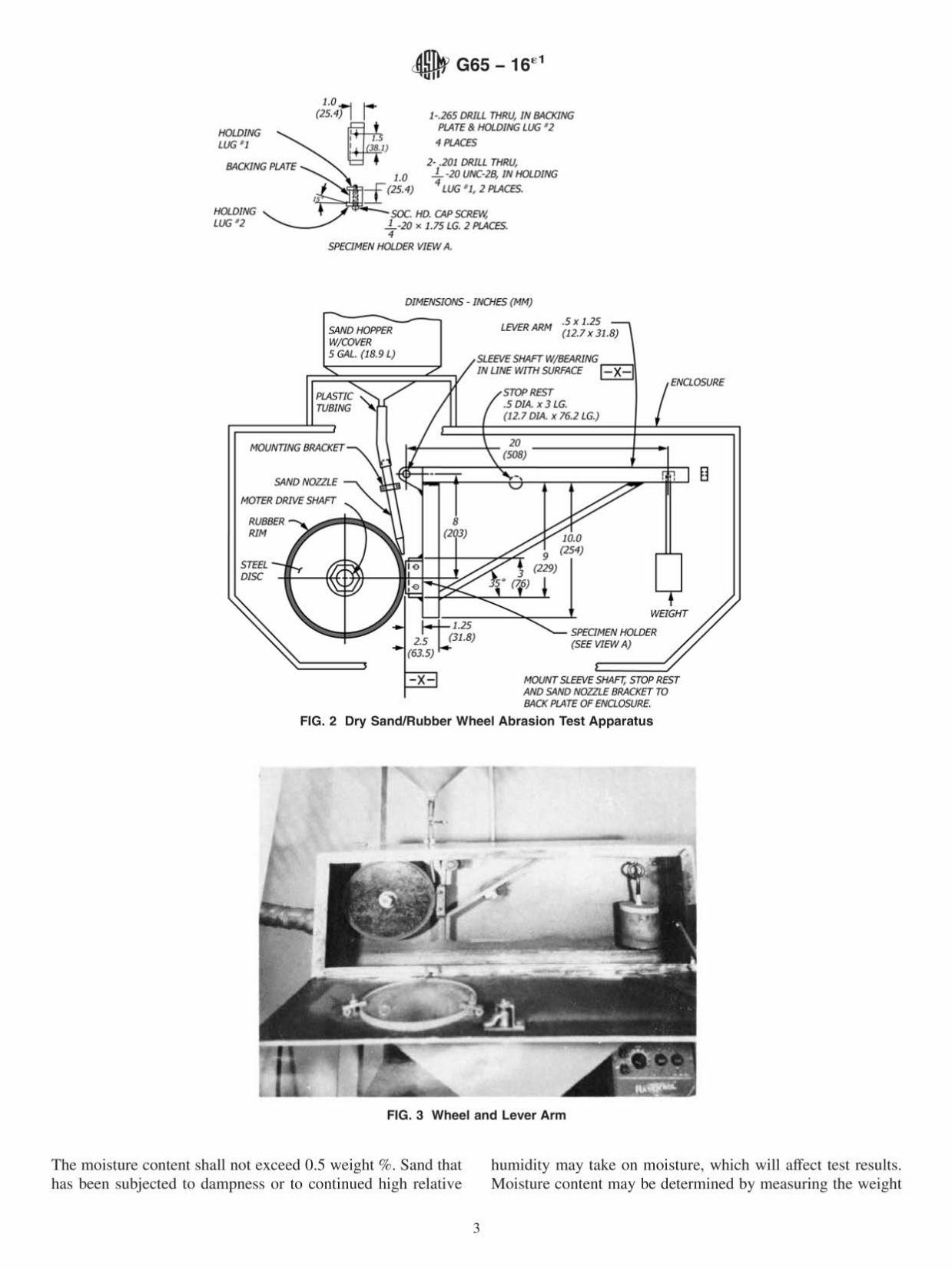


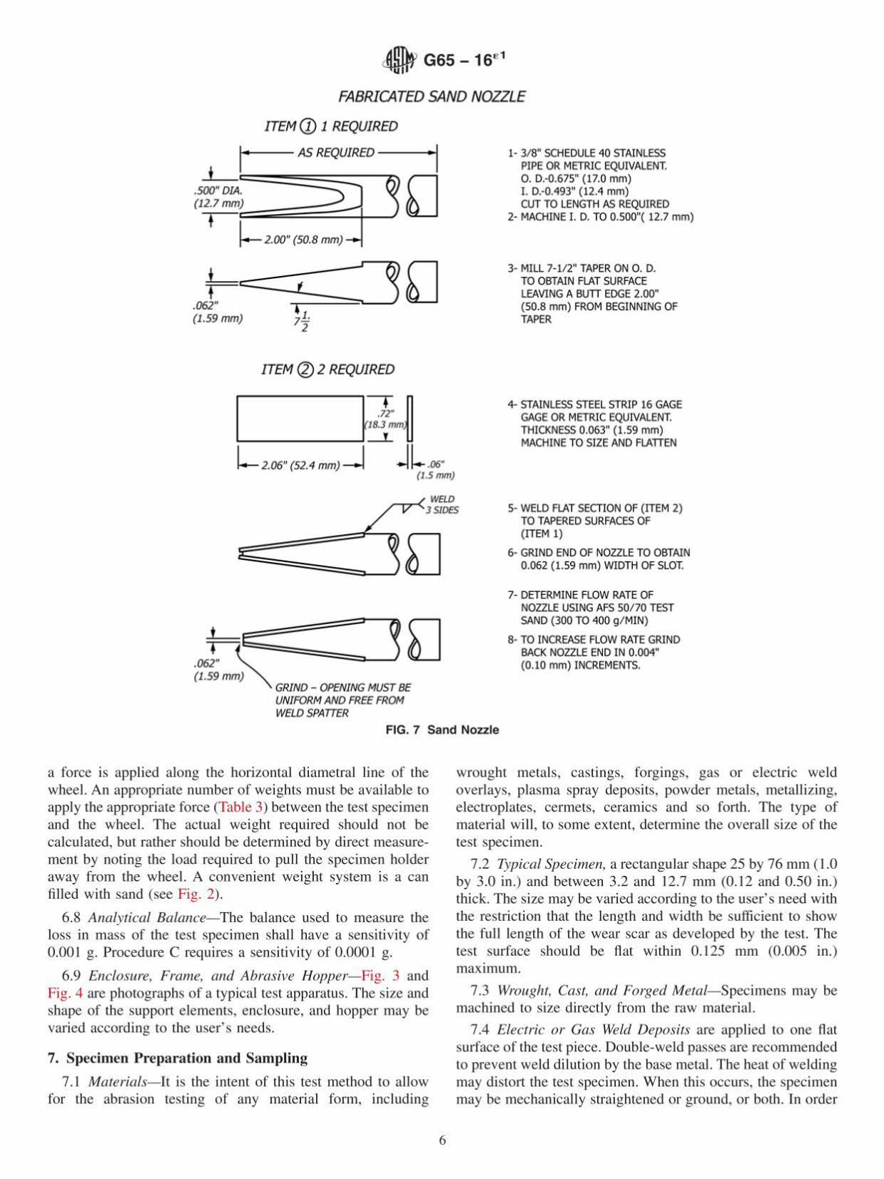

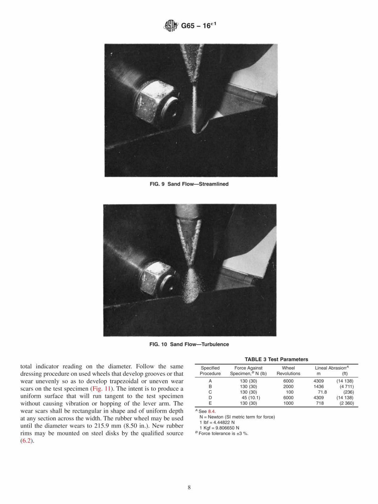
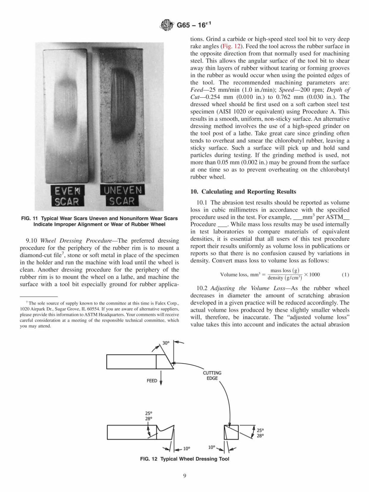
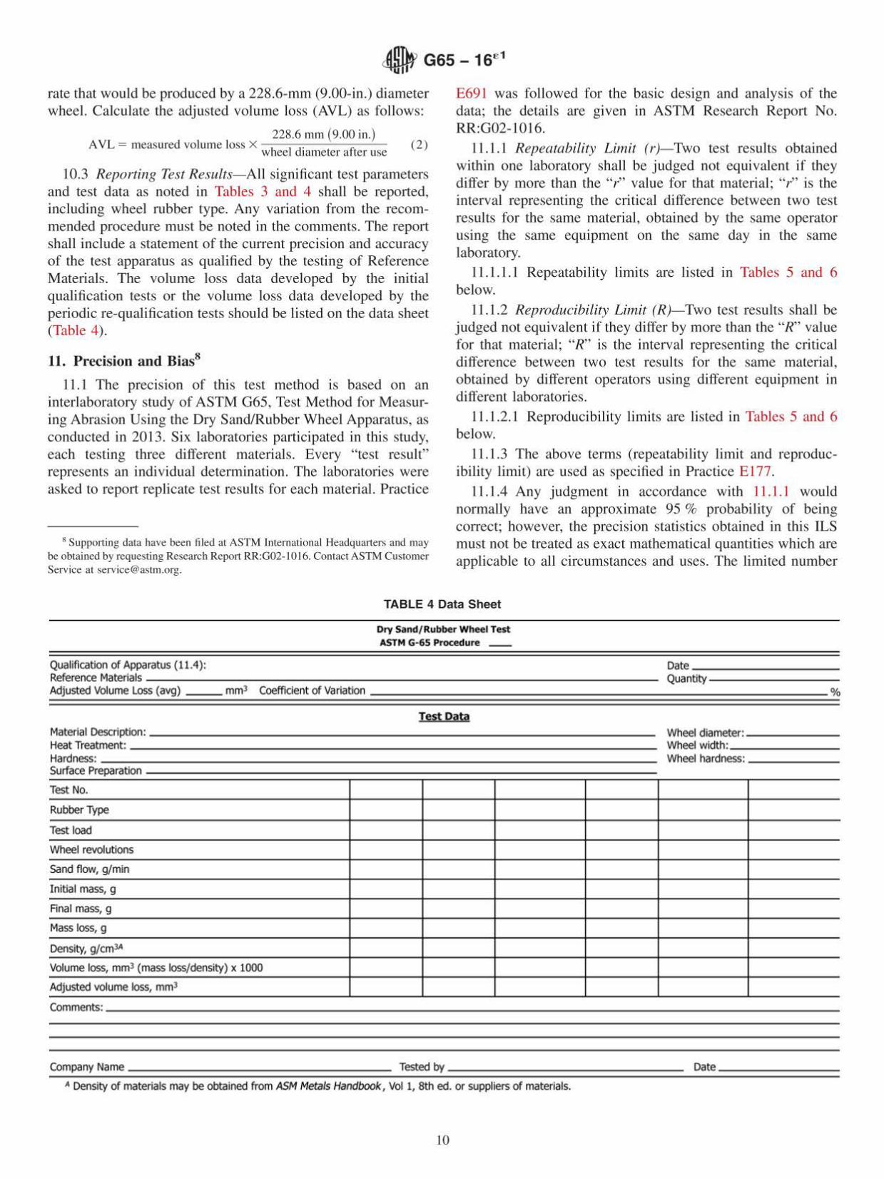
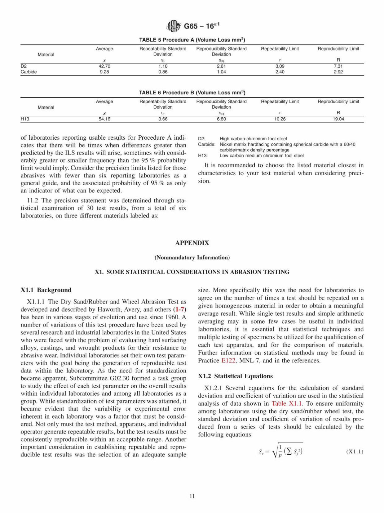
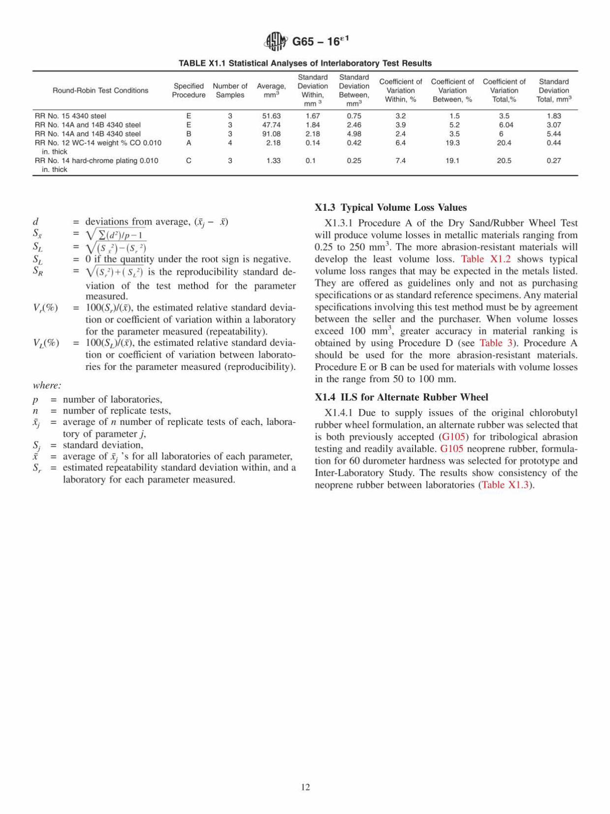


ANEXO 15
NORMA
ASTM G99 – 17

Designation: G99 − 17
Standard Test Method forWear Testing with a Pin-on-Disk Apparatus1
This standard is issued under the fixed designation G99; the number immediately following the designation indicates the year of originaladoption or, in the case of revision, the year of last revision. A number in parentheses indicates the year of last reapproval. A superscriptepsilon (´) indicates an editorial change since the last revision or reapproval.
1. Scope
1.1 This test method covers a laboratory procedure fordetermining the wear of materials during sliding using apin-on-disk apparatus. Materials are tested in pairs undernominally non-abrasive conditions. The principal areas ofexperimental attention in using this type of apparatus tomeasure wear are described. The coefficient of friction mayalso be determined.
1.2 This test method standard uses a specific set of testparameters (load, sliding speed, materials, etc.) that were thenused in an interlaboratory study (ILS), the results of which aregiven here (Tables 1 and 2). (This satisfies the ASTM form inthat “The directions for performing the test should include allof the essential details as to apparatus, test specimen,procedure, and calculations needed to achieve satisfactoryprecision and bias.”) Any user should report that they “fol-lowed the requirements of ASTM G99,” where that is true.
1.3 Now it is often found in practice that users may followall instructions given here, but choose other test parameters,such as load, speed, materials, environment, etc., and therebyobtain different test results. Such a use of this standard isencouraged as a means to improve wear testing methodology.However, it must be clearly stated in any report that, while thedirections and protocol in Test Method G99 were followed (iftrue), the choices of test parameters were different from TestMethod G99 values, and the test results were therefore alsodifferent from the Test Method G99 results. This use should bedescribed as having “followed the procedure of ASTM G99.”All test parameters that were used in such case must be stated.
1.4 The values stated in SI units are to be regarded asstandard. No other units of measurement are included in thisstandard.
1.5 This standard does not purport to address all of thesafety concerns, if any, associated with its use. It is theresponsibility of the user of this standard to establish appro-
priate safety and health practices and determine the applica-bility of regulatory limitations prior to use.
2. Referenced Documents
2.1 ASTM Standards:2
E178 Practice for Dealing With Outlying ObservationsG40 Terminology Relating to Wear and ErosionG117 Guide for Calculating and Reporting Measures of
Precision Using Data from Interlaboratory Wear or Ero-sion Tests (Withdrawn 2016)3
2.2 DIN Standard:4
DIN 50324 Testing of Friction and Wear
3. Summary of Test Method
3.1 For the pin-on-disk wear test, two specimens are re-quired. One, a pin with a radiused tip, is positioned perpen-dicular to the other, usually a flat circular disk. A ball, rigidlyheld, is often used as the pin specimen. The test machinecauses either the disk specimen or the pin specimen to revolveabout the disk center. In either case, the sliding path is a circleon the disk surface. The plane of the disk may be orientedeither horizontally or vertically.
NOTE 1—Wear results may differ for different orientations.
3.1.1 The pin specimen is pressed against the disk at aspecified load usually by means of an arm or lever and attachedweights. Other loading methods have been used, such ashydraulic or pneumatic.
NOTE 2—Wear results may differ for different loading methods.
3.2 Wear results are reported as volume loss in cubicmillimetres for the pin and the disk separately. When twodifferent materials are tested, it is recommended that eachmaterial be tested in both the pin and disk positions.
3.3 The amount of wear is determined by measuring appro-priate linear dimensions of both specimens before and after the
1 This test method is under the jurisdiction of ASTM Committee G02 on Wearand Erosion and is the direct responsibility of Subcommittee G02.40 on Non-Abrasive Wear.
Current edition approved Jan. 1, 2017. Published January 2017. Originallyapproved in 1990. Last previous edition approved in 2016 as G99 – 05 (2016). DOI:10.1520/G0099-17.
2 For referenced ASTM standards, visit the ASTM website, www.astm.org, orcontact ASTM Customer Service at [email protected]. For Annual Book of ASTMStandards volume information, refer to the standard’s Document Summary page onthe ASTM website.
3 The last approved version of this historical standard is referenced onwww.astm.org.
4 Available from Beuth Verlag GmbH (DIN-- DIN Deutsches Institut furNormung e.V.), Burggrafenstrasse 6, 10787, Berlin, Germany, http://www.en.din.de.
Copyright © ASTM International, 100 Barr Harbor Drive, PO Box C700, West Conshohocken, PA 19428-2959. United States
This international standard was developed in accordance with internationally recognized principles on standardization established in the Decision on Principles for theDevelopment of International Standards, Guides and Recommendations issued by the World Trade Organization Technical Barriers to Trade (TBT) Committee.
1

test, or by weighing both specimens before and after the test. Iflinear measures of wear are used, the length change or shapechange of the pin, and the depth or shape change of the diskwear track (in millimetres) are determined by any suitablemetrological technique, such as electronic distance gaging orstylus profiling. Linear measures of wear are converted to wearvolume (in cubic millimetres) by using appropriate geometricrelations. Linear measures of wear are used frequently inpractice since mass loss is often too small to measure precisely.If loss of mass is measured, the mass loss value is converted tovolume loss (in cubic millimetres) using an appropriate valuefor the specimen density.
3.4 Wear results are usually obtained by conducting a testfor a selected sliding distance and for selected values of loadand speed. One set of test conditions that was used in aninterlaboratory measurement series is given in Tables 1-3.Other test conditions may be selected depending on thepurpose of the test. In such cases, the user should report theirresults as “following the procedure of ASTM G99.”
3.5 Wear results may in some cases be reported as plots ofwear volume versus sliding distance using different specimensfor different distances. Such plots may display non-linearrelationships between wear volume and distance over certain
TABLE 1 Characteristics of the Interlaboratory Wear Test Specimens
NOTE 1—See Note 4 for information.
Composition (weight%) Microstructure Hardness (HV 10)RoughnessA
Rz (mean) (µm) Ra (mean) (µm)
Steel ball (100 Cr6) (AISI 52 100)BDiameter 10 mm ←
1.35 to 1.65 Cr0.95 to 1.10 C0.15 to 0.35 Si0.25 to 0.45 Mn
martensitic with minor carbidesand austenite
838 ± 21 0.100 0.010
Steel disc (100 Cr6) (AISI 52 100)CDiameter 40 mm
← <0.030 P<0.030 S
martensitic with minor carbidesand austenite
852 ± 14 0.952 0.113
Alumina ball, diameter = 10 mmD
Alumina disc, diameter = 40.6 mmD
←
←
95 % Al2O3 (with addi-tives of TiO2,MgO, and ZnO)
equi-granular alpha aluminawith very minor secondaryphases
1610 ± 101 (HV 0.2)
1599 ± 144 (HV 0.2)
1.369
0.968
0.123
0.041A Measured by stylus profilometry. Rz is maximum peak-to-valley roughness. Ra is arithmetic average roughness.B Standard ball-bearing balls (SKF).C Standard spacers for thrust bearings (INA).D Manufactured by Compagnie Industrielle des Ceramiques Electroniques, France.
TABLE 2 Results of the Interlaboratory TestsA
NOTE 1—See Note A for test conditions.
NOTE 2—Numbers in parentheses refer to all data received in the tests. In accordance with Practice E178, outlier data values were identified in somecases and discarded, resulting in the numbers without parentheses. The differences are seen to be small.
NOTE 3—Values preceded by ± are one standard deviation.
NOTE 4—Data were provided by 28 laboratories.
NOTE 5—Calculated quantities (for example, wear volume) are given as mean values only.
NOTE 6—Values labeled “NM” were found to be smaller than the reproducible limit of measurement.
NOTE 7—A similar compilation of test data is given in DIN 50324.
Results (ball) (disk)Specimen Pairs
Steel-steel Alumina-steel Steel-alumina Alumina-alumina
Ball wear scar diameter (mm) 2.11 ± 0.27(2.11 ± 0.27)
NM 2.08 ± 0.35(2.03 ± 0.41)
0.3± 0.06(0.3 ± 0.06)
Ball wear volume (10−3 mm3) 198(198)
... 186(169)
0.08(0.08)
Number of values 102(102)
... 60(64)
56(59)
Disk wear scar width (mm) NM 0.64 ± 0.12(0.64 ± 0.12)
NM NM
Disk wear volume (10−3 mm3) ... 480(480)
... ...
Number of values ... 60(60)
... ...
Friction coefficient 0.60 ± 0.11 0.76 ± 0.14 0.60 ± 0.12 0.41 ± 0.08Number of values 109 75 64 76
A Test conditions: F = 10 N; v = 0.1 ms−1, T = 23°C; relative humidity range 12 to 78 %; laboratory air; sliding distance 1000 m; wear track (nominal) diameter = 32 mm;materials: steel = AISI 52 100; and alumina = α-Al2O3.
G99 − 17
2
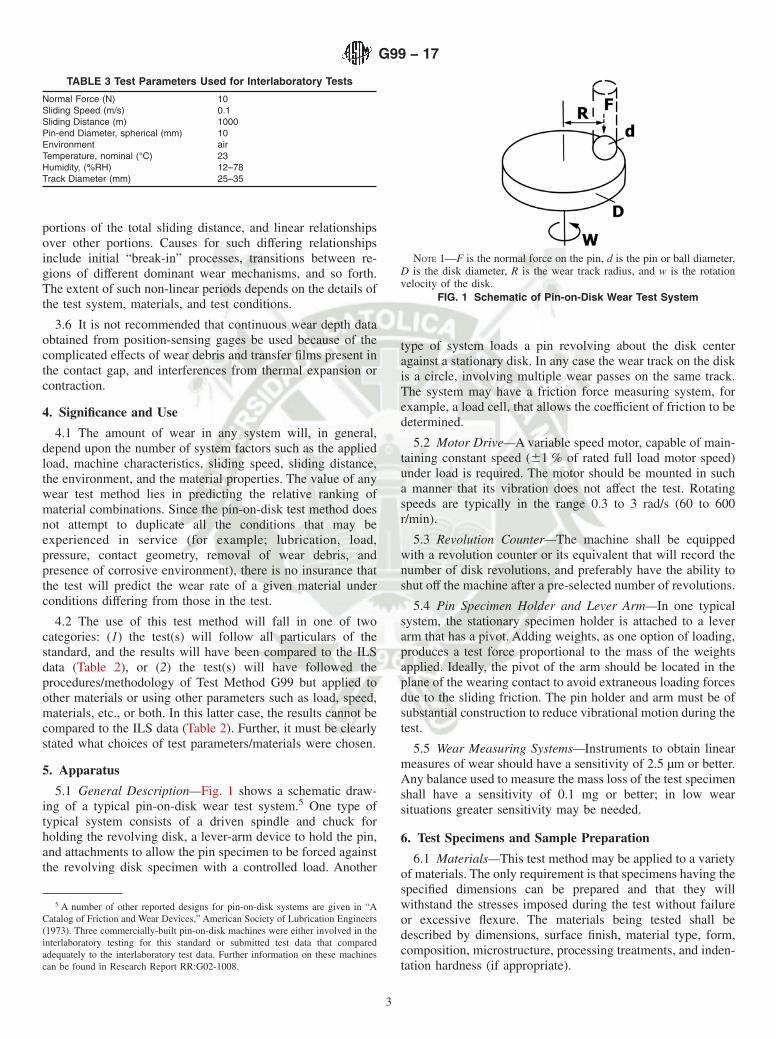
portions of the total sliding distance, and linear relationshipsover other portions. Causes for such differing relationshipsinclude initial “break-in” processes, transitions between re-gions of different dominant wear mechanisms, and so forth.The extent of such non-linear periods depends on the details ofthe test system, materials, and test conditions.
3.6 It is not recommended that continuous wear depth dataobtained from position-sensing gages be used because of thecomplicated effects of wear debris and transfer films present inthe contact gap, and interferences from thermal expansion orcontraction.
4. Significance and Use
4.1 The amount of wear in any system will, in general,depend upon the number of system factors such as the appliedload, machine characteristics, sliding speed, sliding distance,the environment, and the material properties. The value of anywear test method lies in predicting the relative ranking ofmaterial combinations. Since the pin-on-disk test method doesnot attempt to duplicate all the conditions that may beexperienced in service (for example; lubrication, load,pressure, contact geometry, removal of wear debris, andpresence of corrosive environment), there is no insurance thatthe test will predict the wear rate of a given material underconditions differing from those in the test.
4.2 The use of this test method will fall in one of twocategories: (1) the test(s) will follow all particulars of thestandard, and the results will have been compared to the ILSdata (Table 2), or (2) the test(s) will have followed theprocedures/methodology of Test Method G99 but applied toother materials or using other parameters such as load, speed,materials, etc., or both. In this latter case, the results cannot becompared to the ILS data (Table 2). Further, it must be clearlystated what choices of test parameters/materials were chosen.
5. Apparatus
5.1 General Description—Fig. 1 shows a schematic draw-ing of a typical pin-on-disk wear test system.5 One type oftypical system consists of a driven spindle and chuck forholding the revolving disk, a lever-arm device to hold the pin,and attachments to allow the pin specimen to be forced againstthe revolving disk specimen with a controlled load. Another
type of system loads a pin revolving about the disk centeragainst a stationary disk. In any case the wear track on the diskis a circle, involving multiple wear passes on the same track.The system may have a friction force measuring system, forexample, a load cell, that allows the coefficient of friction to bedetermined.
5.2 Motor Drive—A variable speed motor, capable of main-taining constant speed (61 % of rated full load motor speed)under load is required. The motor should be mounted in sucha manner that its vibration does not affect the test. Rotatingspeeds are typically in the range 0.3 to 3 rad/s (60 to 600r/min).
5.3 Revolution Counter—The machine shall be equippedwith a revolution counter or its equivalent that will record thenumber of disk revolutions, and preferably have the ability toshut off the machine after a pre-selected number of revolutions.
5.4 Pin Specimen Holder and Lever Arm—In one typicalsystem, the stationary specimen holder is attached to a leverarm that has a pivot. Adding weights, as one option of loading,produces a test force proportional to the mass of the weightsapplied. Ideally, the pivot of the arm should be located in theplane of the wearing contact to avoid extraneous loading forcesdue to the sliding friction. The pin holder and arm must be ofsubstantial construction to reduce vibrational motion during thetest.
5.5 Wear Measuring Systems—Instruments to obtain linearmeasures of wear should have a sensitivity of 2.5 µm or better.Any balance used to measure the mass loss of the test specimenshall have a sensitivity of 0.1 mg or better; in low wearsituations greater sensitivity may be needed.
6. Test Specimens and Sample Preparation
6.1 Materials—This test method may be applied to a varietyof materials. The only requirement is that specimens having thespecified dimensions can be prepared and that they willwithstand the stresses imposed during the test without failureor excessive flexure. The materials being tested shall bedescribed by dimensions, surface finish, material type, form,composition, microstructure, processing treatments, and inden-tation hardness (if appropriate).
5 A number of other reported designs for pin-on-disk systems are given in “ACatalog of Friction and Wear Devices,” American Society of Lubrication Engineers(1973). Three commercially-built pin-on-disk machines were either involved in theinterlaboratory testing for this standard or submitted test data that comparedadequately to the interlaboratory test data. Further information on these machinescan be found in Research Report RR:G02-1008.
TABLE 3 Test Parameters Used for Interlaboratory Tests
Normal Force (N) 10Sliding Speed (m/s) 0.1Sliding Distance (m) 1000Pin-end Diameter, spherical (mm) 10Environment airTemperature, nominal (°C) 23Humidity, (%RH) 12–78Track Diameter (mm) 25–35
NOTE 1—F is the normal force on the pin, d is the pin or ball diameter,D is the disk diameter, R is the wear track radius, and w is the rotationvelocity of the disk.
FIG. 1 Schematic of Pin-on-Disk Wear Test System
G99 − 17
3

6.2 Test Specimens—The typical pin specimen is cylindricalor spherical in shape. Typical cylindrical or spherical pinspecimen diameters range from 2 to 10 mm. The typical diskspecimen diameters range from 30 to 100 mm and have athickness in the range of 2 to 10 mm. Specimen dimensionsused in an interlaboratory test with pin-on-disk systems aregiven in Table 1.
6.3 Surface Finish—A ground surface roughness of 0.8 µm(32 µin.) arithmetic average or less is usually recommended.
NOTE 3—Rough surfaces make wear scar measurement difficult.
6.3.1 Care must be taken in surface preparation to avoidsubsurface damage that alters the material significantly. Specialsurface preparation may be appropriate for some test programs.State the type of surface and surface preparation in the report.
7. Test Parameters
7.1 Load—Values of the force in Newtons at the wearingcontact.
7.2 Speed—The relative sliding speed between the contact-ing surfaces in metres per second.
7.3 Distance—The accumulated sliding distance in meters.
7.4 Temperature—The temperature of one or both speci-mens at locations close to the wearing contact.
7.5 Atmosphere—The atmosphere (laboratory air, relativehumidity, argon, lubricant, and so forth.) surrounding thewearing contact.
8. Procedure
8.1 Immediately prior to testing, and prior to measuring orweighing, clean and dry the specimens. Take care to remove alldirt and foreign matter from the specimens. Use non-chlorinated, non-film-forming cleaning agents and solvents.Dry materials with open grains to remove all traces of thecleaning fluids that may be entrapped in the material. Steel(ferromagnetic) specimens having residual magnetism shouldbe demagnetized. Report the methods used for cleaning.
8.2 Measure appropriate specimen dimensions to the nearest2.5 µm or weigh the specimens to the nearest 0.0001 g.
8.3 Insert the disk securely in the holding device so that thedisk is fixed perpendicular (61°) to the axis of the resolution.
8.4 Insert the pin specimen securely in its holder and, ifnecessary, adjust so that the specimen is perpendicular (61°) tothe disk surface when in contact, in order to maintain thenecessary contact conditions.
8.5 Add the proper mass to the system lever or bale todevelop the selected force pressing the pin against the disk.
8.6 Start the motor and adjust the speed to the desired valuewhile holding the pin specimen out of contact with the disk.Stop the motor.
8.7 Set the revolution counter (or equivalent) to the desirednumber of revolutions.
8.8 Begin the test with the specimens in contact under load.The test is stopped when the desired number of revolutions isachieved. Tests should not be interrupted or restarted.
8.9 Remove the specimens and clean off any loose weardebris. Note the existence of features on or near the wear scarsuch as: protrusions, displaced metal, discoloration,microcracking, or spotting.
8.10 Remeasure the specimen dimensions to the nearest 2.5µm or reweigh the specimens to the nearest 0.0001 g, asappropriate.
8.11 Repeat the test with additional specimens to obtainsufficient data for statistically significant results.
9. Calculation and Reporting
9.1 The wear measurements should be reported as thevolume loss in cubic millimetres for the pin and disk, sepa-rately.
9.1.1 Use the following equations for calculating volumelosses when the pin has initially a spherical end shape of radiusR and the disk is initially flat, under the conditions that onlyone of the two members wears significantly:
pin ~spherical end! volume loss, mm3 (1)
5π ~wear scar diameter, mm!4
64 ~sphere radius, mm!assuming that there is no significant disk wear. This is anapproximate geometric relation that is correct to 1 % for(wear scar diameter/sphere radius) <0.3, and is correct to5 % for (wear scar diameter/sphere radius) <0.7. The exactequation is given in Appendix X1.
disk volume loss, mm3 (2)
5π ~wear track radius, mm!~ track width, mm!3
6 ~sphere radius, mm!assuming that there is no significant pin wear. This is anapproximate geometric relation that is correct to 1 % for(wear track width/sphere radius) <0.3, and is correct to 5 %for (wear track width/sphere radius) <0.8. The exact equa-tion is given in Appendix X1.
9.1.2 Calculation of wear volumes for pin shapes of othergeometries use the appropriate geometric relations, recogniz-ing that assumptions regarding wear of each member may berequired to justify the assumed final geometry.
9.1.3 Wear scar measurements should be done at least at tworepresentative locations on the pin surfaces and disk surfaces,and the final results averaged.
9.1.4 In situations where both the pin and the disk wearsignificantly, it will be necessary to measure the wear depthprofile on both members. A suitable method uses stylusprofiling. Profiling is the only approach to determine the exactfinal shape of the wear surfaces and thereby to calculate thevolume of material lost due to wear. In the case of disk wear,the average wear track profile can be integrated to obtain thetrack cross-section area, and multiplied by the average tracklength to obtain disk wear volume. In the case of pin wear, thewear scar profile can be measured in two orthogonal directions,the profile results averaged, and used in a figure-of-revolutioncalculated for pin wear volume.
9.1.4.1 If little wear has occurred as evidenced by verysmall wear scars, or if the wear scars are covered by any solidfilm formed during wear, it is best practice to use surfaceprofilometry to determine wear volume. Further, if the amount
G99 − 17
4

of pin wear is small and the pin wear scar is not flat,profilometry must be used.
9.1.5 While mass loss results may be used internally inlaboratories to compare materials of equivalent densities, thistest method reports wear as volume loss so that there is noconfusion caused by variations in density. Take care to use andreport the best available density value for the materials testedwhen calculating volume loss from measured mass loss.
9.1.6 Use the following equation for conversion of massloss to volume loss.
volume loss, mm3 5mass loss, g
density, g/cm3 3 1000. (3)
9.2 If the materials being tested exhibit considerable trans-fer between specimens without loss from the system, volumeloss may not adequately reflect the actual amount or severity ofwear. In these cases, this test method for reporting wear shouldnot be used.
9.3 Friction coefficient (defined in Terminology G40)should be reported when available. Describe the conditionsassociated with the friction measurements, for example, initial,steady-state, and so forth.
9.4 Adequate specification of the materials tested is impor-tant. As a minimum, the report should specify material type,form, processing treatments, surface finish, and specimenpreparation procedures. If appropriate, indentation hardnessshould be reported.
10. Precision and Bias6
10.1 Statement of Precision:10.1.1 The precision of the measurements obtained with this
test method will depend upon the test parameters chosen. Thereproducibility of repeated tests on the same material willdepend upon material homogeneity, machine and materialinteraction, and careful adherence to the specified procedure by
the machine operator. Normal variations in the wear testprocedure will tend to reduce the precision of the test methodas compared to the precision of such material property tests ashardness or density.
10.1.2 Table 2 contains wear data obtained from interlabo-ratory tests. Mean and standard deviation values are given forall measured quantities.
10.1.3 Statistical analysis (using Guide G117) of the steelvs. steel ball wear scar diameter results for 24 laboratoriesleads to a mean and standard deviation of 2.14 and 0.29 mm,respectively. The 95 % repeatability limit (within-lab) was 0.37mm, and the 95 % reproducibility limit (between-labs) was0.81 mm. Statistical analysis of the steel vs. steel ball frictionresults for 25 laboratories leads to a mean and standarddeviation of 0.60 and 0.11, respectively. The 95 % repeatabilitylimit (within-lab) was 0.19, and the 95 % reproducibility limit(between-labs) was 0.32.
10.2 Statement of Bias—No bias can be assigned to theseresults since there are no absolute accepted values for wear.
10.3 General Considerations—Participants in the interlabo-ratory testing that led to the statements of precision and biasgiven above involved 28 laboratories, 2 different materials (4material pairs), 1 test condition, and 3 to 5 replicate measure-ments each (see Note 4). Subsequent to this testing, data werereceived from another laboratory that utilized a commercialtest machine. These data were found consistent with the resultsin the interlaboratory study.
NOTE 4—The interlaboratory data given in Table 1 and Table 2 resultedthrough the cooperation of thirty one institutions in seven countries withthe help of national representatives within the Versailles AdvancedMaterials and Standards (VAMAS) working party on wear test methods.7
11. Keywords
11.1 ceramic wear; friction; metal wear; non-abrasive; pin-on-disk; wear
APPENDIX
(Nonmandatory Information)
X1. EQUATIONS
X1.1 Exact equations for determining wear volume loss areas follows for:
X1.1.1 A spherical ended pin:
pin volume loss 5 ~πh/6!@3d2/41h2# (X1.1)
where:h = r − [r2 − d2/4]½
d = wear scar diameter, andr = pin end radius.
Assuming no significant disk wear.
X1.1.2 A disk:
disk volume loss 5 2πR @r2 sin21~d/2r! 2 ~d/4!~4r2 2 d2!½#
(X1.2)
where:R = wear track radius, andd = wear track width.
Assuming no significant pin wear.
6 Supporting data have been filed at ASTM International Headquarters and maybe obtained by requesting Research Report RR:G02-1008.
7 Czichos, H., Becker, S., and Lexow, J., Wear, Vol 114, 1987, pp. 109–130 andWear, Vol 118, 1987, pp. 379–380.
G99 − 17
5

ASTM International takes no position respecting the validity of any patent rights asserted in connection with any item mentionedin this standard. Users of this standard are expressly advised that determination of the validity of any such patent rights, and the riskof infringement of such rights, are entirely their own responsibility.
This standard is subject to revision at any time by the responsible technical committee and must be reviewed every five years andif not revised, either reapproved or withdrawn. Your comments are invited either for revision of this standard or for additional standardsand should be addressed to ASTM International Headquarters. Your comments will receive careful consideration at a meeting of theresponsible technical committee, which you may attend. If you feel that your comments have not received a fair hearing you shouldmake your views known to the ASTM Committee on Standards, at the address shown below.
This standard is copyrighted by ASTM International, 100 Barr Harbor Drive, PO Box C700, West Conshohocken, PA 19428-2959,United States. Individual reprints (single or multiple copies) of this standard may be obtained by contacting ASTM at the aboveaddress or at 610-832-9585 (phone), 610-832-9555 (fax), or [email protected] (e-mail); or through the ASTM website(www.astm.org). Permission rights to photocopy the standard may also be secured from the Copyright Clearance Center, 222Rosewood Drive, Danvers, MA 01923, Tel: (978) 646-2600; http://www.copyright.com/
G99 − 17
6
ANEXO 16
NORMA
ASTM G133 – 05

Designation: G133 − 05 (Reapproved 2016)
Standard Test Method forLinearly Reciprocating Ball-on-Flat Sliding Wear1
This standard is issued under the fixed designation G133; the number immediately following the designation indicates the year oforiginal adoption or, in the case of revision, the year of last revision. A number in parentheses indicates the year of last reapproval. Asuperscript epsilon (´) indicates an editorial change since the last revision or reapproval.
1. Scope
1.1 This test method covers laboratory procedures for de-termining the sliding wear of ceramics, metals, and othercandidate wear-resistant materials using a linear, reciprocatingball-on-flat plane geometry. The direction of the relativemotion between sliding surfaces reverses in a periodic fashionsuch that the sliding occurs back and forth and in a straightline. The principal quantities of interest are the wear volumesof the contacting ball and flat specimen materials; however, thecoefficient of kinetic friction may also be measured using themethod described. This test method encompasses both unlu-bricated and lubricated testing procedures. The scope of thistest method does not include testing in corrosive or chemicallyaggressive environments.
1.2 The values stated in SI units are to be regarded as thestandard. The values given in parentheses are for informationonly.
1.3 This standard does not purport to address all of thesafety concerns, if any, associated with its use. It is theresponsibility of the user of this standard to establish appro-priate safety and health practices and determine the applica-bility of regulatory limitations prior to use.
2. Referenced Documents
2.1 ASTM Standards:2
E112 Test Methods for Determining Average Grain SizeE1181 Test Methods for Characterizing Duplex Grain SizesG40 Terminology Relating to Wear and ErosionG99 Test Method for Wear Testing with a Pin-on-Disk
ApparatusG115 Guide for Measuring and Reporting Friction Coeffi-
cientsG117 Guide for Calculating and Reporting Measures of
Precision Using Data from Interlaboratory Wear or Ero-sion Tests
G118 Guide for Recommended Format of Wear Test DataSuitable for Databases
3. Terminology
3.1 Definitions:3.1.1 Definitions used in this test method are given in
Terminology G40. The following definitions of importantterms used in this test method are cited from Terminology G40.
3.1.2 friction force—the resisting force tangential to theinterface between two bodies when, under the action of anexternal force, one body moves or tends to move relative to theother.
3.1.3 Hertzian contact pressure—the magnitude of the pres-sure at any specified location in a Hertzian contact area, ascalculated from Hertz’s equations of elastic deformation.
3.1.4 wear—damage to a solid surface, generally involvingthe progressive loss of material due to relative motion betweenthat surface and a contacting surface or surfaces.
3.1.5 wear rate—the rate of material removal or dimen-sional change due to wear per unit of exposure parameter, forexample, quantity removed (mass, volume, thickness) in unitdistance of sliding or unit time.
4. Summary of Test Method
4.1 This test method involves two specimens—a flat speci-men and a spherically ended specimen (herein called the “ball”specimen) which slides against the flat specimen. Thesespecimens move relative to one another in a linear, back andforth sliding motion, under a prescribed set of conditions.
4.2 In this test method, the load is applied verticallydownward through the ball specimen against the horizontallymounted flat specimen. The normal load, stroke length, fre-quency and type of oscillation, test temperature, lubricant (ifany), test duration, and atmospheric environment (includingrelative humidity range) are selected from one of two proce-dures.
4.3 Since this test method involves reciprocating slidingwhere changes in the sliding velocity and direction of motionoccur during the test, constant velocity conditions are notmaintained. The manner in which the velocity varies with time
1 This test method is under the jurisdiction of ASTM Committee G02 on Wearand Erosion and is the direct responsibility of Subcommittee G02.40 on Non-Abrasive Wear.
Current edition approved June 1, 2016. Published June 2016. Originallyapproved in 1995. Last previous edition approved in 2010 as G133 – 05 (2010).DOI: 10.1520/G0133-05R16.
2 For referenced ASTM standards, visit the ASTM website, www.astm.org, orcontact ASTM Customer Service at [email protected]. For Annual Book of ASTMStandards volume information, refer to the standard’s Document Summary page onthe ASTM website.
Copyright © ASTM International, 100 Barr Harbor Drive, PO Box C700, West Conshohocken, PA 19428-2959. United States
1

is determined by the design of the mechanism which drives theball or flat specimen back and forth.
4.4 Dimensional changes for both ball and flat specimensare used to calculate wear volumes and wear rates.
4.5 Friction forces are measured during the test and may beused to assess changes in the contact conditions or the kineticfriction coefficient as a function of time.
5. Significance and Use
5.1 This test method is designed to simulate the geometryand motions that are experienced in many types of rubbingcomponents whose normal operation results in periodic rever-sals in the direction of relative sliding. The wear resulting fromthis mode of movement may differ from that experienced bythe same materials sliding continuously in only one direction(unidirectional sliding) even for comparable durations ofcontact. Test loads and speeds are to be determined by theseverity of the proposed application or purpose of the testing.Either of two sets of testing conditions (designated ProceduresA and B) may be used.
6. Apparatus
6.1 General Description—Fig. 1 shows the arrangement forthe reciprocating ball-on-flat wear test available on a commer-cial machine. The ball is rigidly mounted and has a sphericaltip which moves back and forth across the surface of a polishedflat specimen. Use of a spherical tip alleviates the alignmentproblems associated with flat-ended balls sliding on flat sur-faces. Alternate configurations in which the flat moves and theball specimen is fixed may be used. A provision is made forapplying a uniform normal force (load) to the contact between
the ball and the flat. Temperature measurement and controlcapability is provided to heat and monitor the flat specimenwhich may either be immersed in a lubricant bath or testedwithout lubricant. The tangential force can be measuredcontinuously during oscillating contact and used to obtainfriction coefficient data.3
6.2 Specimen Drive—A drive train, capable of providingsmooth, reciprocating motion to the ball and overcoming thefrictional resistance of the specimens at maximum load, isrequired. For example, a Scotch yoke drive mechanism canprovide a smooth, sinusoidal velocity profile for the ballspecimen relative to the flat specimen without the need for themotor to stop and reverse direction periodically. Stepper-typemotors may also be used provided that the motion is smoothand uniform.
6.3 Ball and Ball Specimen Holder—The ball specimen maybe a fixed bearing ball or any spherically tipped specimen aslong as the sliding contact is equivalent to a ball on a flat plane.If a bearing ball is used, it shall be clamped tightly enough toprevent slippage during the test. The ball holder should be rigidenough so that the periodic reversal in the sliding directiondoes not result in tilting or other misalignment of the contact.
6.4 Flat Specimen Holder—The flat specimen is secured tothe base of the machine to prevent slippage or buckling duringthe test. A variety of shapes and configurations for the flatspecimen are possible. The primary criterion is that the couponpresent a flat, horizontal surface to the ball specimen.
3 Machines of this type are described in A Catalogue of Friction and WearDevices, American Society of Lubrication Engineers (now STLE) 838 BusseHighway, Park Ridge, IL, 1973, pp. 50–72.
FIG. 1 Reciprocating Test—Schematic Diagram
G133 − 05 (2016)
2

6.5 Instrumentation:6.5.1 Friction Force—A tension-compression load cell or
similar force-sensing device may be used to measure thefriction forces generated during sliding. Calibration of thefriction force (see subsection 7.1.3) in both forward and reversesliding directions is required. Since the direction of the frictionforce changes rapidly during the test, traditional strip-chart-type recorders may be too slow to follow these changes at highfrequencies of reciprocation. A commercial version of thismachine is available with a signal conditioner to rectify, andoutput the root-mean-square friction force to a strip-chart-recorder or to a computerized data acquisition system. Themethod of sensing and recording friction force during the testshall be described in the testing report.
6.5.2 Test Duration—In this test method, test duration isspecified in seconds. To compute the sliding distance in metresor number of cycles, use the following:
X 5 0.002 3 t 3 f 3 L (1)
or
N 5 t 3 f (2)
where:X = total sliding distance of the ball, m,N = number of cycles in the test,t = test time, s,f = oscillating frequency, Hz (cycles/s), andL = length of stroke, mm.
A cycle is defined as two stroke lengths (up and back).Electronic timers can be used to terminate the test. If acycle-counter is available, this may be used instead of thetimer, in which case Eq 2 will be used.
6.5.3 Humidity—The wear and friction of many materials issignificantly affected by the moisture in the air. It is thereforerequired that the relative humidity (to an accuracy of 63 %) bemeasured before and during the test. Humidity can vary withair flow and in different parts of the same room, so thehumidity sensor should be located as close to the test speci-mens as reasonably possible, in such a way that the airmovement conditions are the same for humidity sensor as forthe test specimens.
6.5.4 Temperature—The ambient temperature, in degreesCelsius, shall be measured and reported during room tempera-ture tests. In full immersion, liquid-lubricated tests, the bathtemperature shall be measured and reported.
7. Calibration
7.1 The parts of the apparatus that require calibration are(1) the loading system, (2) the motion drive (speed and strokelength), and (3) the friction force sensor.
7.1.1 Loading System—The load (normal force) applied tothe specimen shall be checked periodically. In machines whichapply the load by a spring/lever arrangement and indicate theload on a dial gage, this can be done by substituting apreviously calibrated compression load cell for the specimenand checking the applied load indicated on the loading dialagainst the calibrated load cell output. Statically applied loadsshall be kept constant within a maximum deviation of 62.0 %of the test load. For example, permitted static error of a 25.0-N
normal force would be 60.5 N. During oscillating tests, thenormal force may vary slightly about the mean value due to thedynamics of the machine. This variation is to be expected.
7.1.2 Motion Drive—The oscillating frequency of the mov-ing specimen shall be checked periodically against the drivemotor setting to ensure that the rate of oscillation is known.(Warning—Due to inertial effects, differences in the loadingand fixturing method become more significant as the oscillatingfrequency of the test is increased, and harmonic frequenciescharacteristic of the test machine must be avoided whenselecting the oscillating frequency.)
7.1.3 Friction Force Sensor—The friction force sensor shallbe calibrated periodically in both directions of load application.Depending on the machine, a fixture which applies a calibrat-ing load in line with the normal point of contact between theball and flat should be used.
8. Procedure
8.1 Specimen Preparation—The ball specimen and flatspecimen shall be used either in a polished condition, or in aspecified condition consistent with the application of interest.In a polished condition, the surface should be as free aspossible from preparation artifacts such as grinding-inducedcracks, gross grinding marks, and grain pull-out. Surfaceroughnesses of 0.02 to 0.05-µm Ra (arithmetic roughness) aretypical.
8.2 Clean the specimens using the following procedure:8.2.1 Wash with a mild liquid laboratory glassware cleaner,8.2.2 Hot air dry,8.2.3 Ultrasonically clean in acetone (2 min),8.2.4 Hot air dry,8.2.5 Ultrasonically clean in methanol (2 min), and8.2.6 Hot air dry.8.2.7 If there is considerable porosity in the specimens, it is
necessary that they be baked dry for 4 h at a temperaturegreater than 150°C in a clean oven.
NOTE 1—Certain materials could be adversely affected by cleaning insolvents. Deviations from the prescribed cleaning procedure are permitted,but they shall be described in the report.
8.3 Clean the specimens after they are secured in place inthe test fixture by wiping with acetone and then with methanol-moistened cotton swabs. It is possible that during mounting,some contamination was inadvertently placed on them, and thisfinal cleaning will help alleviate the problem. Inspect the balltip with a hand lens after it is mounted to ensure that there areno defects in the contact area.
8.4 Gently lower the ball specimen upon the flat specimen,and ensure that the reciprocating drive shaft motion is hori-zontal and parallel to the surface of the flat specimen. Theheight of the specimen or mount may require adjustment toensure that this condition is fulfilled. Apply the prescribed testload. Confirm that the desired oscillating speed has been setbefore turning on the motor.
8.5 Two possible testing procedures, one for unlubricatedtests (Procedure A), and one for high-contact stress-lubricatedtests at elevated temperature (Procedure B), are given in 8.5.1.The procedure appropriate for the given materials and test
G133 − 05 (2016)
3

severity should be selected. If neither procedure in 8.5.1 isdetermined to be suitable, other conditions may be used, buttesting will not be in compliance with this test method. See thereporting requirements in Section 10 for reporting exceptionsto Procedures A and B.
8.5.1 The two testing procedures are as follows.8.5.1.1 Procedure A—Unlubricated wear testing at room
temperature.(1) Pin tip radius, 4.76 mm (3⁄16 in.),(2) Normal force, 25.0 N,(3) Stroke length, 10.0 mm,(4) Oscillating frequency, 5.0 Hz,(5) Test duration, 16 min 40 s (sliding distance 100 m),(6) Ambient temperature, 22 6 3°C,(7) Relative humidity, 40 to 60 %, and(8) Lubrication, none applied.
8.5.1.2 Procedure B—Lubricated wear testing at elevatedtemperature.
(1) Pin tip radius, 4.76 mm (3⁄16 in.),(2) Normal force, 200.0 N,(3) Stroke length, 10.0 mm,(4) Oscillating frequency, 10.0 Hz,(5) Test duration, 33 min 20 s (sliding distance 400 m),(6) Temperature, 150 6 2°C,(7) Relative humidity, 40 to 60 %, and(8) Lubrication, full immersion under the selected lubricant
(see Note 2).
NOTE 2—This procedure requires full-immersion lubrication. If othermethods, such a controlled drip feeding system, are used to simulatecertain applications, the provisions of 8.6 will apply.
8.5.2 When heated, liquid-lubricated tests are beingconducted, as in Procedure B, apply the lubricant and heat thespecimens to the selected temperature allowing them to equili-brate for not less than 5 min before applying the load andstarting the test. Bath temperature shall be controlled to withina maximum deviation of 62.0°C from the desired temperature.A fresh supply of lubricant shall be used for each test unless theobjective is to evaluate the effects of used lubricants on frictionand wear.
8.5.3 Set the timer (or cycle counter), if available, for theselected test duration.
8.5.4 Start the friction (and temperature) recording equip-ment and initiate the test.
8.5.5 After the prescribed duration, stop the motor. Removethe normal force to recheck the zero point on the friction forcerecording system.
8.5.6 Allow specimens to cool, if heated, then remove thetest specimens. To measure the wear, it is necessary to clean thespecimens in such a way that the surface features are notaltered. For unlubricated tests, a concentrated jet of air may beused to dispel the debris from the worn area of the specimens.For liquid-lubricated specimens, ultrasonic cleaning in a suit-able solvent may be used. Specimens shall be thoroughly dried.
8.5.7 Examine the tip of the ball specimen to ensure that norolling or other slippage has taken place. Any ball movementwithin the holder during the test invalidates the test results.Similarly, any slippage of the flat specimen in its fixtureinvalidates the test results.
8.6 Alternative Testing Procedures—To achieve certainsimulation conditions, or for other technical reasons, Proce-dures A and B may not be suitable for a given reciprocatingwear testing project. Modifications to the specific test condi-tions prescribed in Procedures A and B may be used forconducting such tests; however, in reporting the results, thespecific parameters which are not in compliance with one ofthe standard testing procedures shall be specifically noted. Astatement such as the following may then be used: “These testsare not in full compliance with the provisions of Test MethodG133, Procedure A, because the normal force in these tests was50.0 N, instead of 25.0 N as prescribed by the standard, and thestroke length was 5.0 mm, instead of 10.0 mm as prescribed bythe standard. All other provisions of Test Method G133 havebeen followed.”
9. Measurement and Calculation of Wear
9.1 Depending upon the relative wear of ball and flatspecimens, various assumptions about the geometric irregular-ity of the wear scars can be made. Fig. 2 shows several possiblewear conditions. In Fig. 2(a), the flat material is much morewear-resistant than the ball material. In Fig. 2(b), the ballmaterial is much more wear-resistant than the flat material. InFig. 2(c), measurable wear occurs on both ball and flatmaterials.
9.2 Wear of the Ball Specimen—Owing to the nature of thistype of test, the wear scar on the ball specimen may not alwaysbe circular or flat. Refer to the following which applies.
9.2.1 If the end of the ball appears flat, but not circular, theaverage of the maximum and minimum dimensions of the scarshall be computed and this value used as the effective ball scardiameter (D). Pin scar measurements may be made by remov-ing the ball specimen holder and placing the wear scar portionunder a reflecting microscope. A calibrated ocular or a photo-micrograph of known magnification may be used to measurescar dimensions.
9.2.1.1 The wear volume (Vp) for a flat ball wear scar ofeffective diameter D (the case in Fig. 2(a)), is found from thesame relationship given in Test Method G99, Appendix X1.1.1:
Vp 5 ~πh/6!@3D2/41h2# (3)
where:h = height of material removed, mm.
Assuming a spherical wear volume, the height of materialremoved can be calculated from D as follows:
h 5 R 2 @R2 2 ~D2/4!#½ (4)
where:R = original ball radius, mm.
(Warning—For lubricated tests in which there is minimalwear, it is possible to be misled in reading the apparent wearscar diameter of the ball tip optically because of elasticrecovery. A small, shallow annulus surrounding the elasticallydeformed area may give the impression of wear, whereas littleor no appreciable wear has actually occurred. Profilometry maybe used to determine whether the wear scar is flat andconsequently whether (Eq 3) and (Eq 4) can be used.)
G133 − 05 (2016)
4
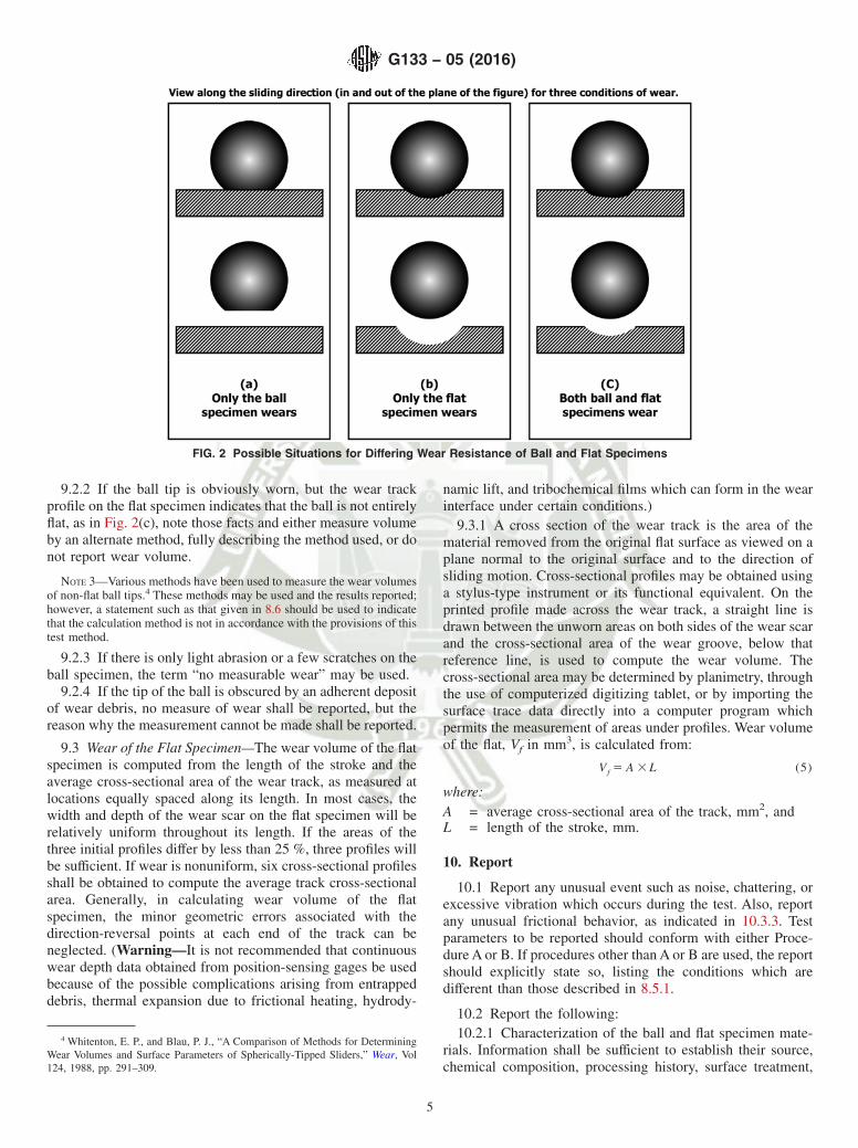
9.2.2 If the ball tip is obviously worn, but the wear trackprofile on the flat specimen indicates that the ball is not entirelyflat, as in Fig. 2(c), note those facts and either measure volumeby an alternate method, fully describing the method used, or donot report wear volume.
NOTE 3—Various methods have been used to measure the wear volumesof non-flat ball tips.4 These methods may be used and the results reported;however, a statement such as that given in 8.6 should be used to indicatethat the calculation method is not in accordance with the provisions of thistest method.
9.2.3 If there is only light abrasion or a few scratches on theball specimen, the term “no measurable wear” may be used.
9.2.4 If the tip of the ball is obscured by an adherent depositof wear debris, no measure of wear shall be reported, but thereason why the measurement cannot be made shall be reported.
9.3 Wear of the Flat Specimen—The wear volume of the flatspecimen is computed from the length of the stroke and theaverage cross-sectional area of the wear track, as measured atlocations equally spaced along its length. In most cases, thewidth and depth of the wear scar on the flat specimen will berelatively uniform throughout its length. If the areas of thethree initial profiles differ by less than 25 %, three profiles willbe sufficient. If wear is nonuniform, six cross-sectional profilesshall be obtained to compute the average track cross-sectionalarea. Generally, in calculating wear volume of the flatspecimen, the minor geometric errors associated with thedirection-reversal points at each end of the track can beneglected. (Warning—It is not recommended that continuouswear depth data obtained from position-sensing gages be usedbecause of the possible complications arising from entrappeddebris, thermal expansion due to frictional heating, hydrody-
namic lift, and tribochemical films which can form in the wearinterface under certain conditions.)
9.3.1 A cross section of the wear track is the area of thematerial removed from the original flat surface as viewed on aplane normal to the original surface and to the direction ofsliding motion. Cross-sectional profiles may be obtained usinga stylus-type instrument or its functional equivalent. On theprinted profile made across the wear track, a straight line isdrawn between the unworn areas on both sides of the wear scarand the cross-sectional area of the wear groove, below thatreference line, is used to compute the wear volume. Thecross-sectional area may be determined by planimetry, throughthe use of computerized digitizing tablet, or by importing thesurface trace data directly into a computer program whichpermits the measurement of areas under profiles. Wear volumeof the flat, Vf in mm3, is calculated from:
Vf 5 A 3 L (5)
where:A = average cross-sectional area of the track, mm2, andL = length of the stroke, mm.
10. Report
10.1 Report any unusual event such as noise, chattering, orexcessive vibration which occurs during the test. Also, reportany unusual frictional behavior, as indicated in 10.3.3. Testparameters to be reported should conform with either Proce-dure A or B. If procedures other than A or B are used, the reportshould explicitly state so, listing the conditions which aredifferent than those described in 8.5.1.
10.2 Report the following:10.2.1 Characterization of the ball and flat specimen mate-
rials. Information shall be sufficient to establish their source,chemical composition, processing history, surface treatment,
4 Whitenton, E. P., and Blau, P. J., “A Comparison of Methods for DeterminingWear Volumes and Surface Parameters of Spherically-Tipped Sliders,” Wear, Vol124, 1988, pp. 291–309.
FIG. 2 Possible Situations for Differing Wear Resistance of Ball and Flat Specimens
G133 − 05 (2016)
5

and root-mean-square surface roughness. Commercial desig-nations for materials should be given, if applicable. If alubricant is used, provide its commercial name or otherdescription, and any other properties needed to identify thesource and traceability of the lubricant. Grain size and percentporosity of specimens may be reported, if applicable. Ifreporting grain size, indicate whether the grain size is nonuni-form or duplex. See Test Methods E112 and E1181. Additionalguidelines for reporting data are found in Guide G118.
NOTE 4—Quantities which have been measured on the same lot used forfabricating wear test specimens should be distinguished from thoseobtained on other lots of material (or handbook values) and assumed toapply to the given test specimens. Tests involving proprietary materials arespecifically excluded from reporting compositions or processes; however,material lot numbers and as many specific identifiers as possible shallotherwise be provided.
10.2.2 Test Parameters:10.2.2.1 Applied normal force, N, and ball tip radius, mm.10.2.2.2 Stroke length, mm.10.2.2.3 Test duration, s or min:s.10.2.2.4 Frequency of oscillation, s−1, and type of motion
produced by the oscillating drive system; for example, sinu-soidal velocity profile, triangular velocity profile, and so forth.
10.2.2.5 Ambient relative humidity, %.10.2.2.6 Ambient temperature, °C.10.2.2.7 Whether lubricated or unlubricated.10.2.3 Results:10.2.3.1 Wear volume only, not wear rate, is reported
because there is no reason to assume that wear occurs at aconstant rate throughout the testing period.
10.2.3.2 Wear volume of the ball specimen, if the scar is flat,in mm3. See 9.2 for a more detailed discussion of thismeasurement.
10.2.3.3 Wear volume of the flat specimen, mm3. See 9.3 fora more detailed discussion of this measurement.
10.2.3.4 A concise description of the appearance of the wearscars, including the presence of debris deposits or films whichform during sliding. Photomicrographs of the scars should beincluded, if available.
10.2.3.5 When reporting the results of multiple tests, indi-cate the number of replicates per material and condition and theaverage wear volumes for ball and flat specimens. Report thestandard deviation.
10.3 Reporting Optional:10.3.1 Report the computed value of the maximum elastic
contact stress (Sc), as calculated by the method developed byHertz. The following equation may be used:
Sc 5 0.918@P/~D2 Eo2!#1/3 (6)
where:P = applied load, N, andD = diameter of the sphere m.
Eo is obtained from:
Eo 5 @~1 2 v12!/E1#1@~1 2 v2
2!/E2# (7)
where:E1,2 = elastic moduli (Young’s moduli) of the two solids in
contact, Pa, and
v1,2 = Poisson’s ratios (dimensionless) of the two materials,respectively.
If the calculated contact stress exceeds the hardness of eithermaterial, there will be permanent plastic deformation andelastic conditions do not apply.
10.3.2 Photomicrographs or surface analysis data for thewear scars on the ball and flat specimens.
10.3.3 A description of the frictional behavior observedduring the test. Kinetic friction coefficient can be calculatedfrom:
µk 5 F/P (8)
where:µk = kinetic friction coefficient,F = nominal, measured friction force during sliding, N, andP = applied load (normal force), N.
10.3.4 On some machines, root-mean-square friction forceis available as an instrumentation output. The test report shouldclearly indicate the manner in which friction force wasobtained. Further guidance in measuring and reporting frictiondata may be found in Guide G115.
NOTE 5—Friction force may vary during an experiment due to run-inand other factors. For example, it may start high then experience atransition to a lower value during the test. It is often useful in analyzingtest results to note the magnitudes and durations of any observed frictiontransitions. If friction force remains steady throughout the test or quicklyreaches a steady state, one nominal value may be sufficient, otherwise, thetype of frictional data reported will depend on the overall trends observedduring the test. If friction never reaches a steady value, its range of valuesmay be reported with appropriate notations as to its behavior.
11. Precision and Bias5
11.1 Precision—The precision of wear determinations isdependent on the wear characteristics of the material under theimposed testing conditions. Some materials wear evenly so asto produce clearly defined wear scars, and wear dimensions canbe measured with a higher degree of precision than for certainother materials which wear in an uneven manner and whosewear scars cannot be delineated as clearly.
11.2 Repeatability and Reproducibility—Procedure A wasused in the same laboratory to conduct eight tests of siliconnitride sliding on silicon nitride. The coefficient of variation ofthe wear volume of the flat specimens was 34.7 %. Thecoefficient of variation for the friction coefficient in the sametests was 1.8 %. The same specimen materials were tested infive laboratories using Procedure B with mineral oil lubrica-tion. The coefficient of variation for the wear volume of the flatspecimens within-laboratory was 623.7 %. Reproducibilitywas reflected in a between-laboratory coefficient of variation of648.6 %. For the friction coefficient, the within-laboratorycoefficient of variation was 62.64 % and the between-laboratory coefficient of variation was 65.29 %. Appendix X1provides examples of the repeatability and reproducibility ofProcedures A and B when applied to tests of silicon nitrideceramics. These numerical values for repeatability and repro-ducibility do not necessarily represent those quantities which
5 Supporting data have been filed at ASTM International Headquarters and maybe obtained by requesting Research Report RR:G02-1010.
G133 − 05 (2016)
6

would be obtained if other material combinations were testedunder Procedures A and B. Since the repeatability and repro-ducibility of wear and friction data are material-dependent, ageneral statement for Procedures A or B cannot be made.
11.3 Bias—Since there is no accepted reference material fordetermining the bias of the procedures in this wear testingmethod, there is no basis upon which to determine the bias.
12. Discussion
12.1 Wear testing involves careful attention to specimenpreparation, characterization, cleaning, and test procedures.Contact geometry, normal force, type of motion, temperature,surface finish, and ambient environment should be as close aspossible to that of a chosen application if wear screening is toprovide meaningful results.
12.2 Wear rate can change during the course of a test orduring the course of the life of a wear part. Run-in wear ratescan exceed steady-state wear rates, and catastrophic transitionsin wear rate can occur to end the useful life of a component. Inthis test method, wear is reported only as the total volume lostafter a set period of sliding. This avoids making the assumptionthat the wear rate was constant during the test. One indirectindication that wear rate may be changing is a significantchange in the nominal level of the friction force during a test.To determine the change in wear rate with test duration,interrupted tests with periodic wear volume assessments maybe made. However, the replacement of the specimens in the
machine to continue testing may not produce identical contactconditions to those when the test was interrupted.
12.3 Moisture in the air (humidity) has been shown to affectboth friction and wear of ceramics, metals, and polymers. Therange of relative humidities over which pronounced changes intribological behavior occur may be relatively short and it mayvary between materials. Therefore, restricting testing to a 50 6
10 % band of relative humidity does not necessarily ensure thatthe friction or wear at each end of the band will be the same.It is better to hold the humidity variation for a series of tests to65 % or less, if possible. Construction of a controlled-humidity enclosure around the testing fixtures is the bestapproach but is not required to meet the requirements of thistest method. Testing on days with similar humidity readings isa less-desirable alternative.
12.4 Unlike material combinations may wear at differentrates depending on which material is the ball specimen andwhich is the flat specimen. The ball specimen experiencesnominally constant contact, whereas the flat specimen surfaceexperiences a changing state of stress as the slider passes andmay wear by a different set of mechanisms. It should thereforenot be assumed that the same relative wear volumes would beobtained if materials for ball and flat specimens were reversed.
13. Keywords
13.1 friction testing; lubricated wear; reciprocating weartest; wear of ceramics; wear of metals; wear testing
APPENDIX
(Nonmandatory Information)
X1. RESULTS OF WITHIN-LABORATORY TESTS USING PROCEDURE A WITH SILICON NITRIDE TEST SPECIMENS
X1.1 Procedure A—The repeatability of test results forProcedure A was determined by two participating laboratories,designated “A” and “B,” each using a different make ofcommercial wear testing machine. Silicon nitride ceramicmaterial was used for both the ball and flat specimens (seeTable X1.1). Flat specimens materials were similar in bulkcomposition although there was a slight difference in thesintering aids. The ball specimens were provided from thesame lot of material. Friction coefficients and wear volumes forthe flat specimens, for eight replicate runs at laboratories “A”and “B,” are compared in Table X1.2 and Table X1.3.
X1.2 Results of Interlaboratory Tests Using Procedure Bwith Silicon Nitride Specimens
X1.2.1 Five laboratories participated. All laboratories usedthe same make and model of commercial testing machine witha Scotch yoke drive mechanism providing a sinusoidal velocityprofile. The specimen materials were the same as thosedescribed in Table X1.1. Mineral oil (J. T. Baker Company,U.S.P. grade, with Vitamin E added as a stabilizer, viscosity byBrookfield viscometer was 140 cP, and the flash point was215°C) was used as the lubricant. Two flat specimens and oneball specimen were supplied to each laboratory. Two wear tests
were performed on each flat specimen using a fresh area of theball specimen for each test; therefore, four tests were con-ducted. Nominal friction coefficient values were obtained fromchart recordings of the root-mean-square friction force. Aspread sheet computer software package designed for GuideG117 was used to process test data on steady-state frictioncoefficient and the computed wear volumes flat specimensfrom stylus traces of the wear grooves (see 9.3). The ball wearvolume was not reported because the scars on the balls werenot flat.
X1.2.2 Results are summarized in Table X1.4 and TableX1.5. As is often the case for wear tests, the within-laboratoryrepeatability is better than the between-laboratory reproduc-ibility. The friction coefficient data (Table X1.4) exhibited lessvariation than the wear volume data (Table X1.5). The latterquantity requires more steps in order to obtain a final numericalvalue so that the potential for compounding measurementuncertainties, rounding errors, and calculation errors is greater.
X1.2.3 These data illustrate the variability of Procedure Bwith a given set of ceramic materials and a single lubricant, andshould not be used to estimate the variability to be expected forother materials or lubricants.
G133 − 05 (2016)
7
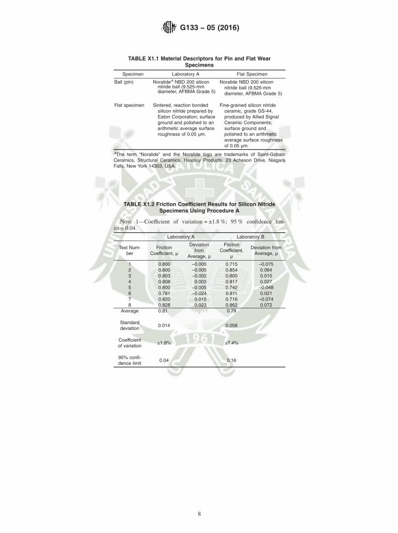
TABLE X1.1 Material Descriptors for Pin and Flat WearSpecimens
Specimen Laboratory A Flat Specimen
Ball (pin) NoralideA NBD 200 siliconnitride ball (9.525-mmdiameter, AFBMA Grade 5)
Noralide NBD 200 siliconnitride ball (9.525-mmdiameter, AFBMA Grade 5)
Flat specimen Sintered, reaction bondedsilicon nitride prepared byEaton Corporation; surfaceground and polished to anarithmetic average surfaceroughness of 0.05 µm.
Fine-grained silicon nitrideceramic, grade GS-44,produced by Allied SignalCeramic Components;surface ground andpolished to an arithmeticaverage surface roughnessof 0.05 µm.
AThe term “Noralide” and the Noralide logo are trademarks of Saint-GobainCeramics, Structural Ceramics, Hexoloy Products, 23 Acheson Drive, NiagaraFalls, New York 14303, USA.
TABLE X1.2 Friction Coefficient Results for Silicon NitrideSpecimens Using Procedure A
NOTE 1—Coefficient of variation = ±1.8 %; 95 % confidence lim-its = 0.04.
Laboratory A Laboratory B
Test Num-ber
FrictionCoefficient, µ
Deviationfrom
Average, µ
FrictionCoefficient,
µ
Deviation fromAverage, µ
1 0.800 −0.005 0.715 –0.0752 0.800 −0.005 0.854 0.0643 0.803 −0.002 0.800 0.0104 0.808 0.003 0.817 0.0275 0.800 −0.005 0.742 –0.0486 0.781 −0.024 0.811 0.0217 0.820 0.015 0.716 –0.0748 0.828 0.023 0.862 0.072
Average 0.81 0.79
Standarddeviation
0.014 0.058
Coefficientof variation
±1.8% ±7.4%
95% confi-dence limit
0.04 0.16
G133 − 05 (2016)
8
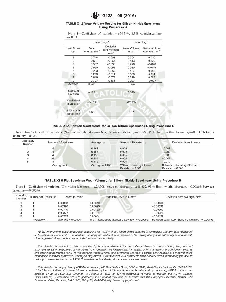
ASTM International takes no position respecting the validity of any patent rights asserted in connection with any item mentionedin this standard. Users of this standard are expressly advised that determination of the validity of any such patent rights, and the riskof infringement of such rights, are entirely their own responsibility.
This standard is subject to revision at any time by the responsible technical committee and must be reviewed every five years andif not revised, either reapproved or withdrawn. Your comments are invited either for revision of this standard or for additional standardsand should be addressed to ASTM International Headquarters. Your comments will receive careful consideration at a meeting of theresponsible technical committee, which you may attend. If you feel that your comments have not received a fair hearing you shouldmake your views known to the ASTM Committee on Standards, at the address shown below.
This standard is copyrighted by ASTM International, 100 Barr Harbor Drive, PO Box C700, West Conshohocken, PA 19428-2959,United States. Individual reprints (single or multiple copies) of this standard may be obtained by contacting ASTM at the aboveaddress or at 610-832-9585 (phone), 610-832-9555 (fax), or [email protected] (e-mail); or through the ASTM website(www.astm.org). Permission rights to photocopy the standard may also be secured from the Copyright Clearance Center, 222Rosewood Drive, Danvers, MA 01923, Tel: (978) 646-2600; http://www.copyright.com/
TABLE X1.3 Wear Volume Results for Silicon Nitride SpecimensUsing Procedure A
NOTE 1—Coefficient of variation = ±34.7 %; 95 % confidence lim-its = 0.53.
Laboratory A Laboratory B
Test Num-ber
WearVolume, mm3
Deviationfrom Average,
mm3
Wear Volume,mm3
Deviation fromAverage, mm3
1 0.746 0.203 0.394 0.0202 0.611 0.068 0.513 0.1393 0.507 −0.036 0.276 –0.0984 0.635 0.092 0.325 –0.0495 0.293 −0.250 0.427 0.0536 0.229 −0.314 0.388 0.0147 0.619 0.076 0.379 0.0058 0.707 0.164 0.287 –0.087
Average 0.543 0.374
Standarddeviation
0.189 0.078
Coefficientof variation
±34.7% ±20.8%
95% confi-dence limit
0.53 0.22
TABLE X1.4 Friction Coefficients for Silicon Nitride Specimens Using Procedure B
NOTE 1—Coefficient of variation (%): within laboratory—2.635; between laboratory—5.285. 95 % limit: within laboratory—0.011; betweenlaboratory—0.023.
LaboratoryNumber
Number of Replicates Average, µ Standard Deviation, µ Deviation from Average
1 4 0.163 0.002 0.0082 4 0.155 0.002 0.0003 4 0.158 0.005 0.0034 4 0.154 0.005 −0.0015 4 0.143 0.005 −0.012
Average = 4 Average = 0.155 Within-Laboratory StandardDeviation = 0.004
Between-Laboratory StandardDeviation = 0.008
TABLE X1.5 Flat Specimen Wear Volumes for Silicon Nitride Specimens Using Procedure B
NOTE 1—Coefficient of variation (%): within laboratory—±23.708; between laboratory—±48.632. 95 % limit: within laboratory—0.00266; betweenlaboratory—0.00546.
LaboratoryNumber
Number of Replicates Average, mm3 Standard Deviation, mm3 Deviation from Average, mm3
1 4 0.00338 0.00049 −0.000632 4 0.00390 0.00090 −0.000923 4 0.00710 0.00132 0.003094 4 0.00377 0.00124 −0.000245 4 0.00272 0.00044 −0.00129
Average = 4 Average = 0.00401 Within-Laboratory Standard Deviation = 0.00095 Between-Laboratory Standard Deviation = 0.00195
G133 − 05 (2016)
9
ANEXO 17
RESULTADOS DE
ENSAYO DE DUREZA
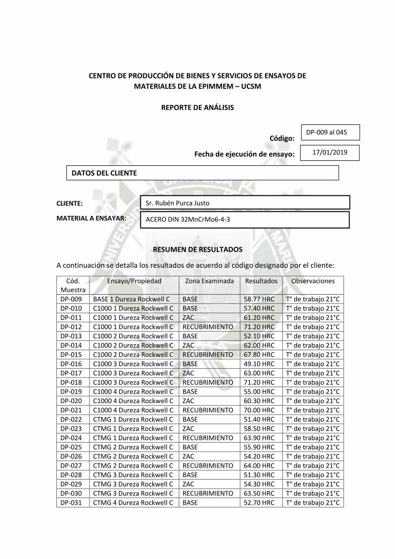
CENTRO DE PRODUCCIÓN DE BIENES Y SERVICIOS DE ENSAYOS DE
MATERIALES DE LA EPIMMEM – UCSM
REPORTE DE ANÁLISIS
Código:
Fecha de ejecución de ensayo:
CLIENTE:
MATERIAL A ENSAYAR:
RESUMEN DE RESULTADOS
A continuación se detalla los resultados de acuerdo al código designado por el cliente:
Cód. Muestra
Ensayo/Propiedad Zona Examinada Resultados Observaciones
DP-009 BASE 1 Dureza Rockwell C BASE 58.77 HRC T° de trabajo 21°C
DP-010 C1000 1 Dureza Rockwell C BASE 57.40 HRC T° de trabajo 21°C
DP-011 C1000 1 Dureza Rockwell C ZAC 61.20 HRC T° de trabajo 21°C
DP-012 C1000 1 Dureza Rockwell C RECUBRIMIENTO 71.20 HRC T° de trabajo 21°C
DP-013 C1000 2 Dureza Rockwell C BASE 52.10 HRC T° de trabajo 21°C
DP-014 C1000 2 Dureza Rockwell C ZAC 62.00 HRC T° de trabajo 21°C
DP-015 C1000 2 Dureza Rockwell C RECUBRIMIENTO 67.80 HRC T° de trabajo 21°C
DP-016 C1000 3 Dureza Rockwell C BASE 49.10 HRC T° de trabajo 21°C
DP-017 C1000 3 Dureza Rockwell C ZAC 63.00 HRC T° de trabajo 21°C
DP-018 C1000 3 Dureza Rockwell C RECUBRIMIENTO 71.20 HRC T° de trabajo 21°C
DP-019 C1000 4 Dureza Rockwell C BASE 55.00 HRC T° de trabajo 21°C
DP-020 C1000 4 Dureza Rockwell C ZAC 60.30 HRC T° de trabajo 21°C
DP-021 C1000 4 Dureza Rockwell C RECUBRIMIENTO 70.00 HRC T° de trabajo 21°C
DP-022 CTMG 1 Dureza Rockwell C BASE 51.40 HRC T° de trabajo 21°C
DP-023 CTMG 1 Dureza Rockwell C ZAC 58.50 HRC T° de trabajo 21°C
DP-024 CTMG 1 Dureza Rockwell C RECUBRIMIENTO 63.90 HRC T° de trabajo 21°C
DP-025 CTMG 2 Dureza Rockwell C BASE 55.90 HRC T° de trabajo 21°C
DP-026 CTMG 2 Dureza Rockwell C ZAC 54.20 HRC T° de trabajo 21°C
DP-027 CTMG 2 Dureza Rockwell C RECUBRIMIENTO 64.00 HRC T° de trabajo 21°C
DP-028 CTMG 3 Dureza Rockwell C BASE 51.30 HRC T° de trabajo 21°C
DP-029 CTMG 3 Dureza Rockwell C ZAC 54.30 HRC T° de trabajo 21°C
DP-030 CTMG 3 Dureza Rockwell C RECUBRIMIENTO 63.50 HRC T° de trabajo 21°C
DP-031 CTMG 4 Dureza Rockwell C BASE 52.70 HRC T° de trabajo 21°C
DP-009 al 045
17/01/2019
DATOS DEL CLIENTE
ACERO DIN 32MnCrMo6-4-3
Sr. Rubén Purca Justo
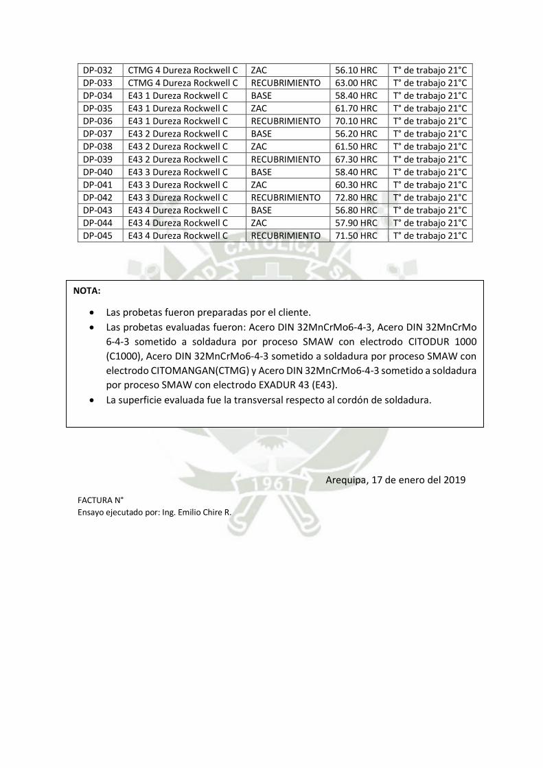
DP-032 CTMG 4 Dureza Rockwell C ZAC 56.10 HRC T° de trabajo 21°C
DP-033 CTMG 4 Dureza Rockwell C RECUBRIMIENTO 63.00 HRC T° de trabajo 21°C
DP-034 E43 1 Dureza Rockwell C BASE 58.40 HRC T° de trabajo 21°C
DP-035 E43 1 Dureza Rockwell C ZAC 61.70 HRC T° de trabajo 21°C
DP-036 E43 1 Dureza Rockwell C RECUBRIMIENTO 70.10 HRC T° de trabajo 21°C
DP-037 E43 2 Dureza Rockwell C BASE 56.20 HRC T° de trabajo 21°C
DP-038 E43 2 Dureza Rockwell C ZAC 61.50 HRC T° de trabajo 21°C
DP-039 E43 2 Dureza Rockwell C RECUBRIMIENTO 67.30 HRC T° de trabajo 21°C
DP-040 E43 3 Dureza Rockwell C BASE 58.40 HRC T° de trabajo 21°C
DP-041 E43 3 Dureza Rockwell C ZAC 60.30 HRC T° de trabajo 21°C
DP-042 E43 3 Dureza Rockwell C RECUBRIMIENTO 72.80 HRC T° de trabajo 21°C
DP-043 E43 4 Dureza Rockwell C BASE 56.80 HRC T° de trabajo 21°C
DP-044 E43 4 Dureza Rockwell C ZAC 57.90 HRC T° de trabajo 21°C
DP-045 E43 4 Dureza Rockwell C RECUBRIMIENTO 71.50 HRC T° de trabajo 21°C
Arequipa, 17 de enero del 2019
FACTURA N°
Ensayo ejecutado por: Ing. Emilio Chire R.
NOTA:
Las probetas fueron preparadas por el cliente.
Las probetas evaluadas fueron: Acero DIN 32MnCrMo6-4-3, Acero DIN 32MnCrMo
6-4-3 sometido a soldadura por proceso SMAW con electrodo CITODUR 1000
(C1000), Acero DIN 32MnCrMo6-4-3 sometido a soldadura por proceso SMAW con
electrodo CITOMANGAN(CTMG) y Acero DIN 32MnCrMo6-4-3 sometido a soldadura
por proceso SMAW con electrodo EXADUR 43 (E43).
La superficie evaluada fue la transversal respecto al cordón de soldadura.

ANEXO 18
RESULTADOS DE
ENSAYO DE
MICROGRAFÍAS
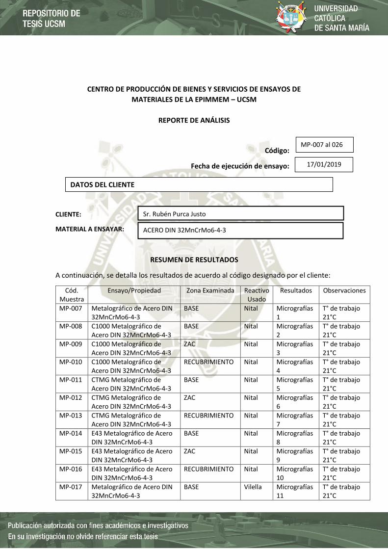
CENTRO DE PRODUCCIÓN DE BIENES Y SERVICIOS DE ENSAYOS DE
MATERIALES DE LA EPIMMEM – UCSM
REPORTE DE ANÁLISIS
Código:
Fecha de ejecución de ensayo:
CLIENTE:
MATERIAL A ENSAYAR:
RESUMEN DE RESULTADOS
A continuación, se detalla los resultados de acuerdo al código designado por el cliente:
Cód. Muestra
Ensayo/Propiedad Zona Examinada Reactivo Usado
Resultados Observaciones
MP-007 Metalográfico de Acero DIN 32MnCrMo6-4-3
BASE Nital Micrografías 1
T° de trabajo 21°C
MP-008 C1000 Metalográfico de Acero DIN 32MnCrMo6-4-3
BASE Nital Micrografías 2
T° de trabajo 21°C
MP-009 C1000 Metalográfico de Acero DIN 32MnCrMo6-4-3
ZAC Nital Micrografías 3
T° de trabajo 21°C
MP-010 C1000 Metalográfico de Acero DIN 32MnCrMo6-4-3
RECUBRIMIENTO Nital Micrografías 4
T° de trabajo 21°C
MP-011 CTMG Metalográfico de Acero DIN 32MnCrMo6-4-3
BASE Nital Micrografías 5
T° de trabajo 21°C
MP-012 CTMG Metalográfico de Acero DIN 32MnCrMo6-4-3
ZAC Nital Micrografías 6
T° de trabajo 21°C
MP-013 CTMG Metalográfico de Acero DIN 32MnCrMo6-4-3
RECUBRIMIENTO Nital Micrografías 7
T° de trabajo 21°C
MP-014 E43 Metalográfico de Acero DIN 32MnCrMo6-4-3
BASE Nital Micrografías 8
T° de trabajo 21°C
MP-015 E43 Metalográfico de Acero DIN 32MnCrMo6-4-3
ZAC Nital Micrografías 9
T° de trabajo 21°C
MP-016 E43 Metalográfico de Acero DIN 32MnCrMo6-4-3
RECUBRIMIENTO Nital Micrografías 10
T° de trabajo 21°C
MP-017 Metalográfico de Acero DIN 32MnCrMo6-4-3
BASE Vilella Micrografías 11
T° de trabajo 21°C
MP-007 al 026
17/01/2019
DATOS DEL CLIENTE
ACERO DIN 32MnCrMo6-4-3
Sr. Rubén Purca Justo
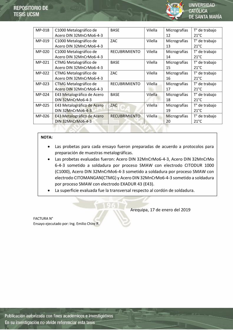
MP-018 C1000 Metalográfico de Acero DIN 32MnCrMo6-4-3
BASE Vilella Micrografías 12
T° de trabajo 21°C
MP-019 C1000 Metalográfico de Acero DIN 32MnCrMo6-4-3
ZAC Vilella Micrografías 13
T° de trabajo 21°C
MP-020 C1000 Metalográfico de Acero DIN 32MnCrMo6-4-3
RECUBRIMIENTO Vilella Micrografías 14
T° de trabajo 21°C
MP-021 CTMG Metalográfico de Acero DIN 32MnCrMo6-4-3
BASE Vilella Micrografías 15
T° de trabajo 21°C
MP-022 CTMG Metalográfico de Acero DIN 32MnCrMo6-4-3
ZAC Vilella Micrografías 16
T° de trabajo 21°C
MP-023 CTMG Metalográfico de Acero DIN 32MnCrMo6-4-3
RECUBRIMIENTO Vilella Micrografías 17
T° de trabajo 21°C
MP-024 E43 Metalográfico de Acero DIN 32MnCrMo6-4-3
BASE Vilella Micrografías 18
T° de trabajo 21°C
MP-025 E43 Metalográfico de Acero DIN 32MnCrMo6-4-3
ZAC Vilella Micrografías 19
T° de trabajo 21°C
MP-026 E43 Metalográfico de Acero DIN 32MnCrMo6-4-3
RECUBRIMIENTO Vilella Micrografías 20
T° de trabajo 21°C
Arequipa, 17 de enero del 2019
FACTURA N°
Ensayo ejecutado por: Ing. Emilio Chire R.
NOTA:
Las probetas para cada ensayo fueron preparadas de acuerdo a protocolos para
preparación de muestras metalográficas.
Las probetas evaluadas fueron: Acero DIN 32MnCrMo6-4-3, Acero DIN 32MnCrMo
6-4-3 sometido a soldadura por proceso SMAW con electrodo CITODUR 1000
(C1000), Acero DIN 32MnCrMo6-4-3 sometido a soldadura por proceso SMAW con
electrodo CITOMANGAN(CTMG) y Acero DIN 32MnCrMo6-4-3 sometido a soldadura
por proceso SMAW con electrodo EXADUR 43 (E43).
La superficie evaluada fue la transversal respecto al cordón de soldadura.
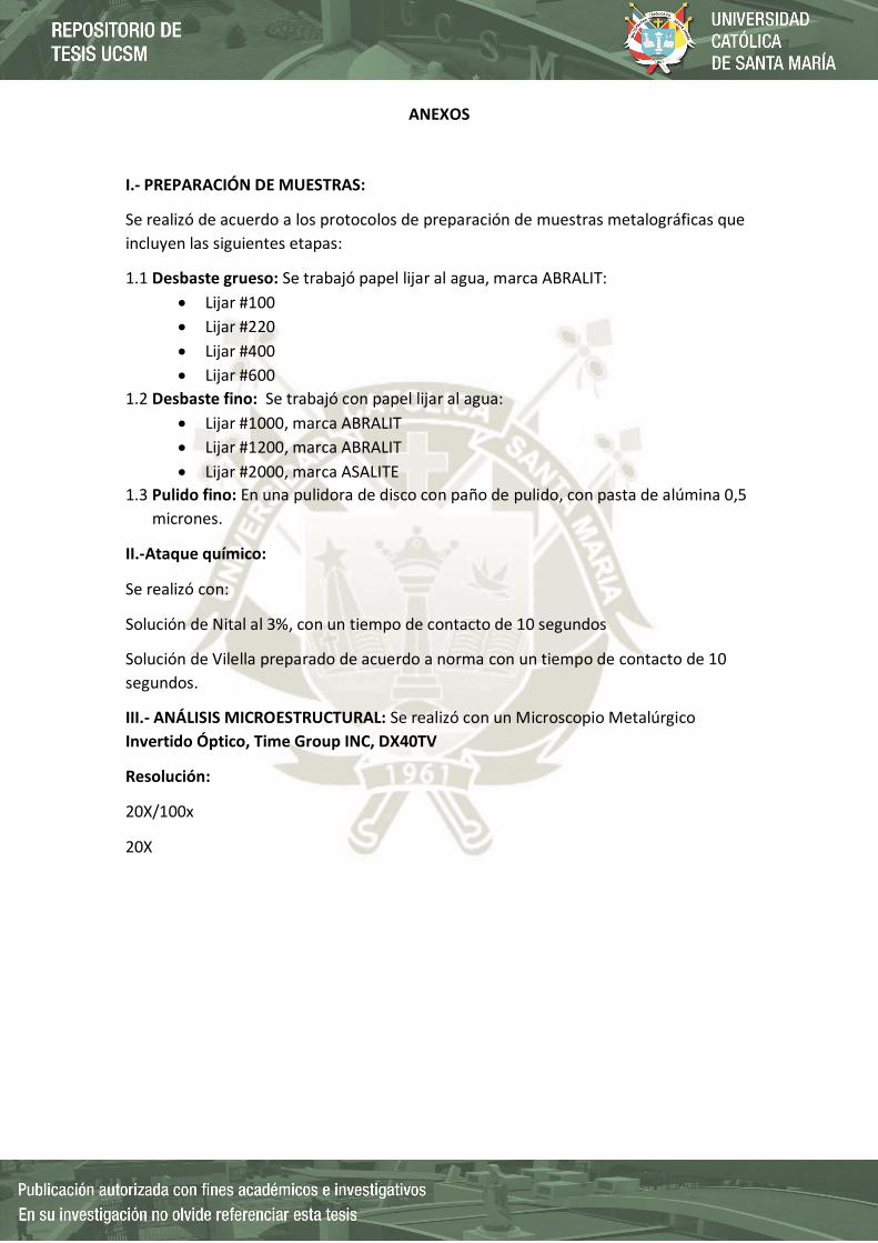
ANEXOS
I.- PREPARACIÓN DE MUESTRAS:
Se realizó de acuerdo a los protocolos de preparación de muestras metalográficas que
incluyen las siguientes etapas:
1.1 Desbaste grueso: Se trabajó papel lijar al agua, marca ABRALIT:
Lijar #100
Lijar #220
Lijar #400
Lijar #600
1.2 Desbaste fino: Se trabajó con papel lijar al agua:
Lijar #1000, marca ABRALIT
Lijar #1200, marca ABRALIT
Lijar #2000, marca ASALITE
1.3 Pulido fino: En una pulidora de disco con paño de pulido, con pasta de alúmina 0,5
micrones.
II.-Ataque químico:
Se realizó con:
Solución de Nital al 3%, con un tiempo de contacto de 10 segundos
Solución de Vilella preparado de acuerdo a norma con un tiempo de contacto de 10
segundos.
III.- ANÁLISIS MICROESTRUCTURAL: Se realizó con un Microscopio Metalúrgico
Invertido Óptico, Time Group INC, DX40TV
Resolución:
20X/100x
20X
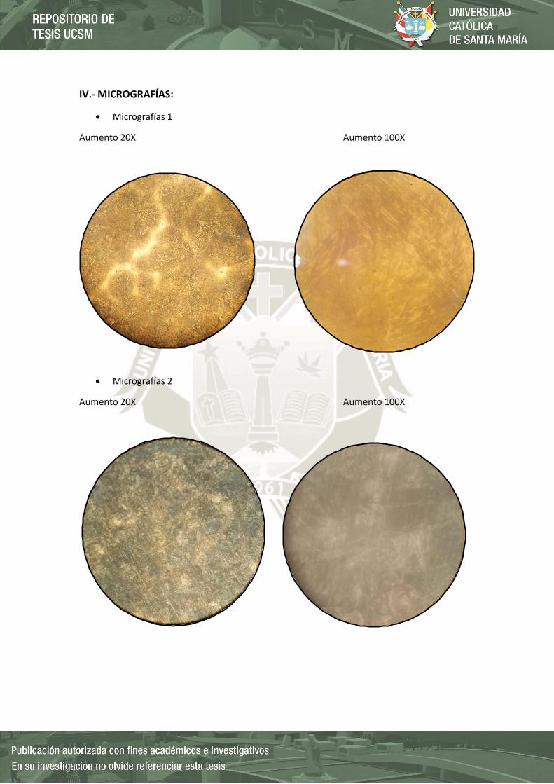
IV.- MICROGRAFÍAS:
Micrografías 1
Aumento 20X Aumento 100X
Micrografías 2
Aumento 20X Aumento 100X

Micrografías 3
Aumento 20X Aumento 100X
Micrografías 4
Aumento 20X Aumento 100X
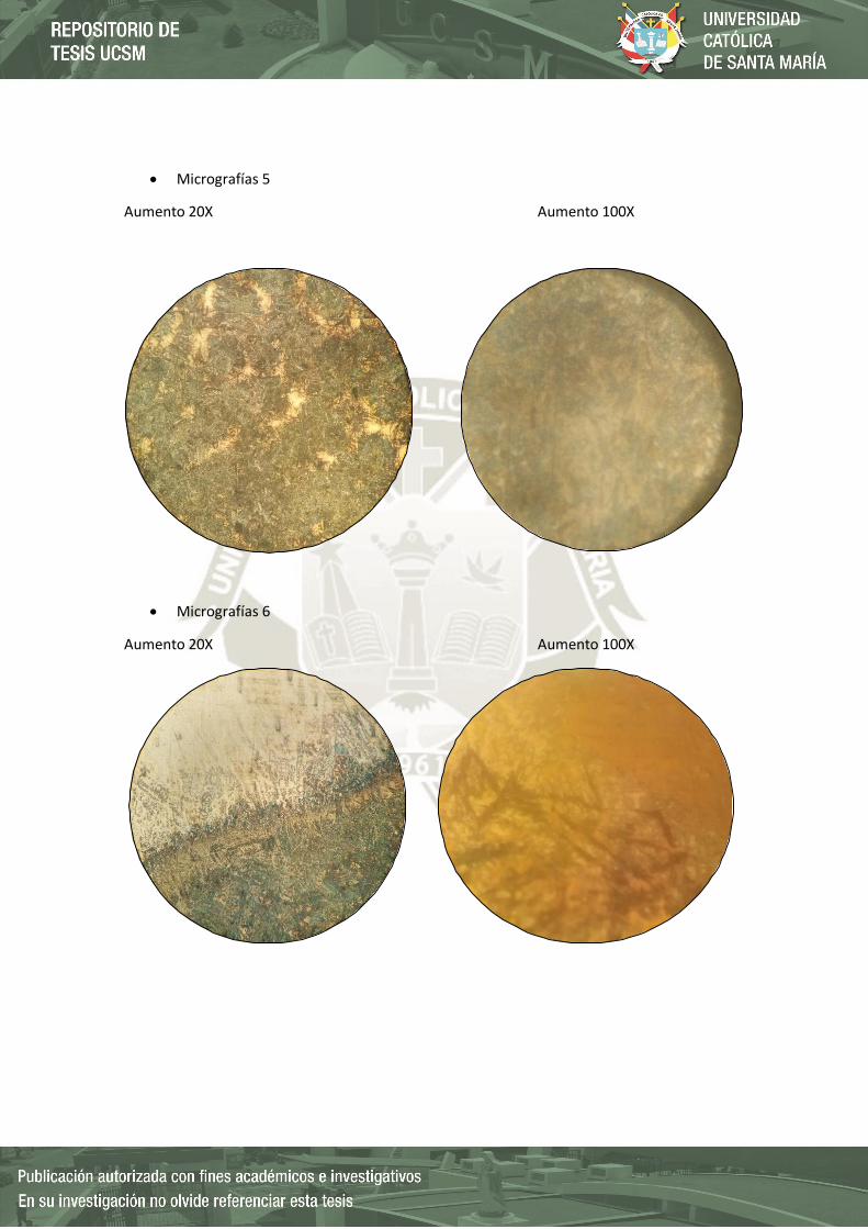
Micrografías 5
Aumento 20X Aumento 100X
Micrografías 6
Aumento 20X Aumento 100X

Micrografías 7
Aumento 20X Aumento 100X
Micrografías 8
Aumento 20X Aumento 100X
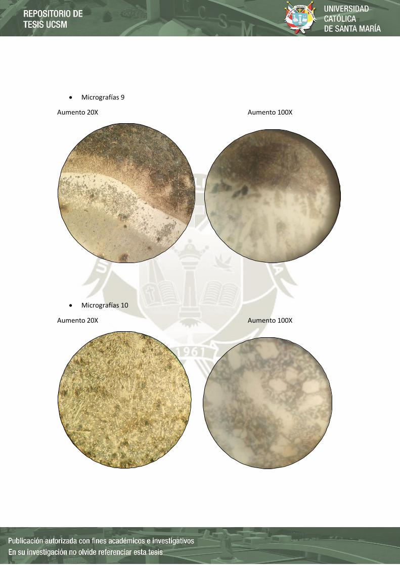
Micrografías 9
Aumento 20X Aumento 100X
Micrografías 10
Aumento 20X Aumento 100X

Micrografías 11
Aumento 20X Aumento 100X
Micrografías 12
Aumento 20X

Micrografías 13
Aumento 20X
Micrografías 14
Aumento 20X

Micrografías 15
Aumento 20X
Micrografías 16
Aumento 20X
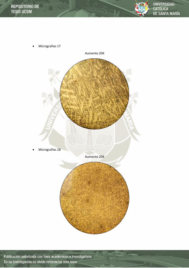
Micrografías 17
Aumento 20X
Micrografías 18
Aumento 20X

Micrografías 19
Aumento 20X
Micrografías 20
Aumento 20X
ANEXO 19
RESULTADOS DE
ENSAYO DE
TRACCIÓN
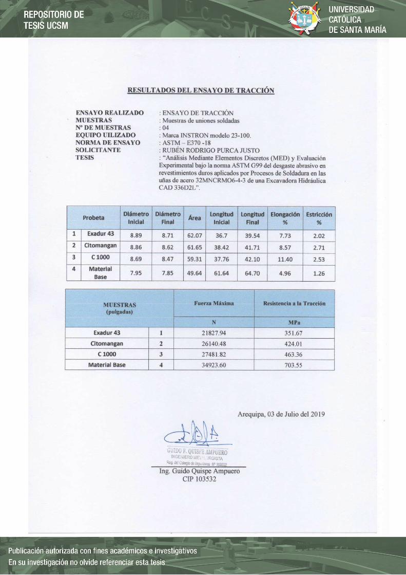
ANEXO 20
RESULTADOS DE
ENSAYO DE
DESGASTE

Anton Paar GmbH
Anton Paar Strasse 20
8054 Graz - Austria
Evaluacion Experimental del desgaste en
revestimientos duros
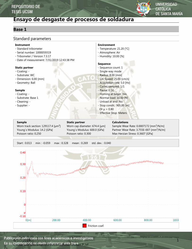
Ensayo de desgaste de procesos de soldadura
Base 1
Standard parameters
Instrument
- Standard tribometer- Serial number: 1000059319- Tribometer / Version 7.3.17- Date of measurement: 7/31/2019 12:43:38 PM
Static partner
- Coating: -- Substrate: WC- Dimension: 6.00 [mm]- Geometry: Ball
Sample
- Coating: -- Substrate: Base 1- Cleaning: -- Supplier: -
Environment
- Temperature: 21.20 [°C]- Atmosphere: Air- Humidity: 10.00 [%]
Sequence
- Sequence count: 1- Single-way mode- Radius: 8.00 [mm]- Lin. Speed: 25.00 [cm/s]- Acquisition rate: 5.0 [Hz]- Cycles sampled: 1/1- Pause: 0 [s]- Homing at begin: Yes- Normal load: 10.00 [N]- Unload at end: No- Stop condit.: 905.00 [m] Or µ > 0.80- Effective Stop: Meters
Sample Static partner Calculations
Worn track section: 129117.4 [µm²]Young´s Modulus: 14.2 [GPa]Poisson ratio: 0.250
Worn cap diameter: 674.4 [µm]Young´s Modulus: 600.0 [GPa]Poisson ratio: 0.300
Sample Wear Rate: 0.0007172 [mm³/N/m]Partner Wear Rate: 3.755E-007 [mm³/N/m]Max Herzian Stress: 0.3607 [GPa]
Start : 0.013 min : -0.059 max : 0.328 mean : 0.269 std. dev. : 0.040
-0.10µ
0
0.10
0.20
0.30
0.40
0[m] 200.00 400.00 600.00 800.00 1E03
Friction coef.
18/12/2019C:\Users\AP\Documents\PRUEBAS\Ruben\Ruben P..ixf
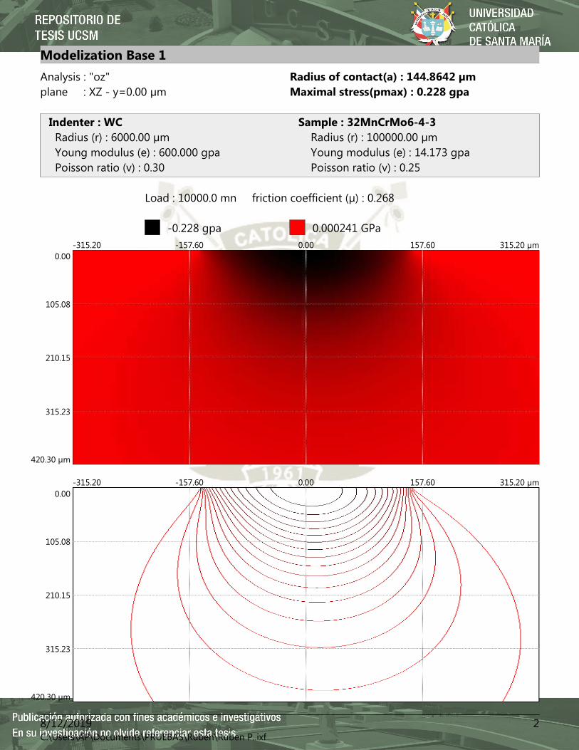
Modelization Base 1
Analysis : "oz" Radius of contact(a) : 144.8642 µm
plane : XZ - y=0.00 µm Maximal stress(pmax) : 0.228 gpa
Indenter : WC Sample : 32MnCrMo6-4-3
Radius (r) : 6000.00 µm Radius (r) : 100000.00 µm Young modulus (e) : 600.000 gpa Young modulus (e) : 14.173 gpa Poisson ratio (v) : 0.30 Poisson ratio (v) : 0.25
Load : 10000.0 mn friction coefficient (µ) : 0.268
-0.228 gpa 0.000241 GPa
-315.200.00
-157.60
105.08
0.00
210.15
157.60
315.23
315.20 µm
420.30 µm
-315.200.00
-157.60
105.08
0.00
210.15
157.60
315.23
315.20 µm
420.30 µm
28/12/2019C:\Users\AP\Documents\PRUEBAS\Ruben\Ruben P..ixf

oz as a function of x for z=0.000
-0.2280
-0.1820
-0.1370
-0.0910
-0.0455
0
-0.32x(mm) -0.19 -0.06 0.06 0.19 0.32
oz as a function of z for x=0.000
-0.42
-0.34
-0.25
-0.17
-0.08
0
-0.2280oz(GPa) -0.1870 -0.1460 -0.1060 -0.0648 -0.0242
38/12/2019C:\Users\AP\Documents\PRUEBAS\Ruben\Ruben P..ixf

oz as a function of x and z
ozXZ
48/12/2019C:\Users\AP\Documents\PRUEBAS\Ruben\Ruben P..ixf

Strain as a function of x
-0.0033Uz(mm)
-0.0026
-0.0020
-0.0013
-0.0007
0
-0.32x(mm) -0.19 -0.06 0.06 0.19 0.32
58/12/2019C:\Users\AP\Documents\PRUEBAS\Ruben\Ruben P..ixf
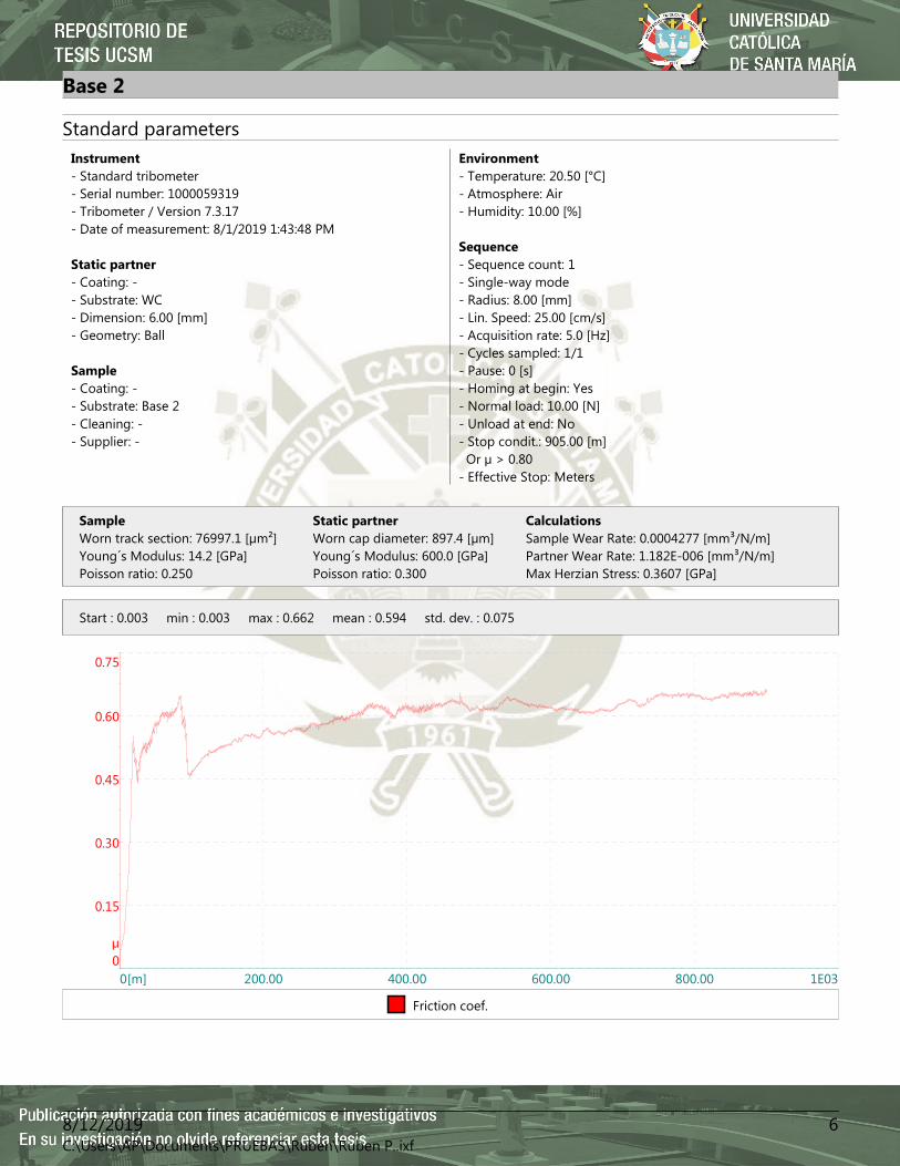
Base 2
Standard parameters
Instrument
- Standard tribometer- Serial number: 1000059319- Tribometer / Version 7.3.17- Date of measurement: 8/1/2019 1:43:48 PM
Static partner
- Coating: -- Substrate: WC- Dimension: 6.00 [mm]- Geometry: Ball
Sample
- Coating: -- Substrate: Base 2- Cleaning: -- Supplier: -
Environment
- Temperature: 20.50 [°C]- Atmosphere: Air- Humidity: 10.00 [%]
Sequence
- Sequence count: 1- Single-way mode- Radius: 8.00 [mm]- Lin. Speed: 25.00 [cm/s]- Acquisition rate: 5.0 [Hz]- Cycles sampled: 1/1- Pause: 0 [s]- Homing at begin: Yes- Normal load: 10.00 [N]- Unload at end: No- Stop condit.: 905.00 [m] Or µ > 0.80- Effective Stop: Meters
Sample Static partner Calculations
Worn track section: 76997.1 [µm²]Young´s Modulus: 14.2 [GPa]Poisson ratio: 0.250
Worn cap diameter: 897.4 [µm]Young´s Modulus: 600.0 [GPa]Poisson ratio: 0.300
Sample Wear Rate: 0.0004277 [mm³/N/m]Partner Wear Rate: 1.182E-006 [mm³/N/m]Max Herzian Stress: 0.3607 [GPa]
Start : 0.003 min : 0.003 max : 0.662 mean : 0.594 std. dev. : 0.075
0µ
0.15
0.30
0.45
0.60
0.75
0[m] 200.00 400.00 600.00 800.00 1E03
Friction coef.
68/12/2019C:\Users\AP\Documents\PRUEBAS\Ruben\Ruben P..ixf

Modelization Base 2
Analysis : "oz" Radius of contact(a) : 144.8642 µm
plane : XZ - y=0.00 µm Maximal stress(pmax) : 0.228 gpa
Indenter : WC Sample : 32MnCrMo6-4-3
Radius (r) : 6000.00 µm Radius (r) : 100000.00 µm Young modulus (e) : 600.000 gpa Young modulus (e) : 14.173 gpa Poisson ratio (v) : 0.30 Poisson ratio (v) : 0.25
Load : 10000.0 mn friction coefficient (µ) : 0.593
-0.228 gpa 0.0023 GPa
-315.200.00
-157.60
105.08
0.00
210.15
157.60
315.23
315.20 µm
420.30 µm
-315.200.00
-157.60
105.08
0.00
210.15
157.60
315.23
315.20 µm
420.30 µm
78/12/2019C:\Users\AP\Documents\PRUEBAS\Ruben\Ruben P..ixf
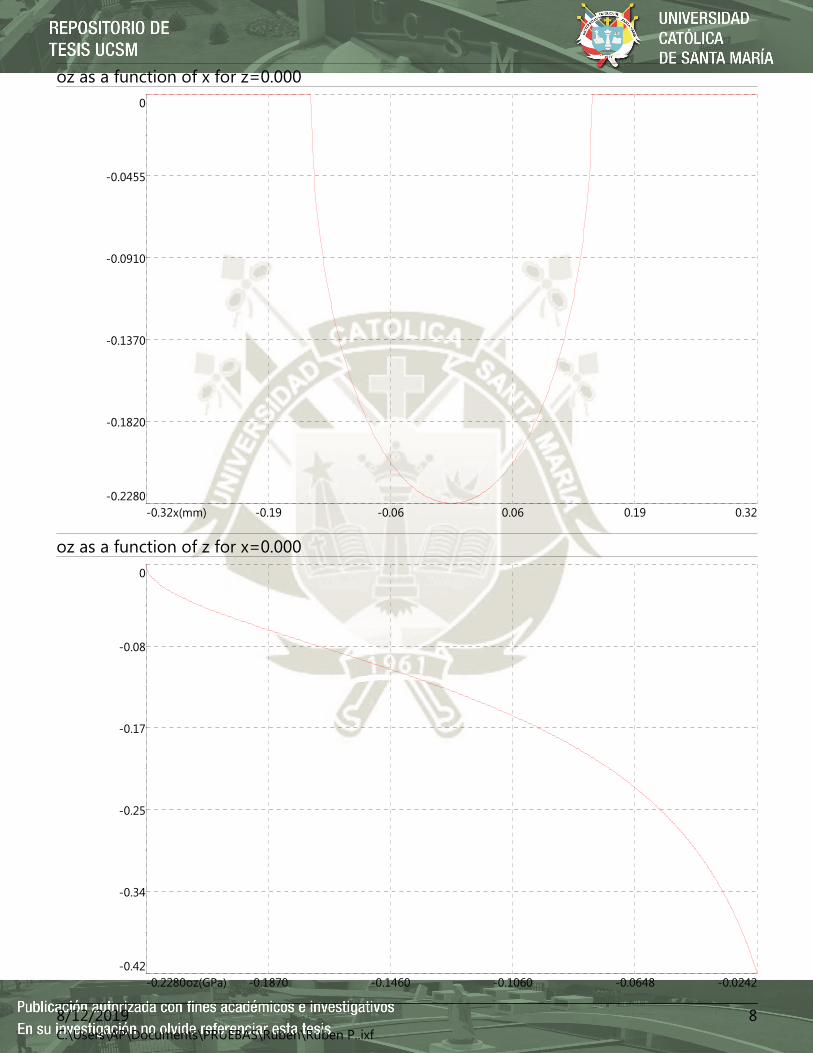
oz as a function of x for z=0.000
-0.2280
-0.1820
-0.1370
-0.0910
-0.0455
0
-0.32x(mm) -0.19 -0.06 0.06 0.19 0.32
oz as a function of z for x=0.000
-0.42
-0.34
-0.25
-0.17
-0.08
0
-0.2280oz(GPa) -0.1870 -0.1460 -0.1060 -0.0648 -0.0242
88/12/2019C:\Users\AP\Documents\PRUEBAS\Ruben\Ruben P..ixf

oz as a function of x and z
ozXZ
98/12/2019C:\Users\AP\Documents\PRUEBAS\Ruben\Ruben P..ixf

Strain as a function of x
-0.0033Uz(mm)
-0.0026
-0.0020
-0.0013
-0.0007
0
-0.32x(mm) -0.19 -0.06 0.06 0.19 0.32
108/12/2019C:\Users\AP\Documents\PRUEBAS\Ruben\Ruben P..ixf

Muestra A
Standard parameters
Instrument
- Standard tribometer- Serial number: 1000059319- Tribometer / Version 7.3.17- Date of measurement: 7/31/2019 4:34:40 PM
Static partner
- Coating: -- Substrate: WC- Dimension: 6.00 [mm]- Geometry: Ball
Sample
- Coating: -- Substrate: Muestra A- Cleaning: -- Supplier: -
Environment
- Temperature: 21.20 [°C]- Atmosphere: Air- Humidity: 10.00 [%]
Sequence
- Sequence count: 1- Single-way mode- Radius: 8.01 [mm]- Lin. Speed: 25.00 [cm/s]- Acquisition rate: 5.0 [Hz]- Cycles sampled: 1/1- Pause: 0 [s]- Homing at begin: Yes- Normal load: 10.00 [N]- Unload at end: No- Stop condit.: 905.00 [m] Or µ > 0.80- Effective Stop: Meters
Sample Static partner Calculations
Worn track section: 72936.0 [µm²]Young´s Modulus: 5.0 [GPa]Poisson ratio: 0.320
Worn cap diameter: 747.0 [µm]Young´s Modulus: 600.0 [GPa]Poisson ratio: 0.300
Sample Wear Rate: 0.0004056 [mm³/N/m]Partner Wear Rate: 5.661E-007 [mm³/N/m]Max Herzian Stress: 0.186 [GPa]
Start : 0.034 min : 0.018 max : 0.641 mean : 0.533 std. dev. : 0.060
0µ
0.15
0.30
0.45
0.60
0.75
0[m] 200.00 400.00 600.00 800.00 1E03
Friction coef.
118/12/2019C:\Users\AP\Documents\PRUEBAS\Ruben\Ruben P..ixf

Modelization A
Analysis : "oz" Radius of contact(a) : 202.1002 µm
plane : XZ - y=0.00 µm Maximal stress(pmax) : 0.117 gpa
Indenter : WC Sample : Sold. Citomangan
Radius (r) : 6000.00 µm Radius (r) : 100000.00 µm Young modulus (e) : 600.000 gpa Young modulus (e) : 4.948 gpa Poisson ratio (v) : 0.30 Poisson ratio (v) : 0.32
Load : 10000.0 mn friction coefficient (µ) : 0.531
-0.117 gpa 0.000874 GPa
-303.200.00
-151.60
101.05
0.00
202.10
151.60
303.15
303.20 µm
404.20 µm
-303.200.00
-151.60
101.05
0.00
202.10
151.60
303.15
303.20 µm
404.20 µm
128/12/2019C:\Users\AP\Documents\PRUEBAS\Ruben\Ruben P..ixf

oz as a function of x for z=0.000
-0.1170
-0.0935
-0.0701
-0.0468
-0.0234
0
-0.30x(mm) -0.18 -0.06 0.06 0.18 0.30
oz as a function of z for x=-0.303
-0.40
-0.32
-0.24
-0.16
-0.08
0
-0.0065oz(GPa) -0.0050 -0.0036 -0.0022 -0.0007 0.0007
138/12/2019C:\Users\AP\Documents\PRUEBAS\Ruben\Ruben P..ixf

oz as a function of x and z
ozXZ
148/12/2019C:\Users\AP\Documents\PRUEBAS\Ruben\Ruben P..ixf

Strain as a function of x
-0.0061Uz(mm)
-0.0049
-0.0037
-0.0025
-0.0012
0
-0.30x(mm) -0.18 -0.06 0.06 0.18 0.30
158/12/2019C:\Users\AP\Documents\PRUEBAS\Ruben\Ruben P..ixf

Muestra A2
Standard parameters
Instrument
- Standard tribometer- Serial number: 1000059319- Tribometer / Version 7.3.17- Date of measurement: 8/12/2019 3:29:13 PM
Static partner
- Coating: -- Substrate: WC- Dimension: 6.00 [mm]- Geometry: Ball
Sample
- Coating: -- Substrate: Muestra A2- Cleaning: -- Supplier: -
Environment
- Temperature: 20.00 [°C]- Atmosphere: Air- Humidity: 10.00 [%]
Sequence
- Sequence count: 1- Single-way mode- Radius: 7.98 [mm]- Lin. Speed: 25.00 [cm/s]- Acquisition rate: 5.0 [Hz]- Cycles sampled: 1/1- Pause: 0 [s]- Homing at begin: Yes- Normal load: 10.00 [N]- Unload at end: No- Stop condit.: 905.00 [m] Or µ > 0.80- Effective Stop: Meters
Sample Static partner Calculations
Worn track section: 67212.0 [µm²]Young´s Modulus: 5.0 [GPa]Poisson ratio: 0.320
Worn cap diameter: 770.7 [µm]Young´s Modulus: 600.0 [GPa]Poisson ratio: 0.300
Sample Wear Rate: 0.0003724 [mm³/N/m]Partner Wear Rate: 6.414E-007 [mm³/N/m]Max Herzian Stress: 0.186 [GPa]
Start : -0.028 min : -0.108 max : 0.438 mean : 0.357 std. dev. : 0.051
-0.30µ
-0.15
-1.19E-08
0.15
0.30
0.45
0[m] 200.00 400.00 600.00 800.00 1E03
Friction coef.
168/12/2019C:\Users\AP\Documents\PRUEBAS\Ruben\Ruben P..ixf

Modelization A2
Analysis : "oz" Radius of contact(a) : 202.1002 µm
plane : XZ - y=0.00 µm Maximal stress(pmax) : 0.117 gpa
Indenter : WC Sample : Sold. Citomangan
Radius (r) : 6000.00 µm Radius (r) : 100000.00 µm Young modulus (e) : 600.000 gpa Young modulus (e) : 4.948 gpa Poisson ratio (v) : 0.30 Poisson ratio (v) : 0.32
Load : 10000.0 mn friction coefficient (µ) : 0.357
-0.117 gpa -0.0909 GPa
-60.600.00
-30.30
20.20
0.00
40.40
30.30
60.60
60.60 µm
80.80 µm
-60.600.00
-30.30
20.20
0.00
40.40
30.30
60.60
60.60 µm
80.80 µm
178/12/2019C:\Users\AP\Documents\PRUEBAS\Ruben\Ruben P..ixf

oz as a function of x for z=0.000
-0.1170
-0.1160
-0.1150
-0.1140
-0.1130
-0.1120
-0.06x(mm) -0.04 -0.01 0.01 0.04 0.06
oz as a function of z for x=-0.061
-0.08
-0.06
-0.05
-0.03
-0.02
0
-0.1120oz(GPa) -0.1070 -0.1030 -0.0991 -0.0950 -0.0909
188/12/2019C:\Users\AP\Documents\PRUEBAS\Ruben\Ruben P..ixf

oz as a function of x and z
ozXZ
198/12/2019C:\Users\AP\Documents\PRUEBAS\Ruben\Ruben P..ixf

Strain as a function of x
-0.0061Uz(mm)
-0.0049
-0.0037
-0.0025
-0.0012
0
-0.06x(mm) -0.04 -0.01 0.01 0.04 0.06
208/12/2019C:\Users\AP\Documents\PRUEBAS\Ruben\Ruben P..ixf

Muestra B
Standard parameters
Instrument
- Standard tribometer- Serial number: 1000059319- Tribometer / Version 7.3.17- Date of measurement: 7/31/2019 5:49:06 PM
Static partner
- Coating: -- Substrate: WC- Dimension: 6.00 [mm]- Geometry: Ball
Sample
- Coating: -- Substrate: Muestra B- Cleaning: -- Supplier: -
Environment
- Temperature: 19.20 [°C]- Atmosphere: Air- Humidity: 10.00 [%]
Sequence
- Sequence count: 1- Single-way mode- Radius: 8.00 [mm]- Lin. Speed: 25.00 [cm/s]- Acquisition rate: 5.0 [Hz]- Cycles sampled: 1/1- Pause: 0 [s]- Homing at begin: Yes- Normal load: 10.00 [N]- Unload at end: No- Stop condit.: 905.00 [m] Or µ > 0.80- Effective Stop: Meters
Sample Static partner Calculations
Worn track section: 43630.4 [µm²]Young´s Modulus: 4.6 [GPa]Poisson ratio: 0.260
Worn cap diameter: 294.5 [µm]Young´s Modulus: 600.0 [GPa]Poisson ratio: 0.300
Sample Wear Rate: 0.0002423 [mm³/N/m]Partner Wear Rate: 1.361E-008 [mm³/N/m]Max Herzian Stress: 0.1715 [GPa]
Start : 0.034 min : -0.059 max : 0.605 mean : 0.502 std. dev. : 0.089
-0.60µ
-0.30
-2.38E-08
0.30
0.60
0.90
0[m] 200.00 400.00 600.00 800.00 1E03
Friction coef.
218/12/2019C:\Users\AP\Documents\PRUEBAS\Ruben\Ruben P..ixf

Modelization B
Analysis : "oz" Radius of contact(a) : 210.1395 µm
plane : XZ - y=0.00 µm Maximal stress(pmax) : 0.108 gpa
Indenter : WC Sample : Sold. Exadur-43
Radius (r) : 6000.00 µm Radius (r) : 100000.00 µm Young modulus (e) : 600.000 gpa Young modulus (e) : 4.550 gpa Poisson ratio (v) : 0.30 Poisson ratio (v) : 0.26
Load : 10000.0 mn friction coefficient (µ) : 0.501
-0.0099 gpa 6.3E-005 GPa
-315.200.00
-157.60
105.08
0.00
210.15
157.60
315.23
315.20 µm
420.30 µm
-315.200.00
-157.60
105.08
0.00
210.15
157.60
315.23
315.20 µm
420.30 µm
228/12/2019C:\Users\AP\Documents\PRUEBAS\Ruben\Ruben P..ixf
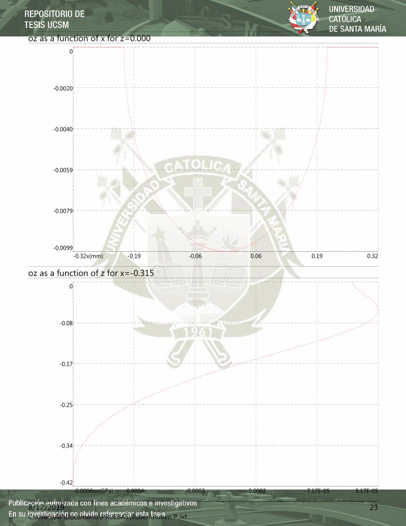
oz as a function of x for z=0.000
-0.0099
-0.0079
-0.0059
-0.0040
-0.0020
0
-0.32x(mm) -0.19 -0.06 0.06 0.19 0.32
oz as a function of z for x=-0.315
-0.42
-0.34
-0.25
-0.17
-0.08
0
-0.0006oz(GPa) -0.0004 -0.0003 -0.0002 -7.17E-05 5.17E-05
238/12/2019C:\Users\AP\Documents\PRUEBAS\Ruben\Ruben P..ixf

oz as a function of x and z
ozXZ
248/12/2019C:\Users\AP\Documents\PRUEBAS\Ruben\Ruben P..ixf
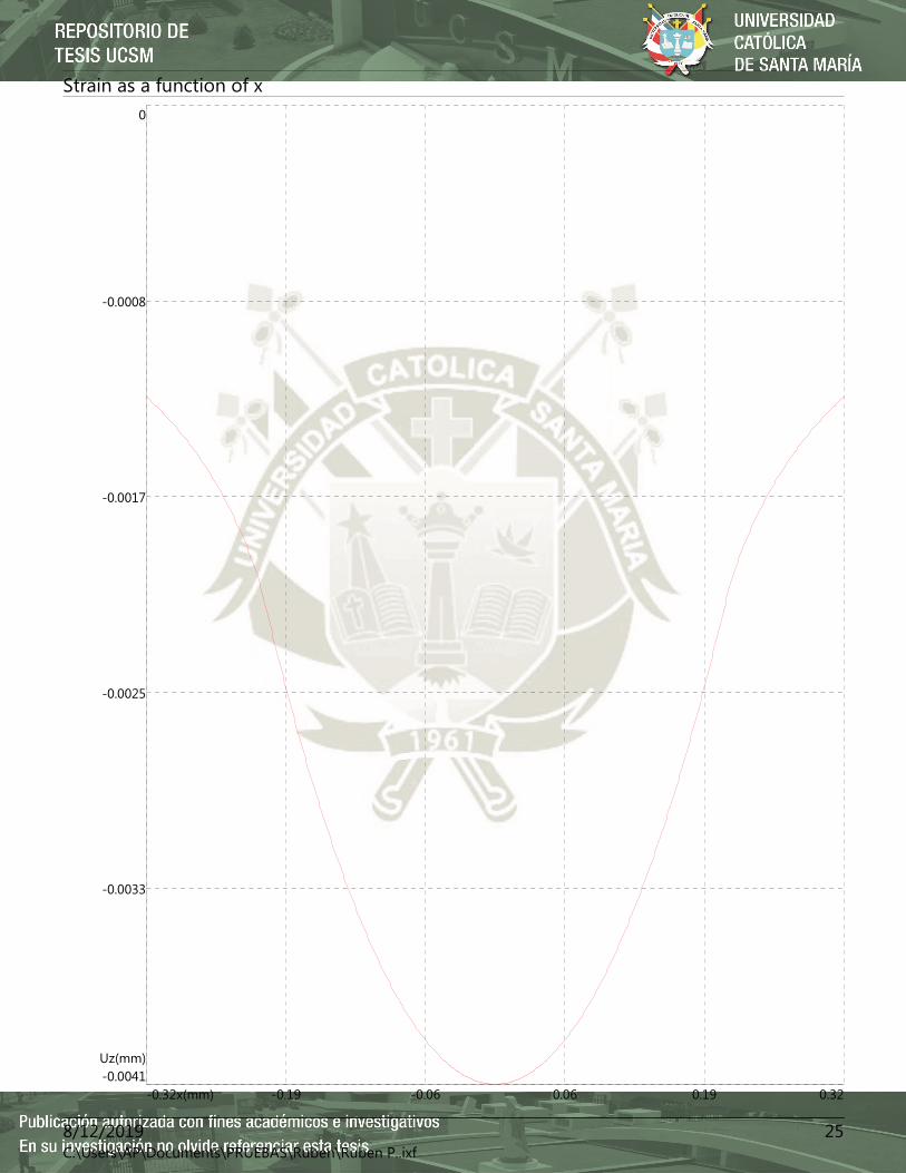
Strain as a function of x
-0.0041Uz(mm)
-0.0033
-0.0025
-0.0017
-0.0008
0
-0.32x(mm) -0.19 -0.06 0.06 0.19 0.32
258/12/2019C:\Users\AP\Documents\PRUEBAS\Ruben\Ruben P..ixf

Muestra B2
Standard parameters
Instrument
- Standard tribometer- Serial number: 1000059319- Tribometer / Version 7.3.17- Date of measurement: 8/1/2019 3:13:30 PM
Static partner
- Coating: -- Substrate: WC- Dimension: 6.00 [mm]- Geometry: Ball
Sample
- Coating: -- Substrate: Muestra B2- Cleaning: -- Supplier: -
Environment
- Temperature: 20.50 [°C]- Atmosphere: Air- Humidity: 10.00 [%]
Sequence
- Sequence count: 1- Single-way mode- Radius: 8.01 [mm]- Lin. Speed: 25.00 [cm/s]- Acquisition rate: 5.0 [Hz]- Cycles sampled: 1/1- Pause: 0 [s]- Homing at begin: Yes- Normal load: 10.00 [N]- Unload at end: No- Stop condit.: 905.00 [m] Or µ > 0.80- Effective Stop: Meters
Sample Static partner Calculations
Worn track section: 24821.5 [µm²]Young´s Modulus: 4.6 [GPa]Poisson ratio: 0.260
Worn cap diameter: 634.3 [µm]Young´s Modulus: 600.0 [GPa]Poisson ratio: 0.300
Sample Wear Rate: 0.000138 [mm³/N/m]Partner Wear Rate: 2.937E-007 [mm³/N/m]Max Herzian Stress: 0.1715 [GPa]
Start : -0.010 min : -0.010 max : 0.639 mean : 0.535 std. dev. : 0.160
-0.60µ
-0.30
-2.38E-08
0.30
0.60
0.90
0[m] 200.00 400.00 600.00 800.00 1E03
Friction coef.
268/12/2019C:\Users\AP\Documents\PRUEBAS\Ruben\Ruben P..ixf

Modelization B2
Analysis : "oz" Radius of contact(a) : 210.1395 µm
plane : XZ - y=0.00 µm Maximal stress(pmax) : 0.108 gpa
Indenter : WC Sample : Sold. Exadur-43
Radius (r) : 6000.00 µm Radius (r) : 100000.00 µm Young modulus (e) : 600.000 gpa Young modulus (e) : 4.550 gpa Poisson ratio (v) : 0.30 Poisson ratio (v) : 0.26
Load : 10000.0 mn friction coefficient (µ) : 0.533
-0.108 gpa 0.000817 GPa
-315.200.00
-157.60
105.08
0.00
210.15
157.60
315.23
315.20 µm
420.30 µm
-315.200.00
-157.60
105.08
0.00
210.15
157.60
315.23
315.20 µm
420.30 µm
278/12/2019C:\Users\AP\Documents\PRUEBAS\Ruben\Ruben P..ixf

oz as a function of x for z=0.000
-0.1080
-0.0865
-0.0649
-0.0433
-0.0216
0
-0.32x(mm) -0.19 -0.06 0.06 0.19 0.32
oz as a function of z for x=-0.315
-0.42
-0.34
-0.25
-0.17
-0.08
0
-0.0060oz(GPa) -0.0047 -0.0033 -0.0020 -0.0007 0.0007
288/12/2019C:\Users\AP\Documents\PRUEBAS\Ruben\Ruben P..ixf

oz as a function of x and z
ozXZ
298/12/2019C:\Users\AP\Documents\PRUEBAS\Ruben\Ruben P..ixf

Strain as a function of x
-0.0069Uz(mm)
-0.0055
-0.0041
-0.0027
-0.0014
0
-0.32x(mm) -0.19 -0.06 0.06 0.19 0.32
308/12/2019C:\Users\AP\Documents\PRUEBAS\Ruben\Ruben P..ixf
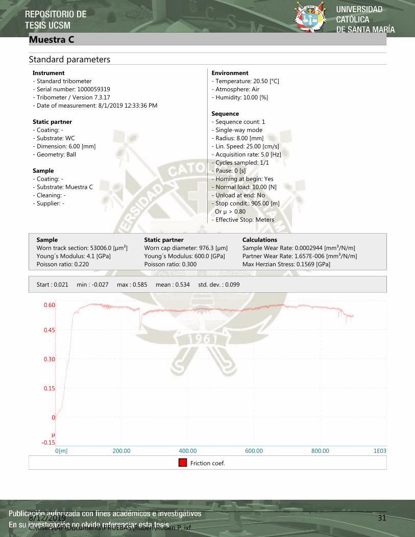
Muestra C
Standard parameters
Instrument
- Standard tribometer- Serial number: 1000059319- Tribometer / Version 7.3.17- Date of measurement: 8/1/2019 12:33:36 PM
Static partner
- Coating: -- Substrate: WC- Dimension: 6.00 [mm]- Geometry: Ball
Sample
- Coating: -- Substrate: Muestra C- Cleaning: -- Supplier: -
Environment
- Temperature: 20.50 [°C]- Atmosphere: Air- Humidity: 10.00 [%]
Sequence
- Sequence count: 1- Single-way mode- Radius: 8.00 [mm]- Lin. Speed: 25.00 [cm/s]- Acquisition rate: 5.0 [Hz]- Cycles sampled: 1/1- Pause: 0 [s]- Homing at begin: Yes- Normal load: 10.00 [N]- Unload at end: No- Stop condit.: 905.00 [m] Or µ > 0.80- Effective Stop: Meters
Sample Static partner Calculations
Worn track section: 53006.0 [µm²]Young´s Modulus: 4.1 [GPa]Poisson ratio: 0.220
Worn cap diameter: 976.3 [µm]Young´s Modulus: 600.0 [GPa]Poisson ratio: 0.300
Sample Wear Rate: 0.0002944 [mm³/N/m]Partner Wear Rate: 1.657E-006 [mm³/N/m]Max Herzian Stress: 0.1569 [GPa]
Start : 0.021 min : -0.027 max : 0.585 mean : 0.534 std. dev. : 0.099
-0.15µ
0
0.15
0.30
0.45
0.60
0[m] 200.00 400.00 600.00 800.00 1E03
Friction coef.
318/12/2019C:\Users\AP\Documents\PRUEBAS\Ruben\Ruben P..ixf
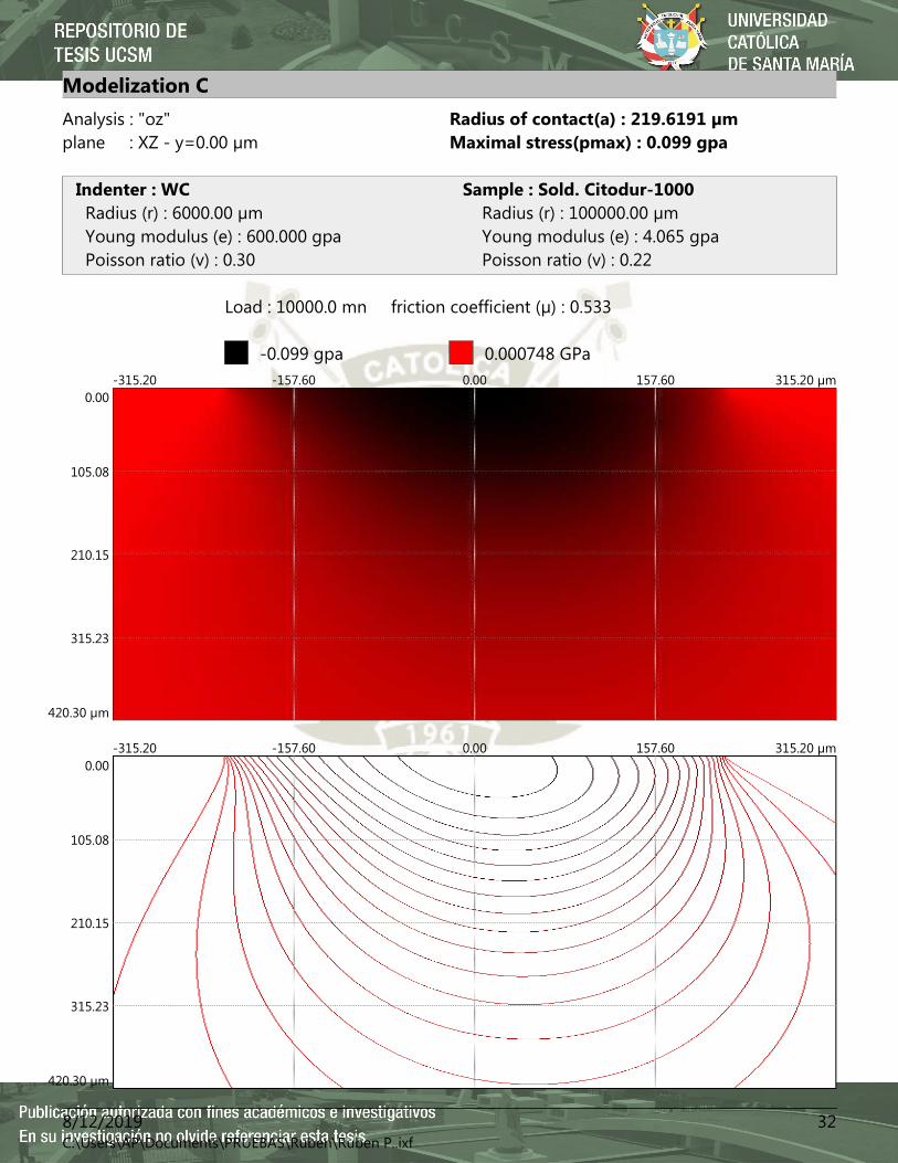
Modelization C
Analysis : "oz" Radius of contact(a) : 219.6191 µm
plane : XZ - y=0.00 µm Maximal stress(pmax) : 0.099 gpa
Indenter : WC Sample : Sold. Citodur-1000
Radius (r) : 6000.00 µm Radius (r) : 100000.00 µm Young modulus (e) : 600.000 gpa Young modulus (e) : 4.065 gpa Poisson ratio (v) : 0.30 Poisson ratio (v) : 0.22
Load : 10000.0 mn friction coefficient (µ) : 0.533
-0.099 gpa 0.000748 GPa
-315.200.00
-157.60
105.08
0.00
210.15
157.60
315.23
315.20 µm
420.30 µm
-315.200.00
-157.60
105.08
0.00
210.15
157.60
315.23
315.20 µm
420.30 µm
328/12/2019C:\Users\AP\Documents\PRUEBAS\Ruben\Ruben P..ixf

oz as a function of x for z=0.000
-0.0990
-0.0792
-0.0594
-0.0396
-0.0198
0
-0.32x(mm) -0.19 -0.06 0.06 0.19 0.32
oz as a function of z for x=-0.315
-0.42
-0.34
-0.25
-0.17
-0.08
0
-0.0060oz(GPa) -0.0047 -0.0034 -0.0020 -0.0007 0.0006
338/12/2019C:\Users\AP\Documents\PRUEBAS\Ruben\Ruben P..ixf

oz as a function of x and z
ozXZ
348/12/2019C:\Users\AP\Documents\PRUEBAS\Ruben\Ruben P..ixf
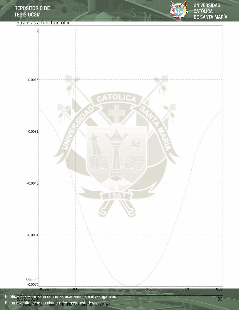
Strain as a function of x
-0.0076Uz(mm)
-0.0061
-0.0046
-0.0031
-0.0015
0
-0.32x(mm) -0.19 -0.06 0.06 0.19 0.32
358/12/2019C:\Users\AP\Documents\PRUEBAS\Ruben\Ruben P..ixf
Summary
Ensayo de desgaste de procesos de soldadura 1
Base 1 1
Standard parameters 1
Modelization Base 1 2
oz as a function of x for z=0.000 3
oz as a function of z for x=0.000 3
oz as a function of x and z 4
Strain as a function of x 5
Base 2 6
Standard parameters 6
Modelization Base 2 7
oz as a function of x for z=0.000 8
oz as a function of z for x=0.000 8
oz as a function of x and z 9
Strain as a function of x 10
Muestra A 11
Standard parameters 11
Modelization A 12
oz as a function of x for z=0.000 13
oz as a function of z for x=-0.303 13
oz as a function of x and z 14
Strain as a function of x 15
Muestra A2 16
Standard parameters 16
Modelization A2 17
oz as a function of x for z=0.000 18
oz as a function of z for x=-0.061 18
oz as a function of x and z 19
Strain as a function of x 20
Muestra B 21
Standard parameters 21
Modelization B 22
oz as a function of x for z=0.000 23
oz as a function of z for x=-0.315 23
368/12/2019C:\Users\AP\Documents\PRUEBAS\Ruben\Ruben P..ixf

oz as a function of x and Z
Strain as a function of x" "'
Muestra 82
Standard parameters
Modelization 82
az as a function of x for z=0.000
oz as a function of zÍor x=-0.315
oz as a function of x and z
Strain as a function of x
Muestra C
Standard parameters
Modelization C
oz as a function of x for z=0.000
oz as a function of z tor x=-0.31-5
oz as a functíon of x and z
Strain as a function of xSummary
24
25
26
26
27
28
28
29
30
31
31
32
33
33
34
35
36
#{
Éfurc/q/l G+Do DE7 LA Bor¿¿l4za& c4¿ad-é7a\ac-tbnJ Fuz¡ a b il,A / D6-
klaf*,rz,tta lgl - Uu +1
8/12/2019C:\Users\AP\Docu ments\PRUEBAS\Ru ben\Ruben p..ixf
37
ANEXO 21
RESULTADOS DE
ANÁLISIS DE
COMPOSICIÓN
QUÍMICA – BOHLER

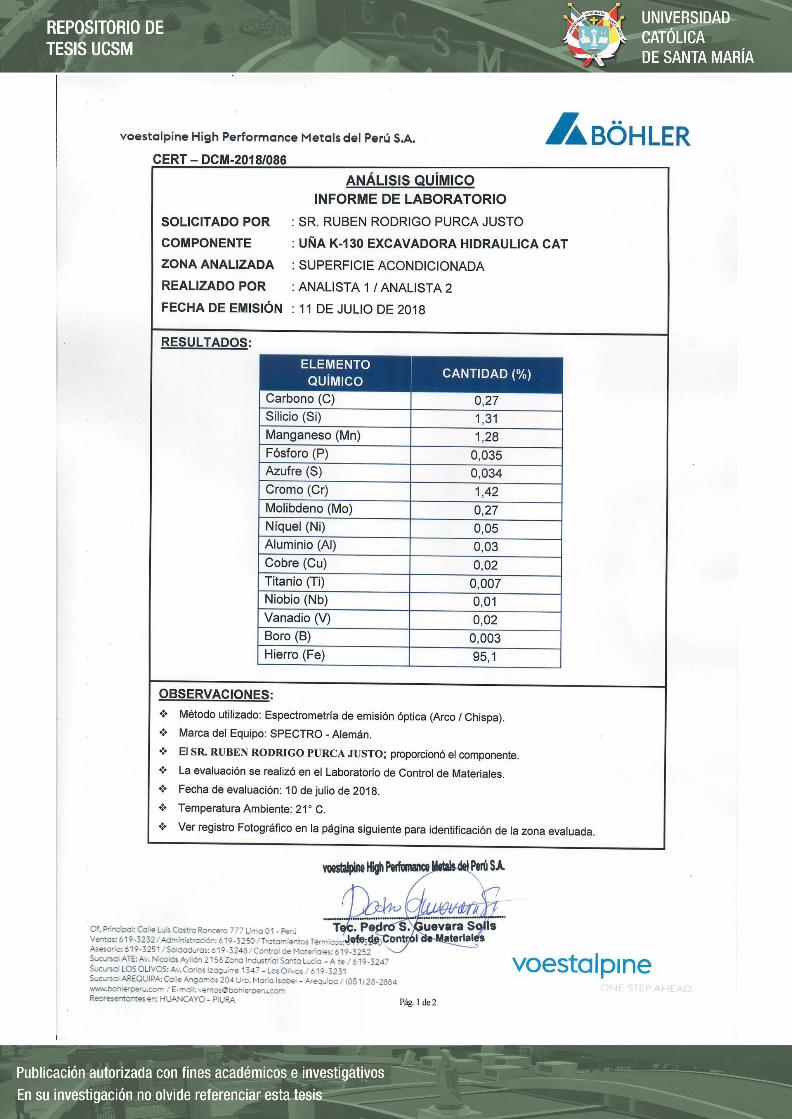

Pág. 1 de 1
CM-18-169-P1
Lima, 28 de diciembre de 2018
SR.
RUBEN RODRIGO PURCA JUSTO.
Presente.- En representación de la empresa voestalpine High Performance Metals del Perú
S.A. (División de Control de Materiales), le hago llegar la presente carta a fin de
ampliar las observaciones a la que se ha llegado después de realizar el análisis
químico en un componente (MATERIAL DE APORTE – CÓDIGO: P-1 E-43) el
mismo que ha sido detallado mediante el Informe Técnico CERT-DCM-2018-169-
P1.
La zona analizada químicamente, hace referencia a un material de alto carbono
y alta aleación (Cromo – Niobio), similar químicamente con la designación
EXADUR 43.
Se adjunta informe de laboratorio y registro fotográfico.
Sin otro particular le envío un cordial saludo.
Atentamente,

Pág. 1 de 2
CERT – DCM-2018/169-P1
ANÁLISIS QUÍMICO
INFORME DE LABORATORIO
SOLICITADO POR : SR. RUBEN RODRIGO PURCA JUSTO.
COMPONENTE : MUESTRA METALICA.
CÓDIGO : P-1 E-43.
ZONA ANALIZADA : MATERIAL DE APORTE (SOLDADURA).
REALIZADO POR : ANALISTA 1 / ANALISTA 4.
FECHA DE EMISIÓN : 28 DE DICIEMBRE DE 2018.
RESULTADOS:
ELEMENTO
QUÍMICO CANTIDAD (%)
Carbono (C) 3,96
Silicio (Si) 1,59
Manganeso (Mn) 1,24
Fósforo (P) 0,028
Azufre (S) 0,013
Cromo (Cr) 20,30
Molibdeno (Mo) 0,10
Níquel (Ni) 0,15
Aluminio (Al) 0,05
Cobre (Cu) 0,07
Titanio (Ti) 0,08
Niobio (Nb) ~4,20
Vanadio (V) 0,04
Boro (B) 0,0005
Hierro (Fe) 67,8
OBSERVACIONES:
Método utilizado: Espectrometría de emisión óptica (Arco / Chispa).
Marca del Equipo: SPECTRO - Alemán.
El cliente SR. RUBEN RODRIGO PURCA JUSTO proporcionó el componente.
La evaluación se realizó en el Laboratorio de Control de Materiales.
Fecha de evaluación: 27 de diciembre de 2018.
Temperatura Ambiente: 22,5° C.
Ver en la página siguiente el registro fotográfico de la zona analizada.

Pág. 2 de 2
REGISTRO FOTOGRÁFICO
CÓDIGO P-1 E-43.
MATERIAL DE APORTE (SOLDADURA).
ZONA ANALIZADA

Pág. 1 de 1
CM-18-169-P2
Lima, 28 de diciembre de 2018
SR.
RUBEN RODRIGO PURCA JUSTO.
Presente.-
En representación de la empresa voestalpine High Performance Metals del Perú
S.A. (División de Control de Materiales), le hago llegar la presente carta a fin de
ampliar las observaciones a la que se ha llegado después de realizar el análisis
químico en un componente (MATERIAL DE APORTE – CÓDIGO: P-2 CTMG.) el
mismo que ha sido detallado mediante el Informe Técnico CERT-DCM-2018-169-
P2.
La zona analizada químicamente, hace referencia a un material de alto carbono
y alta aleación (Manganeso), similar químicamente con la designación
CITOMANGAN.
Se adjunta informe de laboratorio y registro fotográfico.
Sin otro particular le envío un cordial saludo.
Atentamente,
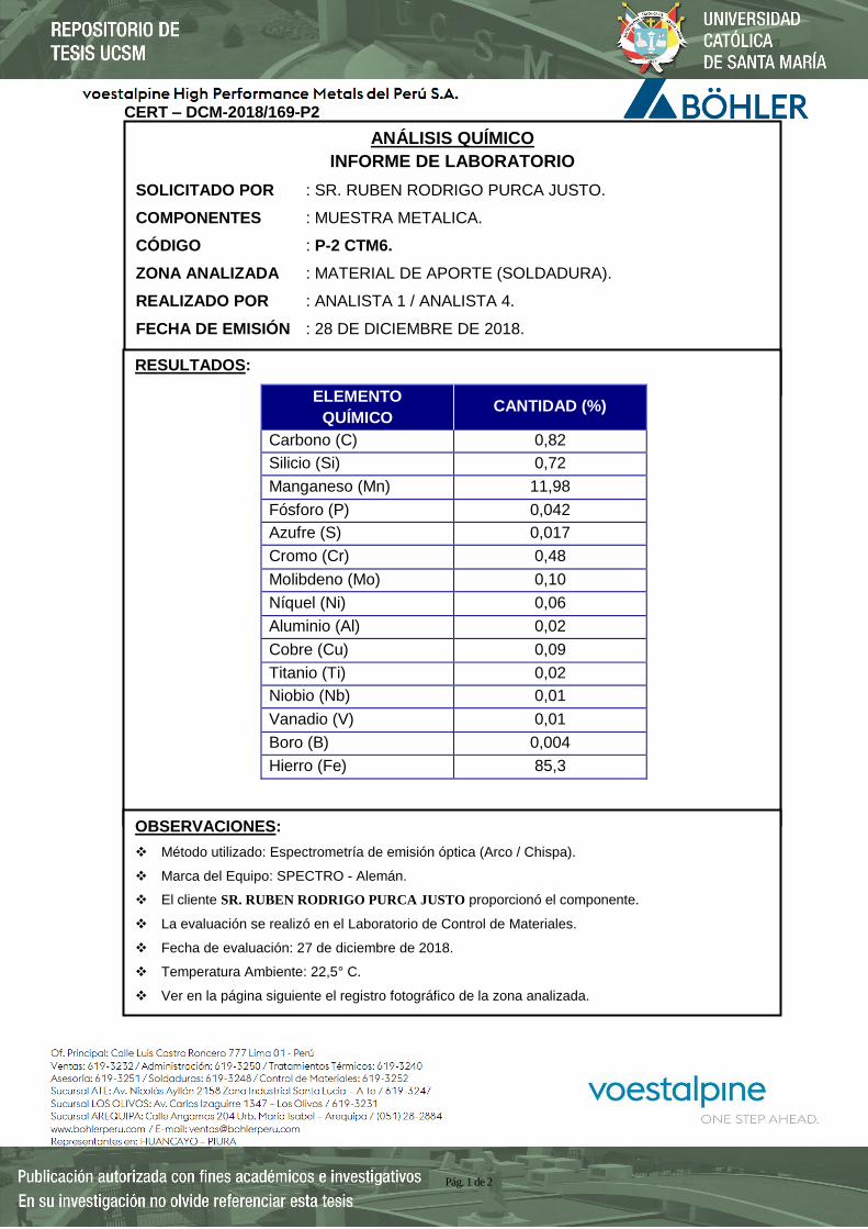
Pág. 1 de 2
CERT – DCM-2018/169-P2
ANÁLISIS QUÍMICO
INFORME DE LABORATORIO
SOLICITADO POR : SR. RUBEN RODRIGO PURCA JUSTO.
COMPONENTES : MUESTRA METALICA.
CÓDIGO : P-2 CTM6.
ZONA ANALIZADA : MATERIAL DE APORTE (SOLDADURA).
REALIZADO POR : ANALISTA 1 / ANALISTA 4.
FECHA DE EMISIÓN : 28 DE DICIEMBRE DE 2018.
RESULTADOS:
ELEMENTO
QUÍMICO CANTIDAD (%)
Carbono (C) 0,82
Silicio (Si) 0,72
Manganeso (Mn) 11,98
Fósforo (P) 0,042
Azufre (S) 0,017
Cromo (Cr) 0,48
Molibdeno (Mo) 0,10
Níquel (Ni) 0,06
Aluminio (Al) 0,02
Cobre (Cu) 0,09
Titanio (Ti) 0,02
Niobio (Nb) 0,01
Vanadio (V) 0,01
Boro (B) 0,004
Hierro (Fe) 85,3
OBSERVACIONES:
Método utilizado: Espectrometría de emisión óptica (Arco / Chispa).
Marca del Equipo: SPECTRO - Alemán.
El cliente SR. RUBEN RODRIGO PURCA JUSTO proporcionó el componente.
La evaluación se realizó en el Laboratorio de Control de Materiales.
Fecha de evaluación: 27 de diciembre de 2018.
Temperatura Ambiente: 22,5° C.
Ver en la página siguiente el registro fotográfico de la zona analizada.

Pág. 2 de 2
REGISTRO FOTOGRÁFICO
CÓDIGO P-2 CTMGMATERIAL DE APORTE (SOLDADURA).
ZONA ANALIZADA

Pág. 1 de 1
CM-18-169-P3
Lima, 28 de diciembre de 2018
SR.
RUBEN RODRIGO PURCA JUSTO.
Presente.-
En representación de la empresa voestalpine High Performance Metals del Perú
S.A. (División de Control de Materiales), le hago llegar la presente carta a fin de
ampliar las observaciones a la que se ha llegado después de realizar el análisis
químico en un componente (MATERIAL DE APORTE – CÓDIGO: P-3 C-1000.) el
mismo que ha sido detallado mediante el Informe Técnico CERT-DCM-2018-169-
P3.
La zona analizada químicamente, hace referencia a un material de alto carbono
y alta aleación (Cromo), similar químicamente con la designación CITODUR
1000.
Se adjunta informe de laboratorio y registro fotográfico.
Sin otro particular le envío un cordial saludo.
Atentamente,

Pág. 1 de 2
CERT – DCM-2018/169-P3
ANÁLISIS QUÍMICO
INFORME DE LABORATORIO
SOLICITADO POR : SR. RUBEN RODRIGO PURCA JUSTO.
COMPONENTES : MUESTRA METALICA.
CÓDIGO : P-3 C-100.
ZONA ANALIZADA : MATERIAL DE APORTE (SOLDADURA).
REALIZADO POR : ANALISTA 1 / ANALISTA 4.
FECHA DE EMISIÓN : 28 DE DICIEMBRE DE 2018.
RESULTADOS:
ELEMENTO
QUÍMICO CANTIDAD (%)
Carbono (C) 3,60
Silicio (Si) 1,13
Manganeso (Mn) 1,10
Fósforo (P) 0,014
Azufre (S) 0,003
Cromo (Cr) 31,57
Molibdeno (Mo) 0,10
Níquel (Ni) 0,06
Aluminio (Al) 0,05
Cobre (Cu) 0,04
Titanio (Ti) 0,16
Niobio (Nb) 0,10
Vanadio (V) 0,02
Boro (B) <0,0005
Hierro (Fe) 61,6
OBSERVACIONES:
Método utilizado: Espectrometría de emisión óptica (Arco / Chispa).
Marca del Equipo: SPECTRO - Alemán.
El cliente SR. RUBEN RODRIGO PURCA JUSTO proporcionó el componente.
La evaluación se realizó en el Laboratorio de Control de Materiales.
Fecha de evaluación: 27 de diciembre de 2018.
Temperatura Ambiente: 22,5° C.
Ver en la página siguiente el registro fotográfico de la zona analizada.
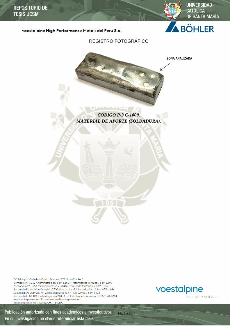
Pág. 2 de 2
REGISTRO FOTOGRÁFICO
CÓDIGO P-3 C-1000.
MATERIAL DE APORTE (SOLDADURA).
ZONA ANALIZADA
ANEXO 22
COSTO DE GETS
TRACTO PARTES
Fecha de impresión: 20/12/2017EQUIPOS ATENUZ SA
PEDIDO DE COMPRA N° 1712100125
Teléfono +5154 223866
DIRECCION FISCAL: AV. MARISCAL BENAVIDES NRO. 615 URB. SELVA
ALEGRE
RUC: 20371463586 Proyecto: BARRICK-LAG.NORTE
PEDIDO DE COMPRA
Motivo compra:
REQUERIMIENTOS Y AUTORIZACIONES Aprobado porRequerido porFechaRequerimiento
1712000062 18/12/2017 MANTENIMIENTO AREQUIPA dguzman
Proveedor:
Dirección:
RUC:
Contacto:
e-mail:
Moneda:
N° Cotización:
RG TRACTO PARTS S.A.C.
MZA. E LOTE. 12 URB. POPULAR COOPERATIVA DE VIVIENDA
BATASOL LTDA (COOP. BATASOL CARRETERA CENTRAL)
-LURIGANCHO-LIMA LIMA
20565496761
Fecha emisión:
Dolar Americano
20/12/2017
ContadoCondición pago:
Contrato
Del
Al
Cantidad UM P.U.
US$
Valor total
US$
Fecha de
entrega
Cod. SAP N° Parte Descripción %Dcto
170ED00042 UND 20.00 1,820.0020/12/2017PUNTA DE PENETRACION K130220-9133 0.00 91.00
Equipo: 47018079 - EXCAVADORA - EXC - 076 Placa/Nº serie:
BARRICK-LAGUNAS NORTE, STOCK DE EDD, CAMBIO DE
UÑAS K130
TOTAL
Impuesto
SUB TOTAL
US$ 327.60
US$ 2,147.60
US$ 1,820.00DEBE CONSIGNAR EL NÚMERO DE ORDEN DE COMPRA EN SU
FACTURA Y/O GUIA DE REMISIÓN
Gerente de AdministraciónJefe del áreaCoordinador Logístico
1. La mercadería deberá ser entregada en nuestros almacenes adjuntando la Guia de Remisión y la Orden de Compra respectivas.
2. Remitir su factura a la Av. Mariscal Benavides N 615 - Urb. Selva Alegre - Arequipa - Arequipa; adjuntando copia de la Orden de Compra y copia de la Guia de Remisión
debidamente sellada por Equipos Atenuz S.A. En señal de conformidad.
3. Las Facturas que no contengan los documentos indicados, no serán aceptadas por recepción.
4. Los proveedores tienen que estar sujetos a las condiciones de seguridad para ingresar a mina según el proyecto lo requiera
Impreso en SAPPágina 1 de 1

ANEXO 23
EXCAVADORA
CAT- 336D2 L
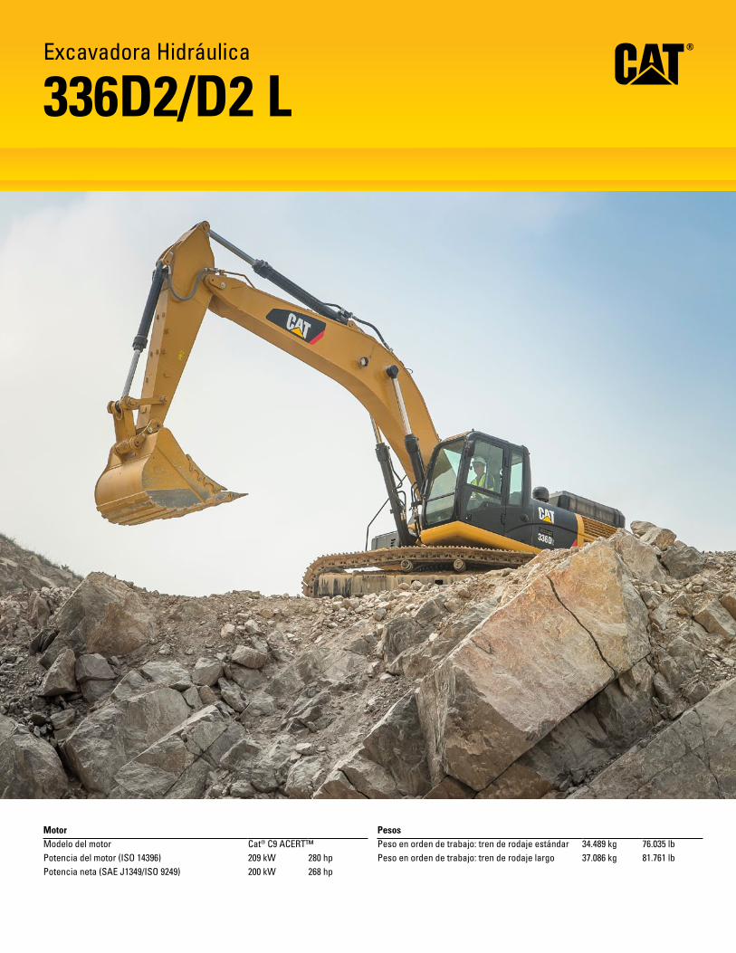
MotorModelo del motor Cat® C9 ACERT™Potencia del motor (ISO 14396) 209 kW 280 hpPotencia neta (SAE J1349/ISO 9249) 200 kW 268 hp
PesosPeso en orden de trabajo: tren de rodaje estándar 34.489 kg 76.035 lbPeso en orden de trabajo: tren de rodaje largo 37.086 kg 81.761 lb
Excavadora Hidráulica
336D2/D2 L
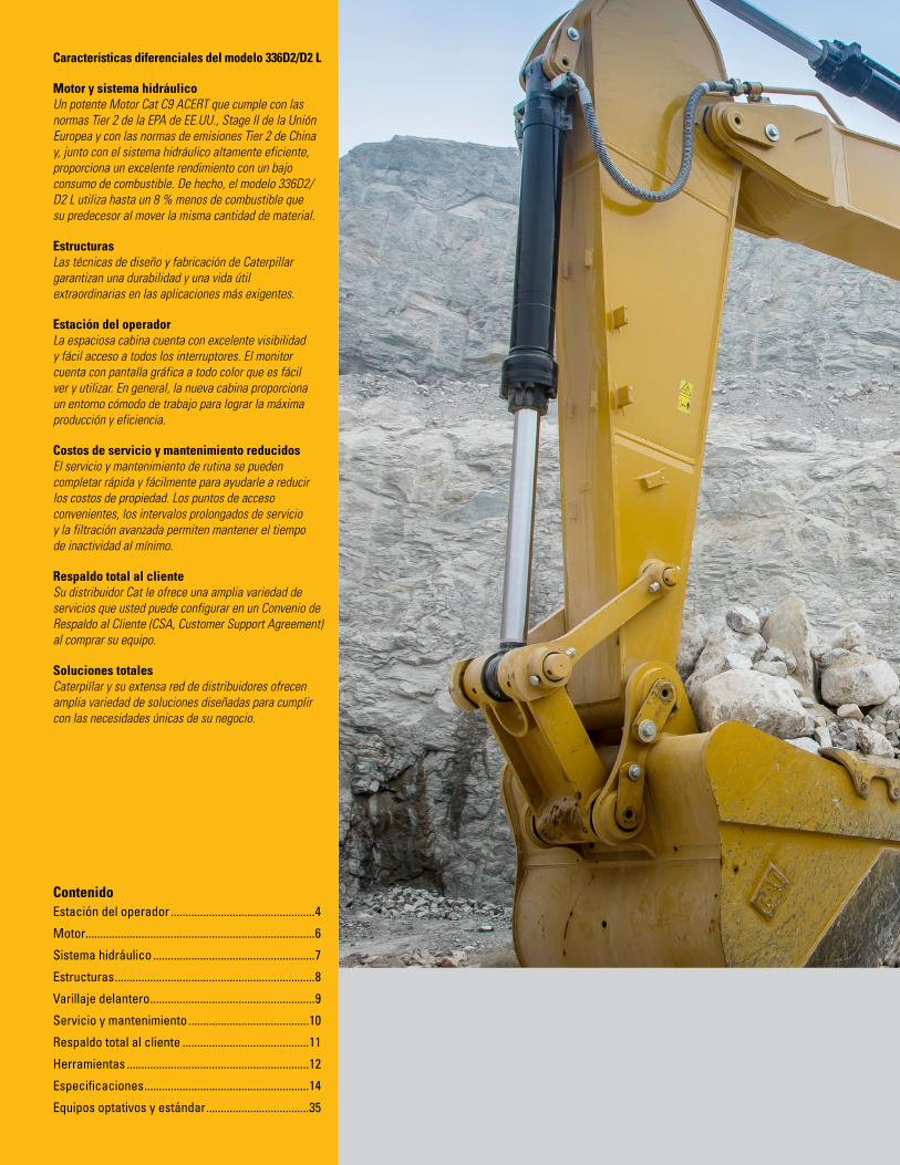
2
Características diferenciales del modelo 336D2/D2 L
Motor y sistema hidráulicoUn potente Motor Cat C9 ACERT que cumple con las normas Tier 2 de la EPA de EE.UU., Stage II de la Unión Europea y con las normas de emisiones Tier 2 de China y, junto con el sistema hidráulico altamente eficiente, proporciona un excelente rendimiento con un bajo consumo de combustible. De hecho, el modelo 336D2/D2 L utiliza hasta un 8 % menos de combustible que su predecesor al mover la misma cantidad de material.
EstructurasLas técnicas de diseño y fabricación de Caterpillar garantizan una durabilidad y una vida útil extraordinarias en las aplicaciones más exigentes.
Estación del operadorLa espaciosa cabina cuenta con excelente visibilidad y fácil acceso a todos los interruptores. El monitor cuenta con pantalla gráfica a todo color que es fácil ver y utilizar. En general, la nueva cabina proporciona un entorno cómodo de trabajo para lograr la máxima producción y eficiencia.
Costos de servicio y mantenimiento reducidosEl servicio y mantenimiento de rutina se pueden completar rápida y fácilmente para ayudarle a reducir los costos de propiedad. Los puntos de acceso convenientes, los intervalos prolongados de servicio y la filtración avanzada permiten mantener el tiempo de inactividad al mínimo.
Respaldo total al clienteSu distribuidor Cat le ofrece una amplia variedad de servicios que usted puede configurar en un Convenio de Respaldo al Cliente (CSA, Customer Support Agreement) al comprar su equipo.
Soluciones totalesCaterpillar y su extensa red de distribuidores ofrecen amplia variedad de soluciones diseñadas para cumplir con las necesidades únicas de su negocio.
ContenidoEstación del operador .................................................4
Motor..............................................................................6
Sistema hidráulico .......................................................7
Estructuras ....................................................................8
Varillaje delantero ........................................................9
Servicio y mantenimiento .........................................10
Respaldo total al cliente ...........................................11
Herramientas ..............................................................12
Especificaciones ........................................................14
Equipos optativos y estándar ...................................35
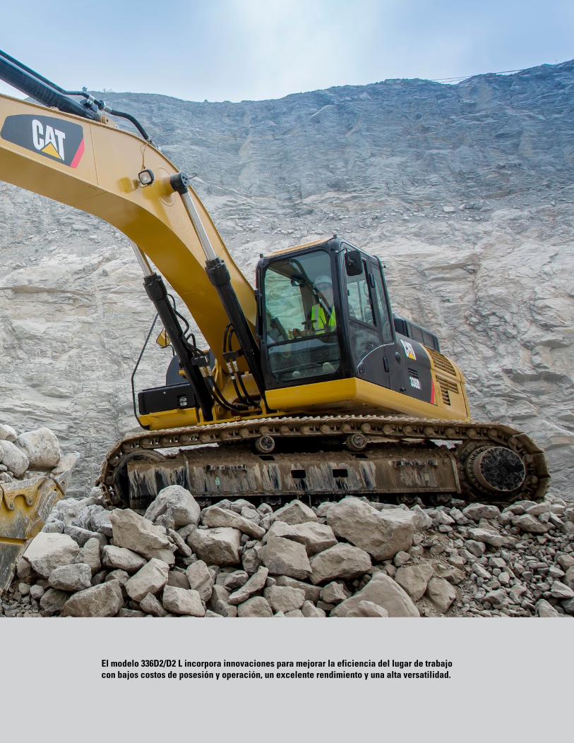
3
El modelo 336D2/D2 L incorpora innovaciones para mejorar la eficiencia del lugar de trabajo con bajos costos de posesión y operación, un excelente rendimiento y una alta versatilidad.

4
Estación del operadorDiseñada ergonómicamente para mantenerlo cómodo y productivo durante todo el día.

5
Estructura y montajes de la cabinaEl revestimiento de la cabina está sujetado al bastidor con montajes de cabina de caucho viscoso, que amortiguan las vibraciones y los niveles de ruido para aumentar la comodidad del operador. Una tubería de acero grueso a lo largo del perímetro inferior mejora la resistencia a la fatiga y a la vibración de la cabina.
AsientoEl asiento con suspensión proporciona una amplia variedad de ajustes para adaptarse a una amplia gama de operadores. El asiento incluye un respaldo reclinable, ajustes deslizantes superior e inferior del asiento y ajustes de la altura y del ángulo de inclinación para satisfacer las necesidades de comodidad y productividad.
Control de palanca universal y consolaLos controles de la palanca universal de bajo esfuerzo operados por piloto están diseñados para adaptarse a la posición natural de la muñeca y del brazo, de manera que puedan entregar máxima comodidad y producir mínima fatiga. Las consolas de palanca universal derecha e izquierda se pueden ajustar para satisfacer sus preferencias individuales, lo que aumenta la comodidad y la productividad general durante toda la jornada de trabajo.
ClimatizaciónLa ventilación filtrada positiva con una cabina presurizada es estándar. Puede seleccionarse aire fresco o aire recirculado con un interruptor ubicado en la consola izquierda.
Ventanas y limpiaparabrisasTodo el vidrio está fijo directamente en la cabina para proporcionar una excelente visibilidad y eliminar los marcos de ventanas. El parabrisas delantero superior se abre, cierra y guarda en el techo sobre el operador con el sistema de liberación con la acción de un toque. Los limpiaparabrisas montados en el pilar aumentan el área de visualización y ofrecen modalidades continuas e intermitentes.
MonitorEl monitor LCD a color se puede ajustar para minimizar el reflejo y tiene la capacidad de mostrar información en 28 idiomas para cumplir con las necesidades de la diversa fuerza de trabajo actual.
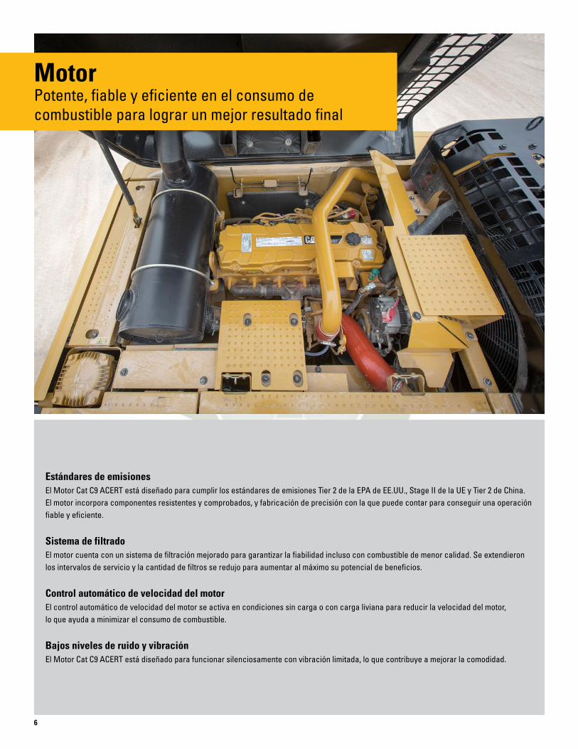
6
MotorPotente, fiable y eficiente en el consumo de combustible para lograr un mejor resultado final
Estándares de emisionesEl Motor Cat C9 ACERT está diseñado para cumplir los estándares de emisiones Tier 2 de la EPA de EE.UU., Stage II de la UE y Tier 2 de China. El motor incorpora componentes resistentes y comprobados, y fabricación de precisión con la que puede contar para conseguir una operación fiable y eficiente.
Sistema de filtradoEl motor cuenta con un sistema de filtración mejorado para garantizar la fiabilidad incluso con combustible de menor calidad. Se extendieron los intervalos de servicio y la cantidad de filtros se redujo para aumentar al máximo su potencial de beneficios.
Control automático de velocidad del motorEl control automático de velocidad del motor se activa en condiciones sin carga o con carga liviana para reducir la velocidad del motor, lo que ayuda a minimizar el consumo de combustible.
Bajos niveles de ruido y vibraciónEl Motor Cat C9 ACERT está diseñado para funcionar silenciosamente con vibración limitada, lo que contribuye a mejorar la comodidad.

7
Sistema hidráulicoLa presión del sistema hidráulico desde el sistema de dos bombas proporciona un grandioso rendimiento y productividad de excavación.‑ El sistema hidráulico y la ubicación de los componentes están diseñados para proporcionar altos niveles de eficiencia del sistema. Las bombas principales, las válvulas de control y el tanque hidráulico están ubicados cerca entre sí para permitir el uso de tubos y tuberías más cortos entre los componentes, lo que reduce la pérdida por fricción y las caídas de presión.
Sistema pilotoUna bomba piloto independiente permite un control preciso para las operaciones del varillaje delantero, de rotación y desplazamiento.
Sistema hidráulico de detección cruzadaEl sistema hidráulico de detección cruzada utiliza ambas bombas hidráulicas al 100 % de la potencia del motor, en todas las condiciones de operación. Esto mejora la productividad gracias a velocidades más altas del implemento y a giros del pivote más rápidos y fuertes.
Válvula hidráulica auxiliarLos circuitos de control están disponibles como accesorios para aumentar la versatilidad. Los controles permiten la operación de herramientas de presión media y alta, como cizallas, garfios, martillos, pulverizadores, multiprocesadores y compactadores de placas vibratorias.
Circuito de recuperación de la pluma y del brazoLos circuitos de recuperación del brazo y de la pluma ahorran energía durante las operaciones en las que la pluma está hacia abajo y el brazo está insertado. Esto aumenta la eficiencia y reduce los tiempos de ciclo y la pérdida de presión para obtener mayor productividad, costos de operación más bajos y mayor eficiencia del combustible.
Amortiguadores de cilindro hidráulicoUbicados en el extremo de varilla de los cilindros de la pluma y en ambos extremos del cilindro del brazo para amortiguar impactos y, al mismo tiempo, reducir los niveles de ruido y prolongar la vida útil del componente.
Palanca de control de accionamiento hidráulicoCon la palanca de activación hidráulica en la posición neutral se aíslan todas las funciones de varillaje delantero, rotación y desplazamiento.
Sistema hidráulicoPotencia y control asombrosos para varias aplicaciones

8
Bastidor principalEl resistente bastidor principal está fabricado para desempeñarse en las aplicaciones más exigentes. El bastidor principal de sección de caja en forma de X proporciona una excelente resistencia a flexión torsional y los bastidores de rodillos de cadena con soldadura robótica y formados en prensa proporcionan resistencia y durabilidad excepcionales.
Rodillos y ruedas locasLos rodillos de cadena, los rodillos portadores y ruedas locas sellados y lubricados proporcionan una excelente vida útil de servicio para mantener la máquina en terreno y trabajar durante más tiempo.
Tren de rodaje estándarEl tren de rodaje estándar se adapta bien para aplicaciones que requieren volver a ubicar con frecuencia la máquina en otro lugar; es también una buena alternativa para espacios de trabajo reducidos o terreno desigual y rocoso.
Tren de rodaje largoEl tren de rodaje largo, amplio y resistente ofrece una excelente plataforma de trabajo para aplicaciones que requieren la máxima estabilidad y capacidad de levantamiento.
ContrapesoUn peso de 6,0 m (6,6 tons) funciona bien en aplicaciones que requieren levantamiento pesado. Está empernado directamente al bastidor principal para ofrecer mayor rigidez.
EstructurasResistentes y duraderas, todo lo que se espera de las excavadoras Cat
Tren de rodajeEl tren de rodaje Cat duradero absorbe los esfuerzos y proporciona una estabilidad excelente. El modelo 336D2/D2 L viene de manera estándar con cadenas lubricadas con grasa. Los eslabones de las cadenas están armados y sellados con grasa para disminuir el desgaste de los bujes internos, reducir el ruido del desplazamiento y prolongar la vida útil, lo que permite bajar los costos de operación.

9
Varillaje delantero para servicio pesadoEl varillaje delantero de alcance (R, reach) de servicio pesado (HD) está fabricado para trabajar en una variedad de aplicaciones difíciles y exigentes, como carga de rocas o martilleo de concreto. La pluma de alcance de servicio pesado de 6,5 m (21' 4 ") está fabricada con acero sólido de alta resistencia a la tracción y cuenta con un diseño de sección de caja grande y placas deflectoras interiores que permiten obtener mayor durabilidad.
Hay tres opciones de brazo disponibles para satisfacer todos los requisitos de las aplicaciones:
•El brazo de 3,9 m (12' 10") es una excelente elección cuando necesita más alcance del trabajo, como carga de camiones y apertura de zanjas profundas.
•El brazo de 3,2 m (10' 6") es una opción versátil que cumple con las necesidades de la mayoría de las aplicaciones de construcción.
•El brazo de 2,8 m (9' 2") se utiliza mejor cuando se trabaja principalmente en aplicaciones de carga de camiones para maximizar la fuerza de desprendimiento y aumentar el factor de llenado del cucharón.
Varillaje delantero de excavación de gran volumenEl varillaje delantero para excavación de gran volumen (ME, Mass Excavation) está diseñado para aumentar al máximo el rendimiento de la máquina gracias a fuerzas de excavación superiores y a una mayor capacidad del cucharón. La pluma para excavación de gran volumen de 6,18 m (20' 3") está reforzado con una sección transversal grande y placas deflectoras internas para una larga vida útil y durabilidad.
La pluma de alcance ME tiene dos opciones de brazos para satisfacer las aplicaciones exigentes:
•El brazo de 2,55 m (8' 4") está diseñado para movimiento de tierra de alto volumen.
•El brazo de 2,15 (7' 1") se utiliza mejor cuando se usa principalmente cucharones de gran capacidad en aplicaciones de carga de camiones para maximizar la fuerza de desprendimiento y aumentar el factor de llenado del cucharón.
Varillaje delanteroFiable, duradero y versátil para satisfacer
todas las necesidades de las aplicaciones.
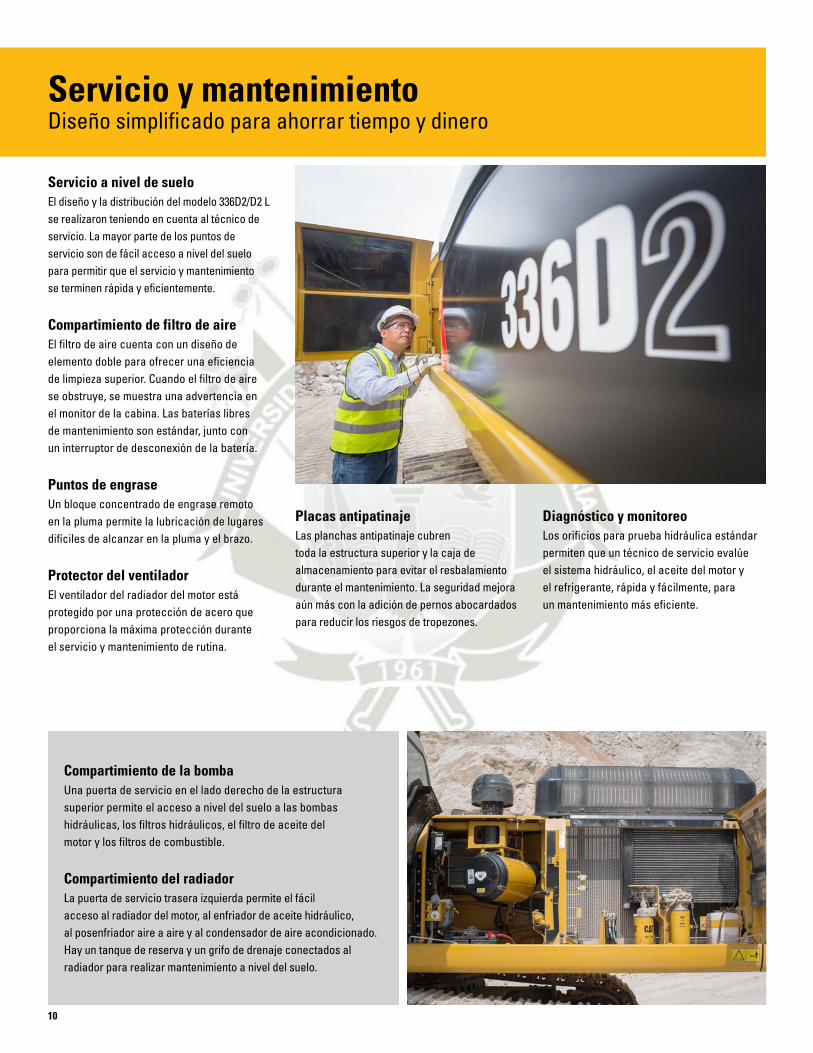
10
Servicio a nivel de sueloEl diseño y la distribución del modelo 336D2/D2 L se realizaron teniendo en cuenta al técnico de servicio. La mayor parte de los puntos de servicio son de fácil acceso a nivel del suelo para permitir que el servicio y mantenimiento se terminen rápida y eficientemente.
Compartimiento de filtro de aireEl filtro de aire cuenta con un diseño de elemento doble para ofrecer una eficiencia de limpieza superior. Cuando el filtro de aire se obstruye, se muestra una advertencia en el monitor de la cabina. Las baterías libres de mantenimiento son estándar, junto con un interruptor de desconexión de la batería.
Puntos de engraseUn bloque concentrado de engrase remoto en la pluma permite la lubricación de lugares difíciles de alcanzar en la pluma y el brazo.
Protector del ventiladorEl ventilador del radiador del motor está protegido por una protección de acero que proporciona la máxima protección durante el servicio y mantenimiento de rutina.
Placas antipatinajeLas planchas antipatinaje cubren toda la estructura superior y la caja de almacenamiento para evitar el resbalamiento durante el mantenimiento. La seguridad mejora aún más con la adición de pernos abocardados para reducir los riesgos de tropezones.
Diagnóstico y monitoreoLos orificios para prueba hidráulica estándar permiten que un técnico de servicio evalúe el sistema hidráulico, el aceite del motor y el refrigerante, rápida y fácilmente, para un mantenimiento más eficiente.
Servicio y mantenimientoDiseño simplificado para ahorrar tiempo y dinero
Compartimiento de la bombaUna puerta de servicio en el lado derecho de la estructura superior permite el acceso a nivel del suelo a las bombas hidráulicas, los filtros hidráulicos, el filtro de aceite del motor y los filtros de combustible.
Compartimiento del radiadorLa puerta de servicio trasera izquierda permite el fácil acceso al radiador del motor, al enfriador de aceite hidráulico, al posenfriador aire a aire y al condensador de aire acondicionado. Hay un tanque de reserva y un grifo de drenaje conectados al radiador para realizar mantenimiento a nivel del suelo.

11
Respaldo total al clienteUna amplia gama de soluciones personalizadas
de su distribuidor Cat.
Respaldo al productoLos distribuidores Cat utilizan una red mundial computarizada para localizar piezas en existencias a fin de reducir el tiempo de inactividad de la máquina. También puede ahorrar dinero con nuestra línea de componentes remanufacturados.
Selección de la máquinaSus distribuidores Cat pueden proporcionar recomendaciones específicas con comparaciones detalladas de las máquinas Cat que sean de su interés antes de efectuar la compra. Esto garantiza que obtenga la máquina del tamaño correcto y las herramientas apropiadas para satisfacer todas las necesidades de su aplicación.
Servicio de mantenimientoLos programas optativos de reparación garantizan el costo de las reparaciones por adelantado. Los programas de diagnóstico y servicios de supervisión de estado, como el análisis programado de aceite, el análisis de refrigerante y el análisis técnico, lo ayudan a evitar reparaciones no programadas.
Convenios de Respaldo al ClienteLos distribuidores Cat ofrecen una variedad de convenios de respaldo al producto que se pueden adaptar para satisfacer sus necesidades específicas. Estos planes pueden cubrir toda la máquina, incluidos los accesorios, para ayudarlo a proteger la inversión.
Reemplazo¿Reparar, reconstruir o reemplazar? Sus distribuidores Cat pueden ayudarle a evaluar los costos involucrados para que pueda tomar la decisión correcta.
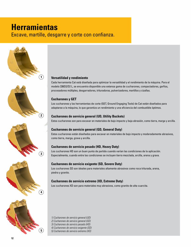
12
Versatilidad y rendimientoCada herramienta Cat está diseñada para optimizar la versatilidad y el rendimiento de la máquina. Para el modelo 336D2/D2 L, se encuentra disponible una extensa gama de cucharones, compactadores, garfios, procesadores múltiples, desgarradores, trituradoras, pulverizadores, martillos y cizallas.
Cucharones y GETLos cucharones y las herramientas de corte (GET, Ground Engaging Tools) de Cat están diseñados para adaptarse a la máquina, lo que garantiza un rendimiento y una eficiencia del combustible óptimos.
Cucharones de servicio general (UD, Utility Buckets)Estos cucharones son para excavar en materiales de bajo impacto y baja abrasión, como tierra, marga y arcilla.
Cucharones de servicio general (GD, General Duty)Estos cucharones están diseñados para excavar en materiales de bajo impacto y moderadamente abrasivos, como tierra, marga, grava y arcilla.
Cucharones de servicio pesado (HD, Heavy Duty)Los cucharones HD son un buen punto de partida cuando varían las condiciones de la aplicación. Especialmente, cuando entre las condiciones se incluyen tierra mezclada, arcilla, arena y grava.
Cucharones de servicio exigente (SD, Severe Duty)Los cucharones SD son ideales para materiales altamente abrasivos como roca triturada, arena, piedra y granito.
Cucharones de servicio extremo (XD, Extreme Duty)Los cucharones XD son para materiales muy abrasivos, como granito de alta cuarcita.
HerramientasExcave, martille, desgarre y corte con confianza.
1
2
3
4
5
1) Cucharones de servicio general (UD) 2) Cucharones de servicio general (GD) 3) Cucharones de servicio pesado (HD) 4) Cucharones de servicio exigente (SD) 5) Cucharones de servicio extremo (XD)

13
AcopladoresLos acopladores rápidos permiten que una persona pueda cambiar las herramientas en segundos para ofrecer un rendimiento y una flexibilidad máximos en un lugar de trabajo. Una máquina puede moverse rápidamente de una tarea a otra, y una flota de máquinas equipadas de modo similar puede compartir un inventario común de herramientas.
Acoplador Center-Lock™Center‑Lock es un acoplador y cuenta con un sistema de traba con patente pendiente. Una traba secundaria altamente visible permite que el operador vea claramente si el acoplador está conectado o no al cucharón o a la herramienta.
Martillos de la serie ELos martillos de la serie E reúnen las expectativas del cliente en cuanto a rendimiento, calidad y facilidad de servicio junto con la experiencia de Caterpillar en fabricación. También son silenciosos; un beneficio significativo en entornos urbanos y áreas de trabajo con restricción de ruido.
DesgarradoresHechos de aceros de alta resistencia y fabricados para durar, los desgarradores Cat resisten las condiciones de trabajo más difíciles. La estructura de sección en caja se ha reforzado para lograr la máxima rigidez y transmitir toda la potencia de la máquina al material en el que se usa. Los desgarradores cuentan con una punta de desgaste reemplazable y la mayoría de los modelos están equipados con un protector del vástago reemplazable.
GarfiosLos garfios Cat hacen que las excavadoras Cat sean la máquina ideal para manipular material suelto, clasificar la basura y limpiar el sitio de demolición. Se dispone de una variedad de estilos y tamaños para adaptar las excavadoras a la tarea actual.
Procesadores múltiplesLos multiprocesadores realizan el trabajo de muchos tipos de herramientas de demolición al usar mandíbulas intercambiables. El cambio de mandíbulas permite que una sola unidad triture, pulverice y realice una variedad de tareas especializadas como corte de barras de refuerzo de acero y tanques.
CizallasLas cizallas Cat están diseñadas para aprovechar plenamente los flujos hidráulicos y las presiones producidas por las excavadoras Cat; todo esto para aumentar la productividad sin sacrificar la seguridad y sin causar el desgaste prematuro de la cizalla o del portador.
PulverizadoresLos pulverizadores mecánicos son herramientas económicas para reciclar basura de hormigón demolida. El cilindro del cucharón en la excavadora propulsa al pulverizador, lo que elimina la necesidad de un cilindro dedicado, un sistema hidráulico asociado y costos de instalación adicionales.
CompactadoresLos compactadores Cat permiten que la compactación en el sitio de trabajo sea eficiente, rápida y económica.
TrituradorasEl triturador hidráulico de concreto es idóneo para los trabajos de demolición en áreas residenciales. La herramienta combina varias operaciones de demolición en un solo equipo:
•Desprendimiento de hormigón desde estructuras fijas
•Pulverización de hormigón
•Corte de varillas de reforzamiento y perfiles de acero pequeños

14
Motor
Modelo del motor Cat C9 ACERT
Potencia del motor (ISO 14396) 209 kW 280 hp
Potencia neta (SAE J1349/ISO 9249) 200 kW 268 hp
Calibre 112 mm 4,41"
Carrera 149 mm 5,87"
Cilindrada 8,8 L 537 pulg3
• ElCatC9cumpleconlasemisionesdeescapeequivalentesalasregulacionesdeemisionesTier2delaEPAdeEE.UU.,StageIIdelaUniónEuropeay Tier2deChina.
• Lapotencianetapublicadaeslapotenciadisponibleenelvolantecuandoelmotorestáequipadoconventilador,filtrodeaire,silenciadory alternador.
• ElMotorC9probadoenterrenopuedetrabajareficazmenteenaltitudesdehasta2.300 m(7.546 pies).
Pesos
Pesoenordendetrabajo
Trenderodajeestándar* 34.489 kg 76.035 lb
Trenderodajelargo** 37.086 kg 81.761 lb
*Trenderodajeestándar,conbrazodealcancede2,8 m(9'2"),zapatasde 600 m(24"),contrapesode6,0 tonsmétricas(6,6 tonsEE.UU.).
**Trenderodajelargoconbrazodeexcavacióndegranvolumende2,55 m (8'4"),zapatasde800 m(32"),contrapesode6,0 tonsmétricas(6,6 tonsEE.UU.).
Mecanismo de giro
Velocidad de giro 8,98 rpm
Par de giro 108,6 kN·m 80.142 lb-pie
Mando
Rendimientoenpendientes 30°/70 %
Velocidadmáximadedesplazamiento 4,85 km/h 3,0 mph
Tracciónmáximaenlabarradetiro 300,5 kN 67.555 lb-pie
Sistema hidráulico
Sistemaprincipal:flujomáximo(cadauno) 265 L/min 70 galEE.UU.
Sistemaderotación:flujomáximo 265 L/min 70 galEE.UU.
Presiónmáxima:equipo 35.000 kPa 5.076 lb/pulg²
Presiónmáxima:desplazamiento 35.000 kPa 5.076 lb/pulg²
Presiónmáxima:giro 29.000 kPa 4.061 lb/pulg²
Sistemapiloto:flujomáximo 40 L/min 10,6 galEE.UU./min
Sistemapiloto:presiónmáxima 4.000 kPa 580,2 lb/pulg²
Cilindrodelapluma:calibre 150 mm 5,9"
Cilindrodelapluma:carrera 1.440 mm 56,7"
Cilindrodelbrazo:calibre 170 mm 6,7"
Cilindrodelbrazo:carrera 1.738 mm 68,4"
Cilindrodelcucharón:calibre 150 mm 5,9"
Cilindrodelcucharón:carrera 1.151 mm 45,3"
Capacidades de llenado de servicio
Capacidaddeltanquedecombustible 620 L 163,79 galEE.UU.
Sistemadeenfriamiento 40 L 10,57 galEE.UU.
Aceite del motor 40 L 10,57 galEE.UU.
Mando de giro 19 L 5,02 galEE.UU.
Mandofinal(cadauno) 8 L 2,11 galEE.UU.
Capacidaddeaceitedelsistemahidráulico(tanqueincluido)
410 L 108,31 galEE.UU.
Aceitedeltanquehidráulico 175 L 46,2 galEE.UU.
Especificaciones de la Excavadora Hidráulica 336D2/D2 L

15
DimensionesTodas las dimensiones son aproximadas.
Opciones de pluma Pluma de alcance de servicio pesado 6,50 m (21' 4")
Pluma para excavación de gran volumen 6,18 m (20' 3")
Opciones de brazos R3.9DB (12' 10") R3.2DB (10' 6") R2.8DB (9' 2") M2.55TB (8' 4") M2.15TB (7' 1")
1 Alturadeembarque* 3.700 mm(12' 2") 3.340 mm(11' 0") 3.570 mm(11' 9") 3.650 mm(12' 0") 3.680 mm(12' 1")
2 Longituddeembarque 11.200 mm(36' 9") 11.150 mm(36' 7") 11.210 mm(36' 9") 10.910 mm(35' 10") 11.200 mm(36' 9")
3 Radio de giro de la cola 3.500 mm(11' 6") 3.500 mm(11' 6") 3.500 mm(11' 6") 3.500 mm(11' 6") 3.500 mm(11' 6")
4 Longitudhastaelcentrodelosrodillos
Trenderodajeestándar 3.610 mm(11' 10") 3.610 mm(11' 10") 3.610 mm(11' 10") 3.610 mm(11' 10") 3.610 mm(11' 10")
Trenderodajelargo 4.040 mm(13' 3") 4.040 mm(13' 3") 4.040 mm(13' 3") 4.040 mm(13' 3") 4.040 mm(13' 3")
5 Longitud de la rueda
Trenderodajeestándar 4.590 mm(15' 1") 4.590 mm(15' 1") 4.590 mm(15' 1") 4.590 mm(15' 1") 4.590 mm(15' 1")
Trenderodajelargo 5.020 mm(16' 6") 5.020 mm(16' 6") 5.020 mm(16' 6") 5.020 mm(16' 6") 5.020 mm(16' 6")
6 Espaciolibresobreelsuelo** 450 mm(1' 6") 450 mm(1' 6") 450 mm(1' 6") 450 mm(1' 6") 450 mm(1' 6")
7 Entrevía
Trenderodajeestándar 2.590 mm(8' 6") 2.590 mm(8' 6") 2.590 mm(8' 6") 2.590 mm(8' 6") 2.590 mm(8' 6")
Trenderodajelargo 2.590 mm(8' 6") 2.590 mm(8' 6") 2.590 mm(8' 6") 2.590 mm(8' 6") 2.590 mm(8' 6")
8 Anchodetransporte:trenderodajelargooestándar
Zapatasde600 mm(24") 3.190 mm(10' 6") 3.190 mm(10' 6") 3.190 mm(10' 6") 3.190 mm(10' 6") 3.190 mm(10' 6")
Zapatasde700 mm(28") 3.290 mm(10' 10") 3.290 mm(10' 10") 3.290 mm(10' 10") 3.290 mm(10' 10") 3.290 mm(10' 10")
Zapatasde800 mm(32") 3.390 mm(11' 2") 3.390 mm(11' 2") 3.390 mm(11' 2") 3.390 mm(11' 2") 3.390 mm(11' 2")
9 Alturadelacabina* 3.140 mm(10' 4") 3.140 mm(10' 4") 3.140 mm(10' 4") 3.140 mm(10' 4") 3.140 mm(10' 4")
10 Espaciolibredelcontrapeso** 1.220 mm(4' 0") 1.220 mm(4' 0") 1.220 mm(4' 0") 1.220 mm(4' 0") 1.220 mm(4' 0")
*Incluye la altura de las orejetas de las zapatas.
**Sin incluir la altura de las orejetas de las zapatas.
6
87
1 9
2
54
3
10
Especificaciones de la Excavadora Hidráulica 336D2/D2 L

Especificaciones de la Excavadora Hidráulica 336D2/D2 L
16
Gamas de trabajoTodas las dimensiones son aproximadas.
Opciones de pluma Pluma de alcance de servicio pesado 6,50 m (21' 4")
Pluma para excavación de gran volumen 6,18 m (20' 3")
Opciones de brazos R3.9DB (12' 10") R3.2DB (10' 6") R2.8DB (9' 2") M2.55TB (8' 4") M2.15TB (7' 1")
1 Profundidadmáximadeexcavación 8.090 mm (26' 7")
7.390 mm (24' 3")
6.990 mm (22' 11")
6.570 mm (21' 7")
6.170 mm (20' 3")
2 Alcancemáximoaniveldelsuelo 11.640 mm (38'2")
10.920 mm (35'10")
10.620 mm (34'10")
10.180 mm (33'5")
9.760 mm (32'0")
3 Alturamáximadecorte 10.710 mm (35'2")
10.240 mm (33'7")
10.300 mm (33'10")
10.070 mm (33'1")
9.740 mm (32'0")
4 Alturamáximadecarga 7.640 mm (25'1")
7.200 mm (23'8")
7.200 mm (23'8")
6.690 mm (21'11")
6.410 mm (21'0")
5 Alturamínimadecarga 2.010 mm (6'7")
2.710 mm (8'11")
3.110 mm (10'2")
3.000 mm (9'10")
3.400 mm (11'2")
6 Profundidadmáximadecorteconfondoplanode2.440 mm(8' 0") 7.960 mm (26'1")
7.230 mm (23'9")
6.820 mm (22'5")
6.400 mm (21'0")
5.970 mm (19'7")
7 Profundidadmáximadeexcavaciónvertical 6.700 mm (22'0")
5.830 mm (19'2")
5.770 mm (18'11")
5.340 mm (17'6")
4.710 mm (15'5")
�
2
3
1
7
� �
�
6
�
�
�
�
�
4
�
�5
�
�
�
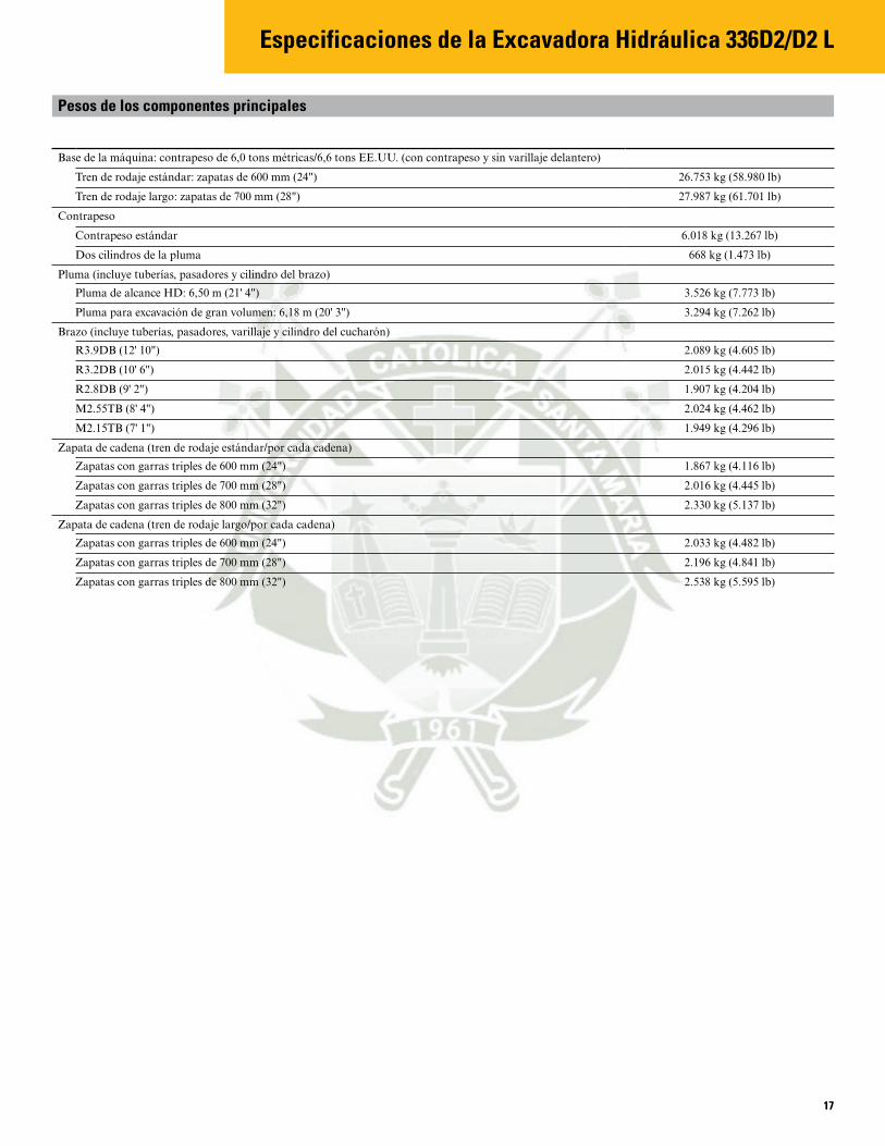
17
Pesos de los componentes principales
Basedelamáquina:contrapesode6,0 tonsmétricas/6,6 tonsEE.UU.(concontrapesoysinvarillajedelantero)
Trenderodajeestándar:zapatasde600 mm(24") 26.753 kg(58.980 lb)
Trenderodajelargo:zapatasde700 mm(28") 27.987 kg(61.701 lb)
Contrapeso
Contrapesoestándar 6.018 kg(13.267 lb)
Doscilindrosdelapluma 668 kg(1.473 lb)
Pluma(incluyetuberías,pasadoresycilindrodelbrazo)
PlumadealcanceHD:6,50 m(21'4") 3.526 kg(7.773 lb)
Plumaparaexcavacióndegranvolumen:6,18 m(20' 3") 3.294 kg(7.262 lb)
Brazo(incluyetuberías,pasadores,varillajeycilindrodelcucharón)
R3.9DB(12' 10") 2.089 kg(4.605 lb)
R3.2DB(10' 6") 2.015 kg(4.442 lb)
R2.8DB(9' 2") 1.907 kg(4.204 lb)
M2.55TB(8' 4") 2.024 kg(4.462 lb)
M2.15TB(7' 1") 1.949 kg(4.296 lb)
Zapatadecadena(trenderodajeestándar/porcadacadena)
Zapatascongarrastriplesde600 mm(24") 1.867 kg(4.116 lb)
Zapatascongarrastriplesde700 mm(28") 2.016 kg(4.445 lb)
Zapatascongarrastriplesde800 mm(32") 2.330 kg(5.137 lb)
Zapatadecadena(trenderodajelargo/porcadacadena)
Zapatascongarrastriplesde600 mm(24") 2.033 kg(4.482 lb)
Zapatascongarrastriplesde700 mm(28") 2.196 kg(4.841 lb)
Zapatascongarrastriplesde800 mm(32") 2.538 kg(5.595 lb)
Especificaciones de la Excavadora Hidráulica 336D2/D2 L
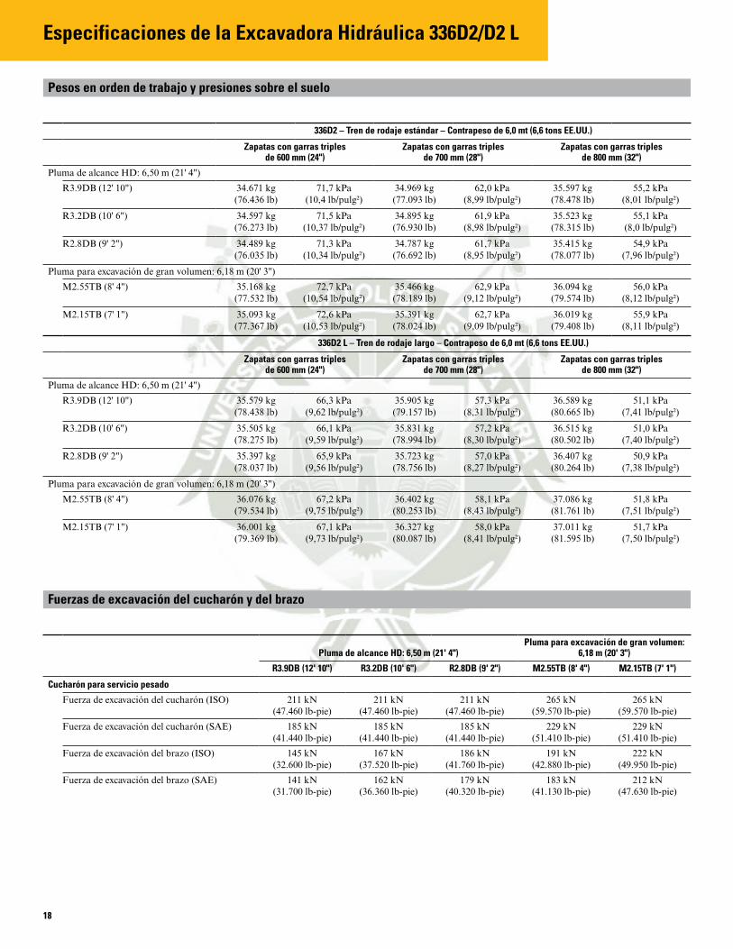
Especificaciones de la Excavadora Hidráulica 336D2/D2 L
18
Pesos en orden de trabajo y presiones sobre el suelo
336D2 – Tren de rodaje estándar – Contrapeso de 6,0 mt (6,6 tons EE.UU.)
Zapatas con garras triples de 600 mm (24")
Zapatas con garras triples de 700 mm (28")
Zapatas con garras triples de 800 mm (32")
PlumadealcanceHD:6,50 m(21'4")
R3.9DB(12' 10") 34.671 kg 71,7 kPa 34.969 kg 62,0 kPa 35.597 kg 55,2 kPa(76.436 lb) (10,4 lb/pulg²) (77.093 lb) (8,99 lb/pulg²) (78.478 lb) (8,01 lb/pulg²)
R3.2DB(10' 6") 34.597 kg 71,5 kPa 34.895 kg 61,9 kPa 35.523 kg 55,1 kPa(76.273 lb) (10,37 lb/pulg²) (76.930 lb) (8,98 lb/pulg²) (78.315 lb) (8,0 lb/pulg²)
R2.8DB(9' 2") 34.489 kg 71,3 kPa 34.787 kg 61,7 kPa 35.415 kg 54,9 kPa(76.035 lb) (10,34 lb/pulg²) (76.692 lb) (8,95 lb/pulg²) (78.077 lb) (7,96 lb/pulg²)
Plumaparaexcavacióndegranvolumen:6,18 m(20' 3")
M2.55TB(8' 4") 35.168 kg 72,7 kPa 35.466 kg 62,9 kPa 36.094 kg 56,0 kPa(77.532 lb) (10,54 lb/pulg²) (78.189 lb) (9,12 lb/pulg²) (79.574 lb) (8,12 lb/pulg²)
M2.15TB(7' 1") 35.093 kg 72,6 kPa 35.391 kg 62,7 kPa 36.019 kg 55,9 kPa(77.367 lb) (10,53 lb/pulg²) (78.024 lb) (9,09 lb/pulg²) (79.408 lb) (8,11 lb/pulg²)
336D2 L – Tren de rodaje largo – Contrapeso de 6,0 mt (6,6 tons EE.UU.)
Zapatas con garras triples de 600 mm (24")
Zapatas con garras triples de 700 mm (28")
Zapatas con garras triples de 800 mm (32")
PlumadealcanceHD:6,50 m(21'4")
R3.9DB(12' 10") 35.579 kg 66,3 kPa 35.905 kg 57,3 kPa 36.589 kg 51,1 kPa(78.438 lb) (9,62lb/pulg²) (79.157 lb) (8,31 lb/pulg²) (80.665 lb) (7,41 lb/pulg²)
R3.2DB(10' 6") 35.505 kg 66,1 kPa 35.831 kg 57,2 kPa 36.515 kg 51,0 kPa(78.275 lb) (9,59 lb/pulg²) (78.994 lb) (8,30 lb/pulg²) (80.502 lb) (7,40 lb/pulg²)
R2.8DB(9' 2") 35.397 kg 65,9 kPa 35.723 kg 57,0 kPa 36.407 kg 50,9 kPa(78.037 lb) (9,56 lb/pulg²) (78.756 lb) (8,27 lb/pulg²) (80.264 lb) (7,38 lb/pulg²)
Plumaparaexcavacióndegranvolumen:6,18 m(20' 3")
M2.55TB(8' 4") 36.076 kg 67,2 kPa 36.402 kg 58,1 kPa 37.086 kg 51,8 kPa(79.534 lb) (9,75 lb/pulg²) (80.253 lb) (8,43 lb/pulg²) (81.761 lb) (7,51 lb/pulg²)
M2.15TB(7' 1") 36.001 kg 67,1 kPa 36.327 kg 58,0 kPa 37.011 kg 51,7 kPa(79.369 lb) (9,73 lb/pulg²) (80.087 lb) (8,41 lb/pulg²) (81.595 lb) (7,50 lb/pulg²)
Fuerzas de excavación del cucharón y del brazo
Pluma de alcance HD: 6,50 m (21' 4")Pluma para excavación de gran volumen:
6,18 m (20' 3")
R3.9DB (12' 10") R3.2DB (10' 6") R2.8DB (9' 2") M2.55TB (8' 4") M2.15TB (7' 1")
Cucharón para servicio pesado
Fuerzadeexcavacióndelcucharón(ISO) 211 kN (47.460 lb-pie)
211 kN (47.460 lb-pie)
211 kN (47.460 lb-pie)
265 kN (59.570 lb-pie)
265 kN (59.570 lb-pie)
Fuerzadeexcavacióndelcucharón(SAE) 185 kN (41.440 lb-pie)
185 kN (41.440 lb-pie)
185 kN (41.440 lb-pie)
229 kN (51.410 lb-pie)
229 kN (51.410 lb-pie)
Fuerzadeexcavacióndelbrazo(ISO) 145 kN (32.600 lb-pie)
167 kN (37.520 lb-pie)
186 kN (41.760 lb-pie)
191 kN (42.880 lb-pie)
222 kN (49.950 lb-pie)
Fuerzadeexcavacióndelbrazo(SAE) 141 kN (31.700 lb-pie)
162 kN (36.360 lb-pie)
179 kN (40.320 lb-pie)
183 kN (41.130 lb-pie)
212 kN (47.630 lb-pie)
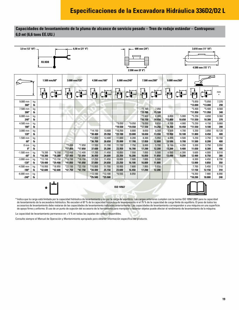
19
Capacidades de levantamiento de la pluma de alcance de servicio pesado – Tren de rodaje estándar – Contrapeso: 6,0 mt (6,6 tons EE.UU.)
1.500 mm/60" 3.000 mm/120" 4.500 mm/180" 6.000 mm/240" 7.500 mm/300" 9.000 mm/360"
mm "
9.000 mm kg *5.850 *5.850 7.370 360" lb *13.000 *13.000 290
7.500 mm kg *7.100 7.050 *5.400 *5.400 8.560 300" lb *15.700 15.100 *11.950 *11.950 340
6.000 mm kg *7.400 6.900 6.800 5.000 *5.250 4.650 9.360 240" lb *16.150 14.850 *13.800 10.650 *11.550 10.300 370
4.500 mm kg *9.050 *9.050 *8.050 6.650 6.700 4.900 *5.250 4.150 9.860 180" lb *19.550 *19.550 *17.550 14.250 14.350 10.450 *11.550 9.100 390
3.000 mm kg *14.150 13.600 *10.700 8.800 8.650 6.300 6.500 4.700 5.350 3.850 10.120120" lb *30.400 29.350 *23.100 19.000 18.650 13.550 13.950 10.100 11.800 8.450 400
1.500 mm kg *17.050 12.400 11.600 8.200 8.300 5.950 6.300 4.500 5.250 3.750 10.15060" lb *36.700 26.650 25.000 17.700 17.850 12.800 13.500 9.700 11.500 8.200 400
0 mm kg *7.850 *7.850 17.550 11.700 11.150 7.750 8.000 5.700 6.150 4.350 5.300 3.750 9.950 0" lb *17.850 *17.850 37.600 25.200 23.950 16.700 17.200 12.200 13.200 9.400 11.650 8.300 400
‑1.500 mm kg *8.200 *8.200 *12.400 *12.400 17.250 11.450 10.850 7.550 7.850 5.500 6.050 4.300 5.600 4.000 9.510 -60" lb *18.300 *18.300 *27.950 *27.950 36.950 24.600 23.350 16.200 16.850 11.850 13.000 9.200 12.400 8.750 380
‑3.000 mm kg *13.150 *13.150 *18.150 *18.150 17.250 11.450 10.800 7.500 7.800 5.500 6.300 4.450 8.790 -120" lb *29.400 *29.400 *41.050 *41.050 37.000 24.650 23.250 16.100 16.800 11.800 13.900 9.850 350
‑4.500 mm kg *18.950 *18.950 *22.150 *22.150 *15.950 11.700 10.950 7.600 7.950 5.650 7.700 5.450 7.710 -180" lb *42.600 *42.600 *47.750 *47.750 *34.400 25.150 23.600 16.450 17.200 12.200 17.150 12.150 310
‑6.000 mm kg *12.100 *12.100 *8.550 8.050 *8.350 7.900 6.090 -240" lb *25.500 *25.500 *18.200 18.000 240
* Indica que la carga está limitada por la capacidad hidráulica de levantamiento y no por la carga de equilibrio. Las cargas anteriores cumplen con la norma ISO 10567:2007 para la capacidad de levantamiento de la excavadora hidráulica. No exceden el 87 % de la capacidad hidráulica de levantamiento ni el 75 % de la capacidad de carga límite de equilibrio. El peso de todos los accesorios de levantamiento debe restarse de las capacidades de levantamiento indicadas anteriormente. Las capacidades de levantamiento corresponden a una máquina en una superficie de apoyo firme y uniforme. El uso de un punto de sujeción del accesorio de la herramienta para manipular o levantar objetos puede afectar el rendimiento de levantamiento de la máquina.
La capacidad de levantamiento permanece en ± 5 % en todas las zapatas de cadena disponibles.
Consulte siempre el Manual de Operación y Mantenimiento apropiado para obtener información específica del producto.
ISO 10567
3,9 m (12' 10")
R3.9DB
6,50 m (21' 4")
2.590 mm (8' 6")
600 mm (24")
4.590 mm (15' 1")
3.610 mm (11' 10")
Especificaciones de la Excavadora Hidráulica 336D2/D2 L

20
Especificaciones de la Excavadora Hidráulica 336D2/D2 L
Capacidades de levantamiento de la pluma de alcance de servicio pesado – Tren de rodaje estándar – Contrapeso: 6,0 mt (6,6 tons EE.UU.)
3.000 mm/120" 4.500 mm/180" 6.000 mm/240" 7.500 mm/300" 9.000 mm/360"
mm "
7.500 mm kg *7.750 6.800 *6.700 6.450 7.710 300" lb *14.800 14.550 300
6.000 mm kg *7.850 6.750 *6.500 5.300 8.580 240" lb *17.200 14.450 *14.300 11.750 340
4.500 mm kg *12.050 *12.050 *9.650 9.200 *8.450 6.500 6.550 4.750 6.400 4.650 9.130 180" lb *20.850 19.850 *18.350 13.950 14.150 10.250 360
3.000 mm kg *15.200 13.050 *11.150 8.600 8.550 6.200 6.450 4.650 6.000 4.300 9.410 120" lb *32.650 28.200 *24.100 18.550 18.400 13.300 13.800 9.950 13.200 9.500 370
1.500 mm kg *17.500 12.050 11.500 8.050 8.250 5.900 6.250 4.500 5.850 4.150 9.440 60" lb *37.700 26.000 24.700 17.400 17.700 12.650 13.500 9.650 12.850 9.150 380
0 mm kg 17 500 11.650 11.100 7.750 8.000 5.650 6.150 4.400 5.950 4.250 9.220 0" lb 37.500 25.050 23.850 16.650 17.200 12.200 13.250 9.400 13.100 9.300 370
‑1.500 mm kg *13.250 *13.250 17.400 11.550 10.950 7.600 7.900 5.550 6.400 4.550 8.750 -60" lb *29.900 *29.900 37.300 24.850 23.550 16.300 17.000 12.000 14.100 10.000 350
‑3.000 mm kg *20.900 *20.900 *16.550 11.700 11.000 7.600 7.950 5.600 7.350 5.200 7.960 -120" lb *47.350 *47.350 *35.800 25.150 23.600 16.400 17.150 12.100 16.300 11.550 320
‑4.500 mm kg *18.550 *18.550 *13.950 12.050 *10.550 7.850 *8.900 6.750 6.750 -180" lb *39.900 *39.900 *30.000 25.900 *22.450 16.950 *19.550 15.050 270
* Indica que la carga está limitada por la capacidad hidráulica de levantamiento y no por la carga de equilibrio. Las cargas anteriores cumplen con la norma ISO 10567:2007 para la capacidad de levantamiento de la excavadora hidráulica. No exceden el 87 % de la capacidad hidráulica de levantamiento ni el 75 % de la capacidad de carga límite de equilibrio. El peso de todos los accesorios de levantamiento debe restarse de las capacidades de levantamiento indicadas anteriormente. Las capacidades de levantamiento corresponden a una máquina en una superficie de apoyo firme y uniforme. El uso de un punto de sujeción del accesorio de la herramienta para manipular o levantar objetos puede afectar el rendimiento de levantamiento de la máquina.
La capacidad de levantamiento permanece en ± 5 % en todas las zapatas de cadena disponibles.
Consulte siempre el Manual de Operación y Mantenimiento apropiado para obtener información específica del producto.
ISO 10567
3,2 m (10' 6")
R3.2DB
6,50 m (21' 4")
2.590 mm (8' 6")
600 mm (24")
4.590 mm (15' 1")
3.610 mm (11' 10")

21
Capacidades de levantamiento de la pluma de alcance de servicio pesado – Tren de rodaje estándar – Contrapeso: 6,0 mt (6,6 tons EE.UU.)
3.000 mm/120" 4.500 mm/180" 6.000 mm/240" 7.500 mm/300" 9.000 mm/360"
mm "
7.500 mm kg *7.750 6.950 *6.700 6.650 7.710 300" lb *14.800 *14.800 300
6.000 mm kg *7.850 6.900 *6.500 5.450 8.580 240" lb *17.200 14.800 *14.300 12.050 340
4.500 mm kg *12.050 *12.050 *9.650 9.450 *8.450 6.650 6.750 4.900 *6.550 4.750 9.130 180" lb *20.850 20.300 *18.350 14.300 *14.350 10.550 360
3.000 mm kg *15.200 13.400 *11.150 8.800 8.750 6.350 6.600 4.750 6.150 4.450 9.410 120" lb *32.650 28.900 *24.100 19.000 18.850 13.650 14.150 10.200 13.550 9.750 370
1.500 mm kg *17.500 12.400 11.800 8.300 8.450 6.050 6.450 4.600 6.000 4.300 9.440 60" lb *37.700 26.700 25.350 17.850 18.200 13.000 13.850 9.900 13.200 9.450 380
0 mm kg 17.950 11.950 11.400 7.950 8.250 5.850 6.350 4.500 6.100 4.350 9.220 0" lb 38.500 25.750 24.500 17.100 17.700 12.550 13.650 9.700 13.450 9.600 370
‑1.500 mm kg *13.250 *13.250 *17.850 11.900 11.250 7.800 8.100 5.750 6.550 4.650 8.750 -60" lb *29.900 *29.900 38.300 25.550 24.150 16.750 17.450 12.350 14.500 10.300 350
‑3.000 mm kg *20.900 *20.900 *16.550 12.000 11.300 7.850 8.150 5.750 7.550 5.350 7.960 -120" lb *47.350 *47.350 *35.800 25.800 24.250 16.850 17.600 12.450 16.750 11.850 320
‑4.500 mm kg *18.550 *18.550 *13.950 12.350 *10.550 8.050 *8.900 6.900 6.750 -180" lb *39.900 *39.900 *30.000 26.550 *22.450 17.400 *19.550 15.450 270
* Indica que la carga está limitada por la capacidad hidráulica de levantamiento y no por la carga de equilibrio. Las cargas anteriores cumplen con la norma ISO 10567:2007 para la capacidad de levantamiento de la excavadora hidráulica. No exceden el 87 % de la capacidad hidráulica de levantamiento ni el 75 % de la capacidad de carga límite de equilibrio. El peso de todos los accesorios de levantamiento debe restarse de las capacidades de levantamiento indicadas anteriormente. Las capacidades de levantamiento corresponden a una máquina en una superficie de apoyo firme y uniforme. El uso de un punto de sujeción del accesorio de la herramienta para manipular o levantar objetos puede afectar el rendimiento de levantamiento de la máquina.
La capacidad de levantamiento permanece en ± 5 % en todas las zapatas de cadena disponibles.
Consulte siempre el Manual de Operación y Mantenimiento apropiado para obtener información específica del producto.
ISO 10567
3,2 m (10' 6")
R3.2DB
6,50 m (21' 4")
2.590 mm (8' 6")
800 mm (32")
4.590 mm (15' 1")
3.610 mm (11' 10")
Especificaciones de la Excavadora Hidráulica 336D2/D2 L

22
Especificaciones de la Excavadora Hidráulica 336D2/D2 L
Capacidades de levantamiento de la pluma de alcance de servicio pesado – Tren de rodaje estándar – Contrapeso: 6,0 mt (6,6 tons EE.UU.)
3.000 mm/120" 4.500 mm/180" 6.000 mm/240" 7.500 mm/300" 9.000 mm/360"
mm "
7.500 mm kg *8.400 6.950 7.340 300" lb *18.550 15.650 290
6.000 mm kg *9.000 *9.000 *8.350 6.650 7.700 5.600 8.250 240" lb *19.500 *19.500 *18.250 14.300 17.100 12.500 330
4.500 mm kg *13.000 *13.000 *10.200 9.100 8.850 6.450 6.750 4.900 8.820 180" lb *27.850 *27.850 *22.050 19.650 19.000 13.850 14.950 10.850 350
3.000 mm kg *16.100 12.800 *11.650 8.550 8.550 6.150 6.400 4.650 6.300 4.550 9.110 120" lb *34.600 27.700 *25.150 18.400 18.350 13.250 13.900 10.000 360
1.500 mm kg *15.900 12.000 11.450 8.050 8.250 5.900 6.300 4.500 6.150 4.400 9.140 60" lb 38.350 25.800 24.650 17.350 17.750 12.700 13.550 9.700 360
0 mm kg 17.550 11.700 11.150 7.750 8.050 5.700 6.300 4.500 8.920 0" lb 37.600 25.150 23.950 16.700 17.300 12.300 13.850 9.900 350
‑1.500 mm kg *12.350 *12.350 17.550 11.700 11.050 7.650 8.000 5.650 6.800 4.850 8.420 -60" lb *28.100 *28.100 37.600 25.150 23.700 16.500 17.150 12.150 15.050 10.700 340
‑3.000 mm kg *21.050 *21.050 *16.000 11.850 11.100 7.750 8.100 5.750 7.950 5.650 7.600 -120" lb *45.750 *45.750 *34.700 25.500 23.900 16.700 17.650 12.550 300
‑4.500 mm kg *16.750 *16.750 *13.000 12.250 *9.650 8.050 *8.800 7.550 6.330 -180" lb *35.950 *35.950 *27.850 26.400 *20.250 17.450 *19.350 16.950 250
* Indica que la carga está limitada por la capacidad hidráulica de levantamiento y no por la carga de equilibrio. Las cargas anteriores cumplen con la norma ISO 10567:2007 para la capacidad de levantamiento de la excavadora hidráulica. No exceden el 87 % de la capacidad hidráulica de levantamiento ni el 75 % de la capacidad de carga límite de equilibrio. El peso de todos los accesorios de levantamiento debe restarse de las capacidades de levantamiento indicadas anteriormente. Las capacidades de levantamiento corresponden a una máquina en una superficie de apoyo firme y uniforme. El uso de un punto de sujeción del accesorio de la herramienta para manipular o levantar objetos puede afectar el rendimiento de levantamiento de la máquina.
La capacidad de levantamiento permanece en ± 5 % en todas las zapatas de cadena disponibles.
Consulte siempre el Manual de Operación y Mantenimiento apropiado para obtener información específica del producto.
ISO 10567
2,8 m (9' 2")
R2.8DB
6,50 m (21' 4")
2.590 mm (8' 6")
600 mm (24")
4.590 mm (15' 1")
3.610 mm (11' 10")

23
Especificaciones de la Excavadora Hidráulica 336D2/D2 L
Capacidades de levantamiento de excavación de gran volumen – Tren de rodaje estándar – Contrapeso: 6,0 tons métricas (6,6 tons EE.UU.)
3.000 mm/120" 4.500 mm/180" 6.000 mm/240" 7.500 mm/300"
mm "
7.500 mm kg *9.250 *9.250 *8.300 8.200 6.590 300" lb *20.450 *20.450 *18.400 *18.400 260
6.000 mm kg *9.600 9.500 8.900 6.500 *7.900 6.350 7.600 240" lb *20.850 20.450 *17.450 14.200 300
4.500 mm kg *13.400 *13.400 *10.650 9.050 8.750 6.350 7.500 5.450 8.210 180" lb *28.750 *28.750 *23.050 19.500 18.750 13.650 16.650 12.100 330
3.000 mm kg *16.350 12.850 11.950 8.500 8.450 6.100 6.950 5.000 8.520 120" lb *35.150 27.700 25.650 18.300 18.200 13.150 15.300 11.050 340
1.500 mm kg 17.900 12.000 11.450 8.050 8.200 5.850 6.750 4.850 8.550 60" lb 38.450 25.900 24.600 17.300 17.650 12.650 14.900 10.700 340
0 mm kg 17.600 11.750 11.150 7.750 8.050 5.700 6.950 5.000 8.310 0" lb 37.700 25.250 23.950 16.750 17.300 12.300 15.350 10.950 330
‑1.500 mm kg *16.900 *16.900 *17.450 11.750 11.050 7.700 8.050 5.700 7.650 5.450 7.780 -60" lb *38.350 *38.350 37.700 25.300 23.800 16.600 17.300 12.300 16.900 12.000 310
‑3.000 mm kg *19.950 *19.950 *15.350 12.000 11.200 7.850 9.250 6.550 6.880 -120" lb *43.300 *43.300 *33.200 25.750 24.150 16.900 20.550 14.550 270
‑4.500 mm kg *11.250 *11.250 *8.900 *8.900 5.430 -180" lb *23.800 *23.800 *19.450 *19.450 210
* Indica que la carga está limitada por la capacidad hidráulica de levantamiento y no por la carga de equilibrio. Las cargas anteriores cumplen con la norma ISO 10567:2007 para la capacidad de levantamiento de la excavadora hidráulica. No exceden el 87 % de la capacidad hidráulica de levantamiento ni el 75 % de la capacidad de carga límite de equilibrio. El peso de todos los accesorios de levantamiento debe restarse de las capacidades de levantamiento indicadas anteriormente. Las capacidades de levantamiento corresponden a una máquina en una superficie de apoyo firme y uniforme. El uso de un punto de sujeción del accesorio de la herramienta para manipular o levantar objetos puede afectar el rendimiento de levantamiento de la máquina.
La capacidad de levantamiento permanece en ± 5 % en todas las zapatas de cadena disponibles.
Consulte siempre el Manual de Operación y Mantenimiento apropiado para obtener información específica del producto.
ISO 10567
2,55 m (8' 4")
M2.55TB
6,18 m (20' 3")
2.590 mm (8' 6")
600 mm (24")
4.590 mm (15' 1")
3.610 mm (11' 10")

24
Especificaciones de la Excavadora Hidráulica 336D2/D2 L
Capacidades de levantamiento de excavación de gran volumen – Tren de rodaje estándar – Contrapeso: 6,0 tons métricas (6,6 tons EE.UU.)
3.000 mm/120" 4.500 mm/180" 6.000 mm/240" 7.500 mm/300"
mm "
7.500 mm kg *10.050 9.550 *10.050 9.450 6.030 300" lb *22.300 21.500 240
6.000 mm kg *10.150 9.400 9.650 7.050 7.120 240" lb *22.150 20.200 *21.350 15.750 280
4.500 mm kg *14.250 13.850 *11.150 8.950 8.700 6.300 8.200 5.950 7.780 180" lb *30.650 29.850 *24.150 19.300 18.650 13.550 18.150 13.200 310
3.000 mm kg 11.850 8.400 8.450 6.100 7.500 5.450 8.100 120" lb *36.850 27.150 25.500 18.150 18.200 13.100 16.550 11.950 320
1.500 mm kg 11.400 8.000 8.200 5.900 7.300 5.250 8.140 60" lb 24.500 17.250 17.700 12.650 16.100 11.550 320
0 mm kg 17.600 11.800 11.150 7.800 8.100 5.750 7.550 5.400 7.890 0" lb 37.750 25.300 24.000 16.800 17.450 12.450 16.650 11.900 310
‑1.500 mm kg *17.800 *17.800 *16.950 11.850 11.150 7.800 8.400 6.000 7.320 -60" lb *40.750 *40.750 *36.750 25.500 23.950 16.750 18.600 13.200 290
‑3.000 mm kg *17.950 *17.950 *14.500 12.150 *11.050 8.000 *10.100 7.450 6.360 -120" lb *39.050 *39.050 *31.350 26.100 *23.550 17.250 *22.250 16.500 250
* Indica que la carga está limitada por la capacidad hidráulica de levantamiento y no por la carga de equilibrio. Las cargas anteriores cumplen con la norma ISO 10567:2007 para la capacidad de levantamiento de la excavadora hidráulica. No exceden el 87 % de la capacidad hidráulica de levantamiento ni el 75 % de la capacidad de carga límite de equilibrio. El peso de todos los accesorios de levantamiento debe restarse de las capacidades de levantamiento indicadas anteriormente. Las capacidades de levantamiento corresponden a una máquina en una superficie de apoyo firme y uniforme. El uso de un punto de sujeción del accesorio de la herramienta para manipular o levantar objetos puede afectar el rendimiento de levantamiento de la máquina.
La capacidad de levantamiento permanece en ± 5 % en todas las zapatas de cadena disponibles.
Consulte siempre el Manual de Operación y Mantenimiento apropiado para obtener información específica del producto.
ISO 10567
2,15 m (7' 1")
M2.15TB
6,18 m (20' 3")
2.590 mm (8' 6")
600 mm (24")
4.590 mm (15' 1")
3.610 mm (11' 10")

25
Especificaciones de la Excavadora Hidráulica 336D2/D2 L
Capacidades de levantamiento de la pluma de alcance de servicio pesado – Tren de rodaje largo – Contrapeso: 6,0 mt (6,6 tons EE.UU.)
1.500 mm/60" 3.000 mm/120" 4.500 mm/180" 6.000 mm/240" 7.500 mm/300" 9.000 mm/360"
mm "
9.000 mm kg *5.850 *5.850 7.370 360" lb *13.000 *13.000 290
7.500 mm kg *7.100 *7.100 *5.400 *5.400 8.560 300" lb *15.700 15.400 *11.950 *11.950 340
6.000 mm kg *7.400 7.050 *7.100 5.100 *5.250 4.750 9.360 240" lb *16.150 15.150 *13.800 10.900 *11.550 10.550 370
4.500 mm kg *9.050 *9.050 *8.050 6.800 *7.500 5.000 *5.250 4.250 9.860 180" lb *19.550 *19.550 *17.550 14.600 *16.450 10.700 *11.550 9.350 390
3.000 mm kg *14.150 13.900 *10.700 9.000 *8.950 6.450 7.650 4.800 *5.400 3.950 10.120120" lb *30.400 29.950 *23.100 19.450 *19.450 13.850 16.450 10.350 *11.850 8.700 400
1.500 mm kg *17.050 12.650 *12.250 8.400 9.850 6.100 7.450 4.650 *5.700 3.850 10.15060" lb *36.700 27.300 *26.500 18.100 21.150 13.100 16.000 9.950 *12.550 8.450 400
0 mm kg *7.850 *7.850 *18.550 12.000 *13.350 7.950 9.550 5.800 7.300 4.500 *6.200 3.850 9.950 0" lb *17.850 *17.850 *40.100 25.800 28.850 17.150 20.550 12.550 15.650 9.650 *13.650 8.500 400
‑1.500 mm kg *8.200 *8.200 *12.400 *12.400 *18.750 11.750 13 150 7.750 9.350 5.650 7.200 4.400 6.700 4.100 9.510 -60" lb *18.300 *18.300 *27.950 *27.950 *40.600 25.250 28.250 16.600 20.150 12.200 15.500 9.450 14.700 9.000 380
‑3.000 mm kg *13.150 *13.150 *18.150 *18.150 *17.950 11.750 13.100 7.700 9.350 5.650 7.500 4.600 8.790 -120" lb *29.400 *29.400 *41.050 *41.050 *38.800 25.250 28.100 16.500 20.100 12.150 16.550 10.150 350
‑4.500 mm kg *18.950 *18.950 *22.150 *22.150 *15.950 12.000 *12.100 7.800 *9.050 5.800 *8.600 5.600 7.710 -180" lb *42.600 *42.600 *47.750 *47.750 *34.400 25.800 *25.950 16.850 *19.050 12.500 *18.950 12.450 310
‑6.000 mm kg *12.100 *12.100 *8.550 8.250 *8.350 8.100 6.090 -240" lb *25.500 *25.500 *18.200 *18.200 240
* Indica que la carga está limitada por la capacidad hidráulica de levantamiento y no por la carga de equilibrio. Las cargas anteriores cumplen con la norma ISO 10567:2007 para la capacidad de levantamiento de la excavadora hidráulica. No exceden el 87 % de la capacidad hidráulica de levantamiento ni el 75 % de la capacidad de carga límite de equilibrio. El peso de todos los accesorios de levantamiento debe restarse de las capacidades de levantamiento indicadas anteriormente. Las capacidades de levantamiento corresponden a una máquina en una superficie de apoyo firme y uniforme. El uso de un punto de sujeción del accesorio de la herramienta para manipular o levantar objetos puede afectar el rendimiento de levantamiento de la máquina.
La capacidad de levantamiento permanece en ± 5 % en todas las zapatas de cadena disponibles.
Consulte siempre el Manual de Operación y Mantenimiento apropiado para obtener información específica del producto.
ISO 10567
3,9 m (12' 10")
R3.9DB
6,50 m (21' 4")
2.590 mm (8' 6")
600 mm (24")
5.020 mm (16' 6")
4.040 mm (13' 3")
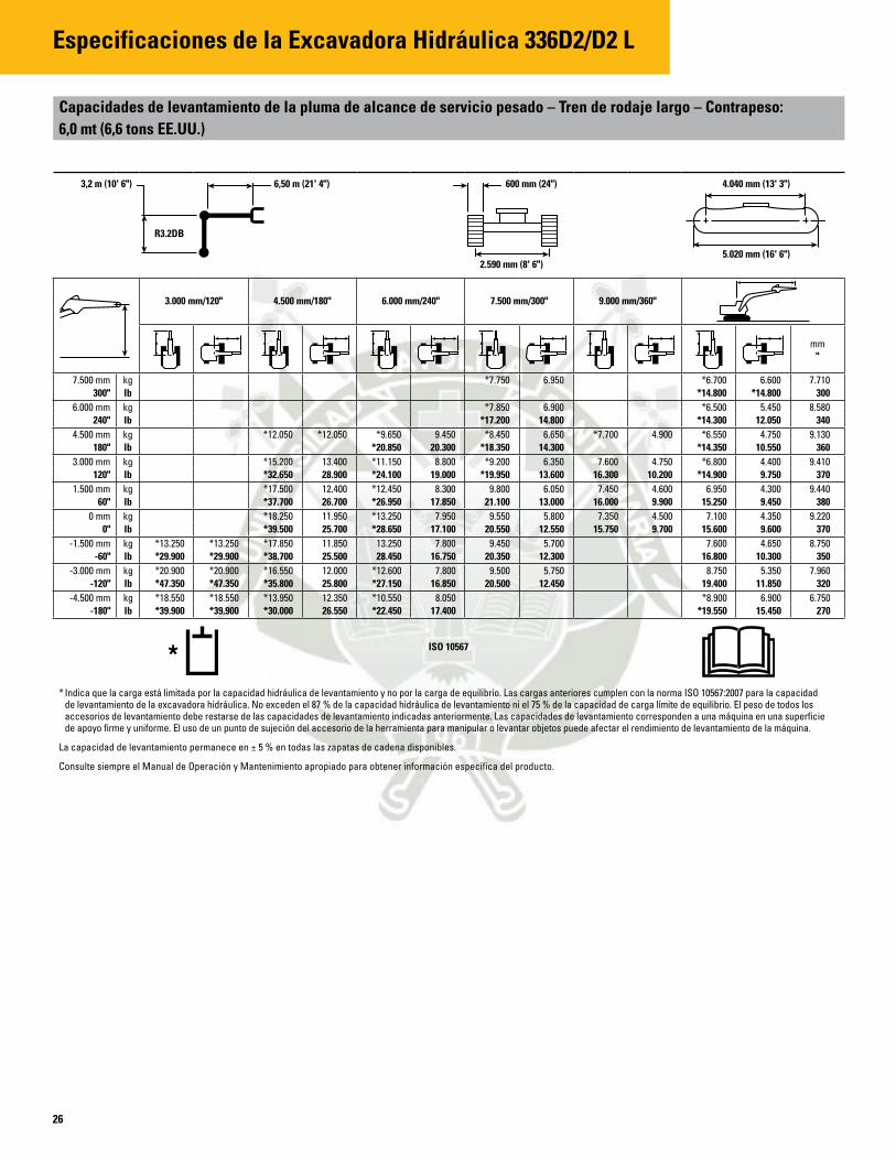
26
Especificaciones de la Excavadora Hidráulica 336D2/D2 L
Capacidades de levantamiento de la pluma de alcance de servicio pesado – Tren de rodaje largo – Contrapeso: 6,0 mt (6,6 tons EE.UU.)
3.000 mm/120" 4.500 mm/180" 6.000 mm/240" 7.500 mm/300" 9.000 mm/360"
mm "
7.500 mm kg *7.750 6.950 *6.700 6.600 7.710 300" lb *14.800 *14.800 300
6.000 mm kg *7.850 6.900 *6.500 5.450 8.580 240" lb *17.200 14.800 *14.300 12.050 340
4.500 mm kg *12.050 *12.050 *9.650 9.450 *8.450 6.650 *7.700 4.900 *6.550 4.750 9.130 180" lb *20.850 20.300 *18.350 14.300 *14.350 10.550 360
3.000 mm kg *15.200 13.400 *11.150 8.800 *9.200 6.350 7.600 4.750 *6.800 4.400 9.410 120" lb *32.650 28.900 *24.100 19.000 *19.950 13.600 16.300 10.200 *14.900 9.750 370
1.500 mm kg *17.500 12.400 *12.450 8.300 9.800 6.050 7.450 4.600 6.950 4.300 9.440 60" lb *37.700 26.700 *26.950 17.850 21.100 13.000 16.000 9.900 15.250 9.450 380
0 mm kg *18.250 11.950 *13.250 7.950 9.550 5.800 7.350 4.500 7.100 4.350 9.220 0" lb *39.500 25.700 *28.650 17.100 20.550 12.550 15.750 9.700 15.600 9.600 370
‑1.500 mm kg *13.250 *13.250 *17.850 11.850 13.250 7.800 9.450 5.700 7.600 4.650 8.750 -60" lb *29.900 *29.900 *38.700 25.500 28.450 16.750 20.350 12.300 16.800 10.300 350
‑3.000 mm kg *20.900 *20.900 *16.550 12.000 *12.600 7.800 9.500 5.750 8.750 5.350 7.960 -120" lb *47.350 *47.350 *35.800 25.800 *27.150 16.850 20.500 12.450 19.400 11.850 320
‑4.500 mm kg *18.550 *18.550 *13.950 12.350 *10.550 8.050 *8.900 6.900 6.750 -180" lb *39.900 *39.900 *30.000 26.550 *22.450 17.400 *19.550 15.450 270
* Indica que la carga está limitada por la capacidad hidráulica de levantamiento y no por la carga de equilibrio. Las cargas anteriores cumplen con la norma ISO 10567:2007 para la capacidad de levantamiento de la excavadora hidráulica. No exceden el 87 % de la capacidad hidráulica de levantamiento ni el 75 % de la capacidad de carga límite de equilibrio. El peso de todos los accesorios de levantamiento debe restarse de las capacidades de levantamiento indicadas anteriormente. Las capacidades de levantamiento corresponden a una máquina en una superficie de apoyo firme y uniforme. El uso de un punto de sujeción del accesorio de la herramienta para manipular o levantar objetos puede afectar el rendimiento de levantamiento de la máquina.
La capacidad de levantamiento permanece en ± 5 % en todas las zapatas de cadena disponibles.
Consulte siempre el Manual de Operación y Mantenimiento apropiado para obtener información específica del producto.
ISO 10567
3,2 m (10' 6")
R3.2DB
6,50 m (21' 4")
2.590 mm (8' 6")
600 mm (24")
5.020 mm (16' 6")
4.040 mm (13' 3")

27
Especificaciones de la Excavadora Hidráulica 336D2/D2 L
Capacidades de levantamiento de la pluma de alcance de servicio pesado – Tren de rodaje largo – Contrapeso: 6,0 mt (6,6 tons EE.UU.)
3.000 mm/120" 4.500 mm/180" 6.000 mm/240" 7.500 mm/300" 9.000 mm/360"
mm "
7.500 mm kg *7.750 7.150 *6.700 *6.700 7.710 300" lb *14.800 *14.800 300
6.000 mm kg *7.850 7.050 *6.500 5.550 8.580 240" lb *17.200 15.150 *14.300 12.400 340
4.500 mm kg *12.050 *12.050 *9.650 *9.650 *8.450 6.800 *7.700 5.050 *6.550 4.900 9.130 180" lb *20.850 20.800 *18.350 14.650 *14.350 10.850 360
3.000 mm kg *15.200 13.700 *11.150 9.050 *9.200 6.500 7.800 4.900 *6.800 4.550 9.410 120" lb *32.650 29.600 *24.100 19.500 *19.950 14.000 16.800 10.500 *14.900 10.050 370
1.500 mm kg *17.500 12.700 *12.450 8.500 *9.950 6.200 7.650 4.750 7.150 4.400 9.440 60" lb *37.700 27.400 *26.950 18.350 *21.550 13.350 16.450 10.200 15.700 9.700 380
0 mm kg *18.250 12.300 *13.250 8.150 9.850 6.000 7.550 4.650 7.300 4.500 9.220 0" lb *39.500 26.450 *28.650 17.600 21.150 12.900 16.250 10.000 16.050 9.900 370
‑1.500 mm kg *13.250 *13.250 *17.850 12.200 *13.300 8.000 9.750 5.900 7.850 4.800 8.750 -60" lb *29.900 *29.900 *38.700 26.250 *28.800 17.250 20.950 12.700 17.300 10.600 350
‑3.000 mm kg *20.900 *20.900 *16.550 12.350 *12.600 8.050 *9.700 5.950 *8.850 5.500 7.960 -120" lb *47.350 *47.350 *35.800 26.500 *27.150 17.350 *20.800 12.800 *19.550 12.200 320
‑4.500 mm kg *18.550 *18.550 *13.950 12.650 *10.550 8.300 *8.900 7.100 6.750 -180" lb *39.900 *39.900 *30.000 27.250 *22.450 17.900 *19.550 15.900 270
* Indica que la carga está limitada por la capacidad hidráulica de levantamiento y no por la carga de equilibrio. Las cargas anteriores cumplen con la norma ISO 10567:2007 para la capacidad de levantamiento de la excavadora hidráulica. No exceden el 87 % de la capacidad hidráulica de levantamiento ni el 75 % de la capacidad de carga límite de equilibrio. El peso de todos los accesorios de levantamiento debe restarse de las capacidades de levantamiento indicadas anteriormente. Las capacidades de levantamiento corresponden a una máquina en una superficie de apoyo firme y uniforme. El uso de un punto de sujeción del accesorio de la herramienta para manipular o levantar objetos puede afectar el rendimiento de levantamiento de la máquina.
La capacidad de levantamiento permanece en ± 5 % en todas las zapatas de cadena disponibles.
Consulte siempre el Manual de Operación y Mantenimiento apropiado para obtener información específica del producto.
ISO 10567
3,2 m (10' 6")
R3.2DB
6,50 m (21' 4")
2.590 mm (8' 6")
800 mm (32")
5.020 mm (16' 6")
4.040 mm (13' 3")

28
Especificaciones de la Excavadora Hidráulica 336D2/D2 L
Capacidades de levantamiento de la pluma de alcance de servicio pesado – Tren de rodaje largo – Contrapeso: 6,0 mt (6,6 tons EE.UU.)
3.000 mm/120" 4.500 mm/180" 6.000 mm/240" 7.500 mm/300" 9.000 mm/360"
mm "
7.500 mm kg *8.400 7.100 7.340 300" lb *18.550 16.000 290
6.000 mm kg *9.000 *9.000 *8.350 6.800 *8.150 5.750 8.250 240" lb *19.500 *19.500 *18.250 14.650 *18.000 12.800 330
4.500 mm kg *13.000 *13.000 *10.200 9.300 *8.850 6.600 8.000 5.050 8.820 180" lb *27.850 *27.850 *22.050 20.100 *19.200 14.200 17.650 11.150 350
3.000 mm kg *16.100 13 150 *11.650 8.750 *9.550 6.300 7.600 4.750 7.450 4.650 9.110 120" lb *34.600 28.350 *25.150 18.850 *20.700 13.600 16.400 10.300 360
1.500 mm kg *15.900 12.300 *12.850 8.250 9.800 6.050 7.450 4.650 7.300 4.550 9.140 60" lb *38.700 26.450 *27.750 17.800 21.100 13.000 16.050 9.950 360
0 mm kg *18.300 12.000 *13.450 7.950 9.600 5.850 7.500 4.650 8.920 0" lb *39.700 25.800 28.900 17.150 20.650 12.600 16.500 10.200 350
‑1.500 mm kg *12.350 *12.350 *17.650 12.000 *13.300 7.850 9.550 5.800 8.100 5.000 8.420 -60" lb *28.100 *28.100 *38.250 25.800 28.650 16.950 20.500 12.500 17.900 11.000 340
‑3.000 mm kg *21.050 *21.050 *16.000 12.200 *12.300 7.950 *9.300 5.900 *9.050 5.800 7.600 -120" lb *45.750 *45.750 *34.700 26.200 *26.550 17.150 *19.950 12.900 300
‑4.500 mm kg *16.750 *16.750 *13.000 12.550 *9.650 8.250 *8.800 7.750 6.330 -180" lb *35.950 *35.950 *27.850 27.050 *20.250 17.900 *19.350 17.350 250
* Indica que la carga está limitada por la capacidad hidráulica de levantamiento y no por la carga de equilibrio. Las cargas anteriores cumplen con la norma ISO 10567:2007 para la capacidad de levantamiento de la excavadora hidráulica. No exceden el 87 % de la capacidad hidráulica de levantamiento ni el 75 % de la capacidad de carga límite de equilibrio. El peso de todos los accesorios de levantamiento debe restarse de las capacidades de levantamiento indicadas anteriormente. Las capacidades de levantamiento corresponden a una máquina en una superficie de apoyo firme y uniforme. El uso de un punto de sujeción del accesorio de la herramienta para manipular o levantar objetos puede afectar el rendimiento de levantamiento de la máquina.
La capacidad de levantamiento permanece en ± 5 % en todas las zapatas de cadena disponibles.
Consulte siempre el Manual de Operación y Mantenimiento apropiado para obtener información específica del producto.
ISO 10567
2,8 m (9' 2")
R2.8DB
6,50 m (21' 4")
2.590 mm (8' 6")
600 mm (24")
5.020 mm (16' 6")
4.040 mm (13' 3")

29
Especificaciones de la Excavadora Hidráulica 336D2/D2 L
Capacidades de levantamiento de la pluma para excavación de gran volumen – Tren de rodaje largo – Contrapeso: 6,0 tons métricas (6,6 tons EE.UU.)
3.000 mm/120" 4.500 mm/180" 6.000 mm/240" 7.500 mm/300"
mm "
7.500 mm kg *9.250 *9.250 *8.300 *8.300 6.590 300" lb *20.450 *20.450 *18.400 *18.400 260
6.000 mm kg *9.600 *9.600 *9.050 6.650 *7.900 6.550 7.600 240" lb *20.850 *20.850 *17.450 14.550 300
4.500 mm kg *13.400 *13.400 *10.650 9.250 *9.300 6.500 *7.900 5.600 8.210 180" lb *28.750 *28.750 *23.050 19.900 *20.300 14.000 *17.400 12.400 330
3.000 mm kg *16.350 13 150 *11.950 8.700 *9.900 6.250 *8.200 5.150 8.520 120" lb *35.150 28.350 *25.900 18.750 *21.500 13.500 *18.050 11.350 340
1.500 mm kg *18.200 12.350 *13.050 8.250 9.750 6.050 8.050 5.000 8.550 60" lb *39.250 26.550 *28.250 17.750 21.000 12.950 17.700 11.000 340
0 mm kg *18.350 12.050 13.450 8.000 9.600 5.850 8.300 5.100 8.310 0" lb *39.800 25.950 28.900 17.200 20.650 12.650 18.250 11.250 330
‑1.500 mm kg *16.900 *16.900 *17.450 12.050 *13.200 7.900 9.600 5.850 9.100 5.600 7.780 -60" lb *38.350 *38.350 *37.800 25.950 *28.550 17.050 20.650 12.650 20.100 12.350 310
‑3.000 mm kg *19.950 *19.950 *15.350 12.300 *11.700 8.050 *9.650 6.750 6.880 -120" lb *43.300 *43.300 *33.200 26.400 *25.100 17.350 *21.200 14.950 270
‑4.500 mm kg *11.250 *11.250 *8.900 *8.900 5.430 -180" lb *23.800 *23.800 *19.450 *19.450 210
* Indica que la carga está limitada por la capacidad hidráulica de levantamiento y no por la carga de equilibrio. Las cargas anteriores cumplen con la norma ISO 10567:2007 para la capacidad de levantamiento de la excavadora hidráulica. No exceden el 87 % de la capacidad hidráulica de levantamiento ni el 75 % de la capacidad de carga límite de equilibrio. El peso de todos los accesorios de levantamiento debe restarse de las capacidades de levantamiento indicadas anteriormente. Las capacidades de levantamiento corresponden a una máquina en una superficie de apoyo firme y uniforme. El uso de un punto de sujeción del accesorio de la herramienta para manipular o levantar objetos puede afectar el rendimiento de levantamiento de la máquina.
La capacidad de levantamiento permanece en ± 5 % en todas las zapatas de cadena disponibles.
Consulte siempre el Manual de Operación y Mantenimiento apropiado para obtener información específica del producto.
ISO 10567
2,55 m (8' 4")
M2.55TB
6,18 m (20' 3")
2.590 mm (8' 6")
600 mm (24")
5.020 mm (16' 6")
4.040 mm (13' 3")
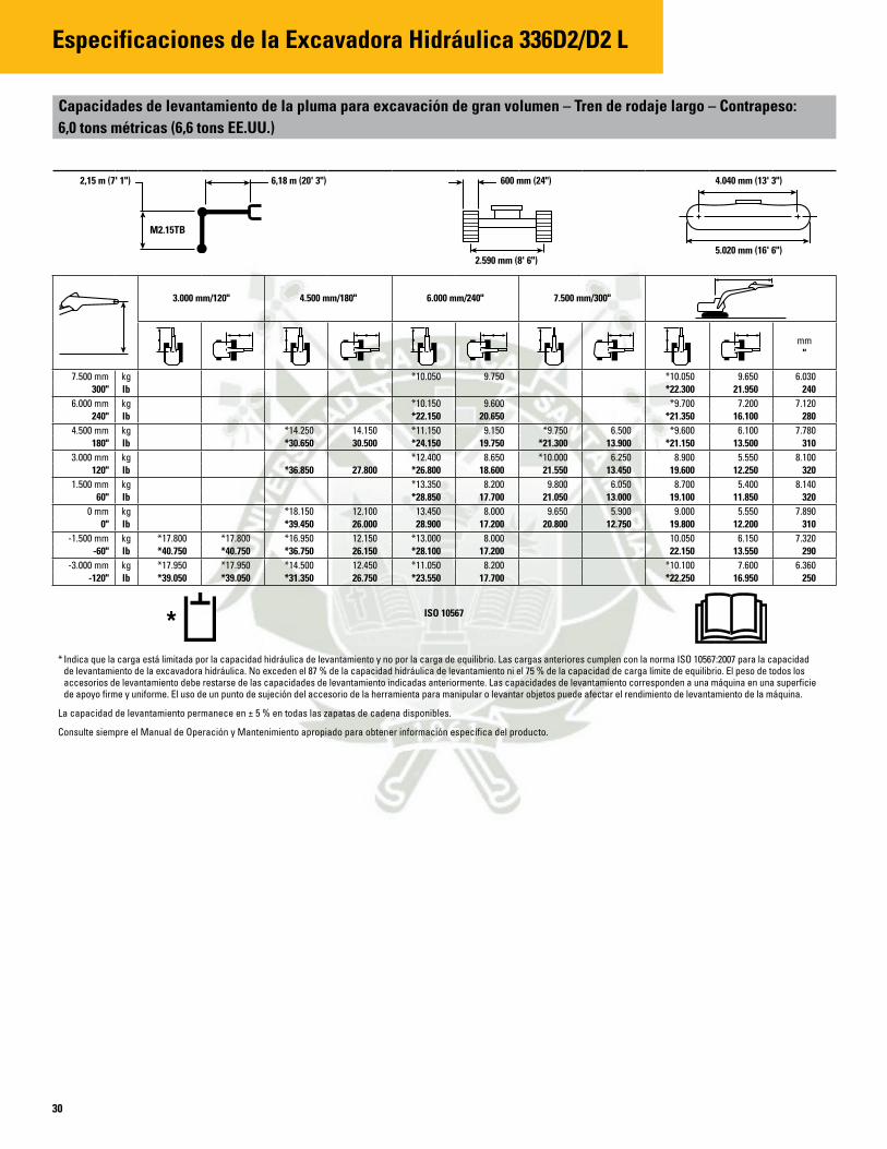
30
Especificaciones de la Excavadora Hidráulica 336D2/D2 L
Capacidades de levantamiento de la pluma para excavación de gran volumen – Tren de rodaje largo – Contrapeso: 6,0 tons métricas (6,6 tons EE.UU.)
3.000 mm/120" 4.500 mm/180" 6.000 mm/240" 7.500 mm/300"
mm "
7.500 mm kg *10.050 9.750 *10.050 9.650 6.030 300" lb *22.300 21.950 240
6.000 mm kg *10.150 9.600 *9.700 7.200 7.120 240" lb *22.150 20.650 *21.350 16.100 280
4.500 mm kg *14.250 14.150 *11.150 9.150 *9.750 6.500 *9.600 6.100 7.780 180" lb *30.650 30.500 *24.150 19.750 *21.300 13.900 *21.150 13.500 310
3.000 mm kg *12.400 8.650 *10.000 6.250 8.900 5.550 8.100 120" lb *36.850 27.800 *26.800 18.600 21.550 13.450 19.600 12.250 320
1.500 mm kg *13.350 8.200 9.800 6.050 8.700 5.400 8.140 60" lb *28.850 17.700 21.050 13.000 19.100 11.850 320
0 mm kg *18.150 12.100 13.450 8.000 9.650 5.900 9.000 5.550 7.890 0" lb *39.450 26.000 28.900 17.200 20.800 12.750 19.800 12.200 310
‑1.500 mm kg *17.800 *17.800 *16.950 12.150 *13.000 8.000 10.050 6.150 7.320 -60" lb *40.750 *40.750 *36.750 26.150 *28.100 17.200 22.150 13.550 290
‑3.000 mm kg *17.950 *17.950 *14.500 12.450 *11.050 8.200 *10.100 7.600 6.360 -120" lb *39.050 *39.050 *31.350 26.750 *23.550 17.700 *22.250 16.950 250
* Indica que la carga está limitada por la capacidad hidráulica de levantamiento y no por la carga de equilibrio. Las cargas anteriores cumplen con la norma ISO 10567:2007 para la capacidad de levantamiento de la excavadora hidráulica. No exceden el 87 % de la capacidad hidráulica de levantamiento ni el 75 % de la capacidad de carga límite de equilibrio. El peso de todos los accesorios de levantamiento debe restarse de las capacidades de levantamiento indicadas anteriormente. Las capacidades de levantamiento corresponden a una máquina en una superficie de apoyo firme y uniforme. El uso de un punto de sujeción del accesorio de la herramienta para manipular o levantar objetos puede afectar el rendimiento de levantamiento de la máquina.
La capacidad de levantamiento permanece en ± 5 % en todas las zapatas de cadena disponibles.
Consulte siempre el Manual de Operación y Mantenimiento apropiado para obtener información específica del producto.
ISO 10567
2,15 m (7' 1")
M2.15TB
6,18 m (20' 3")
2.590 mm (8' 6")
600 mm (24")
5.020 mm (16' 6")
4.040 mm (13' 3")

31
Especificaciones de la Excavadora Hidráulica 336D2/D2 L
Guía de opciones de herramientas del modelo 336D2*
Tipo de pluma Alcance de servicio pesado Gran volumenTamaño del brazo R3.9DB R3.2DB R2.8DB M2.55Martillohidráulico H140Es H140Es H140Es H140Es
H160Es H160Es H160Es H160Es H180Es
Procesadormúltiple MP20conmandíbulaCC MP20conmandíbulaCC MP20contodaslasopcionesdemandíbula
MP30conmandíbulaCC
MP20conmandíbulaCR MP20conmandíbulaCR MP30conmandíbulaCC MP30conmandíbulaCRMP20conmandíbulaPP MP20conmandíbulaPP MP30conmandíbulaCR MP30conmandíbulaPPMP20conmandíbulaPS MP20conmandíbulaPS MP30conmandíbulaPS MP30conmandíbulaPSMP20conmandíbulaS MP20conmandíbulaS MP30conmandíbulaSMP20conmandíbulaTS MP20conmandíbulaTS
Trituradora P325 P325 P325P335 P335
Pulverizador P225 P225 P225 P325P235
Garradedemoliciónyselección G325B G325B G325BG330 G330 G330
Cizallamóvilparachatarraydemolición S325B S325B S325B S365CCompactador(placasvibratorias) CVP110 CVP110 CVP110 CVP110Garfiodecontratista G130B G130B G130B Garfioparabasura
Seencuentrandisponibleslassiguientesherramientasparaelmodelo336D2. ConsulteasudistribuidorCatparaconocerlaopcióncompatibleadecuada.
TenazasGarfiosOrangePeelRastrillosAcopladorCenter-LockAcopladorrápidoCW
Guía de opciones de herramientas del modelo 336D2 L*
Tipo de pluma Alcance de servicio pesado Gran volumenTamaño del brazo R3.9DB R3.2DB R2.8DB M2.55Martillohidráulico H140Es H140Es H140Es H140Es
H160Es H160Es H160Es H160EsH180Es H180Es
Procesadormúltiple MP20conmandíbulaCC MP20contodaslasopcionesdemandíbula
MP20contodaslasopcionesdemandíbula
MP30conmandíbulaCC
MP20conmandíbulaCR MP30conmandíbulaCC MP30conmandíbulaCC MP30conmandíbulaCRMP20conmandíbulaPP MP30conmandíbulaCR MP30conmandíbulaCR MP30conmandíbulaPPMP20conmandíbulaPS MP30conmandíbulaPS MP30conmandíbulaPS MP30conmandíbulaPSMP20conmandíbulaS MP30conmandíbulaS MP30conmandíbulaS MP30conmandíbulaSMP20conmandíbulaTS MP30conmandíbulaTS
Trituradora P325 P325 P325P335 P335 P335
Pulverizador P225 P225 P225 P325P235 P235
Garradedemoliciónyselección G325B G325B G325BG330 G330 G330
Cizallamóvilparachatarraydemolición S325B S325B S325B S365CCompactador(placasvibratorias) CVP110 CVP110 CVP110 CVP110Garfiodecontratista G130B G130B G130BGarfioparabasura
Seencuentrandisponibleslassiguientesherramientasparaelmodelo336D2L. ConsulteasudistribuidorCatparaconocerlaopcióncompatibleadecuada.
TenazasGarfiosOrangePeelRastrillosAcopladorCenter-LockAcopladorrápidoCW
* Las ofertas pueden no estar disponibles en todas las áreas. Las compatibilidades dependen de la configuraciones de la excavadora, con pasador o con instalación de acoplador rápido, montadas en el brazo o en la pluma, trabajo sobre la parte delantera o la parte lateral. Consulte a su distribuidor Cat para determinar lo que se ofrece en su área y para obtener la compatibilidad de herramienta adecuada.
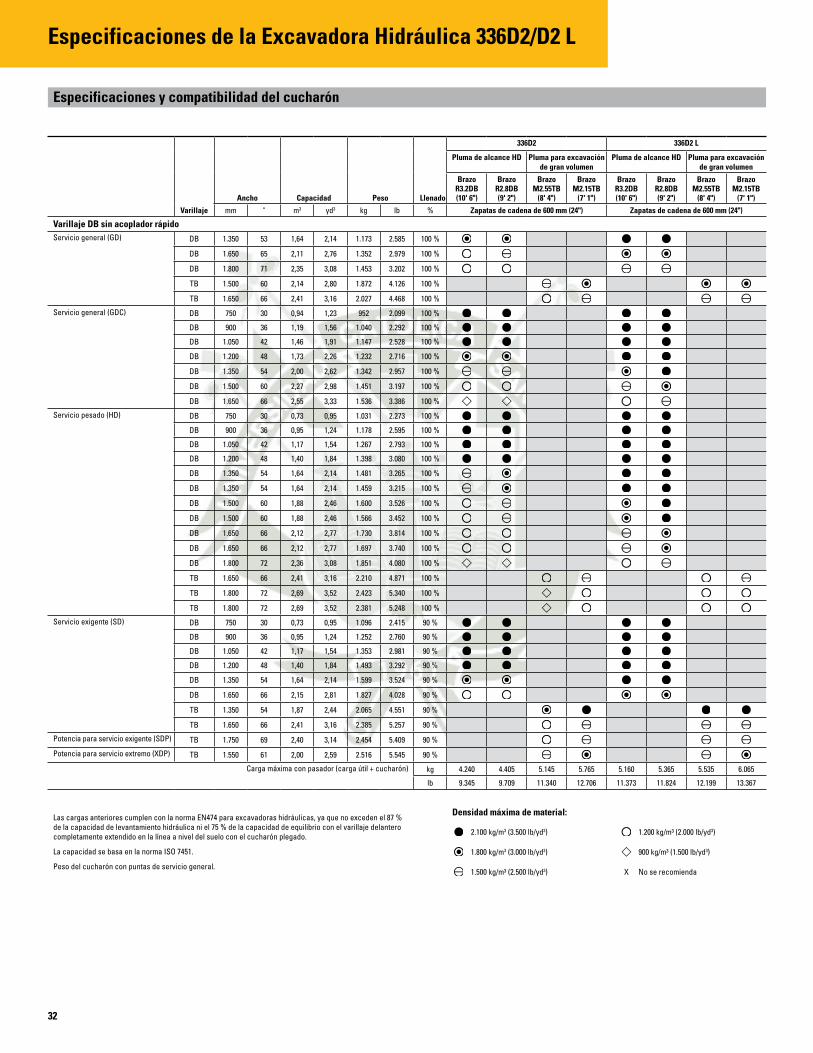
Especificaciones de la Excavadora Hidráulica 336D2/D2 L
32
Especificaciones y compatibilidad del cucharón
Varillaje
Ancho Capacidad Peso Llenado
336D2 336D2 L
Pluma de alcance HD Pluma para excavación de gran volumen
Pluma de alcance HD Pluma para excavación de gran volumen
Brazo R3.2DB (10' 6")
Brazo R2.8DB (9' 2")
Brazo M2.55TB
(8' 4")
Brazo M2.15TB
(7' 1")
Brazo R3.2DB (10' 6")
Brazo R2.8DB (9' 2")
Brazo M2.55TB
(8' 4")
Brazo M2.15TB
(7' 1")
mm " m3 yd3 kg lb % Zapatas de cadena de 600 mm (24") Zapatas de cadena de 600 mm (24")
Varillaje DB sin acoplador rápidoServicio general (GD) DB 1.350 53 1,64 2,14 1.173 2.585 100 %
DB 1.650 65 2,11 2,76 1.352 2.979 100 %
DB 1.800 71 2,35 3,08 1.453 3.202 100 %
TB 1.500 60 2,14 2,80 1.872 4.126 100 %
TB 1.650 66 2,41 3,16 2.027 4.468 100 %
Servicio general (GDC) DB 750 30 0,94 1,23 952 2.099 100 %
DB 900 36 1,19 1,56 1.040 2.292 100 %
DB 1.050 42 1,46 1,91 1.147 2.528 100 %
DB 1.200 48 1,73 2,26 1.232 2.716 100 %
DB 1.350 54 2,00 2,62 1.342 2.957 100 %
DB 1.500 60 2,27 2,98 1.451 3.197 100 %
DB 1.650 66 2,55 3,33 1.536 3.386 100 %
Servicio pesado (HD) DB 750 30 0,73 0,95 1.031 2.273 100 %
DB 900 36 0,95 1,24 1.178 2.595 100 %
DB 1.050 42 1,17 1,54 1.267 2.793 100 %
DB 1.200 48 1,40 1,84 1.398 3.080 100 %
DB 1.350 54 1,64 2,14 1.481 3.265 100 %
DB 1.350 54 1,64 2,14 1.459 3.215 100 %
DB 1.500 60 1,88 2,46 1.600 3.526 100 %
DB 1.500 60 1,88 2,46 1.566 3.452 100 %
DB 1.650 66 2,12 2,77 1.730 3.814 100 %
DB 1.650 66 2,12 2,77 1.697 3.740 100 %
DB 1.800 72 2,36 3,08 1.851 4.080 100 %
TB 1.650 66 2,41 3,16 2.210 4.871 100 %
TB 1.800 72 2,69 3,52 2.423 5.340 100 %
TB 1.800 72 2,69 3,52 2.381 5.248 100 %
Servicio exigente (SD) DB 750 30 0,73 0,95 1.096 2.415 90 %
DB 900 36 0,95 1,24 1.252 2.760 90 %
DB 1.050 42 1,17 1,54 1.353 2.981 90 %
DB 1.200 48 1,40 1,84 1.493 3.292 90 %
DB 1.350 54 1,64 2,14 1.599 3.524 90 %
DB 1.650 66 2,15 2,81 1.827 4.028 90 %
TB 1.350 54 1,87 2,44 2.065 4.551 90 %
TB 1.650 66 2,41 3,16 2.385 5.257 90 %
Potencia para servicio exigente (SDP) TB 1.750 69 2,40 3,14 2.454 5.409 90 %
Potencia para servicio extremo (XDP) TB 1.550 61 2,00 2,59 2.516 5.545 90 %
Carga máxima con pasador (carga útil + cucharón) kg 4.240 4.405 5.145 5.765 5.160 5.365 5.535 6.065
lb 9.345 9.709 11.340 12.706 11.373 11.824 12.199 13.367
Las cargas anteriores cumplen con la norma EN474 para excavadoras hidráulicas, ya que no exceden el 87 % de la capacidad de levantamiento hidráulica ni el 75 % de la capacidad de equilibrio con el varillaje delantero completamente extendido en la línea a nivel del suelo con el cucharón plegado.
La capacidad se basa en la norma ISO 7451.
Peso del cucharón con puntas de servicio general.
Densidad máxima de material:
2.100 kg/m3 (3.500 lb/yd3) 1.200 kg/m³ (2.000 lb/yd3)
1.800 kg/m3 (3.000 lb/yd3) 900 kg/m³ (1.500 lb/yd3)
1.500 kg/m³ (2.500 lb/yd3) X No se recomienda

33
Especificaciones de la Excavadora Hidráulica 336D2/D2 L
Especificaciones y compatibilidad del cucharón
Varillaje
Ancho Capacidad Peso Llenado
336D2 336D2 L
Pluma de alcance HD Pluma para excavación de gran volumen
Pluma de alcance HD Pluma para excavación de gran volumen
Brazo R3.2DB (10' 6")
Brazo R2.8DB (9' 2")
Brazo M2.55TB
(8' 4")
Brazo M2.15TB
(7' 1")
Brazo R3.2DB (10' 6")
Brazo R2.8DB (9' 2")
Brazo M2.55TB
(8' 4")
Brazo M2.15TB
(7' 1")
mm " m3 yd3 kg lb % Zapatas de cadena de 600 mm (24") Zapatas de cadena de 600 mm (24")
Varillaje DB con acoplador rápido Center-LockServicio general (GD) DB 1.350 53 1,64 2,14 1.173 2.585 100 %
DB 1.650 65 2,11 2,76 1.352 2.979 100 %
DB 1.800 71 2,35 3,08 1.453 3.202 100 %
TB 1.500 60 2,14 2,80 1.872 4.126 100 %
TB 1.650 66 2,41 3,16 2.027 4.468 100 %
Servicio general (GDC) DB 750 30 0,94 1,23 952 2.099 100 %
DB 900 36 1,19 1,56 1.040 2.292 100 %
DB 1.050 42 1,46 1,91 1.147 2.528 100 %
DB 1.200 48 1,73 2,26 1.232 2.716 100 %
DB 1.350 54 2,00 2,62 1.342 2.957 100 %
DB 1.500 60 2,27 2,98 1.451 3.197 100 %
DB 1.650 66 2,55 3,33 1.536 3.386 100 %
Servicio pesado (HD) DB 750 30 0,73 0,95 1.031 2.273 100 %
DB 900 36 0,95 1,24 1.178 2.595 100 %
DB 1.050 42 1,17 1,54 1.267 2.793 100 %
DB 1.200 48 1,40 1,84 1.398 3.080 100 %
DB 1.350 54 1,64 2,14 1.481 3.265 100 %
DB 1.350 54 1,64 2,14 1.459 3.215 100 %
DB 1.500 60 1,88 2,46 1.600 3.526 100 %
DB 1.500 60 1,88 2,46 1.566 3.452 100 %
DB 1.650 66 2,12 2,77 1.730 3.814 100 %
DB 1.650 66 2,12 2,77 1.697 3.740 100 %
DB 1.800 72 2,36 3,08 1.851 4.080 100 %
TB 1.650 66 2,41 3,16 2.210 4.871 100 %
TB 1.800 72 2,69 3,52 2.423 5.340 100 %
TB 1.800 72 2,69 3,52 2.381 5.248 100 %
Servicio exigente (SD) DB 750 30 0,73 0,95 1.096 2.415 90 %
DB 900 36 0,95 1,24 1.252 2.760 90 %
DB 1.050 42 1,17 1,54 1.353 2.981 90 %
DB 1.200 48 1,40 1,84 1.493 3.292 90 %
DB 1.350 54 1,64 2,14 1.599 3.524 90 %
DB 1.650 66 2,15 2,81 1.827 4.028 90 %
TB 1.350 54 1,87 2,44 2.065 4.551 90 %
TB 1.650 66 2,41 3,16 2.385 5.257 90 %
Potencia para servicio exigente (SDP) TB 1.750 69 2,40 3,14 2.454 5.409 90 %
Potencia para servicio extremo (XDP) TB 1.550 61 2,00 2,59 2.516 5.545 90 %
Carga máxima con acoplador (carga útil + cucharón) kg 3.682 3.847 4.587 5.207 4.602 4.807 4.977 5.507
lb 8.115 8.479 10.110 11.476 10.143 10.594 10.969 12.137
Las cargas anteriores cumplen con la norma EN474 para excavadoras hidráulicas, ya que no exceden el 87 % de la capacidad de levantamiento hidráulica ni el 75 % de la capacidad de equilibrio con el varillaje delantero completamente extendido en la línea a nivel del suelo con el cucharón plegado.
La capacidad se basa en la norma ISO 7451.
Peso del cucharón con puntas de servicio general.
Densidad máxima de material:
2.100 kg/m3 (3.500 lb/yd3) 1.200 kg/m³ (2.000 lb/yd3)
1.800 kg/m3 (3.000 lb/yd3) 900 kg/m³ (1.500 lb/yd3)
1.500 kg/m³ (2.500 lb/yd3) X No se recomienda
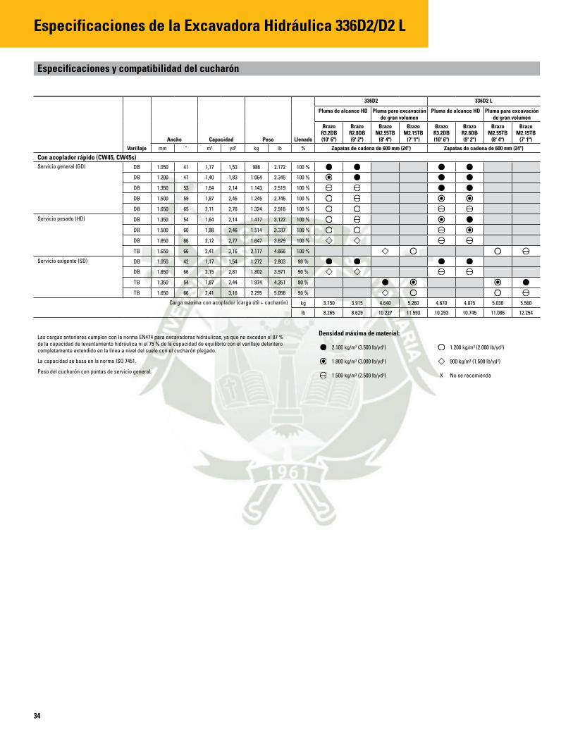
34
Especificaciones de la Excavadora Hidráulica 336D2/D2 L
Especificaciones y compatibilidad del cucharón
Varillaje
Ancho Capacidad Peso Llenado
336D2 336D2 L
Pluma de alcance HD Pluma para excavación de gran volumen
Pluma de alcance HD Pluma para excavación de gran volumen
Brazo R3.2DB (10' 6")
Brazo R2.8DB (9' 2")
Brazo M2.55TB
(8' 4")
Brazo M2.15TB
(7' 1")
Brazo R3.2DB (10' 6")
Brazo R2.8DB (9' 2")
Brazo M2.55TB
(8' 4")
Brazo M2.15TB
(7' 1")
mm " m3 yd3 kg lb % Zapatas de cadena de 600 mm (24") Zapatas de cadena de 600 mm (24")
Con acoplador rápido (CW45, CW45s)Servicio general (GD) DB 1.050 41 1,17 1,53 986 2.172 100 %
DB 1.200 47 1,40 1,83 1.064 2.345 100 %
DB 1.350 53 1,64 2,14 1.143 2.519 100 %
DB 1.500 59 1,87 2,45 1.245 2.745 100 %
DB 1.650 65 2,11 2,76 1.324 2.918 100 %
Servicio pesado (HD) DB 1.350 54 1,64 2,14 1.417 3.122 100 %
DB 1.500 60 1,88 2,46 1.514 3.337 100 %
DB 1.650 66 2,12 2,77 1.647 3.629 100 %
TB 1.650 66 2,41 3,16 2.117 4.666 100 %
Servicio exigente (SD) DB 1.050 42 1,17 1,54 1.272 2.803 90 %
DB 1.650 66 2,15 2,81 1.802 3.971 90 %
TB 1.350 54 1,87 2,44 1.974 4.351 90 %
TB 1.650 66 2,41 3,16 2.295 5.058 90 %
Carga máxima con acoplador (carga útil + cucharón) kg 3.750 3.915 4.640 5.260 4.670 4.875 5.030 5.560
lb 8.265 8.629 10.227 11.593 10.293 10.745 11.086 12.254
Las cargas anteriores cumplen con la norma EN474 para excavadoras hidráulicas, ya que no exceden el 87 % de la capacidad de levantamiento hidráulica ni el 75 % de la capacidad de equilibrio con el varillaje delantero completamente extendido en la línea a nivel del suelo con el cucharón plegado.
La capacidad se basa en la norma ISO 7451.
Peso del cucharón con puntas de servicio general.
Densidad máxima de material:
2.100 kg/m3 (3.500 lb/yd3) 1.200 kg/m³ (2.000 lb/yd3)
1.800 kg/m3 (3.000 lb/yd3) 900 kg/m³ (1.500 lb/yd3)
1.500 kg/m³ (2.500 lb/yd3) X No se recomienda

Equipos estándar y optativos del modelo 336D2/D2 L
Equipos estándarLos equipos estándar pueden variar. Consulte a su distribuidor Cat para obtener más información.
Equipos optativosLos equipos optativos pueden variar. Consulte a su distribuidor Cat para obtener más información.
MOTOR•MotorDieselC9ACERT•Capacidaddealtitudde2.300 m(7.546')•Alternadorde65amperios•Calentadordeadmisióndeaire•Versióndealtapotenciaconmodalidadde administracióndepotencia
•Filtrosdeairedeselloradial (filtrosprimarioysecundario)
•Controlautomáticodevelocidaddelmotor• Separadordeaguaconsensorindicadordel nivel deagua
•Radiadordelaaletadeondaconespaciopara permitirlalimpieza
•Dosvelocidadesdedesplazamiento•Filtrosdecombustiblededos(2)micrones•Bombaeléctricadecebado
SISTEMA HIDRÁULICO•Capacidaddeinstalacióndeválvulasy circuitos adicionales
•Circuitosderecuperaciónparaplumaybrazo•Válvuladeamortiguacióndelarotacióninversa•Frenoautomáticodeestacionamientode la rotación
CABINA•Cinturóndeseguridadretráctil
(51 mm [2"]; 76 mm [3"] de ancho)• Parabrisasdelanterodivididoen70/30• Parabrisasdelanterosuperiorlaminadoy las otrasventanastempladas
•Ventanadepuertasuperiorcorrediza•Aireacondicionadodedosniveles(automático)condesempañador(cabinapresurizada)
• PantallaLCDacolor,coninformaciónde advertencia,cambiodefiltro/fluidoy horas trabajadas
• Palancaneutral(detraba)paratodoslos controles
• Pedalesdecontroldedesplazamientocon palancasmanualesremovibles
•Montajederadio(tamañoDIN)• Suministrodecorrientede10 Aconmáximo
de 12 V – 2וDosaltavocesestéreo• Portavasos•Ganchopararopa,cenicero,portadocumentos•Tragaluzconposibilidaddeapertura•Alfombradepisolavable
TREN DE RODAJE• Protectoresguíadecadenadelaruedalocay la seccióncentral
•Cáncamoderemolqueenbastidorbásico• CadenaslubricadascongrasaGLT2,sellode resina
SISTEMA ELÉCTRICO•Disyuntor•Luz,montadaenlapluma,izquierdayderecha•Luz,montadaenlacajadealmacenamiento
SEGURIDAD• SistemadeseguridadCatdeunasolallave•Cerradurasenlaspuertasycompartimiento•Bocinadeseñalización/advertencia•Espejosretrovisores• Interruptor de corte del motor de emergencia•Ventanatraseradesalidadeemergencia•Capacidaddeconexióndeunabaliza
CONTRAPESO• Contrapesode6,0 tonsmétricas(6,6 tonsEE.UU.)
PIEZAS DELANTERAS• Plumadealcancedeserviciopesado
– BrazoR3.9DB – BrazoR3.2DB – BrazoR2.8DB
•Plumaparaexcavacióndegranvolumen – BrazoM2.55TB – BrazoM2.15TB
•Varillajedelcucharón – VarillajedelcucharónDB (conosincáncamodelevantamiento)
– VarillajedelcucharónTB (conosincáncamodelevantamiento)
TREN DE RODAJE• Protectorinferiordeserviciopesado• Protectordelaunióngiratoriaestándaro de serviciopesado
• Protectordelmotordedesplazamientode serviciopesado
• Protectoresdeguíaparatodalalongitudde la cadena
• FOGS(FallingObjectGuardingSystem,Sistemadeproteccióncontralacaídadeobjetos),empernado
•Cadenasdegarratriplede600 mm,700 mm,800 mm (24", 28", 32")
SISTEMA HIDRÁULICO• Tuberíasdealtapresiónparaplumasybrazos•Tuberíasdepresiónmediaparaplumasybrazos•Tuberíasparalapluma,elbrazoyelacoplador rápido
•Dispositivodecontroldebajadadelapluma/brazo•Circuitodeacopladorrápido•Controlderotaciónprecisa•Aceite biodegradable
CABINA•Asientoconsuspensiónmecánicayposacabeza•Asientoconsuspensiónneumática,posacabeza
y calentador• Suministrodecorrientede12Vy10Acondos(2)enchufestipoencendedordecigarrillos
• Protectorcontralalluviaenelparabrisasdelantero•Radio AM/FM•Cambiadorrápidodelpatróndecontrol•Tercerpedalparadesplazamientorecto
OTROS EQUIPOS OPTATIVOS•Alarmadedesplazamiento• Juegodearranqueparatiempofrío•Bombaeléctricaparaelreabastecimientode combustibleconcorteautomático
TECNOLOGÍAS INTEGRADAS•Cámaradevisióntrasera• ListoparainstalacióndeaccesorioAccuGrade™•CatProductLink™
35

Para obtener más información sobre los productos Cat, los servicios del distribuidor y las soluciones de la industria, visítenos en www.cat.com
© 2014 CaterpillarTodos los derechos reservados
Los materiales y las especificaciones están sujetos a cambio sin previo aviso. Las máquinas que aparecen en las fotografías pueden incluir equipos optativos. Consulte a su distribuidor Cat para conocer las opciones disponibles.
CAT, CATERPILLAR, SAFETY.CAT.COM, sus respectivos logotipos, el color "Caterpillar Yellow" y la imagen comercial de "Power Edge", así como la identidad corporativa y de producto utilizadas en la presente, son marcas registradas de Caterpillar y no pueden utilizarse sin autorización.
ASHQ7176‑01 (07‑2014) (Traducción: 09‑2014)
Reemplaza a ASHQ7176 (ADSD‑S, AME,
APD, CIS, GCN1)