UNIT 21 CAPITAL INVESTMENT DECISIONS

Structure 2 1.1 Introduction

Objectives

2 1.2 Characteristics of Capital Investment

2 1.3 Kinds of Capital Budgeting Decisions 21.3.1 Accept-Reject Decisions 21.3.2 Mutually Exclusive Project Decisions 21.3.3 Capital Rationing Decisions

21.4 Computations in Regard to Future Benefits : CFAT

2 1.5 lllustrative Examples 21.5.1 Single Proposal 21.5.2 Replacement Proposal 21.5.3 Mutually Exclusive Project Proposals 2 1.5.4 Market-based Approximation for Salvage Value

2 1.6 Evaluation TechniquesIApprisal Methods for Capital Budgeting 21.6.1 Traditional Methods 21.6.2 Discounted Cash Flow Techniques

2 1.7 Capital Rationing 21.7.1 The Two-Stage Rocess 21.7.2 Strategic Investments 21.7.3 Period Planning 21.7.4 Project Divisibility

21.8 Risk Analysis

2 1.9 Methods of Incorporating Risk Factors in Capital Budgeting Decisions 21.9.1 Risk-Adjusted Discount Rate Approach 2 1.9.2 Certainty-Equivalent Approach 21.9.3 Sensitivity Analysis 21.9.4 Analysis Based on Probability Distribution of Cash Flows 21.9.5 Decision-Tree Approach

21.10 Summary

2 1.1 1 Answers to SAQs

21.1 INTRODUCTION

"Financial management" is devoted not only to procurement of funds but also on their efficient use with the objective of maximising the owners' wealth. Funds must be allocated both to assets and activities (meaning projects and production to be undertaken). When allocations to assets are to be made, this is referred to as investment decision. In as much as projects, once completed, also create "assets", they too are covered. Investment decisions regarding short-term, or current, assets have been discussed under Unit 20. Long-term, or fixed, assets to be invested upon are covered under Capital Investment Decisions, also designated as capital budgeting (or capital expenditure) decisions and by other designations.

Objectives After studying this unit, you should be able to

understand risk and return as associated with capital investment decisions,

evaluate investment options under both of "accept-reject" criterion and "mutually exclusive choices",

ladder out a demand schedule and decide on capital rationing, and

analyse project investment opportunities in consideration of their risk factors.

Construction Finance Management 21.2 CHARACTERISTICS OF CAPITAL INVESTMENT

A capital investment involves a current cash outlay in anticipation of realising benefits in the future, generally (well) beyond one year. These benefits may be either in the form of increased revenues or reductions in costs -the expenditures are called accordingly as income-expansion, or cost-reduction, expenditures. The cash outlay (as capital expenditure) may go towards addition, disposition, modi'cation, creation and replacement offixed assets. The basic features of capital investment decisions are thus :

(a) . a series of large anticipated benefits;

(b) a relatively high degree of risk; and

(c) a relatively long period over which the returns are likely to be realised.

It must be mentioned that the following descriptions are used synonymously : capital investment decision, capital expenditure decision, capital expenditure management, long-term investment decision, management of fixed assets, capital budgeting decision.

The simplest assumption underlying capital investment decisions is that the required rate of return is given and is the same for all investment projects. This rate of return is designated as the minimum acceptable rate of return (MARR). This assumption presupposes that the selection of any investment project does not alter the L'business-risk companion" of the firm as visualised by the suppliers of capital. Thus, risk, and rate of return are important considerations in capital investment decisions; generally, unless otherwise indicated, risk is held to be constant. Of course, the rate of return may vary with the risk.

Strategic decisions in regard to capital investment may lead to significant changes in the firm's expected profits and in the risks to which these profits will be subjected to. These changes may influence stockholders and creditors to revise their evaluation of the firm.

An investment decision at the right opportunity can boost the profits for quite a few years to come; equally, an ill-advised investment [nay even lead to bankruptcy. Besides this, other impacts on the firm due to any long-term investment may include the following :

(a) Any fixed investment is attended by certain fixed costs in terms of labour, rents, insurance, staff salary, etc. and hence, the break-even points, sales and profits for product ranges would be changed.

(b) Capital investments, once made, are irrecoverable except with losses. There may not be even scrap value in certain cases.

(c) Since funds are blocked on the acquired fixed assets, other investment opportunities may not be financed for want of funds; and thus, besides losses on this asset, potential profits from alternate investments are also lost.

Since future is generally uncertain, there is always an element of risk in estimating the future benefits from an investment. Reliable forecasts of market demands, market share for the firm, consumer preferences, competitors' actions and offers, technological development, changes in economic and potential environment - are the agglomerate of requirements to be carefully looked into. Quantifying the benefits is thus often a "grey" area.

21.3 KINDS OF CAPITAL BUDGETING DECISIONS

In the matter of allocating financial resources to new investment proposals, three types of decisions are basically involved :

(a) Accept-Reject decision;

(b) Mutually exclusive choice decision; and

(c) Capital rationing decision.

21.3.1 Accept-Reject Decisions All proposals which yield a rate of return greater than a certain (pre-establishedlrequired) rate of return, or cost of capital, are acceptable and the rest are rejected. [Note that : "acceptable" is used and not L'accepted' - this is because "acceptance" in the "final sense" may depend on several other considerations following "acceptability". Such considerations include : The line of business thereof being desirable; funds for investment

being available; socio-political influences and mileages that can be acquired thereby; etc.] Capital Investment

One important aspect is that, for acceptance, the project should be independent - i.e, it Decisions

should not be competing with any other project in such a way that the acceptance of one forecloses (or precludes) the possibility of acceptance of another. Ifaccepted, in view of )her considerations also, all so accepted independent projects should be implemented.

Even though f?w proposals in a firm are truly independent, yet, for practical purposes, it is quite reasonable to attribute "independence" in several cases. If a new machine is to be added to improve total production, advertising activity may include information on the prospects of increased production. Yet, the two can be considered as independent proposals - since the proposals arefunctionally different and there is no obvious inviolable dependency between these two proposals. Installing air-conditioning and purchase of fork-lift trucks can be truly independent investment proposals in this manner.

A group of investment proposals may be related to one another in such a way that acceptance of one influences the acceptance of others; like : installing a computer system and purchasing UPS therefor. These are called "dependent" proposals. For purposes of "independence" of projects, such dependent proposals are to be taken together as one independent proposal. .

Another type of relationship between proposals is based on Contingency, i.e. once some initial project is undertaken, other auxiliary investments become feasible; note that the "dependency" is "one-way ", such auxiliary proposals are called "contingent" proposals - since their acceptance is conditional to the acceptance of another proposal. For example, construction of a second floor of a building is contingent on the construction of all lower floors. The pre-requisite proposal is an independent project in such cases.

21.3.2 Mutually-Exclusive Project Decisions Mutually exclusive projects are projects that compete mutually (i.e. with others within the "set" of projects under consideration) in such a way that the acceptance of one will exclude the acceptance of all other alternatives. The total set of alternatives are mutually exclusive since only one could be chosen. In this, two major classifications are possible :

(i) Different levels of investment of the same process of expenditure, with each level attributable with different levels of benefit - e.g. providing heat-insulation on the main steam ducts in a central heating system. Here, the process of expenditure is the same - the provision of thermal lagging; but the level of benefit depends on the thickness of insulation provided - the larger the thickness, the smaller the heat loss and hence, the better the heating. The choice of any one thickness of the thermal insulation precludes the (simultaneous) adoption of any other thickness.

(ii) Different instruments1processes of expenditure - each with the same stream of anticipated benefits. Two different machinery - differing in first cost and annual running cost -but yielding the same benefits. In one case, the first cost may be more and the annual running costs may be less; vice-versa for the other. Variations of this aspect of the classification can be of two further categories :

(a) The capital investment may all be done at once; or may be possible in phases : e.g. A 200-bed hospital may be constructed all at one go; or a 100-bed hospital may be first constructed and, after, say, 10 years, expanded to a 200-bed hospital by adding the next 100-bed provisions.

(b) This is almost like under (ii) but the stream of benefits may extend over unequal durations - say, for 10 years with one possible investment, and for 15 years with another alternative. These are called unequal life situations.

Following two important viewpoints must be noted : Firstly, mutually exclusive project decisions are not independent ofthe accept-reject decisions. Each of the projects should be acceptable under the accept-reject criterion. Then, secondly, some technique should be used to determine which of the acceptable ones is the "best"; the acceptance of this "best" alternative automatically eliminates the other alternatives.

21.3.3 Capital Rationing Decisions If sufficient money is available to invest on the acceptable mutually exclusive alternatives of all projects, all such acceptable proposals could, of course, be undertaken for implementation, i.e. all independent "best-alternative" investment proposals each yielding

Construction Management

Finance return (individually) greater than a pre-determined level can be undertaken. However, in real world situations, the capital budget is often limited; and each of these acceptable proposals competes for these limited funds. Then the firm must "ration" the proposals by its own criterion. Generally, the criterion is that the firm allocates funds within (acceptable) projects in such a way as to maximise the long-term returns. (Linear programing formulation is, of course, the best solution methodology in these cases. However, other intuitive or search methods can also be equally effective. Projects are ranked with reference to a chosen criterion, may be, by net present worth (or internal rate or return) in the descending order of profitability. The available funds are then appropriately allocated amongst the ranked projects, considering the rank mainly, but also having an eye to utilise most of the available funds (as an added criterion.)

SAQ 1 (a) What do you understand by "capital investment decisions" or "capital

budgeting (capital expenditure) decisions" ? Explain their basic features, and also, the assumption affecting capital investment decisions.

(b) How is the firm affected by its decisions on long-term investments ?

SAQ 2 From your experience, give example of occasions for the several classes of mutually exclusive investment decisions to be made.

21.4 COMPUTATIONS IN REGARD TO FUTURE BENEFITS : CFAT

Capital budgeting deals with two components, as has been seen : viz. a present investment as a cost; and a stream future returns as benefits. The essential requirement in this instance is therefore the estimation of future benefits accruing from the investment proposal.

Two approaches are available to quantify the benefits, each leading to the same final figures for any future date of accounting. These are called the accounting profit approach and the cash flow approach. An example is used to illustrate. Consider the following data compiled by the accounting profit approach. Recall that "cash flow" is the sum of profit and depreciation generated by operations.

Data and Computation of CFAT*

Sales volume at year-end Rs. 5.60.000

Less cost of goods sold and cash expenses (-) Rs. 3,10,000

Earningshfi t before depreciation Rs. 2,50,000

Less Depreciation

Earnings/Profit before tax

(-) Rs. 90,000

Rs. 1,60,000

Less Tax at 40% (-) Rs. 64,000

(Accounting) Profit (after tax), i.e. net earnings) Rs. 96,000

Add depreciation Rs. 90,000 - *(CFAT) : Cash Flow (After Tax) Rs. 1.86.000

The above is the Accounting Profit Approach.

Computations by cash flow approach would be as follows :

Revenues Rs. 5,60,000 (1

Less cost of goods sold and cash expenses (-) Rs. 3,10,000 (2)

Less Taxes (-) Rs. 64,000 (6)

*(CFAT) : Cash Flow (After Tax) Rs. 1,86,000 (9)

i Not merely for the reason of ease of computation, but also for other reasons (not intended to be discussed here), the cash flow approach of measuring future benefits of the project is superior to the accounting approach. However, the approach to be followed depends on the contexts in the problem to be analysed.

Another aspect to be considered (or, enough to be considered) for capital budgeting relates to the basis on which the cash outflows and cash inflows are to be estimated. The practice to be adopted is incremental analysis. Under this practice, only differences due to the decision in question need be considered. Other factors may be important but not to the decision at hand. For purposes of estimating cash flows in the analysis of investments, only incremental cash flows are taken into account, i.e. those, and only those, cash flows which are directly attributable to the investment. By this reasoning,

1 fixed overhead costs (which remain the same whether the proposal is accepted or I rejected) are not considered except if there is an increase in them due to the new

I proposal. Sunk costs are also excluded.

I We shall illustrate by two examples. I

I Example 21.1 Consider the previous illustration, with the data therein refemng to the production process being semi-mechanical. Let us consider an alternate proposal where an investment of Rs. 2,00,000 on an equipment, to be depreciated by straight line depreciation over the next 8 years, is being considered which will, even as it keeps the sales volume the same, bring down the cost-cum-cash expenses to Rs. 1,80,000 per year over the next 8 years without affecting the other aspects of depreciation. To determine the benefits of this investment, the accounting computations show the following :

Sales volume Rs. 5,60,000 (1)

Less cost and expenses

Less Depreciation Rs. 90,000 + Rs. 25,000

(-) Rs. 1,80,000 (2)

PBT Rs. 2,65,000 ( 5 )

Taxes @ 40% (-) Rs. 1.06,000 (6)

PAT Rs. 1,59,000 (7)

CFAT Rs. 2,74,000 (9)

Incremental CFAT Rs. 88,000 (By excess over previous CFAT)

Hence, the rate of retrun over the investment of Rs. 2,00,000 should be based on annual income of Rs. 88,000 over the next 8 years, i.e. a CRF of 0.44 for 8 years,

I 0.4122 x (1.4122)~ i.e. the ROR will be 41.22%, = 0.44

(1.4122)~ - 1

(Refer to Section 15.4.2). This ROR is, in fact, the IRR.

Example 21.2 Conveyor system K for transporting coarse aggregate will cost Rs. 4.8 lakhs to install and Rs. 1.1 lakh a year to operate. Conveyor system L, based on a different design, but capable of equal performawe, will cost Rs. 2.9 lakhs to install and Rs. 2.0 lakhs a year to operate. Both systems will be written off by straight line depreciation to zero salvage value at the end of 5 years when the project would be completed. Income tax is 35%. Compare the performances to evaluate the indifference rate of return.

Capital Investment Decisions

Construction Finance Solution Management

Let us compute the after-tax net operating disbursements of each of the systems.

Explanation

For system K, the expenses are Rs. 2,06,000; profit will be reduced by the same amount; hence, taxes will be reduced at 35% thereof; i.e. 35% of the expenses will be savings in tax, i.e. post-tax increase in profit, i.e. post-tax net operating

I disbursements will be reduced by this amount of post-tax increase in profit. 1

I

Thus, the post-tax operating disbursements are : Rs. 38,900 per year for system K, !

and Rs. 1,09,700 for system L, i.e. incremental saving by L is Rs. 70,800 per year. 1

Line No.

( 1 )

(2)

(3)

(4)

(5) = (1) - (4)

Detail

Annual operating disbursements

Depreciation expense,

On incremental basis, system K costs Rs. 1.9 lakhs more to install but saves Rs. 70,800 per year in post-tax net operating disbursements for next 5 years. Then,

1

- - - 70.800

the indifference rate of return is given by a 5-.year CRF of = 0.372632; 1.90.000

System K

Rs. 1,10,000

Rs. 96.000

i.e. ROR = 25.103% (Refer to Section 15.4.2). The "indiffera-ice" is explained by the inference, viz. for MARR < 25.103%; CRF decreases, the incremental saving decreases, system K is less preferable to system L; and if MARR > 25.103%, CRF increases, the incremental saving i~creases, system K is more preferable to system L.

--

System L

Rs. 2,00,000

Rs. 58,000

In conclusion, it must be emphasised that the benefits to be considered are incremental after-tax cash flows (being the sum of after-tax profit plus depreciation generated by operations).

Rs. 2,58,000

Rs. 90,300

Rs. 1,09,700

yearly I

Relevant cash outflows will be : Variable expenses on labour and material (being of incremental nature), marginal taxes (being of incremental nature), and cost of investment (relative, in case two mutually exclusive options are available); irrelevant cash outflows are : fixed overhead expenses and sunk costs (since these remain whether or not the investment is made).

Total Annual expense

Tax saving @ 35%

21.4.1 Cash Flows

--

Rs. 2,06,000 I

Ks. 72,100 -

Cash flows (as defined, as incremental after-tax cash flows) can be recorded and illustrated on cash flow diagrams as illustrated in Section 15.3.1 under Unit 15.

Annual (Post-tax) net 1 Rs. 38,900 operating disbursements 1

When considering cash flows, relatively between two mutually exclusive alternatives, care must be taken

(a) if tax life is more than economic life,

(b) on the depreciation methodology adopted,

(c) if there are gains or losses in disposal, and

(d) if expenditure is either expensed or capitalised.

Also (e) carry-forward of losses of set-off against future income must be considered.

If the cash flow of a new investment option is likely to cause changes in the cash-flow in the ongoing operations with an on-hand investment, the mutual effect must be considered as part of the incremental basis of analysis. If changes in overheads occur due to the investment decision, such changes must be considered. How to consider the effect of taxes and depreciation has been already illustrated.

If there are likely to be any changes in the net working capital (i.e. current assets minus current liabilities), due to the investment proposal, this must be considered as part of the initial cash outlav. The recautured amount o f the work in^ cauital at the end o f the uroiect

must be included in the cash inflow in the terminal year. The same applies to any scrap or Capital Investment

salvage value recovered. Increases or decreases in working capital beyond the initial ~ecisions

outlay should be considered as part of the cash outflow in the respective year.

It will particularly be seen that income-expansion capital investment proposals require additional working capital, and cost-reduction capital investment projects help in "releasing out" of the existing working capital. Such increase or decrease should be accordingly added to or subtracted from the initial cash outlay; and the opposite will be appropriately true at the termination of the project.

Any tax benefits due to investment allowance for eligible assets should be considered, generally at the initial year (or zero time) (or, if so indicated, for a limited number of initial years). Investment allowance is granted to encourage capital investment in designated areas to initiate developmental activity and improve employment opportunities in those areas. Also, in the initial cash outlay should be included : cost of land, building, plant, equipment, etc. if then purchased (or allocated by deemed cost), installation cost of plant and equipment, and any costs of royalty, patents, etc.

SAQ 3 (a) What do you understand by cash flow diagram ?

(b) Collect statements on auditedlunaudited results of business given in newspapers by firms and study them in the light of the discussions hereinabove.

21.5 ILLUSTRATIVE EXAMPLES

21.5.1 Single Proposal This example illustrates what is called "cash flows for a single proposal"

Example 21.3

Assume that 5000 units of a product can be sold at cash price of Rs. 20 each. The cash variable expenses to manufacture and sell the product would be Rs. 12.40 per unit, and fixed overheads Rs. 9,000 per year. A machine is to be purchased for the purpose at a cost of Rs. 70,000 and installation would cost Rs. 13,000. The useful life of the machine is 8 years. For working the machine, working capital requirement would increase by Rs. 45,000, the machine will be depreciated by the straight line method to Rs. 6,000 salvage value. The firm is in the 40% tax bracket. 30% investment allowance is allowed in two equal instalments in the initial two years on installation. Develop the cash flows and evaluate the rate of return. Tax-is to be paid in subsequent year.

Solution [Installation cost could be added to purchase cost to t$e first cost as Rs. 83,000 for all purposes. But this has not been done in this illustration for depreciation purposes and investment allowance.]

Sales revenue = Rs. 1,00,000 per year.

Cash operating costs = (5,000 x 12.40) + 9,000 = Rs. 71,000 per year

Net revenue = Rs. 29,000

Initial expenditure = Cost (Rs. 70,000) + Installation (Rs. 13,000) + Working capital extra (Rs. 45,000) = Rs. 1,28,000.

70,000 - 6,000 Annual Depreciation =

8 = Rs.8,000

Profit before tax = Rs. 21,000

Investment allowance, in 1st and 2nd year, each = 15% of Rs. 70,000

= Rs. 10,500.

Construction Nnance I Management

The following tabulation develops the CFAT and costs. - -- --

Tax paid in end of first year is taken as negative, since this would be adjusted in the total taxes payable by the firm considering its other business activities also. Outlays and expenses are shown negative under CFAT. Two entries are made for EOY 8 as described. The structure of CFAT by its three components may be noted. Appropriate tabulation scheme can be developed for each problem context.

The ROR is now calculated by trials (Refer to Section 15.4.2).

EOY Cash flow , ROR= 18% ROR = 15% ROR = 12.5%

1 9 I - 8,400 , ",22::: 1 - 1,894

- 20,190

0.28426

TOTAL

- 2,388

- 9,106

0.34644

TOTAL

- 2.910 1 + 1,717

ROR, by interpolation, is nearly = 12.9%. This ROR is, in fact the IRR (based on CFAT, inclusive of investment).

The problem will rework as under when installation cost is included into first cost of plant and taken thus for depreciation and investment allowance.

Residual value of Rs. 6,000 is also considered notionally as income by sale at WDV at the 8th year.

Sales revenue = Rs. 1,00,000

Cash operating costs = Rs. 71,000

Net revenue = Rs. 29,000

= Rs. 9,625

Profit before tax = Rs. 19.375

Investment allowance in 1st and 2nd year, each = 15% of Rs. 83.000 = Rs. 12.450.

The following tabulation develops CFAT and costs.

1 5 1 Rs. 9.625 Rs. 19,375 1 Rs. 7,750 1 Rs. 21,251 1

EOY

(a)

0

1

2

3

4

1 6 1 Rs. 9,625 1 Rs. 19,375 1 Rs. 7,750 1 Rs. 21.250 (

Tax paid (dl - (el

1 7 1 Rs. 9.625 1 Rs. 19.375 1 Rs. 7.750 1 Rs. 21.250 1

Depreciation + ( 0 - (k) " 1

(0 -

Rs. 9.625

Rs. 9,625

Rs. 9,625

Rs. 9.625

1 8 1 Rs. 9.625 1 Rs. 19.375 1 Rs. 7.750 1 Rs. 21.250 1

Profit before tax, after depreciation

1 s t I - 1 - 1 Rs. 6.000 1

(g) -

Rs. 19.375

Rs. 19,375

Rs. 19,375

Rs. 19,375

Capital Innstment Decisions

(k) -

(-) Rs. 49,80

Rs. 2,770

Rs. 7,750

Rs. 7,750

0) (-) Rs. 1,28,00

Rs. 33,981

Rs. 26.23( 1

Rs. 2 1,251

Rs. 21.250

8

9

-

-

- -

- Rs. 7,750

Rs. 45,000

(-) Rs. 7750

Construction Finance Mnmgement

ROR is calculated by trials (Refer to Section 15.4.2.)

The realised rate of return = 14.237%.

21.5.2 Replacement Proposal This example illustrates what is called "cash flows for Replacement Proposals".

Example 21.4 A firm is currently using a machine which it had purchased 3 years ago for Rs. 85,000 and it has a remaining useful life of 3 years. It is permitted to be depreciated at 20% every year. Over the next three years, the expected cash inflows before depreciation and taxes are : Rs. 40,000; Rs. 35,000 and Rs. 30,000, respectively. However, it can now be sold for Rs. 90,000. But at the end of the sixth year its book value will be the realisable value on sale.

The fm wishes to replace this machine with a new one which would cost Rs. 1,30,000, with a further expenditure of Rs. 20,000 for installation and an additional working capital of Rs. 25,000. The expected cash flows are Rs. 60,000; Rs. 75,000 and Rs. 65,000 in the next three years, respectively. This machine will be depreciated by SLD over 6 years but is expected to fetch only Rs. 20,000 on disposal at the end of the three years of use.

The firm pays 40% tax on income and has to pay 20% as capital gains tax (wherein capital gain will be computed with reference to original purchase cost).

Compute the CFAT on incremental basis for the new machine and evaluate the rate of return. Tax is to be paid in the same year.

A Note :

Before solving the problem, we shall understand a little on capital gains. Here, we have a case where the resale after three years fetches more than the initial

purchase price, and so definitely more than the then book value. If capital gain is to be considered with reference to initial purchase price, it is customary to "index" the initial purchase price for the year of sale. That is if the cost index at year of purchase was, say 110, and the cost index at year of sale was, say, 150,

150 the indexed (price or) cost at the time of sale will be - times the purchase

110 price; and any capital gain shall be with respect to this indexed price. Here, we are not considering this.

Solution

Step I

For the machine now being used since the last three years, the book value at beginning of year, the depreciation through the year, and the book value at the end of year - for the first three years will be as under.

With resale at Rs. 90,000, the overall profit on sale relative to then BKV is Rs. (90,000 - 43,520) = Rs. 46,480, which is considered in two parts : Rs. 41,480 which is w. r. t. (un-indexed) purchase price of Rs. 85,000 plus Rs. 5,000, this being the excess over the purchase price. Accordingly, tax payable on profits on sale is taken as : 40% on ordinary gain of Rs. 41,480 (because 40% of depreciation provision was saved as tax through the three years) plus 20% on capital gain of Rs. 5,000 = Rs. 16,592 + Rs. 1,000 = Rs. 17,592. [However, if all of Rs. 46,480 is considered as capital gain, the tax payable on profits on sale will be 20% of Rs. 46,480 = Rs. 9,296. Taxation procedures may not admit this.] [Also, if indexing is done according to the figures indicated, the indexed cost (at the time of sale) will be

1st year

2nd year

3rd year

150 = Rs. - x 85,000 = Rs. 1,15,909; and a loss on sale of Rs. 25,909 will be

110 recorded, and this would qualify for a reduction in overall tax in the year to the extent of 20% thereof, viz. Rs. 5,182. (But the 40% of depreciation saved as taxes in earlier years has to be paid in lump sum.)] We solve this example with the first stated procedure, viz. tax payable on profits on sale is taken at Rs. 17,592.

Step 2

BKV at beginning (Rs.)

Rs. 85,000

BKV at beginning (Rs.)

Rs. 68,000

BKV at beginning (Rs.)

Rs. 54,400

Let us then compute what can be called the "effective investment cost" of the "machine which replaces". We should consider, besides the purchase cost, not only installation cost and changes in WC because of this replacing machine, but also the tax-moderated sale proceeds of the existing machine.

Cost of new machine Rs. 1,50,000

Add : Installation cost

Add : Additional WC needed

Depreciation at 20% (Rs.)

Rs. 17,000

Depreciation at 20% (Rs.)

Rs. 13,600

Depreciation at 20% (Rs.)

Rs. 10,880

(+) Rs. 20,000

(+) Rs. 25,000

BKV at end (Its.)

Rs. 68,000

BKV at end (h.1

Rs. 54,400

BKV at end (h)

Rs. 43,520

Less : Sale proceeds of existing machine (-) Rs. 90,000

Add/Subtract : Tax liabilitylsaved in the process of (+) Rs. 17,592 sale of existing machine; Here : Add tax liability

Effective investment wst of newlreplacing machine Rs. 1,22,592

The "effective investment cost" is also called the "notional investment cost". This aspect is crucial in the analysis of "cash flows for Replacement Proposals". This must be considered in the context of "Capital Rationing" also (to be

Construction Nnance Management

discussed later). (While discussing "Capital Rationing", the tax effect is not considered, which implies that the resale value is also not considered. The reason is that, for purposes of "Capital Rationing", all these decisions are just only internal to the company.)

Step 3

Let us now compute the CFAT for the next three years in both options.

For the existing machine, the depreciation chargeable in the next three years is computed by the same methodology as before.

[To check : Rs. 85,000 (1 - 0 .2 )~ = Rs. 22,282.1

For the new equipment, depreciation will be not only on the actual cost paid but on the notional investment cost (inclusive of installation); this latter cost will be

1,50,000 Rs. 15,000. Its depreciation per year will be Rs.

6 = Rs. 25,000 leaving a

residual book value of Rs. 75,000. Its post-tax salvage value will be computed as follows.

Salvage by BKV = Rs. 75000 (1)

(NRV) Net Realisable Value = Rs. ZOO00 (2)

Loss on disposal = Rs. 55000 (3)

Tax saving @ 40?& = Rs. 22000 (4)

Post-tax salvage value = Rs. 42000 (5) = (2) + (4)

Let us now compute CFAT with continuing to use the current equipment (machine) :

(Note that tax has been taken to have been paid in the same year.)

After tax cashflow (existing machine) (All values are in Rs.)

1 First Cost (-) 43.520

Salvage 1 22,282

r I I - 1

3 4 5 6 (CFAT) 27,482 23.785 20.228

Let US now compute CFAT with the new equipment (machine) :

(Note that tax has been taken to have been paid in the same year.)

After tax cashflow (new machine) (All values are in Rs.)

Notional Investment = (-) 1,22.592 (WC included)

Salvage = 42,000 + WC Recovered = 25,000

= 67.000

Figure 21.2

CFAT on Incremental basis for new machine (All values are in Rs.)

Outflow = (-) 79,072 Inflow = 447 18

(Inflows) 18,518 31,215 28,772

Figure 213

Step 4

We can now compute the realised rate of return (which will be the IRR). This works out to be 20.366%.

Capitalising or Expensing

Example 21.5 This example is a variation of the Example 21.4. This considers the effect of considering a major repairing expenditure during the life of an equipment either as a cost on rebuilding, thereby increasing the Book Value or Asset Value which implies Capitalising through depreciation provision in the further years, or as simply reconditioning thereby increasing the M & R (maintenance and repair) costs in the year which implies expensing, i.e. adding to the operational expenses/disbursements during the year.

Consider the Example 21.4 wherein, rather than going in for a replacement, the firm decides to spend Rs. 40.000 on major repairs to make the present machine suitable for continued service on the job for the next three years. At the end of the sixth year its realisable value on sale will remain the same as before, with depreciation continuing at 20% every year. However, over the next three years, the expected cash inflows before depreciation and taxes are : Rs. 56,000; Rs. 48,000, and Rs. 42,000, respectively.

Compute the CFAT for the next three years considering the major repairs expenditure to be (i) capitalised, (ii) expensed.

Capital Investment Lkdsions

Construction Finnna Solution Management

(i) Considering that the major repairs expenditure will be capitalised

The notional investment by considering as rebuilt, i.e. capitalised is computed as follows :

At the end of the third year :

Book Value

Net realisable value

- - Rs. 43,520

- - Rs. 90,000 (A)

Gain, if disposed, - - Rs. 46.480

(Additional to pay) Tax on gain, = Rs. 18,592. (B) if disposed

NRV after tax

Cost to rebuild

- - Rs. 71,408 (C) = (A) - (B)

- - Rs. 40,000

Notional investment = Rs.1,11,408 *

Since we are not actually disposing off, and these computations are only for internal purposes, the ga is not split into two parts.

Since by not selling off, the firm, though it loses a resale value of Rs. 90,000, at the same time, does not have to pay tax to the extent of Rs. 18,592, and hen the after-tax amount foregone by not selling off is only Rs. 7 1,408.

However, the depreciation will now have to be computed on revised book value, viz. the previous residual book value 2111s the cost to rebuild = Rs. 43,: + Rs. 40,000 = Rs. 83,520. Correspondingly, the depreciation chargeable in tl next three years will be computed as under.

Tax-adjusted salvage value will be computed as under :

Realised Salvage - - Rs. 22,282 @)

Book Value - - Rs. 42,762

Loss in realisation - - Rs. 20,480

Tax saving on loss - - Rs. 8,192 (E)

Tax-adjusted Salvage - - Rs. 30,474 (F) = @) + (E)

CFAT from the operations for the next three years is now computed.

Final BKV (RS.1

Rs.66.816

Final BKV (W

Rs. 53.453

Final BKV (W

Rs. 42,762

Depreciation (B.1

Rs. 16,704

Depreciation (Rs.)

Rs. 13,363

Depreciation ( b . 1

Rs. 10.691

4th year

5th year

6th year

Initial BKV (Rs.)

Rs. 83.520

Initial BKV (Rs.1

Rs. 66,816

Initial BKV (b .1

Rs. 53,453

(ii)

Afrer-tax Cash Flow is as follows (noting that there is no change in WC requirements). The IRR is 9.163%.

Fipre 21.4

Considering that the major repairs expenditure will be expensed

The notional investment value after tax after the repairs will be as follows :

Book value = Rs.43.520

Net realisable value

Gain, if disposed,

= Rs.90,000 (A)

= Rs. 46,480

(Addl. to pay) Tax on gain. if disposed = Rs. 18592 (B)

NRV after tax = Rs. 7 1,408 (C) = (A) - (B)

M and R expenses = Rs.40.000

Tax saving on M & R expenses = Rs. 16,000

M and R expenses after tax = Rs.24,000 (G)

Notional investment = Rs. 95,408 @I) = (C) + (G)

Depreciation will now have to be calculated (only) as in Step 3 of Example 21.4. Accordingly, there will be no change in salvage value either.

CFAT from operations for the next three years is now computed.

Afer-tax Cash Flow is as follows; and ZRR is 10.99%. [Note that expense on special repairs is implicitly included in (-) 95,408.1

Fipre 215

The IRR of the relative cash flow (Figure 21.6) works out to be negative; this is seen from the NPV at ROR of zero being Rs. (-) 252. This means that, in this case, capitalising is always a unacceptable proposition compared to expensing, which is verified also by the greater IRR for the expensing alternative.

Construction Finance The relative cash flow by excess in case (i) over in case (ii) will be as follows : Management

(-) 16,000

t I I I I

3 4 5 6

'r T T 2,948 2,560 10,240

Figure 21.6

21.5.3 Mutually Exclusive Project Proposals Example 21.2 has already illustrated this type of problems. It considered uniform annual costs.

We now illustrate another example where we consider annual incomes, and where these are not uniform through the years.

Example 21.6 Cash flows without depreciation and taxes for two mutually exclusive project proposals are as under. Project I is written down by sum-of-year's digit method to 10% of first cost. Project I1 is written down to 15% of first cost by uniform rate on declining balance method. The firm's tax rate is 35%. Determine the CFAT for both projects and the incremental CFAT of project I1 over project I. Comment on the results.

Initial CFBDT, Rs. Cost, Rs.

Year 1 Year 2 Year 3 Year4 Year5

Project 1 2,20,000 74,000 63,000 62,000 55,000 50.000

Project11 3,80,000 1,30,000 1,10,000 85,000 65,000 60,000

Solution Depreciation for Project I through the years will be in the proportions

5 : 4 : 3 : 2 : 1 , i . e . 5 ,4 ,3 ,2 ,1

15 (90% of first cost), i.e. Rs. 66,000, Rs. 52,800,

Rs. 39,600, Rs. 26,400 and Rs. 13,200.

Depreciation for Project I1 will be by the rate = [l - (0.15)ln] = 0.315745.

We now list down the depreciation and residual BKV through the years.

Year 0 - 1 1 - 2 2 - 3 3 - 4 4 - 5

Initial BKV, Rs. 3,80,000 2,60,017 1,77,918 1,21,741 83,302

Dept, Rs. 1,19,983 82,099 56.177 38,439 26,302

To check : BKV at the end of 5th year = Rs. 57,000, which is 15% of Rs. 3,80,000. This is correct.

We can now tabulate the computations for both the projects. All values are in Rs.

Capital Investment

-

- 1,60.000 55,294 40,805 20,752 - 1,164 18,482

Comments

Individually, each project has NPV > 0 for ROR = 0%. Hence, both have positive NPV's for some range of ROR higher than zero. However, the above incremental CFAT has NPV < 0 for ROR = 0%. Hence, for all ROR values, Project I1 is inferior to Project I in terms of profitability.

The same conclusion may be checked by comparison of the IRRs of the two projects. IRR of Project I works out to be : 7.65% (with a NPV of + Rs. 16) as seen below. All values are in Rupees.

EOY 0 1 2 3 4 5

Cash - 2.20,000., 7 1,200 59,430 54,160 44,990 37,120 flow

k

j PWF 1.00000 0.92894 0.86292 0.80160 0.74464 0.69172

' ~ ~ ~ 2 . 1 M 0 0 66,140 51,283 43.415 33,501 25,677

By summation of last row values, NPV = + Rs. 16.

IRR of Project I1 works out to be : 2.195% (with NPV = + Rs. 2). The detailed computations are as under. All Values are in Rupees.

. . . .- . --

flow

PWF 1.00000 0.97852 0.95750 0.93694 0.91081 0.89712 -

PW - 3,80,000 1.23.777 95,9?5 ' 70,188 40,180 49,882

By summation of last row values, NPV = + Rs. 2.

21.5.4 Market-based Approximation for Salvage Value It is difficult to estimate the salvage value of fixed assets (we restrict to other than buildings and land). Several factors influence the possible salvage value, like technological status and innovations, wear and tear, demand pattern changes, inflation, and so on and even urgency to sell or buy. Yet, a seemingly rational method is to compare for similar equipment in the market both as recent past purchase and as available for salvage. It is better illustrated through an example as under.

Example 21.7

A firm is planning to purchase a new machine for a possible use over the next 8 years; and its present market cost is Rs. 2.4 lakhs. The cost of a similar new machine purchased by the same firm or by firms in the peer group 3 years before is Rs. 1 .!2 lakhs. Also, the present market price of a similar machine which has been used far ? years is Rs. 0.6 lakh. It is desired to estimate the possible salvage value of the machine now bought for Rs. 2 lakhs at the end of its 8 years of service.

Construction Finance Solution Manegement

Rate of growth of purchase cost,

Possible purchase price of a similar new machine 7 years before,

2.4 --- - - Rs. 1.39 lakhs. (1 .08117

Rate of decline of book value is given by 1.39 (I - y)7 = 0.6;

i.e. y = 0.1131.

Hence, possible salvage value of the present purchase cost of Rs. 2.4 lakhs after 8 years = 2.4 (1 - 0.1 13 1)* = 0.9188 lakh, say, Rs. 0.92 l a b .

It is seen that we essentially develop two ratios, viz. rate of growth of purchase cost and rate of decline of book value. As an interim step, we hindcast the possible purchase price of a comparable machine whose present salvage value and age are known from market enquiries. Notwithstanding all this, it should be appreciated that in the initial year, often, the depreciation is much more and it declines thereafter and in the terminal years it is again severe, in general.

SAQ 4 Rework all the examples (Example 21.3 to Example 21.7) given in Section 21.5 with increased values (by 10%) of costs/disbursements, all other features remaining unaltered.

21.6 EVALUATION TECHNIQUESIAPPRISAL METHODS FOR CAPITAL BUDGETING

Whereas apprisal is generally referring to enquiring into the worthwhileness of a prospective capital investment, evaluation refers to rigorously checking for the realised worthwhileness after the investment has been made; however, evaluation is just used to refer to enquiring into the worthwhileness both before and after the investment has been made. In this study, both terms are used interchangeably for both pre-, and post-, investment computations for the economic costs and benefits of any capital investments.

Though time value of money has to be taken into account in all cases, yet what are called Traditional methods do not consider the time value of money. As has been mentioned in Sections 15.3 and 15.4, finding the time-adjusted value as at an earlier instant is called "discounting" and as at a later instant is called "compounding". Based on this, methods based on adjusting for time-based values of costs and benefits are generally called Discounted Cash Flow Techniques.

Traditional methods include Pay Back Period method; and Average Rate of Return method. Discounted Cash Flow Technique include : Net Present Value method; Internal Rate of Return method; Annual Equivalent method; Net Terminal Value method; Benefit Cost Ratios or Profitability Indices. Of these, NPV, IRR, AE and BCR methods have already been dealt with in Unit 15 and in the earlier sections in this unit. If rather than finding the NPV at the initial date of the project, the cumulative inflow duly (i.e. even admitting variable rates of interest over the years) compounded, as at the terminal date of the project be computed, and then discounted to the zero-date, that becomes the NTV method. This needs additional information on how the cash flows are to be compounded or made cumulative at the terminal date through interest rates for reinvestment. This is not discussed further in this study. However, some important points regarding the methods already dealt with will also be brought forth herein.

21.6.1 Traditional Methods Pay Back Period (PBP) Method

Payback, or payout, period is the length of time required to recover the first cost of an investment from the net cash inflow produced by that investment for an interest rate equal to zero. If Fo is the first cost of the investment and if F, is the net cash flow in period t, then the payback period is that value of n that satisfies the following equation :

n

Fo + F, = zero t = 1

If F, is constant for all t, then it is the ratio of the initial fixed investment over the annual cash flow (taken numerically and not algebraically). And, the Pay Back Period (PBP) can include fractions of years also. Thus, if the initial cash outlay was Rs. 2,00,000 and the net cash flow in each year was Rs. 48,000, then the PBP

2,00,000 1 is

48,000 = 4- years. If F,'s are unequal over the several t's sequential

6 summation of F,'s are made starting from the first year and fractions interpolated if necessary. Thus, if F,'s were Rs. 25,000; Rs. 45,000; Rs. 65,000; Rs. 35,000; Rs. 40,000; Rs. 25,000 in six successive years, first to sixth, respectively, PBP is' through the fifth year, since the first four years would pay back Rs. 1,70,000 and the first five years would pay back Rs. 2,10,000. Considering pro-rata, PBP would

3 be four years plus three-fourth of the fifth year, i.e. 4- years. 4

If the PBP calculated is less than a-pre-stipulated (maximum) acceptable period, the proposal is accepted; if not, rejected. If the desired PBP was 3 years the above proposal would have been rejected; if desired PBP was 5 years, the proposal would have been accepted. In that case, it matters nothing whether there was any cash flow on sixth year or any later year. This failure to consider the cash flows after the PBP is one main drawback of this method. Moreover, even if the above F,'s had been reordered in the sequence : Rs. 65,000; Rs. 45,000; Rs. 35,000; Rs. 25,000; and then followed by Rs. 40,000 and Rs. 25,000; the PBP would have

3 remained at 4- years. But, obviously, any sane investor would prefer this latter 4

stream of F,'s compared to the former stream, since longer amounts are recovered in earlier years in this latter stream. This is yet another drawback of this method, viz. it does not take into account the magnitude or timing of the cash flows during the PBP; it considers only the recovery as a whole. Additionally, salvage value too is neglected in this method; but this statement can be considered as included in the previous statement that it mattered nothing if there was any cash inflow beyond the PB P.

When ranking mutually exclusive projects, the shorter the PBP of a project, the higher its rank, i.e. it is listed at the top.

By the PBP method, projects with large cash inflow in the latter part of their lives may be rejected in favour of less profitable projects which happen to generate a larger proportion of their cash inflows in the earlier part of their lives. Yet, the advantage is based on the fact that the later the cash flow, the more uncertain its quantum. Also, under politically unstable situations, this method is good enough to assure to oneself of an early return of the investment. The same is true if the firm is under a liquidity crunch; then it must get back its cash outlays as early as possible.

Average Rate of Return (ARR) Method It is also called the Accounting Rate of Return method since it is based on accounting information rather than cash flow. It is the ratio of the average annual profits afer taxes to the average investment in the project. The numerator of this .ratio is just the arithmatic average of the after-tax profits taken year-by-year over the project's life. The average investment in the denominator; on the assumption of straight line depreciation, will be given by :

1 [Net working capital + - (Initial cost - Salvage) + Salvage]. 2

Capital Investment De&iOlM

Construction Finance Management

The following example illustrates the computations :

Let the instaliation cost of new machine be Rs. 2,50,000; its service life 6 years; depreciation by straight line method; salvage after 6 years, Rs. 40,000; and the working capital needed, Rs. 80,000. Then its average investment will be :

Ks'2910'0001, i.e. Rs. 2,25,000. 1 Rs. 80,000 + Rs. 40,000 + L 1

Let the year-by-year estimated income after depreciation and taxes be : Rs. 40,000; Rs. 45,000; Rs. 65,000; Rs. 50,000; Rs. 40,000 and Rs. 30,000, respectively, through the six years. The annual average after-tax income is the arithmatic average of these values, i.e. Rs. 40,000 per year (for 6 years). By this, the

Acceptance of the project is subject to the ARR being no less than a pre-stipulated value which is called the minimum required rate of return or the cut-off rate. If the cut-off rate (also called hurdle rate) prescribed was 2096, the above proposal would be rejected; but if the cut-off was prescribed at 15%; the same proposal would be accepted. Among accepted projects, they may be ranked in the decreasing order of ARR.

This method is easy to calculate compared to the DCF methods. It also considers the benefits received over the entire project life, unlike the PBP method. Like PBP, ARR method also does not take time value of money into account, nor the timings of the incomes. The ARR does not differentiate between the sizes (or quanta) of investment needed; it only takes the ratio of profits to investment (both on average basis); this is not helpful for capital rationing decisions. When a replacement will be considered, ARR method does not resort to incremental cash flow computations. Its main drawback, in short, is that is based on accounting income rather than upon cash flows besides neglecting the timings of the individual incomes. [Note that cash flow includes depreciation.]

21.6.2 Discounted Cash Flow Techniques DCF techniques for capital budgeting consider both the magnitude and the timing of the cash flows in each period covering the project's whole life. All the methods are pinned on the cashflows being discounted at a certain rate which may be the "cost of capital" or which may be compared with the "cost of capital ". "Cost of capital" is the minimum discount rate that must be earned on a project so as to leave the firm's market value unchanged. As said earlier, the NPVand IRR methods are the two main techniques; and BCR, net terminal value and annual equivalent methods are but variations out of these two main techniques. The difference between these two techniques, and very important this difference is. I ' - . I ~ NPV technique depends on the time instant to which the cashflows are discounted (for dny adopted rate of return); but, in the IRR method, once the IRR is evaluated at an instant of time, it is independent of the time instantfor its evaluation; i.e. IRR will remain the same for all time instants for a given cash flow stream. For the same reason, additionally, IRR is indifferent to how ambiguous items are considered, viz. items that may qualify to be viewed either as part of benefits or part of costs - i.e. whether an item, depending on the view taken, either adds to the benefit or diminishes the cost; or, alternatively whether an item, adds to the cost or diminishes the benefit. If rebate on income tax is given against payment 01 insurance premia, the rebate can be taken as an increase in benefit or decrease in cost. If money has to be spent in rehabilitating displaced persons from a project site. it can be considered as a decrease in benefit or an increase in cost.

Net Present Value (NPV) Method

All the cash flow stream components are discounted to an instant defined as "present " and the net sum (i.e. considering whether the component is a cost item or a benefit item) of such discounted values is the NPV at that instant. Generally, the zero-date of the project is taken as "present" instant. The discounting must be done at a specified rate of interest. Detailed computations have already been illustrated in several contexts both in Unit 15 and in this unit. It is but necessary that benefits are in terms of CFAT.

A project is accepted if NPV > 0; and rejected otherwise. This method is very useful in choosing between mutually exclusive projects, particularly if all the

projects have the same duration or life. Most importantly, this method of project Capital Investment

(or asset) selection helps in maximisation of shareholders' wealth. If the NPV is ~ecisions

zero, the return on investment is just equal to the rate of return expected or required by the investors. If NPV > 0, the return would be higher than expected by the investors; and then share prices would increase. Thus, this method stands out as theoretically correct for selection of investment projects. Its one difficulty lies in the selection of the correct discounting rate. With any change in this rate, the NPV will change and the relative acceptability of the project will change. The cost of capital to be used as the discounting rate is often difficult to estimate (due to several complications involved). Care must be taken when the outlays on different projects are different; since, generally, a larger outlay is needed for a larger NPV; going merely by the NPV should not go with being unmindful of the needed outlay to be made. When projects are of different lives, a larger NPV with a longer duration project implies locking up the investment for a longer rime; and this may preclude the choice of any shorter duration projects if these msy have lesser NPV.

Internal Rate of Return (IRR) Method

The Concepts

This technique is also known by other names : yield on investment, marginal efficiency (or productivity) of capital, (the) rate of return. The IRR for an investment proposal is the discount rate that equates the present value of the expected cash outflows with the present value of the expected cash lnflows; i.e. the NPV as at the instant of evaluation is zero. For this reason, the IRR is described as the rate of return that the project earns; and hence, the name as yield on investment.

Since zero net value, if discounted or compounded to any earlier or later instant, respectively, will yet remain zero (no matter what the interest rate - IRR just being one of the multitude of rates of return possible), the estimated IRR is the same for all instants of evaluation.

If there is any item of cash flow that is not clearly classifiable as either benefit or cost, this non-clarity does not affect the magnitude of IRR as seen herewith. IRR requires (B) - (C) (in absolute values of B's and C's) to be zero. Let the ambiguous item within all items considered be called A. Then, it either affects B as (B +A) without affecting C or it can affect C as (C -A) without affecting B. In either case, this leaves the net effect on ( B - C) to be the same, being either [(B +A) - C] or [B - (C -A)]. The same argument holds if it affects B as (B -A) without affecting C or affects C as (C + A) without affecting B, in either case leaving only (B - C ) as either [(B -A) - or [B - (C + A)], these being of the same magnitude.

IRR vs NPV

When compared with the NPV method, the basis of the discount factor is different in both cases. In the NPV method, the discount rate is the required rate of return and is pre-determined, usually at the value of the cost of capital, thus, its determinants are external to the investment proposal being considered. The IRR method is based on the facts (and figures) internal to the proposal; and hence, the description "internal" for this rate of return.

When adopting the IRR method for evaluation of a project, acceptance of the project depends on the derived IRR being greater than the required rTtc of return, also called the cut-off, or hurdle, rate.

Multiple Values of IRR The computation of IRR has repeatedly been illustrated in Unit 15 (Accounting for Construction) and in this unit. Mathematically considered, the IRR can be unique (single) (real positive) value only when there is only one change of sign in the cash flow stream, generally, a single initial cash outflow, followed by a series of cash inflows. If there are more than one changes of sign, again when mathematically considered, the IRR can have multiple real positive values depending on the number of changes of sign in the cash flow stream. The following illustrations help in understanding this concept.

(a) The cash flow stream, - 875 at time 0, + 600 at time 1, and + 700 at time 2. has its IRR as ;0.075%, as seen by the NPV = - 875 + 461.27 + 413.73 = ZERO. [The other IRR will be - 161.5%.]

construction Finrnee (b) Consider the cash flow stream as given in Figure 2 1.7. Management

+ 1.00.000 + 40.320 + 2.87.7 12

Figure 21.7

In this, the interest-less cash-out is Rs. 3,96,800, and cash-in is Rs. 4,28,032, indicating a notional profit of 7.871 %. However, it caq be shown that, given the two changes of sign (between times 0 and 1, and between times 2 and 3) there are two IRR values, these being 8% and 80%. [The details to prove these values can be worked out on the lines as in the above illustration (a).] [Also, as a fourth-order equation, the other two IRR] values are [- 220 f 20 n ] %, which can be verified by application on to the cash flow stream.]

(c) Consider the cash flow stream as given in Figure 2 1.8.

Figure 216

With two changes of signs, both roots of the second order equation in this instance will be real positive numbers. These are 108, and 30%. which can be verified by application into the cash flow stream.

(d) Consider the cash flow stream as given in Figure 2 1.9. + 1.00,000 + 4,78,250

Figure 21.9

With 3 changes sign in this third order equation, all the three roots will be real positive, these being the three IRR values of lo%, 25% and 45%.

The question of which of the multiple IRR values is the relevant one in project apprisal is not dealt with in this study; but suffice it to say that the lowest value is the possible one to be considered in the context of economic and financial apprisal and not the higher values.

Relevance and Utility of IRR as a Criterion for Project Selection The IRR method considers time value of money and also the total cash inflows and cash outflows. It is more easily understood and appreciated : vide : Project X generates 18% against the minimum acceptable rate of return, or cost of capital, of 12% - is a statement better understood than; Project X has net present value of Rs. 18,275 when evaluated at 12% rate of return. This concept reinforces the other advantage in using IRR, viz. IRR concept is independent of cost of capital concept. Also, the wealth maximisation objective of any firm is immediately impressed upon by the statement that IRR is 18% against cost of capital which is 12%. Problems arise in case of existence of multiple IRR's. In such situations, either the lowest IRR value is recognised, or better still, the dual rates of return concept is employed wherein having discounted the later-time cash flows starting from the last one at MARR by one time step at a time, thus going towards the

initial time till only one change of sign is left in the discounted, truncated situations. This has been explained and illustrated in Unit 15. Another illustration follows.

Example 21.8 Consider the following cash flow stream :

Let the MARR be 14%. By discounting one step at a time, with this rate, the effective cash flow at different EOY's from the terminal end are :

Time, EOY

Cash Flow, Rs.

Now the 14% discounted-truncated cash flow has only one change of sign and reads as :

0

- 5000

This has an IRR of 17.2%. This result is quoted as : Given the original cash flow stream with a desired rate of return of 14%, IRR (as a dual rate of return) is 17.2%. [In fact, out of the five possible IRR's that can be developed mathematically for the originally given cash flow, one of the real positive IRR values will be between 14% and 17.2%; in fact, it is : 16.315%.]

T i e , EOY

Cash Flow, Rs.

If the IRR exceeds the cost of capital, share prices tend to rise and this naturally leads to the maximisation of the shareholders' wealth. However, this cannot be an absolute statement and it can be misleading. This is illustrated as follows. Consider a cash flow stream R which is : [- 2880 at time 0; + 2000 at time 1; and + 2000 at time 21. Its IRR = 25%. Consider another cash flow stream S (R and S being mutually exclusive) which is : [- 6875 at time 0; + 4500 at time 1; and + 4500 at time 21. Its IRR = 20%. If MARR is 15%, the NPV of R is 371.4 units; and NPV of S is 440.7 units. Clearly S, though with lesser IRR, yet maximises the shareholders' wealth better than R at the given cut-off or hurdle rate of 15%. This anamoly in the relative ranking by IRR vs by NPV arises because of the very definition of IRR. IRR is concerned (internally) with the yield, o r return, on investment and not on the total yield (in quantity terms) out of the investment. This is explained by considering the incremental situation of S over R : This is : [- 3995 at time 0; + 2500 at time 1; and + 2500 at time 21. This has an IRR of 16.359%. In other words, increasing from R to S does not continue to yield 25% on the increments but yields only 16.359% on the increments. Continuing with the discussions, it is clear that when faced with mutually exclusive projects (each, of course, having a positive NPV), the more the NPV, the better the effect on shareholders' wealth; but the same cannot be said in terms of relative magnitudes of IRR's. A further important point must be emphasised. It is seen that the increment from R to S has on IRR more than the MARR (16.359% > 15%); this means that, in terms of MARR, the firm gets the profits (in terms of NPV) associated with the smaller outlay of R, plus a profit (relative to and better than the MARR) even on the incremental outlay of S, if S is chosen in preference to R. Thus, incremental IRR approach would give the same rankings as NPV approach between mutually exclusive projects.

1

+ 2500

[The aspect of reinvestment assumption in the matter of IRR is not discussed here.]

0

- 5000

[What is called the size-disparity problem in the matter of IRR has amply been discussed above in the discussion on Projects R and S. The "Time-Disparity Problem" is not discussed here, except to say that, again, the cost of capital, and hence, NPV is the criterion for ranking among mutually exclusive projects.]

2

+ 3100

CnpW Investment Deddom

1

+ 2500

3

- 2000

2

+ 3100

4

+ 3000

3

+ 982.56

5 6

- 2000 + 2800

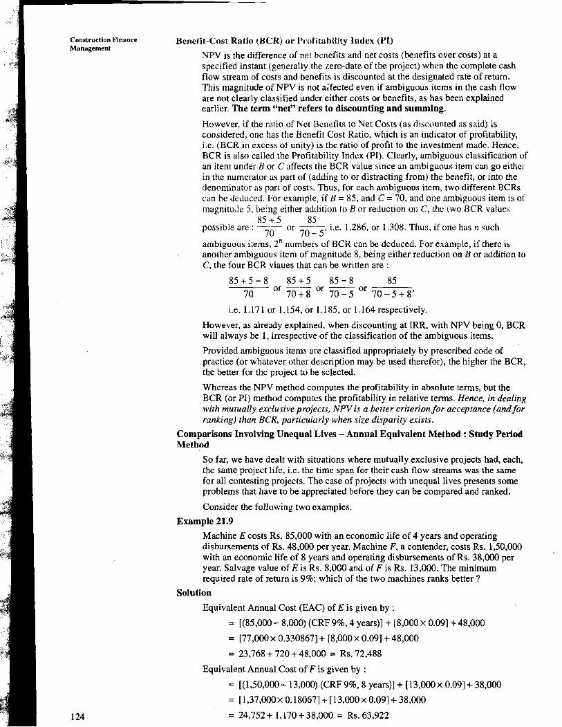
Construction Finance Benetit-Cost Ratio (BCK) or k'rutitahility Index (PI) Management

NPV is the difference of net benefits and net costs (benefits over costs) at a specified instant (generally the zero-date of the project) when the complete cash flow stream of costs and benefits is discounted at the designated rate of return. This magnitude of NPV is not alfected even if ambiguous items in the cash flow are not clearly classified under either costs or benefits, as has been explained earlier. The term "net" refers to discounting and summing.

However, if the ratio of Net Benefits to Net Costs (as discounted as said) is considered, one has the Benefit Cost Ratio, which is an indicator of profitability, i.e. (BCR in excess of unity) is the ratio of profit to the investment made. Hence, BCR is also called the Profitability Index (PI). Clearly, ambiguous classification of an item under B or C affects the BCR value since an ambiguous item can go either in the numerator as part of (adding to or distracting from) the benefit, or into the denominator 3s part of costs. Thus, for each ambiguous item, two different BCRs can he deduced. For example, if B = 85, and C = 70, and one ambiguous item is of ~nagnitudc 5, being either addition to B or reduction on C, the two BCR values

85 + 5 85 possible arc :

70 or --, i.e. 1.286, or 1.308. Thus, if one has n such

7 0 - 5 ambiguous items, 2" numbers of BCR can be deduced. For example, if there is another ambiguous item of magnitude 8, being either reduction on B or addition to C, the four BCR vlaues that can be written are :

i.e. 1.171 or 1.154, or 1.1 85, or 1.164 respectively.

However, as already explained, when discounting at IRR, with NPV being 0, BCR will always be 1, irrespective of the classification of the ambiguous items.

Provided ambiguous items are classified appropriately by prescribed code of practice (or whatever other description may be used therefor), the higher the BCR, the better for the project to be selected.

Whereas the NPV method computes the profitability in absolute terms, but the BCR (or PI) method computes the profitability in relative terms. Hence, in dealing with mutually exclusive projects, NPV is a better criterion for acceptance (and for ranking) than BCR, particularly when size disparity exists.

Comparisons Involving Unequal Lives - Annual Equivalent Method : Study Period Method

So far, we have dealt with situations where mutually exclusive projects had, each, the same project life, i.e. the time span for their cash flow streams was the same for all contesting projects. The case of projects with unequal lives presents some problems that have to be appreciated before they can be compared and ranked.

Consider the following two examples.

Example 21.9

Machine E costs Rs. 85,000 with an economic life of 4 years and operating disbursements of Rs. 48,000 per year. Machine F, a contender, costs Rs. 1,50,000 with an economic life of 8 years and operating disbursements of Rs. 38,000 per year. Salvage value of E is Rs. 8,000 and of F is Rs. 13,000. The minimum required rate of return is 9%; which of the two machines ranks better ?

Solution

Equivalent Annual Cost (EAC) of E is given by :

= [(85,000 - 8,000) (CRF 9%, 4 years)] + [8,000 x 0.091 + 48,000

= [77,000 x 0.3308671 + [8,000 x 0.091 + 48,000

= 23,768 + 720 + 48,000 = Rs. 72,488

Equivalent Annual Cost of F is given by :

= [(1,50,000 - 13,000) (CRF 9%, 8 years)] + [13,000 x 0.091 + 38,000

= [1,37,OOOx 0.180671 + [13,000 x 0.091 + 38,000

= 24,752+ 1,170+ 38,000 = Rs. 63,922

i Should we then call that F has an advantage of Rs. 8,566 per year over E ? May be it is so, but what about the EAC of F at a total value of Rs. 63,922 during the 5th to

i 8th years, both inclusive ? This seems to be acceptable if we assume that during the 5th to 8th year, both inclusive, an exactly equivalent machine E follows the present machine E, which will then need an EAC during this extended period exactly equal to that of the earlier E.

Accordingly, it is reasonable to adopt the above method of comparison based on Equivalent Annual Values (costs in this case). If machines E and F had lives, say, 4 and 7 years respectively, we may argue on the same times that machine E repeats itself over 7 times in 28 years commonly with machine F repeating itself over 4 times in the same 28 years (i.e. the least common multiple of the lives of the individual machines). In other words, disregarding all possible events which might occur after the time duration of shortest life alternative is the method to be adopted. This, therefore, is called the Study Period Method.

We may justify, the study period approach by the following argument also. That EAC of machine E as Rs. 72,488 stands. Regarding machine F, the investment cost and the salvage, which pertain to the entire life period must be prorated for the period of comparison, which is the shorter of the two lives of the machines E and F, this being the life of E, viz. 4 years in this problem. This prorating is'based on the dictum : Having distributed the EAC over the life of F, we collect the costs belonging to the 4-year study period by the following concept.

In the term (1,50,000- 13,000) x (CRF 9%, 8 years), considering the first four years only, the prorated present worth will be by multiplying this amount by USPWF (9%, 4 years), and taking its equivalent annual value over the 4 years will be by multiplying further by CRF (996, 4 years); noting that USPWF and CRF are mutually reciprocals, the term (1,50,000- 13,000), x (CRF 9%, 8 years), remains unaltered. [Likewise a possible second term 113,000 x SFF 9%, 8 years] too remains unaltered even after prorating for the first 4 years and then redistributing over the same 4 years.] Thus, on prorating basis too, the study period method is justified.

The case of unequal expenses through the years is simply to be handled by first getting the Net Present Equivalent cost by discounting individual yearly costs and summating these discounted values; and then distributing this sum as annuities through the years, i.e. by multiplying by the CRF. For example, if the operating disbursements in the 4 years were, respectively, Rs. 44,000; Rs. 47,000; Rs. 50,000 and Rs. 53,000, then, this part of the EAC would be computed as follows :

= [(44,000 x SPPWF 9%, 1 year) + (47,000 x SPPWF 9%. 2 years) + (50,000 x SPPWF 9%,3 years) + (53,000 SPPWF 9%, 4 years)] x (CRF 9%, 4 years)

= [(44,000x 0.91743) + (47,000~ 0.84168) + (47,000~ 0.77218) + (53,000 x 0.70843)] x 0.30867

= [40,367 + 39,559 + 3,6292 + 37,5471 x 0.30867 = Rs. 47,463

Example 21.10 Project A has an initial outlay of Rs. 18,000, with a service life of 2 years through which the yearly CFAT values are Rs. 14,000 and Rs. 12,800, respectively, with zero salvage value. Project B has an initial outlay of Rs. 35,000, with a service life of 4 years through which the yearly CFAT values are Rs. 14,000; Rs. 16,000; Rs. 12,800 and Rs. 10,800, respectively, with zero salvage value. The required rate of return is 10%.

Which of the two projects ranks better ?

Solution Project A

Present worth of the CFAT values

= (14,000 x 0.90909) + (12,800 x 0.82645) = Rs. 23,306

NPV = - 18,000 + 23,306 = + 5,306

EA Benefit = [5,306 x (CRF 10%. 2 years)]

= 5,306 x 0.57619 = Rs. 3,057

Capital Investment Decisions

Construction Nnance Management

Project B

Present worth of all the CFAT values

= Rs. 42,944

NPV = - 35,000 + 42,944 = + 7944

EA Benefit = [7,944 x (CRF 10%. 4 years)]

= 7,944 x 0.3 1547 = Rs. 2,506

Project A ranks better than Project B.

Investment Proposals for Income-Expansion and for Cost-Reduction In Example 21.9, we prefer F to E since the EAC is less for F. In Example 21.10, we prefer A to B since the EAB is more for A. Thus, for invesmentproposals for generating incomes, expansion of income is the criterion for choice; and for investment proposals for contributing towards the costs, reduction in cost is the criterion for choice.

It is generally premised that a cost-reduction expenditure does not affect the gross income. Of course, there can be instances of combined cost-reduction and income-expansion expenditures. For an income-expansion expenditure, the increase in income must be more than the increase in expenditure.

Also, cost-reduction alternatives are mutually exclusive; but mutual exclusivity is not always true of multiple income-exp~nsion alternatives.

Following example illustrates a combined cost-reduction cum income-expansion expenditure.

Example 21.11 Two processes are available for stone crushing at a quany site. One has a first cost of Rs. 4,00,000 with an annual operating cost of Rs. 1,28,000. The other would cost Rs. 5,60,000 with an annual operating cost of Rs. 1,35,000. The second process will also sort the crushed stone and hence, it is expected that annually an extra Rs. 55,000 is realised in profits. The life of equipment in each of the processes is 11 years with zero salvage value. The minimum required rate of return is 10%. Is the extra expenditure in the second process approvable ?

Solution Equivalent Annual Cost (EAC) of the first process is

= [4,00,000x (CRF lo%, 11 years)] + 1,28,000

= (4,00,000x 0.15396) + 1,28,000 = Rs. 1,89,584

Equivalent Annual Cost (EAC) of the second process is

= [5,60,000x (CRF lo%, 11 years)] + 1,35,000- 55,000

= (5,60,000 x 0.15396) + 1,35,000 - 55,000 = Rs. 1,66,218

The extra investment is approvable since EAC is reduced, when considering inclusive of income expansion.

Here, the first process goes relatively for cost reduction; but, because of the extra profits, the second process involves income-expansion. Rather than straightaway tending to chose the first process for cost-reduction purposes, we have to consider the opportunity for income-expansion also if taking to the second process.

A Note We had so far considered that the equipment (or the project) will be used for as long as it will be economically alive even allowing (conceptually) for continuing with like replacements into a long future (as discussed in explaining the study period method).

However, in some instances, the length of service required may be short and known. In such instances, we use this period for capital recovery on the investment cost net of salvage and allow for the interest liability on the salvage.

The following example illustrates this.

Example 21.12 A battery-operated fork-lift costs Rs. 1,70,000 and will have an operating cost of Rs. 40,000 per year and a salvage value of Rs. 65,000. A diesel-operated fork-lift capable of performing the same tasks costs Rs. 1.10.000 with operating cost of Rs. 70,000 per year and a salvage value of Rs. 25,000. The construction job on which the equipment will be needed is likely to be completed in 2 years. The minimum required rate of return is 11%. Which alternative is preferable ?

Solution Annual cost of battery-operated fork-lift is

= [(I ,70,000 - 65,000) x (CRF 11%. 2 years)] + (65,000 x 0.11) + 40,000

= (1,05,000~ 0.57619) + 7,150+ 40,000 = Rs. 1,07,650

Annual cost of diesel-operated fork-lift is

= [(1,10,000- 25,000) x (CRF 11%. 2 years)] + (25,000~ 0.11) + 70,000

= (85,000 x 0.57619) + 2,750 + 70,000 = Rs. 1,21,726

The battery-operated fork-lift is the preferable alternative.

SAQ 5 Rework all the examples (Example 2 1.9 to Example 2 1.12) with costs decreased by 10% and benefits increased by 5%.

21.7 CAPITAL RATIONING

To provide capital for the anticipated well-reasoned and well-investigated projects (or investment opportunities) is a very important and necessary process. Considering in this way, such an exercise is called Capital budgeting in several contexts. However, there always are quite a few p~ojects in the proposal stage whose aggregated demands for capital expenditure generally exceed the supply of capital, particularly if there is a budget ceiling, or constraint, on the amount of funds available that can be invested during a specifiedperiod, say, a year. Besides this constraint on the supply side of funds, there is also a large range of variation in the prospective returns, demand by demand, covering a wide range. And yet a third consideration comes into picture as regards the cost of capital which usually increases with the total quantum of capital; and to make profits, the firm is obliged to look into only such projects which can yield at least a little more than the cost of capital. Such a yield rate is called thz cut-off rate or the hurdle rate. Constraints on the total available supply of capital impact highly if the firm adopts a policy of financing much of the demanded capital expenditure from internal sources, possibly with a view to contain the cost of capital. Also, particular divisions of a large firm may be subjected to specified budget ceilings.

In such circumstances,

(a) it is not only important that none of the limited capital be appropriated to aggressive (i.e. high magnitude) demands, particularly if they may yield rates of return less than the hurdle rate (and worse still if the yield is less than the cost of capital), but

(b) it is also important that the limited funds be given only to the very best investments.

Hence, such an exercise of allocation of funds among the basket of investment opportunities available is better called capital rationing.

Accordingly, capital rationing, also called capital budgeting in certain contexts, is an organised procedure for investigating and quantifying the input and output parameters of alternatives, evaluating each alternative, (listing or) laddering all the alternatives in the order of their merits, separately also determining the sources of capital and their costs, and then appropriating the supply to the best of the demands so as to maximise' the shareholders' wealth (through maximisation of the total NPV).

Capital Investment Deeiaons I

Construction Finance Management

21.7.1 The Two-Stage Process At the same time, the two criteria mentioned above suggest a two-stage solution to the problem of capital rationing.

Firstly, projects that may yield below a certain cut-off rate (or the minimum required1 acceptable rate of return) should be pruned off, since satisfying a project at any lower rate of return would result in insufficient funds to invest in projects with higher rates of return. Incidentally, this leads to two fundamental concepts reflected in practice :

(a) the greater the spread (or difference) between the cut-off rate and cost of capital, the greater the pressure on the firm's management to increase the supply of funds by employinglsecuring outside funds, which, in turn, would generally spiral up the cost of capital; and

(b) whenever the supply does not satisfy the demand, the cost of capital remains as thejoor or bottomline under [we are not saying - ''$orW] the cut-off rate. In such a case, the problem extends not only to just increasing the supply but also to meet demands for all (or most) projects promising rates of return down through to the cost of capital (which would be increasing as the supply is increased).

For the purpose of this first stage, a demand schedule is compiled collating the budgetary requests for the investment funds requested for the forthcoming period for each project, together with the merits of each [usually in the form of expected rate of return (as IRR) or BCR (PI) based on a stipulated MARR] and laddering them in decreasing order of the merit. This organisation of the laddered increments of demand can be presented graphically also by plotting the merit (on y-axis) against cumulative amounts of demand (on x-axis) - on the lines of an "Exceedence Cuwe". Some would prefer to draw the laddered curve for all projects presented for consideration and decide on the pruning off based on information worked out from the curve.

Secondly, either through the BCR (or PI) or the NPV, appropriations must be made to projects (retained after the firstxtage) in the order of their highest contribution to the wealth of the shareholders.

There is yet another view too on this two-stage process as follows. The first stage is effected through IRR or BCR (or PI); and to effect the second stage through NPV considerations.

21.7.2 Strategic Investments When the demand schedule was discussed Section 2 1.6.1, it was tacitly understood that the demands for strategic investments would not be integrated into the demand schedule. Strategic investments, also called irreducible investments cannot be quantitatively evaluated as investments per se, and hence, cannot be assigned "merit" in terms of expected earnings, or BCR (PI). Yet they are necessary investments in the judgement of management. Examples are : providing for health care of employees, constructing and running a recreation centre and conducting annual sports meets; investing money in preparing for a line of business so as to maintain leadership andlor secure a market share. In these instances, returns can neither be calculated, and, if at all calculable, will be insignificant. Then, to define, strategic investments are necessary investments in which a low or insignificant rate of return is overwhelmed by irreducible considerations or advantages.

For these investments, management would follow reasonable methods for fund allocations - viz. by envisaging the demands (as for healthcare services, sports, etc.) or by a percentage of the total supply (for market research for diversification, or support to educational and research institutions).

21.7.3 Period Planning While discussing the compiling of the demand schedule (see Section 21.6.1), it was said, inter alia, "for the forthcoming period". Since several projects may extend through several periods (years, or quarters, as the case may be), it is evident that funds have to be appropriated to projects through several periods. Since the exercise is a multi-period problem in general, the term capital budgeting is equally in vogue as the truly significant and purposeful term capital rationing. The annual budget, for example, cannot lose sight of, and hence, cannot be set up completely independent from, future needs and future supplies. Hence, planning for demands (including for capital equipment

requirements) and supplies is done successively for long-term (say 5 to 10 years hence), medium-term (say2 to 3 years hence) and short-term (generally, the next year in the horizon). Long-term planning must address the question of the optimal capital mix (debt, retained or flowback earnings, and new equity floated) so that the overall cost of capital is minimised.

For this reason, based on the long-term planning, cost of capital is necessarily (to be) a multi-period value and should not be based on a narrow view with disregard to needs and possible supplies (for funds) in future years.

21.7.4 Project Divisibility Selection of individual projects under capital rationing is carried out better when the divisibility or otherwise of the projects is considered. If a project has to be accepted or rejected in toto, and cannot be accepted partially, it is considered as an indivisible project. A divisible project, on the other hand, can be accepted or rejected in part.

In the case of divisible projects, either the components can be separately worked out ab-initio, or the composite data can be split into the divisible components as a best possible approximation.

To illustrate the splitting up of composite data, let us consider a project X which has an initial investment outlay of Rs. 6,00,000, with a BCR (or PI) of 1.30. [It is directly inferred that its NPV = Cost (BCR - 1) = Rs. 6,00,000 (1.3 - 1) = Rs. 1,80,000.] If it should be possible to split it into sub-projects X1 and X2 with respective initial outlays of Rs. 3,60,000 and Rs. 2,40,000 (by balance), and if the BCR of X1 is possibly computed as 1.40, then the NPV of X1 would be Rs. 1,44,000 (being 0.4 x 3,60,000); then the NPV of X2 would be 36,000 (by balance : 1,80,000 - 1,44,000), this at the sany time being 0.15 of its cost of Rs. 2,40,000; hence the BCR of X2 would be 1.15. With this split-up information, X can be first considered in total for rationing funds for it out of the available total capital supply. If it gets its funds rationed out to it in toto, so much so good. If not, the split parts of X1 and X2 can then be considered for capital rationing, either without revising the capital rationing exercise and accepting X1 if possible and desirable; or revising the capital rationing exercise with keeping X1 and X2 as separate entities. Undoubtedly, it would have been better to have listed X1 and X2 separately to start with for drawing out the demand schedule (by laddering). In the unlikely event that X1 and X2 would each have the same BCR as the composite X, then the above-said process would continue to be validly applicable. In case X2 cannot be taken up unless X1 is completed, we consider X in toto; or X1 initially; and, if budget admits, consider X2, subject to maximisation of shareholders' wealth and utilising the budget fully or near-fully.

(Basket of Divisible and Indivisible Projects)

Example 21.13

Consider that a firm has the following investment opportunities and that the total budget outlay available is under three options : Rs. 7,50,000; Rs. 9,00,000; and Rs. 10,50,000.

It is also believed project F can be taken in two parts, the first part F1 with an outlay of Rs. 1,00,000 with a PI of 1.28 and the second part F2 with an outlay of Rs. 1,00,000. [It is very simply calculated that the PI of project F2 will be 1.16.1

All the project proposals are independent of each other (and, mutually exclusive), including F1 and F2 within themselves too. Advise the firm on which projects should be selected. As far as possible project F should be taken up as a whole.

Solution

Rank the projects in descending order of PI and choose going down the rank order. It is tabulated in the following table.

F G

200 100

1.22 1 .SO

Capital Investment Dedsiono

D

400

1.62

C

130

1.35

Project

Initial gutlay, Rs. (10 )

Profitability Index

E

100

1.17

A

150

1.12

B

170

1.42

Construction Finance Management

Rank in descending 1 1st ) 2nd I 3rd / 4th I 5th / 6th ( 7th I order of PI

Project Number

PI

Total Budget Outlay : Rs. 7,50,000

[ NPV, Rs. (101)

The lst, 2nd and 3rd ranks are chosen; Rs. 6,70,000 are exhausted and Rs. 80,000 are left through which Project Fl could not be taken up.

I

D

1.62

The results are : Rs. 80,000 is left unutilised; and the cumulative NPV realised is Rs. 3,69,400.

248

Total Budget Outlay : Rs. 9,00,000

1

G

1.50

Projects D, G, B and C together exhaust Rs. 8,00,000. With the balance of Rs. 1,00,000, sub-project Fl can be taken up. The results are : All available funds are exhausted; and the cumulative NPV realised is Rs. 4,42,900.

50

[Note that the marginal increase in budget of Rs. 1,50,000 fetches an additional gross NPV of Rs. 73,500, i.e. a return of 49%, just short of what Project G yields (this being 50%). Of course, in the earlier case, Rs. 80,000 was unutilised. This incremental return of 49% would clearly recommend this level of funding if cost of capital is managed.]

Total Budget Outlay : Rs. 10,50,000

B

1.42

71.4

Choosing projects D, G, B, C and F exhausts Rs. 10,00,000 of the budget with leaving Rs. 50,000 unutilised; and the cumulative NPV realised will be Rs. 4,58,900. However, if only F1 (of F) is chosen and, if with the balance amount now available (Rs. 1,50,000), Project A is chosen (skipping, of course, Project E), the change in cumulative NPV realised will be : less Rs. 16,000 for F2 plus Rs. 18,000 on A, i.e. an increase of Rs. 2,000. This should be acceptable.

F

1.22

C

1.35

The results are : All available funds are exhausted by taking up projects. D, G, B, C, F1 and A. The cumulative NPV realised will be : Rs. 4,60,900.

Here, one finds that the marginal increase of Rs. 1,50,000 in the funds made available fetch an additional Rs. 18,000 in cumulative NPV realised, i.e. a 12% return on these increments.

E

1.17

45.5

An Observation

A

1.12

17 44

The total budget needed to take up all the projects would be Rs. 12,50,000; and tHen the cumulative NPV realised will be Rs. 4,93,900. This translates into : this final possible increment of Rs.'2,00,000 in budget outlay yields the final incremental return of Rs. 33,000 (being Rs. 16,000 in F2 and Rs. 17,000 in E), indicating a differential yield of 16.5%. So, it can be said that, if all the projects have to be funded, the budget outlay will have to be Rs. 12,50,000; the total NPV realised will be Rs. 4,93,900; i.e. the weighted average yield will be 39.512%. It is therefore worthwhile to arrange for funds for taking up all the projects.

18

One more observation that is also very important is as under. Even though all projects had been laddered, i.e. listed in the demand schedule, only after they were accepted under, say, the minimum required rate of return criterion, yet under capital rationing conditions, we have not been able to accept certain of the listed projects. Thus, under capital rationing the minimum required rate of return is not the acceptance criterion. Also, under capital rationing, the adoptable investment policy is, therefore, less than optimal.

When projects of unequal lives have to be considered for laddering, the accepted project from among the mutully exclusive projects will appear in the ladder in terms of the values as decided by the study period approach.

Consider Example 21.10. Project A will be listed as :

Outlay Rs. 18,000; NPV : Rs. 5,306; and PI = 1.295.

Laddering Arrangement (Cost of Capital given)

Example 21.14 A firm has grouped all the demands for budgetary allocations included in mutually exclusive project proposals for funding in the forthcoming year according to the prospective rates of return on the investments. The complete demand schedule for the full list of demands received is as follows :

It hopes to secure capital at the following weighted average cost of capital.

Estimated Rete of Return, %

Total of demands in the group, lZs. (thousands)

Determine the minimum required rate of return any for project to be accepted for the range of total capital that can be supplied to support the projects proposed.

[Note : Before taking up the solution, certain points' may be made. Since the firm 1

has indicated its accepted feasible maximum cost of capital as 22:%, all projects

245

350

with IRR less than 22t96 will not be selected. Projects with IRR + 2596 sum up to

Weighted Cost of Capital, %

TotalCapitalavailable Rs. (thousands)

a demand of Rs. 5,650 thousands; hence, perhaps, some of the projects in the IRR range of 20 to 25% may also be selected if total capital available is stretched to the maximum of Rs. 5,800 thousands as indicated. For lesser amounts of total capital made available, only lesser number of projects will be selected.]

20

3,800

Solution The demand schedule curve between Rate of Return (8) and cumulative value of projects with IRR not less than the ROR can be developed as given in Figure 21.10 with the help of values given in Table 2 1.2.

40-45

775

18

1,600

Rate of Rcturn (%)

30

35-40

1125

30-35

1450

2 1

4,700

19

3,200

Curvc ofdcrnand ror invcstmcnt

Cut-off ratcs ('%)

Cumulative Demand ( I O ' ~ )

22

5,250

Capital Investment Dedslo~

15-20

3100

25-30

1950

1 22-

2

5,800

20-25

2650

Construction Finance Management

Table 21.2

Cumulative Amounts, i.e. 1 350 1125 / 2250 / 3700 ( 5650 1 8300 1 Total Demand, Rs. (thousands)

Laddered Increments of Demand,

The curve of cumulative demand with reference to rate of return is drawn and is as given in Figure 21.10.

The curve of supply for investment is (likewise) drawn between Rate of Return (%) (now indicating cost of capital) and the total capital available, by simply transferring the data on to the curve (on the same figure).

Amount, Rs. (thousands)

ROR (%)

The cut-off percentages required to be decided on will be decided by the point where the respective supply equals the demand; i.e. the cut-off percentage can be read by projecting the supply point (on the supply curve) vertically on to the demand curve (and reading off the ROR axis). The cut-off percentages read off the figure are indicated on the figure. The values are now tabulated.

350

1 4 5

SAQ 6 (a) Rework Example 21.13, with the PI'S taken in the reverse order, i.e. A with

1.50; B with 1.22; C with 1.17; D with 1.62; E with 1.35; F with 1.42 and G with 1.12.

(b) Rework Example 21.14, with the demand series changed to : 300,800,1200, 1600, 1800,2200 and 2700 units, respectively and with the availability series changed to : 1800,2700,3400,4600,5700 and 6300 units respectively.

775 ---.-- 40-45

( T&I ~a~ital<ailable, ' 1 6 0 0

21.8 RISK ANALYSIS

3200

31.8

Rs. (thousands)

Cut-off, %

Under Section 21 . l , "business risk complexion" of the firm was mentioned. In that discussion, it was held that suppliers of capital could hold the view that the selection of any investment project may not alter, the business-risk complexion of the firm. Thus, risk was held constant; and based on this, the expected future cash flows were analysed. But it is likely that the risk-free assumption is not always either correct or is realisable. Suppliers of capital to the firm (investors and creditors), by and large, are risk-averse; and hence, the least they may do, short of totally withdrawing from supplying capital is, to suitably change their required rate of return as the risk-perception changes.

1125 ' 1450

35-40 / 30-35

38.0

The risk-profile of a project's future cash inflows affects also the firm's value. For example, a project expected to provide a high return may be so risky that the suppliers of capital may consider the firm as risky resulting in decrease in the firm's value inspite of even a good profitability potential.

3800

29.9

In the earlier units and sections, the relationship between profitability and risk has been repeatedly described and demonstrated. Likewise, it is necessary to incorporate the risk factor in project evaluation/apprisal as well as in the accompanying capital investment decisions.

1950

25-30

Rather than covering the risk of the firm as a whole, only the project risk is discussed in the ensuing section. The purpose is to understand how risk affects value.

Several occasions exist where the terms risk and uncertainty are used synonymously notwithstanding the differences between the concepts. Risk is describable by a probability distribution but uncertainty is not.

2650

20-25

-

5800

24.8

4700 ( 5750

3100

3

27.8 26.0

21.8.1 Description of Risky Investment Capital Investment Decldom

First of all, it is necessary to evaluate risky investments. For this, the benefits must be estimated. The term"estimating" itself mirrors out the role of various assumptions - e.g., prices, sales volumes, competitions, effectiveness of advertising and interaction with beneficiaries, clients and customers, several categories of costs, state of the economy, infrastructure, power supply, etc. The actual returns will vary from the estimates in many a case. This variation is the underlying factor in project risk. The greater the variability, the riskier the project and the returns on its investment. But yet one must be able to consider a range of possible cash flows. It must, of course, be emphasised, that any probability description of the range of expected cash flows will only be subjective - after all, the cash flows are yet expected and are not part of a series of past-recorded data, but, based on past experience under comparable circumstances, and well aware of the emerging trends and situations, the concerned group makes the best possible range of estimates along with the probabilities of occurrence of each of the estimated values over the whole range. In continuation of what has been said earlier, it is, of course, true that estimates of returns from cost-reduction type of capital budgeting will be less risky than income-expansion type of capital budgeting. It can also be retold that the greater the range, or the spread, or the estimated values for any one outcome, the greater the riskiness of that outcome.

21.9 METHODS OF INCORPORATING RISK FACTORS IN CAPITAL BUDGETING DECISIONS

The methods can be put into following two general classes :

(1) Those that operate without considering risk profile in detail. These are also called common or general techniques.

(2) Those that operate with considering the risk profile in detail.

Under Method (1) There are two approaches :

(i) Risk-Adjusted Discount Rate Approach; and

(ii) Certainty-Equivalent Approach.

Under Method (2) Also called quantitative methods, there are three types of analyses hereunder :

(i) Sensitivity Analysis (also called "what if ' analysis);

(ii) Analysis through Measures of Risk (Standard Deviation and Coefficient of Variation) based on Probability Distribution; and

(iii) Analysis based on Decision-Tree. [Really speaking, Decision-Tree analysis is a sub-class under Probability Distribution-based Approach.]

21.9.1 Risk-Adjusted Discount Rate Approach Risk-adjusted discount rate approach (written as RAD or RADR approach) is based on adjusting the discount rate to reflect project risk in computing present values. The more risky the project, the higher the discount rate; less risky, or safer, the project, lower the discount rate. This is reflected in a low RAD for risk-free assets such as treasury bills. Lease-purchase capital budgeting involves almost no risk (since no variability is associated with the returns) and interest rate for this is low. If transport trucks are funded even as they operate in unsafe areas, the interest rates charged are high. Cost-reduction projects may have RAD of, say lo%, income-expansion projects, say 12%, new projects in unfamiliar surroundings, say 18 to 2 5 8 , and so on. The risk-adjusted discount rate expresses the combined time-and-risk preference of the investors. The difference between the two rates is called the risk premium.

It is generally believed that RAD rate must increase monotonically from the risk-less, or risk-free, rate of return at risk described by zero magnitude of coefficient of variation [CV, more fully described under Method 2 (ii) hereinafter] to higher values as CV increases.

RAD rate is employed in evaluating the NPV of any risky project (in place of the risk-free rate). Acceptance and ranking depend on the positive magnitude of the NPV. 133

Construction Finnnce If IRR is used as the decision criterion, the IRR derived is to be compared with the Management risk-adjusted required rate of return. If IRR > RADR, the project is acceptable; and

ranking is by the difference (IRR - RADR).

If any particular future year's cash inflow is more risky than in other years, a still higher RAD rate may be applied to that particular year's cash inflow; correspondingly, a lesser RAD rate for a less risky future year's cash flow.

The one important criticism on this method, is that it adjusts the wrong element. It is the future cash income that is subject to risk; rather than adjusting the cash flow for the risk in it, the method adjusts the rate of return to be applied.

Another important criticism is that by adding the risk premium to the discount rate, the method leads to severely compounding the risk over time; i.e. the method axiomatically takes that risk increases exponentially with time (since the discounting factor goes as (1 + i)-" with n as the exponent).

For these reasons, this is a crude method for incorporating risk into capital budgeting analysis and decisions.

21.9.2 Certainty-Equivalent Approach Unlike the RAD rate approach which adjusted the discount rate, this approach adjusts the expected cash flows. The risk-adjustment factor is expressed through a certainty- equivalence coefficient (CEC).

CEC is given by

Certain, or risk less, cash flow CEC =

Risky cash flow

On the one hand, the future.returns are subject to risk and might vary from the estimates made at the time of apprisal; on the other hand, if the returns could be made certain, there will be no element of risk. With this concept as a background, this approach begins with ascertaining the riskless cash flows comparable to the expected (i.e. subject to risk) cash flows from the project.

Let the expected cash flow in a particular future year be Rs. 50,000. Considering the risk involved in it, the risk perception continuing to be only subjective at the firm's level, let it be said that the management, based on its utility preferences for that year in future, would be willing to accept (or consider) Rs. 35,000 as a certain cash flow, i.e. if Rs. 35,000 can be the cash flow with total certainty. (This is like a bettor in a lottery saying that he would rather like to be assured of Rs. 35,000 in that year than expecting Rs. 50,000 with the associated risk perception.) Then, Rs. 35,000 is the certainty equivalent of Rs. 50,000

35,000 for that future year, and the CEC is - = 0.70.

50,000

Admittedly, CEC values can range from 0.00 to 1.00. The higher the risk, the lower the coefficient.

The certainty equivalent is used in the computation of NPV together with the risk-free required rate of return. Beyond this, computations proceed in the normal course. Acceptance criteria continue to be the same as in normal course of computations.

Besides being simple in methodology, the method incorporates management's perception, on a year-to-year basis in the future, adjusting the element subject to risk, viz. the cash flow and not the discount rate. The subjective element in deciding the certainty equivalent is the source of drawback in this method. Yet, certainty equivalent provides for varying risks over the years in future. Though this method is also crude in its outline, it is considerd better than RAD rate method.

21.9.3 Sensitivity Analysis Sensitivity refers to the effect that changes in one or more parameters will have on the conclusions. The analysis consists of purposely changing conditions between possible limits and computing the resultant changes in the parameters for evaluation - NPV, IRR, AE or BCR. Sensitivity analysis implies uncertainty and the analysis takes account of the uncertainty through recognising that any parameters, being only an estimate regarding the future, may happen to be different when the date arrives. A few examples are herewith.

Example 21.15 (Error in Life Period) Consider an investment A of Rs. 25,000 with a zero salvage value after 8 years, with an annual outgo of Rs. 2,000 for OMR. An alternative investment B of Rs. 17,000 with zero salvage value after 8 years would do as well except that its annual OMR disbursements would be Rs. 3,600. Let us compare the performance on a relative basis.

Solution The comparison results in A being better over B by a CRF given by :

Correspondingly, the investment A has an advantageous Rate of Return over B of 11.81%.

If the realised life goes into error by, say + 25%. i.e. if the realised life (in both cases A and B) happens to be 10 years, instead of 8 years as initially envisaged, A has now realised an advantage in Rate of Return over B given by

CRF 10 years = 0.20. i.e. ROR = 15.1%

(15.1 - 11.81) This is an error of

11.81 = + 27.86%

So it is seen that an error of + 25% in realised life leads to an error of' + 27.86% in realised ROR advantage for A over B, OTHER CONDITIONS REMAINING THE SAME. This is one typical point in a plot of ERROR IN ROR (A over B) against ERROR IN PREDICTING LIFE PERIOD. A graph developed with such points by considering a range of variation of realised life, say, from 5 to 12 years can be plotted. This will be the SENSITIVITY CURVE between ROR (A over B) and LIFE PERIOD.

Example 21.16 (Error in Salvage) Supposing other conditions remained the same, except that A might have a salvage value of Rs. 2,000 at the end of the 8th year.

Solution The comparative advantage of A over B, in terns of ROR, will be given by the equation :

(25,000 - 2,000) CRF 8 ,,,, + 2,000 i + 2,000

Thus, we get,

The ROR (= i) works out to be : i = 14.42%. So an error of Rs. 2,000 in realised 14.42 - 11.81

salvage of investment A leads to an error of 11.81

= 22.1% in realised

ROR (A over B).

Again a sensitivity curve can be developed between these two parameters.

Break-Even Analysis Break-even (BE) analysis is the computation of the value of one of the cost factors to break-even if all of the other cost factors included in the analysis are held invariant. In this sense, Pay Back Period is actually the break-even period if salvage and rate of return are both zero, if the definition holds.

Example 21.17 Consider an investment proposal with an initial investment of Rs. 65,000 which is expected to yield a (pre-tax) return of Rs. 19,000 a year for 7 years with a salvage of Rs. 20,000 at that date. The minimum required rate of return (pre-tax) is 15%. What is the break-even (BE) magnitude for the yearly returns, salvage and life-period ?

Cons&uction Flnaace Management

[Note that first cost is not subject of break-even analysis, since it is supposed to be actually counted (and not estimated in future).]

+ 19.000 per year

Figure 21.11

Solution (i) Yearly Returns

= [(65,000 - 20,000) (CRF 15%,7 years)] + (20,000 x 0.15) = [?I

= (45,000 x 0.24036) + 3,000 = Rs. 13,816.20 [BE value]

20,000 Also, Factor of Safety = 3,81 6.20 = 1.448

(ii) Salvage

To break-even, salvage must be given by :

= 165,000 x (CRF 15%,7 years)] - 19,000

= (65,000 x 0.24036) - 19,000 = (-) Rs. 3,376.60

The negative sign is not surprising, considering that yearly returns at Rs. 13,816.20 would just justify the salvage of Rs. 20,000. Moreover, with a negative value of salvage at break-even, the question of factor of safety does not arise.

(iii) Life-Period

To break-even, the life period should necessarily be less than 7 years, since the yearly returns needed to break-even in 7 years is less than the yearly returns as estimated. This should mean that the salvage value must be expected to be more (than Rs. 20,000) in the shorter (BE) life period. Either we should predict this revised salvage (by predicting salvage for each life period between 0 to 7 years), or we may (though reluctantly, or, wrongly) assume the salvage to be constant over the whole period (0 to 7 years). With this latter assumption :

[45,000 x (CRF 15%. n years)] + (20,000 x 0.15) = 19,000

16 i.e. (CFW 15%, n years) = -

45 = 0.35556

Therefore, n = 3.92.years

7 3.92

- 1.786 Also, Factor of Safety = - -

65,000 Alternatively, Payback period = -

19,000' neglecting salvage = 3.421 years with

Factor of Safety of 2.046.

Notes

(1) Break-even point is defined with only one factor held variable with others held at constant (given, estimated) value. In the Payback period, on the other hand, two factors held constant, both at zero value. Hence, the Payback Period is not attributable with any factor of safety in the strict sense. (May recall earlier remark "if definition holds". Also, to recall that no salvage is considered for PBP.)

(2) Like the first cost, the MARR also is not normally subjected to BE analysis since MARR is external to the project and is initially decided by the firm. Yet, it is also sometimes analysed for break-even to assure the firm on the upper limit of cost of capital till which the project will yet be viable. Ifwill be seen that this is the IRR. In the given problem, the break-even MARR (pre-tax) can also be investigated by writing :

[(65,000 - 20,000) x (CRF i, 7 years)] + (20,000 X i) = 19,000

From this equation, i works out to be = 24.5785%

This is the IRR of the project.

24.5785 Also, Factor of Safety = - = 1.639.

15 Best-Worst Choice

Break-even method helped to study the effect of change in one variable assuming that all other variables had been correctly predictedfestimated. The other two examples demonstrated how to probe the relative variation between two of the parameters when others were held constant, i.e. as correctly predicted, particularly on how profitability (represented by IRR) taken as the parameter of study was impinged upon by the variations in the other (variable) parameter.

However, some probability always exists that all of the variables are incorrectly predicted even if only by small amounts each. Such a situation is analysed by the "best-worst choice" method. The variables are adjusted simultaneously to present

(a) the least favourable scenario (i.e. worst choice);

(b) the optimum scenario (i.e. best choice); and

(c) the most reasonable scenario.

This is illustrated by the following which is an extension of Example 21.17.

Example 21.18 Consider the information in Example 21.17 to represent the most reasonable choice with additional information as under. The initial investment needed is expected to be Rs. 65,000 but could be as high as Rs. 67,000 or as low as Rs. 63,500. The annual pre-tax yield is expected to be Rs. 19,000 but could be variable between a high of Rs. 20,400 and a low of Rs. 15,800. The expected life could perhaps range between 9 years to 5 years. Though the anticipated salvage is Rs. 20,000, this too could vary between Rs. 14,000 to Rs. 21,000, un-related to service life (i.e. there is no assurance that if the realised life is shorter than 7 years, the salvage realisation will be more than Rs. 20,000; it can be less too; similarly for the realised life exceeding 7 years). The minimum required (pre-tax) rate of return is at the same level of 15%.

Prepare a sensitivity table for the Best-Worst Choice.

Solution A moment's reflection would admit that for the best choice,

(a) investment should decrease,

(b) annual yield should increase,

(c) life should extend, and

(d) salvage should increase.

Firstly, it will be necessary to complete the computations of the problem in Example 21.17 in respect of NPV.

NPV = - 65,000+ 19,000(USPWF 15%, 7 years) + 20,00O(SPPWF 15%, 7 years)

= - 65,000 + (19,000 x 4.1604) + (20,000 x 0.37594)

= - 65,000+ 79,047.60+ 7,518.80 = Rs. 21566.40

This can be verified through the BE yearly returns of Rs. 13816.2 derived under (i) in Example 21.17. The obtained returns being Rs. 19,000 per year against the break-even (BE) annual returns of Rs. 13,816.20, there is an excess income (by balance) of Rs. 5 183.80 at year-ends of 7 successive years.

The present value of this excess income is

= [5,183.80x (USPWF 15%,7 years)] = 5,183.80~ 4.1604 = Rs. 21,566.60

As a second step, the NPV, IRR and PBP are calculated for each of other cases, viz. worst choice and best choice.

Construction Finance Management

Worst Choice (i = 15%)

I = + 15,800 per year

Figure 21.12

NPV = - 67,000 + (15,800 x USPWF 15%. 5 years) + (14,000 x SPPWF 15%, 5 years)

= - 67,000 + (15,800 x 3.3522) + (14,000 x 0.49718)

= - 67,000 t 52,964.76 + 6,960.52 = (-) Rs. 7,075

IRR = + [(67,000 - 14,000) (CRF i , 5 years)] + 14,000 i = 15,800

Here, i works out to be = 10.84%.

67,000 PBP = - -

15,800 - 4.241 years.

Best Choice

I = + 20.400 per year

Figure 21.13

NPV = - 63,500 + (20,400 x USPWF 15%,9 years) + (21,000 x SPPWF 15%, 9 years)

= - 63.500 + (20,400 x 4.7716) + (21,000 x 0.28426)

= - 63,500 + 97,340.64 + 5,969.46 = Rs. 39.810

IRR = + [(63,500 - 21,000) (CRF i , 9 years)] + 2 1,000 i = 20,400

Here, i works out to be = 30.039%.

63,500 PBP = - = 3.113years.

20,400

The results are now tabulated for consolidated viewing.

PBP; & Variation 4.241 years; + 24% 3.421 years 3.113 years;-9%

If the decision-maker is conservative, he will hesitate to take on this project since the NPV is negative in the worst choice scenario, with the realised rate of return being indicated at only 10.8496, which is much less than the MARR of 15%. even if the most reasonable choice indicates a brighter picture.

Sensitivity analysis can also be relatively made between two mutually exclusive projects as illustrated in Example 21.19; the first cost of each is considered to be firm.

Example 21.19 : Best-Worst choice between Mutually Exclusive Projects Consider two mutually exclusive projects with the following data.

Solution [When comparing mutually exclusive projects for sensitivity, usually, only the NPV magnitudes in the three dternative choices of each are considered. IRR and PBP are not generally emphasised, nor the Equivalent Annuity when lives differ but only marginally.]

Initial cost

Economic Life

Annual (pre-tax) cash flows Worst choice Most likely Best choice

Salvage value Worst choice Most likely Best choice

Required Rate of Return

The NPV values for each project, under each of the three alternative choices, are worked out. The values obtained are included in the Table below.

[CRF 10% 15 years] = 0.13147 and [CRF lo%, 16 years = 0.12782.1

Project K

Rs. 2,50,000

15 years

Rs. 50,000 Rs. 62,000 Rs. 71,000

Rs. 15,000 Rs. 20,000 Rs. 23.000

10%

It is seen that Project K is better than Project L -- what with a spread of Rs. 1,6 1,648 between worst and best choices for K compared with a spread Rs. 1,89,070 for Project L comparatively, with the most likely values being nearly equal. As a secondary reason, one can cite three other factors, a 2 1% reduced investment cost for K with a year's shorter life to recover the investments and nearly the same salvage values.

Remarks on Sensitivity Analysis The following observations are generally true : Rate of return is very sensitive to variations in the first cost (though sensitivity to first cost variations have not been demonstrated - the essential point being that the group that estimates the first cost must be professionally quite very competent) and very insensitive to salvage value. Rate of return is also very sensitive to annual returns (or annual costs, as the case may be). There is less sensitivity to changes in economic life, though exceptional changes in economic life may result in much sensitivity. Break-even analysis can alert the management to set things right since early in the project life. The best-worst choice is a specialised application of sensitivity analysis due to the recognition that variations in one parameter may perhaps (and often do) affect other variations.

In as much as this analysis does not quantify the chances of incidence of the variations, subjectivity effects would persist. It would be more approvable if probability of the occurrence of the variations be also recognised, though yet only subjectively.

Project L

Rs. 3,15,000

16 years

Rs. 56,000 Rs. 69,000 Rs. 80,000

Rs. 16,000 Rs. 20,000 Rs. 22,000

10%

Description of Cash now

Worst choice

Most likely

Best choice

21.9.4 Analysis Based on Probability Distribution of Cash Flows Basics : Probability

If the cash flows can vary in their magnitude at each occasion (end-of-year), one needs to know the odds for a particular magnitude to occur, or be realised. These odds are quantified as probabilities of occurrence. If it is said that a cash flow of Rs. 80,000 has a probability of 0.55, it is subjectively a declaration of the belief

NPV of Project K

Rs. 1,33,905

Rs. 2,26,378

Rs. 2,95,553

NPV of Project L

Rs. 1.26.598

Rs. 2,29,175

Rs. 3,15,668

that this amount of cash flow is likely to be obtained in 55 out of 100 times. Probabilities can lie anywhere between 0 (no chance of occurrence) to 1 (certainty of occurring).

Expected Value

The next step is to estimate the "Expectation" of the cash flow at each particular occasion. If it is said that the expected cash flow at EOY-3 is described by the probability distribution :

the "Expectatiofi" or the "expected magnitude" (designated as p) of this cash flow, in a single measure, will be the weighted average of these individual magnitudes, weighted by their respective probabilities.

In this case, this expected average return (or cash flow) is given by

(0.1 x 86,000)+ (0.2 x84,000)+ (0.3 x 83,000)+ ( 0 . 2 ~ 82,000) + (0.1 x 81,000) + (0.1 x 80,000) = Rs. 82,800.

Probability, %

Magnitude, Rs.

Measures of Risk [SD and CU

10

81,000

The expected value (i.e. the weighted average value) of Rs. 52,800, no doubt, is a better representation of the future cash flow at the said EOY-3, but the very process of computing it has suppressed, as though, the risk implicit in this magnitude in terms of its variability. Hence, additional statistical measures are called for to communicate the risk implicit in this (computed) expected value.

10

80,000

The standard deviation (SD), o, and the coefficient of variation (CV), V, are the measures that communicate the variability associated with this expected value in terms of the degree of risk. Standard Deviation [SD, or, a] is an absolute measure, having the same units of rupees as the cash flow and is quite useful and enough to be used when considering projects with the same outlay. Ifthe projects being compared involve differing outlays, it is better to use an additional non-dimensional measure, which is met by the coefficient of variation [CV or V]. These two measures, together, are also called measures of dispersion.

10

86,000

Standard Deviation is the (positive) square root of the sum of the weighted squared deviations of the individual values; here, deviation is the difference between an outcome and the expected mean of the outcomes. Weighting is again done by the respective probability.

30

83,000

20

84,000

For the above data, the serialised deviations are

20

82,000

The squares of these deviations are, serially :

144x lo4; 1024x 104;,4x lo4; 64x lo4; 324x 104 and 7 8 4 ~ lo4.

The weighted squared deviations are, serially :

(0.2 x 144 x lo4 =) 28.8 x lo4; 102.4 x lo4; 1.2 x 104; 12.8 x lo4; 32.4 x 104; and 78.4 x lo4.

The sum of the weighted squared deviations is = 256 x lo4.

The square root thereof is 16 x lo2 = Rs. 1,600.

This is the standard deviation of this expected cash flow (of magnitude Rs. 82,800).

If the dispersion of the individual outcomes (86,000 to 80,000) = 6,000 around the expected value (Rs. 82,800) were to increase, the standard deviation of the probability distribution-based expected value would also increase. Consider tht following distribution :

Probability, %

Magnitude, Rs.

10

88,000

25

83,000

20

85,000

25

82.000

15

80,000

5

75,000

The expected value, or the weighted average, is

= 8,800 + 17,000 + 20,750 + 20,500 + 12,000 + 3,750

I = Rs. 82,800;

which equals the weighted average of the previous distribution. The standard deviation of this latter distribution is also evaluated; its value is :

[O. 1 x (5200)~ + 0.2 x (2200)~ + 0.25 x (20012 + 0.25 x (- 800)~ + 0.15 x (- 2800)~ + 0.05 x (7800)~]

= Rs. 2,839.

Though the expected values are the same for the two distributions, the earlier distribution had a spread (or dispersion) between Rs. 86,000 and 80,000, i.e. Rs. 6,000; whereas the latter distribution had a spread between Rs. 88,000 and 75,000. With the increased dispersion of the latter distribution, its standard deviation is, as can only be expected, larger.

In spite of having the same expected value for both these distributions, the greater variability of the latter distribution implies a higher degree of risk in it; and this is reflected in its increased standard deviation. To repeat, greater the standard deviation (with the expected value being the same), the greater the risk involved. Ifthe magnituh (or size) of the projects' outlays diper, it is necessaly to use the coeficient of variation to judge the riskiness of the project.

Coefficient of variation [CV] is the ratio of the standard deviation to the expected value in any probability distribution of the outcomes. CV will be a non-dimensional number, being the ratio between two quantities each having the dimension of "rupees". To illustrate, the CV of the former distribution will be as follows :

and of the latter,

The higher the CV, the riskier the project, and vice-versa.

Thus, within themselves, a and CV bring out the riskiness, or risk complexion, of any project and the CV defines the riskiness more finely, for reason of being a relative measure between a and p. In other words, CV adjusts for the size of the cash flow (p) whereas SD (a) does not.

Though CV is a measure of riskiness, the riskiness must, of course, be ascertained based on how the cash flow varies with the ambient economy. If the cash flow varies with the economy, the project risk increases if the correlation of the project cash flow with the economy is either positive or zero. If the project cash flow is negatively correlated with the economy, the project risk decreases.

Behaviour of Cash Flow through Time Application of probability distribution-based analysis to project cash flows depends upon the behaviour of the cash flows, viz. whether the cash flows are independent or dependent. If any future cash flow is not affected by (is not dependent upon) the magnitude of the cash flow in year(s) preceding it, this constitutes an independent cash flow stream. If the cash flow in any one period depends upon the cash flow in the previous periods, this constitutes a dependent cash flow stream.

Evaluation of Expected NPV and its SD for an Independent Cash Flow Stream

Example 21.20 Consider a project with an initial cost of Rs. 2,00,000, with a life of 4 years with zero salvage value and with MARR of 12%. The probability distributions of the ~ n ~ h flows far the 4 vearlv ~eriods are given in following table.

Construction Finance Management

Solution Compute the Expected Value and the Standard Deviation of the cash flows for each period. This is illustrated in following table.

(Wt.1 x (5)

(6)

54056250 35 112500 21 12500 9 112500

20709375 42084375

163187000 = [1277412

[ loS]

676 384 54 32

162 196 361

1865 x 1 6 = [13656.512

t 1041

8468.10 1242.15 252.15

12.15 522.15

1188.10 1664.10 2220.10

15569 x lo4 = [12477.612

[lo6]

60.00 33.75 5.00 5.00

33.75 60.00

197.5 x lo6 = [14053.512

Probability or Weight

(1)

Cash Flow

Rs.

(2)

Expected Value,

Rs.

(3) = (1) x (2)

540562500 175562500 10562500 45562500

138062500 280562500

[lo9

676 256 36 16 81

196 361

[lo4]

8468 1 828 1 1681

81 348 1

11881 16641 22201

[lo?

400 225 25 25

225 400

Period 1

Deviation P - (2) Rs.

(4)

0.10 0.20 0.20 0.20 0.15 0.15

4%-

(5)

50,000 60,000 70,000 80.000 85,000 90.000

s.m 12,000 14,000 16,000 12,750 13,500

- 23,250 - 13,250 - 3,250

6,750 1 1,750 16.750

Weighted 73.250 Mean = p

period 2

0.10 0.15 0.15 0.20 0.20 0.10 0.10

5,000 9.000

10,500 16.000 17.000 9,000 9,500

50.000 60,oOO 70.000 80,000 85.000 90,000 95,000

- 26000 - 16000 -6000

4000 9000

14000 19000

Weighted 76,000 Mean = p

period 3

0.10 0.15 0.15 0.15 0.15 0.10 0.10 0.10

40,000 60,000 65,000 70,000 75.000 80.000 82.000 84,000

Period 4

Weighted 69,100 Mean = p

4.000 9,000 9,750

10,500 1 1,250 8,000 8,200 8.400

0.15 0.15 0.20 0.20 0.15 0.15

-- -

- 29,100 - 9,011 - 4.100

900 5,900

10,900 12,900 14,900

55,000 60,000 70,000 80,000 90,000 95,000

Weighted 75,000 Mean = p

8,250 9~000

14.000 16,000 13.500 14,250

- 20.000 - 15.000 - 5,000

5,000 15,000 20,000

We can find out NPV of the project as under :

73,250 76,000 69,100 75,000 NPV = - +- +- + - - 2,00,000

1.121 1.122 1.123 1.124

= [(PW = 2,22,836.40) - (Invested= 2,00,000)]

= Rs. 22836.40

The PW of each of the yearly SD values is now calculated.

12,774.0 PW of SD of Period 1 = = Rs. 11,405.36

(1.12)~

13,656.5 PW of SD of Period 2 = = Rs. 10;886.88

(1. 1212

12,477.6 PW of SD of Period 3 = = Rs. 8,881.31

(1.1213

14,053.5 PW of SD of Period 4 = = Rs. 8,931.25

(1.12)~

The standard deviation of the Project's PW is calculated as the square root of the sum of the squares the standard deviations of the additive components of the project's PW through the years.

[Square of the standard deviation is called "Variance" in mathematics/statistics. The above statement is a rewording of the general rule : The variance of the sum is the sum of the variances.]

Standard deviation of the Project's (weighted) PW, under the assumption of independence of cash-flows over time,

= d(11405.36)' + (10886.88)~ + (8881.31)' + (8931.25)'

= Rs. 201 80.47 (for the weighted PW of Rs. 2,22,836.40)

Coefficient of variation of the NPV of the project,

= coefficient of variation of the PW of the project (since first cost is not a variable)

21.9.5 Decision-Tree Approach Section 21.9.4 referred, inter alia, to projects with dependent cash flow streams under "Behaviour of cash flow through time". It often happens that if the profits had been good in a certain year, the employees' morale is increased, management is enthused, clientele

4 public takes a fancy to the firm's products and voluntarily serve as propagandists, and thus, the next year's cash flow has a good chance of being of a high magnitude. The same is m e in construction industry too; as the proverb goes, fame travels before the name; if a particular prefab plant has caught the interests of the public, the cash flows in the next year are also good. In adversity also, this happens likewise; if a sewer line has breached this year, whatever the maintenance efforts taken, not only does the chance of disruption remain in the next year, but the public apprehension too persists in the next year.

In such situations where decisions at one point of time affect the decisions of the fbm at later dates also, the decision-tree approach is useful. It is quickly recognisable that this class of cash flow situations are the "dependent cash flow situations" described

I under Section 21.9.4. I Decision-Tree approach develops joint probabilities at the terminal stage, after going

through conditional probabilities in the intermediate stages since starting with I

independent probabilities in the initial stage. Starting from the initial stage, the sequential dependent cash flow in the next stage is studied; this follows likewise into the next stage;

1 and so on till the final stage is reached. The following problem illustrates the concept.

i

Caastruction Finance Example 21.21 MPnegement

Consider a project with an initial outlay of Rs. 4,00,000. The cash flow in the first year can be Rs. 1,60,000 with a probability of 0.4 or Rs. 1.25.000 with a probability of 0.6. If the first year's cash flow had been Rs. 1.60.000. the cash flow in the second year could be in one of three levels : (i) Rs. 1,60,000 with a probability of 0.3, (ii) Rs. 1,80,000 with a probability of 0.3, and (iii) Rs. 2,00,000 with a probability of 0.4. [Such description statements take quite long in time and space; and hence, these are presented on a figure called the Decision-Tree -the subsequent conditional probabilities of all alternatives following each alternative in the prior stage looking like the branches of a tree, further branching as they go down the time horizon.]

The initial period probabilities are independent by themselves, the sequential period probabilities, being conditional or contingent on the probability in the prior period, are conditional probabilities. In the final period, with no further branching of probabilities to follow, the final period probabilities stand as joint probabilities.

We consider this project which spreads over 4 periods. The first two periods have been described. Let us now describe one of the branches of the Decision-Tree beyond the second period following the first of the three levels in the second period.

In case the cash flow in the second period was at the level of Rs. 1,60,000, the cash flow in the third period could be in one of the two levels : Rs. 1,10,000 with a probability of 0.5; and Rs. 1,30,000 with a probability of 0.5. Following the first of these levels, viz. Rs. 1,10,000 in the third period, the cash flow in the fourth period can be in one of three levels : Rs. 1,20,000 with a probability of 0.2; Rs. 1,40,000 with a probability of 0.5; and Rs. 1,50,000 with a probability of 0.3. These truncated (limited, partial) information on the project cash flow are first illustrated on the partial decision-tree as shown in Figure 21.14.

Time 0 Time 1 Time 2 Time 3 Time 4

@ Rs 5307 5 1

@

@

,

I T I I PIgum 21.14 : RrtLl Dddon-Tke

I

Solution

We now describe the independent, conditional and joint probabilities of the branches.

In period 1, (time 0-I), Rs. 1,60,000 as cash flow has an independent probability of 0.4; and Rs. 1,25,000 has an independent probability of 0.6.

In period 2, (time 1-2), the probability of 0.3 for Rs. 1,60,000 is within the three options in that period, but all of these second period probabilities are conditional on the probability in period 1 (for the corresponding cash flow) to have been 0.4. Hence, the absolute probabilities of the three levels in period 2 are only 0 . 4 ~ [0.3, or0.3, or0.41,i.e. 0.12.0.12 and0.16. These are then the joint probabilities of period 1 and period 2 taken together expressed during period 2.

Proceeding to period 3, (time 2-3). each of the conditional probabilities of 0.5, will become joint probabilities taken through periods 1,2 and 3 with values of 0.12 x (0.5 or 0.5), i.e. 0.06 and 0.06 each.

For the purpose of reckoning these conditional probabilies to be converted to absolute probabilities, it is convenient to label the NODES : A's in Time 1, B's in Time 2, C's in Time 3, and D's in Time 4, with the absolute probability of the incoming branch. These values are written within circles beside the respective nodes.

At time 4, all the nodes will carry their joint probabilities as absolute probabilities.

Let MARR be 10%.

Along the branch A, B, C, D, the PW of cash flows through the periods (as at time 0) will be given as :

1.60.000 1,60,000 1,10,000 1,20,000 + + with a probability of 0.012, (1.1)~ (1.1)~ (1.1)~

i.e. the value will be : Rs. 442292.2 x 0.012 = Rs. 5,307.51. This is noted besides the Node Dl.

Such computations and endorsements on the figure of the Decision-Tree must be done carefully to enable doing the analysis correctly.

The problem statement, in its fullness, is now given on the complete Decision-Tree. Going by the identifiable branches along the Tree, PW of the cash flow along that series of branches together with its probability can also be computed. These are shown in Figure 21.15.

Considering the cash flow streams, designated by the terminal nodes, there are 15 possible streams and along the 4 periods - (Time 0-1-2-3-4) - these are tabulated in Table 21.3.

(It is also checked, that the joint probabilities at the terminal ends add up to 1.000.)

The expected PW of the project is the sum of the last column = Rs. 4,42,014 (of Table 21.3) and hence, the expected NPV of the project is Rs. 42,014.

The standard deviations of the expected PW is found by the application of the formula. The deviations from the mean are :

1 The sum of the weighted squares of these deviations are :

The standard deviation of the expected Present Worth (PW) = Rs. 59,439; and hence, its CV = 0.1345.

This approach gives an overall picture of the project with all the probabilities and + their cumulative effects. Adverse possibilities like the route to Dl1 and Dl2

whose PW (before attributing joint probability) is negative (w. r. t. investment of

C Rs. 4,00,000) together with their respective large values of joint probability are to be forewarned about.

SAQ 7 (a) Distinguish between RADR and CE methods in terms of thier criteria being

reasonable/acceptable or otherwise, with due explanations.

(b) Rework Examples 21.15 and 21.16 with : life at 1 1 years (instead of 8); salvage at-Rs. 3,000 [instead of Rs. 2,000).

(c) Rework Example 2 1.18 with most reasonable values revised to - Investment : Rs. 66,000; yearly income : Rs. 18,000; salvage : Rs. 17,000; and life : 6 years.

(d) Rework Example 21.21 with the following revised values of probabilities in the time 1-2, Al-Bl : 0.5; A1-B2 : 0.2; A1-B3 : 0.3; A2-B4 : 0.6; and A2-B5 : 0.4.

I

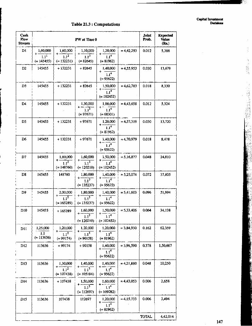
Table 21.3 : Computations

Cash Flow Stream

Dl

D2

D3

D4

D5

D6

D7

D8

D9

Dl0

~ 1 1

Dl2

I Dl3

Dl4

Dl5

1,60,000 +-- 1.1'

(= 145455)

145455

145455

145455

145455

145455

145455

145455

145455

145455

1,25,000

1.1 (= 113636)

113636

113636

113636

1 13636

Joint Prob.

0.012

0.030

0.01 8

0.012

0.030

0.018

0.048

0.072

0.096

0.064

0.162

0.378

0.048

0.006

0.006

TOTAL

Expected Value (-1

5,308

13,679

8,330

5,324

13,720

8.478

24,810

37,805

51,994

34,138

62,359

1.50.667

20,250

2,658

2,494

4.42.014

1,60,000 + --- 1.12

(= 13223 1)

+ 132231

+ 132231

+ 132231

+ 132231

+ 132231

1,80,000 +- 1.12

(= 148760)

148760

2,00,000 +- 1.12

(= 165289)

+ 165289

1,20,000 +- 1.12

(= 99174)

+ 99174

1,30,000 +- 1.12

(= 107438)

+ 107438

107438

PW at Time 0

1,10,000 +- 1.13

(= 82645)

+ 82645

+ 82645

1,30,000 + --- 1.13

(= 97671)

+ 97671

+ 97671

1,60,OOO +- 1.13

(= 120210)

1,80,OOO + --- 1 . 1 ~

(= 135237)

1,80,OOO +- 1.13

(= 135237)

1,60,000

+l.lsItl.ll

1,20,000 +- 1.14

(= 81962)

1,40,000 +- 1.14

(= 95622)

1,50,000 +- 1 . 1 ~

(= 102452)

1,00,000 + -------- 1.14

(= 68301)

1,20,000 +- 1.14

(= 81962)

1,40,000 + ------ 1.14

(= 95622)

1,50,000 +- 1.14

(= 102452)

1,40,000 + --- 1.14

(= 95622)

1,40,000 + --- I. l4

(= 95622)

1,50,000

=4,42,293

= 435,953

= 4,62,783

= 4,43,658

= 4,57,3 19

= 4,7099

= 5,16,877

= 5,25,074

=5,41,603

= 5,33,406

= 3,84,930

= 3,98,590 .

=4,21,880

=4,43,053

=4,15,733

(= 1202 10)

1,20,000 + --- 1.13

(= 90158)

+ 90158

1,40,000 +- 1.13

(= 105184)

1,50,000 +- 1 . 1 ~

(= 112697)

11 2697

(= 102452)

1,20,000 +- 1.14

(= 81962)

1,40,000 +------ 1.14

(= 95622)

1.40.000 +- 1.14

(= 95622)

1,60,000 + --- 1.14

(= 109282)

1,20,000 +- 1. l4

(= 81962)

Construction Finnnce 21.10 SUMMARY Manegement ! Capital investment decisions have long-term implications for any firm. MARR and Cost I of Capital are important parameters in any decisions. Individual decisions may be preliminarily on MARR but a total basket of decisions has to additionally consider cost of capital. Since future benefits are to be necessarily described with the risk-perception 1

about them, such risk factors have to be incorporated by suitable methods. It is also necessary to analyse any investment decision for sensitivity. Projects must be watched i for : independence mutually and dependency of cash flows of benefits.

21.11 ANSWERS TO SAOs

Refer the relevant preceding text in the unit or other useful books on the topics listed in the'section "Further Reading" given at the end of the block to get the answers of the self-assessment questions.

FURTHER READING

Desai, Vasant, Project Management, Himalaya Publishing House.

Van Home, James C., Fundamental of Financial Management.

Erza, Solomon, The Theory of Financial Management, Columbia University Press.

Foster, Geogre, Financial Statement Analysis, Englewood & Cliffs, Prentice Hall.

Mzhta, Dileep R., Working Capital Management, Englewood & Cliffs, Prentice Hall.

Wagner, Harvey M., Principles of Operations Research, Englewood & Cliffs, Prentice Hall.