Technical Background Report to the

Global Atmospheric Mercury Assessment

Citation: AMAP/UNEP, 2008. Technical Background Report to the Global Atmospheric Mercury Assessment. Arctic Monitoring and Assessment Programme / UNEP Chemicals Branch. 159 pp.

This report is available electronically from the AMAP website (www.amap.no) and from the UNEP Chemicals website (www.chem.unep.ch/mercury/).

Acknowledgement: AMAP and UNEP Chemicals Branch would like to acknowledge the financial support received from Denmark, Norway, Sweden and the Nordic Council of Ministers to support the work to prepare this report. AMAP and UNEP Chemicals Branch would also like to thank Jozef Pacyna, John Munthe, Henrik Skov, Oleg Travnikov and Ashu Dastoor for their work as lead authors in drafting this report, and to all others who co-authored or contributed to parts of this report.

Contents Introduction 1

Part A: Global Emissions of Mercury to the Atmosphere 3

A1. Mercury emissions - introduction 4 A2. Sources of mercury to the atmosphere 5

A2.1 Natural sources of mercury 5 A2.2 Anthropogenic sources of mercury to the atmosphere 7

A2.2.1 Major anthropogenic – by-product – sources of mercury 7 A2.2.2 Intentional uses of mercury: Mercury consumption by world region and by application

8

A2.2.2.1 Artisanal gold mining 9 A2.2.2.2 Vinyl chloride monomer production 9 A2.2.2.3 Chlor-alkali production 9 A2.2.2.4 Batteries 10 A2.2.2.5 Dental applications 10 A2.2.2.6 Measuring and control devices 11 A2.2.2.7 Lamps 11 A2.2.2.8 Electrical and electronic devices 12 A2.2.2.9 Other applications of mercury 12

A3. Estimates of current global anthropogenic emissions to the atmosphere 13 A.3.1 Global inventory for the reference year 2005: General approach 13

A3.1.1 Emissions inventory for by-product sectors: Methods and data sources 14 A3.1.2 Emissions from mercury use in products: Methods and data sources 17

A3.1.2.1 Regional economic activity 17 A3.1.2.2 Regional mercury consumption 19 A3.1.2.3 Method for estimating emissions from wastes and product use 21 A3.1.2.4 Method for estimating emissions from mercury use in dental amalgam

24

A3.1.2.5 Method for estimating emissions from mercury use in artisanal gold mining

24

A3.1.3 Methods used to geospatially distribute emissions data 24 A3.1.4 Methods for speciation of inventory emissions 29

A3.2 Discussion of results by source category 29 A3.2.1 Emissions from by-product sectors 29 A3.2.2. Emissions from product use 33

A3.2.2.1 Remarks on emissions from product use of mercury 35 A3.2.2.1.1 Waste incineration 35 A3.2.2.1.2 Long-term fate of mercury in society 35

A3.2.3 Mercury emissions from cremation 36 A3.2.4 Mercury emissions from artisanal and small-scale gold mining 37 A3.2.5 Combined global inventory – emissions by sectors 38

A3.3 Discussion of results by region 40 A3.4 Uncertainties in emission estimates 43

A3.4.1 Uncertainties in by-product emission sources 44 A3.4.2 Uncertainties in emission data for product use, cremations and artisanal gold mining

47

A3.4.2.1 Results of survey on uncertainties and verification addressed to 47

national emissions experts A3.4.2.2 Summary of additional national information reported to UNEP-Chemicals

49

A4. Trends in atmospheric mercury emissions to the atmosphere 50 A4.1 Regional trends in atmospheric mercury emissions 50

A4.1.1. Historical trends of emission until the year 2000 50 A4.1.2 Comparison of the 2000 and 2005 emission inventories 50

A4.2 Emission scenarios and future trends 54 A4.2.1 Selection of scenarios 54 A4.2.2 Methods for scenario emissions estimates for by-product emissions 55 A4.2.3 Methods for scenario emission estimates for intentional use of mercury 57 A4.2.4 Projected future trends in by-product (plus chlor-alkali industry) emissions based on emission scenarios

58

A4.2.5 Discussion of results by region 60 A4.2.6 Future scenarios for emissions from product use, cremation and artisanal gold mining

62

Part B: Atmospheric Pathways, Transport and Fate 64

B5. Atmospheric pathways 65 B5.1 Atmospheric reactions 65

B5.1.1 Polar Regions 68 B5.1.2 Mid- and equatorial latitudes 69 B5.1.3 Continental air masses and free troposphere 69 B5.1.4 Conclusions 70

B5.2 Atmospheric transport and surface fluxes 70 B5.3 Impact of Global change 71

B6. Environmental fate and trends 72 B6.1 Environmental monitoring networks 72 B6.2 Temporal trends derived from environmental measurements 74

B6.2.1 Environmental archives 74 B6.2.2 Long-term monitoring programmes 75 B6.2.3 Geographical distribution 77 B6.2.4 Vertical distribution of mercury fractions 79

B6.3 Climate impacts on future mercury levels 79 B7. Modeling atmospheric transport and deposition 79

B7.1 Model types and methods 80 B7.2 Model applications 84

B7.2.1 Global mercury chemistry 84 B7.2.2 Arctic Mercury Depletion Events 85 B7.2.3 Mercury trend analysis 88 B7.2.4 Long range episodic transport 89 B7.2.5 Model Intercomparison 91

B7.2.5.1 MSC-East intercomparison study 91 B7.2.5.2 US EPA intercomparison study 93

B7.2.6 Mass balance studies 95 B7.3 Mercury air concentrations and deposition patterns 98 B7.4 Source-receptor relationships 103 B7.5 Changes in mercury concentration and deposition levels between 2000 and 2005 106 B7.6 Uncertainties 109

Gaps in knowledge and steps for improvement 111

References 114

Appendices 125

1

Introduction At its meeting in 2007, the United Nations Environment Programme (UNEP) Governing Council requested the Executive Director to prepare a report, drawing on, among other things, ongoing work in other forums addressing:

(a) Best available data on mercury atmospheric emissions and trends including where possible an analysis by country, region and sector, including a consideration of factors driving such trends and applicable regulatory mechanisms;

(b) Current results from modeling on a global scale and from other information sources on the contribution of regional emissions to deposition which may result in adverse effects and the potential benefits from reducing such emissions, taking into account the efforts of the Fate and Transport partnership established under the United Nations Environment Programme mercury programme.

(UNEP GC Decision 24/3)

UNEP cooperated with the Arctic Monitoring and Assessment Programme (AMAP) working group under the Arctic Council to develop a report responding to this request, with the AMAP Secretariat engaged to coordinate the work process. UNEP Chemicals Branch/DTIE has been responsible for the work from UNEP's side. The work includes a summary report for policymakers, ‘Global Atmospheric Mercury Assessment: Sources, Emissions and Transport’, and a detailed technical background report (this report). The technical background report forms the basis for the summary report to the Governing Council and for parts of the AMAP assessment.

The Arctic Monitoring and Assessment Programme has produced two assessments of heavy metals (including mercury) in the Arctic (AMAP, 1998, 2005) and is currently in the process of preparing an updated assessment of mercury in the Arctic to be delivered to the Arctic Council in 2011. As part of the assessment, a new global inventory of anthropogenic mercury emissions to air should be prepared to update that produced in 2002 (Pacyna et al., 2006). AMAP should also undertake new modeling studies, using the updated inventory, to investigate atmospheric transport of mercury.

AMAP is mandated through the Arctic Council to support the activities under UNEP and other international organizations concerning mercury and persistent organic pollutants. The AMAP Working Group therefore agreed to fast-track its proposed work on mercury emissions and atmospheric transport in order that, in addition to contributing to the 2011 AMAP mercury assessment, it could also provide input to UNEP’s 2008 Global Atmospheric Mercury Assessment Report, and to the UN ECE LRTAP Hemispheric Transport of Air Pollutants group that would be preparing a separate report on mercury atmospheric transport in 2010.

The report has been prepared by expert groups engaged by AMAP and UNEP. Information submitted by Governments, intergovernmental and non-governmental organizations and available scientific information have been used in preparing the report. It has also made use of information compiled by the UNEP Global Mercury Partnership (Mercury Air Transport and Fate Research partnership area), in particular in relation to natural sources of mercury and mercury emissions from artisanal and small-scale gold mining.

The report has two main parts. Part A addresses mercury emissions to air, updating the global anthropogenic mercury emissions inventory for the (nominal) year of 2005, and presents three emissions scenario inventories for the year 2020. It also covers the work undertaken to geospatially distribute these inventories (within a 0.5 × 0.5 degree global grid) to facilitate

2

their use as input to atmospheric transport models. The inventory activities expand those conducted in the past by including a first attempt to quantify (at a global scale) emissions associated with intentional use of mercury in products, and their associated entry into waste streams. Part B describes the current state of knowledge concerning atmospheric transport of mercury, with a focus on modeling approaches that can be used to investigate mercury atmospheric transport and fate, source-receptor relationships, and possible effects of changes in emissions. The emissions inventory and modeling components both include a discussion of uncertainties. The estimated ranges of uncertainties associated with current and past inventory estimates are presented so that trends in emissions can be evaluated in an appropriate manner.

The information sources used in the preparation of this document are fully-referenced.

3

Part A: Global Emissions of Mercury to the Atmosphere Authors:

Jozef M. Pacyna, Norwegian Institute for Air Research (NILU), Norway

John Munthe, IVL Swedish Environmental Research Institute, Sweden

Simon Wilson, AMAP Secretariat, Norway

Co-authors:

Peter Maxson Concorde East-West, Belgium (mercury in products)

Kyrre Sundseth, Norwegian Institute for Air Research (NILU), Norway

Elisabeth G. Pacyna, Norwegian Institute for Air Research (NILU), Norway

Ermelinda Harper, Yale University, USA

Karin Kindbom, IVL Swedish Environmental Research Institute, Sweden

Ingvar Wängberg, IVL Swedish Environmental Research Institute, Sweden

Damian Panasiuk, NILU Polska, Poland

Anna Glodek, NILU Polska, Poland

Joy Leaner, Council for Scientific and Industrial Research, South Africa

James Dabrowski, Council for Scientific and Industrial Research, South Africa

Collaborators/Contributors:

Robert Mason, USA (natural mercury emissions)

Prof. Ming Wong, China-Hong Kong

Dr. G.S. Ochoa, Mexico

Dr. Anne Pope, USA

Frits Steenhuisen, Netherlands (spatial distribution of emission inventories)

Kevin Telmer, Canada (mercury emissions from artisanal and small-scale gold mining activities)

4

A1. Mercury emissions - introduction An understanding of mercury emission sources to the atmosphere is critical for the development of relevant and cost-efficient strategies towards reducing the negative impacts of this global pollutant. Emission inventories are used to drive atmospheric chemical-transport and source-receptor models for the distribution of mercury and prediction of deposition rates. An understanding of the different mercury sources is also of importance towards assessing control options since many different mercury sources exist. In addition to anthropogenic point sources, natural sources also exist and mercury once released into the environment can be extensively recycled between different compartments of the environment. In Figure 1.1, a schematic description of the main source types is presented. The primary anthropogenic sources are those where mercury of geological origin is mobilised and released to the environment. The two main source categories of this type are mining (either for mercury or where mercury is a by-product or contaminant in the mining of other minerals) and extraction of fossil fuels where mercury is present as a trace contaminant. The secondary anthropogenic sources are those where emissions occur from the intentional use of mercury, e.g., industry, products or for artisanal gold mining. In both these source types, emissions to the environment can occur via direct discharges of exhaust gases and effluents, although the generation of mercury-containing waste also contributes. Primary natural sources, are defined as those where mercury of geological origin is released via natural processes such as volcanoes or geothermal processes or evasion from natural surfaces geologically enriched in mercury. In addition to these source types, the distribution of mercury is affected by its remobilisation and re-emission pathways. In the latter case, mercury released can be of either natural or anthropogenic origin and it is currently not possible to experimentally distinguish between the two. Anthropogenic activities such as biomass burning and land use changes will affect the magnitude and location of the mercury releases.

Figure 1.1. Schematic description of emission source types and remobilisation processes affecting mercury distribution in the environment. The red arrows represent the release of mercury and subsequent transport and input to ecosystems.

Mining

Fossil fuelextraction

Natural

Primary anthropogenicsources

Hg mining

Byproduct Hg

Ore Hg

Oil

Coal

Gas

Volcanos

Geothermal

Surfaces

Secondary anthropogenicsources

ASGM

Products

Industry

Land usechange Forest fires Surface

re-emissions

Ecosystems

Primary natural sources

IntentionalRecycling

Remobilisation and re-emissions

Mining

Fossil fuelextraction

Natural

Primary anthropogenicsources

Hg mining

By-product Hg

Ore Hg

Oil

Coal

Gas

Volcanoes

Geothermal

Surfaces

Secondary anthropogenicsources

ASGM

Products

Industry

Land usechange

Biomass burning

Surfacere-emissions

Ecosystems

Primary natural sources

Intentional useRecycling

Remobilisation and

Mining

Fossil fuelextraction

Natural

Primary anthropogenicsources

Hg mining

Byproduct Hg

Ore Hg

Oil

Coal

Gas

Volcanos

Geothermal

Surfaces

Secondary anthropogenicsources

ASGM

Products

Industry

Land usechange Forest fires Surface

re-emissions

Ecosystems

Primary natural sources

IntentionalRecycling

Remobilisation and re-emissions

Mining

Fossil fuelextraction

Natural

Primary anthropogenicsources

Hg mining

By-product Hg

Ore Hg

Oil

Coal

Gas

Volcanoes

Geothermal

Surfaces

Secondary anthropogenicsources

ASGM

Products

Industry

Land usechange

Biomass burning

Surfacere-emissions

Ecosystems

Primary natural sources

Intentional useRecycling

Remobilisation and

5

A2. Sources of mercury to the atmosphere

A2.1 Natural sources of mercury Mercury occurs in the earth’s crust, especially as the mineral cinnabar. The metal is released via weathering of rocks and as a result of volcanic activities. In addition, deposited oxidised mercury may be reduced via photochemical or biological processes and be re-emitted to the atmosphere. Re-emission of mercury occurs from soil and vegetation as well as from sea surfaces and is considered significant in comparison to primary sources. As a consequence the mercury concentration in the atmosphere is determined not only by primary sources but also to a significant degree by re-emission. These cycles were also in action in the pre-industrial environment and it is likely that mercury was more or less evenly distributed in the atmosphere as well as in terrestrial and aquatic compartments before (significant) anthropogenic emissions began.

An evaluation of natural emissions of mercury is often made as a part of studies of global mercury budgets and fluxes using global mercury models (Shia et al., 1999; Seigneur et al., 2001, 2004; Lamborg et al., 2002b; Mason and Sheu, 2002; Selin et al., 2007). Flux estimates based on field measurement exist but only represent very limited geographical areas and limited time scales.

Some recent environmental mercury fluxes from global mercury models are shown in Table 1.1. Mason (2008) has made new estimates of major global mercury fluxes and some are shown in Table 1.1. Mercury sources in Table 1.1 are categorized into total emissions from land and total oceanic emissions. The land and oceanic sources are further separated into natural emissions and re-emissions. Natural sources correspond to estimates of pristine fluxes, while re-emissions are the increase in emissions caused by anthropogenic emissions at present and in the past. Primary anthropogenic emissions correspond to direct emissions from human activities. The model results in Table 1.1 are based on similar primary anthropogenic emission values, i.e., 2.2 to 2.6 kton mercury per year. This is close to that from the global anthropogenic mercury emissions inventory for year 2000 (2.2 kton/yr; Pacyna and Pacyna, 2006). However, the estimates of total flux vary among the models. This difference in modeling results comes from how the models treat re-emissions. The Selin et al. (2007) model predicted the re-emissions flux from the ocean to be greater than the primary anthropogenic emissions as shown in Table 1.1. High re-emissions require a short lifetime in order that the modeled atmospheric background concentration of total mercury agrees with measurements of this (relatively well-established) parameter.

The difference in estimates of re-emissions also reflects the importance of primary anthropogenic sources in comparison to total sources as is shown in Table 1.1. In the Lamborg et al. (2002b) model, primary anthropogenic sources constitute about 60% of the total mercury emissions, whereas it is only 31% in the Selin et al. (2007) model. The net mercury load to land and ocean is defined in Table 1.1 as [total deposition] − [total emission from land and ocean]. The net load constitutes an annual loss of mercury from cycling and in all estimates this loss is of the same magnitude as the total emission from anthropogenic sources as shown in Table 1.1. In the Lamborg et al. (2002b) model, the mercury net load to the surface of the oceans is 1.2 kton/yr. About 1.8 kton of the mercury in the ocean’s surface layer is scavenged by particles each year and removed to the deeper layers of the ocean, but is compensated by 0.6 kton/yr upwelling. Hence, the net load of mercury to the oceanic surface water is estimated to be zero at present. In contrast, mercury is accumulated in the deep ocean. This accumulation is 1.2 kton/yr, of which 0.4 kton/yr is buried in sediments of the sea floor, thereby representing a mercury sink. In the Mason and Sheu (2002) model, the ocean is

6

treated in a somewhat simplified manner. The load to the ocean is 0.68 kton/yr, of which 0.2 kton is buried in sediments each year. With regards to the net mercury load to the land, Mason and Sheu (2002) predicted a somewhat larger load than Lamborg et al. (2002b), as shown in Table 1.1. Divalent mercury bonds strongly to sulfur groups in soils that are rich in organic matter and is therefore to a large extent accumulated in the soil (Meili et al., 2003). Hence, the net mercury load to land may constitute a sink of mercury.

Table 1.1. Environmental mercury fluxes from Global Mercury Models.

Hg Fluxes (kton/yr)

Lamborg et al., 2002b

Mason and Sheu,

2002

Selin et al., 2007

Mason, 2008

Friedl et al., 2008

Natural emissions from land 1.0 0.81 0.5 Re-emissions from land 0.79 1.5 Emissions from biomass burning 0.675 (A) Total emissions from land 1.0 1.6 2.0 1.85a Natural emissions from ocean 0.4 1.3 0.4 Re-emissions from ocean 0.4 1.3 2.4 (B) Total oceanic emissions 0.8 2.6 2.8 2.6 (C) Primary anthropogenic emissions 2.6 2.4 2.2 Total sources (A+B+C) 4.4 6.6 7.0 (D) Deposition to land 2.2 3.52 (E) Deposition to ocean 2.0 3.08 Total deposition (D+E) 4.2 6.6 7.0 6.4 Net load to land 1.2 1.72 b Net load to ocean (burial in sediments) 1.2 (0.4) 0.68 (0.2) Total net load (land + ocean) 2.4 2.4 2.2 Other parameters Mercury burden in the troposphere (kton) 5.22 5.00 5.36 GEM lifetime (y) 1.3 0.76 0.79

a Including Hg0 emissions (0.2 kton/yr) in response to Atmospheric Mercury Depletion Events (AMDEs) in polar regions. Biomass burning is not included in the emissions from land in this Table. b Value includes taking account of estimated flux from land to water via rivers (0.2).

The model results by Selin et al. (2007) suggest that oxidized mercury dominates over elemental mercury in the stratosphere. This conclusion is also supported by aircraft measurements indicating that most mercury in the lower stratosphere is presented as oxidized mercury bound to aerosols (Murphy et al., 2006). According to the model elemental mercury is preferentially oxidized to reactive gaseous mercury (RGM) in the upper atmosphere and oxidized mercury (gaseous or in the aerosol phase) constitutes on average as much 16% of the total mercury in the atmosphere. According to the model results, Selin et al. (2007) suggested that dry deposition of RGM is the dominant deposition process being more than two-fold greater than wet deposition.

Model predictions critically depend on present knowledge of atmospheric mercury oxidation and deposition processes. In the models, this information is represented by kinetic parameters describing primary oxidation steps in the gas phase and in cloud water droplets and deposition rates, etc. Much of this information is found in the literature. It is difficult to study these reactions in the laboratory and some mercury gas phase reaction rates have been questioned

7

(Calvert and Lindberg, 2005). This together with uncertainties regarding the total input of mercury to the atmosphere makes model predictions uncertain. More work on homogenous and heterogeneous atmospheric mercury processes is required to obtain more conclusive results regarding the lifetime of mercury in the atmosphere. More information is also needed on re-emission and natural mercury sources. There is also a lack of long time-series observations, especially of background concentrations of RGM and total particulate mercury (TPM). This information is crucial for assessing the status of the environment regarding mercury and is also essential for the further development of models.

One important aspect of the cycling of mercury in the environment is wildfires and biomass burning. Growing biomass and organic surface soils contain mercury originating from atmospheric deposition. When this organic material is burned in accidental wildfires or intentional burning for forest clearing, this mercury is released back to the atmosphere. The global emission of mercury from this source category has been estimated at 675 ± 240 t/yr (Friedl et al., 2008). This is a significant contribution to the atmospheric pool of mercury and needs to be taken into account when calculating global mass balances of mercury or for atmospheric modeling. The largest emissions occur in regions where boreal and tropical forests are burned, whereas burning of agricultural residues are assumed to contribute very small amounts of mercury. The uncertainty in this estimate is large due to incomplete information on the occurrence of fires, the mercury content of the organic material, and the degree to which the mercury is released during the fire.

From a policy perspective, this mercury emission should be treated partly as a re-emission driven by natural processes (i.e., wildfires), and partly as an emission under human control (intentional burning, forest clearing). Reducing the global intensity of forest clearing and biomass burning would thus have the additional beneficial effect of reducing the remobilization of mercury.

Further discussion on global fluxes, chemistry and modeling is found in Part B of this report.

A2.2 Anthropogenic sources of mercury to the atmosphere The following sections present a short overview of the main anthropogenic sources of mercury considered in this work. Further information, on the major ‘by-product’ anthropogenic sectors in particular, can be found in the Global Mercury assessment (UNEP-Chemicals, 2002).

A2.2.1 Major anthropogenic – by-product – sources of mercury Of the primary anthropogenic sources of mercury (see Figure 1.1), the principle sources are those where mercury is emitted mainly as an unintentional ‘by-product’. With the exception of mercury mining itself, the mercury emissions arise from mercury that is present as an ‘impurity’ in the fuel or raw material used. The main ‘by-product’ emissions are from sectors that involve combustion of coal or oil, production of pig iron and steel, production of non-ferrous metals, and cement production.

Stationary combustion of coal, and to a lesser extent other fossil fuels, associated with energy or heat production in major power plants, small industrial or residential heating units or small-scale residential heating appliances as well as various industrial processes, is the largest single source category of anthropogenic mercury emission to air. Although coal does not contain high concentrations of mercury, the amount of coal that is burned and the fact that emissions from coal-burning plants go mainly to the atmosphere mean that coal burning is the largest anthropogenic source of unintentional mercury emissions to the atmosphere.

8

Mining and industrial processing of ores, in particular in primary production of iron and steel and non-ferrous metal production (especially copper, lead and zinc smelting), release mercury as a result of both fuel combustion and mercury present as impurities in ores, and through accelerating the exposure of rock to natural weathering processes. Metal production sources of mercury also include mining and production of mercury itself (a relatively minor source) and production of gold, where mercury is both present in ores and used in some industrial processes to extract gold from lode deposits. Use of mercury to extract gold in artisanal and small-scale gold mining operations is an intentional use discussed in section A2.2.2.1.

The third major source of ‘by-product’ releases of mercury is associated with cement production, where mercury is released primarily as a result of the combustion of fuels (mainly coal but also a range of wastes) to heat cement kilns. Mercury-containing fly-ash is sometimes added to cement following the production process.

In all of the above sectors, technologies exist that can reduce mercury emissions to air, in particular flue-gas emissions from combustion sources. These technologies are being increasingly applied in both developed and developing countries, at major industrial facilities and power plants in particular, which has resulted in marked decreases in mercury emissions in some countries and regions over past decades. Application of control technologies at sites of small-scale industrial activity and from de-centralized residential heating is however a greater challenge.

A2.2.2 Intentional uses of mercury: Mercury consumption by world region and by application A particular focus of the work reported in this document was an attempt to improve the basic data on mercury consumption that may be used to determine mercury in waste streams, and associated mercury releases to the atmosphere. In particular, it summarizes intentional uses of mercury by different geographical regions (e.g., UN regions – North America, South America, Europe, Africa, East Asia, South Asia, Arab States), first, by presenting the state of knowledge of each major intentional use of mercury in products and processes, and then by suggesting a method to better estimate those uses that, up to now have been less studied.

For the purposes of eventually calculating product-related emissions, mercury ‘consumption’ is defined here in terms of regional consumption of mercury products rather than overall regional ‘demand’. For example, although most measuring and control devices are produced in China (reflected in Chinese ‘demand’ for mercury), many are exported, ‘consumed’ and disposed of in other countries.

While continuing its long-term decline in most of the higher income countries, there is evidence that consumption of mercury remains relatively robust in many lower income economies, especially South and East Asia (where significant mercury use continues in products, vinyl chloride monomer production, and artisanal gold mining), and Central and South America (especially mercury use in artisanal and small-scale gold mining). The main factors behind the decrease in mercury consumption in the higher income countries are the substantial reduction or substitution of mercury content in regulated products and processes (e.g., paints, batteries, pesticides, chlor-alkali industry), and a general shift of mercury-product manufacturing operations (e.g., thermometers, batteries) from higher income to lower income countries. The major mercury applications and intentional use sectors are discussed individually in the following sections.

9

A2.2.2.1 Artisanal gold mining Artisanal and small-scale gold mining (ASGM) remains the largest global user of mercury. It reportedly continues to increase with the upward trend in the price of gold and is the largest source of environmental release from intentional use of mercury. It is inextricably linked with issues of poverty and human health.

According to the UNIDO/UNDP/GEF Global Mercury Project (Telmer, 2008), at least 100 million people in over 55 countries depend on ASGM – directly or indirectly – for their livelihood, mainly in Africa, Asia and South America.1 ASGM is responsible for an estimated 20 to 30% of the world’s gold production, or approximately 500 to 800 tonnes per annum. It involves an estimated 10 to 15 million miners, including 4.5 million women and 1 million children. This type of mining relies on rudimentary methods and technologies and is typically performed by miners with little or no economic capital who operate in the informal economic sector, often illegally and with little organization (UNEP, 2006). Because of inefficient mining practices, mercury amalgamation in ASGM results in the consumption and release of an estimated 650 to 1000 tonnes of mercury per annum.

In section A3.2.4, regional estimates of mercury use in ASGM have been derived from country estimates based on personal communications with a number of experts directly involved in the UNIDO/UNDP/GEF Global Mercury Project (Telmer, 2008).

A2.2.2.2 Vinyl chloride monomer production The large and increasing use of mercuric chloride as a catalyst in the production of vinyl chloride monomer (VCM), especially in China, is another area of major concern, especially as it is not yet clear where much of the mercury – estimated to be several hundred tonnes – goes as the catalyst is depleted.

Investigations in China confirmed the demand of an estimated 610 tonnes of mercury in 2004 for this application. This use of mercury has been increasing by 25 to 30% per year as the Chinese economy booms, and as Chinese demand for polyvinyl chloride (PVC) end-products increases (NRDC, 2006; Tsinghua, 2006), and was estimated at 700 to 800 tonnes of mercury in 2005.

Limited use of about 15 tonnes of mercury for the same purpose was reported by Treger to the Mercury Project under the Arctic Council’s Arctic Contaminants Action Programme (ACAP) study of the Russian chemical industry (ACAP, 2005b). Further uses in the CIS (Russian/Soviet Commonwealth of Independent States) region are believed to exist but have not been specifically reported.

A2.2.2.3 Chlor-alkali production The chlor-alkali industry is the third major mercury user worldwide. Many plant operators have phased out this technology and converted to the more energy-efficient and mercury-free membrane process, others have plans to do so, and still others have not announced any such plans. In many cases, governments have worked with industry representatives and/or provided financial incentives to facilitate the phase-out of mercury technology. Recently governments and international agencies have created partnerships with industry to encourage broader industry improvements with regard to the management and releases of mercury.

1 It should be noted that not all artisanal/small-scale gold miners use mercury. Some use cyanide, permitting

more gold to be recovered than when using mercury. Others use gravimetric methods without mercury or cyanide.

10

The range for global mercury consumption2 presented in section A3.1.2.2 is based on previous studies (UNEP, 2006; EEB, 2006). The EU and US mercury consumption figures are based on industry data, as are those of India, Brazil and Russia (UNEP, 2006). Mercury consumption estimates for Mexico and other countries are based on individual plant capacities as provided by various industry actors (SRIC, 2005; WCC, 2006; Euro Chlor, 2007), together with representative mercury consumption factors as known for different world regions (UNEP, 2006).

A2.2.2.4 Batteries The use of mercury in batteries, while still considerable, continues to decline as many nations have implemented policies to deal with the problems related to diffuse mercury releases related to batteries.

While mercury use in Chinese batteries was confirmed to have been high through 2000, most Chinese manufacturers have reportedly now shifted to designs with lower mercury content, following international legislative trends and customer demand in other parts of the world (NRDC, 2006). However, since there are still vast quantities (tens of billions) of batteries produced in China,3 and lesser quantities in other countries as well, the quantities of mercury consumed are still noteworthy. Moreover, trade statistics suggest that there continues to be a reduced, but still significant, trade in mercuric oxide (HgO) batteries, some produced in mainland China, and many more apparently produced in Customs-free trade zones on Chinese territory (NRDC, 2006).

There also remain a large number of button cell batteries manufactured in many different countries, containing up to 2% mercury. These will eventually be replaced by mercury-free button cells,4 but for the moment these batteries, also produced in the tens of billions, consume significant amounts of mercury. Therefore, the global consumption of mercury in batteries still appears to number in the hundreds of tonnes annually.

A draft study for the European Commission (DG ENV, 2008) made an estimate of mercury in batteries for the 25 countries that were members of the European Union in 2006 (EU25). This estimate does not fully account for trade statistics suggesting significant consumption of (mostly larger) HgO batteries, since physical evidence of such consumption levels has not yet been produced. Cain et al. (2007) made an estimate of mercury in batteries for the United States, which can be extrapolated to Canada. Other regional estimates of mercury consumed in batteries are assumed to be correlated with regional economic activity, as described in section A3.1.2.2.

A2.2.2.5 Dental applications Among others, Sweden, Japan, Denmark and Finland have implemented measures to greatly reduce the use of dental amalgams containing mercury. In these and some other higher income countries (e.g., Norway, United States) dental use of mercury is now declining. The

2 The convention here is to calculate mercury ‘consumption’ before any recycling of wastes, with the knowledge

that, as in many industries, some waste is recycled in order to recover the mercury, while most mercury waste is sent for disposal.

3 For just one type of battery, the D-size ‘paste battery,’ the known Chinese production in 2004 was 9.349 billion batteries. The authors (NRDC, 2006) estimated mercury chloride consumption for these batteries at 47.11 tonnes, with an estimated mercury content of 34.91 tonnes. The battery label claims less than 250 ppm mercury content.

4 The National Electrical Manufacturers’ Association in the United States has called for a phase-out of all mercury in button cell batteries in the United States by 2011.

11

main alternatives are composites (most common), glass ionomers and compomers (modified composites). However, the speed of decline varies widely, so that mercury use is still significant in most countries, while in some countries (Sweden, Norway) it has almost ceased. In many lower income countries, changing diets and better access to dental care may actually increase mercury use temporarily.

Regional consumption ranges for dental use of mercury presented in section A3.1.2.2 are based on industry estimates, as reported for the European Union’s 27 member countries (EU27) in a draft report (DG ENV, 2008) for the European Commission. The North America range shown in section A3.1.2.2 is higher than estimated by Cain et al. (2007) but reflects industry estimates, is in line with NEWMOA (Northeast Waste Management Officials’ Association) data, and also includes Canada.

Emissions resulting from use of dental amalgam can occur during production, handling and disposal of dental amalgam and also during cremation of human remains. The emissions inventory reported in section A3 includes emissions from cremations only, although emissions during production, handling and routine disposal of dental amalgams may be significantly larger than the cremation emissions in some countries.

A2.2.2.6 Measuring and control devices There is a wide selection of mercury-containing measuring and control devices, including thermometers, barometers, manometers, still manufactured in various parts of the world, although most international suppliers now offer mercury-free alternatives. European legislation, among others, is being developed to phase out such equipment and to promote mercury-free alternatives since the latter are available for nearly all applications.

In section A3.1.2.2, the global total range for mercury consumption in these applications is based heavily on Chinese production of sphygmomanometers and thermometers (SEPA, 2008), which calculated over 270 tonnes of mercury used in the production of only these two devices in 2004, although Chinese production is likely to represent 80 to 90% of world production of these two products. Likewise, thermometers and sphygmomanometers are considered to represent around 80% of total mercury consumption in this sector.

The EU25 estimate in section A3.1.2.2 is based on the draft DG ENV (2008) study for the European Commission, recognizing significant reduction in EU mercury use in these applications in recent years. The North America estimate in section A3.1.2.2 is based on Cain et al. (2007), with special attention given to the quantities of mercury consumed in dairy manometers, industrial and other thermometers, and sphygmomanometers. Other regional estimates of mercury consumed in measuring and control devices are assumed to be correlated with regional economic activity, as described in section A3.1.2.2.

A2.2.2.7 Lamps Mercury-containing lamps (fluorescent tubes, compact fluorescent, high-intensity discharge lighting) remain the standard for energy-efficient lamps, where ongoing industry efforts to reduce the amount of mercury in each lamp are countered, to some extent, by the ever-increasing number of energy-efficient lamps purchased and installed around the world. There is no doubt that mercury-free alternatives, such as LEDs (light-emitting diodes), will become increasingly available, but for most applications the alternatives are still quite limited and/or quite expensive.

The global total range used in section A3.1.2.2 for mercury consumption in lamps is based on a report by UNEP (UNEP, 2006) which, however, does not take full account of significant

12

mercury use in backlighting of LCD screens (liquid crystal display). For this reason the lower part of the range used in that source has been raised. In China alone, mercury used in the production of (mostly) fluorescent tubes and CFLs (compact fluorescent lamps) was estimated at 55 tonnes for 2004 (SEPA 2008), which may be an underestimate. Many of these lamps were exported.

The EU estimate in section A3.1.2.2 is based on the draft DG ENV (2008) study for the European Commission, which includes significant mercury use in small lamps for backlighting of LCDs. The North America estimate is based on Cain et al. (2007), which did not fully account for backlighting of LCDs. Other regional estimates of mercury consumed in lamps are assumed to be correlated with regional economic activity, as described in section A3.1.2.2.

A2.2.2.8 Electrical and electronic devices Owing to the RoHS Directive (for the restriction of the use of certain hazardous substances in electrical and electronic equipment) in Europe, and similar initiatives in Japan, China and California, among others, mercury-free substitutes for devices such as mercury switches and relays, are being actively encouraged,5 and mercury consumption has declined substantially in recent years. At the same time, the US-based Interstate Mercury Education and Reduction Clearinghouse (IMERC) database6 demonstrates that mercury use in these devices remains significant.

In section A3.1.2.2, the global total range of mercury consumption in this sector is reduced from that estimated for UNEP (2006), based on improved data from both the EU and the United States. At the same time, the lower part of that large range has been raised because a recent US estimate shows higher than expected mercury consumption in this category (Cain et al., 2007), including thermostats, wiring devices, switches and relays. The EU25 estimate in section A3.1.2.2 is based on the draft DG ENV (2008) study for the European Commission, which recognizes significant reduction in mercury use in these applications in recent years as a result of RoHS legislation. Other regional estimates of mercury consumed in electrical and electronic devices are assumed to be correlated with regional economic activity, as described in section A3.1.2.2.

A2.2.2.9 Other applications of mercury The category ‘other applications of mercury’ has traditionally included the use of mercury and mercury compounds in such diverse applications as pesticides, fungicides, laboratory chemicals, pharmaceuticals, as a preservative in paints, traditional medicine, cultural and ritual uses, and cosmetics. However, there are some further applications that have recently come to light in which the consumption of mercury is also especially significant.

The continued use of mercury catalysts in the production of polyurethane elastomers, where the catalysts remain in the final product, is one such use. Likewise, the use of considerable quantities of mercury in porosimetry has until recently escaped special notice. The quantities

5 For California, see http://www.dtsc.ca.gov/HazardousWaste/EWaste/.

For Korea’s RoHS/WEEE/ELV-like legislation called ‘The Act for Resource Recycling of Electrical/Electronic Products and Automobiles’, see http://www.europeanleadfree.net/pooled/articles/BF_NEWSART/view.asp?Q=BF_NEWSART_195645. For Japan, see http://www.jeita.or.jp/index.htm; also http://uk.farnell.com/jsp/bespoke/bespoke8.jsp?bespokepage=farnell/en/rohs/rohs/facts.jsp.

6 All suppliers of mercury containing products to the northeastern United States are required to file annual reports, as described at http://www.newmoa.org.

13

of mercury consumed in these applications in the EU are estimated based on industry information (DG ENV, 2008).

In section A3.1.2.2, the global total range shown is significantly higher than that estimated by UNEP (2006), based on the draft DG ENV (2008) study for the European Commission that includes substantial mercury consumption in compounds used as chemical intermediates and catalysts (other than VCM/PVC production), as well as elemental mercury still used in significant quantities in porosimeters and pycnometers, not to mention lesser uses for routine maintenance of lighthouses. Already in 2000, China claimed to be producing ‘reagents’ containing 467 to 537 tonnes of mercury for domestic use and export to the rest of the world (SEPA, 2008).

The North America estimate of mercury consumed in ‘other’ applications in section A3.1.2.2 is based on evidence that this region has many of the same applications as those identified in the EU. The applications in other regions vary widely, including cultural/ritual uses in Latin America and the Caribbean, traditional uses in Chinese medicine, cultural/religious uses in India, and cosmetic uses such as skin-lightening creams in many countries. Nevertheless, lacking better data, other regional estimates of mercury consumed in ‘other’ applications are assumed to be correlated with regional economic activity, as described in section A3.1.2.2.

A3. Estimates of current global anthropogenic emissions to the atmosphere

A.3.1 Global inventory for the reference year 2005: General approach The work undertaken to prepare the (2005) global inventory of mercury emissions to the atmosphere reported in this document, had two main components.

The first component comprised the estimation of ‘by-product’ mercury releases resulting mainly from combustion of fossil fuels, (primary ferrous and non-ferrous) metal production, and cement production. To a large degree, these emission categories represent the largest anthropogenic sources of mercury, and also those reported most consistently by countries in accordance with various international Conventions and to the European Commission. This component also included quantification of emissions from the chlor-alkali (caustic soda production) industry, from large-scale gold production, and from waste incineration in Europe and the United States. These emission sectors are essentially those that have been included in previous inventories of global anthropogenic emissions to air for the reference years 1990, 1995 and 2000 (Pacyna and Pacyna, 2002, 2005; Pacyna et al., 2003, 2006). The work involved the preparation of national emissions estimates (for the nominal reference year of 2005) for these main emission sectors, and the calculation of similar national estimates for emissions from these sectors in 2020 under certain defined scenarios.

The second component of the work addressed quantification of emissions from sectors that had not previously been included in the global emissions inventories. Principal among these are emissions from artisanal and small-scale gold mining, emissions from use of mercury in dental amalgam (cremation emissions), and emissions from wastes, and from intentional use of mercury in products. The latter category also included emissions from secondary steel production, which are not generally included in the metal production sectors covered by the first component. Estimates for emissions from artisanal and small-scale gold mining were taken directly from the report of Telmer and Veiga (2008). Releases from (intentional) mercury use in products were estimated using a modeling approach that has been applied in Europe and which, under this work was adapted for application at a global scale, and data on

14

regional mercury consumption and product use of mercury compiled by the authors (see section A3.1.2.2). These parts of the inventory work involved preparation of emissions estimates for various regions of the globe. The resulting emissions estimates were then allocated (on the basis of population) to individual countries in order to allow them to be combined with the national emissions estimates derived in the first part of the work. Until better information is available for these sources at the national level, this latter process is the best (only) approach available. Where estimates from both the first and second components of the work were available (e.g., for emissions associated with waste (incineration) in Europe and the United States), these were compared and found to be in reasonable agreement (see below). Where other sources of data were available, such as national reports, the emission estimates derived using the above methodology were checked for confirmation, and in the case of discrepancies efforts were made to find explanations allowing the most appropriate estimate to be chosen.

A3.1.1 Emissions inventory for by-product sectors: Methods and data sources Two methods were used for the calculation of global anthropogenic emissions of mercury from by-product sources for the (nominal) reference year of 2005:

- The first method involved the collection and compilation of emissions data from countries where such data are estimated by national emissions experts or reported to international programs and conventions.

- The second method consisted of estimating emissions on the basis of emission factors and statistical data on the production of industrial goods and/or the consumption of raw materials. These estimates were carried out by the authors of this report, in particular for those countries where reliable national emissions estimates were not available.

Main sources of emissions data used in the preparation of the by-product emissions inventory for 2005 are listed in Table 3.1.

Estimates for Europe were prepared by national experts in 30 European countries and reported to the UN ECE EMEP program (see the EMEP website http://www.emep.int and the link to EMEP Data or http://www.emep.int/index_data.html). These data were used in the report. In addition, emissions experts from Belgium, Bulgaria, Croatia, the Czech Republic, Denmark, Finland, France, Germany, Latvia, Moldova, the Netherlands, Norway, Romania, Slovakia, Sweden, Switzerland, and the United Kingdom provided estimates to UNEP-Chemicals as a contribution to this project. Finally, information from the EU ESPREME project (Integrated Assessment of Heavy Metal Releases in Europe) http://espreme.ier.uni-stuttgart.de was also used for comparison with the estimates provided by national experts.

Estimates for China were prepared by the authors of this report. These estimates were then compared with the emissions data compiled by the UNEP Mercury Fate and Transport Partnership (F&TP) (http://www.cs.iia.cnr.it/UNEP-MFTP/index.htm) by Streets et al. (2008) for emissions from coal combustion and Feng et al. (2008) for emissions from industrial processes. Combustion source estimates produced by the authors of this report (ca. 385 tonnes in 2005) are somewhat higher than those derived by the F&TP (260 tonnes in 2003), whereas emissions from industrial activities (including metal production, cement production and caustic soda production) of 245 tonnes in 2005 are slightly lower than the estimate of 320 tonnes in 2003 in the F&TP report. In general, the differences between the estimates prepared in this work and those reported by Streets et al. (2008) and Feng et al. (2008) were considered to be within the range of estimation uncertainties, given that sectors and years were not always directly comparable.

15

Table 3.1. Source of information on by-product mercury emissions to the atmosphere from anthropogenic sources in 2005.

Region 2005 Europe (excluding Russia) UN ECE EMEP (http://www.emep.int)

National data sent to the project from Belgium, Bulgaria, Croatia, the Czech Republic, Denmark, Finland, France, Germany, Latvia, Moldova, the Netherlands, Norway, Romania, Slovakia, Sweden, Switzerland, the United Kingdom EU25 European Pollutant Emission Register (EPER) / European Pollutant Emissions and Transfer Register (E-PRTR), http://eper.eea.europa.eu/eper EU ESPREME project (http://espreme.ier.uni-stuttgart.de)

Russia This work; ACAP (2005b) Asia (excluding Russia) National data provided by Cambodia, Japan, Philippines, Republic

of Korea; This work North America USA: US EPA National Emissions Inventory (data for 2002)

(http://www.epa.gov/ttn/chief/net/2002inventory.html) Canada: National Pollution Release Inventory (data for 2004 and 2005) (http://www.ec.gc.ca/pdb/npri/); This work

South America National data from Chile, Peru; This work Africa National data from Burkino Faso, South Africa; This work Australasia / Oceania National data for Australia; This work

The collection of mercury emissions data elaborated by national experts as part of this inventory activity and/or reported to international programs/projects, and author’s own estimates for countries with no emissions data are indicated in the above table as ‘This work’.

Estimates for India were also prepared by the authors of this report and compared with the emission data reported to the F&TP by Mukherjee et al. (2008). Mukherjee et al. (2008) used an extremely high value for coal mercury-content of about 0.376 g/tonne (ppm) which resulted in an estimated emission from coal burning of 120.85 tonnes. The average mercury-content of most coals is between 0.1 and 0.2 ppm. The reported geometric mean value of mercury content in Indian coals is 0.3 ppm, which is high but was considered acceptable. The latter concentration was therefore used in the estimates presented in this report. The mercury emissions from the cement industry in India in the (draft) F&TP report available at the time of preparation of the inventory were considered to be considerably underestimated, while the emissions from brick production were considered to be considerably overestimated.

Information from emissions reports provided by environmental protection authorities in Cambodia, Japan, the Philippines, and the Republic of Korea to UNEP-Chemicals was used in the reported work together with the project’s own estimates.

The emissions estimates prepared for Canada utilized information from the Canadian National Pollution Release Inventory. Estimates prepared within the ACAP mercury project (ACAP, 2005a; available at http://www.mst.dk) were also considered in this inventory. The ACAP estimates were used as a source for some Russian emissions sector estimates (ACAP, 2005b; also available at http://www.mst.dk).

Emissions data for the United States were provided by Dr. Ann Pope of the US EPA’s National Emission Inventory for Hazardous Air Pollutants (NEI for HAPs; http://www.epa.gov/air/data/neidb.html). These data were for emissions in 2002; later data were not available for this work.

16

Information from emissions reports provided by environmental protection authorities in Chile and Peru to UNEP-Chemicals was used to estimate emissions in South America, together with the author’s own estimates. Estimates for other countries in South America were made by the author using the procedures outlined above.

South African emissions data were provided by the South African Mercury Assessment (SAMA) program (Leaner et al., 2008). These data are identical to the information on mercury emissions in the country which is used in the South African-Norwegian project on Mercury in South Africa (MERSA) and the same as the data reported to the F&TP. These mercury emissions estimates were recently accepted for publication in the journal Atmospheric Environment (Dabrowski et al., 2008). Mercury emissions estimates for other countries in Africa are based on calculations made by the authors.

Information on mercury emissions in Australia provided by Nelson (2007) was used in the work reported here to estimate emissions in this country, together with the project’s own estimates. Estimates for the other countries in Australasia/Oceania were prepared by the authors.

Emissions data received from national authorities were checked for completeness and comparability. Checking for completeness mainly concerned checking for the inclusion of all relevant major (by-product) source categories which may emit mercury to the atmosphere. No major omissions were detected. All major (by-product) source categories in all countries reporting emissions data were included in this reporting.

It is difficult to verify data obtained from national authorities in certain countries. The following approach was therefore undertaken. Information on emissions of mercury from various sources were brought together with statistics on the production of industrial goods and/or the consumption of raw materials, and these two sets of data were used to calculate emission factors. Emission factors calculated in this manner were then compared with emission factors reported in the Joint EMEP/CORINAIR Atmospheric Emission Inventory Guidebook (UN ECE, 2000; see http://reports.eea.eu.int/EMEPCORINAIR3/en/). In the majority of cases, emission factors estimated on the basis of national emissions data reported to the project were within the range of emission factors proposed in the Guidebook.

Emissions estimates have been prepared in this work for a number of countries where national emissions data were not available (as described above). These estimates were produced using:

• statistical information on the consumption of raw materials and the production of industrial goods in 2005, including the UN Statistical Yearbook (UN, 2007a); and

• emission factors for mercury, estimated by the authors of this work for the UN ECE Task Force on Emission Inventories in the period from 1997 until the present, as reported in the Atmospheric Emission Inventory Guidebook (see the relevant information at http://reports.eea.eu.int/EMEPCORINAIR3/en/). Examples of emission factors used in this paper are presented in Table 3.2.

Emission factors were multiplied by statistical data in order to obtain emissions estimates for the sectors under consideration.

17

Table 3.2. Emission factors for mercury, used to estimate the 2005 emissions.

Category Unit Emission factor Coal combustion g/tonne coal

Power plants 0.1–0.3 Residential and commercial boilers 0.3

Oil combustion g/tonne oil 0.001

Non-ferrous metal production Copper smelters g/tonne Cu produced 5.0 Lead smelters g/tonne Pb produced 3.0 Zinc smelters g/tonne Zn produced 7.0

Cement production g/tonne cement 0.1

Pig iron & steel production g/tonne steel 0.04

Waste incineration g/tonne wastes Municipal wastes 1.0 Sewage sludge wastes 5.0

Mercury production (primary) kg/tonne ore mined 0.2 Gold production (large-scale) g/g gold mined 0.025–0.027

Caustic soda production g/tonne produced 2.5

A3.1.2 Emissions from mercury use in products: Methods and data sources Emissions from products are calculated using distribution factors for the mercury consumed in the different products and emission factors to air for releases of mercury from the different paths of the mercury in the products. The general methodology is further described by Kindbom and Munthe (2007).

The calculations were based on information on the consumption of mercury presented in section A3.1.2.2 (Table 3.4).

A3.1.2.1 Regional economic activity Mercury consumption for various uses has been well studied in the EU and the United States. Apart from specific applications, however, mercury use for most other regions has been only roughly estimated in the past. The analysis reported here, therefore, refines previous estimates by correlating mercury consumption in products (especially batteries, lamps, measuring & control, electrical & electronic, and ‘other’) with regional economic activity, expressed as ‘purchasing power parity’ (PPP).

Table 3.3 shows the population for the defined regions in 2005, the percentage of the regional population that is urban (relevant with regard to the use and disposal of mercury containing products), the GDP (Gross Domestic Product) per capita and per region, and the regional share of global economic activity as expressed by each region’s total ‘purchasing power’.

Note that different definitions of regions may be used for different parts of this report. This is a consequence of differences in the basic statistics used for estimating, for example, mercury consumption and mercury emissions from energy production. Figure 3.1(a) illustrates the regional definition applied for compiling emissions from by-product sectors (sections A3.1.1 and A3.2.1) and for the combined global emissions inventory (discussed in sections A3.2.5 and A3.3). Figure 3.1(b) shows the regional definition applied in compiling data on mercury consumption and emissions from product use, etc. (as discussed in sections A3.1.2 and

18

A3.2.2-A3.2.4).

(a) (b) Figure 3.1. (a) Global division between 6 continental regions and Russia; (b) Global division between 11 mega-

regions.

Figure 3.2 demonstrates graphically that some two-thirds of the global population resides in East & Southeast Asia, South Asia and Sub-Saharan Africa.

In comparison, however, Figure 3.3 demonstrates graphically that some two-thirds of global economic activity takes place in East & Southeast Asia, North America and the European Union. While there are some particular differences in consumption as regards different mercury-containing products, it is evident that these three regions are responsible for the majority of the mercury consumed in products and processes around the world.

Table 3.3. Regional population and economic activity.

Popu

latio

n, to

tal

(mill

ions

) 1

Urb

an p

opul

atio

n (%

of t

otal

pop

ulat

ion)

2

GD

P pe

r ca

pita

, PPP

(2

005

inte

rnat

iona

l $) 3

Reg

iona

l eco

nom

ic a

ctiv

ity,

GD

P to

tal,

PPP

(200

5 in

tern

atio

nal $

- bi

llion

s)

Shar

e of

wor

ld e

cono

mic

act

ivity

, G

DP

tota

l, PP

P (%

)

East and Southeast Asia 2063 44 8185 16882 27.6 South Asia 1493 29 3174 4738 7.8 European Union (25 countries) 460 74 27706 12760 20.9 CIS and other European countries 334 63 9306 3110 5.1 Middle Eastern States 237 66 8943 2126 3.5 North Africa 152 54 5542 844 1.4 Sub-Saharan Africa 757 35 1997 1511 2.5 North America (excl. Mexico) 332 81 41062 13637 22.3 Central America and the Caribbean 180 68 9001 1623 2.7 South America 372 82 8412 3131 5.1 Australia New Zealand and Oceania 26 84 28872 756 1.2 1 UN (2007b); 2 UN (2006); 3 World Bank (2007); aggregates calculated for HDRO by the World Bank. Data available in UNDP Human Development Reports; http://hdrstats.undp.org/indicators/indicators_table.cfm

19

Global population by region - 2005

East and Southeast Asia

South Asia

CIS and other European countries

European Union (25 countries)

South America

Central America and the Caribbean

Middle Eastern States

North Africa

Sub-Saharan Africa

Australia New Zealand and Oceania

North America (excl. Mexico)

Figure 3.2.Global population by region – 2005.

Regional economic activity (GDP as PPP) - 2005

East and Southeast Asia

South Asia

CIS and other European countries

European Union (25 countries)

South America

Central America and the Caribbean

Middle Eastern States

North Africa

Sub-Saharan Africa

Australia New Zealand and Oceania

North America (excl. Mexico)

Figure 3.3. Regional economic activity – 2005.

A3.1.2.2 Regional mercury consumption The above analysis, and especially the relative economic well-being of different regions, may be used to roughly correlate each region’s purchasing power with its consumption of mercury-containing products in cases where actual statistics are lacking.

Based on the assumptions discussed in previous sections, this approach has been applied to the various regions and major uses of mercury, resulting in Table 3.4.

Likewise, Figure 3.4 shows graphically the predominance of China with regard to overall mercury consumption, but mainly in specific sectors – artisanal mining, VCM/PVC production, batteries and measuring & control devices.

20

Table 3.4. Total mercury consumed1 worldwide by region and by major application.

Elemental mercury 2005 (tonnes)

Artisanal gold mining VCM production

Chlor-alkali production Batteries

min max ave min max ave min max ave min max ave East & Southeast Asia 408 514 461 700 800 750 5 11 8 180 300 240South Asia 2 10 6 0 0 0 32 40 36 20 45 33European Union (EU25) 3 5 4 0 0 0 155 195 175 20 35 28CIS & other European countries 18 38 28 15 25 20 95 115 105 8 12 10Middle Eastern States 1 3 2 0 0 0 48 58 53 5 8 7North Africa 0 10 5 0 0 0 7 11 9 2 3 3Sub-Saharan Africa 59 112 86 0 0 0 1 2 1 4 6 5North America 2 4 3 0 0 0 55 65 60 17 20 19Central America & the Caribbean 7 14 11 0 0 0 12 18 15 4 6 5South America 141 256 199 0 0 0 25 35 30 15 25 20Australia, New Zealand & Oceania 0 5 3 0 0 0 0 0 0 2 3 3Total per application 641 971 806 715 825 770 435 550 492 277 463 370

Elemental mercury 2005 (tonnes) Dental applications

Measuring and control devices Lamps

min max ave min max ave min max ave East & Southeast Asia 72 88 80 122 136 129 38 45 42 South Asia 23 32 28 34 38 36 11 12 12 European Union (EU25) 85 105 95 30 45 38 20 30 25 CIS & other European countries 10 12 11 22 25 24 7 9 8 Middle Eastern States 15 25 20 15 18 17 5 6 6 North Africa 4 6 5 6 6 6 2 2 2 Sub-Saharan Africa 6 9 8 11 13 12 3 4 4 North America 35 45 40 40 55 48 21 28 25 Central America & the Caribbean 20 28 24 12 13 13 4 4 4 South America 40 56 48 23 25 24 7 8 8 Australia, New Zealand & Oceania 3 5 4 5 6 6 2 2 2 Total per application 313 411 362 320 380 350 120 150 135

Elemental mercury 2005 (tonnes)

Electrical and electronic devices Other2 Regional totals

min max ave min max ave min max ave East & Southeast Asia 56 66 61 45 63 54 1626 2023 1825 South Asia 16 18 17 12 18 15 150 213 182 European Union (EU25) 10 20 15 75 150 113 398 585 492 CIS & other European countries 10 12 11 8 12 10 193 260 227 Middle Eastern States 7 8 8 5 8 7 101 134 118 North Africa 3 4 4 2 3 3 26 45 36 Sub-Saharan Africa 5 6 6 4 5 5 93 157 125 North America 55 65 60 60 120 90 285 402 344

21

1 Regional mercury ‘consumption’ is defined here in terms of regional market demand for mercury products. For example, although most measuring and control devices are produced in China, many are exported and subsequently ‘consumed’ in other regional markets. 2 ‘Other’ applications include uses of mercury in pesticides, fungicides, catalysts, chemical intermediates, porosimeters, pycnometers, pharmaceuticals, traditional medicine, and cultural and ritual uses.

Figure 3.4. Global mercury consumption by application and by region.

A3.1.2.3 Method for estimating emissions from wastes and product use The intentional use of mercury covers a broad range of applications as described in section A2.2.2. The applications all give rise to releases of mercury to air, water and land (waste). Releases can occur during all steps of the application, i.e. for a mercury-containing product such as thermometers during raw material extraction, manufacturing, use and disposal (UNEP-Chemicals, 2002). Estimates of product related emissions have been made for the EU (Kindbom and Munthe, 2007) using a simple approach where emissions from the use and disposal of products were included. The Draft UNEP Toolkit (UNEP, 2005) provides a more

Central America & the Caribbean 5 6 6 4 6 5 68 95 82 South America 11 12 12 8 12 10 270 429 350 Australia, New Zealand & Oceania 2 3 3 2 3 3 16 27 22 Total per application 180 220 200 225 400 313 3226 4370 3798

22

complete method for estimating emissions but requires a detailed inventory of mercury uses and sources. Product-related emissions of mercury to air are, in a limited number of cases, also included in national inventories as emissions from waste incineration or manufacturing facilities. For the global inventory presented here, the method applied by Kindbom and Munthe (2007) was employed to estimate product-related emissions. This method is assumed to provide conservative estimates of emissions from product use and disposal. For this reason, an upper range emission value has also been estimated. This estimate is included to compensate for emissions during manufacturing and potential higher emissions during use and disposal.

The method presented by Kindbom and Munthe (2007) includes the following paths for distribution of the mercury contained in products: releases through breakage; metal scrap smelting; re-collection to safe storage; waste (incinerated, landfilled, recycled); and mercury remaining in products accumulated in society.

The mercury consumed in each application and geographical region (Table 3.4) was distributed between the above categories according to assumed distribution factors. After this first distribution, the fraction defined as remaining in products accumulated in society after the first distribution was distributed to all categories a second time. The first distribution represents the distribution (and resulting emissions) occurring in the first year of consumption. The second distribution was included to provide a rough estimate of the emissions occurring after the first year, from the same mercury-containing products. Emissions are expected to occur from all paths except from the mercury in products re-collected to safe storage. After this second distribution, a large fraction of the mercury originally consumed is still accumulated in products in society. This mercury remaining in society after the second distribution is not included in the following emission calculations.

Emissions are calculated with emissions factors for the first and the second distribution.

The distribution factors for the fractions of mercury released through breakage, as well as the fractions remaining accumulated in products in society for the respective product types, were set to be the same irrespective of region. Appendix Table AppA.1 shows the distribution factors for each product type and region.

The distribution factor assumptions are based on a study by Kindbom and Munthe (2007), in which estimates of product-related mercury emissions to air in the European Union were made. The distribution factors developed in 2007 for the European Union were retained in this study, and assumptions for other regions were made based on these distribution factors.

For all regions the fractions assigned to be ‘released through breakage’ were assumed to be equal for all regions, as were the fractions ‘remaining accumulated in products still in use in society’. The fractions destined for ‘re-collection and safe storage’, as well as the fraction for ‘metal scrap’ in the different regions were assigned by expert judgment, taking into account the general level of development in each region. Although this approach may introduce large uncertainties owing to the regions not being internally uniform, it is assumed to be adequate for regional and global estimates. Calculated emissions for individual countries may however deviate. The fraction remaining after distributing the mercury according to the above paths was distributed to waste.

The distribution within the fraction ‘waste’ was further refined to account for regional differences regarding waste incineration, waste landfill and emissions from handling at waste recycling separately. The basis for assigning the three different distribution paths within the waste fraction was UN statistics on Municipal Waste treatment from 2005 (http://unstats.un.org/unsd/environment/wastetreatment.htm).

23

The UN statistics present data per country on the total amount of municipal solid waste collected and the fractions of that amount that are incinerated, landfilled, recycled, and composted. Data were aggregated according to the regions and weighted average fractions of waste that is incinerated, landfilled (including composted), and recycled were calculated for each region. These fractions were then used to assign the refined distribution of waste. Furthermore, for the incinerated fraction, assumptions were made on general practices regarding waste incineration, and a distribution between large-scale incineration, with and without control, and small-scale uncontrolled burning. A similar approach was applied for the land-filled fraction of the waste, where a distribution on managed and unmanaged landfills was assigned for each region (Appendix Table AppA.2).

The general distributions for each region in Appendix Table AppA.2 – waste incineration, waste landfill, and recycled – are based on UN statistics. Because of numbers not adding up to 100% in the UN statistics, and to compensate for the composted fraction, an adjustment was made to 100% by assuming that the ‘rest’, not incinerated or recycled, would be landfilled. This assumption can of course be discussed, in conjunction with the questions on how much of the waste generated in the regions is not included in the UN statistics, how this waste is treated and how this should/could be accounted for in the emission estimates.

The assumptions on practices regarding waste incineration as fractions incinerated with or without control measures in large-scale facilities or incinerated on a smaller scale without control, and landfill distributed on managed and unmanaged treatment were made with expert judgment.

The emission factors used for each of the paths of release of mercury to air from products (for ‘Conservative emissions estimates’ only) are presented in Appendix Table AppA.3; (for emission factors used to derive ‘Upper range emission estimates’, see discussion below). The emission factors are in principle the same as were used by Kindbom and Munthe (2007), with a few adjustments. In that study, emissions were accounted for annually on a 10-year time horizon (with a lower emission factor for the consecutive years). The emission factor for release through breakage has been doubled compared to the earlier study to account for that methodological difference. New emission factors have been assigned for the further refinement of waste treatment introduced in the present study with regard to waste incineration divided into three groups, waste landfill into two groups and the added path of losses during waste recycling. The emission factors for large-scale, controlled waste incineration and for managed landfills were those used for waste treatment in the previous study covering the EU. The emission factor for losses during waste recycling and handling was derived from Barr Engineering Company (2001).

As mentioned above, the emissions estimated using the method described above are considered to be conservative based on the selection of distribution and emission factors. Furthermore, it does not include emissions from the manufacturing step. To account for these and other potential discrepancies potentially resulting in underestimation of the emissions, an upper range estimate is also provided. Unfortunately, very little information is available to provide a consistent estimate of an upper range. Examples of higher estimates of product related emissions are Cain et al. (2007) for the USA and Maxson (2007) for dental amalgam emissions in the EU. Additional information on large losses of mercury in the manufacturing step was submitted to UNEP as a part of the review process (e.g. Lennet, 2008). In the absence of specific information on potential higher emissions, a calculation of emissions using adjusted emission factor has been performed. In this calculation, emission factors for the categories ‘released by breaking’, and ‘waste landfill’ were increased by a factor of 3. The emission factor for waste incineration (different categories) was increased by 10%. These

24

changes and the resulting emissions are assumed to represent both emissions from the complete life cycle of the product as well as assumed higher emission fluxes from the use and disposal steps.

A3.1.2.4 Method for estimating emissions from mercury use in dental amalgam Emissions from use of dental amalgam were estimated using available statistics on cremations and consumption of mercury in the dental sector. The estimates are limited to emissions to air from cremations and thus do not take into account any emissions during production, transport, handling and disposal of dental amalgam. Although some studies have indicated large losses of mercury in these steps (Maxson, 2007; Cain et al., 2007) the lack of information and overall uncertainties were judged to be so large that an estimate of the resulting emissions to air was not meaningful.

Statistics on the number of cremations worldwide was obtained from the Cremation Society of Great Britain (http://www.srgw.demon.co.uk/CremSoc5/Stats/Interntl/2006/StatsIF.html). For countries not included in these statistics, the number of cremations was estimated by scaling population data to the average number of cremations per population in the above statistics. Furthermore, it was assumed that cremations do not occur in countries with a predominantly Muslim population, or in some Orthodox Christian countries (e.g., Greece). For the scaling by population data in countries with a partly Muslim population, only the non-Muslim population number was used.

The amount of mercury released in each cremation was estimated using previous estimates of the mercury content per person (2–5 g) for Europe and scaling to different regions using mercury consumption data for dental use in this region.

It should be noted that this method only gives a very rough estimate of the emissions from cremations. For more accurate estimates, more detailed information on the dental status of the population, the number of cremations per country, and the cremation procedure itself is needed.

A3.1.2.5 Method for estimating emissions from mercury use in artisanal gold mining The estimates of mercury emissions to air from its use in artisanal gold mining presented in this report are entirely based on the work of Telmer and Veiga (2008). These authors have examined the available information on the use patterns, technological aspects and fate of mercury in a number of countries in different regions. Relatively reliable information is available from two countries (Brazil and Indonesia) where field studies and assessments have been performed in several regions. Partial information is available from an additional seven countries and information from the remaining around 60 countries where artisanal gold mining is practiced is scarce. The global estimate for emissions to air reported by Telmer and Veiga (2008) was distributed to individual countries on the basis of their consumption of mercury in artisanal and small-scale operations (Telmer and Veiga, 2008). Note: emissions associated with large-scale gold production are accounted for in the ‘by-product’ emission inventory as described in section A3.1.

A3.1.3 Methods used to geospatially distribute emissions data The inventory activities described above produce national emission estimates for defined activity sectors. However, for air transport modeling purposes, it is desirable that these national emission estimates are further ‘geospatially distributed’ to better reflect the spatial

25

patterns of the emissions to air, i.e., the locations of the major source areas within countries.

Current air transport models operate on a range of different spatial resolutions (see Table 7.1). Emissions data for (regional/hemispheric/global) transport models are typically required in the form of gridded emissions datasets, i.e., emissions estimates distributed within regular (normally latitude-longitude) grids. For the most highly resolved models, the current convention is to assign emissions within 0.5 × 0.5 degree grid cells. These gridded emissions datasets can be aggregated to produce emissions estimates in coarser (e.g. 1 × 1 degree) grid cells if desired.

Most mercury emissions to air occur from ‘point sources’, whether these be power plant stacks, industrial units, or landfill sites; even for activities that may be considered to be ‘area sources’ such as artisanal mining operations, or emissions from breakage, the releases themselves will tend to be concentrated in specific general locations (e.g., mining communities or population centers).

If information is available on the location (e.g., latitude-longitude) of these point sources or release ‘points’, and also on the amounts of mercury emitted (or for example, the proportion of the national emissions for a given sector that occur at the release points), then allocation of emissions estimates to geospatial grids is a simple matter. However, this information is generally not available. Where it is available, for example through emissions release registers (such as those compiled within the United States, European Union and Canada), it tends to cover major point sources only. The emissions inventory/register systems available for Canada (http://www.ec.gc.ca/pdb/npri/) and the United States (US-EPA National Emissions Inventory, NEI) are more comprehensive in this respect than that available for Europe (http://eper.eea.europa.eu/eper/), which only includes sources with emissions >10 kg/yr. Many countries also maintain or compile information on emissions of mercury from specific sources (mainly major power plants or industrial facilities), however, getting access to this information is not easy. In some cases, the information is considered to be sensitive (from a commercial or national security perspective), in others it is simply compiled for a given purpose by one agency, but this agency is not the one that receives a request for this information from those preparing, for example, regional or global emissions inventories, or even national emissions inventories. The UNEP Toolkit for Identification and Quantification of Mercury Releases (UNEP, 2005) developed by UNEP-Chemicals does not (unfortunately) include a specification for routinely reporting or compiling information on the locations of the emissions. Even if it only addressed major point sources, this information would be a very valuable addition to the information base that is required for modeling the transport of contaminants such as mercury.

In the absence of comprehensive information on the locations of emissions (as is the case for ca. 80% of all mercury emissions – see Figure 3.5), the common practice (which has been applied not only to mercury emissions inventories in the past, but also to almost all global or regional emissions inventories, see for example EDGAR – Emission Database for Global Atmospheric Research; http://www.mnp.nl/edgar/)) has been to ‘distribute’ the mercury emission according to the distribution of some suitable ‘surrogate’ parameter for which the spatial distribution is defined. Various ‘surrogates’ have been employed for distributing emission inventories (e.g., population, land-use, vegetation, wildfires), however, for mercury, this has almost exclusively involved the use of population distribution (see Wilson et al., 2006). The underlying assumption is simple: the more people that are located in a given area, the more mercury is emitted in that area. This assumption can be justified for example for releases associated with use of mercury in products. Wastes tend to be incinerated or disposed of close to the population centers where they are generated. Industrial activities and power

26

generation are co-located with population concentrations, for obvious reasons, and all other things being equal, the more people the greater the ‘activity’ and the greater the emissions. However, there are obvious exceptions. An example is gold production, where emissions will tend to occur at the sites of extraction, and in most cases these are not the parts of the country with the highest population density (e.g., major cities). The limitations of the use of population as a ‘distribution mask’ for distributing mercury emissions are discussed by Wilson et al. (2006). A major focus of the work undertaken in connection with the 2005 global mercury anthropogenic emission inventory, reported here, was therefore to improve the geospatial distribution procedures. As a first step, several new ‘distribution masks’ were prepared. These included:

- GPOP05 - a ‘global population mask’ derived from the 2005 Gridded Population of the World (GPW) dataset available from CIESIN (Center for International Earth Science Information Network; http://sedac.ciesin.columbia.edu/gpw/)

- GRUMP00 - an ‘urban population mask’ derived from the (2000) Global Rural-Urban Mapping Project (GRUMP) dataset, also from CIESIN

- CARMA - an ‘industrial activity mask’ derived from an inventory of (carbon) emission point sources produced by the Carbon Monitoring for Action (CARMA) organization (see http://carma.org)

- CARMAPP - a ‘major power plant mask’ also derived from the CARMA database

- GOLD - a ‘gold deposits mask’ derived from a GIS (Geographical Information System) dataset on (lode) gold deposits (Gosselin and Dubé, 2005) obtained from the Natural Resources Canada Geoscience Data Repository (http://gdr.nrcan.gc.ca/minres/index_e.php)

- GPOP00 - a previously compiled ‘global population mask’ derived from the 2000 Gridded Population of the World (GPW) dataset from CIESIN that was also available was not used in distributing the 2005 emission inventory.

National anthropogenic mercury emission inventory estimates for 2005 produced for by-product sectors and intentional use sectors (see sections A3.1.1 to A3.1.2.5) were processed, where relevant information was available, to assign part of the national emissions totals to specific point sources (i.e., release locations with known geographical coordinates and reported or calculated annual emissions). All remaining estimated emissions (including those from ‘point sources’ where the locations of the point sources are not known) were considered ‘area source emissions’. Figure 3.5 shows the proportion of emissions that were allocated to ‘point-’and ‘area sources’, respectively, in the different continents. ‘Area source emissions’ for specific sectors from each country were geospatially ‘distributed’ within the territories of the country concerned using the ‘distribution masks’ identified in Table 3.5. In cases where a given ‘mask’ was not available for a given country (e.g., the dataset used to produce the GOLD mask does not contain deposits in all countries for which gold production or artisanal and small-scale gold mining emissions were reported) GPOP05 was used as the default alternative.

‘Distribution masks’ are essentially a numerical matrix of scaling factors, where the matrix corresponds to the grid domain (in this case the 0.5 × 0.5 degree global grid, comprising 259 200 grid cells) and the scaling factors are the proportion of the country’s total value for the parameter concerned (e.g., total population) within that grid cell. These factors are then used as multipliers for the country’s total ‘area source’ emissions for the sector concerned. An example of the GPOP05 mask is shown in Figure 3.6.

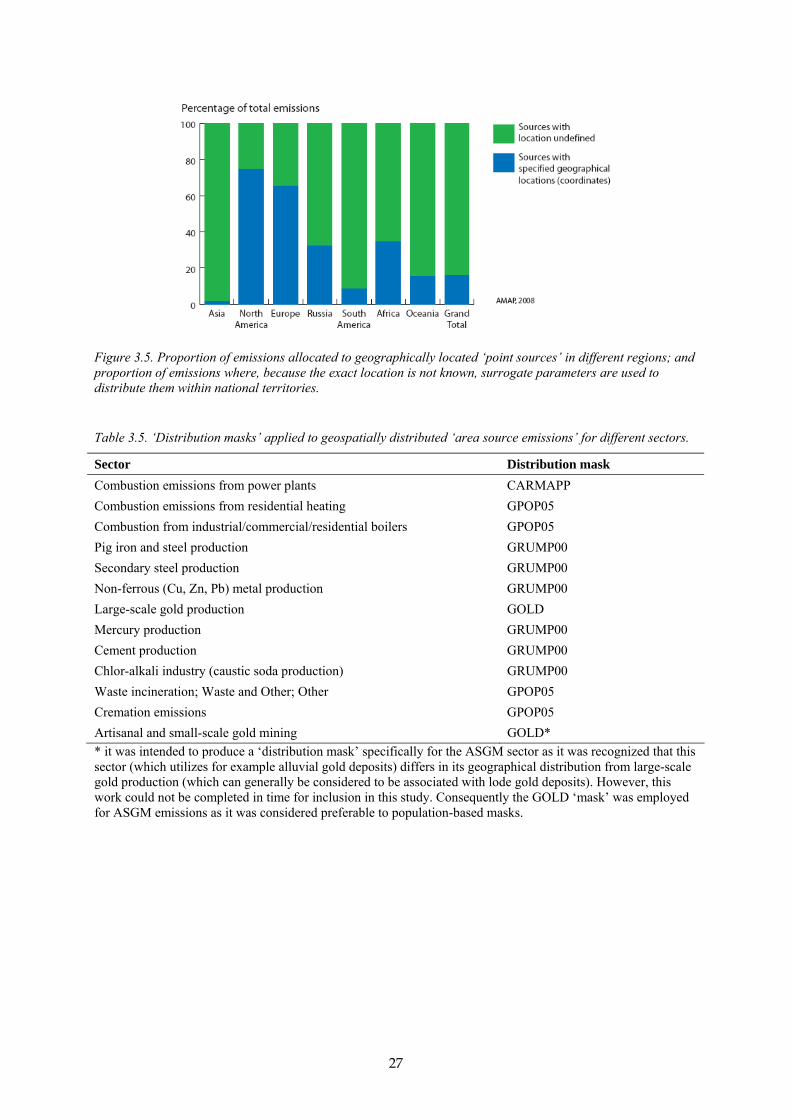
27

Figure 3.5. Proportion of emissions allocated to geographically located ‘point sources’ in different regions; and proportion of emissions where, because the exact location is not known, surrogate parameters are used to distribute them within national territories.

Table 3.5. ‘Distribution masks’ applied to geospatially distributed ‘area source emissions’ for different sectors.

Sector Distribution mask Combustion emissions from power plants CARMAPP Combustion emissions from residential heating GPOP05 Combustion from industrial/commercial/residential boilers GPOP05 Pig iron and steel production GRUMP00 Secondary steel production GRUMP00 Non-ferrous (Cu, Zn, Pb) metal production GRUMP00 Large-scale gold production GOLD Mercury production GRUMP00 Cement production GRUMP00 Chlor-alkali industry (caustic soda production) GRUMP00 Waste incineration; Waste and Other; Other GPOP05 Cremation emissions GPOP05 Artisanal and small-scale gold mining GOLD* * it was intended to produce a ‘distribution mask’ specifically for the ASGM sector as it was recognized that this sector (which utilizes for example alluvial gold deposits) differs in its geographical distribution from large-scale gold production (which can generally be considered to be associated with lode gold deposits). However, this work could not be completed in time for inclusion in this study. Consequently the GOLD ‘mask’ was employed for ASGM emissions as it was considered preferable to population-based masks.

28

Figure 3.6. The GPOP05 ‘distribution mask’. Note: the map does not show global population density. It shows the fraction of each countries population that is within a given grid cell, as derived from the GPW3 global population data set.

A dedicated computer application was developed (in the Python® language) which provided a convenient and flexible means of processing the ‘point/area source’ tagged national emissions inventories for the various sectors to generate the gridded (i.e., geospatially distributed) inventories for those sectors. In addition to performing the geospatial distributions, the application also split the emissions between mercury ‘species’ and ‘emission height’ categories as discussed under section A.3.1.4. A second Python® application was developed to allow files for the various sectors to be combined according to user-defined criteria.

The resulting (sector-specific) gridded emissions inventories for 2005 can be conveniently mapped, as shown in Figure 3.7 (total mercury emissions from the power plant/residential heating combustion sectors), or used as input to models. An example of the map produced for the 2005 inventory summing all sectors for total mercury is shown in Figure 3.17.

Figure 3.7. The gridded distribution of total mercury from (power plant and residential heating) combustion sources.

29

A3.1.4 Methods for speciation of inventory emissions In addition to requiring geospatially distributed (gridded) emission inventories, models also require that these emissions are ‘speciated’, to divide primary emissions between three main types of mercury/mercury compounds: gaseous elemental mercury (GEM, also abbreviated as Hg0 or Hg0), divalent mercury compounds (Hg2+), and particulate associated mercury (Hg-P); together these comprise the total mercury (HgT) emissions. Furthermore, emissions may be apportioned relative to nominal (geometric) emission height classes; emission height being a further factor affecting atmospheric transport. Three such height classes corresponding to emissions below 50 m, between 50 and 150 m, and above 150 m are commonly used.

This apportioning of mercury emissions into (nine) defined speciation-emission height categories is performed using a ‘split factors’ scheme defined for the various source sectors. Table 3.6 shows the split factors employed in classifying the 2005 global anthropogenic mercury emission inventory – which is the same as that employed in classifying previous inventories. Table 3.6. Emission speciation ‘split factors’ applied to the 2005 global anthropogenic emission inventory.

Sector Emission height class

Hg0 split Hg2 split Hg-P split

Combustion emissions from power plants

3 0.5 0.4 0.1

Combustion emissions from residential heating

1 0.5 0.4 0.1

Combustion emissions from industrial/commercial/residential boilers

1 0.5 0.4 0.1

Pig iron and steel production 2 0.8 0.15 0.05 Secondary steel production 2 0.8 0.15 0.05 Non-ferrous (Cu, Zn, Pb) metal production

2 0.8 0.15 0.05

Large-scale gold production 1 0.8 0.15 0.05 Mercury production 1 0.8 0.2 0 Cement production 2 0.8 0.15 0.05 Chlor-alkali industry (caustic soda production)

1 0.7 0.3 0

Waste incineration 1 0.2 0.6 0.2 Waste and Other; Other 1 0.8 0.15 0.05 Cremation emissions 1 0.8 0.15 0.05 Artisanal and small-scale gold mining

1 1.0 0 0

A3.2 Discussion of results by source category

A3.2.1 Emissions from by-product sectors Mercury by-product emissions for the year 2005 were estimated for the following source categories in individual countries of the world:

- combustion of coal in power plants and industrial, commercial, and residential boilers; - combustion of oil products in power plants and industrial, commercial, and residential

30

boilers; - cement production in wet and dry rotary kilns; - primary and secondary zinc production; - primary and secondary copper production; - primary and secondary lead production; - pig iron and steel production; - caustic soda production; - mercury production; - (large-scale) gold production; - waste incineration (Europe and United States); and - other sources.

The category defined as ‘other sources’ provides estimates of mercury emissions in connection with combustion processes in furnaces other than utility, industrial and residential boilers, for example in military and various small uses of mercury not included in the previous sections of this report. The results of the 2005 estimates of global emissions of mercury as a ‘by-product’ from the above-listed anthropogenic sources are presented in Table 3.7. Emissions estimates for individual countries are presented in Appendix Table AppA.6. The largest emissions to the global atmosphere of mercury as a by-product occur from combustion of fossil fuels, mainly coal in power plants and industrial and residential boilers. As much as 60% of the total emission of ca. 1535 tonnes of mercury emitted from all anthropogenic sources worldwide in 2005 came from combustion of fossil fuels. Emissions of mercury from coal combustion are between one and two orders of magnitude higher than emissions from oil combustion, depending on the country.

Various factors affect the emission of mercury to the atmosphere during combustion of fuels. The most important are: 1) the content of mercury in coal, and 2) the type and efficiency of control equipment that can remove mercury from exhaust gases. The amount of combusted fuel is, of course, a key factor.

Concentrations of mercury in coals and crude oils vary substantially depending on the type of fuel and its origin. Sulfide-forming elements, including mercury, are consistently found in the inorganic fraction of coal. Literature data indicate that mercury concentrations in coal vary between 0.01 and 1.5 ppm (a review in EU, 2001). These concentrations are presented in Table 3.8. It should be noted that concentrations of mercury within the same mining field can vary by one order of magnitude or more.

There is only limited information on the content of mercury in oil. In general, mercury concentrations in crude oils range from 0.01 to as much as 30.0 ppm (Pacyna, 1987). Major revision of current data on the mercury content in crude oil indicates a concentration range from 0.01 to 0.5 ppm (ACAP, 2005b). It is expected that mercury concentrations in residual oil are higher than those in distillate oils, which are produced at an earlier stage in an oil refinery.

The type and efficiency of control equipment is the major parameter affecting the amount of mercury released to the atmosphere. Unlike other trace elements, mercury enters the atmosphere from various industrial processes in a gaseous form. However, de-dusting installations, such as electrostatic precipitators (ESPs) and fabric filters (FFs) can also remove up to 30% of mercury from exhaust gases. One should note that ESPs are now commonly used abatement measures in major electric power plants and central heating plants worldwide.

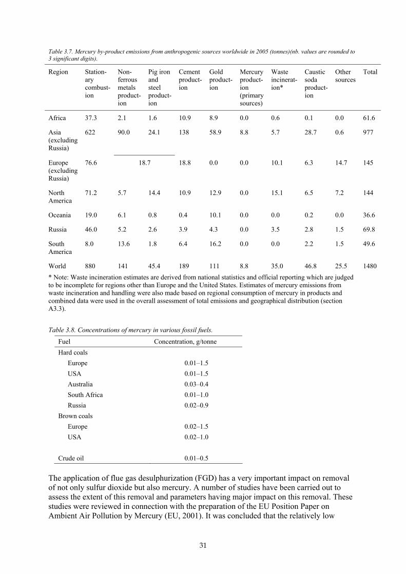
31

Table 3.7. Mercury by-product emissions from anthropogenic sources worldwide in 2005 (tonnes)(nb. values are rounded to 3 significant digits).

Region Station-ary combust-ion

Non- ferrous metals product-ion

Pig iron and steel product-ion

Cement product-ion

Gold product-ion

Mercury product-ion (primary sources)

Waste incinerat-ion*

Caustic soda product-ion

Other sources

Total

Africa 37.3 2.1 1.6 10.9 8.9 0.0 0.6 0.1 0.0 61.6

Asia (excluding Russia)

622 90.0 24.1 138 58.9 8.8 5.7 28.7 0.6 977

Europe (excluding Russia)

76.6 18.7

18.8 0.0 0.0 10.1 6.3 14.7 145

North America

71.2 5.7 14.4 10.9 12.9 0.0 15.1 6.5 7.2 144

Oceania 19.0 6.1 0.8 0.4 10.1 0.0 0.0 0.2 0.0 36.6

Russia 46.0 5.2 2.6 3.9 4.3 0.0 3.5 2.8 1.5 69.8

South America

8.0 13.6 1.8 6.4 16.2 0.0 0.0 2.2 1.5 49.6

World 880 141 45.4 189 111 8.8 35.0 46.8 25.5 1480 * Note: Waste incineration estimates are derived from national statistics and official reporting which are judged to be incomplete for regions other than Europe and the United States. Estimates of mercury emissions from waste incineration and handling were also made based on regional consumption of mercury in products and combined data were used in the overall assessment of total emissions and geographical distribution (section A3.3). Table 3.8. Concentrations of mercury in various fossil fuels.

Fuel Concentration, g/tonne Hard coals

Europe 0.01–1.5 USA 0.01–1.5 Australia 0.03–0.4 South Africa 0.01–1.0 Russia 0.02–0.9

Brown coals Europe 0.02–1.5 USA 0.02–1.0

Crude oil 0.01–0.5

The application of flue gas desulphurization (FGD) has a very important impact on removal of not only sulfur dioxide but also mercury. A number of studies have been carried out to assess the extent of this removal and parameters having major impact on this removal. These studies were reviewed in connection with the preparation of the EU Position Paper on Ambient Air Pollution by Mercury (EU, 2001). It was concluded that the relatively low

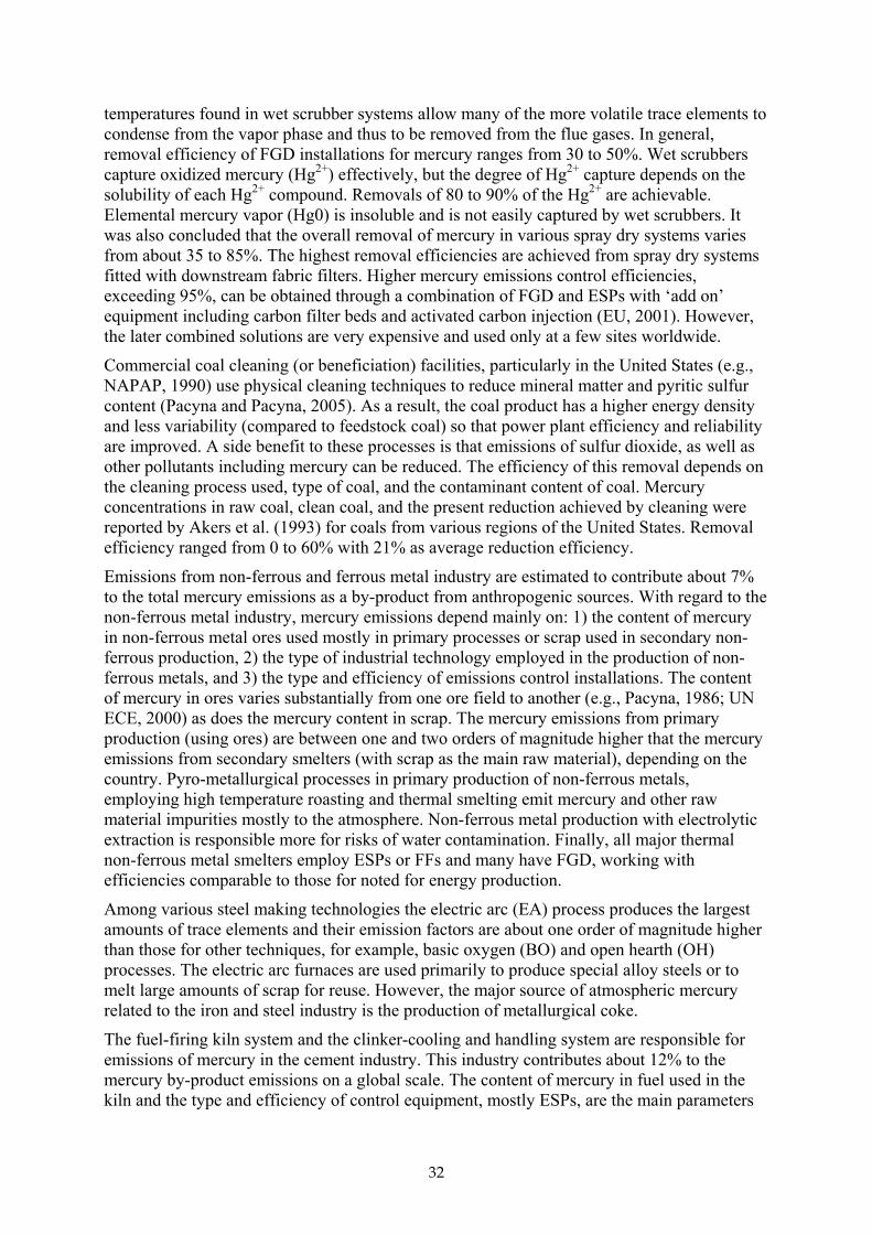
32

temperatures found in wet scrubber systems allow many of the more volatile trace elements to condense from the vapor phase and thus to be removed from the flue gases. In general, removal efficiency of FGD installations for mercury ranges from 30 to 50%. Wet scrubbers capture oxidized mercury (Hg2+) effectively, but the degree of Hg2+ capture depends on the solubility of each Hg2+ compound. Removals of 80 to 90% of the Hg2+ are achievable. Elemental mercury vapor (Hg0) is insoluble and is not easily captured by wet scrubbers. It was also concluded that the overall removal of mercury in various spray dry systems varies from about 35 to 85%. The highest removal efficiencies are achieved from spray dry systems fitted with downstream fabric filters. Higher mercury emissions control efficiencies, exceeding 95%, can be obtained through a combination of FGD and ESPs with ‘add on’ equipment including carbon filter beds and activated carbon injection (EU, 2001). However, the later combined solutions are very expensive and used only at a few sites worldwide.

Commercial coal cleaning (or beneficiation) facilities, particularly in the United States (e.g., NAPAP, 1990) use physical cleaning techniques to reduce mineral matter and pyritic sulfur content (Pacyna and Pacyna, 2005). As a result, the coal product has a higher energy density and less variability (compared to feedstock coal) so that power plant efficiency and reliability are improved. A side benefit to these processes is that emissions of sulfur dioxide, as well as other pollutants including mercury can be reduced. The efficiency of this removal depends on the cleaning process used, type of coal, and the contaminant content of coal. Mercury concentrations in raw coal, clean coal, and the present reduction achieved by cleaning were reported by Akers et al. (1993) for coals from various regions of the United States. Removal efficiency ranged from 0 to 60% with 21% as average reduction efficiency.

Emissions from non-ferrous and ferrous metal industry are estimated to contribute about 7% to the total mercury emissions as a by-product from anthropogenic sources. With regard to the non-ferrous metal industry, mercury emissions depend mainly on: 1) the content of mercury in non-ferrous metal ores used mostly in primary processes or scrap used in secondary non-ferrous production, 2) the type of industrial technology employed in the production of non-ferrous metals, and 3) the type and efficiency of emissions control installations. The content of mercury in ores varies substantially from one ore field to another (e.g., Pacyna, 1986; UN ECE, 2000) as does the mercury content in scrap. The mercury emissions from primary production (using ores) are between one and two orders of magnitude higher that the mercury emissions from secondary smelters (with scrap as the main raw material), depending on the country. Pyro-metallurgical processes in primary production of non-ferrous metals, employing high temperature roasting and thermal smelting emit mercury and other raw material impurities mostly to the atmosphere. Non-ferrous metal production with electrolytic extraction is responsible more for risks of water contamination. Finally, all major thermal non-ferrous metal smelters employ ESPs or FFs and many have FGD, working with efficiencies comparable to those for noted for energy production.

Among various steel making technologies the electric arc (EA) process produces the largest amounts of trace elements and their emission factors are about one order of magnitude higher than those for other techniques, for example, basic oxygen (BO) and open hearth (OH) processes. The electric arc furnaces are used primarily to produce special alloy steels or to melt large amounts of scrap for reuse. However, the major source of atmospheric mercury related to the iron and steel industry is the production of metallurgical coke.

The fuel-firing kiln system and the clinker-cooling and handling system are responsible for emissions of mercury in the cement industry. This industry contributes about 12% to the mercury by-product emissions on a global scale. The content of mercury in fuel used in the kiln and the type and efficiency of control equipment, mostly ESPs, are the main parameters

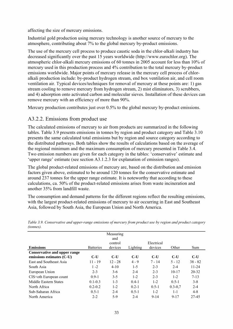
33

affecting the size of mercury emissions.

Industrial gold production using mercury technology is another source of mercury to the atmosphere, contributing about 7% to the global mercury by-product emissions.

The use of the mercury cell process to produce caustic soda in the chlor-alkali industry has decreased significantly over the past 15 years worldwide (http://www.eurochlor.org). The atmospheric chlor-alkali mercury emissions of 60 tonnes in 2005 account for less than 10% of mercury used in this production process and 4% contribution to the total mercury by-product emissions worldwide. Major points of mercury release in the mercury cell process of chlor-alkali production include: by-product hydrogen stream, end box ventilation air, and cell room ventilation air. Typical devices/techniques for removal of mercury at these points are: 1) gas stream cooling to remove mercury from hydrogen stream, 2) mist eliminators, 3) scrubbers, and 4) adsorption onto activated carbon and molecular sieves. Installation of these devices can remove mercury with an efficiency of more than 90%.

Mercury production contributes just over 0.5% to the global mercury by-product emissions.

A3.2.2. Emissions from product use The calculated emissions of mercury to air from products are summarized in the following tables. Table 3.9 presents emissions in tonnes by region and product category and Table 3.10 presents the same calculated total emissions but by region and source category according to the distributed pathways. Both tables show the results of calculations based on the average of the regional minimum and the maximum consumption of mercury presented in Table 3.4. Two emission numbers are given for each category in the tables: ‘conservative’ estimate and ‘upper range’ estimate (see section A3.1.2.3 for explanation of emission ranges).

The global product-related emissions of mercury are, based on the distribution and emission factors given above, estimated to be around 120 tonnes for the conservative estimate and around 237 tonnes for the upper range estimate. It is noteworthy that according to these calculations, ca. 50% of the product-related emissions arises from waste incineration and another 35% from landfill waste.

The consumption and demand patterns for the different regions reflect the resulting emissions, with the largest product-related emissions of mercury to air occurring in East and Southeast Asia, followed by South Asia, the European Union and North America.

Table 3.9. Conservative and upper-range emissions of mercury from product use by region and product category (tonnes).

Emissions Batteries

Measuring and

control devices Lighting

Electrical devices Other Sum

Conservative and upper range emissions estimates (C-U) C-U C-U C-U C-U C-U C-U East and Southeast Asia 11 - 19 12 - 28 4 - 9 7 - 14 5 - 12 38 - 82 South Asia 1 -2 4-10 1-5 2-3 2-4 11-24 European Union 2-3 3-6 2-4 2-3 10-17 20-32 CIS+oth European count 0.9-1 3-5 1-2 2-3 1-2 7-13 Middle Eastern States 0.1-0.3 1-3 0.4-1 1-2 0.5-1 3-8 North Africa 0.2-0.2 1-2 0.2-1 0.5-1 0.3-0,7 2-4 Sub-Saharan Africa 0.5-1 2-4 0.5-1 1-2 1-1 4-8 North America 2-2 5-9 2-4 9-14 9-17 27-45

34

Central America and the Caribbean 0.2-0.3 1-3 0.4 0.6 0.5 3.0 South America 0.6-1 2-5 1-2 1-3 1-2 5-12 Australia New Zealand and Oceania 0.1-0,2 0.3-1 0.1-0.2 0.3-0.4 0.2-0.3 1-2 Sum 20-31 33-74 13-28 26-47 29-58 120-237

Table 3.10. Conservative and upper-range emissions of mercury from product use by region and source category (tonnes).

Emissions Release by breaking

Waste incineration Waste landfill Scrap metal

Waste recollected, recycling - handling Sum

Conservative-upper range emissions estimates C-U C-U C-U C-U C-U C-U C-U East and Southeast Asia 2-6 16-18 16-47 2-3 3-10 39-89 South Asia 0.5-1 4-4 6-18 0.2-0.2 0.1-0.3 11-24 European Union 1-4 13-14 4-11 1-1 1-2 20-32 CIS+other European countries 0.3-1 4-4 2-7 0.3-0.3 0.2-0.4 7-13 Middle Eastern States 0.2-1 0.3-0.3 2-7 0.2-0.2 0-0 3-8 North Africa 0.1-0.2 1-1 1-3 0-0 0-0 2-4 Sub-Saharan Africa 0.2-0.4 2-3 2-5 0.1-0.1 0-0.1 4-8 North America 1-4 14-16 6-18 4-4 1-4 27-45 Central America and the Caribbean 0.2-0.5 1-1 2-6 0.1-0.1 0-0.1 3-7 South America 0.3-1 1-1 3-9 0.3-0.3 0-0.1 5-12 Australia New Zealand and Oceania 0.1-0.2 0.4-0.4 0.3-1 0.2-0.2 0.1-0,2 1-2 Sum 6-18 57-62 45-133 7-7 5-16 120-236

The emission estimates per region (conservative estimate) are also presented in Figure 3.8. East and Southeast Asia and North America account for the largest emissions followed by the European Union and South Asia.

Product emissions by region

Central America and the Caribbean East and Southeast AsiaEurope - CIS and non-EU countriesEuropean UnionMiddle EastNorth AfricaNorth AmericaOceaniaSouth AmericaSouth AsiaSub-Saharan Africa

Figure 3.8. Proportion of estimated emissions of mercury from product use from different regions (conservative estimate).

35

A3.2.2.1 Remarks on emissions from product use of mercury

A3.2.2.1.1 Waste incineration By far most important emission pathway for product use of mercury is via waste handling. Figure 3.9 presents the product-related emissions to air by category (not including cremations). Waste incineration accounts for 47% of the total emissions and landfill for another 37%.

Release by breakingSteel scrapWaste incinerationWaste landfillWaste recycling

Figure 3.9. Product-related emissions to air (excluding cremation emissions) by category (conservative estimate). The waste sector also includes some duplication of (waste incineration) emissions quantified under the ‘by-product’ inventory (section A3.2.1). The emission estimate presented in that section is based on official national data and estimates using official statistics on waste incineration and mercury levels in waste. For most countries this information is incomplete and the emissions are thus underestimated. In the product-based evaluation, the total waste-related emissions of mercury are 106 tonnes globally whereas the ‘by-product’ based evaluations estimate a total of 32.7 tonnes. For the overall (combined) emission inventory presented in section A3.2.5, emissions estimated from the product-use inventory (conservative estimate) have been used for all countries except European countries and the United States, where the officially reported emissions from waste incineration were judged to be more reliable. The different estimates thus available for some countries for the ‘waste’ and ‘other’ emissions categories provides some insight into the comparability between the two approaches used to quantify these emissions. For example, for the United States, the national emission inventory estimates (for 2002) for waste incineration and ‘other’ emissions were ca. 14 900 kg and 6800 kg respectively, and for cremations about 1680 kg. These compare with estimates from the product-use inventory of about 20 700 kg, 3280 kg and 910 kg respectively for ‘waste and other’, secondary steel, and cremation emissions. These results indicate a reasonable degree of agreement for the examples where comparison is possible.

A3.2.2.1.2 Long-term fate of mercury in society The estimates of mercury emissions from use in products are associated with large uncertainties. To calculate the fraction of an amount of mercury used in a specific product category, a number of assumptions concerning the use patterns and fate of the mercury must be made. In reality, these use patterns will vary between and within categories. These estimates are also limited to the emissions occurring in one year and make up a small fraction of the total use. Figure 3.10 shows the total consumption of mercury in products together with the estimated total emissions to air and the estimated fraction which is accounted for in ‘safe

36

storage’ (e.g., controlled landfills or storage for permanent disposal). The main part of the mercury is thus accumulated in society (in the form of products in use) or in landfills (e.g., household waste, ashes). Over longer time scales, this mercury, or a fraction of it, may continue to be released to the environment.

Safe storageEmissions to airRemaining in society

Total consumption 1368 tonnes

Figure 3.10. Total consumption of mercury in products vs the estimated total emissions to air and the estimated fraction which is accounted for in ‘safe storage’.

A3.2.3 Mercury emissions from cremation The estimated emissions of mercury to air from cremations for different regions are presented in Table 3.11 and Figure 3.11. East and Southeast Asia account for the largest contribution followed by the European Union. It should be noted that these estimates are highly uncertain due to a lack of information on actual amounts of mercury in cremations, the number of cremations and the fate of mercury during the process. In addition, these data only represent the estimated emissions from the cremation process itself. Production, handling and disposal of dental amalgam are likely to give rise to additional emissions to air as well as water. These emissions have been estimated to be significantly larger than cremation emissions in Europe and the United States (Maxson, 2007; Cain et al., 2007).

Table 3.11. Emissions of mercury to air from cremations.

Region Cremation emissions by region Central America and the Caribbean 0.4 East and Southeast Asia 16 Europe - CIS and non-EU countries 0.25 European Union 3.5 Middle East 0.02 North America 1 Oceania 0.01 South America 1 South Asia 2.5 Sub-Saharan Africa 0.5 Total 26

37

Crematory emissions by region

Central America and the Caribbean East and Southeast AsiaEurope - CIS and non-EU countriesEuropean UnionMiddle EastNorth AmericaOceaniaSouth AmericaSouth AsiaSub-Saharan Africa

Figure 3.11. Mercury emissions from cremation by region. In previous studies, Cain et al. (2007) and Maxson (2007) have estimated total emissions from production, handling, use and disposal of dental amalgam. For the United States, estimates of emissions from cremation and production of dental amalgam are also included in the US national emissions inventory. For the United States, Cain et al. (2007) estimated emissions of 4.5 tonnes of mercury to air from dental amalgam. The corresponding emission from this study is 1 tonne which also includes Canada. The officially reported emission for the United States for cremation and dental amalgam production is 0.29 and 0.57 tonnes respectively, which is significantly lower than the estimate by Cain et al. (2007). For Europe, Maxson (2007) reported emissions from all steps in the dental amalgam production chain of 23 tonnes, which is considerably higher than the emissions from cremation reported here. Both studies (Cain and Maxson) have adopted a substance flow approach where large losses of mercury have been identified and partly allocated to emissions to air. Although the emissions estimates may be uncertain, they are based on available statistics on mercury use in the dental sector and further studies of the fate of mercury in this production chain are warranted. Nevertheless, for this global report, the available time and resources did not allow a more thorough assessment of the dental sector and only the emissions from cremation were considered.

A3.2.4 Mercury emissions from artisanal and small-scale gold mining Table 3.12 and Figure 3.12 present estimated emissions of mercury from artisanal and small-scale gold mining (Telmer and Veiga, 2008). Table 3.12. Estimated emissions of mercury from artisanal gold mining.

Region Hg emission, tonnes Australia New Zealand and Oceania 0.2 Sub-Saharan Africa 8 Central America and the Caribbean 5 CIS and other European countries 4 East and Southeast Asia 233 Middle Eastern States 3 North America 6 South America 64 South Asia 28 Total 350

38

Australia New Zealand and Oceania

Sub-Saharan Africa

Central America and the Caribbean

CIS and other European countries

East and Southeast Asia

Middle Eastern States

North America

South America

South Asia

Figure 3.12. Mercury emissions from artisanal and small-scale gold mining by region. East and Southeast Asia and South America account for the major part of the artisanal and small-scale gold mining emissions.

Different estimates of Chinese mercury emissions from ASGM activities are reported in the UNEP F&TP report. Feng et al (2008) present an estimate of ca. 30 tonnes. However, Telmer and Veiga (2008) have derived an inventory estimate of ca. 150 tonnes. The lower estimate quoted by Feng et al (2008) is identified with reductions following an official ban on artisanal gold production in China in 1996; they do however acknowledge that their estimate of mercury emissions from metals smelting is subject to a high uncertainty due, among other things, to lack of precise production estimates from small activities. Telmer and Veiga (2008) discuss the work of Gunson and co-workers who reported a minimum of 50 tonnes per year mercury released through ASGM in China, an estimate subsequently revised to between 237 and 652 tones per year following more thorough research. This was considered consistent with “the fact that China became the world’s largest gold producer in 2007, that much of its production is known to come from small mines, and that much of China’s ASGM employs inefficient whole ore amalgamation where the consumption of mercury can be very high”. Telmer and Veiga (2008) also note that currently China officially admits no ASGM operations occur in its territory.

A3.2.5 Combined global inventory – emissions by sectors Summing the emissions from by-product sectors, product use, cremation and artisanal mining (discussed in sections A3.2.1- A3.2.4) results in a global inventory of emissions of mercury to air from anthropogenic sources for the reference year of 2005 of ca. 1930 tonnes. Table 3.13 and Figure 3.13 summarize the emissions accounted to various anthropogenic activities.

39

Table 3.13. Estimated global anthropogenic emissions of mercury to air in 2005 from various sectors (nb. values are rounded to 3 significant digits).

Sector Emissions in 2005 (t)

Low-end estimate

High-end estimate

%

Power plants 498

Residential heat 375

Other Industrial/Residential/Commercial combustion

5.2

Fossil fuel combustion for power and heating 878 595 1160 45.6

Pig iron and steel 54.5

Non-ferrous metals 132

Mercury production 8.8

Secondary steel 4

Metal production (ferrous and non-ferrous, excluding gold)

200 123 276 10.4

Large-scale gold production 111 66 156 5.78

Artisanal and small-scale gold production 351 225 475 18.2

Cement production 189 114 263 9.8

Chlor-alkali industry 46.8 29 64 2.43

Waste incineration (Europe and North America)

35

Other 26.1

Waste & other 63.9

Waste incineration, waste and other 125 53 473 6.49

Dental amalgam (cremation)* 25.7 24 28 1.33

Total 1930

* Does not include other releases from production, handling and disposal of dental amalgam

40

Figure 3.13. Proportion of global anthropogenic emissions of mercury to air in 2005 from various sectors.

A3.3 Discussion of results by region The combined global anthropogenic emissions inventory for by-product sectors, product use, cremation and artisanal mining (see previous section) of ca. 1930 tonnes for the reference year of 2005 can be divided between the continents as summarised in Table 3.14 and Figure 3.14. Figure 3.15 shows the breakdown by continent and the major emission sectors.

Table3.14. Estimated global anthropogenic emissions of mercury to air in 2005 from different regions (nb. values are rounded to 3 significant digits).

Region Emissions in 2005, t

Low-end estimate, t

High-end estimate, t

%

Africa 95.4 57.6 141 4.96 Asia 1280 835 1760 66.5 Europe 150 90.8 309 7.78 North America 153 91.4 305 7.94 Oceania 39.1 28.2 50.0 2.03 Russia 73.9 44.6 132 3.84 South America 133 82.0 196 6.9 Total 1930

41

Figure 3.14. Proportion of global anthropogenic emissions of mercury to air in 2005 from different regions.

Figure 3.15. Global anthropogenic emissions of mercury to air in 2005 from different continents by sector.

From the compiled inventory data, it is possible to rank the countries by their emissions. Table 3.15 and Figure 3.16 present the sector-breakdown of emissions from the ten largest emitting countries.

42

Table 3.15 The largest mercury by-product emitting countries in 2005 (tonnes).

Rank Country Emissions in 2005

% of global total

Category

Stationary combustion

Industrial production

Artisanal gold

Other sources

1 China 825.2 42.85 387.4 243.2 156.0 38.6 2 India 171.9 8.93 139.7 21.6 0.5 10.1 3 USA 118.4 6.15 62.8 31.7 0.5 23.4 4 Russia 73.9 3.84 46.0 18.9 3.9 5.1 5 Indonesia 68.0 3.53 3.3 10.2 50.9 3.6 6 South Africa 43.1 2.24 33.4 5.7 2.6 1.4 7 Brazil 34.8 1.81 4.8 11.4 15.8 2.8 8 Australia 33.9 1.76 17.7 15.2 0.4 0.6 9 Republic of

Korea 32.2 1.67 18.1 12.9 0 1.2

10 Columbia 30. 1.56 0.8 2.3 26.3 0.6

Total 74.33

Figure 3.16. Emissions of mercury to air in 2005 from various anthropogenic sectors in the ten largest emitting countries.

From Figure 3.14 it is apparent that Asian countries contributed about 67% to the global mercury emissions from anthropogenic sources in 2005, followed by North America and

43

Europe. This pattern is similar if by-product emission sectors only are considered (Table 3.7). Russia, with its contribution of about 4% to global emissions is considered separately due to its territories in both Europe and Asia.

Combustion of fuels to produce electricity and heat is the largest source of anthropogenic mercury emissions in Europe, North America, Asia and Russia, and responsible for about 40–50% of the anthropogenic emissions in Oceania and Africa. However, in South America, ASGM is responsible for the largest proportion of the emissions (>55%). Artisanal and small-scale gold mining emissions in some Asian countries as well as several countries in South America also explains why countries such as Indonesia, Brazil and Colombia appear in the top ten ranked mercury emitting countries (Figure 3.16), whereas if by-product emissions sectors alone are considered, no South American countries are represented and all other countries listed have a high degree of industrial development.

China, with its more than 2000 coal-fired power plants, is the largest single emitter of mercury worldwide, by a large margin. Power plant emissions are only a part of the total combustion emissions of mercury in China. Equally significant are emissions from combustion of poor quality coal mixed with various kinds of wastes in small residential units to produce heat and cook food in rural areas. With estimated by-product sector emissions exceeding 600 tonnes, China contributes about 40% to the global mercury by-product emissions, and this contribution may be even higher because mercury emission factors for non-ferrous metal production in China may be underestimated. China also has significant emissions from ASGM.

Together, three countries, China, the United States and India, are responsible for about 60% of the total global mercury emissions from by-product sectors (887 out of 1480 tonnes), and a similar percentage of the total estimated global emission inventory for 2005 (1115 out of 1930 tonnes).

Figure 3.17 presents the global distribution of anthropogenic emissions of mercury in 2005, following application of the geospatial distribution methodology described in section A.3.1.3 to the combined emission inventory.

Figure 3.17. Global distribution of anthropogenic emissions of mercury in 2005.

A3.4 Uncertainties in emission estimates It is important to recognize that the emission estimates (both ‘expert’ estimates and officially reported emissions figures) presented above are just that – estimates. These estimates are

44

based on a number of assumptions, several of which are discussed in section A3.1 where the methods used to produce the inventory are described. These include assumptions regarding mercury consumption, production and use of fossil fuels and other raw materials, emission factors, and technology. Further assumptions are made in order to allocate or distribute these emissions among regions, countries or even finer geographical units (e.g., geospatial distribution of emissions inventories to grid cells for modeling applications). All of the assumptions used are considered to represent the best option currently available for filling gaps in the knowledge required to produce a quantitative distributed global emission inventory for mercury. An obvious consequence of estimations based on assumptions is that the estimates have an associated degree of uncertainty.

A3.4.1 Uncertainties in by-product emission sources Uncertainties in emissions estimates can be grouped depending on source type and category. For major point sources, previously estimated uncertainty ranges are presented in Tables 3.16 and 3.17. In general, the uncertainties reflect the extent to which emissions from a given source sector have been studied and the countries or regions where these studies have been undertaken. Table 3.16. Uncertainty of mercury emissions estimates by source category.

Industrial source Uncertainty (± %) Stationary fossil fuel combustion 25 Non-ferrous metal production 30 Iron and steel production 30 Cement production 30 Waste disposal and incineration As much as 5 times Mercury and gold production ?

Table 3.17. Uncertainty of mercury emissions estimates by continent.

Continent Uncertainty (± %) Africa 50 Asia 40 Australia 30 Europe 30 North America 27 South America 50

The most accurate data on mercury emissions are those for combustion of coal in stationary sources, mainly electric power plants. This relates primarily to the accuracy of emission factors for mercury emitted from various types of coal, boiler and emission control measures applied in coal-fired power plants. Emission factors for mercury and other contaminants emitted during coal combustion have been developed on the basis of either measurements of mercury in the flue gas leaving the combustion zone or material balances for mercury entering the combustion zone with coal on one side of the balance and leaving the combustion zone with bottom ash, fly ash, and flue gas on the other side of the balance.

Measurements of mercury during coal combustion have been carried out over the last two decades. An example of such measurements is the EU project MOE (Mercury Over Europe:

45

http://www.eloisegroup.org). The mercury measurements in the MOE projects were carried out at selected coal-fired power plants and a few waste incinerators in Poland, Germany and Finland, as well as in some waste incinerators in Hungary. They were in good agreement (within 20 to 50%) with the emission factors used in this report to calculate emissions of mercury from coal combustion.

Measurements of mercury emissions in chlorine productions plants were carried out in Poland (Jarosinska et al., 2006). The results of these measurements were used to estimate emission factors for mercury from this source category. Emission factors of about 2.5 to 3.0 g Hg/tonne of chlorine produced were obtained compared to the emissions factor of 2.5 g Hg/tonne of chlorine produced, used in this report.

The emissions measurements would generate the most accurate data on emissions if the proper sampling methods and analytical techniques were used and the samples were collected at representative sites along the path of flue gases in the stack. However, to measure emissions at so many point sources of emissions is for many reasons impossible to accomplish in very many countries. Therefore, less accurate methods, based on emission factors and material balances must be applied.

The mass balance method to estimate emission factors for trace elements, including mercury from coal combustion has been used for at least three decades. This method was described by Pacyna (1980). The mercury emission factor is estimated as a difference between the amount of mercury introduced to the combustion zone with coal and the amounts of mercury leaving the combustion zone with bottom ash and in the fly ash collected by emission control equipment, mainly ESPs or fabric filters. In order to assess the accuracy of such emission factors, they are used together with statistical data on fuel consumption or electricity production in dispersion models to estimate concentrations around a given power plant. These modeled concentrations are then compared with measured concentrations in the same area. A study carried out at the Meteorological Synthesizing Centre-East (MSC-E) of EMEP (EMEP MSC-E) concluded that agreement between model estimates of air concentrations based on mercury emission data derived using emission factors developed by the authors of this report, and air measurements at various EMEP stations in Europe was below 25% for mercury.

Higher levels of uncertainty, of about 30%, were estimated for emissions from major industrial sources, such as non-ferrous metal smelters, iron and steel plants, and cement plants.

Hylander and Herbert (2008) have recently estimated global mercury emissions from non-ferrous metal smelting in 2005 at ca. 275 tonnes. This is considerably higher than the estimate of ca. 140 tonnes for this sector in the global emissions inventory presented in this report. The emissions factors applied by Hylander and Herbert (2008) for Cu-, Pb- and Zn-smelters were 5.81-6.72, ca. 15 and 12-16 (g mercury per tonne metal), respectively. These are higher than those applied to estimate emissions in the by-product emission inventory of 5, 3 and 7 (see Table 3.2), but lower than those applied by Streets et al (2005) (for China) of 9.6, 43.6 and 86.6, respectively. These comparisons demonstrate the effect that different emission factors can have in influencing regional/global emission estimates, in addition to different statistical data on production volumes, etc. An estimated emission of about 185-195 tonnes per year is within the uncertainty band of 30% if applied to both the conservative (140 tonne) and higher (275 tonne) estimates for the non-ferrous metal sector emissions. However, for the current inventory, it was decided to retain the 140 tonne estimate derived using the common methodology described in section A3.1, noting that other estimates produced using different methodologies and underlying statistical data exist. On a regional basis, the estimates of Hylander and Herbert (2008) are higher than those of the 2005 global inventory presented in

46

this report by about 50 tonnes for Russia (though these also include former USSR countries in the Hylander and Herbert estimates); by about 10-15 tonnes for Oceania, North America, Europe and China; and by about 30 tonnes for Asia excluding China. For Europe and North America, the global inventory presented in this report is based mainly on national estimates for emission from the non-ferrous metal sector rather than ‘expert estimates’ derived from independent calculations using emission factors and statistical data.

Future efforts should clearly be directed at further clarifying the reasons for significant differences between emission estimates such as those for the non-ferrous metals sector discussed above, and for example for ASGM emissions for countries such as China, and resolving these.

It is extremely difficult to develop and apply emission factors for waste incineration. The major reason is the highly variable composition of wastes, varying not only from country to country but from one incinerator to another and even within the same incinerator over certain periods. Therefore, the emission factors for incineration of wastes are regarded as the least accurate of all other emission factors used in this work. The approach used in this report to estimate emissions of mercury from waste incineration (for countries other than those reporting incinerator emissions) was presented in section A3.1.2.3.

In summary, only single estimates of mercury emissions are presented in this work for a given source category and country. However, for regional and sector totals, the uncertainty estimates presented in Tables 3.16 and 3.17 have been used to derive ‘high-‘ and ‘low-end’ estimates (ranges of uncertainty). These are presented in Tables 3.13 and 3.14 and included in the information presented in Figures 4.1 and 4.2.

In the case that emissions were estimated using emission factors, these were selected as being the most relevant emission factors in relation to, for example, a given industrial technology, or industrial development in a given country or region, or progress and improvements in application of advanced emission control equipment, or the content of mercury in raw materials.

As the emission data for several countries in Europe, the United States, Canada, Australia, South Africa, Japan, Republic of Korea, Cambodia, Chile and Peru have been evaluated by national emissions experts, it can be assumed that the emissions estimates for these countries may be more accurate than the emissions estimates for other countries.

Despite using a number of the same data sources (e.g., the national report on emissions from South Africa and the artisanal and small-scale gold mining emission estimates of Telmer and Veiga, 2008), the global inventory for 2005 produced by the authors of this report and an inventory (for 2007) for the F&TP by Pirrone et al. (2008) have a number of distinct differences.

The draft F&TP report (version available in May 2008) included two estimates that might be compared with the inventory produced by the authors of this report. First, an inventory of 1750 tonnes (Pirrone et al., 2008, Table 29), which is about 250 tonnes greater than the 1480 tonnes for the comparable sources in the 2005 global inventory in the current report. In part this difference can be explained by the fact that, although for the nominal year of 2007, the F&TP inventory includes data relating to different years from 1995 to 2007. Also, the F&TP inventory includes emissions from China, India, South Africa and Australia, but does not include data for any other countries in Asia, Africa or Oceania, so it would be expected to be a significant under-estimation of the inventory with respect to these continents. Second, an alternative inventory (included by Pirrone et al., 2008, Table 28) presents an estimate for the global anthropogenic inventory of about 2400 tonnes, including 40 tonnes attributed to coal-

47

bed fires and 300 tonnes to ASGM (the latter slightly lower than the 350 tonnes used by the authors of this report). Again, this compilation includes data from a range of years (2000–2007) and shows a number of differences in sector totals compared with the inventory presented in the F&TP report (Pirrone et al., 2008, Table 29). This is the case, for example, with the estimates for non-ferrous metals production – 156 tonnes and 330 tonnes, respectively – which make it difficult to reconcile the inventories or use them for comparison with the 2005 inventory presented in this report.

A3.4.2 Uncertainties in emission data for product use, cremations and artisanal gold mining This inventory represents the first attempt to quantify the global emissions of mercury to air from the above categories. There is thus very little information available for comparison of the results. The basis of the calculations is the information on global demand and supply of mercury presented in section A3.1.2.2. This data is believed to be only moderately uncertain although large errors may occur in specific sectors. For the estimates on distribution (distribution factors) and actual emissions from different categories (emission factors) the uncertainties are large. For many of these factors, no specific information is available and expert estimates have been applied. It is thus not possible to provide a quantitative number for the uncertainties. Instead, values are given for ‘Conservative’ and ‘Upper range’ emission estimates. It may be regarded more relevant to compare the few values where emissions have been quantified using other methods (e.g., point source measurements or engineering estimates). For waste incineration (which is the dominant sector in the product use emission category), nationally reported values are available from a few countries.

A specific sector where emissions are rarely reported is Vinyl Chloride Monomer production. Although this sector consumes large amounts of mercury (700 to 800 tonnes in 2005, see section A2.2.2.2) emission estimates are difficult to make. The ACAP (2005b) inventory of mercury emissions in Russia indicated an emission to air of 0.02 tonnes for a consumption of 7.5 tonnes (with an additional amount of 8 tonnes from recycling), that is, a relatively moderate emission. It is not known if this proportion is representative for other regions and further studies are necessary before a global estimate can be provided.

A3.4.2.1 Results of survey on uncertainties and verification addressed to national emissions experts With the intention to collect information on uncertainties and completeness of reported emissions data on mercury, a request for information was sent to national emissions experts in various countries.

The request comprised four questions on various aspects of emission inventories:

1. Verification of emission estimates. Nationally reported emissions data for mercury are in many cases based on estimates derived using guidelines such as the EMEP CORINAIR Emission Inventory Guidebook. Any information on measurement activities performed to verify the guidebook data would be extremely useful.

2. Missing sources or source categories. While all known major sources of mercury emissions should be covered in inventories, unreported and/or new sources may exist. Information on sources and source categories not included in existing emission inventories is highly relevant.

48

3. Estimated completeness of reported official national inventories. An estimate of completeness and identification of possible missing sources (including the magnitude of the estimated contribution if possible) in reported national inventories would be valuable in order to assess the overall uncertainty in officially available inventories of mercury.

4. Estimated uncertainties. If there are any estimated uncertainties for reported mercury emission data in your national emission inventories, any information on this would be welcome. Information on non-official-expert estimates is also valuable.

A total of ten replies were received:

Several European countries (Latvia, Belgium, Slovakia) reported that their emissions reporting was performed according to the guidelines of the UN ECE LRTAP Convention and that no further information was available.

Denmark reported additional information on uncertainties and provided an estimate of the total uncertainty for national mercury emissions of 220%.

The United Kingdom provided information on continuous effort to improve emissions inventories including point source measurement and analysis of metal contents in fuels. Emissions monitoring results for a small coal-fired heating boiler have been published (AEA Technology, 2001) and include some emission factors for metals. Potentially missing sources for metals include small-scale metal processes such as forges, galvanising plant as well as accidental/malicious fires, demolition, and quarrying. Re-suspension of metals from soils is believed to be important but is also not included in the inventory at the moment. The most recent UK assessment (Dore et al., 2007) suggested quite low uncertainty (with a likely range of −30% to +40% of the best estimate).

The United States of America provided detailed emissions data for mercury for 2002, and additional information on the U.S. EPA’s Mercury Emissions Inventory.

The 2002 NEI has undergone extensive QA (quality assurance) and QC (quality control) by EPA staff, state and local agencies, tribal associations and industry. More information on QA of the data, is available at http://www.epa.gov/ttn/chief/net/2002inventory.html.

For the following mercury categories, emission estimates are based on actual emissions test data: coal-fired utility boilers, hazardous-waste incineration, municipal-waste combustion, and medical-waste incineration. Estimates for some categories are based on a combination of emissions test data and various calculations and assumptions, such as electric arc furnaces and chlor-alkali plants. The US EPA considers the data for these categories to be generally of good quality, with relatively low uncertainties. Moreover, estimates have been verified through regulatory processes for the following categories: pulp and paper production, brick manufacturing, Portland cement production, mineral wool production, ferroalloys, secondary lead production, and shipbuilding. Most of the latter categories are not considered large sources of mercury emissions in the United States. However, some, such as Portland cement, emit notable quantities. In addition, an EPA regional office provided QA of the mercury emissions estimates for the industrial gold mining and production source category, which emitted a notable quantity of mercury in the 2002 timeframe. New mobile source estimates are based on recent source testing.

The US EPA is not aware of missing mercury categories at this time and considers that the largest emitting source categories are contained in the 2002 NEI and estimates are generally complete. The US EPA does not provide quantitative estimates of uncertainty in the NEI. As described above, qualitatively, categories that account for most of the US emissions are based on actual source data, or a combination of source test data and engineering calculations,

49

including the following: coal-fired utility boilers, hazardous-waste incineration, municipal-waste combustion, medical-waste incineration, electric arc furnaces, and chlor-alkali plants. Moreover, RTR data have undergone additional extensive QA as a part of rule-making processes. Emissions factors and activity data are the basis of the majority of emissions estimates in the NEI. Nevertheless, there are some uncertainties in the estimates. However, due to the factors explained above, generally the US EPA believes the uncertainties are relatively low for the main emitting mercury categories. The degree of uncertainty may be greater for some other pollutants (such as polychlorinated biphenyls) because there are less data and because these other pollutants have not been evaluated as thoroughly as mercury.

Nepal reported that there is no inventory of mercury, but that there is an increased use of mercury-based thermometers and other medical equipment. The waste handling system does not have any special practices for mercury-containing waste. Most of the health care institutions have practiced open burning, burning in substandard incinerators and /or mixing waste containing mercury into municipal waste which ends up by the river bank.

In Cambodia an emission inventory for mercury has been conducted based on the UNEP Toolkit for Identification and Quantification of Mercury Releases (UNEP, 2005). The results show that the major source of mercury release into the atmosphere is consumer products with intentional use of mercury, followed by disposal of wastes and then mercury release from gold extraction. The total release of mercury in Cambodia is approximately 770 kg at its lowest and about 14 800 kg at its highest per year. The greatest source of mercury release into the atmosphere is consumer products with intentional use of mercury, causing the release of about 8490 kg of mercury, followed by the disposal of wastes that could release mercury of approximately 4670 kg. The third largest source of mercury release is gold extraction, emitting about 1180 kg of mercury into the environment per year.

A3.4.2.2 Summary of additional national information reported to UNEP-Chemicals Japan A detailed mass-flow analysis of mercury has been prepared by Asari et al. (2008). The amount of mercury flow originating from products was estimated to be 10 to 20 tonnes annually; 5 tonnes of this from fluorescent lamps. The use of fluorescent lamps for backlights is increasing and most fluorescent lamps were disposed of as waste. Only 0.6 tonnes of mercury, about 4% of the total, is recovered annually.

Peru According to a report by Brooks et al. (2006b) Peru imports mercury-containing batteries, electronics and computers, fluorescent lamps, and thermometers. Mercury contained in these lamps and in other products such as batteries and computer electronics is not recycled and may ultimately be released to the environment.

USA A detailed flow analysis was reported by Cain et al. (2007).

50

A4 Trends in atmospheric mercury emissions to the atmosphere

A4.1 Regional trends in atmospheric mercury emissions

A4.1.1. Historical trends of emission until the year 2000 Global emissions inventories for mercury from (mainly by-product) anthropogenic sources were developed for various reference years in the past (Pacyna and Pacyna, 2002; Pacyna et al., 2003). The estimation procedures were based on emission factors and statistical data on the production of industrial goods and the consumption of raw materials in a given reference year. It should be noted, however, that the procedure used to estimate emissions from Russia was improved in the case of the 2000 estimates compared to estimates for earlier years. This improvement was a result of the large body of new data available from the ACAP project (ACAP, 2005b). Taking into account these observations, the estimates of global mercury emissions for the year 2000 can be compared with the estimates made by the authors for the years 1995, and 1990. This comparison is included in Figure 4.1, which also presents ranges of uncertainty in the estimates calculated for each sector-region based on the factors presented in Tables 3.16 and 3.17.

The general results were that mercury emissions on a global scale increased from about 1910 tonnes in 1990 to 2050 tonnes in 1995 (revised from 2235 tonnes following new information received from some countries), but decreased slightly in 2000 to a level of about 1930 tonnes (revised from 2190 tonnes following new information received from some countries, for example South Africa – see section A4.1.2). However, these changes need to be considered on a continent and even country basis. As previously discussed by Pacyna and Pacyna (2005), a major change in industrial production and consumption of various raw materials occurred in Eastern and Central Europe and Asia during the period from 1990 through 1995. This change resulted in a change of emissions of mercury in these regions.

Emissions in Asia increased between 1990 and 1995 by more than 50%, and half of this increase is assigned to changes of emissions in China. The main reason for the change of emissions in Asia is the increased demand for electricity and heat in this region, mostly based on coal combustion. Increased energy demand in Asia is directly related to the increase of population and economic growth in the region. In the period from 1995 through 2000, mercury emissions in Asia changed much less significantly than in the period from 1990 through 2000. The emissions estimated from China did not change significantly between 1995 and 2000. There are various explanations for this change. The energy demand in the region stabilized in the period between 1995 and 2000 and new power plants were being equipped with control installations, including desulfurization technology. Emissions from small residential furnaces used to burn coal for production of heat and in connection with food preparation and heat generation for increasing population in rural areas, however, continued to grow.

A4.1.2 Comparison of the 2000 and 2005 emission inventories Emissions of mercury from by-product sources worldwide are lower in the year 2005 than in 2000. The apparent increase in total anthropogenic emission between 2000 and 2005 in Figure 4.1 is a result of additional emission sectors that are included in the global inventory for the first time in 2005. It was not possible, as part of the current work, to

51

reconstruct estimates of emissions from these additional sectors for previous inventory periods.

Figure 4.1. Change of global anthropogenic emissions of total mercury to the atmosphere from 1990 through 2005.

52

A number of reasons contribute to the lower mercury emissions for 2005, when compared to the 2000 emissions. Two major reasons were: improvement of information on emission estimate methodologies for mercury from various sources in different regions; and implementation of emissions control measures leading to mercury emission reductions in certain source categories in some regions.

The improvement of information on emissions estimate methodologies for mercury from various sources in different regions in 2005 relates both to direct reporting of emissions data from a number of environmental protection authorities in countries worldwide, and to improvement of information needed to calculate emissions by the authors of this report. The 2000 mercury emission inventory included emissions estimates received from national environmental protection authorities in the European countries, the United States, and Canada. The UNEP mercury process has facilitated the production and delivery of emissions data also from other countries, in particular those listed in Table 3.1. As previously mentioned, it is expected that emissions estimates for a given country prepared by national experts from that country would be more complete and accurate than corresponding estimates prepared by independent experts, such as the authors of this report, using statistical database sources. The reason for this is that national emissions experts should have a more detailed knowledge about industrial and utility technologies employed in their countries than might be the case for international experts. Prime examples concern the production of gold in South Africa and the combustion of coal for the production of electricity in Australia.

Estimates for the year 2000 were made on the assumption that gold in South Africa was produced using the mercury-gold amalgam method. However, national experts have now provided information that gold production in South Africa uses a cyanide-based technology that does not involve mercury (Leaner et al., 2008). Although the cyanidation process releases mercury present in ore to the atmosphere, this release is generally orders of magnitude lower than that released in association with the mercury-gold amalgam extraction method. Consequently, the emission factor for gold production in South Africa has been reduced by two orders of magnitude, and estimated emissions of mercury from this national source by about 150 tonnes. This has been adjusted for in the 2000 inventory data presented in Figure 4.1.

The content of mercury in Australian coals reported by Nelson (2007) is significantly lower than the mercury content used previously to estimate emissions for that country. The new information on the mercury content in Australian coals has resulted in a two-fold reduction in Australian coal combustion emissions for 2005 compared to the 2000 emission estimates.

While these national examples indicate revisions greater than the uncertainties stated in Tables 3.16 and 3.17 (see section A3.4.1), the differences are, in most cases, within the stated uncertainties when considering the global emissions or emissions for continents.

In addition to these specific examples, the improvement of the 2005 mercury emission inventory, compared with previous inventories can be attributed to new statistical information on the use of raw materials and the production of industrial goods. Some of this information was obtained directly from countries and is therefore considered more valid in terms of determining the mercury emission estimates than that available from international energy statistics or other statistical yearbooks, such as the UN statistical yearbooks. This applies particularly to the degree of details available in national statistical yearbooks with regard to the use of various types of fuels and their combustion for various purposes, as well as to production of industrial goods using various production

53

technologies, particularly the production of ferrous and non-ferrous metals.

Despite the fact that these improvements in information have resulted in lower emissions estimates for various countries and continents (Africa, Australia, South America and Asia) for 2005 compared with the 2000 mercury emissions inventory, which compound the changes in actual emissions, the inventories constructed over the past two decades are still considered to provide a sufficiently robust basis for some general conclusions regarding global and regional trends in anthropogenic emissions of mercury.

Emissions of mercury from anthropogenic sources continued to decrease in Europe between 2000 and 2005. The main reason for this decrease is further implementation of emissions control measures in Europe, related to the implementation of the EU Directives and the UN ECE LRTAP Convention Protocol on Heavy Metals.

China, the United States, and Russia are among the countries listed in the ten top emitters of anthropogenic mercury in both 2000 and 2005. According to the inventory estimates, total mercury emissions from these countries did not change significantly between 2000 and 2005. Whereas, China’s mercury emissions from coal combustion in 2005 are lower than those estimated in 2000, the opposite is true for industrial mercury emissions. In part, these observed differences can be attributed to more detailed information on the mercury content of coals and ores used in China in 2005, compared with information available when estimating mercury emissions for 2000. Emissions from Japan are significantly lower in 2005 than in 2000 (again due in part to revisions to the available information base); however, emissions from India increased from 2000 to 2005.

The initiation of the project to prepare a state-of-the-art global anthropogenic emissions inventory for 2005 by AMAP and UNEP-Chemicals has contributed significantly to an improvement of knowledge on the sources and emissions of mercury outside Europe, the United States and Canada. This contribution has been achieved through cooperation between national mercury emissions experts in various countries and international emissions experts involved in the developments of global emissions inventories, and their mapping for use by atmospheric modelers. However, it should be noted that, of the top ten emitting countries, only two (South Africa and Australia) provided this much-needed national information; the United States also provided new emissions data, but only for 2002; more recent data were not available.

Figure 4.2 presents the trends in the estimated mercury emissions to air between 1995 and 2005 from the most important by-product sectors and from the chlor-alkali industry. This figure should be viewed with caution as the apparent changes between the 1990–2000 and 2000–2005 periods in part reflect the changing information base that was available for the construction of emissions inventories during different times.

54

Figure 4.2. Comparison of anthropogenic emissions of mercury to air from 1995 to 2005 from different sectors (apparent changes between the 1990–2000 and 2000–2005 periods in part reflect the changing information base that was available for the construction of emission inventories during different times).

A4.2 Emission scenarios and future trends

A4.2.1 Selection of scenarios Future mercury emissions are dependent upon a great many variables: the development of national and regional economies, development and implementation of technologies for reducing emissions, possible regulatory changes, and also factors connected to global climate change.

55

As a first attempt to gain insight into the implications of taking (additional) actions vs. not taking (additional) actions to control mercury emissions on future anthropogenic emissions of mercury, for the target year of 2020, three emissions scenarios were considered:

- The ‘Status Quo’ (SQ) scenario assumes that current patterns, practices and uses that result in mercury emissions to air will continue. Economic activity is assumed to increase, including in those sectors that produce mercury emissions, but emission control practices remain unchanged.

- The ‘Extended Emissions Control’ (EXEC) scenario assumes economic progress at a rate dependent on the future development of industrial technologies and emissions control technologies, that is, mercury-reducing technology currently generally employed throughout Europe and North America would be implemented elsewhere. It further assumes that emissions control measures currently implemented or committed to in Europe to reduce mercury emissions to air or water would be implemented around the world. These include certain measures adopted under the LRTAP Convention, EU Directives, and also agreements to meet IPCC Kyoto targets on reduction of greenhouse gases causing climate change (which will cause reductions in mercury emissions).

- The ‘Maximum Feasible Technological Reduction’ (MFTR) scenario assumes implementation of all available solutions/measures, leading to the maximum degree of reduction of mercury emissions and its discharges to any environment; cost is taken into account but only as a secondary consideration.

In the following discussion, emissions scenarios for by-product sources and intentional use sectors are considered separately. In general, only the scenario results for by-product sources are considered robust at this time, in terms of the methodology employed to generate the scenario emissions estimates; future emissions from intentional use sectors are highly speculative.

A4.2.2 Methods for scenario emissions estimates for by-product emissions Emissions scenarios were estimated on the basis of information on emission factors elaborated within the EU projects ESPREME (http://espreme.ier.uni-stuttgart.de) and DROPS (http://drops.nilu.no) and statistical data on the production of industrial goods, consumption of raw materials, and incineration of wastes.

Table 4.1 summarizes the assumptions made for heavy metals, including mercury for the years 2010 and 2020 within the ESPREME and DROPS projects. The assumptions described for large combustion plants, iron and steel production, cement production and the chlor-alkali industry under the DROPS ‘BAU+C 2020’ (Business as Usual, with a component related to actions to address climate change) and MFTR scenarios were employed for the EXEC and MTFR scenarios, respectively, in the work presented in this report.

56

Table 4.1. DROPS scenario assumptions.

Sector BAU+C 2010 BAU+C 2020 MFTR 2010 MFTR 2020

Large combustion plants

Dedusting: fabric filters and ESPs operated in combination with FGD

• Activated carbon filters

• Sulphur-impregnated adsorbents

• Selenium-impregnated filters

Like BAU+C 2020

• Integrated gasification combined cycle (IGCC)

• Supercritical polyvalent technologies

• In 2020 50% participation in electricity generation by thermal method

Iron and steel production

• In sintering: fine wet scrubbing systems or fabric filters with addition of lignite coke powder

• In blast furnaces: scrubbers or wet ESPs for BF gas treatment

• In BO furnace: dry ESPs or scrubbing for primary dedusting and fabric filters or ESPs for secondary dedusting

• In electric arc furnaces: fabric filters

In sintering: catalytic oxidation

• BAU+C 2010 and 2020 techniques in existing installations

• Sorting of scrap

• New iron-making techniques

• Direct reduction and smelting reduction

Cement industry Dedusting: fabric filters and ESPs - Like BAU+C 2020

• All plants with techniques for heavy metals reduction

• To 2010 activity decrease by 7%

• To 2020 activity decrease by 29%

Agriculture -

• 80% reduction of sewage sludge applications on agricultural areas

• 80% reduction of the use of basic slag for liming • 80% reduced amounts of heavy metals in the

forage of cattle, pigs, poultry, sheep and goats • 80% reduced amount of nitrogen application to

fields in countries outside the EU

Chlor-alkali industry Phase-out of mercury cell plants by 2010

Road transport

Phase-out of leaded petrol in all countries except Russia, Belarus and Serbia-Montenegro (Directive 2003/17/EC for EU-countries)

Emission factors developed and used within the ESPREME and DROPS projects are available from Theloke et al. (2008). Unabated emission factors are presented with the information on emission control efficiency for mercury and other heavy metals for all significant emission categories, and emissions control techniques. Using the unabated emission factors and the degree of emissions control, one may easily calculate the emission factors for a given emission source category and emission control method, such as those presented above as assumption for the 2020 emission scenarios.

The abated emission factors (unabated emission factor multiplied by the efficiency of emission control for a given emission control installation) and the information on the

57

application of a given emission control installation (and the production technology if applicable) presented in the assumptions for scenarios (see Table 4.1) were used to scale the 2005 emissions to obtain the 2020 emissions for the two selected scenarios: EXEC (=BAU+Climate) and MFTR for all countries considered in this report (except Europe for which the information is available from the EU projects ESPREME and DROPS). This was the first step in presenting the emission scenarios for 2020.

In the next step, the information on changes in the consumption of coal combustion and the production of cement between the years 2005 and 2020 was used to further scale the emissions in the year 2005 to obtain the emissions in 2020 for the two selected scenarios and all countries considered in this report (except Europe for which the information is available from the EU projects ESPREME and DROPS). The statistical information was obtained from the Energy Information Administration (2007).

It should be added that the statistical information was available only for selected countries, including the United States, Canada, Australia, China, and India. The scaling factor for statistical information on the consumption of coal for other countries in different continents was then accepted as the same as in the countries for which the statistical information on the change from 2005 to 2020 was available, making sure that this information is assumed with relevance to each continent. For example the scaling factor for the Asian countries was based in the information on the consumption changes between 2005 and 2020 in India. Although, such assumptions introduce further uncertainties into the estimates of future emission of mercury in individual countries, the authors of this report considered that there was no other reasonable way for how to obtain these scaling factors.

The scaling factor for production in the cement industry was obtained on the basis of the information on the cement production scenarios for this industry worldwide. No information was available to the authors of this report on the changes in cement production in individual countries except for Europe (from the EU ESPREME and DROPS projects).

No information on the production changes from 2005 and 2020 for countries other than the European countries was available to the authors of this report. Therefore, the statistical scaling factors obtained for the cement industry was used to scale the production quantities for the ferrous and non-ferrous metal industries. This assumption has introduced another set of possible inaccuracies in the emission estimates presented in this report.

For the SQ scenario, factors are abated at the same level as today, but otherwise no scaling is applied. Mercury emissions to air continue and increase as a result of the assumed increase in economic activity.

A4.2.3 Methods for scenario emission estimates for intentional use of mercury Scenarios for future intentional use of mercury are highly uncertain due to the lack of consistent international agreements or policies to reduce mercury demand. In many countries and regions, large efforts are nevertheless being made to reduce mercury use in products and in industrial applications. The potential for reduction of use is also large since technologically and economically feasible alternatives are often available.

In UNEP (2006), two future scenarios for mercury consumption in different categories were defined. The scenarios were based on a partly qualitative discussion of reduction potentials and ongoing activities to reduce demand. To take into account the unavoidable uncertainties, two different scenarios were considered: a ‘Status Quo scenario’ and ‘Focused mercury reduction scenario’. In the following, the ‘Focused mercury reduction scenario’ is used as an equivalent of the EXEC scenario (see section A4.2.2). For the Status Quo scenario, data on

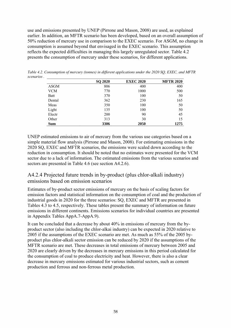
58

use and emissions presented by UNEP (Pirrone and Mason, 2008) are used, as explained earlier. In addition, an MFTR scenario has been developed, based on an overall assumption of 50% reduction of mercury use in comparison to the EXEC scenario. For ASGM, no change in consumption is assumed beyond that envisaged in the EXEC scenario. This assumption reflects the expected difficulties in managing this largely unregulated sector. Table 4.2 presents the consumption of mercury under these scenarios, for different applications.

Table 4.2. Consumption of mercury (tonnes) in different applications under the 2020 SQ, EXEC, and MFTR scenarios .

SQ 2020 EXEC 2020 MFTR 2020 ASGM 806 400 400 VCM 770 1000 500 Batt 370 100 50 Dental 362 230 165 Meas 350 100 50 Light 135 100 50 Electr 200 90 45 Other 313 30 15 Sum 3306 2050 1275

UNEP estimated emissions to air of mercury from the various use categories based on a simple material flow analysis (Pirrone and Mason, 2008). For estimating emissions in the 2020 SQ, EXEC and MFTR scenarios, the emissions were scaled down according to the reduction in consumption. It should be noted that no estimates were presented for the VCM sector due to a lack of information. The estimated emissions from the various scenarios and sectors are presented in Table 4.6 (see section A4.2.6).

A4.2.4 Projected future trends in by-product (plus chlor-alkali industry) emissions based on emission scenarios Estimates of by-product sector emissions of mercury on the basis of scaling factors for emission factors and statistical information on the consumption of coal and the production of industrial goods in 2020 for the three scenarios: SQ, EXEC and MFTR are presented in Tables 4.3 to 4.5, respectively. These tables present the summary of information on future emissions in different continents. Emissions scenarios for individual countries are presented in Appendix Tables AppA.7-AppA.9).

It can be concluded that a decrease by about 40% in emissions of mercury from the by-product sector (also including the chlor-alkai industry) can be expected in 2020 relative to 2005 if the assumptions of the EXEC scenario are met. As much as 55% of the 2005 by-product plus chlor-alkali sector emission can be reduced by 2020 if the assumptions of the MFTR scenario are met. These decreases in total emissions of mercury between 2005 and 2020 are clearly driven by the decreases in mercury emissions in this period calculated for the consumption of coal to produce electricity and heat. However, there is also a clear decrease in mercury emissions estimated for various industrial sectors, such as cement production and ferrous and non-ferrous metal production.

59

Table 4.3. Mercury by-product emissions from anthropogenic sources worldwide for the SQ scenario in 2020 (tonnes).

Region Station-ary combust-ion

Non- ferrous metals product-ion

Pig iron and steel product-ion

Cement product-ion

Gold product-ion

Mercury product-ion (primary sources)

Waste incinerat-ion*

Caustic soda product-ion

Other sources

Total

Africa 44.5 2.1 1.6 16.4 8.9 0.0 0.6 0.0 0.0 74.1

Asia (excluding Russia)

927.5 90.0 24.1 206.6 58.9 8.8 5.7 0.0 0.6 1322.0

Europe (excluding Russia)

76.6 18.7 27.8 0.0 0.0 10.1 0.0 14.7 147.9

North America

71.2 5.7 14.4 16.3 12.9 0.0 15.1 0.0 7.2 142.8

Oceania 19.0 6.1 0.8 0.6 10.1 0.0 0.0 0.0 0.0 36.6

Russia 51.8 5.2 2.6 5.8 4.3 0.0 3.5 0.0 1.5 74.8

South America

11.0 13.6 1.8 9.5 16.2 0.0 0.0 0.0 1.5 53.6

World 1201.5 141.3 45.4 283.0 111.3 8.8 35.0 0.0 25.5 1851.9

Table 4.4. Mercury by-product emissions from anthropogenic sources worldwide for the EXEC scenario in 2020 (tonnes).

Region Station-ary combust-ion

Non- ferrous metals product-ion

Pig iron and steel product-ion

Cement product-ion

Gold product-ion

Mercury product-ion (primary sources)

Waste incinerat-ion*

Caustic soda product-ion

Other sources

Total

Africa 19.8 0.9 0.6 4.8 8.9 0.0 0.1 0.0 0.0 35.0

Asia (excluding Russia)

411.8 32.6 8.7 60.6 58.9 8.8 1.2 0.0 0.6 583.2

Europe (excluding Russia)

48.5 7.3

8.3 0.0 0.0 2.1 0.0 14.7 80.8

North America

31.6 1.5 5.0 4.8 12.9 0.0 3.2 0.0 7.2 66.2

Oceania 8.4 2.2 0.3 0.2 10.1 0.0 0.0 0.0 0.0 21.2

Russia 20.4 1.9 1.0 1.7 4.3 0.0 0.7 0.0 1.5 31.5

South America

4.9 4.9 0.7 2.8 16.2 0.0 0.0 0.0 1.5 31.0

World 545.4 53.6 17.4 83.2 111.3 8.8 7.3 0.0 25.5 852.3

60

Table 4.5. Mercury by-product emissions from anthropogenic sources worldwide for the MFTR scenario in 2020 (tonnes).

Region Station-ary combust-ion

Non- ferrous metals product-ion

Pig iron and steel product-ion

Cement product-ion

Gold product-ion

Mercury product-ion (primary sources)

Waste incinerat-ion*

Caustic soda product-ion

Other sources

Total

Africa 14.4 0.6 0.4 3.5 8.9 0.0 0.1 0.0 0.0 27.9

Asia (excluding Russia)

300.4 23.8 6.4 44.2 58.9 8.8 0.9 0.0 0.6 443.9

Europe (excluding Russia)

42.4 5.3 6.0 0.0 0.0 1.5 0.0 14.7 70.0

North America

23.1 1.5 3.8 3.5 12.9 0.0 2.3 0.0 7.2 54.3

Oceania 6.1 1.6 0.2 0.1 10.1 0.0 0.0 0.0 0.0 18.2

Russia 14.9 1.4 0.7 1.3 4.3 0.0 0.5 0.0 1.5 24.6

South America

3.6 3.6 0.5 2.0 16.2 0.0 0.0 0.0 1.5 27.4

World 404.8 37.7 12.0 60.7 111.3 8.8 5.3 0.0 25.5 666.1

It should be cautioned, however, that the emission estimates in 2020 are based on the scaling of emission factors in the period from 2005 and 2020 estimated for the conditions in Europe. It has been assumed that the production technology and emission control installations in power plants, cement kilns, ferrous metal foundaries, and non-ferrous metal smelters will be similar to those in Europe. This indirectly assumes that environmental legislation introduced in Europe now and in the near future will be acceptable in the year 2020 in other parts of the globe. Although the authors of this report see no reason why this assumption should not be technologically feasible in the current era of industrial globalization it is clear that the scenarios are unlikely to be ‘realistic’ given geo-political and economic realities. The scenarios do however, domonstrate the possible implications of ‘taking actions’ as opposed to ‘doing nothing’.

A4.2.5 Discussion of results by region Changes in mercury emissions from by-product and chlor-alkali industry sources between 2005 and 2020 for different regions are presented in Figure 4.3.

If no major changes in the efficiency of emission control are introduced (the SQ scenario), significant increases in global anthropogenic mercury emissions (equivalent to about one quarter of the 2005 mercury emissions from these sectors) are expected in 2020. It is estimated that the largest increase in emissions of mercury will be for stationary combustion, mainly from combustion of coal. A comparison of the 2020 emissions estimated from the EXEC scenario and the SQ scenario indicates that a further 1000

61

tonnes of mercury could be emitted globally on top of the projected emission of 850 tonnes (under the EXEC scenario) in 2020, if mercury continues to be emitted under the control measures and practices that are in operation today against a background of increasing population and economic growth in some regions. In other words, the implementation of available measures and practices (the basic assumption of the EXEC scenario for reducing mercury emissions in the period to 2020), could result in a benefit of reducing mercury emissions by 1000 tonnes per year by 2020. Doing nothing to improve reduction of mercury emissions is projected to result in emissions in 2020 that are more than 100% above those envisaged under the EXEC scenario. An even greater increase is projected if the 2020 SQ scenario is compared with the 2020 MFTR emission reduction scenario. Emissions of mercury in various industrial sectors, such as cement production and metal manufacturing by the year 2020 could be 2- to 3-fold higher than if nothing is done to improve emission control in comparison to the emissions envisaged under the EXEC scenario.

Figure 4.3. Comparison of anthropogenic emissions (in tonnes per year) of mercury from the ‘by-product’ plus chlor-alkali sectors in 2005 and under the 2020 SQ, EXEC and MFTR scenarios.

62

Under the EXEC scenario, clear decreases in mercury emissions between 2005 and 2020 are projected for all continents. As might be expected, the largest emissions of mercury in 2020 are estimated for Asia. The 2005 emissions in China of almost 635 tonnes (see Appendix Table AppA.7) could decrease in 2020 to between 380 tonnes (under the EXEC scenario) and 290 tonnes (under the MFTR scenario). Thus, the reduction in Chinese emissions could be between 40 and 55%. This decrease assumes that by 2020, all Chinese power plants will be equipped with improved emission control installations. These projections also assume that consumption of coal will increase in China between 2005 and 2020 by a factor of 2, and industrial production by a factor 1.5.

It should be recognized that the projections described for China are based on rigorous implementation of emission reduction measures, particularly those concerning major improvement in the efficiency of installed emission controls. If the improvement is for example 50% lower than assumed under the scenarios, Chinese emissions will increase rather than decrease by 2020 (i.e., would not compensate for the projected increase in emissions due to economic development). A more detailed pre-feasibility study would need to be carried out, however, on the potential for the improvement of efficiency of control equipment and its utilization in power stations and industrial plants in China and other countries, also addressing economic aspects, in order to define more accurately conclusions and eventual recommendations on how the potential improvement described above might be achieved.

For India, similar assumptions as those applied to China were made when scaling emission factors on the basis of projections for improvement of efficiency of emission control installations in Indian power stations and industrial plants by 2020.

The projected decreases in mercury emissions in Europe, North America, Australia and Russia are expected to be between 40 and 60%.

Similar analyses can be presented for any country using the information presented in the Appendix tables with the information on emission scenarios.

A4.2.6 Future scenarios for emissions from product use, cremation and artisanal gold mining This report includes a provisional first attempt to estimate global emissions of mercury from product use, cremation and artisanal gold mining. Very few data exist to support the development of future scenarios for these emission categories. Increased global supply of mercury may lead to increased emissions via several routes, but if recycling and safe handling is implemented in more regions, emissions may decrease or stabilize. Another critical issue is management of household, medical and industrial waste. For emissions related to product use of mercury, the waste sector is responsible for the major part of the emissions, and better waste management, recycling and controlled incineration or landfill disposal can reduce mercury emissions substantially. For artisanal gold mining the use of mercury is likely to continue or increase since it is driven by poverty. Even if mercury supply is decreased, for example via restricting export and trade from Europe, illegal trade may replace this mercury and new or previously active mercury mines may be reopened. ASGM emissions reductions are only likely to occur if emission control efforts or associated activities to provide alternative means of income result in tangible benefits (both to health but in particular economic) to those engaged in these activities.

Table 4.6 presents projected future trends for emissions from intentional use of mercury.

63

Table 4.6. Emissions of mercury from intentional use in three 2020 emission scenarios.

SQ 2020 EXEC 2020 MFTR 2020 ASGM 330 164 164 VCM N.A. N.A. N.A. Batt 20 5 3 Dent 25 16 11 Meas 33 9 5 Lamp 13 9 5 Elec 26 11 6 Other 29 3 1 Sum 475 218 195

N.A. = not available

It should be noted that the scenarios presented above are hypothetical and the future trends in mercury consumption are highly dependent on the development of legislation or voluntary agreements to reduce mercury usage. The reduction potential is large, perhaps even larger than that reflected in the MFTR scenario in some cases, but actual compliance is difficult to estimate. For these reasons, the scenario estimates presented here are not considered robust enough for presentation as projections in the same manner as those calculated for the by-product sectors.

64

Part B: Atmospheric Pathways, Transport and Fate Authors:

Henrik Skov, National Environmental Research Institute (NERI), Denmark (Chapters B5 and B6)

Oleg Travnikov, EMEP Meteorological Synthesizing Centre - East, Russia (Chapter B7)

Ashu Dastoor, Meteorological Service of Canada, Canada (Chapter B7)

Co-authors:

Russel Bullock, US-Environmental Protection Agency, USA (Section B7.5)

Jesper Christensen, National Environmental Research Institute (NERI), Denmark (Chapters B5, B6 and B7)

Lise Lotte Sørensen, National Environmental Research Institute (NERI), Denmark (Chapters B5 and B6)

Collaborators/Contributors:

Eric M. Prestbo (Canada)

David A. Gay (USA)

65

B5. Atmospheric pathways

B5.1 Atmospheric reactions This chapter describes the pathways of mercury (Hg) in the atmosphere, addressing physical and chemical processes determining the dynamics and fate of mercury.

In a general global budget for mercury in the environment proposed by Sunderland and Mason (2007), some 6000 t/yr of mercury are emitted to the atmosphere, whereas only 600 t/yr are transported via rivers to the sea. The atmosphere therefore represents the dominant fast pathway for the transport of mercury in the environment.

Most mercury is emitted to the atmosphere in the form of gaseous elemental mercury (GEM), with minor amounts emitted as oxidized mercury either as oxidized mercury in the gas phase (also termed reactive gaseous mercury; RGM) or as oxidized mercury associated with particles (total particulate mercury; TPM). GEM has a relatively long lifetime in the atmosphere (currently believed to be between 0.5 and 1.5 years), being slowly oxidized to either RGM or TPM (see Figure 5.1), and thus mercury is ubiquitous in the troposphere. RGM and TPM have much shorter lifetimes (hours to days) and are therefore subject to fast removal by wet or dry deposition. Consequently, the RGM and TPM emitted from primary sources tends to be regional in its effect (i.e., tends to be deposited closer to sources), although under certain conditions some TPM may be subject to long-range transport.

The chemistry of mercury in the troposphere is complex and involves both gas phase reactions and aqueous phase reactions. In comprehensive reviews (Calvert and Lindberg, 2005; Lin et al., 2006; Ariya et al., 2008; Steffen et al., 2008) information from studies concerning the most important reactions of GEM have been compiled, and this is summarized in the Tables in Appendix B.

Most studies present data on reaction kinetics only, with few studies (e.g., Pal and Ariya, 2004a,b) addressing reaction products and mechanisms. The lack of product identification adds an extra element of uncertainty to the description of the dynamics of atmospheric mercury. Furthermore, only four groups have studied the temperature dependence of the reactions (see Appendix B) and in general these focus only on the first step of the reaction sequences.

The atmospheric reactions of mercury are critical to determining how mercury is transported in the atmosphere and where it is deposited. As previously stated, the long lifetime of GEM makes it a global pollutant, whereas RGM and TPM are deposited locally or regionally. Because of the local removal of RGM and TPM, the highest depositions of mercury are found close to emission sources in Europe, North America and East Asia (Christensen et al., 2004; Dastoor and Larocque, 2004).

There is ongoing scientific debate about the reactions that may be responsible for removing GEM from the atmosphere and large efforts have been devoted to the study of the chemical removal of GEM.

66

Figure 5.1. Schematic description of emission, chemical transformation and deposition of atmospheric mercury.

Experimental evidence has shown that oxidants like ozone (O3) and hydroxyl radical (OH) can be important reactants for the removal of GEM (Hall, 1995; Sommar et al., 2001; Pal and Ariya, 2004a,b; Sumner et al., 2005). Ozone is produced photo-chemically from the reaction between hydrocarbons and nitrogen oxides from both anthropogenic and natural sources. However, these studies only focus on the first step of the reaction sequences leading to RGM and so may overestimate the conversion of GEM to RGM (Goodsite et al., 2004; Calvert and Lindberg, 2005; Ariya et al., 2007). GEM may also be transported to particles and oxidized by O3 in the particles (Munthe, 1992). The reaction with OH is leading to an HgOH intermediate. This intermediate was found to be short-lived and thermal decomposition could be its dominating fate, which indicates that the reaction with OH is of minor importance (Calvert and Lindberg, 2005; Goodsite et al., 2004). The direct reaction between O3 and GEM to form HgO is endothermic and thus is not occurring in the atmosphere (Calvert and Lindberg, 2005). However, Hg might still react with O3 to form an HgO3 intermediate that can react further, for example heterogeneously. This discussion is based on limited scientific data and more investigations are needed.

The gas phase reaction of GEM with bromine (Br) is emerging as an important reaction in the global atmosphere. This reaction starts a sequence of reactions that eventually lead to RGM. The reaction sequence is temperature-dependent (Goodsite et al., 2004) and the fastest removal of GEM is observed under cold conditions such as those prevailing at the poles or in the upper part of the troposphere, whereas much longer lifetimes are found at warmer temperatures. In the background troposphere only small fluctuations in GEM concentrations are observed (Kim and Kim, 1996; Ebinghaus et al., 2002; Weiss-Penzias et al., 2003), which agrees well with a relatively long atmospheric lifetime of Hg obtained in a model study (Holmes et al., 2006). Bromine atoms can be produced from a number of sources: one is sea spray and is thus connected to the marine boundary layer; a second source is refreezing leads (open water areas in sea ice or between sea ice and the shore) during polar spring, where Br2 is released from bromide-enriched sea-ice surfaces. Thirdly, Br can be produced in the upper part of the troposphere from the photolysis of organo-bromides.

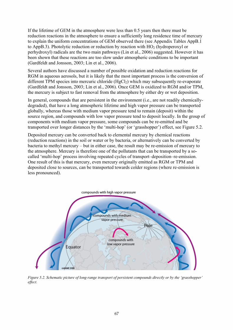
67

If the lifetime of GEM in the atmosphere were less than 0.5 years then there must be reduction reactions in the atmosphere to ensure a sufficiently long residence time of mercury to explain the uniform concentrations of GEM observed there (see Appendix Tables AppB.1 to AppB.3). Photolytic reduction or reduction by reaction with HO2 (hydroperoxyl or perhydroxyl) radicals are the two main pathways (Lin et al., 2006) suggested. However it has been shown that these reactions are too slow under atmospheric conditions to be important (Gardfeldt and Jonsson, 2003; Lin et al., 2006).

Several authors have discussed a number of possible oxidation and reduction reactions for RGM in aqueous aerosols, but it is likely that the most important process is the conversion of different TPM species into mercuric chloride (HgCl2) which may subsequently re-evaporate (Gardfeldt and Jonsson, 2003; Lin et al., 2006). Once GEM is oxidized to RGM and/or TPM, the mercury is subject to fast removal from the atmosphere by either dry or wet deposition.

In general, compounds that are persistent in the environment (i.e., are not readily chemically-degraded), that have a long atmospheric lifetime and high vapor pressure can be transported globally, whereas those with medium vapor pressure tend to remain (deposit) within the source region, and compounds with low vapor pressure tend to deposit locally. In the group of components with medium vapor pressure, some compounds can be re-emitted and be transported over longer distances by the ‘multi-hop’ (or ‘grasshopper’) effect, see Figure 5.2.

Deposited mercury can be converted back to elemental mercury by chemical reactions (reduction reactions) in the soil or water or by bacteria, or alternatively can be converted by bacteria to methyl mercury – but in either case, the result may be re-emission of mercury to the atmosphere. Mercury is therefore one of the pollutants that can be transported by a so-called ‘multi-hop’ process involving repeated cycles of transport–deposition–re-emission. One result of this is that mercury, even mercury originally emitted as RGM or TPM and deposited close to sources, can be transported towards colder regions (where re-emission is less pronounced).

Figure 5.2. Schematic picture of long-range transport of persistent compounds directly or by the ‘grasshopper’ effect.

68

B5.1.1 Polar Regions In 1998, Schroeder and co-workers published results from Alert, Canada showing GEM being depleted from the atmosphere close to the surface in episodes during polar springtime (Schroeder et al., 1998). These episodes were therefore termed atmospheric mercury depletion events (AMDEs). AMDEs were observed to occur together with depletion of ozone, which had been observed for the first time some years earlier (Barrie et al., 1988). These observations led to a series of laboratory, field and theoretical studies of possible reactions of GEM, and today there is no doubt that the principal reaction in AMDEs is between GEM and Br. In the Arctic, the lifetime of GEM is about 10 hours because the reactions initiated by Br are faster at low temperature. This lifetime corresponds to a Br concentration of 0.7 pptv at an average temperature of 245 K (Goodsite et al., 2004), which is well within the range of Br concentrations of 0.2 to 6 pptv that were observed (Tuckermann et al., 1997). The bromine-initiated reactions lead to RGM (Lindberg et al., 2002; Brooks et al., 2006a) or TPM (Steffen et al., 2003) formation, the RGM and/or TPM being then (rapidly) removed to the surface, from which it may be subsequently re-emitted.

The production of atmospheric Br is closely connected to refreezing leads where bromide is pushed out to the surfaces during the refreeze of seawater, see Figure 5.2. AMDEs are only observed when the temperature is below −4 °C over sea ice and when solar light is present (Lindberg et al., 2002).

These reactions between mercury and Br occur in marine-influenced air, thus deposition of mercury is enhanced in Arctic coastal areas during polar springtime (Douglas et al., 2005). It has been estimated that AMDEs enhance the deposition of mercury in polar regions by about 120 t/yr, from 80 t/year that would be expected from normal deposition, to about 200 t/yr (see also section B7).

Hg-HumHgS(HS)Hg(HS)2

Hg(Sn)HS-

Hg-HumHgCln

(n-2)-

Hg(OH)2

HgCIOH

CH3Hg+

Hgo

Hgo

Hgo

Cx + Hgo

Hg(II)Hgo

CH3HgOHCH3HgCl

(CH3)2Hg

Hg(II)

H2S

HgS(S)CH3Hg+

(CH3)2Hg CO2, CH4 + Hg(II)

Algal

Metabolites

Cat

alas

e

Oxidative

Process

Plankton

merB

merA

Snow

Sea ice

Snow

Sea ice

OceanSurface

Frost flowers

Longe range transport

Oxic Water

Anoxic Waters& Sediments

Br2HgBr2

HgoBr

Figure 5.3. Schematic description of atmospheric mercury depletion events followed by a possible uptake of mercury in the food web by copepods followed by bioaccumulation.

69

Figure 5.3 illustrates the processes of AMDE in the atmosphere and the possible fate of mercury after it is deposited. A central issue in relation to the mercury cycle and also for potential impacts on biota is how much of the deposited mercury enters the food web, how much is removed to sediments, and how much is re-emitted to the atmosphere. This is still the subject of scientific debate and study with estimates of the amount of deposited mercury that is re-emitted currently ranging from ca. 20 to 95% (Aspmo et al., 2006; Brooks et al., 2006a; Steffen et al., 2008). High levels of mercury have been observed in snow at Barrow, Alert and Ny-Ålesund following AMDEs but these decrease strongly after the AMDEs (Aspmo et al., 2006). AMDEs are nearly always followed by periods where the GEM signal is elevated; which is assumed to reflect re-emission. Different opinions regarding the extent to which deposited mercury is re-emitted may reflect geographical differences within the Arctic.

B5.1.2 Mid- and equatorial latitudes In the marine boundary layer, bromine is produced from sea spray. At a temperature above 290 K and Br concentrations of 0.1 ppt typical for the marine boundary layer at mid-latitudes this corresponds to an atmospheric lifetime for GEM of more than 4000 hours (ca. 0.45 years) and thus Br has the potential to be the most important oxidant for the removal of GEM from the atmosphere.

The photochemical degradation of organo-bromides increases with height, and organo-bromides are the dominant Br source above an altitude corresponding to 300 hPa. The source strength and mechanisms are discussed by Yang et al. (2005) together with the geographical distribution of bromine sources and bromine compounds. The parameterization of atmospheric bromine compounds is thus very important for a reliable description of the dynamics of atmospheric mercury. Yang and co-workers found the uncertainty to be a factor of 2 for the description of the formation of sea salt particles alone.

Based on this information, it can be concluded that the gas phase reactions of GEM with Br most probably control the atmospheric lifetime of atmospheric mercury outside the polar regions. In the background troposphere, only small fluctuations in GEM concentrations are observed (Kim and Kim, 1996; Ebinghaus et al., 2002; Weiss-Penzias et al., 2003), which agrees well with the relatively long atmospheric lifetime of mercury obtained by Holmes et al. (2006). However, it has to be noted that there are still large uncertainties in the description of the GEM oxidation process and there is a strong need for experimental studies of the reactions between GEM and atmospheric oxidants.

B5.1.3 Continental air masses and free troposphere Hydrocarbons and nitrogen oxides (NOX) have their highest levels in continental air masses and this leads to the formation of the highest levels of both OH and O3 in the troposphere. Bromine has a number of different sources including coal burning, biomass burning and wildfires. These sources are not well described in the literature and little is known about how chemically-active bromine from these sources is. High levels of OH and O3 are often observed together with elevated levels of particles, and this may enhance the importance of heterogeneous processes. Mercury has to undergo phase transfers which are dependent on various equilibriums. Appendix Tables AppB.4 and AppB.5 list constants for phase transfer for some mercury species. GEM is the only mercury species that is identified in air, whereas other species in the table represent candidate species for the RGM and TPM fractions. Thus, the phase transfer is not well described, and the list presents only the range of constants that may be expected for the compounds that may constitute RGM and TPM.

70

B5.1.4 Conclusions Although there has been a substantial gain in knowledge about the dynamics of mercury in the atmosphere in recent years, the previous discussion clearly illustrates the large uncertainty that exists in the description of the chemical removal of GEM from the atmosphere. At present there are some questions that it is not possible to answer; other questions that may be possible to answer have yet to be resolved – doubtless, there are also other questions that have yet to be formulated.

For example the identity of RGM (i.e., the exact mercury species and compounds that constitute RGM) is still not known, and might be different depending on the history of the RGM. Knowledge of the exact composition of RGM is very important for estimating its removal rate through wet and dry deposition, and also for understanding the further fate of mercury, for example its availability for uptake into biological systems.

As this chemistry is central to an understanding of the transport patterns of mercury, this lack of knowledge presents considerable problems in the construction of atmospheric chemical and physical models. Field measurements are therefore of particular importance as they allow models to be validated and can be used to constrain models.

The large uncertainty in the chemistry of mercury makes field measurements very important when describing the transport of mercury using models; these measurements can serve to constrain the models and to check that models produce results that are consistent with reality.

The annual average concentration of GEM observed in the European and North American troposphere at background sites (i.e., unaffected by local sources) is between 1.5 and 1.7 ng/m3; slightly higher than but similar to the 1.2 to 1.4 ng/m3 found at sites in the southern hemisphere (e.g., the monitoring site in South Africa). In East Asia, the regional value for GEM is higher, with a mean of close to 4 ng/m3 (Kim, 2004) thought to reflect proximity to the major emission sources in the Asian region. Close to sources, higher levels of GEM are measured and concentrations of up to 5 µg/m3 (5000 ng/m3) have been measured at Almaden, Spain close to an old silver mine (Ferrara et al., 1998).

By comparison, RGM concentrations in Europe and North America (south of the Arctic) are found at levels of up to around 40 pg/m3, and TPM at levels up to around 60 pg/m3 (Wangberg et al., 2001).

The highest levels of RGM have been measured at Point Barrow, Alaska, at around 1000 pg/m3 (Brooks et al., 2006a). In another Arctic study, at Alert, Canada, the maximum levels of RGM measured were around 40 pg/m3, and TPM around 100 pg/m3 (Cobbett et al., 2007).

B5.2 Atmospheric transport and surface fluxes Concentrations of mercury in the atmosphere are normally too low to represent any risk of adverse health effects for humans. The concern over mercury in the atmosphere is primarily related to its potential to be transported over long distances and that, following deposition, it can be taken up by biota. Mercury can bioaccumulate and biomagnify in food webs, particularly aquatic food webs, to levels that can be harmful to organisms, including humans. This can result in pollution problems in otherwise clean environments far from source areas, as has been documented in the Arctic (AMAP, 1998, 2005). The fact that mercury can be re-emitted (see later sections) means that the transport pattern is complex. Consequently, it is important to investigate the surface-related chemistry of mercury by determining the fluxes of different mercury species over different surfaces.

Since most mercury is emitted to the atmosphere in the form of GEM, and because GEM is

71

slowly oxidized it enters the global ‘atmospheric pool’ and can be transported worldwide. GEM is therefore found at similar concentrations throughout the troposphere. The oxidation products RGM or TPM are deposited locally, or at most regionally. Once RGM is deposited it may be reduced to GEM, either by microbiological activities or by photo-reduction, or it may be methylated by bacteria to become, for example, Hg(CH3)2 (dimethylmercury). In either case, the mercury may then be re-emitted to the atmosphere with the result that the mercury may undergo long-range transport via the ‘grasshopper’ effect. Consequently, surface processes must be included in the description of atmospheric mercury chemistry. Additionally, the primary emitted RGM and TPM may also be reduced following deposition.

It is important to understand that RGM and TPM are fractions of mercury that are operationally defined by the analytical methods. Primary emitted RGM and TPM are therefore not necessarily the same mercury species as the RGM and TPM that is present elsewhere in the atmosphere.

A number of studies have been conducted in the northern hemisphere on wet deposition of mercury (Iverfeldt, 1991; Hall et al., 2005; Sakata et al., 2006). In areas with frequent precipitation, wet deposition dominates. In more arid climates, dry deposition is the dominating deposition processes, as found for example in (high latitude) polar regions. Measurements of wet deposition are available and well documented.

Several groups have studied dry deposition, as well as (re)emission of GEM with either micrometeorological methods (gradient or relaxed eddy accumulation) (Lyman et al., 2007; Steffen et al., 2008) or by enclosure methods (Lindberg et al., 2002, and others), but the fate of atmospheric mercury is largely determined by the deposition of RGM. There is only one study in the literature of the deposition of RGM (Skov et al., 2006). The overall conclusion of these limited studies is that the chemistry within or at the surface layer is very important for the budget and global circulation of mercury. Several studies have looked at the specific reactions within and on various surfaces and have found that fast reduction reactions may reduce oxidized mercury (HgII) to elemental mercury that is afterwards emitted as GEM (Dommergue et al., 2003; Lalonde et al., 2003; Ferrari et al., 2004; Fritsche et al., 2008).

B5.3 Impact of Global change Available information on the global mercury cycle shows that mercury is in a relatively fast equilibrium between the atmosphere and ocean surface waters (tens of years) but slower with the deep ocean waters (hundreds of years) (Lamborg et al., 2002b; Mason et al., 2003; Sunderland and Mason, 2007). In a recent study by Sunderland and Mason (2007), anthropogenic emissions were found to have enriched the atmosphere by 300 to 500%, all surfaces by 25%, and deep ocean waters by 11%. The lag between changes in atmospheric deposition and seawater mercury concentrations was found to vary from decades in most of the Atlantic to centuries in parts of the Pacific (Sunderland and Mason, 2007). Many of the processes in the mercury cycle are temperature-dependent or involve parameters that might change in a changing climate. Temperature changes may affect rates of reactions involving mercury species or reactions that determine the composition of possible reactants. In addition, changes in vegetation, land-use or, for example, the populations of bacteria in the sea may affect the mercury cycle. A thaw of the Arctic tundra could liberate large reservoirs of mercury; a change in humidity or precipitation patterns could lead to more wildfires that are known sources of atmospheric mercury. AMDEs are dependent on the presence of refreezing leads, and their geographical extent is likely to change with higher temperatures in the Arctic and Antarctic (Macdonald et al., 2005; Brooks et al., 2006a); higher ocean temperatures are likely to increase the (re)emissions of volatile mercury species, and changed temperatures

72

may also change the chemical reactions that occur in the atmosphere.

In relation to anthropogenic emissions, future choices regarding energy sources also need to be taken into account. If coal combustion replaces oil it will lead to an increase in anthropogenic mercury emission to the atmosphere. Conversely, if fossil fuel combustion is replaced by ‘clean’ energy sources such as wind/wave or solar energy, mercury emissions will decrease.

The potential effects are many, and can drive the environmental mercury cycle in different directions. Consequently, it is not possible to say whether the combined effect of all these changes will increase or reduce the concentrations of mercury in the atmosphere.

The large gaps in the knowledge of processes controlling atmospheric mercury means that there are large uncertainties connected to the assessment of future atmospheric mercury concentrations and fluxes. The future response of the atmospheric mercury cycle to climatic change is thus a priority issue for both the scientific community and society in general (see chapter B7 for further discussion of climate impact on mercury levels in the environment).

B6 Environmental fate and trends

B6.1 Environmental monitoring networks Several long-term mercury monitoring networks have been established. Historically most of the measurements of mercury have been of wet deposition of mercury (Iverfeldt, 1991). Later GEM concentrations have also been measured, Figure 6.1 and 6.2. Only recently have the remaining fractions of mercury; RGM and TPM, been measured and then only in short campaigns.

In North America, continuous measurements of GEM are carried out within the Canadian Atmospheric Mercury Network (CAMNet). Measurements are carried out at both remote locations and close to local sources. In the United States, the focus has been on local and regional sources and thus there are few remote stations. Monitoring sites were established in Mexico in 2002. Additional measurements of mercury in precipitation are conducted under the Mercury Deposition Network (MDN), where the Canadian component is also a part of CAMNet.

In Europe, monitoring of mercury concentrations and depositions are carried out within the framework of the Cooperative Programme for Monitoring and Evaluation of the Long-range Transmission of Air Pollutants in Europe (EMEP).

The Arctic Monitoring and Assessment Programme (AMAP) is responsible for a coordinated air monitoring program, established in 1991, that covers the circum-Arctic areas of North America and Eurasia.

In Asia, stations have been established to study local and regional sources in China, South Korea and Japan. In the southern hemisphere there are very few measurements. One exception is the recently established monitoring station at Cape Point in South Africa.

Apart from these networks and recently established monitoring sites, several shorter or longer field campaigns have been carried out.

The background concentration of GEM in the northern hemisphere is between 1.5 and 1.7 ng/m3 and between 1.1 and 1.3 ng/m3 in the southern hemisphere (Lindberg et al., 2007). This can be seen in Figure 6.1 and Figure 6.2. These figures show monthly mean concentrations of

73

GEM at Mace Head, Ireland and Cape Point, South Africa, respectively.

As mentioned in section B5, levels of RGM and TPM are much lower than GEM; RGM and TPM species are normally measured in tens of pg/m3 (as exemplified in Figure 6.8). An exception is the polar regions where high concentrations (>900 pg/m3) have been observed during AMDEs (Lindberg et al., 2002).

0

0.5

1

1.5

2

2.5

3

jun-94 okt-95 mar-97 jul-98 dec-99 apr-01 sep-02 jan-04 maj-05 okt-06

Time

GE

M, n

g m

-3

Figure 6.1. Monthly average concentrations of TGM measured from 1998 to 2004 at Mace head, Ireland (from: http://www.nilu.no/projects/ccc/emepdata.html). (GEM is here called TGM = Total Gaseous Mercury, which reflects ongoing discussion of the measurement of the fractions of atmospheric mercury as a method defined parameter).

Figure 6.2. Monthly mean averages of GEM (=TGM) from 1995 to 1999 at Cape Point, South Africa (Baker et al., 2002).

74

B6.2 Temporal trends derived from environmental measurements

B6.2.1 Environmental archives Even the longest established monitoring programs can only provide data on air concentrations and deposition of mercury for the last 15 to 20 years. Natural ‘environmental archives’ such as lake sediments, peat and ice cores are therefore the only link between current and past loadings to terrestrial and aquatic environments. These archives provide a useful means of reconstructing the atmospheric load on a local, regional and global scale (Biester et al., 2007 and references therein).

The differences between archive samples representing pre-industrial times and those from the present day are of particular interest as this can be considered to reflect the influence of anthropogenic sources on the pre-existing natural levels. In both peat cores and lake sediment cores, a clear increase in mercury concentrations is observed today compared to the pre-industrial period, though the magnitude of this increase is distinct in these two natural archive media. In sediments, the peak concentrations are found in samples dating to the 1970s to 1990s, in agreement with (relevant regional) emission inventories, whereas in peat cores the peaks are typically 10 to 20 years earlier (Biester et al., 2007). Neither of these two types of archive can be correlated directly to atmospheric deposition data. The maximum levels in peat are up to 400 higher than those found in sediments, although it might be expected that higher levels would be found in lake sediments as they receive both atmospheric deposition directly and accumulation from the surrounding catchments. Biester et al. (2007) pointed out that results from peat cores should be corrected for various processes that can alter the accumulation rate and dating (diagenesis, and for that 210Pb spreads through the uppermost peat layer). However, based on 14C analysis in macrofossils (and using the atomic bomb test signatures which have resulted in altered labile isotope loads to the environment) raised peat bogs have been demonstrated to be well suited for temporal trend analyses. Using these methods, the peat cores could be dated with a resolution of ± 2 years (Goodsite et al., 2001; Shotyk et al., 2003). The pre-industrial deposition flux was calculated to be 0.3 to 0.5 µg/m2/yr in Greenland, with maximum deposition fluxes reaching 164 µg/m2/yr and 184 µg/m2/yr in Denmark and Greenland, respectively, in samples dated to 1953. The deposition flux declined to 14 µg/m2/yr in 1994 (Shotyk et al., 2003), which is comparable to the deposition flux of 18 µg/m2/yr obtained by the Danish Eulerian Hemispheric Model (DEHM) (Christensen et al., 2004). Biester et al. (2007) proposed that since a lake can be considered a closed system, it can yield more internally consistent and less problematic results than those derived from peat cores. However, lake sediment concentrations also do not provide a direct estimate of atmospheric deposition because of the contribution derived from catchment run-off. Despite this, however, the 3-fold increase in mercury from pre-industrial times to the present day observed in lake sediments at sites around the world does indicate that this is a robust number and consistent with emission inventories (see section A3). This 3-fold increase is also obtained through results from a multi-compartment modeling approach (Sunderland and Mason, 2007). Ice cores have produced a similar result, with 70% of deposited mercury found to be of anthropogenic origin (Schuster et al., 2002).

Recently, Outridge et al. (2007) presented strong evidence that 78% of the increase in mercury in sediments from a High Arctic lake was due to changes in mercury fixation connected to changes in primary productivity due to climate change. Long-range transport of anthropogenic mercury could only account for 22% of the observed increase. Most investigations have been made in the northern hemisphere in North America and Europe from mid-latitudes to the High Arctic.

75

Information about the changes in the levels of mercury in the environment from pre-industrial times to the present day thus provides information about the increase in concentrations that is due to anthropogenic emissions. From historical (environmental) archives such as ice-, peat- and lake-sediment cores, a large increase in mercury deposition has been observed. Lake-sediment cores, for example, provide indications that the flux is now 3-fold greater than it was in the pre-industrial period. Although recent results from High Arctic lakes indicate that this increase may be due in part to an increase in mercury fixation connected to changes in primary productivity in the lakes, possibly in response to increasing temperature, the 3-fold increase appears to be fairly consistent at more southerly sites, and thus appears to be representative of the general trend in the northern hemisphere.

B6.2.2 Long-term monitoring programmes Anthropogenic emissions of mercury have changed dramatically during the last 70 years (Pacyna et al., 1995, 2006; Pacyna and Pacyna, 2002; Hylander and Meili, 2003), see also section A3. Emissions of mercury to the atmosphere have decreased in Europe and North America, whereas they have increased in East Asia. It is therefore important to see how concentrations and wet and dry deposition have responded to these changes.

Measurements of mercury in precipitation go back to the 1980s and both precipitation amount and concentrations of mercury in precipitation have been measured worldwide. Concentrations in Europe and North America have generally decreased as reflected in the monitoring time-series from Rörvik, Sweden (where concentrations in rain water have decreased from 50 µg/L in the late 1980s to about 15 µg/L in the early 2000s, see Figure 6.3) and Florida, United States (see Figure 6.4).

Figure 6.3. Annual wet deposition and annual average concentration in precipitation of mercury measured at Rörvik, Sweden (http://www.nilu.no/projects/ccc/emepdata.html).

0

5

10

15

20

25

30

1994 1996 1998 2000 2002 2004 2006 2008

Year

Dep

ositi

on, µ

g m

-2 y

r-1

0

5

10

15

20

25

30

Con

cent

ratio

n, n

g L-

1

Wet depostionConcentration

Figure 6.4. Annual wet deposition and annual average concentration in precipitation of mercury measured at Everglades, Florida, United States (http://nadp.sws.uiuc.edu/mdn/).

76

The decrease in concentrations of mercury in wet deposition between the late 1980s and the mid-1990s coincide with a decrease in European emissions, of RGM and TPM in particular (see Chapter 3). Although such regional decreases in concentration of mercury in air have been observed, the global background concentration of GEM in air has remained constant.

Long-term data for GEM (=TGM) are sparse. Therefore an attempt has been made to pool data so that global trends could be estimated (Slemr et al., 2003), see Figure 6.5. It has been pointed out that the high and strongly decreasing concentrations observed at the Rörvik location are likely to have been influenced by regional mercury sources, including emission changes in Eastern Europe (following the break-up of the former Soviet Union) (Lindberg et al., 2007). Thus the Rörvik station data are unrepresentative and should not be considered indicative for the global trend, although they do support a decreasing trend in European GEM levels as has also been reported by other authors (Slemr and Scheel, 1998). Excluding the Rörvik series, the measured levels of GEM are relatively stable over the period 1977 to 2002, with slightly higher GEM concentrations in the northern hemisphere than in the southern hemisphere, see also Figure 6.1 and 6.2.

Figure 6.5. Global trends of GEM (=TGM) (Lindberg et al., 2007) a) southern hemisphere and b) northern hemisphere. The data from Rörvik show the influence of reductions in regional sources (see also text).

Analyses of CAMNet data show that there has been a slight decrease in the GEM concentrations at most rural locations in the period from 1995 to 2005. Close to the population centers of Toronto and Montreal decreases of 17% and 13%, respectively were observed (Temme et al., 2007), which was attributed to changes in local emissions.

There are no long-term measurements of RGM and TPM in ambient air, however the mercury concentration measured in precipitation are mainly due to washout of RGM and TPM. In the data from Rörvik, Sweden (Figure 6.3), a strong decrease in mercury concentrations in precipitation was observed; from 52 ng/L to 15 ng/L between 1989 and 1993. Thereafter, the levels have remained relatively constant (with the exception of an isolated peak of 65 ng/L in 1995).

77

B6.2.3 Geographical distribution The previous sections present data from Europe and North America. In China the combustion of coal has increased the emissions of mercury to the atmosphere and today China is the largest contributor to mercury in the atmosphere (Wu et al., 2006), see also Chapter 3. In the past few years, a number of publications have addressed environmental levels of mercury in the Asian region, however, most data are from short field campaigns (Fu et al., 2008 and references therein). As expected, the only long-term measurements show enhanced levels when the monitoring sites are exposed to air masses originating from regional source areas. At Moxi base, in the Gongga Alpine in China, air concentrations up to 21 ng/m3 (geometrical mean 4 ng/m3) were observed (Fu et al., 2008). Some limited results from short-term measurements of GEM at urban (Beijing, Guangzhou), regional (Yangtze delta) and background (Mt. Waliguan) monitoring sites in China are also reported by Wang et al. (2007).

Geographical differences in northern hemisphere GEM levels were reviewed by Kim et al. (2005). Measurements from six monitoring stations were analyzed, see Table 6.1 and Figure 6.6. All stations considered represent rural background areas with the exception of the Seoul station (South Korea), where higher values are observed. AMDEs are clearly affecting the concentrations at Alert, Canada, where very low values are observed during the polar spring. Table 6.1. Station data used for the review of the geographical differences in the northern hemisphere (Kim et al., 2005).

Figure 6.6. Comparison of seasonal variation patterns of all monitoring stations. The upper plot shows results for all stations, whereas the lower plot excludes the SEL station (Kim et al., 2005).

Measurement period (Hourly) Continent Country Location Code Latitude Longitude Start End N Canada Point Petre PPT 43°50' N 77°09' W 1-Jan-97 31-Dec-00 33222 North America

Canada Egbert EGB 44°13' N 79°47' W 1-Jan-97 31-Dec-00 31449

Canada Burnt Island BNT 45°48' N 82°57' W 30-Apr-98 31-Dec-00 22069 Asia Korea Seoul SEL 37°28' N 127°02' E 18-Sep-97 21-Jun-02 26767 Arctic Canada Alert ALT 82°30' N 62°22' W 9-Jan-95 31-Dec-01 49196 Europe Ireland Mace Head MH 53°20' N 9°20' W 1-Jan-96 1-Nov-02 41039

78

Most observations of atmospheric mercury have been performed on land. Information about concentrations of mercury in the marine atmosphere are, however, very important for understanding the dynamics of atmospheric mercury, in particular if, as suggested in section B5, bromine from sea spray is a major oxidant responsible for the removal of GEM from the atmosphere. Figure 6.7 shows results from cruises in the Atlantic Ocean in 1996 and 1999 to 2001.

Figure 6.7. Marine concentrations of GEM (=TGM) in the Atlantic Ocean as function of latitude from four cruises (Temme et al., 2003).

A clear gradient is seen between the northern hemisphere and southern hemisphere, with the lowest values in the southern hemisphere as described in Section 6.1. Some very high concentrations were observed when one of the cruises passed Europe and were explained by the influence of European sources.

A cruise in the Mediterranean Sea measured low concentrations of RGM (<20 pg/m3), Figure 6.8.

Figure 6.8. Measured and modeled concentrations from the Mediterranean Sea in 2000 (Hedgecock et al., 2006).

79

Similar results were obtained at Florida where RGM concentrations also were low when the station received marine air masses (Malcolm et al., 2003).

B6.2.4 Vertical distribution of mercury fractions Few measurements have been carried out on the vertical profile of atmospheric mercury. Slightly lower GEM values (1.635±0.094 ng/m3 at 2500 m altitude) were obtained in the free troposphere above Germany compared to observations in the mixing layer at 900 m (1.77±0.101 ng/m3). The concentrations were evenly distributed over long distances, which agree well with a long atmospheric lifetime of GEM (Ebinghaus and Slemr, 2000). In recent articles, results showing lower concentrations of GEM with height provide evidence of bromine chemistry close to the tropopause (the layer that separates the troposphere and stratosphere) (Holmes et al., 2006; Radke et al., 2007). Brooks (pers. comm. 2007) also observed weak AMDEs on the Greenland Ice Sheet at Summit (3000 m altitude).

In the Arctic, strong vertical profiles of GEM have been observed by several authors, in agreement with the fast chemistry that occurs where GEM in surface air is depleted, however, background concentrations are already observed within a few tens of meters above the surface (Brooks et al., 2006a; Steffen et al., 2002, 2008).

B6.3 Climate impacts on future mercury levels Mercury in the atmosphere is dominated by long-lived GEM, as evident from the uniform distribution in the global background (as observed, for example, at remote sites, in the marine atmosphere, and in the free troposphere). Concentration profiles in peat, sediments and ice cores show that there is an increased deposition of mercury today compared to the pre-industrial period, with an apparent maximum in deposition occurring between the 1950s and the 1970s. There is a general qualitative agreement between the deposition profiles in environmental archives and emission inventories. Therefore, the observed temperature increases in recent years have probably had little effect on atmospheric mercury concentrations or depositions compared to the effect of anthropogenic emission changes. The major sources of mercury emission have also moved over the past two decades; from Europe and North America to Asia. As a consequence, GEM concentrations in Europe appear to have decreased, and it is to be expected that concentrations and depositions in Asia will increase. The interaction between emissions, mercury cycling and a changing climate are very complex and it is not known how a change in climate may affect mercury transport, its deposition and biological accumulation in the future.

B7. Modeling atmospheric transport and deposition Available measurements of mercury concentration in different media (e.g., ambient air, precipitation, seawater, snowpack, sediments) and air-surface exchange cannot cover all requirements of mercury environmental cycling research as well mercury pollution regulation on a global scale. First, current monitoring networks and field measurements are relatively scarce and cover limited parts of the globe: detailed long-term mercury measurements are available in North America, Europe, and the Arctic, with some observations available in Eastern Asia, and very few data available in the southern hemisphere. Second, measurement data have restricted abilities to characterize trans-boundary and intercontinental transport. Third, monitoring data alone cannot be used to evaluate long-term scenarios of mercury

80

pollution changes in future. The solution, to these and other problems, is to use numerical models of mercury dispersion and environmental cycling.

B7.1 Model types and methods Models used for the simulation of mercury atmospheric dispersion vary in their formulation and scope of coverage depending on the investigated problems. For evaluation of concentration and deposition in the immediate vicinity of large emission sources or in the urban environment local-scale models can be employed. They are mostly presented by simple Gaussian type or plume models. Application of these models is restricted to short distances from emission sources where the influence of global mercury background is relatively insignificant.

Regional or continent-scale models address atmospheric dispersion and trans-boundary transport within a continent or particular region. These models are usually applied for detailed simulation of mercury dispersion over large territories containing significant emission sources (e.g., Europe, North America, East Asia). Mercury depositions over such areas are mostly determined by regional emissions of short-lived mercury forms (RGM, Hg-P) but also by in situ oxidation of elemental mercury (Hg0) transported globally. Therefore, the regional modeling results depend to significant extent on the concentrations of mercury species imposed on the boundaries of the modeling domain.

To avoid such restrictions, as well as to generate estimates of global mercury dispersion and intercontinental transport, global transport models are applied. (Hemispheric models present an intermediate case between regional and global models because they cover mercury dispersion over one of the hemispheres but still have a lateral boundary along the equator.) Global and hemispheric models are commonly applied for long-term simulations (at least one or several years, including the model spin-up) but have lower spatial resolution than regional models.

Multi-media box models present a special case of mercury environmental modeling. Such models describe the cycling of mercury between different environmental reservoirs (e.g., atmosphere, ocean, soil, vegetation) in a simplified manner using a mass balance technique based on prescribed exchange rates between media or measurement data. This simple approach allows the simulation of the mercury cycle in the environment over very long periods (hundreds of years) and an evaluation of global mercury fluxes between media.

Characteristics of chemical transport models employed for evaluation of mercury dispersion and cycling in the environment are summarized in Table 7.1. As seen, the spatial coverage of available models varies from the global scale to particular continents and regions. Most regional models consider mercury dispersion over Europe (e.g., ADOM, EMEP-HM, MECAWEx) and North America (CMAQ, REMSAD, TEAM), with only one applied for East Asia (STEM-Hg). Spatial resolution varies from several geographical degrees (corresponding to several thousand kilometers near the equator) for global models to tens of kilometers for regional models. Local-scale models are not considered here.

The majority of dispersion models are focused on mercury fate in the atmosphere. The reason being the dynamic role of atmospheric deposition as a source of mercury input to most terrestrial and aquatic ecosystems, and subsequent human and wildlife exposure via the food chain. Only a few dispersion models (MECAWEx, GEOS-Chem) are coupled to a seawater model to take into account mercury fate in the aquatic media and air-sea exchange. The full mercury cycle in the environment is simulated by multi-media box models (MFM, GRIMM).

Most dispersion models consider the full chain of mercury processes in the atmosphere,

81

including emission from anthropogenic and natural sources, atmospheric transport, chemical transformations, and deposition to the terrestrial or oceanic surfaces. Some models also include re-emission of mercury to the atmosphere – as a part of inter-media exchange (coupled dispersion models) or in the form of parameterized indirect sources (e.g., EMEP-HM, GRAHM).

All the models (except the mass-balance box models) employ extensive chemical schemes describing transformations of mercury species in the atmosphere. Typically, they consider three gaseous species of mercury (Hg0, RGM, Hg-P) and a number of mercury species dissolved in cloud water. Most models include reactions of Hg0 oxidation by O3 and OH in the gaseous and aqueous phases. Some models also consider Hg0 oxidation by other reactants, such as hydrogen peroxide (H2O2) and halogens for example Br and Cl. In the aqueous phase along with the oxidation process the reverse process of HgII reduction to Hg0 is included via formation of sulfite complexes and reaction with hydroperoxy radical (HO2). Few models include explicit treatment of chemical transformations and air-surface exchange during AMDEs and halogen chemistry in the marine boundary layer (MBL). In the former case, rapid oxidation of Hg0 under certain conditions leads to a considerable increase in mercury deposition in the polar regions. In the latter case, fast reactions of mercury oxidation by halogen radicals result in significant enhancement of mercury exchange between the atmosphere and seawater. Discussion of the choice of mercury chemical reactions included in the models and their sensitivity analysis is presented in section B7.2.1.

Processes responsible for removal of mercury from the atmosphere include scavenging of gaseous, particulate and dissolved mercury species by precipitation (wet deposition) and deposition through interaction with the surface (dry deposition). All dispersion mercury models consider both processes. Wet deposition is commonly distinguished between in-cloud and below-cloud washout and is presented in the models using simplified scavenging coefficients or more complicated cloud microphysics techniques. Mercury species undergoing wet deposition include RGM, Hg-P and Hg species dissolved in cloud water. Gaseous Hg0 does not undergo direct scavenging by precipitation because of low solubility but can be washed out indirectly through its solution in cloud water.

The dry deposition process in contemporary atmospheric dispersion models is described using the resistance analogy method or prescribed dry deposition velocities. In the former case, dry deposition velocity is defined as the inverse sum of successive resistances (aerodynamic resistance, quasi-laminar sub-layer resistance, surface resistance) and describes the deposition process more accurately under different stability conditions. All mercury models consider dry deposition of two short-lived mercury species – RGM and Hg-P. In addition, some models explicitly simulate dry deposition of Hg0 to vegetated surfaces using a simple dry deposition velocity technique. Other models (mainly regional models) do not take into account this process assuming compensation of Hg0 dry deposition by re-emission of previously deposited mercury.

82

Table 7.1. Characteristics of chemical transport models employed for evaluation of mercury dispersion and cycling in the environment.

Aqueous agents Model Coverage

Typical horizontal

resolution(a) Media Gaseous oxidation

agents oxidation reduction AMD

E MBL Dry deposition

Wet deposition Reference

ADOM Europe 55×55 km2 Atmosphere O3 O3 SO3= no no RGM, Hg-P yes Petersen et al., 2001

CMAQ-Hg North America

8×8 km2 to 108×108

km2

Atmosphere O3, OH, H2O2, Cl O3, OH, Cl-

SO3=,

HO2, hν no no RGM, Hg-P yes Bullock and Brehme,

2002

DEHM Northern Hemispher

e

150×150/ 50×50 km2

Atmosphere O3 O3 SO3= yes no RGM, Hg-P yes Christensen et al., 2004

EMAP Europe 50×50 km2 Atmosphere O3, OH O3 SO3= no no RGM, Hg-P yes Syrakov, 1995

GRAHM Global Down to 1°×1°

Atmosphere O3, , Br, Cl O3, OH, Cl-

SO3= yes yes RGM, Hg-

P, Hg0 yes Dastoor and Larocque,

2004; Dastoor and Davignon, 2008

HYSPLIT North America

180×180 km2

Atmosphere O3, OH, H2O2, Cl O3, OH, Cl-

SO3= no no RGM, Hg-P yes Cohen et al., 2004

MSCE-HM N. Hemisph. /

Europe

2.5°×2.5°/ 50×50 km2

Atmosphere O3, OH, Cl O3, OH, Cl-

SO3= yes no RGM, Hg-

P, Hg0 yes Travnikov and Ilyin,

2005; Travnikov, 2005

REMSAD North America

36×36 km2 Atmosphere O3, OH, H2O2 O3, OH, Cl-

SO3=, HO2 no no RGM, Hg-P yes ICF, 2005

TEAM North America

100×100 km2

Atmosphere O3, OH, H2O2, Cl, HCl

O3, OH, Cl-

SO3=, HO2 no no RGM, Hg-

P, Hg0 yes Seigneur et al., 2004

CTM-Hg Global 8°×10° Atmosphere O3, OH, H2O2, Cl, HCl, Br

O3, OH, Cl-

SO3=, HO2 no yes RGM, Hg-

P, Hg0 yes Seigneur et al., 2004

GEOS-Chem Global 4°×5° Atmosphere, seawater

O3, OH O3, OH, Cl-

hν no no RGM, Hg-P, Hg0

yes Selin et al., 2007

STEM-Hg East Asia 80×80 km2 Atmosphere O3, OH, H2O2, Cl O3, OH, Cl-

SO3=,

HO2, hν no no RGM, Hg-P yes Pan et al., 2008

MECAWEx Europe 50×50 km2 Atmosphere, seawater

O3, OH, H2O2, Cl, O3, OH, Cl-

SO3=, HO2 no no RGM, Hg-P yes Hedgecock et al., 2006

ECHMERIT Global 2.5°×2.5° Atmosphere O3, OH, H2O2, Cl, Br

O3, OH, Cl-

SO3=, hν no yes RGM, Hg-

P, Hg0 yes Jung et al., 2008

RAMS-Hg North 36×36 km2 Atmosphere O3, OH, H2O2, Cl O3, OH, SO3=, no no RGM, Hg-P yes Voudouri and Kallos,

83

America Cl- HO2, hν 2007 MFM Global Box Multi-media Simplified media exchange fluxes based on measurement data Mason and Sheu, 2002 GRIMM Global Box Multi-media Inverse modeling of media exchange Lamborg et al., 2002b a most models have variable horizontal resolution.

84

B7.2 Model applications The mercury models have been applied to study the current knowledge of mercury physico-chemical processes in the atmosphere through sensitivity studies, to simulate AMDEs and their impact on mercury accumulation in the Arctic, to investigate source-receptor relationships and mercury trends, to simulate long-range transport episodes of mercury, to inter-compare the various models and to provide estimates of mercury mass balance budgets on Earth. Several recent modeling studies have investigated the source attribution of mercury deposition to various regions of the globe (Seigneur et al., 2004; Travnikov, 2005; Sunderland and Mason, 2007; Selin and Jacob, 2008; Strode et al., 2008). More recently, a model intercomparison study of intercontinental source-receptor relationships of mercury was conducted by the Task Force on Hemispheric Transport of Air Pollution (HTAP) (http://www.htap.org). Analysis of source-receptor relationships of mercury deposition resulting from an HTAP study for participating models is presented in section B7.4. The rest of this section describes other applications of mercury models.

B7.2.1 Global mercury chemistry The accuracy of atmospheric mercury models is limited by the current understanding of the basic physical and chemical processes that are represented in the models. At the same time, numerical mercury models of the global cycling of atmospheric mercury can provide valuable information on the feasibility of such new kinetic data because they provide a framework that is constrained by the rates of mercury emissions into the atmosphere, the rates of mercury removal from the atmosphere (by dry and wet deposition), and the observed atmospheric concentrations of mercury species. Although, there are uncertainties with each aspect of the global mercury cycle, nevertheless, some uncertainty bounds can be placed on emission rates and removal rates and the current magnitudes of Hg0 concentrations are now reasonably well established. Consequently, such a framework can be used to investigate whether a specific kinetic rate is compatible with the current understanding of the global cycling of mercury, taking existing uncertainties in other reaction, emission and removal rates into account. Several global and regional mercury modeling studies have examined the sensitivity of mercury cycling to the various chemical mechanisms proposed in the literature.

Seigneur et al. (2006) investigated the gas-phase oxidation of Hg0 by O3, the gas-phase oxidation of Hg0 by OH, the aqueous phase reduction of HgII by HO2 radicals, a pseudo-first-order gas-phase reduction of HgII and the gas-phase reduction of HgII by sulfur dioxide (SO2) using a global atmospheric mercury model. Their modeling results suggest that the reaction rate estimate of Hg0 by O3 by Pal and Ariya (2004b) is fast and would require a commensurate but unidentified reduction reaction to lead to realistic mercury concentrations. An increase in mercury emissions by a factor of 2 or 3 (i.e., within a plausible range of uncertainty) does not lead to realistic Hg0 concentrations because the north/south Hg0 concentration gradient that has been observed over the Atlantic Ocean is not reproduced. They suggest that a reduction reaction with an overall rate similar to that of the reduction of HgII by HO2 is needed to balance the oxidation of Hg0 by OH and O3 currently used in models. The reduction of HgII by HO2 is not needed if the gas-phase oxidation of Hg0 by OH is eliminated. They suggest that some gas-phase oxidation of Hg0 by oxidants such as O3 and OH is needed to obtain realistic Hg0 concentrations.

Recently, Jung et al. (2008) investigated Hg0 reactions with O3 and OH using a global atmospheric circulation model with coupled meteorology and atmospheric chemistry. They showed that it is possible to simulate the observed homogeneous atmospheric elemental

85

mercury distribution using a chemical mechanism which does not include Hg0 oxidation by OH and uses only slow oxidation of Hg0 by O3 (Hall, 1995). Further, Jung et al. (2008) found that including OH reaction with Hg0 leads to a major decrease in simulated Hg0 concentrations around and south of the equator during January, corresponding to the zone of elevated OH levels during the day, which is not supported by observations. Replacing the slow Hg - O3 reaction rate constant with a faster reaction rate measured by Pal and Ariya (2004b) in the above mechanism generates unrealistically low concentrations of Hg0 in tropical regions and significantly diminishes the intercontinental transport of mercury.

In a regional mercury modeling study, Pongprueksa et al. (2008) found that replacing the aqueous HgII-HO2 reduction by either HgII reduction by carbon monoxide (CO) or photo-reduction of HgII with selected reaction rates gives significantly better model agreement with the wet deposition measured by the Mercury Deposition Network (MDN). Pongprueksa et al. (2008) estimated possible ranges of the reduction rates based on model sensitivity results. Lin et al. (2006) found that the simulated mercury dry deposition is most sensitive to Hg0 oxidation product assignment and to the dry deposition schemes for Hg0 and HgII. The simulated wet deposition was found to be sensitive to the aqueous HgII sorption scheme, and to the Hg0 oxidation product assignment. Change in model mercury chemistry (mainly Hg0 oxidation by O3 and HgII reduction by aqueous HO2) was shown to have a greater impact on simulated wet deposition than on dry deposition. They also found that using the faster reaction rates (Pal and Ariya, 2004b) for GEM–O3 reaction or eliminating aqueous HgII–HO2 reaction results in unreasonably high deposition and depletion of gaseous mercury in the domain.

Using the mercury chemical mechanism of GEOS-Chem (a global 3-D chemical transport model), Selin and Jacob (2008) showed that the high wet deposition over the southeast United States in summer is due to scavenging of upper-altitude HgII by deep convection. They also found that the scavenging of HgII from above the boundary layer contributes to over half the wet deposition to the United States in the model. They also find that most HgII in the boundary layer originates from the global mercury pool.

Observations in polar regions and the MBL suggest that Hg0 can undergo fast oxidation in the presence of halogen compounds (Laurier et al., 2003; Steffen et al. 2008). Goodsite et al. (2004) developed a homogeneous mechanism for Hg0-Br chemistry in the troposphere based on theoretical kinetic calculations, and showed that gas phase oxidation of Hg0 by Br could explain the fast oxidation of mercury in these regions. They suggested that this mechanism would be important more generally in the MBL and on the global scale. Lin et al. (2006) suggested that Hg-Br chemistry is also significant in the upper troposphere. Holmes et al. (2006) examined the global lifetime of Hg0 against oxidation by tropospheric Br in a global 3-D model. They found that oxidation by Br in the middle and upper troposphere could be an important sink for Hg0, and that the mechanism yields an atmospheric lifetime of Hg0 consistent with observational constraints. The lifetime of Hg0 in the MBL was studied by Hedgecock and Pirrone (2004) using AMCOTS (Atmospheric Mercury Chemistry Over The Sea), a box model of MBL photo-chemistry including aerosols and detailed mercury chemistry. They showed that under typical summer conditions of temperature and cloudiness, the lifetime of Hg0 in the MBL is around ten days at all latitudes between the equator and 60° N which is much shorter than the generally accepted atmospheric residence time for Hg0 of a year or more. They suggested continuous revolatilization of mercury resulting in a ‘multi-hop’ mechanism for the distribution of mercury.

B7.2.2 Arctic Mercury Depletion Events At polar sunrise, GEM undergoes an exceptional dynamic exchange in the air and at the snow

86

surface, during which it can be rapidly removed from the atmosphere (the so called atmospheric mercury depletion events; AMDEs) (see also section B.5.1.1), as well as re-emitted from the snow within a few hours to days. During AMDEs, GEM is converted to hygroscopic mercury species (RGM and TPM). Laboratory and theoretical research indicate that the GEM oxidation during AMDEs is a gas phase oxidation process caused by halogens, mainly BrO and Br to form RGM and Hg-P (Goodsite et al., 2004; Ariya et al., 2004). Significantly, enhanced concentrations of up to 90 ng/L in the snow were measured as a result of AMDEs (Lindberg et al., 2002). While these occurrences lead to an enhanced deposition of mercury to the snow, it has been shown that this deposited mercury is rapidly reduced and re-emitted to the atmosphere (Kirk et al., 2006; Poulain et al., 2007). The AMDEs and their impact on Arctic mercury deposition has been simulated in several studies (Christensen et al., 2004; Ariya et al., 2004; Travnikov, 2005; Dastoor et al., 2008).

The Danish Eulerian Hemispheric Model (DEHM) simulated the period from October 1998 to December 2000 over the northern hemisphere to evaluate the influence of AMDEs on mercury deposition over the Arctic (Christensen et al., 2004). The simulated total mercury deposition field for the period from 1999 to 2000 is presented in Figure 7.1a. Significant increase in mercury depositions due to AMDEs has been predicted across the entire Arctic area as well as in surrounding areas. According to the model runs performed in this study the total deposition of mercury increases from 89 to 208 t/yr for the area north of the Polar Circle due to the depletion. For the Arctic areas the model results have been compared to available measurements from a number of High Arctic sites. Figure 7.1b compares modeling results against monitoring data at Station Nord in northeastern Greenland for the years 1999–2001. The results demonstrate general agreement between calculated and observed concentrations of elemental mercury.

a

b

Figure 7.1. (a) Total mercury deposition for the period 1999-2000 (μgHg/m2/month) simulated by the DEHM model taking into account AMDEs; (b) comparison of observed (blue curve) and calculated (red - without AMDE, black with AMDE) daily mean concentrations of Hg0 at station Nord (Greenland) (Christensen et al., 2004).

Ariya et al. (2004) included Hg0 reaction with halogens in the polar regions in the Canadian global mercury model GRAHM and estimated 325 t/yr deposition of mercury annually north of 60° N of which 100 t/yr is attributed to AMDEs. Another study by Travnikov (2005) simulated a 20% increase in mercury deposition due to AMDEs in the Arctic. Travnikov also estimated that in coastal regions the contribution of AMDEs to mercury deposition can exceed 50%.

Dastoor et al. (2008) developed a new version of GRAHM which includes the re-emission of mercury from the snowpack following AMDEs, in addition to the mercury halogen oxidation

87

and deposition processes. Brooks et al. (2006a) measured mercury deposition, re-emission and net surface gain fluxes of mercury at Barrow, Alaska, during an intensive measurement campaign for a two week period in spring (25 March to 7 April 2003). They reported 1.7 μg/m2, 1.0 ± 0.2 μg/m2 and 0.7 ± 0.2 μg/m2 deposition, re-emission and net surface gain, respectively. Dastoor et al. (2008) simulated 1.8 μg/m2 deposition, 1.0 μg/m2 re-emission, and 0.8 μg/m2 net surface gain of mercury for the same time period at Barrow. They also estimated an annual deposition of mercury of 428 t/yr, re-emission of mercury of 254 t/yr and net accumulation of mercury of 174 t/yr within the Arctic Circle north of 66.5° N with ±7 tonnes of inter-annual variability for 2002–2004. Figure 7.2 presents GEM concentrations in winter and spring for 2001 simulated by GRAHM, observed and simulated time series of GEM at Alert, Canada, and net accumulation of mercury in the Arctic for all months. The most dramatic seasonal cycle is simulated over the Arctic with lowest Hg0 concentrations in the spring and maximum concentrations in winter. Strong mercury depletion and subsequent re-emission is simulated by the model as observed in the springtime. Their results suggest a significant role for meteorological processes such as transport, boundary layer height, solar radiation reaching ground, clouds, temperature inversion and surface temperature, in addition to the bromine chemistry in establishing AMDEs. Measured and simulated median concentrations of Hg0 at Alert are 1.61 ng/m3 and 1.51 ng/m3 in winter, 1.34 ng/m3 and 1.35 ng/m3 in spring, 1.78 ng/m3 and 1.75 ng/m3 in summer, and 1.53 ng/m3 and 1.52 ng/m3 in autumn. Net accumulation of atmospheric mercury is one of the key questions with respect to its environmental impacts on the Arctic ecosystem. Their estimates of simulated monthly net accumulation of mercury within the Arctic Circle (north of 66.5° N) are presented in Figure 7.2(c). Maximum accumulation is predicted in spring due to AMDEs.

Figure 7.2. (upper) GEM concentrations in winter and spring for 2001 simulated by GRAHM; (middle) Model simulated and measured concentrations of GEM (ng per standard m3) at Alert, Canada for 2002; (lower) monthly net downward mercury flux (tonnes) within the Arctic Circle (north of 66.5° N) averaged for 2002-2004 with the inter-annual range shown. (Dastoor et al. 2008).

88

B7.2.3 Mercury trend analysis Travnikov and Ilyin (2008) estimated long-term changes in mercury deposition in different regions of the northern hemisphere using the MSCE-HM mercury model. They simulated the period 1990 to 2004 using emission datasets available for the years 1990, 1995, and 2000 (Pacyna et al. 2006 and references therein). They found that the most significant decrease in deposition took place in Europe. The average deposition flux in Europe decreased by half, whereas the highest deposition decreased by almost two-thirds (Figure 7.3a). Analysis shows that this reduction is mainly due to considerable emission reductions in Europe during this period. Changes in mercury deposition in North America are less pronounced because of smaller emission reductions and a higher relative contribution from other continents (in particular, from Asia). At the beginning of the period deposition levels in East and Southeast Asia were comparable to those in Europe, whereas by the end of the period deposition in Asia had become the highest in the northern hemisphere (Figure 7.3b).

(a)

(b)

Figure 7.3. Long-term changes in mercury deposition flux in Europe (a) and East and Southeast Asia (b). Solid line shows average flux over the region; shaded area shows 90%-confidence interval of the flux variation over the region (Travnikov and Ilyin, 2008).

Sunderland et al. (2008) combined data from multiple sediment archives and results from three atmospheric chemistry models (CMAQ, GEOS-Chem, HYSPLIT) to evaluate the effectiveness of regulations controlling emissions in the Bay of Fundy region in Canada (Figure 7.4). Based on measured wet deposition, sediment data and modeling results, they suggest a decrease in total mercury deposition in this region beginning in the mid- to late-1990s. They estimated that the contribution from US/Canadian sources to the total deposition declined from 41-85% in the early to mid-1990s to 28-30% in the late-1990s/2000. The contribution from global sources thus increased to 41–53% in recent years. Using HYSPLIT model results, they show that the deposition from US/Canadian sources declined mainly due to the reduction in anthropogenic emissions from incinerators. Using sediment data, they calculated the average natural (pre-industrial) contribution to the total deposition to be 14-32%.

89

Figure 7.4. Relative contributions to atmospheric mercury deposition from pre-industrial, global and Canadian/US sources estimated by combining modeling and sediment data. Figure shows mean values (μg/m2/yr) derived from sediment data and model results with ranges in brackets. n/s, not significant (Sunderland et al. 2008).

B7.2.4 Long range episodic transport Numerous experimental and modeling studies have demonstrated the trans-Pacific transport of air pollutants from East Asia to North America. The main mechanism for the rapid transport of Asian pollution is considered to be the lifting of boundary layer pollution into the free troposphere by mid-latitude cyclones. Once in the free troposphere over the western Pacific, Asian pollution can be transported undiluted to the northeastern Pacific via westerly winds within five to ten days. The subsiding air in anticyclones can bring the pollution to the lower levels affecting western North America and the Arctic. Convection and orographic lifting are also important mechanism in transporting Asian pollution. Transport across the Pacific is complex and usually involves several mid-latitude cyclones and associated warm conveyor belts. Springtime is found to be the most active period for episodic transport of Asian pollution to North America. East Asian mercury emissions are roughly half of the anthropogenic emissions globally.

Jaffe et al. (2005) identified several Asian outflows of mercury at Hedo Station, Okinawa, Japan and the Mount Bachelor Observatory in central Oregon, USA during 2004. They observed mean GEM concentrations of 2.04 ng/m3 at Hedo Station, which is higher than the northern hemispheric background value of 1.8 ng/m3 due to the impact of Asian outflow. They identified several long-range transport episodes at Mount Bachelor. One large episode was observed around 25 April when the peak total Hg concentrations reached ~2.5 ng/m3, which is ~0.7 ng/m3 above the background value. They found the GEM:CO ratio at Mount Bachelor to be very similar to the GEM:CO ratio at Hedo Station. Using the GEM:CO ratio and CO emissions, they inferred mercury emissions from Asia to be two-fold higher than the anthropogenic Asian mercury emissions estimated by Pacyna et al. (2006).

Dastoor and Davignon (2008) investigated the origin of high concentrations of mercury at Mount Bachelor and the transport mechanism during the episode of 25 April 2004 by performing a series of modeling simulations using all global emissions and only anthropogenic Asian emissions at various resolutions (with anthropogenic emissions from Pacyna et al., 2006). They found that the model was able to simulate the transport, timing and magnitude of the observed episode with good accuracy at a high spatial resolution of 0.25° × 0.25° latitude-longitude. Most of the mercury transport occurred between 750 to 400 hPa and took approximately 4 to 5 days to cross the Pacific and descend over western North America through a deep anticyclonic system. Figure 7.5 presents snapshots of the concentrations of

90

Hg0 at 500 hPa for both emission scenarios (all mercury emissions and only anthropogenic Asian emissions) on 25 April 18 UTC 2004. The mercury distribution pattern during this episode is reproduced in the simulation with only Asian emissions confirming East Asia to be the origin of the episode. Although, the depth of the peak in mercury concentrations at Mount Bachelor is reproduced in all emissions simulation, it is under-predicted in only Asian emissions. Model simulations suggest that the natural/re-emissions of Hg0 from the East Asian region contributes significantly to the Hg0 concentrations at Mount Bachelor in the model. The model estimates that the direct anthropogenic emissions in East Asia contribute ~19% of deposition in western North America.

Figure 7.5. Air concentrations of mercury (ng/standard m3) on 18Z 25 April 2004 at 500 mb showing an episode of Asian outflow of mercury reaching North America in agreement with the observations at Mount Bachelor (Jaffe et al., 2005). The top panel shows simulation from all emissions and the bottom panel shows simulation from anthropogenic emission from East Asia (Dastoor and Davignon, 2008). Strode et al. (2008) investigated the trans-Pacific transport of mercury with a global chemical transport model. They conducted tagged simulations by region of origin and for natural and re-emissions from land and ocean. Figure 7.6 shows the time series of simulated tagged experiments and observed concentrations of total gaseous mercury (TAM) at Mount Bachelor, Oregon. The model captures mean concentrations (1.53 + 0.19 ng/m3

observed, 1.61 + 0.09 ng/m3

modeled) of Hg0, but underestimates the magnitude of the observed long-range

91

transport events. North American land emissions explain 46% of the variability in TAM and the Asian emissions (anthropogenic, land and biomass burning) explain 42% in the springtime. Their modeling suggests Asian anthropogenic emissions of mercury contribute 18% and the North American anthropogenic emissions contribute 2% to Hg0

concentrations at Mount Bachelor. They found that the model underestimates the observed Hg:CO ratio in Asian long-range transport events observed at ground-based sites in Okinawa, Japan and Mount Bachelor, Oregon, by 18–26% using the Pacyna et al. (2006) inventory. They show that the mercury from land emissions including re-emissions in Asia (which are co-located with anthropogenic emissions) account for a significant fraction of the observed Hg:CO ratio. They estimated a total Asian source of 1260 to 1470 t/yr Hg0 to be consistent with observations.

Figure 7.6. Time-series of 6-hour running mean observations and modeling output at Mount Bachelor for 2004. (a) Observed (black) and modeled (red) TAM from the standard simulation. (b) TAM tracers tagged by source. Asian long-range transport events from Weiss-Penzias et al. (2003) are shaded in gray (Strode et al. 2008).

B7.2.5 Model intercomparison Owing to the lack of atmospheric mercury monitoring data with which to evaluate model performance, atmospheric mercury model intercomparison has been used to estimate the general magnitude of modeling uncertainty and to identify specific scientific processes where model simulations differ and where future basic research should be focused to reduce scientific uncertainty. While the lack of monitoring data regarding emissions, air concentrations, and depositional fluxes of mercury certainly needs to be addressed, model developers have made considerable progress in identifying the types of input data to which their models are most sensitive and the types of output data that are most relevant to environmental protection. Two major mercury model intercomparison studies have been performed. The first was organized by the Meteorological Synthesizing Centre – East (MSC-East) in Moscow, Russia, and was conducted from 2000 to 2005. The second was organized by the U.S. Environmental Protection Agency (US EPA) in Research Triangle Park, North Carolina, and was conducted from 2004 to 2007.

B7.2.5.1 MSC-East intercomparison study The Intercomparison Study of Numerical Models for Long-Range Atmospheric Transport of Mercury was a first attempt to examine the current knowledge of atmospheric mercury chemistry as simulated in current models (Ryaboshapko et al., 2002, 2007a,b). It was intended

92

to demonstrate the ability of models to evaluate atmospheric transport and trans-boundary fluxes of mercury in Europe.

The MSC-East study was conducted in three stages. The first stage compared simulations of physico-chemical transformations of mercury species in a closed-volume cloud/fog environment with prescribed initial mercury concentrations in ambient air and other physical and chemical parameters relevant for atmospheric mercury transformations. Five scientific groups participated in this stage of the study: U.S. Environmental Protection Agency (USA), GKSS Scientific Research Centre (Germany), Atmospheric and Environmental Research/EPRI (USA), Environmental Research Institute (Sweden), Meteorological Synthesizing Centre-East/EMEP (Russia). Results for the temporal evolution of mercury concentrations in cloud droplets for a variety of initial concentrations in ambient air were obtained from each of the participating groups. In general, the agreement between models in their simulated cloud water mercury concentration was within a factor of about two. However, the models did not always agree on the times during the simulation when mercury concentrations were the highest and lowest.

The second stage focused on the comparison of modeling results with observations obtained during short-term measurement campaigns. Seven regional and global models developed in Canada, Bulgaria, Denmark, Germany, Russia and the United States participated in this stage of the study. The measurements were carried out during two field campaigns, one in 1995 and the other in 1999. Each field campaign spanned a two-week period. Three main atmospheric mercury forms were measured –GEM, RGM and Hg-P. The models were able to simulate average concentrations of GEM well. They also resolved some of the temporal structure of the GEM observations, but some of the short-duration peaks at the Central European stations could not be consistently reproduced. Possible reasons for these discrepancies include (1) errors in the anthropogenic emissions inventory employed; (2) coarse spatial resolution of the models; and (3) uncertainty of natural and re-emitted mercury sources. The comparison of RGM data revealed large differences between the modeling and observations where the difference sometimes exceeded an order of magnitude. The model-to-model agreement in simulated RGM concentration was generally within a factor of four. All models showed better agreement with observations of Hg-P than for RGM. For Hg-P, the agreement between models and measurements was generally within a factor of two.

The third stage involved five regional scale models with a horizontal domain covering the European continent and its surrounding seas, two hemispheric models covering the northern hemisphere, and one global model. The models were compared between each other and with available measurements of total mercury wet deposition and GEM air concentration from 11 monitoring stations of the EMEP measurement network. Because only a very limited number of long-term measurement records of mercury were available, primary attention was given to the intercomparison of modeling results. Monthly and annually averaged values of GEM concentrations and depositions as well as details of the mercury deposition budgets for individual European countries were compared. The models demonstrated good agreement (within ±20%) between modeled and observed values of annual average GEM air concentration. Modeled values of mercury wet deposition in Western and Central Europe agreed with the observations within ±45%. The probability to predict wet depositions within a factor of 2 of the measured values was 50–70% for all the models. Variation in modeling results for dry depositions of mercury was more significant (up to ±50% at the annual scale and even higher for monthly data). However, no dry deposition measurements were available to compare with these modeling results. The general average contribution of dry deposition to the total mercury deposition was estimated at 20 to 30%, but some models showed much higher fractions. Simulated dry deposition fluxes were most elevated during the summer

93

season. The participating models agreed in their predictions of trans-boundary mercury flows for individual countries within ±60% at the monthly scale and within ±30% at the annual scale. For all of the national balance of flows investigated, all models predicted that the majority of national anthropogenic mercury emissions are transported outside the country of origin.

B7.2.5.2 US EPA intercomparison study The North American Mercury Model Intercomparison Study (NAMMIS) was organized by the US EPA to apply regional-scale atmospheric mercury models in a tightly constrained testing environment with a modeling domain in North America where standardized measurements of mercury wet deposition are available from the Mercury Deposition Network (MDN). The intent was to have all regional models in the study use exactly the same input data for initial and boundary conditions, meteorology and emissions, and to have all models applied to exactly the same horizontal modeling domain so that the effects of differing input data could be reduced, thus allowing the effects of differing scientific process treatments to be better understood.

The ultimate goal of the NAMMIS was to determine which scientific process uncertainties were contributing most to observed discrepancies in model simulations of mercury deposition. The participants included governmental, academic and private research organizations. Three regional-scale atmospheric mercury models were the prime subjects of the study: the Community Multi-scale Air Quality model (CMAQ), the Regional Modeling System for Aerosols and Deposition (REMSAD), and the Trace Element Analysis Model (TEAM). As was the case in the earlier MSC-East study, these models simulated three species of mercury; GEM, RGM and Hg-P. Each was applied to simulate the entire year of 2001 using three different initial condition and boundary condition (IC/BC) data sets, each developed from a different global model. The global models used were the CTM-Hg model, the GEOS-Chem model for mercury, and the Global/Regional Atmospheric Heavy Metals (GRAHM) model. All regional modeling results were compared to observed mercury wet deposition data from the MDN and special event-based monitoring at the Proctor Maple Research Center (PMRC) near Underhill, Vermont.

The global models were not the primary subjects of the study, but they did show significant differences in their simulated air concentrations of GEM, RGM and total particulate mercury (TPM) at the lateral boundaries of the regional modeling domain for the NAMMIS, Figure 7.7. Thus, the three IC/BC data sets provided an opportunity to investigate the effect of uncertainty regarding intercontinental transport of mercury species. Although the patterns of GEM air concentration simulated by global models are considerably different, one would not expected these differences to greatly affect the simulated deposition pattern for total mercury across the NAMMIS domain since GEM is deposited quite slowly under most conditions. Conversely, the differences in RGM and Hg-P concentration patterns at the lateral boundaries could be expected to have a greater influence on the total-Hg deposition patterns and the modeling accuracy as compared to observations. Figure 7.8 shows the average annual mercury wet deposition observed at the MDN measurement sites in 2001 and the average values from all regional model simulations conducted for the NAMMIS. Figure 7.9 shows the resulting R2 correlation statistic for simulated annual mercury wet deposition compared to observed values for each of the regional model simulations. In addition to model-to-model differences in these statistics, these results also showed a considerable sensitivity of all three regional models to the IC/BC data sets used.

The US EPA has performed additional qualitative analysis of the CMAQ modeling results for

94

mercury wet deposition obtained from the NAMMIS. This analysis looked at the concentration patterns of Hg0, RGM and Hg-P along all four lateral boundaries for each IC/BC set. It found that Hg0 concentrations at the boundaries had a slight and somewhat negative correlation to the magnitude of the wet deposition flux, both at locations near the boundaries and within the interior of the modeling domain. It may seem illogical that the CMAQ would simulate more total-Hg wet deposition because of lower Hg0 concentrations. The lower Hg0 concentrations simulated by the global models are associated with higher RGM and Hg-P concentrations as a product of simulated oxidation of Hg0 to gaseous and aerosol Hg2+ forms. The analysis of CMAQ sensitivity to RGM concentrations at the boundaries showed obvious positive correlations with simulated mercury wet deposition, especially near the boundaries. The CMAQ showed less sensitivity to Hg-P concentrations at the boundaries as compared to RGM, but positive correlations with total-Hg wet deposition were noted.

In general, the NAMMIS and follow-on studies have shown that RGM concentrations specified at the lateral boundaries of regional modeling domains can have a significant effect on the intensity of mercury wet deposition simulated, not only near the boundary but also in interior regions of the domain. Lateral boundary concentrations specified for other mercury species may also affect simulations of wet deposition. It is difficult to draw firm conclusions about the effect of Hg0 boundary concentrations brought about by simulated or actual intercontinental transport without also considering the effect of boundary fluxes of important oxidants of mercury (e.g., O3, OH, halogens).

Figure 7.7. Annual average air concentrations of elemental mercury (Hg0), reactive gaseous mercury (RGM) and particulate mercury (PHg) across the western boundary of the NAMMIS regional modeling domain as determined from the CTM, GEOS-Chem and GRAHM global simulations.

95

Figure 7.8. Observed and simulated average annual mercury wet deposition for the MDN observation sites operational during the 2001 model test period of the NAMMIS.

Figure 7.9. R2 correlation statistics for the observed and simulated wet deposition of mercury for the 2001 model test period of the NAMMIS.

B7.2.6 Mass balance studies Empirically-constrained mercury mass balance box models have been constructed to provide overall global biogeochemical cycling of mercury between atmosphere, ocean and land. Two recent comprehensive models were presented by Lamborg et al. (2002b) and Mason and Sheu (2002). Lamborg et al. (2002b) developed their model using the inter-hemispheric gradient of total gaseous mercury and sediment historical archives of mercury deposits as the main constraints to constructing pre-industrial and current global budgets of mercury. Mason and Sheu (2002) compiled data on speciation of mercury in the atmosphere, aquatic and terrestrial fluxes and sediments and bog records of atmospheric deposition to describe the pre-industrial

96

and current global budgets of mercury. They considered recent evidence of oxidation of Hg0 to form RGM in the marine boundary layer for their estimates of oceanic evasion and deposition fluxes of mercury. These studies estimate a 2.9-fold (i.e., 26/9) to 3.1-fold (i.e., 25/8) increase in mercury in the atmosphere and a 1.1-fold (i.e., 1440/1320) to 1.9-fold (i.e., 54/29) increase from pre-industrial to present time. The oceans are found to play an important role in cycling the anthropogenic mercury. Estimated fluxes from these two studies and are presented in Table 1.1.

Sunderland and Mason (2007) developed an empirically-constrained multi-compartment box model for mercury cycling in open ocean regions to investigate changes in concentrations resulting from anthropogenic perturbations of the global mercury cycle. They considered lateral and vertical flow between different ocean basins and used variability in measured parameters to simulate the anthropogenic enrichment of mercury in the oceans. They estimated a 25% anthropogenic enrichment in all surface waters and an 11% anthropogenic enrichment in deep ocean waters with regional variance ranging from over 60% in parts of Atlantic and Mediterranean to less than 1% in the deep Pacific. Their model revealed a temporal lag between changes in atmospheric deposition and ocean mercury concentrations from decades to centuries. Figure 7.10 illustrates a comprehensive picture of pre-industrial and present-day global budgets of mercury on Earth.

Figure 7.10. Global budgets for current and pre-industrial mercury cycling in oceans. For the present-day ocean, 90% confidence intervals are shown in brackets. Note that for the present-day budget, river fluxes shown refer to the amounts of mercury deposited in each region (estuaries, shelf, open ocean), not the total flux (sum >14 Mmol). (a) From Mason and Sheu (2002). (b) Calculated by assuming pre-industrial atmosphere is at steady state. (c) Estimated from sediment core data showing contemporary atmospheric deposition to terrestrial systems is approximately three times greater than pre-industrial deposition (Fitzgerald et al., 1998). (d) Lower end of range is year 2000 global anthropogenic emissions from Pacyna et al. (2006). Upper limit of anthropogenic emissions were used in GEOS-Chem simulations and include additional sources described by Selin et al. (2008). (e) Estimate derived by Selin et al. (2008). (after Sunderland and Mason 2007).

97

Selin and co-workers developed a mechanistic representation of land-atmosphere cycling of mercury using a global 3-D ocean-atmosphere chemical transport model of mercury (Selin et al., 2008). This model was used to construct and interpret the pre-industrial and present-day global biogeochemical budgets and cycles of mercury. They examined the global spatial distribution of anthropogenic enrichments to mercury deposition, and the source attribution to mercury deposition in the United States. The pre-industrial cycle of mercury assumes a steady-state and the present-day global deposition enrichment factor of three above pre-industrial deposition in their model. In addition to the natural geogenic sources of mercury, enhanced emissions from evapotranspiration, soil volatilization and prompt recycling of recently deposited mercury and emissions from anthropogenic and biomass burning were used to simulate the present-day biogeochemical cycles of mercury (Figure 7.11). They simulated present-day anthropogenic enrichment of mercury deposition exceeded by a factor of two everywhere, and by a factor of five in continental source regions (Figure 7.11). They also estimated that 68% of the deposition over the United States is of anthropogenic origin, including 20% from North American emissions (20% primary, <1% prompt recycling), 31% from emissions outside North America (22% primary, 9% prompt recycling), and 16% from the legacy of anthropogenic mercury accumulated in soils and the deep ocean.

Figure 7.11. Global pre-industrial (top left), present-day (top right) biogeochemical cycle of mercury in GEOS-Chem (inventories are in tonnes and rates are in tonnes/yr) and enrichment factor of present-day relative to pre-industrial mercury deposition (bottom) (Selin et al. 2008).

98

B7.3 Mercury air concentrations and deposition patterns Atmospheric chemical transport models have been extensively applied during the last decade for assessment of mercury levels in the ambient air and deposition fluxes both on global and regional scales. The global or hemispheric scale models include the global chemical transport model for mercury (CTM-Hg) developed at AER Inc. (Seigneur et al., 2001, 2004), the Danish Eulerian Hemispheric Model (DEHM) used to study mercury pollution of the Arctic (Christensen et al., 2004), the Canadian on-line global mercury dispersion model GRAHM (Dastoor and Larocque, 2004), the EMEP hemispheric mercury transport model MSCE-HM used for operational modeling of mercury pollution levels in the northern hemisphere and in Europe (Travnikov, 2005), and the global atmosphere-ocean coupled mercury dispersion model GEOS-Chem (Selin et al., 2008).

Regional scale models were commonly used for more detailed simulations of mercury concentration and deposition levels in particular regions. For example, mercury pollution levels in Europe were studied with the Acid Deposition and Oxidant Model (ADOM) (Petersen et al., 2001) and the regional version of the EMEP model MSCE-HM (Travnikov and Iliyn, 2005). In addition, the air-seawater coupled regional model MECAWEx was applied for simulation of mercury cycling in the Mediterranean region (Hedgecock et al., 2006). The Community Multiscale Air Quality model (CMAQ) and its modifications were extensively used for mercury modeling over North America (e.g., Bullock and Brehme, 2002; Lin and Tao, 2003; Gbor et al., 2007; Lin et al., 2007). Moreover, mercury deposition to the Great Lakes was studied in detail with the Hybrid Single Particle Lagrangian Integrated Trajectory model (HYSPLIT) (Cohen et al., 2004). Other regional models applied for evaluation of mercury levels in North America include TEAM coupled with the global CTM-Hg (Seigneur et al., 2001, 2004), REMSAD (ICF, 2005) and RAMS-Hg (Voudouri and Kallos, 2007). STEM-Hg is the only regional model used to date for simulation of mercury dispersion over East Asia (Pan et al., 2008).

Current knowledge on mercury dispersion on a global scale and levels of mercury concentration and deposition in different parts of the globe are illustrated below based on simulation results of four global/hemispheric models. The current modeling study was performed under the conditions of the Task Force on Hemispheric Transport of Air Pollution (TF HTAP) models intercomparison (http://aqm.jrc.it/HTAP/). All the models conducted simulations of mercury global or hemispheric dispersion for 2001 using the most suitable model parameterizations and input data. In addition, the models performed a number of perturbation runs to evaluate the mercury deposition response to emission reduction in different regions of the northern hemisphere, which will be considered in the next section. Details of the models and the results can be found in a range of publications (Seigneur et al., 2008; Jaegle et al., 2008; Dastoor and Davignon, 2008; Travnikov and Ilyin, 2008).

Participating models include three global models (CTM-Hg, GEOS-Chem, GRAHM) and one hemispheric model (MSCE-HM). The models significantly differ in their formulation (see Table 7.1). In particular, spatial resolution ranges from 8° × 10° for CTM-Hg to 2° × 2° for GRAHM. On the other hand, of the four models CTM-Hg includes the most complicated chemical scheme. CTM-Hg and GRAHM contain the chemical mechanism for mercury oxidation by reactive halogens, which is particularly important for the marine boundary layer. Furthermore, GRAHM includes explicit treatment of the AMDE phenomenon in the polar regions (mechanistic parameterization of MSCE-HM was not used in this study). Only one of the four models (GEOS-Chem) explicitly considered cycling of mercury between the atmosphere and the ocean using a coupled mixed-layer slab ocean model. Thus, comparison of the modeling results obtained with these models enables estimates of the uncertainty level

99

of current state-of-the-art mercury modeling.

Along with the model parameterization each of the models used their own estimates of anthropogenic and natural emissions, particularly in relation to the latter, which commonly includes mercury emissions from purely natural sources (volcanoes, evasion from mercury enriched soils) and re-emission of previously deposited mercury. Table 7.2 presents global emission estimates used by the models in this study. All the models used anthropogenic emissions data based on the global emissions inventory for 2000 (Pacyna et al., 2006). However, the original data were modified for GEOS-Chem increasing emissions by 50% in Asia and by 30% in other parts of the globe and including additional sources (artisanal mining). Therefore, anthropogenic emissions used by GEOS-Chem were about 55% higher in total than those used by other models.

The difference of natural emission and re-emission estimates between the models is much larger. The highest natural emission value was estimated by GEOS-Chem (5830 t/yr). As previously mentioned this model includes the explicit treatment of mercury cycling between different media and predicts the re-emission process dynamically, whereas the other models use prescribed fluxes of natural emissions and re-emission. The lowest value (1800 t/yr) was used by MSCE-HM and was based on the global estimate by Lamborg et al. (2002b). Taking into account more resent estimates (Mason, 2008) this value appears to underestimate the global natural emission of mercury and can be considered as the lower limit of existing estimates. Thus, total values of global mercury emission from anthropogenic and natural sources vary from 4000 to 9230 t/yr.

Table 7.2. Global estimates of mercury emissions utilized by the models (t/yr).

Emission type CTM-Hg GEOS-Chem GRAHM MSCE-HM (*)

Anthropogenic 2200 (34%) 3400 (37%) 2200 (39%) 2200 (55%)

Natural and re-emission 4340 (66%) 5830 (63%) 3500 (61%) 1800 (45%)

Total 6540 9230 5700 4000 (*) Global estimates used for preparation of emissions data for the hemispheric model

Spatial patterns of mean concentration of bulk atmospheric mercury species – gaseous elemental mercury (Hg0) – in the ambient air simulated by all four models are presented in Figure 7.12. The original simulated patterns with the model intrinsic resolutions were interpolated to the 1° × 1° grid for comparison purposes. All four models predict elevated concentrations (above 1.6 ng/m3) in major industrial regions – East and South Asia, Europe, North America, South Africa. In general, these predicted concentrations agree with available measurements. GEOS-Chem shows higher concentrations in East Asia, probably, because of larger anthropogenic emission estimates used for this region. On the other hand, GEOS-Chem predicts the lowest concentrations in other parts of the northern hemisphere. The difference between the models is most pronounced in the Arctic. The three global models show clear gradients in mercury concentration between the northern and southern hemispheres.

Despite the differences in spatial distributions, the absolute values of Hg0 concentrations predicted by the different models vary insignificantly. Figure 7.13a shows model simulated concentrations of elemental gaseous mercury in different parts of the globe. Configuration of the receptor-regions considered in the analysis is presented in Figure 7.19. Variation in Hg0 concentrations simulated by the different models does not exceed 15%. The highest concentrations were obtained for East Asia and the lowest concentrations for Australia.

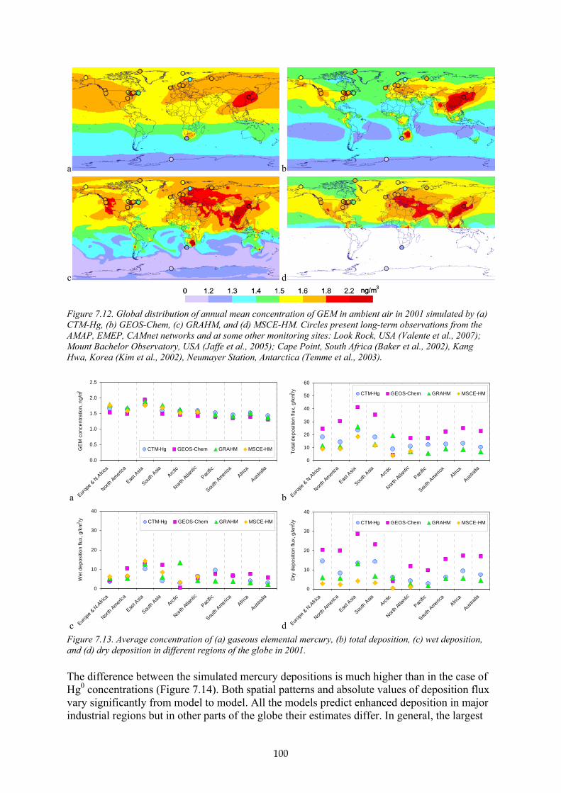
100

a b

c d

Figure 7.12. Global distribution of annual mean concentration of GEM in ambient air in 2001 simulated by (a) CTM-Hg, (b) GEOS-Chem, (c) GRAHM, and (d) MSCE-HM. Circles present long-term observations from the AMAP, EMEP, CAMnet networks and at some other monitoring sites: Look Rock, USA (Valente et al., 2007); Mount Bachelor Observatory, USA (Jaffe et al., 2005); Cape Point, South Africa (Baker et al., 2002), Kang Hwa, Korea (Kim et al., 2002), Neumayer Station, Antarctica (Temme et al., 2003).

a

0.0

0.5

1.0

1.5

2.0

2.5

Europe

& N

.Africa

North A

merica

East A

sia

South

AsiaArct

ic

North A

tlanti

c

Pacific

South

America

Africa

Austra

lia

GE

M c

once

ntra

tion,

ng/

m3

CTM-Hg GEOS-Chem GRAHM MSCE-HM

b

0

10

20

30

40

50

60

Europe

& N

.Africa

North A

merica

East A

sia

South

AsiaArct

ic

North A

tlanti

c

Pacific

South

America

Africa

Austra

lia

Tota

l dep

ositi

on fl

ux, g

/km2 /y CTM-Hg GEOS-Chem GRAHM MSCE-HM

c

0

10

20

30

40

Europe

& N

.Africa

North A

merica

East A

sia

South

AsiaArct

ic

North A

tlanti

c

Pacific

South

America

Africa

Austra

lia

Wet

dep

ositi

on fl

ux, g

/km

2 /y CTM-Hg GEOS-Chem GRAHM MSCE-HM

d

0

10

20

30

40

Europe

& N

.Afric

a

North A

merica

East A

sia

South

AsiaArct

ic

North A

tlanti

c

Pacific

South

America

Africa

Austra

lia

Dry

dep

ositi

on fl

ux, g

/km2 /y CTM-Hg GEOS-Chem GRAHM MSCE-HM

Figure 7.13. Average concentration of (a) gaseous elemental mercury, (b) total deposition, (c) wet deposition, and (d) dry deposition in different regions of the globe in 2001. The difference between the simulated mercury depositions is much higher than in the case of Hg0 concentrations (Figure 7.14). Both spatial patterns and absolute values of deposition flux vary significantly from model to model. All the models predict enhanced deposition in major industrial regions but in other parts of the globe their estimates differ. In general, the largest

101

depositions were simulated by GEOS-Chem (Figure 7.14b) and the lowest by MSCE-HM (Figure 7.14d). This agrees well with the total emission estimates used by the models (see Table 7.2). In particular, GEOS-Chem obtained considerably higher depositions over the oceans. GRAHM and MSCE-HM, in general, agree in the simulation of mercury depositions at temperate latitudes but the former predicts much higher depositions at high latitudes (Figure 7.14c). These elevated depositions in the polar regions result from rapid oxidation of Hg0 and its subsequent deposition during AMDEs. Total mercury deposition averaged over different regions is presented in Figure 7.13b. The highest deposition levels were obtained for East and South Asia, the lowest over the oceans. Estimates by different models vary within a factor of two. To analyze discrepancies in the modeling results wet and dry components of the total deposition are considered below separately.

a b

c d

Figure 7.14. Global distribution of total (wet and dry) deposition of mercury in 2001 simulated by (a) CTM-Hg, (b) GEOS-Chem, (c) GRAHM, and (d) MSCE-HM.

Figure 7.15 shows global distributions of wet mercury deposition simulated by the models and measured at monitoring sites of the EMEP and MDN networks. The difference between wet deposition fields simulated by different models is not as big as for total deposition. Wet deposition of mercury depends on a combination of two factors: precipitation amount and availability of oxidized mercury forms. The most significant wet deposition values are predicted to occur at temperate latitudes: in the vicinity of emission sources and in remote areas with high levels of precipitation. An exception is high deposition in the polar regions predicted by GRAHM due to AMDEs (Figure 7.15c).

All four models generally reproduce wet deposition levels measured in North America and Europe. GEOS-Chem tends to underestimate wet deposition at northern sites, while CTM-Hg and GRAHM somewhat overestimate observed depositions on the northeastern coast of North America, and three of the four models (CTM-Hg, GRAHM, MSCE-HM) underestimate elevated depositions at southwestern North American sites. Nevertheless, the discrepancies are not significant. Thus, the highest deviation of modeling results is characteristic of regions where no regular measurements of mercury deposition are available: over the oceans, in the Arctic, South Asia, and Africa (Figure 7.13c).

The most significant deviation in modeling results is for dry deposition (Figure 7.16). This

102

reflects differences in models parameterization and emissions data used for simulation.

a b

c d

Figure 7.15. Global distribution of wet deposition of mercury in 2001 simulated by (a) CTM-Hg, (b) GEOS-Chem, (c) GRAHM, and (d) MSCE-HM. Circles present long-term observations from the EMEP and MDN monitoring networks.

a b

c d

Figure 7.16. Global distribution of dry deposition of mercury in 2001 simulated by (a) CTM-Hg, (b) GEOS-Chem, (c) GRAHM, and (d) MSCE-HM .

In contrast to wet deposition that is partly constrained by available measurements, dry deposition is highly uncertain because of the absence of any systematic observations. Given observed values of elemental mercury concentration and wet depositions can be successfully reproduced by a model using quite different emissions and dry deposition parameterization.

103

As seen from Figures 7.16 and 7.13d values of dry deposition simulated by different models vary by an order of magnitude. All the models predict larger dry depositions over land then over the ocean. The highest dry depositions are predicted by GEOS-Chem, and the lowest by MSCE-HM. Large difference between the models can be explained by significantly different emissions data (see Table 7.2) and dry deposition parameterization used by the models (e.g., removal with seasalt over the ocean and deposition of Hg0 over land). Thus, higher deposition can be compensated by higher evasion from the surface maintaining realistic levels of air concentration.

Summarizing this analysis, it can be concluded that contemporary models successfully reproduce elemental mercury concentrations in the ambient air (uncertainty does not exceed 15–20%). Uncertainty of model simulation of short-lived mercury species (not considered here) is much higher and is directly connected with uncertainty of mercury deposition. Processes governing mercury deposition are poorly known and uncertainty of simulated total depositions is much higher – a factor of two. The largest contribution to the deposition uncertainty is made by dry deposition. The most significant factors affecting uncertainty of mercury deposition include emissions data (anthropogenic and natural), parameters of chemical reactions leading to oxidation of elemental mercury to short-lived forms, and characteristics of dry deposition. An important factor limiting further improvement of mercury models is the lack of regular measurement data, particularly for air concentrations of short-lived mercury species, and dry and wet deposition.

B7.4 Source-receptor relationships Source attribution of mercury depositions have been studied in a number of previous studies. Relative importance of global versus regional sources and source-receptor relationships in the northern hemisphere were evaluated by Travnikov (2005). Particularly, it was determined that about 40% of annual mercury deposition to Europe originated from external sources including 15% from Asia and 5% from North America. North America is particularly affected by emission sources from other continents: up to 67% of total deposition is from external anthropogenic and natural sources (including about 24% from Asian and 14% from European sources). In contrast, the total contribution of external sources does not exceed 32% for Asia.

Similar results for North America were obtained by Seigneur et al. (2004): North American anthropogenic emissions contribute 30% to total mercury deposition in the contiguous United States; other anthropogenic emissions contribute 37%, with Asia contributing the most (21%), with natural emissions accounting for 33%.

The rest of this section presents an analysis of sources-receptor relationships for mercury depositions at a global scale based on a modeling study performed under the conditions of the TF HTAP models intercomparison (http://aqm.jrc.it/HTAP/). To evaluate the response of mercury deposition to emissions reduction in different source regions all participating models conducted a number of the perturbation runs using anthropogenic emissions decreased by 20% in four major source regions – Europe and North Africa, North America, East Asia and South Asia – with respect to the base case discussed in the previous section. Configuration of the four source regions and the spatial distribution of anthropogenic mercury emissions in 2000 according to Pacyna et al. (2006) are shown in Figure 7.17a. Figure 7.17b shows the relative contribution of the source regions to the global emission. This shows that almost 40% of the total global mercury emission originates in East Asia. It should be noted that one of the models (GEOS-Chem) used updated emissions data that are about 55% larger (see Table 7.2). Nevertheless, the relative contributions of the four source regions were effectively the same in the updated dataset.

104

a b

East Asia839 t/y (38%)

South Asia178 t/y (8%)

Europe & N.Africa

273 t/y (12%)North America144 t/y (7%)

Other756 t/y (35%)

Figure 7.17. (a) Global distribution of anthropogenic mercury emissions in 2000 according to Pacyna et al. (2006) and (b) the relative contribution of four source regions to the global mercury emission. Rectangles show location of the four source regions – Europe and North Africa, North America, East Asia and South Asia.

Response of mercury deposition to emission reduction as simulated by four global/hemispheric scale models (CTM-Hg, GEOS-Chem, GRAHM, MSCE-HM) is illustrated in Figure 7.18. The figure shows global distribution of mercury deposition decrease (in %) due to a 20% emission reduction in the largest mercury emitter – East Asia. The most significant deposition decrease (up to 15%) occurs in the source region itself since a considerable part of the mercury emissions consists of short-lived forms (RGM, Hg-P) which are deposited in the vicinity of the emission sources. A noticeable decrease was also predicted for the North Pacific, the Arctic, and the North Atlantic. The lowest deposition response to emission reduction in East Asia was obtained for other industrial regions and for the southern hemisphere. To facilitate the analysis the modeling results were aggregated for a number of receptor regions across the globe (Figure 7.19); including the source regions themselves, and several terrestrial (South America, Africa, Australia) and aquatic (the Arctic, North Atlantic, Pacific) regions. The aggregated results are presented in Figure 7.20 as bar charts. Each bar presents the relative decrease in mercury deposition in a particular region due to emission reduction in all four source regions. The contributions from different source regions are shown by different colors.

a b

c d

Figure 7.18. Global distribution of total (wet and dry) deposition of mercury in 2001 simulated by (a) CTM-Hg, (b) GEOS-Chem, (c) GRAHM, and (d) MSCE-HM.

105

Figure 7.19. Location of receptor regions considered in the analysis.

a

0

5

10

15

20

Europe &

N.A

frica

North A

merica

East A

sia

South A

siaArct

ic

North A

tlanti

c

Pacific

South

America

Africa

Austra

lia

Dep

ositi

on d

ecre

ase,

%

Europe & N. Africa North AmericaEast Asia South Asia

b

0

5

10

15

20

Europe&

N. A

frica

North A

merica

East A

sia

South A

siaArct

ic

North A

tlanti

c

Pacific

South

America

Africa

Austra

liaD

epos

ition

dec

reas

e, %

Europe & N. Africa North AmericaEast Asia South Asia

c

0

5

10

15

20

Europe&

N. A

frica

North A

merica

East A

sia

South A

siaArct

ic

North A

tlanti

c

Pacific

South

America

Africa

Austra

lia

Dep

ositi

on d

ecre

ase,

%

Europe & N. Africa North AmericaEast Asia South Asia

d

0

5

10

15

20

Europe&

N. A

frica

North A

merica

East A

sia

South A

siaArct

ic

North A

tlanti

c

Pacific

South

America

Africa

Austra

lia

Dep

ositi

on d

ecre

ase,

%

Europe & N. Africa North AmericaEast Asia South Asia

Figure 7.20. Relative decrease in mercury deposition due to a 20% emission reduction in the four source regions simulated by (a) CTM-Hg, (b) GEOS-Chem, (c) GRAHM, and (d) MSCE-HM.

Despite significant discrepancies between the mercury deposition levels simulated by the different models, the models generally agree in terms of quantifying the relative deposition response to emission reductions. All the models predict the highest decrease in deposition in East Asia (8–15%) and the lowest in North America (5–10%). In addition, deposition in all source regions is most sensitive to emission reductions in the source region itself, with the exception of North America, for which two of the four models (CTM-Hg and GEOS-Chem) predicted higher sensitivity to reductions in East Asian emissions. Reduced East Asian emissions are also the most significant in terms of a deposition decrease in all remotes regions. Along with these similarities the total sensitivity of mercury deposition to emissions reduction varies considerably between models. The highest deposition decrease predicted by MSCE-HM is almost twice the decrease simulated by CTM-Hg. The reason for this can be seen by examining the relative contribution of the anthropogenic emissions to total mercury emissions used by the models (Table 7.2); a larger contribution of anthropogenic emissions leads to higher sensitivity to emission reductions since the other part of the emission was assumed to be constant (except GEOS-Chem which included a short-term response of re-emission from the ocean to deposition decrease).

106

B7.5 Changes in mercury concentration and deposition levels between 2000 and 2005 Two of four mentioned above global/hemispheric scale models (GRAHM and MSCE-HM) were applied for evaluation of changes in mercury concentration and deposition levels between 2000 and 2005. For this purpose each of the models have performed simulation runs under similar conditions utilizing two mercury anthropogenic emission inventories for the years 2000 and 2005, respectively (see Part A). In order to avoid the effect of inter-annual meteorological variability both simulation runs were performed using the same dataset of meteorological data related to 2005. Thus, all changes in predicted mercury are defined solely by differences between two emission inventories. These differences are briefly summarized below.

Figure 7.21(a) shows comparison of total mercury emission from major source regions in 2000 and 2005 according to the global emission inventories discussed in Part A of the report. In the Northern Hemisphere total emission of mercury somewhat decreased in Europe, increased in East Asia, and did not change in North America and South Asia (configuration of the source regions is shown in Figure 7.22). In the South Hemisphere total emission increased in South America and significantly decreased in Africa and Australia. It should be noted that difference between two datasets were caused by both implementation of emissions control measures and improvement of emission estimate methodologies applied for 2005 (for more details see Section A4.1.2). Besides, additional emission sectors were included in the global inventory for the first time in 2005 leading to the increase in total anthropogenic emission in some regions (shown by light blue colour in the figure).

a

0

200

400

600

800

1000

Europe

& N. A

frica

North A

merica

East A

sia

South

Asia

South

America

Africa

Austra

lia

Tota

l Hg

emis

sion

, t/y

2000

2005 (new)

2005

b

-400

-300

-200

-100

0

100

200

Europe

& N. A

frica

North A

merica

East A

sia

South

Asia

South

America

Africa

Austra

lia

Tota

l Hg

emis

sion

cha

nge,

t/y

Hg0 Hg2+ HgP

Figure 7.21. Comparison of total anthropogenic emissions of mercury in major source regions (a) and of total emission change between 2000 and 2005 (b) Change of total mercury emission in different regions is shown in more detail in Figure 7.21(b). As seen total increase of mercury emission to the atmosphere in East Asia and South America is mostly presented by increased emissions of elemental mercury (Hg0), whereas emissions of short-lived oxidized mercury forms (Hg2+, HgP) decreased. It would imply reduction of local and regional pollution in these regions and increased contribution to the global atmospheric mercury pool. In contrary, total emission of all mercury forms decreased in Europe, Africa and Australia.

However, inside these regions distribution of emission change is very irregular. For example, in western and central Europe mercury emissions mostly decreased between 2000 and 2005, whereas in some countries of eastern Europe (Turkey, Ukraine, Belarus etc.) there is significant increase of emissions. Similar situation takes place in other source regions. Even in Africa and Australia characterized by significant decrease of anthropogenic emissions there

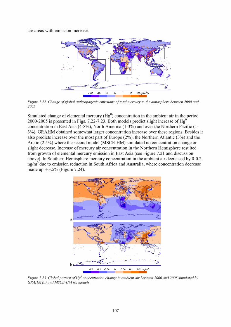
107

are areas with emission increase.

Figure 7.22. Change of global anthropogenic emissions of total mercury to the atmosphere between 2000 and 2005

Simulated change of elemental mercury (Hg0) concentration in the ambient air in the period 2000-2005 is presented in Figs. 7.22-7.23. Both models predict slight increase of Hg0

concentration in East Asia (4-8%), North America (1-3%) and over the Northern Pacific (1-3%). GRAHM obtained somewhat larger concentration increase over these regions. Besides it also predicts increase over the most part of Europe (2%), the Northern Atlantic (3%) and the Arctic (2.5%) where the second model (MSCE-HM) simulated no concentration change or slight decrease. Increase of mercury air concentration in the Northern Hemisphere resulted from growth of elemental mercury emission in East Asia (see Figure 7.21 and discussion above). In Southern Hemisphere mercury concentration in the ambient air decreased by 0-0.2 ng/m3 due to emission reduction in South Africa and Australia, where concentration decrease made up 3-3.5% (Figure 7.24).

a

b

Figure 7.23. Global pattern of Hg0 concentration change in ambient air between 2000 and 2005 simulated by GRAHM (a) and MSCE-HM (b) models

108

-4

-2

0

2

4

6

8

10

Europe

& N. A

frica

North A

merica

East A

sia

South

AsiaArct

ic

North A

tlanti

c

Pacific

South

America

Africa

Austra

lia

Hg0

con

cem

tratio

n ch

ange

, %

GRAHM

MSCE-HM

Figure 7.24. Average relative change of Hg0 concentration in major receptor regions between 2000 and 2005

The pattern of mercury deposition change is more irregular comparing to that of concentration since it is mostly defined by short-lived oxidized mercury forms both from direct atmospheric emissions and in-situ oxidation of elemental mercury in the atmosphere (Figure 7.25). Both models predict decrease of deposition over major part of Eurasia and Africa (Figure 7.26). For example, clearly seen considerable decrease of deposition over the Northern Pacific is caused by emission reduction in Japan. On the other hand, increased emissions in eastern Europe, southern China, and eastern India lead to significant growth of mercury deposition in these regions. One of the models (GRAHM) predicts some increase of deposition (0.3 g/km2/y, 1.6%) over the Arctic, whereas the other model did not obtain considerable change in this region. The reason of this difference is connected with the effect of AMDE taken into account by GRAHM. Mercury removal from the atmosphere during the AMDE takes place over the thicker atmospheric layer (up to 1 km height) and therefore reflects general increase of elemental mercury in the Northern Hemisphere (see discussion above). Mercury deposition decreased in the Southern Hemisphere by 0.2-5 g/km2/y due to emissions reduction in Southern Africa and Australia. In particular, decrease of deposition in these two regions made up 30% and 35%, respectively (Figure 7.26).

a

b

Figure 7.25. Global pattern of total Hg deposition change between 2000 and 2005 simulated by GRAHM (a) and MSCE-HM (b) models

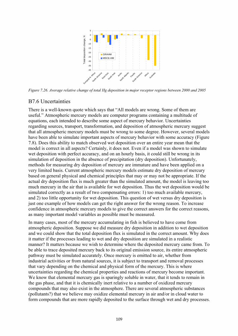
109

-40

-35

-30

-25

-20

-15

-10

-5

0

5

Europe

& N. A

frica

North A

merica

East A

sia

South

AsiaArct

ic

North A

tlanti

c

Pacific

South

America

Africa

Austra

lia

Tota

l dep

ositi

on c

hang

e, %

GRAHMMSCE-HM

Figure 7.26. Average relative change of total Hg deposition in major receptor regions between 2000 and 2005

B7.6 Uncertainties There is a well-known quote which says that “All models are wrong. Some of them are useful.” Atmospheric mercury models are computer programs containing a multitude of equations, each intended to describe some aspect of mercury behavior. Uncertainties regarding sources, transport, transformation, and deposition of atmospheric mercury suggest that all atmospheric mercury models must be wrong to some degree. However, several models have been able to simulate important aspects of mercury behavior with some accuracy (Figure 7.8). Does this ability to match observed wet deposition over an entire year mean that the model is correct in all aspects? Certainly, it does not. Even if a model was shown to simulate wet deposition with perfect accuracy, and on an hourly basis, it could still be wrong in its simulation of deposition in the absence of precipitation (dry deposition). Unfortunately, methods for measuring dry deposition of mercury are immature and have been applied on a very limited basis. Current atmospheric mercury models estimate dry deposition of mercury based on general physical and chemical principles that may or may not be appropriate. If the actual dry deposition flux is much greater than the simulated amount, the model is leaving too much mercury in the air that is available for wet deposition. Thus the wet deposition would be simulated correctly as a result of two compensating errors: 1) too much available mercury, and 2) too little opportunity for wet deposition. This question of wet versus dry deposition is just one example of how models can get the right answer for the wrong reason. To increase confidence in atmospheric mercury models to give the correct answers for the correct reasons, as many important model variables as possible must be measured.

In many cases, most of the mercury accumulating in fish is believed to have come from atmospheric deposition. Suppose we did measure dry deposition in addition to wet deposition and we could show that the total deposition flux is simulated in the correct amount. Why does it matter if the processes leading to wet and dry deposition are simulated in a realistic manner? It matters because we wish to determine where the deposited mercury came from. To be able to trace deposited mercury back to its original emission source, its entire atmospheric pathway must be simulated accurately. Once mercury is emitted to air, whether from industrial activities or from natural sources, it is subject to transport and removal processes that vary depending on the chemical and physical form of the mercury. This is where uncertainties regarding the chemical properties and reactions of mercury become important. We know that elemental mercury gas is sparingly soluble in water, that it tends to remain in the gas phase, and that it is chemically inert relative to a number of oxidized mercury compounds that may also exist in the atmosphere. There are several atmospheric substances (pollutants?) that we believe may oxidize elemental mercury in air and/or in cloud water to form compounds that are more rapidly deposited to the surface through wet and dry processes.

110

It is also likely that oxidized mercury is chemically converted to the elemental form by some other reactions. Otherwise, the oxidation reactions that have been identified and studied so far should cause the average lifetime of atmospheric mercury to be shorter than what we generally observe.

Current models vary in the particular chemical reactions they simulate and the rate at which those reactions occur. In most cases, the reactions that are simulated are only those that have been studied under laboratory conditions where their kinetic rates can be estimated. However, these rates are often estimated for only one specific temperature, while the temperature of air and cloud water can vary over a considerable range. Also, the rates estimated from separate studies of the same reaction are quite different in some cases. In addition to these uncertainties regarding reaction rates, the reaction products are usually not specified either. Oxidized mercury species were first identified in air as a minor ‘reactive’ fraction of total gaseous mercury. This led to the operational term ‘reactive gaseous mercury’ or ‘RGM’. We still have no practical method for the measurement of specific oxidized mercury compounds in air. These many uncertainties regarding the basic chemical system of atmospheric mercury give rise to a variety of modeling results regarding the oxidation state and physical form of the mercury species simulated by the models. Figure 7.7 shows the average air concentrations simulated by three global models for the western boundary of the model testing domain for the North American Mercury Model Intercomparison Study (NAMMIS).

In addition to atmospheric reactions of mercury in air and in cloud water, there are also chemical and physical processes at the earth’s surface that change the oxidation state of mercury. Once deposited, mercury can be converted back to its elemental form and evaporate back into the atmosphere. This ‘evasion’ of mercury is an integral part of mercury cycling. The processes leading to evasion are complex and not fully understood, especially in the case of terrestrial systems where soil and vegetation are both involved. In all cases, this evasion is a combination of natural additions to the mercury cycle and the recycling of natural and anthropogenic mercury. The current ratio of natural to anthropogenic mercury in this recycling process is believed to be about 1:3 on a global basis, but this ratio is still controversial. In areas where historical industrial mercury deposition has been large, the fraction of recycling mercury with industrial origins is certainly more dominant. Net burial of mercury in deep ocean sediments is believed to be the primary vector for removing mercury from the global cycle. Atmospheric mercury models are just now beginning to address air–surface exchanges of mercury. Better scientific definitions of the processes leading to evasion are needed to allow confident modeling assessments of the original sources of mercury depositing and remaining in sensitive ecosystems.

111

Gaps in knowledge and steps for improvement

Part A of the report presents information on sources and quantities of mercury, and as such the report can be considered a state-of-the art in emission inventory on a global scale. The report consists of emission data reported by environmental protection authorities in several countries and emission estimates prepared by the report authors. The collection of information has been carried out through UNEP-Chemicals, as well as other organizations and programs, such as data reported under the UN ECE LRTAP Convention. Emission estimates by the authors of the report are based on emission factors available from the UNEP Toolkit and the EMEP/ CORINAIR Atmospheric Emission Inventory Guidebook. These estimates have also benefited from a comparison with emission and emission factor data presented in the report from the Fate and Transport Group within the Global Mercury Partnership.

Notwithstanding this, there are emissions that are currently poorly quantified or where different inventory estimates require further comparison to resolve differences. These include:

• Emission estimates for ASGM emissions from China;

• Emissions for the non-ferrous metals sector;

• Emissions from mercury consumption in VCM manufacture;

• Emissions from production and use of dental amalgam.

Improvement of information on current emissions Although the Hg emission data present the best data currently available, improvements can be made in their accuracy and completeness through the following efforts:

At country level 1. Measurement programs can be organized to improve the quality of emission factors for

major source categories, and particularly for fossil fuel combustion in large combustion plants (over 350 MWel), waste incinerators, non-ferrous metal smelters, cement kilns and iron and steel foundries. These measurements may include:

- Hg concentrations in flue gases before and after application of emission control equipment; and

- Hg content in raw materials, such as coal, oil, natural gas, ores, limestone, etc. and various wastes, including hazardous, hospital, industrial and municipal wastes.

2. Collection of information and reporting to UNEP should be more complete. The UNEP Toolkit should be employed and more accurate data and information should be provided concerning:

- industrial technologies for production of energy and industrial goods, such as chlor-alkali, ferrous and non-ferrous metals, and cement;

- type and efficiency Hg emission control measures; - changes of industrial technologies and emission control measures over time; and - changes in various uses of Hg, particularly in chlor alkali plants, VCM, etc.

3. Collection and reporting of information needed for spatial distribution of Hg emissions with focus on:

112

- geographical location of major point sources, emission quantities, geometric height of the source, temperature of the flue gases; and

- chemical and physical speciation of emitted mercury.

At international level 4. Improvement of accuracy and completeness of emission factor data to be available in

emission factor guidebooks through inclusion of information from individual countries.

5. Improvement of information on statistical data for consumption of raw materials and production of industrial goods along major fuel types and industrial technologies.

6. Improvement of existing toolkits through collection of information available from various Decision Support Systems (DSS), e.g. the DSS developed within various EU projects to support implementation of the EU legislation.

Improvement of information on future emissions A major development in information is necessary for predicting Hg emissions in the future. Information presented in the report should be regarded as a first step towards achieving Hg emission scenarios. The improvement in developing scenarios for future emissions of Hg can be made through the following efforts:

At a country level 7. Information should be improved on economic indices describing future development of

economies in individual countries, such as indices of the industrial production growth, use of fuels for electricity and heat production, etc.

8. Information can be improved and made available on national plans for:

- use of mercury in various industrial and commercial sectors; - change of fuel types and amounts to meet future energy plans in individual

countries; - change of industrial technologies to meet future energy and industrial good

demands in individual countries; and - change of emission control technology types and Hg control efficiencies in

individual countries.

At international level 9. Information on targets of emission reductions within various international conventions,

emission reduction agreements and protocols can be improved and employed to develop emission scenarios for various regions and the whole globe.

10. Information on emission scenarios for other pollutants relevant for the development of Hg emission scenarios should be collected, e.g. for greenhouse gases and acid rain generation agents. This information should be analyzed with the purpose of using it in development of Hg emission scenarios.

11. Improvement of historical trends of Hg emissions in various geographical regions should be made in order to assess indicators for the development of emission scenarios,

113

particularly for sources, such as artisanal gold production and other uses of Hg in commerce.

Part B of the report summarizes information on atmospheric fate and transport of mercury, including the application of models to investigate the mercury cycle, atmospheric transport, and source-receptor relationships. The following knowledge gaps and needs to fill these are identified in this connection: 12. Need for improved identification of key chemical processes; for example to resolve

questions concerning reactions involving O3 + Hg, OH + Hg, and Hg + Br, both in gas and aqueous phase; and address questions concerning further fate of the initially formed intermediates and their possible reduction reactions, in order to solve questions concerning the chemical lifetime of GEM in the atmosphere.

13. Improved information on seasonal variation in emissions, and better differentiation between GEM, RGM, TPM.

14. Improved information on natural emissions, and in particular re-emissions.

15. Identification of the actual compounds that make up primary emitted RGM and TPM, and photochemically-formed RGM and TPM.

16. Improved data for determining phase transition, including Henrys law constants for RGM species and their temperature dependence following Clasius-Claperons equation, etc.

17. Improved data to determine deposition velocities for GEM, RGM, and TPM to vegetation and other surfaces.

18. Improved information on heterogeneous chemistry, including surface oxidation of GEM, and surface reduction of RGM and TPM.

114

References ACAP, 2005a. Arctic Mercury Releases Assessment. Reduction of Atmospheric Mercury Releases

from Arctic States. The Arctic Council Action Plan (ACAP) to Eliminate Pollution of the Arctic. Report by the Danish Environmental Protection Agency and COWI A/S. Copenhagen.

ACAP, 2005b. Assessment of Mercury Releases from the Russian Federation. The Arctic Council Action Plan (ACAP) to Eliminate Pollution of the Arctic. Report by the Ministry of Natural Resources of the Russian Federation, the Danish Environmental Protection Agency and COWI A/S. Copenhagen.

AEA Technology, 2001. Determination of Atmospheric Pollutant Emission Factors at a Small Coal-fired Heating Boiler. AEA Technology Report AEAT/R/ENV/0517. 31 pp. Available at: http://www.airquality.co.uk/archive/reports/empire/AEAT0517issue1_v2.pdf

Akers, D., R. Dospoy and C. Raleigh, 1993. The Effect of Coal Cleaning on Trace Elements. Development of Algorithms. Technical Report prepared for Electric Power Research Institute, Palo Alto, CA.

AMAP, 1998. AMAP Assessment Report: Arctic Pollution Issues. Arctic Monitoring and Assessment Programme (AMAP), Oslo, Norway.

AMAP, 2005. AMAP Assessment 2002: Heavy Metals in the Arctic. Arctic Monitoring and Assessment Programme (AMAP), Oslo, Norway.

Andersson, M.E., K. Gardfeldt, I. Wangberg and D. Stromberg, 2008. Determination of Henry's law constant for elemental mercury: Chemosphere, 73, 587-592.

Ariya, P.A., A. Khalizov and A. Gidas, 2002. Reactions of gaseous mercury with atomic and molecular halogens: Kinetics, product studies, and atmospheric implications. Journal of Physical Chemistry A, 106: 7310-7320.

Ariya, P.A. Dastoor, M. Amyot, W. Schroeder, L. Barrie, K. Anlauf, F. Raofie, A. Ryzhkov, D. Davignon, J. Lalonde and A. Steffen, 2004. Arctic: A sink for mercury. Tellus, 56B: 397-403.

Ariya, P.A., H. Skov, M.L. Grage and M.E. Goodsite, 2008. Gaseous elemental mercury in the ambient atmosphere: Review of the application of theoretical calculations and experimental studies for determination of reaction coefficients and mechanisms with halogens and other reactants. Advances in Quantum Chemistry 55, Chapter 4, 44-54.

Asari, M., K. Fukui and S. Sakai, 2008. Life-cycle flow of mercury and recycling scenario of fluorescent lamps in Japan. Science of the Total Environment, 393: 1-10.

Aspmo, K., C. Temme, T. Berg, C. Ferrari, P.A. Gauchard, X. Fain and G. Wibetoe, 2006. Mercury in the atmosphere, snow and melt water ponds in the North Atlantic Ocean during Arctic summer. Environmental Science and Technology, 40: 4083-4089.

Baker, P.G.L., E.G. Brunke, F. Slemr and A.M. Crouch, 2002. Atmospheric mercury measurements at Cape Point, South Africa. Atmospheric Environment, 36: 2459-2465.

Balabanov, N.B., B.C. Shepler and K.A. Peterson, 2005. Accurate global potential energy surface and reaction dynamics for the ground state of HgBr2. Journal of Physical Chemistry A, 109: 8765-8773.

Barr Engineering Company, 2001. Substance flow analysis of mercury in products. Prepared for the Minnesota Pollution Control Agency. Minneapolis, MN. Barr Engineering Company. http://www.pca.state.mn.us/publications/hg-substance.pdf

Barrie, L.A., J.W. Bottenheim, R.C. Schnell, P.J. Crutzen and R.A. Rasmussen, 1988. Ozone destruction and photochemical-reactions at polar sunrise in the lower Arctic atmosphere. Nature, 334: 138-141.

Bauer, D., L. D’Ottone, P. Campuzano-Jost and A.J. Hynes, 2003. Gas phase elemental mercury: a comparison of LIF detection techniques and study of the kinetics of reaction with the hydroxyl

115

radical. Journal of Photochemistry and Photobiology A-Chemistry, 157: 247-256.

Biester, H., R. Bindler, A. Martinez-Cortizas and D.R. Engstrom, 2007. Modeling the past atmospheric deposition of mercury using natural archives. Environmental Science and Technology, 41: 4851-4860.

Brooks, S., A. Saiz-Lopez, H. Skov, S. Lindberg, J.M.C. Plane and M.E. Goodsite, 2006a. The mass balance of mercury in the springtime polar environment. Geophysical Research Letters, 33: L13812.

Brooks, W., E. Sandoval, M.A. Yepez and H. Howard, 2007. Peru Mercury Inventory 2006b. USGS Report 2007-1252.

Bullock, O.R., Jr. and K.A. Brehme, 2002. Atmospheric mercury simulation using the CMAQ model: formulation description and analysis of wet deposition results. Atmospheric Environment, 36: 2135-2146.

Cain, A., S. Disch, C. Twaroski, J. Reindl and C.R. Case, 2007. Substance flow analysis of mercury intentionally used in products in the United States. Journal of Industrial Ecology, 11: 61-75.

Calvert, J.G. and S.E. Lindberg, 2005. Mechanisms of mercury removal by O3 and OH in the atmosphere. Atmospheric Environment, 39: 3355-3367.

Christensen, J.H., J. Brandt, L.M. Frohn and H. Skov, 2004. Modelling of mercury in the Arctic with the Danish Eulerian Hemispheric Model. Atmospheric Chemistry and Physics, 4: 2251-2257.

Cobbett, F.D., A. Steffen, G. Lawson and B.J. Van Heyst, 2007. GEM fluxes and atmospheric mercury concentrations (GEM, RGM and Hg-P) in the Canadian Arctic at Alert, Nunavut, Canada (February-June 2005). Atmospheric Environment, 41, 6527-6543.

Cohen, M., R. Artz, R. Draxler, P. Miller, L. Poissant, D. Niemi, D. Ratte, M. Deslauriers, R. Duval, R. Laurin, J. Slotnick, T. Nettesheim and J. McDonald, 2004. Modelling the atmospheric transport and deposition of mercury to the Great Lakes. Environmental Research, 95: 247-265.

Dabrowski, J.M., P.J. Ashton, K. Murray, J. Leane and P. Mason, 2008. Anthropogenic mercury emissions in South-Africa: Coal combustion in Power Plants. Journal of Atmospheric Environment, accepted (AEA8324_proof_21 July 2008).

Dastoor, A.P., D. Davignon, N. Theys, M.V. Roozendael, A. Steffen and P.A Ariya, 2008. Modeling Dynamic Exchange of Gaseous Elemental Mercury at Polar Sunrise. Environ. Sci. Technol., 42, 14, 5183-5188, 10.1021/es800291w.

Dastoor, A. and D. Davignon, 2008. Global Mercury Modelling at Environment Canada. Chapter 17. In: Interim Report of the UNEP Global Partnership on Atmospheric Mercury Transport and Fate Research. Pirrone, N. and R. Mason (eds.) (for latest version of report see: www.chem.unep.ch/mercury/)

Dastoor, A.P. and Y. Larocque, 2004. Global circulation of atmospheric mercury: a modelling study. Atmospheric Environment, 38: 147-161.

DG ENV, 2008. Options for reducing mercury use in products and applications, and the fate of mercury already circulating in society. COWI AS and Concorde East/West Sprl for the European Commission, draft 11 April 2008, Brussels.

Dommergue, A., C.P. Ferrari, L. Poissant, P.A. Gauchard and C.F. Boutron, 2003. Diurnal cycles of gaseous mercury within the snowpack at Kuujjuarapik/Whapmagoostui, Quebec, Canada. Environmental Science and Technology, 37: 3289-3297.

Donohoue, D.L., D. Bauer and A.J. Hynes, 2005. Temperature and pressure dependent rate coefficients for the reaction of Hg with Cl and the reaction of Cl with Cl: A pulsed laser photolysis-pulsed laser induced fluorescence study. Journal of Physical Chemistry A, 109: 7732-7741.

Donohoue, D.L., D. Bauer, B. Cossairt and A.J. Hynes, 2006. Temperature and pressure dependent rate coefficients for the reaction of Hg with Br and the reaction of Br with Br: A pulsed laser

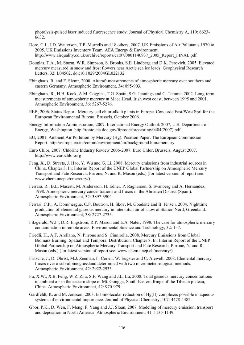
116

photolysis-pulsed laser induced fluorescence study. Journal of Physical Chemistry A, 110: 6623-6632.

Dore, C.J., J.D. Watterson, T.P. Murrells and 18 others, 2007. UK Emissions of Air Pollutants 1970 to 2005. UK Emissions Inventory Team, AEA Energy & Environment. http://www.airquality.co.uk/archive/reports/cat07/0801140937_2005_Report_FINAL.pdf

Douglas, T.A., M. Sturm, W.R. Simpson, S. Brooks, S.E. Lindberg and D.K. Perovich, 2005. Elevated mercury measured in snow and frost flowers near Arctic sea ice leads. Geophysical Research Letters, 32: L04502, doi:10.1029/2004GL022132

Ebinghaus, R. and F. Slemr, 2000. Aircraft measurements of atmospheric mercury over southern and eastern Germany. Atmospheric Environment, 34: 895-903.

Ebinghaus, R., H.H. Kock, A.M. Coggins, T.G. Spain, S.G. Jennings and C. Temme, 2002. Long-term measurements of atmospheric mercury at Mace Head, Irish west coast, between 1995 and 2001. Atmospheric Environment, 36: 5267-5276.

EEB, 2006. Status Report. Mercury cell chlor-alkali plants in Europe. Concorde East/West Sprl for the European Environmental Bureau, Brussels, October 2006.

Energy Information Administration, 2007. International Energy Outlook 2007, U.S. Department of Energy, Washington. http://tonto.eia.doe.gov/ftproot/forecasting/0484(2007).pdf

EU, 2001. Ambient Air Pollution by Mercury (Hg). Position Paper. The European Commission Report. http://europa.eu.int/comm/environment/air/background.htm#mercury

Euro Chlor, 2007. Chlorine Industry Review 2006-2007. Euro Chlor, Brussels, August 2007. http://www.eurochlor.org

Feng, X., D. Streets, J. Hao, Y. Wu and G. Li, 2008. Mercury emissions from industrial sources in China. Chapter 3. In: Interim Report of the UNEP Global Partnership on Atmospheric Mercury Transport and Fate Research. Pirrone, N. and R. Mason (eds.) (for latest version of report see: www.chem.unep.ch/mercury/)

Ferrara, R., B.E. Maserti, M. Andersson, H. Edner, P. Ragnarson, S. Svanberg and A. Hernandez, 1998. Atmospheric mercury concentrations and fluxes in the Almaden District (Spain). Atmospheric Environment, 32: 3897-3904.

Ferrari, C.P., A. Dommergue, C.F. Boutron, H. Skov, M. Goodsite and B. Jensen, 2004. Nighttime production of elemental gaseous mercury in interstitial air of snow at Station Nord, Greenland. Atmospheric Environment, 38: 2727-2735.

Fitzgerald, W.F., D.R. Engstrom, R.P. Mason and E.A. Nater, 1998. The case for atmospheric mercury contamination in remote areas. Environmental Science and Technology, 32: 1–7.

Friedli, H., A.F. Arellano, N. Pirrone and S. Cinnirella, 2008. Mercury Emissions from Global Biomass Burning: Spatial and Temporal Distribution. Chapter 8. In: Interim Report of the UNEP Global Partnership on Atmospheric Mercury Transport and Fate Research. Pirrone, N. and R. Mason (eds.) (for latest version of report see: www.chem.unep.ch/mercury/)

Fritsche, J., D. Obrist, M.J. Zeeman, F. Conen, W. Eugster and C. Alewell, 2008. Elemental mercury fluxes over a sub-alpine grassland determined with two micrometeorological methods. Atmospheric Environment, 42: 2922-2933.

Fu, X.W., X.B. Feng, W.Z. Zhu, S.F. Wang and J.L. Lu, 2008. Total gaseous mercury concentrations in ambient air in the eastern slope of Mt. Gongga, South-Eastern fringe of the Tibetan plateau, China. Atmospheric Environment, 42: 970-979.

Gardfeldt, K. and M. Jonsson, 2003. Is bimolecular reduction of Hg(II) complexes possible in aqueous systems of environmental importance. Journal of Physical Chemistry, 107: 4478-4482.

Gbor, P.K., D. Wen, F. Meng, F. Yang and J.J. Sloan, 2007. Modeling of mercury emission, transport and deposition in North America. Atmospheric Environment, 41: 1135-1149.

117

Goodsite, M.E., W. Rom, J. Heinemeier, T. Lange, S. Ooi, P.G. Appleby, W. Shotyk, W.O. van der Knaap, C. Lohse and T.S. Hansen, 2001. High-resolution AMS C-14 dating of post-bomb peat archives of atmospheric pollutants. Radiocarbon, 43: 495-515.

Goodsite, M.E., J.M.C. Plane and H. Skov, 2004. A theoretical study of the oxidation of Hg-0 to HgBr2 in the troposphere. Environmental Science and Technology, 38: 1772-1776.

Gosselin, P. and B. Dubé, 2005. Gold Deposits of the World: Distribution, Geological Parameters and Gold Content. Geological Survey of Canada, Open File 4895.

Hall, B., 1995. The gas phase oxidation of elemental mercury by ozone. Water, Air and Soil Pollution, 80:301-315.

Hall, B.D., H. Manolopoulos, J.P. Hurley, J.J. Schauer, V.L. St Louis, D. Kenski, J. Graydon, C.L. Babiarz, L.B. Cleckner and G.J. Keeler, 2005. Methyl and total mercury in precipitation in the Great Lakes region. Atmospheric Environment, 39: 7557-7569.

Hedgecock, I.M. and N. Pirrone, 2004 Chasing quicksilver: modeling the atmospheric lifetime of Hg(g)

0 in the marine boundary layer at various latitudes, Environ. Sci. Technol. 38, 69–76.

Hedgecock, I.M., N. Pirrone, G.A. Trunfio and F. Sprovieri, 2006. Integrated mercury cycling, transport, and air-water exchange (MECAWEx) model. Journal of Geophysical Research, 111: D20302, doi:10.1029/2006JD007117.

Holmes, C.D., D.J. Jacob and X. Yang, 2006. Global lifetime of elemental mercury against oxidation by atomic bromine in the free troposphere. Geophysical Research Letters, 33: L20808, doi:10.1029/2006GL027176.

Hylander, L.D. and M. Meili, 2003. 500 years of mercury production: global annual inventory by region until 2000 and associated emissions. Science of the Total Environment, 304: 13-27.

Hylander, L.D. and R. Herbert, 2008. Global emission and production of mercury during the pyrometallurgical extraction of non-ferrous sulfide ores. Environ. Sci. Technol. 42: 5971–5977.

ICF, 2005. User’s Guide to the Regional Modeling System for Aerosols and Deposition (REMSAD). Version 8, ICF Consulting/SAI, San Francisco, California.

Iverfeldt, A., 1991. Occurrence and turnover of atmospheric mercury over the Nordic countries. Water Air and Soil Pollution, 56: 251-265.

Jaegle, L., S. Strode, N. Selin and D. Jacob, 2008. The GEOS-Chem model. Chapter 18. In: Interim Report of the UNEP Global Partnership on Atmospheric Mercury Transport and Fate Research. Pirrone, N. and R. Mason (eds.) (for latest version of report see: www.chem.unep.ch/mercury/)

Jaffe, D., E. Prestbo, P. Swartzendruber, P. Weiss-Penzias, S. Kato, A. Takami, S. Hatakeyama and K. Yoshizumi, 2005. Export of atmospheric mercury from Asia. Atmospheric Environment, 38: 3029-3038.

Jarosinska, D., L. Barregard, M. Biesida, M. Muszynska-Graca, B. Dabkowska, B. Denby, J.M. Pacyna, J. Fudala and U. Zielonka, 2006. Urinary mercury in adults in Poland living near a chlor-alkali plant. The Science of the Total Environment, 368: 335-343.

Jung, G., I. Hedgecock and N. Pirrone, 2008. The ECHMERT model. Chapter 19. In: Interim Report of the UNEP Global Partnership on Atmospheric Mercury Transport and Fate Research. Pirrone, N. and R. Mason (eds.) (for latest version of report see: www.chem.unep.ch/mercury/)

Khalizov, A.F., B. Viswanathan, P. Larregaray and P.A. Ariya, 2003. A theoretical study on the reactions of Hg with halogens: Atmospheric implications. Journal of Physical Chemistry A, 107: 6360-6365.

Kim, K.H., 2004. The signature of diversification of source processes in controlling atmospheric mercury levels in East Asia. Terrestrial Atmospheric and Oceanic Sciences, 15: 261-267.

Kim, K.H. and M.Y. Kim, 1996. Preliminary measurements of atmospheric mercury in mountainous

118

regions of Korea. Journal of Environmental Science and Health Part A, 31: 2023-2032.

Kim, K.-H., M.-Y. Kim, J. Kim and G. Lee, 2002. The concentrations and fluxes of total gaseous mercury in a western coastal area of Korea during late March 2001. Atmospheric Environment, 36: 3413-3427.

Kim, K.H., R. Ebinghaus, W.H. Schroeder, P. Blanchard, H.H. Kock, A. Steffen, F.A. Froude, M.Y. Kim, Hong and J.H. Kim, 2005. Atmospheric mercury concentrations from several observatory sites in the northern hemisphere. Journal of Atmospheric Chemistry, 50: 1-24.

Kindbom, K. and J. Munthe, 2007. Product-related emissions of Mercury to Air in the European Union. IVL, Swedish Environmental Research Institute, Report No B1739. 25 pp. Available at http://www3.ivl.se/rapporter/pdf/B1739.pdf

Kirk, J.L. V.L. St. Louis and M.J. Sharp, 2006. Rapid reduction and reemission of mercury deposited into snowpacks during atmospheric mercury depletion events at Churchill, Manitoba, Canada. Environmental Science and Technology, 40: 7590-7596.

Lalonde, J.D., M. Amyot, M.R. Doyon and J.C. Auclair, 2003. Photo-induced Hg(II) reduction in snow from the remote and temperate Experimental Lakes Area (Ontario, Canada). Journal of Geophysical Research-Atmospheres, 108(D6).

Lamborg, C.H., W.F. Fitzgerald, A.W.H. Damman, J.M. Benoit, P.H. Balcom and D.R. Engstrom, 2002a. Modern and historic atmospheric mercury fluxes in both hemispheres: Global and regional mercury cycling implications. Global Biogeochemical Cycles, 16: 1104, doi:10.1029/2001GB001847.

Lamborg C.H., W.F. Fitzgerald, J. O’Donnell and T. Torgersen, 2002b. A non-steady-state compartment model of global-scale mercury biochemistry with inter-hemispheric atmospheric gradients. Geochimica et Cosmochimica Acta, 66: 1105-1118.

Laurier, F.J.G., R.P. Mason, L. Whalin and S. Kato, 2003. Reactive gaseous mercury formation in the North Pacific Ocean’s marine boundary layer: A potential role of halogen chemistry. J. Geophys. Res., 108, D17, art # 4529.

Leaner, J., J. Dabrowski, R. Mason, T. Resane, M. Richardson, M. Ginster, R. Euripides and E. Masekoameng, 2008. Mercury emissions from point sources in South Africa. Chapter 5. In: Interim Report of the UNEP Global Partnership on Atmospheric Mercury Transport and Fate Research. Pirrone, N. and R. Mason (eds.) (for latest version of report see: www.chem.unep.ch/mercury/)

Lennet, D., 2008. Personal communications with D. Lennet, Natural Resources Defense Council (NRDC), USA.

Lin, X. and Y. Tao, 2003. A numerical modelling study on regional mercury budget for eastern North America. Atmospheric Chemistry and Physics, 3: 535-548.

Lin, C.-J., P. Pongprueksa, S.E. Lindberg, S.O. Pehkonen, D. Byun and C. Jang, 2006. Scientific uncertainties in atmospheric mercury models: Model science evaluation. Atmospheric Environment, 40: 2911-2928.

Lin, C.-J., P. Pongprueksa, O.R. Bullock, S.E. Lindberg, S.O. Pehkonen, C. Jang, T. Braverman and T.C. Ho, 2007b. Scientific uncertainties in atmospheric mercury models II: Sensitivity analysis in the CONUS domain. Atmospheric Environment, 41: 6544-6560.

Lindberg, S.E., S. Brooks, C.J. Lin, K.J. Scott, M.S. Landis, R.K. Stevens, M. Goodsite and A. Richter, 2002. Dynamic oxidation of gaseous mercury in the Arctic troposphere at polar sunrise. Environmental Science and Technology, 36: 1245-1256.

Lindberg, S., R. Bullock, R. Ebinghaus, D. Daniel Engstrom, X. Feng, W. Fitzgerald, N. Pirrone, E. Prestbo and C. Seigneur, 2007. A synthesis of progress and uncertainties in attributing the sources of mercury in deposition. Ambio, 36: 19-32.

Lyman, S.N., M.S. Gustin, E.M. Prestbo and F.J. Marsik, 2007. Estimation of dry deposition of

119

atmospheric mercury in Nevada by direct and indirect methods. Environmental Science and Technology, 41: 1970-1976.

Macdonald, R.W., T. Harner and J. Fyfe, 2005. Recent climate change in the Arctic and its impact on contaminant pathways and interpretation of temporal trend data. Science of the Total Environment, 342: 5-86.

Malcolm, E.G., G.J. Keeler and M.S. Landis, 2003. The effects of the coastal environment on the atmospheric mercury cycle. Journal of Geophysical Research-Atmospheres, 108(D12).

Mason, R., 2008. Mercury emissions from natural sources and their importance in the global mercury cycle. Chapter 7. In: Interim Report of the UNEP Global Partnership on Atmospheric Mercury Transport and Fate Research. Pirrone, N. and R. Mason (eds.) (for latest version of report see: www.chem.unep.ch/mercury/)

Mason R.P. and G.-R. Sheu, 2002. Role of ocean in the global mercury cycle. Global Biogeochemical Cycles, 16: 1093. doi:10.1029/2001GB001440.

Mason, R.P., F.J.G. Laurier, L. Whalin and G.R. Sheu, 2003. The role of ocean-atmosphere exchange in the global mercury cycle. Journal de Physique Iv, 107: 835-838.

Maxson, P., 2007. Mercury in dental use: Environmental implications for the European Union. Report for the European Environmental Bureau, Belgium. http://www.zeromercury.org/EU_developments/Maxson%20Dental%2014May2007%20-%20A5colour.pdf

Meili, M., K. Bishop, L. Bringmark, K. Johansson, J. Munthe, H. Sverdrup and W. Vries, 2003. Critical levels of atmospheric pollution: criteria and concepts for operational modelling of mercury in forest and lake ecosystems. Science of the Total Environment, 304: 83-106.

Miller, G.C., J. Quashnick and V. Hebert, 2001. Reaction rate of metallic mercury with hydroxyl radical in the gas phase. Abstracts of Papers of the American Chemical Society, 221, U47.

Mukherjee, A.B., P. Bhattacharya, R. Zevenhoven and A.Sarkar, 2008. Mercury emissions from industrial sources in India and its effects in the environment. Chapter 4. In: Interim Report of the UNEP Global Partnership on Atmospheric Mercury Transport and Fate Research. Pirrone, N. and R. Mason (eds.) (for latest version of report see: www.chem.unep.ch/mercury/)

Munthe, J., 1992. The aqueous oxidation of elemental mercury by ozone. Atmospheric Environment Part A, 26: 1461-1468.

Murphy, D.M., P.K. Hudson, D.S. Thomson, P.J. Sheridan and J.C. Wilson, 2006. Observations of mercury-containing aerosols. Environmental Science and Technology, 40: 3163-3167.

NAPAP,1990. Technologies and Other Measures for Controlling Emissions: Performance, Costs and Applicability. National Acid Precipitation Assessment Programme, NAPAP, Report 25, Washington D.C.

Nelson, P.F., 2007. Atmospheric emissions of mercury from Australian point sources. Atmospheric Environment, 41: 1717-1724.

NRDC, 2006. Submission to UNEP in response to March 2006 request for information on mercury supply, demand, and trade. Natural Resources Defense Council, Washington, DC, May 2006. http://www.chem.unep.ch/mercury/Trade-information.htm

Outridge, P.M., H. Sanei, G.A. Stern, P.B. Hamilton and F. Goodarzi, 2007. Evidence for control of mercury accumulation rates in Canadian High Arctic lake sediments by variations of aquatic primary productivity. Environmental Science and Technology, 41: 5259-5265.

Pacyna, J.M., 1980. Coal-fired power plants as a source of environmental contamination by trace metals and radionuclides. Wroclaw Technical University Press.

Pacyna, J.M., 1986. Emission factors of atmospheric elements. In: Nriagu, J.O. and C.I. Davidson (eds.), Toxic Metals in the Atmosphere. Advances in Environmental Science and Technology. John

120

Wiley & Sons.

Pacyna, J.M., 1987. Atmospheric emissions of arsenic, cadmium, lead and mercury from high temperature processes in power generation and industry. In: Hutchinson, T.C. and Meema, K.M. (eds.), Lead, Mercury, Cadmium and Arsenic in Environment. John Wiley & Sons.

Pacyna, E.G. and J.M. Pacyna, 2002. Global emission of mercury from anthropogenic sources in 1995. Water, Air and Soil Pollution, 137: 149-165.

Pacyna, J.M. and E.G. Pacyna, 2005. Anthropogenic sources and global inventory of mercury emissions. In: Parsons, M.B. and J.B. Percival (eds.), Mercury: Sources, Measurements, Cycles, and Effects. Mineralogical Association of Canada, Short Course Series Volume No. 32.

Pacyna, J.M., M.T. Trevor, M. Scholtz and Y.-F. Li, 1995. Global budgets of trace metal sources. Environmental Reviews, 3: 145-159.

Pacyna, J.M., E.G. Pacyna, F. Steenhuisen and S. Wilson, 2003. Mapping 1995 global anthropogenic emissions of mercury. Atmospheric Environment, 37-S: 109-117.

Pacyna, E.G., J.M. Pacyna, F. Steenhuisen and S. Wilson, 2006. Global anthropogenic mercury emission inventory for 2000. Atmospheric Environment, 40: 4048-4063.

Pal, B. and P.A. Ariya, 2004a. Gas-phase HO center dot-initiated reactions of elemental mercury: kinetics, product studies, and atmospheric implications. Environmental Science and Technology, 38: 5555-5566.

Pal, B. and P.A. Ariya, 2004b. Studies of ozone initiated reactions of gaseous mercury: kinetics, product studies, and atmospheric implications. Physical Chemistry Chemical Physics, 6: 572-579.

Pan, L., G.R. Carmichael, B. Adhikary, Y. Tang, D. Streets, J.-H. Woo, H.R. Friedli and L.F. Radke, 2008. A regional analysis of the fate and transport of mercury in East Asia and an assessment of major uncertainties. Atmospheric Environment, 42: 1144-1159.

Petersen, G., R. Bloxam, S. Wong, J. Munthe, O. Krüger, S.R. Schmolke and A.V. Kumar, 2001. A comprehensive Eulerian modelling framework for airborne mercury species: model development and applications in Europe. Atmospheric Environment, 35: 3063-3074.

Pirrone, N., S. Cinnirella, D. Streets, X. Feng., A. Mukherjee, J. Leaner, K. Telmer, R. Mason, H. Friedli, R. Finkelman and G. Stracher, 2008. Global mercury emissions to the atmosphere from natural and anthropogenic sources. Chapter 1. In: Interim Report of the UNEP Global Partnership on Atmospheric Mercury Transport and Fate Research. Pirrone, N. and R. Mason (eds.) (for latest version of report see: www.chem.unep.ch/mercury/)

Pongprueksa, P., C.-J. Lin, S.E. Lindberg, C. Jang, T. Braverman, O.R. Bullock, T.C. Ho and H.-W. Chu, 2008. Scientific uncertainties in atmospheric mercury models III: Boundary and initial conditions, model grid resolution, and Hg(II) reduction mechanism. Atmospheric Environment, 42: 1828-1845.

Poulain, A.J., E. Garcia, M. Amyot, P.G.C. Campbel and P.A. Ariya, 2007. Mercury distribution, partitioning and speciation in coastal vs. inland High Arctic snow. Geochimica et Cosmochimica Acta, 71: 3419-3431.

Radke, L.F., H.R. Friedli and B.G. Heikes, 2007. Atmospheric mercury over the NE Pacific during spring 2002: Gradients, residence time, upper troposphere lower stratosphere loss, and long-range transport. Journal of Geophysical Research-Atmospheres, 112(D19).

Raofie, F. and P.A. Ariya, 2004. Product study of the gas-phase BrO-initiated oxidation of Hg-0: evidence for stable Hg1+ compounds. Environmental Science and Technology, 38: 4319-4326.

Ryaboshapko, A., R. Bullock, R. Ebinghaus, I. Ilyin, K. Lohman, J. Munthe, G. Petersen, C. Seigneur and I. Wängberg, 2002. Comparison of mercury chemistry models. Atmospheric Environmental, 36: 3881-3898.

Ryaboshapko, A., O.R. Jr. Bullock, J. Christensen, M. Cohen, A. Dastoor, I. Ilyin, G. Petersen, D.

121

Syrakov, R.S. Artz, D. Davignon, R.R. Draxler and J. Munthe, 2007a. Intercomparison study of atmospheric mercury models: 1. Comparison of models with short-term measurements. Science of the Total Environment, 376: 228-240.

Ryaboshapko, A., O.R. Jr. Bullock, J. Christensen, M. Cohen, A. Dastoor, I. Ilyin, G. Petersen, D. Syrakov, O. Travnikov, R.S. Artz, D. Davignon, R.R. Draxler, J. Munthe and J. Pacyna, 2007b. Intercomparison study of atmospheric mercury models: 2. Modelling results vs. long-term observations and comparison of country deposition budgets. Science of the Total Environment, 377: 319-333.

Sakata, M., K. Marumoto, M. Narukawa and K. Asakura, 2006. Regional variations in wet and dry deposition fluxes of trace elements in Japan. Atmospheric Environment, 40: 521-531.

Schroeder, W.H., K.G. Anlauf, L.A. Barrie, J.Y. Lu, A. Steffen, D.R. Schneeberger and T. Berg, 1998. Arctic springtime depletion of mercury. Nature, 394: 331-332.

Schroeder, W. H. and J. Munthe, 1998, Atmospheric mercury - An overview. Atmospheric Environment, 32, 809-822.

Schuster, P.F., D.P. Krabbenhoft, D.L. Naftz, L.D. Cecil, M.L. Olson, J.F. Dewild, D.D. Susong, J.R. Green and M.L. Abbott, 2002. Atmospheric mercury deposition during the last 270 years: A glacial ice core record of natural and anthropogenic sources. Environmental Science and Technology, 36: 2303-2310.

Seigneur, C., P. Karamchandani, K. Lohman and K. Vijayaraghavan, 2001. Multiscale modeling of the atmospheric fate and transport of mercury. Journal of Geophysical Research, 106: 27,795-27,809.

Seigneur, C., K. Vijayaraghavan, K. Lohman, P. Karamchandani and C. Scott, 2004. Global source attribution for mercury deposition in the United States. Environmental Science and Technology, 38: 555-569.

Seigneur, C., K. Vijayaraghavan and K. Lohman, 2006. Atmospheric mercury chemistry: sensitivity of global model simulations to chemical reactions. Journal of Geophysical Research, 111(D22), D22306.

Seigneur, C., K. Vijayaraghavan, K. Lohman and L. Levin, 2008. The AER/EPRI global chemical transport model for mercury (CTM-Hg). Chapter 21. In: Interim Report of the UNEP Global Partnership on Atmospheric Mercury Transport and Fate Research. Pirrone, N. and R. Mason (eds.) (for latest version of report see: www.chem.unep.ch/mercury/)

Selin, N.E., D.J. Jacob, R.J. Park, R.M. Yantosca, S. Strode, L. Jaegle and D. Jaffe, 2007. Chemical cycling and deposition of atmospheric mercury: Global constraints from observations. Journal of Geophysical Research, 112, D02308, doi:10.1029/2006JD007450.

Selin, N.E., D.J. Jacob, R.M. Yantosca, S. Strode, L. Jaegle, and E.M. Sunderland, 2008. Global 3-D land-ocean-atmosphere model for mercury. Present-day versus preindustrial cycles and anthropogenic enhancement factors for deposition. Global Biogeochemical Cycles, 22: GB2011, doi:10.1029/2007GB003040.

Selin, N.E., and D.J. Jacob, 2008. Seasonal and spatial patterns of mercury wet deposition in the United States: Constraints on the contribution from North American anthropogenic sources. Atmospheric Environment, 42, 5193-5204.

SEPA, 2008. Strategy Proposal for International Actions to Address Mercury Problem - Mercury Situation in China. State Environmental Protection Administration of China (SEPA). Received by UNEP 28 January 2008.

Shia, R.-L., C. Seigneur, P. Pai, M. Ko and N.D. Sze, 1999. Global simulation of atmospheric mercury concentrations and deposition fluxes. Journal of Geophysical Research, 104: 23,747-23,760.

Shotyk, W., M.E. Goodsite, F. Roos-Barraclough, R. Frei, J. Heinemeier, G. Asmund, C. Lohse and T.S. Hansen, 2003. Anthropogenic contributions to atmospheric Hg, Pb and As accumulation recorded by peat cores from southern Greenland and Denmark dated using the 14C ‘bomb pulse

122

curve’. Geochimica et Cosmochimica Acta, 67: 3991-4011.

Skov, H., S. Brooks, M.E. Goodsite, S.E. Lindberg, T.P. Meyers, M. Landis, M.R.B. Larsen, B. Jensen, G. McConville, K.H. Chung and J. Christensen, 2006. The fluxes of reactive gaseous mercury measured with a newly developed method using relaxed eddy accumulation. Atmospheric Environment, 40: 5452-5463.

Slemr, F. and H.E. Scheel, 1998. Trends in atmospheric mercury concentrations at the summit of the Wank mountain, southern Germany. Atmospheric Environment, 32: 845-853.

Slemr, F., E.G. Brunke, R. Ebinghaus, C. Temme, J. Munthe, I. Wangberg, W. Schroeder, A. Steffen and T. Berg, 2003. Worldwide trend of atmospheric mercury since 1977. Geophysical Research Letters, 30(10).

Sommar, J., K. Gardfeldt, D. Stromberg and X.B. Feng, 2001. A kinetic study of the gas-phase reaction between the hydroxyl radical and atomic mercury. Atmospheric Environment, 35: 3049-3054.

SRIC, 2005. Chlorine/Sodium Hydroxide. E. Linak, S. Schlag and K Yokose. CEH Marketing Research Report, SRI Consulting, Zurich, August 2005.

Steffen, A., W. Schroeder, J. Bottenheim, J. Narayan and J.D. Fuentes, 2002. Atmospheric mercury concentrations: measurements and profiles near snow and ice surfaces in the Canadian Arctic during Alert 2000. Atmospheric Environment, 36: 2653-2661.

Steffen, A., W.H. Schroeder, G. Edwards and C. Banic, 2003. Mercury throughout polar sunrise 2002. Journal de Physique Iv, 107: 1267-1270.

Steffen, A., T. Douglas, M. Amyot, P. Ariya, K. Aspmo, T. Berg, J. Bottenheim, S. Brooks, F. Cobbett, A. Dastoor, A. Dommergue, R. Ebinghaus, C. Ferrari, K. Gardfeldt, M.E. Goodsite, D. Lean, A.J. Poulain, C. Scherz, H. Skov, J. Sommar and C. Temme, 2008. A synthesis of atmospheric mercury depletion event chemistry in the atmosphere and snow. Atmospheric Chemistry and Physics, 8: 1445-1482.

Streets, D.G., J. Hao, Y. Wu, J. Jiang, M. Chan, H. Tian and X. Feng, 2005. Anthropogenic mercury emissions in China. Atmospheric Environment 39, 7789–7806.

Streets, D., J. Hao, S. Wang and Y. Wu, 2008. Mercury emissions from coal combustion in China. Chapter 2. In: Interim Report of the UNEP Global Partnership on Atmospheric Mercury Transport and Fate Research. Pirrone, N. and R. Mason (eds.) (for latest version of report see: www.chem.unep.ch/mercury/)

Strode, S., L. Jaeglé, D. Jaffe, P. Swartzendruber, N. Selin, C. Holmes and R. Yantosca, 2008. Trans-Pacific transport of mercury. Journal of Geophysical Research, 113, D15305, doi:10.1029/2007JD009428.

Sumner, A.L., C.W. Spicer, J. Satola, R. Mangaraj, K.A. Cowen, M.S. Landis, R.K. Stevens and T.D. Atkeson, 2005. Environmental chamber studies of mercury reactions in the atmosphere. In: Dynamics of mercury pollution on regional and global scales: Atmospheric processes, human exposure around the world. N. Pirrone and K. Mahaffey (Eds.), Springer Publisher, Norwell, MA, USA. Chapter 9, p. 193-212.

Sunderland, E.M., M.D. Cohen, N.E. Selin and G.L. Chmura, 2008. Reconciling models and measurements to assess trends in atmospheric mercury deposition. Environmental Pollution, 156, 526-535.

Sunderland, E.M. and R.P. Mason, 2007. Human impacts on open ocean mercury concentrations. Global Biogeochemical Cycles, 21(4).

Syrakov, D., 1995. On a PC-oriented Eulerian multi-level model for long-term calculations of the regional sulphur deposition. In: Gryning S.E. and F.A. Schiermeier (eds.). Air Pollution Modelling and its Application, pp. 645-646. XI 21, Plenum Press.

123

Telmer, 2008. Personal communications with experts Telmer, Veiga and Spiegel – All involved in the UNIDO/UNDP/GEF Global Mercury Project.

Telmer, K. and M. Veiga, 2008. World emissions of mercury from artisanal and small scale gold mining. Chapter 6. In: Interim Report of the UNEP Global Partnership on Atmospheric Mercury Transport and Fate Research. Pirrone, N. and R. Mason (eds.) (for latest version of report see: www.chem.unep.ch/mercury/)

Temme, C., F. Slemr, R. Ebinghaus and J.W. Einax, 2003. Distribution of mercury over the Atlantic Ocean in 1996 and 1999-2001. Atmospheric Environment, 37: 1889-1897.

Temme, C., P. Blanchard, A. Steffen, C. Banic, S. Beauchamp, L. Poissant, R. Tordon and B. Wiens, 2007. Trend, seasonal and multivariate analysis study of total gaseous mercury data from the Canadian atmospheric mercury measurement network (CAMNet). Atmospheric Environment, 41: 5423-5441.

Theloke, J., U. Kummer, S. Nitter, T. Geflern, R. Friedrich, A. Voss, J.M. Pacyna and H. D. van der Gon, 2008. Uberarbeitung der Schwermetallkapitel in CORINAIR Guidebook zur Verbesserung der Emissionsinventare unde der Berichterstattung im Rahmen der Genfer Luftreinhaltekonvention. Forderkennzeichen (UFOPLN) 312 01 234, Umweltbundesamt, Berlin, Germany.

Tokos, J.J.S., B. Hall, J.A. Calhoun and E.M. Prestbo, 1998. Homogeneous gas-phase reaction of Hg-0 with H2O2, O-3, CH3I, and (CH3)(2)S: Implications for atmospheric Hg cycling. Atmospheric Environment, 32: 823-827.

Tossell, J.A., 2003. Calculation of the energetics for oxidation of gas-phase elemental Hg by Br and BrO. Journal of Physical Chemistry A, 107: 7804-7808.

Travnikov, O., 2005. Contribution of the intercontinental atmospheric transport to mercury pollution in the Northern Hemisphere. Atmospheric Environment, 39: 7541-7548.

Travnikov, O. and I. Ilyin, 2005. Regional Model MSCE-HM of Heavy Metal Transboundary Air Pollution in Europe. EMEP/MSC-E Technical Report 6/2005, Moscow, Russia. http://www.msceast.org/publications/

Travnikov, O. and I. Iliyan, 2008. The EMEP/MSC-E mercury modeling system. Chapter 20. In: Interim Report of the UNEP Global Partnership on Atmospheric Mercury Transport and Fate Research. Pirrone, N. and R. Mason (eds.) (for latest version of report see: www.chem.unep.ch/mercury/)

Tsinghua, 2006. Improve the Estimates of Anthropogenic Mercury Emissions in China. Tsinghua University, October 2006.

Tuckermann, M., R. Ackermann, C. Golz, H. Lorenzen-Schmidt, T. Sennet, J. Stutz, B. Trost, W. Unold and U. Platt, 1997. DOAS-observation of halogen radical-catalysed Arctic boundary layer ozone destruction during the ARCTOC-campaigns 1995 and 1996 in Ny-Ålesund, Spitsbergen. Tellus. Series B, 49: 533-555.

UN, 2006. World Urbanization Prospects: The 2005 Revision. Database. United Nations, Department of Economic and Social Affairs, Population Division.

UN, 2007a. Statistical Yearbook. United Nations.

UN, 2007b. World Population Prospects 1950-2050: The 2006 Revision. Database. United Nations, Department of Economic and Social Affairs, Population Division. Accessed July 2007.

UN ECE, 2000. Joint EMEP/ CORINAIR Atmospheric Emission Inventory Guidebook. The United Nations Economic Commission for Europe, Geneva, Switzerland.

UNEP, 2005. Toolkit for identification and quantification of mercury releases - pilot draft of November 2005. United Nations Environment Programme, Chemicals Branch, Geneva, 2005. http://www.chem.unep.ch/mercury/Guidance-training-materials.htm.

UNEP, 2006. Summary of supply, trade and demand information on mercury. Analysis requested by

124

UNEP Governing Council decision 23/9 IV. United Nations Environment Programme, Chemicals Branch, Geneva.

UNEP-Chemicals, 2002. Global Mercury Assessment. UNEP-Chemicals, Geneva, Switzerland.

Valente, R., C. Shea, K.L. Humes and R. Tanner, 2007. Atmospheric mercury in the Great Smoky Mountains compared to regional and global levels. Atmospheric Environment, 41: 1861-1873.

Voudouri, A. and G. Kallos, 2007. Validation of the integrated RAMS-Hg modelling system using wet deposition observations for eastern North America. Atmospheric Environment, 41: 5732-5745.

Wang, Z., Z. Chen, N. Duan and X. Zhang, 2007. Gaseous elemental mercury concentration in atmosphere at urban and remote sites in China. Journal of Environmental Sciences, 19(2), 176-180.

Wangberg, I., J. Munthe, N. Pirrone, A. Iverfeldt, E. Bahlman, P. Costa, R. Ebinghaus, X. Feng, R. Ferrara, K. Gardfeldt, H. Kock, E. Lanzillotta, Y. Mamane, F. Mas, E. Melamed, Y. Osnat, E. Prestbo, J. Sommar, S. Schmolke, G. Spain, F. Sprovieri and G. Tuncel, 2001. Atmospheric mercury distribution in Northern Europe and in the Mediterranean region. Atmospheric Environment, 35, 3019-3025.

WCC, 2006. World Chlorine Council Submission [to UNEP] on Global Mercury Partnership for the Reduction of Mercury in the Chlor-alkali Sector, World Chlorine Council, see http://www.worldchlorine.com

Weiss-Penzias, P., D.A. Jaffe, A. McClintick, E.M. Prestbo and M.S. Landis, 2003. Gaseous elemental mercury in the marine boundary layer: Evidence for rapid removal in anthropogenic pollution. Environmental Science and Technology, 37: 3755-3763.

Wilson, S., F. Steenhuisen, J.M. Pacyna and E.G. Pacyna, 2006. Mapping the spatial distribution of global anthropogenic mercury atmospheric emission inventories. Atmospheric Environment, 40: 4621-4632.

World Bank, 2007. World Development Indicators 2007. CD-ROM. Washington, D.C

Wu, Y., S.X. Wang, D.G. Streets, J.M. Hao, M. Chan and J.K. Jiang, 2006. Trends in anthropogenic mercury emissions in China from 1995 to 2003. Environmental Science and Technology, 40: 5312-5318.

Yang, X., R.A. Coc, N.J. Warwick, J.A. Pyle, G.D. Carver, F.M. O’Connor and N.H. Savage, 2005. Tropospheric bromine chemistry and its impacts on ozone: A model study. Journal of Geophysical Research, 110, D23311.

125

Appendix Tables: Appendix A Table AppA.1: Distribution factors

Table AppA.2: Distribution factors for product mercury in the waste fraction

Table AppA.3: Emission factors used for all regions.

Table AppA.4: Safe storage

Table AppA.5: Mercury (tonnes) remaining accumulated in products in society

Table AppA.6: Mercury by-product emissions from anthropogenic sources by country and sectors in 2005.

Table AppA.7: Mercury by-product emissions from anthropogenic sources by country and sectors in 2020 SQ Scenario.

Table AppA.8: Mercury by-product emissions from anthropogenic sources by country and sectors in 2020 EXEC Scenario.

Table AppA.9: Mercury by-product emissions from anthropogenic sources by country and sectors in 2020 MTFR Scenario.

Appendix B Table AppB.1: Reactions, reaction rate constants and when possible reaction products of gas phase

reactions.

Table AppB.2: Reaction rate constants and when possible reaction products of aqueous phase reactions (from Lin et al., 2006).

Table AppB.3: Temperature expression for some reactions listed in Table AppB.1

Table AppB.4: Chemical equilibriums for calculating aqueous phase HgII speciation.

Table AppB.5: Physical and chemical properties for selected compounds.

Appendix C Glossary of Abbreviations

126

Appendix A Table AppA.1 Distribution factors Region

Batteries

Meas. control devices Lighting

Electrical devices

All Release by breaking 0.01 0.05 0.05 0.01 All Remain accumulated in

society 0.1 0.35 0.35 0.35 East and Southeast Asia Recollected, safe storage 0.05 0.05 0.05 0.05 South Asia Recollected, safe storage 0.01 0.01 0.01 0.01 European Union Recollected, safe storage 0.25 0.25 0.25 0.25 CIS+oth European count Recollected, safe storage 0.1 0.1 0.1 0.1 Middle Eastern States Recollected, safe storage 0.05 0.05 0.05 0.05 North Africa Recollected, safe storage 0.01 0.01 0.01 0.01 Sub-Saharan Africa Recollected, safe storage 0.01 0.01 0.01 0.01 North America Recollected, safe storage 0.1 0.1 0.1 0.1 Central America and the Caribbean Recollected, safe storage 0.01 0.01 0.01 0.01 South America Recollected, safe storage 0.1 0.1 0.1 0.1 Australia New Zealand and Oceania Recollected, safe storage 0.25 0.25 0.25 0.25 East and Southeast Asia Scrap metal 0 0 0 0.02 South Asia Scrap metal 0 0 0 0.01 European Union Scrap metal 0 0 0 0.05 CIS+oth European count Scrap metal 0 0 0 0.02 Middle Eastern States Scrap metal 0 0 0 0.02 North Africa Scrap metal 0 0 0 0.01 Sub-Saharan Africa Scrap metal 0 0 0 0.01 North America Scrap metal 0 0 0 0.05 Central America and the Caribbean Scrap metal 0 0 0 0.01 South America Scrap metal 0 0 0 0.02 Australia New Zealand and Oceania Scrap metal 0 0 0 0.05 East and Southeast Asia Waste 0.84 0.55 0.55 0.57 South Asia Waste 0.88 0.59 0.59 0.62 European Union Waste 0.64 0.35 0.35 0.34 CIS+oth European count Waste 0.79 0.5 0.5 0.52 Middle Eastern States Waste 0.84 0.55 0.55 0.57 North Africa Waste 0.88 0.59 0.59 0.62 Sub-Saharan Africa Waste 0.88 0.59 0.59 0.62 North America Waste 0.79 0.5 0.5 0.49 Central America and the Caribbean Waste 0.88 0.59 0.59 0.62 South America Waste 0.79 0.5 0.5 0.52 Australia New Zealand and Oceania Waste 0.64 0.35 0.35 0.34

127

Table AppA.2 Distribution factors for product mercury in the waste fraction

Waste incineration

Waste landfill Recycled

East and Southeast Asia Waste total General distribution 0.045$ 0.71* 0.25 East and Southeast Asia Incineration larger scale, controlled 0.1 East and Southeast Asia Incineration larger scale, no control 0.45

East and Southeast Asia Incineration small scale, uncontrolled 0.45

East and Southeast Asia Landfill managed 0.1 East and Southeast Asia Landfill unmanaged 0.9 South Asia Waste total General distribution$$ 0.05 0.92 0.03 South Asia Incineration larger scale, controlled 0.1 South Asia Incineration larger scale, no control 0.45

South Asia Incineration small scale, uncontrolled 0.45

South Asia Landfill managed 0.1 South Asia Landfill unmanaged 0.9 European Union Waste total General distribution 0.19 0.64* 0.17 European Union Incineration larger scale, controlled 0.6 European Union Incineration larger scale, no control 0.3

European Union Incineration small scale, uncontrolled 0.1

European Union Landfill managed 0.7 European Union Landfill unmanaged 0.3 CIS+other European countries Waste total General distribution 0.12 0.77* 0.11 CIS+oth European count Incineration larger scale, controlled 0.4 CIS+oth European count Incineration larger scale, no control 0.3

CIS+oth European count Incineration small scale, uncontrolled 0.3

CIS+oth European count Landfill managed 0.3 CIS+oth European count Landfill unmanaged 0.7 Middle Eastern States Waste total General distribution 0.01 0.96* 0.03 Middle Eastern States Incineration larger scale, controlled 0.4 Middle Eastern States Incineration larger scale, no control 0.3

Middle Eastern States Incineration small scale, uncontrolled 0.3

Middle Eastern States Landfill managed 0.3 Middle Eastern States Landfill unmanaged 0.7 North Africa Waste total General distribution 0.05 0.92 0.03 North Africa Incineration larger scale, controlled 0 North Africa Incineration larger scale, no control 0

North Africa Incineration small scale, uncontrolled 1

North Africa Landfill managed 0.1 North Africa Landfill unmanaged 0.9 Sub-Saharan Africa Waste total General distribution 0.11 0.85* 0.04 Sub-Saharan Africa Incineration larger scale, controlled 0.1 Sub-Saharan Africa Incineration larger scale, no control 0.45

Sub-Saharan Africa Incineration small scale, uncontrolled 0.45

Sub-Saharan Africa Landfill managed 0.1 Sub-Saharan Africa Landfill unmanaged 0.9

128

North America Waste total General distribution 0.14 0.62* 0.24 North America Incineration larger scale, controlled 0.6 North America Incineration larger scale, no control 0.3

North America Incineration small scale, uncontrolled 0.1

North America Landfill managed 0.7 North America Landfill unmanaged 0.3 Central America and the Caribbean Waste total General distribution 0.03 0.95 0.03 Centr. Amer. and Caribb. Incineration larger scale, controlled 0.1 Centr. Amer. and Caribb. Incineration larger scale, no control 0.45

Centr. Amer. and Caribb. Incineration small scale, uncontrolled 0.45

Centr. Amer. and Caribb. Landfill managed 0.1 Centr. Amer. and Caribb. Landfill unmanaged 0.9 South America Waste total General distribution 0.03 0.95* 0.02 South America Incineration larger scale, controlled 0.4 South America Incineration larger scale, no control 0.3

South America Incineration small scale, uncontrolled 0.3

South America Landfill managed 0.3 South America Landfill unmanaged 0.7 Australia New Zealand and Oceania Waste total General distribution 0.05 0.70 0.25 Australia N. Z. Oceania Incineration larger scale, controlled 0 Australia N. Z. Oceania Incineration larger scale, no control 0

Australia N. Z. Oceania Incineration small scale, uncontrolled 1**

Australia N. Z. Oceania Landfill managed 0.7 Australia N. Z. Oceania Landfill unmanaged 0.3

$ Practices on waste incineration differ considerably in East and Southeast Asia according to UN statistics, e.g. between China (2.5% incinerated) and Japan (74% incinerated). Incineration of Hg-containing waste has been assumed not to exist in Japan, and for the purposes in these calculations the fraction of waste incinerated for this region, calculated without Japan, is 4.5%. $$ No data available in the UN statistics for South Asia. The general distribution has been assumed. * Adjusted data, non-accounted and composted assumed to be landfilled. ** No waste incineration in Australia or New Zealand according to UN statistics.

129

Table AppA.3 - Emission factors used for all regions.

Path Bat

teri

es

Mea

s. co

ntro

l de

vice

s

Lig

htin

g

Ele

ctri

cal

devi

ces

Release by breaking Breaking during use/handling 0.1 0.1 0.1 0.1Scrap metal 0 0 0 0.9Waste incineration Large scale, controlled 0.5 0.5 0.5 0.5Waste incineration Large scale, no control 0.8 0.8 0.8 0.8Waste incineration Small scale, uncontrolled 0.9 0.9 0.9 0.9Waste landfill Managed 0.005 0.05 0.05 0.05Waste landfill Unmanaged 0.01 0.1 0.1 0.1Waste recollected Recycling/handling 0.03 0.03 0.03 0.03Recollected, safe storage 0 0 0 0Remaining accumulated in society 0 0 0 0 Table AppA.4 Safe storage

Safe storage, Min Batteries

Meas. control devices Lighting

Electrical devices Sum

East and Southeast Asia 9.74 6.75 1.42 3.51 21.4 South Asia 0.35 0.68 0.16 0.38 1.6 European Union 6.05 13.50 8.44 10.13 38.1 CIS+oth European count 1.65 2.03 0.95 0.81 5.4 Middle Eastern States 0.44 0.20 0.20 0.07 0.9 North Africa 0.04 0.01 0.01 0.01 0.1 Sub-Saharan Africa 0.08 0.01 0.01 0.01 0.1 North America 1.87 4.59 3.38 3.78 13.6 Central America and the Caribbean 0.04 0.01 0.01 0.01 0.1 South America 1.10 0.41 0.27 0.14 1.9 Australia New Zealand and Oceania 1.10 0.68 0.68 0.34 2.8 Sum 22.5 28.9 15.5 19.2 86.0

Safe storage, Max Batteries

Meas. control devices Lighting

Electrical devices Sum

East and Southeast Asia 16.50 10.13 2.57 6.48 35.7 South Asia 0.98 1.04 0.30 0.73 3.0 European Union 7.70 15.19 11.81 13.16 47.9 CIS+oth European count 4.40 2.97 1.49 1.49 10.3 Middle Eastern States 1.27 0.34 0.27 0.20 2.1 North Africa 0.09 0.03 0.03 0.03 0.2 Sub-Saharan Africa 0.33 0.03 0.03 0.04 0.4 North America 2.20 5.13 3.78 4.59 15.7 Central America and the Caribbean 0.22 0.03 0.03 0.04 0.3 South America 3.52 0.54 0.41 0.41 4.9 Australia New Zealand and Oceania 2.75 1.01 1.01 0.68 5.5 Sum 40.0 36.4 21.7 27.8 125.9

130

Table AppA.5 Mercury (tonnes) remaining accumulated in products in society

Accumulated, Min Batteries

Meas. control devices Lighting

Electrical devices Sum

East and Southeast Asia 1.77 12.25 2.57 6.37 23.0 South Asia 0.32 6.13 1.47 3.43 11.3 European Union 0.22 4.90 3.06 3.68 11.9 CIS+oth European count 0.15 1.84 0.86 0.74 3.6 Middle Eastern States 0.08 0.37 0.37 0.12 0.9 North Africa 0.04 0.12 0.12 0.12 0.4 Sub-Saharan Africa 0.07 0.12 0.12 0.12 0.4 North America 0.17 4.17 3.06 3.43 10.8 Central America and the Caribbean 0.04 0.12 0.12 0.12 0.4 South America 0.10 0.37 0.25 0.12 0.8 Australia New Zealand and Oceania 0.04 0.25 0.25 0.12 0.7 Sum 3.0 30.6 12.3 18.4 64.3

Accumulated, Max Batteries

Meas. control devices Lighting

Electrical devices Sum

East and Southeast Asia 3.00 18.38 4.66 11.76 37.8 South Asia 0.89 9.43 2.70 6.62 19.6 European Union 0.28 5.51 4.29 4.78 14.9 CIS+oth European count 0.40 2.70 1.35 1.35 5.8 Middle Eastern States 0.23 0.61 0.49 0.37 1.7 North Africa 0.08 0.25 0.25 0.25 0.8 Sub-Saharan Africa 0.30 0.25 0.25 0.37 1.2 North America 0.20 4.66 3.43 4.17 12.5 Central America and the Caribbean 0.20 0.25 0.25 0.37 1.1 South America 0.32 0.49 0.37 0.37 1.5 Australia New Zealand and Oceania 0.10 0.37 0.37 0.25 1.1 Sum 6.0 42.9 18.4 30.6 97.9

131

Table AppA.6: Mercury by-product emissions from anthropogenic sources by country and sectors in 2005 (kg, calculation results - implied precision should be ignored).

2005 Stationary combust-

ion

Non- ferrous metals

production

Pig iron and crude

steel production

Cement production

1

Large-scale gold

production

Mercury production (primary sources)

Inciner-ation of

municipal wastes

Caustic sodaa

production

Other sources2

Total

AFRICA Algeria 306.8 175.7 40.3 1024.0 24.2 0.0 0.0 0.0 0.0 1570.9Angola 15.5 0.0 0.0 64.0 0.0 0.0 0.0 0.0 0.0 79.5Benin 0.0 0.0 0.0 24.0 0.0 0.0 0.0 0.0 0.0 24.0Botswana 0.0 0.0 0.0 0.0 108.7 0.0 0.0 0.0 0.0 108.7Burkina Faso 0.0 0.0 0.0 0.0 56.4 0.0 0.0 0.0 0.0 56.4Burundi 0.0 0.0 0.0 0.0 157.0 0.0 0.0 0.0 0.0 157.0Cameroon 19.5 0.0 0.0 80.0 24.2 0.0 0.0 0.0 0.0 123.6Cape Verde 0.0 0.0 0.0 0.0 0.0 0.0 0.0 0.0 0.0 0.0Central African Rep. 0.0 0.0 0.0 0.0 0.0 0.0 0.0 0.0 0.0 0.0

Chad 0.0 0.0 0.0 0.0 0.0 0.0 0.0 0.0 0.0 0.0Comores 0.0 0.0 0.0 0.0 0.0 0.0 0.0 0.0 0.0 0.0Congo-Brazzaville 7.9 0.0 0.0 0.0 0.0 0.0 0.0 0.0 0.0 7.9Cote d'Ivoire 36.2 0.0 0.0 56.0 52.3 0.0 0.0 0.0 0.0 144.6Dem.Rep.of Congo-Kinshasa 30.6 12.5 0.0 32.0 4.0 0.0 0.0 0.0 0.0 79.1

Djibouti 0.0 0.0 0.0 0.0 0.0 0.0 0.0 0.0 0.0 0.0Egypt 700.1 0.0 190.4 2880.0 0.0 0.0 0.0 125.0 0.0 3895.5Equatorial Guinea 3.6 0.0 0.0 0.0 8.1 0.0 0.0 0.0 0.0 11.6Eritrea 0.0 0.0 0.0 8.0 0.0 0.0 0.0 0.0 0.0 8.0Ethiopia 7.7 0.0 0.0 128.0 124.8 0.0 0.0 0.0 0.0 260.5Gabon 7.2 0.0 0.0 24.0 12.1 0.0 0.0 0.0 0.0 43.3Gambia 0.0 0.0 0.0 0.0 0.0 0.0 0.0 0.0 0.0 0.0Ghana 18.1 0.0 1.0 152.0 2500.3 0.0 0.0 0.0 0.0 2671.4Guinea 0.0 0.0 0.0 32.0 704.6 0.0 0.0 0.0 0.0 736.6Guinea-Bissau 0.0 0.0 0.0 0.0 0.0 0.0 0.0 0.0 0.0 0.0Kenya 42.0 0.0 0.8 168.0 24.2 0.0 0.0 0.0 0.0 235.0Liberia 0.0 0.0 0.0 0.0 0.0 0.0 0.0 0.0 0.0 0.0Libyan Arab.Jamah. 167.6 0.0 52.0 288.0 0.0 0.0 0.0 0.0 0.0 507.6

Madagascar 6.8 0.0 0.0 16.0 0.0 0.0 0.0 0.0 0.0 22.8Malawi 11.4 0.0 0.0 8.0 0.0 0.0 0.0 0.0 0.0 19.4Mali 0.0 0.0 0.0 0.0 1779.6 0.0 0.0 0.0 0.0 1779.6Mauritania 1.4 0.0 0.2 24.0 0.0 0.0 0.0 0.0 0.0 25.6Mauritius 57.8 0.0 0.0 0.0 0.0 0.0 0.0 0.0 0.0 57.8Morocco 1156.5 0.0 0.2 880.0 60.4 2.0 0.0 0.0 0.0 2099.1Mozambique 4.6 0.0 0.0 32.0 4.0 0.0 0.0 0.0 0.0 40.6Namibia 0.0 331.8 0.0 0.0 108.7 0.0 0.0 0.0 0.0 440.5Niger 35.6 0.0 0.0 0.0 140.9 0.0 0.0 0.0 0.0 176.5Nigeria 51.9 0.0 4.0 192.0 0.0 0.0 0.0 0.0 0.0 247.9Reunion 0.0 0.0 0.0 32.0 0.0 0.0 0.0 0.0 0.0 32.0Rwanda 0.0 0.0 0.0 8.0 0.0 0.0 0.0 0.0 0.0 8.0Sao Tome and Principe 0.0 0.0 0.0 0.0 0.0 0.0 0.0 0.0 0.0 0.0

Senegal 11.7 0.0 0.0 136.0 24.2 0.0 0.0 0.0 0.0 171.9Seychelles 0.0 0.0 0.0 0.0 0.0 0.0 0.0 0.0 0.0 0.0Sierra Leone 2.7 0.0 0.0 16.0 0.0 0.0 0.0 0.0 0.0 18.7Somalia 0.0 0.0 0.0 24.0 0.0 0.0 0.0 0.0 0.0 24.0South Africa 33840.0 320.0 1314.0 3766.0 320.0 0.0 599.0 0.0 0.0 40159.5St. Helena and Depend. 0.0 0.0 0.0 0.0 0.0 0.0 0.0 0.0 0.0 0.0

Sudan 38.5 0.0 0.0 0.0 189.2 0.0 0.0 0.0 0.0 227.7Swaziland (Ngwane) 0.0 0.0 0.0 0.0 0.0 0.0 0.0 0.0 0.0 0.0

Togo 0.0 0.0 0.0 64.0 0.0 0.0 0.0 0.0 0.0 64.0Tunisia 15.6 0.0 2.4 536.0 0.0 0.0 0.0 0.0 0.0 554.0Uganda 0.0 0.0 0.3 56.0 60.4 0.0 0.0 0.0 0.0 116.7

132

Unit. Rep. Tanzania 13.0 0.0 0.0 112.0 1827.9 0.0 0.0 0.0 0.0 1952.9

Western Sahara 0.0 0.0 0.0 0.0 0.0 0.0 0.0 0.0 0.0 0.0Zambia 36.0 1235.0 0.0 32.0 8.1 0.0 0.0 0.0 0.0 1311.1Zimbabwe 687.0 36.0 6.0 32.0 543.5 0.0 0.0 0.0 0.0 1304.5AFRICA 37333.2 2111.0 1611.6 10926.0 8867.6 2.0 599.0 125.0 0.0 61575.4

NORTHAMERICA Antigua and Barbuda 0.0 0.0 0.0 0.0 0.0 0.0 0.0 0.0 0.0 0.0

Aruba 4.6 0.0 0.0 0.0 0.0 0.0 0.0 0.0 0.0 4.6Bahamas 0.0 0.0 0.0 0.0 0.0 0.0 0.0 0.0 0.0 0.0Barbados 0.0 0.0 0.0 24.0 0.0 0.0 0.0 0.0 0.0 24.0Belize 0.0 0.0 0.0 0.0 0.0 0.0 0.0 0.0 0.0 0.0Bermuda 0.0 0.0 0.0 0.0 0.0 0.0 0.0 0.0 0.0 0.0British Virgin Islands 0.0 0.0 0.0 0.0 0.0 0.0 0.0 0.0 0.0 0.0

Cayman Islands 0.0 0.0 0.0 0.0 4799.2 0.0 0.0 0.0 0.0 4799.2Costa Rica 5.3 0.0 0.0 160.0 0.0 0.0 0.0 0.0 0.0 165.3Cuba 51.1 0.0 8.0 112.0 16.1 0.0 0.0 37.5 0.0 224.7Dominica 0.0 0.0 0.0 0.0 20.1 0.0 0.0 0.0 0.0 20.1Dominican Republic 176.8 0.0 2.4 208.0 0.0 0.0 0.0 0.0 0.0 387.2

El Salvador 9.7 0.0 2.4 112.0 0.0 0.0 0.0 0.0 0.0 124.1Greenland 0.0 0.0 0.0 0.0 0.0 0.0 0.0 0.0 0.0 0.0Grenada 0.0 0.0 0.0 0.0 72.5 0.0 0.0 0.0 0.0 72.5Guadeloupe 0.0 0.0 0.0 16.0 0.0 0.0 0.0 0.0 0.0 16.0Guatemala 95.2 0.0 9.4 144.0 0.0 0.0 0.0 0.0 0.0 248.6Haiti 0.0 0.0 0.0 24.0 28.2 0.0 0.0 0.0 0.0 52.2Honduras 34.8 0.0 0.0 160.0 0.0 0.0 0.0 0.0 0.0 194.8Jamaica 20.5 0.0 0.0 64.0 100.7 0.0 0.0 0.0 0.0 185.2Martinique 2342.2 0.0 0.0 16.0 0.0 0.0 0.0 0.0 0.0 2358.2Mexico 1078.9 3865.6 656.0 2880.0 0.0 3.0 0.0 1012.5 0.0 9496.0Montserrat 0.0 0.0 0.0 0.0 1224.0 0.0 0.0 0.0 0.0 1224.0Netherlands Antilles 108.8 0.0 0.0 0.0 0.0 0.0 0.0 0.0 0.0 108.8

Nicaragua 8.8 0.0 0.0 48.0 0.0 0.0 0.0 0.0 0.0 56.8Panama 0.0 0.0 0.0 64.0 144.9 0.0 0.0 0.0 0.0 208.9Puerto Rico 0.0 0.0 0.0 0.0 8.1 0.0 0.0 0.0 0.0 8.1St. Kitts-Nevis 0.0 0.0 0.0 0.0 0.0 0.0 0.0 0.0 0.0 0.0St. Lucia 0.0 0.0 0.0 0.0 0.0 0.0 0.0 0.0 0.0 0.0St. Pierre-Miquelon 0.0 0.0 0.0 0.0 0.0 0.0 0.0 0.0 0.0 0.0

St. Vincent-Grenadines 0.0 0.0 0.0 0.0 0.0 0.0 0.0 0.0 0.0 0.0

Trinidad and Tobago 67.5 0.0 32.0 64.0 0.0 0.0 0.0 0.0 0.0 163.5

United States 64436.2 100.0 13151.5 6598.3 6485.0 0.0 14921.9 5400.0 6829.0 117921.9Canada 2739.0 1694.9 532.5 170.1 27.8 0.0 197.3 25.0 394.4 5781.0NORTH AMERICA 71179.3 5660.5 14394.3 10864.4 12926.6 3.0 15119.2 6475.0 7223.4 143845.6

SOUTH AMERICA Argentina 459.3 296.8 215.3 608.0 1123.3 0.0 0.0 0.0 0.0 2702.7Bolivia 13.6 0.0 0.0 112.0 314.0 0.0 0.0 0.0 0.0 439.6Brazil 4824.5 3605.0 1265.2 2936.0 1658.8 0.0 0.0 1805.0 0.0 16094.5Chile 988.0 6197.0 62.8 320.0 1626.6 0.0 0.0 135.0 1526.0 10855.4Colombia 787.5 0.0 30.0 800.0 1441.4 0.0 0.0 0.0 0.0 3058.8Ecuador 92.1 0.0 2.9 248.0 217.4 0.0 0.0 0.0 0.0 560.4Falkland Is. (Malvinas) 0.0 0.0 0.0 0.0 0.0 0.0 0.0 0.0 0.0 0.0

French Guiana 0.0 0.0 0.0 8.0 80.5 0.0 0.0 0.0 0.0 88.5Guyana 0.0 0.0 0.0 0.0 446.9 0.0 0.0 0.0 0.0 446.9Paraguay 0.7 0.0 4.0 56.0 0.0 0.0 0.0 0.0 0.0 60.7Peru 273.6 3505.5 30.0 368.0 8366.4 0.0 0.0 220.0 0.0 12763.6Suriname 5.2 0.0 0.0 8.0 426.8 0.0 0.0 0.0 0.0 440.0Uruguay 21.3 0.0 2.2 88.0 72.5 0.0 0.0 0.0 0.0 183.9

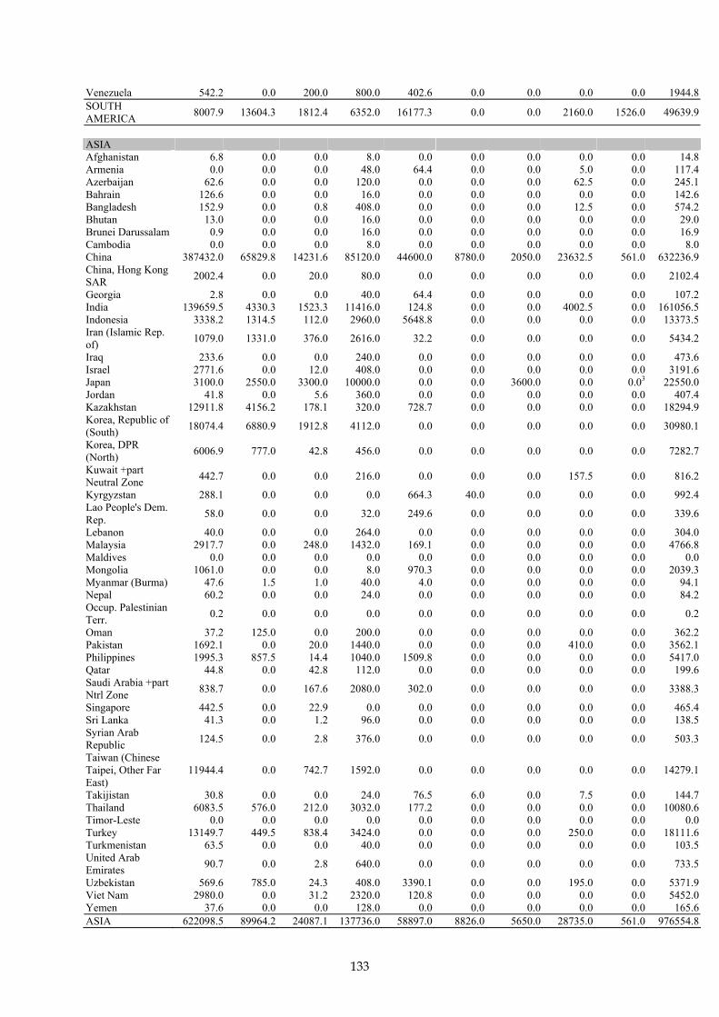
133

Venezuela 542.2 0.0 200.0 800.0 402.6 0.0 0.0 0.0 0.0 1944.8SOUTH AMERICA 8007.9 13604.3 1812.4 6352.0 16177.3 0.0 0.0 2160.0 1526.0 49639.9

ASIA Afghanistan 6.8 0.0 0.0 8.0 0.0 0.0 0.0 0.0 0.0 14.8Armenia 0.0 0.0 0.0 48.0 64.4 0.0 0.0 5.0 0.0 117.4Azerbaijan 62.6 0.0 0.0 120.0 0.0 0.0 0.0 62.5 0.0 245.1Bahrain 126.6 0.0 0.0 16.0 0.0 0.0 0.0 0.0 0.0 142.6Bangladesh 152.9 0.0 0.8 408.0 0.0 0.0 0.0 12.5 0.0 574.2Bhutan 13.0 0.0 0.0 16.0 0.0 0.0 0.0 0.0 0.0 29.0Brunei Darussalam 0.9 0.0 0.0 16.0 0.0 0.0 0.0 0.0 0.0 16.9Cambodia 0.0 0.0 0.0 8.0 0.0 0.0 0.0 0.0 0.0 8.0China 387432.0 65829.8 14231.6 85120.0 44600.0 8780.0 2050.0 23632.5 561.0 632236.9China, Hong Kong SAR 2002.4 0.0 20.0 80.0 0.0 0.0 0.0 0.0 0.0 2102.4

Georgia 2.8 0.0 0.0 40.0 64.4 0.0 0.0 0.0 0.0 107.2India 139659.5 4330.3 1523.3 11416.0 124.8 0.0 0.0 4002.5 0.0 161056.5Indonesia 3338.2 1314.5 112.0 2960.0 5648.8 0.0 0.0 0.0 0.0 13373.5Iran (Islamic Rep. of) 1079.0 1331.0 376.0 2616.0 32.2 0.0 0.0 0.0 0.0 5434.2

Iraq 233.6 0.0 0.0 240.0 0.0 0.0 0.0 0.0 0.0 473.6Israel 2771.6 0.0 12.0 408.0 0.0 0.0 0.0 0.0 0.0 3191.6Japan 3100.0 2550.0 3300.0 10000.0 0.0 0.0 3600.0 0.0 0.03 22550.0Jordan 41.8 0.0 5.6 360.0 0.0 0.0 0.0 0.0 0.0 407.4Kazakhstan 12911.8 4156.2 178.1 320.0 728.7 0.0 0.0 0.0 0.0 18294.9Korea, Republic of (South) 18074.4 6880.9 1912.8 4112.0 0.0 0.0 0.0 0.0 0.0 30980.1

Korea, DPR (North) 6006.9 777.0 42.8 456.0 0.0 0.0 0.0 0.0 0.0 7282.7

Kuwait +part Neutral Zone 442.7 0.0 0.0 216.0 0.0 0.0 0.0 157.5 0.0 816.2

Kyrgyzstan 288.1 0.0 0.0 0.0 664.3 40.0 0.0 0.0 0.0 992.4Lao People's Dem. Rep. 58.0 0.0 0.0 32.0 249.6 0.0 0.0 0.0 0.0 339.6

Lebanon 40.0 0.0 0.0 264.0 0.0 0.0 0.0 0.0 0.0 304.0Malaysia 2917.7 0.0 248.0 1432.0 169.1 0.0 0.0 0.0 0.0 4766.8Maldives 0.0 0.0 0.0 0.0 0.0 0.0 0.0 0.0 0.0 0.0Mongolia 1061.0 0.0 0.0 8.0 970.3 0.0 0.0 0.0 0.0 2039.3Myanmar (Burma) 47.6 1.5 1.0 40.0 4.0 0.0 0.0 0.0 0.0 94.1Nepal 60.2 0.0 0.0 24.0 0.0 0.0 0.0 0.0 0.0 84.2Occup. Palestinian Terr. 0.2 0.0 0.0 0.0 0.0 0.0 0.0 0.0 0.0 0.2

Oman 37.2 125.0 0.0 200.0 0.0 0.0 0.0 0.0 0.0 362.2Pakistan 1692.1 0.0 20.0 1440.0 0.0 0.0 0.0 410.0 0.0 3562.1Philippines 1995.3 857.5 14.4 1040.0 1509.8 0.0 0.0 0.0 0.0 5417.0Qatar 44.8 0.0 42.8 112.0 0.0 0.0 0.0 0.0 0.0 199.6Saudi Arabia +part Ntrl Zone 838.7 0.0 167.6 2080.0 302.0 0.0 0.0 0.0 0.0 3388.3

Singapore 442.5 0.0 22.9 0.0 0.0 0.0 0.0 0.0 0.0 465.4Sri Lanka 41.3 0.0 1.2 96.0 0.0 0.0 0.0 0.0 0.0 138.5Syrian Arab Republic 124.5 0.0 2.8 376.0 0.0 0.0 0.0 0.0 0.0 503.3

Taiwan (Chinese Taipei, Other Far East)

11944.4 0.0 742.7 1592.0 0.0 0.0 0.0 0.0 0.0 14279.1

Takijistan 30.8 0.0 0.0 24.0 76.5 6.0 0.0 7.5 0.0 144.7Thailand 6083.5 576.0 212.0 3032.0 177.2 0.0 0.0 0.0 0.0 10080.6Timor-Leste 0.0 0.0 0.0 0.0 0.0 0.0 0.0 0.0 0.0 0.0Turkey 13149.7 449.5 838.4 3424.0 0.0 0.0 0.0 250.0 0.0 18111.6Turkmenistan 63.5 0.0 0.0 40.0 0.0 0.0 0.0 0.0 0.0 103.5United Arab Emirates 90.7 0.0 2.8 640.0 0.0 0.0 0.0 0.0 0.0 733.5

Uzbekistan 569.6 785.0 24.3 408.0 3390.1 0.0 0.0 195.0 0.0 5371.9Viet Nam 2980.0 0.0 31.2 2320.0 120.8 0.0 0.0 0.0 0.0 5452.0Yemen 37.6 0.0 0.0 128.0 0.0 0.0 0.0 0.0 0.0 165.6ASIA 622098.5 89964.2 24087.1 137736.0 58897.0 8826.0 5650.0 28735.0 561.0 976554.8

134

OCEANIA Australia 17740.0 6080.0 800.0 300.0 7700.0 0.0 0.0 195.0 0.0 32815.0Cook Islands 0.0 0.0 0.0 0.0 0.0 0.0 0.0 0.0 0.0 0.0Fiji 2.6 0.0 0.0 8.0 79.0 0.0 0.0 0.0 0.0 89.6French Polynesia 0.0 0.0 0.0 0.0 0.0 0.0 0.0 0.0 0.0 0.0Kiribati 0.0 0.0 0.0 0.0 0.0 0.0 0.0 0.0 0.0 0.0Marshall Islands 0.0 0.0 0.0 0.0 0.0 0.0 0.0 0.0 0.0 0.0Micronesia 0.0 0.0 0.0 0.0 0.0 0.0 0.0 0.0 0.0 0.0Nauru 0.0 0.0 0.0 0.0 0.0 0.0 0.0 0.0 0.0 0.0New Caledonia 56.2 0.0 0.0 8.0 0.0 0.0 0.0 0.0 0.0 64.2New Zealand 1166.8 0.0 35.6 88.0 307.0 0.0 0.0 0.0 0.0 1597.3Palau 0.0 0.0 0.0 0.0 0.0 0.0 0.0 0.0 0.0 0.0Papua New Guinea 0.9 0.0 0.0 0.0 2005.0 0.0 0.0 0.0 0.0 2005.9Samoa 0.0 0.0 0.0 0.0 0.0 0.0 0.0 0.0 0.0 0.0Solomon Islands 0.0 0.0 0.0 0.0 0.0 0.0 0.0 0.0 0.0 0.0Tonga 0.0 0.0 0.0 0.0 0.0 0.0 0.0 0.0 0.0 0.0Tuvalu 0.0 0.0 0.0 0.0 0.0 0.0 0.0 0.0 0.0 0.0Vanuatu 0.0 0.0 0.0 0.0 0.0 0.0 0.0 0.0 0.0 0.0OCEANIA 18966.4 6080.0 835.6 404.0 10091.0 0.0 0.0 195.0 0.0 36572.0

RUSSIA Russian Federation 46000.5 5162.0 2647.4 3896.0 4300.0 10.0 3500.0 2782.5 1499.0 69797.5

EUROPE Metal production Albania 12.0 1.0 39.8 0.0 0.0 0.0 0.0 27.3 80.0Austria 370.4 663.0 114.8 0.0 0.0 20.6 0.1 32.5 1201.4Belarus 66.0 20.0 616.9 0.0 0.0 0.0 0.0 5.0 707.8Belgium 1351.2 443.3 563.5 0.0 0.0 55.6 268.5 266.3 2948.4Bosnia-Herzegovina 101.7 40.7 47.6 0.0 0.0 0.0 0.0 40.7 230.7

Bulgaria 1473.0 2454.3 127.5 0.0 0.0 0.0 0.0 0.0 4054.8Croatia 291.9 0.0 118.8 0.0 0.0 7.2 0.0 3.1 421.0Cyprus 14.0 0.0 144.0 0.0 0.0 0.0 0.0 0.0 158.0Czech Republic 1929.8 615.7 134.8 0.0 0.0 68.8 0.0 100.7 2849.8Denmark 719.3 0.0 42.8 0.0 0.0 67.0 0.0 29.7 858.8Estonia 520.0 0.0 9.9 0.0 0.0 0.0 0.0 0.0 529.9Finland 212.1 350.9 15.8 0.0 0.0 2.9 67.2 201.9 850.8France 4795.7 617.1 547.6 0.0 0.0 1195.9 818.0 790.8 8765.1Germany 7693.3 4879.2 1980.0 0.0 0.0 3485.2 936.2 1193.6 20167.5Greece 1587.1 65.9 1036.2 0.0 0.0 7.3 78.5 417.2 3192.2Hungary 1277.4 201.4 219.0 0.0 0.0 956.8 0.0 85.8 2740.3Iceland 3.1 0.0 9.6 0.0 0.0 1.7 0.0 7.3 21.7Ireland 172.1 0.0 270.0 0.0 0.0 26.0 0.0 32.9 501.0Italy 5324.9 2481.9 3092.7 0.0 0.0 675.3 1304.9 0.0 12879.7Latvia 100.0 0.0 49.1 0.0 0.0 0.0 0.0 0.0 149.1Lithuania 703.5 0.0 156.2 0.0 0.0 0.0 0.0 44.5 904.2Luxembourg 10.5 454.2 6.7 0.0 0.0 1.9 0.0 0.0 473.2Macedonia 226.6 11.6 31.8 0.0 0.0 0.0 0.0 0.0 270.0Moldova 34.9 150.0 106.7 0.0 0.0 0.0 0.0 0.0 291.6Monaco 80.0 0.0 0.0 0.0 0.0 0.0 0.0 0.0 80.0The Netherlands 206.0 207.0 156.0 0.0 0.0 118.0 42.0 0.0 729.0Norway 40.0 176.9 49.5 0.0 0.0 74.4 0.0 352.0 692.9Poland 8980.0 655.0 1170.0 0.0 0.0 0.0 358.0 8932.0 20095.0Portugal 1738.8 58.8 516.0 0.0 0.0 981.4 0.0 68.6 3363.6Romania 2395.0 284.7 1048.5 0.0 0.0 888.5 0.0 13.7 4630.3Slovakia 2180.0 270.0 270.0 0.0 0.0 82.9 110.0 1620.0 4532.9Slovenia 300.0 96.2 17.6 0.0 0.0 0.0 0.0 0.0 413.8Spain 4898.4 898.6 3508.8 0.0 0.0 163.4 613.6 99.1 10181.8Sweden 190.6 445.2 24.0 0.0 0.0 122.2 36.0 33.9 852.0Switzerland 429.8 500.1 153.0 0.0 0.0 60.9 22.0 41.2 1207.0Ukrainia 22132.5 1037.3 1462.8 0.0 0.0 877.0 311.2 179.2 26000.0United Kingdom 1860.6 537.0 201.2 0.0 0.0 167.8 1321.2 58.6 4146.3Yugoslavia (Serbia & Montenegro) 1600.0 132.4 712.5 0.0 0.0 0.0 0.0 0.0 2444.9

Malta 586.8 0.0 0.0 0.0 0.0 30.9 0.0 0.3 618.0EUROPE 76609.1 18749.2 18771.5 0.0 0.0 10139.7 6287.3 14677.9 145234.7

135

WORLD 880195.0 141331.2 45388.3 188949.9 111259.5 8841.0 35007.8 46759.8 25487.2 1483219.9 1 Cement and limestone production 2 Tabulated values for emissions from ‘other sources’ for countries in Europe plus the USA , Canada and Russia were incorporated in global emissions estimates; for all other continents data derived from the inventory for emissions from product-related sources were used. 3 Japan estimates emissions from ‘other sources’ in 2005 at 2500 kg.

Table AppA.7: Mercury by-product emissions from anthropogenic sources by country and sectors in 2020 SQ Scenario (kg, calculation results - implied precision should be ignored).

SQ 2020 Stationary combustion

Non- ferrous metals

production

Pig iron and crude

steel production

Cement production1

Large-scale gold

production

Mercury production (primary sources)

Inciner-ation of

municipal wastes

Caustic sodaa

production

Other sources2

Total

AFRICA Algeria 331.4 175.7 40.3 1536.0 24.2 0.0 0.0 0.0 0.0 2107.5Angola 15.5 0.0 0.0 96.0 0.0 0.0 0.0 0.0 0.0 111.5Benin 0.0 0.0 0.0 36.0 0.0 0.0 0.0 0.0 0.0 36.0Botswana 0.0 0.0 0.0 0.0 108.7 0.0 0.0 0.0 0.0 108.7

Burkina Faso 0.0 0.0 0.0 0.0 56.4 0.0 0.0 0.0 0.0 56.4

Burundi 0.0 0.0 0.0 0.0 157.0 0.0 0.0 0.0 0.0 157.0Cameroon 19.5 0.0 0.0 120.0 24.2 0.0 0.0 0.0 0.0 163.6Cape Verde 0.0 0.0 0.0 0.0 0.0 0.0 0.0 0.0 0.0 0.0

Central African Rep. 0.0 0.0 0.0 0.0 0.0 0.0 0.0 0.0 0.0 0.0

Chad 0.0 0.0 0.0 0.0 0.0 0.0 0.0 0.0 0.0 0.0Comores 0.0 0.0 0.0 0.0 0.0 0.0 0.0 0.0 0.0 0.0Congo-Brazzaville 7.9 0.0 0.0 0.0 0.0 0.0 0.0 0.0 0.0 7.9

Cote d'Ivoire 36.2 0.0 0.0 84.0 52.3 0.0 0.0 0.0 0.0 172.6

Dem.Rep.of Congo- Kinshasa

36.7 12.5 0.0 48.0 4.0 0.0 0.0 0.0 0.0 101.2

Djibouti 0.0 0.0 0.0 0.0 0.0 0.0 0.0 0.0 0.0 0.0Egypt 774.1 0.0 190.4 4320.0 0.0 0.0 0.0 0.0 0.0 5284.5Equatorial Guinea 3.6 0.0 0.0 0.0 8.1 0.0 0.0 0.0 0.0 11.6

Eritrea 0.0 0.0 0.0 12.0 0.0 0.0 0.0 0.0 0.0 12.0Ethiopia 7.7 0.0 0.0 192.0 124.8 0.0 0.0 0.0 0.0 324.5Gabon 7.2 0.0 0.0 36.0 12.1 0.0 0.0 0.0 0.0 55.3Gambia 0.0 0.0 0.0 0.0 0.0 0.0 0.0 0.0 0.0 0.0Ghana 18.1 0.0 1.0 228.0 2500.3 0.0 0.0 0.0 0.0 2747.4Guinea 0.0 0.0 0.0 48.0 704.6 0.0 0.0 0.0 0.0 752.6

Guinea-Bissau 0.0 0.0 0.0 0.0 0.0 0.0 0.0 0.0 0.0 0.0

Kenya 46.4 0.0 0.8 252.0 24.2 0.0 0.0 0.0 0.0 323.3Liberia 0.0 0.0 0.0 0.0 0.0 0.0 0.0 0.0 0.0 0.0

136

Libyan Arab.Jamah. 167.6 0.0 52.0 432.0 0.0 0.0 0.0 0.0 0.0 651.6

Madagascar 7.2 0.0 0.0 24.0 0.0 0.0 0.0 0.0 0.0 31.2Malawi 13.7 0.0 0.0 12.0 0.0 0.0 0.0 0.0 0.0 25.7Mali 0.0 0.0 0.0 0.0 1779.6 0.0 0.0 0.0 0.0 1779.6Mauritania 1.7 0.0 0.2 36.0 0.0 0.0 0.0 0.0 0.0 37.9Mauritius 69.4 0.0 0.0 0.0 0.0 0.0 0.0 0.0 0.0 69.4Morocco 1375.4 0.0 0.2 1320.0 60.4 2.0 0.0 0.0 0.0 2758.0

Mozambique 5.5 0.0 0.0 48.0 4.0 0.0 0.0 0.0 0.0 57.5

Namibia 0.0 331.8 0.0 0.0 108.7 0.0 0.0 0.0 0.0 440.5Niger 42.7 0.0 0.0 0.0 140.9 0.0 0.0 0.0 0.0 183.6Nigeria 52.0 0.0 4.0 288.0 0.0 0.0 0.0 0.0 0.0 344.0Reunion 0.0 0.0 0.0 48.0 0.0 0.0 0.0 0.0 0.0 48.0Rwanda 0.0 0.0 0.0 12.0 0.0 0.0 0.0 0.0 0.0 12.0

Sao Tome and Principe 0.0 0.0 0.0 0.0 0.0 0.0 0.0 0.0 0.0 0.0

Senegal 11.7 0.0 0.0 204.0 24.2 0.0 0.0 0.0 0.0 239.9Seychelles 0.0 0.0 0.0 0.0 0.0 0.0 0.0 0.0 0.0 0.0

Sierra Leone 2.7 0.0 0.0 24.0 0.0 0.0 0.0 0.0 0.0 26.7

Somalia 0.0 0.0 0.0 36.0 0.0 0.0 0.0 0.0 0.0 36.0

South Africa 40518.0 320.0 1314.0 5649.0 320.0 0.0 599.0 0.0 0.5 48720.5

St. Helena and Depend. 0.0 0.0 0.0 0.0 0.0 0.0 0.0 0.0 0.0 0.0

Sudan 38.5 0.0 0.0 0.0 189.2 0.0 0.0 0.0 0.0 227.7Swaziland (Ngwane) 0.0 0.0 0.0 0.0 0.0 0.0 0.0 0.0 0.0 0.0

Togo 0.0 0.0 0.0 96.0 0.0 0.0 0.0 0.0 0.0 96.0Tunisia 15.6 0.0 2.4 804.0 0.0 0.0 0.0 0.0 0.0 822.0Uganda 0.0 0.0 0.3 84.0 60.4 0.0 0.0 0.0 0.0 144.7Unit. Rep. Tanzania 15.6 0.0 0.0 168.0 1827.9 0.0 0.0 0.0 0.0 2011.5

Western Sahara 0.0 0.0 0.0 0.0 0.0 0.0 0.0 0.0 0.0 0.0

Zambia 42.2 1235.0 0.0 48.0 8.1 0.0 0.0 0.0 0.0 1333.2Zimbabwe 824.4 36.0 6.0 48.0 543.5 0.0 0.0 0.0 0.0 1457.9AFRICA 44508.0 2111.0 1611.6 16389.0 8867.6 2.0 599.0 0.0 0.5 74088.6 NORTH AMERICA

Antigua and Barbuda 0.0 0.0 0.0 0.0 0.0 0.0 0.0 0.0 0.0 0.0

Aruba 4.6 0.0 0.0 0.0 0.0 0.0 0.0 0.0 0.0 4.6Bahamas 0.0 0.0 0.0 0.0 0.0 0.0 0.0 0.0 0.0 0.0Barbados 0.0 0.0 0.0 36.0 0.0 0.0 0.0 0.0 0.0 36.0Belize 0.0 0.0 0.0 0.0 0.0 0.0 0.0 0.0 0.0 0.0Bermuda 0.0 0.0 0.0 0.0 0.0 0.0 0.0 0.0 0.0 0.0

British Virgin Islands 0.0 0.0 0.0 0.0 0.0 0.0 0.0 0.0 0.0 0.0

Cayman Islands 0.0 0.0 0.0 0.0 4799.2 0.0 0.0 0.0 0.0 4799.2

137

Costa Rica 5.3 0.0 0.0 240.0 0.0 0.0 0.0 0.0 0.0 245.3Cuba 51.1 0.0 8.0 168.0 16.1 0.0 0.0 0.0 0.0 243.2Dominica 0.0 0.0 0.0 0.0 20.1 0.0 0.0 0.0 0.0 20.1Dominican Republic 176.8 0.0 2.4 312.0 0.0 0.0 0.0 0.0 0.0 491.2

El Salvador 9.7 0.0 2.4 168.0 0.0 0.0 0.0 0.0 0.0 180.1Greenland 0.0 0.0 0.0 0.0 0.0 0.0 0.0 0.0 0.0 0.0Grenada 0.0 0.0 0.0 0.0 72.5 0.0 0.0 0.0 0.0 72.5

Guadeloupe 0.0 0.0 0.0 24.0 0.0 0.0 0.0 0.0 0.0 24.0

Guatemala 95.2 0.0 9.4 216.0 0.0 0.0 0.0 0.0 0.0 320.6Haiti 0.0 0.0 0.0 36.0 28.2 0.0 0.0 0.0 0.0 64.2Honduras 34.8 0.0 0.0 240.0 0.0 0.0 0.0 0.0 0.0 274.8Jamaica 20.5 0.0 0.0 96.0 100.7 0.0 0.0 0.0 0.0 217.2Martinique 2342.2 0.0 0.0 24.0 0.0 0.0 0.0 0.0 0.0 2366.2Mexico 1078.9 3865.6 656.0 4320.0 0.0 3.0 0.0 0.0 0.0 9923.5Montserrat 0.0 0.0 0.0 0.0 1224.0 0.0 0.0 0.0 0.0 1224.0Netherlands Antilles 108.8 0.0 0.0 0.0 0.0 0.0 0.0 0.0 0.0 108.8

Nicaragua 8.8 0.0 0.0 72.0 0.0 0.0 0.0 0.0 0.0 80.8Panama 0.0 0.0 0.0 96.0 144.9 0.0 0.0 0.0 0.0 240.9Puerto Rico 0.0 0.0 0.0 0.0 8.1 0.0 0.0 0.0 0.0 8.1

St. Kitts-Nevis 0.0 0.0 0.0 0.0 0.0 0.0 0.0 0.0 0.0 0.0

St. Lucia 0.0 0.0 0.0 0.0 0.0 0.0 0.0 0.0 0.0 0.0St. Pierre-Miquelon 0.0 0.0 0.0 0.0 0.0 0.0 0.0 0.0 0.0 0.0

St. Vincent-Grenadines 0.0 0.0 0.0 0.0 0.0 0.0 0.0 0.0 0.0 0.0

Trinidad and Tobago 67.5 0.0 32.0 96.0 0.0 0.0 0.0 0.0 0.0 195.5

United States 64436.2 100.0 13151.5 9897.4 6485.0 0.0 14921.9 0.0 6829.0 115821.0

Canada 2739.0 1694.9 532.5 255.2 27.8 0.0 197.3 0.0 394.4 5841.1NORTH AMERICA 71179.3 5660.5 14394.3 16296.6 12926.6 3.0 15119.2 0.0 7223.4 142802.8

SOUTH AMERICA

Argentina 553.0 296.8 215.3 912.0 1123.3 0.0 0.0 0.0 0.0 3100.4Bolivia 13.6 0.0 0.0 168.0 314.0 0.0 0.0 0.0 0.0 495.6Brazil 6807.5 3605.0 1265.2 4404.0 1658.8 0.0 0.0 0.0 0.0 17740.5Chile 1482.0 6197.0 62.8 480.0 1626.6 0.0 0.0 0.0 1526.0 11374.4Colombia 1101.9 0.0 30.0 1200.0 1441.4 0.0 0.0 0.0 0.0 3773.2Ecuador 92.1 0.0 2.9 372.0 217.4 0.0 0.0 0.0 0.0 684.4Falkland Is. (Malvinas) 0.0 0.0 0.0 0.0 0.0 0.0 0.0 0.0 0.0 0.0

French Guiana 0.0 0.0 0.0 12.0 80.5 0.0 0.0 0.0 0.0 92.5

Guyana 0.0 0.0 0.0 0.0 446.9 0.0 0.0 0.0 0.0 446.9Paraguay 0.7 0.0 4.0 84.0 0.0 0.0 0.0 0.0 0.0 88.7Peru 369.9 3505.5 30.0 552.0 8366.4 0.0 0.0 0.0 0.0 12823.9Suriname 5.2 0.0 0.0 12.0 426.8 0.0 0.0 0.0 0.0 444.0Uruguay 21.4 0.0 2.2 132.0 72.5 0.0 0.0 0.0 0.0 228.0Venezuela 542.2 0.0 200.0 1200.0 402.6 0.0 0.0 0.0 0.0 2344.8SOUTH AMERICA 10989.4 13604.3 1812.4 9528.0 16177.3 0.0 0.0 0.0 1526.0 53637.4

138

ASIA

Afghanistan 10.2 0.0 0.0 12.0 0.0 0.0 0.0 0.0 0.0 22.2

Armenia 0.0 0.0 0.0 72.0 64.4 0.0 0.0 0.0 0.0 136.4Azerbaijan 62.6 0.0 0.0 180.0 0.0 0.0 0.0 0.0 0.0 242.6Bahrain 126.6 0.0 0.0 24.0 0.0 0.0 0.0 0.0 0.0 150.6Bangladesh 222.9 0.0 0.8 612.0 0.0 0.0 0.0 0.0 0.0 835.7Bhutan 19.5 0.0 0.0 24.0 0.0 0.0 0.0 0.0 0.0 43.5Brunei Darussalam 0.9 0.0 0.0 24.0 0.0 0.0 0.0 0.0 0.0 24.9

Cambodia 0.0 0.0 0.0 12.0 0.0 0.0 0.0 0.0 0.0 12.0China 579697.4 65829.8 14231.6 127680.0 44600.0 8780.0 2050.0 0.0 561.0 843429.8

China, Hong Kong SAR 3003.6 0.0 20.0 120.0 0.0 0.0 0.0 0.0 0.0 3143.6

Georgia 4.0 0.0 0.0 60.0 64.4 0.0 0.0 0.0 0.0 128.4India 208842.3 4330.3 1523.3 17124.0 124.8 0.0 0.0 0.0 0.0 231944.8Indonesia 4754.9 1314.5 112.0 4440.0 5648.8 0.0 0.0 0.0 0.0 16270.2

Iran (Islamic Rep. of) 1249.7 1331.0 376.0 3924.0 32.2 0.0 0.0 0.0 0.0 6912.9

Iraq 233.6 0.0 0.0 360.0 0.0 0.0 0.0 0.0 0.0 593.6Israel 4103.0 0.0 12.0 612.0 0.0 0.0 0.0 0.0 0.0 4727.0Japan 4563.8 2550.0 3300.0 15000.0 0.0 0.0 3600.0 0.0 0.0 29013.8Jordan 41.8 0.0 5.6 540.0 0.0 0.0 0.0 0.0 0.0 587.4Kazakhstan 19306.8 4156.2 178.1 480.0 728.7 0.0 0.0 0.0 0.0 24849.9Korea, Republic of (South)

26547.0 6880.9 1912.8 6168.0 0.0 0.0 0.0 0.0 0.0 41508.7

Korea, DPR (North) 9007.5 777.0 42.8 684.0 0.0 0.0 0.0 0.0 0.0 10511.3

Kuwait +part Neutral Zone 442.7 0.0 0.0 324.0 0.0 0.0 0.0 0.0 0.0 766.7

Kyrgyzstan 431.7 0.0 0.0 0.0 664.3 40.0 0.0 0.0 0.0 1136.0

Lao People's Dem. Rep. 87.0 0.0 0.0 48.0 249.6 0.0 0.0 0.0 0.0 384.6

Lebanon 60.0 0.0 0.0 396.0 0.0 0.0 0.0 0.0 0.0 456.0Malaysia 4245.2 0.0 248.0 2148.0 169.1 0.0 0.0 0.0 0.0 6810.3Maldives 0.0 0.0 0.0 0.0 0.0 0.0 0.0 0.0 0.0 0.0Mongolia 1591.5 0.0 0.0 12.0 970.3 0.0 0.0 0.0 0.0 2573.8Myanmar (Burma) 66.1 1.5 1.0 60.0 4.0 0.0 0.0 0.0 0.0 132.6

Nepal 90.3 0.0 0.0 36.0 0.0 0.0 0.0 0.0 0.0 126.3Occup. Palestinian Terr.

0.3 0.0 0.0 0.0 0.0 0.0 0.0 0.0 0.0 0.3

Oman 37.2 125.0 0.0 300.0 0.0 0.0 0.0 0.0 0.0 462.2Pakistan 2481.5 0.0 20.0 2160.0 0.0 0.0 0.0 0.0 0.0 4661.5Philippines 2941.2 857.5 14.4 1560.0 1509.8 0.0 0.0 0.0 0.0 6882.9Qatar 44.8 0.0 42.8 168.0 0.0 0.0 0.0 0.0 0.0 255.6

139

Saudi Arabia +part Ntrl Zone

838.7 0.0 167.6 3120.0 302.0 0.0 0.0 0.0 0.0 4428.3

Singapore 442.8 0.0 22.9 0.0 0.0 0.0 0.0 0.0 0.0 465.7Sri Lanka 50.8 0.0 1.2 144.0 0.0 0.0 0.0 0.0 0.0 196.0

Syrian Arab Republic 124.5 0.0 2.8 564.0 0.0 0.0 0.0 0.0 0.0 691.3

Taiwan (Chinese Taipei, Other Far East)

17657.8 0.0 742.7 2388.0 0.0 0.0 0.0 0.0 0.0 20788.5

Takijistan 46.1 0.0 0.0 36.0 76.5 6.0 0.0 0.0 0.0 164.5Thailand 8891.8 576.0 212.0 4548.0 177.2 0.0 0.0 0.0 0.0 14404.9

Timor-Leste 0.0 0.0 0.0 0.0 0.0 0.0 0.0 0.0 0.0 0.0

Turkey 19594.6 449.5 838.4 5136.0 0.0 0.0 0.0 0.0 0.0 26018.5

Turkmenistan 63.5 0.0 0.0 60.0 0.0 0.0 0.0 0.0 0.0 123.5

United Arab Emirates 90.7 0.0 2.8 960.0 0.0 0.0 0.0 0.0 0.0 1053.5

Uzbekistan 832.9 785.0 24.3 612.0 3390.1 0.0 0.0 0.0 0.0 5644.2Viet Nam 4470.0 0.0 31.2 3480.0 120.8 0.0 0.0 0.0 0.0 8102.0Yemen 37.6 0.0 0.0 192.0 0.0 0.0 0.0 0.0 0.0 229.6ASIA 927459.3 89964.2 24087.1 206604.0 58897.0 8826.0 5650.0 0.0 561.0 1322048.7 OCEANIA Australia 17740.0 6080.0 800.0 450.0 7700.0 0.0 0.0 0.0 0.0 32770.0

Cook Islands 0.0 0.0 0.0 0.0 0.0 0.0 0.0 0.0 0.0 0.0

Fiji 2.6 0.0 0.0 12.0 79.0 0.0 0.0 0.0 0.0 93.6French Polynesia 0.0 0.0 0.0 0.0 0.0 0.0 0.0 0.0 0.0 0.0

Kiribati 0.0 0.0 0.0 0.0 0.0 0.0 0.0 0.0 0.0 0.0Marshall Islands 0.0 0.0 0.0 0.0 0.0 0.0 0.0 0.0 0.0 0.0

Micronesia 0.0 0.0 0.0 0.0 0.0 0.0 0.0 0.0 0.0 0.0Nauru 0.0 0.0 0.0 0.0 0.0 0.0 0.0 0.0 0.0 0.0

New Caledonia 56.2 0.0 0.0 12.0 0.0 0.0 0.0 0.0 0.0 68.2

New Zealand 1166.8 0.0 35.6 132.0 307.0 0.0 0.0 0.0 0.0 1641.3

Palau 0.0 0.0 0.0 0.0 0.0 0.0 0.0 0.0 0.0 0.0Papua New Guinea 0.9 0.0 0.0 0.0 2005.0 0.0 0.0 0.0 0.0 2005.9

Samoa 0.0 0.0 0.0 0.0 0.0 0.0 0.0 0.0 0.0 0.0Solomon Islands 0.0 0.0 0.0 0.0 0.0 0.0 0.0 0.0 0.0 0.0

Tonga 0.0 0.0 0.0 0.0 0.0 0.0 0.0 0.0 0.0 0.0Tuvalu 0.0 0.0 0.0 0.0 0.0 0.0 0.0 0.0 0.0 0.0Vanuatu 0.0 0.0 0.0 0.0 0.0 0.0 0.0 0.0 0.0 0.0OCEANIA 18966.4 6080.0 835.6 606.0 10091.0 0.0 0.0 0.0 0.0 36579.0 RUSSIA

140

Russian Federation 51799.6 5162.0 2647.4 5844.0 4300.0 10.0 3500.0 0.0 1499.0 74762.1

EUROPE Metals production Albania 12.0 1.0 39.8 0.0 0.0 0.0 0.0 27.3 80.0Austria 370.4 663.0 114.8 0.0 0.0 20.6 0.0 32.5 1201.3Belarus 66.0 20.0 616.9 0.0 0.0 0.0 0.0 5.0 707.8Belgium 1351.2 443.3 845.3 0.0 0.0 55.6 0.0 266.3 2961.7

Bosnia-Herzegovina 101.7 40.7 71.3 0.0 0.0 0.0 0.0 40.7 254.5

Bulgaria 1473.0 2454.3 191.3 0.0 0.0 0.0 0.0 0.0 4118.6Croatia 291.9 0.0 178.2 0.0 0.0 7.2 0.0 3.1 480.4Cyprus 14.0 0.0 216.0 0.0 0.0 0.0 0.0 0.0 230.0Czech Republic 1929.8 615.7 202.2 0.0 0.0 68.8 0.0 100.7 2917.3

Denmark 719.3 0.0 64.1 0.0 0.0 67.0 0.0 29.7 880.1Estonia 520.0 0.0 14.9 0.0 0.0 0.0 0.0 0.0 534.9Finland 212.1 350.9 23.7 0.0 0.0 2.9 0.0 201.9 791.5France 4795.7 617.1 821.4 0.0 0.0 1195.9 0.0 790.8 8220.9Germany 7693.3 4879.2 2970.0 0.0 0.0 3485.2 0.0 1193.6 20221.3Greece 1587.1 65.9 1554.3 0.0 0.0 7.3 0.0 417.2 3631.8Hungary 1277.4 201.4 328.5 0.0 0.0 956.8 0.0 85.8 2849.8Iceland 3.1 0.0 14.4 0.0 0.0 1.7 0.0 7.3 26.5Ireland 172.1 0.0 405.0 0.0 0.0 26.0 0.0 32.9 636.0Italy 5324.9 2481.9 4639.1 0.0 0.0 675.3 0.0 0.0 13121.2Latvia 100.0 0.0 73.7 0.0 0.0 0.0 0.0 0.0 173.7Lithuania 703.5 0.0 234.2 0.0 0.0 0.0 0.0 44.5 982.3

Luxembourg 10.5 454.2 10.0 0.0 0.0 1.9 0.0 0.0 476.5

Macedonia 226.6 11.6 47.7 0.0 0.0 0.0 0.0 0.0 285.9Moldova 34.9 150.0 160.1 0.0 0.0 0.0 0.0 0.0 345.0Monaco 80.0 0.0 0.0 0.0 0.0 0.0 0.0 0.0 80.0

The Netherlands 206.0 207.0 234.0 0.0 0.0 118.0 0.0 0.0 765.0

Norway 40.0 176.9 74.3 0.0 0.0 74.4 0.0 352.0 717.6Poland 8980.0 655.0 1755.0 0.0 0.0 0.0 0.0 8932.0 20322.0Portugal 1738.8 58.8 774.0 0.0 0.0 981.4 0.0 68.6 3621.6Romania 2395.0 284.7 1572.7 0.0 0.0 888.5 0.0 13.7 5154.6Slovakia 2180.0 270.0 405.0 0.0 0.0 82.9 0.0 1620.0 4557.9Slovenia 300.0 96.2 26.4 0.0 0.0 0.0 0.0 0.0 422.6Spain 4898.4 898.6 5263.2 0.0 0.0 163.4 0.0 99.1 11322.7Sweden 190.6 445.2 36.0 0.0 0.0 122.2 0.0 33.9 828.0Switzerland 429.8 500.1 229.5 0.0 0.0 60.9 0.0 41.2 1261.5Ukrainia 22132.5 1037.3 2194.2 0.0 0.0 877.0 0.0 179.2 26420.2United Kingdom 1860.6 537.0 301.8 0.0 0.0 167.8 0.0 58.6 2925.7

Yugoslavia (Serbia & Montenegro)

1600.0 132.4 1068.8 0.0 0.0 0.0 0.0 0.0 2801.2

Malta 586.8 0.0 0.0 0.0 0.0 30.9 0.0 0.3 618.0EUROPE 76609.1 18749.2 27771.6 0.0 0.0 10139.7 0.0 14677.9 147947.4 WORLD 1201511.2 141331.2 45388.3 283039.2 111259.5 8841.0 35007.8 0.0 25487.7 1851866.0 1, 2 See footnotes to Appendix Table AppA6.

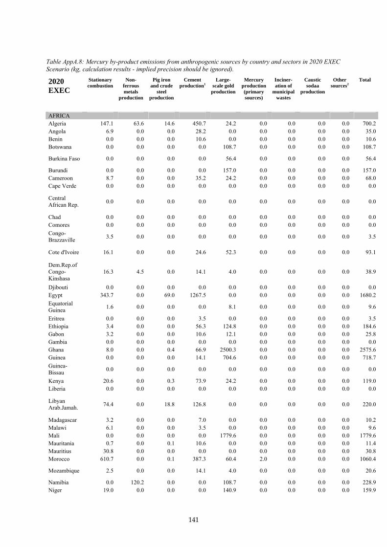
141

Table AppA.8: Mercury by-product emissions from anthropogenic sources by country and sectors in 2020 EXEC Scenario (kg, calculation results - implied precision should be ignored).

2020 EXEC

Stationary combustion

Non- ferrous metals

production

Pig iron and crude

steel production

Cement production1

Large-scale gold

production

Mercury production (primary sources)

Inciner-ation of

municipal wastes

Caustic sodaa

production

Other sources2

Total

AFRICA Algeria 147.1 63.6 14.6 450.7 24.2 0.0 0.0 0.0 0.0 700.2Angola 6.9 0.0 0.0 28.2 0.0 0.0 0.0 0.0 0.0 35.0Benin 0.0 0.0 0.0 10.6 0.0 0.0 0.0 0.0 0.0 10.6Botswana 0.0 0.0 0.0 0.0 108.7 0.0 0.0 0.0 0.0 108.7

Burkina Faso 0.0 0.0 0.0 0.0 56.4 0.0 0.0 0.0 0.0 56.4

Burundi 0.0 0.0 0.0 0.0 157.0 0.0 0.0 0.0 0.0 157.0Cameroon 8.7 0.0 0.0 35.2 24.2 0.0 0.0 0.0 0.0 68.0Cape Verde 0.0 0.0 0.0 0.0 0.0 0.0 0.0 0.0 0.0 0.0

Central African Rep. 0.0 0.0 0.0 0.0 0.0 0.0 0.0 0.0 0.0 0.0

Chad 0.0 0.0 0.0 0.0 0.0 0.0 0.0 0.0 0.0 0.0Comores 0.0 0.0 0.0 0.0 0.0 0.0 0.0 0.0 0.0 0.0Congo-Brazzaville 3.5 0.0 0.0 0.0 0.0 0.0 0.0 0.0 0.0 3.5

Cote d'Ivoire 16.1 0.0 0.0 24.6 52.3 0.0 0.0 0.0 0.0 93.1

Dem.Rep.of Congo- Kinshasa

16.3 4.5 0.0 14.1 4.0 0.0 0.0 0.0 0.0 38.9

Djibouti 0.0 0.0 0.0 0.0 0.0 0.0 0.0 0.0 0.0 0.0Egypt 343.7 0.0 69.0 1267.5 0.0 0.0 0.0 0.0 0.0 1680.2Equatorial Guinea 1.6 0.0 0.0 0.0 8.1 0.0 0.0 0.0 0.0 9.6

Eritrea 0.0 0.0 0.0 3.5 0.0 0.0 0.0 0.0 0.0 3.5Ethiopia 3.4 0.0 0.0 56.3 124.8 0.0 0.0 0.0 0.0 184.6Gabon 3.2 0.0 0.0 10.6 12.1 0.0 0.0 0.0 0.0 25.8Gambia 0.0 0.0 0.0 0.0 0.0 0.0 0.0 0.0 0.0 0.0Ghana 8.0 0.0 0.4 66.9 2500.3 0.0 0.0 0.0 0.0 2575.6Guinea 0.0 0.0 0.0 14.1 704.6 0.0 0.0 0.0 0.0 718.7Guinea-Bissau 0.0 0.0 0.0 0.0 0.0 0.0 0.0 0.0 0.0 0.0

Kenya 20.6 0.0 0.3 73.9 24.2 0.0 0.0 0.0 0.0 119.0Liberia 0.0 0.0 0.0 0.0 0.0 0.0 0.0 0.0 0.0 0.0

Libyan Arab.Jamah. 74.4 0.0 18.8 126.8 0.0 0.0 0.0 0.0 0.0 220.0

Madagascar 3.2 0.0 0.0 7.0 0.0 0.0 0.0 0.0 0.0 10.2Malawi 6.1 0.0 0.0 3.5 0.0 0.0 0.0 0.0 0.0 9.6Mali 0.0 0.0 0.0 0.0 1779.6 0.0 0.0 0.0 0.0 1779.6Mauritania 0.7 0.0 0.1 10.6 0.0 0.0 0.0 0.0 0.0 11.4Mauritius 30.8 0.0 0.0 0.0 0.0 0.0 0.0 0.0 0.0 30.8Morocco 610.7 0.0 0.1 387.3 60.4 2.0 0.0 0.0 0.0 1060.4

Mozambique 2.5 0.0 0.0 14.1 4.0 0.0 0.0 0.0 0.0 20.6

Namibia 0.0 120.2 0.0 0.0 108.7 0.0 0.0 0.0 0.0 228.9Niger 19.0 0.0 0.0 0.0 140.9 0.0 0.0 0.0 0.0 159.9

142

Nigeria 23.1 0.0 1.4 84.5 0.0 0.0 0.0 0.0 0.0 109.1Reunion 0.0 0.0 0.0 14.1 0.0 0.0 0.0 0.0 0.0 14.1Rwanda 0.0 0.0 0.0 3.5 0.0 0.0 0.0 0.0 0.0 3.5

Sao Tome and Principe 0.0 0.0 0.0 0.0 0.0 0.0 0.0 0.0 0.0 0.0

Senegal 5.2 0.0 0.0 59.9 24.2 0.0 0.0 0.0 0.0 89.2Seychelles 0.0 0.0 0.0 0.0 0.0 0.0 0.0 0.0 0.0 0.0

Sierra Leone 1.2 0.0 0.0 7.0 0.0 0.0 0.0 0.0 0.0 8.2

Somalia 0.0 0.0 0.0 10.6 0.0 0.0 0.0 0.0 0.0 10.6

South Africa 17989.8 115.9 475.9 1657.5 320.0 0.0 125.5 0.0 0.0 20684.6

St. Helena and Depend. 0.0 0.0 0.0 0.0 0.0 0.0 0.0 0.0 0.0 0.0

Sudan 17.1 0.0 0.0 0.0 189.2 0.0 0.0 0.0 0.0 206.3Swaziland (Ngwane) 0.0 0.0 0.0 0.0 0.0 0.0 0.0 0.0 0.0 0.0

Togo 0.0 0.0 0.0 28.2 0.0 0.0 0.0 0.0 0.0 28.2Tunisia 6.9 0.0 0.9 235.9 0.0 0.0 0.0 0.0 0.0 243.7Uganda 0.0 0.0 0.1 24.6 60.4 0.0 0.0 0.0 0.0 85.1Unit. Rep. Tanzania 6.9 0.0 0.0 49.3 1827.9 0.0 0.0 0.0 0.0 1884.1

Western Sahara 0.0 0.0 0.0 0.0 0.0 0.0 0.0 0.0 0.0 0.0

Zambia 18.7 447.3 0.0 14.1 8.1 0.0 0.0 0.0 0.0 488.2Zimbabwe 366.0 13.0 2.2 14.1 543.5 0.0 0.0 0.0 0.0 938.9AFRICA 19761.3 880.5 583.7 4808.7 8867.6 2.0 125.5 0.0 0.0 35029.4 NORTH AMERICA

Antigua and Barbuda 0.0 0.0 0.0 0.0 0.0 0.0 0.0 0.0 0.0 0.0

Aruba 2.0 0.0 0.0 0.0 0.0 0.0 0.0 0.0 0.0 2.0Bahamas 0.0 0.0 0.0 0.0 0.0 0.0 0.0 0.0 0.0 0.0Barbados 0.0 0.0 0.0 10.6 0.0 0.0 0.0 0.0 0.0 10.6Belize 0.0 0.0 0.0 0.0 0.0 0.0 0.0 0.0 0.0 0.0Bermuda 0.0 0.0 0.0 0.0 0.0 0.0 0.0 0.0 0.0 0.0

British Virgin Islands 0.0 0.0 0.0 0.0 0.0 0.0 0.0 0.0 0.0 0.0

Cayman Islands 0.0 0.0 0.0 0.0 4799.2 0.0 0.0 0.0 0.0 4799.2

Costa Rica 2.3 0.0 0.0 70.4 0.0 0.0 0.0 0.0 0.0 72.8Cuba 22.7 0.0 2.9 49.3 16.1 0.0 0.0 0.0 0.0 91.0Dominica 0.0 0.0 0.0 0.0 20.1 0.0 0.0 0.0 0.0 20.1Dominican Republic 78.5 0.0 0.9 91.5 0.0 0.0 0.0 0.0 0.0 170.9

El Salvador 4.3 0.0 0.9 49.3 0.0 0.0 0.0 0.0 0.0 54.5Greenland 0.0 0.0 0.0 0.0 0.0 0.0 0.0 0.0 0.0 0.0Grenada 0.0 0.0 0.0 0.0 72.5 0.0 0.0 0.0 0.0 72.5

Guadeloupe 0.0 0.0 0.0 7.0 0.0 0.0 0.0 0.0 0.0 7.0

Guatemala 42.3 0.0 3.4 63.4 0.0 0.0 0.0 0.0 0.0 109.1Haiti 0.0 0.0 0.0 10.6 28.2 0.0 0.0 0.0 0.0 38.7Honduras 15.5 0.0 0.0 70.4 0.0 0.0 0.0 0.0 0.0 85.9

143

Jamaica 9.1 0.0 0.0 28.2 100.7 0.0 0.0 0.0 0.0 137.9Martinique 1039.9 0.0 0.0 7.0 0.0 0.0 0.0 0.0 0.0 1047.0Mexico 479.0 1400.1 237.6 1267.5 0.0 3.0 0.0 0.0 0.0 3387.3Montserrat 0.0 0.0 0.0 0.0 1224.0 0.0 0.0 0.0 0.0 1224.0Netherlands Antilles 48.3 0.0 0.0 0.0 0.0 0.0 0.0 0.0 0.0 48.3

Nicaragua 3.9 0.0 0.0 21.1 0.0 0.0 0.0 0.0 0.0 25.0Panama 0.0 0.0 0.0 28.2 144.9 0.0 0.0 0.0 0.0 173.1Puerto Rico 0.0 0.0 0.0 0.0 8.1 0.0 0.0 0.0 0.0 8.1St. Kitts-Nevis 0.0 0.0 0.0 0.0 0.0 0.0 0.0 0.0 0.0 0.0

St. Lucia 0.0 0.0 0.0 0.0 0.0 0.0 0.0 0.0 0.0 0.0St. Pierre-Miquelon 0.0 0.0 0.0 0.0 0.0 0.0 0.0 0.0 0.0 0.0

St. Vincent-Grenadines 0.0 0.0 0.0 0.0 0.0 0.0 0.0 0.0 0.0 0.0

Trinidad and Tobago 30.0 0.0 11.6 28.2 0.0 0.0 0.0 0.0 0.0 69.7

United States 28609.3 36.2 4763.5 2904.0 6485.0 0.0 3126.2 0.0 6829.0 52753.2

Canada 1216.1 613.9 192.9 74.9 27.8 0.0 41.3 0.0 394.4 2561.3NORTH AMERICA 31603.3 1464.2 5020.7 4781.6 12926.6 3.0 3167.5 0.0 7223.4 66190.3

SOUTH AMERICA

Argentina 245.5 107.5 78.0 267.6 1123.3 0.0 0.0 0.0 0.0 1821.9Bolivia 6.0 0.0 0.0 49.3 314.0 0.0 0.0 0.0 0.0 369.4Brazil 3022.5 1305.7 458.3 1292.2 1658.8 0.0 0.0 0.0 0.0 7737.5Chile 658.0 2244.6 22.7 140.8 1626.6 0.0 0.0 0.0 1526.0 6218.7Colombia 489.2 0.0 10.9 352.1 1441.4 0.0 0.0 0.0 0.0 2293.6Ecuador 40.9 0.0 1.0 109.1 217.4 0.0 0.0 0.0 0.0 368.5Falkland Is. (Malvinas) 0.0 0.0 0.0 0.0 0.0 0.0 0.0 0.0 0.0 0.0

French Guiana 0.0 0.0 0.0 3.5 80.5 0.0 0.0 0.0 0.0 84.0

Guyana 0.0 0.0 0.0 0.0 446.9 0.0 0.0 0.0 0.0 446.9Paraguay 0.3 0.0 1.4 24.6 0.0 0.0 0.0 0.0 0.0 26.4Peru 164.2 1269.7 10.9 162.0 8366.4 0.0 0.0 0.0 0.0 9973.2Suriname 2.3 0.0 0.0 3.5 426.8 0.0 0.0 0.0 0.0 432.6Uruguay 9.5 0.0 0.8 38.7 72.5 0.0 0.0 0.0 0.0 121.5Venezuela 240.7 0.0 72.4 352.1 402.6 0.0 0.0 0.0 0.0 1067.9SOUTH AMERICA 4879.3 4927.5 656.5 2795.6 16177.3 0.0 0.0 0.0 1526.0 30962.1

ASIA

Afghanistan 4.5 0.0 0.0 3.5 0.0 0.0 0.0 0.0 0.0 8.0

Armenia 0.0 0.0 0.0 21.1 64.4 0.0 0.0 0.0 0.0 85.5Azerbaijan 27.8 0.0 0.0 52.8 0.0 0.0 0.0 0.0 0.0 80.6Bahrain 56.2 0.0 0.0 7.0 0.0 0.0 0.0 0.0 0.0 63.2Bangladesh 99.0 0.0 0.3 179.6 0.0 0.0 0.0 0.0 0.0 278.8Bhutan 8.7 0.0 0.0 7.0 0.0 0.0 0.0 0.0 0.0 15.7Brunei Darussalam 0.4 0.0 0.0 7.0 0.0 0.0 0.0 0.0 0.0 7.4

Cambodia 0.0 0.0 0.0 3.5 0.0 0.0 0.0 0.0 0.0 3.5China 257382.8 23843.6 5154.7 37462.9 44600.0 8780.0 429.5 0.0 561.0 378214.4

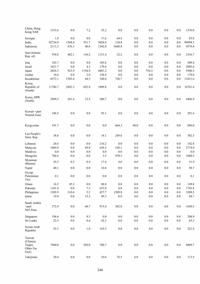
144

China, Hong Kong SAR 1333.6 0.0 7.2 35.2 0.0 0.0 0.0 0.0 0.0 1376.0

Georgia 1.8 0.0 0.0 17.6 64.4 0.0 0.0 0.0 0.0 83.8India 92724.9 1568.4 551.7 5024.4 124.8 0.0 0.0 0.0 0.0 99994.3Indonesia 2111.2 476.1 40.6 1302.8 5648.8 0.0 0.0 0.0 0.0 9579.4

Iran (Islamic Rep. of) 554.8 482.1 136.2 1151.4 32.2 0.0 0.0 0.0 0.0 2356.7

Iraq 103.7 0.0 0.0 105.6 0.0 0.0 0.0 0.0 0.0 209.4Israel 1821.7 0.0 4.3 179.6 0.0 0.0 0.0 0.0 0.0 2005.6Japan 2026.3 923.9 1194.9 4401.2 0.0 0.0 754.2 0.0 0.0 9300.5Jordan 18.6 0.0 2.0 158.4 0.0 0.0 0.0 0.0 0.0 179.0Kazakhstan 8572.1 1505.4 64.5 140.8 728.7 0.0 0.0 0.0 0.0 11011.6Korea, Republic of (South)

11786.7 2492.3 692.8 1809.8 0.0 0.0 0.0 0.0 0.0 16781.6

Korea, DPR (North) 3999.3 281.4 15.5 200.7 0.0 0.0 0.0 0.0 0.0 4496.9

Kuwait +part Neutral Zone 196.5 0.0 0.0 95.1 0.0 0.0 0.0 0.0 0.0 291.6

Kyrgyzstan 191.7 0.0 0.0 0.0 664.3 40.0 0.0 0.0 0.0 896.0

Lao People's Dem. Rep. 38.6 0.0 0.0 14.1 249.6 0.0 0.0 0.0 0.0 302.3

Lebanon 26.6 0.0 0.0 116.2 0.0 0.0 0.0 0.0 0.0 142.8Malaysia 1884.9 0.0 89.8 630.3 169.1 0.0 0.0 0.0 0.0 2774.0Maldives 0.0 0.0 0.0 0.0 0.0 0.0 0.0 0.0 0.0 0.0Mongolia 706.6 0.0 0.0 3.5 970.3 0.0 0.0 0.0 0.0 1680.5Myanmar (Burma) 29.3 0.5 0.4 17.6 4.0 0.0 0.0 0.0 0.0 51.9

Nepal 40.1 0.0 0.0 10.6 0.0 0.0 0.0 0.0 0.0 50.7Occup. Palestinian Terr.

0.1 0.0 0.0 0.0 0.0 0.0 0.0 0.0 0.0 0.1

Oman 16.5 45.3 0.0 88.0 0.0 0.0 0.0 0.0 0.0 149.8Pakistan 1101.8 0.0 7.2 633.8 0.0 0.0 0.0 0.0 0.0 1742.8Philippines 1305.9 310.6 5.2 457.7 1509.8 0.0 0.0 0.0 0.0 3589.2Qatar 19.9 0.0 15.5 49.3 0.0 0.0 0.0 0.0 0.0 84.7

Saudi Arabia +part Ntrl Zone

372.4 0.0 60.7 915.4 302.0 0.0 0.0 0.0 0.0 1650.5

Singapore 196.6 0.0 8.3 0.0 0.0 0.0 0.0 0.0 0.0 204.9Sri Lanka 22.5 0.0 0.4 42.3 0.0 0.0 0.0 0.0 0.0 65.2

Syrian Arab Republic 55.3 0.0 1.0 165.5 0.0 0.0 0.0 0.0 0.0 221.8

Taiwan (Chinese Taipei, Other Far East)

7840.0 0.0 269.0 700.7 0.0 0.0 0.0 0.0 0.0 8809.7

Takijistan 20.4 0.0 0.0 10.6 76.5 6.0 0.0 0.0 0.0 113.5

145

Thailand 3947.9 208.6 76.8 1334.4 177.2 0.0 0.0 0.0 0.0 5744.9

Timor-Leste 0.0 0.0 0.0 0.0 0.0 0.0 0.0 0.0 0.0 0.0

Turkey 8699.9 162.8 303.7 1507.0 0.0 0.0 0.0 0.0 0.0 10673.3

Turkmenistan 28.2 0.0 0.0 17.6 0.0 0.0 0.0 0.0 0.0 45.8

United Arab Emirates 40.3 0.0 1.0 281.7 0.0 0.0 0.0 0.0 0.0 323.0

Uzbekistan 369.8 284.3 8.8 179.6 3390.1 0.0 0.0 0.0 0.0 4232.5Viet Nam 1984.7 0.0 11.3 1021.1 120.8 0.0 0.0 0.0 0.0 3137.8Yemen 16.7 0.0 0.0 56.3 0.0 0.0 0.0 0.0 0.0 73.0ASIA 411787.3 32585.3 8723.8 60620.2 58897.0 8826.0 1183.7 0.0 561.0 583184.4 OCEANIA Australia 7876.5 2202.2 289.8 132.0 7700.0 0.0 0.0 0.0 18200.4

Cook Islands 0.0 0.0 0.0 0.0 0.0 0.0 0.0 0.0 0.0 0.0

Fiji 1.2 0.0 0.0 3.5 79.0 0.0 0.0 0.0 0.0 83.7French Polynesia 0.0 0.0 0.0 0.0 0.0 0.0 0.0 0.0 0.0 0.0

Kiribati 0.0 0.0 0.0 0.0 0.0 0.0 0.0 0.0 0.0 0.0Marshall Islands 0.0 0.0 0.0 0.0 0.0 0.0 0.0 0.0 0.0 0.0

Micronesia 0.0 0.0 0.0 0.0 0.0 0.0 0.0 0.0 0.0 0.0Nauru 0.0 0.0 0.0 0.0 0.0 0.0 0.0 0.0 0.0 0.0New Caledonia 25.0 0.0 0.0 3.5 0.0 0.0 0.0 0.0 0.0 28.5

New Zealand 518.0 0.0 12.9 38.7 307.0 0.0 0.0 0.0 0.0 876.7

Palau 0.0 0.0 0.0 0.0 0.0 0.0 0.0 0.0 0.0 0.0Papua New Guinea 0.4 0.0 0.0 0.0 2005.0 0.0 0.0 0.0 0.0 2005.4

Samoa 0.0 0.0 0.0 0.0 0.0 0.0 0.0 0.0 0.0 0.0Solomon Islands 0.0 0.0 0.0 0.0 0.0 0.0 0.0 0.0 0.0 0.0

Tonga 0.0 0.0 0.0 0.0 0.0 0.0 0.0 0.0 0.0 0.0Tuvalu 0.0 0.0 0.0 0.0 0.0 0.0 0.0 0.0 0.0 0.0Vanuatu 0.0 0.0 0.0 0.0 0.0 0.0 0.0 0.0 0.0 0.0OCEANIA 8421.0 2202.2 302.6 177.8 10091.0 0.0 0.0 0.0 0.0 21194.6 RUSSIA Russian Federation 20424.0 1869.7 958.9 1714.7 4300.0 10.0 733.3 0.0 1499.0 31509.5

EUROPE Metals production

Albania 10.8 0.4 17.5 0.0 0.0 0.0 0.0 27.3 55.9Austria 266.3 257.5 50.5 0.0 0.0 4.3 0.0 32.5 611.2Belarus 31.5 7.8 271.5 0.0 0.0 0.0 0.0 5.0 315.8Belgium 726.8 172.2 248.0 0.0 0.0 11.6 0.0 266.3 1425.0

Bosnia-Herzegovina 45.2 15.8 20.9 0.0 0.0 0.0 0.0 40.7 122.6

Bulgaria 654.0 953.4 56.1 0.0 0.0 0.0 0.0 0.0 1663.5Croatia 224.5 0.0 52.3 0.0 0.0 1.5 0.0 3.1 281.4Cyprus 6.2 0.0 63.4 0.0 0.0 0.0 0.0 0.0 69.6

146

Czech Republic 856.8 239.2 59.3 0.0 0.0 14.4 0.0 100.7 1270.5

Denmark 319.4 0.0 18.8 0.0 0.0 14.0 0.0 29.7 381.9Estonia 242.0 0.0 4.4 0.0 0.0 0.0 0.0 0.0 246.4Finland 106.2 136.3 7.0 0.0 0.0 0.6 0.0 201.9 451.9France 2225.4 239.7 241.0 0.0 0.0 250.6 0.0 790.8 3747.5Germany 4815.3 1895.4 871.4 0.0 0.0 730.2 0.0 1193.6 9505.9Greece 1070.9 25.6 456.1 0.0 0.0 1.5 0.0 417.2 1971.3Hungary 909.7 78.2 96.4 0.0 0.0 200.4 0.0 85.8 1370.5Iceland 2.1 0.0 4.2 0.0 0.0 0.4 0.0 7.3 14.0Ireland 123.8 0.0 118.8 0.0 0.0 5.4 0.0 32.9 281.1Italy 3115.2 964.1 1361.2 0.0 0.0 141.5 0.0 0.0 5582.0Latvia 44.4 0.0 21.6 0.0 0.0 0.0 0.0 0.0 66.0Lithuania 544.0 0.0 68.7 0.0 0.0 0.0 0.0 44.5 657.2

Luxembourg 6.3 176.4 2.9 0.0 0.0 0.4 0.0 0.0 186.0

Macedonia 100.6 4.5 14.0 0.0 0.0 0.0 0.0 0.0 119.1Moldova 15.5 58.3 47.0 0.0 0.0 0.0 0.0 0.0 120.7Monaco 57.8 0.0 0.0 0.0 0.0 0.0 0.0 0.0 57.8

The Netherlands 91.5 80.4 68.7 0.0 0.0 24.7 0.0 0.0 265.3

Norway 31.4 68.7 21.8 0.0 0.0 15.6 0.0 352.0 489.5Poland 4521.4 254.4 514.9 0.0 0.0 0.0 0.0 8932.0 14222.8Portugal 991.1 22.8 227.1 0.0 0.0 205.6 0.0 68.6 1515.2Romania 1063.4 110.6 461.4 0.0 0.0 186.2 0.0 13.7 1835.2Slovakia 1574.0 104.9 118.8 0.0 0.0 17.4 0.0 1620.0 3435.0Slovenia 133.2 37.4 7.7 0.0 0.0 0.0 0.0 0.0 178.3Spain 2209.3 349.1 1544.3 0.0 0.0 34.2 0.0 99.1 4236.0Sweden 97.6 173.0 10.6 0.0 0.0 25.6 0.0 33.9 340.7Switzerland 249.1 194.3 67.3 0.0 0.0 12.8 0.0 41.2 564.6Ukrainia 18761.0 403.0 643.8 0.0 0.0 183.7 0.0 179.2 20170.7United Kingdom 826.1 208.6 88.5 0.0 0.0 35.2 0.0 58.6 1217.0

Yugoslavia (Serbia & Montenegro)

1155.2 51.4 313.6 0.0 0.0 0.0 0.0 0.0 1520.2

Malta 260.5 0.0 0.0 0.0 0.0 6.5 0.0 0.3 267.3EUROPE 48485.4 7283.3 8261.7 0.0 0.0 2124.3 0.0 14677.9 80832.6 WORLD 545361.6 53595.3 17448.6 83160.4 111259.5 8841.0 7334.2 0.0 25487.2 852287.8

1, 2 See footnotes to Appendix Table AppA6.

Table AppA.9: Mercury by-product emissions from anthropogenic sources by country and sectors in 2020 MTFR Scenario (kg, calculation results - implied precision should be ignored).

2020 MFTR

Stationary combustion

Non- ferrous metals

production

Pig iron and crude

steel production

Cement production1

Large-scale gold

production

Mercury production (primary sources)

Inciner-ation of

municipal wastes

Caustic sodaa

production

Other sources2

Total

AFRICA Algeria 107.3 46.4 10.6 328.7 24.2 0.0 0.0 0.0 0.0 517.3Angola 5.0 0.0 0.0 20.5 0.0 0.0 0.0 0.0 0.0 25.6Benin 0.0 0.0 0.0 7.7 0.0 0.0 0.0 0.0 0.0 7.7Botswana 0.0 0.0 0.0 0.0 108.7 0.0 0.0 0.0 0.0 108.7

147

Burkina Faso 0.0 0.0 0.0 0.0 56.4 0.0 0.0 0.0 0.0 56.4Burundi 0.0 0.0 0.0 0.0 157.0 0.0 0.0 0.0 0.0 157.0Cameroon 6.3 0.0 0.0 25.7 24.2 0.0 0.0 0.0 0.0 56.2Cape Verde 0.0 0.0 0.0 0.0 0.0 0.0 0.0 0.0 0.0 0.0Central African Rep. 0.0 0.0 0.0 0.0 0.0 0.0 0.0 0.0 0.0 0.0

Chad 0.0 0.0 0.0 0.0 0.0 0.0 0.0 0.0 0.0 0.0Comores 0.0 0.0 0.0 0.0 0.0 0.0 0.0 0.0 0.0 0.0Congo-Brazzaville 2.6 0.0 0.0 0.0 0.0 0.0 0.0 0.0 0.0 2.6

Cote d'Ivoire 11.7 0.0 0.0 18.0 52.3 0.0 0.0 0.0 0.0 82.0Dem.Rep.of Congo-Kinshasa

11.9 3.3 0.0 10.3 4.0 0.0 0.0 0.0 0.0 29.5

Djibouti 0.0 0.0 0.0 0.0 0.0 0.0 0.0 0.0 0.0 0.0Egypt 250.7 0.0 50.3 924.6 0.0 0.0 0.0 0.0 0.0 1225.6Equatorial Guinea 1.1 0.0 0.0 0.0 8.1 0.0 0.0 0.0 0.0 9.2

Eritrea 0.0 0.0 0.0 2.6 0.0 0.0 0.0 0.0 0.0 2.6Ethiopia 2.5 0.0 0.0 41.1 124.8 0.0 0.0 0.0 0.0 168.4Gabon 2.3 0.0 0.0 7.7 12.1 0.0 0.0 0.0 0.0 22.1Gambia 0.0 0.0 0.0 0.0 0.0 0.0 0.0 0.0 0.0 0.0Ghana 5.9 0.0 0.3 48.8 2500.3 0.0 0.0 0.0 0.0 2555.2Guinea 0.0 0.0 0.0 10.3 704.6 0.0 0.0 0.0 0.0 714.9Guinea-Bissau 0.0 0.0 0.0 0.0 0.0 0.0 0.0 0.0 0.0 0.0

Kenya 15.0 0.0 0.2 53.9 24.2 0.0 0.0 0.0 0.0 93.3Liberia 0.0 0.0 0.0 0.0 0.0 0.0 0.0 0.0 0.0 0.0Libyan Arab.Jamah. 54.3 0.0 13.7 92.5 0.0 0.0 0.0 0.0 0.0 160.5

Madagascar 2.3 0.0 0.0 5.1 0.0 0.0 0.0 0.0 0.0 7.5Malawi 4.4 0.0 0.0 2.6 0.0 0.0 0.0 0.0 0.0 7.0Mali 0.0 0.0 0.0 0.0 1779.6 0.0 0.0 0.0 0.0 1779.6Mauritania 0.5 0.0 0.1 7.7 0.0 0.0 0.0 0.0 0.0 8.3Mauritius 22.5 0.0 0.0 0.0 0.0 0.0 0.0 0.0 0.0 22.5Morocco 445.4 0.0 0.1 282.5 60.4 2.0 0.0 0.0 0.0 790.4Mozambique 1.8 0.0 0.0 10.3 4.0 0.0 0.0 0.0 0.0 16.1Namibia 0.0 87.7 0.0 0.0 108.7 0.0 0.0 0.0 0.0 196.4Niger 13.8 0.0 0.0 0.0 140.9 0.0 0.0 0.0 0.0 154.8Nigeria 16.9 0.0 1.1 61.6 0.0 0.0 0.0 0.0 0.0 79.5Reunion 0.0 0.0 0.0 10.3 0.0 0.0 0.0 0.0 0.0 10.3Rwanda 0.0 0.0 0.0 2.6 0.0 0.0 0.0 0.0 0.0 2.6Sao Tome and Principe 0.0 0.0 0.0 0.0 0.0 0.0 0.0 0.0 0.0 0.0

Senegal 3.8 0.0 0.0 43.7 24.2 0.0 0.0 0.0 0.0 71.6Seychelles 0.0 0.0 0.0 0.0 0.0 0.0 0.0 0.0 0.0 0.0Sierra Leone 0.9 0.0 0.0 5.1 0.0 0.0 0.0 0.0 0.0 6.0Somalia 0.0 0.0 0.0 7.7 0.0 0.0 0.0 0.0 0.0 7.7South Africa 13122.2 84.5 347.2 1209.0 320.0 0.0 91.5 0.0 0.5 15174.9St. Helena and Depend. 0.0 0.0 0.0 0.0 0.0 0.0 0.0 0.0 0.0 0.0

Sudan 12.5 0.0 0.0 0.0 189.2 0.0 0.0 0.0 0.0 201.7Swaziland (Ngwane) 0.0 0.0 0.0 0.0 0.0 0.0 0.0 0.0 0.0 0.0

Togo 0.0 0.0 0.0 20.5 0.0 0.0 0.0 0.0 0.0 20.5Tunisia 5.0 0.0 0.6 172.1 0.0 0.0 0.0 0.0 0.0 177.7

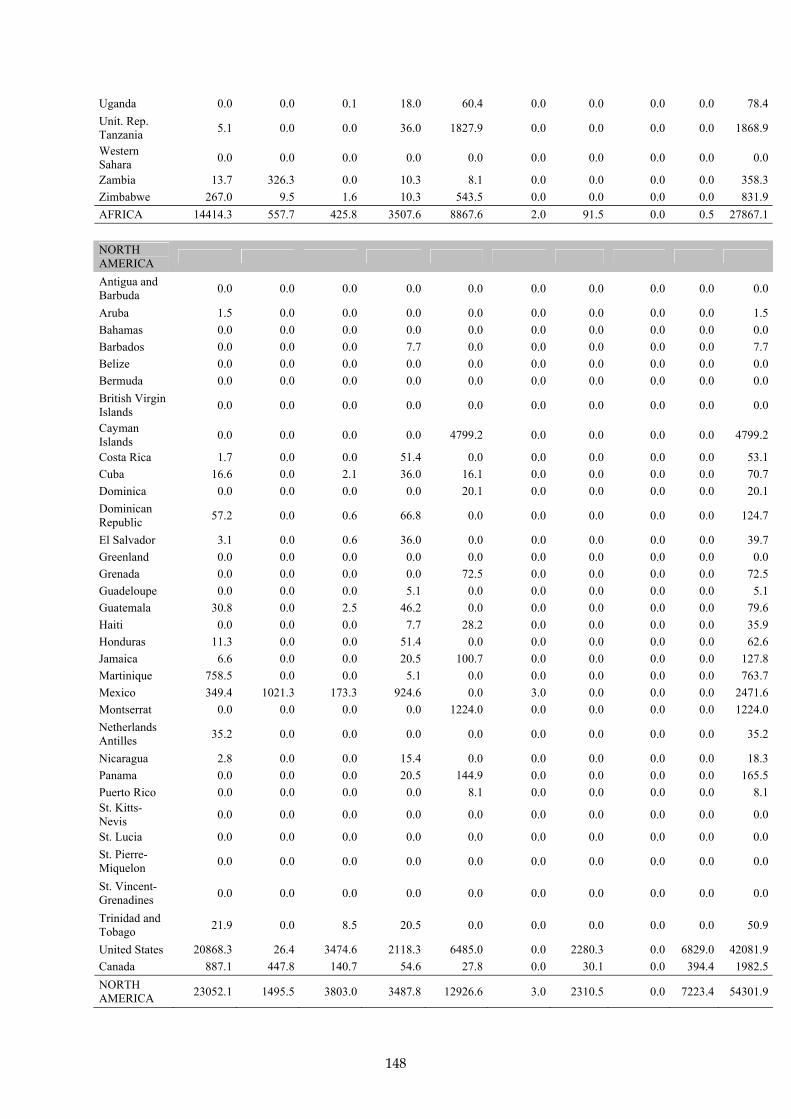
148

Uganda 0.0 0.0 0.1 18.0 60.4 0.0 0.0 0.0 0.0 78.4Unit. Rep. Tanzania 5.1 0.0 0.0 36.0 1827.9 0.0 0.0 0.0 0.0 1868.9

Western Sahara 0.0 0.0 0.0 0.0 0.0 0.0 0.0 0.0 0.0 0.0

Zambia 13.7 326.3 0.0 10.3 8.1 0.0 0.0 0.0 0.0 358.3Zimbabwe 267.0 9.5 1.6 10.3 543.5 0.0 0.0 0.0 0.0 831.9AFRICA 14414.3 557.7 425.8 3507.6 8867.6 2.0 91.5 0.0 0.5 27867.1 NORTH AMERICA

Antigua and Barbuda 0.0 0.0 0.0 0.0 0.0 0.0 0.0 0.0 0.0 0.0

Aruba 1.5 0.0 0.0 0.0 0.0 0.0 0.0 0.0 0.0 1.5Bahamas 0.0 0.0 0.0 0.0 0.0 0.0 0.0 0.0 0.0 0.0Barbados 0.0 0.0 0.0 7.7 0.0 0.0 0.0 0.0 0.0 7.7Belize 0.0 0.0 0.0 0.0 0.0 0.0 0.0 0.0 0.0 0.0Bermuda 0.0 0.0 0.0 0.0 0.0 0.0 0.0 0.0 0.0 0.0British Virgin Islands 0.0 0.0 0.0 0.0 0.0 0.0 0.0 0.0 0.0 0.0

Cayman Islands 0.0 0.0 0.0 0.0 4799.2 0.0 0.0 0.0 0.0 4799.2

Costa Rica 1.7 0.0 0.0 51.4 0.0 0.0 0.0 0.0 0.0 53.1Cuba 16.6 0.0 2.1 36.0 16.1 0.0 0.0 0.0 0.0 70.7Dominica 0.0 0.0 0.0 0.0 20.1 0.0 0.0 0.0 0.0 20.1Dominican Republic 57.2 0.0 0.6 66.8 0.0 0.0 0.0 0.0 0.0 124.7

El Salvador 3.1 0.0 0.6 36.0 0.0 0.0 0.0 0.0 0.0 39.7Greenland 0.0 0.0 0.0 0.0 0.0 0.0 0.0 0.0 0.0 0.0Grenada 0.0 0.0 0.0 0.0 72.5 0.0 0.0 0.0 0.0 72.5Guadeloupe 0.0 0.0 0.0 5.1 0.0 0.0 0.0 0.0 0.0 5.1Guatemala 30.8 0.0 2.5 46.2 0.0 0.0 0.0 0.0 0.0 79.6Haiti 0.0 0.0 0.0 7.7 28.2 0.0 0.0 0.0 0.0 35.9Honduras 11.3 0.0 0.0 51.4 0.0 0.0 0.0 0.0 0.0 62.6Jamaica 6.6 0.0 0.0 20.5 100.7 0.0 0.0 0.0 0.0 127.8Martinique 758.5 0.0 0.0 5.1 0.0 0.0 0.0 0.0 0.0 763.7Mexico 349.4 1021.3 173.3 924.6 0.0 3.0 0.0 0.0 0.0 2471.6Montserrat 0.0 0.0 0.0 0.0 1224.0 0.0 0.0 0.0 0.0 1224.0Netherlands Antilles 35.2 0.0 0.0 0.0 0.0 0.0 0.0 0.0 0.0 35.2

Nicaragua 2.8 0.0 0.0 15.4 0.0 0.0 0.0 0.0 0.0 18.3Panama 0.0 0.0 0.0 20.5 144.9 0.0 0.0 0.0 0.0 165.5Puerto Rico 0.0 0.0 0.0 0.0 8.1 0.0 0.0 0.0 0.0 8.1St. Kitts-Nevis 0.0 0.0 0.0 0.0 0.0 0.0 0.0 0.0 0.0 0.0

St. Lucia 0.0 0.0 0.0 0.0 0.0 0.0 0.0 0.0 0.0 0.0St. Pierre-Miquelon 0.0 0.0 0.0 0.0 0.0 0.0 0.0 0.0 0.0 0.0

St. Vincent-Grenadines 0.0 0.0 0.0 0.0 0.0 0.0 0.0 0.0 0.0 0.0

Trinidad and Tobago 21.9 0.0 8.5 20.5 0.0 0.0 0.0 0.0 0.0 50.9

United States 20868.3 26.4 3474.6 2118.3 6485.0 0.0 2280.3 0.0 6829.0 42081.9Canada 887.1 447.8 140.7 54.6 27.8 0.0 30.1 0.0 394.4 1982.5NORTH AMERICA 23052.1 1495.5 3803.0 3487.8 12926.6 3.0 2310.5 0.0 7223.4 54301.9

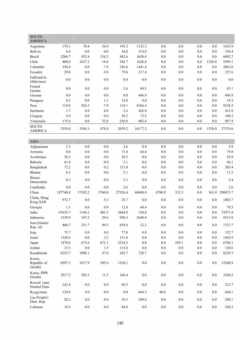
149

SOUTH AMERICA

Argentina 179.1 78.4 56.9 195.2 1123.3 0.0 0.0 0.0 0.0 1632.9Bolivia 4.4 0.0 0.0 36.0 314.0 0.0 0.0 0.0 0.0 354.4Brazil 2204.7 952.4 334.3 942.6 1658.8 0.0 0.0 0.0 0.0 6092.7Chile 480.0 1637.2 16.6 102.7 1626.6 0.0 0.0 0.0 1526.0 5389.1Colombia 356.8 0.0 7.9 256.8 1441.4 0.0 0.0 0.0 0.0 2063.0Ecuador 29.8 0.0 0.8 79.6 217.4 0.0 0.0 0.0 0.0 327.6Falkland Is. (Malvinas) 0.0 0.0 0.0 0.0 0.0 0.0 0.0 0.0 0.0 0.0

French Guiana 0.0 0.0 0.0 2.6 80.5 0.0 0.0 0.0 0.0 83.1

Guyana 0.0 0.0 0.0 0.0 446.9 0.0 0.0 0.0 0.0 446.9Paraguay 0.2 0.0 1.1 18.0 0.0 0.0 0.0 0.0 0.0 19.3Peru 119.8 926.2 7.9 118.1 8366.4 0.0 0.0 0.0 0.0 9538.5Suriname 1.7 0.0 0.0 2.6 426.8 0.0 0.0 0.0 0.0 431.0Uruguay 6.9 0.0 0.6 28.3 72.5 0.0 0.0 0.0 0.0 108.2Venezuela 175.6 0.0 52.8 256.8 402.6 0.0 0.0 0.0 0.0 887.9SOUTH AMERICA 3559.0 3594.3 478.8 2039.2 16177.3 0.0 0.0 0.0 1526.0 27374.6

ASIA Afghanistan 3.3 0.0 0.0 2.6 0.0 0.0 0.0 0.0 0.0 5.9Armenia 0.0 0.0 0.0 15.4 64.4 0.0 0.0 0.0 0.0 79.8Azerbaijan 20.3 0.0 0.0 38.5 0.0 0.0 0.0 0.0 0.0 58.8Bahrain 41.0 0.0 0.0 5.1 0.0 0.0 0.0 0.0 0.0 46.1Bangladesh 72.2 0.0 0.2 131.0 0.0 0.0 0.0 0.0 0.0 203.4Bhutan 6.3 0.0 0.0 5.1 0.0 0.0 0.0 0.0 0.0 11.5Brunei Darussalam 0.3 0.0 0.0 5.1 0.0 0.0 0.0 0.0 0.0 5.4

Cambodia 0.0 0.0 0.0 2.6 0.0 0.0 0.0 0.0 0.0 2.6China 187740.8 17392.2 3760.0 27326.4 44600.0 8780.0 313.3 0.0 561.0 290473.7China, Hong Kong SAR 972.7 0.0 5.3 25.7 0.0 0.0 0.0 0.0 0.0 1003.7

Georgia 1.3 0.0 0.0 12.8 64.4 0.0 0.0 0.0 0.0 78.5India 67635.7 1144.1 402.5 3664.9 124.8 0.0 0.0 0.0 0.0 72971.9Indonesia 1539.9 347.3 29.6 950.3 5648.8 0.0 0.0 0.0 0.0 8515.8Iran (Islamic Rep. of) 404.7 351.7 99.3 839.8 32.2 0.0 0.0 0.0 0.0 1727.7

Iraq 75.7 0.0 0.0 77.0 0.0 0.0 0.0 0.0 0.0 152.7Israel 1328.8 0.0 3.2 131.0 0.0 0.0 0.0 0.0 0.0 1462.9Japan 1478.0 673.6 872.1 3210.3 0.0 0.0 550.1 0.0 0.0 6784.1Jordan 13.5 0.0 1.5 115.6 0.0 0.0 0.0 0.0 0.0 130.6Kazakhstan 6252.7 1098.1 47.0 102.7 728.7 0.0 0.0 0.0 0.0 8229.3Korea, Republic of (South)

8597.5 1817.9 505.4 1320.1 0.0 0.0 0.0 0.0 0.0 12240.9

Korea, DPR (North) 2917.2 205.3 11.3 146.4 0.0 0.0 0.0 0.0 0.0 3280.2

Kuwait +part Neutral Zone 143.4 0.0 0.0 69.3 0.0 0.0 0.0 0.0 0.0 212.7

Kyrgyzstan 139.8 0.0 0.0 0.0 664.3 40.0 0.0 0.0 0.0 844.1Lao People's Dem. Rep. 28.2 0.0 0.0 10.3 249.6 0.0 0.0 0.0 0.0 288.1

Lebanon 19.4 0.0 0.0 84.8 0.0 0.0 0.0 0.0 0.0 104.2

150

Malaysia 1374.9 0.0 65.5 459.7 169.1 0.0 0.0 0.0 0.0 2069.2Maldives 0.0 0.0 0.0 0.0 0.0 0.0 0.0 0.0 0.0 0.0Mongolia 515.4 0.0 0.0 2.6 970.3 0.0 0.0 0.0 0.0 1488.3Myanmar (Burma) 21.4 0.4 0.3 12.8 4.0 0.0 0.0 0.0 0.0 38.9

Nepal 29.2 0.0 0.0 7.7 0.0 0.0 0.0 0.0 0.0 36.9Occup. Palestinian Terr.

0.1 0.0 0.0 0.0 0.0 0.0 0.0 0.0 0.0 0.1

Oman 12.0 33.0 0.0 64.2 0.0 0.0 0.0 0.0 0.0 109.3Pakistan 803.7 0.0 5.3 462.3 0.0 0.0 0.0 0.0 0.0 1271.2Philippines 952.5 226.6 3.8 333.9 1509.8 0.0 0.0 0.0 0.0 3026.6Qatar 14.5 0.0 11.3 36.0 0.0 0.0 0.0 0.0 0.0 61.8Saudi Arabia +part Ntrl Zone

271.6 0.0 44.3 667.7 302.0 0.0 0.0 0.0 0.0 1285.6

Singapore 143.4 0.0 6.0 0.0 0.0 0.0 0.0 0.0 0.0 149.5Sri Lanka 16.4 0.0 0.3 30.8 0.0 0.0 0.0 0.0 0.0 47.6Syrian Arab Republic 40.3 0.0 0.7 120.7 0.0 0.0 0.0 0.0 0.0 161.8

Taiwan (Chinese Taipei, Other Far East)

5718.7 0.0 196.2 511.1 0.0 0.0 0.0 0.0 0.0 6426.0

Takijistan 14.9 0.0 0.0 7.7 76.5 6.0 0.0 0.0 0.0 105.1Thailand 2879.7 152.2 56.0 973.4 177.2 0.0 0.0 0.0 0.0 4238.4Timor-Leste 0.0 0.0 0.0 0.0 0.0 0.0 0.0 0.0 0.0 0.0Turkey 6345.9 118.8 221.5 1099.2 0.0 0.0 0.0 0.0 0.0 7785.4Turkmenistan 20.6 0.0 0.0 12.8 0.0 0.0 0.0 0.0 0.0 33.4United Arab Emirates 29.4 0.0 0.7 205.5 0.0 0.0 0.0 0.0 0.0 235.6

Uzbekistan 269.7 207.4 6.4 131.0 3390.1 0.0 0.0 0.0 0.0 4004.6Viet Nam 1447.7 0.0 8.2 744.8 120.8 0.0 0.0 0.0 0.0 2321.5Yemen 12.2 0.0 0.0 41.1 0.0 0.0 0.0 0.0 0.0 53.3ASIA 300367.0 23768.6 6363.9 44217.9 58897.0 8826.0 863.4 0.0 561.0 443864.7 OCEANIA Australia 5745.3 1606.3 211.4 96.3 7700.0 0.0 0.0 0.0 0.0 15359.3Cook Islands 0.0 0.0 0.0 0.0 0.0 0.0 0.0 0.0 0.0 0.0Fiji 0.8 0.0 0.0 2.6 79.0 0.0 0.0 0.0 0.0 82.4French Polynesia 0.0 0.0 0.0 0.0 0.0 0.0 0.0 0.0 0.0 0.0

Kiribati 0.0 0.0 0.0 0.0 0.0 0.0 0.0 0.0 0.0 0.0Marshall Islands 0.0 0.0 0.0 0.0 0.0 0.0 0.0 0.0 0.0 0.0

Micronesia 0.0 0.0 0.0 0.0 0.0 0.0 0.0 0.0 0.0 0.0Nauru 0.0 0.0 0.0 0.0 0.0 0.0 0.0 0.0 0.0 0.0New Caledonia 18.2 0.0 0.0 2.6 0.0 0.0 0.0 0.0 0.0 20.8

New Zealand 377.9 0.0 9.4 28.3 307.0 0.0 0.0 0.0 0.0 722.5Palau 0.0 0.0 0.0 0.0 0.0 0.0 0.0 0.0 0.0 0.0Papua New Guinea 0.3 0.0 0.0 0.0 2005.0 0.0 0.0 0.0 0.0 2005.3

Samoa 0.0 0.0 0.0 0.0 0.0 0.0 0.0 0.0 0.0 0.0Solomon Islands 0.0 0.0 0.0 0.0 0.0 0.0 0.0 0.0 0.0 0.0

151

Tonga 0.0 0.0 0.0 0.0 0.0 0.0 0.0 0.0 0.0 0.0Tuvalu 0.0 0.0 0.0 0.0 0.0 0.0 0.0 0.0 0.0 0.0Vanuatu 0.0 0.0 0.0 0.0 0.0 0.0 0.0 0.0 0.0 0.0OCEANIA 6142.5 1606.3 220.8 129.7 10091.0 0.0 0.0 0.0 0.0 18190.3 RUSSIA Russian Federation 14897.7 1363.8 699.5 1250.7 4300.0 10.0 534.9 0.0 1499.0 24555.6

EUROPE Metals production Albania 10.5 0.3 12.8 0.0 0.0 0.0 0.0 27.3 50.8Austria 243.8 187.9 36.9 0.0 0.0 3.1 0.0 32.5 504.2Belarus 24.1 5.7 198.0 0.0 0.0 0.0 0.0 5.0 232.8Belgium 591.9 125.6 180.9 0.0 0.0 8.5 0.0 266.3 1173.3Bosnia-Herzegovina 32.9 11.5 15.3 0.0 0.0 0.0 0.0 40.7 100.5

Bulgaria 477.0 695.4 40.9 0.0 0.0 0.0 0.0 0.0 1213.4Croatia 210.0 0.0 38.1 0.0 0.0 1.1 0.0 3.1 252.3Cyprus 4.5 0.0 46.2 0.0 0.0 0.0 0.0 0.0 50.8Czech Republic 625.0 174.5 43.3 0.0 0.0 10.5 0.0 100.7 953.9

Denmark 233.0 0.0 13.7 0.0 0.0 10.2 0.0 29.7 286.6Estonia 181.9 0.0 3.2 0.0 0.0 0.0 0.0 0.0 185.1Finland 83.3 99.4 5.1 0.0 0.0 0.4 0.0 201.9 390.1France 1670.0 174.9 175.8 0.0 0.0 182.8 0.0 790.8 2994.2Germany 4193.4 1382.6 635.6 0.0 0.0 532.6 0.0 1193.6 7937.8Greece 959.4 18.7 332.7 0.0 0.0 1.1 0.0 417.2 1729.1Hungary 830.2 57.1 70.3 0.0 0.0 146.2 0.0 85.8 1189.6Iceland 1.9 0.0 3.1 0.0 0.0 0.3 0.0 7.3 12.6Ireland 113.4 0.0 86.7 0.0 0.0 4.0 0.0 32.9 237.0Italy 2637.8 703.2 992.9 0.0 0.0 103.2 0.0 0.0 4437.1Latvia 32.4 0.0 15.8 0.0 0.0 0.0 0.0 0.0 48.2Lithuania 509.6 0.0 50.1 0.0 0.0 0.0 0.0 44.5 604.2Luxembourg 5.4 128.7 2.1 0.0 0.0 0.3 0.0 0.0 136.5Macedonia 73.4 3.3 10.2 0.0 0.0 0.0 0.0 0.0 86.9Moldova 11.3 42.5 34.3 0.0 0.0 0.0 0.0 0.0 88.1Monaco 53.0 0.0 0.0 0.0 0.0 0.0 0.0 0.0 53.0The Netherlands 66.7 58.7 50.1 0.0 0.0 18.0 0.0 0.0 193.5

Norway 29.5 50.1 15.9 0.0 0.0 11.4 0.0 352.0 458.9Poland 3558.0 185.6 375.6 0.0 0.0 0.0 0.0 8932.0 13051.3Portugal 829.5 16.6 165.7 0.0 0.0 150.0 0.0 68.6 1230.4Romania 775.6 80.7 336.6 0.0 0.0 135.8 0.0 13.7 1342.4Slovakia 1443.0 76.5 86.7 0.0 0.0 12.7 0.0 1620.0 3238.9Slovenia 97.2 27.3 5.7 0.0 0.0 0.0 0.0 0.0 130.1Spain 1628.3 254.6 1126.4 0.0 0.0 25.0 0.0 99.1 3133.5Sweden 77.5 126.2 7.7 0.0 0.0 18.7 0.0 33.9 264.0Switzerland 210.0 141.7 49.1 0.0 0.0 9.3 0.0 41.2 451.3Ukrainia 18032.6 293.9 469.6 0.0 0.0 134.0 0.0 179.2 19109.3United Kingdom 602.6 152.1 64.6 0.0 0.0 25.6 0.0 58.6 903.5

Yugoslavia (Serbia & Montenegro)

1059.1 37.5 228.7 0.0 0.0 0.0 0.0 0.0 1325.3

Malta 190.0 0.0 0.0 0.0 0.0 4.7 0.0 0.3 195.1

152

EUROPE 42408.9 5312.7 6026.3 0.0 0.0 1549.5 0.0 14677.9 69975.2 WORLD 404841.6 37698.9 11991.8 60659.3 111259.5 8841.0 5349.8 0.0 25487.7 666129.4

1, 2 See footnotes to Appendix Table AppA6.

153

Appendix B

*Calculated to be at 1 atm from third reaction rate constant. **First order decay with unit s−1.

Table AppB.1 Reactions, reaction rate constants and when possible reaction products of gas phase reactions (adapted from Ariya et al., 2008).

No. Mechanism Reaction rate constant at 298±5K

Comment Authors

Gas Phase reactions

cm3 molec−1 sec−1

G1 Hg0 + O3 → HgO + O2 (3±2)•10−20

(7.5±0.9)•10−19 (6.4±2.3)•10−19

Hall, 1995 Pal and Ariya, 2004b Sumner and Spicer, 2005

G2 Hg0 + OH → HgO + H (8.7±2.8)•10−14

(1.6±0.2)•10−12

(9.3±1.3)•10−14 <1.2•10−13

Sommar et al., 2001 Miller et al., 2001 Pal and Ariya, 2004a Bauer et al., 2003

G3 Hg0 + H2O2 → HgII

Products <8.5•10−19 Tokos et al., 1998

G4 Hg0 + Cl2 → HgII

Products

(2.7±0.2)•10−18 (2.5±0.9)•10−18

Ariya et al., 2002 Sumner and Spicer, 2005

G5 Hg0 + Br2 → HgII

Products <(9±2)•10−17 2.7•10−31 and 3.4•10−31

No reaction observed Theoretical calc.

Ariya et al., 2002 Sumner and Spicer, 2005 Balabanov et al., 2005

G6 Hg0 + Cl → HgII

Products (1.0±0.2)•10−11 (2.8)•10−11 5.5•10−13

Theoretical calc.

Ariya et al., 2002 Khalizov et al., 2003 Donohoue et al., 2005*

G7 Hg0 + Br → HgII

Products HgBr

(3.2±0.3)•10−12 3.5•10−13 1.1•10−12

Theoretical calc

Ariya et al., 2002 Donohoue et al., 2006* Goodsite et al., 2004

G8 Hg0 + BrO → HgII

Products 10-13-10−15

1•10−14 -

Endothermic

Raofie and Ariya, 2004 Sumner and Spicer, 2005 Tossell, 2003

G9 HgBr → Hg + Br 7.9•10−3 s−1 Theoretical calc.

Goodsite et al., 2004**

G10 HgBr + Br → HgBr2 2.5•10−10 Theoretical calc.

Goodsite et al., 2004

G11 HgBr + OH → HgBr(OH)

2.5•10−10 Theoretical Goodsite et al., 2004

154

*Unit for first order reactions and photolysis is s−1 as indicated

Table AppB.2 Reaction rate constants and when possible reaction products of aqueous phase reactions (from Lin et al., 2006).

Aqueous phase reactions

Mechanism Reaction rate constant *M-1 s-1

Type Comment

A1 HgSO3 → Hg0aq + S(VI) T•exp(31.971T−125

95)/Ts−1 Red

A2 Hg(SO3)22− → Hg0

aq + S(VI)

?10-4 s−1 Red

A3 Hg(OH)2 + h → Hg0aq

+ products 3•10-7 s−1 Red UV light, Midday 60° N

A4 HgIIaq + OOH → Hg0

aq + products

1.7•104 Red

A5 Hg0aq + O3 → Hg2+

aq + products

4.7•107 Ox

A6 Hg0aq + OH → Hg2+

aq + products

2.0•109 Ox

A7 Hg0aq + HOCl → Hg2+

aq + Cl- + OH−

2.09•106 Ox

A8 Hg0aq + OCl− → Hg2+

aq + Cl− + OH−

1.99•106 Ox

A9 Hg0aq + HOBr → Hg2+

aq + Br− + OH−

0.279 Ox

A10 Hg0aq + OBr− → Hg2+

aq + Br− + OH−

0.273 Ox

A11 Hg0aq + Br2 → Hg2+

aq + 2Br−

0.196 Ox

155

*third order reaction rate expressions in cm6 molec−2 sec−1

Table AppB.3 Temperature expression for some reactions listed in Table AppB.1 (Gas phase reaction number refers to numbers in Table AppB.1).

No. Mechanism Reaction rate constant at 298 K

Comment Authors

Gas Phase reactions

cm3 molec−1 sec−1

G1 Hg0 + O3 → HgO + O2

8.43•10−17exp{−1407/T} 283-323 Pal and Ariya, 2004b

G2 Hg0 + OH → HgOH

3.55•10−14exp{(294±16)/T} 283-353 Pal and Ariya, 2004a

G6 Hg0 + Cl → HgCl 1.38•10−12exp{(208.02/T)} (2.2±0.5)•10−32exp{(680±400)(1/T−1/298)}

Theoretical 243-293

Khalizov et al., 2003 Donohoue et al., 2005*

G7 Hg0 + Br → HgBr (1.46±0.34)•10−32•(T/298)−(1.86±1.49)

1.1•10−12(T/298K)−2.37 243-293 Theoretical

Donohoue et al., 2006* Goodsite et al., 2004

G9 HgBr → Hg + Br 1.2•10−10(exp(−8357/T) Theoretical Goodsite et al., 2004 G10 HgBr + Br →

HgBr2

2.5•10−10(T/298)−0.57 Theoretical Goodsite et al., 2004

G11 HgBr + OH → HgBr(OH)

2.5•10−10(T/298)−0.57 Theoretical Goodsite et al., 2004

156

Table AppB.4 Chemical equilibriums for calculating aqueous phase HgII speciation. Source: (Lin et al., 2006)

No. Equilibrium Log(Keq) E1 H2O,SO2 ↔ H+ + HSO3

− −1.91 E2 HSO3

− ↔ H+ + SO32− −7.18

E3 H2O,CO2 ↔ H+ + HCO3− −6.35

E4 HCO3− ↔ H+ + CO3

2− −10.33 E5 Hg2+ + OH− ↔ Hg(OH)+ 10.63 E6 Hg2+ + 2OH− ↔ Hg(OH)2 22.24 E7 Hg2+ + SO3

2− ↔ Hg( SO3) 12.7 E8 Hg2+ + 2SO3

2− ↔ Hg( SO3)22− 24.1

E9 Hg2+ + OH− + Cl− ↔ Hg(OH)Cl 18.25 E10 Hg2+ + Cl− ↔ HgCl+ 7.30 E11 Hg2+ + 2Cl− ↔ HgCl2 14.0 E12 Hg2+ + 3Cl− ↔ HgCl3

− 15.0 E13 Hg2+ + 4Cl− ↔ HgCl4

2− 15.6 E14 Hg2+ + Br− ↔ HgBr+ 9.07 E15 Hg2+ + 2Br− ↔ HgBr2 17.27 E16 Hg2+ + 3Br− ↔ HgBr3

− 19.7 E17 Hg2+ + 4Br− ↔ HgBr4

2− 21.2 E18 Hg2+ + OH− + Br− ↔ Hg(OH)Br 19.7 E19 Hg2+ + CO3

2− ↔ Hg( CO3) 11.0 E20 Hg2+ + SO4

2− ↔ Hg( SO4) 1.34 E21 Hg2+ + 2SO4

2− ↔ Hg( SO4)2− 2.40 E22 Hg2+ + NO3

− ↔ Hg NO3− 0.11

157

* Dimensionless unit, and for equation H [Hgaq] = [Hgair] where H is Henrys law coefficient, [Hgaq] is the concentration in either milli-Q water or artificial seawater, [Hgair] is the concentration in air. ** From Andersson et al. 2008. *** From Sommar et al. 2000.

Table App B.5. Physical and chemical properties for selected compounds (from Schroeder and Munthe, 1998). (Henrys law coefficients in M/atm).

Property Hg0 HgCl2 HgO HgS CH3HgCl Hg(CH3)2 Melting point (ºC)

-39 277 Decomp. @ +500

584 (sublim.)

167 (sublim.)

-

Boiling point (ºC) 357 @ 1 atm 303 @ 1 atm - - - 96 Vapour pressure (Pa)

0.180 @ 20ºC

8.99•10-3 @ 20ºC

9.20•10-12 @ 25ºC

n.d. 1.76 8.30•103 @ 25ºC

Water solubility (g/L)

49.4•10-6 @ 20ºC

66 @ 20ºC 5.3•10-2 @ 25ºC

~2•10-24

@ 25ºC ~5-6 @

2ºC 2.95 @ 24ºC

Henry’s law coefficient*

0.31** @ 20ºC

9.00•10-9 @ 20ºC

9.31•10-15 @ 25ºC

n.d. 1.6•10-5 @ 15ºC and pH = 5.2

0.31 @ 25ºC

0.15 @ 15ºC

Van Hoff's equation

**H = ((-2404.3/T)+6

.92)

***H = 553000• exp[(-

67.2•103)/RT]

- - - -

Octanol-water partition coefficient*

4.2 0.5 - n.d. 2.5 180

158

Appendix C: Glossary of Abbreviations

ACAP Arctic Council’s Arctic Contaminants Action Programme AMAP Arctic Monitoring and Assessment Programme AMDE atmospheric mercury depletion event ASGM artisanal and small-scale gold mining BAU+C scenario Business as Usual, with a component related to actions to

address climate change scenario BO basic oxygen process Br Bromine atom CAMNet Canadian Atmospheric Mercury Network CFLs compact fluorescent lamps CIS CMAQ

(Russian/Soviet) Commonwealth of Independent States Community Multi-scale Air Quality model

CTM-Hg global chemical transport model for mercury DEHM Danish Eulerian Hemispheric Model EA electric arc EMEP Cooperative Programme for Monitoring and Evaluation of

the Long-range Transmission of Air Pollutants in Europe EPA Environmental Protection Agency ESPs electrostatic precipitators EXEC scenario Extended Emissions Control scenario FGD flue gas desulphurization F&TP Fate and Transport Partnership (UNEP partnership area on

mercury) FFs fabric filters GEM gaseous elemental mercury (also as Hg0 or Hg0) GRAHM Global/Regional Atmospheric Heavy Metals model H2O2 hydrogen peroxide Hg mercury HgII divalent mercury compounds HgCl2 mercuric chloride Hg-P particulate associated mercury HgO mercuric oxide HgT Total mercury HO2 hydroperoxyl radical kton kilo-tonne (106 kg) LCDs liquid crystal displays LEDs light-emitting diodes LRTAP Convention UN ECE Convention on Long-Range Transboundary Air

Pollution MBL marine boundary layer MDN Mercury Deposition Network MFTR scenario Maximum Feasible Technological Reduction scenario NAMMIS North American Mercury Model Intercomparison Study NEI (US EPA) National Emissions Inventory O3 ozone OH hydroxyl radical ppm parts per million

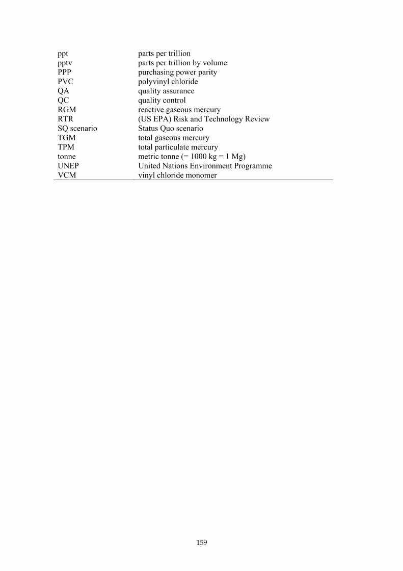
159

ppt parts per trillion pptv parts per trillion by volume PPP purchasing power parity PVC polyvinyl chloride QA quality assurance QC quality control RGM RTR

reactive gaseous mercury (US EPA) Risk and Technology Review

SQ scenario Status Quo scenario TGM total gaseous mercury TPM total particulate mercury tonne metric tonne (= 1000 kg = 1 Mg) UNEP United Nations Environment Programme VCM vinyl chloride monomer