
Housing Tenure, Job Mobility and Unemployment in the UK &ast
Upload
khangminh22Category
view
0download
0
Charles University in Prague
Faculty of Social SciencesInstitute of Economic Studies
BACHELOR THESIS
Unemployment in the Czech Republic andJob Search on the Internet
Author: Ondrej Zacha
Supervisor: Petr Polak, MSc.
Academic Year: 2014/2015

Declaration of Authorship
The author hereby declares that he compiled this thesis independently, using
only the listed resources and literature.
The author grants to Charles University permission to reproduce and to dis-
tribute copies of this thesis document in whole or in part.
Prague, May 15, 2015 Signature

Acknowledgments
I am grateful to my supervisor, Petr Polak, for his useful comments and kind
approach and to Tomas Dombrovsky of LMC (Jobs.cz) and Michal Buzek of
Seznam.cz for their helpfulness and patience and—most of all—provision of
valuable data.
I would like to thank my family and friends for their support throughout the
process of writing this thesis.

Abstract
This thesis examines the relationship between Czech unemployment rate and
job search related behavior of Internet users. The study uses a simple autore-
gressive model and augments it with search query data from two most popular
Czech search engines, Google and Seznam, as well as data on numbers of job
vacancies and reactions to them from job search portal Jobs.cz. Our results
show that data on number of job vacancies can moderately improve short-term
forecasts (“nowcasts”) of Czech unemployment rate in terms of RMSE and
MAE, whereas search query data from Google and Seznam failed to improve
predictive ability of the baseline model.
Keywords unemployment rate, Czech Republic, Google
Econometrics, search engine, job vacancies
Author’s e-mail [email protected]
Supervisor’s e-mail [email protected]
Abstrakt
Tato prace zkouma vztah mezi ceskou mırou nezamestnanosti a chovanım
uzivatelu Internetu tykajıcım se hledanı prace. Studie pouzıva jednoduchy au-
toregresnı model, doplneny o data o vyhledavacıch frazıch ze dvou nejoblıbenejsıch
ceskych internetovych vyhledavacu, Googlu a Seznamu, a soucasne data o poctu
nabızenych pozic a reakcı na ne z portalu pro hledanı prace Jobs.cz. Nase
vysledky ukazujı, ze udaje o poctech nabızenych pozic mohou mırne vylepsit
kratkodobe predpovedi (“nowcasty”) ceske mıry nezamestnanosti z hlediska
RMSE a MAE, zatımco s daty o vyhledavacıch frazıch z Googlu a Seznamu
nebylo dosazeno zlepsenı predpovedı v porovnanı se zakladnım modelem.
Klıcova slova mıra nezamestnanosti, Ceska republika,
Google ekonometrie, internetovy vyh-
ledavac, volne pozice
E-mail autora [email protected]
E-mail vedoucıho prace [email protected]

Contents
List of Tables vii
List of Figures viii
Acronyms ix
Thesis Proposal x
1 Introduction 1
2 Internet in the Czech Republic 3
3 Literature Review 5
4 Data 11
4.1 Czech Statistical Office . . . . . . . . . . . . . . . . . . . . . . . 11
4.2 Google Trends . . . . . . . . . . . . . . . . . . . . . . . . . . . . 12
4.3 Seznam.cz . . . . . . . . . . . . . . . . . . . . . . . . . . . . . . 14
4.4 Jobs.cz . . . . . . . . . . . . . . . . . . . . . . . . . . . . . . . . 16
4.5 Choice of keywords . . . . . . . . . . . . . . . . . . . . . . . . . 17
5 Methodology 20
5.1 ARMA/ARIMA/ARMAX . . . . . . . . . . . . . . . . . . . . . 20
5.2 Seasonal adjustment . . . . . . . . . . . . . . . . . . . . . . . . 21
5.3 Transformation of Google Trends data . . . . . . . . . . . . . . 22
5.4 Stationarity . . . . . . . . . . . . . . . . . . . . . . . . . . . . . 23
5.5 Augmented Dickey-Fuller Test . . . . . . . . . . . . . . . . . . . 24
5.6 Principal Component Analysis . . . . . . . . . . . . . . . . . . . 24
5.7 Forecasting and its evaluation . . . . . . . . . . . . . . . . . . . 25
5.7.1 Evaluation . . . . . . . . . . . . . . . . . . . . . . . . . . 25
5.7.2 Mean Absolute Error (MAE) . . . . . . . . . . . . . . . 26

Contents vi
5.7.3 Root Mean Squared Error (RMSE) . . . . . . . . . . . . 26
5.7.4 Diebold-Mariano (DM) Test . . . . . . . . . . . . . . . . 26
6 Empirical Results 28
6.1 Stationarity . . . . . . . . . . . . . . . . . . . . . . . . . . . . . 28
6.2 Principal Component Analysis (PCA) . . . . . . . . . . . . . . . 29
6.3 Model performance . . . . . . . . . . . . . . . . . . . . . . . . . 29
6.3.1 Models with individual variable performance . . . . . . . 30
6.3.2 Models with multiple or aggregate variables . . . . . . . 31
6.3.3 Models with job search portal data . . . . . . . . . . . . 32
6.4 DM test . . . . . . . . . . . . . . . . . . . . . . . . . . . . . . . 32
7 Discussion 41
8 Conclusion 43
Bibliography 49
A Additional figures I
B Additional tables IV

List of Tables
2.1 Search engine shares in the Czech Republic . . . . . . . . . . . . 4
6.1 ADF test results . . . . . . . . . . . . . . . . . . . . . . . . . . 33
6.2 PCA: Google . . . . . . . . . . . . . . . . . . . . . . . . . . . . 34
6.3 PCA: Seznam . . . . . . . . . . . . . . . . . . . . . . . . . . . . 35
6.4 Models with individual variables: in-sample . . . . . . . . . . . 36
6.5 Models with individual variables: out-of-sample . . . . . . . . . 37
6.6 Models with multiple or aggregate variables: in-sample . . . . . 38
6.7 Models with multiple or aggregate variables: out-of-sample . . . 39
6.8 Models with job search portal data: in-sample . . . . . . . . . . 40
6.9 Models with job search portal data: out-of-sample . . . . . . . . 40
6.10 DM test results . . . . . . . . . . . . . . . . . . . . . . . . . . . 40
B.1 Households with Internet access in CR and EU15 . . . . . . . . IV
B.2 Survey results . . . . . . . . . . . . . . . . . . . . . . . . . . . . V
B.3 Principal component loadings . . . . . . . . . . . . . . . . . . . VI
B.4 PCs: ADF test results . . . . . . . . . . . . . . . . . . . . . . . VII
B.5 Descriptive statistics (1/2) . . . . . . . . . . . . . . . . . . . . . VIII
B.6 Descriptive statistics (2/2) . . . . . . . . . . . . . . . . . . . . . IX

List of Figures
4.1 Search index for query “prace praha” v. Czech unemployment
rate . . . . . . . . . . . . . . . . . . . . . . . . . . . . . . . . . 14
4.2 Search volumes for query “prace praha” v. Czech unemployment
rate . . . . . . . . . . . . . . . . . . . . . . . . . . . . . . . . . 15
4.3 Unemployment rate, job vacancies, reactions . . . . . . . . . . . 18
5.1 Seasonal adjustment: example . . . . . . . . . . . . . . . . . . . 22
6.1 Baseline model . . . . . . . . . . . . . . . . . . . . . . . . . . . 30
A.1 Seznam.cz: ‘neutral’ queries . . . . . . . . . . . . . . . . . . . . I
A.2 Google Trends website . . . . . . . . . . . . . . . . . . . . . . . II
A.3 Seznam.cz search statistics website . . . . . . . . . . . . . . . . III

Acronyms
ADF Augmented Dickey-Fuller
API Application Programming Interface
AR Moving Average
ARIMA Autoregressive Integrated Moving Average
ARIMAX Autoregressive Integrated Moving Average with Exogenous Inputs
ARMA Autoregressive Moving Average
ARMAX Autoregressive Moving Average with Exogenous Inputs
BMA Bayesian Model Averaging
CSV Comma Separated Values
CZSO Czech Statistical Office
DM Diebold-Mariano
GDP Gross Domestic Product
GLS Generalized Least Squares
GT Google Trends
ILO International Labour Organization
MA Autoregressive
MAE Mean Absolute Error
MSE Mean Squared Error
PC Principal Component
PCA Principal Component Analysis
RMSE Root Mean Squared Error
RUR Range Unit Root
SEATS Signal Extraction in ARIMA Time Series
TRAMO Time series Regression with ARIMA noise, Missing values andOutliers

Master Thesis Proposal
Author Ondrej Zacha
Supervisor Petr Polak, MSc.
Proposed topic Unemployment in the Czech Republic and Job Search on
the Internet
Topic characteristics Macroeconomic indicators are usually obtained with a
time lag, but policymakers need to obtain them as soon as possible. Nowadays,
Internet users generate data that can serve as a source for predicting macroeco-
nomic variables almost in real time. Search engines such as Google collect and
publish data about volumes of search queries. Google Econometrics is a field of
econometrics that uses these data for short-term predictions of macroeconomic
variables. Unemployment has been a popular subject of study. One of the
first papers was Google Econometrics and Unemployment Forecasting (Askitas
& Zimmermann 2009). Similar approach has been applied to many countries,
including the Czech Republic. In comparison with western countries, Czech
search engine market is distinguished by extremely high share of Seznam.cz.
In my thesis I will analyse historical data about search queries from Seznam.cz
related to the job search and their usability for estimating rate of unemploy-
ment and check if these data provide results similar to previous studies or there
is some difference.
Hypotheses 1. Internet search query data are a significant variable for es-
timating the rate of unemployment in the Czech Republic. 2. Seznam.cz
outperforms Google Trends as a data source for unemployment predictions. 3.
Web traffic on servers for job search is a significant variable for estimating the
rate of unemployment in the Czech Republic.
Methodology I will use data about search query data from Seznam.cz (from
the analyst department) and Google Trends (publicly available from

Master Thesis Proposal xi
www.google.com/trends) and about visits of servers for job search. These will
be used in a regression model.
Outline
1. Introduction
2. Literature Review
3. Theoretical Concepts
4. Data and Empirical Model
5. Results
6. Conclusion
Core bibliography
1. Askitas, N. & K.F. Zimmermann (2009): “Google Econometrics and Unemployment
Forecasting.” Applied Economics Quarterly 55(2): pp. 107–120.
2. Choi, H. & H.R. Varian (2012): “ Predicting the Present with Google Trends.” The
Economic Record, 88(s1): pp. 2–9
3. D’Amuri, M. & J. Marcucci (2010): “‘Google it!’ Forecasting the US Unemploy-
ment Rate with a Google Job Search index.” FEEM Working Paper 31.2010
4. Ettredge, M. & J. Gerdes & G. Karuga (2005): “Using Web-based Search Data
to Predict Macroeconomic Statistics.” Commun. ACM 48(11): pp. 87–92.
5. Baker, S.R. & A. Fradkin (2011): “What drives job search? Evidence from Google
search data.” Stanford Institute for Economic Policy Research 10-020
Author Supervisor
Chapter 1
Introduction
Decision makers these days need reliable and up-to-date information as a foun-
dation for their decisions, in order to be able to react promptly and accurately.
In particular, macroeconomic indicators should be delivered in a timely manner.
This has become even more important during the economic downturn, when
adequate reaction was especially necessary to apply measures according to the
situation. Nevertheless, many indicators such as GDP or unemployment rate
are usually published with a significant delay, making the timely and adequate
measures difficult to take.
In order to address this issue, economic researchers started to forecast the
contemporaneous values, often using other additional variables that are pub-
lished with smaller or no delay. This activity was later named “nowcasting”.
Similarly to meteorologists, who use this expression for short-term weather
forecasts, economists use the term to describe “predictions of the present, very
near future and very near past” (Banbura et al. 2010).
In 2008, Google launched Google Insights for Search, allowing anyone to
explore and download data about development of popularity of different search
queries from its Google Trends service. This provided researchers with a source
of valuable data useful for various models and gave rise to a new field called
Google Econometrics. In one of the most famous studies, Ginsberg et al. (2009)
showed that Google Trends data can be used for tracking influenza-like illnesses.
In the field of economics, e.g. Suhoy (2009) or Askitas & Zimmermann (2009)
used these data for nowcasting of unemployment rate.
While most of the studies somewhat relied on the fact that Google is by far
the most often used search engine in a majority of countries, this does not apply
completely to the Czech Republic. A local search engine Seznam.cz holds a
1. Introduction 2
substantial share of the searches on the Czech internet. We have obtained data
on a carefully selected set of search queries from Seznam.cz and downloaded
the corresponding series from Google Trends. In addition, we work with the
data on job vacancies and answers to them from one of the most popular Czech
job search portals, Jobs.cz.
We use the obtained data to augment a simple autoregressive model of un-
employment rate. We observe the changes of predictive ability of the models
after adding extra variables to determine their usefulness for unemployment
forecasting in the Czech Republic and also to compare the explanatory and
predictive power of data from the rival search engines. The thesis is struc-
tured as follows. In Chapter 2 (Internet in the Czech Republic), we elaborate
on the description of Czech internet environment, concentrating on job-search
related issues. Chapter 3 (Literature Review) covers previously published stud-
ies on related topics. In Chapter 4 (Data), we describe the utilized data and
their sources. Chapter 5 (Methodology) provides an overview of methods used
in this thesis. Chapter 6 (Empirical Results) shows the final findings of our
study. Chapter 7 (Discussion) mentions several limitations of our approach. In
Chapter 8 (Conclusion), we summarize our results and also suggest ideas for
further research.

Chapter 2
Internet in the Czech Republic
A study examining connection of development of job search on the Internet (or
on Google, to be specific) and development of unemployment rate in a given
country necessarily needs some conditions to be fulfilled. For instance, the share
of people using the Internet or specific search engines has to be high enough for
the sample to be representative. In this chapter, we describe particularities of
Czech internet environment and its differences to situation in other countries.
One of the concerns is the amount of people that use the Internet for job
search related activities or in general. Nowadays this may seem to be a minor
issue; however, at the beginning of the observed time period, the situation
was different. In 2008, the proportion of households with Internet access in
the EU15 area was about 60 %, depending on the area—mentioned statistic
distinguished three types of households according to the density of population
of the area (Eurostat 2015a). As for the Czech Republic, the proportion was
as low as 41 % for sparsely populated areas. Naturally, the percentages have
risen over time and also values for Czech Republic converged to those of EU15,
reaching percentages 74–85 and 77–85, respectively. The full comparison is
available in Table B.1.
Apart from the lower usage of Internet in households, there is another im-
portant difference with western countries. Czech Republic is one of the coun-
tries where Google’s services do not have an indisputably dominant position.
Until about 2010, the majority of the web searches had been provided by Sez-
nam.cz, a leading web portal and search engine in the Czech Republic (Internet
Info 2010). The increase in Google’s popularity in the past years is likely to
be connected with its localization to Czech and expansion of smartphones and
Google Chrome and Mozilla Firefox browsers, which used Google’s search en-

2. Internet in the Czech Republic 4
gine by default. According to TOPlist.cz1, Google dominates Czech web search
with 60 %, leaving 37 % to Seznam.cz. Complete development of search engine
shares is presented in Table 2.1.
Table 2.1: Search engine shares in the Czech Republic
2006 2007 2007 2008 2008 2009 2010 2011 2012 2013 2014 2015Seznam 63% 63% 62% 63% 61% 60% 47% 44% 37% 37% 38% 37%Google 24% 25% 29% 30% 33% 32% 48% 53% 53% 54% 58% 60%
Source: NAVRCHOLU.cz Source: Google Analytics Source: TOPlist.cz
Source: Internet Info (2009; 2010); Effectix.com (2014); TOPlist (2015)
Seznam.cz has been founded in 1996 and has gained substantial popularity
among Czech Internet users since then (Sroka 1998). Besides a search engine,
it runs a variety of services—an Internet version of yellow pages, most impor-
tant in the early years, a free e-mail service, a news website and a map server.
Variety and interconnectedness of the services, wide usage of free e-mail and
popularity of Seznam.cz as a homepage for many internet users have all con-
tributed to the high importance of Seznam.cz for Czech internet. As we wanted
to investigate its role and impact, we use also search query data from Seznam.cz
to explain development of Czech unemployment rate.
Vast majority of previously published studies concerning unemployment
forecasting using data about behaviour of Internet users utilized Google’s search
query data, likely thanks to their easy availability. We wanted to supplement
Google Trends as a predictor with data from another search engine because of
the specific nature of Czech market. Apart from that, we are adding a different
source of data describing internet behaviour of job-seekers—a job search portal
Jobs.cz. This will allow us to include data about both supply and demand.
Already one of the earliest studies by Ettredge et al. (2005) suggested using
this kind of source for explaining unemployment. Nevertheless, to the best of
our knowledge, no study utilizing job search portal data has been published
yet.
The data from Jobs.cz help exploit the negative relationship between the
unemployment rate and job vacancy rate, described by Beveridge (1944). Dur-
ing recessions, there are only few vacancies and high unemployment, during
expansions, numbers of vacancies are high and unemployment is low. This
relationship has become one of the most established stylized facts of macroe-
conomics, its dynamics is described by the Beveridge curve.
1Czech service for measuring web traffic

Chapter 3
Literature Review
After Google Trends and an interface for their exploration, Google Insights for
Search, have been introduced in 2008, a number of works emerged that used
search query data for estimating various phenomena, not only in economics.
In fact, one of the first and most cited studies (Ginsberg et al. 2009) attempts
to estimate weekly influenza activity in the US by analysing influenza-related
Google search queries. Its impact led to launch of a specialized website Google
Flu Trends1 that attempts to predict influenza activity in various countries.
This field, eventually named Google Econometrics, quickly became popular.
In the field of economics, it has been used for forecasting the housing market
(Wu & Brynjolfsson 2009; Kulkarni et al. 2009; Hohenstatt et al. 2011), private
consumption and customer sentiment (Della Penna & Huang 2009; Vosen &
Schmidt 2011; Kholodilin et al. 2010), stock market moves (Preis et al. 2013)
or portfolio risk (Kristoufek 2013), just to name a few.
To the best of our knowledge, as this is a fairly new research topic, there
have been no publications that would address Google Econometrics in a more
broad and comprehensive way. For the increasing usefulness and availability of
the data at the same time, we can probably expect such work to be published
soon.
The very first study that examined usability of web job search data for
predicting unemployment did not use Google Trends, but WordTracker’s Top
500 Keyword Report. It was conducted by Ettredge et al. (2005). The authors
chose six keywords, tracked their daily search volumes and calculated short-
term and long-term usage rates. On top of that, data about initial claims
for unemployment benefits are used. Rather than a time-series model, several
1available at www.google.com/flutrends
3. Literature Review 6
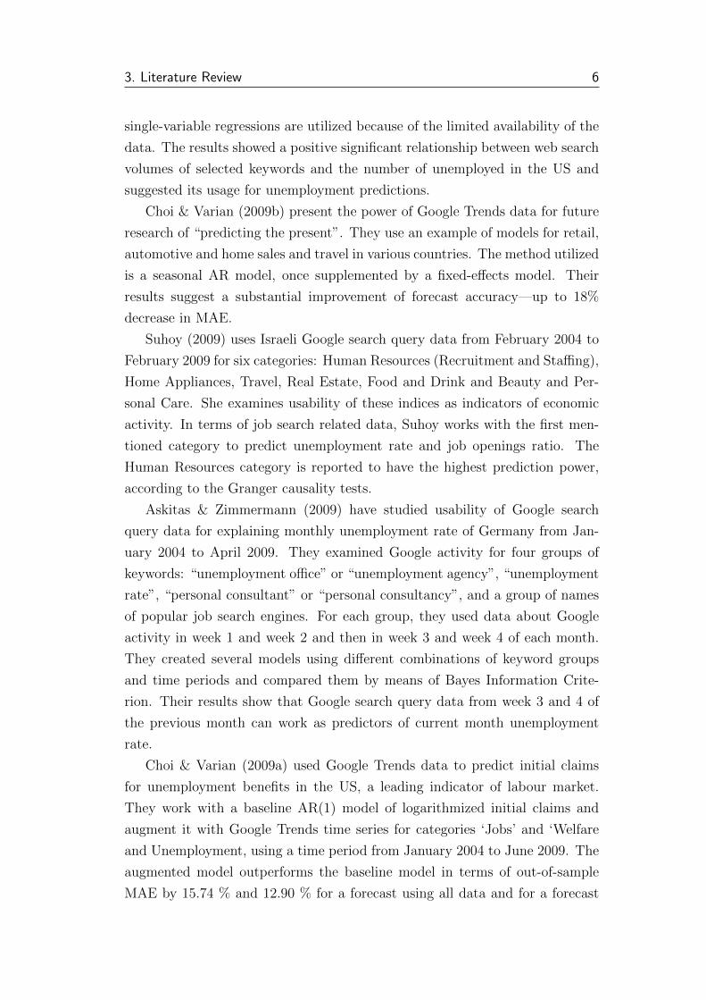
single-variable regressions are utilized because of the limited availability of the
data. The results showed a positive significant relationship between web search
volumes of selected keywords and the number of unemployed in the US and
suggested its usage for unemployment predictions.
Choi & Varian (2009b) present the power of Google Trends data for future
research of “predicting the present”. They use an example of models for retail,
automotive and home sales and travel in various countries. The method utilized
is a seasonal AR model, once supplemented by a fixed-effects model. Their
results suggest a substantial improvement of forecast accuracy—up to 18%
decrease in MAE.
Suhoy (2009) uses Israeli Google search query data from February 2004 to
February 2009 for six categories: Human Resources (Recruitment and Staffing),
Home Appliances, Travel, Real Estate, Food and Drink and Beauty and Per-
sonal Care. She examines usability of these indices as indicators of economic
activity. In terms of job search related data, Suhoy works with the first men-
tioned category to predict unemployment rate and job openings ratio. The
Human Resources category is reported to have the highest prediction power,
according to the Granger causality tests.
Askitas & Zimmermann (2009) have studied usability of Google search
query data for explaining monthly unemployment rate of Germany from Jan-
uary 2004 to April 2009. They examined Google activity for four groups of
keywords: “unemployment office” or “unemployment agency”, “unemployment
rate”, “personal consultant” or “personal consultancy”, and a group of names
of popular job search engines. For each group, they used data about Google
activity in week 1 and week 2 and then in week 3 and week 4 of each month.
They created several models using different combinations of keyword groups
and time periods and compared them by means of Bayes Information Crite-
rion. Their results show that Google search query data from week 3 and 4 of
the previous month can work as predictors of current month unemployment
rate.
Choi & Varian (2009a) used Google Trends data to predict initial claims
for unemployment benefits in the US, a leading indicator of labour market.
They work with a baseline AR(1) model of logarithmized initial claims and
augment it with Google Trends time series for categories ‘Jobs’ and ‘Welfare
and Unemployment, using a time period from January 2004 to June 2009. The
augmented model outperforms the baseline model in terms of out-of-sample
MAE by 15.74 % and 12.90 % for a forecast using all data and for a forecast
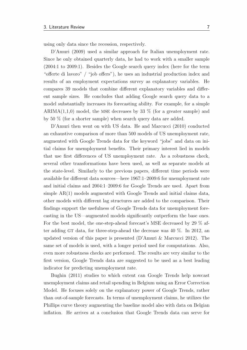
3. Literature Review 7
using only data since the recession, respectively.
D’Amuri (2009) used a similar approach for Italian unemployment rate.
Since he only obtained quarterly data, he had to work with a smaller sample
(2004:1 to 2009:1). Besides the Google search query index (here for the term
“offerte di lavoro” / “job offers”), he uses an industrial production index and
results of an employment expectations survey as explanatory variables. He
compares 39 models that combine different explanatory variables and differ-
ent sample sizes. He concludes that adding Google search query data to a
model substantially increases its forecasting ability. For example, for a simple
ARIMA(1,1,0) model, the MSE decreases by 33 % (for a greater sample) and
by 50 % (for a shorter sample) when search query data are added.
D’Amuri then went on with US data. He and Marcucci (2010) conducted
an exhaustive comparison of more than 500 models of US unemployment rate,
augmented with Google Trends data for the keyword “jobs” and data on ini-
tial claims for unemployment benefits. Their primary interest lied in models
that use first differences of US unemployment rate. As a robustness check,
several other transformations have been used, as well as separate models at
the state-level. Similarly to the previous papers, different time periods were
available for different data sources—here 1967:1–2009:6 for unemployment rate
and initial claims and 2004:1–2009:6 for Google Trends are used. Apart from
simple AR(1) models augmented with Google Trends and initial claims data,
other models with different lag structures are added to the comparison. Their
findings support the usefulness of Google Trends data for unemployment fore-
casting in the US—augmented models significantly outperform the base ones.
For the best model, the one-step-ahead forecast’s MSE decreased by 29 % af-
ter adding GT data, for three-step-ahead the decrease was 40 %. In 2012, an
updated version of this paper is presented (D’Amuri & Marcucci 2012). The
same set of models is used, with a longer period used for computations. Also,
even more robustness checks are performed. The results are very similar to the
first version, Google Trends data are suggested to be used as a best leading
indicator for predicting unemployment rate.
Bughin (2011) studies to which extent can Google Trends help nowcast
unemployment claims and retail spending in Belgium using an Error Correction
Model. He focuses solely on the explanatory power of Google Trends, rather
than out-of-sample forecasts. In terms of unemployment claims, he utilizes the
Phillips curve theory augmenting the baseline model also with data on Belgian
inflation. He arrives at a conclusion that Google Trends data can serve for

3. Literature Review 8
explaining macroeconomic fluctuations—a 10% change in search intensity is
connected with a 0.4% change in unemployment claims.
As a first contribution from an emerging economy, Chadwick & Sengul
(2012) present a similar approach based on data from Turkey from 2005:1
to 2011:12 in order to predict unemployment rate. They introduce Bayesian
Model Averaging (BMA) to cope with model uncertainty—up to 20 keywords
and up to 12 lags are used. Using the BMA procedure, 45 models are selected
to be compared with the benchmark model, which only includes lags of the
dependent variable. The results show that all models augmented with Google
Trends data outperform the benchmark model in terms of RMSE for 1-, 2- and
3-step-ahead forecasts.
Fondeur & Karame (2013) apply a similar technique to data on French youth
unemployment (15- to 24-year olds). This age group is believed to be most likely
to use Google for job search, which thereby minimizes the selection bias, noted
by D’Amuri (2009). Because of the nature of the data (non-stationarity, multi-
ple frequencies), an unobserved components approach is used. The forecasting
results support the previous findings—Google Trends data can significantly
improve unemployment rate predictions—with a 40% decrease of RMSE after
utilizing Google Trends data.
Barreira, Godinho, & Melo (2013) present a comparative study from four
European countries—Portugal, Spain, France and Italy. Apart from unem-
ployment rate, car sales are also nowcasted. Again, they use Google Trends
data for each country to augment the base models that use only lags of the
dependent variable. To cope with the error caused by the sampling procedure
used by Google, the Google Trends data are collected over a 14-day period and
averaged afterwards, a technique used previously by Carriere-Swallow & Labbe
(2013). Also, the data are seasonally adjusted by an ARIMA-X-12 procedure.
The results are not as compelling as those presented in the above-mentioned
studies. Google Trends data improved the predictions of unemployment rate
only in three countries, in Spain, the prediction accuracy worsened after adding
search query data. Regarding car sales, no consistent improvement of predic-
tions accuracy has been achieved in any of the countries.
This corresponds with findings presented in Choi & Varian (2012). In this
paper, they reemploy the methods from the previous version of the paper (Choi
& Varian 2009b) in order to predict retail sales, travel, consumer confidence
and, probably most importantly, initial claims for unemployment benefits in
the US, as presented earlier in Choi & Varian (2009a). For those, they find
3. Literature Review 9
an almost 6% increase in MAE after adding Google Trends data to the model.
Authors point out that the Google Trends-augmented model performs well
during the recession (until 2009), while the results have been less convincing
since then.
Previously mentioned studies examined usefulness of data on job-related
internet search for building unemployment models. The following studies do
not fit perfectly in the described framework; however, they use some innovatory
methods or focus on some minor, omitted but interesting issue.
Kholodilin, Podstawski, & Siliverstovs (2010) investigate usefulness of Google
search query data for nowcasting of US private consumption. They employ an
innovative method of transforming weekly Google Trends data to monthly se-
ries. Also, because multiple search queries are examined, principal components
analysis is utilized to reduce dimensionality of the data.
Carriere-Swallow & Labbe (2013) use data on Google search queries to build
nowcasting models for automobile sales in Chile. As Chile is a less developed
country, not all features of Google Trends are available. They introduce a
novel procedure of downloading the Google Trends series on 50 different days
and average over that period to reduce the bias generated by Google’s sampling
method. In addition, they have to address the problem of missing search query
categories. They construct an index using an auxiliary regression and also
examine usefulness of principal components analysis.
Baker & Fradkin (2011) used Google Trends in their study of the relation-
ship between length and intensity of job search and changes in duration of
unemployment insurance in the US. They used daily data on search intensity
of the keyword “jobs” for a proxy of job search duration.
Scott & Varian (2014) elaborated on the earlier works and developed an au-
tomated system of selecting predictors in a nowcasting model using structural
time series models. They utilize some rather advanced techniques compared to
the previously mentioned works, such as spike-and-slab regression or Markov
chain Monte Carlo. These were used to model weekly initial claims for unem-
ployment benefits and monthly retail sales.
As of now, there have been at least two studies concerning unemployment
nowcasting in the Czech Republic. Platil (2014) examined the applicabil-
ity of Google Econometrics in the Czech Republic. He uses Google search
query data to model unemployment, consumer confidence, consumption and
macroeconomic development. For the unemployment rate model, three dif-
ferent benchmark models have been used. These have been augmented with
3. Literature Review 10
several explanatory variables—monthly share of unemployed, index of indus-
trial production, confidence indicators, composite leading indicators and, most
importantly, Google Trends data for five different keywords. The author thor-
oughly analyzes improvements in prediction error (MSE) after adding search
query data. In addition, the process is repeated for three subsamples. The
results show a statistically significant increase in forecasting accuracy in a vast
majority of cases, with best achieved improvement of 10 %.
The other study (Pavlıcek & Kristoufek 2015) focused straight on unem-
ployment rate nowcasting, namely for Visegrad countries. They use the same
methodology for each country, i.e. a set of three AR models with different lag
structures augmented with Google Trends data for a query “job” translated
to the respective languages. As for the results for the Czech Republic, Google
Trends term turns out to be highly significant and strongly improve adjusted R2
for all three models. All three models also outperform the benchmark models
in terms of forecasting accuracy, for two models, the difference is statistically
significant.

Chapter 4
Data
The data used for this thesis come from four different sources: the explained
variable, unemployment rate, and Google Trends search query data have been
obtained from publicly available sources, while search query data from Sez-
nam.cz and data on job offers published on the job-search website Jobs.cz have
been kindly provided by the analytical departments of the responsible compa-
nies. In this section, all used data sources are described.
4.1 Czech Statistical Office
Our objective is to track and to predict Czech unemployment. The Czech
Statistical Office (CZSO) offers several indicators describing the Czech labour
force: absolute numbers of employed and unemployed persons, employment
rate, general unemployment rate, economic activity rate and share of unem-
ployed persons. All series are seasonally adjusted and apply to those aged 15
to 64. For all of them, separate series for men and women are also available.
Data are collected by means of a Labour Force Survey using a randomly
selected sample of households. The monitored indicators are in accordance with
the definitions of the International Labour Organization (ILO) and Eurostat
methodology (International Labour Organization 1982).
For our study, we selected the general unemployment rate. This indicator
refers to the percentage of unemployed under the ILO standard within all eco-
nomically active persons. According to ILO, “the ‘unemployed’ comprise all
persons above a specified age who during the reference period were:
(a) ‘without work’, i.e. were not in paid employment or self-employment;

4. Data 12
(b) ‘currently available for work’, i.e. were available for paid employment
or self-employment during the reference period;
and (c) ‘seeking work’, i.e. had taken specific steps in a specified recent
period to seek paid employment or self-employment. The specific steps may
include registration at a public or private employment exchange; application to
employers; checking at worksites, farms, factory gates, market or other assem-
bly places; placing or answering newspaper advertisements; seeking assistance
of friends or relatives; looking for land, building, machinery or equipment to
establish own enterprise; arranging for financial resources; applying for permits
and licences, etc.”
Although some indicators are known earlier, general unemployment rate is
published by the CZSO with a month delay at the end of the following month.
The explained variable is monthly general unemployment rate of the aged 15 to
64 years. The series is seasonally adjusted using the TRAMO/SEATS method
(for details, see Section 5.2). Data are available from 1993:01.
4.2 Google Trends
Data for the first explanatory variable come from Google Trends, a public
web service for exploration of popularity of different search-terms on Google’s
search engine. Rather than absolute numbers or percentages of searches, Google
constructs special indices. Although the data have been collected since 2004,
Google Insights for Search, a service allowing anyone examine and download
Google Trends statistics about any search query, have launched first in August
2008. Soon after the launch, many researchers started using the service for
their studies, with Choi & Varian (2009b) or Ginsberg et al. (2009) being some
significant examples. Later, in September 2012, Google Insights for Search have
been merged into Google Trends.
For each search query, Google Trends analyse the development of its per-
centage within all searches for the same parameters, such as time period or
country. Nevertheless, Google does not show the percentage directly, the fig-
ures are rescaled so that the highest percentage for a given time period is
assigned with a value of 100. In addition to the separate search terms, Google
Trends offer statistics also for the whole categories in selected regions. Simi-
larly, a development of percentages of searches is captured, while the scaling
is different—all categories start with a value zero at the beginning of a chosen
period and percentage changes are reported. Google does not report statistics
4. Data 13
about all search queries—only those that pass a certain search volume threshold
are described. The value of the threshold is not publicly known.
It is necessary to note that Google does not use the whole volume of searches
for purposes of Google Trends analysis. As Carriere-Swallow & Labbe (2013)
point out, a different sample is used every 24 hours and that can lead to addi-
tional noise. They built an API to collect data every day over a 50-day period
and then used their average for the final estimation. A 5.8% standard devia-
tion for the observed query “Chevrolet” was reported. Barreira et al. (2013)
used a similar procedure, although only with a 14-day period, to reduce sam-
pling noise for the terms “unemployment” in Portuguese, Spanish, French and
Italian. They report average standard deviations from 3.5 % to 7.6 %.
Google Trends website has an intuitive interface for browsing search query
statistics. For an example, see Figure A.2. Four attributes can be controlled:
location, time period, category and type of search. Google allows to limit
the statistics for a certain country or a smaller region (number of levels varies
among countries) or to explore data worldwide. For the Czech Republic, state
and region-level data are available.
As for the time period, the earliest data that Google reports come from
January 2004. Users are allowed to choose any period from that point. For
periods shorter than 90 days, daily data are reported, for longer periods, it
is only weekly or monthly data, depending on the volume. There is no way
of choosing frequency of the data. Except for three queries with lower search
volumes (“prace jihlava”, “prace ustı nad labem” and “prace karlovy vary”),
we obtained weekly data. Since we needed monthly data for our purpose, a
transformation had to be performed for the rest of the series. See Section 5.3
for details.
Searched queries are automatically sorted into categories for some regions.
Users can use these to define their requested queries more precisely (compare
e.g. search query “jobs” in a category “Jobs & Education” and in “Computer
& Electronics”). In addition, these categories can be examined as a whole—
and e.g. Choi & Varian (2009a) and Suhoy (2009) exploit this possibility.
Unfortunately, categories are not available for the Czech Republic.
The last attribute is the type of search. Apart from Web Search, data for
Image Search, News Search, Google Shopping and YouTube search results are
available; however, we will only use the first one since it is the only relevant
type for job-search purposes.
After setting the attributes, a time-series plot and a regional interest map
4. Data 14
is shown. Up to five queries can be described at the same time. Finally, the
data set can be downloaded in a CSV format.
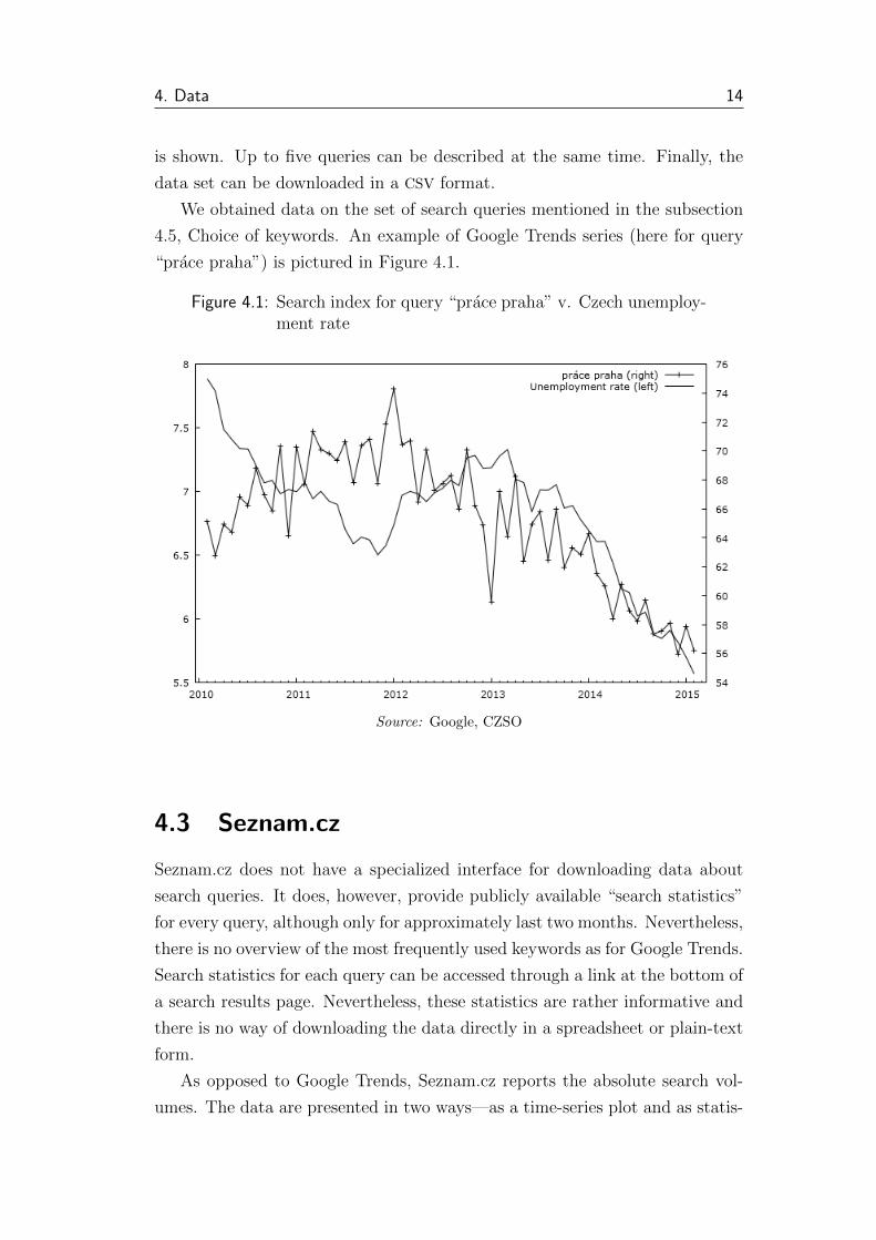
We obtained data on the set of search queries mentioned in the subsection
4.5, Choice of keywords. An example of Google Trends series (here for query
“prace praha”) is pictured in Figure 4.1.
Figure 4.1: Search index for query “prace praha” v. Czech unemploy-ment rate
Source: Google, CZSO
4.3 Seznam.cz
Seznam.cz does not have a specialized interface for downloading data about
search queries. It does, however, provide publicly available “search statistics”
for every query, although only for approximately last two months. Nevertheless,
there is no overview of the most frequently used keywords as for Google Trends.
Search statistics for each query can be accessed through a link at the bottom of
a search results page. Nevertheless, these statistics are rather informative and
there is no way of downloading the data directly in a spreadsheet or plain-text
form.
As opposed to Google Trends, Seznam.cz reports the absolute search vol-
umes. The data are presented in two ways—as a time-series plot and as statis-
4. Data 15
tics of minimum, maximum and average search volumes. For each query, exact
matches are distinguished from extended matches (queries containing given key-
word). An example of the search statistics page is provided in the Appendix:
see Figure A.3.
Because of the limited public availability of the search statistics, complete
data set has been obtained from the head of the analytical department of the
company, Michal Buzek, after a previous e-mail correspondence. The data set
contains absolute search volumes for each selected query from the set, using
exact matches of queries. It covers time-period since 2010:02. An example of
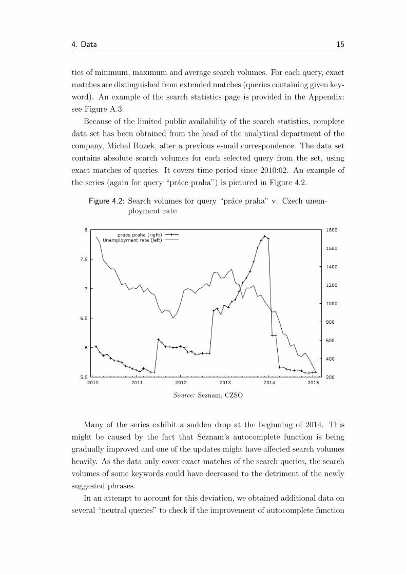
the series (again for query “prace praha”) is pictured in Figure 4.2.
Figure 4.2: Search volumes for query “prace praha” v. Czech unem-ployment rate
Source: Seznam, CZSO
Many of the series exhibit a sudden drop at the beginning of 2014. This
might be caused by the fact that Seznam’s autocomplete function is being
gradually improved and one of the updates might have affected search volumes
heavily. As the data only cover exact matches of the search queries, the search
volumes of some keywords could have decreased to the detriment of the newly
suggested phrases.
In an attempt to account for this deviation, we obtained additional data on
several “neutral queries” to check if the improvement of autocomplete function
4. Data 16
affected their volumes as well. We chose the following queries: “seznamka”
(“dating site”), “youtube”, “email”, “facebook”, “google”, and three queries
concerning adult content.1. Chosen queries are expected not to be subject to
seasonal deviations or external influences—they should keep a roughly constant
share among all queries. This characteristic was checked via a comparison with
corresponding Google Trends series. Hypothetically, these series should show
a similar decline due to improvements of the autocomplete function.
Surprisingly, these series (pictured in Figure A.1) show almost no long run
development (but a strange deviation for one month, possibly an error). This
indicates that the drop in the original data might be caused either by other
external factors or by real decrease of demand for jobs.
4.4 Jobs.cz
The third source of data for explanatory variables differs from those usually
used in the “Google Econometrics” studies. As Ettredge et al. (2005) suggested,
we obtained data from one of the largest job search portals in the Czech Re-
public. Jobs.cz focuses mostly on highly specialized jobs and job seekers with
tertiary education. These are not necessarily unemployed, usually they aim
to switch jobs rather than find a completely new one. This subset of the job
market can, however, still carry enough valuable information about the rest of
the market.
Again, this data is not publicly available and has been obtained from the
analytical department of the job search portal. The head of the department,
Tomas Dombrovsky, has been contacted through e-mail and kindly provided
the data set and also useful insight into company’s own utilization of gathered
information at a personal meeting.
Two types of figures are reported. First, total amounts of job postings pub-
lished on the portal in a given month. It is important to note that job postings
might stay published for more than one month. A comparison with yearly
numbers of job postings (not reported in this thesis) indicates that new job
postings account on average for less than a half of the total monthly amounts.
These are available from 2010:01. Second, monthly amounts of reactions to
the job postings—these are available for a slightly shorter time period—from
1“porno”, “freevideo” and “redtube”

4. Data 17
2011:05. Furthermore, a ratio of these two variables can be used as an addi-
tional variable.
The Figure 4.3 depicts the relationship between levels of unemployment rate
and numbers of job vacancies and reactions to them. Please note that both
series from Jobs.cz have been rescaled for the confidential nature of the data.
Also, time-periods depicted vary according to availability of the data.
4.5 Choice of keywords
The selection of keywords is a key part of the study since it directly affects
the explanatory power of search query data. It is important to capture the
major ways of finding jobs used by job-seekers while bearing in mind possible
increases of noise in the data.
In the previously published studies, there have been different approaches
for the selection of queries. Since the vast majority used Google Trends, some
of them made use of its categories, such as “Jobs” or “Welfare and Unem-
ployment” (Choi & Varian 2009a; Suhoy 2009; Kholodilin et al. 2010; Bughin
2011; Vosen & Schmidt 2011). Some studies use just the keyword “job” or
“jobs” or its equivalent in a given language, for instance D’Amuri (2009),
Fondeur & Karame (2013) or Pavlıcek & Kristoufek (2015). Barreira et al.
(2013) used translations of the word “unemployment”. Others used multiple
keywords and their combinations. Askitas & Zimmermann (2009) utilize four
groups of keywords: “unemployment office OR unemployment agency”, “un-
employment rate”, “personal consultant OR personal consultancy” and a group
of most popular job search engines in Germany, taking advantage of Google’s
support of disjunctions of keywords. Chadwick & Sengul (2012) use a variety of
terms—“looking for a job”, “job announcements”, “cv”, “career”, “unemploy-
ment” and “unemployment insurance”. Similarly for the Czech environment,
Platil (2014) uses a set of queries including terms “job”, “employment”, “job
offers”, “labour office” and “CV”.
There is the same set of keywords used for both search engines, Google
and Seznam. In order to select the keywords, we chose to conduct a survey
among possible job-seekers. The survey had a form of an online questionnaire,
utilizing the Google Docs platform.
Possible participants have been contacted through a number of most popu-
lar Facebook interest groups specialized for job search in Czech cities, such as

4. Data 18
Figure 4.3: Unemployment rate, job vacancies (rescaled), reactions tojob vacancies (rescaled)
170
180
190
200
210
220
230
240
250
2010 2011 2012 2013 2014 2015 5.5
6
6.5
7
7.5
8Unemployment rate (right)
Job vacancies (left)
2400
2500
2600
2700
2800
2900
3000
3100
3200
3300
3400
3500
2012 2013 2014 2015 5.8
6
6.2
6.4
6.6
6.8
7
7.2
7.4Unemployment rate (right)
Reactions to job vacancies (left)
Source: LMC (Jobs.cz), CZSO

4. Data 19
“BRIGADY PRACE PRAHA”2 (“jobs, part-time jobs Prague”). The partici-
pants have been self-selected. Although the whole survey has been conducted
in Czech, I will only provide the English translations. The most important
question was: “If you were to search for a new job using an internet search
engine, which query would you use? Please name at least three.” In addition,
two auxiliary questions have been asked: “Have you ever used the Internet for
a job search?” and “Which internet search engine do you use most often?”. In
the end, participants were asked to enter personal demographic data—age, sex
and region. As a result, 213 unique answers have been collected. More detailed
results of the survey can be found in Table B.2.
The most frequently mentioned query was “prace”, by a wide margin. This
word can be translated as “job”, “work”, “labour” or “employment”; another—
although much less frequently used—meaning is “thesis”. This draws attention
to the possible noise in the data stemming from the ambiguity of the mean-
ing; however, we believe this affects our results only to an acceptable extent.
Other answers included queries such as “nabıdka prace” (“job offer”), “brigada”
(“temporary job”), “volna mısta” and “volna pracovnı mısta” (“vacancies”).
Respondents also frequently used the query “prace” together with a name of a
city, so we included queries containing names of all county towns in the Czech
Republic.
Search engine users can use queries with or without diacritics and thereby
generate slightly different series. We decided to use only search queries with dia-
critics to keep the models simple. Also Seznam.cz seems to merge these queries
for the purpose of creating search statistics, the reported figures for queries
with and without diacritics are identical. The full list of keywords is as fol-
lows: “prace”, “prace praha”, “prace ceske budejovice”, “prace plzen”, “prace
karlovy vary”, “prace ustı nad labem”, “prace liberec”, “prace hradec kralove”,
“prace jihlava”, “prace brno”, “prace olomouc”, “prace ostrava”, “prace zlın”,
“brigada”, “volna mısta”, “volna pracovnı mısta” and “nabıdka prace”.
2available at www.facebook.com/groups/203900279809525/

Chapter 5
Methodology
This utilizes a standard framework commonly used for dealing with macroeco-
nomic time-series. In this chapter, we present the methods used for estimation
of the models as well as the preceding processes.
5.1 ARMA/ARIMA/ARMAX
ARMA (autoregressive–moving-average) model is a time series model for de-
scription of weakly stationary stochastic processes. A general ARMA model of
order (p, q) has a form:
Yt = c+φ1Yt−1 +φ2Yt−2 + . . .+φpYt−p +εt +θ1εt−1 +θ2εt−2 + . . .+θqεt−q (5.1)
With p and q ∈ N being orders of the lag polynomials, Yt explained variable, Yt−i
lagged values of the explained variable and φi their corresponding coefficients;
εt white noise (a process with no serial correlation, zero mean and time invariant
finite variance) εt−i its lagged values and θi their corresponding coefficients.
It can be decomposed into two parts: AR(p) (autoregressive) and MA(q)
(moving average). Both can be understood as special cases of the ARMA(p, q)
model.
A general Moving Average (AR) model of order p has a form:
Yt = c+ φ1Yt−1 + φ2Yt−2 + . . .+ φpYt−p + εt (5.2)
A general Autoregressive (MA) model of order q has a form:
Yt = c+ εt + θ1εt−1 + θ2εt−2 + . . .+ θqεt−q (5.3)
5. Methodology 21
When stationarity condition is not met, a generalization of an ARMA
model can be used in some cases: an Autoregressive Integrated Moving Aver-
age (ARIMA) model. In comparison with the ARMA model, it is extended by an
integrated part I(d), where d stands for the order of integration, and thereby
allows to handle non-stationary series.
In this thesis, we will use only a simple AR(1) process for the baseline
model to retain parsimony; our choice is based on the fact that the same model
is used in the majority of previous studies (e.g. Choi & Varian 2009a; D’Amuri
& Marcucci 2010; Kholodilin et al. 2010), together with the its seasonal version
(Choi & Varian 2009b; Askitas & Zimmermann 2009) and on a series of pre-
tests that compared models using information criteria.
An AR(1) process has a form:
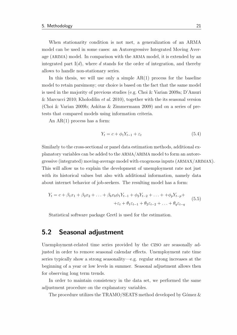
Yt = c+ φ1Yt−1 + εt (5.4)
Similarly to the cross-sectional or panel data estimation methods, additional ex-
planatory variables can be added to the ARMA/ARIMA model to form an autore-
gressive (integrated) moving-average model with exogenous inputs (ARMAX/ARIMAX).
This will allow us to explain the development of unemployment rate not just
with its historical values but also with additional information, namely data
about internet behavior of job-seekers. The resulting model has a form:
Yt = c+ β1x1 + β2x2 + . . .+ βbxbφ1Yt−1 + φ2Yt−2 + . . .+ +φpYt−p+
+εt + θ1εt−1 + θ2εt−2 + . . .+ θqεt−q(5.5)
Statistical software package Gretl is used for the estimation.
5.2 Seasonal adjustment
Unemployment-related time series provided by the CZSO are seasonally ad-
justed in order to remove seasonal calendar effects. Unemployment rate time
series typically show a strong seasonality—e.g. regular strong increases at the
beginning of a year or low levels in summer. Seasonal adjustment allows then
for observing long term trends.
In order to maintain consistency in the data set, we performed the same
adjustment procedure on the explanatory variables.
The procedure utilizes the TRAMO/SEATS method developed by Gomez &
5. Methodology 22
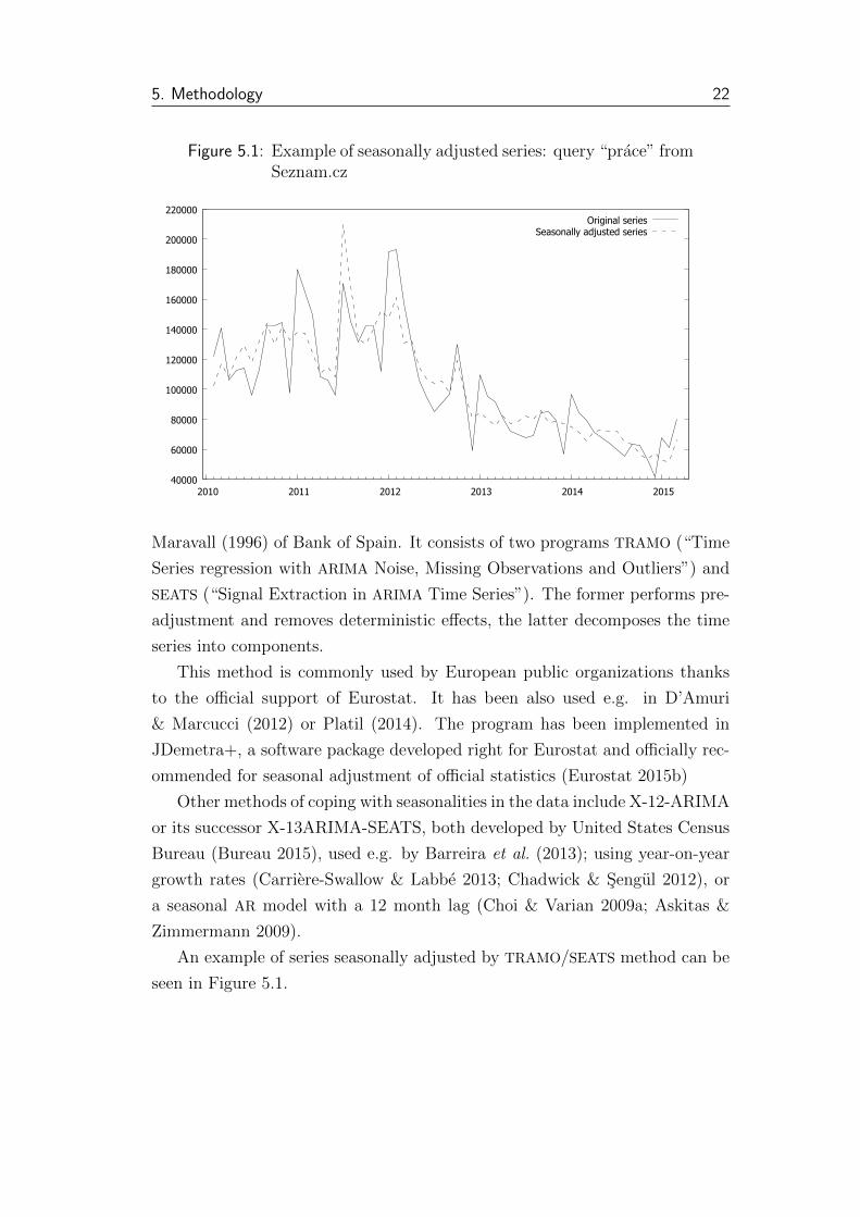
Figure 5.1: Example of seasonally adjusted series: query “prace” fromSeznam.cz
40000
60000
80000
100000
120000
140000
160000
180000
200000
220000
2010 2011 2012 2013 2014 2015
Original seriesSeasonally adjusted series
Maravall (1996) of Bank of Spain. It consists of two programs TRAMO (“Time
Series regression with ARIMA Noise, Missing Observations and Outliers”) and
SEATS (“Signal Extraction in ARIMA Time Series”). The former performs pre-
adjustment and removes deterministic effects, the latter decomposes the time
series into components.
This method is commonly used by European public organizations thanks
to the official support of Eurostat. It has been also used e.g. in D’Amuri
& Marcucci (2012) or Platil (2014). The program has been implemented in
JDemetra+, a software package developed right for Eurostat and officially rec-
ommended for seasonal adjustment of official statistics (Eurostat 2015b)
Other methods of coping with seasonalities in the data include X-12-ARIMA
or its successor X-13ARIMA-SEATS, both developed by United States Census
Bureau (Bureau 2015), used e.g. by Barreira et al. (2013); using year-on-year
growth rates (Carriere-Swallow & Labbe 2013; Chadwick & Sengul 2012), or
a seasonal AR model with a 12 month lag (Choi & Varian 2009a; Askitas &
Zimmermann 2009).
An example of series seasonally adjusted by TRAMO/SEATS method can be
seen in Figure 5.1.
5. Methodology 23
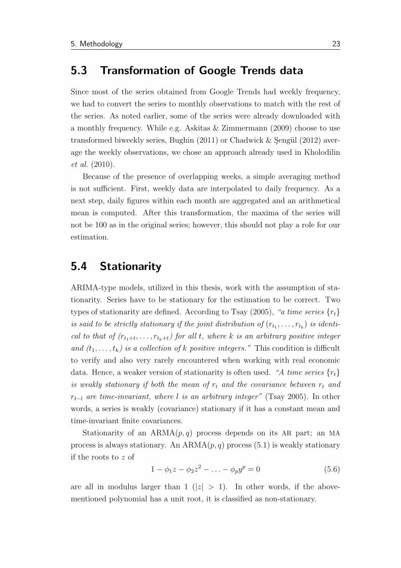
5.3 Transformation of Google Trends data
Since most of the series obtained from Google Trends had weekly frequency,
we had to convert the series to monthly observations to match with the rest of
the series. As noted earlier, some of the series were already downloaded with
a monthly frequency. While e.g. Askitas & Zimmermann (2009) choose to use
transformed biweekly series, Bughin (2011) or Chadwick & Sengul (2012) aver-
age the weekly observations, we chose an approach already used in Kholodilin
et al. (2010).
Because of the presence of overlapping weeks, a simple averaging method
is not sufficient. First, weekly data are interpolated to daily frequency. As a
next step, daily figures within each month are aggregated and an arithmetical
mean is computed. After this transformation, the maxima of the series will
not be 100 as in the original series; however, this should not play a role for our
estimation.
5.4 Stationarity
ARIMA-type models, utilized in this thesis, work with the assumption of sta-
tionarity. Series have to be stationary for the estimation to be correct. Two
types of stationarity are defined. According to Tsay (2005), “a time series {rt}is said to be strictly stationary if the joint distribution of (rt1 , . . . , rtk) is identi-
cal to that of (rt1+t, . . . , rtk+t) for all t, where k is an arbitrary positive integer
and (t1, . . . , tk) is a collection of k positive integers.” This condition is difficult
to verify and also very rarely encountered when working with real economic
data. Hence, a weaker version of stationarity is often used. “A time series {rt}is weakly stationary if both the mean of rt and the covariance between rt and
rt−l are time-invariant, where l is an arbitrary integer” (Tsay 2005). In other
words, a series is weakly (covariance) stationary if it has a constant mean and
time-invariant finite covariances.
Stationarity of an ARMA(p, q) process depends on its AR part; an MA
process is always stationary. An ARMA(p, q) process (5.1) is weakly stationary
if the roots to z of
1− φ1z − φ2z2 − . . .− φpy
p = 0 (5.6)
are all in modulus larger than 1 (|z| > 1). In other words, if the above-
mentioned polynomial has a unit root, it is classified as non-stationary.

5. Methodology 24
If a series is found non-stationary, then it should be differenced (possibly
multiple times) until stationarity is achieved, according to the Box-Jenkins
methodology (Box & Pierce 1970). A process with one unit root is called
integrated of order one, I(1). Similarly, a process with d unit roots is called
integrated of order d, I(d). Such process can be made stationary by taking d
differences.
Macroeconomic series (such as unemployment rate) are often subject to
trends and stationarity is really hard to justify. On the other hand, as Mont-
gomery et al. (1998) or Koop & Potter (1999) point out, unemployment rate,
bounded within the unit interval, should not show signs of presence of a unit
root. Similar limitations apply to the Google Trends series, but not Seznam or
Jobs.cz series; unit root tests thus have to be conducted in any case.
There are several stationarity tests that seek for the presence of a unit root.
The probably most popular one is Augmented Dickey-Fuller test, used also e.g.
by Suhoy (2009) or Barreira et al. (2013), or Kwiatkowski-Phillips-Schmidt-
Shin. They are usually quite sensitive and often easily tend to mark series
as non-stationary (Choi & Moh 2007). D’Amuri & Marcucci (2010) utilize a
modified version the Augmented Dickey-Fuller test, ADF-GLS or a Range Unit
Root (RUR) test to fit better to the characteristics of used series.
5.5 Augmented Dickey-Fuller Test
In this thesis, we will use the Augmented Dickey-Fuller test to examine sta-
tionarity of the series. The ADF test is based on an OLS regression
∆Yt = (c) + (dt) + αYt−1 + ζ1∆Yt−1 + ζ2Yt−2 + . . .+ ζp−1Yt−p+1 + εt, (5.7)
– depending if we consider a constant c and/or a time trend d in the model or
not. ADF test uses a modified t-distribution—Dickey-Fuller distribution. The
ADF statistic is a negative number, lower numbers meaning stronger rejection
of the H0 hypothesis:
H0: α = 0⇔ ‘the series has a unit root’.
H1: α ≤ 0⇔ ‘the series is stationary’.
5. Methodology 25
5.6 Principal Component Analysis
Many of the previous studies used search query data just for one employment-
related keyword, as noted earlier. In our thesis, we want to capture job-seekers’
web search behaviour in a more complex manner, using data from Google
Trends and Seznam.cz. Since Google Trends statistics for the whole categories
are not available for the Czech Republic and there are no similar categories
for the Seznam data, we decided to use multiple search queries based on a
previously conducted survey.
Our data set contains time series for 18 search queries from each search
engine. One of the possibilities would be to use each of them as a separate
variable. In order to keep the collected information from one search engine in
one model and retain a reasonable number of models, we had to “compress”
the information contained in the data set. This approach also increases degrees
of freedom for the estimation compared to the case of using all variables in one
model.
A similar issue has been already addressed earlier in previous studies. Carriere-
Swallow & Labbe (2013) use an auxiliary model to estimate weights used for
construction of a new Google Trends index. A more frequently used technique
(Kholodilin et al. 2010; Vosen & Schmidt 2011; Carriere-Swallow & Labbe 2013;
D’Amuri & Marcucci 2012) makes use of principal component analysis and has
been described by Stock & Watson (2002).
Principal Component Analysis (PCA) is a statistical procedure introduced
by Pearson (1901). It transforms a set of original variables into a new set of
linearly uncorrelated variables—principal components. These have an orthog-
onal structure and are designed to preserve all variance in the data. The first
generated variable—first principal component—accounts for as much variance
as possible, each next component explains as much of the remaining variance
as possible while complying with the condition of uncorrelatedness.
5.7 Forecasting and its evaluation
In this thesis, a comparison of forecasting ability of our models is of greatest
interest. Similarly, most studies from the Google Econometrics field aim to
“nowcast” various economic indicators, having this as a primary goal, rather
than focusing on significance of variables and formal model quality statistics.
Since nowcasting aims for contemporary values, we only work with static

5. Methodology 26
one-step-ahead out-of-sample forecasts. The full sample is divided into two
subsamples—the first one is used for estimation, the second one for forecast
evaluation. Since we forecast values that are already known, this method
is sometimes called “pseudo out-of-sample”. We choose the last 12 months
(March 2013 to February 2015) as “test data” for nowcasting, while estimating
the models on the first 49 months of the selected period (February 2010 to
February 2014).
5.7.1 Evaluation
In order to evaluate the predictive ability of the models, we use Root Mean
Squared Error and Mean Absolute Error. These metrics have been frequently
used in the previous studies, we will thus be able to compare the gains of pre-
dictive ability of our models easily. Moreover, Diebold-Mariano test is utilized
to find statistically significant differences within our set of models.
Each technique operates with the prediction error. It is defined as difference
between the actual values and the predictions:
et+h|t = Yt+h − Yt+h|t (5.8)
5.7.2 Mean Absolute Error (MAE)
Mean Absolute Error is defined as an average of absolute values of the predic-
tion error over the forecasted period.
MAE =1
T
T∑t=1
|et+h|t| (5.9)
5.7.3 Root Mean Squared Error (RMSE)
Root Mean Squared Error is defined as a square root of the average of squared
prediction errors over the forecasted period.
RMSE =
√√√√ 1
T
T∑t=1
(et+h|t)2 (5.10)

5. Methodology 27
5.7.4 Diebold-Mariano (DM) Test
Diebold-Mariano test (Diebold & Mariano 1995) serves to compare accuracy
of two competing forecasts. When comparing a set of forecasts, one is usually
chosen as a benchmark. First, a loss differential dt between model A and B is
defined:
dt = L(eAt+h|t
)− L
(eBt+h|t
), t = 1, . . . , T, (5.11)
where eAt+h|t and eBt+h|t denote prediction errors made by h-step-ahead forecasts
from model A and B, respectively and L denotes a selected loss-function, e.g.
L(x) = |x| or L(x) = x2. The null hypothesis is then defined as follows.
H0 : E[dt] = 0⇔ E[L(eAt+h|t
)]= E
[L(eBt+h|t
)](5.12)
H1 : E[dt] 6= 0⇔ E[L(eAt+h|t
)]6= E
[L(eBt+h|t
)](5.13)
In other words, the null hypothesis states that there are no quantitative
differences between the forecasts of the two models A and B.

Chapter 6
Empirical Results
In this section, we present the results of our analysis of explanatory and fore-
casting power of web job search data. We conduct tests for stationarity, perform
principal component analysis and finally make in-sample and out-of-sample
performance comparison.
6.1 Stationarity
We examine stationarity of our data using an Augmented Dickey-Fuller unit-
root test. We utilize Gretl’s functionality for adjusting the maximum lag order
by means of Akaike Information Criterion, with the highest lag set to 10 ac-
cording to the recommendation by Schwert (1989).
Majority of the series shows signs of non-stationarity, with the exception
of a few search query series, mostly from Seznam.cz. In order to get rid of
stationarity, we take first differences of each series. For all of the new series, we
reject the null of presence of unit-root even at 99% level, except for two Google
variables (“prace liberec”, “prace pardubice”). For these we take also second
differences to examine the order of integration.
The results, reported in table 6.1, indicate that most of the series in dataset
are integrated of order 1, two series show order of integration 2 and 12 series are
stationary. Since we want to keep the models interpretable, we will continue
to work with first difference series.
6. Empirical Results 29
6.2 Principal Component Analysis (PCA)
In the next step, principal component analysis of two 18-item sets of variables—
those from Google and from Seznam.cz—is carried out. Tables of both sets of
principal components and the respective percentages of explained variance are
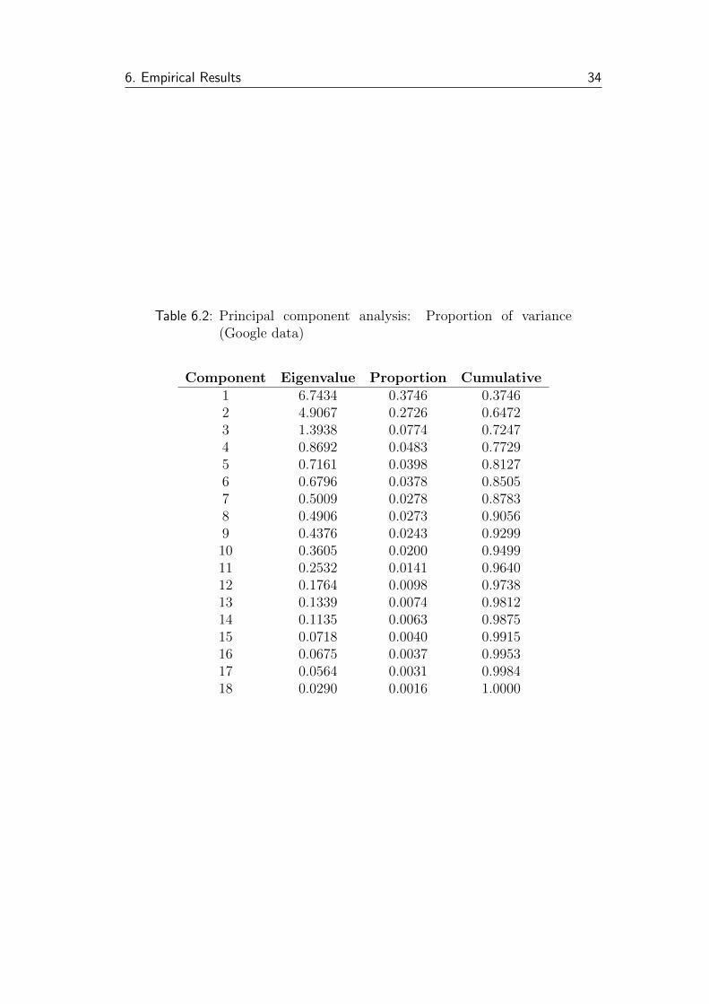
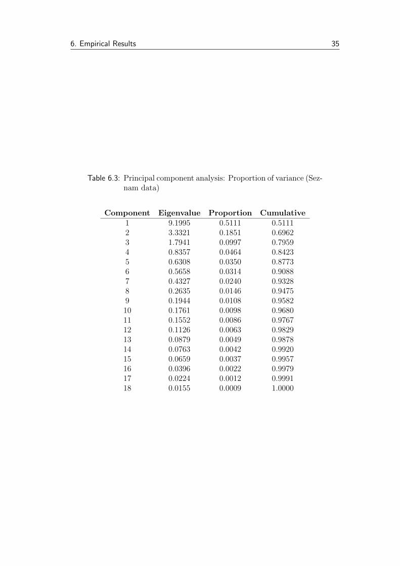
reported below (Tables 6.2 and 6.3); additional details in Table B.3.
Both sets of PCs show a high concentration of variance in the first PCs—first
three PCs for Google and Seznam data account for 72 % and 80 %, first ten
account for 95 % and 97 % of variance, respectively. For the newly generated
PCs, ADF tests are conducted. The series again show signs of non-stationarity
in most cases. Taking first differences removes stationarity for all but the
third and fourth PCs for Seznam data. For these series, second differences are
generated—and according to the ADF test, the new series are stationary. See
Table B.4 for complete results.
6.3 Model performance
Our goal is to compare the explanatory and predictive (nowcasting) power of
web search query data from Google and Seznam and also examine the usability
of data from the job portal Jobs.cz. We will describe the results in three
subsections. In the first subsection, we will compare the predictive power of
each individual query from both Google and Seznam. In the second subsection,
we will compare aggregate models for data from both search engines to compare
their usefulness as a whole. Lastly, we will inspect the Jobs.cz data and a set
of models utilizing them. In each subsection, we will inspect both in-sample
and out-of-sample performance of the models, using a few different measures.
In-sample performance is described by Adjusted R2 (R2), computed man-
ually as a squared correlation between fitted and original series, Root Mean
Squared Error (RMSE) and Mean Absolute Error (MAE). For the comparison
out-of-sample performance, RMSEs and MAEs are computed. The best perform-
ing models are then also tested for significant differences in forecast accuracy
by means of a Diebold Mariano test.
First, we estimate our baseline model, which will be later used in all subsec-
tions. We use an AR(1) model for differenced unemployment rate, estimated
using exact maximum likelihood method. All models are estimated using the
time period from February 2010 to February 2015.
The regression results for the baseline model are reported in the Figure 6.1.

6. Empirical Results 30
Figure 6.1: Baseline model estimation results
Model 1: ARMA, using observations 2010:02–2014:02 (T = 49)Dependent variable: d unempSA1Standard errors based on Hessian
Coefficient Std. Error z p-value
φ1 0.120364 0.141550 0.8503 0.3951
Mean dependent var −0.024997 S.D. dependent var 0.111730Mean of innovations −0.022207 S.D. of innovations 0.112530Log-likelihood 37.50689 Akaike criterion −71.01378Schwarz criterion −67.23014 Hannan–Quinn −69.57827
Real Imaginary Modulus FrequencyAR
Root 1 8.3081 0.0000 8.3081 0.0000
6.3.1 Models with individual variable performance
The baseline model is now augmented with the search query variables, one by
one. We build 36 models, one for each variable. The in-sample results (reported
in table 6.4) are somewhat ambiguous. All models are affected by the short
length of the available sample and the models have a rather poor fit. For most
of them, R2 has even negative values.
From the set of Google variables, only five increase the fit of the model:
“prace praha”, “prace ustı nad labem”, “prace ostrava”, “volna pracovnı mısta”
and “nabıdka prace”. The last mentioned variable increased the fit by more
than 1300 %. Together with “volna pracovnı mısta” are these the only variables
that decrease the in-sample error.
Seznam variables show a similar performance, with only four variables im-
proving the R2—“prace ceske budejovice”, “prace liberec”, “prace jihlava” and
“prace olomouc”. None of the Seznam variables decreases the in-sample error.
Out-of-sample performance (described in Table 6.5) is rather poor, none
of the variables improves the nowcasts. The nowcast accuracy worsens after
adding any individual variable. There are no substantial differences between
performances of models with Google and Seznam variables. The RMSEs in-
creases range from 9 to 22 %, MAEs worsen by 6 to 20 %.

6. Empirical Results 31
6.3.2 Models with multiple or aggregate variables
In this subsection, we compare the models that aggregate all information from
each search engine, in order to evaluate and compare collective power of all
search queries. The results are presented in tables 6.6 and 6.7. First, we
incorporate all 18 variables from each search engine (denoted G ALL and S
ALL for Google and Seznam, respectively). Second, since data from Seznam.cz
are not indices but absolute numbers, it is meaningful generate a new variable
“s sum”—a simple horizontal sum of all Seznam variables. Third, we make
use of principal components. We use up to 18 (i.e. all) PCs for each search
engine. The number in parentheses denotes the last principal component—e.g.
“sPC (5)” stands for a model that includes first five principal components for
Seznam data.
Adding all Google and all Seznam variables increases the in-sample fit sub-
stantially, with R2 increasing up to 0.30 and 0.36, respectively. While adding
complete set of Seznam variables improves the R2 slightly more than adding
corresponding Google variables, the latter reduce the in-sample RMSE and MAE
more substantially.
Seznam data surprisingly do not add any explanatory power to the model, as
measured by the R2 and in-sample errors, similarly to the individual variables
described in the previous subsection.
In a comparison of PC performance, those for Google data seem to explain
the dependent variable better, showing an R2 increase to 0.13 already for first
two PCs. That indicates a good potential for further usage for modeling and
forecasting purposes since these two PCs cumulatively account for more than 64
% of variance in the Google data set (see Table 6.2). On the contrary, Seznam’s
PCs show even negative R2 values for models with up to 15 PCs. Given the
distribution of variance among PCs (see Table 6.3), Seznam’s PCs show rather
poor potential for further usage.
Nevertheless, most of these models suffer from overfitting the training data,
which is often encountered when too many variables are included in the model.
While the in-sample performance looks promising, the out-of-sample perfor-
mance is poor. The nowcast accuracy worsens by 5 to more than 300 % in
terms of RMSE and by 3 to almost 250 % in terms of MAE.
6. Empirical Results 32
6.3.3 Models with job search portal data
Lastly, we want to assess the nowcast ability of Jobs.cz data on job vacan-
cies and reactions to them. We focus mainly on the number of job vacancies
published, but we also examine the reactions. The tables summarizing perfor-
mance of the models are presented below (table 6.8 and 6.9). JV stands for job
vacancies, JR for reactions. The number in parentheses denotes the highest
included lag order of the JV variable.
Job vacancies improve the in-sample fit substantially at various lag order
levels. A model incorporating this variable up to the third lag shows R2 0.1,
more than 16 times greater than the baseline model. On the contrary, reactions
to job vacancies seem to have rather poor fit, getting negative R2 values.
Regarding out-of-sample performance, job vacancies seem to be the only
variable improving the nowcast performance, according to our computations.
Models augmented with job vacancies series up to the second lag to the model
decreases RMSE by approx. 2 %. MAE decreases even in more cases, for models
with maximum lag orders up to 6 and also 11 and 12, 7.6 % being the greatest
improvement. The second variable, reactions to job vacancies, increases the
prediction errors by more than 8 %.
6.4 DM test
For the forecasts that outperform the baseline model, we conduct the Diebold
Mariano test to determine whether the difference in forecasting performance is
statistically significant. The results are presented in a table 6.10.
We cannot reject the null hypothesis of identical forecast performance even
at 10% level, the improvement of forecast accuracy is thus statistically insignif-
icant.

6. Empirical Results 33
Table 6.1: ADF test results for original variables: p-values
LevelFirst
differenceSecond
differenceunemp 0.81 <0.01 -j vacancies 1.00 <0.01 -j reactions 0.87 <0.01 -g p 0.65 <0.01 -g p praha <0.01 - -g p ceskebudejovice 0.91 <0.01 -g p plzen 0.39 <0.01 -g p karlovyvary 0.78 <0.01 -g p ustinadlabem 0.37 <0.01 -g p liberec 0.80 0.28 <0.01g p hradeckralove 0.86 <0.01 -g p pardubice 0.56 0.31 <0.01g p jihlava 0.45 <0.01 -g p brno 0.01 - -g p olomouc 0.96 <0.01 -g p ostrava <0.01 - -g p zlin 0.78 0.02 -g brigada 0.22 <0.01 -g volnamista 0.55 <0.01 -g nabidkaprace 0.84 <0.01 -g volnapracovnimista 0.83 <0.01 -s p <0.01 - -s p praha 0.78 <0.01 -s p ceskebudejovice 0.91 <0.01 -s p plzen 0.89 <0.01 -s p karlovyvary 0.01 - -s p ustinadlabem 0.17 <0.01 -s p liberec <0.01 - -s p hradeckralove 0.09 <0.01 -s p pardubice 0.03 <0.01 -s p jihlava 0.18 <0.01 -s p brno 0.64 <0.01 -s p olomouc 0.42 <0.01 -s p ostrava 0.97 <0.01 -s p zlin <0.01 - -s brigada <0.01 - -s volnamista <0.01 - -s nabidkaprace <0.01 - -s volnapracovnimista <0.01 - -s sum <0.01 - -
6. Empirical Results 34
Table 6.2: Principal component analysis: Proportion of variance(Google data)
Component Eigenvalue Proportion Cumulative1 6.7434 0.3746 0.37462 4.9067 0.2726 0.64723 1.3938 0.0774 0.72474 0.8692 0.0483 0.77295 0.7161 0.0398 0.81276 0.6796 0.0378 0.85057 0.5009 0.0278 0.87838 0.4906 0.0273 0.90569 0.4376 0.0243 0.929910 0.3605 0.0200 0.949911 0.2532 0.0141 0.964012 0.1764 0.0098 0.973813 0.1339 0.0074 0.981214 0.1135 0.0063 0.987515 0.0718 0.0040 0.991516 0.0675 0.0037 0.995317 0.0564 0.0031 0.998418 0.0290 0.0016 1.0000
6. Empirical Results 35
Table 6.3: Principal component analysis: Proportion of variance (Sez-nam data)
Component Eigenvalue Proportion Cumulative1 9.1995 0.5111 0.51112 3.3321 0.1851 0.69623 1.7941 0.0997 0.79594 0.8357 0.0464 0.84235 0.6308 0.0350 0.87736 0.5658 0.0314 0.90887 0.4327 0.0240 0.93288 0.2635 0.0146 0.94759 0.1944 0.0108 0.958210 0.1761 0.0098 0.968011 0.1552 0.0086 0.976712 0.1126 0.0063 0.982913 0.0879 0.0049 0.987814 0.0763 0.0042 0.992015 0.0659 0.0037 0.995716 0.0396 0.0022 0.997917 0.0224 0.0012 0.999118 0.0155 0.0009 1.0000

6. Empirical Results 36
Table 6.4: In-sample performance of models incorporating individualvariables
R2 ∆ RMSE ∆ MAE ∆(baseline) 0.006 0.130 0.094g p 0.012 97% 0.131 0.5% 0.094 0.7%g p praha -0.012 -294% 0.132 1.6% 0.099 5.4%g p ceskebudejovice -0.009 -248% 0.132 1.7% 0.099 5.5%g p plzen -0.013 -319% 0.132 1.8% 0.099 5.3%g p karlovyvary -0.011 -286% 0.132 1.6% 0.098 4.7%g p ustinadlabem 0.024 309% 0.132 1.6% 0.095 1.2%g p liberec -0.015 -348% 0.132 1.8% 0.098 4.6%g p hradeckralove 0.002 -74% 0.131 1.0% 0.095 1.8%g p pardubice -0.013 -317% 0.132 1.8% 0.098 4.7%g p jihlava -0.011 -279% 0.133 2.2% 0.098 5.0%g p brno -0.002 -136% 0.131 0.8% 0.095 1.2%g p olomouc -0.011 -293% 0.132 1.6% 0.098 4.4%g p ostrava 0.048 712% 0.128 -1.1% 0.093 -0.3%g p zlin -0.009 -256% 0.131 1.2% 0.098 4.6%g brigada -0.015 -350% 0.132 1.7% 0.098 4.3%g volnamista 0.003 -53% 0.132 1.4% 0.095 1.8%g volnapracovnimista 0.030 398% 0.130 0.3% 0.102 9.0%g nabidkaprace 0.084 1308% 0.130 -0.1% 0.092 -1.7%
s p -0.009 -257% 0.132 2.0% 0.098 4.3%s p praha -0.001 -124% 0.131 1.0% 0.096 2.9%s p ceskebudejovice 0.025 316% 0.133 2.4% 0.099 6.1%s p plzen -0.005 -177% 0.132 2.0% 0.098 4.8%s p karlovyvary -0.015 -360% 0.132 1.8% 0.098 4.5%s p ustinadlabem -0.004 -164% 0.132 1.9% 0.098 4.5%s p liberec 0.028 364% 0.132 1.7% 0.098 4.5%s p hradeckralove -0.004 -161% 0.132 1.8% 0.098 4.2%s p pardubice -0.004 -164% 0.133 2.1% 0.098 4.3%s p jihlava 0.031 422% 0.131 0.9% 0.097 3.3%s p brno -0.001 -109% 0.132 1.8% 0.098 4.4%s p olomouc 0.007 25% 0.132 1.7% 0.097 3.8%s p ostrava -0.013 -326% 0.133 2.1% 0.098 4.4%s p zlin -0.015 -353% 0.132 1.8% 0.098 4.5%s brigada -0.010 -265% 0.132 1.9% 0.098 4.3%s volnamista -0.014 -333% 0.132 1.9% 0.099 5.3%s volnapracovnimista -0.015 -345% 0.132 1.8% 0.098 4.5%s nabidkaprace -0.015 -361% 0.132 1.8% 0.098 4.6%
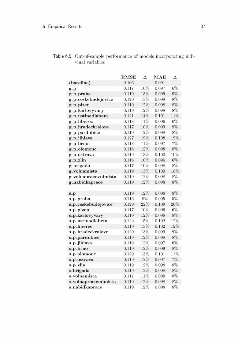
6. Empirical Results 37
Table 6.5: Out-of-sample performance of models incorporating indi-viual variables
RMSE ∆ MAE ∆(baseline) 0.106 0.091g p 0.117 10% 0.097 6%g p praha 0.119 13% 0.099 9%g p ceskebudejovice 0.120 13% 0.098 8%g p plzen 0.119 12% 0.098 8%g p karlovyvary 0.119 12% 0.098 8%g p ustinadlabem 0.121 14% 0.101 11%g p liberec 0.118 11% 0.096 6%g p hradeckralove 0.117 10% 0.099 9%g p pardubice 0.119 12% 0.098 8%g p jihlava 0.127 19% 0.108 19%g p brno 0.118 11% 0.097 7%g p olomouc 0.118 12% 0.098 8%g p ostrava 0.119 13% 0.100 10%g p zlin 0.116 10% 0.096 6%g brigada 0.117 10% 0.098 8%g volnamista 0.119 13% 0.100 10%g volnapracovnimista 0.119 12% 0.098 8%g nabidkaprace 0.119 12% 0.098 8%
s p 0.119 12% 0.098 8%s p praha 0.116 9% 0.095 5%s p ceskebudejovice 0.129 22% 0.109 20%s p plzen 0.117 10% 0.096 6%s p karlovyvary 0.119 12% 0.098 8%s p ustinadlabem 0.122 15% 0.102 12%s p liberec 0.119 13% 0.102 12%s p hradeckralove 0.120 13% 0.099 9%s p pardubice 0.119 12% 0.098 8%s p jihlava 0.119 12% 0.097 6%s p brno 0.119 12% 0.099 8%s p olomouc 0.120 13% 0.101 11%s p ostrava 0.119 12% 0.097 7%s p zlin 0.119 12% 0.098 8%s brigada 0.119 12% 0.098 8%s volnamista 0.117 11% 0.098 8%s volnapracovnimista 0.119 12% 0.098 8%s nabidkaprace 0.119 12% 0.098 8%

6. Empirical Results 38
Table 6.6: In-sample performance of models incorporating multipleor aggregate variables
R2 ∆ RMSE ∆ MAE ∆(baseline) 0.006 0.130 0.094G ALL 0.299 4946% 0.099 -24% 0.074 -21%S ALL 0.359 5950% 0.101 -23% 0.085 -9%s sum -0.012 -305% 0.132 2% 0.098 4%gPC (1) 0.005 -9% 0.132 1% 0.096 3%gPC (2) 0.131 2115% 0.126 -3% 0.087 -7%gPC (3) 0.115 1836% 0.126 -3% 0.087 -8%gPC (4) 0.099 1564% 0.126 -3% 0.086 -8%gPC (5) 0.079 1236% 0.126 -3% 0.086 -8%gPC (6) 0.109 1732% 0.122 -6% 0.086 -8%gPC (7) 0.091 1432% 0.122 -6% 0.086 -8%gPC (8) 0.072 1105% 0.122 -6% 0.086 -8%gPC (9) 0.063 965% 0.121 -7% 0.086 -8%gPC (10) 0.044 644% 0.122 -6% 0.087 -7%gPC (11) 0.060 912% 0.120 -7% 0.088 -6%gPC (12) 0.115 1840% 0.116 -11% 0.085 -9%gPC (13) 0.154 2499% 0.112 -14% 0.083 -11%gPC (14) 0.167 2710% 0.109 -16% 0.081 -13%gPC (15) 0.156 2536% 0.108 -17% 0.081 -13%gPC (16) 0.267 4391% 0.102 -21% 0.076 -19%gPC (17) 0.251 4124% 0.103 -20% 0.076 -19%gPC (18) 0.271 4467% 0.101 -22% 0.076 -19%sPC (1) 0.013 120% 0.133 2% 0.097 4%sPC (2) -0.005 -186% 0.133 2% 0.097 3%sPC (3) 0.008 31% 0.130 0% 0.097 4%sPC (4) -0.014 -337% 0.130 0% 0.097 4%sPC (5) -0.033 -648% 0.131 1% 0.097 4%sPC (6) -0.055 -1025% 0.131 1% 0.096 2%sPC (7) -0.054 -1011% 0.132 1% 0.099 5%sPC (8) 0.017 182% 0.132 2% 0.101 8%sPC (9) 0.018 196% 0.131 1% 0.100 6%sPC (10) 0.007 11% 0.130 0% 0.100 7%sPC (11) -0.019 -418% 0.133 2% 0.097 4%sPC (12) -0.046 -882% 0.133 2% 0.097 4%sPC (13) -0.066 -1219% 0.133 2% 0.097 4%sPC (14) -0.078 -1412% 0.133 2% 0.097 4%sPC (15) -0.042 -801% 0.133 2% 0.097 4%sPC (16) 0.015 155% 0.133 2% 0.097 4%sPC (17) 0.233 3823% 0.133 2% 0.097 4%sPC (18) 0.320 5292% 0.133 2% 0.097 4%
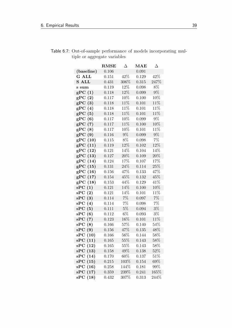
6. Empirical Results 39
Table 6.7: Out-of-sample performance of models incorporating mul-tiple or aggregate variables
RMSE ∆ MAE ∆(baseline) 0.106 0.091G ALL 0.151 42% 0.129 42%S ALL 0.431 306% 0.315 247%s sum 0.119 12% 0.098 8%gPC (1) 0.118 12% 0.099 9%gPC (2) 0.117 10% 0.100 10%gPC (3) 0.118 11% 0.101 11%gPC (4) 0.118 11% 0.101 11%gPC (5) 0.118 11% 0.101 11%gPC (6) 0.117 10% 0.099 9%gPC (7) 0.117 11% 0.100 10%gPC (8) 0.117 10% 0.101 11%gPC (9) 0.116 9% 0.099 9%gPC (10) 0.115 8% 0.098 7%gPC (11) 0.119 12% 0.102 12%gPC (12) 0.121 14% 0.104 14%gPC (13) 0.127 20% 0.109 20%gPC (14) 0.124 17% 0.107 17%gPC (15) 0.131 24% 0.114 25%gPC (16) 0.156 47% 0.133 47%gPC (17) 0.154 45% 0.132 45%gPC (18) 0.153 44% 0.129 41%sPC (1) 0.121 14% 0.100 10%sPC (2) 0.121 14% 0.101 11%sPC (3) 0.114 7% 0.097 7%sPC (4) 0.114 7% 0.098 7%sPC (5) 0.111 5% 0.094 3%sPC (6) 0.112 6% 0.093 3%sPC (7) 0.123 16% 0.101 11%sPC (8) 0.166 57% 0.140 54%sPC (9) 0.156 47% 0.135 48%sPC (10) 0.166 56% 0.144 58%sPC (11) 0.165 55% 0.143 58%sPC (12) 0.165 55% 0.143 58%sPC (13) 0.158 49% 0.138 52%sPC (14) 0.170 60% 0.137 51%sPC (15) 0.215 103% 0.154 69%sPC (16) 0.258 144% 0.181 99%sPC (17) 0.359 239% 0.241 165%sPC (18) 0.432 307% 0.313 244%
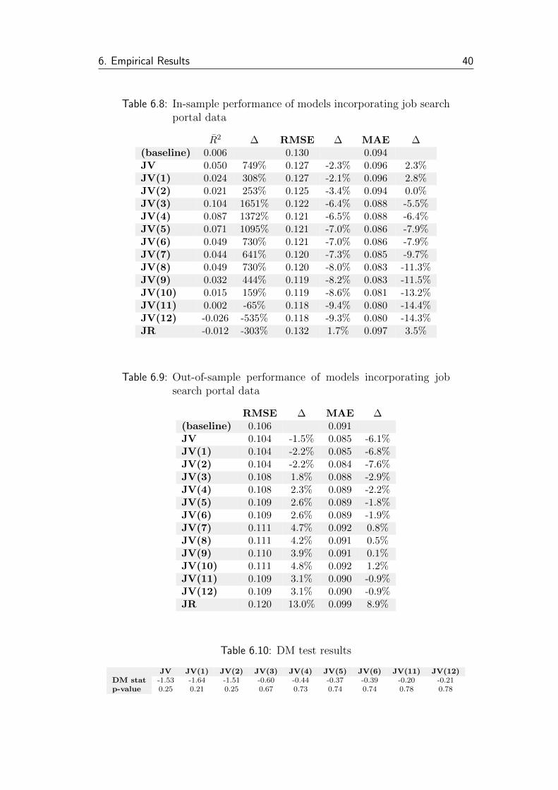
6. Empirical Results 40
Table 6.8: In-sample performance of models incorporating job searchportal data
R2 ∆ RMSE ∆ MAE ∆(baseline) 0.006 0.130 0.094JV 0.050 749% 0.127 -2.3% 0.096 2.3%JV(1) 0.024 308% 0.127 -2.1% 0.096 2.8%JV(2) 0.021 253% 0.125 -3.4% 0.094 0.0%JV(3) 0.104 1651% 0.122 -6.4% 0.088 -5.5%JV(4) 0.087 1372% 0.121 -6.5% 0.088 -6.4%JV(5) 0.071 1095% 0.121 -7.0% 0.086 -7.9%JV(6) 0.049 730% 0.121 -7.0% 0.086 -7.9%JV(7) 0.044 641% 0.120 -7.3% 0.085 -9.7%JV(8) 0.049 730% 0.120 -8.0% 0.083 -11.3%JV(9) 0.032 444% 0.119 -8.2% 0.083 -11.5%JV(10) 0.015 159% 0.119 -8.6% 0.081 -13.2%JV(11) 0.002 -65% 0.118 -9.4% 0.080 -14.4%JV(12) -0.026 -535% 0.118 -9.3% 0.080 -14.3%JR -0.012 -303% 0.132 1.7% 0.097 3.5%
Table 6.9: Out-of-sample performance of models incorporating jobsearch portal data
RMSE ∆ MAE ∆(baseline) 0.106 0.091JV 0.104 -1.5% 0.085 -6.1%JV(1) 0.104 -2.2% 0.085 -6.8%JV(2) 0.104 -2.2% 0.084 -7.6%JV(3) 0.108 1.8% 0.088 -2.9%JV(4) 0.108 2.3% 0.089 -2.2%JV(5) 0.109 2.6% 0.089 -1.8%JV(6) 0.109 2.6% 0.089 -1.9%JV(7) 0.111 4.7% 0.092 0.8%JV(8) 0.111 4.2% 0.091 0.5%JV(9) 0.110 3.9% 0.091 0.1%JV(10) 0.111 4.8% 0.092 1.2%JV(11) 0.109 3.1% 0.090 -0.9%JV(12) 0.109 3.1% 0.090 -0.9%JR 0.120 13.0% 0.099 8.9%
Table 6.10: DM test results
JV JV(1) JV(2) JV(3) JV(4) JV(5) JV(6) JV(11) JV(12)DM stat -1.53 -1.64 -1.51 -0.60 -0.44 -0.37 -0.39 -0.20 -0.21p-value 0.25 0.21 0.25 0.67 0.73 0.74 0.74 0.78 0.78

Chapter 7
Discussion
Irrespective of the results, the selected approach has some limitations and draw-
backs that have to be taken into account. Some issues are common to all Google
Econometrics studies while others are specific to this thesis.
In general, one of the main limitations of variables that are based on job-
search related data from search engines is that they do not cover only searches
made by unemployed people. As D’Amuri (2009) noted, part of the searches
is driven by working people that e.g. intend to switch a job.This is important
mostly because unemployed job search is believed to be anti-cyclical, the on the
job search should be cyclical. Nevertheless, impact of this problem is difficult
to estimate since there is little information on the number of working people
looking for a new job.
Another issue is that job seekers that use the internet for their search ac-
tivities might not be randomly selected. Search engines might be expected to
be utilized more by young and/or educated people. This has been partially
addressed by Fondeur & Karame (2013) who focused solely on youth unem-
ployment.
It is also important to note that the predictive ability of search query data
may vary over time (Suhoy 2009). This has been confirmed e.g. by Choi
& Varian (2012), who report substantial decrease of performance of Google
variables after the recession.
As mentioned earlier, another limitation is caused by the sampling proce-
dure used by Google to measure volumes of searches. This generates additional
noise which is difficult to treat with the limited possibilities of data downloading
on the Google Trends website.
As for the issues specific for this thesis, the limited length of the time-

7. Discussion 42
period has to be considered. The earliest month when data from all sources
are available is February 2010, that means 61 observations until February 2015.
Thus, principal component analysis as well as estimation and nowcasting results
are somewhat less reliable.
Some bias might be also present in the Seznam data because of the changes
in Seznam’s search application. For details, see Section 5 (Methodology).
Chapter 8
Conclusion
In this thesis, we wanted to examine the usefulness of job search related web-
based data for predictions of unemployment rate in the Czech Republic. We
focused specifically on a comparison of performance of models augmented with
search query data from Google and Seznam, two most popular search engines
in the Czech Republic. We compared them in two ways—first, we inspected
the contribution of each single added search query variable to the in-sample fit
and out-of-sample forecast accuracy. Second, we compared models augmented
with multiple or aggregated search query variables. Apart from this comparison
of contributions of different search engines, we examined the usability of data
on numbers of job vacancies and answers to them, obtained from a Czech job
search portal Jobs.cz. In total, we estimated and compared 91 different models.
Adding individual search query variables mostly worsens both in-sample and
out-of-sample performance compared to the baseline model for both Google and
Seznam data. Out of 18 models with Google variables, only five outperformed
the baseline model in terms of R2. Out of the same number of models using
Seznam variables, only four had higher R2 than the baseline model. Regarding
out-of-sample performance, none of the variables improved the nowcasts after
adding to the model. The MAE increased in all cases, with the differences
ranging from 6 to 20 %.
Comparison of models that are attempting to incorporate all information
gathered from each search engine brings more interesting results. Models using
all 18 variables at once show great improvements of in-sample fit, up to 0.30
for a model with Google data and 0.36 for a model with Seznam data. We
also utilized principal component analysis to aggregate the information from
Google and Seznam data. In terms of in-sample performance, Google PCs
8. Conclusion 44
explain the unemployment rate somewhat better. A model incorporating first
two Google PCs reaches R2 of 0.131. Nevertheless, none of the models improves
the out-of-sample nowcast accuracy—the MAE increases by 7 to more than 240
%. In general, we found that none of the models augmented with any Google or
Seznam variables helps improve the nowcasts and we cannot hence effectively
distinguish which one improves the predictions more.
The last area of our interest was the usefulness of data on job vacancies
and answers to them obtained from Jobs.cz. Here we find the most consistent
improvements of fit, including improvement of out-of-sample performance. This
however holds only for number of job vacancies, the reactions worsened both
in-sample and out-of-sample performance, when added to the baseline model.
As for the models that include the job vacancies variable, the R2 reaches up
to 0.104. What is more important is the nowcasting performance—9 models
increase the accuracy in terms of MAE. The greatest improvement is a 7.6%
decrease in MAE. Nevertheless, none of the forecasts improvement turns out to
be statistically significant, according to the Diebold-Mariano (DM) test.
All in all, our results do not look very compelling. We were not able to
find any improvements of unemployment rate predictions after adding Google
or Seznam data. This might be caused by the variability of predictive ability
of web search data over time or by the shorter time period which does not
allow to build reliable enough models. Further issues are discussed in the
previous chapter. On the other hand, we achieved good results with the models
augmented with job vacancies data. This is especially interesting given the
comparison with search query data performance and also the fact that the job
search portal used focuses only on a small subset of the labour market.
Our research could be enhanced in two possible ways. First, given the
Czech Republic data, it would be useful to reestimate the models later when
more information is collected and/or utilize some more sophisticated models.
Second, a similar research using data on job vacancies as a dependent variable
in other countries or involving a more widely oriented job search portal would
be interesting to confirm or reject their usefulness for explaining unemployment
rate.

Bibliography
Askitas, N. & K. F. Zimmermann (2009): “Google Econometrics and Unem-
ployment Forecasting.” IZA Discussion Paper 4201, Institute for the Study
of Labor (IZA).
Baker, S. & A. Fradkin (2011): “What Drives Job Search? Evidence from
Google Search Data.” Discussion Paper 10-020, Stanford Institute for Eco-
nomic Policy Research.
Banbura, M., D. Giannone, & L. Reichlin (2010): “Nowcasting.” Working
Paper Series 1275, European Central Bank.
Barreira, N., P. Godinho, & P. Melo (2013): “Nowcasting unemployment
rate and new car sales in south-western Europe with Google Trends.” Net-
nomics 14(3): pp. 129–165.
Beveridge, W. H. (1944): Full Employment in a Free Society: A Report.
Allen & Unwin.
Box, G. E. P. & D. A. Pierce (1970): “Distribution of Residual Autocorre-
lations in Autoregressive-Integrated Moving Average Time Series Models.”
Journal of the American Statistical Association 65(332): pp. 1509–1526.
Bughin, J. R. (2011): “’Nowcasting’ the Belgian Economy.” SSRN Scholarly
Paper ID 1903791, Social Science Research Network, Rochester, NY.
Bureau, U. S. C. (2015): “X-13arima-SEATS Seasonal Adjustment Program.”
Carriere-Swallow, Y. & F. Labbe (2013): “Nowcasting with Google
Trends in an Emerging Market.” Journal of Forecasting 32(4): pp. 289–
298.
Chadwick, M. G. & G. Sengul (2012): “Nowcasting Unemployment Rate in
Turkey : Let’s Ask Google.” Working Paper 1218, Research and Monetary
Policy Department, Central Bank of the Republic of Turkey.
Bibliography 46
Choi, C.-Y. & Y.-K. Moh (2007): “How useful are tests for unit-root in
distinguishing unit-root processes from stationary but non-linear processes?”
Econometrics Journal 10(1): pp. 82–112.
Choi, H. & H. Varian (2009a): “Predicting initial claims for unemployment
benefits.” Google Inc .
Choi, H. & H. Varian (2012): “Predicting the Present with Google Trends.”
The Economic Record 88(s1): pp. 2–9.
Choi, H. & H. R. Varian (2009b): “Predicting the Present with Google
Trends.” SSRN Scholarly Paper ID 1659302, Social Science Research Net-
work, Rochester, NY.
D’Amuri, F. (2009): “Predicting unemployment in short samples with internet
job search query data.” MPRA Paper 18403, University Library of Munich,
Germany.
D’Amuri, F. & J. Marcucci (2010): “a€sGoogle it!a€tForecasting the US
Unemployment Rate with a Google Job Search index.” Working Paper
2010.31, Fondazione Eni Enrico Mattei.
D’Amuri, F. & J. Marcucci (2012): “The predictive power of Google
searches in forecasting unemployment.” Temi di discussione (Economic
working papers) 891, Bank of Italy, Economic Research and International
Relations Area.
Della Penna, N. & H. Huang (2009): “Constructing Consumer Sentiment
Index for U.S. Using Google Searches.” Working Paper 2009-26, University
of Alberta, Department of Economics.
Diebold, F. X. & R. S. Mariano (1995): “Comparing Predictive Accuracy.”
Journal of Business & Economic Statistics 13(3): pp. 253–63.
Effectix.com (2014): “V ceskem vyhledavanı opet posılil Google nad Sez-
namem.”
Ettredge, M., J. Gerdes, & G. Karuga (2005): “Using web-based search
data to predict macroeconomic statistics.” Communications of the ACM
48(11): pp. 87–92.
Eurostat (2015a): “Households - level of internet access.”

Bibliography 47
Eurostat (2015b): “JDemetra+ officially recommended as software for the
seasonal adjustment of official statistics.”
Fondeur, Y. & F. Karame (2013): “Can Google data help predict French
youth unemployment?” Economic Modelling 30: pp. 117–125.
Ginsberg, J., M. H. Mohebbi, R. S. Patel, L. Brammer, M. S. Smolinski,
& L. Brilliant (2009): “Detecting influenza epidemics using search engine
query data.” Nature 457(7232): pp. 1012–1014.
Gomez, V. & A. Maravall (1996): “Programs TRAMO and SEATS, In-
struction for User (Beta Version: september 1996).” Banco de Espadz˝a
Working Paper 9628, Banco de Espadz˝a.
Hohenstatt, R., M. Kaesbauer, & W. Schaefers (2011): “”Geco” and
its potential for real estate research: Evidence from the US housing market.”
Journal of Real Estate Research 33(4): pp. 471–506.
International Labour Organization (1982): “Resolution concerning
statistics of the economically active population, employment, unemployment
and underemployment.”
Internet Info (2009): “NAVRCHOLU.cz: Windows Live Search zamıchal
statistikou podılu vyhledavacu - Internet Info.”
Internet Info (2010): “NAVRCHOLU.cz: Podıly vyhledavacu zustaly v roce
2009 stabilnı - Internet Info.”
Kholodilin, K. A., M. Podstawski, & B. Siliverstovs (2010): “Do Google
Searches Help in Nowcasting Private Consumption?: A Real-Time Evidence
for the US.” Discussion Papers of DIW Berlin 997, DIW Berlin, German
Institute for Economic Research.
Koop, G. & S. Potter (1999): “Dynamic Asymmetries in U.S. Unemploy-
ment.” Journal of Business & Economic Statistics 17(3): pp. 298–312.
Kristoufek, L. (2013): “Can Google Trends search queries contribute to risk
diversification?” Paper 1310.1444, arXiv.org.
Kulkarni, R., K. E. Haynes, R. R. Stough, & J. H. P. Paelinck (2009):
“Forecasting Housing Prices with Google Econometrics.” SSRN Scholarly
Paper ID 1438286, Social Science Research Network, Rochester, NY.
Bibliography 48
Montgomery, A. L., V. Zarnowitz, R. S. Tsay, & G. C. Tiao (1998):
“Forecasting the U.S. Unemployment Rate.” Journal of the American Sta-
tistical Association 93(442): pp. 478–493.
Pavlıcek, J. & L. Kristoufek (2015): “Nowcasting unemployment rates
with Google searches: Evidence from the Visegrad Group countries.”
FinMaP-Working Paper 34, Collaborative EU Project FinMaP - Financial
Distortions and Macroeconomic Performance: Expectations, Constraints and
Interaction of Agents.
Pearson, K. (1901): “On lines and planes of closest fit to systems of points
in space.” Philosophical Magazine Series 6 2(11): pp. 559–572.
Platil, L. (2014): Google Econometrics: An Application to the Czech Repub-
lic. Master Thesis, Charles University, Prague.
Preis, T., H. S. Moat, & H. E. Stanley (2013): “Quantifying Trading
Behavior in Financial Markets Using Google Trends.” SSRN Scholarly Paper
ID 2260189, Social Science Research Network, Rochester, NY.
Schwert, G. W. (1989): “Tests for Unit Roots: A Monte Carlo Investigation.”
Journal of Business & Economic Statistics 7(2): pp. 147–59.
Scott, S. L. & H. R. Varian (2014): “Predicting the present with Bayesian
structural time series.” International Journal of Mathematical Modelling and
Numerical Optimisation 5(1): pp. 4–23.
Sroka, M. (1998): “Commercial development of the Internet and WWW in
Eastern Europe.” Online and CD-Rom Review 22(6): pp. 367–376.
Stock, J. & M. Watson (2002): “Forecasting Using Principal Components
From a Large Number of Predictors.” Journal of the American Statistical
Association 97: pp. 1167–1179.
Suhoy, T. (2009): Query indices and a 2008 downturn: Israeli data. Research
Department, Bank of Israel.
TOPlist (2015): “TOPlist - Historie.”
Tsay, R. S. (2005): Analysis of Financial Time Series. John Wiley & Sons.

Bibliography 49
Vosen, S. & T. Schmidt (2011): “Forecasting private consumption: survey-
based indicators vs. Google trends.” Journal of Forecasting 30(6): pp. 565–
578.
Wu, L. & E. Brynjolfsson (2009): “The future of prediction: how Google
searches foreshadow housing prices and quantities.” ICIS 2009 Proceedings
p. 147.
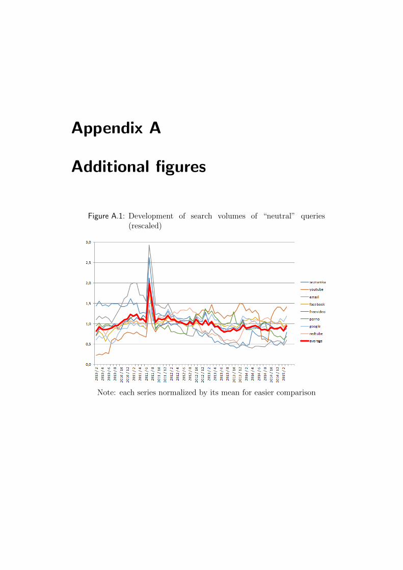
Appendix A
Additional figures
Figure A.1: Development of search volumes of “neutral” queries(rescaled)
Note: each series normalized by its mean for easier comparison

A. Additional figures II
Figure A.2: Google Trends website
Source: http://www.google.com/trends
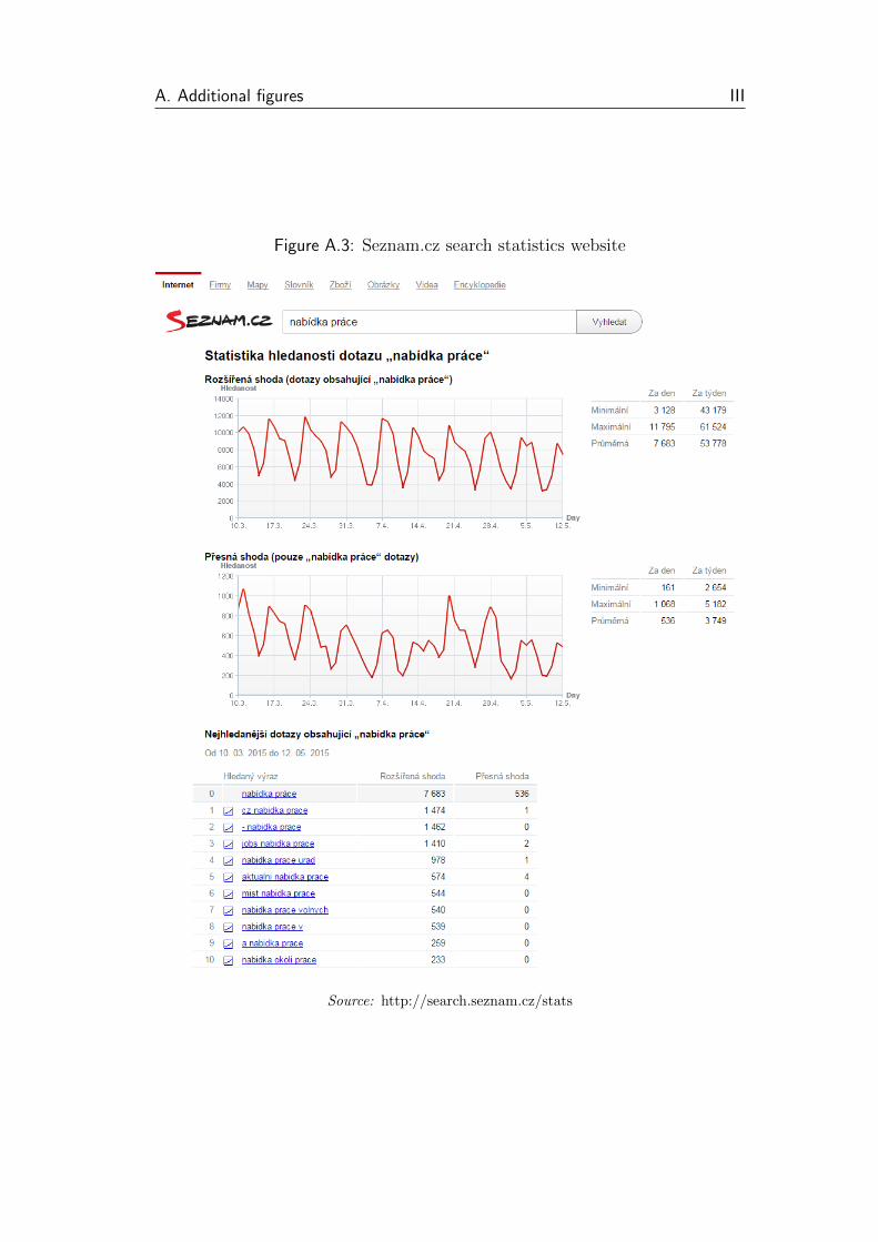
A. Additional figures III
Figure A.3: Seznam.cz search statistics website
Source: http://search.seznam.cz/stats
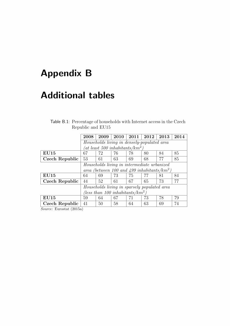
Appendix B
Additional tables
Table B.1: Percentage of households with Internet access in the CzechRepublic and EU15
2008 2009 2010 2011 2012 2013 2014Households living in densely-populated area(at least 500 inhabitants/km2)
EU15 67 72 76 78 80 84 85Czech Republic 53 61 63 69 68 77 85
Households living in intermediate urbanizedarea (between 100 and 499 inhabitants/km2)
EU15 64 69 73 75 77 81 84Czech Republic 44 52 61 67 65 73 77
Households living in sparsely populated area(less than 100 inhabitants/km2)
EU15 59 64 67 71 73 78 79Czech Republic 41 50 58 64 63 69 74
Source: Eurostat (2015a)

B. Additional tables V
Table B.2: Survey results: Frequencies of most used search queries
Search Query Freq Search Query FreqPrace 34 zkraceny uvazek 3prace praha 17 nabidky prace praha 3brigada 16 prace ceske budejovice 3Praha 14 prace v cb 2administrativa 14 pracovni prilezitosti 2volna pracovni mista 14 prace z domova 2volna mista 14 delnice 2Hledam praci 14 prace na hpp 2nabidka prace 13 fajn-brigady.cz 2brigada praha 9 prace v Jihlave 2brigady 7 hledam 2asistentka 6 pracovni nabidky
praha2
prace zlin 6 HPP 2volne pracovni pozice 6 volna pracovni mista
ceske Budejovice2
prace v praze 6 jobs 2hosteska 5 prace pro studenty 2zamestnani 5 nabidka prace 2brigada pro studenty 4 prace v ceskych bude-
jovicich2
urad prace 4 Bar 2brigady praha 4 prace vysocina 2prace.cz 4 ponuka prace 2nabidky prace 4 pracovni nabidky 2obchod 3 pozice 2kuchar 3 pracovni portal 2brigada zlin 3 prace cb 2Prace 3 brigada Plzen 2volna pozice 3 prace jihlava 2prodavacka 3 volne pracovni mista 2hlidani deti 3 Prace Jihlava 2recepcni 3 ... 2

B. Additional tables VI
Tab
leB
.3:
Pri
nci
pal
com
pon
ent
load
ings
data
gPC1
gPC2
gPC3
gPC4
gPC5
gPC6
gPC7
gPC8
gPC9
gPC10
gPC11
gPC12
gPC13
gPC14
gPC15
gPC16
gPC17
gPC18
gp
0.346
0.149
0.007
0.160
0.174
0.030
0.081
-0.006
0.158
0.112
-0.022
-0.015
-0.018
-0.002
0.058
0.066
-0.016
0.865
gp
praha
0.355
0.035
0.096
0.192
0.092
0.002
0.158
0.169
-0.120
-0.043
-0.101
-0.305
-0.020
0.201
-0.011
0.703
-0.216
-0.253
gp
ceskebudejo
vic
e0.045
-0.397
-0.008
0.129
-0.059
0.014
0.080
-0.267
-0.377
-0.275
-0.095
0.527
0.178
-0.110
0.343
0.249
0.062
0.103
gp
plz
en
0.189
-0.137
-0.429
-0.381
-0.224
0.048
0.575
0.338
-0.027
0.040
0.266
0.093
-0.062
0.109
0.100
-0.076
-0.067
0.019
gp
liberec
0.203
-0.315
0.016
-0.366
0.159
0.191
-0.005
-0.122
0.180
-0.035
-0.104
-0.015
0.408
0.038
-0.531
0.137
0.368
0.011
gp
hradeckralo
ve
0.098
-0.265
-0.204
0.308
-0.685
-0.190
-0.168
0.021
0.271
0.244
-0.265
0.022
-0.074
0.072
-0.132
0.080
0.105
0.027
gp
pardubic
e0.209
-0.341
-0.002
-0.139
0.059
0.025
-0.128
0.027
0.101
-0.122
0.062
-0.298
-0.437
-0.677
0.136
0.057
0.099
-0.028
gp
brno
0.317
0.226
-0.008
0.058
0.063
0.025
-0.039
-0.041
0.160
0.112
0.066
-0.012
0.053
0.169
0.510
-0.060
0.663
-0.245
gp
olo
mouc
0.063
-0.309
0.400
-0.004
0.063
-0.325
0.165
-0.251
-0.252
0.511
0.352
-0.024
-0.209
0.159
-0.115
-0.053
0.080
0.004
gp
ostrava
0.347
0.042
0.006
0.104
0.093
0.145
-0.188
-0.011
0.096
-0.295
0.157
0.461
-0.527
0.261
-0.311
-0.102
-0.035
-0.121
gp
zlin
0.144
-0.374
-0.004
-0.170
0.083
0.173
-0.116
-0.252
0.083
-0.059
-0.301
-0.295
-0.048
0.439
0.321
-0.317
-0.332
0.001
gbrig
ada
0.319
-0.016
0.117
0.362
0.127
-0.080
0.388
0.154
-0.151
-0.015
-0.395
0.007
0.129
-0.239
-0.170
-0.493
-0.005
-0.180
gvoln
am
ista
-0.142
-0.161
-0.497
0.223
0.534
-0.240
0.088
-0.163
0.378
0.225
0.016
0.162
0.010
-0.052
0.022
0.102
-0.135
-0.167
gvoln
apracovnim
ista
-0.155
-0.315
-0.032
0.277
0.112
-0.346
-0.073
0.343
-0.011
-0.486
0.281
-0.265
0.105
0.251
-0.027
-0.111
0.221
0.148
gnabid
kaprace
0.334
-0.072
0.049
0.184
-0.112
0.160
-0.282
0.038
0.110
0.101
0.532
0.032
0.480
-0.170
0.063
-0.128
-0.356
-0.122
gp
jihla
va
0.153
0.267
-0.330
0.060
-0.186
-0.173
0.152
-0.660
-0.148
-0.293
0.178
-0.310
0.019
-0.041
-0.169
-0.055
0.012
-0.011
gp
ustin
adla
bem
0.233
0.066
-0.404
-0.190
0.153
-0.249
-0.492
0.190
-0.555
0.207
-0.136
-0.001
0.033
0.015
-0.062
-0.054
0.018
0.039
gp
karlo
vyvary
0.206
0.142
0.261
-0.391
-0.052
-0.682
-0.027
0.004
0.299
-0.206
-0.118
0.192
0.119
-0.047
0.104
0.025
-0.191
-0.038
Seznam
data
sPC1
sPC2
sPC3
sPC4
sPC5
sPC6
sPC7
sPC8
sPC9
sPC10
sPC11
sPC12
sPC13
sPC14
sPC15
sPC16
sPC17
sPC18
sp
0.260
0.298
-0.026
-0.032
-0.021
0.050
0.077
-0.225
-0.052
0.415
0.332
-0.111
0.010
0.167
0.126
-0.299
-0.562
0.190
sp
praha
0.071
-0.433
-0.298
-0.034
0.032
-0.457
0.104
-0.359
-0.106
0.103
0.023
-0.040
0.026
0.063
-0.185
-0.070
-0.125
-0.534
sp
ceskebudejo
vic
e0.278
-0.147
-0.012
-0.243
0.163
-0.094
-0.411
0.254
-0.160
-0.167
0.085
0.371
-0.529
0.229
0.146
-0.099
-0.102
-0.020
sp
plz
en
-0.038
-0.449
0.271
0.032
0.032
0.059
0.374
0.520
0.288
0.368
0.124
0.011
-0.046
0.217
-0.110
-0.105
-0.019
-0.022
sp
karlo
vyvary
0.271
-0.034
-0.146
-0.168
-0.467
-0.004
0.234
0.235
0.066
-0.616
0.181
-0.093
0.258
0.123
-0.020
-0.108
-0.167
-0.011
sp
ustin
adla
bem
0.281
0.058
0.017
-0.183
0.387
-0.263
-0.226
0.340
-0.224
0.123
-0.023
-0.153
0.575
0.045
-0.128
0.226
-0.000
0.095
sp
liberec
0.189
0.075
0.041
0.776
-0.328
-0.261
-0.088
0.223
-0.308
0.085
-0.059
0.009
-0.056
0.083
0.055
0.020
0.042
-0.022
sp
hradeckralo
ve
0.293
0.059
0.099
0.161
0.175
-0.146
-0.192
-0.110
0.548
-0.169
-0.291
-0.460
-0.211
0.171
-0.229
-0.120
-0.016
0.087
sp
pardubic
e0.310
-0.030
0.105
-0.014
-0.014
0.142
0.092
-0.113
-0.111
0.045
-0.400
0.435
0.193
-0.152
-0.342
-0.531
0.118
0.113
sp
jihla
va
0.307
-0.054
0.153
-0.088
0.017
0.192
0.025
0.054
-0.026
0.082
-0.230
-0.270
0.068
-0.193
0.659
-0.179
0.136
-0.414
sp
brno
0.289
-0.164
-0.136
-0.167
-0.205
-0.106
0.085
-0.255
-0.029
0.194
0.175
-0.084
-0.053
0.231
0.133
0.078
0.632
0.402
sp
olo
mouc
0.176
-0.212
0.457
0.083
0.148
0.384
0.144
-0.275
-0.433
-0.217
0.071
-0.187
-0.084
0.205
-0.201
0.265
-0.079
-0.038
sp
ostrava
0.137
-0.480
-0.090
0.050
-0.084
-0.036
0.006
-0.079
0.076
0.014
-0.281
0.059
-0.001
-0.360
0.214
0.313
-0.408
0.443
sp
zlin
0.301
0.072
-0.113
-0.115
-0.190
0.165
-0.082
0.180
-0.033
0.198
0.240
-0.202
-0.297
-0.581
-0.410
0.134
0.069
-0.143
sbrig
ada
0.195
0.368
-0.151
-0.178
-0.086
0.003
0.397
0.066
0.025
0.158
-0.453
0.176
-0.184
0.265
-0.040
0.450
-0.082
-0.162
svoln
am
ista
0.178
0.051
-0.403
0.315
0.590
0.072
0.436
0.069
0.001
-0.218
0.198
0.065
-0.100
-0.157
0.103
-0.053
0.101
0.084
snabid
kaprace
0.296
0.005
0.116
0.206
-0.007
0.168
-0.206
-0.200
0.467
0.027
0.303
0.452
0.272
0.023
0.045
0.307
0.031
-0.247
svoln
apracovnim
ista
0.057
0.194
0.568
-0.124
0.041
-0.584
0.300
-0.091
0.039
-0.131
0.154
0.130
-0.118
-0.311
0.084
0.030
0.022
0.045
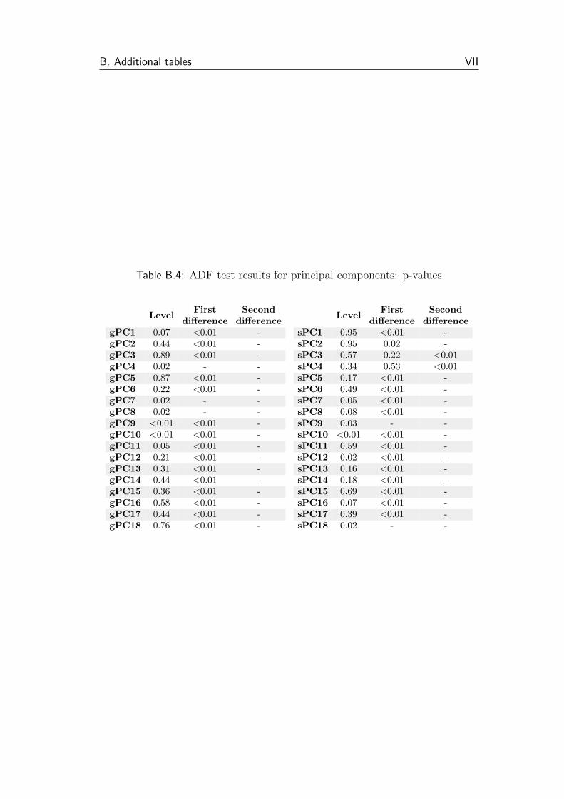
B. Additional tables VII
Table B.4: ADF test results for principal components: p-values
LevelFirst
differenceSecond
differenceLevel
Firstdifference
Seconddifference
gPC1 0.07 <0.01 - sPC1 0.95 <0.01 -gPC2 0.44 <0.01 - sPC2 0.95 0.02 -gPC3 0.89 <0.01 - sPC3 0.57 0.22 <0.01gPC4 0.02 - - sPC4 0.34 0.53 <0.01gPC5 0.87 <0.01 - sPC5 0.17 <0.01 -gPC6 0.22 <0.01 - sPC6 0.49 <0.01 -gPC7 0.02 - - sPC7 0.05 <0.01 -gPC8 0.02 - - sPC8 0.08 <0.01 -gPC9 <0.01 <0.01 - sPC9 0.03 - -gPC10 <0.01 <0.01 - sPC10 <0.01 <0.01 -gPC11 0.05 <0.01 - sPC11 0.59 <0.01 -gPC12 0.21 <0.01 - sPC12 0.02 <0.01 -gPC13 0.31 <0.01 - sPC13 0.16 <0.01 -gPC14 0.44 <0.01 - sPC14 0.18 <0.01 -gPC15 0.36 <0.01 - sPC15 0.69 <0.01 -gPC16 0.58 <0.01 - sPC16 0.07 <0.01 -gPC17 0.44 <0.01 - sPC17 0.39 <0.01 -gPC18 0.76 <0.01 - sPC18 0.02 - -
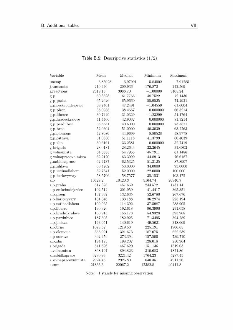
B. Additional tables VIII
Table B.5: Descriptive statistics (1/2)
Variable Mean Median Minimum Maximum
unemp 6.85028 6.97991 5.84002 7.91285j vacancies 210.440 209.936 176.872 242.569j reactions 2319.15 3086.70 −1.00000 3405.24g p 60.3628 61.7766 48.7522 72.1430g p praha 65.2626 65.9660 55.9525 74.2921g p ceskebudejovice 39.7401 47.2491 −1.04559 61.6004g p plzen 38.0938 38.4667 0.000000 66.3214g p liberec 30.7449 31.0329 −1.23299 54.1764g p hradeckralove 41.4406 42.9032 0.000000 81.3214g p pardubice 38.8881 40.6000 0.000000 73.3571g p brno 52.0304 51.0900 40.3039 63.2263g p olomouc 42.8080 44.9699 8.80528 58.9778g p ostrava 51.0336 51.1118 41.3799 60.4039g p zlin 30.6161 33.2581 0.000000 52.7419g brigada 28.0181 28.2643 22.2645 31.6802g volnamista 54.3335 54.7955 45.7911 61.1486g volnapracovnimista 62.2120 63.3999 44.8913 76.6187g nabidkaprace 62.4737 62.5325 51.3125 87.8907g p jihlava 60.4262 58.0000 34.0000 93.0000g p ustinadlabem 52.7541 52.0000 22.0000 100.000g p karlovyvary 58.5706 58.7577 35.1531 103.175s p 10328.2 10420.3 5164.74 20940.7s p praha 617.328 457.659 244.572 1731.14s p ceskebudejovice 192.512 201.959 41.4417 365.351s p plzen 137.992 132.635 52.6780 267.676s p karlovyvary 131.346 133.188 36.2974 225.194s p ustinadlabem 109.965 114.392 37.5987 288.905s p liberec 190.326 192.618 96.3990 291.058s p hradeckralove 160.915 156.178 54.9328 393.968s p pardubice 187.305 182.925 71.3495 394.289s p jihlava 143.051 140.619 49.5621 318.669s p brno 1078.52 1219.53 225.191 1906.65s p olomouc 353.991 321.673 187.075 622.239s p ostrava 392.459 273.394 157.500 739.710s p zlin 194.125 198.207 128.018 250.964s brigada 541.696 467.620 151.136 1519.03s volnamista 868.197 894.823 310.683 1874.86s nabidkaprace 3280.93 3221.42 1764.23 5287.45s volnapracovnimista 2924.45 2925.80 640.351 4911.26s sum 21833.3 22067.2 12382.8 40411.8
Note: –1 stands for missing observation
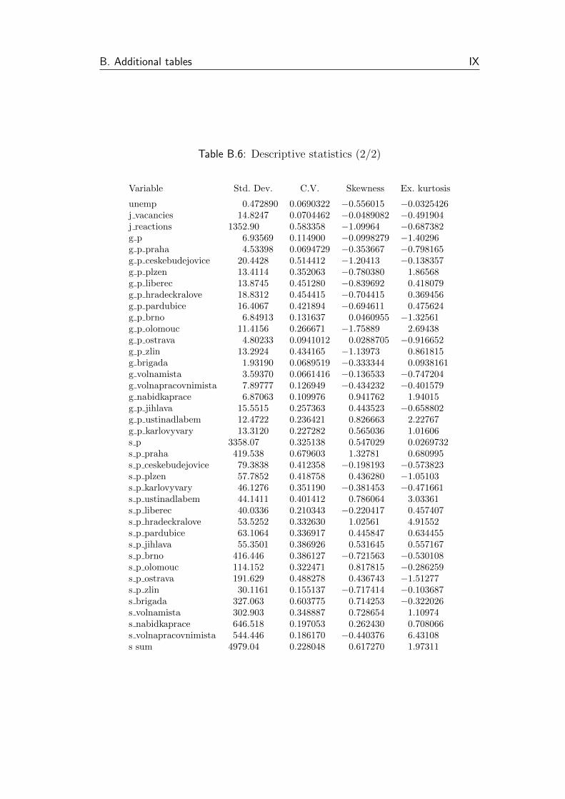
B. Additional tables IX
Table B.6: Descriptive statistics (2/2)
Variable Std. Dev. C.V. Skewness Ex. kurtosis
unemp 0.472890 0.0690322 −0.556015 −0.0325426j vacancies 14.8247 0.0704462 −0.0489082 −0.491904j reactions 1352.90 0.583358 −1.09964 −0.687382g p 6.93569 0.114900 −0.0998279 −1.40296g p praha 4.53398 0.0694729 −0.353667 −0.798165g p ceskebudejovice 20.4428 0.514412 −1.20413 −0.138357g p plzen 13.4114 0.352063 −0.780380 1.86568g p liberec 13.8745 0.451280 −0.839692 0.418079g p hradeckralove 18.8312 0.454415 −0.704415 0.369456g p pardubice 16.4067 0.421894 −0.694611 0.475624g p brno 6.84913 0.131637 0.0460955 −1.32561g p olomouc 11.4156 0.266671 −1.75889 2.69438g p ostrava 4.80233 0.0941012 0.0288705 −0.916652g p zlin 13.2924 0.434165 −1.13973 0.861815g brigada 1.93190 0.0689519 −0.333344 0.0938161g volnamista 3.59370 0.0661416 −0.136533 −0.747204g volnapracovnimista 7.89777 0.126949 −0.434232 −0.401579g nabidkaprace 6.87063 0.109976 0.941762 1.94015g p jihlava 15.5515 0.257363 0.443523 −0.658802g p ustinadlabem 12.4722 0.236421 0.826663 2.22767g p karlovyvary 13.3120 0.227282 0.565036 1.01606s p 3358.07 0.325138 0.547029 0.0269732s p praha 419.538 0.679603 1.32781 0.680995s p ceskebudejovice 79.3838 0.412358 −0.198193 −0.573823s p plzen 57.7852 0.418758 0.436280 −1.05103s p karlovyvary 46.1276 0.351190 −0.381453 −0.471661s p ustinadlabem 44.1411 0.401412 0.786064 3.03361s p liberec 40.0336 0.210343 −0.220417 0.457407s p hradeckralove 53.5252 0.332630 1.02561 4.91552s p pardubice 63.1064 0.336917 0.445847 0.634455s p jihlava 55.3501 0.386926 0.531645 0.557167s p brno 416.446 0.386127 −0.721563 −0.530108s p olomouc 114.152 0.322471 0.817815 −0.286259s p ostrava 191.629 0.488278 0.436743 −1.51277s p zlin 30.1161 0.155137 −0.717414 −0.103687s brigada 327.063 0.603775 0.714253 −0.322026s volnamista 302.903 0.348887 0.728654 1.10974s nabidkaprace 646.518 0.197053 0.262430 0.708066s volnapracovnimista 544.446 0.186170 −0.440376 6.43108s sum 4979.04 0.228048 0.617270 1.97311
Copyright © 2022 FDOKUMEN