Evaluating the impact on wages and unemployment duration

of a mandatory job search program∗

Luıs CentenoCEETA, Lisbon

lcenteno@telepac.pt

Mario CentenoBanco de Portugal and ISEG

mcenteno@bportugal.pt

Alvaro A. NovoBanco de Portugal and ISEGI

anovo@bportugal.pt

4th April 2005Draft version

Abstract

We assess the impact on unemployment duration and re-employment wages of a large scalejob search program implemented in Portugal during the late 1990’s and early 2000’s, targetingeligible individuals registered as unemployed at the Portuguese employment agency. Based onthe class of difference-in-differences matching methods, relatively to a situation without thetreatment, the estimates of the average effects of the treatment on the treated point towards:(i) a reduction in unemployment spells inferior to 1 month, rather small in the context of longunemployment spells observed in Portugal and (ii) a negative impact in the re-employmentwages of the treated.

Keywords: job search assistance; unemployment duration; policy evaluation; wagesJEL Classification: J18, J23, J38, J64, J68

∗We thank participants at the 2004 LoWER Conference, London, the 2004 EALE Annual Conference, Lisbonand the 2004 AIEL Conference, Modena. We acknowledge the collaboration given by the Portguese employmentagency, IEFP, in particular, for the access and detailed discussion of the data. The opinions expressed herein are notnecessarily those of Banco de Portugal. All errors remain ours.

1

1 Introduction

It is a well-known fact in many European countries that unemployment duration is rather long,

generating problems associated with long-term unemployment, such as weak labor market attach-

ment. In Portugal, despite the low level of the unemployment rate, long-term unemployment is

quite common, making the low unemployment level a social and economic issue. This pattern of

unemployment duration can be seen as a trap, making long periods in that state increasingly harder

to leave, either due to the depreciation of skills or because long unemployment spells send a negative

signal to the labor market.

In response to the high unemployment figures for specific labor market groups, such as young

workers, women and those aged 45 or more, European Union countries increased their spending

on active labor market policies, targeting these groups. The Portuguese program’s goal was to

increase the employability of the long-term unemployed (the Reage program) and to act earlier

on youth unemployment, preventing episodes of long-term unemployment at the beginning of their

labor market career (the InserJovem program). In this paper, we assess the impact of the large

(mandatory) job search programs implemented in Portugal during the late 1990’s and early 2000’s

on two important outcomes, namely, the unemployment duration and the starting wages after the

spell of unemployment.

The objective of this paper is to determine the effects of the programs comparatively to the

outcome of the individual had he/she continued to search for a job in the absence of the job search

support provided by the program. The focus is on the direct effects of the programs; no attempt

is made to assess the general equilibrium implications. However, we should stress that displace-

ment effects, the ones that could be identified in general equilibrium approaches, are more likely in

employment assistance programs (for example, with wage subsidies) than through the kind of job

search programs we are evaluating here.

With this objective in mind and the estimation issues that arise in non-experimental studies,

mainly due to the problem of missing data, we apply a set of methods developed to address such

settings. The methodologies used include: (i) matching methods (Rosenbaum & Rubin 1983); (ii)

difference-in-difference-in-differences (Meyer 1995) and (iii) as proposed by Heckman, Ichimura &

Todd (1997) and Heckman, Ichimura, Smith & Todd (1998) a combination of the two methodologies,

termed difference-in-differences matching, used to eliminate potential sources of bias (Smith &

Todd 2004). In the same spirit, we extend Meyer’s (1995) approach by combining it with the

matching estimators.

2

Previous microeconometric studies of active labor market programs in European countries, taking

place at around the same time period, include Blundell, Dias, Meghir & Reenen (2004) and Larsson

(2003). The results of these studies are mixed. Whereas Blundell et al. (2004) for the UK find an

important “program introduction effect”, the program effect is much larger in the first quarter than

later on, Larsson finds no significant effect in the Swedish programs. If anything she finds a negative

impact of certain aspects of the program, namely on wages.

Our assessment of the Portuguese program points out to a small, non-significant, reduction on

unemployment duration and sometimes negative impact on wages. Put in another perspective, in

the absence of the program, we estimate that unemployment duration of treated individuals would

increase by at most 1 month, which does not represent a large increase in duration given that some

workers can spend a large number of months unemployed. In terms of wages, after leaving unemploy-

ment, we estimate a null impact for women and a large negative impact on males’ re-employment

wages. Arguably, the results may be driven by ‘forcing’ individuals out of unemployment (the lower

duration), which in turn may result in lower quality matches (the lower wages).

The paper is organized as follows. The evaluation problem, as well as the identification and

estimation of average treatment effects are addressed in section 2. The labor market program is

described in Section 3. Section 4 presents the data and results. Finally, concluding remarks are

presented in Section 5.

2 Econometric evaluation strategies

The problem of evaluating active labor market programs has been extensively studied in the litera-

ture (Heckman, LaLonde & Smith 1999). In recent years, a wealth of methods to address the main

problem of missing data present in all non-experimental studies has been proposed. These methods

suggest different solutions to the problem of generating conveniently designed comparison groups

necessary to perform program evaluations. Given the non-experimental feature of these programs,

the feasibility of any evaluation exercise depends crucially on the ability that researchers have to

generate such comparison groups from the data available on the program implementation. Typical

methodologies proposed to tackle these issues include: (i) matching methods (Rubin 1977, Rosen-

baum & Rubin 1983), in which the propensity score matching can be based on different definitions

of neighborhood; (ii) regression methods – in particular, duration models (Cox 1972, Abbring &

van den Berg 2003) to estimate the shift in the unemployment hazard attributable to the program,

and, finally, (iii) difference-in-difference-in-differences (Meyer 1995) modeling strategy to tackle the

3

problems associated with selection on non-observables. In the empirical section, we will use the

difference-in-differences matching estimator proposed by Heckman et al. (1997) and Heckman et al.

(1998). This method, recently reviewed and compared with the other methods by Smith & Todd

(2004), is a combination of the propensity score matching with the difference-in-differences, having

the potential benefit of eliminating some sources of bias present in non-experimental settings.

2.1 The evaluation problem

Active job search programs have the objective of easying/speeding the transition from unemployment

to employment. Thus, this study aims at evaluating the impact of such a program in the duration

of unemployment spells of the target population – young experiencing short-lived unemployment

(under 25 years and unemployment spell above 6 months) and older individuals with long-term

unemployment (over 25 years old and spell over 12 months). The effect on re-employment wages is

also studied. Since it is plausible that the matching process is also affected by the program, we will

also study the effect on re-employment wages.

As with all non-experimental cases, this study also faces the problem of missing data in the

evaluation problem. The fact that the same individual is not observed simultaneously in the two

states – treatment and control – conditions the entire evaluation. It is, therefore, necessary to

devise sampling strategies and use methods that attempt to overcome such observational limitations,

which may have deeper statistical consequences (e.g. due to self-selection, Heckman (1979)) in the

estimation process.

2.2 Econometric Methods

We now review in more detail the estimators to be used in the empirical section.

2.2.1 Matching as an evaluation estimator

One of the most important issues in the evaluation of non-experimental employment programs is

that of the comparision of individuals who are indeed comparable (Rubin 1977). How such concern

is addressed is key to identifying the effect of the treatment.

For that purpose, the selection of the control group can be achieved with recourse to the non-

parametric method of matching in the propensity score. In short, the methodology compresses the

indivuals’ observable multivariate information, and as such difficult to compare, in an univariate

indicator – the propensity score. The distance between the individual propensity scores is minimized

to construct a control group as comparable as possible in the observables with the treatment group

(Rubin 1977, Rosenbaum & Rubin 1983).

4

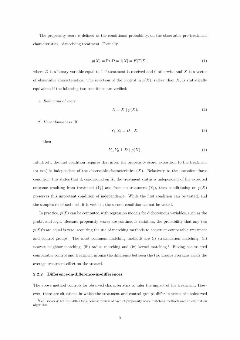
The propensity score is defined as the conditional probability, on the observable pre-treatment

characteristics, of receiving treatment. Formally,

p(X) = Pr[D = 1|X] = E[T |X], (1)

where D is a binary variable equal to 1 if treatment is received and 0 otherwise and X is a vector

of observable characteristics. The selection of the control in p(X), rather than X, is statistically

equivalent if the following two conditions are verified:

1. Balancing of score.

D ⊥ X | p(X). (2)

2. Unconfoundness. If

Y1, Y0 ⊥ D | X, (3)

then

Y1, Y0 ⊥ D | p(X). (4)

Intuitively, the first condition requires that given the propensity score, exposition to the treatment

(or not) is independent of the observable characteristics (X). Relatively to the unconfoundness

condition, this states that if, conditional on X, the treatment status is independent of the expected

outcome resulting from treatment (Y1) and from no treatment (Y0), then conditioning on p(X)

preserves this important condition of independence. While the first condition can be tested, and

the samples redefined until it is verified, the second condition cannot be tested.

In practice, p(X) can be computed with regression models for dichotomous variables, such as the

probit and logit. Because propensity scores are continuous variables, the probability that any two

p(X)’s are equal is zero, requiring the use of matching methods to construct comparable treatment

and control groups. The most commom matching methods are (i) stratification matching, (ii)

nearest neighbor matching, (iii) radius matching and (iv) kernel matching.1 Having constructed

comparable control and treatment groups the difference between the two groups averages yields the

average treatment effect on the treated.

2.2.2 Difference-in-difference-in-differences

The above method controls for observed characteristics to infer the impact of the treatment. How-

ever, there are situations in which the treatment and control groups differ in terms of unobserved1See Becker & Ichino (2002) for a concise review of each of propensity score matching methods and an estimation

algorithm.

5

characteristics, resulting in two groups that are not fully comparable. In such circunstances, the

difference-in-differences method offers a possible solution.

Let Y Dit be the potential outcome for individual i at time t given that he/she is in state D, where

D is as above. Let treatment take place at time t = 1. The fundamental identification problem lies

in the fact that we do not observe, at time t = 1, individual i in both states. Therefore, we cannot

compute the individual treatment effect, Y 1i1 −Y 0

i1. One can, however, estimate the average effect of

the treatment on the treated, E[Y 1i1 − Y 0

i1 | D = 1]. In order to achieve identification, the following

assumption is fundamental:

E[Y 0i1 − Y 0

i0 | D = 1] = E[Y 0i1 − Y 0

i0 | D = 0]. (5)

It states that the temporal evolution of the outcome variable of treated individuals (D = 1) in the

event that they had not been exposed to the treatment would have been the same as the observed

for the individuals not exposed to the treatment D = 0. If the assumption expressed in (5) holds,

then the average treatment effect on the treated can be estimated by the sample analogs of

{E[Yi1 | D = 1]− E[Yi1 | D = 0]} − {E[Yi0 | D = 1]− E[Yi0 | D = 0]}. (6)

There are two threats to the validity of the difference-in-differences estimator. First, if cross-

sectional data are used, compositional changes over time may invalidate the results. Second, if there

are non-parallel dynamics. In particular, if such dynamics are not explained (by adding) observables,

but the outcome variable depends on non-observables, identification breaks down.

Meyer (1995) proposed a difference-in-difference-in-differences approach that attempts to fur-

ther correct for non-observables that threaten the validity of the difference-in-differences estimator.

Suppose that the data have two dimensions – space and time. Then, it is possible to control for

a space-time dimension. For instance, consider Table 1 with a time dimension (before-after) and a

space dimension (treatment region and no-treatment region), where Y DRt stands for the outcome of

group D, treatment or control, in space R, treatment or no-treatment regions, at time t.

Consider the top panel of Table 1, labeled “Treatment”. Reading in row, the difference between

the two rows gives a first measure of the impact of the treatment on the treated. That is, it corrects

the evolution of the outcome variable of treated individuals (1st row) with the effect on pseudo-

treated (defined using the same eligibility criteria) observed in a different space R = 0; it corrects for

common factors influencing the target group.2 The standard D-in-D estimator is Y 11t-Y

11t′ -Y

10t+Y 1

0t′

2This resembles the estimation strategy of the matching estimators.

6

Table 1: Difference-in-difference-in-differences estimator (DDD)

Group Region Before (t′) After (t) Estimators

Eligible R=1 Y 11t′ Y 1

1t D-in-D1R=0 Y 10t′ Y 1

0t

Y 11t′ -Y

10t′ Y 1

1t-Y10t Y 1

1t-Y11t′ -Y

10t+Y 1

0t′

Non-Eligible R=1 Y 01t′ Y 0

1t D-in-D0R=0 Y 00t′ Y 0

0t

Y 01t′ -Y

00t′ Y 0

1t-Y00t Y 0

1t-Y01t′ -Y

00t+Y 0

0t′

DDD (D-in-D1− D-in-D0)Y 1

1t-Y11t′ -Y

10t+Y 1

0t′

Estimator −Y 01t+Y 0

1t′+Y 00t-Y

00t′

Note: Superscripts denote treatment status; subscripts refer to space and time.

(D-in-D1).

It is, however, possible that there are effects/shocks specific to the space of implementation, which

although related with the treatment are not directly attributable to the program. The bottom panel

of Table 1 estimates such effects by performing the same exercise as in the top panel (D-in-D1),

but now for a “control” group (those not complying with the program’s eligibility criteria). This

measure, Y 01t-Y

01t′ -Y

00t+Y 0

0t′ (D-in-D0), is a measure of indirect effects of the program affecting the

group of non-eligible. Under the hypothesis that such effects would have not occured in the absence

of the program, they need to be taken into account in the effect computed for the treated. Thus, the

corrected effect of the treatment is given by the DDD estimator Y 11t-Y

11t′ -Y

10t+Y 1

0t′−Y 01t+Y 0

1t′+Y 00t-Y

00t′

(D-in-D1− D-in-D0).

2.2.3 Difference-in-differences matching

Heckman et al. (1997) and Heckman et al. (1998) introduced the D-in-D matching estimator. This

estimator combines the two previous approaches, and according to a recent study of Smith & Todd

(2004) has the potential to reduce sources of bias in non-experimental settings. Intuitively, the

benefits may arise from the fact that: (i) relatively to the propensity score matching estimator, the

D-in-D matching adds the control for non-observables that characterizes the D-in-D estimator, while

(ii) relatively to the D-in-D estimator, its matching version adds the comparability on observable

that characterizes the propensity score matching estimator.

Depending on the type of data available, the estimator can take two forms. With cross-sectional

data, propensity score estimates of the average treatment effect on the treated for each period –

before and after – are computed and then the difference between these two estimates yields the D-

in-D matching estimate. If longitudinal data is available, the process is somewhat reversed. First,

for each individual a difference between the after and before outcomes is computed and then using

7

the propensity score matching each treatment unit is matched to control unit(s), yielding an average

treatment effect on the treated.

In the empirical section, we will use the cross-section version of the estimator, and posteriorly,

extending it to the DDD estimator. In terms of Table 1, rather than computing simple differences

in sample averages, we pre-match individuals from each of the eligible and non-eligible panels. In

particular, for the eligible in the top panel, we match the individuals in region R=1 with those in

region R=0, both before and after the program. Thus, the differences in behavior before and after

are based on propensity score average effects of matched individuals. Subsequently, the difference

between the after and before estimates yields the D-in-D matching estimates. The same procedure

is used to individuals in the non-eligible panel of Table 1. Finally, the difference in the D-in-D

matching estimates, D-in-D1− D-in-D0, yields the DDD matching estimate.

3 The program: a brief description

We study a large-scale program, implemented in Portugal in the context of the European Employ-

ment Strategy. Similar programs in other European countries have been subject to evaluation (see,

for example, Larsson (2003), for a study of the Swedish Youth Practice Program and Blundell et al.

(2004) for the British New Deal Program). The Portuguese program is fundamentally a job search

support program and its main goal is to improve the employability of two specific groups of un-

employed individuals: those aged less than 25 years old and unemployed for more than six months

(the InserJovem program) and those over 25 and unemployed for longer than 12 months (the Reage

program). The programs were launched in a period of low unemployment rate, but with a poor

performance of the unemployed in terms of duration, specially among demographic groups such

as the less educated young and females. These two groups are more likely to be registered in the

National Employment Offices, representing a large share of our sample.

The program is composed of intensive job-search assistance and small basic skills courses. Each

individual is enrolled in a number of interviews with placement officers to help her improve her job-

search skills. In case the placement team considers necessary, the individuals can enter a number

of vocational or non-vocational training courses. The whole process of job-search assistance ended

in most cases, but not necessarily, with the elaboration of a “Personal Employment Plan” (PEP),

that included detailed information on the unemployed job search effort. According to this Plan,

the unemployed was expected to meet on a regular basis with the placement officer at the local

employment office and to actively search for a job. Unjustified rejection of job offers lead to a

8

cancellation of any due subsidies. The program is mandatory in the sense that failing to comply

with it results in a cancellation of the workers registration. The benefits of being registered at

the Employment Agency are not confined to receiving unemployment insurance, but they also

include special access to health services and other programs offered by the Agency, namely training

programs.

The design of the program does not exclude the possibility of spillover effects from its imple-

mentation to other workers not participating in the program. However, these general equilibrium

effects are likely to be small given the nature of the program and the fact that there are no wage

subsidies involved.

4 Empirical results

We study the impact of the program on the average unemployment spell duration and on the starting

wages after re-employment. In both cases, we begin the analysis by using propensity scores to match

treatment and control groups, controlling for observed characteristics. Then, we use two layers of

control for unobserved characteristics. First, a difference-in-difference estimator and, finally, by

taking advantage of the wealth of information in the database, we introduce an additional layer of

control by computing a difference-in-difference-in-differences estimator.

An explicit aim of active labor market policies is to improve the employability of the unem-

ployed. Hence, a shorter unemployment duration, a higher probability of future employment or

higher employment attachment – that can operate through better matches, and higher earnings –

are possible measures of a program’s success. However, increasing the speed of transition out of

unemployment can be made at the expense of lower wages, both because there is a payoff to longer

spells of unemployment (Centeno 2004), or due to shifts in labor supply that are not matched by the

demand side of the labor market. In this context, it is crucial to study the impact of the program

on wages after leaving unemployment.

We begin by analyzing the impact of the program on unemployment duration and then comple-

ment the analysis by studying the impact on starting wages.3

4.1 Unemployment duration

4.1.1 Description of the data

The Portuguese employment agency collected data from all registered unemployed regardless of their

“treatment status”. The SIGAE dataset, comprising over 2 million observations for over 1.5 million3In a companion paper, we do look at employment stability for post-unemployment job matches.

9

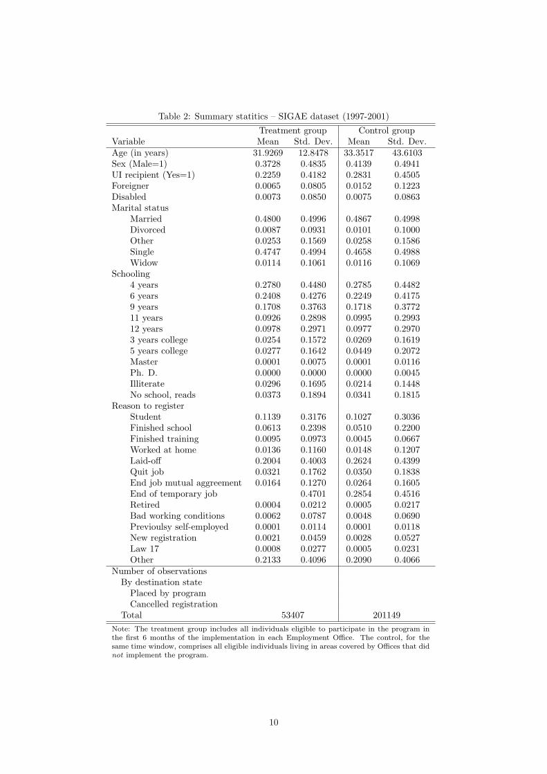
Table 2: Summary statitics – SIGAE dataset (1997-2001)

Treatment group Control groupVariable Mean Std. Dev. Mean Std. Dev.Age (in years) 31.9269 12.8478 33.3517 43.6103Sex (Male=1) 0.3728 0.4835 0.4139 0.4941UI recipient (Yes=1) 0.2259 0.4182 0.2831 0.4505Foreigner 0.0065 0.0805 0.0152 0.1223Disabled 0.0073 0.0850 0.0075 0.0863Marital status

Married 0.4800 0.4996 0.4867 0.4998Divorced 0.0087 0.0931 0.0101 0.1000Other 0.0253 0.1569 0.0258 0.1586Single 0.4747 0.4994 0.4658 0.4988Widow 0.0114 0.1061 0.0116 0.1069

Schooling4 years 0.2780 0.4480 0.2785 0.44826 years 0.2408 0.4276 0.2249 0.41759 years 0.1708 0.3763 0.1718 0.377211 years 0.0926 0.2898 0.0995 0.299312 years 0.0978 0.2971 0.0977 0.29703 years college 0.0254 0.1572 0.0269 0.16195 years college 0.0277 0.1642 0.0449 0.2072Master 0.0001 0.0075 0.0001 0.0116Ph. D. 0.0000 0.0000 0.0000 0.0045Illiterate 0.0296 0.1695 0.0214 0.1448No school, reads 0.0373 0.1894 0.0341 0.1815

Reason to registerStudent 0.1139 0.3176 0.1027 0.3036Finished school 0.0613 0.2398 0.0510 0.2200Finished training 0.0095 0.0973 0.0045 0.0667Worked at home 0.0136 0.1160 0.0148 0.1207Laid-off 0.2004 0.4003 0.2624 0.4399Quit job 0.0321 0.1762 0.0350 0.1838End job mutual aggreement 0.0164 0.1270 0.0264 0.1605End of temporary job 0.4701 0.2854 0.4516Retired 0.0004 0.0212 0.0005 0.0217Bad working conditions 0.0062 0.0787 0.0048 0.0690Previoulsy self-employed 0.0001 0.0114 0.0001 0.0118New registration 0.0021 0.0459 0.0028 0.0527Law 17 0.0008 0.0277 0.0005 0.0231Other 0.2133 0.4096 0.2090 0.4066

Number of observationsBy destination state

Placed by programCancelled registration

Total 53407 201149Note: The treatment group includes all individuals eligible to participate in the program inthe first 6 months of the implementation in each Employment Office. The control, for thesame time window, comprises all eligible individuals living in areas covered by Offices that didnot implement the program.

10

individuals, monitors the different features of the program and individuals during their complete

spells of unemployment. The information in the dataset includes most demographic variables used

in labor market studies (age, sex, nationality, schooling, place of residence), and a large number

of variables related with previous labor market experience (previous occupation, desired sector of

employment, unemployment duration, reason for job displacement). The unemployed is observed

for the complete duration of the unemployment spell and, at the moment of termination, we can

observe her destination state (either employment, training or out of the labor force).

The main limitations of our data are the lack of wage information, which we try to overcome

using a different dataset in the next subsection, and the difficulty in following up the individuals after

they leave the program. In fact, there is no income-related information at the Employment Offices

and follow up interviews were not carried out (although they were part of the original program

design).

4.1.2 Sample construction

We take advantage of both the characteristics of the dataset and of the program implementation

to construct treatment and control groups using different criteria. In particular, we explore (i) the

longitudinal nature of the data, and (ii) the two sources of variation coming from the eligibility

criteria and the different implementation phases (which generate spatial and time differences).

The program design and implementation generated a natural way to construct treatment and

control groups along several dimensions. One such dimension is the eligibility criteria (based on age

and unemployment duration) and the other is the phased implementation of the program across the

Portuguese territory that generated a sequence of implementation areas. The local Employment

Offices were assigned to the program at different moments in time – starting in June and October

of 1998, and continuing through February, May, July and November of 1999 and finally in April,

June and September of 2000.

The treatment group includes all individuals eligible to participate in the InserJovem and

REAGE programs in the first six months of their implementation in each Employment Office.

This generates a large group of individuals already unemployed at the moment the programs were

initiated in each office (see Table 2 for the dimensions of treatment and control groups).

The construction of the comparison group was determined by the same eligibility criteria, but

considering instead locations outside the areas already implementing the program. Thus, for the

same six months time windows, the control group comprises all eligible individuals living in the

areas covered by Employment Offices that did not implement the programs.

11

Given the non-experimental nature of the program, the timing of implementation at each Em-

ployment Office is a concern. However, we believe that the selection of Offices presents no sistematic

economic bias, i.e., it was not dictated by special labor market conditions at the regional level. For

example, as it can be seen in Figure 1, the regions with the highest (or lowest) unemployment rate

were not the ones to be selected first to participate in the program. This suggests that the treatment

and control groups can be though of as a “random” draw from the local Employment Offices at any

point in time.

●

●

●

●

●

●

●

●

24

68

1012

14

Implementation date

Unem

ploym

ent r

ate

●

●

●

●

●

●

●

●

●

●

●

●

●

●

●

●

●

●

●

●

●

●

●

●

●

●

● ●

199807 199810 199902 199905 199907 199911 200004 200006 200009

Avg. at implementation offices

● Avg. at other offices

Figure 1: Employment Offices’ average unemployment rates at the implementation dates

In Table 2, we present summary statistics for the two groups of interest. The two groups are not

very different according to the characteristics presented in the table. However, treated individuals

are slightly younger, and they are more likely to be female. Among treated individuals the share of

unemployment insurance (UI) recipients is smaller. The control group has a sligtly larger fraction

of workers with college education, but the two groups are not very different along this dimension.

The largest differences can be found in the “reason to register” attribute. The unemployed that

were subject to treatment were more likely to have ended a temporary job than those in the control

group, who are much more likely to have been laid-off prior to registration. Overall, these summary

12

statistics are reassuring in terms of our ability to match individuals in the two groups to perform

our evaluation exercise.

4.1.3 Unemployment duration impact

Our results in Table 3, using the two econometric methods presented above, suggest a negligible

impact in the employability of those receiving treatment (youth unemployed and older long term

unemployed). The program’s impact on the average unemployment spell ranges from a reduction

of approximately 1 month to a slight increase of about 0.2 months. The analysis by gender and

type of exit from registered unemployment reveals some differences, but still the impacts are rather

small. While younger males tend to benefit more than younger females, older females benefit the

most from the treatment.

Difference-in-differences matching

The implementation of the matching method follows the algorithm presented in Becker & Ichino

(2002), while the D-in-D matching estimator follows Smith & Todd (2004). Due to the heterogeneity

of the individuals in each of the groups and, not independently, the fact that there are two programs

– Inserjovem and Reage –, we splitted the sample into these two subsamples. The two subsamples

are then analyzed according to: (i) the type of exit from the pool of registered unemployed – all

exits, placed and canceled4 and (ii) the gender – female, male and all. Therefore, in total, there are

18 DDD estimates.

The propensity score matching results are based on the stratification method, imposing the

common support option. The matching process typically led to balanced treatment and control

groups.5

In Table 3, the lines labeled ‘PEP=1’ report the D-in-D estimates based on individuals that

participated in the program (treatment group) and on the individuals that had the potential to

participate in the program, but lived outside the implementation areas (control group). Each entry

in the table is computed as the difference between the ‘after implementation’ and the ‘before im-

plementation’ propensity score matching estimates of the treatment effects on the treated.6 Lines

labeled ‘PEP=0’ report the same estimates, but for a sample of non-eligible individuals, that is,4The exit category placed includes all individuals who either through the program or by themselves are reported

has having been placed in the labor market or in a training program; the exit category canceled includes all individualswho saw their registration canceled by the Employment Offices due to having failed to fulfill one or more criteria.

5For the entire set of estimates presented below, there are some cases where the two groups are unbalanced alongsome of the dimensions of the X vector. However, despite the fact that the balancing property failed to hold instatistical terms, the economic dimension of the difference in averages on the variable age was not significant. Thedifferences in average age between the treatment and control groups were typically of a few months, which clearly donot affect the required comparability of the two groups. These balancing property difficulties tended to arise moreoften in the Reage program analysis.

6The disaggregated estimates, i.e., the propensity score matching estimates, are reported in the Appendix.

13

Table 3: Effects on unemployment duration (in months): D-in-D and DDD matching estimates

All Male FemaleType of Exit Effect s.e. Effect s.e. Effect s.e.

InserJovem

D-in-D for PEP=1All -0.15 0.096 -0.22 0.146 -0.11 0.126

Placed 0.18 0.211 -0.04 0.300 0.21 0.278Canceled -0.36 0.115 -0.38 0.175 -0.35 0.151

D-in-D for PEP=0All 0.00 0.013 -0.01 0.020 -0.01 0.017

Placed 0.00 0.026 -0.03 0.039 0.02 0.033Canceled -0.02 0.016 -0.02 0.025 -0.02 0.021

DDDAll -0.15 0.097 -0.21 0.147 -0.10 0.128

Placed 0.18 0.213 -0.01 0.303 0.20 0.280Canceled -0.34 0.116 -0.36 0.177 -0.33 0.152

Reage

D-in-D for PEP=1All -0.54 0.165 -0.48 0.222 -0.75 0.231

Placed 0.09 0.330 0.38 0.428 -0.04 0.471Canceled -0.56 0.197 -0.42 0.265 -0.89 0.278

D-in-D for PEP=0All 0.21 0.020 0.21 0.033 0.20 0.026

Placed 0.29 0.035 0.31 0.057 0.29 0.044Canceled 0.10 0.027 0.05 0.045 0.13 0.034

DDDAll -0.75 0.166 -0.69 0.225 -0.95 0.232

Placed -0.20 0.332 0.06 0.431 -0.33 0.473Canceled -0.66 0.199 -0.47 0.269 -1.01 0.280

1) ‘Inserjovem’ and ‘Reage’ are the programs targeting young and older unemployed, respectively.

2)‘PEP=1’ indicates estimates based on eligible individuals; ‘PEP=0’ indicates estimates basedon non-eligible individuals.

3) ‘Placed’ refers to individuals (re-)entering employment or training. ‘Canceled’ refers to individ-uals entering inactivity from unemployment.

4) The DDD estimates are the difference between the ‘D-in-D for PEP=1’ and the ‘D-in-D forPEP=0’. The propensity score matching estimates underlying the reported D-in-D matchingestimates are reported in the Appendix in Table A1.

5) A negative sign implies a reduction in the average unemployment spell.

young individuals unemployed for less than 6 months or older individuals with less than 12 months

of unemployment. We start by focusing our attention on the ‘PEP=1’ lines.

The two sets of ‘PEP=1’ results report rather minor positive effects of the two programs, which

translate into marginally smaller unemployment durations for the treated relatively to a situation

without treatment. In Figure 2, the first column of plots summarizes these results of the difference-

in-differences matching estimator, providing 95% confidence intervals. The following results are

worth highlighting:

i) The impact of the program Inserjovem is lower than Reage’s. Furthermore, the impact on the

youth is statistically (and economically) insignificant. This result confirms the findings obtained

for similar programs in other European countries (see Blundell et al. (2004), Larsson (2003));

ii) The effect is stronger for females in Reage, that is, the D-in-D estimates are more negative (or

14

less positive) than those observed for males. In the younger population, the gender differences

are rather small, but slightly in favor of men;

iii) In terms of the type of exit, the results are mixed, highlighting the importance of such disag-

gregation. Thus, when analyzing exits from the pool of registered unemployed due to either i)

self-placement, ii) training or iii) placement through the Employment Offices’ efforts, which we

aggregate in the class “placed”, the D-in-D estimates for both programs are typically positive,

but statistically insignificant. That is, the impact on duration is negligible, reaching in the

best case a reduction of -0.04 months and in the worst case an increase of 0.38 months. When

analyzing the group of individuals who entered inactivity – the class “canceled” – the estimates

are negative and statistically significant. Somehow, the new rules applied with the program

seem to make the system more aware of the “irregularities”, leading the Employment Offices to

take action earlier. Whether this is a desirable result is questionable – it may have a positive

(warning) impact on the individuals, leading them to correct their behavior, but it can also

be associated with increasing welfare stigma. Overall, pooling all types of exits, the programs

seem to have reduced unemployment duration, but only statistically significant for the Reage

program, resulting, at best, in an unemployment reduction of about one month.

Next, we control for other potential non-observable effects.

Selection on unobservables difference-in-difference-in-differences

The motivation to introduce an additional layer of control for unobserved effects is the possibility

that at the time of implementation of the program there were shocks to the “treatment” areas that,

even if not directly attributable to the program, are correlated with the program. For example,

the simple awareness of the program might increase the firms’ willingness to hire. Thus, we create

another level of control. For that purpose, we repeat the D-in-D matching procedure, but this time

we consider the individuals that do not meet the eligibility criteria to participate in the program

(‘PEP=0’). The results of the ‘D-in-D for PEP=0’ and the DDD estimates – the difference between

the two groups’ D-in-D matching estimates – are reported in the remaining panels of Figure 2.

For the group of non-eligibles (see PEP=0 column in Figure 2), the D-in-D estimates are (as

expected) rather tiny. While older individuals in the region of implementation actually suffered a

negative impact on durations (increase by 0.1 to 0.3 months), the younger individuals’ durations

before and after the program implementation are about the same, resulting in a null estimate of the

D-in-D treatment effect. This can be interpreted as an indication that the non-observables are not

15

* **

Months

D−in−D Matching, PEP=1

Exi

t: A

ll

+ +

+

A

A

MM

F

F

−1.

5−

1.0

−0.

50.

00.

5

* * *

Months

D−in−D Matching, PEP=0

+ − Reage A − All

* − Inserjovem M − Male

95% confidence intervals F − Female

+ + +A

A

M

M

F

F

−1.

5−

1.0

−0.

50.

00.

5

* **

Months

DDD Matching

+ +

+

A

A

M

M

F

F

−1.

5−

1.0

−0.

50.

00.

5

**

*

Months

Exi

t: P

lace

d

++

+

AA

M

M

FF

−1.

5−

1.0

−0.

50.

00.

51.

01.

5

* * *

Months

+ − Reage A − All

* − Inserjovem M − Male

95% confidence intervals F − Female

+ + +A

A

M

M

F

F

−1.

5−

1.0

−0.

50.

00.

51.

01.

5

**

*

Months

++

+

AA

M

MF

F−

1.5

−1.

0−

0.5

0.0

0.5

1.0

1.5

* * *

Months

Exi

t: C

ance

led

++

+

A AM

MF

F

−1.

5−

1.0

−0.

50.

00.

5

* * *

Months

+ − Reage A − All

* − Inserjovem M − Male

95% confidence intervals F − Female

+ + +AA

MM

F

F

−1.

5−

1.0

−0.

50.

00.

5

* * *

Months

++

+

A

A

MM

F

F

−1.

5−

1.0

−0.

50.

00.

5

Figure 2: D-in-D and DDD matching estimates: unemployment duration (in months)

16

unduly influencing our estimates of the program impact. Nonetheless, we proceed by computing the

DDD estimates.

The DDD matching estimates provide us with a corrected estimate for the average treatment

effect on the treated, which is slightly larger for the older individuals, resulting in smaller un-

employment spells compared with the absence of treatment, but about the same for the younger

population. The estimates and 95% confidence intervals are reported in the last column of Figure

2. Qualitatively, gender and type of exit effects described earlier still hold true.

4.2 Re-employment Wages

In the previous analysis we studied the effect on the duration of unemployment as a measure of

the program’s success/failure. As aforementioned, another obvious and important candidate as an

outcome variable is re-employment wages. Thus, we extend our study to the analysis of the impact

of the program on initial wages after leaving unemployment. In our application wages are measured

as a continuous variable in monthly terms, using an alternative dataset.

4.2.1 Data source

We collect the earnings data from Inquerito ao Emprego (IE), the Portuguese quarterly labor force

survey. This is a unique dataset that samples the entire Portuguese population. The survey sample

has more than 40,000 individuals each quarter and very detailed information on demographics and

labor market status. As is common with other European labor force surveys individuals are inter-

viewed up to six consecutive quarters allowing us to create a short panel and observing transitions

out of unemployment during the observation period.

Of special interest for our application is the information on unemployed workers searching behav-

ior. Among the information available for unemployed workers we know whether they are registered

at the Employment Offices, a crucial variable to identify the treatment and control groups as we did

with the administrative data. The implementation of the job search program described in section 2

guarantees that registered unemployed satisfying the two eligibility criteria (age and unemployment

duration) were automatically enrolled in the program. This feature of the program allows us to

identify enrolled (i.e. treated) unemployed in Employment Offices applying the program, and the

correct comparison group – either individuals in Employment Offices not applying the program or

unemployed individuals, before the program implementation, that would be enrolled if the same

program would have been in place.

We use the available subsample of registered unemployed of the IE to study the program impact

17

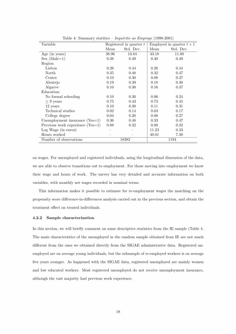
Table 4: Summary statitics – Inquerito ao Emprego (1998-2001)

Variable Registered in quarter t Employed in quarter t + 1Mean Std. Dev. Mean Std. Dev.

Age (in years) 38.96 13.84 33.18 11.80Sex (Male=1) 0.38 0.49 0.40 0.49Region:

Lisbon 0.26 0.44 0.26 0.44North 0.35 0.48 0.32 0.47Center 0.10 0.30 0.08 0.27Alentejo 0.19 0.39 0.18 0.38Algarve 0.10 0.30 0.16 0.37

Education:No formal schooling 0.10 0.30 0.06 0.24≤ 9 years 0.75 0.43 0.73 0.4512 years 0.10 0.30 0.11 0.31Technical studies 0.02 0.14 0.03 0.17College degree 0.04 0.20 0.08 0.27

Unemployment insurance (Yes=1) 0.36 0.48 0.33 0.47Previous work experience (Yes=1) 0.88 0.32 0.88 0.32Log Wage (in euros) – – 11.23 0.33Hours worked – – 40.01 7.38Number of observations 18382 1194

on wages. For unemployed and registered individuals, using the longitudinal dimension of the data,

we are able to observe transitions out to employment. For those moving into employment we know

their wage and hours of work. The survey has very detailed and accurate information on both

variables, with monthly net wages recorded in nominal terms.

This information makes it possible to estimate for re-employment wages the matching on the

propensity score difference-in-differences analysis carried out in the previous section, and obtain the

treatment effect on treated individuals.

4.2.2 Sample characterization

In this section, we will briefly comment on some descriptive statistics from the IE sample (Table 4.

The main characteristics of the unemployed in the random sample obtained from IE are not much

different from the ones we obtained directly from the SIGAE administrative data. Registered un-

employed are on average young individuals, but the subsample of re-employed workers is on average

five years younger. As happened with the SIGAE data, registered unemployed are mainly women

and low educated workers. Most registered unemployed do not receive unemployment insurance,

although the vast majority had previous work experience.

18

4.2.3 Results of the application to wages

In Table 5, we report the D-in-D matching estimates of the effect on wages, as well as its disag-

gregation into the average treatment effect on the treated (ATT)7 for the periods before and after

the treatment implementation. The left panel (PEP=1) presents results for eligible individuals

(i.e. individuals that satisfy both the age and unemployment duration requirements). Each of the

ATT estimates (columns 1 and 2) is obtained using as treatment group individuals in employment

offices that implemented the program and as control group registered unemployed in employment

offices that did not implement the program by the time the observation is being recorded. The

third column in each panel is the difference-in-difference matching estimate. It is obtained as the

difference between the ATT after the program implementation and the ATT before the program

implementation. The right panel (PEP=0) presents similar results for non-eligible individuals (those

not satisfying one of the two requirements).

Our results show a negative impact, although not statistically different from zero, of the pro-

gram on wages. On average eligible unemployed workers finding a job in employment offices that

implemented the program had a starting wage that was on average 2.4 per cent lower than the

one obtained by matched workers in employment offices not implementing it. When compared

with wages obtained in the period prior to the program implementation we see that individuals in

employment offices that implemented the program used to get wages that are 3.1 per cent higher

than those in offices not implementing it. This results in a D-in-D estimate of minus 5.5 per cent

for the ATT on the treated. The right panel corrects these figures for general trends observed for

individuals not covered by the program and thus not directly affected by its implementation. The

D-in-D estimate for this group of workers is a 8.5 per cent increase of wage since the period after the

program implementation. Overall, it results in a statistically significant DDD estimate of minus 14

percent. Thus, after correcting for general trends on wages and for the composition of the treated

group, we obtained a sizable wage loss associated with the program.

We also present results for two dimensions of individual heterogeneity, namely gender and pro-

gram type. In terms of gender differences, our results point to a very large and negative impact of

the program on re-employment wages for male workers (minus 28 per cent for the DDD matching

estimate) and a close to zero impact on female wages (0.3 per cent). The main source of this differ-

ence comes from the large increase in wages obtained by noneligible unemployed after the program

implementation.7Using the propensity score stratificaton method for matching individuals.

19

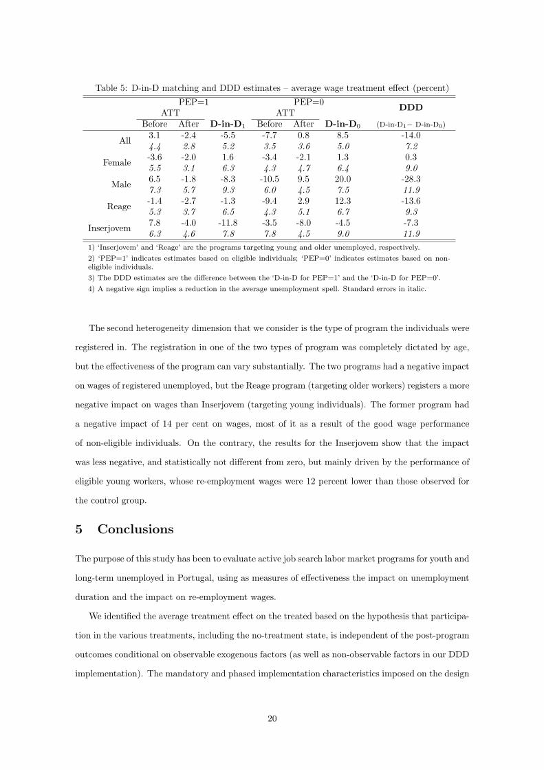
Table 5: D-in-D matching and DDD estimates – average wage treatment effect (percent)

PEP=1 PEP=0DDDATT ATT

Before After D-in-D1 Before After D-in-D0 (D-in-D1− D-in-D0)

All 3.1 -2.4 -5.5 -7.7 0.8 8.5 -14.04.4 2.8 5.2 3.5 3.6 5.0 7.2

Female -3.6 -2.0 1.6 -3.4 -2.1 1.3 0.35.5 3.1 6.3 4.3 4.7 6.4 9.0

Male 6.5 -1.8 -8.3 -10.5 9.5 20.0 -28.37.3 5.7 9.3 6.0 4.5 7.5 11.9

Reage -1.4 -2.7 -1.3 -9.4 2.9 12.3 -13.65.3 3.7 6.5 4.3 5.1 6.7 9.3

Inserjovem 7.8 -4.0 -11.8 -3.5 -8.0 -4.5 -7.36.3 4.6 7.8 7.8 4.5 9.0 11.9

1) ‘Inserjovem’ and ‘Reage’ are the programs targeting young and older unemployed, respectively.

2) ‘PEP=1’ indicates estimates based on eligible individuals; ‘PEP=0’ indicates estimates based on non-eligible individuals.

3) The DDD estimates are the difference between the ‘D-in-D for PEP=1’ and the ‘D-in-D for PEP=0’.

4) A negative sign implies a reduction in the average unemployment spell. Standard errors in italic.

The second heterogeneity dimension that we consider is the type of program the individuals were

registered in. The registration in one of the two types of program was completely dictated by age,

but the effectiveness of the program can vary substantially. The two programs had a negative impact

on wages of registered unemployed, but the Reage program (targeting older workers) registers a more

negative impact on wages than Inserjovem (targeting young individuals). The former program had

a negative impact of 14 per cent on wages, most of it as a result of the good wage performance

of non-eligible individuals. On the contrary, the results for the Inserjovem show that the impact

was less negative, and statistically not different from zero, but mainly driven by the performance of

eligible young workers, whose re-employment wages were 12 percent lower than those observed for

the control group.

5 Conclusions

The purpose of this study has been to evaluate active job search labor market programs for youth and

long-term unemployed in Portugal, using as measures of effectiveness the impact on unemployment

duration and the impact on re-employment wages.

We identified the average treatment effect on the treated based on the hypothesis that participa-

tion in the various treatments, including the no-treatment state, is independent of the post-program

outcomes conditional on observable exogenous factors (as well as non-observable factors in our DDD

implementation). The mandatory and phased implementation characteristics imposed on the design

20

of the program allow us to be confident about our identification strategy, namely the comparability

of our treatment and control groups.

The results from our analysis point to a positive, but rather small, effect of the treatment on

unemployment duration on the treated group. We estimate a reduction of less than 1 month on

unemployment duration. Given the generally high levels of unemployment duration in Portugal

(that can reach several years), these numbers are not impressive. Indeed, they are in line with what

has been obtained for other countries and surveyed in Heckman et al. (1999). In terms of the other

chosen measure of effectiveness of the program – wages –, qualitatetively the results are in line

with the duration ones. The average re-employment wages effect on the treated women is null and

negative for men. Overall, even ignoring the costs of implementation, we conclude that the program

effectiveness can be questioned.

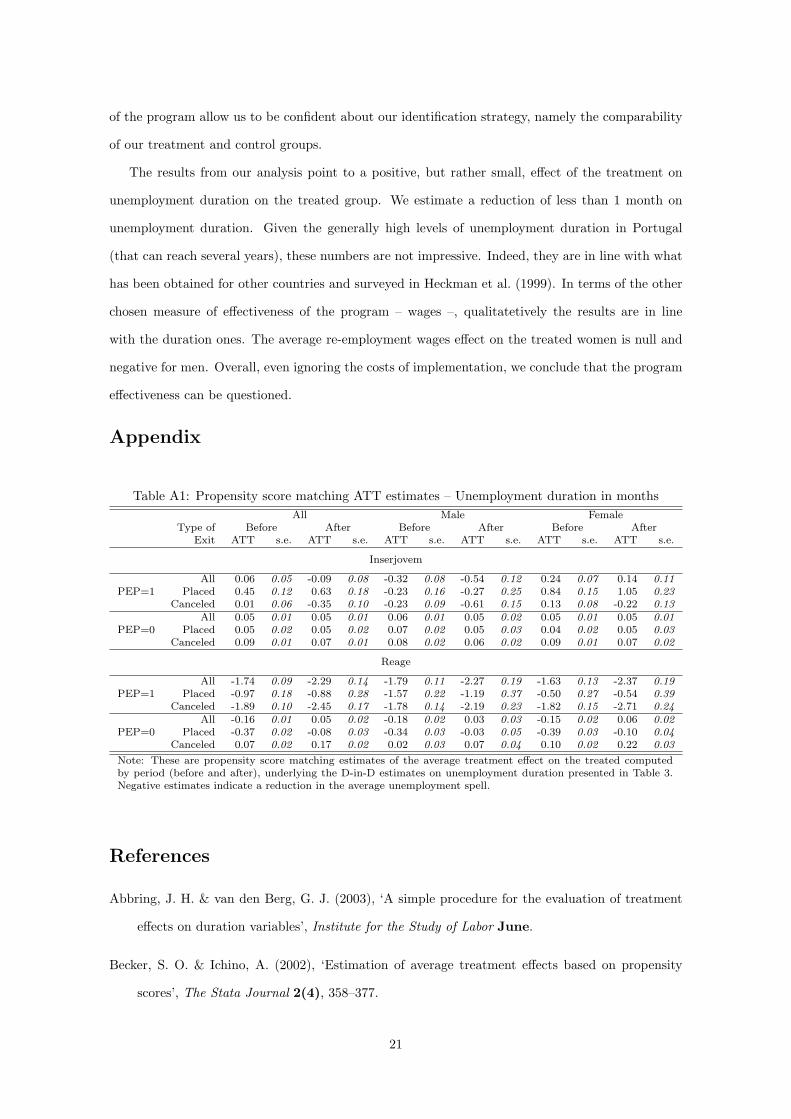
Appendix

Table A1: Propensity score matching ATT estimates – Unemployment duration in monthsAll Male Female

Type of Before After Before After Before AfterExit ATT s.e. ATT s.e. ATT s.e. ATT s.e. ATT s.e. ATT s.e.

Inserjovem

All 0.06 0.05 -0.09 0.08 -0.32 0.08 -0.54 0.12 0.24 0.07 0.14 0.11PEP=1 Placed 0.45 0.12 0.63 0.18 -0.23 0.16 -0.27 0.25 0.84 0.15 1.05 0.23

Canceled 0.01 0.06 -0.35 0.10 -0.23 0.09 -0.61 0.15 0.13 0.08 -0.22 0.13All 0.05 0.01 0.05 0.01 0.06 0.01 0.05 0.02 0.05 0.01 0.05 0.01

PEP=0 Placed 0.05 0.02 0.05 0.02 0.07 0.02 0.05 0.03 0.04 0.02 0.05 0.03Canceled 0.09 0.01 0.07 0.01 0.08 0.02 0.06 0.02 0.09 0.01 0.07 0.02

Reage

All -1.74 0.09 -2.29 0.14 -1.79 0.11 -2.27 0.19 -1.63 0.13 -2.37 0.19PEP=1 Placed -0.97 0.18 -0.88 0.28 -1.57 0.22 -1.19 0.37 -0.50 0.27 -0.54 0.39

Canceled -1.89 0.10 -2.45 0.17 -1.78 0.14 -2.19 0.23 -1.82 0.15 -2.71 0.24All -0.16 0.01 0.05 0.02 -0.18 0.02 0.03 0.03 -0.15 0.02 0.06 0.02

PEP=0 Placed -0.37 0.02 -0.08 0.03 -0.34 0.03 -0.03 0.05 -0.39 0.03 -0.10 0.04Canceled 0.07 0.02 0.17 0.02 0.02 0.03 0.07 0.04 0.10 0.02 0.22 0.03

Note: These are propensity score matching estimates of the average treatment effect on the treated computedby period (before and after), underlying the D-in-D estimates on unemployment duration presented in Table 3.Negative estimates indicate a reduction in the average unemployment spell.

References

Abbring, J. H. & van den Berg, G. J. (2003), ‘A simple procedure for the evaluation of treatment

effects on duration variables’, Institute for the Study of Labor June.

Becker, S. O. & Ichino, A. (2002), ‘Estimation of average treatment effects based on propensity

scores’, The Stata Journal 2(4), 358–377.

21

Blundell, R., Dias, M., Meghir, C. & Reenen, J. V. (2004), ‘Evaluating the employment impact of

a mandatory job search assistance program’, Journal of the European Economic Association

2(4), 569–606.

Centeno, M. (2004), ‘The match quality gains from unemployment insurance’, Journal of Human

Resources 39(3), 839–863.

Cox, D. R. (1972), ‘Regression models and life-tables’, Journal of the Royal Statistical Society Series

B 34, 187–220.

Heckman, J. (1979), ‘Sample selection bias as a specification error’, Econometrica 47, 153–161.

Heckman, J., Ichimura, H., Smith, J. & Todd, P. (1998), ‘Characterizing selection bias using exper-

imental data’, Econometrica 66(5), 1017–1098.

Heckman, J., Ichimura, H. & Todd, P. (1997), ‘Matching as an econometric evaluation estima-

tor: Evidence from evaluating a job training programme’, The Review of Economic Studies

64(4), 605–654.

Heckman, J., LaLonde, R. & Smith, J. (1999), ‘The economics and econometrics of active labor

market programs in’, Handbook of Labor Economics 3A.

Larsson, L. (2003), ‘Evaluation of swedish youth labor market programs’, The Journal of Human

Resources 38(4), 891–927.

Meyer, B. D. (1995), ‘Natural and quasi-experiments in economics’, Journal of Business & Economic

Statistics 13, 151–162.

Rosenbaum, P. & Rubin, D. (1983), ‘The central role of the propensity score in observational studies

for causal effects’, Biometrika 70, 41–55.

Rubin, D. (1977), ‘Assignment to a treatment group on the basis of a covariate’, Journal of Educa-

tional Statistics 2, 1–26.

Smith, J. & Todd, P. (2004), ‘Does matching overcome LaLonde’s critique of nonexperimental

estimators?’, Journal of Econometrics forthcoming.

22