UNDERSTANDING MECHANICAL BEHAVIOR OF LUNAR ...
662
UNDERSTANDING MECHANICAL BEHAVIOR OF LUNAR SOILS FOR THE STUDY OF VEHICLE MOBILITY by HEATHER ANN ORAVEC Submitted in partial fulfillment of the requirements For the degree of Doctor of Philosophy Dissertation Adviser: Dr. Xiangwu Zeng Department of Civil Engineering CASE WESTERN RESERVE UNIVERSITY May, 2009
-
Upload
khangminh22 -
Category
Documents
-
view
1 -
download
0
Transcript of UNDERSTANDING MECHANICAL BEHAVIOR OF LUNAR ...

UNDERSTANDING MECHANICAL BEHAVIOR OF LUNAR SOILS FOR THE
STUDY OF VEHICLE MOBILITY
by
HEATHER ANN ORAVEC
Submitted in partial fulfillment of the requirements
For the degree of Doctor of Philosophy
Dissertation Adviser: Dr. Xiangwu Zeng
Department of Civil Engineering
CASE WESTERN RESERVE UNIVERSITY
May, 2009

CASE WESTERN RESERVE UNIVERSITY
SCHOOL OF GRADUATE STUDIES
We hereby approve the thesis/dissertation of
_____________________________________________________
candidate for the ______________________degree *.
(signed)_______________________________________________ (chair of the committee) ________________________________________________ ________________________________________________ ________________________________________________ ________________________________________________ ________________________________________________ (date) _______________________ *We also certify that written approval has been obtained for any proprietary material contained therein.

Dedication:
To my best friend and my greatest supporter, my mother Ruth Marie Hlasko

i
TABLE OF CONTENTS
List of Tables vii
List of Figures x
Acknowledgements xxii
List of Abbreviations xxiv
Glossary xxvi
Abstract xxix
CHAPTER ONE
INTRODUCTION 1
1.1 History of Lunar Exploration 1
1.2 Future of Lunar Exploration 11
1.2.1 Why the Moon? 12
1.3 Motivation for This Research 15
1.4 Introduction to Surface Mobility 17
1.4.1 Development of Off-Road Vehicles 19
1.4.2 Development of Terramechanics 21
1.5 General Factors Affecting Surface Mobility 22
1.6 Soil Properties Affecting Surface Mobility 25
1.6.1 Bevameter Technique for Determining Soil Strength 28
1.6.1.1 Bearing Capacity 30

ii
1.6.1.2 Shear Strength 43
1.6.2 Other Techniques for Measuring Soil Properties in
Terramechanics 54
1.6.2.1 Direct Shear Test 55
1.6.2.2 Torsional Shear Test 57
1.6.2.3 Triaxial Test 59
1.6.2.4 Cone Penetrometer Test 63
1.6.2.5 Shear Vane, Vane-Cone, and Cohron Sheargraph Tests 70
1.7 Nature of the Lunar Terrain 74
1.7.1 The Lunar Environment 74
1.7.1.1 The Lunar Landscape 76
1.7.2 The Lunar Regolith 81
1.7.2.1 Formation of the Lunar Regolith 82
1.7.2.2 Engineering Properties of the Lunar Regolith 84
1.7.2.3 Trafficability Parameters 94
1.7.3 Important Aspects for Lunar Surface Mobility 97
1.7.3.1 Cohesion 97
1.7.3.2 Friction 99
1.8 Problem Statement and Objectives 100
1.8.1 Scope of Work 103
1.8.2 Basic Assumptions 104
1.9 Organization of the Dissertation 105

iii
CHAPTER TWO
LITERATURE REVIEW 107
2.1 Review of Lunar Soil Investigations 107
2.1.1 Soil Investigations on the Moon 108
2.1.1.1 Robot Interaction 110
2.1.1.2 Spacecraft Interaction 114
2.1.1.3 Footprint Analysis 117
2.1.1.4 Trenching Tests and Boulder Tracks 119
2.1.1.5 Penetrometer Tests 123
2.1.2 Soil Investigations on Returned Lunar Soil 135
2.1.2.1 Apollo Soil Samples 137
2.1.2.2 Laboratory Tests 142
2.2 Review of Lunar Soil Simulants 150
2.2.1 MLS-1 151
2.2.2 JSC-1 155
2.2.3 JSC-1A 159
2.2.4 Other Lunar Soil Simulants 163
2.3 Review of Lunar Vehicle Mobility Studies 166
2.3.1 Lunar Roving Vehicle 166
2.3.1.1 Trafficability and Wheel-Soil Interaction Studies 170

iv
CHAPTER THREE
DEVELOPMENT OF A NEW LUNAR SOIL SIMULANT: GRC-1 189
3.1 Method for Creating GRC-1 189
3.2 Initial Characterization of GRC-1 197
3.2.1 Particle Size Distribution 198
3.2.2 Specific Gravity 205
3.2.3 Maximum and Minimum Bulk Density with Respect to
Relative Density 209
3.2.4 Porosity and Void Ratio 213
3.2.5 Compressibility 215
3.2.6 Angle of Inclination 221
3.3 Comparison to Lunar Soil and Lunar Soil Simulants 224
CHAPTER FOUR
TRIAXIAL TESTING FOR STRENGTH OF GRC-1 230
4.1 Triaxial Apparatus at NASA Glenn 230
4.2 Experimental Procedure 234
4.3 Test Results and Analysis 240
4.4 Comparison with Lunar Soil 253
4.5 Effect of Strength Properties on Vehicle Mobility 254

v
CHAPTER FIVE
BEVAMETER TESTING FOR STRENGTH OF GRC-1 261
5.1 Development of NASA Glenn Laboratory Bevameter 261
5.2 Experimental Setup and Limitations 267
5.2.1 Soil Preparation Method 267
5.2.2 Soil Bin Requirements 275
5.2.3 End Effector Requirements 307
5.3 Pressure-Sinkage Test for Vehicle Mobility 312
5.3.1 Experimental Procedure 316
5.3.2 Test Results and Analysis 319
5.4 Shear Test for Vehicle Mobility 332
5.4.1 Experimental Procedure 336
5.4.2 Test Results and Analysis 339
5.5 Comparison with Lunar Soil 350
CHAPTER SIX
CONE PENETROMETER TESTING FOR STRENGTH OF GRC-1 352
6.1 Cone Penetrometer Device at NASA Glenn 352
6.2 Experimental Procedure 354
6.3 Test Results and Analysis 358
6.4 Comparison with Lunar Soil 374

vi
CHAPTER SEVEN
SUMMARY AND CONCLUSIONS 381
7.1 Overview 381
7.2 Conclusions 382
7.3 Suggestions for Practical Use of GRC-1 387
7.4 Suggestions for Future Work 392
APPENDICES
Appendix A: Lunar soil and simulant properties 395
Appendix B: Initial characterization of GRC-1 414
Appendix C: Triaxial test results for GRC-1 416
Appendix D: Table bevameter results for GRC-1 492
Appendix E: Cone penetration test results for GRC-1 604
BIBLIOGRAPHY 616

vii
LIST OF TABLES
Table 1.1 Lunar exploration summary 7
Table 1.2 Lunar exploration themes 13
Table 1.3 Subcategorized objectives for lunar exploration 14
Table 1.4 Comparison of the Moon and Earth 75
Table 1.5 Bulk density of lunar soil 89
Table 1.6 Relative density of the lunar soil 90
Table 1.7 Porosity and void ratio of the lunar soil 92
Table 1.8 Recommended values of lunar soil cohesion and friction angle 94
Table 1.9 Recommended trafficability parameters 96
Table 2.1 In-situ geotechnical properties of lunar soil from Lunokhod
observations 113
Table 2.2 Results of analysis on astronaut footprint depths 119
Table 2.3 Average cone index gradient for lunar soil near the Apollo 15
landing site 134
Table 2.4 Bulk density and void ratio of returned lunar soils 143
Table 2.5 Comparison of friction angle and cohesion of lunar soils and MLS-1 155
Table 2.6 Results of triaxial tests performed on JSC-1 158
Table 2.7 Results of triaxial tests performed on JSC-1A 162
Table 2.8 Comparison of lunar soil and simulated lunar soil 164
Table 2.9 Results of special tests on Yuma sand 178
Table 3.1 Initial target recipe for coarse grained lunar soil simulant 191

viii
Table 3.2 Histogram by weight for Best Sands compared to the target mixture
for a coarse lunar soil simulant 195
Table 3.3 Sieve sizes used for particle size distribution analysis 198
Table 3.4 Typical values of the temperature correction factor 208
Table 3.5 Results of specific gravity tests on GRC-1 208
Table 3.6 Results of maximum bulk density tests for GRC-1 212
Table 3.7 Results of minimum bulk density tests for GRC-1 212
Table 3.8 Porosity and void ratio of GRC-1 214
Table 3.9 Angle of repose of GRC-1 223
Table 3.10 Comparison of GRC-1 with lunar soil and lunar soil simulants 225
Table 4.1 Sample preparation method and corresponding density 241
Table 4.2 Results of triaxial tests from DS7 242
Table 4.3 Summary of GRC-1 internal angle of friction from triaxial tests 245
Table 4.4 Results of triaxial tests on GRC-1 using alternative analysis 250
Table 4.5 Cohesion and friction angle as determined using q and p 251
Table 4.6 Mohr’s circles compared with q-p method 252
Table 4.7 Friction angle of GRC-1 compared to lunar soil and lunar soil
simulants 253
Table 4.8 Typical properties of different vehicles 258
Table 4.9 Error in thrust caused by variation in cohesion 259
Table 4.10 Acceptable variability in cohesion 261
Table 5.1 Results of calibration for bevameter sensors 267

ix
Table 5.2 Current design properties of various prospective lunar exploration
vehicles 309
Table 5.3 Typical Bekker parameters for dry sand 325
Table 5.4 Bekker parameters for GRC-1 at various densities 330
Table 5.5 Summary of shear bevameter results for GRC-1 345
Table 5.6 Summary of shear bevameter results for GRC-1 using grousers 349
Table 5.7 Typical shear parameters for dry sand 350
Table 5.8 Comparison of lunar soil parameters to those of GRC-1 as
determined by bevameter testing 351
Table 6.1 Variation of cone index gradient with depth 362
Table 6.2 First test results for large cone 364
Table 6.3 Second test results for large cone 365
Table 6.4 First test results for small cone 366
Table 6.5 Second test results for small cone 367
Table 6.6 Results of cone penetration tests at various densities of GRC-1 371
Table 6.7 Cone index gradient of lunar soil based on Apollo missions 378

x
LIST OF FIGURES
Figure 1.1 Stonehenge 2
Figure 1.2 Sputnik 1 3
Figure 1.3 JFK calls for a mission to send man to the moon during a joint
session of Congress on May 25, 1961 4
Figure 1.4 Surveyor 6 model on Earth 5
Figure 1.5 Landing sites of the Luna, Ranger, Apollo, and Surveyor missions 10
Figure 1.6 Lunar landing site chart 10
Figure 1.7 President Bush announces plan for man’s return to Moon 11
Figure 1.8 Evolution of land locomotion 19
Figure 1.9 Terramechanics issues flowchart 22
Figure 1.10 Forces acting on a single wheel 25
Figure 1.11 Loading condition on the base of a single wheel 25
Figure 1.12 Schematic of typical bevameter 29
Figure 1.13 Typical pressure-sinkage curves 32
Figure 1.14 Schematic of the method for determining Bekker sinkage moduli and
exponent n 34
Figure 1.15 Typical load-sinkage curves for a dry sandy terrain 39
Figure 1.16 Typical values for Bekker parameters of various terrain type and
condition 40
Figure 1.17 The three phases of soil deformation during a typical plate-sinkage
test 42

xi
Figure 1.18 Typical horizontal stress-strain curves 45
Figure 1.19 Typical horizontal stress-strain curves for a sandy terrain 52
Figure 1.20 Overview of direct shear test 56
Figure 1.21 Typical direct shear test setup 56
Figure 1.22 Typical triaxial test setup 60
Figure 1.23 Typical triaxial test results from Mohr’s circle and Lambe methods 62
Figure 1.24(a) Army Corps of Engineers original laboratory cone penetrometer 66
Figure 1.24(b) Typical hand-held cone penetrometer 66
Figure 1.25 Vane-cone penetrometer 71
Figure 1.26 Shear vane end effector 72
Figure 1.27 Cohron sheargraph 73
Figure 1.28 Lunar highlands and maria 77
Figure 1.29 Hadley rille near the Apollo 15 landing site 78
Figure 1.30 Lunar domes at the Mons Rümker volcanic formation 79
Figure 1.31 King Crater 81
Figure 1.32 Typical lunar soil profile 84
Figure 1.33 Cartoon of lunar space weathering process 85
Figure 1.34 Particle size distribution of lunar soil 87
Figure 1.35 Typical lunar soil agglutinate particle 87
Figure 1.36 Cartoon displaying subgranular porosity of the lunar soil 88
Figure 1.37(a) Honeycomb structure of uncompressed granular soils 92
Figure 1.37(b) Compressed structure of granular soils 92
Figure 1.38(a) USSR Lunokhod 95

xii
Figure 1.38(b) Apollo LRV 95
Figure 1.39 Schematic of objectives for this research 104
Figure 2.1 Famous footprint left on the Moon by Neil Armstrong,
demonstrating the apparent cohesion of the regolith 109
Figure 2.2 Trail of Lunokhod’s 9th wheel 111
Figure 2.3 Frequency distribution of bearing strength of the lunar soil in
kg/cm2 as determined by Lunokhod 1 and Lunokhod 2 113
Figure 2.4 Variation of footprint depth with average porosity and relative
density 118
Figure 2.5 Trench excavated near rim of Shorty Crater of Station 4 during
Apollo 17 121
Figure 2.6 Taurus-Littrow area of the Apollo 17 mission 122
Figure 2.7 Friction angle values from boulder track analysis during Apollo 17 122
Figure 2.8 Lunokhod cone-vane penetrometer 123
Figure 2.9 Lunokhod 1 cone-vane penetrometer data 125
Figure 2.10 Lunokhod 2 cone-vane penetration curves 125
Figure 2.11 Location of Luna 17 landing and Lunokhod 1 traverses 126
Figure 2.12 Cartoon of Apollo SRP 128
Figure 2.13 Cartoon of recording drum 129
Figure 2.14 Apollo 15 EVA traverses 130
Figure 2.15 Stress penetration curve from Apollo 15 SRP Index No. 2 132
Figure 2.16 Original data from Apollo 15 SRP Index No. 2 133
Figure 2.17 Apollo 16 EVA traverses 135

xiii
Figure 2.18 Lunar sampling rake 139
Figure 2.19 Comparison of different Apollo mission core tube sampling bits 141
Figure 2.20 Density as a function of depth for the Apollo 15, 16, and 17 drill
stems 142
Figure 2.21 Compressibility curve represented as a coefficient of porosity versus
loading pressure for Luna 16 returned soil and Luna 20 returned soil 145
Figure 2.22 Shear strength parameters as a function of packing load 146
Figure 2.23 Ultra-high vacuum test chamber and shear box 148
Figure 2.24 Electron microprobe image of grain size and chemical composition
of MLS-1 152
Figure 2.25 Particle size distributions of MLS-1 and JSC-1 153
Figure 2.26 Electron microprobe image of grain size and chemical composition
of JSC-1 156
Figure 2.27 JSC-1 particle size distribution compared to upper and lower range
particle size distributions for the lunar soil 158
Figure 2.28 Particle size distribution of JSC-1A 161
Figure 2.29 Typical dimensions of the LRV 168
Figure 2.30 LRV wheel 169
Figure 2.31 Friction angle versus relative density as determined by various shear
testing methods 174
Figure 2.32 Typical CPT penetration resistance versus depth curves for Yuma
sand 176
Figure 2.33 Soil parameters of LSS1 as determined by WES 181

xiv
Figure 2.34 Soil parameters of LSS4 as determined by WES 181
Figure 2.35 Grain size distribution of Yuma sand, LSS, and Apollo 11 and 12
bounds 183
Figure 2.36 Yuma, LSS4, and LSS5 geotechnical properties 183
Figure 3.1 NASA Glenn lunar vehicle mobility team shown at the SLOPE
facility with the Modular Mobility Technology Demonstrator
shown in the background 188
Figure 3.2 Upper, lower, and average bounds on particle size distribution
of the lunar soil 191
Figure 3.3 Typical silica sand grades from the Best Sands Corp. 192
Figure 3.4 Verification of particle size distribution provided by Best Sands
Corp. 193
Figure 3.5 Coarse lunar average particle size distribution versus Best Sands
ideal mixture particle size distribution 196
Figure 3.6 Histogram representation of particle size distribution 197
Figure 3.7 Humboldt sieve shaker for particle size distribution analysis 199
Figure 3.8 Particle size distribution of initial GRC-1 mixture 201
Figure 3.9 Particle size distributions of 4.5 kg and 45.4 kg GRC-1 samples
compared with coarse lunar regolith average 202
Figure 3.10 Histogram representation of particle size distribution 203
Figure 3.11 Particle size distribution of 317.5 kg GRC-1 sample 205
Figure 3.12 Specific gravity test at CWRU 207
Figure 3.13 Typical standard compaction molds 210

xv
Figure 3.14 Compaction mold bolted on shake table 211
Figure 3.15 Plot of bulk density versus relative density of GRC-1 213
Figure 3.16 Typical consolidation test setup 217
Figure 3.17 Typical dial reading versus time plot 218
Figure 3.18 Results of one-dimensional consolidation testing on GRC-1 221
Figure 3.19 Homemade Hele-Shaw cell 223
Figure 3.20 GRC-1 particle size distribution versus that of actual lunar soil 226
Figure 3.21 Bulk density versus relative density for GRC-1 and the lunar soil 228
Figure 4.1 Tri-Flex 2/DataSystem triaxial test set from ELE International 232
Figure 4.2 Triaxial cell accessories (base plate, cap, porous stones, sealing rings,
drainage lines) from ELE International 233
Figure 4.3 DS7 DataSystem triaxial software from ELE International 233
Figure 4.4(a) Split mold with rubber membrane folded over the top 238
Figure 4.4(b) Rubber membrane tight against the inner wall of the split mold 238
Figure 4.5 Freestanding triaxial soil sample with internal vacuum applied 239
Figure 4.6 Typical bulge in soil after failure 239
Figure 4.7 Typical plot of corrected deviator stress versus axial strain used to
determine the ultimate strength of the soil sample 243
Figure 4.8 Typical Mohr’s circle plot to determine friction angle and cohesion 243
Figure 4.9 Stress at failure versus confining pressure 244
Figure 4.10 Friction angle versus relative density for GRC-1 246
Figure 4.11 Typical q versus p plot used to determine friction angle and cohesion 251
Figure 4.12 Comparison between Mohr’s circles and q-p friction angle values 252

xvi
Figure 5.1(a) Table bevameter shown with plate-sinkage end effector 262
Figure 5.1(b) Portable bevameter shown with shear ring end effector 262
Figure 5.2(a) Soils Design Laboratory 263
Figure 5.2(b) SLOPE facility 263
Figure 5.3 Schematic of table bevameter 265
Figure 5.4 Bevameter data acquisition system 266
Figure 5.5 Typical scatter experienced in pressure-sinkage bevameter tests 268
Figure 5.6(a) Shovel for random soil preparation 269
Figure 5.6(b) Plastic funnel for hopper soil preparation 269
Figure 5.7 Bevameter setup for pressure-sinkage tests 270
Figure 5.8 Plot of load-sinkage data collected from the hopper soil
preparation tests and the random soil preparation tests 273
Figure 5.9 Plot of the raw data and curve-fit for the random soil preparation tests 273
Figure 5.10 Plot of raw data and curve-fit for the hopper soil preparation tests 274
Figure 5.11 Plot of raw data and mean curve-fit for random soil preparation tests
and hopper soil preparation tests 274
Figure 5.12 Standard deviation of the random soil preparation tests and hopper
soil preparation tests 275
Figure 5.13 Pressure bulb for a circular plate 278
Figure 5.14 Large soil hopper for quicker soil preparation 282
Figure 5.15 3 cm, Test 1 286
Figure 5.16 3 cm, Test 2 286
Figure 5.17 3 cm, Test 3 286

xvii
Figure 5.18 6 cm, Test 1 286
Figure 5.19 9 cm, Test 1 287
Figure 5.20 12 cm, Test 1 287
Figure 5.21 18 cm, Test 1 287
Figure 5.22 18 cm, Test 2 287
Figure 5.23 Comparison of mean pressure-sinkage curves tested at various
depths of soil 288
Figure 5.24 Comparison of mean pressure-sinkage curves tested at various
depths of soil (focusing on lunar pressure range) 288
Figure 5.25 Converging pressure-sinkage curves 289
Figure 5.26 3 cm, Test 1 290
Figure 5.27 6 cm, Test 1 290
Figure 5.28 9 cm, Test 1 291
Figure 5.29 Converging pressure-sinkage curves 291
Figure 5.30 3 cm, Test 1 293
Figure 5.31 6 cm, Test 1 293
Figure 5.32 9 cm, Test 1 294
Figure 5.33 12 cm, Test 1 294
Figure 5.34 15 cm, Test 1 294
Figure 5.35 15 cm, Test 2 294
Figure 5.36 18 cm, Test 1 294
Figure 5.37 21 cm, Test 1 294

xviii
Figure 5.38 24 cm, Test 1 295
Figure 5.39 27 cm, Test 1 295
Figure 5.40 Comparison of mean pressure-sinkage curves for various soil depths 296
Figure 5.41 Comparison of mean pressure-sinkage curves for various soil depths
(focusing on the lunar pressure range) 297
Figure 5.42 Schematic for the approximate solution of the settlement of a circular
footing under uniform loading 299
Figure 5.43 For a fixed soil thickness, how does the plate size affect settlement? 302
Figure 5.44 For a fixed radius, how does the soil thickness affect settlement? 304
Figure 5.45 Reformulated data from pressure-sinkage tests performed using
the 10.2 cm diameter penetration plate 305
Figure 5.46 Normalized reformulated data from pressure-sinkage tests performed
using the 10.2 cm diameter penetration plate compared with
theoretical trend for settlement 306
Figure 5.47 ATHLETE robotic vehicle designed by JPL 308
Figure 5.48 Chariot lunar truck vehicle 309
Figure 5.49 Penetration plates used in pressure-sinkage bevameter tests 310
Figure 5.50(a) Bottom view of shear bevameter ring with grousers 312
Figure 5.50(b) Angular view of shear bevameter ring with grousers 312
Figure 5.51 Raw data and mean pressure-sinkage vector for 7.6, 10.2, and 19 cm
penetration plates 321
Figure 5.52 Raw data compared to Bekker curve-fit 322
Figure 5.53 Bekker curve-fits for entire range of data 324

xix
Figure 5.54(a) Typical amount of sinkage for 19 cm diameter plate 325
Figure 5.54(b) Punching shear failure of 7.6 cm diameter plate 325
Figure 5.55 Comparison of GRC-1 Bekker parameters and parameters derived by
Wong et al. (1984) for a dry sandy terrain 327
Figure 5.56 Clear acrylic soil bin 328
Figure 5.57 Pressure-sinkage curves for GRC-1 at 1.64 g/cc 329
Figure 5.58 Pressure-sinkage curves for GRC-1 at 1.67 g/cc 329
Figure 5.59 Pressure-sinkage curves for GRC-1 at 1.75 g/cc 330
Figure 5.60 New manual rotation system attached to load/torque cell 337
Figure 5.61 Shear bevameter test results for GRC-1 at 14-percent relative density 342
Figure 5.62 Shear bevameter test results for GRC-1 at 24-percent relative density 343
Figure 5.63 Shear bevameter test results for GRC-1 at 52-percent relative density 344
Figure 5.64 Typical failure envelope for determining cohesion and friction angle 345
Figure 5.65 Shear bevameter results for GRC-1 at 1.64 g/cc using grousers 348
Figure 5.66 Shear bevameter results for GRC-1 at 1.75 g/cc using grousers 349
Figure 6.1(a) CP40II Cone Penetrometer form ICT International 353
Figure 6.1(b) CP40II accessories 353
Figure 6.2 Typical readout of CP40II data 354
Figure 6.3(a) Soil hopper 356
Figure 6.3(b) Partially filled soil bin 356
Figure 6.4 Cone penetration test at the NASA Glenn soils lab 358
Figure 6.5 Typical testing grid for 74.2 cm square soil bin 359
Figure 6.6 First test results for large cone 364

xx
Figure 6.7 Second test results for large cone 365
Figure 6.8 First test results for small cone 366
Figure 6.9 Second test results for small cone 367
Figure 6.10 Comparison between large and small cone 369
Figure 6.11 Cone index gradient versus relative density of GRC-1 371
Figure 6.12 Cone index gradient versus relative density of GRC-1 with respect to
mean cone index values and standard deviation 372
Figure 6.13 Additional cone penetrometer tests performed in conjunction with
bevameter testing on GRC-1 373
Figure 6.14 Apollo 15 data for Test Index 2 in terms of cone index gradient 375
Figure 6.15 Apollo 15 data for Test Index 3 in terms of cone index gradient 375
Figure 6.16 Apollo 15 data for Test Index 4 in terms of cone index gradient 376
Figure 6.17 Apollo 15 data for Test Index 5 in terms of cone index gradient 376
Figure 6.18 Apollo 16 data for Test Index 5 in terms of cone index gradient 377
Figure 6.19 Apollo 16 data for Test Index 10 in terms of cone index gradient 377
Figure 6.20 Comparison of typical lunar cone index gradient values and possible
cone index gradient values of GRC-1 381
Figure 6.21 Comparison of all lunar cone index gradient values and possible
cone index gradient values of GRC-1 381
Figure 7.1 Combination of triaxial, CPT, and bevameter data for GRC-1
compared to lunar soil 388
Figure 7.2 Diagram demonstrating soil preparation for large scale soil bins 389
Figure 7.3 Proper shoveling technique to loosen soil in soil bin 390

xxi
Figure 7.4(a) Turn shovel in opposite direction 390
Figure 7.4(b) Loosen soil in opposite direction 390

xxii
ACKNOWLEDGEMENTS
I would like to express my most sincere gratitude to Dr. Xiangwu Zeng and the faculty of
the Case Western Reserve University Civil Engineering Department for the opportunity
they have given me to accomplish my educational goals. Their guidance, support, and
true passion for teaching have been a huge influence in my academic career. They have
led me to realize my academic potential and have pushed me to reach beyond that point.
Without their insight I would not be where I am today. The many accomplishments that
have been obtained by Dr. Zeng and the rest of the faculty at Case are immeasurable and
I can only dream of accomplishing such success in years to come! I would also like to
acknowledge the NASA Glenn Research Center for funding this project and providing
outstanding testing facilities without which this research would not have been possible.
Specifically, I would like to thank Mr. Vivake Asnani for mentoring and guiding me
throughout this project. He taught me many things throughout the duration of this project
including how to approach research from not only an engineer’s point of view, but in an
analytical and scientific way as well. In addition, I would like to acknowledge Colin
Creager, Steve Bauman, and Efrain Patino of NASA Glenn as well as Ben Taylor of
Virginia Tech. They played an integral role in minimizing laboratory testing time via
assisting in soil preparation and assisting in some of the experimental soil tests as well as
fabrication of the testing equipment. I sincerely appreciate all the help they offered to
me! Additionally, I would like to acknowledge the support of the Ohio Space Grant
Consortium through the OSGC Fellowship, as well as the Eisenhower Fellowship, and
the Saada Family Fellowship. The encouragement and assistance of these groups is

xxiii
greatly appreciated! Finally, I would like to thank my family, especially my husband
Matt, for all of his support and understanding throughout this portion of my academic
career and for never doubting my success.

xxiv
LIST OF ABBREVIATIONS
1. ALSD – Apollo Lunar Surface Drill
2. ALSEP – Apollo Lunar Surface Experiments Package
3. ASAE – American Society of Agricultural Engineers
4. ASP – Apollo Simple Penetrometer
5. ASTM - American Society for Testing and Materials
6. ATHLETE - All-Terrain Hex-Legged Extra-Terrestrial Explorer
7. CD – Consolidated Drained (triaxial test)
8. CI – Cone Index
9. CPR – Cone Penetration Resistance
10. CTC – Conventional Triaxial Test
11. CU – Consolidated Undrained (triaxial test)
12. CWRU – Case Western Reserve University
13. CPT - Cone Penetrometer Testing
14. DEM – Discrete Element Model
15. EVA – Extra-Vehicular Activity
16. FEM – Finite Element Model
17. GMC – General Motors Company
18. GRC – Glenn Research Center
19. ISRU – In-Situ Resource Utilization
20. ISTVS – International Society for Terrain-Vehicle Systems
21. JPL – Jet Propulsion Laboratory

xxv
22. JSC – Johnson Space Center
23. LLL – Land Locomotion Laboratory
24. LM – Lunar Module
25. LRL – Lunar Receiving Laboratory
26. LRV – Lunar Roving Vehicle
27. LSS – Lunar Soil Simulant
28. LVDT – Linear Variable Differential Transducer
29. MET – Modular Equipment Transporter
30. MLS – Minnesota Lunar Simulant
31. MRB – Mobility Research Branch
32. MSDS – Material Safety Data Sheet
33. MSFC – Marshall Space Flight Center
34. NASA - National Aeronautics and Space Administration
35. NSSDC – National Space Science Data Center
36. NVB – Napa Valley Basalt
37. RCI – Rating Cone Index
38. RI – Remolding Index
39. SLOPE – Simulated Lunar Operations (facility)
40. SRP – Self-Recording Penetrometer
41. UU – Unconsolidated Undrained (triaxial test)
42. VCI – Vehicle Cone Index
43. VT – Virginia Tech
44. WES – Waterways Experiment Station

xxvi
GLOSSARY
Agglutinate – A fragile, irregularly shaped particle composed of lithic, mineral, and glass fragments welded together by glass splashes from micrometeorite impacts. Angle of internal friction - A measure of the ability of rock or soil to withstand shear stress. It is the angle (φ ), measured between the normal force and resultant force that is attained when failure occurs in response to a shearing stress. Its tangent is the coefficient of sliding friction. Angle of repose – The maximum angle of slope, measured from horizontal, at which loose, cohesionless material will come to rest on a pile of similar material. Anorthosite – Igneous rock made up almost entirely of plagioclase feldspar. This rock type forms a major part of the lunar highlands. Apparent cohesion - In soil mechanics, the resistance of particles to being pulled apart due to the surface tension of the adsorbed moisture film surrounding each particle. Basalt – Fine-grained, dark-colored rock of volcanic origin composed primarily of plagioclase feldspar, and pyroxene, with other minerals usually including olivine and ilmenite. Breccia – Rock that consists of coarser fragments or clasts of rock, mineral, or glass, enclosed in a matrix that is of a finer grain size and may be of similar or different material Bulk density – The mass of a material divided by its volume, including volume of pore spaces. Chromite – A widely distributed black to brownish-black chromium ore. Cohesion – Shear strength in a sediment not related to interparticle friction. Compressibility - Property of a soil pertaining to a decrease in the volume of a soil mass resulting when subjected to load. Cone index – The force per unit base area required to push the cone penetrometer through a specified small increment of soil. Cone penetrometer – A device typically used to measure the cone index or penetration resistance of a soil.

xxvii
Derivative simulant – Simulant obtained through processing of a root simulant to achieve a simulant of specific properties. Drawbar pull – In vehicle mobility, it is the difference between the tractive effort and the resisting forces acting on a vehicle, Fd. End effector – A term used to describe the part of the bevameter that penetrates the terrain, and is mounted at the end of the vertical shaft. Three types of end effectors are typical: penetration plates, shear rings, and cones. Fidelity – Describes the degree of accuracy with which a simulant material approximates the properties of planetary material. Illmenite – Iron-black mineral which is the most abundant opaque mineral found in lunar rocks, mostly in mare basalts. Irradiation - The act of exposing or the condition of being exposed to radiation. Meteoroid – A naturally occurring solid body traveling through space, which is too small to be referred to as an asteroid or comet. Micrometeoroids – A meteoroid that has a diameter less than 1 mm and mass less than 10-2 grams. Olivine – A silicate mineral that displays a solid solution series between Forsterite and Fayalite. Permeability – The capacity of a porous rock or soil for transmitting a fluid (gas or liquid). Plagioclase - Silicates of aluminum with calcium and sodium, a member of the feldspar family; an important constituent of many plutonic and volcanic rocks. Porosity – The percentage of bulk volume of rock or soil occupied by interstices. Pyroxene – Any of a group of silicate minerals, usually calcium, magnesium and iron silicate, often found in igneous rocks. Regolith – The layer or mantle of fragmental, incoherent, unconsolidated rocky material that overlies bedrock. Rolling resistance - The resistance of a tire to free rolling. In other words, it is the force required to keep a tire moving at a constant speed. The lower the rolling resistance, the less energy needed to keep a tire moving.

xxviii
Root simulant – A term used to describe the collection and development of basic materials for the development of simulant materials for the Moon. Shear strength – The resistance of a body to shear stress. Slip - The change in distance traveled per tire revolution due to driving or braking conditions; expressed as a percentage of the distance traveled under a free rolling condition. Solar flare – Nuclei sporadically ejected from the Sun that strike the lunar surface with energies of 1 to 100 MeV (mega electron-volts) per nucleon and penetrate 1 mm into the regolith grains. Solar wind – Nuclei, mostly protons (hydrogen), with 10% alpha particles (helium), ejected from the Sun that strike the lunar surface at approximately 1 keV (kilo electron-volts) per nucleon and penetrate approximately 100 Å (1 angstrom = 1.0 × 10⁻¹⁰ meters) into the regolith grains. Lunar soil – The portion of the lunar regolith having grains less than one centimeter in size. Sputtering - The ejection of material from a solid or liquid surface following the impact of energetic ions, atoms, or molecules. Stress path – A line that connects a series of points representing a successive stress state experienced by a soil specimen typically during the progression of a triaxial test. Terramechanics – The study of the interaction between wheeled or tracked vehicles and the terrain upon which they are driven. Trafficability - The physical ability of a soil to withstand traffic and to provide traction for movement. Void ratio - The ratio of the volume of void space to the volume of solid substance in any material consisting of void space and solid material, such as a soil sample, a sediment, or a powder.

xxix
Understanding Mechanical Behavior of Lunar Soils for the Study of Vehicle
Mobility
Abstract
By
HEATHER ANN ORAVEC
The mechanical properties of the lunar regolith are critical parameters in predicting
vehicle performance on the Moon. In preparation for Man’s return to the Moon, surface
exploration vehicles must be tested on terrain that represents the mechanical strength of
the lunar terrain. A soil that simulates the lunar trafficability conditions must have a
similar compaction and shear response underneath the wheel. This dissertation discusses
the development of a new lunar soil simulant, GRC-1, and the soil-preparation method to
emulate the measured compaction and shear characteristics of the Moon’s surface. A
semi-empirical design approach was used incorporating particle sieve and hydrometer
analyses, triaxial strength testing, cone penetrometer testing, and bevameter testing. Soil
preparations were developed to match stress-strain curves resulting from in-situ lunar
experiments. Additionally, results of laboratory strength tests with returned lunar soil
samples and lunar soil simulants were compared to provide insight into the material’s
relative strength properties. Results show that grain size distribution, specific gravity,
relative density, cone index, and strength parameters of GRC-1 are similar to that of the
actual lunar soil. Supplemental recommendations are provided for the use of GRC-1 in
vehicle mobility testing.

1
CHAPTER ONE
INTRODUCTION
1.1 HISTORY OF LUNAR EXPLORATION
The Moon has been one of Man’s greatest interests for thousands of years. It has not
only provoked the brilliant minds’ of the scientific community, but has provided an outlet
for the imagination of the general earth-based population in the forms of art and
literature. Throughout the years the Moon has played an integral role in ancient
mythology. Various gods and goddesses have been named in her (the Moon’s) honor,
such as Artemis the Greek goddess of the Moon and Máni the god of the Moon (in Norse
mythology). Multiple numbers of shrines and monuments have been built in her honor.
In Knowth, Ireland there exists a 5,000 year old rock carving that is believed to be one of
the earliest representations of the Moon that has been revealed to date (Anonymous
2006). Another famous structure which has been linked to the Moon is Stonehenge. One
of the suggested purposes of the notorious Stonehenge creation is based on the
combination of both astronomical observation and ritual function (refer to Figure 1.1).
Many believed that the Moon’s orbital movement had a supernatural but gratifying effect
on the lives of human beings. Additionally, calendars such as the Islamic calendar have
been designed to follow the lunar cycle. Furthermore, many of today’s psychological
superstitions and stereotypes have been described by the state of the Moon.
Psychologists once believed that the occurrence of a full Moon had an effect on the
mental state of human beings. Similarly, the term “lunatic” derived from the Latin word

2
“luna” or Moon is used to describe a person with erratic or insane behavior (Anonymous
2001).
Figure 1.1 Stonehenge (Brennan 2007).
It was not until the invention of the telescope by Galileo Galilei in 1609 that the first
distinct observations of the Moon took place and sparked human interest in the study of
the Moon. Galileo’s telescope, comparable to a pair of opera glasses, enabled him to
become the first man to view the craters and mountains of the lunar surface (Anonymous
2007). The beginning of the Space Age was then defined in the mid 1940’s by the father
of the United States space program, Wernher Von Braun, and his development of the first
successful ballistic rocket (Anonymous 1995). During this time, the Cold War had
initiated a space race between the United States and the Soviet Union. The goals in mind
were to explore outer space with artificial satellites (as distinguished from natural
satellites), launch human beings into outer space, and ultimately to land humans on the
Moon. However, the space race was not officially declared until 1957 when the Russians
successfully launched Sputnik 1, the first artificial satellite in space (refer to Figure 1.2).

3
Figure 1.2 Sputnik 1 (credit NASA).
The explicit history of lunar exploration began in 1959 with the Soviet Union’s launch of
the Luna satellites. By 1966, the Russians had achieved the first satellite to orbit the
Moon (Luna 1); were the first to impact the Moon (Luna 2); were the first to photograph
the far side of the Moon (Luna 3); and were the first to soft-land on the Moon (Luna 9)
(Culp 2007). In addition, they had been the first to put a man and woman, Yuri Gagarin
and Valentina Tereshkova, into outer space in 1961 and 1963, respectively (Anonymous
1995). During this time of Russian victory, President John F. Kennedy presented to
Congress a sense of urgency to find some way to stop the success of the Russians who
had beaten America in every space milestone. President Kennedy proposed the notion
that America would safely land a man on the Moon and return him to earth before the end
of the decade (1960). “No single space project in this period will be more impressive to
mankind, or more important for the long-range exploration of space, and none will be so
difficult or expensive to accomplish,” Kennedy announced (Stenger 2001).

4
Figure 1.3 JFK calls for a mission to send man to the moon during a joint session of Congress on
May 25, 1961 (Stenger 2001). America had continued to improve rocket technology and lunar landing vehicle design
through the years. This technology included the Saturn rockets, led by Wernher Von
Braun, of which Saturn 1B and Saturn V were the most successful. Wernher Von Braun
stated, “We must continually set goals to challenge the human spirit to the utmost”
(Sibille et al. 2005). These rockets were used to power the infamous Apollo missions.
Improved technologies also included the Surveyor series of which Surveyor 6 (launched
November 7, 1967) landed on and successfully off [again] from the lunar surface
(Anonymous 1995). It was these leaps in technology which paved the way for the future
of lunar exploration and allowed the dreams of landing a human being on the Moon to
become a reality. Indeed, on July 20th, 1969, John F. Kennedy and the United States of
America became the leaders of the space race when Neil Armstrong stepped off the
Apollo 11 and became the first man to walk on the Moon. This feat opened the gate for
direct lunar exploration and all subsequent Apollo missions. As Neil Armstrong said,
this milestone in space would prove to be, "one small step for man, one giant leap for
mankind."

5
Figure 1.4 Surveyor 6 model on Earth (Anonymous 2004b).
To summarize, in the decade spanning from the mid-1960’s to the mid-1970’s a total of
65 various artificial manned and robotic space crafts reached the Moon. This includes
the ten crafts that reached the Moon in 1971 alone. However, only 18 of these total
missions experienced controlled landings on the Moon, of which nine completed a round
trip from Earth and successfully returned geologic Moon samples (Anonymous 2007).
Table 1.1 provides a complete summary of lunar exploration missions throughout the
mid-1970’s. In addition, Figures 1.5 and 1.6 provide a map of the locations of the
various mission’s landing sites on the Moon.
After the United States’ successful attempts in landing humans on the Moon and the
several successful missions in returning lunar soil and rock samples to the Earth, the
fascination with lunar exploration seemed to dissolve. The Soviet Union and the United
States soon shifted their focus to the planetary exploration of Venus and Mars,

6
respectively. It was not until the Japanese entered the picture and orbited the Moon in
January of 1990 that attention was brought back to the Moon. Shortly after, the U.S.
launched the Clementine in 1994 and the Lunar Prospector in 1998, both unmanned
missions. However, for nearly four decades the Moon has remained untouched by
humans.
Table 1.1 Lunar exploration summary (Vaniman et al. 1991a, Anonymous 2008)
Date Mission Country Tasks Results
Oct-58 Pioneer 1 USA lunar orbit failed to obtain lunar trajectory

7
Nov-58 Pioneer 2 USA lunar orbit failed to orbit Dec-58 Pioneer 3 USA lunar probe launch failure Jan-59 Luna 1 USSR lunar impact 1st lunar flyby, failed to impact
Mar-59 Pioneer 4 USA lunar probe passed within 37,300 miles of Moon
Sep-59 Luna 2 USSR lunar impact 1st lunar impact near the Sea of Serenity
Oct-59 Luna 3 USSR lunar probe 1st photos of lunar farside Nov-59 Pioneer P-3 USA lunar orbit launch failure Aug-61 Ranger 1 USA lunar probe launch failure Nov-61 Ranger 2 USA lunar probe launch failure Jan-62 Ranger 3 USA lunar landing missed the Moon by 22,862 miles Apr-62 Ranger 4 USA lunar landing crashed on lunar farside Oct-62 Ranger 5 USA lunar landing missed Moon by 450 miles Jan-63 Sputnik 25 USSR lunar probe unsuccessful lunar attempt Apr-63 Luna 4 USSR lunar orbit missed Moon by 5,282 miles
Jan-64 Ranger 6 USA lunar photography cameras failed, impacted near Sea of Tranquility
Jul-64 Ranger 7 USA lunar photography 1st close-up photos of the Moon, impacted near Sea of Clouds
Feb-65 Ranger 8 USA lunar photography high quality photos of the Moon, impacted near Sea of Tranquility
Mar-65 Ranger 9 USA lunar photography high quality photos of the Moon, impacted in Crater of Alphonsus
May-65 Luna 5 USSR lunar landing 1st soft landing attempt, crashed near Sea of Clouds
Jun-65 Luna 6 USSR lunar landing missed Moon by 100,041 miles Jul-65 Zond 3 USSR lunar probe photographed lunar farside Oct-65 Luna 7 USSR lunar landing crashed near Ocean of Storms Dec-65 Luna 8 USSR lunar landing crashed near Ocean of Storms
Jan-66 Luna 9 USSR lunar landing 1st lunar soft landing near Ocean of Storms, first TV transmission from lunar surface
Mar-66 Cosmos 111 USSR lunar probe unsuccessful lunar attempt
Mar-66 Luna 10 USSR lunar orbit
1st lunar satellite, studied lunar surface radiation and magnetic field intensity, monitored strength and variation of lunar gravitation
May-66 Surveyor 1 USA lunar landing 1st soft-landed robotic lab near Ocean of Storms, high quality images and selenological data
Aug-66 Lunar Orbiter 1 USA lunar orbit
lunar satellite, photographed over 2 million square miles of the Moon's surface, impacted lunar farside
Aug-66 Luna 11 USSR lunar orbit lunar satellite Sep-66 Surveyor 2 USA lunar landing crashed near Crater Copernicus

8
Oct-66 Luna 12 USSR lunar orbit
lunar satellite, large-scale pictures of Sea of Rains and Crater Aristarchus, tested motor for Lunokhod's wheels
Nov-66 Lunar Orbiter 2 USA lunar orbit lunar satellite, photographed landing sites, impacted Moon
Dec-66 Luna 13 USSR lunar landing soft landed near Ocean of Storms, measured soil density and surface radioactivity
Feb-67 Lunar Orbiter 3 USA lunar orbit
lunar satellite, photographed landing sites, provided gravitational field and environmental data, impacted Moon
Apr-67 Surveyor 3 USA lunar landing soft landed robotic laboratory near Ocean of Storms, returned photos and data on a soil sample
May-67 Lunar Orbiter 4 USA lunar orbit lunar satellite, first pictures of lunar south pole, impacted Moon
Jul-67 Surveyor 4 USA lunar landing impacted near Sinus Medii
Jul-67 Explorer 35 USA lunar orbit
lunar satellite, used Moon as an anchor for probing interplanetary magnetic fields, plasma, and meteoroid fluxes
Aug-67 Lunar Orbiter 5 USA lunar orbit lunar satellite, impacted Moon
Sep-67 Surveyor 5 USA lunar landing soft landed robotic lab near Sea of Tranquility
Nov-67 Surveyor 6 USA lunar landing soft landed robotic lab near Sinus Medii
Jan-68 Surveyor 7 USA lunar landing soft-landed robotic lab near Crater Tycho
Apr-68 Luna 14 USSR lunar orbit lunar satellite, studied gravitational field
Sep-68 Zond 5 USSR circumlunar 1st lunar flyby and Earth return Nov-68 Zond 6 USSR circumlunar lunar flyby and Earth return Dec-68 Apollo 8 USA piloted lunar orbital flight first humans to orbit the Moon
May-69 Apollo 9 USA piloted lunar orbital flight 1st docking maneuvers in lunar orbit, tested all aspects of a piloted lunar landing
Jul-69 Luna 15 USSR lunar sample return crashed near Sea of Crises
Jul-69 Apollo 11 USA piloted lunar landing
1st humans on the Moon, landed near Sea of Tranquility, 2 astronauts deployed experiments and collected lunar samples during EVA
Aug-69 Zond 7 USSR circumlunar lunar flyby and Earth return Sep-69 Cosmos 300 USSR lunar probe unsuccessful lunar attempt Oct-69 Cosmos 305 USSR lunar probe unsuccessful lunar attempt

9
Nov-69 Apollo 12 USA piloted lunar landing
2nd group of humans on Moon, landed near Ocean of Storms, 2 astronauts deployed experiments, collected lunar samples, and retrieved pieces of Surveyor 3 spacecraft during lunar EVA
Sep-70 Luna 16 USSR lunar sample return first robotic sample return, collected lunar samples (100g) in Sea of Fertility area
Apr-70 Apollo 13 USA piloted lunar landing aborted human landing attempt Oct-70 Zond 8 USSR circumlunar lunar flyby and Earth return
Nov-70 Luna 17 USSR lunar rover (Lunokhod 1) 1st robotic rover (traveled 6.5 miles), landed near Sea of Rains
Jan-71 Apollo 14 USA piloted lunar landing
3rd group of humans on Moon, landed near Fra Mauro area, 2 astronauts deployed experiments and collected lunar samples during lunar EVA
Jul-71 Apollo 15 USA piloted lunar landing
4th group of humans on Moon, landed near Hadley Rille area, 2 astronauts deployed experiments and collected lunar samples with lunar roving vehicle
Sep-71 Luna 18 USSR lunar landing crashed near Sea of Fertility
Sep-71 Luna 19 USSR lunar orbit lunar satellite, studied Moon's gravitational field
Feb-72 Luna 20 USSR lunar sample return 2nd robotic sample return, collected samples near Sea of Crises
Apr-72 Apollo 16 USA piloted lunar landing
fifth group of humans on Moon, landed near Descartes area, 2 astronauts deployed experiments and collected lunar samples with lunar roving vehicle
Dec-72 Apollo 17 USA piloted lunar landing
6th group of humans on Moon, landed near Taurus-Littrow area, 2 astronauts deployed experiments and collected lunar samples with lunar roving vehicle
Jan-73 Luna 21 USSR lunar rover robotic lunar rover (traveled 23 miles), landed near Sea of Serenity
May-74 Luna 22 USSR lunar sample return lunar satellite
Oct-74 Luna 23 USSR lunar sample return landed on the southern part of the Sea of Crises, failed robot sampler
Aug-76 Luna 24 USSR lunar sample return 3rd robotic sample return (170 g), collected near the Sea of Crises

10
Figure 1.5 Landing sites of the Luna, Ranger, Apollo, and Surveyor missions (Vaniman et al. 1991a)
Figure 1.6 Lunar landing site chart (Sibille et al. 2005).

11
1.2 FUTURE OF LUNAR EXPLORATION
On January 14th of 2004, President Bush, following in the footsteps of predecessor John
F. Kennedy, announced a plan that would not only put Man back on the Moon by the
year 2020, but would establish a permanent outpost on the Moon for future manned deep-
space missions.
Figure 1.7 President Bush announces plan for Man's return to Moon (O’Brien and King 2004).
This new program referred to as “Moon, Mars, and Beyond” has committed the United
States to send manned missions to the Moon within the timeframe of 2015 to 2020. This
program includes sending a crew of three to four humans to the Moon for several days to
several weeks with the goal of constructing permanent bases and test beds for future
deeper space missions such as missions to Mars. Bush exclaimed that with the
knowledge and experience gained on the Moon, humans would be prepared to take the
next steps of space exploration. He stated, "Mankind is drawn to the heavens for the
same reason we were once drawn into unknown lands and across the open sea. We

12
choose to explore space because doing so improves our lives and lifts our national spirit,"
(O’Brien and King 2004). President Bush described this program not as a race, but as a
journey in which all nations are invited to participate for the benefit of mankind. Since
then the National Aeronautics and Space Administration (NASA) has put much time and
effort into reorganizing, restructuring, and remotivating space enthusiasts for a successful
trip(s) back to the Moon.
1.2.1 Why the Moon?
As part of the “Global Exploration Strategy,” in 2006 NASA focused on finding the
answers to two very important questions with respect to the future of space exploration.
More than 1,000 people from all over the world with various backgrounds including
scientists, engineers, and academia, as well as the general public were asked: “Why
should we return to the Moon?” and “What do we hope to accomplish through lunar
exploration?” (Wilson 2007). From these questions, six major themes and over 200
subcategorized objectives were developed as justifiable grounds for supporting returned
lunar exploration and as goals to attain during lunar exploration. These themes and
objectives are presented in Tables 1.2 and 1.3, respectively.

13
Table 1.2 Lunar exploration themes (Wilson 2007).
Topic Details
Human Civilization Extend human presence to the Moon to enable settlement
Scientific Knowledge Pursue scientific activities that address fundamental
questions about the history of the Earth, the solar system, and the universe with relation to mankind's role in them
Exploration Preparation
Test technologies, systems, flight operations, and exploration techniques to reduce risks and increase the productivity of
future missions to Mars and beyond
Global Partnerships Provide a challenging, shared and peaceful activity that unites nations in pursuit of common objectives
Economic Expansion Expand the Earth's economic sphere, and conduct lunar activities with benefits to life on the home planet
Public Engagement
Use a vibrant space exploration program to engage the public, encourage students and help develop the high-tech
workforce that will be required to address the challenges of tomorrow
The diverse list of themes listed in Table 1.2 above and the considerable list of objectives
in Table 1.3 can only begin to portray the importance of Man’s return to the Moon.
Furthermore, the Moon is important in its own right as well. Some believe that the Moon
holds the answers to the nature and origin of the solar system as well as the evolution of
the planets. Most importantly though, it is envisioned that the Moon can and will be
utilized as the ultimate source of resources for all space activity.

14
Table 1.3 Subcategorized objectives for lunar exploration (Wilson 2007).
Topics:
Objectives:
Hum
an
Civ
iliza
tion
Scie
ntifi
c K
now
ledg
e E
xplo
ratio
n Pr
epar
atio
n G
loba
l Pa
rtne
rshi
ps
Eco
nom
ic
Exp
ansi
on
Publ
ic
Eng
agem
ent
Astronomy and Astrophysics x x x
Heliophysics x x x x
Earth Observation x x
Geology x x x x
Materials Science x x x x
Human Health x x x x x
Environmental Characterization x x x
Environmental Hazard Mitigation x x Operational Environmental
Monitoring x x x x
Life Support & Habitat x x x x
General Infrastructure x x x x
Operations, Testing, and Verification x x x x x
Power x x x
Communication x x x x x x
Position, Navigation & Timing x x x x
Transportation x x x
Surface Mobility x x
Crew Activity Support x x x x
Lunar Resource Utilization x x x x
Historic Preservation x x x x
Development of Lunar Commerce x x x x
Commercial Opportunities x x x x x
Global Partnerships x x x x x
Public Engagement and Inspiration x x x x x x

15
1.3 MOTIVATION FOR THIS RESEARCH
Of the aforementioned objectives to be accomplished via returned lunar exploration, this
research is particularly focused on one minute but imperative aspect: surface mobility (as
listed in Table 1.3). More specifically, this research encompasses the investigation of the
mechanical and engineering properties of the lunar soil and lunar soil simulants and their
interaction with vehicle traction systems for the study of vehicle mobility on the Moon.
Surface mobility for lunar exploration is currently one of the most pressing issues for
Man’s successful return to the Moon. It is a key asset that not only improves the
efficiency of human exploration on the lunar surface, but is essential for in-situ resource
utilization (ISRU) and is necessary for construction and transportation purposes.
In order to develop effective lunar vehicles and validate mobility models, it is necessary
to test prototypes under simulated terrain conditions. The design of robotic lunar roving
vehicles and manned lunar exploration vehicles presents a sizeable challenge as it
depends critically on the measurement of the mechanical properties of the lunar soil as
well as on the understanding of the behavior of the lunar soil under different loading
conditions. Karl Terzaghi commented that, “unfortunately, soils are made by nature and
not by man, and the products of nature are always complex” (Sibille et al. 2005). In this
case additional difficulty lies in the limited amount and unreliability of geotechnical
information currently provided about the lunar soil. Adding to the challenge, only a
small quantity (on the order of hundreds of kilograms) of lunar soil was returned to the
Earth from past lunar missions. The current lunar soil sample inventory is insufficient in

16
quantity to support such projects as vehicle mobility studies. In addition, the scientific
value of the lunar soil samples is too grand to be sacrificed during destructive testing.
The process of obtaining even the smallest quantity of lunar soil is extremely involved
and must go through the lunar sample curator. Access to lunar samples is granted based
on a well defined and peer-reviewed research plan and only after all other possibilities of
material use have been explored (Sibille et al. 2005). Thus, the difficulty in obtaining
lunar soil samples for study leads to the fact that the knowledge obtained through these
returned lunar samples is not comprehensive. There are simply too few lunar soil
samples which, in addition, only represent a minute fraction of the Moon’s surface.
Various lunar soil simulants have been developed for Earth-based lunar soil studies.
However, most were created from mined and other uncommon materials which are no
longer available or are only available in relatively small quantities. These small
quantities are insufficient for large-scale laboratory testing such as that necessary for
vehicle mobility testing. Other simulants are too costly to obtain in large enough
quantities for large-scale vehicle mobility testing. It was discussed at the 2005 Workshop
on Lunar Regolith Simulant Materials that the quantities of simulant materials for
currently funded projects exceeds 100 metric tons (Schlagheck et al. 2005). Most likely
even more will be needed. Thus, it is imperative to produce a lunar soil simulant created
from readily-available terrestrial soils which emulates the critical mechanical properties
(relative to vehicle mobility) of the lunar soil. Other soil properties, such as mineral
composition and chemistry or mineralogy, are not important for mobility assessment. In
addition this simulant must be able to be produced in large quantities at a reasonably

17
affordable cost. Thus, it is the goal of this research to provide such a lunar soil simulant
for lunar exploration vehicle mobility testing sponsored by the NASA Glenn Research
Center of Cleveland, Ohio.
The following sections provide a comprehensive introduction to the concepts of vehicle
mobility with respect to wheel-soil interaction. In addition the nature of the lunar terrain
is amply introduced including the major differences between the lunar environment and
the Earth’s environment and the effect that these environmental differences have on the
corresponding soils. Subsequent to the presentation of this introductory material, the
problem statement and objectives for this research are introduced including the complete
scope of work and basic initial assumptions.
1.4 INTRODUCTION TO SURFACE MOBILITY
The general idea of surface mobility can be traced back for thousands of years, possibly
even dating back to the invention of the wheel around 3500 B.C. However, mobility or
transportation in general can be recognized since the beginning of time [on Earth]. A
general evolution of mobility can be correlated to the ever changing environment as
described by Bekker (1962). Some 300 million years ago amphibians confined to the
seas of the Silurian period evolved into the first true land “locomotors”. As such, they
began using their bellies for ground support and their legs for paddles when the Earth
crust began to crumble, and forced the sea to withdraw from the inland, leaving wetland
areas behind. These amphibians continued to evolve during the Mesozoic period when

18
the marshes and swamps began to dry and form solid terrain. The amphibians’ legs and
arms, which were previously used as paddles, elongated and they gained the ability to
walk, run, and jump (Bekker 1962). At this point a general trend can be seen in the
evolution of mobility. With every change in the Earth’s environment there came a
corresponding evolution in current life forms which served to improve mobility as well as
increase mobility speed. As such, Man developed as a result of the change from the
Cenozoic period, characterized by plains and forests, to the Anthropozoic period,
characterized by mountains and eventually paved roads. During this time Man continued
the evolution of mobility in a different way by inventing the wheel. This literally paved
the way for monumental advances in vehicle mobility (both on and off-road) as we know
it today.
Looking back, throughout the evolution of mobility in life forms another general trend
can be observed. This trend is that the amount of mobility or improvement in mobility
and mobility speed is directly proportional to the linear dimension of the locomotor or
vehicle as implied in Figure 1.8 (Bekker 1962). In addition, mobility is inversely
proportional to the vehicle weight (Bekker 1963). These two statements are true for any
type of terrain ranging from soft and weak terrain to hard and rocky terrain and are
important to keep in mind when considering vehicle mobility studies.

19
Figure 1.8 Evolution of land locomotion (Bekker 1962).
1.4.1 Development of Off-Road Vehicles
The development of off-road vehicles has become increasingly important throughout the
years. It is imperative in such fields of work as agriculture and farming, mining, logging,
oil drilling, and many others (Reece 1964a). As the demand for the products from these
professions increase it is necessary for companies to expand their resources and begin to
explore and develop in more remote locations and challenging terrain. Thus, there is a
need for improved and more capable vehicles and machines to traverse once inaccessible
regions. This also holds true for military applications. With the development of atomic
weapons and modern warfare, it is required that “armies be able to operate in small units

20
capable of rapid dispersal in order to avoid an offensive independently of the normal
static means of transport which must be assumed to be destroyed” (Reece 1964a).
Therefore, it is generally implied that the more challenging the mission, the more
challenging the terrain and thus there is a need for enhanced and more reliable forms of
transportation. The biggest challenge of all, however, is the development of reliable
vehicles with exceptional performance for exploration and eventual construction on the
Moon and other planets.
In past years, the development of [Earth-based] off-road vehicles has been strictly based
on empirical data and past experience. This was due in part to the lack of knowledge of
soil mechanics and soil behavior; and to the lack of understanding the relationships
between vehicle-soil interactions. As time progressed and the economy developed
globally, increasing competition between industries deemed the empirical development of
off-road vehicles unsatisfactory with respect to cost and efficiency (Wong 2006). Hence,
the need for new and complete vehicle-terrain interaction studies for the development of
off-road vehicles has become necessary to satisfy requirements such as cost and
efficiency as well as to provide a more solid foundation for vehicle design with respect to
implementing new development and design guidelines. This is especially necessary
when it comes to developing off-road vehicles for military applications as previously
mentioned or for space exploration, such as lunar roving vehicles, in which the soil
properties are not fully understood or easily accessible for study and there is not much
experience or data from past missions in order to develop a vehicle empirically. The cost
of such missions can be extremely high in terms of both monetary value and human

21
safety. Therefore it is not only a necessity, but a demand that the optimum vehicle be
developed to satisfy the given mission requirements and that this development be
accomplished in a timely fashion.
1.4.2 Development of Terramechanics
Interest in the relationship between the vehicle and the soil surface over which it moved
began to increase with the need to explore and traverse more difficult terrain. As a result,
the term “terramechanics” was created by Mieczysław Gregory Bekker (M.G. Bekker) in
the 1960’s (Wong 2006). Terramechanics is currently defined as the study of soil
properties; more specifically with respect to the interaction and performance of wheeled
or tracked vehicles on various terrain surfaces. The physical ability of a soil to withstand
“traffic” is defined as trafficability. In other words, trafficability is the extent to which
the terrain will allow continued movement of a vehicle. The trafficability of a given
terrain is dependent on the mechanical properties of the soil composing the terrain. It
should be noted that vehicle properties are important factors in trafficability as well and
that for each terrain or soil condition encountered, trafficability will be different for each
different vehicle.
As terramechanics is concerned with the general performance of a vehicle with respect to
the terrain, it encompasses three major issues (Wong 2006). The first issue is
determining the mechanical properties, strength characteristics, and surficial
characteristics (including obstacles, slopes, wetlands, and water) of the terrain. The

22
second issue involves the modeling of the vehicle-terrain interaction. The final issue is
tying everything together and relating vehicle design to terrain characteristics as well as
to vehicle performance. In other words, how does the vehicle performance relate to the
vehicle design and terrain characteristics (refer to Figure 1.9)? The focus of this research
is mainly concerned with the first issue in terramechanics relating to the mechanical
properties, strength characteristics, and surficial characteristics of the terrain or soil over
which a vehicle will be traversing. More specifically, it focuses on the lunar soil over
which lunar type roving vehicles will be traversing.
Figure 1.9 Terramechanics issues flowchart (Wong 2006).
1.5 GENERAL FACTORS AFFECTING SURFACE MOBILITY
There are several factors which affect the mobility of a wheeled or tracked vehicle on an
off-road type terrain. The most critical factor in vehicle mobility is the tractive
performance of the vehicle over the natural unprocessed terrain. Other factors include:
Vehicle Performance
(tractive performance, drawbar
pull, etc.)
Vehicle Design
(running-gear, weight, geometry,
power requirements)
Soil Properties
(strength properties, mechanical properties, obstacles, slopes)

23
ride quality, maneuverability, acceleration characteristics, braking characteristics,
obstacle handling (rocks, potholes, craters, fallen trees, etc.), slope handling ability, and
the ability to cross wetland areas. The tractive performance of a vehicle in turn
characterizes the ability of that vehicle to develop drawbar pull, accelerate, climb slopes,
and surmount obstacles (Wong 2006). In other words, the tractive performance of a
vehicle represents the ability of the vehicle to efficiently thrust off the ground and propel
the vehicle. Drawbar pull is defined as the resultant force between the soil thrust and the
motion resistance available to pull or push masses. In other words, a vehicle will become
immobilized when the thrust becomes equal to the motion resistance. Drawbar pull is
extremely important when implementing vehicles for excavation, towing, and
construction.
The basic and most general mobility equation for a single wheel can be written as
∑−= RFFd (1)
where dF is the net traction or drawbar pull available for towing, slope climbing, and
acceleration, etc. It is represented as the difference between the gross traction F,
otherwise described as the tractive effort, thrust, or the force required to shear the soil
under the vehicle footprint; and the resultant resisting force, ∑R . The resultant
resisting force acting on the vehicle consists of the external resistance due to the vehicle
running-gear and terrain interaction Rc, otherwise known as motion resistance or rolling
resistance; the obstacle resistance Ro; the terrain grade or slope resistance Rg; and the

24
aerodynamic resistance Ra in the case that the vehicle speed is significant. A general
schematic of the forces involved in single wheel-terrain interaction is shown in Figure
1.10. This figure includes both W and T, vehicle weight and torque, respectively, which
are not included in equation (1), but are necessary to incorporate into the schematic.
Vehicle weight affects the normal stress on the contacting surface and in turn affects the
maximum thrust that can be provided by the soil while T is the source of energy provided
by the engine which pushes the vehicle forward. Ignoring Ri which is defined as the sum
of the obstacle, slope, and aerodynamic resistances in Figure 1.10; and assuming for the
sake of simplicity that the contacting surface between the wheel and the soil is flat, the
loading condition on the contacting surface of a single wheel can be represented as shown
in Figure 1.11, where W is the vehicle weight, A is the footprint area or contact patch,
σ is the normal stress under the wheel, and τ is the shear stress developed on the
contacting surface.

25
Figure 1.10 Forces acting on a single wheel.
Figure 1.11 Loading condition on the base of a single wheel.
1.6 SOIL PROPERTIES AFFECTING SURFACE MOBILITY
As previously mentioned, for a vehicle to perform well in a given terrain, it is critical to
select the appropriate running-gear; i.e. an appropriate size and form (wheels, tracks,
Fd
F Rc
*Ri
W
T
*Ri is representative of any other applicable resisting forces, i.e. Ro, Rg, and Ra.
W
A
τ
σ

26
grousers, etc.) of the ground contact area as well as an appropriate loading condition.
The appropriate selection of these parameters is in-turn dependent upon two critical
terrain factors. These factors as described by Bekker (1962) are the vertical and
horizontal stress-strain characteristics of the terrain along with the geometry of the
ground surface (with respect to quality of the ride). More specifically, with respect to the
vertical and horizontal stress-strain characteristics, the two most critical terrain factors in
surface mobility are whether or not the soil has enough bearing capacity to support the
vehicle and whether or not the soil has a sufficient tractive capacity to produce resistance
between the soil and the running-gear (wheel or track) to provide the forward thrust that
is necessary to overcome motion resistance as described in Trafficability of Soils
(Department of the Army Corps of Engineers Mississippi River Commission 1948).
Both the bearing and tractive capacity of a soil are dependant on the shear strength of the
soil. It is important to keep in mind that the bearing capacity referred to in this report is
different than the bearing capacity usually employed in engineering, which is entirely
based on settlement due to compaction (Department of the Army Corps of Engineers
Mississippi River Commission 1948). Bearing capacity with respect to trafficability
depends in part on settlement due to soil compaction under the vehicle weight (especially
if the soil is of dry, loose, and granular nature with a large amount of voids), but is more
predominantly governed by the settlement that occurs as a result of shear failure
(Department of the Army Corps of Engineers Mississippi River Commission 1948).
Generally speaking, the settlement or “sinkage” of the vehicle running-gear causes
motion resistance which in turn opposes the tractive capacity of the vehicle. The tractive

27
capacity of a soil more simply depends on the ability of the running-gear to dig into the
soil surface and shear it. In the horizontal direction, this stress-strain relationship is
known as soil thrust. The thrust imposed on a vehicle is the result of the terrain surface
being sheared by the vehicle running-gear, i.e. thrust is developed by the traction between
the soil and the wheel. Thus, the shearing behavior of the terrain is a major factor in
determining the tractive performance of an off-road vehicle. Simply put, the interaction
between the soil surface and vehicle running-gear affects both the tractive effort and
motion resistance of the vehicle, which permits and restricts the movement of the vehicle,
respectively (Benoit and Gotteland 2004).
Some vehicle mobility issues that occur are critically dependant on the shearing
resistance of soils. These include slip and sinkage. Slip is well defined in Trafficability
of Soils (Department of the Army Corps of Engineers Mississippi River Commission
1948) as a condition that is developed when a soft layer of soil overlies a harder layer.
The softer layer of soil acts as a “lubricant” preventing traction from developing since the
vehicle wheel or track cannot dig into the hard layer of soil. Sinkage occurs as the result
of a soil with low bearing capacity which allows the vehicle to “settle” in the soil. This
creates a wall of soil as described in Trafficability of Soils (Department of the Army
Corps of Engineers Mississippi River Commission 1948) which exists in front of the
running-gear and increases the motion resistance. In order to overcome the motion
resistance, the soil wall must be moved out of the path of the wheel or track. This can
easily be done if the soil is very soft with little shearing resistance, but if the soil is harder
or stiffer with a lot of shearing resistance it becomes more difficult to move. The vehicle

28
effort to push this soil out of the way thus becomes a function of the shearing resistance
of the soil (Department of the Army Corps of Engineers Mississippi River Commission
1948). Therefore, it is important to be able to quantify the vertical and horizontal stress-
strain characteristics of a given soil which, in turn, are essential in determining the
strength characteristics of the soil.
1.6.1 Bevameter Technique for Determining Soil Strength
Several approaches have been created throughout the years in order to determine the
stress-strain or strength characteristics of a soil in relation to vehicle mobility. However,
only one technique has been developed which can determine both the vertical and
horizontal stress-strain relationships of a soil by simulating the normal and shear loading
applied by the vehicle running-gear to the terrain surface. The device capable of this is
called a bevameter (short for the Bekker-Value-Meter), formally developed by M.G.
Bekker in the 1950’s. Instruments of this type have been developed and utilized by
institutes ranging from the German Research Institute for Agricultural Research in
Germany, to the GM Defense Research Laboratories, as well as the U.S. Army’s Land
Locomotion Laboratory, and the Caterpillar Corporation (Bekker 1969). A schematic of
a typical bevameter type device is shown in Figure 1.12. This device is capable of
performing two main tests as described by (Wong 2006): a load-penetration test (also
referred to as plate-sinkage or pressure-sinkage test throughout this dissertation) to
determine the vertical stress-strain relationship of the soil; and an annular shear test to
determine the horizontal stress-strain relationship of the soil. During a load-penetration

29
test, a sinkage plate that simulates the contact area of the vehicle running-gear is pushed
vertically into the terrain (usually with a constant rate of penetration). From this test, the
applied force and resulting sinkage are measured and used to determine the pressure-
sinkage relationship of the soil. During a shear test, a shear ring with a predetermined
applied normal pressure is used to simulate the shearing action of the vehicle running-
gear by rotating on the terrain surface. The applied torque and resulting angular
displacement are measured and used to determine the horizontal stress-strain relationship
of the soil. The bevameter is also capable of performing repetitive normal and shear
loading tests which are used to simulate the repetitive loading or shearing of a multi-axel
wheeled vehicle. However, this particular test is outside the scope of work and therefore
will not be described in further detail. More information on this topic can be found in
(Wong 1989).
Figure 3.12 Schematic of typical bevameter (Wong 2006).

30
1.6.1.1 Bearing Capacity
M.G. Bekker developed the vertical stress-strain relationship supporting the bevameter
technique from early attempts by Bernstein and Goriatchkin who basically generalized
cases of formulas used in civil engineering soil mechanics and applied them to vehicle
mobility (Bekker 1962). Initially, Bernstein, who’s main line of work was in agricultural
engineering, experimentally proved that if a plate penetrates soil to a depth z under a
given pressure p, then the experimental pressure-sinkage curve obtained in this fashion
could be curve-fit with the following equation,
5.0kzp ≅ (2)
where k is a modulus of inelastic deformation, and 0.5 is the exponent of sinkage (Bekker
1969, Bernstein 1913). This equation was later modified by Russian investigators, who
concluded that the formula could be simplified to the following form,
nkzp = (3)
where n ranged in value from zero to one (Bekker 1969, Goriatchkin et al. 1936). These
equations were found to be very limited in application as the value of k was dependent on
the size and shape of the test plate and was therefore not a true modulus of deformation.

31
Bekker, while working for the Canadian Army and later for the U.S. Army’s Land
Locomotion Laboratory further developed the Bernstein-Goriatchkin equations to be
applicable to any size or shape of plate. Bekker’s Equation is written as,
nc zkbk
p ⋅⎥⎦⎤
⎢⎣⎡ += φ (4)
where p is the pressure and z is the soil depth or sinkage as before, but ck and φk are
moduli of deformation with respect to cohesion and friction (independent of plate shape
and size), b is the smaller dimension of the rectangular loading area or the radius of a
circular plate, and n is the empirical soil value which defines the shape of the load-
penetration curve (Bekker 1962, 1969). Bekker’s equation for load-penetration is
currently the most commonly used and widely accepted technique applicable to any type
(sand, clay, etc.) of homogeneous soil. Looking more closely at equation (4), it can be
recognized that Bekker’s load-penetration equation is nothing more than a generalized
form of the well known load-penetration equation for structures in civil engineering,
where n is equal to one and b is equal to the length of the structure (Taylor 1948).
Bekker’s load-penetration technique is thus used to predict the sinkage of a vehicle by
use of the bevameter and the interpretation of the resulting plate-sinkage data, which
must take into account the mechanical behavior of the soil (refer to Figure 1.13). The
basic concept behind Bekker’s theory is that the normal stress beneath a wheel at a

32
certain depth below the original ground surface equals that obtained in a plate-sinkage
test at the same depth.
Figure 1.13 Typical pressure-sinkage curves (Bekker 1969).
However, the accuracy of this prediction is one of the more challenging problems in
terramechanics. The general methodology behind its use is as follows (Sela and Ehrlich
1972):
1. An ensemble of plate-sinkage tests are conducted in the specified soil.
2. Parameters of the prediction equation are calculated via curve-fitting techniques.
3. These parameters are then used in the prediction equation to predict load-sinkage
characteristics of other objects.
More specifically, a minimum of two load-penetration tests, each using a different plate
size, must be run in order to determine the vertical stress-strain relationship of the soil.
Each test results in two pressure-sinkage curves following the form of equation (4). If
plotted on a log p-log z graph the following set of equations are thus defined as,

33
znkbk
p c logloglog1
1 +⎥⎦
⎤⎢⎣
⎡+⎟⎟
⎠
⎞⎜⎜⎝
⎛= φ (5)
znkbk
p c logloglog2
2 +⎥⎦
⎤⎢⎣
⎡+⎟⎟
⎠
⎞⎜⎜⎝
⎛= φ (6)
where the subscripts 1 and 2 represent each different bevameter load-penetration test.
These equations define two parallel lines whose slope defines the value n; and the values
of the cohesive modulus of deformation ck and the frictional modulus of deformation φk
are readily determined from the values of pressures acting on the two different plates at a
sinkage equal to one (Bekker 1969, Wong 1980). Figure 1.14 depicts this method for
determining the sinkage moduli and corresponding exponent (Wong 1980, 2006). This
method for determining ck , φk , and n experiences a lot of issues due to the fact that
experimental data from the load-penetration tests rarely fit equation (4) exactly (Wong
1980). Therefore, there is a lot of user manipulation when plotting the log p-log z curves
to approximate the straight lines. In addition, these lines usually are not exactly parallel
which requires further manipulation of the data. This method is highly dependent on the
experience and judgment of the investigator which means that if two different people are
running the same tests, they are likely to get two very different answers.

34
Figure 1.14 Schematic of the method for determining Bekker sinkage moduli and exponent n. Note that a1 and a2 represent the pressures corresponding to the sinkage of z = 1 for each plate size (Wong
1980, 2006).
Since the development of Bekker’s technique for determining the vertical stress-strain
characteristics of terrain, many researchers have added to or modified the method to
eliminate the human error or at least provide a measurement of the error involved in the
curve-fitting of the load-sinkage data. In 1963, Dewhirst proposed a vertical stress-strain
relationship based on a polynomial of two degrees or higher. He claimed that this
eliminated size effects that occurred when using a modified form of Bekker’s equation
for cohesionless dry soils,
nzkp φ= (7)
Fifty-one sets of random soil data were considered and evaluated using both Bekker’s
equation and a third degree polynomial,
b1
log p
log z b2
αs
a2
a1
n = tan αs

35
33
221 papapaz ++= (8)
where a1, a2, and a3 are constants, z is sinkage, and p is pressure. Out of all 51 cases, 46
cases resulted in a smaller root-mean-square error1 by using the polynomial method than
by using the Bekker method. Dewhirst (1963) concluded that any polynomial of degree
two or more gives a better fit to the majority of data considered. He also anticipated it
would provide a better fit for layered non-homogeneous soils where softer soils overly
harder soils, vice versa. The only downfall to this method of curve-fitting pressure-
sinkage data was the question of where to truncate the polynomial, which in Dewhirst’s
(1963) words “is a tradeoff between accuracy and complexity.”
In 1964, Reece (Reece 1964a) challenged Bekker’s equation for the vertical stress-strain
relationship of a soil stating that it is not applicable to cohesive or incompressible soils
such as clay because it does not follow the bearing capacity theory of Terzaghi and
Meyerhof (Terzaghi 1956, Meyerhof 1951). Reece therefore proposed the following
pressure-sinkage equation, equation (9), where pressure is a function of both sinkage and
plate size instead of just sinkage as in Bekker’s equation.
( )( )nc bzbkckp ''
φγ+= (9)
1 ( )[ ] 2/12 /~ Nzz − where z is the measured sinkage, z~ is the calculated sinkage, and N is the number of data points used in the curve-fit.

36
In this equation c and γ represent the cohesion and weight density of the soil,
respectively, and 'ck , '
φk , and n are parameters of the soil. This equation has been shown
to fit the experimental results of both [homogeneous] sand and [homogeneous] clay
materials very well. However, this improvement was not significant enough to warrant
the rejection of Bekker’s equation (Reece 1964a, Hegedus and Liston 1966).
In addition, during this same time period, Reece developed a minimum error curve-fitting
method which was based on the selection of suitable limits for the pressure-sinkage curve
(Reece 1964b). He used the limits of one inch (2.54 cm) of sinkage and 30 pounds per
square inch (6.89 kPa) of pressure (corresponding to 10 inches or 25.4 cm of sinkage)
and successfully determined the amount of error based on the pressure difference
between the actual curve and theoretical curve. Minimizing these limiting error values
could thus be accomplished by making the errors equal. The downfall to this method is
that it is still a graphical method which relies in part on the experience of the investigator
and can still provide two different solutions for two different investigators (Wong 1980).
In both the Bekker and Reece equations for the vertical stress-strain relationship of a soil
there is a lot of manipulation, skill, and experience involved in obtaining the soil
parameters n, ck , φk , and 'ck and '
φk . Wong attempted to correct this issue by imposing
a weighted least squares method to obtain unique parameter values (Wong 1980, 2006).
The step-by-step approach to this method is thoroughly described by Wong (1980).
When applied to the Bekker equation for pressure-sinkage, equation (4), Wong’s method

37
for data processing derives the best-fitted values of the pressure-sinkage terrain
parameters by minimizing the following function using a weighting factor p2,
( )[ ]∑ −+−= 22 ln/lnln znkbkppF c φ (10)
Minimization of equation (10) involves taking the partial derivatives of the function with
respect to n and eqk , where ( )φkbkk ceq += / , and setting them equal to zero. Solving
the resulting equations simultaneously gives rise to the following equations for n and eqk .
( ) ( )∑ ∑ ∑
∑ ∑ ∑ ∑−
−= 22222
2222
lnln
lnlnlnln
zpzpp
zpppzpppn (11)
∑
∑ ∑−= 2
22 lnlnln
pzpnpp
keq (12)
When using two different plate sizes a unique n is usually obtained for each. Therefore,
it is required to use the average n-value resulting from the two different plates when
calculating the natural logarithm of eqk in equation (12). However, since
( )φkbkk ceq += / there will be two resulting eqk -values: one for plate size b1 and another
for plate size b2. Accordingly, the values of ck and φk can be determined using the
subsequent equations. It should be noted that the value for ck as determined using this
analysis is often negative for dry granular soils (Dewhirst 1963).

38
( ) ( )
2112
21 bbbbkk
k beqbeqc −
−= (13)
( ) ( ) ( )2
12
211
bbbkk
kk beqbeq
beq ⎥⎦
⎤⎢⎣
⎡
−
−−=φ (14)
Wong (1980) also developed a method for defining the error between the experimental
and theoretical data. He referred to this as the “goodness-of-fit” equation which defines
the ratio of the root mean square error to the mean value of pressure as follows,
( )[ ]( )∑
∑−
−
=Np
Npp
m
cm
/2
2
ε (15)
in which pm is the experimental value of pressure or the measured value, pc is the
calculated value of pressure using equation (4) in combination with equations (11)
through (14), and N is the number of points used when curve-fitting. The pressure-
sinkage curve-fit is defined as “perfect” when the goodness-of-fit value ε is equal to zero
(Wong 1980). A typical pressure-sinkage curve following Wong’s data processing
method versus experimental data is shown in Figure 1.15. This technique can also be
applied to Reece’s equation, equation (9), in order to eliminate investigator error when
defining the corresponding terrain parameters as discussed in (Wong 1980). A chart

39
providing typical terrain parameters based on the equations developed by Bekker is
provided in Figure 1.16.
Figure 1.15 Typical load-sinkage curves for a dry sandy terrain (Wong 1980).
With the development of a new mathematical approach to define the terrain parameters in
mind, there still exist a few more downfalls to Bekker’s prediction equation for off-road
vehicle performance that must be discussed. First of all, equation (4) is only able to
predict accurately within the limitations of the plate-sinkage test itself, i.e. within the
sinkage range and only for similar plate sizes and shapes. It cannot accurately predict the
performance of plates of a much different size or shape (Sela and Ehrlich 1972). Since
plate-penetration tests are performed in order to predict vehicle mobility it is acceptable

40
to conclude that the larger the plate size the better, i.e. plate size should be similar to
contact area of the wheel footprint; and the larger the difference between the two plate
sizes used for the prediction equation the better, i.e. it is acceptable to a certain extent to
predict pressure-sinkage relationships for plate sizes or contact areas within the range of
plate sizes used for testing.
Figure 1.16 Typical values for Bekker parameters of various terrain type and condition (Wong
2001).
More recent studies have focused on improving these areas where Bekker’s technique for
predicting the vertical stress-strain characteristics of a terrain falls short. In 1985,
McKyes and Fan investigated the improvement in variability of the soil parameters n, ck ,
and φk of sand when multiple [small] circular plate tests (more than the recommended
two tests) were utilized. They found that the variability in the value of n was reduced

41
from 82-percent to as low as 16-percent when groups of four tests were run instead of
two. They also found that an ensemble of five small plate tests (ranging in size from 4.5
to 6.5 cm in diameter) could be used to accurately predict the sinkage characteristics of a
large plate having three times the diameter of the small plates.
In 1987, Holm et al. performed several laboratory tests to determine the influence of plate
shape and size on the pressure-sinkage relationship of sand, loam, and clay. Both plates
(round and rectangular) and cones of various sizes and aspect ratios were used in the
investigation. Several conclusions were drawn. However, the gist of the investigation
showed that small penetrometer bodies were more sensitive to small changes in the soil
consistency and laboratory preparation; and that in vehicle mobility studies it is not so
important as to what shape of penetration device is used (cones or plates), but to what
size of penetration device used, i.e. the larger the penetration device the better.
In 1997, Alexandrou and Earl challenged Bekker’s technique by claiming that plate-
sinkage tests do not provide any insight into the deformation process of the soil that
occurs below the plate during the test (Alexandrou and Earl 1997, Earl 1997). Earl
(1997) proposed a theoretical model predicting the severity of soil deformation
underneath a circular plate. This theory was based on experimental data from both plate-
sinkage tests and confined compression tests (Earl 1997). It was suggested that when soil
experiences an increasing load below the plate it goes through three different phases of
deformation as shown in Figure 1.17. As described by Earl and Alexandrou (Earl and
Alexandrou 2001a), the first phase is accompanied by compaction underneath the plate

42
with a constant lateral stress, Lσ . This occurs as a result of the air being forced out of the
voids in the soil. The second phase entails compaction with an increase in lateral stress.
This phase continues until the lateral stress becomes larger than the confining stress of
the soil otherwise termed the “compaction point” (Earl and Alexandrou 1997) after which
the final phase begins and exhibits further compaction with lateral deformation.
Figure 1.17 The three phases of soil deformation during a typical plate-sinkage test, where σL
represents the lateral stress (Earl and Alexandou 2001). Together, Earl and Alexandrou (2001a) derived several mathematical models to predict
which mode of failure occurs below the plate and to what extent the soil deforms.
Laboratory plate-sinkage and confined compression tests incorporating long exposure
photography were performed on sandy loam in order to observe the deformation
processes and to test the capability of the mathematical models (Earl and Alexandrou
2001b). It was found that the predictions made as to the mode of failure and the
deformation extents based on the mathematical models were in good agreement with the
experimental results.

43
Most recently, in 2006, Gotteland and Benoit proposed a “New Model of Mobility”
otherwise known as N2M which takes into account both the elastic and plastic behavior
of a soil experiencing small and large sinkage, respectively (Gotteland and Benoit 2006).
The new model proposes a new pressure-sinkage equation governed by four parameters.
These four parameters representing a defined soil and its “physical state” are determined
similarly to Bekker’s parameters by running two plate-sinkage tests, each with a different
diameter plate. The benefit of this equation over Bekker’s is that it is completely
independent of the plate size which means it could “pave the way for the extrapolation to
the scale of full size vehicles” (Gotteland and Benoit 2006). Laboratory tests were
conducted on soils including sand, silt, and silty sand. Initial tests showed good
comparison between the N2M model and the experimental data for all three soil types. In
addition, when compared to Bekker’s model it showed a general improvement in the
prediction capability for silt and silty sand.
1.6.1.2 Shear Strength
In 1944, Micklethwaite made a huge breakthrough in terramechanics by modifying
Coulomb’s well known equation to predict the maximum tractive effort of a vehicle
(Micklethwaite 1944). Coulomb’s equation for shear stress is generally defined as
follows,
φστ tanmax += c (16)

44
where c and φ are the cohesion and friction angle of the soil, respectively, and σ is the
normal stress or ground pressure under the loaded area. It can be seen that the cohesion
c, unlike the friction angle φ , is independent of the normal pressure on the loaded or
shearing area. Assuming the load on the wheel is uniformly distributed over the
contacting surface, Micklethwaite determined that the gross tractive effort or the thrust,
F, can be represented as,
φtanWAcF += (17)
where A is the ground contact area and W is the vehicle weight. This equation is
extremely important in determining the effect of the horizontal stress-strain relationship
or more specifically the effect of cohesion c and friction angleφ on vehicle mobility.
Bekker soon modified this equation to account for the slip of the vehicle (as discussed
previously). The horizontal stress-strain equation that resulted was of the form,
( ) ( )[ ] ( )[ ]( )jKKKjKKKc 12221
222 1exp1exptan −−−−−+−+= φστ (18)
in which j is the shear deformation and K1 and K2 are coefficients of slip (Bekker 1969).
This equation is applicable to all soil types including both brittle sand materials and
plastic clay materials. Figure 1.18 displays the two typical horizontal stress-strain curves
that are commonly seen as a result of shear bevameter testing. Curve 1 in Figure 1.18
exhibits a peak shear stress “hump” followed by a quick drop-off and then linear portion

45
after the soil yields. This linear portion is generally referred to as the residual shear stress
and is labeled as rτ in Figure 1.18 (Wong 1980). This trend is generally seen in brittle
soils such as dense compacted sand.
Figure 1.18 Typical horizontal stress-strain curves (Wong 1980).
Following equation (18), Bekker proposed an equation that exclusively represented the
shear stress-shear displacement relationship of brittle soils (Bekker 1969, Wong 1989).
The equation is as follows,
( ) [ ] [ ][ ] [ ] ⎟
⎟
⎠
⎞
⎜⎜
⎝
⎛
−−−−−+−
−−−−−+−+=
0122201
222
12221
222
1exp1exp
1exp1exp*tan
jKKKjKKK
jKKKjKKKc φστ (19)
where τ is the shear stress, j and j0 are the shear displacement and shear displacement at
the maximum shear stress, respectively, and K1 and K2 are empirical constants. Attempts
were made by several investigators including Weiss (1955) and Sela (1961) to derive the
values of the empirical constants K1 and K2. However, the derivation involved
complicated graphical solutions that lead to a great deal of error (Bekker 1969, Wong

46
1989). Bekker (1969) remarked that “accurate definitions of K1 and K2 are difficult
without computer methods.” Another downfall to this equation is that when the shear
displacement j approaches infinity the value of shear strength approaches zero instead of
approaching a residual shear strength value as typically seen in the experimental data for
most soils (Wong 1989).
In 1979, Oida improved on Bekker’s equation, equation (19), for brittle soils to eliminate
some of its previous limitations (Oida 1979). The new relationship between horizontal
shear stress and shear displacement also involved the derivation of two K parameters: Kr
and Kw, in which Kr represents the ratio of the shear stress to the maximum shear stress,
otherwise known as the normalized shear stress, and Kw represents the shear displacement
at which the maximum shear stress occurs. This equation, more thoroughly described by
Oida (1979), satisfies the condition that when the shear displacement is equal to Kw, the
shear stress is equal to the maximum shear stress. In addition, when the shear
displacement is equal to Kw, the derivative of the shear stress with respect to the shear
displacement is equal to zero. In other words, the maximum shear displacement occurs at
the peak of the “hump.” Finally, in contrast with Bekker’s equation, when the shear
displacement approaches Kw, the shear stress approaches a residual shear stress. The
downfall to Oida’s stress-strain relationship is that the value of Kr is not always obvious
with experimental data. Therefore, a long and complicated iterative procedure is needed
to obtain Kr (Wong 1989). In addition, the shear stress-shear displacement relationship is
quite intricate which makes any attempt at predicting the vehicle relationship between

47
thrust and slip difficult (Wong 1989). Wong (1989) presented a solution to these
difficulties with the following relationship,
( )( ) ⎥⎦
⎤⎢⎣
⎡⎟⎟⎠
⎞⎜⎜⎝
⎛ −−⎥
⎦
⎤⎢⎣
⎡⎟⎟⎠
⎞⎜⎜⎝
⎛−⎥
⎦
⎤⎢⎣
⎡−
−+=
wwrr K
jK
jeK
K exp11exp1/11
11*maxττ (20)
where Kr and Kw are the same parameters as defined in Oida’s relationship and it satisfies
the same conditions as Oida’s excluding the correlation that when the shear displacement
is equal to Kw, the derivative of stress with respect to the shear displacement is equal to
zero (Wong 1989). In Wong’s relationship, this condition only holds true when Kw is
equal to the value 0.66, which means that for all other values of Kw the maximum shear
stress will not match that of the experimental data exactly (Wong 1989). However, the
value of Kr is now much easier to obtain following a method involving the least squares
principal (Wong 1989).
Refocusing attention to the additional curve shown in Figure 1.18, which is the typical
stress-strain trend for soils that are plastic in nature, such as loose non-compacted sand or
clay; one can see that this relationship typically maintains a maximum stress value. For
this type of curve a modification was made to Bekker’s equation, equation (19), which
simplified the stress-strain relationship for these types of soil. This new relationship
representing the shear stress underneath a wheel was proposed as an exponential form by
Janosi and Hanamoto in 1961 and is written as follows,

48
⎟⎟⎠
⎞⎜⎜⎝
⎛−=
−K
j
e1maxττ (21)
where maxτ is the maximum shearing stress or shear strength of the soil, j is the shear
displacement, and K is the shear deformation modulus of the soil which can be
considered a measure of the magnitude of the shear displacement required to develop the
maximum shear stress in a given soil (Janosi and Hanamoto 1961, Wong 1989). It is
important to note that equation (21) is a special case of Wong’s equation, equation (20),
when Kr is greater than or equal to one (Asaf et al. 2006).
The general methodology behind the use of equation (19), equation (20), and equation
(21) for the horizontal stress-strain relationship of a terrain is similar to that presented in
the previous section for the vertical stress-strain relationship:
1. An ensemble of annular shear bevameter tests are conducted in the specified
soil/terrain.
2. Parameters of the prediction equation are calculated via curve-fitting techniques.
3. These parameters are then used in the prediction equation to predict shear stress-
shear displacement characteristics of similar objects.
More specifically, a minimum of three annular shear tests, but more typically five to
seven tests, each using a different applied normal load must be run in order to determine
the envelope of Mohr’s circles based on the Coulomb failure criterion of soil (Bekker
1969). Using this procedure along with general soil mechanics procedures, the values of

49
cohesion and friction angle can be determined to define the strength of the soil as well as
the type of ground material, i.e. plastic or brittle as previously mentioned.
The evaluation of the coefficients K, K1, and K2 is not a very easy task. As in the Bekker
pressure-sinkage equation, equation (4), it involves the curve-fitting of empirical data,
which in the case of K1 and K2 turns out to be a very long and complicated process
(Bekker 1969, Wong 1989). Many investigators tried to improve upon the Bekker
equation or simplify the process and minimize the error in defining K. One such
investigator was Weiss who worked at the Army Tank Automotive Center as part of the
Land Locomotion Laboratory team in Michigan (Weiss 1962). According to Reece
(1964), Weiss’s method was soon forgotten, but was later resurrected by Wills (1966).
Wills proposed that a “family of theoretical curves” with different K-values be plotted
against experimental data in order to obtain an optimum K-value corresponding to the
experimental data. The downfall to this method as commonly seen is that it relies on the
investigator’s judgment and experience, which means that a unique K-value is impossible
to obtain. During the same time period, Reece proposed a theory that the deformation
parameter K was dependent on the normal pressure resulting in a modification to
Bekker’s equation as shown in the following equation,
( )( )Kjc /exp1tan σφστ −−+= (22)
where σ is the normal pressure (Reece and Adams 1962). Further experimentation
proved that equation (22) could not accurately describe vertical stress-strain relationships.

50
Later, Reece modified a method of determining K proposed by Janosi and Hanamoto
(1961) where K was determined by drawing the tangent to the experimental stress-strain
curve beginning at the origin. However both methods were found to be very difficult and
lead to inaccurate K-values.
As before, Wong developed a simpler more reliable data processing methodology to
obtain the horizontal stress-strain terrain parameters (Wong 1980). Since most terrain
encountered falls under the category of plastic type soils the following methodology will
pertain entirely to equation (21). Again, Wong used a weighted least squares method in
order to determine the best possible value of K that minimizes error in the curve-fit.
Wong’s procedure as described in Wong (1980) begins with taking the natural logarithm
of both sides of equation (21). This leads to the following function,
∑ ⎥⎦
⎤⎢⎣
⎡+⎟⎟
⎠
⎞⎜⎜⎝
⎛−⎟⎟
⎠
⎞⎜⎜⎝
⎛−=
2
max
2
max
1ln1KjF
ττ
ττ (23)
which must be minimized in order to determine the best value of K. It should be noted
that this function has an applied weighting factor of ( )2max/1 ττ− . In order to minimize
equation (23), the first partial derivative of the function with respect to K is taken and set
equal to zero. This in turn leads to the final equation, equation (24), which computes the
optimum value of K in order to minimize the error from the curve-fit.

51
[ ]∑∑
−−
−−=
)/1ln()/1()/1(
max2
max
22max
ττττττj
jK (24)
Figure 1.19 shows the results of the curve-fitting method described by Wong as applied
to experimental results from shear bevameter testing in a sandy terrain. Again the
“goodness-of-fit” of the predicted or curve-fit stress-strain curve with the experimental
data can be determined by the following equation,
( )[ ]( )∑
∑−
−
=N
N
m
cm
/2
2
τ
ττ
ε (25)
where τm is the experimentally obtained value of shear stress or the measured value and τc
is the calculated value of shear stress. Similarly, the shear stress-shear displacement
curve-fit is defined as “perfect” when the goodness-of-fit value ε is equal to zero.

52
Figure 1.19 Typical horizontal stress-strain curves for a sandy terrain (Wong 1980).
In summary, Bekker’s shear bevameter technique in combination with the Janosi-
Hanamoto equation, equation (21), for obtaining the horizontal stress-strain relationship
of a soil has proven to be a reasonable model for the tractive performance of a vehicle. It
should be noted, however, that this method has certain downfalls which need to be
considered. Similar to the plate-sinkage test, equation (21) is only able to predict
accurately within the limitations of the annular shear bevameter itself, i.e. within the
pressure range and only for similar annular ring sizes (in terms of contact area) and shape
(including number and spacing of grousers, etc.). Since annular shear bevameter tests are
performed in order to predict vehicle mobility, it is reasonable to conclude that the larger
the annular ring size the better, i.e. annular ring should be similar in contact area to that
of the wheel footprint; and the larger the range of normal pressures used for the

53
prediction equation the better. However, it should be noted that the maximum size of the
shear ring is limited by the terrain characteristics. If the test is performed in the field, the
largest ring size should be used that will viably contact the entire surface area (avoiding
lumps, bumps, or furrows, etc.). In the laboratory, the maximum size of the ring is
restricted only by the limitations of the instrument in terms of allowable normal load
(Bekker 1969) as well as limitations of the soil bin with respect to boundary conditions.
In either case, the larger the diameter the larger the horizontal shearing area and the better
linear shear is approximated, leading to more accurate values of the cohesion and friction
angle (Bekker 1969). Additionally, it should be noted that a thin ring (with respect to
diameter) has a more uniform or similar stress development from the inner diameter to
the outer diameter of the ring.
More recently, investigators have been trying to utilize finite element (FEM) and discrete
element models (DEM) to simulate the stress-strain relationships of shear plates in soil.
Asaf et al. (2006) developed a discrete element model for track-soil interaction and
compared it to the semi-empirical relationships developed by Bekker (1969), Janosi and
Hanamoto (1961), and Wong (1980). Poor correlation between the Bekker model and
DEM model was obtained. However, a high confidence interval was attained. In
addition, the Janosi and Hanamoto (1961) model was found to correlate well with respect
to plastic soils, while Wong’s model correlated well with respect to both brittle and
plastic soils. Overall, the research by Asaf et al. (2006) provides a solid foundation for
the application of DEM in terramechanics and vehicle mobility studies.

54
In conclusion, the application of the parameters n, ck , φk , K, c, and φ to the prediction
and design of vehicle mobility and vehicle running-gear, respectively, has been proven to
be a practical and reliable technique within the limitations and assumptions made (Bekker
1969). Although many attempts have been made in the past and are still currently being
made to improve and refine the technique, “no other equally comprehensive concept of a
soil value system has yet been proposed” (Bekker 1969).
1.6.2 Other Techniques for Measuring Soil Properties in Terramechanics
Currently there are no standard methods for determining the mechanical properties of the
terrain for vehicle mobility studies. However, there are a great number of techniques and
testing methods used in the field of civil engineering that are applicable to this issue.
Aside from the bevameter technique previously introduced, there are several other
techniques that have been used to determine the mechanical properties of the terrain.
Any investigation involving soil usually necessitates a measurement of the basic soil
properties otherwise known as index properties, which are typically used to categorize or
classify the soil. These properties include: soil type, grain size distribution, Atterberg
limits, specific gravity, bulk density, void ratio, moisture content, and many more. To
measure these index properties for mobility studies, the soil is usually sampled from the
field and tested in a soils laboratory. These tests to determine the index properties of a
soil have all been standardized by the American Society for Testing and Materials
(ASTM). The standard procedures for conducting these tests can be found in any basic
geotechnical engineering laboratory manual. In contrast, vehicle mobility studies require

55
more than just the basic properties of the soil composing a terrain. As described in the
previous sections of this dissertation, vehicle mobility studies require an in-depth
investigation into the strength properties of the soil. As noted by Wills (1966), the tests
available to measure the shear strength of a soil can be classified into three major
categories. These categories consist of translational, torsional, and triaxial laboratory
tests. In addition, the U.S. Army Corps of Engineers typically uses cone penetration tests
for trafficability studies. These tests will be described in depth in the following sections
of this dissertation.
1.6.2.1 Direct Shear Test
The simplest and most general form of a translational test is known as the direct shear
test. It is also the oldest form of shear testing in existence. The direct shear test is
basically a “linear two-dimensional” test which “simulates the effects of shear loads
acting on a predetermined failure surface” (Wills 1966, Bardet 1997). This test is used to
determine the cohesion c, friction angleφ , and undrained shear strengthτ , of the soil.
Results are typically best when direct shear tests are performed on dry sandy materials.
In a direct shear test a soil sample is confined within a rigid square or circular container
called a shear box which is split into two horizontal halves. The top of the shear box is
subjected to an applied normal load which in turn applies a normal stressσ to the soil
specimen. While the normal load is being applied, a shear force is simultaneously
applied to the top half of the soil box so that the soil will fail in shear (refer to Figures

56
1.20 and 1.21). A minimum of three direct shear tests with varying normal loads is
suggested to obtain accurate strength parameters. The strength parameters, c andφ , are
then determined by plotting the maximum shear stress τ versus the corresponding
normal stress σ for the direct shear test ensemble. Using a best-fit line to connect the
test points on the resulting plot, the friction angle is defined as the angle of the best-fit
line from the horizontal axis; while the cohesion is defined as the intercept of the best-fit
line on the vertical axis. The equation for this line follows the coulomb strength criterion
defined in equation (16).
Figure 1.20 Overview of direct shear test (Das 2002).
Figure 1.21 Typical direct shear test setup (Bardet 1997).

57
Direct shear tests have many benefits as well as several shortcomings. The direct shear
test is much less complicated and quicker to run than a standard triaxial test and it
generally gives fairly reliable strength values (c and φ ) when compared to triaxial test
results. For sands with friction angles that are less than 35-degrees the difference
between direct shear and triaxial test results are negligible. However, for sands with a
friction angle that is greater than 35-degrees the difference between direct shear and
triaxial tests range from one to four degrees, with the direct shear overestimating the
friction angle (Bowles 1992). This has been attested to the fact that the direct shear test
forces a horizontal failure plane instead of allowing the soil to fail along its weakest
plane. One downfall to this test is that it utilizes a very small soil sample, which can
easily magnify the effects of user or soil preparation errors. It is also more difficult to
measure the volume change in a direct shear test since most samples fail at relatively
small deformations. In addition, the direct shear test cannot completely define the stress
state of the soil as a triaxial test can. This is because the normal and shear stresses are
solely being measured in the horizontal direction (Bardet 1997). It is unknown as to what
these parameters are on the vertical surfaces.
1.6.2.2 Torsional Shear Test
Torsional shear tests, otherwise known as ring shear tests, have been used for many years
in an attempt to measure the strength properties of soil. In this type of test the soil
specimen is prepared in a thin solid circular or annular circular shear cell of specified
dimensions and is confined between rings. A shear cell lid with bent bars similar to

58
grousers, which are intended to prevent slipping of the soil at the lid, is placed on the
sample and a normal load is applied. The specimen is then subjected to torsion and is
pre-sheared until a steady-state shear value has been reached, at which point the stress is
reduced to zero. At this point, an instantaneous test is performed by reducing the normal
load and shearing the sample until a maximum shear value is reached and subsequently
reduced. Each shear test provides a single data point that forms part of a yield locus for
the specified soil and soil conditions. This yield point is plotted as the yield stress (or the
maximum stress before failure) versus the normal stress. Typically a minimum of six
shear tests are performed to create a single complete yield locus. Each test is plotted as
previously mentioned and the method of least squares is applied to best-fit a straight line
through the yield points. The angle of inclination of this line defines the friction angle of
the sample, while the y-intercept of the line determines the cohesion.
Some benefits of the torsional shear test over the direct shear test are that the cross-
sectional area of the soil specimen does not change during the test and the specimen can
be sheared continuously in one rotational direction for any magnitude of displacement,
unlike the direct shear test; and that it can be used to measure displacement as well. In
addition, the torsional shear test is exempt from the bulldozing effect that is a typical
issue of direct shear tests. When the soil gets pushed in front of the rectangular plate in a
direct shear test, it usually results in increased shear values which require some correction
in order to determine the true yield locus (Bekker 1969). On the contrary, the torsional
shear test involves more skill and has a higher difficulty of preparing the soil sample than

59
the direct shear test. Additionally, in torsional shear tests, the shearing is not necessarily
linear and there is variation in the stress radially.
1.6.2.3 Triaxial Test
The triaxial test is used to determine the stress-strain strength characteristics of soils
under controlled drainage conditions. Although significantly more complicated, this test
has the capability of reproducing (in a laboratory) the initial effective stresses and stress
changes of soils in-situ in a more realistic way than the direct and torsional shear tests.
The triaxial test offers “the most accurate method for the determination of the maximum
shearing resistance [of a soil] and the stress-strain relationship up to failure” (Wills
1966). In a typical triaxial test, a rubber latex membrane encases a cylindrical soil
specimen in a cell filled with some relatively incompressible confining medium, typically
water or air (refer to Figure 1.22). Within the membrane, the soil sample is sandwiched
by porous stones and a top and bottom platen which are connected to the drainage system
for saturating and/or draining the soil sample (depending on the type of triaxial test being
conducted). Pressurizing the confining medium within the triaxial cell confines the
specimen, which is then subjected to loading at a constant strain rate in the axial direction
until failure is reached.

60
Figure 1.22 Typical triaxial test setup (Bardet 1997).
The most common and simplest triaxial test is called the conventional triaxial test or
CTC. Within the CTC there are three major categories of triaxial tests, each dependent
on the in-situ stress state of the soil as well as the drainage conditions: the undrained
unconsolidated (UU) also called the quick test; the consolidated undrained (CU); and the
consolidated drained (CD). In the conventional triaxial test a constant pressure cσ is
maintained within the cell while the soil specimen is loaded in the axial direction at a
constant deformation rate until failure. Typically at least three samples are tested, each
with a different cell pressure cσ . Load and deformation readings are taken for each test
so that stress-strain curves can be plotted to obtain the maximum shear stress maxτ . The
triaxial test data are then used to plot the Mohr’s stress circles using major and minor
principal stresses, 1σ and 3σ , respectively. For routine testing the cell pressure cσ is
defined as the minor principal stress 3σ (which in most cases is identical to the

61
intermediate principal stress 2σ ), while the major principal stress is the sum of the minor
principal stress 3σ and the stress from the axial load obtained from the stress-strain curve
1σΔ (otherwise known as the deviator stress or principal stress difference). From at least
two (but typically three) Mohr’s circles with differing cell pressures, the shear strength
parameters c and φ can be obtained by graphically drawing a best-fit tangent to the
circles. The intercept of the curve envelope with the ordinate is the cohesion intercept c
and its best-fit slope is the angle of internal frictionφ .
Results of triaxial tests can also be represented in terms of stress paths. In 1964, Lambe
(cited Bowles 1992) suggested a type of stress path representative of the top of the
Mohr’s circles. This particular stress path plots q against p where p and q are the x- and
y-coordinates of the top of the Mohr’s circles, respectively. The variables p and q are
defined by the following expressions described by the major and minor principal stress
values,
2
31 σσ +=p (26)
2
31 σσ −=q (27)
These coordinates can be from either total or effective stress values of the major and
minor principal stresses. A triaxial test series with each test under a different confining
pressure provides a locus of points defined by p and q. The best-fit line through these

62
points is defined as the Kf-line. The intercept and slope of the Kf-line are ultimately used
to determine the cohesion and friction angle of the soil via the following equations,
αφ tansin = and φcos
ac = (28, 29)
where α is the angle of the Kf-line from the horizontal and a is the value at which the Kf –
line intercepts the q-axis. One advantage of using this method is that it is much simpler
than a Mohr’s circle construction, where the circles may overlap or not align perfectly.
The Mohr’s circle method requires a skilled investigator and involves some judgment
which may result in a large amount of error. Typical triaxial test results using both
Mohr’s circle method and the Lambe method are shown in Figure 1.23.
Figure 1.23 Typical triaxial test results from Mohr’s circle and Lambe methods (Bowles 1992).
There are many advantages of using the triaxial test over the direct shear and torsional
shear tests. First, the measurement of the specimen volume change is more accurate in

63
the triaxial test. Second, the complete state of stress is assumed to be known at every
stage of the triaxial test. In the direct shear test the stresses at failure are the only ones
known. Finally, the triaxial test is more versatile and is adaptable to special testing
requirements. Studies performed by Bailey and Webber in 1964 compared the results
from triaxial tests and shear annulus tests performed on both sandy and clay type soils
(Bekker 1969). The investigation revealed that the triaxial tests resulted in a straight-line
envelope of Mohr’s circles while the shear annular tests resulted in a non-linear curved
line that was more representative of vehicles. This was the case for both sand and clay.
However, the triaxial test as well as the direct and torsional shear tests has been
questioned as to the applicability of these tests to vehicle mobility. It has been argued
that these tests are not similar enough in shearing action to that of a vehicle developing
thrust. It is suggested that the most suitable tests for vehicle mobility are those that can
simulate the ground contact area of the wheel or track and those that apply normal loads
simulating that of the vehicle ground pressure (Bekker 1969).
1.6.2.4 Cone Penetrometer Test
An empirical approach to the prediction of trafficability (more specifically vehicle
sinkage and motion resistance) via the measurement of soil strength was developed
during the Second World War by the Waterways Experiment Station (WES) of the Army
Corps of Engineers in the early 1940’s (Department of the Army Corps of Engineers
Mississippi River Commission 1948, Wong 1989). The testing device developed,
referred to as the cone penetrometer, was intended to provide a convenient way of

64
determining the trafficability of a soil for the mobility of army vehicles. The cone
penetrometer was able to combine the mechanical properties of the soil which in mobility
are used to characterize soil drag and soil thrust into a single value (Bekker 1969). The
Department of the Army Corps of Engineers believed that this data obtained from the
cone penetrometer could be interrelated to the trafficability of the soil (and therefore
vehicle mobility) using known military vehicles. They implemented a “go/no go” type
analysis which was based on past results of known vehicles, but it was soon discovered
that this method was difficult to use on vehicles that had not previously been tested
(Wong 1989, Shoop 1993).
Another intention of the cone penetrometer was to resolve typical issues incurred when
measuring soil strength via shear tests. The major issue with shear tests, such as the shear
bevameter test, lies in the fact that when applying the test results to predict trafficability
there is no knowledge of the stresses that result in the soil underneath the applied load. In
the 1940’s accurate stress information was considered to be too difficult to obtain and
was not accepted in testing methods for trafficability studies. Therefore, the cone
penetrometer was developed and implemented for use as a soil strength indicator. The
hand-held cone penetrometer for field testing, shown in Figure 1.24(b), was based off of
the original laboratory cone penetrometer as shown in Figure 1.24(a). The standard cone
penetrometer developed at the U.S. Army’s Waterways Experiment Station was
composed of a 1.59 cm diameter rod, a proving ring with a dial gauge for measuring the
applied force, and a 30-degree cone tip with a 323 mm2 base area (Shoop 1997, Wong
1989). Since then, it has been improved upon to include electronic force sensing devices

65
and usually is equipped with an automated data acquisition system. Today cone
penetrometers are either hand-held instruments or are integrated onto a vehicle which
electrically or hydraulically forces them into the ground (Wong 1989).
There are two standard cone sizes that are used for different soil conditions, both with a
30-degree apex angle. Typically in weaker coarser grained soils like sands, a large cone
with a 323 mm2 base area is used. For harder, more compact, and fine grained soils such
as clays a smaller cone with base area of 130 mm2 is used. The metric associated with
the cone penetrometer is defined as a dimensionless cone index or CI which represents
the force per unit base area required to push the cone into the soil. This only provides an
index to the penetration resistance or the shearing resistance of the soil being tested. It
does not provide an actual physical measurement of the soil strength. In reality, the CI
represents a combination of soil properties including shear strength, compressibility, and
sidewall friction, but cannot separately define any of these properties (Shoop 1993,
Mulqueen et al. 1977).

66
(a) (b)
Figure 1.24 (a) Army Corps of Engineers original laboratory cone penetrometer (Department of the Army Corps of Engineers Mississippi River Commission 1948). (b) Typical hand-held cone
penetrometer used in the field (Shoop 1993).
In a typical cone penetration test, the cone is pushed into the soil at a constant rate and
the first reading is taken when the base of the cone is flush with the soil surface and
thereafter at uniformly spaced intervals. The recommended rate of penetration is on the
order of 3 cm/s (Wong 1989). The resulting penetration resistance is plotted versus the
corresponding soil depth and the cone index is typically taken as the resistance to
penetration per unit base area. However, as previously stated, the CI is used as a
dimensionless parameter. Another common index of soil penetration resistance is termed
the cone index gradient G which is calculated as the slope of the resulting penetration
resistance versus depth curve (over the linear portions of the curve). From G one can
obtain an idea of the relative strength or density of the soil (through correlation) over a
range of soil depth as opposed to the CI which is indicative of the strength at a specific
depth. Typically the higher the G-value the stronger the soil. It is generally

67
recommended that a minimum of five cone penetration tests be performed to get a
representative average (Shoop 1993). The American Society of Agricultural Engineers
provides a thorough document containing the standard method for running a cone
penetration test (ASAE 1985).
In addition to the cone index, there are several other indices that can be obtained from the
cone penetrometer. These include the remolding index (RI), the rating cone index (RCI),
and the vehicle cone index (VCI). The remolding index is used to determine the change
in soil strength under repeated load cycles such as that of vehicle traffic. Mathematically,
it is the ratio of the CI from the soil state after it has been driven on to that of the natural
soil state. The rating cone index is a representation of the actual soil strength under
repeated load cycles as opposed to the change in soil strength as represented by the RI.
Mathematically, it is the product of the RI and the original or natural soil state CI value.
Finally, the vehicle cone index is the representation of the trafficability of the soil. The
VCI is based on a critical soil thickness which is dependent on the type and weight of the
vehicle. The thickness of this layer increases with increasing vehicle weight. As
suggested by Wong (1989), for wheeled vehicles and tracked vehicles up to 22,727 lbs
(10,309 kg) and 45,454 lbs (20,618 kg), respectively, the critical soil thickness ranges
from 15.2 to 30.5 cm. The thickness increases to values ranging from 22.9 to 38.1 cm
when the vehicles surpass these weights. Now that the critical layer has been defined, the
VCI can be defined as the smallest CI value of a soil within the critical layer which
allows a vehicle to make a specified number of passes without becoming immobilized.

68
In an attempt to expand the use of the cone penetrometer and its ability to define the
mechanical properties of soil for mobility studies, several researchers such as Colins
(1971) and Mulqueen et al. (1977) investigated the relationship of the cone penetrometer
penetration resistance to other standard engineering properties of soil such as moisture
content and soil strength. Mulqueen et al. (1977), who suggested that the CI is an all
inclusive parameter representing a combination of shear strength, compressive strength,
and skin friction; also showed that these components of the CI from homogeneous soils
which experienced repetitive loading changed with the moisture content of the soil.
However, it was discovered that the changes in the shear and compressive strengths were
not reflected in the resulting CI values of soils with high moisture contents. In 1981,
Rohani and Baladi were able to develop relationships between the cone penetrometer
cone index value and engineering properties such as the shear strength (including friction
angle and cohesion), density, and the stiffness of a soil as represented by the shear
modulus (Rohani and Baladi 1981). However, these relationships were limited to
homogeneous frictional soils only. In addition, it should be mentioned that these
relationships between the CI and the mechanical properties of the soil are non-linear
(Wong 1989). Therefore, it is simple to obtain the CI from a soil with known friction
angle, cohesion, density, and shear modulus, but extremely difficult to determine these
parameters from the CI. In 1982, Ayers and Perumpral investigated the effect of the
moisture content and density on the value of the cone index as well (Ayers and Perumpral
1982). On the contrary, several researchers have argued the validity of the cone
penetrometer for use in trafficability. Reece and Peca (1981) investigated this issue and
determined that the cone penetrometer accurately determined the strength characteristics

69
of remolded clay, but failed to do so for sand. In 1984, Turnage investigated the
prediction of wheel performance in sand utilizing the cone penetration resistance
gradient. He determined that the gradient needed to be correlated with the original
undisturbed properties of the soil such as density and grain size distribution as well as
after the wheel had passed over the soil (Turnage 1984). Unfortunately, it has been well
accepted that the cone index alone cannot provide all the answers for the prediction of
vehicle mobility.
In comparison with the bevameter, which is useful in all types of soil (including snow)
and provides several soil parameters, the cone penetrometer was designed specifically for
use in fine grained soils or sands that have the potential to behave like fine grained soils,
and only provides a single soil parameter (Bekker 1969). The several parameters
obtained through plate-sinkage and shear tests via the bevameter technique provide more
data than the single cone penetrometer index. The bevameter soil parameters have been
related to vehicle mobility through mathematical models that have been experimentally
tested, whereas the cone index has been related to vehicle mobility strictly through
empirical investigation. This is part of the reason why, as mentioned before, that the
cone penetrometer cannot solely be used for the prediction of vehicle mobility.
Interestingly, the value of the cone index was successfully related to the bevameter soil
parameters n, ck , and φk by Janosi in 1959 (Bekker 1969). The relationship is as
follows,

70
( )[ ] ( )( )( )
( )⎪⎭
⎪⎬⎫
⎪⎩
⎪⎨⎧
⎥⎦
⎤⎢⎣
⎡
++
−+
+++
++−+
+=
+++++
15.1
2215.1517.05.1
1625.1
12211
nzz
nz
nnzkzz
nk
CInnn
nncφ (30)
where z is the amount of cone sinkage. However, this relationship is not commonly used
in vehicle mobility studies. Further information on the appropriate use of this equation
can be found in Bekker (1969).
1.6.2.5 Shear Vane, Vane-Cone, and Cohron Sheargraph Tests
In another attempt to expand the use of the cone penetrometer and its ability to define the
mechanical properties of soil for mobility studies, a vane-cone device as shown in Figure
1.25 was developed by Young et al. in 1975. This device operates in the same fashion as
the cone penetrometer developed at the Waterways Experiment Station, but has the
additional capability to determine the shear strength of the soil. The device is pressed
into the soil and then held at a specific depth while rotated. The vane-cone device,
however, does not escape the aforementioned limitations of the cone penetrometer (Wong
1989). It is best used in clay materials and unfortunately is unable to separate the
cohesive and frictional components of the shear strength of the material (Wills 1964).

71
Figure 1.25 Vane-cone penetrometer (Shoop 1993).
A similar device, simpler in application, was designed solely to measure the shear
strength of clays (Shoop 1993). This device is known as the shear vane and can be used
in either laboratory or field tests. The shear vane typically consists of four thin, equally
sized plates that are welded to a steel torque rod (Das 2002). The shear vane operates in
a similar fashion to the vane-cone penetrometer. It is pushed into the ground to the
desired depth, and then rotated at a uniform speed. A soil cylinder of height h and
diameter d, as shown in Figure 1.26, resists the torque until the soil fails in shear. The
torque required to rotate the device is recorded and used to determine the shear strength
of the soil. However, this device cannot be used to obtain the penetration resistance of
soils and is not suitable for sandy soils. In addition, the applicability of this device is
limited by the strength of the soil being tested.
Several studies have been carried out to compare the results of the soil strength
measurement from the shear vane to that of the triaxial and direct shear devices. Stafford

72
and Tanner (1982) compared the strength measurements of six different soils varying
from sand to sandy clay and clay using six different testing devices including the annular
torsional shear device, the direct shear box, drained and undrained triaxial tests, and the
shear vane instrument. The measurements obtained via the shear vane instrument
consistently resulted in the highest values of cohesion. Similar studies performed by
Kogure et al. (1988) resulted in the same conclusion. The shear vane testing device
yielded the highest values of shear strength compared to direct shear and triaxial testing
devices.
Figure 1.26 Shear vane end effector (Shoop 1993).
Another shear testing device that has been in use for years is the Cohron sheargraph. The
Cohron sheargraph is a device used to measure the in-situ shear strength of soils. It
consists of a torsional shear-head with a smooth rubber or metal vane surface. The shear-
head is connected to a recording drum by means of a spiral spring. The Cohron
sheargraph is operated by setting the shear-head on the terrain surface, applying a desired

73
normal load, and then rotating the device at the wheel-like handle (refer to Figure 1.27).
The drum simultaneously records both the normal and shear forces applied. By applying
a combination of normal and torsional loads, a normal stress versus shear stress curve can
be produced. By running several tests under different constant normal loads, a yield
locus can be obtained from which the cohesion and angle of internal friction of the soil
can be determined.
Figure 1.27 Cohron sheargraph (Shoop 1993).
The Cohron sheargraph is one of the simplest shear testing devices. However, it is not
widely used or generally accepted. “Its light weight and small size make it a handy field
instrument, but at the same time, the readings are less consistent because of the small area
sampled and the sensitivity to operator error” (Shoop 1993).

74
1.7 NATURE OF THE LUNAR TERRAIN
In order to evaluate vehicle mobility on the Moon, it is important to understand the issues
that are unique to mobility on the Moon, specifically the behavior of the lunar surface
materials. Vehicle mobility studies necessitate the understanding of the engineering
properties of the lunar soil. The engineering properties of the lunar soil, or the
geotechnical properties of any soil for that matter, are critically dependent upon the
environment in which the soil exists. Halajian (2007) states, “Earth soils, unlike Moon
soils are a multi-phase system consisting of solid particles, pore fluids (air and water),
and an adsorbed film coating each particle and inhibiting their solid-to-solid contact.”
Due to the lunar environment, Moon soils should then be a monophase system of solid
particles only. Thus, it is necessary to begin the study of the lunar soil with a general
understanding of the lunar environment and its affect on the geology of the Moon.
1.7.1 The Lunar Environment
There are several obvious differences between the Earth and the Moon which make the
Moon’s environment stand out as truly distinctive. Obvious variations include: the
Moon’s almost negligible atmosphere; extreme temperature fluctuations between lunar
day and night; hard vacuum on the order of 10-12 Torr; and low gravity compared to that
experience on the Earth. Some environmental variations that are not so apparent include
ionizing, solar, and cosmic radiations which have a huge impact on the development and
state of the lunar surficial materials. For example, the Apollo astronauts noted the

75
electrostatic levitation of lunar dust. Other variations in physical properties between the
Moon and Earth are summarized in Table 1.4 below.
Table 1.4 Comparison of the Moon and Earth (Vaniman et al. 1991b)
Property Moon Earth
Mass 7.353 x 10²² kg 5.976 x 1024 kg
Radius 1,738 km 6,371 km
Surface Area 37.9 x 10⁶ km2 510.1 x 10⁶ km2; 149.8 x 10⁶ km2 land
Mean density 3.34 g/cm3 5.517 g/cm3
Gravity at the equator 1.62 m/sec2 9.81 m/sec2
Escape velocity at the equator 2.38 km/sec 11.2 km/sec
Mean surface temperature 107ºC day; -153ºC night 22ºC
Temperature extremes 123ºC to -233ºC 58ºC to -89ºC
Atmosphere ~104 molecules/cm3 day; 2 x 10⁵ molecules/cm3 night 2.5 x 10¹⁹ molecules/cm3
Moment of inertia 0.395 0.3315
Heat flow ~29 mW/m2 63 mW/m2
Seismic energy 2 x 10¹⁰ J/yr 1017 to 1018 J/yr
Magnetic field 0 24 to 56 A/m
The lunar environment has a strong influence on the structure of the lunar terrain and
surficial materials, i.e. on the geology on the Moon. It is not necessary to present a
detailed history of the geology of the Moon. However, it is important to understand that
the formation of the lunar soil, including materials ranging from boulders to silt sized
particles, has been controlled by two main phenomena including high velocity impacts
and volcanism. These external and internal lunar phenomena have resulted in two very
distinct land formations on the Moon: the lunar highlands and the maria.

76
1.7.1.1 The Lunar Landscape
One of the most distinctive aspects of the Moon is the vibrant contrast between light and
dark regions on the visible surface as shown in Figure 1.28. These contrasting areas
define the landscape that composes the lunar surface. Generally speaking, the bright
areas on the Moon are called the lunar highlands, which are characteristically rough and
highly cratered regions. The highlands are also commonly referred to as terrae. The
darker areas are referred to as the lunar maria and are generally smooth in nature. The
lunar maria, appropriately named after the Latin term for “seas”, are the by-products of
the volcanic processes on the Moon. One-third of the nearside of the Moon is defined by
these “lava-filled plains”, while the farside of the moon has very few areas of mare
(Anonymous 2008). Although described as smooth in nature, it is not refuted that the
maria does contain a large number of craters. However, because the mare is younger
than the highlands it has a significantly less cratered appearance. In addition, the maria
contain basins that are encompassed by high ridged mountains created from high velocity
impacts. Basaltic lavas fill these basins which results in its characteristic smooth
appearance and low-albedo surface.

77
Figure 1.28 Lunar highlands and maria (Anonymous 2008).
Chemically, the maria and highlands are quite different as well. Calcium and aluminum
dominate the chemical composition of the highlands, while the maria are rich in iron and
titanium. Other major differences lie in the mineralogical composition and rock type of
the highland and the maria. The highland area is known to contain anorthositic rocks of
deep igneous origin or impact-shocked plutonic rocks while the maria have rocks that are
of a basaltic lava nature. More specifically, plagioclase feldspar makes up the vast
majority of the highlands while the maria are rich in pyroxene (Vaniman et al. 1991a).
In addition to the highlands and maria, the lunar landscape includes many other less
prominent features such as rilles, domes, ridges, and impact craters. The term rille comes
directly from the German word for “groove”. Rilles are typically described as the long
narrow channels that are depressed into the lunar surface. The exact formation of the
lunar rilles is unknown. However, most believe that they are related to lava channels,
collapsed lava tunnels, or possibly faults resulting from volcanism. Three classifications
of rilles have been noted on the lunar surface. These include sinuous or river-like

78
channels; arcuate rilles, or curved rilles found near the perimeter of the lunar maria; and
linear or straight rilles (Anonymous 2008). One of the most well known lunar rilles is the
Hadley Rille shown in Figure 1.29, which was explored as part of the Apollo 15 mission
in 1971. This rille is approximately 125 kilometers (75 miles) long and nearly 400
meters (0.25 miles) deep. Another notable rille, Schroter’s Valley, exists near the
Oceanus Procellarium mare (Anonymous 2008). This rille is 160 kilometers long (99
miles) and approximately 1300 meters (over 0.75 miles) deep.
Figure 1.29 Hadley rille near the Apollo 15 landing site (credit NASA).
Lunar domes are similar to shield volcanoes, or large volcanoes with shallowly sloped
sides, that exist on the Earth. It is believed that lunar domes are formed by viscous lava
that after eruption from a “localized vent” tends to cool very slowly (Anonymous 2008).
Typically domes are described as, “wide, rounded, circular features with a gentle slope
rising in elevation a few hundred meters to the mid-point” (Anonymous 2008). High
populations of lunar domes are found as part of the Mons Rümker volcanic formation

79
within the Oceanus Procellarium mare shown in Figure 1.30. The domes shown in the
photograph are nearly eight to 12 kilometers (5 to 7.5 miles) in diameter, but can be up to
as large as 20 km (12.5 miles) in diameter (Anonymous 2008).
Wrinkle-ridges typically exist within the lunar maria as surficial winding ridges. Similar
to the lunar rilles, wrinkle-ridges can extend up to several hundred kilometers in length.
These ridges represent “tectonic features created when the basaltic lava [of the lunar
maria] first cooled and contracted” (Anonymous 2008). These ridges are prominent
surrounding structures such as craters that are buried beneath the lunar maria.
Figure 1.30 Lunar domes at the Mons Rümker volcanic formation (Anonymous 2008).
In addition, the lunar terrain is covered with impact craters of various shapes and sizes
from slight concavities to massive sharp rimmed basins filled with boulders and rocks
(Hörz et al. 1991). The phenomenon termed “impact cratering” is the most prominent of
the geological processes on the Moon. Generally speaking, craters are formed as part of

80
the space weathering process when objects, ranging in size from microscopic dust
particles to massive asteroids, impact the lunar surface at high rates of speed (on the order
of 17 km per second). The difference in mass of these objects ranges from 10-15 to 1020
grams covering 35 orders of magnitude (Hörz et al. 1991). Such impacts result in the
development of kinetic energy creating “compression shockwaves” which propagate
away from the point of impact (Anonymous 2008). The response to these compression
shockwaves are “rarefaction waves” which cause debris and geological matter to be
ejected from the impact site resulting in the formation of craters. Craters can be as small
as those occurring on individual particles of soil to large craters and impact basins up to
several hundred kilometers in span and several kilometers in depth. Smaller craters
typically form a “bowl shape”, whereas craters of larger magnitude generally portray a
central peak surrounded by smooth floors, a downward sloping wall, and a raised rim as a
result of the ejected material (Anonymous 2008). Overtime, the smaller impacts on the
lunar surface by micrometeorites tend to weather the features of craters and give them a
more rounded appearance. Impact craters can be used to estimate of the age of the lunar
surface by determining the number of craters per unit area. This is due to the fact that
impact craters typically accrue at a constant rate and superpose on the lunar surface.
King Crater shown in Figure 1.31 is a prominent lunar impact crater that is located on the
farside of the moon. Among the countless number of craters on the Moon some
prominent lunar craters include Copernicus, Galileai, Maginus, Littrow, and the South
Pole Aitken basin which is the largest crater on the Moon.

81
Although it is incorrect to state that the Moon has no atmosphere, the atmosphere on the
Moon is on the order of 14 times less than that experienced on the Earth, but it is
distinctly composed of neon, hydrogen, helium, and argon resulting predominately from
outgassing and the process of sputtering; it is the negligible atmosphere that allows these
craters to maintain their structure. In fact, it is the deficient atmosphere as well as the
lack of water, weather, and the presence of life that contribute to the preservation of the
lunar landscape and all it encompasses.
Figure 1.31 King Crater (Anonymous 2008).
1.7.2 Lunar Regolith
Regolith is universally defined as “the layer of fragmental or unconsolidated rock
material, whether residual or transported, and of highly varied character, that forms the
surface of the land and overlies bedrock (McKay et al. 1991). In Greek, the term regolith

82
is literally translated as “blanket rock.” The overwhelming majority of the lunar surface,
minus a few crater walls and lava channels, is covered by several meters of this dark to
light grey highly fractured and pulverized material. On the Moon, this material is
referred to as the lunar regolith or lunar soil. Before proceeding, it is necessary to
differentiate between the terms lunar regolith and lunar soil. Although the terms “lunar
soil” and “lunar regolith” are synonymously used, the lunar science community presents
a physical difference between the two that is solely based on particle size. Lunar soil is
defined as the finer grained fraction of the lunar regolith, more specifically, “the sub
centimeter fraction of the lunar regolith” (McKay et al. 1991). As a side note, the lunar
soil can further be divided into a smaller particle size (sub 50 μm), which is referred to as
dust. Dust makes up about 40 to 50-percent of the lunar regolith (Schlagheck et al.
2005). In any case, the term lunar soil will be informally used throughout this
dissertation to represent the lunar regolith and all it encompasses.
1.7.2.1 Formation of the Lunar Regolith
Again, the negligible atmosphere and lack of water in combination with weathering and
erosional processes unfamiliar to those on the Earth creates a unique environment which
has defined the formation of the lunar regolith. The creation of the lunar regolith is owed
to the space weathering process dominated by continuous impacts by meteorites and
micrometeorites. With these constant bombardments the lunar regolith is continuously
fragmented, mixed, and altered or “cultivated”. In addition, there is a continuous
combination of destructive and constructive processes occurring when the lunar surface is

83
impacted. Destructively, the impact energy causes fracture or pulverization of soil
particles. Constructively, the heat resulting from the high impact energy causes
agglutination, or the melting and fusing together of soil particles resulting in impact-
produced breccias and impact melt rocks containing minerals, rocks, and glass (McKay et
al. 1991). The resulting impact melts are known as agglutinates. It is the glass in these
agglutinates which, when continuously fractured and distributed throughout the soil,
contribute to the unique geotechnical properties of the lunar soil. As described by
McKay et al. (1991), regolith formation is a two stage process. At locations of any
exposed bedrock or bedrock that is exposed by the eruption of a lava flow, the impacts
penetrate the minute fraction of regolith that exists on the surface and exhume new
bedrock. As more meteors and meteorites impact the surface, the regolith quickly
accumulates. With a thicker layer of regolith most impacts are no longer able to
penetrate to bedrock. This causes the regolith to be churned and pulverized into smaller
particles. At this stage, the development of new regolith is much slower and requires
larger impacts to penetrate through the regolith to the bedrock. In addition to the impact
process, other space weathering processes which are less influential in the formation of
regolith include particle irradiation and sputtering via solar wind, landslides of various
degrees, electrostatic particle transportation, and volcanic activity. With the formation
processes in mind a general rule of thumb is that the thicker the regolith and the smaller
the particle size, the older the lunar surface. Accordingly, the regolith typically varies in
thickness from three to five meters in the lunar maria regions and from approximately 10
to 20 meters in the highland regions. Below the surficial layer of finely fractured lunar
regolith exists a layer referred to as the megaregolith. This layer, as shown in Figure

84
1.32, is much thicker and generally consists of fractured bedrock and large-scale ejecta
(typically larger than 1 meter). Currently the properties, characteristics, and the behavior
of the megaregolith layer are not well understood.
Figure 1.32 Typical lunar soil profile (Hörz et al. 1991).
1.7.2.2 Engineering Properties of the Lunar Regolith
All the space weathering processes (described in the preceding section and shown Figure
1.33) experienced on the lunar surface combine to “produce a regolith whose structure,

85
stratigraphy, and history may vary widely, even between locations only a few meters
apart” (McKay et al. 1991). It has taken a huge effort, including countless analytical
investigations and numerous statistical models to even begin to understand the
complexity of the lunar regolith. Again, as Karl Terzaghi (1963) stated, “Unfortunately,
soils are made by nature and not by man, and the products of nature are always complex.”
This section provides a general summary of the engineering properties of the lunar soil as
determined by investigations performed on the lunar soil both on the Moon (by astronauts
and robots) and on returned lunar samples, as well as by remote sensing from the Earth.
A tabulated summary of all recommended soil parameters for the lunar soil is provided in
Appendix A. The properties summarized below are generally physical properties of the
lunar soil as the chemical properties of the lunar soil are not pertinent to vehicle mobility
studies. An in-depth discussion on the chemical composition of the lunar soil can be
found in Haskin and Warren (1991). In addition, the information presented below is only
a summary. A more formal discussion about the engineering properties of the lunar soil
is discussed in the Literature Review in Chapter Two of this dissertation.
Figure 1.33 Cartoon of lunar space weathering process (credit NASA).
Particle Size and Shape

86
The particle size distribution of the lunar soil is an extremely important engineering
property which influences the strength and compressibility of the material as well as
governs the optical, thermal, and seismic properties (Carrier 1983). The particle size
distribution of the lunar soil is determined entirely by the impact processes which are
responsible for its formation. More specifically, the grain size distribution is dependent
on the comminution, agglutination, and continuous mixing processes previously
described. The lunar soil consists of several different particle types. These include
crystalline rock fragments, mineral fragments, breccias, agglutinates, and glasses (Carrier
et al. 1991). It is important to note that the proportion of these particle types which
compose the lunar soil vary from location to location as well as with depth. However, the
majority of these lunar soil particles fall in a fairly narrow range of particle size
distribution as shown in Figure 1.34. This figure specifically represents the upper and
lower bounds of the lunar particle size distribution for all the Apollo mission sites (Sibille
et al. 2005). As reported in Carrier et al. (1991), the mean grain size distribution of the
lunar soil ranges from 40 to 800 micrometers (μm). However the majority of the grains
fall between 45 to 100 μm. The median grain size distribution of the lunar soil ranges
from 40 to 130 μm with and average of 70 μm. Approximately half of the lunar soil
consists of very fine particles that are much smaller than typical beach sand found on the
Earth (Sibille et al. 2005). In general, the lunar soil is a well-graded, silty sand to sandy
silt material otherwise described as SW-SM to ML as determined by the Unified Soil
Classification System (USCS).

87
Figure 1.34 Particle size distribution of lunar soil (Carter et al. 2004).
The lunar soil particles tend to be irregular in shape, ranging from round to very angular,
and can be fairly elongated as shown in Figure 1.35. With these properties the individual
particles become highly abrasive and tend to interlock. Though the lunar soil is unique
compared to terrestrial soils, it can best be compared with a cobble-bearing silty sand,
fine grained slag, or terrestrial volcanic ash (Carrier et al. 1991).
Figure 1.35 Typical lunar soil agglutinate particle (McKay et al. 1991).
Specific Gravity

88
The specific gravity of the lunar soil ranges from 2.3 to greater than 3.2. This means that
the density of the individual soil particles is at least 2.3 times greater than that of water
which is approximately 1 g/cc. More specifically, specific gravity is a ratio of the mass
of the soil to the mass of the same volume of water at 4º Celsius. It is a function of the
proportions of rock and minerals which make up the soil (Sibille et al. 2005). Carrier et
al. (1991) suggests a working value of 3.1 to be used for all engineering analyses
pertaining to the lunar soil. This is due to the fact that the lunar soil exhibits subgranular
porosity which exists as voids enclosed within the interior of the lunar soil particles as
shown in Figure 1.36. During specific gravity testing in which a soil sample is
submerged in water to determine the volume that it displaces; water cannot fill these
subgranular voids. Essentially, this causes the specific gravity of the lunar soil to be
underestimated. Other authors such as Carrier et al. (1991) suggest that the specific
gravity of lunar soils range from 2.9 to 3.5 which in the author’s opinion may be a more
realistic range of specific gravity taking subgranular porosity into account.
Figure 1.36 Cartoon displaying subgranular porosity of the lunar soil (Carrier et al. 1991).
Density

89
The major factors that influence the physical and geotechnical properties of soil are the
soil’s bulk density and relative density. The bulk density of the lunar soil is a
fundamental property in predicting vehicle mobility as it influences the soil’s bearing
capacity and slope stability. In addition, the soil density influences the soil strength,
compressibility, and permeability. Carrier et al. (1991) provides the best approximations
of the lunar soil bulk density with respect to depth, which are shown in Table 1.5. These
estimates come directly from a paper written by Mitchell et al. (1974) as a result of the
Apollo soil mechanics experiment S-200. Generally speaking, the bulk density of the
lunar soil tends to increase with increasing depth. It is important to keep in mind that
these values represent the best estimates for the bulk density of intercrater areas. The
“best estimates” for bulk density were determined by taking into account the different
testing methods and soil sampling techniques including any degree of soil disturbance
accompanying the soil sampling techniques (Carrier et al. 1991).
Table 1.5 Bulk density of lunar soil (Carrier et al. 1991).
Average Bulk Density (g/cc) Depth (cm)
1.50 ± 0.05 0 – 15 1.58 ± 0.05 0 – 30 1.74 ± 0.05 30 – 60 1.66 ± 0.05 0 – 60
The relative density of the lunar soil is dependent on the sizes and shapes of the
individual soil grains, and is determined based on the following relationship:

90
%100minmax
minmax ×−
−×=
ρρρρ
ρρ
RD (31)
where maxρ is the maximum bulk density, minρ is the minimum bulk density, and ρ is the
bulk density of the soil sample. The relative density generally refers to the degree of
particle packing of the lunar soil. The relative density of the lunar soil is vital to vehicle
mobility as it controls the shear strength and compressibility of the soil as well as defines
the absolute bulk density. Mitchell et al. (1974) and Houston et al. (1974) estimated the
relative density of the lunar soil with respect to depth, corresponding to the best estimates
of bulk density previously tabulated. In turn, these values for relative density have been
correlated to describe the soil in terms of loose to very dense. The results are
summarized in Table 1.6. Generally speaking, the relative density of the lunar soil tends
to increase with increasing depth. Again, it is important to note that these values of
relative density correspond only to the lunar soil composing intercrater areas.
Table 1.6 Relative density of the lunar soil (Carrier et al. 1991).
Relative Density (%) Depth (cm) Soil Description (Lambe and Whitman 1969)
65 ± 3 0 – 15 Medium to Dense 74 ± 3 0 – 30 Dense 92 ± 3 30 – 60 Very Dense 83 ± 3 0 – 60 Dense
Using the best estimates for the specific gravity of the lunar soil in combination with the
best estimates for the bulk density of the lunar soil, other engineering properties such as
porosity and void ratio of the lunar soil can be estimated. The bulk density, specific
gravity, and porosity of a soil are related as:

91
( )nG w −= 1ρρ (32)
where ρ is the bulk density of the soil, G is the specific gravity of the soil, wρ is the
density of water (1 g/cc), and n is the porosity of the soil. Rearranging equation (32), the
porosity of the soil can expressed as:
wG
nρρ
−= 1 (33)
which is representative of the ratio of the volume of the voids to the total volume of the
soil sample. The void ratio of a soil in general is defined as the ratio of the volume of the
voids to the volume of the soil solids. Mathematically, it is related to the soil porosity by
the following equation,
n
ne−
=1
(34)
The best estimates of the porosity and void ratio of the lunar soil are presented in Table
1.7. Generally speaking, the porosity and void ratio of the lunar soil tend to decrease
with increasing depth.

92
Table 1.7 Porosity and void ratio of the lunar soil (Carrier et al. 1991).
Depth Range (cm) Average Porosity, n Average Void Ratio, e
0-15 52 ± 2 1.07 ± 0.07 0-30 49 ± 2 0.96 ± 0.07 30-60 44 ± 2 0.78 ± 0.07 0-60 46 ± 2 0.87 ± 0.07
Compressibility
The compressibility of a soil is defined as the change in the volume of the soil when a
confining pressure is applied. In other words, it describes the densification of the soil
under an applied confining pressure. Generally, compressibility occurs in two phases.
The first phase takes place under low initial confining pressures or when the soil exists in
a state of relatively low density. When this happens intergranular slippage occurs and
the particles reorient themselves to fill in voids that previously existed in the “honeycomb
soil structure” (refer to Figure 1.37). The second phase takes place when the confining
pressure is increased or if the initial density of the soil is fairly high. During this phase,
the particles themselves are deformed and/or fractured, generally breaking near the points
of contact.
(a) (b) Figure 1.37 (a) Honeycomb structure of uncompressed granular soils. (b) Compressed structure of
granular soils (Duncan 1998).

93
The typical metric associated with the compressibility of a soil is termed the compression
index Cc and is defined as:
v
ceCσlogΔ
Δ−= (35)
where e is the void ratio and vσ is the applied vertical stress. The value for Cc is
obtained from the straight-line portion past the preconsolidation pressure of the
associated semilog plot of void ratio versus log pressure. Typically the compression
index of a soil is measured by performing a one-dimensional oedometer test. Carrier et
al. (1991) recommends typical values of 0.3 for loose lunar soils and 0.05 for dense lunar
soils based on oedometer tests performed by Carrier et al. (1972). In addition, the
compression index of lunar soils typically decreases with increasing initial relative
density (Carrier et al. 1991).
Strength Properties
The most critical soil properties for the mobility of a wheeled vehicle on the lunar surface
are the friction angle and cohesion (as previously described). Together these properties
can be combined in the classic Mohr-Coulomb equation to represent the ultimate shear
strength of the soil, which directly affects the bearing capacity, slope stability, and
potential to thrust against the lunar terrain. The relationship between the ultimate shear
strength, friction angle, and cohesion of the soil was previously defined in section 1.6.1.2,
Shear Strength, by equation (16). Some of the best pre-Apollo estimates of the ultimate

94
strength of the lunar soil tend to be under-conservative and near the lower bounds of the
actual lunar soil shear strength. For example, Scott and Roberson (1969) approximated
values of 0.35 to 0.70 kPa for cohesion and values of 35 to 37-degrees for friction angle
of the lunar soil based on the data obtained from the Surveyor soil mechanics surface
sampler. Later, Mitchell et al. (1972, 1974) used data from the Apollo missions to
determine what they felt were more representative values of the shear strength parameters
of the lunar soil. These values ranged from 0.1 to 1 kPa for cohesion and 30 to 50
degrees for friction angle. Carrier et al. (1991) provides a table of recommended shear
strength parameters for the lunar soil of inter-crater areas as shown in Table 1.8. These
values of cohesion and friction angle generally increase with the increasing density of the
soil.
Table 1.8 Recommended values of lunar soil cohesion and friction angle (Carrier et al. 1991).
Cohesion (kPa) Friction Angle (º) Depth Range (cm) Average Range Average Range 0-15 0.52 0.44-0.62 42 41-43 0-30 0.9 0.74-1.1 46 44-47 30-60 3 2.4-3.8 54 52-55 0-60 1.6 1.3-1.9 49 48-51
1.7.2.3 Trafficability Parameters
It was once believed that trafficability on the Moon would be very poor and that it would
be difficult for vehicles to become mobile (Carrier et al. 1991). However after the launch
of the Apollo Lunar Roving Vehicle (LRV), it was demonstrated that vehicles with round
wheels can and do perform satisfactorily on the lunar surface. There have been three

95
types of wheeled vehicles, to date, which have successfully operated on the lunar surface.
These include the U.S.S.R. Lunokhod, the Apollo 14 Modular Equipment Transporter
(MET), and the Apollo Lunar Roving Vehicle.
(a) (b) Figure 1.38 (a) USSR Lunokhod. (b) Apollo LRV (Carrier et al. 1991).
Before the development of the LRV there was no actual mobility performance or
trafficability data relating to wheel-soil interaction involving extremely light wheel loads
and fine-grained granular soils. In order to plan the LRV traverses, trafficability soil
parameters were recommended, i.e. n, ck , φk , K, c, and φ were estimated. These
estimates are shown in Table 1.9. Due to the NASA Request for Proposals being
initiated only a month and a half after the Apollo 11 mission, the guidelines for
trafficability were based on the soil mechanics data obtained from previous unmanned
Surveyor missions (Costes et al. 1972). Based on a range of recommended trafficability
and soil parameters as shown in Table 1.9, five analytical soil models were proposed,
representing the lower, mid, and upper range of the recommended total range (Carrier et
al. 2006). It is the median design values which are recommended as the “best” values for
lunar trafficability parameters in the Lunar Sourcebook (Carrier et al. 1991).

96
Table 1.9 Recommended trafficability parameters (Costes et al. 1972, Carrier et al. 1991).
Soil Parameter Description Recommended Range of Values Best Value
ck 0 – 0.28 N/cm2 0.14 N/cm2
φk 0.82 N/cm3 0.82 N/cm3 n
Bekker pressure-sinkage characteristics
1.0 1
c Coefficient of soil/wheel cohesion 0 – 0.035 N/cm2 0.017 N/cm2
φ Soil/wheel friction angle 35 ± 4º 35º K Coefficient of soil slip 1.78 ± 0.76 cm 1.8 cm
It is important to note that these parameters are general parameters used to design and
plan for the LRV mission. According to Carrier et al. (2006), there were no actual soils
with the same parameters as the five defined soil models. In addition, it should be kept in
mind that the lunar surface materials vary from location to location and that there exist
soft soil areas (specifically near craters) which are likely to immobilize a wheeled
vehicle. According to the MSFC Lunar Environmental Criteria Document for the
development of the LRV (Costes et al. 1972), “these recommendations might be subject
to change as a more comprehensive and realistic analysis of data relating to lunar soil-
vehicle interaction would become available.” It was not concluded until after the Apollo
15 mission was completed, and the performance of the LRV was evaluated, that the soil
parameters listed as “best” values in Table 1.9 were truly the most representative of the
performance of the LRV on the lunar soil (Costes et al. 1973 and Mitchell et al. 1974
cited by Carrier et al. 2006). Carrier et al. (1991, 2006) also concluded that, “From the
experience of the Apollo and Lunokhod missions, we now know that almost any vehicle
with round wheels will perform satisfactorily on the lunar surface provided the ground
contact pressure is no greater than about 7 to 10 kPa.” However, it can be argued that

97
this statement is too general and that the empirical data supporting it is too sparse to come
to such a bold conclusion.
1.7.3 Important Aspects for Lunar Surface Mobility
It is important to understand the impact of the lunar environment and the nature of the
lunar terrain on lunar surface mobility. Soil response to vehicle action is determined by a
complex interaction of forces, including body forces due to vehicle weight, inertia of the
vehicle, and cohesive and frictional forces from within the soil (Halajian 1963). These
forces are heavily influenced by the lunar vacuum and the low lunar gravity and are
further discussed in the subsequent sections of this dissertation.
1.7.3.1 Cohesion
Cohesion is defined as the bonding or attraction between particles of certain fine-grained
soils that enhances shear strength and is independent of confining pressure. It is the
component of the shear strength of a soil that is independent of interparticle friction. On
the particulate level, an adsorbed film exists on the surface of the soil particles. “Surface
tension and viscosity in the adsorbed phase that separates the particles produce cohesive
forces between these particles” (Halajian 1963). When the thickness of the adsorbed film
surrounding the soil particles is high, particle to particle contact cannot occur. However,
when the adsorbed surface film is non-existent a special case of cohesion occurs which is
called adhesion. In this case there is actual particle to particle interaction. Lunar soil in

98
the traditional sense is termed a cohesionless soil because it does not obtain its cohesion
from materials like clay which provide inter-particle adhesion after drying (Craig 1992
cited by Sibille et al. 2005). The apparent cohesion of the lunar soil is instead obtained
from the angular and re-entrant particles which interlock during settling as well as from
an electrostatic surface charge (Sibille et al. 2005). Therefore, the cohesion of lunar soil
is not necessarily independent of friction. Other researchers add that the low
environmental pressure and hard vacuum experienced on the Moon result in “clean” soil
particle surfaces which cause interparticle forces to exist and ultimately increase the
apparent cohesion of the soil (Vey and Nelson 1963).
Gross traction of a vehicle interacting with a cohesionless soil is directly proportional to
the vehicle weight. In turn, gross traction becomes proportional to the gravitational field.
Essentially, in lower gravity environments, such as experienced on the Moon, the ratio of
gross traction to vehicle weight will be increased ultimately improving vehicle mobility.
Any increase in the cohesion of the soil will only add to the gross traction per unit
weight. In addition, it is believed (Carrier et al. 1991) that in a low gravity field, such as
on the Moon, the interparticle cohesion is “likely to be effective within a wider spectrum
of soil grain size.” High temperatures and radiation effects are also believed to cause
cold welding of soil particles which also increases the shear strength of the lunar soil
(Vey and Nelson 1963).
1.7.3.2 Friction

99
Simply defined, friction is the shear force between surfaces in contact. Rather than the
interlocking mechanism created by the surface roughness, it is now accepted that the
sliding friction between two surfaces is due to chemical bonding or molecular attraction
between the asperities of the surfaces (Halajian 1963). The friction force is therefore
proportional to the normal force pushing the surfaces together. Greater normal forces
result in greater deformation of the surficial asperities which in turn creates a larger
contact area increasing adhesion between the two particles (Carrier et al. 1991). With
respect to vehicle-soil interaction, friction is the component of the shear strength between
soil particles which contributes greatly to the gross traction of the vehicle. The frictional
resistance in this case is typically represented by the coefficient of friction or the internal
friction angle. A few basic laws of frictional behavior are present during the shearing of
soils as described by Lambe and Whitman (1969). These include the aforementioned law
that the shear resistance between two bodies is proportional to the normal force between
them as well as the law that the shear resistance between two bodies is independent of the
dimensions of the bodies. In soil mechanics, there are a number of mechanisms which
take place during the shearing of soils which contribute to the frictional resistance
between the particles. Some of these processes include: the sliding and rearrangement of
particles, resistance to volume change and dilatancy effects, particle interlocking, particle
crushing, and strain rate dependent inertia effects. These frictional processes which occur
in soil mechanics are far more complicated and much less understood than large masses
sliding over one another, such as a wooden block sliding across a wooden surface.
On the Moon, the influence of a hard vacuum on soils results in the absence of adsorbed
films on the surface of soil particles, which results in increased particle-to-particle

100
contact. Hinners (1964) states, “No doubt a mineral surface cleaned of lubricating
moisture and gases, will have a higher coefficient of static friction than a contaminated
surface.” In turn, the adhesion and friction between soil particles is enhanced promoting
larger gross traction and drawbar pull (Carrier et al. 1991). An increase in mechanical
friction is also promoted by the lack of atmosphere which causes the soil grains to be of
increased angularity instead of becoming rounded by abrasion as in terrestrial soils
(Hinners 1964). In addition, the absence of water and other pore fluids in the lunar soil is
beneficial to trafficability as it results in a decreased rolling resistance. Typically as these
pore fluids are forced out from the soil there is a decrease in the effective stress of the soil
which results in greater sinkage of the vehicle applying load. The lunar vacuum in
combination with the lack of water on the Moon prevents this type of sinkage and
therefore improves the net traction of the vehicle. It is apparent that the “overall effect of
the harsh lunar environment would be one of increasing the shear strength of the lunar
soil and it’s bearing capacity rather than reducing it” (Vey and Nelson 1963).
1.8 PROBLEM STATEMENT AND OBJECTIVES
As previously stated in section 1.3, Motivation for This Research, lunar exploration
vehicle design depends critically on the measurement of the mechanical properties of
lunar soils. In order to design vehicles for surface exploration on the Moon, it is essential
to understand the mechanical behavior of lunar soils as well as the soil interaction with
the vehicle system. One of the first steps in off-road vehicle design is the selection of the
vehicle running-gear. Running-gear geometry is the primary consideration for traction

101
(and power consumption) of an off-road vehicle. Traction design relies on an accurate
simulation of the geotechnical soil properties including cohesion and angle of internal
friction as a function of bulk density. In the case of lunar vehicles it is even more
challenging to select the appropriate running-gear as the running-gear must be chosen to
meet the requirements of a given mission. This includes minimizing launch mass and
volume, meeting the climbing and other work requirements, while keeping within the
power limitations of the mission. Thus, it is the goal at the NASA Glenn Research
Center to develop and validate a parametric model that relates running-gear geometry to
in-situ tractive performance. The collection of validation data within the lunar
environment would be much too costly and impractical. Therefore it is necessary to
conduct experiments on Earth, and predict lunar trafficability from the model by
extrapolation of the environmental parameters. As such, the first requirement for
experimentation under Earth ambient conditions is the development and understanding of
a large-scale lunar soil simulant for mobility testing. All trafficability testing must be
done in soil that emulates the deformations and shear behavior of the lunar soil when
acted on by a wheel. The soil simulant used for laboratory testing will greatly influence
the precision and reliability of the mobility model. Therefore, it is imperative to
thoroughly investigate and understand the geotechnical behavior of the lunar soil
simulant.
1.8.1 Scope of Work

102
The focus of this research is on the development of a replica of the lunar soil based on
known physical and mechanical properties, with an emphasis on the strength. More
specifically, the objective of this research is to develop a soil that emulates the
compaction and shear strength of the lunar soil when driven on by wheels in Earth
ambient conditions. The research takes into account the results of past lunar missions
including, but not limited to: data obtained by astronaut’s observations, in-situ lunar soil
tests, returned lunar soil samples, and laboratory lunar soil tests. In addition, the
composition and mechanical properties of past lunar soil simulants is taken into
consideration in the development of a new lunar soil simulant. These lunar simulants
include: MLS-1, JSC-1, and JSC-1a. Such a soil could be prepared to emulate various
lunar terrain conditions, in order to validate lunar vehicle trafficability models, and
evaluate various lunar vehicle prototypes.
The purpose of this dissertation is to present the development of a new lunar soil
simulant, GRC-1; to check and correlate its properties with several semi-empirical
models; and to suggest its proper use for vehicle mobility testing at the NASA Glenn
Research Center in Cleveland, Ohio. The sub-objectives of this study are as follows:
1. To review the properties of the actual lunar soil and understand the conditions
under which these properties were determined.
2. To review the properties of current and past lunar soil simulants and understand
the purpose and intent of creation and use.
3. To understand the interaction between soil and the running-gear of off-road
vehicles and the challenges facing lunar vehicle mobility.

103
4. To develop a new lunar soil simulant, GRC-1, and determine its geotechnical
properties as well as compare these properties to those of the lunar soil and other
lunar soil simulants.
5. To analyze the cohesion and internal friction angle of GRC-1 using conventional
triaxial testing.
6. To investigate the horizontal and vertical stress-strain relationships of GRC-1
utilizing bevameter testing.
7. To analyze the strength characteristics of GRC-1 using cone penetrometer testing.
8. To compare the strength properties of GRC-1 to the strength properties of the
lunar soil and other lunar soil simulants. To understand the statistical variation of
these properties and how the variation could affect the prediction of vehicle
mobility.
9. To provide general recommendations for the use of this material as a lunar soil
simulant for vehicle mobility testing at the NASA Glenn Research Center. More
specifically, to provide recommendations on the soil preparation of GRC-1 on the
Earth so that vehicles will respond similarly on the Moon.
10. To critically review the results of this study and develop suggestions for future
work in this subject area.

104
Figure 1.39 Schematic of objectives for this research (after Karafiath 1970).
1.8.2 Basic Assumptions
There are several general assumptions that are basic to the arguments presented in this
dissertation. The first and foremost assumption is that the lunar surface is covered with a
layer of unconsolidated, highly fractured or pulverized, silty sand to sandy silt material,
with low cohesion; and that the geotechnical properties of this material are best estimated
Basic Soil Properties
Bevameter Plate-Sinkage Tests
Soil Mechanics Strength Tests
Cone Penetrometer
Tests
n, ck , φk γ, c, φ CI (cone index), G (cone index
gradient)
Terrain Parameters
Stress Distribution Underneath
Wheels
Terrain Parameters
Stress Distribution Underneath
Wheels
Terrain Parameters
Stress Distribution Underneath
Wheels
Wheel Performance

105
as discussed in section 1.7.2, The Lunar Regolith, and as presented in Table A1 of
Appendix A. In addition, it is assumed that the basic concepts in vehicle mobility and
soil mechanics as developed by Bekker and Terzaghi (as described in section 1.5,
General Factors Affecting Surface Mobility and section 1.6, Soil Properties Affecting
Surface Mobility) are applicable to vehicle-soil interaction on the Moon. Finally and
equally as important, it is assumed that a dry granular soil that has similar cone
penetration resistance to the lunar soil will have similar compaction and shear stress
resistance under a wheel.
1.9 ORANIZATION OF THE DISSERTATION
This dissertation presents the development, experimental procedures, testing results, and
recommendations for the new lunar soil simulant, GRC-1, created for vehicle mobility
studies at the NASA Glenn Research Center. While Chapter One was a brief
introduction to terramechanics and the nature of the lunar soil, a more extensive literature
review is provided in Chapter Two. This review presents an overview of lunar soil and
lunar soil simulant studies as well as a review of vehicle mobility studies for lunar
application. Chapter Three includes a detailed description of the development of GRC-1
and initial characterization of GRC-1. In addition, the index properties of GRC-1 are
compared to index properties of the lunar soil and other lunar soil simulants. Chapter
Four through Chapter Six present the experimental testing, testing results, and analyses
for the strength properties of GRC-1. More specifically, Chapter Four outlines the
experimental testing and resulting shear strength properties as determined by triaxial

106
testing. Chapter Five outlines the experimental testing and resulting strength properties
as determined by bevameter testing. Chapter Six outlines the experimental testing and
resulting strength indices as determined by cone penetrometer testing. Finally, Chapter
Seven provides general conclusions and recommendations for the use of GRC-1 as a
lunar soil simulant for vehicle mobility studies as well as outlines suggestions for future
research in this subject area.

107
CHAPTER TWO
LITERATURE REVIEW
2.1 REVIEW OF LUNAR SOIL INVESTIGATIONS
This literature review begins with the review of lunar soil investigations. According to
Gromov (1999), “the study of the physical and mechanical properties of the lunar soil had
been started even before the first flights to the Moon were realized.” Earth based studies
were performed using radio-telescope investigations of the lunar surface. Photographs
were obtained by the United States Ranger and Orbiter missions (Scott 1975). Soft
landings of the Surveyor and Luna spacecrafts provided estimates of the lunar soil
properties. However, even after several successful missions to the Moon and with the
return of lunar soil and rock materials the existing knowledge about the lunar soil is still
lacking in several areas. This is due, in part, to the fact that investigations on the Moon
were incomprehensive and investigations on returned lunar soil samples are only
representative of a tiny fraction of the materials covering the lunar surface. In addition,
the lunar environment and it’s affect on the behavior of lunar soils is not well understood.
The review below provides a general summary of past investigations that have been
performed to provide a better understanding of the lunar soil and its typical behavior.
Studies of physical and mechanical properties of lunar soil are grouped as follows: (1)
studying the physical and mechanical properties of lunar soil under in-situ conditions; (2)
testing of returned lunar soil samples in order to determine the major trends and relation

108
of the physical and mechanical properties with respect to the bulk density; and (3)
studying lunar soil simulants for conducting tests on the Earth.
2.1.1 Soil Investigations on the Moon
Measurements of the in-situ soil properties on the Moon were made possible by the
successful lunar landings of the Surveyor, Apollo, and Soviet Luna missions to name a
few. The in-situ properties of lunar soils were obtained via spacecraft including Luna 9
and 13, rovers including Lunokhod 1 and 2, and astronaut observations from the Apollo
missions (Gromov 1999). According to Gromov (1999), “the Lunokhod operations
resulted in making 1000 measurements of physical and mechanical properties of the soil
surface.” In June of 1966, Surveyor I successfully [soft] landed on the Moon. It was
quickly followed in success by Surveyors III, V, VI, and VII (Johnson et al. 1995).
Through experiments performed by the Surveyor Surface Sampler, which was capable of
making bearing capacity, impact, and trenching tests; initial estimates of the mechanical
properties of the lunar soil could be determined. Based on these results it was
approximated that the surficial layer of the lunar surface near the landing site of the
Surveyor missions was comprised of an incompressible, slightly cohesive, silty to fine-
grained sand material with a bulk density of 1.5 g/cc, a friction angle ranging from 35 to
37-degrees, and cohesion in the range of 0.35 to 0.7 kPa (Scott 1975, Johnson et al.
1995). In addition, general observations confirmed that the small cohesion existent in the
lunar soils contributed immensely to the strength characteristics of the soil due to the low
lunar gravity. Calculations based on the results of Surveyor missions indicated that an

109
astronaut’s boots should not sink more than approximately 1 to 2 inches (2.54 to 5.08 cm)
into the lunar soil provided that the soil extended to a depth of several feet (Scott 1975).
In addition, surface mobility was anticipated to be very good with problems expected to
occur only in traversing crater slopes at angles greater than 15-degrees.
Figure 2.1 Famous footprint left on the Moon by Neil Armstrong, demonstrating the apparent
cohesion of the regolith (Sibille et al. 2005).
Lunar soil data from the Surveyor missions was greatly expanded upon by the Apollo
missions 11, 12, 14, 15, 16, and 17 during which similar soil experiments were carried
out in addition to new and more advanced experiments. According to Scott (1975),
“The main sources from which soil mechanics data could be extracted were as follows:
1. Real-time astronaut observations, descriptions, and comments. 2. Television coverage of the astronaut activities on the lunar surface.
(Astronaut activity outside the LM on the lunar surface is referred to as extravehicular activity EVA).
3. Sequence camera, still camera, and close-up stereo camera photography.
4. Spacecraft flight mechanics telemetry data.

110
5. Interactions between various objects of known geometry and weight and the lunar surface, such as: (a) The Lunar Module, (b) The Astronauts, (c) The Early Apollo Scientific Experiments Package (EASEP) Instrument Units.
6. The Apollo Lunar Hand Tools (ALHT). 7. Various poles and shafts which were inserted into the lunar surface
in the course of the extravehicular activities, including a contingency sampler handle, the Solar Wind Composition Experiment Staff, a flagpole, and core tubes.
8. Astronaut debriefings. 9. Preliminary examination of earth-returned lunar soil and rock
samples at the Lunar Receiving Laboratory.”
However, the Apollo 15 mission offered the best opportunity for the study of the lunar
soil as a result of an extended stay time, the addition of the Lunar Roving Vehicle, and
the addition of new and improved soil testing and collection equipment including the
Self-Recording Penetrometer (Costes et al. 1972). It is important to note that the Apollo
missions were limited to investigations in the mare regions and locations in close
proximity to the highland terrain. Very little highland material has been investigated.
The lunar soil experiments performed in-situ are categorized and summarized in the
following subsections. For convenience, a complete summary of in-situ soil experiments
and resulting geotechnical properties has been tabulated in Appendix A as Table A2.
2.1.1.1 Robot Interaction
The in-situ properties of the lunar soil were able to be estimated using the physical
distortion of the soil and interaction process as caused by the mover of the self-propelled
Lunokhod chassis (Gromov 1999). According to Leonovich et al. (1976), observations
of the soil destruction beneath the chassis mover resulted in cracks, shear planes, and

111
steep trench-like walls typical of fine-grained soil with notable cohesion. Much
information was also obtained from the images of wheel tracks left in the soil surface
transmitted by television. More specifically, as described in Leonovich et al. (1976),
“The structure of the soil was determined from the visual assessment of the character of
the deformation of soil beneath Lunokhod’s mover and 9th wheel while analyzing
television images and panoramas of the lunar surface.” He additionally states, “Under
the effect of the 9th wheel a clear-cut trail is formed having a lighter tone than
undeformed surface which attests to small-grained structure of soil.” Since Lunokhod 1
and 2 identically utilized this technique, the results obtained from both soil investigations
can effectively be compared.
Figure 2.2 Trail of Lunokhod's 9th wheel (credit The Planetary Society).
From these observations conclusions were drawn about the classification and physical
properties of the lunar soil. As determined by the depth of the 9th wheel’s track, the
surficial layer of soil to depths of 2 cm was notably loose with a high bearing strength of
2 to 4 kPa (Leonovich et al. 1976). A more in-depth table of geotechnical properties of
the in-situ lunar soil based on the void ratio of the lunar soil is shown in Table 2.1 as well

112
as displayed as a frequency distribution of bearing strength of the soil according to the
data from Lunokhod 1 and 2 (Figure 2.3). According to Gromov (1999), “the void ratio
for soil in-situ was determined on the basis of experimental measurements of bearing
capacity versus void ratio made on simulants chosen according to results of studying
physical and mechanical properties of lunar soil samples delivered to Earth.” As can be
seen in Table 2.1, the existence of very loose soil (void ratio >1.3) is not typically found
in-situ. It is more likely to come across dense lunar soils as a result of the geological
processes which create and compact the uppermost layer of the lunar surface materials.
The bearing capacity frequency distribution of Lunokhod 1 is very similar to that of
Lunokhod 2, though the bearing capacity of the soil encountered by Lunokhod 2 is
slightly higher than Lunokhod 1.
In comparison, Leonovich et al. (1971) cited by Johnson and Carrier (1971) suggested
that the bearing strength of the lunar soil ranged from 0.2 to 1.0 kg/cm2 with a value of
0.34 kg/cm2 occurring most frequently. These values convert to 19.6 kPa to 98.1 kPa,
and 33.3 kPa, respectively, which are slightly higher than those values reported by
Gromov (1999). In addition, the data from Lunokhod 1, according to Costes et al. (1971)
as well as Johnson and Carrier (1971), suggest that the density as well as the mechanical
strength parameters of the in-situ lunar soil generally increase with increasing depth.

113
Table 2.1 In-situ geotechnical properties of lunar soil from Lunokhod observations (Gromov 1999). Void Ratio Soil Parameters >1.3 1.3 – 1.0 1.0 – 0.9 0.9 – 0.8 <0.8
Bearing Capacity, kPa <7 7 - 25 25 - 36 36 - 55 >55
Cohesion, kPa <1.3 1.3 – 2.2 2.2 – 2.7 2.7 – 3.4 >3.4 Angle of Internal
Friction, º <10 10 - 18 18 - 22 22 - 27 >27
Relative Frequency of
Occurrence (%) 0.005 0.25 0.3 0.3 0.15
Typical Locations on the Lunar
Surface
Isolated bumps and small beds
of fine-grained material
Fresh crater edges with
small dimensions; steep slopes
On elements of very eroded craters
Inter-crater areas
Areas of shallow
depth or re-worked
soils; stone like
formations, isolated stones
Figure 2.3 Frequency distribution of bearing strength of the lunar soil in kg/cm2 as determined by
Lunokhod 1 and Lunokhod 2 (Leonovich et al. 1976).

114
Analysis of tracks created by the Modular Equipment Transporter of the Apollo 14
mission were also investigated and analyzed using various methods including bearing
capacity theory (Mitchell et al. 1972). Based on the MET tracks, friction angles of the
lunar soil were estimated to range from 37 to 47-degrees. It was also noted that soil in
the intercrater areas was weaker than soil on the crater rims and slopes.
2.1.1.2 Spacecraft Interaction
The interaction of the Apollo Lunar Module with the lunar surface provided much insight
into the characteristics of the lunar soil, especially with respect to various locations on the
Moon. One characteristic immediately noticed during all Apollo missions, as noted
during Surveyor missions as well, was that any disturbed areas on the lunar surface
appeared darker than the undisturbed areas (Mitchell et al. 1973). The reason for this is
not certain. However it has been accounted for by texture-related changes which
influence the light reflected off the soil as well as to the differences in scale between
views from the lunar surface and views from orbit.
Astronauts’ Neil Armstrong and Buzz Aldrin noted that as the Apollo 11 spacecraft
initiated it’s decent to the lunar surface, surficial dust was kicked up via the exhaust gas
and visibility was impaired at altitudes of 30.5 m (100 ft) and 73 m (240 ft) above ground
surface, respectively. It was concluded that the first observations of surface erosion were
visible at altitudes ranging from 70 to 27 m (230 to 90 ft) above ground surface (Scott
1975). It was assumed that the material being eroded was a surficial layer of lunar

115
regolith with lower strength than the underlying remaining layer of soil. However, it was
noted that even the surficial layer of lunar soil must consist of some amount of cohesion.
Otherwise erosion and soil disturbance would have been notable at much higher altitudes.
It is not quantitatively known how much soil was eroded upon landing. However, it is
estimated that four to six inches (10.16 to 15.24 cm) of erosion is realistic. This is
supported by the fact that the footpads on the Lunar Module only penetrated the soil to
depths of 8 cm (3 in) as well as the fact that as the astronauts ventured further from the
spacecraft, their boot impressions became increasingly deeper.
The astronauts of the Apollo 12 mission also noted a decrease in visibility due to erosion
of the soil. However, unlike the Apollo 11 astronauts, they encountered a complete loss
of visibility during the final stages of decent. This was accounted for in Scott (1975) by
several factors including a different descent profile as the Apollo 11 covered a longer
lateral distance upon landing than the Apollo 12 and that there was a higher thrust of the
Apollo 12 Lunar Module (by approximately 5-percent). Footpads of the Apollo 12 LM
penetrated the lunar surface on the order of 2.54 cm (1 in), while the depth of astronaut
boot prints was similar to those of the Apollo 11 astronauts.
Dust was first observed by the Apollo 14 astronauts at an altitude of 30.5 m (100 ft)
above ground surface, but seemed to be less visually disturbing than the dust encountered
during Apollo 11 and 12 descents. Scott (1975) points out that it is important to note that
the sun angle was different for each of the three missions and therefore the visibility of
dust may not be a reliable indication of the amount of material actually removed from the

116
surface of the Moon during landing. However, the behavior of the soil to the landing of
the Lunar Module via the penetration of the footpads in the soil reveal that the
mechanical properties of the Apollo 14 landing site soil are similar to the mechanical
properties of the lunar soil at the previous landing sites.
The astronauts of the Apollo 15 commented that they first observed lunar surface dust
erosion at altitudes of 42.5 m (140 ft) above ground surface and stated that there was no
visibility during the last 16.5 m (54 ft) of descent. The visibility conditions were reported
as being worse than that of the Apollo 12 landing (Scott 1975). However as previously
stated this could have been caused by the angle of the sun rather than the amount of soil
being eroded by the descent engine. Footpads of the LM penetrated into the soil a couple
of centimeters as in the previous missions.
The first visibility of dust erosion was reported by the Apollo 16 astronauts at altitudes
ranging from 24 m to 14.5 m (78 to 48 ft) above the lunar ground surface. In addition,
they reported absolutely no visibility issues throughout the entire landing process, the
first report of this phenomenon out of all previous Apollo missions. Penetration of the
Lunar Module footpads into the lunar soil was again minimal, sinking only a few
centimeters into the surface.
Similar to Apollo 16, Apollo 17 astronauts reported visible signs of erosion at altitudes of
18 m (60 ft) above ground surface, but had no difficulty with visibility throughout the
landing. The surrounding area to a distance of approximately 50 m from the LM

117
appeared to have been affected by the descent exhaust (Mitchell et al. 1973). Fewer
small rock fragments (less than 10 cm in diameter) and soil clumps were seen within the
Lunar Module landing site. Based on the crew members’ observations and comments,
the mechanical properties of the lunar soil in this area did not seem to differ greatly from
the lunar soil in areas of previous Apollo landings. Thus, it was concluded that the
erosion and visibility issues due to dust expelled by the descent engines are dependent on
the descent trajectory, descent rate, sun angle, and torque, etc. (Scott 1975).
2.1.1.3 Footprint Analysis
Theoretical analyses were performed on the depth of astronauts’ footprints on the Moon
to determine the corresponding porosity and relative density of the surficial layer of lunar
soil (Mitchell et al. 1973). After the Apollo 17 mission a total of 144 footprints were
analyzed. Results are shown in Figure 2.4 for the first 10 cm of the lunar soil. The
estimated contact stress of the lunar footprint is 7 kPa. The relative density estimates
were based on previous assumptions that the maximum and minimum porosity of the
lunar soil is 58.3 and 31.0-percent as determined from a crushed basalt lunar soil simulant
(Mitchell et al. 1973). This relative density can be calculated using the following
equation,
( )( )
( )minmax
maxmin *1
1nn
nnn
nDr −
−−−
= (36)

118
where n is the in-situ porosity of the lunar soil, and nmax and nmin are the maximum and
minimum porosity of the lunar soil, respectively. It should be noted that based on this
estimate of maximum and minimum porosity, there may exist some variability in the in-
situ estimates of porosity, especially with respect to different locations on the Moon.
Figure 2.4 Variation of footprint depth with average porosity and relative density (Mitchell et al.
1973).
The mean porosity from all footprint observations in the Taurus-Littrow region is
approximately 43.2-percent, corresponding to a relative density of 67-percent. This data
agrees well with porosity and relative density estimates from previous Apollo missions as
shown in Table 2.2.
Table 2.2 Results of analysis on astronaut footprint depths (Mitchell et al. 1973). Location/Mission Observations Mean Standard Mean Relative

119
Porosity (%)
Deviation Density (%)
Apollo 17/ All Data 144 43.4 2.4 67 Apollo 17/ LM and
ALSEP areas 80 43.2 2.65 67
Apollo 17/ All traverse stations 64 43.65 1.95 66
Apollo 11 / Intercrater areas 30 43.3 1.8 67
Apollo 12 / Intercrater areas 88 42.8 3.1 68
Apollo 14 / Intercrater areas 38 43.3 2.2 67
Apollo 15 / Intercrater areas 117 43.4 2.9 67
Apollo 16 / Intercrater areas 273 45.0 2.8 61.5
Apollo 17 / Intercrater areas 141 43.4 2.4 67
2.1.1.4 Trenching Tests and Boulder Tracks
Trenches were first dug into the lunar surface by the surface sampler of Surveyor III and
VII. Trenches that were dug during the Surveyor III mission were reinvestigated and
photographed by the astronauts of the Apollo 12 mission. These trenches standing to
vertical depths as great as 17.5 cm were still in very good condition after the lapse of 31
months between missions (Johnson et al. 1995). It was noted that the cohesion which
makes these lunar trenches stand vertical is not affected over time by the unique
environment and space weathering processes of the Moon. The cohesion of the lunar soil
which allows these trench walls to stand nearly vertical is, in part due, to the elongated
and angular shape of the soil particles. Observation of the Surveyor VII trench reported a

120
thin layer of soil (2 to 15 cm) overlying a solid foundation of rock material (Johnson et
al. 1995).
It was reported that the walls of the Apollo 12 trench, excavated to a depth of 20 cm,
remained vertical in nature. It consisted of three general strata of soil including a dark
surficial layer, an intermediate agglutinate or glassy layer, and a lighter colored layer. In
contrast the walls of the Apollo 14 trench, which was dug near the rim of a crater, were
very weak and caved in a very short period of time. It was estimated that the cohesion of
the soil in this area was only 10-percent that of the soil in surrounding areas on the Moon
(Johnson et al. 1995). This data is indicative of the fact that the soil on the crater slopes
is typically less dense and weaker than the soil overlying flat and level surfaces. A trench
excavated into the lunar soil near the rim of Shorty Crater at Station 4 during the Apollo
17 mission revealed a very high cohesion in the material (refer to Figure 2.5). This was
observed according to Mitchell et al. (1973) as, “a tendency of the material to break into
chunks.” A core tube taken from this location revealed that the upper layer of soil
consisted mostly of an orange soil composed of a significant portion of glass or
agglutinate particles. The unusually high cohesion is likely a result of the irregular shape
and interlocking of these particles.

121
Figure 2.5 Trench excavated near rim of Shorty Crater at Station 4 during Apollo 17 (Mitchell et al.
1973).
In summary, results of the trenching tests led investigators to believe that there are
definite regional variations and variations with depth in the soil properties on the Moon.
In addition to the trenching tests performed during various lunar missions, the Apollo 17
astronauts investigated the tracks created by lunar boulders rolling or skidding down
lunar slopes (Mitchell et al. 1973). Mitchell et al. (1973) stated, “In a qualitative sense,
boulder tracks serve as exploratory trenches and can provide information about regolith
thickness and history, and the relative sharpness of track features provides some
indication of soil movement after track formation.” Additionally, analyses can be
performed which relate information collected about the boulder track, such as slope angle
and bearing pressure, to the strength and density of the lunar soil in the region of the
boulder track (Hovland and Mitchell 1971 cited by Mitchell et al. 1973). Analyses for
friction angle values were performed by applying the bearing capacity theory for footings
on slopes (Meyerhof 1951 cited by Mitchell et al. 1972). The frequency distribution of
friction angle values deduced from several boulder tracks in the Taurus-Littrow area of
the Apollo 17 mission are shown in Figure 2.7.

122
Figure 2.6 Taurus Littrow area of the Apollo 17 mission (credit NASA).
Figure 2.7 Friction angle values from boulder track analysis during Apollo 17 (Mitchell et al. 1973).

123
These friction angle values were determined based on an assumed soil density of 1.6 g/cc
and a cohesion of 1 kPa representative of the upper values for cohesion determined on the
Moon (Mitchell et al. 1973). Mitchell et al. (1973) noted that the effect of an error in the
estimated cohesion of up to 10 kPa results in an insignificant error in the calculation of
friction angle of only one to two degrees. An average friction angle of 37.3-degrees with
a standard deviation of 5.6-degrees was estimated for the Taurus Littrow region on the
Moon.
2.1.1.5 Penetrometer Tests
The first type of lunar penetrometer test was performed by the Soviet Union Lunokhod 1
penetrometer as part of the Luna 17 mission in 1970. This device consisted of a cone-
vane end effector with a cone base area of 5 cm2, a cone height of 4.4 cm, and as apex
angle of 60-degrees. There were four cone vanes each separated by an angular distance
of 90-degrees. The diameter of these vanes spanned approximately 7 cm.
Figure 2.8 Lunokhod cone-vane penetrometer (Leonovich et al. 1971)

124
Mounted on the chassis of Lunokhod 1, the Lunokhod 1 penetrometer measured the
strength of the lunar soil once the vehicle was at rest and the cone-vane was driven into
the soil and rotated. A set of sensors was used to measure the depth of penetration and
corresponding force required. In addition, the force required to rotate the vanes as well
as the rotation angle was recorded. The device was capable of a maximum penetration
depth of 10 cm and an applied force greater than 196 N (44 lb). Although the penetration
tests were performed regularly every 15 to 30 meters of traverse, data from only four
different locations on the lunar surface are provided in the report written by Johnson and
Carrier (1971). This data has been reproduced in excel format and is shown in Figure
2.9. It is important to note that the depth at which the base of the cone is flush with the
ground surface is plotted as zero depth. Therefore, all the negative values of penetration
shown in the plot are representative of the initial insertion of the cone up to the point
where the base of the cone is flush with the soil surface. A similar plot for the cone-vane
penetrometer results of Lunokhod 2 is shown in Figure 2.10 as reported by Leonovich et
al. (1976). Leonovich et al. (1976) noted that 7.5-percent of all tests accounted for cases
in which loose soil overlaid a hard base; 3-percent accounted for cases of hard stony soil;
and 4-percent accounted for hard soil overlying loose soil. It was noted from both
Lunokhod missions that the strength of crater rims was generally much higher than in
inter-crater locations. In addition, it was observed that the decrease in the size of a crater
(with respect to diameter) corresponded to a decrease in the soil strength of the rim of the
crater. This makes sense as the relocation of lunar soil from the interior of the crater to
the rim of the crater occurs via ballistic flight paths. Therefore, the rate of settlement of
this material on the rim of the crater increases with flight distance and with crater size.

125
-4.4
-3.2
-2
-0.8
0.4
1.6
2.8
4
0 10 20 30 40 50 60 70 80 90 100 110
Stress (N/cm^2)
Pene
trat
ion
(cm
)
Horizontal Section
Crater Slope
Crater Rim
Surface Covered by Small Stones
Figure 2.9 Lunokhod 1 cone-vane penetrometer data.
Figure 2.10 Lunokhod 2 cone-vane penetration curves (P = load in kg, h = penetration depth in mm).
1 - destruction of stone; 2 - hard stony soil; 3 - hard cover on loose base; 4 - homogeneous soil; 5 - loose cover on hard base; 6 - loose soil (Leonovich et al.1976).

126
The locations on the lunar surface from which these data sets were recorded are not
specifically described. Instead, they are generalized as: horizontal section of the lunar
surface, crater slope, crater rim, and surface section covered by small stones (Johnson and
Carrier 1971). In general the Lunokhod 1 traversed over 10,000 meters of the lunar mare
near the Sea of Rains. So it can be inferred that these four penetrometer tests were
recorded at locations within this vicinity (refer to Figure 2.11). The route of motion of
Lunokhod 2 traversed through the region of the Lemonnier crater (located in the Mare
Serenitatis directly east of the Mare Ibrium) in the transitional zone from the sea or mare
region to the highland region (Leonovich et al. 1976).
Figure 2.11 Location of Luna 17 landing and Lunokhod 1 traverses (Anonymous 2004a).
The Apollo 14 made use of a device called the Apollo Simple Penetrometer or ASP for
short. The ASP consisted of a 30-degree cone tip attached to a shaft approximately 0.95
cm in diameter and 68 cm in length. The purpose of this device was to determine the

127
variation of penetration resistance with respect to location on the Moon. Johnson et al.
(1995) provides a general description of the operation of this device on the Moon. This
simple device was manually pushed into the lunar terrain as far as possible with one
hand. Upon the maximum penetration, it was manually pushed further into the ground
with the use of both hands. This operation was performed by a single astronaut,
Astronaut Mitchell. With the known forces that Mitchell could apply, both single and
double-handedly, and the depth of the penetration, it was possible to determine the
penetration resistance of the lunar soil. The maximum penetration that was obtained was
the limiting depth of 68 cm below lunar ground surface. The results from these tests
were related to values of cohesion and internal angle of friction and compared to the
results of these values obtained from Surveyor data. It was found that the values of
cohesion and friction angle were somewhat higher than the Surveyor data. It is important
to note that the results of the ASP are only estimates as precise measurements of applied
force were not determined.
The Apollo 15 and 16 astronauts made use of an advanced lunar cone penetrometer called
the Self-Recording Penetrometer (SRP). The SRP, developed at the Geotechnical
Research Laboratory at the Marshall Space Flight Center (MSFC) Space Science
Laboratory, was designed to provide a graphical representation of the in-situ penetration
resistance of the lunar soil versus depth. Its basic fabrication included a detachable
component with a handle, a data recording unit, and probe components. Figure 2.12
shows a cartoon of the SRP in more detail where label 10 is the entire SRP unit, 12 is the
handle component, 14 is the data recording component, 16 is part of the probe

128
component, 19 is the astronaut, 20 is the surface pad assembly, and 21 is the upper
crossbar.
Figure 2.12 Cartoon of Apollo SRP (Fletcher et al. 1973).
According to Fletcher et al. 1973,
“The handle connects to the upper end of the data recording unit, and the probe connects to the lower end thereof. The data recording component has a metal recording drum on which a stylus scribes a permanent record. A pad assembly is slidably mounted on the probe to serve as a reference plane by resting against the soil surface before the probe is forced into the soil. The pad assembly is connected by a cable to the data recording component so that the movement of the pad assembly relative to the probe as it enters the soil will actuate the scribe to indicate the depth of penetration. Also, the data recording component includes a mechanism to rotate the drum proportionately to the amount of force exerted on the handle to cause penetration of the probe into the soil. The independent motions of the drum and stylus combined to produce a continuous force-penetration diagram on the surface of the recording drum.”
Basically, as the instrument was pushed into the ground with an applied downward force
a gold plated cylindrical drum rotated correspondingly and was simultaneously scratched

129
along its height (by a stylus) according to the penetration depth. The cartoon of a typical
scribed drum is shown in Figure 2.13 where label 30 represents the recording drum, 130
represents the slotted upper end to allow for expansion within the complete assembly,
132 is the beveled end of the recording drum which prevents damage to the stylus during
assembly, 134 corresponds to the curved portion of the trace recording when the
penetrometer is being forced into the soil, and 136 and 137 are the result of the end of the
test when the probe is removed and the surface pad assembly is returned to its lowest
position (also indicating a new test).
Figure 2.13 Cartoon of recording drum (Fletcher et al. 1973).
This device was also equipped with interchangeable end effectors including three
different sized cones with base areas of 129, 323, and 645 square mm, respectively, (each
with a 30-degree apex angle) and a 2.54 by 12.7 cm flat bearing plate. This device was
restricted by a maximum load of 111 N or 25 lbs (applied through a spring-loading
mechanism) and a maximum depth of penetration of 75 cm (Johnson et al. 1995). The
SRP had a total Earth weight of 23 N (5 lb).

130
During the Apollo 15 mission, the SRP was used for a total of six “runs” or tests: four
tests performed with the 323 mm2 cone tip and two tests performed with the 2.54 x 12.7
cm flat bearing plate. The records were scribed on the recording drum, which was
returned to Earth for analysis. Each run was performed on August 1, 1971 during the end
of the second extra-vehicular activity (EVA). All readings were taken near the Lunar
Module at Station 8 as shown on Figure 2.14. This location is also the site of the Apollo
Lunar Surface Experiments Package or ALSEP, which was comprised of a set of
scientific equipment designed to run autonomously and provide long term environmental
information about the Moon.
Figure 2.14 Apollo 15 EVA traverses (credit NASA).
Each penetrometer test was indexed and performed by Lunar Module pilot James Irwin.
According to Costes et al. (1972), “two of the cone penetration measurements were made
within and adjacent to an LRV track, and the other two were made adjacent to and at the
bottom of a 30-cm deep trench with a vertical sidewall.” The raw data from these

131
penetration tests was obtained from the National Space Science Data Center as scanned
images from microfilm restored as part of the NSSDC’s Lunar Data Project. The soil
mechanics data obtained from these documents are in the form of handwritten plots
portraying the stress applied at the penetrometer tip as a function of depth of penetration;
tables; and general notes from runs using the SRP on the Apollo 15 mission as shown in
the following Figures 2.15 and 2.16. Each table provided the mission, date, flight unit,
lunar drum, index number, and end effector used, as well as general comments. In
addition, the drum load was given in degrees/minutes and decimal degrees, the drum
circumference deflection in mm, and finally the load in Newtons and stress in Newtons
per square centimeter, which was plotted as stress on the corresponding plots. Additional
columns included the initial drum depth/final in cm, the actual drum depth reading from
post-flight calibration in cm, and a corrected depth reading in cm which accounted for the
additional length of the cone attached to the bottom of the penetrometer rod. A complete
graphical set of the Apollo 15 SRP data (index numbers two through seven) is provided
in excel format in Appendix A.
It was noted that during these SRP tests, the surface-reference pad tended to ride up the
shaft of the device when it was vibrated. This was due to the fact that the friction
between the reference-pad busing and the shaft was less than had originally been
anticipated. So, although the weight of the reference pad was essentially balanced, by the
force on the spring which was designed to retract the pad, it was not enough to keep it
from slipping. Therefore, it is difficult to accurately and precisely determine the depth of
penetration from the tests. However, the stress-penetration curves provided from these

132
experiments ultimately provide an upper bound on the depth of penetration for the
respective applied force. Another possible source of error was noted when placing the
SRP onto the lunar surface while holding it by the housing. This resulted in vertical
penetration scribes without any accompanying recorded force. These spikes were also
seen when the astronaut leaned on the penetrometer to provide a “steady push” of the
penetrometer into the ground and lost balance. This loss of balance, which was a
common occurrence, required that the astronaut remove some weight from the
penetrometer which caused the instrument to “give” or more specifically allowed the
spring to essentially “back off” resulting in spiked readings.
Figure 2.15 Stress-penetration curve from Apollo 15 SRP Index No. 2 (credit NSSDC).

133
Figure 2.16 Original data from Apollo 15 SRP Index No. 2 (credit NSSDC).
In relation to the cohesion and internal angle of friction, it was estimated that the SRP
encountered soils ranging from 0.25 to 1.0 kPa in cohesion and 46.5 to 51.5-degrees in
friction angle (Carrier et al. 1991 cited by Johnson et al. 1995). Mitchell et al. (1972) as
cited by Costes et al. (1972) provided a summary of cone penetration resistance test
results in terms of average penetration resistance gradient from the Apollo 15 landing
site. This summary is provided in Table 2.3 and is specific to data collected using the
cone tip with a base area of 323 mm2. Additionally, the comparison of penetration test
results with terrestrial simulations resulted in an estimated in-situ lunar soil density (near

134
the trench at Station 8) to range between 1.92 and 2.01 g/cc (Costes et al.1972). Based
on a specific gravity estimate of 3.1 the corresponding void ratio of the lunar soil in this
area ranges from 0.54 to 0.61.
Table 2.3 Average cone index gradient for lunar soil near the Apollo 15 landing site (Costes et al. 1972).
Location Penetration Depth (cm)
Average Penetration Resistance Gradient
(kPa/mm) Adjacent to trench 8.25 4.06 Bottom of trench <10.25 >3.25 In LRV Track:
Upper 2 cm Lower 4 cm
5.25
5.97 4.36
Adjacent to LRV Track <11.25 2.98
During the Apollo 16 mission, the SRP was used for a total of ten runs: two tests
performed with the 323 mm2 cone tip, six tests performed with the 129 mm2 cone tip, and
two tests performed with the 2.54 x 12.7 cm flat bearing plate. Each run was performed
on April 22, 1972 during the second extra-vehicular activity. Each penetrometer test was
indexed and performed by Lunar Module pilot Charles Duke. All readings were taken
either at an astronaut-proclaimed “Bench Crater” or at the ALSEP shown on Figure 2.17.
The first four SRP tests were performed at Station 4, in the side of Stone Mountain near
the edge of Bench Crater. The last eight SRP tests were performed at Station 10, the
ALSEP site. During these last tests, index number nine was skipped over before
beginning the series and index 14 incurred errors in recording. These two indices are
therefore not included in the data set. The raw data from these penetration tests was also
obtained from the National Space Science Data Center as scanned images from microfilm
restored as part of the NSSDC’s Lunar Data Project. Therefore, the soil mechanics data

135
obtained from these documents are in the same formats as that of the Apollo 15 mission.
However, it is important to note that the penetration depths for the Apollo 16 data were
not corrected for the additional length of the cone attached to the bottom of the
penetrometer. Again, a complete graphical set of the Apollo 16 SRP data (index numbers
five through eight, ten through thirteen, fifteen, and sixteen) is provided in excel format
in Appendix A.
Figure 2.17 Apollo 16 EVA traverses (credit NASA).
2.1.2 Soil Investigations on Returned Lunar Soil
Sources for lunar soil investigation on the Earth can be categorized into three major
groups. These categories include returned lunar soil from the Apollo missions, returned
lunar soil from the Soviet Luna missions, and finally lunar meteorites that have been

136
discovered on the Earth. The most abundant amount of lunar soil was returned from the
Apollo missions. According to Scott (1975), “The Apollo lunar landing missions
provided the first opportunity for direct collection of data relating to the physical
characteristics and mechanical behavior of the surface materials of an extraterrestrial
body by other than remote means.” A total of 381.7 kilograms (841.5 lbs) of lunar soil
and rock fragments were collected from the six successful Apollo landings including
Apollo 11, 12, 14, 15, 16, and 17 (Vaniman et al. 1991a). The majority of these samples
are representative of the dark basaltic lunar mare material while very little material
(mainly from the Apollo 16 mission) represents the lighter-colored feldspar-rich
anorthositic rocks from the lunar highlands. According to Sibille et al. (2005), these
Apollo lunar soil samples were transported to the Earth in containers which were
intended to preserve them in their original vacuum environment. However, the seals on
the containers failed due to the contamination of the seals by lunar dust and the lunar soil
was thus exposed to the Earth’s atmosphere. Currently these geological lunar samples
are housed at the Johnson Space Center (JSC) Lunar Reviving Laboratory (LRL) in
Houston Texas. The samples are stored in nitrogen filled cabinets to protect them from
further chemical alteration and contamination. A Lunar Sample Curator keeps thorough
documentation, both electronic and paper records, on any activity involving the returned
lunar materials especially on the state of the sample both before and after any laboratory
experimentation has been performed (Vaniman et al. 1991a). A mere 321 grams of lunar
surface material was returned to the USSR as a result of Luna missions 16, 20, and 24
(refer to Figure 1.5 from Chapter One of this dissertation). These samples are
representative of the lunar mare material. Since 1979, a total of 10 meteorites of lunar

137
origin have been recovered on the Earth (Vaniman et al. 1991a). These meteorites have
been found on the Antarctic ice caps. It is believed that these meteorites impacted the
Earth on the order of millions of years ago and were preserved by the ice caps. Studies
suggest that these meteorites are of definite lunar origin, but are not similar enough in
composition of the lunar materials to be from the different locations where geologic
samples had been recovered and returned to the Earth. For convenience a complete
summary of returned lunar soil experiments and resulting geotechnical properties has
been tabulated in Appendix A as Table A3.
2.1.2.1 Apollo Soil Samples
According to Vaniman et al. (1991a) several types of soil samples were collected during
the successful Apollo missions listed above. These samples included contingency
samples, bulk samples, documented samples, selected samples, raked samples, and core
samples. Contingency samples were taken upon landing of Apollo missions 11, 12, 14,
and 15 by the first astronaut to exit the lunar module and set foot on the surface of the
Moon. These samples were collected via the contingency sampler device which is
representative of a small rake and scoop. The astronaut would rake, scoop, and bag a
small amount of the surficial lunar material. The majority of the material collected
consisted of the finer grained fraction of the lunar regolith. However, the sampling
astronaut typically made an effort to collect a few small rocks as well. These
contingency samples were taken as an “insurance policy” so that some lunar soil would
be returned to the Earth in case the mission had to be terminated early and the astronauts

138
could not perform further investigation. It is important to keep in mind that these
samples are only representative of a minute fraction of the lunar surface materials taken
near the Apollo landing sites. In addition to the smaller contingency samples, a bulk soil
sample was collected by Neil Armstrong during the Apollo 11 mission (Vaniman et al.
1991a). The bulk soil sample was representative of a larger sample area including 23
sample locations near the lunar module. A total of 38.3 kilograms (84.5 lbs) of lunar soil
and rock material was collected and combined into a single container for return to the
Earth. For laboratory testing purposes these samples were considered “highly disturbed”
and it was noted that these samples could not provide a reliable estimate of the bulk
density of the in-situ lunar soil (Johnson et al. 1995).
Documented samples as described in Vaniman et al. (1991a) included rock and soil
samples that were completely documented with photographs and written observations
both before and after sample collection. Each sample was collected and placed in a
sample bag which was numbered correspondingly. The corresponding documentation
and photographs were used to help determine the “relationship of a sample and its
surroundings before astronaut activity disturbed the surface” and “the effects of
collection activity on the surface characteristics” after astronaut activity and collection of
the sample (Vaniman et al. 1991a). This documentation was useful in identifying and
classifying the sample in terms of color, reflectivity, identification of surface features
near the sample, and orientation and depth of burial (for rock samples). Similarly,
selected samples were documented both before and after collection. However, instead of
complete documentation including photographs, these samples only included written

139
documentation of observations made by the astronauts. Though these samples lacked the
thorough investigation of documented samples, they were able to be collected in a
quicker fashion allowing for a larger number of samples to be collected.
Rake samples were collected during the Apollo 15, 16, and 17 missions to include a
larger portion of rock material than soil material. The lunar sampling rake device, similar
to the contingency sampler, allowed the astronaut to rake the surface materials of the
Moon while retaining only rocks greater than 1 centimeter in size and allowing all other
finer materials to pass through (refer to Figure 2.18). After the rock samples were placed
in individual bags a scoop of the lunar soil, taken adjacent to the rake sample location,
was collected and added to the bag containing the corresponding rock sample.
Figure 2.18 Lunar sampling rake (Batiste and Sture 2005).
Core samples, as reported by Vaniman et al. (1991a), represent a small fraction of the
samples collected on the Moon via the Apollo missions. However, they constitute some
of the most valuable samples returned to the Earth for study. Vaniman et al. (1991a)
stated, “A returned core is the only type of Apollo sample that permits the detailed study

140
of variations in the physical and chemical properties of the lunar regolith with depth.”
The core tubes consisted of thin-walled hollow aluminum tubes that were 37.5 cm in
length with an inner diameter of 4.13 cm and an outer diameter of 4.38 cm. These tubes
could be used individually or connected together to form what was called a “double core
tube.” A flat disk-like device termed a “keeper” which had the same diameter as the
inside of the tube was placed inside the top end of the tube and pushed down to the top of
the sample to keep it in place. Upon removal of the tube from the ground, the bottom end
was covered with a Teflon cap. A total of 21 hammer driven cores were collected near
the landing sites of the six successful Apollo missions (Johnson et al. 1995). Samples
ranged from 2 to 4 cm in diameter, depending on the type of drive tube used, and ranged
from approximately 10 cm to 3 m in length (Vaniman et al. 1991a, Johnson et al. 1995).
The Apollo 15 mission was the first to make use of new thin-walled aluminum core
tubes. These tubes were developed to reduce the amount of sample disturbance, increase
the size and amount of sample received, and to create an easier sampling method for the
astronauts (Costes et al. 1972). A comparison between the core tube bits for the different
Apollo missions is shown in Figure 2.19. Upon comparison of astronaut observations it
was noted that the experience of driving the core tubes into the lunar soil varied for each
different location and mission. Observations from the Apollo 11 and 12 missions
revealed that the cored tubes were easily driven into the ground. The opposite was
reported during the Apollo 14 mission in which the core tubes could only be driven to
shallow depths (Johnson et al. 1995). Apollo 17, in which double core tubes were used,
resulted in higher density in the lower tube than in the upper tube (Mitchell et al. 1973).
This indicates that the lunar soil density generally increases with increasing depth. The

141
same was found to be true for Apollo 15 and 16 core tube samples (Mitchell et al. 1973).
In general, the soil samples collected with the larger diameter and thinner walled core
tubes resulted in less disturbed and more reliable densities.
Figure 2.19 Comparison of different Apollo mission core tube sampling bits (Carrier et al. 1991, Costes et al. 1972).
In addition a battery powered rotary drill, named the Apollo lunar surface drill (ALSD),
was used to collect three additional core samples during the Apollo 15, 16, and 17
missions. These drilled samples were 2 cm in diameter and were representative of the
first 221 to 292 cm of the lunar regolith (Vaniman et al. 1991a). The density of the soil
samples collected with the deep drill near the trench at Station 8 (Apollo 15) was
estimated to range from 1.62 to 2.15 g/cc, averaging 1.80 g/cc (Costes et al. 1972). The
bulk density as a function of depth for the Apollo 15, 16 and 17 deep drill samples are
shown in Figure 2.20. As can be seen, the bulk densities of the Apollo 17 soil are
generally higher than that of Apollo 15 and 16. The soil from the Apollo 16 drill stems

142
seemed to be exceptionally softer than the other two missions’ drill samples. According
to Mitchell et al. (1973) this suggests that the soil at the Apollo 17 site incurred a
“depositional history” and consists of a composition significantly different from that of
the Apollo 15 and 16 sites. In addition, the soft soil conditions for the Apollo 16 site
were verified by depth measurements of the astronauts’ footprints as well as impressions
left by LRV tracks.
Figure 2.20 Density as a function of depth for the Apollo 15, 16, and 17 drill stems (Carrier et al.
1991, Mitchell et al. 1973). Stippled area represents range of densities for Apollo 16 drill core. Horizontal ruled area represents range of densities for Apollo 17 drill core.
2.1.2.2. Laboratory Tests
The particle size distribution of the lunar soil is the characteristic which greatly
influences the physical and mechanical properties of the soil. According to Stacheev
(1979) cited by Gromov (1999), the particle size distribution of the lunar soil samples
returned to Earth was determined by dispersion, conductometric method, and by

143
microphotography. It was found that the spatial variation of the lunar soil samples did
not significantly influence the overall uniformity of the particle size distribution.
However, investigations performed on the particle size distribution of the lunar soils from
Soviet investigations, Luna 16 and Luna 20, showed that the average particle size
generally increased with increasing sample depth. It was observed that the lunar soil
samples consisted of “small mineral particles that differ in shape” and that the particles
“easily stick to each other to form separate clods and aggregates” (Gromov 1999).
Another influential property on the physical characteristics of the lunar soil is the “degree
of packing” as described by Gromov (1999). The degree of packing is generally
estimated in terms of the void ratio of the soil sample. The bulk density and void ratio
for loose and dense conditions of returned lunar soil samples are shown in Table 2.4
below.
Table 2.4 Bulk density and void ratio of returned lunar soils (Gromov 1999). Lunar Mission Bulk Density, g/cc Void Ratio Soil Condition Loose Dense Loose Dense
Luna 16 1.115 1.793 1.69 0.67 Luna 20 1.040 1.798 1.88 0.67
Apollo 11 1.36 1.8 1.21 0.67 Apollo 12 1.15 1.93 N/A N/A Apollo 14 0.87 – 0.89 1.51 – 1.55 2.37 – 2.26 0.94 – 0.87 Apollo 15 1.1 1.89 1.94 0.71
According to Gromov (1999), the cohesion and friction angle of the returned lunar soil
was measured under different packing conditions (via compression under various static
pressures) in order to determine the general relationships. In these tests, the average void
ratio ranged from less than 0.9 to greater than 1.3. Correspondingly, cohesion ranged
from greater than 2.5 kPa to less than 1 kPa, while the angle of internal friction ranged
from greater than 20-degrees to less than 10-degrees. Several conclusions were drawn

144
based on the results. It was inferred that the geotechnical properties of the lunar soil are
similar no matter the location (of sample collection). It was observed, as is typical of
granular soils, that the majority of compression took place during the initial phase of
loading. In addition, “the main factors that control the lunar soil packing process are
particles sliding and tighter compression of soil particles and aggregates” along with
“distortion of the particles at their points of contact” (Gromov 1999). Failure of the lunar
soil due to an applied load was detected as local or punching shear failure when loosely
prepared. However, in densely compacted soils, failure was characterized by general
shear failure. Finally, Gromov (1999) noted that the Mohr-Coulomb shear strength
criterion appropriately described that of the returned lunar soil. It was noted that the
angle of internal friction and cohesion of the soil generally increased with increasing soil
density.
Much of Gromov’s (1999) work was based on the work performed by Leonovich et al.
(1976) on returned lunar samples from Luna 20. According to Leonovich et al. (1976),
“To study the mechanical properties of the lunar soil delivered to Earth by Luna 20 a
sample was chosen corresponding to the uppermost layer of lunar soil in natural bedding
with a depth of about 100 mm.” This sample was taken from the highland region of the
Moon and was light gray in color with an average particle size of 70 to 80 microns.
Investigations were performed on the character of soil destruction, the compressibility of
the soil, and the shear strength of the soil. Investigations on the character of soil
destruction were performed in a Coulomb instrument with a moving partition to induce
soil deformation. Deformation of the returned Luna 20 soil resulted in a relative

145
volumetric strain of 0.8 and an increase in bulk density from 1.04 to 1.3 g/cc. The
investigators noticed no visible lines of shear or slide and noted that the surface remained
horizontal and smooth. A similar experiment on packed soil with an initial bulk density
of 1.63 g/cc resulted in a visible shear plane corresponding to an angle of internal friction
of 32-degrees. Investigations on the compressibility of the returned lunar soil were
conducted in a compression chamber with dimensions of 25.2 mm in diameter and 12
mm in height. Compressive stress was applied in increasing increments of 9.8 kPa
ranging from 0 to 98 kPa. As expected of a granular soil, the biggest deformation
occurred during the initial pressure increase from 0 to 49 kPa and then significantly
tapered off to pressures of 98 kPa as shown in Figure 2.21.
Figure 2.21 Compressibility curve represented as coefficient of porosity versus packing pressure (in
kg/cm2) for Luna 16 returned soil (1) and Luna 20 returned soil (2) (Leonovich et al. 1976).
This behavior can be explained by the fact that in granular soils with little cohesion the
initial stage of compression results in a decrease in porosity due to the rearrangement or

146
“transfer and denser packing” of soil particles (Leonovich et al. 1976). Upon completion
of this stage, further compression results in the destruction or fracture of the actual soil
particles near their contact surface with other particles. Finally, the investigation of the
shear strength of the Luna 20 returned soil was performed as stated in Leonovich et al.
(1976) by a “method of additionally packed soil which made it possible to obtain shear
strength graphs with practically constant bulk weight and to trace the change in the
parameters of soil’s shear as a function of the degree of soil packing.” This experimental
technique was not explained in further detail. Results of the investigation are shown in
Figure 2.22 where, φ is the angle of internal friction in degrees, c is the reduced cohesion
in kg/cm2, and co is the initial cohesion of the soil in kg/cm2 at the normal pressure equal
to zero. The values of internal angle of friction range from 0 to 25-degrees while the
values for reduced cohesion and initial cohesion range from 0 to 0.1 kg/cm2 (9.8 kPa) and
0 to 0.04 kg/cm2 (4 kPa), respectively. As can be seen, the increase in packing pressure
corresponds to an initial increase in angle of internal friction and initial cohesion which
eventually taper off and reach some stable value after pressures greater than 0.5 kg/cm2
(49 kPa). This phenomenon is explained in Leonovich et al. (1976) via the initial
increase in particle to particle contact and particles sticking together and then the
significant decrease in the increase of particle contact so that the increase of particle
contact had become almost negligible. In addition, when there is no packing pressure
applied during shearing, the soil tends to become less packed and the inter-particle
cohesion tends to decrease. The opposite is experienced when packing pressure is
applied during shearing thus explaining the linearity of the reduced cohesion as shown in
Figure 2.22.

147
Figure 2.22 Shear strength parameters as a function of packing load (kg/cm2) (Leonovich et al.
1976). In the early 1970’s, state-of-the-art strength and compressibility tests were performed on
a 200 g sample of lunar soil taken from near the Apollo 12 Lunar Module landing site
(Carrier et al. 1972, 1973). A total of two vacuum oedometer or one-dimensional
compression tests and three direct shear tests were performed on the material. All tests
were prepared in a glove test chamber at the Lunar Receiving Laboratory and placed in a
shear box which was ultimately inserted into an ultra-high vacuum test chamber.
Samples were prepared at a pressure of under 2 x 10⁻⁶ Torr and were tested at pressures
under 5 x 10⁻⁸ Torr to avoid any contamination from the Earth’s atmosphere. Previously,
upon return of the lunar samples to the Earth, samples had been stored for over a year at
pressures of 10-9 Torr. A schematic of the testing device is shown in Figure 2.23.
Results of these tests were intended to provide answers to the following questions as
stated in Carrier et al. (1973):
• Does the lunar soil behave notably different than terrestrial simulants?

148
• Is the vacuum environment necessary for soil preparation and is it necessary to test
in the vacuum environment as well? How do the results differ?
• Is the sample reusable after testing or do the stresses endured during testing result in
a functional and mechanical change of the material?
Figure 2.23 Ultra-high vacuum test chamber and shear box (Carrier et al. 1972).
Based on previous estimates of in-situ density at the Apollo 12 landing site the two
oedometer tests were prepared to densities of 1.67 g/cc and 1.84 g/cc, corresponding to a
loose and medium dense condition on the lunar surface, respectively. Assuming a
specific gravity of 3.1 as suggested by Carrier (1970) cited by Carrier et al. (1972), these
initial densities correspond to void ratios2 of 0.684 and 0.854, respectively. During
testing each sample was loaded or compressed in a series of increments and then sheared.
For comparison of the results, similar oedometer tests were performed on a terrestrial
basalt sand simulant with similar grain size distribution and initial void ratio. According
2 Void ratio = ( ) ( )ρρ 1/1.3 −=e

149
to Carrier et al. (1972) it was found that the compressibility of the Apollo 12 returned
lunar soil in hard vacuum conditions is equal to or greater than the compressibility of the
terrestrial basalt in the same conditions. The lunar soil showed a significantly larger
decrease in void ratio during the initial load increment when compared to the terrestrial
basalt. However, Carrier et al. (1972) mentioned that this may have been the result of
complications in the testing system when applying normal load to the sample. It was
noted that further testing was required to validate the results of these initial tests.
The three direct shear tests were performed at void ratios of 0.612, 0.55, and 0.708,
respectively. They were consolidated at forces no greater than 70 kPa. Shear failure was
reached at a shear displacement of 0.27 cm in all three samples. The cohesion was
estimated to range between 0 and 0.7 kPa, while the friction angles were 28-degrees for
the loose sample and 34 and 35-degrees for the medium dense samples. These results
were compared with strength testing performed on terrestrial basalt simulant measured in
ambient conditions via Mitchell and Houston (1970) cited by Carrier et al. (1972).
Carrier et al. (1972) concluded that the frictional strength as represented by tan φ (from
the Mohr-Coulomb equation) of the Apollo lunar soil sample was approximately 65
percent of the frictional strength of the terrestrial basalt (at the same void ratio). It was
assumed that this was a result of the crushing of fragile particles in the lunar soil such as
breccias and glass agglutinate particles.
2.2 REVIEW OF LUNAR SOIL SIMULANTS

150
The development of lunar soil simulants stem from the problem that the current
availability of lunar soil (on the Earth) is too small to support the lunar technology
projects. The value of this lunar soil to the space community is too great to be
compromised by destructive laboratory studies. Therefore, lunar soil simulants have
been created to replicate the physical and/or chemical properties of the lunar soil and to
take the place of the actual lunar soil in scientific investigations. According to Sibille et
al. (2005) lunar simulants are defined as “any material manufactured from natural or
synthetic terrestrial or meteoritic components for the purpose of simulating one or more
physical and/or chemical properties of a lunar rock or soil.” There are two major
categories defined for lunar soil simulants. These include root simulants and derivative
simulants. Root simulants are composed of terrestrial rock, minerals, and/or synthetic
sources. They are designed to represent an end-product with respect to grain size
distribution and mineralogical properties (with a minimal degree of processing). Root
simulants are typically created to replicate soils from specific regions on the Moon.
Derivative simulants are created by modifying the root simulant with the addition of
materials that better define the simulant to meet the needs of specific processes to be
tested (such as vehicle mobility). They are created to replicate a specific characteristic of
the lunar regolith. The quality of simulants is typically measured in terms of simulant
fidelity. The higher the fidelity, the more representative the simulant is of the actual
lunar soil. The ability to develop high fidelity simulants is dependent on comparing the
characteristics and behavior of the simulant during Earth-based testing to that of the
actual lunar soil. Since testing on the actual lunar soil is not realistic in most cases the

151
use of data obtained during past missions is required. Some of the most reliable lunar
simulants are presented in the following subsections. However, it should be noted that
these simulant used in recent years are either no longer produced or are insufficient in
available quantity to meet the needs of current lunar technology projects such as vehicle
mobility studies.
2.2.1 MLS-1
MLS-1, otherwise known as Minnesota Lunar Simulant-1, was originally developed at
the Space Science Center at the University of Minnesota in the 1970’s. MLS-1 is a
standardized simulant that emulates the bulk chemistry of the Apollo 11 soils. It was not
designed to represent the geotechnical properties of the lunar soil. MLS-1 is composed
of a crushed terrestrial basalt material mined from an abandoned quarry in Duluth,
Minnesota. This material has a very high composition of titanium, which matches the
Apollo 11 basalt material. It also contains minerals such as plagioclase, olivine, ilmenite,
titanomagnetite, and clinopyroxene as shown in Figure 2.24. Since the chemical
composition of the lunar soil is not pertinent to this research, the chemical composition of
the lunar soil simulants will not be discussed in detail.

152
Figure 2.24 Electron microprobe image of grain size and chemical composition of MLS-1 (Sibille et
al. 2005).
According to Sibille et al. (2005), MLS-1 was crushed and milled in order to produce a
particle size distribution and particle size characteristics similar to the Apollo 11 lunar
regolith material. The particle size distribution of MLS-1 is shown in Figure 2.25, which
includes the particle size distribution of JSC-1 as well. MLS-1 generally has a coarse
grain size which is most representative of the coarse lunar basalts. It is important to note
that the particle size distribution as shown in Figure 2.25 is representative of MLS-1 that
has been “reground” to more accurately represent the particle size distribution of Apollo
soils and which classifies it as a silty sand material. It is not representative of the actual
distribution MLS-1 simulant. Thus, MLS-1 poorly emulates fine-grained lunar basalts.
This is due to the milling process in which the material is crushed to create the finer
fraction or dust component of the simulant. During this process the rock fragments break
down and result in the release of large mineral fragments. Lunar soils, in opposition, are
composed of lithic or rock fragments even down to the finer dust fraction of the material.
The physical as well as chemical behavior of MLS-1 (especially in melting processes)

153
will vary from that of the lunar soil due to the mineral fragment composition instead of
lithic fragment composition. Another shortcoming of MLS-1 is that is does not contain
the glassy agglutinate fraction that is prominent in the composition of the lunar regolith.
This again results in melting behavior that varies from the melting behavior of the lunar
soil. Although these limitations can be problematic for certain investigations and
experiments, MLS-1 has experienced much success as a lunar soil simulant. However,
due to the fact that it was mined from an abandoned quarry, it is no longer available for
use as a lunar soil simulant. In fact, production of this material ceased more than 10
years ago (Schlagheck et al. 2005). Sibille et al. (2005) points out that it is always
beneficial to make use of active quarries which profit due to assistance from current
mining operations and the assurance of the availability of fresh rock.
Figure 2.25 Particle size distribution of MLS-1 and JSC-1 (Perkins and Madson 1996 cited by Sibille
et al. 2005).

154
A large portion of MLS-1 was distributed to the University of Colorado for geotechnical
testing as well as for the determination of the engineering properties of the material
(Batiste and Sture 2005). The specific gravity of MLS-1 was found to be 3.2 while the
maximum and minimum bulk densities were found to be 2.20 and 1.50 g/cc, respectively.
These values correspond to void ratios of 1.13 and 0.454, respectively (Perkins et al.
1992). It was found that MLS-1 had a lower maximum void ratio than the Apollo lunar
soil samples which is believed to be due to the absence of agglutinates in MLS-1.
According to Batiste and Sture (2005), “an increase in maximum void ratios for Apollo
12, Apollo 15, and Apollo 14 samples follows the trend of increasing average agglutinate
contents of 15-percent, 33-percent, and 52-percent, respectively.” Essentially, the
angular and obtrusive shape of the agglutinate particles allocates a much looser density.
Results of triaxial and compression tests on MLS-1 are summarized and compared to the
lunar soil in Table 2.5. The results for angle of internal friction for the lower bound are
similar to that of the lunar soil; however MLS-1 shows an increased upper limit on
friction. This is most likely due, as explained in Perkins et al. (1992), to differences in
testing conditions with respect to confining pressure. It is also noted that the results for
cohesion tend to be too low. This is believed to be caused by the absence of agglutinate
particles as well as the lack of electrostatic charging in the Earth’s atmosphere.
Table 2.5 Comparison of friction angle and cohesion of lunar soil and MLS-1 (Perkins et al. 1992, Batiste and Sture 2005).
Material Density, Confining Stress, Angle of Internal Cohesion,

155
g/cc kPa Friction, º kPa 1.89 26.0 48.8 -- 1.71 52.6 40.7 -- 1.50 -- 42.0 0.52
Lunar Regolith
1.75 -- 54.0 3.0 1.90 13.8 49.8 -- 1.90 34.5 48.4 -- 1.70 34.5 42.9 -- 1.70 68.9 41.4 0 – 0.1
MLS-1
2.17 -- 66.7 1.5
Willman and Boles (1995) conducted conventional triaxial compression tests on MLS-1
as well. The MLS-1 was prepared to a density of 1.92 g/cc and tested at confining
pressures of 1.7, 3.44, and 6.89 kPa which are low enough to simulate the low
overburden pressures experienced on the Moon. Results of these tests yielded a friction
angle of 37-degrees and a cohesion of 0.9 kPa as determined by the Mohr-Coulomb
failure criterion. The value of friction angle is much lower than that determined by
Perkins et al. (1992) and Batiste and Sture (2005), but can be attributed to different
methods of testing, especially with respect to confining pressure.
2.2.2 JSC-1
The production of JSC-1 resulted from a 1991 workshop on the production and uses of
simulated lunar materials. This mare basalt simulant was first developed and produced in
1993 at the Johnson Space Center, hence the name JSC-1. It was developed for use in
specific scientific and engineering investigations, specifically extravehicular activity
investigations, which required large amounts of soil. JSC-1 is a silty terrestrial soil
created from mined volcanic ash deposits located in a cinder ash quarry on the edge of

156
Merriam Crater in the San Francisco volcano field near Flagstaff, Arizona. This volcanic
ash is of predominately basaltic composition (Chua and Johnson 1998). It simulates the
chemical, mineralogical, and textural properties of the lunar mare regolith in the Apollo
regions of exploration. More specifically, it matches an average Apollo 14 mare basalt
material which is generally low in composition of titanium and high in composition of
potassium and phosphorous. The mineralogical composition of JSC-1 includes
plagioclase, olivine, pyroxene, ilmenite, and in contrast to MLS-1, it includes basaltic
glass as shown in Figure 2.26. Compared to MLS-1, JSC-1 better emulates the texture
and mineralogy of the lunar soil. Although JSC-1 represents a root mare simulant
because of its composition as an “average” Apollo 14 soil with intermediate compositions
of titanium, calcium, aluminum, potassium and phosphorous; JSC-1 can be used in
studies that require a simulant that represents both a mare and highland soil (Sibille et al.
2005).
Figure 2.26 Electron microprobe image of grain size and chemical composition of JSC-1 (Sibille et
al. 2005).

157
Similar to MLS-1, JSC-1 was milled and crushed in order to attain a particle size
distribution similar to typical lunar soils. The particle size distribution of JSC-1 is shown
in comparison to that of MLS-1 in Figure 2.25. Figure 2.27 shows the particle size
distribution of JSC-1 compared to the upper and lower bound particle size distributions of
the actual lunar soil. The median particle size distribution for JSC-1, as defined by
McKay et al. (1994), is between 98 and 117 μm. The mean particle size distribution
ranges from 81 to 105 μm. JSC-1 is classified as a nonplastic, well graded silty sand with
approximately 40-percent passing the number 200 sieve (<75 μm) (Klosky et al. 2000).
The average specific gravity of JSC-1 is 2.9 which falls on the low end of the lunar range
suggested by Carrier et al. (1991) cited by McKay et al. (1994). The maximum and
minimum bulk densities of JSC-1 are 1.91 and 1.43 g/cc, respectively (Klosky et al.
1996). The angle of internal friction for JSC-1 is approximately 45-degrees and the
cohesion is approximately 1.0 kPa providing a “good mechanical analog to lunar soil”
(McKay et al. 1994). These values were determined using the Mohr-Coulomb failure
criterion with data from samples tested in a triaxial cell at confining pressures of 34.5, 69,
and 103 kPa (Turk 1992 cited by McKay et al. 1994).

158
Figure 2.27 JSC-1 particle size distribution compared to upper and lower range particle size
distributions for the lunar soil (Carter et al. 2004).
Klosky et al. (1996) also performed triaxial tests on JSC-1. These tests were performed
at two different densities corresponding to 40 and 60-percent relative density or loose and
medium dense consistencies, respectively. The samples were 20 cm in height and 10 cm
in diameter and were loaded at a constant rate until 0.75-percent strain was achieved.
The cohesion and internal angle of friction were determined using the standard Mohr-
Coulomb failure criterion. Results of this study are provided in Table 2.6.
Table 2.6 Results of triaxial tests performed on JSC-1 (Klosky et al. 1996). Soil Density, g/cc Relative Density, % φ , º c, kPa
1.62 40 44.4 3.9 1.72 60 52.7 13.4
1 10 100 1000 100000
10
20
30
40
50
60
70
80
90
100
Grain Size, Micrometers
Acc
umul
ativ
e P
erce
ntLunar Regolith
JSC-1

159
As can be seen, the values of friction angle and cohesion are directly dependant on the
relative density of JSC-1. In addition, these values generally agree with the previous
studies of McKay et al. (1994).
JSC-1 has been a very successful simulant for the lunar regolith. According to Sibille et
al. (2005), approximately 12,000 kg of JSC-1 was produced in the 1990’s. It has been
distributed to a vast number of academic researchers and used in countless NASA
sponsored investigations as well as been distributed among the educational outreach
community. However, due to poor recordkeeping and unsupervised distribution of this
lunar soil simulant, it is not known how much of this material remains or what condition
the remaining material is in and as with MLS-1 the production of JSC-1 ceased more than
10 years ago (Schlagheck et al. 2005). Currently, there is no supply of JSC-1 available
for distribution to the space exploration community.
2.2.3 JSC-1A
JSC-1A was developed as a replacement simulant for JSC-1 and is produced by Orbital
Technologies Corporation of Madison Wisconsin for widespread use in research projects
and to support NASA’s future exploration of the lunar surface (Zeng et al. 2007).
Similarly to JSC-1, it is mined from a volcanic ash deposit in a commercial cinder quarry
located in the San Francisco volcano field near the Merriam Crater just outside of
Flagstaff, Arizona. This material emulates a low-titanium mare regolith and contains
major crystalline silicate phases of plagioclase, pyroxene, and olivine, with minor oxide

160
phases of ilmenite and chromite, and traces of clay. This material is available in three
different forms: JSC-1A, JSC-1AF, and JSC-1AC; which represent JSC-1A as a whole,
the fine grained fraction of JSC-1A, and the coarse grained fraction of JSC-1A,
respectively. The material safety data sheet (MSDS) provided by Orbital Technologies
Corporation reports JSC-1A as a gray powder similar to sand or dirt with a specific
gravity of 2.9, angle of internal friction of 45-degrees, and cohesion of 1.0 kPa.
Several laboratory tests have been conducted recently at Case Western Reserve
University by Dr. Xiangwu Zeng and graduate student Chunmei He to determine and
verify the benchmark properties of JSC-1A (Zeng et al. 2007). These laboratory tests
included investigations of particle size distribution, specific gravity, bulk density,
compaction, shear strength, and compressibility of the material. All testing procedures
followed standard testing methods specified by ASTM (1991), commonly used by
today’s geotechnical engineering community to ensure comparability of the results. In
addition, all tests were repeated multiple times to ensure repeatability of the data. Both
sieve and hydrometer tests were run to determine the coarse and fine grained
(respectively) particle size distribution of JSC-1A. Results from repeat tests are shown in
Figure 2.28 and compared with the typical range of lunar soils. As can be seen, the
particle size distribution of JSC-1A generally falls between the upper and lower bound of
lunar soils, but does not exactly replicate the average range. According to the USCS,
JSC-1A is classified as a poorly graded silty sand (MS) containing 53-percent sand and
47-percent silt. It was also found that JSC-1A has a D10 equal to 0.017 mm, D30 equal to
0.042 mm, and D60 equal to 0.11 mm which represent the particle diameters which are

161
larger than 10, 30, and 60 percent of the particles (by weight), respectively. The
coefficient of uniformity, Cu, of JSC-1A is 6.47 and the coefficient of curvature, Cc, is
0.94.
0
10
20
30
40
50
60
70
80
90
100
0.0000.0010.0100.1001.00010.000
Particle diameter, mm
Perc
ent f
iner
Lunar soil average Lunar soil average + 1 standard deviationLunar soil average - 1 standard deviation JSC-1A (1)JSC-1A (2)
Figure 2.28 Particle size distribution of JSC-1A (Zeng et al. 2007).
The specific gravity of JSC-1A was found to be 2.875 which is somewhat lower than the
recommended working value for the lunar soil of 3.1 (Carrier et al. 1991). Average
maximum and minimum bulk density for JSC-1A were determined as 2028 kg/m3 (2.03
g/cc) and 1566 kg/m3 (1.57 g/cc), respectively. Based on the maximum and minimum
densities as well as the specific gravity of JSC-1A the maximum and minimum void
ratios were computed as 0.826 and 0.410, respectively. Compaction tests were performed

162
in order to determine the best way to attain compaction for the material in order to
simulate extreme conditions possibly encountered on the Moon for engineering related
work. It was determined that a maximum dry density of 1746 kg/m3 (1.75 g/cc) could be
attained via compaction provided the optimum moisture content was 13.5-percent. In
addition, the shear strength of JSC-1A was determined from a total of nine triaxial tests
performed at three different dry densities. Following the Mohr-Coulomb failure
criterion, the friction angle of the soil was determined as summarized in Table 2.7. As
can be seen, the friction angle of JSC-1A tends to increase with increase in density of the
soil. In addition, it was concluded that the range of friction angle agrees well with the
friction angle reported for the lunar soil (Carrier et al. 1991). It was noted that the
measured cohesion was too low to present a meaningful conclusion. The final test
performed on JSC-1A determined the compressibility of the material as defined by the
compression index which was 0.068 and by the swelling index which was 0.001. These
low values indicate that JSC-1A is less compressible with lower swelling than most
conventional terrestrial soils. However, Zeng et al. (2007) concluded that this data agrees
well with the compressibility data of the lunar soil as provided in the Lunar Sourcebook
(Carrier et al. 1991).
Table 2.7 Results of triaxial tests performed on JSC-1A (Zeng et al. 2007). Average Bulk
Density (kg/m3)Relative Density
Peak Friction Angle (º)
1659 24.6% 41.87 1789 54.7% 46.48 1940 84.6% 56.70

163
2.2.4 Other Lunar Soil Simulants
Besides the aforementioned lunar soil simulants MLS-1, JSC-1, and JSC-1A, there are
countless other simulants that have been created. In 1974, the US Army Engineer
Waterways Experiment Station conducted research aimed at predicting the performance
of the wheels of the LRV (Melzer 1974). In order to accomplish this task a lunar soil
simulant had to be created which replicated the strength characteristics of the actual lunar
soil. The simulant created did not have a specific name, but was created by crushing
basaltic rocks into small particles of various sizes. The particles were sieved and
recombined to match the grain size distribution of the lunar soil representative of that
collected on the Apollo 11 and 12 missions. Three different test methods were used to
evaluate the strength characteristics of primary importance in vehicle mobility. A total of
three complete vacuum triaxial tests were conducted at confining pressures of 3.5, 6.9,
and 20.7 kPa in order to determine the friction angle of the material. A trenching test
technique similar to the technique used on the Moon during the Surveyor missions was
used to evaluate the cohesion. In addition, cone penetration resistance tests were
conducted using the standard WES cone penetrometer. Results of all three tests were
compared to strength parameters of the lunar soil as determined by Mitchell et al. (1972)
and are shown in Table 2.8. It was concluded that the lunar soil strength conditions could
successfully be simulated. This simulant is discussed in more detail in section 2.3.1.1,
Trafficability and Wheel-Soil Interaction Studies, of this dissertation.

164
Table 2.8 Comparison of lunar soil and simulated lunar soil (Melzer 1974).
Lunar Soil Lunar Soil Simulant
Bulk Density, g/cc 0.8 – 2.0 1.4 – 1.9
Cohesion, kPa 0.03 – 2.1 0 – 2.9
Friction Angle, º 30 - 50 36 – 49
Penetration Resistance Gradient, MPa/m 0.8 - 30 0.2 - 70
Jensan Scientific, LLC produced a lunar soil simulant called JS-Lunar Simulant which
was intended to emulate a lunar mare basalt material (Sibille et al. 2005). This simulant
is composed of a mixture of 10-percent aged brecciated basalt from the Colorado Rockies
mountain range, 40-percent unweathered vesicular basalt from Hawaii, 40-percent basalt
from Pullman Washington, and 5-percent anorthite from the San Gabriel Mountains in
California. This simulant was designed specifically as a geotechnical material.
More recently, a lunar simulant has been produced in Ontario, Canada. Its current design
replicates the grain size distribution of the lunar soil for the support of geotechnical work
for the RESOLVE project (Schlagheck et al. 2005). In 1995 the Japanese Aerospace
Exploration Agency (JAXA) in conjunction with the Shimizu Corporation developed a
lunar soil simulant called FJS-1 which was created from a mixture of Mount Fuji basaltic
lava, olivine, and ilmenite. This simulant replicates the bulk mechanical properties and
chemical composition of Apollo samples in the mare region of the Moon. FJS-1 is
comparable to JSC-1.
Another lunar simulant, CAS-1, developed in China was created from volcanic ash of
alkaline basaltic composition from a location called Jinlingdingzi, otherwise known as

165
the Golden Peak, which is in the Jilin Province of Northeast China. Mineralogically this
material consists of glass, plagioclase, and olivine. To this point in time, CAS-1 has been
ground and sized and placed into storage for later use. Li et al. (2006) created a lunar soil
simulant from similar material mined from the Huinan district in the Jilin province of
China. This simulant specifically emulated the Apollo 14 soil samples and was created
specifically for use in vehicle-terramechanics investigations. Again, the composition
consists of olivine, pyroxene, feldspar, and volcanic glass. Hematite sand was added to
the mixture to create a specific gravity more similar to that of the lunar soil, without
affecting the mineralogy of the material significantly. Initially five different samples
were prepared based on different particle size distributions and the amount of hematite
added to the composition. The sample that best correlated with the lunar soil from
Apollo 14, as well as JSC-1, was selected as the appropriate simulant for vehicle mobility
testing. This sample contained 6-percent hematite and had a specific gravity of 2.9. The
specific gravity is on the low end of the lunar soil specific gravity, but corresponds well
to the specific gravity of JSC-1 (McKay et al. 1994). The mean particle diameter was
0.13 mm while the median particle diameter was 0.097 mm. The coefficient of
uniformity was 5.16 and the coefficient of curvature was 0.94. The angle of internal
friction and cohesion as determined by direct shear testing were 32.75-degrees and 1.79
kPa, respectively. The value for internal angle of friction is within the range of that of
the lunar soil; however the cohesion value is slightly higher. In addition, the
compressibility coefficient and the relative compaction were 0.19 MPa-1 and 0.66,
respectively (as determined via consolidometer tests). Li et al. (2006) concluded that,
“the data indicates that the properties of compounded simulant lunar regolith is close to

166
the real lunar soil, and can be used in the vehicle-terramechanics tests and other related
engineering researches.”
2.3 REVIEW OF LUNAR VEHICLE MOBILITY STUDIES
This section provides a general review of the design and developmental procedures of
past lunar surface exploration vehicles such as the Lunar Roving Vehicle as well as the
development of lunar soil simulants which helped to make the LRV a success. Focus is
placed on the physical and mechanical properties of the soils used for soil-wheel
interaction studies.
2.3.1 Lunar Roving Vehicle
The Lunar Roving Vehicle (LRV) was developed prior to the Apollo 15 mission in 1971
by the National Aeronautics and Space Administration under the leadership of the
Marshall Space Flight Center in Huntsville, Alabama (Costes et al. 1972). Preliminary
design requirements for the LRV were proposed as early as 1969. The purpose of the
LRV was ultimately for a more advanced and a more complete investigation of the lunar
surface. According to Costes et al. (1972),
“The LRV [or rover] was the first manned surface vehicle to be used in lunar exploration. It was designed to transport two astronauts with their life support equipment; scientific apparatus and geological tools; lunar soil and rock samples; and television, movie, and still cameras, along geological traverses covering regions that have embraced a much greater

167
surface area than that explored and sampled during previous manned and unmanned lunar surface missions.”
The development of the LRV was extremely challenging as it was to be completed in a
relatively short time span (17 months), had little information and no past experience to go
off of, and had to be developed in such a way that it met the space and loading limitations
of the transporting space shuttle. In addition, design requirements for the vehicle had not
been finalized until early 1970. The battery powered LRV ultimately weighed a total of
2130 N on the Earth and was designed to carry a payload of 4800 N on the Moon minus
the weight of two astronauts, their life support systems, and other scientific equipment
which totaled 265 N. It spanned a size of 3.1 m long, 1.83 m wide, and 1.14 m in height
(refer to Figure 2.29). In addition, the LRV was designed to operate at a maximum speed
of 14 km/hr (terrain dependent) and was limited to carrying the maximum payload for a
total of 120 km. It was operable a minimum of 78 hours per lunar day. With these
criteria in mind, the LRV was able to cover an area of 290 square kilometers, which is 10
times the area the astronauts would have been able to cover on foot. The only limiting
factor was that the LRV was not permitted to explore more than 9.7 km from the lunar
module. This safety factor was imposed as the maximum distance the crew could walk
back to the LM in case the vehicle broke down.

168
Figure 2.29 Typical dimensions of the LRV (Costes et al. 1971).
The wheels of the LRV, as shown in Figure 2.30, were constructed of zinc-coated piano
wires that were intertwined to form a woven mesh. Each wheel had “chevron-shaped” or
inverted “V” shaped titanium treads covering approximately 50-percent of the wheel.
The purpose of these treads was to “provide sufficient flotation without degrading
traction” (Costes et al. 1972). In addition, each wheel had an aluminum hub and titanium
“bump stop” which prevented excess deformation of the tire upon heavy impacts. The
size of each wheel was approximately 81.3 cm in diameter and 22.9 cm in width. The
total weight of each wheel was approximately 53.3 N. It is not necessary for this study to
provide a complete description of the drive system, operating equipment, navigation
system, instrument panel, etc. For the interested audience a thorough description is
provided in Costes et al. (1972).

169
Figure 2.30 LRV wheel (credit NASA).
The following statements from the Apollo 15 crew summarize the actual performance of
the LRV on the lunar surface in the Hadley-Apennine region (as cited by Costes et al.
1972):
“The performance of the vehicle was excellent. The lunar terrain conditions in general were very hummocky, having a smooth texture and only small areas of fragmental debris. A wide variety of craters was encountered. Approximately 90-percent had smooth, subdued rims which were, in general, level with the surrounding surface. Slopes up to approximately 15-percent were encountered. The vehicle could be maneuvered through any region very effectively. The surface material varied from a thin powdered dust (which the boots would penetrate to a depth of 2 to 3 inches on the slope of the Apennine Front) to a very firm rille soil which was penetrated only a quarter inch to a half inch by the boot. In all cases, the rover’s performance was changed very little.”
The depth of wheel tracks on average were approximately 1.25 cm, but varied by as
much as 5 cm, with significant wheel sinkage near crater rims (Mitchell et al. 1973). The
astronauts observed a clear imprint of the chevron tread which meant that the lunar soil is

170
somewhat cohesive in nature and that the amount of wheel slip was very small (on the
order of less than 20-percent). It was noted that the LRV was capable of climbing slopes
as steep as 20-degrees without issues although it was recommended not to park the
vehicle on steep slopes because the vehicle had a tendency to slide downslope (Mitchell
et al. 1973).
In conclusion, the Apollo 15 Lunar Roving Vehicle performed very satisfactorily. It
easily met the expectations that were placed on it and served to greatly enhance the
scientific aspect of the lunar mission. The following section discusses the investigations
and studies that led to the success of the LRV.
2.3.1.1 Trafficability and Wheel-Soil Interaction Studies
The success of the Apollo 15 mission in relation to performance of the LRV was directly
dependent on several factors. Most importantly it was dependent on the accuracy of the
knowledge on the following topics: topography of the site, lunar soil conditions, and the
prediction of the wheel-soil interaction in the lunar environment (1/6th gravity and
extreme vacuum conditions). Prior to the Apollo 15 mission, soil mechanics experiments
had been included in the Surveyor program and all previous Apollo missions as well as
Soviet missions including the Luna program. Based on the results of these investigations
a general idea of the physical and mechanical properties of the lunar soils was defined (as
discussed in the previous section 2.1, Review of Lunar Soil Investigations, of this
dissertation). It was established that lunar soil parameters representative of the first 15 to

171
20 cm in depth would be influential to the performance of the LRV (Costes et al. 1972).
However, prior to the LRV there was no actual vehicle mobility data for the specific case
of the behavior of light wheel loads (experienced in low gravity fields) on fine-grained
sandy soils. Instead most tests had been conducted on vehicles with pneumatic tires and
relatively heavy loads of 1000 N or more. To ensure success of the LRV the U.S. Army
Engineer Waterways Experiment Station performed several single and multi-wheel
mobility tests. This testing program was imperative to develop knowledge of vehicle
performance incorporating wheels of the type expected to be used on the Moon and
carrying light loads similar to those expected to be carried on the Moon. In addition, the
vehicle must operate in test conditions utilizing soil with cohesive and frictional or
strength components emulating those of the lunar soil.
In 1969, the personnel of the Mobility Research Branch (MRB), Mobility and
Environmental Division, and the U.S. Army WES conducted tests to investigate
principles to provide a better understanding of the interaction of lightly loaded,
nonpneumatic wheels with soil exhibiting small amounts of cohesion. Their ultimate
goal was to evaluate the effectiveness of various types of wheels as traction and transport
devices on lunar surfaces (Freitag et al. 1970). Additionally, and more pertinent to the
current research, the soil properties of interest were quantified and the effect of soil
cohesion on wheel performance was investigated. All tests were conducted on Yuma
sand which is a wind-deposited fine dune sand collected from the desert near Yuma,
Arizona. Both single wheel and multi-wheel vehicle tests were conducted in various
conditions of Yuma sand ranging from loose to very dense relative density and ranging in

172
cohesions from 0 to 1.8 kPa; as well as various loading conditions corresponding to
wheel contact pressures up to 16 kPa simulating lunar conditions. The various soil tests
performed included triaxial compression tests, vacuum triaxial tests, direct shear tests, in-
situ plate shear tests, rotational shear tests, bevameter shear tests, vane shear tests,
Cohron sheargraph tests, trenching tests, density and moisture content determination,
particle size distribution, cone penetrometer tests, and bevameter plate-sinkage tests.
These tests will be discussed in detail as reported by Freitag et al. (1970) in the
succeeding paragraphs.
Results of conventional triaxial tests under confining pressures of 48.2 to 289.4 kPa and
various relative densities revealed that the friction angle was constant for a given relative
density when the initial relative density of the Yuma sand was below 50-percent. When
the initial relative density of Yuma sand was above 50-percent, the friction angle
appeared to vary according to the confining pressure. It was also determined that the
friction angle increased linearly with increasing initial relative density. This type of
relationship is expected for a cohesionless soil. The values for internal angle of friction
ranged between 35 and 42-degrees for a relative density of zero and 100-percent,
respectively. In contrast, vacuum triaxial tests under confining pressures of 3.5 to 20.7
kPa tended to increase nonlinearly with increasing relative density. Internal angle of
friction values for vacuum triaxial tests on the same material under different initial
relative densities ranged from 35 to greater than 45-degrees. However, a true friction
angle was calculated for the vacuum triaxial tests taking into account energy corrections
to the deviator stress due to volume change and vertical displacement. The true friction

173
angle was thus found to be 34.3-degrees and was constant with increasing initial relative
density. In comparison, results of direct shear tests showed a typically linear increase in
friction angle with increasing initial relative density. Friction angles, however, only
ranged from 34.6 to 37.4-degrees, but showed a larger amount of scatter than the triaxial
tests. This was accounted for by “routine inaccuracy in the test procedure” (Freitag
1970). Similarly to the confining pressures in conventional triaxial tests, normal
pressures ranged from 47.5 to 287.0 kPa in the direct shear tests. In-situ plate shear tests
under low normal pressures ranging from 0.7 to 10.3 kPa resulted in internal friction
angles ranging from 28.1 to 34.4-degrees linearly increasing with increasing initial
relative density. Due to the low confining pressure, the energy correction was applied as
in the vacuum triaxial tests and the true friction angle was determined to be 33.4-degrees.
Additionally, the maximum shear stress in this test increased directly with increase in
normal load for the same soil condition. It was noted that no apparent cohesion was
found for the Yuma sand in any of the shear tests. In summary Freitag et al. (1970)
stated, “The true friction angle is constant for a certain cohesionless soil and independent
of the testing method as verified for the vacuum triaxial and in situ shear tests.”
However, he mentions that the true friction angle should not be relied upon because the
angle of friction of a cohesionless material is almost always coupled with a volume
change during shear tests. Since the volume change is affected by boundary conditions
and stress conditions, the angle of internal friction is in turn affected. Therefore, the
angle of internal friction is dependent on the initial relative density as well as the testing
method and in Freitag et al.’s (1970) words, “until it has been proven that the stress-
deformation mechanism beneath a wheel is at least similar to one of the shear tests” none

174
of the angle of internal friction values can be used to solve the problem of wheel-soil
interaction.
Figure 2.31 Friction angle versus relative density as determined by various shear testing methods
(Freitag et al. 1970). Since no apparent cohesion was determined from the shear testing methods, trenching
tests were implemented. The sand for trenching tests was prepared at a specific moisture
content and density. Moisture contents varied from zero to 2.8-percent while relative
density ranged from zero to 100-percent. A vertical wall ranging in lengths from 0.2 to
1.2 meters was excavated into the prepared soil until failure (defined by the wall

175
collapsing). Dimensions of the resulting excavation were recorded and apparent cohesion
was determined using both the Coulomb wedge (graphic) method and via slope stability
analyses. These procedures are described in detail in Freitag et al. (1970). Results of
these analyses confirmed that the apparent cohesion of Yuma sand increased with
increasing relative density (for the same moisture content). In addition, apparent
cohesion increased with increasing moisture content up to 2-percent at which point
apparent cohesion began to decrease. This makes sense as a soil that is fully saturated
would exhibit no cohesive properties. Values of apparent cohesion for Yuma sand
generally ranged between 0 and 2.0 kPa.
Cone penetration tests were performed to determine the cone index gradient G with
respect to relative density and moisture content. A standard WES cone penetrometer was
used to penetrate the soil at a constant speed of 0.03 m/sec to a depth of 36 cm using a
30-degree cone tip. Typical results are shown in Figure 2.32 where S1 and S2 are air-
dried Yuma sand samples prepared to loose and very dense conditions, respectively; and
C1, C2, and C3 are wet Yuma sand samples prepared to medium dense conditions. It is
important to note that the penetration resistance data was recorded as soon as the tip of
the cone touched the surface of the soil sample. The cone index gradient was taken over
the range of penetration resistance curve where the cone was flush with the soil surface to
a depth of approximately 19 cm. As can be seen in Figure 2.32, the Yuma sand
preparations were fairly uniform through the first 19 cm of depth and then tended to
increase in strength with increasing depth.

176
Figure 2.32 Typical CPT penetration resistance versus depth curves for Yuma sand (Freitag et
al.1970).
The cone index gradient was also related to the relative density and moisture content of
the material. For the same relative density, the cone index gradient increased with
increasing moisture content up to 2-percent moisture content. In addition, it was found
that at the same moisture content the cone index gradient tended in increase nonlinearly
with increasing relative density.
Other tests such as the Cohron sheargraph, shear vane, bevameter ring shear, and
bevameter plate-sinkage tests were classified as “special tests” during this investigation

177
(Freitag et al. 1970). The purpose of these special tests was not for validation of the
aforementioned soil properties, but was for the sole purpose to list the results according
to routine soil mechanics tests or special soil mechanics tests. These tests were
conducted in conjunction with each wheel test and performed until the characterization of
the soil was determined to be sufficient. Plate-sinkage tests were conducted using flat,
circular plates with diameters of 5.1, 7.6, and 10.2 cm. Plates were forced to depths of
10.2 cm at a constant speed of 0.0025 m/sec. Bevameter shear ring tests were conducted
with a ring having an outer diameter dimension of 17.8 cm and a thickness of 1.9 cm
(corresponding to an inner diameter of 14 cm) and fitted with 0.5 cm tall grousers spaced
at 20-degree intervals around the ring. Normal pressure was applied using deadweights
and the shear head was rotated via an electric motor to a maximum angular distance of
80-degrees. Results of the shear testing were interpreted graphically via hand drawing
the Mohr shear line. This resulted in a large amount of personal interpretation and errors
due to personal judgment. Plate-penetration tests were, however, evaluated using
computer techniques which did not involve human error. These techniques were not
discussed in any detail. Typical results are shown in the following table, Table 2.9,
where kc is in (kN/m)(cm-n), kφ is in (kN/m2)(cm-n), n is unitless, and sv is in kN/m2.

178
Table 2.9 Results of special tests on Yuma sand (Freitag et al. 1970). Soil Condition S1 Soil Condition S2 Soil Condition C1 Soil Condition C2 Soil Condition C3
Max
Min
Avg
Max
Min
Avg
Max
Min
Avg
Max
Min
Avg
Max
Min
Avg
kc 0.08 -0.08
-0.01 0.16 0.07 0.10 0.41 0.16 0.27 0.62 0.17 0.36 0.92 0.51 0.79
kφ 23.3 4.44 11.4 74.6 58.2 65.1 35.5 19.8 27.8 57.7 42.0 51.0 75.9 52.1 67.0
Bek
ker S
oil V
alue
s
n 0.96 0.84 0.91 0.51 0.49 0.51 0.70 0.61 0.64 0.79 0.50 0.59 0.49 0.46 0.48
Shea
r St
ress
sv 0 0 0 4.9 3.0 4.0 2.8 0.9 2.1 8.5 5.1 7.4 10.7 5.8 8.0
After single wheel and multi-wheeled vehicles were tested under these various
conditions, Freitag et al. (1970) proposed several conclusions pertinent to the
understanding of vehicle-soil interaction and the study of terramechanics. The following
general conclusions were made:
• For single wheel tests, drawbar pull and pull coefficient or pull to vehicle weight
ratio increased with increasing relative density of the Yuma sand.
• The cohesion of the Yuma sand is not influential at loads lighter than 130 N. The
reasoning behind these results is that the drawbar pull at light loads is not affected
by energy losses due to sinkage. The effect of cohesion was seen at higher loads.
• The pull coefficient is independent of the average contact pressure at the soil-wheel
interface for pressures up to 3.5 kPa.
• Most importantly, it was agreed that Yuma sand could be used in various conditions
to emulate the basic lunar soil conditions for vehicle mobility testing.

179
In 1970, another NASA sponsored investigation was conducted by the U.S. Army
Engineer WES (Green and Melzer 1971). The purpose of this investigation was to
determine the performance of several different LRV wheel design concepts and tread
covers developed by the General Motors Company (GMC) in conjunction with the
Boeing Company under carefully controlled laboratory conditions. In order to satisfy the
requirements of this investigation a series of single-wheel slip tests were performed in a
crushed basalt material simulating the lunar soil. The investigation performed by WES
began with an initial investigation of the lunar soil simulant. It is the simulation,
preparation, and soil testing schedule that are of importance to the current research. As
described in Green and Melzer (1971), the soil used was a crushed basalt from Napa,
California which was classified as “granular with angular to subangular grains” and
exhibiting “a small amount of cohesion when moist or compacted” (Green and Melzer
1971). Four different consistencies of this material were prepared at varying void ratios
and moisture contents to simulate a range of cohesive and frictional properties as
determined from the Apollo 11 and 12 missions. The four consistencies were labeled as
LSS1 through LSS4 (where LSS is an acronym for lunar soil simulant) which
corresponded to very loose and very dense compositions, respectively. In general these
lunar soil simulants were referred to as the Napa Valley Basalt Simulants or the NVB.
Soil preparation methods included plowing and air drying, compaction via vibratory
compacter, and wetting with water (Sibille et al. 2005). A number of different tests
were performed on these soils to determine the geotechnical properties of the four
different preparations. These included grain size analyses, vacuum triaxial compression
tests, in-situ plate shear strength tests, trenching tests for vertical stability, density, void-

180
ratio, in-place moisture content determinations, cone penetration resistance tests (using
the standard WES cone penetrometer), bevameter plate-penetration, and bevameter ring
shear tests, as well as a few shear vane tests and Cohron sheargraph tests. Typical soil
values of LSS1 and LSS4 are shown in the following Figures 2.33 and 2.34, respectively.
It should be noted that LSS4 was prepared with water and thoroughly mixed to represent
a soil with a uniform distribution of water. According to Melzer (1971), “based on the
results of the soil mechanics tests following the Apollo 11 and 12 missions LSS4
appeared to have the predominant strength condition of the lunar soil.” A complete set of
soil values for all four consistencies can be found in Green and Melzer (1971) as well as
Costes et al. (1972). From the results of these soil tests it was concluded that the crushed
basalt material could be effectively used to quantitatively measure the performance of
LRV wheels on a soil similar in range to that of the soil encountered during the Apollo 11
and 12 missions. In addition Costes et al. (1972) stated that, “the effect of soil gradation,
packing characteristics, strength, and deformability on the mobility performance of the
LRV wheels was assessed directly.”

181
Figure 2.33 Soil parameters of LSS1 as determined by WES (Green and Melzer 1971).
Figure 2.34 Soil parameters of LSS4 as determined by WES (Green and Melzer 1971).
This material was later used by the WES for additional testing to determine the influence
of vehicle velocity, wheel speed and acceleration, wheel load, influence of a fender,
travel direction, sloped surfaces, and the effect of soil strength on the LRV wheel

182
performance (Melzer 1971). Again, it is the lunar soil simulant and the effect of the soil
strength on the wheel performance that is pertinent to the current research. In addition to
LSS1 through LSS4 a fifth simulant was added based on indications of higher soil strength
from the Apollo 12 and 14 missions. The fifth simulant, LSS5, was prepared with water
similar to the LSS4, but it was prepared to a slightly higher moisture content. In addition,
Yuma sand from the desert near Yuma, Arizona was used for comparison with the LSS
during some of the wheel tests. It was questioned whether or not similar trends would be
observed in both the LSS and desert sand. The grain size distribution of LSS, Yuma
sand, and the approximate band for Apollo 11 and 12 soils are shown in Figure 2.35. In
addition, the geotechnical properties of LSS4, LSS5, and Yuma sand are compared in
Figure 2.36. Cone penetrometer tests were performed through the duration of the study
both before and after wheel tests. The standard WES mechanical cone penetrometer was
used for these tests and the penetration resistance gradient of each cone insert was
recorded. The surface moisture content as well as the density was determined, both
before and after conducting wheel tests. In addition, vacuum triaxial and plate shear tests
were conducted to determine the shear strength parameters focusing on the angle of
internal friction. Cohesion was estimated from trenching tests in which the height at
failure was measured and related to known density-friction angle relations (Green and
Melzer 1971).

183
Figure 2.35 Grain size distribution of Yuma sand, LSS, and Apollo 11 and 12 bounds (Melzer 1997).
Figure 2.36 Yuma, LSS4, and LSS5 geotechnical properties (Melzer 1971).
From the results of wheel speed tests on LSS4 and Yuma sand it was concluded that the
wheels behaved similarly in the two different soils when the soils were prepared to the
same strength and when the wheel speed was 0.9 m/sec. However, contrary to the wheel
performance in LSS4, when wheel speed was increased in the Yuma sand the
performance (efficiency with respect to power requirements) of the wheel improved. In
LSS4, the efficiency was found to be independent of the wheel speed. It was suggested

184
that this effect could have been caused by the existence of air-pore pressure in the LSS,
which resulted from the low permeability of the “silt-to-fine-sand” material (Melzer
1971). As described by Melzer (1971), the existence of air-pore pressure has a
weakening effect on the internal friction or shear potential of the soil which ultimately
leads to a decrease in pull (or the force causing acceleration of the wheel). Since the
magnitude of air-pore pressure is interdependent with the shear velocity, as the wheel
speed increases the pull decreases. In addition, the wheel-soil interaction experiences a
dynamic force which results as a soil momentum created by the action of the wheel,
which is in constant contact with fresh soil (Melzer 1971). This dynamic force ultimately
contributes to the pull and to the wheel support. Therefore, as the shear velocity is
increased, the efficiency of the system increases as well. In conclusion, it was suspected
that this phenomenon in combination with the phenomenon caused by air-pore pressure
would cancel each other out and the efficiency would become independent of the wheel
speed as verified in the case of LSS4.
Further studies between LSS4 and LSS5 revealed that for a given slip of 20-percent, more
pull was developed on LSS5 than on LSS4. This follows suit as the shear potential of the
LSS5 was larger than that of the LSS4 as shown in Figure 2.36. However with this
increase in shear potential follows an increase in the torque required to utilize it for a
given slip (Melzer 1971). Inversely, for a given pull to vehicle weight ratio, the slip
developed in the LSS5 was smaller than the slip developed in the LSS4. Melzer (1971)
suggests that this was expected. Typically, in a stronger soil there will be less sinkage.
In supplement, the power requirements (torque required per unit weight per unit distance

185
of travel) for a vehicle with a given pull-to-weight ratio will be larger for weaker soil than
for stiffer soil as verified by the slope climbing ability of the same vehicle operating on
LSS4 and LSS5. On LSS5 the maximum slope attained was approximately 23-degrees
whereas it was only 19-degrees for the same vehicle on LSS4. Finally, it was determined
that the efficiency3 of the system was higher for LSS5 than for LSS4 with a given power
requirement. Overall, these basic vehicle mobility performance characteristics formed a
baseline upon which further studies could be evaluated and verified.
In addition to these tests performed in ambient conditions, an additional set of wheel-soil
interaction tests were performed under simulated 1/6th gravity conditions on the U.S. Air
Force C-135A aircraft (Mullis 1971 cited by Costes et al. 1972). Scale model LRV
wheels without fenders were tested on the same crushed basalt LSS materials used in the
WES tests while inside a vacuum chamber aboard the aircraft. According to Costes et al.
(1972) a complete overview of the test methods and results can be found in Mullis
(1971), though the major variables in these tests were normal load, wheel revolutions per
minute, and degree of vacuum. In spite of some questionable data obtained during these
tests, there were several general observations that were noted (Costes et al. 1972). One
conclusion follows that, in concord with the results of WES testing, under reduced
gravity and with negligible pore pressures vehicle mobility performance is improved. In
addition the wheel performance and energy requirements were not affected by the
accumulation and release of soil within the wire mesh wheel.
3 Efficiency is defined by Melzer (1971) as, “the ratio of recoverable energy to total energy input, reflecting the ratio of the net pull that is developed over and above the pull that allows the wheel or vehicle to propel itself, to the total energy input.”

186
Observations and post-mission power analyses of the operation of the LRV on the lunar
surface during the Apollo 15 mission provided several conclusions in relation to these
pre-mission wheel-soil interaction investigations. Costes et al. (1972) states that,
“qualitative observations on the interaction of the vehicle with the lunar surface agree
with pre-mission estimates on the vehicle’s behavior, based on wheel-soil interaction
tests performed on lunar soil simulants under terrestrial and 1/6-g gravity conditions
onboard the C-135A aircraft.” In addition it was noted that significant variations in the
soil values prescribed by the U.S. Army WES LLL including n, ck , φk , K, c, and φ do
not notably influence the energy consumption of the LRV. According to Costes et al.
(1972), throughout the entire Apollo 15 mission the energy consumption only varied
between 11.4 and 16-percent (in terms of percent deviation of energy consumption per
kilometer traversed). In general though, higher values of n, ck , and φk are typically
associated with lower energy consumption values. It was also verified that based on
percent deviation of energy consumption per kilometer for the entire Apollo 15 mission
the best values as recommended by the MSFC in section 1.7.2.3, Trafficability
Parameters, were indeed the best soil values. According to Sibille et al. (2005), “The
LSS materials are no longer available and their exact properties are not well documented,
but they demonstrated that the use of standard simulant materials by lunar surface
hardware development engineers contributed to the historical success of the lunar
missions.”

187
CHAPTER THREE
DEVELOPMENT OF A NEW LUNAR SOIL SIMULANT: GRC-1
As can be seen from the literature review of Chapter 2, the mechanical and engineering
properties of the lunar soil are not well understood or clearly defined, especially with
respect to vehicle-soil interaction. Several different investigations have been performed
on lunar soils both in-situ and on returned lunar samples. These investigations resulted in
multiple variations of the geotechnical properties of the lunar soil indicating both regional
and local variations on the Moon, variations with respect to depth, and variations with
respect to testing methods and interpretation of the results. Several different lunar soil
simulants have been created for various small and large scale engineering investigations
of the lunar soil (when the lunar soil is not available for testing). However, most of these
simulants are no longer in production or are too costly for large scale investigations such
as vehicle mobility testing. In addition, the properties of these simulants are not clearly
defined, as was found for the actual lunar soil, and tend to simulate certain specific
aspects of the lunar soil while neglecting others depending on the nature of the
investigation. This can greatly affect the reliability of testing results especially with
respect to vehicle mobility. In the literature review, several different simulants were used
in vehicle mobility testing for development of the lunar rover wheels and performance
prediction of the LRV on the Moon. This makes it difficult to compare results and come
to meaningful conclusions about the performance of a vehicle. Additionally, none of
these simulants matched the lunar soil composition or mechanical properties exactly.
The use of water, an unrealistic component of the actual lunar soil, was even

188
implemented to attain specific strength conditions. Thus, there is a definite need for the
development of a standard lunar soil simulant made specifically for vehicle mobility
testing. This chapter describes both the development and initial characterization of a
lunar soil simulant, GRC-1, which is intended to be used as a standard vehicle mobility
lunar simulant at the NASA Glenn Research Center for which it is named after. It should
be noted that the development and characterization of GRC-1 is part of a cooperative
investigation of vehicle traction for prospective lunar roving vehicles by the NASA
Glenn Research Center Mechanical Components Branch, Case Western Reserve
University, Goodyear Tire and Rubber Company, and Virginia Tech. The common goal
is to be able to develop effective lunar vehicles and validate mobility models for future
missions to the Moon. Thus, it is necessary to test prototype wheels and vehicles under
simulated terrain conditions.
Figure 3.1 NASA Glenn lunar vehicle mobility team shown at the SLOPE facility with the Modular
Mobility Technology Demonstrator shown in the background (credit NASA). From left to right: Fred Oswald, Steve Bauman, Tim Krantz, Phil Abel, Heather Oravec, Efrain Patino, Vivake Asnani,
Damon Delap.

189
3.1 METHOD FOR CREATING GRC-1
According to Schlagheck et al. (2005) as a result of the 2005 Workshop on Lunar
Regolith Simulant Materials, the development of new simulants must be able to support
both near term and long term needs; be accurately characterized and evaluated; be based
on well defined requirements; and be a material which can be used for comparative
research and advancement in technology development. In addition, a new lunar soil
simulant must be reproducible and distributable. The critical knowledge obtained by the
careful study of in-situ testing and testing on lunar samples returned by past lunar
missions, although limited and sometimes inconclusive, enables us to define a lunar
simulant material that can be used as a lunar soil analog in vehicle mobility testing. It is
important to note that GRC-1 is considered a low fidelity simulant because it does not
match both the compositional and textural features of the lunar soil. Additionally, it is
most important to recognize the relevance of the material and the fact that it is
specifically designed for vehicle mobility studies and may not be suitable for lunar
studies in other areas such as in-situ resource utilization. The chemical composition of
the lunar soil does not have a significant effect on lunar surface mobility and therefore is
not included in the development of GRC-1. Therefore, GRC-1 aims to simulate a subset
of features of the lunar soil specifically pertaining to the performance of vehicles and
mainly encompassing soil strength.
The particle size distribution of soil is an extremely important engineering property
which influences the strength properties and compressibility of the material. According

190
to Sibille et al. (2005), the particle size distribution, “affects the resistance to mechanical
action.” High fidelity of the simulation of particle size distribution is one of the most
critical factors in creating a lunar soil simulant. The replication of the particle size
distribution of the lunar soil is the basis for creating GRC-1. An accurate simulation of
the particle size distribution will likely lead to similarities in strength properties and other
mechanical properties as well. According to the Lunar Sourcebook (Heiken et al. 1991),
there were a wide variety of soils encountered during the early lunar missions. In terms
of particle size distribution, a band of soil particle sizes have been identified by Carter et
al. (2004) as upper bounds and lower bounds for the particle size distribution of the lunar
soil, shown as a cumulative distribution plot in Figure 3.2. The first task for this project is
to create a soil mixture that has a particle size distribution similar to that of the average of
lunar regolith, which is also shown in Figure 3.2. However, with this first step, a
decision was made to omit the finer fraction of soil particles. This decision was imposed
as a safety precaution to prevent dust generation during testing. Generally speaking, fine
particles allow a granular material to be prepared to a higher density and raise the shear
strength of the soil. As such, GRC-1 is expected to have less strength than a soil mixture
that includes fines. However, this is acceptable for this investigation because a weaker
soil is more conservative for mobility studies. The values estimated from Figure 3.2
representing the coarser fraction (excluding particles finer than 75μm or the #200 sieve)
of the average lunar soil particle size distribution are laid out in Table 3.1 along with the
corresponding sieve number and particle sizes. The “Histogram by Weight” column
gives the percentage of the total mass that would be contained in that particular sieve, but

191
would fall through the sieve above it; i.e. the percentage of the entire sample mass that is
larger than the corresponding grain size, but smaller than the previous grain size.
Table 3.1 Initial target recipe for coarse grained lunar soil simulant.
Sieve Number Grain Size (mm) Percent Finer by Weight (%)
Histogram by Weight (%)
10 4.75 96.2 3.8 20 2.0 83.0 13.2 40 0.425 60.4 22.6 70 0.212 45.3 15.1 100 0.150 28.3 17.0 200 0.075 0.0 28.3
0
10
20
30
40
50
60
70
80
90
100
0.0010.010.1110
Particle Size, mm
Perc
ent F
iner
Lunar Soil Upper Bound Lunar Soil Lower Bound Average Lunar Soil
Figure 3.2 Upper, lower, and average bounds on particle size distribution of the lunar soil.

192
Sands produced by a regional sand manufacturer, Best Sand Corporation of Chardon,
Ohio (affiliated with Fairmount Minerals) were compared to determine possible
combinations of sand that would have similar grain-size distributions to the lunar soil.
The various silica sand products of the Best Sand Corporation are shown in Figure 3.3
below.
Figure 3.3 Typical silica sand grades from the Best Sands Corp.
In order to use the commercially available sands from the Best Sands Corporation to
obtain the optimum mixture for coarse lunar regolith, it is necessary to ensure the sand
samples from the Best Sand Corporation have particle size distributions consistent with
the specifications provided by the manufacturer. To do this, tests to determine the
particles size distribution of the Best Sands were carried out in the geotechnical
laboratory at Case Western Reserve University (CWRU). These tests followed ASTM
standards for sieve analysis of coarse particles (ASTM D422) and for hydrometer
analysis of fine particles (ASTM D423). Particle size distribution analysis was carried

193
out on four randomly selected types of Best Sand including BS1020, BS565, BS530, and
BS110. The results of sieve and hydrometer analysis are shown in Figure 3.4 below.
0
10
20
30
40
50
60
70
80
90
100
0.010.1110Particle Size (mm)
Per
cent
Fin
er b
y W
eigh
t
BS1020 - Manufacturer BS565 - Manufacturer BS530 - Manufacturer BS110 - Manufacturer
BS1020 - CWRU BS565 - CWRU BS530 - CWRU BS110 - CWRU
Figure 3.4 Verification of particle size distribution provided by Best Sands Corp. As shown in Figure 3.4, the particle size distribution curves obtained from the laboratory
at CWRU are close (within 5-percent) to that provided from the manufacturer, suggesting
that the process of manufacturing sands at the Best Sands Corporation is reliable.
Therefore, Best Sands silica sand products can confidently be used to obtain the
appropriate simulant mixture.
To obtain a sand mixture that has a particle size distribution which closely simulates that
of the coarse lunar regolith, while at the same time can be easily produced in large

194
quantities; four types of Best Sands silica sands that have particle sizes encountered in the
coarse lunar regolith were chosen. These include BS1635, BS565, BS530, and BS110,
the latter three of which were verified in Figure 3.4. The histogram by weight for each of
the four sands is provided in Table 3.2 along with the histogram by weight of the coarse
lunar regolith target. It is important to note the row labeled “Actual” in Table 3.2 is
representative of the percentage of the entire sample mass that is larger than the
corresponding grain size, but smaller than the previous grain size, based on a 24 kg (53
lb) soil sample. A careful statistical analysis was conducted to mix the sands at specific
proportions so as to achieve an overall particle size distribution closely matching that of
the coarse lunar regolith. This was done by first determining the average particle size
distribution of the lunar soil and quantifying the amount of soil passing the number 10,
20, 40, 70, 100, and 200 sieves based on an initial 45 kg (100 lb) sample. Barring the
finer fraction of material (passing the number 200 sieve or less than 75 μm in diameter) it
was determined that 24 kg (53 lb) of material composed the coarser grained average of
the lunar soil particle size distribution. Based on this it was determined that 3.8-percent
of the lunar soil is greater in diameter than the number 10 sieve; 13.2-percent passed the
number 10 sieve; 22.6-percent passed the number 20 sieve; 15.1-percent passed the
number 40 sieve; 17.0-percent passed the number 70 sieve; and 28.3-percent passed the
number 100 sieve, but was retained by the number 200 sieve. Using the particle size
distribution of the sands provided by the Best Sands Corporation (and as reinstated in
Table 3.2), it was easy to determine the percentage of each of the four selected sands that
should be combined to match the average coarse-grained fraction of the lunar soil. The
total Best Sands mixture is thus composed of approximately 32-percent BS1635, 24-

195
percent BS565, 8-percent BS530, and 36-percent BS110. Figure 3.5 is a cumulative
distribution plot comparing the particle size distribution for the coarse lunar regolith
average and the actual Best Sands ideal simulant mixture. It is clear that the sand mixture
agrees well (within 5-percent) with the coarse lunar regolith particle size distribution.
Another figure, Figure 3.6, is provided to display the histogram grain-size distribution for
the coarse lunar regolith and sand mixture. The histogram plot gives a better idea of
which size grain particles are more prominent in the sand and of which ones more are
required. It can be seen from Figure 3.6 that the coarse lunar soil average is primarily
composed of larger grains and is much more heavily weighted in this size region than the
Best Sands ideal or target mixture.
Table 3.2 Histogram by weight for Best Sands compared to the target mixture for a coarse lunar soil simulant.
#10 #20 #40 #70 #100 #200 4.75 mm 2.00 mm 0.425 mm 0.212 mm 0.150 mm 0.075 mmBS1635 1% 35% 61% 4% 0% 0% BS565 0% 0% 3% 55% 29% 13% BS530 3% 8% 17% 57% 13% 3% BS110 0% 0% 0% 1% 15% 71% Target 3.8% 13.2% 22.6% 15.1% 17.0% 28.3% Actual 0.56% 11.8% 21.6% 19.4% 13.4% 28.9%

196
0
10
20
30
40
50
60
70
80
90
100
0.010.1110Particle Size (mm)
Per
cent
Fin
er b
y W
eigh
t
Coarse Lunar Average Best Sand Target Mixture
Coarse Lunar Upper Bound Coarse Lunar Lower Bound
Figure 3.5 Coarse lunar average particle size distribution versus Best Sands ideal mixture particle size distribution.

197
0
5
10
15
20
25
30
00.511.522.533.544.55
Particle Size (mm)
His
togr
am o
f Per
cent
Fin
er b
y W
eigh
t
Coarse Lunar Average Best Sands Target Mixture
Figure 3.6 Histogram representation of particle size distribution.
3.2 INITIAL CHARACTERIZATION OF GRC-1
After the proper mixture of Best Sands for the creation of GRC-1 was obtained, the next
step was to measure the index and mechanical properties of the simulant and compare
them with that of the lunar regolith. A small initial sample of GRC-1 was created in
order to first verify that the grain size distribution matched that of the target mixture.
Once verified, larger samples could be created for laboratory experiments to measure the
index and mechanical properties. This section discusses the initial characterization of
GRC-1 as provided by particle size distribution, specific gravity, bulk density, porosity
and void ratio, relative density, compressibility, and angle of inclination.

198
3.2.1 Particle Size Distribution
A 4.5 kg (10 lb) sample of GRC-1 was initially mixed for verification of particle size
distribution. Based on the recipe for GRC-1 provided in the preceding section, a total of
1451.5 g (3.2 lb) of BS1635, 1088.6 g (2.4 lb) of BS565, 362.9 g (0.8 lb) of BS530, and
1632.9 g (3.6 lb) of BS110 were needed for the mixture. The sample was hand mixed
and tested for particle size distribution via sieve testing following ASTM Standard D422.
Hydrometer analysis was not needed due to the fact that the finer fraction of the soil was
omitted. The sieve test was performed in the soils laboratory at the NASA Glenn
Research Center using a Humboldt H4325 sieve shaker which applies a tapping action at
140 beats per minute to separate the soil particles (as shown in Figure 3.7). Table 3.3
presents the sieve numbers and corresponding particle diameters which were used for
testing.
Table 3.3 Sieve sizes used for particle size distribution analysis.
Sieve NumberCorresponding
Grain Size (mm)
4 4.75 10 2 20 0.85 40 0.425 60 0.25 70 0.212 80 0.18 100 0.15 120 0.125 140 0.106 170 0.09 200 0.075

199
Figure 3.7 Humboldt sieve shaker for particle size distribution analysis.
The soil separation test procedure using the standard sieves as listed in Table 3.3 is as
follows:
1. Properly clean sieves before conducting a new test. This involves emptying the
sieves of any residual soil from past experiments via tapping the sides of the
sieves to loosen soil particles and using a wire brush to clean the openings of the
sieve mesh.
2. Record the mass of each empty sieve, including the bottom pan, to the most
accurate value possible (in this case 0.001 g).
3. Stack sieves on the sieve shaker in proper order (pan on bottom, then stack by
decreasing sieve numbers) and pour a representative amount of GRC-1 into the
top sieve (approximately 1000 g is sufficient). Record the mass of this initial soil
sample.

200
4. Place lid on top sieve and secure crossbar. Tap sides of sieve stack to help loosen
up any clumps and to even out the soil.
5. Run sieve shaker for approximately 5 to 10 minutes. Typically, the larger the
sample the longer the shake time.
6. Remove the stack of sieves from the shaker, carefully separate the sieves and put
each one on a paper towel. From the top down weigh each sieve with the soil
retained on it (sieve plus retained soil). If the sieving has not been done well
some particles may drop out of the mesh onto the paper towel during handling.
Place this soil into the next lower sieve before it is weighed.
7. Obtain the mass retained on each sieve by subtracting the sieve mass from the
sieve mass plus retained soil mass. Record these values and sum them including
the weight of the pan. Ensure that this mass is not more than 2-percent by weight
of the initial weight of soil that was placed in the top sieve. If it is greater than 2-
percent start over at Step 1.
8. Compute the percent retained on each sieve by dividing the weight retained on
each sieve by the original sample mass.
9. Compute the percent passing or percent finer by beginning with 100-percent and
subtracting the percent retained on each sieve in a cumulative fashion.
The results of the initial 4.5 kg mixture of GRC-1 are displayed as a cumulative
distribution plot in Figure 3.8 comparing the particle size distribution of GRC-1 with that
of the coarse lunar regolith average and the Best Sands ideal simulant mixture. As can be

201
seen, the initial mixture agrees very well (within 5-percent) with the coarse lunar average
particle size distribution, even better than the targeted ideal mixture of Best Sands.
0
10
20
30
40
50
60
70
80
90
100
0.010.1110
Particle Size (mm)
Per
cent
Fin
er b
y W
eigh
t
4.5 kg GRC-1 Mixture Coarse Lunar Average Best Sands Ideal Mixture
Figure 3.8 Particle size distribution of initial GRC-1 mixture.
In order to ensure repeatability of the results as well as check the homogeneity of the
GRC-1 simulant, a larger quantity totaling 45.4 kg (100 lbs) was created. Based on the
recipe for GRC-1 provided in the preceding section, a total of 14.5 kg (32 lb) of BS1635,
10.9 kg (24 lb) of BS565, 3.6 kg (8 lb) of BS530, and 16.3 kg (36 lb) of BS110 was
needed for the mixture. The sample was mixed for 10 minutes in a Humboldt Electric
Concrete Mixer and then tested for particle size distribution via sieve testing following
ASTM Standard D422 and the procedure previously outlined. Figure 3.9 displays the
particle size distribution of this new mixture compared with the initial mixture of GRC-1

202
as well as the coarse lunar regolith average particle size distribution. A nearly exact
replication of the particle size distribution of GRC-1 has been attained, thus, ensuring the
reliability of the mixture process. For comparison, a histogram of the coarse lunar
regolith average and the mixtures of GRC-1 is provided in Figure 3.10. It can be seen
from Figure 3.10 that the coarse lunar soil average is primarily composed of larger grains
and is more heavily weighted in this size region than the GRC-1 simulant. This suggests
that the addition of the finer fraction of soil particles to GRC-1 in future investigations
may not be as imperative or as “large scale” as initially assumed.
0
10
20
30
40
50
60
70
80
90
100
0.010.1110Particle Size (mm)
Per
cent
Fin
er b
y W
eigh
t
45.4 kg Mixture 4.5 kg Mixture Coarse Lunar Average
Figure 3.9 Particle size distribution of 4.5 kg and 45.4 kg GRC-1 samples compared with coarse lunar regolith average.

203
0
5
10
15
20
25
30
00.511.522.533.544.55
Particle Size (mm)
His
togr
am o
f Per
cent
Fin
er b
y W
eigh
t
Coarse Lunar Average 4.5 kg Mixture 45.4 kg Mixture
Figure 3.10 Histogram representation of particle size distribution. In order to classify GRC-1 using the Unified Soil Classification System it was necessary
to determine the grain sizes D10, D30, and D60 where D denotes the size or apparent
diameter of the soil particles and the numeric subscripts refer to the percentage that is
smaller. For example, D10 is approximately equal to 0.094 mm for GRC-1 in Figure 3.9.
This means that 10-percent of the sample grains are smaller than 0.094 mm. Continuing
in this fashion for GRC-1, D30 for GRC-1 is approximately equal to 0.16 mm and D60 is
approximately equal to 0.39 mm. These values were used to determine the coefficient of
uniformity CU and the coefficient of concavity or curvature CC for GRC-1. The
coefficient of uniformity is an indication of the range of particle sizes and is given by the
following equation,

204
10
60
DD
CU = (37)
Typically, a large value of CU is indicative that the D10 and D60 grain sizes differ
considerably. The coefficient of concavity is a measure of the shape of the curve
between the D60 and D10 grain sizes. It is defined by the following equation:
6010
230
DDD
CC = (38)
where a CC value much different from 1.0 suggests that there are particle sizes missing
between the D60 and D10 grain sizes. The values obtained for the coefficient of
uniformity and coefficient of curvature of GRC-1 was approximately 4.15 and 0.698,
respectively. Using the USCS this classifies GRC-1 as a poorly graded sand, SP, with
little to no fines. A copy of the USCS can be found in Appendix B, Table B1.
In addition to the 45.5 kg quantity of GRC-1, which was used for the initial investigation
of the index properties of the material; an even larger quantity of GRC-1 was created for
large scale laboratory tests to obtain the strength properties of the material. A total of
317.5 kg (700 lbs) of GRC-1 was created using a total of 101.6 kg (224 lb) of BS1635,
76.2 kg (168 lb) of BS565, 25.4 kg (56 lb) of BS530, and 114.3 kg (252 lb) of BS110.
The particle size distribution was verified and is shown in Figure 3.11. As can be seen,
the particle size distribution of this sample does not fit that of the coarse lunar regolith
average as well as the last two GRC-1 samples. However, the particle size distribution

205
for the 317.5 kg GRC-1 sample does fall between the upper and lower bounds for the
coarse lunar regolith and is acceptable for use in initial strength testing for vehicle
mobility studies.
0
10
20
30
40
50
60
70
80
90
100
0.010.1110Particle Size (mm)
Per
cent
Fin
er b
y W
eigh
t
Coarse Lunar Average 317.5 kg Mixture
Coarse Lunar Upper Bound Coarse Lunar Lower Bound
Figure 3.11 Particle size distribution of 317. 5 kg GRC-1 sample.
3.2.2 Specific Gravity
The specific gravity of a soil is defined as the ratio of the mass density of solid particles
to the mass density of pure water at 4ºC. In this study, three samples of GRC-1 were
tested in the laboratory at CWRU following ASTM standard D854. The general
procedure for testing is as follows:

206
1. Fill a 500 mL volumetric flask with distilled-deaerated water up to the volume
mark (the bottom of the meniscus should be at the calibrated mark). Dry the
neck of the flask above the calibrated mark. Record the mass of the flask and
water to obtain Mw.
2. Obtain a representative sample of oven dried GRC-1 (generally between 100
and 120 g is acceptable). Record the mass of the soil as Ms. Put the sample
into a 500 mL volumetric flask ensuring that no soil is lost. Add deaerated
distilled water until the flask is approximately two-thirds full.
3. Attach the flask to a high vacuum for approximately 10 minutes or until air
bubbles are no longer seen (refer to Figure 3.12). This can take up to several
hours. If the water level drops more than 3 mm when the stopper is pulled to
break the vacuum, deaeration is NOT complete and must be continued. During
vacuum it is important to gently agitate the mixture by carefully shaking and
turning the flask.
4. When the deaerating process is complete, add temperature stabilized deaerated
water to the flask until the bottom of the meniscus is exactly at the volume
mark. Be careful not to reintroduce air into the flask when this water is added.
Carefully dry the neck of the flask above the volume mark.
5. Weigh the flask plus its contents to obtain Mbws. Insert a thermometer and take
the temperature reading to the nearest 1ºC.

207
Figure 3.12 Specific gravity test at CWRU.
The specific gravity, Gs, of the GRC-1 is calculated using the following equation,
bwssw
ss MMM
MG
−+=
α (39)
where α is a temperature correction coefficient to account for temperature effects on the
density of water. In this test, the volumetric flask is calibrated to hold a known volume
of distilled water at 20ºC. At water temperatures above this value, the volume will be
slightly more, while at temperatures below 20ºC the volume will be slightly less. Thus
the temperature correction coefficient can be computed as,
C°
=20ρρ
α τ (40)

208
which is the ratio of the density of water at the test temperature T to the temperature of
water at 20ºC formulated so that the value of specific gravity obtained at the test
temperature T is appropriately reduced (assuming T is greater than 20ºC). Typical values
of the temperature correction factor are listed in Table 3.4 below as listed in Bowles
(1992). The correction factor for values in-between the temperature values listed below
can accurately be interpolated as well.
Table 3.4 Typical values of the temperature correction factor (Bowles 1992). T (ºC) α ρw (g/cc)
16 1.0007 0.99897 18 1.0004 0.99862 20 1.0000 0.99823 22 0.9996 0.99780 24 0.9991 0.99732 26 0.9986 0.99681
The results of the three specific gravity tests conducted on GRC-1 are summarized in
Table 3.5 below. As shown, the results of the three tests show very little difference
(within 0.3-percent of each other) in specific gravity which implies good repeatability.
Thus, the average specific gravity of GRC-1 is approximately 2.583 with a standard
deviation of ±0.004.
Table 3.5 Results of specific gravity tests on GRC-1. Test Number Ms (g) Mw + Ms + Mbws (g) T (ºC) α Gs
1 100.03 38.69 25 1.00062 2.5872 101.76 39.43 25 1.00062 2.5823 100.03 38.81 25 1.00062 2.579
Average -- -- -- -- 2.583

209
3.2.3 Maximum and Minimum Bulk Density with Respect to Relative Density
The state of density of a cohesionless soil, such as GRC-1, is typically measured as a
relative term with regards to the maximum and minimum densities possible. Therefore it
is important to determine the maximum and minimum densities of GRC-1. From the
measured in-situ density of the soil, the corresponding relative density can be calculated
as previously stated as:
%100minmax
minmax ×−
−×=
ρρρρ
ρρ
RD (41)
where maxρ is the maximum bulk density, minρ is the minimum bulk density, and ρ is the
in-situ bulk density of the soil sample. As previously explained, the relative density of
the soil generally refers to the degree of particle packing. It is one of the most important
factors in determining the strength and stiffness of a soil.
A total of six tests were performed in the laboratory at CWRU in order to determine the
maximum and minimum bulk density of GRC-1 (three repeat tests for maximum bulk
density and three repeat tests for minimum bulk density). These tests followed ASTM
standards D4253 and D4254 for maximum and minimum index density, respectively.
The general procedure used is as follows for obtaining the maximum bulk density:
1. Measure and record the inner diameter, height, and mass (not including collar) of
the standard compaction mold (as shown in Figure 3.13). Place the mold on the
vibration table and bolt in place (as shown in Figure 3.14).

210
2. Obtain a representative sample of oven dried GRC-1 (typically 2500 to 5000 g is
sufficient).
3. Using a funnel, place the soil into the mold in three layers. For each layer, place a
confining block on the surface of the soil and vibrate the soil for three minutes.
4. Carefully remove the mold and measure the mass of the soil plus the mold.
5. Calculate the maximum density of the soil sample by dividing the soil weight by
the volume it occupied in the mold.
Figure 3.13 Typical standard compaction molds.

211
Figure 3.14 Compaction mold bolted on shake table.
The general procedure used is as follows for obtaining the minimum bulk density of
GRC-1:
1. Using the same mold as for the maximum bulk density tests, pour the oven dried
GRC-1 into the mold using a funnel. Place the end of the funnel close to the base
of the mold and let the soil evenly deposit into the mold via lifting the bottom of
the funnel throughout the process so that the bottom is always just above the soil
surface. Continue this process until the mold is filled.
2. Remove the compaction mold collar and carefully level the soil surface.
3. Measure the mass of the soil plus the mass of the mold.
4. Calculate the minimum bulk density of GRC-1 by dividing the mass of the soil by
the volume the soil occupied in the compaction mold.
The results of the maximum and minimum bulk density tests on GRC-1 are summarized
in Table 3.6 and Table 3.7. As shown, the results of the three tests show very little
difference (within 2.7-percent and 0.6-percent of each other for maximum and minimum

212
bulk density, respectively) in bulk density which implies good repeatability. Thus, the
average maximum bulk density of GRC-1 is approximately 1.89 g/cc with a standard
deviation of ±0.032 g/cc and the average minimum bulk density of GRC-1 is
approximately 1.60 g/cc with a standard deviation of ±0.006 g/cc.
Table 3.6 Results of maximum bulk density tests for GRC-1.
Test Number Soil Mass (g) Volume Occupied (cc)
Maximum Dry Density (g/cc)
1 3910 2118.4 1.85 2 3215 1686.5 1.91 3 3245 1707.5 1.90
Average -- -- 1.89
Table 3.7 Results of minimum bulk density tests for GRC-1.
Test Number Soil Mass (g) Volume Occupied (cc)
Maximum Dry Density (g/cc)
1 1457 913.3 1.60 2 1464 913.3 1.60 3 1453 913.3 1.59
Average -- -- 1.60
Applying equation (39), these average values for maximum and minimum bulk density
correspond to relative densities of 100-percent and 0-percent, respectively. A plot of
bulk density versus relative density is displayed in Figure 3.15. This plot is very useful in
characterizing the density of GRC-1 during testing and will be referred back to
throughout the extent of this dissertation.

213
Bulk Density = 0.0029(R d ) + 1.6
1.6
1.63
1.66
1.69
1.72
1.75
1.78
1.81
1.84
1.87
1.9
0 20 40 60 80 100Relative Density (%)
Bul
k D
ensi
ty (g
/cc)
Very Loose
Medium Dense
Loose Dense Very Dense
Figure 3.15 Plot of bulk density versus relative density for GRC-1.
3.2.4 Porosity and Void Ratio
Using the average specific gravity of the GRC-1 in combination with the average
maximum and minimum bulk density of the soil, other engineering properties such as
porosity and void ratio of the GRC-1 can be estimated. The bulk density, specific
gravity, and porosity of a soil are related as:
wG
nρρ
−= 1 (42)

214
where ρ is the bulk density of the soil, G is the specific gravity of the soil, wρ is the
density of water (1 g/cc), and n is the porosity of the soil. This equation is representative
of the ratio of the volume of the voids to the total volume of the soil sample. The void
ratio of a soil, in general, is defined as a ratio of the volume of the voids to the volume of
the soil solids. Mathematically, it is related to the soil porosity by the following equation,
n
ne−
=1
(43)
Using equations (42) and (43) the porosity4 and void ratio of GRC-1 has been determined
and is related to bulk density and relative density as shown in Table 3.8. It is important
to note that the porosity and void ratio as listed in Table 3.8 actually correspond to
minimum values for maximum densities and maximum values for minimum densities. In
other words a maximum bulk density means that the soil sample will have as few voids as
possible whereas a minimum bulk density means that the soil sample will have the largest
amount of voids possible. Therefore, the maximum porosity of GRC-1 is 0.380 while the
minimum porosity is 0.263 and the maximum void ratio of GRC-1 is 0.613 wile the
minimum void ratio is 0.364.
Table 3.8 Porosity and void ratio of GRC-1.
ρ (g/cc) RD (%) n e
Maximum 1.89 100 0.267 0.364
Minimum 1.60 0 0.380 0.613
4 Porosity was calculated using the average specific gravity of 2.58 for GRC-1.

215
3.2.5 Compressibility
For the design of vehicles it is necessary to know the load-settlement relationship for
GRC-1. The soil parameters that are used to describe this relationship can be determined
from a consolidation tests conducted in the laboratory following the standard procedures
described in ASTM D2435. However since the conditions on the Moon are not likely to
include water, GRC-1 can be tested without saturation of the sample. This means that
consolidation of the specimen will occur almost instantaneously as expected in dry
granular soils. In either case, during a consolidation test, a soil is subjected to a series of
one-dimensional loads with a gradual increase in intensity. The corresponding
deformation of the material is measured. The results are then plotted as void ratio versus
effective stress on a semi-logarithmic scale. From the linear portion of the plotted
relationship the compression index CC is determined as:
( )
⎟⎟⎠
⎞⎜⎜⎝
⎛−
=
1
2
21
logppeeCC (44)
where e1 and e2 are the void ratios of the soil sample corresponding to the effective
vertical stresses p1 and p2, respectively. After completion of this process, the sample is
unloaded by gradually reducing the vertical load in steps, similarly to how it was applied.
The resulting void ratio at these steps is measured and recorded on the same plot. This
portion of the curve is referred to as the unloading line. From the unloading line, the

216
swelling index of the soil can be determined similarly to the previous equation, equation
(44), as:
( )
⎟⎟⎠
⎞⎜⎜⎝
⎛−
=
1
2
21
logppeeCS (45)
The following general procedure was used for consolidation tests on GRC-1.
1. Calibrate the equipment to account for compression of the load block, porous
stones, and filter paper under load increments which would ultimately produce
larger dial readings than those solely from the soil compression. Do this by
placing the loading block onto the two porous stones with two pieces of filter
paper between. Adjust the dial gauge and cross-arm assembly and apply the load
sequence to determine the equipment compression for each load increment.
Record these values for later use as eHΔ .
2. Carefully place the soil sample in the consolidometer with one of the porous
stones on each face, making sure that the stones penetrate into the sample ring.
Place the consolidometer into the loading device and attach the dial gauge (refer
to Figure 3.16). Measure and record the mass and height of the soil sample, Ms
and Hi, respectively.

217
Figure 3.16 Typical consolidation test set up.
3. Apply a seating load of approximately 5 kPa and ensure that the porous stones do
not hang on the sample ring. After 5 minutes of this load application, zero the
deformation dial gauge (leaving the seating load on the soil).
4. Apply the first load increment, which should be a sufficient additional load to
develop the first desired load increment. Typically, the load should be applied in
a geometric progression with a load ratio of pp /Δ equal to one. This is so that
the soil does not build up internal resistance to the loads. Simultaneously take
deformation readings at pre-determined elapsed times. Typically 0.1, 0.2, 0.5,
1.0, 2.0, 4.0, 8.0, 15.0, and 30.0 minutes; and 1, 2, 4, 8, and 24 hours for each load
are satisfactory.

218
5. When there is little to no change in deformation between two successive readings
of the dial gauge, increase the load to the succeeding value and repeat the elapsed-
time interval readings as in the previous step.
6. Continue this process throughout the desired load range. For each load increment,
plot the dial reading versus the time data on a semi-logarithmic plot. Plot the dial
reading on the arithmetic scale and the corresponding elapsed time on a
logarithmic scale (as shown in Figure 3.17).
60
62
64
66
68
70
72
74
76
78
800.1 1 10 100
Log Time, min
Dia
l Rea
ding
Figure 3.17 Typical dial reading versus time plot.
7. Convert this plot to a time-consolidation curve using the theory of consolidation.
a. Determine the end of primary consolidation (D100) and the time at which it
occurs (t100) by fitting a tangent line to the steepest part of the curve. Do
the same at the end portion of the curve. At the intersection of the two
tangent lines draw a horizontal line to the ordinate and read D100. Project

219
this horizontal line to the actual curve and then down to the logarithmic
axis and read t100.
b. To obtain D0, or the dial reading at the beginning of the test, visually
project the initial curve branch to the left towards log 0. If this gives an
initial dial reading close to the actual initial dial reading then this value
can be used as D0.
c. A D50 reading or a dial reading at 50-percent consolidation is also needed
in addition to the corresponding time at which it occurs, t50. D50 is
obtained via the following equation,
2
100050
DDD
+= (46)
Project D50 to the curve and draw a vertical line to the logarithmic axis and
read t50.
8. After the specimen has consolidated under the maximum load, remove the load in
decrements, taking ¾ of the load off successively for each of the first two
decrements and as desired thereafter. Take readings of the dial indicator as each
decrement is removed to determine the rebound of the specimen.
9. Record and plot the dial readings versus time. Again, load should not be removed
until the dial reading versus logarithm of time curve indicates completion of
rebound. When the dial indicator readings indicate no further significant rebound
after the final load is removed, remove the dial indicator and disassemble the
apparatus.

220
10. Compute the height of the soil solids, void ratio before and after the test, and
density before the test.
11. Obtain the final dial reading for each load increment that corresponds to the
selected time interval and record these values. Compute the void ratios of the
specimen corresponding to different load increments. The void ratio is
numerically equal to the height of the voids divided by the height of the solids and
can be calculated via the following equation,
( )
S
e
HHD
eeΔ+
−= 1000 (47)
where e0 is the initial void ratio, D100 is the dial reading at the end of 100-percent
consolidation, eHΔ is the equipment calibration correction factor, and HS is the
height of the soil solids.
12. Plot the void ratios obtained in the previous step versus the corresponding
pressure on a semilogarithmic plot where the void ratio is on the arithmetic scale
and the pressure in on the logarithmic scale. Determine the compression index
using equation (44). Determine the swelling index using equation (45).
Two one-dimensional consolidation tests were performed on GRC-1 in the laboratory at
Case Western Reserve University to determine the compression and swelling indices as
well as to check the repeatability of the test itself. The results are shown in Figure 3.18 in
the form of e versus log p curves. As shown, the test results were very repeatable. From
this data it was found that the compression index of GRC-1 is approximately 0.03 and

221
swelling index is approximately 0.008. Both values are pretty low, indicating the soil is
less compressible with lower swelling than most conventional soils. A complete data set
can be found in Appendix B as Table B2.
0.3
0.35
0.4
0.45
0.5
0.55
0.6
1 10 100 1000
log p, kPa
Void
Rat
io, e
Figure 3.18 Results of one-dimensional consolidation testing on GRC-1.
3.2.6 Angle of Inclination
Particle size distribution and associated grain shape are the most influential factors in
defining the angle of inclination or angle of repose of a soil. These properties affect the
ability of particles to interlock and flow. The angle of repose of a soil is defined as the
maximum angle at which the unconsolidated material can remain stable without sliding

222
or crumbling. It is an engineering property of granular materials determined by friction,
cohesion, and the shapes of the particles.
To observe and measure the angle of repose consistently, a Hele-Shaw cell can be used.
Typically a Hele-Shaw cell is a box with two parallel sheets of rigid transparent material
spaced a few millimeters apart. A Hele-Shaw cell can easily be constructed out of a CD
case as shown in Figure 3.19. The general procedure for determining the angle of repose
of GRC-1 is as follows:
1. Place the Hele-Shaw cell flat on a level surface.
2. Obtain a representative amount of GRC-1 (approximately 50 grams is sufficient).
3. Slowly pour the soil into the funnel at the top of the Hele-Shaw cell. Keep the
Hele-Shaw cell upright and motionless during this process. Observe how the slope
of the pile of granular material is established. Stop pouring when the bottom of
the slope approaches the far side of the cell.
4. Measure the angle of repose of the soil from the horizontal with a protractor.
Ensure that that bottom of the soil slope goes through the center point of the
protractor when measuring the angle.

223
Figure 3.19 Homemade Hele-Shaw cell.
A total of five repeat Hele-Shaw cell tests were performed in the laboratory at Case
Western Reserve University to determine the average angle of repose of GRC-1. The
results are shown in Table 3.9 below. As can be seen, the average angle of repose for
GRC-1 is approximately 35.3-degrees with a standard deviation of ±0.711-degrees.
Table 3.9 Angle of repose of GRC-1.
Tests Number Angle of Repose (º)
1 34.1
2 35.4
3 35.5
4 36.0
5 35.5
Average 35.3

224
3.3 COMPARISON TO LUNAR SOIL AND LUNAR SOIL SIMULANTS
Several initial laboratory tests were performed, as described in the preceding sections of
this dissertation, to determine the index properties of the proposed lunar soil simulant
GRC-1. These measurements form the basis to judge whether this new simulant is
effective in simulating the properties of lunar soil which are essential to the study of
vehicle mobility. Based on the results of the study, a summary comparing the properties
of GRC-1 to the lunar soil and past lunar soil simulants is presented in Table 3.10.
Values for lunar soil properties were determined from the Lunar Sourcebook (Heiken et
al. 1991) “best estimates” as provided in Chapter 1 of this dissertation. The properties
for the lunar soil simulants were determined as presented in Chapter 2 of this dissertation.
It is important to note that the lunar soil properties as reported in Table 3.10 represent the
properties corresponding to the entire composition of the lunar soil, while GRC-1 was
designed to represent to coarser grained fraction of the lunar soil. Thus it is expected that
GRC-1 will have geotechnical properties corresponding to a coarser particle size
distribution and therefore be weaker than the actual lunar soil.

225
Table 3.10 Comparison of GRC-1 with lunar soil and lunar soil simulants.
Soil Properties GRC-1 Lunar Soil MLS-1 JSC-1 JSC-1A
Median Particle Size (mm) 0.27 0.04 -
0.13 0.095 0.098 – 0.117 0.085
D10 (mm) 0.094 0.013 0.019 0.019 0.017
D30 (mm) 0.160 0.034 0.049 0.057 0.042
D60 (mm) 0.390 0.140 0.150 0.150 0.110 Coefficient of Uniformity,
CU 4.150 10.769 7.895 7.895 6.47
Coefficient of Curvature, CC 0.698 0.635 0.842 1.140 0.94
ρmax (g/cc) 1.89 1.81 2.20 1.91 2.03
ρmin (g/cc) 1.60 0.92 1.50 1.43 1.57
Specific Gravity, Gs 2.58 2.3 - >3.2 3.2 2.9 2.875
emax 0.613 32.333 1.130 1.028 0.826
emin 0.364 0.712 0.454 0.517 0.410
nmax 0.380 0.970 0.531 0.507 0.4539
nmin 0.267 0.416 0.313 0.341 0.294
USCS Classification SP SW-SM to ML SP - SM SW - SM SP - SM
Compression Index, CC 0.03 0.3 – 0.05 - - - - 0.068
Swelling Index, Cs 0.008 - - - - - - 0.001
Angle of Repose (º) 35.3 405 - - - - - -
As can be seen from Table 3.10, the particle sizes of GRC-1 are typically greater than
that of the lunar soil and lunar soil simulants as expected. This is verified in Figure 3.19
which compares the particle size distribution of the actual lunar soil (including the finer
fraction) with GRC-1. Sixty percent of the GRC-1 soil particles have a particle size less
than 0.39 mm compared to 60 percent of the lunar soil particles having a particle size less
than 0.14 mm. It should be noted that the values of D10, D30, and D60 displayed for the 5 Angle of repose is based on the analysis of data collected from the Lunokhod missions for lunar soil near its landing site. The exact angle is dependent on parameters such as location on the surface, amount of compaction, and presence of stones (R. Zeller personal communication, August 2006).

226
lunar soil were taken from the average particle size distribution as shown in Figure 3.2
and Figure 3.20. Looking at the coarse grained average particle size distribution of the
lunar soil as shown in Figure 3.5 it is clear that 60-percent of the particles have a particle
size of approximately 0.41 mm or less. This is much closer to that of GRC-1 as expected.
Based on the coefficient of curvature and the coefficient of uniformity, GRC-1 is
classified corresponding to Unified Soil Classification System as poorly graded sand. In
comparison the lunar soil is a well graded silty sand to silt material. This discrepancy
makes sense due to the fact that the actual lunar soil contains a larger amount of fines
than GRC-1. In addition, GRC-1 is poorly graded as it focuses on replicating the coarse
grained fraction of the lunar soil, whereas the actual lunar soil has a more even
distribution of particle sizes.
0
10
20
30
40
50
60
70
80
90
100
0.0010.010.1110
Particle Size, mm
Per
cent
Fin
er
Lunar Soil Upper Bound Lunar Soil Lower Bound
Average Lunar Soil GRC-1
Figure 3.20 GRC-1 particle size distribution versus that of actual lunar soil.

227
The maximum and minimum bulk density of the lunar soil was determined by combining
Tables 1.5 and 1.6, which consist of the best estimates for the bulk density and relative
density of the lunar soil, respectively; and plotting them as bulk density versus relative
density as shown in Figure 3.21. A least squares approach was used to curve-fit the four
data points provided in the tables (Tables 1.5 and 1.6). Projecting this trendline through
0-percent and 100-percent relative density makes it possible to interpolate the
corresponding minimum and maximum bulk density of the lunar soil, respectively,
keeping in mind that these values are based on approximated average densities.
Compared with the relationship of bulk density to relative density for GRC-1, it can be
seen that at the same relative density, the bulk density of the lunar soil is much less than
that of GRC-1. At 0-percent relative density, the bulk density of the lunar soil is
approximately 1.5 g/cc less than that of GRC-1. This difference in bulk density tends to
decrease as the relative density increases, until 100-percent relative density where the
bulk density of the lunar soil is approximately 0.08 g/cc less than that of GRC-1. One
would expect this trend to be opposite, i.e. at the same relative density the lunar soil
might be expected to have a higher bulk density due to the increased number of fines in
the material. Typically, this should result in more particles per unit volume and therefore
more mass per unit volume. However, it is possible that at some point, the size of the soil
particles is more influential on the mass per unit volume than the number of particles
themselves. If the mass of the larger soil particles in GRC-1 is greater than the mass of
all the finer particles in the lunar soil, even though there are more particles per unit
volume, the GRC-1 will have a greater density due to the larger mass. This would
account for the higher bulk densities of GRC-1 in Figure 3.21.

228
Bulk Density = 0.0029(R d ) + 1.6
Bulk Density = 0.0089(R d ) + 0.9222
0.6
0.8
1
1.2
1.4
1.6
1.8
2
0 20 40 60 80 100Relative Density (%)
Bulk
Den
sity
(g/c
c)
GRC-1
Lunar Soil
Linear (GRC-1)
Linear (Lunar Soil)
Very Loose
Medium Dense
Loose Dense Very Dense
Figure 3.21 Bulk density versus relative density for GRC-1 and the lunar soil.
The specific gravity of GRC-1 was found to be approximately 2.58 which is toward the
low end of the specific gravity range for the lunar soil and much lower than the specific
gravity values for the lunar soil simulants. However, it is still considered within the
range of the lunar soil as the minimum value of lunar specific gravity has been
approximated at 2.3. The maximum void ratio and porosity of GRC-1 are surprisingly
low compared to that of the lunar soil and lunar soil simulants. The opposite holds true
for the minimum void ratio. In both cases though, one would expect that a coarser
grained granular soil would have a larger amount of voids than a finer grained soil.
However, the packing characteristics of soils are highly dependent of the shape of the soil
particles. It is well known that the shape of the lunar soil particles, especially the
agglutinate particles, is somewhat elongated and angular in nature. Since GRC-1 is a

229
manufactured material the particles are likely to be much more uniform and round in
shape. This would allow for the GRC-1 to pack more tightly in spite of the particle size,
which would account for the lower void ratio and porosity as compared to that of the
lunar soil.
In conclusion, the soil properties of GRC-1 as listed in Table 3.10 show that it is a much
coarser grained soil than the lunar soil and lunar soil simulants as expected. This is
beneficial to the study of vehicle mobility, because coarser grained soils are generally
weaker in nature. Since the properties of the lunar soil are not well known or well
understood it is best to represent to worst case scenario when performing vehicle mobility
tests. This will ensure that if the vehicle is able to perform well in the worst case, i.e.
weakest soil condition, then it is likely to perform even better if the lunar soil is stronger
than that of the worst case. Further information is needed on the strength properties of
GRC-1 in order to determine if it can sufficiently emulate the strength conditions of the
soil on the Moon for successful vehicle mobility studies. The focus of the subsequent
chapters will therefore be on the strength properties of the lunar soil as well as the stress-
strain relationships pertinent to vehicle mobility.
CHAPTER FOUR

230
TRIAXIAL TESTING FOR STRENGTH PROPERTIES OF GRC-1
4.1 TRIAXIAL APPARATUS AT NASA GLENN
The most critical soil properties for the mobility of a wheeled vehicle on the lunar surface
are the friction angle and cohesion. Together they can be combined in the classic Mohr-
Coulomb equation to represent the ultimate shear strength of the soil, which directly
affects the bearing capacity, slope stability, and potential to thrust against the lunar
terrain. The equation for shear strength as previously defined is as follows,
φστ tan+= c (48)
where τ is the ultimate shear strength of the soil, c is the cohesion, σ is the normal stress
applied to the soil, and φ is the internal angle of friction (Das 1985). Values of cohesion
and internal angle of friction for GRC-1 were determined via the most commonly used
laboratory test to determine the shear strength and stress-strain relationship of soil: the
triaxial test. More specifically, the unconsolidated undrained (UU) triaxial test was used
to determine the aforementioned soil parameters. This is the simplest of all triaxial tests
as it does not require saturation of the soil sample (compared to the consolidated drained
tests and the consolidated undrained tests).
A brand new triaxial testing system was purchased by the NASA Glenn Research Center
for strength testing of lunar soil simulants including GRC-1. This equipment was

231
purchased from ELE International6 of Loveland, Colorado. It is specifically designed to
follow ASTM D2850-95 standards for the testing of unconsolidated compressive strength
of cohesive soils in triaxial compression. The Tri-Flex 2/DataSystem triaxial test set (as
shown in Figure 4.1) includes the following equipment:
• A 50 kN capacity Digital Tritest 50 Load Frame with a microprocessor-
controlled stepper motor drive system with speeds ranging from 9.99 mm/min
to 0.00001 mm/min.
• A Triaxial Cell complete with accessories for drained and undrained testing
of 70 mm (2.8 in) diameter specimens to confining pressures of up to 1000
kPa (145 psi). Accessories include the following (as shown in Figure 4.2):
o 70 mm base pedestal and specimen cap
o 70 mm drainage lines
o 70 mm porous stones and filter paper disks
o 70 mm rubber membranes and sealing rings
o 70 mm two-part split mold and suction membrane device
• ADU Data Acquisition Unit with eight channels for automated data
acquisition and recording of test parameters.
• Electronic Measurement Transducers for load, displacement, pressure, and
volume change. The following transducers are included:
o Axial strain transducer
o 1000 kPa pressure transducers
o Volume change transducer
6 http://www.eleusa.com/

232
o 5 kN submersible load transducer
• DataSystem Triaxial Software (as shown in Figure 4.3) for recording,
analysis and report generation in English or Metric units. Software programs
include:
o Quick Undrained triaxial software
o CU\CD effective stress triaxial software
• Tri-Flex 2 Master Control Panel and De-Aired Water Tank System for
precise applications of confining, back, and saturation pressures.
Figure 4.1 Tri-Flex 2/Data System triaxial test set from ELE International.

233
Figure 4.2 Triaxial cell accessories (base plate, cap, porous stones, sealing rings, drainage lines) from
ELE International.
Figure 4.3 DS7 DataSystem triaxial software form ELE International.

234
4.2 EXPERIMENTAL PROCEDURE
The procedure outlined below was generally followed for determining the shear strength
of GRC-1 via UU triaxial tests.
1. In a glass beaker weigh a representative amount of GRC-1 slightly larger than the
amount to be used for the test specimen (typically 1000 g is acceptable).
2. Place the rubber membrane over the bottom platen or base plate and seal with two
o-rings. Insert a porous stone and filter paper into the membrane so they enclose
the bottom of the soil sample. Assemble and mount the split mold. Fold back the
membrane on the top rim of the mold as shown in Figure 4.4(a).
3. Evacuate the air between the rubber membrane and the membrane stretcher using
a vacuum pump. The membrane should be tight to the inside wall of the mold as
shown in Figure 4.4(b).
4. Pour the sand inside the membrane by means of a funnel. The desired density
may be achieved by tapping, tamping, or vibrating the specimen. It is important
to note that a specimen which is properly formed will deform in a symmetric
fashion upon loading.
5. Weigh the unused GRC-1 to calculate the dry sample weight.
6. Once the membrane is filled to the desired height, place a filter disk and porous
stone on the top of the specimen (ensuring not to compress the specimen). Next,
plate the specimen cap on top of the porous stone and roll the membrane over the
specimen cap, sealing it with o-rings.

235
7. Simultaneously apply vacuum to the inside of the soil specimen while removing
vacuum from the outside of the soil specimen. Keep the intensity of the vacuum
relatively small to avoid consolidation of the specimen (approximately 200 to 250
mm of mercury). Remove the split mold from the sample. It should now be free-
standing as shown in Figure 4.5.
8. Determine the dimensions of the sample using calipers. Typically three height
measurements should be made at intervals approximately 120-degrees apart. The
average value should be recorded. In addition, three diameter readings at
intervals approximately 120-degrees apart at the top, near the middle, and at the
base of the sample should be taken. Make sure to correct the diameters for the
membrane thickness (typically 0.35 mm thick). The average diameter is typically
determined using the following equation,
4
2 basemiddletopavg
dddd
++= (49)
where, dtop, dmiddle, and dbase correspond to the sample diameters at the top, middle,
and base of the soil sample, respectively. This equation allows more weight to be
placed on the middle diameter of the sample.
9. Calculate the initial density of the soil sample.
10. Assemble the triaxial cell ensuring an airtight seal is created and place the cell in
the loading device or compression machine. Adjust the machine (raise or lower
the cell) so that the loading piston just barely comes in contact with the specimen
cap. Ensure that the piston is directly in the center of the sample.

236
11. Simultaneously increase the confining pressure in the triaxial cell to the desired
value while removing the vacuum from inside the sample. Typically water is
used as the confining medium, however, in this case, compressed air is used to
better simulate the environment that exists on the Moon, which does not include
any free water source. The only advantages to using water as a confining medium
is that it typically provides a more uniform pressure on the sample (Bowles 1992).
In addition, it is more viscous than air and is not as sensitive to membrane leaks.
The sample is now held together by the external confining pressure and no longer
by the internal vacuum.
12. Zero the load transducer and the axial displacement transducer.
13. Select a loading rate of approximately 0.5-percent of the axial strain per minute
(the appropriate loading rate is predetermined by the DS7 DataSystem triaxial
software).
14. Begin loading the sample. The applied axial load and piston displacement is
simultaneously recorded and plotted via the DS7 DataSystem triaxial software.
Be sure to monitor the cell pressure continually. If the cell pressure varies by
more than 5 kPa there is a leak in the cell and the test must be redone. This slight
change in cell pressure is enough to significantly alter the deviator stress which
defines the failure of the sample.
15. After having completed the axial loading (until visible sample failure: typically
the sample will bulge outward at the center as shown in Figure 4.6; until 20 to 25-
percent axial strain; or until the load peaks and then fall or holds constant for

237
three or four successive readings), remove the confining pressure, reverse the
compression machine, and disassemble the triaxial cell and soil sample.
16. Repeat steps 1 through 15 for a total of three different confining pressures (at the
same sample density7 within 0.02 to 0.05 g/cc). Typically confining pressures of
50, 100, and 200 kPa are used.
17. For each test a plot of deviator stress versus unit strain is automatically compiled
by the DS7 DataSystem triaxial software. The peak stress or ultimate stress is
manually selected and entered into the program.
18. Using the maximum deviator stress the software automatically computes the
major principal stress for each test as:
131 σσσ Δ+= (50)
where 1σ is the major principal stress, 3σ is the corresponding cell pressure, and
1σΔ is the maximum deviator stress.
19. Using 1σ and 3σ , the DS7 DataSystem triaxial software automatically plots the three
resulting Mohr’s circles. The program manually allows the user to create a best-fit
tangent line to all three circles. Once the line has been created, the program measures
the ordinate intercept for the cohesion c and the slope angle for the angle of internal
friction φ . If the curve envelope does not fit reasonably well to all three Mohr’s
7 It is important to note that the density of the soil sample is only as accurate as the measurements of diameter and height. For a more accurate density additional values for height and diameter should be carefully measured.

238
circles either one or more of the tests may be bad and additional tests will need to be
performed.
(a) (b) Figure 4.4 (a) Split mold with rubber membrane folded over the top. (b) Rubber membrane tight
against the inner wall of the split mold.

239
Figure 4.5 Freestanding triaxial soil sample with internal vacuum applied.
Figure 4.6 Typical bulge in soil after failure.

240
4.3 TEST RESULTS AND ANALYSIS
A total of 10 unconsolidated undrained triaxial test sets were performed at the NASA
Glenn Research Center. Each test set consisted of three individual triaxial tests (indexed
as A, B, and C) at confining pressures of 50, 100, and 200 kPa, respectively; for a total of
30 individual triaxial tests. All three tests were prepared to approximately the same
density. Ten different soil preparation methods were used to achieve an increased density
for each complete triaxial test set. The sample preparation methods and corresponding
densities are listed in Table 4.1. The results of the triaxial testing in terms of angle of
internal friction and cohesion are summarized in Table 4.2 as determined by the DS7
DataSystem triaxial software for UU triaxial tests following ASTM D2850-95. Figure
4.7 and 4.8 correspond to typical deviator stress versus axial strain and Mohr’s circle
plots as produced by DS7. Complete triaxial test result reports from DS7 are provided
for each of the ten complete triaxial tests in Appendix C.

241
Table 4.1 Sample preparation method and corresponding density.
Test Index Sample Preparation Density
(g/cc)
Average Density (g/cc)
Standard Deviation
(g/cc) Test 1
A 1.60 B 1.61 C
Funnel pour (bottom of funnel just touching top of soil layer as soil pours out) 1.59
1.60 ±0.010
Test 2 A 1.63 B 1.59 C
Funnel pour (bottom of funnel slightly elevated from top of soil layer as soil pours
out) 1.63 1.62 ±0.023
Test 3 A 1.64 B 1.63 C
Funnel pour in 3 layers (tap 2 sides of split mold 10 times per layer with metal rod) 1.64
1.64 ±0.006
Test 4 A 1.65 B 1.66 C
Funnel pour in 5 layers (tap 2 sides of split mold 10 times per layer with metal rod) 1.66
1.66 ±0.006
Test 5 A 1.70 B 1.70 C
Funnel pour in 3 layers (tap 2 sides of split mold 20 times per layer with metal rod) 1.73
1.71 ±0.017
Test 6 A 1.73 B 1.72 C
Funnel pour in 5 layers (tap 2 sides of split mold 20 times per layer with metal rod) 1.75
1.73 ±0.015
Test 7 A 1.77 B 1.76 C
Funnel pour in 5 layers (shake each layer 30 seconds with shake table at medium
intensity) 1.76 1.76 ±0.006
Test 8 A 1.79 B 1.82 C
Funnel pour in 3 layers (shake each layer 1 minute with shake table at medium intensity) 1.73
1.78 ±0.046
Test 9 A 1.80 B 1.78 C
Funnel pour in 3 layers (shake each layer 30 seconds with shake table at medium
intensity) 1.79 1.79 ±0.010
Test 10 A 1.83 B 1.80 C
Funnel pour in 3 layers (shake each layer 1 minute with shake table at medium intensity while applying 1 kg weight to top of sample) 1.83
1.82 ±0.017

242
Table 4.2 Results of triaxial tests from DS7 (void ratio is calculated assuming Gs = 2.58).
Test Index
Density (g/cc)
Void Ratio
Cell Pressure
(kPa)
Compressive Strength
(kPa)
Axial Strain (%)
Internal Angle of Friction
(º)
Cohesion (kPa)
Test 1 A 1.60 0.61 50.7 125.8 7.26 B 1.61 0.60 100.3 244.2 8.29 C 1.59 0.62 200.1 417.7 10.44
29.84 8.71
Test 2 A 1.63 0.58 51.7 139.2 9.61 B 1.59 0.62 99.2 238.1 8.72 C 1.63 0.58 199.0 440.3 12.99
30.40 9.92
Test 3 A 1.64 0.57 49.6 102.4 5.51 B 1.63 0.58 101.0 278.4 6.92 C 1.64 0.57 200.1 556.7 7.27
33.28 0.00
Test 4 A 1.65 0.56 50.2 85.2 2.80 B 1.66 0.55 100.3 243.1 4.09 C 1.66 0.55 200.1 488.0 5.13
33.38 0.00
Test 5 A 1.70 0.52 50.2 152.7 6.51 B 1.70 0.52 100.3 257.4 6.39 C 1.73 0.49 199.6 527.1 5.39
33.83 7.17
Test 6 A 1.73 0.49 44.8 136.6 2.57 B 1.72 0.50 100.7 329.9 3.92 C 1.75 0.47 200.5 605.5 4.61
37.18 0.00
Test 7 A 1.77 0.46 50.9 172.1 2.44 B 1.76 0.47 99.8 386.6 2.72 C 1.76 0.47 200.6 658.7 4.04
38.43 4.85
Test 8 A 1.79 0.44 50.6 224.2 3.10 B 1.82 0.42 100.0 456.2 3.23 C 1.73 0.49 200.0 817.3 3.29
42.06 4.30
Test 9 A 1.80 0.43 49.3 253.2 2.70 B 1.78 0.45 100.9 460.4 3.38 C 1.79 0.44 200.1 868.3 3.18
42.43 9.04
Test 10 A 1.83 0.41 49.8 260.0 2.81 B 1.80 0.43 99.8 452.4 2.99 C 1.83 0.41 199.6 965.5 3.44
44.38 1.64

243
Shearing Stage (Stress Vs Axial Strain %)
33.4
83.4
133.4
183.4
233.4
283.4
333.4
383.4
433.4
0 2 4 6 8 10 12 14 16
Axial Strain %
Cor
rect
ed D
evia
tor S
tres
s k
Pa
Figure 4.7 Typical plot of corrected deviator stress versus axial strain used to determine the ultimate strength of the soil sample.
Figure 4.8 Typical Mohr’s circle plot to determine friction angle and cohesion.

244
0
100
200
300
400
500
600
700
800
900
1000
0 50 100 150 200 250
Confining Pressure (kPa)
Stre
ss a
t Fai
lure
(kP
a)
Test 1 Test 2 Test 3 Test 4 Test 5Test 6 Test 7 Test 8 Test 9 Test 10Linear (Test 10) Linear (Test 9) Linear (Test 8) Linear (Test 7) Linear (Test 6)Linear (Test 3) Linear (Test 5) Linear (Test 4) Linear (Test 2) Linear (Test 1)
Figure 4.9 Stress at failure versus confining pressure.
It is clear from Figure 4.7 that GRC-1 exhibits the typical stress-strain trend for soils that
are plastic in nature, such as loose non-compacted sand or clay. One can see that this
relationship typically maintains a maximum stress value. Figure 4.9 above depicts the
general relationship between the stress at failure and the corresponding confining
pressure. In general, the stress at failure linearly increases with increasing confining
pressure. In addition, this relationship appears to shift upward on the plot with increasing
density. Thus, as the confining pressure and density of the sample increase, the soil can
withstand higher stresses before failure. Based on this ultimate stress value and the
Mohr’s circles, the internal angle of friction of the material is more clearly summarized in
Table 4.3. It is clear that the angle of internal friction of GRC-1 generally increases with

245
increasing density. Figure 4.10 displays the internal angle of friction versus the relative
density of GRC-1. Relative density is used instead of bulk density because it indicates
the consistency of the soil and affords a qualitative means for comparing different soil
conditions. The data points have been curve-fit using a least-squares approach. The
trend is clearly linear and is accurate within ±2.5-percent error as shown. The maximum
and minimum internal angle of friction of GRC-1 can therefore be interpolated as 29.31-
degrees and 48.16-degrees, respectively.
Table 4.3 Summary of GRC-1 internal angle of friction from triaxial tests. Average Density (g/cc) Relative Density (%) Friction Angle (º)
1.60 0.00 29.84 1.62 6.90 30.40 1.64 13.79 33.28 1.66 20.69 33.38 1.71 37.93 33.83 1.73 44.83 37.18 1.76 55.17 38.43 1.78 62.07 42.06 1.79 65.52 42.43 1.82 75.86 44.38

246
Friction Angle = 0.1885(R d ) + 29.305
25
30
35
40
45
50
0 10 20 30 40 50 60 70 80 90 100
Relative Density (%)
Inte
rnal
Ang
le o
f Fric
tion
(deg
rees
)
Figure 4.10 Friction angle versus relative density for GRC-1 (as shown with 2.5-percent error bars).
The cohesion values are significantly more difficult to accurately predict. As shown in
Table 4.2, the cohesion values for GRC-1 range from 0 to 9.92 kPa with no observable
trend. Typically for granular cohesionless soils, such as GRC-1, the cohesion intercept
should be very small (unless the soil is damp in which case surface tension becomes
measured as cohesion). Bowles (1992) attributes cohesion values up to 14 kPa that are
obtained from triaxial tests on dry granular soils to the rubber membrane used to surround
the sample. He states that, “values of 7 to 14 kPa are generally neglected.” As this may
partially account for the erroneous cohesion values, it is more likely that the current
method of evaluating cohesion is not very accurate. More specifically, the triaxial tests
performed herein were conducted with considerably high effective confining pressures.
However, in order to measure cohesion accurately it is necessary to use very low

247
effective confining pressures. In addition, as pointed out by Das (1985), the
determination of cohesion from triaxial tests may be difficult as a straight line
extrapolation of the failure envelope back to the normal stress of zero. It is more likely
that the strength envelope is curved in the region of small confining pressures. However,
due to the fact that there is neither an easy way to perform tensile tests on a soil nor a
reliable way to conduct triaxial tests at a low effective confining pressure (Mitchell
1993); the task of accurately determining the cohesion of a soil remains a challenge.
Willman et al. (1995) also poses the question of uncertainty of cohesion associated with
the actual causes of cohesion or reason for the cohesion.
Additionally, it is important to evaluate these data to determine the influence of normal
stress nσ and relative density rD on the friction angleφ as well as to verify the results as
determine by the Mohr’s circle method. These results are plotted using stress paths in a q
versus p relation shown in equations (51) and (52) below and as previously described in
section 1.6.2.3 of this dissertation entitled Triaxial Test.
2
31 σσ −=q and
231 σσ +
=p (51, 52)
In this plot each Mohr’s circle appears as a single point. The best-fit line through the
locus of points obtained from a test series is called the Kf-line. For a given relative
density,

248
31
31sintanσσσσ
φα+−
== (53)
Where 1σ is the major principal stress or the minor principal stress plus the deviator
stress, 3σ is the minor principal stress equal to the cell pressure or confining pressure, φ
is the internal angle of friction, and α is the angle of the Kf-line. This line, projected
back to the p or horizontal axis cuts the q or vertical axis with an intercept a. From the
plot geometry one can obtain c the cohesion as:
φcos
ac = (54)
One advantage of this procedure as pointed out by Bowles (1992) is that it poses a
graphical presentation of the possible path traced by an increase in stress. In addition, it
is much simpler to use than Mohr’s circles. The values of p and q as determined by
equations (51) and (52) are summarized in Table 4.4 below. A typical q versus p plot is
displayed in Figure 4.11 from which cohesion and angle of internal friction of GRC-1 can
be determined. A complete set of q-p plots can be found in Appendix C. The data points
have been curve-fit using a least squares approach. The results of this analysis in terms
of internal friction angle and cohesion are listed in Table 4.5. As can be seen, overall the
angle of internal friction generally increases with increasing density of the material.
However, there is a discrepancy between a relative density of 13.79-percent and 37.93-
percent (corresponding to tests three, four, and five), which was not observed in the
Mohr’s circles analysis. In addition, the cohesion values now range from -10.14 kPa to

249
10.74 kPa in no logical order. It should be noted that in the DS7 DataSystems triaxial
program cohesion values below zero are not permitted. Therefore, when using this
program and applying a tangent line to the three Mohr’s circles, it is possible that this line
is not actually the best-fit line with respect to the circles. However, it is the best-fit line
assuming that the cohesion is zero. This leads to the difference in friction angle and
cohesion values between the Mohr’s circle and q-p analyses as shown in Table 4.6. From
Table 4.6 it can be more clearly seen that the most likely cause of the discrepancy with
increasing friction angle is the forcing of zero cohesion in tests three and four when using
the Mohr’s circles method. It is possible that one or more of these tests may have had
some internal source of error and ultimately should have been redone to obtain more
accurate values. However, it can be seen from Figure 4.12 that this discrepancy does not
significantly affect the friction angle. More specifically it can be interpolated that from
the q-p method at a relative density of zero-percent the friction angle is approximately
30.30-degrees. Similarly for a relative density of 100-percent the friction angle is
approximately 47.48-degrees. This is a change of less than ±0.7-degrees from the Mohr’s
circles approximations for the friction angle of GRC-1. The issue of accurately
determining the cohesion of GRC-1 is not clarified using the q-p procedure. This task
still remains a challenge.

250
Table 4.4 Results of triaxial tests on GRC-1 using alternative analysis. Test
Index Density (g/cc)
Void Ratio
3σ (kPa) 1σΔ (kPa) 1σ
(kPa) p (kPa) q (kPa)
Test 1 A 1.60 0.61 50.7 125.8 176.5 113.6 62.9 B 1.61 0.60 100.3 244.2 344.5 222.4 122.1 C 1.59 0.62 200.1 417.7 617.8 409.0 208.9
Test 2 A 1.63 0.58 51.7 139.2 190.9 121.3 69.6 B 1.59 0.62 99.2 238.1 337.3 218.3 119.1 C 1.63 0.58 199.0 440.3 639.3 419.2 220.2
Test 3 A 1.64 0.57 49.6 102.4 152.0 100.8 51.2 B 1.63 0.58 101.0 278.4 379.4 240.2 139.2 C 1.64 0.57 200.1 556.7 756.8 478.5 278.4
Test 4 A 1.65 0.56 50.2 85.2 135.4 92.8 42.6 B 1.66 0.55 100.3 243.1 343.4 221.9 121.6 C 1.66 0.55 200.1 488.0 688.1 444.1 244.0
Test 5 A 1.70 0.52 50.2 152.7 202.9 126.6 76.4 B 1.70 0.52 100.3 257.4 357.7 229.0 128.7 C 1.73 0.49 199.6 527.1 726.7 463.2 263.6
Test 6 A 1.73 0.49 44.8 136.6 181.4 113.1 68.3 B 1.72 0.50 100.7 329.9 430.6 265.7 165.0 C 1.75 0.47 200.5 605.5 806.0 503.3 302.8
Test 7 A 1.77 0.46 50.9 172.1 223.0 137.0 86.1 B 1.76 0.47 99.8 386.6 486.4 293.1 193.3 C 1.76 0.47 200.6 658.7 859.3 530.0 329.4
Test 8 A 1.79 0.44 50.6 224.2 274.8 162.7 112.1 B 1.82 0.42 100.0 456.2 556.2 328.1 228.1 C 1.73 0.49 200.0 817.3 1017.3 608.7 408.7
Test 9 A 1.80 0.43 49.3 253.2 302.5 175.9 126.6 B 1.78 0.45 100.9 460.4 561.3 331.1 230.2 C 1.79 0.44 200.1 868.3 1068.4 634.3 434.2
Test 10 A 1.83 0.41 49.8 260.0 309.8 179.8 130.0 B 1.80 0.43 99.8 452.4 552.2 326.0 226.2 C 1.83 0.41 199.6 965.5 1165.1 682.4 482.8

251
q = 0.491(p) + 9.3592
0
50
100
150
200
250
300
350
400
450
0 100 200 300 400 500 600 700 800
p (kPa)
q (k
Pa)
Figure 4.11 Typical q versus p plot used to determine friction angle and cohesion.
Table 4.5 Cohesion and friction angle as determined using q and p. Average Density
(g/cc) Relative Density
(%) Friction Angle (º) Cohesion (kPa)
1.60 0.00 29.41 10.74 1.62 6.90 30.34 9.84 1.64 13.79 36.84 -9.39 1.66 20.69 34.81 -10.14 1.71 37.93 34.02 4.23 1.73 44.83 36.81 3.16 1.76 55.17 37.98 7.56 1.78 62.07 41.51 9.00 1.79 65.52 42.16 11.19 1.82 75.86 44.85 0.44
Table 4.6 Mohr's circles compared with q-p method. Mohr’s Circles q-p

252
Relative Density (%)
Friction Angle (º)
Cohesion (kPa)
Friction Angle (º)
Cohesion (kPa)
0.00 29.84 8.71 29.41 10.74 6.90 30.40 9.92 30.34 9.84 13.79 33.28 0.00 36.84 -9.39 20.69 33.38 0.00 34.81 -10.14 37.93 33.83 7.17 34.02 4.23 44.83 37.18 0.00 36.81 3.16 55.17 38.43 4.85 37.98 7.56 62.07 42.06 4.30 41.51 9.00 65.52 42.43 9.04 42.16 11.19 75.86 44.38 1.64 44.85 0.44
Friction Angle = 0.1885(R d ) + 29.305
Friction Angle = 0.1718(Rd ) + 30.296
25
30
35
40
45
50
0 10 20 30 40 50 60 70 80 90 100
Relative Density (%)
Inte
rnal
Ang
le o
f Fric
tion
(deg
rees
)
Mohr's Circles q-p method Linear (Mohr's Circles) Linear (q-p method)
Figure 4.12 Comparison between Mohr's circles and q-p friction angle values.
4.4 COMPARISON WITH LUNAR SOIL

253
The purpose of these unconsolidated undrained triaxial tests was to determine the stress-
strain strength characteristics of GRC-1 under Earth ambient conditions and to compare
them to the accepted values of the lunar soil stress-strain strength characteristics from
previous studies. The goal is to determine whether GRC-1 will properly simulate the
strength conditions of the lunar soils and if this material can legitimately be used for
Earth-based lunar mobility studies. With that in mind, the results of the triaxial tests on
GRC-1 show very good comparison with the best estimates of the friction angle for the
actual lunar soil as provided in the Lunar Sourcebook (Heiken et al. 1991). Table 4.7
summarizes the friction angle of GRC-1 as compared to the lunar soil and lunar soil
simulants. It is clear that GRC-1 covers almost the full range of internal angle of friction
expected for the soils on the Moon. It also appears to cover the lower range of friction
angles much better than any other lunar soil simulant. This is a beneficial characteristic
for a lunar soil simulant for lunar exploration vehicle mobility studies. More specifically,
GRC-1 is able to simulate the worst case scenario for mobility on the Moon in terms of
soil friction angle based on triaxial testing.
Table 4.7 Friction angle of GRC-1 compared with lunar soil and lunar soil simulants. Friction Angle (º) Minimum Maximum Average
GRC-1 29.31 48.16 38.74 Lunar Soil 30 50 40
MLS-1 <41.4 >66.7 - - JSC-1 <44.4 >52.7 45
JSC-1A <41.87 >56.70 - -

254
Unfortunately, a meaningful conclusion could not be drawn based on the measured
values of cohesion from the triaxial tests. It is safe to assume, however, that dry GRC-1
has very low cohesion values (less than 10 kPa), but no accurate comparison can be made
with that of the lunar soil or lunar soil simulants at this point.
4.5 EFFECT OF STRENGTH PROPERTIES ON VEHICLE MOBILITY
For vehicle mobility studies it is important to reflect the magnitude of possible error in
cohesion and/or internal angle of friction upon the tractive performance of the vehicle. In
other words it is important to understand how thrust is affected by errors in the soil
parameters obtained from conventional triaxial test methods. The following analysis on
the results of the unconsolidated undrained triaxial tests performed on GRC-1 attempt to
clarify this issue.
One major issue seen in the results of the triaxial tests on GRC-1 is that the cohesion
values of the material show a lot of scatter and a high amount of variability and
inconsistency. From the Mohr’s circles analysis it was shown that the cohesion values
for GRC-1 ranged from 0.0 kPa to approximately 10 kPa in no logical order. For dry
granular soils these high values of cohesion seem unreasonable. Thus, it is important to
understand how these values of cohesion affect the predicted thrust of a wheeled vehicle.
The thrust of a vehicle is the result of the terrain surface being sheared by the vehicle
running-gear, e.g. wheels. Thus, the shearing behavior of the terrain is a major factor in
determining the tractive performance of an off-road vehicle. Following Janosi and

255
Hanamoto’s (1961) theory, the shear stress underneath a wheel is given by the following
equation,
⎟⎟⎠
⎞⎜⎜⎝
⎛−=
−K
j
e1maxττ (54)
where maxτ is the maximum shearing stress or shear strength of the soil, j is the shear
displacement, and K is the shear deformation modulus of the soil which can be
considered a measure of the magnitude of the shear displacement required to develop the
maximum shear stress in a given soil.
The maximum shear strength of the soil is commonly defined using the Mohr-Coulomb
strength criterion as shown in equation (55) below.
φστ tanmax += c (55)
where c and φ are the cohesion and friction angle of the soil, respectively, as typically
determined via triaxial testing. The shearing behavior of the soil, applicable for plastic
soils following equation (54), can be characterized by an exponential equation resulting
from the combination of equations (54) and (55) as follows,
( ) ⎟⎟⎠
⎞⎜⎜⎝
⎛−+=
−K
j
ec 1tanφστ (56)

256
Assuming that ( )jσ is equal to 0σ and assuming that K is much smaller than the contact
length of the wheel, equation (56) simplifies to the following equation:
φστ tan0+≅ c (57)
Assuming that the load on the wheel is uniformly distributed over the contacting surface,
the thrust can be represented as:
AF τ= (58)
where τ is the shear strength and A is the contact area of the wheel on the soil surface.
Integrating equation (58) over the length of the contacting surface (of the wheel) leads to
the following progression of equations,
∫ ∂⋅⋅≅ 0
00
lxbF τ (59)
( )φσ tan000 +⋅≅ clbF (60)
( )φσ tan0+≅ cAF (61)
φtanWcAF +≅ (62)

257
where b0 is the width (or radius) of the contacting surface, l0 is the length of the
contacting surface, 0σ is the applied normal pressure, and W is the vehicle weight.
Assuming that the friction angles obtained in the UU triaxial tests are with minimal error
and that the cohesion varies from some minimum value cmin to some maximum value
cmax, the following error equation is developed,
%100*FFErrorthrust
Δ= (63)
( ) ( )
%100*tantan minmax
FWAcWAc
Errorthrustφφ +−+
= (64)
( )( ) %100*
tanminmax
φWcAAcc
Errorthrust +−
= (65)
Thus, applying equation (65) to the triaxial test data from the Mohr’s circles analysis in
Table 4.6 the effect of the variation of cohesion on thrust can be determined. Choosing
the test set with the lowest friction angle projects the maximum possible error in thrust
out of all ten tests. In contrast, choosing the test set with the highest friction angle
provides the minimum possible error in thrust out of all ten tests. Test number one has
the lowest friction angle of 29.84º (0.5028 radians). Looking at all ten test sets, the
maximum value for cohesion is 9.92 kPa and the minimum value is 0.00 kPa.

258
Substituting these values into equation (65) the following equation for error in thrust is
determined as:
( )( )( ) %100*
5208.0tan00.092.9
WcAAkPakPaErrorthrust +
−= (66)
( )( ) %100*
5736.092.9WcA
AkpaErrorthrust += (67)
where A and W are vehicle specific parameters corresponding to the ground contact area
of the wheel and the vehicle weight, respectively. Table 4.8 provides wheel contact areas
and vehicle weights of three different lunar vehicle cases or prototypes, of which the first
case represents the lunar roving vehicle8.
Table 4.8 Typical properties of different vehicles (Case 1 represents the lunar roving vehicle).
Vehicle Wheel Contact Area (m2)
Vehicle Weight (kN)
Case 1 0.0353 0.254 Case 2 0.08 2.18 Case 3 0.08 0.55
The error in thrust as determined for cases one through three in Table 4.8 and using the
cohesion values obtained from the Mohr’s circles evaluation of the triaxial data as shown
in Table 4.6 is shown in the subsequent table, Table 4.9. As can be seen, the errors
associated with the variation in cohesion are extremely high.
8 Cases 2 and 3 in Table 4.8 represent the current design parameters of two prospective lunar roving vehicles: the Athlete and the Chariot, respectively. It is important to note that these values are subject to change.

259
Table 4.9 Error in thrust caused by variation in cohesion. c (kPa) Errorthrust Case 1 (%) Errorthrust Case 2 (%) Errorthrust Case 3 (%)
8.71 77.27 40.75 78.40 9.92 70.62 38.82 71.55 0.00 240.36 63.47 251.55 0.00 240.35 63.47 251.55 7.17 87.81 43.51 89.26 0.00 240.35 63.47 251.55 4.85 110.50 48.44 112.81 4.30 117.71 49.77 120.34 9.04 75.33 40.21 76.41 1.64 172.00 57.44 177.67
The allowable variability in the values of cohesion for the triaxial tests can be determined
by assuming that a 10-percent error in thrust is acceptable via back calculating the values
for FΔ in equation (67) as follows,
( )
( ) %100*5736.0
%10 minmax
WcAAcc
+−
= (68)
The acceptable variability in cohesion for a 10-percent error in thrust is shown in Table
4.10 and is based on the cohesion and internal angle of friction values used in the
preceding calculations. It is important to note that this variability in cohesion is only
acceptable provided that the values for cohesion and friction angle used in the evaluation
are accurate values. As can be seen, the acceptable variability in cohesion is relatively
small. For this specific case the variability appears to be on the order of 2.6 kPa or less.
However, it is observed that the magnitude of the cohesion affects the acceptable
variability of this parameter. Generally speaking, it appears that the larger the cohesion
the larger the acceptable variability. This means that for dry granular soils such as those

260
encountered on the Moon, the small cohesion values of 1 kPa and less have significant
influence on the thrust and must be considerably accurate.
Table 4.10 Acceptable variability in cohesion.
c (kPa) Errorthrust
Case 1 (%)
Acceptable (cmax-cmin)
(kPa)
Errorthrust Case 2
(%)
Acceptable (cmax-cmin)
(kPa)
Errorthrust Case 3
(%)
Acceptable (cmax-cmin)
(kPa) 8.71 77.27 1.28 40.75 2.43 78.40 1.27 9.92 70.62 1.40 38.82 2.56 71.55 1.39 0.00 240.36 0.41 63.47 1.56 251.55 0.39 0.00 240.35 0.41 63.47 1.56 251.55 0.39 7.17 87.81 1.13 43.51 2.28 89.26 1.11 0.00 240.35 0.41 63.47 1.56 251.55 0.39 4.85 110.50 0.90 48.44 2.05 112.81 0.88 4.30 117.71 0.84 49.77 1.99 120.34 0.82 9.04 75.33 1.32 40.21 2.47 76.41 1.30 1.64 172.00 0.58 57.44 1.73 177.67 0.56
In summary, it can be concluded that the values of cohesion below 1 kPa have a
significant effect on the thrust or gross traction of a lunar wheeled vehicle (which has a
relatively low weight and large ground contact area compared to typical Earth vehicles) if
not accurately predicted or determined. A high range of variability in cohesion resulting
from errors or limitations of triaxial testing can have a significant impact on the thrust or
gross traction of a wheeled vehicle. This error can be reduced by decreasing the error in
cohesion and by increasing the vehicle weight (as shown from Case 2 and Case 3).

261
CHAPTER FIVE
BEVAMETER TESTING FOR STRENGTH PROPERTIES OF GRC-1
5.1 DEVELOPMENT OF NASA GLENN LABORATORY BEVAMETER
Current vehicle mobility models are based on the semi-empirical equations presented by
the father of terramechanics, M.G. Bekker. In off-road operations, such as lunar surface
exploration, a variety of terrain is expected to be encountered. The soil properties of the
various terrains have a significant influence on the performance of the off-road vehicles
selected to traverse the terrain. As such, vehicle mobility performance models are
dependent on the soil or terrain parameters as determined by the plate-sinkage and
torsional shear bevameter tests. Thus, it was deemed necessary to perform bevameter
testing, which is known to best measure the terrain properties most influential to vehicle
mobility under the loading conditions similar to those exerted on off-road vehicles; on
GRC-1 in order to determine the stress-strain or strength characteristics of this soil in
relation to lunar exploration vehicle mobility. More specifically, it is necessary to
measure the mechanical properties of GRC-1 as they relate directly to the compaction
and shear under a wheel or track and in this case under a lunar exploration vehicle wheel.
However, there is no standard bevameter testing device in existence as there are standard
testing devices for other tests such as the triaxial test and cone penetration test, etc.
Therefore, it was necessary to manufacture a bevameter at the NASA Glenn Research
Center in order to perform the necessary tests.

262
Two different bevameter testing devices were constructed for use in the GRC soils
laboratories. The first bevameter designated here on out as the “table bevameter” was
designed for use in the Soils Design Laboratory at NASA Glenn to perform small scale
laboratory tests for the characterization of various lunar soil simulants including GRC-1.
The second bevameter designated here on out as the “portable bevameter” was designed
for use in the SLOPE facility (Simulated Lunar Operations facility) at NASA Glenn to
perform large scale laboratory tests for the measurement of terrain properties during
vehicle mobility tests. These two bevameters are shown in Figure 5.1(a) and 5.1(b),
respectively. Figure 5.2(a) and 5.2(b) show the Soils Design Laboratory and SLOPE
facility in which each of the respective bevameters are be used. All bevameter tests on
GRC-1 were carried out with the table bevameter which will therefore be the focus of this
chapter. More specifically, in this chapter, the bevameter technique and the
methodologies for processing the test data measured using the table bevameter and for
characterizing the behavior of GRC-1 are presented.
(a) (b) Figure 5.1 (a) Table bevameter shown with plate-sinkage end effector. (b) Portable bevameter
shown with shear ring end effector.

263
(a)
(b) Figure 5.2 (a) Soils Design Laboratory. (b) SLOPE facility.
The basic design behind the table bevameter consists of a table mounted structure
supporting a vertical shaft, at the bottom of which various end effectors are mounted.
The shaft and end effectors can be driven into the soil with a known force while the
corresponding sinkage is measured. They can also be rotated with a known angular

264
velocity while the corresponding torque is measured. The schematic of the table
bevameter is shown in Figure 5.3. It consists of the pressure-sinkage test component
including load cell and linear variable differential transformer (LVDT) for measuring
normal load and sinkage, respectively; the shear test component including torque cell and
potentiometer for measuring torque and angular displacement, respectively; and the data
acquisition system. The load/torque cell is a single unit which was purchased from
SensorData Technologies, Inc.9 of Sterling Heights, Michigan. The manufacturer
specifications of this device are provided in Appendix D. This device is limited to a
maximum of 113 N-m of torque (1000 lb-in) and a maximum of 907 kg of thrust (2000
lb). In the pressure-sinkage test, the sinkage plate or end effector is attached to the end
effector mount, which is attached to the base of the load/torque cell. The load/torque cell
is attached to a shaft to which a platform for placement of the dead weights is mounted.
In the shear tests, the shear head or end effector is manually rotated via the wheel type
structure mounted at the top of the shaft. The shear head is directly attached to the base
of the load/torque cell, which is in-turn attached to the shaft. A potentiometer is
connected directly to the torque cell through a system of gears to measure the rotational
displacement of the shear head.
9 www.sensordata.com

265
Figure 5.3 Schematic of table bevameter.

266
The pressure-sinkage test and the shear test are each performed separately. The test data
is collected using the data acquisition system as outlined in Figure 5.4. The methods for
processing the test data are described in the following respective pressure-sinkage and
shear testing sections. It is important to note that after the complete construction of the
bevameter and before performing any pressure-sinkage or shear tests, the load cell, torque
cell, LVDT, and potentiometer had to be calibrated. The results of the calibration are
summarized in Table 5.1. These include a second calibration which was performed after
some minor modifications were made to the bevameter system.
Figure 5.4 Bevameter data acquisition system.
Power Conditioner
Agilent E3620A DC Power Supply
Yokogawa DL708E
Oscilloscope
AC Power Source
Voltage Module 1
Voltage Module 2
Strain Module 3
Strain Module 4
1
2
3
4
LVDT
Pot.
Torque
Thrust
Preston 830XWB Amplifier (Isolators,
Filters, Gains)
AC
Bridge Excitation
Voltage Source
Voltage Signals
AC

267
Table 5.1 Results of calibration for bevameter sensors. Calibration September 2007 February 2008 Load Cell 1170.2 N/(mV/V) 1155.1 N/(mV/V)
Torque Cell 53.6255 Nm/(mV/V) 56.4216 Nm/(mV/V) Potentiometer 2389.9 deg*V 2389.9 deg*V
LVDT 1126.3 mm*V 1139.8 mm*V
5.2 EXPERIMENTAL SETUP AND LIMITATIONS
In the performance of bevameter tests there are several requirements which need to be
met and techniques which need to be followed in order to ensure reliability and
repeatability of the results. This section discusses the effects of the soil preparation
method, soil bin size, and end effector size and geometry on the results of pressure-
sinkage and shear bevameter testing. Recommendations for proper soil preparation
method, optimum soil bin size, and optimum end effector sizes and geometries are also
presented.
5.2.1 Soil Preparation Method
Simulation of the geotechnical properties of the lunar regolith in experimental tests
requires the proper choice of simulant material as well as the proper preparation of the
test bin or test bed. According to Sibille et al. (2005) preparation of the lunar soil
simulant (in this case GRC-1) in a test bin should effectively reproduce the range of bulk
density, cohesion, and frictional properties of the lunar soil. In the case of pressure-
sinkage bevameter testing, Bekker (1969) points out that, “even the best laboratory
methods applied to the easiest soil, dry sand, to reproduce its original condition cannot

268
prevent the scatter of measured data.” Figure 5.5 shows typical scatter in plate-sinkage
data for a 5 cm diameter (2 in) penetration plate in moist sand. In other words, it is
essentially impossible to reprocess soil to the same exact condition in order to repeat
pressure-sinkage experiments. Some degree of scatter will always exist in the measured
data provided that all external factors are constant (i.e. bin size, method of soil
preparation, environmental conditions, plate size, etc.).
Figure 5.5 Typical scatter experienced in pressure-sinkage bevameter tests (Bekker 1969).
Therefore, it is necessary to determine the most efficient and most repeatable method of
preparing and reprocessing GRC-1 for each new pressure-sinkage bevameter test. In this
investigation two different methods of soil preparation were used as shown in Figure
5.6(a) and Figure 5.6(b). These included a random shoveling process and a hopper pour
process. In the random shoveling process, the soil was randomly poured into the soil bin
by a scoop similar to the one shown in Figure 5.6(a). In the hopper process, the soil was

269
poured into the soil bin through a plastic funnel similar to the one shown in Figure 5.6(b).
The funnel was held no more than an inch (2.54 cm) above the soil surface at all times
(the higher the funnel the more dense the soil) and was moved around the soil bin in a
sweeping fashion to evenly layer the soil as it was poured.
(a) (b) Figure 5.6 (a) Shovel for random soil preparation. (b) Plastic funnel for hopper soil preparation.
Each method was used to create seven 12 cm deep GRC-1 soil samples of minimum bulk
density10. The soil samples were prepared in a rigid polypropylene bin with an
approximate diameter of 55.3 cm. A 19 cm penetration plate was mounted to the table
bevameter load/torque cell and was used for all plate-penetration tests (for both methods
of soil preparation). Results were curve-fit using a decaying exponential model and a
least squares approach. A statistical analysis was additionally performed to show the
effect of the soil preparation method on the pressure-sinkage tests. The general
methodology of the testing procedure and analysis is as follows:
1. Data from each pressure-sinkage test was collected via the Yokogawa data
acquisition linked to the LVDT and load cell as shown in Figure 5.4. The LVDT
10 Since each test is being conducted under the same conditions, the bottom boundary conditions of the soil bin will have the same affect on each of the test results. Therefore, the depth of the soil sample is not significant. A height of 12 cm was selected as a conservative value based on time constraints with respect to soil preparation. The same holds true for sidewall boundary effects.

270
data was recorded in units of V/V while the load cell data was recorded in units of
mV/V.
2. As shown in Figure 5.7, the penetration plate was physically balanced and then
lowered until it became flush with the surface of the soil. The load cell was
electrically balanced. The LVDT data was offset so its output was zero (or close
to zero); indicating zero sinkage at this stage.
3. Weights were placed on the bevameter platform, as shown in Figure 5.3, in
increments of 2 kg until a total of 10 kg was reached (to get good resolution at
small loads and small sinkages) and then in increments of 5 kg until the maximum
load of 55 kg was reached. After each load increment the LVDT and load cell
data was recorded. Thus, a total of 15 data points were collected for each sensor.
Figure 5.7 Bevameter setup for pressure-sinkage tests.

271
In the data processing steps, the variable i represents the soil preparation method
( [ ]2,1∈i ) where 1 is representative of the random shovel method and 2 is representative
of the hopper method; and j represents the test number index ( [ ]7,1∈j ). For each of the
seven tests performed with the ith soil preparation method, the same loads were applied.
However, the resulting force varied slightly because of friction in the bevameter system.
To compensate for this minor variation, a least squares method was employed to fit the
data to the following decaying exponential function using a uniformly spaced force
vector fi.
( ) fff efcefbeafz −−− ⋅⋅+⋅⋅+−⋅= 21)( (69)
Here, z is the sinkage in mm, f is the load in N, and {a, b, c} are dimensionless constants
that control the relationship. The resulting sinkage data was stored in vectors zij. Using
these vectors, the ensemble mean and ensemble deviations were calculated as follows,
respectively:
∑=
=n
jiji n 1
1 zz (70)
∑=
−⋅−
=n
jiiji n 11
1ˆ zzz (71)

272
where n is the total number of observations. The corresponding MATLAB code for the
data processing is provided in Appendix D. The results of the analysis are as shown in
Figure 5.8 thorough Figure 5.12. As can be seen, in Figure 5.8 and Figure 5.12, the use
of the hopper method for soil preparation generally results in less scatter of the repeat
pressure-sinkage tests. Also, in using the hopper method for soil preparation, a looser
soil consistency seems to be achieved as shown by the consistently lower load-sinkage
curves shown in Figure 5.8 and Figure 5.11. One final observation is that the scatter of
the load-sinkage in both methods of soil preparation seems to be worse at increasingly
higher loads as shown in Figure 5.12. The reason for this is not clear at this point. One
possible explanation is that under the initial loading of the system the soil tends to
compact by rearrangement of the soil structure so that the voids are filled. Upon increase
in load, compaction occurs by the actual compression and eventual breakage and
fracturing of individual soil particles usually are their points of contact. Since the soil is
re-prepared for each pressure-sinkage test it is impossible for the soil particles to be
arranged in the exact same structure as that of the previous test. Therefore, where the
initial compression or minimization of the voids may be similar in all tests, the secondary
compression or fracturing of the soil particles may not be similar which may result in
greater scatter of the data at increased loads.

273
0 100 200 300 400 500 600-70
-60
-50
-40
-30
-20
-10
0ο Hopper Data+ Random Data
Load (N)
Dep
th (m
m)
Figure 5.8 Plot of load-sinkage data collected from the hopper soil preparation tests and the random
soil preparation tests.
0 100 200 300 400 500 600-70
-60
-50
-40
-30
-20
-10
0
Load (N)
Dep
th (m
m)
+ Raw Data- Curve Fit
Figure 5.9 Plot of the raw data and curve-fit for the random soil preparation tests.

274
0 100 200 300 400 500 600-70
-60
-50
-40
-30
-20
-10
0
Load (N)
Dep
th (m
m)
o Raw Data- Curve Fit
Figure 5.10 Plot of raw data and curve-fit for hopper soil preparation tests.
0 100 200 300 400 500 600-70
-60
-50
-40
-30
-20
-10
0ο Hopper Data- Mean of Hopper Data+ Random Data-- Mean of Random Data
Load (N)
Dep
th (m
m)
Figure 5.11 Plot of raw data and mean curve-fit for random soil preparation tests and hopper soil
preparation tests.

275
0 50 100 150 200 250 300 350 400 450 5000
1
2
3
4
5
6
7
8+ Randomο Hopper
Load (N)
Sta
ndar
d D
evia
tion
of D
epth
(mm
)
Figure 5.12 Standard deviation of the random soil preparation tests and hopper soil preparation
tests.
5.2.2 Soil Bin Requirements
There are several requirements to consider when selecting the appropriate soil bin for
pressure-sinkage and shear bevameter testing. These requirements include boundary
effects caused by both the sidewalls and bottom of the soil bin, as well as time constraints
as far as the size of the bin and corresponding soil preparation time is concerned, and
feasibility of the system, i.e. can the soil bin be managed by a single person? From
experience, Bekker (1969) suggested that to avoid any sidewall effect, the soil bin should
be at least five times the diameter of the largest penetration plate or shear ring in width
(or diameter). He also suggested that to avoid any bottom boundary effect the height of
the soil bin should be five times the diameter of the largest penetration plate or shear ring.

276
Jo Wong suggested that the soil bin should be able to support soil to a depth of at least
five times deeper than the anticipated sinkage in order to avoid bottom boundary effects
(personal communication, 18 Sept 2007). Ference Pavlics who worked with M.G.
Bekker at General Motors developing the original bevameter based terramechanics work
also agreed that the “rule of five” (five times the diameter of the plate in width and depth)
was sufficient to overcome boundary effects during testing (personal communication, 19
Aug 2008).
Looking at classical soil mechanics theory, settlement is generally defined as the action
by which a footing pushes into the soil in response to the load to which it is subjected
(Duncan 1998). In terms of bevameter testing, it is a function of the size of the plate, the
load to which the plate is subjected, and the geotechnical characteristics of the soil
beneath the plate. Granular materials that have no cohesion, such as pure dry sands
similar to GRC-1, rely on the particle-to-particle contact and interlocking of particles to
resist plate penetration or settlement. In an undisturbed state sand typically takes on a
honeycomb structure due to the various shapes and sizes of the particles. In this type of
soil arrangement the larger particles tend to brace the gap over the voids as the smaller
particles tend to settle out. This is a highly unstable soil arrangement. As load is applied
to the soil surface, the particles shift and rearrange to minimize the voids and create a
more solid and stable structure. This phenomenon is generally referred to as
intergranular slippage. The quantitative amount of settlement is directly dependent on
the degree of intergranular slippage. The amount of settlement is also dependent on
lateral yielding of the soil as the pressure from the plate dissipates into the ground in all

277
directions. In addition, each individual soil particle is compressible to a certain extent.
However, the amount of settlement that results from this elastic type deformation is
almost negligible compared to the settlement from both intergranular slippage and lateral
yielding.
Looking more closely at the lateral yielding of the soil as the pressure from the plate
dissipates; circular plates under an applied load are known to distribute pressure to the
soil underlying the plate as well as to the soil surrounding the plate, i.e. the pressure
varies both laterally and vertically. Pressure is generally greatest at the point directly
below the center of the plate and diminishes with increasing horizontal distance and
depth from the center of the plate. This phenomenon has been termed the pressure bulb
effect (Duncan 1998). The pressure bulb for a circular footing or plate is shown in Figure
5.13. Generally speaking, bearing pressure has negligible influence in the soil beyond the
10-percent gradient line of the pressure bulb. The pressure gradient at 0.10 (10-percent)
of contact pressure has a conservative depth and width of 2D and 1D, respectively, where
D is the diameter of the circular plate. Therefore, it can be expected that two different
plate sizes (experiencing the same contact pressure) will have two very different pressure
bulbs. Obviously, the larger plate will have an equally larger pressure bulb. This would
mean that in order to avoid any effects of the sidewalls of the soil bin on the pressure
bulb created underneath and surrounding the penetration plate a bin diameter greater than
two times the diameter of the plate should be sufficient. Correspondingly, in order to
avoid any effects of the bottom boundary of the soil bin on the pressure bulb created

278
underneath the penetration plate a bin depth (or soil depth) greater than 2 times the
diameter of the plate should be sufficient.
Figure 5.13 Pressure bulb for a circular plate (Duncan 1998).
With respect to the size of the soil bin, the largest plate size used for pressure-sinkage
bevameter testing, as discussed in the subsequent section, is 19 cm in diameter (which is
larger than the shear ring used for shear bevameter testing as well). Assuming that a
conservative approach would be to follow the advice of Bekker and employ the rule of
five, a conservative bin size would have a minimum diameter and depth of 95 cm. Based
on the minimum bulk density of GRC-1 (1.60 g/cc) to fill a soil bin of this size would
require approximately 1,077,409 g (2375 lbs) of soil. This amount of soil is not feasible
for one person to manually fill and empty the soil bin for each new bevameter test and
would cost too much time in soil preparation. It is more feasible to choose a bin less
conservatively in the eyes of Bekker, but more conservative than classic soil mechanics

279
theory and choose a bin that has a diameter and depth at least three times the diameter of
the largest penetration plate. This results in a minimum bin diameter of 57 cm as well as
a bin depth of 57 cm. In this case a soil mass of approximately 232,720 g (513 lbs) is
required to fill the soil bin, which is more feasible for a single person to handle, but still
costs a lot of time in soil preparation.
Therefore, in order to verify the minimum soil depth to which the soil should be prepared
(which will ultimately govern the height of the soil bin) a simple experiment was
conducted. The idea was to repeatedly perform pressure-sinkage tests on GRC-1
prepared to various increasing depths in a rigid soil bin. It was hypothesized that this
process would reveal the minimum depth at which the pressure-sinkage data starts to
converge (meaning that the bottom boundary effects have become negligible). In other
words, the bearing strength of the soil, as represented by corresponding pressure-sinkage
curves will become weaker as the prepared soil depth increases, until a limiting soil depth
is reached where the bottom of the bin adds negligible strength to the soil. At this soil
depth and each increasing soil depth thereafter, the corresponding load-sinkage curves
should converge and remain constant, assuming that the soil has been prepared to the
same relative density and in a repeatable uniform fashion. It was also assumed that for
the specific plate sizes11 used in this experiment (7.6 cm and 19 cm diameter), the soil bin
is large enough to ignore the sidewall boundary effects of the soil bin. Since the
pressure-sinkage test results are related to vehicle testing by assuming that the
compaction pressure and resulting sinkage that occurs underneath a wheel may be
11 Various penetration plate sizes were used to better understand the size effect of the plate with respect to bottom boundary conditions.

280
represented by an equivalent pressure underneath a flat plate; the ultimate goal of this
investigation was to determine the minimum soil depth in the vehicle testing facility of
the SLOPE Lab, so that the bottom boundary conditions will not have an effect on the
performance of the vehicle. The general procedure followed for this investigation is as
follows:
1. Measure and record the soil bin geometry such that the soil density may later be
calculated.
2. Measure and record the bevameter penetration plate geometry such that the
applied ground pressure may later be calculated.
3. Prepare GRC-1 in the designated rigid soil bin to approximately 50-percent of the
maximum bulk density or to a density of 1.75 g/cc using the hopper method
discussed in the preceding section. In an attempt to decrease the preparation time
a much larger soil hopper was created as shown in Figure 5.14. This new soil
hopper has a single 2.54 cm diameter orifice from which soil can flow at a
maximum rate of 350 g/sec. It was created using an aluminum funnel with a
flexible 91 cm (3 ft) hose attached to the bottom to mitigate the creation of dust
when the soil falls through the funnel orifice as well as to direct the location of
soil fall so that the soil can be dispersed in even layers in the respective soil bin.
This funnel is seated in a five gallon pail lift which can easily be raised and
lowered for optimum height of soil fall.
a. Back-calculate the mass of GRC-1 needed to fill the soil bin to the
predetermined soil depth at a bulk density of 1.75 g/cc using the following
equation,

281
s
s
Hrm
ccg
⋅⋅= 275.1π
(72)
where ms is the mass of the soil in g, r is the inner radius of the soil bin in
cm (or in the case of a rectangular soil bin r2 can be replaced with the
length and width of the soil bin in cm), and Hs is the known depth of the
soil in the soil bin in cm.
b. Measure and mark or scribe the inside of the soil bin to indicate the
predetermined soil depth.
c. Pour the soil into the soil bin in uniform layers using the hopper, keeping
the height of fall of the soil approximately 2.54 cm (1 in) or less from the
surface of the soil in the bin. Upon completion of pouring the soil, the
level of the soil should be slightly higher than the predetermined soil depth
scribed in the wall of the soil bin.
d. Use the Syntron 76.2 cm (30 in) square vibrating table at an intensity level
of two to compact the soil in the soil bin down to the predetermined soil
depth as scribed in the wall of the soil bin. This is the most accurate
method (investigated in this dissertation) of preparing the soil to a density
of 1.75 g/cc (ensuring that the soil surface is level and as close to the
predetermined height as possible12).
12 It should be noted that depending on the dimensions of the soil bin, especially in soil bins that have larger diameters than heights, a variation in depth of the soil from the predetermined height by as little as 0.5 cm can lead to significant errors in density. For a square soil bin with a width of 74.2 cm and predetermined soil height of 18 cm, it was found that for an error of 0.5 cm, the density could vary by as much as 0.04 g/cc, which is a significant difference.

282
Figure 5.14 Large soil hopper for quicker soil preparation.
4. Perform pressure-sinkage bevameter tests as described in the preceding section
(for the determination of the best soil preparation method).
a. Data from each pressure-sinkage test was collected via the Yokogawa data
acquisition linked to the LVDT and load cell as shown in Figure 5.4. The
LVDT data was recorded in units of V/V while the load cell data was
recorded in units of mV/V.
b. As shown in Figure 5.7, the penetration plate was physically balanced and
then lowered until it became flush with the surface of the soil. The load
cell was electrically balanced. The LVDT data was offset so its output
was zero (or close to zero); indicating zero sinkage at this stage.
c. Weights were placed on the bevameter platform, as shown in Figure 5.3,
in increments of 1 kg until a total of 5 kg was reached (to get good
resolution at small loads and small sinkages), then in increments of 2 kg
until 15 kg was reached, and finally in increments of 5 kg until the

283
maximum load of 55 kg was reached. After each load increment the
LVDT and load cell data was recorded. Thus, a total of 19 data points
were collected for each sensor.
5. After completion of each bevameter test, remove the soil from the soil bin, and
repeat steps 3 and 4, using the same soil bin, the same soil depth, the same soil
density, and the same penetration plate size. Follow this procedure for a total of
five repeat pressure-sinkage tests. Bekker (1969) suggests that in optimum
laboratory conditions, typically two or three repeat tests are sufficient for
averaging the scatter that is unavoidable in pressure-sinkage data. Therefore, a
total of five should be more than sufficient to obtain a representative average
pressure-sinkage curve for determining the minimum soil depth in the soil bin.
6. Repeat steps 3 through 5 for increasing predetermined soil depths until pressure-
sinkage curves converge. Typical soil depths used include 3 cm, 6 cm, 9 cm, 12
cm, etc., and in some cases up to 24 cm soil depth.
7. Repeats steps 3 through 6 for additional penetration plate size to account for plate
size effects with respect to bottom boundary conditions.
In the data processing steps, the variable i represents the plate number ( [ ]1, 2i∈ ) and j
represents the test number index ( [ ]1,5j∈ ). For each of the five tests done with the ith
plate size, the same loads were applied. However, the resulting plate pressure varied
slightly because of friction in the bevameter system. To compensate for this minor
variation, a least squares method was employed to fit the data to the following decaying
exponential function using a uniformly spaced pressure vector pi.

284
( ) ppp epcepbeapz −−− ⋅⋅+⋅⋅+−⋅= 21)( (69)
Here, z is the sinkage in mm, p is the pressure in N/mm2, and {a, b, c} are dimensionless
constants that control the relationship. The resulting sinkage data was stored in vectors,
zij. Using these vectors, the ensemble mean and ensemble deviations were calculated as
follows, respectively:
∑=
=n
jiji n 1
1 zz (73)
∑=
−⋅−
=n
jiiji n 11
1ˆ zzz (74)
where n is the total number of observations. The corresponding MATLAB code for the
data processing is provided in Appendix D.
All tests were performed in a rigid polypropylene bin with manufacturer dimensions of
74.2 cm in width (29 in), 74.2 cm in length (29 in), and 50 cm in height (20 in) as shown
in Figure 5.7. A total of eight test sets or 40 individual pressure-sinkage tests were
performed using the 7.6 cm penetration plate. Five repeat tests were performed for
predetermined soil depths of 3 cm, 6 cm, 9 cm, 12 cm, and 18 cm. Testing at 3 cm soil
depth was repeated a total of three times (for a total of 15 individual tests or five tests per
each of the three repetitions). This was to evaluate the repeatability of the mean pressure-

285
sinkage curves. Testing at 18 cm was repeated twice (for a total of 10 individual tests or
five tests per each of the two repetitions). This again, was to evaluate the repeatability of
the mean pressure-sinkage curves. The results are shown in Figure 5.15 though Figure
5.25 below. Figures 5.15 through 5.22 show the raw data and mean curve-fit for each of
the test sets conducted at various predetermined soil depths. As can be seen, the scatter
of the data is relatively low excluding that of Figure 5.16, Figure 5.19, and Figure 5.22,
for 3 cm, 9 cm, and 18 cm soil depths, respectively. Figures 5.23 and 5.24 display a
comparison of the mean pressure-sinkage curves from each of the eight test sets shown in
Figures 5.15 through 5.22 over two different pressure ranges. The pressure range in
Figure 5.24 represents the maximum ground pressure expected from lunar exploration
vehicle wheels on the lunar terrain. At first glance, the pressure-sinkage curves do not
tend to converge at any particular soil depth. However, if the second test at 3 cm is
neglected, the test at 9 cm is neglected, and the second test at 18 cm is neglected (based
on the increased amounts of scatter associated with these data sets), it becomes clear that
the pressure-sinkage curves tend to converge at depths greater than 6 cm as shown in
Figure 5.25. The reason that some data sets tend to have more scatter than others is not
clear, but could have to do with the random nature of soil and the fact that the tests results
are only as good as the test method itself. It is possible that in these cases the soil was
not as uniformly prepared as in the other cases. In addition, it is clear from the first and
third test sets at 3 cm soil depth, shown in Figure 5.23, that the mean pressure-sinkage
curves for those data sets with minimal scatter are fairly repeatable. Based on the
subjective judgment call to discard those data sets which showed an increased amount of
scatter, it is reasonable to assume that for a 7.6 cm diameter penetration plate and GRC-1

286
prepared to a density of 1.75 g/cc, the minimum depth of soil preparation should be 6 cm
to neglect bottom boundary effects from the soil bin. This seems to be shallow compared
to soil depths following the “rule of five” or classic soil mechanics theory, in which a 7.6
cm plate should no longer experience boundary effects at soil depths of 38 cm and 15.2
cm, respectively.
0 20 40 60 80 100 120
-10
-9
-8
-7
-6
-5
-4
-3
-2
-1
0ο Raw Data- Mean
Pressure (kPa)
Dep
th (m
m)
0 20 40 60 80 100 120
-10
-9
-8
-7
-6
-5
-4
-3
-2
-1
0ο Raw Data- Mean
Pressure (kPa)
Dep
th (m
m)
Figure 5.15 3cm, Test 1. Figure 5.16 3cm, Test 2.
0 20 40 60 80 100 120-10
-9
-8
-7
-6
-5
-4
-3
-2
-1
0ο Raw Data- Mean
Pressure (kPa)
Dep
th (m
m)
0 20 40 60 80 100 120
-10
-9
-8
-7
-6
-5
-4
-3
-2
-1
0ο Raw Data- Mean
Pressure (kPa)
Dep
th (m
m)
Figure 5.17 3cm, Test 3. Figure 5.18 6cm, Test 1.

287
0 20 40 60 80 100 120-10
-9
-8
-7
-6
-5
-4
-3
-2
-1
0ο Raw Data- Mean
Pressure (kPa)
Dep
th (m
m)
0 20 40 60 80 100 120
-10
-9
-8
-7
-6
-5
-4
-3
-2
-1
0ο Raw Data- Mean
Pressure (kPa)
Dep
th (m
m)
Figure 5.19 9cm, Test 1. Figure 5.20 12cm, Test 1.
0 20 40 60 80 100 120-10
-9
-8
-7
-6
-5
-4
-3
-2
-1
0ο Raw Data- Mean
Pressure (kPa)
Dep
th (m
m)
0 20 40 60 80 100 120
-10
-9
-8
-7
-6
-5
-4
-3
-2
-1
0ο Raw Data- Mean
Pressure (kPa)
Dep
th (m
m)
Figure 5.21 18cm, Test 1. Figure 5.22 18cm, Test 2.

288
0 20 40 60 80 100 120-10
-9
-8
-7
-6
-5
-4
-3
-2
-1
0
Pressure(kPa)
Dep
th(m
m)
3cm Test 13cm Test 23 Test 36cm Test 19cm Test 112cm Test 118cm Test 118cm Test 2
Figure 5.23 Comparison of mean pressure-sinkage curves tested at various depths of soil.
0 5 10 15 20 25 30 35 40-5
-4.5
-4
-3.5
-3
-2.5
-2
-1.5
-1
-0.5
0
Pressure(kPa)
Dep
th(m
m)
3cm Test 13cm Test 23cm Test 36cm Test 19cm Test 112cm Test 118cm Test 118cm Test 2
Figure 5.24 Comparison of mean pressure-sinkage curves tested at various depths of soil (focusing
on lunar pressure range).

289
0 20 40 60 80 100 120-10
-9
-8
-7
-6
-5
-4
-3
-2
-1
0
Pressure(kPa)
Dep
th(m
m)
3cm Test 13cm Test 36cm Test 112cm Test 118cm Test 1
Figure 5.25 Converging pressure-sinkage curves.
A second set of tests to determine the minimum soil depth was conducted using a 19 cm
diameter penetration plate. In this case, a total of three tests sets or 15 individual
pressure-sinkage tests were conducted. Five repeat tests were performed for
predetermined soil depths of 3 cm, 6 cm, and 9 cm. No repeat test sets were performed
for the 19 cm diameter plate13. The same rigid polypropylene soil bin was used that was
used for the previous tests. The results of these tests are shown in Figure 5.26 through
Figure 5.29 below. Figures 5.26 through 5.28 show the raw data and mean curve-fit for
each of the test sets conducted at various predetermined soil depths. No repeat test sets
were performed for any of the soil depths tested, so it is difficult to subjectively judge the
amount of scatter in the data sets. The results in Figure 5.29 clearly show converging
pressure-sinkage curves for soil depths greater than 3 cm. This suggests that for a 19 cm
13 Typically the larger the penetration plate, the less scatter in the resulting pressure-sinkage data (Bekker 1969).

290
diameter penetration plate and GRC-1 prepared to a density of 1.75 g/cc, the minimum
depth of soil preparation should be 3 cm to neglect bottom boundary effects from the soil
bin. This is surprising compared to soil depths following the “rule of five” or classic soil
mechanics theory, in which a 19 cm plate should no longer experience boundary effects
as soil depths of 95 cm and 38 cm, respectively. Clearly, the smaller 7.6 cm diameter
penetration plate should experience convergence at shallower soil depths than the larger
19 cm diameter penetration plate. It is possible that the decision to stop testing at 9 cm
soil depth based upon convergence of the data was premature and that at deeper soil
preparations the pressure-sinkage curves may diverge and then eventually converge
again. At these shallow depths, due to the large size of the plate and the large pressure
bulb created in the soil underneath the penetration plate it is possible that similar
pressure-sinkage relationships were experienced, but that at deeper soil depths the
pressure-sinkage relationships will diverge due to the diminishing effect of the pressure
bulb.
0 2 4 6 8 10 12 14 16 18 20-5
-4.5
-4
-3.5
-3
-2.5
-2
-1.5
-1
-0.5
0
ο Raw Data- Mean
Pressure (kPa)
Dep
th (m
m)
0 2 4 6 8 10 12 14 16 18 20
-5
-4.5
-4
-3.5
-3
-2.5
-2
-1.5
-1
-0.5
0
ο Raw Data- Mean
Pressure (kPa)
Dep
th (m
m)
Figure 5.26 3cm, Test 1. Figure 5.27 6cm, Test 1.

291
0 2 4 6 8 10 12 14 16 18 20-5
-4.5
-4
-3.5
-3
-2.5
-2
-1.5
-1
-0.5
0
ο Raw Data- Mean
Pressure (kPa)
Dep
th (m
m)
Figure 5.28 9cm, Test 1.
0 2 4 6 8 10 12 14 16 18 20-5
-4.5
-4
-3.5
-3
-2.5
-2
-1.5
-1
-0.5
0
Pressure (kPa)
Dep
th (m
m)
3cm Test 16cm Test 19cm Test 1
Figure 5.29 Converging pressure-sinkage curves.
In order to test this theory a third set of plate penetration tests were conducted using an
intermediate penetration plate size of 10.2 cm in diameter. In this case, a total of 10 test
sets or 50 individual pressure-sinkage tests were conducted. Five repeat tests were
performed for predetermined soil depths of 3 cm, 6 cm, 9 cm, 12 cm, 15 cm, 18, cm, 21

292
cm, 24 cm, and 27 cm. One repeat test set was performed for the 10.2 cm diameter plate
at a soil depth of 15 cm to evaluate the repeatability of the resulting mean pressure-
sinkage curve. The same rigid polypropylene soil bin was used that was used for the
previous two tests. As for the previous two investigations, the MATLAB code for data
processing can be found in Appendix D14.
The results of these tests are shown in Figure 5.30 through Figure 5.41 below. Figures
5.30 through 5.39 show the raw data and mean curve-fit for each of the test sets
conducted at various predetermined soil depths. From a subjective point of view, little
scatter is seen in all of the ten test sets. Additionally, Figures 5.34 and 5.35 in
conjunction with Figure 5.40 show good repeatability of the mean pressure-sinkage curve
for a soil depth of 15 cm. The results of Figure 5.40 are difficult to analyze. It appears
that the mean pressure-sinkage follows a general trend of becoming weaker with
increasing soil depth. However there are a few obvious anomalies to this trend, the most
obvious of which is the mean pressure-sinkage curve for the 21 cm soil depth. Toward
the higher pressure ranges (greater than 80 kPa) there appears to be some convergence of
mean pressure-sinkage curves for 12 cm, 15 cm, and, 18 cm soil depths. However, this is
followed by a divergence of the mean pressure-sinkage curves at 21 cm, 24 cm, and 27
cm soil depths. Looking only at the pressure range that is expected to be experienced on
the Moon, Figure 5.41 does not clearly show the general trend expected of weakening
pressure-sinkage curves with increasing soil depth. Several anomalies are apparent
including the mean pressure-sinkage curves for the 12 cm, 15 cm, and 18 cm soil depths,
14 It should be noted that for the data processing of these test in an effort to save processing time the application of the curve-fit was eliminated. It was found that the curve-fit had little effect on the outcome of the data except to smooth out the pressure-sinkage curves.

293
respectively. There appears to be a convergence of mean pressure-sinkage curves at soil
depths of 21 cm and 24 cm, however this is again followed by a divergent mean pressure-
sinkage curve at the 27 cm soil depth. For a 10.2 cm diameter penetration plate,
following the “rule of five” or classic soil mechanics theory, boundary effects should no
longer be experienced at soil depths of 51 cm or 20.4 cm, respectively. Therefore, clear
convergence of mean pressure-sinkage curves should have been apparent at minimum
soil depths of 21 cm. As a result of the aforementioned observations, no meaningful
conclusion can be drawn as to the minimum soil depth needed to eliminate bottom
boundary effects from the soil bin. However, it can be concluded that the results from the
previous tests using 7.6 cm diameter plates and 19 cm diameter plates are probably based
on soil depths that are too shallow to completely ignore bottom boundary effects.
0 20 40 60 80 100 120
0
0.5
1
1.5
ο Raw Data
- Mean
Pressure, kPa
Sin
kage
, cm
0 20 40 60 80 100 120
0
0.5
1
1.5
ο Raw Data
- Mean
Pressure, kPa
Sin
kage
, cm
Figure 5.30 3cm, Test 1. Figure 5.31 6cm, Test 1.

294
0 20 40 60 80 100 120
0
0.5
1
1.5
ο Raw Data
- Mean
Pressure, kPa
Sin
kage
, cm
0 20 40 60 80 100 120
0
0.5
1
1.5
ο Raw Data
- Mean
Pressure, kPa
Sin
kage
, cm
Figure 5.32 9cm, Test 1. Figure 5.33 12cm, Test 1.
0 20 40 60 80 100 120
0
0.5
1
1.5
ο Raw Data
- Mean
Pressure, kPa
Sin
kage
, cm
0 20 40 60 80 100 120
0
0.5
1
1.5
ο Raw Data
- Mean
Pressure, kPa
Sin
kage
, cm
Figure 5.34 15cm, Test 1. Figure 5.35 15cm, Test 2.
0 20 40 60 80 100 120
0
0.5
1
1.5
ο Raw Data
- Mean
Pressure, kPa
Sin
kage
, cm
0 20 40 60 80 100 120
0
0.5
1
1.5
ο Raw Data
- Mean
Pressure, kPa
Sin
kage
, cm
Figure 5.36 18cm, Test 1. Figure 5.37 21cm, Test 1.

295
0 20 40 60 80 100 120
0
0.5
1
1.5
ο Raw Data
- Mean
Pressure, kPa
Sin
kage
, cm
0 20 40 60 80 100 120
0
0.5
1
1.5
ο Raw Data
- Mean
Pressure, kPa
Sin
kage
, cm
Figure 5.38 24cm, Test 1. Figure 5.39 27cm, Test 1.
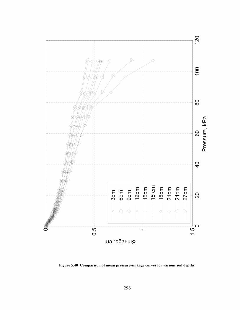
296
Figure 5.40 Comparison of mean pressure-sinkage curves for various soil depths.
020
4060
8010
012
0
0
0.5 1
1.5
Pre
ssur
e, k
Pa
Sinkage, cm
3cm
6cm
9cm
12cm
15cm
15 c
m18
cm21
cm24
cm27
cm

297
Figure 5.41 Comparison of mean pressure-sinkage curves for various soil depths (focusing on the lunar pressure range).
05
1015
2025
3035
40
0
0.05 0.1
0.15 0.2
0.25 0.3
Pre
ssur
e, k
Pa
Sinkage, cm
3cm
6cm
9cm
12cm
15cm
15 c
m18
cm21
cm24
cm27
cm

298
In an effort to better understand the effect of plate size and depth of soil on settlement of
and stress distribution underneath a circular plate a theoretical analysis for the settlement
of circular footings in sand was performed. This analysis was based on the Boussinesq
stress distribution within a soil mass resulting from vertical surface loading and
settlement based on linear-elastic theory and the Schmertmann method for sandy soil. An
in depth discussion on these topics can be found in McCarthy (2002) and Das (2004).
The initial assumptions made in this analysis are as follows. A schematic of the problem
statement is displayed in Figure 5.42 below.
• The soil behaves elastically and experiences uniform soil properties throughout the
sample, i.e. is a homogeneous isotropic material.
• The influence of the rigid base on the stress distribution is ignored so that
Boussinesq’s equation for vertical stress underneath the center of a flexible circular
foundation is applicable.
• The settlement at the center of the footing is calculated and is treated as a one-
dimensional problem.
• r is the radius of the footing, Ho is the thickness of the soil layer, q is the applied
pressure or load intensity, z is the respective coordinate under the centerline of the
circular foundation, and S is the settlement of the footing.

299
Figure 5.42 Schematic for the approximate solution of the settlement of a circular footing under
uniform loading.
Following Boussinesq’s formulation, the stress increase at a depth z (in the center of the
footing) is,
( ) ⎥
⎥⎦
⎤
⎢⎢⎣
⎡
+−=
⎪⎪⎪
⎭
⎪⎪⎪
⎬
⎫
⎪⎪⎪
⎩
⎪⎪⎪
⎨
⎧
⎥⎥⎦
⎤
⎢⎢⎣
⎡⎟⎠⎞
⎜⎝⎛+
−=Δ2
322
3
23
21
1
11zr
zq
zr
qσ (75)
Following linear elastic theory, for a small thickness of soil z∂ at depth z, the settlement
due to σΔ is,
zE
S ∂⋅Δ
=∂σ (76)
z
Ho
0
q
r r
Rigid Foundation
Soil

300
where E is the elastic modulus or Young’s modulus of the soil. The settlement of the
entire soil layer can thus be determined by integrating equation (76) over the thickness of
the soil layer, Ho, as follows,
∫ ∂Δ
=oH
SE
S0
σ (77)
⎥⎥⎦
⎤
⎢⎢⎣
⎡
+−+−+=
20
2
220
20 2
HrrHrrH
EqS (78)
From equation (78), relationships between the depth of the soil (or soil thickness), the
radius of the footing (or penetration plate), and settlement can be determined. More
specifically, the following questions can be answered:
1. For a fixed soil depth, how does the plate size (radius) affect the settlement?
2. For a fixed plate size (radius), how is the settlement affected by the thickness of
the soil layer (soil depth)?
Normalizing the plate radius r with the soil thickness H0 the following relationships can
be determined and plotted as shown in Figure 5.43:
0H
rc = (79)

301
1
1212
22
0+
−+−+=⋅ c
ccc
EqH
S (80)
Several conclusions can be drawn based on Figure 5.43. First, it can be seen that the
larger the plate radius the larger the settlement for a certain contact stress q. More
specifically, as the plate radius increases, settlement increases trending towards a
maximum potential settlement at which point the increase in the size of the plate no
longer has an affect on the settlement. Secondly, as the soil thickness increases, the size
of the plate radius needed to reach maximum potential settlement increases. This makes
sense based on the theory of the pressure bulb for which a larger plate is required to
create stress deeper in the soil. Also, for a fixed value of c, settlement is proportional to
the soil thickness. This implies that settlement increases by a factor of x when r and H0
are simultaneously increased by x. Additionally, it can be estimated that for a fixed value
of soil thickness, the plate radius must be approximately 2.2 times the soil thickness in
order to achieve 98-percent of the maximum potential settlement. However, it should be
noted that in order for these relationships to hold true, the value of q/E must be much less
than unity.

302
0%
10%
20%
30%
40%
50%
60%
70%
80%
90%
100%
0.0 0.5 1.0 1.5 2.0 2.5 3.0 3.5 4.0 4.5 5.0
Plate Radius / Soil Thickness
Settl
emen
t / (q
/E *
Soi
l Thi
ckne
ss)
Figure 5.43 For a fixed soil thickness, how does the plate size affect settlement?
Similarly, normalizing the soil thickness H0 with the plate radius r the following
relationships can be determined and plotted as shown in Figure 5.44:
r
Hd 0= (81)
( )2
2
122
ddd
Eqr
S+
+−++=
⋅ (82)
Several conclusions can be drawn based on Figure 5.44. First, it is obvious that the larger
the soil thickness the larger the settlement for a certain contact stress q. More
specifically, as the soil thickness increases, the settlement increases trending toward a
maximum potential settlement at which point the increase in soil thickness has no affect

303
on the settlement. Secondly, as the size of the plate increases, the soil thickness needed
to achieve the maximum potential settlement increases. This again makes sense based on
the pressure bulb theory. Additionally, for a fixed value of d, the settlement is
proportional to the plate radius. This implies that the settlement increases by a factor of
y, when r and H0 are simultaneously increased by y. This also implies that increased
settlement is always possible for a given soil type and contact stress, i.e. settlement can
always be increased by simultaneously increasing the plate size and soil depth. Finally, it
can be observed that for a fixed radius, in order to achieve 98-percent of the maximum
potential settlement, the soil thickness must be approximately 37-times the plate radius.
This means that for the rigid polypropylene soil bin used for plate-sinkage testing at
NASA Glenn, which has the capability of supporting a maximum soil thickness of 30 cm,
the maximum penetration plate size that can be used in order to achieve 98-percent of the
maximum potential settlement is approximately 1.6 cm in diameter. This is an extremely
small plate size and is smaller than the smallest penetration plate available for use in
bevameter testing at GRC which has a diameter of 5.1 cm.

304
0%
10%
20%
30%
40%
50%
60%
70%
80%
90%
100%
0 20 40 60 80 100 120 140
Soil Thickness / Plate Radius
Settl
emen
t / (q
/E *
Pla
te D
iam
eter
)
Figure 5.44 For a fixed radius, how does the soil thickness affect settlement?
Comparing the test results from the 10.2 cm diameter pressure-sinkage bevameter tests to
the theoretical curves of Figure 5.43 and 5.44, it is clear that the test results do not
necessarily follow the general trends expected from theory. Re-plotting the data from
Figure 5.40 in terms of soil thickness (soil depth) and settlement (sinkage) for various
applied pressures, as shown in Figure 5.45, clarifies the previous statement. It can be
seen in Figure 5.45 that as the soil thickness is increased, the settlement does not increase
in the general trend expected as shown in Figure 5.44. Instead, there exist several
undulations in the trend in which the settlement increases and then decreases and then
increases and decreases again, with increasing soil depth. These undulations appear to be
more intense for higher pressures. Figure 5.46 shows the same data normalized with
plate radius (as well as with the ratio of stress to elastic modulus) and compared to the
theoretical trend as shown in Figure 5.44. It is important to note that a value of 645 kPa
was used for the elastic modulus of GRC-1 as estimated from the stress-strain curves of

305
previous triaxial tests on this material15. With the normalization, the data from the
pressure-sinkage tests using the 10.2 cm diameter penetration plate should have
converged and formed a similar trend as shown by the theoretical line in Figure 5.45.
Clearly the experimental data does not follow the theoretical expectations.
0.00
0.20
0.40
0.60
0.80
1.00
1.20
1.40
3 6 9 12 15 18 21 24 27
Soil Thickness, cm
Settl
emen
t, cm
10 kPa 20 kPa 30 kPa 40 kPa 60 kPa 70 kPa
80 kPa 90 kPa 100 kPa 110 kPa
Figure 5.45 Reformulated data from pressure-sinkage tests performed using the 10.2 cm diameter
penetration plate.
15 It should be noted that this value for elastic modulus of a medium dense sandy soil is much lower than suggested by the CRC Handbook of Engineering Tables (Dorf 2004), which suggests a range of 17 to 28 MPa for medium dense sandy soil.

306
0%
10%
20%
30%
40%
50%
60%
70%
80%
90%
100%
0 1 2 3 4 5 6 7
Soil Thickness / Plate Radius
Settl
emen
t / (q
/E *
Pla
te D
iam
eter
)
10 kPa 20 kPa 30 kPa 40 kPa 60 kPa 70 kPa80 kPa 90 kPa 100 kPa 110 kPa Theory
Figure 5.46 Normalized reformulated data from pressure-sinkage tests preformed using the 10.2 cm diameter penetration plate compared with theoretical trend for settlement.
In conclusion, it can be stated that the behavior of GRC-1 under pressure-sinkage tests is
not appropriately described by the semi-empirical theory of linear-elastic deformation. It
is possible that the behavior of GRC-1 under pressure-sinkage tests could better be
described using plastic theory for deformation. This however is not in the scope of work
and will not be covered. Thus, even though the relationships between soil thickness,
plate size, and settlement are better understood, no clear assessment can be made as to the
minimum soil depth required to eliminate bottom boundary effects. Therefore, a
judgment call was made, based on a combination of soil preparation time and
recommendations from Bekker, Wong, and Pavlics (as previously discussed) and
traditional soil mechanics theory; that a conservative soil depth for all future bevameter

307
testing should be no less than 24 cm (for a maximum penetration plate size of 19 cm in
diameter).
5.2.3 End Effector Requirements
As previously discussed, the term end effector is used to describe the part of the
bevameter that penetrates the terrain or soil. The end effectors of the table bevameter are
mounted either directly to the base of the load/torque cell or to the end effector mount
which is attached to the base of the load/torque cell. There are three major categories of
end effectors that can be used with the table bevameter, two of which are solely used for
pressure-sinkage and shear tests. The first category of end effectors are cones such as the
type used in cone penetration tests. This type is not used for testing of GRC-1 and will
therefore not be discussed in further detail. The second category of end effectors is
penetration plates. Penetration plates are rigid metal discs that connect to the end effector
mount as shown in Figure 5.3. These plates are pushed into the ground during pressure-
sinkage tests in order to measure the ground compaction resistance. In order to minimize
the shearing resistance caused by the sidewall of the plate, the outer edge of all plates
should be a maximum of 5 mm thick. In addition, the plates should be rigid enough so as
not to deflect more than a few millimeters in the worst case scenario. The diameter of the
penetration plates are determined based on the ground contact area that bounds the wheel
sizes of the prospective lunar exploration vehicles being considered. Currently three
different lunar exploration vehicles are being considered for operation in future missions
to the Moon. The first is a replica of the original lunar roving vehicle. The second is the

308
Mobile Lander with ATHLETE (All-Terrain Hex-Legged Extra-Terrestrial Explorer)
robotic vehicle mobility system designed by the Jet Propulsion Laboratory (JPL) in
California. The ATHLETE, as shown in Figure 5.47, is designed with the capabilities of
rolling over Apollo-like undulating terrain and "walking" over exceptionally rough or
steep terrain so that robotic or human missions on the surface of the Moon can load,
transport, manipulate, and deposit payloads to essentially any desired sites of interest.
Figure 5.47 ATHLETE robotic vehicle designed by JPL (credit NASA).
The third exploration vehicle being considered for operation in future missions to the
Moon is the Chariot “lunar truck” as shown in Figure 5.48. Developed by NASA’s
Exploration Technology Development Program's Human-Robotics Systems Project, the
Chariot features 12 wheels driven by two electric motors through a two-speed
transmission. The modular design consists of a steel alloy frame which can be fitted with
several different crew/payload combinations, including a small pressurized cabin and a

309
sample collector. The current estimated nominal tire load and ground contact area of
these prospective vehicle are summarized in Table 5.2 below16.
Figure 5.48 Chariot lunar truck vehicle (credit NASA).
Table 5.2 Current design properties of various prospective lunar exploration vehicles.
LRV17 (NASA)
ATHLETE(JPL)
Chariot (NASA)
Contact Area, cm2 353 800 800 Design Load, kN 0.254 2.18 0.55
Design Pressure, kPa 7.2 27.25 6.88 Based on these current design parameters three different penetration plate sizes were
chosen for pressure-sinkage testing. These plate sizes include a 7.6 cm diameter plate
corresponding to a contact area of 45.36 cm2; a 10.2 cm diameter plate corresponding to a
16 These design parameters are not absolute and are subject to change at any time. The parameters listed are the most current parameters to date. 17 It is important to note that these values as listed in Table 5.2 for the LRV are based on the design load and contact area. However, after operation of the LRV during the Apollo 15 mission, it was learned that the nominal wheel load was actually 0.2885 kN which was supported by only 43.3 cm2 of the wheel contact area (Personal communication with Vivake Asnani, 19 Feb 2008).

310
contact area of 81.71 cm2; and a 19 cm diameter plate corresponding to a contact area of
283.53 cm2. These plates are shown in Figure 5.49 below. This approximately covers
the range of contact areas experienced by the LRV (as noted in Footnote 17). However
the upper range of contact areas expected to be experienced by the ATHLETE and
Chariot could not be met due to limitations imposed by the size of the soil bin as
discussed in the preceding section as well as loading limitations of the table bevameter
(in order to meet the maximum expected contact pressure).
Figure 5.49 Penetration plates used in pressure-sinkage bevameter tests.
The third and final category of end effectors includes the shear rings for shear bevameter
testing. The shear ring is a metal annulus shaped plate that may or may not have evenly
spaced, radially oriented grousers. During the shear test, a constant normal load is
applied and the shear ring is rotated at a constant velocity. During the test, the grousers
move or shear the soil, so that the internal soil shear resistance is measured. If the shear
ring does not have grousers, then the metal-soil (or material-soil) shear resistance is
measured. Typically, grousers are implemented to determine the internal shear strength

311
of the soil whereas shear rings lined with rubber, sandpaper, or various other materials
are implemented to determine the shearing characteristics between the material
(representative of the material composing the exterior of the wheel) and the soil or
terrain. Due to the fact that the soil “flows” during shear testing, the shear ring will
ultimately sink. Therefore the shear rings are designed to be mounted on a “cup” which
has ample clearance so as not to impede the sinkage. The dimensions of the shear rings
selected for shear bevameter testing were based on four main considerations. These
include: soil bin boundary effects which ultimately limited the size of the penetration
plates as previously described; the ground pressure range that bounds the vehicles being
considered; shear ring geometry effects that occur due to forcing the failure to shear in a
rotational rather than linear fashion and cause the soil failure to occur outside the
direction of motion (typically larger shear rings eliminate this effect); and the ground
contact area that bounds the vehicles being considered. Based on the size of the soil bin
as discussed in the previous section, as well as the loading limitations of the table
bevameter, a shear ring with outer diameter of 17.9 cm and inner diameter of 14.0 cm
was selected with corresponding normal loads ranging from 5 to 30 kg. This provides a
contact area of 97.71 cm2 with contact pressures ranging from 5.02 to 30.1 kPa.
Although this size ring does not correspond to the contact areas of any of the above
proposed lunar vehicles, it is more important to simulate the range of ground pressures, as
shown in Table 5.2, which is successfully achieved with this shear ring. Two different
finishes were used on this shear ring for shear bevameter testing. The first finish
consisted of the shear ring lined with a low grit sandpaper to simulate the material-terrain
shear interaction of several prototype wheels currently being tested at the NASA Glenn

312
Research Center. The second finish consisted of the shear ring with attached grousers
having a height of 0.5 cm, a width equal to that of the annular shear ring (1.95 cm), and a
thickness of 0.2 mm, spaced equally around the shear ring at intervals of 20-degrees.
This was used to determine the internal shear strength of GRC-1. The shear ring with
grousers is shown in Figure 5.50(a) and Figure 5.50(b) below.
(a) (b) Figure 5.50 (a) Bottom view of shear bevameter ring with grousers. (b) Angular view of shear
bevameter ring with grousers.
5.3 PRESSURE-SINKAGE TEST FOR VEHICLE MOBILITY
The bevameter test designated to simulate the normal loads exerted by a vehicle on the
terrain surface is the pressure-sinkage or plate-sinkage test (used interchangeably
throughout this dissertation). The results of the pressure-sinkage test allow for the
prediction of vehicle sinkage and motion resistance to the compaction of the terrain. In
the pressure-sinkage test, various sizes of plates are used to simulate the range of possible
contact area of a vehicle wheel or track on the soil surface, and both the penetration force
and the corresponding sinkage are recorded. Typically, penetration speed is kept at low

313
rates of approximately 1 cm/s in order to reduce dynamic effects of the system (Chen
1993). However, the table bevameter is designed to operate in a static type fashion as the
penetration is manually controlled as dead weights are incrementally placed on the shaft
of the bevameter by the operator. The pressure on the penetration plate is obtained by
dividing the penetration force by the contact area of the plate as shown in the following
equation,
2rLp⋅
=π
(83)
where p is the normal pressure, L is the penetration force, and r is the radius of the
penetration plate. Contact pressure is more or less closely related to deflection and load.
Thus, it is extremely important to ensure that the entire surface area of the penetration
plate is in contact with the soil.
A single bevameter test is not generally reliable for extrapolative purposes. Multiple
penetration tests are needed due to the small chance of a given measurement being
reliable. In the case of bevameter tests on actual terrain, multiple measurements are
needed over a large area of the terrain for the reason previously mentioned and to ensure
representative results of the entire terrain. However, a single bevameter plate-sinkage
test is useful in the case that it is used in conjunction with other experiments. For
example, if it is known that the soil is homogeneous via additional testing methods (such
as the cone penetrometer test), then the quantitative data from the single bevameter test
would enable the establishment of reasonable limits for the soil constants (Hinners 1964).

314
Bekker (1969) recommends a minimum of two to three pressure-sinkage curves produced
by plates of two or three sizes for soil characterization. Bekker states that this amount of
testing is appropriate for a practical evaluation of the error caused by differences in
penetration plate size and the vehicle’s ground contact areas as well as errors due to
instrumentation and random nonhomogeneities of the soil.
The pressure-sinkage relationship used in this dissertation is the equation proposed by
Bekker (1969), which was defined in equation (4). For clarity the Bekker equation takes
the following form:
nc zkbk
p ⋅⎥⎦⎤
⎢⎣⎡ += φ (84)
where p is the pressure and z is the sinkage, ck and φk are moduli of deformation with
respect to cohesion and friction, b is the contact width of a rectangular plate or the radius
of a circular plate, and n is the empirical soil value which defines the shape of the load-
penetration curve (Bekker 1962, 1969). ck , φk , and n are otherwise known as the terrain
constants. In order to process the experimental data, namely the pressure p and sinkage z
curves, obtained from the plate-sinkage bevameter tests to determined the terrain
constants, Wong’s (1980) weighted least squares method is employed. This method was
originally derived as reflected in equations (10) through (14) of section 1.6.1.1, Bearing
Capacity, for bevameter tests using two different plate sizes. Again for clarity, Wong’s

315
method for data processing derives the best fitted values of the pressure-sinkage terrain
parameters by minimizing the following function using a weighting factor p2,
( )[ ]∑ −+−= 22 ln/lnln znkbkppF c φ (85)
Minimization of equation (85) involves taking the partial derivatives of the function with
respect to n and eqk , where ( )φkbkk ceq += / , and setting them equal to zero. Solving
the resulting equations simultaneously gives rise to the following equations for n and eqk .
( ) ( )∑ ∑ ∑
∑ ∑ ∑ ∑−
−= 22222
2222
lnln
lnlnlnln
zpzpp
zpppzpppn (86)
∑
∑ ∑−= 2
22 lnlnln
pzpnpp
keq (87)
When using two different plate sizes a unique n is usually obtained for each. Therefore,
it is required to use the average n-value resulting from the two different plates when
calculating eqkln in equation (87). However, since ( )φkbkk ceq += / there will be two
resulting eqk -values, one for plate size b1 and another for plate size b2. Accordingly, the
values of ck and φk can be determined using the following equations, equations (88) and
(89). It should be noted that these equations were derived based on two plate sizes, but
can easily be modified to account for a third plate size using a lest squares approach.

316
( ) ( )
2112
21 bbbbkk
k beqbeqc −
−= (88)
( ) ( ) ( )2
12
211
bbbkk
kk beqbeq
beq ⎥⎦
⎤⎢⎣
⎡
−
−−=φ (89)
The initial characterization of GRC-1 was determined by performing a total of 15
pressure-sinkage tests. Five repeat tests were conducted using a penetration plate size of
7.6 cm in diameter. Five repeat tests were conducted using a penetration plate size of
10.2 cm in diameter. The final five repeat tests were conducted using a penetration plate
size of 19 cm in diameter. All tests were conducted in the 74.2 cm square polypropylene
soil bin at a soil depth of 24 cm. The test procedure followed for all pressure-sinkage
tests for the determination of the soil parameters for GRC-1 is discussed in the following
section.
5.3.1 Experimental Procedure
The following experimental procedure was used for pressure-sinkage bevameter testing
to determine the Bekker soil parameters of GRC-1:
1. Prepare GRC-1 to a depth of 24 cm in the 74.2 cm square rigid polypropylene soil
bin (using the hopper method) to a density of 1.67 g/cc (24-percent relative
density).
2. Collect plate-load and sinkage data as usual, using a load cell and LVDT,
respectively.

317
3. Physically balance the penetration plate (using the counter balance platform as
shown in Figure 5.3) and then lower the penetration plate until it just touches the
soil surface (ensuring that the penetration plate is near the center of the soil bin).
Electrically balance the load cell and offset the LVDT data so that the output now
corresponds to zero load and zero sinkage.
4. Place weights on the bevameter load platform (as shown in Figure 5.3) in
increments of 1 kg until 10 kg (to get good resolution at small loads and
sinkages), then in increments of 2 kg until 20 kg, and 5 kg until 65 kg is reached.
If additional load is necessary continue in increments of 9 kg (20 lb weights) until
failure, which occurs when the plate “punches” through the soil.
5. Repeat steps 1 through 4 a total of 5 times for each penetration plate size, using
penetration plate sizes of 7.6 cm, 10.2 cm, and 19 cm diameters.
In the data processing steps, the variable i represents the penetration plate number
( [ ]3,1∈i ) where 1 is representative of the 7.6 cm diameter plate, 2 is representative of the
10.2 cm diameter plate, and 3 is representative of the 19 cm diameter plate; and j
represents the test number index ( [ ]5,1∈j ). For each of the five repeat tests performed
with the ith penetration plate, the same loads were applied. However, the resulting force
varied slightly because of friction in the bevameter system. To correct for this minor
variation, a cubic spline18 was used to resample the sinkage data for each plate size to a
common and uniformly spaced pressure vector pi. The resulting sinkage data was stored
18 In MATLAB, the cubic spline is constructed of piecewise third-order polynomials which pass through a set of control points. The second derivative of each polynomial is commonly set to zero at the endpoints to provide a boundary condition that completes the system of equations. This creates a cubic spline which leads to a simple tridiagonal system that can be solved easily to give the coefficients of the polynomials.

318
in vectors zij. Using these vectors19, the ensemble mean and ensemble deviations were
calculated as follows, respectively:
∑=
=n
jiji n 1
1 zz (90)
∑=
−⋅−
=n
jiiji n 11
1ˆ zzz (91)
where n is the total number of observations. Using the new pressure vectors pi and the
mean sinkage vectors iz , equations (86) through (89) are employed to determine ni and
ieqk for each corresponding plate size. Following a least squares approach20, ck and
φk are determined as follows (using navg including all three plates):
bxA =⋅ (92)
bAx \= (93)
Where,
⎥⎥⎥
⎦
⎤
⎢⎢⎢
⎣
⎡=
111111
3
2
1
bbb
A , ⎥⎥⎥
⎦
⎤
⎢⎢⎢
⎣
⎡
=
3
2
1
eq
eq
eq
kkk
b , and ⎥⎦
⎤⎢⎣
⎡=
φkk
x c
19 In this sense the term “vector” is intended to represent a column array. 20 As implemented in MATLAB.

319
Finally, with the values of values of ck , φk , navg, and bi, the Bekker curve-fit was applied
to each corresponding data set following equation (84) and the goodness-of-fit of this
curve-fit to the data set was calculated using equation (15). The corresponding
MATLAB code for the data processing is provided in Appendix D.
5.3.2 Test Results and Analysis
Initial pressure-sinkage tests for the determination of the Bekker soil parameters of GRC-
1 were performed using three plate sizes as previously stated; 7.6 cm diameter, 10.2 cm
diameter, and 19 cm diameter. The results of these tests on GRC-1 prepared to a density
of 1.67 g/cc or 24-percent relative density are shown in Figures 5.51 and 5.52 below. It
is important to note that although data was collected to pressures exceeding those shown
in the plots below (for the small and medium sized penetration plates), the pressure range
over which the data was evaluated was selected to represent the range of expected ground
pressures from lunar exploration vehicles on the Moon. Figure 5.51 displays the raw data
collected from each of the five repeat tests for each penetration plate; as well as the mean
pressure-sinkage curve for each data set. The maximum standard deviations of these
pressure-sinkage curves are 0.5 mm, 0.4 mm, and 0.8 mm, for the 7.6 cm, 10.2 cm, and
19 cm plate, respectively. Figure 5.52 displays the results of Bekker curve-fit and soil
parameters. As can be seen, the Bekker curve-fit corresponds to the experimental data
very well. The “goodness-of-fit” as determined by equation (15) was 0.069 for the 7.6
cm diameter plate, 0.143 for the 10.2 cm diameter plate, and 0.249 for the 19 cm
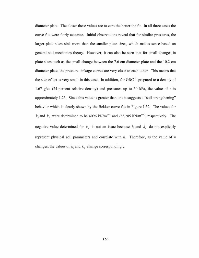
320
diameter plate. The closer these values are to zero the better the fit. In all three cases the
curve-fits were fairly accurate. Initial observations reveal that for similar pressures, the
larger plate sizes sink more than the smaller plate sizes, which makes sense based on
general soil mechanics theory. However, it can also be seen that for small changes in
plate sizes such as the small change between the 7.6 cm diameter plate and the 10.2 cm
diameter plate, the pressure-sinkage curves are very close to each other. This means that
the size effect is very small in this case. In addition, for GRC-1 prepared to a density of
1.67 g/cc (24-percent relative density) and pressures up to 50 kPa, the value of n is
approximately 1.23. Since this value is greater than one it suggests a “soil strengthening”
behavior which is clearly shown by the Bekker curve-fits in Figure 1.52. The values for
ck and φk were determined to be 4096 kN/mn+1 and -22,285 kN/mn+2, respectively. The
negative value determined for φk is not an issue because ck and φk do not explicitly
represent physical soil parameters and correlate with n. Therefore, as the value of n
changes, the values of ck and φk change correspondingly.

321
Figure 5.51 Raw data and mean pressure-sinkage vector for 7.6, 10.2, and 19 cm penetration plates.
05
1015
2025
3035
4045
50
0 1 2 3 4 5 6 7 8 9 10
Pres
sure
, kN/
m2
Sinkage, mm
7.6
cm P
late
10.2
cm
Plat
e
19 c
m P
late

322
Figure 5.52 Raw data compared to Bekker curve-fit.
05
1015
2025
3035
4045
50
0 1 2 3 4 5 6 7 8 9 10
Pres
sure
, kN/
m2
Sinkage, mm
7.6
cm P
late
10.2
cm
Plat
e
19 c
m P
late
n =
1.23
2, k
c =
4096
.353
7 kN
/mn+
1 , kph
i = -2
2284
.578
6 kN
/mn+
2

323
For comparison with the Bekker curve-fits over the entire range of data (not just the lunar
range) collected for the three penetration plates, Figure 5.53 is shown below. As can be
seen, the Bekker curve-fits are not as good as for the lunar pressure range. The
“goodness-of-fit” now ranges from 0.466 to 0.794 which is much greater than the
goodness-of-fit for the lunar range and is significantly higher than zero. This is most
likely due to the large amount of scatter in the data that is seen in the higher pressure
ranges, especially for the 7.6 cm plate. The maximum standard deviation for the
pressure-sinkage curves over the entire pressure range were 12 mm, 1.6 mm, and 1.7 mm
for the 7.6 cm, 10.2 cm, and 19 cm plate, respectively. These values are much larger than
experienced over the lunar pressure range. During the repeat tests for the 7.6 cm
diameter plate a few tests actually experienced soil failure, where the plate “punched”
through the soil as shown in Figure 5.54(b). Punching shear is typical for compressible
soil such as sands having low relative density and being subjected to significant bearing
pressure. The other tests experienced general shear failure and therefore did not sink to
such great extents. As a result, the scatter in the data is very large and the mean pressure-
sinkage curve may not have been truly representative of a 7.6 cm plate bearing on GRC-1
at 24-percent relative density. As such, the Bekker parameters show a “soil weakening”
condition where n is less than one as compared to the soil strengthening condition over
the lunar pressure range. For the complete pressure range tested, the n value of GRC-1 is
approximately 0.81. The values for ck and φk were determined to be approximately 97
kN/mn+1 and 1744 kN/mn+2, respectively.

324
Figure 5.53 Bekker curve-fits for entire range of data.
020
4060
8010
012
014
016
0
0 5 10 15 20 25
Pres
sure
, kN/
m2
Sinkage, mm
7.6
cm P
late
10.2
cm
Plat
e
19 c
m P
late
n =
0.80
563,
kc
= 97
.06
kN/m
n+1 , k
phi =
174
4.24
95 k
N/m
n+2

325
(a) (b) Figure 5.54 (a) Typical amount of sinkage for 19 cm diameter plate (as shown by resulting
impression in GRC-1). (b) Punching shear failure of 7.6 cm diameter plate (plate is completely submerged in GRC-1, just the end effector mount is visible).
It is difficult to directly compare these soil parameters for GRC-1 with typical values for
dry sandy soil found in the literature. This is because most cases of pressure-sinkage
bevameter tests were conducted in the field on “terrain” instead of in laboratory
conditions of manually prepared “soil”. Therefore, the density corresponding to these
sandy terrains were not determined or not reported and the Bekker parameters presented
are representative of that specific type of terrain, not a specific density of a soil.
Nevertheless, typical Bekker parameters for dry sandy terrains are presented in Table 5.3.
As can be seen, the value of n obtained for GRC-1 is definitely comparable to typical
sandy terrain parameters determined by previous investigators.
Table 5.3 Typical Bekker parameters for dry sand.
n kc, kN/mn+1
φk , kN/mn+2 Source
0.6 0 624.6 NASA 1970 0.793 102 5301 Wong et al. 1984 0.8 0 520.8 NASA 1970 0.93 118 8501 Wong 1980 1.1 0.99 1528.43 Wong 2001 1.29 -27.83 3579.8 Sela and Ehrlich 1972 1.68 29.31 8378.5 Chen 1993

326
In order to compare the general trend of the pressure-sinkage curves obtained for GRC-1
with those from the previous researchers listed in Table 5.3, i.e. the Bekker parameters
determined by these investigators were used to derive pressure-sinkage curves following
the experimental parameters of the tests performed on GRC-1 (7.6 cm , 10.2 cm, and 19
cm plate diameters). The closest parameters to those of the parameters obtained for
GRC-1 over the entire pressure range21 were Wong et al.’s (1984). Thus, these
parameters were selected to directly compare to GRC-1. The results are shown in Figure
5.55. As can be seen, the general trends are very similar, i.e. for similar pressure, the
larger plates sink more than the smaller plates; and both show the general trend of “soil
weakening”. However, GRC-1 appears to be weaker than the dry sandy terrain as tested
by Wong et al. (1984). It is difficult to make a definite conclusion as to why, but most
likely the terrain was more compact and therefore denser than GRC-1 prepared to a
density of 1.67 g/cc or 24-percent relative density.
21 The Bekker parameters for the entire pressure range of GRC-1 were selected for this analysis (over those for the lunar pressure range) because typical pressure-sinkage tests in terrestrial terrain were evaluated over much larger pressure ranges. Thus, it was felt that parameters over this pressure range would be more comparable to parameters obtained from previous investigations on dry sandy terrain.

327
0 100 200 300 400 500 600
0
5
10
15
20
25
30
35
40
GRC-1
Wong et al. 1984
Pressure, kN/m2
Sin
kage
, mm
Figure 5.55 Comparison of GRC-1 Bekker parameters and parameters derived by Wong et al.
(1984) for a dry sandy terrain. Additional plate-sinkage tests were performed on GRC-1 prepared to various densities so
that a general relationship or better understanding of the relationship between the Bekker
parameters and relative density of GRC-1 could be determined. A total of nine new tests
were completed. These tests were performed following the same procedure as the
previous pressure-sinkage tests on GRC-1. However, only a single test was performed
for each plate size rather than the five repeat tests. Although Bekker recommends a
minimum of at least two repeat tests, Hinners (1964) as previously stated, suggests that a
single bevameter plate-sinkage test is useful in the case that it is used in conjunction with
other experiments. The results from a single bevameter test on GRC-1 can be compared
to the results of cone-penetration tests on GRC-1 to establish reasonable limits for the soil
parameters as will be discussed in subsequent chapters. Additionally, as a measure to

328
save time and increase reliability of the soil density a new soil bin was used. This soil
bin was a clear acrylic soil bin with a wall thickness of 1.27 cm (0.5 in). It is extremely
rigid compared to the previous soil bin. Thus, it ensures that no bowing out of the bin
walls will take place during soil preparation or testing (which could affect the soil
density). Additionally, since the bin is clear, it has the advantage of visually ensuring a
level soil surface at the desired height. This bin, as shown in Figure 5.56, has an inner
diameter of 59.7 cm (23.5 in), which is over three times the diameter of the largest plate
(19 cm), and has a height of 30.5 cm (12 in). GRC-1 was again prepared to a depth of 24
cm, but was prepared to densities of 1.64 g/cc, 1.67 g/cc, and 1.75 g/cc or 14, 24, and 52-
percent relative density, respectively. It was found to be increasingly difficult to
uniformly prepare GRC-1 to densities greater than 1.75 g/cc. Test results are shown in
Figure 5.57 through Figure 5.59 together with the corresponding Bekker curve-fits over
the lunar pressure range. The soil parameters are summarized in Table 5.4.
Figure 5.56 Clear acrylic soil bin.

329
0 5 10 15 20 25 30 35 40 45 50
0
1
2
3
4
5
6
7
8
9
10
Pressure, kN/m2
Sin
kage
, mm
19 cm Plate10.2 cm Plate
7.6 cm Plate
n = 0.95024, kc = 221.2618 kN/mn+1, kphi =1957.5095 kN/mn+2
Figure 5.57 Pressure-sinkage curves for GRC-1 at 1.64 g/cc.
0 5 10 15 20 25 30 35 40 45 50
0
1
2
3
4
5
6
7
8
9
10
Pressure, kN/m2
Sin
kage
, mm
19 cm Plate
10.2 cm Plate
7.6 cm Plate
n = 1.0119, kc = 649.6448 kN/mn+1, kphi =-1199.1232 kN/mn+2
Figure 5.58 Pressure-sinkage curves for GRC-1 at 1.67 g/cc.

330
0 5 10 15 20 25 30 35 40 45 50
0
1
2
3
4
5
6
7
8
9
10
Pressure, kN/m2
Sin
kage
, mm
19 cm Plate
10.2 cm Plate
7.6 cm Plate
n = 1.1107, kc = 1581.1504 kN/mn+1, kphi =-5139.1398 kN/mn+2
Figure 5.59 Pressure-sinkage curves for GRC-1 at 1.75 g/cc.
Table 5.4 Bekker parameters for GRC-1 at various densities.
Density (g/cc)
Relative Density (%) n kc, kN/mn+1 φk ,
kN/mn+2
Average Goodness
of Fit 1.64 14 0.95 221.26 1957.51 0.238 1.67 24 1.01 649.64 -1199.12 0.598 1.75 52 1.11 97.06 1744.15 0.282
As shown, the goodness-of-fit for the Bekker curve-fits to the raw pressure-sinkage data
for GRC-1 are relatively good. The n-values tend to increase with increasing density
going from a soil weakening condition at a low relative density to a soil strengthening
condition at mid relative densities. The ck and φk values show no obvious trends with
respect to density. However, these parameters are difficult to analyze as they are
dependent on the pressure, sinkage, and n. To check the validity of this data since it was

331
determined based on a single test, the test results for GRC-1 at 1.67 g/cc can be compared
to previous test results for GRC-1 at 1.67 g/cc based on multiple repeat tests. Recall that
for the lunar pressure range the Bekker parameters were 1.23, 4096 kN/mn+1, and -22,285
kN/mn+2 for n, ck , and φk , respectively, with an average goodness-of-fit of 0.154.
Compared to the new results for GRC-1 (1.01, 649.64 kN/mn+1, and -1199.12 kN/mn+2,
respectively, with an average goodness of fit of 0.598), the n value is much higher
therefore forcing ck and φk to be higher and lower, respectively; and the goodness-of-
fit is much better. This however, does not invalidate the new data. It simply suggests
two things: that the density of the material may have varied from test to test and may not
have been 1.67 g/cc in both cases; and that based on the goodness-of-fit, the Bekker
parameters from the repeat tests are more reliable than those from the single test. It has
been shown that the value of n is extremely sensitive to the soil density (Bekker, 1969).
Unfortunately, soil density is one of the most difficult soil parameters to control.
Based on the scatter naturally associated with bevameter plate-sinkage tests, it is difficult
to make a definite conclusion about the Bekker parameters of GRC-1. However, from
the results of the data collected over the lunar pressure range it is reasonable to assume
that the value of n is slightly greater than or equal to one for a loose to medium dense soil
preparation. Thus, GRC-1 is generally a strong soil and tends to “strengthen” as it
compacts. Additionally, under low pressures (up to 50 kPa) sinkage is expected to be
less than 10 mm (0.4 in) for contact areas ranging from 45 cm2 to 284 cm2. Therefore,
wheels operating in GRC-1 under very light loads produce relatively flat contact patches
and such small sinkage that, for practical purposes, that latter might be neglected.

332
Therefore, the “soil potential” available for the wheel to produce forward pull would be
equal to the horizontal force given by the Coulomb relationship and modified by
Micklethwait (1944) cited by Freitag et al. (2007), as described in section 1.6.1.2 of this
dissertation entitled Shear Strength. For clarity the equation is repeated as,
φtanWAcF += (94)
Where A is the contact area of the wheel and W is the vehicle weight or load. Thus, the
bevameter shear test is extremely important for the characterization of GRC-1 with
respect to lunar exploration vehicle mobility. The bevameter shear tests on GRC-1 are
discussed in the subsequent section.
5.4 SHEAR TEST FOR VEHICLE MOBILITY
The bevameter test designated to simulate the shear loads exerted by a vehicle on the
terrain surface is the shear test. The results of the bevameter shear test provide the basis
for the prediction of vehicle traction in a specific terrain. According to Bekker (1969),
“since one of the basic conditions for predicting vehicle performance is that the vehicle’s
shear action be simulated by instrument-predictor, the values of devices like the triaxial
shear apparatus has been questioned, inasmuch as their operation is too dissimilar to
actual conditions for developing vehicle thrust.” In the bevameter shear test, two
different types of shear rings are used. The first shear ring used is for measuring the
internal shear strength of the soil. It consists of a shear ring with grousers. The second

333
shear ring is used to measure the wheel material-terrain shearing characteristics. This
shear ring surface is covered with low grit sandpaper. For each different shear test,
various normal loads are applied on the shear ring to represent the range of normal
pressures expected to be experienced by the vehicle. During each test, the shear
displacement or the rotational distance traveled by the shear ring and the torque are
recorded. Additional information such as sinkage (slip-sinkage) and variation of the
normal load can be recorded as well. The shear stress of the soil according to Chen
(1993) is obtained by dividing the torque by the product of the contact area of the shear
ring and the average radius of the shear ring as shown in the following equation,
( )( )22
2 ioio rrrr
T
−+=π
τ (95)
where τ is the shear stress, T is the torque measured, and ro and ri are the outer and inner
radii of the shear ring, respectively. The shear stress (strength) of soil is heavily
dependent on the bulk properties of the soil such as the grain size distribution, bulk
density, cohesion, angle of friction, and grain shape and hardness. The shape of the soil
grains affects their ability to interlock which increases friction and shear strength. More
specifically, round or spherical particles typically flow easily while angular soil particles
or glass particles such as lunar agglutinates typically interlock and obstruct soil flow.
The shear strength of soils under load is directly related to friction between grains and
provides a measure of aggregate interlock and soil structure as well.

334
According to Bekker (1969), a minimum of three shear tests at different normal pressures
(within the range of ground pressure expected to be exerted from the wheels of a vehicle)
is necessary to accurately determine the terrain parameters from stress-deformation
curves produced by shear bevameter tests. Moreover, he recommends a total of five tests
at various normal pressures, especially for investigations conducted in the field. It is
suggested to perform two repetitive tests in order to determine the size of discrepancy
between the two. Based on this information, the minimum number of tests can be
determined subjectively by the investigator. Generally, in a laboratory environment five
tests is sufficient to accurately determine the soil parameters. Since shear tests are less
sensitive to variation in density than pressure-sinkage tests, repeat tests usually show a
negligible scatter of data.
The stress-deformation or stress-displacement (used interchangeably) relationship used in
this dissertation is the exponential equation previously defined by equation (21),
proposed by Janosi and Hanamoto (1961). For clarity, the equation is as follows,
⎟⎟⎠
⎞⎜⎜⎝
⎛−=
−K
j
e1maxττ (96)
where maxτ is the maximum shearing stress or shear strength of the soil, j is the shear
displacement, and K is the shear deformation modulus of the soil which can be
considered a measure of the magnitude of the shear displacement required to develop the
maximum shear stress in a given soil. In order to obtain the shear parameters of the soil,

335
Wong’s (1980) weighted least squares principle is applied as previously described by
equations (23) through (25). Again, for clarity, Wong’s procedure as previously
described begins with taking the natural logarithm of both sides of equation (21). This
leads to the following function,
∑ ⎥⎦
⎤⎢⎣
⎡+⎟⎟
⎠
⎞⎜⎜⎝
⎛−⎟⎟
⎠
⎞⎜⎜⎝
⎛−=
2
max
2
max
1ln1KjF
ττ
ττ (97)
which must be minimized in order to determine the best value of K. Note that this
function has an applied weighting factor of ( )2max/1 ττ− . In order to minimize equation
(97), the first partial derivative of the function with respect to K is taken and set equal to
zero. This in-turn leads to the final equation which computes the optimum value of K in
order to minimize the error from the curve-fit.
[ ]∑∑
−−
−−=
)/1ln()/1()/1(
max2
max
22max
ττττττj
jK (98)
The initial characterization of GRC-1 was determined by performing a total of 18 shear
bevameter tests. Five shear tests at various normal pressures ranging from 5 kPa to 30
kPa (within the expected lunar pressure range and within limitations of the table
bevameter shear system) in order to determine the shear parameters of GRC-1 at a
specified density. A total of three complete test sets were performed: one at a density of
1.64 g/cc, a second at a density of 1.67 g/cc, and a final at a density of 1.75 g/cc, or 14,

336
24, and 52-percent relative density, respectively. Again, it was difficult to uniformly
prepare GRC-1 to densities greater than 1.75 g/cc. One repeat test set was performed for
a density of 1.67 g/cc at three various normal loads to check the repeatability of the tests.
All tests were conducted in the 59.7 cm diameter acrylic soil bin at a soil depth of 24 cm.
The shear ring used for these tests was an annular ring with an inner diameter of 14 cm
and an outer diameter of 17.9 cm, with the bottom surface covered with a low grit
sandpaper. The test procedure followed for all shear bevameter tests for the
determination of the soil parameters of GRC-1 is discussed in the following section.
5.4.1 Experimental Procedure
The following experimental procedure was used for shear bevameter testing to determine
the Bekker soil parameters of GRC-1:
1. Prepare GRC-1 to a depth of 24 cm in the 59.7 cm diameter rigid acrylic soil bin
(using the hopper method) to a predetermined density of 1.64, 1.67, or 1.75 g/cc.
2. Collect plate-load and sinkage data as usual, using a load cell and LVDT,
respectively. In addition, collect torque and angular displacement data using a
torque cell and potentiometer, respectively.
3. Physically balance the shear ring (using the counter balance platform as shown in
Figure 5.3) and then lower the shear ring until it just touches the soil surface
(ensuring that the shear ring is near the center of the soil bin). Electrically
balance the load/torque cell and offset the LVDT and potentiometer data so that
the output now corresponds to zero sinkage and zero displacement.

337
4. Place weights on the bevameter load platform (as shown in Figure 5.3) to obtain a
normal pressure of approximately 5 kPa. For the size shear ring used this
corresponds to 5 kg of normal force.
5. Shear the soil by rotating the shear ring using the new moment arms22 attached to
the top of the load/torque cell as shown in Figure 5.60. According to Bekker
(1969), the rate of deformation has little effect on the resulting soil strength.
Therefore, the rate of rotation is not critical as long as it is kept at a nearly
constant rate.
6. Repeat steps 1 through 4 a total of five times for increasing normal pressures of 5,
7, 10, 20, and 30 kPa (5, 7, 10, 20, 30 kg).
Figure 5.60 New manual rotation system attached to load/torque cell.
22 Originally the table bevameter was designed to be rotated manually using the shear wheel as shown in Figure 5.3. However through preliminary shear testing it was discovered that there was a significant amount of elasticity in the system which led to a slip-stick phenomenon. Essentially, the end effector or shear ring “sticks” in place until enough torque is generated to move it. The shaft and moment arm act like a spring coil, winding and then unwinding each time the end effector “sticks” in the soil. Therefore, the shaft, which was assumed to have the most elasticity, was bypassed and new moment arms were designed to be placed directly on the load/torque cell as shown in Figure 5.60. This new design eliminated the dynamic effects from the slip-stick phenomenon.
Moment Arms

338
In the data processing steps, the variable i represents the normal pressure number
( [ ]5,1∈i ) where 1 is representative of the 5 kPa normal pressure, 2 is representative of
the 7 kPa normal pressure, and so on. The resulting K values were stored in vectors Ki.
Using these vectors, the mean and standard deviations of K were calculated as follows,
respectively:
∑=
=n
iiK
nK
1
1 (99)
∑=
−⋅−
=n
iiKK
nK
111ˆ (100)
where n is the total number of observations, in this case five. Although equation (98)
provides the value of K that minimizes the error in curve-fitting, the optimum value of
maxτ is still unknown ( maxτ is not necessarily the maximum value of τ experimentally
obtained). Therefore, to obtain the optimum value of maxτ , an iterative procedure was
implemented. In this procedure a value for maxτ is approximated from the experimental
data. The value of K is obtained as previously described. The goodness-of-fit is then
evaluated using equation (25). If the goodness-of-fit is at its minimum possible value
(zero is a perfect fit) then the process is completed. However, if the goodness-of-fit is not
at its minimum value then a new maxτ is estimated based on the current information, and
the process is repeated and continued until the minimum goodness-of-fit is reached. The
resulting maxτ values are then stored in vectors imaxτ , while the corresponding normal

339
pressures are stored in vectors pi. Using the pressure vectors pi and the maximum shear
stress vectors imaxτ , the cohesion and friction angle of the soil at the specified density can
be obtained following the Mohr-Coulomb failure criterion (as described in equation (16))
and implementing a least squares approach. In this case,
bxA =⋅ (101)
bAx \= (102)
Where,
⎥⎥⎥⎥⎥⎥
⎦
⎤
⎢⎢⎢⎢⎢⎢
⎣
⎡
=
11111
5
4
3
2
1
ppppp
A ,
⎥⎥⎥⎥⎥⎥
⎦
⎤
⎢⎢⎢⎢⎢⎢
⎣
⎡
=
5
4
3
2
1
max
max
max
max
max
τττττ
b , and ⎥⎦
⎤⎢⎣
⎡=
cx
φtan
All data processing was performed in Microsoft Excel, the raw data for all shear tests is
provided in Appendix D.
5.4.2 Test Results and Analysis
Results of the initial shear tests performed on GRC-1 at relative densities of 14, 24, and
52-percent are shown in Figures 5.61 through 5.63. A typical failure envelope for

340
determining cohesion and friction angle is shown in Figure 5.64. It is important to note
that the curve-fits in Figure 5.61 through 5.63 were based on a K-value determined for
only the first 5 cm of the data. It was important to determine K so that curve-fits fit the
first 5 cm of data as best as possible. This distance was based on a maximum expected
slip for lunar exploration vehicles of 20-percent which directly affects the traction or
drawbar pull of a vehicle. Given the three prospective lunar vehicles: the LRV,
ATHLETE, and Chariot; the maximum contact length of the wheel on the ground surface
currently is approximately 27 cm. This corresponds to a shear displacement of
approximately 5 cm (under 20-percent slip). Therefore, it is important to best-fit the data
in this given range of shear displacement and extrapolate the curve-fit to shear
displacements beyond 5 cm. The resulting soil parameters are summarized in Table 5.5.
As shown, the average value of K tends to increase with increasing density of GRC-1.
This makes physical sense because when the density of a soil is higher, there will be
fewer voids to fill and it will therefore take a shorter shear displacement for the soil
particles to rearrange themselves and fill in the voids to ultimately reach a point where
the soil reaches its maximum shear strength. In addition, the increase in density tends to
have very little effect on the friction angle and cohesion of the soil. The friction angle
ranged from 33 to 34-degrees and the cohesion held steady near 0 kPa. Because the
friction angle and cohesion in this case are based on the interaction between the
sandpaper and the soil, these properties of friction angle and cohesion are not as sensitive
to the change in density. The negative values in cohesion are again a result of the
difficulties experienced in measuring cohesion when using the Mohr-Coulomb failure
criterion. As previously stated for the triaxial results, the determination of cohesion may

341
be difficult as a straight line extrapolation of the failure envelope back to the normal
stress of zero. It is more likely that the strength envelope is curved in the region of small
confining pressures. None-the-less, it is reasonable to assume, based on the results, that
the cohesion for GRC-1 is very small (on the order of 1 kPa or less). One final
observation is that the repeatability of the shear bevameter tests is very good as shown by
the repeat tests at 1.67 g/cc in Table 5.5. The average K-values varied by only 0.01 cm
while the friction angles varied by only 0.1-degree. This is especially good for the
variation in applied pressure experienced with the table bevameter system. It was found
that during the shear bevameter tests it was very difficult to control the normal load when
applying torque. In some cases the normal pressure varied by as much as 0.8 kPa
(typically it varied more for larger loads than for smaller loads) which is why some of the
resulting stress-displacement curves are not as smooth as they could or theoretically
should be. However, it is assumed that the overall trend is correct. Therefore, an average
value of normal load was used in the determination of the cohesion and friction angle
values. In an ideal situation, a shear bevameter should have a normal load controlled by
dead weights and a rotation controlled by a motor to avoid the variation of load due to
additional load or removal of load by manual rotation. However, it is not known if
bevameters of this type are better at controlling the normal load as the results of shear
tests found in the literature (by these types of bevameters) did not report on the normal
load or in most cases did not even have a load cell incorporated into the system to
monitor the normal load. The portable bevameter at NASA Glenn, which operated with
hydraulic load and motor controlled rotation, encountered many problems in holding a

342
constant normal load. In any case, this seems to be a common issue in shear bevameter
tests and would be a viable issue to look into in future research.
0
5000
10000
15000
20000
0.00 0.05 0.10 0.15 0.20 0.25
Shear Displacement, m
She
ar S
tress
, Pa
4.80 kPa Fitted 7.03 kPa Fitted 10.87 kPa
Fitted 19.89 kPa Fitted 29.01 kPa Fitted
Figure 5.61 Shear bevameter results for GRC-1 at 14-percent relative density.

343
0
2000
4000
6000
8000
10000
12000
14000
16000
18000
20000
0.00 0.05 0.10 0.15 0.20 0.25
Shear Displacement, m
She
ar S
tress
, Pa
4.94 kPa Fitted 7.10 kPa Fitted 10.22 kPa
Fitted 19.85 kPa Fitted 29.14 kPa Fitted
Figure 5.62 Shear bevameter results for GRC-1 at 24-percent relative density.

344
0
2000
4000
6000
8000
10000
12000
14000
16000
18000
20000
0.00 0.05 0.10 0.15 0.20 0.25
Shear Displacement, m
Shea
r Stre
ss, P
a
5.13 kPa Fitted 7.08 kPa Fitted 10.30 kPa
Fitted 19.72 kPa Fitted 29.61 kPa Fitted
Figure 5.63 Shear bevameter results for GRC-1 at 52-percent relative density.

345
phi = 33.3 degrees c = 0.01 kPa
0
2000
4000
6000
8000
10000
12000
14000
16000
18000
20000
0 5000 10000 15000 20000 25000 30000
Normal Load, Pa
Max
She
ar S
treng
th, P
a
Figure 5.64 Typical failure envelope for determining cohesion and friction angle (result for 1.64 g/cc
GRC-1).
Table 5.5 Summary of shear bevameter results for GRC-1.
Density (g/cc)
Relative Density (%)
Average K (cm)
Standard Deviation
(cm) c (kPa) φ (º)
1.64 14 2.55 ±0.92 0.01 33.3 1.67 24 2.42 ±0.82 -0.10 33.7 1.67 24 2.43 ±1.29 -0.03 33.6 1.75 52 1.81 ±0.85 -0.48 34.0
In the bevameter shear tests, lateral failure limits the magnitude of applicable shear
stresses, just as in the case of wheels. Therefore, bevameter tests as reported above (apart
from effects of geometry) are representative of the strength that may be developed at the
wheel-soil interface rather than of the internal friction of the soil (Karafiath 1970). The
addition of grousers to wheels adds more vehicle thrust due to the forces produced by the
vertical shear surfaces. Furthermore, the addition of grousers to shear bevameter tests

346
results in cohesion and friction angles more representative of the internal angle of friction
of the soil rather than the surficial friction between the soil and the material of the wheel.
Therefore, a total of six additional tests were performed on GRC-1 in order to determine
the internal friction angle of the soil and to evaluate any difference in the K-values
obtained by using grousers. These tests were performed in the same rigid acrylic soil bin
as the previous tests. Additionally, the same shear annulus was used; however the
sandpaper was replaced by grousers as shown in Figure 5.50. GRC-1 was prepared to
two different densities including 1.64 g/cc and 1.75 g/cc or 14 and 52-percent relative
density, respectively. Three tests shear tests were performed for each density at normal
pressures of 5 kPa, 10 kPa, and 30 kPa, respectively. The results of these tests are shown
in Figure 5.65 and Figure 5.66. Table 5.6 provides a summary of the soil parameters
obtained.
As shown, the average value of K tends to decrease with increasing density of GRC-1 as
previously experienced. Again, the increase in density tends to have very little effect on
the friction angle and cohesion of the soil. The friction angle ranged from 33.5 to 35-
degrees and the cohesion again held steady near 0 kPa. None-the-less it is reasonable to
assume that the cohesion for GRC-1 is very small (on the order of 1 kPa or less). It was
initially expected that the internal angle of friction would increase with increasing
density. However this is not what the results show. The results show the opposite, but
vary in friction angle by only 1.5-degrees. This is most likely due to errors caused by the
variation in normal pressure. For the shear ring with grousers the normal pressure
seemed even more difficult to control than previously experienced. In some cases it

347
varied by as much as 3.2 kPa (again, typically it varied more for larger loads than for
smaller loads). Therefore an average value of normal load was used in the determination
of the cohesion and friction angle values, which could have easily thrown off the results
by a couple degrees. In comparison to the data for the shear ring lined with sandpaper,
the results generally agree very well. For a density of 1.64 g/cc the K-values varied by
0.23 cm and for a density of 1.75 g/cc the K-values varied by 0.19 cm. The cohesion
remained small and is still assumed to be in the range of 1 kPa or less and the friction
angles agreed well, remaining in the range of 33 to 35-degrees. From this it can be
determined that the addition of grousers to prospective wheels for the lunar exploration
vehicles is not necessary to gain vehicle thrust. The sandpaper appears to be sufficient.

348
0
5000
10000
15000
20000
0.00 0.05 0.10 0.15 0.20 0.25
Shear Displacement, m
Shea
r Stre
ss, P
a
5.14 kPa Fitted 9.79 kPa Fitted 27.70 kPa Fitted
Figure 5.65 Shear bevameter results for GRC-1 at 1.64 g/cc using grousers.

349
0
5000
10000
15000
20000
0.0000 0.0500 0.1000 0.1500 0.2000 0.2500
Shear Displacement, m
Shea
r Stre
ss, P
a
4.99 kPa Fitted 9.28 kPa Fitted 28.04 kPa Fitted
Figure 5.66 Shear bevameter results for GRC-1 at 1.75 g/cc using grousers.
Table 5.6 Summary of shear bevameter results for GRC-1 using grousers.
Density (g/cc)
Relative Density (%)
Average K (cm)
Standard Deviation
(cm) c (kPa) φ (º)
1.64 14 2.32 ±0.53 0.28 35.0 1.75 52 2.00 ±0.32 0.41 33.5
As with the pressure-sinkage bevameter tests, it is difficult to compare the results
obtained for GRC-1 with results for sandy soil as reported in the literature, due to the fact
that the resulting parameters were typically determined for a specific terrain type and not
a soil tested in laboratory conditions. Therefore, the density and moisture content of the
soil corresponding to the terrain tested were typically not reported. In addition, these

350
tests were typically conducted under much higher normal pressures than attainable in the
soils lab at NASA Glenn. None-the-less, the typical parameters for dry sandy terrains as
determined by previous investigators are reported in Table 5.7 below.
Table 5.7 Typical shear parameters for dry sand. Shear Ring
Type Average K
(cm) c (kPa) φ (º) Source
Grousers 1.9 1.08 25 Rubber 1.9 0.22 27.7 Chen 1993
Rubber 3.3 0 27.6 Wong 1980 - - - - 1.04 28 Wong 2001 - - 1.02 0 34 ± 3 - - 0.89 0 34 ± 3 NASA 197023
As shown, the results for GRC-1 tend to agree fairly well with typical results for dry sand
terrain. Typical results for K-values range from 0.89 to 3.3 cm, whereas GRC-1 ranged
from 1.81 to 2.55 cm. Typical results for the friction angle of dry sand terrain ranged
from 25 to 34-degrees whereas GRC-1 was on the higher end ranging from 33 to 35-
degrees. The cohesion values typically reported for dry sandy terrain are near 1 kPa or
less as suggested for GRC-1. Thus, it can be concluded that the soil shear parameters
obtained for GRC-1 are reasonable values for a dry sandy soil.
5.5 COMPARISON WITH LUNAR SOIL
There are no available terrain parameters directly measured for the lunar soil. The closest
soil parameters available for comparison are those recommended in the Lunar
Sourcebook (Heiken et al.1991) which were empirically determined based on a proposal 23 The first listing in table 5.7 is for uncompacted dry sand. The second listing is for the same compacted dry sand.

351
for the LRV as previously described in section1.7.2.3, Trafficability Parameters, of this
dissertation. These values are listed in Table 5.8 compared to those obtained for GRC-1.
Table 5.8 Comparison of lunar soil parameters to those of GRC-1 as determined by bevameter testing.
Lunar Soil GRC-1 n 1.0 .95 – 1.23
kc, kN/mn+1 1.4 97 – 4096
φk , kN/mn+2 820 -22285 – 1958 K (cm) 1.8 1.81 – 2.55 c (kPa) 0.17 0 – 1.0 φ (º) 35 33 – 35
As shown, the soil parameters generally agree very well between the lunar soil and that of
GRC-1, excluding the kc and kφ values. Based on the results of GRC-1, it appears that a
loose to medium dense preparation more accurately simulates the stress-strain
relationships and terrain parameters of the lunar soil. However, it is important to
remember that these are not actual terrain parameters for the lunar soil and are only best
estimates based on laboratory testing of lunar soil simulants compared to the actual
performance of the LRV after Apollo 15.
CHAPTER SIX

352
CONE PENETROMETER TESTING FOR STRENGHT PROPERTIES OF GRC-1
6.1 CONE PENETROMETER DEVICE AT NASA GLENN
Prior to conducting lunar exploration vehicle mobility tests on large specimens of dry
sand, specifically GRC-1, it was necessary to develop procedures and techniques for
controlled preparation of these specimens. This preparation requirement generated a
need for a non-destructive test that could be used to determine a characteristic physical
property of the specimen and also to assess the uniformity of the specimen construction
and its similarity in strength to the actual lunar soil. The cone penetrometer test was
selected as the device having the greatest potential for this test, as a result of the
instrument’s capabilities and the available cone penetrometer data from the Apollo
missions. The cone penetrometer has the ability to quickly and easily provide cone
penetration resistance (CPR) as a function of depth for in-situ material, while creating
little disturbance of the soil specimen. It is important to note that the CPR represents an
indirect measurement of soil properties (and is unitless), but can be correlated with more
basic properties such as relative density as will be discussed later in this chapter.
All cone penetration tests on GRC-1 were performed at the NASA Glenn Research
Center using the CP40II Cone Penetrometer from ICT International24 of Australia.
Figures 6.1(a) and 6.1(b) show the device and its accessories, respectively. This device
was designed to follow ASAE standard S313.3 for soil cone penetrometers. It consists of
two interchangeable 30-degree cone tips with base areas of 130 mm2 for harder soils and 24 www.ictinternational.com.au

353
323 mm2 for softer soils. The shaft size is approximately 9.53 mm in diameter. Using
the small cone, a maximum pressure of 5600 kPa can be applied. Using the large cone, a
maximum pressure of 2200 kPa can be applied. Both of these pressure ratings
correspond to 75 kg of mass pushing the cone into the soil.
(a) (b) Figure 6.1 (a) CP40II Cone Penetrometer from ICT International. (b) CP40II accessories.
Via load cell and ultrasonic transducer, respectively, the CP40II measures and records
cone index values of the load required to insert the cone through the soil. The device
automatically plots the cone index values against the depth in a graphical representation
of the hardness of the soil as shown in Figure 6.2. These results can be downloaded to a
PC from the CP40II retrieval software provided. The penetrometer can record up to 2047
insertions (individual penetration tests) with depths of up to 750 mm25. During each
insertion the CP40II takes readings from both the load cell and ultrasonic transducer at
the rate of 40 readings per second. The device then averages those results and stores the
average as the data for that interval. The interval can be set to 10, 15, 20, or 25 mm
depending on the total depth of the penetration test. So, if the interval was set to 10 mm,
25 The device is designed to record zero depth as the point at which the base of the cone is flush with the soil surface, i.e. the point of burial of the cone.

354
the CP40II would take readings from 0 to 10 mm depth and average them for the first
interval. Then it would take readings from 10 to 20 mm depth and average them for the
second interval and so on, until the last interval is recorded at the end of the insertion.
The company claims that this method of processing data minimizes errors caused by
“jittering” of the CP40II by small pockets of air, stones, sticks, roots, etc.
Figure 6.2 Typical readout of CP40II data.
6.2 EXPERIMENTAL PROCEDURE
The procedure outlined below was generally followed in accordance with ASAE
standards S313.3 and ASAE EP542 to determine the cone penetration resistance as well
as the cone index gradient of GRC-1 with respect to depth and density.
1. Prepare GRC-1 to a predetermined density in a designated rigid soil bin26.
26 Three different soil bins were used throughout the duration of CPT testing. Initial tests were performed in a rigid 74.2 cm square polypropylene bin. Later tests were conducted in a circular polypropylene bin with approximate diameter of 55.3 cm, as well as a circular acrylic bin with approximate diameter of 58.4cm.

355
a. Begin with a specified density of GRC-1.
b. Back calculate the mass of GRC-1 needed to obtain this density, using the
known bin dimensions and a soil height of 18 cm. For example, to obtain
a soil density of 1.60 g/cc the following steps would be taken to determine
the mass of the soil needed:
volumemass
ccg=60.1
cmcmcm
massccg
18*2.74*2.7460.1 =
lbgmass 57.34943.158562 ≅=
c. Measure the appropriate amount of GRC-1 and fill the bin in uniform
layers using the single-orifice soil hopper with an average flow rate of 350
g/sec and a maximum fall height (the height at which soil falls out of the
hopper and into the soil bin) of no more than 2.54 cm (1 inch). Figures
6.3(a) and 6.3(b) show the soil hopper and partially filled soil bin,
respectively. It should be noted that the larger the fall height the more
dense the soil will be.
d. Place the bin on the Syntron 76.2 cm (30 in) square vibrating table and
shake at a power level of three until the soil is compacted to the desired
height of 18 cm. The power level may need to be increased to six in order

356
to obtain very dense soil samples. In the case of minimum density this
step may not be necessary.
(a) (b) Figure 6.3 (a) Soil hopper. (b) Partially filled soil bin.
2. Place the cone penetrometer target over the desired testing location, ensuring that
the target is level. Be careful not to test too close to the sidewalls of the soil bin
as boundary effects will ultimately increase the strength of the soil.
3. Keeping the target on the ground, hold the weight of the CP40II to stop the cone
from sinking into the soil. The cone needs to be above the ground to start the
insertion. Once the insertion is started, push the cone through the soil vertically,
putting no sideways/lateral force against the shaft, following the hole made by the
cone smoothly and at a constant speed (aiming for 2 cm per second or less) until
the insertion is finished and the maximum depth27 is attained (refer to Figure 6.4).
4. Save the data, remove the cone from the soil, and repeat steps 2 through 3
ensuring ample space between test location so that the test is not performed on an 27 To avoid influence of bottom boundary conditions from the soil bin, measurements were only taken to a depth of 120 mm (not the full 180 mm of soil).

357
area of previously disturbed soil. Perform a minimum of sixteen tests per soil
preparation (depending on the size of the soil bin) in order to obtain a
representative average of the cone penetration resistance of GRC-1 throughout the
soil bin. ASAE standard EP542 recommends a minimum of 20 cone penetration
tests be performed to provide a reliable estimate of the mean CI. However, this
standard is for in-situ conditions. Since the GRC-1 is prepared in a controlled
laboratory environment the results are likely to be more repeatable. In addition
GRC-1 is a dry material. Therefore, moisture content will have no impact on the
cone index results. Statistical analyses of similar cone penetration tests performed
on dry sand by Poplin (1965) showed that four penetration tests produced a
computed mean value of CPR that should be within 10-percent of the true mean
value; the average of eight observations should be within 6-percent of the true
value; and the average of 25 observations should be within 2.5-percent of the true
mean value; i.e. the more penetration tests within a given area of soil sample, the
more statistically sound the evaluation.
5. Repeat steps one through three for various soil densities to determine the
relationship between penetration resistance and density.

358
Figure 6.4 Cone penetration test at the NASA Glenn soils lab.
6.3 TEST RESULTS AND ANALYSIS
Initially, four complete tests of 16 insertions each (for a total of 64 CPT tests) were
performed in ambient conditions at the NASA Glenn Research Center to determine the
effect of cone size on penetration resistance as well as to determine the repeatability of
testing. Four different samples of GRC-1 were prepared in the 74.2 cm square
polypropylene soil bin to a density of 1.69 g/cc (relative density of approximately 31-
percent). Two of the samples were tested with the large cone (323 mm2) and the other
two were tested with the small cone (130 mm2). Each test was inserted to a depth of 120
mm with the averaging interval set to 10 mm. For each soil preparation, a testing grid

359
was mapped out so that each of the 16 individual tests would be approximately 150 mm
(6 inches) apart from each other (from center to center) and from the sidewalls of the bin.
This ensured a minimum distance of at least seven times the diameter of the large cone
between testing locations. The typical testing grid is shown in Figure 6.5 below which is
numbered corresponding to the test index.
Figure 6.5 Typical testing grid for 74.2 cm square soil bin.
For each test the cone penetration resistance was recorded in kPa with the corresponding
depth in mm28. A plot of cone penetration resistance versus depth was created. The
corresponding cone index gradient G was determined for each test via determining the
slope of the linear regression line through the data points for each set of penetration
resistance curves as follows,
28 Since the CP40II takes an average cone penetration resistance over a specified depth interval, the corresponding depth is taken as the median value of that interval. For example, if the interval is 10 mm, the cone penetration resistance would be recorded with a corresponding depth of 5 mm for the first interval, 15 mm for the second interval, and so on.
1 2 3 4
16 15 14
12 11 10
13
9
8 7 6 5
150 mm
150 mm

360
( )( )
( )∑
∑
=
=
−
−−= n
ii
n
iii
xx
yyxxG
1
2
1 (103)
where yi is the value of measurement of a single cone penetration resistance observation
in kPa for corresponding depth xi in mm, x and y are the arithmetical mean or average
depths and penetration resistance values in mm and kPa, respectively, i is the test index,
and n is the total number of observations in the set of data. These mean values are
determined as,
n
xx
n
ii∑
== 1 and n
yy
n
ii∑
== 1 (104, 105)
where xi is the value of measurement of a single observation of soil depth in mm, i is the
test index, and n is the total number of observations in the data set (in this case 16).
Similarly, yi is the value of measurement of a single observation of cone penetration
resistance in kPa, i is the test index, and n is the total number of observations in the data
set. The standard deviation of the cone index gradient was determined using the
following equation,
( )( )1
1
2
−
−=∑=
n
GGn
ii
Gσ (106)

361
where Gi is the value of measurement of a single observation of the cone index gradient
in kPa/mm, G is the arithmetic mean or average cone index gradient in kPa/mm
determined using the format of equations (104) and (105), i is the test index, and n is the
total number of observations in the data set.
The results of the first four tests are shown in Table 6.2 through Table 6.5 as well as
Figure 6.6 through Figure 6.9. As can be seen, throughout all four tests the cone
penetration resistance generally increases linearly with increasing depth. The linearity of
the cone penetration resistance versus depth curve reflects the homogeneity of the soil
with depth, i.e. the more linear the curve, the more homogeneous the soil sample. The
homogeneity of the soil can be evaluated by applying a second order polynomial curve-fit
to the mean penetration resistance versus depth curve for each complete test and
determining the linearity of the equation via inspecting the coefficient of the second order
term (as shown in Figures 6.6 through 6.9). The closer this coefficient is to zero, the
more linear the curve and the more homogeneous the soil. If the coefficient is slightly
positive, this suggests a general increase in soil strength with increasing depth. The
opposite is true for slightly negative values. As can be seen, all four tests show
coefficients representing nearly linear curves. All are slightly positive which suggests
that the soil increases in strength with increasing depth. This behavior is expected as dry
granular soils tend to compress under load and gain strength.
Another important note is that the cone index gradient for all four tests was determined
by evaluating the slope of the penetration resistance versus depth curve over the entire

362
testing depth, i.e. over 120 mm. If the penetration resistance versus depth curve is not
linear as determined by the first coefficient of the second order polynomial curve-fit as
previously described, then the cone index gradient will vary at different points along the
penetration resistance versus depth curve. The magnitude of the variation is dependent
on the magnitude (absolute value) of the linearity coefficient; the larger the magnitude of
the linearity coefficient, the more significant the variation of cone index gradient. Out of
all four tests, the worst case had a linearity coefficient of 0.0126 as shown in Figure 6.7.
This case corresponds to a cone index value of 5.0 kPa/mm. Dividing this mean
penetration resistance versus depth curve into sections of 10 mm the variation in the cone
index gradient can be determined, i.e. evaluate the slope at an interval of 5 to 15 mm
depth, 15 to 25 mm depth, 25 to 35, mm depth, and so on. The results are as shown in
Table 6.1.
Table 6.1 Variation of cone index gradient with depth. Soil Depth, mm Cone Index Gradient, kPa/mm
5 – 15 4.03 15 – 25 4.01 25 – 35 4.56 35 – 45 4.09 45 – 55 5.06 55 – 65 4.93 65 – 75 5.08 75 – 85 5.79 85 – 95 5.78 95 – 105 5.74 105 – 115 6.91
As seen, the value of the cone index gradient can vary significantly with respect to depth.
In this worst case it varies from 4.01 kPa/mm to 6.91 kPa/mm which is a difference of 2.9
kPa/mm. Compared with the cone index gradient of 5.0 that was determined over the
entire depth (0 to 120 mm) range, the fact that the penetration resistance versus depth

363
curve is not linear can cause a significant difference in cone index gradient. Therefore, it
is important to note the range of depth over which the cone index gradient was
determined. For all cone penetration tests presented in this chapter (performed on GRC-
1) the cone index gradient is determined over the entire depth range. Additional
observations of the test results show that the uniformity of the soil is fairly consistent
throughout the soil bin and that there is no notable increase in strength for those tests
conducted nearest the sidewalls of the soil bin (tests 1, 2, 3, 4, 5, 8, 9, 12, 13, 14, 15, 16).
Therefore, boundary conditions are negligible. In all four tests there exists a notable
increase in scatter of the cone penetration resistance data with increasing depth. The
reason for this is not clear but could be caused by human error induced when applying
greater pressure to the CP40II to push the cone deeper into the soil. The more force
required to push the cone into the ground, the more likely the operator is to “lean” on the
CP40II device causing the cone to veer from vertical when being pushed into the soil. It
is also likely that the operator pushes on the CP40II in a “jerking” fashion when it
becomes more difficult to penetrate the soil. This is likely to cause variation in
penetration rate which could also be a likely source of error. One final observation is that
the penetration resistance curves shown in Figures 6.6 through 6.9 tend to be shifted on
the vertical axis and do not necessarily intersect the plot at the origin as expected. This is
due to the limitations of the ultrasonic sensor in determining the depth of the cone. It was
observed during testing that the device had trouble determining the zero ground reference
(when the base of the cone was flush with the soil surface). This limitation does not,
however, influence the cone index gradient upon which the analyses are made.

364
Table 6.2 First test results for large cone. Depth, mm 5 15 25 35 45 55 65 75 85 95 105 115 C.I. Gradient,
kPa/mmTest
1 15 46 95 150 199 238 279 308 330 360 408 461 3.92 40 84 132 177 215 242 271 311 333 368 435 480 3.83 52 84 122 161 197 243 285 309 358 391 407 451 3.74 52 83 124 169 205 239 271 309 353 362 384 464 3.65 78 123 166 211 258 305 359 407 455 528 589 632 5.16 96 162 178 229 324 338 426 467 545 672 741 793 6.47 65 105 152 204 254 310 372 435 505 575 639 686 5.88 76 112 162 200 242 298 345 388 428 490 539 601 4.79 68 114 156 201 246 306 377 435 583 636 663 726 6.3
10 76 124 169 262 294 357 421 491 598 657 721 698 6.311 54 89 132 182 230 278 315 371 423 464 484 525 4.412 46 82 123 168 217 245 276 352 347 382 444 500 4.013 49 83 127 170 214 266 316 362 404 433 491 558 4.614 82 130 183 241 287 338 380 476 492 580 601 674 5.415 51 84 125 170 223 273 330 382 437 510 525 589 5.116 86 107 146 191 235 297 339 389 438 508 519 574 4.7
mean, kPa 62 101 143 193 240 286 335 387 439 495 537 588 4.9 1.0
Stan
dard
Dev
iatio
n of
Con
e In
dex
Gra
dien
t, ±k
Pa/m
m
Pene
trat
ion
Res
ista
nce,
kPa
y = 0.0041x2 + 4.3634x + 35.483
0
100
200
300
400
500
600
700
800
900
0 20 40 60 80 100 120 140
Depth, mm
Pen
etra
tion
Res
ista
nce,
kPa
Test 1 Test 2 Test 3 Test 4 Test 5Test 6 Test 7 Test 8 Test 9 Test 10Test 11 Test 12 Test 13 Test 14 Test 15Test 16 Mean Poly. (Mean)
Figure 6.6 First test results for large cone.

365
Table 6.3 Second test results for large cone. Depth, mm 5 15 25 35 45 55 65 75 85 95 105 115 C.I. Gradient,
kPa/mmTest
1 81 120 138 174 207 245 265 302 352 426 477 528 4.02 82 120 156 226 232 272 313 358 412 453 495 547 4.23 70 103 141 193 225 276 302 341 395 406 457 3.94 51 78 105 132 154 180 223 239 281 298 351 365 2.95 65 95 122 156 191 246 299 346 407 444 509 582 4.76 101 154 210 259 307 359 419 478 539 597 670 755 5.87 80 135 185 232 282 331 397 476 566 665 682 747 6.38 73 110 149 200 248 297 347 410 466 583 619 692 5.79 71 122 171 217 273 335 442 506 557 633 710 845 6.8
10 52 90 128 178 222 266 297 316 381 410 448 510 4.011 32 86 99 170 201 243 288 344 365 420 493 519 4.412 83 128 179 223 278 331 363 409 465 540 632 683 5.313 66 101 173 196 241 295 367 440 486 544 611 679 5.614 54 95 143 185 241 295 349 400 460 499 556 573 5.015 44 75 112 156 204 287 315 371 442 513 580 677 5.716 60 97 139 182 228 286 346 408 496 564 624 692 5.9
mean, kPa 67 107 147 192 233 284 333 384 442 500 557 626 5.0 1.0
Pene
trat
ion
Res
ista
nce,
kPa
Stan
dard
Dev
iatio
n of
Con
e In
dex
Gra
dien
t, ±k
Pa/m
m
y = 0.0126x2 + 3.5282x + 50.446
0
100
200
300
400
500
600
700
800
900
0 20 40 60 80 100 120 140
Depth, mm
Pen
etra
tion
Res
ista
nce,
kPa
Test 1 Test 2 Test 3 Test 4 Test 5Test 6 Test 7 Test 8 Test 9 Test 10Test 11 Test 12 Test 13 Test 14 Test 15Test 16 Mean Poly. (Mean)
Figure 6.7 Second test results for large cone.

366
Table 6.4 First test results for small cone.
Depth, mm 5 15 25 35 45 55 65 75 85 95 105 115 C.I. Gradient, kPa/mm
Test 1 8 37 69 95 129 151 195 214 271 287 337 388 3.42 16 56 94 121 168 228 266 312 366 422 499 494 4.63 45 71 143 199 243 298 366 383 449 446 448 462 4.14 20 67 112 147 183 227 269 309 354 422 489 527 4.55 20 57 97 138 172 228 255 279 333 348 419 474 4.06 46 90 148 217 306 323 392 455 510 582 590 721 5.97 60 121 187 244 299 372 442 542 620 696 803 938 7.78 32 87 145 203 245 326 429 504 573 634 726 813 7.29 21 67 116 157 201 241 281 308 401 537 514 484 4.8
10 39 101 166 231 290 370 444 501 558 667 691 6.711 47 114 173 234 297 369 448 545 636 719 806 893 7.812 34 83 142 183 288 365 381 441 484 545 568 657 5.613 12 46 78 128 198 256 304 355 413 478 549 570 5.414 29 83 140 196 235 287 337 448 427 459 468 522 4.515 8 46 93 149 183 246 297 330 372 405 439 479 4.416 15 52 90 136 176 229 275 334 391 410 469 4.6
mean, kPa 28 74 125 174 226 282 336 391 447 504 551 602 5.3 1.4
Stan
dard
Dev
iatio
n of
Con
e In
dex
Gra
dien
t, ±k
Pa/m
m
Pene
trat
ion
Res
ista
nce,
kPa
y = 0.002x2 + 5.0717x - 2.0543
0
100
200
300
400
500
600
700
800
900
1000
0 20 40 60 80 100 120 140
Depth, mm
Pene
tratio
n R
esis
tanc
e, k
Pa
Test 1 Test 2 Test 3 Test 4 Test 5Test 6 Test 7 Test 8 Test 9 Test 10Test 11 Test 12 Test 13 Test 14 Test 15Test 16 Mean Poly. (Mean)
Figure 6.8 First test results for small cone.

367
Table 6.5 Second test results for small cone.
Depth, mm 5 15 25 35 45 55 65 75 85 95 105 115 C.I. Gradient, kPa/mm
Test 1 16 45 75 101 141 175 221 257 293 324 358 415 3.62 43 79 130 180 236 306 349 403 482 498 579 609 5.43 35 86 159 205 267 339 406 463 526 581 593 676 5.94 27 80 138 192 253 302 365 420 562 616 705 807 7.05 8 44 90 126 155 216 259 311 374 459 491 565 5.16 43 107 184 258 345 435 477 578 636 705 796 967 7.97 56 128 207 269 401 432 539 666 716 830 1076 1132 9.78 39 99 150 217 311 407 481 549 653 773 868 969 8.69 2 39 88 134 177 214 252 292 327 383 403 483 4.2
10 15 60 126 208 311 374 471 572 670 778 885 993 9.111 42 93 173 247 332 426 528 551 629 777 813 897 8.012 25 78 131 191 266 327 386 465 524 584 658 689 6.313 14 53 104 147 183 250 282 412 402 470 507 550 5.114 30 83 135 192 261 307 359 414 486 534 571 691 5.715 31 87 145 202 289 336 377 429 444 512 534 603 5.116 21 67 124 173 223 281 342 404 457 590 560 624 5.7
mean, kPa 28 77 135 190 259 320 381 449 511 588 650 729 6.4 1.8
Stan
dard
Dev
iatio
n of
Con
e In
dex
Gra
dien
t, ±k
Pa/m
m
Pene
trat
ion
Res
ista
nce,
kPa
y = 0.0041x2 + 4.3634x + 35.483
0
200
400
600
800
1000
1200
0 20 40 60 80 100 120 140
Depth, mm
Pene
tratio
n R
esis
tanc
e, k
Pa
Test 1 Test 2 Test 3 Test 4 Test 5Test 6 Test 7 Test 8 Test 9 Test 10Test 11 Test 12 Test 13 Test 14 Test 15Test 16 Mean Poly. (Mean)
Figure 6.9 Second test results for small cone.

368
A direct comparison between the mean of the repeat tests of the cones and between the
mean of the large cone and small cone is shown in Figure 6.10 below. As can be seen,
the results of Test 1 and Test 2 (the repeat tests for the large cones) are very repeatable.
This is also suggested by the cone index gradient determined in Tables 6.2 and 6.3. The
cone index gradient for Test 1 was 4.9 kPa/mm and the cone index gradient for Test 2
was 5.0 kPa/mm, both with standard deviations of ±1.0 kPa/mm. The results for the two
small cone tests were not as repeatable. The first small cone test, Test 3, agrees well with
the large cone results; having a cone index gradient of 5.3 kPa/mm with a standard
deviation of ±1.4 kPa/mm as shown in Table 6.4. However Test 4 has a much higher
cone index gradient of 6.4 kPa/mm and a corresponding standard deviation of ±1.8
kPa/mm. It is difficult to tell whether the uniformity of the soil was better in one test
preparation over another or if local variations in the soil sample truly existed or were the
result of boundary conditions or lateral pressure; however these test results suggests
several general conclusions. First, the results of the cone penetration tests indicate some
significant differences in cone index gradient over the area of the specimens. However,
the statistical analysis indicated the average cone index gradient value expected and
standard deviation of that value. Secondly, it seems that the size of the cone does not
have a significant effect on the cone index gradient or penetration resistance of GRC-1.
However, the higher standard deviations of the small cones as compared to that of the
large cones suggest that the repeatability of the cone penetration tests with the small cone
is not as good. This is most likely due to area effects being accounted for better with the
larger cone than the smaller cone. It is believed that the observed variations in cone
index gradient were probably due to minor variations in density not detectable by

369
standard methods of measurement (although other factors could have contributed to the
variations). The variations are believed to have been induced largely by the method of
placement of the soil. Modification of the placement technique to reduce operator-
induced bias is anticipated to reduce some scatter in the data. However, since it seems
that the large cone is not as sensitive to these variations as the small cone; the large 323
mm2 cone will be used for all further cone penetration testing in GRC-1. This selection
of cone use is also beneficial for the comparison of GRC-1 to the actual lunar soil as the
majority of the Apollo SRP tests were performed using a cone of the same dimensions.
0
100
200
300
400
500
600
700
800
0 20 40 60 80 100 120 140
Depth, mm
Pene
tratio
n R
esis
tanc
e, k
Pa
Test 1 - Large Cone Test 2 - Large Cone Test 3 - Small Cone Test 4 - Small Cone
Figure 6.10 Comparison between large and small cones.

370
Additional cone penetration tests were performed in a rigid circular polypropylene soil
bin with approximate diameter of 55.3 cm in order to determine the relationship between
cone index gradient and relative density of GRC-1. GRC-1 was prepared to a total of 11
different densities following the method outlined in step one of section 6.2, Experimental
Procedure. Due to the smaller size of the soil bin and in an effort to save time a total of
nine cone penetration tests were performed for each soil preparation (corresponding to a
single density). The large 323 mm2 cone tip was used for all tests. In an effort to
characterize a larger range of the soil, testing was performed to a depth of 170 mm (out of
180 mm total soil depth). Data was processed similarly to the initial tests performed on
GRC-1 described above. All corresponding data tables and penetration resistance versus
depth plots can be found in Appendix E. The results of cone index gradient versus bulk
density and relative density are summarized in Table 6.6. As can be seen, the mean cone
index gradient typically increases with increasing relative density of GRC-1. To
determine the general trend, all data points, including those data points from the large
cone tests previously run on GRC-1, were plotted on a cone index gradient versus relative
density graph. A least squares approach was used to determine the linear curve-fit for the
data. This approach was used instead of plotting the mean cone index gradient values
versus the standard deviation because a larger number of tests were performed at a
density of 1.69 g/cc (31.03-percent relative density) than at any other density. This
method gives an equal weight to all data points when curve-fitting (no matter the amount
of tests conducted at a specific density). The results are displayed in Figure 6.11.

371
Table 6.6 Results of cone penetration tests at various densities of GRC-1.
Bulk Density (g/cc)
Relative Density (%)
Mean Cone Index Gradient (kPa/mm)
Standard Deviation
(±kPa/mm) 1.60 0.00 1.59 0.21 1.63 10.34 2.32 0.14 1.65 17.24 3.21 0.31 1.68 27.59 4.21 0.41 1.70 34.48 4.03 0.60 1.71 37.93 4.73 0.47 1.73 44.83 5.96 0.92 1.75 51.72 5.85 0.67 1.76 55.17 5.92 0.63 1.78 62.07 5.86 0.73 1.80 68.97 8.98 0.74
y = 0.086x + 1.7858
0
2
4
6
8
10
12
0 20 40 60 80 100
Relative Density, %
G, k
Pa/
mm
Figure 6.11 Cone index gradient versus relative density of GRC-1.

372
The accuracy of this data as displayed in Figure 6.11 is better portrayed as shown in
Figure 6.12, where the linear trendline, as determined above, is plotted with the mean
values of the cone index gradient and their corresponding standard deviations. The fit is
fairly accurate with just a few data points towards the higher relative density range falling
outside the error bounds. It should be noted that at higher relative densities, the deviation
or scatter in the cone penetration data seems to be consistently higher than at lower
relative densities (less than 30-percent). This may suggest that using the shake table for a
longer duration to compact the soil to higher densities may not do so uniformly
throughout the soil sample. It is probably more likely that there will be pockets of higher
and lower densities throughout the soil sample as compared to a soil sample with
minimum vibration applied. Therefore, the cone penetration results at higher densities
may not be as accurate as those at lower densities, i.e. may not be representative of a
single specific density.
0
2
4
6
8
10
12
0 20 40 60 80 100
Relative Density, %
G, k
pa/m
m
Figure 6.12 Cone index gradient versus relative density of GRC-1 with respect to mean cone index
values and standard deviation.

373
A total of 49 additional cone penetration tests were performed throughout bevameter
testing to check the accuracy of the soil density as well as the accuracy of the cone index
gradient versus relative density of GRC-1 as determined above in Figures 6.11 and 6.12.
These tests were conducted in the rigid circular acrylic soil bin following the same
procedures as all previous cone penetration tests. However, in these tests the soil was
prepared (following the requirements of the bevameter tests) to a depth of 24 cm and the
cone penetration tests were conducted to a depth of 19 cm. The data was again analyzed
in terms of cone index gradient and relative density as shown in Figure 6.13. A complete
summary of the data for these tests is provided in Appendix E. As shown, the results
agree well with the previous cone penetration test results, thus verifying the density of the
soil preparation for bevameter testing.
0
2
4
6
8
10
12
0 20 40 60 80 100
Relative Density, %
G, k
Pa/m
m
Old Tests Bevameter Tests Linear (Old Tests)
Figure 6.13 Additional cone penetrometer tests performed in conjunction with bevameter testing on GRC-1.

374
6.4 COMPARISON WITH LUNAR SOIL
As previously discussed in Chapter 2, section 2.1.1.5, Penetrometer Tests, the actual data
from the Apollo 15 and 16 Self-Recording Penetrometer tests is available for comparison
with the results of cone penetrometer testing on GRC-1. All Apollo 15 and 16 data taken
with the 323 mm2 cone has been reanalyzed in terms of cone index gradient for direct
comparison with the data from testing with GRC-1. This includes the first four tests
(Test Index 2 through 5) of the Apollo 15 mission and the first and fifth test (Test Index 5
and 10) of the Apollo 16 mission (as shown in Appendix A). It is important to note that
for this analysis all likely anomalies caused by the friction in the surface pad assembly,
operator error, and the scribe marking the end of a test were removed from the data sets
so that a more accurate linear trendline could be fit to the data in the determination of the
cone index gradient. It is also important to note that due to the errors caused by the
surface pad assembly as described in section 2.1.1.5, Penetrometer Tests, the zero ground
reference was difficult to determine. Therefore, the penetration resistance versus depth
curves may seem shifted on the depth axis and the actual depth may not be correct.
However, this does not affect the value of the cone index gradient as it represents the
slope of the data points. The cone index gradient is determined in the same fashion as it
was determined for GRC-1, following equation (103). The results of the analyses are
shown in Figures 6.14 through 6.19 and are summarized in Table 6.7.

375
G = 4.803 kPa/mm
0
50
100
150
200
250
300
350
400
0 50 100 150 200
Depth, mm
Pene
tratio
n R
esis
tanc
e, k
Pa
First Run, Index 2 Linear (First Run, Index 2)
Figure 6.14 Apollo 15 SRP data for Test Index 2 in terms of cone index gradient.
G = 13.01 kPa/mm
0
50
100
150
200
250
300
350
400
0 50 100 150 200
Depth, mm
Pen
etra
tion
Res
ista
nce,
kP
a
Second Run, Index 3 Linear (Second Run, Index 3)
Figure 6.15 Apollo 15 SRP data for Test Index 3 in terms of cone index gradient.

376
G = 5.08 kPa/mm
0
50
100
150
200
250
300
350
400
0 50 100 150 200
Depth, mm
Pene
tratio
n R
esis
tanc
e, k
Pa
Third Run, Index 4 Linear (Third Run, Index 4)
Figure 6.16 Apollo 15 data for Test Index 4 in terms of cone index gradient.
G = 11.306 kPa/mm
0
50
100
150
200
250
300
350
400
0 50 100 150 200
Depth, mm
Pen
etra
tion
Res
ista
nce,
kP
a
Fourth Run, Index 5 Linear (Fourth Run, Index 5)
Figure 6.17 Apollo 15 data for Test Index 5 in terms of cone index gradient.

377
G= 3.32 kPa/mm
0
100
200
300
400
500
600
700
0 50 100 150 200 250 300
Depth, mm
Pene
tratio
n R
esis
tanc
e, k
Pa
First Run, Index 5 Linear (First Run, Index 5)
Figure 6.18 Apollo 16 data for Test Index 5 in terms of cone index gradient.
G = 2.22 kPa
0
100
200
300
400
500
600
700
0 50 100 150 200 250 300
Depth, mm
Pen
etra
tion
Res
ista
nce,
kP
a
Fifth Run, Index 10 Linear (Fifth Run, Index 10)
Figure 6.19 Apollo 16 data for Test Index 10 in terms of cone index gradient.

378
Table 6.7 Cone index gradient of lunar soil based on Apollo missions.
Mission Landing Site Test Index Test Location Cone Index
Gradient (kPa/mm)
Apollo 15 Hadley-Apennine Region
First Run, Index 2
Station 8, adjacent to
trench 4.80
Apollo 15 Hadley-Apennine Region
Second Run, Index 3
Station 8, trench bottom 13.01
Apollo 15 Hadley-Apennine Region
Third Run, Index 4
Station 8, in rover track 5.08
Apollo 15 Hadley-Apennine Region
Fourth Run, Index 5
Station 8, adjacent to rover track
11.31
Apollo 16 Descartes Highlands Region
First Run, Index 5
Station 4, top part of crater 3.32
Apollo 16 Descartes Highlands Region
Fifth Run, Index 10
Station 10 near ALSEP, near rover track
2.22
As can be seen from Table 6.7, the cone index gradient of the lunar soil varies greatly
from location to location. It makes sense that the gradient would be much higher for the
Apollo 15 test taken at Station 8 at the bottom of the 30 cm deep trench, as the top layer
of soil has been excavated and is not included in the data set. It was previously noted in
Chapter 1, section 1.7.2.2, Engineering Properties of the Lunar Regolith, that the lunar
soil typically increases in density with increasing depth. It is not clear as to why the
fourth Apollo test (Index 5) cone index gradient is so high compared to the other values
and is assumed to be the result of regional variation of the lunar regolith. As shown, the
lower end of cone index gradients for the lunar soil ranges from values of 2.22 to 5.08
kPa/mm. Mitchell et al. (1972) as cited by Costes et al. (1972) suggested values of 4.06,
>3.25, 5.97, and 2.98 kPa/mm for the average cone index gradient values corresponding
to the first four Apollo 15 SRP data sets. It is important to recognize that the lower the
cone index gradient, the weaker the soil; which corresponds to a worst case scenario for

379
vehicle mobility. This is important to keep in mind when comparing the lunar soil with
GRC-1. Although it is difficult to directly compare these cone index gradient values for
the lunar soil with that of GRC-1 due to the lack of knowledge of soil density in the areas
in which the penetration data was recorded, several differences in the experimentation
method between the SRP on the Moon and the CPT on the Earth can be expected to lead
to variation in data. These differences and their possible effects include the following:
• A stronger gravitational pull on the Earth will likely cause a greater compaction of
the GRC-1 soil samples and therefore results in stronger cone penetrometer readings
than those experienced on the Moon.
• Due to the limitations of the NASA Glenn soils lab as well as time constraints with
respect to soil preparation, samples of GRC-1 were tested in various plastic
containers which may have caused boundary constraints and lateral compression
leading to stronger cone penetrometer readings.
• The dense samples of GRC-1 were artificially consolidated using a shake table.
Apollo data, however, was taken from unconsolidated lunar soil in low gravity
which was compacted only via processes of space weathering and settlement over
extended periods of time. This would likely lead to different strength values as
determined by cone penetration testing.
• Although GRC-1 is a dry granular material, trace amounts of water vapor and the
humidity experienced in ambient testing conditions may result in more cohesive
properties of the samples as well as stronger cone penetrometer readings. In
addition, all tests on GRC-1 were performed at room temperature, in contrast with

380
tests performed on the lunar soil at the extreme temperatures of the lunar surface.
This difference in temperature is likely to have some affect on the soil properties.
In summary, it can be stated that many differences exist; most notably the material and
atmosphere. However, it was our primary assumption that these differences do not
matter, as long as the same cone penetration terrain response can be achieved. Therefore,
despite these differences, a general recommendation for the preparation of GRC-1 to
simulate the strength of the lunar soil can be provided. Assuming that the lower bounds
of the lunar soil cone index gradient values range from approximately 2.22 kPa/mm to
5.08 kPa/mm the following Figure 6.20 provides a visual analysis of the possible cone
index gradients of GRC-1 and the relative densities at which they fall within the lower
lunar bounds (corresponding to a conservative case for vehicle mobility studies). As
shown the minimum and maximum assumed values of G for the lunar soil intersect the
cone index gradient versus relative density curve for GRC-1 at values of 5.05 and 38.30-
percent relative density, respectively. This suggests that a preparation of GRC-1 within
this range of relative densities will simulate the worst case scenario of the lunar soil
strength with respect to cone index gradient. For comparison, Figure 6.21 shows the full
range of measured values for the lunar soil. It can be concluded that based on the
analysis of cone penetration tests, GRC-1 can be used to successfully simulate the
strength conditions of the lunar soil for vehicle mobility testing; and since the range of G-
values for GRC-1 matches the range of G-values for the lunar soil GRC-1 may be
applicable for use in studies other than just vehicle mobility. However, this is not
included in the scope of work and will not be discussed in further detail.

381
0
2
4
6
8
10
12
0 10 20 30 40 50 60 70 80 90 100
Relative Density, %
G, k
Pa/m
m
Apollo 15, Index 4 : In LRV Track
Apollo 16, Index 10 : Near LRV
Suitable Relative Density Range for Preparing GRC-1
to Lunar-Like Conditions
Figure 6.20 Comparison of typical lunar cone index gradient values and possible cone index gradient
values of GRC-1.
0
2
4
6
8
10
12
14
0 10 20 30 40 50 60 70 80 90 100
Relative Density, %
G, k
Pa/
mm
Apollo 15, Index 4 : In LRV Track
Apollo 16, Index 10 : Near LRV
Apollo 16, Index 5 : Crater Top
Apollo 15, Index 2 : Near Trench
Apollo 15, Index 3 : Trench Bottom
Apollo 15, Index 5 : Near LRV Track
Figure 6.21 Comparison of all lunar cone index gradient values and possible cone index gradient
values of GRC-1.

382
CHAPTER SEVEN
SUMMARY AND CONCLUSIONS
7.1 OVERVIEW
A comprehensive investigation was performed on the geotechnical properties of the lunar
soil and lunar soil simulants with respect to those properties most important to the
prediction of vehicle mobility performance. In order to develop vehicles for surface
exploration on the Moon, it is necessary to perform large scale laboratory tests under
simulated lunar conditions. As such, a new lunar soil simulant, GRC-1, was developed
from industrially manufactured sands by emulating the particle size distribution of the
coarse grained fraction of the lunar soil in order to simulate the stress-strain properties of
the lunar soil and those properties most critical to vehicle mobility. This material was
developed based on the requirements of being cost efficient and being available to be
reproduced in massive quantities for a long period of time.
A comprehensive laboratory testing program was conducted in ambient conditions to
determine the geotechnical properties of this new lunar simulant, GRC-1. These
measurements were used to form the basis to judge whether the simulant is effective in
simulating the critical properties of lunar soil with respect to vehicle mobility as well as
to determine the proper preparation of GRC-1 to best simulate the worst case conditions
on the Moon which have the highest potential to immobilize an exploration vehicle. The

383
following sections provide recommendations for use of this material as well as
conclusions based on the results of the laboratory tests.
7.2 CONCLUSIONS
Founded on the results of the analyses performed throughout this investigation it can be
concluded that GRC-1 is a useful lunar soil simulant for lunar exploration vehicle
mobility studies. As GRC-1 is created from industrially produced silica sand products
from the Best Sand Corporation of Chardon, Ohio; it can be easily reproduced in large
quantities for large scale laboratory testing at a relatively low cost. Based on the results
of this investigation, the following additional conclusions can be drawn:
1. The particle size distribution of GRC-1 simulant falls within the upper and lower
bounds for the coarse grained fraction of the lunar soil. Over the majority of the
particle size ranges, it closely simulates the average of the coarse grained lunar
soil particle size distribution. Without the finer fraction of the lunar soil (sub 75
μm) GRC-1 can be used for large scale laboratory tests with a lesser amount of
dust generation. The simulant is classified as a poorly-graded sand.
2. The average specific gravity was found to be 2.583, which is slightly lower than
that of typical lunar regolith. However it is still within the recommended lunar
range of 2.3 to 3.2.
3. The bulk density of GRC-1 ranges from 1.60 to 1.89 g/cc which correspond to a
maximum void ratio of 0.613 and a minimum void ratio of 0.364. This range in
bulk density that can be achieved by GRC-1 is slightly higher than that observed

384
for the lunar soil, which typically ranges form 0.92 to 1.81 g/cc. This is most
likely attributed to the round particle shapes of GRC-1 versus the angular particle
shapes of the lunar soil which allow for greater voids in the lunar soil and thus
lower density. In addition, it can be concluded for this study, that a good way to
achieve a uniformly dense compaction of GRC-1 is by vibration with a vertical
surcharge.
4. The compressibility and swelling index of GRC-1 are considerably lower than
typical soils. The compression index of GRC-1 is approximately 0.03 while that
of the lunar soil is estimated to be between 0.3 and 0.05.
5. The angle of internal friction of GRC-1 increases with increasing density as
determined by results of triaxial testing. It was found that the angle of internal
friction of GRC-1 ranges from 29.31-degrees to 48.16-degrees which is almost
identical to the range of the lunar soil from 30 to 50-degrees.
6. It is quite difficult to measure the cohesion of the dry simulant accurately as the
cohesion is relatively low. However, it is reasonable to assume that GRC-1 has
cohesion in the range of 1 kPa and lower which agrees with that of the lunar soil.
Additionally, it was determined that an error in the estimate of cohesion
especially for lower ranges of cohesion (1 kPa and less) can lead to significant
errors in the predicted thrust or gross traction of a lunar exploration wheeled
vehicle which is lower in weight and has a higher ground contact area than typical
Earth vehicles.

385
7. Using a hopper and shake table to prepare GRC-1 to the desired density is one of
the more reliable ways to ensure homogeneity of the sample and repeatability of
the density.
8. The soil parameters as determined by Bekker and the pressure-sinkage bevameter
test are typically influenced by a significant amount of scatter in the pressure-
sinkage data. Despite this scatter reasonable values for n, kc, and φk can be
determined for use in vehicle modeling. The value of n derived for GRC-1 varied
from 0.95 to 1.23 for the soil densities tested, typically increasing slightly with
increasing soil density. This suggests that GRC-1 is typically a “soil
strengthening” material and generally increases in strength with compaction. The
value for n suggested for the lunar soil is 1.0 which can definitely be achieved by
GRC-1. The values of kc and φk were more difficult to evaluate and compare to
recommended soil parameters for GRC-1 because they do not represent any
specific physical soil property and are only moduli of deformation. As the values
of kc and φk are coupled with n, they are subject to change accordingly with a
change in n. However, it has been shown that the typical deformation curve of
GRC-1 is comparable to that of similar dry sandy terrains.
9. The soil parameters obtained from shear bevameter testing agree well with similar
sandy terrains as well as the lunar soil. The value of K obtained for GRC-1
ranged from 1.81 to 2.55 cm while the recommended value for the lunar soil is 1.8
cm. Additionally, the friction angle ranged from 33 to 35-degrees which
compares to a recommended value of 35-degrees for the lunar soil. The cohesion
for GRC-1 was more difficult to evaluate, but is assumed to range between 0 and

386
1 kPa, while the recommended value for lunar soil is 0.17 kPa. It was also
determined that there was very little difference between using a shear ring with
grousers or a shear ring with sandpaper for shear bevameter tests on GRC-1.
10. Common issues with the shear bevameter encountered during testing include slip-
stick phenomenon and variation of the normal load during testing. These issues
can result in unreliable cohesion and friction angle values. The dynamic response
from slip-stick phenomenon is avoidable by removing all sources of elasticity
from the system, i.e. making the system completely rigid as well as placing the
source of rotation as close to the end effector as possible.
11. The cone index gradient for GRC-1 ranges from 1.79 kPa/mm to 10.39 kPa/mm.
Based on SRP data from the Apollo 15 and 16 missions, a preparation of GRC-1
in the range of 5 and 38-percent relative density most closely simulates the lower
bound strength of the lunar soil. However, the cone index gradients for GRC-1
correspond well to all the measurements from Apollo 15 and 16 missions.
Therefore, GRC-1 may be used for additional studies beyond the realm of vehicle
mobility which may necessitate a stronger preparation of the soil.
In summary, the majority of the geotechnical properties of GRC-1 are similar to that of
lunar soils excluding the cohesion, which is difficult to measure. A better understanding
of and the development of a reliable way to measure the small amount of cohesion
experienced in dry granular soils needs further study. Additional suggestions for future
work can be found in section 7.4, Suggestions for Future Work, of this dissertation. The

387
following section provides recommendations as to the proper use and preparation of
GRC-1 in vehicle mobility testing.
7.3 SUGGESTIONS FOR PRACTICAL USE OF GRC-1
Based on the results of laboratory testing performed on GRC-1 several recommendations
can be made as to the proper preparation of the material for use in lunar exploration
vehicle mobility studies. Figure 7.1 is extremely useful in comparing the range of
properties attainable by GRC-1 to the range of properties reported and recommended for
the actual lunar soil. This plot is based on data results from triaxial, bevameter, and cone
penetration testing on GRC-1 as well as the SRP results from the Apollo 15 and 16
missions. As shown, to be within the typical lower bound strength range of lunar soil,
GRC-1 must be prepared to relatively loose densities. In order to replicate a worst case
scenario on the Moon in which the soil is fairly weak, GRC-1 should be prepared to a
relative density of no greater than 10-percent. However, anywhere from approximately 5
to 35-percent relative density should be sufficient for vehicle mobility testing, though it is
possible to achieve less conservative preparations as well. It is important to note that in
Figure 7.1 the friction angle scale only applies to the triaxial data and the shear bevameter
data and is not intended to correspond to the cone penetrometer data. Additionally, it is
important to note that the friction angle obtained from the triaxial tests and the shear
bevameter tests are not (necessarily) directly comparable as the friction angle from
triaxial tests is obtained under confined conditions, while the friction angle from
bevameter tests is obtained under unconfined conditions.

388
0
2
4
6
8
10
12
14
0 20 40 60 80 100
Relative Density (%)
Con
e In
dex
Gra
dien
t (kP
a/m
m)
25
30
35
40
45
50
55
Fric
tion
Angl
e (d
egre
es)
CPT Tests Apollo 15 DataApollo 16 Data Triaxial TestsShear Bevameter Tests Linear (Triaxial Tests)Linear (Shear Bevameter Tests) Linear (CPT Tests)
Apollo 16, Index 10 : Near LRV
Apollo 15, Index 4 : In LRV Track
Figure 7.1 Combination of triaxial, CPT, and bevameter data for GRC-1 compared to lunar soil.
It is recommended that all soil preparations be prepared via hopper for small scale
laboratory tests. However, this will not work for large scale testing in which several tons
of soil is being prepared. Therefore, it is necessary to develop a time efficient and
repeatable manner of preparing the soil before vehicle mobility testing. A trial procedure
was tested in the large soil bin at the Virginia Tech Vehicle Dynamics Laboratory and it
was found that this procedure provided repeatable cone index gradients within 0.3
kPa/mm with relatively linear penetration resistance curves (ensuring homogeneity to the
bottom of the soil bin). The suggested method for preparation in the soil bin at the

389
SLOPE facility at the NASA Glenn Research Center based on experimentation at
Virginia Tech is as follows:
1. To initially return the soil to an uncompacted state a flat blade shovel is
implemented. With force, thrust the shovel perpendicular to the soil surface
starting close to wall A as shown in Figure 7.2. It is important that the shovel
reach the bottom of the bin. Push the shovel in with the bottom of the foot,
similar to digging a hole.
Figure 7.2 Diagram demonstrating soil preparation for large-scale soil bins.
2. Pull down on shovel handle so that soil is lifted slightly from the bin. Lift the
handle up and slowly remove the shovel, allowing the soil to fall back into place
gently as shown in Figure 7.3.
WALL “A”
WALL “B”
SIDE “C”
SIDE “D”

390
Figure 7.3 Proper shoveling technique to loosen soil in soil bin.
3. Repeat steps 1 and 2 every three to four inches from wall A to wall B.
4. Turn the shovel around and repeat steps 1 through 3 starting from wall B and
going to wall A (the opposite direction of step 3) as shown in Figure 7.4(a) and
7.4(b).
(a) (b)
Figure 7.4 (a) Turn shovel in opposite direction. (b) Loosen soil in opposite direction.
5. Repeat this complete method for the entire test bed length, overlapping shovel
paths by one to two inches (2.54 to 5.08 cm).

391
6. Pull a leveling tool (a simple aluminum or steel blade attached to a shovel handle)
across the soil surface beginning at side C of the test area and progressing to side
D of the test area (as shown in Figure 7.2).
7. Compact the soil to the desired density using a tamper. Begin by holding the
tamper approximately three to eight centimeters off the soil surface starting in the
lower left corner (corner C-B) of the soil test area.
8. Release the tamper, ensuring no external force has been applied to the tamper.
Make sure that the tamper is released when it is at a level position so that it hits
the soil surface with full/solid contact (there should be little to no rocking motion
when it hits the soil surface). Lift the tamper from the soil straight up so as not to
disturb the soil.
9. Repeat steps 7 and 8 moving from wall B to wall A (along side C). Make sure to
overlap at least half of the area that was previously tamped.
10. Repeat steps 7 through 9 until the entire surface area has been tamped from side C
to side D ensuring to overlap at least half of the area that was previously tamped.
Repeat this procedure until the desired density is achieved as determined by cone
penetration testing. In lieu of a tamp which can take a significant amount of time
to compact soil in large soil bins, a roller filled with sand may be pulled across the
surface of the soil instead.

392
7.4 SUGGESTIONS FOR FUTURE WORK
Recommendations for future work in this area of study may include but not be limited to:
• Investigation and analysis of the primary assumption proving that matching the cone
penetration curves of GRC-1 and the lunar soil will yield similar compaction and
shear responses.
• Since the gravity on the Moon is 1/6th that on the Earth and the mechanical properties
of soils are critically dependent on the effective confining pressure, which is gravity
dependent, it is necessary to develop relevant simulation rules and scaling laws so
that the results of studies conducted on the Earth can be properly related to the
conditions expected on the Moon.
• It may prove more useful, for vehicle mobility studies, to perform UU triaxial tests
using an internal vacuum as the confining pressure on the soil instead of the typical
external confining pressure. The current triaxial test setup at NASA Glenn can be
modified into a new vacuum triaxial test with the capability to place the soil sample
under lower confining pressures. The vacuum triaxial test would feature internal
confining pressures ranging from approximately 6 to 50 kPa. These lower confining
pressures should better represent the vehicle-terrain pressures of prototype Moon
vehicles (wheels in particular). Additionally, the low confining pressures should also
provide more reliable values of cohesion for GRC-1.
• In order to better validate simulation models of soil strength, such as finite element
or discrete element models of triaxial testing, it is important to determine the triaxial
lateral bulge profile versus vertical displacement, i.e. lateral extension distribution at

393
discrete points throughout the length of the triaxial specimen per vertical
displacement. This is a challenge as the volume change of the material under the
applied normal load cannot physically be measured at NASA Glenn due to
limitations of the equipment. In addition, if the limitations to the equipment were not
an issue, it is often-times very difficult to completely saturate a triaxial soil sample in
order to accurately determine the volume change. This test procedure is very
difficult and extremely sensitive. Other methods such as directly measuring the
dimensions of the soil sample at regular intervals throughout the application of the
normal load are not feasible as the sample must be enclosed within the triaxial
chamber to maintain the external confining pressure. One plausible method however
would be to place a sheet of graph paper behind the sample and take high quality
digital photographs over time to develop the general volume change trend. Although
plausible, this method proves challenging as it requires the development of scaling
laws to account for refraction errors imposed on the digital image by the triaxial
chamber walls.
• Further study should be conducted on the minimum depth to which soil can be
prepared in a soil bin without being influenced by bottom boundary conditions.
• It would be of great benefit to lunar vehicle mobility studies to develop relationships
between the relative density of GRC-1 and the corresponding Bekker parameters ck ,
φk , and n, as well as K for the complete range of bulk density of the material.
• Small scale vacuum bevameter testing would be useful for testing soil simulants
under the environmental conditions of the lunar surface for vehicle mobility studies.

394
This would be functional for estimating the lunar terrain strength where there are no
in-situ measurements.
• An investigation on the rheology or flow of GRC-1 over a range of mobility speeds
and surface loads would be beneficial to understanding the dynamic interaction
between the soil and traction systems. This understanding can assist in the
determination of the amount of wheel slippage and the amount of regolith retained in
open mesh wheels, among other things.
• The development of GRC-1 including the finer fraction of lunar regolith would be
beneficial for vehicle mobility studies as well as other studies such as in-situ resource
utilization. It would provide the ability to prepare a more dense or stronger simulant
which would be extremely useful in ISRU studies where the worst case scenario
would be an extremely strong soil as opposed to the weak soil necessary for vehicle
mobility.

395
APPENDIX A LUNAR SOIL AND SIMULANT PROPERTIES
________________________________________________________________________
Table A1: Recommended Lunar Soil Parameters (Carrier et al. 1991).
Depth (cm) Bulk Density, ρ (g/cc)
Relative Density, Rd
(%)
Soil Description
Average Porosity, n
(%)
Average Void
Ratio, e
Average Cohesion, c
(kPa)
Average Friction
Angle, Φ (º)
0-15 1.50 ± 0.05 65 ± 3 Medium to Dense 52 ± 2 1.07 ±
0.07 0.52 42
0-30 1.58 ± 0.05 74 ± 3 Dense 49 ± 2 0.96 ± 0.07 0.9 46
30-60 1.74 ± 0.05 92 ± 3 Very Dense 44 ± 2 0.78 ± 0.07 3 54
0-60 1.66 ± 0.05 83 ± 3 Dense 46 ± 2 0.87 ± 0.07 1.6 49
Specific Gravity, G = 2.3 to >3.2, with a recommended value of 3.1 for engineering analyses
USCS = SW-SM to ML
Mean Particle Size = 40 to 800 μm
Average Median Particle Size = 70 μm

396
Figure A1. Apollo 15 SRP stress-penetration curve (first run, index 2) adjacent to trench using 323 mm2 cone tip (credit NSSDC).
0 5 10 15 20 25
010
2030
40
Stre
ss, N
/cm
^2
Penetration, cm
Firs
t Run
, Ind
ex 2

397
Figure A2. Apollo 15 SRP stress-penetration curve (second run, index 3) from trench bottom using 323 mm2 cone tip (credit NSSDC).
0 5 10 15 20 25
010
2030
40
Stre
ss, N
/cm
^2
Penetration, cm
Seco
nd R
un, I
ndex
3

398
Figure A3. Apollo 15 SRP stress-penetration curve (third run, index 4) from rover track using 323 mm2 cone tip (credit NSSDC).
0 5 10 15 20 25
010
2030
40
Stre
ss, N
/cm
^2
Penetration, cm
Third
Run
, Ind
ex 4

399
Figure A4. Apollo 15 SRP stress-penetration curve (fourth run, index 5) adjacent to rover track using 323 mm2 cone tip (credit NSSDC).
0 5 10 15 20 25
010
2030
40
Stre
ss, N
/cm
^2
Penetration, cm
Four
th R
un, I
ndex
5

400
Figure A5. Apollo 15 SRP stress-penetration curve (fifth run, index 6) from trench bottom using bearing plate tip (credit NSSDC).
0 5 10
01
23
4
Stre
ss, N
/cm
^2
Penetration, cm
Fifth
Run
, Ind
ex 6

401
Figure A6. Apollo 15 SRP stress-penetration curve (sixth run, index 7) from top of trench wall using bearing plate tip (credit NSSDC).
0 5 10
01
23
4
Stre
ss, N
/cm
^2
Penetration, cm
Sixt
h R
un, I
ndex
7

402
Figure A7. Apollo 16 SRP stress-penetration curve (first run, index 5) uphill on top part of crater using 323 mm2 cone tip (credit NSSDC).
0 5 10 15 20 25
010
2030
4050
6070
Stre
ss, N
/cm
^2
Penetration, cm
Firs
t Run
, ind
ex 5

403
Figure A8. Apollo 16 SRP stress-penetration curve (second run, index 6) from edge of crater using 129 mm2 cone tip (credit NSSDC).
0 10 20 30 40 50 60 70 80
050
100
150
Stre
ss, N
/cm
^2
Penetration, cm
Seco
nd R
un, I
ndex
6

404
Figure A9. Apollo 16 SRP stress-penetration curve (third run, index 7) from edge of crater using 129 mm2 cone tip (credit NSSDC).
0 10 20 30 40 50 60 70 80
050
100
150
200
Stre
ss, N
/cm
^2
Penetration, cm
Third
Run
, Ind
ex 7

405
Figure A10. Apollo 16 SRP stress-penetration curve (fourth run, index 8) downhill on crater using 129 mm2 cone tip (credit NSSDC).
0 10 20 30 40 50 60 70 80
050
100
150
200
Stre
ss, N
/cm
^2
Penetration, cm
Four
th R
un, I
ndex
8

406
Figure A11. Apollo 16 SRP stress-penetration curve (fifth run, index 10) from near rover using 323 mm2 cone tip (credit NSSDC).
0 5 10 15 20 25
010
2030
4050
6070
Stre
ss, N
/cm
^2
Penetration, cm
Fifth
Run
, Ind
ex 1
0

407
Figure A12. Apollo 16 SRP stress-penetration curve (sixth run, index 11) from near rover next to index 10 using 129 mm2 cone tip (credit NSSDC).
0 10 20 30 40 50 60 70 80
050
100
150
200
Stre
ss, N
/cm
^2
Penetration, cm
Sixt
h R
un, I
ndex
11

408
Figure A13. Apollo 16 SRP stress-penetration curve (seventh run, index 12) from southwest of rover using 129 mm2 cone tip (credit NSSDC).
0 10 20 30 40 50 60 70 80
050
100
150
200
Stre
ss, N
/cm
^2
Penetration, cm
Seve
nth
Run
, Ind
ex 1
2
*Onl
y ha
lf of
the
data
is a
vaila
ble
from
th
e re
sour
ce.
This
plo
t sho
uld
actu
ally
go to
bel
ow 4
0 cm
dep
th.

409
Figure A14. Apollo 16 SRP stress-penetration curve (eighth run, index 13) from southwest of rover using 129 mm2 cone tip (credit NSSDC).
0 10 20 30 40 50 60 70 80
050
100
150
200
Stre
ss, N
/cm
^2
Penetration, cm
Eigt
h R
un, I
ndex
13

410
Figure A15. Apollo 16 SRP stress-penetration curve (tenth run, index 15) from near rover using bearing plate (credit NSSDC).
0 1 2 3 4 5 6 7 8 9 10
01
23
45
67
Stre
ss, N
/cm
^2
Penetration, cm
Tent
h R
un, I
ndex
15

411
Figure A16. Apollo 16 SRP stress-penetration curve (eleventh run, index 16) from near rover using bearing plate (credit NSSDC).
0 1 2 3 4 5 6 7 8 9 10
01
23
45
67
Stre
ss, N
/cm
^2
Penetration, cm
Elev
enth
Run
, Ind
ex 1
6

412
Table A2: In-Situ Lunar Soil Properties
Mission Evaluation Method Soil Parameter Value Soil Depth SourceLunokhod 1 vane-cone penetrometer shear strength 2.9 - 8.8 kPa - - Cherkasov and Shvarev 1973
Luna 17,21distortion from Lunokhod
chassis bearing capacity <7 - >55 kPa - - Gromov 1999
Luna 17,21distortion from Lunokhod
chassis bearing capacity 19.6 - 98.1 kPa - - Leonovich et al. 1971 cited by Johnson and Carrier 1971Lunokhod II ninth wheel bearing capacity 2-4 kPa 1 to 2 cm Leonovich et al. 1976
Luna 13Russian probe / gamma-ray
device density 0.8 g/cc - - Cherkasov et al. 1968 cited by Costes et al. 1972Luna 16 rotary drill sample density 1.2 g/cc - - Vinogradov 1971 cited by Costes et al. 1972Luna 16 - - density 1.5 - 1.7 g/cc - - Leonovich et al. 1971 cited by Mitchell et al. 1972
Surveyor I p
interactions density 1.5 g/cc - - Christensen et al. 1967 cited by Costes et al. 1972Surveyor V - - density 1.1 g/cc - - Christensen et al. 1968 cited by Costes et al. 1972
Surveyor III & VIIIsoil mechanics surface
sample experiments density 1.5 g/cc - - Scott and Roberson 1968 cited by Costes et al. 1972
Surveyor I, III, V, VI, VII
footpad interactions and Surface Sampler
experiments density 1.5 g/cc lunar surface layer Johnson et al 1995Apollo 11 core tube density 0.75 - 1.75 g/cc - - Scott et al. 1971 cited by Mitchell et al. 1972Apollo 11 penetration resistance density 1.81 - 1.94 g/cc - - Costes et al. 1972 cited by Mitchell et al. 1972Apollo 12 penetration resistance density 1.81 - 1.84 g/cc - - Costes et al. 1972 cited by Mitchell et al. 1972Apollo 12 core tube density 1.6 - 2.0 g/cc - - Scott et al. 1971 cited by Carrier et al. 1972Apollo 12 core tube simulation density 1.55 - 1.9 g/cc - - Houston and Mitchell 1971 cited by Mitchell et al. 1972Apollo 12 core tube simulation density 1.7 - 1.9 g/cc - - Carrier et al. 1971 cited by Carrier et al. 1972Apollo 14 core tube samples density 1.45 - 1.6 g/cc - - Carrier et al. 1972 cited by Mitchell et al. 1972
Apollo 15SRP test results and terrestrial simulations density 1.92 - 2.01 g/cc - - Mitchell et al. 1972 cited by Costes et al. 1972
Apollo 15 deep drill stem density 1.62 - 1.93 g/cc - - Carrier et al. 1972 cited by Mitchell et al.1972Apollo 17 double core tube density 1.60 - 1.73 g/cc - - Mitchell et al. 1973Apollo 17 double core tube density 2.03 - 2.29 g/cc up to 70 cm Mitchell et al. 1973Apollo 17 double core tube density 1.57 g/cc 16.2 cm Mitchell et al. 1973Apollo 17 double core tube density 1.67 - 1.74 g/cc - - Mitchell et al. 1973Apollo 17 double core tube density 1.77 g/cc 28 cm Mitchell et al. 1973
Apollo 15penetration resistance and
simulation studies void ratio 0.54 - 0.61 - - Mitchell et al. 1972
Apollo 15penetration resistance and
simulation studies porosity 35 - 38% - - Mitchell et al. 1972
soil mechanics trench cohesion <0.03 - 0.3 kPa - - Mitchell et al . 1971 cited by Costes et al. 1972Lunar Orbiter boulder track analysis cohesion 0.35 kPa - - Nordmeyer 1967 cited by Costes et al. 1972Lunar Orbiter boulder track records cohesion 0.1 kPa - - Moore 1970 cited by Costes et al. 1972Lunar Orbiter boulder track records cohesion 1.0 kPa - - Hovland and Mitchell 1971 cited by Costes et al. 1972
Luna 17,21distortion from Lunokhod
chassis cohesion <1.3 - >3.4 kPa - - Gromov 1999Surveyor I strain gage and TV data cohesion 0.15 - 15 kPa - - Jaffe 1967 cited by Costes et al. 1972Surveyor I cohesion 0.13 - 0.4 kPa - - Christensen et al. 1967 cited by Costes et al. 1972Surveyor III landing data cohesion 0 kPa - - Christensen et al. 1968 cited by Costes et al. 1972Surveyor III landing data cohesion 10 kPa - - Christensen et al. 1968 cited by Costes et al. 1972Surveyor VI vernier engine firing cohesion >0.07 kPa - - Christensen et al. 1968 cited by Costes et al. 1972Surveyor VI altitude control jets cohesion 0.5 - 1.7 kPa - - Christensen et al. 1968 cited by Costes et al. 1972
Surveyor I, III, V, VI, VII
footpad interactions and Surface Sampler
experiments cohesion 0.35 - 0.7 kPa lunar surface layer Johnson et al 1995
Apollo 11penetration of core tubes,
flagpole shaft cohesion 0.8 - 2.1 kPa - - Costes et al. 1971 cited by Costes et al. 1972
Apollo 12penetration of core tubes,
flagpole shaft cohesion 0.6 - 0.8 kPa - - Costes et al. 1971 cited by Costes et al. 1972
Apollo 15 and 16 Self Recording Penetrometer cohesion 0.25 - 1.0 kPa up to 75 cm deep Carrier et al . 1991 cited by Johnson et al . 1995
Apollo 15 SRP and slope stability
analysis cohesion 1.0 kPa - - Costes et al. 1972cohesion 0.52 0 - 15 cm Carrier et al . 1991 cited by Perkins et al. 1992cohesion 3 30 - 60 cm Carrier et al . 1991 cited by Perkins et al. 1992
soil mechanics trench friction angle 35 - 45º - - Mitchell et al . 1971 cited by Costes et al. 1972MET tracks friction angle 37 - 47º - - Mitchell et al . 1971 cited by Costes et al . 1972
Lunar Orbiter boulder track analysis friction angle 33º - - Nordmeyer 1967 cited by Costes et al. 1972Lunar Orbiter boulder track records friction angle 10 - 30º - - Moore 1970 cited by Costes et al. 1972Lunar Orbiter boulder track records friction angle 19 - 53º - - Hovland and Mitchell 1971 cited by Costes et al. 1972
Table A3: Returned Lunar Soil Properties

413
Mission Evaluation Method Soil Parameter Value Soil Depth Source
Luna 16dispersion, conductometric method, microphotography average particle size .085 mm - - Gromov 1999
Luna 20dispersion, conductometric method, microphotography average particle size .077 mm - - Gromov 1999
Luna 20 - - average particle size .07 to .08 mm - - Leonovich et al. 1976
Apollo 11dispersion, conductometric method, microphotography average particle size .098 mm - - Gromov 1999
Apollo 12dispersion, conductometric method, microphotography average particle size 0.118 mm - - Gromov 1999
Apollo 14dispersion, conductometric method, microphotography average particle size 0.138 mm - - Gromov 1999
Apollo 15dispersion, conductometric method, microphotography average particle size 0.061 mm - - Gromov 1999
Apollo 16dispersion, conductometric method, microphotography average particle size 0.153 mm - - Gromov 1999
Apollo 16 - - average particle size 0.101 - 0.268 mm - - McKay et al. 1991 cited by McKay et al. 1994
Apollo 17dispersion, conductometric method, microphotography average particle size 0.079 mm - - Gromov 1999
Apollo 17 average particle size 0.042 - 0.166 mm - - McKay et al. 1991 cited by McKay et al. 1994
Apollo 11 - - median particle size 48 - 105 μm - - McKay et al. 1991 cited by McKay et al. 1994Apollo 12 - - median particle size 42 - 94 μm - - McKay et al. 1991 cited by McKay et al. 1994Apollo 14 - - median particle size 75 - 802 μm - - McKay et al. 1991 cited by McKay et al. 1994Apollo 15 - - median particle size 51 - 108 μm - - McKay et al. 1991 cited by McKay et al. 1994
Luna 16 - - loose bulk density 1.115 g/cc - - Gromov 1999Luna 16 - - compact bulk density 1.793 g/cc - - Gromov 1999Luna 20 - - loose bulk density 1.04 g/cc - - Gromov 1999Luna 20 - - compact bulk density 1.798 g/cc - - Gromov 1999
Apollo 11achieved in a nitrogen
atmosphere density 1.36 g/cc - - Costes et al. 1970 cited by Carrier et al. 1972Apollo 11 - - loose bulk density 1.36 g/cc - - Gromov 1999Apollo 11 - - compact bulk density 1.8 g/cc - - Gromov 1999Apollo 11 - - density 1.54 - 1.66 g/cc - - Costes et al. 1969 cited by Costes et al. 1972Apollo 11 core tube density 1.59 - 1.71 g/cc - - Costes et al. 1969 cited by Mitchell et al. 1972Apollo 11 core tube density 1.54 - 1.75 g/cc - - Costes and Mitchell 1970 cited by Costes et al. 1972Apollo 11 - - density 0.74 - >1.75 g/cc - - Scott et al. 1971 cited by Costes et al. 1972Apollo 11 - - density 1.81 - 1.92 - - Costes et al. 1972Apollo 12 - - loose bulk density 1.15 g/cc - - Gromov 1999Apollo 12 - - compact bulk density 1.93 g/cc - - Gromov 1999Apollo 12 - - density 1.6 - 2.0 g/cc - - Scott et al. 1971 cited by Costes et al. 1971Apollo 12 - - density 1.80 - 1.84 g/cc - - Costes et al. 1971 cited by Costes et al. 1972Apollo 12 - - density 1.55 - 1.90 g/cc - - Houston and Mitchell 1971 cited by Costes et al. 1972Apollo 12 - - density 1.7 - 1.9 g/cc - - Carrier et al. 1971 cited by Costes et al. 1972Apollo 14 - - loose bulk density 0.89 g/cc - - Gromov 1999Apollo 14 - - compact bulk density 1.55 g/cc - - Gromov 1999Apollo 14 - - loose bulk density 0.87 g/cc - - Gromov 1999Apollo 14 - - compact bulk density 1.51 g/cc - - Gromov 1999Apollo 14 - - density 1.45 - 1.6 g/cc - - Carrier et al. 1972 cited by Costes et al. 1972Apollo 15 - - loose bulk density 1.1 g/cc - - Gromov 1999Apollo 15 - - compact bulk density 1.89 g/cc - - Gromov 1999Apollo 15 - - density 1.35 - 2.15 g/cc - - Mitchell et al. 1972 cited by Costes et al. 1972Apollo 15 - - density 1.92 - 2.01 g/cc - - Mitchell et al. 1972 cited by Costes et al. 1972Apollo 11 - - density 1.36 - 1.8 g/cc - - Johnson et al 1995Apollo 12 - - density 1.7 - 2.0 g/cc - - Johnson et al 1995Apollo 15 - - density 1.62 - 2.15 g/cc - - Costes et al. 1972
- - - - density 1.4 - 2.2 g/cc - - Carrier 1971 cited by Sibille et al . 2005Apollo 17 - - density 1.76 g/cc - - Mitchell et al. 1973Apollo 17 - - density 2.11 g/cc - - Mitchell et al. 1973Apollo 17 - - density 1.62 g/cc - - Mitchell et al. 1973Apollo 17 - - density 1.80 g/cc - - Mitchell et al. 1973Apollo 17 - - density 1.85 g/cc - - Mitchell et al. 1973Apollo 17 - - density 1.84 g/cc - - Mitchell et al. 1973Apollo 17 - - density 1.83 g/cc - - Mitchell et al. 1973Apollo 17 - - density 1.71 g/cc - - Mitchell et al. 1973
- - - - relative density 65% 0-15 cm Carrier 1971 cited by Sibille et al . 2005- - - - relative density 90% >30cm Carrier 1971 cited by Sibille et al . 2005
loose void ratio 1.69 - - Gromov 1999Luna 16 - - compact void ratio 0.67 - - Gromov 1999Luna 16 - - loose void ratio 1.88 - - Gromov 1999Luna 20 - - compact void ratio 0.67 - - Gromov 1999Luna 20 - - loose void ratio 1.21 - - Gromov 1999
APPENDIX B INITIAL CHARACTERIZATION OF GRC-1

414
________________________________________________________________________
Table B1: Unified Soil Classification System (Bowles 1991)
Table B2: One-Dimensional Consolidation Tests on GRC-1

415
One Dimensional Consolidation Test #1: Initial Height = 20.13 mmDial readings = .0001 inches per unit (200 total units per revolution) Initial Void Ratio = 0.525
1 psi 2 psi 4 psi 8 psi 16 psi 32 psi 8 psi 2 psiTime (min) Dial Readings Dial Readings Dial Readings Dial Readings Dial Readings Dial Readings Dial Readings Dial Readings
0 0 28 44.5 71 99.5 143 189.5 1690.1 26.5 44 69.5 97.5 140.5 185.5 169.5 1470.2 26.5 44.5 69.5 97.5 141 186 169 1470.5 26.5 44.5 69.5 98 141.5 186.5 169 1471 26.5 44.5 70 98.5 141.5 187 169 1472 28 44.5 70.5 98.5 142 188 169 1474 28 44.5 71 99.5 142.5 188.5 169 1478 28 44.5 71 99.5 142.5 189 169 14715 28 44.5 71 99.5 143 189.5 169 147
One Dimensional Consolidation Test #2: Initial Height = 18.42 mmDial readings = .0001 inches per unit (200 total units per revolution) Initial Void Ratio = 0.406
1 psi 2 psi 4 psi 8 psi 16 psi 32 psi 8 psi 2 psiTime (min) Dial Readings Dial Readings Dial Readings Dial Readings Dial Readings Dial Readings Dial Readings Dial Readings
0 0 3 39.5 52 89 131.2 181.5 156.50.1 2 37 49 86 128 177.5 156.5 1310.2 2 38 50 86 128.5 178 156.5 1310.5 3 38.5 50.5 87 129 179 156.5 1311 3 38.5 51 87 129.5 179.5 156.5 1312 3 39 51 88 130 180 156.5 1314 3 39.5 51.5 89 130.5 180.5 156.5 1318 3 39.5 52 89 131.2 181 156.5 13115 3 39.5 52 89 131.2 181.5 156.5 131
One Dimensional Consolidation Test #1:e p (kPa)
0.406 00.4 6.89
0.397 13.790.392 27.580.387 55.160.378 110.320.37 220.630.371 55.160.378 13.79
One Dimensional Consolidation Test #2:e p (kPa)
0.525 00.524 6.890.517 13.790.515 27.580.508 55.160.5 110.32
0.49 220.630.495 55.160.5 13.79
APPENDIX C

416
TRIAXIAL TEST RESULTS FOR GRC-1 ________________________________________________________________________
It is important to note for the following reports that the “Specimen Reference Letter”
does not necessarily correspond to the test index provided in Tables 4.1 and 4.2 of
Chapter 4. In addition, the initial diameters, initial dry unit weights, and void ratios
provided in these reports have not been corrected for membrane thickness. The
appropriate values (after correction) are as listed in Tables 4.1 and 4.2 of Chapter 4.

417
Report C1: Triaxial Test 1 Results

418
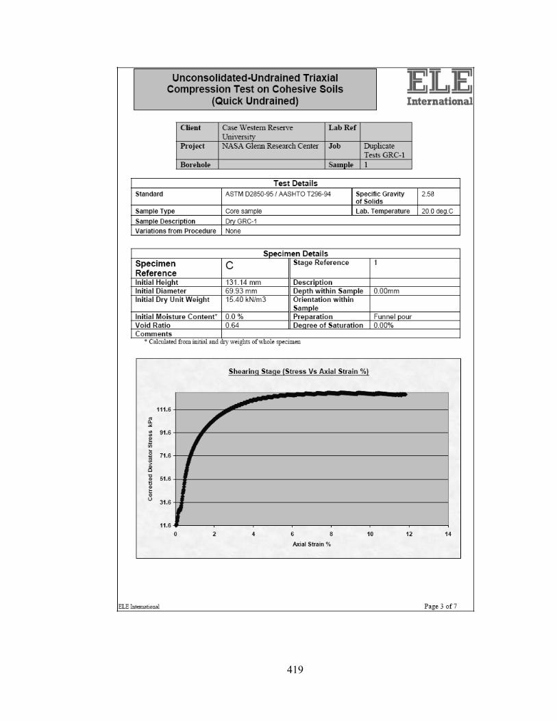
419

420

421

422

423

424
Report C2: Triaxial Test 2 Results

425

426

427

428

429
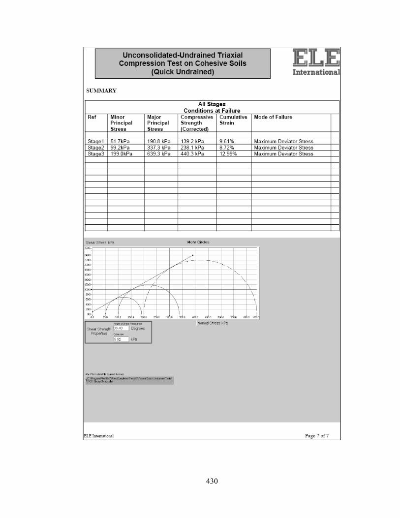
430

431
Report C3: Triaxial Test 3 Results

432

433

434

435

436

437

438
Report C4: Triaxial Test 4 Results

439

440

441

442

443

444

445
Report C5: Triaxial Test 5 Results

446

447

448

449

450

451

452
Report C6: Triaxial Test 6 Results

453

454

455

456

457

458

459
Report C7: Triaxial Test 7 Results

460

461

462

463

464

465

466
Report C8: Triaxial Test 8 Results

467

468

469

470

471

472

473
Report C9: Triaxial Test 9 Results

474

475

476

477

478

479

480
Report C10: Triaxial Test 10 Results

481

482

483

484

485

486

487
Figure C1: q versus p analysis of triaxial test 1 on GRC-1.
q = 0.491(p) + 9.3592
0
50
100
150
200
250
300
350
400
450
0 100 200 300 400 500 600 700 800
p (kPa)
q (k
Pa)
Figure C2: q versus p analysis of triaxial test 2 on GRC-1.
q = 0.5052(p) + 8.4954
0
50
100
150
200
250
300
350
400
450
0 100 200 300 400 500 600 700 800
p (kPa)
q (k
Pa)

488
Figure C3: q versus p analysis of triaxial test 3 on GRC-1.
q = 0.5996(p) - 7.5126
0
50
100
150
200
250
300
350
400
450
0 100 200 300 400 500 600 700 800
p (kPa)
q (k
Pa)
Figure C4: q versus p analysis of triaxial test 4 on GRC-1.
q = 0.5709(p) - 8.3291
0
50
100
150
200
250
300
350
400
450
0 100 200 300 400 500 600 700 800
p (kPa)
q (k
Pa)

489
Figure C5: q versus p analysis of triaxial test 5 on GRC-1.
q = 0.5595(p) + 3.5081
0
50
100
150
200
250
300
350
400
450
0 100 200 300 400 500 600 700 800
p (kPa)
q (k
Pa)
Figure C6: q versus p analysis of triaxial test 6 on GRC-1.
q = 0.5991(p) + 2.5322
0
50
100
150
200
250
300
350
400
450
0 100 200 300 400 500 600 700 800
p (kPa)
q (k
Pa)

490
Figure C7: q versus p analysis of triaxial test 7 on GRC-1.
q = 0.6154(p) + 5.9561
0
50
100
150
200
250
300
350
400
450
0 100 200 300 400 500 600 700 800
p (kPa)
q (k
Pa)
Figure C8: q versus p analysis of triaxial test 8 on GRC-1.
q = 0.6627(p) + 6.7427
0
50
100
150
200
250
300
350
400
450
0 100 200 300 400 500 600 700 800
p (kPa)
q (k
Pa)
Figure C9: q versus p analysis of triaxial test 9 on GRC-1.

491
q = 0.6712(p) + 8.2915
0
50
100
150
200
250
300
350
400
450
0 100 200 300 400 500 600 700 800
p (kPa)
q (k
Pa)
Figure C10: q versus p analysis of triaxial test 10 on GRC-1.
q = 0.7053(p) + 0.313
0
50
100
150
200
250
300
350
400
450
500
0 100 200 300 400 500 600 700 800
p (kPa)
q (k
Pa)
APPENDIX D TABLE BEVAMETER RESULTS FOR GRC-1
________________________________________________________________________

492
Table D1: Specifications of Load/Torque Cell (from www.sensordata.com)

493

494
Code D1: Determination of Best Soil Preparation Method
%Soil Depth experiment (10/8/07): Oravec. %Experiment to check the effects of soil preparation on plate sinkage. %Weights were applied to the 19cm plate with a soil depth of 12cm %prepared by funnel pour and compared to results from random soil %preparation %Sinkage tests were repeated seven times, removing and replacing the %soil after each one. %Load cell sensitivity -1170.2 N / (mV/V) %LVDT sensitivity -1091.1 mm / (Vout/Vin) clear;clc;close all %Random Soil Preparation %Test #1: depth = 12cm, plate diam = 19cm, soil freshly prepared Load_1 = [0 2 4 6 8 10 15 20 25 30 35 40 45 50 55]; %applied weights %(kg) z_1 = -10^-3*[.6001 6.6001 10.29 13.1 16 17.3 20.9 23.5 26.5 28.2 29.7 31.3 33.1 34.8 37.5]'; %LVDT Output (V/V) f_1 = [-.0014 .0085 .0192 .0338 .0447 .0575 .0986 .1339 .1705 .2084 .2456 .2846 .3232 .3642 .4037]'; %Negative Load Cell (mV/V) %Offset Correction to 0-intercept z_1 = [(z_1+(-10^-3*-.6001))]; f_1 = [(f_1+.0014)]; %curve-fit the data with the exponential equation: z(f) = a*((e^-f)-%1)+b*f*e^-f+c*f^2*e^-f M_1 = [(exp(-(f_1))-1) f_1.*exp(-(f_1)) f_1.^2.*exp(-(f_1))]; C_1 = M_1\z_1; N = 15; F_1 = (linspace(0,max(f_1),N))'; %Curve-fit Load Cell Ouput (mV/V) Z_1 = ([(exp(-F_1)-1) F_1.*exp(-F_1) F_1.^2.*exp(-(F_1))]*C_1); %Curve-%fit LVDT Ouput (V/V) F_1 = F_1*1170.2; %Converting (mV/V) to N Z_1 = Z_1*1091.1; %Converting (V/V) to mm f_1 = f_1*1170.2; z_1 = z_1*1091.1; %Test #2: depth = 12cm, plate diam = 19cm, soil freshly prepared %LVDT WENT OUT OF RANGE AT 20KG LOAD %Load_2 = [0 2 4 6 8 10 15]; %applied weights (kg) %z_2 = -10^-3*[1.3901 3.4 5.69 8.5001 10.79 12.09 14.8]'; %LVDT output %(V/V) %f_2 = [.0001 .0147 .0311 .0478 .064 .0799 .1200]'; %load cell %compression (mV/V) %Test #3: depth = 12cm, plate diam = 19cm, soil freshly prepared Load_3 = [0 2 4 6 8 10 15 20 25 30 35 40 45 50 55]; %applied weights %(kg) z_3 = -10^-3*[.090003 2.5901 4.9001 6.4001 8.1 9.6 13.1 16.2 19.5 21.6 24.1 26.4 29 31.69 34.59]'; %LVDT output (V/V) f_3 = [-.0004 .0146 .0314 .0471 .064 .0791 .1181 .1590 .2009 .2404 .2841 .3214 .3619 .402 .4414]'; %load cell compression (mV/V) %Offset Correction to 0-intercept z_3 = [(z_3+(-10^-3*-.090003))]; f_3 = [(f_3+.0004)]; %curve-fit the data with the exponential equation: M_3 = [(exp(-f_3)-1) f_3.*exp(-f_3) f_3.^2.*exp(-(f_3))]; C_3 = M_3\z_3; N = 15; F_3 = (linspace(0,max(f_3),N))'; %Curve-fit Load Cell Ouput (mV/V) Z_3 = ([(exp(-F_3)-1) F_3.*exp(-F_3) F_3.^2.*exp(-(F_3))]*C_3); %Curve-%fit LVDT Ouput (V/V) F_3 = F_3*1170.2; %Converting (mV/V) to N

495
Z_3 = Z_3*1091.1; %Converting (V/V) to mm f_3 = f_3*1170.2; z_3 = z_3*1091.1; %Test #4: depth = 12cm, plate diam = 19cm, soil freshly prepared Load_4 = [0 2 4 6 8 10 15 20 25 30 35 40 45 50 55]; %applied weights %(kg) z_4 = -10^-3*[.23842 3.4 6.0003 9.4001 12 15.2 19.79 23.4 27.1 30.3 33.39 35.8 38.89 41.09 46.19]'; %LVDT output (V/V) f_4 = [-.0004 .0147 .0292 .0447 .0598 .0759 .1168 .1562 .1963 .2375 .2798 .3213 .3576 .3983 .443]'; %load cell compression (mV/V) %Offset Correction to 0-intercept z_4 = [(z_4+(-10^-3*-.23842))]; f_4 = [(f_4+.0004)]; %curve-fit the data with the exponential equation: M_4 = [(exp(-f_4)-1) f_4.*exp(-f_4) f_4.^2.*exp(-(f_4))]; C_4 = M_4\z_4; N = 15; F_4 = (linspace(0,max(f_4),N))'; %Curve-fit Load Cell Ouput (mV/V) Z_4 = ([(exp(-F_4)-1) F_4.*exp(-F_4) F_4.^2.*exp(-(F_4))]*C_4); %Curve-%fit LVDT Ouput (V/V) F_4 = F_4*1170.2; %Converting (mV/V) to N Z_4 = Z_4*1091.1; %Converting (V/V) to mm f_4 = f_4*1170.2; z_4 = z_4*1091.1; %Test #5: depth = 12cm, plate diam = 19cm, soil freshly prepared Load_5 = [0 2 4 6 8 10 15 20 25 30 35 40 45 50 55]; %applied weights %(kg) z_5 = -10^-3*[.20003 4.7001 9.6 11.59 13.69 15.49 19.69 23.7 27.39 30.3 34 37.4 41.09 44.49 49.19]'; %LVDT output (V) f_5 = [0 .0152 .0327 .048 .0641 .0815 .1219 .1639 .2039 .2451 .2890 .3268 .3675 .4076 .4494]'; %load cell compression (mV/V) %Offset Correction to 0-intercept z_5 = [(z_5+(-10^-3*-.20003))]; f_5 = [(f_5+0)]; %curve-fit the data with the exponential equation: M_5 = [(exp(-f_5)-1) f_5.*exp(-f_5) f_5.^2.*exp(-(f_5))]; C_5 = M_5\z_5; N = 15; F_5 = (linspace(0,max(f_5),N))'; %Curve-fit Load Cell Ouput (mV/V) Z_5 = ([(exp(-F_5)-1) F_5.*exp(-F_5) F_5.^2.*exp(-(F_5))]*C_5); %Curve-%fit LVDT Ouput (V/V) F_5 = F_5*1170.2; %Converting (mV/V) to N Z_5 = Z_5*1091.1; %Converting (V/V) to mm f_5 = f_5*1170.2; z_5 = z_5*1091.1; %Test #6: depth = 12cm, plate diam = 19cm, soil freshly prepared Load_6 = [0 2 4 6 8 10 15 20 25 30 35 40 45 50 55]; %applied weights %(kg) z_6 = -10^-3*[.6001 5.4902 9.7901 12.1 14.49 16.7 20.89 24.2 27.5 30.3 33.4 36.5 40.2 43.8 47]'; %LVDT output (V/V) f_6 = [.0005 .017 .0343 .051 .0671 .0841 .1264 .1671 .2076 .2478 .2877 .3301 .3694 .4106 .4508]'; %load cell compression (mV/V) %Offset Correction to 0-intercept z_6 = [(z_6+(-10^-3*-.6001))]; f_6 = [(f_6+-.0005)]; %curve-fit the data with the exponential equation: M_6 = [(exp(-f_6)-1) f_6.*exp(-f_6) f_6.^2.*exp(-(f_6))]; C_6 = M_6\z_6; N = 15; F_6 = (linspace(0,max(f_6),N))'; %Curve-fit Load Cell Ouput (mV/V) Z_6 = ([(exp(-F_6)-1) F_6.*exp(-F_6) F_6.^2.*exp(-(F_6))]*C_6); %Curve-%fit LVDT Ouput (V/V)

496
F_6 = F_6*1170.2; %Converting (mV/V) to N Z_6 = Z_6*1091.1; %Converting (V/V) to mm f_6 = f_6*1170.2; z_6 = z_6*1091.1; %Test #7: depth = 12cm, plate diam = 19cm, soil freshly prepared Load_7 = [0 2 4 6 8 10 15 20 25 30 35 40 45 50 55]; %applied weights %(kg) z_7 = -10^-3*[1.1902 6.2902 10.8 14.49 19.3 21.2 26.9 30.9 35.4 38.2 40.7 44.29 46.89 50.1 54.4]'; %LVDT output (V/V) f_7 = [.0007 .0173 .0345 .0511 .0678 .084 .1257 .1666 .2074 .2489 .2881 .3311 .3711 .4108 .4528]'; %load cell compression (mV/V) %Offset Correction to 0-intercept z_7 = [(z_7+(-10^-3*-1.1902))]; f_7 = [(f_7+-.0007)]; %curve-fit the data with the exponential equation: M_7 = [(exp(-f_7)-1) f_7.*exp(-f_7) f_7.^2.*exp(-(f_7))]; C_7 = M_7\z_7; N = 15; F_7 = (linspace(0,max(f_7),N))'; %Curve-fit Load Cell Ouput (mV/V) Z_7 = ([(exp(-F_7)-1) F_7.*exp(-F_7) F_7.^2.*exp(-(F_7))]*C_7); %Curve-%fit LVDT Ouput (V/V) F_7 = F_7*1170.2; %Converting (mV/V) to N Z_7 = Z_7*1091.1; %Converting (V/V) to mm f_7 = f_7*1170.2; z_7 = z_7*1091.1; %Mean value of old Data Matrix_old_F = (cat(2,F_1,F_3,F_4,F_5,F_6,F_7))'; Mean_old_F = mean(Matrix_old_F); Matrix_old_Z = (cat(2,Z_1,Z_3,Z_4,Z_5,Z_6,Z_7))'; Mean_old_Z = mean(Matrix_old_Z); %Hopper Soil Preparation %Test #1: depth = 12cm, plate diam = 19cm, soil freshly prepared Load_1a = [0 2 4 6 8 10 15 20 25 30 35 40 45 50]; %applied weights (kg) z_1a = -10^-3*[0.10014 5.7001 13.4 18.4 22.2 24.6 29.2 32.79 35.7 37.49 39.8 42.7 45.19 47.2]'; %LVDT output (V/V) f_1a = 1*[0 .0136 .0283 .043 .0604 .0747 .1157 .1619 .1975 .2427 .2795 .322 .3616 .4008]'; %Load cell compression (mV/V) %Offset correction to 0-intercept z_1a = [(z_1a+(-10^-3*-.10014))]; f_1a = [(f_1a+0)]; %curve-fit the data with the exponential equation: M_1a = [(exp(-f_1a)-1) f_1a.*exp(-f_1a) f_1a.^2.*exp(-(f_1a))]; C_1a = M_1a\z_1a; N = 14; F_1a = (linspace(0,max(f_1a),N))'; %Curve-fit Load Cell Ouput (mV/V) Z_1a = ([(exp(-F_1a)-1) F_1a.*exp(-F_1a) F_1a.^2.*exp(-(F_1a))]*C_1a); %Curve-fit LVDT Ouput (V/V) F_1a = F_1a*1170.2; %Converting (mV/V) to N Z_1a = Z_1a*1091.1; %Converting (V/V) to mm\ f_1a = f_1a*1170.2; z_1a = z_1a*1091.1; %Test #2: depth = 12cm, plate diam = 19cm, soil freshly prepared Load_2a = [0 2 4 6 8 10 15 20 25 30 35 40 45 50]; %applied weights (kg) z_2a = -10^-3*[.40019 4.4 9.3002 13.6 16.2 18.4 24 29.2 32.69 37.6 41.7 45 48.4 50.99]'; %LVDT output (V/V) f_2a = 1*[-.0011 .0133 .0286 .0443 .0601 .0765 .1177 .16 .2007 .2413 .2825 .3227 .3646 .404]'; %Load cell compression (mV/V) %Offset correction to 0-intercept z_2a = [(z_2a+(-10^-3*-.40019))]; f_2a = [(f_2a+.0011)];

497
%curve-fit the data with the exponential equation: M_2a = [(exp(-f_2a)-1) f_2a.*exp(-f_2a) f_2a.^2.*exp(-(f_2a))]; C_2a = M_2a\z_2a; N = 14; F_2a = (linspace(0,max(f_2a),N))'; %Curve-fit Load Cell Ouput (mV/V) Z_2a = ([(exp(-F_2a)-1) F_2a.*exp(-F_2a) F_2a.^2.*exp(-(F_2a))]*C_2a); %Curve-fit LVDT Ouput (V/V) F_2a = F_2a*1170.2; %Converting (mV/V) to N Z_2a = Z_2a*1091.1; %Converting (V/V) to mm f_2a = f_2a*1170.2; z_2a = z_2a*1091.1; %Test #3: depth = 12cm, plate diam = 19cm, soil freshly prepared %DATA NOT USED DUE TO SLIGHT VARIATION IN SOIL PREPARATION %Load_3a = [0 2 4 6 8 10 15 20 25 30 35 40 45 50]; %applied weights %(kg) %z_3a = -10^-3*[.40019 4.1901 7.9001 11.3 12.29 13.99 18.3 21.1 23.6 %26.79 29.2 31.4 33.8 37.6]; %LVDT output (V/V) %f_3a = 1*[-.0011 .0117 .027 .0424 .0565 .0727 .1136 .1522 .1924 .2332 %.2731 .3126 .3523 .3925]; %Load cell compression (mV/V) %Test #4: depth = 12cm, plate diam = 19cm, soil freshly prepared %DATA NOT USED DUE TO SLIGHT VARIATION IN SOIL PREPARATION %Load_4a = [0 2 4 6 8 10 15 20 25 30 35 40 45 50]; %applied weights %(kg) %z_4a = -10^-3*[.20027 3.4903 5.3002 6.4902 7.2002 8.5001 10.9 13 15.3 %17.99 19.69 22.1 24.6 27.7]; %LVDT output (V/V) %f_4a = 1*[0 .0125 .0289 .0454 .0605 .0771 .1167 .158 .1992 .2388 .2825 %.3198 .3599 .3997]; %Load cell compression (mV/V) %Test #5: depth = 12cm, plate diam = 19cm, soil freshly prepared Load_5a = [0 2 4 6 8 10 15 20 25 30 35 40 45 50]; %applied weights (kg) z_5a = -10^-3*[.31042 5.9003 11.4 13.39 16.7 19.3 26 30.3 33.3 36.2 38.5 40.8 43.2 46.1]'; %LVDT output (V/V) f_5a = 1*[-.0026 .0113 .0262 .0419 .0579 .0741 .1151 .1562 .1969 .2361 .2771 .3169 .3573 .399]'; %Load cell compression (mV/V) %Offset correction to 0-intercept z_5a = [(z_5a+(-10^-3*-.31042))]; f_5a = [(f_5a+.0026)]; %curve-fit the data with the exponential equation: M_5a = [(exp(-f_5a)-1) f_5a.*exp(-f_5a) f_5a.^2.*exp(-(f_5a))]; C_5a = M_5a\z_5a; N = 14; F_5a = (linspace(0,max(f_5a),N))'; %Curve-fit Load Cell Ouput (mV/V) Z_5a = ([(exp(-F_5a)-1) F_5a.*exp(-F_5a) F_5a.^2.*exp(-(F_5a))]*C_5a); %Curve-fit LVDT Ouput (V/V) F_5a = F_5a*1170.2; %Converting (mV/V) to N Z_5a = Z_5a*1091.1; %Converting (V/V) to mm f_5a = f_5a*1170.2; z_5a = z_5a*1091.1; %Test #6: depth = 12cm, plate diam = 19cm, soil freshly prepared Load_6a = [0 2 4 6 8 10 15 20 25 30 35 40 45 50]; %applied weights (kg) z_6a = -10^-3*[.90015 5.3903 9.1002 11.6 14.7 16.4 21.7 26.6 30.09 32.8 35.8 38.5 40.9 43.2]'; %LVDT output (V/V) f_6a = 1*[0 .0141 .0295 .044 .0597 .0758 .1149 .1549 .1959 .235 .2765 .3163 .3571 .3966]'; %Load cell compression (mV/V) %Offset correction to 0-intercept z_6a = [z_6a+(-10^-3*-.90015)]; f_6a = [f_6a+0]; %curve-fit the data with the exponential equation: M_6a = [(exp(-f_6a)-1) f_6a.*exp(-f_6a) f_6a.^2.*exp(-(f_6a))]; C_6a = M_6a\z_6a; N = 14; F_6a = (linspace(0,max(f_6a),N))'; %Curve-fit Load Cell Ouput (mV/V)

498
Z_6a = ([(exp(-F_6a)-1) F_6a.*exp(-F_6a) F_6a.^2.*exp(-(F_6a))]*C_6a); %Curve-fit LVDT Ouput (V/V) F_6a = F_6a*1170.2; %Converting (mV/V) to N Z_6a = Z_6a*1091.1; %Converting (V/V) to mm f_6a = f_6a*1170.2; z_6a = z_6a*1091.1; %Test #7: depth = 12cm, plate diam = 19cm, soil freshly prepared Load_7a = [0 2 4 6 8 10 15 20 25 30 35 40 45 50]; %applied weights (kg) z_7a = -10^-3*[.80013 8.6901 13.49 17.6 21 22.7 29 33.89 38 41.3 46.5 50.3 51.79 54.39]'; %LVDT output (V/V) f_7a=1*[-.0001 .0154 .0307 .0468 .0629 .0791 .1207 .1617 .2027 .2427 .283 .3251 .3644 .4049]'; %Load cell compression (mV/V) %Offset correction to 0-intercept z_7a = [z_7a+(-10^-3*-.80013)]; f_7a = [f_7a+.0001]; %curve-fit the data with the exponential equation: M_7a = [(exp(-f_7a)-1) f_7a.*exp(-f_7a) f_7a.^2.*exp(-(f_7a))]; C_7a = M_7a\z_7a; N = 14; F_7a = (linspace(0,max(f_7a),N))'; %Curve-fit Load Cell Ouput (mV/V) Z_7a = ([(exp(-F_7a)-1) F_7a.*exp(-F_7a) F_7a.^2.*exp(-(F_7a))]*C_7a); %Curve-fit LVDT Ouput (V/V) F_7a = F_7a*1170.2; %Converting (mV/V) to N Z_7a = Z_7a*1091.1; %Converting (V/V) to mm f_7a = f_7a*1170.2; z_7a = z_7a*1091.1; %Determining the mean value of the new data set Matrix_new_F = (cat(2,F_1a,F_2a,F_5a,F_6a,F_7a))'; Mean_new_F = mean(Matrix_new_F); Matrix_new_Z = (cat(2,Z_1a,Z_2a,Z_5a,Z_6a,Z_7a))'; Mean_new_Z = mean(Matrix_new_Z); %Figure without curve-fit figure %New Data - Hopper plot(f_1a,z_1a,'ko');hold on; plot(f_2a,z_2a,'ko');hold on; plot(f_5a,z_5a,'ko');hold on; plot(f_6a,z_6a,'ko');hold on; plot(f_7a,z_7a,'ko');hold on; text(450,-3,'\o Hopper Data') %Old Data - Random plot(f_1,z_1,'k+');hold on; plot(f_3,z_3,'k+');hold on; plot(f_4,z_4,'k+');hold on; plot(f_5,z_5,'k+');hold on; plot(f_6,z_6,'k+');hold on; plot(f_7,z_7,'k+');hold on; text(450,-6,'+ Random Data') axis([0 600 -70 0]); grid on xlabel('Load (N)') ylabel('Depth (mm)') %Figure with both sets of data figure plot(f_1a,z_1a,'ko');hold on; plot(f_2a,z_2a,'ko');hold on; plot(f_5a,z_5a,'ko');hold on; plot(f_6a,z_6a,'ko');hold on; plot(f_7a,f_7a,'ko');hold on; text(400,-3,'\o Hopper Data') plot(Mean_new_F,Mean_new_Z,'k-');hold on text(400,-6,'- Mean of Hopper Data') plot(f_1,z_1,'k+');hold on;

499
plot(f_3,z_3,'k+');hold on; plot(f_4,z_4,'k+');hold on; plot(f_5,z_5,'k+');hold on; plot(f_6,z_6,'k+');hold on; plot(f_7,z_7,'k+');hold on; text(400,-9,'+ Random Data') plot(Mean_old_F,Mean_old_Z,'k--');hold on; text(400,-12,'-- Mean of Random Data') xlabel('Load (N)') ylabel('Depth (mm)') grid on axis([0 600 -70 0]) %Plot to check curve-fit for random soil pour: figure plot(f_1,z_1,'k+');hold on; plot(F_1,Z_1,'k-');hold on; plot(f_3,z_3,'k+');hold on; plot(F_3,Z_3,'k-');hold on; plot(f_4,z_4,'k+');hold on; plot(F_4,Z_4,'k-');hold on; plot(f_5,z_5,'k+');hold on; plot(F_5,Z_5,'k-');hold on; plot(f_6,z_6,'k+');hold on; plot(F_6,Z_6,'k-');hold on; plot(f_7,z_7,'k+');hold on; plot(F_7,Z_7,'k-');hold on; xlabel('Load (N)') ylabel('Depth (mm)') grid on axis([0 600 -70 0]) text(450,-3,'+ Raw Data') text(450,-6,'- Curve Fit') %Plot to check curve-fit for hopper soil pour: figure plot(f_1a,z_1a,'ko');hold on; plot(F_1a,Z_1a,'k-');hold on; plot(f_2a,z_2a,'ko');hold on; plot(F_2a,Z_2a,'k-');hold on; plot(f_5a,z_5a,'ko');hold on; plot(F_5a,Z_5a,'k-');hold on; plot(f_6a,z_6a,'ko');hold on; plot(F_6a,Z_6a,'k-');hold on; plot(f_7a,z_7a,'ko');hold on; plot(F_7a,Z_7a,'k-');hold on; xlabel('Load (N)') ylabel('Depth (mm)') grid on axis([0 600 -70 0]) text(450,-3,'+ Raw Data') text(450,-6,'- Curve Fit') %Standard Deviation Calculation for random data %For all Loads Matrix_old_SD = (cat(2,Z_1,Z_3,Z_4,Z_5,Z_6,Z_7))'; Standard_Deviation_old = std(Matrix_old_SD); %Standard Deviation Calculation for hopper data %For all Loads Matrix_new_SD = (cat(2,Z_1a,Z_2a,Z_5a,Z_6a,Z_7a))'; Standard_Deviation_new = std(Matrix_new_SD); %Plot for Standard Deviation figure plot(F_1,Standard_Deviation_old,'k+');hold on; plot(F_1a,Standard_Deviation_new,'ko');hold on; text(45,7.5,'+ Random') text(45,7.1,'\o Hopper') xlabel('Load (N)')

500
ylabel('Standard Deviation of Depth (mm)') grid on
Code D2: Determination of Minimum Soil Depth for 7.6 cm Plate

501
%Soil Depth Experiment - Run test preparing the soil to the same exact %density every time. To do this back calculate the weight of the soil %needed to create 1.75g/cc sample at predetermined soil depth. The %Measure that amount of soil using the scale then pour it into soil %bin. Shake the soil down to the desired depth. Run pressure-sinkage %test. December 5, 2007: 7.6cm diameter plate close all; clear all; clc; A1 = pi*(7.6/2)^2*100; %small plate area mm^2 %Test #1: 3cm depth Vin1 = 10.0058; Z_11 = -10^-3*[-.19991 9.3001 10.9 12.3 13.6 15.89 18.4 19.7 20.9 22.2 23.1 24.7 26 27.8 28.29]';%(V/V) F_11 = [-.0001 .0089 .0244 .0402 .0559 .0735 .1128 .1531 .1935 .234 .274 .3138 .3545 .395 .4349]';%(mV/V) Z_11 = Z_11-(-.19991*-10^-3);%zeroing the sinkage F_11 = F_11+.0001;%zeroing the load %curve-fit the data with the exponential equation M_11 = [(exp(-(F_11))-1) F_11.*exp(-(F_11)) F_11.^2.*exp(-(F_11))]; C_11 = M_11\Z_11; N = 15; F_11 = (linspace(0,max(F_11),N))'; %Curve-fit Load Cell Ouput (mV/V) Z_11 = ([(exp(-F_11)-1) F_11.*exp(-F_11) F_11.^2.*exp(-(F_11))]*C_11); %Curve-fit LVDT Ouput (V/V) Z_11 = 1126.3*Z_11/Vin1;%mm F_11 = 1170.2*F_11;%N F_11 = F_11/A1*1000; %kPa %Test #2: 3cm depth Vin2 = 10.0059; Z_21 = -10^-3*[-.29993 4.4901 6.5901 7.7002 8.4001 10.4 12 13.1 14.29 15.59 16.5 17.8 18.7 19.79 20.9]';%(V/V) F_21 = [-.0006 .0112 .027 .0432 .0598 .0768 .1161 .1554 .1954 .236 .2751 .3168 .355 .3956 .4356]';%(mV/V) Z_21 = Z_21-(-.29993*-10^-3);%zeroing the sinkage F_21 = F_21+.0006;%zeroing the load %curve-fit the data with the exponential equation M_21 = [(exp(-(F_21))-1) F_21.*exp(-(F_21)) F_21.^2.*exp(-(F_21))]; C_21 = M_21\Z_21; N = 15; F_21 = (linspace(0,max(F_21),N))'; %Curve-fit Load Cell Ouput (mV/V) Z_21 = ([(exp(-F_21)-1) F_21.*exp(-F_21) F_21.^2.*exp(-(F_21))]*C_21); %Curve-fit LVDT Ouput (V/V) Z_21 = 1126.3*Z_21/Vin2;%mm F_21 = 1170.2*F_21;%N F_21 = F_21/A1*1000; %kPa %Test #3: 3cm depth Vin3 = 10.006; Z_31 = -10^-3*[.23842*10^-3 3.8002 7.1002 9.4901 11.5 14.3 17 19.4 20.6 22.1 23.6 25.1 26.4 28.4 30]';%(V/V) F_31 = [.0001 .0139 .0305 .0469 .0633 .0802 .1206 .1616 .2015 .242 .2824 .3231 .3639 .4044 .4449]';%(mV/V) Z_31 = Z_31-(.23842*10^-3*-10^-3);%zeroing the sinkage F_31 = F_31-.0001;%zeroing the load %curve-fit the data with the exponential equation M_31 = [(exp(-(F_31))-1) F_31.*exp(-(F_31)) F_31.^2.*exp(-(F_31))];

502
C_31 = M_31\Z_31; N = 15; F_31 = (linspace(0,max(F_31),N))'; %Curve-fit Load Cell Ouput (mV/V) Z_31 = ([(exp(-F_31)-1) F_31.*exp(-F_31) F_31.^2.*exp(-(F_31))]*C_31); %Curve-fit LVDT Ouput (V/V) Z_31 = 1126.3*Z_31/Vin3;%mm F_31 = 1170.2*F_31;%N F_31 = F_31/A1*1000; %kPa %Test #4: 3cm depth Vin4 = 10.006; Z_41 = -10^-3*[.11921*10^-3 2.8001 5.3 6.8001 8.3002 11.5 13.49 16 17.2 18.4 20.3 21.3 22.3 23.6 25.09]';%(V/V) F_41 = [0 .0125 .0282 .0441 .0603 .0801 .118 .1591 .1979 .2384 .2795 .3185 .3579 .3975 .4384]';%(mV/V) Z_41 = Z_41-(.11921*10^-3*-10^-3);%zeroing the sinkage F_41 = F_41-0;%zeroing the load %curve-fit the data with the exponential equation M_41 = [(exp(-(F_41))-1) F_41.*exp(-(F_41)) F_41.^2.*exp(-(F_41))]; C_41 = M_41\Z_41; N = 15; F_41 = (linspace(0,max(F_41),N))'; %Curve-fit Load Cell Ouput (mV/V) Z_41 = ([(exp(-F_41)-1) F_41.*exp(-F_41) F_41.^2.*exp(-(F_41))]*C_41); %Curve-fit LVDT Ouput (V/V) Z_41 = 1126.3*Z_41/Vin4;%mm F_41 = 1170.2*F_41;%N F_41 = F_41/A1*1000; %kPa %Test #5: 3cm depth Vin5 = 10.006; Z_51 = -10^-3*[.11009 2.6001 5.7101 7.8101 9.910 13.41 16.51 18.11 20.1 21.31 22.6 24.21 25.31 26.5 27.91]';%(V/V) F_51 = [-.0001 .0094 .0265 .0425 .0585 .0754 .1152 .1542 .1951 .2341 .2739 .3153 .3533 .3921 .4345]';%(mV/V) Z_51 = Z_51-(.11009*-10^-3);%zeroing the sinkage F_51 = F_51+.0001;%zeroing the load %curve-fit the data with the exponential equation M_51 = [(exp(-(F_51))-1) F_51.*exp(-(F_51)) F_51.^2.*exp(-(F_51))]; C_51 = M_51\Z_51; N = 15; F_51 = (linspace(0,max(F_51),N))'; %Curve-fit Load Cell Ouput (mV/V) Z_51 = ([(exp(-F_51)-1) F_51.*exp(-F_51) F_51.^2.*exp(-(F_51))]*C_51); %Curve-fit LVDT Ouput (V/V) Z_51 = 1126.3*Z_51/Vin5;%mm F_51 = 1170.2*F_51;%N F_51 = F_51/A1*1000; %kPa %---------------------------------------------------------------------- %Determining the mean value of the scattered curves. Matrix_Z1 = [Z_11 Z_21 Z_31 Z_41 Z_51]'; Matrix_F1 = [F_11 F_21 F_31 F_41 F_51]'; Std_Z1 = std(Matrix_Z1); Mean_Z1 = Mean(Matrix_Z1,1); Mean_F1 = Mean(Matrix_F1,1); W1 = mean(Std_Z1); %---------------------------------------------------------------------- figure plot(F_11,Z_11,'ko'); hold on; plot(F_21,Z_21,'ko'); hold on; plot(F_31,Z_31,'ko'); hold on; plot(F_41,Z_41,'ko'); hold on; plot(F_51,Z_51,'ko'); hold on;

503
plot(Mean_F1,Mean_Z1,'k-','linewidth',2); hold on; text(90, -0.5,'\o Raw Data') text(90, -1, '- Mean') xlabel('Pressure (kPa)') ylabel('Depth (mm)') grid on axis([0 120 -10 0]) %---------------------------------------------------------------------- %Test #1: 6cm depth Vin7 = 10.0052; Z_13 = -10^-3*[.0098944 1.9001 6.6001 10.59 14.49 20.3 27.5 33.1 37.2 40.49 43.3 46.7 49.2 52.6 55.5]';%(V/V) F_13 = [.0003 .0127 .0295 .0465 .063 .0814 .1212 .1619 .2032 .2432 .283 .3235 .3633 .404 .4442]';%(mV/V) Z_13 = Z_13-(.0098944*-10^-3);%zeroing the sinkage F_13 = F_13-.0003;%zeroing the load %curve-fit the data with the exponential equation M_13 = [(exp(-(F_13))-1) F_13.*exp(-(F_13)) F_13.^2.*exp(-(F_13))]; C_13 = M_13\Z_13; N = 15; F_13 = (linspace(0,max(F_13),N))'; %Curve-fit Load Cell Ouput (mV/V) Z_13 = ([(exp(-F_13)-1) F_13.*exp(-F_13) F_13.^2.*exp(-(F_13))]*C_13); %Curve-fit LVDT Ouput (V/V) Z_13 = 1126.3*Z_13/Vin7;%mm F_13 = 1170.2*F_13;%N F_13 = F_13/A1*1000; %kPa %Test #2: 6cm depth Vin8 = 10.0062; Z_23 = -10^-3*[-.10002 1.0002 2.8001 5.3001 7.2001 12.2 16.69 21.3 26.09 29.7 33.1 37 39.7 43 46.4]';%(V/V) F_23 = [.0001 .0114 .0278 .0438 .0606 .0787 .1187 .1593 .2006 .2403 .2809 .3219 .3616 .4003 .441]';%(mV/V) Z_23 = Z_23-(-.10002*-10^-3);%zeroing the sinkage F_23 = F_23-.0001;%zeroing the load %curve-fit the data with the exponential equation M_23 = [(exp(-(F_23))-1) F_23.*exp(-(F_23)) F_23.^2.*exp(-(F_23))]; C_23 = M_23\Z_23; N = 15; F_23 = (linspace(0,max(F_23),N))'; %Curve-fit Load Cell Ouput (mV/V) Z_23 = ([(exp(-F_23)-1) F_23.*exp(-F_23) F_23.^2.*exp(-(F_23))]*C_23); %Curve-fit LVDT Ouput (V/V) Z_23 = 1126.3*Z_23/Vin8;%mm F_23 = 1170.2*F_23;%N F_23 = F_23/A1*1000; %kPa %Test #3: 6cm depth Vin9 = 10.0056; Z_33 = -10^-3*[-.10991 1.1902 3.9002 5.7 7.7001 12.2 16.6 19.7 22.6 25 27.59 29.79 32.69 34.6 37.5]';%(V/V) F_33 = [-.0006 .0091 .0241 .0394 .0557 .0725 .1115 .1519 .192 .2318 .2726 .3122 .3523 .3913 .4307]';%(mV/V) Z_33 = Z_33-(-.10991*-10^-3);%zeroing the sinkage F_33 = F_33+.0006;%zeroing the load %curve-fit the data with the exponential equation M_33 = [(exp(-(F_33))-1) F_33.*exp(-(F_33)) F_33.^2.*exp(-(F_33))]; C_33 = M_33\Z_33; N = 15; F_33 = (linspace(0,max(F_33),N))'; %Curve-fit Load Cell Ouput (mV/V) Z_33 = ([(exp(-F_33)-1) F_33.*exp(-F_33) F_33.^2.*exp(-(F_33))]*C_33); %Curve-fit LVDT Ouput (V/V)

504
Z_33 = 1126.3*Z_33/Vin9;%mm F_33 = 1170.2*F_33;%N F_33 = F_33/A1*1000; %kPa %Test #4: 6cm depth Vin10 = 10.0056; Z_43 = -10^-3*[.090182 1.5001 5.1901 6.6001 7.7901 11.19 14.4 16.4 18.3 21.39 23 24.79 26.49 28.9 31.6]';%(V/V) F_43 = [0 .0098 .0254 .0425 .0579 .0753 .1164 .1571 .1968 .2383 .278 .3183 .3581 .3986 .4404]';%(mV/V) Z_43 = Z_43-(.09018*-10^-3);%zeroing the sinkage F_43 = F_43;%zeroing the load %curve-fit the data with the exponential equation M_43 = [(exp(-(F_43))-1) F_43.*exp(-(F_43)) F_43.^2.*exp(-(F_43))]; C_43 = M_43\Z_43; N = 15; F_43 = (linspace(0,max(F_43),N))'; %Curve-fit Load Cell Ouput (mV/V) Z_43 = ([(exp(-F_43)-1) F_43.*exp(-F_43) F_43.^2.*exp(-(F_43))]*C_43); %Curve-fit LVDT Ouput (V/V) Z_43 = 1126.3*Z_43/Vin10;%mm F_43 = 1170.2*F_43;%N F_43 = F_43/A1*1000; %kPa %Test #5: 6cm depth Vin11 = 10.0056; Z_53 = -10^-3*[.10014 1.3001 4.8001 6.5001 8.3001 12.6 17.5 21.5 25.6 29.1 34.7 38.4 43.1 47.9 53.19]';%(V/V) F_53 = [0 .0106 .0282 .0442 .0601 .0784 .1193 .1602 .2012 .2421 .2824 .3223 .3609 .4009 .11406]';%(mV/V) Z_53 = Z_53-(.10014*-10^-3);%zeroing the sinkage F_53 = F_53;%zeroing the load %curve-fit the data with the exponential equation M_53 = [(exp(-(F_53))-1) F_53.*exp(-(F_53)) F_53.^2.*exp(-(F_53))]; C_53 = M_53\Z_53; N = 15; F_53 = (linspace(0,max(F_53),N))'; %Curve-fit Load Cell Ouput (mV/V) Z_53 = ([(exp(-F_53)-1) F_53.*exp(-F_53) F_53.^2.*exp(-(F_53))]*C_53); %Curve-fit LVDT Ouput (V/V) Z_53 = 1126.3*Z_53/Vin11;%mm F_53 = 1170.2*F_53;%N F_53 = F_53/A1*1000; %kPa %----------------------------------------------------------------------%Determining the mean value of the scattered curves. Matrix_Z3 = [Z_13 Z_23 Z_33 Z_43 Z_53]'; Matrix_F3 = [F_13 F_23 F_33 F_43 F_53]'; Std_Z3 = std(Matrix_Z3); Mean_Z3 = Mean(Matrix_Z3,1); Mean_F3 = Mean(Matrix_F3,1); W3 = mean(Std_Z3); %---------------------------------------------------------------------- figure plot(F_13,Z_13,'ko'); hold on; plot(F_23,Z_23,'ko'); hold on; plot(F_33,Z_33,'ko'); hold on; plot(F_43,Z_43,'ko'); hold on; plot(F_53,Z_53,'ko'); hold on; plot(Mean_F3,Mean_Z3,'k-','linewidth',2'); hold on; text(90, -0.5,'\o Raw Data') text(90, -1, '- Mean') xlabel('Pressure (kPa)') ylabel('Depth (mm)') grid on

505
axis([0 120 -10 0]) %---------------------------------------------------------------------- %Test #1: 12cm depth Vin12 = 10.0058; Z_14 = -10^-3*[-.49996 1.9001 6.9002 11.79 14.4 20.6 27.3 31.6 35.3 38.7 42.3 45.49 49.1 52.5 56.5]';%(V/V) F_14 = [0 .0106 .026 .042 .0579 .0764 .1157 .157 .1976 .2366 .2768 .3171 .3574 .3968 .4361]';%(mV/V) Z_14 = Z_14-(-.49996*-10^-3);%zeroing the sinkage F_14 = F_14;%zeroing the load %curve-fit the data with the exponential equationM_14 = [(exp(-(F_14))-1) F_14.*exp(-(F_14)) F_14.^2.*exp(-(F_14))]; C_14 = M_14\Z_14; N = 15; F_14 = (linspace(0,max(F_14),N))'; %Curve-fit Load Cell Ouput (mV/V) Z_14 = ([(exp(-F_14)-1) F_14.*exp(-F_14) F_14.^2.*exp(-(F_14))]*C_14); %Curve-fit LVDT Ouput (V/V) Z_14 = 1126.3*Z_14/Vin12;%mm F_14 = 1170.2*F_14;%N F_14 = F_14/A1*1000; %kPa %Test #2: 12cm depth Vin13 = 10.0059; Z_24 = -10^-3*[.11921*10^-3 1.9002 5.4000 8.5001 11.3 15.8 20.99 25.29 29.2 32.49 36.4 40.1 43.99 48 52.99]';%(V/V) F_24 = [-.0015 .0097 .0258 .0414 .0579 .0748 .1145 .1551 .1949 .2351 .2754 .3148 .3549 .3945 .434]';%(mV/V) Z_24 = Z_24-(.11921*10^-3*-10^-3);%zeroing the sinkage F_24 = F_24+.0015;%zeroing the load %curve-fit the data with the exponential equation M_24 = [(exp(-(F_24))-1) F_24.*exp(-(F_24)) F_24.^2.*exp(-(F_24))]; C_24 = M_24\Z_24; N = 15; F_24 = (linspace(0,max(F_24),N))'; %Curve-fit Load Cell Ouput (mV/V) Z_24 = ([(exp(-F_24)-1) F_24.*exp(-F_24) F_24.^2.*exp(-(F_24))]*C_24); %Curve-fit LVDT Ouput (V/V) Z_24 = 1126.3*Z_24/Vin13;%mm F_24 = 1170.2*F_24;%N F_24 = F_24/A1*1000; %kPa %Test #3: 12cm depth Vin14 = 10.006; Z_34 = -10^-3*[0 2.7001 7.1001 9.2001 11.2 16.09 20.1 24.1 27.5 31.7 34.6 38.29 42.5 46.2 49.79]';%(V/V) F_34 = [0 .0108 .0271 .0425 .0582 .0764 .1151 .1552 .1959 .2374 .2765 .3156 .3549 .3964 .435]';%(mV/V) Z_34 = Z_34-(0*-10^-3);%zeroing the sinkage F_34 = F_34;%zeroing the load %curve-fit the data with the exponential equation M_34 = [(exp(-(F_34))-1) F_34.*exp(-(F_34)) F_34.^2.*exp(-(F_34))]; C_34 = M_34\Z_34; N = 15; F_34 = (linspace(0,max(F_34),N))'; %Curve-fit Load Cell Ouput (mV/V) Z_34 = ([(exp(-F_34)-1) F_34.*exp(-F_34) F_34.^2.*exp(-(F_34))]*C_34); %Curve-fit LVDT Ouput (V/V) Z_34 = 1126.3*Z_34/Vin14;%mm F_34 = 1170.2*F_34;%N F_34 = F_34/A1*1000; %kPa %Test #4: 12cm depth Vin15 = 10.0061;

506
Z_44 = -10^-3*[.10026 2.0902 4.5002 6.7002 8.8003 13.4 16.8 19.7 22.4 24.1 26.49 28.5 30.5 32.89 34.8]';%(V/V) F_44 = [-.0002 .0109 .0266 .0424 .0578 .0758 .115 .1547 .1954 .2339 .2738 .313 .3542 .3941 .4332]';%(mV/V) Z_44 = Z_44-(.10026*-10^-3);%zeroing the sinkage F_44 = F_44+.0002;%zeroing the load %curve-fit the data with the exponential equation M_44 = [(exp(-(F_44))-1) F_44.*exp(-(F_44)) F_44.^2.*exp(-(F_44))]; C_44 = M_44\Z_44; N = 15; F_44 = (linspace(0,max(F_44),N))'; %Curve-fit Load Cell Ouput (mV/V) Z_44 = ([(exp(-F_44)-1) F_44.*exp(-F_44) F_44.^2.*exp(-(F_44))]*C_44); %Curve-fit LVDT Ouput (V/V) Z_44 = 1126.3*Z_44/Vin15;%mm F_44 = 1170.2*F_44;%N F_44 = F_44/A1*1000; %kPa %Test #5: 12cm depth Vin16 = 10.006; Z_54 = -10^-3*[.10002 1.1902 3.7901 6.4001 8.4901 12.9 16.3 20.89 22.99 24.69 27.5 30.19 32.2 35.2 37.7]';%(V/V) F_54 = [0 .0122 .0279 .0448 .0602 .0779 .118 .1599 .1994 .2383 .2778 .3192 .3576 .3975 .4376]';%(mV/V) Z_54 = Z_54-(.10002*-10^-3);%zeroing the sinkage F_54 = F_54;%zeroing the load %curve-fit the data with the exponential equation M_54 = [(exp(-(F_54))-1) F_54.*exp(-(F_54)) F_54.^2.*exp(-(F_54))]; C_54 = M_54\Z_54; N = 15; F_54 = (linspace(0,max(F_54),N))'; %Curve-fit Load Cell Ouput (mV/V) Z_54 = ([(exp(-F_54)-1) F_54.*exp(-F_54) F_54.^2.*exp(-(F_54))]*C_54); %Curve-fit LVDT Ouput (V/V) Z_54 = 1126.3*Z_54/Vin16;%mm F_54 = 1170.2*F_54;%N F_54 = F_54/A1*1000; %kPa %-------------------------------------------------------------------------- %Determining the mean value of the scattered curves. Matrix_Z4 = [Z_14 Z_24 Z_34 Z_44 Z_54]'; Matrix_F4 = [F_14 F_24 F_34 F_44 F_54]'; Std_Z4 = std(Matrix_Z4); Mean_Z4 = Mean(Matrix_Z4,1); Mean_F4 = Mean(Matrix_F4,1); W4 = mean(Std_Z4); %---------------------------------------------------------------------- figure plot(F_14,Z_14,'ko'); hold on; plot(F_24,Z_24,'ko'); hold on; plot(F_34,Z_34,'ko'); hold on; plot(F_44,Z_44,'ko'); hold on; plot(F_54,Z_54,'ko'); hold on; plot(Mean_F4,Mean_Z4,'k-','linewidth',2'); hold on; text(90, -0.5,'\o Raw Data') text(90, -1, '- Mean') xlabel('Pressure (kPa)') ylabel('Depth (mm)') grid on axis([0 120 -10 0]) %---------------------------------------------------------------------- %Test #1: 3cm depth REDO Vin17 = 10.0051; Z_11r = -10^-3*[-.19991 5.6902 13.3 18.8 21.89 27.2 31.8 35.09 37.8 39.5 41.59 43.8 44.99 46.4 47.99]';%(V/V)

507
F_11r = [-.0124 -.0143 -.0051 .0038 .0132 .0246 .0606 .094 .1311 .0654 .2017 .2378 .2741 .3111 .3484]';%(mV/V) Z_11r = Z_11r-(-.19991*-10^-3);%zeroing the sinkage F_11r = F_11r+.0124;%zeroing the load %curve-fit the data with the exponential equation: M_11r = [(exp(-(F_11r))-1) F_11r.*exp(-(F_11r)) F_11r.^2.*exp(-(F_11r))]; C_11r = M_11r\Z_11r; N = 15; F_11r = (linspace(0,max(F_11r),N))'; %Curve-fit Load Cell Ouput (mV/V) Z_11r = ([(exp(-F_11r)-1) F_11r.*exp(-F_11r) F_11r.^2.*exp(-(F_11r))]*C_11r); %Curve-fit LVDT Ouput (V/V) Z_11r = 1126.3*Z_11r/Vin17;%mm F_11r = 1170.2*F_11r;%N F_11r = F_11r/A1*1000; %kPa %Test #2: 3cm depth REDO Vin18 = 10.005; Z_21r = -10^-3*[.11921*10^-3 1.8902 6 12.3 15.6 21.49 26.59 30.6 34 36.5 38.8 40.5 42.2 44.6 46.3]';%(V/V) F_21r = [-.0042 .0042 .0182 .0324 .0456 .0608 .0989 .1366 .1754 .2134 .2518 .289 .3285 .3672 .4032]';%(mV/V) Z_21r = Z_21r-(.11921*10^-3*-10^-3);%zeroing the sinkage F_21r = F_21r+.0042;%zeroing the load %curve-fit the data with the exponential equation: M_21r = [(exp(-(F_21r))-1) F_21r.*exp(-(F_21r)) F_21r.^2.*exp( (F_21r))]; C_21r = M_21r\Z_21r; N = 15; F_21r = (linspace(0,max(F_21r),N))'; %Curve-fit Load Cell Ouput (mV/V) Z_21r = ([(exp(-F_21r)-1) F_21r.*exp(-F_21r) F_21r.^2.*exp(-(F_21r))]*C_21r); %Curve-fit LVDT Ouput (V/V) Z_21r = 1126.3*Z_21r/Vin18;%mm F_21r = 1170.2*F_21r;%N F_21r = F_21r/A1*1000; %kPa %Test #3: 3cm depth REDO Vin19 = 10.0052; Z_31r = -10^-3*[.099897 3.3 7.3 11 13.3 18.09 23.9 29.19 32.7 36.49 39.7 43.1 45.79 49.29 51.5]';%(V/V) F_31r = [-.0009 .0104 .0263 .0423 .0571 .0726 .1126 .1527 .1923 .2332 .2731 .3128 .3524 .3912 .4308]';%(mV/V) Z_31r = Z_31r-(.099897*-10^-3);%zeroing the sinkage F_31r = F_31r+.0009;%zeroing the load %curve-fit the data with the exponential equation: M_31r = [(exp(-(F_31r))-1) F_31r.*exp(-(F_31r)) F_31r.^2.*exp(-(F_31r))]; C_31r = M_31r\Z_31r; N = 15; F_31r = (linspace(0,max(F_31r),N))'; %Curve-fit Load Cell Ouput (mV/V) Z_31r = ([(exp(-F_31r)-1) F_31r.*exp(-F_31r) F_31r.^2.*exp(-(F_31r))]*C_31r); %Curve-fit LVDT Ouput (V/V) Z_31r = 1126.3*Z_31r/Vin19;%mm F_31r = 1170.2*F_31r;%N F_31r = F_31r/A1*1000; %kPa %Test #4: 3cm depth REDO Vin20 = 10.0054; Z_41r = -10^-3*[.20003 2.7 5.0901 6.8001 8.400 12.3 14.9 17.2 19.6 21.3 23.2 24.9 26.6 28.1 29.2]';%(V/V) F_41r = [-.0009 .0122 .0283 .0443 .0599 .0759 .1154 .1556 .1954 .2345 .2739 .3135 .3526 .3914 .4289]';%(mV/V) Z_41r = Z_41r-(.20003*-10^-3);%zeroing the sinkage F_41r = F_41r+.0009;%zeroing the load

508
%curve-fit the data with the exponential equation: M_41r = [(exp(-(F_41r))-1) F_41r.*exp(-(F_41r)) F_41r.^2.*exp(-(F_41r))]; C_41r = M_41r\Z_41r; N = 15; F_41r = (linspace(0,max(F_41r),N))'; %Curve-fit Load Cell Ouput (mV/V) Z_41r = ([(exp(-F_41r)-1) F_41r.*exp(-F_41r) F_41r.^2.*exp(-(F_41r))]*C_41r); %Curve-fit LVDT Ouput (V/V) Z_41r = 1126.3*Z_41r/Vin20;%mm F_41r = 1170.2*F_41r;%N F_41r = F_41r/A1*1000; %kPa %Test #5: 3cm depth REDO Vin21 = 10.0056; Z_51r = -10^-3*[.059605*10^-3 2.5 6.8902 9.6001 13.2 17.8 22.19 24.3 28.19 29.89 31.7 33.2 34.9 36.4 38.7]';%(V/V) F_51r = [-.0002 .0113 .0269 .0426 .0579 .075 .1154 .1549 .1959 .2352 .2757 .3157 .3552 .3944 .4341]';%(mV/V) Z_51r = Z_51r-(.059605*10^-3*-10^-3);%zeroing the sinkage F_51r = F_51r+.0002;%zeroing the load %curve-fit the data with the exponential equation: M_51r = [(exp(-(F_51r))-1) F_51r.*exp(-(F_51r)) F_51r.^2.*exp(-(F_51r))]; C_51r = M_51r\Z_51r; N = 15; F_51r = (linspace(0,max(F_51r),N))'; %Curve-fit Load Cell Ouput (mV/V) Z_51r = ([(exp(-F_51r)-1) F_51r.*exp(-F_51r) F_51r.^2.*exp(-(F_51r))]*C_51r); %Curve-fit LVDT Ouput (V/V) Z_51r = 1126.3*Z_51r/Vin21;%mm F_51r = 1170.2*F_51r;%N F_51r = F_51r/A1*1000; %kPa %----------------------------------------------------------------------%Determining the mean value of the scattered curves. Matrix_Z1r = [Z_11r Z_21r Z_31r Z_41r Z_51r]'; Matrix_F1r = [F_11r F_21r F_31r F_41r F_51r]'; Std_Z1r = std(Matrix_Z1r); Mean_Z1r = Mean(Matrix_Z1r,1); Mean_F1r = Mean(Matrix_F1r,1); W1r = mean(Std_Z1r); %---------------------------------------------------------------------- figure plot(F_11r,Z_11r,'ko'); hold on; plot(F_21r,Z_21r,'ko'); hold on; plot(F_31r,Z_31r,'ko'); hold on; plot(F_41r,Z_41r,'ko'); hold on; plot(F_51r,Z_51r,'ko'); hold on; plot(Mean_F1r,Mean_Z1r,'k-','linewidth',2'); hold on; text(90, -0.5,'\o Raw Data') text(90, -1, '- Mean') xlabel('Pressure (kPa)') ylabel('Depth (mm)') grid on axis([0 120 -10 0]) %---------------------------------------------------------------------- %Test #1: 3cm depth REDO2 Vin22 = 10.0058; Z_11r2 = -10^-3*[-.099897 1.2002 2.8 3.7001 4.7902 7.7901 9.6002 11.19 12.6 13.6 14.9 15.89 17.1 18.3 19.29]';%(V/V) F_11r2 = [-.0007 .0114 .0275 .0436 .0591 .0765 .1156 .1556 .1953 .2343 .2737 .3142 .3539 .3942 .4338]';%(mV/V) Z_11r2 = Z_11r2-(-.099897*-10^-3);%zeroing the sinkage F_11r2 = F_11r2+.0007;%zeroing the load

509
%curve-fit the data with the exponential equation: M_11r2 = [(exp(-(F_11r2))-1) F_11r2.*exp(-(F_11r2)) F_11r2.^2.*exp(-(F_11r2))]; C_11r2 = M_11r2\Z_11r2; N = 15; F_11r2 = (linspace(0,max(F_11r2),N))'; %Curve-fit Load Cell Ouput (mV/V) Z_11r2 = ([(exp(-F_11r2)-1) F_11r2.*exp(-F_11r2) F_11r2.^2.*exp(-(F_11r2))]*C_11r2); %Curve-fit LVDT Ouput (V/V) Z_11r2 = 1126.3*Z_11r2/Vin22;%mm F_11r2 = 1170.2*F_11r2;%N F_11r2 = F_11r2/A1*1000; %kPa %Test #2: 3cm depth REDO2 Vin23 = 10.0059; Z_21r2 = -10^-3*[-.0097752 3.3002 6.3002 8.3002 9.5001 12.39 14.6 16.59 18 20 21.1 22.99 23.89 25.1 26.6]';%(V/V) F_21r2 = [-.0001 .0122 .0277 .0444 .0598 .0771 .1176 .1572 .1969 .2374 .2771 .3193 .3572 .3961 .4361]';%(mV/V) Z_21r2 = Z_21r2-(-.0097752*-10^-3);%zeroing the sinkage F_21r2 = F_21r2+.0001;%zeroing the load %curve-fit the data with the exponential equation: M_21r2 = [(exp(-(F_21r2))-1) F_21r2.*exp(-(F_21r2)) F_21r2.^2.*exp(-(F_21r2))]; C_21r2 = M_21r2\Z_21r2; N = 15; F_21r2 = (linspace(0,max(F_21r2),N))'; %Curve-fit Load Cell Ouput (mV/V) Z_21r2 = ([(exp(-F_21r2)-1) F_21r2.*exp(-F_21r2) F_21r2.^2.*exp(-(F_21r2))]*C_21r2); %Curve-fit LVDT Ouput (V/V) Z_21r2 = 1126.3*Z_21r2/Vin23;%mm F_21r2 = 1170.2*F_21r2;%N F_21r2 = F_21r2/A1*1000; %kPa %Test #3: 3cm depth REDO2 Vin24 = 10.0059; Z_31r2 = -10^-3*[.11921*10^-3 2.4902 5.8901 8.4002 10.99 15.4 19.2 21.69 24 26.1 28.4 30.3 32.1 33.7 35.6 ]';%(V/V) F_31r2 = [-.0001 .012 .0286 .0448 .0612 .0784 .1183 .1592 .1991 .2403 .2815 .3251 .3621 .4015 .4431]';%(mV/V) Z_31r2 = Z_31r2-(.11921*10^-3*-10^-3);%zeroing the sinkage F_31r2 = F_31r2+.0001;%zeroing the load %curve-fit the data with the exponential equation: M_31r2 = [(exp(-(F_31r2))-1) F_31r2.*exp(-(F_31r2)) F_31r2.^2.*exp(-(F_31r2))]; C_31r2 = M_31r2\Z_31r2; N = 15; F_31r2 = (linspace(0,max(F_31r2),N))'; %Curve-fit Load Cell Ouput (mV/V) Z_31r2 = ([(exp(-F_31r2)-1) F_31r2.*exp(-F_31r2) F_31r2.^2.*exp(-(F_31r2))]*C_31r2); %Curve-fit LVDT Ouput (V/V) Z_31r2 = 1126.3*Z_31r2/Vin24;%mm F_31r2 = 1170.2*F_31r2;%N F_31r2 = F_31r2/A1*1000; %kPa %Test #4: 3cm depth REDO2 Vin25 = 10.006; Z_41r2 = -10^-3*[.10014 2.6902 5.5001 7.3901 9.0001 12.3 15.8 18.3 21 22.1 23.8 26 27.6 29.19 30.8]';%(V/V) F_41r2 = [.0001 .0117 .0285 .0447 .0613 .0782 .1191 .1595 .2003 .2409 .2801 .321 .3607 .4007 .4399]';%(mV/V) Z_41r2 = Z_41r2-(.10014*-10^-3);%zeroing the sinkage F_41r2 = F_41r2-.0001;%zeroing the load %curve-fit the data with the exponential equation: M_41r2 = [(exp(-(F_41r2))-1) F_41r2.*exp(-(F_41r2)) F_41r2.^2.*exp(-(F_41r2))]; C_41r2 = M_41r2\Z_41r2; N = 15;

510
F_41r2 = (linspace(0,max(F_41r2),N))'; %Curve-fit Load Cell Ouput (mV/V) Z_41r2= ([(exp(-F_41r2)-1) F_41r2.*exp(-F_41r2) F_41r2.^2.*exp(-(F_41r2))]*C_41r2); %Curve-fit LVDT Ouput (V/V) Z_41r2 = 1126.3*Z_41r2/Vin25;%mm F_41r2 = 1170.2*F_41r2;%N F_41r2 = F_41r2/A1*1000; %kPa %Test #5: 3cm depth REDO2 Vin40 = 10.006; Z_51r2 = -10^-3*[.10014 1.1002 2.8001 5.2001 7.6001 11.4 15.2 17.49 19.4 20.8 22.3 23.4 24.6 25.9 27]';%(V/V) F_51r2 = [.0007 .013 .0293 .046 .0622 .0798 .1213 .1625 .2031 .2435 .284 .3247 .3658 .4059 .4463]';%(mV/V) Z_51r2 = Z_51r2-(.10014*-10^-3);%zeroing the sinkage F_51r2 = F_51r2-.0007;%zeroing the load M_51r2 = [(exp(-(F_51r2))-1) F_51r2.*exp(-(F_51r2)) F_51r2.^2.*exp(-(F_51r2))]; C_51r2 = M_51r2\Z_51r2; N = 15; F_51r2 = (linspace(0,max(F_51r2),N))'; %Curve-fit Load Cell Ouput (mV/V) Z_51r2 = ([(exp(-F_51r2)-1) F_51r2.*exp(-F_51r2) F_51r2.^2.*exp(-(F_51r2))]*C_51r2); %Curve-fit LVDT Ouput (V/V) Z_51r2 = 1126.3*Z_51r2/Vin40;%mm F_51r2 = 1170.2*F_51r2;%N F_51r2 = F_51r2/A1*1000; %kPa %---------------------------------------------------------------------- %Determining the mean value of the scattered curves. Matrix_Z1r2 = [Z_11r2 Z_21r2 Z_31r2 Z_41r2 Z_51r2]'; Matrix_F1r2 = [F_11r2 F_21r2 F_31r2 F_41r2 F_51r2]'; Std_Z1r2 = std(Matrix_Z1r2); Mean_Z1r2 = Mean(Matrix_Z1r2,1); Mean_F1r2 = Mean(Matrix_F1r2,1); W1r2 = mean(Std_Z1r2); %---------------------------------------------------------------------- figure plot(F_11r2,Z_11r2,'ko'); hold on; plot(F_21r2,Z_21r2,'ko'); hold on; plot(F_31r2,Z_31r2,'ko'); hold on; plot(F_41r2,Z_41r2,'ko'); hold on; plot(F_51r2,Z_51r2,'ko'); hold on; plot(Mean_F1r2,Mean_Z1r2,'k-','linewidth',2'); hold on; text(90, -0.5,'\o Raw Data') text(90, -1, '- Mean') xlabel('Pressure (kPa)') ylabel('Depth (mm)') grid on axis([0 120 -10 0]) %---------------------------------------------------------------------- %Test #1: 18cm depth Vin26 = 10.0065; Z_12 = -10^-3*[.090241 3 8.1002 11.1 13.7 18.3 23.3 26.99 31.4 34.5 38 40.6 44.4 46.59 50.4]';%(V/V) F_12 = [-.0002 .0102 .027 .0432 .0587 .0781 .1181 .1584 .1995 .2394 .2797 .3191 .3599 .401 .4411]';%(mV/V) Z_12 = Z_12-(.090241*-10^-3);%zeroing the sinkage F_12 = F_12+.0002;%zeroing the load M_12 = [(exp(-(F_12))-1) F_12.*exp(-(F_12)) F_12.^2.*exp(-(F_12))]; C_12 = M_12\Z_12; N = 15; F_12 = (linspace(0,max(F_12),N))'; %Curve-fit Load Cell Ouput (mV/V) Z_12 = ([(exp(-F_12)-1) F_12.*exp(-F_12) F_12.^2.*exp(-(F_12))]*C_12); %Curve-fit LVDT Ouput (V/V)

511
Z_12 = 1126.3*Z_12/Vin26;%mm F_12 = 1170.2*F_12;%N F_12 = F_12/A1*1000; %kPa %Test #2: 18cm depth Vin27 = 10.0065; Z_22 = -10^-3*[-.099778 5.1003 7.6002 9.4001 11.9 14.8 18.09 20.5 22.7 25.2 26.8 28.9 31.3 33.09 36]';%(V/V) F_22 = [.0002 .0146 .029 .0458 .0622 .0797 .1203 .1613 .2015 .2408 .2823 .3212 .3614 .4017 .4404]';%(mV/V) Z_22 = Z_22-(-.099778*-10^-3);%zeroing the sinkage F_22 = F_22-.0002;%zeroing the load M_22 = [(exp(-(F_22))-1) F_22.*exp(-(F_22)) F_22.^2.*exp(-(F_22))]; C_22 = M_22\Z_22; N = 15; F_22 = (linspace(0,max(F_22),N))'; %Curve-fit Load Cell Ouput (mV/V) Z_22 = ([(exp(-F_22)-1) F_22.*exp(-F_22) F_22.^2.*exp(-(F_22))]*C_22); %Curve-fit LVDT Ouput (V/V) Z_22 = 1126.3*Z_22/Vin27;%mm F_22 = 1170.2*F_22;%N F_22 = F_22/A1*1000; %kPa %Test #3: 18cm depth Vin41 = 10.0059; Z_32 = -10^-3*[.11921*10^-3 4.9002 8.5002 11.2 13.09 17.6 22.2 26.1 28.89 33 35.29 38.6 41.8 44.7 48]';%(V/V) F_32 = [.0005 .0133 .0293 .0459 .0623 .0814 .121 .1621 .2029 .2446 .2834 .3238 .3642 .4048 .4443]';%(mV/V) Z_32 = Z_32-(.11921*10^-3*-10^-3);%zeroing the sinkage F_32 = F_32-.0005;%zeroing the load M_32 = [(exp(-(F_32))-1) F_32.*exp(-(F_32)) F_32.^2.*exp(-(F_32))]; C_32 = M_32\Z_32; N = 15; F_32 = (linspace(0,max(F_32),N))'; %Curve-fit Load Cell Ouput (mV/V) Z_32 = ([(exp(-F_32)-1) F_32.*exp(-F_32) F_32.^2.*exp(-(F_32))]*C_32); %Curve-fit LVDT Ouput (V/V) Z_32 = 1126.3*Z_32/Vin41;%mm F_32 = 1170.2*F_32;%N F_32 = F_32/A1*1000; %kPa %Test #4: 18cm depth Vin28 = 10.006; Z_42 = -10^-3*[.11921*10^-3 2.8902 5.2001 7.3003 8.7003 14.5 16.4 19.9 22.99 25.7 27.9 31.8 35.29 37.6 40.3]';%(V/V) F_42 = [-.0002 .013 .0289 .045 .0615 .0793 .1198 .1608 .2019 .2418 .2811 .3225 .362 .4013 .4416]';%(mV/V) Z_42 = Z_42-(.11921*10^-3*-10^-3);%zeroing the sinkage F_42 = F_42+.0002;%zeroing the load M_42 = [(exp(-(F_42))-1) F_42.*exp(-(F_42)) F_42.^2.*exp(-(F_42))]; C_42 = M_42\Z_42; N = 15; F_42 = (linspace(0,max(F_42),N))'; %Curve-fit Load Cell Ouput (mV/V) Z_42 = ([(exp(-F_42)-1) F_42.*exp(-F_42) F_42.^2.*exp(-(F_42))]*C_42); %Curve-fit LVDT Ouput (V/V) Z_42 = 1126.3*Z_42/Vin28;%mm F_42 = 1170.2*F_42;%N F_42 = F_42/A1*1000; %kPa %Test #5: 18cm depth Vin29 = 10.006;

512
Z_52 = -10^-3*[.30017 2.5002 5.7002 8.4903 11.09 14.89 18.79 22.5 25.4 29.2 32.3 35.2 38.2 41.1 45.5]';%(V/V) F_52 = [.0001 .0118 .0285 .0452 .0622 .0797 .1204 .1612 .2009 .2411 .2814 .3215 .3607 .3995 .4381]';%(mV/V) Z_52 = Z_52-(.30017*-10^-3);%zeroing the sinkage F_52 = F_52-.0001;%zeroing the load M_52 = [(exp(-(F_52))-1) F_52.*exp(-(F_52)) F_52.^2.*exp(-(F_52))]; C_52 = M_52\Z_52; N = 15; F_52 = (linspace(0,max(F_52),N))'; %Curve-fit Load Cell Ouput (mV/V) Z_52 = ([(exp(-F_52)-1) F_52.*exp(-F_52) F_52.^2.*exp(-(F_52))]*C_52); %Curve-fit LVDT Ouput (V/V) Z_52 = 1126.3*Z_52/Vin29;%mm F_52 = 1170.2*F_52;%N F_52 = F_52/A1*1000; %kPa %---------------------------------------------------------------------- %Determining the mean value of the scattered curves. Matrix_Z2 = [Z_12 Z_22 Z_32 Z_42 Z_52]'; Matrix_F2 = [F_12 F_22 F_32 F_42 F_52]'; Std_Z2 = std(Matrix_Z2); Mean_Z2 = Mean(Matrix_Z2,1); Mean_F2 = Mean(Matrix_F2,1); W2 = mean(Std_Z2); %---------------------------------------------------------------------- figure plot(F_12,Z_12,'ko'); hold on; plot(F_22,Z_22,'ko'); hold on; plot(F_32,Z_32,'ko'); hold on; plot(F_42,Z_42,'ko'); hold on; plot(F_52,Z_52,'ko'); hold on; plot(Mean_F2,Mean_Z2,'k-','linewidth',2'); hold on; text(90, -0.5,'\o Raw Data') text(90, -1, '- Mean') xlabel('Pressure (kPa)') ylabel('Depth (mm)') grid on axis([0 120 -10 0]) %---------------------------------------------------------------------- %Test #1: 18cm depth REDO Vin30 = 10.0061; Z_12r = -10^-3*[.20015 2.5901 6.9002 9.3001 11.7 16.19 22 27.29 33.6 39 45 59.6 91.1 210.7 211.3]';%(V/V) F_12r = [.0003 .0142 .031 .0474 .0636 .0806 .1214 .1616 .2023 .2427 .2826 .3219 .3625 .4036 .4436]';%(mV/V) Z_12r = Z_12r-(.20015*-10^-3);%zeroing the sinkage F_12r = F_12r-.0003;%zeroing the load M_12r = [(exp(-(F_12r))-1) F_12r.*exp(-(F_12r)) F_12r.^2.*exp(-(F_12r))]; C_12r = M_12r\Z_12r; N = 15; F_12r = (linspace(0,max(F_12r),N))'; %Curve-fit Load Cell Ouput (mV/V) Z_12r = ([(exp(-F_12r)-1) F_12r.*exp(-F_12r) F_12r.^2.*exp(-(F_12r))]*C_12r); %Curve-fit LVDT Ouput (V/V) Z_12r = 1126.3*Z_12r/Vin30;%mm F_12r = 1170.2*F_12r;%N F_12r = F_12r/A1*1000; %kPa %Test #2: 18cm depth REDO Vin31 = 10.0061; Z_22r = -10^-3*[.20015 3.8 11.2 14.79 18.59 24.7 32 38.8 48.09 56.8 73.8 105.8 203.2 203.7 204.5]';%(V/V)

513
F_22r = [0 .0147 .0306 .0468 .0631 .0804 .1203 .1307 .2012 .2415 .2814 .3214 .3632 .4015 .441]';%(mV/V) Z_22r = Z_22r-(.20015*-10^-3);%zeroing the sinkage F_22r = F_22r;%zeroing the load M_22r = [(exp(-(F_22r))-1) F_22r.*exp(-(F_22r)) F_22r.^2.*exp(-(F_22r))]; C_22r = M_22r\Z_22r; N = 15; F_22r = (linspace(0,max(F_22r),N))'; %Curve-fit Load Cell Ouput (mV/V) Z_22r = ([(exp(-F_22r)-1) F_22r.*exp(-F_22r) F_22r.^2.*exp(-(F_22r))]*C_22r); %Curve-fit LVDT Ouput (V/V) Z_22r = 1126.3*Z_22r/Vin31;%mm F_22r = 1170.2*F_22r;%N F_22r = F_22r/A1*1000; %kPa %Test #3: 18cm depth REDO Vin32 = 10.0062; Z_32r = -10^-3*[.10002 3.1 6.8902 9.7901 13.8 17.7 22.59 26.3 31 33.29 36.1 38.5 41 43.7 46.6]';%(V/V) F_32r = [0 .0137 .0303 .0466 .063 .0789 .1233 .161 .2022 .2426 .2835 .3223 .3639 .4018 .4429]';%(mV/V) Z_32r = Z_32r-(.10002*-10^-3);%zeroing the sinkage F_32r = F_32r;%zeroing the load M_32r = [(exp(-(F_32r))-1) F_32r.*exp(-(F_32r)) F_32r.^2.*exp(-(F_32r))]; C_32r = M_32r\Z_32r; N = 15; F_32r = (linspace(0,max(F_32r),N))'; %Curve-fit Load Cell Ouput (mV/V) Z_32r = ([(exp(-F_32r)-1) F_32r.*exp(-F_32r) F_32r.^2.*exp(-(F_32r))]*C_32r); %Curve-fit LVDT Ouput (V/V) Z_32r = 1126.3*Z_32r/Vin32;%mm F_32r = 1170.2*F_32r;%N F_32r = F_32r/A1*1000; %kPa %Test #4: 18cm depth REDO Vin33 = 10.0062; Z_42r = -10^-3*[.20027 2.8002 4.4003 5.5903 6.7002 9.8902 12.6 15.5 17.7 20.4 22.4 25 27.39 30 33.2]';%(V/V) F_42r = [-.0002 .0117 .0278 .0444 .0599 .0775 .117 .1569 .198 .2377 .2779 .3169 .3563 .3978 .4369]';%(mV/V) Z_42r = Z_42r-(.20027*-10^-3);%zeroing the sinkage F_42r = F_42r+.0002;%zeroing the load M_42r = [(exp(-(F_42r))-1) F_42r.*exp(-(F_42r)) F_42r.^2.*exp(-(F_42r))]; C_42r = M_42r\Z_42r; N = 15; F_42r = (linspace(0,max(F_42r),N))'; %Curve-fit Load Cell Ouput (mV/V) Z_42r = ([(exp(-F_42r)-1) F_42r.*exp(-F_42r) F_42r.^2.*exp(-(F_42r))]*C_42r); %Curve-fit LVDT Ouput (V/V) Z_42r = 1126.3*Z_42r/Vin33;%mm F_42r = 1170.2*F_42r;%N F_42r = F_42r/A1*1000; %kPa %Test #5: 18cm depth REDO Vin42 = 10.0062; Z_52r = -10^-3*[.10014 1.4001 3.3001 5.0002 6.3901 10.6 13.8 16.59 19.59 22.1 25.4 28.19 31.09 34.09 37.3]';%(V/V) F_52r = [.0003 .0216 .0303 .0452 .0611 .0788 .1191 .16 .2015 .2403 .2806 .3206 .3601 .4 .4403]';%(mV/V) Z_52r = Z_52r-(.10014*-10^-3);%zeroing the sinkage F_52r = F_52r-.0003;%zeroing the load M_52r = [(exp(-(F_52r))-1) F_52r.*exp(-(F_52r)) F_52r.^2.*exp(-(F_52r))]; C_52r = M_52r\Z_52r;

514
N = 15; F_52r = (linspace(0,max(F_52r),N))'; %Curve-fit Load Cell Ouput (mV/V) Z_52r = ([(exp(-F_52r)-1) F_52r.*exp(-F_52r) F_52r.^2.*exp(-(F_52r))]*C_52r); %Curve-fit LVDT Ouput (V/V) Z_52r = 1126.3*Z_52r/Vin42;%mm F_52r = 1170.2*F_52r;%N F_52r = F_52r/A1*1000; %kPa %---------------------------------------------------------------------- %Determining the mean value of the scattered curves. Matrix_Z2r = [Z_12r Z_22r Z_32r Z_42r Z_52r]'; Matrix_F2r = [F_12r F_22r F_32r F_42r F_52r]'; Std_Z2r = std(Matrix_Z2r); Mean_Z2r = Mean(Matrix_Z2r,1); Mean_F2r = Mean(Matrix_F2r,1); W2r = mean(Std_Z2r); %---------------------------------------------------------------------- figure plot(F_12r,Z_12r,'ko'); hold on; plot(F_22r,Z_22r,'ko'); hold on; plot(F_32r,Z_32r,'ko'); hold on; plot(F_42r,Z_42r,'ko'); hold on; plot(F_52r,Z_52r,'ko'); hold on; plot(Mean_F2r,Mean_Z2r,'k-','linewidth',2'); hold on; text(90, -0.5,'\o Raw Data') text(90, -1, '- Mean') xlabel('Pressure (kPa)') ylabel('Depth (mm)') grid on axis([0 120 -10 0]) %---------------------------------------------------------------------- %Test #1: 9cm depth Vin9 =10.0058 ; Z_9 = -10^-3*[-.99981 1.3902 2.8001 8.1002 8.5002 10.3 12.4 16.29 19.2 20.8 22.1 26.3 38.6 43.0 49.4 57.29 95.69 181.8 182.69]';%(V/V) F_9 = [ -.05 -.0528 -.0491 -.0488 -.0422 -.0386 -.0277 -.0151 -.0034 .0096 .0209 .0572 .1023 .1384 .1774 .2156 .2535 .2871 .3250]';%(mV/V) Z_9 = Z_9-(-.99981*-10^-3);%zeroing the sinkage F_9 = F_9+.05;%zeroing the load %curve-fit the data with the exponential equation M_9 = [(exp(-(F_9))-1) F_9.*exp(-(F_9)) F_9.^2.*exp(-(F_9))]; C_9 = M_9\Z_9; N = 15; F_9 = (linspace(0,max(F_9),N))'; %Curve-fit Load Cell Ouput (mV/V) Z_9 = ([(exp(-F_9)-1) F_9.*exp(-F_9) F_9.^2.*exp(-(F_9))]*C_9); %Curve-fit LVDT Ouput (V/V) Z_9 = 1126.3*Z_9/Vin9;%mm F_9 = 1170.2*F_9;%N F_9 = F_9/A1*1000; %kPa %Test #2: 9cm depth Vin91 = 10.0056; Z_91 = -10^-3*[.23842*10^-3 2.3001 2.9001 4.0902 4.6002 5.5002 7.8901 8.9003 12.4 13.8 15.19 27.4 32.3 38.19 48.6 76.4 152.3 153.6 288.1]';%(V/V) F_91 = [-.0078 -.0338 -.0315 -.0275 -.0249 -.0205 -.011 -.0058 .0072 .0208 .0344 .078 .117 .1559 .1949 .2344 .2719 .3101 .3493]';%(mV/V) Z_91 = Z_91-(.23842*10^-3*-10^-3);%zeroing the sinkage F_91 = F_91+.0078;%zeroing the load %curve-fit the data with the exponential equation M_91 = [(exp(-(F_91))-1) F_91.*exp(-(F_91)) F_91.^2.*exp(-(F_91))]; C_91 = M_91\Z_91; N = 15; F_91 = (linspace(0,max(F_91),N))'; %Curve-fit Load Cell Ouput (mV/V)

515
Z_91 = ([(exp(-F_91)-1) F_91.*exp(-F_91) F_91.^2.*exp(-(F_91))]*C_91); %Curve-fit LVDT Ouput (V/V) Z_91 = 1126.3*Z_91/Vin91;%mm F_91 = 1170.2*F_91;%N F_91 = F_91/A1*1000; %kPa %Test #3: 9m depth Vin92 = 10.0054; Z_92 = -10^-3*[1.1002 1.9002 2.7002 3.1002 4.1002 5.4002 8.8 10.8 14.8 17.09 19.4 32.89 38.39 46.9 57.19 96.6 176 177.6 180.7]';%(V/V) F_92 = [-.0348 -.0415 -.0429 -.0408 -.0398 -.0388 -.0295 -.0189 -.0076 .0038 .0184 .0601 .0941 .1268 .1635 .2017 .2371 .2726 .3106]';%(mV/V) Z_92 = Z_92-(1.1002*-10^-3);%zeroing the sinkage F_92 = F_92+.0348;%zeroing the load %curve-fit the data with the exponential equation M_92 = [(exp(-(F_92))-1) F_92.*exp(-(F_92)) F_92.^2.*exp(-(F_92))]; C_92 = M_92\Z_92; N = 15; F_92 = (linspace(0,max(F_92),N))'; %Curve-fit Load Cell Ouput (mV/V) Z_92 = ([(exp(-F_92)-1) F_92.*exp(-F_92) F_92.^2.*exp(-(F_92))]*C_92); %Curve-fit LVDT Ouput (V/V) Z_92 = 1126.3*Z_92/Vin92;%mm F_92 = 1170.2*F_92;%N F_92 = F_92/A1*1000; %kPa %Test #4: 9cm depth Vin93 =10.0057 ; Z_93 = -10^-3*[-.99981 7.2 8.0001 8.9002 9.7001 10.3 13.29 17.4 18.8 20.3 21.3 24.6 27.7 31.29 34.9 39.7 43.9 63.29 166.6]';%(V/V) F_93 = [-.0102 -.0105 -.006 -.0008 .0034 .0079 .0216 .0353 .0496 .0638 .0784 .1159 .1546 .1921 .2309 .2692 .3081 .3587 .3980]';%(mV/V) Z_93 = Z_93-(-.99981*-10^-3);%zeroing the sinkage F_93 = F_93+.0102;%zeroing the load %curve-fit the data with the exponential equation M_93 = [(exp(-(F_93))-1) F_93.*exp(-(F_93)) F_93.^2.*exp(-(F_93))]; C_93 = M_93\Z_93; N = 15; F_93 = (linspace(0,max(F_93),N))'; %Curve-fit Load Cell Ouput (mV/V) Z_93 = ([(exp(-F_93)-1) F_93.*exp(-F_93) F_93.^2.*exp(-(F_93))]*C_93); %Curve-fit LVDT Ouput (V/V) Z_93 = 1126.3*Z_93/Vin93;%mm F_93 = 1170.2*F_93;%N F_93 = F_93/A1*1000; %kPa %Test #5: 9cm depth Vin94 =10.0057 ; Z_94 = -10^-3*[-3.3098 6.2002 7.9002 9.3002 10.2 11.3 12.6 15 19.2 19.8 20.99 31.29 34.5 37.69 40.5 43.8 46.59 49.9 53.6]';%(V/V) F_94 = [-.0048 -.004 .0015 .0072 .0128 .0195 .0335 .0478 .0634 .0772 .0917 .1385 .1777 .2169 .2565 .296 .336 .3757 .4154]';%(mV/V) Z_94 = Z_94-(-3.3098*-10^-3);%zeroing the sinkage F_94 = F_94+.0048;%zeroing the load %curve-fit the data with the exponential equation M_94 = [(exp(-(F_94))-1) F_94.*exp(-(F_94)) F_94.^2.*exp(-(F_94))]; C_94 = M_94\Z_94; N = 15; F_94 = (linspace(0,max(F_94),N))'; %Curve-fit Load Cell Ouput (mV/V) Z_94 = ([(exp(-F_94)-1) F_94.*exp(-F_94) F_94.^2.*exp(-(F_94))]*C_94); %Curve-fit LVDT Ouput (V/V) Z_94 = 1126.3*Z_94/Vin94;%mm F_94 = 1170.2*F_94;%N

516
F_94 = F_94/A1*1000; %kPa %Test #6: 9cm depth Vin95 = 10.0057; Z_95 = -10^-3*[-.58985 3.9999 5.8103 7.4 8.7001 10.2 13.6 17.31 19.1 21.4 22.8 34.6 38.5 50.4 52.31 60.3 105.1 189.8 193.7]';%(V/V) F_95 = [-.0401 -.0465 -.0421 -.0396 -.0362 -.0315 -.0186 -.0062 .0076 .0212 .0353 .0745 .01127 .152 .1913 .2306 .2699 .309 .3493]';%(mV/V) Z_95 = Z_95-(-.58985*-10^-3);%zeroing the sinkage F_95 = F_95+.0401;%zeroing the load %curve-fit the data with the exponential equation M_95 = [(exp(-(F_95))-1) F_95.*exp(-(F_95)) F_95.^2.*exp(-(F_95))]; C_95 = M_95\Z_95; N = 15; F_95 = (linspace(0,max(F_95),N))'; %Curve-fit Load Cell Ouput (mV/V) Z_95 = ([(exp(-F_95)-1) F_95.*exp(-F_95) F_95.^2.*exp(-(F_95))]*C_95); %Curve-fit LVDT Ouput (V/V) Z_95 = 1126.3*Z_95/Vin95;%mm F_95 = 1170.2*F_95;%N F_95 = F_95/A1*1000; %kPa %---------------------------------------------------------------------- %Determining the mean value of the scattered curves. Matrix_Z9 = [Z_9 Z_91 Z_92 Z_93 Z_94 Z_95]'; Matrix_F9 = [F_9 F_91 F_92 F_93 F_94 F_95]'; Std_Z9 = std(Matrix_Z9); Mean_Z9 = Mean(Matrix_Z9,1); Mean_F9 = Mean(Matrix_F9,1); W9 = mean(Std_Z9); %---------------------------------------------------------------------- figure plot(F_9,Z_9,'ko'); hold on; plot(F_91,Z_91,'ko'); hold on; plot(F_92,Z_92,'ko'); hold on; plot(F_93,Z_93,'ko'); hold on; plot(F_94,Z_94,'ko'); hold on; plot(F_95,Z_95,'ko'); hold on; plot(Mean_F9,Mean_Z9,'k-','linewidth',2'); hold on; text(90, -0.5,'\o Raw Data') text(90, -1, '- Mean') xlabel('Pressure (kPa)') ylabel('Depth (mm)') grid on axis([0 120 -10 0]) %---------------------------------------------------------------------- figure %plot of all the mean value curves at different soil height preparations plot(Mean_F1,Mean_Z1,'-kx','markersize',7); hold on; %3cm plot(Mean_F1r,Mean_Z1r,'--kx','markersize',7); hold on; %3cm REDO plot(Mean_F1r2,Mean_Z1r2,':kx','markersize',7); hold on; %3cm REDO2 plot(Mean_F3,Mean_Z3,'-ko'); hold on; %6cm plot(Mean_F9,Mean_Z9,'-ks'); hold on; %9cm plot(Mean_F4,Mean_Z4,'-kd'); hold on; %12cm plot(Mean_F2,Mean_Z2,'-k*','markersize',7); hold on; %18cm plot(Mean_F2r,Mean_Z2r,'-k+','markersize',7); hold on; %18cm REDO Title('Minimum Soil Depth Preparation Determination') Legend('3cm Test 1','3cm Test 2','3 Test 3','6cm Test 1','9cm Test 1','12cm Test 1','18cm Test 1','18cm Test 2','Location','SouthWest') xlabel('Pressure(kPa)') ylabel('Depth(mm)') axis([0 120 -10 0]) grid on figure %plot of all the mean value curves at different soil height preparations plot(Mean_F1,Mean_Z1,'-kx','markersize',7); hold on; %3cm

517
plot(Mean_F1r,Mean_Z1r,'--kx','markersize',7); hold on; %3cm REDO plot(Mean_F1r2,Mean_Z1r2,':kx','markersize',7); hold on; %3cm REDO2 plot(Mean_F3,Mean_Z3,'-ko'); hold on; %6cm plot(Mean_F9,Mean_Z9,'-ks'); hold on; %9cm plot(Mean_F4,Mean_Z4,'-kd'); hold on; %12cm plot(Mean_F2,Mean_Z2,'-k*','markersize',7); hold on; %18cm plot(Mean_F2r,Mean_Z2r,'-k+','markersize',7); hold on; %18cm REDO Title('Minimum Soil Depth Preparation Determination') Legend('3cm Test 1','3cm Test 2','3 Test 3','6cm Test 1','9cm Test 1','12cm Test 1','18cm Test 1','18cm Test 2','Location','SouthWest') xlabel('Pressure(kPa)') ylabel('Depth(mm)') axis([0 40 -5 0]) grid on figure %plot of all the mean value curves at different soil height preparations plot(Mean_F1,Mean_Z1,'-kx','markersize',7); hold on; %3cm plot(Mean_F1r2,Mean_Z1r2,':kx','markersize',7); hold on; %3cm REDO2 plot(Mean_F3,Mean_Z3,'-ko'); hold on; %6cm plot(Mean_F4,Mean_Z4,'-kd'); hold on; %12cm plot(Mean_F2,Mean_Z2,'-k*','markersize',7); hold on; %18cm Title('Minimum Soil Depth Preparation Determination') Legend('3cm Test 1','3 Test 3','6cm Test 1','12cm Test 1','18cm Test 1','Location','SouthWest') xlabel('Pressure(kPa)') ylabel('Depth(mm)') axis([0 120 -10 0]) grid on figure %plot of all the mean value curves at different soil height preparations plot(Mean_F1,Mean_Z1,'-kx','markersize',7); hold on; %3cm plot(Mean_F1r2,Mean_Z1r2,':kx','markersize',7); hold on; %3cm REDO2 plot(Mean_F3,Mean_Z3,'-ko'); hold on; %6cm plot(Mean_F4,Mean_Z4,'-kd'); hold on; %12cm plot(Mean_F2,Mean_Z2,'-k*','markersize',7); hold on; %18cm Title('Minimum Soil Depth Preparation Determination') Legend('3cm Test 1','3 Test 3','6cm Test 1','12cm Test 1','18cm Test 1','Location','SouthWest') xlabel('Pressure(kPa)') ylabel('Depth(mm)') axis([0 40 -5 0]) grid on
Code D3: Determination of Minimum Soil Depth for 19 cm Plate
%Soil Depth Experiment - Run test preparing the soil to the same exact %density every time. To do this back calculate the weight of the soil %needed to create 1.75g/cc sample at predetermined soil depth. The %Measure that amount of soil using the scale then pour it into soil %bin. Shake the soil down to the desired depth. Run pressure-sinkage %test. February 13, 2008: 19cm diameter plate close all; clear all; clc; A2 = pi*(19/2)^2*100; %large plate area in mm^2 %---------------------------------------------------------------------- %Test #1: 3cm depth

518
V_in1 = 10.0066; %input voltage Z_11 = -10^-3*[.20015 .89025 2.5902 4.7903 7.5002 11 12.7 14.3 16.4 17.99 19.4 22.4 24.7 27.9 29.3 31.3 33.1 35.2 36.7]';%sinkage in(V/V) F_11 = [-.0011 .0054 .0131 .0218 .0315 .0417 .056 .0707 .0876 .1044 .1204 .1608 .2018 .2438 .2837 .3241 .3642 .4069 .4465]';%load in (mV/V) Z_11 = Z_11-(.20015*-10^-3);%zeroing the sinkage so we start with zero sinkage at time zero F_11 = F_11+.0011;%zeroing the load so we start with zero load at time zero %curve-fit the data with the exponential equation: M_11 = [(exp(-(F_11))-1) F_11.*exp(-(F_11)) F_11.^2.*exp(-(F_11))]; C_11 = M_11\Z_11; %Determining the coefficients a, b, c N = 15; %Used below F_11 = (linspace(0,max(F_11),N))'; %Determining 15 regularly spaced load points to evaluate the model Z_11 = ([(exp(-F_11)-1) F_11.*exp(-F_11) F_11.^2.*exp(-(F_11))]*C_11); %Curve-fit LVDT Ouput (V/V) i.e. evaluating the model using evenly spaced load intervals %convert units from voltage to engineering units (sinkage (mm) vs. pressure(kPa)) %1126.3 mm/(V/V)calibration factor for LVDT %1170.2 N/(mV/V)calibration factor for Load Cell Z_11 = 1126.3*Z_11/V_in1;%mm F_11 = 1170.2*F_11;%N F_11 = F_11/A2*1000;%kPa %Test #2: 3cm depth V_in2 = 10.006; %input voltage Z_12 = -10^-3*[.30017 1.7904 2.6002 3.0903 3.6001 5.1003 5.6901 6.7002 7.3001 10.4 14.3 15.49 16.8 18.49 19.8 20.3 21.7 23 27.5 ]';%sinkage in(V/V) F_12 = [.0006 .0041 .0123 .0204 .0277 .0359 .0499 .0667 .082 .0985 .1234 .1614 .2016 .2422 .2819 .3224 .3616 .4024 .4424]';%load in (mV/V) Z_12 = Z_12-(.30017*-10^-3); F_12 = F_12-.0006; %curve-fit the data with the exponential equation: M_12 = [(exp(-(F_12))-1) F_12.*exp(-(F_12)) F_12.^2.*exp(-(F_12))]; C_12 = M_12\Z_12; %Determining the coefficients a, b, c N = 15; %Used below F_12 = (linspace(0,max(F_12),N))'; Z_12 = ([(exp(-F_12)-1) F_12.*exp(-F_12) F_12.^2.*exp(-(F_12))]*C_12); %convert units from voltage to engineering units (sinkage (mm) vs. pressure(kPa)) %1126.3 mm/(V/V)calibration factor for LVDT %1170.2 N/(mV/V)calibration factor for Load Cell Z_12 = 1126.3*Z_12/V_in2;%mm F_12 = 1170.2*F_12;%N F_12 = F_12/A2*1000;%kPa %Test #3: 3cm depth V_in3 = 10.0064; %input voltage Z_13 = -10^-3*[.70012 1.8001 3.9002 6.7 8 9.9002 13.5 18.29 21.69 23.2 23.89 26.1 28.7 29.9 31.4 33.3 34.99 37.2 39.1 ]';%sinkage in(V/V) F_13 = [.0007 .007 .0152 .0242 .034 .0424 .0578 .0871 .097 .1148 .1302 .1706 .2157 .2551 .2935 .3339 .3727 .4141 .4558]';%load in (mV/V) Z_13 = Z_13-(.70012*-10^-3); F_13 = F_13-.0007; %curve-fit the data with the exponential equation: M_13 = [(exp(-(F_13))-1) F_13.*exp(-(F_13)) F_13.^2.*exp(-(F_13))]; C_13 = M_13\Z_13; %Determining the coefficients a, b, c N = 15; %Used below F_13 = (linspace(0,max(F_13),N))'; Z_13 = ([(exp(-F_13)-1) F_13.*exp(-F_13) F_13.^2.*exp(-(F_13))]*C_13); %convert units from voltage to engineering units (sinkage (mm) vs. pressure(kPa)) %1126.3 mm/(V/V)calibration factor for LVDT %1170.2 N/(mV/V)calibration factor for Load Cell

519
Z_13 = 1126.3*Z_13/V_in3;%mm F_13 = 1170.2*F_13;%N F_13 = F_13/A2*1000;%kPa %Test #4: 3cm depth V_in4 = 10.0066; %input voltage Z_14 = -10^-3*[.11921*10^-3 2.5001 3.9001 4.7901 7.7901 9.8902 11.59 13.29 15.3 19.4 23.3 25.8 28.8 32.49 35 37.5 40.4 42.9 47.2]';%sinkage in(V/V) F_14 = [0 .0037 .0112 .0198 .0303 .0394 .0551 .0709 .0868 .1044 .1217 .1608 .2012 .2426 .2838 .3244 .3649 .407 .4596]';%load in (mV/V) Z_14 = Z_14-(.11921*10^-3*-10^-3); F_14 = F_14-0; %curve-fit the data with the exponential equation: M_14 = [(exp(-(F_14))-1) F_14.*exp(-(F_14)) F_14.^2.*exp(-(F_14))]; C_14 = M_14\Z_14; %Determining the coefficients a, b, c N = 15; %Used below F_14 = (linspace(0,max(F_14),N))'; Z_14 = ([(exp(-F_14)-1) F_14.*exp(-F_14) F_14.^2.*exp(-(F_14))]*C_14); %convert units from voltage to engineering units (sinkage (mm) vs. pressure(kPa)) %1126.3 mm/(V/V)calibration factor for LVDT %1170.2 N/(mV/V)calibration factor for Load Cell Z_14 = 1126.3*Z_14/V_in4;%mm F_14 = 1170.2*F_14;%N F_14 = F_14/A2*1000;%kPa %Test #5: 3cm depth % NOT USED!!! DATA ERROR DURING TESTING. % V_in5 = 10.0066; %input voltage % % Z_15 = -10^-3*[.10014 5.1903 9.3001 12.5 14.49 15.39 18.2 20.49 24.3 28.59 30.7 33 34.9 36.9 38.39 39.9 41.39 43 49.6]';%sinkage in(V/V) % F_15 = [0 .0031 .0111 .0191 .028 .0352 .0498 .0645 .08 .0956 .1094 .1458 % .1832 .2208 .2587 .2972 .3359 .3752 .4521]';%load in (mV/V) %Test #6: 3cm depth V_in11 = 10.0066; %input voltage Z_16 = -10^-3*[-.99981 4.4001 6.1002 7.6 10.2 11 11.9 12.29 13.5 17 19.9 22 24.3 26.49 28.5 30.2 31.59 34 38.1]';%sinkage in(V/V) F_16 = [-.0418 -.0522 -.0561 -.057 -.0545 -.0571 -.0462 -.0338 -.0211 -.0146 -.0052 .0307 .067 .1049 .1426 .1801 .2165 .2542 .3011]';%load in (mV/V) Z_16 = Z_16-(-.99981*-10^-3); F_16 = F_16+.0418; %curve-fit the data with the exponential equation: M_16 = [(exp(-(F_16))-1) F_16.*exp(-(F_16)) F_16.^2.*exp(-(F_16))]; C_16 = M_16\Z_16; %Determining the coefficients a, b, c N = 15; %Used below F_16 = (linspace(0,max(F_16),N))'; Z_16 = ([(exp(-F_16)-1) F_16.*exp(-F_16) F_16.^2.*exp(-(F_16))]*C_16); %convert units from voltage to engineering units (sinkage (mm) vs. pressure(kPa)) %1126.3 mm/(V/V)calibration factor for LVDT %1170.2 N/(mV/V)calibration factor for Load Cell Z_16 = 1126.3*Z_16/V_in11;%mm F_16 = 1170.2*F_16;%N F_16 = F_16/A2*1000;%kPa %---------------------------------------------------------------------- %Determining the mean value of the scattered curves. Matrix_Z1 = [Z_11 Z_12 Z_13 Z_14 Z_16]'; Matrix_F1 = [F_11 F_12 F_13 F_14 F_16]'; Std_Z1 = std(Matrix_Z1); Mean_Z1 = Mean(Matrix_Z1,1); Mean_F1 = Mean(Matrix_F1,1); W1 = mean(Std_Z1);

520
%---------------------------------------------------------------------- figure plot(F_11,Z_11,'ko'); hold on; plot(F_12,Z_12,'ko'); hold on; plot(F_13,Z_13,'ko'); hold on; plot(F_14,Z_14,'ko'); hold on; plot(F_16,Z_16,'ko'); hold on; plot(Mean_F1,Mean_Z1,'k-','linewidth',2); hold on; text(15, -0.7,'\o Raw Data') text(15, -1, '- Mean') xlabel('Pressure (kPa)') ylabel('Depth (mm)') grid on axis([0 20 -5 0]) %---------------------------------------------------------------------- %Test #1: 6cm depth V_in6 = 10.0061; %input voltage Z_21 = -10^-3*[-.10002 .19014 2.2902 4.6 5.5002 6.1901 7.1001 8.1 8.9 11.6 12.7 14.69 17 17.69 19.7 21.4 21.09 22.79 26.5]';%sinkage in(V/V) F_21 = [-.001 .004 .0127 .0206 .0285 .0368 .05121 .0676 .0829 .0981 .1134 .152 .1921 .2258 .2686 .3088 .3395 .3797 .4239 ]';%load in (mV/V) Z_21 = Z_21-(-.10002*-10^-3); F_21 = F_21+.001; %curve-fit the data with the exponential equation: M_21 = [(exp(-(F_21))-1) F_21.*exp(-(F_21)) F_21.^2.*exp(-(F_21))]; C_21 = M_21\Z_21; %Determining the coefficients a, b, c N = 15; %Used below F_21 = (linspace(0,max(F_21),N))'; Z_21 = ([(exp(-F_21)-1) F_21.*exp(-F_21) F_21.^2.*exp(-(F_21))]*C_21); %convert units from voltage to engineering units (sinkage (mm) vs. pressure(kPa)) %1126.3 mm/(V/V)calibration factor for LVDT %1170.2 N/(mV/V)calibration factor for Load Cell Z_21 = 1126.3*Z_21/V_in6;%mm F_21 = 1170.2*F_21;%N F_21 = F_21/A2*1000;%kPa %Test #2: 6cm depth V_in7 = 10.0063; %input voltage Z_22 = -10^-3*[-1.6998 3.9002 5.5001 7.6001 8.5002 10.5 11.6 12.7 13.9 16.2 17.7 20.19 22.5 23.59 15.4 26.9 29 30.5 36.7 ]';%sinkage in(V/V) F_22 = [0 .0056 .0133 .0215 .0284 .0374 .0523 .068 .0835 .0992 .114 .153 .1916 .2311 .1692 .3073 .3456 .3846 .4317]';%load in (mV/V) Z_22 = Z_22-(-1.6998*-10^-3); F_22 = F_22-0; %curve-fit the data with the exponential equation: M_22 = [(exp(-(F_22))-1) F_22.*exp(-(F_22)) F_22.^2.*exp(-(F_22))]; C_22 = M_22\Z_22; %Determining the coefficients a, b, c N = 15; %Used below F_22 = (linspace(0,max(F_22),N))'; Z_22 = ([(exp(-F_22)-1) F_22.*exp(-F_22) F_22.^2.*exp(-(F_22))]*C_22); %convert units from voltage to engineering units (sinkage (mm) vs. pressure(kPa)) %1126.3 mm/(V/V)calibration factor for LVDT %1170.2 N/(mV/V)calibration factor for Load Cell Z_22 = 1126.3*Z_22/V_in7;%mm F_22 = 1170.2*F_22;%N F_22 = F_22/A2*1000;%kPa %Test #3: 6cm depth V_in8 = 10.0063; %input voltage Z_23 = -10^-3*[-.49984 1.7 4.2 6.4 9.8 12 14.5 17.2 18.09 20.1 24.2 27.6 32.3 33.89 35.3 36.6 38.4 40.2 44 ]';%sinkage in(V/V) F_23 = [.0003 .0059 .0149 .0229 .0321 .0397 .0563 .0738 .0891 .1051 .1302 .1759 .2137 .2553 .2943 .3346 .3745 .4147 .4558]';%load in (mV/V) Z_23 = Z_23-(-.49984*-10^-3);

521
F_23 = F_23-.0003; %curve-fit the data with the exponential equation: M_23 = [(exp(-(F_23))-1) F_23.*exp(-(F_23)) F_23.^2.*exp(-(F_23))]; C_23 = M_23\Z_23; %Determining the coefficients a, b, c N = 15; %Used below F_23 = (linspace(0,max(F_23),N))'; Z_23 = ([(exp(-F_23)-1) F_23.*exp(-F_23) F_23.^2.*exp(-(F_23))]*C_23); %convert units from voltage to engineering units (sinkage (mm) vs. pressure(kPa)) %1126.3 mm/(V/V)calibration factor for LVDT %1170.2 N/(mV/V)calibration factor for Load Cell Z_23 = 1126.3*Z_23/V_in8;%mm F_23 = 1170.2*F_23;%N F_23 = F_23/A2*1000;%kPa %Test #4: 6cm depth V_in9 = 10.0055; %input voltage Z_24 = -10^-3*[-.49996 1.7002 4.1002 8.1002 9.9902 11.4 14.6 15.99 16.79 18.7 22.29 24.3 26 27.7 30.5 32.4 34.9 36.6 41.8]';%sinkage in(V/V) F_24 = [-.0128 -.0313 -.0285 -.0269 -.0247 -.0212 -.0082 .0026 .0151 .0288 .0484 .0697 .1082 .1464 .1856 .2251 .2648 .3031 .3411]';%load in (mV/V) Z_24 = Z_24-(-.49996*-10^-3); F_24 = F_24+.0128; %curve-fit the data with the exponential equation: z(f) M_24 = [(exp(-(F_24))-1) F_24.*exp(-(F_24)) F_24.^2.*exp(-(F_24))]; C_24 = M_24\Z_24; %Determining the coefficients a, b, c N = 15; %Used below F_24 = (linspace(0,max(F_24),N))'; Z_24 = ([(exp(-F_24)-1) F_24.*exp(-F_24) F_24.^2.*exp(-(F_24))]*C_24); %convert units from voltage to engineering units (sinkage (mm) vs. pressure(kPa)) %1126.3 mm/(V/V)calibration factor for LVDT %1170.2 N/(mV/V)calibration factor for Load Cell Z_24 = 1126.3*Z_24/V_in9;%mm F_24 = 1170.2*F_24;%N F_24 = F_24/A2*1000;%kPa %Test #5: 6cm depth V_in10 = 10.0065; %input voltage Z_25 = -10^-3*[-.099778 1.5001 2.6002 4.3 5.8001 6.4002 7.6002 9.0002 13.39 14.19 16 18.4 20.99 22.69 25.6 26.4 28.2 29.59 33.6]';%sinkage in(V/V) F_25 = [-.0016 .0037 .0106 .0184 .0259 .0332 .0485 .0642 .0851 .0963 .1115 .1516 .1926 .2335 .2733 .3140 .3544 .3939 .446 ]';%load in (mV/V) Z_25 = Z_25-(-.099778*-10^-3); F_25 = F_25+.0016; %curve-fit the data with the exponential equation: M_25 = [(exp(-(F_25))-1) F_25.*exp(-(F_25)) F_25.^2.*exp(-(F_25))]; C_25 = M_25\Z_25; %Determining the coefficients a, b, c N = 15; %Used below F_25 = (linspace(0,max(F_25),N))'; Z_25 = ([(exp(-F_25)-1) F_25.*exp(-F_25) F_25.^2.*exp(-(F_25))]*C_25); %convert units from voltage to engineering units (sinkage (mm) vs. pressure(kPa)) %1126.3 mm/(V/V)calibration factor for LVDT %1170.2 N/(mV/V)calibration factor for Load Cell Z_25 = 1126.3*Z_25/V_in10;%mm F_25 = 1170.2*F_25;%N F_25 = F_25/A2*1000;%kPa %---------------------------------------------------------------------- %Determining the mean value of the scattered curves. Matrix_Z2 = [Z_21 Z_22 Z_23 Z_24 Z_25]'; Matrix_F2 = [F_21 F_22 F_23 F_24 F_25]'; Std_Z2 = std(Matrix_Z2); Mean_Z2 = Mean(Matrix_Z2,1); Mean_F2 = Mean(Matrix_F2,1);

522
W2 = mean(Std_Z2); %---------------------------------------------------------------------- figure plot(F_21,Z_21,'ko'); hold on; plot(F_22,Z_22,'ko'); hold on; plot(F_23,Z_23,'ko'); hold on; plot(F_24,Z_24,'ko'); hold on; plot(F_25,Z_25,'ko'); hold on; plot(Mean_F2,Mean_Z2,'k-','linewidth',2); hold on; text(15, -0.7,'\o Raw Data') text(15, -1, '- Mean') xlabel('Pressure (kPa)') ylabel('Depth (mm)') grid on axis([0 20 -5 0]) %---------------------------------------------------------------------- %Test #1: 9cm depth V_in12 = 10.0067; %input voltage Z_31 = -10^-3*[0 3 5.8901 7.7001 9.9001 10.6 14.2 15.9 19.7 22 22.7 24.59 31.1 33.3 35.29 39.6 39.49 41.1 42.6 ]';%sinkage in(V/V) F_31 = [.0004 .0061 .0148 .0218 .0301 .0363 .0594 .0759 .0907 .1072 .1229 .1625 .2093 .2510 .2918 .3321 .3676 .4074 .4482]';%load in (mV/V) Z_31 = Z_31-(0*-10^-3); F_31 = F_31-.0004; %curve-fit the data with the exponential equation: M_31 = [(exp(-(F_31))-1) F_31.*exp(-(F_31)) F_31.^2.*exp(-(F_31))]; C_31 = M_31\Z_31; %Determining the coefficients a, b, c N = 15; %Used below F_31 = (linspace(0,max(F_31),N))'; Z_31 = ([(exp(-F_31)-1) F_31.*exp(-F_31) F_31.^2.*exp(-(F_31))]*C_31); %convert units from voltage to engineering units (sinkage (mm) vs. pressure(kPa)) %1126.3 mm/(V/V)calibration factor for LVDT %1170.2 N/(mV/V)calibration factor for Load Cell Z_31 = 1126.3*Z_31/V_in12;%mm F_31 = 1170.2*F_31;%N F_31 = F_31/A2*1000;%kPa %Test #2: 9cm depth V_in13 = 10.0059; %input voltage Z_32 = -10^-3*[-.40972 .50020 2.2001 2.6001 4.0001 4.3002 4.6 5.4902 5.9901 7.7001 9.3002 10.8 11.49 12.39 13.5 14.3 22.7 25 25.5]';%sinkage in(V/V) F_32 = [-.0258 -.0408 -.0397 -.0389 -.0363 -.0374 -.0281 -.0232 -.0105 .0032 .0102 .0454 .0814 .1193 .1584 .1954 .2393 .278 .3117]';%load in (mV/V) Z_32 = Z_32-(-.40972*-10^-3); F_32 = F_32+.0258; %curve-fit the data with the exponential equation: M_32 = [(exp(-(F_32))-1) F_32.*exp(-(F_32)) F_32.^2.*exp(-(F_32))]; C_32 = M_32\Z_32; %Determining the coefficients a, b, c N = 15; %Used below F_32 = (linspace(0,max(F_32),N))'; Z_32 = ([(exp(-F_32)-1) F_32.*exp(-F_32) F_32.^2.*exp(-(F_32))]*C_32); %convert units from voltage to engineering units (sinkage (mm) vs. pressure(kPa)) %1126.3 mm/(V/V)calibration factor for LVDT %1170.2 N/(mV/V)calibration factor for Load Cell Z_32 = 1126.3*Z_32/V_in13;%mm F_32 = 1170.2*F_32;%N F_32 = F_32/A2*1000;%kPa %Test #3: 9cm depth V_in14 = 10.0064; %input voltage Z_33 = -10^-3*[-.29981 2.8001 5.8002 6.2002 7.0001 7.1901 10.19 11.39 12.69 14.2 16.3 18.29 20.6 23.39 25.8 27.59 29 30.4 35.1]';%sinkage in(V/V)

523
F_33 = [-.0002 .0059 .0148 .0226 .0311 .0384 .0531 .07 .0861 .102 .1175 .1578 .198 .2385 .2783 .3195 .3646 .4032 .4521]';%load in (mV/V) Z_33 = Z_33-(-.29981*-10^-3); F_33 = F_33+.0002; %curve-fit the data with the exponential equation: M_33 = [(exp(-(F_33))-1) F_33.*exp(-(F_33)) F_33.^2.*exp(-(F_33))]; C_33 = M_33\Z_33; %Determining the coefficients a, b, c N = 15; %Used below F_33 = (linspace(0,max(F_33),N))'; Z_33 = ([(exp(-F_33)-1) F_33.*exp(-F_33) F_33.^2.*exp(-(F_33))]*C_33); %convert units from voltage to engineering units (sinkage (mm) vs. pressure(kPa)) %1126.3 mm/(V/V)calibration factor for LVDT %1170.2 N/(mV/V)calibration factor for Load Cell Z_33 = 1126.3*Z_33/V_in14;%mm F_33 = 1170.2*F_33;%N F_33 = F_33/A2*1000;%kPa %Test #4: 9cm depth V_in15 = 10.0062; %input voltage Z_34 = -10^-3*[-.59974 1.3002 3.9003 5.4002 6.7003 8.9003 11.5 12.09 12.8 14.5 14.9 16.4 17.4 18.49 19.79 21.09 22.1 23.4 26.99]';%sinkage in(V/V) F_34 = [-.0286 -.0461 -.046 -.0444 -.0418 -.0413 -.0338 -.0225 -.0115 -.0055 .0034 .0389 .0736 .1088 .1454 .1812 .2166 .2538 .3017]';%load in (mV/V) Z_34 = Z_34-(-.59974*-10^-3); F_34 = F_34+.0286; %curve-fit the data with the exponential equation: M_34 = [(exp(-(F_34))-1) F_34.*exp(-(F_34)) F_34.^2.*exp(-(F_34))]; C_34 = M_34\Z_34; %Determining the coefficients a, b, c N = 15; %Used below F_34 = (linspace(0,max(F_34),N))'; Z_34 = ([(exp(-F_34)-1) F_34.*exp(-F_34) F_34.^2.*exp(-(F_34))]*C_34); %convert units from voltage to engineering units (sinkage (mm) vs. pressure(kPa)) %1126.3 mm/(V/V)calibration factor for LVDT %1170.2 N/(mV/V)calibration factor for Load Cell Z_34 = 1126.3*Z_34/V_in15;%mm F_34 = 1170.2*F_34;%N F_34 = F_34/A2*1000;%kPa %Test #5: 9cm depth V_in16 = 10.0059; %input voltage Z_35 = -10^-3*[-.49973 .30017 1.5001 3.8903 4.7003 4.9002 7.2002 10.6 12.4 13.4 15.3 23.5 25.2 26.99 28.9 30.39 32.09 33.39 35.3]';%sinkage in(V/V) F_35 = [-.0076 -.0244 -.0325 -.0282 -.0218 -.0192 -.0057 .0036 .0225 .0318 .0464 .0948 .1308 .1695 .2088 .2485 .2889 .3279 .3685 ]';%load in (mV/V) Z_35 = Z_35-(-.49973*-10^-3); F_35 = F_35+.0076; %curve-fit the data with the exponential equation: M_35 = [(exp(-(F_35))-1) F_35.*exp(-(F_35)) F_35.^2.*exp(-(F_35))]; C_35 = M_35\Z_35; %Determining the coefficients a, b, c N = 15; %Used below F_35 = (linspace(0,max(F_35),N))'; Z_35 = ([(exp(-F_35)-1) F_35.*exp(-F_35) F_35.^2.*exp(-(F_35))]*C_35); %convert units from voltage to engineering units (sinkage (mm) vs. pressure(kPa)) %1126.3 mm/(V/V)calibration factor for LVDT %1170.2 N/(mV/V)calibration factor for Load Cell Z_35 = 1126.3*Z_35/V_in16;%mm F_35 = 1170.2*F_35;%N F_35 = F_35/A2*1000;%kPa %---------------------------------------------------------------------- %Determining the mean value of the scattered curves. Matrix_Z3 = [Z_31 Z_32 Z_33 Z_34 Z_35]'; Matrix_F3 = [F_31 F_32 F_33 F_34 F_35]';

524
Std_Z3 = std(Matrix_Z3); Mean_Z3 = Mean(Matrix_Z3,1); Mean_F3 = Mean(Matrix_F3,1); W3 = mean(Std_Z3); %---------------------------------------------------------------------- figure plot(F_31,Z_31,'ko'); hold on; plot(F_32,Z_32,'ko'); hold on; plot(F_33,Z_33,'ko'); hold on; plot(F_34,Z_34,'ko'); hold on; plot(F_35,Z_35,'ko'); hold on; plot(Mean_F3,Mean_Z3,'k-','linewidth',2); hold on; text(15, -0.7,'\o Raw Data') text(15, -1, '- Mean') xlabel('Pressure (kPa)') ylabel('Depth (mm)') grid on axis([0 20 -5 0]) %---------------------------------------------------------------------- figure %plot of all the mean value curves at different soil height preparations plot(Mean_F1,Mean_Z1,'-kx','markersize',7); hold on; %3cm plot(Mean_F2,Mean_Z2,'-ko'); hold on; %6cm plot(Mean_F3,Mean_Z3,'-kd'); hold on; %9cm legend('3cm Test 1','6cm Test 1', '9cm Test 1') xlabel('Pressure (kPa)') ylabel('Depth (mm)') grid on axis([0 20 -5 0])
Code D4: Determination of Minimum Soil Depth for 10.2 cm Plate
%7/10/08 %Plate-Sinkage Testing to Determine Soil Depth at Which Boundary Conditions %Can be Ignored (Extension of Previous Testing Using New Plate Sizes: 10.2 cm) %GRC-1 prepared in polypropylene bin, 74.2cm x 74.2cm, to a density of %1.75g/cc. %Notation: i = soil depth suite (1 = 3cm, 2 = 6cm, etc.), j = test index (1-5) close all; clear all; clc; %Sensitivity for LVDT and Load Cell: z = 1139.8; %mm/V f = 1155.1; %N/(mV/V) %Plate Size: d1 = 10.2; %cm diameter a1 = pi*(d1/2)^2; %cm^2 area

525
%3cm Soil Depth------------------------------------------------------------ %Test #1: %Raw Data: v11 = 10.0522; %input voltage z11 = 10^-3.*[-.20003 -.20015 1 1.5001 2.1901 2.9901 3.4901 4.4 4.6901 5.2 5.3999 6.2001 6.7 7.1001 7.69 8.3001 10 11.49 13.1 14.2 15.7 17 18.5 19.9 21.39 28.4 31.59 34.59]'; %LVDT f11 = [.0005 .0067 .0159 .0238 .0322 .0408 .0495 .0581 .0664 .0741 .0828 .0994 .1158 .1319 .1486 .1653 .2069 .2486 .2905 .3327 .3747 .4161 .4583 .5006 .5423 .6114 .6855 .7599]'; %Load Cell (mV/V) %Zeroing the Data: z11 = z11-(10^-3*-.20003); f11 = f11-.0005; %Converting to Engineering Units Using Sensitivity: z11 = z11./v11.*z; %mm sinkage f11 = f11.*f; %N load %Convert to Pressure: p11 = f11./a1; %N/cm^2 pressure %Convert to cm and kPa: z11 = z11.*0.1; %cm sinkage p11 = p11.*10; %kPa pressure %Test #2: %Raw Data: v12 = 10.0523; %input voltage z12 = 10^-3.*[.00011921 .40019 1.8002 2.7001 3.6901 4.7001 6.1001 6.8002 7.1901 7.5902 7.9901 8.8902 9.9001 10.59 11.2 12 13.59 15 16.49 18 19.49 20.79 22.3 23.6 24.9 30.7 33.7 36.59]'; %LVDT f12 = [-.0003 .0063 .0149 .0234 .032 .0411 .0494 .0588 .0669 .0754 .084 .1002 .1167 .1337 .1505 .1676 .2094 .2511 .2933 .335 .3771 .4194 .4608 .5026 .5443 .6133 .6873 .7595]'; %Load Cell (mV/V) %Zeroing the Data: z12 = z12-(10^-3*.00011921); f12 = f12+.0003; %Converting to Engineering Units Using Sensitivity: z12 = z12./v12.*z; %mm sinkage f12 = f12.*f; %N load %Convert to Pressure: p12 = f12./a1; %N/cm^2 pressure %Convert to cm and kPa: z12 = z12.*0.1; %cm sinkage p12 = p12.*10; %kPa pressure %Test #3: %Raw Data: v13 = 10.0522; %input voltage z13 = 10^-3.*[.10014 .40007 1.2 2.2 3.0901 3.9901 5.0001 5.9001 6.3001 6.9001 7.3901 8.2901 8.6901 9.59 10.5 11.1 13.2 14.69 16.39 17.9 19.3 20.9 22.29 23.59 24.8 30.3 33.1 35.7]'; %LVDT f13 = [-.0009 .0059 .0149 .0236 .032 .0405 .0492 .0572 .0654 .0738 .0821 .099 .1153 .1316 .1486 .1654 .2069 .2484 .2911 .3334 .3744 .4166 .4589 .4998 .5424 .611 .6852 .7593]'; %Load Cell (mV/V) %Zeroing the Data: z13 = z13-(10^-3*.10014); f13 = f13+.0009; %Converting to Engineering Units Using Sensitivity: z13 = z13./v13.*z; %mm sinkage f13 = f13.*f; %N load %Convert to Pressure: p13 = f13./a1; %N/cm^2 pressure %Convert to cm and kPa: z13 = z13.*0.1; %cm sinkage p13 = p13.*10; %kPa pressure %Test #4: %Raw Data:

526
v14 = 10.0521; %input voltage z14 = 10^-3.*[.00011921 1.3002 2.9001 4.5002 5.9001 7.3901 8.4001 9.9901 10.6 11.4 11.9 13.6 14.4 15.2 16.1 17 18.89 20.19 21.6 23 24.49 25.79 26.99 28.4 29.8 35.19 37.8 40.2]'; %LVDT f14 = [.0003 .0084 .0164 .0248 .0333 .0425 .0497 .0538 .0657 .074 .082 .0982 .1148 .1309 .1475 .1640 .2049 .246 .2875 .3291 .3706 .4117 .4529 .4945 .536 .6032 .6768 .7500]'; %Load Cell (mV/V) %Zeroing the Data: z14 = z14-(10^-3*.00011921); f14 = f14-.0003; %Converting to Engineering Units Using Sensitivity: z14 = z14./v14.*z; %mm sinkage f14 = f14.*f; %N load %Convert to Pressure: p14 = f14./a1; %N/cm^2 pressure %Convert to cm and kPa: z14 = z14.*0.1; %cm sinkage p14 = p14.*10; %kPa pressure %Test #5: %Raw Data: v15 = 10.0521; %input voltage z15 = 10^-3.*[.00011921 .5002 1.6 2.8001 3.9001 4.7902 5.6001 6.8001 7.1001 7.6001 7.7902 9.0001 9.8001 10.5 11.3 12 14.1 15.8 17.5 19.29 20.59 22.1 23.4 24.89 27.2 32.3 35.09 38]'; %LVDT f15 = [.0005 .0059 .0146 .0235 .0315 .0398 .048 .0566 .0639 .0719 .0798 .096 .112 .1282 .1444 .1604 .2011 .2416 .2832 .3237 .3647 .4051 .4458 .4868 .5312 .5949 .6685 .7414]'; %Load Cell (mV/V) %Zeroing the Data: z15 = z15-(10^-3*.00011921); f15 = f15-.0005; %Converting to Engineering Units Using Sensitivity: z15 = z15./v15.*z; %mm sinkage f15 = f15.*f; %N load %Convert to Pressure: p15 = f15./a1; %N/cm^2 pressure %Convert to cm and kPa: z15 = z15.*0.1; %cm sinkage p15 = p15.*10; %kPa pressure m11z = mean([z11 z12 z13 z14 z15]')'; m11p = mean([p11 p12 p13 p14 p15]')'; %6cm Soil Depth------------------------------------------------------------ %Test #1: %Raw Data: v21 = 10.0518; %input voltage z21 = 10^-3.*[-.20969 .40007 1.4901 2.9 3.9001 4.7001 5.6901 6.5901 7.1002 7.6001 8 8.9 9.8001 10.6 11.4 12.09 13.79 15.49 17.2 18.9 20.4 21.8 23.4 25 27.09 32.59 35.8 39.3]'; %LVDT f21 = [-.0002 .0069 .016 .0249 .0332 .0418 .0502 .0587 .0673 .076 .0843 .1008 .1179 .1351 .1515 .1683 .2105 .2527 .295 .3366 .3789 .4207 .463 .5058 .5493 .6169 .6919 .7666]'; %Load Cell (mV/V) %Zeroing the Data: z21 = z21-(10^-3*-.20969); f21 = f21+.0002; %Converting to Engineering Units Using Sensitivity: z21 = z21./v21.*z; %mm sinkage f21 = f21.*f; %N load %Convert to Pressure: p21 = f21./a1; %N/cm^2 pressure %Convert to cm and kPa: z21 = z21.*0.1; %cm sinkage p21 = p21.*10; %kPa pressure %Test #2: %Raw Data:

527
v22 = 10.0518; %input voltage z22 = 10^-3.*[-.0098944 .30005 1.4002 2.3001 3.3001 4.0002 4.9002 5.7001 5.99 6.5001 6.9002 8.09 8.8 9.7001 10.1 10.8 13 14.49 15.9 17.4 19.1 20.6 22.1 23.7 25.1 30.9 33.69 36.9]'; %LVDT f22 = [0 .0057 .0146 .0241 .033 .041 .0496 .0584 .0659 .0745 .0828 .0999 .1169 .1338 .1508 .1677 .2096 .2518 .2933 .3355 .3779 .4191 .4608 .5026 .5446 .6131 .6852 .7584]'; %Load Cell (mV/V) %Zeroing the Data: z22 = z22-(10^-3*-.0098944); f22 = f22-0; %Converting to Engineering Units Using Sensitivity: z22 = z22./v22.*z; %mm sinkage f22 = f22.*f; %N load %Convert to Pressure: p22 = f22./a1; %N/cm^2 pressure %Convert to cm and kPa: z22 = z22.*0.1; %cm sinkage p22 = p22.*10; %kPa pressure %Test #3: %Raw Data: v23 = 10.0517; %input voltage z23 = 10^-3.*[.00011921 .70012 1.3901 2.3001 3.2002 4.1 5.1901 6 6.4002 7.0001 7.7002 8.5902 9.4 10.29 10.9 11.8 13.5 15.2 16.69 18.2 19.6 20.99 22.29 23.9 25.29 30.79 33.7 37.3]'; %LVDT f23 = [.0007 .0089 .0161 .0253 .034 .043 .0509 .0607 .0684 .0767 .0854 .1023 .1188 .1357 .1524 .1694 .2111 .2532 .2957 .3379 .3793 .4212 .4634 .506 .5479 .6155 .6899 .764]'; %Load Cell (mV/V) %Zeroing the Data: z23 = z23-(10^-3*.00011921); f23 = f23-.0007; %Converting to Engineering Units Using Sensitivity: z23 = z23./v23.*z; %mm sinkage f23 = f23.*f; %N load %Convert to Pressure: p23 = f23./a1; %N/cm^2 pressure %Convert to cm and kPa: z23 = z23.*0.1; %cm sinkage p23 = p23.*10; %kPa pressure %Test #4: %Raw Data: v24 = 10.0516; %input voltage z24 = 10^-3.*[.00011921 2.8 3.7001 4.3001 5.1001 6 6.6001 7.5002 7.9002 9.0901 9.4001 11.1 11.6 12.3 13.2 13.9 15.89 17.69 19.29 20.59 22.1 23.5 25.2 26.5 27.8 33.7 36.5 39.3]'; %LVDT f24 = [.0001 .01 .0194 .0271 .0339 .0425 .0504 .0591 .0667 .0751 .0831 .1005 .1162 .1327 .1487 .1655 .2073 .2486 .2901 .3322 .3751 .4152 .4577 .4992 .5412 .6092 .6834 .7573]'; %Load Cell (mV/V) %Zeroing the Data: z24 = z24-(10^-3*.00011921); f24 = f24-.0001; %Converting to Engineering Units Using Sensitivity: z24 = z24./v24.*z; %mm sinkage f24 = f24.*f; %N load %Convert to Pressure: p24 = f24./a1; %N/cm^2 pressure %Convert to cm and kPa: z24 = z24.*0.1; %cm sinkage p24 = p24.*10; %kPa pressure %Test #5: %Raw Data: v25 = 10.0516; %input voltage z25 = 10^-3.*[-.0097752 .5002 1.5002 2.7001 3.7001 4.6 5.7001 6.6001 6.7902 7.5002 7.6901 8.8 9.3902 10.3 10.8 11.6 13.59 15.29 17.1 18.7 20.1 21.5 23.5 25.19 26.7 33.29 36.5 39.6]'; %LVDT

528
f25 = [.0003 .0059 .0139 .023 .0318 .0402 .0486 .0568 .0646 .0734 .0812 .0975 .1139 .1303 .1469 .1635 .2056 .2468 .2887 .3303 .3718 .4137 .456 .4984 .5393 .6071 .6822 .7561]'; %Load Cell (mV/V) %Zeroing the Data: z25 = z25-(10^-3*-.0097752); f25 = f25-.0003; %Converting to Engineering Units Using Sensitivity: z25 = z25./v25.*z; %mm sinkage f25 = f25.*f; %N load %Convert to Pressure: p25 = f25./a1; %N/cm^2 pressure %Convert to cm and kPa: z25 = z25.*0.1; %cm sinkage p25 = p25.*10; %kPa pressure m21z = mean([z21 z22 z23 z24 z25]')'; m21p = mean([p21 p22 p23 p24 p25]')'; %9cm Soil Depth------------------------------------------------------------ %Test #1: %Raw Data: v31 = 10.0515; %input voltage z31 = 10^-3.*[0 .30017 .80013 1.6001 2.4 2.9001 3.89 4.6 5.0001 5.3002 5.5903 6.4901 7.4 8.19 8.8 9.49 11.7 13.69 15.5 17.09 18.79 20.6 22.4 26 26.8 32.4 36 39.29]'; %LVDT f31 = [-.0005 .0069 .0146 .023 .0307 .0387 .0473 .0557 .0636 .0714 .0797 .096 .1128 .1291 .1458 .1623 .2044 .2457 .2876 .328 .3697 .4111 .4533 .4972 .5365 .6035 .6781 .7501]'; %Load Cell (mV/V) %Zeroing the Data: z31 = z31-(10^-3*0); f31 = f31+.0005; %Converting to Engineering Units Using Sensitivity: z31 = z31./v31.*z; %mm sinkage f31 = f31.*f; %N load %Convert to Pressure: p31 = f31./a1; %N/cm^2 pressure %Convert to cm and kPa: z31 = z31.*0.1; %cm sinkage p31 = p31.*10; %kPa pressure %Test #2: %Raw Data: v32 = 10.0517; %input voltage z32 = 10^-3.*[0 1.09 2.7002 4.8002 6.1002 6.9903 8.2902 9.0002 9.5001 10.6 10.89 12.3 13.3 14.29 15 15.9 18.2 19.7 21.3 22.79 24.3 25.79 27.4 29.1 30.8 37.5 40.5 43.8]'; %LVDT f32 = [-.0003 .0061 .0142 .0239 .0319 .0405 .0488 .057 .0645 .0731 .0811 .0972 .1136 .1298 .1463 .1633 .2048 .246 .2869 .3283 .3692 .4106 .4524 .4941 .5358 .6052 .6773 .7513]'; %Load Cell (mV/V) %Zeroing the Data: z32 = z32-(10^-3*0); f32 = f32+.0003; %Converting to Engineering Units Using Sensitivity: z32 = z32./v32.*z; %mm sinkage f32 = f32.*f; %N load %Convert to Pressure: p32 = f32./a1; %N/cm^2 pressure %Convert to cm and kPa: z32 = z32.*0.1; %cm sinkage p32 = p32.*10; %kPa pressure %Test #3: %Raw Data: v33 = 10.0518; %input voltage z33 = 10^-3.*[.10014 .90015 2.4001 3.5902 4.7902 5.8002 6.5001 7.9001 8.4001 9.0903 9.5901 11.19 12.09 13.1 14 15 17.7 19.5 21.4 23 24.7 26.19 27.8 29.59 31.29 38 41.3 44.7]'; %LVDT

529
f33 = [.0005 .0079 .0168 .0254 .0334 .0415 .0503 .0596 .0671 .0753 .0833 .1001 .1167 .1335 .15 .167 .2097 .2519 .2938 .3356 .378 .4196 .4617 .5032 .545 .6093 .6817 .754]'; %Load Cell (mV/V) %Zeroing the Data: z33 = z33-(10^-3*.10014); f33 = f33-.0005; %Converting to Engineering Units Using Sensitivity: z33 = z33./v33.*z; %mm sinkage f33 = f33.*f; %N load %Convert to Pressure: p33 = f33./a1; %N/cm^2 pressure %Convert to cm and kPa: z33 = z33.*0.1; %cm sinkage p33 = p33.*10; %kPa pressure %Test #4: %Raw Data: v34 = 10.0518; %input voltage z34 = 10^-3.*[.10014 1 2.4 3.7001 5.0001 5.9901 6.8902 8 8.5001 9.1001 9.5 10.8 11.5 12.5 13.4 14.3 16.29 17.99 19.8 21.6 22.9 24.3 25.8 27.39 29 34.99 37.8 40.59]'; %LVDT f34 = [.0002 .0082 .0172 .0262 .035 .0435 .0523 .0614 .0693 .0774 .0857 .103 .1194 .1364 .153 .1699 .2123 .2545 .2965 .3391 .3798 .4214 .4639 .5066 .5477 .6107 .6846 .7622]'; %Load Cell (mV/V) %Zeroing the Data: z34 = z34-(10^-3*.10014); f34 = f34-.0002; %Converting to Engineering Units Using Sensitivity: z34 = z34./v34.*z; %mm sinkage f34 = f34.*f; %N load %Convert to Pressure: p34 = f34./a1; %N/cm^2 pressure %Convert to cm and kPa: z34 = z34.*0.1; %cm sinkage p34 = p34.*10; %kPa pressure %Test #5: %Raw Data: v35 = 10.0518; %input voltage z35 = 10^-3.*[-.10979 .50008 1.5001 2.6002 3.7903 5.0002 6.0002 6.9002 7.8 8.8001 9.2902 10.3 11.3 11.89 12.9 13.9 15.8 17.7 19.4 21.2 22.8 24.4 25.9 27.5 29.1 35 38.2 41.29]'; %LVDT f35 = [-.0002 .0052 .0134 .0205 .029 .0373 .0458 .0537 .0619 .0702 .0779 .0947 .1113 .1275 .144 .1608 .2017 .2438 .2848 .3262 .3679 .4092 .4511 .4932 .5348 .6024 .6757 .7502]'; %Load Cell (mV/V) %Zeroing the Data: z35 = z35-(10^-3*-.10979); f35 = f35+.0002; %Converting to Engineering Units Using Sensitivity: z35 = z35./v35.*z; %mm sinkage f35 = f35.*f; %N load %Convert to Pressure: p35 = f35./a1; %N/cm^2 pressure %Convert to cm and kPa: z35 = z35.*0.1; %cm sinkage p35 = p35.*10; %kPa pressure m31z = mean([z31 z32 z33 z34 z35]')'; m31p = mean([p31 p32 p33 p34 p35]')'; %12cm Soil Depth------------------------------------------------------------ %Test #1: %Raw Data: v41 = 10.0516; %input voltage z41 = 10^-3.*[.20003 .70012 1.8002 3.2903 4.5903 5.8901 6.8003 7.9901 8.4902 9.6903 10 11.2 12.1 12.8 13.59 14.5 16.9 19 21.1 23.1 25 27 28.89 31.3 33.59 40.7 44.8 49.89]'; %LVDT

530
f41 = [.0008 .0088 .0176 .0272 .0345 .0431 .0517 .0596 .068 .0765 .0843 .102 .1185 .1349 .1518 .1684 .2102 .252 .2938 .3361 .3777 .4192 .461 .5053 .5455 .6133 .6854 .7593]'; %Load Cell (mV/V) %Zeroing the Data: z41 = z41-(10^-3*.20003); f41 = f41-.0008; %Converting to Engineering Units Using Sensitivity: z41 = z41./v41.*z; %mm sinkage f41 = f41.*f; %N load %Convert to Pressure: p41 = f41./a1; %N/cm^2 pressure %Convert to cm and kPa: z41 = z41.*0.1; %cm sinkage p41 = p41.*10; %kPa pressure %Test #2: %Raw Data: v42 = 10.0516; %input voltage z42 = 10^-3.*[.19038 .60016 2.1001 3.4001 4.8003 6.3002 7.3003 8.5002 8.9002 9.8003 10.2 11.4 12.4 13.49 14.29 15.1 17.6 19.6 21.99 23.69 26 27.99 30 32.3 34.5 43.1 47.1 51.3]'; %LVDT f42 = [.0002 .0052 .0136 .0217 .0299 .0388 .0474 .0556 .0635 .0716 .0795 .0958 .1128 .1292 .1459 .1625 .2048 .2462 .2882 .3297 .3719 .4134 .4553 .4972 .5393 .6085 .6807 .7545]'; %Load Cell (mV/V) %Zeroing the Data: z42 = z42-(10^-3*.19038); f42 = f42-.0002; %Converting to Engineering Units Using Sensitivity: z42 = z42./v42.*z; %mm sinkage f42 = f42.*f; %N load %Convert to Pressure: p42 = f42./a1; %N/cm^2 pressure %Convert to cm and kPa: z42 = z42.*0.1; %cm sinkage p42 = p42.*10; %kPa pressure %Test #3: %Raw Data: v43 = 10.0515; %input voltage z43 = 10^-3.*[.090122 .6001 1.3901 2.6002 3.7001 4.7902 6.0902 7.0001 7.7001 8.3001 8.7001 10.29 11.19 11.9 12.49 13.4 16 17.7 19.69 21.39 23.09 24.79 26.7 28.69 30.6 37.1 40.4 43.99]'; %LVDT f43 = [-.0004 .0045 .0127 .0215 .0298 .0388 .047 .0549 .063 .0706 .0792 .0956 .112 .1285 .1454 .1619 .2033 .2445 .286 .3275 .3688 .4103 .4518 .4945 .5364 .6036 .6774 .7509]'; %Load Cell (mV/V) %Zeroing the Data: z43 = z43-(10^-3*.090122); f43 = f43+.0004; %Converting to Engineering Units Using Sensitivity: z43 = z43./v43.*z; %mm sinkage f43 = f43.*f; %N load %Convert to Pressure: p43 = f43./a1; %N/cm^2 pressure %Convert to cm and kPa: z43 = z43.*0.1; %cm sinkage p43 = p43.*10; %kPa pressure %Test #4: %Raw Data: v44 = 10.0515; %input voltage z44 = 10^-3.*[.00011921 1 2.7002 4.8903 7.3001 9.1002 10.8 12.3 12.99 14 14.5 15.99 16.89 17.69 18.99 19.8 21.99 23.9 25.9 27.9 29.5 31.7 33.89 36.09 37.9 45.89 49.8 54.1]'; %LVDT f44 = [-.0001 .0072 .0156 .0235 .0324 .0409 .0491 .0584 .0665 .0748 .0832 .1002 .1163 .1334 .1506 .167 .2093 .2511 .2935 .3356 .3771 .4186 .4611 .5038 .5459 .609 .683 .7552]'; %Load Cell (mV/V) %Zeroing the Data: z44 = z44-(10^-3*.00011921); f44 = f44+.0001;

531
%Converting to Engineering Units Using Sensitivity: z44 = z44./v44.*z; %mm sinkage f44 = f44.*f; %N load %Convert to Pressure: p44 = f44./a1; %N/cm^2 pressure %Convert to cm and kPa: z44 = z44.*0.1; %cm sinkage p44 = p44.*10; %kPa pressure %Test #5: %Raw Data: v45 = 10.0515; %input voltage z45 = 10^-3.*[.00011921 .00030017 1.2002 2.2901 3.4903 4.5002 5.5002 6.4903 7.3003 7.9002 8.4001 9.4903 10.5 11.7 12.6 13.6 16.4 18.7 21.1 23.3 25.6 27.89 30.3 32.3 34.6 43.3 47.4 51.69]'; %LVDT f45 = [.0002 .0052 .0131 .0215 .0301 .0382 .0464 .0542 .0622 .0699 .078 .0946 .1113 .1277 .1446 .1608 .2015 .2428 .284 .3257 .3666 .4085 .4504 .4919 .5338 .6304 .6751 .749]'; %Load Cell (mV/V) %Zeroing the Data: z45 = z45-(10^-3*.00011921); f45 = f45-.0002; %Converting to Engineering Units Using Sensitivity: z45 = z45./v45.*z; %mm sinkage f45 = f45.*f; %N load %Convert to Pressure: p45 = f45./a1; %N/cm^2 pressure %Convert to cm and kPa: z45 = z45.*0.1; %cm sinkage p45 = p45.*10; %kPa pressure m41z = mean([z41 z42 z43 z44 z45]')'; m41p = mean([p41 p42 p43 p44 p45]')'; %15cm Soil Depth------------------------------------------------------------ %Test #1: %Raw Data: v51 = 10.0514; %input voltage z51 = 10^-3.*[-.20981 .19002 1.0902 2.3 3.1902 4.4001 5.2902 6.1902 6.7002 7.1999 7.8901 9.0001 9.8001 10.6 11.6 12.4 15 16.8 18.9 20.8 22.7 24.49 26.4 28.7 30.2 37.2 41.4 45.6]'; %LVDT f51 = [0 .0076 .0157 .0249 .0326 .0415 .0499 .0585 .0662 .0743 .0826 .0996 .1163 .1331 .15 .1666 .2082 .2495 .2922 .3339 .3752 .4171 .4584 .5021 .5428 .6105 .6851 .7597]'; %Load Cell (mV/V) %Zeroing the Data: z51 = z51-(10^-3*-.20981); f51 = f51-0; %Converting to Engineering Units Using Sensitivity: z51 = z51./v51.*z; %mm sinkage f51 = f51.*f; %N load %Convert to Pressure: p51 = f51./a1; %N/cm^2 pressure %Convert to cm and kPa: z51 = z51.*0.1; %cm sinkage p51 = p51.*10; %kPa pressure %Test #2: %Raw Data: v52 = 10.0515; %input voltage z52 = 10^-3.*[-.009656 -.19991 .89014 2.1901 3.6001 4.9001 5.9901 7.1002 7.6902 8.5902 9.5001 10.690 12.3 13.5 14.6 15.9 18.9 21.79 24.29 27 29.4 31.9 34.7 36.9 43.8 50.3 54.59 60.99]'; %LVDT f52 = [.0002 .0056 .0132 .0216 .0298 .0384 .0472 .0546 .0629 .0714 .0794 .096 .1126 .129 .1459 .1625 .2042 .2461 .2881 .3298 .3716 .4131 .4554 .4973 .5403 .6092 .6802 .7536]'; %Load Cell (mV/V) %Zeroing the Data: z52 = z52-(10^-3*-.009656); f52 = f52-.0002;

532
%Converting to Engineering Units Using Sensitivity: z52 = z52./v52.*z; %mm sinkage f52 = f52.*f; %N load %Convert to Pressure: p52 = f52./a1; %N/cm^2 pressure %Convert to cm and kPa: z52 = z52.*0.1; %cm sinkage p52 = p52.*10; %kPa pressure %Test #3: %Raw Data: v53 = 10.0515; %input voltage z53 = 10^-3.*[.20015 .89014 1.6001 6.3902 6.7002 9.3902 9.9002 10.5 10.69 11.09 11.4 11.89 12.7 13.5 14.2 14.7 17 19 20.89 22.7 24.69 26.49 28.4 30.29 32.39 39.19 43.2 46.8]'; %LVDT f53 = [.0011 .0089 .0169 .0284 .0343 .0424 .0507 .0601 .0677 .0768 .0842 .1004 .1176 .1344 .1509 .1676 .2094 .2512 .2928 .3347 .3763 .4182 .46 .5016 .5436 .6107 .6849 .7589]'; %Load Cell (mV/V) %Zeroing the Data: z53 = z53-(10^-3*.20015); f53 = f53-.0011; %Converting to Engineering Units Using Sensitivity: z53 = z53./v53.*z; %mm sinkage f53 = f53.*f; %N load %Convert to Pressure: p53 = f53./a1; %N/cm^2 pressure %Convert to cm and kPa: z53 = z53.*0.1; %cm sinkage p53 = p53.*10; %kPa pressure %Test #4: %Raw Data: v54 = 10.0515; %input voltage z54 = 10^-3.*[.00011921 .30005 1.4001 2.0001 3.1003 3.9001 4.7002 5.6901 6.3001 6.9902 7.3 9.6901 9.8001 10.39 11.2 12.09 14.8 16.6 18.8 21.2 23.4 25.2 27.3 29.1 31.29 38.9 42.89 46.8]'; %LVDT f54 = [-.0012 .005 .0141 .0212 .0305 .0389 .047 .0555 .0633 .072 .08 .0969 .1135 .1305 .1472 .1638 .206 .2472 .2891 .3307 .3724 .4141 .4553 .4971 .539 .6064 .6804 .7537]'; %Load Cell (mV/V) %Zeroing the Data: z54 = z54-(10^-3*.00011921); f54 = f54+.0012; %Converting to Engineering Units Using Sensitivity: z54 = z54./v54.*z; %mm sinkage f54 = f54.*f; %N load %Convert to Pressure: p54 = f54./a1; %N/cm^2 pressure %Convert to cm and kPa: z54 = z54.*0.1; %cm sinkage p54 = p54.*10; %kPa pressure %Test #5: %Raw Data: v55 = 10.0516; %input voltage z55 = 10^-3.*[.00011921 .10026 .5002 1.4902 2.1002 3.1902 3.7001 4.6002 5.2001 5.5002 6.0002 7.1002 8.1002 8.8001 9.8001 10.7 12.8 14.8 17.19 19.1 20.9 22.7 24.6 26.59 28.5 35.59 39.5 43.4]'; %LVDT f55 = [-.0002 .0055 .0122 .0218 .0294 .0385 .0464 .0553 .0635 .0714 .0796 .0961 .1126 .1291 .1465 .1628 .2046 .2464 .2886 .3303 .3714 .4132 .4548 .4964 .538 .6055 .6793 .7533]'; %Load Cell (mV/V) %Zeroing the Data: z55 = z55-(10^-3*.00011921); f55 = f55+.0002; %Converting to Engineering Units Using Sensitivity: z55 = z55./v55.*z; %mm sinkage f55 = f55.*f; %N load %Convert to Pressure: p55 = f55./a1; %N/cm^2 pressure

533
%Convert to cm and kPa: z55 = z55.*0.1; %cm sinkage p55 = p55.*10; %kPa pressure m51z = mean([z51 z52 z53 z54 z55]')'; m51p = mean([p51 p52 p53 p54 p55]')'; %15cm Soil Depth (Retest)-------------------------------------------------- %Test #1: %Raw Data: v61 = 10.0515; %input voltage z61 = 10^-3.*[.00011921 .10002 .69022 1.4001 2.3 2.8001 3.6001 4.5002 4.7002 5.2001 5.7 6.5002 7.5002 7.9002 9.2001 9.6002 11.7 13.49 15.6 17.39 18.9 20.7 22.7 24.19 26.1 32.5 36.2 39.3]'; %LVDT f61 = [-.0001 .0069 .0157 .0248 .0339 .0413 .0503 .0589 .0674 .0758 .0847 .1013 .1187 .1353 .1522 .1691 .2108 .2535 .2963 .3381 .3807 .4426 .4646 .5072 .549 .6148 .6874 .7593]'; %Load Cell (mV/V) %Zeroing the Data: z61 = z61-(10^-3*.00011921); f61 = f61+.0001; %Converting to Engineering Units Using Sensitivity: z61 = z61./v61.*z; %mm sinkage f61 = f61.*f; %N load %Convert to Pressure: p61 = f61./a1; %N/cm^2 pressure %Convert to cm and kPa: z61 = z61.*0.1; %cm sinkage p61 = p61.*10; %kPa pressure %Test #2: %Raw Data: v62 = 10.0515; %input voltage z62 = 10^-3.*[.00023842 .60022 2.1002 3.5002 5.0002 6.1001 7.2001 8.7001 9.1903 10.09 10.6 11.9 13.2 14.29 15 15.9 18.7 21 23.29 25.9 28.2 30.09 32.5 34.9 37.4 46.69 50.99 55.9]'; %LVDT f62 = [-.0013 .0051 .0143 .0233 .0318 .04 .0483 .0566 .065 .0732 .0818 .0983 .115 .1322 .1488 .1656 .2073 .249 .2915 .3339 .3761 .4183 .4603 .5021 .544 .6107 .6847 .7579]'; %Load Cell (mV/V) %Zeroing the Data: z62 = z62-(10^-3*.00023842); f62 = f62+.0013; %Converting to Engineering Units Using Sensitivity: z62 = z62./v62.*z; %mm sinkage f62 = f62.*f; %N load %Convert to Pressure: p62 = f62./a1; %N/cm^2 pressure %Convert to cm and kPa: z62 = z62.*0.1; %cm sinkage p62 = p62.*10; %kPa pressure %Test #3: %Raw Data: v63 = 10.0515; %input voltage z63 = 10^-3.*[.00023842 .20027 1.0002 1.9002 2.8002 3.6001 4.3001 5.3002 5.7002 6.1001 6.4002 7.3001 8.3901 9.1001 9.6002 10 11.39 12.9 14.2 16.09 17.3 19 20.5 22.7 24.09 30.3 33.8 37.9]'; %LVDT f63 = [-.0004 .0057 .0122 .0216 .0298 .0385 .0474 .0558 .0641 .0727 .0808 .0975 .1153 .1319 .1487 .165 .2068 .2486 .2901 .3326 .3738 .416 .4573 .5001 .542 .6081 .6819 .7571]'; %Load Cell (mV/V) %Zeroing the Data: z63 = z63-(10^-3*.00023842); f63 = f63+.0004; %Converting to Engineering Units Using Sensitivity: z63 = z63./v63.*z; %mm sinkage f63 = f63.*f; %N load %Convert to Pressure: p63 = f63./a1; %N/cm^2 pressure

534
%Convert to cm and kPa: z63 = z63.*0.1; %cm sinkage p63 = p63.*10; %kPa pressure %Test #4: %Raw Data: v64 = 10.0514; %input voltage z64 = 10^-3.*[.00011921 .59021 1.8002 2.6902 3.5902 4.5 5.5001 6.3001 6.9901 7.3003 7.9002 9.0902 9.9902 11 11.8 12.6 14.69 17.1 19.1 20.8 23.19 25.1 27.2 29.7 31.8 40 44.2 49.5]'; %LVDT f64 = [.0002 .0084 .0171 .0258 .0348 .0427 .0511 .06 .068 .0763 .0848 .1013 .1177 .1344 .1513 .1685 .2101 .2519 .2937 .3351 .3767 .4187 .4605 .5026 .5445 .6105 .6851 .7609]'; %Load Cell (mV/V) %Zeroing the Data: z64 = z64-(10^-3*.00011921); f64 = f64-.0002; %Converting to Engineering Units Using Sensitivity: z64 = z64./v64.*z; %mm sinkage f64 = f64.*f; %N load %Convert to Pressure: p64 = f64./a1; %N/cm^2 pressure %Convert to cm and kPa: z64 = z64.*0.1; %cm sinkage p64 = p64.*10; %kPa pressure %Test #5: %Raw Data: v65 = 10.0513; %input voltage z65 = 10^-3.*[.00011921 1.4901 2.5001 3.6001 4.9002 5.7902 6.6901 7.7002 8.2002 8.6001 8.7 10.2 10.89 11.39 12 12.8 14.7 17.2 18.5 20.4 22.4 24.4 26.4 28.39 30.3 37.79 41.8 46.2]'; %LVDT f65 = [.0018 .0097 .0173 .0261 .0345 .043 .0516 .0598 .0681 .0764 .0848 .1016 .1183 .1354 .1524 .1689 .2113 .2542 .296 .3382 .3803 .422 .4646 .5066 .5482 .6151 .6891 .7633]'; %Load Cell (mV/V) %Zeroing the Data: z65 = z65-(10^-3*.00011921); f65 = f65-.0018; %Converting to Engineering Units Using Sensitivity: z65 = z65./v65.*z; %mm sinkage f65 = f65.*f; %N load %Convert to Pressure: p65 = f65./a1; %N/cm^2 pressure %Convert to cm and kPa: z65 = z65.*0.1; %cm sinkage p65 = p65.*10; %kPa pressure m61z = mean([z61 z62 z63 z64 z65]')'; m61p = mean([p61 p62 p63 p64 p65]')'; %18cm Soil Depth----------------------------------------------------------- %Test #1: %Raw Data: v71 = 10.0511; %input voltage z71 = 10^-3.*[.00023842 .80013 1.7903 2.6902 3.4001 4.2 4.9002 5.8001 6.3002 6.6003 7.1001 8.1002 8.7003 9.4002 10.1 11.19 13 14.5 16.29 17.7 19.6 21.2 23.7 25 26.8 33.5 36.79 40.4]'; %LVDT f71 = [.0002 .0088 .0179 .0265 .0345 .0426 .0514 .0606 .0688 .0774 .0858 .1025 .1194 .1358 .1526 .1703 .2115 .2533 .2949 .3366 .3783 .42 .4633 .5045 .5463 .6136 .6865 .7605]'; %Load Cell (mV/V) %Zeroing the Data: z71 = z71-(10^-3*.00023842); f71 = f71-.0002; %Converting to Engineering Units Using Sensitivity: z71 = z71./v71.*z; %mm sinkage f71 = f71.*f; %N load %Convert to Pressure: p71 = f71./a1; %N/cm^2 pressure

535
%Convert to cm and kPa: z71 = z71.*0.1; %cm sinkage p71 = p71.*10; %kPa pressure %Test #2: %Raw Data: v72 = 10.0510; %input voltage z72 = 10^-3.*[-.099659 .30029 1.6904 2.9002 4.0002 5.0002 5.8004 6.9003 7.6001 8.7003 8.8903 9.9003 10.8 11.49 13.1 13.5 16 18.1 20.3 22.5 24.6 26.5 28.8 31.2 33.29 41.5 46.3 50.1]'; %LVDT f72 = [-.0012 .0056 .0148 .0233 .0322 .041 .0501 .0585 .0664 .0753 .0834 .1003 .117 .1337 .1508 .1667 .2091 .2505 .2923 .3343 .3757 .4175 .4596 .5019 .5436 .6107 .6858 .7592]'; %Load Cell (mV/V) %Zeroing the Data: z72 = z72-(10^-3*-.099659); f72 = f72+.0012; %Converting to Engineering Units Using Sensitivity: z72 = z72./v72.*z; %mm sinkage f72 = f72.*f; %N load %Convert to Pressure: p72 = f72./a1; %N/cm^2 pressure %Convert to cm and kPa: z72 = z72.*0.1; %cm sinkage p72 = p72.*10; %kPa pressure %Test #3: %Raw Data: v73 = 10.0509; %input voltage z73 = 10^-3.*[.29027 1.2001 2.2 3.0003 4.0901 4.8901 5.7001 6.6 7.4002 7.8902 8.1002 9.1901 9.8001 10.3 11.1 11.7 13.89 15.8 17.8 19.7 21.4 23.69 25.89 27.99 30.2 38.9 43.2 48.09]'; %LVDT f73 = [-.0007 .0071 .0162 .0243 .0338 .0421 .0503 .0589 .0671 .0752 .0838 .1004 .117 .1338 .1505 .1674 .2091 .2511 .2927 .3347 .3763 .4181 .4601 .5019 .5441 .6111 .6856 .7601]'; %Load Cell (mV/V) %Zeroing the Data: z73 = z73-(10^-3*.29027); f73 = f73+.0007; %Converting to Engineering Units Using Sensitivity: z73 = z73./v73.*z; %mm sinkage f73 = f73.*f; %N load %Convert to Pressure: p73 = f73./a1; %N/cm^2 pressure %Convert to cm and kPa: z73 = z73.*0.1; %cm sinkage p73 = p73.*10; %kPa pressure %Test #4: %Raw Data: v74 = 10.0509; %input voltage z74 = 10^-3.*[.10026 .30017 1.1003 2.0001 3.1002 4.1003 4.9002 5.8001 6.1002 6.7903 7.1002 8.4002 9.1002 10.1 11.09 12.1 14.4 16.7 19.4 21.1 23.2 25.59 28.9 30.6 32.9 42 46.4 51.3]'; %LVDT f74 = [0 .0063 .0143 .0231 .0321 .0411 .0493 .0581 .0665 .0747 .083 .1008 .1174 .1345 .1519 .1685 .2097 .2518 .2939 .3353 .377 .4188 .4614 .503 .5445 .6084 .6818 .7554]'; %Load Cell (mV/V) %Zeroing the Data: z74 = z74-(10^-3*.10026); f74 = f74-0; %Converting to Engineering Units Using Sensitivity: z74 = z74./v74.*z; %mm sinkage f74 = f74.*f; %N load %Convert to Pressure: p74 = f74./a1; %N/cm^2 pressure %Convert to cm and kPa: z74 = z74.*0.1; %cm sinkage p74 = p74.*10; %kPa pressure %Test #5:

536
%Raw Data: v75 = 10.0508; %input voltage z75 = 10^-3.*[.10026 .30017 1.2002 2.0002 2.9002 3.5001 4.4001 5.2001 5.6003 6.2002 6.3901 7.6002 8.7001 9.3902 10.19 11.2 13.8 15.79 17.8 20.4 23.09 24.8 26.6 28.99 31.9 39.69 45 50]'; %LVDT f75 = [.0011 .0072 .0153 .0235 .0319 .0406 .0491 .0571 .0649 .0737 .0814 .0988 .1153 .1321 .1486 .1658 .2109 .2512 .294 .3354 .3796 .419 .4601 .5019 .5475 .6115 .6815 .7527]'; %Load Cell (mV/V) %Zeroing the Data: z75 = z75-(10^-3*.10026); f75 = f75-.0011; %Converting to Engineering Units Using Sensitivity: z75 = z75./v75.*z; %mm sinkage f75 = f75.*f; %N load %Convert to Pressure: p75 = f75./a1; %N/cm^2 pressure %Convert to cm and kPa: z75 = z75.*0.1; %cm sinkage p75 = p75.*10; %kPa pressure m71z = mean([z71 z72 z73 z74 z75]')'; m71p = mean([p71 p72 p73 p74 p75]')'; %21cm Soil Depth----------------------------------------------------------- %Test #1: %Raw Data: v81 = 10.0507; %input voltage z81 = 10^-3.*[1.0003 1.9002 2.8001 4.6 5.2003 6.4104 7.2001 8.2002 8.9002 9.4101 10.2 10.9 11.9 12.81 13.5 14.4 17.111 19.5 21.8 24.5 27.4 29.6 34.49 37.6 39.4 52.3 60.09 72.4]'; %LVDT f81 = [.0031 .0103 .0182 .0283 .036 .0449 .0532 .0625 .0706 .0794 .0881 .1052 .1222 .1391 .1549 .1717 .2137 .2566 .2987 .3412 .3836 .4243 .4678 .5093 .5488 .6147 .687 .7568]'; %Load Cell (mV/V) %Zeroing the Data: z81 = z81-(10^-3*1.0003); f81 = f81-.0031; %Converting to Engineering Units Using Sensitivity: z81 = z81./v81.*z; %mm sinkage f81 = f81.*f; %N load %Convert to Pressure: p81 = f81./a1; %N/cm^2 pressure %Convert to cm and kPa: z81 = z81.*0.1; %cm sinkage p81 = p81.*10; %kPa pressure %Test #2: %Raw Data: v82 = 10.0507; %input voltage z82 = 10^-3.*[.20015 .51033 2.0001 3.8002 5.4002 6.9102 8.0001 9.4101 10.31 10.9 11.7 13.1 14.8 16.2 17.2 18.3 22.31 25.5 28.71 32.3 35.3 38.91 42.9 47.91 51.4 71.6 92.21 140.79]'; %LVDT f82 = [0 .006 .0142 .023 .0318 .0405 .0492 .058 .0662 .0747 .0835 .1009 .1177 .1344 .1511 .1684 .2104 .2528 .2938 .3371 .3775 .4186 .4612 .5034 .5433 .6091 .6836 .7588]'; %Load Cell (mV/V) %Zeroing the Data: z82 = z82-(10^-3*.20015); f82 = f82-0; %Converting to Engineering Units Using Sensitivity: z82 = z82./v82.*z; %mm sinkage f82 = f82.*f; %N load %Convert to Pressure: p82 = f82./a1; %N/cm^2 pressure %Convert to cm and kPa: z82 = z82.*0.1; %cm sinkage p82 = p82.*10; %kPa pressure %Test #3:

537
%Raw Data: v83 = 10.0507; %input voltage z83 = 10^-3.*[.090241 .090241 .70024 2.1002 3.4002 5.0001 5.9004 7.4004 8.3002 8.9903 9.6003 11.5 12.4 13.69 14.59 15.6 18.8 21.2 23.6 25.69 28 30 32.8 34.59 36.79 48.6 52.2 56.79]'; %LVDT f83 = [.0001 .0057 .0129 .0212 .0298 .0382 .0464 .0558 .0641 .0724 .0804 .0974 .1137 .1304 .1471 .1643 .2058 .2482 .289 .3306 .3736 .4142 .4558 .4972 .5391 .6072 .6824 .7572]'; %Load Cell (mV/V) %Zeroing the Data: z83 = z83-(10^-3*.090241); f83 = f83-.0001; %Converting to Engineering Units Using Sensitivity: z83 = z83./v83.*z; %mm sinkage f83 = f83.*f; %N load %Convert to Pressure: p83 = f83./a1; %N/cm^2 pressure %Convert to cm and kPa: z83 = z83.*0.1; %cm sinkage p83 = p83.*10; %kPa pressure %Test #4: %Raw Data: v84 = 10.0506; %input voltage z84 = 10^-3.*[-.089765 .80013 1.3001 2.4102 3.5002 4.4001 5.4102 6.3103 6.8001 7.3003 7.9001 9.0002 10 11.1 12 12.9 16.51 19.3 22.51 25.51 29.5 33.21 37.1 43.3 46.81 70.59 94.09 138.6]'; %LVDT f84 = [-.0015 .0059 .0138 .022 .0316 .0392 .047 .0551 .0634 .072 .0804 .0974 .1135 .1304 .1473 .1633 .2066 .2483 .2905 .3323 .3742 .4159 .4573 .5013 .5412 .6126 .6826 .7585]'; %Load Cell (mV/V) %Zeroing the Data: z84 = z84-(10^-3*-.089765); f84 = f84+.0015; %Converting to Engineering Units Using Sensitivity: z84 = z84./v84.*z; %mm sinkage f84 = f84.*f; %N load %Convert to Pressure: p84 = f84./a1; %N/cm^2 pressure %Convert to cm and kPa: z84 = z84.*0.1; %cm sinkage p84 = p84.*10; %kPa pressure %Test #5: %Raw Data: v85 = 10.0506; %input voltage z85 = 10^-3.*[.10026 1.1001 2.09 3.2001 4.1902 5.0901 6.2 6.9002 7.5001 8.0001 8.4901 9.3902 10.59 11.4 12.29 13.1 16.19 18.69 21 23.49 25.99 28.8 31.6 34.4 37.6 50.8 60 74.8]'; %LVDT f85 = [-.0018 .0039 .0132 .0214 .0303 .039 .0473 .0549 .0636 .072 .0804 .0975 .1148 .1309 .1485 .1658 .208 .249 .2915 .3334 .3757 .4167 .4577 .5007 .5417 .6114 .6851 .7573]'; %Load Cell (mV/V) %Zeroing the Data: z85 = z85-(10^-3*.10026); f85 = f85+.0018; %Converting to Engineering Units Using Sensitivity: z85 = z85./v85.*z; %mm sinkage f85 = f85.*f; %N load %Convert to Pressure: p85 = f85./a1; %N/cm^2 pressure %Convert to cm and kPa: z85 = z85.*0.1; %cm sinkage p85 = p85.*10; %kPa pressure m81z = mean([z81 z82 z83 z84 z85]')'; m81p = mean([p81 p82 p83 p84 p85]')'; %24cm Soil Depth----------------------------------------------------------- %Test #1:

538
%Raw Data: v91 = 10.0511; %input voltage z91 = 10^-3.*[.00023842 .50008 1.9903 3.6001 5.1001 6.1001 7.5903 9.0002 9.6902 10.59 11.3 12.6 13.9 15.2 15.69 16.9 19.7 21.5 23.39 25.3 27.59 29.3 31.3 33.4 35.7 43.1 48.4 53.1]'; %LVDT f91 = [.0031 .0106 .0187 .0273 .0361 .0439 .0521 .0604 .0684 .0766 .0847 .1005 .117 .1331 .1497 .1666 .208 .2491 .2908 .3321 .3752 .4164 .4571 .5001 .5441 .6075 .6833 .7553]'; %Load Cell (mV/V) %Zeroing the Data: z91 = z91-(10^-3*.00023842); f91 = f91-.0031; %Converting to Engineering Units Using Sensitivity: z91 = z91./v91.*z; %mm sinkage f91 = f91.*f; %N load %Convert to Pressure: p91 = f91./a1; %N/cm^2 pressure %Convert to cm and kPa: z91 = z91.*0.1; %cm sinkage p91 = p91.*10; %kPa pressure %Test #2: %Raw Data: v92 = 10.0512; %input voltage z92 = 10^-3.*[.00023842 .70012 1.3001 2.1001 3.0001 3.5901 4.3001 5.0002 5.6002 6.09 6.3001 7.3001 8.0001 8.8 9.5901 10.3 12.8 14.69 17.19 19.3 21.49 23.7 26.9 29 32.19 41.59 48.39 57.79]'; %LVDT f92 = [.0002 .007 .015 .0236 .0323 .0406 .0487 .0568 .0651 .0734 .0815 .0985 .1148 .1317 .1481 .1647 .2081 .2489 .2917 .3338 .3748 .4167 .4594 .5019 .5433 .6079 .6837 .7549]'; %Load Cell (mV/V) %Zeroing the Data: z92 = z92-(10^-3*.00023842); f92 = f92-.0002; %Converting to Engineering Units Using Sensitivity: z92 = z92./v92.*z; %mm sinkage f92 = f92.*f; %N load %Convert to Pressure: p92 = f92./a1; %N/cm^2 pressure %Convert to cm and kPa: z92 = z92.*0.1; %cm sinkage p92 = p92.*10; %kPa pressure %Test #3: %Raw Data: v93 = 10.0513; %input voltage z93 = 10^-3.*[-.099897 1.9001 4.2002 5.5903 7.4 8.4002 9.7003 10.6 11.3 12.7 13.5 14.49 15.39 16.5 17.49 18.5 21.6 23.8 25.9 28.3 29.89 31.99 34.09 36.69 39 46.2 50.39 54.7]'; %LVDT f93 = [-.0002 .0073 .0164 .0254 .0334 .0413 .0503 .0579 .0659 .0746 .0832 .0998 .1165 .1332 .1498 .1665 .21 .2515 .2931 .3349 .3767 .419 .4594 .5031 .5443 .6111 .6846 .7583]'; %Load Cell (mV/V) %Zeroing the Data: z93 = z93-(10^-3*-.099897); f93 = f93+.0002; %Converting to Engineering Units Using Sensitivity: z93 = z93./v93.*z; %mm sinkage f93 = f93.*f; %N load %Convert to Pressure: p93 = f93./a1; %N/cm^2 pressure %Convert to cm and kPa: z93 = z93.*0.1; %cm sinkage p93 = p93.*10; %kPa pressure %Test #4: %Raw Data: v94 = 10.0514; %input voltage

539
z94 = 10^-3.*[.20015 1.3001 2.6002 3.6001 4.9001 6.1002 7.2001 7.8903 8.5002 9.1001 9.9002 11.2 12.5 13.4 14.29 15.19 18 20.5 23.1 25.89 28.2 30.8 33.4 36.7 39.09 49.9 56 63.5]'; %LVDT f94 = [.0008 .0074 .0166 .0247 .0338 .0432 .052 .0604 .0691 .0778 .0862 .1033 .1198 .1369 .1536 .1707 .2125 .2563 .2972 .339 .3807 .4242 .4642 .5072 .548 .6145 .6875 .7598]'; %Load Cell (mV/V) %Zeroing the Data: z94 = z94-(10^-3*.20015); f94 = f94-.0008; %Converting to Engineering Units Using Sensitivity: z94 = z94./v94.*z; %mm sinkage f94 = f94.*f; %N load %Convert to Pressure: p94 = f94./a1; %N/cm^2 pressure %Convert to cm and kPa: z94 = z94.*0.1; %cm sinkage p94 = p94.*10; %kPa pressure %Test #5: %Raw Data: v95 = 10.0514; %input voltage z95 = 10^-3.*[.10014 .90003 1.8002 3.7901 4.5002 5.8903 6.6901 7.4002 7.9001 8.6002 9.6002 10.59 11.39 12.29 13.09 15.69 17.7 20.5 22.4 24.5 26.79 29.2 21.4 33.8 42.19 47.69 52.6]'; %LVDT f95 = [-.0012 .0068 .0142 .025 .0328 .049 .0574 .0665 .0745 .0835 .1005 .1176 .1343 .1508 .1677 .21 .2516 .2945 .3351 .3772 .4202 .461 .5033 .5457 .6122 .6871 .7587]'; %Load Cell (mV/V) %Zeroing the Data: z95 = z95-(10^-3*.10014); f95 = f95+.0012; %Converting to Engineering Units Using Sensitivity: z95 = z95./v95.*z; %mm sinkage f95 = f95.*f; %N load %Convert to Pressure: p95 = f95./a1; %N/cm^2 pressure %Convert to cm and kPa: z95 = z95.*0.1; %cm sinkage p95 = p95.*10; %kPa pressure m91z = mean([z91 z92 z93 z94]')'; m91p = mean([p91 p92 p93 p94]')'; %27cm Soil Depth------------------------------------------------------------ %Test #1: %Raw Data: v101 = 10.0512; %input voltage z101 = 10^-3.*[.10002 1.5903 3.0001 4.3002 6.0002 7.5002 8.4902 9.6002 10.2 11.1 11.8 13 14.1 15 16.09 17.2 19.9 22.3 24.19 26.39 28.8 31.6 33.9 37.49 40.89 52.7 65.5 97.9]'; %LVDT f101 = [-.0001 .0085 .0167 .0252 .0338 .0436 .0512 .0596 .0678 .0765 .0847 .1018 .1181 .1346 .1513 .1684 .2107 .254 .2945 .3356 .3777 .4222 .4619 .5056 .5488 .6154 .6875 .7614]'; %Load Cell (mV/V) %Zeroing the Data: z101 = z101-(10^-3*.10002); f101 = f101+.0001; %Converting to Engineering Units Using Sensitivity: z101 = z101./v101.*z; %mm sinkage f101 = f101.*f; %N load %Convert to Pressure: p101 = f101./a1; %N/cm^2 pressure %Convert to cm and kPa: z101 = z101.*0.1; %cm sinkage p101 = p101.*10; %kPa pressure %Test #2: %Raw Data: v102 = 10.0512; %input voltage

540
z102 = 10^-3.*[-.099897 2.2004 4.2002 6.1003 7.8903 9.1004 10.49 11.7 12.7 13.49 15.1 16.6 18.19 19.39 20.6 21.99 25.79 29 32 35.5 38.59 42.6 45.8 50.8 54.2 72.1 90.5 124.9]'; %LVDT f102 = [.0009 .009 .0172 .0262 .0352 .0431 .0516 .0603 .0687 .0768 .0852 .1018 .1183 .1346 .1515 .1683 .2113 .253 .294 .336 .3793 .4207 .4628 .5052 .5462 .6138 .6882 .763]'; %Load Cell (mV/V) %Zeroing the Data: z102 = z102-(10^-3*-.099897); f102 = f102-.0009; %Converting to Engineering Units Using Sensitivity: z102 = z102./v102.*z; %mm sinkage f102 = f102.*f; %N load %Convert to Pressure: p102 = f102./a1; %N/cm^2 pressure %Convert to cm and kPa: z102 = z102.*0.1; %cm sinkage p102 = p102.*10; %kPa pressure %Test #3: %Raw Data: v103 = 10.0512; %input voltage z103 = 10^-3.*[.19026 1.3902 4.7901 4.9002 5.9001 6.9902 8.2 9.0001 9.5903 10.39 10.9 12.4 13.3 14.4 15.3 16.5 19.79 21.8 23.8 25.6 27.7 29.59 32.3 34.2 36.2 43.4 48.6 52.8]'; %LVDT f103 = [.0004 .0079 .0192 .0256 .034 .0426 .0523 .06 .0688 .0775 .0863 .1031 .1203 .1368 .1536 .1727 .2138 .2568 .2979 .3392 .3812 .423 .4653 .5089 .5497 .615 .6918 .7633]'; %Load Cell (mV/V) %Zeroing the Data: z103 = z103-(10^-3*.19026); f103 = f103-.0004; %Converting to Engineering Units Using Sensitivity: z103 = z103./v103.*z; %mm sinkage f103 = f103.*f; %N load %Convert to Pressure: p103 = f103./a1; %N/cm^2 pressure %Convert to cm and kPa: z103 = z103.*0.1; %cm sinkage p103 = p103.*10; %kPa pressure %Test #4: %Raw Data: v104 = 10.0511; %input voltage z104 = 10^-3.*[.20015 1.9002 3.7001 5.1903 6.4002 7.7901 8.5901 10 10.69 11.1 11.59 12.5 13.6 14.5 15.3 16.2 19.4 21.6 23.7 25.9 28 29.89 32.3 34.5 36.79 45.1 49.9 56.39]'; %LVDT f104 = [-.0016 .0061 .0141 .0229 .0323 .0414 .0489 .0579 .0665 .0747 .0831 .1003 .1171 .1339 .1502 .1672 .2106 .2521 .2936 .3349 .3758 .4137 .4595 .5009 .5426 .6072 .6805 .7535]'; %Load Cell (mV/V) %Zeroing the Data: z104 = z104-(10^-3*.20015); f104 = f104+.0016; %Converting to Engineering Units Using Sensitivity: z104 = z104./v104.*z; %mm sinkage f104 = f104.*f; %N load %Convert to Pressure: p104 = f104./a1; %N/cm^2 pressure %Convert to cm and kPa: z104 = z104.*0.1; %cm sinkage p104 = p104.*10; %kPa pressure %Test #5: %Raw Data: v105 = 10.0511; %input voltage z105 = 10^-3.*[.090241 .99027 2.1002 3.0901 4.2002 5.1903 5.9001 6.8901 7.6002 8.0001 8.5001 9.6 10.4 11.4 12.2 12.89 15.5 17.7 19.8 21.79 23.9 26.4 28.4 31.19 33.6 42.79 48.69 55.9]'; %LVDT f105 = [-.0013 .0072 .0158 .0241 .033 .0412 .0496 .0582 .0667 .075 .0834 .1 .1166 .133 .1496 .166 .209 .2506 .2928 .3334 .3755 .4175 .4592 .504 .5433 .613 .6865 .7602]'; %Load Cell (mV/V)

541
%Zeroing the Data: z105 = z105-(10^-3*.090241); f105 = f105+.0013; %Converting to Engineering Units Using Sensitivity: z105 = z105./v105.*z; %mm sinkage f105 = f105.*f; %N load %Convert to Pressure: p105 = f105./a1; %N/cm^2 pressure %Convert to cm and kPa: z105 = z105.*0.1; %cm sinkage p105 = p105.*10; %kPa pressure m101z = mean([z101 z102 z103 z104 z105]')'; m101p = mean([p101 p102 p103 p104 p105]')'; figure plot(m11p,m11z,'k-x','markersize',7); hold on plot(m21p,m21z,'k-o'); hold on plot(m31p,m31z,'k-d'); hold on plot(m41p,m41z,'k-*','markersize',7); hold on plot(m51p,m51z,'k-+','markersize',7); hold on plot(m61p,m61z,'k-.','markersize',7); hold on plot(m71p,m71z,'k-p','markersize',7); hold on plot(m81p,m81z,'k-h','markersize',7); hold on plot(m91p,m91z,'k-^','markersize',7); hold on plot(m101p,m101z,'k-v','markersize',7); hold on legend('3cm','6cm','9cm','12cm','15cm','15 cm', '18cm','21cm','24cm','27cm','location','SouthWest') title('Boundary Effect on Soil Depth') xlabel('Pressure, kPa') ylabel('Sinkage, cm') axis([0 120 0 1.5]) grid on set(gca,'YDir','reverse') figure plot(m11p,m11z,'k-x','markersize',7); hold on plot(m21p,m21z,'k-o'); hold on plot(m31p,m31z,'k-d'); hold on plot(m41p,m41z,'k-*','markersize',7); hold on plot(m51p,m51z,'k-+','markersize',7); hold on plot(m61p,m61z,'k-.','markersize',7); hold on plot(m71p,m71z,'k-p','markersize',7); hold on plot(m81p,m81z,'k-h','markersize',7); hold on plot(m91p,m91z,'k-^','markersize',7); hold on plot(m101p,m101z,'k-v','markersize',7); hold on legend('3cm','6cm','9cm','12cm','15cm','15 cm', '18cm','21cm','24cm','27cm','location','SouthWest') title('Boundary Effect on Soil Depth') xlabel('Pressure, kPa') ylabel('Sinkage, cm') axis([0 40 0 0.3]) grid on set(gca,'YDir','reverse') figure plot(p11,z11,'ko',p12,z12,'ko',p13,z13,'ko',p14,z14,'ko',p15,z15,'ko'); hold on plot(m11p,m11z,'k-'); hold on text(10,1.2,'\o Raw Data') text(10, 1.3,'- Mean') xlabel('Pressure, kPa') ylabel('Sinkage, cm') axis([0 120 0 1.5]) grid on set(gca,'YDir','reverse') figure plot(p21,z21,'ko',p22,z22,'ko',p23,z23,'ko',p24,z24,'ko',p25,z25,'ko'); hold on plot(m21p,m21z,'k-'); hold on text(10,1.2,'\o Raw Data') text(10, 1.3,'- Mean')

542
xlabel('Pressure, kPa') ylabel('Sinkage, cm') axis([0 120 0 1.5]) grid on set(gca,'YDir','reverse') figure plot(p31,z31,'ko',p32,z32,'ko',p33,z33,'ko',p34,z34,'ko',p35,z35,'ko'); hold on plot(m31p,m31z,'k-'); hold on text(10,1.2,'\o Raw Data') text(10, 1.3,'- Mean') xlabel('Pressure, kPa') ylabel('Sinkage, cm') axis([0 120 0 1.5]) grid on set(gca,'YDir','reverse') figure plot(p41,z41,'ko',p42,z42,'ko',p43,z43,'ko',p44,z44,'ko',p45,z45,'ko'); hold on plot(m41p,m41z,'k-'); hold on text(10,1.2,'\o Raw Data') text(10, 1.3,'- Mean') xlabel('Pressure, kPa') ylabel('Sinkage, cm') axis([0 120 0 1.5]) grid on set(gca,'YDir','reverse') figure plot(p51,z51,'ko',p52,z52,'ko',p53,z53,'ko',p54,z54,'ko',p55,z55,'ko'); hold on plot(m51p,m51z,'k-'); hold on text(10,1.2,'\o Raw Data') text(10, 1.3,'- Mean') xlabel('Pressure, kPa') ylabel('Sinkage, cm') axis([0 120 0 1.5]) grid on set(gca,'YDir','reverse') figure plot(p61,z61,'ko',p62,z62,'ko',p63,z63,'ko',p64,z64,'ko',p65,z65,'ko'); hold on plot(m61p,m61z,'k-'); hold on text(10,1.2,'\o Raw Data') text(10, 1.3,'- Mean') xlabel('Pressure, kPa') ylabel('Sinkage, cm') axis([0 120 0 1.5]) grid on set(gca,'YDir','reverse') figure plot(p71,z71,'ko',p72,z72,'ko',p73,z73,'ko',p74,z74,'ko',p75,z75,'ko'); hold on plot(m71p,m71z,'k-'); hold on text(10,1.2,'\o Raw Data') text(10, 1.3,'- Mean') xlabel('Pressure, kPa') ylabel('Sinkage, cm') axis([0 120 0 1.5]) grid on set(gca,'YDir','reverse') figure plot(p81,z81,'ko',p82,z82,'ko',p83,z83,'ko',p84,z84,'ko',p85,z85,'ko'); hold on plot(m81p,m81z,'k-'); hold on text(10,1.2,'\o Raw Data') text(10, 1.3,'- Mean') xlabel('Pressure, kPa') ylabel('Sinkage, cm') axis([0 120 0 1.5]) grid on set(gca,'YDir','reverse')

543
figure plot(p91,z91,'ko',p92,z92,'ko',p93,z93,'ko',p94,z94,'ko',p95,z95,'ko'); hold on plot(m91p,m91z,'k-'); hold on text(10,1.2,'\o Raw Data') text(10, 1.3,'- Mean') xlabel('Pressure, kPa') ylabel('Sinkage, cm') axis([0 120 0 1.5]) grid on set(gca,'YDir','reverse') figure plot(p101,z101,'ko',p102,z102,'ko',p103,z103,'ko',p104,z104,'ko',p105,z105,'ko'); hold on plot(m101p,m101z,'k-'); hold on text(10,1.2,'\o Raw Data') text(10, 1.3,'- Mean') xlabel('Pressure, kPa') ylabel('Sinkage, cm') axis([0 120 0 1.5]) grid on set(gca,'YDir','reverse')

544
Code D5: Determination of Bekker Parameters for GRC-1
%Determining Bekker Parameters from good plate sinkage data: Plate sinkage %data was taken using 7.6, 10.2, and 19 cm plate diameters. The square %polypropylene bin was filled with GRC-1 to a depth of 24 cm. The density %is 1.67 g/cc or 24% relative density. Each test was repeated a total of %5 times. Wong’s data processing methodology is used to determine the kc, %kphi, and n parameters for GRC-1. %Data processing using all THREE plates!!! close all; clear all; clc; %Constants///////////////////////////////////////////////////////////////// %i indicates plate size: 1 = small, 2 = medium, 3 = large d1 = .076; %m diameter "small plate" d2 = .102; %m diameter "medium plate" d3 = .19; %m diameter "large plate" b1 = d1/2; %m radius "small plate" b2 = d2/2; %m radius "medium plate" b3 = d3/2; %m radius "large plate" %Area of Plates: a1 = pi*b1^2; %m^2 a2 = pi*b2^2; %m^2 a3 = pi*b3^2; %m^2 %Sensitivity for load cell and LVDT: z = 1139.8; %mm*V f = 1155.1; %N/(mV/V) %Test Data///////////////////////////////////////////////////////////////// %Small plate (7.6 cm diameter):-------------------------------------------- %Test 1: v11 = 10.0511; %input voltage z11 = 10^-3.*[-.99981 -.66976 .80025 2.0003 4.2002 5.5001 7.1002 8 8.9003 10 13 14.31 16.71 18.7 21 29.51 39.4 59.2 100.5 166.7 169.5 275.99 294.9 401.3 403.99 516.59 535.6]'; %LVDT f11 = [.0001 .0085 .0178 .025 .0342 .0428 .0518 .0602 .0686 .0772 .0945 .111 .1289 .1457 .1629 .2049 .2465 .2888 .3302 .3715 .413 .4557 .4957 .5503 .5997 .6907 .7482]'; %Load Cell (mV/V) z11 = z11 - (10^-3*-.99981); f11 = f11 - (.0001); z11 = (z11./v11).*z./1000; %m sinkage f11 = f11.*f./1000; %kN p11 = f11./a1; %kPa

545
%Test 2: v12 = 10.051; z12 = 10^-3.*[.00011921 .11039 .5002 1.6 2.8001 3.8003 5.2002 5.9001 6.7003 7.3001 8.1003 9.4002 10.5 11.8 13.1 14.5 18.2 22 25.4 29.9 34.1 40.9 64.5 168.9 271.39 278.1 393.6 534.8]'; f12 = [-.0008 .0041 .0104 .0187 .027 .0355 .0443 .0533 .062 .0699 .0783 .0953 .1121 .1294 .1462 .1639 .2054 .2475 .2896 .3314 .3732 .4161 .4591 .5001 .5462 .6036 .6842 .7705]'; z12 = z12 - (10^-3*.00011921); f12 = f12 - (-.0008); z12 = (z12./v12).*z./1000; %m sinkage f12 = f12.*f./1000; %kN p12 = f12./a1; %kPa %Test 3: v13 = 10.0506; z13 = 10^-3.*[.10026 1.5104 2.9002 3.9001 5.1003 6.1002 7.0003 7.9105 8.3002 9.1001 9.6105 11.1 12.21 13.6 14.81 16.3 22.5 30.4 52.8 115.41 183.6 186 341.89 342.6 343.3 423.5 436.59 565.89]'; f13 = [.0007 .0105 .0196 .028 .0366 .0448 .0543 .0627 .0709 .0796 .0881 .1045 .1212 .1378 .1544 .1712 .2128 .2546 .2945 .3354 .3761 .4156 .4665 .5062 .5455 .5999 .6741 .7487]'; z13 = z13 - (10^-3*.10026); f13 = f13 - (.0007); z13 = (z13./v13).*z./1000; %m sinkage f13 = f13.*f./1000; %kN p13 = f13./a1; %kPa %Test 4: v14 = 10.0506; z14 = 10^-3.*[.41032 2.2103 4.5003 6.3002 8 9.6002 11 12.41 13.5 15.01 16 17.4 18.41 20.11 21.41 23.4 27.7 32.6 39.6 48.4 70.81 152.4 156.8 335 335.2 340.39 438.59 443.6]'; f14 = [0 .0086 .0182 .0267 .0356 .0442 .0525 .0609 .0692 .0781 .087 .1035 .1198 .1364 .1529 .1696 .2131 .2547 .2965 .3383 .3802 .4146 .4567 .5057 .5447 .6048 .68 .7527]'; z14 = z14 - (10^-3*.41032); f14 = f14 - (0); z14 = (z14./v14).*z./1000; %m sinkage f14 = f14.*f./1000; %kN p14 = f14./a1; %kPa %Test 5: v15 = 10.0507; z15 = 10^-3.*[.00023842 .90003 2.3 4.0001 5.1 6.5 7.8001 9.0001 10 10.7 11.41 13.4 14.3 16 17.5 18.31 22.2 25.3 28.3 31.3 33.9 37.01 41 44.6 47.31 60.51 70.9 407.1]'; f15 = [-.0002 .0075 .0159 .0252 .034 .0429 .0516 .0597 .0682 .0769 .0851 .1029 .1187 .1356 .1529 .1693 .2119 .2539 .2963 .3399 .3802 .4218 .4661 .5082 .5477 .6171 .6896 .7515]'; z15 = z15 - (10^-3*.00023842); f15 = f15 - (-.0002); z15 = (z15./v15).*z./1000; %m sinkage f15 = f15.*f./1000; %kN p15 = f15./a1; %kPa %Medium Plate (10.2 cm diameter):------------------------------------------ %Test 1: v21 = 10.0511; %input voltage z21 = 10^-3.*[.00023842 .50008 1.9903 3.6001 5.1001 6.1001 7.5903 9.0002 9.6902 10.59 11.3 12.6 13.9 15.2 15.69 16.9 19.7 21.5 23.39 25.3 27.59 29.3 31.3 33.4 35.7 43.1 48.4 53.1]'; %LVDT f21 = [.0031 .0106 .0187 .0273 .0361 .0439 .0521 .0604 .0684 .0766 .0847 .1005 .117 .1331 .1497 .1666 .208 .2491 .2908 .3321 .3752 .4164 .4571 .5001 .5441 .6075 .6833 .7553]'; %Load Cell (mV/V) z21 = z21 - (10^-3*.00023842); f21 = f21 - (.0031); z21 = (z21./v21).*z./1000; %m sinkage f21 = f21.*f./1000; %kN p21 = f21./a2; %kPa %Test 2: v22 = 10.0512; %input voltage

546
z22 = 10^-3.*[.00023842 .70012 1.3001 2.1001 3.0001 3.5901 4.3001 5.0002 5.6002 6.09 6.3001 7.3001 8.0001 8.8 9.5901 10.3 12.8 14.69 17.19 19.3 21.49 23.7 26.9 29 32.19 41.59 48.39 57.79]'; %LVDT f22 = [.0002 .007 .015 .0236 .0323 .0406 .0487 .0568 .0651 .0734 .0815 .0985 .1148 .1317 .1481 .1647 .2081 .2489 .2917 .3338 .3748 .4167 .4594 .5019 .5433 .6079 .6837 .7549]'; %Load Cell (mV/V) z22 = z22 - (10^-3*.00023842); f22 = f22 - (.0002); z22 = (z22./v22).*z./1000; %m sinkage f22 = f22.*f./1000; %kN p22 = f22./a2; %kPa %Test 3: v23 = 10.0513; %input voltage z23 = 10^-3.*[-.099897 1.9001 4.2002 5.5903 7.4 8.4002 9.7003 10.6 11.3 12.7 13.5 14.49 15.39 16.5 17.49 18.5 21.6 23.8 25.9 28.3 29.89 31.99 34.09 36.69 39 46.2 50.39 54.7]'; %LVDT f23 = [-.0002 .0073 .0164 .0254 .0334 .0413 .0503 .0579 .0659 .0746 .0832 .0998 .1165 .1332 .1498 .1665 .21 .2515 .2931 .3349 .3767 .419 .4594 .5031 .5443 .6111 .6846 .7583]'; %Load Cell (mV/V) z23 = z23 - (10^-3*-.099897); f23 = f23 - (-.0002); z23 = (z23./v23).*z./1000; %m sinkage f23 = f23.*f./1000; %kN p23 = f23./a2; %kPa %Test 4: v24 = 10.0514; %input voltage z24 = 10^-3.*[.20015 1.3001 2.6002 3.6001 4.9001 6.1002 7.2001 7.8903 8.5002 9.1001 9.9002 11.2 12.5 13.4 14.29 15.19 18 20.5 23.1 25.89 28.2 30.8 33.4 36.7 39.09 49.9 56 63.5]'; %LVDT f24 = [.0008 .0074 .0166 .0247 .0338 .0432 .052 .0604 .0691 .0778 .0862 .1033 .1198 .1369 .1536 .1707 .2125 .2563 .2972 .339 .3807 .4242 .4642 .5072 .548 .6145 .6875 .7598]'; %Load Cell (mV/V) z24 = z24 - (10^-3*.20015); f24 = f24 - (.0008); z24 = (z24./v24).*z./1000; %m sinkage f24 = f24.*f./1000; %kN p24 = f24./a2; %kPa %Test 5: v25 = 10.0514; %input voltage z25 = 10^-3.*[.10014 .90003 1.8002 3.7901 4.5002 5.8903 6.6901 7.4002 7.9001 8.6002 9.6002 10.59 11.39 12.29 13.09 15.69 17.7 20.5 22.4 24.5 26.79 29.2 31.4 33.8 42.19 47.69 52.6]'; %LVDT f25 = [-.0012 .0068 .0142 .025 .0328 .049 .0574 .0665 .0745 .0835 .1005 .1176 .1343 .1508 .1677 .21 .2516 .2945 .3351 .3772 .4202 .461 .5033 .5457 .6122 .6871 .7587]'; %Load Cell (mV/V) z25 = z25 - (10^-3*.10014); f25 = f25 - (-.0012); z25 = (z25./v25).*z./1000; %m sinkage f25 = f25.*f./1000; %kN p25 = f25./a2; %kPa %Large Plate (19 cm diameter): %Test 1: v31 = 10.052; %input voltage z31 = 10^-3.*[.20027 1 2.1102 3.2002 5.3002 6.2002 7.3001 8.4001 9.0002 9.8102 10.4 13.1 13.7 15 16 17.01 19.9 22.51 24.4 26.5 28.3 30.1 39.5 42.8 46.6 49.7 60.8 65.99]'; %LVDT f31 = [0 .0082 .0162 .0243 .0326 .0406 .0492 .0574 .0653 .0736 .0817 .0979 .1137 .1303 .1463 .1622 .2029 .2434 .2839 .3247 .3656 .4073 .4663 .5121 .5553 .5976 .6995 .7746]'; %Load Cell (mV/V) z31 = z31 - (10^-3*.20027); f31 = f31 - (0); z31 = (z31./v31).*z./1000; %m sinkage f31 = f31.*f./1000; %kN p31 = f31./a3; %kPa %Test 2: v32 = 10.0519;

547
z32 = 10^-3.*[ .10026 .31042 1 1.7003 2.6002 3.5002 4.3002 4.8003 5.3 5.7002 6.9001 7.5103 8.4106 9.4 9.8002 11.81 13.7 15.5 17.31 18.8 20.6 32.6 34.9 36.2 38.9 45.51 49.9]'; f32 = [ .0035 .0093 .0178 .0262 .0353 .0441 .0532 .0617 .0702 .0784 .0962 .1127 .1295 .1461 .1631 .2057 .2475 .2892 .331 .3734 .4148 .4702 .5129 .5565 .6119 .7002 .7768]'; z32 = z32 - (10^-3*.10026); f32 = f32 - (.0035); z32 = (z32./v32).*z./1000; %m sinkage f32 = f32.*f./1000; %kN p32 = f32./a3; %kPa %Test 3: v33 = 10.0514; z33 = 10^-3.*[.10014 .90015 1.9001 2.8104 3.8 5.3002 6.5001 7.3003 8.2 9.5001 10.91 12.4 13.7 15.21 16.11 18.61 21.21 23.1 25.01 26.8 28.41 37.41 39.4 41.5 45.11 50.61 54.8]'; f33 = [.0017 .0158 .0248 .0334 .0423 .0513 .06 .0678 .0762 .0844 .101 .1175 .1338 .1509 .167 .2086 .2501 .2921 .3346 .377 .4191 .4826 .5242 .5685 .62 .7072 .7833]'; z33 = z33 - (10^-3*.10014); f33 = f33 - (.0017); z33 = (z33./v33).*z./1000; %m sinkage f33 = f33.*f./1000; %kN p33 = f33./a3; %kPa %Test 4: v34 = 10.0514; z34 = 10^-3.*[.00011921 .60022 1.9001 3.5102 5.0002 6.3001 7.5002 8.9002 9.5104 10.6 11.3 12.2 13.71 14.3 14.9 15.7 17.8 19.5 21.3 22.8 24.6 29 39.6 42.4 44.8 46.7 54.9 58.91]'; f34 = [.0006 .0075 .016 .0247 .0338 .0414 .0494 .0578 .0662 .0744 .0821 .0976 .1143 .1304 .1468 .1632 .2047 .2455 .2872 .3293 .3714 .4219 .4831 .5228 .5673 .6101 .7102 .7863]'; z34 = z34 - (10^-3*.00011921); f34 = f34 - (.0006); z34 = (z34./v34).*z./1000; %m sinkage f34 = f34.*f./1000; %kN p34 = f34./a3; %kPa %Test 5: v35 = 10.0512; z35 = 10^-3.*[.00011921 .51033 1.9002 2.8001 4.1 4.8102 5.9001 7.2001 7.5002 8.2103 8.6105 9.3001 9.9103 10.6 11.21 11.61 13.1 14.7 16 17.4 18.5 20 29.51 31.5 33.5 36.6 43.5 47.7]'; f35 = [-.0003 .0078 .0171 .0248 .0331 .0408 .0485 .0579 .0662 .0738 .0816 .0977 .1139 .1309 .1469 .1629 .2046 .2464 .2876 .3297 .3712 .4132 .4718 .5128 .5576 .6095 .6985 .7753]'; z35 = z35 - (10^-3*.00011921); f35 = f35 - (-.0003); z35 = (z35./v35).*z./1000; %m sinkage f35 = f35.*f./1000; %kN p35 = f35./a3; %kPa %Create a common and uniformly distributed pressure vector in order to %determine the mean pressure-sinkage curve of all five data sets for each %plate size. ////////////////////////////////////////////////////////////// %Small Plate:-------------------------------------------------------------- x1 = 0:.5:50; %new uniformly distributed pressure vector, kN/m^2 y11 = spline(p11,z11,x1); %new sinkage vector, m y12 = spline(p12,z12,x1); %new sinkage vector, m y13 = spline(p13,z13,x1); %new sinkage vector, m y14 = spline(p14,z14,x1); %new sinkage vector, m y15 = spline(p15,z15,x1); %new sinkage vector, m %Medium Plate:------------------------------------------------------------- x2 = 0:.5:50; %new uniformly distributed pressure vector, kN/m^2 y21 = spline(p21,z21,x2); %new sinkage vector, m y22 = spline(p22,z22,x2); %new sinkage vector, m y23 = spline(p23,z23,x2); %new sinkage vector, m y24 = spline(p24,z24,x2); %new sinkage vector, m

548
y25 = spline(p25,z25,x2); %new sinkage vector, m %Large Plate:------------------------------------------------------------- x3 = 0:.5:30; %new uniformly distributed pressure vector, kN/m^2 y31 = spline(p31,z31,x3); %new sinkage vector, m y32 = spline(p32,z32,x3); %new sinkage vector, m y33 = spline(p33,z33,x3); %new sinkage vector, m y34 = spline(p34,z34,x3); %new sinkage vector, m y35 = spline(p35,z35,x3); %new sinkage vector, m %Determine the mean sinkage values of each plate size test series////////// %Small Plate:-------------------------------------------------------------- matrix1 = [y11; y12; y13; y14; y15]; %5X321 matrix containing all sinkage test results m1 = mean(matrix1); %mean of the sinkage vectors s1 = std(matrix1) %standard deviation of the sinkage vectors figure(1) %of all data plotted with the mean pressure-sinkage vector plot(p11,z11*1000,'ko',p12,z12*1000,'ko',p13,z13*1000,'ko',p14*1000,z14,'ko',p15,z15*1000,'ko'); hold on plot(x1,m1*1000,'k-'); hold on title('Mean Pressure-Sinkage Curves'); xlabel('Pressure, kN/m^2'); ylabel('Sinkage, mm'); text(41,1.2,'7.6 cm Plate') grid on axis([0 50 0 10]) set(gca,'YDir','reverse') %Medium Plate:-------------------------------------------------------------- matrix2 = [y21; y22; y23; y24; y25]; %5X211 matrix containing all sinkage test results m2 = mean(matrix2); %mean of the sinkage vectors s2 = std(matrix2) %standard deviation of the sinkage vectors figure(1) %of all data plotted with the mean pressure-sinkage vector plot(p21,z21*1000,'k^',p22,z22*1000,'k^',p23,z23*1000,'k^',p24,z24*1000,'k^',p25,z25*1000,'k^'); hold on plot(x2,m2*1000,'k--'); hold on title('Mean Pressure-Sinkage Curves'); xlabel('Pressure, kN/m^2'); ylabel('Sinkage, mm'); text(35.5,3.2,'10.2 cm Plate') grid on axis([0 50 0 10]) set(gca,'YDir','reverse') %Large Plate:-------------------------------------------------------------- matrix3 = [y31; y32; y33; y34; y35]; %5X61 matrix containing all sinkage test results m3 = mean(matrix3); %mean of the sinkage vectors s3 = std(matrix3) %standard deviation of the sinkage vectors figure(1) %of all data plotted with the mean pressure-sinkage vector plot(p31,z31*1000,'ks',p32,z32*1000,'ks',p33,z33*1000,'ks',p34,z34*1000,'ks',p35,z35*1000,'ks'); hold on plot(x3,m3*1000,'k.'); hold on title('Mean Pressure-Sinkage Curves'); xlabel('Pressure, kN/m^2'); ylabel('Sinkage, m'); text(31,4.5,'19 cm Plate') grid on axis([0 50 0 10]) set(gca,'YDir','reverse') %Determining the Bekker parameters for the mean pressure-sinkage data. %Analysis cannot handle log zero:------------------------------------------

549
%Data for small plate: m1_edit = m1(4:end); x1_edit = x1(4:end); %Data for medium plate: m2_edit = m2(2:end); x2_edit = x2(2:end); %Data for small plate: m3_edit = m3(2:end); x3_edit = x3(2:end); %n value:------------------------------------------------------------------ %Small Plate: num1 = sum(x1_edit.^2).*sum(x1_edit.^2.*log(x1_edit).*log(m1_edit))-sum(x1_edit.^2.*log(x1_edit)).*sum(x1_edit.^2.*log(m1_edit)); den1 = sum(x1_edit.^2).*sum(x1_edit.^2.*(log(m1_edit)).^2)-(sum(x1_edit.^2.*log(m1_edit))).^2; n1 = num1/den1; %Medium Plate num2 = sum(x2_edit.^2).*sum(x2_edit.^2.*log(x2_edit).*log(m2_edit))-sum(x2_edit.^2.*log(x2_edit)).*sum(x2_edit.^2.*log(m2_edit)); den2 = sum(x2_edit.^2).*sum(x2_edit.^2.*(log(m2_edit)).^2)-(sum(x2_edit.^2.*log(m2_edit))).^2; n2 = num2/den2; %Large Plate num3 = sum(x3_edit.^2).*sum(x3_edit.^2.*log(x3_edit).*log(m3_edit))-sum(x3_edit.^2.*log(x3_edit)).*sum(x3_edit.^2.*log(m3_edit)); den3 = sum(x3_edit.^2).*sum(x3_edit.^2.*(log(m3_edit)).^2)-(sum(x3_edit.^2.*log(m3_edit))).^2; n3 = num3/den3; navg = (n1+n2+n3)/3; %keq:---------------------------------------------------------------------- ln_keq1 = (sum(x1_edit.^2.*log(x1_edit))-navg.*sum(x1_edit.^2.*log(m1_edit)))./(sum(x1_edit.^2)); ln_keq2 = (sum(x2_edit.^2.*log(x2_edit))-navg.*sum(x2_edit.^2.*log(m2_edit)))./(sum(x2_edit.^2)); ln_keq3 = (sum(x3_edit.^2.*log(x3_edit))-navg.*sum(x3_edit.^2.*log(m3_edit)))./(sum(x3_edit.^2)); keq1 = exp(ln_keq1); keq2 = exp(ln_keq2); keq3 = exp(ln_keq3); %kc and kphi--------------------------------------------------------------- A = [1/b1 1; 1/b2 1; 1/b3 1]; %Matrix for least squares evaluation of kc and kphi b = [keq1; keq2; keq3]; %Matrix of observations x = A\b; %least squares evaluation kc = x(1); kphi = x(2); %Determining Goodness of Fit (Zero is Perfect)----------------------------- %APPLY TO ALL PLATES %Apply Bekker Parameters/Equation to get the Curve-Fit: p1_calc = ((kc/b1)+kphi).*(m1).^navg; p2_calc = ((kc/b2)+kphi).*(m2).^navg; p3_calc = ((kc/b3)+kphi).*(m3).^navg; %Goodness of Fit: e1 = sqrt(sum((x1-p1_calc).^2)./(length(m1)-2))./(sum(x1)/length(m1)) e2 = sqrt(sum((x2-p2_calc).^2)./(length(m2)-2))./(sum(x2)/length(m2)) e3 = sqrt(sum((x3-p3_calc).^2)./(length(m3)-2))./(sum(x3)/length(m3)) %Plots/////////////////////////////////////////////////////////////////////

550
figure %Original pressure-sinkage data vs curve-fit (entire range) plot(p11,z11*1000,'ko',p12,z12*1000,'ko',p13,z13*1000,'ko',p14,z14*1000,'ko',p15,z15*1000,'ko',p1_calc,m1*1000,'k-'); hold on plot(p21,z21*1000,'k^',p22,z22*1000,'k^',p23,z23*1000,'k^',p24,z24*1000,'k^',p25,z25*1000,'k^',p2_calc,m2*1000,'k--'); hold on plot(p31,z31*1000,'ks',p32,z32*1000,'ks',p33,z33*1000,'ks',p34,z34*1000,'ks',p35,z35*1000,'ks',p3_calc,m3*1000,'k.'); hold on title('Experimental Pressure-Sinkage Data Vs. Bekker Curve-Fit') xlabel('Pressure, kN/m^2'); ylabel('Sinkage, mm'); axis([0 50 0 10]); text(41,1.2,'7.6 cm Plate') text(35.5,3.2,'10.2 cm Plate') text(31,4.5,'19 cm Plate') grid on set(gca,'YDir','reverse') gtext(['n = ',num2str(navg),', kc = ',num2str(kc) ' kN/m^n^+^1',', kphi = ',num2str(kphi) ' kN/m^n^+^2'])

551
Table D1: Shear bevameter results for tests at low pressure and low density.
Low Pressure (approximately 5 kPa) 1.64 g/cc Density Grousers: Sandpaper:
Shear Displacement
Shear Stress
Calculated Shear Stress
Shear Displacement
Shear Stress
Calculated Shear Stress
-0.0006 -22.45 -139.39 0.0009 221.56 224.69 -0.0009 68.06 -210.95 0.0005 244.01 126.75 -0.0005 76.75 -115.82 0.0015 244.01 366.06 -0.0001 135.40 -22.89 0.0007 203.46 176.09 -0.0013 112.95 -308.34 -0.0001 244.01 -25.94 -0.0005 122.36 -115.82 0.0011 212.87 272.54 -0.0006 94.85 -139.39 0.0013 239.66 319.66 -0.0005 26.79 -115.82 0.0007 235.32 176.09 -0.0005 -26.79 -115.82 0.0005 217.22 126.75 -0.0008 -99.20 -186.96 0.0003 257.76 76.63 -0.0006 -99.20 -139.39 0.0017 217.22 411.75 -0.0006 -58.65 -139.39 0.0008 253.42 200.49 -0.0006 -26.79 -139.39 0.0013 253.42 319.66 -0.0014 31.86 -333.04 0.0011 239.66 272.54
0 -13.76 0.00 0.0004 293.97 101.79 -0.0001 -22.45 -22.89 0.0004 262.11 101.79 -0.0009 26.79 -210.95 0.0004 289.62 101.79 -0.0004 58.65 -92.38 0.0007 285.28 176.09 -0.0009 131.05 -210.95 0.0005 257.76 126.75 -0.0014 135.40 -333.04 0.0003 289.62 76.63 -0.0004 144.81 -92.38 0.0009 244.01 224.69 -0.0006 153.50 -139.39 0.0001 253.42 25.74 -0.0002 140.47 -45.92 0.0003 235.32 76.63 -0.0009 162.91 -210.95 0.0005 212.87 126.75
0 153.50 0.00 0.0007 262.11 176.09 -0.0004 167.26 -92.38 0.0007 235.32 176.09 -0.0006 162.91 -139.39 0 257.76 0.00 -0.0008 135.40 -186.96 0.0007 271.52 176.09 -0.001 158.57 -235.08 0.0005 253.42 126.75 -0.0002 117.30 -45.92 0.0009 303.38 224.69

552
-0.0012 144.81 -283.78 0.0007 280.21 176.09 -0.0001 135.40 -22.89 0.0012 312.07 296.19 -0.0004 62.99 -92.38 0.0008 303.38 200.49 -0.0004 49.96 -92.38 0.0008 293.97 200.49 0.0003 0.00 67.88 0.0005 330.17 126.75 -0.0005 -4.34 -115.82 0.0004 307.72 101.79 -0.0012 -13.76 -283.78 -0.0009 339.58 -240.82 -0.0001 -44.89 -22.89 0.0003 334.51 76.63 -0.0005 -26.79 -115.82 0.0009 321.48 224.69 -0.0012 -62.99 -283.78 0.0009 362.03 224.69 -0.0014 -54.30 -333.04 0.0008 334.51 200.49 -0.0005 -31.86 -115.82 0.0008 380.13 200.49 -0.001 -54.30 -235.08 0.0012 366.37 296.19 -0.0012 -31.86 -283.78 0.002 352.61 478.97 -0.0006 -36.20 -139.39 0.0007 416.33 176.09 -0.0005 4.34 -115.82 0.0003 402.57 76.63 -0.0002 31.86 -45.92 0.0003 416.33 76.63 -0.0012 36.20 -283.78 0.0008 406.92 200.49 -0.0001 72.41 -22.89 0.0004 398.23 101.79 -0.0004 49.96 -92.38 0 430.09 0.00 -0.0004 58.65 -92.38 0.0007 402.57 176.09 -0.0004 62.99 -92.38 0.0005 416.33 126.75 -0.0006 36.20 -139.39 0.0011 406.92 272.54 -0.0016 58.65 -382.89 0.0004 402.57 101.79 -0.0013 -26.79 -308.34 0.0008 448.19 200.49 -0.001 -90.51 -235.08 0.0009 443.12 224.69 0.0002 -144.81 45.39 0.0009 461.22 224.69 -0.0005 -221.56 -115.82 0.0017 488.73 411.75 -0.0004 -207.80 -92.38 0.0005 466.29 126.75 0.0002 -207.80 45.39 0.0009 533.63 224.69 0.0002 -140.47 45.39 0.0012 511.18 296.19 -0.0006 -8.69 -139.39 0.0007 561.14 176.09 -0.001 90.51 -235.08 0.0009 574.90 224.69 -0.0006 176.67 -139.39 0.0011 561.14 272.54 -0.0009 86.16 -210.95 -0.0007 601.69 -185.85 -0.001 26.79 -235.08 0.0011 587.93 272.54 -0.001 -36.20 -235.08 0.0008 615.44 200.49 -0.0014 -104.26 -333.04 0.0011 619.79 272.54 -0.0008 -54.30 -186.96 0.0012 647.30 296.19 -0.0005 -26.79 -115.82 0.0003 742.15 76.63 -0.0008 8.69 -186.96 0.0009 724.05 224.69 -0.0017 36.20 -408.04 -0.0001 778.36 -25.94 -0.0009 49.96 -210.95 0.0003 796.46 76.63 -0.0008 104.26 -186.96 0.0008 800.80 200.49 -0.0002 117.30 -45.92 0.0008 859.45 200.49 -0.0002 122.36 -45.92 0.0016 873.21 388.99 -0.0006 122.36 -139.39 0.0015 981.81 366.06
0 36.20 0.00 0.0011 1076.66 272.54 -0.0006 0.00 -139.39 0.0019 1212.79 456.74 -0.0005 -62.99 -115.82 0.0016 1430.00 388.99

553
0.0002 -86.16 45.39 0.0026 1583.50 608.86 -0.0005 -104.26 -115.82 0.003 1782.62 692.17 -0.0004 -140.47 -92.38 0.0026 1950.60 608.86 -0.001 -126.71 -235.08 0.0029 2063.55 671.59 0.0003 -140.47 67.88 0.0034 2226.46 772.96 -0.0009 -135.40 -210.95 0.0042 2303.21 927.26 -0.0012 -104.26 -283.78 0.0053 2411.82 1124.47 -0.0004 -104.26 -92.38 0.0052 2479.88 1107.22
0 -26.79 0.00 0.0062 2484.22 1273.85 -0.0009 -8.69 -210.95 0.007 2570.38 1398.22 -0.0008 44.89 -186.96 0.0081 2574.73 1557.17 -0.0006 104.26 -139.39 0.0087 2629.03 1638.36 0.0002 86.16 45.39 0.0091 2660.89 1690.44 -0.0006 122.36 -139.39 0.0103 2647.13 1837.40 -0.0008 99.20 -186.96 0.0114 2697.09 1960.68 -0.0008 126.71 -186.96 0.0123 2660.89 2054.06 -0.0008 158.57 -186.96 0.0143 2669.58 2239.78 -0.0004 117.30 -92.38 0.0146 2678.99 2265.26 -0.0008 112.95 -186.96 0.0154 2651.48 2330.38 -0.0002 49.96 -45.92 0.0171 2710.85 2456.13 -0.0005 31.86 -115.82 0.0196 2692.75 2613.56 -0.0009 18.10 -210.95 0.02 2733.29 2636.06 -0.0008 -31.86 -186.96 0.0219 2751.40 2733.93 -0.0001 -8.69 -22.89 0.0232 2747.05 2793.11 -0.0002 -40.55 -45.92 0.0254 2823.80 2880.69 -0.0008 -31.86 -186.96 0.0266 2810.04 2922.56 -0.0009 -18.10 -210.95 0.0282 2832.49 2972.70 -0.0009 -54.30 -210.95 0.0302 2846.25 3027.28 -0.0012 -8.69 -283.78 0.0322 2841.90 3074.07 -0.0002 -36.20 -45.92 0.035 2896.21 3128.56 -0.0002 -22.45 -45.92 0.0362 2882.45 3148.55
0 13.76 0.00 0.0384 2914.31 3180.73 -0.0002 49.96 -45.92 0.0396 2909.96 3196.12 -0.0012 167.26 -283.78 0.0421 2900.55 3223.95 -0.0004 207.80 -92.38 0.0434 2964.27 3236.43 0.0007 285.28 156.55 0.0456 2950.51 3254.91 -0.0001 352.61 -22.89 0.0468 2959.20 3263.75 -0.0001 388.82 -22.89 0.0487 2986.71 3276.17 -0.0005 488.73 -115.82 0.0503 2972.96 3285.31 -0.0006 533.63 -139.39 0.0521 3022.92 3294.33 -0.0006 619.79 -139.39 0.0536 2995.40 3300.95 -0.001 696.54 -235.08 0.0551 3031.60 3306.85 -0.0013 728.40 -308.34 0.0567 3059.12 3312.43 -0.0008 814.56 -186.96 0.0585 3049.71 3317.94 -0.0004 832.66 -92.38 0.0605 3131.52 3323.23 0.0004 877.55 90.24 0.0621 3117.77 3326.92 -0.0014 931.85 -333.04 0.0633 3158.31 3329.40 -0.0008 941.27 -186.96 0.0657 3185.83 3333.72 -0.0004 1013.67 -92.38 0.0673 3172.07 3336.18
0 1022.36 0.00 0.0683 3230.72 3337.58

554
0 1090.42 0.00 0.0697 3217.69 3339.36 0.0008 1180.93 178.39 0.0718 3248.82 3341.70 0.0008 1248.99 178.39 0.0734 3248.82 3343.24 -0.0001 1384.39 -22.89 0.0748 3222.03 3344.44 0.0008 1498.06 178.39 0.0756 3266.92 3345.07
0 1655.91 0.00 0.0784 3244.48 3347.00 0.0015 1810.13 327.76 0.0792 3262.58 3347.48 -0.0001 1936.84 -22.89 0.0801 3280.68 3347.98 0.001 2099.75 221.70 0.0823 3266.92 3349.07 0.002 2172.15 430.77 0.0833 3294.43 3349.51
0.0021 2253.25 451.01 0.0856 3262.58 3350.40 0.0016 2298.86 348.61 0.0865 3262.58 3350.71 0.002 2285.11 430.77 0.0881 3258.23 3351.21
0.0028 2357.51 589.42 0.0898 3248.82 3351.67 0.0025 2393.71 530.79 0.092 3280.68 3352.19 0.0036 2403.13 740.80 0.0927 3244.48 3352.34 0.0039 2421.23 795.76 0.0956 3248.82 3352.87 0.0055 2407.47 1073.11 0.0956 3266.92 3352.87 0.006 2466.12 1154.58 0.0981 3262.58 3353.25
0.0052 2497.98 1023.07 0.0995 3330.64 3353.42 0.0062 2674.65 1186.50 0.102 3308.19 3353.70 0.0074 2868.69 1370.39 0.1022 3321.22 3353.72 0.0074 2986.71 1370.39 0.1045 3316.88 3353.93 0.0078 3145.28 1428.86 0.1069 3294.43 3354.11 0.0086 3208.27 1541.78 0.1082 3348.74 3354.19 0.0105 3276.33 1789.65 0.1106 3326.29 3354.33 0.0115 3330.64 1909.43 0.1105 3362.50 3354.32 0.0122 3357.43 1989.19 0.1134 3384.94 3354.46 0.0122 3443.59 1989.19 0.1148 3384.94 3354.52 0.0133 3439.25 2108.11 0.1175 3439.25 3354.61 0.0139 3493.55 2169.81 0.1187 3425.49 3354.64 0.0143 3584.06 2209.75 0.1207 3443.59 3354.69 0.0153 3615.91 2305.61 0.1238 3466.04 3354.76 0.0167 3697.01 2430.71 0.1253 3421.14 3354.78 0.0161 3674.56 2378.35 0.1271 3471.10 3354.81 0.0172 3624.60 2472.95 0.1294 3447.93 3354.84 0.0187 3534.10 2592.51 0.131 3461.69 3354.86 0.0188 3429.83 2600.11 0.1322 3457.35 3354.87 0.0196 3471.10 2659.36 0.1346 3425.49 3354.89 0.0209 3493.55 2749.90 0.1365 3475.45 3354.91 0.0211 3475.45 2763.22 0.1392 3461.69 3354.93 0.0224 3421.14 2846.14 0.1412 3484.14 3354.94 0.0227 3330.64 2864.39 0.1421 3529.75 3354.94 0.0233 3285.02 2899.95 0.144 3520.34 3354.95 0.0245 3145.28 2967.42 0.1458 3588.40 3354.96 0.026 3099.67 3045.34 0.1491 3584.06 3354.97
0.0257 3131.52 3030.30 0.1498 3615.91 3354.97 0.0257 3131.52 3030.30 0.1527 3606.50 3354.97 0.0274 3199.58 3112.15 0.1539 3584.06 3354.98 0.0285 3176.41 3160.92 0.1559 3624.60 3354.98

555
0.0289 3167.73 3177.89 0.1585 3574.64 3354.98 0.0302 3172.07 3230.37 0.1607 3574.64 3354.99 0.031 3104.01 3260.74 0.1622 3547.85 3354.99
0.0323 3127.18 3307.14 0.1634 3511.65 3354.99 0.0325 3131.52 3313.97 0.1654 3538.44 3354.99 0.0345 3217.69 3378.04 0.1678 3497.89 3354.99 0.0351 3316.88 3395.84 0.1691 3497.89 3354.99 0.0357 3290.09 3413.03 0.172 3511.65 3354.99 0.0376 3312.54 3463.63 0.173 3511.65 3354.99 0.0374 3280.68 3458.56 0.175 3552.20 3355.00 0.0398 3298.78 3515.59 0.1767 3547.85 3355.00 0.0404 3312.54 3528.63 0.1785 3565.95 3355.00 0.0406 3303.12 3532.88 0.1807 3552.20 3355.00 0.0419 3366.84 3559.31 0.1833 3511.65 3355.00 0.0432 3394.35 3583.80 0.1845 3552.20 3355.00 0.0447 3429.83 3609.83 0.1858 3515.99 3355.00 0.0455 3489.20 3622.81 0.1877 3552.20 3355.00 0.0465 3479.79 3638.20 0.1894 3561.61 3355.00 0.0468 3511.65 3642.64 0.1914 3529.75 3355.00 0.0478 3457.35 3656.90 0.1931 3579.71 3355.00 0.0504 3407.39 3690.28 0.1943 3552.20 3355.00 0.0506 3403.04 3692.64 0.196 3597.81 3355.00 0.0521 3334.98 3709.51 0.1981 3602.16 3355.00 0.0518 3357.43 3706.26 0.1999 3579.71 3355.00 0.0529 3339.33 3717.92 0.2014 3638.36 3355.00 0.0541 3366.84 3729.82 0.2024 3602.16 3355.00 0.0554 3394.35 3741.79 0.2046 3634.02 3355.00 0.0561 3380.60 3747.87 0.2065 3634.02 3355.00 0.0567 3457.35 3752.89 0.209 3592.74 3355.00 0.058 3475.45 3763.17 0.2106 3656.46 3355.00
0.0592 3547.85 3771.99 0.2115 3634.02 3355.00 0.0598 3620.26 3776.18 0.2142 3670.22 3355.00 0.0613 3602.16 3786.01 0.2148 3665.15 3355.00 0.0627 3642.70 3794.44 0.2169 3660.81 3355.00 0.0636 3610.85 3799.51 0.2172 3710.76 3355.00 0.0637 3606.50 3800.06 0.2203 3683.25 3355.00 0.0648 3610.85 3805.86 0.222 3715.11 3355.00 0.0657 3556.54 3810.34 0.2237 3728.87 3355.00 0.067 3534.10 3816.41 0.2252 3701.35 3355.00
0.0672 3484.14 3817.30 0.2265 3733.21 3355.00 0.069 3466.04 3824.88 0.2289 3710.76 3355.00
0.0705 3479.79 3830.62 0.2312 3733.21 3355.00 0.0711 3461.69 3832.77 0.2331 3728.87 3355.00 0.0718 3502.24 3835.19 0.2343 3678.91 3355.00 0.0738 3479.79 3841.59 0.2363 3706.42 3355.00 0.0737 3507.31 3841.29 0.2383 3660.81 3355.00 0.076 3552.20 3847.81 0.2395 3688.32 3355.00
0.0767 3507.31 3849.63 0.2412 3688.32 3355.00 0.0783 3520.34 3853.51 0.2436 3652.12 3355.00 0.0795 3502.24 3856.20 0.2453 3697.01 3355.00

556
0.0802 3511.65 3857.68 0.2474 3678.91 3355.00 0.0817 3534.10 3860.65 0.2482 3719.45 3355.00 0.0837 3525.41 3864.23 0.2498 3733.21 3355.00 0.0847 3584.06 3865.87 0.2518 3715.11 3355.00 0.0861 3584.06 3868.01 0.253 3751.31 3355.00 0.0885 3615.91 3871.29 0.2539 3719.45 3355.00 0.0894 3620.26 3872.40 0.2567 3728.87 3355.00 0.0901 3552.20 3873.23 0.258 3715.11 3355.00 0.0917 3529.75 3875.00 0.2587 3678.91 3355.00 0.0933 3421.14 3876.61 0.2603 3715.11 3355.00 0.0949 3384.94 3878.08 0.2622 3674.56 3355.00 0.097 3389.29 3879.81 0.262 3683.25 3355.00
0.0984 3384.94 3880.85 0.2651 3683.25 3355.00 0.1007 3475.45 3882.38 0.2657 3674.56 3355.00 0.1007 3574.64 3882.38 0.2674 3728.87 3355.00 0.1023 3697.01 3883.33 0.2687 3697.01 3355.00 0.1047 3755.66 3884.60 0.2698 3733.21 3355.00 0.1062 3710.76 3885.31 0.2701 3719.45 3355.00 0.108 3697.01 3886.08 0.2722 3683.25 3355.00
0.1105 3624.60 3887.02 0.2734 3719.45 3355.00 0.1114 3597.81 3887.33 0.275 3683.25 3355.00 0.1141 3579.71 3888.16 0.275 3692.66 3355.00 0.1154 3507.31 3888.52 0.2752 3697.01 3355.00 0.117 3493.55 3888.92
0.1196 3461.69 3889.49 0.1219 3425.49 3889.94 0.1224 3461.69 3890.03 0.1248 3479.79 3890.42 0.1265 3529.75 3890.66 0.1286 3534.10 3890.93 0.1305 3570.30 3891.15 0.131 3620.26 3891.20
0.1341 3656.46 3891.50 0.1354 3728.87 3891.61 0.1372 3701.35 3891.75 0.1395 3692.66 3891.91 0.1409 3683.25 3891.99 0.1424 3624.60 3892.08 0.1449 3602.16 3892.20 0.146 3529.75 3892.25
0.1474 3497.89 3892.31 0.1497 3493.55 3892.40 0.1513 3479.79 3892.45 0.1527 3502.24 3892.50 0.1541 3529.75 3892.54 0.1557 3588.40 3892.58 0.1574 3624.60 3892.62 0.159 3656.46 3892.65
0.1594 3710.76 3892.66 0.1621 3715.11 3892.71

557
0.1625 3733.21 3892.72 0.1647 3728.87 3892.75 0.1662 3660.81 3892.77 0.1681 3628.95 3892.80 0.1697 3565.95 3892.81 0.1715 3565.95 3892.83 0.1726 3597.81 3892.84 0.1746 3588.40 3892.86 0.1762 3656.46 3892.87 0.1778 3638.36 3892.88 0.1794 3665.15 3892.89 0.1807 3660.81 3892.90 0.1832 3579.71 3892.92 0.185 3565.95 3892.92
0.1864 3493.55 3892.93 0.1873 3475.45 3892.93 0.1897 3525.41 3892.94 0.1909 3565.95 3892.95 0.1937 3634.02 3892.95 0.1946 3620.26 3892.96 0.1956 3715.11 3892.96 0.1972 3833.13 3892.96 0.1998 3882.36 3892.97 0.2015 3986.63 3892.97 0.2035 3946.08 3892.97 0.2057 3964.18 3892.98 0.2074 3982.28 3892.98 0.2081 3972.87 3892.98 0.2109 4009.07 3892.98 0.2109 3964.18 3892.98 0.2134 3927.98 3892.99 0.2148 3905.53 3892.99 0.2174 3841.82 3892.99 0.2192 3805.62 3892.99 0.2203 3746.97 3892.99 0.2211 3728.87 3892.99 0.2225 3728.87 3892.99 0.2241 3701.35 3892.99 0.2257 3751.31 3892.99 0.2268 3746.97 3892.99 0.2277 3787.51 3892.99 0.2296 3833.13 3892.99 0.2302 3819.37 3892.99 0.2311 3873.68 3892.99 0.2331 3873.68 3893.00 0.2339 3918.57 3893.00 0.2354 3982.28 3893.00 0.2359 3986.63 3893.00 0.2367 4063.38 3893.00 0.2376 4068.45 3893.00

558
0.2376 4127.09 3893.00 0.2386 4213.26 3893.00 0.2392 4208.19 3893.00 0.239 4235.70 3893.00
0.2407 4203.84 3893.00 0.2415 4221.95 3893.00 0.2413 4258.15 3893.00 0.2427 4240.05 3893.00 0.2421 4249.46 3893.00 0.2421 4231.36 3893.00 0.2435 4213.26 3893.00 0.2444 4217.60 3893.00 0.2444 4171.99 3893.00 0.2443 4231.36 3893.00 0.2435 4240.05 3893.00 0.2448 4262.49 3893.00 0.2452 4285.66 3893.00 0.2454 4267.56 3893.00 0.2465 4312.45 3893.00 0.2461 4298.69 3893.00 0.2466 4316.80 3893.00 0.2478 4298.69 3893.00 0.2476 4208.19 3893.00 0.2482 4181.40 3893.00 0.248 4122.75 3893.00
0.2493 4090.89 3893.00 0.2488 4072.79 3893.00 0.2494 4018.49 3893.00 0.2505 4045.28 3893.00 0.2505 4059.03 3893.00 0.2506 4086.55 3893.00 0.2526 4095.24 3893.00 0.2527 4095.24 3893.00 0.2529 4131.44 3893.00 0.2535 4131.44 3893.00 0.2533 4149.54 3893.00 0.2548 4181.40 3893.00 0.2556 4185.74 3893.00 0.2559 4240.05 3893.00 0.2566 4258.15 3893.00 0.2566 4298.69 3893.00 0.258 4326.21 3893.00
0.2582 4298.69 3893.00 0.2592 4362.41 3893.00 0.2594 4376.17 3893.00 0.2592 4380.51 3893.00 0.2598 4380.51 3893.00 0.2596 4344.31 3893.00 0.2603 4366.76 3893.00 0.2611 4330.55 3893.00

559
0.2609 4358.07 3893.00 0.2617 4366.76 3893.00 0.262 4353.00 3893.00
0.2617 4366.76 3893.00 0.2629 4344.31 3893.00 0.2631 4348.65 3893.00 0.2629 4348.65 3893.00 0.2633 4316.80 3893.00 0.2637 4344.31 3893.00 0.2646 4362.41 3893.00 0.2646 4507.22 3893.00 0.2645 4652.03 3893.00 0.2649 4724.44 3893.00 0.2648 4760.64 3893.00 0.2657 4715.02 3893.00 0.2664 4638.27 3893.00 0.2665 4597.73 3893.00 0.2674 4484.78 3893.00 0.2678 4461.61 3893.00 0.2684 4412.37 3893.00 0.2684 4407.30 3893.00 0.2692 4466.67 3893.00 0.2693 4489.12 3893.00 0.2697 4529.67 3893.00 0.2703 4529.67 3893.00 0.2702 4633.93 3893.00 0.2711 4706.34 3893.00 0.2722 4715.02 3893.00 0.2719 4738.19 3893.00 0.2734 4701.99 3893.00 0.2734 4683.89 3893.00 0.2739 4674.48 3893.00 0.2745 4633.93 3893.00 0.2745 4660.72 3893.00 0.2742 4656.38 3893.00 0.275 4701.99 3893.00

560
Table D2: Shear bevameter results for tests at low pressure and high density.
Low Pressure (approximately 5 kPa) 1.75 g/cc Density Grousers: Sandpaper:
Shear Displacement
Shear Stress
Calculated Shear Stress
Shear Displacement
Shear Stress
Calculated Shear Stress
0.0003 19.55 48.84 -0.0001 58.65 -23.44 -0.0001 33.31 -16.46 -0.0001 31.86 -23.44 -0.0005 46.34 -83.18 -0.0002 76.75 -47.04
0 19.55 0.00 0 44.89 0.00 -0.0001 51.41 -16.46 0.0006 68.06 137.15 -0.0004 42.00 -66.36 0.0002 76.75 46.37 -0.0004 37.65 -66.36 0.0007 31.86 159.44 0.0004 73.85 64.95 0.0015 68.06 332.14 -0.0002 33.31 -33.00 0.0003 36.20 69.31 0.0003 55.75 48.84 0.0008 62.99 181.58 0.0006 28.24 96.90 0.0012 62.99 268.54 0.0006 23.89 96.90 0.0008 36.20 181.58
0 46.34 0.00 0.0002 90.51 46.37 0.0008 19.55 128.51 -0.0002 40.55 -47.04
0 51.41 0.00 0 76.75 0.00 -0.0001 23.89 -16.46 0.0002 72.41 46.37 0.0008 37.65 128.51 0.0002 40.55 46.37 0.0006 60.10 96.90 -0.0001 81.09 -23.44 -0.0006 19.55 -100.09 0.0004 58.65 92.09
0 51.41 0.00 0.0002 62.99 46.37 0.0006 23.89 96.90 0.0008 58.65 181.58 0.0002 23.89 32.65 0.0003 40.55 69.31 0.0004 55.75 64.95 0.0002 68.06 46.37 0.0006 5.79 96.90 0.001 36.20 225.37 0.0002 37.65 32.65 0.0007 44.89 159.44 0.0002 23.89 32.65 0 54.30 0.00 0.0002 15.21 32.65 0 31.86 0.00 0.0007 46.34 112.75 0 72.41 0.00
0 23.89 0.00 0.0003 40.55 69.31

561
0 42.00 0.00 0.0007 54.30 159.44 0.0003 33.31 48.84 0 58.65 0.00 -0.0009 23.89 -151.36 0.0002 40.55 46.37 0.0004 33.31 64.95 0.0006 68.06 137.15 -0.0001 5.79 -16.46 0.0002 36.20 46.37 -0.0002 55.75 -33.00 0.0006 58.65 137.15 -0.0002 23.89 -33.00 0.0002 58.65 46.37 -0.0008 37.65 -134.17 0.0006 36.20 137.15 0.0011 51.41 175.29 -0.0005 72.41 -118.88 -0.001 10.14 -168.63 0.001 31.86 225.37 0.0003 42.00 48.84 -0.0006 49.96 -143.17 -0.0002 15.21 -33.00 0.0007 44.89 159.44
0 23.89 0.00 -0.0002 31.86 -47.04 -0.0001 55.75 -16.46 0.0003 62.99 69.31 0.001 19.55 159.78 -0.0005 31.86 -118.88
0.0002 64.44 32.65 0.0003 44.89 69.31 0.0002 23.89 32.65 0.0004 49.96 92.09 -0.0005 33.31 -83.18 0 26.79 0.00 -0.0001 42.00 -16.46 -0.0005 68.06 -118.88 -0.0008 10.14 -134.17 0.0006 22.45 137.15 0.0002 46.34 32.65 -0.0002 49.96 -47.04 0.0003 37.65 48.84 0.0003 26.79 69.31 0.0007 23.89 112.75 0.0008 13.76 181.58 -0.0002 46.34 -33.00 0.0006 54.30 137.15 -0.0002 10.14 -33.00 0.0003 18.10 69.31 0.0006 28.24 96.90 -0.0004 44.89 -94.76
0 15.21 0.00 0 58.65 0.00 0.0012 37.65 190.71 0.0006 8.69 137.15 0.0003 51.41 48.84 0.0003 62.99 69.31 0.0004 19.55 64.95 0.0012 36.20 268.54 -0.0001 60.10 -16.46 -0.0009 62.99 -217.10
0 46.34 0.00 0.0004 62.99 92.09 0.0002 46.34 32.65 -0.0006 13.76 -143.17 0.0004 69.51 64.95 0.001 68.06 225.37 -0.0002 37.65 -33.00 0.0002 31.86 46.37 -0.0006 69.51 -100.09 -0.0002 44.89 -47.04
0 33.31 0.00 0.0006 58.65 137.15 -0.0002 37.65 -33.00 0.0006 22.45 137.15
0 46.34 0.00 0.0008 76.75 181.58 0.001 23.89 159.78 0.0007 40.55 159.44
0.0004 46.34 64.95 -0.0001 49.96 -23.44 0.0003 33.31 48.84 -0.0001 76.75 -23.44 0.0002 23.89 32.65 0.0004 36.20 92.09
0 55.75 0.00 -0.0001 86.16 -23.44 0 15.21 0.00 0 49.96 0.00
0.0012 51.41 190.71 0.0004 58.65 92.09 -0.0001 42.00 -16.46 0.0007 76.75 159.44
0 51.41 0.00 0.0006 36.20 137.15 0 82.54 0.00 0.0003 72.41 69.31 0 60.10 0.00 0.0007 40.55 159.44

562
-0.0002 96.30 -33.00 0.0011 58.65 247.03 0.0003 60.10 48.84 0.0008 68.06 181.58 0.0003 69.51 48.84 -0.0001 31.86 -23.44 0.0002 100.64 32.65 0.0007 81.09 159.44 -0.0005 37.65 -83.18 0.001 58.65 225.37 0.0002 78.20 32.65 0.0003 54.30 69.31 0.0007 55.75 112.75 0.0004 68.06 92.09 0.0003 46.34 48.84 0.0006 26.79 137.15 -0.0004 73.85 -66.36 0.0011 68.06 247.03 0.0006 37.65 96.90 0 31.86 0.00 0.0002 73.85 32.65 0.0008 40.55 181.58 -0.0001 51.41 -16.46 -0.0002 62.99 -47.04 -0.0005 55.75 -83.18 0.0002 22.45 46.37 0.0003 78.20 48.84 0.0015 62.99 332.14 -0.0004 55.75 -66.36 0.0004 36.20 92.09 0.0003 69.51 48.84 0.0014 54.30 311.09 0.0006 46.34 96.90 0.0003 76.75 69.31 -0.0001 55.75 -16.46 0.0004 58.65 92.09 -0.0001 82.54 -16.46 0.0011 94.85 247.03 0.0003 46.34 48.84 0.0015 76.75 332.14 0.0006 82.54 96.90 -0.0005 144.81 -118.88 0.0006 55.75 96.90 0.0007 185.36 159.44
0 69.51 0.00 -0.0002 212.87 -47.04 0 96.30 0.00 0.0002 321.48 46.37
0.0004 60.10 64.95 0.0003 362.03 69.31 0.001 96.30 159.78 0.0004 448.19 92.09
-0.0004 78.20 -66.36 0.0006 538.69 137.15 0.0002 69.51 32.65 0.0012 606.03 268.54 0.0004 114.40 64.95 -0.0001 728.40 -23.44 0.001 60.10 159.78 0.0007 810.21 159.44
0.0003 96.30 48.84 0.0002 927.51 46.37 0.0004 60.10 64.95 0.0004 1031.77 92.09 0.0011 60.10 175.29 -0.0002 1112.87 -47.04 -0.0001 69.51 -16.46 -0.0002 1267.09 -47.04 -0.0004 28.24 -66.36 -0.0002 1343.84 -47.04 0.0004 69.51 64.95 0.0006 1488.65 137.15 0.0011 60.10 175.29 0.0008 1651.56 181.58 0.0004 73.85 64.95 0.0011 1773.93 247.03 -0.0002 91.95 -33.00 0.0016 1954.94 353.04 -0.0009 42.00 -151.36 0.0014 2072.24 311.09
0 64.44 0.00 0.002 2217.05 435.16 0.0006 37.65 96.90 0.0024 2343.76 514.96 -0.0001 46.34 -16.46 0.0014 2403.13 311.09 -0.0001 73.85 -16.46 0.0026 2516.08 554.01 0.0008 23.89 128.51 0.0028 2520.42 592.51 0.0003 60.10 48.84 0.0028 2520.42 592.51 -0.0002 37.65 -33.00 0.0036 2502.32 741.09 0.0006 42.00 96.90 0.0028 2484.22 592.51 0.0003 64.44 48.84 0.0048 2511.74 948.60 0.0003 23.89 48.84 0.0044 2560.97 881.40

563
0.0003 64.44 48.84 0.0056 2647.13 1077.36 -0.0001 46.34 -16.46 0.006 2741.98 1139.02 0.0006 33.31 96.90 0.0071 2783.25 1299.77 0.0007 46.34 112.75 0.0071 2868.69 1299.77 0.001 37.65 159.78 0.0093 2850.59 1585.65
0.0006 73.85 96.90 0.0093 2878.11 1585.65 0.0004 46.34 64.95 0.01 2886.79 1667.57 0.0003 60.10 48.84 0.0106 2837.56 1734.59 0.0007 69.51 112.75 0.012 2896.21 1880.20 -0.0002 42.00 -33.00 0.0118 2864.35 1860.28 0.0003 73.85 48.84 0.013 2868.69 1975.63
0 51.41 0.00 0.0143 2882.45 2089.89 0.0003 37.65 48.84 0.0158 2828.15 2209.18 0.0002 60.10 32.65 0.0177 2860.00 2342.98 -0.0002 37.65 -33.00 0.0177 2873.76 2342.98 0.0012 60.10 190.71 0.0192 2904.90 2436.49 0.0003 33.31 48.84 0.0195 2936.75 2454.01 0.0007 37.65 112.75 0.0212 2878.11 2546.51 -0.0001 69.51 -16.46 0.0222 2860.00 2595.89 0.0003 37.65 48.84 0.0238 2778.19 2667.90 0.0006 60.10 96.90 0.0259 2760.08 2750.71
0 37.65 0.00 0.0269 2783.25 2785.98 0.0008 37.65 128.51 0.0287 2796.29 2843.43 0.0011 55.75 175.29 0.0298 2846.25 2875.06
0 33.31 0.00 0.0328 2814.39 2949.68 0.0007 60.10 112.75 0.0338 2860.00 2971.19 0.0003 55.75 48.84 0.0346 2900.55 2987.33 -0.0006 60.10 -100.09 0.0367 2900.55 3025.54 0.0003 96.30 48.84 0.0392 2972.96 3064.14
0 60.10 0.00 0.0408 2964.27 3085.45 -0.0001 96.30 -16.46 0.0415 2936.75 3094.03 0.0002 69.51 32.65 0.0434 2882.45 3115.27 0.0004 69.51 64.95 0.0456 2855.66 3136.52 0.0003 87.61 48.84 0.0475 2886.79 3152.35
0 42.00 0.00 0.0492 2882.45 3164.81 -0.0001 78.20 -16.46 0.0505 2932.41 3173.36 -0.0002 60.10 -33.00 0.0529 2972.96 3187.20 0.0006 69.51 96.90 0.0543 2959.20 3194.24
0 82.54 0.00 0.0577 3000.47 3208.67 0.0013 55.75 206.05 0.0591 3000.47 3213.66 0.0007 69.51 112.75 0.0603 3013.50 3217.56 -0.0004 73.85 -66.36 0.0622 3013.50 3223.08 0.0004 73.85 64.95 0.0648 2972.96 3229.53 0.0004 78.20 64.95 0.0661 3041.02 3232.32 0.0002 42.00 32.65 0.0688 3022.92 3237.37 -0.0002 73.85 -33.00 0.07 3031.60 3239.31 0.0008 46.34 128.51 0.0725 3063.46 3242.87
0 46.34 0.00 0.0745 3049.71 3245.29 0.0003 55.75 48.84 0.0763 3109.08 3247.19 0.0003 33.31 48.84 0.0787 3117.77 3249.37

564
-0.0006 55.75 -100.09 0.0807 3153.97 3250.92 0.0002 42.00 32.65 0.0823 3181.48 3252.01
0 60.10 0.00 0.0853 3140.21 3253.75 0.0002 82.54 32.65 0.0861 3172.07 3254.15 0.0006 51.41 96.90 0.0874 3117.77 3254.76 -0.0001 82.54 -16.46 0.0894 3135.87 3255.59
0 64.44 0.00 0.0916 3172.07 3256.38 -0.0006 60.10 -100.09 0.093 3172.07 3256.82
0 87.61 0.00 0.0951 3244.48 3257.41 0 51.41 0.00 0.0967 3244.48 3257.80
0.0008 73.85 128.51 0.0988 3258.23 3258.24 0.0003 55.75 48.84 0.1004 3316.88 3258.54 0.001 69.51 159.78 0.1021 3316.88 3258.82 0.001 96.30 159.78 0.104 3366.84 3259.10
0.0004 55.75 64.95 0.1052 3357.43 3259.26 0.0002 91.95 32.65 0.1077 3371.18 3259.54
0 51.41 0.00 0.109 3362.50 3259.67 0.0007 82.54 112.75 0.1108 3334.98 3259.83 0.001 82.54 159.78 0.1116 3394.35 3259.90
-0.0002 64.44 -33.00 0.1143 3362.50 3260.09 0 87.61 0.00 0.1155 3407.39 3260.17
-0.0001 55.75 -16.46 0.1178 3407.39 3260.29 0.0006 69.51 96.90 0.1184 3371.18 3260.32 -0.0001 91.95 -16.46 0.1202 3457.35 3260.40 0.0003 69.51 48.84 0.1229 3425.49 3260.51 0.0003 91.95 48.84 0.1245 3443.59 3260.56 -0.0006 73.85 -100.09 0.1255 3425.49 3260.59 -0.0006 87.61 -100.09 0.1285 3366.84 3260.67 0.0006 110.06 96.90 0.1301 3407.39 3260.71 0.0002 82.54 32.65 0.1331 3371.18 3260.76 0.001 128.16 159.78 0.1341 3425.49 3260.78
0.0003 91.95 48.84 0.1366 3489.20 3260.82 0 91.95 0.00 0.1388 3466.04 3260.84 0 100.64 0.00 0.14 3543.51 3260.86
0.0004 64.44 64.95 0.1428 3497.89 3260.88 0 82.54 0.00 0.1448 3484.14 3260.90
0.0003 69.51 48.84 0.1464 3520.34 3260.91 0.0008 69.51 128.51 0.1496 3502.24 3260.93 0.0002 87.61 32.65 0.1521 3588.40 3260.94 -0.0002 78.20 -33.00 0.1542 3565.95 3260.95 0.0006 123.81 96.90 0.156 3552.20 3260.95 0.0004 132.50 64.95 0.1579 3570.30 3260.96 0.0008 154.95 128.51 0.1616 3507.31 3260.97 -0.0005 164.36 -83.18 0.1643 3565.95 3260.97 0.0006 128.16 96.90 0.1658 3552.20 3260.98
0 164.36 0.00 0.1686 3579.71 3260.98 0.0002 146.26 32.65 0.171 3579.71 3260.98 0.0003 146.26 48.84 0.1735 3525.41 3260.99 -0.0002 150.60 -33.00 0.1758 3515.99 3260.99 0.0002 96.30 32.65 0.1768 3457.35 3260.99

565
0.0003 123.81 48.84 0.1803 3453.00 3260.99 -0.0001 91.95 -16.46 0.1827 3502.24 3260.99
0 91.95 0.00 0.1857 3497.89 3260.99 -0.0008 128.16 -134.17 0.1876 3547.85 3261.00 0.0004 118.74 64.95 0.1901 3507.31 3261.00 0.0008 160.02 128.51 0.1926 3497.89 3261.00
0 132.50 0.00 0.1937 3466.04 3261.00 0.0002 141.91 32.65 0.1958 3429.83 3261.00 0.0002 146.26 32.65 0.1995 3461.69 3261.00 0.0008 110.06 128.51 0.2009 3443.59 3261.00 0.0003 164.36 48.84 0.2035 3434.90 3261.00 -0.0001 154.95 -16.46 0.2057 3434.90 3261.00 -0.0002 186.81 -33.00 0.2074 3394.35 3261.00 -0.0006 232.42 -100.09 0.2095 3389.29 3261.00 -0.0006 218.66 -100.09 0.2119 3339.33 3261.00 0.0002 250.52 32.65 0.2141 3334.98 3261.00 -0.0005 245.45 -83.18 0.2154 3407.39 3261.00 0.0003 268.62 48.84 0.2172 3403.04 3261.00 0.0004 304.83 64.95 0.2195 3439.25 3261.00 0.0002 286.72 32.65 0.2205 3407.39 3261.00 0.0006 309.17 96.90 0.2227 3371.18 3261.00 0.0003 313.51 48.84 0.2235 3362.50 3261.00 0.0004 345.37 64.95 0.2252 3334.98 3261.00 0.0003 399.68 48.84 0.2268 3407.39 3261.00
0 385.92 0.00 0.2276 3398.70 3261.00 0.0003 472.08 48.84 0.2298 3416.80 3261.00 0.0007 480.77 112.75 0.231 3403.04 3261.00 0.0004 558.24 64.95 0.2318 3366.84 3261.00 0.0007 639.34 112.75 0.2329 3375.53 3261.00 -0.0005 679.88 -83.18 0.234 3375.53 3261.00 0.0004 779.80 64.95 0.2358 3407.39 3261.00 -0.0006 829.76 -100.09 0.2372 3447.93 3261.00 0.0004 924.61 64.95 0.2384 3447.93 3261.00 0.0008 1046.98 128.51 0.2401 3461.69 3261.00 0.0003 1119.38 48.84 0.24 3398.70 3261.00 -0.0001 1290.98 -16.46 0.2412 3389.29 3261.00 0.0004 1422.04 64.95 0.2423 3421.14 3261.00 -0.0002 1580.60 -33.00 0.2441 3434.90 3261.00 -0.0004 1739.17 -66.36 0.2442 3534.10 3261.00 0.0002 1797.82 32.65 0.2457 3511.65 3261.00 0.0008 1946.97 128.51 0.2461 3534.10 3261.00 0.0008 2065.00 128.51 0.2477 3484.14 3261.00 0.0002 2246.01 32.65 0.2487 3461.69 3261.00 0.0031 2481.32 468.53 0.2498 3479.79 3261.00 0.0027 2671.03 412.38 0.2511 3479.79 3261.00 0.0033 2861.45 496.15 0.2514 3520.34 3261.00 0.004 2960.65 590.51 0.2518 3534.10 3261.00
0.0047 3056.22 681.38 0.2538 3489.20 3261.00 0.0055 3087.36 781.11 0.2546 3511.65 3261.00 0.0063 2988.16 876.63 0.255 3475.45 3261.00

566
0.0074 2911.41 1001.42 0.2568 3489.20 3261.00 0.0089 2770.95 1160.08 0.257 3489.20 3261.00 0.0101 2707.23 1278.09 0.2583 3461.69 3261.00 0.0112 2684.78 1379.76 0.2597 3479.79 3261.00 0.013 2630.48 1533.64 0.26 3447.93 3261.00
0.0149 2630.48 1680.65 0.2616 3447.93 3261.00 0.0159 2603.69 1752.18 0.2616 3457.35 3261.00 0.018 2608.03 1890.41 0.2628 3447.93 3261.00
0.0196 2634.82 1985.70 0.2633 3484.14 3261.00 0.022 2576.18 2114.08 0.2645 3497.89 3261.00
0.0241 2621.79 2213.55 0.2646 3525.41 3261.00 0.0263 2652.93 2306.36 0.2658 3543.51 3261.00 0.0293 2657.99 2416.41 0.2668 3520.34 3261.00 0.0318 2621.79 2495.45 0.2682 3538.44 3261.00 0.0358 2521.87 2601.70 0.2676 3502.24 3261.00 0.0374 2521.87 2638.19 0.2695 3529.75 3261.00 0.0406 2508.11 2702.36 0.2709 3538.44 3261.00 0.0428 2567.49 2740.47 0.2711 3525.41 3261.00 0.0455 2662.34 2781.47 0.2713 3570.30 3261.00 0.0488 2652.93 2824.11 0.2728 3534.10 3261.00 0.0512 2698.54 2850.69 0.2738 3543.51 3261.00 0.0546 2652.93 2882.91 0.2752 3556.54 3261.00 0.0579 2644.24 2909.01 0.2746 3534.10 3261.00 0.0613 2630.48 2931.46 0.2764 3588.40 3261.00 0.0633 2567.49 2942.87 0.2759 3574.64 3261.00 0.0674 2553.73 2962.73 0.2763 3602.16 3261.00 0.0708 2481.32 2976.18 0.2768 3624.60 3261.00 0.0735 2499.43 2985.24 0.0761 2521.87 2992.79 0.0795 2521.87 3001.21 0.0825 2612.38 3007.45 0.0851 2626.14 3012.10 0.0893 2630.48 3018.36 0.0915 2680.44 3021.12 0.0951 2644.24 3024.98 0.0978 2676.09 3027.42 0.1009 2644.24 3029.82 0.1047 2666.68 3032.26 0.108 2730.40 3034.01
0.1098 2734.74 3034.85 0.1143 2807.15 3036.60 0.1175 2829.59 3037.62 0.1199 2893.31 3038.27 0.124 2983.82 3039.21
0.1266 3010.61 3039.70 0.1302 3056.22 3040.29 0.1327 3020.02 3040.63 0.136 3006.26 3041.02
0.1398 3014.95 3041.38 0.1417 2978.75 3041.54

567
0.1457 3014.95 3041.82 0.1481 3010.61 3041.97 0.1511 3046.81 3042.12 0.1542 3119.21 3042.26 0.1575 3123.56 3042.38 0.1608 3159.76 3042.48 0.1636 3123.56 3042.55 0.1669 3101.11 3042.63
0.17 3110.53 3042.68 0.1726 3083.01 3042.72 0.1756 3119.21 3042.77 0.1795 3128.63 3042.81 0.1825 3159.76 3042.84 0.1856 3182.93 3042.86 0.1884 3169.17 3042.88 0.1923 3241.58 3042.90 0.1955 3195.96 3042.92 0.1978 3191.62 3042.93 0.2011 3191.62 3042.94 0.2036 3123.56 3042.95 0.207 3155.42 3042.96
0.2101 3119.21 3042.96 0.2129 3114.87 3042.97 0.215 3141.66 3042.97
0.2184 3114.87 3042.98 0.2203 3155.42 3042.98 0.2241 3151.07 3042.98 0.2265 3173.52 3042.98 0.2288 3191.62 3042.99 0.2321 3169.17 3042.99 0.2339 3209.72 3042.99 0.2362 3209.72 3042.99 0.2374 3237.23 3042.99 0.2404 3268.37 3042.99 0.2428 3264.02 3042.99 0.2461 3309.64 3042.99 0.247 3309.64 3043.00
0.2488 3354.53 3043.00 0.2501 3404.49 3043.00 0.2518 3376.98 3043.00 0.2539 3445.04 3043.00 0.256 3445.04 3043.00
0.2572 3499.34 3043.00 0.2591 3549.30 3043.00 0.2607 3513.10 3043.00 0.2627 3563.06 3043.00 0.2631 3531.20 3043.00 0.2645 3539.89 3043.00 0.2665 3603.61 3043.00 0.2678 3589.85 3043.00

568
0.2686 3644.15 3043.00 0.2707 3621.71 3043.00
Table D3: Shear bevameter results for tests at medium pressure and low density.
Medium Pressure (approximately 10 kPa) 1.64 g/cc Density
Grousers: Sandpaper:
Shear Displacement
Shear Stress
Calculated Shear Stress
Shear Displacement
Shear Stress
Calculated Shear Stress
-0.0009 253.42 -240.42 -0.0006 267.18 -145.26 -0.0015 312.07 -405.20 -0.0002 249.07 -48.08 -0.0014 298.31 -377.48 -0.0005 312.07 -120.84 -0.0005 339.58 -132.58 0.0003 307.72 71.50 -0.0006 321.48 -159.39 0.0011 330.17 258.57 -0.0005 303.38 -132.58 0.0007 357.68 165.69 -0.0007 325.82 -186.31 0.0016 325.82 372.87 -0.0005 293.97 -132.58 0.0003 352.61 71.50 0.0001 298.31 26.22 0 303.38 0.00 -0.0011 257.76 -294.94 0.0011 289.62 258.57 -0.0003 262.11 -79.26 0.0012 285.28 281.59 0.0001 267.18 26.22 0.0007 235.32 165.69 -0.0005 253.42 -132.58 0.0003 257.76 71.50 -0.0009 280.21 -240.42 0.0008 230.97 189.03 -0.0013 257.76 -349.87 0.001 225.90 235.47 -0.0002 257.76 -52.74 0.0006 230.97 142.26 -0.0005 289.62 -132.58 0.0015 176.67 350.17 -0.0005 262.11 -132.58 0.0014 199.11 327.39 -0.0011 293.97 -294.94 0.0008 171.60 189.03 -0.0006 285.28 -159.39 0.0016 162.91 372.87 0.0001 275.86 26.22 0.001 158.57 235.47 -0.0006 312.07 -159.39 0.0012 112.95 281.59 -0.0005 275.86 -132.58 0.0003 162.91 71.50 -0.0001 303.38 -26.32 0.0006 108.61 142.26 -0.0006 271.52 -159.39 0.0007 117.30 165.69 -0.0003 257.76 -79.26 0.0014 131.05 327.39 -0.0009 271.52 -240.42 0.0006 104.26 142.26 -0.0013 225.90 -349.87 0.0007 126.71 165.69 -0.0005 249.07 -132.58 0.0006 86.16 142.26 -0.0011 230.97 -294.94 0.0003 108.61 71.50 -0.0006 212.87 -159.39 0.0003 112.95 71.50 -0.0001 230.97 -26.32 0.0003 81.09 71.50

569
-0.0009 203.46 -240.42 0.0004 117.30 95.17 -0.0009 207.80 -240.42 0.0008 81.09 189.03 -0.0003 176.67 -79.26 0.0008 86.16 189.03 -0.0006 176.67 -159.39 0.0006 90.51 142.26 -0.0006 199.11 -159.39 0.0011 62.99 258.57 -0.0005 185.36 -132.58 0.0015 94.85 350.17 -0.0007 217.22 -186.31 -0.0005 72.41 -120.84 0.0002 199.11 52.35 0.0014 90.51 327.39 -0.001 181.01 -267.63 0.0015 104.26 350.17 0.0001 194.77 26.22 0.0011 81.09 258.57 -0.0006 158.57 -159.39 0.0007 117.30 165.69 -0.0002 176.67 -52.74 0.0011 81.09 258.57 0.0002 158.57 52.35 0.0004 76.75 95.17 -0.0003 158.57 -79.26 0.0012 104.26 281.59 -0.0006 171.60 -159.39 0.001 68.06 235.47 -0.0011 149.15 -294.94 0.0011 112.95 258.57 -0.0006 189.70 -159.39 0.0008 99.20 189.03 0.0001 207.80 26.22 0 112.95 0.00 -0.0009 212.87 -240.42 0.0014 108.61 327.39 0.0002 275.86 52.35 0.001 58.65 235.47 -0.0014 253.42 -377.48 0.001 86.16 235.47 -0.0006 293.97 -159.39 0.001 40.55 235.47 -0.0006 253.42 -159.39 0.0008 54.30 189.03 -0.0007 253.42 -186.31 0.0011 68.06 258.57 -0.0007 253.42 -186.31 -0.0002 40.55 -48.08 -0.0014 225.90 -377.48 0.0007 68.06 165.69 -0.0002 267.18 -52.74 0.001 26.79 235.47 -0.0009 239.66 -240.42 0.0003 40.55 71.50 -0.0003 235.32 -79.26 -0.0002 62.99 -48.08 -0.0003 249.07 -79.26 0.0011 22.45 258.57 -0.0013 203.46 -349.87 0.0007 62.99 165.69 -0.0005 230.97 -132.58 0 26.79 0.00 -0.0001 212.87 -26.32 -0.0005 40.55 -120.84 -0.0013 217.22 -349.87 0.0004 40.55 95.17 -0.0006 253.42 -159.39 0.001 8.69 235.47 -0.0014 257.76 -377.48 0.0003 26.79 71.50 -0.0011 321.48 -294.94 0.0007 0.00 165.69 -0.0007 339.58 -186.31 0.0004 18.10 95.17 0.0001 380.13 26.22 0 31.86 0.00 -0.0006 425.02 -159.39 0.0006 4.34 142.26 -0.0013 398.23 -349.87 0 31.86 0.00 -0.0003 425.02 -79.26 0.0008 22.45 189.03 -0.0009 398.23 -240.42 0.001 36.20 235.47 -0.0005 393.88 -132.58 0.0014 62.99 327.39 -0.0003 406.92 -79.26 0.0008 26.79 189.03 -0.0005 375.78 -132.58 0 81.09 0.00 -0.0002 398.23 -52.74 0.0007 62.99 165.69 -0.0007 380.13 -186.31 0.0003 86.16 71.50 -0.0006 384.47 -159.39 0.0008 140.47 189.03 -0.001 425.02 -267.63 0.0008 108.61 189.03 -0.0007 416.33 -186.31 0.0003 185.36 71.50

570
-0.0003 461.22 -79.26 0.0012 199.11 281.59 -0.0014 484.39 -377.48 0.001 285.28 235.47 -0.0007 520.59 -186.31 0.0008 411.99 189.03 -0.0003 565.48 -79.26 0.0014 515.52 327.39 -0.0005 556.80 -132.58 0.0018 696.54 418.04 0.0001 597.34 26.22 0.0011 805.15 258.57 0.0002 593.00 52.35 0.001 931.85 235.47 -0.0011 611.10 -294.94 0.0006 1022.36 142.26 -0.0007 669.75 -186.31 0.0008 1094.77 189.03 -0.0007 705.95 -186.31 -0.0002 1248.99 -48.08 -0.0009 800.80 -240.42 0.0006 1438.69 142.26 -0.0006 846.42 -159.39 0.001 1737.72 235.47 -0.0003 900.72 -79.26 0.0006 2072.24 142.26 -0.0001 991.23 -26.32 0.0015 2361.86 350.17 -0.0009 1022.36 -240.42 0.001 2642.79 235.47 -0.0001 1108.52 -26.32 0.0012 2805.70 281.59 -0.0009 1144.73 -240.42 0.0016 2950.51 372.87 -0.0005 1185.27 -132.58 0.0014 3090.98 327.39 -0.0003 1271.43 -79.26 0.0016 3163.38 372.87 -0.0006 1303.29 -159.39 0.001 3334.98 235.47 -0.001 1407.56 -267.63 0.001 3434.90 235.47 0.0003 1448.10 78.38 0.0022 3538.44 507.44 -0.0006 1529.20 -159.39 0.0022 3597.81 507.44 -0.0007 1651.56 -186.31 0.0019 3656.46 440.51 0.0001 1751.48 26.22 0.001 3828.06 235.47 -0.0002 1914.39 -52.74 0.0022 3977.94 507.44 -0.0006 2077.30 -159.39 0.0027 4145.20 617.45 -0.0005 2316.97 -132.58 0.0025 4231.36 573.68 0.0009 2588.48 232.58 0.0032 4244.39 725.57 0.0018 2805.70 457.56 0.0039 4321.86 873.81 0.0006 3059.12 155.91 0.0043 4308.11 956.91 0.0002 3258.23 52.35 0.0044 4267.56 977.51 0.0015 3461.69 383.39 0.0051 4171.99 1119.69 0.0012 3715.11 308.40 0.0057 4072.79 1238.84 0.002 3932.32 506.55 0.0055 4072.79 1199.40
0.0026 4145.20 651.37 0.0068 4090.89 1450.93 0.0024 4231.36 603.46 0.0068 4127.09 1450.93 0.0038 4235.70 931.58 0.0065 4145.20 1393.89 0.0035 4213.26 862.69 0.0078 4090.89 1636.82 0.0038 4149.54 931.58 0.0088 4063.38 1816.36 0.0054 4163.30 1286.42 0.0096 3990.97 1955.56 0.0047 4122.75 1133.75 0.0101 3936.67 2040.62 0.0057 4131.44 1350.65 0.0116 3946.08 2287.09 0.0068 4185.74 1580.18 0.0113 3936.67 2238.82 0.0079 4231.36 1800.59 0.0126 3977.94 2444.41 0.0081 4321.86 1839.71 0.0146 4000.39 2743.11 0.0089 4362.41 1993.35 0.0151 4068.45 2814.59 0.0104 4376.17 2269.48 0.0155 4104.65 2870.89 0.0116 4380.51 2479.65 0.0174 4059.03 3127.87 0.0122 4339.97 2581.30 0.0178 4086.55 3179.85 0.0138 4394.27 2841.62 0.0198 4068.45 3429.14

571
0.0145 4484.78 2950.76 0.0206 4104.65 3524.10 0.0153 4611.48 3072.10 0.0215 4145.20 3627.83 0.0167 4688.23 3276.02 0.0227 4135.78 3761.17 0.0185 4652.03 3523.20 0.0241 4226.29 3909.87 0.019 4611.48 3589.00 0.0253 4253.80 4031.69
0.0208 4534.01 3816.08 0.0277 4285.66 4260.60 0.021 4457.26 3840.39 0.0284 4358.07 4323.84
0.0227 4507.22 4039.97 0.0301 4407.30 4471.18 0.024 4602.07 4184.37 0.0312 4452.92 4561.98
0.0251 4769.33 4301.26 0.032 4394.27 4625.86 0.026 4841.73 4393.43 0.0325 4412.37 4664.90
0.0271 4909.79 4502.01 0.035 4475.36 4850.22 0.0293 5000.30 4706.40 0.0355 4502.88 4885.39 0.0301 4946.00 4776.70 0.0372 4597.73 5000.50 0.0313 4883.00 4878.35 0.0387 4606.42 5096.57 0.031 4756.30 4853.36 0.0406 4638.27 5211.28
0.0328 4760.64 4999.24 0.0419 4597.73 5285.51 0.0336 4846.80 5061.03 0.044 4515.91 5398.55 0.0355 4869.25 5200.69 0.0445 4575.28 5424.27 0.0365 4959.75 5270.35 0.0464 4561.53 5518.03 0.0375 5054.60 5337.50 0.0482 4629.59 5601.33 0.0383 5154.52 5389.46 0.0494 4733.13 5654.03 0.0399 5172.62 5488.89 0.0508 4760.64 5712.79 0.0402 5136.42 5506.89 0.0531 4823.63 5803.34 0.0418 5158.87 5599.59 0.0546 4805.53 5858.61 0.0412 5176.97 5565.47 0.0554 4859.83 5886.93 0.0439 5158.87 5713.26 0.0578 4914.14 5967.32 0.044 5172.62 5718.45 0.0587 4923.55 5995.77
0.0459 5140.77 5813.63 0.0603 5022.75 6044.21 0.0468 5195.07 5856.43 0.0612 5064.02 6070.30 0.0476 5226.93 5893.31 0.0632 5104.56 6125.43 0.0497 5249.37 5985.09 0.0655 5154.52 6184.26 0.0509 5308.02 6034.43 0.0657 5167.56 6189.16 0.0513 5376.08 6050.39 0.0674 5285.58 6229.44 0.0524 5498.45 6093.11 0.069 5344.23 6265.24 0.0544 5552.75 6166.47 0.0705 5444.14 6297.04 0.0547 5593.30 6177.02 0.0718 5493.38 6323.29 0.0557 5607.06 6211.34 0.0738 5480.35 6361.42 0.0579 5588.95 6282.53 0.0749 5543.34 6381.29 0.0586 5629.50 6304.00 0.0759 5593.30 6398.71 0.0593 5579.54 6324.92 0.077 5710.60 6417.18 0.0618 5570.85 6395.38 0.0772 5824.27 6420.47 0.0619 5647.60 6398.06 0.0791 5842.37 6450.54 0.063 5665.70 6426.96 0.082 5891.61 6492.79
0.0644 5701.91 6462.08 0.0825 5837.30 6499.65 0.066 5697.56 6500.06 0.084 5869.16 6519.54
0.0681 5746.80 6546.63 0.0853 5955.32 6535.95 0.0677 5819.20 6538.03 0.0861 6036.42 6545.69 0.0696 5851.06 6577.75 0.0865 6136.34 6550.46 0.071 5901.02 6605.28 0.088 6136.34 6567.77 0.072 5878.58 6624.10 0.09 6145.03 6589.48

572
0.0741 5878.58 6661.42 0.091 6145.03 6599.78 0.0753 5878.58 6681.49 0.0921 6131.99 6610.71 0.0759 5783.00 6691.19 0.0939 6240.60 6627.71 0.0781 5783.00 6725.00 0.0937 6276.80 6625.88 0.0795 5774.31 6745.12 0.0961 6321.69 6647.10 0.0808 5810.51 6762.90 0.0971 6326.04 6655.44 0.0823 5905.37 6782.39 0.0987 6285.49 6668.18 0.0839 5973.43 6802.02 0.0998 6313.01 6676.54 0.0849 6050.18 6813.71 0.1004 6331.11 6680.97 0.0869 6122.58 6835.84 0.1012 6434.65 6686.73 0.0872 6172.54 6839.02 0.1035 6494.02 6702.43 0.0892 6190.64 6859.35 0.1047 6480.26 6710.14 0.0905 6113.89 6871.79 0.1053 6480.26 6713.87 0.0921 6104.48 6886.29 0.1065 6444.06 6721.11 0.0938 6032.07 6900.80 0.1078 6502.71 6728.62 0.0947 6032.07 6908.12 0.109 6620.73 6735.25 0.0969 6104.48 6925.02 0.1104 6665.62 6742.65 0.0974 6095.79 6928.67 0.1121 6751.78 6751.17 0.0986 6186.30 6937.17 0.1138 6701.82 6759.19 0.0996 6240.60 6943.97 0.1155 6688.06 6766.76 0.101 6263.05 6953.08 0.1166 6665.62 6771.42
0.1027 6294.90 6963.52 0.1174 6651.86 6774.70 0.1045 6281.15 6973.89 0.1183 6697.48 6778.28 0.1063 6267.39 6983.60 0.121 6701.82 6788.38 0.1077 6240.60 6990.71 0.1216 6724.27 6790.50 0.1087 6281.15 6995.57 0.1229 6733.68 6794.94 0.1106 6344.14 7004.33 0.1251 6706.17 6802.01 0.1108 6367.31 7005.22 0.1272 6729.34 6808.28 0.1122 6439.72 7011.24 0.1284 6733.68 6811.66 0.1141 6452.75 7018.94 0.1296 6801.74 6814.90 0.1157 6494.02 7025.02 0.1312 6856.04 6819.02 0.1171 6557.01 7030.05 0.1327 6828.53 6822.68 0.1182 6566.42 7033.82 0.1343 6837.94 6826.37 0.1202 6638.83 7040.30 0.1359 6783.64 6829.87 0.1216 6679.38 7044.57 0.1383 6787.98 6834.77 0.1218 6683.72 7045.16 0.139 6819.84 6836.12 0.1236 6724.27 7050.28 0.1409 6837.94 6839.63 0.1256 6711.23 7055.60 0.1423 6932.79 6842.07 0.1259 6729.34 7056.36 0.1441 6923.38 6845.04 0.1267 6706.17 7058.35 0.1457 6919.04 6847.52 0.1283 6724.27 7062.17 0.1474 6905.28 6850.02 0.1294 6756.13 7064.67 0.1485 6842.29 6851.56 0.1314 6733.68 7068.96 0.1504 6874.15 6854.08 0.132 6856.04 7070.19 0.1514 6869.08 6855.34
0.1335 6896.59 7073.14 0.1526 6896.59 6856.80 0.1351 6914.69 7076.11 0.1545 6919.04 6858.98 0.1357 6995.79 7077.18 0.1555 6869.08 6860.08 0.1374 6964.65 7080.08 0.1576 6900.94 6862.25 0.1381 6955.24 7081.23 0.1586 6878.49 6863.24 0.1394 6950.90 7083.28 0.16 6896.59 6864.56 0.1403 6946.55 7084.64 0.1612 6964.65 6865.64

573
0.142 6932.79 7087.09 0.1629 6977.69 6867.09 0.1433 6910.35 7088.86 0.1629 7037.06 6867.09 0.1447 6964.65 7090.68 0.166 6995.79 6869.53 0.1452 6973.34 7091.31 0.167 6969.00 6870.27 0.1469 7005.20 7093.36 0.169 6959.58 6871.66 0.1477 7055.16 7094.28 0.1696 6928.45 6872.06 0.1484 7000.86 7095.06 0.1714 6959.58 6873.21 0.1512 7050.09 7098.00 0.1729 6928.45 6874.11 0.1505 7037.06 7097.29 0.1739 6919.04 6874.69 0.1524 7037.06 7099.17 0.1754 6932.79 6875.52 0.155 7104.39 7101.53 0.1775 6874.15 6876.61
0.1558 7100.05 7102.21 0.1783 6928.45 6877.00 0.1567 7118.15 7102.95 0.1798 6923.38 6877.71 0.1584 7095.71 7104.29 0.1812 6959.58 6878.35 0.1596 7100.05 7105.19 0.1833 6964.65 6879.24 0.1595 7095.71 7105.12 0.1849 6937.14 6879.87 0.1627 7045.75 7107.33 0.1854 6946.55 6880.07 0.164 7091.36 7108.16 0.1882 6905.28 6881.08
0.1655 7068.19 7109.06 0.1893 6955.24 6881.45 0.1667 7100.05 7109.75 0.1913 7037.06 6882.09 0.1681 7172.46 7110.52 0.1922 7068.19 6882.37 0.1697 7145.67 7111.35 0.1939 7113.81 6882.86 0.1713 7181.87 7112.13 0.1964 7073.26 6883.54 0.1713 7190.56 7112.13 0.1968 7077.60 6883.64 0.1735 7181.87 7113.13 0.1984 7127.56 6884.04 0.1745 7226.76 7113.56 0.2015 7127.56 6884.75 0.1765 7236.17 7114.38 0.202 7168.11 6884.86 0.179 7262.96 7115.31 0.204 7140.60 6885.27
0.1799 7244.86 7115.63 0.2048 7127.56 6885.43 0.182 7272.37 7116.33 0.2068 7140.60 6885.80
0.1819 7290.48 7116.29 0.208 7118.15 6886.02 0.184 7236.17 7116.94 0.2094 7176.80 6886.25
0.1859 7258.62 7117.49 0.2109 7168.11 6886.49 0.1876 7218.07 7117.95 0.2121 7176.80 6886.68 0.1894 7222.42 7118.40 0.2138 7176.80 6886.93 0.1909 7281.06 7118.75 0.2146 7131.91 6887.04 0.1918 7299.16 7118.96 0.2164 7140.60 6887.28 0.1938 7385.33 7119.39 0.2172 7068.19 6887.38 0.195 7403.43 7119.63 0.218 7059.50 6887.48
0.1974 7407.77 7120.08 0.2198 7059.50 6887.69 0.1982 7389.67 7120.23 0.2207 7031.99 6887.80 0.2006 7299.16 7120.63 0.2217 7068.19 6887.90 0.2027 7308.58 7120.96 0.2227 7068.19 6888.01 0.2032 7272.37 7121.03 0.224 7109.46 6888.14 0.2043 7290.48 7121.19 0.2239 7172.46 6888.13 0.2061 7317.27 7121.43 0.2264 7168.11 6888.37 0.2074 7294.82 7121.60 0.2265 7213.00 6888.38 0.2096 7367.23 7121.87 0.2274 7176.80 6888.46 0.2114 7371.57 7122.07 0.2288 7158.70 6888.58 0.2129 7389.67 7122.22 0.2294 7181.87 6888.63 0.2141 7425.87 7122.34 0.2302 7181.87 6888.70

574
0.2163 7421.53 7122.55 0.231 7249.20 6888.76 0.2184 7448.32 7122.73 0.2325 7240.52 6888.87 0.2204 7448.32 7122.90 0.2327 7254.27 6888.89 0.2211 7471.49 7122.95 0.2342 7272.37 6889.00 0.2233 7516.38 7123.11 0.2341 7258.62 6888.99 0.2247 7512.04 7123.20 0.2358 7321.61 6889.10 0.2266 7570.68 7123.33 0.2374 7285.41 6889.21 0.228 7566.34 7123.41 0.2386 7290.48 6889.28 0.229 7562.00 7123.47 0.2386 7285.41 6889.28
0.2302 7588.79 7123.53 0.2396 7254.27 6889.34 0.2319 7575.03 7123.62 0.2403 7290.48 6889.38 0.2341 7624.99 7123.73 0.2397 7267.31 6889.34 0.2357 7643.09 7123.80 0.2416 7294.82 6889.45 0.2376 7679.29 7123.88 0.2425 7317.27 6889.50 0.2382 7733.60 7123.91 0.2435 7299.16 6889.55 0.2392 7724.91 7123.95 0.2444 7357.81 6889.59 0.2412 7761.11 7124.02 0.2447 7349.12 6889.61 0.2431 7761.11 7124.09 0.2462 7367.23 6889.68 0.2445 7779.21 7124.13 0.2465 7385.33 6889.69 0.2452 7833.51 7124.16 0.2469 7317.2658 6889.7112030.2469 7833.51 7124.21 0.2481 7344.7797 6889.7638680.2478 7887.82 7124.23 0.2488 7317.2658 6889.7935890.2485 7896.51 7124.25 0.2494 7331.0227 6889.818495
0.25 7942.12 7124.29 0.2498 7367.2253 6889.8348130.2505 7996.43 7124.31 0.2503 7353.4683 6889.8548940.2519 7978.32 7124.34 0.2505 7403.4279 6889.8628290.253 8018.87 7124.37 0.2521 7385.3266 6889.9243610.255 7996.43 7124.41 0.2523 7380.9823 6889.931815
0.2567 7987.01 7124.45 0.2537 7371.5696 6889.9825640.257 8032.63 7124.45 0.2542 7331.0227 6890.000099
0.2583 8014.53 7124.48 0.2551 7335.367 6890.0309020.2598 8036.97 7124.51 0.2558 7321.6101 6890.0542030.2603 8045.66 7124.52 0.2555 7317.2658 6890.0442870.2616 8036.97 7124.54 0.2572 7317.2658 6890.0991380.2631 8036.97 7124.56 0.2583 7262.9619 6890.1329410.2635 8009.46 7124.57 0.2594 7290.4758 6890.1654750.2648 8059.42 7124.59 0.2599 7254.2733 6890.1798580.2653 8055.07 7124.60 0.2605 7258.6176 6890.1967890.266 8059.42 7124.61 0.2619 7258.6176 6890.23495
0.2685 8123.14 7124.64 0.2688 8123.14 7124.65
0.27 8136.17 7124.66 0.2707 8105.03 7124.67 0.2714 8105.03 7124.68 0.2721 8131.82 7124.69

575
Table D4: Shear bevameter results for tests at medium pressure and high density.
Medium Pressure (approximately 10 kPa) 1.75 g/cc Density Grousers: Sandpaper:
Shear Displacement
Shear Stress
Calculated Shear Stress
Shear Displacement
Shear Stress
Calculated Shear Stress
-0.0011 189.70 -416.84 -0.0001 117.30 -68.98 -0.0003 221.56 -111.14 0.0005 122.36 333.45 -0.0001 185.36 -36.84 -0.0005 58.65 -352.81 -0.0007 203.46 -262.27 -0.0003 72.41 -209.29 -0.0004 199.11 -148.60 0 90.51 0.00 -0.0005 171.60 -186.28 0.0002 99.20 135.64 -0.0005 199.11 -186.28 0 153.50 0.00 -0.0004 158.57 -148.60 0.0001 112.95 68.20 -0.0008 185.36 -300.59 0.0006 108.61 397.91 -0.0013 185.36 -495.43 0 90.51 0.00 -0.0001 176.67 -36.84 0.0009 72.41 586.99 -0.0005 203.46 -186.28 0.0001 104.26 68.20 -0.0015 176.67 -574.92 0.0001 117.30 68.20
0 199.11 0.00 0.0004 144.81 268.26 -0.0007 199.11 -262.27 0.0002 135.40 135.64 -0.0011 185.36 -416.84 -0.0005 76.75 -352.81 -0.0001 221.56 -36.84 0.0006 94.85 397.91 -0.0011 185.36 -416.84 0 68.06 0.00 -0.0012 217.22 -456.02 0.0004 108.61 268.26 -0.0005 199.11 -186.28 0.0001 131.05 68.20 -0.0008 194.77 -300.59 0.0002 104.26 135.64 0.0004 230.97 145.30 0.0001 99.20 68.20 0.0005 217.22 181.12 0.0002 58.65 135.64 -0.0001 225.90 -36.84 0.0002 58.65 135.64 -0.0007 221.56 -262.27 -0.0008 -108.61 -574.24 -0.0009 194.77 -339.12 -0.0004 -94.85 -280.64 -0.0009 239.66 -339.12 -0.0007 40.55 -499.60 -0.0005 203.46 -186.28 0 62.99 0.00 -0.0012 217.22 -456.02 -0.0001 126.71 -68.98 -0.0003 212.87 -111.14 -0.0005 189.70 -352.81 0.0005 194.77 181.12 0.0005 199.11 333.45 -0.0007 235.32 -262.27 0.0009 307.72 586.99

576
-0.0001 203.46 -36.84 -0.0001 316.41 -68.98 0.0002 212.87 73.06 0.0002 352.61 135.64 -0.0005 207.80 -186.28 0 343.92 0.00 -0.0009 189.70 -339.12 -0.0007 303.38 -499.60 -0.0001 217.22 -36.84 0.0002 334.51 135.64 -0.0004 185.36 -148.60 -0.0011 325.82 -803.31 -0.0003 203.46 -111.14 0 380.13 0.00 -0.0003 185.36 -111.14 0.0005 380.13 333.45 0.0002 176.67 73.06 -0.0005 325.82 -352.81 -0.0004 217.22 -148.60 0.0004 312.07 268.26 -0.0001 181.01 -36.84 0 262.11 0.00 0.0001 221.56 36.63 0.0005 280.21 333.45 -0.0001 217.22 -36.84 -0.0011 293.97 -803.31 -0.0008 189.70 -300.59 0.0008 257.76 524.67 -0.0011 221.56 -416.84 -0.0005 267.18 -352.81 -0.0001 181.01 -36.84 0.0004 207.80 268.26 -0.0003 207.80 -111.14 0 225.90 0.00 0.0001 203.46 36.63 -0.0003 235.32 -209.29 -0.0004 189.70 -148.60 -0.0001 235.32 -68.98
0 225.90 0.00 -0.0004 298.31 -280.64 -0.0007 185.36 -262.27 0.0005 244.01 333.45 -0.0009 212.87 -339.12 -0.0003 235.32 -209.29 -0.0009 212.87 -339.12 0.0002 221.56 135.64 -0.0001 203.46 -36.84 -0.0008 199.11 -574.24 0.0004 217.22 145.30 0.0001 253.42 68.20
0 185.36 0.00 0.0004 257.76 268.26 -0.0003 212.87 -111.14 0.0005 298.31 333.45
0 207.80 0.00 -0.0001 275.86 -68.98 -0.0001 189.70 -36.84 -0.0001 207.80 -68.98 -0.0012 212.87 -456.02 0.0001 217.22 68.20 -0.0012 189.70 -456.02 0.0009 185.36 586.99 -0.0008 225.90 -300.59 0.0004 221.56 268.26 -0.0005 221.56 -186.28 -0.0004 253.42 -280.64 0.0002 199.11 73.06 0.0016 271.52 1004.05 -0.0004 225.90 -148.60 -0.0004 298.31 -280.64 -0.0005 185.36 -186.28 -0.0003 244.01 -209.29 -0.0003 207.80 -111.14 0 221.56 0.00 -0.0004 207.80 -148.60 0.0001 235.32 68.20 -0.0003 185.36 -111.14 -0.0004 217.22 -280.64 0.0001 212.87 36.63 -0.0003 271.52 -209.29 -0.0005 189.70 -186.28 -0.0001 217.22 -68.98 -0.0007 221.56 -262.27 0.0004 221.56 268.26 0.0005 203.46 181.12 0.0005 212.87 333.45
0 189.70 0.00 0.0002 185.36 135.64 0.0001 221.56 36.63 0.0002 225.90 135.64 -0.0011 203.46 -416.84 0.001 207.80 648.61 -0.0004 225.90 -148.60 -0.0005 203.46 -352.81 -0.0001 235.32 -36.84 0.0002 212.87 135.64 -0.0007 225.90 -262.27 0.0009 189.70 586.99 -0.0011 280.21 -416.84 0.0002 257.76 135.64

577
0.0002 267.18 73.06 0.0013 257.76 829.34 -0.0004 303.38 -148.60 0.0002 271.52 135.64 -0.0011 312.07 -416.84 0.0001 239.66 68.20
0 330.17 0.00 -0.0009 203.46 -649.74 -0.0008 388.82 -300.59 0.001 249.07 648.61 -0.0001 384.47 -36.84 0 262.11 0.00 -0.0008 443.12 -300.59 0.0002 325.82 135.64 -0.0004 502.49 -148.60 0.0002 357.68 135.64 -0.0008 556.80 -300.59 0.0005 330.17 333.45 0.0009 642.23 322.39 0.0004 380.13 268.26
0 655.99 0.00 -0.0003 398.23 -209.29 -0.0009 714.64 -339.12 -0.0001 493.08 -68.98 -0.0003 746.50 -111.14 0.0002 565.48 135.64 -0.0004 782.70 -148.60 -0.0001 611.10 -68.98 -0.0005 905.06 -186.28 0.0005 687.85 333.45 -0.0001 963.71 -36.84 -0.0007 724.05 -499.60 0.0001 1122.28 36.63 0.0005 841.35 333.45 -0.0004 1275.78 -148.60 0.0006 991.23 397.91 -0.0007 1416.25 -262.27 0.0001 1122.28 68.20 -0.0003 1611.01 -111.14 -0.0009 1285.19 -649.74 -0.0001 1733.38 -36.84 0.0004 1353.25 268.26 0.0001 1896.29 36.63 -0.0003 1479.96 -209.29
0 1995.49 0.00 -0.0004 1669.66 -280.64 -0.0001 2104.09 -36.84 0.0006 1909.32 397.91 0.0004 2289.45 145.30 0.0016 2258.32 1004.05 0.0005 2484.22 181.12 0.0004 2570.38 268.26 0.0001 2765.15 36.63 0.0001 2886.79 68.20 0.0013 3045.36 460.53 0.0006 3145.28 397.91 0.0012 3334.98 426.29 0.0004 3357.43 268.26 0.0008 3678.91 287.37 0.0006 3638.36 397.91 0.0006 3932.32 216.74 0.0013 3809.96 829.34 0.0018 4190.09 628.89 0.0004 3986.63 268.26 0.0018 4380.51 628.89 0.0018 4195.16 1117.29 0.0017 4461.61 595.59 0.0021 4384.86 1282.42 0.0026 4543.42 888.61 0.0012 4665.79 769.77 0.002 4515.91 694.92 0.0022 4828.70 1336.23 0.003 4493.46 1014.16 0.002 4964.10 1228.00
0.0032 4448.57 1075.89 0.0022 5036.50 1336.23 0.0022 4434.82 760.21 0.0033 5050.26 1889.78 0.0028 4557.18 951.74 0.0033 5167.56 1889.78 0.003 4629.59 1014.16 0.003 5221.86 1745.56
0.0045 4678.82 1460.62 0.0034 5339.88 1936.77 0.0049 4674.48 1573.45 0.0034 5430.39 1936.77 0.0033 4620.17 1106.49 0.0037 5448.49 2074.63 0.0053 4565.87 1683.78 0.0048 5475.28 2541.97 0.0048 4425.40 1545.48 0.005 5416.63 2620.88 0.0053 4402.96 1683.78 0.0053 5420.97 2735.96 0.0061 4434.82 1897.13 0.0046 5457.18 2461.26 0.0073 4493.46 2199.70 0.0049 5511.48 2581.65 0.0079 4638.27 2343.51 0.0059 5593.30 2954.76

578
0.0081 4647.69 2390.37 0.0065 5543.34 3159.23 0.0086 4701.99 2505.26 0.0058 5629.50 2919.31 0.0095 4710.68 2704.10 0.0074 5575.20 3441.11 0.0094 4746.88 2682.50 0.0079 5448.49 3585.78 0.0104 4919.21 2893.13 0.0081 5426.04 3641.39 0.0118 5040.85 3168.82 0.0091 5362.33 3901.41 0.0124 5127.01 3280.50 0.0097 5326.12 4043.91 0.0127 5082.12 3334.94 0.0091 5276.16 3901.41 0.0139 4941.65 3543.75 0.0103 5203.76 4177.08 0.0139 4828.70 3543.75 0.0114 5231.27 4398.99 0.0147 4728.78 3675.33 0.0123 5203.76 4561.14 0.0159 4810.60 3861.94 0.0138 5231.27 4797.35 0.016 4932.24 3876.93 0.0146 5249.37 4907.90
0.0168 5018.40 3993.87 0.0149 5258.06 4946.85 0.0177 5181.31 4119.30 0.0169 5348.57 5175.38 0.0184 5190.73 4212.55 0.0175 5366.67 5234.48 0.0195 5172.62 4351.89 0.0188 5439.08 5349.57
0.02 5140.77 4412.43 0.0196 5507.14 5412.45 0.0208 5077.05 4505.83 0.0216 5493.38 5546.92 0.0212 5077.05 4550.98 0.022 5525.24 5570.36 0.0222 5054.60 4659.50 0.0245 5475.28 5695.15 0.0228 5064.02 4721.75 0.0254 5452.83 5732.12 0.0241 5077.05 4849.64 0.0269 5466.59 5785.98 0.0245 5113.25 4887.14 0.0289 5529.58 5844.98 0.0254 5226.93 4968.51 0.0289 5692.49 5844.98 0.0263 5253.72 5045.87 0.0308 5701.91 5889.95 0.0274 5312.37 5135.25 0.0316 5715.66 5906.18 0.0271 5348.57 5111.42 0.0348 5675.12 5958.26 0.0281 5357.98 5189.32 0.0351 5607.06 5962.25 0.0289 5402.87 5248.56 0.0361 5710.60 5974.60 0.0298 5312.37 5312.11 0.0377 5810.51 5991.68 0.0311 5299.33 5398.40 0.0398 5896.68 6009.89 0.0315 5317.44 5423.71 0.0413 5905.37 6020.50 0.0319 5294.27 5448.45 0.0433 5869.16 6032.12 0.0332 5294.27 5525.14 0.0441 5882.92 6036.08 0.0336 5271.82 5547.63 0.0453 5864.82 6041.39 0.0346 5281.23 5601.70 0.0473 5937.22 6048.78 0.0357 5276.16 5657.76 0.0477 5991.53 6050.07 0.0368 5303.68 5710.47 0.05 5973.43 6056.46 0.0367 5434.73 5705.81 0.0512 5964.01 6059.19 0.0375 5493.38 5742.35 0.0528 5901.02 6062.29 0.0385 5579.54 5785.77 0.0547 5882.92 6065.32 0.0394 5579.54 5822.82 0.0563 5937.22 6067.42 0.0409 5457.18 5880.56 0.0579 5959.67 6069.17 0.0416 5416.63 5905.88 0.0588 6045.83 6070.02 0.0426 5353.64 5940.36 0.0608 6000.22 6071.63 0.044 5308.02 5985.50 0.0625 5995.87 6072.74
0.0442 5276.16 5991.67 0.0642 5995.87 6073.66 0.0455 5308.02 6030.09 0.0654 6023.39 6074.21 0.0462 5457.18 6049.64 0.0666 6131.99 6074.69

579
0.0477 5507.14 6089.04 0.0665 6150.09 6074.65 0.0487 5579.54 6113.52 0.07 6118.24 6075.75 0.0499 5565.78 6141.13 0.0699 6054.52 6075.72 0.0507 5493.38 6158.54 0.072 5964.01 6076.20 0.0518 5493.38 6181.22 0.0732 5991.53 6076.43 0.0534 5407.94 6211.81 0.074 6054.52 6076.56 0.0534 5389.84 6211.81 0.0757 6181.23 6076.81 0.0548 5412.29 6236.42 0.0773 6226.84 6077.01 0.0565 5502.79 6263.80 0.0779 6100.14 6077.08 0.0568 5593.30 6268.37 0.0793 6082.03 6077.21 0.059 5565.78 6299.61 0.0806 6068.28 6077.32
0.0602 5543.34 6315.09 0.0809 6136.34 6077.34 0.0604 5498.45 6317.57 0.0822 6249.29 6077.43 0.062 5416.63 6336.44 0.0834 6281.15 6077.50
0.0637 5398.53 6354.71 0.0843 6249.29 6077.55 0.0641 5362.33 6358.76 0.0853 6176.88 6077.60 0.0661 5407.94 6377.71 0.0865 6199.33 6077.65 0.0675 5480.35 6389.76 0.0878 6326.04 6077.70 0.0685 5489.04 6397.81 0.0902 6430.30 6077.77 0.0691 5480.35 6402.42 0.0904 6557.01 6077.77 0.071 5398.53 6416.05 0.0918 6520.81 6077.81
0.0734 5394.18 6431.31 0.0927 6434.65 6077.83 0.0741 5353.64 6435.39 0.0941 6448.40 6077.85 0.0751 5289.92 6440.94 0.0943 6462.16 6077.85 0.0765 5348.57 6448.21 0.0953 6584.53 6077.87 0.078 5380.43 6455.39 0.0961 6629.42 6077.88
0.0784 5452.83 6457.20 0.0988 6643.17 6077.91 0.08 5480.35 6464.06 0.0993 6615.66 6077.92
0.0814 5470.93 6469.58 0.1005 6588.87 6077.93 0.0828 5475.28 6474.68 0.1018 6611.32 6077.94 0.0847 5439.08 6480.99 0.1033 6625.07 6077.95 0.0857 5452.83 6484.05 0.1034 6651.86 6077.95 0.0874 5462.25 6488.88 0.1055 6679.38 6077.96 0.0879 5448.49 6490.21 0.107 6575.11 6077.97 0.0891 5561.44 6493.26 0.1075 6570.77 6077.97 0.0915 5629.50 6498.78 0.1091 6534.57 6077.97 0.0919 5674.39 6499.63 0.1102 6552.67 6077.98 0.0933 5661.36 6502.46 0.1118 6557.01 6077.98 0.0955 5620.09 6506.47 0.1137 6525.15 6077.98 0.0967 5597.64 6508.46 0.1137 6502.71 6077.98 0.0976 5534.65 6509.87 0.1157 6462.16 6077.99 0.0985 5565.78 6511.21 0.1174 6462.16 6077.99 0.1005 5607.06 6513.95 0.1182 6543.25 6077.99 0.102 5661.36 6515.81 0.1202 6575.11 6077.99
0.1029 5819.20 6516.86 0.1224 6647.52 6077.99 0.1047 5842.37 6518.80 0.1229 6561.36 6077.99 0.1054 5851.06 6519.50 0.1257 6488.95 6078.00 0.1074 5882.92 6521.36 0.1259 6462.16 6078.00 0.1092 5887.26 6522.86 0.1283 6439.72 6078.00 0.1108 5941.57 6524.08 0.1295 6538.91 6078.00

580
0.1122 5955.32 6525.06 0.1315 6570.77 6078.00 0.1127 6045.83 6525.39 0.1333 6570.77 6078.00 0.1137 6072.62 6526.02 0.1335 6530.22 6078.00 0.1156 6086.38 6527.13 0.1353 6462.16 6078.00 0.1173 6145.03 6528.03 0.1364 6516.46 6078.00 0.1196 6104.48 6529.12 0.1377 6552.67 6078.00 0.1213 6113.89 6529.84 0.1392 6579.46 6078.00 0.1221 6126.92 6530.15 0.1419 6606.97 6078.00 0.1235 6104.48 6530.67 0.1423 6552.67 6078.00 0.1253 6145.03 6531.28 0.1451 6552.67 6078.00 0.1262 6168.20 6531.56 0.1457 6525.15 6078.00 0.1282 6213.09 6532.14 0.1468 6543.25 6078.00 0.1295 6235.53 6532.48 0.1487 6606.97 6078.00 0.131 6213.09 6532.85 0.1498 6593.21 6078.00
0.1318 6258.70 6533.03 0.1513 6611.32 6078.00 0.1333 6204.40 6533.35 0.1531 6520.81 6078.00 0.1349 6244.95 6533.67 0.1549 6525.15 6078.00 0.1376 6289.84 6534.13 0.1552 6561.36 6078.00 0.1382 6285.49 6534.23 0.1569 6570.77 6078.00 0.1393 6331.11 6534.40 0.1578 6615.66 6078.00 0.1412 6317.35 6534.66 0.1589 6557.01 6078.00 0.1426 6307.94 6534.84 0.1613 6530.22 6078.00 0.1434 6349.21 6534.93 0.1613 6561.36 6078.00 0.1453 6344.14 6535.14 0.1635 6557.01 6078.00 0.1473 6362.24 6535.34 0.1647 6625.07 6078.00 0.1478 6321.69 6535.38 0.1657 6643.17 6078.00 0.1499 6353.55 6535.56 0.1653 6675.03 6078.00 0.1529 6357.90 6535.79 0.1672 6711.23 6078.00 0.1527 6344.14 6535.77 0.1696 6647.52 6078.00 0.1541 6448.40 6535.87 0.1708 6661.28 6078.00 0.157 6439.72 6536.04 0.1715 6615.66 6078.00
0.1578 6452.75 6536.08 0.1729 6633.76 6078.00 0.1594 6502.71 6536.16 0.1748 6675.03 6078.00 0.1613 6470.85 6536.24 0.1764 6675.03 6078.00 0.1626 6516.46 6536.30 0.1782 6733.68 6078.00 0.1651 6534.57 6536.39 0.1782 6729.34 6078.00 0.1665 6557.01 6536.44 0.1796 6760.47 6078.00 0.1682 6557.01 6536.49 0.1805 6742.37 6078.00 0.1686 6561.36 6536.50 0.1827 6679.38 6078.00 0.1708 6620.73 6536.56 0.1839 6738.02 6078.00 0.1716 6588.87 6536.58 0.186 6751.78 6078.00 0.1735 6633.76 6536.62 0.1872 6792.33 6078.00 0.1755 6661.28 6536.66 0.1883 6769.88 6078.00 0.1764 6629.42 6536.68 0.1894 6665.62 6078.00 0.1781 6697.48 6536.71 0.1912 6629.42 6078.00 0.179 6706.17 6536.72 0.1924 6588.87 6078.00
0.1804 6724.27 6536.74 0.1937 6615.66 6078.00 0.1809 6765.54 6536.75 0.1949 6625.07 6078.00 0.1823 6756.13 6536.77 0.1965 6593.21 6078.00 0.1843 6792.33 6536.79 0.1977 6615.66 6078.00

581
0.1855 6792.33 6536.81 0.2001 6593.21 6078.00 0.187 6846.63 6536.82 0.2011 6647.52 6078.00
0.1875 6878.49 6536.83 0.2035 6706.17 6078.00 0.1887 6864.73 6536.84 0.2046 6715.58 6078.00 0.1899 6937.14 6536.85 0.2058 6747.44 6078.00 0.1915 6900.94 6536.86 0.2071 6733.68 6078.00 0.192 6937.14 6536.87 0.2086 6738.02 6078.00 0.194 6950.90 6536.88 0.2095 6697.48 6078.00
0.1948 6914.69 6536.88 0.2123 6615.66 6078.00 0.1952 6969.00 6536.89 0.2135 6588.87 6078.00 0.1968 6959.58 6536.90 0.214 6552.67 6078.00 0.1974 6959.58 6536.90 0.217 6566.42 6078.00 0.1985 6964.65 6536.91 0.2186 6593.21 6078.00 0.1989 6995.79 6536.91 0.2185 6570.77 6078.00 0.1996 7027.65 6536.91 0.2207 6570.77 6078.00 0.2009 7009.54 6536.92 0.2225 6552.67 6078.00 0.2017 7045.75 6536.92 0.2235 6588.87 6078.00 0.2035 7063.85 6536.93 0.2238 6656.93 6078.00 0.2037 7045.75 6536.93 0.2259 6647.52 6078.00 0.2059 7091.36 6536.94 0.2272 6679.38 6078.00 0.2054 7086.29 6536.94 0.2287 6625.07 6078.00 0.207 7081.95 6536.94 0.2278 6647.52 6078.00
0.2075 7077.60 6536.94 0.2297 6679.38 6078.00 0.2092 7013.89 6536.95 0.2311 6665.62 6078.00 0.2088 7045.75 6536.95 0.232 6719.9232 6078 0.2115 7037.06 6536.95 0.2331 6656.9307 6078 0.2129 7086.29 6536.96 0.2352 6625.0724 6078 0.2139 7081.95 6536.96 0.2358 6625.0724 6078 0.2143 7068.19 6536.96 0.2374 6633.761 6078 0.2164 7109.46 6536.97 0.2382 6693.1333 6078 0.2172 7091.36 6536.97 0.2391 6669.9636 6078 0.2176 7100.05 6536.97 0.2402 6683.7206 6078 0.2193 7104.39 6536.97 0.2417 6706.1662 6078 0.2215 7050.09 6536.97 0.2439 6661.275 6078 0.2229 7118.15 6536.98 0.2435 6679.3763 6078 0.2242 7127.56 6536.98 0.2454 6643.1737 6078 0.226 7136.25 6536.98 0.2462 6643.1737 6078
0.2274 7140.60 6536.98 0.2476 6647.518 6078 0.2291 7095.71 6536.98 0.2491 6625.0724 6078 0.2299 7127.56 6536.98 0.2496 6675.032 6078 0.2307 7118.15 6536.98 0.2509 6679.3763 6078 0.2312 7163.77 6536.99 0.252 6643.1737 6078 0.2324 7208.66 6536.99 0.2533 6625.0724 6078 0.2336 7181.87 6536.99 0.2554 6552.6672 6078 0.2344 7240.52 6536.99 0.2558 6584.5255 6078 0.2354 7240.52 6536.99 0.2573 6629.4167 6078 0.2365 7267.31 6536.99 0.2582 6693.1333 6078 0.2366 7281.06 6536.99 0.2603 6756.1257 6078 0.2377 7258.62 6536.99 0.2615 6729.3358 6078 0.239 7303.51 6536.99 0.2615 6575.1128 6078

582
0.2394 7308.58 6536.99 0.2634 6317.3505 6078 0.24 7335.37 6536.99 0.2642 6226.844 6078
0.2409 7367.23 6536.99 0.2655 6271.7352 6078 0.2423 7362.88 6536.99 0.2658 6321.6948 6078 0.2429 7407.77 6536.99 0.2676 6425.9582 6078 0.2439 7394.02 6536.99 0.2688 6434.6468 6078 0.2443 7425.87 6536.99 0.2693 6470.8494 6078 0.2454 7435.29 6536.99 0.2705 6494.0191 6078 0.2458 7389.67 6536.99 0.2712 6466.5051 6078 0.2467 7412.12 6536.99 0.2723 6498.3634 6078 0.2479 7357.81 6536.99 0.2725 6470.8494 6078 0.2483 7367.23 6536.99 0.2741 6466.5051 6078 0.2499 7371.57 6536.99 0.2742 6480.2621 6078 0.2503 7353.47 6536.99 0.2742 6412.2012 6078 0.2501 7399.08 6536.99 0.2744 6412.2012 6078 0.2513 7353.47 6537.00 0.2528 7339.71 6537.00 0.2532 7331.02 6537.00 0.2541 7285.41 6537.00 0.2554 7308.58 6537.00 0.2556 7285.41 6537.00 0.2569 7285.41 6537.00 0.2574 7290.48 6537.00 0.2586 7249.20 6537.00 0.259 7281.06 6537.00
0.2606 7267.31 6537.00 0.261 7272.37 6537.00
0.2617 7308.58 6537.00 0.2629 7299.16 6537.00 0.2642 7344.78 6537.00 0.2637 7335.37 6537.00 0.2642 7371.57 6537.00 0.2658 7394.02 6537.00 0.266 7349.12 6537.00
0.2668 7399.08 6537.00 0.2675 7412.12 6537.00 0.2686 7443.97 6537.00 0.2678 7498.28 6537.00 0.2686 7471.49 6537.00 0.2694 7448.32 6537.00 0.2707 7371.57 6537.00 0.2717 7344.78 6537.00 0.2724 7349.12 6537.00 0.2732 7344.78 6537.00 0.2741 7380.98 6537.00 0.2745 7394.02 6537.00 0.2754 7462.08 6537.00 0.2762 7516.38 6537.00 0.2769 7498.28 6537.00 0.2761 7498.279 6537.00

583
0.2773 7430.22 6537.00 0.2782 7389.67 6537.00 0.2788 7385.33 6537.00 0.2793 7335.37 6537.00 0.2788 7353.47 6537.00
Table D5: Shear bevameter results for tests at high pressure and low density.
High Pressure (approximately 30 kPa) 1.64 g/cc Density Grousers: Sandpaper:
Shear Displacement
Shear Stress
Calculated Shear Stress
Shear Displacement
Shear Stress
Calculated Shear Stress
-0.0005 -144.81 -392.53 -0.0042 579.24 -2217.70 0.0003 -122.36 231.82 -0.0053 561.14 -2839.96 -0.0008 -131.05 -631.80 -0.0037 569.83 -1940.73 -0.0008 -149.15 -631.80 -0.005 597.34 -2668.47 -0.0005 -131.05 -392.53 -0.0041 565.48 -2162.02 -0.0008 -158.57 -631.80 -0.0049 597.34 -2611.61 -0.0006 -112.95 -471.97 -0.0042 569.83 -2217.70 0.0004 -126.71 308.49 -0.004 587.93 -2106.48 -0.0004 -144.81 -313.40 -0.0054 597.34 -2897.42 -0.0005 -122.36 -392.53 -0.0044 587.93 -2329.51 -0.0004 -149.15 -313.40 -0.0046 633.55 -2441.91 -0.0002 -122.36 -156.08 -0.004 615.44 -2106.48 -0.0005 -112.95 -392.53 -0.0052 629.20 -2782.65 -0.0004 -131.05 -313.40 -0.0052 647.30 -2782.65
0 -86.16 0.00 -0.0045 629.20 -2385.64 -0.0005 -131.05 -392.53 -0.0054 651.65 -2897.42 -0.0001 -94.85 -77.89 -0.0052 624.13 -2782.65 -0.0005 -99.20 -392.53 -0.004 647.30 -2106.48 0.0002 -112.95 154.85 -0.0045 665.40 -2385.64 -0.0009 -76.75 -712.18 -0.0045 642.23 -2385.64 -0.0006 -122.36 -471.97 -0.0046 683.50 -2441.91 -0.0002 -94.85 -156.08 -0.0038 651.65 -1995.83 -0.0022 -112.95 -1786.64 -0.0044 647.30 -2329.51 0.0005 -122.36 384.85 -0.0037 665.40 -1940.73 -0.0001 -81.09 -77.89 -0.0046 629.20 -2441.91 -0.0002 -90.51 -156.08 -0.0049 651.65 -2611.61 0.0007 -54.30 536.68 -0.0044 619.79 -2329.51 -0.0004 -36.20 -313.40 -0.004 633.55 -2106.48 -0.0002 -44.89 -156.08 -0.0044 637.89 -2329.51 -0.0002 -4.34 -156.08 -0.0041 615.44 -2162.02 -0.0005 -44.89 -392.53 -0.0049 647.30 -2611.61 -0.0006 -18.10 -471.97 -0.0042 606.03 -2217.70

584
0.0003 -27.51 231.82 -0.0046 624.13 -2441.91 0.0007 -49.96 536.68 -0.0042 637.89 -2217.70 -0.0001 0.00 -77.89 -0.0038 611.10 -1995.83 -0.0001 -36.20 -77.89 -0.0045 629.20 -2385.64 0.0008 -9.41 612.14 -0.004 597.34 -2106.48 0.0008 -13.76 612.14 -0.0045 597.34 -2385.64 0.0003 -40.55 231.82 -0.0045 611.10 -2385.64 -0.0001 -9.41 -77.89 -0.005 579.24 -2668.47 -0.0012 -44.89 -955.26 -0.0046 615.44 -2441.91 -0.0009 -18.10 -712.18 -0.0042 579.24 -2217.70 -0.0002 -18.10 -156.08 -0.0044 597.34 -2329.51 -0.001 -40.55 -792.89 -0.0044 633.55 -2329.51 -0.0005 -9.41 -392.53 -0.0037 574.90 -1940.73
0 -40.55 0.00 -0.004 611.10 -2106.48 -0.0012 -18.10 -955.26 -0.0046 587.93 -2441.91 -0.0013 -18.10 -1036.93 -0.0042 601.69 -2217.70 -0.0005 -31.86 -392.53 -0.0042 624.13 -2217.70 0.0008 -9.41 612.14 -0.0053 597.34 -2839.96 -0.0002 -31.86 -156.08 -0.0034 629.20 -1776.27
0 -4.34 0.00 -0.005 606.03 -2668.47 -0.0001 -18.10 -77.89 -0.0042 624.13 -2217.70 -0.0001 -36.20 -77.89 -0.0048 642.23 -2554.89 -0.0004 13.76 -313.40 -0.0048 619.79 -2554.89 -0.0006 -27.51 -471.97 -0.0042 669.75 -2217.70 -0.0005 4.34 -392.53 -0.0044 633.55 -2329.51 -0.0001 13.76 -77.89 -0.0045 647.30 -2385.64 -0.0005 -27.51 -392.53 -0.0048 655.99 -2554.89 0.0007 8.69 536.68 -0.0041 624.13 -2162.02 -0.0002 -27.51 -156.08 -0.0046 642.23 -2441.91 -0.0008 -9.41 -631.80 -0.0041 611.10 -2162.02 -0.0005 -13.76 -392.53 -0.0044 619.79 -2329.51 -0.0001 0.00 -77.89 -0.0046 624.13 -2441.91 -0.0002 31.86 -156.08 -0.0049 601.69 -2611.61 -0.0001 18.10 -77.89 -0.0044 624.13 -2329.51 0.0004 54.30 308.49 -0.0042 611.10 -2217.70 0.0002 62.99 154.85 -0.0044 624.13 -2329.51 -0.0001 44.89 -77.89 -0.004 660.34 -2106.48 -0.0006 86.16 -471.97 -0.0045 633.55 -2385.64 0.0007 49.96 536.68 -0.0044 665.40 -2329.51 -0.0008 86.16 -631.80 -0.0045 669.75 -2385.64 -0.0004 90.51 -313.40 -0.0045 678.44 -2385.64 0.0002 76.75 154.85 -0.0044 724.05 -2329.51 -0.0005 99.20 -392.53 -0.0046 701.61 -2441.91 0.0003 76.75 231.82 -0.0037 724.05 -1940.73 -0.0002 86.16 -156.08 -0.0044 696.54 -2329.51 -0.0005 72.41 -392.53 -0.004 696.54 -2106.48 -0.0002 54.30 -156.08 -0.0041 719.71 -2162.02 -0.0004 90.51 -313.40 -0.0053 692.19 -2839.96 -0.0006 54.30 -471.97 -0.0048 732.74 -2554.89 -0.0004 94.85 -313.40 -0.0042 728.40 -2217.70

585
0 90.51 0.00 -0.0042 732.74 -2217.70 0.0002 86.16 154.85 -0.0046 760.25 -2441.91 -0.0008 112.95 -631.80 -0.0042 737.81 -2217.70 -0.0002 99.20 -156.08 -0.0048 774.01 -2554.89 -0.0009 126.71 -712.18 -0.0046 768.94 -2441.91 -0.0004 140.47 -313.40 -0.0041 814.56 -2162.02 -0.0002 140.47 -156.08 -0.0049 846.42 -2611.61 0.0002 199.11 154.85 -0.0045 864.52 -2385.64 0.0004 199.11 308.49 -0.0041 949.96 -2162.02 -0.0009 257.76 -712.18 -0.0042 995.57 -2217.70 -0.0001 275.86 -77.89 -0.0044 1108.52 -2329.51
0 289.62 0.00 -0.0044 1239.58 -2329.51 -0.0001 348.27 -77.89 -0.0038 1339.50 -1995.83 -0.0005 380.13 -392.53 -0.004 1506.75 -2106.48 -0.0004 493.08 -313.40 -0.0044 1624.77 -2329.51 -0.0008 574.90 -631.80 -0.0036 1778.27 -1885.77 -0.0004 647.30 -313.40 -0.0046 1973.04 -2441.91 0.0004 782.70 308.49 -0.0053 2140.30 -2839.96 -0.0005 868.86 -392.53 -0.0042 2403.13 -2217.70 -0.0002 1018.02 -156.08 -0.0042 2620.34 -2217.70 -0.0002 1172.24 -156.08 -0.0042 2886.79 -2217.70 -0.0005 1317.05 -392.53 -0.0046 3153.97 -2441.91 -0.0004 1506.75 -313.40 -0.0048 3398.70 -2554.89 -0.0012 1619.70 -955.26 -0.0052 3710.76 -2782.65
0 1773.93 0.00 -0.0049 3982.28 -2611.61 0.0002 1878.19 154.85 -0.0048 4326.21 -2554.89 -0.0006 1977.39 -471.97 -0.0042 4660.72 -2217.70 0.0002 2117.85 154.85 -0.0049 4937.31 -2611.61 0.0008 2208.36 612.14 -0.0054 5245.03 -2897.42 -0.0006 2375.61 -471.97 -0.0045 5470.93 -2385.64 -0.0002 2506.67 -156.08 -0.0042 5746.80 -2217.70 -0.0004 2629.03 -313.40 -0.0037 6023.39 -1940.73 -0.0008 2805.70 -631.80 -0.0044 6267.39 -2329.51 0.0004 2932.41 308.49 -0.0038 6575.11 -1995.83 -0.001 3109.08 -792.89 -0.0041 6824.19 -2162.02 -0.0009 3226.37 -712.18 -0.0044 7086.29 -2329.51 -0.0004 3308.19 -313.40 -0.0046 7394.02 -2441.91 0.0004 3403.04 308.49 -0.0037 7638.74 -1940.73 0.0002 3380.60 154.85 -0.0034 7960.22 -1776.27 0.0002 3290.09 154.85 -0.0042 8204.23 -2217.70 -0.0002 3226.37 -156.08 -0.0041 8407.69 -2162.02 -0.0002 3298.78 -156.08 -0.0042 8557.57 -2217.70 0.0012 3457.35 911.03 -0.0036 8521.36 -1885.77
0 3547.85 0.00 -0.0038 8362.80 -1995.83 0.0004 3688.32 308.49 -0.003 7914.61 -1559.00 0.0008 3783.17 612.14 -0.0023 7367.23 -1184.21 0.0011 3859.92 836.75 -0.0017 6828.53 -868.38 0.0011 4009.07 836.75 -0.0008 6398.44 -403.84 0.0028 4072.79 2060.47 -0.0003 6263.05 -150.45 0.0015 4231.36 1132.12 0.0004 6258.70 198.77

586
0.0025 4421.06 1850.45 0.0009 6353.55 444.32 0.0021 4652.03 1566.52 0.0026 6394.10 1255.56 0.0024 4964.10 1779.89 0.003 6444.06 1441.25 0.0027 5154.52 1990.74 0.0045 6693.13 2120.53 0.0036 5285.58 2608.51 0.0058 7059.50 2688.04 0.0047 5344.23 3334.34 0.0073 7534.48 3319.31 0.0044 5380.43 3139.50 0.0085 7928.37 3806.77 0.0043 5516.55 3074.04 0.0098 8131.82 4317.86 0.0052 5656.29 3653.98 0.0101 8290.39 4433.36 0.0058 5851.06 4029.30 0.0109 8435.20 4736.95 0.0064 5969.08 4395.83 0.0118 8742.92 5070.97 0.0057 6113.89 3967.36 0.0138 9041.23 5785.66 0.006 6389.76 4152.44 0.0144 9159.25 5992.87
0.0068 6679.38 4635.41 0.016 9254.10 6529.78 0.0068 7104.39 4635.41 0.0175 9367.06 7013.12 0.0069 7562.00 4694.71 0.0189 9539.38 7447.43 0.007 8000.77 4753.78 0.0197 9747.18 7688.55
0.0065 8349.04 4456.08 0.0207 9860.86 7982.94 0.0078 8362.80 5218.03 0.022 10104.86 8354.30 0.0076 8236.09 5103.34 0.0226 10448.79 8521.48 0.0074 7982.67 4987.74 0.0242 10910.73 8954.67 0.007 7765.45 4753.78 0.0258 11421.91 9370.09
0.0073 7688.70 4929.60 0.026 11783.94 9420.81 0.0066 7656.85 4516.09 0.0274 11856.35 9768.47 0.0068 7896.51 4635.41 0.029 11693.43 10150.51 0.007 8267.95 4753.78 0.0299 11679.68 10358.48 0.007 8702.38 4753.78 0.0306 11788.28 10516.88 0.007 9104.95 4753.78 0.0317 11842.59 10760.00 0.007 9290.31 4753.78 0.033 11983.05 11038.45
0.0076 9448.87 5103.34 0.0331 12182.17 11059.47 0.0068 9543.72 4635.41 0.0347 12544.19 11388.56 0.0061 9638.58 4213.65 0.0351 12987.31 11468.70 0.007 9792.80 4753.78 0.0358 13286.35 11606.94
0.0077 9792.80 5160.80 0.0368 13358.75 11800.08 0.0069 9584.27 4694.71 0.0372 13250.14 11875.93 0.0072 9073.09 4871.22 0.0379 13272.59 12006.78 0.0073 8543.81 4929.60 0.0388 13467.36 12171.52 0.0076 8217.99 5103.34 0.0393 13625.93 12261.38 0.0084 8136.17 5556.72 0.0405 13688.92 12472.31 0.0085 8358.45 5612.39 0.04 13670.82 12385.23 0.0081 8706.72 5388.38 0.0417 13847.49 12676.72 0.0093 9136.81 6049.93 0.0407 14145.80 12506.83 0.0092 9634.23 5995.99 0.0413 14394.87 12609.30 0.0107 10005.67 6783.14 0.0415 14507.82 12643.10 0.011 10267.78 6935.04 0.0428 14250.06 12858.54
0.0107 10259.09 6783.14 0.0432 13987.95 12923.36 0.0114 10122.97 7134.81 0.044 13901.79 13051.00 0.0123 10109.21 7572.90 0.0437 13865.59 13003.45 0.0121 10132.38 7476.89 0.0448 13797.53 13175.99 0.0129 10249.67 7856.43 0.0448 13662.13 13175.99

587
0.013 10376.38 7903.03 0.0454 13725.12 13268.03 0.0134 10571.15 8087.62 0.0457 13996.64 13313.51 0.0134 10896.98 8087.62 0.047 14141.45 13506.52 0.0139 11096.09 8314.29 0.0475 14069.05 13579.02 0.0143 11136.64 8492.43 0.0482 14100.91 13678.94 0.0141 11037.44 8403.71 0.049 14431.07 13790.92 0.015 10996.17 8797.48 0.0495 14571.54 13859.72
0.0158 11100.44 9135.94 0.0505 14408.63 13994.66 0.0155 11168.50 9010.27 0.0503 14336.22 13967.95 0.017 11327.06 9623.98 0.0523 14481.03 14228.81
0.0167 11399.47 9504.13 0.0524 14829.30 14241.50 0.0168 11358.20 9544.24 0.0539 15024.07 14427.89 0.0174 11417.57 9781.59 0.0544 15019.73 14488.41 0.0172 11584.83 9703.10 0.0558 15078.38 14653.71 0.0191 11770.18 10424.32 0.0564 15060.27 14722.73 0.018 11774.53 10013.38 0.0564 15064.62 14722.73 0.019 11860.69 10387.70 0.0584 14996.56 14945.09
0.0195 12114.11 10569.38 0.0593 14996.56 15041.42 0.02 11906.31 10747.51 0.0599 15150.78 15104.38
0.0204 11566.72 10887.51 0.0617 15249.98 15287.46 0.0211 11598.58 11127.23 0.0632 15277.49 15433.58 0.0223 12033.01 11523.08 0.0638 15241.29 15490.43 0.0229 12503.65 11714.08 0.0649 15186.98 15592.38 0.0233 12779.51 11838.92 0.0666 15295.59 15744.27 0.0233 13132.12 11838.92 0.0678 15390.44 15847.49 0.0245 13240.73 12201.82 0.0686 15386.10 15914.53 0.0252 12892.46 12405.70 0.0699 15327.45 16020.51 0.0253 12467.45 12434.37 0.0718 15263.73 16169.06 0.026 12232.13 12631.91 0.0731 15454.16 16266.52
0.0266 12367.53 12796.93 0.075 15684.41 16403.13 0.0272 12516.68 12958.09 0.0758 15793.01 16458.65 0.0272 12675.25 12958.09 0.0765 15698.16 16506.28 0.0284 12956.18 13269.17 0.0776 15675.72 16579.40 0.0292 13055.37 13468.51 0.0793 15951.58 16688.33 0.0296 13028.59 13565.85 0.0807 16082.63 16774.46 0.0301 12982.97 13685.37 0.0817 16087.70 16834.09 0.0315 13005.42 14007.75 0.0832 16128.25 16920.65 0.0306 12938.08 13802.56 0.0842 16236.86 16976.49 0.0323 12783.86 14184.12 0.0853 16440.32 17036.26 0.0319 12919.98 14096.63 0.0862 16526.48 17083.89 0.0329 13209.60 14312.78 0.0873 16512.72 17140.61 0.0342 13358.75 14581.31 0.0883 16526.48 17190.77 0.0342 13499.22 14581.31 0.0894 16612.64 17244.45 0.0351 13584.66 14759.30 0.0909 16757.45 17315.21 0.0351 13557.87 14759.30 0.0919 16707.49 17360.86 0.0366 13376.85 15042.25 0.0922 16643.77 17374.32 0.0375 13340.65 15204.14 0.0938 16612.64 17444.37 0.039 13444.91 15461.48 0.0955 16526.48 17515.65
0.0383 13313.14 15343.28 0.096 16535.17 17536.02 0.0403 13399.30 15672.51 0.0979 16522.13 17611.04

588
0.0403 13598.41 15672.51 0.0983 16589.47 17626.36 0.0408 13602.76 15750.83 0.0993 16743.69 17663.97 0.042 13657.06 15932.61 0.1011 16892.85 17729.24
0.0423 13996.64 15976.73 0.1017 17005.80 17750.32 0.0437 14300.02 16175.82 0.1037 16902.26 17818.25 0.0452 14078.46 16377.26 0.1052 16866.06 17866.91 0.046 13888.03 16479.91 0.1062 16924.71 17898.31
0.0466 13956.10 16554.80 0.1071 16942.81 17925.87 0.0476 13788.84 16675.74 0.1082 16987.70 17958.68 0.0486 13711.37 16791.99 0.1102 16997.11 18015.98 0.0497 14100.91 16914.67 0.1122 17123.82 18070.36 0.0502 14422.38 16968.70 0.112 17359.14 18065.05 0.0509 14422.38 17042.57 0.1136 17540.15 18106.76 0.0521 14507.82 17164.54 0.1148 17703.06 18136.92 0.0527 14824.96 17223.39 0.1163 17775.47 18173.32 0.0537 14621.50 17318.43 0.1173 17852.22 18196.79 0.0543 14295.68 17373.68 0.1201 17856.56 18259.36 0.0566 14512.89 17573.73 0.1197 17721.16 18250.70 0.057 14666.39 17606.71 0.1209 17639.35 18276.41
0.0574 14444.83 17639.16 0.1228 17621.24 18315.50 0.0583 14399.21 17710.35 0.1248 17729.85 18354.59 0.0594 14756.90 17793.98 0.1249 17902.18 18356.50 0.0603 15074.03 17859.75 0.1259 17992.68 18375.24 0.0612 15218.84 17923.22 0.127 18155.59 18395.30 0.0625 15671.37 18011.02 0.1293 18209.90 18435.43 0.0636 15979.10 18081.86 0.1295 18264.20 18438.80 0.065 15784.33 18167.69 0.1312 18290.99 18466.80 0.066 15635.17 18226.15 0.1324 18277.96 18485.83
0.0664 15508.46 18248.90 0.1343 18354.71 18514.75 0.0672 15227.53 18293.32 0.1357 18350.36 18535.17 0.0685 15087.06 18362.59 0.1364 18517.62 18545.10 0.0695 15621.41 18413.50 0.1369 18634.92 18552.08 0.0699 16341.12 18433.31 0.1388 18616.82 18577.79 0.0711 16612.64 18490.89 0.1383 18752.94 18571.15 0.0725 16784.24 18554.71 0.1399 18802.90 18592.10 0.073 16956.57 18576.66 0.1409 18807.24 18604.76
0.0744 16829.86 18635.87 0.1417 18730.49 18614.65 0.0747 16544.58 18648.13 0.1428 18576.27 18627.92 0.0775 16354.15 18755.87 0.144 18580.61 18641.96 0.0774 16254.96 18752.22 0.1444 18608.13 18646.54 0.0783 16069.60 18784.53 0.1469 18694.29 18674.13 0.0789 16092.05 18805.43 0.147 18857.20 18675.20 0.0805 16390.36 18858.82 0.1485 19078.76 18690.86 0.082 16472.17 18905.89 0.1506 19209.81 18711.78
0.0821 16508.38 18908.93 0.1506 19191.71 18711.78 0.0836 16739.35 18953.12 0.1522 19128.72 18726.97 0.085 16866.06 18992.07 0.1531 18952.05 18735.23 0.086 16798.00 19018.60 0.1548 18752.94 18750.33
0.0868 16752.38 19039.08 0.1565 18752.94 18764.77 0.0872 16779.90 19049.08 0.1575 18771.04 18772.96

589
0.0889 16661.88 19089.87 0.1584 18857.20 18780.16 0.0902 16679.98 19119.26 0.1607 18952.05 18797.80 0.0921 16960.91 19159.59 0.1618 19033.15 18805.86 0.0927 16979.01 19171.71 0.1633 19137.41 18816.50 0.0935 16938.46 19187.43 0.1659 19110.62 18833.97 0.0951 17010.87 19217.42 0.1667 18988.25 18839.11 0.097 16992.77 19250.65 0.1687 18815.93 18851.50
0.0993 16811.75 19287.68 0.1698 18571.92 18858.04 0.1001 16761.80 19299.79 0.1708 18350.36 18863.83 0.1001 17028.97 19299.79 0.172 18141.84 18870.57 0.1025 17141.92 19333.91 0.1736 18087.53 18879.25 0.1028 17250.53 19337.95 0.175 18209.90 18886.54 0.105 17535.81 19366.18 0.1763 18336.61 18893.08
0.1057 17503.95 19374.65 0.1776 18535.72 18899.40 0.1066 17318.59 19385.21 0.1784 18671.12 18903.19 0.1087 17191.88 19408.44 0.1801 18807.24 18910.97 0.1095 17019.56 19416.80 0.1814 18902.09 18916.69 0.1109 16757.45 19430.80 0.1828 18938.29 18922.64 0.1127 16666.94 19447.70 0.1837 18974.50 18926.35 0.1139 16811.75 19458.31 0.1854 18956.40 18933.13 0.1142 16748.04 19460.89 0.1862 19015.04 18936.21 0.1158 16834.20 19474.13 0.1865 19096.86 18937.35 0.1174 17286.73 19486.55 0.1894 19101.21 18947.93 0.1188 17512.64 19496.80 0.1902 19155.51 18950.71 0.1191 17590.11 19498.92 0.19 19096.862 18950.02 0.1208 17811.67 19510.49 0.1916 19006.355 18955.43 0.122 17924.62 19518.20 0.1943 18915.849 18964.07
0.1228 17789.22 19523.14 0.1949 18815.93 18965.91 0.1241 17693.65 19530.84 0.1953 18807.241 18967.11 0.1246 17761.71 19533.70 0.1967 18807.241 18971.25 0.126 17472.09 19541.41 0.1977 18924.537 18974.11
0.1269 17146.27 19546.15 0.1996 19046.902 18979.35 0.1282 17123.82 19552.70 0.1998 19105.55 18979.88 0.1295 16938.46 19558.92 0.2024 19255.429 18986.60 0.1299 16666.94 19560.77 0.2028 19358.968 18987.59 0.1317 16757.45 19568.75 0.204 19458.888 18990.51 0.1323 16974.67 19571.28 0.2054 19549.394 18993.81 0.1339 17069.52 19577.76 0.2059 19567.495 18994.95 0.1346 17372.89 19580.47 0.2079 19630.488 18999.39 0.1359 17938.38 19585.30 0.2087 19666.69 19001.11 0.1367 18096.95 19588.15 0.2102 19739.096 19004.22 0.1375 18024.54 19590.92 0.2107 19843.359 19005.23 0.1399 18169.35 19598.70 0.2124 19865.805 19008.57 0.1403 18024.54 19599.93 0.2136 19857.116 19010.84 0.142 17766.05 19604.94 0.2143 19766.61 19012.14
0.1423 17753.02 19605.78 0.2153 19635.556 19013.94 0.144 17775.47 19610.41 0.2164 19481.333 19015.87
0.1452 17562.60 19613.49 0.2181 19286.563 19018.75 0.1469 17544.50 19617.62 0.2193 19205.469 19020.71 0.1474 17793.57 19618.78 0.2206 19105.55 19022.76

590
0.1478 17703.06 19619.69 0.2212 19119.307 19023.68 0.1498 17662.52 19624.05 0.2225 19151.166 19025.63 0.1502 17956.48 19624.88 0.2238 19137.409 19027.52 0.1522 18001.37 19628.84 0.2243 19277.875 19028.23 0.153 18024.54 19630.33 0.2262 19332.179 19030.84
0.1547 18340.95 19633.37 0.2269 19431.374 19031.77 0.155 18535.72 19633.88 0.2286 19499.434 19033.95
0.1563 18503.86 19636.04 0.2286 19539.981 19033.95 0.1572 18644.33 19637.47 0.2302 19626.143 19035.92 0.1579 18875.30 19638.55 0.2303 19639.9 19036.04 0.1604 18716.73 19642.16 0.2312 19694.204 19037.11 0.1605 18639.99 19642.30 0.2327 19820.913 19038.84 0.1624 18771.04 19644.81 0.2344 19902.007 19040.72 0.1628 18521.96 19645.31 0.2353 20010.615 19041.68 0.164 18381.50 19646.78 0.2356 20010.615 19042.00
0.1653 18621.88 19648.29 0.2363 20028.716 19042.72 0.1673 18766.69 19650.47 0.2373 20051.886 19043.74 0.1675 18843.44 19650.68 0.2392 19997.582 19045.59 0.1681 19164.92 19651.30 0.2392 19965.724 19045.59 0.1695 19545.05 19652.68 0.241 19947.622 19047.27 0.1699 19567.50 19653.06 0.2409 19929.521 19047.18 0.1711 19720.99 19654.17 0.2422 19920.108 19048.34 0.1723 19997.58 19655.23 0.2433 19915.764 19049.30 0.172 19893.32 19654.97 0.2442 19965.724 19050.06 0.174 19861.46 19656.64 0.2445 19961.379 19050.31
0.1758 20060.57 19658.04 0.2459 19947.622 19051.45 0.1751 20015.68 19657.51 0.2474 19870.873 19052.63 0.176 19902.01 19658.19 0.2474 19807.156 19052.63
0.1764 19983.82 19658.48 0.2494 19852.772 19054.13 0.1775 20010.61 19659.27 0.2503 19825.258 19054.77 0.1779 19766.61 19659.55 0.2507 19802.812 19055.06 0.1795 19870.87 19660.62 0.2526 19825.258 19056.37 0.1792 20151.08 19660.42 0.2523 19762.265 19056.16 0.1809 20132.98 19661.50 0.2545 19784.711 19057.61 0.1813 20282.13 19661.74 0.2565 19748.508 19058.85 0.1829 20495.01 19662.68 0.2572 19726.063 19059.27 0.1833 20323.41 19662.90 0.2579 19793.399 19059.69 0.1852 20182.94 19663.92 0.2583 19784.711 19059.92 0.1848 20291.55 19663.71 0.259 19857.116 19060.32 0.1858 20251.00 19664.23 0.2608 19925.177 19061.32 0.1866 20106.19 19664.63 0.2614 19983.825 19061.64 0.1877 20196.70 19665.15 0.263 19938.21 19062.48 0.1897 20264.03 19666.05 0.2629 19920.108 19062.42 0.1883 20187.28 19665.43 0.2642 20001.926 19063.08 0.1907 20400.15 19666.48 0.2651 19974.412 19063.52 0.1916 20581.17 19666.84 0.2663 19997.582 19064.09 0.1926 20626.06 19667.24 0.2678 20028.716 19064.78 0.1932 20848.34 19667.47 0.2681 20069.987 19064.92 0.195 20975.05 19668.12 0.269 20169.182 19065.31
0.1959 20979.4 19668.43 0.2692 20178.595 19065.40
591
0.1952 20975.05 19668.19 0.2712 20219.142 19066.25 0.1961 20983.74 19668.50 0.2723 20237.243 19066.69 0.1981 20920.75 19669.14 0.2728 20191.628 19066.89 0.1991 20807.07 19669.45 0.2732 20196.696 19067.05 0.1996 20897.58 19669.60 0.2739 20137.324 19067.32 0.201 20915.68 19669.99 0.2745 20096.777 19067.55
0.2017 20906.99 19670.18 0.2756 20046.817 19067.96 0.2026 20965.64 19670.42 0.2038 20888.89 19670.73 0.2036 20834.59 19670.68 0.2046 20830.24 19670.92 0.2049 20807.07 19670.99 0.2067 20807.07 19671.41 0.2057 20788.97 19671.18 0.2079 20933.78 19671.67 0.2086 20979.40 19671.81 0.2093 20988.08 19671.95 0.2105 21056.15 19672.19 0.2116 21015.60 19672.39 0.2112 20975.05 19672.32 0.2122 20911.34 19672.50 0.214 20838.93 19672.81
0.2138 20757.84 19672.77 0.2155 20667.33 19673.05 0.216 20662.26 19673.13
0.2161 20613.03 19673.14 0.2163 20639.82 19673.17 0.2187 20712.22 19673.52 0.2192 20721.63 19673.59 0.2201 20843.27 19673.71 0.221 20920.75 19673.82
0.2213 20920.75 19673.86 0.2229 20997.50 19674.05 0.223 20997.50 19674.06
0.2242 20997.5 19674.20 0.2252 20965.64 19674.31 0.2258 20920.75 19674.37 0.2267 20915.68 19674.46 0.2282 20893.23 19674.61 0.229 20979.4 19674.68
0.2282 21019.94 19674.61 0.2299 21069.9 19674.76 0.2304 21187.2 19674.81 0.2312 21223.4 19674.88 0.2316 21287.12 19674.91 0.2326 21291.46 19674.99 0.2339 21273.36 19675.09 0.2344 21282.77 19675.13 0.2352 21228.47 19675.19 0.235 21250.92 19675.17

592
0.236 21214.71 19675.24 0.2364 21200.96 19675.27 0.2369 21305.22 19675.30 0.2381 21436.27 19675.38 0.2384 21572.39 19675.40 0.2395 21599.18 19675.47 0.2396 21558.64 19675.48 0.2402 21540.54 19675.51 0.2412 21440.62 19675.57 0.2416 21418.17 19675.59 0.2417 21418.17 19675.60 0.2429 21445.69 19675.66 0.2428 21540.54 19675.66 0.2429 21544.88 19675.66
0.2441 21554.29 19675.72 0.2436 21518.09 19675.70 0.2454 21450.03 19675.79 0.2446 21413.83 19675.75 0.2462 21373.28 19675.83 0.2465 21395.73 19675.84 0.2477 21409.48 19675.89 0.2474 21431.93 19675.88
0.249 21526.78 19675.95 0.2486 21522.43 19675.93 0.2494 21518.09 19675.96 0.2498 21431.93 19675.98
0.251 21327.66 19676.03 0.2518 21295.81 19676.06 0.2527 21223.4 19676.09 0.2536 21309.56 19676.12 0.2542 21337.08 19676.14 0.2549 21345.77 19676.17 0.2557 21377.62 19676.19 0.2565 21318.98 19676.22 0.2576 21300.87 19676.25 0.2581 21282.77 19676.27 0.2589 21282.77 19676.29 0.2609 21368.21 19676.34
0.261 21431.93 19676.35 0.2629 21572.39 19676.39 0.2628 21626.7 19676.39 0.2628 21649.14 19676.39 0.2646 21735.31 19676.43 0.2653 21707.79 19676.45 0.2662 21753.41 19676.47 0.2666 21807.71 19676.48 0.2687 21906.91 19676.52 0.2696 22011.17 19676.53 0.2691 22006.83 19676.52
0.271 22029.27 19676.56

593
0.2707 22015.51 19676.55 0.2703 22024.93 19676.55 0.2715 22151.64 19676.57 0.2728 22242.14 19676.59 0.2727 22395.64 19676.59
0.273 22477.46 19676.59 0.2738 22477.46 19676.61 0.2736 22504.25 19676.60 0.2739 22477.46 19676.61 0.2749 22526.69 19676.62 0.2744 22630.96 19676.61 0.2755 22793.87 19676.63 0.2755 22952.44 19676.63 0.2756 22952.44 19676.63 0.2753 22974.88 19676.63 0.2757 22717.12 19676.63

594
Table D6: Shear bevameter results for tests at high pressure and high density.
High Pressure (approximately 30 kPa) 1.75 g/cc Density
Grousers: Sandpaper:
Shear Displacement
Shear Stress
Calculated Shear Stress
Shear Displacement
Shear Stress
Calculated Shear Stress
0.0001 131.05 78.12 -0.0009 343.92 -601.99 0.0004 185.36 310.51 -0.0006 312.07 -399.29 0.0003 153.50 233.37 -0.0002 312.07 -132.20 0.0004 185.36 310.51 -0.0003 253.42 -198.63 0.0003 181.01 233.37 -0.0006 207.80 -399.29 -0.0001 167.26 -78.45 0 162.91 0.00
0 194.77 0.00 0 62.99 0.00 0 181.01 0.00 0 62.99 0.00
0.0001 181.01 78.12 -0.0001 26.79 -65.99 -0.0003 176.67 -236.35 0.0012 26.79 774.69 0.0005 167.26 387.32 0 40.55 0.00 0.0003 203.46 233.37 -0.0002 22.45 -132.20
0 171.60 0.00 -0.0003 76.75 -198.63 0.0001 203.46 78.12 0.0007 76.75 455.72
0 221.56 0.00 0.0008 126.71 519.94 -0.0003 221.56 -236.35 -0.0003 171.60 -198.63
0 262.11 0.00 0.0007 171.60 455.72 -0.0004 244.01 -315.81 0.0002 239.66 131.31 0.0005 262.11 387.32 0.0002 244.01 131.31
0 267.18 0.00 -0.0001 262.11 -65.99 0 239.66 0.00 -0.0001 293.97 -65.99 0 271.52 0.00 0.001 271.52 647.75 0 257.76 0.00 0.0006 316.41 391.27
-0.0001 293.97 -78.45 0.001 293.97 647.75 0.0009 303.38 691.34 -0.0002 312.07 -132.20 0.0001 280.21 78.12 -0.0005 334.51 -332.18 -0.0006 330.17 -475.72 0 285.28 0.00
0 307.72 0.00 0 289.62 0.00 -0.0001 316.41 -78.45 -0.0003 267.18 -198.63 0.0001 307.72 78.12 0.001 249.07 647.75 -0.0003 285.28 -236.35 -0.0005 235.32 -332.18 0.0003 330.17 233.37 0.0002 189.70 131.31
0 285.28 0.00 0 221.56 0.00

595
-0.0004 312.07 -315.81 0 207.80 0.00 -0.0005 312.07 -395.60 -0.0002 212.87 -132.20 -0.0003 298.31 -236.35 -0.0001 253.42 -65.99 0.0001 348.27 78.12 0.0006 235.32 391.27 -0.0003 321.48 -236.35 0.0008 271.52 519.94 0.0009 366.37 691.34 0.0006 239.66 391.27
0 357.68 0.00 0.0002 253.42 131.31 0.0003 330.17 233.37 0 271.52 0.00 0.0003 362.03 233.37 -0.0001 235.32 -65.99 0.0001 330.17 78.12 0.0003 271.52 196.63 -0.0009 357.68 -718.15 0.0002 249.07 131.31
0 348.27 0.00 0.0007 262.11 455.72 -0.0004 312.07 -315.81 0.0006 298.31 391.27 0.0007 321.48 539.97 -0.0006 257.76 -399.29 -0.0001 293.97 -78.45 -0.0001 289.62 -65.99
0 330.17 0.00 -0.0005 262.11 -332.18 0.0001 334.51 78.12 -0.0001 280.21 -65.99 0.0001 312.07 78.12 0.0006 307.72 391.27 -0.0004 357.68 -315.81 0.0008 289.62 519.94 -0.001 348.27 -799.64 0.0006 366.37 391.27 0.0005 352.61 387.32 0 380.13 0.00 0.0007 357.68 539.97 -0.0007 398.23 -466.63
0 330.17 0.00 -0.0002 438.78 -132.20 0.0005 366.37 387.32 0 416.33 0.00 0.0009 330.17 691.34 -0.0001 443.12 -65.99 -0.0003 330.17 -236.35 0.0002 438.78 131.31 0.0003 321.48 233.37 -0.0006 434.43 -399.29 0.0004 280.21 310.51 -0.0001 452.53 -65.99 -0.0001 321.48 -78.45 0.0004 411.99 261.73 -0.0005 280.21 -395.60 0.0004 425.02 261.73 -0.0006 321.48 -475.72 -0.0006 393.88 -399.29
0 339.58 0.00 0.0006 388.82 391.27 0 321.48 0.00 -0.0005 402.57 -332.18
0.0003 384.47 233.37 -0.0001 343.92 -65.99 -0.0004 348.27 -315.81 0.0007 325.82 455.72 0.0003 375.78 233.37 0.0003 289.62 196.63 -0.0001 388.82 -78.45 0.0003 293.97 196.63 -0.0004 352.61 -315.81 -0.0005 343.92 -332.18 0.0001 366.37 78.12 -0.0005 343.92 -332.18 0.0008 325.82 615.82 -0.0006 416.33 -399.29 -0.0001 348.27 -78.45 0.0006 452.53 391.27 -0.0001 348.27 -78.45 -0.0003 543.04 -198.63 0.0001 330.17 78.12 0.0006 678.44 391.27 -0.0003 352.61 -236.35 0 787.04 0.00 -0.0003 321.48 -236.35 0.0004 1036.12 261.73 0.0007 352.61 539.97 -0.0002 1235.23 -132.20
0 375.78 0.00 0.0004 1456.79 261.73 -0.0005 357.68 -395.60 -0.0001 1674.01 -65.99 0.0001 420.67 78.12 -0.0001 1778.27 -65.99 0.0003 366.37 233.37 -0.0003 1891.22 -198.63
0 402.57 0.00 0.0008 1909.32 519.94

596
0 402.57 0.00 0.0002 1954.94 131.31 -0.0003 366.37 -236.35 -0.0002 2027.34 -132.20 0.0008 420.67 615.82 -0.0003 2108.44 -198.63 0.0003 388.82 233.37 -0.0003 2316.97 -198.63 0.0008 411.99 615.82 -0.0001 2497.98 -65.99 0.0001 425.02 78.12 0 2733.29 0.00 0.0001 406.92 78.12 0.0004 3013.50 261.73 -0.0013 461.22 -1046.20 -0.0001 3244.48 -65.99 -0.0009 434.43 -718.15 0.0007 3620.26 455.72 0.0005 466.29 387.32 0.0002 4014.14 131.31 0.0004 466.29 310.51 0.0007 4534.01 455.72 -0.0006 425.02 -475.72 0.0004 5131.35 261.73
0 443.12 0.00 -0.0003 5651.95 -198.63 -0.0006 384.47 -475.72 0.0008 6190.64 519.94 -0.0004 393.88 -315.81 -0.0005 6593.21 -332.18 0.0003 402.57 233.37 -0.0002 6977.69 -132.20 0.0008 406.92 615.82 0.0002 7335.37 131.31 -0.0005 479.32 -395.60 0.0006 7643.09 391.27 0.0001 493.08 78.12 0.0004 7991.36 261.73 0.0001 565.48 78.12 -0.0001 8294.74 -65.99
0 619.79 0.00 0.001 8606.80 647.75 0.0001 619.79 78.12 0 8910.18 0.00 0.0001 701.61 78.12 0.0016 9181.70 1026.01 -0.0004 724.05 -315.81 0.0004 9521.28 261.73 -0.0008 841.35 -637.00 0.0004 9847.10 261.73
0 986.16 0.00 -0.0003 10263.43 -198.63 0.0001 1117.94 78.12 0.0014 10724.65 900.77 -0.0001 1317.05 -78.45 0.0011 11082.33 711.32 0.0005 1470.55 387.32 0.0015 11403.81 963.50 0.0009 1697.18 691.34 0.0016 11484.91 1026.01 -0.0009 1896.29 -718.15 0.0016 11371.95 1026.01 0.0003 2095.41 233.37 0.0027 11077.99 1699.88 0.0003 2393.71 233.37 0.002 10543.64 1273.96 -0.0008 2620.34 -637.00 0.0022 9923.85 1396.68 0.0011 2882.45 841.43 0.0023 9195.46 1457.73 0.0007 3067.81 539.97 0.0043 8606.80 2636.39 0.0008 3163.38 615.82 0.0039 8217.99 2406.99 0.0011 3298.78 841.43 0.0056 8118.07 3360.87
0 3393.63 0.00 0.006 8222.33 3577.45 0.0001 3642.70 78.12 0.0069 8280.98 4054.20 0.0001 3982.28 78.12 0.0071 8403.34 4158.19 -0.0004 4339.97 -315.81 0.0089 8461.99 5063.10 0.0004 4733.13 310.51 0.0097 8380.90 5447.95 -0.0004 4950.34 -315.81 0.0104 8656.76 5776.25 0.0003 5090.81 233.37 0.0113 8950.73 6187.10 -0.0001 5127.01 -78.45 0.0129 9322.16 6887.34 -0.0003 5113.25 -236.35 0.0134 9756.60 7098.51 0.0001 5203.76 78.12 0.0163 9878.96 8255.33 0.0004 5294.27 310.51 0.017 10082.42 8517.98 -0.0004 5543.34 -315.81 0.0179 10362.63 8846.67 0.0003 5882.92 233.37 0.0196 10245.33 9440.89

597
0.0009 6231.19 691.34 0.0206 10272.12 9774.80 0.0001 6638.83 78.12 0.022 10788.37 10223.72
0 6850.98 0.00 0.0234 10838.33 10651.89 0.0004 6955.24 310.51 0.0248 10878.88 11060.26 0.0001 6987.10 78.12 0.0261 11376.30 11422.54 0.0007 6977.69 539.97 0.0275 11489.98 11795.29 0.0005 7150.01 387.32 0.0276 11738.33 11821.24 0.0005 7435.29 387.32 0.0293 12164.07 12249.33 0.0007 7896.51 539.97 0.0309 12150.31 12630.36 0.0015 8262.88 1137.83 0.0314 12385.63 12745.27 0.0019 8349.04 1429.26 0.0336 12552.88 13228.42 0.0019 8258.53 1429.26 0.0343 12620.94 13374.77 0.0019 8050.73 1429.26 0.0341 13028.59 13333.31 0.0024 7932.71 1786.69 0.0343 12933.01 13374.77 0.0029 7968.91 2136.64 0.0369 12896.81 13889.00 0.0031 8086.93 2274.56 0.0374 13236.39 13982.81 0.0043 8330.94 3078.04 0.0379 13358.75 14075.05 0.0052 8543.81 3654.46 0.0375 13652.72 14001.38 0.0064 8805.92 4389.68 0.0392 13793.18 14307.70 0.007 9041.23 4743.53 0.0394 13729.47 14342.60
0.0073 9199.80 4917.13 0.0403 13847.49 14496.74 0.0077 9435.12 5145.18 0.0408 14050.95 14580.36 0.0094 9706.64 6072.52 0.0411 14268.16 14629.86 0.0109 10086.76 6837.21 0.0419 14453.52 14759.44 0.0111 10349.59 6935.55 0.0424 14390.53 14838.66 0.0117 10494.40 7225.64 0.043 14109.59 14931.98 0.0119 10666.00 7320.71 0.0432 14105.25 14962.67 0.013 10815.16 7829.48 0.044 14399.21 15083.36
0.0143 11064.23 8401.03 0.0443 14607.74 15127.79 0.015 11263.35 8696.02 0.0441 14829.30 15098.22
0.0151 11308.96 8737.46 0.0457 14797.44 15329.25 0.0159 11317.65 9062.69 0.0452 14507.82 15258.39 0.0163 11303.89 9221.23 0.0464 14557.78 15426.47 0.0167 11394.40 9377.11 0.0456 14702.59 15315.18 0.0174 11548.62 9643.64 0.0471 14811.20 15521.41 0.0187 11697.78 10118.17 0.0472 14843.06 15534.79 0.0179 11914.99 9829.24 0.048 14680.15 15640.22 0.0183 12051.12 9974.93 0.0483 14648.29 15679.02 0.0187 12208.96 10118.17 0.0492 14720.69 15793.11 0.0186 12263.26 10082.59 0.0489 14861.16 15755.47 0.0191 12159.72 10259.01 0.0501 15024.07 15903.78 0.0203 12168.41 10667.52 0.0504 15028.42 15939.92 0.0201 12172.76 10600.86 0.051 14992.21 16011.13 0.0203 12277.02 10667.52 0.0508 15114.58 15987.55 0.0203 12345.08 10667.52 0.0532 15159.47 16260.19 0.0204 12421.83 10700.63 0.053 15155.12 16238.31 0.0209 12612.26 10864.13 0.0545 15186.98 16398.89 0.0216 12702.76 11087.29 0.0547 15137.02 16419.70 0.0207 12747.65 10799.14 0.0553 15137.02 16481.27 0.0219 12711.45 11180.93 0.0567 15309.35 16620.17 0.0233 12657.15 11602.55 0.0569 15394.79 16639.48

598
0.0242 12779.51 11860.70 0.0581 15485.29 16752.64 0.0237 12707.11 11718.49 0.0585 15526.56 16789.36 0.0264 12376.94 12451.89 0.0606 15390.44 16974.16 0.0276 12046.05 12751.92 0.0595 15458.50 16879.00 0.0281 11973.64 12872.51 0.062 15526.56 17090.28 0.0286 12195.93 12990.57 0.0622 15422.30 17106.42 0.0297 12381.28 13241.70 0.0645 15549.01 17284.44 0.031 12620.94 13523.81 0.064 15571.45 17246.91
0.0326 13150.23 13850.41 0.0655 15454.16 17357.62 0.0344 13775.08 14192.36 0.0661 15589.56 17400.36 0.0351 13987.95 14318.47 0.0673 15571.45 17483.27 0.037 13562.21 14642.54 0.0681 15585.21 17536.71
0.0386 13023.52 14895.96 0.0697 15838.63 17639.35 0.0391 12516.68 14971.70 0.0704 15829.22 17682.54 0.0411 12177.82 15259.15 0.0709 15725.68 17712.77 0.0431 12345.08 15523.30 0.0726 15784.33 17811.80 0.044 12697.69 15635.07 0.0738 15730.02 17878.36
0.0453 13046.69 15789.19 0.0746 15911.03 17921.26 0.0461 13489.81 15879.90 0.0753 16281.75 17957.85 0.0481 14109.59 16093.72 0.0757 16349.81 17978.38 0.0507 14621.50 16345.97 0.0771 16367.91 18048.07 0.051 14738.79 16373.34 0.0782 16485.93 18100.56
0.0531 14712.01 16555.45 0.0794 16435.97 18155.64 0.0531 14562.13 16555.45 0.0799 16625.67 18177.94 0.055 14399.21 16706.86 0.0814 16852.30 18242.62
0.0572 14163.90 16867.63 0.0814 16824.79 18242.62 0.0575 13684.58 16888.42 0.0827 16897.19 18296.08 0.0587 13634.62 16968.98 0.0832 16951.50 18316.02 0.0596 14308.71 17026.78 0.0843 16947.15 18358.73 0.0617 15128.33 17153.38 0.0845 17069.52 18366.33 0.0619 15702.51 17164.86 0.0856 17254.87 18407.20 0.0627 15933.48 17209.83 0.0864 17363.48 18435.99 0.0648 16132.59 17320.88 0.0878 17490.19 18484.53 0.0649 16341.12 17325.93 0.088 17594.45 18491.27 0.0661 16467.83 17384.85 0.0881 17566.94 18494.63 0.0672 16259.30 17436.29 0.0902 17535.81 18562.57 0.0668 15630.10 17417.86 0.0898 17680.62 18550.00 0.0676 15273.15 17454.42 0.0909 17775.47 18584.17 0.0681 15363.65 17476.64 0.0921 17906.52 18620.02 0.069 15571.45 17515.48 0.092 18010.78 18617.09
0.0694 15734.37 17532.28 0.0934 17997.03 18657.26 0.0697 15929.14 17544.69 0.0935 18115.05 18660.05 0.0706 16372.26 17580.99 0.0951 18164.28 18703.54 0.071 16748.04 17596.69 0.0949 18155.59 18698.23
0.0726 16748.04 17656.88 0.0963 18155.59 18734.65 0.0723 16526.48 17645.90 0.097 18091.88 18752.22 0.0742 16186.90 17713.14 0.0975 18141.84 18764.52 0.0735 15924.79 17689.00 0.0992 18173.70 18804.82 0.0755 15630.10 17756.13 0.0994 18259.86 18809.41 0.0764 15381.75 17784.54 0.101 18372.81 18845.03 0.0774 15299.94 17814.86 0.1019 18449.56 18864.24

599
0.0784 15394.79 17843.92 0.1024 18549.48 18874.66 0.0792 15734.37 17866.31 0.1029 18562.51 18884.91 0.0801 16023.99 17890.60 0.1045 18608.13 18916.56 0.0813 16028.33 17921.59 0.1052 18684.88 18929.88 0.0825 15892.93 17951.04 0.1068 18648.67 18959.16 0.084 15730.02 17985.82 0.1076 18662.43 18973.21
0.0857 15748.12 18022.66 0.1088 18580.61 18993.60 0.0868 15698.16 18045.12 0.1093 18644.33 19001.85 0.0889 15508.46 18085.21 0.1113 18771.04 19033.51 0.0901 15462.85 18106.57 0.112 18847.79 19044.09 0.093 15575.80 18153.93 0.1134 18988.25 19064.52
0.0942 15847.32 18171.89 0.1146 19010.70 19081.27 0.0955 16005.89 18190.34 0.1158 19006.36 19097.36 0.0975 15915.38 18216.83 0.1167 18974.50 19109.01 0.0989 15842.97 18234.08 0.119 18897.75 19137.21 0.1011 15779.98 18259.21 0.1199 18897.75 19147.67 0.1033 15897.28 18282.11 0.1206 18843.44 19155.58 0.1045 15933.48 18293.73 0.1229 18861.54 19180.30 0.1057 15979.10 18304.77 0.124 18924.54 19191.46 0.1083 16323.02 18326.86 0.1256 18915.85 19206.96 0.1103 16716.18 18342.28 0.1264 18970.15 19214.41 0.1123 17047.07 18356.45 0.1286 18988.25 19233.88 0.1139 17182.47 18366.95 0.1292 19042.56 19238.94 0.1151 17209.98 18374.37 0.1309 19105.55 19252.74 0.1176 17291.08 18388.68 0.1314 19092.52 19256.65 0.1197 17146.27 18399.58 0.1338 19133.06 19274.52 0.1221 16874.75 18410.91 0.135 19114.96 19282.93 0.1233 16553.27 18416.16 0.1359 19133.06 19289.01 0.1246 16313.61 18421.55 0.1378 19227.92 19301.27 0.1273 16341.12 18431.85 0.1384 19295.98 19304.98 0.1293 16426.56 18438.75 0.1404 19404.58 19316.81 0.1302 16625.67 18441.67 0.1407 19427.03 19318.52 0.1326 16829.86 18448.94 0.1424 19485.68 19327.88 0.1354 17037.66 18456.54 0.1428 19476.99 19330.00 0.1371 17295.42 18460.73 0.1447 19427.03 19339.70 0.1384 17367.83 18463.74 0.1468 19458.89 19349.73 0.1396 17372.89 18466.37 0.148 19427.03 19355.15 0.1416 17259.22 18470.48 0.1482 19476.99 19356.03 0.1433 17182.47 18473.71 0.1496 19513.19 19362.04 0.145 17182.47 18476.71 0.1514 19485.68 19369.36
0.1467 17047.07 18479.50 0.1525 19521.88 19373.61 0.1491 16974.67 18483.12 0.1537 19513.19 19378.08 0.1509 16915.29 18485.60 0.1551 19539.98 19383.07 0.1522 16829.86 18487.28 0.1566 19630.49 19388.16 0.1535 16852.30 18488.87 0.1584 19658.00 19393.94 0.1551 16784.24 18490.71 0.1586 19752.85 19394.56 0.1575 16802.34 18493.25 0.1596 19766.61 19397.60 0.1584 16856.65 18494.13 0.1602 19802.81 19399.37 0.1607 16892.85 18496.25 0.1623 19825.26 19405.31 0.1624 16965.25 18497.69 0.1636 19857.12 19408.78 0.1629 16987.70 18498.10 0.1645 19902.01 19411.09

600
0.1654 17055.76 18499.99 0.166 19879.56 19414.80 0.1663 17119.48 18500.63 0.168 19938.21 19419.45 0.1675 17141.92 18501.44 0.1678 19992.51 19419.00 0.1702 17091.96 18503.12 0.17 19965.72 19423.80 0.1724 16956.57 18504.35 0.1708 19983.82 19425.46 0.1728 16902.26 18504.56 0.1726 19965.72 19429.04 0.1752 16884.16 18505.76 0.1729 20006.27 19429.61 0.1767 16888.50 18506.45 0.1735 20074.33 19430.74 0.1788 17047.07 18507.35 0.1755 20083.02 19434.36 0.1803 17259.22 18507.94 0.1766 20169.18 19436.24 0.181 17544.50 18508.21 0.1764 20146.74 19435.90
0.1837 17771.12 18509.15 0.1792 20182.94 19440.43 0.1849 17928.97 18509.54 0.1787 20196.70 19439.65 0.1869 18073.78 18510.15 0.1815 20191.63 19443.84 0.1881 18069.43 18510.49 0.1817 20273.45 19444.12 0.1903 18087.53 18511.06 0.1825 20245.93 19445.24 0.1918 18046.99 18511.43 0.1837 20269.10 19446.86 0.193 17974.58 18511.70 0.1849 20273.45 19448.42
0.1951 17952.14 18512.15 0.186 20255.34 19449.79 0.1977 17947.07 18512.66 0.187 20255.34 19450.99 0.198 18042.64 18512.71 0.1881 20219.14 19452.27
0.1995 18123.74 18512.98 0.1888 20205.38 19453.06 0.201 18196.14 18513.22 0.19 20164.84 19454.37 0.203 18399.60 18513.53 0.1909 20056.23 19455.32
0.2046 18562.51 18513.76 0.1914 20028.72 19455.83 0.2057 18702.98 18513.90 0.1933 19965.72 19457.71 0.2071 18802.90 18514.08 0.1943 19925.18 19458.65 0.2083 18924.54 18514.23 0.1947 19875.22 19459.01 0.2103 19151.17 18514.45 0.1952 19734.75 19459.47 0.2116 19291.63 18514.59 0.1967 19648.59 19460.78 0.2124 19463.23 18514.67 0.1983 19535.64 19462.11 0.2132 19539.98 18514.75 0.1988 19495.09 19462.51 0.214 19558.08 18514.82 0.2004 19422.68 19463.74
0.2148 19585.60 18514.89 0.2013 19295.98 19464.41 0.2165 19503.78 18515.04 0.2013 19282.22 19464.41 0.2179 19508.85 18515.15 0.2035 19205.47 19465.96 0.2187 19563.15 18515.21 0.2045 19159.85 19466.62 0.2204 19653.66 18515.34 0.2058 19141.75 19467.46 0.2213 19847.70 18515.40 0.2068 19042.56 19468.07 0.2217 19961.38 18515.43 0.2089 18974.50 19469.30 0.2222 20096.78 18515.46 0.2094 18883.99 19469.58 0.2233 20196.70 18515.53 0.2119 18834.03 19470.91 0.2245 20232.90 18515.60 0.2123 18847.79 19471.12 0.2254 20327.75 18515.65 0.2135 18834.03 19471.71 0.2259 20354.54 18515.68 0.2148 18888.33 19472.32 0.2265 20463.15 18515.72 0.216 18920.19 19472.87 0.2271 20563.07 18515.75 0.2176 18952.05 19473.56 0.2283 20607.96 18515.81 0.2187 18988.25 19474.01 0.2287 20694.12 18515.83 0.2187 19015.04 19474.01 0.2304 20631.13 18515.91 0.2205 19078.76 19474.72 0.2304 20626.06 18515.91 0.2216 19078.76 19475.13

601
0.2312 20589.86 18515.95 0.2233 19119.31 19475.74 0.2318 20476.90 18515.97 0.224 19191.71 19475.98 0.232 20490.66 18515.98 0.2256 19187.37 19476.51
0.2334 20450.11 18516.04 0.225 19268.46 19476.31 0.2339 20540.62 18516.06 0.227 19268.46 19476.94 0.2343 20649.23 18516.08 0.2282 19327.83 19477.30 0.2355 20734.67 18516.12 0.229 19368.38 19477.54 0.2364 20830.24 18516.15 0.2299 19350.28 19477.79 0.2372 20861.38 18516.18 0.2309 19422.68 19478.06 0.2375 20965.64 18516.19 0.2323 19440.79 19478.43 0.2379 20993.15 18516.21 0.2335 19521.88 19478.73 0.239 20920.75 18516.24 0.2342 19599.35 19478.90
0.2398 20911.34 18516.27 0.2347 19626.14 19479.02 0.2412 20770.87 18516.31 0.2366 19689.86 19479.45 0.2416 20744.08 18516.32 0.2372 19680.45 19479.59 0.2425 20766.52 18516.35 0.2375 19720.99 19479.65 0.2436 20784.63 18516.38 0.2389 19766.61 19479.94 0.2447 20875.13 18516.40 0.2395 19789.06 19480.07 0.2466 20897.58 18516.45 0.2405 19820.91 19480.26 0.2458 20911.34 18516.43 0.2409 19784.71 19480.34 0.2479 20857.03 18516.48 0.2424 19820.91 19480.62 0.2473 20812.14 18516.47 0.2436 19847.70 19480.83
0.25 20893.23 18516.52 0.2446 19816.57 19481.01 0.2508 20947.54 18516.54 0.2456 19829.60 19481.17 0.2519 21029.36 18516.56 0.246 19789.06 19481.24 0.2523 21110.45 18516.57 0.2472 19829.60 19481.43 0.2535 21174.17 18516.59 0.2478 19847.70 19481.52 0.254 21277.71 18516.60 0.2485 19811.50 19481.62
0.2552 21241.50 18516.62 0.2495 19825.26 19481.77 0.2561 21313.91 18516.63 0.2503 19820.91 19481.88 0.2563 21345.77 18516.64 0.2502 19843.36 19481.87 0.2567 21327.66 18516.64 0.2525 19911.42 19482.18 0.258 21409.48 18516.66 0.2527 19929.52 19482.20
0.2596 21427.58 18516.68 0.2534 20024.37 19482.29 0.26 21518.09 18516.69 0.2537 20083.02 19482.33
0.2606 21599.18 18516.70 0.2546 20146.74 19482.44 0.2612 21694.03 18516.70 0.2548 20237.24 19482.46 0.2633 21820.74 18516.73 0.2548 20264.03 19482.46 0.2629 21789.61 18516.72 0.2566 20336.44 19482.67 0.2637 21816.40 18516.73 0.2567 20291.55 19482.68 0.2649 21825.81 18516.75 0.2575 20255.34 19482.77 0.2659 21820.74 18516.76 0.2576 20255.34 19482.78 0.2659 21870.7 18516.76 0.2588 20187.28 19482.91 0.2662 21862.01 18516.76 0.2589 20205.38 19482.92 0.2674 21843.91 18516.77 0.2589 20201.04 19482.92 0.2679 21721.55 18516.78 0.2595 20245.93 19482.98 0.2687 21499.99 18516.78 0.2604 20313.99 19483.07 0.2694 21332.01 18516.79 0.2608 20309.65 19483.11 0.2703 21078.59 18516.80 0.2627 20336.44 19483.29
0.2616 20318.34 19483.19 0.2632 20318.34 19483.34

602
0.2627 20309.65 19483.29 0.2645 20277.79 19483.45 0.2658 20327.75 19483.56 0.2649 20305.30 19483.49 0.2661 20305.30 19483.59 0.267 20295.89 19483.66 0.2673 20269.10 19483.68 0.2674 20327.75 19483.69 0.2685 20287.20 19483.77 0.2678 20201.04 19483.72 0.2691 20164.84 19483.82 0.2698 20124.29 19483.87 0.2705 20201.04 19483.92 0.2701 20227.83 19483.89 0.271 20255.34 19483.95 0.2714 20282.13 19483.98 0.2718 20282.13 19484.01 0.2723 20354.54 19484.04 0.2719 20382.05 19484.02 0.2731 20404.50 19484.09 0.2735 20408.84 19484.12 0.2731 20345.85 19484.09 0.2743 20318.34 19484.17 0.2735 20209.73 19484.12 0.2739 20209.73 19484.15 0.274 20255.34 19484.15 0.2756 20259.69 19484.25 0.2742 20345.85 19484.16 0.2754 20408.84 19484.24 0.2746 20445.05 19484.19 0.275 20277.79 19484.21

603
APPENDIX E
CONE PENETRATION TEST RESULTS FOR GRC-1 ________________________________________________________________________
Table E1: CPT Test 1 at 1.60 g/cc.
Depth, mm 5 15 25 35 45 55 65 75 85 95 105 115 125 135 145 155 165 G , kPa/mm R d (%)Test
1 11 18 29 44 58 73 85 97 114 119 132 140 158 162 166 195 197 1.19 0.002 9 18 29 45 57 78 99 115 129 142 154 163 173 187 194 209 212 1.35 0.003 0 0 4 15 32 66 82 94 117 146 153 159 180 194 197 223 228 1.59 0.004 0 12 17 36 62 81 102 133 135 157 162 176 187 200 204 217 227 1.50 0.005 11 25 41 59 81 102 120 132 150 173 182 202 216 232 236 259 310 1.73 0.006 0 0 2 10 21 38 59 93 100 121 131 170 168 199 202 224 265 1.71 0.007 1 10 49 60 82 104 129 145 156 183 184 195 223 241 278 276 308 1.86 0.008 0 0 2 22 32 52 70 103 111 126 146 160 178 194 219 227 250 1.68 0.009 12 23 40 62 89 109 131 143 163 186 203 220 228 244 258 244 252 1.66 0.00
mean, kPa 4.9 12 24 39 57 78 97 117 131 150 161 176 190 206 217 230 250 1.59 0.21
Stan
dard
Dev
iatio
n of
G,
±kPa
/mm
Pene
trat
ion
Res
ista
nce,
kPa
Figure E1: CPT Test 1 at 1.60 g/cc.

604
y = -0.0011x2 + 1.7748x - 14.242
0
50
100
150
200
250
300
350
0 20 40 60 80 100 120 140 160 180
Depth, mm
Pene
tratio
n R
esis
tanc
e, k
Pa
Test 1 Test 2 Test 3 Test 4Test 5 Test 6 Test 7 Test 8Test 9 Mean Poly. (Mean)
Table E2: CPT Test 2 at 1.63 g/cc.
Depth, mm 5 15 25 35 45 55 65 75 85 95 105 115 125 135 145 155 165 G , kPa/mm R d (%)Test
1 0 3 17 49 97 117 140 169 177 190 216 244 255 289 288 294 341 2.15 10.342 18 46 61 82 106 134 148 171 183 209 240 277 294 317 354 351 431 2.40 10.343 0 6 38 59 89 122 147 167 194 215 238 263 283 316 321 331 346 2.32 10.344 18 39 59 79 106 127 150 175 203 221 242 257 280 308 324 341 360 2.18 10.345 23 41 59 84 109 128 151 178 198 217 239 269 297 325 347 379 429 2.44 10.346 0 1 10 25 45 67 88 114 138 157 176 202 229 252 279 306 321 2.16 10.347 0 4 21 51 90 121 145 170 200 222 234 250 277 304 325 364 410 2.51 10.348 0 9 26 56 100 142 166 190 215 234 250 266 289 309 315 321 334 2.25 10.349 0 3 40 61 110 142 159 181 207 227 246 263 290 318 342 372 400 2.50 10.34
mean, kPa 6.6 17 37 61 95 122 144 168 191 210 231 255 277 304 322 340 375 2.32 0.14
Stan
dard
Dev
iatio
n of
G,
±kPa
/mm
Pene
trat
ion
Res
ista
nce,
kPa
Figure E2: CPT Test 2 at 1.63 g/cc.

605
y = -0.0007x2 + 2.448x - 15.456
0
50
100
150
200
250
300
350
400
450
500
0 20 40 60 80 100 120 140 160 180
Depth, mm
Pene
tratio
n R
esis
tanc
e, k
Pa
Test 1 Test 2 Test 3 Test 4Test 5 Test 6 Test 7 Test 8Test 9 Mean Poly. (Mean)
Table E3: CPT Test 3 at 1.65 g/cc.
Depth, mm 5 15 25 35 45 55 65 75 85 95 105 115 125 135 145 155 165 G , kPa/mm R d (%)Test
1 23 48 75 114 145 186 207 243 272 306 342 387 413 450 475 515 533 3.29 17.242 0 0 7 36 55 91 131 184 236 270 288 316 352 425 435 440 494 3.38 17.243 25 54 84 114 140 167 210 253 283 314 351 378 419 448 483 510 533 3.29 17.244 12 33 53 110 128 153 186 233 245 302 344 344 371 395 412 431 430 2.85 17.245 26 48 67 93 128 151 187 229 250 281 316 353 394 421 464 516 572 3.34 17.246 0 1 12 27 71 87 118 155 181 222 265 280 309 335 384 402 548 3.15 17.247 0 4 19 82 120 170 212 237 281 334 365 400 437 456 498 552 570 3.80 17.248 28 59 78 107 130 177 196 236 260 289 327 345 379 407 442 463 495 2.96 17.249 0 1 13 28 44 66 93 123 149 188 215 251 307 310 355 395 407 2.79 17.24
mean, kPa 13 28 45 79 107 139 171 210 240 278 313 339 376 405 439 469 509 3.21 0.31
Stan
dard
Dev
iatio
n of
G,
±kPa
/mm
Pene
trat
ion
Res
ista
nce,
kPa
Figure E3: CPT Test 3 at 1.65 g/cc.

606
y = 0.0024x2 + 2.7926x - 16.147
0
100
200
300
400
500
600
700
0 20 40 60 80 100 120 140 160 180
Depth, mm
Pene
tratio
n R
esis
tanc
e, k
Pa
Test 1 Test 2 Test 3 Test 4Test 5 Test 6 Test 7 Test 8Test 9 Mean Poly. (Mean)
Table E4: CPT Test 4 at 1.68 g/cc.
Depth, mm 5 15 25 35 45 55 65 75 85 95 105 115 125 135 145 155 165 G , kPa/mm R d (%)Test
1 23 65 111 149 198 244 294 331 397 418 462 516 537 570 612 602 607 3.96 27.592 59 80 117 160 205 250 299 337 386 427 503 528 603 634 676 750 819 4.76 27.593 14 43 61 98 171 241 301 326 377 413 439 500 521 565 567 585 585 3.99 27.594 34 61 101 137 176 213 252 287 334 373 412 462 515 539 601 678 725 4.26 27.595 18 33 43 67 98 130 160 199 227 261 303 361 396 454 497 535 551 3.60 27.596 0 1 15 38 69 112 158 201 236 292 345 396 427 466 527 553 615 4.10 27.597 8 26 53 101 180 231 276 324 369 419 466 523 573 626 664 727 736 4.89 27.598 0 10 32 62 95 131 166 206 239 284 354 425 467 505 532 543 553 3.97 27.599 0 1 14 31 55 95 142 186 226 276 332 464 478 514 553 578 605 4.36 27.59
mean, kPa 17 36 61 94 139 183 228 266 310 351 402 464 502 541 581 617 644 4.21 0.41
Stan
dard
Dev
iatio
n of
G,
±kPa
/mm
Pene
trat
ion
Res
ista
nce,
kPa
Figure E4: CPT Test 4 at 1.68 g/cc.

607
y = 0.0026x2 + 3.7629x - 25.377
0
100
200
300
400
500
600
700
800
900
0 20 40 60 80 100 120 140 160 180
Depth, mm
Pene
tratio
n R
esis
tanc
e, k
Pa
Test 1 Test 2 Test 3 Test 4Test 5 Test 6 Test 7 Test 8Test 9 Mean Poly. (Mean)
Table E5: CPT Test 5 at 1.70 g/cc.
Depth, mm 5 15 25 35 45 55 65 75 85 95 105 115 125 135 145 155 165 G , kPa/mm R d (%)Test
1 3 29 77 130 167 210 260 297 354 403 428 482 533 570 613 668 665 4.39 34.482 24 47 79 120 151 191 226 263 316 372 412 460 514 531 576 605 619 4.03 34.483 0 4 20 40 67 98 130 175 306 327 401 423 438 474 488 521 559 3.98 34.484 35 56 72 83 109 164 229 272 329 357 405 434 469 499 520 532 527 3.61 34.485 28 51 81 108 141 168 200 246 277 332 394 429 484 523 587 686 693 4.29 34.486 0 2 17 36 60 95 134 170 213 251 283 331 366 408 447 505 530 3.56 34.487 0 4 29 70 124 204 285 328 392 422 472 517 573 629 688 751 804 5.30 34.488 0 8 29 55 87 144 179 221 256 303 352 401 445 516 520 532 558 3.93 34.489 0 0 4 20 45 74 109 149 198 229 262 298 308 360 390 444 485 3.21 34.48
mean, kPa 10 22 45 74 106 150 195 236 293 333 379 419 459 501 537 583 604 4.03 0.60
Stan
dard
Dev
iatio
n of
G,
±kPa
/mm
Pene
trat
ion
Res
ista
nce,
kPa
Figure E5: CPT Test 5 at 1.70 g/cc.

608
y = 0.0034x2 + 3.458x - 35.531
0
100
200
300
400
500
600
700
800
900
0 20 40 60 80 100 120 140 160 180
Depth, mm
Pene
tratio
n R
esis
tanc
e, k
Pa
Test 1 Test 2 Test 3 Test 4Test 5 Test 6 Test 7 Test 8Test 9 Mean Poly. (Mean)
Table E6: CPT Test 6 at 1.71 g/cc.
Depth, mm 5 15 25 35 45 55 65 75 85 95 105 115 125 135 145 155 165 G , kPa/mm R d (%)Test
1 0 15 40 88 173 264 327 347 400 457 502 551 603 620 664 665 676 4.76 37.932 48 78 114 149 197 236 281 338 355 415 462 511 558 621 648 718 726 4.45 37.933 0 1 15 40 74 118 178 340 388 432 490 535 558 582 609 607 602 4.71 37.934 0 5 19 42 82 124 174 221 260 317 368 420 442 510 544 587 603 4.22 37.935 40 65 99 167 188 221 250 279 318 366 414 464 517 575 623 691 771 4.38 37.936 0 2 18 44 94 149 210 257 406 454 503 554 609 640 674 716 747 5.38 37.937 1 19 51 116 187 222 246 280 325 367 390 452 515 543 593 619 631 4.17 37.938 2 25 70 123 200 266 312 361 404 456 509 569 611 669 726 786 845 5.34 37.939 0 2 19 53 179 199 223 248 372 388 517 531 562 624 697 720 726 5.15 37.93
mean, kPa 10 24 49 91 153 200 245 297 359 406 462 510 553 598 642 679 703 4.73 0.47
Stan
dard
Dev
iatio
n of
G,
±kPa
/mm
Pene
trat
ion
Res
ista
nce,
kPa
Figure E6: CPT Test 6 at 1.71 g/cc.

609
y = -0.0001x2 + 4.7523x - 50.902
0
100
200
300
400
500
600
700
800
900
0 20 40 60 80 100 120 140 160 180
Depth, mm
Pene
tratio
n R
esis
tanc
e, k
Pa
Test 1 Test 2 Test 3 Test 4Test 5 Test 6 Test 7 Test 8Test 9 Mean Poly. (Mean)
Table E7: CPT Test 7 at 1.73 g/cc.
Depth, mm 5 15 25 35 45 55 65 75 85 95 105 115 125 135 145 155 165 G , kPa/mm R d (%)Test
1 11 52 109 205 305 401 451 538 582 666 728 812 875 954 1047 1115 1201 7.48 44.832 50 94 139 194 260 315 367 430 495 554 600 657 722 749 755 773 750 4.97 44.833 35 95 149 200 262 341 428 483 559 606 646 733 741 746 770 772 749 5.04 44.834 58 94 137 176 235 282 338 395 451 541 632 657 739 817 907 1015 1067 6.43 44.835 10 31 78 94 138 204 301 426 454 552 591 663 706 764 998 1009 1169 7.19 44.836 0 4 22 59 150 206 336 367 447 501 570 638 664 704 724 733 719 5.45 44.837 3 22 50 107 303 402 424 537 593 643 708 728 782 790 832 837 842 5.90 44.838 31 54 130 162 220 291 339 401 449 528 579 645 741 827 850 914 934 6.04 44.839 11 33 61 103 169 215 269 316 377 428 488 552 598 677 710 739 760 5.14 44.83
mean, kPa 23 53 97 144 227 295 361 433 490 558 616 676 730 781 844 879 910 5.96 0.92
Stan
dard
Dev
iatio
n of
G,
±kPa
/mm
Pene
trat
ion
Res
ista
nce,
kPa
Figure E7: CPT Test 7 at 1.73 g/cc.

610
y = -0.0045x2 + 6.7179x - 50.737
0
200
400
600
800
1000
1200
1400
0 20 40 60 80 100 120 140 160 180
Depth, mm
Pen
etra
tion
Res
ista
nce,
kPa
Test 1 Test 2 Test 3 Test 4Test 5 Test 6 Test 7 Test 8Test 9 Mean Poly. (Mean)
Table E8: CPT Test 8 at 1.75 g/cc.
Depth, mm 5 15 25 35 45 55 65 75 85 95 105 115 125 135 145 155 165 G , kPa/mm R d (%)Test
1 40 86 143 202 256 327 400 479 550 620 708 766 859 909 950 988 954 6.49 51.722 41 72 113 174 221 298 378 437 512 558 627 713 767 855 875 912 936 6.14 51.723 50 85 115 133 278 297 383 463 510 593 641 697 716 726 751 775 743 5.09 51.724 0 19 53 92 236 243 384 411 431 449 517 558 637 753 755 757 733 5.25 51.725 48 81 124 172 231 279 319 379 433 492 551 627 694 750 915 945 983 6.04 51.726 8 28 57 90 128 193 265 317 366 415 550 567 666 718 800 878 934 6.10 51.727 56 106 161 230 279 341 415 479 574 621 721 768 868 931 1012 1079 1138 6.98 51.728 5 27 56 95 133 195 269 324 367 422 489 564 680 725 742 784 801 5.58 51.729 0 4 22 44 74 115 207 216 262 302 360 390 465 552 616 760 770 4.98 51.72
mean, kPa 28 56 94 137 204 254 336 389 445 497 574 628 706 769 824 875 888 5.85 0.67
Stan
dard
Dev
iatio
n of
G,
±kPa
/mm
Pene
trat
ion
Res
ista
nce,
kPa
Figure E8: CPT Test 8 at 1.75 g/cc.

611
y = 0.0027x2 + 5.395x - 31.208
0
200
400
600
800
1000
1200
0 20 40 60 80 100 120 140 160 180
Depth, mm
Pen
etra
tion
Res
ista
nce,
kPa
Test 1 Test 2 Test 3 Test 4Test 5 Test 6 Test 7 Test 8Test 9 Mean Poly. (Mean)
Table E9: CPT Test 9 at 1.76 g/cc.
Depth, mm 5 15 25 35 45 55 65 75 85 95 105 115 125 135 145 155 165 G , kPa/mm R d (%)Test
1 16 57 105 199 300 358 421 469 545 607 696 744 803 881 867 850 849 5.90 55.172 64 116 150 202 260 331 401 466 546 613 711 760 826 893 1005 1044 1113 6.81 55.173 2 21 58 135 246 353 414 464 537 591 687 753 808 846 852 845 828 6.08 55.174 4 26 55 87 139 190 296 314 375 428 495 566 643 839 836 925 909 6.28 55.175 54 81 114 153 208 265 320 368 420 498 559 626 730 775 866 975 1047 6.28 55.176 49 81 103 131 234 270 333 392 452 490 546 611 662 742 795 812 804 5.30 55.177 7 23 53 86 122 161 207 243 277 319 399 457 553 630 700 748 766 5.10 55.178 15 41 87 152 225 294 367 427 495 557 625 694 775 833 891 949 990 6.48 55.179 0 10 30 58 91 131 176 218 272 313 369 443 494 565 643 725 800 5.06 55.17
mean, kPa 23 51 84 134 203 261 326 373 435 491 565 628 699 778 828 875 901 5.92 0.63
Stan
dard
Dev
iatio
n of
G,
±kPa
/mm
Pene
trat
ion
Res
ista
nce,
kPa
Figure E9: CPT Test 9 at 1.76 g/cc.

612
y = 0.0042x2 + 5.2094x - 32.72
0
200
400
600
800
1000
1200
0 20 40 60 80 100 120 140 160 180
Depth, mm
Pen
etra
tion
Res
ista
nce,
kPa
Test 1 Test 2 Test 3 Test 4Test 5 Test 6 Test 7 Test 8Test 9 Mean Poly. (Mean)
Table E10: CPT Test 10 at 1.78 g/cc.
Depth, mm 5 15 25 35 45 55 65 75 85 95 105 115 125 135 145 155 165 G , kPa/mm R d (%)Test
1 67 120 173 219 293 357 425 474 562 599 694 800 833 938 1027 1103 1166 7.00 62.072 43 91 158 219 272 327 393 433 494 562 658 717 766 836 853 883 839 5.63 62.073 0 12 44 91 151 227 293 353 403 483 574 635 726 777 771 786 765 5.77 62.074 50 82 129 188 236 280 337 382 435 487 564 633 728 783 867 958 1031 6.12 62.075 8 35 64 109 150 221 283 354 425 490 564 684 705 735 822 851 1071 6.42 62.076 40 69 100 141 197 249 311 370 460 524 610 685 757 797 905 971 1024 6.52 62.077 0 8 36 69 112 162 215 273 319 383 432 492 564 650 718 766 846 5.49 62.078 0 6 29 59 107 151 184 225 273 315 368 423 493 539 593 668 764 4.74 62.079 0 9 31 60 96 136 180 221 263 311 374 454 514 580 606 698 809 5.01 62.07
mean, kPa 23 48 85 128 179 234 291 343 404 462 538 614 676 737 796 854 924 5.86 0.73
Pene
trat
ion
Res
ista
nce,
kPa
Stan
dard
Dev
iatio
n of
G,
±kPa
/mm
Figure E10: CPT Test 10 at 1.78 g/cc.

613
y = 0.0097x2 + 4.2057x - 19.427
0
200
400
600
800
1000
1200
1400
0 20 40 60 80 100 120 140 160 180
Depth, mm
Pen
etra
tion
Res
ista
nce,
kPa
Test 1 Test 2 Test 3 Test 4Test 5 Test 6 Test 7 Test 8Test 9 Mean Poly. (Mean)
Table E11: CPT Test 11 at 1.80 g/cc.
Depth, mm 5 15 25 35 45 55 65 75 85 95 105 115 125 135 145 155 165 G , kPa/mm R d (%)Test
1 16 50 152 196 302 433 554 678 780 905 1016 1094 1093 1389 815 1447 1470 9.23 68.972 21 63 118 222 281 375 449 540 661 765 737 8.02 68.973 0 8 32 62 113 196 290 382 486 565 820 1075 1213 1287 1341 1291 1243 10.09 68.974 66 95 126 203 237 300 405 517 601 698 787 879 984 1115 1162 1222 1251 8.29 68.975 54 93 136 191 245 306 382 490 597 698 807 865 1041 1100 1331 1388 1525 9.43 68.976 7 34 81 306 347 418 508 630 723 816 950 1026 1163 9.82 68.977 26 54 84 139 220 329 368 488 600 716 854 985 8.85 68.978 46 88 119 181 243 309 379 436 565 676 823 857 974 1088 1171 990 1334 8.13 68.979 0 10 78 226 262 341 445 506 580 634 664 699 813 1240 1304 1337 1394 9.00 68.97
mean, kPa 34 68 117 205 268 353 435 540 647 753 853 935 1040 1203 1187 1279 1370 8.98 0.74
Pene
trat
ion
Res
ista
nce,
kPa
Stan
dard
Dev
iatio
n of
G,
±kPa
/mm
Figure E11: CPT Test 11 at 1.80 g/cc.

614
y = 0.0078x2 + 7.6103x - 58.026
0
200
400
600
800
1000
1200
1400
1600
1800
0 20 40 60 80 100 120 140 160 180
Depth, mm
Pen
etra
tion
Res
ista
nce,
kPa
Test 1 Test 2 Test 3 Test 4Test 5 Test 6 Test 7 Test 8Test 9 Mean Poly. (Mean)
Table E12: CPT test results corresponding to soil preparations for bevameter tests.

615
Depth, mm 5 15 25 35 45 55 65 75 85 95 105 115 125 135 145 155 165 175 185 G , kPa/mm R d , %Test
2 31 66 106 150 204 267 312 363 399 449 482 526 568 572 593 652 659 742 741 4.04 24.143 0 7 32 77 115 163 216 257 295 325 364 369 460 455 499 529 544 629 626 3.69 24.144 0 49 75 135 199 271 343 385 424 475 540 553 551 571 609 656 735 733 749 4.26 24.145 0 0 24 68 102 148 197 246 287 319 355 398 454 484 494 523 581 674 684 3.97 24.146 50 96 141 197 257 327 368 429 515 549 631 672 754 785 862 862 992 961 1055 5.71 51.727 16 64 129 202 284 385 485 590 656 807 919 1042 1057 1191 1195 1259 1319 1285 1417 8.37 51.728 1 29 69 141 221 271 317 378 428 469 528 608 633 671 731 798 869 932 956 5.44 51.729 4 37 79 155 203 301 362 439 510 552 599 682 729 752 795 890 916 908 968 5.68 51.72
10 24 62 109 174 232 277 342 412 438 530 573 626 656 737 772 783 858 922 951 5.29 51.7211 1 30 88 158 296 374 455 538 622 665 760 798 882 882 981 1018 1023 1095 1074 6.54 51.7212 42 89 148 205 275 336 388 451 534 602 646 690 776 794 832 929 991 996 1021 5.73 51.7213 33 82 133 215 288 360 447 532 629 666 789 844 927 999 1063 1136 1168 1262 1251 7.34 51.7214 30 79 147 258 297 384 450 517 549 663 674 688 745 798 823 876 926 926 1025 5.36 51.7215 48 96 141 218 277 372 482 546 608 697 760 842 869 933 1016 1033 1128 1121 1286 6.84 51.7216 15 46 65 86 114 137 162 186 212 226 237 263 283 283 321 355 388 389 418 2.18 13.7917 0 1 18 41 69 98 147 168 200 236 240 255 288 327 330 359 404 393 447 2.57 13.7918 1 23 58 101 141 189 216 250 295 308 318 338 383 389 386 419 493 508 491 2.80 13.7919 13 37 61 91 123 160 198 226 252 278 296 330 372 379 421 449 497 510 493 2.88 13.7920 3 22 46 72 103 137 164 191 223 300 315 320 330 352 363 390 414 457 518 2.74 13.7921 8 36 72 119 168 210 243 276 303 329 344 355 364 383 409 482 475 478 482 2.68 13.7922 11 42 81 151 167 190 212 237 271 281 306 337 366 406 446 473 533 547 614 3.07 13.7923 41 75 120 156 199 231 299 304 339 368 388 431 468 518 517 541 587 611 629 3.28 13.7924 12 46 80 109 147 178 198 236 257 279 315 322 327 343 405 419 431 506 533 2.68 13.7925 35 88 124 159 193 231 272 305 346 372 375 386 401 433 459 503 546 538 559 2.82 13.7926 0 8 27 54 83 115 148 179 209 245 259 301 316 373 382 438 440 474 536 3.00 13.7927 0 0 5 35 66 90 112 136 157 181 212 244 273 294 314 359 388 412 462 2.61 13.7928 3 34 96 148 192 239 264 283 316 353 376 399 445 425 431 459 492 569 593 2.98 13.7929 0 1 21 49 88 126 160 206 233 275 316 324 343 360 396 444 451 434 464 2.87 13.7930 36 75 130 182 223 263 306 338 373 399 427 468 549 552 529 555 613 721 723 3.63 24.1431 32 62 110 168 208 277 351 372 404 445 510 504 542 588 610 608 622 647 698 3.70 24.1432 15 67 162 235 341 441 503 570 619 675 746 776 828 914 943 1004 1103 1095 1131 6.30 51.7233 43 101 171 246 328 423 502 567 674 766 868 884 1028 1057 1075 1130 1184 1272 1330 7.37 51.7234 40 117 186 235 283 329 378 425 482 526 560 599 649 694 747 783 842 912 957 4.83 51.7235 1 34 98 176 271 364 457 535 592 655 744 798 859 952 983 1042 1135 1154 1196 7.01 51.7236 4 30 68 126 179 240 293 341 380 417 450 485 522 571 566 569 569 585 626 3.60 24.1437 0 19 51 79 116 152 182 195 222 254 0 275 292 310 331 364 402 424 454 2.36 24.1438 12 41 74 100 123 148 173 199 215 239 271 323 331 349 393 443 451 487 570 2.85 13.7939 13 49 94 137 201 256 294 339 359 396 446 458 481 518 577 569 647 661 668 3.70 13.7940 2 20 41 72 112 158 188 213 249 0 278 308 337 357 0 399 447 501 566 2.57 13.7941 10 41 82 170 189 218 246 265 293 323 341 373 407 434 468 497 526 576 585 3.08 13.7942 1 15 46 85 137 185 219 240 271 304 0 346 392 429 469 489 483 484 510 2.97 13.7943 6 29 60 95 134 187 213 250 291 327 351 371 385 401 425 447 465 495 543 2.92 13.7944 5 29 63 102 132 157 180 204 229 263 294 312 332 347 365 386 413 433 480 2.51 13.7945 16 41 72 111 155 191 226 257 273 297 322 346 372 397 423 443 460 482 546 2.78 13.7946 1 34 78 137 194 275 342 390 439 475 515 538 550 583 606 629 647 689 776 4.11 24.1447 20 52 112 158 199 243 278 321 365 398 443 476 489 505 519 549 601 677 680 3.58 24.1448 0 26 82 161 252 343 403 477 568 631 693 783 797 848 977 977 1020 1079 1155 6.64 51.7249 29 83 145 217 288 342 405 474 538 586 634 695 744 777 810 855 905 943 1006 5.39 51.72
Pene
trat
ion
Res
ista
nce,
kPa
BIBLIOGRAPHY

616
[1] American Society for Testing and Materials, 1991. Annual book of ASTM
standards. West Conshohocken, Pennsylvania.
[2] American Society for Testing and Materials, 1995. Annual book of ASTM
standards. West Conshohocken, Pennsylvania.
[3] Anonymous, 1995. The History of Moon Exploration [Online]. Available from:
http://www. telescope.org/nuffield/pas/moon/moon7.html [Accessed 18
December 2007].
[4] Anonymous, 2001. Lunar Prospector: Moon Mythology [Online]. Available
from: http://lunar. arc. nasa. gov/history/mythology.htm [Accessed 18
December 2007].
[5] Anonymous, 2004a. Wikipedia: Mare Ibrium [Online]. Available from:
http://en.wikipedia.org/wiki/Sea_of_Rains [Accessed 29 October 2008].
[6] Anonymous, 2004b. Wikipedia: Surveyor 6 [Online]. Available from:
http://en.wikipedia. org/wiki/Surveyor_6 [Accessed 24 December 2007].
[7] Anonymous, 2006. Space Today Online: Moon Stone Lunar Map in Ireland
[Online]. Available from: http://www.spacetoday.org/SolSys/Earth/
OldStarCharts.html [Accessed 24 December 2007].
[8] Anonymous, 2007. About.com: Inventors: History of the Telescope – Binocular
[Online]. Available from: http://inventors.about.com/library/inventors/
bltelescope.htm [Accessed 18 December 2007].
[9] Anonymous, Last Updated: 2007. Wikipedia: Moon [Online]. Available from:
http://en.wikipedia.org/wiki/Moon [Accessed 24 December 2007].

617
[10] Anonymous, Last Updated: 2008. Wikipedia: Geology of the Moon [Online].
Available from: http://en.wikipedia.org/wiki/Geology_of_the_Moon
[Accessed 19 August 2008].
[11] ASAE, 1985. Soil cone penetrometer. American Society of Agricultural
Engineers, Standard ASAE S313.2.
[12] Asaf, Z., Rubinstein, D. and Shmulevich, I., 2006. Evaluation of link-track
performances using DEM. Journal of terramechanics, 43, 141-161.
[13] Alexandrou, A. and Earl, R., 1997. Development of a technique for assessing the
behavior of soil under load. Journal of agricultural engineering research,
68, 169-180.
[14] Ayers, P.D. and Perumpral, J.V., 1982. Moisture and density effect on cone index.
Transactions of the ASAE, 25 (5), 1169-1172.
[15] Bardet, J.P., 1997. Experimental soil mechanics. New Jersey: Prentice-Hall.
[16] Batiste, S.N. and Sture, S., 2005. Lunar regolith simulant MLS-1: production and
engineering properties. In Lunar regolith simulant materials workshop:
book of abstracts. Marshall Space Flight Center: Huntsville, Alabama, 12-
13.
[17] Bekker, M.G., 1962. Land locomotion on the surface of planets. ARS journal,
1651 – 1659.
[18] Bekker, M.G., 1963. Mechanics of locomotion and lunar surface vehicle concepts.
Paper presented at the Automotive Engineering Congress.
[19] Bekker, M.G., 1969. Introduction to terrain-vehicle systems. Ann Arbor: The
University of Michigan Press.

618
[20] Benoit, O. and Gotteland, P., 2005. Modeling of sinkage tests in tilled soils for
mobility study. Soil & tillage research, 80, 215 – 231.
[21] Bowles, J.E., 1992. Engineering properties of soil and their measurement. 4th ed.
Boston: Irwin/McGraw-Hill.
[22] Bernstein, R., 1913. Problems of experimental mechanics of motor ploughs. Der
Motorwagen, 199-227.
[23] Brennan, M., 2007. Stonehenge [Online]. Available from: http://en.wikipedia.
org/wiki/Stonehenge [Accessed 24 December 2007].
[24] Carrier, W.D. III, 1973. Lunar soil grain size distribution. The Moon, 6, 250-263.
[25] Carrier, W.D. III, 2006. Lunar soil simulation and trafficability parameters.
Florida: Lunar Geotechnical Institute.
[26] Carrier, W.D. III, Bromwell L.G., and Martin R.T., 1972. Strength and
compressibility of returned lunar soil. Proceedings of the 3rd Lunar
Science Conference. 3223-3234.
[27] Carrier, W.D. III, Bromwell L.G., and Martin R.T., 1973. Behavior of returned
lunar soil in vacuum. Journal of the Soil Mechanics and Foundations
Division, 99, 979 – 996.
[28] Carrier, W.D. III, Olhoeft, G.R., and Mendell, W., 1991. Physical properties of
the lunar surface. In: G.H. Heiken, D.T. Vaniman, and B.M. French, eds.
Lunar Sourcebook. New York: Cambridge University Press. 475-594.
[29] Carter, J.L., et al., 2004. Lunar simulant JSC-1 is gone: The need for new
standardized root simulants. Proceedings of Space Resources Roundtable
VI. Johnson Space Center.

619
[30] Chen, S.T., 1993. Analysis of the tractive performance of pneumatic tires over
soft terrain. Thesis (PhD). Carleton University.
[31] Cherkasov, I.I. and Shvarev, V.V., 1973. Soviet investigations of the mechanics
of lunar soils. National Association of the USSR for Soil Mechanics and
Foundation Engineering, No. 4, 12 – 15.
[32] Chua, K.M. and Johnson, S.W., 1998. Martian and lunar cold region soil
mechanics considerations. Journal of aerospace engineering, 138-147.
[33] Collins, J.G., 1971. Forecasting trafficability of soils. Technical memo 3-331,
Vicksburg, Mississippi: USA Corps of Engineers Waterways Experiment
Station.
[34] Costes, N.C., Farmer, J.E., and George, E.B., 1972. Mobility performance of the
lunar roving vehicle: terrestrial studies – Apollo 15 results. Washington
D.C.: National Aeronautics and Space Administration.
[35] Culp, R., 2007. Time Line of Space Exploration [Online]. Available from:
http://my.execpc.com/~culp/space/timeline.html [Accessed 18 December
2007].
[36] Das, B.M., 2002. Principles of geotechnical engineering. 5th ed. United States:
Brooks/Cole Thomson Learning.
[37] Das, B.M., 2004. Principles of foundation engineering. 5th ed. United States:
Brooks/Cole Thomson Learning.
[38] Dewhirst, D.L., 1963. A load-sinkage equation for lunar soil. AIAA Journal, 2 (4),
761 – 762.
[39] Dorf, R.C., 2004. CRC handbook of engineering tables. New York: CRC Press.

620
[40] Duncan, C.I., 1998. Soils and foundations for architects and engineers. 2nd ed.
Boston: Kluwer Academic.
[41] Department of the Army Corps of Engineers Mississippi River Commission,
1948. Trafficability of Soils: Laboratory tests to determine effects of
moisture content and density variations. Technical Memorandum No. 3-
240: First Supplement. Vicksburg, Mississippi: Waterways Experiment
Station.
[42] Earl, R., 1997. Assessment of the behavior of field soils during compression.
Journal of agricultural engineering research, 68, 147-157.
[43] Earl, R. and Alexandrou, A., 2001a. Deformation processes below a plate sinkage
test on sandy loam soil: theoretical approach. Journal of terramechanics,
38, 163-183.
[44] Earl, R. and Alexandrou, A., 2001b. Deformation processes below a plate sinkage
test on sandy loam soil: experimental approach. Journal of
terramechanics, 38, 153-162.
[45] Fletcher, J.C., et al., 1973. Self-recording portable soil penetrometer. United
States Patent Application 161,028. 1971-06-09.
[46] Freitag, D.R., Green, A.J., and Melzer, K.J., 1970. Performance evaluation of
wheels for lunar vehicles. Vicksburg, Mississippi: U.S. Army Engineer
Waterways Experiment Station.
[47] Goriatchkin, V.P., 1936. Theory and Manufacturing of Agricultural Machines.
Moscow: USSR Government.

621
[48] Gotteland, Ph. and Benoit, O., 2006. Sinkage tests for mobility study, modeling
and experimental validation. Journal of terramechanics, 43, 451-467.
[49] Green, A.J. and Melzer, K.J., 1971. Performance of Boeing LRV wheels in a lunar
soil simulant: Report 1 – Effect of wheel design and soil. Vicksburg,
Mississippi: U.R. Army Engineer Waterways Experiment Station Mobility
and Environmental Division.
[50] Gromov, V.V., 1999. Physical and mechanical properties of lunar and planetary
soils. In: Ehrenfreund, P., et al., eds. Laboratory astrophysics and space
research. The Netherlands: Kluwer Academic.
[51] Halajian, J.D., 1963. Vehicle-soil mechanics on the Moon. Society of Automotive
Engineers, Paper 632B, Detroit, Michigan.
[52] Halajian, J.D., 2007. Moon stories. Oklahoma: Tate Publishing & Enterprises.
[53] Haskin, L., and Warren, P., 1991. Lunar Chemistry. In: G.H. Heiken, D.T.
Vaniman, and B.M. French, eds. Lunar Sourcebook. New York:
Cambridge University Press. 357-474.
[54] Hegedus, E. and Liston, R.A., 1966. Recent investigations of vertical load-
deformation characteristics of soils (Research Report No. 6). Warren,
Michigan: Army-Tank Automotive Center Land Locomotion Laboratory.
[55] Heiken, G.H., Vaniman, D.T., and French, B.M., 1991. Lunar sourcebook: a
user’s guide to the Moon. New York: Cambridge University Press.
[56] Hinners, N.W., 1964. Lunar soil mechanics. Washington D.C.: Bellcomm, Inc.

622
[57] Holm, C., Hefer, G.J., and Hintze, D., 1987. The influence of a penetration body
on the pressure-sinkage relationship. Germany: University of the Federal
Armed Forces.
[58] Horslev, M.J. Torsion shear tests and their place in the determination of the
shearing resistance of soils. Proceedings of the Symposium on Shear
Testing of Soils. American Society for Testing Materials.
[59] Hörz, F., et al., 1991. Lunar surface processes. In: G.H. Heiken, D.T. Vaniman,
and B.M. French, eds. Lunar Sourcebook. New York: Cambridge
University Press. 61-120.
[60] Houston, W.N., Mitchell, J.K., and Carrier, W.D. III, 1974. Lunar soil density
and porosity. Proceedings of the 5th Lunar Science Conference. 2361-
2364.
[61] Janosi, Z. and Hanamoto, B., 1961. Analytical determination of drawbar pull as a
function of slip for tracked vehicles in deformable soils. Proceedings of
the 1st International Conference on Terrain-Vehicle Systems. Edizioni
Minerva Tecnica, Torino.
[62] Johnson, S.W. and Carrier, W.D. III, 1971. Soil mechanics results of Luna 16 and
Lunokhod I: a preliminary report. Houston, Texas: NASA-Manned
Spacecraft Center.
[63] Johnson, S.W., Koon, M.C., and Carrier, W.D. III, 1995. Lunar soil mechanics.
Journal of British interplanetary society, 43-48.
[64] Karafiath, L.L., 1970. Application of the theory of plasticity to the analysis of
stress distribution beneath wheels. TRW-International Society for Terrain-

623
Vehicle Systems Off-Road Mobility Symposium, 3-4 November 1970 Los
Angeles.
[65] Klosky, J.L., et al., 1996. Mechanical properties of JSC-1 lunar regolith simulant.
ASCE Engineering, Construction, and Operations in Space V
Albuquerque, New Mexico, June 1-6. New York: ASCE, 680-688.
[66] Klosky, J.L., et al., 2000. Geotechnical behavior of JSC-1 lunar soil simulant.
Journal of aerospace engineering. 13 (4), 133-138.
[67] Kogure, K., Yamaguchi, H., and Ohira, Y., 1988. Comparison of strength and soil
thrust characteristics among different soil shear tests. Journal of
terramechanics, 25(2), 201-222.
[68] Lambe T.W. and Whitman R.V., 1969 Soil mechanics. New York: John Wiley
and Sons.
[69] Leonovich, A.K., et al., 1971. Studies of lunar ground mechanical properties with
the self-propelled Lunokhod-1. In Peredvizhnaya Labotatoriya na Luna-
Lunokhod-1, Chapter 8, 120 – 135.
[70] Leonovich, A.K., et al., 1976. Investigation of the physical and mechanical
properties of the lunar sample brought by Luna-20 and along the route of
motion of Lunokhod 2. Oxford: Pergamon Press.
[71] Li, J., et al., 2006. Simulation of lunar regolith for vehicle-terramechancis. China:
Jilin University.
[72] McCarthy, D.F., 2002. Essentials of soil mechanics and foundations. New Jersey:
Prentice Hall.

624
[73] McKay, D.S., et al., 1991. Lunar regolith. In: G.H. Heiken, D.T. Vaniman, and
B.M. French, eds. Lunar Sourcebook. New York: Cambridge University
Press. 285-356.
[74] McKay, D.S., et al., 1994. JSC-1: a new lunar soil simulant. ASCE Engineering,
construction, and operations in space IV. 857 – 866.
[75] McKyes, E. and Fan, T., 1985. Multiplate penetration tests to determine soil
stiffness moduli. Journal of terramechanics, 22 (3), 175-162.
[76] Melzer, K.J., 1971. Performance of the Boeing LRV wheels in a lunar soil
simulant: Report 2 – Effects of speed, wheel load, and soil. Vicksburg,
Mississippi: U.S. Army Waterways Experiment Station.
[77] Melzer, K.J., 1974. Methods for investigating the strength characteristics of a
lunar soil simulant. Geotechnique, 24 (1), 13-20.
[78] Meyerhof, G.G., 1951. The ultimate bearing capacity of foundations.
Geotechnique, 2, 301-332.
[79] Micklethwaite, E.W.E., 1944. Soil mechanics in relation to fighting vehicles.
Chertsey: Military College of Science.
[80] Mitchell, J.K., 1993. Fundamentals of soil behavior. New York: John Wiley and
Sons.
[81] Mitchell, J.K., et al., 1972. Mechanical properties of lunar soil: density, porosity,
cohesion, and angle of friction. Proceedings of the 3rd Lunar Science
Conference. 3235 – 3253.

625
[82] Mitchell, J.K., et al., 1973. Soil mechanics. Apollo 17 preliminary science
report. Johnson Space Center: National Aeronautics and Space
Administration, 8-1 – 8-22.
[83] Mitchell, J.K., et al., 1974. Apollo soil mechanics experiment S-200. Final
Report, NASA Contract NAS 9-11266, Space Sciences Laboratory Series
15 (7), University of California, Berkley.
[84] Mulqueen, J., Stafford, J.V., and Tanner, D.W., 1977. Evaluation of
penetrometers for measuring soil strength. Journal of terramechanics, 14
(3), 137-151.
[85] National Aeronautics and Space Administration. National Space Science Data
Center: Sputnik 1 [Online]. Available from: http://nssdc.gsfc.nasa.gov/
nmc/masterCatalog.do?sc=1957-001B [Accessed 24 December 2007].
[86] National Aeronautics and Space Administration, 1970. Design and manufacture
of wheels for a dual-mode lunar surface roving vehicle. Alabama:
Marshall Spaceflight Center.
[87] National Space Science Data Center. Apollo 15 and 16 soil mechanics: Lunar
Self-Recording Penetrometer data [Online]. Available from:
http://nssdc.gsfc.nasa.gov/planetary/lunar/lunar_data/soil_mech_browse.
html [Accessed 16 August 2007].
[88] O’Brien, M. and King, J., 2004. Bush unveils vision for Moon and beyond
[Online]. Available from: http://www.cnn.com/2004/TECH/space/01/14/
bush.space/index.html [Accessed 16 August 2008].

626
[89] Oida, A., 1979. Study on equation of shear stress-displacement curves. Report
No. 5. Farm Power and Machinery Laboratory, Kyoto University.
[90] Perkins, S.W., Sture, S., and Ko, H.Y., 1992. Experimental, physical and
numerical modeling of lunar regolith and lunar regolith structures.
Proceedings of the 3rd international conference on engineering,
construction, and operations in space. Denver, Colorado.
[91] Poplin, J.K., 1965. Statistical evaluation of cone-penetration-test data.
Vicksburg, Mississippi: U.S. Army Engineer Waterways Experiment
Station.
[92] Reece, A.R., 1964a. Problems of soil vehicle mechanics. Warren, Michigan: U.S.
Army Tank-Automotive Center.
[93] Reece, A.R., 1964b. Curve fitting technique in soil vehicle mechanics. Journal of
terramechanics, 1(2), pp. 44-55.
[94] Reece, A.R. and Adams, J., 1962. An aspect of tracklayer performance. ASAE
Paper No. 62-623, Chicago.
[95] Reece, A.R. and Peca, J.O., 1981. An assessment of the value of the cone
penetrometer in mobility prediction. Proceedings of the 7th International
Conference of the ISTVS: 3. A1-A33.
[96] Rohani, B. and Baladi, G.Y., 1981. Correlation of mobility cone index with
fundamental engineering properties of soil. Proceedings of the 7th
International Conference of ISTVS: 3. 959-990.

627
[97] Schlagheck, R., Sibille, L., and Carpenter, P., 2005. The status of lunar simulants.
Key findings from the 2005 workshop on lunar regolith simulant materials
January 24-26, 2005, Huntsville, Alabama.
[98] Scott, R.F., 1975. Apollo program soil mechanics experiment final report.
Pasadena: California Institute of Technology.
[99] Scott R.F. and Roberson F.I., 1969. Soil mechanics surface sampler. Surveyor
Program Results. NASA SP-184., 171-179.
[100] Sela, A.D. and Ehrlich, I.R., 1972. Load support capabilities of flat plates of
various shapes in soils. Journal of terramechanics, 8(3), 39-69.
[101] Seybold, C.C., 1995. Characteristics of the lunar environment. [Online].
Available from: http://www.tsgc.utexas.edu/tadp/1995/spects/
environment. html [Accessed 19 August 2008].
[102] Shoop, S.A., 1993. Terrain Characterization for Trafficability. CRREL Report
93-6. U.S. Army Corps of Engineers: Cold Regions Research &
Engineering Laboratory.
[103] Sibille, L., et al., 2005. Lunar regolith simulant materials: recommendations for
standardization, production and usage. National Aeronautics and Space
Administration: Marshall Space Flight Center.
[104] Stafford, J.V. and Tanner, D.W., 1982. Field measurement of soil shear strength
and a new design of field shear meter. Proceedings of the 9th conference
of the International Soil Tillage Research Organisation, Yugoslavia.

628
[105] Stenger, R., 2001. Man on the Moon: Kennedy speech ignited the dream [Online].
Available from: http://archives.cnn. com/2001/TECH/
space/05/25/kennedy.moon/ [Accessed 18 December 2007].
[106] Taylor, D.P., 1948. Fundamentals of soil mechanics. New York: John Wiley and
Sons.
[107] Terzaghi, K., 1956. Theoretical soil mechanics. New York: John Wiley.
[108] Texas Space Grant Consortium, 2006. Everything you ever wanted to know about
the Moon. [Online]. Available: http://www.tsgc.utexas.edu/everything/
moon/missions.html [Accessed 16 August 2008].
[109] Turnage, G.W., 1984. Prediction of in-sand tire and wheeled vehicle drawbar
performance. Proceedings of the 9th International Conference of the
ISTVS: 1. 121-150.
[110] Vaniman, D., et al., 1991a. Exploration, samples, and recent concepts of the
Moon. In: G.H. Heiken, D.T. Vaniman, and B.M. French, eds. Lunar
Sourcebook. New York: Cambridge University Press. 5-26.
[111] Vaniman, D., et al., 1991b. The lunar environment. In: G.H. Heiken, D.T.
Vaniman, and B.M. French, eds. Lunar Sourcebook. New York:
Cambridge University Press. 27-60.
[112] Vey, E. and Nelson, J.D., 1963. Studies of lunar soil mechanics. Washington
D.C.: National Aeronautics and Space Administration.
[113] Weiss, S.J., et al., 1962. Preliminary study of snow values related to vehicle
performance. Detroit Arsenal: Land Locomotion Research Laboratory.

629
[114] Willman, B.M. and Boles, W.W., 1995. Soil-tool interaction theories as they
apply to lunar soil simulant. Journal of aerospace engineering, 8 (2), 88 –
99.
[115] Wills, B.M.D., 1966. Horizontal shear in soil vehicle mechanics. Research Report
No. 6. Warren, Michigan: Army Tank-Automotive Center Land
Locomotion Laboratory.
[116] Wilson, J., 2007. Exploration: NASA’s plans to explore the Moon, Mars and
beyond. [Online]. Available from: http://www.nasa.gov/mission
_pages/exploration/mmb/why_moon.html [Accessed 12 December 2007].
[117] Wong, J.Y., 1980. Data processing methodology in the characterization of the
mechanical properties of terrain. Journal of terramechanics, 17(3), 13-41.
[118] Wong, J.Y., 1989. Terramechanics and off-road vehicles. Amsterdam: Elsevier.
[119] Wong, J.Y., 2001. Theory of ground vehicles. 3rd ed. New York: Wiley.
[120] Wong, J.Y., 2006. Fundamentals of terramechanics: its applications to the
evaluation of planetary rover mobility. Cleveland, OH: NASA Glenn
Research Center.
[121] Wong, J.Y., Garber, M., Preston-Thomas, J., 1984. Theoretical prediction of an
experimental substantiation of the ground pressure distribution and
tractive performance of tracked vehicles. Proceedings of the Institution of
Mechanical Engineers, 198D (15), 265-285.
[122] Yong, R.N., Youssef, A.F., and Fattah, E.A., 1975. Vane-cone measurements for
assessment of tractive performance in wheel-soil interaction. Proceedings
of the 7th International Conference of the ISTVS, 3. 796-788.

630
[123] Zeng, X., et al., 2007. Geotechnical properties of JSC-1A lunar soil simulant.
ASCE Journal of Aerospace Engineering,(in review).