Electronic copy available at: http://ssrn.com/abstract=1668154

Understanding Electoral Frauds through Evolution of

Russian Federalism: from “Bargaining Loyalty” to

“Signaling Loyalty” ∗

Kirill Kalinin† Walter R. Mebane, Jr.‡

March 24, 2011

Abstract

We argue that the phenomenon of fraudulent elections in Russia can be explained

by combining a theory of federalism with a formal signaling game model. We argue

that the growth of electoral frauds from the mid-1990s to the 2000s can be explained

by changes in rational strategies of the governors tied to the evolution of Russian

federal relations. If in the mid-1990s Russian decentralization motivated the

governors of powerful regions to provide the center with favorable electoral outcomes

in exchange for political, institutional and financial resources, in the 2000s the

subsequent political recentralization led regional governors to send signals about their

loyalty to the Center by means of fraudulently augmented turnout and to get certain

rewards in exchange, such as political survival or postelectoral transfers. The

argument is supported by statistical analysis of empirical data.

∗Prepared for presentation at the Annual Meeting of the Midwest Political Science Association, Chicago,IL, March 31–April 2, 2011.

†Ph.D. student, Department of Political Science, University of Michigan (E-mail:kkalinin@umich.edu).

‡Professor, Department of Political Science and Department of Statistics, University ofMichigan, Haven Hall, Ann Arbor, MI 48109-1045 (E-mail: wmebane@umich.edu).

1

Electronic copy available at: http://ssrn.com/abstract=1668154

Introduction

Over the most recent election cycles Russian elections have become increasingly unfree and

unfair, characterized by suppression of electoral competition, rising levels of administrative

interference and drastic growth of electoral frauds (Freedom House 2010). Previous

research (Myagkov and Ordeshook 2008; Myagkov, Ordeshook, and Shaikin 2008; 2009;

Mebane and Kalinin 2009; 2010) focused primarily on diagnostics of fraudulently enacted

turnout. Mebane and Kalinin (2009; 2010) analyzed the 2003 and 2007 Duma elections and

the 2004 and 2008 presidential elections to show that it is useful to augment analysis of

Russian elections that focuses on voter turnout statistics with information about the

distribution of the significant digits in precinct-level vote counts. Mebane and Kalinin

concluded that a combination of various methods of electoral diagnostics is the important

way to reveal falsifications of turnout and voting anomalies. In this paper we explore

influential factors which are conducive to the emergence of fraudulent turnout.

We propose that the phenomenon of fraudulent elections in Russia can be explained by

combining a theory of federalism with a game-theoretic model. We argue that the growth

of electoral frauds from the mid-1990s to the 2000s can be explained by changes in rational

strategies of the governors, changes tied to the evolution of Russian federal relations.

Specifically, in the mid-1990s Russian decentralization motivated governors to use

strategies of preelectoral bargaining, in which powerful regions provided the center with

favorable electoral outcomes in exchange for political, institutional and financial resources

(Treisman 1997,1998). In the 2000s the subsequent political recentralization has led to

revision of bargaining agreements and the imposition of what in this paper we term

electoral signaling. This is a strategy employed by regional governors to signal their loyalty

to the Center by means of fraudulently augmented electoral results and to get certain

rewards in exchange, such as political survival or postelectoral transfers.

As a measure of electoral fraud here we use the last digit of the turnout percentage

(Beber and Scacco 2008), which proved to be a good measure of fraud in Mebane and

1

Kalinin (2009). Unlike other approaches, it has a direct interpretation linked with electoral

signaling, and it matches our theoretical assumptions stressing the importance of turnout

percentages rather than vote counts.

To explain the possibility of preelectoral bargaining and electoral signaling, we develop

a game theoretic model—a signaling model—which we use to motivate a set of empirical

models that we estimate using data from the four most recent Presidential elections in

Russia: 1996, 2000, 2004 and 2008.

1 Bargaining versus Signaling strategies

Preelectoral period and bargaining strategies in the 1990s By the early 1990s the

majority of Russian regions hosted centralized political regimes with executive authority

concentrated in the office of chief executives. The governors were able to establish political

regimes without significant constraints from the Center, concentrating regional political

and economic resources in their hands. The power asymmetry between the Center and the

regions resulted in “opportunistic” bargaining during the 1990s. The bargaining included

the process of distribution and acquisition of federal resources by the regions in exchange

for providing electoral support to the Center during national elections. The resources

provided to the regions by the federal center included various institutional resources, which

could be used by the regions to systematically violate federal laws. They included

economic resources, which assumed distribution of state property and tax revenues in favor

of some regions. Finally they included political relations, the change in economic and

political status of some of the regions made manifest by the Center signing bilateral

treaties with half of the regions (Gelman 2006). The resulting federal asymmetry enabled

specific groups of regions to play a greater role in federal politics and continue their

bargaining policies with growing levels of concessions from the center. In a long-term

perspective, such bargaining enabled the regions to institutionalize their opportunistic

2

behavior. By 1998, 42 bilateral treaties were signed between the Center and the regions,

delegating specific political and economic rights to these regions versus the remaining

regions, which were excluded from such bargaining.

Unlike Russian oblasts, ethnic Russia regions (republics) were more successful in using

bargaining strategies, by providing electoral support to the Center in exchange for political

and economic resources (Treisman 1999). In fact, Republican elites considered promotion

and management of ethnic revival on their territories as a way of getting a better

bargaining position with the federal center (Gorenburg 1999). Moreover, the greater

electoral legitimacy of Republican leaders compared to the appointed heads of the Russian

regions until the mid-1990s also added to their bargaining leverage (Treisman 1999).

In return for concessions from the Center, the governors mobilized their regional

“political machines” to provide necessary electoral support to the national ruling elites

(Gel’man 2009). Since 1996 all of the Russian regions hosted gubernatorial elections,

however, so the possibility of electoral punishment by regional constituencies could

constrain governors from committing electoral frauds in the region. In other words, in

general electoral frauds were politically costly to the governors. This cost could vary

depending on the governor’s capacity to mobilize his or her “political machine” to provide

expected fraudulent results. Another factor that could affect a governor’s decision to

commit fraud could be the governor’s “moral” obligations to the Center, if the governor

was appointed before the elections. During the preelectoral period financial resources

provided by the Center were directed to increased public spending in the region and

contributed to increase in electoral support of both office-seekers, i.e. the elected governors,

and the President, which could make any electoral frauds simply unnecessary. Treisman

offers empirical evidence to support his claim that the governors who opposed Yeltsin

would use central transfers in a way that would boost local support for the Center and

themselves, though this reduced their leverage in the future bargaining with the Center

(Treisman 1999:111-115).

3

Hence, our basic assumptions are: preelectoral bargaining takes place before elections;

preelectoral bargaining should lack frauds.

Signaling strategies during postelectoral period in the 2000s After Putin’s

accession in 2000 the nature of federal relations was reviewed by Kremlin. The Center

reestablished its control over the regions through administrative recentralization (return of

Center’s control over regional branches of federal agencies), recentralization of economic

resources (growing concentration of financial resources in the hands of the Center at the

expense of the regions), finally, political recentralization (Putin demanded compliance of

regional laws and constitutions with that of the federal governance) (Kahn 2002; Gel’man

2006). The policy of recentralization was launched to restore the Center’s control over the

regions by revision and cancellation of the majority of the bargaining agreements of the

1990s. Specifically, recentralization was expected to undermine the growing bargaining

leverage of the Republics, which hindered sustainability of the Russian state.

Recentralization led to considerable reduction of bargaining resources of the regions and

dramatic increase of coercive economic and political resources of the Center. As a result,

the regions became politically integrated into the superstructure of the Center with

economic resources flowing from the Center to the regions. Gubernatorial elections were

abolished in 2004, as a result of which the governors lost their independent political base:

the political survival of the governor was put under the Center’s judgment. This led

governors’ “political machines” to be co-opted into the power vertical. As a result, political

loyalty in addressing Kremlin’s political needs was regarded by Kremlin as a crucial quality

for the governors. Loyalty implied both the governor’s ability to put under his/her control

political, social and economic spheres in the region, and it implied that the governor would

provide Kremlin with favorable electoral outcomes, especially during national elections.

With the abolition of gubernatorial elections, the costs for committing frauds by the

governors were reduced: if in the 1990s they could be electorally punished by their regional

4

constituency, in 2008 electoral punishment was no longer possible. Moreover, if in 2008 a

governor failed to provide a certain level of political outcome to Kremlin, s/he could be

considered as non-loyal and lose the seat. The benefits from committing frauds could far

outweigh the actual costs: if Kremlin was satisfied with electoral results, the governor kept

the job and the size of transfers could eventually increase.

Additional political control over the governors was insured with the creation of the

party of power, i.e. Unity/United Russia, that was designed to provide strong incentives

for elite coordination and generating mechanisms for sanctioning defectors (Smyth

2007:123). The governors were expected to demonstrate their loyalty to United Russia and

mobilize both administrative and financial resources of their regional apparatus to help

United Russia to win the elections prior to presidential elections (Buzin, Lubarev 2008).

After gubernatorial elections were abolished in December 2004, by the spring of 2007, 70 of

85 governors announced their participation in the party of power (Gel’man 2007). The

practice was to head the party lists of United Russia, when a governor would head the

party list as a poster candidate, helping the party to win more seats, but retreat as soon as

elections end (Tkacheva 2009). This not only helped to gain greater electoral support for

United Russia in the regions, but also signaled about governor’s loyalty and capability to

provide electoral results for more crucial presidential elections, which usually followed

parliamentary elections.

In Soviet times to meet the figures in the plan and not be punished the regional bosses

often applied “false accounting” (pripiski), affecting the measures of the level of regional

output (Harrison 2009). No wonder that with the start of new Russian recentralization in

2000s, such Soviet practices were restored in relation to Russian contemporary elections.

As a result, the federal and regional elections were transformed into “electoral type

events,” characterized by demonstration of loyalty with electoral pripiski rather than real

elections with electoral accountability of rulers to the citizens. As a result, the presence of

electoral frauds became a basic signaling mechanism of regional bosses’ loyalty and of their

5

ability to control the administrative resources to Kremlin’s benefit. According to Gel’man

“the compromise between the federal and local leaders, achieved on the basis of the scheme

‘monopoly control on power in exchange for the “correct” results in the elections’ was the

most important part of Russia’s subnational authoritarianism” (Gel’man 2009). The

growth of electoral manipulations and crude falsifications, their widespread systematic

pattern can be referred to as “mass administrational electoral technology” (Buzin, Lubarev

2008).

Electoral signaling can be readily detected by analyzing the percentages of electoral

outcomes. If electoral signaling occurs, electoral pripiski are most likely to take place with

rounded percentages of turnout, which is the easiest and most readily detected way to

report basic information to superiors. In such case, favorable percentages are first sent

down from Kremlin to the regional elections commissions, which pass this information

further down to the territory-level commissions and, finally, precincts. Since the

territory-level commissions serve as an intermediate body between regional and precinct

level commissions, we suppose that these have the highest leverage to produce faked

numbers in the system and report them to the upper level in percentages. Thus, we expect

numeric anomalies with percentages to be detected at both tiers of the system, i.e. precinct

and territory levels.

Both the level of turnout and level of electoral support have been important indicators

of the regime’s sustainability and consistency. In Mebane and Kalinin (2009) as well as in

Buzin and Lubarev (2008, Appendix, Illustration 38) there is strong empirical evidence

about the presence of anomalies in the distribution of turnout in the most recent electoral

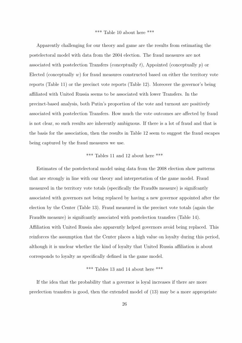
cycle (2007-2008) compared to (2003-2004). As is shown in Figure 1, by displaying kernel

density estimates Mebane and Kalinin (2009) found the presence of spikes for oblasts at

locations corresponding to the excess of turnout figures at values of 70%, 80% and 90%, a

pattern also noticed by Shpilkin and Shulgin (Buzin and Lubarev 2008, 201). Moreover, for

both oblasts and republics there is a spike of precincts with turnout at or very near 100

6

percent with a higher proportion of precincts in the republics than in the oblasts having

this feature. In the distribution for oblasts, spikes are apparent at round number

percentages of turnout above 60%. The only plausible explanation for the spiked

distributions is a wide-spread adjustment of turnout to specific “rounded” figures.

Moreover, the analysis of the last digits of turnout counts (Beber and Scacco 2008) showed

there are always too many zeros, with one exception too few nines, and usually too many

fives. As one moves from 2003 to 2008 the fakery with turnout seems to be much worse at

the end of the time period than at the beginning (Mebane and Kalinin 2009).

*** Figure 1 about here ***

Hence, we argue that the nature of fraudulent electoral results can be explained by the

presence of signaling games between the regions and the Center. The fraudulent electoral

results display the extent to which favorable electoral results can be delivered by the

regional elites to display their loyalty to the Center in exchange for administrative and

financial rewards.

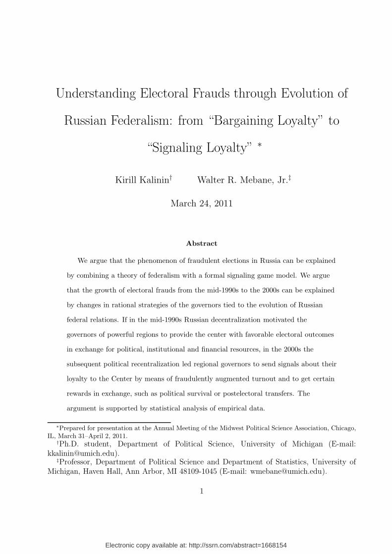
2 A Formal Model

Consider the signaling game represented by the diagram in Figure 2. N denotes a random

move by Nature to produce a first player (the governor, G) who is either loyal (L) or not

(¬L). Then Prob(L) = λ and Prob(¬L) = 1− λ. In the election the governor then either

commits fraud (F ) or not (¬F ). Player 2 (the Center, K) does not know whether G is

loyal, but K does observe G’s move. K then either punishes (P ) or not (¬P ). The payoffs

are given at the bottom of Figure 2. The interpretation of the symbols used in the payoff

definitions is as follows.

• w ≥ 0 is the value of electoral punishment by voters for fraud committed in the election;

w > 0 in years before elections are abolished, and w = 0 after 2004

7

• p > 0 is the value of punishment imposed by K

• v > 0 is the value of excess votes produced by fraud

• t > 0 is the value of transfers from K to G

• b is a coefficient that when multiplied by t gives the present discounted value of the

future expected to be produced by a transfer; this may be positive or negative

• d > 0 is the value to K of replacing a disloyal G

*** Figure 2 about here ***

Here are some comments to further explain the payoffs. Given equivalent actions by K,

fraud is always worse for G due to the sanction from voters. That is, if G is loyal and K

always punishes, then playing F gives G a payoff of −w − p while playing ¬F gives −p. If

there is no sanction from voters, w = 0, then F and ¬F give G the same payoff given an

identical response from K. The payoffs to G from F are always w subtracted from the

corresponding payoff from ¬F .

If fraud happens, K always gains excess votes v. If K doesn’t punish, then G always

gains a transfer from K, t, which costs −t to K. If K punishes, then G always loses −p

which also costs −p to K. But if a disloyal G is punished (e.g., fired), then K gains d.

One key difference between a loyal G and a disloyal one is who retains any future

surplus generated by a transfer from K. Compare the payoffs when a loyal G commits fraud

and is not punished to the payoffs when a disloyal G commits fraud and is not punished:

the difference is that the term bt is added to K’s payoff in the former case but is added to

G’s payoff in the latter case. A similar situation holds when G does not commit fraud and is

not punished: the disloyal G retains the surplus while with a loyal G K retains the surplus.

We represent the game in multiagent normal form (Myerson 1991). To facilitate doing

that, we relabel the moves as shown in Figure 3. The strategies of the loyal G are now

denoted F1 and ¬F1 while the disloyal G’s strategies are F2 and ¬F2. K’s strategies are

8

now P1 and ¬P1 if acting after fraud and are P2 and ¬P2 if acting after no fraud. The

multiagent strategic normal form of the game appears in Table 1.

*** Figure 3 and Table 1 about here ***

We test necessary conditions to be a perfect Nash equilibrium for the set of possible

pure strategy equilibria. The strategy profiles along with the payoffs that go to G and K

are listed in Table 2. The strategy profiles, the results of testing whether the profile can be

a Nash equilibrium and a brief description of the reqirements for the profile to be an

equilibrium appear in Table 3. The tests are done by comparing payoffs produced with

each profile to the payoffs produced with the profiles produced by changing each agent’s

strategy while holding the other strategies constant. For instance, comparing the payoffs

produced by (F1, F2,¬P1,¬P2) (profile I*) to the payoffs produced respectively by

(¬F1, F2,¬P1,¬P2), (F1,¬F2,¬P1,¬P2), (F1, F2, P1,¬P2) and (F1, F2,¬P1, P2) shows that

(F1, F2,¬P1,¬P2) gives a weakly greater payoff than the adjacent payoffs only if λ = 1 and

w = 0. This result is the equilibrium condition for profile I* in Table 3. Sometimes a

profile cannot produce payoffs that are weakly greater than those produced by the adjacent

profiles, given the domains defined for the parameters. In such cases the equilibrium

conditions appear in Table 3 as “never.” The equilibrium conditions for (F1, F2,¬P1, P2)

(profile III*) are too complicated to describe in Table 3. Those appear in Table 4.

*** Tables 2, 3 and Table 4 about here ***

Several profiles that can be equilibria have conditions that require either λ = 0 or

λ = 1. These are the profiles labeled I*, II*, V*, VI*, XI* and XVI*.1 While some of these

equilibria have potentially interesting features, we think the extreme conditions λ = 0 or

λ = 1 make them too brittle to describe the reality in Russia. Loyalty in reality is a choice

each governor makes and not an immutable personality trait, and K cannot know for sure

1Explicitly, these profiles are I*, (F1, F2,¬P1,¬P2); II*, (F1,¬F2,¬P1, P2); V*, (F1,¬F2, P1,¬P2); VI*,(F1,¬F2,¬P1,¬P2); XI*, (¬F1, F2,¬P1, P2) and XVI*, (¬F1, F2,¬P1,¬P2).

9

that a G is loyal (λ = 1) or disloyal (λ = 0), so we think that a practically relevant

equilibrium is one that admits uncertainty: λ ∈ (0, 1). Subsequently we will see some

reasons to reconsider this.

The profiles that can be equilibria and admit uncertainty about G’s loyalty are the ones

labeled III*, IX*, XII* and XV*.2 Of these profiles we think IX* does not apply because it

requires w = 0, and we think this condition is satisfied only after gubernatorial elections

are abolished, in 2004, but then it also requires that the expected long-term returns from

transfers to the regions be negative (b < 0). We believe this was so during the 1990s, but

ceased to be the case during the 2000s. Profile XII* we rule out because it requires that

the electoral punishment of G by voters for committing fraud is greater than the sum of

punishment imposed by K and the value of transfers from K (w ≥ p + t). While w may be

comparable to p if p corresponds to being removed from office, we know of no case where a

governor was voted out of office for having committed election fraud, so we think in fact

p > w. These considerations leave only profiles III* and XV* as, in our judgment,

practically viable equilibria.

The two equilibria, III* and XV*, can sometimes exist simultaneously. For XV* to be

an equilibrium it is required that (t+ p)/(w+ t+ p) ≤ λ < 1 and p > t+ v, and a condition

for III* to be an equilibrium with 0 < λ < 1 is p ≥ t− (v + d); but p ≥ t− (v + d) is always

true if p > t+ v is true. Another condition for XV* to be an equilibrium is

p ≥ (1− λ)d+ (1− λb)t. If XV* is an equilibrium, then λ < 1 and b < 0, so

(1− λ)d+ (1− λb)t > 0. The most important aspect of this result is the presence of d on

the lefthand side of p+ v + d ≥ t but on the righthand side of p ≥ (1− λ)d+ (1− λb)t: as

the value d that K places on having a loyal G rises, for fixed values of p and t, the

conditions for III* to be an equilibrium become satisfied while the conditions for XV* to be

an equilibrium may cease to be satisfied.

2Explicitly, these profiles are III*, (F1, F2,¬P1, P2); IX*, (F1, F2, P1, P2); XII*, (¬F1,¬F2,¬P1, P2) andXV*, (¬F1,¬F2, P1,¬P2).

10

Expectations about the long-term returns from transfers from K to the region also

affect whether the two equilibria exist simultaneously. In order for XV* to be an

equilibrium, these expectations must satisfy

−(p+ t)

(1− λ)t≥ b ≥ v + t− p

t, (1)

which implies b < 0. The equilibrium conditions for III* impose no upper bound on b, but

specify lower bounds that depend on λ:

b ≥

(w − p− t)/t, λ = 0

[(1− λ)d+ t− p]/(λt), 0 < λ < 1

(t− p)/t, λ = 1 .

(2)

All these lower bounds are negative, so under III* as an equilibrium b may be either

positive or negative. XV* and III* can both be equilibria simultaneously if the intervals

defined by (1) and (2) overlap and b is contained in this overlapping region.

If III* and XV* exist as equilibria simultaneously, which one will G and K act to

instantiate? To answer this question we first evaluate the players’ payoffs under the

respective equilibria, and in particular we ask whether one equilibrium benefits the players

more than the other one. If so, we expect the players will enact the equilibrium that pays

them the most.

Consider the situation where the intervals defined by (1) and (2) overlap, and define

bδ = δ−(p + t)

(1− λ)t+ (1− δ)

v − p+ t

t, δ ∈ [0, 1] . (3)

11

Now, with b = bδ, compare the payoffs under III* to those under XV*. The payoffs are

weakly better under III* when

G: − w + t[1 + bδ(1− λ)] ≥ −p ⇒ (1− δ)[t+ λp+ (v + t)(1− λ)] ≥ w (4)

K: v + t(λbδ − 1) ≥ λ(bδ − 1)t− (1− λ)t ⇒ v ≥ 0 (5)

The difference between K’s payoffs under III* versus XV* does not vary with b: whenever

both equilibria exist simultaneously, (5) shows that K always gains v by being in

equilibrium III* instead of equilibrium XV*. For G the difference in payoffs depends on the

relative sizes of p, t, v and w. If (4) is true, then G is weakly better off with III*, otherwise

G is better off with XV*. Even if p > w, as we believe, (4) is false for δ sufficiently large or

λ sufficiently small, as long as w > 0. So if the voters do exact some electoral punishment

on G for committing fraud, and the likelihood that G is disloyal is sufficiently high or the

expected returns from transfers are sufficiently negative, G benefits more from being in

equilibrium XV* rather than equilibrium III*. Eliminating gubernatorial elections and

hence setting w = 0 guarantees that G is better off under equilibrium III* than under

equilibrium XV*.

If III* and XV* are simultaneously equilibria and (4) is false, then even though K is

better off if III* is enacted than if XV* is enacted, K should predict that G will play ¬F

instead of F , and so K should play ¬P2 instead of P2. Playing (P1, P2) when G plays

(F1, F2) is not rational for K in any case, since we are considering the case when XV* is an

equilibrium.

The foregoing discussion suggests that whether III* or XV* is enacted should depend

on the levels of d, p, t, v and w. As d, p, t and v increase, or as w decreases, the prospects

of III* happening rather than XV* should be higher. As the value K places on G loyalty,

the value of punishment imposed by K, the value of transfers from K and the value of

excess votes produced by fraud increase, or as the value of electoral punishment for G’s

12

committing fraud decreases, we should expect fraud to become more prevalent. We use

these insights to motivate our empirical investigation, below.

Our argument so far does not show how fraud can be associated with transfers,

punishments and the like when expectations for the returns from transfers are positive

(b > 0). Such conditions rule out XV* as an equilibrium. Likewise after 2004, when

elections for governor are abolished and so w = 0, (4) suggests XV* will never happen. But

our empirical analysis below shows that transfers and punishments are in fact associated

with election fraud after 2004.

One consideration is that in III*, t and p affect the range of λ values that are

compatible with equilibrium. If 0 < λ < 1 and b < 0, bounds on λ are given by

1 +t+ p

bt≤ λ ≤ 1− t(b− 1) + p

bt + d.

The lower bound is negative and so never binding on λ, but the upper bound is zero if

p = t + d. If XV* is an equilibrium—in which case we must havet+ p

w + t+ p≤ λ—then G

may do ¬F instead of F . But if λ does not satisfy the necessary conditions for either III*

and XV* to be an equilibrium, then it is unclear what G will do.3 If on the other hand

0 < λ < 1 and b > 0, then bounds on λ are given by

1 +t+ p

bt≥ λ ≥ 1− t(b− 1) + p

bt + d. (6)

Now the upper bound is never binding, but the lower bound may be. The lower bound may

or may not be increasing in t,4 but in any case as t → ∞, the bound approaches 1/b > 0.

As p → ∞ the bound grows to infinity and III* can never be an equilibrium. If b is

positive, then III* can be an equilibrium only if the chances of G being disloyal are not too

3We don’t know yet whether there is some mixed strategy equiibrium that may apply in the situtationbeing considered here.

4If z ≡ 1 − [t(b − 1) + p]/(bt + d), then ∂z/∂t = [bp + (1 − b)d]/(bt+ d)2, so the bound increases in t ifbp+ d > bd.

13

high. If b > 0 and III* is not an equilibrium because λ is too low but not zero, then the

game’s only equilibrium is XII*, which predicts G plays ¬F rather than the F of III*. But

XII* requires implausibly high values of w, and in fact w = 0 after gubernatorial elections

were abolished in 2004. In any case, these arguments are enough to establish that in some

cases fraud can be associated with transfers and punishments even when expectations for

the returns from transfers are positive.

Another way to account for the association between transfers, punishments and fraud in

and after 2004, when we think b > 0 is likely, is to reconsider our stance against profiles

whose equilibrium status depends on extreme loyalty beliefs. In particular we may allow

that once Kremlin eliminates elections for governors and begins appointing governors, the

idea that K has no doubt that G is loyal (λ = 1) becomes plausible. Allowing this brings

profiles II*, V* and VI* back in as feasible equilibria.5

If λ = 1, then II* can be an equilibrium for a range of both positive and negative values

of b:

t + p

t≥ b ≥ t− p− v

t.

In general III* weakly dominates II*, but if λ = 1 the two profiles have equal payoffs. So

λ = 1 induced by Kremlin’s having appointed the governors may explain why disloyal

governors do not commit fraud—II* includes the move ¬F2—but taking II* into account

cannot explain why transfers and punishments are associated with fraud.

If λ = 1, then V* can be an equilibrium only if b ≤ 0, because a condition for V* to be

an equilibrium with λ = 1 is (1− b)t ≥ p ≥ t. Comparing the equilibrium payoffs with

λ = 1, the conditions for III* to give higher payoffs than V* are

G: t ≥ p (7)

K: p ≥ −t(b− 1) . (8)

5We ignore I*, which also is an equilibrium only if λ = 1, because actions under I* are identical to thoseunder III* for behavior on the equilibrium path.

14

Given λ = 1, t ≥ p may be true and p ≥ −t(b− 1) is necessarily true if III* is an

equilibrium. A condition for V* to be an equilibrium is p ≥ t. So a decrease in t may give

one or both players higher payoffs under V* than under III*, and an increase in p may give

G a higher payoff under V* than under III*. But profile III* is (F1, F2,¬P1, P2) while

profile V* is (F1,¬F2, P1,¬P2). This suggests one way an increase in t may be associated

with a greater frequency of observed fraud in the period during and after 2004, but only if

b ≤ 0 then.

If λ = 1, then VI* can be an equilibrium for b ≥ 0 but only if t ≥ p. Profile VI* is

(F1,¬F2,¬P1,¬P2), so again an increase in t or a decrease in p may be associated with a

greater frequency of observed fraud in the period during and after 2004.

3 Empirical specification

According to our model, three parameters are central to our understanding of why specific

equilibria hold and why the shift from the “preelectoral bargaining” equilibrium of the

1990s to the “electoral signaling” equilibrium of the 2000s occurs. These parameters are d,

the value to the Center of replacing a disloyal governor, λ, the probability that a governor

is loyal, which is presumably increased by having the governor be appointed instead of

elected, and b, the future returns expected to be produced by a transfer.

For the 1990s there are two scenarios, identified by one’s belief about the value of b.

More precisely, we imagine that over all of Russia, regions are diverse, so a single

configuration of parameter values does not characterize the whole country.6 So b may be

positive or negative. Negative b values we associate with corruption and political

opportunism: as far as the Center is concerned, economic resources transfered to a corrupt

region are expected to produce no significant value in the future, and if the resources

6Note that we have modeled the relationship between the Center and one governor. We assume that theCenter plays such a game independently in each region, and that regional actors learn nothing from oneanother’s experience. Reality undoubtedly involves more interaction between regions than this, but it isintractable to extend the game to one in which the Center simultaneously interacts with all 89 regions.

15

facilitate regions’ gaining further autonomy and even independence, the return on transfers

to a region may even be evaluated as strictly negative. Or b may be positive. Indeed, if b is

like a normal investment, we should have b ≥ 1: the transfer is at least expected to pay for

itself. Different regions may at any one time have different values of b. But during the

1990s, the threat of regions leaving the Russian federation was very real, so we think that

often b was negative.

If b < 0, then we think the relationship between Center and governor during the 1990s

is best described by thinking of the possible equilibrium profiles as III*, or

(F1, F2,¬P1, P2), and XV*, or (¬F1,¬F2, P1,¬P2). But during the 1990s the value of d was

very low, w > 0 in cases where the governor was elected, and λ tended to be low due to

governors’ high degree of autonomy. Because III* requires p+ v + d ≥ t but XV* requires

p ≥ (1− λ)d+ (1− λb)t, low d suggests XV*, and recalling (4), a higher value of w also

suggests XV*. The value of λ may be so low that b is less than the lower bound identified

by (2) as necessary for III* to be an equilibrium. But in this case XV* may be unlikely to

be an equilibrium, because small λ means that the lower bound on b needed for III*,

[(1− λ)d+ t− p]/(λt), is probably less than the lower bound needed for XV*, which from

(1) is (v+ t− p)/t. In this case we have no reason to think that variations in t and p, if they

do not bring III* into equilibrium status, will be associated with the incidence of fraud.

If b > 0, then we think III* and XII* are the best candidates to describe the

relationship between Center and governor during the 1990s. Recall that XII* is the profile

(¬F1,¬F2,¬P1, P2). The key question becomes whether the value of λ is so low that (6)

rules III* out as an equilibrium. Since governors managed to bargain successfully, it is

reasonable to suppose t is large so that the bound is not far from the limiting value of 1/b.

How big is b? Even if transfers, thought of as investments, were expected eventually to

produce a return that doubled the original transfer, we would have 1/b = 0.5, and it would

be reasonable to think that λ in the 1990s was usually smaller than that. This leaves for an

equlibrium only the profile described by XII* in which there is no fraud. If t > w, then

16

XII* cannot be an equilibrium, but with the low value of λ having ruled out III*, we have

no reason to expect the occurrence of fraud to be associated with transfers.

In the 2000s the clearest change is that the value of d increased. Recentralization

signals such a change, and the abolition of gubernatorial elections in 2004 decisively

indicates it. The increase in d reflects how local “political machines” were coopted into the

power vertical. Recentralization also greatly reduced separatist concerns, so that b > 0,

and indeed b > 1, is easy to assume. The positive value of b rules out XV* as an

equilibrium, and w = 0 rules out XII*. Recentralization and having governors be appointed

likely raised the typical value of λ, so that b may more often exceed the lower bound in (6).

If having governors be appointed means that often λ = 1, then VI*, or (F1,¬F2,¬P1,¬P2),

comes into play as a possible equilibrium alternative to III*, with the oscillation between

the two depending on the balance between transfers and punishments. If transfers are high

enough, VI* may come into play so that only truly loyal governors commit fraud.

If VI* comes in in this way during the 2000s, then it is the only strategy profile we

expect to observe that involves a separating equilibrium, and because VI* requires λ = 1,

strictly speaking if VI* is the equilibrium in effect then there are no disloyal governors.

Mostly we expect that governors, in committing or not committing fraud, are masking

their types.

We use empirical data to assess a number of implications from the formal model,

focusing on the presence or absence of associations between the occurrence of election fraud

and variables that measure transfers, punishments and appointments. In the empirical

assessments, timing is important. One set of tests relates preelection covariates to measures

of fraud in the election, while the other set relates measures of fraud to postelection

covariates. The order of moves in the game directly motivates the postelection models: in

the game, the governor first commits or does not commit fraud, then the Center acts. The

connection to the preelection models is indirect: the game model does not have any

implications for the relationship between preelection covariates and election fraud; we

17

examines simple regressions of such variables on measures of fraud, expecting to see no

associations during the 1990s.

An informal extension of the game model motivates what we think of as a sharper set of

tests. The game has the governor moving before the Center, with Nature first selecting the

type of the governor. In reality the governor makes a decision whether to be loyal, in

response to anticipations of what the Center will do and in light of preelection conditions.

Among those conditions are preelection actions by the Center. A simple way to connect

preelection actions to the game model is to imagine that they influence the value of λ:

preelection actions affect the likelihood that the governor is loyal. We present a set of

modified postelectoral empirical models designed to reflect these ideas.

The game model also suggests that fraud should be positively associated with

indicators of whether the governor is appointed or with other indicators of the governor’s

loyalty to the Center. An appointed governor or an otherwise especially loyal governor goes

with a higher value of λ and so should be associated with a higher incidence of fraud.

The theoretical model supports different predictions about the relationships among

fraud, transfers and other variables in different time periods. The model gives no reason to

predict that transfers, which measure the fruits of preelection bargaining, will be associated

with measures of fraud during the 1990s, so we do not expect to see an association between

these variables at that time. During the 2000s, once Kremlin commences recentralization

and Putin comes to power, and particularly after 2004 when gubernatorial elections are

abolished, the model predicts the incidence of fraud will be positively associated with

transfers and negatively associated with punishments.

We use several regression-type statistical models to assess the associations. Regression

relationships based on linear predictors are not specifically implied by our theoretical

model, but they represent the easiest way to get at possible relationships, taking into

account the likelihood that multiple, correlated and conceptually distinct variables are

associated with the occurrence of fraud.

18

Preelectoral Bargaining Model The preelectoral bargaining model is a logit

regression model, measuring effects of various preelectoral factors on electoral frauds. The

number of variables varies across years, depending on data availability. For the 1996 and

2000 elections electoral frauds are measured at the territory level. For 2004 and 2008

presidential elections electoral frauds are measured at both the precinct level and the

territory level and are used in two separate models. The linear predictor is

logit(Frauds Indexi) = a0 + a1 (Bilateral Treatyi) + a2Governor URi

+ a3 Republicsi + a4 (Gross Regional Producti)

+ a5 Electedi + a6Appointedi + a7Transfersi , (9)

where in one set of estimates i indexes precincts and in another set territories. The

outcome variable is Frauds Index, which is a dummy variable equal to 1 if there are 0s or

5s in the last digit of the percent of presidential election turnout across territories (or

precincts) and equal to 0 for other digits. The covariates are the following. Bilateral Treaty

is a dummy variable, measuring if the regions signed a bilateral treaty by the year of

elections: 1 is signed, 0 otherwise. Governor UR is a dummy variable, measuring if a

governor openly supported Unity/United Russia 1 after 1999 parliamentary elections, 0

otherwise. Republics is a dummy variable, measuring if a region belongs to Republic (1) or

not (0). Gross Regional Product measures gross regional product a year before the

elections (divided by one million). Elected is a dummy variable with 1 if a new governor

was elected within a year before the elections, which is conceptually the preelectoral period

of the same year elections take place. Appointed is a dummy variable with 1 if the

governor was appointed a year before the elections. Transfers measures the amount of

transfers per 10000 people allocated to the region: it accounts for a year before the

elections and an electoral year (divided by one million).

Some of the covariates beside Transfers, which represents t, have clear theoretical

19

meanings. Bilateral Treaty or Governor UR or Appointed being positive are associated

with higher loyalty and so presumably higher values of λ. If a region is a republic

(Republics = 1), then loyalty may be less and voters may be less concerned with fraud so

that the value of w is less. If the expected future returns from transfers are negative

(b < 0), which in particular they may be in republics, then the implications of higher λ are

unclear, in view of (4), but (4) suggests that lower w should go with higher incidences of

fraud. If b > 0, then the chances that equilibrium involves committing fraud depends on λ

and (6), so that positive values for Bilateral Treaty or Governor UR or Appointed or not

being a republic may go with more fraud.

Postelectoral Signaling Model For the postelectoral model we use three separate

regression models with different outcome variables. There is a linear regression model in

which Transfers is the dependent variable, and two are logistic regression models in which

the dependent variables are Elected and Appointed. The models for Transfers, Elected and

Appointed use data measured at or aggregated to the regional level. The linear predictors

are

Transfersi = b0 + b1 (Bilateral Treatyi) + b2 (Governor URi) + b3 Republicsi

+ b4 (Gross Regional Producti) + b5 Turnouti + b6 Incumbenti

+ b7 Fraud0si + b8 Fraud5si (10)

logit(Electedi) = c0 + c1 (Bilateral Treatyi) + c2 (Governor URi) + c3Republicsi

+ c4 (Gross Regional Producti) + c5Turnouti + c6 Incumbenti

+ c7 Fraud0si + c8 Fraud5si (11)

20

logit(Appointedi) = d0 + d1 (Bilateral Treatyi) + d2 (Governor URi) + d3Republicsi

+ d4 (Gross Regional Producti) + d5Turnouti + d6 Incumbenti

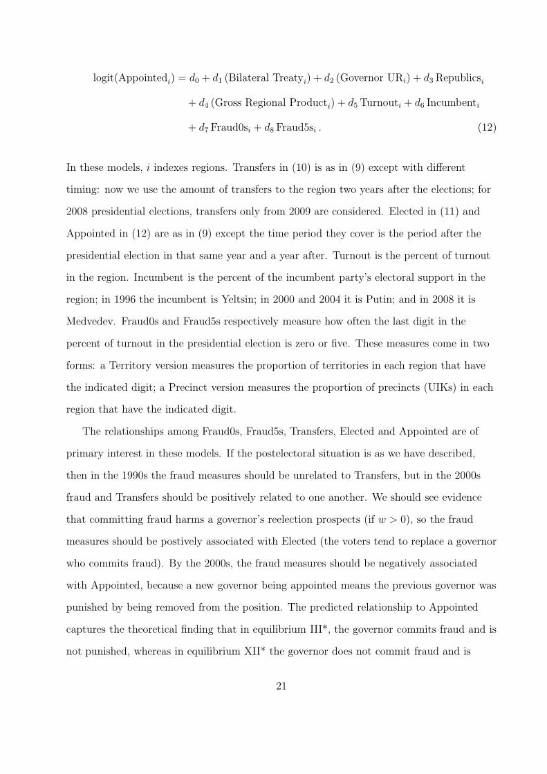
+ d7 Fraud0si + d8 Fraud5si . (12)

In these models, i indexes regions. Transfers in (10) is as in (9) except with different

timing: now we use the amount of transfers to the region two years after the elections; for

2008 presidential elections, transfers only from 2009 are considered. Elected in (11) and

Appointed in (12) are as in (9) except the time period they cover is the period after the

presidential election in that same year and a year after. Turnout is the percent of turnout

in the region. Incumbent is the percent of the incumbent party’s electoral support in the

region; in 1996 the incumbent is Yeltsin; in 2000 and 2004 it is Putin; and in 2008 it is

Medvedev. Fraud0s and Fraud5s respectively measure how often the last digit in the

percent of turnout in the presidential election is zero or five. These measures come in two

forms: a Territory version measures the proportion of territories in each region that have

the indicated digit; a Precinct version measures the proportion of precincts (UIKs) in each

region that have the indicated digit.

The relationships among Fraud0s, Fraud5s, Transfers, Elected and Appointed are of

primary interest in these models. If the postelectoral situation is as we have described,

then in the 1990s the fraud measures should be unrelated to Transfers, but in the 2000s

fraud and Transfers should be positively related to one another. We should see evidence

that committing fraud harms a governor’s reelection prospects (if w > 0), so the fraud

measures should be postively associated with Elected (the voters tend to replace a governor

who commits fraud). By the 2000s, the fraud measures should be negatively associated

with Appointed, because a new governor being appointed means the previous governor was

punished by being removed from the position. The predicted relationship to Appointed

captures the theoretical finding that in equilibrium III*, the governor commits fraud and is

not punished, whereas in equilibrium XII* the governor does not commit fraud and is

21

punished.7

The theoretical designation of variables included in both the postelectoral empirical

models and the preelectoral models is the same, but the theoretical model does not specify

any particular effects for these variables in the present regressions. Likewise the Turnout

and Incumbent variables may be associated with Transfers, Elected and Appointed, but

whether such associations represent effects of fraud as described in our theoretical model is

unclear. Any relationships may reflect the operations of normal patronage: people who do

well get rewarded. In the current analysis we consider only Fraud0s and Fraud5s to be

measures of fraud. As Figure 1 illustrates, it is not so much extraordinarily high turnout

but turnout figures occurring in round numbers that indicate fraud.

Extended Postelectoral Signaling Model An extension of the postelectoral model

assesses how preelection actions by the Center may affect the relationship between fraud

and postelection covariates, in particular the relationship between the fraud measures

(Fraud0s and Fraud5s) and Transfers. The extended model is defined by the predictor

Transfersi = b0 + b1 (Bilateral Treatyi) + b3 Republicsi

+ b4 (Gross Regional Producti) + b5 Turnouti + b6 Incumbenti

+ λib7 Fraud0si + λib8 Fraud5si , (13)

where λi is a function of preelection Transfers. We use two different specifications for λi:

λ(1)i =1

1 + exp(−b29 Transfersi,t−1), λ(2)i =

2

1 + exp(−b29 Transfersi,t−1)− 1

where Transfersi,t−1 denotes the value of Transfersi in the year t− 1 before the election.

The range of λ(1)i is [.5, 1) while λ(2)i ranges over [0, 1). We use nonlinear least squares to

estimate the parameters in this model.

7In considering XII* relevant for 2008, we finesse the issue that w = 0 is incompatible with XII* beingan equilibrium.

22

This model represents a very simple implementation of a mixture model. Fraud

measures and Transfers are related when the governor is loyal and not otherwise, and the

probability that the governor is loyal depends on—increases with (b29 ≥ 0)—preelection

transfers. Loyalty may depend on preelection transfers either because the transfers

persuade governors to become loyal or because governors who are already known to be

loyal get the transfers. All parameters besides the coefficients of the fraud measures (b7 and

b8) are assumed to be identical for the respective types of governors, so an interaction term

is sufficient to represent the mixture.

We specify λi two different ways because while the full range of λ values ([0, 1]) may be

expected during earlier periods, after 2004 values less than 1/2 may not be plausible. In

this case λ(1)i and not λ(2)i may apply to data from the later years.

Data Sources The data used in this research were taken from multiple sources. The

data on financial transfers for different periods were kindly provided by Daniel Treisman

and Andrei Starodubtsev. The data on governor’s affiliation with United Russia in 2003

and 2008 were kindly given by Olesya Tkacheva, the governors affiliation with Unity was

taken from Republics (2000). The electoral data for 1996 and 2000 presidential elections

were sent to us by Alexei Sidorenko. The data for 1996 and 2000 include only

territory-level election reports. The electoral data for 2004 and 2008 were obtained from

the website of Russian Central Elections Commission (http://www.cikrf.ru). The data

for 2004 and 2008 include both precinct-level (UIK-level) and territory-level election

reports. Other data were collected by the authors from the databases of Federal State

Statistics Service and the websites of regional administrations.

4 Empirical Results

The preelectoral models match our expectations in the sense that in territory data for 1996

there is no significant association between Transfers and the omnibus fraud measure (Table

23

5). During the first round of the election, fraud is more apparent in Republics, and recently

appointed governors governors commit more fraud. During the second round of voting

none of the covariates show a significant association with fraud.

*** Table 5 about here ***

Significant associations between the fraud measure and preelection covariates are also

sparse in territory data in other years, even though many associations appear in precinct

data. In the analysis of territory data from the 2000 election, none of the covariates has a

significant effect (Table 6). In 2004, when both precinct and territory data are available, no

covariate has a significant effect in the territory data but all effects are significant in the

precinct data (Table 7). With such a large number of precinct observations (N = 87, 518),

the existence of so many significant associations is perhaps not surprising, but in particular

the coefficients of Transfers and Appointed are positive: more preelection transfers and

having a recently appointed governor are both associated with more fraud. Also there is

more fraud when the governor is affiliated with United Russia, when the region has a

bilateral treaty with the Center and in republics. Results in 2008 are largely the same as in

2004, with one exception (Table 8). Notwithstanding the large number of precincts

(N = 91, 998 in 2008), the coefficient for Transfers is only marginally significant in the

precinct data (a7 = 0.060 with s.e. = 0.035). These results do not contradict the relatively

weak expectations the game model provides for the association between election fraud and

preelection covariates.

*** Tables 6, 7 and 8 about here ***

Turning to the postelectoral model, in 1996 the two fraud measures are mostly not

associated with postelection transfers, as our argument and our interpretation of the game

model suggest. The Frauds0s measure based on votes recorded in the first round of the

election is significantly associated with Transfer during 1996, but the effect is small (Table

24

9). Fraud0s based on votes in the second round is not associated with Transfers, and there

is no association between Transfers and Fraud5s measured in either round.

*** Table 9 about here ***

Contrary to the presumption in the game model, fraud (measured by Fraud0s)

committed in the first round of the election is not associated with the governor

subsequently being punished by voters. The Fraud0s measure of fraud in the first round of

the presidential election is significantly negatively associated with Elected: governors who

committed fraud were less likely to be replaced in their next gubernatorial election than

those who did not commit fraud. This certainly does not suggest w > 0. It suggests that

during this period there are at the least not high levels of voter vigilance. Most likely,

during the 1990s most of the governors who were capable of committing election fraud

could mobilize their “political machines” during regional elections to avoid electoral

punishment related to frauds from the voters. Although its theoretical significance is

unclear, it is interesting that governors in regions where Yeltsin (the incumbent) received a

higher proportion of the votes also were less likely to the replaced by the voters. Because

we don’t know how much fraud affected Yeltsin’s vote share, it is not possible to say

precisely what implication this relationship has for our theoretical questions.

Postelectoral model estimates for 2000 (Table 10) show no significant association

between the fraud measures and either postelection transfers or postelection gubernatotial

election results. Such results suggest that the 2000 election should be counted as part of

“the 1990s.” Putin was elected for the first time in that election, even though he took office

already in 1999, but there is no clear sign of the kind of connection between fraud and

postelection rewards that the equilibria of the game identify. The consequences of Putin’s

recentralization inititative apparently had yet to take hold. The governor’s political

affiliation with Unity during 1999 State Duma elections did have a positive effect on

postelection transfers. A governor’s demonstration of open loyalty by support of Unity was

later rewarded by larger amount of financial inflows to the region.

25

*** Table 10 about here ***

Apparently challenging for our theory and game are the results from estimating the

postelectoral model with data from the 2004 election. The fraud measures are not

associated with postelection Transfers (conceptually t), Appointed (conceptually p) or

Elected (conceptually w) for fraud measures constructed based on either the territory vote

reports (Table 11) or the precinct vote reports (Table 12). Moreover the governor’s being

affiliated with United Russia seems to be associated with lower Transfers. In the

precinct-based analysis, both Putin’s proportion of the vote and turnout are positively

associated with postelection Transfers. How much the vote outcomes are affected by fraud

is not clear, so such results are inherently ambiguous. If there is a lot of fraud and that is

the basis for the association, then the results in Table 12 seem to suggest the fraud escapes

being captured by the fraud measures we use.

*** Tables 11 and 12 about here ***

Estimates of the postelectoral model using data from the 2008 election show patterns

that are strongly in line with our theory and interpretation of the game model. Fraud

measured in the territory vote totals (specifically the Fraud0s measure) is signifcantly

associated with governors not being replaced by having a new governor appointed after the

election by the Center (Table 13). Fraud measured in the precinct vote totals (again the

Fraud0s measure) is signifcantly associated with postelection transfers (Table 14).

Affiliation with United Russia also apparently helped governors avoid being replaced. This

reinforces the assumption that the Center places a high value on loyalty during this period,

although it is unclear whether the kind of loyalty that United Russia affiliation is about

corresponds to loyalty as specifically defined in the game model.

*** Tables 13 and 14 about here ***

If the idea that the probability that a governor is loyal increases if there are more

preelection transfers is good, then the extended model of (13) may be a more appropriate

26

specification than the original postelectoral specification of (10). Comparisons between

(13) and a version of (10) that omits Governor URi are reported in Table 15, in the form of

a set of F -tests for the hypothesis that the added parameter and covariate in (13) does

nothing to improve the performance of the empirical model.8 The test results in Table 15

show that the extended model usually performs better, in the sense that the extended

model usually produces a residual sum-of-squares (summarized by the standard error of the

regression σ) that is significantly smaller than with the original specification.

*** Table 15 about here ***

Notwithstanding that the extended model apparently fits the data better, the results

from applying that model to the 1996 election data show patterns that are hard to

reconcile with signaling of the type we have discussed in which fraud is encouraged by the

prospect of rewards in terms of transfers. Using either λ(1)i or λ(2)i, the Fraud0s measure

based on the voting in round 1 of the presidential election shows a significant but small

positive association with postelection transfers (Table 16). But when using data from

round 2 of the election, only the specification that uses λ(2)i can be estimated, and in that

case it appears that the b9 parameter is not identified. To get the parameter estimates in

Table 16, we fix b9 = 1.0 and then estimate the remaining unknown parameters. The result

of doing this is that fraud as measured by Fraud0s is significantly negatively associated

with postelection transfers. For the specification that uses λ(1)i, the model could be

estimated only when the b9 parameter—not its square—is used in the definition of λ(1)i,

and the estimated value of b9 that then results is negative.9 The negative estimate for b9 in

the modified model suggests, if anything, that preelection transfers reduce the probability

that the governor is loyal, contradicting the implications of all the other extended model

8Rather than just dropping Governor URi, which we think is strongly related to λ, it may be better toinclude Governor URi in functions like λ(1)i and λ(2)i.

9The nonlinear least squares estimator does not converge when, with λ(1)i properly defined using b29, the

starting values are the estimates shown in Table 16 with b9 started at√5246. The model with λ(1)i properly

defined and b9 = 1.0 also does not converge.

27

specifications used with the 1996 election data. The best conclusion, probably, is that the

extended postelectoral model does not at all describe the 1996 data, and consequently the

entire postelectoral signaling idea does not apply to the 1996 election. This matches our

conclusion that the game model does not imply the existence of an equilibrium relationship

connecting transfers and punishments to election fraud in the 1990s.

*** Table 16 about here ***

In contrast, estimates from the extended model seems to place the 2000 election firmly

in the “2000s” category rather the “1990s” category. Using either λ(1)i or λ(2)i, the Fraud5s

measure is significantly and positively associated with postelection transfers. Estimating

the model with λ(2)i again requires that we set b9 = 1.0 then estimate the remaining

unknown parameters. The resulting estimate for b8 suggests a significant, large and

positive return in terms of postelection transfers from committing vote fraud. The estimate

for b8 when λ(1)i is used is much smaller: 0.45 versus 17.87. The model that uses λ(2)i has a

much smaller value of σ than does the model that uses λ(1)i, so perhaps that is a reason to

prefer the λ(2)i model. The question is whether it is correct to interpret λ(2)i as measuring

the probability that the governor is loyal. If so, the current results strongly confirm that

the 2000 election can be interpreted in terms of the game model.

*** Table 17 about here ***

Estimates from the extended postelectoral model applied to data from the 2004 election

strongly suggest that the signaling regime that ties election fraud to postelection transfers

was firmly in place by the time of that election. Both fraud measures are significantly and

positively related to postelection transfers when the fraud measures are based on territory

vote totals and λ(2)i is used (Table 18). When the fraud measures are based on precinct

totals, the measures are significantly and positively related to postelection transfers using

either λ(1)i or λ(2)i (Table 19). The extended postelectoral model has much smaller σ when

28

λ(2)i is used than with λ(1)i in both the territory-based and the precinct-based

specifications. Notably in the precinct-based specification it is not necessary to set b9 = 1.0

in order to estimate the model definition that uses λ(2)i.

*** Tables 18 and 19 about here ***

Results from estimating the extended postelectoral model using data from the 2008

election are nearly as strongly confirmatory of the theory and of the game model. Both

fraud measures are significantly and positively related to postelection transfers using λ(1)i

in both the territory-based and precinct-based cases (Tables 20 and 21). The Fraud0s

measure has a significant positive association with postelection transfers using either

territory-based or precinct-based data and λ(2)i. The one anomaly, relative to the theory, is

that b8 < 0 in the precinct-based specification with λ(2)i. Once again we set b9 = 1.0 in

order to estimate the models that use λ(2)i.

*** Tables 20 and 21 about here ***

The extended postelectoral model fits the data much better than the original

postelectoral model does, and it is arguably more tightly integrated with the motivating

theory in that it represents that the relationship between election frauds and transfers

depends on beliefs about the loyalty of the governor. The results from estimating the

model using data from the various elections very strongly confirm the theoretical argument

that refers to the game model. Russian presidential elections from 2000 on, but not the

election of 1996, are subject to widespread fraud motivated by the governors’ desire to

signal their individual loyalties to the Center.

5 Conclusion

Overall, our theoretical propositions are supported by our data. The results sometimes

display a complex picture. The presidential election of 1996 seems to contain elements of

29

bargaining—recently appointed governors and Republics were more likely to commit frauds

with the turnout, but signaling as described by the game seems not to have been occurring.

The presidential election of 2000 reflects political uncertainty: governors signaling by

committing fraud seems to have been rewarded in an incipient way. By 2004 and

continuing into 2008, the fraud-signal-transfers-and-appointments-reward regime seems to

be fully in place. If anything the rewards in terms of postelection transfers from

committing fraud in order to signal seem to be smaller in 2008 than in 2004: extended

model estimates for the b7 and b8 parameters are typically larger in connection with the

2004 election. This is despite the fact that Mebane and Kalinin (2009) find that

rounded-number turnout fraud is more prevalent in 2008 than in 2004. The relation

between frauds and appointments-punishments seems to be stronger in 2008 than in 2004,

however (recall the estimates for d7).

The prevalent “signaling” mechanism raises a fundamental problem for the new

political regime: regional elites after being coopted by the Center were inclined to exploit

the existing asymmetry in distribution of information between the Center and themselves

for their own benefit, by systematically distorting information in their best interests,

including electoral information. Demonstration of political loyalty, in exchange for no

interference on the part of the Center has led to greater informational asymmetry between

the regions and the Center, making the Center unable to separate the types of the heads of

the regions—who is really supportive of the regime and who is not but is successfully

faking their support.

References

1. Beber, Bernd and Alexandra Scacco (2008). What the Numbers Say: A Digit-Based

Test for Election Fraud Using New Data from Nigeria. Paper prepared for the Annual

Meeting of the American Political Science Association, Boston, MA, August 28–31,

30

2008.

2. Buzin, Andrei and Arkadii Lubarev (2008). Crime without Punishment: Admin-

istrative Technologies of Federal Elections of 2007-2008 (In Russian: Prestupleniye

bez nakazaniya. Administrativniye tekhnologii federal’nih viborov 2007-2008 godov).

Moscow: Nikkolo M.

3. Freedom House (2010). Report on Russia.

http://www.freedomhouse.org/template.cfm?page=1

4. Gel’man, Vladimir (2006). Vozvrashenie Leviafana? Politika Recentralizatsii v Sovre-

mennoi Rossii. POLIS (2):90-109

5. Gel’man, Vladimir (2007). Political Trends in the Russian regions on the Eve of State

Duma Elections. Russian Analytical Digest (21): 27.

6. Gel’man, Vladimir (2009). The Dynamics of Sub-National Authoritarianism: Russia

in Comparative Perspective. APSA 2009 Toronto Meeting Paper.

7. Gorenburg, Dmitrii. (1999). Regional Separatism in Russia: Ethnic Mobilization or

Power Grab? Europe-Asia Studies 51 (2).

8. Hale, Henry E. (2003). Explaining Machine Politics in Russia’s Regions: Economy,

Ethnicity, and Legacy. Post-Soviet Affairs 19 (3): 228-263.

9. Harrison, Mark. (2009). Forging Success: Soviet Managers and False Accounting,

1943-1962. Working paper, October 26, 2009.

10. Kahn, Jeffrey (2002). Federalism, Democratization, and the Rule of Law in Russia.

Oxford: Oxford University Press.

11. Kornya, A. (2008). Propavshie dushi (Lost souls). Vedomosti 06.03.2008, No.41 (2063).

Comment on the change in the number of voters during the federal elections 2007-2008.

31

(Kommentarii obizmenenii chislennosti izbiratelei v hode federal’nih viborov 2007-2008

godov).

12. Mebane, Walter R., Jr. and Kirill Kalinin (2009). Comparative Election Fraud Detec-

tion. Paper presented at the 2009 Annual Meeting of the American Political Science

Association, Toronto, Canada, Sept 3-6, 2009.

13. Mebane, Walter R., Jr., and Kirill Kalinin (2010). Electoral Fraud in Russia: Vote

Counts Analysis using Second-digit Mean Tests. Prepared for presentation at the 2010

Annual Meeting of the Midwest Political Science Association, Chicago, IL, April 22-25.

14. Myagkov, Mikhail, Peter C. Ordeshook, and Dimitry Shaikin (2009). The Forensics

of Election Fraud: With Applications to Russia and Ukraine. New York: Cambridge

University Press.

15. Myagkov, Misha, Peter C. Ordeshook, and Dimitry Shaikin (2008). Estimating the

Trail of Votes in Russia’s Elections and the Likelihood of Fraud. In R. Michael Al-

varez, Thad E. Hall, and Susan D. Hyde, editors, The Art and Science of Studying

Election Fraud: Detection, Prevention, and Consequences. Washington, DC: Brook-

ings Institution.

16. Myerson, Roger B. 1991. Game Theory: Analysis of Conflict. Cambridge: Harvard

University Press.

17. Republics (2000). The Republics and Regions of the Russian Federation: A Guide to

Politics, Policies, and Leaders. Robert W. Orttung (Editor). Eastwest Institute, USA.

18. Starodubtsev, Andrei (2006). The Effects of Political Factors on the interbudgetary

financial transfers in the Russian Federation (in Russian: Vliyaniye politicheskih fak-

torov na formirovaniye mezhbudzhetnih finansovih transfertov v Rossiiskoi Federatsii).

MA Dissertation. European University at St. Petersburg.

32

19. Tkacheva, Olesya (2009). Governors as Poster-Candidates in Russia’s Legislative Elec-

tions, 2003-2008. Working paper. University of Michigan, Ann Arbor.

20. Treisman, Daniel (1997). Russia’s “Ethnic Revival”: The Separatist Activism of Re-

gional Leaders in a Postcommunist Order. World Politics, Vol. 49:2, pp. 212-249.

21. Treisman, Daniel (1998). Dollars and democratization: The Role and Power of Money

in Russia’s Transitional elections. Comparative Politics 31, 1:21, November.

22. Treisman, Daniel (1999). After the Deluge. Regional Crisis and Political Consolidation

in Russia. The University of Michigan Press. Ann Arbor.

33

Figure 1: Distribution of turnout (%) across precincts for 2008 in Republics and oblasts

0.0 0.2 0.4 0.6 0.8 1.0

0.0

0.5

1.0

1.5

2.0

Distribution of Turnout across UIKs, 2008 Oblasts

N = 78384 Bandwidth = 0.01447

Den

sity

0.2 0.4 0.6 0.8 1.0

01

23

45

6

Distribution of Turnout across UIKs, 2008 Republics

N = 17865 Bandwidth = 0.01786

Den

sity

1− λλ N

¬F

F

G is L

¬F

F

G is ¬L

K

K

¬P

B

P

A

¬P

D

P

C

¬P

G

P

E

¬P

I

P

H

Payoffs

symbol G CA −w − p v − pB −w + t (b− 1)t+ vC −w − p v − p+ dD −w + (b+ 1)t v − tE −p −pG t (b− 1)tH −p −p+ dI (b+ 1)t −t

Figure 2: Game Diagram

1− λλ N

¬F1

F1

G is L

¬F2

F2

G is ¬L

K

K

¬P1

B

P1

A

¬P1

D

P1

C

¬P2

G

P2

E

¬P2

I

P2

H

Figure 3: Game Diagram with Multiagent Annotated Moves

Table 1: Game in Multiagent Strategic Normal Form

P2

P1 ¬P1

F1 F2 −w − p, −w + t[1 + b(1 − λ)],v − p+ (1− λ)d v + t(λb− 1)

F1 ¬F2 −λw − p, −p(1− λ)− λ(w − t),λw − p + (1− λ)d λ[(b− 1)t+ v] + (1− λ)(d− p)

¬F1 F2 −(1 − λ)w − p, −λp+ (1− λ)[(b+ 1)t− w],−p + (1− λ)(v + d) −λp + (1− λ)(v − t)

¬F1 ¬F2 −p, −p + (1− λ)d −p, −p+ (1− λ)d

¬P2

P1 ¬P1

F1 F2 −w − p, −w + t[1 + b(1 − λ)],v − p+ (1− λ)d v − t(λb− 1)

F1 ¬F2 −λ(w + p) + (1− λ)(b+ 1)t, −λw + t[1 + (1− λ)b],λ(v − p)− (1− λ)t λv + (λb− 1)t

¬F1 F2 −λ(w + p) + (1− λ)t, t[1 + (1− λ)b]− (1− λ)w,λ(b− 1)t + (1− λ)(v − p+ d) (1− λ)v + (λb− 1)t

¬F1 ¬F2 −p, λ(b− 1)t− (1− λ)t t[1 + (1− λ)b], (λb− 1)t

Table 2: Payoffs for Strategy Profileslabel profile governor’s payoff Center’s payoffI* (F1, F2,¬P1,¬P2) −w + t[1 + (1− λ)b] v + (λb− 1)tII* (F1,¬F2,¬P1, P2) −p(1 − λ)− λ(w − t) λ[(b− 1)t+ v] + (1− λ)(d− p)III* (F1, F2,¬P1, P2) −w + t[1 + b(1− λ)] v + t(λb− 1)IV* (F1,¬F2, P1, P2) −λw − p λv − p+ (1− λ)dV* (F1,¬F2, P1,¬P2) −λ(w − p) + (1− λ)(b+ 1)t λ(v − p) + (1− λ)(−t)VI* (F1,¬F2,¬P1,¬P2) −λw + t[1 + (1− λ)b] λv + (λb− 1)tVII* (¬F1,¬F2,¬P1,¬P2) t[1 + (1− λ)b] (λb− 1)tVIII* (¬F1,¬F2, P1, P2) −p −p + (1− λ)dIX* (F1, F2, P1, P2) −w − p v − p+ (1− λ)dX* (¬F1, F2, P1, P2) −(1 − λ)w − p −p + (1− λ)(v + d)XI* (¬F1, F2,¬P1, P2) −λp + (1− λ)[(b+ 1)t− w] −λp + (1− λ)(v − t)XII* (¬F1,¬F2,¬P1, P2) −p −p + (1− λ)dXIII* (F1, F2, P1,¬P2) −w − p v − p+ (1− λ)dXIV* (¬F1, F2, P1,¬P2) −λ(w + p) + (1− λ)t λ(b− 1)t + (1− λ)(v − p+ d)XV* (¬F1,¬F2, P1,¬P2) −p λ(b− 1)t + (1− λ)(−t)XVI* (¬F1, F2,¬P1,¬P2) t[1 + (1− λ)b]− (1− λ)w (1− λ)v + (λb− 1)t

Table 3: Some Equilibrium Tests

label profile equilibrium conditionsI* (F1, F2,¬P1,¬P2) : λ = 1 ∩ w = 0

II* (F1,¬F2,¬P1, P2) : λ = 0 ∩ −p− t

t≥ b, λ = 1 ∩ t+ p

t≥ b ≥ t− p− v

tIII* (F1, F2,¬P1, P2) : complicated (see Table 4)IV* (F1,¬F2, P1, P2) : neverV* (F1,¬F2, P1,¬P2) : λ = 0 ∩ p ≥ −(1 + b)t,

λ = 1 ∩ b ≤ 0 ∩ (1− b)t ≥ p ≥ t ∩ 2p ≥ wVI* (F1,¬F2,¬P1,¬P2) : λ = 1 ∩ w = 0 ∩ t ≥ p ∩ b ≥ 0VII* (¬F1,¬F2,¬P1,¬P2) : neverVIII* (¬F1,¬F2, P1, P2) : never

IX* (F1, F2, P1, P2) : λ < 1 ∩ w = 0 ∩ −(p + t)

(1− λ)t≥ b

X* (¬F1, F2, P1, P2) : never

XI* (¬F1, F2,¬P1, P2) : λ = 0 ∩ w = 0 ∩ b ≥ w − p− t

tXII* (¬F1,¬F2,¬P1, P2) : w ≥ p+ t ∩ t+ d ≥ p+ vXIII* (F1, F2, P1,¬P2) : neverXIV* (¬F1, F2, P1,¬P2) : never

XV* (¬F1,¬F2, P1,¬P2) :t+ p

w + t+ p≤ λ < 1 ∩ −(p+ t)

(1− λ)t≥ b ≥ v + t− p

tXVI* (¬F1, F2,¬P1,¬P2) : λ = 0 ∩ w = 0 ∩ b ≥ 0 ∩ p ≥ d+ t

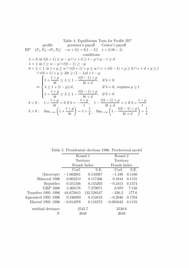
Table 4: Equilibrium Tests for Profile III*profile governor’s payoff Center’s payoff

III* (F1, F2,¬P1, P2) −w + t[1 + b(1 − λ)] v + t(λb− 1)

conditions:λ = 0 ⇛ t(b+ 1) ≥ w − p ∩ v + d ≥ t− p ∩ p− t ≥ dλ = 1 ⇛ t ≥ w − p ∩ t(b− 1) ≥ −p0 < λ < 1 ⇛ t + p ≥ w ∩ t(b+ 1) + p ≥ w ∩ v + t(b− 1) + p ≥ 0 ∩ v + d+ p ≥ t

∩ t(b+ 1) + p ≥ λbt ≥ (1− λ)d+ t− p

⇒

1 +t + p

bt≤ λ ≤ 1− t(b− 1) + p

bt + d, if b < 0

λ ≥ 1 + (t− p)/d, if b = 0, requires p ≥ t

1 +t + p

bt≥ λ ≥ 1− t(b− 1) + p

bt + d, if b > 0

b < 0 : 1 +t+ p

bt= 0 if b = −t + p

t, 1− t(b− 1) + p

bt+ d= 1 if b =

t− p

t

b > 0 : limt→∞

(

1 +t+ p

bt

)

= 1 +1

b, limt→∞

(

1− t(b− 1) + p

bt + d

)

=1

b

Table 5: Presidential elections 1996: Preelectoral model

Round 1 Round 2Territory Territory

Frauds Index Frauds IndexCoef. S.E. Coef. S.E.

(Intercept) −1.662681 0.143367 −1.430 0.1456Bilateral 1996 0.002214 0.117406 0.1044 0.1155

Republics 0.351246 0.145203 −0.2415 0.1574GRP 1996 5.369176 7.279971 6.970 7.150

Transfers 1995–1996 64.673815 132.528547 −326.2 177.6Appointed 1995–1996 0.346093 0.154818 −0.2046 0.1704

Elected 1995–1996 −0.014978 0.118272 −0.001642 0.1158

residual deviance 2545.7 2538.6N 2648 2648

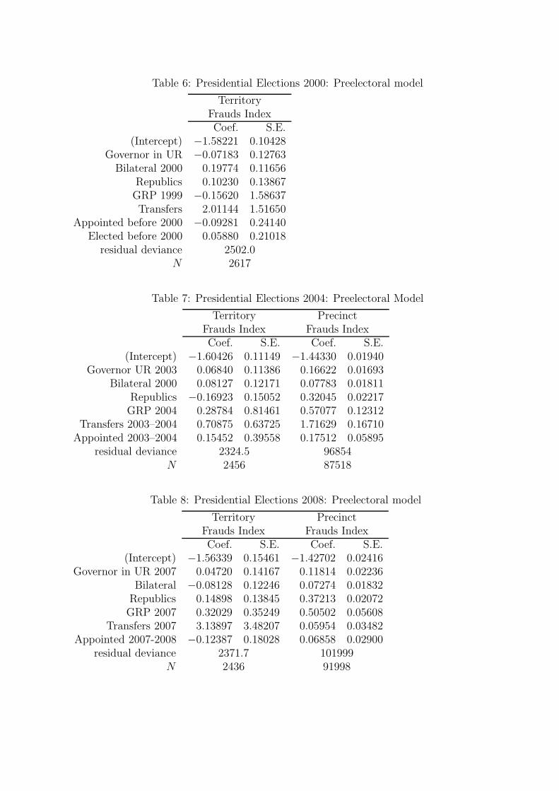
Table 6: Presidential Elections 2000: Preelectoral model

TerritoryFrauds IndexCoef. S.E.

(Intercept) −1.58221 0.10428Governor in UR −0.07183 0.12763Bilateral 2000 0.19774 0.11656

Republics 0.10230 0.13867GRP 1999 −0.15620 1.58637Transfers 2.01144 1.51650

Appointed before 2000 −0.09281 0.24140Elected before 2000 0.05880 0.21018

residual deviance 2502.0N 2617

Table 7: Presidential Elections 2004: Preelectoral Model

Territory PrecinctFrauds Index Frauds IndexCoef. S.E. Coef. S.E.

(Intercept) −1.60426 0.11149 −1.44330 0.01940Governor UR 2003 0.06840 0.11386 0.16622 0.01693

Bilateral 2000 0.08127 0.12171 0.07783 0.01811Republics −0.16923 0.15052 0.32045 0.02217GRP 2004 0.28784 0.81461 0.57077 0.12312

Transfers 2003–2004 0.70875 0.63725 1.71629 0.16710Appointed 2003–2004 0.15452 0.39558 0.17512 0.05895

residual deviance 2324.5 96854N 2456 87518

Table 8: Presidential Elections 2008: Preelectoral model

Territory PrecinctFrauds Index Frauds IndexCoef. S.E. Coef. S.E.

(Intercept) −1.56339 0.15461 −1.42702 0.02416Governor in UR 2007 0.04720 0.14167 0.11814 0.02236

Bilateral −0.08128 0.12246 0.07274 0.01832Republics 0.14898 0.13845 0.37213 0.02072GRP 2007 0.32029 0.35249 0.50502 0.05608

Transfers 2007 3.13897 3.48207 0.05954 0.03482Appointed 2007-2008 −0.12387 0.18028 0.06858 0.02900

residual deviance 2371.7 101999N 2436 91998

Table 9: Presidential Elections 1996: Postelectoral model (Territory)Round 1

ElectedTransfers 1996 1996-1997Coef. S.E. Coef. S.E.

(Intercept) 1.358e-04 1.361e-04 2.70161 1.73757Bilateral 1996 −4.100e-05 7.518e-05 −1.37909 0.96710

Republics 4.128e-05 8.327e-05 2.02719 0.99154Yeltsin % 3.651e-04 3.470e-04 −11.42155 5.56054GRP 1996 0.004473 0.004860 43.93624 59.40421Turnout % −6.693e-06 2.367e-06 0.03051 0.02970

Fraud0s (Territory) 0.001086 5.547e-04 −19.07901 8.03813Fraud5s (Territory) −2.137e-04 5.492e-04 −5.77215 6.33825

σ or res. dev. 0.0002722 58.407N 78 79

Round 2Elected

Transfers 1996 1996-1997Coef. S.E. Coef. S.E.

(Intercept) 2.282e-04 1.654e-04 −0.115947 1.792065Bilateral 1996 −7.289e-05 7.289e-05 −0.986808 0.876607

Republics 4.816e-05 7.975e-05 1.474755 0.896096Yeltsin % 5.945e-04 3.023e-04 −6.876520 3.682949GRP 1996 0.004138 0.004765 1.049861 53.071801Turnout % −5.885e-06 2.309e-06 0.008716 0.029340

Fraud0s (Territory) −0.001263 6.306e-04 6.121172 6.284862Fraud5s (Territory) −8.836e-04 5.137e-04 10.251929 5.729894

σ or res. dev. 0.0002683 62.948N 78 79

Table 10: Presidential Elections 2000: Postelectoral model (Territory)Transfers 2001 Elected 2001Coef. S.E. Coef. S.E.

(Intercept) 0.01097 0.03131 0.36100 1.92916Governor UR 0.02666 0.01120 0.13527 0.67780Bilateral 2000 −0.01230 0.01156 −1.25949 0.86955

Republics 0.01886 0.01217 0.40935 0.62498Putin % −0.01913 0.04915 −2.49886 3.03974

GRP 2001 0.4193 0.1584 −4.88397 10.30791Turnout % −4.578e-05 2.811e-04 −0.01286 0.01903

Fraud0s (Territory) −0.1650 0.1013 1.69859 6.15880Fraud5s (Territory) 0.09724 0.07265 1.15516 4.33217

σ or res. dev. 0.04264 77.867N 78 79

Table 11: Presidential Elections 2004: Postelectoral model (Territory)Appointed Transfers Elected2004-2005 2005 2004-2005Coef. S.E. Coef. S.E. Coef. S.E.

(Intercept) −2.56984 4.34220 −0.0325580 0.0643192 3.451429 3.800182Governor UR 2003 −0.32417 0.85492 −0.0278228 0.0144536 −0.967568 0.923576

Bilateral 1.40667 0.84918 −0.0048061 0.0156538 −1.327910 1.176850Republics −1.56374 1.23995 0.0232431 0.0171178 −1.215205 1.256508Putin, % −0.15198 5.11158 0.1347290 0.0817538 −4.475372 4.827577

GRP 2005 5.79140 3.50748 0.0487417 0.0772565 −10.287571 10.692427Turnout, % −0.02670 0.03167 0.0001321 0.0003025 0.001548 0.018118

Fraud0s (Territory) −0.26461 6.17770 −0.0370057 0.0850085 −2.190567 4.869040Fraud5s (Territory) 5.63180 8.41200 −0.1737772 0.1252700 −4.047614 6.505070

σ or res. dev. 50.059 0.05609 51.263N 77 75 77

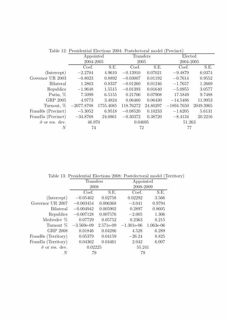
Table 12: Presidential Elections 2004: Postelectoral model (Precinct)Appointed Transfers Elected2004-2005 2005 2004-2005Coef. S.E. Coef. S.E. Coef. S.E.

(Intercept) −2.2704 4.9610 −0.13910 0.07021 −9.4879 6.0374Governor UR 2003 −0.8023 0.8892 −0.03007 0.01192 −0.7614 0.9552

Bilateral 1.2863 0.8337 −0.01260 0.01246 −1.7657 1.2669Republics −1.9648 1.5515 −0.01393 0.01640 −5.0955 3.0577Putin, % 7.5099 6.5155 0.21706 0.07908 17.5849 9.7488

GRP 2005 4.9773 3.4824 0.06460 0.06430 −14.5486 11.9953Turnout, % −2077.8708 1755.4085 118.76272 24.80297 −1894.7650 2049.3965

Fraud0s (Precinct) −5.3052 6.9518 −0.08520 0.10233 −1.6205 5.6131Fraud5s (Precinct) −34.8768 24.0861 −0.30372 0.38720 −8.4134 20.2216

σ or res. dev. 46.970 0.04695 51.263N 74 72 77

Table 13: Presidential Elections 2008: Postelectoral model (Territory)Transfers Appointed2008 2008-2009

Coef. S.E. Coef. S.E.(Intercept) −0.05462 0.02758 0.02292 3.566

Governor UR 2007 −0.003454 0.006368 −3.041 0.9794Bilateral −0.004942 0.005902 0.2897 0.8605Republics −0.007128 0.007576 −2.005 1.306

Medvedev % 0.07729 0.05752 0.2363 8.215Turnout % −3.569e-09 2.571e-09 −1.301e-06 1.063e-06GRP 2008 0.01846 0.04286 4.528 6.289

Fraud0s (Territory) 0.05379 0.04159 −26.24 8.825Fraud5s (Territory) 0.04362 0.04461 2.042 6.007

σ or res. dev. 0.02225 55.241N 79 79

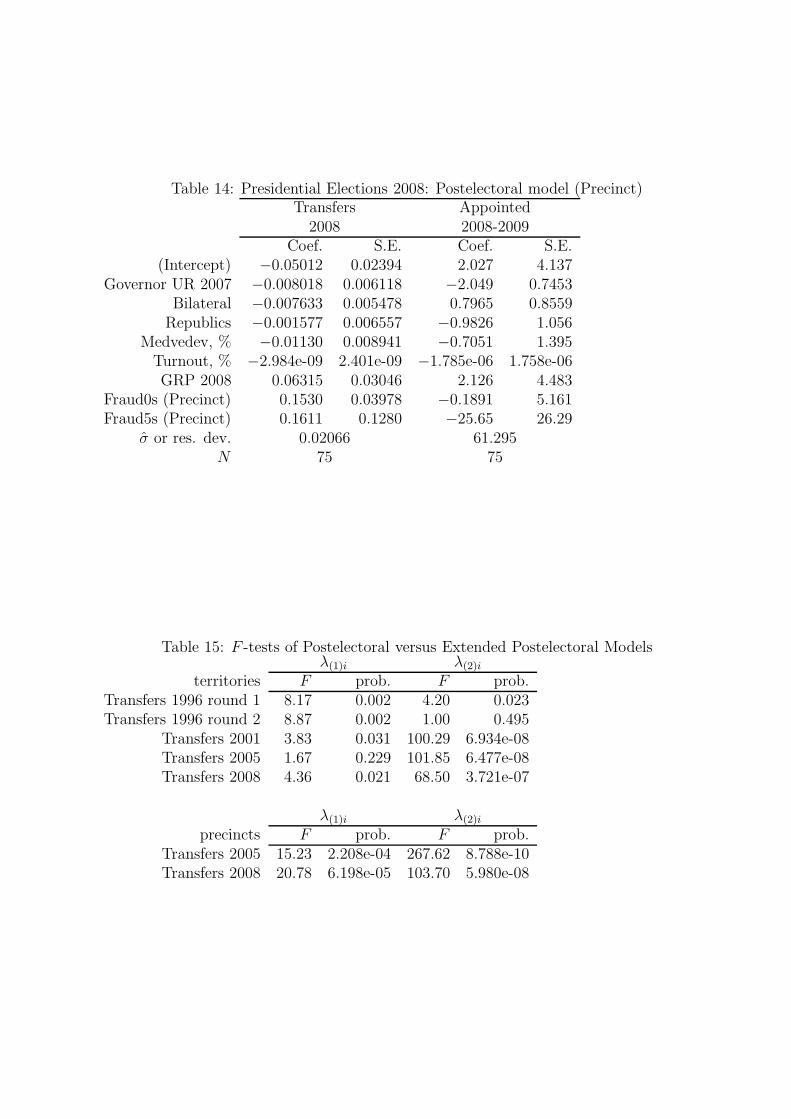
Table 14: Presidential Elections 2008: Postelectoral model (Precinct)Transfers Appointed2008 2008-2009

Coef. S.E. Coef. S.E.(Intercept) −0.05012 0.02394 2.027 4.137

Governor UR 2007 −0.008018 0.006118 −2.049 0.7453Bilateral −0.007633 0.005478 0.7965 0.8559Republics −0.001577 0.006557 −0.9826 1.056

Medvedev, % −0.01130 0.008941 −0.7051 1.395Turnout, % −2.984e-09 2.401e-09 −1.785e-06 1.758e-06GRP 2008 0.06315 0.03046 2.126 4.483

Fraud0s (Precinct) 0.1530 0.03978 −0.1891 5.161Fraud5s (Precinct) 0.1611 0.1280 −25.65 26.29

σ or res. dev. 0.02066 61.295N 75 75

Table 15: F -tests of Postelectoral versus Extended Postelectoral Modelsλ(1)i λ(2)i

territories F prob. F prob.Transfers 1996 round 1 8.17 0.002 4.20 0.023Transfers 1996 round 2 8.87 0.002 1.00 0.495

Transfers 2001 3.83 0.031 100.29 6.934e-08Transfers 2005 1.67 0.229 101.85 6.477e-08Transfers 2008 4.36 0.021 68.50 3.721e-07

λ(1)i λ(2)i

precincts F prob. F prob.Transfers 2005 15.23 2.208e-04 267.62 8.788e-10Transfers 2008 20.78 6.198e-05 103.70 5.980e-08

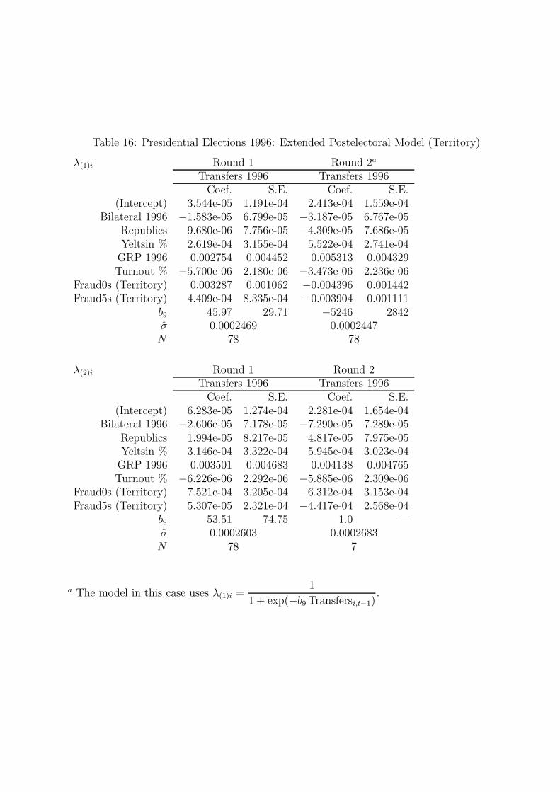
Table 16: Presidential Elections 1996: Extended Postelectoral Model (Territory)

λ(1)i Round 1 Round 2a

Transfers 1996 Transfers 1996Coef. S.E. Coef. S.E.

(Intercept) 3.544e-05 1.191e-04 2.413e-04 1.559e-04Bilateral 1996 −1.583e-05 6.799e-05 −3.187e-05 6.767e-05

Republics 9.680e-06 7.756e-05 −4.309e-05 7.686e-05Yeltsin % 2.619e-04 3.155e-04 5.522e-04 2.741e-04GRP 1996 0.002754 0.004452 0.005313 0.004329Turnout % −5.700e-06 2.180e-06 −3.473e-06 2.236e-06

Fraud0s (Territory) 0.003287 0.001062 −0.004396 0.001442Fraud5s (Territory) 4.409e-04 8.335e-04 −0.003904 0.001111

b9 45.97 29.71 −5246 2842σ 0.0002469 0.0002447N 78 78

λ(2)i Round 1 Round 2Transfers 1996 Transfers 1996Coef. S.E. Coef. S.E.

(Intercept) 6.283e-05 1.274e-04 2.281e-04 1.654e-04Bilateral 1996 −2.606e-05 7.178e-05 −7.290e-05 7.289e-05

Republics 1.994e-05 8.217e-05 4.817e-05 7.975e-05Yeltsin % 3.146e-04 3.322e-04 5.945e-04 3.023e-04GRP 1996 0.003501 0.004683 0.004138 0.004765Turnout % −6.226e-06 2.292e-06 −5.885e-06 2.309e-06

Fraud0s (Territory) 7.521e-04 3.205e-04 −6.312e-04 3.153e-04Fraud5s (Territory) 5.307e-05 2.321e-04 −4.417e-04 2.568e-04

b9 53.51 74.75 1.0 —σ 0.0002603 0.0002683N 78 7

a The model in this case uses λ(1)i =1

1 + exp(−b9Transfersi,t−1).

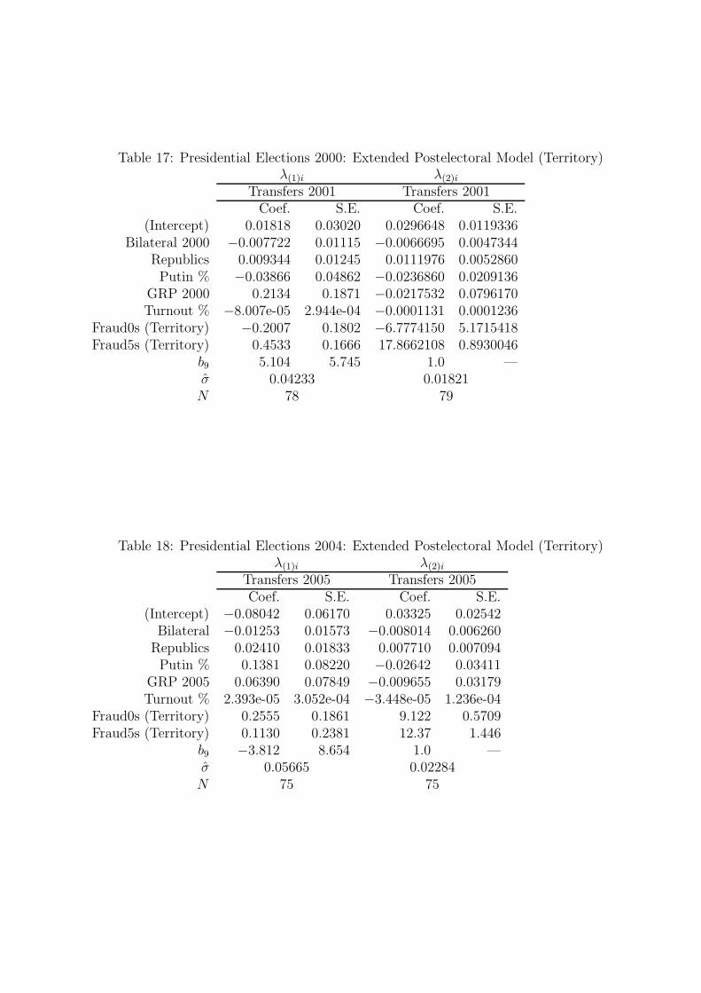
Table 17: Presidential Elections 2000: Extended Postelectoral Model (Territory)λ(1)i λ(2)i

Transfers 2001 Transfers 2001Coef. S.E. Coef. S.E.

(Intercept) 0.01818 0.03020 0.0296648 0.0119336Bilateral 2000 −0.007722 0.01115 −0.0066695 0.0047344

Republics 0.009344 0.01245 0.0111976 0.0052860Putin % −0.03866 0.04862 −0.0236860 0.0209136

GRP 2000 0.2134 0.1871 −0.0217532 0.0796170Turnout % −8.007e-05 2.944e-04 −0.0001131 0.0001236

Fraud0s (Territory) −0.2007 0.1802 −6.7774150 5.1715418Fraud5s (Territory) 0.4533 0.1666 17.8662108 0.8930046

b9 5.104 5.745 1.0 —σ 0.04233 0.01821N 78 79

Table 18: Presidential Elections 2004: Extended Postelectoral Model (Territory)λ(1)i λ(2)i

Transfers 2005 Transfers 2005Coef. S.E. Coef. S.E.

(Intercept) −0.08042 0.06170 0.03325 0.02542Bilateral −0.01253 0.01573 −0.008014 0.006260Republics 0.02410 0.01833 0.007710 0.007094Putin % 0.1381 0.08220 −0.02642 0.03411

GRP 2005 0.06390 0.07849 −0.009655 0.03179Turnout % 2.393e-05 3.052e-04 −3.448e-05 1.236e-04

Fraud0s (Territory) 0.2555 0.1861 9.122 0.5709Fraud5s (Territory) 0.1130 0.2381 12.37 1.446

b9 −3.812 8.654 1.0 —σ 0.05665 0.02284N 75 75

Table 19: Presidential Elections 2004: Extended Postelectoral Model (Precinct)λ(1)i λ(2)i

Transfers 2005 Transfers 2005Coef. S.E. Coef. S.E.

(Intercept) −0.256676 0.050041 0.0013641 0.0121894Bilateral −0.007236 0.010645 0.0004738 0.0025249Republics −0.026079 0.015342 −0.0046020 0.0036353Putin % 0.125115 0.068497 0.0028995 0.0170468

GRP 2005 0.063683 0.056004 −0.0104384 0.0133645Turnout % 82.522712 22.236045 4.7807056 5.9000086

Fraud0s (Precinct) 0.438302 0.148198 1.2397901 0.4435296Fraud5s (Precinct) 2.141560 0.607678 10.1019907 3.1625350

b9 3.378322 1.031086 −1.3927399 0.2324904σ 0.03999 0.009462N 71 71

Table 20: Presidential Elections 2008: Extended Postelectoral Model (Territory)λ(1)i λ(2)i

Transfers 2008 Transfers 2008Coef. S.E. Coef. S.E.

(Intercept) −0.07379 0.02720 −0.009244 0.01455Bilateral −0.004225 0.005653 4.503e-04 0.003086Republics −0.01164 0.007291 −0.001557 0.003901

Medvedev % 0.09365 0.05707 0.03039 0.03072GRP 2008 −3.944e-09 2.480e-09 −1.627e-09 1.342e-09Turnout % 0.01051 0.04303 −0.008943 0.02333

Fraud0s (Territory) 0.2072 0.09424 1.999 0.2436Fraud5s (Territory) 0.2015 0.09052 −0.2681 0.2099

b9 −1.415 1.520 1.0 —σ 0.02114 0.01155N 75 75

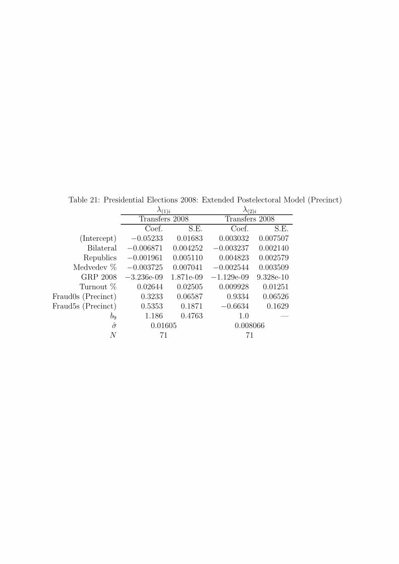
Table 21: Presidential Elections 2008: Extended Postelectoral Model (Precinct)λ(1)i λ(2)i

Transfers 2008 Transfers 2008Coef. S.E. Coef. S.E.

(Intercept) −0.05233 0.01683 0.003032 0.007507Bilateral −0.006871 0.004252 −0.003237 0.002140Republics −0.001961 0.005110 0.004823 0.002579

Medvedev % −0.003725 0.007041 −0.002544 0.003509GRP 2008 −3.236e-09 1.871e-09 −1.129e-09 9.328e-10Turnout % 0.02644 0.02505 0.009928 0.01251

Fraud0s (Precinct) 0.3233 0.06587 0.9334 0.06526Fraud5s (Precinct) 0.5353 0.1871 −0.6634 0.1629

b9 1.186 0.4763 1.0 —σ 0.01605 0.008066N 71 71