Unclassified ECO/WKP(2008)11 - OECD

Unclassified ECO/WKP(2008)11 Organisation de Coopération et de Développement Économiques Organisation for Economic Co-operation and Development 08-Apr-2008 ___________________________________________________________________________________________

English - Or. English ECONOMICS DEPARTMENT

OIL PRICE SHOCKS, RIGIDITIES AND THE CONDUCT OF MONETARY POLICY: SOME LESSONS FROM A NEW KEYNESIAN PERSPECTIVE ECONOMICS DEPARTMENT WORKING PAPER No. 603

By Romain Duval and Lukas Vogel

All OECD Economics Department Working Papers are available on the OECD Internet website at www.oecd.org/eco/working_papers

JT03243792

Document complet disponible sur OLIS dans son format d'origine Complete document available on OLIS in its original format

EC

O/W

KP(2008)11

Unclassified

English - O

r. English

ECO/WKP(2008)11

2

ABSTRACT/RÉSUMÉ

Oil Price Shocks, Rigidities and the Conduct of Monetary Policy: Some Lessons from a New Keynesian Perspective

The strong and sustained rise in oil prices observed in recent years poses a challenge to monetary

policy and its ability to simultaneously achieve low inflation and stable output. Against this background, the paper studies monetary policy in a small open economy New Keynesian DSGE model including oil as a production input and a component of final demand. It investigates the performance of alternative price level definitions, notably headline and core CPI, in standard interest rate rules with respect to output and inflation stabilisation. The analysis puts special emphasis on the impact of price and real wage rigidity and their interaction on the policy trade-off induced by the oil price shock. While the degree of price rigidity alone is found to have little impact on the shock transmission and generates only small differences between alternative monetary strategies, the simulations suggest a more important role for real wage stickiness. Real wage stickiness triggers second round effects and complicates stabilisation whatever the policy rule. A focus on core inflation tends to limit the contraction of output in this context. The results also point to some interaction between nominal price and real wage rigidities. In the presence of real wage rigidity, greater price flexibility is found to be destabilising, as it amplifies the initial inflation effect of shocks, thereby triggering a stronger monetary policy response and a larger output effect.

JEL classification: E30; F41; Q43 Key words: DSGE model; monetary policy; price stickiness; real wage rigidity; oil price shocks

Chocs pétroliers, rigidités et conduite de la politique monétaire : quelques leçons tirées d’une perspective néo-keynésienne

La hausse forte et persistante des prix pétroliers au cours des années passées constitue un défi pour la politique monétaire et sa capacité à stabiliser simultanément l’inflation et la production. Dans ce contexte, ce document étudie le comportement de la politique monétaire dans un modèle DSGE néo-keynésien d’une petite économie ouverte, incluant le pétrole à la fois comme bien de consommation final et comme facteur de production. L’analyse met l’accent sur la performance de définitions alternatives de l’indice des prix, notamment des indices de prix courant et sous-jacent, dans des règles de politique monétaire courantes, en matière de stabilisation du niveau de production et de l’inflation. En particulier, l’analyse met en évidence l’impact des rigidités de prix et de salaire réel, ainsi que de leur interaction, sur l’arbitrage engendré par le choc pétrolier. Tandis que le degré de rigidité des prix seul a peu d’effet sur la transmission des chocs et n’engendre que des écarts mineurs entre différentes stratégies de politique monétaire, les simulations suggèrent un impact plus important de la rigidité des salaires réels. La rigidité des salaires réels entraîne des effets de second tour et complique la stabilisation quelle que soit la règle de politique monétaire. Cibler l’inflation sous-jacente tend à limiter la contraction du niveau de production dans ce contexte. En outre, les résultats suggèrent une interaction entre rigidité des prix nominaux et rigidité des salaires réels. Pour un degré de rigidité donné des salaires réels, une forte flexibilité des prix apparait déstabilisatrice car elle amplifie l’effet initial du choc sur l’inflation, ce qui amplifie la réaction de politique monétaire et, ce faisant, entraîne une variation plus forte du niveau de production. Classification JEL : E30; F41; Q43 Mots clés : modèle DSGE ; politique monétaire ; rigidité des prix ; rigidité des salaires réels Copyright, OECD, 2008 Application for permission to reproduce or translate all, or part of, this material should be made to: Head of Publications Service, OECD, 2 rue André-Pascal, 75775 Paris Cedex 16, France

ECO/WKP(2008)11

3

TABLE OF CONTENTS

OIL PRICE SHOCKS, RIGIDITIES AND THE CONDUCT OF MONETARY POLICY: SOME LESSONS FROM A NEW KEYNESIAN PERSPECTIVE .......................................................................... 5

1. Introduction and summary of main findings ........................................................................................... 5 2. Theoretical framework ............................................................................................................................ 7 3. Alternative monetary policy rules ........................................................................................................... 8 4. Simulation scenarios ............................................................................................................................... 9 5. Results ................................................................................................................................................... 10 6. Conclusion ............................................................................................................................................ 14 References ..................................................................................................................................................... 27

ANNEX 1. THE NEW KEYNESIAN OPEN ECONOMY MODEL .......................................................... 29

1.1 The small open economy ................................................................................................................ 29 1.1.1 Household sector ....................................................................................................................... 29 1.1.2 Aggregate demand .................................................................................................................... 31 1.1.3 Aggregate supply ...................................................................................................................... 32

1.2 The rest of the world ...................................................................................................................... 34 1.3 The oil price shock ......................................................................................................................... 36

ANNEX 2. THE LINEARISED MODEL .................................................................................................... 37

Boxes Box 1. Model equations Box 2. Model calibration Tables

Table 1: Monetary policy rules under alternative degrees of nominal price rigidity Table 2: Monetary policy rules under alternative degrees of real wage rigidity Table 3: Taylor rule with large inflation coefficient Table 4: Monetary policy rules under real wage rigidity and alternative degrees of price rigidity Figures Figure 1: Taylor rule under alternative degrees of nominal rigidity Figure 2: Targeting expected inflation under alternative degrees of nominal rigidity Figure 3: Taylor rule under alternative degrees of real rigidity Figure 4: Targeting expected inflation under alternative degrees of real rigidity Figure 5: Taylor rule under real rigidity and alternative degrees of nominal rigidity Figure 6: Targeting expected inflation with real rigidity and alternative degrees of nominal rigidity

ECO/WKP(2008)11

4

ECO/WKP(2008)11

5

OIL PRICE SHOCKS, RIGIDITIES AND THE CONDUCT OF MONETARY POLICY: SOME LESSONS FROM A NEW KEYNESIAN PERSPECTIVE

By Romain Duval and Lukas Vogel1

1. Introduction and summary of main findings

1. Conventional monetary policy wisdom suggests that forward-looking and credible central banks committed to medium-term price stability objectives can essentially look through one-off oil price shocks. However, this may no longer hold in the case of persistent or even permanent shocks such as those experienced across the OECD over the past few years. A sustained rise in oil prices has the potential to push inflation above its explicit or implicit target for some time, prompting central banks to react.

2. The monetary policy reaction to oil price shocks and its effects on inflation, output and welfare can be best studied in the context of a so-called “New Keynesian” framework, which has become the standard workhorse of monetary analysis over the past decade and allows an explicit micro-founded modelling of the transmission channels. This and previous literature suggests that three factors may play a particularly prominent role in shaping the monetary policy response, namely the average degree of nominal rigidity in the economy, the degree of real wage rigidity and the inflation indicator targeted by the central bank, as well as interactions across them. In particular, most recent research has stressed that real rigidities create an output-inflation stabilisation trade-off in the presence of supply and especially commodity price shocks (Blanchard and Galí, 2007a, 2007b). Regarding the choice of the inflation target, the literature is not clearly settled.2 While there seems to be a clear theoretical case for targeting those prices that are stickiest (Altissimo et al., 2006; Woodford, 2003), some papers have suggested the choice of the inflation indicator to be virtually irrelevant in practice from a welfare standpoint (Galí and Monacelli, 2005). However, the latter conclusion has not been tested in a context of real rigidities and shocks to relative prices.3 In particular, in the presence of real wage rigidities, commodity price shocks may prompt a stronger monetary policy response and significantly larger output fluctuations if the central bank focuses on headline inflation rather than on some measure of core inflation.

3. Against this background, the present paper builds on a New Keynesian dynamic stochastic general equilibrium (DSGE) model to study the extent to which the dynamics of inflation and the output gap in the

1 We would like to thank Peter Hoeller, Diego Moccero, Annabelle Mourougane and Jean-Luc Schneider for helpful comments and suggestions. Remaining errors and omission are the responsibility of the authors. The views expressed in this paper do not necessarily reflect those of the OECD. 2 Mankiw (2007) lists the choice of the appropriate inflation indicator as one of the three open questions about price dynamics, along with the formation of inflation expectations and the existence of a trade-off between inflation and output stabilisation. 3 Based on a DSGE model with energy use, durable goods and nominal – but not real – rigidities, Dhawan and Jeske (2007) find that a central bank performs better by using core rather than headline inflation in its Taylor rule because it can remain vigilant on core inflation while incurring a smaller output loss. However, it is unclear whether their findings can be extended to a more general framework.

ECO/WKP(2008)11

6

aftermath of oil price shocks is affected by various types of rigidities and by the choice of the inflation indicator made by the central bank.4 Two possible inflation indicators – headline and core CPI inflation, where the later is CPI inflation excluding energy – and two possible monetary policy rules – a Taylor rule reacting to inflation and output gaps and a forward-looking inflation targeting rule that only reacts to expected future inflation – are considered. While the paper is mainly concerned with the implications of rigidities and the choice of the inflation indicator for the response of economies to oil price shocks, it has also implications for the conduct of monetary policy and the design of policies and institutions in labour and product markets.

4. The main findings from this paper are:

• In general, nominal price rigidity alone has little impact on oil price shock transmission and generates only small differences between alternative monetary policy strategies. One exception is the stronger monetary tightening and the larger output contraction under strong nominal price rigidity when the central bank follows a Taylor rule focusing on headline inflation. In this case, nominal price rigidity flattens the Phillips curve, forcing the central bank to react more in order to achieve a given degree of inflation stabilisation. By contrast, under (expected) inflation targeting the monetary policy responses are benign and the resulting output gap is small whatever the degree of nominal rigidity and the inflation indicator targeted.

• Real wage rigidity induces second-round effects on production costs and inflation, making it more difficult for monetary policy to achieve both output and inflation stabilisation in the presence of oil price shocks. As a result, the degree of monetary policy tightening, the output contraction and the initial spike in inflation are all larger under real wage rigidity, whatever the monetary policy rule and the inflation indicator used by the central bank.

• In the presence of real wage rigidity, the choice of the inflation indicator by the central bank becomes a more important issue, as it has a larger impact on the dynamic adjustment of the economy to temporary oil price shocks. Under a Taylor rule focusing on core inflation, i.e. CPI inflation excluding energy, the central bank achieves significantly more stable output at the cost of more unstable headline CPI inflation, compared with a Taylor rule focusing on headline inflation. Under (expected) inflation targeting, the central bank achieves more stable headline – and by implication core – inflation and fairly similar output stability by targeting core rather than headline inflation. The latter finding holds under the assumptions of temporary oil price shocks and full rational expectations, however.

• Real and nominal rigidities interact in such a way that, for a given degree of real persistence, lower nominal inertia increases the volatility of output gaps and inflation rates. Flexible prices amplify the initial inflation effect of oil price and other cost-push shocks. In the presence of real wage rigidity, this puts pressure on nominal wages, cetereris paribus, thereby reinforcing inflationary pressures. The stronger monetary policy response then engineers a larger fall in output, while not being sufficient to achieve the same degree of inflation stability. This tentatively suggests that in those currency areas where both types of rigidities are strong, reducing nominal rigidities through, e.g., product market reforms may not help the conduct of monetary policy – at least in the event of oil price and other cost-push shocks – in the absence of parallel labour market reforms aimed at lowering the degree of real wage rigidity.

4 For a comprehensive treatment of the New Keynesian modelling approach and the underlying assumptions, see in particular Woodford (2003). The importance of commodity prices in policy models of inflation is emphasised by Kohn (2007).

ECO/WKP(2008)11

7

5. The remainder of this paper proceeds as follows. Section 2 presents a New Keynesian open economy model with oil – a shortcut for commodities more broadly – as both production input and component of the consumption basket, extending the framework developed by Galí and Monacelli (2005). Section 3 then discusses the Taylor-type rule and the (expected) inflation targeting rule to be considered for analysis. Section 4 presents the oil price shock scenario and Section 5 explores the output and inflation effects of oil price shocks under both monetary policy rules for different degrees of nominal and real rigidity and for alternative inflation indicators. Section 6 sums up and concludes.

2. Theoretical framework

6. The paper builds up a New Keynesian open economy model with real wage rigidities and oil as production input and consumption good. The New Keynesian framework has become a standard approach to analyse the dynamic output and inflation responses to supply and demand shocks. It has the particular advantage of providing a micro-founded dynamic macroeconomic model that clearly identifies the demand and supply side effects of exogenous shocks. In the context of this paper, the model offers an explicit specification of the channels through which commodity prices affect the behaviour of households and firms. Furthermore, the micro-founded approach allows a transparent and detailed analysis of the impact of various nominal and real rigidities on shock transmission and absorption. Broadly speaking, sustained increases in the price of oil reduce the purchasing power of household income and thereby consumption. Additionally, they raise the price of factor inputs and production costs. Therefore, persistent increases in the price of oil have a negative impact on both demand and supply in oil-importing countries. Stabilising production costs to stabilise core or headline CPI price inflation then requires a decline in wages in order to offset cost pressures stemming from rising oil prices. Real wage rigidity delays such adjustment process.

7. The underlying New Keynesian DSGE model consists of two country blocks, namely the small open economy and the rest of the world. The small open economy uses oil as consumption good and production input. It produces differentiated manufactured goods and sells them on both local and world markets. The rest of the world produces both oil and manufactured goods. All households consume a bundle of oil and manufactured goods. Households and firms maximize inter-temporal utility and profit over an infinite planning horizon. Firms operate under monopolistic competition with infrequent price adjustment.5 Regarding the open economy extension, capital markets are assumed internationally integrated, allowing households to diversify the income risk. For analytical simplicity, perfect international risk sharing and the law of one price (at the individual good level) are assumed to hold.6 The common price assumption is plausible at least for oil, which is the main focus of this paper. Annexes 1 and 2 respectively describe the full model in detail and its linearisation around the steady state. Box 1 sums up the smaller and simpler set of equations obtained after such linearisation.

8. The model illustrates the direct and indirect effects of oil prices and of real rigidity on consumer choices and production costs and, consequently, on output and inflation. On the demand side, consumption is determined in three steps. First, the representative, intertemporally optimising household decides on the total level of current consumption, which negatively depends on the real interest rate. Second, total consumption is allocated between oil and non-oil goods depending on their relative price. Increases in the relative price of oil trigger a substitution of non-oil goods for oil, with the elasticity of substitution between oil and goods determining the strength of this substitution effect. Third, the consumption of non-oil goods is spread over domestic production and imports depending on relative import prices.

5 Given that fiscal policy is not central to the discussion in this paper, for simplicity the model abstracts from both distortionary taxation and public spending. 6 Both assumptions drastically improve the tractability of the model (see Galí and Monacelli, 2005).

ECO/WKP(2008)11

8

9. On the supply side, firms produce with labour and oil. Each firm chooses the cost-minimising input combination, which implies that firms substitute labour for oil when the oil price increases. Such factor substitution exerts upward pressure on real production wages, ceteris paribus. On the other hand, rising oil prices reduce the purchasing power of household earnings, thereby reducing real consumption wages. As labour supply is a function of the opportunity cost of leisure in our model, it will also decline with falling real wages. The decline in labour supply further increases production costs and inflationary pressures.7

10. Following Blanchard and Galí (2007a), the model introduces real wage rigidity in the form of real wage persistence. Current real wages are assumed to be a weighted average of the lagged real wage and the equilibrium real wage that prevails under optimal labour supply in a fully competitive labour market. The sluggish adjustment of real wages to changes in labour demand amplifies the reaction of marginal production costs to the oil price shock and, as discussed below, makes it more difficult for central banks to stabilise both output and inflation.

11. The model calibration uses standard parameter values. It assumes logarithmic consumption utility, i.e. unit intertemporal elasticity of substitution, and unit elasticity of substitution between imports and exports of manufactured goods. The share of oil in the consumption basket is set equal to 7%, with a low elasticity of substitution between oil and manufactured goods. The input share of oil in the (Cobb-Douglas) production function is 2.5% (see De Fiore et al., 2006). Box 2 describes the calibration in more detail.

3. Alternative monetary policy rules

12. The model is used to compare the dynamic adjustment to oil price disturbances under a set of different monetary policy rules. Two distinct policy rules are considered:

(1)

(2)

Equation (1) is a standard Taylor-type rule, where the nominal interest rate, it, deviates from the steady-state real rate, , in reaction to contemporaneous inflation, πt, and the contemporaneous output gap, .8 It also features intrinsic persistence in the policy rate, because such persistence is generally optimal9 (Rotemberg and Woodford, 1999; Woodford, 2001) and is a feature of actual policy rules

7 This illustration of the supply-side transmission of oil price shocks highlights the importance of underlying assumptions on the production process. The analysis considers labour and oil to be substitutes. An increase in oil prices triggers a substitution of labour for oil under flexible relative factor prices. Alternatively, one could assume a complementary relationship between both inputs. The increase in oil prices would then exclude substitution and uniformly reduce both oil and labour demand (see, e.g., Atkeson and Kehoe, 1999; Leduc and Sill, 2006). 8 An alternative Taylor-type rule where monetary policy reacts to expected inflation one period ahead and the current output gap was also considered. Such policy rule generates smaller amplitudes in initial policy and output responses along with higher initial inflation, while subsequent adjustment paths of all variables are very similar to those emerging under rule (1). A Taylor rule reacting to future inflation and current output is initially more accommodative than both rules (1) and (2). It looks through the initial spike in inflation, but at the same time reacts to the negative output gap resulting from the oil price shock. Consequently, a Taylor rule with expected inflation would generate stronger initial inflation and lower initial output losses than identically calibrated policy rules (1) and (2). 9 Insofar as aggregate demand depends as much on expected future short-term real interest rates as on the current short-term rate in the forward-looking framework, intrinsic persistence in the policy rate allows monetary policy to achieve a given degree of stabilisation with less volatile short-term interest rates. Another theoretical argument supporting monetary policy inertia is that it mitigates the risk of explosive dynamics in forward-looking models – thereby making the theoretical models more realistic – and facilitates learning by private agents of the rational

ECO/WKP(2008)11

9

followed by central banks, reflecting their preference for interest rate stability (e.g. Clarida et al., 1998; Eleftheriou et al., 2006; Sack and Wieland, 2000). Policy rule (2) captures an inflation targeting regime, where monetary policy reacts in a forward-looking manner to expected inflation, Etπt+1. The simulations consider two different measures of inflation to be used in the policy rules, namely headline CPI inflation and core CPI inflation, which is defined as CPI inflation excluding energy.10 The analysis in this paper takes the form of a positive evaluation of alternative monetary policy rules. In particular, impulse responses of inflation and the output gap are compared across rules. A normative evaluation, which would compare policy regimes based on minimising a micro-funded welfare loss function, has been undertaken in a companion paper and yields results that are largely consistent with those from the current paper.11

13. The baseline calibration of policy responses uses the parameter values ψi=0.5, ψx=0.5 and ψπ=1.5 for the monetary policy rule (1) and ψπ=1.5 for rule (2). The coefficients on inflation and the output gap in rule (1) equal the Taylor (1993) rule coefficients. Additionally, the analysis considers a version of rule (1) with a stronger weight on inflation. In the latter case, the coefficients are ψπ=3.5 and ψx=0.5, corresponding to the Gerdesmeier and Roffia (2003) estimate of the relative inflation and output weights on synthetic euro area data for the period 1985-2002.12

4. Simulation scenarios

14. Oil price shocks are modelled as a temporary but highly persistent shock to the relative price of oil in the world market:

( ) ttCtOotCtO pppp ερ +−=− −−*

1,*

1,*

,*

, ˆˆˆˆ (3)

expectations equilibrium (Bullard and Mitra, 2007), an issue which is absent from the full rational expectations framework adopted in this paper. 10 There are other price level definitions available, such as the GDP price deflator, which measures the price level of domestically produced goods and services. While the discussion in the text focuses on headline CPI and core CPI inflation as the two inflation concepts, the tables in Section 5 also display results for policy rules that use the change in the GDP price deflator. 11 Ramsey optimal monetary policy has also been computed as a robustness check for the conclusions drawn from simple calibrated rules in this paper, in particular as regards the effects of nominal and real rigidities on output and inflation responses to the oil price shock. Ramsey optimal monetary policy is the optimal commitment solution for the interest rate path, i.e. the best possible path in terms of welfare. It implies the monetary policy maker solves a complex optimisation problem which is fully known and fully credible to private agents. Overall, it should probably be seen as a theoretical benchmark rather than as a policy central banks are likely to follow in practice. See Duval and Vogel (2007) for the welfare costs of oil price shocks under Ramsey optimal policy. The conclusions from a policy evaluation based on a linear-quadratic loss function over output and inflation would depend on the inflation measure appearing in the loss function. A basic closed-economy model with sticky prices suggests targeting the GDP deflator, which is identical to both headline and core CPI inflation in this environment (see Woodford, 2003). Adding sticky wages, Erceg et al. (2000) find that optimal policy should target an average of wage and price inflation. In an open economy model, Galí and Monacelli (2005) find GDP prices to be the appropriate target. Their framework is still relatively simple, however, since it assumes labour being the only input to production, a unit elasticity of substitution between imports and exports and the identity of the core and the headline CPI. The fairly elaborate framework adopted in this paper does not allow deriving a tractable micro-funded objective function over the variances of inflation and the output gap. 12 Two recent papers on the monetary reaction to oil shocks in a closed-economy DSGE framework are Blanchard and Galí (2007b) and Dhawan and Jeske (2007). Blanchard and Galí (2007b) consider the impact of real wage rigidity on stabilisation policy, but only consider a policy rule with core CPI inflation. Dhawan and Jeske (2007) combine nominal rigidity with capital adjustment costs and assess the relative stabilising performance of CPI versus core CPI inflation in Taylor rules, without varying the degree of rigidity across scenarios.

ECO/WKP(2008)11

10

with a persistence parameter ρo=0.95.13 Impulse responses are based on an initial doubling of the relative price of oil. As the model is set up in log-linear terms the doubling implies εt=0.69.14 Given that the theoretical model considers oil as the single source of energy and is calibrated using the overall share of fuel and gas in consumption and production, the shock could be interpreted as an energy price shock, rather than strictly as an oil price shock.

15. The simulations study the impact of nominal and real rigidities on impulse responses for the interest rate – which in turn depends on the policy rule, the output gap and inflation. The analysis proceeds in three steps. First, responses to the oil price shock are compared across two different degrees of nominal price rigidity, low and high. Low and high degrees of price rigidity correspond to average price durations of 2 and 5 quarters, respectively, in line with the findings in Altissimo et al. (2006) regarding the average frequency of price adjustment in the US and the euro area. In order to isolate the impact of nominal price rigidity, real wages are assumed to be perfectly flexible in these simulations. In a second step, real wage rigidity is introduced, keeping price rigidity constant at the low value. Real wage rigidity is assumed to correspond to a persistence coefficient ρw=0.80 in the real wage equation, which implies a half-life of deviations of the real wage from its equilibrium level of about 3 quarters.15 In a final step, interactions between nominal and real rigidities are explored.

5. Results

The degree of nominal price rigidity matters if the central bank follows a Taylor role focusing on headline inflation but makes little difference otherwise

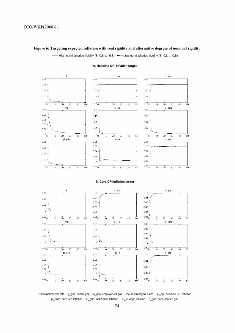
16. Figures 1 and 2 show the impulse responses for two distinct and empirically plausible degrees of price inertia under a Taylor rule and under forward-looking inflation targeting, respectively. Table 1 expresses the results in terms of standard deviations of output gap and various measures of inflation. Impulse responses are shown for the policy rate(i), the output gap (y_gap), the employment gap (n_gap), real marginal costs (mc), headline CPI inflation (pi_cpi), core CPI inflation (pi_core), GDP price inflation (pi_gdp), wage inflation (pi_w), and the consumption gap (c_gap), with units on the time axes being quarters throughout. In each figure, Panel A assumes the central bank uses headline CPI inflation as the relevant inflation measure, while panel B assumes it focuses core CPI inflation.16,17

13 A roughly equivalent specification would be to consider a temporary shock to the absolute oil price level or a permanent shock to the absolute oil price level with other prices gradually catching up. Alternatively, one could analyse permanent shocks to relative oil prices, i.e. excluding the possibility for other prices to catch up and restore initial relative prices. The latter scenario would potentially conflict with the assumption that oil prices are exogenous. While the exogeneity assumption seems sensible for the analysis of temporary oil price shocks, it may no longer be the case when it comes to analysing permanent oil price shocks, because the latter should trigger larger substitution mechanisms in both production and consumption, with significant feedback effects on oil prices. Nevertheless, the robustness of results to the assumption of a permanent oil price shock, i.e. ρo=1.00, has been tested for. The findings from this exercise are summarised at the end of Section 5. 14 Dhawan and Jeske (2007) also consider an initial doubling of oil prices as the benchmark case. Shocks are smaller in De Fiore et al. (2006), Kamps and Pierdzioch (2002), and in Blanchard and Galí (2007b), which use 0.2, 0.14 and 0.11 standard deviations, respectively. De Fiore et al. (2006) and Kamps and Pierdzioch (2002) also consider a larger set of disturbances, including productivity, preference, labour supply, pricing and government spending shocks, however. Roeger (2005) analyses a permanent increase of oil prices by 50%. 15 This value is actually at the lower end of recent estimates for European economies. Arpaia and Pichelmann (2007) estimate wage equations for the euro area countries over the period 1980-2005 and find half-lives between about 2 and 10 quarters. 16 Another option would be for the central bank to focus on GDP price rather than core CPI inflation. However, this is found to make little difference to the central bank’s response to the shock and the resulting degree of output and

ECO/WKP(2008)11

11

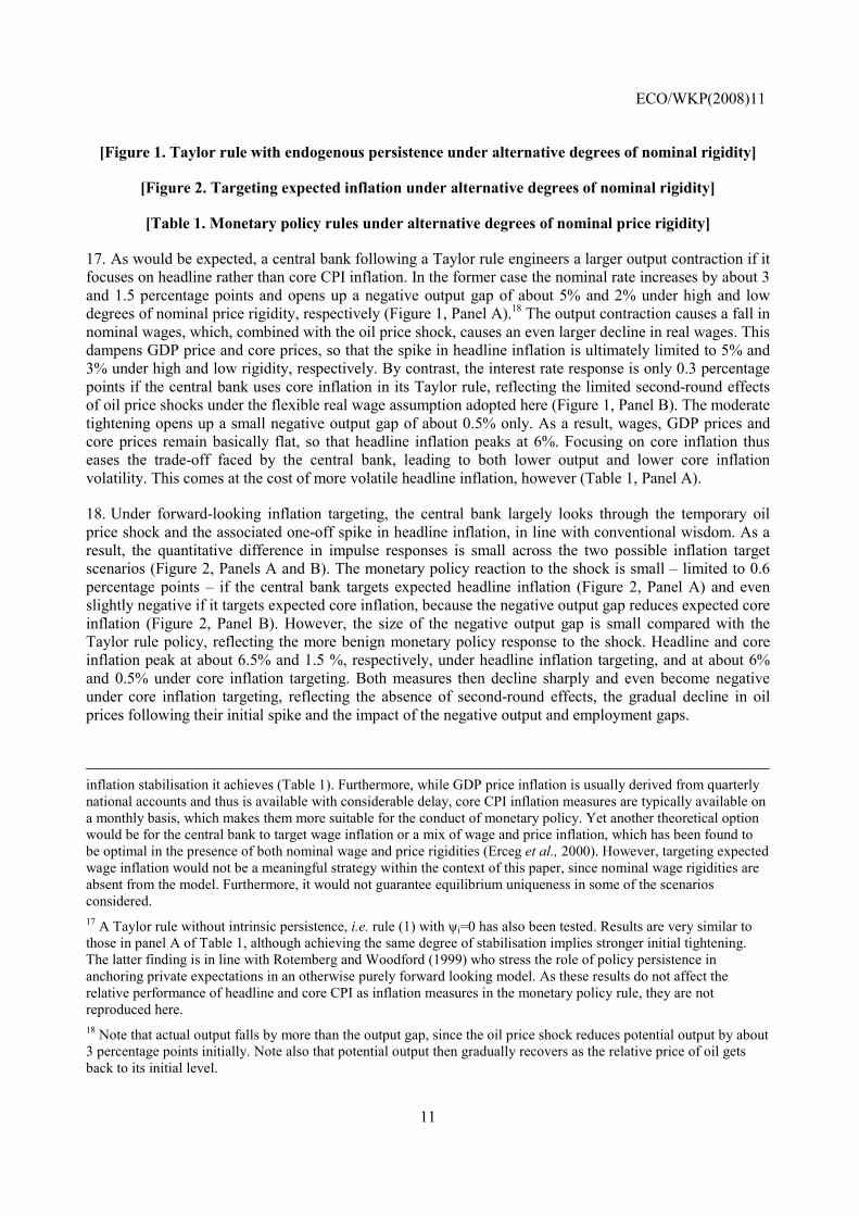
[Figure 1. Taylor rule with endogenous persistence under alternative degrees of nominal rigidity]

[Figure 2. Targeting expected inflation under alternative degrees of nominal rigidity]

[Table 1. Monetary policy rules under alternative degrees of nominal price rigidity]

17. As would be expected, a central bank following a Taylor rule engineers a larger output contraction if it focuses on headline rather than core CPI inflation. In the former case the nominal rate increases by about 3 and 1.5 percentage points and opens up a negative output gap of about 5% and 2% under high and low degrees of nominal price rigidity, respectively (Figure 1, Panel A).18 The output contraction causes a fall in nominal wages, which, combined with the oil price shock, causes an even larger decline in real wages. This dampens GDP price and core prices, so that the spike in headline inflation is ultimately limited to 5% and 3% under high and low rigidity, respectively. By contrast, the interest rate response is only 0.3 percentage points if the central bank uses core inflation in its Taylor rule, reflecting the limited second-round effects of oil price shocks under the flexible real wage assumption adopted here (Figure 1, Panel B). The moderate tightening opens up a small negative output gap of about 0.5% only. As a result, wages, GDP prices and core prices remain basically flat, so that headline inflation peaks at 6%. Focusing on core inflation thus eases the trade-off faced by the central bank, leading to both lower output and lower core inflation volatility. This comes at the cost of more volatile headline inflation, however (Table 1, Panel A).

18. Under forward-looking inflation targeting, the central bank largely looks through the temporary oil price shock and the associated one-off spike in headline inflation, in line with conventional wisdom. As a result, the quantitative difference in impulse responses is small across the two possible inflation target scenarios (Figure 2, Panels A and B). The monetary policy reaction to the shock is small – limited to 0.6 percentage points – if the central bank targets expected headline inflation (Figure 2, Panel A) and even slightly negative if it targets expected core inflation, because the negative output gap reduces expected core inflation (Figure 2, Panel B). However, the size of the negative output gap is small compared with the Taylor rule policy, reflecting the more benign monetary policy response to the shock. Headline and core inflation peak at about 6.5% and 1.5 %, respectively, under headline inflation targeting, and at about 6% and 0.5% under core inflation targeting. Both measures then decline sharply and even become negative under core inflation targeting, reflecting the absence of second-round effects, the gradual decline in oil prices following their initial spike and the impact of the negative output and employment gaps.

inflation stabilisation it achieves (Table 1). Furthermore, while GDP price inflation is usually derived from quarterly national accounts and thus is available with considerable delay, core CPI inflation measures are typically available on a monthly basis, which makes them more suitable for the conduct of monetary policy. Yet another theoretical option would be for the central bank to target wage inflation or a mix of wage and price inflation, which has been found to be optimal in the presence of both nominal wage and price rigidities (Erceg et al., 2000). However, targeting expected wage inflation would not be a meaningful strategy within the context of this paper, since nominal wage rigidities are absent from the model. Furthermore, it would not guarantee equilibrium uniqueness in some of the scenarios considered. 17 A Taylor rule without intrinsic persistence, i.e. rule (1) with ψi=0 has also been tested. Results are very similar to those in panel A of Table 1, although achieving the same degree of stabilisation implies stronger initial tightening. The latter finding is in line with Rotemberg and Woodford (1999) who stress the role of policy persistence in anchoring private expectations in an otherwise purely forward looking model. As these results do not affect the relative performance of headline and core CPI as inflation measures in the monetary policy rule, they are not reproduced here. 18 Note that actual output falls by more than the output gap, since the oil price shock reduces potential output by about 3 percentage points initially. Note also that potential output then gradually recovers as the relative price of oil gets back to its initial level.

ECO/WKP(2008)11

12

19. Somewhat surprisingly, it is also found that core inflation targeting is more successful than headline inflation targeting at stabilising both headline and core CPI inflation, while achieving a roughly comparable degree of output stabilisation (Table 1, Panel B). However, this result is contingent on the assumptions made here about the temporary nature of the shock and the formation of inflation expectations. Under full rational expectations, the temporary nature of the oil shock is supposed to be known, so that agents expect negative oil price inflation after the initial shock. Negative future rates of oil price inflation mean that headline inflation stabilisation is compatible with, and therefore generates the expectation of, positive core inflation rates. By contrast, a central bank targeting core inflation will be expected to seek zero rather than positive core inflation in the future. As a result, expectations of future core inflation will be higher under headline than under core inflation targeting, leading to higher core and headline inflation both now and in the future. As would be expected, simulations with the full, non-linear model version show that this difference between forward-looking headline and core CPI inflation targeting vanishes under a permanent oil price shock. This is because expected core and headline inflation rates then converge in the long-run, so that differences in the policy stance between headline and core inflation targeting disappear.

20. Finally, Figures 1 and 2 show that the degree of nominal rigidity has relatively little impact on the policy rate, output and inflation responses to oil price shocks in general, with the noticeable exception of stronger monetary tightening and larger output contraction in the presence of strong nominal rigidity when the central bank follows a Taylor rule focusing on headline inflation (Figure 1, panel A).19 The latter result is a consequence of the flatter Phillips curve under strong nominal rigidity: a negative output gap has a smaller negative impact on core and therefore on headline inflation, forcing the central bank to react more to the oil price shock in order to stabilise inflation, thereby engineering a larger output contraction. This effect more than offsets the mitigating impact strong nominal rigidity has on the immediate effect of the oil price shock on CPI inflation.

Real wage rigidity makes it more difficult to achieve output and inflation stabilisation, thereby triggering a more aggressive policy response and a larger output contraction

21. The introduction of real wage persistence impedes the downward adjustment of nominal wages and induces second-round effects on production costs and inflation. The temporary oil price shock pushes up nominal wage claims, ceteris paribus, which then feed into higher production costs and higher consumer prices. This makes it more difficult for the central bank to achieve both output and inflation stabilisation. As a result, the degree of monetary policy tightening, the output contraction and the initial spike in inflation are all larger under real wage rigidity, whatever the monetary policy rule and the inflation indicator used by the central bank (Figures 3 and 4, and Table 2).20

22. Under a Taylor rule focusing on headline inflation, real wage persistence increases the magnitudes of the monetary policy tightening, the decline in output and the increase in headline inflation by about 1, 2.5 and 2 percentage points, respectively (Figure 3, Panel A). Orders of magnitude are fairly similar if the central bank focuses on core inflation (Figure 3, Panel B). More broadly, real wage rigidity increases both output and inflation volatility in the presence of oil price shocks (Table 2, Panel A).21 Also, compared with

19 This finding is in line with the results in Dhawan and Jeske (2007). 20 Computation of the Ramsey optimal policy confirms that real wage rigidity implies stronger monetary policy tightening and a higher welfare loss. 21 Impulse responses for the Taylor rule with ψi=0 are qualitatively very similar to the policy rule with intrinsic persistence. The absence of intrinsic persistence implies a stronger initial tightening and a stronger initial contraction, but it does not achieve better control of inflation. Again, this points to the stabilising impact of policy inertia in a model with important forward-looking components (see Rotemberg and Woodford, 1999; Woodford, 2001).

ECO/WKP(2008)11

13

a flexible real wage environment, focusing on core rather than headline inflation now yields a larger gain in terms of output stabilisation22 at the cost of a larger loss in terms of headline inflation stabilisation. This is because a less aggressive monetary policy response now allows larger increases in nominal wages and therefore larger second-round effects on inflation.

[Figure 3. Taylor rule with endogenous persistence under alternative degrees of real rigidity]

[Table 2. Monetary policy rules under alternative degrees of real wage rigidity]

23. While differences in the interest rate and output responses under the Taylor and inflation-targeting rules were large in the absence of real wage rigidity (Figures 1 and 2), they now become much smaller (Figures 3 and 4). A central bank targeting expected core or headline inflation can no longer look through the temporary oil price shock and thus reacts strongly, due to its expected second-round effects (Figure 4). The monetary policy response remains smaller than under a Taylor rule, however, because the central bank neglects the initial peak in inflation. Finally, as was already the case in the absence of real wage rigidity, core inflation targeting remains moderately more successful than headline inflation targeting at stabilising inflation, while achieving a roughly comparable degree of output stabilisation (Figure 4 and Table 2, Panel B). However, as explained above, this result hinges on the assumption of a temporary oil price shock.

[Figure 4. Targeting expected inflation under alternative degrees of real rigidity]

Increasing the weight on headline inflation in the Taylor rule can significantly increase the output cost of oil price shocks in the presence of real wage rigidity

24. Table 3 presents the volatility of output and inflation induced by the oil price shock under a Taylor rule assigning a higher coefficient to inflation, i.e. 3.5 instead of 1.5 previously. Increasing the weight on inflation relative to the output gap in the Taylor rule reinforces monetary tightening. However, with flexible real wages, the additional increase in the policy rate and the associated output contraction are quantitatively small. In the presence of real wage rigidity, the trade-off between inflation and output stabilisation is steeper, and the effort made by the monetary authority to stabilise inflation now comes at a large output cost and achieves only limited headline inflation stabilisation. As was already the case in the absence of real rigidities (Table 1, Panel A), focusing on core rather than headline CPI inflation eases the trade-off faced by the central bank, enabling it to reduce output volatility while achieving very stable core inflation.

[Table 3. Taylor rule with large inflation coefficient]

Real and nominal rigidities interact, with nominal rigidities dampening the detrimental effects of real ones

25. Interactions between nominal and real rigidities play an important role in shaping the interest rate, output and inflation responses to oil price shocks. However, instead of reinforcing the effect of real wage inertia, nominal price rigidity dampens both inflation and output volatility, for a given level of real persistence (Table 4, Figures 5 and 6). Flexible prices steepen the Phillips curve. While this steepening reduces the sacrifice ratio, i.e. the output loss required to dampen inflation, it also increases the sensitivity of inflation to production costs and cost-push shocks. Therefore, price flexibility amplifies the initial inflation effect of the oil price shock. In a context where real wages adjust only slowly to the decline in

22 The initial output gap is -2.5% under core inflation targeting, versus almost -5% under headline inflation targeting. This 2.5 percentage point gain in output is to be compared with the smaller 1.5 percentage points gain achieved by targeting core inflation in the absence of real wage rigidity.

ECO/WKP(2008)11

14

output and labour demand, the higher initial inflation effect pushes up nominal wages, cetereris paribus, thereby reinforcing inflationary pressures. This induces the central bank to react more strongly and to engineer a larger fall in output. By contrast, for given real rigidity, higher nominal price rigidity dampens initial inflationary pressures and enables the central bank to better stabilise both inflation and output.

26. Figure 5 shows, in the presence of substantial real wage rigidity, the impulse responses under a Taylor rule for two alternative degrees of nominal rigidity. Under low nominal inertia, the initial increase in the policy rate is 0.5 percentage point higher, the output gap is about 1 percentage point larger, and the initial inflation spike is almost 1 percentage point higher despite the stronger policy reaction (Figure 5, Panel A). If the central bank focuses on core rather than headline inflation in its Taylor rule, the difference between the interest rate and output responses under the two alternative degrees of nominal rigidity becomes much larger (Figure 5, Panel B). While generating a larger initial impact of the shock, low nominal inertia speeds up the return to baseline afterwards. Similar patterns arise under inflation targeting. Regardless of whether the central bank targets headline or core inflation, the initial interest rate and output responses are about 4 and 3 percentage points higher under low than under high nominal rigidity, but the return to baseline is quicker afterwards (Figure 6, Panels A and B). Table 4 sums up all these results. It confirms that for a given degree of real wage rigidity, the volatility of output gaps and inflation rates declines with increasing nominal inertia, irrespective of the policy rule followed by the central bank and the inflation indicator it focuses on.23

[Figure 5. Taylor rule with real rigidity and alternative degrees of nominal rigidity]

[Figure 6. Inflation targeting rule with real rigidity and alternative degrees of nominal rigidity]

[Table 4. Taylor rule under real wage rigidity and alternative degrees of nominal price rigidity]

27. The sensitivity of the previous results with regard to model specification has been tested along two dimensions. First, the full, non-linear version of the model is used to investigate the consequences of reducing the substitution elasticity between labour and oil in production from unity to 0.5. The simulations indicate that all previous results are qualitatively robust to this change in calibration. While the initial amplitudes of the output and price responses are somewhat smaller, the impulse responses qualitatively replicate the dynamics portrayed in Figures 1-6. Second, the non-linear model was submitted to a permanent oil price shock. Simulations with such a unit-root oil price shock also confirm previous findings. The results are qualitatively in line with the linearised model under the persistent but non-permanent shock, while initial amplitudes and quantitative differences across simulations with different degrees of rigidity and/or different policy rules are generally more pronounced.24

6. Conclusion

28. Based on a calibrated New Keynesian model incorporating oil in both production and consumption, this paper shows that real rigidities greatly matter for the interest rate, output and inflation responses to oil price shocks, even when the latter are only temporary. Real wage rigidity induces second-round effects

23 Computation of the Ramsey optimal policy shows that under real wage rigidity, increasing nominal price flexibility implies stronger monetary policy tightening and a higher welfare loss. While the first-best policy option in the context of the present model is to lower real rigidities, this finding suggests that a second-best solution would be to increase nominal rigidities. 24 One exception is inflation targeting in the absence of real wage rigidity, i.e. the scenario displayed in Table 1, Panel B. In this case, standard deviations are (almost) identical across both degrees of nominal inertia. This is because the policy rule reacts to expected future inflation and therefore looks through the initial and permanent increase in the price of oil and its effects on current output.

ECO/WKP(2008)11

15

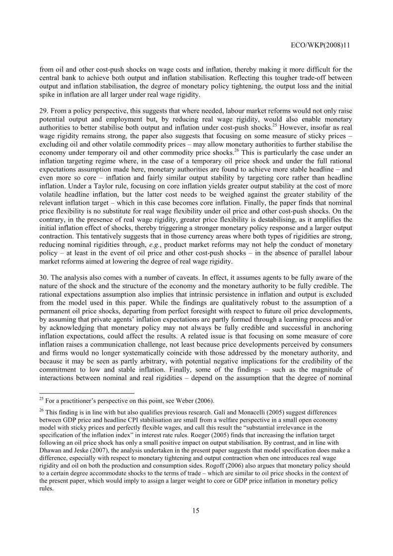
from oil and other cost-push shocks on wage costs and inflation, thereby making it more difficult for the central bank to achieve both output and inflation stabilisation. Reflecting this tougher trade-off between output and inflation stabilisation, the degree of monetary policy tightening, the output loss and the initial spike in inflation are all larger under real wage rigidity.

29. From a policy perspective, this suggests that where needed, labour market reforms would not only raise potential output and employment but, by reducing real wage rigidity, would also enable monetary authorities to better stabilise both output and inflation under cost-push shocks.25 However, insofar as real wage rigidity remains strong, the paper also suggests that focusing on some measure of sticky prices –excluding oil and other volatile commodity prices – may allow monetary authorities to further stabilise the economy under temporary oil and other commodity price shocks.26 This is particularly the case under an inflation targeting regime where, in the case of a temporary oil price shock and under the full rational expectations assumption made here, monetary authorities are found to achieve more stable headline – and even more so core – inflation and fairly similar output stability by targeting core rather than headline inflation. Under a Taylor rule, focusing on core inflation yields greater output stability at the cost of more volatile headline inflation, but the latter cost needs to be weighed against the greater stability of the relevant inflation target – which in this case becomes core inflation. Finally, the paper finds that nominal price flexibility is no substitute for real wage flexibility under oil price and other cost-push shocks. On the contrary, in the presence of real wage rigidity, greater price flexibility is destabilising, as it amplifies the initial inflation effect of shocks, thereby triggering a stronger monetary policy response and a larger output contraction. This tentatively suggests that in those currency areas where both types of rigidities are strong, reducing nominal rigidities through, e.g., product market reforms may not help the conduct of monetary policy – at least in the event of oil price and other cost-push shocks – in the absence of parallel labour market reforms aimed at lowering the degree of real wage rigidity.

30. The analysis also comes with a number of caveats. In effect, it assumes agents to be fully aware of the nature of the shock and the structure of the economy and the monetary authority to be fully credible. The rational expectations assumption also implies that intrinsic persistence in inflation and output is excluded from the model used in this paper. While the findings are qualitatively robust to the assumption of a permanent oil price shocks, departing from perfect foresight with respect to future oil price developments, by assuming that private agents’ inflation expectations are partly formed through a learning process and/or by acknowledging that monetary policy may not always be fully credible and successful in anchoring inflation expectations, could affect the results. A related issue is that focusing on some measure of core inflation raises a communication challenge, not least because price developments perceived by consumers and firms would no longer systematically coincide with those addressed by the monetary authority, and because it may be seen as partly arbitrary, with potential negative implications for the credibility of the commitment to low and stable inflation. Finally, some of the findings – such as the magnitude of interactions between nominal and real rigidities – depend on the assumption that the degree of nominal

25 For a practitioner’s perspective on this point, see Weber (2006). 26 This finding is in line with but also qualifies previous research. Galí and Monacelli (2005) suggest differences between GDP price and headline CPI stabilisation are small from a welfare perspective in a small open economy model with sticky prices and perfectly flexible wages, and call this result the “substantial irrelevance in the specification of the inflation index” in interest rate rules. Roeger (2005) finds that increasing the inflation target following an oil price shock has only a small positive impact on output stabilisation. By contrast, and in line with Dhawan and Jeske (2007), the analysis undertaken in the present paper suggests that model specification does make a difference, especially with respect to monetary tightening and output contraction when one introduces real wage rigidity and oil on both the production and consumption sides. Rogoff (2006) also argues that monetary policy should to a certain degree accommodate shocks to the terms of trade – which are similar to oil price shocks in the context of the present paper, which would imply to assign a larger weight to core or GDP price inflation in monetary policy rules.

ECO/WKP(2008)11

16

rigidity is independent of the size of shocks – the so-called “time-dependent”, as opposed to “state-dependent”, pricing rule. Yet, in practice, there is some evidence that firms tend to reset their prices more frequently in the presence of shocks.27 There is therefore ample room for further research.

27 See, e.g., Altissimo et al. (2006).

ECO/WKP(2008)11

17

Box 1. Model equations The linearised model consists of 10 equations, which derive from a micro-founded model described in the Annex:

(1) ( ) ( )( ) ( ) *1

*1,

*1,1,1 ˆ1ˆˆ

1lnˆˆˆ +++++ ∆−+−−

−++−−= tttCttOttHttttt cEEEEiyEy ωππεω

γγβπω

(2) ( ) ( ) ( ) ( ) ( ) ( )( )

**,

*, ˆ

111ˆˆ

1111~

ttCtOt cppyϕωθ

ωθϕθγ

ϕθγεθωϕγωθ++

−−++−

−+−++−

−=

(3) ttt yyx ~ˆˆ −≡

(4)

( ) [ ]( ) ( )

( )( ) ( ) [ ]( ) ( )*,

*,

*,1,,

ˆˆ11ˆˆ1

ˆˆ1111

ˆˆ

tttCt

tCtOtHttH

cypw

ppE

−−+−+

+−−+

−

−+−+−

−++= +

ωαγγθθλθλ

εω

αγγθθγ

γθλπβπ

(5) [ ]( )( ) ( )*,

*,,,,, ˆˆ

1ˆˆ1ˆˆ tCtOtHtFtHtC pppppp −

−+−−++=

γγαγγ

(6) ( )tOtCtM ppp ,,, ˆˆ1

1ˆ γγ

−−

=

(7) ( ) ( ) ( )( )( ) ( )

( )( )( )( )

( )( )( )( ) *

*,

*,1,1,

ˆ1111111ˆ111

111

ˆˆ11111ˆˆ

11ˆˆ

tw

wt

w

w

tCtOw

wtCt

w

wtCt

cy

pppwpw

+−−−

−+−

+

+−−

+−+−

+

−

+−

−−+−

+−−+

=− −−

ωϕθγα

ϕθρρ

ωϕθγαϕ

ϕθρρ

ωγεϕθαϕθ

ϕθρρ

ϕθρρ

(8) ( ) ( ) ( )( )( )( ) ( )*

,*

,* ˆˆ

111111ˆ tCtOt ppc −+−−−+++−

−=ϕθγ

γεϕθθϕγθ

(9) ( )( ) ( )( )( ) ( ) ( )( ) **

,*

,*

,*

, ˆ1

11ˆˆˆ11

111ˆ ttCtCtOtF cppppϕθ

ϕθϕθγ

γεϕθθϕγ+

+−++−

+−−++−

=

(10) ( ) *,

*,

*, ˆˆ1ˆ tOtFtC ppp γγ +−=

Where variables and parameters are defined as follows:

Output Potential output Output gap

GDP price inflation Consumer price index (CPI) Core CPI

Nominal wage

Foreign consumption Foreign core CPI Foreign CPI

Nominal interest rate

World market oil price

ECO/WKP(2008)11

18

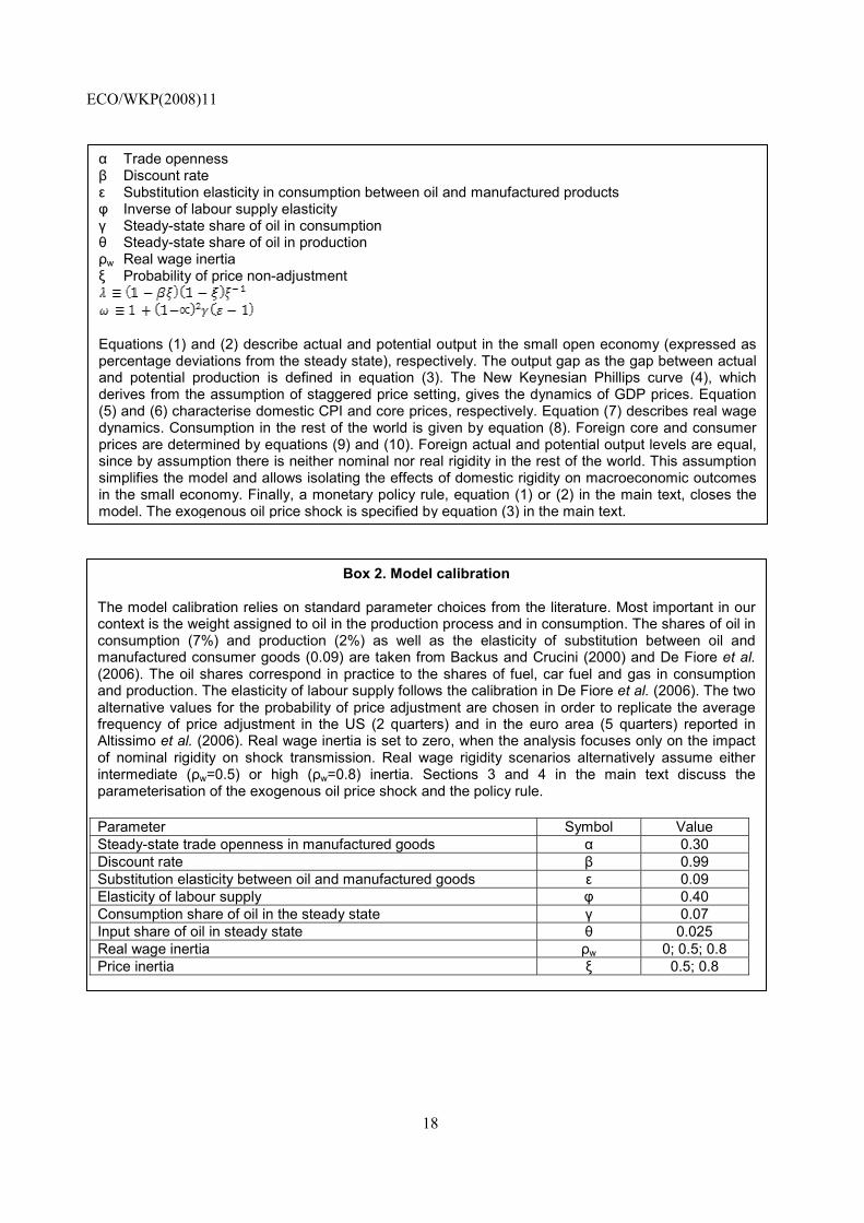
α Trade openness β Discount rate ε Substitution elasticity in consumption between oil and manufactured products φ Inverse of labour supply elasticity γ Steady-state share of oil in consumption θ Steady-state share of oil in production ρw Real wage inertia ξ Probability of price non-adjustment

Equations (1) and (2) describe actual and potential output in the small open economy (expressed as percentage deviations from the steady state), respectively. The output gap as the gap between actual and potential production is defined in equation (3). The New Keynesian Phillips curve (4), which derives from the assumption of staggered price setting, gives the dynamics of GDP prices. Equation (5) and (6) characterise domestic CPI and core prices, respectively. Equation (7) describes real wage dynamics. Consumption in the rest of the world is given by equation (8). Foreign core and consumer prices are determined by equations (9) and (10). Foreign actual and potential output levels are equal, since by assumption there is neither nominal nor real rigidity in the rest of the world. This assumption simplifies the model and allows isolating the effects of domestic rigidity on macroeconomic outcomes in the small economy. Finally, a monetary policy rule, equation (1) or (2) in the main text, closes the model. The exogenous oil price shock is specified by equation (3) in the main text.

Box 2. Model calibration The model calibration relies on standard parameter choices from the literature. Most important in our context is the weight assigned to oil in the production process and in consumption. The shares of oil in consumption (7%) and production (2%) as well as the elasticity of substitution between oil and manufactured consumer goods (0.09) are taken from Backus and Crucini (2000) and De Fiore et al. (2006). The oil shares correspond in practice to the shares of fuel, car fuel and gas in consumption and production. The elasticity of labour supply follows the calibration in De Fiore et al. (2006). The two alternative values for the probability of price adjustment are chosen in order to replicate the average frequency of price adjustment in the US (2 quarters) and in the euro area (5 quarters) reported in Altissimo et al. (2006). Real wage inertia is set to zero, when the analysis focuses only on the impact of nominal rigidity on shock transmission. Real wage rigidity scenarios alternatively assume either intermediate (ρw=0.5) or high (ρw=0.8) inertia. Sections 3 and 4 in the main text discuss the parameterisation of the exogenous oil price shock and the policy rule. Parameter Symbol Value Steady-state trade openness in manufactured goods α 0.30 Discount rate β 0.99 Substitution elasticity between oil and manufactured goods ε 0.09 Elasticity of labour supply φ 0.40 Consumption share of oil in the steady state γ 0.07 Input share of oil in steady state θ 0.025 Real wage inertia ρw 0; 0.5; 0.8 Price inertia ξ 0.5; 0.8

ECO/WKP(2008)11

19

Figure 1: Taylor rule under alternative degrees of nominal rigidity

pi_core: core CPI inflation - pi_gdp: GDP price inflation - pi_w: wage inflation - c_gap: consumption gap

▬▬ High nominal price rigidity (θ=0.8) ••••• Low nominal price rigidity (θ=0.5)

A. Taylor rule with headline CPI inflation

B. Taylor rule with core CPI inflation

i: nominal interest rate - y_gap: output gap - n_gap: employment gap - mc: real marginal costs - pi_cpi: headline CPI inflation

ECO/WKP(2008)11

20

Figure 2: Targeting expected inflation under alternative degrees of nominal rigidity


▬▬ High nominal price rigidity (θ=0.8) ••••• Low nominal price rigidity (θ=0.5)

A. Headline CPI inflation target

B. Core CPI inflation target


ECO/WKP(2008)11

21

Figure 3: Taylor rule under alternative degrees of real rigidity


▬▬ High real wage rigidity (ρ=0.8, θ=0.5) ••••• No real wage rigidity (ρ=0.0, θ=0.5)




ECO/WKP(2008)11

22

Figure 4: Targeting expected inflation under alternative degrees of real rigidity


▬▬ High real wage rigidity (ρ=0.8, θ=0.5) ••••• No real wage rigidity (ρ=0.0, θ=0.5)




ECO/WKP(2008)11

23

Figure 5: Taylor rule under real rigidity and alternative degrees of nominal rigidity


▬▬ High nominal price rigidity (θ=0.8, ρ=0.8) ••••• Low nominal price rigidity (θ=02, ρ=0.8)




ECO/WKP(2008)11

24

Figure 6: Targeting expected inflation with real rigidity and alternative degrees of nominal rigidity


▬▬ High nominal price rigidity (θ=0.8, ρ=0.8) ••••• Low nominal price rigidity (θ=02, ρ=0.8)




ECO/WKP(2008)11

25

Table 1: Monetary policy rules under alternative degrees of nominal price rigidity

Nominal Real Lagged instrument

Output gap

CPI inflation

Core inflation

GDP price inflation

Output gap

CPI inflation

Core inflation

GDP price inflation

Wage inflation

0.5 - 0.5 0.5 1.5 - - 0.024 0.033 0.034 0.034 0.1060.5 - 0.5 0.5 - 1.5 - 0.018 0.059 0.013 0.013 0.0210.5 - 0.5 0.5 - - 1.5 0.018 0.065 0.014 0.011 0.0140.8 - 0.5 0.5 1.5 - - 0.043 0.047 0.023 0.020 0.1550.8 - 0.5 0.5 - 1.5 - 0.012 0.061 0.009 0.007 0.0220.8 - 0.5 0.5 - - 1.5 0.016 0.061 0.012 0.009 0.011


Output gap

CPI inflation

Core inflation

GDP price inflation

Output gap

CPI inflation

Core inflation

GDP price inflation

Wage inflation

0.5 - - - 1.5 - - 0.017 0.068 0.027 0.025 0.0260.5 - - - - 1.5 - 0.013 0.059 0.005 0.002 0.0140.5 - - - - - 1.5 0.015 0.057 0.006 0.004 0.0140.8 - - - 1.5 - - 0.008 0.069 0.024 0.022 0.0210.8 - - - - 1.5 - 0.014 0.056 0.005 0.002 0.0140.8 - - - - - 1.5 0.018 0.059 0.006 0.005 0.016

B. Inflation targeting regime

Degree of rigidity Coefficients on Standard deviation of

A. Taylor rule


Table 2: Monetary policy rules under alternative degrees of real wage rigidity


Output gap

CPI inflation

Core inflation

GDP price inflation

Output gap

CPI inflation

Core inflation

GDP price inflation

Wage inflation

0.5 - 0.5 0.5 1.5 - - 0.024 0.033 0.034 0.034 0.1060.5 - 0.5 0.5 - 1.5 - 0.018 0.059 0.013 0.013 0.0210.5 - 0.5 0.5 - - 1.5 0.018 0.065 0.014 0.011 0.0140.5 0.8 0.5 0.5 1.5 - - 0.055 0.060 0.024 0.024 0.0270.5 0.8 0.5 0.5 - 1.5 - 0.036 0.080 0.030 0.030 0.0530.5 0.8 0.5 0.5 - - 1.5 0.038 0.086 0.035 0.035 0.055


Output gap

CPI inflation

Core inflation

GDP price inflation

Output gap

CPI inflation

Core inflation

GDP price inflation

Wage inflation

0.5 - - - 1.5 - - 0.017 0.068 0.027 0.025 0.0260.5 - - - - 1.5 - 0.013 0.059 0.005 0.002 0.0140.5 - - - - - 1.5 0.015 0.057 0.006 0.004 0.0140.5 0.8 - - 1.5 - - 0.039 0.091 0.054 0.053 0.0600.5 0.8 - - - 1.5 - 0.037 0.079 0.034 0.034 0.0450.5 0.8 - - - - 1.5 0.033 0.093 0.045 0.045 0.061


Degree of rigidity Coefficients on

A. Taylor rule


Standard deviation of

ECO/WKP(2008)11

26

Table 3: Taylor rule with large inflation coefficient


Output gap

CPI inflation

Core inflation

GDP price inflation

Output gap

CPI inflation

Core inflation

GDP price inflation

Wage inflation

0.5 - 0.5 0.5 3.5 - - 0.034 0.013 0.044 0.044 0.1380.5 - 0.5 0.5 - 3.5 - 0.016 0.055 0.003 0.004 0.0240.8 - 0.5 0.5 3.5 - - 0.074 0.026 0.030 0.019 0.2510.8 - 0.5 0.5 - 3.5 - 0.015 0.054 0.003 0.002 0.0340.8 0.5 0.5 0.5 3.5 - - 0.072 0.027 0.026 0.015 0.1120.8 0.5 0.5 0.5 - 3.5 - 0.018 0.056 0.005 0.002 0.0190.8 0.8 0.5 0.5 3.5 - - 0.079 0.028 0.022 0.009 0.0350.8 0.8 0.5 0.5 - 3.5 - 0.033 0.058 0.008 0.006 0.038


Table 4: Monetary policy rules under real wage rigidity and alternative degrees of price rigidity


Output gap

CPI inflation

Core inflation

GDP price inflation

Output gap

CPI inflation

Core inflation

GDP price inflation

Wage inflation

0.2 0.8 0.5 0.5 1.5 - - 0.061 0.063 0.030 0.033 0.0330.2 0.8 0.5 0.5 - 1.5 - 0.048 0.090 0.042 0.049 0.0540.2 0.8 0.5 0.5 - - 1.5 0.048 0.093 0.045 0.051 0.0550.5 0.8 0.5 0.5 1.5 - - 0.054 0.055 0.020 0.019 0.0230.5 0.8 0.5 0.5 - 1.5 - 0.037 0.080 0.030 0.030 0.0530.5 0.8 0.5 0.5 - - 1.5 0.038 0.082 0.034 0.033 0.0530.8 0.8 0.5 0.5 1.5 - - 0.050 0.051 0.021 0.018 0.0220.8 0.8 0.5 0.5 - 1.5 - 0.018 0.064 0.013 0.010 0.0470.8 0.8 0.5 0.5 - - 1.5 0.016 0.067 0.015 0.011 0.052


Output gap

CPI inflation

Core inflation

GDP price inflation

Output gap

CPI inflation

Core inflation

GDP price inflation

Wage inflation

0.2 0.8 - - 1.5 - - 0.049 0.119 0.077 0.080 0.0780.2 0.8 - - - 1.5 - 0.052 0.124 0.079 0.081 0.0790.2 0.8 - - - - 1.5 0.048 0.157 0.111 0.113 0.1150.5 0.8 - - 1.5 - - 0.036 0.084 0.043 0.043 0.0520.5 0.8 - - - 1.5 - 0.036 0.079 0.033 0.033 0.0460.5 0.8 - - - - 1.5 0.033 0.091 0.045 0.044 0.0590.8 0.8 - - 1.5 - - 0.014 0.068 0.030 0.028 0.0510.8 0.8 - - - 1.5 - 0.022 0.062 0.011 0.008 0.0430.8 0.8 - - - - 1.5 0.017 0.060 0.012 0.009 0.043


A. Taylor rule



ECO/WKP(2008)11

27

References

Altissimo, F., M. Ehrmann and F. Smets (2006), Inflation Persistence and Price-Setting Behaviour in the Euro Area: A Summary of the IPN Evidence, ECB Occasional Paper No. 46.

Atkeson, A. and P. Kehoe (1999), “Models of Energy Use: Putty-Putty versus Putty-Clay”, American Economic Review Vol. 89, No. 4.

Arpaia, A. and K. Pichelmann (2007): Nominal and Real Wage Flexibility in EMU, European Economy Economic Papers, No. 281.

Backus, D. and M. Crucini (2000), “Oil Prices and the Terms of Trade”, Journal of International Economics Vol. 50, No. 1.

Blanchard, O. and J. Galí (2007a), “Real Wage Rigidities and the New Keynesian Model”, Journal of Money, Credit and Banking, Vol. 39, No. 1.

Blanchard, O. and J. Galí (2007b), The Macroeconomic Effects of Oil Price Shocks: Why Are the 2000s so Different from the 1970s?, NBER Working Paper No. 13368.

Bullard, J. and K. Mitra (2007), “Determinacy, Learnability and Monetary Policy Inertia”, Journal of Money, Credit and Banking, Vol. 39, No. 5.

Campolmi, A. (2006), Which Inflation to Target? A Small Open Economy with Sticky Wages Indexed to Past Inflation, Universitat Pompeu Fabra Department of Economics and Business Working Papers No. 961.

Christoffel, K. and T. Linzert (2005), The Role of real Wage Rigidity and Labor Market Frictions for Unemployment and Inflation Dynamics, ECB Working Paper Series No. 556.

Clarida, R., J. Galí and M. Gertler (1998), “Monetary Policy Rules in Practice: Some International Evidence”, European Economic Review, Vol. 42, No. 6.

De Fiore, F., G. Lombardo and V. Stebunovs (2006), Oil Price Shocks, Monetary Policy Rules and Welfare, Computing in Economics and Finance 2006/402.

Dhawan, R. and K. Jeske (2007), Taylor Rules with Headline Inflation: A Bad Idea, Federal Reserve Bank of Atlanta Working Paper Series No. 2007-14.

Duval, R. and L. Vogel (2007), How Do Nominal and Real Rigidities Interact? A Tale of the Second Best, MPRA Paper No. 7282, available at: http://mpra.ub.uni-muenchen.de/7282.

Eleftheriou, M., D. Gerdesmeier and B. Roffia (2006), Monetary Policy Rules in the Pre-EMU Era: Is There a Common Rule?, ECB Working Paper Series No. 659.

Erceg, Ch., D. Henderson and A. Levin (2000), “Optimal Monetary Policy with Staggered Wage and Price Contracts”, Journal of Monetary Economics Vol. 46, No. 2.

Galí, J. and T. Monacelli (2005), “Monetary Policy and Exchange Rate Volatility in a Small Open Economy”, Review of Economic Studies Vol. 72, No. 3.

ECO/WKP(2008)11

28

Gerdesmeier, D. and B. Roffia (2004), “Empirical Estimates of Reaction Functions for the Euro Area”, Swiss Journal for Economics and Statistics Vol. 140, No. 1.

Kamps, Ch. and Ch. Pierdzioch (2002), Monetary Policy Rules and Oil Price Shocks, Kiel Institute of World Economics Working Paper No. 1090.

Kohn, D. (2007), “Inflation Modeling: A Policymaker’s Perspective”, Journal of Money, Credit and Banking, Vol. 39, No. 1.

Le Barbanchon, T. (2007), The Changing Response to Oil Price Shocks in France: A DSGE Type Approach, INSEE Working Paper Series No. G 2007/07.

Leduc, S. and K. Sill (2006), “Monetary Policy, Oil Shocks, and TFP: Accounting for the Decline in U.S. Volatility”, Board of Governors of the Federal Reserve System International Finance Discussion Papers No. 873.

Mankiw, G. (2007), “Price Dynamics: Three Open Questions”, Journal of Money, Credit and Banking, Vol. 39, No. 1.

Obstfeld, M. and K. Rogoff (1996), Foundations of International Macroeconomics, Boston: MIT Press.

Roeger, W. (2005), “International Oil Price Changes: Impact of Oil Prices on Growth and Inflation in the EU/ OECD”, International Economics and Economic Policy Vol. 2, No. 1.

Rogoff, K. (2006), “Impact of Globalization on Monetary Policy”, Paper presented at the Federal Reserve Bank of Kansas City Symposium, Jackson Hole, Wyoming, August 24-26, 2006.

Rotemberg, J. and M. Woodford (1999), “Interest Rate Rules in an Estimated Sticky Price Model”, in: J. Taylor (ed.), Monetary Policy Rules, Chicago: Chicago University Press.

Sack, B. and V. Wieland (2000), “Interest-Rate Smoothing and Optimal Monetary Policy: A Review of Recent Empirical Evidence”, Journal of Economics and Business Vol. 52, No. 1.

Taylor, J. (1993), “Discretion versus Policy Rules in Practice”, Carnegie-Rochester Conference Series on Public Policy Vol. 39, December 1993.

Taylor, J. (1999), “Staggered Price and Wage Setting in Macroeconomics”, in: J. Taylor and M. Woodford (eds.), Handbook of Macroeconomics, Vol. 1, North-Holland: Elsevier.

Weber, A. (2006): “Oil price shocks and monetary policy in the euro area”, Whitaker Lecture at the Central Bank and Financial Services Authority of Ireland, Dublin, 11 May 2006.

Woodford, M. (2001), “The Taylor Rule and Optimal Monetary Policy”, American Economic Review, Vol. 91, No. 2.

Woodford, M. (2003), Interest and Prices: Foundations of a Theory of Monetary Policy, Princeton: Princeton University Press.

ECO/WKP(2008)11

29

ANNEX 1. THE NEW KEYNESIAN OPEN ECONOMY MODEL

This annex describes the open economy model with oil as both a production input and consumption good. Annex 2 derives the log-linear approximation of this framework. The log-linearised model gives a more compact representation of the economic structure and thus facilitates the understanding of the shock transmission. The modelling approach draws on various strands of previous research. The open economy framework heavily relies on Galí and Monacelli (2005). The modelling of oil as a consumption good and factor input borrows from De Fiore et al. (2006) and Roeger (2005). The introduction of real wage inertia follows Blanchard and Galí (2007a) as well as Christoffel and Linzert (2005). The model developed here combines a small open economy block with a simplified model for the rest of the world. Households are forward-looking and behave identically across countries. They choose consumption and labour supply to maximize household welfare. In doing so, they are not subject to liquidity constraints.

1.1 The small open economy

1.1.1 Household sector

The representative household maximizes lifetime utility over an infinite planning horizon. The overall household welfare equals the expected value of the discounted stream of period utility:

(1.1) .

Period utility Ut is the sum of the utility of consumption Ct and the disutility of hours worked Nt:

(1.2) ϕ

κϕ

+−=

+

1ln

1t

ttN

CU .

The assumption of log consumption utility implies a unit intertemporal elasticity of substitution for consumption. The parameter κ indicates the relative weight of leisure to consumption utility, while φ-1 and β are the elasticity of labour supply and the discount factor, respectively. If φ-1>0, transitory increases in the real wage induce transitory increases in labour supply. For simplicity the model abstracts from public consumption, so that household utility may not depend on government spending.

Choosing the optimal level of consumption and of labour supply, the representative household is subject to the period budget constraint:

(1.3) ( ) 1,1 ++=−+++ tttCtttttt BCPTBiDNW .

Wt is the nominal wage, Dt is dividend income from firm ownership, (1+it)Bt is the return from risk-free one-period bonds, and Tt are lump-sum taxes. On the right-hand side, PC,t is the index of consumer prices, Ct is real consumption, and Bt+1 captures the new investment in bonds.

The representative household maximizes welfare (1.1) under the constraint (1.3). The first order conditions provide the intertemporal consumption equation:

ECO/WKP(2008)11

30

(1.4) ( )

+=

++ 1,

,

1

11tC

tC

t

ttt P

PCC

Eiβ

and the equation for the optimal labour supply:

(1.5) ϕκ

1,

~−=ttC

t

CN

PW

,

stating that real wages should equal the household’s marginal rate of substitution between consumption and leisure. To capture labour market rigidity, a sluggish adjustment of real wages is assumed. Real wages are the weighted average of previous real wage and the marginal rate of substitution and equal:

(1.6) ww

tC

t

tC

t

tC

t

PW

PW

PW

ρρ −

−

−

=

1

,1,

1

,

~.

The weight 0≤ρw≤1 indicates the degree of real wage inertia. As will be seen later on, real wage persistence also introduces inertia in marginal production costs.28

The representative household consumes a bundle of non-oil goods, Mt, and imported oil, Ot. Both consumption components enter a CES consumption utility function:

(1.7) ( )11111

1−−−

+−=

εε

εε

εεε

ε γγ ttt OMC .

The parametersγ andε characterise the steady-state consumption share of oil and the elasticity of substitution between the two components, respectively.

At a third stage, the household spreads the demand for non-oil goods over domestic production, MH, and imported goods, MF. For simplicity, a unit elasticity of substitution between domestic and imported goods is assumed, which yields a Cobb-Douglas utility function:

(1.8) ααtFtHt MMM ,,

−1=

for manufactured goods consumption. The parameter 0≤α≤1 indicates the equilibrium import share in the non-oil consumption and thus provides a measure of non-oil trade openness.

Maximizing consumption utility (1.7) and (1.8) with PO,t, PM,t, PH,t and PF,t as the prices of oil, non-oil consumer goods, domestic production and non-oil imports, respectively, yields the demand functions:

28 The modelling of real wage rigidity adopted here follows Blanchard and Galí (2007a) and Christoffel and Linzert (2005) and introduces the log of present real wages as the weighted average of previous log real wages and the wage level under optimal labour supply (1.5). This approach is a simplifying shortcut. It notably ignores that, under sluggish real adjustment, wage setting may also become a question of dynamic optimisation analogously to the forward-looking staggered price setting of firms.

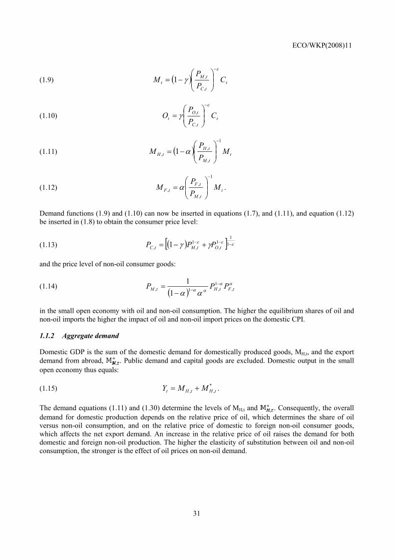
ECO/WKP(2008)11

31

(1.9) ( ) ttC

tMt C

PP

Mε

γ−

−=

,

,1

(1.10) ttC

tOt C

PP

Oε

γ−

=

,

,

(1.11) ( ) ttM

tHtH M

PP

M1

,

,, 1

−

−= α

(1.12) ttM

tFtF M

PP

M1

,

,,

−

= α .

Demand functions (1.9) and (1.10) can now be inserted in equations (1.7), and (1.11), and equation (1.12) be inserted in (1.8) to obtain the consumer price level:

(1.13) ( )[ ] εεε γγ −−− +−= 11

1,

1,, 1 tOtMtC PPP

and the price level of non-oil consumer goods:

(1.14) ( )

αααα αα tFtHtM PPP ,

1,1, 1

1 −−−

=

in the small open economy with oil and non-oil consumption. The higher the equilibrium shares of oil and non-oil imports the higher the impact of oil and non-oil import prices on the domestic CPI.

1.1.2 Aggregate demand

Domestic GDP is the sum of the domestic demand for domestically produced goods, MH,t, and the export demand from abroad, . Public demand and capital goods are excluded. Domestic output in the small open economy thus equals:

(1.15) *,, tHtHt MMY += .

The demand equations (1.11) and (1.30) determine the levels of MH,t and . Consequently, the overall demand for domestic production depends on the relative price of oil, which determines the share of oil versus non-oil consumption, and on the relative price of domestic to foreign non-oil consumer goods, which affects the net export demand. An increase in the relative price of oil raises the demand for both domestic and foreign non-oil production. The higher the elasticity of substitution between oil and non-oil consumption, the stronger is the effect of oil prices on non-oil demand.

ECO/WKP(2008)11

32

1.1.3 Aggregate supply

The model uses a simple representation of the representative firm and overall supply. Specifically, it is assumed that each firm produces output only with labour, Nt, and oil, Ot, using a Cobb-Douglas production function:

(1.16) θθththtth ONAY ,

1,,−= ,

with 0≤θ≤1, yielding constant returns to scale. The production technology is identical across all firms. The level of technology is exogenous. Given the topic in this paper, total factor productivity, At, can be normalized to unity.29

Firms operate in an environment of monopolistic competition. Domestic output, Yt, is a bundle of differentiated goods, each one provided by a single producer. The range of differentiated products has a mass of one. The demand for the product variety h follows from the demand function:

(1.17) ttH

thth Y

PP

Yµ−

=

,

,,

and depends on its relative price. The parameter µ indicates the elasticity of substitution between domestic product varieties. The higher the elasticity of substitution, the higher is the sensitivity of demand to changes in the relative price of h.

Combining equations (1.16) and (1.17) together with the fact that in equilibrium all firms choose the same optimal input combination yields the aggregate production function:

(1.18) θθ

µ

tttH

tht ONdh

PP

Y −

−

=

∫ 11

0 ,

,

that relates output to factor demand. The price dispersion term on the left side of (1.18) distorts consumption decisions. Equation (1.18) also shows that for µ>0 factor demand negatively depends on the relative price dispersion.

The optimizing firm chooses the cost-minimizing factor mix. The latter depends on both relative factor prices and relative factor productivity. Minimizing the production costs WtNh,t+PO,tOh,t under the production function (1.16) gives:

29 Alternatively, in order to check the robustness of the findings under a lower elasticity of substitution between

inputs, a CES production function is used: ( )11

,

11

,

1

, 1−−−

+−=

ηη

ηη

ηηη

η θθ ththtth ONAY , with 0≤θ≤1 as the steady-state input share

of oil and η as the elasticity of substitution between the two inputs. For representations of the production process with three factor inputs (labour, capital and oil) and more complex functional forms see, e.g. De Fiore et al. (2006), Le Barbanchon (2007), Leduc and Sill (2006), and Roeger (2005).

ECO/WKP(2008)11

33

(1.19) tO

tC

tC

t

t

t

PP

PW

NO

,

,

,1 θθ−

=

as the optimal mix of production inputs for given relative factor prices and:

(1.20) thtO

tC

tC

tth N

PP

PW

Y ,,

,

,, 1

θ

θθ

−=

as the cost minimizing production in the absence of adjustment costs in the production process.

Finally, under constant returns to scale, identical production technology and cost minimisation, real marginal production costs in the domestic economy, MCt, amount to:

(1.21) ( ) tH

tC

tC

tO

tC

tt P

PPP

PW

MC,

,

,

,

1

,11

1θθ

θθ θθ

−=

−

−.

Producers sell on goods markets under monopolistic competition. They set prices with a mark-up over marginal costs. The size of the mark-up varies inversely with the elasticity of substitution between product varieties. It is thus a positive function of the firm’s market power.

Empirical research (e.g. Altissimo et al. 2006, Taylor 1999) has provided ample evidence for sluggish price adjustment in goods markets. Producers do reset prices only from time to time. Resetting costs, costs of information gathering and contractual obligations figure among the potential explanations of price inertia.30 Following Calvo (1983), firms are assumed to set prices in staggered contracts of random duration. In any period, each firm gets to announce a new price with probability 1-ξ. Old prices remain valid otherwise.

Given the persistence of goods prices, the price determination becomes a problem of dynamic optimization. The firm chooses its target price Ph,t such as to maximize the present value of profits over the expected duration of the price contract:

(1.22) ( ) ithithitH

th

iitHit

it YMC

PP

PE +++

∞

=++

−∑ ,,

,

,

0,

~λξβ ,

where λt+i is the marginal utility of nominal wealth. The producer’s first order condition from maximizing (1.22) under the demand equation (1.17) is:

(1.23) ( )( )

( ) ititHi

iti

t

ititHiti

iti

t

th

YPE

YPMCEP

++

∞

=+

++++

∞

=+

∑

∑−

−=

µ

µ

λξβ

λξβτ

µµ

,0

1,

0, 1

1~

,

30 Altissimo et al. (2006) and Taylor (1999) provide a summary of the empirical evidence concerning the plausibility of the various mechanisms or determinants of price persistence.

ECO/WKP(2008)11

34

where τ is a production subsidy financed via the lump-sum tax in the budget constraint (1.3). If τ=µ-1, the subsidy exactly offsets the distortion that originates from monopolistic competition and keeps output below the efficient level. A production subsidy τ=µ-1 thus ensures steady-state production to be the efficient steady-state level of output.

Due to the law of large numbers, the individual probability of price correction, 1-ξ, also characterises the aggregate price-setting dynamics. The share 1-ξ of domestic producers resets prices in a given period, whereas the share ξ of firms does not adjust. The probability parameter ξ is therefore also a measure of aggregate price rigidity. The price level of domestic production evolves according to the equation:

(1.24) ( ) µµµ ξξ −−

−− +−= 11,

1,

1,

~1 tHtHtH PPP .

The price dispersion term in the equation (1.18) for domestic output finally follows as:

(1.25) .

All firms produce with identical technology and inputs. Therefore, the product price Ph,t would equal the price level of domestic production PH,t if prices and wages were perfectly flexible. The price-dispersion term would equal one in the latter case. Under τ=µ-1 domestic firms then produce the efficient level of output. The output gap measures the percentage gap between the actual level of output and the production level in the flexible economy.

1.2 The rest of the world

Trade and capital flows link the small country to the rest of the world. The rest of the world is exogenous to firm behaviour, household decisions and policy in the small domestic economy, but it affects the variables of the small country. Therefore a closed-economy framework is added in order to represent the rest of the world. For simplicity, behavioural similarity is assumed between domestic and foreign households and producers. A utility function equivalent to equation (1.1) and (1.2) captures household welfare in the rest of the world. Foreign households face a budget constraint equivalent to the domestic constraint (1.3), where dividends also include the income from oil extraction. This gives first order conditions analogous to (1.4) and (1.5) for consumption and the labour supply. Equating the Euler equations for domestic and foreign consumers gives:

t

t

tC

tCt

t

t

tCt

tCt C

CPPS

CC

PSP

E*

,

*,

*1

1*

1,1

1,1

=

+

+

++

+ ,

where the asterisk denotes variables in the rest of the world and St is the nominal exchange rate. If capital markets are perfectly integrated and risk perfectly diversified, the expectations term on the right side of the equation becomes a constant, , reflecting the relative wealth of representative foreign and domestic households. In this case, one obtains the relationship:

(1.26) *

,

*,

ttC

tCtt C

PPS

C ϑ=

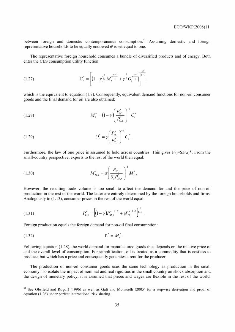
ECO/WKP(2008)11

35

between foreign and domestic contemporaneous consumption.31 Assuming domestic and foreign representative households to be equally endowed is set equal to one.

The representative foreign household consumes a bundle of diversified products and of energy. Both enter the CES consumption utility function:

(1.27) ( )11

*11

*1

* 1−−−

+−=

εε

εε

εεε

ε γγ ttt OMC ,

which is the equivalent to equation (1.7). Consequently, equivalent demand functions for non-oil consumer goods and the final demand for oil are also obtained:

(1.28) ( ) **,

*,* 1 ttC

tMt C

PP

Mε

γ−

−=

(1.29) **,

*,*

ttC

tOt C

PP

Oε

γ−

= .

Furthermore, the law of one price is assumed to hold across countries. This gives PF,t=StPM,t*. From the small-country perspective, exports to the rest of the world then equal:

(1.30) *

1

*,

,*, t

tMt

tHtH M

PSP

M−

= α .

However, the resulting trade volume is too small to affect the demand for and the price of non-oil production in the rest of the world. The latter are entirely determined by the foreign households and firms. Analogously to (1.13), consumer prices in the rest of the world equal:

(1.31) ( )[ ] εεε γγ −−−+−= 1

11*

,1*

,*, 1 tOtMtC PPP .

Foreign production equals the foreign demand for non-oil final consumption:

(1.32) **tt MY = .

Following equation (1.28), the world demand for manufactured goods thus depends on the relative price of and the overall level of consumption. For simplification, oil is treated as a commodity that is costless to produce, but which has a price and consequently generates a rent for the producer.

The production of non-oil consumer goods uses the same technology as production in the small economy. To isolate the impact of nominal and real rigidities in the small country on shock absorption and the design of monetary policy, it is assumed that prices and wages are flexible in the rest of the world.

31 See Obstfeld and Rogoff (1996) as well as Galí and Monacelli (2005) for a stepwise derivation and proof of equation (1.26) under perfect international risk sharing.

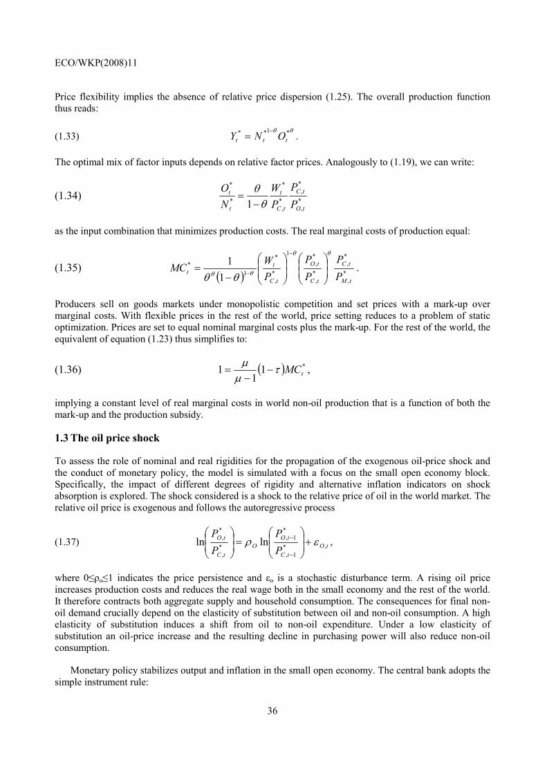
ECO/WKP(2008)11

36

Price flexibility implies the absence of relative price dispersion (1.25). The overall production function thus reads:

(1.33) θθ *1**

ttt ONY −= .

The optimal mix of factor inputs depends on relative factor prices. Analogously to (1.19), we can write:

(1.34) *,

*,

*,

*

*

*

1 tO

tC

tC

t

t

t

PP

PW

NO

θθ−

=

as the input combination that minimizes production costs. The real marginal costs of production equal:

(1.35) ( ) *

,

*,

*,

*,

1

*,

*

1*

11

tM

tC

tC

tO

tC

tt P

PPP

PW

MCθθ

θθ θθ

−=

−

−.

Producers sell on goods markets under monopolistic competition and set prices with a mark-up over marginal costs. With flexible prices in the rest of the world, price setting reduces to a problem of static optimization. Prices are set to equal nominal marginal costs plus the mark-up. For the rest of the world, the equivalent of equation (1.23) thus simplifies to:

(1.36) ( ) *11

1 tMCτµµ

−−

= ,

implying a constant level of real marginal costs in world non-oil production that is a function of both the mark-up and the production subsidy.

1.3 The oil price shock

To assess the role of nominal and real rigidities for the propagation of the exogenous oil-price shock and the conduct of monetary policy, the model is simulated with a focus on the small open economy block. Specifically, the impact of different degrees of rigidity and alternative inflation indicators on shock absorption is explored. The shock considered is a shock to the relative price of oil in the world market. The relative oil price is exogenous and follows the autoregressive process

(1.37) tOtC

tOO

tC

tO

PP

PP

,*1,

*1,

*,

*, lnln ερ +

=

−

− ,

where 0≤ρo≤1 indicates the price persistence and εo is a stochastic disturbance term. A rising oil price increases production costs and reduces the real wage both in the small economy and the rest of the world. It therefore contracts both aggregate supply and household consumption. The consequences for final non-oil demand crucially depend on the elasticity of substitution between oil and non-oil consumption. A high elasticity of substitution induces a shift from oil to non-oil expenditure. Under a low elasticity of substitution an oil-price increase and the resulting decline in purchasing power will also reduce non-oil consumption.

Monetary policy stabilizes output and inflation in the small open economy. The central bank adopts the simple instrument rule:

ECO/WKP(2008)11

37

(1.38) ( ) ( ) ( ) ( ) ( )11 lnln1~lnln1ln1 −− −−+−−++−−= ttittyitiit PPYYii παραρρβρ .

The policy rule (1.38) allows for an inertial adjustment of interest rates. The parameter ρi quantifies the degree of intrinsic interest rate persistence. Monetary policy reacts to both inflation and the output gap, i.e. the log difference between actual and flex-price production. The central bank may target different measures of inflation, such as headline or core CPI inflation or changes in the GDP deflator, which is the price level of home produced non-oil goods. The main text discusses alternative inflation targets and their impact on impulse responses.

The rest of the world is assumed to operate under price and wage flexibility and to produce the potential world output level. The flexibility assumption allows disregarding monetary policy settings in the rest of the world. The economic structure is kept constant in the rest of the world in order to concentrate on the effects of real and nominal rigidity in the small open economy.

ANNEX 2. THE LINEARISED MODEL

The non-linear model can be approximated linearly. The linearisation simplifies the model equations and illustrats the net impact of nominal and real rigidities and the impact of oil prices on economic activity.

Some of the model equations yield exact log-linear relationships, while others only provide a linear approximation around the steady state. The approximate linear relations are obtained from a first-order Taylor expansion of the non-linear equation around the steady state. Lower case letters refer to log variables, and denominates the percentage deviation of a variable from its steady state.

The linearised equations for the optimal path of consumption (1.4) and for consumption under perfect international risk sharing (1.26) are:

(2.1) ( )βπ lnˆˆˆ 1,1 +−−= ++ tCttttt EicEc

(2.2) *,

*,ln ttCttCt cpspc +−++= ϑ ,

respectively, where πC,t denotes domestic CPI inflation and –lnβ is the equilibrium real interest rate. The linearised demand functions (1.9)-(1.12) read

(2.3) ( ) ttCtMt cppm ˆˆˆˆ ,, +−−= ε

(2.4) ( ) ttCtOt cppo ˆˆˆˆ ,, +−−= ε

(2.5) ( ) ttMtHtH mppm +−−= ,,, .

(2.6) ( ) ttMtFtF mppm +−−= ,,, .

The log-linear demand functions in the rest of the world derive from (1.28)-(1.30):

ECO/WKP(2008)11

38

(2.7) ( ) **,

*,

* ˆˆˆˆ ttCtMt cppm +−−= ε

(2.8) ( ) **,

*,

* ˆˆˆˆ ttCtOt cppo +−−= ε

(2.9) ( ) **,

*,

*, ˆˆ ttMtHtH mppm +−−= .

The price level equations (1.13- (1.14) give the expressions:

(2.10) ( ) tOtMtC ppp ,,, ˆˆ1ˆ γγ +−=

(2.11) ( ) ( ) ( ) tFtHtM ppp ,,, 1ln1ln1 αααααα +−+−−−−= .

Consumer prices in the rest of the world (1.31) approximately follow:

(2.12) ( ) *,

*,

*, ˆˆ1ˆ tOtMtC ppp γγ +−= .

Given the law of one price and the negligible impact of domestic prices on the rest of the world, one can also write:

(2.13) ttOtO spp += *,,

(2.14) ttHtH spp += *,,

(2.15) ttMtF spp += *,, .

The linear expansion of the domestic GDP identity (1.15) around the steady-state yields:

(2.16) ( ) *,, ˆˆ1ˆ tHtHt mmy αα +−= .

Replacing domestic and export demand by the equations (2.3), (2.5), (2.7) and (2.9) and using the price level equations (2.10)-(2.14) gives the expression:

(2.17) ( ) ( )[ ]( ) ( ) ( ) **,

*,,,

2 ˆˆ1ˆˆ1

ˆˆ111ˆ tttCtOtFtHt ccppppy ααεγ

γγεα +−+−−

+−−−+−= .

A higher elasticity of substitution between oil and non-oil consumer goods increases the impact of oil prices on the demand for domestically produced goods. Substituting the Euler equation (2.1) and the price level definitions (2.10)-(2.15) and combining the equation (2.17) with (2.2) to replace the non-oil terms of trade gives:

(2.18) ( ) ( )( ) ( ) *1

*1,

*1,1,1 ˆ1ˆˆ

1lnˆˆ +++++ ∆−+−−

−++−=∆ tttCttOttHtttt cEEEEiyE ωππωε

γγβπω ,

with , as the linear approximation of the forward looking intertemporal demand equation for the small open economy.

ECO/WKP(2008)11

39

The aggregated production function (1.18) defines aggregate supply. Galí and Monacelli (2005) show

the approximation of the price dispersion term, , to be of second order. The linear

approximation of the aggregate production function (1.18) with a cost-minimizing factor mix (1.19) follows as:

(2.19) ( )tOttt pwny ,ˆˆˆˆ −+= θ .

For real marginal production costs (1.21) the log-linear expression is:

(2.20) ( ) ( )( ) ( ) ( ) ( )θθθθθθ −−−−−−−−+−= 1ln1ln1 ,,,,, tCtHtCttCtOt pppwppmc .

Equation (2.17) can be combined with (2.2) and the price definitions (2.10)-(2.15) to replace the price level of domestic production. Marginal costs around the steady state then become:

(2.21)

( ) [ ]( ) ( )

( )( ) ( ) [ ]( ) ( )*,

*,

*,

ˆˆ11ˆˆ1

ˆˆ1111

ˆ

tttCt

tCtOt

cypw

ppcm

−−+−+

+−−+

−

−+−+−

−+=

ωαγγθθθ

εω

αγγθθγ

γθ.

Linearising the wage equation (1.6) and then inserting the production function (2.19), the price level definitions (2.10)-(2.15), and equation (2.2) for domestic consumption, and (2.17) for the terms of trade in manufactures yields:

(2.22)

( )( )

( )( )( )

( )( )( ) ( )

( )( )( )( ) ( )*

*,

*,

1,1,

ˆˆ1111111

ˆˆ11111

11ˆ11

11ˆˆ

ˆˆ

ttw

w

tCtOw

w

w

tw

w

tCtwtCt

cy

pp

ypwpw

−

−

+−−−+−

+

−

+−

−−+−

+

−++−

+−+−

=− −−

ωϕθγα

ϕθρρ

ωγεϕθαϕθ

ϕθρρ

ϕθρϕρ

ϕθρρ

for real wages in the small open economy. An increase in oil prices affects real wages in two ways. First, it increases consumer prices and reduces the real wage. Second, producers will substitute cheaper labour for expensive oil, which increases labour demand and its remuneration.

The dynamic pricing equation (1.23) and (1.24) determine the price level of domestically produced goods. The linear approximation of the pricing dynamics yields the forward-looking New Keynesian Phillips curve:

(2.23) ttHttH cmE ˆˆˆ 1,, λπβπ += + ,

with . The impact of current marginal production costs on prices increases and the impact of inflation expectations decreases in the frequency of price adjustment, 1-ξ.32

32 Among many others, Woodford (2003) provides a stepwise derivation of the New Keynesian Phillips curve.

ECO/WKP(2008)11

40

Output under flexible prices derives from equations (2.21) and (2.22) that fix real marginal costs. When firms can constantly adjust prices, real marginal costs do not deviate from their steady state, so that

. Potential output is defined as the production level in the absence of both price and wage rigidity, i.e. ξ=0 and ρw=0. Potential output of the small open economy is obtained by inserting (2.22) in (2.21). Subtracting potential, , from actual output finally gives the domestic output gap .

For simplicity prices and real wages are assumed to be flexible in the rest of the world. Consequently, world production is at its potential level. Equation (1.36) shows that real marginal costs are constant in this case. Taking logs of equation (1.35) and inserting (2.12) indicates a negative relationship between oil prices and real wages and sets the real wage prevailing under flexible prices:

(2.24) ( )( ) ( )*,

*,

*,

* ˆˆ1

ˆˆ10 tCtOtCt pppw −

−

++−−=γ

γθθ .

The real wage determines consumption and labour supply. The share of household expenditure spent on non-oil consumer goods:

(2.25) ( ) **,

*,

* ˆˆˆ1

ˆ ttCtOt cppy +−−

=γ

γε .

derives from linearising equations (1.28) and (1.32). Combining (1.33) with (1.34) and taking logs of the resulting expression finally yields world employment:

(2.26) ( ) ( )*,

*,

*,

***tCtOtCttt pppwyn −+−−= θθ ,

which depends on world non-oil demand and the relative factor costs that are determined by equation (2.24).

Unclassified ECO/WKP(2008)11 - OECD

Documents

Transcript of Unclassified ECO/WKP(2008)11 - OECD