ULTRASONIC STRESS MEASUREMENT FOR EVALUATING THE ADEQUACY

OF GUSSET PLATES

A Thesis presented to the Faculty of the Graduate School at the University of

Missouri - Columbia

In Partial Fulfillment of the Requirements for the Degree

Master of Science

By

JASON PAUL KLEMME

Dr. Glenn Washer, Graduate Advisor

December 2012

The undersigned, appointed by the dean of the Graduate School, have examined

the thesis entitled

ULTRASONIC STRESS MEASUREMENT FOR

EVALUATING THE ADEQUACY OF GUSSET PLATES

Presented by Jason Klemme,

A candidate for the degree of Master of Science,

And hereby certify that, in their opinion, it is worthy of acceptance.

Professor Glenn Washer

Professor Steven Neal

Professor Brent Rosenblad

ii

ACKNOWLEDGEMENTS

I would sincerely like to thank my mentor and friend, Dr. Glenn Washer,

associate professor in the Civil and Environmental Engineering Department at

the University of Missouri. This thesis would not have been possible without the

knowledge and guidance of Dr. Washer.

I would also like to thank Mr. Mike Trial, Mr. Brian Samuels, Mr. Rex Gish

and Mr. Richard Oberto for their help and input on various aspects of this project.

Thanks too, to Dr. Robert J. Connor, Associate Professor of Civil Engineering at

Purdue University, for providing test materials. None of this would have been

possible without the help of these gentlemen.

I would like to extend thanks to Dr. Steven Neal and Dr. Brent Rosenblad

for serving as members of my thesis defense committee.

I would like to give a special thanks to both of my parents for the

continuous love and support that they have given me. A very special thanks also

goes to my grandmother who has read this thesis several times and provided

vital feedback.

Lastly, but certainly not least, I would like to thank my sister Kayla for

being an inspiration to me. Thank you all!

iii

TABLE OF CONTENTS

ACKNOWLEDGEMENTS .................................................................................... ii

TABLE OF CONTENTS ...................................................................................... iii

LIST OF FIGURES .............................................................................................. vi

LIST OF TABLES ............................................................................................... ix

Abstract .............................................................................................................. xi

1 Introduction ...................................................................................................... 1

1.1 Goal and Objectives .................................................................................... 1

1.2 Scope .......................................................................................................... 3

1.3 I-35W Bridge Collapse ................................................................................ 4

1.4 Dead Load Measurement ............................................................................ 9

1.5 Existing Technologies and Their Limitations ............................................. 11

1.5.1 X-Ray Diffraction Method ................................................................... 11

1.5.2 Hole Drilling ........................................................................................ 13

1.5.3 Barkhausen Noise Analysis ................................................................ 15

1.6 Discussion ................................................................................................. 16

2 Background .................................................................................................... 17

2.1 Ultrasonic Measurement Theory ............................................................... 17

2.1.1 The Acoustoelastic Effect ................................................................... 17

2.1.2 Ultrasonic Acoustic Birefringence ....................................................... 21

iv

2.1.3 Natural Birefringence .......................................................................... 24

2.1.4 Description of Prior Art ....................................................................... 27

3. Experimental Procedures ............................................................................ 36

3.1 Test Setup ................................................................................................. 37

3.2 Sensors and Hardware ............................................................................. 37

3.3 Timing Measurements............................................................................... 42

3.4 Test Materials ........................................................................................... 45

3.5 Summary of the Test Matrix ...................................................................... 46

3.5.1 Loading Patterns ................................................................................ 47

3.5.1.1 Incremental Step-Loading ............................................................ 48

3.5.1.2 Discontinuous Incremental Step-Loading .................................... 49

3.5.1.3 Single Loading ............................................................................. 50

3.6 Texture Directions ..................................................................................... 52

4. Results........................................................................................................... 55

4.1 Introduction ............................................................................................... 55

4.2 A36 Steel Specimen ................................................................................. 55

4.2.1 Characterization of Texture Directions ............................................... 56

4.2.2 Incremental Step-Loading Test .......................................................... 58

4.2.3 Discontinuous Incremental Step-Loading Test ................................... 65

4.2.4 Single Loading Test ............................................................................ 70

v

4.3 Gusset Plate Specimen............................................................................. 74

4.3.1 Characterization of Texture Directions ............................................... 74

4.3.2 Incremental Step-Loading Test .......................................................... 77

4.3.3 Discontinuous Incremental Step-Loading Test ................................... 81

4.3.4 Single Loading Test ............................................................................ 85

4.4 Discussion ................................................................................................. 89

5. Conclusions .................................................................................................. 93

References ........................................................................................................ 96

vi

LIST OF FIGURES

Figure Page

Figure 1-1. Bowing in gusset plates at node U10 was documented in 2003 [1]…8

Figure 1-2. The entire river span of the I-35W Bridge collapsed into the River

after the gusset plate at node U10 failed[1]. .................................................. 9

Figure 1-3. Bragg’s Law with the incident and diffracted x-rays making an angle θ

with the diffracting planes. ........................................................................... 13

Figure 2-1. Schematic view of the acoustoelastic measurement configuration that

was used in the research is shown. ............................................................. 18

Figure 2-2. Acoustoelastic effect. (A) energy as a function of atomic separation;

(B) force as a function of atomic separation; (C) stress as a function of strain

for an elastic solid. ....................................................................................... 19

Figure 2-3. Shear waves propagate perpendicular to the stress axis with

polarization directions parallel and perpendicular to the stress axis. ........... 21

Figure 3-1. Standard compression loading machine and ultrasonic

instrumentation are shown. ......................................................................... 37

Figure 3-2. Configuration of the ultrasonic instrumentation is shown. ................ 39

Figure 3-3. (A) Shear wave transducer and (B) transducer casing used in the

research. ..................................................................................................... 40

Figure 3-4. (A) Signals received and stored for timing the ultrasonic signals and

(B) arrangement of shear wave transducer on the surface of the plate,

shown here on desktop for clarity. ............................................................... 43

Figure 3-5. The graphical user interface of the specially designed timing software

is shown. ..................................................................................................... 44

Figure 3-6. Test materials are shown with (a) a material from a decommissioned

highway bridge gusset plate and (b) an A36 steel plate obtained from a steel

fabrication shop. .......................................................................................... 46

Figure 3-7. The process used to locate texture directions is shown. .................. 53

vii

Figure 3-8. (a) Test results indicate directions of texture in a steel specimen (b)

which allows for texture directions to be oriented coincident with the stress

axis. ............................................................................................................. 54

Figure 4-1. Velocity of ultrasonic shear waves at polarization angles from 0° to

360°. ............................................................................................................ 56

Figure 4-2. The fast direction of wave polarization (texture direction) was aligned

as shown. .................................................................................................... 59

Figure 4-3. Shear wave velocities for two orthogonally polarized shear waves

under applied loading. ................................................................................. 60

Figure 4-4. Ultrasonic birefringence resulting from applied loads for the A36 test

plate. ........................................................................................................... 61

Figure 4-5. The method used for the error analysis is shown. ............................ 63

Figure 4-6. Shear wave velocities for two orthogonally polarized shear waves

under applied loading in the intermittent monitoring scenario. ..................... 66

Figure 4-7. Ultrasonic birefringence resulting from applied loads for discontinuous

incremental step-loading test done on the A36 test plate is shown. ............ 67

Figure 4-8. Shear wave velocities for orthogonally polarized shear waves under

three different applied loadings. .................................................................. 71

Figure 4-9. The standard deviation from the single loading test is shown. ......... 73

Figure 4-10. Velocity of ultrasonic shear waves at polarization angles from 0° to

360°. ............................................................................................................ 75

Figure 4-11. Shear wave velocities for two orthogonally polarized shear waves

under applied loading. ................................................................................. 78

Figure 4-12. Ultrasonic birefringence resulting from applied loads for the gusset

plate specimen. ........................................................................................... 79

Figure 4-13. Shear wave velocities for two orthogonally polarized shear waves

under applied loading are shown. ................................................................ 82

Figure 4-14. Ultrasonic birefringence resulting from applied loads is shown. ..... 83

Figure 4-15. Shear wave velocities for orthogonally polarized shear waves under

three different applied loads. ....................................................................... 86

viii

Figure 4-16. The standard deviation from the single loading test done on the

gusset plate is shown. ................................................................................. 88

Figure 4-17. The texture directions were set in the loading machine in different

directions for the A) A36 and B) gusset plate steel specimen. .................... 90

ix

LIST OF TABLES

Table 3-1. Tests conducted as a part of the study. ............................................. 47

Table 3-2. The load range for the incremental step-loading test is given. .......... 49

Table 3-3. Loads and number of ultrasonic measurements made for the single

loading test are shown. ............................................................................... 52

Table 4-1. Data from three separate texture tests corresponding to Figure 4-1 is

shown. ......................................................................................................... 58

Table 4-2 Velocity and load comparison from three incremental step-loading tests

performed on the A36 steel specimen. ........................................................ 62

Table 4-3. Results of the error analysis for the incremental step-loading tests on

the A36 plate are shown. ............................................................................. 64

Table 4-4. Average birefringence and predicted stress range (error) for different

load steps ranging from 20 to 160 kips. ....................................................... 65

Table 4-5. Average velocity and average absolute error for different load steps

ranging from 20 to 160 kips. ........................................................................ 68

Table 4-6. Average velocity and predicted stress range (error) for different load

steps ranging from 20 to 160 kips. .............................................................. 69

Table 4-7. Average birefringence and predicted stress range (error) for different

load steps ranging from 20 to 160 kips. ....................................................... 70

Table 4-8. The range of velocities for both polarization directions is shown for the

loads corresponding to Figure 4-8. .............................................................. 72

Table 4-9. Velocity and load comparison from the single loading tests is shown.

.................................................................................................................... 74

Table 4-10. Data from three separate texture tests performed on the gusset plate

steel specimen are shown. .......................................................................... 77

Table 4-11. Velocity and load comparison from three incremental step-loading

tests performed on the gusset plate specimen. ........................................... 80

Table 4-12. Results of the error analysis for the incremental step-loading tests

performed on the gusset plate. ........................................................................

x

Table 4-13. Average birefringence and predicted stress range (error) for different

load steps ranging from 15 to 75 kips. ......................................................... 81

Table 4-14. Velocity and load comparison from the discontinuous incremental

step-loading tests performed on the gusset plate steel specimen. .............. 84

Table 4-15. The results from the error analysis for the discontinuous incremental

step-loading tests are shown. ...................................................................... 84

Table 4-16. Average birefringence and predicted stress range (error) for different

loading steps ranging from 15 to 75 kips. .................................................... 85

Table 4-17. The range of velocities for both polarization directions is shown for all

loads of the single loading test corresponding to Figure 4-15. .................... 87

Table 4-18. Velocity and load comparison from the single loading tests performed

on the gusset plate steel specimen. ............................................................ 89

Table 4-19. A comparison of the results from all three tests done on both steel

specimens is shown. ................................................................................... 92

xi

Abstract

The I35W bridge in Minneapolis, MN collapsed on August 1, 2007,

resulting in the deaths of 13 people. The National Transportation Safety Board’s

(NTSB) investigation of the catastrophe found that the cause of the collapse was

an overstressed gusset plate that connected key members of the bridge. A

significant challenge in determining the safety margin for gusset plates is

determining the level of stresses carried in the plate. The goal of the research

presented in this thesis is to improve the safety of highway bridges by developing

and testing an ultrasonic stress measurement methodology for determining

actual stress in steel gusset plates, evaluating the accuracy and precision of the

measurements, and assess if the methodology has sufficient accuracy and

precision to be a potential tool in the safety analysis of gusset plates. This

research utilizes the acoustoelastic effect to evaluate actual stress levels by

assessing the acoustic birefringence in a steel material. The birefringence

measurement evaluates normalized variations of polarized shear waves

propagating through the plate thickness, which vary proportionally as a function

of stress. Results from tests conducted in a laboratory setting indicated

uncertainties in the measurements of 7.5 ksi or less, or 20 % of yield strength for

a typical steel. This thesis discusses exploratory testing to evaluate the potential

of the approach as a tool for the condition assessment of gusset plates.

1

1 Introduction

1.1 Goal and Objectives

The overall goal of the research reported herein was to improve the safety

of highway bridges. The objectives of this research were:

To develop and test an ultrasonic stress measurement methodology for

determining actual stress in steel gusset plates,

Evaluate the accuracy and precision of the measurements in the

laboratory, and

Assess if the methodology has sufficient accuracy and precision to be a

potential tool in the safety analysis of gusset plates.

As discussed in Chapter 1.2 of this report, the disastrous collapse of the

I35W bridge in Minneapolis, Minnesota was caused by an overstressed gusset

plate. Determining the actual, in-situ stresses carried in a gusset plate is a

significant challenge in the analysis of gusset plate capacity, because the actual

loads carried in the members connected by the plate can only be estimated from

2

design drawings and idealized models. Unexpected load paths and redistribution

of forces as a result of displacements, damage or deterioration can undermine

the accuracy of these estimates. As a result, a means of measuring the actual

loads (stresses) in the gusset plate in-situ would provide a valuable tool for

confirming the adequacy of the analysis.

The approach used in the research is to measure the ultrasonic

birefringence – that is, the difference in velocity of orthogonally polarized shear

waves – to assess the actual in-situ stresses in a gusset plate. This approach

capitalizes on the acoustoelastic effect, or the variation in ultrasonic wave

velocity due to the presence of stress. The relationship between velocity of an

acoustic wave and stress is most readily observed when varying stresses are

applied, such that changes in the applied stress from some initial state are

measured, which simplifies the measurement. However, for a gusset plate,

invariant stresses resulting from the dead load of the structure provide the

majority of the applied load, and hence a technology is needed that can measure

these constant (in time) stresses, combined with any applied stresses that are

not constant in time such as live load stresses, thermal stresses, etc. This

measurement must be made without having the initial, unstressed state available

for assessment because the subject gusset plates are already in service. As a

result, unstressed samples of the material are typically unavailable.

Theoretically, acoustic birefringence measures anisotropy in the material

resulting from applied stresses, and can hence identify the orientation and

magnitude of the principle stresses in the material. Gusset plates typically

3

connect both tension members and compression members, and thus carry

tensile stresses in some areas and compression stresses in others.

Consequently, stress fields within such a gusset plate are very complex.

Acoustic birefringence has the potential to be used to make quantitative

assessments of both the compressive and tensile stresses in the gusset plate. In

addition the method measures the combined stresses resulting from all loads on

the plate, including: dead load, live load, thermal loads, etc. It measures these

stresses through the thickness of the material to provide an average stress.

These unique capabilities separate the approach from other available

technologies which either measure only live loads (e.g. strain gages) or surface

stresses (e.g. x-ray diffraction). The developed technology will significantly

impact the evaluation of bridge capacities, enabling more reliable assessments to

ensure bridge safety.

1.2 Scope

The scope of this research was to study the variability in birefringence

measurements made under uniaxial compressive forces in the laboratory,

variability due to equipment set-up, inherent variability in the measurement and

variability in the results between different steel materials.

This research explored ultrasonic stress measurements as a

nondestructive evaluation (NDE) method to measure actual, in-situ stresses in a

gusset plate. If such a technology could be successfully developed, these

measured stresses could be compared to the loading anticipated in the analysis

of the gusset plate (and the resulting stresses) to assess the accuracy of the

4

analysis. Alternatively, an ultrasonic stress measurement technology could be

used as a screening tool to identify at-risk gusset plates, by assessing if the

actual in-situ stresses were high. This could be an effective tool to identify

gusset plates that need to be further assessed to determine their adequacy, even

if a complete structural analysis were unavailable. Such a nondestructive

technique to assist in the analysis of gusset plate adequacy would provide a

valuable tool for bridge owners and help ensure the reliability of bridges.

1.3 I-35W Bridge Collapse

On August 1, 2007 the I-35W bridge in Minneapolis, Minnesota collapsed

into the Mississippi River killing 13 people and injuring 145 others[1]. The bridge,

which first opened to traffic in November 1967, was over 600 meters long with 14

spans (11 approach spans and 3 river spans). The bridge was a heavily used

thoroughfare; the most recent figures from the structure inventory report in 2004

gave an average daily traffic for the bridge of 141,000 vehicles with 5,640 of

those being heavy commercial vehicles[1].

At the time of the collapse the bridge was undergoing its third significant

renovation since its opening in 1967[2]. The first renovation was completed in

1977 and added a wearing course of 50.8 mm of low slump concrete. The added

concrete applied to the bridge from this renovation increased the dead load of the

bridge by 13.4 percent[1]. The second renovation involved an upgrade to the

traffic railings and replacement of the median barrier, which increased the bridge

dead load by 6.1 percent[1]. By the time the third renovation was underway in

5

the summer of 2007, the dead load of the bridge had increased by 19.5 percent

since it first opened.

The third renovation included a new 50.8 mm thick concrete overlay on all

eight traffic lanes. To accommodate construction materials and activities, several

traffic lanes were closed. The concrete used in the overlay had abnormally high

cement content which caused the concrete to solidify too rapidly, making storing

and mixing materials off-site impractical[1]. As a result, aggregates and other

construction materials were placed on the bridge deck during construction,

adding an additional load to the structure. The construction materials were

placed above the gusset plate connection at node U10. This node was a

connecting point where the upper or lower chords were joined to vertical and

diagonal members with gusset plates. The additional weight added to the bridge

from the construction materials placed at node U10, as well as weight added to

the structure from the two prior renovations, substantially increased the stress in

the structural members of the bridge. The National Transportation Safety Board

(NTSB) concluded in its highway accident report that the cause of the collapse of

the I-35W bridge was an overstressed gusset plate at the U10 node of span 7,

which resulted in the plate buckling under the applied loads[1].

The original design calculations for the I-35W bridge did not include any

details for the design of the gusset plates in the structure. As a result it was

impossible for investigators to check the original design calculations of the gusset

plates. The design of gusset plates was typically done using general beam

theory and sound engineering judgment[3]. The only gusset plate design

6

specifications that existed at the time the I-35W bridge was designed in 1964

was the American Association of State Highway Officials (AASHO) guidelines

that stated:

“Gusset plates shall be of ample thickness to resist shear, direct

stress, and flexure, acting on the weakest or critical section of

maximum stress[4].”

The AASHO specification for gusset plate thickness had a provision that

requires the ratio of the unsupported edge length divided by the thickness not

exceed 48 for the steel (A441-σy=50ksi[1]) used for the gusset plates in the I-

35W bridge. Ratios exceeding 48 were required to have stiffeners to avoid

compromising the capacity of the gusset plate due to buckling[4]. In the gusset

plate at node U10 - where the failure originated - the ratio of the length of the free

edge of the gusset plate to the thickness was 60[5], greatly exceeding the

criterion of 48. The gusset plate U10 had a thickness of 12.7 mm with an

unsupported edge length of .762 m, which would require it to be stiffened along

its free edge; however, no such stiffener support was added to the gusset plate

meaning that, according to AASHO specifications, the plate was inadequate from

the time the bridge opened in 1967. In addition to lacking stiffener support, the

gusset plate was not of ample thickness to carry the applied loads that resulted

from the combined self-weight of the structure and live loads due to vehicle

traffic. Had the gusset plate been of sufficient thickness, the plate would not

require stiffeners as the ratio criterion specified by AASHO guidelines would have

been met.

7

The I-35W bridge was fracture critical, defined as a “steel member in

tension, or with a tension element, whose failure would probably cause a portion

of or the entire bridge to collapse”[6]. The National Bridge Inspection Standards

(NBIS) requires that fracture critical bridges be inspected at least once every

twenty-four months, with shorter intervals for certain bridges with known

deterioration or damage[1, 6]. To comply with NBIS standards for fracture critical

bridges, the I-35W had been inspected annually since 1971. Due to fatigue

cracking in bridges of similar age to the I-35W, the Minnesota Department of

Transportation (MNDOT) contracted with URS Corporation to initiate hands-on

inspections for fracture critical members of the structure. In 2003 URS

documented nearly every structural member of the bridge with photographs.

One of these photographs, shown in Figure 1-1, appears to reveal some bowing

in all four gusset plates at both U10 nodes. Bowing of gusset plates at the U10

node was a sign of over-stressing of the plate, which could cause the plate to

lose its load-bearing capacity.

8

Figure 1-1. Bowing in gusset plates at node U10 was documented in 2003[1].

Upon failure of the gusset plates at node U10, the I-35W Bridge

underwent a progressive collapse – spread of an initial local failure from element

to element resulting in the collapse of the entire structure as shown if Figure 1-

2[6]. This collapse illustrates the urgent need for improved methods for the

condition assessment of bridges, including the assessment of gusset plates to

evaluate the applied loads and ensure adequate load carrying capacity.

9

Figure 1-2. The entire river span of the I-35W Bridge collapsed into the River after the gusset plate at node U10 failed[1].

This research reported herein addresses this need through the

development of an ultrasonic stress measurement technology based on acoustic

birefringence. The research focuses on exploratory, proof of concept testing to

demonstrate the feasibility of the measurement and develop initial data on

potential accuracy and precision of such a measurement. The development and

application of this technology could potentially help prevent the type of

catastrophic collapse experienced at the I-35W bridge in Minneapolis, Minnesota

by providing a tool for the assessment of gusset plate safety.

1.4 Dead Load Measurement

Structural failures are sometimes the result of the combination of dead

loads and live loads exceeding a critical load level, resulting in buckling, fracture,

or rupture of a component. The loading applied to a component under field

conditions can be difficult to determine due to variations in construction,

10

materials, load distributions within a structure, and section loss resulting from

corrosion. As a result, there is a need to develop tools that allow for the

assessment of applied loads in the fields, and the resulting stresses in critical

components of structures. For example, determining the safety margin, i.e. the

ratio of capacity to load, requires an assessment of the level of stresses carried

from both dead loads and live loads, and potential buckling or instability. Live

loads are generally small compared to dead loads for highway bridges, and can

be easily measured with electrical resistance strain gages. However, stresses

resulting from dead loads cannot be measured using strain gages, unless the

gages are installed prior to construction and stresses tracked continuously

throughout the duration of the construction process and into service[7].

Additionally, residual stresses can be present as a result of the fabrication

process, during welding and forming of the component. These stresses in the

material can reduce the available load-carrying capacity of a component, but

cannot be measured with conventional tools such as strain gages.

In recent years considerable progress has been made in experimental

techniques used to measure actual stresses in a material in-situ[8]. Research

reported herein investigates the ultrasonic acoustic birefringence method as a

means to measure the combined dead, live and residual stresses. Several other

technologies exist and are described in the following section, but have certain

limitations that make them less favorable for this particular application. Each of

these methods and their key limitations are described in Section 1.4.

11

1.5 Existing Technologies and Their Limitations

A significant challenge for the condition assessment of structures is the

evaluation of both the actual in-situ stresses and residual stresses. Residual

stresses can be detrimental when the service stresses are superimposed on the

already present residual stresses[8]. The presence of residual stresses

sometimes goes unrecognized until after failure or malfunction occurs; as a

result, there is a need to develop technologies to measure such stresses in

gusset plates and other structural components. There are a number of available

nondestructive technologies for assessing stresses in a metal component.

These technologies are usually focused on the assessment of residual stresses

that can result from fabrication, which are often difficult to characterize or

estimate analytically. Common state-of-the art technologies used to measure

residual stress in mechanical components include: x-ray diffraction, hole drilling,

and the Barkhausen noise effect. Each of these technologies assesses the total

combined stresses in the material, including dead load, live load and any residual

stresses, however, these technologies have important limitations that affect their

application to gusset plate assessments. The following sections describe the

characteristics of these current state-of-the-art technologies for evaluating

stresses in structural components.

1.5.1 X-Ray Diffraction Method

X-ray diffraction is a nondestructive method used to determine surface

stresses[9]. To apply x-ray diffraction, the medium (in this case steel) must have

a crystalline structure; the atoms in the solid must be arranged in a regular,

12

repeating pattern. When an x-ray beam of a single wavelength or frequency

irradiates the steel, it is scattered by the atoms making up the steel[9]. Upon the

incident beam being scattered, x-rays of the same wavelength will be refracted at

preferential angles based on the geometry of the crystal lattice. The spatial

distributions and intensities of the scattered x-rays form a unique diffraction

pattern that is related to the crystal structure of the steel, specifically the

interatomic distance between atoms in the lattice of the steel specimen[10].

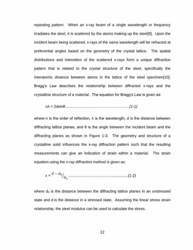
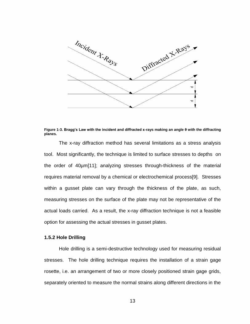
Bragg’s Law describes the relationship between diffracted x-rays and the

crystalline structure of a material. The equation for Bragg’s Law is given as:

nλ = 2dsinθ……………………………………………(1-1)

where n is the order of reflection, λ is the wavelength, d is the distance between

diffracting lattice planes, and θ is the angle between the incident beam and the

diffracting planes as shown in Figure 1-3. The geometry and structure of a

crystalline solid influences the x-ray diffraction pattern such that the resulting

measurements can give an indication of strain within a material. The strain

equation using the x-ray diffraction method is given as:

ε =

⁄ ………………………………..............(1-2)

where d0 is the distance between the diffracting lattice planes in an unstressed

state and d is the distance in a stressed state. Assuming the linear stress strain

relationship, the steel modulus can be used to calculate the stress.

13

Figure 1-3. Bragg’s Law with the incident and diffracted x-rays making an angle θ with the diffracting planes.

The x-ray diffraction method has several limitations as a stress analysis

tool. Most significantly, the technique is limited to surface stresses to depths on

the order of 40µm[11]; analyzing stresses through-thickness of the material

requires material removal by a chemical or electrochemical process[9]. Stresses

within a gusset plate can vary through the thickness of the plate, as such,

measuring stresses on the surface of the plate may not be representative of the

actual loads carried. As a result, the x-ray diffraction technique is not a feasible

option for assessing the actual stresses in gusset plates.

1.5.2 Hole Drilling

Hole drilling is a semi-destructive technology used for measuring residual

stresses. The hole drilling technique requires the installation of a strain gage

rosette, i.e. an arrangement of two or more closely positioned strain gage grids,

separately oriented to measure the normal strains along different directions in the

14

underlying surface of the test material. The strain gages measure the surface

strain relief in the material after a hole is drilled in the center of the rosette[8, 12].

Drilled holes are typically 1-4mm in diameter at a depth approximately equivalent

to the diameter. Residual stresses within the material are calculated from the

strain relief measured by the strain gage rosette.

As was the case with x-ray diffraction, as described in Chapter 1.4.1

above, the hole drilling method has limitations which affect its usefulness in

measuring in-situ stresses in gusset plates. The application of strain gages

coupled with the removal of material needed in the hole drilling method is time

consuming, each test can take several hours depending on field conditions[9].

Accuracy and precision of the method is also a limitation, because results can be

highly scattered. The method must also be calibrated before it can be used in

the field; calibration is done by testing its application to known stress

conditions[9]. If there is a varying stress gradient in the material (such as the

case in gusset plates), incremental hole drilling may be required which will further

complicate the process. Additionally, the hole drilling method can have low

sensitivity due to misplacement of the strain sensors or drilled hole. The further

the applied strain gages are located away from the edge of the hole, the more

the relieved strains decay, causing the gages to measure only 25-40% of the

original residual strain at the hole location[9]. In addition, if the hole is not drilled

in the center of the strain gage rosette, eccentricity will lead to erroneous

calculations and scattered results. Due to these factors, the hole drilling method

is not a viable option for measuring stresses in gusset plates.

15

1.5.3 Barkhausen Noise Analysis

Barkhausen noise analysis is another nondestructive method used for

measuring residual stresses. The method uses a concept of the inductive

measurement of a noise signal that is generated when a magnetic field is applied

to a ferromagnetic material[13, 14]. All ferromagnetic materials have domain

regions that experience changes in structure when a magnetic field or

mechanical stress is applied[9]. When these changes occur domain walls break

free from dislocations, grain boundaries and precipitates, and the material

undergoes a corresponding spike in magnetization[13]. Such spikes in the

material are known as Barkhausen noise. The intensity of Barkhausen noise is

dependent on the microstructure and stresses in the material[9]. With proper

calibration, this method can be used to measure surface stresses.

As was the case with the two stress measurement methods mentioned

previously, Barkhausen noise also has limitations that render it less than ideal to

measure the in-situ stresses in gusset plates. The method is limited to surface

layers of the material with an effective measurement depth between that of x-ray

diffraction (20-40μm) and hole drilling (up to 2mm)[9]. In materials that have a

positive magnetic anisotropy, such as a steel gusset plate, tensile stresses

increase the intensity of Barkhausen noise while compressive stresses decrease

the noise[14]. Gusset plates also have varying stress gradients which may be

difficult to distinguish using the Barkhausen noise method. Additionally, the

method is sensitive to variations in material microstructure, which can make it

challenging to separate stress signals from simultaneous changes within the

16

microstructure. The limitations of the Barkhausen noise method make it less

than ideal for stress measurement in gusset plates.

1.6 Discussion

These technologies for nondestructive assessment of residual stresses

each are limited to surface or near surface measurements and have other

limitations. In contrast, ultrasonic birefringence is a through-thickness method

that produces an assessment of the average stress in the material, which is more

appropriate for engineering analysis of forces. Acoustic shear waves propagate

through the full thickness of the material such that the resulting velocities are

dependent on the average stress, not just the surface stresses. These through-

thickness measurements are path-independent; the actual travel distance of the

shear wave, i.e. the thickness of the material, does not need to be known. This

is advantageous because it is often times difficult to determine the actual

thickness of a gusset plate due to large thickness tolerances allowed and section

loss due to corrosion, which may be localized and obviously time-variant.

The theory and accompanying equations of ultrasonic acoustic

birefringence are discussed in greater detail in Chapter 2 of this report.

17

2 Background

2.1 Ultrasonic Measurement Theory

This chapter describes the ultrasonic measurement theory, including: the

acoustoelastic effect, ultrasonic acoustic birefringence, description of prior art,

and natural birefringence. The research capitalized on the ultrasonic

measurement theory to develop and test an ultrasonic stress measurement

methodology for determining actual stress in gusset plates and evaluate the

accuracy and precision of the measurement. The theories described herein are

the foundation for the use of ultrasonics as a stress measurement tool for

evaluating the adequacy of gusset plates.

2.1.1 The Acoustoelastic Effect

The acoustoelastic effect is the variation of ultrasonic velocity due to the

presence of stress. When changes in the acoustic wave’s velocity are small

(typically less than 1%), the relationship between the measured velocity of an

acoustic wave and stress is linear and can be conceptually described by the

relation:

V = V0 + kσ………………………………………………………………….(2-1)

18

where V0 is the velocity of a wave in an unstressed medium, K is a material-

dependent acoustoelastic constant, and σ is the stress[7, 9]. The relationship

between stress and velocity is most readily observed when stresses are applied

to the material so that the change in applied stress from an initial stress state can

be measured[15].

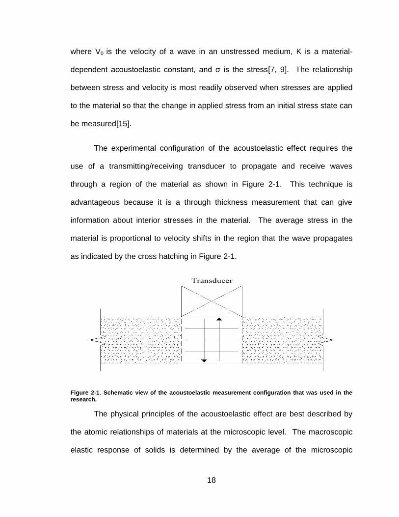
The experimental configuration of the acoustoelastic effect requires the

use of a transmitting/receiving transducer to propagate and receive waves

through a region of the material as shown in Figure 2-1. This technique is

advantageous because it is a through thickness measurement that can give

information about interior stresses in the material. The average stress in the

material is proportional to velocity shifts in the region that the wave propagates

as indicated by the cross hatching in Figure 2-1.

Figure 2-1. Schematic view of the acoustoelastic measurement configuration that was used in the research.

The physical principles of the acoustoelastic effect are best described by

the atomic relationships of materials at the microscopic level. The macroscopic

elastic response of solids is determined by the average of the microscopic

19

interatomic forces[9]. Atoms of materials in the stress-free state will have

equilibrium separation – this corresponds to a position of minimum energy and

zero interatomic force as indicated by ‘a’ in Figures 2-2A and 2-2B, respectively.

When a material becomes strained, the atomic separation between atoms will

differ from the equilibrium position. As the atomic separation increases under

applied stresses, the energy between the pair of atoms also increases from the

equilibrium position as shown in Figure 2-2B. The force between atoms

increases initially. When the atomic separation between atoms decreases, the

energy between the atoms theoretically increases infinitely while the force

decreases infinitely. It is the average of these interatomic forces that give the

macroscopic elastic response of a solid material as shown in Figure 2-2C[9].

Figure 2-2. Acoustoelastic effect. (A) energy as a function of atomic separation; (B) force as a function of atomic separation; (C) stress as a function of strain for an elastic solid.

The stress strain curve shown in Figure 2-2C is nonlinear, i.e. the modulus

is dependent on strain. The velocity of an acoustic shear wave is dependent on

the modulus, E; and, therefore, the velocity is dependent on strain. Engineering

stress strain diagrams are typically assumed linear because of scale; however,

20

the short wavelengths of ultrasonic waves are affected by the nonlinearity in

stress strain diagrams and as such a linear modulus cannot be assumed.

The macroscopic elastic response of a solid is determined by the average

of the materials microscopic responses such that strain in a material will cause

microscopic responses as shown in Figures 2-2A and 2-2B and a macroscopic

response as shown in Figure 2-2C. The stress strain curve of a typical

macroscopic response has both a linear and nonlinear modulus shift when stress

increases from a static stress state. Both the linear and nonlinear moduli must

be considered when describing the relationship between stress and strain. This

relationship is described as:

σ = Eε + E’ε2………………………………………………………………...(2-2)

where σ is the stress, ε is the strain, E is the linear modulus of elasticity and E’ is

the nonlinear modulus of elasticity. Equation 2-2 describes the relation between

stress and strain in one dimension. To describe the relation in three dimensions,

second and third-order elastic constants must be introduced. The use of second

and third-order elastic constants in the description of the acoustoelastic effect

has been developed by previous researchers [16-18] and is used in the

description of ultrasonic acoustic birefringence presented herein.

21

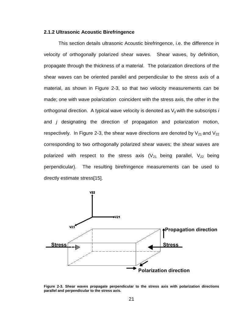
2.1.2 Ultrasonic Acoustic Birefringence

This section details ultrasonic Acoustic birefringence, i.e. the difference in

velocity of orthogonally polarized shear waves. Shear waves, by definition,

propagate through the thickness of a material. The polarization directions of the

shear waves can be oriented parallel and perpendicular to the stress axis of a

material, as shown in Figure 2-3, so that two velocity measurements can be

made; one with wave polarization coincident with the stress axis, the other in the

orthogonal direction. A typical wave velocity is denoted as Vij with the subscripts i

and j designating the direction of propagation and polarization motion,

respectively. In Figure 2-3, the shear wave directions are denoted by V21 and V22

corresponding to two orthogonally polarized shear waves; the shear waves are

polarized with respect to the stress axis (V21 being parallel, V22 being

perpendicular). The resulting birefringence measurements can be used to

directly estimate stress[15].

Figure 2-3. Shear waves propagate perpendicular to the stress axis with polarization directions parallel and perpendicular to the stress axis.

22

When an ultrasonic shear wave is pulsed into an isotropic, homogeneous

material, the wave will travel at a single velocity regardless of the wave

polarization direction. However, stress and preferred grain orientation within a

material will cause the material to be anisotropic. The velocity of a shear wave

pulsed into an anisotropic material will be dependent on the polarization

orientation of the wave such that waves polarized orthogonally to one another

may have different velocities. Birefringence is defined by the equation:

⁄ ………………………………………………..……….(2-3)

where the subscripts f and s denote the fast and slow velocities of orthogonally

polarized shear waves respectively, and VAvg is the average velocity.

Birefringence changes as a function of stress; that is, as stress within a

material changes so too does the difference in velocity of orthogonally polarized

shear waves. For a gusset plate, the relationship between birefringence and

stress can be expressed as:

( ) ……………………….………(2-4)

where B0 is the texture-induced birefringence in the stress-free state, k is an

acoustoelastic constant and σxx, σyy and σxy are the in-plane stresses,

respectively. It is assumed in this analysis that the out-of-plane stress

components, σxz, σyz and σzz do not contribute to the birefringence measurement

because of symmetry[9].

23

In an unstressed material, anisotropy of the specimen caused by a

preferred grain orientation within the material will control the fast and slow

polarization directions of the shear waves. When stress is introduced to the

specimen, the pure-mode polarization will be controlled by a combination of the

texture and stress directions causing the fast and slow polarization directions of

the shear waves to rotate. For this reason, it is imperative to determine the angle

between the texture and stress directions within the material. The angle between

the preferred grain orientation and the pure-mode polarization is expressed as:

………………………………………………..……(2-5)

A combination of Equations 2-4 and 2-5 allows shear stresses to be

calculated independently from texture effects, and is given by:

………………………………………………….………….….(2-6)

The shear stress, σxy, can be determined by measurements of Birefringence, B

and the angle between the preferred grain orientation and the pure mode

polarization, φ. The normal stresses, σxx and σyy, are then determined by

integrating the calculated shear stress:

∫

………………………………………...…..…..(2-7)

∫

……………………………………………...…(2-8)

If shear stress is equal to zero and the rolling direction of the material

coincides with the stress direction then the pure mode polarization of the shear

24

waves will be coincident with both. When shear stress and the angle between

stress and rolling direction are both zero, the previous equations can be reduced

to:

………………………………………….………….…....(2-9)

To determine the principle stresses, the birefringence in the unstressed

state, i.e. the natural birefringence, B0, resulting from texture in the plate will

need to be measured. As a result of the intricate stress fields carried within a

gusset plate, a location of zero stress in the plate may not be known. This

problem and the effect of texture on birefringence measurements are discussed

in further detail in the following section.

2.1.3 Natural Birefringence

When an ultrasonic pulse is generated in a homogeneous, isotropic

material, shear waves will travel at a single velocity, independent of the polarized

orientation direction of the wave. When stress is introduced to the specimen, the

shear waves will split into two orthogonally polarized components. In the

absence of stress, the pure mode polarization will be coincident with the rolling

directions of the plate due to material anisotropy introduced to the specimen

during the rolling process. A metal that is subjected to mechanical working

during fabrication will have a certain degree of texture in it. In polycrystalline

materials such as steel, texture will cause marked differences in acoustic wave

velocities in different propagation and polarization directions because of the

25

elastic anisotropy of single crystals. The difference in velocity of orthogonally

polarized acoustic shear waves due to the texture of the material is known as

natural birefringence, B0. Researchers have shown that a material that exhibits a

strong texture will have a variation of ultrasonic velocity from the isotropic value

in the range of 2.5%[18]. This change in velocity due to texture is of the same

order of magnitude, or even greater than, the velocity changes resulting from the

presence of stress. Therefore, the natural birefringence must be determined to

distinguish between the texture and stress effects so that birefringence resulting

from texture is not erroneously attributed to stress.

The rolling processes in fabrication of a structural component cause the

grains making up the material to elongate. This process gives a texture to the

material by elongating all of the grains in a preferred orientation. The rolling, or

texture, orientation is easily determined in a laboratory setup by rotating the wave

polarization direction 360° while continuously monitoring the time-of-flight of the

received signals. A material displaying texture orientation will have repeating

time-of-flight data at 180° intervals as the polarization direction is rotated. A

higher wave velocity is observed in the direction where grains are elongated and

a lower velocity in the directions perpendicular to grain elongations[28]. Thus,

the fast directions observed in the 360° rotation are coincident with the rolling

direction of the specimen.

It is more difficult to determine the texture orientation in a highway bridge

gusset plate. The stress field in a gusset plate will be complex because some

primary truss members connected at the plate carry uniaxial compression, while

26

others carry uniaxial tension, both of which must be resolved in the gusset plate

for equilibrium. The complex nature of the stress field in gusset plates make it

difficult to measure B0 because there is likely not a zero stress state anywhere in

the plate. However, researchers have shown that it is possible to obtain ‘zero

stress positions’ in a complex stress field by a combination of appropriate tensile

and compressive stresses of appropriate values in two different directions[29].

The author of this thesis proposes that ‘zero stress positions’ in gusset plates can

be located by scanning the transducer across the plate until the time-of-flight of

the pulsed acoustic shear waves correlate with data from unstressed plates.

When there is no stress present in the gusset plate, the rolling direction

will control the polarization dependence, when stressed, a combination of the

rolling and stress directions controls. In the presence of shear stress, the

polarization direction will rotate from the rolling direction through the angle ᵠ

described in equation 2-5 above. To determine the principle stresses in a gusset

plate, the natural birefringence resulting from the texture of the plate must be

determined. Previous researchers [18, 22, 28, 29] have studied and developed

methodologies for determining stresses in textured materials. This research took

advantage of the methodologies previous researchers have developed to

separate the effects of stress induced and texture induced (natural)

birefringence.

27

2.1.4 Description of Prior Art

The welding, aerospace, and foundry industries have long used

ultrasonics as a means for locating discontinuities. Other uses of ultrasonics

have included: thickness gauging, weld testing, defect sizing, bond testing,

composite material testing, concrete testing, and, more recently, stress analysis.

As the demand for and use of ultrasonics continues to grow in the field of

nondestructive testing, the methods and techniques will have to continue to

develop to meet the demands. This section investigates the origins of ultrasonics

as well as prior research – specifically acoustic birefringence as a stress

measurement technique.

The phenomenon of sound waves was first described in detail by Strut

and Rayleigh[19, 20] in the 1870’s. In their work, entitled The Theory of Sound,

they laid out the physical attributes that constitute the foundation of sound. They

transferred their findings into the field of the principle of Mechanics. Strut and

Rayleigh observed that, although air is the most common vehicle of sound;

solids, liquids, and gases were also capable of transporting sound. Their findings

also showed that mediums transporting sound are in a state of vibration showing

a close correlation between sound and vibration. The Theory of Sound was the

first step taken in the development of ultrasonics.

The acoustoelastic effect was discovered over 70 years ago when

researchers concluded that the propagation of elastic waves in a stressed

material is fundamentally different than the stress free state[21, 22]. In 1951

Murnaghan[17], using his knowledge of the acoustoelastic effect, introduced

28

three third order elastic constants l, m, and n in his theory of non-linear elasticity.

Using the third order elastic constants developed by Murnaghan in addition to the

second-order Lame constants, λ, and μ, Hughes and Kelly further developed the

theory of acoustoelasticity in 1953[16, 23, 24]. Hughes and Kelly developed the

following expressions relating strains and ultrasonic wave velocities in a uniaxial

stress state:

……………………(2-10)

……………………..….….(2-11)

…………………….…..…(2-12)

where the density is ρ0, the sum of the principal strains (ε1 + ε2 + ε3) is θ, ν is

Poisson’s ratio and l, m and n are third order elastic constants[25]. The first

index in the velocity equations is the propagation direction and the second is

polarization direction. Equation 2-10 is the wave speed for a longitudinal wave

with propagation and polarization in the same direction, i.e. a longitudinal wave.

Equations 2-11 and 2-12 are shear waves polarized in orthogonal directions.

These equations were the first expressions relating the principal deformations (or

strains) with ultrasonic wave speeds. The work of Murnaghan[17] and Hughes

and Kelly[19] provided the framework for the use of ultrasonic stress

measurements going forward.

After Hughes and Kelly’s work in 1958, the birefringence phenomenon of

acoustic waves was discovered by Bergman and Shahbender[23, 26]. The

29

researchers generated short ultrasonic pulses in an aluminum column by using a

Sperry reflectoscope to drive a set of quartz crystals at a frequency of 5 MHz. A

similar set of crystals were used to detect the ultrasonic pulses and display the

results on an oscilloscope. A range of tests was performed and experimental

data was obtained. Two tests involved stressing an aluminum column within its

elastic range at 50% and 66% of its yield load, respectively. Two other tests

were done loading the column until it buckled. Each test was either loaded in

increments until the desired stress was reached, or loaded and unloaded in

increments to complete a full cycle of loading and unloading. The researchers

concluded in their study that:

“The experimental results indicate that the relevant elastic constant for longitudinal waves is independent of stress, while that for the shear waves is stress dependent and also depends on the relative orientation of the particle motion and the direction of applied stress[26].”

The results of the testing indicated that change in velocity of the

longitudinal waves could be accounted for by the change in density resulting from

the applied stresses. However, the change in velocity of the shear waves was

due to both the change in density and a change in the elastic constants. The

researchers noted that the velocity differences between horizontally and vertically

polarized shear waves changed as a function of increased loading.

In 1959, Benson and Raelson[15] further confirmed the findings of

Bergman and Shabender. In their report, Acoustoelasticity, they reported that the

polarization orientation of acoustic waves will rotate when propagating through a

30

stressed material and that there is a direct relationship between degree of

rotation and magnitude of stress. The researchers applied compressive loads to

a 0.127 m x 0.025 m aluminum bar. Polarized ultrasonic waves were generated

using a radio frequency pulse generator coupled to a Y-cut quartz crystal. A

second crystal, used to receive the ultrasonic waves, was placed at the opposite

end of the sample. The crystals were orientated at 45° with respect to the

principal stress axis so that the polarized sound wave would consist of two

components – one along each axis of principle stress. The researchers found

that when an external load was applied to the aluminum test specimen, different

stresses were created along the principal axes. Since velocity of sound is a

function of stress within a material, the velocities of the two components of the

shear wave were different. This discovery, coupled with the results of Bergman

and Shabender, helped to introduce birefringence as a new nondestructive

technique for stress measurement analysis.

Ultrasonic acoustic birefringence has been extensively studied and

developed in the past several decades. The increase in the usage of this

technique can mostly be attributed to new electronic instruments and high-speed

data acquisition systems that are now available. Researchers have used the

birefringence technique to: characterize texture and texture-related properties of

rolled parts[23], evaluate stresses in steel plates and bars[15], evaluate true

stresses in integral abutment bridges[7], and for stress measurements in hanger

plates in pin and hanger connections[27].

31

In 1995, Schneider[23] used ultrasonic birefringence to characterize the

texture and stress states in the rims of railroad wheels. An ultrasonic transducer,

coupled to the surface of the test specimen, was rotated 180° with the change in

the time-of-flight continuously monitored throughout the duration of the test so

that effects of texture on the time-of-flight of ultrasonic waves could be

measured. The study materials consisted of three railroad wheel rims each with

varying degrees of texture. The outcomes of the three tests were plotted

showing shear wave time-of-flight as a function of polarization direction. Wheel

one had no change in the time-of-flight measured at 0°, 90° or 180°, indicating a

perfectly isotropic material. The measured time-of-flight in wheels two and three

showed a pronounced change at 90° signifying anisotropy due to texture. The

results of these tests enabled the researchers to locate texture directions within

railroad wheel rims, which in turn allowed the researchers to compare the effects

that texture and stress have on birefringence.

Using the birefringence technique, Schneider[23] characterized stress

states in new forged railroad wheels after different braking loads were applied.

The braking of railroad wheels generates heat by pressing brake-shoes onto the

surface of the wheel. After several cycles of heating and subsequent cooling,

tensile stresses develop in the wheel rims. The research tested different stress

states in wheels by applying a range of forces in the lab. Shear waves were

polarized in the radial and tangential directions of the wheel allowing for the

researchers to evaluate the principal stresses. Birefringence measurements

were taken at different distances from the outer edge of the wheel. Results of

32

the testing showed that in new wheels with no braking forces applied, the radial

and tangential stress difference was low. However, the principal stress

difference increased as more braking force was applied. The highest forces in

the railroad wheel were found approximately 7 mm from the outer edge of the

wheel. Schneider showed in his research that ultrasonic birefringence had the

potential to determine texture and stress states in railroad wheels.

In 1996, Clark, Fuchs and Lozev[7] used birefringence as a technique for

stress surveys in bridge structures. Tests were performed on two bridges, one a

simply supported structure and the other an integral backwall bridge. Ultrasonic

acoustic shear waves were generated with electromagnetic-acoustic transducers

(EMATs). The use of EMATs was favored over piezoelectric transducers since

they are generally easier to fix to the surface and require no couplant. The

EMAT enabled the researchers to measure live load, dead load and residual

stresses in a bridge girder. Live load stresses were referenced to the static state

(no traffic on bridge) while dead load stresses were referenced to an absolute

zero stress state. The data, which was collected over a short period of time and

represented a relatively small sample set, showed good correlation between the

EMAT and strain gage readings. In addition to stress measurements,

experiments were also performed to characterize the effect of paint, operating

frequency, magnetic artifacts, measurement echo and lift-off of the EMAT system

on the accuracy of ultrasonics. Results of the testing showed that magnetic

artifacts from machining processes and a lift-off of the transducer from the

specimen of up to 0.5 mm did not significantly alter measurements. However,

33

paint affected the received ultrasonic signals of the EMATs possibly due to the

difference in acoustic impedance between the paint and steel. The results from

the analysis showed that the birefringence measurements using an EMAT

system was capable of performing applied stress measurements on actual bridge

structures.

In 1999, Clark, Fuchs and Lozev used the birefringence technique to

characterize the status of pin and hanger connections in bridges[27].

Birefringence measurements were made on opposite sides of hangers and

related to uniaxial stress by the following equation:

)…………………………………………….….(2-13)

where “l” and “r” are readings on the left and right sides of the hanger

respectively. In properly functioning hangers, there will be only uniaxial stress

and the difference in birefringence measurements will be zero. A defective pin

and hanger connection that has locked up due to corrosion will have bending

stresses along with uniaxial stresses causing the difference in birefringence

measurements of equation 2-13 to no longer be zero indicating a distressed

connection.

To prove the birefringence technique, the researchers constructed a pin

and hanger connection simulation. Several scenarios were tested in the lab,

including; scenario one - continuous monitoring, scenario two - intermittent

monitoring of stress change from a known initial state and scenario three -

determination of stress with no a priori information. The best agreement between

34

strain gage and ultrasonic results was observed in scenario one and the worst in

scenario three. However, results for all three scenarios were encouraging and

confirmed the proof of concept of the birefringence technique. Scenario three is

the most likely application of the technique because no a priori information of pin

and hanger connections will be available in the field.

In 2002, Bray and Santos, Jr.[15] compared the effectiveness of shear and

longitudinal waves for determining stress states in steel plates. The research

capitalized on the acoustic wave velocities dependency on the state of elastic

strain in the material. The magnitude of acoustoelastic responses is dependent

on the material and type of wave being propagated. The study used a hydraulic

manual pump to apply tensile stress to a 0.8 m long x 0.06 m wide x 0.01 m thick

steel plate. The stress was calculated by dividing the tensile force applied by the

pump by the cross sectional area of the steel specimen. Voltage resistant strain

gages were applied to the specimen to measure strain. True stress

measurements were made from the strain results and then compared to

calculated stress.

Bray and Santos used shear and longitudinal critically refracted (LCR)

waves in their tests to compare the sensitivity of both methods. Calculations of

the stress changes for both shear and LCR waves were done using the

acoustoelastic equations:

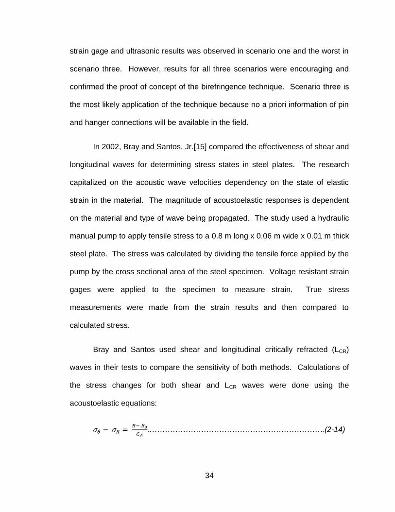
..………………………………………………………….(2-14)

35

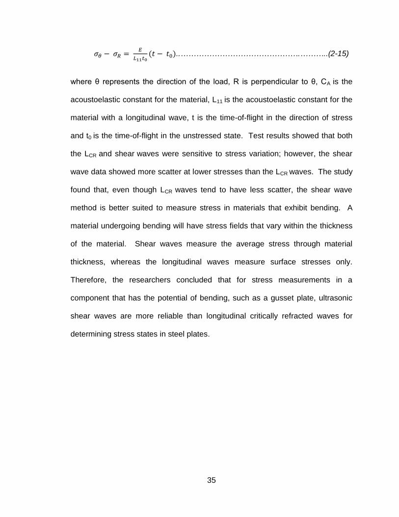
..……………………………………….………..(2-15)

where θ represents the direction of the load, R is perpendicular to θ, CA is the

acoustoelastic constant for the material, L11 is the acoustoelastic constant for the

material with a longitudinal wave, t is the time-of-flight in the direction of stress

and t0 is the time-of-flight in the unstressed state. Test results showed that both

the LCR and shear waves were sensitive to stress variation; however, the shear

wave data showed more scatter at lower stresses than the LCR waves. The study

found that, even though LCR waves tend to have less scatter, the shear wave

method is better suited to measure stress in materials that exhibit bending. A

material undergoing bending will have stress fields that vary within the thickness

of the material. Shear waves measure the average stress through material

thickness, whereas the longitudinal waves measure surface stresses only.

Therefore, the researchers concluded that for stress measurements in a

component that has the potential of bending, such as a gusset plate, ultrasonic

shear waves are more reliable than longitudinal critically refracted waves for

determining stress states in steel plates.

36

3. Experimental Procedures

This chapter describes the experimental testing and design completed

during the research. The basic experimental test setup used to record the

amplitude of the waveforms detected by the transducer is described in Section

3.1. Section 3.2 details the sensors and hardware used in the test setup. Section

3.3 describes the method used to time waveforms. The next two sections (3.4

and 3.5) describe the test materials and the test matrix used as part of this study.

Section 3.7 outlines the texture directions existing within the materials.

37

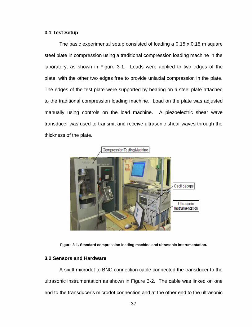
3.1 Test Setup

The basic experimental setup consisted of loading a 0.15 x 0.15 m square

steel plate in compression using a traditional compression loading machine in the

laboratory, as shown in Figure 3-1. Loads were applied to two edges of the

plate, with the other two edges free to provide uniaxial compression in the plate.

The edges of the test plate were supported by bearing on a steel plate attached

to the traditional compression loading machine. Load on the plate was adjusted

manually using controls on the load machine. A piezoelectric shear wave

transducer was used to transmit and receive ultrasonic shear waves through the

thickness of the plate.

Figure 3-1. Standard compression loading machine and ultrasonic instrumentation.

3.2 Sensors and Hardware

A six ft microdot to BNC connection cable connected the transducer to the

ultrasonic instrumentation as shown in Figure 3-2. The cable was linked on one

end to the transducer’s microdot connection and at the other end to the ultrasonic

38

instrumentation’s (diplexer) BNC connection. The transducer was placed on the

surface of the plate such that the propagation direction of the ultrasonic waves

was orthogonal to the applied force. Pulses were generated using a Ritec RAM-

10000 pulser-receiver. The RAM-10000 used short radio frequency (RF) burst

excitations to power the transducer.

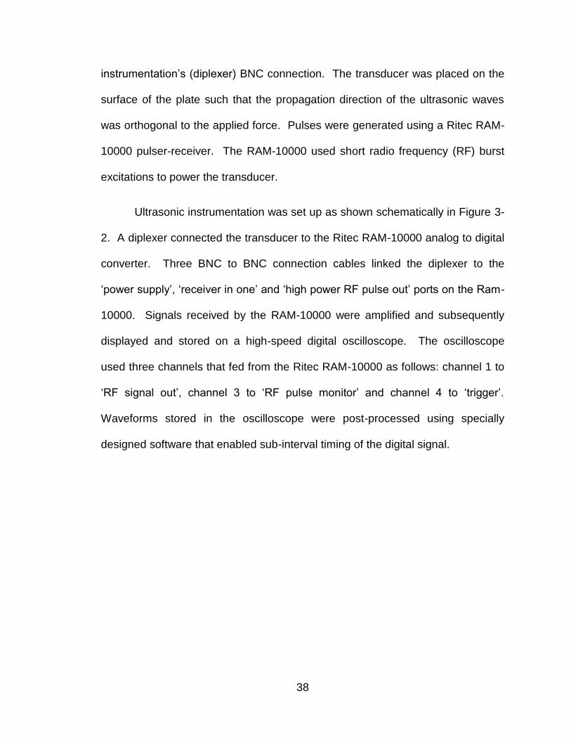
Ultrasonic instrumentation was set up as shown schematically in Figure 3-

2. A diplexer connected the transducer to the Ritec RAM-10000 analog to digital

converter. Three BNC to BNC connection cables linked the diplexer to the

‘power supply’, ‘receiver in one’ and ‘high power RF pulse out’ ports on the Ram-

10000. Signals received by the RAM-10000 were amplified and subsequently

displayed and stored on a high-speed digital oscilloscope. The oscilloscope

used three channels that fed from the Ritec RAM-10000 as follows: channel 1 to

‘RF signal out’, channel 3 to ‘RF pulse monitor’ and channel 4 to ‘trigger’.

Waveforms stored in the oscilloscope were post-processed using specially

designed software that enabled sub-interval timing of the digital signal.

39

Figure 3-2. Configuration of the ultrasonic instrumentation is shown.

This section details the sensors and hardware used in the research

presented herein.

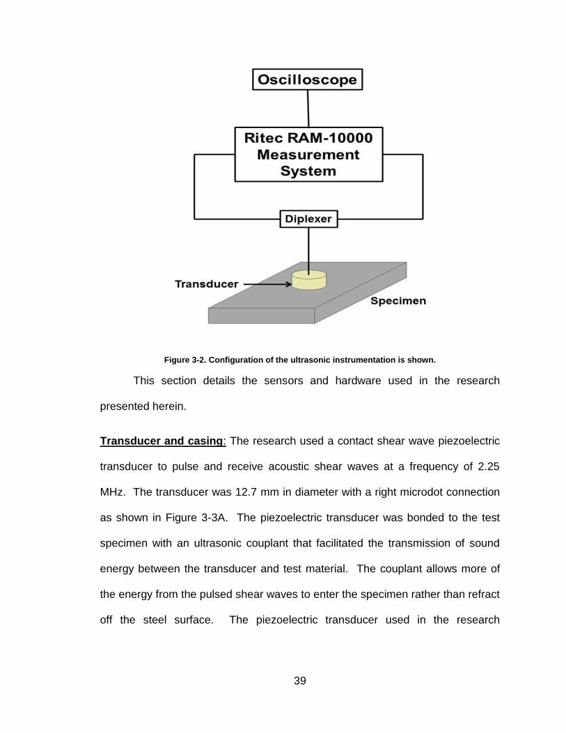
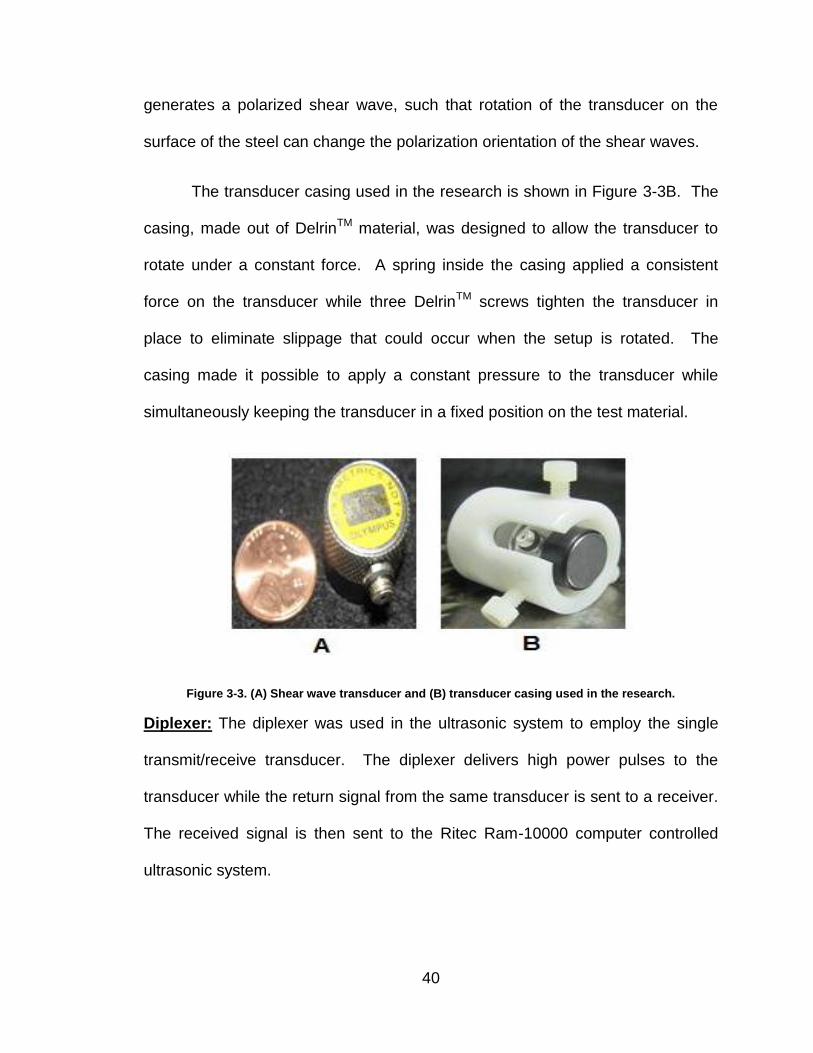
Transducer and casing: The research used a contact shear wave piezoelectric

transducer to pulse and receive acoustic shear waves at a frequency of 2.25

MHz. The transducer was 12.7 mm in diameter with a right microdot connection

as shown in Figure 3-3A. The piezoelectric transducer was bonded to the test

specimen with an ultrasonic couplant that facilitated the transmission of sound

energy between the transducer and test material. The couplant allows more of

the energy from the pulsed shear waves to enter the specimen rather than refract

off the steel surface. The piezoelectric transducer used in the research

40

generates a polarized shear wave, such that rotation of the transducer on the

surface of the steel can change the polarization orientation of the shear waves.

The transducer casing used in the research is shown in Figure 3-3B. The

casing, made out of DelrinTM material, was designed to allow the transducer to

rotate under a constant force. A spring inside the casing applied a consistent

force on the transducer while three DelrinTM screws tighten the transducer in

place to eliminate slippage that could occur when the setup is rotated. The

casing made it possible to apply a constant pressure to the transducer while

simultaneously keeping the transducer in a fixed position on the test material.

Figure 3-3. (A) Shear wave transducer and (B) transducer casing used in the research.

Diplexer: The diplexer was used in the ultrasonic system to employ the single

transmit/receive transducer. The diplexer delivers high power pulses to the

transducer while the return signal from the same transducer is sent to a receiver.

The received signal is then sent to the Ritec Ram-10000 computer controlled

ultrasonic system.

41

Ritec RAM-10000: The Ritec RAM-10000 is an ultrasonic measurement system

used for research applications. The ultrasonic research tool provided

reproducible measurements using short radio frequency (RF) burst excitations to

power the transducer. The transmitted signal was produced by a fast switching,

synthesized continuous wave (CW) frequency source. The ability to measure

signals automatically and accurately made the RAM-10000 a powerful ultrasonic

research tool. The instrument was coupled with software to process the readings

which allowed for acoustic time-of-flight information to be obtained. Signals

received by the RAM-10000 were subsequently displayed and stored on a high-

speed digital oscilloscope.

Oscilloscope: The digital oscilloscope model used was an HP Infinium 54815A.

Signals displayed on the oscilloscope were sampled and averaged 16 times with

a sampling rate of 100 Msa/s. The high speed digital oscilloscope captured

signals by using the edge triggering method. In the edge triggering method,

circuitry inside the oscilloscope identifies the exact instant in time when the input

signal passes through a user defined voltage threshold. When the input signal

passes through the trigger level, a precisely shaped pulse is generated and the

signal acquisition cycle starts. When the desired output signal is displayed on

the screen, the operator can save the waveform in the oscilloscope. The data

can then be exported from the oscilloscope to specially designed software that

enabled sub-interval timing of the digital signal.

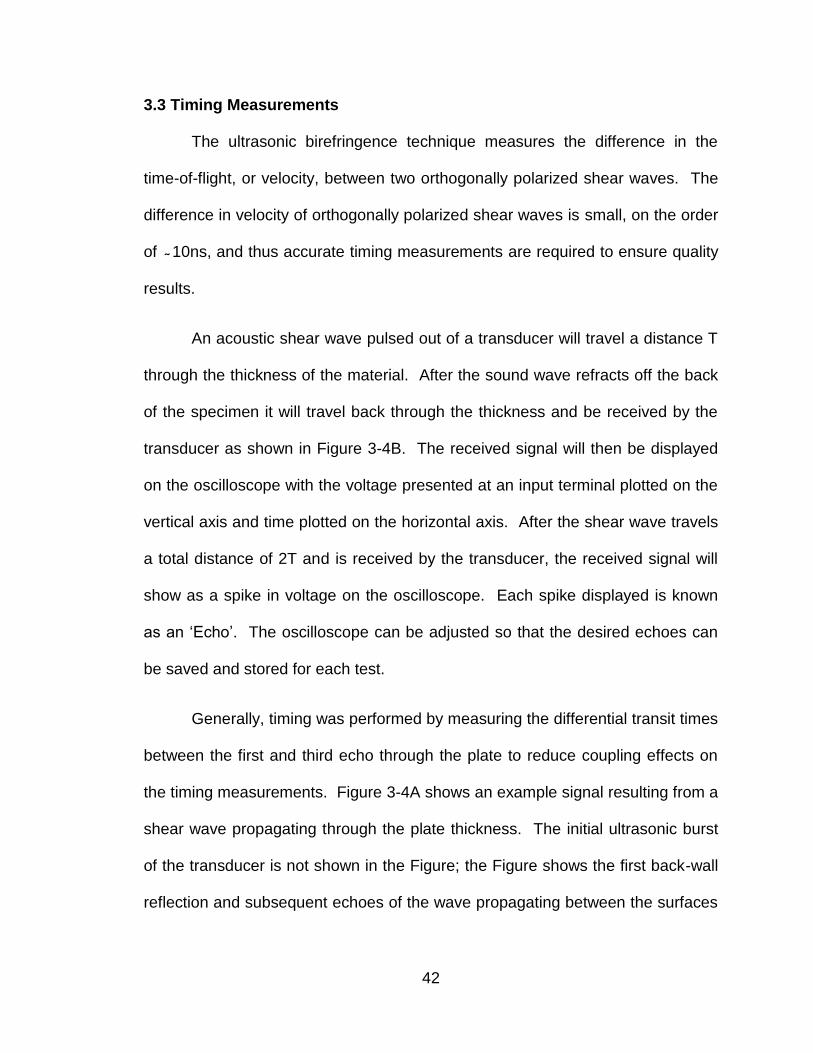
42

3.3 Timing Measurements

The ultrasonic birefringence technique measures the difference in the

time-of-flight, or velocity, between two orthogonally polarized shear waves. The

difference in velocity of orthogonally polarized shear waves is small, on the order

of 10ns, and thus accurate timing measurements are required to ensure quality

results.

An acoustic shear wave pulsed out of a transducer will travel a distance T

through the thickness of the material. After the sound wave refracts off the back

of the specimen it will travel back through the thickness and be received by the

transducer as shown in Figure 3-4B. The received signal will then be displayed

on the oscilloscope with the voltage presented at an input terminal plotted on the

vertical axis and time plotted on the horizontal axis. After the shear wave travels

a total distance of 2T and is received by the transducer, the received signal will

show as a spike in voltage on the oscilloscope. Each spike displayed is known

as an ‘Echo’. The oscilloscope can be adjusted so that the desired echoes can

be saved and stored for each test.

Generally, timing was performed by measuring the differential transit times

between the first and third echo through the plate to reduce coupling effects on

the timing measurements. Figure 3-4A shows an example signal resulting from a

shear wave propagating through the plate thickness. The initial ultrasonic burst

of the transducer is not shown in the Figure; the Figure shows the first back-wall

reflection and subsequent echoes of the wave propagating between the surfaces

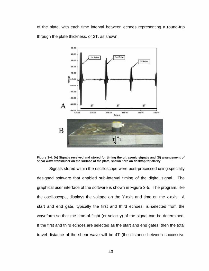
43

of the plate, with each time interval between echoes representing a round-trip

through the plate thickness, or 2T, as shown.

Figure 3-4. (A) Signals received and stored for timing the ultrasonic signals and (B) arrangement of shear wave transducer on the surface of the plate, shown here on desktop for clarity.

Signals stored within the oscilloscope were post-processed using specially

designed software that enabled sub-interval timing of the digital signal. The

graphical user interface of the software is shown in Figure 3-5. The program, like

the oscilloscope, displays the voltage on the Y-axis and time on the x-axis. A

start and end gate, typically the first and third echoes, is selected from the

waveform so that the time-of-flight (or velocity) of the signal can be determined.

If the first and third echoes are selected as the start and end gates, then the total

travel distance of the shear wave will be 4T (the distance between successive

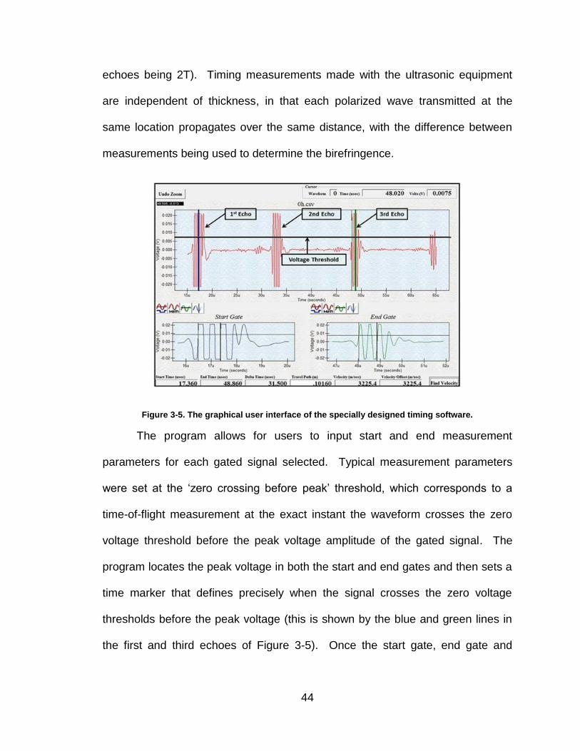
44

echoes being 2T). Timing measurements made with the ultrasonic equipment

are independent of thickness, in that each polarized wave transmitted at the

same location propagates over the same distance, with the difference between

measurements being used to determine the birefringence.

Figure 3-5. The graphical user interface of the specially designed timing software.

The program allows for users to input start and end measurement

parameters for each gated signal selected. Typical measurement parameters

were set at the ‘zero crossing before peak’ threshold, which corresponds to a

time-of-flight measurement at the exact instant the waveform crosses the zero

voltage threshold before the peak voltage amplitude of the gated signal. The

program locates the peak voltage in both the start and end gates and then sets a

time marker that defines precisely when the signal crosses the zero voltage

thresholds before the peak voltage (this is shown by the blue and green lines in

the first and third echoes of Figure 3-5). Once the start gate, end gate and

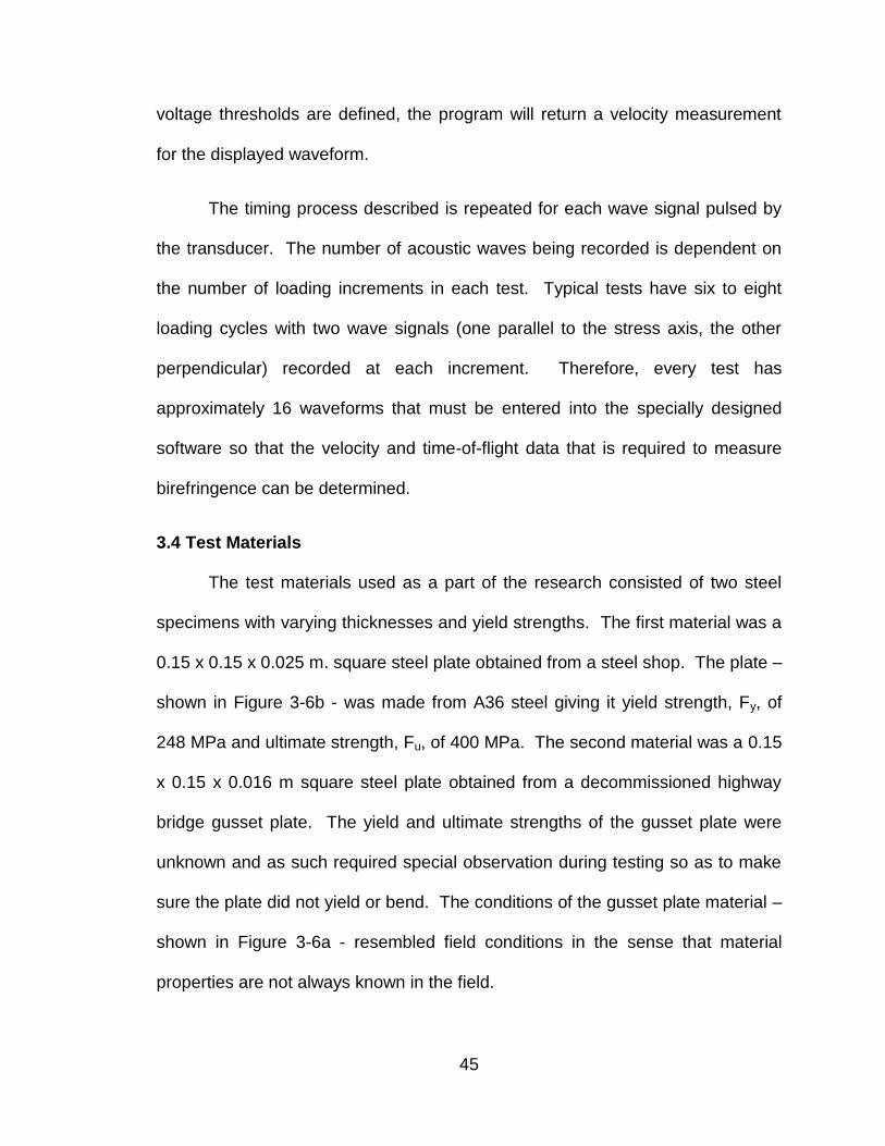
45

voltage thresholds are defined, the program will return a velocity measurement

for the displayed waveform.

The timing process described is repeated for each wave signal pulsed by

the transducer. The number of acoustic waves being recorded is dependent on

the number of loading increments in each test. Typical tests have six to eight

loading cycles with two wave signals (one parallel to the stress axis, the other

perpendicular) recorded at each increment. Therefore, every test has

approximately 16 waveforms that must be entered into the specially designed

software so that the velocity and time-of-flight data that is required to measure

birefringence can be determined.

3.4 Test Materials

The test materials used as a part of the research consisted of two steel

specimens with varying thicknesses and yield strengths. The first material was a

0.15 x 0.15 x 0.025 m. square steel plate obtained from a steel shop. The plate –

shown in Figure 3-6b - was made from A36 steel giving it yield strength, Fy, of

248 MPa and ultimate strength, Fu, of 400 MPa. The second material was a 0.15

x 0.15 x 0.016 m square steel plate obtained from a decommissioned highway

bridge gusset plate. The yield and ultimate strengths of the gusset plate were

unknown and as such required special observation during testing so as to make

sure the plate did not yield or bend. The conditions of the gusset plate material –

shown in Figure 3-6a - resembled field conditions in the sense that material

properties are not always known in the field.

46

Figure 3-6. Test materials are shown with (a) a material from a decommissioned highway bridge gusset plate and (b) an A36 steel plate obtained from a steel fabrication shop.

3.5 Summary of the Test Matrix

A variety of tests were done in the research to do a proof-of-concept of the

acoustoelastic theory, as well as to determine the consistency and repeatability

of the methodology. Table 3-1 shows the range of testing conducted as a part of

the study. Tests were done in accordance with the loading patterns detailed in

the following sections. For example, both of the steel materials were tested

under all three loading patterns, including: incremental step-loading,

discontinuous incremental step-loading and single loading. Tests were also done

to characterize the effects that existing texture within the steel specimens had on

ultrasonic velocity. The results of the testing done in accordance with Table 3-1

are presented in detail in Chapter 4.

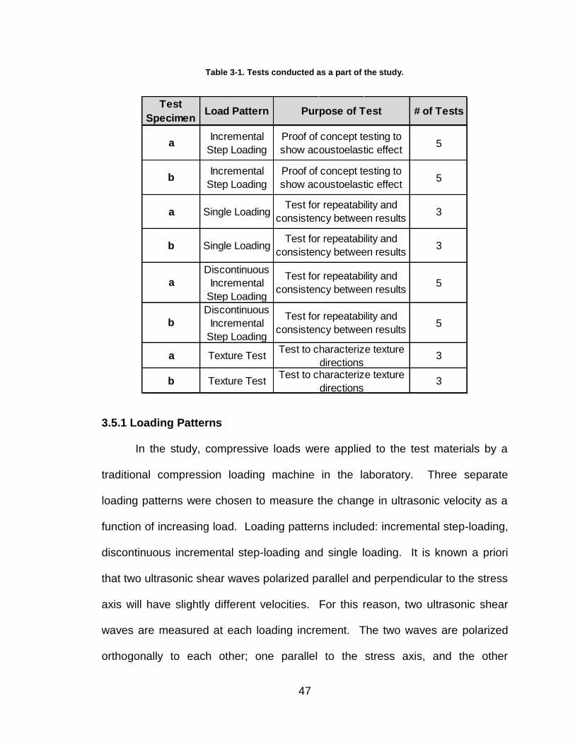
47

Table 3-1. Tests conducted as a part of the study.

3.5.1 Loading Patterns

In the study, compressive loads were applied to the test materials by a

traditional compression loading machine in the laboratory. Three separate

loading patterns were chosen to measure the change in ultrasonic velocity as a

function of increasing load. Loading patterns included: incremental step-loading,

discontinuous incremental step-loading and single loading. It is known a priori

that two ultrasonic shear waves polarized parallel and perpendicular to the stress

axis will have slightly different velocities. For this reason, two ultrasonic shear

waves are measured at each loading increment. The two waves are polarized

orthogonally to each other; one parallel to the stress axis, and the other

Test

SpecimenLoad Pattern # of Tests

aIncremental

Step Loading5

bIncremental

Step Loading5

a Single Loading 3

b Single Loading 3

a

Discontinuous

Incremental

Step Loading

5

b

Discontinuous

Incremental

Step Loading

5

a Texture Test 3

b Texture Test 3

Purpose of Test

Proof of concept testing to

show acoustoelastic effect

Test for repeatability and

consistency between results

Test for repeatability and

consistency between results

Test for repeatability and

consistency between results

Test to characterize texture

directionsTest to characterize texture

directions

Proof of concept testing to

show acoustoelastic effect

Test for repeatability and

consistency between results

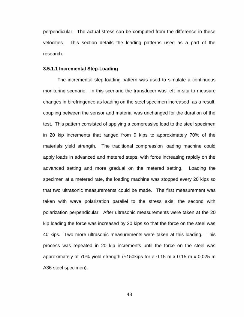
48

perpendicular. The actual stress can be computed from the difference in these

velocities. This section details the loading patterns used as a part of the

research.

3.5.1.1 Incremental Step-Loading

The incremental step-loading pattern was used to simulate a continuous

monitoring scenario. In this scenario the transducer was left in-situ to measure

changes in birefringence as loading on the steel specimen increased; as a result,

coupling between the sensor and material was unchanged for the duration of the

test. This pattern consisted of applying a compressive load to the steel specimen

in 20 kip increments that ranged from 0 kips to approximately 70% of the

materials yield strength. The traditional compression loading machine could

apply loads in advanced and metered steps; with force increasing rapidly on the

advanced setting and more gradual on the metered setting. Loading the

specimen at a metered rate, the loading machine was stopped every 20 kips so

that two ultrasonic measurements could be made. The first measurement was

taken with wave polarization parallel to the stress axis; the second with

polarization perpendicular. After ultrasonic measurements were taken at the 20

kip loading the force was increased by 20 kips so that the force on the steel was

40 kips. Two more ultrasonic measurements were taken at this loading. This

process was repeated in 20 kip increments until the force on the steel was

approximately at 70% yield strength (≈150kips for a 0.15 m x 0.15 m x 0.025 m

A36 steel specimen).

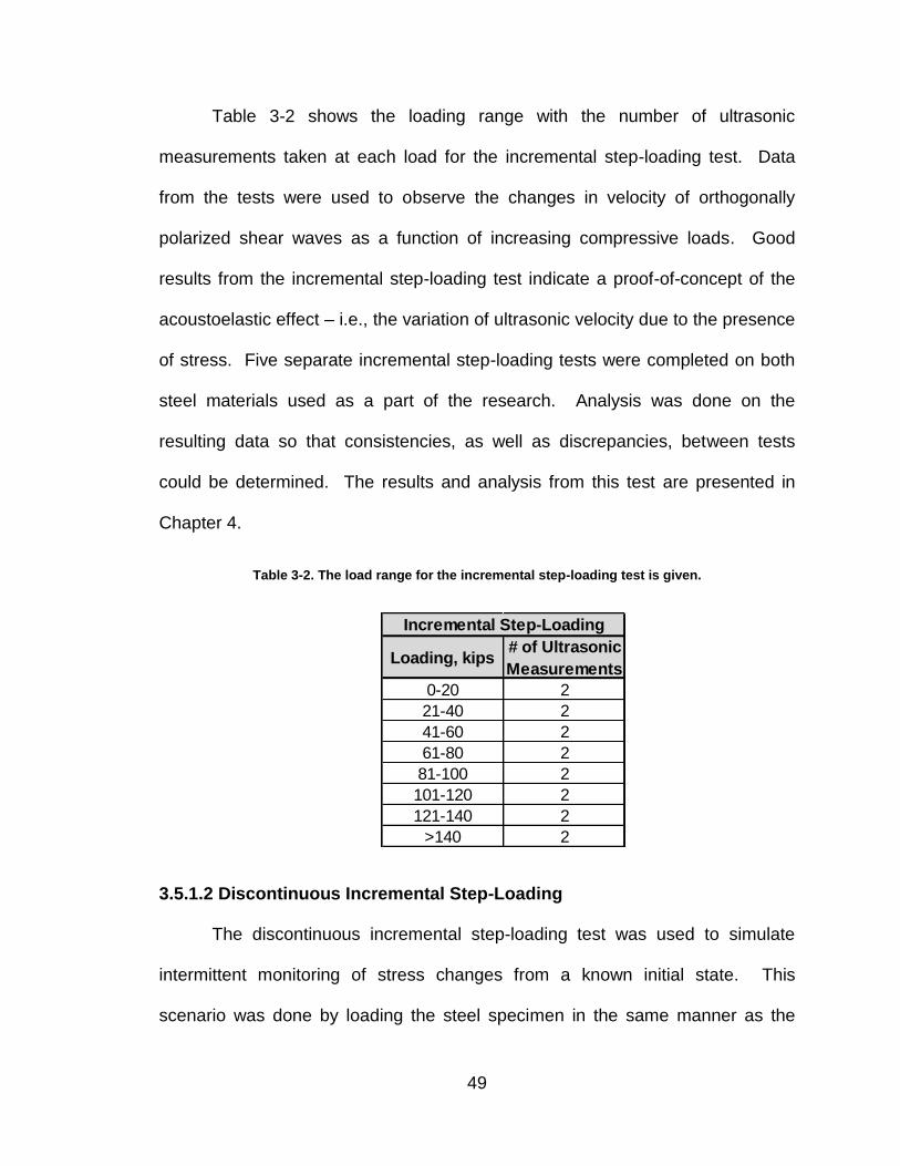
49

Table 3-2 shows the loading range with the number of ultrasonic

measurements taken at each load for the incremental step-loading test. Data

from the tests were used to observe the changes in velocity of orthogonally

polarized shear waves as a function of increasing compressive loads. Good

results from the incremental step-loading test indicate a proof-of-concept of the

acoustoelastic effect – i.e., the variation of ultrasonic velocity due to the presence

of stress. Five separate incremental step-loading tests were completed on both

steel materials used as a part of the research. Analysis was done on the

resulting data so that consistencies, as well as discrepancies, between tests

could be determined. The results and analysis from this test are presented in

Chapter 4.

Table 3-2. The load range for the incremental step-loading test is given.

3.5.1.2 Discontinuous Incremental Step-Loading

The discontinuous incremental step-loading test was used to simulate

intermittent monitoring of stress changes from a known initial state. This

scenario was done by loading the steel specimen in the same manner as the

Loading, kips# of Ultrasonic

Measurements

0-20 2

21-40 2

41-60 2

61-80 2

81-100 2

101-120 2

121-140 2

>140 2

Incremental Step-Loading

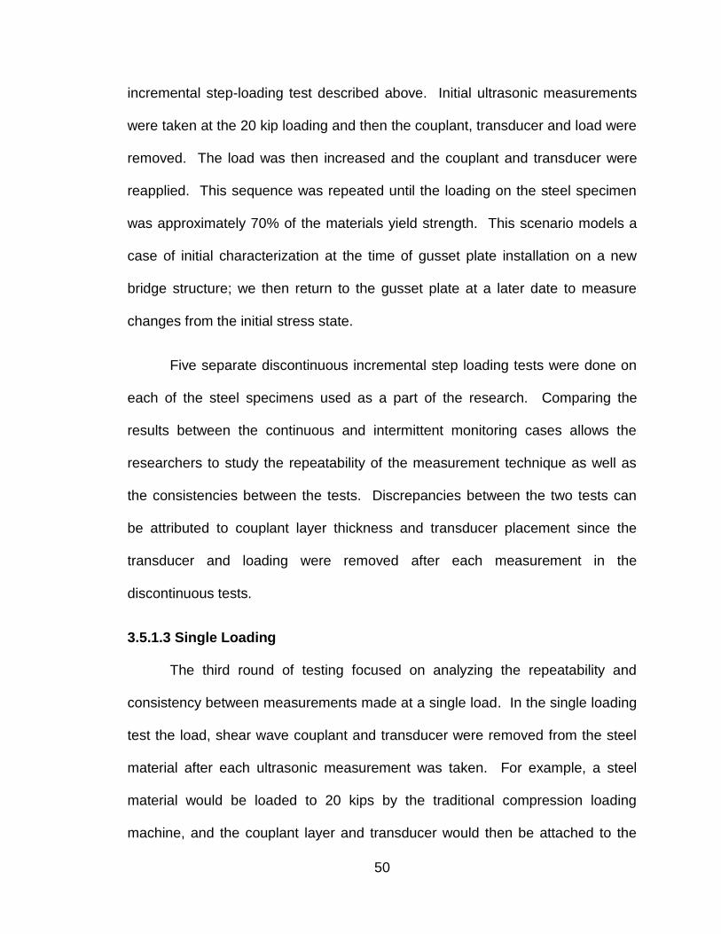
50

incremental step-loading test described above. Initial ultrasonic measurements

were taken at the 20 kip loading and then the couplant, transducer and load were

removed. The load was then increased and the couplant and transducer were

reapplied. This sequence was repeated until the loading on the steel specimen

was approximately 70% of the materials yield strength. This scenario models a

case of initial characterization at the time of gusset plate installation on a new

bridge structure; we then return to the gusset plate at a later date to measure

changes from the initial stress state.

Five separate discontinuous incremental step loading tests were done on

each of the steel specimens used as a part of the research. Comparing the

results between the continuous and intermittent monitoring cases allows the

researchers to study the repeatability of the measurement technique as well as

the consistencies between the tests. Discrepancies between the two tests can

be attributed to couplant layer thickness and transducer placement since the

transducer and loading were removed after each measurement in the

discontinuous tests.

3.5.1.3 Single Loading

The third round of testing focused on analyzing the repeatability and

consistency between measurements made at a single load. In the single loading

test the load, shear wave couplant and transducer were removed from the steel

material after each ultrasonic measurement was taken. For example, a steel

material would be loaded to 20 kips by the traditional compression loading

machine, and the couplant layer and transducer would then be attached to the

51

steel. The transducer would be rotated so that the pulsed shear wave would be

polarized horizontally (perpendicular) to the stress axis. After the ultrasonic

measurement was taken the load, couplant layer and transducer would be

removed from the steel material. Next, the steel would once again be loaded to

20 kips and the transducer and accompanying couplant layer would be reapplied.

An ultrasonic measurement would again be taken with wave polarization

horizontal to the stress axis. This process was repeated 25 times at the 20 kip

load, with a single ultrasonic measurement taken each time. The same

procedure was repeated with polarization direction vertical (parallel) to the stress

axis.

Table 3-3 outlines the loads used in the single loading test. For the A36

steel, loads of 20, 50 and 100 kips were chosen. The gusset plate steel was

loaded at 15, 45 and 75 kips. There were 50 individual measurements taken at

each load; with 25 being in the horizontal polarization direction and 25 in the

vertical direction for a total of 300 single ultrasonic measurements for one test.

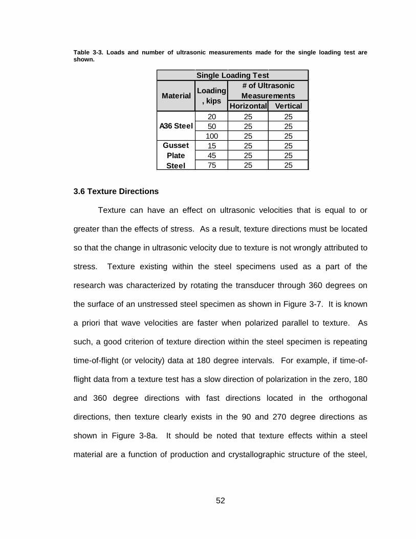
52

Table 3-3. Loads and number of ultrasonic measurements made for the single loading test are shown.

3.6 Texture Directions

Texture can have an effect on ultrasonic velocities that is equal to or

greater than the effects of stress. As a result, texture directions must be located

so that the change in ultrasonic velocity due to texture is not wrongly attributed to

stress. Texture existing within the steel specimens used as a part of the

research was characterized by rotating the transducer through 360 degrees on

the surface of an unstressed steel specimen as shown in Figure 3-7. It is known

a priori that wave velocities are faster when polarized parallel to texture. As

such, a good criterion of texture direction within the steel specimen is repeating

time-of-flight (or velocity) data at 180 degree intervals. For example, if time-of-

flight data from a texture test has a slow direction of polarization in the zero, 180

and 360 degree directions with fast directions located in the orthogonal

directions, then texture clearly exists in the 90 and 270 degree directions as

shown in Figure 3-8a. It should be noted that texture effects within a steel

material are a function of production and crystallographic structure of the steel,

Horizontal Vertical

20 25 25

50 25 25

100 25 25

15 25 25

45 25 25

75 25 25

Single Loading Test

MaterialLoading

, kips

# of Ultrasonic

Measurements

A36 Steel

Gusset

Plate

Steel

53

such that a different material of similar yield strength and chemistry may exhibit

different texture effects.

Figure 3-7. The process used to locate texture directions is shown.

The direction of fast and slow directions of the A36 steel plate were

coincident with the axis of the plate specimen, and likely are related to the rolling

direction of the plate. Upon locating the texture directions within the steel

materials, the fast direction of wave polarization was aligned coincident with the

direction of the applied loads as shown in Figure 3-8b.

54

Figure 3-8. (a) Test results indicate directions of texture in a steel specimen (b) which allows for texture directions to be oriented coincident with the stress axis.

55

4. Results

4.1 Introduction

This chapter provides the results of the ultrasonic birefringence testing

conducted to characterize the effects of stress on ultrasonic velocities in steel

specimens. Results are presented in two main sections; Chapter 4.2 presents

the results from all the tests conducted on an A36 steel plate and Chapter 4.3

presents the results for the tests conducted on a specimen of steel removed from

an in-service highway bridge. These tests were performed to assess the

birefringence effect; tests included: characterization of texture directions,

incremental step-loading, discontinuous incremental step-loading and single

loading. Factors found from these results are also discussed herein.

4.2 A36 Steel Specimen

This section describes the results from the texture characterization tests

that were conducted to determine the texture directions and magnitudes for the

A36 specimen. This texture measurement was used to establish the direction of

texture, that is, the fast and slow direction of waves. The following section

presents the results from the texture tests.

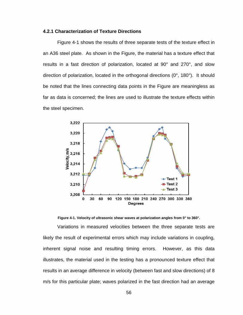
56

4.2.1 Characterization of Texture Directions

Figure 4-1 shows the results of three separate tests of the texture effect in

an A36 steel plate. As shown in the Figure, the material has a texture effect that

results in a fast direction of polarization, located at 90° and 270°, and slow

direction of polarization, located in the orthogonal directions (0°, 180°). It should

be noted that the lines connecting data points in the Figure are meaningless as

far as data is concerned; the lines are used to illustrate the texture effects within

the steel specimen.

Figure 4-1. Velocity of ultrasonic shear waves at polarization angles from 0° to 360°.

Variations in measured velocities between the three separate tests are

likely the result of experimental errors which may include variations in coupling,

inherent signal noise and resulting timing errors. However, as this data

illustrates, the material used in the testing has a pronounced texture effect that

results in an average difference in velocity (between fast and slow directions) of 8

m/s for this particular plate; waves polarized in the fast direction had an average

57

velocity of 3220 m/s and waves polarized in the orthogonal direction averaged

3212 m/s. It is important to note that this texture effect described herein is a

function of production and crystallographic structure of the plate, such that a

different material of similar yield strength and chemistry may exhibit different

texture effects. The direction of the fast and slow directions of the plate were

coincident with the axis of the plate specimen, and likely are related to the rolling

direction of the plate.

Table 4-1 shows the velocities for each time-of-flight measurement from 0°

to 360° for the three texture tests conducted on the material. The results vary

slightly between the three tests; however, all three tests agree quite well on the

texture directions in the steel plate. The Table also shows the average absolute

error – a statistical measure of how far measurements are from the average

values; this measurement shows that, on average, for all polarization directions

(with the 0° polarization direction being an exception) the absolute error was less

than 1 m/s. The average absolute error for all polarization directions was slightly

greater than 0.5 m/s. The Table also shows the standard deviation – a measure

of the dispersion of the velocities from the average velocity; the average standard

deviation for the texture tests was 0.71 m/s.

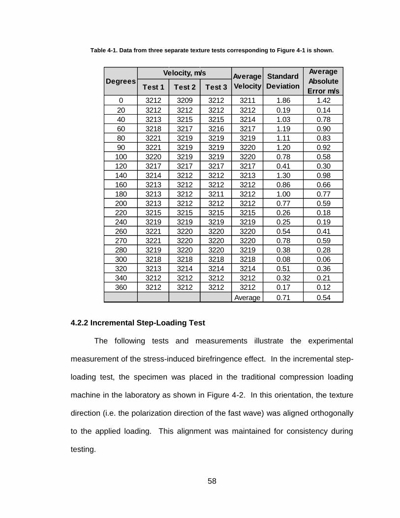
58

Table 4-1. Data from three separate texture tests corresponding to Figure 4-1 is shown.

4.2.2 Incremental Step-Loading Test

The following tests and measurements illustrate the experimental

measurement of the stress-induced birefringence effect. In the incremental step-

loading test, the specimen was placed in the traditional compression loading

machine in the laboratory as shown in Figure 4-2. In this orientation, the texture

direction (i.e. the polarization direction of the fast wave) was aligned orthogonally

to the applied loading. This alignment was maintained for consistency during

testing.

Test 1 Test 2 Test 3

0 3212 3209 3212 3211 1.86 1.42

20 3212 3212 3212 3212 0.19 0.14

40 3213 3215 3215 3214 1.03 0.78

60 3218 3217 3216 3217 1.19 0.90

80 3221 3219 3219 3219 1.11 0.83

90 3221 3219 3219 3220 1.20 0.92

100 3220 3219 3219 3220 0.78 0.58

120 3217 3217 3217 3217 0.41 0.30

140 3214 3212 3212 3213 1.30 0.98

160 3213 3212 3212 3212 0.86 0.66

180 3213 3212 3211 3212 1.00 0.77

200 3213 3212 3212 3212 0.77 0.59

220 3215 3215 3215 3215 0.26 0.18

240 3219 3219 3219 3219 0.25 0.19

260 3221 3220 3220 3220 0.54 0.41

270 3221 3220 3220 3220 0.78 0.59

280 3219 3220 3220 3219 0.38 0.28

300 3218 3218 3218 3218 0.08 0.06

320 3213 3214 3214 3214 0.51 0.36

340 3212 3212 3212 3212 0.32 0.21

360 3212 3212 3212 3212 0.17 0.12

Average 0.71 0.54

Average

Absolute

Error m/s

Average

VelocityDegrees

Velocity, m/s Standard

Deviation

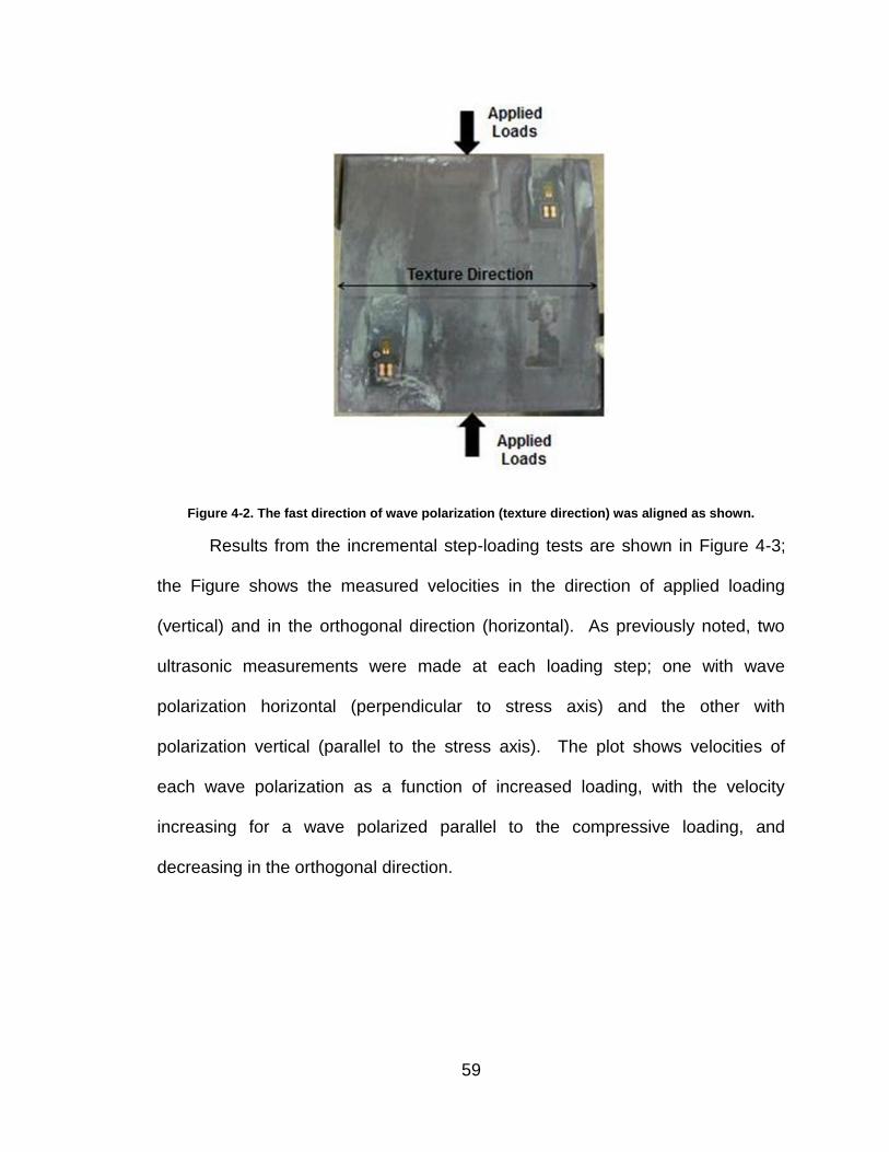
59

Figure 4-2. The fast direction of wave polarization (texture direction) was aligned as shown.

Results from the incremental step-loading tests are shown in Figure 4-3;

the Figure shows the measured velocities in the direction of applied loading

(vertical) and in the orthogonal direction (horizontal). As previously noted, two

ultrasonic measurements were made at each loading step; one with wave

polarization horizontal (perpendicular to stress axis) and the other with

polarization vertical (parallel to the stress axis). The plot shows velocities of

each wave polarization as a function of increased loading, with the velocity

increasing for a wave polarized parallel to the compressive loading, and

decreasing in the orthogonal direction.

60

Figure 4-3. Shear wave velocities for two orthogonally polarized shear waves under applied loading.

The coefficient of determination (R2) values of the data set are displayed

with the trend lines on the Figure. The R2 value of the vertical polarization data

is close to one, indicating that the regression line fits the data well. The

coefficient of determination value of the horizontal polarization data is 0.3,

indicating it does not agree as well as the vertical data. However, this may be

caused by one or more outlying values within the data.

Figure 4-4 shows the resulting ultrasonic birefringence as a function of

applied load as determined from the shear wave velocity measurements shown

in Figure 4-3. This Figure illustrates that the birefringence measurement varies

in a linear function of applied loads (i.e. stresses). Correlation with the linear fit is

relatively high, with an R2 value of greater than 0.8. Recall that for this test, the

transducer remained in-situ for the duration of the test to simulate a continuous

monitoring situation.

61

Figure 4-4. Ultrasonic birefringence resulting from applied loads for the A36 test plate.

Table 4-2 shows the average velocity from the incremental step-loading

tests at each loading increment in both the horizontal and vertical polarization

directions. The Table also shows the average absolute error at each loading; the

average of the average absolute error was approximately 0.4 m/s in each

polarization direction. Note the trends in velocity as the load increases; waves

polarized in the horizontal direction are steadily decreasing while waves

polarized in the orthogonal directions are increasing.

62

Table 4-2 Velocity and load comparison from three incremental step-loading tests performed on the A36 steel specimen.

An error analysis was done using measured data from the incremental

step-loading test to determine the uncertainties in the measurements relative to

the linear trend lines in Figures 4-3 & 4-4. The error analysis was completed by

calculating the load that a given birefringence measurement would indicate

according to the linear trend lines. For example, in Figure 4-4, the linear trend

line of all the measurements taken in the vertical polarization direction had a

linear fit equation of:

Y = 1E-08x+.0025…………………………………………………….(4-1)

where Y is the velocity or birefringence and x is the load. Taking each measured

velocity or birefringence and rearranging Equation 4-1 to solve for x would give

the expected load that each velocity or birefringence measurement should be

given the linear fit equation. Next, subtracting the calculated load from the actual

load would give the difference between the two values. Dividing this difference

by the area of the material (0.0039 m2 for the A36 steel) gives the uncertainty in

the measurement in terms of stress (ksi). Figure 4-5 shows the process taken in

Load,

kips

Horizontal

m/s

Average

Absolute

Error m/s

Vertical

m/s

Average

Absolute

Error m/s

20 3222 1.02 3214 0.18

40 3221 0.08 3215 0.19

60 3221 0.41 3216 0.47

80 3221 0.20 3216 0.39

100 3221 0.26 3217 0.56

120 3221 0.37 3218 0.50

140 3220 0.61 3218 0.54

Average 0.42 Average 0.40

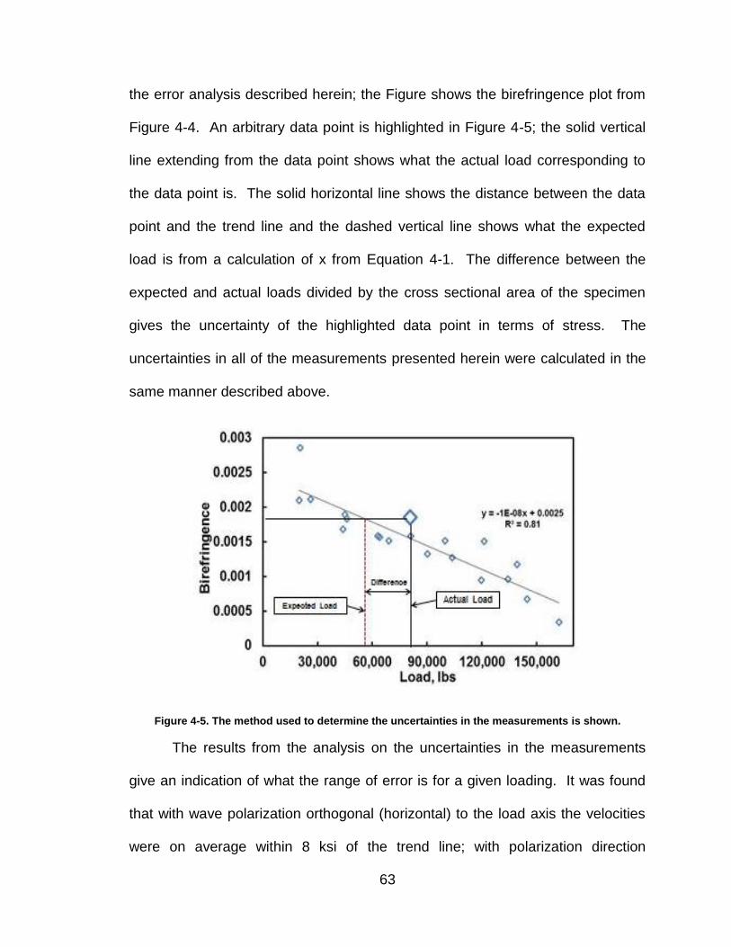
63

the error analysis described herein; the Figure shows the birefringence plot from

Figure 4-4. An arbitrary data point is highlighted in Figure 4-5; the solid vertical

line extending from the data point shows what the actual load corresponding to

the data point is. The solid horizontal line shows the distance between the data

point and the trend line and the dashed vertical line shows what the expected

load is from a calculation of x from Equation 4-1. The difference between the

expected and actual loads divided by the cross sectional area of the specimen

gives the uncertainty of the highlighted data point in terms of stress. The

uncertainties in all of the measurements presented herein were calculated in the

same manner described above.

Figure 4-5. The method used to determine the uncertainties in the measurements is shown.

The results from the analysis on the uncertainties in the measurements

give an indication of what the range of error is for a given loading. It was found

that with wave polarization orthogonal (horizontal) to the load axis the velocities

were on average within 8 ksi of the trend line; with polarization direction

64

coincident (vertical) with the load axis, the velocities were within 3 ksi of the trend

line. The average stress range for a velocity measurement at a given load is

shown in Table 4-3 for both polarization directions.

Table 4-3. Average velocity and measurement uncertainties for different load steps ranging from 20 to 160 kips.

Table 4-4 shows the average uncertainties for all birefringence

measurements at a given loading; the Table shows the average birefringence

corresponding to Figure 4-4. On average, the data is within approximately 4 ksi

of the trend line. Note that the average birefringence data shown in Table 4-4 is

the average of three separate readings; for example, the average birefringence

for three separate incremental step-loading tests at a loading of 20 kips was

0.0024.

20 16 3221.9 20 1 3214.3

40 7 3221.2 40 2 3215.4

60 7 3220.9 60 3 3215.9

80 4 3221.3 80 2 3216.1

100 7 3220.9 100 4 3216.4

120 9 3221.1 120 3 3217.2

140 5 3220.9 140 4 3217.9

Average 8 Average 3

Horizontal Polarization Vertical Polarization

Load,

kips

Measurement

Uncertainty,

ksi

Average

Velocity

Load,

kips

Measurement

Uncertainty,

ksi

Average

Velocity

65

Table 4-4. Average birefringence and predicted stress uncertainty (error) for different load steps ranging from 20 to 160 kips.

4.2.3 Discontinuous Incremental Step-Loading Test

In the discontinuous incremental step-loading test the material was loaded

in the same manner as the continuous step-loading test; however, after

ultrasonic measurements were made at each load, the transducer and load were

removed and then subsequently reapplied with an increase in loading. This

models a case of intermittent monitoring of stress change from a known initial

state. For example, there is an initial characterization of the birefringence in the

gusset plate at the time of installation; we then return to the gusset plate to

measure changes from this initial state.

Results from the discontinuous incremental step-loading tests are shown

in Figure 4-6; the figure shows the measured velocities in the direction of applied

loading (vertical) and in the orthogonal direction (horizontal) as a function of

increased loading. Like the results from the continuous monitoring tests, the

intermittent monitoring results show the velocity increasing for a wave polarized

20 0.0024 4.9

40 0.0018 4.1

60 0.0016 4.9

80 0.0016 3.0

100 0.0014 1.7

120 0.0012 4.8

140 0.0009 3.5

Average 3.8

Load,

kips

Average

Birefringence

Measurement

Uncertainty,

ksi

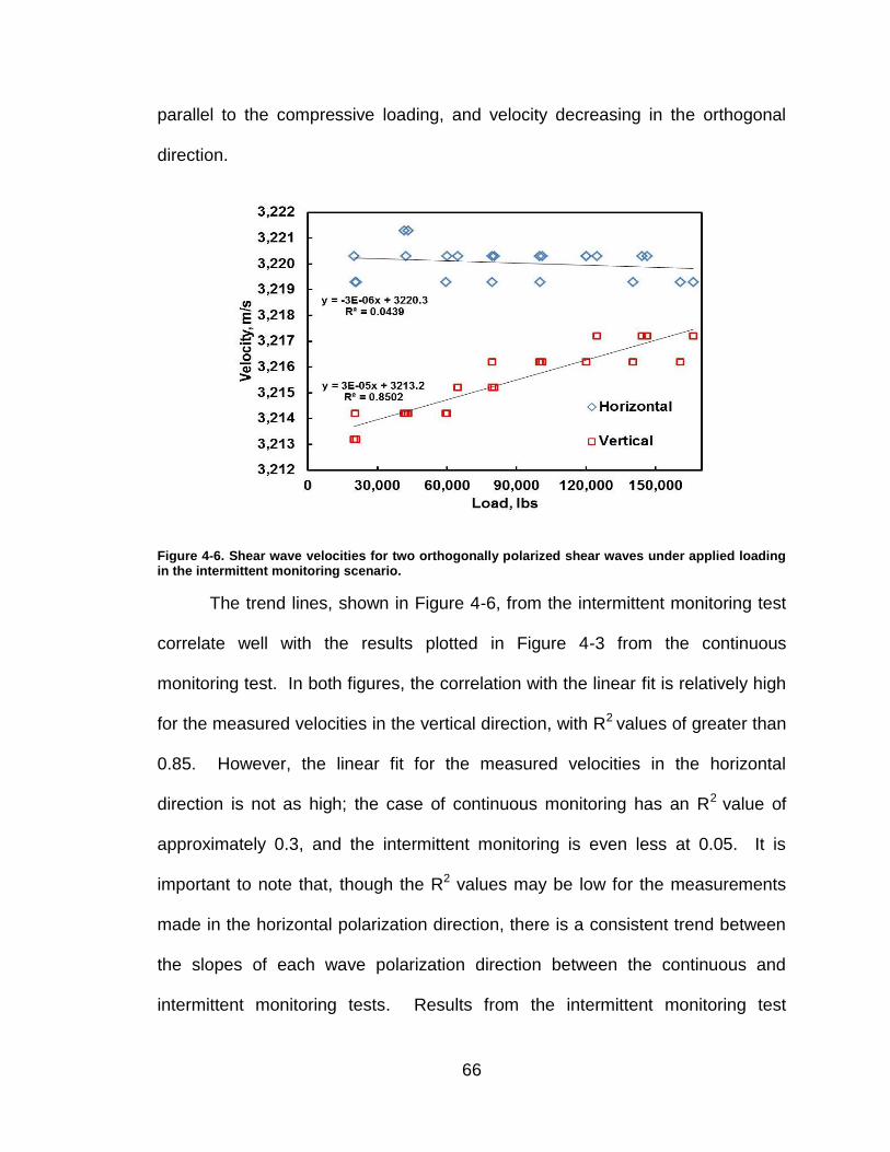
66

parallel to the compressive loading, and velocity decreasing in the orthogonal

direction.

Figure 4-6. Shear wave velocities for two orthogonally polarized shear waves under applied loading in the intermittent monitoring scenario.

The trend lines, shown in Figure 4-6, from the intermittent monitoring test

correlate well with the results plotted in Figure 4-3 from the continuous

monitoring test. In both figures, the correlation with the linear fit is relatively high

for the measured velocities in the vertical direction, with R2 values of greater than

0.85. However, the linear fit for the measured velocities in the horizontal

direction is not as high; the case of continuous monitoring has an R2 value of

approximately 0.3, and the intermittent monitoring is even less at 0.05. It is

important to note that, though the R2 values may be low for the measurements

made in the horizontal polarization direction, there is a consistent trend between

the slopes of each wave polarization direction between the continuous and

intermittent monitoring tests. Results from the intermittent monitoring test

67

indicate that it is possible to obtain consistent measurements when the

transducer and loading is not left in-situ.

Figure 4-7 shows the resulting ultrasonic birefringence as a function of

applied load, as determined from the shear wave velocity measurements shown

in Figure 4-6. This Figure illustrates that the birefringence varies in a linear

function of applied loads (i.e. stresses). Correlation with the linear fit is relatively

high, with an R2 value of greater than 0.75. The results from this test illustrate

that, though the transducer and load were removed after each ultrasonic

measurement, the data agrees quite well with the data from the case of leaving

the transducer and load in-situ for the duration of the test.

Figure 4-7. Ultrasonic birefringence resulting from applied loads for discontinuous incremental step-loading test done on the A36 test plate is shown.

Table 4-5 shows the average velocity from the discontinuous incremental

step-loading tests at each loading increment in both the vertical and horizontal

polarization directions. The Table also shows the average absolute error at each

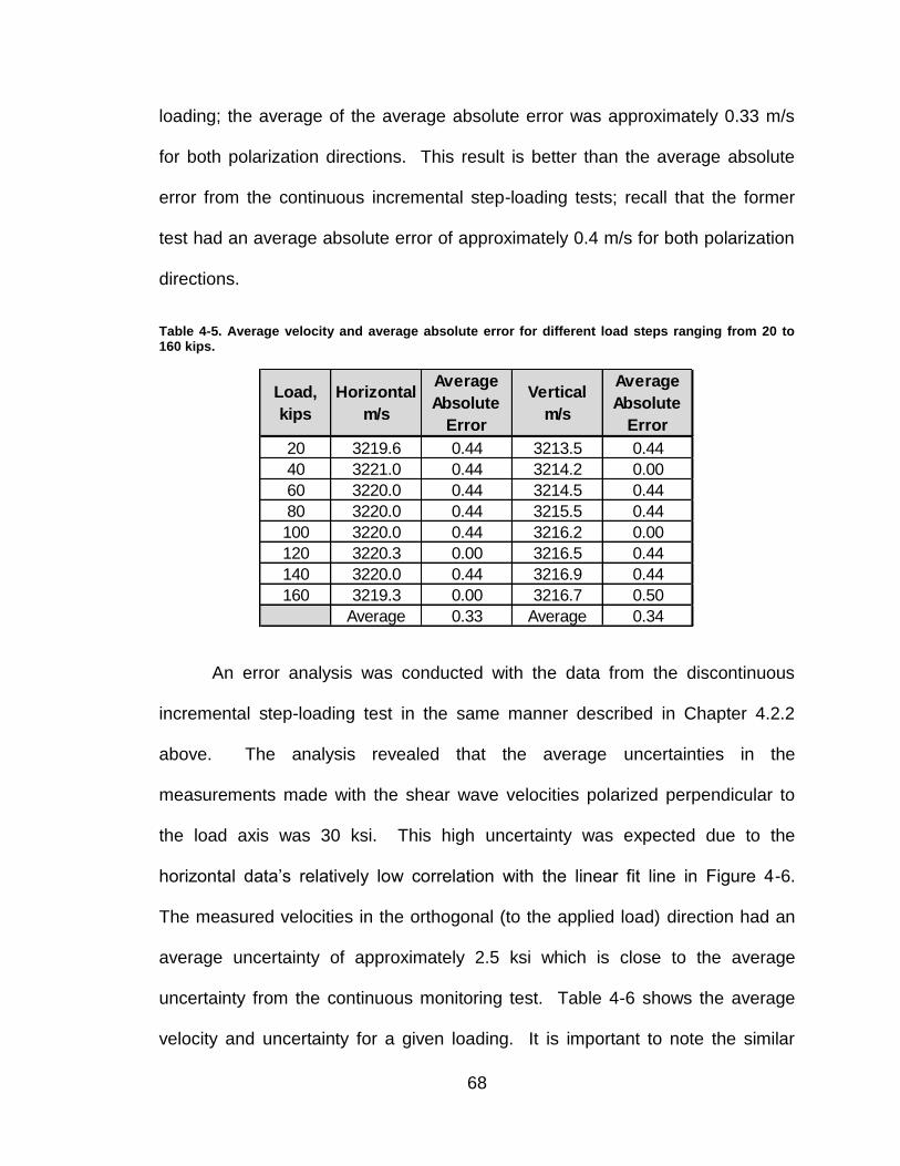
68

loading; the average of the average absolute error was approximately 0.33 m/s

for both polarization directions. This result is better than the average absolute

error from the continuous incremental step-loading tests; recall that the former

test had an average absolute error of approximately 0.4 m/s for both polarization

directions.

Table 4-5. Average velocity and average absolute error for different load steps ranging from 20 to 160 kips.

An error analysis was conducted with the data from the discontinuous

incremental step-loading test in the same manner described in Chapter 4.2.2

above. The analysis revealed that the average uncertainties in the

measurements made with the shear wave velocities polarized perpendicular to

the load axis was 30 ksi. This high uncertainty was expected due to the

horizontal data’s relatively low correlation with the linear fit line in Figure 4-6.

The measured velocities in the orthogonal (to the applied load) direction had an

average uncertainty of approximately 2.5 ksi which is close to the average

uncertainty from the continuous monitoring test. Table 4-6 shows the average

velocity and uncertainty for a given loading. It is important to note the similar

Load,

kips

Horizontal

m/s

Average

Absolute

Error

Vertical

m/s

Average

Absolute

Error

20 3219.6 0.44 3213.5 0.44

40 3221.0 0.44 3214.2 0.00

60 3220.0 0.44 3214.5 0.44

80 3220.0 0.44 3215.5 0.44

100 3220.0 0.44 3216.2 0.00

120 3220.3 0.00 3216.5 0.44

140 3220.0 0.44 3216.9 0.44

160 3219.3 0.00 3216.7 0.50

Average 0.33 Average 0.34

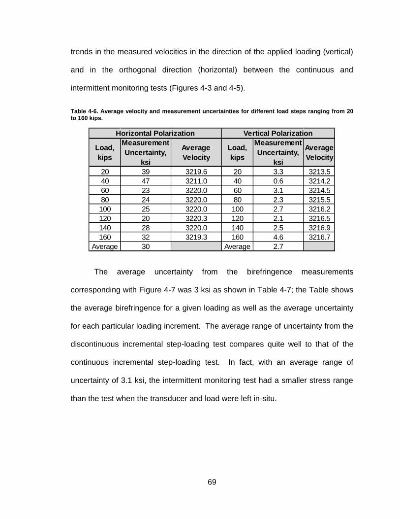
69

trends in the measured velocities in the direction of the applied loading (vertical)

and in the orthogonal direction (horizontal) between the continuous and

intermittent monitoring tests (Figures 4-3 and 4-5).

Table 4-6. Average velocity and measurement uncertainties for different load steps ranging from 20 to 160 kips.

The average uncertainty from the birefringence measurements

corresponding with Figure 4-7 was 3 ksi as shown in Table 4-7; the Table shows

the average birefringence for a given loading as well as the average uncertainty

for each particular loading increment. The average range of uncertainty from the

discontinuous incremental step-loading test compares quite well to that of the

continuous incremental step-loading test. In fact, with an average range of

uncertainty of 3.1 ksi, the intermittent monitoring test had a smaller stress range

than the test when the transducer and load were left in-situ.

20 39 3219.6 20 3.3 3213.5

40 47 3211.0 40 0.6 3214.2

60 23 3220.0 60 3.1 3214.5

80 24 3220.0 80 2.3 3215.5

100 25 3220.0 100 2.7 3216.2

120 20 3220.3 120 2.1 3216.5

140 28 3220.0 140 2.5 3216.9

160 32 3219.3 160 4.6 3216.7

Average 30 Average 2.7

Horizontal Polarization Vertical Polarization

Load,

kips

Measurement

Uncertainty,

ksi

Average

Velocity

Load,

kips

Measurement

Uncertainty,

ksi

Average

Velocity

70

Table 4-7. Average birefringence and predicted stress range (error) for different load steps ranging from 20 to 160 kips.

4.2.4 Single Loading Test

Three arbitrary loads were selected for the single loading test conducted

on the steel specimen, including; 20, 50 and 100 kip loadings. There were a total

of 50 separate measurements made at each loading; 25 measurements were

made with the shear wave polarized transversely to the stress axis, and 25 more

measurements were made in the orthogonal direction giving a total of 150

separate measurements. Figure 4-8 shows the results of the 150 separate

measurements; the Figure shows velocities for a given loading as well as the

standard deviation for each loading increment. For both horizontal and vertical

polarization directions at the 50 kip loading, the data is out of place compared to

the other two loadings; however, the linear fit lines display similar slopes to those

of the continuous and intermittent monitoring tests. As expected, the R2 values

are significantly lower for the single loading tests, due in large part to

experimental errors that come from removing the transducer and load after every

measurement.

20 0.0019 4.5

40 0.0021 5.3

60 0.0017 2.2

80 0.0014 4.5

100 0.0012 2.3

120 0.0012 2.6

140 0.0010 1

160 0.0008 2.4

Average 3.1

Load,

kips

Average

Birefringence

Measurement

Uncertainty,

ksi

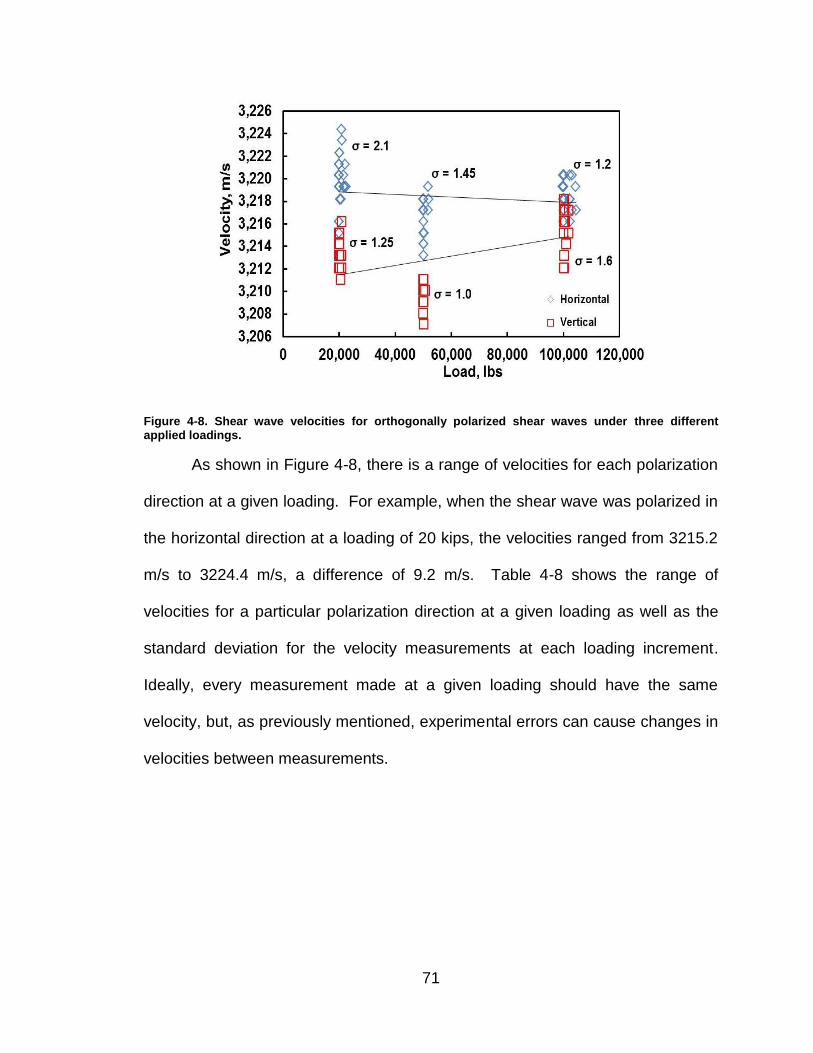
71

Figure 4-8. Shear wave velocities for orthogonally polarized shear waves under three different applied loadings.

As shown in Figure 4-8, there is a range of velocities for each polarization

direction at a given loading. For example, when the shear wave was polarized in

the horizontal direction at a loading of 20 kips, the velocities ranged from 3215.2

m/s to 3224.4 m/s, a difference of 9.2 m/s. Table 4-8 shows the range of

velocities for a particular polarization direction at a given loading as well as the

standard deviation for the velocity measurements at each loading increment.

Ideally, every measurement made at a given loading should have the same

velocity, but, as previously mentioned, experimental errors can cause changes in

velocities between measurements.

72

Table 4-8. The range of velocities for both polarization directions is shown for the loads corresponding to Figure 4-8.

Figure 4-9 shows the standard deviation for all 150 measurements

conducted in the single loading test. Although there is a range of variance

between velocities at a single loading, 66% of the measurements fall within +/- 1

standard deviation of the mean. The average standard deviation for each set of

measurements at a given loading was approximately 1.5 m/s; meaning for a

single measurement, we would expect the velocity to be within 1.5 m/s of the

average velocity 66% of the time. Furthermore, 95% of the data from the single

loading test fell within +/- 2 standard deviations, i.e. the data fell within +/- 3 m/s

of the mean.

Velocity

Range, m/s

Standard

Deviation

Velocity

Range, m/s

Standard

Deviation

20 9.2 2.1 5.1 1.3

50 6.1 1.5 4.0 1.0

100 4.1 1.2 6.1 1.6

Load,

kips

VerticalHorizontal

73

Figure 4-9. The standard deviation from the single loading test is shown.

Table 4-9 shows the average velocity at each respective loading

increment (20, 50 and 100 kips) in both the vertical and horizontal polarization

directions. The Table also shows the standard deviation as well as the average

absolute error at each loading; the average of the average absolute error was

approximately 1.3 m/s in the horizontal direction and 1.1 m/s in the orthogonal

direction. As expected for this test, the average absolute error is higher in the

single loading test than the other two tests; however, the data shows a

correlation between the linear fit lines from all three tests. A comparison of the

results from all of the tests is presented in Chapter 4.4 of this report.

74

Table 4-9. Velocity and load comparison from the single loading tests is shown.

4.3 Gusset Plate Specimen

This section describes test results to determine the texture effect

directions and magnitudes for the gusset plate specimen. This texture

measurement was used to establish the direction of texture within the specimen.

The following section presents the results from the texture tests.

4.3.1 Characterization of Texture Directions

Figure 4-10 shows the results of three separate tests of the texture effect

in a steel plate material that was obtained from a decommissioned highway

bridge gusset plate. As shown in the Figure, the gusset plate material has a

texture effect that results in a fast direction of polarization, located at 0°, 180° and

360°, and slow direction of polarization, located in the orthogonal directions (90°,

270°). The gusset plate material has an average variation in velocity (between

fast and slow directions) of 7 m/s, similar to the velocity variation within the A36

steel material. Recall that the A36 steel material had an average variation in

velocity (between fast and slow directions) of 8 m/s.

Velocity,

m/s

Standard

Deviation

Average

Absolute

Error

Velocity,

m/s

Standard

Deviation

Average

Absolute

Error

20 3220.0 2.1 1.59 3213.4 1.3 1.03

50 3216.7 1.5 1.19 3209.7 1.0 0.86

100 3218.6 1.2 1.09 3216.0 1.6 1.25

Average 1.6 1.29 Average 1.3 1.05

Horizontal Polarization Vertical Polarization

Load,

kips

75

Figure 4-10. Velocity of ultrasonic shear waves at polarization angles from 0° to 360°.

76

Table 4-10 shows the velocities for each time-of-flight measurement for

the three texture tests performed on the gusset plate material for polarization

directions through 360°. Included in the Table are standard deviation and

average absolute error values for each polarization direction. The error analysis

shows that the average absolute error was higher for the gusset plate steel than

the A36 steel plate. The total average absolute error was slightly less than 1.5

m/s for all polarization directions. Though this error was approximately 1 m/s

greater than the error from the tests on the prior material, the data illustrates the

existence of texture directions within the gusset plate material. The average

standard deviation – a measure of the dispersion of the velocities from the

average velocity – for the data was 2 m/s. All three of the texture tests indicate

fast directions at 0°, 180° and 360° which coincide with texture directions along

the same axis.

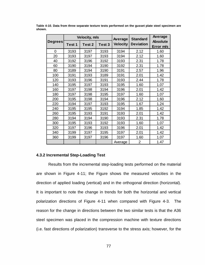
77

Table 4-10. Data from three separate texture tests performed on the gusset plate steel specimen are shown.

4.3.2 Incremental Step-Loading Test

Results from the incremental step-loading tests performed on the material

are shown in Figure 4-11; the Figure shows the measured velocities in the

direction of applied loading (vertical) and in the orthogonal direction (horizontal).

It is important to note the change in trends for both the horizontal and vertical

polarization directions of Figure 4-11 when compared with Figure 4-3. The

reason for the change in directions between the two similar tests is that the A36

steel specimen was placed in the compression machine with texture directions

(i.e. fast directions of polarization) transverse to the stress axis; however, for the

Test 1 Test 2 Test 3

0 3193 3197 3193 3194 2.12 1.60

20 3193 3197 3193 3194 2.12 1.60

40 3192 3196 3192 3193 2.31 1.78

60 3190 3194 3190 3192 2.31 1.78

80 3189 3194 3190 3191 2.57 1.96

100 3191 3193 3189 3191 2.01 1.42

120 3193 3196 3191 3193 2.44 1.78

140 3195 3197 3193 3195 1.60 1.07

160 3197 3198 3194 3196 2.01 1.42

180 3197 3198 3195 3197 1.60 1.07

200 3195 3198 3194 3196 2.12 1.60

220 3194 3197 3193 3195 1.67 1.24

240 3195 3195 3192 3194 1.85 1.42

260 3195 3193 3191 3193 2.01 1.42

280 3194 3194 3190 3193 2.31 1.78

300 3195 3193 3192 3193 1.60 1.07

320 3197 3196 3193 3196 2.01 1.42

340 3199 3197 3195 3197 2.01 1.42

360 3199 3197 3196 3197 1.60 1.07

Average 2 1.47

DegreesVelocity, m/s Average

Velocity

Average

Absolute

Error m/s

Standard

Deviation

78

gusset plate material, the texture directions were aligned coincident with the

stress axis causing the trend lines to be altered between the two tests.

Figure 4-11. Shear wave velocities for two orthogonally polarized shear waves under applied loading.

The trend lines in Figure 4-11 show that when the shear wave was

polarized in the horizontal direction (transverse to the applied loading and texture

directions) the velocity of the wave decreased as a function of increasing load.

Conversely, for the wave polarized in the vertical direction (coincident to the

applied loading and texture directions) the velocity steadily increased as loading

was increased. Notice how the coefficient of determination, R2, values are not as

high for the gusset plate material as they were for the A36 steel material. This is

likely attributed to the fact that the gusset plate had inconsistencies in material

thickness and displayed signs of bowing both of which could cause discrepancies

within the results.

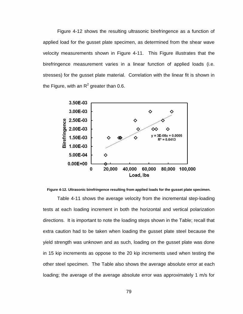
79

Figure 4-12 shows the resulting ultrasonic birefringence as a function of

applied load for the gusset plate specimen, as determined from the shear wave

velocity measurements shown in Figure 4-11. This Figure illustrates that the

birefringence measurement varies in a linear function of applied loads (i.e.

stresses) for the gusset plate material. Correlation with the linear fit is shown in

the Figure, with an R2 greater than 0.6.

Figure 4-12. Ultrasonic birefringence resulting from applied loads for the gusset plate specimen.

Table 4-11 shows the average velocity from the incremental step-loading

tests at each loading increment in both the horizontal and vertical polarization

directions. It is important to note the loading steps shown in the Table; recall that

extra caution had to be taken when loading the gusset plate steel because the

yield strength was unknown and as such, loading on the gusset plate was done

in 15 kip increments as oppose to the 20 kip increments used when testing the

other steel specimen. The Table also shows the average absolute error at each

loading; the average of the average absolute error was approximately 1 m/s for

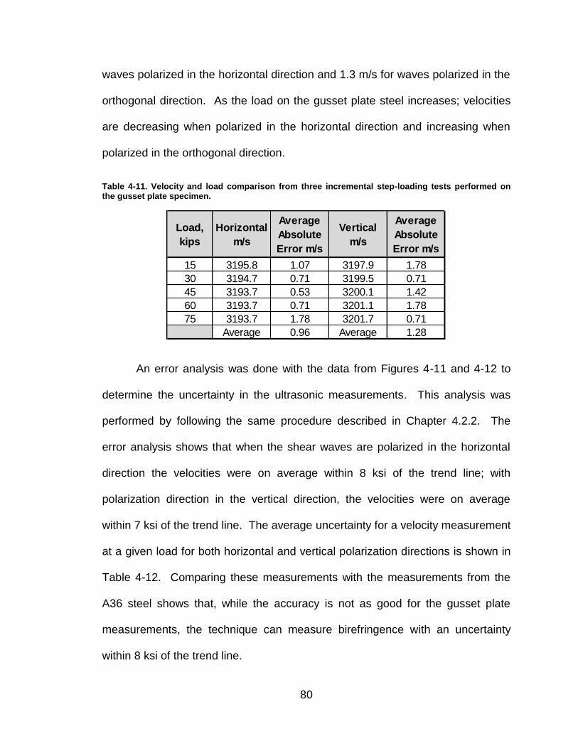
80

waves polarized in the horizontal direction and 1.3 m/s for waves polarized in the

orthogonal direction. As the load on the gusset plate steel increases; velocities

are decreasing when polarized in the horizontal direction and increasing when

polarized in the orthogonal direction.

Table 4-11. Velocity and load comparison from three incremental step-loading tests performed on the gusset plate specimen.

An error analysis was done with the data from Figures 4-11 and 4-12 to

determine the uncertainty in the ultrasonic measurements. This analysis was

performed by following the same procedure described in Chapter 4.2.2. The

error analysis shows that when the shear waves are polarized in the horizontal

direction the velocities were on average within 8 ksi of the trend line; with

polarization direction in the vertical direction, the velocities were on average

within 7 ksi of the trend line. The average uncertainty for a velocity measurement

at a given load for both horizontal and vertical polarization directions is shown in

Table 4-12. Comparing these measurements with the measurements from the

A36 steel shows that, while the accuracy is not as good for the gusset plate

measurements, the technique can measure birefringence with an uncertainty

within 8 ksi of the trend line.

Load,

kips

Horizontal

m/s

Average

Absolute

Error m/s

Vertical

m/s

Average

Absolute

Error m/s

15 3195.8 1.07 3197.9 1.78

30 3194.7 0.71 3199.5 0.71

45 3193.7 0.53 3200.1 1.42

60 3193.7 0.71 3201.1 1.78

75 3193.7 1.78 3201.7 0.71

Average 0.96 Average 1.28

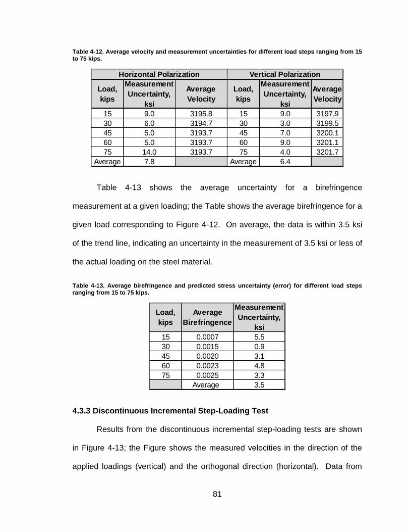
81

Table 4-12. Average velocity and measurement uncertainties for different load steps ranging from 15 to 75 kips.

Table 4-13 shows the average uncertainty for a birefringence

measurement at a given loading; the Table shows the average birefringence for a

given load corresponding to Figure 4-12. On average, the data is within 3.5 ksi

of the trend line, indicating an uncertainty in the measurement of 3.5 ksi or less of

the actual loading on the steel material.

Table 4-13. Average birefringence and predicted stress uncertainty (error) for different load steps ranging from 15 to 75 kips.

4.3.3 Discontinuous Incremental Step-Loading Test

Results from the discontinuous incremental step-loading tests are shown

in Figure 4-13; the Figure shows the measured velocities in the direction of the

applied loadings (vertical) and the orthogonal direction (horizontal). Data from

15 9.0 3195.8 15 9.0 3197.9

30 6.0 3194.7 30 3.0 3199.5

45 5.0 3193.7 45 7.0 3200.1

60 5.0 3193.7 60 9.0 3201.1

75 14.0 3193.7 75 4.0 3201.7

Average 7.8 Average 6.4

Horizontal Polarization Vertical Polarization

Load,

kips

Measurement

Uncertainty,

ksi

Average

Velocity

Load,

kips

Measurement

Uncertainty,

ksi

Average

Velocity

15 0.0007 5.5

30 0.0015 0.9

45 0.0020 3.1

60 0.0023 4.8

75 0.0025 3.3

Average 3.5

Load,

kips

Average

Birefringence

Measurement

Uncertainty,

ksi

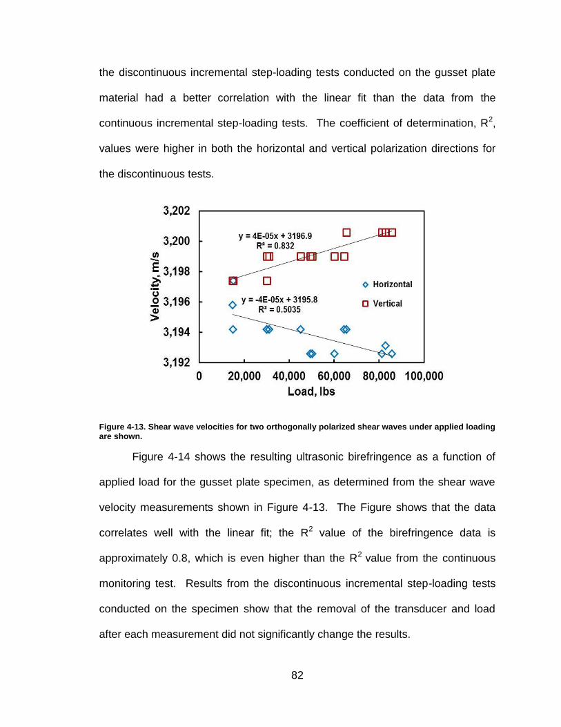
82

the discontinuous incremental step-loading tests conducted on the gusset plate

material had a better correlation with the linear fit than the data from the

continuous incremental step-loading tests. The coefficient of determination, R2,

values were higher in both the horizontal and vertical polarization directions for

the discontinuous tests.

Figure 4-13. Shear wave velocities for two orthogonally polarized shear waves under applied loading are shown.

Figure 4-14 shows the resulting ultrasonic birefringence as a function of

applied load for the gusset plate specimen, as determined from the shear wave

velocity measurements shown in Figure 4-13. The Figure shows that the data

correlates well with the linear fit; the R2 value of the birefringence data is

approximately 0.8, which is even higher than the R2 value from the continuous

monitoring test. Results from the discontinuous incremental step-loading tests

conducted on the specimen show that the removal of the transducer and load

after each measurement did not significantly change the results.

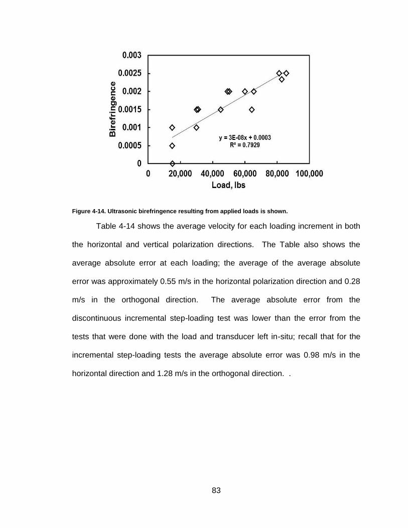
83

Figure 4-14. Ultrasonic birefringence resulting from applied loads is shown.

Table 4-14 shows the average velocity for each loading increment in both

the horizontal and vertical polarization directions. The Table also shows the

average absolute error at each loading; the average of the average absolute

error was approximately 0.55 m/s in the horizontal polarization direction and 0.28

m/s in the orthogonal direction. The average absolute error from the

discontinuous incremental step-loading test was lower than the error from the

tests that were done with the load and transducer left in-situ; recall that for the

incremental step-loading tests the average absolute error was 0.98 m/s in the

horizontal direction and 1.28 m/s in the orthogonal direction. .

84

Table 4-14. Velocity and load comparison from the discontinuous incremental step-loading tests performed on the gusset plate steel specimen.

An error analysis was conducted with the data from the discontinuous

incremental step-loading test in the same manner described in Chapter 4.2.2

above. The analysis revealed that the average uncertainty for wave velocities

polarized transversely to the load axis was 5 ksi. A shear wave polarized

coincidently with the stress axis would be within 2 ksi of the given loading. The

stress uncertainties from the discontinuous incremental step-loading tests are

better than the uncertainties from the test when the load and transducer were left

in-situ for the duration of the test. Table 4-15 shows the velocity and

measurement uncertainties at a given loading increment.

Table 4-15. Average velocity and measurement uncertainties for different load steps ranging from 15 to 75 kips.

Load,

kips

Horizontal

m/s

Average

Absolute

Error m/s

Vertical

m/s

Average

Absolute

Error m/s

15 3195.8 1.10 3197.4 0.00

30 3194.2 0.00 3198.5 0.71

45 3193.1 0.71 3199.0 0.00

60 3193.7 0.71 3199.5 0.71

75 3192.8 0.24 3200.6 0.00

Average 0.55 Average 0.28

15 8.7 3195.8 15 1.0 3197.4

30 3.0 3194.2 30 4.6 3198.5

45 6.2 3193.1 45 0.6 3199.0

60 6.2 3193.7 60 4.2 3199.5

75 1.6 3192.8 75 0.5 3200.6

Average 5.1 Average 2.2

Horizontal Polarization Vertical Polarization

Load,

kips

Measurement

Uncertainty,

ksi

Average

Velocity

Load,

kips

Measurement

Uncertainty,

ksi

Average

Velocity

85

The average uncertainties from the birefringence measurements

corresponding with Figure 4-14 was under 3 ksi as shown in Table 4-16; the

Table shows the average birefringence for a given loading as well as the average

uncertainty in each measurement for each loading increment. The average

uncertainty from the discontinuous incremental step-loading test is very similar to

the uncertainty from the incremental step-loading tests. Results from this test

indicate that the method of removing and subsequently replacing the load and

transducer after each measurement does not significantly alter results.

Table 4-16. Average birefringence and measurement uncertainty (error) for different loading steps ranging from 15 to 75 kips.

4.3.4 Single Loading Test

Three arbitrary loads were selected for the single loading test done on the

gusset plate steel specimen, including: 15, 45 and 75 kip loadings. There were a

total of 24 separate measurements made at each loading; 12 measurements

were made with the shear wave polarized transversely to the stress axis, and 12

more measurements were made in the orthogonal direction giving a total of 72

separate measurements. Figure 4-15 shows the results of the 72 separate

measurements; the Figure shows velocities for a given loading as well as the

15 0.0005 3.7

30 0.0013 2.3

45 0.0018 1.7

60 0.0018 3.2

75 0.0024 3.1

Average 2.8

Load,

kips

Average

Birefringence

Measurement

Uncertainty,

ksi

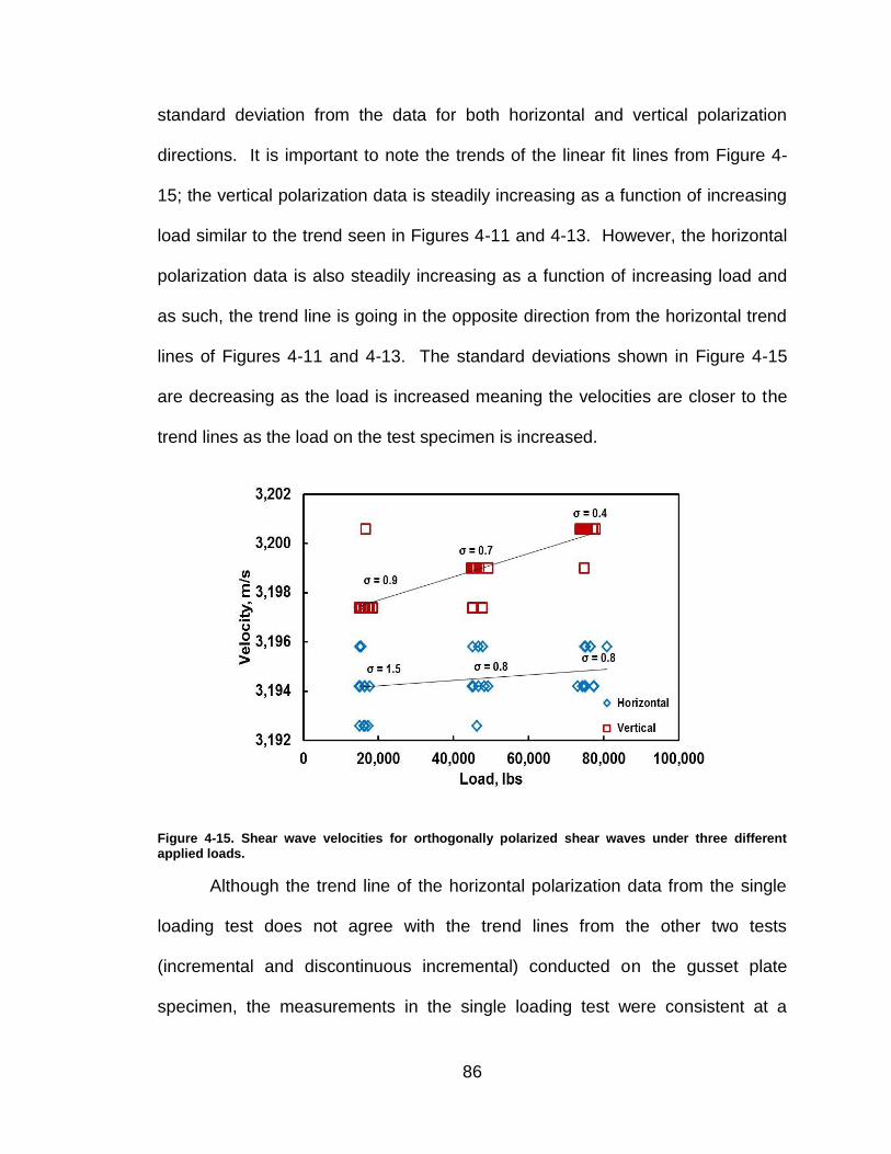
86

standard deviation from the data for both horizontal and vertical polarization

directions. It is important to note the trends of the linear fit lines from Figure 4-

15; the vertical polarization data is steadily increasing as a function of increasing

load similar to the trend seen in Figures 4-11 and 4-13. However, the horizontal

polarization data is also steadily increasing as a function of increasing load and

as such, the trend line is going in the opposite direction from the horizontal trend

lines of Figures 4-11 and 4-13. The standard deviations shown in Figure 4-15

are decreasing as the load is increased meaning the velocities are closer to the

trend lines as the load on the test specimen is increased.

Figure 4-15. Shear wave velocities for orthogonally polarized shear waves under three different applied loads.

Although the trend line of the horizontal polarization data from the single

loading test does not agree with the trend lines from the other two tests

(incremental and discontinuous incremental) conducted on the gusset plate

specimen, the measurements in the single loading test were consistent at a

87

single loading. Table 4-17 shows the range of velocities at a given loading; the

range of velocities shown in the table is considerably less than the range of

velocities from the same test done on the A36 steel (as shown in Table 4-8).

Also shown in the table are the standard deviations for the velocity

measurements made at each loading increment.

Table 4-17. The range of velocities for both polarization directions is shown for all loads of the single loading test corresponding to Figure 4-15.

Figure 4-16 shows the standard deviation for all 72 measurements from

the single loading test conducted on the steel specimen; the Figure confirms

what is shown in Table 4-17 in that the results were consistent for a given

loading. The average standard deviation for each set of measurements at a

given loading was approximately 0.86 m/s; meaning for a single measurement,

we would expect the velocity to be within 0.86 m/s of the average velocity 66% of

the time. Furthermore, 94% of the data fell within +/- 2 standard deviations, i.e.

the data fell within 1.9 m/s of the mean 94% of the time.

Velocity

Range, m/s

Standard

Deviation

Velocity

Range, m/s

Standard

Deviation

15 4.8 1.5 3.2 0.9

45 3.2 0.8 1.6 0.7

75 1.6 0.8 1.6 0.4

Load,

kips

Horizontal Vertical

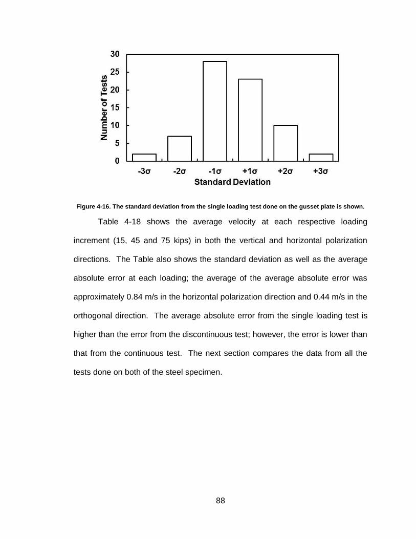
88

Figure 4-16. The standard deviation from the single loading test done on the gusset plate is shown.

Table 4-18 shows the average velocity at each respective loading

increment (15, 45 and 75 kips) in both the vertical and horizontal polarization

directions. The Table also shows the standard deviation as well as the average

absolute error at each loading; the average of the average absolute error was

approximately 0.84 m/s in the horizontal polarization direction and 0.44 m/s in the

orthogonal direction. The average absolute error from the single loading test is

higher than the error from the discontinuous test; however, the error is lower than

that from the continuous test. The next section compares the data from all the

tests done on both of the steel specimen.

89

Table 4-18. Velocity and load comparison from the single loading tests performed on the gusset plate steel specimen.

4.4 Discussion

When comparing test results between the A36 and gusset plate steel

specimen it is important to note that the texture directions were not aligned in the

same orientation during loading procedures. The A36 steel was loaded in the

traditional loading machine with its texture direction orthogonal to the load axis

and the gusset plate specimen was loaded with texture direction coincident to the

load axis as shown in Figure 4-17. Rotating the texture direction causes the

direction of fast and slow velocities to rotate also. For example, for the

incremental step-loading test, the wave polarized in the horizontal direction was

the fast wave in the A36 plate whereas the vertically polarized wave was the fast

wave in the gusset plate. Thus it is important to keep the texture directions in

mind when comparing results between the two test materials.

Velocity,

m/s

Standard

Deviation

Average

Absolute

Error m/s

Vertical

m/s

Standard

Deviation

Average

Absolute

Error m/s

15 3194.2 1.5 1.07 3197.7 0.9 0.49

45 3194.5 0.8 0.67 3198.6 0.7 0.60

75 3194.9 0.8 0.78 3200.5 0.4 0.24

Average 1.0 0.84 Average 0.7 0.44

Horizontal Polarization Vertical Polarization

Load,

kips

90

Figure 4-17. The texture directions were set in the loading machine in different directions for the A) A36 and B) gusset plate steel specimen.

Table 4-19 shows the results from all three tests done on both steel

materials; the Table shows the R2 values as well as the trend line equations for

both the horizontal and vertical wave polarization directions. It is important to

note that, though the steel specimens were loaded in the loading machine with

their respective texture directions aligned differently, their trend line equations

have similar trends. All of the tests show that waves polarized perpendicular

(horizontal) to the load axis decrease in velocity as loading is increased and all

the waves polarized in the parallel (vertical) direction increase with increasing

loading; however, the horizontally polarized wave from the single loading test on

the gusset plate was an exception to this trend.

Another trend that arises from Table 4-19 is the coefficient of

determination, i.e. the R2 values, for waves polarized in the horizontal direction.

For each test on both steel specimens, the R2 value for the horizontal polarization

91

direction is always less than the R2 value from the vertical polarization direction.

Furthermore, when waves are polarized in the horizontal direction, the coefficient

of determination does not exceed 0.5 for any of the tests. The reason the

coefficient of determination values are consistently low for waves polarized in the

horizontal direction is because of the small change in velocities (when compared

to the vertically polarized waves). Recall, that the coefficient of determination is

a statistical measure that predicts future outcomes based on the related

information within a data set. Since the waves polarized in the horizontal

direction have a very small slope (see Figures 4-3 and 4-6), it is hard to predict

the future outcomes. For example, notice the data from the horizontally polarized

shear waves in Figure 4-6; the Figure shows shear wave velocities for both the

horizontal and vertical polarization directions. The horizontal data points are

scattered above and below the trend line without much change in slope, whereas

the vertical data points are consistently increasing in velocity as load is

increased. Based on Figure 4-6, one could reasonably predict the velocity of a

wave polarized in the vertical direction at an arbitrary load. However, it would be

much harder to predict the velocity of a wave polarized in the horizontal direction

because of the scatter within the data. It is for this reason that the R2 values are

much lower for waves polarized in the horizontal direction; and as such, it is hard

to predict future outcomes based on the information in the horizontal data set.

92

Table 4-19. A comparison of the results from all three tests done on both steel specimens is shown.

Although the coefficient of determination is consistently low for waves

polarized in the horizontal direction, all horizontally polarized waves show a

similar trend. As the load on the specimen is increased, waves polarized in the

horizontal direction tend to decrease in velocity. The results of the tests between

the A36 and gusset plate steel specimen shows that consistent and repeatable

results can be obtained with ultrasonic birefringence.

Horizontal Vertical Horizontal Vertical Horizontal Vertical

R2 0.30 0.86 0.04 0.85 0.03 0.221

Trend

Line

y=-9E-

6x+3221.9

y=3E-

5x+3213.9

y=-3E-

6x+3220.3

y=3E-

5x+3213.2

y=-1E-

5x+3219

y=4E-

5x+3210.6

Horizontal Vertical Horizontal Vertical Horizontal Vertical

R2 0.29 0.38 0.50 0.83 0.06 0.71

Trend

Line

y=-

0.04x+3196.0

y=0.05x+319

7.5

y=-4E-

5x+3195.8

y=4E-

5x+3196.9

y=1E-

5x+3194

y=5E-

5x+3196.8

Discontinuous

Incremental Step LoadingIncremental Step Loading

Incremental Step LoadingDiscontinuous

Incremental Step Loading

A36 Steel

Gusset Plate Steel

Single Loading

Single Loading

93

5. Conclusions

Initial testing of ultrasonic acoustic birefringence as a stress measurement

technique to evaluate the adequacy of steel gusset plates has been completed.

Experimental measurements discussed in this paper included illustrating the

effect of texture and applied loading on the ultrasonic velocity of polarized shear

waves. Birefringence was measured in steel specimens by timing the transit of a

wave polarized parallel to the direction of applied force, and the transit of a

second wave polarized orthogonal to the direction of applied force. Results from

the experimental measurements demonstrate that the birefringence effect is

measurable in the steel specimens tested, indicating that the ultrasonic acoustic

birefringence approach as a stress measurement tool has potential to be used as

a means of assessing actual stresses in gusset plates. Data analysis from the

experimental measurements has yielded the following results:

Accuracy and variability of the methodology was evaluated by applying a

series of tests to each steel specimen and determining the uncertainty in

each measurement in terms of ksi. These tests led to the following

conclusions:

94

For the A36 steel specimen, in the continuous monitoring

scenario, the uncertainties of the measurements were within

an average of 5.5 ksi of the applied stress in the plate.

For the A36 steel specimen, in the intermittent monitoring

scenario, the uncertainties of the measurements were within

an average of 6 ksi of the applied stress in the plate.

For the gusset plate steel specimen, in the continuous

monitoring scenario, the uncertainties of the measurements

were within an average of 7.5 ksi of the applied stress in the

plate.

For the gusset plate steel specimen, in the intermittent

monitoring scenario, the uncertainties of the measurements

were within an average of less than 4 ksi of the appliedl

stress in the plate.

Precision of the methodology was evaluated by applying a series of tests

to each steel specimen. These tests led to the following conclusions:

For the A36 steel specimen, in the single loading test, the

average absolute error was not more than 2 m/s.

For the gusset plate steel specimen, in the single loading

test, the average absolute error was not more than 1 m/s.

The testing conducted in this research indicates uncertainties of 7.5 ksi or

less, or 15-20% of yield strength for typical steel. Current load rating procedures

for gusset plates assume uncertainties in loading of 30 to 50% or greater, such

95

that the results from this research indicate that the technology has the potential

to be a useful tool in evaluating the adequacy of gusset plates by assessing the

stresses in the plate. The results from the ultrasonic measurements assess the

stress (or strain) relative to an unstressed state, and as such, the measurements

could be used to assess the actual stresses in the plate, including dead load, live

load and residual stresses. Future work will take the results presented herein

and use them to implement the methodology for application of the approach in a

complex stress field so that the effects of dead load, live load and residual

stresses within the gusset plate can be resolved and the adequacy of the plate

can be evaluated.

96

References

1. Board, N.T.S., Collapse of I-35W Highway Bridge Minneapolis, Minnesota August 1, 2007. 2008, National Transportation Safety Board: Washington DC. p. 178.

2. III, J.A.W. I-35W Bridge (Old) Former I-35W Mississippi River Crossing Minneapolis, MN. Highways, Byways and Bridge Photography; Webpage]. Available from: http://www.johnweeks.com/i35w/ms16.html.

3. M. C. H. Yam, J.J.R.C., Behavior and design of gusset plate connections in compression. Journal of Constructional Steel Research, 2002: p. 17.

4. Administration, F.H., Adequacy of the U10 and L11 Gusset Plate Designs for the Minnesota Bridge No. 9340. 2008, Turner-Fairbank Highway Research Center. p. 20.

5. Astaneh-Asl, A. PROGRESSIVE COLLAPSE OF STEEL TRUSS BRIDGES,THE CASE OF I-35W COLLAPSE. in 7th International Conference on Steel Bridges,. 2008. Guimarăes, Portugal,.

6. Crowder, B. Definition of Progressive Collapse. 2005 March 21, 2005.

7. Lozev, M.G., J. Alfred V. Clark, and P.A. Fuchs, Application of Electromagnetic-Acoustic Transducers for Nondestructive Evaluation of Stresses in Steel Bridge Structures. 1996, Virginia Transportation Research Council: Charlottesville, VA. p. 37.

8. Group, V.P., Measurement of residual stresses by the hole drilling* strain gage method. 2010, Vishay Precision Group. p. 19-33.

9. Francois, M., J.M. Sprauel, and C.F. Dehan, Handbook of Measurement of Residual Stresses, ed. D.J. Lu. 1996: The Fairmont Press, Inc. 238.

10. He, B.B., Two-Dimensional X-Ray Diffraction. 2009, Hoboken, NJ, USA: Wiley.

97

11. LLC, E.A.G. X-ray Diffraction (XRD). 2012 [cited 2012; Available from: http://www.eaglabs.com/techniques/analytical_techniques/xrd.php?utm_source=google&utm_medium=cpc&utm_campaign=XRD&gclid=CIDTtODotq0CFYHAKgodAGdymA.

12. Schajer, G., Advances in Hole-Drilling Residual Stress Measurements. Experimental Mechanics, 2010. 50(2): p. 159-168.

13. Stewart, D.M., K.J. Stevens, and A.B. Kaiser, Magnetic Barkhausen noise analysis of stress in steel. Current Applied Physics, 2003: p. 308-311.

14. Technologies, A.S. Barkhuasen Noise Analysis (BNA).

15. Jr., A.A.d.S. and D.E. Bray, Comparison of Acoustoelastic Methods to Evaluate Stresses in Steel Plates and Bars. Journal of Pressure Vessel Technology, 2002. 124(3): p. 354-358.

16. Hughes, D.S. and J.L. Kelly, Second-Order Elastic Deformation of Solids. Physical Review, 1953. 92(5): p. 1145-1149.

17. Murnaghan, F.D., Finite deformation of an elastic solid. Applied mathematics series. 1951, New York: Wiley. 140 p.

18. Allen, D.R., et al., The Use of Ultrasonics to Measure Residual Stresses. Research Techniques in Nondestructive Testing, 1983. VI: p. 151-209.

19. Rayleigh, J.W.S. and R.B. Lindsay, The theory of sound. 1945, New York: Dover Publications.

20. Hellier, C., Handbook of nondestructive evaluation. 2001: McGraw-Hill.

21. Biot, M.A., The Influence of Initial Stress on Elastic Waves. Journal of Applied Physics, 1940. 11(8): p. 522-530.

22. Thompson, R.B., J.F. Smith, and S.S. Lee, Absolute determination of stress in textured materials. 1983. Medium: X; Size: Pages: 16.

23. E., S., Ultrasonic birefringence effect—Its application for materials characterisations. Optics and Lasers in Engineering, 1995. 22(4–5): p. 305-323.

98

24. Gokhale, S.A., Determination of applied stresses in rails using the acoustoelastic effect of ultrasonic waves, in Texas A&M. 2007, Texas A&M University

25. Santos, A.A., et al., Evaluation of the Rolling Direction Effect in the Acoustoelastic Properties for API 5L X70 Steel Used in Pipelines. ASME Conference Proceedings, 2004. 2004(46792): p. 85-90.

26. Bergman, R.H. and R.A. Shahbender, Effect of Statically Applied Stresses on the Velocity of Propagation of Ultrasonic Waves. Journal of Applied Physics, 1958. 29(12): p. 1736-1738.

27. Clark, A.V., et al., Ultrasonic Measurement of Stress in Pin and Hanger Connections. Journal of Nondestructive Evaluation, 1999. 18(3): p. 103-113.

28. A, A., Effect of texture and stress on acoustic birefringence. Scripta Metallurgica, 1984. 18(8): p. 763-766.

29. Goebbels, K. and S. Hirsekorn, A new ultrasonic method for stress determination in textured materials. NDT International, 1984. 17(6): p. 337-341.