UG Laboratory Manual

Megnad Saha C. V. Raman S. Ramanujan

S. N. Bose J. C. Bose

S. S. Bhatnagar S. Chandrashekar

H. J. Bhabha H. Chandra V. Sarabhai

Physics LaboratoryManual

AUGUST 2012

PHYSICS LABORATORY MANUALPH1005-Physics Laboratory

FOR USE BY

B.E. (Regular & PTDC) Students

OFSHRI G. S. INSTITUTE OF TECHNOLOGY & SCIENCE,

INDORE

PREPARED BY

FACULTY MEMBERS

DEPARTMENT OF APPLIED PHYSICS

AUGUST - 2012

Preface

This Laboratory Manual provides the theory of the experiments, the circuit diagram, methodology,observation table etc. for the experiments to be performed in the first and second semester of B.E.Programme of Shri Govindram Seksaria Institute of Technology & Science, Indore.This manual gives necessary details to perform the experiments. The experiments included are meantto offer basic understanding of Physics. Most of the experiments are designed to go hand – to – handwith the theoretical courses on Physics being taught during the first and second semesters.Some additional experiments away from the theory courses are added to enhance the scope of learningbeyond the subjects covered in the theory. The necessary theory for this type of experiments isdescribed in the manual in self-explanatory manner. However, all efforts are made to clarify any doubtby the teachers engaging these laboratory classes.We thankfully acknowledge the support, contributions and suggestions received from present and pastFaculty members and Research Scholars of Department of Applied Physics. Special thanks to Prof.P. Sen, Prof. S. Kumbhaj, N. Oswal, G. G. Soni, V. Kaushik, K. Choudhary, J. Solanki, K. Kumawat,Om P. Choudhury, A. Tripathi, L. Jain, D. Malviya and A. Pal, for content evaluation of this manual.

Dr. J . T. Andrews Dr. P. K. SenDepartment of Applied Physics,

Shri G S Institute of Technology & Science, Indore.

August 2012

ii

iii

Following symbols are used in the margin for enhanced understanding.The symbol and meaning are:

Some interesting information may be useful to you.

Extra care needed, since these experiments work at high voltage (≈ 20V - 20kV).

Read the corresponding instruction(s) carefully.

These experiments are performed with lasers. Save your eye from direct viewing.

You may need to use desktop computers for these experiments. Do not work withunnecessary work with it. USE IT ONLY FOR THE PURPOSE FOR WHICH ITIS DEDICATED.

These are some additional questions may be asked during viva-voce as well asin end exam. CAUTION: But these are some sample questions only. Read andperform more for more questions and understanding.

SGSITS, Indore Department of Applied Physics

Contents

General Instructions 1

1 To determine the wavelength of sodium light by Newton’s rings method. 5

2 To study the Variation of magnetic field along the axis of a circular coil carryingcurrent and to calculate the radius of the coil. 12

3 To measure the numerical aperture of given optical fiber 14

4 To determine the frequency of AC Mains with the help of Sonometer. 18

5 To study and measure the resolving power of given telescope. 22

6 To measure Planck’s constant using light emitting diodes (LED) and to obtain VIcharacteristics of junction diodes. 27

7 To determine the variation of refractive index of an equilateral prisms as a functionof wavelength. 31

8 CUPS & PhET 34

9 To study the relationship between the length, tension and mass of a string and thefrequencies of standing waves on a string using Melde’s method. 41

10 To study the Dispersion by a triangular prism and to verify the laws of refractionusing Raytrace. 45

11 To study the features of a CRO. Measurement of voltage and frequency of a givensignal and to measure an unknown frequency using Lissajous figures. 49

12 To understand and confirm HeisenbergŠs uncertainty principle using single slit diffrac-tion. 53

13 To understand the phenomena of electrical equivalent of heat, to measure the electri-cal equivalent of heat of water and to measure the efficiency of a given incandescentlamp. 58

14 To determine the wavelength of prominent spectral lines of mercury light by a planetransmission grating using normal incidence. 62

15 To measure the charge to mass ratio of electron using Thomson method and to findthe sign charge of electron. 69

16 To understand Error and Analysis in Physics Laboratory measurements. 73

A CRO 76

2 Color Tables 80

3 Some useful data and information 81

4 Brief History of Indian Nobel Laureates 83section

1

General Instructions

1. Objectives of Physics Labo-ratory

The laboratory component of your physics coursehas many objectives. Some important ones are:

Experience with scientific apparatus: Thisranges from being able to read instrument scales,to know safety hazards, to effectively use specificpieces of equipment, to use computer for few vir-tual experiments.

Data analysis: How do you assess whethertheory and experiment are in agreement? Youwill become familiar with the formal proceduresassociated with data analysis such as propaga-tion of errors and linear regression analysis. Ifrequired, you may use a spreadsheet on the lab’spersonal computers for data analysis.

Communication skills: To learn how to presentyour results in a report. Guidelines are given be-low.

Physical concepts: The lab should reinforcethe physics from your lecture courses.

2. Ground Rules

Attendance You must attend each laboratoryperiod and do the assigned experiment. In gen-eral, you will not be permitted to do your exper-iments in another day / class.

Preparation Before each laboratory class youare expected to read the experimental write-upand any related sections of the text so that youare familiar with the theory and the experimentalprocedure. As it is often impossible to have thelaboratory come after the relevant material hasbeen discussed in lecture, you will often have toread ahead in your textbook. If the write-up hasprelab questions, those must be understood be-fore coming to the laboratory for performing theexperiments.

Conduct Academic discussions is allowed whileloud talking and disruptive behavior are prohib-ited.

Partners Generally, you will work with one ortwo partners. Rotate the experimental tasks sothat each partner becomes familiar with all as-pects of the experiments, e.g., do not have onepartner take all the data while the other does allthe recording or analysis.

Data Sheets Each partner must have his orher own data sheets. The data sheets may comefrom the writeup, a ray diagram printout, or youmay have to write up your own data sheets. Allnecessary data should be on these data sheets.All data (single item and tabulated) should beclearly labeled with a description of the numberand its units, and when appropriate, its uncer-tainty. If you use the ray diagram printout, putdate at the top and put data labels and units atthe top of each column - you can do this by hand.

The data sheets should be initialed by theinstructor at the end of the period. Thisis not a guarantee that the performance inthe lab was adequate, though the instructorshould check that the data appears reason-able. Graphs made in the lab during theexperiment make it much easier to detecterrors or omissions. Guard the data sheet –it is the only proof that you performed theexperiment.

Repeating All or Part of the ExperimentIf the instructor finds a report unacceptable, youmay not get a chance for repeating the experi-ment, hence perform the experiment carefully.

Checking Out If you finish early, begin prepar-ing the laboratory report. In some cases, you maybe able to finish it in class. Clean up your area,leaving it as you found it, unless specified other-wise. Groups coming after you should expect tofind all the equipment in working order. If some-thing broke during your experiment, report it tothe instructor so a replacement can be made.

1

Contents 2 Contents

Laboratory Exam Two viva-voce examina-tions will be held. First viva-voce will be heldafter you complete the third experiment. Whilethe second viva-voce will be on your sixth ex-periment. However, it will be announced in theNotice-Board of Physics Laboratory.

3. Laboratory Guidelines

You should take care that the data you obtainis the best possible. Make graphs of the datawhile you are in the lab and compare them withother groups’. Show them to the instructor. Doall the calculations in the lab, including the erroranalysis. Before you leave the lab, you shouldknow whether the theory and experiment are inagreement.

4. The Report

Your lab write-ups are to be turned in at the be-ginning of the following lab session. It shouldcontain the following information:

The right hand side pages of the notebookmay contain the following:

• Name of the experiment,

• The date on which the experiment is per-formed and the serial number of the exper-iment

• Aim(s) of the experiment

• Apparatus required,

• brief theory of the experiment

• Procedures for performing the experimentand

• Results

The left hand side pages (unruled pages)may contain diagram, tables, other observationsand calculations.

Usage of rough notebook and pencil for tak-ing data is strictly prohibited in Physics labo-ratory. If a data taken is found to be wrong,just make a cross mark on the data and pro-ceed further. If a set of data is found wrong,make a new table and record data again.

Calculations , including Error analysis: When-ever possible calculations should be done in thelab. Include in your calculations the units as-sociated with any variable and, where appropri-ate, cancel units or change them to derived units(e.g., change kg·m/s2 to N). Describe and showall work.

Graphs, when appropriate, should include a ti-tle, and axis labels with units. These should alsobe done in the lab, if possible. If straight line fit-ting is performed on the data, by hand rememberto record the slope and intercept and their uncer-tainties. The graph sheets must be pasted firmlyon the note book. Just putting the graph sheetsin between the pages is not allowed.

Conclusions: This should include a brief dis-cussion of the main findings. For example: "Wefound that there is a linear relationship betweenthe measured variable . . . and . . . This can beseen from the graph and is predicted by the the-ory." Also state whether your results agree withexpectations to within the uncertainties of themeasurements: For example: "The slope of thegraph of . . . versus . . . as determined by (linearregression, hand fitting) was . . .±. . . (units).This value, together with Eqn. . . . , and themeasured quantities . . . =. . .±. . . (units), and. . . =. . .±. . . (units), allowed for a determina-tion of . . . =. . .±. . . (units). This is within . . .standard deviations of the accepted value of . . .(units)." Discuss the main sources of error. "Themain sources of uncertainty in the determinationof . . . are . . . ."

Students are advised to strictly follow thesafety regulations necessary for performingthe experiments.


Contents 3 Contents

5. List of Experiments & Labo-ratory Layout

Please, note that you have to perform theexperiment in the following order only. Stu-dents may not be allowed to perform theexperiment if he/she is not adhering to thisorder.

Common to All: Error analysis in Physics Labo-ratory. Common to all students. To be performedon the first day of the laboratory course.

1. To determine the wavelength of sodium lightby Newton’s rings method.

2. To study the Variation of magnetic fieldalong the axis of a circular coil carrying cur-rent and to calculate the radius of the coil.

3. To measure the numerical aperture of givenoptical fiber.

4. To determine the frequency of AC Mainswith the help of Sonometer.

5. To study and measure the resolving powerof given telescope.

6. To measure Planck’s constant using lightemitting diodes (LED) of various colors andto understand work function.

7. To determine the variation of refractive in-dex of an equilateral prisms as a functionof wavelength.

8. To understand upper level physics using soft-ware “ Consortium for Upper-Level PhysicsSoftware” with Quantum Mechcanics andElectro-magnetism modules and to studyworking of laser using PhET Module.

9. To study the relationship between the length,tension and mass of a string and the fre-quencies of standing waves on a string us-ing Melde’s method.

10. To study the Dispersion by a triangular prismand to verify the laws of refraction usingRaytrace.

11. To study the features of a CRO. Measure-ment of voltage and frequency of a givensignal and to measure an unknown frequencyusing Lissajous figures.

12. To understand and confirm Heisenberg’s un-certainty principle using single slit diffrac-tion.

13. To understand the phenomena of electricalequivalent of heat, to measure the electricalequivalent of heat of water and to measurethe efficiency of a given incandescent lamp.

14. To determine the wavelength of prominentspectral lines of mercury light by a planetransmission grating using normal incidence.

15. To measure the charge to mass ratio ofelectron using Thomson method and to findthe sign charge of electron.


Contents 4 Contents

En

tran

ce

Dark Room

Dark Room

Teacher

Lab

Tec

hnic

ian Black Board

1

14

9

5

6

712

4

10

6

2

3

15

8

Semi-

1

13

11

12

Figure 1: Layout of location of different exper-iments in Physics Laboratory. Check the listof experiments given in the above list to findlocations.


1 Interference by Newton’s rings Method

1.1 Objective

To determine the wavelength of sodium light byNewton’s rings method.

1.2 Short Biography of Sir Is-sacNewton

Sir Isaac Newton, FRS (4 January 1643 - 31March 1727) was an English physicist, mathe-matician, astronomer, natural philosopher, alchemist,and theologian and one of the most influentialmen in human history. His Philosophie NaturalisPrincipia Mathematica, published in 1687, is con-sidered to be among the most influential booksin the history of science, laying the groundworkfor most of classical mechanics. In this work,Newton described universal gravitation and thethree laws of motion which dominated the sci-entific view of the physical universe for the nextthree centuries. Newton showed that the mo-tions of objects on Earth and of celestial bodiesare governed by the same set of natural laws bydemonstrating the consistency between Kepler’slaws of planetary motion and his theory of gravi-tation, thus removing the last doubts about helio-centrism and advancing the scientific revolution.

In mechanics, Newton enunciated the principlesof conservation of both momentum and angularmomentum. In optics, he built the first practi-cal reflecting telescope and developed a theory ofcolour based on the observation that a prism de-composes white light into the many colors whichform the visible spectrum. He also formulated anempirical law of cooling and studied the speed ofsound.

In mathematics, Newton shares the credit withGottfried Leibniz for the development of the dif-ferential and integral calculus. He also demon-strated the generalized binomial theorem, devel-oped the so-called "Newton’s method" for ap-proximating the zeros of a function, and con-tributed to the study of power series.

Figure 1.1: A portrait of Isaac Newton (aged46) by Godfrey Kneller in 1689. The inset isthe signature of Newton.

Newton’s stature among scientists remains at thevery top rank, as demonstrated by a 2005 surveyof scientists in Britain’s Royal Society asking whohad the greater effect on the history of science,Newton or Albert Einstein. Newton was deemedthe more influential. Newton was also highly reli-gious (though unorthodox), producing more workon Biblical hermeneutics than the natural sciencehe is remembered for today.

1.3 Apparatus required

An optical arrangement for Newton’s rings witha plano-convex lens of large radius of curvature(nearly 100 cm) and an optically plane glass plate,A short focus convex lens, sodium light source.Traveling microscope, magnifying lens, readinglamp and a spherometer.

1.4 Description of apparatus

The experimental apparatus for obtaining the New-ton’s rings is shown in the Figure 1.2. A plano-convex lens L of large radius of curvature is placedwith its convex surface in contact with a plane

5

Expt. 1. Newtons’s Rings 6 1.5. Working Principle

glass plate P. At a suitable height over this com-bination, is mounted a plane glass plate G inclinedat an angle of 45 degrees with the vertical. Thisarrangement is contained in a wooden box.

Light from a broad monochromatic sodium sourcerendered parallel with the help of convex lens L1

is allowed to fall over the plate G, which partiallyreflects the light in the downward direction. Thereflected light falls normally on the air film en-closed between the plano-convex lens L, and theglass plate P. The light reflected from the upperand the lower surfaces of the air film produce in-terference fringes. At the center the lens is incontact with the glass plate and the thickness ofthe air film is zero. The center will be dark asa phase change of π radians is introduced dueto reflection at the lower surface of the air filmas the refractive index of glass plate P (µ=1.5) ishigher than that of the air film (µ = 1). So this isa case of reflection by the denser medium. As weproceed outwards from the center the thickness ofthe air film gradually increases being the same allalong the circle with center at the point of con-tact. Hence the fringes produced are concentric,and are localized in the air film (Figure 1.4) Thefringes may be viewed by means of a low powermicroscope (traveling microscope)Mas shown inthe figure. 1.3.

1.5 Working Principle

When a plano-convex lens of large radius of cur-vature is placed with its convex surface in contactwith a plane glass plate P a thin wedge shapedfilm of air is enclosed between the two. The thick-ness of the film at the point of contact is zeroand gradually increases as we proceed away fromthe point of contact towards the periphery of thelens. The air film thus possesses a radial sym-metry about the point of contact. The curves ofequal thickness of the film will, therefore, be con-centric circles with point of contact as the center(Fig. 1.4).

In Figure 1.3 the rays BC and DE are the twointerfering rays corresponding to an incident rayAB. As Newton’s rings are observed in reflectedlight, the effective path difference x between the

two interfering rays is given by:

x = 2µt cos(t+ θ) + λ/2 (1.1)

Where t is the thickness of the air film at B andθ is the angle of film at that point. Since the ra-dius of curvature of the plano-convex lens is verylarge, the angle θ is extremely small and can beneglected. The term λ/2 corresponds to a phasechange of π radians introduced in the ray DE dueto reflection at the denser medium (glass). Forair the refractive index (µ) is unity and for normalincidence, angle of refraction is zero. So the pathdifference x becomes:

x = 2t+ λ/2 (1.2)

At the point of contact the thickness of the filmis zero, i.e., t = 0, So x = λ/2. And this isthe condition for the minimum intensity. Hencethe center of the Newton’s rings is dark. Further,the two interfering rays BC and DE interfere con-structively when the path difference between thetwo is given by

x = 2t+ (λ/2) = 2nλ/2 (1.3)

or2t = (2n− 1)λ/2 [Maxima] (1.4)

and they interfere destructively when the pathdifference

x = 2t+ λ/2 (1.5)= (2n+ 1)λ/2 (1.6)

or 2t = 2nλ/2 [Minima] (1.7)

From these equations it is clear that a maxima orminima of particular order n will occur for a givenvalue of t. Since the thickness of the air film isconstant for all points lying on a circle concentricwith the point of contact, the interference fringesare concentric circles. These are also known asfringes of equal thickness.


Expt. 1. Newtons’s Rings 7 1.6. Experimental Methods

1.6 Experimental Methods

1.6.1 Calculation of the diameters rings:

Figure 1.2: Schematic of experimental setup ofNewton’s Rings. The lower image is the actualsetup used in the experiment.

Let rnbe the radius of Newton’s ring correspond-ing to a point B, where the thickness of the film ist, Let R be the radius of curvature of the surfaceof the lens in contact with the glass plate p, thenfrom the triangle CMB (Figure 1.3), we have:

R2 = r2n + (R− t)2 or r2

n = 2Rt− t2 (1.8)

Since t is small as compared to R, we can neglectt2 .and therefore

R2n = 2Rt, or 2t = r2

n/R (1.9)

If the point B lies over the nth dark ring thensubstituting the value of 2t from equation (4) wehave,

[r2n/R = 2nλ/2], or r2

n = nλR (1.10)

If Dn is the diameter of the nth ring then,

D2n = 4nRλ (1.11)

Similarly, if the point B lies over a nth order brightring we have

D2n = 2(2n− 1)λR (1.12)

1.6.2 Calculation of λ:

From equation (1.12), if Dn+p is the diameter of(n+p)th bright ring, we have

D2n+p = 2[2(n+ p)− 1]λR (1.13)

Subtracting equation (1.12) , from equation (1.13),we get :

D2n+p −Dn2 = 4pλR (1.14)

λ =D2n+p −D2

n

4pR(1.15)

By measuring the diameters of the various brightrings and the radius of curvature of the planoconvex lens, we can calculate λ from the equation(1.15).

Figure 1.3: Schematic of method used to calcu-late the diameter of lens and hence the wave-length of light used.


Expt. 1. Newtons’s Rings 8 1.7. Methodology

1.6.3 Formula used

The wavelength λ of the sodium light employedfor Newton’s rings experiment is given by:

λ =D2n+p −D2

n

4pR

Where Dn+p and Dn are the diameter of (n+p)th

and nth bright rings respectively, p being an inte-ger number. R is the radius of curvature of theconvex surface of the plano-convex lens.

1.7 Methodology

1. Level the traveling microscope table and setthe microscope tube in a vertical position.Find the vernier constant (least count) ofthe horizontal scale of the traveling micro-scope.

2. Clean the surface of the glass plate p, thelens L and the glass plate G. Place themin position as shown in Figure 1.3 and asdiscussed in the description of apparatus.Place the arrangement in front of a sodiumlamp so that the height of the center of theglass plate G is the same as that of the cen-ter of the sodium lamp. Place the sodiumlamp in a wooden box having a hole suchthat the light coming out from the hole inthe wooden box may fall on the Newton’srings apparatus such that a parallel beam ofmonochromatic sodium lamp light is madeto fall on the glass plate G at an angle of45 degrees.

3. Adjust the position of the traveling micro-scope so that it lies vertically above thecenter of lens L. Focus the microscope, sothat alternate dark and bright rings are clearlyvisible.

4. Adjust the position of the traveling micro-scope till the point of inter-section of thecross wires (attached in the microscope eye-piece) coincides with the center of the ringsystem and one of the cross-wires is per-pendicular to the horizontal scale of micro-scope.

Figure 1.4: Typical Newton’s Rings as ob-served in Physics Laboratory of SGSITS, In-dore. Courtesy Ms. K. Dudhe (PG student2007-2009).

5. Slide the microscope to the left till the cross-wire lies tangentially at the center of the20th dark ring (See Figure ) Note the read-ing on the vernier scale of the microscope.Slide the microscope backward with the helpof the slow motion screw and note the read-ings when the cross-wire lies tangentially atthe center of the 18th , 16th, 14th, 12th,10th, 8th, 6th, and 4th dark rings respec-tively [Observations of first few rings fromthe center are generally not taken becauseit is difficult to adjust the cross-wire in themiddle of these rings owing to their largewidth.]

6. Keep on sliding the microscope to the rightand note the reading when the cross-wireagain lies tangentially at the center of the4th, 6th, 8th, 10th, 12th, 14th, 16th, 18th ,and 20th dark rings respectively.

7. Remove the plano-convex lens L and findthe radius of curvature of the surface of thelens in contact with the glass plate P ac-curately using a spherometer. The formulato be used is:

R =l2

6h+h

2(1.16)

Where l is the mean distance between the twolegs of the spherometer h is the maximum heightof the convex surface of the lens from the planesurface.

1. Find the diameter of the each ring fromthe difference of the observations taken on


Expt. 1. Newtons’s Rings 9 1.8. Observations

the left and right side of its center. Plot agraph between the number of the ring onX-axis and the square of the correspond-ing ring diameter on Y-axis. It should bea straight line as given by the equation9(see figure ). Take any two points on thisline and find the corresponding values of(D2

n+p- D2n) and p for them.

2. Finally calculate the value of wavelength ofthe sodium light source using the formula.

1.8 Observations

1.8.1 Determination of the Least Count:

Determination of the Least Count of the Horizon-tal Scale of traveling Microscope

1. Value of one division of the horizontal mainscale of traveling microscope = . . . . . . . . . . . . cm.

2. Total number of divisions on the Vernierscale = . . . .which are equal to . . . . . . . . . . . .

divisions of main scale of the horizontalscale of the traveling microscope.

3. Value of one division of the Vernier scale =. . . . . . cm.

4. Least count of the horizontal scale of themicroscope (given by the value of one divi-sion of main scale – the value of one divi-sion of Vernier scale)=. . . . . . cm.

1. Pitch of the screw = . . . . . . . . . cm

2. Number of divisions on circular head = =. . . . . . . . . .

3. Least count of the spherometer = =. . . . . . . . . .cm

4. Mean distance between the two legs of thespherometer, l=. . . . . . . . . cm

5. The radius of curvature R of the plano con-vex lens is (as given by equation 1.16):

R = [l2/6h+h/2]= . . . . . . . . . cm

Tab

le1.1:

DeterminationofD

2 n+p−D

2 nan

dp

Order

.of

The

Rings

Reading

ofthe

microscop

eleft

hand

side

(a)cm

Right

hand

side

(b)

cm

Diameter

ofthering

(a∼

b)cm

.

Diameter

2

(a∼

b)2

cm2

D2 n

+p-D

2 n

forp=

4cm

2

20D

2 20-D

2 16=..

18D

2 18-D

2 14=..

16D

2 16-D

2 12=..

14D

2 14-D

2 10=..

12D

2 12-D

2 8=..

10D

2 10-D

2 6=..

8D

2 8-D

2 4=..

(1.17)


Expt. 1. Newtons’s Rings 10 1.10. Sources of errors and precautions:

Table 1.2: Determination of R (radius of cur-vature of the lens L) using a spherometerS.No

Spherometerreading on

Hcm

Mean

Planeglassplate

Convexsurfaceof lens

a ∼ b h

a (cm) b (cm) (cm) (cm)

6. The wavelength λ of sodium light is (asgiven by equation 1.15):

λ = (D2n+p- D

2n)/4pR. = . . . . . . . . . cm.

= . . . . . . . . . Angstrom units.

Calculations from the graph:

1. Plot a graph taking squares of the diame-ters, D2

nalong the Y-axis and the numberof rings along the X-axis (See Figure ).

2. The curve should be a straight line.

3. Take two points P1and P2 on this line andfind the corresponding values of D2

n+p - D2n

and p from it, calculate the value of wave-length of the sodium light from these val-ues.

1.9 Results

The value of the wavelength of the sodium lightsource as calculated

• Using the observations directly = . . . . . . . . .Ao

• Using the graphical calculations = . . . . . . . . .Ao

• Mean value of the wavelength of Sodiumlight = . . . . . . . . . Ao

• Standard average value of the wavelengthof the sodium light = 5893 Ao.

• Percentage error = . . . . . .%

1.10 Sources of errors and pre-cautions:

• The optical arrangement as shown in Fig-ure 1.2 should be very clean (use spirit forcleaning these optical elements) and so madethat the beam of light falls normally on theplano-convex lens L and glass plate P com-bination.

• The plano-convex lens used for the produc-tion of Newton’s rings should have largevalue of radius of curvature. This will keepthe angle of wedge shape air film very smalland therefore the rings will have a larger di-ameter and consequently the accuracy inthe measurement of the diameter of therings will be increased.

• To avoid any backlash error, the microme-ter screw of the traveling microscope shouldbe moved very slowly and be moved in onedirection while taking observations.

• While measuring diameters, the microscopecross-wire should be adjusted in the middleof the ring.

• The amount of light from the sodium lightsource should be adjusted for maximum vis-ibility. Too much light increases the generalillumination and decreases the contrast be-tween bright and dark rings.

1.11 Sample oral questions :

• What do you understand by the interfer-ence of light?

• What are essential conditions for obtaininginterference of light?

• What do you understand by coherent sources?

• Is it possible to observe interference patternby having two independent sources such astwo candles?


Expt. 1. Newtons’s Rings 11 1.11. Sample oral questions :

• Why should be two sources be monochro-matic?

• Why are the Newton’s rings circular?

• Why is central ring dark?

• Where are these rings formed?

• Sometimes these rings are elliptical or dis-torted, why?

• What is the difference between the ringsobserved by reflected light and those ob-served by transmitted light?

• What will happen if the glass plate is sil-vered on the front surface?

• What will happen when a little water is in-troduced in between the plano-convex lensand the plate?

• How does the diameter of rings change onthe introduction of liquid?

• Can you find out the refractive index of aliquid by this experiment?

• Is it possible to have interference with alens of small focal length?

• What will happen if the lens is cylindrical?

• Why do the rings gets closer and finer aswe move away from the center.


2 Steward & Gee’s Tangent Galavanometer

2.1 Aim

To study the Variation of magnetic field alongthe axis of a circular coil carrying current and tocalculate the radius of the coil.

2.2 History

2.3 Equipment required

Stewart & Gee’s apparatus, DC power supply,commutator, keys, connecting wires, etc.

Figure 2.1: Photography at the top showsthe Stewart-Gee’s apparatus used in SGSITS.The bottom figure is connection diagramfor performing the experiment. The insetshows the circuitry. L-lechlanche cell, Rh-Rheostat, K-key, A-Ammeter, C-commutator,S-G-apparatus, N-coil selector.

2.4 Theory

For a current I going around a circular loop ofwire of radius r, the strength of the magneticfield along the axis of the circular loop (z = 0at the center of the circular loop and is positiveabove the loop and negative below the loop) isgiven by

B(z) =µ0I

2

r2

32√r2 + z2

(2.1)

This equation assumes SI units, so the currentis in amperes, distances are in meters, and themagnetic field is in Tesla (T). The constant µ0 =4π×10−7N/A2. Notice that along the axis of thecircular loop, the magnetic field is parallel to theaxis. Its relationship to the current in the circularloop is given by a right hand rule. Curl the figuresof your right hand around the circular loop sothey point in the direction of the current; yourthumb then gives the direction of the magneticfield along the axis of the circular loop. If insteadof a single circular loop there are N turns of a coilin the form of a circular loop, then the magneticfield is simply N times the magnetic field due toa single circular loop.

If the tangent-galvanometer is set such that theplane of the coil is along the magnetic meridiani.e. B is perpendicular to BH (BH is the horizon-tal component of the Earths magnetic field), theneedle rests along the resultant. From tangentlaw, one can write,

B(z) = BH tan θ. (2.2)

orB(z) ∝ tan θ. (2.3)

That means, bu measuring the deflection in thetangent galvanometer, one can calculate the valueof magnetic filed indirectly.

From equation 2.1, the maximum value of B =Bmax = µ0I/2r occurs when z = 0. Hence thevalue of B(z) is found to be

B(r) =Bmax

2√

2= 0.35×Bmax.

sinceB(r) ∝ tan θ

B(r) ∝ 0.35× tan θmax (2.4)

12

Expt. 2. Tangent Galvanometer 13 2.6. Results

2.5 Procedure

Figure 2.2: Graph between z and tan θ. Notea horizontal line at tan.

• Use the given compass box (tangent Gal-vanometer - TG) to find the east and westdirections. (The needles of the given com-pass always show east-west direction, why?Why not the North-South as taught in book?)Now the plane of the circular coil is said tobe parallel to the magnetic meridian.

• Place the compass box exactly at the centerof the wooden sliding bench. (Why theinstrument is made of wood? Is it non-magnetic?).

• Connect all electrical wires as per the dia-gram given in Figure 2.2. First select thecircular coil between 0 and 5.

• Adjust the rheostat to generate a deflectionof about ± 70. Also note that the currentis not exceeding ...A. (Why?). Monitor thisvalue is a constant throughout the experi-ment. If the value varies adjust the rheostatto keep it constant.

• Now move the TG to on end (say 30cm)of the sliding bench. Record the corre-sponding value of (z) as -25cm in the table.Observe the value of magnetic needle andrecord it as (θ1 and θ2).

• Reverse the current using commutator andrecord the values of θ3 and θ4.

• Move the box slowly towards center around2-3cm, and record the values of θ1, θ2, θ3

and θ4.

• Repeat the previous procedure till the otherend of the sliding bench.

• Now select the circular wires at 0-10 turnsand repeat steps 5-8.

• Now select the circular wires at 0-25 turnsand repeat steps 5-8.

• Plot the data as graph between distance (z)in X-axis and tan θ in Y-axis for all threedata sets.

• Draw a straight line parallel to 0.35 tan θmax,draw two vertical lines where the two linesare crossing (see Figure 2.2).

• Find the diameter and then the radius ofcoil and report.

No of coils used:.........Value of current:........

S. distance Deflection (deg) tan θNo. z(cm) θ1 θ2 θ3 θ4 mean θ1 -242 -21– –9 0– –18 2119 24

Maximum value of tan θ =....... .

2.6 Results

1. Magnetic field along the axis of a circularcoil is studied.

2. The radius of the circular coil is found tobe ............. cm.


3 Numerical Aperture of Optical Fiber

3.1 Aim

To measure the numerical aperture of given op-tical fiber.


He-Ne or semiconductor laser, optical fiber, photodetector, translation stage, etc.

IMPORTANT : DO NOT LOOK INTOTHE LIGHT BEAM EMITTED FROMTHE LASER OR FROM THE FIBER.THIS MAY LEAD TO PERMANENTDAMAGE TO YOUR EYE.

3.3 Brief history of optical fiber

The earliest attempts to communicate via lightundoubtedly go back thousands of years. Earlylong distance communication techniques, such as"smoke signals", developed by native North Amer-icans and the Chinese were, in fact, optical com-munication links.

Jean-Daniel Colladon, a 38-year-old Swiss profes-sor at University of Geneva, demonstrated lightguiding or Total internal reflection (TIR) for thefirst time in 1841. He wanted to show the fluidflow through various holes of a tank and the break-ing up of water jets.

In 1870, John Tyndall, using a jet of water thatflowed from one container to another and a beamof light, demonstrated that light used internal re-flection to follow a specific path. As water pouredout through the spout of the first container, Tyn-dall directed a beam of sunlight at the path ofthe water. The light, as seen by the audience,followed a zigzag path inside the curved path ofthe water.

Fiber optic technology experienced a phenomenalrate of progress in the second half of the twenti-eth century. Early success came during the 1950with the development of the fiberscope. This mo-tivated scientists to develop glass fibers that in-

cluded a separate glass coating. The innermostregion of the fiber, or core, was used to transmitthe light, while the glass coating, or cladding, pre-vented the light from leaking out of the core byreflecting the light within the boundaries of thecore. Commercial applications followed soon af-ter. In 1977, both AT&T and GTE installed fiberoptic telephone systems in Chicago and Bostonrespectively. In 1990, Bell Labs transmitted a2.5 Gb/s signal over 7,500 km without regener-ation. Today, DWDM technology continues todevelop. As the demand for data bandwidth in-creases, driven by the phenomenal growth of theInternet, the move to optical networking is thefocus of new technologies.

Figure 3.1: Portaits of Jean-Daniel Colladonand John Tyndall. The bottom image showsearly TIR demonstration.

3.4 Theory

An optical fiber (or fibre) is a glass or plasticfiber that carries light along its length. Fiber

14

Expt. 3. Numerical Apertue of OF 15 3.5. Procedure:

optics is the overlap of applied science and en-gineering concerned with the design and applica-tion of optical fibers. Optical fibers are widelyused in fiber-optic communications, which per-mits transmission over longer distances and athigher bandwidths (data rates) than other formsof communications. Fibers are used instead ofmetal wires because signals travel along themwith less loss, and they are also immune to elec-tromagnetic interference. Fibers are also used forillumination, and are wrapped in bundles so theycan be used to carry images, thus allowing view-ing in tight spaces. Specially designed fibers areused for a variety of other applications, includingsensors and fiber lasers.

Light is confined in the core of the optical fiber bytotal internal reflection. This causes the fiber toact as a waveguide. Fibers which support manypropagation paths or transverse modes are calledmulti-mode fibers (MMF), while those which canonly support a single mode are called single-modefibers (SMF). Multi-mode fibers generally havea larger core diameter, and are used for short-distance communication links and for applicationswhere high power must be transmitted. Single-mode fibers are used for most communicationlinks longer than 550 metres (1,800 ft).

Joining lengths of optical fiber is more complexthan joining electrical wire or cable. The endsof the fibers must be carefully cleaved, and thenspliced together either mechanically or by fusingthem together with an electric arc. Special con-nectors are used to make removable connections.

Multimode optical fiber will only propagate lightthat enters the fiber within a certain cone (seeFigure 3.2), known as the acceptance cone of thefiber. The half-angle of this cone is called the ac-ceptance angle, θmax. For step-index multimodefiber, the acceptance angle is determined only bythe indices of refraction:

n sin θmax = NA =√n2

1 − n22, (3.1)

where n1 is the refractive index of the fiber core,and n2 is the refractive index of the cladding.

For example, taking 1.62 for n1 and 1.52 for n2,we find the NA to be 0.56. By calculating the

Figure 3.2: Demonstration of TIR in an opticalfiber.

sin−1(0.56) = 34, we determine THE CRITI-CAL ANGLE.

As this fiber accepts light up to 34 degrees off axisin any direction, we define the ACCEPTANCEANGLE of the fiber as twice the critical angle orin this case, 2×34=68.

3.5 Procedure:

Important Precaution: Do not look into the light beam emitted from the laseror from the optical fiber. It may lead topermanent damage to you eye.

IMPORTANT PRECAUTION: DO NOTLOOK INTO THE LIGHT BEAM

EMITTED FROM THE LASER OR FROMTHE FIBER. THIS MAY LEAD TO

PERMANENT DAMAGE TO YOUR EYE.

1. Switch on the laser.

2. Adjust the hight and position the opticalfiber such that light is launched into the


Expt. 3. Numerical Apertue of OF 16 3.6. Data recording:

2 4 6 80

1

2

3

Figure 3.3: Sample curves obtained at differentz. The inset shows the method to calculateFWHM w.

fiber. Use a small paper nearer to the otherend of the optical fiber to check light out-put.

3. Mount the detector nearer to the other endof the fiber, adjust the height and positionthe detector for maximum coupling.

4. Make sure that the fiber at both ends areparallel to the optical bench.

5. Place the detector nearly 1cm from the endof the optical fiber. Move the detector fromcenter to edge.

6. Move the detector towards the center, recordthe position values and intensity of light asgiven by the detector in your notebook.

7. Now move the detector around 5cm fromthe detector and repeat the initial adjust-ments for detector and measure the inten-sity profile.

8. Repeat the previous steps for six more dis-tances.

9. In a graph paper plot the Intensity alongY-axis and scan distance along X-axis.

10. To find the width of the line, draw a hor-izontal line at 50% of maximum. The in-tersection of the curve gives the diameterof the spot w (this is also known as FullWidth at Hal Maximum (FWHM)). Referto figure 3.3.

11. Record the values of spot size w at differentdistances z.

12. Plot another graph between the distance zand spot size w. Find the slope w/z.

13. The sine of slope of the curve directly givesthe Numerical aperture of the given opticalfiber. NA = sin θ = sin(tan−1w/2z).

3.6 Data recording:

z - Distance from fiber to detectorz=....cm z=....cm

Distance Intensity Distance Intensity(cm) (V) (cm) (V)0.1 .. 0.1 ..0.3 .. 0.5 .... .. .. ..3.0 .. 5.0 ..

z (cm) 1.0 5.0 ... 40w(cm) ... ... ... ...

3.6.1 Results

1. Light is coupled to an optical fiber.

2. The numerical aperture of the optical fiberis ......... .

3.7 Probable Questions

1. What is an optical fiber?

2. How numerical aperture and acceptance conecan be explained?

3. What are the sources for fabricating opticalfiber?

4. Discuss some applications of FO.

5. Is light of any wavelength can be coupledto optical fiber?


Expt. 3. Numerical Apertue of OF 17 3.8. Suggested reading

3.8 Suggested reading

1. www.lightandmatter.com (Download Bookon Optics, it is free!).

2. F. A. Jenkins and H. E. White, Fundamen-tals of Optics, (McGraw-Hill, New York,1957).

3. M. Born and E. Wolf, Principles of Optics,(Pergamon, Oxford 1986).


4 Measurement of f using Sonometer.

4.1 Aim

To determine the frequency of AC Mains with thehelp of Sonometer.

4.2 Apparatus

Sonometer with non-magnetic wire (Nichrome),Ammeter, step down transformer (2-10 Volts),Horse shoe magnet with stand, Set of 50 gmmasses, Screw gauge and meter scale (fitted withthe sonometer).

4.3 Description of the appara-tus

As shown in the given figure below, an uniformNichrome (non-magnetic) wire is stretched ona hollow wooden box (sonometer), one side ofwhich is tied to the hook, while the other passesover a frictionless pulley. A hanger carrying massesis also attached to this end of the non-magneticwire. A permanent strong horse shoe magnet iskept at the middle of the Nichrome wire in sucha way that it produces a magnetic field perpen-dicular to the direction of current, to be flownin the Nichrome wire. Two movable sharp edgedbridges A and B are provided on the wooden boxfor stretching wire. A step down transformer (2-10V) is connected across the wire.

4.4 Working Principle

Let a sonometer wire stretched under a constantload be placed in an uniform magnetic field ap-plied at the right angles to the sonometer wire inthe horizontal plane and let an alternating currentof low voltage (by means of the step down trans-former) be passed through the wire. On accountof interaction, between the magnetic field and thecurrent in the wire (F = il x B ), the wire willbe deflected. The direction of deflection is be-ing given by the Fleming’s left hand rule. As thecurrent is alternating, for half the cycle the wire

Figure 4.1: Circuit diagram for the experi-ment on determination of ac frequency usingsonometer.

will move upwards and for the next half the wirewill move downwards. Therefore the sonometerwire will receive impulses alternately in oppositedirections at the frequency of the alternating cur-rent passing through the wire. As a consequencethe wire will execute forced vibrations with a fre-quency of the AC mains (under the conditions ofresonance) in the sonometer wire.

The frequency of AC Mains, which is equal to thefrequency of vibration of the sonometer wire in itsfundamental mode (only one loop between thetwo bridges A and B, i.e., having two nodes andone antinode between the two bridges) is givenby (under resonance conditions):

n =1

2l

√T

m(4.1)

where T is the tension applied on the wire andgiven by T = Mg,M being the total mass loadedon the wire (i.e., total mass kept on the hangerand the mass of the hanger) and g the accelera-tion due to gravity. Symbol l presents the lengthof the sonometer wire between the two bridges.The mass per unit length of the sonometer wireis represented by symbol m and can be calculatedin terms of the radius r of the sonometer wire,and the density d of the material wire (Nichrome)

18

Expt. 4. Sonometer 19 4.6. Observations

asm = πr2d. (4.2)

Substitution of value of m, evaluated from theequation (4.1), in equation (4.2), gives the valueof frequency of AC mains.

4.5 Procedure

1. Measure the diameter of the wire with ascrew gauze at several points along its length.At each point two mutually perpendiculardiameters should be measured. Evaluatethe radius of the sonometer wire.[See ob-servation table (a)]

2. Connect the step down transformer to ACmains and connect the transformer output(6 Volts connection) to the two ends of thesonometer wire through a rheostat, amme-ter and a key, as shown in the figure.

3. Place the two movable sharp-edged bridgesA and B at the two extremities of the woodenbox.

4. Mount the horse shoe magnet vertically atthe middle of the sonometer wire such thatthe wire passes freely in between the polesof the magnet and the face of the magnetis normal to the length of the wire. The di-rection of current flowing through the wirewill now be normal to the magnetic field.

5. Apply a suitable tension to the wire, say byputting 100 gm masses on the hanger [ ten-sion in the wire = (mass of the hanger +mass kept on the hanger) ×g]. Switch onthe mains supply and close the key K andthen adjust the two bridges A and B tillthe wire vibrates with the maximum am-plitude (in the fundamental mode of res-onance) between the two bridges. Mea-sure the distance between the two bridges(l).[See observation table (b)]

6. Increasing the load M by steps of 50 gm,note down the corresponding values of l formaximum amplitude (in the fundamentalmode of resonance). Take six or seven suchobservations.

7. Knowing all the parameters, using the rela-tions given in equations 1 and 2 calculatethe frequency of AC mains for each set ofobservation separately and then take mean

8. Also plot a graph between the mass loaded,M along the X-axis and the square of thelength l2 along Y -axis. This graph shouldbe a straight line. Find the slope of thisline and then using the equations (4.1) and(4.1), calculate the frequency of AC mainsfrom this graph also. (Frequency =

√g/(4× slope×m))

4.6 Observations

4.6.1 Measurement of radius of sonome-ter wire (r)

Least count of screw gauge = ............. cm

Zero error of the screw gauge = .......... cm

4.6.2 Measurement of T , l and fre-quency of the AC Mains

• Mass of the hanger = 50 gm

• Acceleration due to gravity(g) = 980 cm/sec2.

• Density of sonometer wire (nichrome) =8.18848 gm/cc

• Mean value of the AC Mains frequency =.. .. ..Hz.

• Calculations from the graph are also to begiven on the left side of paper.

• The slope of graph plotted between Massloaded (M) and the square of length S =units

• AC mains frequency when calculated fromthe graph =

√g/(4× slope×m) = Hz

4.7 Results

The frequency of AC Mains as calculated


Expt. 4. Sonometer 20 4.7. Results

Tab

le4.1:

Measurementof

radius

ofsono

meter

wire(r)

S.No.

Diameter

ofwire

alon

gon

edirection.

cm

Diameter

ofwire

inCm

Mean

ob-

served

di-

ameter

cm.

mean

cor-

rected

di-

ameter

cm.

mean

ra-

dius

rcm

1. 2. 3. 4. 5.

Tab

le4.2:

Measurementof

T,l

andfreque

ncyof

theAC

Mains

S. No

Total

Mass

Load

ed=

Mass

ofha

nger

+Masson

itM

gm.

Ten

sion

inwire

T=

Mxg

Gm-

cm/s2

Position

offirst

bridge

acm

.

Position

ofsecond

bridge

bcm

l2 cm2

Leng

thof

wire

be-

tween

two

bridges

l=a-bcm

Freque

ncy

inHz

1 2 3 4 5 6 7


Expt. 4. Sonometer 21 4.9. SAMPLE ORAL QUESTIONS

A Experimental calculations : .. ±.. Hz (donot estimate the error from standard value).

B Graphical calculations : Hz (Graph is at-tached)

4.8 Sources of errors and pre-cautions

• The sonometer wire should be uniform andwithout kinks.

• The pulley should be frictionless

• The wire should be horizontal and pass freelyin between the poles of magnet.

• The horse shoe magnet should be placedvertically at the center of the wire with itsface normal to the length of wire.

• The current should not exceed one Ampereto avoid the overheating of the wire.

• The movement of bridges on the wire shouldbe slow so that the resonance point can befound easily

• The diameter of the wire must be measuredaccurately at different points in two mutu-ally perpendicular directions.

• The sonometer wire and the clamp used tohold the magnet should be non-magnetic.

4.9 SAMPLE ORAL QUESTIONS

• What do you understand by the frequencyof AC Mains?

• Distinguish between AC and DC. What isthe use of magnet here?

• How does the sonometer wire vibrate whenAC is passed through it?

• If you pass a DC through the wire, will itvibrate?

• What are the chief sources of errors in thisexperiment?

• What is the use of magnet here?

• What is Fleming’s left hand rule?

• What is resonance?

• What is fundamental mode of vibration?

• Why do we take the material of wire to benon-magnetic?

• What is the principle of this experiment?


5 Resolving power of telescope

5.1 Aim

To study and measure the resolving power of giventelescope with different size of aperture, differentwavelengths and with observation distance..


Telescope with adjustable height arrangement, stan-dard aperture, color filter, scale (1m), etc.

5.3 History of Telescope

The story of Galileo’s telescope is well known,as he recounted it himself in the Starry Messen-ger. In July 1609, Galileo was in Venice, when heheard of an invention that allowed distant objectsto be seen as distinctly as if they were nearby. InOctober 1608, a Flemish spectacle-maker by thename of Hans Lipperhey had already applied for apatent (which was refused), and news of the gad-get was widespread in Europe by the time Galileohad heard of it. Around the same time, a for-eigner turned up in Padua with the instrument;Galileo rushed back to Padua, only to learn thatthe foreigner had gone to Venice to sell his instru-ment. Galileo’s friend, Paolo Sarpi, had advisedthe Venetian government against purchasing theinstrument from the foreigner, since Galileo couldat least match such an invention. By then, Galileohad worked out the principle of the telescope andreturned to Venice himself with an eight-powertelescope. The Venetian government doubled hissalary, though Galileo felt that the original condi-tions were not honoured.

Galileo gradually improved the power of his tele-scope, grinding lenses himself, and began observ-ing the heavens. In the first two months of 1610,he was writing The Starry Messenger, and by 12March, the book was already printed at Venice,dedicated to Cosimo de’ Medici. Galileo contin-ued his observations with his telescope, some ofwhich he conveyed in ciphers to Johannes Kepler,who had already responded enthusiastically withthe Conversation with Galileo’s Sidereal Messen-

Figure 5.1: Statue of Galileo Galilei outsidethe Uffizi, Florence. The inset is a portrait ofGalileo by Giusto Sustermans.

ger. Galileo’s discovery of the ’handles’ of Sat-urn was encoded in ’Smaismrmilmepoetaleumi-bunenugttaviras’, which could be unscrambled as’Altissimum planetam tergeminum observavi’: Ihave observed the highest of the planets three-formed. Kepler deciphered this within one letteras ’Salve umbistineum geminatum Martia proles’:’Be greeted, double knob, children of Mars.’ Forthe discovery of the phases of Venus, the code’Haec immatura a me jam frustra leguntur oy’(this was already tried by me in vain too early) hidthe message, ’Cynthiae figurae aemulatur materamorum’ (The mother of lovers [Venus] imitatesthe shapes of Cynthia [the moon]). Despite thisexchange, Galileo never accepted Kepler’s ellipti-cal orbits.

From 1616, Galileo tried to apply his knowledgeof the satellites of Jupiter to the determination oflongitude at sea. In order to ensure observation atsea, the Tuscan arsenal made for Galileo a head-gear which had a telescope attached. Aroundthis time, he also designed a brass ’Jovilabe’, acomputing device for prediction positions of thesatellites. He hoped to gain support from the

22

Expt. 5. Resolving power of telescope 23 5.5. Resolving power of telescope

Spanish crown for this project, but failed.

5.4 Theory

Due to diffraction, the image of a point objectformed by an optical instrument has finite dimen-sions. It consists of a diffraction pattern, a cen-tral maximum surrounded by alternate dark andbright rings. Two point objects, are resolvable byan optical instrument if their diffraction patternare sufficiently small or are far enough apart sothat they can be distinguished as separate imagepatterns. The resolving power of an optical in-strument is defined as its ability to produce sep-arate and distinguishable images of two objectslying very close together. The diffraction effectsset a theoretical limit to the resolving power ofany optical instrument. The term resolving poweris used in two contexts.

5.4.1 Geometrical resolving power

When the purpose is to see as separate two ob-jects close together or when fine structure is seenthrough a telescope or microscope. In the case oftelescope (or eye), the resolving power is definedas the smallest angle subtended at the objectiveof the telescope (or the eye) by two point objectswhich can be seen just separate and distinguish-able. Smaller is this angle, the greater will be theresolving power of the instrument. For a micro-scope the resolving power is defined as the linearseparation which the two neighbouring point ob-jects can have and yet be observed as just sep-arate and distinguishable when seen through themicroscope.

5.4.2 Rayleigh Criterion

Lord Rayleigh has set a criterion to decide asto how close the two diffraction patterns can bebrought together such that the two images canjust be recognized as separate and distinguishedfrom each other. The criterion is applicable toboth the geometrical as well as spectroscopic re-solving powers. According to Rayleigh’s criterionthe two point sources are just resolvable by an

optical instrument when their distance apart issuch that the central maximum of the diffractionpattern of one source coincides in position withthe first diffraction maximum of the diffractionpattern of the other source. When applied to theresolution of spectral lines, this principle is equiv-alent to the condition that for just resolution theangular separation between the principle maximaof the two spectral lines in a given order should beequal to half angular width of either of the prin-cipal maximum. In this latter case, it is assumedthat the two spectral lines have equal intensities.See Fig. 5.4.2, to understand the Rayleigh crite-rion.

Figure 5.2: Demonstration of conditions ofRayleigh Criterion for resolving power (a) Wellresolved (b) just resolved and (c) unresolved.The last one does not able to differentiate thetwo lines, hence unresolved. In the present ex-periment, you will search for a condition simi-lar to (b).

5.5 Resolving power of telescope

Resolving power is the ability of the componentsof an imaging device to measure the angular sep-aration of the points in an object. The term reso-lution or minimum resolvable distance is the min-imum distance between distinguishable objects inan image, although the term is loosely used bymany users of microscopes and telescopes to de-scribe resolving power. In scientific analysis theterm "resolution" is generally used to describethe precision with which any instrument measuresand records (in an image or spectrum) any vari-able in the specimen or sample under study.

The imaging system’s resolution can be limited


Expt. 5. Resolving power of telescope 24 5.6. Procedure:

either by aberration or by diffraction. These twophenomena have different origins and are unre-lated. Aberrations can be explained by geomet-rical optics and can in principle be solved by im-proving the optical quality and cost of the sys-tem. On the other hand, diffraction comes fromthe wave nature of light and is determined by thefinite aperture of the optical elements.

The interplay between diffraction and aberrationcan be characterized by the Point Spread Func-tion. The PSF of a lens is ultimately limited bydiffraction. The lens’ circular aperture is analo-gous to a two-dimensional version of the single-slit experiment. Light passing through the lens in-terferes with itself creating a ring-shaped diffrac-tion pattern, known as the Airy pattern, if thewavefront of the transmitted light is taken to bespherical or plane over the exit aperture. Theresult is a blurring of the image. An empiricaldiffraction limit is given by the Rayleigh criterioninvented by Lord Rayleigh:

The images of two different points are regarded asjust resolved when the principal diffraction maxi-mum of one image coincides with the first mini-mum of the other. If the distance is greater, thetwo points are well resolved and if it is smaller,they are not resolved. Mathematically, this trans-lates into:

sin θ = 1.22λ

d(5.1)

where θ is the angular resolution, λ is the wave-length of light used and d is the diameter of lensaperture.

Two more point-like sources separated by an an-gle smaller than the angular resolution cannot beresolved. A single optical telescope may havean angular resolution less than one arcsecond,but astronomical seeing and other atmosphericeffects make attaining this very hard.

The angular resolution R of a telescope can usu-ally be approximated by

R =λ

d(5.2)

Resulting R is in radians with λ is the wavelengthof the source and d is the diameter of the tele-scope objective. Sources larger than the angu-lar resolution are called extended sources or dif-

fuse sources, and smaller sources are called pointsources. When a point source of diameter a andif the telescope is at a distance of D from thesource, equation 5.2 may be rewritten as

R = θ =a

D. (5.3)

Here, theta is the angular resolution.

Figure 5.3: Ray diagram of a laboratory gradetelescope. The lower image is Giant MeterwaveRadio Telescope (dish like structures) for radioastronomical research installed at Pune, India.

5.6 Procedure:

1. The axis of the telescope is made horizontalby means of spirit level and its height is soadjusted that the images of the pair of slitsare symmetrical with respect to the crosspoint of the cross wires. Make sure that thestandard chart is mounted upside down.

2. Place the telescope nearly 1m from the ob-ject.

3. The images are brought into sharp focus byadjusting the telescope.

4. Find the smallest dots which could be wellresolved by the telescope (say 5). Find the


Expt. 5. Resolving power of telescope 25 5.7. Questions

S. No. 1 2 3 4Diameter (mm) 0.10 0.15 0.20 0.25

S. No. 5 6 7 8Diameter (mm) 0.30 0.50 0.75 1.0

S. No. 9 10 11Diameter (mm) 1.5 2.0 3.0

Color Filter Red Yellow GreenWavelength (nm) 545.6 616 708

Table 5.1: Details of Standard Chart

corresponding diameter of the object fromthe chart (0.30mm) and record it.

5. Gradually increase the distance (move back-ward) between the chart and adjust thetelescope for best focus every time. Findthe place where the separation between thedots vanishes (well resolved → resolved →not resolved). The corresponding distancemay be recorded n the table. Also notedown the next smallest object resolvablefrom the chart (may be 6 or 7) and recordthe corresponding diameter.

D

S Lamp

Figure 5.4: Experimental setup for measuringthe resolving power of telescope.

6. Repeat the previous steps for all unresolvedobjects from the charts within the limita-tions of the size of laboratory.

7. The distance between the standard chart(sources) and the objective of the telescopeis measured by means of measuring tape.

8. After reaching the extreme end of the lab-oratory repeat the same procedure in theforward direction.

Figure 5.5: Standard chart used for measur-ing resolving power of telescope at SGSITS,Indore. The dimensions of the holes are givenin Table 5.1.

5.7 Questions

1. What do you mean by resolving power of atelescope?

2. On what factors does the resolving powerof a telescope depend?

3. Why are the telescopes fitted with objec-tives of large diameter ?

4. Does the resolving power of a telescope de-pend upon the focal length of its objective?

5. What is Rayleigh criterion of resolution?

6. What is the resolving power of the eye?

7. Does the resolving power of a telescope de-pend upon the distance between the tele-scope and the objects to be resolved?


Expt. 5. Resolving power of telescope 26 5.7. Questions

Table 5.2: Table for collecting data with wavelength; Distance between Telescope and Object(D) = ......... cm

Size of. radius (a) of source Unresolved Resolving Powerobjective white Red Yellow Green White Red Yellow Green(mm) (mm) (mm) (mm) (mm) Rad/sec Rad/sec Rad/sec Rad/sec1......25

Table 5.3: Table for collecting data with distance

Source Diameter Aperture size Mean (d) RPNumber (a) Increasing Decreasing (d1 + d2)/2in chart (mm) d1 (mm) d2 (mm) D (mm) Rad/sec

4 0.255 0.30–11 3.0


6 Measurement of Planck’s constant using LEDs

6.1 Aim

To measure Planck’s constant using light emit-ting diodes (LED) of various colors, to understandwork function and to obtaine VI charcateristics ofjunction diodes and Zenor diode.


LEDs of various colors (Blue, Green, Yellow, Or-ange, Red, Infrared, etc), pn junction diodes, Zenerdiode, power source, connecting wires, Volt me-ter, Ammeter etc.

6.3 Theory

6.3.1 Historical Perspectives

Max Planck (1858-1947) was born in Kiel Ger-many and attended schools in Munich and Berlin.Planck was pioneer in the field of quantum physics.Around 1900 Planck developed the concept of afundamental unit of energy, a quantum, to ex-plain the spectral distribution of blackbody radi-ation. This idea of a basic quantum of energyis fundamental to quantum mechanics of mod-ern physics. Planck received a Nobel Prize forhis work in the early development of quantummechanics in 1918. Interestingly, Planck him-self remained skeptical of practical applicationsfor quantum theory for many years.

In order to explain blackbody radiation, Planckproposed that atoms absorb and emit radiationin discrete quantities given by

E = nhν (6.1)

where:

n is an integer known as a quantum number

ν is the frequency of vibration of the molecule,and

h is a constant, Planck’s constant.

Figure 6.1: Max Planck presents Albert Ein-stein with the Max-Planck medal of the Ger-man Physical Society, June 28, 1929 in Berlin.

Planck named these discrete units of energy quanta.The smallest discrete amount of energy radiatedor absorbed by a system results from a changein state whereby the quantum number, n, of thesystem changes by one.

In 1905 Albert Einstein (1879-1955) published apaper in which he used Planck’s quantization ofenergy principle to explain the photoelectric ef-fect. The photoelectric effect involves the emis-sion of electrons from certain materials when ex-posed to light and could not be explained by clas-sical models. For this work Einstein received theNobel Prize in Physics in 1921.

Niels Bohr (1885-1962) used Planck’s ideas onquantization of energy as a starting point in de-veloping the modern theory for the hydrogen atom.Robert Millikan made the first measurement ofPlanck’s constant in 1916. The best current valuefor Planck’s constant is 6.62607554 x 10−34 Js.

6.4 Experiment

In this experiment, you will use light emittingdiodes (LED) to measure Planck’s constant. Youshould be familiar with semiconductors and diodesfrom Modern Physics. To review: LEDs are semi-conductors that emit electromagnetic radiation inoptical and near optical frequencies when a volt-

27

Expt. 6. Finding h using LED & VI study of diodes. 28 6.5. Procedure

age is applied to them. LEDs emit light only whenthe voltage is forward biased and above a mini-mum threshold value. This combination of con-ditions creates an electron hole pair in a diode.Electron hole pairs are charge carriers and movewhen placed in an electrical potential. Thus manyelectron hole pairs produce a current when placedin an electric field. Above the threshold value thecurrent increases exponentially with voltage.

A quanta of energy is required to create an elec-tron hole pair and this energy is released when anelectron and a hole recombine. In most diodesthis energy is absorbed by the semiconductor asheat, but in LEDs this quanta of energy producesa photon of discreet energy E = hν. Becausemultiple states may be excited by increasing thevoltage across a diode, photons of increasing en-ergies will be emitted with increasing voltage.Thus the light emitted by an LED may span arange of discrete wavelengths that decrease withincreasing voltage above the threshold voltage(shorter wavelength ⇒ higher energy). We areinterested in the maximum wavelength that is de-termined by the minimum energy needed to cre-ate an electron hole pair. It is numerically equalto the turn on voltage of the LED. The relationbetween the maximum wavelength, λ, and theturn on voltage, V0, is

E = hν =hc

λ= eV0 = eVthreshold (6.2)

where:

ν is the frequency of the emitted photons,

c is the velocity of light,

e is the electronic charge, and

h is Planck’s constant.

The maximum wavelength of the LED can bemeasured to a resolution of a few nanometerswith a good spectrometer. If the turn on volt-age, V0, is measured for several diodes of differentcolor (and different maximum wavelength, λ), agraph of V0 vs. 1/λ should be linear with a slopeof hc/e. An experimental value of Planck’s con-stant may then be determined by using the knownvalues of the speed of light, c, and the charge ofan electron, e.

6.5 Procedure

1. Common procedure for LEDs

(a) The circuit that will be used to experi-mentally determine Planck’s constantis illustrated in Figure 6.2.

+ --

V

A

Figure 6.2: Circuit diagram and experimentalsetup for measuring Planck’s constant.

(b) Connect any one LED (say red) tothe circuit. The wire color almostmatches with the color emitted by LED.

(c) Put the multimeter to 10mA mode.(d) Make sure that the knobs of power

supply are at the lowest. Switch onthe power supply and check the volt-age is zero.

(e) Slowly increase the voltage and ob-serve the corresponding change in thecurrent value.


Expt. 6. Finding h using LED & VI study of diodes. 29 6.6. Questions

(f) Record the voltage (from power sup-ply) and current values in your notebook.

(g) Now change the connections to an-other LED.

(h) Repeat steps 2-7 for all LEDS andrecord your data.

(i) Now plot V-I characteristics of all LEDS.

BreakdownReverse Forward

Figure 6.3: Sample V-I characteristic of a junc-tion diode, note that the scale used +ve and -veaxes are not same. The middle one shows theLED VI curve of LED. Find Vo by extrapolat-ing the data. The last graph shows the linearfit of data V0 vs 1/λ.

(j) Find the threshold voltage (V0 for eachone of them, by extrapolating the lin-

Diode No. λ (nm)Ultraviolet LED-1 401

Blue LED-2 454Green LED-3 505Yellow LED-4 514Orange LED-5 596Red LED-6 647

Infrared LED-7 942

Zener Diode D-1 —Si Diode D-2 —Ge Diode D-3 —

Table 6.1: Wavelength and color of LED

ear part of the cruve to x-axis as shownin figure 6.3.

(k) If possible plot all LEDS in the samegraph sheet.

(l) Record the values of λ, 1/λ and cor-responding V0 in another table.

(m) Plot another graph of V0 vs 1/λ. Makea straight line fit to the data.

(n) The slope of the graph is hc/e. Findthe Planks constant by multiplying theslope with e/c.

2. Common Procedure for junction and Zenerdiodes

(a) Connect the junction diodes similar toan LED

(b) increase the voltage across the pn junc-tion of diodes

(c) Record the values of current and volt-age.

(d) Once the saturatu

(e) In a third graph sheet plot the VI char-acteristics (use both +ve and -ve axesof X and Y)

(f) Report the result with error calcula-tion from the standard value of

6.6 Questions

1. What is photoluminescent?


Expt. 6. Finding h using LED & VI study of diodes. 30 6.6. Questions

S. No. LED λ 1/λ V0

Color (nm) (nm)−1 (Volt)1 IR2 Red3 Orange4 Yellow5 Green6 Blue7 UV

Table 6.2: Data from the V-I plots for LEDs.

2. What is a LED?What is Laser Diode? Whatis Photoelectric effect?

3. Which LED has the highest work function(W0)? Explain what does this mean.

4. Choose one of your LEDs, then calculatethe final velocity of an electron as it travelsacross the LED point gap. How would thisvelocity change with color? (Hint: KEmax =qV o = 1

2mv2)

5. If the point gap approximates 1.0 mm, cal-culate the acceleration (v2 = 2ad) of theelectron and the time t to cross the gap.What vector field supplies the acceleratingforce?

Color

ofLE

DJu

nction

Diode

sUV

-.-.-

IRSi-D

iode

Ge-diod

eZe

ner

Voltage

Current

Voltage

Current

Voltage

Current

Voltage

Current

Voltage

Current

Voltage

Current

(V)

(m/µ

)A(V

)(m

/µ)A

(V)

(m/µ

)A(V

)(m

/µ)A

(V)

(m/µ

)A(V

)(m

/µ)A

0.01

—-

0.01

—-

0.01

—-

0.01

—-

0.01

—-

0.01

—-

0.02

—-

0.02

—-

0.02

—-

0.02

—-

0.02

—-

0.02

—-

–—-

–—-

–—-

–—-

–—-

–—-

3.0

—-

2.0

—-

1.0

—-

-0.01

-0.xx

-0.01

—-

-1.0

—-

–—-

–—-

–—-

–—-

–—-

–—-

–—-

–—-

–—-

-4.0

—-3.0

—-

-5.0

-3.8

Tab

le6.3:

Recordof

V-I

data

forLE

Ds.

Draw

tensets

ofsimila

rtables

forthesevenLE

Dsan

dthreediod

es.Fo

rjunc

tion

andzene

rdiod

esthe

voltagean

dcu

rrentvalues

may

betakenas

negativeforreversebias.

The

values

show

nin

thetables

areforindicative

purposeon

ly.


7 Dispersive power of prism

7.1 Aim

To determine the variation of refractive index ofan equilateral prisms as a function of wavelength.


Spectrometer, Mercury gas discharge tube, Prism,reading lens, table lamp, etc.

7.3 Theory

When light propagates through a dense transpar-ent medium (e.g. glass) the interaction varieswith the wavelength of the light. The responsecan be described classically in terms of the re-sponse of N oscillators each of massme and eachhaving an electric charge q. The outcome is a for-mula - a dispersion equation - for the refractiveindex n(ω), where ω is the angular frequency ofthe incident light defined as

n(ω)2 = 1 +Nq2

ε0me

1

(ω2o − ω2)

. (7.1)

Here, εo is the vacuum permittivity and ωe isthe oscillator (in present case it is prism) naturalfrequency of oscillation. Recasting the disper-sion equation as an explicit function of λ, whereω = 2π/λ, we can write

n = α+ β/λ2 (7.2)

where α and β are constants for the glass, theirvalues being in the region of 1.6 and 10−10cm2,respectively, for many types of glass. This is theequation of a straight line (y = mx + c), forwhich m/c = λ2

o. The prism spectrometer canused to measure the refractive index at a givenwavelength using the formula

n =sinA+δm

2

sin(A/2)(7.3)

where A is the prism angle and δm is angle of min-imum deviation for that wavelength. The spec-trometer is a precision instrument and is easilycapable of measuring the refractive to an accu-racy of four significant figures.

Figure 7.1: Experimental setup to measure thedispersive power of prism. XYZ is the prism,1, 2, 3 are the adjustment screws of prismtable. Light enters the collimator and leavesthrough the telescope.

Figure 7.2: Successive views as the turntable isrotated through the angle of minimum devia-tion. Measure the angles when you see Position-3 as shown here.

31

Expt. 7. Dispersive power of prism 32 7.4. Procedure:

7.4 Procedure:

7.4.1 Spectrometer Setup

1. Remove prism from the turntable.

2. Bring the spectrometer outside the darkroom.

3. Position the instrument so that the tele-scope can be pointed at some distant ob-ject (e.g. the end of the corridor or towardsthe vehicle parking area).

4. Adjust the eyepiece of the telescope (it slidesin and out) until the cross wires are in fo-cus.

5. Focus the telescope on the distant object.

6. Once the focus is clear, you will not bedisturbing the telescope through outthe experiment. Bring the spectrometerinside the dark room.

7. Position the instrument on the laboratorytable - ensure that you can see through thetelescope when it is at least 60 to eitherside of the principal axis of the collimator.

8. Position a mercury vapor lamp close to theslit at the end of the collimator.

9. Rotate the telescope so that it faces thecollimator and you can observe the slit im-age. Adjust the collimator only until theslit image is in focus.

10. Adjust the slit width until its image is justwider than the cross wires.

7.4.2 Turntable Setup

1. The rotation axis of the turntable should beperpendicular to the plane containing theprincipal axes of the telescope and collima-tor.

2. Place a prism on the centre of the turntablesuch that one face is approximately perpen-dicular to a line joining level adjustmentscrews 1 and 2.

3. Adjust the height of the turntable until thecollimator is centred on the vertical dimen-sion of the prism.

4. Rotate the turntable and telescope until arefracted slit image is observed. If the im-age is not in the centre of the ield of view,the refracting edge of the prism is not par-allel to the axis of rotation of the telescopeand the turntable will need to be levelledusing a sprit level (if required you may con-tact Lab Technician).

5. Rotate turntable and telescope so that areflected slit image can be observed fromface XY. Adjust screw 2 until the reflectedslit image is in the centre of the ield of view.

6. Rotate turn table (but not the telescope)so that a reflected slit image can be ob-served from face YZ. Adjust screw 3 untilthe reflected slit image is in the centre ofthe field of view.

7.4.3 Measurement of δmin.

1. Rotate the turntable and telescope untillight will pass approximately symmetricallythrough the prism (see Figure 7.3)

2. Rotate the telescope until the successionof views shown in Figure 7.3 is observed asthe turntable is rotated consistently in thesame direction. Record the angle of thetelescope from both windows (V1 and V2).

3. Rotate the turntable by approximately 120degrees so that the refracting edge of theprism is pointing in the opposite direction.

4. Rotate the telescope until light will pass ap-proximately symmetrically through the prism.

5. Rotate the telescope until the succession ofviews shown in Figure 10.2 is observed asthe turntable is rotated consistently in thesame direction. Record the angle of thetelescope from both windows (V1 and V2).

6. The angle between the two telescope posi-tions is twice the minimum deviation angleδmin.


Expt. 7. Dispersive power of prism 33 7.5. Calculations

7. Repeat steps 1-6 several times to obtaina best estimate for the minimum deviationangle δmin

8. Repeat steps 1-7 for light of different wave-lengths.

9. Record all data in Table 1.

7.5 Calculations

Figure 7.3: Graph to verify the prism equation.

1. Using equation 7.2, calculate the refractiveindex for different colors and record it inTable 2.

2. Plot a graph showing refractive index (nas ordinate and 1/λ2 as abscissa, whichshould be a straight line, the gradient ofwhich is β and the intercept on the axis isα (see Fig. 10.2).

3. Determine the values of α and β from yourgraph and compare them with the suggestedapproximate values given under "Theory"above.

7.6 Interesting Notes

Check Appendix -B for various spectrum fromlamp sources. You may need color printer or colormonitor to view the spectrum in color.

Telescope

read

ing(b)forDirectIm

age:

V1=

(b1)=

...........de

g..........min

.......sec

V2=

(b2)=...........

deg..........min

.......sec

Tab

le7.1:

Determinationofδ m

Color

Ang

leforminim

umde

viation

δ mMean

ofthe

Windo

wV1

Windo

wV2

V1

V2

line

MainSc

ale

Vernier

Total

(a1)

MainSc

ale

Vernier

Total

(a2)

(a1∼b 1)

(a2∼b 2)

δ m

Red

Yellow

Blue

Violet


8 Consortium for Upper-Level Physics Software

8.1 Aim

To understand upper level physics using software“ Consortium for Upper-Level Physics Software”with QuantumMechcanics and Electro-magnetismmodules and to study working of laser using “PhET”Laser Module.


PC, CUPS software with appropriate modules.

8.3 CUPS- Brief Introduction

The Consortium for Upper-Level Physics Soft-ware (CUPS) has developed a comprehensive se-ries of nine Book/Software packages that havebeen published by Wiley. CUPS is an interna-tional group of 27 physicists, all with extensivebackgrounds in the research, teaching, and de-velopment of instructional software, that havebeen carefully developing this series over the last4 years.

All of the computer simulations have been pro-vided in executable form and, although they canbe run without reading the text, the text is nec-essary to achieve an understanding of the under-lying physics and for exploring alternative waysto use the programs. The individual chaptersand computer programs cover “mainstream” top-ics that are found in the standard textbooks foreach course. However, because they are intendedto be used as supplementary texts, there are top-ics missing that the standard texts would include.

8.3.1 General Features of CUPS

The simulations are extremely flexible, they canbe used by everyone from the undergraduate physicsmajor to a Ph.D physicist. They can provide an

understanding of basic principles, yet are sophisti-cated enough for explorations of new ideas. Theycan also be used as a source for lecture demon-strations, or to create computer models for thetesting of physics theories.

Each chapter of the text provides a large numberof exercises which can be assigned as homeworkor serve as the basis for student projects.

The Pascal source code has been provided for allprograms and a number of exercises suggest spe-cific ways the programs can be modified; rangingin difficulty from the alteration of a single proce-dure to extensive additions for ambitious projects.The intent is to develop physical intuition and adeeper understanding of the physics, not compu-tational skills.

The simulations are programs that include com-plex, often realistic, calculations of models of var-ious physical systems, and the output is usuallypresented in the form of graphical (often ani-mated displays.

Many of the simulations can produce numericaloutput—sometimes in the form of output filesthat could be analyzed by other programs. Theuser generally may vary many parameters of thesystem, and interact with it in other ways to studyits behavior in real time. The use of the termsimulation should not convey the idea that theprograms are bypassing the necessary physics cal-culations, and simply producing images that look"more or less" like the real thing.

The simulations will complement the analyticalwork in each course in a manner that is mutuallyreinforcing. Considerable analytical work is nec-essary to modify the programs or to really under-stand the results of a simulation—an importantuse of the simulations is to suggest conjecturesthat may then be verified, modified, or falsifiedanalytically.

34

Expt. 8. CUPS - Upper Level Physics & PhET 35 8.4. Theory

Figure 8.1: Schematic of an em-wave.

8.4 Theory

8.4.1 Electromagentic waves

Maxwell?s equations in free space, there is vac-uum, no free charges, no currents, J = ρ = 0,both E and B satisfy wave equation,

∇2E = ε0µ0∂2E

∂t2.

we can use the solutions of wave optics,

E(r, t) = E0 exp(iωt) exp(−ik · r),

B(r, t) = B0 exp(iωt) exp(−ik · r),

A schematic of propagation of an electro-magneticwave is exhibited in figure 8.1.

8.4.2 Basic ideas of quantummechan-ics.

Postulate 1: An isolated quantum system is de-scribed by a vector in a Hilbert space. Two vec-tors differing only by a multiplying constant rep-resent the same physical state.

• quantum state: |Ψ〉 = Σiαi|ψi〉,

• completeness: Σi|ψ〉〈ψ| = I,

• probability interpretation (projection): Ψ(x) =〈x|Ψ〉,

• operator: A|Ψ〉 = |φ〉

• representation: 〈φ|A|ψ〉,

• hermitian operator: H = H†,

• unitary operator: U U † = U †U = I.In addition to these a well-behaved wave-function satisfies three conditions, viz.,

• The wavefunction (ψ(x)) is continuous

• Its derivative also is continuous.

• It is normalizable

⇒∫ ∞−∞|ψ(x)|2dx = 1

8.4.3 Making of a LASER

LASER is an acronym for Light Amplification byStimulated Emission of Radiation. In other words,it is Coherent Light generation by the process ofLight oscillation and Stimulated Emission of radi-ation. The lasing from laser source need to satisfythe following

1. A lasing medium, cavity mirror and pump.

2. Population inversion between the lasing lev-els

3. Multiple oscillations between the cavity toenhance number of photons to achieve sta-ble operation.

The medium and pump satisfy the following con-ditions:

1. The pump energy should exactly match withthe energy gap between the two level, (incase of 2-level laser, 2LL)

2. In order to achieve the population inversionin a 2LL, the upper level shoul have verylarge life time.

3. While in a 3LL, the intermediate level needslarge life time.

4. In a 3LL population inverstion can be achievedby pumping atoms to third level directly,which is having lower life time. The stim-ulated emission can be achieved betweenthe lower and intermediate level (this levelneed to have larger life time.)

In this experiment the above mentioned ideas willbe verified and understood.


Expt. 8. CUPS - Upper Level Physics & PhET 36 8.5. Procedure & Observations

8.5 Procedure & Observations

8.5.1 QUANTUMMECHANICSMOD-ULE

1. Double click the Cups-QM batch file fromdesktop.

2. Wait till “CUPS QUANTUM MECHNAN-ICS” appear

3. Click on “One Dimensional Bound StateProblems”After reading the information press ENTERfrom keyboard

4. Parts menu -> Square well potential.(What is SWP?)

5. Parameters -> Well parameters, enterDepth= 100eV and width=0.2nm (Whatare eV and nm?)Click on VIEW, what do you see?Click OK

Figure 8.2: A CUPS window showing the cal-culated values of energy eigenvalue, ψ and |ψ|2for V = 400eV and width = 0.05nm.

6. Spectrum -> Find Eigen values (Whatdo you see here?, What are the horizontallines representing?)

7. Spectrum -> See the WavefunctionType 1, enter, what do you observe? Whatdoes the curve represent?Type 2, 3, 4, what do you observe now?What are these curves represent?Record the correspdong energy values of

each line on your notebook.Type 5 or greater number, what is the errormessage means? Does n > 4 not exist?

8. Spectrum -> Wavefun. & Prob.Repeate the previous steps and record theobservations. what are the two lines corre-sponds to?Why one of them is always positive?

9. File -> Save as -> Give file name withyour roll number.

10. Method -> Try energy values from mouse,Click the mouse at energy values correspond-ing to the previously measured positions.What do you observe? Click the mouse atvarious other locations. What do you ob-serve? What are the measuring of curvesappearing?

11. Change well depth to 25eV find energy val-ues and record, change depth to 400eV andrecord data.

12. Change well width to 0.2nm, 0.1nm and0.05nm, find the number of energy levelsand record them.If required save some of the windows.

8.5.2 ELECTRO-MAGENTISMMOD-ULE

1. Double click the Cups-EM shortcut fromdesktop.Wait till “CUPS ELECTRICITY &MAGEN-TISM SIMULATIONS” appear.Click on “Electromagentic Plane Waves”After reading the information press ENTERfrom keyboard.Find the followig shortcut keys from the toprow of the keyboard.Short cut keys: F1 - Help, F2 - Fast, F3- Slow, F4 - Stepwise, F5 - rotate, F10 -Main menu (esc key may also be used), ar-row keys for rotate tilt the observation win-dow.Use the arrow keys to understand the in-put wave, what does the two colors of theoscillations represent?



2. F10 -> SHOW WHAT -> Wave on Interface.Record the values of ε, µ and σ. Changethe value of ε = 10, click OK.What happened to the input and outputsignal?Why the input signal shows huge oscilla-tions?

Figure 8.3: A CUPS window showing the gen-eration of circularly polarised light after pass-ing through a polariser and a waveplate at anangle of 30 deg.

3. F10 -> SHOW WHAT -> Wave on Interface.Change ε = 1, µ = 10, repeat your obser-vations and answer the questions.

4. F10 -> SHOW WHAT -> Wave on Interface.Change ε = 10, µ = 10, repeat your obser-vations and answer the questions.

5. F10 -> Wave + PolaroidSet value of theta to 5 deg, click OK.Press F5 and observe the angle of polaroidshown on the left and observe the outputsignal.How the amplitude is modified? Why doesthe signal reduce?

6. F10 -> Wave + PolaroidSet value of theta to 95 deg, click OK.

7. Press F5 and observe the angle of polaroidshown on the left and observe the outputsignal.Why does the signal increase?Use left, right, up, down arrow keys, so thatthe direction of em waves are perpendicularto the surface of the monitor.Now use F5 key to rotate the angle of po-laroids. Record your observation. Why theplane of polarization changes?

8. F10 -> Wave + WaveplateSet value of theta to 5 deg, click OK.What do you observe? Are the output planepolarised? In answer is NO, what is that?Use F5 key to rotate the waveplate. AT45 deg, what do you see? For angles otherthan 45 and 135, what do you see?At 0 deg, 90deg and at 180deg what doyou understand?Use arrow keys to visulaize better. Discussyour observations and understandings.

9. F10 -> Wave + Waveplate + PolaroidSet value of polariser angle 0 and waveplateangle to 30. Observe the output.Rotate the polariser from 0 to 90. At 30deg, what is the nature of output light, isit plane polarised?Is it identical to that of input? Explain.At 60 and 90deg of polariser, observe andexplain. AT 90deg, what happened to theoutput light?

10. F10 -> Wave + Waveplate + PolaroidSet value of polariser angle 0 and waveplateangle to 45. Observe the output. Repeatthe previous set of observations.Explain how and why the situation is dif-ferent here?

Figure 8.4: A front panel of PhET windowshowing the Lamp-1, medium and power levels.

8.5.3 Making of a LASER

This part of the experiment expects the studentto understand the processes of Absorption, spon-taneous emission and stimulated emission pro-cess. Also, this module will help you understand



the process of population inversion, laser oscilla-tion, and lasing process.

1. Open the Laser module from desktop short-cut.

2. Observe various parts of the system, lo-cate find the operating with the following(i) Lamp control with intensity and wave-length, (ii) Laser power indicator, (iii) en-erg levels of the 2-L system, and (iv) otheroptions.

3. Increase the power of lamp, What do youobserve?

4. Hold the Level - 2 and drag up and down,what do you observe? At a particular valuethe atoms goes from State 1 → 2, whatdoes this mean? What is the name of thisprocess? What is the minimum require-ment here in terms of energies?

5. Now keeping the energy levels constant, ad-just the wavelength of source. What is yourobservation for what values does the atomgoes to excited states? What is the min-imum requirement here in terms of ener-gies?

6. Make pump and atom energies equal. Theatom goes to exited state in both mediumand energy level diagram. Reduce the life-time to minimum. What do you observe?The level system shows the Why does theatom is staying in the exited state (upperlevel)?

7. Increase the life time, put source power tomaximum. Click on the enable mirror (cav-ity). How many photons are trapped in thecavity. Some of them escape through thesystem, some does not, why? Is the atomgo to excited state? For how long the pho-tons are trapped in the cavity?

8. Now reduce the life time to minimum, arethe photons trapped? Explain your obser-vations?

9. Increase lifetime, disable and enable the cav-ity to trap some more photons. Reduce thereflectivity gradually from 100 to 50, recordand explain your observations.

10. Select Three level system.

11. Increase the power of Lamp 2, carefully ob-serve what is happening. Is the atom goesto levels 1, 2 and 3.

12. Reduce the lifetime level 2, where does theelectron stays? Record and explain youranswer.

13. Reduce the lifetime level 3, where does theelectron stays? Record and explain youranswer.

14. Click Waveview for lower transition. Whattype of radiation is coming out, explain.

15. Change the internediate energy level, tunewavelength of Lamp - 1 to match. Is theradiation coming out. How critical is this?What type of process is this? Why the en-ergy needs to be many degrees accuratehere?

16. Enable mirrors. Make sure that atleast twophotons of Lamp -1, are trapped and os-cillating, otherwise disable and enable mir-ror. Once stable conditions is achieved, ob-serve carefully, wait for about 20 secondsand monitor the internal power to build up.When green indicators reaches 50%, slowlyreduce the reflectivity to 90%, What do youobserved. Explain the complete process asper your understanding.

17. Wait for few seconds, why all the energydrains very fast. Repeat the previous step.Make lower transition to Photons. Whythe generated photons are always doublet.Compare the results obtained in step - 8, tothis. What is their path? Change to waveview. Reduce the refrlactivity to 99%. Howlong does the lasing continues? How toexplain the process happened in this step?

18. Make lifetime of upperlevel to maximumand for lowerlevel minimum. Explain yourobservations. What are the optimum val-ues of lifetime of levels?

19. Summarise the observations.


Expt. 8. CUPS - Upper Level Physics & PhET 39 8.7. Results

8.6 Other questions to be an-swered

Answers to the following questions need to besubmitted in the results section:

1. Use the default “square well” and study thesolutions of the Schrödinger equation byusing Method: Try energy. Choose the en-ergies 100, 150 and 200 eV and study thebehavior of the wave functions.

(a) How should the wave functions be-have according to the theory when x→∞?

(b) Do the wave functions behave as ex-pected? If not, what may be the rea-son?

(c) Study the “physically correct” energylevels and the corresponding wave func-tions by choosing Spectrum. Of thethree lowest lying wave functions, whichone(s) satisfy the condition ψ(−x) =ψ(x) (even function) and which sat-isfy ψ(−x) = −ψ(x) (odd function)?

2. Choose asymmetric well and Spectrum: Findeigenvalues. Then, choose Part 2, wavefunction properties and Psi 1 | Eigenstate,Psi 2 | Eigenstate.

(a) Check if the eigenfunctions are nor-malized to 1 and if functions corre-sponding to different energy eigenval-ues are orthogonal to each other.

(b) Choose Operator x and let CUPS cal-culate the expectation value of x forall five eigenfunctions. What is thephysical meaning of this quantity?

(c) Try to calculate the expectation val-ues: 〈V 〉 of the potential energy, 〈H〉(=〈E〉) of the total energy, 〈Ekin〉 ofthe kinetic energy, and 〈p〉 of the mo-mentum as in previous one. Noticehow the wave functions are changedwhen the different operators are ap-plied. One has to be careful aboutthe calculation of 〈Ekin〉. Can you

find the correct operator in the pro-gram, or can the expectation value becalculated in some other way? (Hint:how can the Schrödinger equation beused to find relations between energyexpectation values?) Concerning 〈p〉,is it possible to determine it using aphysical argument without any calcu-lations?

3. Choose double square well with default val-ues and let CUPS calculate the eigenval-ues. Then choose part 3: time develop-ment. Here, the time development of an ar-bitrary linear combination (superposition)of the states can be studied.

(a) Study the time development of theground state ψ1 and the superposi-tion (ψ1 +ψ2)/

√2. Describe how the

probability to find the electron in theleft and right “well” varies with time inthe two cases. Notice the time scale:fs (10−15s).

(b) Decrease the width of the middle bar-rier to half of its initial value. Howwill the time development of the su-perposition change compared to (a)?

8.7 Results

• Report all plots of wavefunction, energies,probability amplitudes

• Report all results associated with polaroids,waveplates, etc

• Report a diagram of the laser with condi-tions for laser output

• Summarise answers to all questions askedabove.

8.8 Additional Resources

• Visit the following websites for downloadsimulations and manuals.

– http://physics.gmu.edu/~cups/


http://physics.gmu.edu/~cups/

Expt. 8. CUPS - Upper Level Physics & PhET 40 8.8. Additional Resources

– http://www.compadre.org/student/items/detail.cfm?ID=7

– http://www.rose-hulman.edu/Users/groups/packets/HTML/modern/cupspg.htm

– Book: ISBN:0471548820

– http://www.rpi.edu/dept/phys/Dept2/cups/

– http://phet.colorado.edu/

• Read the following books

– Quantum Mechanics, L. I. Schiff

– Concepts of Modern Physics, A. Beiser,Tata McGraw, New Delhi 2010.

– Optics, A. Ghatak, Tata McGraw, NewDelhi, 2012.


http://www.compadre.org/student/items/detail.cfm?ID=7

http://www.compadre.org/student/items/detail.cfm?ID=7

http://www.rose-hulman.edu/Users/groups/packets/HTML/modern/cupspg.htm



http://www.rpi.edu/dept/phys/Dept2/cups/

http://www.rpi.edu/dept/phys/Dept2/cups/

http://phet.colorado.edu/

9 Standing Wave on a String

9.1 Aim

To study the relationship between the length, ten-sion and mass of a string and the frequencies ofstanding waves on a string using Melde’s method.


Massless String, pan with mass, meter scale, me-chanical wave driver / vibrator and other mechan-ical components.

9.3 Theory

A mechanical wave is a disturbance which movesthrough some medium. The apparatus used inthis experiment is shown in Figure 9.1. A 50Hz ac source supplies a sinusoidal voltage thatdrives the mechanical vibrator. A string is at-tached to the vibrator at one end, and a weighthanger at the other, stretching over the pulleywhich is clamped to a table. Ths frequency ofoscillation of the vibrator can also be found fromthe relationship

Figure 9.1: Experimental setup for generatingstanding wave pattern.

f = 1/T (9.1)

where T is the period or time for one cycle ofthe sinusoidal voltage waveform. The waveformis displayed on the oscilloscope screen. A stringthat is fixed at both ends can oscillate at variousfrequencies that are determined by the length,tension, and mass of the string. When oscillatingin this way all parts of the string undergo simple

Figure 9.2: Standing waves in a vibrationstring with four nodes.

harmonic motion at the same frequency but theamplitude varies from point to point.

The oscillating states are known as stationaryor standing waves, and the frequencies of thewaves are the natural or resonant frequencies ofthe stretched string. Standing waves may be re-garded as a superposition of propagating wavesthat are repeatedly reflected at the ends of thestring; the term standing or stationary refers tothe fact that the nodes (minima) and antinodes(maxima) of the wave remain fixed in position,as shown in Figure 2.

In Melde’s Experiment one end of a stretchedstring is attached to a vibrating support and theother end passes over a pulley to a hanging weightwhich produces tension in the string. The stretchedstring is set in motion by the vibrating support,but if the frequency of vibration is not one of thenatural frequencies of the string the vibrationalamplitude of the string is very small. However,when the frequency f of the vibrating supportis the same as one of the natural frequencies (orthe harmonics) of the string the vibrational ampli-tude will be large and will exhibit clearly definednodes and segments or loops corresponding to thestanding wave of that particular frequency. Theequations you need to analyze your data are sim-ply given here, but are derived in the textbooks.It will be helpful for you to refer to your textbook.The standing waves are not propagating but theyare the superposition of propagating waves andtheir frequency and wavelength satisfy the waverelation

fλ = v (9.2)

where v is the wave velocity on the string. Thevelocity of a transverse wave on a string that has

41

Expt. 9. Melde’s Experiment 42 9.4. Procedure:

a mass per unit length µ and is under tension T is

ν =

√T

µ(9.3)

In this discussion we are assuming that the endsof the string are fixed. The wavelengths of thestanding waves are determined by the conditionthat a whole number of half-wavelengths mustequal the length of the string. In this experimentthe length and or weight in the pan is adjusteduntil the string vibrates in segments forming astanding wave pattern. If the standing wave has nsegments (n = 4 in Figure 2) then the wavelengthµ and the string length L are related by

L = nλ/2 (9.4)orλ = 2L/n (9.5)

Combining these relations leads to

f2L

n=

√T

µ(9.6)

as the fundamental relation connecting the fre-quency of oscillation and the parameters of thestring (length, tension, mass per unit length) whenit is vibrating in a standing wave pattern with nloops. Solving for the frequency

f =n

2L

√T

µ(9.7)

The tension is provided by the weight in newtonsof the hanging mass. In this experiment, one endof the vibrating string is attached to the mechan-ical vibrator, which moves up and down a smalldistance. This end moves with the vibrator, andas a result cannot be a true node, thereby intro-ducing a systematic error. When you report yourresults you will need to consider the effects of thiserror.

9.4 Procedure:

1. Arrange vibrator, pan and string as shownin Figure 1.

2. Switch on the vibrator. Set the frequencyto 20Hz.

3. Put 50gm in the pan and adjust the lengthof wire (move vibrator) to get 2-3 loops.

4. Now adjust the length of the wire slightlyto make maximum amplitude and stablestanding wave pattern. Make sure that theoscillations are on a single plane only.

5. Record the distance L between the pulleyand vibrator, Tension T on the wire, num-ber of loops n, mass per unit length µ andfrequency f . All these five values of equa-tion 9.7 are known now.

6. Part 1 : to prove f ∝ n:

(a) Keep the values of T and L constantand record.

(b) Using equation 9.7, do calculationsfor the resonant frequency fcalc forloops 1, 2, 3, 4 ... and enter the val-ues in note book.

(c) Change the frequency to obtain therequired number of loops. Record therespective frequencies as fmeas in thenotebook.

(d) Repeat the above procedure for max-imum number of loops.

7. Part 2 : to prove f ∝ L−1:

(a) Keep the values of T and n (say n =3) constant and record.

(b) Using equation 9.7, do calculationsfor the resonant frequency for vari-ous resonant lengths for every addi-tional 2 cm and enter the values innote book as fcalc .

(c) Move the oscillator slightly to reachthe necessary value of length. Changethe frequency to obtain the requirednumber of stable loops. Record therespective frequencies as fmeas in thenotebook.

(d) Repeat the above procedure for max-imum possible length L.

8. Part 3 : to prove f ∝√T :


Expt. 9. Melde’s Experiment 43 9.5. Interesting Notes

(a) Keep the values of n and L constantand record.

(b) Using equation 9.7, do calculationsfor the resonant frequency for variousloads starying from 50gm and for ev-ery additional 5 gm and enter the val-ues in note book as fcalc .

(c) Add weight to pan. Change the fre-quency to obtain the required numberof stable loops. Record the respectivefrequencies as fmeas in the notebook.

(d) Repeat the above procedure for max-imum possible load T .

9. Plot all three sets of data in a single graphbetween for fcalc vs fmeas. Note that theit should be straight line, otherwise fit thecurve to a straight line fit.

10. Plot three other graphs for (i) fcalc vs n,(ii) fcalc vs L and (i) f2

calc vs T . Discussthe nature of curve obtained. If necesaryfit the data linearly.

9.5 Interesting Notes

1. Why do blue and yellow colors become vis-ible when objects spin or vibrate under flu-orescent lights?

You may see yellow and blue on the vi-brating string. This has to do with theway fluorescent light works. Most fluo-rescent tubes have had the air inside re-moved and replaced by a small amount ofmercury vapor and argon gas. The insideof the glass tube is coated with a whitephosphor powder. When electricity flows inthe tube, almost instantly the argon emitsblue light and the mercury vapor emits ul-traviolet. The ultraviolet light strikes thephosphor powder and after a brief delaythe phosphor re-emits yellow light. Thefamiliar white fluorescent light is due tothe combination of the two complemen-tary colors of blue and yellow light. Dueto the slight delay in the production of yel-low, there is a moment at start-up when

Table 9.1: Table for collecting dataTo show f ∝ n

Load m = ..............gLength L = ...........cmNo. of fcalc fmeasLoops (Hz) (Hz)

1 —23..10

To show f ∝ L−1

Load m = .............gLoops n = ..............

Length fcalc fmeas(cm) (Hz) (Hz)50 —55....80

To show f ∝√T

Length m = .............cmLoops n = ..............Load fcalc fmeas(g) (Hz) (Hz)50 —55....80

only blue is visible and a moment at turn-offwhen only yellow is visible. Because we usealternating current to run these lights, wego through many on-off cycles every sec-ond. This produces a repeated sequenceof blue and yellow moments. For station-ary objects these alternating colors are re-flected from the same location and persis-tence of vision causes them to combine intowhite. However, if the object changes po-sition quickly, like the vibrating string, wesee the blue reflection in a different loca-tion than the yellow reflection. Because theimages don’t overlap, our eyes do not com-bine the colors and we see separate blue and


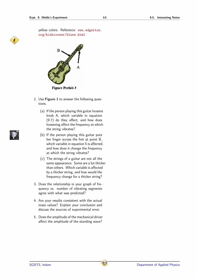
Expt. 9. Melde’s Experiment 44 9.5. Interesting Notes

yellow colors. Reference: www.edgerton.org/kidscorner/blues.html

2. Use Figure 1 to answer the following ques-tions.

(a) If the person playing this guitar loosensknob A, which variable in equation(9.7) do they affect, and how doesloosening affect the frequency at whichthe string vibrates?

(b) If the person playing this guitar putsher finger across the fret at point B,which variable in equation 5 is affected,and how does it change the frequencyat which the string vibrates?

(c) The strings of a guitar are not all thesame appearance. Some are a lot thickerthan others. Which variable is affectedby a thicker string, and how would thefrequency change for a thicker string?

3. Does the relationship in your graph of fre-quency vs. number of vibrating segmentsagree with what was predicted?

4. Are your results consistent with the actualmass values? Explain your conclusion anddiscuss the sources of experimental error.

5. Does the amplitude of the mechanical driveraffect the amplitude of the standing wave?


www.edgerton.org/kidscorner/blues.html

www.edgerton.org/kidscorner/blues.html

10 Raytracing of optical components

10.1 Aim

To study the Dispersion by a triangular prism andto verify the laws of refraction using Raytrace.

10.1.1 Apparatus Required

Ray trace software and PC

10.2 Part 1: To study the dis-persion

10.2.1 Introduction

RAYTRACE is a software, that simulates differentcomponents of an optical system, namely prisms,lenses, glass plates and different kind of sources.It enables one to manipulate the environmentalvariables, like refractive index, wavelength of lightetc. and see the effects on light rays. This soft-ware is in perfect coordination with the ideas ofray optics and hence is useful in devising opticalsystems for various operations. It has nothing todo with wave optics, however and this poses alimitation on the user in terms of use. It is in noway able to simulate wave optical phenomena.

10.2.2 Experiment

Objectives

The experiment aims at; understanding refractionfrom prism and find the angle of minimum devia-tion for a particular colour and hence finding therefractive index for that colour and comparing itwith the standard value for the material of theprism.

10.2.3 Procedure

The following steps are to be followed to attainthe objectives.

1. Click on the desktop icon of RAYTRACE.

2. As the window opens, first press S on thekeyboard and then G. You will see smalldots appearing in the window. These arecalled grid points and the whole window iscalled grid. This helps us in finding distanceand pasting objects.

3. Now click on the following menu items inthe following order Edit→ Library→ Pastefrom. A new window opens. Click on theChange Library.

4. A new window opens. You will see Conics,Lenses, Prisms etc.

5. Click on Prisms and then click on OK.

6. Now you will see a list of types of prismsunder the button Change Library. ChooseTriangle 60-60-60 from there. (It is thelast type in the list.)

7. Click on Paste. A small window opens Ray-trace: Paste element. Click the close but-ton on it.

8. Now click on the center of the screen.

9. You will see a prism on the screen. (No-tice that the three vertices of the triangu-lar cross section of the prism lie on threeof the grid points. This is the reason wepress S and G buttons of the keyboardin the step 1. If we do not do this theprism will not be having its three verticeson three grid points.)

10. Now click on the following menu items inthe following order Create → Source →Point.

11. A new window opens. Make the number ofrays 3, which you will see 10, by default.

12. Click on the boxesDrag on create andDragsymmetrically. Click OK.

13. You will see that a + sign appears on thescreen and moves with your mouse. In asmall box it is written create. This meansnow we can create rays.

45

Expt. 10. Virtual experiments 46 10.2. Prism

14. Click with this plus sign on the left of theprism, some distance apart from its base.You will see that with your click the cre-ate written in the box with the plus signchanges to aperture and a 1 appears in abox adjacent to the plus sign.

15. Drag this plus sign to the left side of thetriangle preferably to the mid-point of theside. As you drag the plus sign you willsee that an arrow appears. Make the tipof this arrow touch the mid-point of theside of the triangular prism. By doing thisyou are choosing the position where thecentral ray should incident. If you choosethis to be the mid-point of the side, youmay have a symmetric diagram, that willbe easier to handle. in other case youmay find it to be clumsy enough for mea-surement purpose.

16. As you touch the tip of the arrow to the leftside, click you mouse again. you will seethe number change from 1 to 2. Keepingmouse at the same position click again. Sothat all the rays fall on the same point

17. Click once again and you see that the plussign disappears and the three rays have beencreated. Note that you see only a singleray.

18. Click on the point from where the rays haveinitiated. You will see that the rays areselected. This is confirmed by small redrectangles appearing at the end points.

19. Now select the incident ray, then click onthe Modify button of the menu and selectRay. A window appears.

20. Click on the buttons in the following se-quence red → next → green → next →blue → OK. You will see that there arethree rays coming out. The lower most rayhas become blue, the upper most has be-come red and the ray in between is green.This means we have generated the ray ofthree colours and that is why in the previ-ous step we have said that the three rayshave been created. It is worthwhile tonote that initially the rays wer of one

Figure 10.1: Prism at angle of minimum de-viation. Note that the ray inside the prism isparallel to the base.

colour Red, so even after passing throughprism we were able to see a single ray.Now since we have made the three raysof three different colours, we see the com-mon phenomenon of dispersion of light.

21. Now you see the incident ray becomes blue,because of the sequence we have chosenthe colours. It’s nothing to worry about.Chose this ray, as you did it last time. PressF5; this draws a normal at the point of in-cidence. We will use this to measure theangle of incidence. Press F6, This extrap-olates the incident ray. this we will use tomeasure the angle of deviation.

22. Select the incident ray press F5 then F6,this will extrapolate the incident ray andthe draw normal to the incident plane.

23. Select the ray of the colour (on the otherside of the prism), for which you have tomeasure the angle of minimum deviationand press F7. This will extrapolate the outcoming ray in the backward direction. Nowyou are able to see the angle of incidenceand the angle of deviation. Refer to figure10.1

24. Strictly follow this procedure to measureangle of incidence: Click on the menu but-ton Create and select protractor, (Now mouseshows center), click the mouse at the bi-secting point of incident ray to the per-pendicular. Press E click on the startingpoint of incident ray, then go to the end ofthe tangent line and click. You will see a


Expt. 10. Virtual experiments 47 10.3. Rectangular Block

Figure 10.2: Finished raytracing of a prism.

small line showing the angle. Now you canmove the incident ray to change angle ofincidence.

25. Click on the vertex of the angle you wantto measure. Now click on one arm andthen on the other. You see an angle valueappears. This is the angle subtended.

26. Adjust the incident ray such that the angleof minimum deviation is satisfied for rayin “RED” color. Note down the angle ofincidence.

27. Use protractor to measure angle of mini-mum deviation. Refer to 10.3. Repeat theprocedure for green and red. Record yourdata in the note book.

28. Save your file with your rollnumber as filename. This my be useful for taking printout.

29. The refractive index of the material may becalculated from the formula;

µ =sin(A+δm

2

)sin A

2

(10.1)

10.3 Part 2. Verification of lawsof refraction

10.3.1 Theory

Light rays travel in straight lines in a homoge-neous medium. But whenever a light ray passes

from one transparent medium to another, it de-viates from its original path at the interface ofthe two media. In the second medium the ray ei-ther bends towards the normal to the interface oraway from the normal. The bending of the light-ray from its path in passing from one medium tothe other medium is called ŚrefractionŠ of light.If the refracted ray bends towards the normal rel-ative to the incident ray, then the second mediumis said to be ŚdenserŠ than the first medium. Butif the refracted ray bends away from the normal,then the second medium is said to be ŚrarerŠthan the first medium.

The refraction of light takes place according tothe following two laws known as the Ślaws of re-fractionŠ:

1. The incident ray, the refracted ray and thenormal to the interface at the incident pointall lie in the same plane.

2. For any two media and for light of a givencolour (wavelength), the ratio of the sineof the angle of incidence to the sine of theangle of refraction is a constant.

If the angle of incidence is i and the angle ofrefraction is r, then

sin i

sin r= constant = n (10.2)

10.3.2 Procedure

1. Open New file. In order to make a rectan-gular block follow this procedure.

2. Select Create → Element → Region

3. Mouse will be changed to START. You haveto make Click at any point on the screen,move horizontally to 10 grid points, then godown six points, go horizontally backwards10 points, then go up six points. Now youmight have reached the start point. Rightclick the mouse and click on Finished. Youwill see a blue colored rectangular box now.

4. Select Create menu and select Ray. Themouse change to START. Start a ray from


Expt. 10. Virtual experiments 48 10.4. Results

Figure 10.3: Finished raytracing of a rectangu-lar block.

the top side and allow the ray to fall theupper side of the block at some angle. Leftclick the mouse and select Finished. Nowthe ray might be making refraction and pass-ing though the block.

5. Select the incident ray and press F2 then f5.you might see reflected rays and the Normaldrawn from the incident planes. If required,click on the reflected rays and reduced thelength by dragging the end points to ap-propriate length.

6. Measure the angle of incidence and refrac-tion as discussed in the previous procedure.

7. Now select the rectangular region, selectModify → Element → Refractive Index.Change the refractive index of red colourto 1.00. Is θi = θr? Why?

8. Now change the refractive index of red colourto 2.00, find the values of θi and θr.

9. Record all values of angles in the table.

10.4 Results

1. Raytracing of a prism and a rectangularblock is done with a PC.

2. Laws of reflection and refraction are veri-fied.

Table 10.1: Observation Table for Raytracingwith a prism. Angle of the prism = A = 60

Color θi δm µ =sin(A+δm

2 )sin A

2

RedGreenBlue

Table 10.2: Observation Table for Raytracingwith a rectangular block. Angle of the prism:60

Refractive θi θr µ =sin θisin θr

index1.51.02.0


11 Measurement of V & f using CRO

11.1 Aim

To study the features of a CRO. Measurementof voltage and frequency of a given signal and tomeasure an unknown frequency using Lissajousfigures.

11.2 Introduction

A cathode ray oscilloscope can be used to mea-sure the voltage and frequency of given unknownsignal. (A brief description of CRO is given at theend of this manual as Appendix-A). A RC oscil-lator can be used to generate an electrical signalof desired frequency and amplitude. In the givenexperiment the RC oscillator has to be used togenerate the signal and the CRO will be used tomeasure its voltage and frequency.

11.3 Procedure

11.3.1 Preparing the CRO

Before switching on the CRO, set the controlswitches as follows:

1. FOCUS control to mid-position

2. Y-POSITION control to mid-position

3. X-POSITION control to mid-position

4. Y-gain to 1 V/DIV with the VARIABLE toCAL (calibrated) position

5. Time base to 5 ms/DIV or 10 ms/DIV withthe VARIABLE to CAL (calibrated) posi-tion

6. TRIG MODE selector to AUTO and LEVELcontrol to mid-position

7. Source selector INT/EXT to INT

8. Slope selector +/- to +

9. AC/GND/DC selector to DC

Figure 11.1: The Cathode ray oscilloscope andfunction generator used in Physics Laboratory,SGSITS.

Alter the controls to get a sharp line in the centreof the screen. Turn the brightness to about halfand set the channel you wish to use to A.C. Ifthere is no spot or line visible, make sure the time-base is turned on and the stability control turnedfully to one side (clockwise). If this does notproduce the spot or line, the trigger level couldbe set too low.

Figure 11.2: Schematic of internal wirings of aCRO.

11.3.2 Selection of frequency

The RC oscillator is having several knobs, whichcan be used to select frequency of the signal to be

49

Expt. 11. C R O 50 11.4. Lissajous Figures

generated. In the top left hand corner you wouldsee three knobs. These knobs can be used to se-lect frequency value, which can be represented bythree digits. For example, suppose you are set-ting the left knob to 6, the middle knob to 5 andthe extreme right knob to 4. Then the selectedfrequency will be 654Hz. below these three knobsyou will get a multiplier. The multiplier will mul-tiply the above selected frequency. Thus if youselect 654Hz and multiplier position is 10 thenthe overall frequency will be 6540Hz.

11.3.3 Selecting amplitude of the sig-nal

The RC oscillator provides you option to vary thevoltage of the signal to be generated. This canbe done using two voltage selecting knobs (Fineand Coarse). Therefore, using different knobs asignal of given amplitude and given frequency canbe generated by the RC oscillator. This signalcan now be used as an input to the CRO and itsfrequency and voltage can be measured.

Figure 11.3: Sample Lissajous Figures for fre-quency ratio as mentioned in the figures.

11.3.4 Voltage Measurements

Use the signal generated by RC oscillator as aninput to CRO. Place the Y amplifier in propervalue. From vertical scale measure the peak to

peak value. This will give the value of peak topeak voltage of the signal.

11.3.5 Calculation of frequency

Adjust your waveform so that you are able tocount the number of divisions for one wavelengthof your trace. Count the number of divisions (x)and obtain from the time-base control, the valuefor ’time per division’ (ms/div) and (t). Note,1ms = 1 ×10−3s.

Period of oscillation by (T = xt)=...........Frequency of oscillation by (f = 1/T ) = ...........Compare your value to that set on your signalgenerator.

11.4 Lissajous Figures

When two simple harmonic motions are plottedagainst each other at right angles, the resultingconfiguration is called a Lissajous figure. Simpleharmonic motions plotted against time gives si-nusoidal configurations. Two sinusoidal electricalinputs given to an oscilloscope will give a Lis-sajous pattern on the screen. The particular pat-tern depends upon the frequency, amplitude andphase of the applied inputs.

The frequency ratio of the inputs may be deter-mined from an analysis of the Lissajous figureproduced. If a Lissajous figure is enclosed in arectangle whose sizes are parallel to the forma-tion axes of the figure, the frequency ratio of thetwo inputs may be determined by counting thepoints of tangency to the sides of the rectangleenclosing the pattern. Once the frequency ratiois known, the input frequency can also be deter-mined from the same.


Expt. 11. C R O 51 11.4. Lissajous Figures

11.4.1 Procedure

1. Connect one signal generator to the vertical input and the other (unknown source) to thehorizontal input of the oscilloscope. Switch controls so that the oscilloscope accepts the outputof the signal generator instead of the horizontal sweep. Set both the generators for 1000cycles(say) and make gain adjustments until an ellipse of satisfactory size is observed on thescreen. Adjust controls as necessary to stop the ellipse. By switching one of the generatorsoff and on, cause the ellipse to change phase, noting the various shapes it assumes. By phasechanges and amplitude adjustments, one may try to get a circular configuration.

2. Leaving the vertical input at 1000 cycles and assuming it to be the standard, adjust the horizontalinput generator (the variable) approximately 500 c.p.s. to obtain the 1-2 Lissajous figure, afigure 8 on its side.

3. Next obtain the 2:1 pattern by varying the horizontal input frequency This is an upright figure8.

4. In like manner, obtain Lissajous figures down to 1:5 and upto 5:1. Sketch all the figures obtainedand compare the frequency. Obtained from the Lissajous ratios with the dial reading of thehorizontal input signal generator.

Figure 11.4: Calculating frequency using Lissajous method. Sample measurements are shown inFigure D and E. Number of tangent points along X and Y idicates the ration of frequency fxand fy.

5. Now, remove one signal generator from the oscilloscope and connect the given unknown source.Changing the frequency of the signal generator, various Lissajous figures may be obtained (e.g.circle, 8 shape, etc.). Hence, from the known ratio of the respective Lissajous figures, thefrequency of the AC source can be measured.


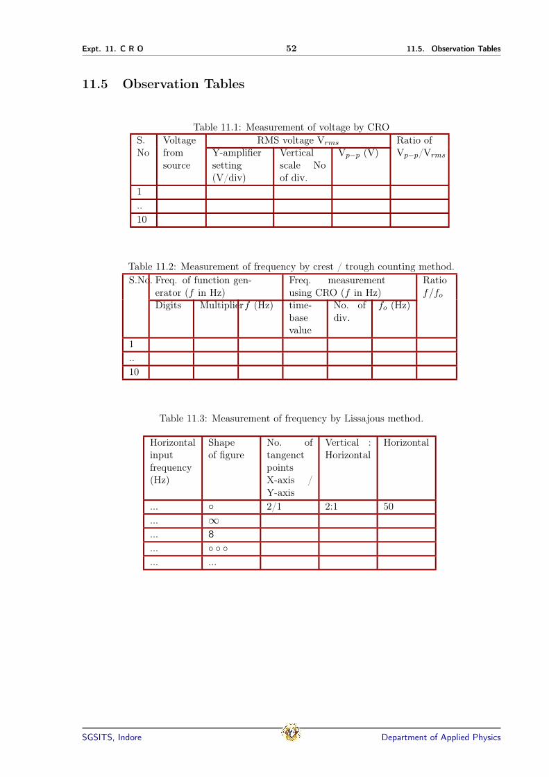
Expt. 11. C R O 52 11.5. Observation Tables

11.5 Observation Tables

Table 11.1: Measurement of voltage by CROS. Voltage RMS voltage Vrms Ratio ofNo from

sourceY-amplifiersetting(V/div)

Verticalscale Noof div.

Vp−p (V) Vp−p/Vrms

1..10

Table 11.2: Measurement of frequency by crest / trough counting method.S.No. Freq. of function gen-

erator (f in Hz)Freq. measurementusing CRO (f in Hz)

Ratiof/fo

Digits Multiplierf (Hz) time-basevalue

No. ofdiv.

fo (Hz)

1..10

Table 11.3: Measurement of frequency by Lissajous method.

Horizontalinputfrequency(Hz)

Shapeof figure

No. oftangenctpointsX-axis /Y-axis

Vertical :Horizontal

Horizontal

... 2/1 2:1 50

... ∞

... 8

...

... ...


12 Verification of Heisenberg’s Uncertainty Principle

12.1 Aim

To determination of the intensity distribution ofthe Fraunhofer diffraction patterns due to varioussingle slits using laser and to calculate the uncer-tainty of momentum from the diffraction patternsof single slits of differing widths and to confirmHeisenbergŠs uncertainty principle.


He-Ne or semiconductor laser, single slits differingwidths, photo detector, translation stage, etc.

12.3 Brief biography of Huy-gens

Christiaan Huygens, one of the more significantphysicists during the last three centuries, alongwith Isaac Newton, was born in April 1629 atThe Hague, the second son of Constantijn Huy-gens, (1596 - 1687), a friend of mathematicianand philosopher René Descartes.

Christiaan studied law and mathematics at theUniversity of Leiden and the College of Orange inBreda before turning to science. Huygens achievednote for his arguments that light consisted ofwaves, which became instrumental in the under-standing of wave-particle duality. He generallyreceives credit for his role in the development ofmodern calculus and his original observations onsound perception (see Repetition Pitch).

In 1655, Huygens proposed that Saturn was sur-rounded by a solid ring, "a thin, flat ring, nowheretouching, and inclined to the ecliptic." Using a 50power refracting telescope that he designed him-self, Huygens also discovered the first of Saturn’smoons, Titan. In the same year he observed andsketched the Orion Nebula. His drawing, the firstsuch known of the Orion nebula, was publishedin Systema Saturnium in 1659. Using his moderntelescope he succeeded in subdividing the neb-ula into different stars. (The brighter interior ofthe Orion Nebula bears the name of the Huygens

Region in his honor.) He also discovered sev-eral interstellar nebulae and some double stars.Huygens formulated also what is now known asthe second law of motion of Isaac Newton in aquadratic form. Newton reformulated and gener-alized that law.

Figure 12.1: A portrait of Huygens.

He also worked on the construction of accurateclocks, suitable for naval navigation. In 1658 hepublished a book on this topic called Horologium.In fact his invention on Christmas 1656, the pen-dulum clock (patented 1657), was a breakthroughin timekeeping. The oldest known Huygens stylependulum clock is dated 1657 and can be seenat the Museum Boerhaave in Leiden, which alsoshows an important astronomical clock ownedand used by Huygens.

Huygens also developed a balance spring clockmore or less contemporaneously with, though sep-arately from, Robert Hooke, and controversy overwhose invention was the earlier persisted for cen-turies. In February 2006, a long-lost copy ofHooke’s handwritten notes from several decades’Royal Society meetings was discovered in a cup-board in Hampshire, and the balance-spring con-troversy appears by evidence contained in thosenotes to be settled in favor of Hooke’s claim.

53

Expt. 12. Heisenberg Uncertainty 54 12.4. Theory

12.4 Theory

12.4.1 Principle

The distribution of intensity in the Fraunhoferdiffraction pattern of a slit is measured. Theresults are evaluated both from the wave pat-tern viewpoint, by comparison with KirchhoffŠsdiffraction formula, and from the quantum me-chanics standpoint to confirm HeisenbergŠs un-certainty principle

Diffraction is a wave phenomenon that is depen-dent on wavelength. Light waves bend as theypass by the edge of a narrow aperture or slit.This effect is approximated by:

θ =λ

D(12.1)

where θ the diffraction angle, λ wavelength ofradiant energy, and D the aperture diameter. Adiffraction grating uses the interference of wavescaused by diffraction to separate light angularlyby wavelength. Narrow slits then select the por-tion of the spectrum to be measured. The nar-rower the slit, the narrower the bandwidth thatcan be measured. However, diffraction in the slititself limits the resolution that can ultimately beachieved.

When a parallel, monochromatic and coherentlight beam of wave-length λ passes through asingle slit of width d, a diffraction pattern witha principal maximum and several secondary max-ima appears on the screen (Fig. 12.2). The inten-sity, as a function of the angle of deviation α, inaccordance with KirchhoffŠs diffraction formula,is

I(αn) = I(0)

(sinβnβn

)2

(12.2)

whereβn =

πd

λsinαn

The intensity minima are at

αn = sin−1

(nλ

d

)where n = 1, 2, 3 Ě

Figure 12.2: Experimental setup and diffrac-tion pattern from a single slit.

The angle for the intensity maxima are

α0 = 0

α1 = sin−1 1.430λ

d

α2 = sin−1 2.459λ

d(12.3)

The relative heights of the secondary maxima are:

I(α1) = 0.0472 I(0)

I(α2) = 0.0165 I(0)

(12.4)

12.4.2 Heisenberg Uncertainty - Quan-tum mechanics treatment

The Heisenberg uncertainty principle states thattwo canonically conjugate quantities such as po-sition and momentum cannot be determined ac-curately at the same time. Let us consider, for


Expt. 12. Heisenberg Uncertainty 55 12.4. Theory

Figure 12.3: Geometry of diffraction at a singleslit a) path covered b) velocity component of aphoton.

example, a totality of photons whose residenceprobability is described by the function fy andwhose momentum by the function fp. The un-certainty of location y and of momentum p aredefined by the standard deviations as follows

∆y∆p ≥ h/4π = ~/2 (12.5)

where h = 6.6262 × 10−34Js and h = 1.054 ×10−34Js, PlanckŠs constant (Şconstant of actionŤ),the equals sign applying to variables with a Gaus-sian distribution.

For a photon train passing through a slit of widthd, the expression is

∆y = d (12.6)

Whereas the photons in front of the slit move onlyin the direction perpendicular to the plane of theslit (x-direction), after passing through the slitthey have also a component in the y-direction.

The probability density for the velocity compo-nent vy is given by the intensity distribution inthe diffraction pattern. We use the first mini-mum to define the uncertainty of velocity (Figs.12.2 and 12.3).

∆vy = c sinα1 (12.7)

where α1 = angle of the first minimum. Theuncertainty of momentum is therefore

∆py = mc sinα1 (12.8)

where m is the mass of the photon and c is thevelocity of light. The momentum and wavelengthof a particle are linked through the de Broglierelationship:

h

λ= p = mc (12.9)

Figure 12.4: Actual experimental setup for sin-gle slit diffraction.

Thus,

∆py =h

λsinα1 (12.10)

According to equation 12.2, the angle α1 of thefirst minimum is thus

sinα1 = sin

(sin−1

(nλ

d

))=λ

d. (12.11)

If we substitute (12.11) in (12.10) and (12.6) weobtain the uncertainty relationship

∆y = ∆py = h (12.12)

If the slit width ∆y is smaller, the first minimumof the diffraction pattern occurs at larger anglesα1.

In our experiment the angle α1 is obtained fromthe position of the first minimum (Fig. 12.3a):

tanα1 =a

b(12.13)

If we substitute (12.13) in (12.10) we obtain

∆py =h

λsin(

tan−1 a

b

)(12.14)

Substituting (12.6) and (12.14) in (12.12) andafter dividing by h gives

d

λsin(

tan−1 a

b

)= 1. (12.15)

If the above parameters are substituted (with λ =670nm)one can verify Heisenberg’s uncertainty principleusing single slit diffraction. However, the resultsof the measurements confirm (12.15) within thelimits of error.


Expt. 12. Heisenberg Uncertainty 56 12.6. Probable Questions

12.5 Procedure:

1. Remove the CCD, filter, slit, etc except thelaser from the mounts.

2. Switch ON the laser. Align the laser paral-lel to the ground and optical bench.

3. Mount the detector at the another end ofthe optical bench.

4. Make sure that the laser falls on the detec-tor and its shows some value.

Figure 12.5: Schematic of experimental setupfor Laser diffraction from a single slit. LD-laser, F-Filter, S-slit or target and D-detector.The filter may be required if the detector showssaturation.

5. Insert the single slit #1 and put a plainpaper behind it. Adjust the position of theslit, so that the laser is passing through thecenter of the slit. Observe the diffractionpattern on the paper.

6. Record the width of the slit in the notebook. Move the detector to the other endof the optical bench.

7. Adjust the micrometer screw to minimumvalue and note down the value of intensity.

8. Rotate the micrometer screw and recordthe values of position and intensity.

9. After completing the procedure replace withslit #2. #3 .... Repeat the previous pro-cedure to record the diffraction pattern innote book.

10. Use a graph paper to draw curves for dis-tance along x-axis and intensity along y-axis.

11. Calculate the value of a as shown in figure12.2. Record the same in Table 2.

12. Complete the calculations and submit toteacher.

12.5.1 Data recording:

Table 12.1: Recording Single slit diffractionS. No. Distance Intensity (in mV))1 12 1.13 . . ... . . .50 10.1

Table 12.2: Verification of uncertainty relation

slitwidth

First Minima dλ sin

(tan−1 α

b

)d (mm) α (mm) b (mm)0.12 ... ... ...... ... ... ...0.4 ... ... ...

12.5.2 Results

1. Single slit diffraction using a laser is stud-ied.

2. Diffraction pattern for single slits of differ-ent widths are observed, plotted and thegraphs are attached.

3. Heisenberg uncertainty principle is under-stood and verified.

12.6 Probable Questions

1. What is Huygens principle?

2. What do you understand by interference bylight?

3. What are Fraunhofer and Fresnel class ofdiffraction?


Expt. 12. Heisenberg Uncertainty 57 12.7. Suggested reading

4. How coherence is important for interfer-ence / diffraction?

5. What is laser? Do you know laser safety?

6. What are the precautions required while us-ing laser?

12.7 Suggested reading

1. www.lightandmatter.com (Download Bookon Optics, it is free!).

2. F. A. Jenkins and H. E. White, Fundamen-tals of Optics, (McGraw-Hill, New York,1957).

3. M. Born and E. Wolf, Principles of Optics,(Pergamon, Oxford 1986).


13 Measurement of Electrical Equivalent of Heat

13.1 Aim

To understand the phenomena of electrical equiv-alent of heat, to measure the electrical equivalentof heat of water and to measure the efficiency ofa given incandescent lamp.

13.2 Equipment Required:

Regulated DC power supply, digital Volt-Ammeter,thermometer, stop watch, incandescent lamp, elec-trical equivalent jar, calorimeter, Indian Ink.

13.3 Part 1: Measurement ofthe Electrical Equivalentof Heat of water

13.3.1 Procedure

1. Measure and record the room temperature(T ).

2. Weigh the Jar (with the lid on), and recordits mass (Mj).

3. Remove the lid of the EEH Jar and fill thejar to the indicated water line with coldwater. DO NOT OVERFILL. The wa-ter should be approximately 5-10C belowroom temperature, but the exact tempera-ture is not critical.

4. Add about 3-5 drops of Indian ink to thewater; enough so the lamp filament is justbarely visible when the lamp is illuminated.

5. Using leads with banana plug connectors,attach your power supply to the terminalsof the EEH Jar. Connect a voltmeter andammeter as shown in Figure 13.3.1.1 so youcan measure both the current (I) and volt-age (V ) going into the lamp. NOTE: Forbest results, connect the voltmeter leadsdirectly to the binding posts of the jar.

6. Turn on the power supply and quickly ad-just the power supply voltage to about 11.5

volts, then shut the power off. DO NOTLET THE VOLTAGE EXCEED 12 VOLTS.

7. Insert the EEH Jar into one of the Calorime-ters.

8. Insert your thermometer or thermistor probethrough the hole in the top of the EEH Jar.Stir the water gently with the thermometeror probe while observing the temperature.When the temperature warms to about 6or 8 degrees below room temperature, turnthe power supply on.

9. NOTE: You may want to turn the lampon to help the cold water reach this start-ing temperature. If you do, be sure thatyou turn the lamp off for several minutesbefore you begin your measurements, soyou are sure the water temperature is eventhroughout the jar. Record the startingtime (ti) and the temperature (Ti).

10. Record the current, I, and voltage, V . Keepan eye on the ammeter and voltmeter through-out the experiment to be sure these valuesdo not shift significantly. If they do shift,use an average value for V and I in yourcalculations.

11. When the temperature is as far above roomtemperature as it was below room tempera-ture (Tr−Ti = Temperature - Tr), shut offthe power and record the time (tf ). Con-tinue stirring the water gently. Watch thethermometer or probe until the tempera-ture peaks and starts to drop. Record thispeak temperature (Tf ).

12. Weigh the EEH Jar with the water, andrecord the value (Mjw).

Data

13.3.2 Calculations

In order to determine the electrical equivalent ofheat (Je), it is necessary to determine both thetotal electrical energy that flowed into the lamp(E) and the total heat absorbed by the water (H).

58

Expt. 13. Electrical eq. of heat 59 13.4. Part. 2: Efficiency of an Incandescent Lamp

Figure 13.1: Actual setup and schematic ofelectrical connections to bulb, multimeter,power supply.

Room temperature Tr= _______Mass of jar Mj= _______Mass of Jar + water Mjw= _______Voltage V= _______Current I= _______Starting time ti= _______Final time tf= _______Starting temperature Ti= _______Final temperature Tf= _______

E, the electrical energy delivered to thelamp:

E = Electrical Energy into the LampE = V .I .t = _______t = tf - ti = the time during which power wasapplied to the lamp = _______

H, the heat transferred to the water (andthe EEH Jar):

H = (Mw+Me)(1 cal/gm C)(Tf -Ti) =_______Mw = Mjw – Mj = Mass of water heatedMw = ___________________Me - thermal mass of jar = 193gram.Hj=H Je = _______________

Some of the heat produced by the lamp is ab-sorbed by the Jar. For accurate results, therefore,the heat capacity of the jar must be taken intoacount (The heat capacity of the Jar is equivalentto that of approximately 193 grams of water.)

Je , the Electrical Equivalent of Heat:

Je = E/H = ___________________

13.4 Part. 2: Efficiency of anIncandescent Lamp

13.4.1 Procedure

Repeat Experiment 1, except do not use the Indiaink (step 4) or the styrofoam Calorimeter (step7). Record the same data as in Experiment 1, anduse the same calculations to determine E and H.



(Convert H to Joules by multiplying by Je fromthe first lab.)

In performing the experiment with clear water andno Calorimeter, energy in the form of visible lightis allowed to escape the system. However, wateris a good absorber of infrared radiation, so mostof the energy that is not emitted as visible lightwill contribute toH, the thermal energy absorbedby the water.

The efficiency of the lamp is defined as the energyconverted to visible light divided by the total elec-trical energy that goes into the lamp. By makingthe assumption that all the energy that doesn’tcontribute to H is released as visible light, theequation for the efficiency of the lamp becomes:

Efficiency = (E −Hj/E).

13.4.2 Data

Room temperature Tr= _______Mass of jar Mj= _______Mass of Jar + water Mjw= _______Voltage V= _______Current I= _______Starting time ti= _______Final time tf= _______Starting temperature Ti= _______Final temperature Tf= _______

13.4.3 Calculations

In order to determine the efficiency of the lamp, itis necessary to determine both the total electricalenergy that flowed into the lamp (E) and the totalheat absorbed by the water (H).

E, the electrical energy delivered to thelamp:

E = Electrical Energy into the LampE = V .I .t = = ________t = tf - ti = the time during which power wasapplied to the lamp = ________.

H, the heat transferred to the water (andcalorimeter):

H = (Mw +Me )(1 cal/gm C)(Tf -Ti)H = = ________Mw = Mjw – Mj = Mass of water heatedMw = = ________Hj = H Je = = ________Me = 193 grams. Some of the heat produced bythe lamp is absorbed by the EEH Jar. For accu-rate results, therefore, the heat capacity of thejar must be taken into acount (The heat capacityof the EEH Jar is equivalent to that of approxi-mately 23 grams of water.)

Efficiency:

(E-Hj)/E = = ________

13.4.4 Questions

1. What effect are the following factors likelyto have on the accuracy of your determi-nation of Je, the Electrical equivalent ofHeat? Can you estimate the magnitude ofthe effects?

(a) The inked water is not completely opaqueto visible light.

(b) There is some transfer of thermal en-ergy between the EEH Jar and theroom atmosphere. (What is the ad-vantage of beginning the experimentbelow room temperature and endingit an equal amount above room tem-perature?)

2. How does Je compare with J, the mechan-ical equivalent of heat. Why?

3. Water is not completely transparent to vis-ible light.

4. Not all the infrared radiation is absorbed bythe water.

5. The styrofoam Calorimeter was not used,so there is some transfer of thermal energybetween the EEH Jar and the room atmo-sphere.



6. Is an incandescent lamp more efficient as alight bulb or as a heater.

7. How does the amount of energy gained bythe Water compare to the energy given bythe power supply? Explain.

8. Could any heat be gained or lost by thesystem?


14 Wavelength of spectral lines by grating

14.1 Aim

To determine the wavelength of prominent spec-tral lines of mercury light by a plane transmissiongrating using normal incidence.


A spectrometer, mercury lamp, transmission grat-ing. reading lamp and reading lens.

14.3 Description of Apparatus

14.3.1 Spectrometer

This is an arrangement for producing pure spec-trum. The essential parts of a spectrometer in-clude collimator, prism table, and a telescope (SeeFigure 14.1).

14.3.2 Collimator

The collimator provides a narrow parallel beamof light. It consists of a horizontal, cylindrical,metallic tube fitted with an achromatic conver-gent lens at one end and a short coaxial tube atthe other end. The short coaxial tube, which hisprovided with a vertical slit of adjustable widthat the outer end, can be moved inside the maintube with the help of a rack and pinion arrange-ment. The slit is illuminated by the source oflight, whose spectrum is to be examined and thedistance between the slit and the convergent lensis so adjusted that the slit lies in the first focalplane of the lens. Under this condition, the raysof light emerging from the collimator are paral-lel. Usually in a spectrometer, the collimator isrigidly fixed with its axis horizontal, but in sameinstruments, it can be rotated about the verticalaxis passing through the center of instrument.

Figure 14.1: Photo of optical spectrometermounted with a prism and ray diagrams of thesame. The bottom figure shows the three mea-surements using a grating. T0 is direct readingwhile T and T’ are the left and right measure-ments for a particular order m.

14.3.3 Prism Table

It is a circular table supported horizontally on avertical rod at the center of the spectrometer.It can be rotated independently of the collima-tor and telescope about the vertical axis pass-ing through instrument’s center of a circular scalegraduated in half degrees carried by the telescope(See Figure 2) the rotation of the prism table canbe read with the help of two diametrically oppo-site verniers attached to it and sliding over thecircular scale. The prism table can be clampedto the main body of the instrument in any de-sired position with the help of a clamping screwand then a fine rotation can be given to it with

62

Expt. 14. Grating Diffraction 63 14.4. Measure angle

the help of a tangent screw provided at the base.The prism table can be raised or lowered and maybe clamped at any desired height with the helpof a clamping screw provided for it. It is alsoprovided with the three leveling screws P, Q, R(See Figure 2) so that the refracting faces of theprism can be adjusted parallel to the axis of theinstrument Concentric circles and straight linesparallel to the line joining any two of the level-ing screws are drawn on the surface of the prismtable, which help in placing the prism in properposition during the experiment.

14.3.4 Telescope

It is simple astronomical telescope and consists ofa horizontal, cylindrical metallic tube fitted withan achromatic convergent lens (called the objec-tive) at one end and a short coaxial tube calledeyepiece tube at the end. The eyepiece tube (pro-vided with the cross-wires and Ramsden eyepiece)can be moved inside the main tube with the helpof rack and pinion arrangement. Pulling or push-ing the eyepiece in eyepiece tube by hand can alsochange the distance between the cross-wires andthe eyepiece. Thus the telescope can be adjustedto receive parallel rays and to form a clear im-age upon the cross-wires, which in their turn aredistinctly visible through the eyepiece. The tele-scope can be rotated about the central axis ofthe instrument. It is also provided with a clamp-ing and a tangent screw at the base by which aslow rotation can be given to it. The main cir-cular scale is attached with the telescope so thatwhen the telescope is rotated, the main circularscale also rotates with it. The angle, throughwhich the telescope is rotated, can be measuredby reading the positions of the Verniers attachedto the prism table and sliding over the main scale.

14.3.5 Plane Transmission Grating

An arrangement, which is equivalent in its ac-tion to a large number of parallel slits of samewidth separated by equal opaque spaces is calleddiffraction grating. It is constructed by rulingfine equidistant parallel lines on an optically planeglass plate with the help of a sharp diamond point

of an automatically plane transmission grating. Ifthe rulings are made on a metallic surface, thegrating is called reflection grating. The numberof ruled lines in a grating varies from 15000 to30000 per inch and the ruled surface varies from2’’ to 6’’. The gratings available in our SGSITS,Physics laboratory are having 15000 ruled linesper inch and the ruled surface is of around 2’’

14.3.6 Grating Element

The distance between the centers of any two con-secutive ruled lines or transparent spaces actingas a slit is called grating element. Let e be thewidth of the transparent space and d be the widthof ruled space, then the grating element = (e+d)

14.4 Measurement of angles withthe help of spectrometer

The spectrometer scales are angle measuring util-ities for the positions of the telescope which canbe rotated about the central axis of the instru-ment. The main circular scale is attached withthe telescope so that when the telescope is ro-tated, the main circular scale also rotates withit. The angle, through which the telescope is ro-tated, can be measured by reading the positionsof the verniers attached to the prism table andsliding over the main scale. In a spectrometerthere are two sets of main circular scales (fittedwith the telescope) and vernier scale (attachedwith the prism table). Both sets are diagonally(left hand and right hand sides) fixed in the in-strument and measures angle for a particular tele-scope position with a difference of 180 degrees.These scales can be used in a similar manner as asimple Vernier Caliper or traveling microscope isused. The vernier Caliper or traveling microscopeis used to measure small distances (in centime-ters and fractions whereas spectrometer scales areused to measure small angular displacements (indegrees, minutes, and seconds)1 degree is equalto 60 minutes, and 1 minute is equal to 60 sec-onds; (1 = 60’ and 1’ = 60”)


Expt. 14. Grating Diffraction 64 14.6. Procedure

14.4.1 Least Count of the Spectrom-eter Scale:

Physics Laboratory, SGSITS has two types of spec-trometers in which

1. 60 divisions of vernier Scale are equal to 59divisions of the Main Scale, and

2. 30 divisions of vernier Scale are equal to 29divisions of the Main scale.

Now, we will find out the least count in first casewhich 60 divisions of Vernier scale are equal to59 divisions of the main scale. The method is asfollows:

1. Value of one division of circular main scale= 0.5 = 30’ (as 1 = 60’)

2. Value of one division of sliding vernier scale= (59/60) x 0.5

3. Least count of spectrometer scale = Valueof 1 div. of main scale - value of 1 div. ofvernier = 0.5- [(59/60) x 0.5] = [0.5 x1/60] = 0.5’ = 30” (THIRTY SECONDS)

4. Similarly the least count of the spectrom-eter scale in second case in which 30 divi-sions of Vernier scale are equal to 29 divi-sions of the circular main scale can also becalculated. In this case the value of leastcount will be 1’ or 60”

14.5 Formula Used:

The wavelength λ of any spectral line using planetransmission grating can be calculated from theformula (e + d) sin θ = nλ , Where (e + d) isthe grating element, θ is the angle of diffraction,and n is the order of the spectrum. If there are Nlines per inch ruled on the grating surface then thegrating element is given by (e+d) = 2.54/N cm.Hence (2.54/N) sin θ = nλ or λ = 2.54 sin θ/nNcm

14.6 Procedure

The whole experiment is divided into two parts (i)Adjustments, and (ii) Measurement of the diffrac-tion angle θ.

Adjustment

14.6.1 Adjustment of the Spectrom-eter:

Before doing any measurement with the spec-trometer, the following adjustments exactly in thesequence given below must be made:

• The axis of the collimator and the telescopemust intersect at the perpendicular to thecommon axis of the prism table and thetelescope (usually being made by the man-ufacturer)

• The eyepiece should be focused on the cross-wires. For doing it turn the telescope to-wards a white wall and adjust the distancebetween the objective and eyepiece of thetelescope with the help of rack and pin-ion arrangement such that the field of viewappears bright. Now alter the distance be-tween eyepiece and the cross-wires by pullingor pushing the eyepiece in the eyepiece tube,till the cross-wires are distinctly visible. Thisfocuses the eyepiece on the cross-wires.

Adjustment of Collimator and the telescopemust be adjusted respectively for emitting andreceiving parallel rays of light. This can be donein the following manner.

1. Illuminate the slit of the collimator with thesource of light, whose spectrum is to beanalyzed (mercury vapor lamp in this ex-periment). Bring the telescope in line withthe collimator with the help of rack andpinion arrangements such that the imageof the collimator slit as seen through thetelescope appears to be sharp and well fo-cused. Make the collimator slit as narrowas possible (of course with a clear appear-ance through the telescope).


Expt. 14. Grating Diffraction 65 14.6. Procedure

2. Mount the prism on the prism table suchthat its center coincides with the center ofthe prism table and adjust the height of theprism table such that the prism is in levelwith the collimator and the telescope.

If necessary, the telescope may be slightly turnedto keep he spectrum in the field of view but its(telescope) focusing arrangement is not to be dis-turbed while focusing collimator. Focus the tele-scope on he spectrum with the help of its rackand pinion arrangement to make the spectrum assharp as possible. This time do not disturb theprecious arrangement of the collimator.

14.6.2 Adjustment of the grating fornormal incidence:

For this proceed as follows:

• Bring the telescope in line with the colli-mator such that the direct image of theslit falls on the vertical cross wire of thetelescope. Note the readings on both spec-trometer scales.

• Rotate the telescope through 900 from thisposition and then clamp it. The axis of thetelescope will now be perpendicular to theaxis of collimator.

• Mount the grating on the prism table suchthat its ruled surface passes through thecenter of the prism table and is also perpen-dicular to the line joining the two levelingscrews E1 and E2 as shown in Figure 14.1b.The prism table is now rotated till the re-flected image of the slit from the gratingsurface falls on the vertical cross wire. Ad-just the screws E1 and E2 if necessary toget the image in the center of the field ofview. The grating surface is now inclinedat an angle of 450 with the incident rays.Note the readings of both the spectrometerscales.

• Rotate the prism table through 450 or 1350

as the case may be so that the ruled sur-face of the grating becomes normal to the

incident rays and faces the telescope. Nowclamp the prism table.

• The ruling of the grating should be parallelto the main axis of the instrument: Forthis unclamp the telescope and rotate. Thediffracted images of the slit or the spectrallines will be observed in the field of viewof the telescope. Adjust the leveling screwK, if necessary, to get these images at thecenter of the cross wires. When this is donethe rulings of the grating will be parallel tothe main axis of the instrument.

• The slit should be adjusted parallel to therulings of the gratings

For this rotate the slit in its own plane tillthe diffracted images of the spectral linesbecome as bright as possible. The obser-vations may now be taken.

14.6.3 Measurement of the Angle ofDiffraction:

• To measure the angle of diffraction, pro-ceed as follows:

• Rotate the telescope to one side (say left)of the direct image of the slit till the spec-trum of the first order (n=1) is visible inthe field of view of telescope. Clamp thetelescope and then move it slowly by tan-gent screw till the vertical cross wire co-incides with the red line of the spectrum.Note the readings of both the verniers. Thusgo on moving the telescope so that thevertical cross wire coincides in turn withthe different spectral lines namely, yellow,green, violet, etc. Each time note the read-ings of both the spectrometer scales (leftand right verniers).

• Unclamp the telescope and rotate it to theother side (say right) of the direct imagetill the first order spectrum is again visiblein the field of view. Clamp the telescopeand use the tangent screw to coincide thevertical cross wire on various spectral linesin turn and each time note the readings ofthe verniers.


Expt. 14. Grating Diffraction 66 14.7. Observations

• Find the difference in the readings of thesame kind of vernier for the same spectralline in two settings. This gives an angleequal to twice the angle of diffraction forthat spectral line in the first order (n=1).Half of it is will give the angle of diffraction.Similarly calculate the angle of diffractionfor other spectral lines.

• Repeat the above observations for secondorder spectrum also.

• The number of lines per inch on the grat-ing surface is usually written on the grating(the grating used in SGSITS have 15,000lines per inch).

14.7 Observations

14.7.1 For the adjustment of gratingfor normal incidence:

1. Least count of the Spectrometer scale:

Value of 1 division of main scale = . . . . . . . . . . . .

Division of main scale are equal to . . . . . .divisions of vernier scale.

Value of 1 division of vernier scale.

Least count of Spectrometer scale:

= value of 1 division of main scale – 1 di-vision of vernier scale.

2. Reading of the telescope for direct imageof the slit:

V1 = . . . . . . . . . . . . V2 = . . . . . . . . . . . .

3. Reading of the telescope after rotating itthrough 900:

V1 = . . . . . . . . . . . . V2 = . . . . . . . . . . . .

4. Reading of prism table when reflected im-age of the slit coincides with the verticalcross wire:

V1 =. . . . . . . . . . . . V2 = . . . . . . . . . . . .

5. Reading of prism table when rotated through450 or 1350:

V1 =. . . . . . . . . . . . V2 = . . . . . . . . . . . .

6. Number of lines N ruled per inch on thegrating

7. Grating element (e+ d) = 2.54/N


Expt. 14. Grating Diffraction 67 14.8. Results

14.7.2 Calculations:

For first order, n=1, λ = (e+ d) sin θ/2 cm.

λ for violet I colour = . . . . . . ..cm.

Calculate λ for all visible spectral lines also.

The mean value of λ for Violet I colour = . . . . . . . . . . . . cm.

(Calculate the mean value of λ for other visible spectral lines also.)

Table 14.1: Table for the measurement of the angle of diffraction θ

color Wndows Spectrum to the leftof the direct images

Spectrum to theright of the directimages

2θ = x-y Angle θ

MainScale

VernierScale

Total(x)

MainScale

VernierScale

Total(y)

Violet Window 1Window 2

Blue Window 1Window 2

Green Window 1Window 2

Yellow Window 1Window 2

Red Window 1Window 2

14.8 Results

Table 14.2: Observations for grating element (e+ d)

Colour Wavelength λ errorStandard measured

(Å) (Å) (%)Violet I 4047Blue 4358Green 5461Yellow I 5770Red 6234


Expt. 14. Grating Diffraction 68 14.9. Sample Questions

14.8.1 Source of Error and Precau-tions

• The axes of the telescope and the collima-tor must intersect at and be perpendicularto the main axis of the spectrometer.

• The collimator must be so adjusted as togive out parallel rays.

• The telescope must be so adjusted as toreceive parallel rays and form a well definedimage of the slit on the crosswire.

• The prism table must be optically leveled.

• The grating should be so mounted on theprism table that its ruled lines are parallelto the main axis of the spectrometer.

• The plane of the grating should be normalto the incident light and its ruled surfacemust face the telescope so that the errordue to nonparallelism of the incident raysis minimum.

• The slit should be as narrow as possible andparallel to the ruled surface of the grating.

• While handling the grating one should nottouch its faces but hold it between the thumband the fingers by edges only.

• While taking observations of the spectrallines, the prism table must remain clamped.

• The reading of both the verniers should berecorded. This eliminates the error due tonon-coincidence of the center of the grad-uated scale with the main axis of the spec-trometer.

14.9 Sample Questions

• What do you understand by diffraction oflight?

• How does it differ from interference of light?

• What is a diffraction grating? How is itconstructed?

• How do you measure the wavelength of lightusing grating?

• What is grating element?

• How do you adjust telescope and collimatorfor parallel rays?

• How do you set the grating for normal in-cidence?

• Why should the ruled surface of gratingface forwards the telescope?

• How many orders of spectra are you gettingwith the grating?

• What is the difference between a prism spec-trum and a grating spectrum?

• What are the various series of lines ob-served in hydrogen spectrum?

• What is Rydberg constant?

• . When white light passes through a diffrac-tion grating, what is the smallest value ofm for which the visible spectrum of order moverlaps the next one, of order m+1? (Thevisible spectrum runs from about 400 nmto about 700 nm.)

• Is a CD (compact Disk) a grating?

CHECK APPENDIX - B FOR ATOMICSPECTRA FROM MERCURY


15 e/m by Thomson Method

15.1 Aim

To measure the charge to mass ratio of elec-tron using Thomson method and to find the signcharge of electron.

15.2 Apparatus requires

Cathode ray tube, High and low tension powersupplies, bar magnets, scale, etc.

15.3 Discovery of electron

Roentgen set out to study cathode rays but wasrewarded, on or about Christmas 1895, with thediscovery of X-rays. Becquerel searched for a sus-pected but nonexistent link between Roentgen’srays and phosphorescence. Instead, he found some-thing totally unexpected: radioactivity. Sir JohnJoseph Thomson at Caven- dish Laboratory atCambridge University discovered electron in 1898.The word ’electron’ first used by G. J. Stoney in1891 had been used to denote the unit of chargefound in experiments that passed electric currentthrough chemicals.

Thomson was investigating ’Cathode Rays’ whichhad been a puzzle for a long time. Through hisexperiments Thomson put forward a then contro-versial theory in which the ’Cathode Rays’ weremade up of streams of particles much smallerthan atoms, Thomson called these particles ’cor-puscles’. Thomson mistakenly believed that these’corpuscles’ made up the entire atom. This ideawas controversial as most people at this timethought that the atom was the smallest particlein matter and was divisible.

Thomson’s theory was not explicitly supported byhis experiments. It took more experimental workby Thomson and others to conclusively prove thetheory. The atom is now known to contain otherparticles as well. Yet Thomson’s bold suggestionthat ’Cathode Rays’ were material constituentsof atoms turned out to be correct. The raysare made up of electrons: very small, negatively

charged particles.

Figure 15.1: Sir Joseph John Thomson (1856 -1940). Portrait by Arthur Hacker.

The present experiment is an exact copy of whatJ J Thomson performed while discovering a neg-atively charged particle, later known as electron.

15.4 Theory

Electrons are accelerated in an electric field andenter a magnetic field at right angles to the direc-tion of motion. The specific charge of the elec-tron is determined from the accelerating voltage,the magnetic field strength and the radius of theelectron orbit.

Figure 15.2: Schematic of an electron-gun usedin the experiment. A sample electron gun with-out housing and phosphor screen is shown atthe lower corner. More details may be foundin Appendix-A.

69

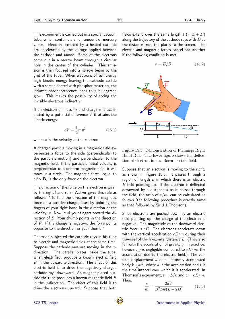
Expt. 15. e/m by Thomson method 70 15.4. Theory

This experiment is carried out in a special vacuumtube, which contains a small amount of mercuryvapor. Electrons emitted by a heated cathodeare accelerated by the voltage applied betweenthe cathode and anode. Some of the electronscome out in a narrow beam through a circularhole in the center of the cylinder. This emis-sion is then focused into a narrow beam by thegrid of the tube. When electrons of sufficientlyhigh kinetic energy leaving the cathode collidewith a screen coated with phosphor materials, theinduced phosphorescence leads to a blue/greenglow. This makes the possibility of seeing theinvisible electrons indirectly.

If an electron of mass m and charge e is accel-erated by a potential difference V it attains thekinetic energy:

eV =1

2mv2 (15.1)

where v is the velocity of the electron.

A charged particle moving in a magnetic field ex-periences a force to the side (perpendicular tothe particle’s motion) and perpendicular to themagnetic field. If the particle’s initial velocity isperpendicular to a uniform magnetic field, it willmove in a circle. The magnetic force, equal toe~v ×B, is the only force on the electron.

The direction of the force on the electron is givenby the right-hand rule. Walker gives this rule asfollows: "To find the direction of the magneticforce on a positive charge, start by pointing thefingers of your right hand in the direction of thevelocity, v. Now, curl your fingers toward the di-rection of B. Your thumb points in the directionof F . If the charge is negative, the force pointsopposite to the direction or your thumb."

Thomson subjected the cathode rays in his tubeto electric and magnetic fields at the same time.Suppose the cathode rays are moving in the x-direction. The parallel plates inside the tube,when electrified, produce a known electric fieldE in the upward z-direction. The effect of thiselectric field is to drive the negatively chargedcathode rays downward. An magnet placed out-side the tube produces a known magnetic field Bin the y-direction. The effect of this field is todrive the electrons upward. Suppose that both

fields extend over the same length l (= L + D)along the trajectory of the cathode rays withD asthe distance from the plates to the screen. Theelectric and magnetic forces cancel one anotherif the following condition is met

v = E/B. (15.2)

Figure 15.3: Demonstration of Flemings RightHand Rule. The lower figure shows the deflec-tion of electron in a uniform electric field.

Suppose that an electron is moving to the right,as shown in Figure 15.3. It passes through aregion of length L in which there is an electricE field pointing up. If the electron is deflecteddownward by a distance d as it passes throughthe field, the ratio of e/m, can be calculated asfollows (the following procedure is exactly sameas that followed by Sir J J Thomson).

Since electrons are pushed down by an electricfield pointing up, the charge of the electron isnegative. The magnitude of the downward elec-tric force is eE. The electrons accelerate downwith the vertical acceleration eE/m during theirtraversal of the horizontal distance L. (They alsofall with the acceleration of gravity g. In practice,however, g is negligible compared to eE/m, theacceleration due to the electric field.) The ver-tical displacement d of a uniformly acceleratedbody is 1

2at2, where a is the acceleration and t is

the time interval over which it is accelerated. InThomson’s experiment, t = L/v and a = eE/m.Thus:

e

m=

2dV

B2Lw(L+ 2D)(15.3)


Expt. 15. e/m by Thomson method 71 15.5. Procedure

where we substituted E = V/Lw, w is the widthof the plate.

15.5 Procedure

The measurement has two parts first to measurethe deflection then to measure the DC magneticfield.

15.5.1 To measure magnetic field

1. Use the tangent galvanometer (TG) / com-pass box to align the wooden stand parallelto the North-South Direction to nullify theearths magnetic field (Why?).

2. Note the value of deflections (zero?) θ0 inyour note book.

3. Mount bar magnets to two extreme pointson the scale but at equal distance from cen-ter. Move the bar magnets towards thecenter simultaneously so that equal distancebetween them is maintained.

4. When the TG starts showing deflectionsrecord the values of θ1 and θ2 and corre-sponding distance X1 and X2 in your notebook. Is X1 = X2?

5. After calculating the value of magnetic fieldB = BH tan θ, plot a curve between dis-tance X (X-axis) and magnetic field B (Y-axis). This can also be carried out aftercompleting the next part of experiment.

Figure 15.4: Experimental setup used in thelaboratory to measure e/m of electron.

15.5.2 To measure deflection

1. Now replace the TG with the electron tube.Remove the magnets. Switch on the powersupply. Adjust the focus and intensity tobest value, so that the spot is smaller andvisible clearly at the center of the tube. Ifthe initial deflection (d0) at zero voltage isfinite (6= 0, record it otherwise is record itas 0.

2. Now apply finite voltage to electron gun(say 20V).

3. Record the value of deflection (d1). Placethe magnet on the ends of wooden arms.Move the magnets simultaneously towardsthe center to nullify the deflection to d1 →d0. Record the position of magnets. (Thecorresponding magnetic field can be calcu-lated from the graph drawn from the pre-vious measurements).

4. Remove the magnet, reverse the voltageand repeat the previous step to find d2.

5. Remove the magnet. Apply voltage say30V. and repeat the previous two steps.

6. Repeat the experiment for different valuesof voltage.

7. Use the calibration curve ploted from thedata of Table 15.1, to find out the mean θand hence the magnetic field correspondingto the mean X observed in this table.

X (cm)

BH ta

n0

(G

au

ss)

Figure 15.5: Showing calibration curve ob-tained from Table 15.1.


Expt. 15. e/m by Thomson method 72 15.6. Results

15.6 Results

Charge to mass ratio of electron = ............ C/kg.Actual Value = ............ C/kg.Error in measurement = ...........%.

15.7 Questions

1. What element controls the number of electrons striking the screen?

2. What element is controlled to focus the beam?

3. Why are the electrostatic fields between the electron gun elements called lenses?

4. What is the function of the second anode?

5. What effect do longer deflection plates have on the electron beam?

6. If a compass needle’s north points north, what does that say when it is at the north pole?

7. What do you think will happen if you place a magnet flat onto the front of the monitor screen?

8. What do you think the field around the toroidal magnet would be? (Hint: the poles are on thetwo flat faces).

9. In what direction should the apparatus be aligned to minimize the effects of the Earth’s magneticfield? Explain.

Table 15.1: To measure magnetic fieldDeflection in the absence of magnet = θ0 =......X1 X2 MeanX θ1 θ1 Mean θ BH×(cm) (cm) (cm) tan θ

25 25 2522 22 22– –– –

The value of Earths Magnetic field is BH =

Table 15.2: To measure deflection dDeflection in the absence of applied voltage = d0 =......(mm)

S. Applied Deflection Magnetic fieldNo. Voltage d1 d2 Mean D1 D2 Mean D B

(V) (mm) (mm) (mm) deg deg deg (Gauss)1 202 30– –– –


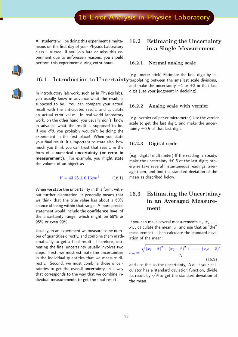
16 Error Analysis in Physics Laboratory

All students will be doing this experiment simulta-neous on the first day of your Physics Laboratoryclass. In case, if you join late or miss this ex-periment due to unforeseen reasons, you shouldperform this experiment during extra hours.

16.1 Introduction to Uncertainty

In introductory lab work, such as in Physics labs,you usually know in advance what the result issupposed to be. You can compare your actualresult with the anticipated result, and calculatean actual error value. In real-world laboratorywork, on the other hand, you usually don’t knowin advance what the result is supposed to be.If you did, you probably wouldn’t be doing theexperiment in the first place! When you stateyour final result, it’s important to state also, howmuch you think you can trust that result, in theform of a numerical uncertainty (or error inmeasurement). For example, you might statethe volume of an object as

V = 43.25± 0.13cm3 (16.1)

When we state the uncertainty in this form, with-out further elaboration, it generally means thatwe think that the true value has about a 68%chance of being within that range. A more precisestatement would include the confidence level ofthe uncertainty range, which might be 68% or95% or even 99%.

Usually, in an experiment we measure some num-ber of quantities directly, and combine them math-ematically to get a final result. Therefore, esti-mating the final uncertainty usually involves twosteps. First, we must estimate the uncertaintiesin the individual quantities that we measure di-rectly. Second, we must combine those uncer-tainties to get the overall uncertainty, in a waythat corresponds to the way that we combine in-dividual measurements to get the final result.

16.2 Estimating the Uncertaintyin a Single Measurement

16.2.1 Normal analog scale

(e.g. meter stick) Estimate the final digit by in-terpolating between the smallest scale divisions,and make the uncertainty ±1 or ±2 in that lastdigit (use your judgment in deciding).

16.2.2 Analog scale with vernier

(e.g. vernier caliper or micrometer) Use the vernierscale to get the last digit, and make the uncer-tainty ±0.5 of that last digit.

16.2.3 Digital scale

(e.g. digital multimeter) If the reading is steady,make the uncertainty ±0.5 of the last digit; oth-erwise take several instantaneous readings, aver-age them, and find the standard deviation of themean as described below.

16.3 Estimating the Uncertaintyin an Averaged Measure-ment

If you can make several measurements x1, x2, . . .xN , calculate the mean, x, and use that as “the”measurement. Then calculate the standard devi-ation of the mean:

σm =

√(x1 − x)2 + (x2 − x)2 + . . .+ (xN − x)2

N(16.2)

and use this as the uncertainty, ∆x. If your cal-culator has a standard deviation function, divideits result by

√N to get the standard deviation of

the mean.

73

Expt. 16. Error Analysis 74 16.5. General Procedure

16.4 Combining Uncertaintiesin Calculated Results

In the following equations, ∆x means the abso-lute uncertainty in x, which is the number you getfrom one of the methods above; it has units justlike the measurement itself has. ∆x % means thepercent (or fractional) uncertainty in x, which isthe uncertainty expressed as a percentage or frac-tion of the measurement; it has no units.

16.4.1 Addition and Subtraction

If z = x+ y or z = x– y,

∆z =√

∆x2 + ∆y2 (16.3)

If you’re adding and subtracting more variables,simply add more terms

inside the square root.

16.4.2 Multiplication and Division

If z= xy or z = x/y,

∆z

z=

√(∆x

x

)2

+

(∆y

y

)2

(16.4)

or (same thing in different notation).

∆z% =

√(∆x%)2 + (∆y%)2 (16.5)

If you’re multiplying and dividing more variables,simply add more terms inside the square root.

16.4.3 Powers, Including Roots

If z = xn,∆z

z= n

(∆x

x

)(16.6)

16.4.4 More Complicated Calculations

Sometimes you can combine the three rules givenabove, doing the calculation one step at a time,

combining uncertainties as you go along, and switch-ing back and forth between absolute and percentuncertainties as necessary. However, you cannotdo this if the same variable appears more thanonce in the equation or calculation, or if you havesituations not covered by the rules given above,such as trig functions. In such cases you mustuse the general procedure given below.

The following table gives an idea about the rela-tion between error and actual equation:

Table 16.1: Some examples

S. Relation bet- Relation betweenNo. ween Z & (A,B) ∆Z & (∆A, ∆B)1 Z = A + B (∆Z)2 = (∆A)2 + (∆B)2

2 Z = A - B (∆Z)2 = (∆A)2 + (∆B)2

2 Z = AB(

∆ZZ

)2=(

∆AA

)2+(

∆BB

)23 Z = A / B

(∆ZZ

)2=(

∆AA

)2+(

∆BB

)24 Z = An ∆Z

Z = n∆AA

5 Z = ln A ∆Z = ∆AA

6 Z = eA ∆ZZ = ∆A

16.5 General Procedure

If z = f(x,y), first calculate the differences causedby the uncertainty in each variable separately:

(∆z)x = f((x+ ∆x), y)− f(x, y)(∆z)y = f(x, (y + ∆y))− f(x, y)

(16.7)

Then combine the differences to get the total un-certainty:

(∆z) =√

(∆z)2x + (∆z)2

y (16.8)

If there are more variables, extend these equationsappropriately by adding more terms. If a variableoccurs more than once in the formula for f(x,y),change all occurrences simultaneously when cal-culating the difference for that variable.

To illustrate the procedure for calculation the er-ror in an experiment, we will work out the av-erage (mean) value xand the standard deviation


Expt. 16. Error Analysis 75 16.6. Suggested Experiments:

of the mean, σ and the standard deviation of anindividual data point, σ, using the position mea-surements in the accompanying Table (16.2).

Table 16.2: Position Measurements.xi (m) xi − xi (m) (xi − xi)2 (m2)

15.68 0.15 0.022515.42 0.11 0.012115.03 0.50 0.250015.66 0.13 0.016915.17 0.36 0.129615.89 0.36 0.129615.35 0.18 0.032415.81 0.28 0.078415.62 0.09 0.008115.39 0.14 0.019615.21 0.32 0.102415.78 0.25 0.062515.46 0.07 0.004915.12 0.41 0.168115.93 0.40 0.160015.23 0.30 0.090015.62 0.09 0.008115.88 0.35 0.122515.95 0.42 0.176415.37 0.16 0.025615.51 0.02 0.0004

From the Table (16.2) we can make the followingcalculations:

N= 21;N∑i=1

xi = 326.08m,N∑i=1

(xi − xi)2 = 1.61998m2.

and then evaluate the following quantities:

x =

∑Ni=1 xiN

=326.08

21= 15.53m (16.9)

σ =

√∑Ni=1(xi − x)2

N(N − 1)=

√1.6201

20 · 21= 0.062m

(16.10)

σ =

√∑Ni=1(xi − x)2

N − 1=

√1.6201

20= 0.063m

(16.11)

The error or spread in individual measurements isσ = 0.28 m. But for the mean x± σ= 15.53 ±

0.06 m. This says the average is 15.53 m whichhas an error of 0.06m. Or putting it another way,there is about a 68% probability that the truevalue of x falls in the range 15.47 m to 15.59 m.In some cases the fractional error σ x, or relativeerror, is of more interest than the absolute valueof σ. It is possible that the size of σ is large whilethe fractional error is small. Note that increas-ing the number of individual measurements onthe uncertainty of the average reduces the statis-tical uncertainty (random errors); this improvesthe “precision”. On the other hand, more mea-surements do not diminish systematic error in themean because these are always in the same direc-tion; the “accuracy” of the experiment is limitedby systematic errors.

16.6 Suggested Experiments:

1. Measure the diameter of a wire using ascrew gauge at 10 different places on thewire. Calculate the standard deviation inyour measurements.

2. Measure the thickness of a tabletop at us-ing a scale in cm. Calculate the error inyour measuremen ts.

3. Measure the period of oscillations of a pen-dulum using your wrist watch and recordyour data ten times. Estimate the standarddeviation and error in your measurements.

4. Ask your partner to drop a solid object at asame height for 10 times. Measure the timeof flight with your wrist watch. The samecan be repeated by your other partners also.Compare the standard deviation of each ofyour measurements.


A Cathode Ray Oscilloscope

This following text is given to make you under-stand the equipment. The teacher may checkyour understanding of the equipment by askingquestions from this part of the text.

A.1 Introduction

The cathode ray oscilloscope (CRO, for short) isa versatile laboratory instrument used for the vi-sual observation, measurement, and analysis ofwaveforms. With the help of transducers, manyphysical quantities like pressure, strain, tempera-ture, acceleration etc. can be converted into volt-age which can be displayed on CRO. Thus manydynamic phenomena can be studied by means ofCRO.

The heart or the major component of the oscil-loscope is the cathode ray tube (CRT). The restof the CRO consists of circuitry to operate theCRT. The CRT is discussed in detail in the fol-lowing section.

A.2 CATHODE RAY TUBE

The internal structure of a CRT is schematicallyshown in Fig. A.1. The CRT consists of a highlyevacuated funnel-shaped glass tube. The elec-trons are emitted from an indirectly heated thermioniccathode. A number of electrodes transform theemitted electrons into a high-velocity electron beam,known as a cathode ray. The electron beamtravels through the evacuated space of the tubetowards a fluorescent screen. When the beamstrikes the screen, the kinetic energy of the elec-trons is converted into light emission. A smalllight spot is thus produced on the CRT screenat a place where the electrons hit it. On itsway towards the screen the electron beam canbe deflected by suitable voltages. Usually, thesignal under test deflects the spot vertically onthe screen. Another voltage proportional to timeis employed to deflect the spot horizontally. Thetime variation of the signal is thus displayed onthe screen.

The main component of a general purpose CRT

are (i) electron gun, (ii) deflecting system, and(iii) fluorescent screen. These components arebriefly discussed below.

Figure A.1: Basic elements of a cathode-raytube. The width of the electron beam is exag-gerated for clarity.

A.2.1 Electron gun:

This part of the CRT emits electrons, transformsthem into a narrow beam, and focuses the beamon the fluorescent screen. It consists of an in-directly heated cathode, a control grid, an ac-celerating electrode, a focusing anode, and a fi-nal accelerating anode. These electrodes have acylindrical shape, and they are connected to thepins on the base.

The name “electron gun” originates from the anal-ogy between the motion of an electron emittedfrom the CRT gun structure and that of a bulletfired from a gun. The cathode emitting the elec-trons is completely surrounded by a control gridconsisting of a nickel cylinder with a small holeat the center. The electrons that manage to passthrough this small hole constitute the electronbeam. The density of the electrons in the beamis controlled by varying the negative voltage ofthe control grid with respect to the cathode. Ifthe control grid voltage is made more negative,the beam current and hence the brightness of thespot diminishes. On the other hand, if the con-trol grid voltage is made less negative, the beamcurrent and consequently the brightness of thespot increases. The grid bias control is thus abrightness or intensity control.

A high positive voltage is applied to the acceler-

76

Appendix 77 A.2. CATHODE RAY TUBE

ating electrode with respect to the cathode. Theaccelerating electrode thus speeds up the electronbeam passing through it. The combined actionof the focusing anode and the final acceleratinganode focuses the electron beam into a sharplydefined tiny spot on the screen. The action ofthe anode system is analogous to that of an op-tical lens focusing a beam of light. Hence theanode system is referred to as an electron opticalsystem. The focusing anode is kept at a positivevoltage with respect to the cathode. A higherpositive voltage is applied to the final accelerat-ing electrode with respect to the cathode. Fo-cusing can be obtained by adjusting the relativevoltage of the focusing and the final accelerat-ing anodes. Usually, the final accelerating anodevoltage is kept fixed, and focusing is achieved bychanging the focusing anode voltage.

A.2.2 Deflecting system:

In general purpose oscilloscopes, electrostatic de-flection of the electron beam is employed. Herethe deflecting system comprises a pair of hori-zontal deflecting plates and a pair of vertical de-flecting plates. The electron beam is deflectedand the spot is swept on the screen by the volt-ages applied to the deflecting plates. Considertwo parallel deflecting plates A and B betweenwhich the electron beam passes. In the absenceof any deflecting voltage between A and B, thebeam is focused at the point O on the screen.Let a positive voltage be applied to the plate Awith respect to the plate B. As the electronsare negatively charged, they will be attracted to-wards the positive plate A and will come to focusat point P1 on the screen. The deflection OP1isproportional to the deflecting voltage between Aand B. A reversal of the polarity of the deflectingvoltage causes the spot to appear at the point P2

on the other side of the point O.

The voltage applied to the vertical deflecting platesdeflects the beam vertically. The beam is shiftedsideways by the voltage applied to the horizon-tal deflecting plates. If an alternating voltage isapplied to the vertical deflecting plates, the spotis swept up and down on the screen at the fre-quency of the alternating voltage. The moving

Figure A.2: Simple block diagram of an analogcathode ray oscilloscope.

spot appears as a continuous luminous verticalline owing to the persistence of the screen andthe human eye. If the frequency is very low, themotion of the spot is clearly visible. An alternat-ing voltage, applied to the horizontal deflectingplates, will similarly generate a continuous lumi-nous horizontal line.

A.2.3 Fluorescent screen:

The inner surface of the face plate of the CRTis coated with a fluorescent material, also knownas the phosphor. The electrons, after hitting thescreen, must come back to the anode so that thecircuit is closed. Otherwise, the negative chargeaccumulated on the screen will repel the electronbeam, preventing it from reaching the screen.The return path of the electrons is provided bycoating the sidewalls of the CRT with carbon par-ticles, referred to as aquadag and by connectingthis coating to the accelerating anode.

The accelerating anode is usually held at the groundpotential and the other electrodes are kept at neg-ative voltages with respect to it. Possible high-voltage shock are thus avoided. The aquadagcoating is not directly connected to the screen.The electrons are removed from the screen by sec-ondary emission, and no accumulation of negativecharge can occur on the screen. The secondaryelectrons are trapped by the aquadag coating.These electrons thus move to the anode and thento the cathode via the power supply. The circuit


Appendix 78 A.4. A basic oscilloscope

is thereby completed.

A.3 Waveform Display

For the visual display of signal waveform on theCRT screen, a time-base generator is needed.This generator gives a sawtooth voltage wave-form, as depicted in figure. Each cycle of this pe-riodic waveform has a linearly increasing part fol-lowed by a linearly decreasing part. The time overwhich the voltage V increases linearly with time istermed the sweep time. The time over which thevoltage falls linearly with time to return to initialvalue is known as the return time or the flybacktime. The return time is a small fraction of thesweep time. The sawtooth voltage can be gener-ated using a unijuntion transistor The sawtoothvoltage, also referred to as the sweep voltage isapplied to the horizontal deflecting plates of theCRT. Since the sweep voltage increases linearlywith time, the spot moves horizontally at a con-stant velocity across the screen from left to right.At the end of the sweep, when the sawtooth volt-age drops, the spot returns quickly to its startingposition at the left. This cycle is repeated.

Let a sinusoidal voltage wave of frequency equalto the recurrence frequency of the sawtooth volt-age be applied to the vertical deflecting plates si-multaneously with the sawtooth voltage appliedto the horizontal deflecting plates. The spot nowsuffers a horizontal deflection proportional to timeand a vertical deflection in accordance with themagnitude and the polarity of the vertical signal.The resulting motion of the spot thus traces thewaveform of the signal to be displayed (which issinusoidal here) as a function of time. Such apattern on the CRT screen is referred to as anoscillogram.

If the frequency of the signal to be displayed is ntimes the repetition frequency of the sweep volt-age, n cycles of the sine wave are traced on theCRT screen in the sweep time.

To measure time, the horizontal displacement onthe CRT screen is calibrated in time. The hori-zontal axis is then referred to as time base. Thecalibration of the horizontal axis is read from the

front panel control marked VOLT/DIV. The sweepand the signal voltages are amplified before appli-cation to the deflecting plates. The correspond-ing amplifiers are known as horizontal amplifierand vertical amplifier, respectively.

To obtain a stable display of the signal on theCRT screen, the beginning of each sweep is lockedor synchronized to the signal to be displayed.This is achieved by starting each sweep at thesame point on the signal waveform. For this pur-pose, a sample of the input waveform is fed to atrigger circuit that generates a trigger pulse at aselected point of the input waveform. This trig-ger pulse starts the sweep generator.

Usually, the leading edge of the signal is used toactivate the trigger generator. Since the actionrequires some definite time interval, the sweepdoes not operate till the leading edge of the signalhas passed. Consequently, the leading edge ofthe waveform is not displayed on the screen. Bymeans of a delay line the arrival of the signal atthe vertical deflecting plates is retarded till thesweep is started. In this way the leading edge ofthe waveform can be viewed.

A.4 A basic oscilloscope

The major components of a general purpose CROare depicted in the simplified block diagram ofFig. A.2 They are: (i) cathode-ray tube (CRT),(ii) vertical amplifier, (iii) delay line, (iv) triggercircuit, (v) sweep generator, (vi) horizontal am-plifier, and (vii) power supply.

The horizontal displacement of the CRT spot isobtained by the sweep generator incorporated inthe CRO assembly or by an external signal appliedto the horizontal input terminal. The vertical dis-placement of the spot is caused by the signal ap-plied to the vertical input terminal. The gain ofthe vertical amplifier can be usually varied, but itis calibrated for quantitative measurements. Thebandwidth of the amplifier determines the fre-quency range over which the oscilloscope can beused. The greater the bandwidth of he ampli-fier, the greater the usable frequency range of theCRO. The gain and the bandwidth of horizontal


Appendix 79 A.5. Applications of CRO:

amplifier are usually less than those of the verticalamplifier. The trigger circuit of the sweep gener-ator can be activated either by the signal appliedto the vertical input terminal or by an externaltrigger signal.

The power supply incorporated in the CRO as-sembly has high-voltage section to operate theCRT and a low-voltage section to operate theassociated electronic circuitry. These supplies areconventionally designed.

The impedance offered by the CRO to the signalat the input terminals is referred to as the inputimpedance of the CRO. Typically, the input im-pendence consists of a resistance (about 1 MΩ)in shunt with a capacitance (about 40 pF). Themeasurement error for a CRO is generally about5 percent, but in specially designed oscilloscopes,it can be less than 1 percent.

A.5 Applications of CRO:

1. Visual display and qualitative study ofsignal waveforms: To display a signal onthe CRT screen, the signal is applied to thevertical input terminals. The time variationof the signal is visualized by means of thesweep generator displacing the spot in pro-portion to time in the horizontal direction.The nature of the signal can be qualita-tively studied from the trace on the CRTscreen. For example, one can get a visualimpression if the signal is sinusoidal or richin harmonics.

2. Measurement of voltage: The calibra-tion of the vertical scale gives the voltagecorresponding to the vertical deflection ofthe spot on the CRT screen. Thus themagnitude of an applied dc voltage or thevoltage at different times of a time-varyingsignal can be measured.

3. Measurement of frequency:

(a) Using the time base: The calibrationof the horizontal scale, i.e. the timebase helps to determine the frequencyof a time-varying signal displayed on

the CRT screen. If N complete cyclesof the ac signal are found to appearin a time interval t, the time period ofthe signal is T = t/N . The frequencyof the signal is f=1/T = N/t.

(b) Using Lissajous figures: The patternsgenerated on the CRT screen upon si-multaneous application of sine wavesto the horizontal and the vertical de-flection plates, are known as Lissajousfigures. Various patterns are obtaineddepending on the relative amplitudes,frequencies and phases of the wave-forms. Using Lissajous figure frequencyof a wave form can be determined.


2 Color Tables

2.1 Color and wavelength (nm)

Take color print-out for clarity or use color monitor to viewing.

360 380 400 420 440 460 480 500 520 540 560 580 600 620 640 660 680 700 720 740 760 780 800 Wavelength and thecorrsponding color.

2.2 Standard values for Mercury Spectrum.

Name yellow 2 yellow 1 green blue-green blue violet 2 violet 1Colorλ(nm) 579.0 577 546 491 435 407 404

Table 2.1: Standard values for Mercury Spectrum and corresponding color.

2.3 A Mercury Spectrum obtained from a spectrograph.

Figure 2.1: Typical spectrum one observes in Physics Laboratory at SGSITS, Indore.

80

3 Some useful data and information

Table 3.1: Base SI unitsName Symbol Unitlength m metertime s secondmass kg kilogram

electric current A ampereTemperature K kelvin

Amount of substance mol moleLuminous intensity cd candela

Table 3.2: Derived SI UnitsName Symbol Unitenergy J joule

electric charge C coulombelectric potential V volt

electric capacitance F faradelectric resistance Ω ohm

electric conductance S siemensmagnetic Flux Wb weberinductance H henrypressure Pa pascal

magnetic Flux density T teslafrequency Hz hertzpower W wattforce N newtonangle rad radianangle sr steradian

81

Appendix 82

Table 3.3: Common ExponentSymbol Name name of ten Factor

Y yatta 1024

Z zetta 1021

E exa 1018

p peta 1015

T tera trillion 1012

G giga billion 109

M mega million 106

k kilo thousand 103

h hecto hundred 102

da deca ten 101

d deci tenth 10−1

c centi hundredth 10−2

m milli thousandth 10−3

µ micro millionth 10−6

n nano billionth 10−9

p pico trillionth 10−12

f femto 10−15

a atto 10−18

z zepto 10−21

y yocto 10−24

Table 3.4: Constantssymbol Name Value unitsh Planck’s constant 6.626 068 76 ×10−34 J sR gas constant per mole (8.20545±0.00037) ×10−2 liter atm/K-molekB Boltzmann’s constant (1.38042±0.00010) ×10−23 J/Kσ Stefan-Boltzmann con-

stant(5.6686±0.0005)×10−8 W/m2K4

c velocity of light (2.99793±0.00001) ×108 m/se elementary charge (1.60207±0.00007) ×10−19 coulombsme mass of electron (9.10958±0.00005) ×10−31 kgN Avogadro number (6.02472±0.00036) ×1023 molecule/moleε 1/µ0C permittivity of

free space(8.8542±0.0001) ×10−12 farad/m

µ permeability of freespace

4π = 12.5664 ×10−7 henry/m

Mass per unit length ofNichrome

1 mg/cm


4 Brief History of Indian Nobel Laureates

The Nobel Prize is the most respected award the world over and here is a list of those Indians whohave won this award and made the country proud.

4.1 Rabindranath Tagore (1861 - 1941)

Nobel Prize for Literature (1913) Tagore was born and lived in Calcutta for most of hislife. He was one of modern India’s greatest poets and the composer of independent India’s nationalanthem. In 1901 he founded his school, the Santiniketan, at Bolpur as a protest against the existingbad system of education. The school was a great success and gave birth to Viswabharati. He wasawarded the 1913 Nobel Prize in Literature for his work "Gitanjali"; for the English version, publishedin 1912. The noble citation stated that it was "because of his profoundly sensitive, fresh and beautifulverse, by which, with consummate skill, he has made his poetic thought, expressed in his own Englishwords, a part of the literature of the West." In 1915, he was knighted by the British King GeorgeV. Tagore renounced his knighthood in 1919 following the Amritsar massacre or nearly 400 Indiandemonstrators.

4.2 Sir C.V. Raman (Chandrasekhara Venkata Raman)(1888 -1970)

Nobel Prize for Physics (1930) C V Raman was born on 7th Nov. 1888 in Thiruvanaikkaval,in the Trichy district of Tamil Nadu. He finished school by the age of eleven and by then he hadalready read the popular lectures of Tyndall, Faraday and Helmoltz. He acquired his BA degreefrom the Presidency College, Madras, where he carried out original research in the college laboratory,publishing the results in the philosophical magazine. Then went to Calcutta and while he was there, hemade enormous contributions to vibration, sound, musical instruments, ultrasonics, diffraction, photoelectricity, colloidal particles, X-ray diffraction, magnetron, dielectrics, and the celebrated "RAMAN"effect which fetched him the Noble Prize in 1930. He was the first Asian scientist to win the NobelPrize. The Raman effect occurs when a ray of incident light excites a molecule in the sample, whichsubsequently scatters the light. While most of this scattered light is of the same wavelength as theincident light, state (i.e. getting the molecule to vibrate). The Raman effect is usef

4.3 Dr. Hargobind Khorana

Nobel Prize for Medicine and Physiology (1968) Dr. Hargobind Khorana was born on9th January 1922 at Raipur, Punjab (now in Pakistan). Dr. Khorana was responsible for producingthe first man-made gene in his laboratory in the early seventies. This historic invention won himthe Nobel Prize for Medicine in 1968 sharing it with Marshall Nuremberg and Robert Holley forinterpreting the genetic code and analyzing its function in protein synthesis. They all independentlymade contributions to the understanding of the genetic code and how it works in the cell. Theyestablished that this mother of all codes, the biological language common to all living organisms, isspelled out in three-letter words: each set of three nucleotides codes for a specific amino acid.

83

4.4 Dr. Subramaniam Chandrasekar

Nobel Prize for physics (1983) Subramaniam Chandrashekhar was born on October 19, 1910in Lahore, India (later part of Pakistan). He attended Presidency College from 1925 to 1930, followingin the footsteps of his famous uncle, Sir C. V. Raman. His work spanned over the understandingof the rotation of planets, stars, white dwarfs, neutron stars, black holes, galaxies, and clusters ofgalaxies. He won the Nobel Prize in 1983 for his theoretical work on stars and their evolution.

4.5 Mother Teresa (1910 - 1997)

Nobel Prize for peace (1979) Born in 1910, Skoplje, Yugoslavia (then Turkey) and originallynamed Agnes Gonxha Bojaxhiu, Mother Teresa dedicated her life to helping the poor, the sick, andthe dying around the world, particularly those in India, working through the Missionaries Of Charity inCalcutta. The Society of Missionaries has spread all over the world, including the former Soviet Unionand Eastern European countries. They provide effective help to the poorest of the poor in a numberof countries in Asia, Africa, and Latin America, and they undertake relief work in the wake of naturalcatastrophes such as floods, epidemics, and famine, and for refugees. The order also has houses inNorth America, Europe and Australia, where they take care of the shut-ins, alcoholics, homeless, andAIDS sufferers. Mother Teresa died on September 5, 1997.

4.6 Dr. Amartya Sen

Nobel Prize for Economics (1998) Born in 1933, Bolpur, in West Bengal, Amartya Sen is thelatest in our list of Nobel Laureates. He was honored with the Nobel Prize for his work in Welfareeconomics. When Thailand’s Baht plummeted, markets from Bombay to New York were in turmoiland there was talk of worldwide depression, Sen’s argument that growth should be accompaniedby democratic decision-making seemed only too correct. Amidst the human suffering caused bymass unemployment and exacerbated – as many felt – by the stringent economic policies of theInternational Monetary Fund and ideas of free-market capitalism, Sen’s call for social support indevelopment appeared humane and wise. A new brand of softer, gentler economics seemed in order.Although Sen is probably best known for his research on famines, his work on women – the attentionhe has drawn to their unequal status in the developing world, and his calls for gender-specific aidprograms – is just as important.

4.7 V.S. Naipaul (1932- )

British writer of Indian origin, Sir Vidiadhar Surajprasad Naipaul was awarded the Nobel Prize forLiterature 2001 "for having united perceptive narrative and incorruptible scrutiny in works that compelus to see the presence of suppressed histories."

4.8 ___________________

(Do you want to have your name here?) Work hard, read and understand more science, may be oneday your dream might become true.

We hope you enjoyed working inPhysics Laboratory.

This manual is typeset by Dr. J. T. Andrews, us-ing LATEX2εwith binaries of MikTEX 2.9 and usingTEXniCenter2α4 frontend with report class option andother packages. For more information visit:

http://www.miktex.orghttp://www.sourceforge.nethttp://www.ctan.orghttp://www.tug.org/usergroups.html

The front cover page theme is “Scientists of India”. Thephotographs shown are clockwise from top left cornerin a circle, Megnad Saha (1893), Sir ChandrasekharaVenkata Raman(1888), Srinivasa Ramanujan (1887),Sir Jagadish Chandra Bose (1858), Subramaniam Chan-drasekhar (1910), Vikram Sarabhai (1919), Harish Chandra(1923), Homi Jehangir Bhabha (1909), Shanti SwarupBhatnagar (1894) and Satyendra Nath Bose (1894).There are no women scientists in this page, Why? Readhttp://science.education.nih.gov/women/index.html,http://www.nature.com/nature/debates/women/women_frameset.htmlCourtesy: Archieves of TIFR, Mumbai, India.

Megnad Saha C. V. Raman S. Ramanujan

S. N. Bose J. C. Bose

S. S. Bhatnagar S. Chandrashekar

H. J. Bhabha H. Chandra V. Sarabhai

Physics LaboratoryManual

AUGUST 2012

http://www.miktex.org

http://www.sourceforge.net

http://www.ctan.org

http://www.tug.org/usergroups.html

http://science.education.nih.gov/women/index.html

http://www.nature.com/nature/debates/women/women_frameset.html

http://www.nature.com/nature/debates/women/women_frameset.html

UG Laboratory Manual

Documents

Transcript of UG Laboratory Manual