UCGE Reports Number 20347

Department of Geomatics Engineering

Analysis of Radarsat-2 Full Polarimetric Data for

Forest Mapping

(URL: http://www.geomatics.ucalgary.ca/graduatetheses)

by

Yasser Maghsoudi

December 2011

THE UNIVERSITY OF CALGARY

Analysis of Radarsat-2 Full Polarimetric Data for Forest Mapping

by

Yasser Maghsoudi

A THESIS

SUBMITTED TO THE FACULTY OF GRADUATE STUDIES

IN PARTIAL FULFILLMENT OF THE REQUIREMENTS FOR THE

DEGREE OF PhD

DEPARTMENT OF GEOMATICS

CALGARY, ALBERTA

December, 2011

© Yasser Maghsoudi 2011

Abstract

Forests are a major natural resource of the Earth and control a wide range of environ-

mental processes. Forests comprise a major part of the planet's plant biodiversity and

have an important role in the global hydrological and biochemical cycles. Among the

numerous potential applications of remote sensing in forestry, forest mapping plays a

vital role for characterization of the forest in terms of species. Particularly, in Canada

where forests occupy 45% of the territory, representing more than 400 million hectares

of the total Canadian continental area. In this thesis, the potential of polarimetric

SAR (PolSAR) Radarsat-2 data for forest mapping is investigated.

This thesis has two principle objectives. First is to propose algorithms for ana-

lyzing the PolSAR image data for forest mapping. There are a wide range of SAR

parameters that can be derived from PolSAR data. In order to make full use of the

discriminative power o�ered by all these parameters, two categories of methods are

proposed. The methods are based on the concept of feature selection and classi�er en-

semble. First, a nonparametric de�nition of the evaluation function is proposed and

hence the methods NFS and CBFS. Second, a fast wrapper algorithm is proposed

for the evaluation function in feature selection and hence the methods FWFS and

FWCBFS. Finally, to incorporate the neighboring pixels information in classi�cation

an extension of the FWCBFS method i.e. CCBFS is proposed. The second objective

of this thesis is to provide a comparison between leaf-on (summer) and leaf-o� (fall)

season images for forest mapping. Two Radarsat-2 images acquired in �ne quad-

polarized mode were chosen for this study. The images were collected in leaf-on and

leaf-o� seasons. We also test the hypothesis whether combining the SAR parameters

obtained from both images can provide better results than either individual datasets.

The rationale for this combination is that every dataset has some parameters which

iii

may be useful for forest mapping.

To assess the potential of the proposed methods their performance have been

compared with each other and with the baseline classi�ers. The baseline methods

include the Wishart classi�er, which is a commonly used classi�cation method in

PolSAR community, as well as an SVM classi�er with the full set of parameters.

Experimental results showed a better performance of the leaf-o� image compared

to that of leaf-on image for forest mapping. It is also shown that combining leaf-

o� parameters with leaf-on parameters can signi�cantly improve the classi�cation

accuracy. Also, the classi�cation results (in terms of the overall accuracy) compared

to the baseline classi�ers demonstrate the e�ectiveness of the proposed nonparametric

scheme for forest mapping.

iv

Acknowledgements

First of all, I would like to take this opportunity to express my deep gratitude to my

supervisor Dr. Michael Collins for his guidance, advice and invaluable assistance dur-

ing my studies at the university of Calgary. Without his kind direction and constant

encouragements, I would have never been able to develop my project.

I would like to extend my appreciation to Dr. Donald Leckie for his many valu-

able comments and constructive suggestions. His expert knowledge of the Petawawa

Research Forest was very helpful in this research.

I also wish to acknowledge the Canadian Forest Service, Natural Resource Canada

in Victoria BC and Canadian Space Agency. They provided me valuable images

and �eld data as well as advice on forest conditions in Petawawa. I would like to

thank Dave Hill for helping me on the preparation of the ground truth data and

pre-processing of Radarsat-2 images.

I also thank the fellow graduate students from the department of Geomatics En-

gineering, particularly the fellow students in Trailer H.

Finally, I would like to thanks my parents for their strong support of my studies,

for their courage, for standing behind me from thousands of miles away. Mom and

Dad you have been and always will be a source of inspiration. You stood over my

shoulder whenever I needed you.

v

Contents

Approval Page ii

Abstract iii

Acknowledgments v

Contents vi

List of Tables viii

List of Figures ix

Epigraph xi

1 Introduction 1

1.1 Background . . . . . . . . . . . . . . . . . . . . . . . . . . . . . . . . 11.2 Motivations and Innovations . . . . . . . . . . . . . . . . . . . . . . . 21.3 Organization of the proposal . . . . . . . . . . . . . . . . . . . . . . . 6

2 Polarimetry and Polarimetric Decomposition 8

2.1 Introduction . . . . . . . . . . . . . . . . . . . . . . . . . . . . . . . . 82.2 SAR Polarimetry . . . . . . . . . . . . . . . . . . . . . . . . . . . . . 9

2.2.1 Basics . . . . . . . . . . . . . . . . . . . . . . . . . . . . . . . 92.2.2 Stokes vs. Jones Formalism . . . . . . . . . . . . . . . . . . . 122.2.3 Scattering Matrix vs. Muller Matrix . . . . . . . . . . . . . . 162.2.4 Polarization Basis Transformation . . . . . . . . . . . . . . . . 212.2.5 Deterministic vs. Non-Deterministic Scatterers . . . . . . . . . 23

2.3 Polarimetric Decomposition . . . . . . . . . . . . . . . . . . . . . . . 252.3.1 Coherent Decomposition . . . . . . . . . . . . . . . . . . . . . 262.3.2 Incoherent Decomposition . . . . . . . . . . . . . . . . . . . . 31

2.4 SAR discriminators . . . . . . . . . . . . . . . . . . . . . . . . . . . 422.5 summary . . . . . . . . . . . . . . . . . . . . . . . . . . . . . . . . . . 44

3 PolSAR Classi�cation 47

3.1 Supervised vs. unsupervised . . . . . . . . . . . . . . . . . . . . . . . 483.1.1 Supervised . . . . . . . . . . . . . . . . . . . . . . . . . . . . 483.1.2 Unsupervised . . . . . . . . . . . . . . . . . . . . . . . . . . . 50

3.2 Full covariance matrix vs. selected features . . . . . . . . . . . . . . . 543.3 Single- vs. multi-classi�ers . . . . . . . . . . . . . . . . . . . . . . . . 573.4 Incorporating spatial context . . . . . . . . . . . . . . . . . . . . . . . 593.5 Parametric vs. nonparametric classi�ers . . . . . . . . . . . . . . . . 613.6 Summary . . . . . . . . . . . . . . . . . . . . . . . . . . . . . . . . . 63

vi

4 Methods 64

4.1 Nonparametric methods . . . . . . . . . . . . . . . . . . . . . . . . . 654.1.1 Single Classi�er: NFS . . . . . . . . . . . . . . . . . . . . . . 654.1.2 Multiple Classi�er System: CBFS . . . . . . . . . . . . . . . . 72

4.2 Wrapper methods . . . . . . . . . . . . . . . . . . . . . . . . . . . . 754.2.1 Single Classi�er: FWFS . . . . . . . . . . . . . . . . . . . . . 774.2.2 Multiple Classi�er System: FWCBFS . . . . . . . . . . . . . . 79

4.3 Contextual Multiple Classi�er System: CCBFS . . . . . . . . . . . . 79

5 Study area and dataset description 82

5.1 Study area description . . . . . . . . . . . . . . . . . . . . . . . . . . 825.2 Dataset description . . . . . . . . . . . . . . . . . . . . . . . . . . . . 83

5.2.1 Ground truth data . . . . . . . . . . . . . . . . . . . . . . . . 835.2.2 SAR data . . . . . . . . . . . . . . . . . . . . . . . . . . . . . 87

5.3 Data preprocessing . . . . . . . . . . . . . . . . . . . . . . . . . . . . 895.3.1 Speckle �ltering . . . . . . . . . . . . . . . . . . . . . . . . . . 915.3.2 SAR parameters . . . . . . . . . . . . . . . . . . . . . . . . . 935.3.3 Georeferencing . . . . . . . . . . . . . . . . . . . . . . . . . . 93

6 Results and Discussion 96

6.1 Nonparametric Methods: Single (NFS) vs. Multiple(CBFS) Classi�ers 976.2 Wrapper Methods: Single (FWFS) vs. Multiple (FWCBFS) Classi�ers 1056.3 Context-based Method: CCBFS . . . . . . . . . . . . . . . . . . . . . 1106.4 Summary . . . . . . . . . . . . . . . . . . . . . . . . . . . . . . . . . 116

7 Conclusions and Further Works 120

7.1 Conclusions . . . . . . . . . . . . . . . . . . . . . . . . . . . . . . . . 1207.2 Further Works . . . . . . . . . . . . . . . . . . . . . . . . . . . . . . . 121

Bibliography 123

vii

List of Tables

2.2 polarimetric parameters used in this research . . . . . . . . . . . . . . 46

5.2 List of classes and training and testing sample sizes . . . . . . . . . . 875.4 Overview of the principal characteristics of the RS-2 data . . . . . . . 885.7 Acquired image details . . . . . . . . . . . . . . . . . . . . . . . . . . 895.8 PolSAR parameters used in this thesis . . . . . . . . . . . . . . . . . 94

6.1 Cross tabulation of number of correct and wrongly classi�ed pixels fortwo classi�cations . . . . . . . . . . . . . . . . . . . . . . . . . . . . . 97

6.2 the calculated p-values for the leaf-on vs. leaf-o� . . . . . . . . . . . . 996.3 the calculated p-values for the leaf-o� vs. leaf-on-o� . . . . . . . . . . 996.4 classi�cation accuracies in di�erent classes using the combined leaf-on-

o� dataset . . . . . . . . . . . . . . . . . . . . . . . . . . . . . . . . . 1026.5 selected features (the superscript 1 and 2 in the third row refer to

leaf-on and leaf-o� features respectively ) . . . . . . . . . . . . . . . . 1036.6 the calculated p-values for the leaf-on vs. leaf-o� . . . . . . . . . . . . 1066.7 the calculated p-values for the leaf-o� vs. leaf-on-o� . . . . . . . . . . 1066.8 selected features (the superscript 1 and 2 in the third row refer to

leaf-on and leaf-o� features respectively ) . . . . . . . . . . . . . . . . 1096.9 selected features for each class (the superscript 1 and 2 in the third

row refer to leaf-on and leaf-o� features respectively ) . . . . . . . . . 1116.10 classi�cation accuracies in di�erent classes using the combined leaf-on-

o� dataset . . . . . . . . . . . . . . . . . . . . . . . . . . . . . . . . . 1146.11 classi�cation accuracies in di�erent classes using the combined leaf-on-

o� dataset . . . . . . . . . . . . . . . . . . . . . . . . . . . . . . . . . 117

viii

List of Figures

1.1 Research outline . . . . . . . . . . . . . . . . . . . . . . . . . . . . . . 7

2.1 The propagation of an EM wave. The Electric �eld vector (red) com-prises horizontal (green) and vertical (blue) components (adapted from[83]) . . . . . . . . . . . . . . . . . . . . . . . . . . . . . . . . . . . . 10

2.2 Polarization ellipse (adapted from [83]) . . . . . . . . . . . . . . . . . 112.3 The Poincare Sphere . . . . . . . . . . . . . . . . . . . . . . . . . . . 142.4 Coherent response of a resolution cell: a) without a dominant scatterer

b) with a dominant scatterer . . . . . . . . . . . . . . . . . . . . . . 232.5 Decomposition taxonomy . . . . . . . . . . . . . . . . . . . . . . . . . 26

3.1 A review of PolSAR classi�cation methods . . . . . . . . . . . . . . . 473.2 Entropy-alpha feature space (adapted from [79]) . . . . . . . . . . . 51

4.1 Steps taken to analyze RS-2 images for forest mapping . . . . . . . . 654.2 Separating hyperplanes in SVM: left (linear case) and right (non-linear

case) . . . . . . . . . . . . . . . . . . . . . . . . . . . . . . . . . . . . 694.3 The proposed multi-classi�er schema . . . . . . . . . . . . . . . . . . 764.4 simple (a) vs. spatially consistent (b) combination rules . . . . . . . . 81

5.1 Petawawa Research Forest (adapted from Google maps) . . . . . . . . 835.2 The forest inventory stands overlaid on high resolution images obtained

from Google earth . . . . . . . . . . . . . . . . . . . . . . . . . . . . . 855.3 Undesirable polygons:(a) mixture of red pine and poplar (b) edgy polygon(c)

clear-cut area(d) partial cut area (e) low density area . . . . . . . . . 865.4 leaf-o� (a) and leaf-on (b) images in Pauli basis R:|HH−V V | , G:|HV |

and B:|HH + V V | . . . . . . . . . . . . . . . . . . . . . . . . . . . . 905.5 The T11 image before (left) and after (right) applying speckle �lter . 93

6.1 classi�cation accuracy vs. number of features in three datasets . . . . 1006.2 Quantitative comparison of nonparametric methods with baseline meth-

ods using the three datasets . . . . . . . . . . . . . . . . . . . . . . . 1006.3 classi�cation accuracy vs. number of features in the leaf-on, leaf-o�

and combined leaf-on-o� datasets using the FWFS method . . . . . . 1076.4 Quantitative comparison of wrapper methods with baseline classi�ers

using the three datasets . . . . . . . . . . . . . . . . . . . . . . . . . 1086.5 FWCBFS vs. FWFS using the combined leaf-on-o� dataset . . . . . . 1086.6 the leaf-on features selected by FWCBFS and their frequency . . . . 1126.7 the leaf-o� features selected by FWCBFS and their frequency . . . . 1136.8 increasing the window size in CCBFS method . . . . . . . . . . . . . 1156.9 the window size e�ect over di�erent classes: solid lines represent the

classes with fairly large number of samples and dotted lines indicatethe classes with small number of samples . . . . . . . . . . . . . . . . 116

ix

6.10 summary of the results: the classi�cation accuracies in nonparamet-ric, wrapper and context-based methods in di�erent classes. Wishartclassi�cation results in di�erent classes served as the baseline and thedi�erences in classi�cation accuracies with respect to the baseline areplotted. . . . . . . . . . . . . . . . . . . . . . . . . . . . . . . . . . . 119

x

Glory be to Almighty God who is the source of all knowledge, wisdom

and understanding.

xi

Chapter 1

Introduction

1.1 Background

Forest mapping is one of the core applications in remote sensing. Many studies

are based on multispectral optical images. Also, the use of hyperspectral data are

increasing due to their increased information content. Unfortunately, the weather

conditions limit the use of those optical images. On the other hand the Synthetic

Aperture Radar (SAR) data are not only independent of the weather conditions, they

are also sensitive to target geometry. For these reasons, these properties make the

SAR data a useful tool for applications such as forest mapping.

The extraction of information from SAR data has been an active area of research

for many years and they are becoming more and more important in remote sensing

applications. Despite all their advantages, the use of SAR data are subject to ge-

ometric limitations which a�ects the SAR data by shadows, layover, foreshortening

and variation in pixel resolution over the image. In addition, because of the coherent

nature of the SAR sensors, the images su�ers from speckle noise [94]. Because of

these reasons, it is very di�cult to obtain satisfactory results from classi�cation of

single channel SAR data even if advanced classi�cation techniques are used.

In order to achieve reliable results, multichannel measurements are generally nec-

essary. The multichannel datasets can be achieved by using multi-temporal data

[104, 135], multi-frequency data [70], multi-polarization data [38], fusion of di�erent

SAR sensors [117] and fusion of SAR data and optical data [21]. A combination of

these approaches are also considered in several studies [21, 16, 32, 41]. While multi-

temporal, multi-frequency and multi sensor approaches are widely used and fairly

well documented, SAR polarimetry is a relatively new approach which yields some

1

advantages over the conventional methods. In this context, the remote sensing com-

munity has become increasingly interested in the use of polarimetric SAR data for

the land cover mapping and forest mapping.

Polarimetric data allow to identify di�erent classes by analyzing the multi-polarization

of the backscattering coe�cient; on the other hand, there are a lot of SAR parameters

which can be extracted from the polarimetric data. These parameters are either de-

rived using the well-known decomposition methods, or obtained directly from original

data, or can be the SAR discriminators. The use of these parameters can improve

the separability of the classes in the feature space. For these reasons, polarimetric

SAR data have become a relatively operational tool for classi�cation problems.

Extraction of SAR parameters is a primary step prior to classi�cation. Polari-

metric target decomposition (TD) is developed to separate polarimetric radar mea-

surements into basic scattering mechanisms. TD methods are often categorized as

coherent and incoherent methods. The coherent methods are based on the scattering

matrix that possess 5 independent parameters while incoherent methods are based

on the incoherently averaged covariance or coherency matrices that have 9 indepen-

dent parameters. These target decomposition parameters along with the original data

features and SAR discriminators are fully explained in section 2.3.

1.2 Motivations and Innovations

There are a wide range of SAR parameters (features) which can be extracted from

polarimetric SAR data. Target decomposition theory laid down the basis for the

classi�cation of polarimetric SAR images and almost all classi�cation algorithms are

based on them. Particularly, the formalism worked out by Cloude [30] led to the

introduction of an unsupervised classi�cation scheme [29], further augmented and

improved by subsequent contributions [99, 78, 80].

Despite the signi�cant number of works carried out for terrain and land-use clas-2

si�cation [108, 32, 16, 29, 10], very few researches have been performed to investigate

the potential of C-band polarimetric data for forest classi�cation [128] [58]. Proisy et

al. [102] in 2000 employed Radarsat-1 HH polarization and ERS-1 VV polarization

for forest mapping and concluded that the C-band SAR data can not provide a good

discrimination of forest species. Touzi et. al. [128] in 2006 used the airborne C-band

polarimetric Convair-580 SAR data for forest classi�cation. They showed that using

radiometric intensity of the conventional C-band SAR polarizations HH, HV, and VV

can only perform a limited discrimination of various tree species. However, the polar-

ization information provided by fully polarimetric SAR clearly improved forest type

discrimination under leafy and no-leaves conditions and permits the demonstration

of the signi�cance of SAR illumination angle on forest scattering mechanisms.

Although a large variety of works have already taken place for the classi�cation

of polarimetric SAR images, most of them have concentrated on the use of a very

limited number of features. For instance, in the method proposed by Cloude and Pot-

tier [33], which is one of the most used approaches, the polarimetric information is

converted into three parameters (entropy H, α-angle and anisotropy A) each of which

have been associated to an elegant physical interpretation. Then, they subdivided

the feature space formed by the three parameters into regions that corresponds to

distinct scattering behaviors (See chapter 3 for a review of various SAR polarimetric

data classi�cation approaches). In very complex scenes like forests it is very useful

to make full use of the discriminative power o�ered by all these features. However,

due to the small training sample size problem, using all these features for the classi-

�cation is not feasible. Furthermore, some of these features might carry redundant

information. Therefore, a key stage in a classi�er design is the selection of most dis-

criminative and informative features. Most of the SAR parameters are of complex

and sometimes unknown statistical properties. For this reason, the conventional fea-

3

ture selection algorithms cannot be applied. To account for this, a new classi�cation

approach, which is based on a nonparametric feature selection (NFS) and support

vector machine classi�er is proposed. The feature selection process generally involves

a search strategy and an evaluation function. In this research, the sequential for-

ward �oating selection (SFFS) [64] method will be used as the search algorithm to

generate subsets of features from the original features. For the evaluation function, a

non-parametric separability measure will be adopted to evaluate the generated feature

subsets. To formulate the criteria of class separability, the between-class and within

class scattering matrices have to be calculated. The employed separability measure is

the ratio of the determinant of the between-class scatter matrix to the determinant of

the sum of within-class scatter matrices. Upon the selection of the most appropriate

features, they are transferred to the classi�cation step. Because of its ability to take

numerous and heterogeneous features into account, as well as its ability handle lin-

early non separable cases, the support vector machine (SVM) algorithm is proposed

as the classi�er.

Most of the feature selection algorithms seek only one set of features that distin-

guish among all the classes simultaneously and hence a limited amount of classi�cation

accuracy. Recently, there has been a great interest for using an ensemble of classi�ers

for solving problems in pattern recognition community. Thus, in order to take ad-

vantage of heterogeneous features provided by the polarimetric target decomposition

and hence to improve the classi�cation accuracy, a multi classi�er schema is used for

the next part of this research. In doing so, a class-based feature selection (CBFS),

which is based on the theory of multiple classi�ers, is proposed. In this schema, in-

stead of using feature selection for the whole classes, the features are selected for each

class separately. The selection is based on the calculation of the determinant of the

between-class scatter matrix to the determinant of within-class scatter matrices for a

4

speci�c class. It should be noted that unlike the previous method, the between class

scatter matrix is de�ned as the distance between that speci�c class and the rest of

classes (and not the distance between all classes). Also, instead of the determinant of

the sum of within-class scatter matrices, the determinant is calculated for the class

of interest. Afterwards, an SVM classi�er is trained on each of the selected feature

subsets. Finally, the outputs of the classi�ers are combined through a combination

mechanism. The proposed schema was already successfully tested in our previous

works for the classi�cation of hyperspectral images [86] and multitemporal Radarsat-

1 images [87]. In this study, we will investigate the potential of the CBFS method

for the classi�cation of polarimetric SAR images.

The inter-class distance measures as the evaluation function of the feature selection

although a reasonable method of the similarity and dissimilarity, they are not directly

related to the ultimate classi�cation accuracy. A question arises as to whether it

is possible to use a more direct criterion as the evaluation function. According to

the evaluation function, the feature selection approaches can be broadly grouped

into �lter and wrapper methods [69]. Wrappers utilize the classi�cation accuracy

as the evaluation function whereas �lters uses the inter-class distance measures as

the evaluation function. The optimized problem in �lters in di�erent from the real

problem. Nonetheless, �lters are faster because the problem they solve is in general

simpler. Alternatively, wrappers try to solve the real problem and the considered

criterion is really optimized which means that the ultimate problem has to be solved

numerous times. For this reason wrappers are potentially very time consuming. This

time complexity in our work is mainly due to the SVM training time. In this thesis, in

order to alleviate this problem, a fast wrapper feature selection (FWFS) is proposed.

We tried to reduce the training time by reducing the number of training samples.

The number of support vectors for each class was taken as the degree of training

5

reduction for that class. Like the NFS method, the method was used in the context

of a class-based feature selection schema and hence the name FWCBFS.

One of the disadvantages of the classi�cation methods described so far is that

each pixel is classi�ed independently of its neighbors. When a majority of pixels in

a certain region are assigned to the a single class, it becomes highly unlikely that

a pixel in this region belongs to another class. This misassignment could likely be

due to the speckle noise. Therefore, in the last part of this research we will take

the spatial consistency into account. In particular, in the combination mechanism of

the multi classi�er schema we will incorporate the spatial context. A more detailed

explanation of these methodologies can be found in chapter 4. In summary, all the

proposed methodologies are illustrated in �gure 1.1.

1.3 Organization of the proposal

This thesis is organized in seven chapters. In the previous sections, the background

and motivation of the research being conducted are explained. In Chapter 2, �rst

some of the basic concepts on polarimetry (section 2.2 ) are explained. Next, an

overview on target decomposition methods is given based on a categorization scheme

(section 2.3). Some of the well-known approaches for the classi�cation of polarimetric

SAR images are then explained in chapter 3. Chapter 4 focuses on the description of

the proposed methodologies. Then, a description of the dataset, study area and the

preprocessing results are given in chapter 5. Discussion of the experimental results

and their analysis are given in chapter 6. Finally, conclusions and further works are

described in chapter 7.

6

Figure 1.1: Research outline

7

Chapter 2

Polarimetry and Polarimetric Decomposition

2.1 Introduction

Radar polarimetry is the science and technology of acquiring, processing and analyz-

ing the polarization state of an electromagnetic �eld [9]. The complex structure of

forests manifests itself in polarimetric SAR (PolSAR) data by a challenging diversity

of scattering mechanisms. This extensive source of polarization information contained

in fully polarimetric SAR data shows great potential for measuring forest scattering

characteristics and producing separation between di�erent forest species. In order to

understand the information content of polarimetry and the physical relationship of

polarimetric parameters with natural media, such as forests, a theoretical grounding

is necessary.

The main goal of this chapter is to explain the SAR parameters that can be

extracted from PolSAR data. These are the parameters that will be used as the input

features in the forest classi�cation step next. Therefore, a detailed understanding

of these parameters plays a vital role in interpretation and evaluation of the �nal

results. The polarimetric features can be divided into three categories: the features

obtained directly from original data, the features which are derived using the well-

known decomposition methods, and the SAR discriminators.

The �rst part of this chapter (section 2.2) provides a mathematical and physical

background to polarimetry which is essential for understanding the PolSAR param-

eters. Also, the explanation of the original data features i.e. scattering matrix,

covariance matrix and coherency matrix can be found in this section. Section 2.3

deals with di�erent target decomposition methods. Within this framework, di�erent

coherent and incoherent decompositions are explained. There are several quantities

8

derived from PolSAR data to be used as indicators to discriminate among surface

types or land covers. These SAR discriminators are explained in section 2.4.

The main reason to consider di�erent SAR parameters is to take advantage of

the complementary information provided by the di�erent parameters in the �eld of

forest classi�cation. For instance, incoherent algorithms performs an averaging of the

returned signals. This provides a statistically smoother description of the behaviour

of the scatterers. These parameters are mainly believed to be better for randomly

distributed targets. For instance, within forests they can distinguish between volumes

and surface scatterers. It has also been shown that some of the incoherent parameters

are very promising for forest structure characterization and detection of forest changes

between leaf-on and leave-o� conditions [126]. On the contrary, the coherent methods

can be used to maintain the full resolution. Indeed, by avoiding the averaging at the

�rst stage, the coherent methods are able to extract features that may be lost in

the early averaging step. By combining these parameters, various forest features are

emphasized. Coherent methods focuses on the more detailed characteristics of the

trees such as the leaves, branches and twigs whereas the incoherent parameters reveals

the high scale components e.g. the canopy structure.

Because of these reasons, it is expected that the concurrent application of both co-

herent and incoherent methods would provide complementary information and hence

improve the forest classi�cation results.

2.2 SAR Polarimetry

2.2.1 Basics

Polarization is an important property of a plane electromagnetic (EM) wave. It refers

to the alignment and regularity of the electric �eld component of the wave, in a plane

perpendicular to the direction of propagation (as the magnetic �eld is directly related

to electric �eld and can always be obtained from it, we direct our attention to the9

Figure 2.1: The propagation of an EM wave. The Electric �eld vector (red) compriseshorizontal (green) and vertical (blue) components (adapted from [83])

electric �eld component). Figure 2.1 illustrates the propagation of an EM wave.

The Electric �eld of a plane wave can be described by the sum of two orthogonal

components, i.e horizontal and vertical components [15]. The path of the end point

of the Electric wave vector traces out an ellipse in its general form as shown in �gure

2.2. The ellipse has a semi-major axis of length Exo and a semi-minor axis of length

Eyo . A is the wave amplitude, φ(0o 6 φ 6 180o) is the orientation angle which is

the angle of the semi-major axis, τ(0 6 τ 6 45o) is the ellipticity angle, de�ned as

τ = arctan(Eyo/E

xo ). τ describes the degree to which the ellipse is oval (�gure 2.2).

The magnitudes and relative phase between the horizontal and vertical components

of the Electric �eld vector governs the shape of the ellipse. For instance, when the

components are in phase (τ = 0), the polarization ion is linear . As the relative

phase angle increases to 90o, the ellipticity increases to 45o, representing circular

polarization.

The propagation of a plane EM wave is described in a three dimensional space

with the coordinates given by the three axes x, y and z. The z axis is in the direction

of propagation, while the x and y axes lie in a plane perpendicular to the direction

10

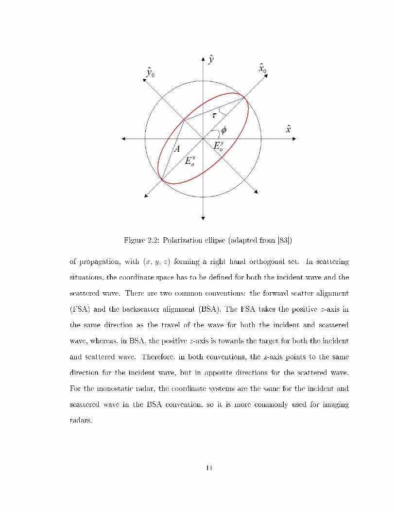
Figure 2.2: Polarization ellipse (adapted from [83])

of propagation, with (x, y, z) forming a right hand orthogonal set. In scattering

situations, the coordinate space has to be de�ned for both the incident wave and the

scattered wave. There are two common conventions: the forward scatter alignment

(FSA) and the backscatter alignment (BSA). The FSA takes the positive z-axis in

the same direction as the travel of the wave for both the incident and scattered

wave, whereas, in BSA, the positive z-axis is towards the target for both the incident

and scattered wave. Therefore, in both conventions, the z-axis points to the same

direction for the incident wave, but in opposite directions for the scattered wave.

For the monostatic radar, the coordinate systems are the same for the incident and

scattered wave in the BSA convention, so it is more commonly used for imaging

radars.

11

2.2.2 Stokes vs. Jones Formalism

In order to characterize the polarization state of a plane wave, George Stokes in 1852

introduced a 4-element vector,

[S0 S1 S2 S3

]T, known as the Stokes vector.

S0

S1

S2

S3

=

|Ey|2 + |Ex|2

|Ey|2 − |Ex|2

2Re{EyE∗x}

2Im{EyE∗x}

=

|Ey|2 + |Ex|2

|Ey|2 − |Ex|2

2EyEx cos δ

2EyEx sin δ

=

S0

S0 cos 2φ cos 2τ

S0 sin 2φ cos 2τ

S0 sin 2τ

(2.1)

where Ey and Ex are the vertical and horizontal components of Electric �eld, δ =

δx − δy is the phase di�erence between Ey and Ex, φ and τ are the orientation and

ellipticity angles respectively, |.| is the absolute value and ∗ is the complex conjugate.

This formalism indicates that the polarization state of a plane wave can be described

by orientation and ellipticity, plus a parameter S0. S0 is proportional to the total

intensity of the wave, S1 is the di�erence between the density powers related to the

horizontal and vertical polarizations. Parameters S2 and S3 are related to the phase

di�erence between the horizontal and vertical components of the electric �eld.

An EM plane wave can be completely polarized, partially polarized and completely

unpolarized. In the completely polarized case, only 3 of the Stokes parameters are

independent because

S20 = S2

1 + S22 + S2

3 (2.2)

In this case, a geometrical interpretation of the Stokes parameters is used to map the

polarization state on a sphere with radius S0 and Cartesian coordinates (S1, S2, S3).

This visualized representation of the polarization state of the wave, which is called

the Poincare sphere, is shown in �gure 2.3. The latitude and longitude of a point on

the sphere corresponds to 2τ and 2φ. Based on this notation, the linear polarizations12

lie on the equator, with horizontal and vertical polarizations opposite each other.

Left hand and right hand circular polarizations lie on the north and south poles

respectively. All other points on the sphere refer to the elliptical polarizations with

di�erent τ and φ. Points on the sphere which are opposite to each other are referred

to as cross polarizations and they represent polarizations that are orthogonal to each

other.

For partially polarized waves, not all the super�cial density powers is contained

in the polarized components and thus the total intensity of the wave is greater than

the polarized components

S20 > S2

1 + S22 + S2

3 (2.3)

The degree of polarization is the ratio of the polarized power to the total power

p =

√S21 + S2

2 + S23

S0

(2.4)

If the EM wave is partially polarized, it can be expressed as the sum of a completely

polarized wave and a completely unpolarized or noise-like wave as follow

S0

S1

S2

S3

=

1− p

0

0

0

+ S0p

1

cos 2φ cos 2τ

sin 2φ cos 2τ

sin 2τ

(2.5)

in which the �rst term and the second term in the right side represent the completely

unpolarized and completely polarized components.

The Jones vector [65] is another formalism for characterizing the polarization state

of a plane wave. In this formalism, instead of a 3D real space, as of the Stokes vector,

a 2D complex space is used. The Electric �eld of a wave propagating in the z can be

13

Figure 2.3: The Poincare Sphere

14

written as

~E(z, t) =

Ex

Ey

Ez

=

Eox cos(ωt− kz − δx)

Eoy cos(ωt− kz − δy)

0

=

Eox exp(−jkz) exp(jδx)

Eoy exp(−jkz) exp(jδy)

0

(2.6)

where Ex, Ey, Ez are the real electric �eld vector components, Eox, Eoy are the Carte-

sian components of the real electric �eld vector ~E(z, t), ω is the angular frequency, t

is the time, k is the wave number, and δx and δy are the x and y phases of the electric

�eld components when projected onto the x− y plane.

The Jones vector is the phasor of the real electric �eld vector given by 2.6

J =

Ex

Ey

=

Eox exp(jδx)

Eoy exp(jδy)

(2.7)

The Jones vector can be written as

J = Eox

1

ρ

(2.8)

in which ρ is called complex polarization ratio [1]

ρ =EoyEox

. ej(δy−δx) =cos(2τ) + j sin(2τ)

1− cos(2φ) cos(2τ)(2.9)

Assuming |J | = 1, the following equation can be obtained as the normalized Jones

vector J [119]

J(τ, φ) =

cos(φ) cos(τ)− j sin(φ) sin(τ)

sin(φ) cos(τ) + j cos(φ) sin(τ)

(2.10)

Unlike the Stokes formalism, Jones vector does not depend on the intensity power of

15

the Electric �eld. For linear polarization (τ = 0), the Jones vector is only dependent

on the orientation angle

Jlin(φ) =

cosφ

sinφ

(2.11)

Alternatively, the circular (τ = 45) right-hand and left-hand polarization can be

expressed as

JR =1√2

1

−j

JL =1√2

1

j

(2.12)

2.2.3 Scattering Matrix vs. Muller Matrix

Scattering Matrix

Fully polarimetric radar antennas are able to transmit and then receive waves in both

x and y polarizations. Horizontal (H) and Vertical (V ) polarizations are often chosen

as x and y. The H polarization is �rst transmitted and both backscattered H and

V polarizations are simultaneously received. Also, the V polarization is transmitted

and both H and V backscattered polarizations are received simultaneously. Thus, for

a given ground resolution cell, all four transmitting and receiving con�gurations are

recorded at the same time.

There are two ways for representing the scattering behavior of the target: Scat-

tering matrix and the Muller matrix. These matrices can be used to relate the

backscattered wave to the incident wave. The scattering matrix is based on the

Jones formalism whereas Muller matrix is based on Stokes formalism.

Given the Jones vectors of the incident and the scattered waves, ~Ei and ~Esrespectively,

the scattering process occurring at the target of interest is [116]

~Es =ejkr

r[S] ~Ei =

ejkr

r

SHH SV H

SHV SV V

~Ei (2.13)

16

where r is the distance between target and antenna, [S] is a complex scattering

matrix, called Sinclair matrix. The elements of [S] are complex as Sij = |Sij| ejφij

where i, j ∈ {H, V }. The diagonal elements of the scattering matrix receive the

name of co-polar terms, since they relate the same polarization for the incident and

the scattered �elds. The o�-diagonal elements are known as cross-polar terms as they

relate orthogonal polarization states. Finally, the term ejkr

rtakes into account the

propagation e�ects both, in amplitude and phase.

It can be deduced from equation 2.13 that the characterization of a given target by

means of the scattering matrix allows the possibility to explore the phase information

provided by the phase of complex scattering coe�cients, and not only the inten-

sity or amplitude. It can be concluded that polarimetry opens the door to consider

phase measurements to characterize the targets. There are objects which cannot be

di�erentiated in terms of the radar cross section coe�cients, whereas they are seen

as di�erent objects if they are analyzed by means of the corresponding scattering

matrices (an example for this are trihedral and dihedral objects).

Since the scattering matrix [S] is employed to characterize a given target, it can be

parametrized as follows

[S] =e−jkr

r

|SHH | ejϕHH |SV H | ejϕHV

|SHV | ejϕV H |SV V | ejϕV V

= (2.14)

e−jkrejϕHH

r

|SHH | |SV H | e(jϕHV −ϕHH)

|SHV | ej(ϕV H−ϕHH) |SV V | e(jϕV V −ϕHH)

The absolute phase term in 2.14 is not considered as an independent parameter

since it presents an arbitrary value due to its dependence on the distance between the

radar and the target. Consequently, it is assumed that the scattering matrix can be

parametrized by 7 independent parameters: four amplitudes |SHH | , |SHV | , |SV H | , |SV V |17

and three relative phases (ϕHV −ϕHH), (ϕV H−ϕHH), (ϕV V −ϕHH). As a conclusion,

a given target of interest is determined by 7 independent parameters in the most

general case and an absolute value. Usually, in SAR applications a monostatic con-

�guration is used in which the transmitter and receiver use the same antenna which

for reciprocal targets states that

SHV = SV H (2.15)

One important property of this con�guration is that a given target is characterized by

5 independent parameters namely three amplitudes {|SHH | , |SHV | , |SV V |} and two

relative phases {(ϕHV − ϕHH), (ϕV V − ϕHH)} and one additional absolute phase.

The scattering matrix can be represented by the following four component complex

vector [28].

−→k =

1

2tr([S]Ψ) = [k0, k1, k2, k3] (2.16)

in which tr[S] is the sum of the diagonal elements of [S], Ψ is a complete set of 2× 2

complex basis matrices. Two bases are commonly used:

• Lexicographic basis

Also referred as Borgeaud basis [10]. It is formed by the following matrices

ΨB =

2

1 0

0 0

, 2

0 1

0 0

, 2

0 0

1 0

, 2

0 0

0 1

(2.17)

This corresponds to the following complex vector kB called lexicographic vector

−→kB =

[SHH , SHV , SV H , SV V

]T(2.18)

This vector is directly related to the system measurables.

18

• Pauli basis

This basis is more related to the physics of wave scattering. It is formed by the

following matrices [10]

ΨP =

√2

1 0

0 1

, √2

1 0

0 −1

, √2

0 1

1 0

, √2

0 −i

i 1

(2.19)

The complex vector corresponding to Pauli basis is

−→kP =

1√2

[SHH + SV V , SHH − SV V , SHV + SV H , j(SV H − SHV )

]T(2.20)

The norm of the scattering vector−→k is equal to the total scattered power

∣∣∣−→k ∣∣∣2 =−→kP∗T ∗−→kP =

−→kB∗T ∗−→kB = (|SHH |2 + |SHV |2 + |SV H |2 + |SV V |2) (2.21)

This justi�es the use of factor 2 in 2.17 and the factor√

2 in 2.19.

Muller Matrix

The Muller matrix is another way of transforming the incident EM wave into the

backscattered wave [131]. If−→Si is the Stokes vector of the incident wave and

−→Ss is the

Stokes vector of the backscattered wave, these two are related through the Mueller

matrix [M ] as follows

−→Ss =

1

r2.[M ].

−→Si (2.22)

The Matrix [M ] is a 4× 4 real matrix, which is completely de�ned as [52]

19

[M ] =

|SHH |2 |SHV |2

|SV H |2 |SV V |2

2Re(SHHS∗V H) 2Re(SHV S

∗V V )

−2Im(SHHS∗V H) −2Im(SHV S

∗V V )

(2.23)

Re(SHHS∗HV ) Im(SHHS

∗HV )

Re(SV HS∗V V ) Im(SV HS

∗V V )

2Re(SHHS∗V V + SHV S

∗V H) Im(SHHS

∗V V + SV HS

∗HV )

−Im(SHHS∗V V + SHV S

∗V H) Re(SHHS

∗V V − SHV S∗V H)

The Mueller matrix is used in the FSA convention. The Kennaugh matrix [K]

is the version of the Mueller matrix used in BSA convention. They are related by

[M ] = diag[1, 1, 1,−1][K]. Th trace of the matrix [K] equals the total power, while

the trace of the matrix [M ] does not. The [K] matrix can be written under the

following from

[K] =

A0 +B0 C H F

C A0 +B E G

H E A0 −B D

F G D −A0 +B

(2.24)

where the parameters are called Huynen parameters and are given by

20

A0 = 14|SHH + SV V |2

B0 = 14|SHH − SV V |2 + |SHV |2 B =

1

4|SHH − SV V |2 − |SHV |2

C = 12|SHH + SV V |2 D = Im(SHHS

∗V V )

E = Re(S∗HV (SHH − SV V )) F = Im(S∗HV (SHH − SV V )) (2.25)

G = Im(S∗HV (SHH + SV V )) H = Re(S∗HV (SHH + SV V ))

It should be noted that the [K] matrix is symmetric like the scattering [S] matrix. As

the monostatic polarimetric dimension of the target is equal to �ve, it is concluded

that the nine Huynen parameters are related to each other by (9-5)=4 equations

which are called the monostatic target structure equations and are given by

2A0(B0 +B) = C2 +D2

2A0(B0 −B) = G2 +H2

2A0E = CH −DG (2.26)

2A0F = CG−DH

Another dependency relationship which will be important in Huynen decomposition

(section 2.3.2 ) is

B0 = B2 + E2 + F 2 (2.27)

2.2.4 Polarization Basis Transformation

One of the main advantages of radar polarimetry is that once a target response

is measured in one polarization basis (transmitting/receiving transformation), the

response in any basis can be obtained from by a simple mathematical transformation

21

without any additional measurements. This can be performed by applying a special

unitary transformation as follow

S(B,B⊥) = UTS(A,A⊥)U (2.28)

where S(B,B⊥) is the desired Sinclair matrix, S(A,A⊥) is the current Sinclair matrix and

U is the unitary basis transformation matrix de�ned as

U =

cos (τ) −j sin (τ)

−j sin (τ) cos (τ)

cos (φ) sin (φ)

− sin (φ) cos (φ)

=1√

1 + ρρ∗

1 ρ∗

ρ 1

(2.29)

in which φ and τ are the relative orientation and ellipticity angles between the two

polarization bases. To transform the scattering matrix [S] in the linear (H,V ) polar-

ization basis to an arbitrary basis (x, y) using equations 2.28 and 2.29 and assuming

2.15 we have

Sxx =1√

1 + ρρ∗[SHH + 2ρSHV + ρ2SV V

]Sxy =

1√1 + ρρ∗

[ρSHH + (1− ρρ∗)SHV − ρ∗SV V ]

Syx =1√

1 + ρρ∗[ρSHH + (ρρ∗ − 1)SHV − ρ∗SV V ] (2.30)

Syy =1√

1 + ρρ∗[ρ2SHH + 2ρSHV + SV V

]It is a common practice to measure the scattering matrix in a linear polarization basis

(H, V ) and transform to a circular polarization(R,L), where R and L are the right

and left circular polarization respectively. The elements of [S]RL can be calculated as

22

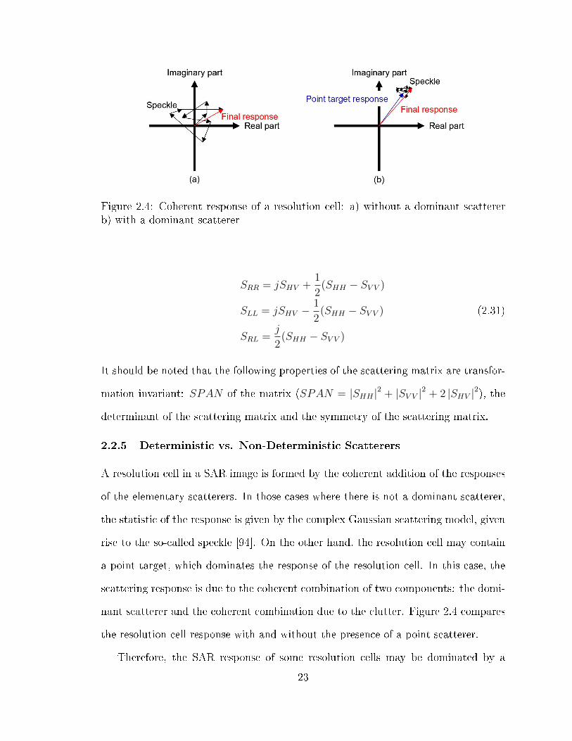
Figure 2.4: Coherent response of a resolution cell: a) without a dominant scattererb) with a dominant scatterer

SRR = jSHV +1

2(SHH − SV V )

SLL = jSHV −1

2(SHH − SV V ) (2.31)

SRL =j

2(SHH − SV V )

It should be noted that the following properties of the scattering matrix are transfor-

mation invariant: SPAN of the matrix (SPAN = |SHH |2 + |SV V |2 + 2 |SHV |2), the

determinant of the scattering matrix and the symmetry of the scattering matrix.

2.2.5 Deterministic vs. Non-Deterministic Scatterers

A resolution cell in a SAR image is formed by the coherent addition of the responses

of the elementary scatterers. In those cases where there is not a dominant scatterer,

the statistic of the response is given by the complex Gaussian scattering model, given

rise to the so-called speckle [94]. On the other hand, the resolution cell may contain

a point target, which dominates the response of the resolution cell. In this case, the

scattering response is due to the coherent combination of two components: the domi-

nant scatterer and the coherent combination due to the clutter. Figure 2.4 compares

the resolution cell response with and without the presence of a point scatterer.

Therefore, the SAR response of some resolution cells may be dominated by a

23

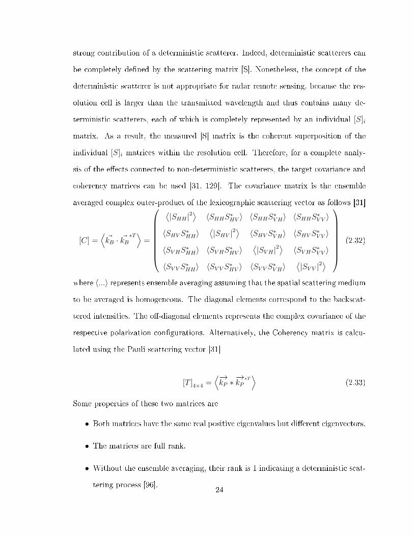
strong contribution of a deterministic scatterer. Indeed, deterministic scatterers can

be completely de�ned by the scattering matrix [S]. Nonetheless, the concept of the

deterministic scatterer is not appropriate for radar remote sensing, because the res-

olution cell is larger than the transmitted wavelength and thus contains many de-

terministic scatterers, each of which is completely represented by an individual [S]i

matrix. As a result, the measured [S] matrix is the coherent superposition of the

individual [S]i matrices within the resolution cell. Therefore, for a complete analy-

sis of the e�ects connected to non-deterministic scatterers, the target covariance and

coherency matrices can be used [31, 129]. The covariance matrix is the ensemble

averaged complex outer-product of the lexicographic scattering vector as follows [31]

[C] =⟨~kB · ~kB

∗T⟩=

⟨|SHH |2

⟩〈SHHS∗HV 〉 〈SHHS∗V H〉 〈SHHS∗V V 〉

〈SHV S∗HH〉⟨|SHV |2

⟩〈SHV S∗V H〉 〈SHV S∗V V 〉

〈SV HS∗HH〉 〈SV HS∗HV 〉⟨|SV H |2

⟩〈SV HS∗V V 〉

〈SV V S∗HH〉 〈SV V S∗HV 〉 〈SV V S∗V H〉⟨|SV V |2

⟩

(2.32)

where 〈...〉 represents ensemble averaging assuming that the spatial scattering medium

to be averaged is homogeneous. The diagonal elements correspond to the backscat-

tered intensities. The o�-diagonal elements represents the complex covariance of the

respective polarization con�gurations. Alternatively, the Coherency matrix is calcu-

lated using the Pauli scattering vector [31]

[T ]4×4 =⟨−→kP ∗

−→kP∗T⟩

(2.33)

Some properties of these two matrices are

• Both matrices have the same real positive eigenvalues but di�erent eigenvectors.

• The matrices are full rank.

• Without the ensemble averaging, their rank is 1 indicating a deterministic scat-

tering process [96].24

• As we shall see later in section 2.3, the interpretation of physical scattering

mechanism is easier using the coherency matrix.

It should be noted that assuming reciprocity (equation 2.15), the Pauli scattering

vector would take the following form

~kP3 =1√2

[SHH + SV V , SHH − SV V , 2SHV

]T(2.34)

Applying ~kP3, the following 3× 3 coherency matrix can be de�ned

[T ]3×3 =⟨−→kP3.−→kP3

∗T⟩

=1

2

⟨|M |2

⟩〈MN∗〉 〈MP ∗〉

〈M∗N〉⟨|N |2

⟩〈NP ∗〉

〈M∗P 〉 〈N∗P 〉⟨|P |2

⟩ (2.35)

where M = SHH + SV V , N = SHH − SV V and P = 2SHV .

It should be noted that in a pure target case, there exist a one-to-one correspon-

dence between the Kennaugh matrix and the [T ]3×3 matrix, given by [125]

[T ]3×3 =

2A0 C − jD H + jG

C + jD B0 +B E + jF

H − jG E − jF B0 −B

(2.36)

2.3 Polarimetric Decomposition

The main goal of target decomposition (TD) methods is to decompose or express

the average matrix into a sum of independent matrices representing independent ele-

ments and to associate a physical mechanism with each element. This decomposition

facilitates the interpretation of the scattering process.

Based on the type of matrix that is used for decomposition, Cloude [33] categorized

the TD methods into three groups: those employing the coherent decomposition of

the scattering matrix, those employing Muller matrix and Stokes vector and those25

Figure 2.5: Decomposition taxonomy

using an eigenvector analysis of the covariance or coherency matrix.

In this research we divide the TD methods into coherent and incoherent ap-

proaches. The incoherent approaches are divided into Huynen based, eigenvector

based and model based methods. Figure 2.5 shows a taxonomy of the methods we

investigated in this research.

The main reason for using this categorization is that the SAR parameters pro-

vided by coherent and incoherent parameters can complement each other for our goal

of forest classi�cation. Incoherent algorithms performs an averaging of the returned

signals. This provides a statistically smoother description of the behaviour of the

scatterers. Alternatively, the coherent methods, by avoiding the averaging at the �rst

stage, can be used to maintain the full resolution. By combining these parameters,

various forest features are emphasized. Coherent methods focuses on the more de-

tailed characteristics of the trees such as the leaves, branches and twigs whereas the

incoherent parameters reveals the high scale components e.g. the canopy structure.

2.3.1 Coherent Decomposition

A �rst class of TD theorems are coherent decomposition methods. The objective

of the coherent decompositions is to express the measured scattering matrix by the

26

radar, i.e. [S], as a combination of the scattering responses of simpler objects [33]

[S] =k∑i=1

ci [S]i (2.37)

In 2.37, the symbol [S]i stands for the response of every simpler objects, also known

as canonical objects, whereas ci indicates the weight of [S]i in the combination leading

to the measured [S].

In general, a direct analysis of the matrix [S], with the objective to infer the

physical properties of the scatterers under study, is shown very di�cult. Thus, the

physical properties of the target under study are extracted and interpreted through

the analysis of the simpler responses [S]i and the corresponding coe�cients ci in 2.37.

Pauli and Krogager are some of the important examples of such a decomposition

which are explained in the following sections.

The Pauli Decomposition

The Pauli decomposition expresses the measured scattering matrix [S] in the Pauli

basis. Recalling the four matrices in equation 2.19, the Pauli basis [S]a, [S]b, [S]c, [S]d

is given by the following four 2Ö2 matrices

[S]a =1√2

1 0

0 1

[S]b =

1√2

1 0

0 −1

(2.38)

[S]c =1√2

0 1

1 0

[S]d =

1√2

0 −1

1 0

27

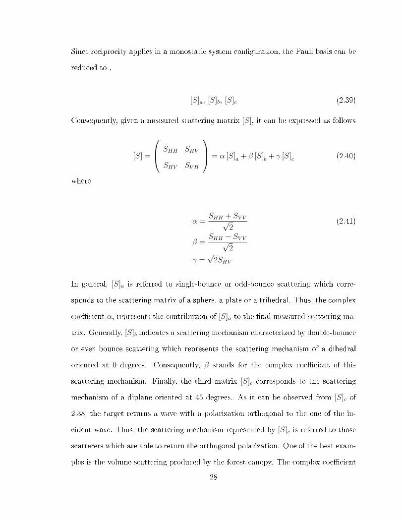
Since reciprocity applies in a monostatic system con�guration, the Pauli basis can be

reduced to ,

[S]a, [S]b, [S]c (2.39)

Consequently, given a measured scattering matrix [S], it can be expressed as follows

[S] =

SHH SHV

SHV SV H

= α [S]a + β [S]b + γ [S]c (2.40)

where

α =SHH + SV V√

2(2.41)

β =SHH − SV V√

2

γ =√

2SHV

In general, [S]a is referred to single-bounce or odd-bounce scattering which corre-

sponds to the scattering matrix of a sphere, a plate or a trihedral. Thus, the complex

coe�cient α, represents the contribution of [S]a to the �nal measured scattering ma-

trix. Generally, [S]b indicates a scattering mechanism characterized by double-bounce

or even-bounce scattering which represents the scattering mechanism of a dihedral

oriented at 0 degrees. Consequently, β stands for the complex coe�cient of this

scattering mechanism. Finally, the third matrix [S]c corresponds to the scattering

mechanism of a diplane oriented at 45 degrees. As it can be observed from [S]c of

2.38, the target returns a wave with a polarization orthogonal to the one of the in-

cident wave. Thus, the scattering mechanism represented by [S]c is referred to those

scatterers which are able to return the orthogonal polarization. One of the best exam-

ples is the volume scattering produced by the forest canopy. The complex coe�cient

28

γ is thus the contribution of [S]c to [S].

The Krogager Decomposition

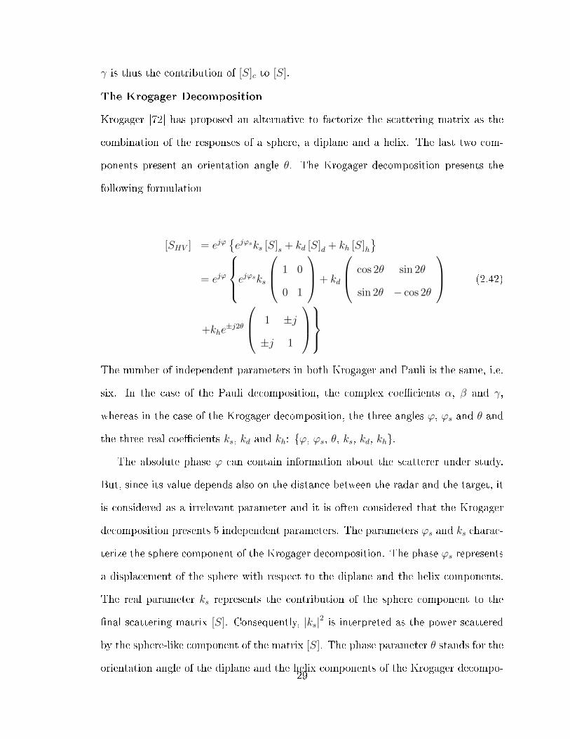
Krogager [72] has proposed an alternative to factorize the scattering matrix as the

combination of the responses of a sphere, a diplane and a helix. The last two com-

ponents present an orientation angle θ. The Krogager decomposition presents the

following formulation

[SHV ] = ejϕ{ejϕsks [S]s + kd [S]d + kh [S]h

}= ejϕ

ejϕsks

1 0

0 1

+ kd

cos 2θ sin 2θ

sin 2θ − cos 2θ

(2.42)

+khe±j2θ

1 ±j

±j 1

The number of independent parameters in both Krogager and Pauli is the same, i.e.

six. In the case of the Pauli decomposition, the complex coe�cients α, β and γ,

whereas in the case of the Krogager decomposition, the three angles ϕ, ϕs and θ and

the three real coe�cients ks, kd and kh: {ϕ, ϕs, θ, ks, kd, kh}.

The absolute phase ϕ can contain information about the scatterer under study.

But, since its value depends also on the distance between the radar and the target, it

is considered as a irrelevant parameter and it is often considered that the Krogager

decomposition presents 5 independent parameters. The parameters ϕs and ks charac-

terize the sphere component of the Krogager decomposition. The phase ϕs represents

a displacement of the sphere with respect to the diplane and the helix components.

The real parameter ks represents the contribution of the sphere component to the

�nal scattering matrix [S]. Consequently, |ks|2 is interpreted as the power scattered

by the sphere-like component of the matrix [S]. The phase parameter θ stands for the

orientation angle of the diplane and the helix components of the Krogager decompo-29

sition. Finally, the coe�cients kd and kh correspond to the weights of the diplane and

the helix components. Thus, |kd|2 and |kh|2 are interpreted as the power scattered

by the diplane and the helix components of the Krogager decomposition.

The value of these 5 parameters can be easier derived in a circular basis (r, l).

Reformulation of 2.42 in (r, l) gives

[Srl] =

Srr Srl

Slr Sll

=

|Srr| ejφrr |Srl| ejφrl

|Srl| ejφrl − |Sll| ej(φrr+π)

(2.43)

= ejϕ

ejϕsks

0 j

j 0

+ kd

ej2θ 0

0 −e−j2θ

+ kh

ej2θ 0

0 0

According to this formulation:

ks = |Srl|

φ =1

2(φrr + φll − π)

θ =1

4(φrr − φll + π) (2.44)

φs = φrl −1

2(φrr + φll)

Based on the di�erence in absolute value of Srr and Sll, Krogager considered two

cases:

|Srr| ≥ |Sll| ⇒

k+d = |Sll|

k+h = |Srr| − |Sll|⇐ Left sense helix (2.45)

|Srr| ≤ |Sll| ⇒

k−d = |Srr|

k−h = |Sll| − |Srr|⇐ Right sense helix

The formulations in 2.42 and 2.43 can be related using

30

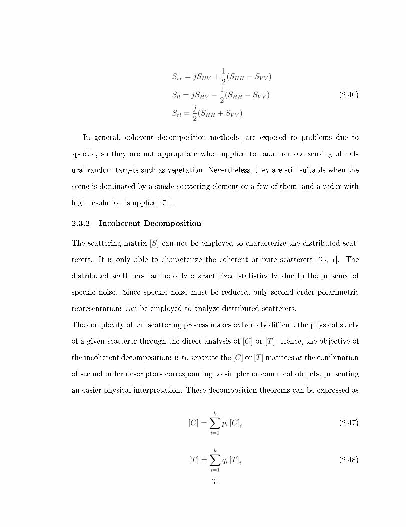
Srr = jSHV +1

2(SHH − SV V )

Sll = jSHV −1

2(SHH − SV V ) (2.46)

Srl =j

2(SHH + SV V )

In general, coherent decomposition methods, are exposed to problems due to

speckle, so they are not appropriate when applied to radar remote sensing of nat-

ural random targets such as vegetation. Nevertheless, they are still suitable when the

scene is dominated by a single scattering element or a few of them, and a radar with

high resolution is applied [71].

2.3.2 Incoherent Decomposition

The scattering matrix [S] can not be employed to characterize the distributed scat-

terers. It is only able to characterize the coherent or pure scatterers [33, 7]. The

distributed scatterers can be only characterized statistically, due to the presence of

speckle noise. Since speckle noise must be reduced, only second order polarimetric

representations can be employed to analyze distributed scatterers.

The complexity of the scattering process makes extremely di�cult the physical study

of a given scatterer through the direct analysis of [C] or [T ]. Hence, the objective of

the incoherent decompositions is to separate the [C] or [T ] matrices as the combination

of second order descriptors corresponding to simpler or canonical objects, presenting

an easier physical interpretation. These decomposition theorems can be expressed as

[C] =k∑i=1

pi [C]i (2.47)

[T ] =k∑i=1

qi [T ]i (2.48)

31

where pi and qi denote the coe�cients of these components in [C] or [T ], respectively.

Di�erent compositions can be presented based on this formulation.

Huynen-based decomposition

Huynen decomposition

The main idea of the Huynen target decomposition is to separate from the incoming

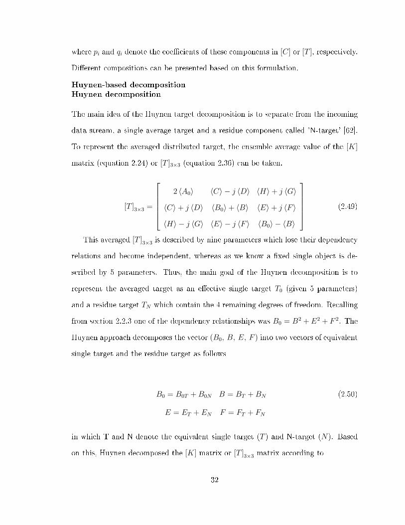
data stream, a single average target and a residue component called 'N-target' [62].

To represent the averaged distributed target, the ensemble average value of the [K]

matrix (equation 2.24) or [T ]3×3 (equation 2.36) can be taken.

[T ]3×3 =

2 〈A0〉 〈C〉 − j 〈D〉 〈H〉+ j 〈G〉

〈C〉+ j 〈D〉 〈B0〉+ 〈B〉 〈E〉+ j 〈F 〉

〈H〉 − j 〈G〉 〈E〉 − j 〈F 〉 〈B0〉 − 〈B〉

(2.49)

This averaged [T ]3×3 is described by nine parameters which lose their dependency

relations and become independent, whereas as we know a �xed single object is de-

scribed by 5 parameters. Thus, the main goal of the Huynen decomposition is to

represent the averaged target as an e�ective single target T0 (given 5 parameters)

and a residue target TN which contain the 4 remaining degrees of freedom. Recalling

from section 2.2.3 one of the dependency relationships was B0 = B2 +E2 + F 2. The

Huynen approach decomposes the vector (B0, B, E, F ) into two vectors of equivalent

single target and the residue target as follows

B0 = B0T +B0N B = BT +BN (2.50)

E = ET + EN F = FT + FN

in which T and N denote the equivalent single target (T ) and N-target (N). Based

on this, Huynen decomposed the [K] matrix or [T ]3×3 matrix according to

32

[T ]3×3 =

〈2A0〉 〈C〉 − j 〈D〉 〈H〉+ j 〈G〉

〈C〉+ j 〈D〉 〈B0〉+ 〈B〉 〈E〉+ j 〈F 〉

〈H〉 − j 〈G〉 〈E〉 − j 〈F 〉 〈B0〉 − 〈B〉

= T0 + TN (2.51)

where

T0 =

〈2A0〉 〈C〉 − j 〈D〉 〈H〉+ j 〈G〉

〈C〉+ j 〈D〉 B0T +BT ET + jFT

〈H〉 − j 〈G〉 ET − jFT B0T −BT

and (2.52)

TN =

0 0 0

0 B0N +BN EN + jFN

0 EN − jFN B0N −BN

(2.53)

It is important to note that the N-target corresponds to a perfectly non-symmetric

target (because it is de�ned with only the parameters (B0N , BN , EN , FN) ). Due

to this fact, the N-target does not change with target tilt angle (roll-invariant). In

other words, the N-target is independent of rotation along the line of sight between

radar and target. These 4 parameters are determined using 2.51. Alternatively,

the parameters (B0T , BT , ET , FT ), which corresponds to the single target, can be

reconstructed uniquely using the target structure equations (equation 2.26) which

can be rewritten as [98]

2A0(B0T +BT ) = C2 +D2

2A0(B0T −BT ) = G2 +H2

2A0ET = CH −DG (2.54)

2A0FT = CG−DH33

In summary, the Huynen target decomposition method factorizes the measured co-

herency matrix [T ]3×3 into a rank one pure target T0 and into a distributed and

roll-invariant N-target TN .

Barnes decomposition

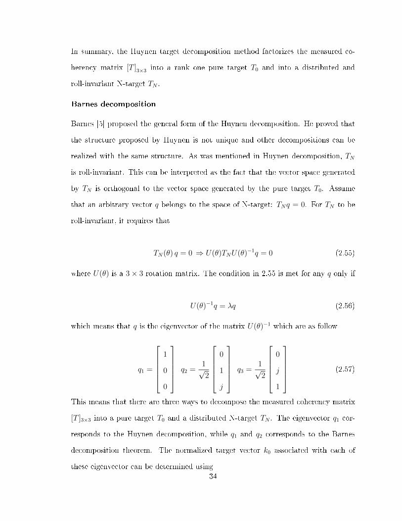
Barnes [5] proposed the general form of the Huynen decomposition. He proved that

the structure proposed by Huynen is not unique and other decompositions can be

realized with the same structure. As was mentioned in Huynen decomposition, TN

is roll-invariant. This can be interpreted as the fact that the vector space generated

by TN is orthogonal to the vector space generated by the pure target T0. Assume

that an arbitrary vector q belongs to the space of N-target: TNq = 0. For TN to be

roll-invariant, it requires that

TN(θ) q = 0 ⇒ U(θ)TNU(θ)−1q = 0 (2.55)

where U(θ) is a 3× 3 rotation matrix. The condition in 2.55 is met for any q only if

U(θ)−1q = λq (2.56)

which means that q is the eigenvector of the matrix U(θ)−1 which are as follow

q1 =

1

0

0

q2 =1√2

0

1

j

q3 =1√2

0

j

1

(2.57)

This means that there are three ways to decompose the measured coherency matrix

[T ]3×3 into a pure target T0 and a distributed N-target TN . The eigenvector q1 cor-

responds to the Huynen decomposition, while q1 and q2 corresponds to the Barnes

decomposition theorem. The normalized target vector k0 associated with each of

these eigenvector can be determined using34

T q = T0 q + TN q = T0q = k0kT∗0 q

qT∗q T = qT∗k0kT∗0 q =

∣∣kT∗0 q∣∣2

⇒ K0 =T q

kT∗0 q=

T q√qT∗q T

(2.58)

Plugging the 2.49 and 2.57 into the equation 2.58 the three normalized target vectors

can be obtained as

k01 =1√〈2A0〉

2 〈A0〉

〈C〉+ j 〈D〉

〈H〉 − j 〈G〉

(2.59)

k02 =1√

2(〈B0〉 − 〈F 〉)

〈C〉 − 〈G〉+ j 〈H〉 − j 〈D〉

〈B0〉+ 〈B〉 − 〈F 〉+ j 〈E〉

〈E〉+ j 〈B0〉 − j 〈B〉 − j 〈F 〉

k03 =1√

2(〈B0〉+ 〈F 〉)

〈H〉+ 〈D〉+ j 〈C〉+ j 〈G〉

〈E〉+ j 〈B0〉+ j 〈B〉+ j 〈F 〉

〈B0〉 − 〈B〉+ 〈F 〉+ j 〈E〉

Eigenvector based decomposition

H/A/α decomposition

The eigenvector-eigenvalue based decomposition is based on the eigen decomposition

of the coherency matrix [T ]. According to the eigen decomposition theorem, the 3×3

Hermitian matrix [T ] can be decomposed as follows [29]

[T ] = [U3][∑]

[U3]−1 (2.60)

The 3× 3, real, diagonal matrix [∑

] contains the eigenvalues of [T ]

35

[∑]=

λ1 0 0

0 λ2 0

0 0 λ3

(2.61)

where λ1 > λ2 > λ3 > 0 . The 3× 3 unitary matrix [U3] contains the eigenvectors ui

for i = 1, 2, 3 of [T ]

[U3] =

[u1 u2 u3

](2.62)

The eigenvectors ui of [T ] can be formulated as follows

ui =

[cosαi sinαi cos βie

jδi sinαi cos βiejγi

]T(2.63)

Considering the expressions 2.61 and 2.62, the eigen decomposition of [T ], i.e. 2.60,

can be written as follows

[T ] =3∑j=1

λiuiu∗Ti (2.64)

As 2.64 shows, the rank 3 matrix [T ] can be decomposed as the combination of three

rank 1 coherency matrices formed as

[T ] = T01 + T02 + T03 (2.65)

The obtained eigenvalues and eigenvectors are considered as the primary parameters

of the eigen decomposition of [T ]. In order to simplify the analysis of the physical

information provided by this eigen decomposition, three secondary parameters are

de�ned as a function of the eigenvalues and the eigenvectors of [T ] [31, 29]:

• Scattering Entropy H

The degree of randomness of target scattering is represented by H. It is com-

puted from the eigenvalues of the target coherency matrix according to:

36

H =3∑i=1

−Pi logn (Pi) (2.66)

where pi is de�ned as:

Pi =λi3∑

k=1

λk

(2.67)

The entropy is a scalar between 0 and 1. It can be also interpreted as the degree

of statistical disorder. In this way [100]:

H�0⇒ λ1 = SPAN λ2 = 0 λ3 = 0 ⇒one pure target

H�1⇒ λ1 = SPAN3

λ2 = SPAN3

λ3 = SPAN3

⇒3 pure targets

0 < H < 1⇒ three di�erent eigen value λi ⇒3 weighted pure targets

(2.68)

In the �rst case, the scattering matrix [T ] presents rank 1 and the scattering

process corresponds to a pure target. In the second case, the scattering matrix

[T ] presents rank 3, that is the scattering process is due to the combination of

three pure targets (distributed targets). In the third case, the �nal scattering

mechanism given by [T ] results from the combination of the three pure targets

given by ui, but weighted by the corresponding eigenvalues.

• Anisotropy A

The anisotropy can be derived from eigenvalues of the target coherency matrix

according to

A =λ2 − λ3λ2 + λ3

(2.69)

37

The anisotropy A, is a parameter complementary to the entropy. The anisotropy

measures the relative importance of the second and the third eigenvalues of the

eigen decomposition. From a practical point of view, the anisotropy can be

employed as a source of discrimination only when H > 0.7. The reason is that

for lower entropies, the second and third eigenvalues are highly a�ected by noise.

Consequently, the anisotropy is also very noisy.

• Alpha angle

The parameter alpha provides information on the dominant scattering mecha-

nism. It is computed as the weighted average of the value

α =3∑i=1

piαi (2.70)

The next list reports the interpretation of α:

α�0: The scattering corresponds to single-bounce scattering produced by a

rough surface.

α→ π4: The scattering mechanism corresponds to volume scattering.

α → π2: The scattering mechanism is due to double-bounce scattering. The

eigen decomposition of the coherency matrix is also referred as theH/A/α de-

composition [99].

Holm decomposition

Holm decomposition [59] improves the Huynen approach by combining the concept

of the single target plus noise model of the Huynen method with eigenvalue analysis.

Based upon this, the measured coherency matrix (T ) is decomposed into a pure target

matrix (T1) plus a mixed target state (T2) and an unpolarized mixed state equivalent

to a noise term (T3)

38

T = T1 + T2 + T3 (2.71)

where

T1 ⇒ Pure target state

T2 ⇒ Mixed target state (2.72)

T3 ⇒ Unpolarized mixed state (noise)

For a detailed explanation of the Holm decomposition method the reader is referred

to [83].

Model-based decomposition

Freeman-Durden decomposition

The Freeman and Durden [47] presented a method which is based on the physics of

radar scattering and less bound to pure mathematical models. The Freeman decom-

position describes the scattering as due to three physical mechanisms, i.e. �rst order

Bragg surface scatterer from a moderately rough surface (s), even- or double-bounce

scattering mechanism (d) and canopy (or volume) scattering from randomly oriented

dipoles (v). According to this model, the measured power P can be �nally expressed

as

P = SPAN =⟨|SHH |2

⟩+⟨|SV V |2

⟩+ 2

⟨|SHV |2

⟩= Ps + Pd + Pv (2.73)

These three components can be calculated using the elements of the covariance matrix.

In this process, a series of intermediate parameters i.e. fs, fd, fv, α and β are �rst

introduced as follows

39

Ps = fs(1 + |β|2)

Pd = fd(1 + |α|2) (2.74)

Pv =8

3fv

These parameters are then related to elements of covariance matrix using

⟨|SHH |2

⟩= fs |β|2 + fd |α|2 + fv⟨

|SV V |2⟩

= fs + fd + fv (2.75)

〈SHHS∗V V 〉 = fsβ + fdα +fv3⟨

|SHV |2⟩

=fv3

It should be noted that due to re�ection symmetry i.e. 〈SHHS∗HV 〉 = 〈SHV S∗V V 〉 =

0, the remaining covariance matrix element were omitted. There are 4 equations with

5 unknowns. One of the unknowns can be �xed using the method of van Zyl by

deciding whether double-bounce or surface scatter is the dominant contribution based

on the sign of the real part of SHHS∗V V . If Re {〈SHHS∗V V 〉} ≥ 0, then surface scatter

is dominant and α is �xed with α = −1. If Re {〈SHHS∗V V 〉} ≤ 0, then double-bounce

scatter is dominant and β is �xed with β = 1.

While this decomposition is useful in providing features for distinguishing between

di�erent surface cover types, it has two limiting assumptions, namely the three com-

ponent scattering model which is not always applicable and the re�ection symmetry

assumption [33].

Generally, forests have strong volume scattering. However, due to di�erent canopy

structure as well as di�erent shape of the leaves, this volume scattering varies among

di�erent trees. These can make the canopy scattering as a useful parameter for our

40

case of forest mapping.

Freeman two component decomposition

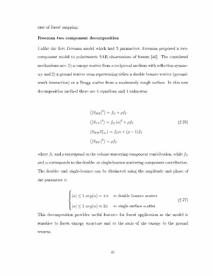
Unlike the �rst Freeman model which had 3 parameters, Freeman proposed a two-

component model to polarimetric SAR observations of forests [46]. The considered

mechanisms are: 1) a canopy scatter from a reciprocal medium with re�ection symme-

try and 2) a ground scatter term representing either a double bounce scatter (ground-

trunk interaction) or a Bragg scatter from a moderately rough surface. In this new

decomposition method there are 4 equations and 4 unknowns

⟨|SHH |2

⟩= fG + ρfV⟨

|SV V |2⟩

= fG |α|2 + ρfV (2.76)

〈SHHS∗V V 〉 = fGα + (ρ− 1)fV⟨|SHV |2

⟩= ρfV

where fV and ρ correspond to the volume scattering component contribution, while fG

and α corresponds to the double- or single-bounce scattering component contribution.

The double- and single-bounce can be distincted using the amplitude and phase of

the parameter α

|α| ≤ 1 arg(α) = ±π ⇐ double bounce scatter

|α| ≤ 1 arg(α) ≈ 2φ ⇐ single surface scatter

(2.77)

This decomposition provides useful features for forest application as the model is

sensitive to forest canopy structure and to the ratio of the canopy to the ground

returns.

41

Touzi decomposition

In contrast to the H/A/α decomposition, which uses the α angle to describe target

scattering type, the Touzi decomposition characterizes uniquely the scattering type

with the following parameters: the symmetric scattering type magnitude (αs) and

phase (φs), the target helicity (τs), the orientation angle (ψs) and the dominant

eigenvalue (λs).

Touzi et al. have shown that the use of αs,τs and λs parameters can lead to

e�cient wetland classi�cation [126]. In this study, we investigate the usefulness of

these parameters for forest mapping.

2.4 SAR discriminators

Several quantities have been derived from PolSAR data to be used as indicators to

discriminate among surface types or land covers. These include:

1. SPAN: the SPAN of the scattering matrix is de�ned as the sum of the squares

of all the original scattering matrix elements

SPAN = |SHH |2 + |SV V |2 + 2 |SHV |2 (2.78)

1. Extrema of the received power: Evans et al. [40] used the maximum and min-

imum of the received power at di�erent polarizations to discriminate di�erent

land cover types. The procedure for calculating these extrema comprises vary-

ing the polarization angles (φ, τ) of the transmitted wave and computation of

the corresponding received powers for each transmitted polarization angle. Al-

though, the calculation of these extrema is computationally expensive, they can

be useful for separating di�erent areas in polarimetric image.

2. Fractional polarization: it is de�ned as

42

F =(Pmax − Pmin)

(Pmax + Pmin)(2.79)

in which Pmax and Pmin are the maximum and minimum of the received power.

It can be used as a measure of the polarization purity of the return signal.

3. Extrema of the degree of polarization (polarized and unpolarized intensity ex-

trema): The degree of polarization is the ratio between the intensity of the

polarized part and the total scattered intensity. Touzi et al. [127] proposed a

systematic and analytic computation method for the calculation of the maxi-

mum and minimum degree of polarization

p =

√S21 + S2

2 + S23

S0

(2.80)

S0 is proportional to the total intensity of the wave, S1 is the di�erence between

the density powers related to the horizontal and vertical polarizations. Param-

eters S2 and S3 are related to the phase di�erence between the horizontal and

vertical components of the electric �eld. In this thesis, we used the maximum

and minimum degree of polarization.

4. Extrema of the total scattered intensity: Touzi et al. [127] divided the total

scattered intensity into the completely polarized and completely unpolarized

components, and for each one the extrema was calculated. He showed that

these indicators along with the extrema of the degree of the polarization can be

combined with other indices for target discrimination. Note that for the case of

extrema of the completely unpolarized scattered intensity, the minimum compo-

nent was only considered because the maximum of the completely unpolarized

scattered intensity and the coe�cient of fractional polarization are correlated.

5. Pedestal height: The pedestal height is de�ned as the minimum value of the

43

co-polarization response and is based on the polarization synthesis at each pixel.

It indicates the depolarization within the image. The pedestal height is higher

for a higher degree of depolarization.

6. Complex corelation coe�cients (coherence): the four correlation coe�cients

between polarizations are important parameters in PolSAR data, and were used

in this study

ρ12 =〈SHHS∗HV 〉√|SHH |2 |SHV |2

ρ13 =〈SHHS

∗V V 〉√

|SHH |2|SV V |2(2.81)

ρ23 =〈SHHS∗V V 〉√|SHH |2 |SV V |2

ρRL =〈SRRS

∗LL〉√

|SRR|2|SLL|2

7. depolarization ratio: The depolarization ratio describes how completely a target

depolarizes incident polarized signal. It can be calculated as

d =〈ShvS∗hv〉

〈ShhS∗hh〉+ 〈SvvS∗vv〉(2.82)

Roughness causes a depolarization of the incident wave and the cross-polarized

response is very sensitive to the roughness variations. Therefore, it may be used

to separate forest types with di�erent roughness types.

2.5 summary

The chapter aimed at providing various PolSAR features that might be useful for for-

est classi�cation. At the beginning, a brief introduction of SAR polarimetry including

polarimetry basics, di�erent formalism (Stokes vs. Jones Formalism, Scattering Ma-

trix vs. Muller Matrix ) and deterministic vs. non-deterministic scatterers was given.

This theoretical grounding is necessary for a better understanding of the di�erent

SAR parameters.44

Afterwards, the chapter reviewed di�erent target decomposition approaches i.e.

coherent and incoherent methods. Then, the SAR discriminators that are used in

this thesis were listed. These PolSAR parameters provide the necessary features for

forest classi�cation. Table 2.2 lists the parameters used in this thesis. Some remarks

on these parameters are given below

• The amplitude of the 3 upper triangle elements of the covariance matrix are

used in this research. It should be noted that the diagonal elements of the

covariance matrix were already employed as the scattering matrix elements

• The amplitude of the 5 diagonal and upper triangle coherency matrix elements

were used. Note that the third diagonal element of the coherency matrix ([T ]33)

was not considered because it was exactly twice as much as the second element

of the covariance matrix ([C]22), and hence redundant.

• In the case of Huynen , Barnes and Holm decompositions the 6 amplitudes of

the upper triangle elements of the corresponding matrices were considered in

this thesis

45

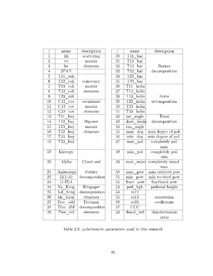
# name description # name description1 hh scattering 30 T11_bar2 vv matrix 31 T12_bar3 hv elements 32 T13_bar Barnes4 SPAN 33 T22_bar decomposition5 T11_coh 34 T23_bar6 T12_coh coherency 35 T33_bar7 T13_coh matrix 36 T11_holm8 T22_coh elements 37 T12_holm9 T23_coh 38 T13_holm Holm10 C12_cov covariance 39 T22_holm decomposition11 C13_cov matrix 40 T23_holm12 C23_cov elements 41 T33_holm13 T11_huy 42 psi_angle Touzi14 T12_huy Huynen 43 dom_landa decomposition15 T13_huy matrix 44 tau_angle16 T22_huy elements 45 max_deg max degree of pol.17 T23_huy 46 min_deg min degree of pol.18 T33_huy 47 max_pol completely pol.

max19 Entropy 48 min_pol completely pol.

min20 Alpha Cloud and 49 max_unpo completely unpol.

max21 Anisotropy Pottier 50 max_pow max received pow22 H(1-A) decomposition 51 min_pow min received pow23 (1-H)A 52 fract_pow fractional pow24 Ks_Krog Krogager 53 ped_hgh pedestal height25 Kd_Krog decomposition 54 ro1226 kh_Krog elements 55 ro13 correlation27 Free_odd Freeman 56 ro23 coe�cients28 Free_dbl decomposition 57 CCC29 Free_vol elements 58 depol_ind depolarization

ratio

Table 2.2: polarimetric parameters used in this research

46

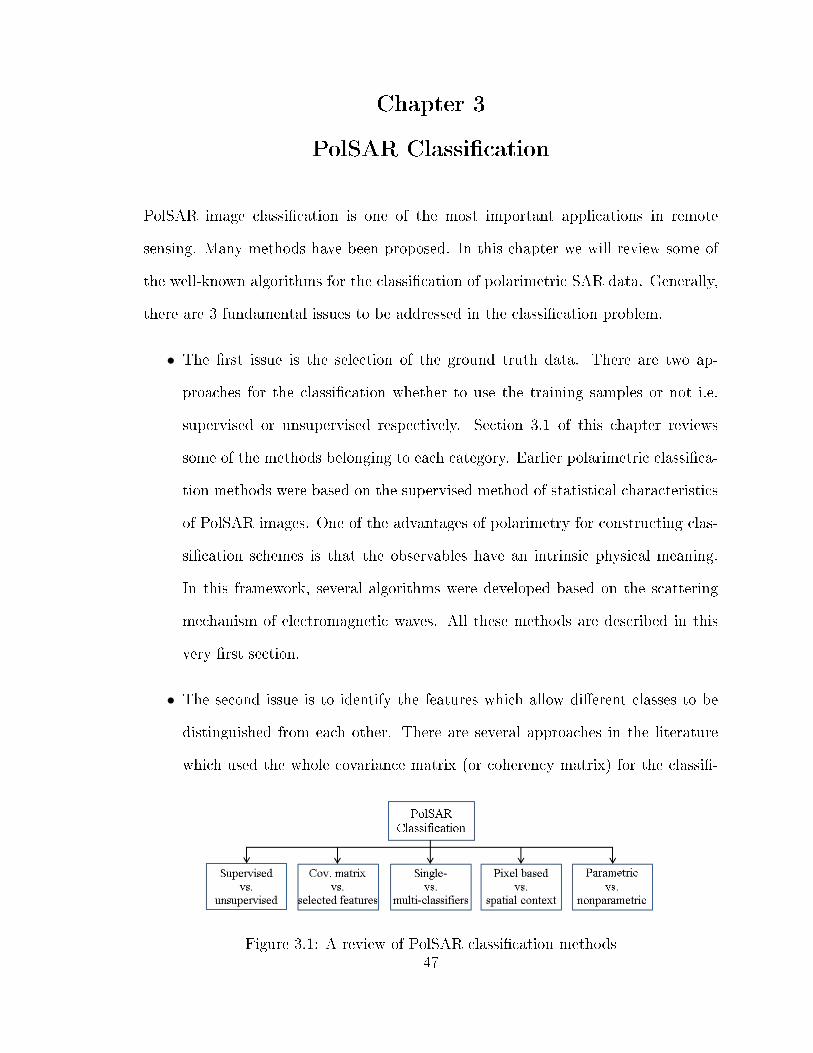
Chapter 3

PolSAR Classi�cation

PolSAR image classi�cation is one of the most important applications in remote

sensing. Many methods have been proposed. In this chapter we will review some of

the well-known algorithms for the classi�cation of polarimetric SAR data. Generally,

there are 3 fundamental issues to be addressed in the classi�cation problem.

• The �rst issue is the selection of the ground truth data. There are two ap-

proaches for the classi�cation whether to use the training samples or not i.e.

supervised or unsupervised respectively. Section 3.1 of this chapter reviews

some of the methods belonging to each category. Earlier polarimetric classi�ca-

tion methods were based on the supervised method of statistical characteristics

of PolSAR images. One of the advantages of polarimetry for constructing clas-

si�cation schemes is that the observables have an intrinsic physical meaning.

In this framework, several algorithms were developed based on the scattering

mechanism of electromagnetic waves. All these methods are described in this

very �rst section.

• The second issue is to identify the features which allow di�erent classes to be

distinguished from each other. There are several approaches in the literature

which used the whole covariance matrix (or coherency matrix) for the classi�-

Figure 3.1: A review of PolSAR classi�cation methods47

cation. On the other hand, there are approaches which employ a set of selected

features for that speci�ed problem. These methods are discussed in section 3.2.

• The third issue is to devise a classi�cation technique which uses these features

in the classi�cation problem. Depending on whether the classi�er assumes the

data �t a speci�c distribution, the classi�cation techniques are divided into para-

metric and nonparametric classi�ers (section 3.5). Recently, there has been a

great interest for using an ensemble of classi�ers for solving problems in pattern

recognition community. There are di�erent methods for creating such an ensem-

ble, which are discussed in section 3.3. There are another category of methods

which tend to incorporate spatial context into classi�cation. The main idea is

that two neighboring pixels are not entirely statistically independent. Some of

these methods are reviewed in section 3.4. Figure 3.1 shows an overview of

di�erent categories for PolSAR classi�cation.

3.1 Supervised vs. unsupervised

There are basically two approaches to classi�cation: unsupervised or supervised. The

supervised approach (section 3.1.1) requires ground truth. However it may lead to am-

biguities because the scene characteristics required by the analyst may not necessarily

be supported by the properties of the data. Unsupervised classi�cation (section 3.1.2)

leads to an understanding of the class separability in the scene that is supported by

the polarimetric signatures of the data. A di�culty with unsupervised classi�cation

is that convergence depends on the initial seeding of candidate classes [108].

3.1.1 Supervised

As one of the earlier algorithms, Kong et al. derived a distance measure based on the

complex Gaussian distribution and used it for maximum likelihood (ML) classi�cation

of single look complex PolSAR data:48

d(k, ωi) = k∗TC−1i k + ln∣∣∣Ci∣∣∣ (3.1)

in which k is the SAR observable k = [SHH ,√

2SHV , SV V ] which has a multivariate

complex circular Gaussian probability density function Nc(0, Ci), where Ci is the

complex covariance matrix for class ωi. |Ci| is the determinant of Ci. During the

classi�cation process a pixel is assigned to the minimum distance cluster.

For multilook data represented in covariance or coherency matrices, Lee et al.

[82, 81] proposed a method based on the maximum likelihood classi�er using the

complex Wishart classi�er. They show that assuming that target vectors have a

Nc(0, Ci) distribution, a sample n-look covariance matrix Z = 1nΣnk k

∗T follows a

complex Wishart distribution with n degrees of freedom, given by

p(Z) =nqn |Z|n−q exp[−tr(nC−1Z)]

K(n, q) |C|n(3.2)

with K(n, q) = πq(q−1)

2

q∏i=1

Γ(n− i+ 1)

where q is the dimension of the vector k which is 3 in our case, Γ() represents the

Gamma function. Based on equation 3.2, the Wishart distance is de�ned as

d(Z, ωi) = n ln∣∣∣Ci∣∣∣+ ntr(CiZ) + qn lnn− (n− q) ln |Z|+ lnK(n, q) (3.3)

and removing the unnecessary terms from the above distance, the �nal decision rule

will be

Decide k belong to the classωi, if arg min(d(Z, ωi)) with (3.4)

d(Z, ωi) = n ln∣∣∣Ci∣∣∣+ ntr(CiZ)

49

For the supervised classi�cation, the covariance matrix for class i i.e. Ci is estimated.

Then, for each pixel the Wishart distance measure d(Z, ωi) is calculated for each

class and the pixel is assigned to the class with the minimum distance. Lee et al.

[81] showed that by the use of supervised classi�cation and a Wishart classi�er, high

classi�cation accuracies for various land cover types could be obtained.

3.1.2 Unsupervised

One of the advantages of PolSAR data for classi�cation is that no prior knowledge is

required about the scene because the observables have an intrinsic physical meaning.

This makes the PolSAR data ideal for unsupervised classi�cation.

Cloude and Pottier [33] found that the target entropy and alpha angle can be

e�ective at classifying the SAR image according to scattering mechanism using P,L

or C-band SAR data. This is done by forming a two dimensional feature space and

subdividing it into eight possible categories. The categories are found by de�ning the

ranges of alpha angle that gives rise to surface scattering (0o−42o), volume scattering

(42o − 48o) and double bounce scattering (48o − 90o) and de�ning low, medium and

high levels of entropy [29]. Figure 2 shows the subdivided entropy-alpha feature

space and an example of how the pixels in a SAR image may be distributed among

the partitioned zones. Here is a summary of the physical scattering characteristics of

each of the nine zones [29]:

� Zone 9: Low entropy surface scattering (e.g. Bragg surface scattering, specular

scattering phenomena which do not involve 180 phase inversions between HH and VV

and very smooth land surfaces such as water at L and P-Bands).

� Zone 8: Low entropy dipole scattering (e.g. strongly correlated mechanisms

which have a large imbalance between HH and VV in amplitude and scattering from

vegetation with strongly correlated orientation of anisotropic scattering elements).

� Zone 7: Low entropy multiple scattering events( double or 'even' bounce scat-

50

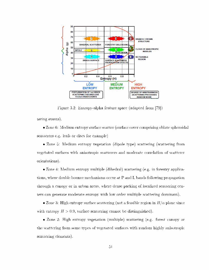
Figure 3.2: Entropy-alpha feature space (adapted from [79])

tering events).

� Zone 6: Medium entropy surface scatter (surface cover comprising oblate spheroidal

scatterers e.g. leafs or discs for example)

� Zone 5: Medium entropy vegetation (dipole type) scattering (scattering from

vegetated surfaces with anisotropic scatterers and moderate correlation of scatterer

orientations).

� Zone 4: Medium entropy multiple (dihedral) scattering (e.g. in forestry applica-

tions, where double bounce mechanisms occur at P and L bands following propagation

through a canopy or in urban areas, where dense packing of localized scattering cen-

ters can generate moderate entropy with low order multiple scattering dominant).

� Zone 3: High entropy surface scattering (not a feasible region in H/α plane since

with entropy H > 0.9, surface scattering cannot be distinguished).

� Zone 2: High entropy vegetation (multiple) scattering (e.g. forest canopy or

the scattering from some types of vegetated surfaces with random highly anisotropic

scattering elements).

51

� Zone 1: High entropy double bounce scattering (e.g. in forestry applications or

in scattering from vegetation which has a well developed branch and crown structure).

The basic scattering mechanism of each pixel of a polarimetric SAR image can

then be identi�ed by comparing its entropy and α parameters to �xed thresholds.

The segmentation in the H/α plane permits to identify in a macroscopic way the

type of scattering mechanism. Agricultural �elds and bare soils are characterized by

surface scattering. Scattering over forested areas is dominated by volume di�usion

while urban areas are mainly characterized by double bounce scattering.

Lee et al. [78] used the H/α decomposition as a basis for the unsupervised clas-

si�cation of the polarimetric data. A segmentation based on the H/α feature space

[33] is �rst applied. The result of this segmentation was then used as the initial

training set. Using this obtained training set, the Wishart distribution parameters

and then the Wishart distance measure are obtained. In the next step the classi�ed

results are used as new training sets based on which the new distance measures are

calculated. This process will continue until the number of pixels migrating between

classes becomes less than a prede�ned threshold. One of the limitations in using such

H/α initialization is that di�erent objects, like water and road might be assigned to

the same class due to the same surface scattering behavior. In order to overcome

this problem some other information has to be used. The next two approaches are

examples of this.

Pottier et al. [99] showed that by explicitly including the anisotropy informa-

tion during the segmentation procedure the H/α method can be further improved.

As mentioned in section 2.3, the parameter A indicates the relative importance of

secondary mechanisms. Thus, using this parameter could be useful to discriminate

scattering mechanisms with di�erent eigenvalue distributions but with similar inter-

mediate entropy values. In such cases, a high value of A represents two dominant

52

scattering mechanisms and a less signi�cant third mechanism. A low value of A shows

that there is a dominant �rst scattering mechanism and two non-negligible secondary

mechanisms with equal importance. The A parameter can be used to provide further

class re�nement [41]. The method is implemented in two successive classi�cation pro-

cedures. At �rst a H/α classi�cation approach is employed. Once the convergence is

reached, the 8 output classes of the �rst step is decomposed into 16 classes by com-

paring the parameter A of each pixel to a threshold �xed to 0.5. The �nal Wishart

ML is applied on these new sets of clusters.

Since the H and α parameters alone are not su�cient for a good interclass resolu-

tion, additional information is needed. Hellmann [54] showed by using the backscatter

intensity information contained in the �rst eigenvalue λ1, a better interclass resolu-

tion can be achieved. This is because the pure H/α approach has a limited interclass

resolution. Therefore, a combination of H, α with λ1 can improve the interclass res-

olution. This improvement is mainly for the areas where surface scattering occurs.

For example, for the classes of low vegetation, road like structures and water the �rst

eigenvalue λ1 is dominant. Applying this approach to the E-SAR data, it provided

the best interclass resolution and a good classi�cation accuracy was also reported.

But the interpretation of the data is more di�cult [54].

One of the shortcomings of the previous approaches was that the classi�cation

result lacked details, because of the preset zone boundaries in the H and α plane.

This could cause the clusters to fall on the boundaries. Also, more than one cluster

may be enclosed in a zone . To solve this problem, Lee et al. [80] proposed a new

method which not only uses a statistical classi�er, but also preserves the dominant

polarimetric scattering properties. The algorithm �rst applies the Freeman and Dur-

den decomposition to divide pixels into three scattering categories: surface scattering,

volume scattering, and double-bounce scattering. A merge criterion was also devel-

53

oped using the Wishart distance measure to merge the clusters in each scattering

category. Finally, an iterative Wishart classi�er was applied. In comparison with

H/A/α Wishart classi�er, this algorithm was more e�cient in terms of the stability

in convergence.

3.2 Full covariance matrix vs. selected features

There are basically two approaches for the use of input features in PolSAR classi�-

cation. One approach is the use of full covariance (coherency) matrix as the input

features. One of the common approaches in this category is the method proposed

by Lee et al. [81]. The classi�cation method is a supervised method, using a dis-

tance measure based on Wishart statistics and this measure could be incorporated

in several classi�cation algorithms [78, 41]. A possible drawback to these approaches

is that only second order representations were considered when operating these clas-

si�ers [80] and it does not allow combining the covariance data with other types of

features such as those obtained from other decomposition methods or textural fea-

tures or backscattered intensity. Alberga [3] showed that the methods based on the

covariance matrix provide important information about the scatterers on the ground,

but extra features would be needed in order to distinguish complex classes.

The second approach try to employ the best features in the classi�cation problem.

The solution of applying feature selection before classi�cation was suggested by dif-

ferent authors [50, 67, 64, 111, 66, 113]. The feature selection problem can be stated

as follows: Given a set of N features �nd the best subset of m features to be used

for classi�cation. This process generally involves a search strategy and an evalua-

tion function [50]. The aim of the search algorithm is to generate subsets of features

from the original feature space and the evaluation function compares these feature

subsets in terms of discrimination. The output of the feature selection algorithm is

the best feature subset found for this purpose. Optimal search algorithms determine54

the best feature subset in terms of an evaluation function, whereas suboptimal search

algorithms determine a good feature subset. When the number of features increased,

using an optimal search algorithm is computationally expensive and thus not feasible.

According to the evaluation function, the feature selection approaches can be

broadly grouped into �lter and wrapper methods[69]. Wrapper methods utilize the

classi�cation accuracy as the evaluation function whereas �lter methods uses the

inter-class distance measures as the evaluation function. The most widely used inter-

class measures are Bhattacharyya distance, divergence and Je�ries-Matusita (JM)

distance.

Zhang et al.[138] employed Multiple-Component Scattering Model (MCSM) as

the decomposition method to generate features. These features along with the tex-

ture features formed the input features for classi�cation. The Sequential Backward

Selection (SBS) was chosen in the feature selection procedure, in which the features

were sequentially removed from a full candidate set until the removal of further fea-

tures increases the criterion. The number of support vectors was considered as the

measurement of feature selection. They found that with the decreasing number of

support vectors, the precision of classi�cation increases. Finally a SVM was �nally

used for the classi�cation. This schema, though simple and straightforward, has a

weakness: the authors limited themselves to the MCSM decomposition method. The

other decomposition methods could have been used to expand the input feature vec-

tor.

The Logistic Regression (LR), which is a statistical tool for distinguishing the

target class from background, has been adopted for the classi�cation of polarimetric

SAR data [14]. LR's task is optimize the βi's coe�cients in the following nonlinear

function called logistic function:

55

p(target |x) =exp [β0 +

∑i xiβi]

1 + exp [β0 +∑

i xiβi](3.5)

p(target |x) is the conditional probability that a pixel belongs to the target class

given the vector of input features x for that class. For a dichotomous problem, the

probability of background will be:

p(background |x) = 1− p(target |x) (3.6)

LR �nds a combination of the features that optimizes the following log-likelihood:

L(β) =n∑i=1

{yi ln [p(target |x)] + (1− yi) ln [1− p(target |x)]} (3.7)

in which yi is 1 for targets and 0 for background. Therefore, LR implicitly performs

a feature selection: the features that contribute signi�cantly to the discrimination

between the background and the target are added to the model.

Shimoni et al. [114] derived a large feature set from multi-frequency multi-

polarization PolSAR and PolInSAR data. They developed two level fusion method

i.e. LR as feature-level fusion and neural network (NN) method for higher level fusion.

According to their work, LR selects the most discriminative features automatically

and combines them in order to distinguish the investigated class from all others. Good

results were obtained and LR was proved to be as a powerful tool for fusion.

In order to improve the discrimination power and classi�cation accuracy, the tex-

ture measures of the SAR image were also in the feature set [139, 27, 130]. For

example in [139], gray-level co-occurrence matrix (GLCM) based texture features

were added to the span image and the H, Alpha and A parameters. A principle

component analysis (PCA) was then used to reduce the feature set. A 3-layer neural

network is �nally constructed for the classi�cation. In some other studies, fusion of

physical and textural information that are derived from various SAR polarizations56

has improved the classi�cation results [35, 11].

In [55] a supervised classi�cation method based on neural networks and fuzzy logic

is used to learn the class borders from the available learning samples. The advantage

of this approach is that other input features can be easily added in order to increase

the discrimination ability of the classi�cation.

In addition, a method based on the manual selection of features was evaluated on

a subset of the Flevoland dataset [57].

3.3 Single- vs. multi-classi�ers

Multiple classi�er systems (MCS) or classi�er ensembles are another machine learn-

ing concept; there has been a great interest for using such an ensemble for solving

problems in pattern recognition community recently[6]. By combining di�erent inde-

pendent classi�ers, MCS can improve the classi�cation accuracy in comparison to a

single classi�er.

There are di�erent methods for creating such an ensemble. These methods include

modifying the training samples (e.g. bagging [18] and boosting [42]), manipulating

the input features (the input feature space is divided into multiple subspaces [56]),

manipulating the output classes (multi-class problem is decomposed into multiple two-

class problems, e.g. the error correcting output code (ECOC) [36]). After creation

of an ensemble of classi�ers, a decision fusion is used to combine the outputs of the

classi�ers. Several fusion algorithms have been developed and employed, for example,

majority voting, D-S evidence theory, fuzzy integral, weighted summation, consensus,

mixed neural network and hierarchical classi�er system [120, 2, 20].

Although classi�er ensembles have given promising results, only a few applications

are known for SAR data, in particular for PolSAR data. She et al. [112] introduced

Adaboost for PolSAR image classi�cation. Comparing with traditional methods such

as Wishart distance classi�er, it was found to be more �exible and robust. Chen57

et al. [25] proposed a supervised classi�cation scheme based on Adaboost . Each

independent element of the Mueller matrix as well as the extracted parameters formed

a weak classi�er. By the Adaboost procedure, each classi�er was endowed with a

weight. The weight presented the e�ectiveness of the corresponding feature. All the

weak classi�ers were combined together to form a strong classi�er using majority

weighted voting. They found that this scheme was more robust and more accurate

than the traditional maximum likelihood classi�er. Min et al. [93] also employed

polarimetric decomposition and the Adaboost algorithm to solve a PolSAR image

classi�cation problem. Their simulation results validated their method compared

with H/α classi�cation algorithm.

In 2010, Zou et al. [141] took advantage of Random Forests [19] for the generation

of multiple classi�ers. They proposed two feature combination strategies and in the

classi�cation stage they employed a robust classi�er named Extremely randomized

Clustering Forests (ERCFs), which are ensembles of randomly created clustering trees,

for terrain classi�cation using Polarimetric data. Comparing with other classi�ers,

ERCFs got slightly better classi�cation accuracy than SVM with less computational

time.

The Logistic Regression (LR), which is a statistical tool for distinguishing the

target class from background, has been adopted for the classi�cation of polarimetric

SAR data: Shimoni et al. [114] derived a large feature set from multi-frequency

multi-polarization PolSAR and PolInSAR data. They developed two level fusion

method i.e. LR as feature-level fusion and neural network (NN) method for higher

level fusion. According to their work, LR selects the most discriminative features

automatically and combines them in order to distinguish the investigated class from

all others. Good results were obtained and LR was proved to be as a powerful tool

for fusion.

58

3.4 Incorporating spatial context

One disadvantage of most of the methods reviewed so far is that each pixel is treated

to be independent of its neighbors. The local neighborhood have a signi�cant in�u-

ence on a pixel's class membership. Spatial context as an additional classi�cation

knowledge was taken into account in the literature. The main idea behind these

methods is that when a certain region has already been classi�ed, with high con�-

dence, as belonging to a single class, it becomes comparatively unlikely that a pixel

in this region belongs to another class. This means that two neighboring pixels are

not entirely statistically independent.

Basically, there are three ways to incorporate spatial context into a classi�cation

i.e. preprocessing, post-processing and processing.

In preprocessing methods, texture channels are often generated and are added to

the input features for classi�cation. These spatial features can be extracted using the

texture features.

The post-processing approaches are applied after the classi�cation of the original

image. The essence of these approaches is to �lter the labels in the thematic map,

e.g. a mode �lter. Another approach in this category for incorporating the spatial

context into classi�cation is the probabilistic label relaxation [109, 51, 53]. Label

relaxation is based on the the modi�cation of the probability values of each pixel

according to the probability compatibility among pixels in a local neighborhood. The

goal of label relaxation is to reduce the uncertainty and improve the consistency in

the assignment of one of the labels to each pixel in a set of related pixels [106]. In

its simplest form, the probabilistic label relaxation involves de�ning a neighborhood

function that expresses support from the neighbors for the labeling of the gth pixel

at the kth iteration of the form

59

Qkg(wi) =

∑n

dn∑j

pgn(wi|wj)pkn(wj) (3.8)

in which dn weights the in�uence of the nth neighbor, pkn(wj) is the posterior probabil-

ity that the neighbor n has the label wj,∑

j pgn(wi|wj) is the conditional probability

that pixel g is labeled wi if the neighbor n is labeled wj.

Finally, the methods on the processing level incorporate spatial reasoning into the

classi�cation. These classi�ers are termed as contextual classi�ers. For classifying a

certain pixel, a contextual classi�er directly make use of the contextual information

from a pixel window by means of a spectral-spatial distance.

In the context of SAR data, there have been several works taken place in recent

years. Reigber et al. [105] employed probabilistic label relaxation in the framework

of an unsupervised classi�cation scheme of PolSAR data based on the statistical par-

titioning of the covariance matrix feature space. They took advantage of this spatial

context by taking into account the local neighborhood by altering the probabilities

of class membership using a neighborhood function. In this way, robust and homo-

geneous classi�cation results were obtained even in the presence of strong speckle

noise.

Markov Random Fields (MRFs) is a popular model for incorporating spatial con-

text into image classi�cation. They are frequently employed to model neighborhood

and class label structure for the classi�cation of remotely sensed data. In particular,

[107] and [118] have used MRF models in the classi�cation of SAR data and obtained

better results than ordinary classi�cation methods without use of spatial consistency.

Some newer works in the context of SAR data can be found in [121] and [43]. One

of the weaknesses of the MRFs is that they are computationally complex due to the

complicated structure of their likelihood function.

In [12, 13, 14] spatial consistency was also taken into account. They used majority

60

voting for spatial regularization (MVR): in a neighborhood of each pixel the sum of

the conditional probability for each class is determined and the pixel is assigned

to the class corresponding to the highest sum. In [14] , in order to avoid blurring

of linear objects such as roads by the MVR method, they improved this method by

replacing the MVR by the second best class regularization (SBR) i.e. in miss-classi�ed

pixels, the correct class often corresponds to the second highest value. This method

signi�cantly reduced isolated misclassi�ed pixels.

3.5 Parametric vs. nonparametric classi�ers

The main objective in this section is to review the works according to the type of

classi�ers that they are employing. During the past years, di�erent classi�er types

and di�erent classi�er architecture were used for the classi�cation of PolSAR data [82,

26, 63, 8, 49, 24, 37]. These methods can be broadly categorized into parametric and

nonparametric methods. Parametric methods, for example the maximum likelihood

(ML) [82], is based on the assumption of the complex Wishart distribution of the

covariance matrix. If the distribution is not good enough, the classi�cation result is

not good either. However, the assumption on the distribution is not necessary when

nonparametric classi�ers are employed for a classi�cation task.

In 1991, Pottier et al. [101] �rstly introduced the Neural Networks (NNs) to Pol-

SAR image classi�cation. In 1999, Hellmann [92] further introduced fuzzy logic with

neural networks classi�er. More recently, neural network based approaches [139, 137]

for classi�cation of polarimetric synthetic aperture radar data have been shown to

outperform other aforementioned well-known techniques. Compared with other ap-

proaches, neural network classi�ers have the advantage of adaptability to the data

without making a priori assumption of a particular probability model or distribution.

However, their performance depends on the network structure, training data, initial-

ization and parameters. Also, they usually converge slowly and tends to converge to61

a local optimization.

Support Vector Machine (SVM) has become an increasing popular tool for machine

learning tasks involving classi�cation, recognition, or detection. SVM is based on

statistic learning theorem; however, SVM method does not need the statistic features

of the training samples and it can deal with high dimension data and nonlinear

problem easily and can also achieve global optimization [132, 133]. It has been mostly

applied to hyperspectral remote sensed data and few studies have also been conducted

with SAR data [49, 91].

PolSAR image classi�cation using SVM has shown exceptional growth in recent

years. Fukuda et al. [48] introduced Support Vector Machine (SVM) to land cover

classi�cation with higher accuracy. Additionally, Lardeux et al. [76] showed that the

SVM classi�cation algorithm is well suited for full polarimetric data with similar ac-

curacy as Wishart classi�cation. Also, the possibility to add di�erent polarimetric or

textural indices makes the SVM algorithm very interesting as the overall performance

increased.

Another approach that is applied on remote sensing imagery is Self-learning de-

cision tree classi�ers (DT) [95, 115]. The handling of DTs is rather simple and their

training time is relatively low compared to computationally complex approaches such

as neural networks [95]. In contrast to other classi�er algorithms, which use the whole

feature space at once and make a single membership decision, a decision tree is based

on a hierarchical concept. It is composed of an initial root node, several split nodes

and the �nal leaf nodes. At each node the most relevant feature is selected and used

for the construction of a binary test (i.e., decision boundary). In the context of Pol-

SAR data Zhixin et al. [140] integrated polarimetric decomposition, object-oriented

image analysis, and decision tree algorithms for RADARSAT-2 PolSAR data. The

data were then combined with the parameters of the backscattering and coherency

62

matrix to form a multichannel image. The decision tree algorithm was used to se-

lect features and create a decision tree for the classi�cation. Their obtained results

showed that the method outperforms the Wishart supervised classi�cation.

3.6 Summary

The chapter reviewed some of the common algorithms for the classi�cation of PolSAR

data. The algorithms were grouped into 5 categories. In the �rst category, several

supervised and unsupervised methods were reviewed. In this research, the reference

data have already been collected from the study area. Thus, the proposed methods

are supervised. In the second category, several methods were discussed in terms of

the input features for classi�cation. In this thesis, a feature selection is adopted to

select the most informative features for the classi�cation. In the third category, it

was shown that using a classi�er ensemble might provide better results than single

classi�er scheme. Therefore, a multiple classi�er scheme is proposed in this thesis.

Next, the methods were categorized into parametric and nonparametric methods. In

this work, a support vector machine, which is a nonparametric method, is used as the

core classi�cation algorithm. Finally, as was shown in the last category, using the con-

textual information can improve the classi�cation results. Therefore, the neighboring

pixels information are incorporated in the proposed schema.

63

Chapter 4

Methods

A �owchart (�gure 4.1) was used to describe the steps taken in order to analyze

Radarsat-2 images for forest mapping. Dataset preparation along with the ground

truth preparation will be explained in chapter 5. After generating SAR parameters

which was explained in chapter 2, this chapter focuses on the methodologies and

experimental design used for the classi�cation of polarimetric data. As can be seen in

�gure 4.1, the classi�cation section is categorized into single classi�er, multi classi�er

and one that incorporates context. For the single classi�er, two methods are proposed.

The �rst method is a nonparametric feature selection (NFS) algorithm (section 4.1.1)

which is based on a nonparametric de�nition of the evaluation function in feature

selection. The second is a fast wrapper feature selection (FWFS) method (section

4.2.1). FWFS uses the classi�cation accuracy as the evaluation function. In this

regard, a random sampling strategy is proposed to speed up the training process. The

single classi�er methods are extended to multiple classi�ers schemes, by proposing a

class-based de�nition of the evaluation function to create an ensemble of classi�ers.

In this framework, two methods are proposed: class-based feature selection (CBFS)

method (section 4.1.2) and fast wrapper class-based feature selection (FWCBFS)

method (section 4.2.2) which are the ensemble-based versions of the NFS and FWFS

respectively. Finally, in order to incorporate the neighboring pixels information in

the classi�cation, a contextual class-based feature selection (CCBFS) method (section

4.3) is proposed. In a certain point of view, CCBFS can be considered as the evolution

of the FWCBFS.

64

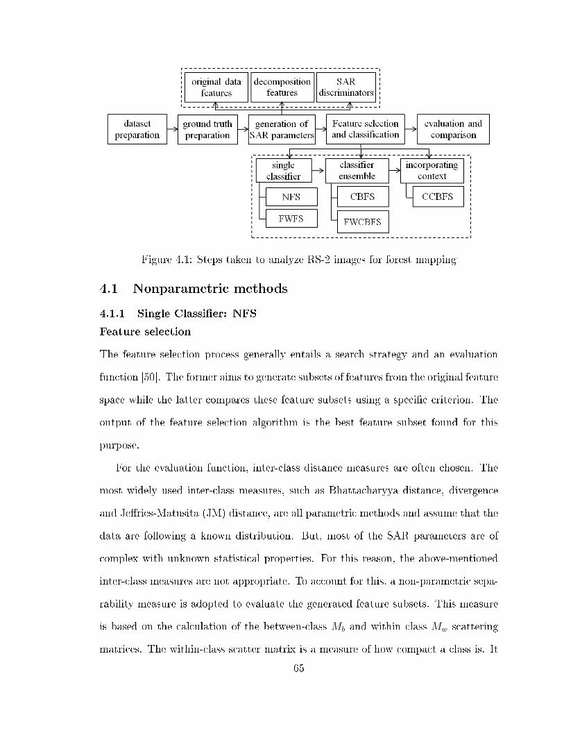
Figure 4.1: Steps taken to analyze RS-2 images for forest mapping

4.1 Nonparametric methods

4.1.1 Single Classi�er: NFS

Feature selection

The feature selection process generally entails a search strategy and an evaluation

function [50]. The former aims to generate subsets of features from the original feature

space while the latter compares these feature subsets using a speci�c criterion. The

output of the feature selection algorithm is the best feature subset found for this

purpose.

For the evaluation function, inter-class distance measures are often chosen. The

most widely used inter-class measures, such as Bhattacharyya distance, divergence

and Je�ries-Matusita (JM) distance, are all parametric methods and assume that the

data are following a known distribution. But, most of the SAR parameters are of

complex with unknown statistical properties. For this reason, the above-mentioned

inter-class measures are not appropriate. To account for this, a non-parametric sepa-

rability measure is adopted to evaluate the generated feature subsets. This measure

is based on the calculation of the between-class Mb and within class Mw scattering

matrices. The within-class scatter matrix is a measure of how compact a class is. It

65

is de�ned as

Mw = ΣNi=1Mi where Mi = Σni

j=1(xj − µi)(xj − µi)T (4.1)

where ni is the number of samples in class i , xj is the jth sample in class i , µi is

the mean vector for class i , Mi is the within class scattering matrix for class i, Mw

is the sum of the within class scattering matrices for all classes and N is the number

of classes. The between-class scatter matrix measures the separation between classes

and is de�ned as

Mb = ΣNj=1nj(µj − µ)(µj − µ)T (4.2)

where Mb is the between class scattering matrix.

An objective function F can be obtained using the Fisher class separability mea-

sure which is the ratio of the determinant of the between-class scatter matrix to the

determinant of the sum of within-class scatter matrices[39]

F =|Mb||Mw|

(4.3)

The measure described above, although simple and straightforward, has several dis-

advantages. One is that it only works well when the distribution of the classes are

normal. But, in SAR parameters the data distributions are often complicated and not

normal. Second, the rank of the matrix Mb equals N − 1, so the maximum number

of features that can be selected is N − 1. But in applications where the classes are

very close, a large number of features would be required to solve the classi�cation

problem. So, this limits the performance of the �nal classi�cation.

In order to solve these limitations Kuo and Landgrebe [74] proposed a nonparamet-

ric de�nition for the calculation of Mb and Mw. Although, the method was originally

proposed for the feature extraction in hyperspectral data, we are using the method66

for the calculation of Fisher ratio as the evaluation function for feature selection. The

method is based on the discriminant analysis feature extraction by focusing on sam-

ples near the decision boundaries. The main idea is to put di�erent weights on each

sample to compute the �weighted means� and de�ning new nonparametric between-

class and within-class scatter matrices to obtain more than N�1 features [75] . In this

method, the nonparametric between-class scatter matrix for N classes is de�ned as:

Mb =N∑i=1

piNi

N∑j=1

Ni∑k=1

λ(i,j)k (x

(i)k −Mj(x

(i)k ))(x

(i)k −Mj(x

(i)k ))T (4.4)

where x(i)k refers to the kth sample from class i, Ni is training sample size of class i, Pi

denotes the prior probability of class i. The scatter matrix weight λ(i,j)k is a function

of x(i)k and Mj(x

(i)k ) , and de�ned as:

λ(i,j)k =

dist (x(i)k , Mj(x

(i)k ))−1∑Ni

l=1 dist (x(i)l , Mj(x

(i)l ))−1

(4.5)

where dist (a, b) denotes the Euclidean distance from a to b. Mj(x(i)k ) denotes the

weighted mean x(i)k in class j and de�ned as:

Mj(x(i)k ) =

Ni∑l=1

W(i,j)lk x

(i)l (4.6)

where,

W(i,j)lk =

dist (x(i)k , x

(j)l )−1∑Ni

l=1 dist (x(i)k , x

(j)l )−1

(4.7)

The nonparametric within-class scatter matrix is de�ned as:

Mw =N∑i=1

piNi

Ni∑k=1

λ(i,j)k (x

(i)k −Mi(x

(i)k ))(x

(i)k −Mi(x

(i)k ))T (4.8)

Once the between-class and within-class scatter matrices are de�ned, they are

plugged into equation 4.3 to calculate the �sher ratio for the evaluation function of

67

the feature selection.

For the search strategy, the sequential forward �oating selection (SFFS) method

[103] was used in this thesis. According to Jain and Zongker [64], sequential �oating

search methods are probably the most e�ective search algorithms for feature selection.

SFFS starts with a null feature set and, for each step, the best feature that satis�es the

evaluation function is included with the current feature set. The algorithm also veri�es

the possibility of improvement of the evaluation function if a feature is excluded. In

this case, the worst feature (in terms of the evaluation function) is eliminated from

the set. Therefore, the SFFS proceeds dynamically increasing and decreasing the

number of features until the desired number of features is reached.

Classi�cation

Upon the selection of the most appropriate features, they are transferred to the classi-

�cation step. Because of its ability to take numerous and heterogeneous features into

account, such as the intensity channels and di�erent SAR polarimetric parameters, as

well as its ability handle linearly non separable cases, a support vector machine (SVM)

algorithm is proposed for the classi�cation step. The LIBSVM package [23] available

at http://www.csie.ntu.edu.tw/~cjlin/libsvm was used for the SVM classi�cation in

our work.

The Support Vector Machine (SVM) is a relatively recent approach introduced

by Vapnik [132, 133], for solving supervised classi�cation and regression problems.

SVM based approaches have received much attention as a promising tool for the

classi�cation of remotely sensed images. It has been shown in several studies that

classi�cation by a SVM can be more accurate than other nonparametric classi�ers

such as neural networks and decision trees as well as parametric classi�ers such as

maximum likelihood classi�cation [44, 61, 90]. In the following a brief description of

the SVM is given, and more detail can be found in [22].

68

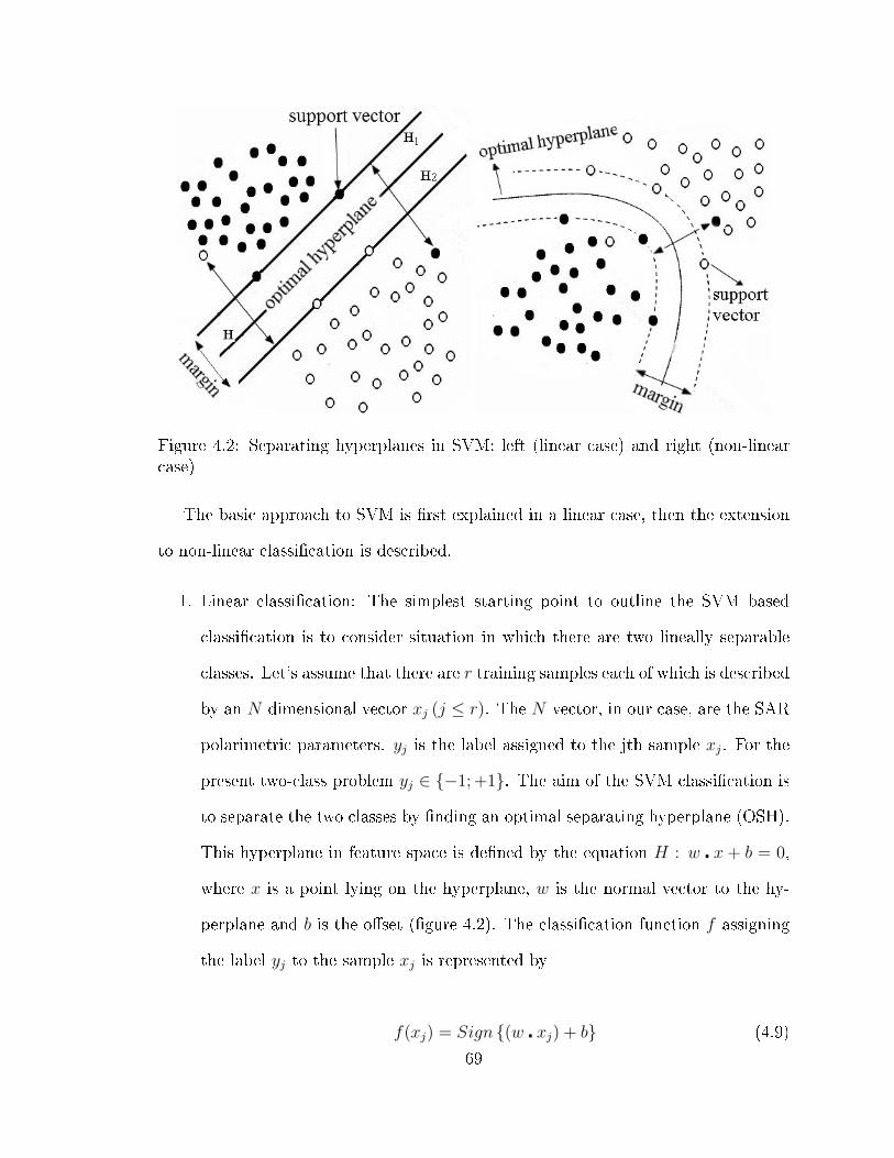
Figure 4.2: Separating hyperplanes in SVM: left (linear case) and right (non-linearcase)

The basic approach to SVM is �rst explained in a linear case, then the extension

to non-linear classi�cation is described.

1. Linear classi�cation: The simplest starting point to outline the SVM based

classi�cation is to consider situation in which there are two lineally separable

classes. Let's assume that there are r training samples each of which is described

by an N dimensional vector xj (j ≤ r). The N vector, in our case, are the SAR

polarimetric parameters. yj is the label assigned to the jth sample xj. For the

present two-class problem yj ∈ {−1; +1}. The aim of the SVM classi�cation is

to separate the two classes by �nding an optimal separating hyperplane (OSH).

This hyperplane in feature space is de�ned by the equation H : w � x + b = 0,

where x is a point lying on the hyperplane, w is the normal vector to the hy-

perplane and b is the o�set (�gure 4.2). The classi�cation function f assigning

the label yj to the sample xj is represented by

f(xj) = Sign {(w � xj) + b} (4.9)

69

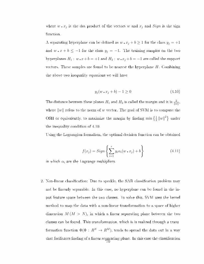
where w � xj is the dot product of the vectors w and xj and Sign is the sign

function.

A separating hyperplane can be de�ned as w � xj + b ≥ 1 for the class yj = +1

and w � x + b ≤ −1 for the class yj = −1. The training samples on the two

hyperplanes H1 : w �x+ b = +1 and H2 : w �xj + b = −1 are called the support

vectors. These samples are found to be nearest the hyperplane H. Combining

the above two inequality equations we will have

yj(w � xj + b)− 1 ≥ 0 (4.10)

The distance between these planes H1 and H2 is called the margin and it is 2‖w‖ ,

where ‖w‖ refers to the norm of w vector. The goal of SVM is to compute the

OSH or equivalently, to maximize the margin by �nding min{

12‖w‖2

}under

the inequality condition of 4.10.

Using the Lagrangian formalism, the optimal decision function can be obtained

f(xj) = Sign

{r∑i=1

yiαi(w � xj) + b

}(4.11)

in which αi are the Lagrange multipliers.

2. Non-linear classi�cation: Due to speckle, the SAR classi�cation problem may

not be linearly separable. In this case, no hyperplane can be found in the in-

put feature space between the two classes. To solve this, SVM uses the kernel

method to map the data with a non-linear transformation to a space of higher

dimension M (M > N), in which a linear separating plane between the two

classes can be found. This transformation, which is is realized through a trans-

formation function Φ(Φ : RN → RM), tends to spread the data out in a way

that facilitates �nding of a linear separating plane. In this case the classi�cation70

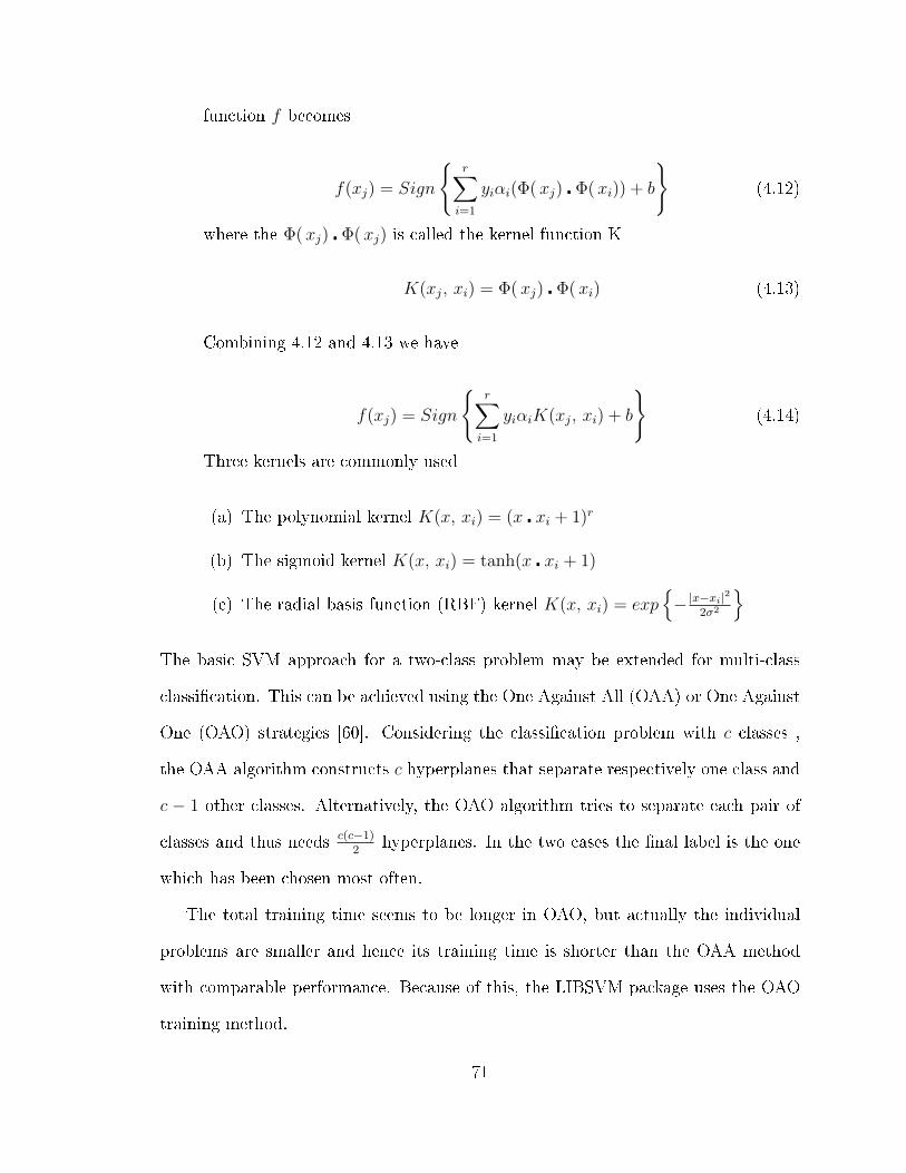
function f becomes

f(xj) = Sign

{r∑i=1

yiαi(Φ(xj) � Φ(xi)) + b

}(4.12)

where the Φ(xj) � Φ(xj) is called the kernel function K

K(xj, xi) = Φ( xj) � Φ(xi) (4.13)

Combining 4.12 and 4.13 we have

f(xj) = Sign

{r∑i=1

yiαiK(xj, xi) + b

}(4.14)

Three kernels are commonly used

(a) The polynomial kernel K(x, xi) = (x � xi + 1)r

(b) The sigmoid kernel K(x, xi) = tanh(x � xi + 1)

(c) The radial basis function (RBF) kernel K(x, xi) = exp{− |x−xi|

2

2σ2

}The basic SVM approach for a two-class problem may be extended for multi-class

classi�cation. This can be achieved using the One Against All (OAA) or One Against

One (OAO) strategies [60]. Considering the classi�cation problem with c classes ,

the OAA algorithm constructs c hyperplanes that separate respectively one class and

c − 1 other classes. Alternatively, the OAO algorithm tries to separate each pair of

classes and thus needs c(c−1)2

hyperplanes. In the two cases the �nal label is the one

which has been chosen most often.

The total training time seems to be longer in OAO, but actually the individual

problems are smaller and hence its training time is shorter than the OAA method

with comparable performance. Because of this, the LIBSVM package uses the OAO

training method.

71

4.1.2 Multiple Classi�er System: CBFS

Most of the feature selection algorithms seek only one set of features that distinguish

among all the classes simultaneously. This, in one hand, can increase the complex-

ity of the decision boundary between classes in the feature space [73] and limit the

classi�cation accuracy. On the other hand, considering one set of features for all the

classes requires a large number of features.

To overcome these problems, a multi classi�er schema is used in this research. In

doing so, a class-based feature selection (CBFS), is proposed. The main idea of the

CBFS is that from the large number of SAR parameters extracted from PolSAR data

there are some parameters which can discriminate each class better than the others.

The method comprises two parts: the feature selection, and classi�cation.

Feature selection

Instead of using feature selection for all classes, CBFS selects the features for each

class separately. First of all, the feature selection process is applied for the �rst class;

hence, the most appropriate features for discriminating the �rst class from the others

is selected. Next, the most discriminative features for the second class are selected

by using the same procedure for the second class. This process is repeated until all

the feature subsets for all classes are selected (see �gure 4.3).

The evaluation function used for NFS can not be applied in this method. Because,

NFS considers all the classes in each round of feature selection whereas CBFS focuses

on one class in each round of feature selection. Thus, here we are proposing a class-

based de�nition of the Fisher ratio

FCB(i) =

∣∣MCBb (i)

∣∣|MCB

w (i)|(4.15)

where MCBb (i) and MCB

w (i) are the class-based de�nition of the between-class and

within-class scatter matrices for class i. For each class m the MCBb is de�ned as

72

MCBb (m) =

pmNm

N∑j=1

Nm∑k=1

λ(m,j)k (x

(m)k −Mj(x

(m)k ))(x

(m)k −Mj(x

(m)k ))T (4.16)

As can be seen, the between-class scatter matrix is de�ned as the distance between

the speci�c class m and the rest of classes (and not the distance between all classes).

The MCBw is also de�ned as

MCBw (m) =

pmNm

Nm∑k=1

λ(m,j)k (x

(m)k −Mm(x

(m)k ))(x

(m)k −Mm(x

(m)k ))T (4.17)

It is obvious that instead of sum of within-class scatter matrices, the class-based

within class scattering matrix is only calculated for the class of interest m at each

time.

Classi�cation

After creating the feature subsets, an SVM classi�er is trained on each of the selected

feature subsets and the outputs of the classi�ers are combined through a combination

mechanism.

Based on the classi�ers outputs there are several consensus rules for the combi-

nation process. When the outputs of classi�ers are labels, voting techniques can be

used for combination. Apparently, the most informative outputs are when the clas-

si�ers provide probabilities. These probabilities states the con�dence of the classi�er

on di�erent classes. Thus, it is highly desirable to use a special SVM classi�er with

multi-class probability estimates.

Basically, SVM is a discriminative classi�er that predicts only the class label,

without probability information. However, it can be extended to give the probability

estimates. Methods for translating the output of SVM into probability estimates are

discussed and compared in [136]. In our implementation we use the LIBSVM package

73

which supports probability estimates for SVM classi�er based on the methods of [136].

The objective is to estimate, for each pixel x, the probabilities to belong to each class

of interest:

pk = p(y = k |x) , k = 1, ..., M

For this purpose, the outputs of each SVM are mapped into the pairwise class prob-

abilities rij for all classes i and j using a simple logistic sigmoid model [97]

rmn =1

1 + exp (Af(x) +B)(4.18)

where f(x) represents the output of the SVM trained to separate the class m from

class n for the input value x. A and B are estimated by minimizing the negative

log likelihood of training data using their labels and decision values. Once the values

of rmn are estimated for all classes, the posterior probabilities for all classes can be

estimated as follows

arg minpm

N∑m=1

∑n:n6=m

(rnm pm − rmnpn)2

subject toN∑m=1

pm = 1, pm ≤ 0, ∀m.

When each classi�er produce N measurements (one for each of N classes) for each

classifying pixel, the simplest means of combining them to obtain a decision are

the the measurement-level methods [68]. The most commonly used measurement

level methods are mean and product combination rules. Mean rule simply adds the

probabilities provided by each classi�er for every class, and assigns the class label with

the maximum score to the given input pattern. Analogously, product-rule multiplies

the probabilities for every class and then outputs the class with the maximum score.

74

These rules perform the same classi�cation in most cases. Kittler et al. [68] showed

that the mean rule is less sensitive to noise than other rules. Therefore, in this

research, we applied the mean rule as the combination method. According to mean

combination rule the pixel x is assigned to the class ωi if

M∑j=1

p(xj|ωi) =N

maxk=1

M∑j=1

p(xj|ωk) (4.19)

in which M is the number of classi�ers and N is the number of classes. In our case

N = M .

4.2 Wrapper methods

The inter-class distance measures as the evaluation function of the feature selection

although a reasonable method of the similarity and dissimilarity, they are not directly

related to the ultimate classi�cation accuracy. A question arises as to whether it

is possible to use a more direct criterion as the evaluation function. According to

the evaluation function, the feature selection approaches can be broadly grouped

into �lter and wrapper methods [69]. Wrappers utilize the classi�cation accuracy

as the evaluation function whereas �lters uses the inter-class distance measures as

the evaluation function. The optimized problem in �lters is di�erent from the real

problem. Nonetheless, �lters are faster because the problem they solve is in general

simpler. Alternatively, wrappers try to solve the real problem and the considered

criterion is really optimized which means that the ultimate problem has to be solved

numerous times. For this reason wrappers are potentially very time consuming. In

particular, as SVM is used as the ultimate classi�er in this research, it involves time

consuming optimization. Furthermore, as the number of data points increases, the

limitation of SVM as the evaluation function becomes more signi�cant.

This time complexity is mainly due to the SVM training time. This is because

75

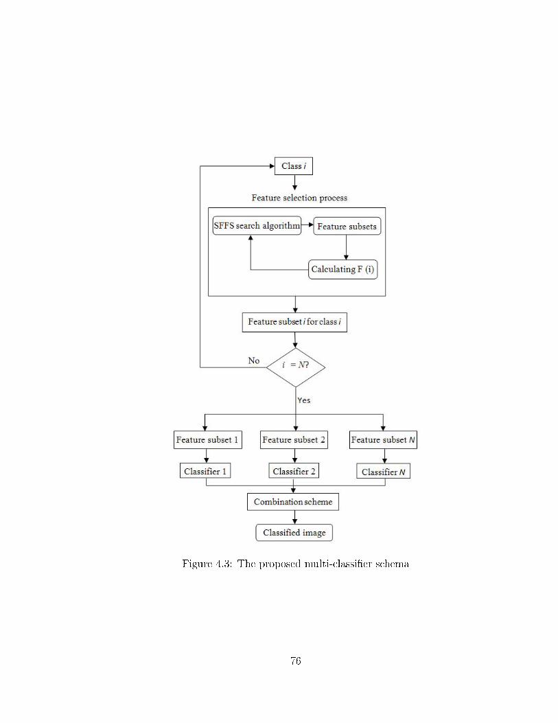
Figure 4.3: The proposed multi-classi�er schema

76

quadratic programming (QP) problems need to be solved for training SVMs. There

have been several methods in the literature to accelerate the SVM training process.

Some methods, called subset selection, try to decompose the original QP problem into

a number of sub-problems which decrease the training time [65, 34]. Despite reducing

the time complexity, it still cannot meet the requirements needed in optimization.

Because, in the optimization process, the SVM classi�er will repeat over and over

again until a pre-speci�ed condition (i.e. the desired number of features) is achieved.

Therefore, these algorithms are not e�cient for optimization. Sampling a small num-

ber of training data out of the original dataset has also been used to reduce the time

complexity [122]. Speci�cally, some random sampling methods e.g. [134] has been

used to speed up the SVM training process [84]. Random sampling is a simple and

e�cient method for reducing time complexity. However, it has some shortcomings: 1)

some of the e�ective samples could be sacri�ced during the sampling process; and 2)

the randomly selected points may not be a true representative of the whole dataset.

4.2.1 Single Classi�er: FWFS

In order to alleviate the above-mentioned shortcomings, a fast wrapper feature se-

lection (FWFS) method is proposed in this thesis. The method adopts a random

selection type algorithm based on the notion of support vectors. The support vectors

are the essential or critical training samples which lie closest to the decision bound-

ary. If all other training samples were removed and training was repeated, the same

separating hyperplanes would be obtained. The number of support vectors (nSV )

also characterizes the complexity of the classi�cation task: if nSV is small, then that

suggests that only a few examples are important, and that many samples can be disre-

garded without any loss in accuracy. Alternatively, if nSV is large, then nearly every

sample is important. This concept is used in our study for training data reduction.

This reduction procedure is performed in two steps:

77

1. Random sampling: Instead of sampling the same number of data points from

all the classes, the number of the support vectors for each class was taken as

a measure for the amount of training points reduction for that class. An SVM

classi�cation with full feature set is run before the feature selection process

begins. Depending on the number of support vectors in each class, the random

sampling of the training data is followed next. The amount of reduction in each

class i is obtained using

R(i) = 1− nSV (i)

Nr (i)i = 1, 2, ...,M (4.20)

in which Nr (i) and nSV (i) are the number of samples and the number of

support vectors in each class i respectively. R(i) is the amount of reduction for

the class i.

2. Using support vectors: Although, the above step reduces the number of training

samples, this reduced training sample set is still not enough for our goal of using

SVM for feature selection. To further reduce the number of training samples,

using the above reduced samples, an SVM classi�er is trained on the full feature

set. Finally, the support vectors of each class are used as the training samples.

After reducing the training samples, we go to the feature selection step. Like the NFS

method, we again used the sequential forward �oating selection (SFFS) method [103]

as the search strategy in this thesis to generate subsets of features from the original

feature space. However, unlike the NFS method which used a nonparametric de�ni-

tion of separability measure, here we use the overall accuracy of the SVM classi�er as

the evaluation function for feature selection. For each feature subset s this evaluation

function F is de�ned as:

F = overall(s) (4.21)78

The searching process proceeds until the desired number of features is reached.

4.2.2 Multiple Classi�er System: FWCBFS

The same as the NFS method , we propose the FWFS in the context of a class-

based feature selection schema and hence the name FWCBFS. Trying to optimize

the classi�cation accuracy for each class, the FWCBFS method �nds the best SAR

parameters for each class separately. For each class i, the producer accuracy for that

class i is used as the evaluation function.

F (i) = producer(s(i)) (4.22)

This process is repeated until all the feature subsets for all classes are selected. The

general schema of the CBFS method was already described in section 4.1.2.

4.3 Contextual Multiple Classi�er System: CCBFS

One of the disadvantages of the classi�cation methods described above is that each

pixel is classi�ed independently of its neighbors. When a majority of pixels in a

certain region are assigned to a single class, it becomes highly unlikely that a pixel in

this region belongs to another class. This misassignment could likely be due to the

speckle noise. Therefore, an improvement was proposed to the FWCBFS method to

take the spatial context into account.

In this research, we propose to incorporate the spatial consistency in the combina-

tion mechanism of the class-based schema and hence the name contextual class-based

feature selection (CCBFS). The method can be categorized as a post-processing tech-

nique. It does not only consider the generated probabilities of the classifying pixel

in di�erent classi�ers, the neighboring probabilities of the that pixel are also taken

into account. Recalling the simple combination rule in equation 4.19, we see that the

combination is performed pixel by pixel regardless of their neighborhood. Instead, the79

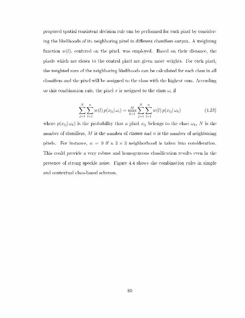
proposed spatial consistent decision rule can be performed for each pixel by consider-

ing the likelihoods of its neighboring pixel in di�erent classi�ers output. A weighting

function w(l), centered on the pixel, was employed. Based on their distance, the

pixels which are closer to the central pixel are given more weights. For each pixel,

the weighted sum of the neighboring likelihoods can be calculated for each class in all

classi�ers and the pixel will be assigned to the class with the highest sum. According

to this combination rule, the pixel x is assigned to the class ωi if

N∑j=1

n∑l=1

w(l) p(xlj|ωi) =M

maxk=1

N∑j=1

n∑l=1

w(l) p(xlj|ωk) (4.23)

where p(xlj|ωk) is the probability that a pixel xlj belongs to the class ωk, N is the

number of classi�ers, M is the number of classes and n is the number of neighboring

pixels. For instance, n = 9 if a 3 × 3 neighborhood is taken into consideration.

This could provide a very robust and homogeneous classi�cation results even in the

presence of strong speckle noise. Figure 4.4 shows the combination rules in simple

and contextual class-based schemes.

80

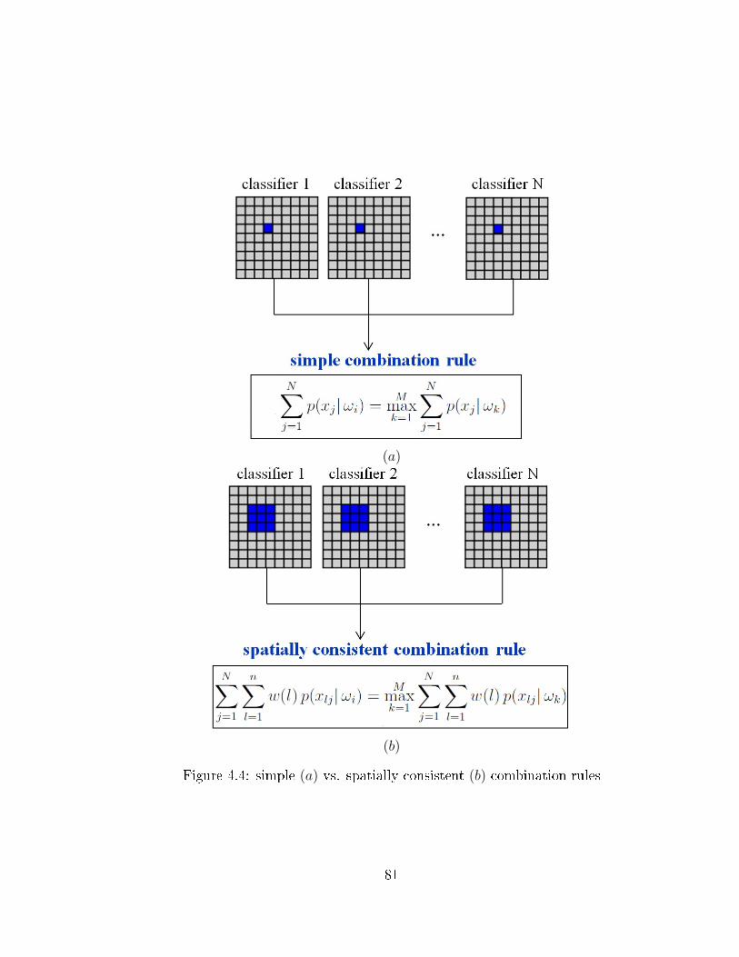
(a)

(b)

Figure 4.4: simple (a) vs. spatially consistent (b) combination rules

81

Chapter 5

Study area and dataset description

5.1 Study area description

The study site selected is the Petawawa Research Forest (PRF) located near Chalk

River, Ontario (45◦57' N, 77◦34' W). It is approximately 200 km west of Ottawa and

180 km East of North Bay, Ontario, Canada. Figure 5.1 shows the map of the study

area.

The PRF is the oldest continuously operated forest research center in Canada.

It maintains more than 2000 experimental plots and sites making it an excellent

resource for advanced remote sensing technologies. This experimental forest is larger

than 100 km2 in size and is characterized by white, red and jack pine, white and black

spruce, poplar and red oak. About 85% of the PRF is productive forest land with

growing stock estimated to be 1.5 million m2. Harvesting schedules vary depending

on research program needs but the typical volume of harvested wood is 2400 - 7000

m2 per year.

The forest lies on the southern edge of the Canadian Shield with bedrock consisting

largely of granites and gneisses. Thin soils are a result of signi�cant glacial impact.

This also makes the terrain relatively at consisting of sandy plains, gently rolling hills

and bedrock outcrops. The elevation ranges from 140 - 280 m above sea level. Climate

is continental with winter temperatures cold enough to support a �xed period of snow

cover. The precipitation is evenly distributed through the year with 600 mm in the

form of rain and 200 mm in the form of snow. January is the coldest month with a

mean temperature of -12.4◦C and July is the warmest with a mean temperature of

19.1◦C. The site is in the Great Lakes St. Lawrence forest region [110] and contains

both boreal and temperate forest species. Common species are white pine (Pinus

82

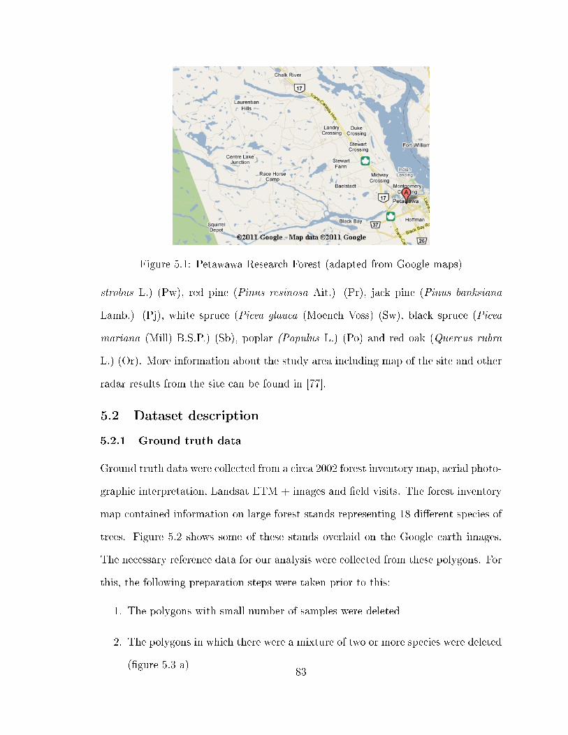
Figure 5.1: Petawawa Research Forest (adapted from Google maps)

strobus L.) (Pw), red pine (Pinus resinosa Ait.) (Pr), jack pine (Pinus banksiana

Lamb.) (Pj), white spruce (Picea glauca (Moench Voss) (Sw), black spruce (Picea

mariana (Mill) B.S.P.) (Sb), poplar (Populus L.) (Po) and red oak (Quercus rubra

L.) (Or). More information about the study area including map of the site and other

radar results from the site can be found in [77].

5.2 Dataset description

5.2.1 Ground truth data

Ground truth data were collected from a circa 2002 forest inventory map, aerial photo-

graphic interpretation, Landsat ETM + images and �eld visits. The forest inventory

map contained information on large forest stands representing 18 di�erent species of

trees. Figure 5.2 shows some of these stands overlaid on the Google earth images.

The necessary reference data for our analysis were collected from these polygons. For

this, the following preparation steps were taken prior to this:

1. The polygons with small number of samples were deleted

2. The polygons in which there were a mixture of two or more species were deleted

(�gure 5.3 a)83

3. Edgy stands i.e. those polygons existing on the steep slope were not considered

(5.3 b)

4. The low density stands or stands with two di�erent densities were ignored (�gure

5.3 e)

5. Depleted areas including clearcut (�gure 5.3 c) or partial cut (�gure 5.3 d) after

the inventory were deleted

As some changes could have occurred in the study area before or after the collection

of image data, a consultation was held with Don Leckie of the Paci�c Forestry Center

who has expert knowledge of the study area as well as remote sensing principles. He

provided us with their most recent Petawawa site evaluation carried out in March

2008. In this documentation, the sites were examined for oddities such as: forest

composition, terrain in terms of topography, species, damage, holes, non-uniformity,

two storied stands, residual trees that might a�ect radar, inclusions of wetlands, roads

and streams that night a�ect radar, etc. The inventory data were also checked for

changes from the date of the inventory in 2002 including clear-cuts, partial-cuts and

sites which have now been split because of a road or other features. All these notes

were taken into account in the preparation step. Figure 5.3 shows some examples of

this pruning process.

In order to evaluate the classi�cation algorithms with di�erent types of ground

truth data, a variety of forest classes were considered in this study including highly

similar species (e.g. red pine, white pine and jack pine) and highly di�erent classes

(e.g. ground vegetation and poplar), classes with a fairly large number of samples

(e.g. red oak) and �nally classes with very small sample size (e.g. white spruce and

mixed species). A total of nine classes were �nally considered in this study including

red oak, poplar, mixed hardwood species (mostly maple (Acer L.), birch (Betula L.)

and beech (Fagus grandifolia Ehrh.)), white pine, red pine, jack pine, black spruce,84

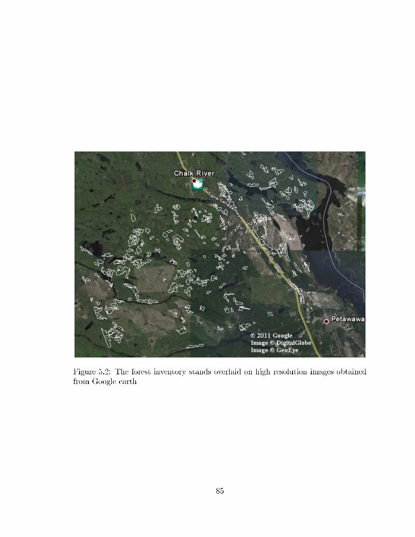
Figure 5.2: The forest inventory stands overlaid on high resolution images obtainedfrom Google earth

85

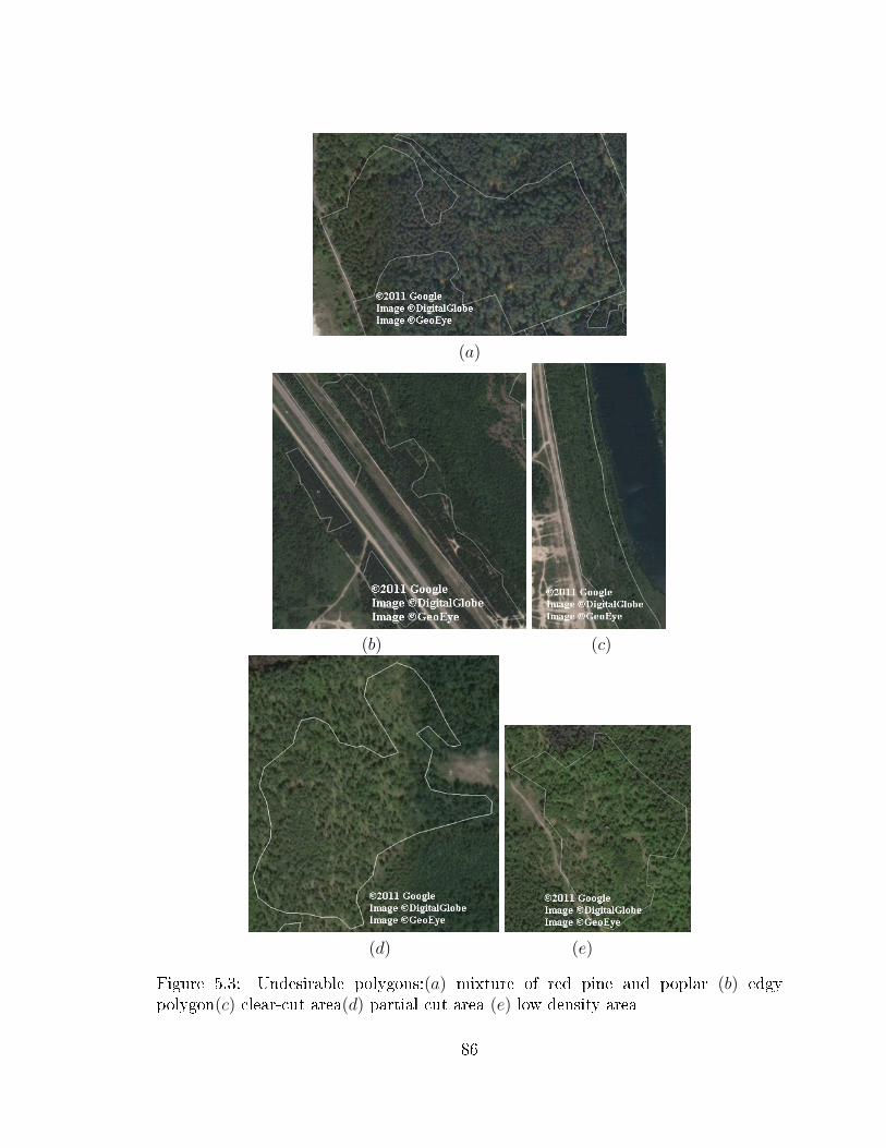
(a)

(b) (c)

(d) (e)

Figure 5.3: Undesirable polygons:(a) mixture of red pine and poplar (b) edgypolygon(c) clear-cut area(d) partial cut area (e) low density area

86

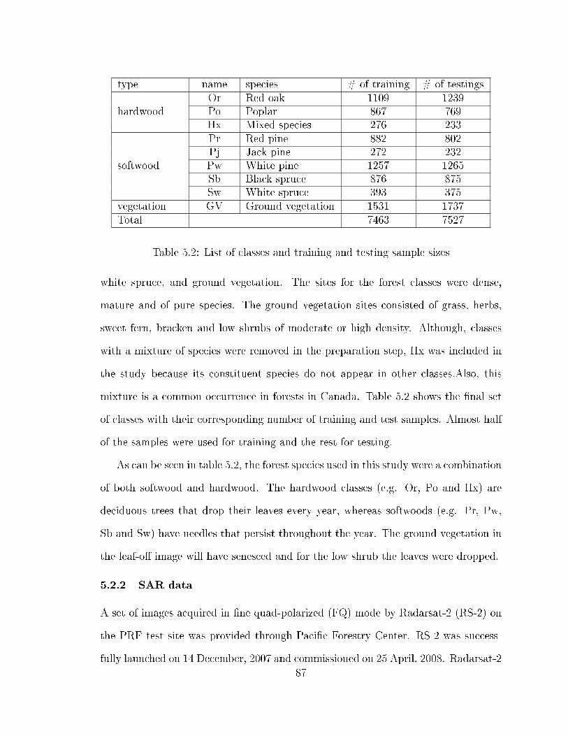
type name species # of training # of testingsOr Red oak 1109 1239

hardwood Po Poplar 867 769Hx Mixed species 276 233Pr Red pine 882 802Pj Jack pine 272 232

softwood Pw White pine 1257 1265Sb Black spruce 876 875Sw White spruce 393 375

vegetation GV Ground vegetation 1531 1737Total 7463 7527

Table 5.2: List of classes and training and testing sample sizes

white spruce, and ground vegetation. The sites for the forest classes were dense,

mature and of pure species. The ground vegetation sites consisted of grass, herbs,

sweet fern, bracken and low shrubs of moderate or high density. Although, classes

with a mixture of species were removed in the preparation step, Hx was included in

the study because its constituent species do not appear in other classes.Also, this

mixture is a common occurrence in forests in Canada. Table 5.2 shows the �nal set

of classes with their corresponding number of training and test samples. Almost half

of the samples were used for training and the rest for testing.

As can be seen in table 5.2, the forest species used in this study were a combination

of both softwood and hardwood. The hardwood classes (e.g. Or, Po and Hx) are

deciduous trees that drop their leaves every year, whereas softwoods (e.g. Pr, Pw,

Sb and Sw) have needles that persist throughout the year. The ground vegetation in

the leaf-o� image will have senesced and for the low shrub the leaves were dropped.

5.2.2 SAR data

A set of images acquired in �ne quad-polarized (FQ) mode by Radarsat-2 (RS-2) on

the PRF test site was provided through Paci�c Forestry Center. RS-2 was success-

fully launched on 14 December, 2007 and commissioned on 25 April, 2008. Radarsat-2

87

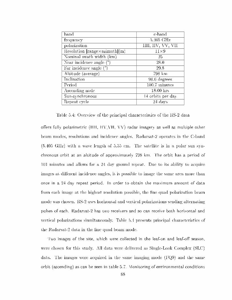
band c-bandfrequency 5.405 GHzpolarization HH, HV, VV, VHResolution [range×azimuth](m) 11Ö9Nominal swath width (km) 25Near incidence angle (°) 28.0Far incidence angle (°) 29.8Altitude (average) 798 kmInclination 98.6 degreesPeriod 100.7 minutesAscending node 18:00 hrsSun-synchronous 14 orbits per dayRepeat cycle 24 days

Table 5.4: Overview of the principal characteristics of the RS-2 data

o�ers fully polarimetric (HH, HV,VH, VV) radar imagery as well as multiple other

beam modes, resolutions and incidence angles. Radarsat-2 operates in the C-band

(5.405 GHz) with a wave length of 5.55 cm. The satellite is in a polar sun syn-

chronous orbit at an altitude of approximately 798 km. The orbit has a period of

101 minutes and allows for a 24 day ground repeat. Due to its ability to acquire

images at di�erent incidence angles, it is possible to image the same area more than

once in a 24 day repeat period. In order to obtain the maximum amount of data

from each image at the highest resolution possible, the �ne quad polarization beam

mode was chosen. RS-2 uses horizontal and vertical polarizations sending alternating

pulses of each. Radarsat-2 has two receivers and so can receive both horizontal and

vertical polarizations simultaneously. Table 5.4 presents principal characteristics of

the Radarsat-2 data in the �ne quad beam mode.

Two images of the site, which were collected in the leaf-on and leaf-o� season,

were chosen for this study. All data were delivered as Single-Look Complex (SLC)

data. The images were acquired in the same imaging mode (FQ9) and the same

orbit (ascending) as can be seen in table 5.7. Monitoring of environmental conditions

88

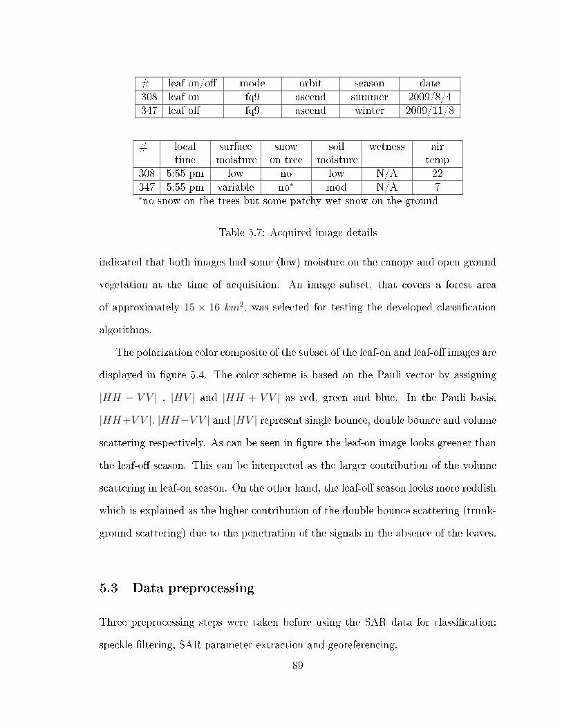
# leaf on/o� mode orbit season date308 leaf on fq9 ascend summer 2009/8/4347 leaf o� fq9 ascend winter 2009/11/8

# localtime

surfacemoisture

snowon tree

soilmoisture

wetness airtemp

308 5:55 pm low no low N/A 22347 5:55 pm variable no∗ mod N/A 7∗no snow on the trees but some patchy wet snow on the ground

Table 5.7: Acquired image details

indicated that both images had some (low) moisture on the canopy and open ground

vegetation at the time of acquisition. An image subset, that covers a forest area

of approximately 15 × 16 km2, was selected for testing the developed classi�cation

algorithms.

The polarization color composite of the subset of the leaf-on and leaf-o� images are

displayed in �gure 5.4. The color scheme is based on the Pauli vector by assigning

|HH − V V | , |HV | and |HH + V V | as red, green and blue. In the Pauli basis,

|HH+V V |, |HH−V V | and |HV | represent single bounce, double bounce and volume

scattering respectively. As can be seen in �gure the leaf-on image looks greener than

the leaf-o� season. This can be interpreted as the larger contribution of the volume

scattering in leaf-on season. On the other hand, the leaf-o� season looks more reddish

which is explained as the higher contribution of the double bounce scattering (trunk-

ground scattering) due to the penetration of the signals in the absence of the leaves.

5.3 Data preprocessing

Three preprocessing steps were taken before using the SAR data for classi�cation:

speckle �ltering, SAR parameter extraction and georeferencing.

89

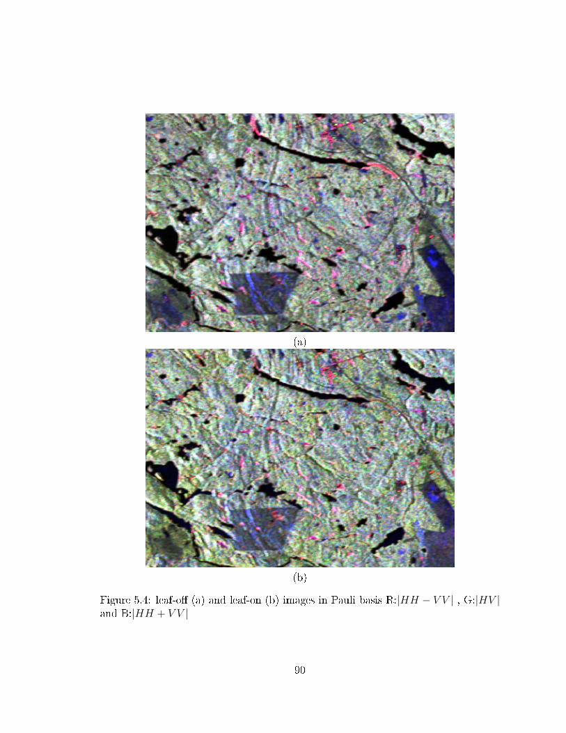
(a)

(b)

Figure 5.4: leaf-o� (a) and leaf-on (b) images in Pauli basis R:|HH − V V | , G:|HV |and B:|HH + V V |

90

5.3.1 Speckle �ltering

Radarsat-2 transmits pulses to illuminate the earth's surface. When that surface is

rough on the scale of the radar wavelength (5 cm), the return signal is a combination

of waves re�ected from a number of elementary scatterers within the IFOV. If all the

individual re�ected waves add in a relatively constructive manner, a strong signal is

received whereas if they are relatively out of phase, the returned signal is weak. The

resulting e�ect, namely, speckle, complicates image interpretation and analysis as well

as decreases the e�ectiveness of feature selection and image classi�cation. Because

of this, speckle reduction in PolSAR data is an important step for the extraction of

useful information from polarimetric images.

On the other hand, speckle signi�cantly a�ects the accuracy of the extracted

target decomposition parameters. Several studies have been reported to investigate

the speckle e�ect on target decomposition [123, 124, 85]. Lopez et al. [85] showed

that the PolSAR speckle noise has a big impact on quantitative physical parameter

estimation, especially in high entropy environments. They showed that the sample

eigenvalues are biased, with bias that decreases with an increase in the number of

independent samples.

Touzi [124] showed that the processing window size signi�cantly in�uences the

accuracy of the estimates derived from the incoherent decomposition parameters. The

results indicated that for unbiased estimation of the incoherent target decomposition

parameters, the coherency matrix has to be estimated within a moving window that

includes a minimum of 60 independent samples. However, coherent decomposition

should be limited to coherent targets with su�ciently high signal to clutter ratios. It

was also shown that the averaged parameters derived from coherent decomposition

in application that involve extended natural targets might be signi�cantly biased.

As a result, we followed two scenarios in our study. For the incoherent parameters,

91

the coherency matrix elements were �rst speckle �ltered. The incoherent observables

were then extracted from the resulting coherency matrix. Alternatively, for the coher-

ent parameters, the averaging was avoided at the �rst processing stage and coherent

observables were extracted from un�ltered coherency matrix. Thereby, the coherent

techniques maintain the full resolution during the feature extraction process, while

�ltering is applied once the features are obtained. We used the method proposed by

[4] to calculate the ENL. Using this method, a processing window size of 13 was found

su�cient to maintain the minimum ENL of 60 as proposed by Touzi [124].

The next issue that should be addressed is the type of the �lter and �lter size.

Nowadays, there are various approaches to �lter speckle noise in case of PolSAR data.

An evaluation of some of the PolSAR speckle �lters can be found in [45].

In this study, a simple boxcar �lter was used. The boxcar �lter has three advan-

tages: �rst, it is simple to apply, second, it is an e�ective method for speckle reduction

in homogeneous areas and �nally it preserves the mean value. Therefore, over ho-

mogeneous areas, the boxcar �lter presents the best �ltering performance. However,

in the presence of inhomogeneous areas the performance signi�cantly decreases due

to indiscriminately averaging pixels with inhomogeneous objects such as roads and

buildings.

As was mentioned in the dataset description, the original ground truth data were

pruned of any non-uniformity in terms of holes, roads and streams, residual trees,

inclusion of wetlands and any damages. On the other hand, the selected ground

truth regions are within large fairly homogeneous forest regions, thus there are no

edge e�ect within the sample areas. Because of these reasons, we used a boxcar �lter

in this study for speckle suppression. The speckle �lter cannot be directly applied

onto scattering matrix elements. The scattering matrix [S] has to be converted to an

incoherent second order representation, e.g. [T3] matrices. Figure 5.5 shows the a

92

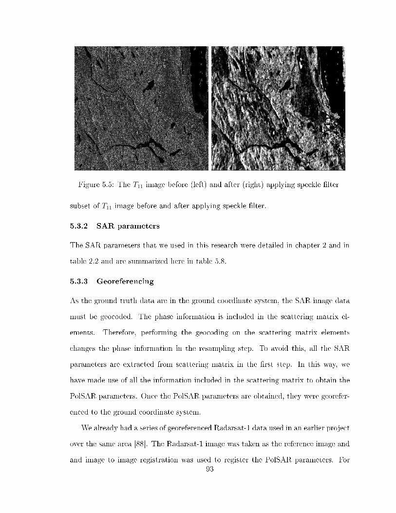
Figure 5.5: The T11 image before (left) and after (right) applying speckle �lter

subset of T11 image before and after applying speckle �lter.

5.3.2 SAR parameters

The SAR parameters that we used in this research were detailed in chapter 2 and in

table 2.2 and are summarized here in table 5.8.

5.3.3 Georeferencing

As the ground truth data are in the ground coordinate system, the SAR image data

must be geocoded. The phase information is included in the scattering matrix el-

ements. Therefore, performing the geocoding on the scattering matrix elements

changes the phase information in the resampling step. To avoid this, all the SAR

parameters are extracted from scattering matrix in the �rst step. In this way, we

have made use of all the information included in the scattering matrix to obtain the

PolSAR parameters. Once the PolSAR parameters are obtained, they were georefer-

enced to the ground coordinate system.

We already had a series of georeferenced Radarsat-1 data used in an earlier project

over the same area [88]. The Radarsat-1 image was taken as the reference image and

and image to image registration was used to register the PolSAR parameters. For93

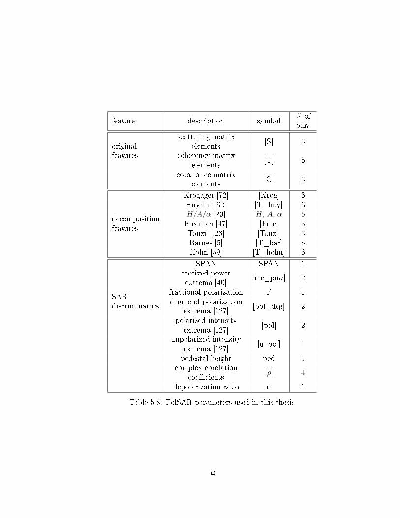
feature description symbol# ofpars

originalfeatures

scattering matrixelements

[S] 3

coherency matrixelements

[T] 5

covariance matrixelements

[C] 3

Krogager [72] [Krog] 3

decompositionfeatures

Huynen [62] [T_huy] 6H/A/α [29] H, A, α 5Freeman [47] [Free] 3Touzi [126] [Touzi] 3Barnes [5] [T_bar] 6Holm [59] [T_holm] 6

SARdiscriminators

SPAN SPAN 1received powerextrema [40]

[rec_pow] 2

fractional polarization F 1degree of polarization

extrema [127][pol_deg] 2

polarized intensityextrema [127]

[pol] 2

unpolarized intensityextrema [127]

[unpol] 1

pedestal height ped 1complex corelation

coe�cients[ρ] 4

depolarization ratio d 1

Table 5.8: PolSAR parameters used in this thesis

94

this goal, a set of 45 ground control points (GCPs) were collected over the image. A

digital elevation model (DEM) of the area was obtained from Geobase and also used

to correct for relief displacement. Geobase (www.geobase.ca) is a portal for Canadian

geospatial information operated by the Canadian Council on Geomatics. The total

root mean squared (RMS) of the registration was 1.1 pixels and the x and y RMS

were both less than 1.0 pixel.

95

Chapter 6

Results and Discussion

In this thesis, the proposed algorithms were compared with two baseline methods.

The Wishart classi�er proposed by Lee [81] was used as the �rst baseline method in

this thesis. This is one of the most common methods for the classi�cation of Pol-

SAR data. The main idea of the Wishart classi�er is that the polarimetric covariance

matrix Z may be described by a complex multivariate Wishart distribution. Let

Cm = E(Z |ωm ) be the mean covariance matrix for class ωm , based on the maxi-

mum likelihood classi�er and the complex Wishart distribution, the Wishart distance

measure was derived as

dm = ln |Cm|+ Tr (C−1m Z) (6.1)

The supervised classi�cation rule becomes as follows: assign the pixel to class ωi

i ∈ {1, 2, · · · , k}, if

d(i)m ≤ d(j)m ∀ωj 6= ωi (6.2)

The common framework of all the proposed algorithms is a feature selection

scheme. Therefore, in order to investigate the e�ectiveness of the proposed meth-

ods, an SVM with the full set of features was used as the second baseline method.

Throughout this thesis this baseline method is called SVM.

The comparison of classi�cation accuracies are undertaken using a statistical

method. For this goal, a statistical test is used to determine whether the di�erences

between the classi�cation results are statistically signi�cant or not. Various tests have

been proposed to evaluate such signi�cance [17]. In this thesis, a McNemar test [89]

was used to assess the statistical signi�cance of di�erences in the accuracy of classi-96

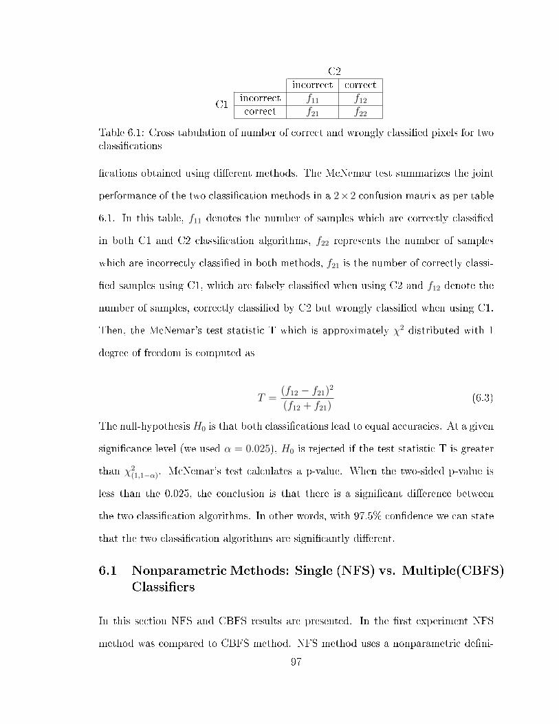
C2incorrect correct

C1incorrect f11 f12correct f21 f22

Table 6.1: Cross tabulation of number of correct and wrongly classi�ed pixels for twoclassi�cations

�cations obtained using di�erent methods. The McNemar test summarizes the joint

performance of the two classi�cation methods in a 2×2 confusion matrix as per table

6.1. In this table, f11 denotes the number of samples which are correctly classi�ed

in both C1 and C2 classi�cation algorithms, f22 represents the number of samples

which are incorrectly classi�ed in both methods, f21 is the number of correctly classi-

�ed samples using C1, which are falsely classi�ed when using C2 and f12 denote the

number of samples, correctly classi�ed by C2 but wrongly classi�ed when using C1.

Then, the McNemar's test statistic T which is approximately χ2 distributed with 1

degree of freedom is computed as

T =(f12 − f21)2

(f12 + f21)(6.3)

The null-hypothesis H0 is that both classi�cations lead to equal accuracies. At a given

signi�cance level (we used α = 0.025), H0 is rejected if the test statistic T is greater

than χ2(1,1−α). McNemar's test calculates a p-value. When the two-sided p-value is

less than the 0.025, the conclusion is that there is a signi�cant di�erence between

the two classi�cation algorithms. In other words, with 97.5% con�dence we can state

that the two classi�cation algorithms are signi�cantly di�erent.

6.1 Nonparametric Methods: Single (NFS) vs. Multiple(CBFS)Classi�ers

In this section NFS and CBFS results are presented. In the �rst experiment NFS

method was compared to CBFS method. NFS method uses a nonparametric de�ni-

97

tion of evaluation function (equation 4.3) for selecting the best parameters from the

available feature set. An SVM classi�er is then used for the classi�cation step. CBFS

is based on the theory of multiple classi�ers. It provides a class-based de�nition of the

evaluation function (equation 4.15) to generate multiple features sets. Afterwards,

for each feature set an SVM classi�er is trained. Finally, a combination scheme is

used to combine the outputs of the classi�ers.

The �rst question that arises here is: what is the optimal number of parameters

for classi�cation? To answer this question, given the initial set of 58 features, the

NFS method was used for selecting di�erent number of features for leaf-on and leaf-

o� datasets. The results of classi�cation for di�erent number of features are shown

in �gure 6.1. As can be seen, increasing the number of features the classi�cation

accuracy at �rst increases and then saturates. For both leaf-on and leaf-o� cases the

best classi�cation accuracy were obtained when using 12 features.

Figure 6.1 also shows that the leaf-o� dataset provided better results than leaf-

on image. This can be interpreted as the higher penetration of the SAR signal in

leaf-o� season. In leaf-on season the canopy surface is mainly responsible for the

backscattering whereas in leaf-o� season the backscattering is substantially from in-

side canopy branches and twigs. These results indicate that leaf-o� conditions were

a better data source for our case of forest mapping. Also, it should be noted that in

the leaf-o� season the hardwood classes receive double bounce scattering while the

softwood classes do not. This di�erence in backscattering mechanisms increases the

discrimination between hardwood and softwood classes and thus improves the hard-

wood/softwood classi�cation. Further analysis is required to fully elucidate di�erent

species behaviour in leaf-o� and leaf-on seasons.

A McNemar test was performed to analyze the statistical signi�cance of the dif-

ferences between three datasets. The p-values are given in table 6.2. As can be seen,

98

# 3 4 5 6 7 8 9 10 11 12 13 14 15 16 17 18p 0.091 0 0 0 0 0 0 0 0 0 0 0 0 0 0.003 0.002

Table 6.2: the calculated p-values for the leaf-on vs. leaf-o�

# 3 4 5 6 7 8 9 10 11 12 13 14 15 16 17 18p 0 0 0 0.071 0.004 0 0 0 0 0 0 0 0 0 0 0

Table 6.3: the calculated p-values for the leaf-o� vs. leaf-on-o�

except for the cases of the 3, 17 and 18 features the p-values are on the order of 10−5

for the other cases. Using the 3 features the calculated p-value is larger than 0.025.

This shows that in this case the di�erence is not signi�cant. For other cases, the

leaf-o� dataset was signi�cantly better than the leaf-on dataset. The same compari-

son was made using the leaf-on dataset and the combined leaf-on-o� dataset. Table

6.3 shows that except for the case of 6 features, the combined leaf-on-o� dataset

signi�cantly provided better results than leaf-o� dataset.

The results are compared with baseline classi�ers. Here, the Wishart classi�er

employs 9 elements of the covariance matrix. The classi�cation accuracies for the

leaf-o� and leaf-on seasons are summarized in �gure 6.2. A look at �gure 6.2 reveals

that the NFS method gives much better results than those obtained with Wishart

and SVM classi�ers. Compared to the Wishart classi�er, this improvement is 9%

and 10% for the leaf-o� and leaf-on datasets respectively. Also, in comparison with

the SVM method, an improvement of 6% and 4% were obtained for the leaf-o� and

leaf-on datasets respectively.

In the next experiment, the leaf-on and leaf-o� features are combined. The ratio-

nale for this combination is that every dataset has some features which may be useful

for forest mapping. The features related to leaf-on season give information relating

to the characteristics of leaves and twigs whereas there are some leaf-o� features

concentrate mainly on the main branches, trunk and even ground information. This

di�erence in backscattering mechanisms between leaf-on and leaf-o� seasons especially

99

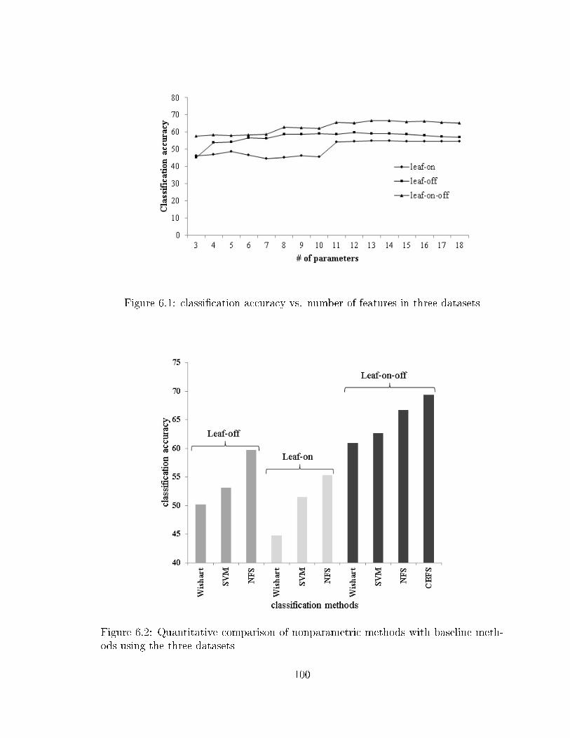
Figure 6.1: classi�cation accuracy vs. number of features in three datasets

Figure 6.2: Quantitative comparison of nonparametric methods with baseline meth-ods using the three datasets

100

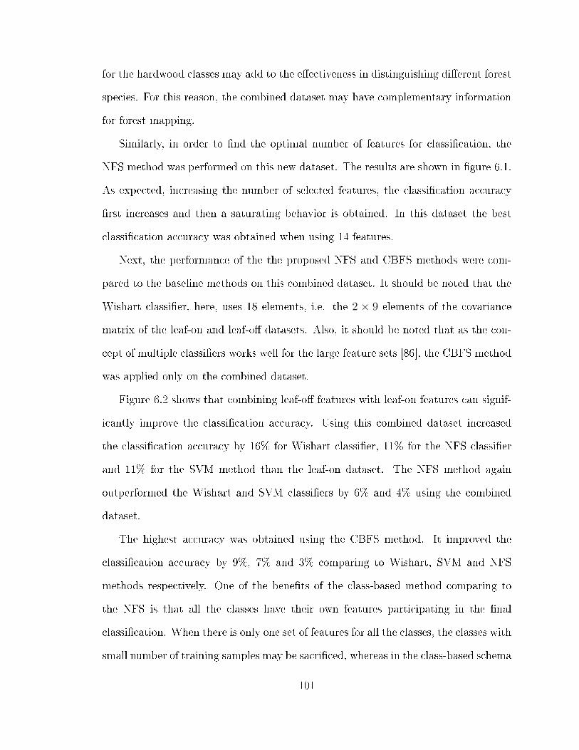
for the hardwood classes may add to the e�ectiveness in distinguishing di�erent forest

species. For this reason, the combined dataset may have complementary information

for forest mapping.

Similarly, in order to �nd the optimal number of features for classi�cation, the

NFS method was performed on this new dataset. The results are shown in �gure 6.1.

As expected, increasing the number of selected features, the classi�cation accuracy

�rst increases and then a saturating behavior is obtained. In this dataset the best

classi�cation accuracy was obtained when using 14 features.

Next, the performance of the the proposed NFS and CBFS methods were com-

pared to the baseline methods on this combined dataset. It should be noted that the

Wishart classi�er, here, uses 18 elements, i.e. the 2 × 9 elements of the covariance

matrix of the leaf-on and leaf-o� datasets. Also, it should be noted that as the con-

cept of multiple classi�ers works well for the large feature sets [86], the CBFS method

was applied only on the combined dataset.

Figure 6.2 shows that combining leaf-o� features with leaf-on features can signif-

icantly improve the classi�cation accuracy. Using this combined dataset increased

the classi�cation accuracy by 16% for Wishart classi�er, 11% for the NFS classi�er

and 11% for the SVM method than the leaf-on dataset. The NFS method again

outperformed the Wishart and SVM classi�ers by 6% and 4% using the combined

dataset.

The highest accuracy was obtained using the CBFS method. It improved the

classi�cation accuracy by 9%, 7% and 3% comparing to Wishart, SVM and NFS

methods respectively. One of the bene�ts of the class-based method comparing to

the NFS is that all the classes have their own features participating in the �nal

classi�cation. When there is only one set of features for all the classes, the classes with

small number of training samples may be sacri�ced, whereas in the class-based schema

101

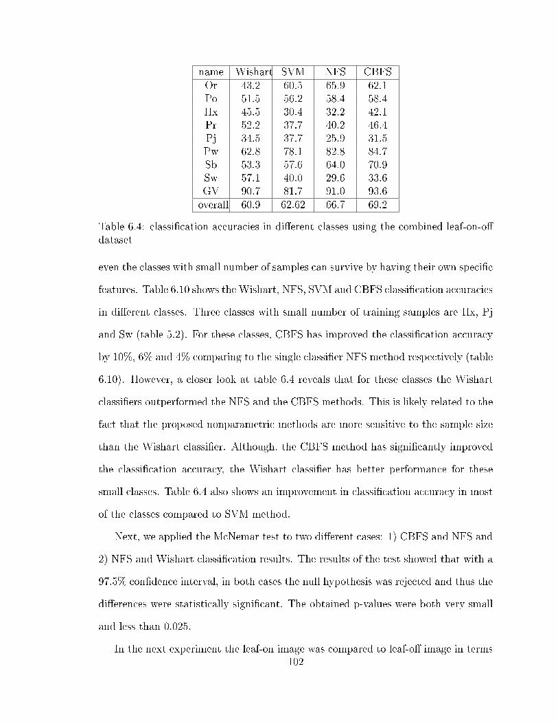
name Wishart SVM NFS CBFSOr 43.2 60.5 65.9 62.1Po 51.5 56.2 58.4 58.4Hx 45.5 30.4 32.2 42.1Pr 52.2 37.7 40.2 46.4Pj 34.5 37.7 25.9 31.5Pw 62.8 78.1 82.8 84.7Sb 53.3 57.6 64.0 70.9Sw 57.1 40.0 29.6 33.6GV 90.7 81.7 91.0 93.6overall 60.9 62.62 66.7 69.2

Table 6.4: classi�cation accuracies in di�erent classes using the combined leaf-on-o�dataset

even the classes with small number of samples can survive by having their own speci�c

features. Table 6.10 shows theWishart, NFS, SVM and CBFS classi�cation accuracies

in di�erent classes. Three classes with small number of training samples are Hx, Pj

and Sw (table 5.2). For these classes, CBFS has improved the classi�cation accuracy

by 10%, 6% and 4% comparing to the single classi�er NFS method respectively (table

6.10). However, a closer look at table 6.4 reveals that for these classes the Wishart

classi�ers outperformed the NFS and the CBFS methods. This is likely related to the

fact that the proposed nonparametric methods are more sensitive to the sample size

than the Wishart classi�er. Although, the CBFS method has signi�cantly improved

the classi�cation accuracy, the Wishart classi�er has better performance for these

small classes. Table 6.4 also shows an improvement in classi�cation accuracy in most

of the classes compared to SVM method.

Next, we applied the McNemar test to two di�erent cases: 1) CBFS and NFS and

2) NFS and Wishart classi�cation results. The results of the test showed that with a

97.5% con�dence interval, in both cases the null hypothesis was rejected and thus the

di�erences were statistically signi�cant. The obtained p-values were both very small

and less than 0.025.

In the next experiment the leaf-on image was compared to leaf-o� image in terms102

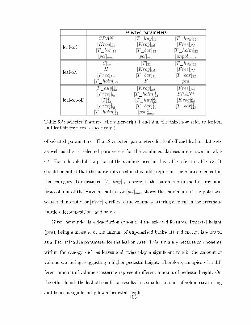
selected parameters

leaf-o�

SPAN [T_huy]11 [T_huy]12[Krog]ks [Krog]kd [Free]Pd[T_bar]11 [T_bar]23 [T_holm]22[pol]max [pol]min [unpol]max

[S]vv [T ]22 [T_huy]22

leaf-onH [Krog]kd [Free]Pd

[Free]Pv [T_bar]11 [T_bar]22[T_holm]22 F ped

leaf-on-o�

[T_huy]122 [Krog]1kd [Free]1Pd[Free]1Pv [T_holm]122 SPAN2

[T ]222 [T_huy]222 [Krog]2kd[Free]2Pd [T_bar]211 [T_bar]223

[T_holm]222 [pol]2max

Table 6.5: selected features (the superscript 1 and 2 in the third row refer to leaf-onand leaf-o� features respectively )

of selected parameters. The 12 selected parameters for leaf-o� and leaf-on datasets

as well as the 14 selected parameters for the combined dataset are shown in table

6.5. For a detailed description of the symbols used in this table refer to table 5.8. It

should be noted that the subscripts used in this table represent the related element in

that category. For instance, [T_huy]11 represents the parameter in the �rst row and

�rst column of the Huynen matrix, or [pol]max shows the maximum of the polarized

scattered intensity, or [Free]Pv refers to the volume scattering element in the Freeman-

Durden decomposition, and so on.

Given hereunder is a description of some of the selected features. Pedestal height

(ped), being a measure of the amount of unpolarized backscattered energy, is selected

as a discriminative parameter for the leaf-on case. This is mainly because components

within the canopy such as leaves and twigs play a signi�cant role in the amount of

volume scattering, suggesting a higher pedestal height. Therefore, canopies with dif-

ferent amount of volume scattering represent di�erent amount of pedestal height. On

the other hand, the leaf-o� condition results in a smaller amount of volume scattering

and hence a signi�cantly lower pedestal height.103

The Freeman-Durden volume scattering element ([Free]Pv) was also selected for

the leaf-on case. The volume scattering coming from the leaf canopy at the tops of the

trees is mainly responsible for this parameter. This volume scattering varies among

trees with di�erent shape of the leaves and di�erent canopy structure. This makes

the the freeman canopy scattering parameter a useful feature for the leaf-on case.

As expected, for the case of leaf-o� the Freeman-Durden double-bounce scattering

parameter ([Free]Pd) is selected. This can be interpreted as the higher interaction of

trunk-ground scattering mechanism.

In the leaf-on season there is an increase in entropy (H) due to the higher volume

scattering and due to canopy propagation e�ects. Thus, di�erent trees with di�erent

types of leaves and canopy structure result in di�erent amount of entropy. For this,

the entropy (H) is selected as an informative parameter for the leaf-on season.

However, it should be noted that the above discussion is only valid for the hard-

wood classes as they drop their leaves in the leaf-o� season. For the softwood classes,

on the other hand, the green foliage is persistent throughout the year, and thus the

signal penetration does not vary from season to season.

Table 6.5 also shows that there are some PolSAR parameters that play role in both

leaf-on and leaf-on cases. For example, the Krogager decomposition parameters were

selected in both cases. This shows that the coherent decomposition, which operates

on the individual pixels on a coherent basis, can also provide useful information for

the forest mapping. Other instances of this type of parameters are [T_bar]11 and

[T_holm]22.

The third row in table 6.5 shows the selected features for the combined dataset.

The superscript 1 and 2 in the third row refer to leaf-on and leaf-o� features respec-

tively. In this case, 5 features were selected from the leaf-on image and 9 features

were from leaf-o� image. This shows the higher signi�cance of the leaf-o� image as

104

expected.

6.2 Wrapper Methods: Single (FWFS) vs. Multiple (FWCBFS)Classi�ers

One of the main disadvantages of the nonparametric methods is that the evaluation

function it uses for feature selection is not directly related to the �nal goal of clas-

si�cation. Wrappers on the other hand optimizes the real problem by utilizing the

classi�cation accuracy as the evaluation function of the feature selection. However,

they are time consuming. In order to overcome this, the notion of the support vectors

was used to reduce the training samples and a fast wrapper feature selection (FWFS)

was proposed. The method was also proposed in a class-based schema (FWCBFS).

For a detailed explanation, the reader is referred to section 4.2. Regarding the ran-

dom nature of the proposed method for the training sample reduction, the reduction

procedure was performed once and the reduced training samples were used for all the

experiments in this section. In this way, the di�erences in the obtained classi�cation

results can be thoroughly related to the performance of the methods rather than the

employed training samples.

Similar to the nonparametric methods, the leaf-on, leaf-o� and the the combined

leaf-on-o� images were used in our experiments. In the �rst experiment, the FWFS

method was used over the three datasets using di�erent number of features. The

results can be seen in �gure 6.3.

As can be seen in �gure 6.3, the leaf-o� image provided better results than the

leaf-on image dataset except for the cases of 7, 8, 9 and 14 features for which the two

images provided almost the same classi�cation accuracy. The highest improvement

was for the case of using 13 features. In this case a 4 percent improvement was

reported.

Next, comparisons are made between the combined leaf-on-o� dataset and the

105

# 3 4 5 6 7 8 9 10p 0.019 0.001 0.001 0.179 0.046 0.214 0.329 0.019

# 11 12 13 14 15 16 17 18p 0.001 0.005 0 0.311 0 0 0 0

Table 6.6: the calculated p-values for the leaf-on vs. leaf-o�

# 3 4 5 6 7 8 9 10 11 12 13 14 15 16 17 18p 0 0 0 0 0 0 0 0 0 0 0 0 0 0 0 0

Table 6.7: the calculated p-values for the leaf-o� vs. leaf-on-o�

individual datasets. As is shown in �gure 6.3, using the combined leaf-on-o� dataset,

the classi�cation accuracy was signi�cantly improved. The highest improvement re-

ported was 15% which was for the case of using 14 features. This con�rms the result

obtained previously indicating that the PolSAR parameters obtained from leaf-on

image and leaf-o� image are not redundant at all but rather complementary for our

goal of forest mapping. These results are in agreement with the results obtained from

nonparametric methods.

A look at the p-values obtained from McNemar test at table 6.6 shows that in

the cases of 6, 7, 8, 9 and 14 features the di�erences between leaf-o� and leaf-on

datasets are not signi�cant. For these cases, the p-values are larger than 0.025. For

all other cases the leaf-o� dataset signi�cantly provided better results. The same

experiment was carried out for comparing the combined leaf-on-o� dataset with leaf-

o� dataset. The obtained p-values in table 6.7 shows that for all cases the di�erences

are signi�cant.

Next, the performance of the FWFS and FWCBFS were compared to the baseline

methods i.e. Wishart and SVM classi�ers. Again, the comparison were made over

the three datasets. The results are illustrated in �gure 6.4. As can be seen, using the

FWFS method, the classi�cation accuracy has improved compared to the Wishart

and SVM classi�ers. Compared to Wishart classi�er the amount of improvement was

10%, 14% and 12% for leaf-o�, leaf-on and leaf-on-o� datasets and compared to SVM106

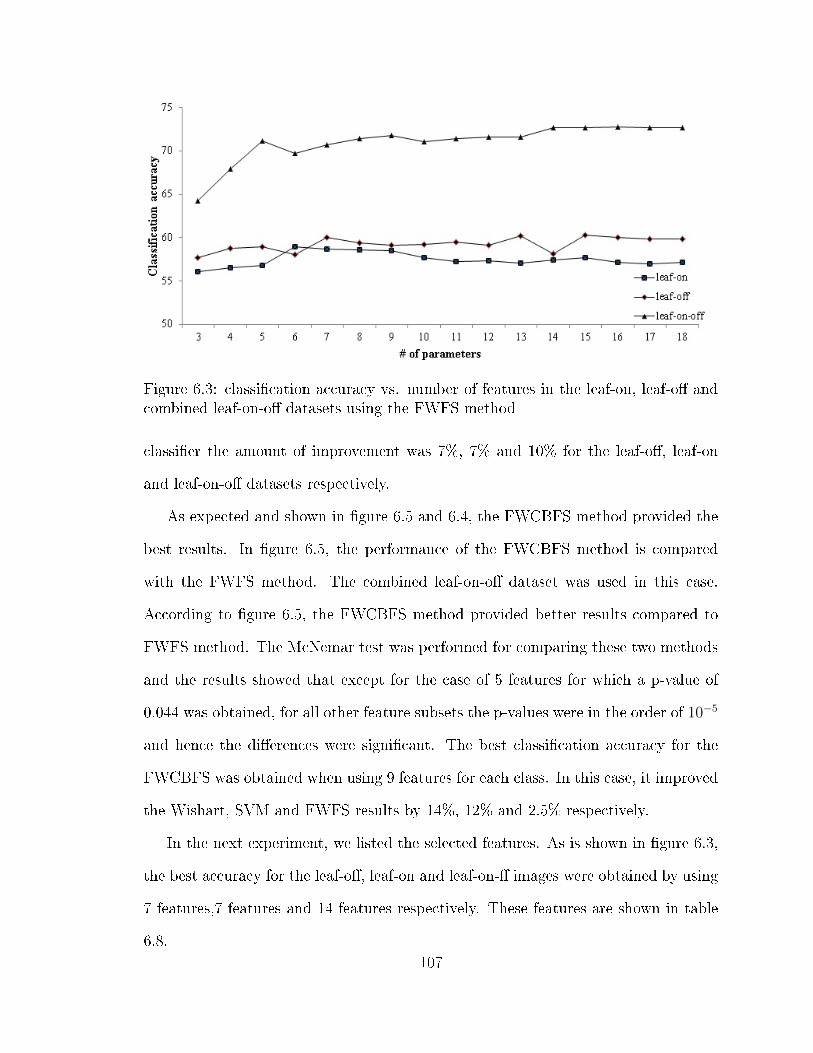
Figure 6.3: classi�cation accuracy vs. number of features in the leaf-on, leaf-o� andcombined leaf-on-o� datasets using the FWFS method

classi�er the amount of improvement was 7%, 7% and 10% for the leaf-o�, leaf-on

and leaf-on-o� datasets respectively.

As expected and shown in �gure 6.5 and 6.4, the FWCBFS method provided the

best results. In �gure 6.5, the performance of the FWCBFS method is compared

with the FWFS method. The combined leaf-on-o� dataset was used in this case.

According to �gure 6.5, the FWCBFS method provided better results compared to

FWFS method. The McNemar test was performed for comparing these two methods

and the results showed that except for the case of 5 features for which a p-value of

0.044 was obtained, for all other feature subsets the p-values were in the order of 10−5

and hence the di�erences were signi�cant. The best classi�cation accuracy for the

FWCBFS was obtained when using 9 features for each class. In this case, it improved

the Wishart, SVM and FWFS results by 14%, 12% and 2.5% respectively.

In the next experiment, we listed the selected features. As is shown in �gure 6.3,

the best accuracy for the leaf-o�, leaf-on and leaf-on-� images were obtained by using

7 features,7 features and 14 features respectively. These features are shown in table

6.8.

107

Figure 6.4: Quantitative comparison of wrapper methods with baseline classi�ersusing the three datasets

Figure 6.5: FWCBFS vs. FWFS using the combined leaf-on-o� dataset

108

selected parameters

leaf-o�[T_huy]11 [Krog]kd [T_bar]23

[T_holm]12 [pol_deg]max [rec_pow]maxd

[T_huy]11 H [Krog]ksleaf-on [Free]Pv [T_bar]33 [T_holm]11

F

leaf-on-o�

[T_huy]112 [H(1− A)]1 [Krog]1kd[T_holm]112 [pol_deg]1max d1

[C]212 H [T_bar]223[Touzi]2ψs

[pol_deg]2max [pol_deg]2minF 2 d2

Table 6.8: selected features (the superscript 1 and 2 in the third row refer to leaf-onand leaf-o� features respectively )

It was shown earlier that the best classi�cation results for FWCBFS are obtained

using 9 features for each class. These features are listed in table 6.9. Again, the

superscript 1 and 2 refer to leaf-on and leaf-o� features respectively. The �rst column

shows whether the species is a hardwood (h) or softwood (s) class. In order to better

understand the importance of each selected feature for softwood and hardwood classes,

they are divided into softwood and hardwood features. Figure 6.6 and 6.7 show

the selected softwood and the hardwood features for the leaf-on and leaf-o� seasons

respectively. They show how frequent the features are selected for the hardwood and

the softwood classes. The more the frequency of a feature, the more the importance

of that feature. Some remarks on the selected features are given below:

• On the whole, 32 features were selected from leaf-on dataset and 40 features

were selected from leaf-o� image. This con�rms the higher usefulness of the

leaf-o� image for forest mapping.

• The most signi�cant features for the softwood during the leaf-on season were

[T_huy]12, [T_huy]22 and [Free]d. Each of these features were selected twice

for the softwood species during leaf-on season (�gure 6.6).

109

• [T_bar]11 was the most signi�cant feature for the hardwood during leaf-on

season. It was selected twice for the hardwood species during leaf-on season

(�gure 6.6).

• [S]hh, H, [Free]d, [T_bar]13, [T_bar]22 and [T_bar]11were the most signi�cant

PolSAR parameters for the softwood during the leaf-o� season. The �rst �ve

were selected twice and the last one was selected three times for di�erent hard-

wood species (�gure 6.7). There is not a signi�cant feature during this season

for the hardwood species, as all the selected parameters are considered only

once.

• [T_huy]22 is the only feature which was found to be useful for both softwood

and hardwood in both leaf-on and leaf-o� seasons.

Thus far, the overall accuracy was used to compare di�erent methods. In order

to see the classi�cation accuracies in di�erent classes, producer accuracy was used.

Table 6.10 shows the producer accuracies for the three di�erent methods using the

leaf-on-o� dataset. Notice that the Wishart classi�er, here, uses 18 elements, i.e. the

2× 9 elements of the covariance matrix of the leaf-on and leaf-o� datasets, SVM uses

the full set of features, FWFS uses 14 selected features and FWCBFS uses 9 features

for each class. A look at table 6.10 reveals that except class Sw, the classi�cation

accuracies were improved for the rest of the classes. Although, the FWCBFS method

improved the classi�cation accuracy for class Sw compared to FWFS, it is still lower

than the Wishart classi�er for this class.

6.3 Context-based Method: CCBFS

The method was described in section 4.3. In order to incorporate the neighboring

information, the method extends the simple combination rule i.e. equation 4.19 to

equation 4.23 which is repeated below110

type class selected parameters

hardwood

[T_huy]113 [T_huy]122 [Free]1dOr [T_bar]111 [T_holm]122 [ro]112

[ro]1ccc [C]223 [T_huy]222[S]1hv [T_huy]112 [krog]1Ks

Po [T_bar]111 [S]2hh [Touzi]2lan[pol]2max [unpol]2max F 2

[S]1hh α1 [krog]1KhHx d1 [T_huy]223 H(1− A)2

[krog]2Kh [T_bar]212 [T_holm]212[Free]1d [S]2hh [C]223

softwood

Pr (1−H)A2 [Free]2d [T_bar]211[T_bar]212 [T_bar]222 [T_holm]211

[C]113 [T_huy]113 [Touzi]1lanPj H2 α2 [T_bar]213

[Touzi]2ψs[ro]2ccc d2

[S]1vv [T_huy]112 [krog]1KdPw [T_bar]123 [T_holm]112 ped1

[Thuy]222 [T_bar]222 [pol]2max[T ]111 [T_huy]111 [T_huy]122

Sb [Free]1d [T_huy]212 [T_bar]211[T_bar]213 [T_holm]222 [ro]212[T_huy]112 [T_huy]122 [Free]1s

Sw [S]2hh [T ]222 H2

[Free]2d [T_bar]211 [T_holm]213

vegetation[T ]123 [T_bar]122 [T ]222

GV [T ]223 [C]223 [T_bar]212[T_bar]223 [T_holm]223 [ro]213

Table 6.9: selected features for each class (the superscript 1 and 2 in the third rowrefer to leaf-on and leaf-o� features respectively )

111

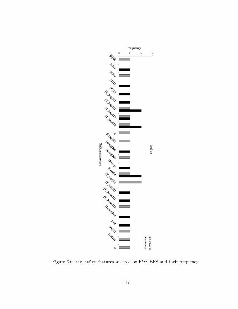
Figure 6.6: the leaf-on features selected by FWCBFS and their frequency

112

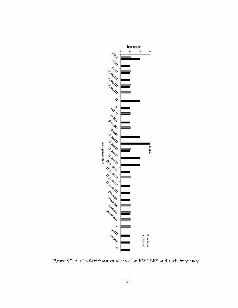
Figure 6.7: the leaf-o� features selected by FWCBFS and their frequency

113

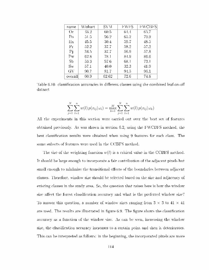
name Wishart SVM FWFS FWCBFSOr 43.2 60.5 64.4 65.7Po 51.5 56.2 65.2 70.9Hx 45.5 30.4 59.7 48.5Pr 52.2 37.7 58.2 57.2Pj 34.5 37.7 56.9 57.8Pw 62.8 78.1 84.9 86.6Sb 53.3 57.6 68.1 73.1Sw 57.1 40.0 32.3 41.9GV 90.7 81.7 94.5 96.1overall 60.9 62.62 72.6 74.8

Table 6.10: classi�cation accuracies in di�erent classes using the combined leaf-on-o�dataset

N∑j=1

n∑l=1

w(l) p(xlj|ωi) =M

maxk=1

N∑j=1

n∑l=1

w(l) p(xlj|ωk)

All the experiments in this section were carried out over the best set of features

obtained previously. As was shown in section 6.2, using the FWCBFS method, the

best classi�cation results were obtained when using 9 features for each class. The

same subsets of features were used in the CCBFS method.

The size of the weighting function w(l) is a critical value in the CCBFS method.

It should be large enough to incorporate a fair contribution of the adjacent pixels but

small enough to minimize the transitional e�ects of the boundaries between adjacent

classes. Therefore, window size should be selected based on the size and adjacency of

existing classes in the study area. So, the question that raises here is how the window

size a�ect the forest classi�cation accuracy and what is the preferred window size?

To answer this question, a number of window sizes ranging from 3 Ö 3 to 41 Ö 41

are used. The results are illustrated in �gure 6.9. The �gure shows the classi�cation

accuracy as a function of the window size. As can be seen, increasing the window

size, the classi�cation accuracy increases to a certain point and then it deteriorates.

This can be interpreted as follows: in the beginning, the incorporated pixels are more

114

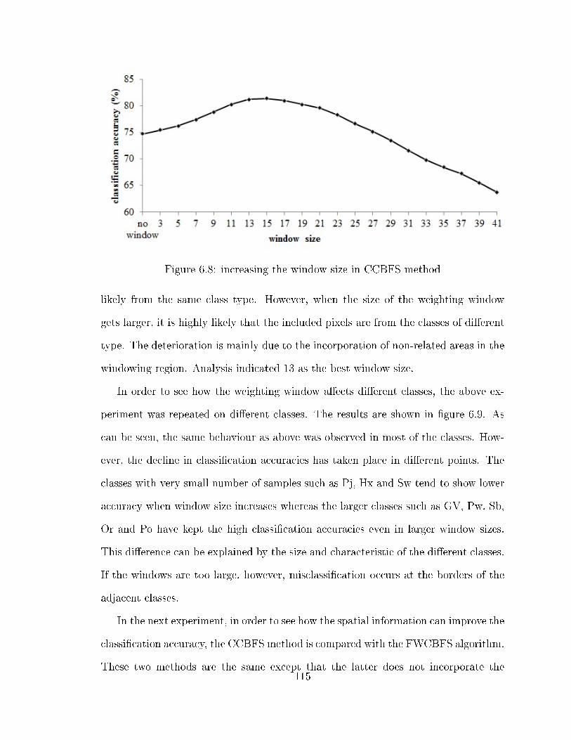
Figure 6.8: increasing the window size in CCBFS method

likely from the same class type. However, when the size of the weighting window

gets larger, it is highly likely that the included pixels are from the classes of di�erent

type. The deterioration is mainly due to the incorporation of non-related areas in the

windowing region. Analysis indicated 13 as the best window size.

In order to see how the weighting window a�ects di�erent classes, the above ex-

periment was repeated on di�erent classes. The results are shown in �gure 6.9. As

can be seen, the same behaviour as above was observed in most of the classes. How-

ever, the decline in classi�cation accuracies has taken place in di�erent points. The

classes with very small number of samples such as Pj, Hx and Sw tend to show lower

accuracy when window size increases whereas the larger classes such as GV, Pw, Sb,

Or and Po have kept the high classi�cation accuracies even in larger window sizes.

This di�erence can be explained by the size and characteristic of the di�erent classes.

If the windows are too large, however, misclassi�cation occurs at the borders of the

adjacent classes.

In the next experiment, in order to see how the spatial information can improve the

classi�cation accuracy, the CCBFS method is compared with the FWCBFS algorithm.

These two methods are the same except that the latter does not incorporate the115

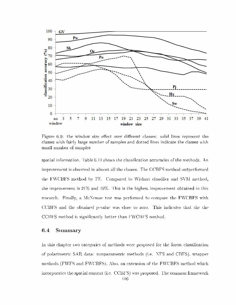
Figure 6.9: the window size e�ect over di�erent classes: solid lines represent theclasses with fairly large number of samples and dotted lines indicate the classes withsmall number of samples

spatial information. Table 6.11 shows the classi�cation accuracies of the methods. An

improvement is observed in almost all the classes. The CCBFS method outperformed

the FWCBFS method by 7%. Compared to Wishart classi�er and SVM method,

the improvement is 21% and 19%. This is the highest improvement obtained in this

research. Finally, a McNemar test was performed to compare the FWCBFS with

CCBFS and the obtained p-value was close to zero. This indicates that the the

CCBFS method is signi�cantly better than FWCBFS method.

6.4 Summary

In this chapter two categories of methods were proposed for the forest classi�cation

of polarimetric SAR data: nonparametric methods (i.e. NFS and CBFS), wrapper

methods (FWFS and FWCBFS). Also, an extension of the FWCBFS method which

incorporates the spatial context (i.e. CCBFS) was proposed. The common framework116

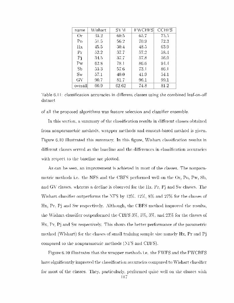
name Wishart SVM FWCBFS CCBFSOr 43.2 60.5 65.7 75.5Po 51.5 56.2 70.9 72.3Hx 45.5 30.4 48.5 63.9Pr 52.2 37.7 57.2 58.4Pj 34.5 37.7 57.8 56.0Pw 62.8 78.1 86.6 94.4Sb 53.3 57.6 73.1 86.1Sw 57.1 40.0 41.9 54.1GV 90.7 81.7 96.1 99.1overall 60.9 62.62 74.8 81.2

Table 6.11: classi�cation accuracies in di�erent classes using the combined leaf-on-o�dataset

of all the proposed algorithms was feature selection and classi�er ensemble.

In this section, a summary of the classi�cation results in di�erent classes obtained

from nonparametric methods, wrapper methods and context-based method is given.

Figure 6.10 illustrated this summary. In this �gure, Wishart classi�cation results in

di�erent classes served as the baseline and the di�erences in classi�cation accuracies

with respect to the baseline are plotted.

As can be seen, an improvement is achieved in most of the classes. The nonpara-

metric methods i.e. the NFS and the CBFS performed well on the Or, Po, Pw, Sb,

and GV classes, whereas a decline is observed for the Hx, Pr, Pj and Sw classes. The

Wishart classi�er outperforms the NFS by 13%, 12%, 8% and 27% for the classes of

Hx, Pr, Pj and Sw respectively. Although, the CBFS method improved the results,

the Wishart classi�er outperformed the CBFS 3%, 5%, 3%, and 23% for the classes of

Hx, Pr, Pj and Sw respectively. This shows the better performance of the parametric

method (Wishart) for the classes of small training sample size namely Hx, Pr and Pj

compared to the nonparametric methods (NFS and CBFS).

Figure 6.10 illustrates that the wrapper methods i.e. the FWFS and the FWCBFS

have signi�cantly improved the classi�cation accuracies compared to Wishart classi�er

for most of the classes. They, particularly, performed quite well on the classes with117

small sample size. The FWFS improved the classi�cation accuracies by 14%, 6%,

and 22% for the classes of Hx, Pr, and Pj respectively. These improvements were 3%,

5%, and 24% for the FWCBFS method. Sw was the only class for which the Wishart

classi�er outperformed all the proposed methods. Further investigations are required

to elucidate the cause of this behaviour.

Results obtained from CCBFS method demonstrated markedly improvement com-

pared to all other methods. This is more evident for the classes of large sample size

such as Or, Pw and Sb. For these classes an improvement of 32%, 32% and 33%

were observed compared to Wishart classi�er. Even for the class Sw for which the

Wishart classi�er signi�cantly outperformed the other methods, the CCBFS method

presented almost the same performance as the Wishart classi�er.

118

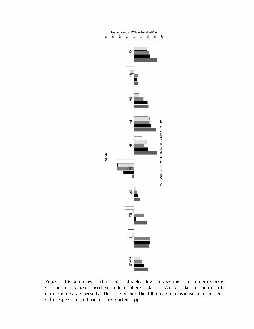
Figure 6.10: summary of the results: the classi�cation accuracies in nonparametric,wrapper and context-based methods in di�erent classes. Wishart classi�cation resultsin di�erent classes served as the baseline and the di�erences in classi�cation accuracieswith respect to the baseline are plotted. 119

Chapter 7

Conclusions and Further Works

7.1 Conclusions

Two series of algorithms based on the feature selection and classi�er ensemble have

been devised, developed and implemented to classify polarimetric SAR images for for-

est mapping. nonparametric feature selection (NFS) method used a nonparametric

de�nition of evaluation function for selecting the best parameters from the avail-

able feature set. class-based feature selection (CBFS) method provided a class-based

de�nition of the evaluation function to generate multiple features sets. These two

methods, though simple and fast, the evaluation function in feature selection is not

directly related to the ultimate goal of classi�cation. To overcome this, fast wrapper

feature selection (FWFS) and fast wrapper class-based feature selection (FWCBFS)

were proposed. They signi�cantly improved the classi�cation accuracy compared to

the nonparametric methods. Also, in comparison to the Wishart classi�er, which is a

commonly used method for the classi�cation of PolSAR data, a signi�cant improve-

ment was achieved. Finally, an extension of the FWCBFS method which incorporated

the information from neighboring pixels was proposed. Results obtained from this

contextual class-based feature selection (CCBFS) method demonstrated the high-

est improvement compared to all other methods. This proved that the neighboring

information provides valuable information for the classi�cation of PolSAR data.

The three datasets were then compared in terms of the classi�cation accuracy and

the selected parameters. In general, the leaf-o� dataset provided better results than

leaf-on image. This may be related to higher penetration of the SAR signal in the leaf-

o� season especially for the hardwoods and greater contrast between hardwood and

softwood. However, the best results were obtained when using the combined dataset.

120

This is mainly because the combined dataset may have complementary information for

forest mapping. The backscattering mechanisms are di�erent in each season especially

for the hardwood classes and this add to the e�ectiveness in distinguishing di�erent

forest species using the combined dataset.

7.2 Further Works

The proposed algorithms generally provided good performance. However, there is

still room for improvement. Several di�erent directions for future research are listed

below

• In this thesis, the combination of leaf-on with leaf-o� image signi�cantly im-

proved the classi�cation accuracy compared to the individual datasets. How-

ever, the employed images had the same incidence angle. It would be useful

to examine the combination of images of multiple incidence angles. Each inci-

dence angle presents its own backscattering scattering mechanisms. Combining

the SAR parameters obtained from these images can provide complementary

information for forest mapping.

• All the proposed algorithms in this research, adopts the classi�cation in a species

by species manner. Perhaps an extension of this is to employ a decision tree to

initially categorize the species into softwood and hardwood and then subdivide

each category into its constituting species.

• While this dissertation has focused primarily on the use of PolSAR data for

the forest mapping, the framework is general and may be applied to other

applications which involves discriminating di�erent classes.

• In this research, for the extraction of the coherent parameters, the averaging was

avoided at the �rst processing stage and coherent observables were extracted

121

122from un�ltered coherency matrix. It would be desirable to investigate the e�ect

of applying �lter before and after the extraction of coherent parameters for

forest mapping.

• A more in depth look into the behaviour of di�erent species in the leaf-on and

leaf-o� seasons should be investigated.

Bibliography

[1] A. Agrawal and W. Boerner. Redevelopment of kennaught's target character-

istics polarization state theory using the polarization ratio formalism for the

coherent case. IEEE Transaction on Geoscience and Remote Sensing, 27:2�14,

1989.

[2] A. Al-Ani and M. Deriche. A new technique for combining multiple classi�ers

using the Dempster-Shafer theory of evidence. Journal of Arti�cial Intelligence

Research, 17:333�361, 2002.

[3] V. Alberga. Comparison of polarimetric methods in image classi�cation and

SAR interferometry applications. PhD thesis, Fakultat �ir Elektrotechnik und

Informationstechnik der Technischen Universitat Chemnitz genehmigte, 2003.

[4] S. N. An�nsen, A. P. Doulgeris, and T. Eltoft. Estimation of the equivalent

number of looks in polarimetric synthetic aperture radar imagery. IEEE Trans-

action on Geoscience and Remote Sensing, 47(11):3795�3809, November 2009.

[5] R. M. Barnes. Roll invariant decompositions for the polarization covariance

matrix. Internal report, Lincoln Laboratory, MIT, Lex., MA 02173-0073, 1988.

[6] J. A. Benediktsson, J. Chanussot, and M. Fauvel. Multiple classi�er systems in

remote sensing: From basics to recent developments. In Kittler J. Roli Haindl,

M., editor, MCS 2007, volume 4472, pages 501�512. Springer, Heidelberg, 2007.

[7] U. Benz. Supervised fuzzy analysis of single- and multi-channel SAR data.

IEEE Transaction on Geoscience and Remote Sensing, 37:1023�1037, 1999.

[8] H. Bischof, W. Schneider, and A. J. Pinz. Multispectral classi�cation of landsat-

images using neural networks. IEEE Transaction on Geoscience and Remote123

124Sensing, 30(3):482�490, 1992.

[9] W. Boerner. Polarimetry in radar remote sensing. Basic and applied concepts,

in Manual of Remote Sensing: Principles and Applications of Imaging Radar,

3 ed.,, volume 8. Wiley, 1998.

[10] M. Borgeaud. Theoretical models for polarimetric microwave remote sensing

of earth terrain. Journal of Electromagnetic Waves and Applications, 3:6181,

1989.

[11] D. Borghys and C. Perneel. A supervised classi�cation of multi-channel high-

resolution SAR data. In Earsel, volume 6, pages 26�37, 2007.

[12] D. Borghys, C. Perneel, M. Keller, A. Pizurica, and W. Philips. Supervised

feature-based classi�cation of multi-channel SAR images using logistic regres-

sion. In EUSAR 04, Ulm, May 2004.

[13] D. Borghys, Y. Yvinec, C. Perneel, A. Pizurica, and W. Philips. Hierarchical su-

pervised classi�cation of multi-channel SAR images. In 3rd Internat. Workshop

on Pattern Recognition in Remote Sensing, Kingston-Upon-Thames, August

2004.

[14] D. Borghys, Y. Yvinec, C. Perneel, A. Pizurica, and W. Philips. Supervised

feature-based classi�cation of multi-channel SAR images. Pattern Recognition

Letters, 27(4):252�258, March 2006.

[15] M. Born and E. Wolf. Principles of Optics: Electromagnetic Theory of Prop-

agation, Interference and Di�raction of Light. Cambridge University Press, 7

edition, October 1999.

[16] B. A. M. Bouman and D. Hoekman. Multi-temporal, multi-frequency radar

measurements of agricultural crops during the agriscatt-88 campaign in the

125netherlands. International Journal of Remote Sensing, 14:1595�1694, 1993.

[17] J. V. Bradley. Distribution-Free Statistical Tests. Prentice-Hall, Englewood

Cli�s, New Jersey, 1968.

[18] L. Breiman. Bagging predictors. Machine Learning, 24(2):123�140, 1996.

[19] L. Breiman. Random forests. Machine Learning, 45(1):5�32, 2001.

[20] G. J. Briem, J. A. Benediktsson, and J. R. Sveinsson. Multiple classi�ers ap-

plied to multisource remote sensing data. IEEE Transaction on Geoscience and

Remote Sensing, 10:2291�2299, 2002.

[21] L. Bruzzone, D. F. Prieto, and S. B. Serpico. A neural-statistical approach

to multitemporal and multisource remote-sensing image classi�cation. IEEE

Transaction on Geoscience and Remote Sensing, 37:1350�1359, 1999.

[22] C. J. Burges. A tutorial on support vector machines for pattern recognition. In

Data Mining Knowledge Discovery, volume 2, pages 121�167, 1998.

[23] Chih C. Chang and Chih J. Lin. LIBSVM: a library for support vector machines,

2001.

[24] C. T. Chen, K. S. Chen, and J. S. Lee. The use of fully polarimetric informa-

tion for the fuzzy neural classi�cation of SAR images. IEEE Transaction on

Geoscience and Remote Sensing, 41(9):2089�2100, 2003.

[25] J. Chen, Y. Chen, , and J. Yang. A novel supervised classi�cation scheme

based on adaboost for polarimetric SAR signal processing. In 9th International

Conference on Signal Processing (ICSP 2008) Beijing, China, pages 2400�2403,

October 2008.

126[26] K. S. Chen, W. P. Huang, and D. H. Tsay. Classi�cation of multifrequency

polarimetric SAR imagery using a dynamic learning neural network. IEEE

Transaction on Geoscience and Remote Sensing, 34(3):814�820, 1996.

[27] D. A. Clausi. An analysis of co-occurrence texture statistics as a function of

grey level quantization. Canadian Journal of Remote Sensing, 28(1):45�62,

2002.

[28] S. Cloude. Polarimetry: The Characterization of Polarimetric E�ects in EM

Scattering. PhD thesis, University of Birmingham, UK, 1999.

[29] S. Cloude and E. Pottier. An entropy based classi�cation scheme for land

applications of polarimetric SAR. IEEE Transaction on Geoscience and Remote

Sensing, 35:68�78, 1997.

[30] S. R. Cloude. Group theory and polarisation algebra. Optik, 75:26�36, 1986.

[31] S. R. Cloude. Uniqueness of target decomposition theorems in radar polarime-

try. In W.M. Boerner et al, editor, Direct and Inverse Methods in Radar Po-

larimetry, Part I, NATO-ARW. Kluwer Academic Publishers, 1992.

[32] S. R. Cloude, K. P. Papathanassiou, A. Riegber, and W. M. Boerner. Multifre-

quency polarimetric SAR interferometry for vegetation structure extraction. In

International Geoscience and Remote Sensing Symposium, IGARSS,, volume 1,

pages 129�131, July 2000.

[33] S. R. Cloude and E. Pottier. A review of target decomposition theorems in radar

polarimetry. IEEE Transaction on Geoscience and Remote Sensing, 34:498�

518, 1996.

[34] R. Collobert and S. Bengio. Svmtorch: Support vector machines for large-scale

regression problems. Journal of Machine Learning Research, 1:143�160, 2001.

127[35] M. M. Crawford, S. Kumar, M.R. Ricard, J. C. Gibeaut, and A. Neuenschwan-

der. Fusion of airborne polarimetric and interferometric SAR for classi�cation

of coastal environments. IEEE Transaction on Geoscience and Remote Sensing,

3(1):1306�1315, 1999.

[36] T. G. Dietterich and R. Bakiri. Solving multiclass learning problems using error

correcting output codes. journal of Arti�cial Intelligence Research, 2(1):263�

286, 1995.

[37] L. Du and J S. Lee. classi�cation of earth terrain covers using complex po-

larimetric SAR data. International Journal of Remote Sensing, 17(4):809�826,

1996.

[38] L. J. Du and J. S. Lee. Polarimetric SAR image classi�cation based on target

decomposition theorem and complex Wishart distribution. In International

Geoscience and Remote Sensing Symposium, IGARSS, Lincoln, volume 1, pages

439�441, May 1996.

[39] R. O. Duda, P. E. Hart, and D. G. Stork. Pattern Classi�cation. Wiley-

Interscience, 2001.

[40] D.L. Evans, T.G. Farr, J.J. van Zyl, and H.A. Zebker. Radar polarimetry:

analysis tools and applications. IEEE Transaction on Geoscience and Remote

Sensing, 26:774 �789, 1988.

[41] L. Ferro-Famil, E. Pottier, and J. S. Lee. Unsupervised classi�cation of multi-

frequency and fully polarimetric SAR images based on the H/A/Alpha- Wishart

classi�er. IEEE Transaction on Geoscience and Remote Sensing, 39:2332�2342,

November 2001.

[42] Y. Feund and R.E. Schapire. Experiments with a new boosting algorithm. In

12813th International Conference on Machine Learning, Morgan Kaufman, pages

148�156, 1996.

[43] R. Fjortoft, Y. Delignon, W. Pieczynski, M. Sigelle, and F. Tupin. Unsupervised

classi�cation of radar images using hidden markov chains and hidden random

�elds. IEEE Transaction on Geoscience and Remote Sensing, 41:675�686, 2003.

[44] G. M. Foody and A. Mathur. A relative evaluation of multi class image clas-

si�cation by support vector machines. IEEE Transaction on Geoscience and

Remote Sensing, 42(6):1335�1343, 2004.

[45] S. Foucher and C. Lopez-Martinez. An evaluation of PolSAR speckle �lters.

In International Geoscience and Remote Sensing Symposium, IGARSS, pages

845�848, 2009.

[46] A. Freeman. Fitting a two-component scattering model to polarimetric SAR

data from forests. IEEE Transaction on Geoscience and Remote Sensing,

45(8):2583�2592, 2007.

[47] A. Freeman and S. Durden. A three component scattering model to describe

polarimetric sar data. In SPIE, Radar Polarimetry, volume 1748, pages 213�

224, 1992.

[48] S. Fukuda and H. Hirosawa. Support vector machine classi�cation of land cover:

application to polarimetric SAR data. In International Geoscience and Remote

Sensing Symposium (IGARSS), volume 1, pages 187�189, Sydney, Australia,

July 2001.

[49] S. Fukuda, R. Kataqiri, and H. S. Hirosawa. Unsupervised approach for polari-

metric SAR image classi�cation using support vector machine. In International

129Geoscience and Remote Sensing Symposium, IGARSS, Toronto, Canada,, num-

ber 5, pages 2599�2601, 2002.

[50] K. Fukunaga. Introduction to Statistical Pattern Recognition. Academic Press,

New York, 2 edition, 1990.

[51] P. Gong and P.J. Howarth. Performance analyses of probabilistic relaxation

methods for land-cover classi�cation. Remote Sensing of Environment, 30:33�

42, 1989.

[52] A. Guissard. Radar polarimetry with applications to satellite remote sensing.

TELE, U.C.L, 1:51�64, 2003.

[53] R. Harris. Contextual classi�cation post-processing of landsat data using a

probabilistic relaxation model. International Journal of Remote Sensing, 6:847�

866, 1985.

[54] M. Hellmann. A new approach for interpretation of SAR-data using polarimet-

ric techniques. In International Geoscience and Remote Sensing Symposium,

IGARSS, volume 4, pages 2195�2197, July 1998.

[55] M. Hellmann. Classi�cation of fully polarimetric SAR-data for cartographic

applications. PhD thesis, Fakultat Elektrotechnik der Technischen Universitat

Dresden, Dresden, June 2000.

[56] T. K. Ho. The random subspace method for constructing decision forests. IEEE

Transaction on Pattern Analyis and Machine Intelligence, 20(8):832�844, 1998.

[57] D. Hoekman. A new polarimetric classi�cation approach evaluated on agricul-

tural crops. In ESA POLINSAR Workshop, Italy, 2003.

130[58] D. Hoekman and M. Quinones. Biophysical forest type characterization in

the colombian amazon by airborne polarimetric SAR. IEEE Transaction on

Geoscience and Remote Sensing, 40(6):1288�1300, Jun 2002.

[59] W.A. Holm and R.M. Barnes. On radar polarization mixed target state decom-

position techniques. In Proceedings of the 1988 National Radar Conference,

pages 248�254, April 1988.

[60] C.W. Hsu and C.-J. Lin. A comparison of methods for multiclass support vector

machines. IEEE Transactions on Neural Networks, 15(2):415�425, March 2002.

[61] C. Huang, L.S. Davis, and J. R. G. Townshend. An assessment of support

vector machines for land cover classi�cation. International Journal of Remote

Sensing, 23:725�749, 2002.

[62] J. Huynen. Phenomenological Theory of Radar Targets. PhD thesis, University,

Delft, The Netherlands, 1970.

[63] Y. Ito and S. Omatu. Polarimetric SAR data classi�cation using competitive

neural networks. International Journal of Remote Sensing, 19(14):2665�2684,

1998.

[64] A. Jain and D. Zongker. Feature selection: Evaluation, application and small

sample performance. IEEE Transaction on Pattern Analyis and Machine In-

telligence, 19:153�158, 1997.

[65] R. Jones. A new calculus for the treatment of optical systems, description and

discussions. Journal of Optical Society of America, 31:488�493, 1941.

[66] T. Kavzoglu and P. M. Mather. The role of feature selection in arti�cial neural

network applications. International Journal of Remote Sensing, 23(15):2919�

2937, 2002.

131[67] J. Kittler. Feature Selection and Extraction. Handbook of Pattern Recognition

and Image Processing. Academic Press, New York, 1986.

[68] J. Kittler, M. Hatef, R. P. W. Duin, and J. Matas. On combining classi�ers.

IEEE Transaction on Pattern Analysis and Machine Intelligence, 20:226�239,

1998.

[69] R. Kohavi and G. H. John. Wrappers for feature subset selection. Art�cial

Intelligence., 97(1-2):273�324, 1997.

[70] Y. Kouskoulas, F. Ulaby, and M. C. Dobson. Classi�cation of short vegetation

using multifrequency SAR. In Proc. IEEE, volume 1, pages 103�105, 1998.

[71] E. Krogager. Aspects of Polarimetric Radar Imaging. PhD thesis, Technical

University of Denmark, Copenhagen, Denmark, 1993.

[72] E. Krogager, J. Dall, and S. Madsen. Properties of sphere, diplane and helix

decomposition. In Proceedings of the 3rd International Workshop on Radar

Polarimetry, 1995.

[73] S. Kumar, J. Ghosh, and M. Crawford. Best-bases feature extraction algorithms

for classi�cation of hyperspectral data. IEEE Transaction on Geoscience and

Remote Sensing, 39:1368�1379, 2001.

[74] B.-C. Kuo and D. A. Landgrebe. A robust classi�cation procedure based on

mixture classi�ers and nonparametric weighted feature extraction. IEEE Trans-

action on Geoscience and Remote Sensing, 40(11):2486�2494, November 2002.

[75] D. A. Landgrebe. Signal Theory Methods in Multispectral Remote Sensing.

John Wiley and Sons, New Jersey, 2003.

132[76] C. Lardeux, P-L. Frison, C. Tison, D. Dele�ie, J-C. Souyris, J-P. Rudant, and

B. Stoll. Comparison of compact polarimetric with full polarimetric radar data

for land use discrimination based on svm classi�cation. In POLinSAR, Frascati,

Italy, January 2007.

[77] D. G. Leckie, D. Hill, A.S. Bhogal, W. Burt, and E. Malta. Radarsat imagery of

forest terrain and the role of environmental factors, detection of partial distur-

bances and complementarity with landsat data. Final report to canadian space

agency, Paci�c Forestry Centre, Canadian Forest Service, Natural Resources

Canada Victoria, B.C., April 2003.

[78] J. Lee, M. Grunes, T. Ainsworth, L. Du, D. Schuler, and S. Cloude. Unsuper-

vised classi�cation using polarimetric decomposition and the complex Wishart

classifer. IEEE Transaction on Geoscience and Remote Sensing, 37:2249�2258,

1999.

[79] J. S. Lee. SAR polarimetry: basics, processing techniques and applications. In

International Geoscience and Remote Sensing Symposium, IGARSS, Tutorial,

2006.

[80] J. S. Lee, M. Grunes, E. Pottier, and L. Ferro-Famil. Unsupervised terrain clas-

si�cation preserving polarimetric scattering characteristics. IEEE Transaction

on Geoscience and Remote Sensing, 42:722�731, 2004.

[81] J. S. Lee, M. R. Grunes, and E. Pottier. Quantitative comparison of classi�-

cation capability: fully polarimetric versus dual and single-polarisation SAR.

IEEE Transaction on Geoscience and Remote Sensing, 39(11):2343 �2351, 2001.

[82] J S Lee, Grunes M R, and Kwok R. Classi�cation of multi-look polarimetric

SAR imagery based on complex Wishart distribution. International Journal of

Remote Sensing, 15(11):2299 �2311, 1994.

133[83] Jong-Sen Lee and Eric Pottier. Polarimetric Radar Imaging From Basic To

Applications. CRC Press, 2009.

[84] Y.J. Lee and O.L. Mangasarian. Rsvm: reduced support vector machine. In

Proceedings of the 1st SIAM International Conference on Data Mining, Chicago,

2001.

[85] C. Lopez-Martinez, E. Pottier, and S. Cloude. Statistical assessment of eigen-

vector based target decomposition theorems in radar polarimetry. IEEE Trans-

action on Geoscience and Remote Sensing, 43(9):2058�2074, September 2005.

[86] Y. Maghsoudi, M. J. Valadan Zoej, and M. J. Collins. Using a class-based fea-

ture selection for the classi�cation of hyperspectral data. International Journal

of Remote Sensing, 32:4311�4326, 2011. In Press.

[87] Yasser Maghsoudi, Michael Collins, and Don Leckie. On the use of feature se-

lection for classifying multi-temporal radarsat-1 images for the forest mapping.

IEEE Geoscience and Remote sensing letters, 8:904�908, 2011.

[88] Yasser Maghsoudi, Michael Collins, and Don Leckie. Speckle reduction for

the forest mapping analysis of multi-temporal radarsat-1 images. International

Journal of Remote Sensing, 33(5):1349 � 1359, November 2011.

[89] Quinn McNemar. Note on the sampling error of the di�erence between corre-

lated proportions or percentages. Psychometrika, 12(2):153�157, 1947.

[90] F. Melgani and L. Bruzzone. Classi�cation of hyperspectral remote sensing

images with support vector machines. IEEE Transaction on Geoscience and

Remote Sensing, 42:1778�1790, 2004.

[91] G. Mercier and F. Girard-Ardhuin. Unsupervised oil slick detection by SAR im-

agery using kernel expansion. In International Geoscience and Remote Sensing

134Symposium, IGARSS, volume 1, pages 494�497, July 2005.

[92] M.Hellmann, G. Jaeger, E. Kraetzschmar, and M. Habermeyer. Classi�cation

of full polarimetric SAR-data using arti�cial neural networks and fuzzy algo-

rithms. In International Geoscience and Remote Sensing Symposium, IGARSS,

volume 4, pages 1995�1997� Hamburg, Germany, July 1999.

[93] R. Min, X. Yang, and Z. Zhao. Application of adaboost in polarimetric SAR

image classi�cation. In Radar Conference, IEEE, 2009.

[94] C.J. Oliver and S. Quegan. Understanding Synthetic Aperture Radar Images.

Artech House, 1998.

[95] M. Pal and P. M. Mather. An assessment of the e�ectiveness of decision

tree methods for land cover classi�cation. Remote Sensing of Environment,

86(4):554�565, 2003.

[96] K. Papathanassiou. Polarimetric SAR interferometry. PhD thesis, DLR,

Oberpfaenhofen, Germany, 1999.

[97] J. Platt. Probabilistic outputs for support vector machines and comparison to

regularized likelihood methods. In A. J. Smola, P. L. Bartlett, B. Scholkopf,

and D. Schuurmans, editors, Advances in Large Margin Classi�ers, pages 61�74,

Cambridge, 2000. MIT Press.

[98] E. Pottier. Dr. j. r. huynen's main contributions in the development of polari-

metric radar techniques and how the 'radar targets phenomenological concept'

becomes a theory. In SPIE, volume 1748, pages 72�85, 1992.

[99] E. Pottier. The h/a/alpha polarimetric decomposition approach applied to Pol-

SAR data processing. In in Proceedings of the PIERS-Workshop on Advances

in Radar Methods, 1998.

135[100] E. Pottier, L. Ferro-Famil, and J. S. Lee J.S. . Polsarpro v3.0 -lecture notes:

Advanced concepts. Technical report, http://earth.esa.int/polsarpro/, 2008.

[101] E. Pottier and J. Saillard. On radar polarization target decomposition theorems

with application to target classi�cation by using network method. In Interna-

tional Conference on Antennas and Propagation (ICAP 91), pages 265�268,

York, UK, April 1991.

[102] C. Proisy, E. Mougin, E. Dufrene, and V. Le Dantec. Monitoring seasonal

changes of a mixed temperature forest using ers SAR observations. IEEE Trans-

action on Geoscience and Remote Sensing, 38(1):540�552, 2000.

[103] P. Pudil, J. Novovicova, and J. Kittler. Floating search methods in feature

selection. Pattern Recognition Letters, 15:1119�1125, 1994.

[104] S. Quegan, T. Le Toan, J. J. Yu, F. Ribbes, and N. Floury. Multitemporal ERS

SAR analysis applied to forest mapping. IEEE Transaction on Geoscience and

Remote Sensing, 38:741�753, 2000.

[105] A. Reigber, M. Jager, M. Neumann, and L. Ferro-Famil. Polarimetric fuzzy

k-means classi�cation with consideration of spatial context. In POLINSAR-

Applications of SAR Polarimetry and Polarimetric Interferometry, 2007.

[106] J. A. Richards and X. Jia. Remote Sensing Digital Image Analysis. Berlin,

Germany: Springer-Verlag, 4 edition, 2006.

[107] E. Rignot and R. Chellappa. Segmentation of polarimetric synthetic aperture

radar data. IEEE Transaction on Image Processing, 1(3):281�300, July 1992.

[108] A. Rodriguez, D. G. Corr, E. Pottier, L. Ferro-Famil, and D. Hoekman. Land

cover classi�cation using polarimetric SAR data. In Proc. PolInSAR Confer-

ence, ESA-ESRIN, Frascati, January 2003.

136[109] A. Rosenfeld, R.A. Hummel, and S.W. Zucker. Scene labeling by relaxation

operations. IEEE Transaction on System, Man, and Cybernetics, 6:420�433,

1976.

[110] J.S. Rowe. Forest Regions of Canada. Canadian Forestry Service, Ottawa,

Ontario, 1972.

[111] S. B. Serpico and L. Bruzzone. A new search algorithm for feature selection

in hyperspectral remote sensing images. IEEE Transaction on Geoscience and

Remote Sensing, 39(7):1360�1367, 2000. Special Issue on Analysis of Hyper-

spectral Image Data.

[112] X. L. She, J. Yang, and W. J. Zhang. The boosting algorithm with application

to polarimetric SAR image classi�cation. In The 1st Asian and Paci�c Con-

ference on Synthetic Aperture Radar (APSAR 2007) Huangshan, China, pages

779�783, November 2007.

[113] D. She�er and Y. Ultchin. Comparison of band selection results using di�erent

class separation measures in various day and night conditions. In SPIE Conf.

Algorithms and Technologies for Multispectral, Hyperspectral, and Ultraspectral

Imagery IX, volume 5093, pages 452�461, 2003.

[114] M. Shimoni, D. Borghys, R. Heremans, C. Perneel, and M. Acheroy. Fusion of

PolSAR and PolInSAR data for land cover classi�cation. International Journal

of Applied Earth Observation and Geoinformation, 11(3):169�180, 2009.

[115] M. Simard, S. S. Saatchi, and G. De Grandi. The use of decision tree and

multiscale texture for classi�cation of jers-1 SAR data over tropical forest. IEEE

Transaction on Geoscience and Remote Sensing, 38(5):2310�2321, 2000.

[116] G. Sinclair. Modications of the radar range equation for arbitrary target and

137arbitrary polarizations. Technical Report 302-19, Antenna Laboratory, The

Ohio State University Research Fundation, September 1948.

[117] B. Solaiman, L. Pierce, and F. T. Ulaby. Multisensor data fusion using fuzzy

concepts: Application to land-cover classi�cation using ERS-1/JERS-1 SAR

composites. IEEE Transaction on Geoscience and Remote Sensing, 37:1316�

1326, 1999.

[118] A.H. Schistad Solberg, T. Taxt, and A.K. Jain. A markov random �eld model

for classi�cation of multisource satellite imagery. IEEE Transactions on Geo-

science and Remote Sensing, 34(1):100�113, January 1996.

[119] K. Soren. Bismuth iron garnet �lms for magneto-optical photonic Crystals.

PhD thesis, Laboratory of Solid State Devices, IMIT, Stockholm, 2004.

[120] B.M. Steele. Combining multiple classi�ers: An application using spatial and

remotely sensed information for land cover type mapping. Remote Sensing of

Environment, 74:545�556, 2000.

[121] C. Tison, J. Nicolas, F. Tupin, and H. Maire. A new statistical model of

urban areas in high resolution SAR images for markovian segmentation. IEEE

Transaction on Geoscience and Remote Sensing, 42:2046�2057, 2004.

[122] S. Tong and D. KollerHuang. Support vector machine active learning with ap-

plications to text classi�cation. In Proceedings of the 17th International Con-

ference on Machine Learning (ICML 2000), pages 999�1006, 2000.

[123] R. Touzi. Target scattering decomposition of one-look and multi-look SAR data

using a new coherent scattering model: The tsvm. In International Geoscience

and Remote Sensing Symposium, IGARSS, pages 2491�2494, Anchorage, AK,

2004.

138[124] R. Touzi. Speckle e�ect on polarimetric target scattering decomposition of SAR

imagery. Canadian Journal of Remote Sensing, 33(1):60�68, 2007.

[125] R. Touzi. Target scattering decomposition in terms of roll-invariant target

parameters. IEEE Transaction on Geoscience and Remote Sensing, 45:73�84,

2007.

[126] R. Touzi, A. Deschamps, and A.M. Demers. Phase of target scattering for

wetland characterization using polarimetric c-band SAR. IEEE Transaction on

Geoscience and Remote Sensing, 47(9):3241�3261, 2009.

[127] R. Touzi, S. Goze, T. Le Toan, A. Lopes, and E. Mougin. Polarimetric discrim-

inators for SAR images. IEEE Transaction on Geoscience and Remote Sensing,

30(5):973�980, September 1992.

[128] R. Touzi, R. Landry, and F. J. Charbonneau. Forest type discrimination using

calibrated c-band polarimetric SAR data. Canadian Journal of Remote Sensing,

30(3):543�551, 2004.

[129] K. Tragl. Polarimetric radar backscattering from reciprocal random targets.

IEEE Transaction on Geoscience and Remote Sensing, 28:590�597, 1990.

[130] Ince Turker, Serkan Kiranyaz, and Moncef Gabbouj. Classi�cation of polari-

metric SAR images using evolutionary rbf networks. In ICPR'2010, pages 4324�

4327, 2010.

[131] F. Ulaby and C. Elachi. Radar Polarimetry for Geoscience Applications. Artech

House, 1990.

[132] V. N. Vapnik. Statistical Learning Theory. John Wiley & Sons, New York,

USA, 1998.

139[133] V. N. Vapnik. An overview of statistical learning theory. IEEE Transactions

on Neural Networks, 10(5):988�999, 1999.

[134] O. Watanabe, J.L. Balczar, and Y. Dai. A random sampling technique for

training support vector machines. In Proceedings of the IEEE International

Conference on Data Mining (ICDM 2001), pages 43�50, San Jose, CA, 2001.

[135] U. Wegmuller, A. Wiesmann, T. Strozzi, and C. L. Werner. Forest mapping

with multitemporal SAR. In ForestSAT2002 Conference, Edinburgh, U.K, 2002.

[136] T.-F. Wu, C.-J. Lin, and R-.C. Weng. Probability estimates for multi-class clas-

si�cation by pairwise coupling. Journal of Machine Learning Research, 5:975�

1005, 2004.

[137] S. Y. Yang, M. Wang, and L. C. Jiao. Radar target recognition using contourlet

packet transform and neural network approach. Signal Processing, 89(4):394�

409, 2009.

[138] Lamei Zhang, Bin Zou, Junping Zhang, and Ye Zhang. Classi�cation of polari-

metric SAR image based on support vector machine using multiple-component

scattering model and texture features. EURASIP Journal on Advances in Sig-

nal Processing, 2010:9 pages, 2010.

[139] Y-D. Zhang, L-N. Wu, and G. Wei. A new classi�er for polarimetric SAR

images. Progress In Electromagnetics Research, PIER 94, 94:83�104, 2009.

[140] Q. Zhixin, A. G. O. Yeh, L. Xia, and L. Zheng. Integrating object-oriented

image analysis and decision tree algorithm for land use and land cover classi�-

cation using radarsat-2 polarimetric SAR imagery. In International Geoscience

and Remote Sensing Symposium, IGARSS, pages 3098 �3101, July 2010.

140[141] T. Zou, W. Yang, D. Dai, and H. Sun. Polarimetric SAR image classi�cation

using multifeatures combination and extremely randomized clustering forests.

EURASIP Journal on Advances in Signal Processing, 2010:1�9, 2010.