TWO TOPICS

IN

2D QUANTUM FIELD THEORY

Dissertation by

Gil Rivlis

In Partial Fulfillment of the Requirements

for the Degree of

Doctor of Philosophy

California Institute of Technology

Pasadena, California

1991

(Submitted May 15, 1991)

11

for my parents

1Il

ACKNOWLEDGEMENTS

As any list is bound to omissions I thank, without mentioning names, all my

friends that made Caltech an enjoyable place to be in.

I also wish to thank the people on the fourth floor and, in particular, Eric Raiten

and David Montano for collaboration and stimulating physics discussions.

I especially wish to thank my advisor, John Schwarz, for his advice and invaluable

support.

iv

ABSTRACT

Two topics in two-dimensional quantum field theory are presented. The first

is a classification of 2- and 3-field rational conformal field theories. Using the fact

that the fusion algebra of a RCFT is specified in terms of integers that are related

to modular transformation properties, we classify 2- and 3-field chiral RCFT's. We

show that the only possibilities for the non-trivial fusion rule in the 2-field case are

4> X 4> = 1 or <p X <p = 1 + <p. Similar results are obtained for the 3:field case. A partial

classification of possible conformal dimensions and central charges for these theories

is also obtained. The second topic is in two-dimensional quantum gravity. Explicit

computation of the non-perturbative correlation functions of the (1, q) models of

KdV-gravity is presented. This computation includes contributions from high genus

as well as correlation functions of descendant fields. A ghost number conservation

law for these models is derived from purely algebraic considerations. A hint of further

selection rules is found.

v

CONTENTS

Dedication . . . .

Acknowledgements

Abstract

Contents

I. Introduction

1. Introduction to 2D Physics

2. Classification of Conformal Field Theories

3. (1, q) Models of KdV Gravity .....

II. Classification of Two- and Three-Field Rational Conformal

Field Theories

1. Introduction to Conformal Field Theories

1.1. The Virasoro Algebra, Primary Fields, and All That

1.2. Extended Chiral Algebras

2. Modular Invariance in CFT

2.1. CFT on the Torus . . .

2.2. Some Simple Consequences of Modular Invariance

2.3. The ADE Classification and Other Theories.

3. The Classification Scheme . . . . . . . . . .

3.1. Correlation Functions and Verlinde's Formula

3.2. The Scheme and One-Field Theories

4. The Two-Field Case ....... .

4.1. The Sand T Matrices and the Fusion Algebra.

4.2. The Solution

5. The Three-Field Case

5.1. Non-Trivial Charge Conjugation Matrix (C I- 1)

5.2. Trivial Charge Conjugation Matrix (C = 1)

5.3. The Solution

6. Conclusions

III. Solving (l,q) KdV Gravity

1. Introduction to 2D Gravity and Quantum Gravity

1.1. 2D Gravity . . . . . . . . . .

1.2. Quantum 2D Gravity and Scaling

11

• 111

IV

V

1

2

4

8

11

12

13

18

23

23

27

28

31

31

33

35

35

36

41

41

43

47

52

54

55

55

56

VI

2. The Matrix Models . . . . . . . 59

2.1. Discrete 2D Gravity and the Matrix Models. . . . . . . . . . 59

2.2. The Method of Orthogonal Polynomials and the String Equation 61

3. KdV Hierarchy and KdV Gravity . 65

3.1. The Generalized KdV Hierarchy 65

3.2. From Matrix Models to KdV 68

3.3. KdV Gravity . . . . . . 70

4. The Structure of (1, q) Models 73

4.1. Q, P, and Other Operators 73

4.2. The Basic Theorem 75

5. Correlation Functions and Selection Rules of (1, q) Models 79

5.1. Selection Rules 79

5.2. Correlation Functions 82

6. Summary and Discussion 84

Appendix A. Some Explicit Formulae 86

Fteferences . . . . . . . . . . . . 89

1

Part I

INTRODUCTION

2

1. Introduction to 2D Physics

The world around us is four-dimensional, but lower dimensional physics has

proved invaluable in its investigation. First, lower dimensions provide simpler ex­

amples and toy models that share the properties, or similar properties, of the four­

dimensional theory. Thus, one may gain insight into the more ~omplex problem by

dealing with a simpler case. Second, the basic ingredient of string theory, which is

still the major candidate for a 'theory of everything,' is a two-dimensional world­

sheet. Hence, in a sense, string theory is a two-dimensional field theory. Third,

two-dimensional theories have some properties that are not shared by theories in

higher dimensions. This opens up new areas of investigation both in mathematics

and physics that may be very important for further developments.

In this thesis, which is based on published[l,21 and unpublished work, we will

investigate two aspects of two-dimensional quantum field theory. The first is a clas­

sification of conformal field theories and the second is a solution of certain models of

two-dimensional quantum gravity. These will be presented in full detail in Parts II

and III.

Conformal field theory is a subject that demonstrates the points above. First,

it has been argued that in statistical mechanics, two-dimensional systems at critical

points are conformal field theories. This is because a statistical model at a critical

point (of a second-order phase transition) is scale invariant in two dimensions (i.e.,

there are fluctuations of the order parameter on any length scale). It has been proven

that scale invariance is equivalent to conformal invariance in two dimensions[31. For

example, the famous Ising model in two dimensions is equivalent, at its critical point,

to the (4,3) minimal model of Belavin, Polyakov and Zamolodchikov[41. The exact

solution of two-dimensional statistical mechanical models might shed light on higher

dimension systems.

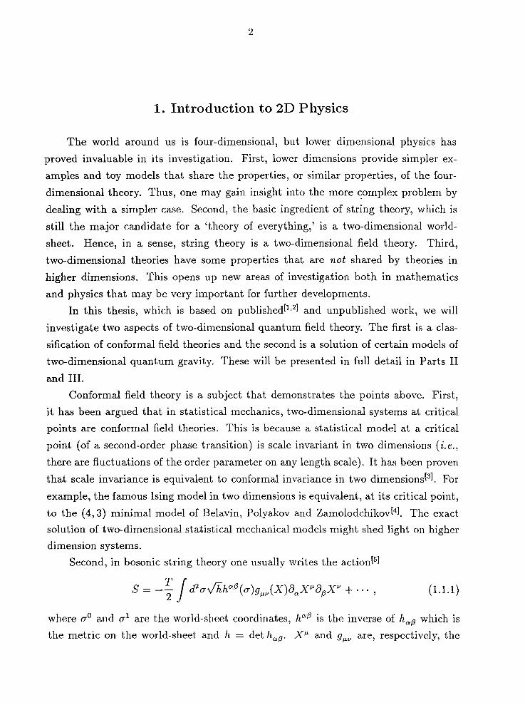
Second, in bosonic string theory one usually writes the action[51

(1.1.1)

where 17° and 171 are the world-sheet coordinates, ha/3 is the inverse of ha/3 which is

the metric on the world-sheet and h = det ha /3' XI-' and 91-'v are, respectively, the

3

coordinates and the metric of space-time. The metric in two dimensions has three

independent components and, since the action is reparametrization invariant, one can

eliminate two of them. This allows a gauge choice in which the metric takes the so­

called conformal form, haf3 = f( (J" ) 'TJaf3 , where f is some function. However, there is

one more symmetry at our disposal-Weyl symmetry. One can easily check that the

classical string action is also invariant under the Weyl rescaling

(1.1.2)

All these symmetries amount to the fact that the world-sheet theory is conform ally

invariant, at least at the classical level. This means that a vacuum state of string

theory is a conformal field theory, at least to leading order in the loop expansion.

Third, the conformal group is infinite dimensional in two dimensions, as will be

shown in the Part II. This property is not shared with a conformal group in higher

dimensions*. In the last decade conformal field theory has proved to be a useful tool

in the investigation of many areas in mathematics, such as infinite dimensional alge­

bras (Kat-Moody algebras[6]), loop groups[7] and more. Indeed, Kat-Moody algebras

have proved to be of importance in physics, especially in string theory, and in the

construction of new conformal field theories[8,9].

The second topic of this thesis also demonstrates the points above. Quantum

gravity is a problem of vast interest, and knowledge of the two-dimensional theory

should help us understand the four-dimensional counterpart. The world sheet in

string theory is reparametrization invariant and hence may be viewed as a gravitating

two-dimensional system. A connection has been found between the KdV hierarchy,

topology and certain infinite dimensional algebras using random matrix models­

which in turn have been used to derive more connections and to get more insight into

the two-dimensional problemt.

In the next two chapters the two topics of this thesis will be discussed in a general

way, and some more specific motivation for their investigation will be presented. The

main results will also be presented without too many details.

* In fact, in d dimensions the local conformal group has dimension Hd + l)(d + 2). The global

conformal group might be of smaller dimension. In two dimensions, the global conformal group

on the sphere is finite dimensional!

tReferences will be presented in a later section.

4

2. Classification of Conformal Field Theories

Two-dimensional quantum field theory with conformal invariance[4,lOl is a system

with an infinite number of conserved currents, since the conformal group in two

dimensions is infinite dimensional. The symmetry algebra, the Virasoro algebra[lll,

is defined by the commutation relations

[Lm' Lnl = (m - n)Lm+n + 1c2 m(m

2 - 1)8m+n,o

[Lm,Lnl = 0 - - - C 2

[Lm' Lnl = (m - n)Lm+n + 12 m(m - 1)8m+n,o,

(1.2.1a)

(1.2.1b)

(1.2.1c)

where m and n are integers. This algebra splits into a direct product of a holomor­

phic part (spanned by the Ln's) and anti-holomorphic part (spanned by the Ln's).

We will denote this algebra V 0 V. Because of this very large symmetry algebra,

some conformal field theories can be solved exactly-meaning that one can explicitly

calculate correlation functions of the various fields.

The fields in the theory decompose into irreducible highest-weight representations

of the Virasoro algebra. Given such a representation, the highest weight field itself

is known as a primary field and is specified by a pair of numbers-the so-called

conformal dimensions (h,Ji). The rest of the fields (i.e., non-primary fields) are

known as descendants.

Classification of conformal field theories (CFT's) has been investigated exten­

sively in the last few years[12-161. A complete classification does not exist yet, but

one does know, at least conceptually, how to classify rational conformal field theo­

ries. Moreover, rational conformal field theories are the ones that can be explicitly

solved, as was done for the special case of minimal models in the fundamental paper

by Belavin, Polyakov and Zamolodchikov[41.

A rational conformal field theory (RCFT) is defined as a CFT that has a finite

number of primary fields. It has been shown by Kac[171 that in the representation

theory of the Virasoro algebra, the only RCFT's are the minimal models of Belavin,

Polyakov and Zamolodchikovf41 . The central charge, c, of these minimal models is in

a list of discrete values that are bounded from above by 1.

5

The problem now was to construct RCFT's with c larger than 1. At first this

seems impossible-it has been proved[18] that CFT's that are invariant under the Vi­

rasoro algebra and have c > 1 must have an infinite number of primary fields. The

solution was to extend the symmetry algebra with the hope the under the new en­

larged symmetry the fields will decompose into fewer representations, maybe even a

finite number. Indeed, this was accomplished in different ways, by including super­

symmetry and thus getting the superconformal algebras, by extending the algebra

with spin one currents and getting the Kac-Moody algebras, by W-algebras[19] and

more. Today there is an extensive list of possible extended symmetry algebras.

Let us denote the extended algebra by A@ A and, as is apparent in the notation,

we assume that it decomposes into a direct product of a holomorphic part (some­

times known as the chiral part) and an anti-holomorphic part (antichiral)*. This

algebra contains the Virasoro algebra V @ V as a sub algebra. The (infinite number

of) fields of the theory decompose into irreducible highest-weight representations of

this algebra. Each associated highest-weight field is a primary field, and it has spe­

cific conformal dimensions, (h, Ii), as before. However, each primary field has some

additional 'quantum' numbers that characterize it in terms of the extended algebra.

RCFT's are defined, as before, by demanding that the theory has a finite number of

primary fields.

One might ask the following question: Is there a relation between the chiral

and anti-chiral parts of the symmetry algebra? At first glance, looking only at the

representation theory, one can find a chiral CFT (i.e., one looks only at the chiral

part), and this theory seems to be independent of the antichiral part-the symmetry

algebra is a direct product, and hence the representation theory decomposes. Hence,

the answer to the question seems to be no. However, this answer is true only when

the Riemann surface on which the theory is defined is the sphere. Motivated by string

theory loop expansions, one wishes to define CFT's on higher genus surfaces and then

other considerations must be applied.

For example, on the torus, we encounter modular invariance. It turns out that the

conform ally inequivalent tori are specified by a complex parameter, 7, known as the

modular parameter. However, there are different 7'S, connected by so-called modular

transformations, that specify the same torus, i. e., two tori that are connected by a

modular transformation are conform ally equivalent. The symmetry group generated

*Sometimes the whole algebra is referred to as a 'chiral algebra' and sometimes 'chiral' refers only

to the holomorphic part.

6

by these transformations is the modular group. Demanding that the CFT under

investigation be modular invariant leads to severe restrictions on the possible chiral­

antichiral combinations in the symmetry algebra and also on the field content of the

theory. One may think that one needs to take into account the modular structure of

higher genus Riemann surfaces (and in general their moduli space is not even known),

but it has been proved that it is sufficient to consider only modular invariance on the

torus[20].

To classify RCFT's, one first has to classify all possible chiral algebras that have

a finite number of irreducible representations. After doing that~ one has to find all

possible modular invariant combinations of chiral and antichiral parts. This method

has a few drawbacks. First, there is no classification of chiral algebras. Second, even

for known chiral algebras, the representation theory is not always known.

The motivation for this work is to see what one can say about a RCFT without

fully knowing the symmetry algebra. The work will be restricted to chiral rational

conformal field theories, i. e., the anti-holomorphic part, .4, of A ®.4, will be ignored.

In any case, the left-right combinations of fields is quite trivial for the two- and

three-field theories that will be dealt with.

A chiral rational conformal field theory (CRCFT) has a finite number of primary

fields. These fields satisfy the fusion rules

N-l

<Pi X <Pj = ~ Ni/<Pkl (1.2.2) k=O

where N is the number of primary fields and Ni/ are non-negative integers that

specify the number of channels to get <Pk when fusing <Pi and <p}21,22]. These integers

must satisfy certain relations because of modular invariance.

In Part II the constraints of modular invariance on the fusion algebra, the con­

formal dimensions of the primary fields, and the central charge of two- and three-field

rational conformal field theories will be investigated. The main tool we will use is a

formula found by Verlinde[21] that connects the integers Ni/ to a certain matrix that

describes the modular transformation properties of the theory. It will be shown that

the two-field case can be classified, i.e., a list of possible theories with their conformal

dimensions and central charge will be presented. The three-field case is harder to deal

with but similar results still hold, although the classification is not yet complete.

The analysis demonstrates the crucial role of modular invariance but also shows

that this symmetry is not enough to completely classify rational conformal field the-

7

ones. However, in the cases investigated, the fusion rules themselves, (1.2.2), do get

classified. It is tempting to conjecture that this is true in general, i.e., for any RCFT

our method will classify the fusion rules.

8

3. (l,q) Models ofKdV Gravity

In the past year and a half there has been a lot of progress in the investigation of

two-dimensional quantum gravity. A quantum theory of gravity has proved over the

years to be very elusive and many attempts to formulate it have been unsuccessful.

Superstring theory provides a theory of gravity in space-time with dimension D ~ 10,

but we still lack complete understanding of all the special features that are present

in string theory, and there is a lot of ambiguity concerning its vacuum and its low

energy limit.

In a brilliant set of papers by various authors, a formulation of two-dimensional

quantum gravity was presented based on random matrix models[23-281. It has been

demonstrated that the continuum limit of certain random matrix models at suitable

critical points can be solved[29-311. That is, a non-perturbative solution can be found.

It has also been conjectured, and a lot of evidence has been presented, that the

solution satisfies the KdV-hierarchy[321.

The KdV hierarchy is a hierarchy of non-linear, partial differential equations

that is completely integrable[331. The first non-trivial equation in the hierarchy is the

original Korteweg-deVries equation. It is best presented in terms of pseudo-differential

operators, 00

O(k) = L oJ X )Dk- i , (1.3.1) i=O

where D = :x and k is a certain integer that specifies the highest-order derivative.

With a definition of the way the operator D-1 operates, the set of such operators

form an algebra. The KdV hierarchy is represented by the equations

aQ = [Qi/q Q] at· +" t

(1.3.2)

where Q is a differential operator of order q and certain fractional powers of Q have

been introduced. (The '+' picks out the differential operator part.) The details will

be presented in Part III.

In KdV gravity the operators {Qi/q}~l are associated with the fields of the theory

and, adding some extra conditions (the 'string equation'), we can compute correlation

9

functions, at least in principle. The parameters ti introduced in equation (1.3.2)

are called flow parameters. One may think of them, in a field theoretical context,

as the coefficient of perturbations that may be added to the action. In this way,

taking partial derivatives of a correlation function with respect to these parameters

corresponds to inserting additional operators into the correlation function. In the end

these parameters are set to zero (or some other appropriate critical values).

The string equation, defined with the help of another differential operator P of

order p, is

[P, Q] = 1. (1.3.3)

The operator P is connected with the potential chosen by the matrix model, and

its order p is related to the order of this potential. The operator Q is related to

the number of matrices in the model. One may think of P and Q as 'momentum'

and 'position' operators in the space of eigenvalues of the matrices used to define

the random matrix model. The string equation can be identified with the canonical

commutation relation. By choosing different operators Q and P, one chooses different

models. If P = (QP/q)+, one gets the so-called (p, q) model.

Other approaches to two-dimensional quantum gravity are based on quantum

Liouville theory[34-37] and topological field theory[38]. The latter approach provides a

simple understanding of some aspects of two-dimensional gravity. Indeed, a certain

class of KdV gravity models are topological field theories. Topological field theory

also provides the hints that are needed in order to identify the fields in the theory.

The matrix model approach, on the other hand, is somewhat ambiguous in dealing

with descendant fields.

In Part III the matrix models and the KdV hierarchy will be defined and an

explicit solution will be presented to the (1, q) models of KdV gravity. A 'ghost'

number selection rule for the computation of correlation functions will be proven. It

will be shown that one can assign a ghost charge to each field,

gh (Pi) = i - q - 1, (1.3.4)

and that the correlation function of n fields vanishes unless n

L gh (Pi) = 2(q + 1)(1 - g). (1.3.5) i=1

In the above, 9 is a non-negative integer multiple of one-half, q is a positive integer

that specifies the (1, q) model and Pi are the various fields. It turns out that 9

10

represents the genus of the Riemann surface on which the correlation function does

not vanish.

11

Part II

CLASSIFICATION OF TWO- AND THREE-FIELD

RATIONAL CONFORMAL FIELD THEORIES

12

1. Introduction to Conformal Field Theory

Consider a d-dimensional flat space (Rd) with the Minkowski type metric gil-v =

'TIll-V of signature (p, q). Under a change of coordinates, x --+ x', the metric transforms

as

(2.1.1)

The conformal group is defined as the subgroup of coordinate transformations having

the property that the metric is invariant up to a scale factor,

(2.1.2)

Note that the Poincare group is a subgroup of the conformal group, as it leaves the

metric invariant.

To find the generators of the conformal group, consider an infinitesimal coordi­

nate transformation, xll- --+ xll- + EIl-(X), under which the line element ds2 = gll-vdxll-dxV

transforms by

(2.1.3)

2 81l- Ev + 8vEIl- = d(8. E)gll-v' (2.1.4)

where the proportionality constant is determined by tracing (2.1.4) with gil-V = 'TIll-v.

It also follows from this equation that

(2.1.5)

This can be derived by first applying 81l- to (2.1.4) (summing the index f-L) and then

applying 8 Il- (there is no f-L index left). Repeating with the index v (i. e., applying 8v

and then 8v ) and adding the two resulting equations one gets the required result (up

to substitution of (2.1.4) again).

The difference between two dimensions and d > 2 dimensions is now obvious.

When d > 2, the dimension of the conformal group is finite since Ell- can be at most

13

quadratic in x. In two dimensions, however, choosing Euclidean signature (1]jJ-v = bjJ-J,

equation (2.1.4) reduces to the Cauchy-Riemann equations

(2.1.6)

It is then natural to transform to the complex coordinate z = Xl +ix2 and its complex

conjugate z = x l -ix2. We similarly define E{Z) = E1 +iE2 and l(z) = E1-ic2' The two­

dimensional coordinate transformations thus coincide with the analytic coordinate

transformations

z -+ J(z) and z -+ ](z). (2.1.7)

The local algebra of these transformation is infinite dimensional. For this reason,

i.e., the existence of an infinite number of conserved currents, one can get a lot of

information about theories that have conformal symmetry in two dimensions.

1.1. The Virasoro Algebra, Primary Fields, and All That

A two-dimensional conformal field theory is defined as a complete set of fields,

{¢i(z, z)}, together with a symmetry algebra, A @ A, defined on some Riemann sur­

face. We demand that the symmetry algebra decomposes into a direct product of

chiral (i. e., holomorphic) and anti-chiral parts, and that it contains the Virasoro al­

gebra, V @ V, as a subalgebra. We also demand a strong version of the operator

product expansion (OPE). OPE in the usual definition is only an asymptotic expan­

sion; however, in conformal field theory the expansion is exact-that is, it converges.

One can argue that since the theory has no scale, the OPE cannot obtain terms that -I

are proportional to e Z=:W; such terms would generically ruin the exactness of the 0 PE.

The Virasoro algebra is described in terms of the stress-energy tensor, T(z)*,

which satisfies the following operator product expansion (OPE),

c/2 2T(w) 8T(w) T(z)T(w) "-' ( )4 + ( )2 + + non singular terms. z-w z-w z-w

(2.1.8)

C IS called the central charge of the algebra. One may understand this OPE as

encoding in a convenient way the commutation relations of the generators, L n , of the

Virasoro algebra. These generators are the modes of the stress-energy tensor

T(z) = L Z::2' nEZ

(2.1.9)

*We will suppress writing the anti-holomorphic operator r(f), as it behaves in a similar way.

14

and satisfy the commutation relation

(2.1.10)

The fields of a 2D eFT can be arranged in irreducible highest-weight represen­

tations of the chiral algebra. The highest weight field is called a primary field and, if

the chiral algebra is just the Virasoro algebra, it is defined by the OPE

(2.1.11 )

where the non-singular terms are not written, as will be the practice from now on.

The number h is called the conformal dimension of the primary field. A similar

expression with h holds for the anti-holomorphic part, '1'(z). This means that the

primary fields transform an (h, h) tensor under coordinate transformations

-J.. ( -)d hd-h -J..' (' -')d ,hd-'h 'Ph,h z, Z Z Z = 'Ph,h Z ,z Z z. (2.1.12)

We stress that non-primary fields do not transform in such a simple way. In a general

chiral algebra this condition, (2.1.11), is still satisfied, but it is no longer the complete

definition. One needs to add the condition that the primary field is the highest weight

of a highest-weight representation of the whole chiral algebra and not just the Virasoro

subalgebra. The details depend, of course, on the knowledge of the chiral algebra.

The above statements can also be written in mode expansions. The vacuum

state, 10), is defined as the state with zero energy that is annihilated by all lowering

operatorst

LoIO) = 0 (2.1.13)

(2.1.14)

Then a primary state, I h), is defined by

(2.1.15)

It follows that

Lolh) = hlh) (2.1.16)

tIt follows from (2.1.10) that also L_tlO) = O. This is the source of an SL(2, R) symmetry of the

vacuum.

15

Lnlh)=O for n>O. (2.1.17)

That is, Ih) is an eigenvector of La with eigenvalue h. The second line means that

Ih) is a highest-weight state. One gets the rest of the states in the representation

by using the raising operators (L_ n for positive n in the case that the chiral algebra

is just the Virasoro algebra). These fields (or states) are usually called descendant

fields, or descendants for short. The exact form depends on the chiral algebra, but

supposing for now that the chiral algebra is just the Virasoro algebra, one can write

an expression for a generic descendant state

(2.1.18)

where n is the list {nl' n 2 , ... , n k' ••• }. It is not hard to show that the descendants

are also eigenvectors of La with eigenvalue h + 2:k knk

Loin, h) = (h + L knk)ln, h). (2.1.19) k

The value 2:k knk is usually called the level (not to be confused with the level of

Kac-Moody algebras that will be mentioned later).

A question that one may ask is whether all the descendants are independent.

Another question, that turns out to be equivalent to the first one, is whether one

can get a descendant that behaves like a primary field-that is, it satisfies (2.1.16)

and (2.1.17). The answer is usually no. However, there are models with such states.

This was exploited in the paper of Belavin, Polyakov and Zamolodchikov[4] to find

the so-called minimal models. A bit more on these models will be presented later.

The fields of a eFT satisfy OPEs

<Pi(Z, z)<pj(O, 0) = L CijkZ-D..ijk Z-~ijk <Pk(O, 0) , k

(2.1.20)

where ~ijk and liijk are simple combinations of the conformal dimensions of the fields,

~··k = h· + h· - hk tJ t J and LS.··k = h. + h· - hk tJ , J • (2.1.21)

The fields in the above equation may be primary or not; their dimensions are their

eigenvalues under the generators La and La (see (2.1.19)) in any case.

Let us note that knowledge of the coefficients Cijk actually provides a complete

solution of the theory. To show that, one uses the fact that the one-point correlation

16

function (on the sphere) vanishes unless the field happens to be the identity (or a

descendant of the identity). Then the two-point function is

(2.1.22)

where the z dependence has been omitted. Moreover, it can be shown[lO) that this

correlation vanishes unless hI = h2 • Usually one renormalizes the fields such that

CijO = bijt . Computation of the three-point functions follows in a similar way, and

the details will not be presented here. However, the three-point functions determine

the rest of the coefficients Cijk . No further information is needed to compute higher­

point correlation functions. This is because the OPE is associative and, hence, when

one computes correlation functions, one can use (2.1.20) to reduce the correlation to a

function of the Cijk'S. Indeed, some methods of classification involve the classification

of different possible values for these coefficients allowed by crossing symmetry of the

four-point functions[39-42,15,16j. That is, performing the OPE (2.1.20) on different fields

in the four-point function provides alternative ways to get the result. Demanding

that these results be identical provides constraints on the values of Cijk . This is

demonstrated in Fig. 1.

t k

t k

I: CijsCkls S

= LCiktCjlt s

J J I

Figure 1: The crossing symmetry of the four-point function (<Pi<Pj<Pk<PI)'

Essential information that is encoded in the OPE is the answer to the following

question. Given two primary fields on the left hand-side of equation (2.1.20), which

representations appear on the right-hand side? The answer is encoded in the so-called

fusion algebra

<Pi X <Pj = L Ni/<Pk· (2.1.23) k

tUowever, there is a slight subtlety that we will deal with in Chapter 3.

17

Here, one understands the fields as primaries that represent the whole representation,

and the sum runs over all the primary fields in the given theory. These are just the

rules for decomposing Kronecker tensor products into irreducible representations,

analogous to 8 X 8 = 1 + 8 + 8 + 10 + 1-0 + 27 in the case of SU(3). It follows that

the coefficients Ni/ are non-negative integers.

Generically, there is an infinite number of primary fields, and a detailed analysis

is very difficult. However, there are some models in which the number of primary

fields is finite. These models are known as rational conformal field theories. Of course,

the finiteness of the number of primaries depends on the chiral. algebra. That is, a

RCFT with respect to some chiral algebra is usually not a RCFT with respect to the

Virasoro subalgebra. Indeed, it has been shown that if the chiral algebra is just the

Virasoro algebra, then the number of primary fields is finite only if the central charge,

c, is in a discrete list of values

6(r - s)2 c = 1 - ---'-----'--

rs (2.1.24 )

These are the minimal models mentioned above. In equation (2.1.24) rand s are

relatively prime (;::: 2), the number of primary fields is (s - l)(r - 1)/2, and the

conformal dimensions of the primary fields are

(ps - qr)2 - (s - r)2 h = ,

p,q 4rs (2.1.25)

where 1 ::; P ::; r - 1 and 1 ::; q ::; s - 1 §.

One immediately sees from equation (2.1.24) that for all the minimal models

c ::; 1. This suggests the problem of finding solvable conformal field theories with

c > 1. This is especially desired in the context of string theory. In the bosonic string

theory, for example, the reparametrization ghosts contribute central charge -26, and,

to avoid conformal anomalies at the quantum level, one needs a vanishing total central

charge. The solution is to add a conformal field theory of central charge 26. Usually

this CFT is composed of four free bosons (that represent space-time coordinates) and

another c = 22 eFT that represents the 'internal' degrees of freedom. Preferably,

we would like a finite number of internal degrees of freedom, and that is the reason

to look for RCFTs with c > 1. One solution to this problem is to extend the chiral

algebra, for example by supersymmetry or by Kat-Moody algebras. Nowadays there

is a long list of extended chiral algebras.

§ Actually, these values count each primary twice.

18

1.2. Extended Chiral Algebras

In this section extended chiral algebras are briefly discussed. The idea is to extend

the Virasoro algebra by chiral fields so that under the extended symmetry the fields in

the theory decompose into fewer representations. Historically, the first such extension

was the superconformal algebra[43,44]. This algebra contains a supercurrent, G(z), in

addition to the energy-momentum tensor. The resulting algebra has the following

OPE

T(z)T(w) rv c/2 + 2T(w) + 8T(w). (z - W)4 (z - w)2 z - w

(2.1.26a)

T(z)G(w) rv ~G(W)2 + 8G(w) (z-w) z-w

(2.1.26b)

~c 2T(w) G(z)G(w) rv (z _ w)3 + z - w . (2.1.26c)

This superconformal algebra has (super)-minimal models with the following values

for the central charge[45,46]

c= ~ (1- 2(s _r)2). 2 rs

(2.1.27)

Here, the limiting value for c is ~. A similar N = 2 superconformal algebra[47-49] (with

two supercurrents and an additional U(l) current) yields a limiting c of 3[50-52]. The

supersymmetric extensions to the Virasoro algebra have been classified by Ramond

and Schwarz[53].

There is one subtlety in dealing with super conformal algebras that will be demon­

strated for the (N = 1) superconformal algebra, (2.1.26). The OPEs only describe the

local behavior of the algebra, and the global behavior is linked to boundary conditions

on the operators. T(z) always has periodic boundary condition since otherwise confor­

mal symmetry would be broken. The other generators, however, can have antiperiodic

boundary conditions. In the superconformal case there are only two possibilities, the

Ramond sector, in which G(z) has integer modes, and the Neveu-Schwarz sector,

in which G(z) has half-integral modes. These two algebras are not equivalent, i.e.,

there is no automorphism between them. Similarly, in the N = 2 case, there are two

sectors, the twisted sector (T-sector), which is usually not encountered in eFT, and

the NSR sector. The fact that the modes are not necessarily integral can yield, in

equation (2.1.19), half-integral levels.

19

We will discuss Kat-Moody algebras[54-56,6] in a more detailed way as these have

proved to be of extreme importance in CFT**. One may think of them as central

extensions of the algebra of the loop group of a Lie group. A Kat-Moody algebra, 9k, based on the compact finite dimensional Lie algebra g, is defined by dim (g) currents,

Ja(z), satisfying the OPE

(2.1.28)

k is known as the level of the algebra (not to be confused with the level of a de­

scendant) and rbe are the structure constants of the Lie algebr~ g. The Lie algebra

9 could be simple, semi-simple, or it could have U(1) factors. We will assume for

simplicity that the algebra 9 is simple.

Using the Sugawara[57,58] construction, we define a stress-energy tensor

1 dimg

T(z) = k + Q L: r(z)r(z) :, '" a=l

(2.1.29)

where Q", is the quadratic casimir of the adjoint representation defined by fed a r db =

Q ",{)ab, and ': :' is a normal ordering prescription that removes the singularity that

results from multiplying two operators at the same pointtt. This T(z) satisfies the

Virasoro algebra OPE, (2.1.8), with central charge

Note that generically C > 1.

kdimg cg = k + Q",. (2.1.30)

Conformal field theories that are based on this construction have a finite num­

ber of primary fields, labeled by the highest weights of the representations of the

underlying Lie algebra. The possible representations are restricted by the condition

2A .1jJ k 0::; 1jJ2 ::; 1jJ2 E Z,

**For a review, see Goddard and Olive[8].

tt For example,

(2.1.31)

20

where A is the highest weight of a representation and 'lj; is the highest root of the

Lie algebra g. The origin of this formula is as follows. In the mode expansion

(J(z) = L:z Jnz-n-l) one can choose the analogue of the Cartan-Weyl basis. In

that basis, the generators E1cx, E'::.l and ;2 (~ - a . Ho) form a sub algebra that is

isomorphic to 5U(2). Here a is a root, E~ are the raising and lowering operators

and the H~ 's belong to the Cart an subalgebra. Since those operators form an 5U(2)

algebra, the 'spin' must be quantized to be half integral. Since 2cx~!jQ is quantized

(this is a basic fact from the theory of Lie algebras), :2 must be quantized as well.

We can extremize this quantization rule by selecting the highest root of g, 'lj;.

The other part of the formula follows from demanding that the vector E~ll/-l)

be of positive norm. Here /-l is a weight in the representation. The requirement that

this vector be of positive norm is a consequence of unitarity-that is, we build the

Kac-Moody algebra representation on unitary representations of the underlying Lie

algebra. Since this algebra is compact (as chosen), those representations are finite

dimensionaltt .

The primary fields have conformal dimensions

(2.1.32)

where Q A is the quadratic Casimir of the representation A. For example, the con­

formal field theory based on 5 U (2) at level k has primaries with dimensions (of the

8U(2) representation) 1 ::; 2j + 1 < k, where j is the highest weight (spin). The

conformal dimensions are

h. = j(j + 1) J k + 2 . (2.1.33)

We will return to 5U(2)(k) in the next chapter. All these theories can be constructed

as Wess-Zumino-Witten (WZW) models[59-61j based on non-linear sigma models.

An important construction, known as the coset or GKO construction[62,9j, is

used to generate many more CFT's by taking cosets of 9 and one of its subalgebras,

say h. If T a( z) and T H( z) are the Virasoro currents for 9 and h, respectively, then

Ta/H(z) = Ta(z) - TH(z) also satisfies the Virasoro algebra with central charge

(2.1.34)

ttThere are extensions of this construction to non-compact or non-unitary groups, but we will not

deal with them here.

21

By substituting (2.1.30) and choosing the algebras g and h carefully, one can get

c's that are smaller than 1. For example, by choosing g = 5U(2)(k) 0 5U(2)(1)

and h = 5U(2)(k+1), one gets the central charges of the minimal models (2.1.24).

Moreover, it has been proved that this construction actually gives the minimal models.

Similar results hold for the superconformal algebras. It has been conjectured that all

rational conformal field theories can be represented as coset models. Certainly it is

true for the known models.

The last point we will discuss is the problem of modes. Strictly speaking, a

chiral algebra is defined as a set of holomorphic and anti-holomqrphic operators that

have integer dimensions[631. The superconformal algebra seems to contradict this

statement, and there are other examples such as parafermion theories[641 and orbifold

theories[651. These cases are examples in which a complicated chiral algebra is ex­

tended with fractional dimension chiral fields and the resulting structure has a chiral

algebra-like appearance. We usually project these modes out. Further examples are

discussed by Goddard and Schwimmer[661. We will assume that the chiral algebra has

only integer spin currents§§.

We will conclude this section with a rigorous definition of a rational conformal

field theory, as given by Moore and Seiberg[631. We start with the definition of a

conformal field theory.

Definition 1: Conformal Field Theory

A conformal field theory is an inner product space 1i which can be decomposed

into a direct sum

1i = EB V(h, c) 0 V(Ii, c) (2.1.35) h,h

of irreducible highest weight modules of V 0 V such that

a. (Vacuum) There is a unique 5L(2, R)05L(2, R) invariant state, 10), with (h, Ii) =

(0,0).

b. (Operators and Duals) For each vector 0' E 1i there is an operator <Po:(z) on 1i,

parametrized by z E C. Also, for every operator <Po: there exists a conjugate

operator <Po:t (partially) characterized by the requirement that the OPE <Po:<Po:t

contains a descendant of the unit operator.

c. (Primary Fields) For 0' = i, a highest-weight state, we have [Ln' <Pi(Z, z)] =

(zn+l tz + hi(n + l)zn) <Pi(z, z).

§§ Actually, for our purpose, it is enough to demand integer modes.

22

d. (Duality) The inner products (OI¢\(Zi1,ZiJ"'<PiJZin,ZiJIO) exist for IZill > .. , > IZi I > 0 and admit an unambiguous real-analytic continuation, indepen-

n

dent of ordering, to en minus diagonals.

e. (Modular Invariance) The one-loop partition function and correlation functions,

computed as traces, exist and are modular invariant.

Definition 2: Chiral Algebra

In a conformal field theory, a closed set (under OPE) of holomorphic (and anti­

holomorphic) fields is called a chiral algebra. A maximal set of such operators is a

maximal chiral algebra.

Definition 3: Rational Conformal Field Theory

Rational conformal field theories are conformal field theories such that the (phys­

ical) Hilbert space, H, is given by the finite sum

N

H = E9 Nr,r Hr 0 Hr, (2.1.36) r,r=O

where Hr (1-{r) is an irreducible representation of A (A), the (anti-)holomorphic part

of the chiral algebra. Nr,r is an integer counting the multiplicity of Hr 0 Hr in H.

2. Modular Invariance in eFT

Conformal field theory was initially defined on the sphere (or plane) but it is

seen in its full beauty when considered on an arbitrary Riemann surface. Indeed, in

string theory, the sphere is just the first term in a genus perturbation expansion and

so we are interested also in CFT's on higher genus surfaces. T~e first of these is the

torus, so one goal is to formulate a consistent conformal field theory on the torus.

Cardy was the first to discuss the importance of modular invariance in restricting the

operator content of a CFT[18].

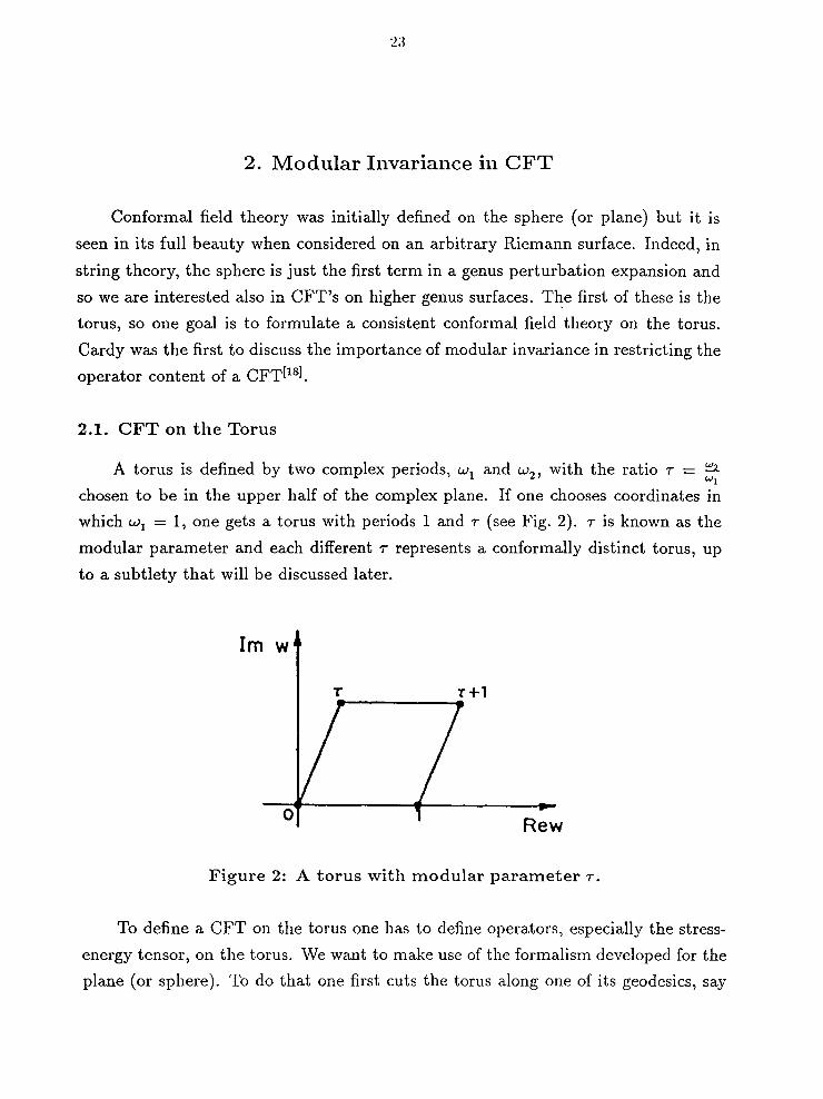
2.1. eFT on the Torus

A torus is defined by two complex periods, WI and W 2 , with the ratio T = ~ WI

chosen to be in the upper half of the complex plane. If one chooses coordinates in

which WI = 1, one gets a torus with periods 1 and T (see Fig. 2). T is known as the

modular parameter and each different T represents a conformally distinct torus, up

to a subtlety that will be discussed later.

Im w

T T+l e_------..

o Rew

Figure 2: A torus with modular parameter T.

To define a CFT on the torus one has to define operators, especially the stress­

energy tensor, on the torus. We want to make use of the formalism developed for the

plane (or sphere). To do that one first cuts the torus along one of its geodesics, say

24

WI' In this way we get a cylinder that can be mapped to an annulus in the plane by

the exponential map (see Fig. 3)

21riW W -l- Z = e w1 • (2.2.1 )

1

Figure 3: Mapping the cylinder to the plane with (2.2.1).

By this mapping the translation operator along W 2 , the 'Hamiltonian,' gets trans­

formed into a combination of dilation and rotation operators on the plane. To find

this transformation explicitly recall that under conformal transformations, T( z) trans­

forms according to equation (2.1.8). That is, T(z) is not a primary field (see equation

(2.1.11)) and, hence, writing a similar expression to (2.1.12) one has

T(w) = T(z) (oz)2 + ~ fu;~ - ~ (B-)2 Ow 12 (~~)2

(2.2.2)

The second term is the conformal anomaly term (Schwarzian derivative) which is

proportional to the central charge c. Plugging (2.2.1) into (2.2.2) the transformation

law for T(z) is obtained

Tcvlinder(w) = _ 471"2 (TPlane(z)z2 _~) . wi 24

(2.2.3)

Now the Hamiltonian can be found. The generator that corresponds to transla­

tions in the mode expansion of T(z) 00

T(z) = L (2.2.4 ) n=-OO

25

. L S t' Lcylinder fi d IS -1' 0 compu mg -1 one n s

(2.2.5)

Therefore, the translation along W 2 is*

(2.2.6)

The next stage is to define the partition function on the torus, or the zero-point

function, to be

(2.2.7)

where the trace is, as usual, over all states, and we have defined

(2.2.8)

Now, as the Hilbert space decomposes into irreducible representation of the Virasoro

algebra, V 0 V (or, in general, the chiral algebra A 0.it), one can decompose the trace

in equation (2.2.7) to a sum

Z(T) = LNh,liXh(T)X}i(T), (2.2.9) h,h

w here the character X h ( T) is defined by

(2.2.10)

The trace here is carried over the highest-weight representation with highest weight

h. The coefficients Nh,h must be non-negative integers as they count how many times

a given representation appears in the theory. Also, No,o is always 1, to express the

fact the the identity operator (or vacuum) is unique.

*Note that we include the antiholomorphic part here!

2G

'Ne now return to the subtlety alluded to above. In calculating the partition

function, the two periods, W l and W 2 , were not treated on the equal footing. The

periodicity in W 2 was taken care of by the trace, but what about w l ? More generally,

one should associate Z ( T) to a lat tice spanned by those periods and not to the periods

themselves. (Or, equivalently, the original torus can be defined with other periods

that are associated to the original periods.) The result is that this kind of lattice

is invariant under unimodular transformations of the periods. Or, equivalently, the

partition function should be invariant under modular transformations of the modular

parameter T:

I aT + b T ~ T = ,

CT + d (2.2.11)

where a, b, C and d are integers that satisfy ad - bc = l.

These transformations form a discrete infinite group called the modular group

(usually denoted r and is isomorphic to P5L(2, Z) ~ 5L(2, Z)/Z2)' This group is

generated by the two transformations T : T --+ T + 1 and 5 : T --+ -~. In Fig. 4 the

transformations T and U = T- 15T-1 (T --+ T / (T + 1)) are shown.

T

T T+l

o 1 o

Figure 4: The modular transformations T and U.

It turns out that the requirement of modular invariance of Z( T) is very restrictive

and, in general, quite hard to satisfy. Specifically, it restricts the Nh,h that are allowed

in (2.2.9).

27

2.2. Some Simple Consequences of Modular Invariance

To examine the consequences of modular invariance let us see how the characters

transform under a modular transformation. It is enough to check the transformation

properties under the two basic transformations mentioned at the end of the previous

section. Usually those transformations are denoted T and S,

1 S: T -+ --.

T

T will be examined first. When T -+ T + 1,

= e - ~~c L (<Pi I e21rir ( Lo- f.- ) e21riLo I <Pi) t

= e-~~c L(<Pile21rir(Lo-f.-)e21ri(h+n;)l<pi)

• = e- ~~c +21rih L (<Pi le21rir ( Lo- f.- ) I <Pi)

i

(2.2.12)

(2.2.13)

(2.2.14)

where the sum is over all the states in the module based on the primary field I h, Ii) t,

and ni is the level of the descendant. As discussed in Section 1.2 it has been assumed

that the modes of the symmetry operators that are used to generate the representation

are integers.

Substituting (2.2.14) into the partition function (2.2.9),

Z(T + 1) = LNh,he-22~i(c-c)e21ri(h-h)Xh(T)Xh(T). hh

Now, since a eFT always has No,o = 1, one gets

c - c = O(mod24)

and for each nonzero Nh h ,

h - h = O(mod1).

(2.2.15)

(2.2.16)

(2.2.17)

t In general, the chiral algebra is not just the Virasoro algebra and the primaries are primary fields

with respect to the full chiral algebra.

28

Hence, one concludes that if one wants a consistent conformal field theory on the

torus, then the only possible primary fields are those with integral difference between

their holomorphic and antiholomorphic conformal dimensions. Also, we see that c - C

must be a multiple of 24. Frequently, one chooses the chiral and anti-chiral parts

of the symmetry algebra to be isomorphic, and then their central charge is equal.

However, there are examples, based on Kat-Moody algebras, with non-isomorphic

algebras. This will be discussed some more later. The heterotic string is another

example in which one needs different central charges for the left and right movers.

Next, we look into the consequences of the other generator of modular transfor­

mations, S. One cannot immediately say what the transformation rule is, but the

characters must transform among themselves. In other words, the characters carry a

linear representation of the modular group. That is, when T ---+ -~,

(2.2.18)

where the sum is over all the characters. Using (2.2.18) one gets, in matrix form, the

following condition on the values of Nh,h in the partition function

(2.2.19)

The next step is to find all the matrices N that satisfy this constraint.

Easier said then done. Usually the form of S is not known and even if known

it is very complicated. Indeed, we can find some simple solutions to (2.2.19), but

the problem of finding all the solutions has been solved in only a few cases. For

example, if the underlying symmetry is a Kat-Moody algebra, then the matrix S is

known. It is given by the famous Weyl-Kac formula[61. In that case, S is unitary

(indeed, we will explain later that S is always unitary) and, hence, one possibility

is always the so-called diagonal solution specified by Nh,/i = Oh,/i, where 0 is the

Kronecker delta. 'Sporadic' solutions, which are not diagonal, have been found for

various algebras[12,67-721, but a complete classification exists only for SU(2).

2.3. The ADE Classification and Other Theories

The ADE classification[72,731 demonstrates the complexity of finding modular in­

variant partition functions. The fact that to date only SU(2)-the simplest Kat­

Moody algebra-has been classified shows how complicated the problem is.

29

Ak+1 2:~!~ IXAI2 k2:1

D 2P+2 2:~~d~=llxA + X4p+2_AI2 + 21X2P+112 k = 4p, P 2: 1

D 2P+1 2:4p

- l 1 12 1 12 Aodd=l XA + X2p

+ 2:~~~e2n=2(XAX~P_A + C.C.) k = 4p - 2, p 2: 2

E6 IXl+X712 + IX4 + XSl2 + IXs + Xnl2 k-= 10

E7 IXl+X1712 + IXs + xd2 + IX7 + xlll2

+IX912 + [(X3 + XlS)X9 + c.c] k = 16

Es IXI +Xll + X19 + X2912

+IX7 + X13 + X17 + X2312 k = 28

Table 1: Modular invariant partition functions for SU(2)(k).

The eFT based on SU(2) at level k has k + 1 primary fields of dimensions

h = O,!, ... ,~. Letting ,\ = 2h + 1 and N = 2(k + 2), the characters are

00 1 "'" . (nN+>.)2

XA(r) = ry3(r) n~oo (nN + '\)e1rlT

N , (2.2.20)

where ry( r) is the Dedekind eta function

00

ry(T) = e ~1 II (1 _ e21rinT) • (2.2.21 ) n=l

Then the matrix S has the components

A' f2. ( 7r ,\N ) SA = V k+2 sm k + 2 . (2.2.22)

It has been shown that the possible modular invariant partition functions for

SU(2) are classified in the so-called ADE classification. They are presented in Table 1.

30

Some more conformal field theories (that are modular invariant) will be presented

next. They will be especially useful later when we will try to identify the models

derived by the classification method with known conformal field theories.

A useful procedure to derive more eFT's is by taking products of already-known

conformal field theories. One should treat such a product as a direct tensor product.

The number of primary fields in the product theory is the product of the number of

fields in the factor theories, their conformal dimensions is the sum of their conformal

dimensions, and the central charge of the product theory is the sum of the central

charges of the factor theories.

The first example is Es-based eFT. At levell there is only one primary field­

the identity field (with conformal dimension 0). The central charge is 8. It has

been proved, though, that X~ (the character cubed) is a modular invariant by itselflt

That is, the conformal field theory based on (Es? at levell as the chiral part of the

chiral algebra and the identity§ in the antichiral part is a consistent eFT. Note that

c - c = 24 - 0 = O( mod 24), as it must be. An important observation here is that

given a conformal field theory, one can generate more conformal field theories with

the same number of fields with the same conformal dimensions just by multiplying

by (E~l»)~hiral X lantichiral' The only difference is that the chiral central charge, c, is

increased by 24. Similarly, one can multiply both chiral and antichiral parts by the

same power of Es levell, and the number and conformal dimensions of the primary

fields will not change (but c and c will).

t The character is a modular form, as it must transform into itself under modular transformations

(there are no other characters to transform to). Thus, if one cubes the character, it can be shown

that the answer is unique-it is the modular invariant function j[74].

§The identity theory (the trivial theory) has just the Virasoro algebra as a chiral algebra and has

a single primary field-the identity. The difference between Es and 1 is the chiral algebra-that

is, there are other generators that one can use to get descendants. That means that the identity

modules (which are in fact the whole theory) are not the same.

31

3. The Classification Scheme

The classification scheme is based on a remarkable formula found by Verlinde[2l1.

3.1. Correlation Functions and Verlinde's Formula

When one computes correlation functions on the sphere, one gets, from conformal

symmetry, unique expressions. For the two-point function of two primary fields one

can show that

(2.3.1)

where Cl ,2 is a constant, Zl2 = Zl - Z2' and h = hI = h2 (and similarly for Z12 and

h) because of the Kronecker delta. Usually, one normalizes C1 ,l = 1, i.e., a field

is conjugate to itself. However, sometimes one gets a conformal field theory with

a non-trivial 'charge conjugation' matrix. Consider an example. The CFT based

on the Kac-Moody algebra SU(3) at level 1 has 3 primary fields. They are, in the

conventional notation for SU(3), 1, 3 and 3. As is well known, the product of 3 and

3 gives the singlet and the octet representations of SU(3). In the conformal field

theory case, since there is no octet at level 1, it is just 'ignored.' Similarly, 3 x 3

that ordinarily gives a 3 and a 6 has to be truncated. That is, the fusion rules for

SU(3)(l) are

3x3=3

3x3=1

3 x 3 = 3.

(2.3.2a)

(2.3.2b)

(2.3.2c)

Thus, the 3 and 3 are conjugate to each other. Generically, one constructs a charge

conjugation matrix, C, that shows which fields are conjugate to which. For example,

in the SU(3) case,

(2.3.3)

32

where the rows and columns correspond to 1, 3 and 3. The consequences of charge

conjugation symmetry will be obvious in a moment. Let us write, again, the fusion

algebra

"', X "', = N .. k"'k ~. ~J 'J ~ • (2.3.4)

Now, suppose that <Pi is conjugate to itself. Then, from the definition of a CFT, one

gets

<Pi X <Pi = <Po + some other fields. (2.3.5)

<Po is the identity field and it will be denoted that way from now on. This means

that Niio = 1 if <Pi is self-conjugate. If, on the other hand, <Pi is not self-conjugate

but is conjugate to, say, <Pn then we get N itO = 1. We can use the charge conjugation

matrix, C, (and its inverse, which is the same thing) to raise and lower indices of Nil (and also of Si

j).

We are now in the position to quote Verlinde's formula[211. It gives a relation

between Sij and Nijk that reads as follows

_ ~ SinSjnSkn Nijk - ~ S '

n=O On

(2.3.6)

where N is the number of primary fields. This has been proved by Dijkgraaf and

Verlinde[221 using the so-called pentagonal identity[121. They also used this formula to

prove that the matrix S is symmetric and unitary.

If the RCFT is unitary, there is another fact one can prove. A unitary theory

is a theory in which the norms of the states are positive. If one looks at the norm

IIL_1Ih)II2, for any primary state Ih), then from the commutation relations (2.1.10)

we easily get h > 0 (if we assumed that Ih) has positive norm). It follows that all the

conformal dimensions in a unitary theory must be positive (or zero for the identity).

Similarly, one can show that c is positive. The fact that was proven by Dijkgraaf and

Verlinde[221 is that for a unitary theory the first row (and column) of the S matrix

must have the same sign. That is,

SiQ = A~O) > 0 Vi. Soo •

(2.3.7)

Conversely, if the signs are not the same, the theory is non-unitary. In general, for

any S matrix, the first row (and column) cannot vanish (or else, (2.3.6) would not

make sense).

33

3.2. The Scheme and One-Field Theories

We can now present our method of classification. For a given number of primary

fields, one writes the most general fusion rules and S matrix possible. Then one uses

Verlinde's formula to investigate the constraints on both Sij and N ijk .

A few remarks are in place here. First, if one applies the S transformation twice,

then one should get the identity transformation. This is almost true. If the charge

conjugation matrix is trivial then, indeed, S2 = 1. However, if C =f:. 1 then one gets

S2 = C. This can be explained by the fact that the characters are identical for a

field and its conjugate. (e.g., for SU(3)(1), X3 = x:d The relation S2 = 1, or its

generalization S2 = C, is one of the defining relations of the modular group.

Second, one can make use of the other defining relation of the modular group,

which is (ST)3 = 1 (or the generalization (ST)3 = C). This will turn out to be quite

important in determining T. One should remember that the knowledge of T is the

knowledge of the central charge and the conformal dimensions of the primary fields

(modulo integers), as is obvious from the T transformation properties of Xi(T) (see

equation (2.2.14)).

Another point to notice is the following fact due to Vafa (as reported by Ver­

linde[21]). The point i in the complex T plane is a fixed point of the S transformation.

That is,

This means that

S . 1.

: T = Z --+ -- = Z. T

(2.3.8)

(2.3.9)

or, that the N dimensional vector (of numbers) (Xj(i)) is an eigenvector of the S

matrix with eigenvalue 1. Moreover, the components of the eigenvector must be

all positive or all negative! This can be seen by plugging i into the definition of

the character, (2.2.10), and noting that e-21r(Lo-c/24) is always positive. This is quite

important, as one can just demand that S has such eigenvector. This further restricts

the possible S matrices.

Two last simple remarks are the following. In the case that the charge conjugation

is trivial, we have S2 = 1 and, because S is a unitary matrix, we have st S = 1. This

means that S is hermitian. So, since S is also symmetric, it must be real! The other

fact is that if Sand T are a given solution, then -S and -T are also a solution.

One of those solutions can be eliminated using Vafa's argument from the previous

34

paragraph. Usually, it is not easy to know in advance which of the solutions is the

correct one. U nitarity is usually also fixed by the classification method, i. e., some

solutions are constrained enough to decide whether the theory is unitary or not.

Let us demonstrate the classification method for the somewhat trivial case of one

primary field. In this case, one does not gain information from the fusion algebra as

it consists only of the trivial rule

<Po x <Po = <Po· (2.3.10)

That is, Noaa = 1 is the only element. Also, as is immediately clear, C = 1 and S is a

1 x 1 matrix. Then, from the condition S2 = C = 1, we get S = ±l. Vafa's argument

can now be used to restrict S to be 1. (-1 does not have a positive eigenvalue!) Next,

one computes T by (ST? = (IT? = T3 = C = 1 and gets 3(h - ;4) = O(modl),

and, since h = 0 (identity field!), one gets c = O( mod 8). These theories can be

identified with the trivial theory and powers of the Es level 1 theory, as mentioned in

previous sections. One notes that there are no other possible values for the central

charge in a one-field rational conformal field theory. It is also seen that those theories

are unitary.

35

4. The Two-Field Case

4.1. The Sand T Matrices and the Fusion Algebra

When there are two primary fields, one of them must be t~e identity field with

conformal dimension O. The other should be different with h i= O. Hence, the charge

conjugation matrix must be trivial-the identity matrix. The fusion algebra for a

two-field RCFT can be written, in the most general form, as

cPo X cPo = cPo

cPo X cPI = cPI

cPI X cPI = cPo + n cPI'

(2.4.1 )

where n is a non-negative integer. Most of the Nijk are determined by associativity

and commutativity of the fusion algebra and the fact that cPo is the identity field.

Making use of the symmetry of Sij and the fact that it's real, one has

(2.4.2)

where a, band c are real numbers. Then, substituting into equation (2.3.6), one gets

the following constraints

Nooo = 1 = a2 + b2

Nool = 0 = ab + be

NOll = 1 = b2 + e2

b3 e3

Nlli = n = - + -. a b

(2.4.3a)

(2.4.3b)

(2.4.3c)

(2.4.3d)

The numbers a and b cannot vanish, as mentioned after (2.3.7), and, hence, from

(2.4.3b) we get c = -a. Equations (2.4.3a) and (2.4.3c) are then identical. Equation

(2.4.3d) is then solved and gives

1 4 + n 2 n ,------:--= ±-V4+n2 • a 2 2 2

(2.4.4)

36

This representation of the solution will be convenient later.

Letting

(2.4.5)

and substituting into the constraint (ST? = 1, one gets

bY(XY + a2(X _ y)2) ) -aY(2XY _ X2 + a2(X _ y)2 = 1.

(2.4.6)

From the off-diagonal terms-remembering that a, b, X and Y- cannot vanish-one

gets XY = -a2(X - y)2. Substituting into the diagonal terms yields the single

equation aXY(X - Y) = 1. Solving for X and Y, we get

X = (-1)~ (~ ± iV1 _ 1 ) 2a 4a2 (2.4.7)

and

(2.4.8)

To further restrict the solution, one looks at the eigenvector of S that belongs to

the + 1 eigenvalue. This eigenvector is

(2.4.9)

where e is some number. There must be a same-sign component eigenvector for a

consistent theory. This will determine the signs of a and b. For a unitary theory a

and b are of the same sign. Then, by looking at (2.4.9), one sees that only if a (and

b) are positive one gets bl(1 - a) > 0*. Conversely, if a and b have opposite signs

(i.e., a non-unitary theory) then inspecting (2.4.9) shows that a < 0 and b> 0 is the

consistent choice. We conclude that b must be positive in any case, unitary or not.

4.2. The Solution

For n = 0, there's only one solution for b which is b = h' Then the S matrix

has two solutions,

(2.4.10)

*Remember that lal and Ibl are less then 1, as can be seen from a2 + b2 = 1.

37

S_ is the case for a non-unitary theory and S+ applies to unitary theories. Let's start

with the unitary case.

Plugging into (2.4.7) we get (remembering that X = e-~~c from (2.2.14)) e = 1( mod 8) for the plus sign and e = 7( mod 8) for the minus. Plugging into (2.4.8)

gives the corresponding values for the conformal dimension, h = ~(mod 1) for the

plus and H mod 1) for the minus. A quick search finds known models with these

values. The model based on SU(2)(1) has e = 1 and h = ~, and the model based on

E~l) has e = 7 and h = ~. The fact that our result is modulo 8 for the central charge

is not surprising in view of our remark on powers of the Es level 1 theory.

The non-unitary case is handled similarly. We get two possible solutions, either

e = -3 and h = -~ or e = -5 and h = -~. These numbers are mod8 and modI,

respectively, but we suggestively wrote them as negative, reminding ourselves that

those theories are non-unitary.

For n = 1 we get two possibilities for b,

b=J5±..J5 10 '

(2.4.11)

and for each b we have a unitary and a non-unitary solution. Starting with the larger

b (with the 'plus' sign), we get for the unitary case two solutions:

(2.4.12)

These models can be identified with G~l) 0 (E~l)) I and FP) 0 (E~l)) I, where 1 is

some non-negative integer. For the non-unitary models we get

(2.4.13)

For the other value of b, for the unitary models, we get

(2.4.14)

and for the non-unitary theories we get

18 4 22 1 (e, h) = (-5' -5) or (-5' -5)·

The second model can be identified with the Lee-Yang singularity[751-the (2,5) model

of the minimal model series (see (2.1.24) and (2.1.25)).

38

Let us note that there is a natural pairing of the solutions, as was apparent

above. The solutions are paired into couples whose central charges sum to 8 and

whose conformal dimensions sum to 1. This can be traced back to the formula for X.

One may define an angle a by

Then X takes the simple form

1 cosa = 2a. (2.4.15)

(2.4.16)

The pairing is due to the ± in the exponent. (By the way, the other factor, (_1)1/\

is responsible for the modulo 8 freedom for c.) Based on the observation that most

paired models above do indeed exist, one is tempted to conjecture that the partner

to the Lee-Yang singularity exists also. We were not able to find this model and the

problem seems hard.

Proceeding to n ~ 2, one notes immediately that one of the solutions for a

presents a problem. The solution with the plus sign now satisfies

1 1 J4 + n 2 n - = ±- + -v'4 + n 2 > 1 2a 2 2 2

for n ~ 2. (2.4.17)

This means that X no longer has absolute value 1. The negative solution is fine, but

if one tries to compute its central charge and conformal dimension, one apparently

gets irrational values. This was proved by Caselle and Ponzano[76].

According to our scheme, there is no reason to reject irrational solutions. How­

ever, one can use some more knowledge of conformal field theory to restrict these

values further. This is accomplished by investigating the analyticity properties of the

four-point function. It can be proved that in rational conformal field theories the

conformal dimensions (and, hence, the central charge) must be rational. This was

first proved by Vafa[77]. This result can even be extended to give a restriction on the

form of h. It was shown by Christe and Ravanini[15] that in a two-field RCFT, the

non-trivial conformal dimension must satisfy

(n + 4)h = O( mod 1), (2.4.18)

where n is the integer that appears in the fusion rule (2.4.1). Thus, in our classifica­

tion, we will ignore the irrational models, since they do not make sense as rational

conformal field theories. We have to remember, however, that we used the analyticity

of the four-point function.

39

One last point is that for n = 00 we again get a rational solution! In this case

a = 1 so b = 0, in contradiction to our demand that a and b will not vanish. However,

one may be tempted to identify this as some degeneration of two-field theories. One

finds that one of these models has central charge 8 and conformal dimension ~. There

is a model with one field and central charge 8, the E8 level 1 model[13]. However, the

conformal dimension of the field is (obviously) o. In any case, this theory does not

make sense as a two-field theory.

Table 2 lists all the rational solutions for the two-field theories. This includes

the unphysical solution of n = 00.

n h( mod 1) c( mod8) Identified model

0 !. 1 Al level 1 4 0 3 7 E 7 level1 4 0 1 -5 unknown -4:

0 3 -3 unknown -4:

1 2 14 G2 level1 5 5

1 ~ 26 F4 level 1 5 5

1 2 34 unknown -5 -s 1 - ~ - § unknown 5 5

1 !. !. unknown 5 5

1 4 38 unknown 5 5

1 1 22 Lee-Yang singularity -s -s-1 4 18 unknown -s -s-

00 1 0 unphysical 6

00 5 8 unphysical (;

Table 2: Possible two-field rational solutions

The final comment is that the reasoning may be inverted to give a classification

of the fusion algebras. It is obvious from the analysis above that n ~ 2 gives an

inconsistent rational conformal field theory. The bottom line is that there are only

two possible fusion algebras for a two-field RCFT. One has the following non-trivial

rule

(2.4.19)

40

and the other has

(2.4.20)

41

5. The Three-Field Case

In the case of two non-identity fields, we can have a non-trivial charge conjugation

matrix of the form

(2.5.1)

We will deal with the two cases separately, starting with the non-trivial charge con­

jugation. Surprisingly, this case is actually simpler then the self-conjugate case, even

without taking into account the fact that the conformal dimensions of the two non­

identity fields are the same.

5.1. Non-trivial Charge Conjugation Matrix (C =1= 1)

Writing a symmetric matrix for 5 we can solve the matrix equation 52 - C.

One gets two solutions,

b _!!.± i

2 2 a i

-2 =f 2

where a and b are complex numbers subject to

(2.5.2)

(2.5.3)

We note that 5 is not hermitian or real. Taking unitarity into account, one gets the

extra condition

(2.5.4)

These two conditions, (2.5.3) and (2.5.4), are compatible only if a and b are real.

The eigenvector with eigenvalue +1 is proportional to

(2.5.5)

42

and since 1 - a is always positive, b must be positive in order to get a same-sign

component eigenvector. (Again, lal < 1 or else b would vanish.) Hence, for a unitary

theory a must be positive, and for a non-unitary one a could be negative.

Using (2.3.6) one finds the values of N ijk and, raising the last index, one finds

the following form for the fusion algebra

where

and

<PI X <PI = m<Pl + n<P2

<PI X <P2 = <Po + m<Pl + m<P2

<P2 X <P2 = n<Pl + m<p2'

1 - 3a2

m = -v'sr:S:--a ";---;;::::::1 =-=a===2

1 + a2

n = -v'sr:S:--a ";----;;:=1 =-=a~2 •

(2.5.6)

(2.5.7)

(2.5.S)

We note that, as required, these fusion rules are symmetric under charge conjugation,

i.e., under <PI f-+ <P2' The coefficients m and n must be non-negative integers, and, thus, we can restrict

the solution further. Solving for a in terms of the ratio ': and substituting the result

back into n, one easily sees that there is only one solution: m = 0 and n = 1. The

value of b is Js*. We now write a general form for T, remembering that hI = h2 t ,

T=U : n (2.5.9)

and then solve the condition (ST? = C. For the unitary case (i.e., positive a) we get

only one solution for each S matrix. For S+ we get c = 2 and h = ~ and for S_ we

get c = 6 and h = ~. These can be identified as the SU(3)(1) and E~I) Kac-Moody

models, respectively.

The non-unitary case (negative a) is also easy to solve, though we were not able

to identify the models. The results are summarized in Table 3.

*From crossing symmetry of the four-point function one derives the condition m 2 + 1 = n 2 , which

has only one solution, the one given above. So, in fact, modular invariance is not really needed to

classify this fusion algebra.

t Actually, one can show that for a general choice, with hl -# h2 , we get an inconsistency-i.e.,

(ST? -# c.

43

hI h2 (mod 1) c (mod 8) Identified model

I 2 A2 level 1 3

2 6 E6 level 1 3

2 -2 unknown -3 I -6 unknown -3

Table 3: The solution for three-field theory-non-trivial C.

We stress that in this case (of non- trivial C) we completely classified the central

charge and conformal dimensions and also the fusion algebra. The only fusion algebra

possible is

<PI X <PI = <P2

<PI X <P2 = <Po

<P2 X <P2 = <Pl'

5.2. Trivial Charge Conjugation Matrix (C = 1)

(2.5.10)

When C = 1, one has 5 t 5 = 52 = 1, and, hence, 5 is hermitian. Since 5 is also

symmetric, it must be real. Let us write a general form for a symmetric 5, as follows

(2.5.11)

where a, b, ... , and f are real. This matrix is then subject to the equations 52 = l. A convenient change of variables is the following l

b = 2yz , c = 2xz , e = 2xy. (2.5.12)

Substituting this change of variables into the equation 52 = 1 immediately leads to

the solution

a = _ x 2 _ y2 + z2

d = _ x 2 + y2 _ z2

f = + x 2 _ y2 _ Z2,

lThis change is legitimate. It is easy to check that these equations are independent.

(2.5.13)

44

subject to the extra condition

(2.5.14)

This means that x, y and z are either all real or all purely imaginary since, by

definition, xy, yz and xz must be real. If all are imaginary, it is just equivalent to an

overall negative sign in the S matrix-a property we knew of before. Hence, we can

rewri te the S matrix as follows

(

2Z2 - 1

S± = ± 2yz

2xz

2yz

2y2 -1

2xy

where x, y and z are real and are subject to the constraint

(2.5.15)

(2.5.16)

We note that, without loss of generality, one can choose the sign of one of the variables,

say x, to be positive. This is because S does not change if we flip the signs of x, y

and z together.

So far it seems that there is no difference between the plus and minus signs in

front of S. However, a closer look reveals a difference. When one computes the

eigenvalues of S, one finds that they are +1 and -1. But, with S+ the +1 eigenspace

is one dimensional and with S_ this eigenspace is two dimensional. This should be

used to determine the relative signs of x, y and z, as we remember that we must have

a same-sign component eigenvector of a + 1 eigenvalue in order to get a consistent

solution.

To be more specific, let us look first at the plus case. After some algebra, we

find that the eigenspace is generated by the vector

(2.5.17)

It is obvious, then, that if we want x y and z to be of the same sign, and since we

chose x to be positive, then y and z are positive as well. Note that this argument

does not depend on unitarity.

In the minus case, on the other hand, the + 1 eigenspace is generated by

(

XVI )

-YV:~ ZV1

(2.5.18)

45

where VI and V 2 are real (and span the eigenspace). Since x is positive, VI and V 2 must

be non-negative. Hence, at least one of y and z must be negative. If one adds the

unitarity condition then, from the form of S, y is positive and, hence, z is negative.

We are now in a position to calculate the fusion algebra. Substituting the S

matrix into (2.3.6), we get the most general fusion algebra

<PI X <PI = <Po + k <PI + l <P2

<PI X <P2 = l <PI + m <P2

<P2 X <P2 = <Po + m <PI + n <P2'

where k, l, m and n are given by

k = ..:....( 1_------=6y=---2..:..,-) (=---1_-_2_z-,2 )_+-----=4 y,---4 2yz( -1 + 2z2)

l = _ x(1 - 2X2) z(1 - 2z2)

y(1 - 2y2) m=-

z(1 - 2z2)

(2.5.19)

(2.5.20)

(2.5.21 )

(2.5.22)

(2.5.23)

These coefficients should be non-negative integers, as usual. Note that since in (2.3.6)

one has a sum of quartics in the S matrix elements, these formulae for k, l, m and n

apply to both S + and S _.

A remark is in place here. When one computes four-point correlation functions

of primary fields, one gets a consistency condition on the fusion algebra. This is the

crossing symmetry mentioned in Section 2.1. This is translated into a condition on

the coefficients Nijk in the fusion algebra,

(2.5.24 ) m m

However, Verlinde's formula already ensures that this relation is satisfied. Hence, we

get a non-trivial check on the self-consistency of our formulae.

In the three-field case there is one non-trivial crossing relation. That is

l(l-n)+m(m-k) = 1. (2.5.25)

46

It is straightforward to check that the formulae for k, I, m and n satisfy this relation.

This will be useful in computing the solutions.

The next stage would be to solve the equations for k, I, m and n with the

constraint that they are non-negative integers. The general solution is not easy to

find in a 'nice' form. In general we should be able to solve for, say, m and n if

we know k and 1 and then we should implement the fact that they are integers. In

the next subsection we will present a few simple solutions. We were not able to

find the general solution, but it has been proved by Caselle and Ponzano(76) that the

solutions we will write in the next section actually exhaust the space of solutions.

Their reasoning takes into account the fact that the conformal dimensions must be

rational in a rational conformal field theory.

Let us now continue with the presentation of the formal solution. Let the T

matrix be

(2.5.26)

Then, we need to solve the equations (ST? = 1 that appear to be, at first sight,

a mess. However, after some algebraic manipulation, we can reduce them to the

following three equations. First, we remember that x, y and z and A, Band Care

non-zero. Then we look at the off diagonal terms and cancel the non-zero factors.

Taking differences of those components we always get the same equation, which is

AZ + BY + C X = 0, (2.5.27)

where X = 1 - 2x2, Y = 1 - 2y2 and Z = 1 - 2z2. We next solve this equation

for A and substitute back into (ST)3. The off diagonal terms are now all equal and

demanding that they vanish we get the second equation,

BC(2X + 2Y - 1) + XY(B - C? = o. (2.5.28)

Last, we look at the trace of (ST)3, which should be 3, and get the following equation

(2.5.29)

where the minus (plus) sign corresponds to S+ (S_). The differences between diagonal

terms are zero by the second equation, (2.5.28).

In principle, all we have to do now is to solve for the S matrix as mentioned

above, and then solve for T using equations (2.5.27), (2.5.28) and (2.5.29). Of course,

47

it helps to remember that IAI = lEI = lei = 1. This should yield all possible

three-field theories consistent with our assumptions.

5.3. The Solution

We first investigate the constraints from the diophantine equation (2.5.25). This

system has infinitely many solutions with non-negative integers. One notes that I and

m must be relative primes§. The solutions for 1= 0, 1 and 2 are presented in Table 4.

k I m n Extra conditions

0 0 1 n n = 0,1,2, ...

k 1 m m(m - k) m = 1,2, ... ; 0:::; k:::; m

2j 2 2i + 1 (2i + 1)( i - j) + (2 - i) i = 1,2, ... ; 0 :::; j :::; i

Table 4: A few solutions of equation (2.5.25).

We note that there is a symmetry among the solutions, which is obvious by

looking at the fusion algebra. We get the same solution by letting

(2.5.30)

I +--+ m.

Thus, we can restrict the analysis to half of the solution space.

(i) I = 0 solution

By letting I = 0 we immediately see from (2.5.21) that x = h **. Then from

(2.5.20) we get y2 = ~ and from (2.5.22) we get z2 = ~. We find that n must vanish.

For a unitary theory we have y = ~ and then from (2.5.22) we must have z = -~. This means that we must choose S _ to be the S matrix. We get for the S matrix

§And so must / and m - k or /- nand m, etc.

**Remember that we assumed that x is positive.

!. 2

!. 2

(2.5.31 )

and the fusion algebra

48

<PI X <PI = <Po

<PI X <P2 = <P2

<P2 X <P2 = <Po + <Pl'

(2.5.32)

We then solve for T using the equations in the previous section. We find that A

remains arbitrary, B = -A and C = A-2• Letting

(2.5.33)

we get hI = H mod 1) and h2 = H mod 1), while c remains a free parameter. We

readily identify many models with such values. The first among them is the Ising

model (the (3,4) minimal model, see (2.1.24) and (2.1.25)).

For the non-unitary theory all we can do is change the signs of y and z. In this

case, S must once again be S _, and solving for T we get the same result as for the

unitary case. The results are summarized in Table 5.

One thing to emphasize is that in this solution (with I = 0) the central charge

c remains undetermined. This is different from the two field case, and if we want to

further restrict the models we must use other considerations, such as analyticity of

the four-point function.

(ii) I = 1 solution

Plugging the I = 1 solution from Table 4 into equations (2.5.20)-(2.5.23), one

can show, after some tedious algebra, that there are only two possibilities for the

fusion algebra coefficients

(k,l,m,n) = (k,1,2k,2k 2) for k 2: 1 (2.5.34)

and

(k, I, m, n) = (1,1,1,0). (2.5.35)

We will start with (2.5.23). One can solve equation (2.5.23) for Z2 and then from

the constraint (2.5.16) we get y2. From the ratio kim = 1 we get the equation that

x must satisfy

6 4 x 2 1 x -x + - - - = O.

4 56 (2.5.36)

49

This equation has 3 positive solutions

cos(f) + 1 3 ~ 0.814858 3

cos(O + 27r) + 1 3 3 ~ 0.362646

3

cos(O + 47r) + 1 3 3 ~ 0.452212,

3

where cos e = ~~. For each x there is only one consistent solution for Y and z

(Yl' Zl) =( -x2 , +x3 )

(Y2' z2) =( +x3, +x1)

(Y3' Z3) =(-Xl' -x2)·

(2.5.37)

(2.5.38)

We note that for the second solution we must choose S +, whereas for the other two

we choose S _. Also, we see that we do not have a choice whether a solution is unitary

or not. These solutions are constrained enough to tell us if a unitary solution is

possible. Since for a unitary solution we must have positive y, it follows that only

the second solution can be unitary. The other two are not, and, indeed, the first one

includes a known non-unitary model-the (2,7) model of the minimal Virasoro series

(see (2.1.25)). For the values of the conformal dimensions and central charge, see

Table 5.

With the other fusion algebra, (2.5.34), one gets two solutions

k± k~ k± x± = 2 ' Y± = ± .J2 and Z = -2'

where

The S matrix is (taking S _ tt)

(ki - l)/k

ki -1

(k~ - l)/k

ttThe new ± sign is not related to the old one.

P /2 ) (k~ ~ l)/k .

k~/2

(2.5.39)

(2.5.40)

(2.5.41 )

50

(k, I, m, n) c( modS) hI (mod 1) h2( mod 1) Identified Models

(0,0,1,0) c 1 E Ising Model (c = ~) 2 8

SU(2)(2) (c = ~) SO(2n + l)(I)(c = n +~) E(2)

8 (c = 3n

c 1 c ? -2" 8

(1,1,1,0) 12 3 2 (2,7) Model -7" -7 -7 44 4 5 ? -7" -7 -7

48 2- !. ? 7 7 7 §. 2 !? ? 7 7 7

52 6 4 ? -"1 -"7 7 4 1 3 ? -"7 -"7 -"7

Table 5: Some solutions for trivial C-three-field case.

We can now solve equations (2.5.27)-(2.5.29). We get

C = Be=Fic>,

where

(2.5.42)

(2.5.43)

(2.5.44)

(2.5.45)

One immediately sees that S~k) is not a consistent solution because I cos al is

larger then 1 (unless k = 0, which we assumed is not the case). We can also deduce

that hI = =t=27ra( mod 1), h2 = 2hl (mod 1) and c = 24hI + 4( mod 8).

This solution is consistent with all our assumptions so far. However, if we take

analyticity into account, a numerical computation suggests that (at least for many

values of k) the value of hI is not rational. It is natural to conjecture that this is

the case for all k, and, hence, only the Ising model algebra and the (2,7) algebra are

consistent. Indeed, it has been proved by Caselle and Ponzano in work done at the

same time as ours that this is the case[76).

For I > 1, a numerical computation hints that already the system (2.5.20)­

(2.5.23) is not solvable. This has been proved, and it is rather non-trivial, by Caselle

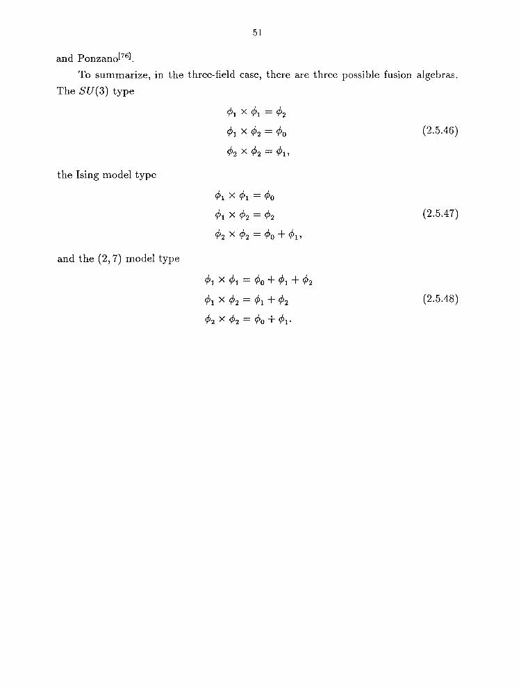
51

and Ponzano[76].

To summarize, in the three-field case, there are three possible fusion algebras.

The 5U(3) type

the Ising model type

and the (2, 7) model type

<PI X <PI = <P2

<PI X <P2 = <Po

<P2 X <P2 = <Pu

<PI X <PI = <Po

<PI X <P2 = <P2

<P2 X <P2 = <Po + <PI'

<PI X <PI = <Po + <PI + <P2

<PI X <P2 = <PI + <P2

<P2 X <P2 = <Po + <PI·

(2.5.46)

(2.5.47)

(2.5.48)

52

6. Conclusions

We used modular invariance to classify possible chiral RCFT's without assuming

any specific knowledge of the chiral algebra. We found that in the two-field case there

are only two possible fusion algebras, which account for all previously known models.

However, we also found a few possibilities that we were not able to identify. It is

possible, of course, that models do not exist for these cases for some other reasons,

but at least one of them-the partner to the (2,5) model (the Lee-Yang singularity)­

should exist. It should be an interesting exercise to identify the chiral algebra and to

construct it explicitly.

In the three-field case we obtained only three possible fusion algebras-the Ising

type algebra, the (2,7) type and the SU(3)(1) type. Again, all known models are

accounted for, but the classification still has a free parameter in the case of the Ising­

type theories. We know from analyticity arguments that for a RCFT the conformal

dimensions and the central charge must be rational and our method does not enforce

that requirement. Indeed, one can add this demand to the classification scheme, and

it seems that we must do so in order to classify RCFT's.

We conclude that modular invariance alone is not sufficient to classify rational

conformal field theories, and we need analyticity of the four-point function also. In­

deed, it has been proven by Sonoda[20) that knowledge of the four-point function on

the sphere and the one-point function on the torus is enough to reconstruct confor­

mal field theory on an arbitrary Riemann surface. This agrees with our analysis,

which demonstrated that modular invariance on the torus is not enough and we need

analyticity-four-point function-on the sphere.

However, modular invariance does seem to be sufficient to classify the fusion

algebras themselves. This was demonstrated in the two- and three-field cases above.

It may be tempting to conjecture that only algebras with fusion coefficients 1 or 0

are possible, but there are counter examples for high-level Kat-Moody algebras. For

example, for the SU(3) Lie algebra,

8 x 8 = 1 + 8 + 8 + 10 + 1-0 + 27. (2.6.1)

So, if we take the Kat-Moody algebra SU(3)(k) at high enough k, the representation

8 appears twice. That is, Nss s = 2.

53

Other methods of classification have been used to classify rational conformal field

theories. One of them is based on classifying the OPE coefficients Cijk in (2.1.20).

This method, since it does not consider modular invariance, is not strong enough.

Similarly, Christe and Ravanini[15] used the crossing relations to classify possible

fusion algebras. They restricted their classification to Ni~ :::; 1 (and we showed that

these theories do not exist in any case) and found four possible fusion algebras. In

Chapter 5 we showed that there are only three.

Other methods that do include modular invariance have been used. For example,

Mathur, Mukhi and Sen[13] and also Kiritsis[14] used modular .invariance to write

differential equations to compute the characters. This is a powerful method, but it

is too complicated to apply to the three-field case. Their solution included only the

two-field situation. Another difference is that their solution contains two characters

and not two fields. The difference being that there are three-field theories-the one

with non-trivial charge conjugation matrix-that have the same character for two of

the fields. Actually, there is even an example of a four-field theory-SO(8) level 1-

in which three of the fields have the same character*. Our method works relatively

well for the three-field case, although it will probably be hard to solve the four-field

theories. The reason for the relative ease of our method is the fact that it is purely

algebraic and we do not need to solve for the characters.

*This is a result of the triality symmetry of D 4 0

54

Part III

SOLVING (l,q) KdV GRAVITY

55

1. Introduction to 2D Gravity and QuantulTI Gravity

Einstein's field equations for gravity coupled to matter in any dimension are

(3.1.1)

where G/l1I = R/l1I - ~g/lIlR is Einstein's curvature tensor, A is a cosmological con­

stant, g/lll is the metric of space-time, K is a coupling constant, and T/l1I is the

stress-energy tensor[78j. In three dimensions the Riemann curvature tensor R/lIIPU

has

six independent components, exactly the number of components in the Ricci tensor

R/l1I = gPU R/lPllu . This leads to the well-known result that in three dimensions Ein­

steinian gravity does not have a propagating degree of freedom-or, in other words,

the vacuum solution (A = T/l1I = 0) is always locally flat.

1.1. 2D Gravity

In two dimensions the Riemann tensor has only one independent component

(and so has the Ricci tensor) that can be expressed in terms of the curvature scalar,

R = g/lll R as /lll'

(3.1.2)

so R determines completely the local geometry. This is a hint that metric gravity is

trivial in two dimensions. Moreover, the Einstein tensor G vanishes identically in two

dimensions, rendering the field equations meaningless.

Looking at the vacuum Einstein-Hilbert action (with cosmological constant) in

two dimensions

(3.1.3)

we can find the reason for this behavior. The first term is proportional to the Euler

characteristic class, which is purely topological (i.e., independent of the metric*).

Hence, extremizing (3.1.3) with respect to the metric gives, for A =1= 0, the condition

(3.1.4)

*In the classical theory, So is a constant equal to 21,. (2(1 - g) - AA), where g is the genus and A

is the area af the manifold.

56

which is unacceptable. For A = 0 there are no restrictions on the metric at all.

A modification of the equations of motion is needed. A choice that is possible

only in two dimensions is

(3.1.5)

This equation has solutions of space-time with constant curvature and no propagating

degrees of freedom. Since all two-dimensional manifolds are conform ally flat, one can

choose local coordinates in which the metric has the form

(3.1.6)

where </> is called the Liouville mode. The equation of motion (3.1.5) then becomes

(3.1.7)

This is Liouville's equation, which is completely integrable. This equation can be

obtained by varying the action

-J 2! 2 ¢ SLiouville - dx (2 (8</» - e A). (3.1.8)

1.2. Quantum 2D Gravity and Scaling

When one tries to include quantum fluctuations of the metric, the problem ap­

pears to be non-trivial. Quantizing the Liouville action, (3.1.8), is still a problem

under investigation. Following Polyakov[791, we consider the partition function

(3.1.9)

where So is given by (3.1.3) and SM(X,g) is the matter part of the theory. The

integration is carried over all metrics (and matter fields X) for a given topology and

given moduli of the manifold. To keep conformal invariance the matter fields X must

be chosen to form a conformal field theory. Polyakov suggested to study this action

in the conformal gauge, that is, to choose local coordinates in which the metric takes

the form

(3.1.10)

where g(O) is a background metric that depends, generically, on a finite number of

moduli that represent the conformally inequivalent geometries of a given topology.

57

This is a generalization of (3.1.6). This partition function, for A = 0, is invariant

classically under the conformal transformation (of the conformal mode tP)

(3.1.11 )

but, because of the conformal anomaly, this invariance is violated at the quantum

level. To find the effective action for the Liouville mode, Polyakov integrated out the

matter fields and the ghost fields that are introduced by the gauge fixing (3.1.10).

This gives

r[g] = -9~?r J d2(J"~ J d2(J"'Jlg(J"')IR(J") (_l~)~a: R(J"')

+AR J d2(J"~+ ... , (3.1.12)

where c is the central charge (= Cmatter - 26), (i)' is the propagator (without zero

modes of the Laplacian, ~), AR is a shifted cosmological constant (renormalized by

some UV regulator), and the ' ... ' represents the moduli dependent part. (If we

substitute g1?J = 'TJ/1-V' we will recover (3.1.8).)

The semi-classical regime corresponds to c -+ -00 since in this limit the kinetic

term of the Liouville action is positive. However, for a positive effective cosmological

constant (AR > 0) the vacuum is anti de Sitter (R < 0). It is in the regime c -+ 00,

that the vacuum is a de Sitter space for positive effective cosmological constant. In

this regime the kinetic term is negative. This instability of the vacuum is very similar

to the instability in the Einstein theory in four dimensions (or more precisely, 3 + 1

dimensions) .

The full quantum treatment of the Liouville action includes the quantization of

the Liouville field itself, together with the matter fields and the ghost sector. This is a

hard problem for AR > 0, since the Liouville theory is interacting in this region (even

though it's integrable). This aspect has been pursued mainly by Gervais, Neveu and

their collaborators[SO-s21. We shall not describe this work here.

Knizhnik, Polyakov and Zamolodchikov[341, Distler and Kawai[351 and David[361

showed the following. Consider the fixed area partition function

ZA,g = J D[g, A] J D[X]e-S[g,Xl, (3.1.13)

where D[g, A] means integration over all topologically different metrics on a surface

of genus 9 with fixed area A, and X are matter fields. The total partition function is

58

(aside from possible nonperturbative effects)

z= ~ ,\2g jdAe-AA Z ~ A,g' g=O

(3.1.14)

where we sum over each different genus weighted by the string coupling constant '\,

and A is the cosmological constant. It was shown that in the large area (or small

coupling constant) limit,

(3.1.15)

where cg is some constant, Ac is a critical cosmological constant, and the critical index

,(9) depends linearly on the genus

1-9 ,(9) = 2 + 2' '0 - (3.1.16)

where '0 is a constant depending on the matter content of the theory. Inserting this

into (3.1.14) gives, in the same limit,

(3.1.17)

We see that up to an overall factor, the partition function Z depends only on the

combination ,\2 j(Ac - A)2-")'0. That is, there is a scaling relation in the partition

function, i.e., Z(A,'\) can be written as a function of one variable.

This scaling behavior also shows up in the discrete version of quantum gravity

that will be discussed in the next chapter. This scaling behavior allows one to take

the 'double scaling' limit, which is defined by

Ac - A ---+ 0 and (3.1.18)

while keeping ,\2 j(Ac - A)2-")'0 fixed. Since'\ is the bare string coupling constant, the

limit ,\2 ---+ 0 is a 'weak' coupling limit allowing an exact evaluation of the partition

function. On the other hand, the effective coupling, ,\2 j (Ac - A )2-")'0, is kept fixed,

and, hence, no information about the partition function is lost in this limit. This is

the trick that allows the matrix model to be analyzed exactly and, thus, one derives

non-perturbative results. (At least those that follow from assuming that (3.1.14) is

exact.)

59

2. The Matrix Models

2.1. Discrete 2D Gravity and Matrix Models

In the discretized version of Euclidean 2D gravity we consider a discretized ver­

sion of the partition function (3.1.14). Assume that we triangulate a closed Riemann

surface with nF triangles. One can compute the Euler characteristic X or the genus

g by Euler's theorem

nF - ny + nE = X = 2(1 - g), (3.2.1)

where nF' nE and ny are the numbers of faces, edges and vertices, respectively.

Actually, in general one can discretize the surface with arbitrary n-gons rather than

just triangles and (3.2.1) will still hold.

Given a surface discretized with n-gons, one associates an area a; to each triangle

and a; (n - 2) to each n-gon (thinking of an n-gon as composed of n - 2 triangles and

assuming that all edges have the same length). The total area is then

2~ i-2 A=a ~nFi-2-'

•

where np' is the number of i-gons*. The discrete version of (3.1.14) is then •

discretizations

(3.2.2)

(3.2.3)

where S is the part of the action that depends on the matter content and possible

weight factors for different n-gons.

The basic trick to solve the random discrete model is to realize that the dual

graph to a triangulated surface is a Feynman diagram of a </>3 scalar field theory. In

a general discretization into different polygons there are higher order vertices with

a </>n interaction term corresponding to each n-gon. One thing, however, which is

still needed is another parameter (besides Planck's constant) that will control the

60

topology-the genus. The way to do it is to look at an N X N hermitian matrix as

the field instead of a single scalar field. N will be that extra parameter.

The partition function for the one-matrix model reads

Z . = J d["'] e-f3Tr U(,p) matrtx 'P , (3.2.4)

where M

U( <fJ) = ~<fJ2 + L un<fJn n=3

(3.2.5)

and f3 = k. <fJ is now an N X N hermitian matrix and we choose the flat measure

d[<fJ) = IT d<fJii IT d[R(<fJij))d[8'(<fJij))' (3.2.6) i<j

1

When one rescales the matrix field <fJ --+ ~ = (~) 2" <fJ, one gets

M n-2

f3U(<fJ) = ~ ~2 + ~ unN (~) 2 ~n

= N OJ' + t,finJn) (3.2.7)

= N(j(~).

One can compute the propagator on the sphere

(3.2.8)

and then read off the coefficients that go into the perturbation expansion. Each

propagator contributes i" a closed index loop yields a factor of N (tracing (3.2.8)) n-2

and each ~n vertex gives N (~) -2- Un = NUn' One can now compute Zmatrix using

dual description of the discretized Riemann surface. For the matrix model, for a given

Feynman diagram, we have nv loops, n E propagators, and n F. vertices of type ~i . . Thus we get

" ;-2

(N)L...J; -2 nF;

Zmatrix rv L NnV-nE+nF f3 W(U), graphs

(3.2.9)

where M

W(U) = IT U~F;. (3.2.10) i=3

61

Comparing (3.2.9) with (3.2.3), one identifies the bare string coupling constant

A with Jv and ~ with e(Ac- A )a2

• We now wish to take the continuum limit, but before

we can do that we need to explain the method of orthogonal polynomials[24,83j.

2.2. The Method of Orthogonal Polynomials and the String Equation

Let us first note that Tr f)(~) in the partition function (3.2.4) (using (3.2.7)) is

invariant under unitary transformations-that is, under matrices in U(N). We can

use this invariance to change variables and integrate out the irrelevant 'phases.' To

be more specific, let ~ = OAOt where oot = 1 and

A= (3.2.11)

Integrating out the 0 dependence in the partition function gives the result

N

Z . = J II dA· ~(A)2e-NL;:1 0(.\;) matrtx t ,

i=1

(3.2.12)

where ~(A) is the Vandermonde determinant

~(A) = II (\ - AJ. (3.2.13) i<j

We introduce now the 'monic' polynomials

(3.2.14)

which are orthogonal with respect to the measure df.1(A) = e-NO('\)dA. That is,

(3.2.15)

where Sn are (clearly) positive numbers to be determined. We can now compute the

partition function (3.2.12) by noting that

1 Al AN- 1 1 7l"O(Al) 7l"1(A1) 7l"N_l(A1)

1 A2 AN- 1 7l"o(A2) 7l" 1 (A2) 7l"N_l (A2) ~(A) =

2 (3.2.16)

1 AN AN- 1 N 7l"o(AN) 7l"1(AN) 7l"N_1(AN)

62

This can be shown by standard manipulations of the determinant det(7fj_l (\)). Plug­

ging this into (3.2.12) one gets

N-l

Zmatrix = N! II Si· i=O

(3.2.17)

To compute the Sn's, one uses recursion relations, which are obtained by considering

how multiplication and differentiation by A act on the polynomials 7f n. Let

(3.2.18a) m=O

(3.2.18b)

By inspection, one sees that bnm = 0 for m ~ n + 2 and that anm = 0 for m ~ n.

Also A7fn = An+1 + ... means that bn ,n+1 = 1 and :>. 7fn = nAn

-1 + ... shows that

an,n-l = n.

Next use the orthogonality relation (3.2.15) on (3.2.18a),

and get, from the symmetry, that bnm = 0 for 1m - nl > 1 and

We also denote bn n = bn • ,

b - b Sn n,n-l = n = S·

n-l

(3.2.19)

(3.2.20)

We can now write Zmatrix in terms of the bn (and So). For convenience, we write

the free energy

N-l

F = -lnZ = -In(N!Sr/) - I)N - n)lnbn . (3.2.21 ) n=l

From (3.2.18b) and (3.2.19) we derive

and hence

(3.2.23)

63

where B is the matrix whose elements are bmn . Substituting m = n in (3.2.23) we get

(U'(B)) = 0, n,n

(3.2.24)

and substituting m = n - 1 we get

( -') n U(B) =N' n,n-l

(3.2.25)

Equations (3.2.24) and (3.2.25) are, in fact, recursion relations that determine Sn' bn and bn in terms of the initial conditions.

As a simple example, consider the potential Up..) = >'22 + a>';. Then one gets the

recursion relations

(3.2.26)

and

(3.2.27)

Another simple example is the potential Up..) = ~ (>.; - >'44). In this case one

can argue that because U(.\) is even, the polynomials 71"(.\) must be even or odd.

Thus, bn = 0, and we need only the one recursion relation

(3.2.28)

The large N limit is obtained as follows. We assume that bn (and bn in general)

becomes a smooth function of the continuous parameter x = ~. In the limit one can

easily get from (3.2.28)

gx = V(b) = b(x) - 3b(x)2, (3.2.29)

and from (3.2.21) the free energy

F = -N211 (1 - x) In(b(x)) dx, (3.2.30)

where we have dropped terms that are subleading in powers of iv. This free energy has a critical point. That is, it is ill defined when b(x) becomes

negative (or zero). This point can be found by solving V'(b) = ° at x = 1. One gets

1 1 9 = V(b ) = - and b = -.

C C 12 c 6 (3.2.31 )

64

The double scaling limit is then obtained as follows. Consider g close to gc and n

close to N in such a way that

t = Nt (gc - g) and x = Nt (1 - ~) gc N (3.2.32)

are fixed when we let N -+ <Xl. bn scales as

(3.2.33)

and (3.2.28) becomes, after substituting (3.2.33) and (3.2.32) and using the criticality

values,

(3.2.34)

This is the celebrated 'string equation.'

The free energy (3.2.21) has divergent parts proportional to N 2 +N and N -+ 00.

However, its finite part is

F(t) = fp 1= xu(x, t) dx, (3.2.35)

where ~fp' stands for 'finite part.' One can show that u(O, t) is the 'specific heat'-that

IS,

fJ2F u(O, t) = - 8t2 • (3.2.36)

An interesting thing to note is that the string equation is the first equation

(integrated) of the KdV hierarchy. We will show this in greater detail in the next

section, since this rich structure is the main point of our computation.

A few remarks are in place here. The string equation (3.2.34) is relatively simple.

Other interaction potentials give higher-order differential equations and, as we will

see later, they are also equations in the KdV hierarchy.

The second point concerns the so-called multi-matrix models. We could general­

ize the matrix model partition function (3.2.4) by considering q -1 hermitian matrices

and the partition function q-l

Z . = J II dlv[.e-N(Ef~: C j M j M j+1 + Ei~: Vj(Mj )) mult, , ,

i=1

(3.2.37)

where C i are some constants, Aii are the matrices and Vi(x) are some potentials.

These models have been conjectured to give as string equations, equations from the

q-th generalized KdV hierarchy [321. Evidence has been brought to justify that claim

and, indeed, from the topological approach to quantum gravity it seems to be true[841.

More on this later.

65

3. KdV Hierarchy and KdV Gravity

In this section we will present the KdV approach to two-dimensional quantum

gravity[32,85,86]. But first, we introduce the KdV hierarchy[33] itself.

3.1. The Generalized KdV Hierarchy

We will describe the generalized KdV hierarchy in the so-called Lax form, as it

is the most useful for our purposes. This form is based on the algebra of pseudodif­

ferentialoperators. A pseudodifferential operator, 0, is the formal sum

00

0= Laj(x)Dn- i , (3.3.1) i=O

where aj(x) are formal power series (or analytic functions), n is some integer, and

D = :x. In order to multiply these operators we need to know how D-1 operates. We

get this by demanding that DD-1f(x) = f(x). One can show that the generalized

Liebniz rule is

D-nf(x) = ~(_1)i(~+i-1)!f(i)D-n-i; n > 0, ~ z!(m -I)! t=O

(3.3.2)

and

(3.3.3)

In the above, D±n is an operator that continues to operate through other operators.

That is, Df(x) = J'(x) + f(x)D, and, thus, D±n f· 9 = D±n(Jg).

We define the order of the pseudo differential operator, 0, to be

ord(O) = n, (3.3.4)

the order of the highest derivative.

Given a differential operator of the form *

(3.3.5)

*The generalization to pseudodifferential operators is straightforward.

66

we can define the q-th root in the following way. We formally write

(3.3.6)

We can recursively get all the unknown functions ai(x) as polynomials in the Ui(X) 1

and their derivatives by demanding that (Qq-)q = Q. The fact that we do not have a

term in Q that is proportional to Dq-l is the reason that this root is unique.

The q-th generalized KdV hierarchy is defined in the following way. First, assume

that in addition to the variable x, the functions Ui(x) in Q (of equation (3.3.5)) are

also functions of an infinite number of 'time' variables ti' i = 1,2, ..... We then define

the flow of the operator Q (in the space of operators) by the following set of partial

differential equations

~~ = [ ( Q i ) ~ , Q] , (3.3.7)

where 0+ is the differential part of 0 (i.e., dropping all negative derivatives). This

truncation operation is performed after raising to powers unless specifically written

otherwise (i.e., O~ = (Oi)+ unless written as (O+)i). As an example, consider the simplest non-trivial Q possible, Q = D2 + u(x, t).

Then

Qt = D + u(x, t) D-l _ u'(x, t) D-2 + ... 2 4

(3.3.8)

is its square root. The i = 1 equation in (3.3.7) is then

8u(x,t) [ 2 ( )] '( ) 8 = D,D +ux,t =u x,t, tl

(3.3.9)

where the prime will denote (from now on) differentiation with respect to x. We see

that u(x, tll t2, . .. ) depends only on x + tl and the other t's and, hence, we can, if we

want, shift tl (or x) to remove one variable from the equations. It is easy to see that

this is always the case for the first equation of the generalized KdV hierarchy. This 1

is obvious because Q+ - D for any q.

The second equation, and actually any equation for which i is even (when q = 2),

is trivial. This can be easily seen by

( Q t ) ~ = Q~ = Qj, (3.3.10)

and, hence, since [Qj, QJ = 0, we get

(3.3.11)

67

This means that the even flows are trivial. This, again, can be generalized to any q.

In this case, all the equations of order j, where j is a multiple of q, are trivial.

The third equation in the q = 2 hierarchy is

fJu [3 3 3u' 2 ] 3 I 1 11/ - = D + -uD - - D +u = -2 uU + -4u . fJt3 2 4 '

(3.3.12)

This is the original Korteweg-de Vries equation that gives its name to the entire

hierarchy. The higher have higher orders and higher non-linearities. In the generalized

KdV hierarchy the situation is similar. The only difference being the fact that the

equations involve q - 1 unknown functions.

Next, we quote a few facts about the KdV hierarchy. The first and most im­

portant is that this system of differential equations is integrable[871. A system of

differential equations is integrable when there is the same number of degrees of free­

dom as integrals (i. e., constants) of motion. If the system is finite the problem (of

proving that a system is integrable) is not very hard. However, for an infinite system

(like the KdV hierarchy) this is not easy to prove. In physics terms, the idea is to

find a canonical transformation that transforms the theory to a free one (as has been

done with the sine-Gordon equation[331). For the KdV hierarchy this has been proved,

but the proof will not be presented here. However, one of the consequences is that

the flows commute. That is the basic reason why we wrote the KdV hierarchy in the

form (3.3.7).

Another fact is the following. If a differential operator 0 commutes with Q, then

the flow of this operator is given by the equations

(3.3.13)

To prove this one differentiates [0, QJ with respect to ti and then makes use of the

KdV hierarchy to substitute fJQ / fJt i with a commutator. Next, the Jacobi identity is

used to move 0 around. Then, using [Q, OJ = 0, one gets

(3.3.14)

One can then show that this commutator vanishes only if equation (3.3.13) is satis­

fied[881.

We will end this subsection with some notations and definitions. Given a pseu­

dodifferential operator 0, as in (3.3.1), we define Res 0 as the coefficient of D-t,

68

Res 0 = at. (3.3.15)

The order of the operator ord 0 has been defined in (3.3.4) to be n.

If the coefficient of the highest derivative is 1 t, then we can define scaling dimen­

sions for the operator 0 and the coefficient functions ai( x)t,

dimO = ordO = n

dimD = 1

(3.3.16a)

(3.3.16b)

(3.3.16c)

where nand ai(x) refer to the symbols used in (3.3.1). The idea is that under the

rescaling D --t )"D and ai(x) --t )..iai(x) then 0 --t )..nOi. That means, especially,

that each term in 0 transforms in the same way. That will be very useful later.

3.2. From Matrix Models to KdV

Returning to quantum gravity, we will show in this subsection how the KdV

hierarchy arises. We start with the partition function for the matrix models (3.2.12),

and assume, for convenience, that the potential U()") is an even of order function 2m.

We then define orthonormal functions[89]

(3.3.17)

which generate an abstract Hilbert space with an inner product

(3.3.18)

We define two operators, Q and P, acting in this Hilbert space by§

(3.3.19) n

and

(3.3.20)

tao(x) = 1 in equation (3.3.1).

tNote that a/ox does not necessarily transform as x-l. One should treat D and x as independent

when dealing with scaling dimensions.

§These are like 'position' and 'momentum' operators.

69

These matrices satisfy

Q = Qt and P = -pi, (3.3.21 )

as well as the commutation relation

[P, Q] = 1. (3.3.22)

It can also be shown that

Qpq = 0 if 1p - q1 > 1 (3.3.23)

and

Ppq = 0 if Ip - q I > 2m - 1. (3.3.24)

For the m = 2 model in the scaling limit, n/N becomes a continuous variable x

and (3.3.23) and (3.3.24) imply that P and Q become differential operators of orders

3 and 2, respectively. In fact, their explicit form is

Q = D2 - u(x), (3.3.25)

and

P = 4D3 - 4u(x)D - 3u'(x), (3.3.26)

where D = a/ax as defined before, and u(x) is the 'specific heat,' (3.2.36). The

commutator, (3.3.22), implies an extra constraint on u(x),

u lll

[P,Q] = 2uu' - 3 = 1. (3.3.27)

This is the string equation (3.2.34) differentiated once. On the other hand, one

recognizes [P, Q] as the right-hand side of the third flow in the q = 2 generalized KdV

hierarchy (see, (3.3.7) and (3.3.12)), up to a change of sign of u and multiplication

by a constant.

This remarkable connection holds also for larger m. In general, (3.3.23) and

(3.3.24) imply that Q and P are differential operators of orders 2 and 2m - 1 (at

most). Hence, P can be identified as (Qt) :m-l, and the string equation is the

constraint of the canonical commutation. More precisely, we should identify P with

a linear combination of operators

~ ( 1)2i-l P = ~ti Q2 i=l +

(3.3.28)

70

Setting the coefficients ti to specific values picks out a critical point of the theory.

In the multi-matrix models, (3.2.37)' the operators P and Q are differential

operators of orders q and p, where q - 1 is the number of matrices in the model and

p is the order of the potential used. It has been conjectured (and shown for q = 3

and p = 4[86]) that Q and P are operators in the generalized KdV hierarchy. Q is the

basic operator and P is a combination as in equation (3.3.28), except that ~ should

be replaced by 1. q

In fact, the connection to the KdV hierarchy is even stronger. From the topologi-

cal approach to quantum gravity, one identifies u( x) (or uq_ 2 for multi-matrix models)

as the two-point correlation function of the so-called puncture operator, P. This is

because the puncture operator arises from differentiation of the partition function

with respect to x, which is identified with the cosmological constant in the contin­

uum limit. This identification will be extended in the next section to a map between

all the fields in the matrix models (or in the topological approach) and operators in

the KdV hierarchy.

3.3. KdV Gravity

In this subsection we will define quantum gravity models in terms of the gener­

alized KdV hierarchy and present a method to compute correlation functions, which,

in some sense, solves the theory.

We start with a qth order differential operator Q,

(3.3.29)

with q - 1 (as yet) unknown functions. We also construct the various powers of the

q-th root of Q, . 00

Qi/q - (Q~)' = Di + 2:: vY) Di-j, (3.3.30) j=2

where the V)i} are functionals of the u i III (3.3.29) and their derivatives. We then

define P as the sum p

P = 2:: ti (Qi/q) + . (3.3.31 ) i=1

This is a p-th order differential operator.

Next, we write the string equation

[P, QJ = 1. (3.3.32)

71

This is a system of differential equations that determines the functions ui( x) (up to

constants of integration). In a sense, this equation (or, actually the choice of P)

determines which critical point we must choose-or which model we are defining. We

define the (p, q )-model as the model for which P is the single operator

(3.3.33)

(Later we will explicitly solve the (1, q)-models and prove some interesting selection

rules for them.)

To continue, we now give the map between fields in the theory and operators in

the KdV-hierarchy. For each 'primary field' or matrix PO! in the original matrix model

there is a corresponding pseudodifferential operator QO!/q in the KdV hierarchy[84.85]

(3.3.34)

The 'descendant' fields Pi correspond to pseudodifferential operators as follows

P _ P = (P) t-+ Qm+O!/q i - O!+mq - am O! i > q. (3.3.35)

It should be noted that the fields come in natural groupings of q - 1 fields. This is

because P qm is mapped to a differential operator, Qm, and, as we will see shortly,

it does not contribute to correlation functions because of the trivial way in which it

flows under the KdV hierarchy. We also note that, by the mapping (3.3.35), we can

associate

(3.3.36)

where' ord ' is defined in (3.3.4).

The correlation functions in these (KdV gravity) models are determined as fol­

lows. We identify the function of lowest scaling dimension (defined in equation

(3.3.16c)), U q_ 2 , with the two-point function of lowest dimension primary fields. The I

lowest dimension primary, P ll called the puncture operator, is mapped to Qq. The

identification of u q _ 2 with the specific heat is correct up to a proportionality constant.

Choosing this constant to be q** we can write

(3.3.37)

The higher point correlation functions are determined by the flows of the KdV hierar­

chy. Each operator has a flow parameter, t i , and differentiating a correlation function

**One can rescale the fields to get rid of this proportionality constant.

72

with respect to this parameter is equivalent to the insertion of the corresponding

operator in the correlation function. Using the flows of the KdV hierarchy, (3.3.7),

we have a prescription to compute the higher point functions. To compute correla­

tion functions with less than two punctures one has to integrate with respect to the

cosmological constant. There is some ambiguity as to the nature of the constants

of integration. We will return to this ambiguity when we discuss the computation

in greater detail in Chapter 5. For the time being, we will only consider correlation

functions with at least two punctures.

One last remark about the correlation functions. Suppose that we had an action

for our models. Then we might imagine adding, as a perturbation to the action, all

the fields in the theory with coefficients t i . Differentiating the partition function with

respect to one of these parameters is equivalent to inserting the corresponding oper­

ator (field) into the partition function-making it a one point correlation function.

Taking more derivatives brings down more fields. In the end, we should set all the pa­

rameters to zero to obtain the correlation functions. The idea in KdV gravity is that

the extra information carried by these derivatives corresponds to flows of the KdV

hierarchy whose solution, therefore, constitutes a solution to the original problem.

73

4. The Structure of (l,q) Models

In this section we will explain the structure of (1, q) models-their advantage be­

ing that one can explicitly write the operators and compute the exact non-perturbative

correlation functions. In general (p, q) models, the solution depends on the exact so­

lution of the string equation, and this equation usually cannot be solved analytically.

For example, Di Francesco and Kutasov[85] have computed some correlation functions

of the (q+ 1, q) models, but their calculation is only complete to the first order in the

genus expansion (i. e., for the sphere).

4.1. Q, P, and Other Operators

The (1, q) models are defined by the identification

1 P - Qq - D - + - .

The string equation is then given by

[P, Q] = [D, Q] = 1,

which implies (see (3.3.5))

(3.4.1)

(3.4.2)

(3.4.3)

The integration constants are set to zero in order to have well-defined scaling di­

mensions. This is required for the following reason. The functions U i have scaling

dimensions (compare (3.3.1), (3.3.5), and (3.3.16c))

dimui(x) = q - i, i = 0,1, ... ,q - 2. (3.4.4)

If Ui(X) = Ci for i f= 0 where Ci are constants, then, clearly, (3.4.4) requires setting

these constants to zero. Similarly, in the above, x = U o has scaling dimension q.

Thus, the derivative of x, a constant, must have a scaling dimension of q + 1 *, but

this is inconsistent with the scaling behavior the constants of integration would have

*N ote that x and a/ax are scaled differently as mentioned before.

74

III (3.4.4). Thus, the constants of integration must all be set to zero. This is also

consistent with the topological field theory interpretation of these models.

Equation (3.4.4) implies that the (1, q) models are defined by the Q-operator,

Q = Dq + x. (3.4.5)

These models exhibit some interesting structure due to the simple form of Q. Since

U o = x, with dimuo = q, is the only building block (apart from derivatives), the

operators in the theory have a form that we will call p-typet .

Definition: P-Type Operator

A pseudodifferential operator, 0,

00

0= '2:0i(x)D-i+n (3.4.6) i=O

is a p-type operator of index q if, for some positive integer q, 0i(x) are poly­

nomials in x of the form

{

oi xk + oi x k-(q+1) + ... + oixk-l(q+1) + ... + oi xkmod(q+1) Oi(X)= 00 1 I [k/q+1] '

,

where the integer k is given by

k = [~] - (i mod q), q

and [x] is the greatest integer less than or equal to x.

if k ~ 0;

if k < O. (3.4.7)

(3.4.8)

For example, let Ql/q = D + 2:~1 ai( x )D-i. Then the scaling dimension of ai( x)

is i + 1. So, if (say) q = 4, a2S(x) = ax6 + f3x is the only form a 2S(x) can have.

Let us explain the basic structure that distinguishes p-type operators from other

operators. If the operator is of order n then the coefficient of Dn (the highest term) is

a constant. The next term possible is of order n - q and its coefficient is proportional

to U o = x. That is, we have a gap of q terms. The next one is of order n - q -1 and its

coefficient is a constant (equal to a derivative of U o = x). Then we have another gap,

this time of q - 1 terms, and the next order is Dn-2q, with coefficient proportional

to u5 = x2 , and so forth. The other thing to notice is that when we get to order

q( q + 1) we start getting polynomials in x as the coefficients. This is because (u~)q is

a constant of the same dimension as U6+1 = x q+1 .

tThis name was chosen because in the first formulation of this solution we denoted the q-th root

of Q by P and we found that all the powers of P had the same general form.

75

1

It is easy now to convince oneself that Q q is a p-type operator. For this reason

one can compute many terms of this q-th root, the first few being

1 x q-1 q-1 Qq = D + _D1-q - --D-q _ __ x2 D I - 2q + .... q 2q 2q2

(3.4.9)

In the Appendix we present all the terms we have computed for the more general

operator Qi/q.

If 0 1 and O 2 are p-type, then so is the product 0 1 0 2 • Hence, QOI/q are all p-type.

However, the sum 0 1 + O2 is not always of this type. Only when the orders of the

operator agree can we sum them (up to some shift modulo q +1, as will be proved

in Lemma 1 in the next section). As we will see later, we need a way to sum such

operators, but we have to do it only in commutators. For this we need a theorem

that we will present in the next section.

4.2. The Basic Theorem

In this section we prove a theorem, which we will use in Chapter 5 to derive

selection rules and correlation functions.

Theorem

Let ( 0) and oem) be p-type operators of orders I and m and same index q,

respectively. Then the commutator [0(1), oem)] is a p-type operator of index

q and order less than or equal to m + 1- (q + 1).

Before we give the proof, let us present two useful lemmas.

Lenlma 1

Let oem) and o(n) be p-type operators of index q and orders m and n. Then

the operator oem) + o(n) is a p-type operator of index q if m = n( mod q + 1).

The order of this operator is max( m, n).

Proof of Lemma 1

Without loss of generality, let n = m + l(q + 1), where I is some positive integer.

Letting (change summation index in (3.4.6))

00

001 = L (OI)Oi(X)D- i , (3.4.10) i=-a

where a = m,n, the coefficient of D-i in oem) + o(n) is (m)Oi(X) + (n)Oi(X). We can

compute the dimensions

(3.4.11)

76

and, hence,

dim (n)Oi(X) - dim (m)Oi(X) = n - m = l(q + 1) = Omod (q + 1). (3.4.12)

Thus, the polynomials agree since the powers of x that appear in both are the same

modulo q + 1. (Formally, xrum(n)o;(x)-dim(m)o;(x) = x n - m = x 1(q+1).) Obviously, the

order of the resulting operator OCt is n. QED.

Lemma 2

Let o(n) be an order n p-type operator of index q,

00

o(n) = I:0i(x)Dn- i . (3.4-13) i=O

Then the operator o(n)/ defined by

00

o(n)/ = I: o~(x)Dn-i i=O

is a p-type operator of index q and order n - q.

Proof of Lemma 2

Using (3.4.7) we get oo(x) ex:: 1 and 0i(x) = 0 for 1 ::; i < q. Thus,

00

o(n)/ = I:0~(x)Dn-i

i=O 00

i=q 00 (3.4.15)

= I: oj+q(x)Dn-j-q j=O

00

- I: OJ(x )Dn-j-q, j=O

where we changed the summation index and defined Oi(X). We see that ord o(n)/ = n - q. Next, since OJ(x) = 0J+q(x), we have from (3.4.7)

OJ(x) = (o~xk + oixk- q- 1 + ... )' = ko~xk-l + (k - q - 1)0~ x k- q- 2 + ... ,

where k is given by (3.4.8)

k = [j + q 1 - ((j + q) mod q). q

(3.4.16)

(3.4.17)

Hence,

77

k -1 = [~l- (jmodq). q

This completes the proof. In Table 6 we illustrate this Lemma.

Order n Coeff. in on Coeff. in onl Order m = n - q

n 1 0 -

n-1 0 0 -

n-2 0 0 -

-

n-q+1 0 0 -

n-q x 1 m

n-q-1 1 0 m-1

n-q-2 0 0 m-2

n - 2q + 1 0 0 m-q+1

n - 2q x 2 x m-q

n - 2q-1 x 1 m-q-1

n - 2q - 2 1 0 m-q-2

n-q(q+1) x q+1 1 , xq,O m_q2

Table 6: Differentiation maps a p-type operator of order n

into one of order m = n - q.

Proof of Theorem

The commutator [0(1), o(m)] is a sum of commutators of the form

(3.4.18)

(3.4.19)

where f(x) and g(x) are some polynomials as in the definition of p-type operators.

We can treat f(x)Da as if it's an order 1 p-type operator (of index q) and, similarly,

78

g(x)Db is order m p-type. To prove the theorem we have to show that the commutator

(3.4.19) is a p-type operator of order m + 1 - q - 1 and then, by Lemma 1, we can

sum these commutators and get the required result.

So, we decompose (3.4.19) as follows

(3.4.20)

On the right-hand side, f(x )Da-l is order 1 - 1 (p-type), and [D, g(x )Db] is order

m - q by Lemma 2. Thus, the first term on the right-hand side is a p-type operator

of order 1 - 1 + m - q = 1 + m - q - 1. The second term still appears to be of order

1 + m. We now continue, recursively, in the same decomposition as in (3.4.20), with

[f(x)Da-t,g(x)D b] D, and at each stage we get an order 1 + m - q -1 operator with

an m + lone. The last stage yields

(3.4.21 )

where we used Lemma 1 to sum the operators and ol+m-q-l is some p-type operator

of order m + 1 - q - l.

Proceeding, in the same way, with the difference being that we use g(x)Db and

operates on f(x), the end result is

(3.4.22)

where ol+m-q-l is an order m + 1 - q - 1 p-type. But, obviously,

[f(x),g(x)] = 0, (3.4.23)

and, thus, we proved the theorem.

Corollary

Let 0(1) and o(m) be p-type operators of orders land m and same index q.

Then the commutator [0£), o(m)] is a p-type operator of index q and order

less than or equal to m + 1 - (q + 1). Proof: O£) is also p-type.

79

5. Correlation Functions and Selection Rules of (l,q) Models

5.1. Selection Rules

As was mentioned in Chapter 3, for any KdV gravity model, all correlation func­

tions with two punctures are given by the KdV flows of the two-puncture correlation

function,

(3.5.1)

1

where we have denoted, for simplicity, Q'i - R (for Root). Then, one can compute

higher point functions as follows,

(3.5.2)

where the last step follows from (3.5.1). vVe now use the KdV flows (3.3.7) and get

[) -[) Res R = Res [R~, R] = Res [R, R~].

ti

We have used the fact that

(3.5.3)

(3.5.4)

where 0_ = 0 - 0+. Then we note that [O~),O~)] does not have a residue (first

non-vanishing order is at least -2), so we can change Rj in the right-hand expression

of (3.5.4) into R~. Also, [O~), O~)] does not have a residue (lowest order is at most

2) so we change R~ into Ri and then into R~. Thus, using R+ = D, we get,

(3.5.5)

To prove the last step, let Ri = L:~o T'j(x )Di-j. Thus,

00 00

(3.5.6) j=O j=O

80

To compute the two-point function (PI Pi), we integrate (3.5.5) with respect to

tl = x and, as explained earlier, choose the constant of integration to be zero, In

agreement with references [84,86]. Hence, we get

(3.5.7)

which is consistent with (3.5.1). Similarly, we get formulae for higher correlation

functions* ,

(PIPiPj ) = ~. ResRj = Res [R~, Rj] , ,

(3.5.8)

(3.5.9)

and so on. The general structure is as follows. For every new operator insertion in the

correlation function, we replace, in the residue argument, each possible operator by a

commutator of the form [R~, Rj] or [R~, Rj]+, e.g., we replace [R~, Rj] in equation

(3.5.8) by the sum in (3.5.9).

Now comes the important step. According to the basic theorem of Chapter 4,

when we compute the operator inside the residue, in each stage of the computation we

have, recursively, a commutator of a truncated p-type operator with another p-type

operator. Thus, again according to the theorem, each new flow changes the order of

the operator inside the residue by (ord 0) - (q + 1). Hence, for a general correlation

function, we have

(PIP. p. . .. p. ) = Res 0 'I '2 'n ' (3.5.10)

where 0 is a p-type operator, and we can easily compute the order of this operator.

It is (at most t) n-I

ord 0 = in - L (q + 1 - i j ), (3.5.11 ) j=1

where we choose Rin as the 'first' operator on which we begin to compute, and at

each subsequent insertion we reduce the order of the resulting operator by the amount

q + 1 - i j •

*No need for integration here, since we can use the KdV flows on equation (3.5.7).

tIt may happen, by 'accident,' that the highest order (or few highest) will disappear. The operator

is still p-type of the order given, but as a regular operator it might be of lower order.

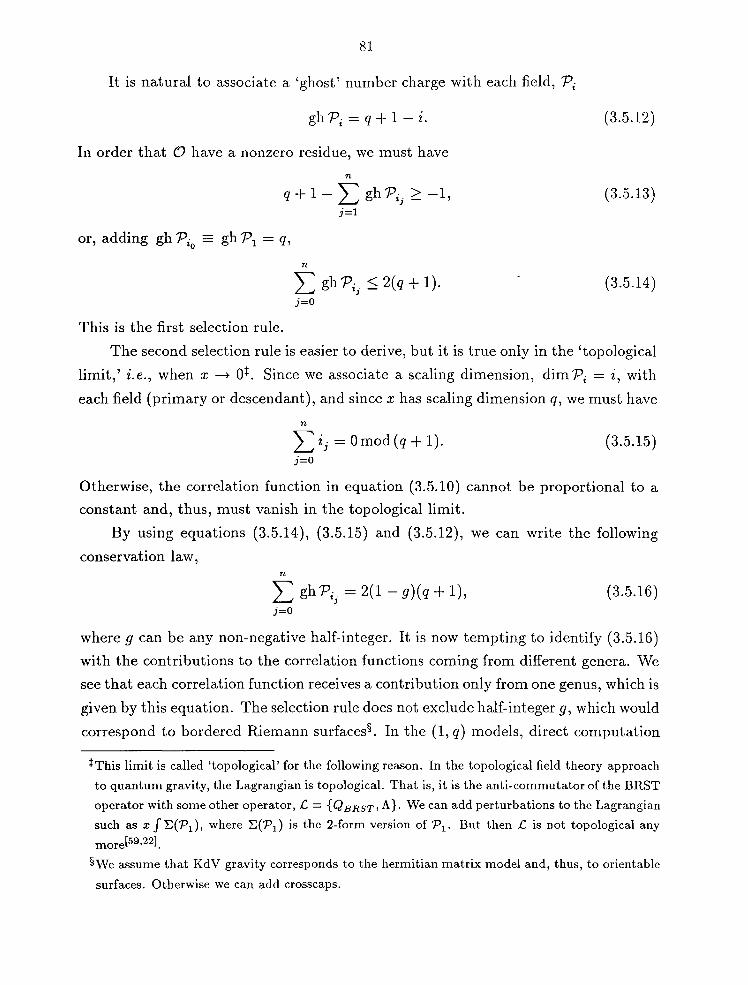
81

It is natural to associate a 'ghost' number charge with each field, Pi

gh Pi = q + 1 - i.

In order that 0 have a nonzero residue, we must have

n

q + 1- L gh Pij ~ -1, j=1

or, adding gh Pio gh PI = q,

n

L gh Pij :S 2(q + 1). j=O

This is the first selection rule.

(3.5.12)

(3.5.13)

(3.5.14)

The second selection rule is easier to derive, but it is true only in the 'topological

limit,' i.e., when x -+ 0+. Since we associate a scaling dimension, dim Pi = i, with

each field (primary or descendant), and since x has scaling dimension q, we must have

n

L i j = 0 mod (q + 1). (3.5.15) j=O

Otherwise, the correlation function in equation (3.5.10) cannot be proportional to a

constant and, thus, must vanish in the topological limit.

By using equations (3.5.14), (3.5.15) and (3.5.12), we can write the following

conservation law, n

L gh Pij = 2(1 - g)(q + 1), (3.5.16) j=O

where g can be any non-negative half-integer. It is now tempting to identify (3.5.16)

with the contributions to the correlation functions coming from different genera. We

see that each correlation function receives a contribution only from one genus, which is

given by this equation. The selection rule does not exclude half-integer g, which would

correspond to bordered Riemann surfaces§. In the (1, q) models, direct computation

+This limit is called 'topological' for the following reason. In the topological field theory approach

to quantum gravity, the Lagrangian is topological. That is, it is the anti-commutator of the BRST

operator with some other operator, .c = {Q BRST, A}. We can add perturbations to the Lagrangian

such as x f~(Pl)' where ~(Pl) is the 2-form version of Pl. But then .c is not topological any more[59,22j.

§We assume that KdV gravity corresponds to the hermitian matrix model and, thus, to orientable

surfaces. Otherwise we can add crosscaps.

82

of the correlation functions (that will be presented in the next section and in the

appendix) indicates that only integer valued genera contribute. This hints at the

existence of more symmetry.

Let us note that this conservation law, or even the slightly weaker selection rule

(3.5.14), is very restrictive. If we consider correlation functions of primary fields only,

the ghost numbers are all positive, as seen by the definition (3.5.12) and the fact

that the scaling dimension is less than q for primary fields. The limit in (3.5.14) is

therefore saturated quickly. For example, if q = 4 (say), then the only primary field

correlation functions that can be non-zero in the limit x --t 0 ~re (P;P2 ) , (PIP;),

(PI P;), (p;pn and (P~). The last two correlation functions do not contain the

puncture operator, which means that we would need to integrate a higher correlation

function (once) to compute them.

5.2. Correlation Functions

To explicitly compute some correlation functions we need an expression for Ri.

A direct computation, using R = QI/q and Q = Dq + x, leads to the following form

for Ri ** , Ri =Di + ixDi-q _ i(q - i) Di-q-I _ i(q - i) x2 D i- 2q+

q 2q 2q2

i(q - i)(2q - i) xDi- 2q-I _ i(q - i)(2q - i)(5q - 3i + 4) D i - 2q-2+ 2q2 24q2

i( q - i)(2q - i) x3 Di- 3q _ i( q - i)(2q - i)(3q - i) x2 Di- 3q-I + 6q3 4q3

(3.5.17)

i(q - i)(2q - i)(3q - i)(8q - 3i + 4) Di- 3q-2 24q3 X + ....

One can verify this formula by noting that Ri Rj = Ri+j and that Rq = Dq + x Q. Hence, we can now compute the correlation functions explicitly. We restrict ourselves

to correlation functions of primary fields only. In the Appendix we provide some

expressions for correlation functions of descendants. When computing correlation

functions with two punctures, which are well defined without integration, one sees that

they vanish for four-point and higher as a consequence of ghost number conservation.

For the one puncture correlation functions, one gets

q-1 (PI Pi) = --x8i q-I q , (3.5.18)

** In the Appendix we present the full expression, to the order we have computed, together with

some descendant correlation functions.

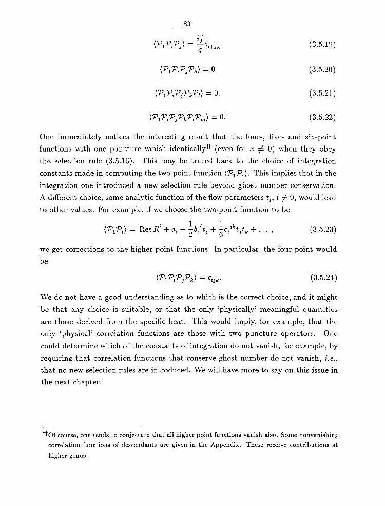
83

(3.5.19)

(3.5.20)

(3.5.21)

(3.5.22)

One immediately notices the interesting result that the four-, five- and six-point

functions with one puncture vanish identicallytt (even for x =f. 0) when they obey

the selection rule (3.5.16). This may be traced back to the choice of integration

constants made in computing the two-point function (PI Pi)' This implies that in the

integration one introduced a new selection rule beyond ghost number conservation.

A different choice, some analytic function of the flow parameters t i , i =f. 0, would lead

to other values. For example, if we choose the two-point function to be

(3.5.23)

we get corrections to the higher point functions. In particular, the four-point would

be

(3.5.24)

We do not have a good understanding as to which is the correct choice, and it might

be that any choice is suitable, or that the only 'physically' meaningful quantities

are those derived from the specific heat. This would imply, for example, that the

only 'physical' correlation functions are those with two puncture operators. One

could determine which of the constants of integration do not vanish, for example, by

requiring that correlation functions that conserve ghost number do not vanish, i.e.,

that no new selection rules are introduced. We will have more to say on this issue in

the next chapter.

ttOf course, one tends to conjecture that all higher point functions vanish also. Some nonvanishing

correlation functions of descendants are given in the Appendix. These receive contributions at

higher genus.

84

6. Sumnlary and Discussion

We have explicitly computed correlation functions of fields in the (l,q) model

of KdV gravity. As has been explained, these correspond to the critical topological

point of the KdV hierarchy. Though these models have a very simple string equation,

their solutions possess very interesting properties. We have shown how ghost number

conservation, a property of a topological field theory, arises algebraically in the (l,q)

senes. It was also easy to see how the genus expansion follows from this ghost

number conservation. Some of these properties are special to the (l,q) models. Ghost

number is not conserved at the higher critical points, since these points are reached

by perturbing with operators carrying ghost number (in the topological sense). It is

natural to suppose that solutions of the first critical theory are sufficient to derive,

by perturbation, the solutions to the higher critical point theories.

We have been somewhat conservative in our discussion of the (l,q) models. It

has been claimed, at least for the one matrix model, that the partition function may

be a special T function of the KdV hierarchy[9o,911. This T function would the Virasoro

constraints and, thus, be determined uniquely. For the multi-matrix models one has

to impose further constraints to fix T uniquely, i. e., W-algebra constraints. For the

one matrix model, the constraint L_l T = 0 can be derived by integrating the string

equation. The other constraints are determined using the KdV flows. This procedure

would then provide an unambiguous way to determine any correlation function with or

without punctures, given the T function. From KdV gravity we only have information

about the specific heat, u q _ 2 = D 2 10g T. Even the string equation is only a constraint

on the specific heat. Integrating this equation in order to derive the first Virasoro

constraint requires dropping a constant of integration, which is, in general, a function

of the t i , i f. O. Indeed, since the KdV and string equations only involve the specific

heat, the partition function is only determined up to which differ by multiplication by

a function independent of t1 . If one wishes to maintain ghost number conservation,

then it is further constrained. We have thus followed a more conservative attitude

and basically only discussed correlators derived from the specific heat and not the

partition function.

On the other hand, it might well be that the definition of KdV gravity is not

85

restricted enough. The natural extension is to impose the Virasoro constraints in the

one-matrix model or the Wn constraints in the n-l matrix models. In the one-matrix

case this indeed amounts to integrating the string equation and fixing the integration

constants to be zero.

86

Appendix A. Some Explicit Fonnulae

In this appendix we present explicit expressions for Ri (given Rq = Dq + x) to

all the orders that we have computed and for some correlation functions involving

descendants.

Ri can be written in the following compact form

00 j

Ri = L L (ij,kxj-k Di-jq-k.

j=O k=O

The coefficients are as follows:

j-l

i 1 II(' ) 0: j,O = ~ z - nq J. n=O

. > 0 J _

j

i 1 II(' ). > 1 0: j,l = 2(j _ 1)! n=O Z - nq J_

i. _ 3i - 4 - (3j - l)q IIj . _ . > 2 0: 3,2- 24(j-2)! n=o(Z nq) J_

i. _ (i - 2 - jq)(i - 2 - (j - l)q) IIj . _ . > 3 0: 3,3 - 48(j _ 3)! n=O (z nq) J-

o:i4,4 = 57160 (-288 + 320i - 120i2 + 15i3

- 1072q + 800iq - 150i2q

4

- 1288q2 + 485iq2 - 502q3) II (i - nq) n=O

o:i 5,4 = 57160 (-288 + 320i - 120i2 + 15i

3 - 1392q + 1040iq - 195i2 q

5

- 2208q2 + 830iq2 - 1152q3) II (i - nq) n=O

o:i64 =_1_(_288 + 320i -120i2 + 15i3 -1712q + 1280iq - 240i2q , 11520

6

- 3368q2 + 1265iq2 - 2192q3) II (i - nq) n=O

(3.A.1)

(3.A.2)

(3.A.3)

(3.A.4)

(3.A.5)

(3.A.6)

(3.A.7)

(3.A.8)

87

i (i - 4 - 5q)(i - 4 - 4q)(24 -16i + 3i2 + 64q - 23iq + 38q2) rr5 (. ) a - z - nq 5,5 - 11520

n=O

(3.A.9)

i _ (i - 4 - 6q)(i - 4 - 5q)(24 - 16i + 3i2 + 80q - 29iq + 64q2) rr6 (i _ ) a 6,5 - 11520 nq

n=O (3.A.10)

ai 6,6 = 290~040 ( -69120 + 82656i - 40544i2 + 10080i3

- 1260i4 + 63i5 - 420768q+

408576iq - 151536i2q + 25200i3 q - 1575i4q - 1002976q2.+ 741384iq2

- 184884i2q2 + 15435i3 q2 - 1172904q3 + 586656iq3 - 73801i2q3

6

- 674256q4 + 171150iq4 - 152696l) rr (i - nq). n=O

(3.A.11)

The above expression has been proved to order i - 7 q - 3. The general expressions

for aijk for k = 0, 1, 2 and 3 are only a conjecture that works for the orders we

computed.

One can now use this expression for Ri to compute some correlation functions.

For convenience, we computed them in the topological limit, x ---+ 0, although one

can compute them almost as easily for a general point. The only difference is that

their form is not as elegant. In the following, 1 :::; i :::; q - 1 (primary field range)

unless something is a multiple of q ( that is, q - i + 2, say, could be a multiple of q

and then the correlation function must vanish) . Also, k ranges over all non-negative

integers such that we have at least one puncture operator, Pl.

(3.A.12)

(3.A.13)

(3.A.14)

(3.A.15)

88

( )( )k+1 k+2

(pk+2 (p.) (P .)) = k + 1 -1 II(· _ ) 1 0"1 t O"k q-t k+2 Z nq

q n=O

(3.A.16)

(3.A.17)

It should be noted that correlation functions with descendants receive contri­

butions at higher genus. The genus at which the above correlation functions are

nonvanishing can be determined by computing the ghost number and using (3.5.16).

Thus, for the correlation functions above, (3.A.12), (3.A.14) and (3.A.16) are at genus

o and (3.A.13), (3.A.15) and (3.A.17) are at genus 1. For correlations that receive

contribution at higher genus we have, for example,

(3.A.18)

at genus 2, and

5 (P10"6(PS )) = 580608

q6 (q2 - 25)( q2 - 1 )(2q + 1 )(2q + 5)(3q + 5)

(3.A.19) (4q + 5)(6q + 5)(8q2 - 13q - 13)

at genus 3.

We can prove that for a correlation function of one puncture, Pu and n descen­

dants, the contribution is always from genus higher than zero. The proof is as follows.

The sum of the ghost numbers of the fields is

n

2(1-g)(q+ 1) = q+ I)q+ 1- i j ), (3.A.20) j=l

where i j is the dimension of the j-th descendant. q is the ghost number of Pl. Since

i j ~ q + 1 (the fields are all descendants), we have

n

2(1 - g)(q + 1) = q + n - L(ij - q) :::; q + n - n = q. (3.A.21) j=l

Thus, 9 is larger than zero. Similar arguments apply to level k descendants where

the genus is larger than k.

89

REFERENCES

[1] G. Rivlis, Mod. Phys. Lett., A5 (1990) 2063.

[2] D. Montano and G. Rivlis, Solving (l,q) KdV Gravity, Caltech Preprint 68-1675,

1990, to appear in Nucl. Phys. B.

[3] A. M. Polyakov, JETP Lett., 12 (1970) 38l.

[4] A. A. Belavin, A. M. Polyakov and A. B. Zamolodchikov, Nucl. Phys., B241

(1984) 333.

[5] M. B. Green, J. H. Schwarz and E. Witten, Superstring Theory, vols. 1 and 2,

Cambridge University Press, 1987.

[6] V. G. Kat, Infinite dimensional Lie algebras, Second Edition, Cambridge Uni­

versity Press, 1985.

[7] A. Pressley and G. Segal, Loop Groups, Oxford Science Publications, Clarendon

Press, Oxford, 1986.

[8] P. Goddard and D. Olive, Int. J. Mod. Phys., Al (1989) 303.

[9] M. R. Douglas, G/H Conformal Field Theories, Ph.D. Thesis, Caltech, 1988.

[10] For reviews on CFT see:

P. Ginsparg, Applied conformal field theory, Les Houches lectures (Summer 1988),

Les Houches, Session XLIX, 1988, Fields, Strings and Critical Phenomena, ed.

by E. Brezin and J. Zinn-Justin (1990).

J. Cardy, Conformal invariance and statistical mechanics, Les Houches lectures

(Summer 1988), op.cit.

[11] M. A. Virasoro, Phys. Rev., 1 (1970) 2933.

[12] G. Moore and N. Seiberg, Nucl. Phys., B313 (1989) 16.

[13] S. D. Mathur, S. Mukhi and A. Sen, Phys. Lett., 213B (1988) 303; Nucl. Phys.,

B312 (1989) 15; Nucl. Phys., B318 (1989) 483.

[14] E. Kiritsis, Nucl. Phys., B324 (1989) 475; Nucl. Phys., B329 (1990) 59l.

[15] P. Christe and F. Ravanini, Phys. Lett., 217B (1989) 252.

[16] J. Fuchs, Nucl. Phys., B328 (1989) 585.

[17] V. G. Kat, Contravariant form for infinite-dimensional Lie algebras and super­

algebras, in: W. Beiglb6k, A. B6hm and E. Takasugi (eds.), Group Theoretical

Methods in Physics, Lecture Notes in Physics, Vol. 94, Springer-Verlag, Berlin­

New York, 1979.

[18] J. 1. Cardy, Nucl. Phys., B270 [FSI6] (1986) 186.

90

[19] V. A. Fateev and S. 1. Lykyanov, Int. J. Afod. Phys., A2 (1988) 507.

[20] H. Sonoda, Nucl. Phys., B311 (1988/89) 401; Nucl. Phys., B311 (1988/89)

417.

[21] E. Verlinde, Nucl. Phys., B300 (1988) 360.

[22] R. Dijkgraaf and E. Verlinde, Annecy Field Theory 1988:87.

[23] E. Brezin, C. Itzykson, G. Parisi and J.-B. Zuber, Comm. Math. Phys., 59

(1978) 23.

[24] D. Bessis, Comm. Math. Phys., 69 (1979) 147.

[25] V. A. Kazakov, Phys. Lett., 50B (1985) 282.

[26] F. David, Nucl. Phys., B257 [FSI4] (1985) 433.

[27] V. A. Kazakov, I. K. Kostov and A. A. Migdal, Phys. Lett., 57B (1985) 295.

[28] V. A. Kazakov A. A. Migdal, Nucl. Phys., B311 (1988/89) 17l.

[29] E. Brezin and V. A. Kazakov, Phys. Lett., 236B (1990) 144.

[30] M. R. Douglas and S. Shenker, Nucl. Phys., B335 (1990) 653.

[31] D. Gross and A. A. Migdal, Phys. Rev. Lett., 64 (1990) 127.

[32] M. R. Douglas, Phys. Lett., 238B (1990) 176.

[33] I. M. Gel'fand and 1. A. Dikii, Russ. Math. Surv. 30, 5 (1975) 77.

[34] V. G. Knizhnik, A. M. Polyakov and A. B. Zamolodchikov, Mod. Phys. Lett.,

A3 (1988) 819.

[35] J. Distler and H. Kawai, Nucl. Phys., B321 (1989) 509.

[36] F. David, Mod. Phys. Lett., A3 (1988) 165l.

[37] A. M. Polyakov, Mod. Phys. Lett., A2 (1987) 899.

[38] E. Witten, Nucl. Phys., B340 (1990) 281;

E. Verlinde and H. Verlinde, Nucl. Phys., B348 (1991) 457.

[39] V. S. Dotsenko, Nucl. Phys., B235 [FSll] (1984) 54.

[40] V. S. Dotsenko and V. A. Fateev, Nucl. Phys., B240 [FSI2] (1984) 312.

[41] V. S. Dotsenko and V. A. Fateev, Nucl. Phys., B251 [FSI3] (1985) 69l.

[42] V. A. Fateev and A. B. Zamolodchikov, JETP, 62 (1985) 215.

[43] P. Ramond, Phys. Rev.,3 (1971) 2415.

[44] A. Neveu and J. H. Schwarz, Nucl. Phys., B31 (1971) 86.

[45] D. Friedan, Z. Qiu and S. Shenker, Phys. Lett., 151B (1985) 37.

[46] M. A. Bershadsky, V. G. Knizhnik and M. G. Teitelman, Phys. Lett., 151B

(1985) 3l.

[47] M. Ademollo, L. Brink, A. D'Adda, R. D'Auria, E. Napolitano, S. Sciuto, E. Del

Guido, P. Di Vecchia, S. Ferrara, F. Gliozzi, R. Musto, R. Pettorini and

91

J. H. Schwarz, Nucl. Phys., BIll (1976) 77.

[48] M. Ademollo, L. Brink, A. D' Adda, R. D'Auria, E. Napolitano, S. Sciuto, E. Del

Guido, P. Di Vecchia, S. Ferrara, F. Gliozzi, R. Musto and R. Pettorini, Nucl.

Phys., Bl14 (1976) 297.

[49] M. Ademollo, L. Brink, A. D'Adda, R. D'Auria, E. Napolitano, S. Sciuto, E. Del

Guido, P. Di Vecchia, S. Ferrara, F. Gliozzi, R. Musto and R. Pettorini, Phys.

Lett., 62B (1976) 105.

[50] W. Boucher, D. Friedan and A. Kent, Phys. Lett., 172B (1986) 316.

[51] P. Di Vecchia, T. L. Peterson and M. Yu, Phys. Lett., 1726 (1986) 21l.

[52] A. B. Zamolodchikov and V. A. Fateev, Zh. Eksp. Theor. Fiz., 90 (1986) 1553.

[53] P. Ramond and J. H. Schwarz, Phys. Lett.,64B (1976) 75.

[54] V. G. Kat, Math. USSR /zvestija, 2 (1968) 127l.

[55] I. L. Kantor, Sov. Math. Doklady, 9 (1968) 409.

[56] R. V. Moody, J. Algebra, 10 (1968) 21l.

[57] H. Sugawara, Phys. Rev., 170 (1968) 1659.

[58] C. Sommerfield, Phys. Rev., 176 (1968) 2019.

[59] E. Witten, Comm. Math. Phys., 92 (1984) 455.

[60] V. G. Knizhnik and A. B. Zamolodchikov, Nucl. Phys., B247 (1984) 83.

[61] D. Gepner and E. Witten, Nucl. Phys., B278 (1986) 493.

[62] P. Goddard, A. Kent and D. Olive, Comm. !vIath. Phys., 103 (1986) 105.

[63] G. Moore and N. Seiberg, Comm. Math. Phys., 123 (1989) 177.

[6c1] A. B. Zamolodchikov and V. A. Fateev, Sov. Phys. JETP, 62 (1985) 215.

[65] L. Dixon, J. A. Harvey, C. Vafa and E. Witten, Nucl. Phys., B261 (1985) 678;

Nucl. Phys., B274 (1986) 285.

[66] P. Goddard and A. Schwimmer, Phys. Lett., 206B (1988) 62.

[67] D. Bernard, Nucl. Phys., B288 (1987) 628.

[68] C. Itzykson, Nucl. Phys., B5 (Proc. supl., 1988) 150.

[69] D. Altschuler, J. Lacki and P. Zaugg, Phys. Lett., 205B (1988) 28l.

[70] P. Christe and F. Ravanini, Int. J. lvfod. Phys., A4 (1989) 897.

[71] A. N. Schellekens and S. Yankielowicz, Nucl. Phys., B327 (1989) 327.

[72J A. Capelli, C. Itzykson and J.-B. Zuber, Nucl. Phys., B280 [FS18J (1987) 445.

[73] D. Gepner and Z. Qiu, Nucl. Phys., B285 [FS18] (1987) 423.

[74] J.-P. Serre, A Course in Arithmetic, Springer-Verlag, 1973.

[75] C. N. Yang and T. D. Lee, Phys. Rev., 87 (1952) 404;

T. D. Lee and C. N. Yang, Phys. Rev., 87 (1952) 410;

92

J. L. Cardy, Phys. Lett., 54B (1985) 1354.

[76] M. Caselle and G. Ponzano, Int. J. Mod. Phys., A5 (1990) 4697; Phys. Lett.,

242B (1990) 52.

[77] C. Vafa, Phys. Lett., 206B (1988) 42l.

[78] C. W. Misner, K. S. Thorne and J. A. vVheeler, Gravitation, W. H. Freeman and

Company, New York, 1973.

[79] A. M. Polyakov, Phys. Lett., 103B (1981) 207.

[80] J. L. Gervais and A. Neveu, Nucl. Phys., B199 (1982) 59; Nucl. Phys., B209

(1982) 125.

[81] J. L. Gervais and A. Neveu, Nucl. Phys., B224 (1983) 329.

[82] J. L. Gervais and A. Neveu, Nucl. Phys., B238 (1984) 125; Nucl. Phys., B238

(1984) 396.

[83] D. Bessis, C. Itzykson and J.-B. Zuber, Adv. App. Alath., (1980) 109.

[84] R. Dijkgraaf and E. Witten, Nucl. Phys., B342 (1990) 486.

[85] P. Di Francesco and D. Kutasov, Nucl. Phys., B342 (1990) 589.

[86] P. Ginsparg, M. Goulian, M. R. Plesser and J. Zinn-Justin, Nucl. Phys., B342

(1990) 539.

[87] G. Segal and G. Wilson, Pub. Math. IHES, 61 (1985) 5.

[88] G. Wilson, Math. Proc. Camb. Phil. Soc., 86 (1979) 13l.

[89] S. Chadha, G. Mahoux and M. Mehta, J. Phys., A14 (1981) 579.

[90] M. Fukuma, H. Kawai and R. Nakayama, Continuum Schwinger-Dyson equations

and universal structures in 2d quantum gravity, Tokyo preprint, UT-562.

[91] R. Dijkgraaf, E. Verlinde and H. Verlinde, Nucl. Phys., B348 (1991) 435.