Two-phase flow characteristics in multiple orifice valves

Experimental Thermal and Fluid Science 34 (2010) 1324–1333

Contents lists available at ScienceDirect

Experimental Thermal and Fluid Science

journal homepage: www.elsevier .com/locate /et fs

Two-phase flow characteristics in multiple orifice valves

Claudio Alimonti a, Gioia Falcone b,*, Oladele Bello b

a Sapienza University of Rome, Department ICMA, Via Eudossiana 18, 00184 Roma, Italyb The Harold Vance Department of Petroleum Engineering, Texas A&M University, 3116 TAMU, Richardson Building, College Station, TX 77843, United States

a r t i c l e i n f o a b s t r a c t

Article history:Received 20 October 2009Received in revised form 15 June 2010Accepted 15 June 2010

Keywords:Multiphase flow meterMultiple orifice valveVoid fractionTwo-phase frictional multipliersFrictional pressure dropTwo-phase flow correlations

0894-1777/$ - see front matter � 2010 Elsevier Inc. Adoi:10.1016/j.expthermflusci.2010.06.004

* Corresponding author. Tel.: +1 979 847 8912; faxE-mail address: [email protected] (G. Falc

This work presents an experimental investigation on the characteristics of two-phase flow throughmultiple orifice valve (MOV), including frictional pressure drop and void fraction. Experiments werecarried out using an MOV with three different sets of discs with throat thickness-diameter ratios(s/d) of 1.41, 1.66 and 2.21. Tests were run with air and water flow rates ranging between 1.0 and3.0 m3/h, respectively. The two-phase flow patterns established for the experiment were bubblyand slug. Two-phase frictional multipliers, frictional pressure drop and void fraction were analyzed.The determined two-phase multipliers were compared against existing correlations for gas–liquidflows. None of the correlations tested proved capable of predicting the experimental results. The largediscrepancy between predicted and measured values points at the role played by valve throat geom-etry and thickness-diameter ratio in the hydrodynamics of two-phase flow through MOVs. A modifi-cation to the constants in the two-phase multiplier equation used for pipe flow fitted theexperimental data. A comparison between computed frictional pressure drop, calculated with themodified two-phase multiplier equation and measured pressure drop yielded better agreement, withless than 20% error.

� 2010 Elsevier Inc. All rights reserved.

1. Introduction

Flow control devices are of major importance in the petroleum,energy, nuclear, mining, chemical, process and food industries.Multiphase flow control devices currently used by these industriesinclude mechanical valves, such as rotary, screw, butterfly andslide valves. A special type of flow control device is the choke valve.A choke valve can be classified as an angle valve, apart from thefact that the flow follows a reverse path (it is first diverted, thenit passes through a restriction). One particular type of choke valveis known as the multiple orifice valve (MOV), which is less complexand expensive when compared to other throttling devices. For thistype of valve, the flow regulation mechanism is represented by aset of two matched discs, each with one pair of circular openingsto create variable flow areas by rotating one disc relative to theother.

In the oil and gas industry, wellhead chokes are used to controlthe production from wells, avoid pressure fluctuations down-stream of the choke and prevent formation damage due to exces-sive drawdown by providing the necessary backpressure on thereservoir. There has been continued interest in the use of the MOVsin the petroleum industry as discussed by Alimonti and Falcone [6],Alimonti and Falcone [7], and Falcone et al. [15]. However,

ll rights reserved.

: +1 979 845 1307.one).

gas–liquid flow phenomena in MOVs are difficult to characterise,due to the complex geometry of the restriction and the resultingflow configuration. Special attention must therefore be paid whenselecting the best model to predict gas–liquid pressure lossesthrough MOVs for choke design. The complex flow geometry im-poses limitations on the model’s performance, requiring calibra-tion or the use of empirical correlations.

Alimonti et al. [3] and Alimonti [4] investigated gas–liquid flowcharacterisation in MOVs using both industrial and laboratoryfacilities. The industrial facility used was the large-scale multi-phase loop of the Italian National Agency for New Technologies,Energy and the Environment (ENEA), as part of a larger projecton the use of choke valves as multiphase flow meters. The labora-tory experimental programs were carried out in the facility at the‘‘Sapienza” University of Rome, where a Plexiglas replica of a WillisMOV was used. The experimental results obtained by Alimontiet al. [3] and Alimonti [4] suggested the need for further investiga-tions and developments in this area.

The objective of the present work is to: (1) investigate the influ-ence of MOVs’ throttling geometry on two-phase (air–water) flowdistribution and hydrodynamic characteristics using different setsof discs; (2) obtain values of discharge coefficient constants andtwo-phase air–water frictional pressure drop multiplier datathrough void fraction; (3) evaluate the performance of a newly im-proved model and several existing models against experimentalpressure drop and frictional multiplier data.

http://dx.doi.org/10.1016/j.expthermflusci.2010.06.004

mailto:[email protected]

http://dx.doi.org/10.1016/j.expthermflusci.2010.06.004

http://www.sciencedirect.com/science/journal/08941777

http://www.elsevier.com/locate/etfs

Nomenclature

Symbolss thickness (m)p pressure (Pa)R gas–liquid ratio (–)V mass flowrate (kg/s)CG coefficient in Gilbert correlation (–)C coefficient in power law (–)CL coefficient in Lockhart correlation (–)A area (m2)v velocity (m/s)V specific volume (m3/kg)q density (kg/m3)r area ratio (–)Dp pressure drop (Pa)D diameter full pipe (m)d diameter (m)K coefficientU2 two-phase flow pressure drop multiplier (–)x quality (–)l viscosity (Pa s)S slip ratio (–)Q flow rate (m3/s)c specific gravity (–)e void fraction or gas volume fraction (–)n exponent (–)

m exponent (–)XP Martinelli parameter (–)G total mass flux (kg/s m2)f friction factor (–)B Chisholm parameter (–)y exponent in Simpson model (–)

Subscriptsa areaw waterG gasL liquidch choked dischargeLo liquid onlytp two phasev valvec contractionvc vena contractasp single phaset throatwh well headm mixtureh homogeneouss superficial

C. Alimonti et al. / Experimental Thermal and Fluid Science 34 (2010) 1324–1333 1325

2. Theoretical background

2.1. Review of choke valve models

In the oil and gas industry, wellhead chokes are used to controlthe production from wells, avoid pressure fluctuations down-stream of the choke and prevent formation damage due to exces-sive drawdown by providing the necessary backpressure on thereservoir. Modelling choke performance allows petroleum engi-neers to optimise the field operating conditions and predict theoil and gas flow rates that can be produced by a given well. Thefirst investigation on gas–liquid two-phase flow through restric-tions was carried out by Tangren et al. [42] who showed that, whengas bubbles are added to an incompressible fluid above a criticalflow velocity, a pressure change downstream of the restriction can-not travel upstream against the flow direction.

Over the past 50 years, several models have been developed forthe interpretation of flow through choke valves. The majority of themodels is of an empirical nature and applies to critical flow. Thebest know empirical correlation for critical flow is that of Gilbert[19]. It is a correlation based on three parameters, in which the vol-umetric flow rate is linearly proportional to the upstream pressure.Other authors, such as Baxendell [10], Achong [1], Secen [37], Sin-gleton [40], Gassan et al. [18], and Osman and Dokla [31], revisitedGilbert’s correlation. In general, these models can be summarizedby:

pwh ¼CG � Rm � Q

dnch

ð1Þ

where pwh is the upstream pressure, Q is the gross liquid flow rate, Ris the gas–liquid ratio, dch is the choke size and CG, m and n areempirical constants and coefficients related to fluid properties.

It must be noted that the downstream pressure does not appearin the above correlation, as it has no influence on the flow rate un-der critical flow conditions.

Another category of choke valve correlations is that of theoret-ical models, based on the energy conservation equation applied tothe fluid passing through the choke (Ros [34], Ashford [8], Ashfordand Pierce [9], Pilehvari [33], Sachadeva [35], Surbey et al. [41], andHaugen et al. [22]). Together with the energy conservation equa-tion, another independent equation is written, to describe the gasexpansion within the multiphase mixture. The control volume isdelimited by the inlet and the throat of the restriction. The rela-tionships for mass flow rate M obtained with the theoretical mod-els are of the type:

M ¼ CAtv t

Vm;tð2Þ

where vt is the fluid flow velocity at the throat, Vm,t is the specificvolume of the mixture at the throat, C is the so-called flow coeffi-cient and At is the throat area.

From the literature it appears that, since Tangren’s formulation,the approach to theoretical modelling has not changed consider-ably. In Tangren’s model, the mixture is assumed to be homoge-neous and that the gas bubbles are small and uniformlydistributes in the continuous liquid phase. Because the mixture istaken as homogeneous, the gas and liquid are considered to betravelling at the same velocity during the polytropic expansion ofthe gas. This assumption is reasonable for cases where the volu-metric gas–liquid ratio is less than 1. If, on the other hand, theliquid represents the dispersed phase, there are pressure dropsdue to the slippage between gas and liquid.

Fortunati [16] was the first investigator to present a modelapplicable to both critical and subcritical two-phase flow throughchokes. Fortunati’s model focused on the influence of void fractionon the mixture behaviour and demonstrated how the void fractionaffects the fluid velocity, which in turn determines the critical flowconditions. The model by Ros [34] can be taken as the base for allthe modelling efforts that followed. Ashford and Pierce [9] derivedan equation to predict the critical pressure ratio. Their model isvery much in line with that by Ros. However, the energy conserva-

1326 C. Alimonti et al. / Experimental Thermal and Fluid Science 34 (2010) 1324–1333

tion equation is written in a way that neglects all irreversible en-ergy losses, included that due to the slippage between liquid andgas. The model by Ashford and Pierce assumes that the derivativeof the flow rate with respect to the downstream pressure is zero atcritical flow conditions. Pilehvari [33] studied the flow throughchoke valves under subcritical flow conditions. Sachadeva [35]noted that the pressure upstream of the valve also has an influenceon the critical flow conditions. If it increases, the gas becomes den-ser and the sonic velocity of the mixture increases. Thus, largerrates must transit through the valve for the critical flow conditionsto be achieved. This implies a higher pressure difference betweenupstream and downstream that is a lower critical ratio. With sim-ilar reasoning, if the temperature increases (leaving all otherparameters the same), the gas density decreases, causing largercritical pressure ratios. Surbey et al. [41] discussed the applicationof MOVs to both critical and subcritical flow. Additional studies onsafety relief valves, chokes and orifices are given by Chisholm [11],Wallis and Sullivan [44], Lin [26], Lewis and Davidson [25], Al-Attarand Abdul-Majeed [2], Morris [29], Osakabe and Isono [30], Len-zing et al. [24], Kendoush et al. [23], Cremers et al. [13], Guoet al. [21], Shuller et al. [38], Alimontic et al. [5], Gould [20], Saberi[36], and Perkins [32].

2.2. Single-phase flow through orifices

The characteristics of MOVs reflect the geometry of the orificeplate inside them. Thus, the flow through MOVs can be related tothe flow through orifices. There is extensive literature coveringcorrelations for two-phase flows through various types of contrac-tions, expansions and orifices. Those models are strongly related tothe geometry of the fittings and to the throat length. In single-phase flow, the contraction causes a convergence of flow lines thataccelerates the fluid, reducing the pressure and forming a vena con-tracta downstream of the contraction. When the length of the ori-fice is less than the expansion zone, the orifice is called ‘‘thin”;when the expansion zone is shorter than the length of the orifice,the orifice is called ‘‘thick”. Taking the ratio between the throatthickness and diameter (st/dt) as a reference, a thick orifice is onefor which st/dt ratio is greater than 0.5. Fig. 1 shows the flow profileacross a thin and a thick orifice.

Assuming that:

� the fluid expansion occurs irreversibly;� the fluid is incompressible,

the single-phase flow pressure drop, Dpsp through the orificecan be defined as [17]:

Dpsp ¼qv2

21

rrvc� 1

� �2

ð3Þ

where r ¼ dtD

� �2;rvc ¼ dvc

D

� �2, q is the fluid density and v is the mean

velocity.

st

dt

A Avc

D

dvc

st

dt

A Avc

D

dvc

(a)Fig. 1. Fluid flow across thin (a) and thick (b) orifices. D is the full pipe diameter, dt is tcross-sectional area of the full pipe.

For thick orifices, the energy losses are due to a double expan-sion, as shown in Fig. 1b. The overall pressure drop can thereforebe expressed as:

Dpsp ¼qv2

21

rrvc

� �2

� 1� 2r2

1rvc� 1

� �� 2

1rvc� 1

� �" #ð4Þ

2.3. Two-phase flow through orifices

To estimate the pressure drop under two-phase flow conditions,it is standard practice to apply a correction factor to the pressuredrop calculated for single-phase flow. It is possible, for instance,to adopt the same concept as the frictional pressure drop multi-plier that is used for predicting pressure losses in pipes. The two-phase flow pressure drop, Dptp is related to the actual pressure dif-ference for the liquid flow alone, DpLo via the frictional pressuredrop multiplier, U2

Lo:

Dptp ¼ DpLoU2Lo ð5Þ

A number of models have been developed to predict the frictionalpressure drop multiplier for a variety of two-phase flows and theyare reviewed as follows.

2.3.1. The homogenous model [43]The homogenous model treats the two-phase (gas–liquid) flow

assuming no slip between the phases. The pressure drop multiplieris expressed as:

U2Lo ¼

qL

qGxþ ð1� xÞ ð6Þ

where x is the gas quality. The subscripts G and L denote the gas andliquid phase, respectively, q is the phase density.

2.3.2. The Lockhart and Martinelli model (1949)This model assumes separated two-phase flow following the

Lockhart Martinelli approach [27]. The frictional pressure dropmultiplier is expressed as:

U2Lo ¼ 1þ CL

XPþ 1

X2P

ð7Þ

where the value of CL depends on the flow regime. The parameter XP

is expressed is defined as:

X2P ¼ðdp=dzÞLðdp=dzÞG

ð8Þ

where

dpdz

� �L

¼ fL2G2ð1� xÞ2

DqLð9Þ

dpdz

� �G

¼ fG2G2x2

DqGð10Þ

A

dt

Avc

D

dvc

A

dt

Avc

D

A

dt

Avc

D

dvc

(b)he throat diameter, Avc is the cross-sectional area of the vena contracta and A is the


In the above expression, f, q, x, G and D are the phase friction factor,phase density, gas quality, total mass flux and pipe diameter,respectively.

2.3.3. The Chisholm model (1983)Chisholm [12] developed the following expression for the two-

phase frictional pressure drop multiplier:

U2Lo ¼ 1þ qL

qG� 1

� �� B � x � ð1� xÞ þ x2� �

ð11Þ

where the parameter B is a function of slip ratio, S, flow area ratio, r,and contraction coefficient (which will be introduced later). For thinorifices, the value of B is 0.5, while for thick orifices it is 1.5.

2.3.4. The Morris model (1985)Morris [28] defines the pressure multiplier as:

U2Lo ¼ x � qL

qGþ S � ð1� xÞ

� �� xþ 1� x

S

� �� 1þ ðS� 1Þ2

ðqL=qGÞ0:5 � 1

!" #

ð12Þ

According to Chisholm the slip ratio S is a function of qualityand density ratio. Typically, for low quality mixtures (x < 0.005),the slip ratio could be expressed as

S ¼ qL

qh

� �0:5

¼ 1þ x � qL

qG� 1

� �� 0:5

ð13Þ

Pump

Separator

Tank

MOV

Mixer

QL

QG

ε

p pG

p

Pump

Separator

Tank

MOV

Mixer

QL

QG

ε

p pG

p

Fig. 2. Schematic of the ARIEL test rig and data acquisition system.

2.3.5. The Simpson et al. model (1983)In this model, the phase frictional pressure drop multiplier is

expressed as:

U2Lo ¼ ½1þ x � ðS� 1Þ� � ½1þ x � ðS5 � 1Þ� ð14Þ

S ¼ qL

qG

� �y

ð15Þ

where the exponent y ranges from 0 (for homogenous flow) to 0.5(for maximum slip). A value of 1/6 was proposed by Simpsonet al. [39], based on comparisons with experimental data.

2.4. Choke valve model used in this study

The most convenient method of relating flow rates to pressuredrop through valves is the valve coefficient, Kv, which is purelyempirical and varies with the type, size and opening of the valve.Kv is defined as the flow rate of water flowing through the valveper unit of pressure drop across the restriction:

Kv ¼ Qffiffiffiffiffiffic

Dp

rð16Þ

where Q is the total flow rate across the valve, c the specific gravityof the fluid relative to water, and Dp the measured pressure dropacross the valve. Valve coefficients are normally quoted based on100% choke opening, for each individual valve size.

A parameter that is commonly used in sizing orifices is the dis-charge coefficient, Cd defined as the ratio of the actual to the idealdischarge value. Cd is less than one because of irreversible energylosses due to friction and contraction effects.

Kv can be related to Cd as follows:

Q ¼ ACdCa

ffiffiffiffiffiffiffiffiffi2Dpq

s) Kv ¼ ACdCa

ffiffiffiffiffiffi2qw

sð17Þ

where A is the total flow area, q is the fluid density, qw is the waterdensity and Ca is the flow area coefficient, which is the ratiobetween actual orifice area and full-opening orifice area.

The discharge coefficient can be expressed as:

Cd ¼ Cv � Cc ð18Þ

where Cv is the coefficient of velocity, defined as the ratio of actualto ideal flow velocity, and Cc is the contraction coefficient, that is:

Cc ¼Avc

At¼ Avc

Arð19Þ

Avc is the cross-sectional area of the vena contracta, At is the cross-sectional area of the orifice throat and r is as previously defined(see Fig. 1).

For the results presented in this paper, the valve coefficient wasobtained from experimental calibration with single-phase (water)flow, using the measured pressure drop across the valve and thereference water flow rate. A pressure drop multiplier was then ap-plied to the measured single-phase pressure drop to predict thetwo-phase pressure drop. The expression used for the pressuredrop multiplier is as follows:

U2Lo ¼

Cð1� eÞn

ð20Þ

where e is the void fraction. C and the n can be obtained from exper-imental calibration.

3. Experimental set-up and testing procedure

The experimental tests described in this work were carried outin the ARIEL rig, located in the Department ICMA of the ‘‘Sapienza”University of Rome. The loop consists of a water supply system, awater reservoir, an air supply system, a 4 m long vertical Plexiglastest section with an internal diameter of 0.05 m (2-in.) and anupper degassing tank mounted at the top of the vertical tube,downstream of a Plexiglas replica of a Willis MOV. Willis chokevalves consist of an inlet section, followed by a diverting section.After the change in direction, the stream flows through two orificescreated by two regulation discs, both carrying two diametricallyaligned holes of the same size.

The regulation of the flow rate is achieved via rotation of one ofthe two discs over the other, which is fixed. This allows a change intotal orifice flow area. Downstream of the regulation disc is anexpansion section. A sketch of the experimental set-up and thedata acquisition system is given in Fig. 2.

Fig. 3 shows the replica of the Willis MOV that was used for theexperiments, together with two sets of discs.

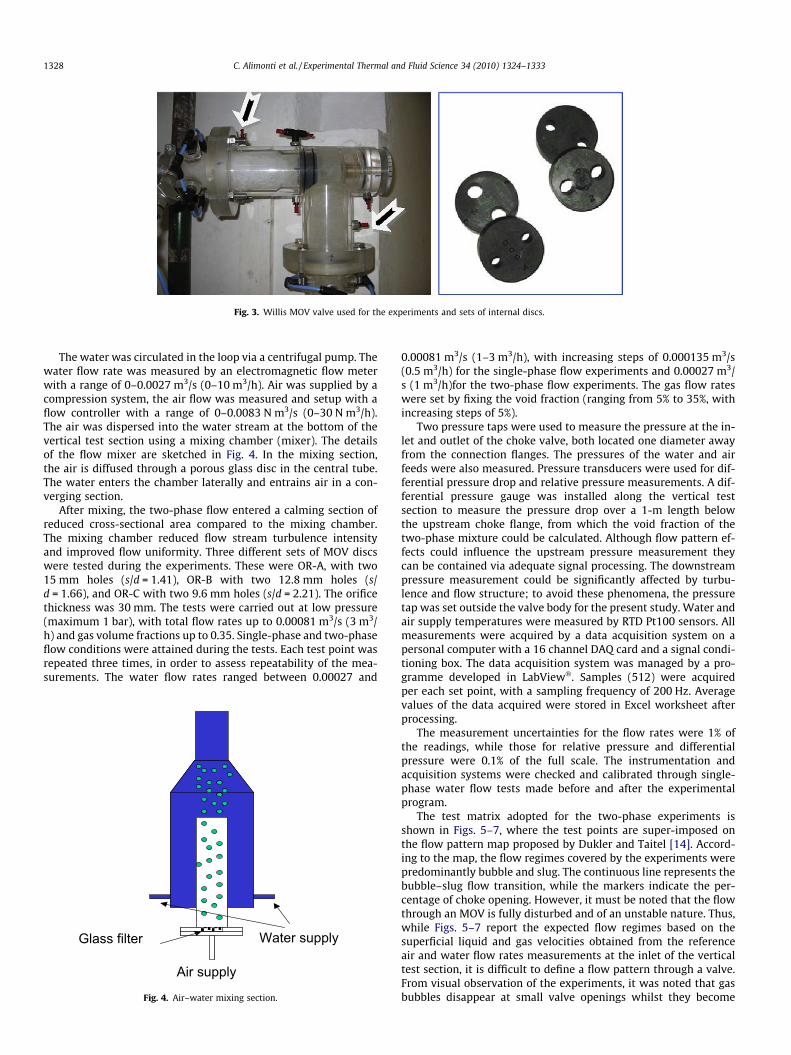
Fig. 3. Willis MOV valve used for the experiments and sets of internal discs.


The water was circulated in the loop via a centrifugal pump. Thewater flow rate was measured by an electromagnetic flow meterwith a range of 0–0.0027 m3/s (0–10 m3/h). Air was supplied by acompression system, the air flow was measured and setup with aflow controller with a range of 0–0.0083 N m3/s (0–30 N m3/h).The air was dispersed into the water stream at the bottom of thevertical test section using a mixing chamber (mixer). The detailsof the flow mixer are sketched in Fig. 4. In the mixing section,the air is diffused through a porous glass disc in the central tube.The water enters the chamber laterally and entrains air in a con-verging section.

After mixing, the two-phase flow entered a calming section ofreduced cross-sectional area compared to the mixing chamber.The mixing chamber reduced flow stream turbulence intensityand improved flow uniformity. Three different sets of MOV discswere tested during the experiments. These were OR-A, with two15 mm holes (s/d = 1.41), OR-B with two 12.8 mm holes (s/d = 1.66), and OR-C with two 9.6 mm holes (s/d = 2.21). The orificethickness was 30 mm. The tests were carried out at low pressure(maximum 1 bar), with total flow rates up to 0.00081 m3/s (3 m3/h) and gas volume fractions up to 0.35. Single-phase and two-phaseflow conditions were attained during the tests. Each test point wasrepeated three times, in order to assess repeatability of the mea-surements. The water flow rates ranged between 0.00027 and

Air supply

Water supply Glass filter

Fig. 4. Air–water mixing section.

0.00081 m3/s (1–3 m3/h), with increasing steps of 0.000135 m3/s(0.5 m3/h) for the single-phase flow experiments and 0.00027 m3/s (1 m3/h)for the two-phase flow experiments. The gas flow rateswere set by fixing the void fraction (ranging from 5% to 35%, withincreasing steps of 5%).

Two pressure taps were used to measure the pressure at the in-let and outlet of the choke valve, both located one diameter awayfrom the connection flanges. The pressures of the water and airfeeds were also measured. Pressure transducers were used for dif-ferential pressure drop and relative pressure measurements. A dif-ferential pressure gauge was installed along the vertical testsection to measure the pressure drop over a 1-m length belowthe upstream choke flange, from which the void fraction of thetwo-phase mixture could be calculated. Although flow pattern ef-fects could influence the upstream pressure measurement theycan be contained via adequate signal processing. The downstreampressure measurement could be significantly affected by turbu-lence and flow structure; to avoid these phenomena, the pressuretap was set outside the valve body for the present study. Water andair supply temperatures were measured by RTD Pt100 sensors. Allmeasurements were acquired by a data acquisition system on apersonal computer with a 16 channel DAQ card and a signal condi-tioning box. The data acquisition system was managed by a pro-gramme developed in LabView�. Samples (512) were acquiredper each set point, with a sampling frequency of 200 Hz. Averagevalues of the data acquired were stored in Excel worksheet afterprocessing.

The measurement uncertainties for the flow rates were 1% ofthe readings, while those for relative pressure and differentialpressure were 0.1% of the full scale. The instrumentation andacquisition systems were checked and calibrated through single-phase water flow tests made before and after the experimentalprogram.

The test matrix adopted for the two-phase experiments isshown in Figs. 5–7, where the test points are super-imposed onthe flow pattern map proposed by Dukler and Taitel [14]. Accord-ing to the map, the flow regimes covered by the experiments werepredominantly bubble and slug. The continuous line represents thebubble–slug flow transition, while the markers indicate the per-centage of choke opening. However, it must be noted that the flowthrough an MOV is fully disturbed and of an unstable nature. Thus,while Figs. 5–7 report the expected flow regimes based on thesuperficial liquid and gas velocities obtained from the referenceair and water flow rates measurements at the inlet of the verticaltest section, it is difficult to define a flow pattern through a valve.From visual observation of the experiments, it was noted that gasbubbles disappear at small valve openings whilst they become

0.100

1.000

0.010 0.100 1.000VsG (m/s)

v sL (m

/s)

405060708090T&D Transition

BUBBLE FLOW

SLUG FLOW

D&T transition

Fig. 5. Flow pattern map for the OR-A disc set test conditions.

0,1

1

0,01 0,1 1Vsg (m/s)

Vsl (

m/s

)


BUBBLE FLOW

SLUG FLOW

D&T transition

Fig. 6. Flow pattern map for the OR-B disc set test conditions.

0,1

1

0,01 0,1 1Vsg (m/s)

Vsl (

m/s

)


BUBBLE FLOW

SLUG FLOW

D&T transition

Fig. 7. Flow pattern map for the OR-C disc set test conditions.


0

0.2

0.4

0.6

0.8

1

1.2

0 0.2 0.4 0.6 0.8 1 1.2Valve opening

Kv /

Kv,

100

OR-AOR-BOR-C

Fig. 8. MOV calibration coefficient vs. valve opening from calibration tests.

0.5

0.55

0.6

0.65

0.7

0.75

0.8

0.85

0.9

0.95

1

0 10000 20000 30000 40000 50000 60000Re

Cd,

100

OR-AOR-BOR-C

Fig. 9. MOV discharge coefficient vs. Reynolds number for the calibration tests.


relatively large (Ø > 5 mm) when liquid velocity increases and coa-lescence occurs, resulting in Taylor bubbles.

4. Results and discussion

4.1. Single-phase flow calibration

The results of the calibration tests are shown in Fig. 8. The valvecoefficient obtained from Eq. (16) is expressed as a fraction of thefull-opening value, Kv,100. The calculated valve coefficient wastaken as constant for a given valve opening (Standard Devia-tion < 1.5%). The values of Kv,100 were 15.8 m3/h per bar for OR-A,11.7 m3/h per bar for OR-B, and 6.5 m3/h per bar for OR-C. TheKv,100 measured for the OR-A set confirmed previous experimentaltests realised under the same experimental conditions [4]. Thecurves in Fig. 8 represent polynomial regressions of the experimen-tal data.

Fig. 9 reports the results for the discharge coefficient, Cd, ex-pressed as Cd,100 versus the liquid phase Reynolds number.

0.0

1.0

2.0

3.0

4.0

0.00 0.10 0.20 0.30 0.40 0.50Void fraction

Pres

sure

dro

p m

ultip

lier

90 80 70 60 50

(a) (

Fig. 10. Pressure drop multiplier vs. void fraction. (

4.2. Two-phase flow

For the two-phase flow experiments, the modelling approachdescribed in Section 2.4 was adopted and Eq. (20) was used forthe pressure drop multiplier. The parameter n remained constantand equal to 2, independently from valve opening and flowconditions.

Fig. 10a and b illustrates the experimental results obtained forthe OR-A set at different rotation angles of the regulation disc, from100% to 45% valve opening. The continuous line represents rela-tionship (20). From Fig. 10a and b, it is possible to see that, if thecoefficient C of Eq. (20) is set to 1, the pressure drop multiplier be-comes greater than 1 when closing the valve. Thus, the coefficient Cdepends on the valve opening and the relationship between thetwo can be expressed via a power law function (Fig. 11). For theexperimental tests illustrated here, C varied from 1, for 100% open-ing, to 0.75, for 45% opening.

The comparison between pressure drop multiplier values ob-tained using relationship (20) after applying the above fit to thecoefficient C and those calculated from a larger set of experimentaldata is presented in Fig. 12. The experimental data here include the

0.00 0.10 0.20 0.30 0.40 0.500.0

1.0

2.0

3.0

4.0

Void fraction

Pres

sure

dro

p m

ultip

lier

90 80 70 60 50

b)

a) Without correction and (b) with correction.

C = 1.0032 open 0.3704

0

0.2

0.4

0.6

0.8

1

1.2

0% 20% 40% 60% 80% 100%

Open [%]

Coe

ffici

ent C

Fig. 11. Coefficient C in relationship (20) vs. valve opening.

0

1

2

3

4

5

6

7

8

0 0.1 0.2 0.3 0.4 0.5 0.6Void fraction

Two-

phas

e M

ultip

lier

HomogeneousChisholmMorrisSimpsonOurThis work

Fig. 13. Comparisons of reference models for two-phase pressure drop multiplier.

0

1

2

3

4

5

6

7

8

0 0.1 0.2 0.3 0.4 0.5 0.6Void fraction

Two-

phas

e M

ultip

lier

HomogeneousChisholmMorrisSimpsonThomOurThis work

Fig. 14. Comparisons of reference models for two-phase pressure drop multiplier.


data gathered with the present work – in circles (OR-A, OR-B andOR-C) – and also data from previous experimental campaigns - intriangles (low void fractions) and squares [4] – carried out underdifferent conditions. The dashed lines define an error band of±15% and the agreement is quite good. The trend of the coefficientC can be explained by taking into account the deflection of the flowthat takes place at the outlet of the restriction. Such deflection isdue to the geometry of the orifices created by the two superposingdiscs: the smaller the valve opening, the more diverted is the flow.

Figs. 13 and 14 compare the reference models with the mea-sured two-phase pressure drop multiplier of 300 data points usingthe three sets of discs. The markers display the results of differentvalve openings, and the line symbols show the results calculatedby the reference models. The prediction of the reference modelsfor the two-phase pressure drop multiplier shows poor agreementwith these experimental data sets. This means that using the refer-ence models for these experimental conditions provided inade-quate accuracy.

Visual observation of the flow pattern at the outlet of the valveconfirmed presence of swirling. Thus, a radial component of theflow velocity is active at the outlet, which affects the pressure

0,0

0,5

1,0

1,5

2,0

2,5

3,0

3,5

4,0

0,00 0,05 0,10 0,15 0,20 0

Void

Pres

sure

dro

p m

ultip

lier

Fig. 12. Pressure drop multiplier vs.

value. This is strictly related to the density of the fluid and as thedensity is smaller for air–liquid flows rather than for liquid flows,the pressure at the valve outlet is higher for two-phase flows.

,25 0,30 0,35 0,40 0,45 0,50

fraction

void fraction (with correction).

0

0,2

0,4

0,6

0,8

1

1,2

0 0,2 0,4 0,6 0,8 1 1,2Pressure drop measured (bar)

Pres

sure

dro

p ca

lcul

ated

(bar

)

90 80 70 60 50

-20%

+20%

0

0,05

0,1

0,15

0,2

0 0,05 0,1 0,15 0,2Pressure drop measured (bar)

Pres

sure

dro

p ca

lcul

ated

(bar

)

90 80 70 60 50

-20%

+20%

(a) (b)

Fig. 15. Measure vs. predicted frictional pressure drop using the modified two-phase flow multiplier. (a) Full range; (b) very low pressure drop (highlighted area).


Fig. 15a and b compares the estimated and measured frictionalpressure drop of the 300 data points for the MOVs with the threesets of discs. The majority of the frictional pressure drop experi-mental data are reproduced within ±20% error range with mostdata points located tightly around the parity lines. However, atlow valve openings, the errors appeared to be larger and hencean additional correction factor of 1.5 had to be applied in orderto obtain a good fit. This correction factor predicts 93% of the fric-tional pressure drop experimental data points inside the ±20%error boundary.

5. Conclusions

In this paper, the hydrodynamic characteristics of two-phase(air–water) flow through an MOV were experimentally investi-gated. Based on the results obtained from the experimental inves-tigations, the following conclusions can be made:

� The two-phase (air–water) flow pressure drop multiplier for anMOV cannot be properly represented by conventional correla-tions. A modification of the two-phase frictional multiplier isneeded to improve predictions and account for the MOV geo-metric effects.� Based on a unique experimental dataset, a new correlation was

proposed for the two-phase (gas–liquid) flow pressure dropmultiplier for an MOV. The correlation includes a modificationto the constants of the conventional two-phase multiplier usedfor pipe flow calculations.� Significant effects of geometry on the hydrodynamic character-

istics of flow through an MOV were observed. At high velocities,the gas phase is concentrated in the core vortex, leading to aseparated boundary layer of liquid flowing along the valve’swalls.� Swirling flow was observed to occur, inducing a radial distribu-

tion of the liquid axial velocity due to the influence of the MOVgeometry configuration at the downstream section. The swirl-ing flow could propagate several diameters away from theMOV outlet.

The experimental results presented in this paper enrich thecurrent knowledge and understanding of two-phase (gas–liquid)flow through MOVs. Such information can be used to optimise

the performance of existing MOV systems and to better designnew installations.

References

[1] I.B. Achong, Revised Bean and Performance Formula for Lake Maracaibo wells,Shell Internal Report, October 1961

[2] H.H. Al-Attar, G.H. Abdul-Majeed, Revised bean performance equation for eastBaghdad oil wells, SPE Production Engineering (1988) 127–131.

[3] C. Alimonti, M. Annunziato, M. Marsili, A. Mazzoni, A well testing monitoringsystem based on conventional and noise measurement on a choke valve, in:7th Int. Conf. Multiphase 95, Cannes, 7–9 June 1995.

[4] C. Alimonti, A monitoring system to control the flow through choke valve. Flowrate and flow regime predictions, in: 3rd Int. Conf. on Multiphase Flow, Leone,France, June 8–12 1998

[5] C. Alimonti, U. Bilardo, G. Falcone, Checking the Ashford–Pierce model througha field data base, in: OMC’99, Ravenna, March 19–21 1999, pp. 1245–1248.

[6] C. Alimonti, G. Falcone, Integration of multiphase flow metering, artificialneural networks and fuzzy logic in field performance monitoring, SPEProduction and Facilities (2004) 25–32.

[7] C. Alimonti, G. Falcone, Improving multiphase flow metering performanceusing artificial intelligence algorithms, in: Proceedings of the 2nd InternationalSymposium on Two-Phase Modelling and Experimentation, Pisa, Italy, 22–24September 2004

[8] F.E. Ashford, An evaluation of critical multiphase flow performance throughwellhead chokes, Journal of Petroleum Technology (1974).

[9] F.E. Ashford, P.E. Pierce, Determining multiphase pressure drops and flowcapacities in downhole safety valves, Journal of Petroleum Technology 27(1975) 1145–1152.

[10] P.B. Baxendell, Bean Performance-Lake Wells, Shell Internal Report, October1957.

[11] D. Chisholm, Flow of incompressible two-phase mixtures through sharpededged orifices, Mechanical Engineering Science 9 (1967) 72–78.

[12] D. Chisholm, Two-phase Flow in Pipelines and Heat Exchangers, GeorgeGodwin (Longman Group Ltd.) and IchemE, London, 1983.

[13] J. Cremers, L. Friedel, B. Pallaks, Validated sizing rule against chatter of reliefvalves during gas service, Journal of Loss Prevention in the Process Industries14 (2001) 261–267.

[14] A.E. Dukler, Y. Taitel, Flow pattern transitions in gas–liquid systems:measurement and modelling, in: G.F. Hewitt, J.M. Delahaye, N. Zuber (Eds.),Multiphase Science and Technology, vol. 2, Hemisphere, Washington, DC,1986, pp. 1–94.

[15] G. Falcone, C. Alimonti, G.F. Hewitt, B. Harrison, Multiphase flow metering:current trends and future developments in offshore multiphase productionoperations, SPE Reprint Series 2 (58) (2004) (Part IV, December).

[16] F. Fortunati, Two-phase flow through wellhead chokes. SPE Paper Number3472, Presented at the SPE European Meeting, Amsterdam, May 1972.

[17] M. Fossa, G. Guglielmini, Pressure drop and void fraction profiles duringhorizontal flow through thin and thick orifices, Experimental Thermal andFluid Science 26 (2002) 513–523.

[18] H. Gassan, A. Abdul-Majeed, R.A. Maha, Correlations developed to predict two-phase flow through wellhead chokes, The Journal of Canadian PetroleumTechnology 30 (1991) 47–55.

[19] W.E. Gilbert, Flowing and gas-lift well performance, API Drilling andProduction Practice (1954) 126–157.


[20] T.L. Gould, Discussion of an evaluation of critical multiphase flow performancethrough wellhead chokes, Journal of Petroleum Technology 26 (1974) 849–850.

[21] B. Guo, A.S. Al-Bemani, A. Ghalambor, Applicability of Sachdeva’s choke flowmodel in Southwest Louisiana gas condensate wells, Paper SPE 75507 Presentedat the SPE Gas Technology Symposium, Calgary, 30 April–2 May 2002.

[22] K. Haugen, P.J. Nilsen, R. Sandberg, S. Selmer-Olsen, H. Holm, Subsea chokes asmultiphase flowmeters, in: 7th Int. Conf. Multiphase 95, Cannes, 7–9 June1995.

[23] A.A. Kendoush, Z.A. Sarkis, H.B.M. Al-Muhammedawi, Thermo-hydrauliceffects of safety relief valves, Experimental Thermal and Fluid Science 19(1999) 131–139.

[24] T. Lenzing, L. Friedel, J. Cremers, M. Alhusein, Predictions of the maximum fulllift safety valve two-phase flow capacity, Journal of Loss Prevention in theProcess Industries 11 (1998) 307–321.

[25] D.A. Lewis, J.F. Davidson, Pressure drop for bubbly gas–liquid flow throughorifice plates and nozzles, Chemical Engineering Science Research and Design63 (1985) 149–156.

[26] Z.H. Lin, Two-phase flow measurements with sharp-edged orifices,International Journal of Multiphase Flow 8 (6) (1982) 683–693.

[27] R.W. Lockhart, R.C. Martinelli, Proposed correlation of data for isothermal two-phase two-component flow in pipes, Chemical Engineering Progress 45 (1949)39–48.

[28] S.D. Morris, Two-phase pressure drop across valves and orifice plates, in:European Two-Phase Conference. Paper E2, Matchwood EngineeringLaboratories, Southampton, UK, 4–7 June 1985.

[29] S.D. Morris, Liquid flow through safety valves: diameter ratio effects ondischarge coefficients, sizing and stability, Journal of Loss Prevention in theProcess Industries 9 (3) (1996) 217–224.

[30] M. Osakabe, M. Isono, Effect of valve lift and disk surface on two-phase criticalflow at hot water relief valve, International Journal of Heat and Mass Transfer39 (1996) 1617–1624.

[31] M.E. Osman, M.E. Dokla, Correlations predict gas condensate flow throughchokes, Oil and Gas Journal 90 (11) (1996) 43.

[32] T.K. Perkins, Critical and subcritical flow of multiphase mixtures throughchokes, SPE Drilling and Completion 8 (4) (1993) 271–276.

[33] A.A. Pilehvari, Experimental Study of Subcritical Two-phase Flow throughWellhead Chokes, Research Report, TUFFP, June 1981.

[34] N.C.J. Ros, An analysis of critical simultaneous gas–liquid flow through arestriction and its application to flow metering, Flow, Turbulence andCombustion 9 (I) (1960) 374–388.

[35] R. Sachadeva, Two-phase Flow through Chokes, MS Thesis, University of Tulsa,1984.

[36] M. Saberi, A Study on Flow through Wellhead Chokes and Chokes SizeSelection, MS Thesis, University of Southwestern Louisiana, Lafayette, 1996.

[37] J.A. Secen, Surface choke measurement equation improved by field testing andanalysis, Oil and Gas Journal 30 (1976) 65–68.

[38] R.B. Shuller, T. Solbakken, S. Selmer-Olsen, Evaluation of multiphase flow ratemodels for chokes under subcritical oil/water/gas flow conditions, SPE 84961,SPE Production and Facilities (2003) 170–181.

[39] H.C. Simpson, D.H. Rooney, E. Grattan, Two-phase flow through gate valvesand orifice plates, in: Proc. of Int. Conf. on the Physical Modelling ofMultiphase Flow, Coventry, England, 19–21 April 1983.

[40] E.W. Singleton, Development of a high-performance choke valve withreference to sizing for multiphase flow, Measurement and Control 24 (1991)273.

[41] D.W. Surbey, B.G. Kelkar, J.P. Brill, Study of multiphase subcritical flow throughwellhead chokes, SPEPE (1988).

[42] R.F. Tangren et al., Compressibility effects in two-phase flow, Journal ofApplied Physics 20 (1949) 637–645.

[43] G.B. Wallis, One Dimensional Two-phase Flow, McGraw-Hill, New York, 1969.[44] G.B. Wallis, D.A. Sullivan, Two-phase air–water nozzle flow, Journal of Basic

Engineering 94 (1972) 788–794.

Two-phase flow characteristics in multiple orifice valves

Documents

Transcript of Two-phase flow characteristics in multiple orifice valves