TWO-DIMEN SIO NAL INTERPRETATION OF SCHL UMBERG ER SOUNDINGS

ANO HEAD-ON DATA WI TH EXAMPLES FROM EYJAFJORDUR ICELAND,

ANO OLKARIA, KENYA

Martin N. Mwangi*

UNU Geothe rm al Training Programme,

Na tional Energy Authority,

Crensasvegur 9, 10 8 Reykjavik, Iceland.

* Permanent address:

East African Power and Ligh ting Company,

Ceothermal Section,

p.a. Box 30099, Na irobi, Kenya.

3

ABSTRACT

The theory of resistivity soundings and interpretation in

geothermal exploration over two-dimensional half-space is

discussed. The basic principles of the head - on method are

reviewed and some theoretical models presented . These

models include low and high resistivity dikes, vertical

contacts and a dipping low resistivity dike. The effect of

burying a low resistivity dike at different depths and a

structure with the uppermost layer having a vertical

contact were studied. These models are very important type

structures in geothermal fields and could help in the

exploration for permeable zones. The head-on method

detects such structures more easily than class i cal methods.

Some resistivity data from Eyjafjordur in Iceland were

interpreted in one - and two-dimensions.

valley, sediments with resistivities in the

In Eyjafjordur

range of 3 - 5

ohmm and about 175m thick occur at the bottom of the valley

and extend about 300m in the E-W direction. They are

underlain by a substratum with a resistivity of about

150 - 380 ohmm. The resistivity of the substratum is in

general lower (about 150 ohmm) east of the valley.

Head-on data from the Olkaria geothermal field, Kenya, was

successfully interpreted two-dimensionally. This was

intergreted with Schlumberger soundings and gravity data.

A thin vertical structure with a resistivity of about 1

ohmm was revealed. The structure was not evident from the

gravity data. It is possible that this structure is the

conduit for some weak fumaroles in the vicinity of the

resistivity profile. This work demonstrates that the

head-on data which could not previously be interpreted

quantitatively can be successfully interpeted by computer

modelling. An interpretation of the data south of the

present profile should facilitate the mapping of this

vertical structure. This should greatly assist in the

siting of mo r e productive boreholes in this area.

5

TABLE OF CONTENTS

ABSTRACT ... .. ...•....•. . .. . ...... . .. ..•.... . ..... • .. . •.... 3

INTRODUCTION

1.1 Scope of work .................. • .. .. .... . . .• ....•... 9

1.2 Introduction to r e sistivity interpretation.. .... .... 9

2 THEORY OF RESISTIVITY INTERPRETATION

2.1 Introduction . . .... . .... . ..................•....•.... 11

2.2 Determination of apparent r e sistivity... ... .... ..... 11

2.3 Resistivity sounding with Schlumberger array... .•... 12

2.4 Sounding over non-horizontal earth. ..... .. . .... • .. . . 13

2.4.1 Dipping contacts. . ............................ 14

2.4.2 Vertical contacts . ... ... ..•. .... .... .•... .•... 15

2.4.3 A thin vertical dike. ... . ... . .. . . ... .•.. ..•... 17

2.5 2-D Modelling of Schlumberger soundings .... ... . ..... 18

2.6 Head-on profiling...... . ............ . ...... . . . .. . ... 2 2

2.6.1 Introduction ............................ . . . ... 2 2

2.6.2 Pr ocedure and apparent resistivity equation ... 2 2

2.6.3 Head-on profiles over thin dikes . ... ... . ... . .. 24

3 TWO DIMENSIONAL SCHLUMBERGER SOUNDING INTERPRETATION

3.1 Introduction.... . ... . ..... . ..... .. .................. 26

3.2 Geological setting.. . ............................ . .. 26

3 . 3 Resistivity measurements. . .•. . . . • .... .•. . . . •.. . .•... 27

3.4 The 2-D interpretation.............................. 29

3.4.1 Initial model approximation. ... . • ... . . . . ... ... 29

3.4.2 2-D Computer modelling.. ... .... .•... .•.. ..• . .. 34

3.4.3 Results of modelling .... ... .... ... . . ... • ... ... 37

3 . 5 Discussion ...... ..... .... .... . .. • . . .. •. .. . • • . ... . . .. 39

3.6 Conclusi o ns .......... . ..... • ...............•....... . 40

4 HEAD-ON THEORETICAL MODELS

4.1 Introduction... ... . . ... .. ..•... .• .. ...• . .. .• ... .• ... 41

4.2 Conductive fractures .... . ... .... ... . .. • . ........ .... 41

4.3 Penetration depth . . . ... . . ... . ... .•...... .... .... .•. . 4 2

6

4.4 Inhomogenei ties ..................................... 42

4.5 Two conductive dikes or fractures .. .... .... .... ..... 46

4.6 Dipping structure.. ..... .... ....... .....• .. ..•...... 47

4.7 Resistive dike ..... ..... .... ... .. .. ......... .. • ..... 49

4.8 Vertical contact............ .. ...................... 50

5 INTERPR ETATION OF HE AD-ON DATA FROM OLKARIA, KENYA

5.1 Introduction........................................ 51

5.2 Local Geology ....................................... 51

5.3 Head-on and Gravity measurements . ..• ....•......... . . S3

5.4 Interpretation ...................................... 54

5.5 Discussion . ...... .•.. .. ••..........•.... • •.......... 60

5.6 Conclusions . ..... .•... .•.. .... ... .. • .......... . .. ... 61

ACKNOWLEDGEMENTS. ..•.. ..•. . ..•. .... .•. .... ..... .... .•. .... 62

REFERENCES ....•....•. .. .•...••. .... ••..........•...••..... 63

APPENDIX I

APPENDIX Il APPENDIX III APPENDIX IV

LIST OF FIGURES

65

67

69

71

2.1 Electrode array for an arbitrary geometric factor .... 12

2.2 Schlumberger array........... ..•. .................... 12

2.3 ReSistIvity sounding made with array parallel to a

dipping contact and over horizontal layers (from

Kunetz, 1966) .•......••.•• . ...•••.•..•••.•••..••..... 14

2.4 Resistivity soundings made with array perpendicular to

the strike of a dipping co n tact (from Kunetz, 1966) 16

2.5 Resistivity sounding near a vertical contact underlain

by an infInitely resistant substratum (from Kunetz,

7

1966) ..• ... ............. .. . ... .. ....•...••..........• 17

2.6 Resistivity soundings near a thin vertical dike

underlain by an infinitely resistant substratum 18

2.7 Head - on array ........•.....•.. ... • . ...•.... • •. ....... 22

2.B Head-on and Schlumberger apparent resistivity profiles

over resistive and conductive dikes .. . .... .. . . ....... 25

3.1 Map of Eyjafjordur showing the location of Schlum­

berger soundings and interpreted resistivity profile

(Flovenz and Eyjolfsson, 1981) ....................... 28

3.2 CIRCLE2 fits to AK69 sounding curve . . ... ... . ... ... ... 30

3.3 CIRCLE2 interpretation section for profile AB .. ... .. . 32

3 .4 2-D interpretation section of profile AB ....... ... ... 35

3.5 Measured and computed pseudosections .. ............ ... 36

3.6 Tw o - dimensional model made in 1981 (Flovenz and

Eyjolfsson, 1981) .. ....•.. ......... .... ..... ... ...... 38

4.1 Head-on and Schlumberger profiles over a conductive

dike buried at different depths . . .. . .. ... . .. . ... . .. .. 43

4.2 Head-on and Schlumberger profiles showing how lateral

resistivity change near the surface reduces the

penetration depth........................ .. .. .. ...... 44

4.3 Head-on and Schlumberger profiles over near - surface

inhomogenei ties ...................................... 45

8

4.4 Head-on and Schlumberger pLofiles showing electrode

effects for AB/2dOOm ....•..... .. ...... .............. 46

4.5 Head-on and Sch lumb erger profiles across two

conductive dikes ..... ..... ..... . . .... .... ........ .... 47

4 . 6 Model whose crossover does not coi ncide with

Schlumberger resistivity profile trough 48

4.7 Head - on and Schlumberger profiles over a dipping dike. 49

4.8 Head-on and Sc hlu mberger pr ofiles over a vertical

boundary.................. ........................... 50

5. 1 Map of Olkaria s howing faults and the locatIon of

head-on profile...................................... 52

5 . 2 Resistivity section interpreted from Schlumberger

sou nd ings ...... ........ ......................• ..... .. 54

5.3 Head-on model for AB/2 =500m .... . .•.............•••..• 55

5.4 Head-on model for AB/2 =250m ....••.•...••..•••.•...... 57

5.5 Head-on model for AB/2 =80Qm ... ....... ..•......... .•.. 58

5.6 Gravity model........................................ 60

9

1 INTRODUCTION

1.1 Scope of work

This report is a part of the work undertaken by the author

during six months training at the UNU Geoth e rmal Tr aining

Programme attended by the author in Iceland under the

sponsorship of the United Nations University and the

Icelandic government in 1982.

The training started by 5 weeks of introductory lectures

and seminars on geology, exploration geophysics, borehole

geophysics, geochemistry, groundwater hydrology, reservoir

engineering, drilling and geothermal utilization.

The author received specialized training for 2 months in

collecting and interpreting Schlumberger soundings,

head-on, gravity and magnetic data. He also went on a

2-week field excursion to the main low and high temperature

areas of Ic e land.

Thls report consists of theoretical model studies on the

head-on me thod and two-dimensional interpretations of

Schlumberger soundings and head-on data from Eyjafjordur,

Iceland and Olkaria, Kenya, respectively. The work was

done as a project In the last two and a half months of the

training programme.

1.2 Introduction to resistivity interpretation

Until recently most DC apparent resistivity curves have

in geophysi cal exploration been interpreted assuming a

horizontally layered earth free from inhomogeneities. This

was because the master curves and one-dimensional (1-0)

computer interpretations methods were based upon

horizontally layered models of infinite l ateral extents .

There exis t ed no sound interpretation procedure of

interpreting apparent resistivity curves strongly affected

10

by lateral resistivity changes due to faults or

irregularly shaped bodies. However, resistivity curves for

simple models from mathematical computation and scaled

model experiments have been published McPhar

Geophysics,1967; Apparao et al., 1969).

Faults and irregularly shaped bodies are very common in

geothermal areas. Low resistivity bodies caused by deep

hydrothermal alterations are fairly irregular in such

cases. Volcanic plugs , dykes and lava flows are generally

of finite extents and in earlier years there were no ways

of allowing for this in the one dimension interpretation.

Oey and Morrison (1977) published an algorithm for

computing the apparent resistivity from 2-D structures of

infinite extents in the strike direction. The algorithm

solves simultaneously some finite difference equations of

potential distribution on the surface of a half-space due

to point current sources. The 2-D computer program of Oey

(1976) based on the finite difference algorithm was used by

8eyer (1977) to compute the apparent resis tivities for 2-D

models of several configurations.

During the author 1 s training the 2-D program by Dey (1976)

was used to interpret some Schlumberger resistivity

soundings from Akureyri,N-Iceland. The 2-D program has

been modified at the National Energey Authority of Iceland

to compute the head-on resistivity. The program was also

used to

Olkaria

interpret head-on data collected by the author in

geothermal field, Kenya, and to compute some

theoretical models d iscussed in section 4 of this r eport.

This work is described in the report.

11

2. THEORY OF RESISTIVITY INTERPRETATION

2.1 Introduction

In the electrical methods, where current is driven into the

ground through electrodes, any subsurface variation in

conductivity alters the form of the current flow in the

earth and this affects the distribution of the electric

potential. The degree to which the potential at the

surface is affected depends on the size, shape, location

and the electrical resistivity of the subsurface masses.

It is therefore possible to obtain information about the

distribution of these bodies both vertically and laterally

from the potential measurements made at the surface. The

parameter determined from the measured potential

distribution is the apparent resistivity.

2.2 Determination of apparent resistivity

A positive current I is driven into the ground through a

current electrode A and a negative current comes out

through electrode 8. A potential difference, V, is

measured between two points M and N at the surface of the

earth. The apparent resistivity is given by

p -a ~v G I

where for general configuration in Fig.(2.1),

1 G '"' 2n

(2.1)

12

N M

A B

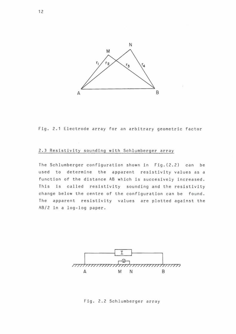
Fig. 2.1 Electrode array for an arbitrary geometric factor

2.3 Resistivity sounding with SChlurnberger array

The Schlumberger configuration shown in Fig.(2.2) can be

used to determine the apparent resistivity values as a

function of the distance AB which is succesively increased.

This is c all ed resistivity sounding and the resistivity

change below the centre of the configuration can be found.

The apparent resistivity values are plotted against the

AB/2 in a log-log paper.

A M N B

Fig. 2.2 Schlumberger array

13

If the half-space consists of a homogeneous and isotropic

single layer of infinite thickness, the sounding curve will

be a straight line of apparent resistivity equal to the

true resistivity. In many cases the assumption is that the

half-space consists of many layers each having a

resistivity and finite thickness. In that

different

case the

apparent resistivity curves can be interpreted using master

curves and/or auxiliary point graphs and by automatic or

non-automatic computer iteration techniques (Johansen,

1975; Koefoed, 1979). These methods are based on the

following assumptio ns:

(1) The subsurface consists of horizontal strata

separated by horizontal boundary planes,the

thickness of the deepest layer is infinite and

all the other layers have finite thicknesses.

(2) Each of the layers is electrically homogeneous

and isotropic.

2.4 Sounding over non-horizontal earth

The effects of dipping and vertical contacts and

inhomogeneities depend o n the size,location relative to the

sounding centre and the resistivity contrasts. The biggest

problem in the interpretation of curves with these effects

has been the difficulty in the mathematical formulation of

potential caused by the irregularly shaped bodies. Creat

efforts are being put towards finding these mathematical

formulations (Lee, 1981). Stud i es have been limited to

very simple st ructures owing to the above problem.

Van Nostrand and Cook (1955), De Cery and Kunetz(1956) and

others have published master curves over simple structures

using the method of images proposed by Unz (1953). Tank

model experiments have also been used (McPhar GeophysIcs,

1967). However, i t is practically difficult to find a very

homogeneous material easy to work with and for which one

14

can vary the resistivity convlniently through the necessary

range. In practice, soundings in tank models have also

been limited to a few cases such as vertical or dipping

faults in the overburden over l ying an infinitely resistant

basement.

2.4.1 Dipping contacts

Flg.(2.3) shows the apparent resistivity curves whi c h would

be obtained by a Schlumberger array expanded parallel to

the dipping contact and over horizontal layers of the same

resistivity contrast. The shape of the curve does not appear

different from those of the horizontal

curvature of the dipping model is more.

layers except

1 Thlllme true re,IIIL\,I\y aDd the IIrGe Dormal dill"oce froll!. the conftluralloD to the btdd!1Ii pl&ue (eul"lt 1 alld 2) 2 The lame ratio 01 Apparent re.lt tl,'aiel and the ... me urmptote lor IroaU electrode Itparatiotll (curve S) or l~'ie

electrode Hparlotlotll (turve 4)

• i $ - -----

-,- -- ,-, " ,

, [ , j.

i I : ; I ' , ! 11 • • • "

the

Fig. 2.3 Resistivity soundings made with array parallel to

a dipping contact and over horizontal la ye rs

(from Kunetz, 1966)

15

This curvature increases with the increase in the angle of

dip. For dips less than 10 degrees, the effect is small

and can be ignored (Koefoed, 1979).

For a configuration oriented perpendicular to the contact,

the curves show sharp discontinuities. Fig.(2.4) shows

some typical curves depending on the distance between the

sounding centre and the contact. In Fig.(2.4a) where the

centre of the array is downdip and Pl < P2 the apparent

resistivity increases much faster. This is because the

current is concentrated in the low resistivity layer (more

conductive) as the resistive layer reduces the flow beyond

the contact. When one current electrode crosses the

contact, the resistivity starts to decrease and then rises

gradually .

2.4.2 Vertical contacts

Vertical contacts as created by faults are quite common in

geothermal areas. The strongest effects are again realized

when the profiles are oriented perpendicular and close to

the structures (Fig.2.5). When the centre is in the low

resistivity layer, the curve rises steeply, sometimes

exceeding the limiting 45 degrees slope both in the

parallel and perpendicular sou ndings. The perpendicular

soundings will show a sharp break as the current electrode

is positioned at the contact. I t is important to note that

these breaks are less conspicuos if the contacts are buried

at depths by the overlying layers and also when the

reslstivities have little co n trast .

16

I P, 9 , .

, I p, ~-;:.=--t---------,- - --- -~---+-- - ¥-I I , , I I

~ .. 1/9

, , ' o,'p, - - -- - - ---t - - - - - -- -- - - - - - ;a-- - -------- - - - ,;-;--

et ....

! p.

P,

, ' _...l. ____ ___ _ _ ___ _ ---.l __ _ O"P, ------ "D--------- - -- IOD I OC ~

Fig. 2.4 Resistivity soundings made with an arr ay

perpendicular to the strike of the dipping

contact (from Kunetz, 1966)

•

mp -r---- ------- ---- --.'

<"-'h '-=-----" '. Pi I ~/~ VJljj? 1"-2h l , £;,Ja

_~<:=7<1J 1------~~h--~l.h------~mh;~

17

Fig. 2 . 5 Resistivity curves near a vertical contact under­

la i n by an i nfinitely resistant substratum

(fr o m Kunetz, 1966).

2.4.3 A thin vertical dike

A thin vertical dike , even when it has a highly co ntrasting

resistivity to the host rock will not effect any c hange in

th e sounding paral l el to it . On the other hand,a resistant

dike ca uses a steep slope in the the first part of the

curve and a vertical discontinuity as soon as the electrode

crosses it (Flg.2.6).

18

M;- --- .

1111;

Tf"OlISYel'u /'esi.!I(1l!c~: f(-~ - 0 "-A

l(Jp---- - -- - - - - --- - - -- -- ----. ------

I O- QSh I ~ __ __ ~18

Fig . 2.6 Resistivity soundings near a thin vertical dike

underlain by an infinitely resistant substratum

(from Kunetz, 1966)

2.5 2-D Modelling of the Schlumberger soundings

The apparent resistivity values at a few specified

electrode positions are computed by the program of Oey

(1976) over two dimensional earth defined by grid nodes. The

program uses the

discussed in detail

algorithm of

by Oey and

finite difference met h od

Morr ison (1976) , Using

19

Ohm's law the potential ~ at a point defined by (x,y , z)

and conductIvity

point (x s 'Ys

o(x,y,z) due to a current

are related in

differential expression

source at a

the part i al

- Ij . [ o (x, y, z)lj~ (x, y, z)) - !e. 6 · (x ) 6 (y ) 6 (z ) at 5 5 S

(2.5.1)

The layers are assumed to be infinite in the strike

direction so that if the conductivity in the y direction is

made constant, eq.(2.5.1) becomes

- ii' [ 0 (x,z) ii~ (x,y,z) )

(2.5.2)

Equation (2.5.2) can easily be solved by taking the Fourfer

transformation Ky of y. The transformed form of equation

(2.5.2) is

(2.5.3)

where $(x,Ky,Z) is the transformed potential equation and

Q is the constant steady state current density in the

(x,y,z) given by

I ~ = 26A

6A is a representative area in the x- z plane around the

current source at (x , y,z).

The solution of ~(x,Ky , z) in equation (2.5.3) is obtained

by the finite difference me t hod by an area discretization

20

in a grid. The boundary conditions, namely continuity of

the potential and the current density across t he

boundaries, are considered in the formulation of the fin i te

difference equations. The solution is obtained by the

approximation of a system of linear finite difference

equations in the form

(2.5.4)

where Cij is the coupling coefficients between nodes. The

program of Dey (1976) solves equation (Z.5.4) for a given

resistivity model and positions of current source points

for a certain number of filter values Ky • After a Fourier

transformation the values of potential $ in the (x,y,z)

domain are obtained and used to determine the apparent

resistivity.

The rectangular grid used consists of 113 nodes in the

x-direction and 16 nodes in the z-direction. At the centre

of the sounding, the grid is equally spaced but it becomes

more widely spaced farther apart in order to simulate the

infinite extent of the model layers. This is also the c a se

in the z-direction. The nodes are defined in unit lengths

so that it is possible to change the length of a unit when

desired.

The 2-0 earth model is divided into blocks according to the

grid and the unit size. Thus, the smallest distance which

can be used is the unit length. The current and potential

electrode positions are also defined. In fact a net input

file is made specifing the grid size, the unit length and

the position of the electrodes so that they need not be

made each time the program is run.

The determination of the apparent resistivity values

depends on the number of filter coefficients and the size

of the grid. Usually, the more the filter points and the

21

bigger the grid the more accurately the apparent

resistIvity can be determined. However , this is on the

expense of much more computer time. The pr ogram is writte n

to use a maximum of 30 filter points, 161x32 grid and

compute apparent resistivity at 20 current electrode

spacings for profiles perpendicular to the strike only .

However, because o f the computer time and accuracy, 113x16

g r id, 9 filter coefficients and 9 electrode spacings are

used. Thi s takes about 1 computer hour irrespective of the

number of blocks in t he earth model using the POP11/34

computer.

As the model is defined using the gr i d, it is therefore not

possible to

the dipping

disadvantage

define accurately some geological shapes like

contacts or round bodies etc. Another

is that one is r estricted by the unit length.

This causes some unrealistic thicknesses and lengths to be

used.For example,w hen the unit length of 25m is used the

thinest dike will be 25m whereas dikes are normally about

Srn .

An example of a typical 2-D model and the comp ut ed apparent

resistivity values are given in the Appendix I.

22

2.6 Head-on profiling

2.6. 1 Introduction

Profiling is the process of obtaining the lateral

resistivity variations. This is accomplished by using a

constant current electrode spacing suitably chosen to

penetrate to a desired depth.

The combined !'head-on" method has been used with success in

the Peoples Republic of China to detect faults and dip

directions (Cheng, 1980) but the technique is beginning to

spread to the rest of the world.

2.6 . 2 Procedure and apparent resistivity equation

The head - on profiling method uses the normal Schlumberger 4

electrode array and a fifth e!ectrode,C, fixed at infinity

(Fig.2.7).

C

QC ~ 2AB

A M Q N B

fig. 2.7 Head-on array

23

The current is driven into the ground through AC and the

potential difference is measured between the usual

electrodes, MN. This is repeated with the current through

BC and AB. The centre is then moved to the next station

along a traverse li ne.

For a given current I driven between AC or BC, the apparent

resistivity is given by

(2.6.1)

Since C is at infinity, 1/CM and lIeN are approximately

zero and equation (2.6.1) becomes

Il V _-;-2=...::.......,_ I 1 1

£"1 lii~) (2.6.2)

The apparent resistivity is obtained by equation (2.6 . 2)

and it can be shown that the

that of the Schlumberger array. AC BC

geometric constant is

In fact p~B is the

twice

mean

of P a and P a

In practice it is difficult to keep C very far. It has

been found that

distance ~ 2AB

it is possible to position C at a finite

and determine the resistivity wi th

reasonable accuracy. Whe n using this AC equation (2.6.2) is used to calculate Pa

demands that the geometrical constant in

finite distance, BC and Pa . This

equation (2.6.1)

be determined for each position of the stations. For a

station perpendicular to C, equation (2.6.1) reduces to

equation (2.6.2). However,for the stations on either side

of C the geometric constant differs from that of equation

(2.6 . 2). The error which would be realized if the

geometric constant of equation (2.6.2) was used constantly

has been computed by the author. The maximum error of

24

about 2.3% occurs when the station and electrode C are at

an angle of about 54 degrees to the profile. The error

decreases for greater and lesser angles. This error is in

general small and therefore, equation (2.6.2) can be used

all the time for the determination of the resistivity.

2 . 6.3 Head-on profiles over thin dikes

Fig.(2.8) shows the

thin conductive and

AC AB BC AB shapes of Da -Da andPa -Da across a

resistive dikes. These model graphs

are computed by a modified version o f Ocy (1976) program.

Since p~B is the mean of p~C and P~C,it has been found

convenient to plot P~C _p~B and p~C _p~B It can be

seen from Flg.(2.8) that the graphs of P~C and P~C cross

each other just above the dikes. The profiles for the

conductive dike can be explained as follows: When the

centre of the array is to the left and electrode B is to

right of the dike, some of the potential due to B is

concentrated at the dike so that the potential at the

measuring electrodes is less than that due to A. As the

measuring centre approac hes the dike, the screening effect

of the dike is stronger and the potential due to B further

decreases whereas that due to A increases. However, when

the centre is at the dike , the potential due to A and B is

the same. The situation is reversed beyond the dike. For

the resistant dike, the graphs cross at thr e e places the

middle one being cente r ed at the dike.

The graph of the for the co ndu ctive dike has a

characteristic trough whereas a resistant dike has a crest.

It is therefore possible to use the head-on crossover as

signatures for the exploration for low resistivity dikes

and distinguish them from the resistant ones.

Some theoretical head -o n models are presented in chapter 4

of this report.

HUD ON PROfILE A812 • 5OQ. AuunY[ DIKE

I£,U)-t'H PRCf""'--E

-~"'.~

--- Rh. _. ,--,

,,' M ----- -------

- ------------ ---? v,,' -

5CfLt;IIBEJt;ER PRtflli

..... IQl-, ... 1

_AL------

-

- -1.1

i -1 I ' 00

M '00

'*

MEAD ON PflOfILE A812- 500-CONDUCTIV£ OllCE

---~ " ,

,.,

.. , •

:1 ,J

, ;; 500 4 ; 0

,-

- ---------

1Oh..)

-

'00

---, , ,

~,:

V

I.

- .... -----Rf<>c, --IOhaoo)

fEU)...(l1l PItOFU

---

-'-

scHltM8fRiER PROFIlf

-1.1

".

-... --~-~ ~ ~

Oht.nc. 1.1 Oht*'\c. (.1

Fig. 2. 8 Head-on and Sch l umberge r a pparent resistivity p r ofiles over re sis tive an d conductive di kes

N

'"

26

3. 2-D SCHLUMBERGER SOUNDING INTERPRETATION

3.1 Introduction

Geophysical inverstigations have been made in the vicin i ty

of the town of Akureryi in the EyjafjorOur area in central

northern Iceland. Resist iv ity soundings and magnetic

measurements have been used to locate drill holes close to

the town. Six successful wells 12km south of Akureyri

produce about 150 lis of 80-96 · C hot water

(Bjornsson , 1981) .

Eyjafjordur is a V-shaped valley and most of the earl i er

resistivity measurements were made parallel to the val l ey

in order to avoid the steep terrain on the flanks of the

valley. Th e interpretation of the measurements sho wed that

the bottom of the valley contained low resistiv i ty

sediments, which made the 1-D interpretation of the

resistivity sounding data difficult. In 1981, measu rements

were carried out perpendicular to the valley so that they

could be interpreted by the 2-D mod el ling techinique

(Flovenz and Eyjolfsson, 1981).

Some of these recent soundings have been reinterpreted by

the author as a training excercise in the 2-D modelling

method of the Shlumberger data.

3.2 Geological setting

The strata around Akureyri co nsists of Tertiary subaerial

basaltic lava flows 8-10 M.y. old. The individual lava

flows are thin and are occasionally intercalated with

sediments and volcanic scoria. The lava pile dips by 5-7

degrees south and southeast towards the Neovolcanic zone.

Dikes are numerous and form about 6% of the total volcanic

mass (Bjornsson and Saemundsson, 1975). The main faults

have the same direction as the dikes.

27

Prior to drilling there were about 20 locations with hot

springs with an initial natural flow of about 14 l/s. The

temperature of the springs ranged from 10 to 70 ~ C.

These springs

particulary where

from detecting

are associated with dikes and occur

two dikes intersect.

the general hot water

Therefore, apart

ar e as commonly

characterized by low resistivity due to high porosity, the

geophysical investigations have been aimed at mapping the

dikes associated with hot water which are usually buried

under an overburden and therefore, difficult to map

geologically.

3.3 Resistivity measurements

A total of 120 Schlumberger soundings were made between 1975

and 1980 and 35 more soundings in 1981 (Fig.3.l). The

latter soundings were measured perpendicular to the

Eyjafjordur valley specifically for the 2-D interpretation

around Laugaland and Gryta. Most of these recent

measurements were expanded to a maximum electrode spacing

of AB/2 =1580m and the sounding locations were so chosen

that the

overlapped.

to identify

neighbouring current electrode spacings

The overlap is very important because it helps

and locate the strong lateral resistivity

variations which might be confused for bad measurements

etc. The 1981 soundings were of high quality even at large

current electrode spacings because they were measured with

dc-equipment which employs a modern signal enhancement

receiver. Therefore, most of the jumps or breaks in the

apparent resistivity curves can be attributed to vertical

boundaries and surface inhomogeneities.

28

r.r::I __ <tn_ w. w· .. .. 1 ..

HRAFNACILS- GC ONCULST ADAHREPPUR Locafl on of SclJlumb.'ge, soundings

'\ , )

/

\ ) ,

~

f

) i .....

, ""'It .. j ) ,

"',", • ,,' M ' 0 "

-, , \ M{

'or I , ". ,

I

",,·lto

I

/ M'"

",",---~, "

/

,,'

M_

...... ---, ,..,.:.

D

/ , I , ".

""1':-" '

M"\

.....

A' .. _IS'

...... o

" ." r_

.-' '.

- ;" / •• - c-

U"" I

.~-

~~ ' -1 .1 /, o ,~

•• /

\.,----..... o • "" ..

-----Fig. 3.1 Map of Eyjafjordur s~owing the location of

Schlumberger soundings and interpreted resistivity pr of il e (Flovenz and Eyjolfsson, 1981).

,

29

3.4 The 2-D Interpretation

3.4.1 Initial model approximation

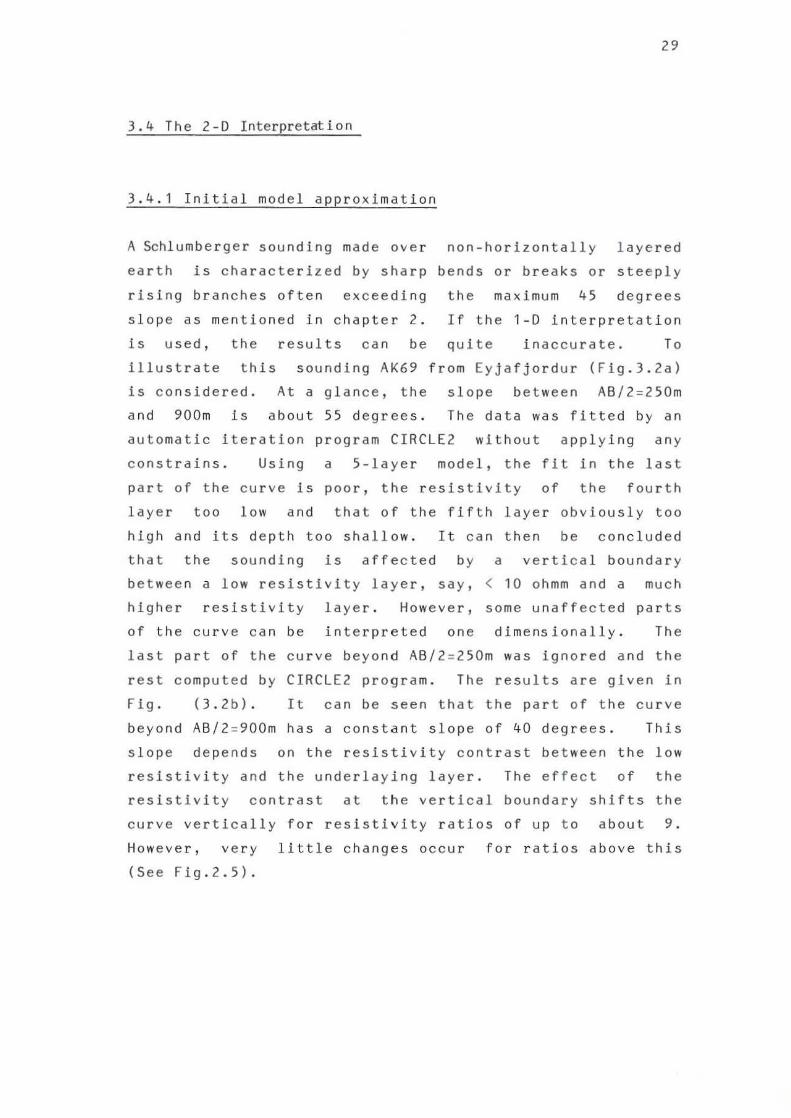
A Schlumberger sounding made over non-horizontally layered

earth is characterized by sharp bends or breaks or steeply

rising branches often exceeding the maximum 45 degrees

slope as mentioned in chapter 2. If the 1-0 interpretation

is used, the results can be quite inaccurate. To

illustrate this sounding AK69 from Eyjafjordur (Fig.3.2a)

is considered. At a glance, the slope between AB/2=250m

and 900m is about 55 degrees. The data was fitted by an

automatic iteration program CIRCLE2 without applying any

constrains. Using a 5-1ayer model, the fit in the last

part of the curve is poor, the resistivity of the fourth

layer too low and that of the fifth layer obviously too

high and its depth too shallow . It can then be concluded

that the sounding is affected by a vertical boundary

between a low resistivity layer, say, < 10 ohmm and a much

higher resistivity layer. However, some unaffected parts

of the curve can be interpreted one dimensionally. The

last part of the curve beyond AB/2 =250m was ignored and the

rest computed by CIRCLE2 program. The results are given in

Fig. (3.2b). It can be seen that the part of the curve

beyond AB/2=900m has a constant slope of 40 degrees. This

slope depends on the resistivity contrast between the low

resistivity and the underlaying layer. The effect of the

resistivity contrast at the vertical boundary shifts the

curve vertically for resistivity ratios of up to about 9.

However, very little changes occur for ratios above this

(See Fig.2.5).

30 10'

4 ~

E c= 2 ~

E 10' '0 C to > ~

4 0 ~ 2 C '>' en 102

4

2

10'

4

10'

4

E c= 2 ~

E 10 '0

, C to > 4 ~

o -g 2 '>' en 10

,

4

2

10 ,

4

AK69

a

0 y

\ / V-0

.. 1.'

3.5 2S .l 25.8 • 30.3 511. 1 1.0 I ~3000 0" ••

2 4 101 2 4 4 10' 2 4 10'

Lengd [m]

AK69

b

0 0 ",0

\ 0

0 0

0

0

0

1\0 00

0

1.2 IS.O ,

2 .1 24.8 , • 60.0 57.S ' .1

, oh ••

2 4 101 2 4 4 103 2 4 10'

Lengd [m]

Fig. 3.2 CIRCLE2 fits to AK69 sounding curve.

31

If we assume a ratio of at least 9, and the resistivity of

the low resistivity layer to be 5 ohmm from CIRCLE2, then

the resistivity of the medium beyond the contact is at

least 45 ohmm or more. The resistivity of the substratum

is at least 200 ohmm if it is assummed the resisitivity

contrast causing the 40 degrees slope is about 40.

The vertical shift of the curve due to the substratum is

smaller than that caused by the position of the vertical

contact. As the distance to the contact is increased the

effect is delayed. This is because the vertical boundary

affects the potential horizontal current flow pattern

before the current penetrates too deep into the underlaying

layers . The low reSistivity layers have a strong effect

and cause sharp V-shapes in the curve. For the high

resistivity boundary of AK69, the position of the contact

is at the value of AB/2, wher e the steep slope join the 40

degrees part of the last branch.

AB/2 =800m.

This happens at

Using CIRCLE2 program, five E-W Shlumberger soundings from

Eyjafjordur were interpreted and the fitted curves are

shown in Appendix 11. The pro c edure mentioned above was

used to infer the main vertical boundaries.

The shallow thin layers and inhomogeneities were ignored.

However,layers thicker than 25m in the first 100m depth

were considered. Actually, the average resistivity for the

first 25m was used in the model. The procedure discussed

above was used to

considering all

interpreted section

infer the vertical discontinuities,

the neighbouring soundings. The

is shown in Fig.(3.3).

The interpretation started from sounding AK152 on the

valley floor. The sounding is located on a low resistivity

area whose resistivity was estimated to be about 5 ohmm.

f"i"n .tlO- H$I-6 000-M.M. t..:.l:J 62.09. 11 12 - 1.5.

A

<0O m

,J AK 135

.... .L 3SO

°1 -- - --

" -'00

-400

o 100 .. "-------' Horizonta l (l od unicol scol ,

Es t imat od von icol b"~ndary

E.ti",oled borl .ontol boundary.

PROFILE A-8

CIRCLE2 INTERPRETAT IONS

AKUREYRI, N. E ICELA ND

R c}'j~fj~'''~'Q

1 AK 152 AK 134

......

" "

,

~IOO

AK 153

I

'"

0> 100

AI( 142 ,

''''---- - -w

~ I OO

Fig. ).J CIRCLE2 interpretation sect ion of profile AB

B

' 00

' 00

°

-'00

-400

~

N

33

The steeply ascending last branch of the curve indicates

that there is a much higher resistivity change either

vertically or laterally or a combination of both. This

sounding is short but it seems to have a general shape as

AK69 which is located 600m to the north and expanded along

the strike of the valley. The vertical contact as

interpreted from AK69 is SOOm to the north. The sound i ng

also reveales a high resistIvity substratum with a value of

about 200 ohmm. It is assumed that the substratum at AK 152

probably has a resistivity of the same order of magnitude.

Sounding AK153 differs slightly from AK152 and it shows an

elevated resistivity la yer (20 ohmm) overlying t he

substratum. A sharp minimum at AB/2 =250m marks t he

boundary between the 5 ohmm and the 20 ohmm layers on t he

AK152 side. The slope of the l ast part of the curve is

steep but less than 45 degrees. The interpre t ed

resistivity of 200 ohmm is either true or overestima t ed

because of a vertical boundary . Again the sounding was t oo

short to be used further.

The 20 ohmm layer found at AK153 Is confirmed by AK142.

The interpreted resistivity of the substratum by CIRCLE2 is

about 400 ohmm. Noting that the interpreted depth to the

substratum i s about the same both from AK153 and this

sounding, it would appear that the difference in the

interpreted substratum resistivity is attributable to the

presence of a probable vertical contact which is not

apparent from both these curves. There Is no sounding much

further to the east of AK142 which could be used to decide

this side of the boundary.

However, c onsidering AK134, a thick resistivity layer of

about 80 ohmm is seen and it could extend laterally towards

AK152. The sharp minimum at AB/2 =850m marks the western

boundary of the low resistivity of 5 ohmm. The 80 ohmm

layer extends eastwards and it is the one affecting

soundings AK152, AK153 and AK142. The reason why the

boundary can not be cle a rly identified from AK152 is

34

because the minimum of the curve, due to the substratum,

coincides with the contact. Sounding AK135 is interpreted

reasonably well except that the last branch indicates a

high resistivity vertical contact at 1300m to the west of

the sounding. This is because the contact can not be

correlated with any other on the eastern side.

3.4.2 2-D computer modelling

In the 2-D modelling, as mentioned in chapter 2, the earth

medium is divided into blocks of thicknesses and lengths in

a multiple of a specified unit length. The Shlumberger

apparent resistivity at var i ous electrode spacings is

computed and the curve compared with the measured one

manually. The resistivity and the block sizes are changed

until a reasonable fit is obtained.

The section interpreted one dimensionally was used as t he

initial model. The boundaries were arranged according to

the grid of a unit length 25m. For each sounding , t he

model was defined at least over a distance greater than

1500m which was about the maximum electrode spacing used in

the field measurements. This ensured that the relevant

information over 80% of the profile was included. The

results of the 2 - D modelling is given in Fig.(3.4). The

apparent resistivity pseudo sections of the computed and

measured curves are shown in Fig.(3.Sl.

" m

,

'00 ,

-200 ,

-mOO

A

AK 1~5

"" '"

o ~. L.........> Ho, i:OIlIa' olld v,"ico' lcol.

PROFILE A·S

DltoI2 INTERPRETATIONS AKUREYRI, N. ICELAND

" fjljllf/Q,4"";

AK 134 I AK 152

I 1

mo 80 ,

':->80 '"0

AI':; 153

I

"'0

Fi g, 3.4 2-D i nterpetation sectio n of profIle AB

B

AK 142

..l

'" 20

''''

.00 m

200

, o

200

<00

'" ~

36

I"jT=l J'lD-HS" -6000- "' .M L.:....I:...i B2 0 9 "'~ - !S

AI<. 135

I

MEASURED APPARENT RESISTIVITY PSEUDOSECTION

AK 134 AI( 152 I

AI(153

'00 "~ ;:t! -~'l.OO 22. -

30" ,"$7

~o '" ~

~ ~

"Of I ,. 6CO

, N 700 , • •

800

1100

1200

'''' "0 35O

, "" N "" , • 0>" •

7'"

"''' ''''

1000

'" --::::::, ~

"

;,

;.

AI<. 135 I

70

. 0

" "

, "

"

o 100 .. ~

COMPUTED APPARENT RE SISTIVITY PSEUDOSECTlON

AK I34 I

Hori aon'o i ond ,,,' I~a l u:o l.

AK I52 I

AI<. 142 AI<. 61 I I

AI<. 142 AK 61

I

Fig. 3.5 Meas ured a nd computed pseudosections.

37

3.4.3 Results of the modelling

The pseudosection of the computed apparent resistivity

agrees very well with that of the field data. These,

model, seem to reflect the together with

geophysical

the computed

condition of this area. The most important

features affecting the model are the low resistivity of

about 3 ohmm at AK152, the vertical contact immediately to

the west of AK152, and the resistant substratum . Sounding

AK134 was the most difficult to fit

(Fig.3.4) . The 40 ohmm block just below

necessary to be included in the profile.

extend to the west because it would affect

into the profile

AK134 was found

It seems not to

AK135 badly. If

the simple model was to be maintained, the 380 ohmm

substratum below AK134 and AK152 had to be used ,Decreasing

this resistivity produced a poor fit. Yet, it could not be

extended to AK153 and AK142. Keeping the model constant,

resistivities much higher than 150 ohmm again affected the

fits of AK153 and AK142. The only way of reducing th e

r e sistivity of the substratum below AK134 to AK142 was by

inserting blocks of high resistivity in the upper 200m, an

exercise that would make the whole model not only too

complicated but also cause uneven depth to the substratum

difficult to exp l ain . Not a ll the resistivities could be

tried between 200 ohmm and 400 ohmm but the resistivity is

in this range. There is a vertical contact about 1200m to

the west of AK135 not shown in the section. This was

necessary to account for t he ascending last branch o f this

sounding. The high resistivity substratum seems to be absent

at AK135. Any attempt to include this substratum demanded

the presence of a low resistivity block, say of about 40

ohmm, below the sounding. The effec t of this block caused

most of the curve for AB/2 < 850m to fit badly unless mor e

changes were made to the overly ing 350 ohmm layer which is

consistent in the neighbourhood. Sounding AK51 located

close to AK135 (see Fig.3.1) indicate rather clearly that,

the laye r below 350 ohmm layer is too thick as the

interpretation of AK135 shows.

38

Compared with the 1- 0 interpretation, the 2-D model is

nearly the same. The major differences are t he presence of

the 40 ohmm block at AK134. The 2-D model defines the

depth to and the resistivity values of the substratum. Th e

resistivities are in a reasonable order of magn itud e, the

differences being attributable to equivalence caused by the

use of a fixed grid in the 2 - D program.

The resistivity of the co ndu ctive sediments in the valley

is in the range of 3 - 5 ohmm and their base is not more than

200m below the surface or about 125m below sea level. The

2 - D model also shows the discontniuty of the substratum

west of AK134 and its decrease in resistivity to the east

of AK152. The 1981 model of Flovenz and Eyjolfsson (1981)

is presented in Fig.(3.6). Comparing this and the present

f';:~/:':'''' ~ '' PROFILE A-B

, ~'"

'" '" "" '" "" "'" '" '"

~.ft\O(li'U.OI I Enofjor&!l,o IIfUnoiouq ~Iouf

A~ - '3~ A~ ·'~4 J J- j A"' - ' ~2 AK_ I ~3 j AK·142 , , m nm ""nm =n. 45n., 2011.., "n. oon. 'SOn .. ",n.

! >on. 110n",

200~'" I .n.

"nm 'On. 25n", lOOn", ",n. 14511. ... ) 2011.",

"on., lIOn", 40n.,

""n. loon ... 19011. ... 2oon., non., non., 200n.,

. .. -- --. r Fig. 3.6 Two dimensional mo del made in 1981,

(Flovenz and Eyjolfsson, 1981).

39

model (see Fig.3.S), they both reflect th e same overall

resistivity in the Eyjafjordur area near Laugaland.The main

difference is that the present model is much simpler and

seems to define the top of the resistive substratum more

clearly.

3.5 Discussion

In the 2-D modelling, the problem of equivalence is common.

The reasons for this are mainly due to the grid

inflexibility in the 2 - D program on the one hand, and the

infinity set of solutions inherent in the resistivity

method on the other. One way of reducing the problem is by

constraining the model

drilling, geophysical logs

using

etc.

some

Since

information from

this external

information was lacking, the problem of equivalence must not

be overlooked. However, the models indicate the main

geophysical boundaries which are extremely useful.

The main structures to be inferred from the present work

are:

(1) The conductive 3-5 ohmm sediments in the middle of

the EyjafjorOur valley, which are of marine origin

deposited after the formation of the fjord . The base

of these sediments mark the bottom of the glacial

valley which is about 200m below the surface.

(2) A decrease in resistivity east of the valley.

(3) A discontinuity immediately to the west of AK134

which could probably be a fault.

It is uncertain wether the 20 oh mm layer is associated

with the hot water. According to Flovenz and Eyjolfsson

(1981), the decrease in resistivity in the low-temperature

area is a function of porosity.

that the rocks in the eastern

It would seem therefore,

side of the valley are

40

probably more permiable. Bjornsson (1981) and Flovenz and

Eyjolfsson (1981) are of the opinion that the hot water in

the Eyjafjor6ur area flows along t he dikes and appears as

springs at various places. Soundings AK140, AK153, and

AK155 (Fig .3 ,l) to the south of the profile, indicat e the

presence of a north-south dike but none of the soundings in

this profile.

3.6 Conclusions

The present work clearly demonstrates how the 1-D and 2- D

methods can be intergrated to improve the Schlumberger

sounding interpretations.

A simple model was favoured;

model was made the more

modelling became. It was

the more complicated the

difficult and frustrating the

actually found worthy to

recognize the distorted parts of the Sclumberger soundings

carefully to mark the consistent vertical boundaries, and

to use all the available data from the area. The 1-0

interpretation should be used as far as possible to control

the 2-D modelling.

The sediments in the middl e of the E y jafjor~ur valley are

not extensive laterally and their base does not exceed 200m

below the surface. The sediments overly a resistant

substratum with a resistivity of 100-400 ohmm. Th e hot

water implication is not clear from the model . It is

therefore agreed that the main conduit of the hot water

appearing as springs at Laugaland and elsewhere is pro bably

assosciated with dikes. Dikes, unless they are more

resistive than the surrounding ro c ks, would be rather

difficult to detect by Shlumberger soundings so that other

methods,for example magnetic and head-on, have to be

resorted to.

41

4 HEAD - ON THEORETICAL MODELS

4.1 Introduction

The apparent resistivity profiles for the head-on

configuration (Flg.Z.7) were computed using a 2-D finite

difference program, DIM2~, over several simple

2-dimensional structures. It is convenient to plot the

difference between the head - on and the Schlumberger

resistivity values instead of the actual head-on values.

The Schlumberger profile is also plotted. The theory of

the head-on profile is given in Chapter 2 and the

theoretical models are given below. Since the theoretical

computation takes a very long time, only a few models were

computed. However, the few models will illustrate a few

facts about the method and may be found useful in the

interpretation of the head-on data.

4.2 Conductive fractures

This is perhaps the most attractive structure as far as

geothermal exploration is concerned. It is assumed that a

geothermal brine in a fault or a fracture creates a

conductive zone. The head-on response over such a zone

(hereafter referred to as conductive dike) I n a homogeneous

earth is shown in Fig . (2.8). The apparent resistivit y due

to the leading current electrode is less than that due to

the lagging one. However, the resistivities are the same

over the middle of the dike and the situation is the

reverse as soon as the measuring centre crosses the structure.

On the other hand, the Schlumberger profile has a trough over

the dike. The head-on profiles are symmetrical and the

amplitudes decreases gently away from the crossover . The

size of the amplitude depends on the resistivity contrast

between the dike and the surrounding rock.

42

4.3 Penetration depth

Flg.(4.1) shows that theoretically, the penetration is up

to about AB/2 used in the profiling but the amplitudes are

reduced so much that would be difficult to measure it in

the field. The measurable data can only be obtained

reasonably to a depth of about AB/4. However, if there are

strong lateral contrasts in the top layers, the penetration

is reduced considerably as shown in Flg.(4.2).

4.4 Inhomogeneities

The head-on data is sensitive to vertical structures very

near or on the surface for short electrode spacings.

Conseqently, the presence of a crossover may not necessary

mean that the conductor extends very deep. Any vertical

conductor within the probing depth may cause a crossover

provided its size and the resistivity contrast with the

surrounding rocks is reasonable. Some examples of models of

this type are shown in Fig.(4.3). The Schlumberger

profiles show strong electrode effects caused when the

electrodes cross the lateral boundaries. Fig.(4.4)

illustrates this for

AB/2 =300m, which has

the Schlumberger profile with

two lows 300m on either side of the

low resistivity structure. These lows may be confused with

the resistivity material in the ground; they are absent

for AB/2=500m profile. Therefore,during exploration, it is

recommended to use larger electrode spacings or to be

careful when using the Schlumberger profile in the

interpretation. It is most recommended to use two or more

electrode spacings so as to prove whether the anomaly stIll

exits to a substantial depth as would be required for a

dike.

IlEUI OH PROf"lU .lII12 • soo.

",,---- --- ------- -----1.1 - ~ ________ • _______ ~/"\...

". , .... , • -,

SCHLUH8E:RGfJl PROF!r.E:

,.'

.- - -,

'" '"

." " < ~

,i

'" '" ,-

-.". ~

-- -lit>. _ . ,"-,

-t_

... 1.1

HEAD ON PItOf"IL[ lIln 4 500.

1.1 --

". 1000ul • -] -

-•

,~

!

'"

."

'" ,- ------- ---

')CHllJr.BEI$£R PROFILE:

'"

."

'"

- .. _. _4 4'"

-

-­,"-,

'-

-1.1

---- -

- . ~ . D"~_. 1.1

Fig. 4.1 Head-on and dik e buried

Sc hlumber ger at differ e nt

pr ofiles depths

over a

Dt.IAnU I.J

conduc ti ve

~ ~

,

ft(AO ON PI!OF lLE A912 • soo.

----- ------------

-- 'M ----- 11". _. ,-,

I .) - - -------------- -

Rh. .. tot... ) - • ~MUl'\eER~ Pl:ff!l f

,.

- - (.1

"" '"

... ., •

IIfAO -OM PItOf'ILE aal2-$OO

,: --------- --------- -

--"'. --- . -ttt.. •• ,-,

" . - \--- ~

Ih. (":Ih_l • -'.

-

~

SCHlOft8EaG~ FRff!L£

------~/---------

-,.)

,,. "'"

... .,

" - < - .

J .;

,- '''' '''' ,,. ".

,-.-----~ i -- - ~ -Ol.hn.c. (,. )

Fig. 4.2

01.'."". 1.1

Head - on and Schlumberger profiles showing how lateral res i stivity changes near the surface r e du ce the penetration depth

t he

~ ~

HI:_ '_on~l "n·~ "'''-110.

,., .• O\> < - ""'" vv---r

" .~

'. l..:.-

-i • • • •

~ .•

....

- ""0 .. -.. .- .111. . .....

,(11, •• ,

•

.•

'" '

-'" ....... -.

-~-... -,- ,

---===~J====---,.", ~

'. , .... _,,'

-!

It£~ __ ZL!

Ufl·"e .."n·n

1. 1 '''~_'''''''1~_O:'':'='=''''~'o' --;;~

.-.... -""'" • • ~ 0' - ~

o. ,. o. l:

"

~

.~ , ~ D,.,." •• < • •

45

.. ,-,

Fig. 4.3 Head- on and Schlumberger profiles over nea r-surfa ce inhomogenities

46

• •

,.

-

- ....... ....... ,­•

..... ' ~ .•

'.

....... 00.. • •

,,'

•

~. -

v

, .........

Fig. 4.4 Head-on and Schlumberger profiles showing

electrode effects for AB/2 = 300m

4.5 Two conductive dikes or fractures

•

.. , t, ., I c .•

Two conductive dikes can have a neutralising effect if they

are spaced less or equal to the electrode spacing used in

the profile measurement. This is more so when the contrast

is the same on either side of the two dikes. An example of

this case Is shown in Fig.(4,5). Note in the figure that

the dike to the right causes a crossover but not what would

be ca l led a total crossover as wo uld be effected by a

sing le dike. Although the Schlumberger profile has a

trough coinciding with the crossover, this is not always

the case where the conductive dike is buried by an

47

overburden and the ground is compli c ated. Fig . (4.6) shows

an example where a resistivity trough does not coincide

with the crossover.

HEAP-ON P~QFllE

• B/2· ~OO. ~/2'2~

A~ _ .. ~Otro:,

to ., ••••

• •

" · M ·M ,. · -- -

" ,. . " " " " " " "

-~ .... .. . , ' 1Iko .. . ..

11)10,. .1

•

,.,

Fig 4.5 Head-on (top) and Sc hlumber ger ( c enter)

profiles across two condu c tive dikes

4.5 Dipping structure

Fig.(4.7) shows the computed head-on profiles

degrees dipping conductiv e dike using two

over a 45

electrode

spacings. Ideally, the profile with a greater probing

detpth is shifted to the direction of the dip. The

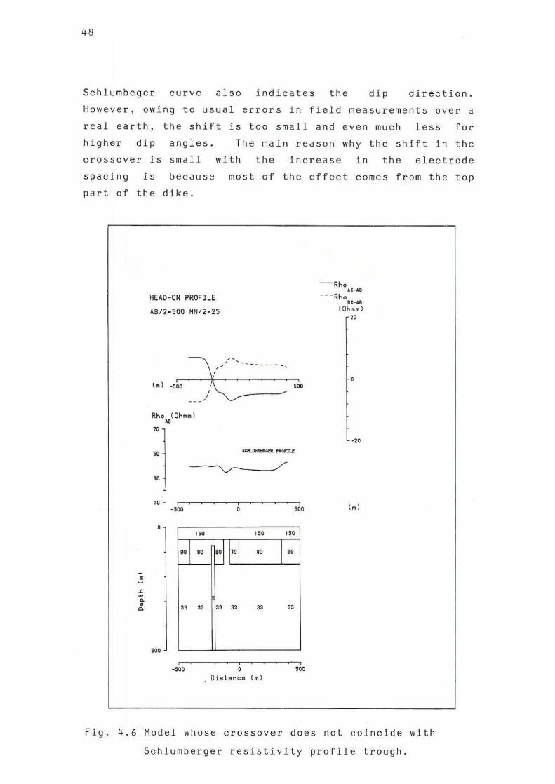
48

Schlumbeger curve also indicates the dip direction.

However, owing to usual errors in field measurements over a

real earth, the shift is too small and even much less for higher dip

crossover is

angles.

small

The main reason why the s hift in the

spacing

part of

with the incre a se in the elec t rode

is because most of the effect comes from the top

the dike.

• ~

" • Q

HEAD-ON PROFILE 118/2-500 '1NI2-25

=v:---- m

---

Rho (Oh",," J .. " "

-~v----_/

"

50'

"

"

, -500

'50

" "

" "

'" '50

" " I ..

" " "

, 50'

-Rh, AC-AB

---Rho at - AB

(01'0111111)

"

,.1

Fig. 4.6 Model whose crossover does not coincide with

Schlumberger resistivity profile trough.

,

-~-.. __ ........ --... ... '"-.... . " .. ....... -.-~ . ........ . . / "' .

-~--~ -~-\,.-----­.--------T'--- - -__."' ,.,

~I. . , "

49

-~-

.. __ ............... .. ............ -.-. .. _ -:1. ( ....... . . .... -.... _---._,.,./

-'-'" --\---

_.-----.,:::-----.-...

-s.. .. ~ .

" .. . - .• .• j .•

. .",_. 1.,

.•

Fig. 4.7 Head-on and Schlumberger profiles over a dippi ng

dike

4.6 Resistive dike

The model profiles for a resistive dike are shown in

Fig.(2.8) . The dike has three crossovers the middle one

being centered over the dike. The profile amplitudes are

relatively smaller than those of a conductive dike. As

would be expected, the Schlumberger profile has a crest

over the dike.

50

4.7 Vertical contact

The head-on profiles diverge at the vertical contact as

shown in Fig.(4.8) and define the contact unambiguosly. It

can be gleaned from the figure that it is also possible to

know which side of the contact the resisitivity is lower

than the other. The Schlumberger profile can be used to

approximate these resisitivities. Seemingly, the head-on

method can be used to detect structures such as grabens,

hosts etc which are very important structures in geothermal

fields. Therefore, it is clear that only a narrow

structure with a contrasting resistivity would cause a

crossover.

------..,.. ,-"' " ' ... _-

-r---

.----====",..---..,.,

• , .

. .... '-, ..

Fig. 4.8 Head - on and Schlumberger profiles over a vert i cal

boundary

51

5.INTERPRETATION OF HEAD-ON DATA FROM OLKARIA.KENYA

5.1 Introdution

In 1981, head-on measurements were made by the author along

several profiles in Ol karia geothermal field, Kenya. The

aim was to investigate whether the head-on method could

viably be used to detect fracture zones, their dip

direction and the amount of dip which could greatly assist

in siting geot hermal wells. The measurements were made at

the recommendation of the scientific review meeting (Kenya

Power Company, 1980). The profiles were located close to

exploratio n drill sites. These sites have been loc a ted

near assumed faults . The head-on data from one of the

profiles, HO, was sent to the Geothermal Institute at

for analysis. Unfortunately, a Auckland University

suitable model could not be obtained (Sudarman, pers.

comm., 1982). The same profile has been reinterpreted by

the author using a modi fed 2-D program, OIM2K, at the

Orkustofnun t Iceland. Due to lack of adequate time, this

was the only profile interpreted from Olkaria.

5.2 Local Geology

The geology of the Olkaria geothermal field comprises

Quaternary volcanics. These are mainly comenditic and

rhyolitic lava flows and domes, and large volumes of

pumiceous pyroc l stics erupted from central volcanoes and

vents (Nyalor, 19 7 2; Noble and Ojiambo, 1976).

North - south faults are predominant but several

northeast - southwest trend i ng faults ex i st, the most being

the Ololbutot fault. The Ololbutot fau l t is seismically

active. Several phreatic pu mice explosions have occured.

The latest eruption culminated with the recent Ololbutot

flow of pumiceous obsidian (Fig.5 . l) which is considered to

be 300 - 400 years o l d (Naylor, 19 72). The boreholes in the

52

~ JHO-HS I -9000-M.M. ~ 82.09. 1165-I.S.

, , \ , ,

\t , \

LEGEND:

HO

. ~.

o

Foult or Fracture zone

Head - on Resistivity Profile

Present Production Field, 01 ko rio

LAKE

Fig. 5.1 Map of Olkar ia showing faults and the locatio n of head-on pr ofile

53

present geothermal field reveal the presence of tuffs, lake

beds and lava flows in the top 400m. Below this depth the

strata is characterized by trachytes at 400-500m, basalts

and pyroclastlcs at 500 - 700m, rhyolites at 700-BOOm, and

trachytes, rhyolites and basalts at 800- 1300m (Browne,

1981 ) . The producing zones are found at 600 - BOOm

the steam zone, and 800-900m and 1000-1100m in the

dominated part of the reservoir.

5.3 Head-on and gravity measurements

depth in

liquid

Profile HO is located 80 metres from exploration well 101.

It Is 1000m long across an assumed fracture (FIg.5.l).

Head-on stations were lOOm apart. The measurements were

made with AB/2 ; 250m and SOOm with MN/2 =24m in both cases.

The fifth electrode, C, was kept at 2km. Later, it was

found necessary to conduct more measurements with a larger

spacing. This was done with AB/2 =800m, MN/2 =100m and

electrode C at 3.2km . Two Schlumberger soundings were

expanded at both ends of the profile with electrode

of AB/2=1000m. Three more soundings spacings

AB/2:350m were made in between the long ones. The

with

later

measurements were taken during the drilling of well 101 and

the readings were found to fluctuate, probably due to

leakage currents from the rig . However, the readings

considered here were thought to be satisfactory. The

soundings were intended to provide the intitial model. The

data is given in Appendix Ill.

Gravity measurements were made along the same head-on

traverse using a Scintrex CG Gravity Meter with a

sensitivity of 1 g.u. Twenty five stations were occupied

along a 1.4km long line.

where

Between stations 0 and 300W,

54

the head-on da ta indic ate d a possible occurence of a

fracture , the measurements were made after e very 20m. Free

air and Bouger- corr ectio ns wer e made for 19QOm altitude

using a density of 2.0 g/ccm. Since t he profile was on a

relati ve ly flat ground the topographical correct i on was not

necessary. The data is given in Appendix IV.

5.4 Int e rpretatI on

The Schlumberger soundings were interpreted using CI RCLE2

program. The resulting section is given in Fig.(5.2) a nd

the fitted r.urves in App endi x IV. A thin layer of 3-20

ohmm exis ts i n t he uppermost 50m and is not s hown in the

section.

r, L -j J HO . HS I · 9000-101."'1. l.-. L 82 .09. 1142- 1.5.

INTERPRETATION OF RESISTIVITY SOUNDINGS

PRO FILE HD-OLKARIA, KENYA

W

0

'00

200

WI II-IQI

HO- 5W HO - 2W : HO-DD Ho - 2E HO - SE

J J ,

J j j , • '" ~U_~_I '" .0 .0

'00 ., " 30

" "

0,-, ~_'o~· '" H O';ZO~IO I o~d . e fl ;eol Ito le

100 ! nlef~ .. led trye .uI1l ;"iI, In Ohm m

j Aosymed ¥, . tleo l boyndo"

Fig. 5.2 . ResistivIty section interpreted from Schlumberger

soundings

E

fIELD DATA HEAD-OH PROFILE HO OLKARIA A8/2-S00. MH/2-2~~

, , , , -,

-, i ' , ,

'---~"

W, ~ , e.l ~oo /\ 500

Rho eOhll~i _. , , 10 ~-

"

"

, , , ,

E

10 JW, , lE

'" , '"

-Rh, K-U

---Rho .e-.IoI.,

(Oh~.l

20

,

-20

<.1

Fig. 5.3 Head-on model for AB/2 =500m

.!

'" • • 0

HEAD-OH PROFILE HO. OLKARIA A8/2-S00~ HN/2-2S.

-' , ,

" " " , ",

W v ( ~ ) sOo it s.io , , , , Rho (Qh.~'"

U

"

'"

" ~

E

,oJ W, , E '" '00

,001 " I:~ 1"1++ I"

" 11 " "

'00 , , '" ." Dl .. t.nc;. (~J

-Rh, _C-Ui

---Rho .c ..... (Oh~.)

20

,

-20

t.I

'" '"

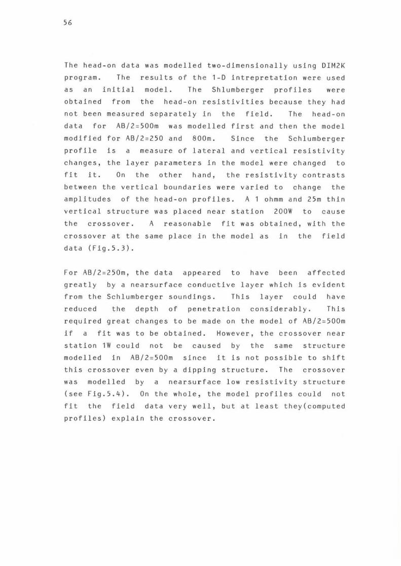
56

The head - on data was modelled two - dimensionally using DIM2K

program. The results of the 1-D intrepretatlon were used

as an initial model. The Shlumberger profiles were

obtained from the head-on resistivities because they had

not been measured separately in the field. The head-on

data for AB/2 ; SOOm was modelled first and then the model

modified for AB/2 =250 and aDOrn . SInce the Schlumberger

profIle is a measure of la t eral and vertical resistivity

changes, the layer parameters in the model were changed to

fit it. On the other hand, the resistivity contrasts

between the vertical boundaries were varied to change the

amplitudes of the head-on profiles. A 1 ohmm a nd 2Sm thin

vertical structure was placed near station 200W to cause

the crossover. A reasonable fit was obtained, with the

crossover at the same place 1n the model as in the field

data (Fig.5.3).

For AB/2 =250m, the data appeared to have been affected

greatly by a nearsurface conductive layer which is evident

from the Schlumberger soundings. This layer could have

reduced the depth of penetration considerably. This

required great changes to be made on the model of AB/2 =500m

if a fit was to be obtained. However, the crossover near

station 1W could not be caused by the same structure

modelled in

this crossover

was modelled

(see Fig.5.4).

AB/2 =500m since it is not possible to shift

even by a dipping structure. The crossover

by a nearsurface low resistivity structure

On the whole, the model profiles could not

fit the field data very well, but at least they(computed

profiles) explain the crossover.

FIELD DATA

HEAD-ON PROFILE HO.OLKARIA AB/2-2S0~ HN/2~24~

------

w y' E (~l :s:x, " \: s~o

Rho (Q.hul 10 AI ~~~

" ..

, , , , ,

, , , ,

10 J W, , E 500 500

-Rh. AC-IoII .

---Rho ~u

(Ohll..)

20

-20

1.1

Fig. 5.4 Head-on model for AB/2 =250m

." ~ ~ • • a

HEAD-ON PROFILE HO. OLKARIA AB/2 M 2S0 MN/2-2S~

I~-\ . ' , I \' \ , ~i ~_~

, .. w, I

11111 sQo ,I , " \~-~'-~'-'

Rho (Ohul .. "

"

"

E

10 J W, • E 500 SOO

1001 80 I~f ~ eo [if

" "

'" ,--T i

SOO SOO

Oisotlll'lc. (,,11

-Rh. u-..

---Rho .~ ..

(Oh ... )

"

,

-"

1.1

~

~

58

~ .~

• • " , " 0 "L ,

0 0 0 L L a a

I ~

, ~ , , , , , 0 x , , ~

, ~ , ~ , ~ , 0 • , a 0 ~ 0 ---z • 0 N , , 0 z ~ < ~ x • 0 ~ 0 ~ H ~ a • ,. ~ N ~ , ~ ~ ~ 0 ~

~ ". ~l! , 0 o 0 < < -a a

I , ,

• H a < ~ ~ , 0 ,

• 00 XO

~ .. ~N

H' ~z 0< • a

~ ~ , • 0 0 zo O~

0 , • ~ ON ~ .,

IT! ~ W~ ~ X~

" ,

--- ----, ,

f • 0

L • • • a

0 ,

~

, ~ , , , , , , , , , , , ,

----, , , ~

" '. 0 '< ",'

'0 -. 0

-" < • a

•

~ • • • 0 -

0 f-;-

-c-=-T

• g ~I g I ,. -

•

" • ,

~

~

0

,.~

• • •

• -

" "

o •

• • o 0 , • •

o

• 0 0 ., " N -CO

"" " 0 .... ~

~

." 0

• C 0 , ." ~ ~

:z: ~

~

'" ~ "-

59

The model obtained for AB/2 =800m is shown in Flg.(S.5).

Although th e model is no t bad, the crossover is s lightl y to

the west of the field data. The r esistivity and thickness

of the block und er station 300W had to be increased

considerably in order to shift the crossover from station

20QW towards station 100W as in the field data. A dipping

co ndu ctive dike was tried with no success. It is probable

that the crossover is indeed caused by the same low

resistivity structure as f or AB/2 =500m, but the shift to

the east is due to extremely high resistivity. This

apparent high resistivity could possibly have been created

by leakage curre nt s from the rig drilling near station 100W

at the time of the measurements. The part of the dike

below 2s0m was modelled slightly to the east of station

200W (see Fig.s.s) and this coul d not s hift the crossover

and is not signif icant. It is most prob able that the

structure is approximately vertical.

The interpreted mode l of the gravity data is shown in

Fig.(s.6). A 2- D gravity model was used assuming a

r egional of 2 . 0 g/ccm and an ano maly density of 2.3 g/ccm,

wh ich Is reasonable for rhyo l itic lavas in Olkaria. The

computed anomaly fits the field data well.

60

r.n JHO-HSP - 9000-M.M. ~e2 . 09, ' 14I-1S

GR AVITY ALONG RES ISTIV IT Y PROF ILE HO

OLKARIA. KENYA

, w

CL_~,fOIll HorizonTal scale

5.5 Discussion

oeSERVEC _

_COMPUTED

• •

Fig 5.6 Gravity model

-100

- 150

,

i z • • • • • , g

The model for AB/2=250m (Fig.5.4) is probably too venerable

to near surface inhomogeneities and the probing depth is

shallow due the conductive layer (about 10m thick) defined

by the sounding data. The crossover near station 100W is

caused by a shallow conductive material.

The AB/2 =500m model (Fig . S.3) is perhaps the most reliable

model. The

overestimated.

thicknesses of the layers are probably

The part of t he model east of station 100W

is comparable to the the gravity model, particulary the 90

ohmm layer.

crossover

resistivity.

at

The 1 ohmm resistivity zone causing the

station 200W has probably too low a

Because of equivalance, it could have higher

resistivity and the structure thinner.

61

The data for AB/2=800m (Fig.S.S) is rather unreliable

because the measurements must have been affected by leakage

currents generated by the rig operating at the time of

measurements thus creating a temporary high resistivity

zone near station 300W. However, provided the unreal i stic

150 ohmm layer at 300W is ignored, this model supports the

existence of the low resistivity structure as in the model

for AB/2 =SOOm.

The consistent denser mass of rock east of station 2E found

in gravity and resistivity models is probably a rhyo l itic

lava flow 100-1S0m thick. This continues to the south

where it outcrops. The structure between stations 10QW and

20QW is probably a rhyolite plug. Seemingly, the gravity

model does not support the presence of a fault near the

conductive structure causing the crossover at deeper

levels.

5.6 Conclusions

The head-on data from profile HO in Olkaria has been

two-dimensionally modelled. A vertical conductive narrow

zone at station 200W is responsible for the crossovers in

the head-on data. It is most likely that this structure is

the conduit of weak fumaroles that existed about 100m to

the north of of the resistivity profile probably in the

strike direction of the structure. This could also mean

that well 101 could not intersect the structure. More

head-on measurements to the south of profile HO are ,

therefore, necessary in order to confirm and trace this

structure further south before any other well is drilled in

this area. This work has clearly demontrated that i t is

possible to interpret the head-on data by two - dimes i onal

modelling. The task should seriously be undertaken to

interpret the rest of the data particulary that collected

across the main Ololbutot fault.

62

ACKNOWLEDGEMENTS

I wish to acknowledge the following persons: Brynjolfur

Eyjolfsson,who supervised the work in this report; Axel

Bjornsson and Ingvar B. Fridleifsson for their very active

part in the geothermal training and reading the manuscr i ptj

The lecturers at the United Nations University; 519urjon

Asbjornsson and So l veig Jonsdottir, who took care of us

during our stay in Iceland; All those people at the

National Energy Authority and Iceland as a whole, who

helped me in a great many ways.

The gravity data was collected with the assistance of Or

J.C.Swain of Unversity of Nairobi whom I owe special

gratitude .

I am grateful for the award of the United

Fellowship,1982.

Nations

The East African Power and Lighting Company,Kenya,gave me

the subertical leave whIch I would like to acknowledge.

Thanks to the United Nations Univeristy fellows for a

wonderful time together.

REFERENCES

Apparao,A.,Roy,A., and Mallick,K., 1969: ResistIvity model

experiments. Geoexploration, 7 , 45.

63

Beyer,J.H . , 1977 : Tellur i c and D.e. resistivity techn i ques

applied to the geophysica l investigation of Basin and

Range Geothermal Systems, Part 11: A numerica l study of

the dipole-dipole and Schlumberger resistivIty methods.

Ph.D. Thesis,LBL,6325 2/3 .

Bjornsson,A, 1981, Exploration and exploitation of

low - temperature geothermal fields for district heating

system in Akureyri, North Iceland.Geothermal Resources

Transactions,S, 495 - 498.

Bjornsson,A.and Saemundsson,K., 1975: Geothermal areas in

the vicinity of Akureyri.A report of the National

Energy Authority,Iceland. OSJ HD 7 55 7 (In Icelandic),

Browne,P.R. L., 198 1 : Petrographyic study of cuttings from

ten wells drilled at the Olkaria Geothermal field,

Kenya. Geothermal Institute of Auckland, NZ. A report

for Kenya Power Company.

Cheng,Y.W. ,1980: Location of nearsurface faults in

geothermal prospects by "combined head - on resistivity

profiling method " . Proceedings of the New Zealand

Ceothermal workshop, 1980, 163-166.

Dey,A, ,1976: Resistivity modelling for arbitrarily shaped

two-dimensional structures Part 11: User's guide to the

FORTRAN algorithm RESIS2D. LBL-5283.

Dey,A. and Morrison,H.F.,19 79: Resistivity modelling for

arbitrarily shaped two-dimensional structures.

Geophys.Prospect., 27,106 - 136.

64

Flovenz,O.G. and Eyjolfsson,B.,1981: ResistIvity soundings

an estimate of geothermal areas in Eyjafjordur.

National Energy Authority report, Iceland,

OS81029/JHD17 ( in Icelandic with English summary).

De Gery,J.C. and Kunetz,G.,1956: Potential and resistIvity

over dipping beds. Geophysics, 21,780-793.

Johansen,K,1977: A man/computer system for interpreting

resistIvIty soundings over a horizontal stratified

earth. Ceophys.Prospect., 25,667-691.

Koefoed,O.,1979: Geosounding Principles 1: Resistivity

sounding measurements. Elsevler, Amsterdam, 276.

Kenya Power Company,1980: Minutes for Scientific Review

Meeting 1 - 5 Dec., 1980. Unpublished Geothermal

Project report.

Lee,T.,1981: Direct interpretaion of resistivity data over

two-dimensional structures. Geophys.Prospect., 29,

462-469.

McPhar Geophysics,1967: Catalogue of resistivity and IP

model data. McPhar Geophysics Ltd., Ontario, Canada .

Naylor,W.I.,19 72: The geology of Eburru and Olkaria

geothermal prospects. Unpublished report for UNOP/EAPL

Geothermal Exploration Prospects.

Noble J.W.and Ojiambo,S.B.,1976: Geothermal Exploration in

Kenya. Second UN Geothermal Proc.,(Lawrence Berkeley

Lab., Calif.), 189 - 204.

Unz,M.,1953: Apparent resistivity curves for dipping beds.

Geophysics, 18, 116-137.

Van Nostrand,R.G. and Cook,K.L.,1956: Apparent resistivity

for dipping beds - a discussion. Geopysics, 20,140-147.

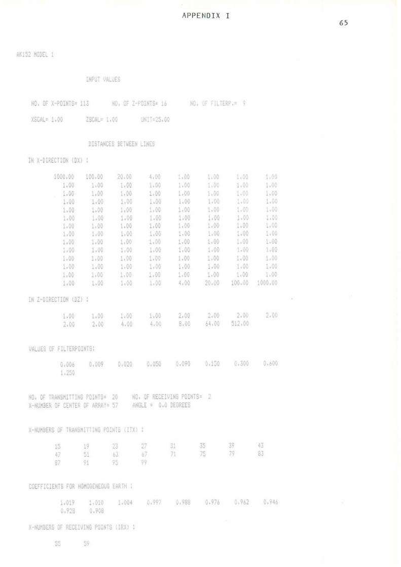
APPENDIX I

xsu.. o ! .00

r!STAhCE~ B, TWEEK ~INt~

I. X-DIREC'ION (DXi

1000.00 100.00 2C,OO 1.0, 1.00 1.00 !.Olo 1.0r 1.0v LOO 1. 00 : ,00 1.00 :.c ... 1.'.! • 00 .i..00 i. .00

: " 1.00 l.~

1 C. 1 • t .... 1.00 100 1 c; 1 • . . • . , 1.00 1.00 : .00 l.C .... 1 C. 1 00 1.00 1.1." , ...... ! 00 ~.OO 1 00

:~ Z~~IRECTION r~z)

1.00 1.00 : 00 2.00 :. JC ~.,o

iJA .... (S "F n~ "'ERr'J!NTS.

o 006 0 ;9 y t,.;,)

1 )

HO. TtAN.~lTT '''1.1 v~~TS~ 20 X· NU~BE" ( .. "Di t G AAAAY c;

~'IIO • 00 "\t~ 1.0 I 1 !, O~ 1 _, .,)

~ .00 .. 00 1, vC .

~. '\,I ,.t .. ~ .C~ , .00 : .00 1.00 .00 1.00 :.N ! ... J 1 ..... : 1.00 1.00 .. 00 :.i"J : .00 1.00 1.00 1.00 , ,00 : . .;,~ Lev "G~ ! ,('0 1.00 .. 00 • ,0 ~.oo 20.00

1.01..1 2.00 •• 00 ~.i10 3.00 !~ 00

.;. ,50 090 v. ~JO

NC. w' RE:Er'ylro~ rt~~TS- .. AHGU: 11 0.0 DEG?EES

X' NiJJ4.BEF:5 UI T AA.;.iI. T N." r1NT .. I'X

.. ., 4. .. ., B) 11

: 010 0.90B

, " ,.

.1 31 lS • ,.

"

1 00. , " y,"S8 .....9 6

. ..

••

• 1.00 1 QO 1 ( . , "IjO

.. ~ ;::'.00

300

" 71

o ,

1 • 1 0 • 01 1 •

f~

1 " I 00

'0 .

2

0·1.1'

• "

65

66

"

... ~'

--,

x

. " . . , . . '

"

APPENDIX II 67

, ='""".c. ~ ,

1~ • , ,

• , '.-_ ..

• .' I' ,

" r. ,

• ,

• ,

, , . .' , • 0' , • .. , • 0'

Leo,d [m] Leo,d [m]

ru QRl(USTOf"tlUN j. ".00." # .. -

........ .. 'Sl

0'

JAROVION~MSM.tELlNG ~ ~I:n_" _ _ ' ..

I jlla "" S,d ...

M" '"~ IS"''''' • ~ -"..il -, • -

• T T • ~

, ~ ,

E E ~ ~

c' -

< <

" '" > • .~ ;; 0

• ~ ~ < e , .~ .~

~ ~ c '

' ' , .. , " ,

, • ,

, 1\ " . 't-- - -

•

f..- " 2 I , . .. , .. , -• 0' , • , • o , • 0 '

Le ngd [m] Lengd [m]

68

~ " NO. ,

• ~ ,

,

• ,

• ,

• ~ , ,

• ~n: ,

, , 2 .. 10' 2 .. 0' , • .. , . O·

Lengd [m]

APP EN DI X II I PROFILE r~D , OLKIIP.III 69

HEIID - Oll DlImll IIR / 2=250n lHl/ 2=24n

ST nho lie Rho ~c Rho IIn

50017 76 . 0 50 . 7 63 . 4 40017 65 . 7 35 . 5 50 . 6 3001' 65 . 7 31.5 48 . 6 20017 56 . 8 32 . 4 44 . 6 10011 44.8 36 . 4 40 . 6 0 . 00 38 . 0 42 . 6 40 .3 lODE 32 . 4 43 . 9 38 . 2 200E 38 . 8 55 . 5 -· 7.2 300E 45 . 6 63 . 8 54 . 7 400£ '5 . 6 65 . 6 55 . 6 500E 42 . 8 65 . 2 54 . 0

IIB / 2=500n Htl/ 2=24n 500:: 57. 6 30 .1 43 . 6 40011 53 . 5 24 . 0 39 . 2 300\1 46 . 6 30 . 6 38 . 6 200'[; 36 . 7 36 .7 36 . 7 l oon 22 . 9 36 . 9 29 . 9 0 . 00 21 . 4 48 . 4 34 . 9 lO DE 21. 3 43 . 9 32 . 6 200E 20 . 4 46 . 6 33 . 5 300E 25 . 8 42 . 1 34 . 0 400B 34 . 3 51. 0 42 . 7 500E 35 . 7 44 . 9 40 . 3

118 / 2=80011 IlI'/ 2=1 00n 50011 0 . 4 25 . 9 34 . 7 400\: 51. 8 30 . 2 41. 0 3001-) 5C . 5 34 . 5 46 . 5 200H 55 . 5 32 . 6 M . l IOW 26 . 2 33 . 8 30 . 0 0 . 00 16 . 9 45 . 7 31. 3 lODE 15. 2 37.1 26 . 2 200E 19.8 34 . 6 27 . 2 300E 23.2 34 . 6 28.9 400B 26 . 4 43 .7 35 . 5 500E 30 . 6 52 . 3 41.5

70 OLKARIA G!'JWITY DATE, PROFILF I!D

CORR!:CTED Fon I'F.IGHTS ABOVE BOOn DE~TS ITY USED = 2 . 0 g/cliI eu . fTATI0tlS NA!lFD fly TPf.~IP" DI STN'fC['E; PRm~ STl\TI01! 0

S7ATlon 7 00\! 60 O\'! 50011 ~OOlT 3001'; 260lT 24011 2200 20011 1 80lT 16077 140ll 12011 100,') SOlT 60t-7 4011 o l ODE 200E 300E ~OOE 500E 600E 700E

LrWEL~) ( m) 19 90 . 2'.8 1990 .1 85 1990 . 225 1990 . 140 1991. 868 1991 . 019 1908 . 293 1906 . 952 1 986 . Gee 1986 .1 02 1985 . 394 1985 . 024 1904 . 569 1 9C4 . 4~8 1984 . 239 1984 . 059 1983 . 797 1903 . 1'4 1981.474 1970 . 514 1974 . 90 1 1971.071 1970 . 146 1968 . 616 1 9GG . 956

HE I GllTS ( n ) 90 . 248 90 .1 85 90 . 225 90 . 140 91. 868 91 . 019 80 . 293 86 . 952 86 . 688 86 . 102 05 . 394 85 . 024 84 . 569 S4 . ~48 84 . 239 84 . 059 83 . 7 97 83 . 14 4 81 . 4 7 ~ 78 . 514 7 ~ . 90 1 71. 071 70 . 146 60 . 616 6[ • ge6

GP-V . ( g u)

455 . 6 455 . 5 455 . 7 455 . 9 ~53 . 6 456 . 5 ~6il .l 46 7 . 6 468 . 1 ~69 . 5 471. 0 472 . 5 472 . 7 ~ 7 3 . 5 473 . 7 473 . 45 473 . 3 474 . 3 ~ 7 9 . 5 ~e8 . 4 500 . 5 512 . 4 516 . 2 512 . 0 526 .1

DRIP. Cl' 453 . 7 453 . 6 453 . 9 451] . 1 '51. 9 454 . 8 462 . 5 466 . 0 1,66 . 6 460 . 0 469 . 5 ~71 . 1 47 1.3 "72 . 1 472 . ~ 472 . 15 472 . 0 473 . 1 ~77. 7 486 . 6 490 . 8 51 0 . 8 514 . 7 519 . 6 5~<1 . 8

(h"2. 248 ) 202 . 9 202 . 7 202 . 8 202 . 6 206 . 5 201, . 6 1 98 .5 195 . 5 19~ . 9 193 . 6 192 . 0 191 . 1 190 . 1 189 . 8 IB9 . ~ 189.0 lAB . " 186 . 9 183 . 2 17 6 . 5 lOP . 4 159 . 8 157 .7 15~ . 2 150 . 5

F. . A ( gu ) 656 . 6 656 . 3 656 . 7 656 .7 658 . 4 659 . 4 661. 0 661.5 661.5 661. 6 661.5 6G2 . 2 6f,1.4 661. 9 661.8 661. 2 660 . 4 660 . 0 660 . 9 600 . 1 667 . 2 670 . 6 672 . ~ 673 . 8 675 . 3

APPENilIX IV

,

•

• E ~ ,

le nqd [m]

~ .'~------+-----~------i-----~ • .. ": .. • ~ • ~.·t------+-~~-i-------r------

" • , " • E

~,

· E . 'l " > • ;; ~ • , -~

~ .. , •

,

,

• , ,

• ,

• , ,

• ,

•

.

1---

".0

-.' • "

71

[ljOAMVS TOfNVN .' -- 0 - ...... !>

JAROVION.b.MSM~lING H!IItI.U '" ." --. ,.K,. = "

~'OJ< :::&I . -= """" ! • ,-.. ~.1I . 1,,_.

r --

.

. , , -. .., .. , . " Leo,d [m)

~ LING~

J

,

• 2 4 10' 2 • .. , . .., . Leo,d [m) L",d [m)

72

"Bi I I ,

I • ~ ,

• ,

• ,

• "" ,

•

2_ 10' 24 10' 2410'2 • c'

LenQd {m]