1

Tutorial 1A: Using CHAID to Profile LatentClass SegmentsIn Latent GOLD Choice Tutorial #1, 3 LC segments were obtained. The Importance output is one way toexamine differences between these segments. As shown below, the first LC segment, mostly valuesFASHION over QUALITY, while the reverse is true for LC segment #2. LC segment #3 values bothFASHION and QUALITY about the same, and all are equally price sensitive. In addition, segment #1 wasmost likely to choose the ‘None’ option, when presented with the different choice alternatives. Thesepatterns adequately reflected the assumed utility structure that was used to generate the data.

Figure 1. Importance Output

The Classification Table shows how well the modal assignment rule reproduces the actual (probabilistic)LC segments, the latter based on the model parameters. The large quantities in the diagonal table entriesindicate that overall, the modal class assignment does quite well. Only a small number ofmisclassifications are shown in the off-diagonal cells.

Note that overall, the modal classifications do not reproduce perfectly the marginal distribution of theclasses. For example, of the 400 cases, 201.4323 (50.36%) would be expected to be in class #1. Using themodal classification, 204 cases are so classified.

Figure 2. Classification Table

2

It is also useful to profile the LC segments in terms of exogenous variables (covariates). The CHAIDoption for doing this utilizes the posterior membership probabilities as weights and hence will reproducethe actual (Probabilistic, not Modal) classes. Thus, the CHAID approach has zero misclassification error.

Growing the CHAID Tree

SI-CHAID consists of 2 programs, called ‘CHAID Define’ and ‘CHAID Explore’. Typically, the Defineprogram is used first to set the analysis options and then the Explore command is executed to perform theCHAID analysis.

In this tutorial, we will first use the Explore program with the default settings in the .chd file generated intutorial #1, to examine demographic profiles associated with all 3 segments, in a way that is somewhatanalogous to a 3-group discriminant analysis. We will then use the Define program to examinedemographic profiles associated with each segment (vs. the others), one at a time.

Ø Open SI-CHAID Explore

Ø File Open ‘Tutor 1a.chd’

Figure 3. Root Node for Tutor1a.chd

The root node of the tree appears, with the overall sizes of the 3 LC segments.

Ø From the Tree menu, select Auto.

3

Figure 4. Tree Diagram after Auto

The CHAID analysis first splits on SEX, then on AGE, resulting in 6 demographic segments.

To examine the significance associated with these predictors at the root node of the tree,

Ø From the Tree menu, choose Select

Figure 5. Select Predictor Dialog Box

4

We see that both SEX and AGE are highly significant. For example, for SEX, p=4.7 x 10-24. Also, forAGE, the 3 categories are all significantly different from each other, as indicated by a space between each(“1 2 3”), and thus none of these categories would be combined in growing the first level of the tree.

Note that these p-values indicate that the relationships between these covariates and the segments arestronger than those indicated by the Wald tests in the Parameters output. That is because the LC variable istreated as an observed variable in CHAID; the posterior membership probabilities are treated as fixedweights, with no error.

To reproduce the Profile output tables obtained from Latent GOLD Choice

Ø From the Windows menu, select New TableØ Right click on the table to retrieve the Table Display PanelØ From the Cell format section select ‘Column Percents’Ø From the Contents section select ‘Before Merge’Ø From the Predictors section, select ‘All’ to display both tables

Figure 6. Tables for SEX and AGE with Table Display Panel

5

We see for example, that segment 1 (labeled ‘CLU#1), has a higher percentage of the youngest (AGE = 16-24) and the highest percentage female of the 3 segments.

Next, we will use the SI-CHAID Define program to change the default options to develop a separate profilefor this segment vs. the other 2.

Using CHAID to Profile Segment 1 vs. Others

Ø Open the CHAID Define program.

From the File Menu

Ø Select ‘Open’ ‘Tutor 1a.chd’

The default settings are displayed in the Contents Pane

Figure 7. Default Settings for Tutor 1a.chd in the CHAID Define program.

Ø Double click on Model1 to open the Analysis Dialog box

6

Figure 8: The Analysis Dialog Box

Notice that a checkmark appears next to the ‘Dep Prob’ box. This indicates that posterior membershipprobabilities are used to specify the categories of the dependent variable. For this 3-class model, theposterior probabilities obtained from Latent GOLD Choice are labeled ‘CLU#1’, ‘CLU#2’ and ‘CLU#3’.Only CLU#1 is visible in the Dependent box.

Ø In the Dependent box, scroll down to display all three variablesØ Select ‘CLU#2’ and ‘CLU#3’ and click the Dependent Box to restore them to the Variables List box

7

Figure 9. CLU#2’ and ‘CLU#3 restored to the Variables List Box

Ø Click to add a Checkmark to the ‘Other’ box. This tells SI-CHAID to create a second category for thedependent variable consisting of all other categories – in this case, categories for classes 2 and 3.

To grow the tree:

Ø Click ‘Explore’

CHAID prompts you to save the updated definition file named Model1.chd (the default name)

8

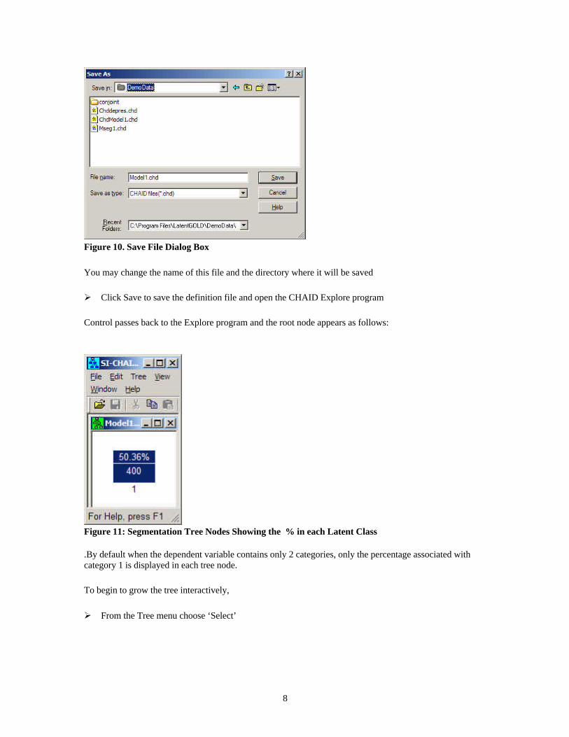
Figure 10. Save File Dialog Box

You may change the name of this file and the directory where it will be saved

Ø Click Save to save the definition file and open the CHAID Explore program

Control passes back to the Explore program and the root node appears as follows:

Figure 11: Segmentation Tree Nodes Showing the % in each Latent Class

.By default when the dependent variable contains only 2 categories, only the percentage associated withcategory 1 is displayed in each tree node.

To begin to grow the tree interactively,

Ø From the Tree menu choose ‘Select’

9

Figure 11. Select Predictor Dialog Box

Now we see that AGE is more significant than SEX for distinguishing LC segment 1 from the others. Inaddition, we see that CHAID has combined age levels 2 and 3 because they are not significantly different inpredicting the probability of being in LC segment 1.

Ø Click the OK button to use AGE for the first split

Figure 12. Tree Diagram after selecting AGE as first split

As was suggested earlier, the primary difference between segment 1 and the others is that this segmentcontains a much higher percentage of the youngest age range (aged 16-24). The tree indicates that amongthis youngest group (node 1), 76% are in segment 1, compared to only 28% of the older respondents (node2).

Ø To continue the analysis of the youngest respondents in interactive mode:

10

Ø Click on node 1 to make it activeØ From the Tree menu choose ‘Select’Ø Select OK to split on SEX

Your tree now looks like this:

Figure 13. Tree Diagram after selecting SEX in Node 1

We see that 85.73% of young females (AGE = 1, SEX = 2) are in LC segment 1.

Ø Click on the node corresponding to the other categories of AGE (node 3) to make it activeØ From the Tree menu choose ‘Select’Ø Select OK to split on SEX

Our final tree now looks like this:

11

Figure 14. Tree Diagram after selecting SEX in Node 3

Thus, only 4 demographic segments are required to profile segment 1 vs. the others.

We can repeat these steps to obtain separate profiles for LC segments 2 and 3.