Journal of Asian Scientific Research, 2014, 4(1): 14-27

14

TUNED SIMULATED ANNEALING BASED ON BOLTZMANN AND BOSE-

EINSTEIN DISTRIBUTION APPLIED TO MAXSAT PROBLEM

Juan Frausto-Solis

Ernesto Liñán-García, Guillermo Santamaria-Bonfil

ABSTRACT

In this paper, a hybrid Simulated Annealing algorithm using Boltzmann and Bose-Einstein

Distributions (SABBE) is proposed. SABBE was designed for solving satisfiability (SAT) instances,

and it has three phases: i) BP (Boltzmann Phase), ii) BEP (Bose-Einstein Phase), and iii) DEP

(Dynamical Equilibrium Phase). BP and BEP are simulated annealing searching procedures based

on Boltzmann and Bose-Einstein distributions respectively. BP ranges from high to low

temperature values, while BEP goes from low to very low temperatures. Another simulated

annealing search procedure, DEP, is applied at the final temperature of the second phase.

However, DEP uses a particular heuristic for detection of stochastic equilibrium by employing a

least squares method during its execution. Finally, SABBE parameters are tuned with an analytical

method, which considers the maximal and minimal deterioration of SAT instances.

Keywords: C630 - Computational Techniques, Simulated Annealing, Heuristic Algorithms.

1. INTRODUCTION

Satifiability problem (SAT) plays a significant role in combinatorial optimization and

computational complexity theory. It is well known that SAT is NP-Complete (Cook, 1971), and

any instance of an NP problem may be converted to a SAT instance. Thus, any efficient algorithm

for SAT problem might be used for solving other NP-Complete problems. In this paper, a particular

SAT problem known as MaxSat is boarded. The goal of MaxSat is to maximize the number of

clauses of a boolean formula. Satisfiability problem consists in finding a truth assignment such that

it satisfies a well formed arbitrary boolean expression (Garey and Johnson, 1979). Usually, any

SAT instance is in the Conjunctive Normal Form (CNF). A SAT (or MaxSAT) instance is defined

as follows: a) a set of m clauses: C1, C2,…Cm, b) a set of n variables x1, x2,..,xn, and c) a set of

literals, where a literal is a variable or a negation of it. MaxSAT can be solved by several efficient

algorithms as Simulated Annealing (SA) (Spears, 1996; Neuhaus et al., 2011), Genetic Algorithms

(Dejong and Spears, 1989; Munawar et al., 2009), Neural Networks (Abdechiri and Reza-Meybodi,

2011) (Spears, 1993), Guided Local Search (Mills and Tsang, 2000), Swarm optimization (Layeb,

2010), Extreme optimization (Menai and Batouche, 2002; 2003; Zeng et al., 2011), and so on. SA

Journal of Asian Scientific Research

journal homepage: http://aessweb.com/journal-detail.php?id=5003

Journal of Asian Scientific Research, 2014, 4(1): 14-27

15

has shown to be very efficient for solving combinatorial optimization problems, specifically the

SAT problem. SA is a heuristic algorithm, which has shown a high performance solving SAT

instances in a reasonable processing time (Frausto-Solis and Martinez-Rios, 2008).

In order to obtain high quality solutions efficiently, our approach tunes SA parameters using an

analytical method (Sanvicente and Frausto-Solís, 2004) for determining system temperature and the

length of the Markov Chain of the Metropolis Cycle (MC). This technique establishes the

temperature values based on maximum and minimum deterioration of a SAT instance. In order to

enhance exploration process of the solution space and avoid local optima, Boltzmann and Bose-

Einstein distribution are applied by the SABBE algorithm. Boltzmann distribution is used at high

temperatures, and Bose-Einstein distribution is used at low temperatures. As a means to reduce

system temperature, two different cooling schemes are employed.

This paper is organized as follows: Section 2 describes the classic Simulated Annealing

algorithm. Section 3 explains the analytical tuning method, and section 4 introduces SABBE

algorithm. Finally section 5 presents the experimental results, and paper conclusions are explained

in section 6.

2. SIMULATED ANNEALING ALGORITHM

In this section, classical Simulated Annealing is briefly described; we discuss how this

algorithm uses the Boltzmann distribution in order to accept poor quality solutions and escape from

local optima. Later, Bose-Einstein distribution is described, and the new algorithm based on

Boltzmann and Bose-Einstein distribution is introduced

2.1. Classical Simulated Annealing

Simulated Annealing (SA) algorithm based on Boltzmann Distribution was introduced in the

combinatorial optimization area by Kirkpatrick (Kirkpatrick et al., 1983), and (Cerny, 1985).

Boltzmann distribution is fundamental for statistical mechanics, and it is defined by the assumption

that all particles are distinguishable, and all possible energy divisions occur with the same

probability. Simulated Annealing can find optimal or near-optimal solutions of a specific

combinatorial optimization problem. SA randomly explores the solution space of a specific

instance, while an objective function is maximizing (or minimizing). Therefore, SA is an

approximation algorithm for finding the global optimum. For the MaxSAT problem, the ideal

solution is obtained when all clauses are satisfied. SA approach always accepts better solutions.

However, when a new solution does not improve the previous one, it is accepted or rejected in

accordance to the Boltzmann distribution (1). This function is related to the difference of energy

between two solutions (Si and, Sj), and the current temperature value.

( ) (1)

Where )( EP is the solution probability acceptance, E is the energy difference between Si

and Sj solutions, and T is the current temperature value. SA is composed by two cycles: The

Journal of Asian Scientific Research, 2014, 4(1): 14-27

16

external cycle which diminish the temperature, and the internal Metropolis Cycle (MC) which

explores solution neighborhood by using a distribution function in accordance to the current system

temperature. Boltzmann distribution function is applied in MC to examine the space of solutions in

a neighborhood for a given temperature. According to the classical thermodynamics properties at

high temperatures the probability to change between two energy states is very high. Therefore, the

probability of accepting bad solutions at very high temperatures can be taken as number close to

one. However, as the system is cooled, this probability decreases towards zero.

2.2. Simulated Annealing Based on Bose-Einstein Distribution

Statistical mechanics consists of a set of methods to analyze the properties of large numbers of

atoms in the physical environment. The systems modeled by these mechanics contain very large

quantities of atoms, therefore only the most probable behavior of the system in thermal equilibrium

at a given temperature is observed (Eisberg and Resnick, 1985). In classical physics particles obey

Maxwell-Boltzmann distribution; nevertheless quantum particles, like Bosons and fermions, are

expressed by a different behavior. While bosons tend to overlap at the same energy level following

a Bose-Einstein distribution, only one fermion can occupy an energetic state. If we compare bosons

with classical particles at very high temperatures or a high density system, Bose–Einstein becomes

Maxwell–Boltzmann statistics. Nevertheless at low temperatures, bosons behave differently from

other particles and tend to congregate at the same lowest-energy state, the result is known as a

Bose–Einstein condensate (Cornell and Wieman, 2001). Thus, bosons and classical particles

behavior is totally different at low temperatures. Therefore, the hypothesis explored in this paper is

that Simulated Annealing Algorithm applying both Boltzmann and Bose-Einstein distributions for

accepting bad solutions for high and low temperatures will enhance SABBE performance

(promoting a fast quality convergence at low temperatures) over the classical Simulated Annealing

based exclusively on Boltzmann distribution. Bose-Einstein distribution is given by equation (2).

11

)()/(

KTEee

Eh

(2)

Where T is the temperature parameter, is the total bosons in the system and k is the

Boltzmann's constant. Notice that (2) becomes Boltzmann distribution when is equal to one. The

use of this distribution as acceptance criteria is detailed in section 3.

3. ANALYTICAL TUNING METHOD In this section, we firstly describe the tuning method used in this paper. Secondly, the process

to determine the length of the Markov chain is shown.

3.1 Setting Initial and Final Temperatures

The parameters of SABBE are tuned by an analytical method (Sanvicente and Frausto-Solís,

2004; Frausto-Solis and Martinez-Rios, 2008; DongYoub and Wexler, 2011). This computation is

based on the deterioration (maximal and minimal) of the SAT instances, and the acceptance

probability of solutions. As mentioned before, probability for accepting any new solution is close to

one at high temperatures; consequently, the cost function deterioration is maximal. Thus, the initial

temperature T0 is associated with the maximal deterioration ΔZmax. On the other hand, the

Journal of Asian Scientific Research, 2014, 4(1): 14-27

17

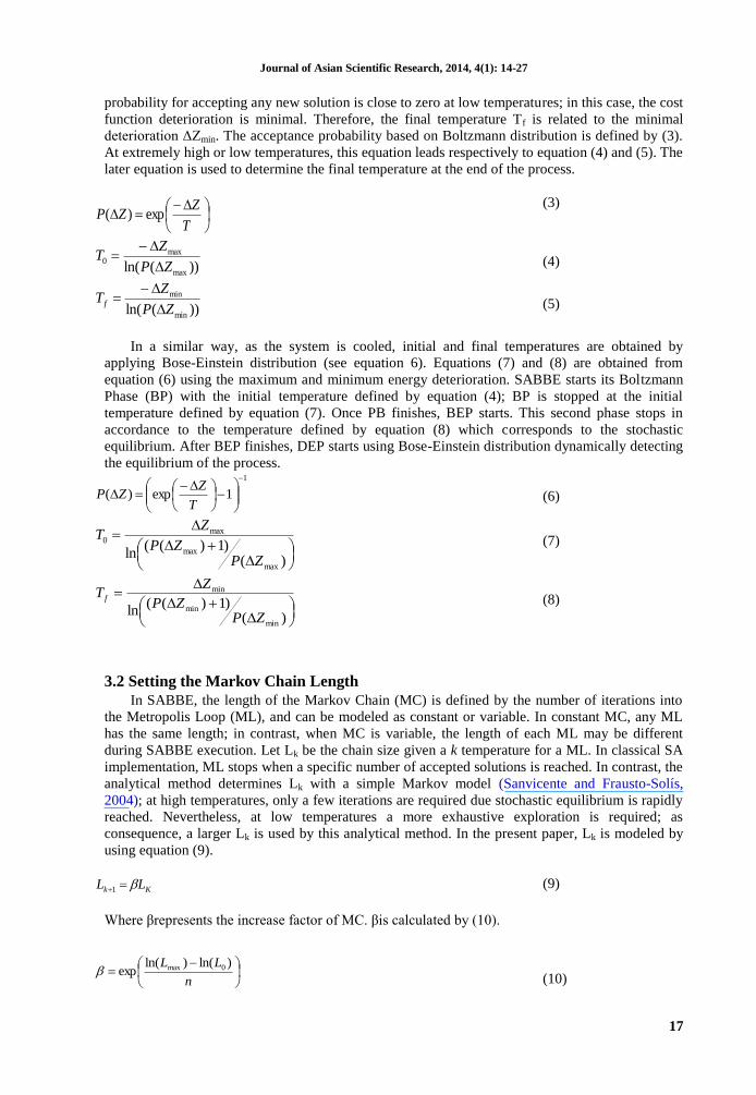
probability for accepting any new solution is close to zero at low temperatures; in this case, the cost

function deterioration is minimal. Therefore, the final temperature Tf is related to the minimal

deterioration ΔZmin. The acceptance probability based on Boltzmann distribution is defined by (3).

At extremely high or low temperatures, this equation leads respectively to equation (4) and (5). The

later equation is used to determine the final temperature at the end of the process.

T

ZZP exp)(

(3)

))(ln( max

max0

ZP

ZT

(4)

))(ln( min

min

ZP

ZTf

(5)

In a similar way, as the system is cooled, initial and final temperatures are obtained by

applying Bose-Einstein distribution (see equation 6). Equations (7) and (8) are obtained from

equation (6) using the maximum and minimum energy deterioration. SABBE starts its Boltzmann

Phase (BP) with the initial temperature defined by equation (4); BP is stopped at the initial

temperature defined by equation (7). Once PB finishes, BEP starts. This second phase stops in

accordance to the temperature defined by equation (8) which corresponds to the stochastic

equilibrium. After BEP finishes, DEP starts using Bose-Einstein distribution dynamically detecting

the equilibrium of the process. 1

1exp)(

T

ZZP

(6)

)()1)((

lnmax

max

max0

ZPZP

ZT

(7)

)()1)((

lnmin

min

min

ZPZP

ZT f

(8)

3.2 Setting the Markov Chain Length

In SABBE, the length of the Markov Chain (MC) is defined by the number of iterations into

the Metropolis Loop (ML), and can be modeled as constant or variable. In constant MC, any ML

has the same length; in contrast, when MC is variable, the length of each ML may be different

during SABBE execution. Let Lk be the chain size given a k temperature for a ML. In classical SA

implementation, ML stops when a specific number of accepted solutions is reached. In contrast, the

analytical method determines Lk with a simple Markov model (Sanvicente and Frausto-Solís,

2004); at high temperatures, only a few iterations are required due stochastic equilibrium is rapidly

reached. Nevertheless, at low temperatures a more exhaustive exploration is required; as

consequence, a larger Lk is used by this analytical method. In the present paper, Lk is modeled by

using equation (9).

Kk LL 1 (9)

Where βrepresents the increase factor of MC. βis calculated by (10).

n

LL )ln()ln(exp 0max

(10)

Journal of Asian Scientific Research, 2014, 4(1): 14-27

18

Let L1 be Lk at T0, Lmax be the maximum MC length, and n is the number of times that the

temperature will be decreased during the algorithm. System temperature is reduced using a cooling

scheme, such as, (11) or (12).

17.0,...;1,01 kTT kK (11)

17.0,...;1,01

kTeT kK (12)

Whether cooling function (11) is applied, n is calculated by equation (13). Thus, if cooling function

(12) is used, n is obtained by equation (14).

)ln(

)ln()ln( 0

TTn

f

(13)

)ln()ln( 0TTn

f

(14)

4. SABBE ALGORITHM

As mentioned before, SABBE is a hybrid algorithm which has three phases (see Figure 1): i)

Boltzmann Phase (BP) from high to low temperatures, ii) Bose-Einstein Phase (BEP) from low to

very low temperatures, and iii) Dynamical Equilibrium Phase (DEP). For accepting bad solutions,

BP and BEP apply Boltzmann and Bose-Einstein distributions respectively. This is performed in

order to escape from local optima. DEP is a kind of BEP extension, where the stochastic

equilibrium is detected in a dynamical way. This is done by using a regression method into the

metropolis cycle; the number of iterations is considered as the independent variable, while each

energy value represents the dependent variable. The criteria used to find equilibrium is the slope of

the energy function of the metropolis cycle. Figure 2 shows the BP pseudo code. During each phase

depicted in figure 1, better solutions are always accepted. On the other hand, worse solutions are

accepted or rejected in accordance to an acceptance function. The length of the Markov chain (i.e.

the internal cycle length) for each MC is determined by equation (9), where the increment factor β

is calculated by equation (10). In Figure 3, BEP and DEP pseudo code are shown. In BEP, the

external cycle decreases temperature accordingly to cooling function (11) or (12). The metropolis

cycle length is constant and equal to the maximum length of last metropolis cycle of BP.

Journal of Asian Scientific Research, 2014, 4(1): 14-27

19

Fig- 1. SABBE phases

Fig- 2.BP pseudo code.

BP()

Begin

T = value calculated by equation (4)

n = value calculated by equation(13)or(14)

Si = Create_initial_solution()

i = 1

While (i < n) do

k = 1

while (k<=CM) do

Journal of Asian Scientific Research, 2014, 4(1): 14-27

20

For practical reasons DEP is considered as a third phase. DEP goal is to detect system energy

equilibrium by analyzing the energy slope between two solutions in accordance to an objective

function. Let define xi as the iteration number for the metropolis cycle (1, 2,..., n), and E i as the

current energy (number of satisfied clauses) found by the algorithm in iteration xi. Using a standard

least squares method, the slope for n iterations is defined by equation (15).

n

i

n

i

ii

n

i

i

n

i

i

n

i

ii

xxn

ExExn

m

1

2

1

2

111

(15)

The former formula becomes

nnK

nnKwhereEKiEKm

n

i

n

i

ii

2231

1 1

21

6;

12

(16)

Notice that the complexity of computing equation (16) is O(n) because both of the summations

are computed using a simple data structure (as is shown in Fig. 3), and K1 and K2 are only constants

for a particular n value.

Fig- 3.BEP/DEP Pseudo code.

BEP()

Begin

T = equation (7)

Tfinal = equation (8)

While (T >Tfinal) do

k = 1

while (k<=CM) do

Sj = perturbate_system(Si)

If E(Sj)=total_clausule then stop()

ΔE= Ej – Ei

If (ΔE ≥0) then

Si = Sj

ElseIf ((1/(exp(ΔE/T)-1))[0,1])then

Si = Sj

End if

K = k + 1

end while

T = α*T or T = e-α*T

End while

End

DEP()

Begin

While (m≈0)do

n = 1

while (k<=CM) do

Sj = perturbate_system(Si)

If E(Sj)=total_clausule then stop()

ΔE = Ej – Ei

If (ΔE ≥0) then

Si = Sj

ElseIf ((1/(exp(ΔE/T)-1))[0,1])then

Si = Sj

End if

n = n + 1

∑iE=∑iE + n*Ei

∑E=∑E + Ei

end while

T = α*T or T = e-α*T

k1=12/(n^3-n)

k2=6/(n^2+n)

End while

End

5. EXPERIMENTAL RESULTS & DISCUSSION

SABBE algorithm was tested with 36 SAT instances taken from the 2009 SAT competition1

which are shown in Table 1. These instances are grouped by their ρ value (number of

1 SAT Competition, 2009. Satcompetition.Org. Available from http://www.satcompetition.org/2009.

Journal of Asian Scientific Research, 2014, 4(1): 14-27

21

clauses/number of variables) between 2.07 to 4.25. The temperature ranges for Boltzmann and

Bose-Einstein Phases were calculated by applying equations (4), (5), (7), and (8). Table 2 shows

the values for T0 for Boltzmann Phase, as well as T0 and Tf for Bose-Einstein Phase. Observe that

Tf for all instances is equal to 0.68 with the minimum deterioration equal to one; P(ΔZmin) was

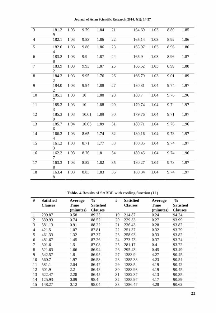
taken as 0.3. Table 3 shows n and β parameters for these instances. Results obtained applying the

cooling function (11) and (12) are shown in Table 4 and 5 respectively. The number of satisfied

clauses, average time (minutes), and percentage of satisfied clauses are included in these tables.

The mean percentage of satisfied clauses is 90.70% (with 1.81 minutes of executing time), and

89.4868 (with 0.1732 minutes) respectively. Whether only satisfiable instances are evaluated, these

figures are 88.71% and 87.4269%.

6. CONCLUSIONS

SABBE algorithm is proposed in this paper. This algorithm can generate high quality solutions

for SAT instances. The obtained results show that applying Boltzmann and Bose-Einstein

distributions along with a Dynamical Equilibrium heuristic provide a good method for solving SAT

instances. SABBE is a hybrid algorithm based on two acceptance distribution functions; these

improve SA exploration capacity of solution space by exploiting bosons behavior at low

temperatures, altering the acceptance probability of bad solutions in relation to system’s

temperature. In addition, the processing time required to find an optimal or near-optimal solution is

reduced applying a tuning process over the SA parameters (i.e. number of Metropolis cycles) and

the Dynamical Equilibrium heuristic. The processing cost required for these techniques is

polynomial. Experimentation show that when simulated annealing is executed with both

distribution functions at different temperature levels along with DEP, solutions quality is improved

over the classical SA with only the Boltzmann distribution function.

Table- 1.Instances tested

# Name C V SA

T

# Name C V SA

T

1 sat-140-

100

336 140 2.

4

Y 19 unsat-109-100 228 109 2.09 N

2 sat-160-

100

384 160 2.

4

Y 20 unsat-115-100 244 115 2.12 N

3 sat-180-

100

432 180 2.

4

Y 21 unsat-121-100 252 121 2.08 N

4 sat-200-

100

480 200 2.

4

Y 22 unsat-127-100 268 127 2.11 N

5 sat-220-

100

528 220 2.

4

Y 23 unsat-133-100 276 133 2.08 N

6 sat-230-

100

552 230 2.

4

Y 24 unsat-139-100 292 139 2.1 N

7 sat-240-

100

576 240 2.

4

Y 25 unsat-145-100 300 145 2.07 N

8 sat-250-

100

600 250 2.

4

Y 26 unsat-151-100 316 151 2.09 N

9 sat-260- 624 260 2. Y 27 V360-c1530- 153 360 4.25 Y

Journal of Asian Scientific Research, 2014, 4(1): 14-27

22

100 4 S144043535-002 0

10 sat-270-

100

648 270 2.

4

Y 28 V360-c1530-

S368632549-051

153

0

360 4.25 Y

11 sat-280-

100

672 280 2.

4

Y 29 V360-c1530-

S722433227-030

153

0

360 4.25 Y

12 sat-290-

100

696 290 2.

4

Y 30 V360-c1530-

S1293537826-039

153

0

360 4.25 Y

13 sat-300-

100

720 300 2.

4

Y 31 V360-c1530-

S1448866403-060

153

0

360 4.25 Y

14 unsat-61-

100

132 61 2.

16

N 32 V360-c1530-

S1459690542-033

153

0

360 4.25 Y

15 unsat-73-

100

156 73 2.

14

N 33 V360-c1530-

S1684547485-073

153

0

360 4.25 Y

16 unsat-85-

100

180 85 2.

12

N 34 V360-c1530-

S1711406314-093

153

0

360 4.25 Y

17 unsat-97-

100

204 97 2.

1

N 35 V360-c1530-

S1826927554-087

153

0

360 4.25 Y

18 unsat-

103-100

220 103 2.

14

N 36 V360-c1530-

S2032263657-035

153

0

360 4.25 Y

Table- 2.Initial and final temperatures for tested instances

# T0 BP T0 BEP TfBEP # T0 BP T0 BEP Tf BEP

1 8009.68 115.92 0.68 19 3741.17 50.99 0.68

2 8795.73 123.08 0.68 20 3847.3 56.72 0.68

3 9067.69 128.71 0.68 21 3870.52 59.01 0.68

4 9455.74 134.92 0.68 22 3960.07 56.15 0.68

5 9721.07 141.03 0.68 23 4132.53 58.72 0.68

6 10046.1 141.8 0.68 24 4119.27 60.73 0.68

7 10377.76 143.37 0.68 25 4251.93 59.3 0.68

8 10540.28 144.61 0.68 26 4311.63 62.16 0.68

9 10434.14 148.34 0.68 27 8626.58 116.3 0.68

10 11067.62 151.39 0.68 28 8799.04 134.35 0.68

11 11100.79 158.84 0.68 29 8377.83 115.44 0.68

12 11190.34 158.89 0.68 30 8384.46 113.15 0.68

13 11405.92 154.35 0.68 31 8487.28 125.18 0.68

14 3081.16 42.11 0.68 32 8560.25 122.6 0.68

15 3240.36 46.41 0.68 33 8643.16 122.32 0.68

16 3419.45 49.27 0.68 34 8686.28 125.18 0.68

17 3618.45 52.14 0.68 35 8606.68 123.46 0.68

18 3638.35 52.42 0.68 36 8636.53 119.74 0.68

Table- 3.n and parameters for every tested instance

Cooling

function (11)

Cooling

function (12)

Cooling

function (11)

Cooling

function (12)

# n

value value

n

value

β

value

# n

value

β

value

n

value

β

value

1 178.8

7

1.03 9.66 1.82 19 164.03 1.03 8.86 1.84

2 180.6

9

1.03 9.76 1.83 20 164.57 1.03 8.89 1.84

Journal of Asian Scientific Research, 2014, 4(1): 14-27

23

3 181.2

9

1.03 9.79 1.84 21 164.69 1.03 8.89 1.85

4 182.1 1.03 9.83 1.86 22 165.14 1.03 8.92 1.86

5 182.6

4

1.03 9.86 1.86 23 165.97 1.03 8.96 1.86

6 183.2

8

1.03 9.9 1.87 24 165.9 1.03 8.96 1.87

7 183.9

2

1.03 9.93 1.87 25 166.52 1.03 8.99 1.88

8 184.2

2

1.03 9.95 1.76 26 166.79 1.03 9.01 1.89

9 184.0

2

1.03 9.94 1.88 27 180.31 1.04 9.74 1.97

10 185.1

7

1.03 10 1.88 28 180.7 1.04 9.76 1.96

11 185.2

3

1.03 10 1.88 29 179.74 1.04 9.7 1.97

12 185.3

9

1.03 10.01 1.89 30 179.76 1.04 9.71 1.97

13 185.7

6

1.04 10.03 1.89 31 180.71 1.04 9.76 1.96

14 160.2

4

1.03 8.65 1.74 32 180.16 1.04 9.73 1.97

15 161.2

3

1.03 8.71 1.77 33 180.35 1.04 9.74 1.97

16 162.2

7

1.03 8.76 1.8 34 180.45 1.04 9.74 1.96

17 163.3

8

1.03 8.82 1.82 35 180.27 1.04 9.73 1.97

18 163.4

8

1.03 8.83 1.83 36 180.34 1.04 9.74 1.97

Table- 4.Results of SABBE with cooling function (11)

# Satisfied

Clauses

Average

Time

(minutes)

%

Satisfied

Clauses

# Satisfied

Clauses

Average

Time

(minutes)

%

Satisfied

Clauses

1 299.87 0.58 89.25 19 214.87 0.24 94.24

2 339.93 0.74 88.52 20 229.33 0.27 93.99

3 381.13 0.91 88.22 21 236.43 0.28 93.82

4 421.5 1.07 87.81 22 251.37 0.32 93.79

5 461.33 1.32 87.37 23 258.93 0.33 93.82

6 481.67 1.45 87.26 24 273.73 0.37 93.74

7 501.6 1.5 87.08 25 281.17 0.4 93.72

8 521.63 1.66 86.94 26 295.43 0.45 93.49

9 542.57 1.8 86.95 27 1383.9 4.27 90.45

10 560.7 1.97 86.53 28 1385.33 4.23 90.54

11 581.1 2.04 86.47 29 1383.5 4.19 90.42

12 601.9 2.2 86.48 30 1383.93 4.19 90.45

13 622.47 2.28 86.45 31 1382.37 4.13 90.35

14 125.93 0.09 95.4 32 1385.97 4.17 90.59

15 148.27 0.12 95.04 33 1386.47 4.28 90.62

Journal of Asian Scientific Research, 2014, 4(1): 14-27

24

16 170.77 0.16 94.87 34 1384.4 4.25 90.48

17 192.7 0.2 94.46 35 1386.17 4.28 90.6

18 207.50 0.24 94.32 36 1385.90 4.26 90.58

Table- 5.Results of SABBE with cooling function (12)

# Satisfied

Clauses

Average

Time

(minutes)

%

Satisfied

Clauses

# Satisfied

Clauses

Average

Time

(minutes)

%

Satisfied

Clauses

1 292.87 0.05 87.16 19 212.47 0.02 93.19

2 331.73 0.08 86.39 20 226.37 0.03 92.77

3 371.93 0.06 86.09 21 234.4 0.03 93.02

4 411.53 0.09 85.74 22 248.83 0.03 92.85

5 450.97 0.11 85.41 23 255.7 0.03 92.64

6 470.47 0.11 85.23 24 269.87 0.04 92.42

7 491.5 0.13 85.33 25 277.1 0.03 92.37

8 512.57 0.16 85.43 26 292.63 0.06 92.6

9 532.9 0.17 85.4 27 1373.93 0.39 89.8

10 550.47 0.17 84.95 28 1373.4 0.4 89.76

11 570.93 0.21 84.96 29 1375.9 0.4 89.93

12 590.4 0.23 84.83 30 1374.37 0.35 89.83

13 614.6 0.36 85.36 31 1374.2 0.38 89.82

14 124.83 0.01 94.57 32 1374.77 0.47 89.85

15 146.97 0.01 94.21 33 1375.87 0.38 89.93

16 168.17 0.01 93.43 34 1376.17 0.42 89.95

17 190.37 0.01 93.32 35 1374.90 0.43 89.86

18 205.30 0.02 93.32 36 1374.13 0.37 89.81

Table- 6.Results of Classical Simulated Annealing with cooling function (11)

Instanc

e

Satisfied

Clauses

Average

Time

(minutes)

%

Satisfied

Clauses

Instance Satisfied

Clauses

Average

Time

(minutes)

%

Satisfied

Clauses

1 298.4 0.44 88.81 19 214.83 0.19 94.22

2 338.57 0.57 88.17 20 229.37 0.21 94

3 379.57 0.71 87.86 21 236.67 0.22 93.92

4 420.93 0.86 87.69 22 251.03 0.25 93.67

5 461.5 1.01 87.41 23 258.73 0.25 93.74

6 481.8 1.11 87.28 24 273.43 0.28 93.64

7 500.57 1.18 86.9 25 280.5 0.3 93.5

8 519.83 1.3 86.64 26 295.03 0.33 93.36

9 541.73 1.39 86.82 27 1383.03 3.28 90.39

10 559.63 1.5 86.36 28 1383.83 3.24 90.45

11 581.47 1.59 86.53 29 1383.8 3.22 90.44

12 601.07 1.69 86.36 30 1384.43 3.21 90.49

13 620.6 1.77 86.19 31 1382.7 3.26 90.37

14 125.83 0.07 95.33 32 1383.63 3.3 90.43

15 148.37 0.1 95.11 33 1383.2 3.28 90.41

16 170.4 0.12 94.67 34 1383.37 3.27 90.42

17 192.13 0.15 94.18 35 1383.9 3.27 90.45

18 207.23 0.17 94.2 36 1383.43 3.28 90.42

Journal of Asian Scientific Research, 2014, 4(1): 14-27

25

Table- 7.Results of Classical Simulated Annealing with cooling function (12)

Instance Satisfied

Clauses

Average

Time

(minutes)

%

Satisfied

Clauses

Instance Satisfied

Clauses

Average

Time

(minutes)

%

Satisfied

Clauses

1 289.1 0.02 86.04 19 211.93 0.01 92.95

2 328.13 0.03 85.45 20 226.4 0.01 92.79

3 369.3 0.03 85.49 21 233.13 0.01 92.51

4 411.17 0.06 85.66 22 247.47 0.02 92.34

5 447.8 0.07 84.81 23 254.4 0.02 92.17

6 466.03 0.07 84.43 24 269.3 0.02 92.23

7 486.63 0.08 84.48 25 276.13 0.02 92.04

8 505.07 0.08 84.18 26 290.57 0.03 91.95

9 525.97 0.09 84.29 27 1369.7 0.16 89.52

10 546.93 0.09 84.4 28 1370.57 0.16 89.58

11 565.8 0.12 84.2 29 1369 0.16 89.48

12 587.63 0.13 84.43 30 1367.5 0.16 89.38

13 606 0.14 84.17 31 1367.47 0.16 89.38

14 123.87 0 93.84 32 1368 0.16 89.41

15 145.3 0.01 93.14 33 1368.93 0.16 89.47

16 167 0.01 92.78 34 1369.1 0.16 89.48

17 189.37 0.01 92.83 35 1370.67 0.16 89.59

18 203.87 0.01 92.67 36 1370.70 0.16 89.59

REFERENCES

Abdechiri, M. and M. Reza-Meybodi, 2011. A hybrid Hopfield network-imperialist competitive algorithm for

solving the SAT problem. 2011 3rd International Conference on Signal Acquisition and Processing

(ICSAP 2011), 2: 37-41.

Cerny, V., 1985. Thermodynamical approach to the traveling salesman problem: An efficient simulation

algorithm. Journal of Optimization Theory and Applications, 45(1): 41-51.

Cook, S., 1971. The complexity of theorem proving-procedures. STOC'71, Proceedings of the third annual

ACM symposium on theory of Computing, ACM. pp: 151-158.

Cornell, E. and C. Wieman, 2001. Bose-einstein condensation in a dilute gas; the first 70 years and some

recent experiments. Nobel lecture, University of Colorado and National Institute of Standards and

Technology, 3(6): 77-108.

Dejong, K. and W. Spears, 1989. Using genetic algorithms to solve NP-Complete problems. Proceeding of the

third international conference on genetic algorithms: 124-132.

DongYoub, L. and A. Wexler, 2011. Simulated annealing implementation with shorter markov chain length to

reduce computational burden and its application to the analysis of pulmonary airway architecture.

Comput. Biol. Med. 41(8): 707-715.

Eisberg, R. and R. Resnick, 1985. Quantum physics of atoms, molecules, solids, nuclei and particles. Wiley.

Frausto-Solis, J. and F. Martinez-Rios, 2008. Golden ratio annealing for satisfiability problems using

dynamically cooling schemes. Foundations of Intelligente Systems, Springer Berlin, 4994: 215-224.

Garey, M. and D. Johnson, 1979. Computers and Intractability: A guide to the theory of NP Completeness.

W.H. Freeman & Co., New York.

Kirkpatrick, S., S. Gelatt and C. Vecchi, 1983. Optimization by simulated annealing. Science, 220: 671-680.

Journal of Asian Scientific Research, 2014, 4(1): 14-27

26

Layeb, A., 2010. A quantum inspired particle swarm algorithm for solving the maximum satisfiability

problem. Journal of Combinatorial Optimization Problems and Informatics, 1(1): 13-23.

Menai, M.B. and M. Batouche, 2002. Extremal Optimization for MAXSAT, Proceedings of the International

Conference on Artificial Intelligence (IC-AI'02), Las Vegas, USA: 954-958.

Menai, M.B. and M. Batouche, 2003. Efficient initial solution to extremal optimization algorithm for weighted

MAXSAT problem. IEA/AIE-03, LNAI 2718: 592-603.

Mills, P. and E. Tsang, 2000. Guided local search for solving SAT and weighted MAX-SAT problems.

Journal of Automated Reasoning, Special Issue on Satisfiability Problems, Kluwer, 24: 205-223.

Munawar, A., M. Wahib, M. Munetomo and K. Akama, 2009. Hybrid of genetic algorithm and local search to

solve MAX-SAT problem using nVidi CUDA framework. Genetic Programming and Evolvable

Machines, 10(4): 391-415.

Neuhaus, T., M. Peschina, K. Michielsen and H. de Raedth, 2011. Classical and quantum annealing in the

median of three satisfiability. Physical Review A, 83: 012309.

Sanvicente, H. and J. Frausto-Solís, 2004. A method to establish the cooling scheme in simulated annealing

like algorithms. ICCSA 2004 LNCS, 3045: 775-763.

Spears, W., 1993. A NN algorithm for hard satisfiability problems. Proceedings of the International

Conference on Neural Networks: NCARAI Technical Report AIC: 93-014.

Spears, W., 1996. Simulated Annealing for Hard satisfiability problems. DIMACS Series in discrete

mathematics and theoretical computer science, 26: 533-558.

Zeng, G., Y. Lu and W. Mao, 2011. Modified extremal optimization for the hard maximum satisfiability

problem. Journal of Zhejiang University - Science C, 12 (7): 589-596.

FULL CONTACT INFORMATION

J. Frausto-Solís received the Ph.D.degree from Institut national

Polytechnique de Grenoble, France in 1982.He has worked as a researcher in

IIE (Mexico) and was a full researcher at Tecnologico de Monterrey for

many years. Now he is a Professor in Computer Science in UPEMOR

University where he leads the Combinatorial Optimization and Intelligent

Systems Research group. His research areas include machine learning,

heuristic and optimization algorithms.

Contact: Universidad Politécnica del Estado de Morelos Cuauhnáhuac 566,

Col. Lomas del Texcal, CP 62550, Morelos, México, juan.frausto@upemor.edu.mx

E. Liñan-García, Electronic Systems Bh. Computer Science M.sc, Ph.D.

Tecnologico de Monterrey. He is a Full Professor in Computer Science at

University of Coahuila, Mexico. His research areas are Simulatead

Annealing and Algorithms applied to NP hard Problems as Satisfiability

and Folding Problems.

Journal of Asian Scientific Research, 2014, 4(1): 14-27

27

Contact: Universidad Autónoma de Coahuila, Salvador González Lobo s/n Colonia Republica, CP

25280, Coahuila, México, ernesto_linan_@uadc.edu.mx

G. Santamaria-Bonfil, Computer sciences engineer, at ITESM Campus

Cuernavaca. He worked for IBM (2005-2009). Currently he is a PhD.

Candidate at ITESM Campus Cuernavaca. His research areas are machine

learning, decision making, and affective computing.

Contact: ITESM Campus Cuernavaca, Autopista del Sol km 104, Col. Real

del Puente, CP 62790, Morelos, México, alveuz@gmail.com