Lifetimes of Stratospheric Ozone-Depleting Substances, Their ...
Upload
khangminh22Category
view
1download
0
Transport of very short livedhalogenated substances from the
tropical East Pacific to the stratosphereand the influence of El Niño 2015/16
Sarah GJERMO
Thesis submitted for the degree ofMaster in Meteorology and Oceanography(Ocean & Middle Atmosphere Interactions)
60 credits
Department of GeosciencesFaculty of Mathematics and Natural Sciences
UNIVERSITY OF OSLO
November 14, 2017

© 2017 Sarah GJERMO
Transport of very short lived halogenated substances from the tropical East Pacific to thestratosphere and the influence of El Niño 2015/16
http://www.duo.uio.no/
Printed: Reprosentralen, University of Oslo
i
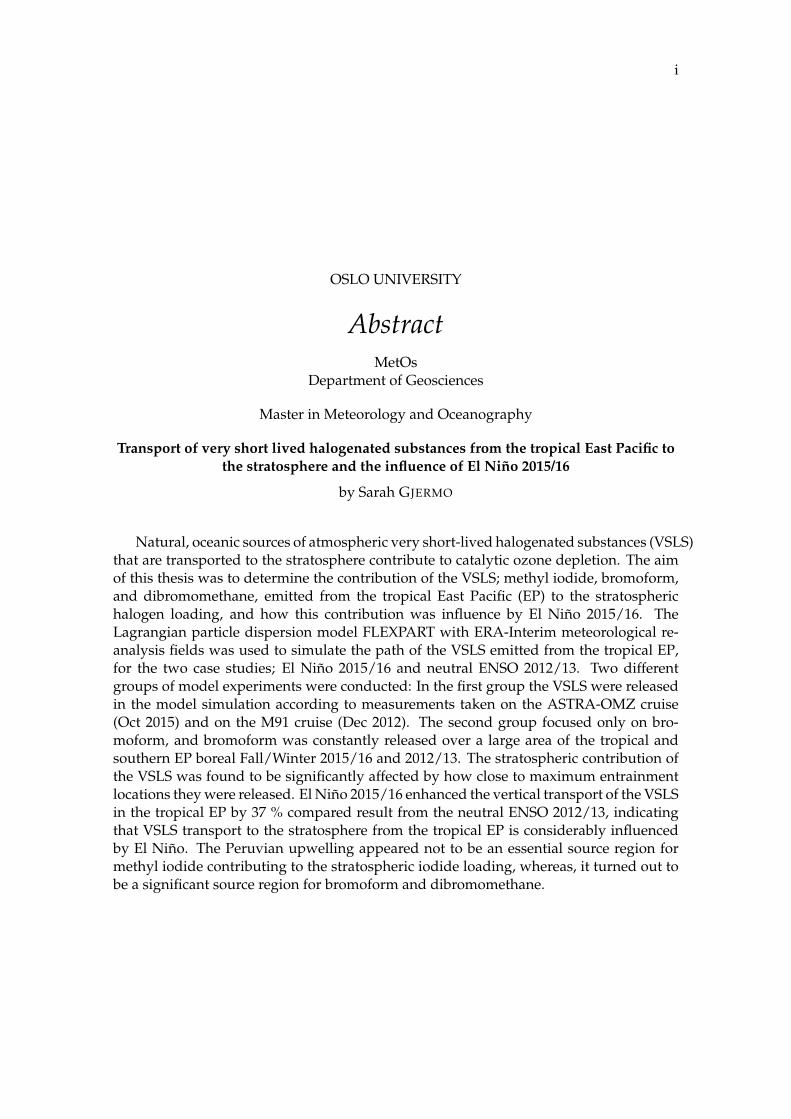
OSLO UNIVERSITY
AbstractMetOs
Department of Geosciences
Master in Meteorology and Oceanography
Transport of very short lived halogenated substances from the tropical East Pacific tothe stratosphere and the influence of El Niño 2015/16
by Sarah GJERMO
Natural, oceanic sources of atmospheric very short-lived halogenated substances (VSLS)that are transported to the stratosphere contribute to catalytic ozone depletion. The aimof this thesis was to determine the contribution of the VSLS; methyl iodide, bromoform,and dibromomethane, emitted from the tropical East Pacific (EP) to the stratospherichalogen loading, and how this contribution was influence by El Niño 2015/16. TheLagrangian particle dispersion model FLEXPART with ERA-Interim meteorological re-analysis fields was used to simulate the path of the VSLS emitted from the tropical EP,for the two case studies; El Niño 2015/16 and neutral ENSO 2012/13. Two differentgroups of model experiments were conducted: In the first group the VSLS were releasedin the model simulation according to measurements taken on the ASTRA-OMZ cruise(Oct 2015) and on the M91 cruise (Dec 2012). The second group focused only on bro-moform, and bromoform was constantly released over a large area of the tropical andsouthern EP boreal Fall/Winter 2015/16 and 2012/13. The stratospheric contribution ofthe VSLS was found to be significantly affected by how close to maximum entrainmentlocations they were released. El Niño 2015/16 enhanced the vertical transport of the VSLSin the tropical EP by 37 % compared result from the neutral ENSO 2012/13, indicatingthat VSLS transport to the stratosphere from the tropical EP is considerably influencedby El Niño. The Peruvian upwelling appeared not to be an essential source region formethyl iodide contributing to the stratospheric iodide loading, whereas, it turned out tobe a significant source region for bromoform and dibromomethane.

iii
Contents
Abstract i
Contents iii
1 Introduction 1
2 Background 52.1 Atmospheric Transport and Circulation . . . . . . . . . . . . . . . . . . . . 5
2.1.1 The Hadley Cell . . . . . . . . . . . . . . . . . . . . . . . . . . . . . . 52.1.2 The Walker Circulation . . . . . . . . . . . . . . . . . . . . . . . . . 62.1.3 The El Niño Southern Oscillation . . . . . . . . . . . . . . . . . . . . 72.1.4 Troposphere-to-Stratosphere Transport in the Tropics . . . . . . . . 8
2.2 Methyl iodide, Bromoform and Dibromomethane . . . . . . . . . . . . . . 102.2.1 Marine Sources . . . . . . . . . . . . . . . . . . . . . . . . . . . . . . 102.2.2 Transport from the Ocean to the Stratosphere . . . . . . . . . . . . . 102.2.3 Atmospheric Removal and Ozone Depletion . . . . . . . . . . . . . 12
2.3 Meteorology during ASTRA-OMZ and M91 . . . . . . . . . . . . . . . . . . 13
3 Data and Methods 193.1 The ASTRA-OMZ Cruise . . . . . . . . . . . . . . . . . . . . . . . . . . . . . 19
3.1.1 Meteorological Observations . . . . . . . . . . . . . . . . . . . . . . 193.1.2 Surface Ocean and Atmospheric Halocarbon Measurements . . . . 193.1.3 Halocarbon Emissions . . . . . . . . . . . . . . . . . . . . . . . . . . 19
3.2 The FLEXPART Model and ERA-Interim Data . . . . . . . . . . . . . . . . 213.3 Cruise VSLS Emissions Experiment . . . . . . . . . . . . . . . . . . . . . . . 23
3.3.1 VSLS Lifetime Profiles . . . . . . . . . . . . . . . . . . . . . . . . . . 233.3.2 FLEXPART Setup . . . . . . . . . . . . . . . . . . . . . . . . . . . . . 23
3.4 East Pacific Bromoform Emission Experiment . . . . . . . . . . . . . . . . . 253.4.1 Surface water concentrations . . . . . . . . . . . . . . . . . . . . . . 253.4.2 Choosing surface atmospheric concentrations . . . . . . . . . . . . 253.4.3 Final bromoform emission fields . . . . . . . . . . . . . . . . . . . . 293.4.4 FLEXPART Setup . . . . . . . . . . . . . . . . . . . . . . . . . . . . . 30
4 Results and Discussions 314.1 ASTRA-OMZ and M91 Data . . . . . . . . . . . . . . . . . . . . . . . . . . . 314.2 Cruise VSLS Emissions Experiment . . . . . . . . . . . . . . . . . . . . . . . 394.3 East Pacific Bromoform Emission Experiment . . . . . . . . . . . . . . . . . 45
5 Summary and Outlook 53
List of Abbrevations 55
List of Figures 57
List of Tables 61

iv
Bibliography 63
Acknowledgements 69
1
Chapter 1
Introduction
Oceanic halocarbons contribute to ozone depletion in the stratosphere (Carpenter et al.,2014b; Solomon et al., 1994), and thus their transport to the stratosphere is of interest. El-evated concentrations of oceanic halocarbons, especially over oceanic upwelling regionsin the tropics and subtropics, are related to biological activity (Hepach et al., 2014, 2016;Quack et al., 2007). Because of the pronounced coastal upwelling, the tropical East Pa-cific (EP) is one of the most productive regions worldwide (Mann and Lazier, 2013). ElNiño–Southern Oscillation (ENSO) has a large impact on the equatorial Pacific and theWalker Circulation (WC), and is therefore also likely to affect oceanic halocarbon emis-sions and their transport to the stratosphere.
Halocarbons are carbon based compounds containing halogen atoms. They are po-tential carriers of halogens to the stratosphere, which contribute to catalytic ozone de-pletion. In this thesis three halocarbons prominent to ozone depletion, namely methyliodide, bromoform and dibromomethane, are investigated. These halocarbons have lifetimes of less than 6 months in the atmosphere, and are therefore termed very short-livedhalogenated substances (VSLS) (Carpenter et al., 2014b). In this thesis the transport of theVSLS emitted from the Tropical EP, to the stratosphere is studied using the LagrangianFLEXPART model together with ERA-Interim reanalysis data. Calculations of strato-spheric entrainment, over the tropical East Pacific will be compared to findings fromother tropical oceans, and the impact of El Niño 2015 will be compared with ENSO neu-tral state in the EP in 2012. The El Niño 2015 was one of the four strongest El Niños since1950 (Stramma et al., 2016).
Since the ozone hole over Antarctica in late austral winter and early spring first wasdiscovered (Chubachi, 1984; Farman et al., 1985), a huge effort has been devoted to ozoneresearch. Ozone has a unique role in the stratosphere, because it absorb ultraviolet solarradiation, and thus acts as a protective shield around our planet. The health of humans,animals and plants are affected by increased ultraviolet light transmitted through theozone layer (Solomon, 1999). Before the ozone hole was discovered, anthropogenic ozonedepleting substances (ODS), mainly chlorofluorocarbons (CFC’s), was widely used bothin industry and in households. These halogenated substances had only been demon-strated to deplete ozone in laboratories, and environmental damage caused by strato-spheric ozone depletion had not yet been witnessed. In spite of the uncertainties, leadersfrom 36 nations joined together in 1989 and signed the Montreal Protocol to reduce oreliminate the use of these substances (DeSombre, 2000). The Montreal Protocol is nowconsidered a major success in reducing the emission of anthropogenic ODS, and finallythe ozone hole is showing signs of healing (Solomon et al., 2016). Research on the ozonedepletion is however still of major interest, as the regular stratospheric WMO Ozone as-sessments highlight.
The principal cause of stratospheric ozone depletion is the long-lived anthropogenicsubstances (Carpenter et al., 2014a), but recent observations have shown that also theVSLS are important stratospheric halogen sources (Dorf et al., 2006; Laube et al., 2008;
2 Chapter 1. Introduction
Sturges et al., 2000). Dorf et al. (2006) found that the measured stratospheric ozone-depleting bromine burden (10 years of balloon-borne observations) was significantlyhigher than what long-lived gases could be accounted for. The discrepancy was amongothers attributed to natural originated VSLS (Dorf et al., 2006). Henceforth, researcheshave been striving for a better understanding of the VSLS sources, emissions to the at-mosphere, atmospheric chemistry, and their transport pathway to the stratosphere.
The main research method for estimating global oceanic halocarbon emissions thathas been used is: the bottom-up approach based on surface-water and atmospheric halo-carbon measurements (Quack and Wallace, 2003). In contrast, the top-down approachis based on chemical transport modeling studies reproducing measurements of atmo-spheric VSLS concentrations (Warwick et al., 2006). There is a gap in the estimation of theoceanic halocarbon emission between the two methods, where the top-down approachleads to higher VSLS emission values (Hossaini et al., 2010; Liang et al., 2010). A possibleexplanation for that gap may be an under-representation of coastal emissions and smallspatial and temporal extreme emission events in the bottom-up emission estimations(Ziska et al., 2013). Hossaini et al. (2010) claims that one uncertainty bottom-up approachwas the assumption of a constant prescribed lifetime of Br_y in the troposphere, and Tegt-meier et al. (2013) suggested that the available upper air measurements of methyl iodidewere not representative of global estimates due to strong variations in the geographicalmethyl iodide entrainment distribution. Hence, the top-down emission approach maytherefore lead to overestimations. A problem with both of these approaches is that theydon’t include seasonality for the surface oceanic concentrations. A newer model studyhas now been introduced; using a biogeochemical model where both the biological andphotochemical production mechanisms for the VSLS are considered, with the productionfollowing the seasonal insolation cycle (Hense and Quack, 2009; Stemmler et al., 2015).
There are several uncertainties to the processes of VSLS contribution to stratospherichalogen loading and ozone depletion. A large part of the uncertainty is related to theconcentration of VSLS in the marine atmospheric boundary layer (MABL) (Quack andWallace, 2003). Significant amounts of VSLS have been observed over oceanic upwellingin the eastern tropical Atlantic, and may be solely explained by oceanic sources, withoutthe need of additional continental sources (Hepach et al., 2014). Fuhlbrügge et al. (2013)found that the MABL height variations influences the volume mixing ratio (VMR) ofhalocarbons especially over oceanic upwelling systems, and it has been hypothesize thata common phenomenon over coastal upwelling systems is low MABL height, high halo-carbon emissions and high atmospheric mixing ratios (Fuhlbrügge et al., 2013; Hepachet al., 2014).
Another major uncertainty is the process of stratospheric VSLS transport and scav-enging in the tropical tropopause layer (TTL). The injection of stratospheric halogen fromVSLS comprises both the VSLS source gas injection (SGI) and product gas injection (PGI)(Ko and Poulet, 2003). Liang et al. (2014) studied the convective transport of the veryshort lived bromocarbons using the NASA Goddard Earth Observing System (GEOS)Chemistry Climate Model (GEOSCCM), and found that the amount of bromocarbonsreaching the stratosphere was actually weakened for very strong convection conditions,opposite to earlier presumptions. This weakening was attributed to the increased scav-enging of the soluble product gases, which lead to a high decrease in PGI exceeding theminor SGI increase (Liang et al., 2014). In this thesis I am only focusing on the directtransport of the VSLS source gases.
Recent papers on the effect of ENSO variations on the convection of VSLS to thestratosphere are Aschmann et al. (2011) and Ashfold et al. (2012). By long-term modeling
Chapter 1. Introduction 3
the impact of VSLS on stratospheric bromine loading using a three-dimensional chem-istry transport model, Aschmann et al. (2011) found that intensified atmospheric con-vection leads to higher amounts of VSLS in the upper troposphere/lower stratosphere,especially under extreme conditions like El Niño seasons. Ashfold et al. (2012) used atrajectory model (NAME) to investigate the timescales over which air parcels reach theTTL above Borneo (West Pacific), and they compared the ENSO neutral year 2008 to themoderate El Niño year 2006 and the moderate La Niña year 2007. They found that moreparcels traveled from the boundary layer to the TTL during the La Niña year, and lessduring the EL Niño year, although one should bear in mind that the influence of ENSOis different in other parts of the Tropics (Ashfold et al., 2012).
Researchers have now started to get a better understanding of the impact of the halo-carbons to the stratospheric ozone depletion (Carpenter et al., 2014b). However, there isstill a gap between modeled halogen loading and halogen measurements in the strato-sphere, and therefore more studies are necessary. The pronounced oceanic coastal up-welling and the tropical atmosphere suggests that halocarbon emissions from the EP maybe important for the stratospheric halogen loading. This is however not necessarily true,because the tropical EP is also a region with climatologically sinking of air masses, asit is the eastern branch of the WC, suppressing the vertical transport of the VSLS. Fur-thermore, the Peruvian upwelling along the West Coast of South America leads to a pro-nounced stable MABL layer, acting as a transport barrier for the VSLS (Fuhlbrügge et al.,2016a). Hardly any studies have investigated the transport of VSLS from the Tropical EPto the stratosphere (Aschmann et al., 2011). Hence, it is not yet known how importantthe region is for the stratospheric halogen budget. Moreover, the EP is a key region whenstudying the effect of El Niño, as the main convection over the West Pacific ocean shiftseastward during an El Niño event, closer to the EP VSLS sources. Furthermore, the weak-ening of the WC during El Niño events decreases the airmass suppression over the EP(Wallace and Hobbs, 2006), favoring more convection. The regional setting of this thesis,makes it therefore very relevant for this field of study.
The aim of this thesis is to investigate the role of VSLS transport to the stratosphereabove the tropical EP, and to contribute to the research on El Niño’s influence on thistransport. In particular, this thesis will examine three main research questions: 1. Towhat extent is the tropical EP a source for VSLS to the atmosphere? 2. How much ofthese VSLS is transported to the stratosphere? 3. How does El Niño affect the VSLStransport from the tropical EP to the stratosphere? The reader should bear in mind thatthis study is based on two ship campaigns carried out in the tropical EP, namely ASTRA-OMZ (Oct 2015) and M91 (Dec 2012), and so the data used is limited in time and space.
The overall structure of the thesis takes the form of five chapters, including this intro-ductory chapter. Chapter 2 begins by laying out the background information necessaryfor the scientific research. The 3. Chapter is concerned with the data and method used forthis thesis. Chapter 4. presents the results and discussions, which is divided into threesections: In the first section a meteorological overview is given, together with halocar-bon measurements from the ASTRA-OMZ cruise, and a comparison with the M91 cruiseamong others. In Section 2, a FLEXPART model study of the transport of the VSLS to thestratosphere, based on the ASTRA-OMZ and the M91 campaigns, is presented. In the 3.Section a regional case study of bromoform is given. Two model experiments were setupwith bromoform emissions over the tropical and southern EP, one for El Niño 2015 andone for ENSO Neutral 2012. Modeled VSLS VMR results from this section are comparedwith in-situ cruise measurements in the MABL and in-situ aircraft measurements. Thefinal chapter concludes the results and highlights the implication of the findings to futureresearch in this area.

5
Chapter 2
Background
A brief introduction to the atmospheric transport and circulation relevant for this the-sis is presented in Section 2.1, consisting of the four subsections: The Hadley Cell, TheWalker Circulation, The El Niño Southern Oscillation, and Troposphere-to-Stratospheretransport in the tropics. The three halocarbons methyl iodide, bromoform, and dibro-momethane, which transport to the stratosphere is investigated in this thesis, are pre-sented in Section 2.2. Section 2.2 consists of the subsections: Marine Sources, transportfrom the Ocean to the Stratosphere, Atmospheric Removal and Ozone Depletion. Fi-nally an overview of the meteorological setting at the time and place of the two cruisesASTRA-OMZ and M91, which this thesis is based upon, is given in Section 2.3.
2.1 Atmospheric Transport and Circulation
2.1.1 The Hadley Cell
The Hadley cell is named after George Hadley (1685-1768), who was an English meteorol-ogist (Wallace and Hobbs, 2006). When seeking for the origin of the trade winds, Hadleyrealized that they must be caused by the uneven distribution of solar insolation betweenthe equator and the poles. He visualized one great thermally directly driven cell on eachhemisphere. Heated air is convected over the equator and is transported towards thepoles where it cools, sinks, and flows back towards equator (Holton, 2004, pp. 314–316).Although Hadley’s idea of one major cell in each hemisphere did not prevail, his conceptsof that differences in heating give rise to persistent large-scale atmospheric overturningcirculation and of that zonal winds can be attributed deflection of meridional winds have(Aguado and Burt, 2010, pp. 201–202). A more realistic model is the three-cell modeldividing the circulation of each hemisphere into three major transport cells, namely; theHadley cell which circulates air between the tropics and sub-tropics, the mid-latitudinalFerrel cell and the Polar cell (Aguado and Burt, 2010, p. 203).
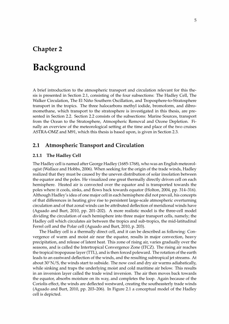
The Hadley cell is a thermally direct cell, and it can be described as following: Con-vergence of warm and moist air near the equator, results in major convection, heavyprecipitation, and release of latent heat. This zone of rising air, varies gradually over theseasons, and is called the Intertropical Convergence Zone (ITCZ). The rising air reachesthe tropical tropopause layer (TTL), and is then forced poleward. The rotation of the earthleads to an eastward deflection of the winds, and the resulting subtropical jet streams. Atabout 30◦N/S, the winds start to subside. The now cool and dry air warms adiabatically,while sinking and traps the underlying moist and cold maritime air below. This resultsin an inversion layer called the trade wind inversion. The air then moves back towardsthe equator, absorbs moisture on its way, and completes the loop. Again because of theCoriolis effect, the winds are deflected westward, creating the southeasterly trade winds(Aguado and Burt, 2010, pp. 203–206). In Figure 2.1 a conceptual model of the Hadleycell is depicted.
6 Chapter 2. Background
FIGURE 2.1: Conceptual model of the Hadley Cells, together with thetropical tropopause layer (TTL) and the Inter-tropical convergence zone
(ITCZ). Adapted from Fiehn (2017, p. 6).
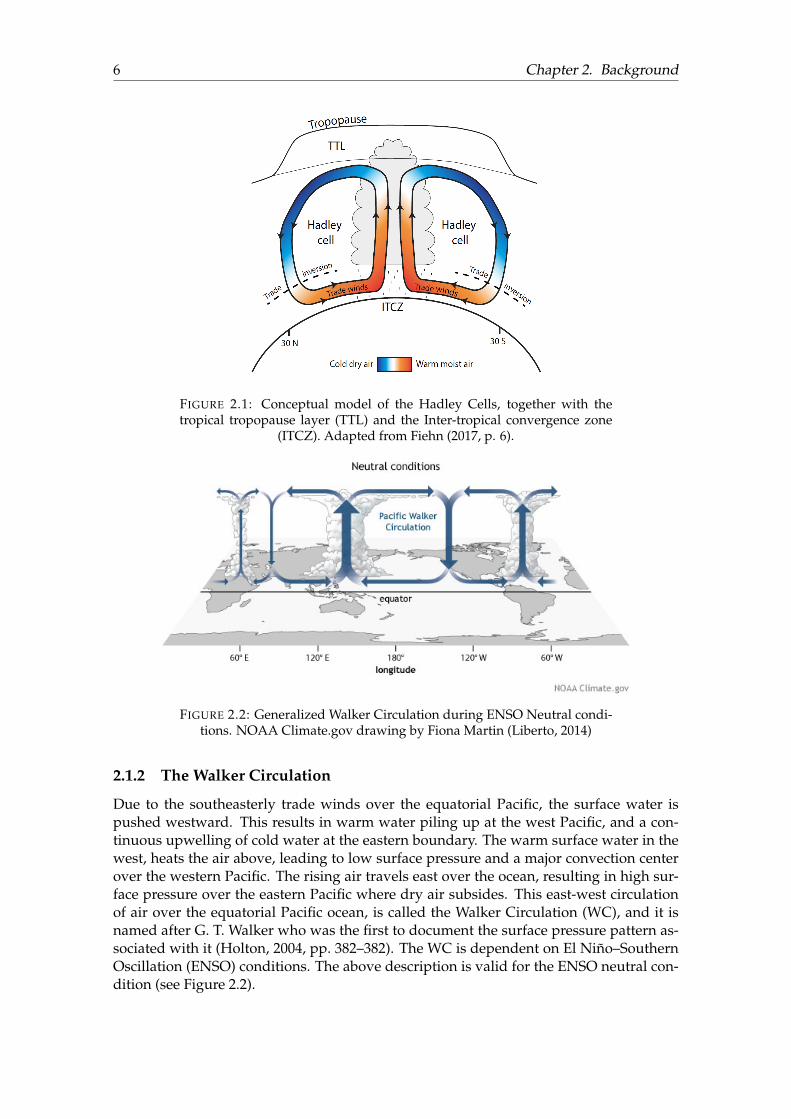
FIGURE 2.2: Generalized Walker Circulation during ENSO Neutral condi-tions. NOAA Climate.gov drawing by Fiona Martin (Liberto, 2014)
2.1.2 The Walker Circulation
Due to the southeasterly trade winds over the equatorial Pacific, the surface water ispushed westward. This results in warm water piling up at the west Pacific, and a con-tinuous upwelling of cold water at the eastern boundary. The warm surface water in thewest, heats the air above, leading to low surface pressure and a major convection centerover the western Pacific. The rising air travels east over the ocean, resulting in high sur-face pressure over the eastern Pacific where dry air subsides. This east-west circulationof air over the equatorial Pacific ocean, is called the Walker Circulation (WC), and it isnamed after G. T. Walker who was the first to document the surface pressure pattern as-sociated with it (Holton, 2004, pp. 382–382). The WC is dependent on El Niño–SouthernOscillation (ENSO) conditions. The above description is valid for the ENSO neutral con-dition (see Figure 2.2).
2.1. Atmospheric Transport and Circulation 7
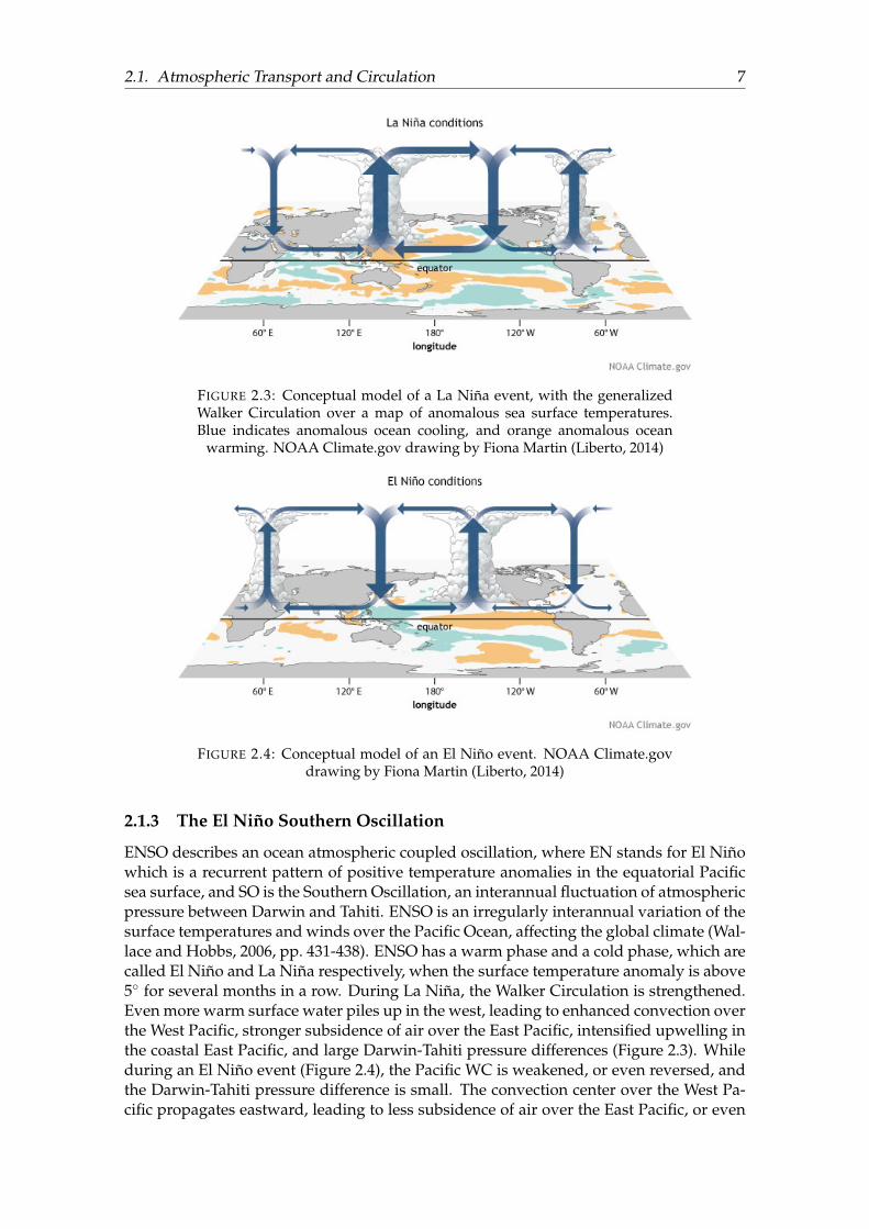
FIGURE 2.3: Conceptual model of a La Niña event, with the generalizedWalker Circulation over a map of anomalous sea surface temperatures.Blue indicates anomalous ocean cooling, and orange anomalous ocean
warming. NOAA Climate.gov drawing by Fiona Martin (Liberto, 2014)
FIGURE 2.4: Conceptual model of an El Niño event. NOAA Climate.govdrawing by Fiona Martin (Liberto, 2014)
2.1.3 The El Niño Southern Oscillation
ENSO describes an ocean atmospheric coupled oscillation, where EN stands for El Niñowhich is a recurrent pattern of positive temperature anomalies in the equatorial Pacificsea surface, and SO is the Southern Oscillation, an interannual fluctuation of atmosphericpressure between Darwin and Tahiti. ENSO is an irregularly interannual variation of thesurface temperatures and winds over the Pacific Ocean, affecting the global climate (Wal-lace and Hobbs, 2006, pp. 431-438). ENSO has a warm phase and a cold phase, which arecalled El Niño and La Niña respectively, when the surface temperature anomaly is above5◦ for several months in a row. During La Niña, the Walker Circulation is strengthened.Even more warm surface water piles up in the west, leading to enhanced convection overthe West Pacific, stronger subsidence of air over the East Pacific, intensified upwelling inthe coastal East Pacific, and large Darwin-Tahiti pressure differences (Figure 2.3). Whileduring an El Niño event (Figure 2.4), the Pacific WC is weakened, or even reversed, andthe Darwin-Tahiti pressure difference is small. The convection center over the West Pa-cific propagates eastward, leading to less subsidence of air over the East Pacific, or even
8 Chapter 2. Background
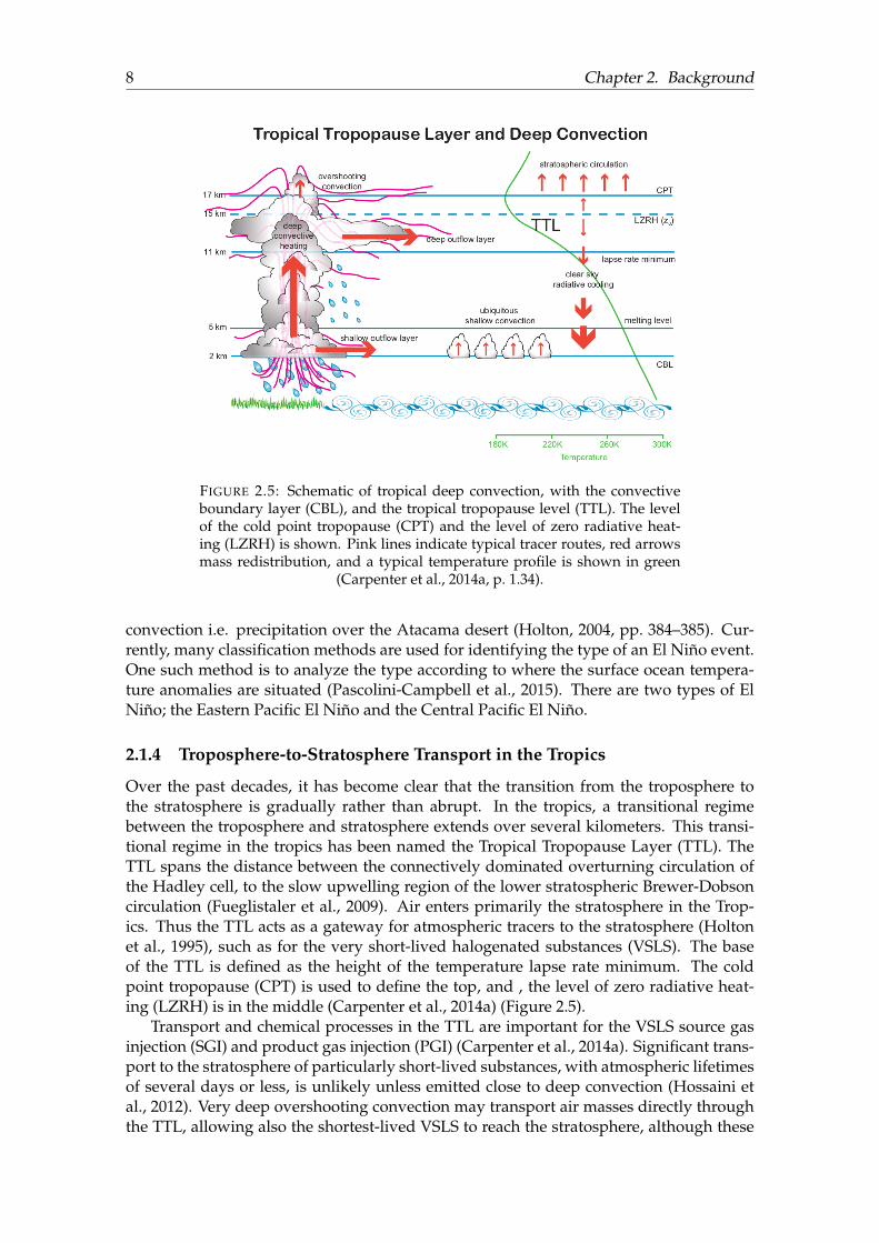
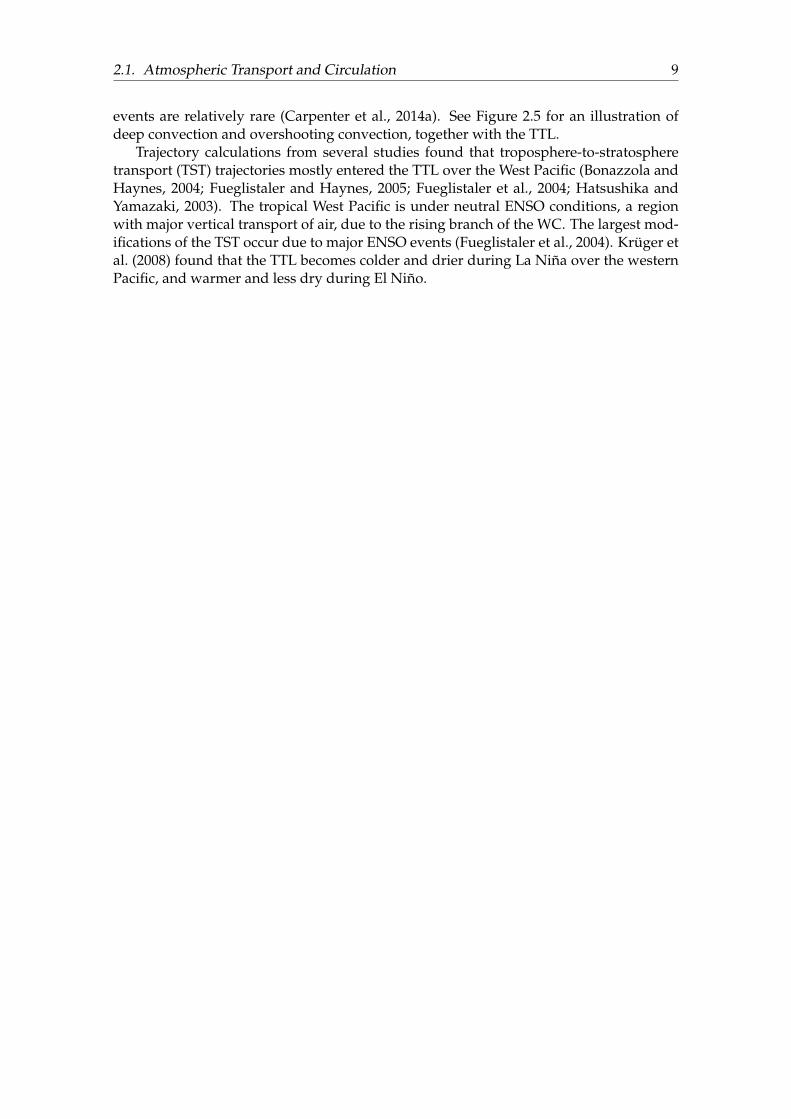
FIGURE 2.5: Schematic of tropical deep convection, with the convectiveboundary layer (CBL), and the tropical tropopause level (TTL). The levelof the cold point tropopause (CPT) and the level of zero radiative heat-ing (LZRH) is shown. Pink lines indicate typical tracer routes, red arrowsmass redistribution, and a typical temperature profile is shown in green
(Carpenter et al., 2014a, p. 1.34).
convection i.e. precipitation over the Atacama desert (Holton, 2004, pp. 384–385). Cur-rently, many classification methods are used for identifying the type of an El Niño event.One such method is to analyze the type according to where the surface ocean tempera-ture anomalies are situated (Pascolini-Campbell et al., 2015). There are two types of ElNiño; the Eastern Pacific El Niño and the Central Pacific El Niño.
2.1.4 Troposphere-to-Stratosphere Transport in the Tropics
Over the past decades, it has become clear that the transition from the troposphere tothe stratosphere is gradually rather than abrupt. In the tropics, a transitional regimebetween the troposphere and stratosphere extends over several kilometers. This transi-tional regime in the tropics has been named the Tropical Tropopause Layer (TTL). TheTTL spans the distance between the connectively dominated overturning circulation ofthe Hadley cell, to the slow upwelling region of the lower stratospheric Brewer-Dobsoncirculation (Fueglistaler et al., 2009). Air enters primarily the stratosphere in the Trop-ics. Thus the TTL acts as a gateway for atmospheric tracers to the stratosphere (Holtonet al., 1995), such as for the very short-lived halogenated substances (VSLS). The baseof the TTL is defined as the height of the temperature lapse rate minimum. The coldpoint tropopause (CPT) is used to define the top, and , the level of zero radiative heat-ing (LZRH) is in the middle (Carpenter et al., 2014a) (Figure 2.5).
Transport and chemical processes in the TTL are important for the VSLS source gasinjection (SGI) and product gas injection (PGI) (Carpenter et al., 2014a). Significant trans-port to the stratosphere of particularly short-lived substances, with atmospheric lifetimesof several days or less, is unlikely unless emitted close to deep convection (Hossaini etal., 2012). Very deep overshooting convection may transport air masses directly throughthe TTL, allowing also the shortest-lived VSLS to reach the stratosphere, although these
2.1. Atmospheric Transport and Circulation 9
events are relatively rare (Carpenter et al., 2014a). See Figure 2.5 for an illustration ofdeep convection and overshooting convection, together with the TTL.
Trajectory calculations from several studies found that troposphere-to-stratospheretransport (TST) trajectories mostly entered the TTL over the West Pacific (Bonazzola andHaynes, 2004; Fueglistaler and Haynes, 2005; Fueglistaler et al., 2004; Hatsushika andYamazaki, 2003). The tropical West Pacific is under neutral ENSO conditions, a regionwith major vertical transport of air, due to the rising branch of the WC. The largest mod-ifications of the TST occur due to major ENSO events (Fueglistaler et al., 2004). Krüger etal. (2008) found that the TTL becomes colder and drier during La Niña over the westernPacific, and warmer and less dry during El Niño.
10 Chapter 2. Background
2.2 Methyl iodide, Bromoform and Dibromomethane
In this thesis, the troposphere-to-stratosphere transport (TST) of the three halocarbonsmethyl iodide, bromoform, and dibromomethane, is studied. Halocarbons are carbonbased compounds containing halogen atoms, where halogen is the name for group sevenof the periodic table of the elements, including e.g. chlorine, bromine and iodine. Thethree halocarbons studied in this project, are recognized as being contributers to thestratospheric halogen loading (Carpenter et al., 2014b), where they are involved in ozonedepletion (Carpenter et al., 2014b; Salawitch et al., 2005). The knowledge about the halo-carbons spatial and temporal variability in emission, loss, and transport processes, arelargely based on limited data (Hepach et al., 2016; Quack et al., 2007; Ziska et al., 2013).It is known that the main atmospheric source for these halocarbons is oceanic (Carpenteret al., 2014b). Although, oceanic measurements of halocarbons are few, high concentra-tions especially over upwelling regions in the tropics and subtropics have been found.Thus, they are considered important source regions (Hepach et al., 2016; Quack et al.,2007). The intense Peruvian Upwelling is considered one of the most productive oceanicregions in the world (Mann and Lazier, 2013). Therefore, studying halogen transportfrom this region is of great interest.
2.2.1 Marine Sources
Bromoform and dibromomethane are the primary natural contributors to atmosphericorganic bromine (Quack et al., 2007). The source for the bromine-containing source gasesis mainly natural and oceanic. For methyl iodide, the oceanic contribution to the atmo-spheric loading is more than 80% (Carpenter et al., 2014b).
The dominant producer of bromocarbons in the open ocean is phytoplankton (Mooreet al., 1995b). Other known sources are macro algae and cyanobacteria (Nightingale etal., 1995; Wever and Horst, 2013). Hill and Manley (2009) suggested that a considerableformation pathway for the production of polyhalogenated compounds may be indirectthrough algal release of hypoiodous acid (HOI) and hypobromous acid HOBr, reactingwith dissolved organic matter (DOM). The seaweed and phytoplankton produces H2O2during photosynthesis and photorespiration (and stress for macro algae), which reactswith bromine in the water, to form HOBr, by enzymatic activity of haloperoxidases (Hep-ach et al., 2016). The HOBr then reacts with DOM, and forms polybromomethanes likebromoform and dibromomethane (Wever and Horst, 2013).
For methyl iodide is produces by non-biological, photochemical degradation of io-dide containing DOM, and biologically by algae and phytoplankton (Carpenter et al.,2014b; Tegtmeier et al., 2013). Methyl iodide may possibly also be formed via bacteria(Hepach et al., 2016)
Hepach et al. (2016) found the Peruvian upwelling region to be only a moderatesource region for bromocarbons, but significant source region for iodocarbons, Decem-ber 2012. Previously high concentration of iodocarbons in the tropical oceans have beenconnected with mainly the photochemical source (Hepach et al., 2016). Stemmler et al.(2015) used a global three-dimensional ocean biogeochemistry model to simulate bromo-form cycling in the ocean, and it was found to match observations well.
2.2.2 Transport from the Ocean to the Stratosphere
When the ocean is supersaturated with halocarbons, the halocarbons are emitted from theocean, transported horizontally and vertically mixed in the marine atmospheric bound-ary layer (MABL). The rate at which the halocarbon ocean-to-atmosphere exchange oc-curs depends on the air-sea halocarbon concentration gradient. The air-sea concentration
2.2. Methyl iodide, Bromoform and Dibromomethane 11
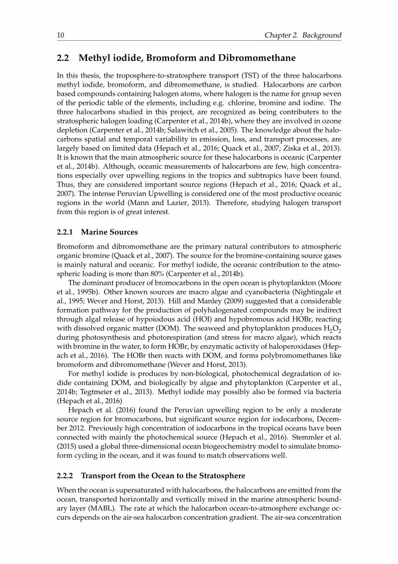
FIGURE 2.6: Schematic of the oceanic sources and the atmospheric pro-cesses relevant for methyl iodide (CH3I), bromoform (CHBr3) and dibro-
momethane (CH2Br2).
gradient is significantly affected by oceanic upwelling (Fuhlbrügge et al., 2013, 2016a).When there is coastal oceanic upwelling of cold water to the surface, the air over theocean cools, resulting in a stable and isolated MABL and high atmospheric halocarbonmixing ratios. The high atmospheric mixing ratios decreases the halocarbon sea-air con-centration gradient, hence the emission to the atmosphere is reduced. Fuhlbrügge etal. (2013, 2016a) found that a strong trade inversion acts as a transport barrier, leadingto a near-surface accumulation of halocarbons in the atmosphere. The trade inversionis a temperature inversion that occurs due to large scale subsidence in the descendingbranches of the Hadley Cell and the Walker Cell, and is found where the cold dry sub-sided air meets the underlaying warm moist air. The coastal emission of oceanic halo-carbons also vary due to the change in amount and types of algae, and with the diurnaland tidal cycles (Carpenter et al., 2014b; Wever and Horst, 2013). Local emission maximalinked to upwelling areas, over the tropical oceans, have been observed (Quack et al.,2007; Wever and Horst, 2013). Stemmler et al. (2015) simulated emissions of bromoforminto the atmosphere, using observational-based estimates from Ziska et al. (2013) of near-surface atmospheric bromoform volume mixing ratio (VMR) as upper boundary condi-tion. These were found to be lower than previous estimates by Ziska et al. (2013). Thisis because seasonality is considered and less bromoform is produced in non-bloomingseasons reversing the sea-air flux of bromoform, and also because coastal emissions ofbromoform is not represented in this model (Stemmler et al., 2015).
VSLS are defined as substances with atmospheric lifetimes of less than six months(WMO, 2006). The current estimated atmospheric lifetimes at 10 km altitude are 17 daysfor bromoform, 150 days for dibromomethane, and 3.5 days for methyl iodide (Carpen-ter et al., 2014b). Hence, all three compounds belong to the VSLS category. Especiallyshort-lived VSLS, like methyl iodide and bromoform, need to be emitted close to deep,convective systems to be able to reach the Stratosphere (Tegtmeier et al., 2013). Theirimpact on stratospheric halogen loading is still uncertain due to limited observations(Carpenter et al., 2014b). Several studies have found indications that methyl iodide andbromoform reaches the stratosphere over tropical regions, i.e., Fiehn et al. (2017), Hos-saini et al. (2015), Saiz-Lopez et al. (2015), and Tegtmeier et al. (2013) in despite of thestable MABL and the trade inversion.
The VSLS sources to the stratosphere halogen loading is typically separated between
12 Chapter 2. Background
SGI and PGI (Ko and Poulet, 2003), where the SGI is the direct injection of the VSLSsources, and the PGI is the injection of halogens from the atmospheric degraded VSLSproducts. In this thesis, only the SGI of VSLS has been focused on.
2.2.3 Atmospheric Removal and Ozone Depletion
The main sink of methyl iodide in the troposphere is photolysis (Carpenter et al., 2014b).The tropospheric sinks of bromocarbons are OH oxidation and photolysis (Carpenteret al., 2014b). Photolysis is the most important removal for bromoform, and a majorsink process is oxidation by OH radicals for dibromomethane (Carpenter et al., 2014b).Other sinks of atmospheric VSLS are uptake by the oceans and soil microbial degradation(Carpenter et al., 2014b).
When bromine and iodine containing halocarbons are degraded in the atmosphere,they form reactive halogen radicals. This takes place both in the troposphere and strato-sphere, and they therefore differ from chlorofluorocarbons (CFC’s) which can only bebroken down in the Stratosphere by ultra-violet radiation (Wever and Horst, 2013). Oneof the halogen radical’s most important reaction is ozone depletion. Ozone in the tropo-sphere is an active greenhouse gas, and it is also toxic for humans. The halocarbon emis-sions from the sea can lower tropospheric ozone, which contribute to reducing globalwarming, and inproving air quality. The VSLS source gases and product gases whichreaches the stratosphere will take part in catalytic ozone depletion there (Wever andHorst, 2013). Thus, VSLS contribute to increased transmission of harmful ultravioletlight through the ozone layer.
PGI of bromine containing VSLS makes a non-negligible contribution to the strato-spheric bromine loading, with bromoform and dibromomethane as the most importantsources. The PGI of brominated VSLS can range from 1.1 to 4.3 ppt. By including brominecontaining VSLS in modeling studies, the modeled O3 trends have been closer to obser-vations. The PGI of idodine containing VSLS to the stratosphere is still uncertain. Ithas been estimated to be less than 0.15 ppt, and is suggested to be a minor sink for O3(Hossaini et al., 2012).
2.3. Meteorology during ASTRA-OMZ and M91 13
2.3 Meteorology during ASTRA-OMZ and M91
The meteorological setting at the time and place of the two cruises ASTRA-OMZ andM91, is presented in this section. The cruises took place along the west coast of SouthAmerica, during October 2015 (ASTRA-OMZ) and during December 2012 (M91). Moreinformation about ASTRA-OMZ is given in Chapter 3, and the M91 cruise is describedin more detail in Fuhlbrügge et al. (2016a) and Hepach et al. (2016).
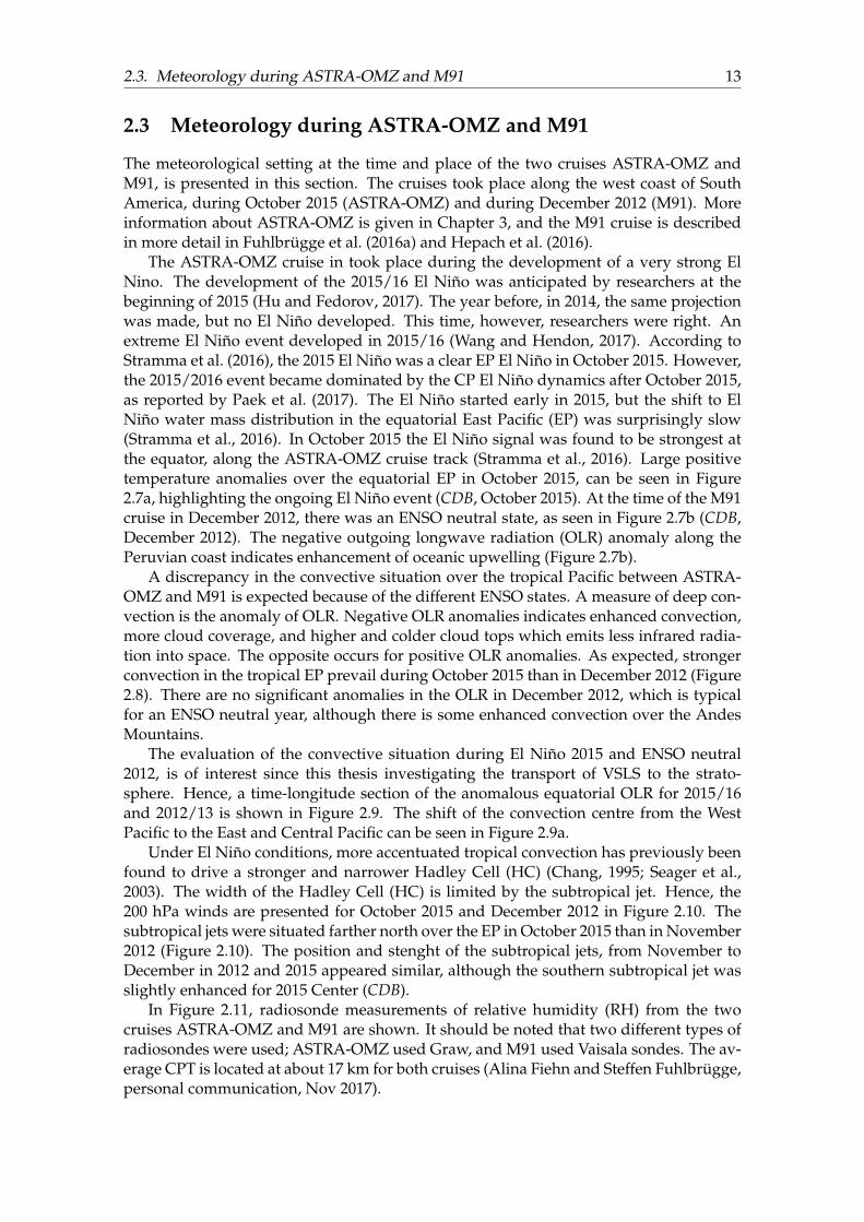
The ASTRA-OMZ cruise in took place during the development of a very strong ElNino. The development of the 2015/16 El Niño was anticipated by researchers at thebeginning of 2015 (Hu and Fedorov, 2017). The year before, in 2014, the same projectionwas made, but no El Niño developed. This time, however, researchers were right. Anextreme El Niño event developed in 2015/16 (Wang and Hendon, 2017). According toStramma et al. (2016), the 2015 El Niño was a clear EP El Niño in October 2015. However,the 2015/2016 event became dominated by the CP El Niño dynamics after October 2015,as reported by Paek et al. (2017). The El Niño started early in 2015, but the shift to ElNiño water mass distribution in the equatorial East Pacific (EP) was surprisingly slow(Stramma et al., 2016). In October 2015 the El Niño signal was found to be strongest atthe equator, along the ASTRA-OMZ cruise track (Stramma et al., 2016). Large positivetemperature anomalies over the equatorial EP in October 2015, can be seen in Figure2.7a, highlighting the ongoing El Niño event (CDB, October 2015). At the time of the M91cruise in December 2012, there was an ENSO neutral state, as seen in Figure 2.7b (CDB,December 2012). The negative outgoing longwave radiation (OLR) anomaly along thePeruvian coast indicates enhancement of oceanic upwelling (Figure 2.7b).
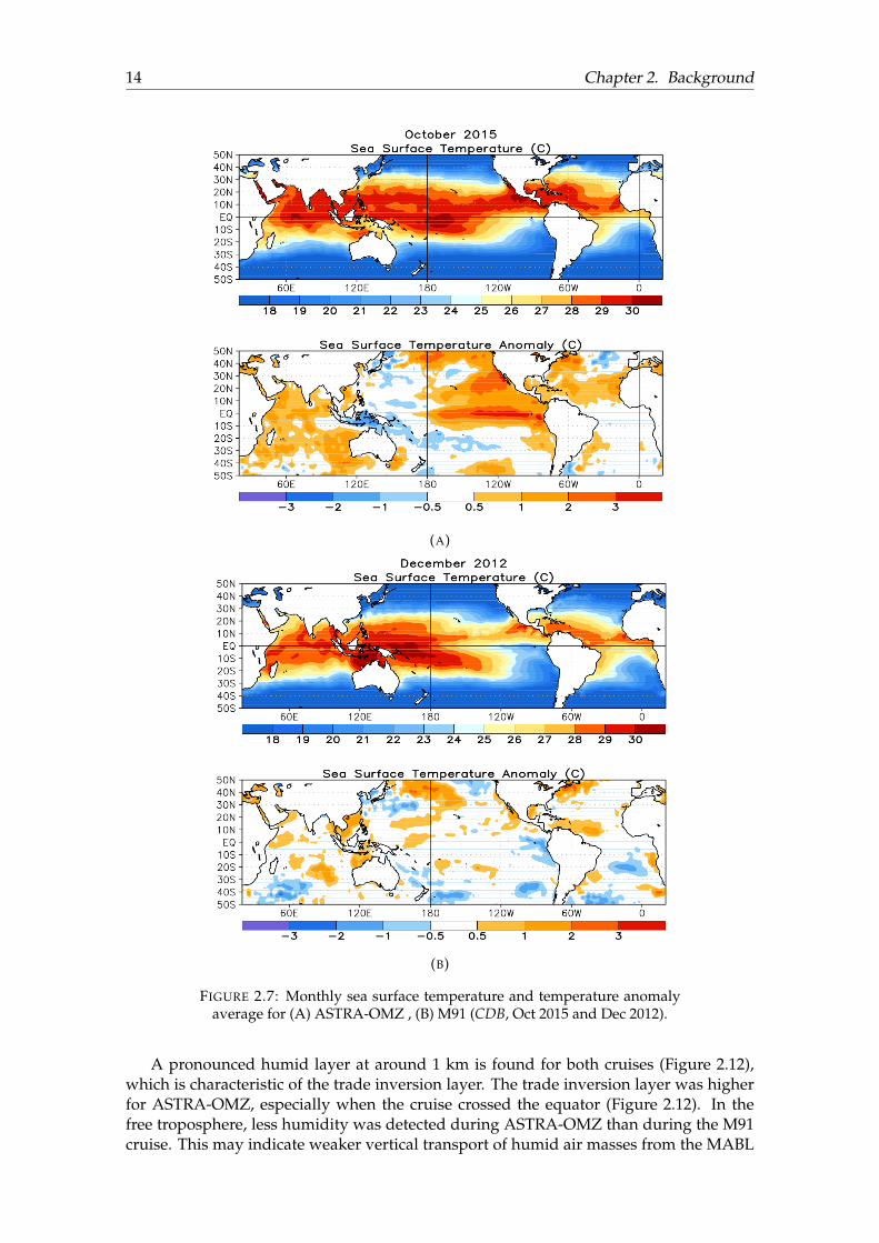
A discrepancy in the convective situation over the tropical Pacific between ASTRA-OMZ and M91 is expected because of the different ENSO states. A measure of deep con-vection is the anomaly of OLR. Negative OLR anomalies indicates enhanced convection,more cloud coverage, and higher and colder cloud tops which emits less infrared radia-tion into space. The opposite occurs for positive OLR anomalies. As expected, strongerconvection in the tropical EP prevail during October 2015 than in December 2012 (Figure2.8). There are no significant anomalies in the OLR in December 2012, which is typicalfor an ENSO neutral year, although there is some enhanced convection over the AndesMountains.
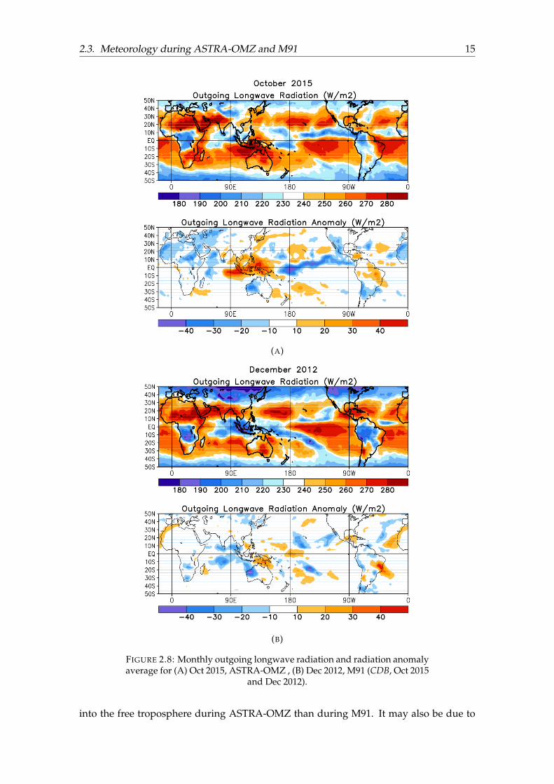
The evaluation of the convective situation during El Niño 2015 and ENSO neutral2012, is of interest since this thesis investigating the transport of VSLS to the strato-sphere. Hence, a time-longitude section of the anomalous equatorial OLR for 2015/16and 2012/13 is shown in Figure 2.9. The shift of the convection centre from the WestPacific to the East and Central Pacific can be seen in Figure 2.9a.
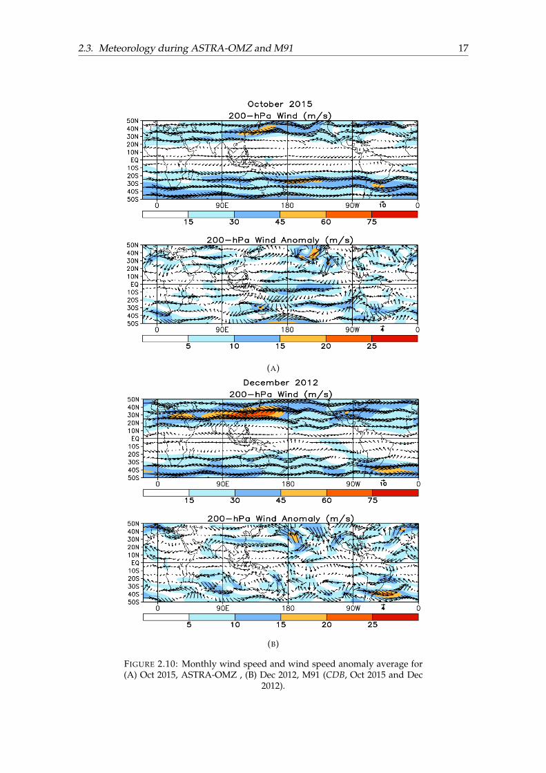
Under El Niño conditions, more accentuated tropical convection has previously beenfound to drive a stronger and narrower Hadley Cell (HC) (Chang, 1995; Seager et al.,2003). The width of the Hadley Cell (HC) is limited by the subtropical jet. Hence, the200 hPa winds are presented for October 2015 and December 2012 in Figure 2.10. Thesubtropical jets were situated farther north over the EP in October 2015 than in November2012 (Figure 2.10). The position and stenght of the subtropical jets, from November toDecember in 2012 and 2015 appeared similar, although the southern subtropical jet wasslightly enhanced for 2015 Center (CDB).
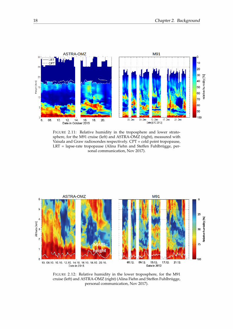
In Figure 2.11, radiosonde measurements of relative humidity (RH) from the twocruises ASTRA-OMZ and M91 are shown. It should be noted that two different types ofradiosondes were used; ASTRA-OMZ used Graw, and M91 used Vaisala sondes. The av-erage CPT is located at about 17 km for both cruises (Alina Fiehn and Steffen Fuhlbrügge,personal communication, Nov 2017).
14 Chapter 2. Background
(A)
(B)
FIGURE 2.7: Monthly sea surface temperature and temperature anomalyaverage for (A) ASTRA-OMZ , (B) M91 (CDB, Oct 2015 and Dec 2012).
A pronounced humid layer at around 1 km is found for both cruises (Figure 2.12),which is characteristic of the trade inversion layer. The trade inversion layer was higherfor ASTRA-OMZ, especially when the cruise crossed the equator (Figure 2.12). In thefree troposphere, less humidity was detected during ASTRA-OMZ than during the M91cruise. This may indicate weaker vertical transport of humid air masses from the MABL
2.3. Meteorology during ASTRA-OMZ and M91 15
(A)
(B)
FIGURE 2.8: Monthly outgoing longwave radiation and radiation anomalyaverage for (A) Oct 2015, ASTRA-OMZ , (B) Dec 2012, M91 (CDB, Oct 2015
and Dec 2012).
into the free troposphere during ASTRA-OMZ than during M91. It may also be due to
16 Chapter 2. Background
(A) (B)
FIGURE 2.9: Anomalous outgoing longwave radiation averaged between5N-5S for (A) 2015/16 and (B) 2012/13 (CDB, Mar 2016 and Mar 2013).
radiosonde differences (Kirstin Krüger, personal communication, Nov 2017). The meanheight of the MABL was 307 m for M91 (Fuhlbrügge et al., 2016a) and 470 m for ASTRA-OMZ (Alina Fiehn, personal communication, Nov 2017).
2.3. Meteorology during ASTRA-OMZ and M91 17
(A)
(B)
FIGURE 2.10: Monthly wind speed and wind speed anomaly average for(A) Oct 2015, ASTRA-OMZ , (B) Dec 2012, M91 (CDB, Oct 2015 and Dec
2012).
18 Chapter 2. Background
FIGURE 2.11: Relative humidity in the troposphere and lower strato-sphere, for the M91 cruise (left) and ASTRA-OMZ (right), measured withVaisala and Graw radiosondes respectively. CPT = cold point tropopause,LRT = lapse-rate tropopause (Alina Fiehn and Steffen Fuhlbrügge, per-
sonal communication, Nov 2017).
FIGURE 2.12: Relative humidity in the lower troposphere, for the M91cruise (left) and ASTRA-OMZ (right) (Alina Fiehn and Steffen Fuhlbrügge,
personal communication, Nov 2017).
19
Chapter 3
Data and Methods
3.1 The ASTRA-OMZ Cruise
Data from the two cruises ASTRA-OMZ and M91 is used in this thesis. The ASTRA-OMZcruise was conducted on the R/V SONNE (SO243; 5 to 22 October 2015) from Guayaquilin Ecuador to Antofagasta in Chile, and the M91 cruise was carried on R/V METEOR (1 to26 December 2012) starting and ending in Lima, Peru. Descriptions of the meteorologicalobservations, and the oceanic and atmospheric halocarbons, for ASTRA-OMZ, are givenin the subsequent sections. The M91 cruise have been described earlier by Fuhlbrüggeet al. (2016a) and Hepach et al. (2016).
3.1.1 Meteorological Observations
Meteorological observations of sea surface temperature (SST), surface air temperature(SAT), wind speed, wind direction, relative humidity, and air pressure were done everysecond. The wind were measured at about 30 m height above sea level. The data wereaveraged to 10 min intervals. GRAW DFM-09 radiosondes were regularly launched everysix hours, with a total of 64 launches (Alina Fiehn, personal communication, Nov. 2017and Marandino, 2016).
3.1.2 Surface Ocean and Atmospheric Halocarbon Measurements
Both surface oceanic and atmospheric halocarbon measurements were collected every 3hours. Water samples were taken at a depth of about 5 m from a continuously workingwater pump in the hydrographic shaft of the ship. The water samples were then analyzedfor halogenated trace gases with a gas chromatographer attached to a mass spectrome-ter (GC/MS) onboard the ship (Alina Fiehn, personal communication, Nov. 2017 andMarandino, 2016). The precision of the analysis is of 10% (1α). More detailed descriptionof the measurements is given by Hepach et al. (2014).
The atmospheric air samples were taken at about 10 m height above sea level at thebow of the ship, using a jib of 4 meters. The samples were collected in stainless steelcanisters, pressurized to 2 atm, and later analyzed at the Rosenstiel School for Marine andAtmospheric Sciences, University of Miami (Alina Fiehn, personal communication, Nov.2017 and Marandino, 2016). Details about the atmospheric very short-lived halogenatedsubstances (VSLS) samplings can be read in Fuhlbrügge et al. (2013).
3.1.3 Halocarbon Emissions
For calculating sea-to-air VSLS emission, the level of halocarbon saturation in the oceansurface layer is taken and converted to a flux by multiplying with an average transfer ve-locity (kw) (Moore et al., 1995a). The level of saturation is given as the difference between
20 Chapter 3. Data and Methods
the actual water concentration (cw) and the water concentration at which the concen-tration is at equilibrium with the above air. The theoretical equilibrium concentrationis given as catm
H , where catm is the atmospheric concentration of the halocarbon, and H isHenry’s law constant. Henry’s law constant is defined as the concentration in air devidedby the equilibrium water concentration (Moore et al., 1995a).
F = kw · (cw −catm
H) (3.1)
The transfer velocity coefficient by Nightingale et al. (2000) was used for the cruise VSLSemissions experiment. kw varies with sea level pressure, sea surface temperature, sea sur-face salinity, and the wind speed at 10 m height. Air pressure and sea surface temperatureare taken from the ERA-Interim monthly means, and the sea surface salinity is taken fromthe World Ocean Atlas 2005. The 10 m wind speeds are parameterized from the observedwind speeds during ASTRA-OMZ and M91, using a logarithmic wind profile:
u10 = u(z)κ√
CD
κ√
CD + log( z10 )
(3.2)
where κ = 0.41 is the von Kármán constant, CD is the neutral drag coefficient (Garratt,1977), and z is the height of the observed wind speed u. For more information on themethod of calculating the halocarbon emission flux see Hepach et al. (2014).
3.2. The FLEXPART Model and ERA-Interim Data 21
3.2 The FLEXPART Model and ERA-Interim Data
FLEXPART ("FLEXible Particle dispersion model") is a Lagrangian particle dispersionmodel originally designed for forecasting mesoscale point source pollutant dispersion,such as radionuclides released in a nuclear power plant accident (Stohl et al., 1998).FLEXPART has since been applied to studies of intercontinental pollutant transport, globalpollution transport on climatic time scales, stratosphere–troposphere exchange, and more.Lagrangian dispersion models have proven useful for gaining a better understanding ofthe atmospheric flow properties, such as mixing of tracers, transport, and dispersion(Bowman et al., 2013). For this thesis the FLEXPART versions 9.2 has been used.
The FLEXPART model was chosen for this thesis because it is a widely used andtested Lagrangian particle dispersion model (Hegarty et al., 2013). In Lagrangian modelsindividual infinitesimally small air parcels are simulated, forward or backward in time,in the atmosphere. Hence the trajectory information for each parcel is provided, which isfavorable when having point sources (e.g. ship measurements as in our case). In nature,the atmosphere is Lagrangian in the sense that air constitutes of tiny molecules, flowingwith the winds. Thus Lagrangian models are ideal for modeling atmospheric transport,and flow phenomena like turbulent eddies, transport barriers, and mixing. Additionally,Lagrangian models have minimal numerical diffusion (because sharp gradients are wellsimulated) and they are always numerically stable. Moreover, they conserve mass, en-ergy, and momentum, and they are computationally cheap (Lin, 2013). Another greatadvantage is that Lagrangian models are independent of a computational grid, unlikeEulerian models. In Eulerian models, the concentration of tracer released from a pointsource is immediately mixed within a grid box, while in Lagrangian models subgrid-scale information are carried by the air parcels, providing the best possible resolution(Hegarty et al., 2013). A drawback of the parcel information not being bound to any grid,is that in order for parcels to represent, e.g., dynamic volume, additional procedures arenecessary (Lin, 2013).
The meteorological input I have used for the FLEXPART experiments is global 3hourly ERA-Interim atmospheric reanalysis data produced by the European Center forMedium-Range Weather Forecast (ECMWF) a numerical weather prediction model, pro-viding horizontal and vertical wind components, temperature, specific humidity, surfacepressure, total cloud cover, dew-point temperature, large scale and convective precipita-tion, sensible heat flux, surface stress, and topography (Stohl et al., 2005). ERA-Interimdata has a 1°× 1° resolution, and 60 vertical model levels from the surface to 1 hPa. Itincludes a 4-dimensional variational analysis (4D-Var) with an analysis window of 12hours(Dee et al., 2011). 4D-Var is a four-dimensional data assimilation method, whichpurpose is to determine a best possible initial state based on available observations. Anevolving forecast error covariance is calculated, where observations are used at the ob-servation time, or as close as possible. The atmosphere is integrated forward and thenbackward in time, so that the initial state is optimized to fit the observations, from thebeginning to the end of the 12 hourly window (Kalnay, 2003).
Weaknesses in the Era-Interim meteorological reanalysis data are affecting the FLEX-PART results, i.e., representing the convective overturning in the troposphere, since thatis not resolved sufficiently by the spatial model resolution of the Era-Interim reanalysis.FLEXPART therefore have the option to use a moist convection scheme developed byEmanuel and Živkovic-Rothman (1999). The following brief explanation of the scheme isbased on Forster et al. (2007). The parameterization is called every synchronization timestep, and it uses time-interpolated specific humidity and temperature profiles from theEra-Interim reanalysis to redistribute particles within a column. Convection is activated
22 Chapter 3. Data and Methods
when:TLCL+1
vp ≥ TLCL+1v + Tt. (3.3)
Here TLCL+1vp is the virtual temperature of a surface air parcel lifted to the level above the
lifting condensation level (LCL) and TLCL+1v is the virtual temperature of the environment
at the same level. Tt = 0.9 K is the threshold temperature value. The virtual temperatureof a moist air parcel is the temperature at which a dry air parcel would have the samepressure and density as the moist air parcel. The mass fraction displaced from one ver-tical level to another is calculated based on the buoyancy sorting principle, and whetheran individual particle is displaced. The position of the particles in their respective des-tination layers, are determined by selecting a random number between [0,1]. After therandom displacement of particles by the convection, a compensating subsidence velocityacts on the remaining particles in the grid box.
Certain boundary layer parameters are parameterized in FLEXPART. Friction veloci-ties and heat fluxes in the boundary layer are parameterized using available accumulatedsurface sensible heat fluxes and surface stresses from the ECMWF reanalysis. The atmo-spheric boundary layer (ABL) heights are parameterized by using the critical Richardsonnumber concept, according to Vogelezang and Holtslag (1996). Spatial and temporalvariations in the ABL heights, that are not resolved by the ECMWF, are accounted for byusing a subgrid terrain effect parameterization. This subgrid terrain effect parameteriza-tion have been switched on for the model experiments in this thesis.
Forster et al. (2007) evaluated the subgrid-scale convection scheme in FLEXPART, andfound that the convection was greatly dependent on whether the parcel was located oversea or land. This is a challenge since the cruise measurements that were used as tracersources for the FLEXPART runs were taken very close to land and the steep Andes moun-tains. However, Forster et al. (2007) also found that the total precipitation, combining theconvective precipitation and the large-scale precipitation from the ERA-40 data (the pre-vious ECMWF reanalysis), was closer to observations than without including the convec-tion precipitation. Furthermore, FLEXPART model simulations and aircraft observationsof VSLS volume mixing ratio (VMR) in the upper tropical tropopause layer (TTL) andthe free troposphere have shown good agreement when including the boundary layerscheme and the convective scheme (Fuhlbrügge et al., 2016b; Tegtmeier et al., 2013).
In this thesis, the two FLEXPART model versions 9.2.2 and 9.2.3 have been used.Tegtmeier et al. (2012) upgraded FLEXPART version 9.2 by supplying with a chemicallifetime height profile, as an option to the constant lifetime for the substances. In FLEX-PART version 9.2.3, an online calculation of the cold point tropopause is included (AlinaFiehn, personal communication, Nov. 2017). This calculation is helpful for estimatingthe amount of VSLS entering the bottom of the Stratosphere. Other than adding extrainformation about the height of the cold point tropopause (CPT), the FLEXPART version9.2.3 is the same as version 9.2.2.
3.3. Cruise VSLS Emissions Experiment 23
3.3 Cruise VSLS Emissions Experiment
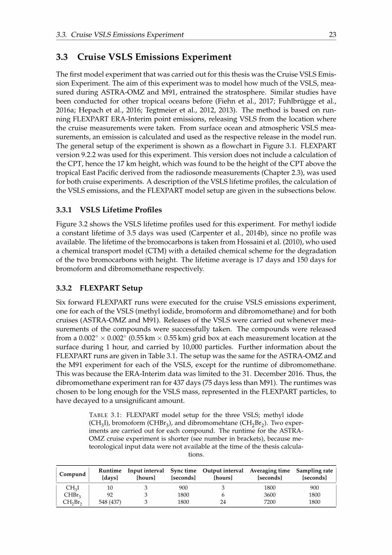
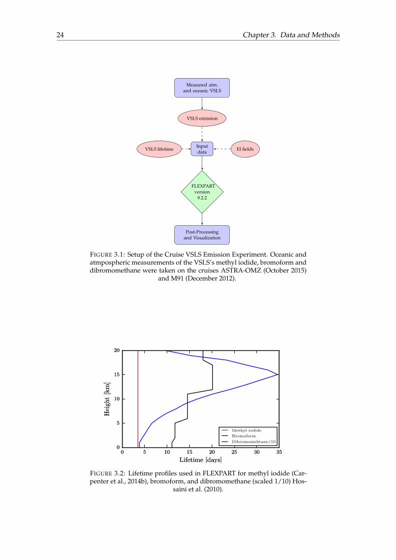
The first model experiment that was carried out for this thesis was the Cruise VSLS Emis-sion Experiment. The aim of this experiment was to model how much of the VSLS, mea-sured during ASTRA-OMZ and M91, entrained the stratosphere. Similar studies havebeen conducted for other tropical oceans before (Fiehn et al., 2017; Fuhlbrügge et al.,2016a; Hepach et al., 2016; Tegtmeier et al., 2012, 2013). The method is based on run-ning FLEXPART ERA-Interim point emissions, releasing VSLS from the location wherethe cruise measurements were taken. From surface ocean and atmospheric VSLS mea-surements, an emission is calculated and used as the respective release in the model run.The general setup of the experiment is shown as a flowchart in Figure 3.1. FLEXPARTversion 9.2.2 was used for this experiment. This version does not include a calculation ofthe CPT, hence the 17 km height, which was found to be the height of the CPT above thetropical East Pacific derived from the radiosonde measurements (Chapter 2.3), was usedfor both cruise experiments. A description of the VSLS lifetime profiles, the calculation ofthe VSLS emissions, and the FLEXPART model setup are given in the subsections below.
3.3.1 VSLS Lifetime Profiles
Figure 3.2 shows the VSLS lifetime profiles used for this experiment. For methyl iodidea constant lifetime of 3.5 days was used (Carpenter et al., 2014b), since no profile wasavailable. The lifetime of the bromocarbons is taken from Hossaini et al. (2010), who useda chemical transport model (CTM) with a detailed chemical scheme for the degradationof the two bromocarbons with height. The lifetime average is 17 days and 150 days forbromoform and dibromomethane respectively.
3.3.2 FLEXPART Setup
Six forward FLEXPART runs were executed for the cruise VSLS emissions experiment,one for each of the VSLS (methyl iodide, bromoform and dibromomethane) and for bothcruises (ASTRA-OMZ and M91). Releases of the VSLS were carried out whenever mea-surements of the compounds were successfully taken. The compounds were releasedfrom a 0.002◦ × 0.002◦ (0.55 km× 0.55 km) grid box at each measurement location at thesurface during 1 hour, and carried by 10,000 particles. Further information about theFLEXPART runs are given in Table 3.1. The setup was the same for the ASTRA-OMZ andthe M91 experiment for each of the VSLS, except for the runtime of dibromomethane.This was because the ERA-Interim data was limited to the 31. December 2016. Thus, thedibromomethane experiment ran for 437 days (75 days less than M91). The runtimes waschosen to be long enough for the VSLS mass, represented in the FLEXPART particles, tohave decayed to a unsignificant amount.
TABLE 3.1: FLEXPART model setup for the three VSLS; methyl idode(CH3I), bromoform (CHBr3), and dibromomehtane (CH2Br2). Two exper-iments are carried out for each compound. The runtime for the ASTRA-OMZ cruise experiment is shorter (see number in brackets), because me-teorological input data were not available at the time of the thesis calcula-
tions.
CompundRuntime
[days]Input interval
[hours]Sync time[seconds]
Output interval[hours]
Averaging time[seconds]
Sampling rate[seconds]
CH3I 10 3 900 3 1800 900CHBr3 92 3 1800 6 3600 1800CH2Br2 548 (437) 3 1800 24 7200 1800
24 Chapter 3. Data and Methods
Measured atm.and oceanic VSLS
VSLS emission
Inputdata
VSLS lifetime EI fields
FLEXPARTversion
9.2.2
Post-Processingand Visualization
FIGURE 3.1: Setup of the Cruise VSLS Emission Experiment. Oceanic andatmpospheric measurements of the VSLS’s methyl iodide, bromoform anddibromomethane were taken on the cruises ASTRA-OMZ (October 2015)
and M91 (December 2012).
0
5
10
15
20
Hei
ght
[km
]
0 5 10 15 20 25 30 35
Lifetime [days]
0
5
10
15
20
Hei
ght
[km
]
0 5 10 15 20 25 30 35
Lifetime [days]
Methyl iodide
Bromoform
Dibromomehtane/10
FIGURE 3.2: Lifetime profiles used in FLEXPART for methyl iodide (Car-penter et al., 2014b), bromoform, and dibromomethane (scaled 1/10) Hos-
saini et al. (2010).
3.4. East Pacific Bromoform Emission Experiment 25
3.4 East Pacific Bromoform Emission Experiment
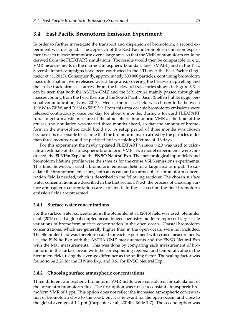
In order to further investigate the transport and dispersion of bromoform, a second ex-periment was designed. The approach of the East Pacific bromoform emission experi-ment was to release bromoform over a large area, so that the VMR of bromoform could bederived from the FLEXPART simulations. The results would then be comparable to, e.g.,VMR measurements in the marine atmospheric boundary layer (MABL) and in the TTL.Several aircraft campaigns have been conducted in the TTL over the East Pacific (Tegt-meier et al., 2013). Consequently, approximately 800 000 particles, containing bromoformmass information, were released over a large area, covering the Peruvian upwelling andthe cruise track airmass sources. From the backward trajectories shown in Figure 3.3, itcan be seen that both the ASTRA-OMZ and the M91 cruise mainly passed through airmasses coming from the Peru Basin and the South Pacific Basin (Steffen Fuhlbrügge, per-sonal communication, Nov. 2017). Hence, the release field was chosen to be between100◦W to 70◦W, and 20◦N to 50◦S 3.9. From this area oceanic bromoform emissions werereleased continuously, once per day for about 6 months, during a forward FLEXPARTrun. To get a realistic measure of the atmospheric bromoform VMR at the time of thecruises, the simulation was started three months ahead, so that the amount of bromo-form in the atmosphere could build up. A setup period of three months was chosenbecause it is reasonable to assume that the bromoform mass carried by the particles olderthan three months, would be perished by its e-folding lifetime of 16 days.
For this experiment the newly updated FLEXPART version 9.2.3 was used to calcu-late an estimate of the atmospheric bromoform VMR. Two model experiments were con-ducted; the El Niño Exp and the ENSO Neutral Exp. The meteorological input fields andbromoform lifetime profile were the same as for the cruise VSLS emissions experiments.This time, however, I used a bromoform emission field for a large area as input. To cal-culate the bromoform emissions, both an ocean and an atmospheric bromoform concen-tration field is needed, which is described in the following sections: The chosen surfacewater concentrations are described in the first section. Next, the process of choosing sur-face atmospheric concentrations are explained. In the last section the final bromoformemission fields are presented.
3.4.1 Surface water concentrations
For the surface water concentrations, the Stemmler et al. (2015) field was used. Stemmleret al. (2015) used a global coupled ocean biogeochemistry model to represent large scalevariations of bromoform surface concentration in the open ocean. Coastal bromoformconcentrations, which are generally higher than in the open ocean, were not included.The Stemmler field was therefore scaled for each experiment with cruise measurements,i.e., the El Niño Exp with the ASTRA-OMZ measurements and the ENSO Neutral Expwith the M91 measurements. This was done by comparing each measurement of bro-moform in the surface ocean with the corresponding regional and temporal value in theStemmlers field, using the average difference as the scaling factor. The scaling factor wasfound to be 2.28 for the El Niño Exp, and 0.61 for ENSO Neutral Exp.
3.4.2 Choosing surface atmospheric concentrations
Three different atmospheric bromoform VMR fields were considered for calculation ofthe ocean-atm bromoform flux. The first option was to use a constant atmospheric bro-moform VMR of 1 ppt. This option does not reflect the increased atmospheric concentra-tion of bromoform close to the coast, but it is relevant for the open ocean, and close tothe global average of 1.2 ppt (Carpenter et al., 2014b, Table 1-7). The second option was
26 Chapter 3. Data and Methods
FIGURE 3.3: 10 days backward trajectories for ASTRA-OMZ and M91(Steffen Fuhlbrügge, personal communication, Nov. 2017).
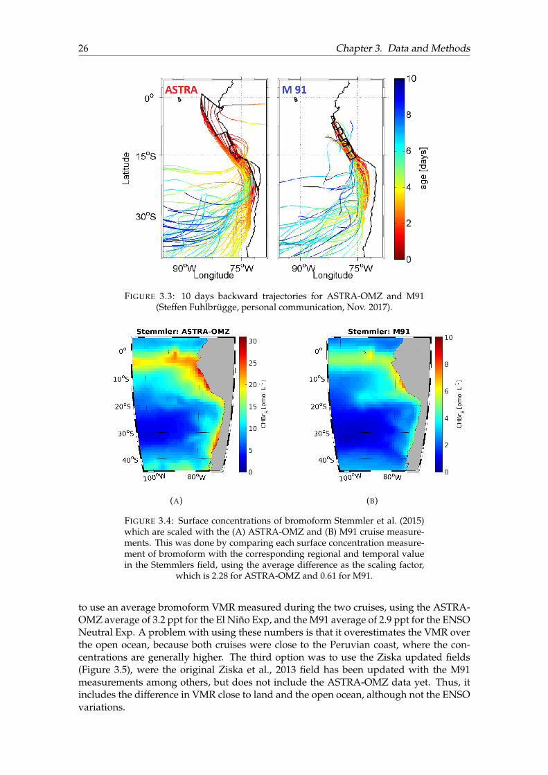
(A) (B)
FIGURE 3.4: Surface concentrations of bromoform Stemmler et al. (2015)which are scaled with the (A) ASTRA-OMZ and (B) M91 cruise measure-ments. This was done by comparing each surface concentration measure-ment of bromoform with the corresponding regional and temporal valuein the Stemmlers field, using the average difference as the scaling factor,
which is 2.28 for ASTRA-OMZ and 0.61 for M91.
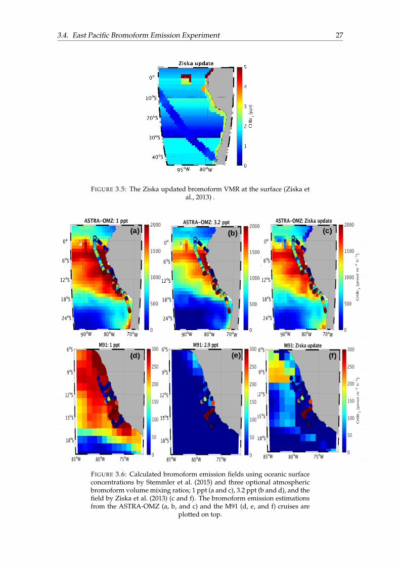
to use an average bromoform VMR measured during the two cruises, using the ASTRA-OMZ average of 3.2 ppt for the El Niño Exp, and the M91 average of 2.9 ppt for the ENSONeutral Exp. A problem with using these numbers is that it overestimates the VMR overthe open ocean, because both cruises were close to the Peruvian coast, where the con-centrations are generally higher. The third option was to use the Ziska updated fields(Figure 3.5), were the original Ziska et al., 2013 field has been updated with the M91measurements among others, but does not include the ASTRA-OMZ data yet. Thus, itincludes the difference in VMR close to land and the open ocean, although not the ENSOvariations.
3.4. East Pacific Bromoform Emission Experiment 27
FIGURE 3.5: The Ziska updated bromoform VMR at the surface (Ziska etal., 2013) .
FIGURE 3.6: Calculated bromoform emission fields using oceanic surfaceconcentrations by Stemmler et al. (2015) and three optional atmosphericbromoform volume mixing ratios; 1 ppt (a and c), 3.2 ppt (b and d), and thefield by Ziska et al. (2013) (c and f). The bromoform emission estimationsfrom the ASTRA-OMZ (a, b, and c) and the M91 (d, e, and f) cruises are
plotted on top.
28 Chapter 3. Data and Methods
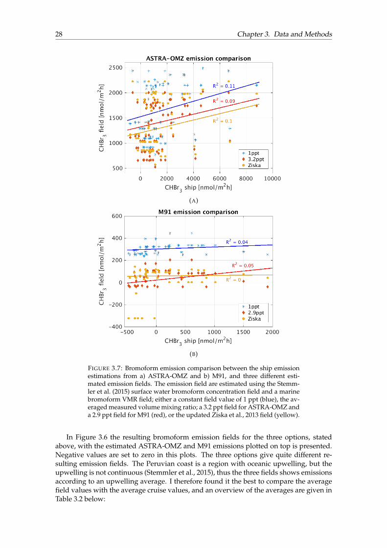
(A)
(B)
FIGURE 3.7: Bromoform emission comparison between the ship emissionestimations from a) ASTRA-OMZ and b) M91, and three different esti-mated emission fields. The emission field are estimated using the Stemm-ler et al. (2015) surface water bromoform concentration field and a marinebromoform VMR field; either a constant field value of 1 ppt (blue), the av-eraged measured volume mixing ratio; a 3.2 ppt field for ASTRA-OMZ anda 2.9 ppt field for M91 (red), or the updated Ziska et al., 2013 field (yellow).
In Figure 3.6 the resulting bromoform emission fields for the three options, statedabove, with the estimated ASTRA-OMZ and M91 emissions plotted on top is presented.Negative values are set to zero in this plots. The three options give quite different re-sulting emission fields. The Peruvian coast is a region with oceanic upwelling, but theupwelling is not continuous (Stemmler et al., 2015), thus the three fields shows emissionsaccording to an upwelling average. I therefore found it the best to compare the averagefield values with the average cruise values, and an overview of the averages are given inTable 3.2 below:
3.4. East Pacific Bromoform Emission Experiment 29
TABLE 3.2: Mean oceanic bromoform emissions for two experiments; theEl Niño Exp and the ENSO Neutral Exp. In the first column the mean of thecorresponding cruise emission estimated are shown (ASTRA-OMZ for theEl Niño Exp and M91 for the ENSO Neutral Exp). For the other columns amean over the stated field is shown. The field averages were taken over abig enough lat-lon box to include the respective cruise track. The values in
the brackets includes negative emissions.
BROMOFORM EMISSIONS [p mol m−2 h−1]
Experiment Cruise 1 ppt 2.9 ppt 3.2 ppt Ziska update field
El Niño Exp 1639 (1588) 1225 (1225) – 821 (818) 1079 (1079)ENSO Neutral Exp 232 (117) 227 (227) 15 (-97) – 36 (-32)
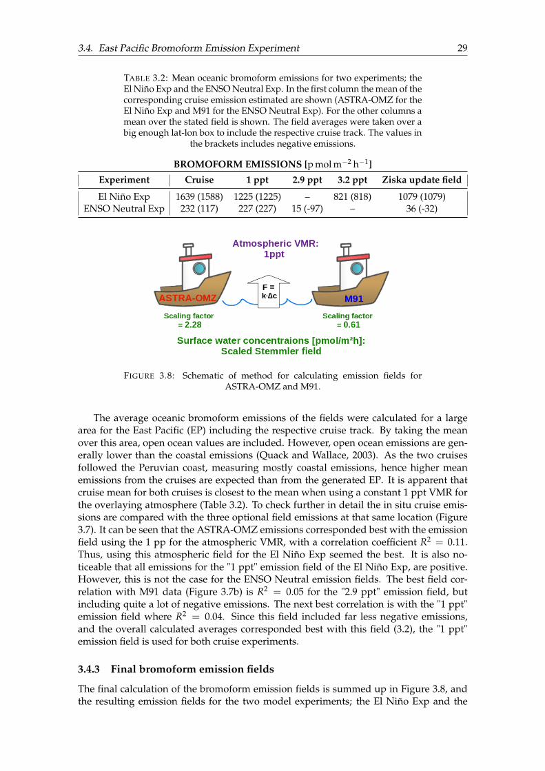
FIGURE 3.8: Schematic of method for calculating emission fields forASTRA-OMZ and M91.
The average oceanic bromoform emissions of the fields were calculated for a largearea for the East Pacific (EP) including the respective cruise track. By taking the meanover this area, open ocean values are included. However, open ocean emissions are gen-erally lower than the coastal emissions (Quack and Wallace, 2003). As the two cruisesfollowed the Peruvian coast, measuring mostly coastal emissions, hence higher meanemissions from the cruises are expected than from the generated EP. It is apparent thatcruise mean for both cruises is closest to the mean when using a constant 1 ppt VMR forthe overlaying atmosphere (Table 3.2). To check further in detail the in situ cruise emis-sions are compared with the three optional field emissions at that same location (Figure3.7). It can be seen that the ASTRA-OMZ emissions corresponded best with the emissionfield using the 1 pp for the atmospheric VMR, with a correlation coefficient R2 = 0.11.Thus, using this atmospheric field for the El Niño Exp seemed the best. It is also no-ticeable that all emissions for the "1 ppt" emission field of the El Niño Exp, are positive.However, this is not the case for the ENSO Neutral emission fields. The best field cor-relation with M91 data (Figure 3.7b) is R2 = 0.05 for the "2.9 ppt" emission field, butincluding quite a lot of negative emissions. The next best correlation is with the "1 ppt"emission field where R2 = 0.04. Since this field included far less negative emissions,and the overall calculated averages corresponded best with this field (3.2), the "1 ppt"emission field is used for both cruise experiments.
3.4.3 Final bromoform emission fields
The final calculation of the bromoform emission fields is summed up in Figure 3.8, andthe resulting emission fields for the two model experiments; the El Niño Exp and the
30 Chapter 3. Data and Methods
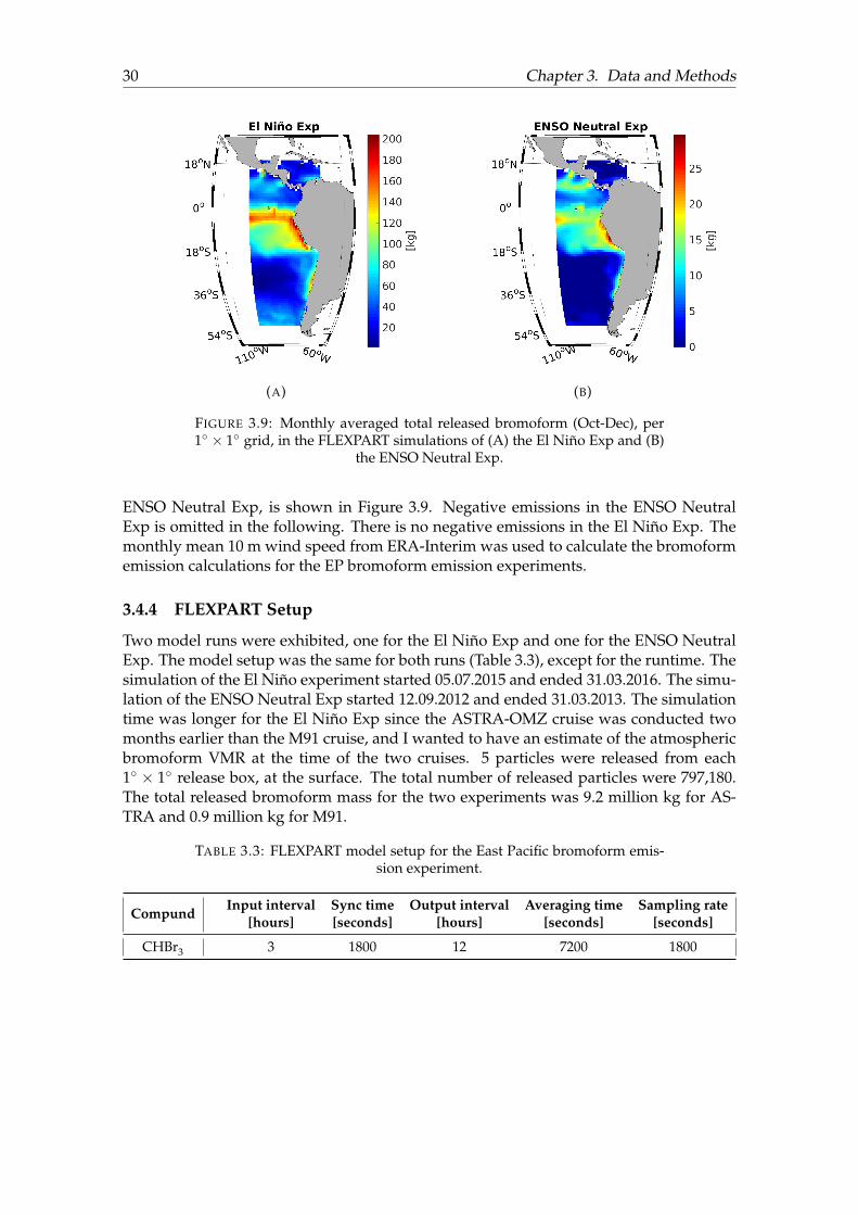
(A) (B)
FIGURE 3.9: Monthly averaged total released bromoform (Oct-Dec), per1◦ × 1◦ grid, in the FLEXPART simulations of (A) the El Niño Exp and (B)
the ENSO Neutral Exp.
ENSO Neutral Exp, is shown in Figure 3.9. Negative emissions in the ENSO NeutralExp is omitted in the following. There is no negative emissions in the El Niño Exp. Themonthly mean 10 m wind speed from ERA-Interim was used to calculate the bromoformemission calculations for the EP bromoform emission experiments.
3.4.4 FLEXPART Setup
Two model runs were exhibited, one for the El Niño Exp and one for the ENSO NeutralExp. The model setup was the same for both runs (Table 3.3), except for the runtime. Thesimulation of the El Niño experiment started 05.07.2015 and ended 31.03.2016. The simu-lation of the ENSO Neutral Exp started 12.09.2012 and ended 31.03.2013. The simulationtime was longer for the El Niño Exp since the ASTRA-OMZ cruise was conducted twomonths earlier than the M91 cruise, and I wanted to have an estimate of the atmosphericbromoform VMR at the time of the two cruises. 5 particles were released from each1◦ × 1◦ release box, at the surface. The total number of released particles were 797,180.The total released bromoform mass for the two experiments was 9.2 million kg for AS-TRA and 0.9 million kg for M91.
TABLE 3.3: FLEXPART model setup for the East Pacific bromoform emis-sion experiment.
CompundInput interval
[hours]Sync time[seconds]
Output interval[hours]
Averaging time[seconds]
Sampling rate[seconds]
CHBr3 3 1800 12 7200 1800
31
Chapter 4
Results and Discussions
The Results and Discussions Chapter is divided into three sections. Meteorological ob-servations and halocarbon measurements from the two cruises; ASTRA-OMZ (October2015) and M91 (December 2012), are presented in Section 4.1. The first research questionwill be discussed in this first section: 1. To what extent is the tropical East Pacific (EP)a source for very short-lived halogenated substances (VSLS) to the atmosphere? Sec-tion 4.2 is mainly concerned with the second: 2. How much of these VSLS are trans-ported to the stratosphere? The last section (Section 4.3) further investigates the trans-port of bromoform to the stratosphere in a "seasonal" case study. The third researchquestion is mainly answered in this last section: 3. How does El Niño affect the VSLStransport from the tropical EP to the stratosphere?
4.1 ASTRA-OMZ and M91 Data
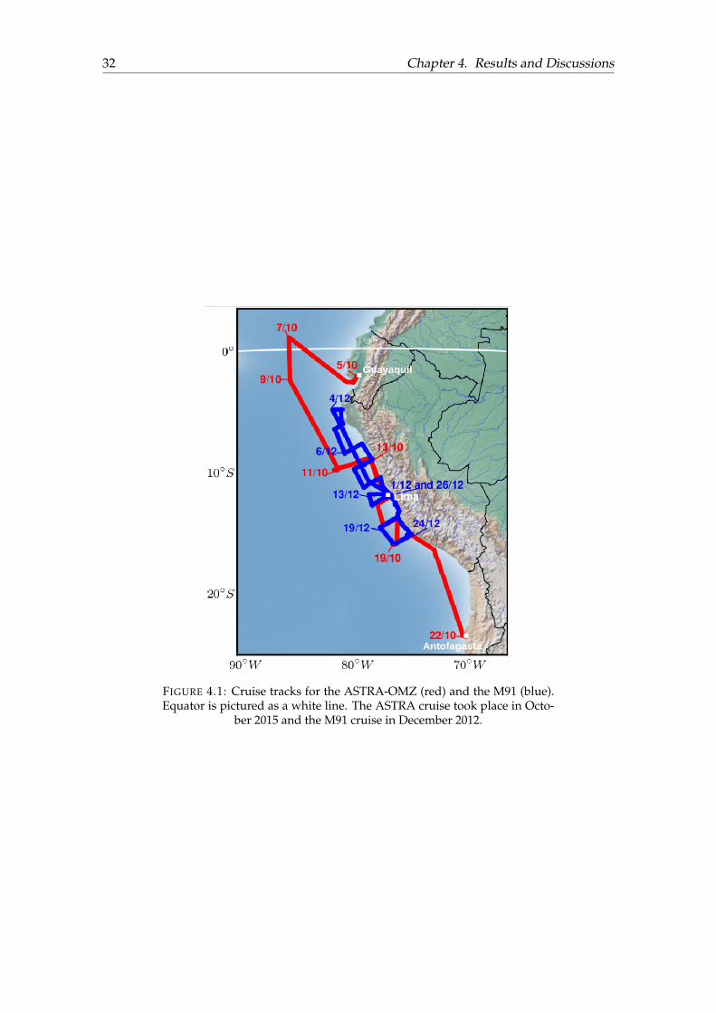
Data from two cruises ASTRA-OMZ and M91 have been used as a base for this thesis. TheASTRA-OMZ cruise was conducted on the R/V SONNE (SO243; 5 to 22 October 2015)from Guayaquil in Ecuador to Antofagasta in Chile, and the M91 cruise was carried onR/V METEOR (1 to 26 December 2012) starting and ending in Lima, Peru (Figure 4.1).The ASTRA-OMZ cruise went farther north, crossing the Equator, and also further souththan the M91 cruise. Both cruises alternated between open-ocean sections and sectionsclose to the coast.
The overall goal of the ASTRA-OMZ cruise was to determine the impact of low oxy-gen conditions on trace element cycling and distributions, and how air-sea exchangeof tracers is influenced by the pronounced productivity in the EP (Marandino, 2016).Whereas, the main goal of M91 was to study on the upwelling region off Peru in order toinvestigate its importance for emission of climate-relevant atmospheric trace gases andfor tropospheric chemistry (Bange, 2013). This thesis is concerned with the contribu-tion of the VSLS, emitted from the tropical EP, to the stratospheric halogen budget. Themeteorological measurements and the halocarbon measurements of methyl iodide, bro-moform, and dibromomethane, taken during the ASTRA-OMZ cruise, are presented inthis section, and compared with M91, previously analyzed by Fuhlbrügge et al. (2016a).
An overview of the ASTRA-OMZ DSHIP data is shown in Figure 4.2. Time periodsof oceanic upwelling is shaded blue in the figure, chosen according to when the SSTdropped to around 18◦C. Stramma et al. (2016) observed upwelling of warm, saline, andoxygen-rich water about 9◦S. Hence, it is likely that periods of upwelling, not shown inFigure 4.2, occurred at the more northern parts of the route. The same figure is shownfor M91 (Figure 4.3), adapted from Fuhlbrügge et al. (2016a), for comparison. Larger SSTdrops occurred during M91, up to 5◦C, than during ASTRA-OMZ; with a max of 3.5◦C.This suggest that stronger upwelling occured during M91 than ASTRA-OMZ. This is inaccordance with a deep pycnocline and thermocline observed in October 2015, indicatingreduced equatorial upwelling (Stramma et al., 2016). As can be seen from both figures,
32 Chapter 4. Results and Discussions
FIGURE 4.1: Cruise tracks for the ASTRA-OMZ (red) and the M91 (blue).Equator is pictured as a white line. The ASTRA cruise took place in Octo-
ber 2015 and the M91 cruise in December 2012.
4.1. ASTRA-OMZ and M91 Data 33
14
16
18
20
22
24
26
SA
T[◦
C]
(a)
65
70
75
80
85
90
95
100
RH
[%]
(b)
0
50
100
150
200
250
300
350
Win
dd
ir.
[deg
]
(c)
0
20
40
60
80
100
120
CH
3I
[pm
olL−
1]
(d)
0
1
2
3
4
5
6
CH
3I
[pp
t] (e)
Oct 06 2015 Oct 08 2015 Oct 10 2015 Oct 12 2015 Oct 14 2015 Oct 16 2015 Oct 18 2015 Oct 20 2015 Oct 22 2015
date [UTC]
−202468
10121416
CH
3I
[nm
olm−
2h−
1]
(f)
14
16
18
20
22
24
26
28
SS
T[◦
C]
9101112131415161718
AH
[g/m
3]
0
2
4
6
8
10
12
14
16
Win
dsp
d.
[m/s
]
0
20
40
60
80
100
120
CHBr 3
[pm
olL−
1]
0
20
40
60
80
100
120
CH
2Br 2
[pm
olL−
1]
0
1
2
3
4
5
6
CHBr 3
[pp
t]
0
1
2
3
4
5
6
CH
2Br 2
[pp
t]
−20246810121416
CHBr 3
[nm
olm−
2h−
1]
−20246810121416
CH
2Br 2
[nm
olm−
2h−
1]
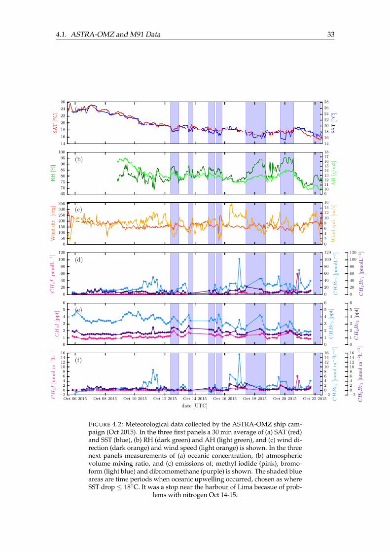
FIGURE 4.2: Meteorological data collected by the ASTRA-OMZ ship cam-paign (Oct 2015). In the three first panels a 30 min average of (a) SAT (red)and SST (blue), (b) RH (dark green) and AH (light green), and (c) wind di-rection (dark orange) and wind speed (light orange) is shown. In the threenext panels measurements of (a) oceanic concentration, (b) atmosphericvolume mixing ratio, and (c) emissions of; methyl iodide (pink), bromo-form (light blue) and dibromomethane (purple) is shown. The shaded blueareas are time periods when oceanic upwelling occurred, chosen as whereSST drop ≤ 18◦C. It was a stop near the harbour of Lima becasue of prob-
lems with nitrogen Oct 14-15.
34 Chapter 4. Results and Discussions
15
16
17
18
19
20
21
22
23
SA
T[◦
C]
(a)
65
70
75
80
85
90
95
100
RH
[%]
(b)
0
50
100
150
200
250
300
350
Win
dd
ir.
[deg
]
(c)
0
5
10
15
20
25
30
35
40
CH
3I
[pm
olL−
1]
(d)
0
1
2
3
4
5
6
CH
3I
[pp
t] (e)
Dec 02 2012 Dec 05 2012 Dec 08 2012 Dec 11 2012 Dec 14 2012 Dec 17 2012 Dec 20 2012 Dec 23 2012 Dec 26 2012
date [UTC]
−1
0
1
2
3
4
5
CH
3I
[nm
ol
m−
2h−
1]
(f)
14151617181920212223
SS
T[◦
C]
9101112131415161718
AH
[g/m
3]
0
2
4
6
8
10
12
14
16
Win
dsp
d.
[m/s
]
0
5
10
15
20
25
30
35
40
CHBr 3
[pm
olL−
1]
0
5
10
15
20
25
30
35
40
CH
2Br 2
[pm
olL−
1]
0
1
2
3
4
5
6CHBr 3
[pp
t]
0
1
2
3
4
5
6
CH
2Br 2
[pp
t]
−1
0
1
2
3
4
5
CHBr 3
[nm
olm−
2h−
1]
−1
0
1
2
3
4
5
CH
2Br 2
[nm
olm−
2h−
1]
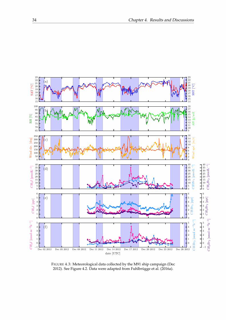
FIGURE 4.3: Meteorological data collected by the M91 ship campaign (Dec2012). See Figure 4.2. Data were adapted from Fuhlbrügge et al. (2016a).
4.1. ASTRA-OMZ and M91 Data 35
there is an increase in the RH and the atmospheric volume mixing ratio (VMR) of thehalocarbons when oceanic upwelling occurred. This can be explained by the fact thatwhen cold water is transported to the surface, it cools the air above, leading to a a sta-ble atmospheric surface layer with suppressed vertical mixing and higher atmosphericmixing ratios (Fuhlbrügge et al., 2016a). It is also visible from the Figures 4.2 and 4.3that the measured oceanic concentration of methyl iodide is low, and that the measuredbromocarbon concentration is high for ASTRA-OMZ, while the opposite for M91. Theatmospheric VMR of the halocarbons are similar for the two cruises, resulting in lowmethyl iodide emissions and high bromocarbon emissions for ASTRA-OMZ, and againthe opposite for M91.
(A) (B)
(C) (D)
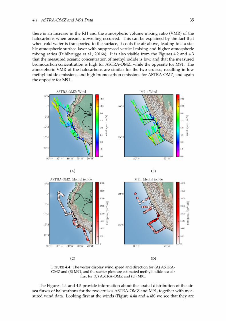
FIGURE 4.4: The vector display wind speed and direction for (A) ASTRA-OMZ and (B) M91, and the scatter plots are estimated methyl iodide sea-air
flux for (C) ASTRA-OMZ and (D) M91.
The Figures 4.4 and 4.5 provide information about the spatial distribution of the air-sea fluxes of halocarbons for the two cruises ASTRA-OMZ and M91, together with mea-sured wind data. Looking first at the winds (Figure 4.4a and 4.4b) we see that they are
36 Chapter 4. Results and Discussions
(A) (B)
(C) (D)
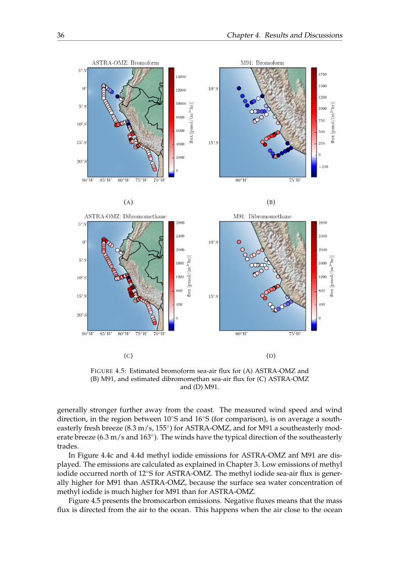
FIGURE 4.5: Estimated bromoform sea-air flux for (A) ASTRA-OMZ and(B) M91, and estimated dibromomethan sea-air flux for (C) ASTRA-OMZ
and (D) M91.
generally stronger further away from the coast. The measured wind speed and winddirection, in the region between 10◦S and 16◦S (for comparison), is on average a south-easterly fresh breeze (8.3 m/s, 155◦) for ASTRA-OMZ, and for M91 a southeasterly mod-erate breeze (6.3 m/s and 163◦). The winds have the typical direction of the southeasterlytrades.
In Figure 4.4c and 4.4d methyl iodide emissions for ASTRA-OMZ anf M91 are dis-played. The emissions are calculated as explained in Chapter 3. Low emissions of methyliodide occurred north of 12◦S for ASTRA-OMZ. The methyl iodide sea-air flux is gener-ally higher for M91 than ASTRA-OMZ, because the surface sea water concentration ofmethyl iodide is much higher for M91 than for ASTRA-OMZ.
Figure 4.5 presents the bromocarbon emissions. Negative fluxes means that the massflux is directed from the air to the ocean. This happens when the air close to the ocean
4.1. ASTRA-OMZ and M91 Data 37
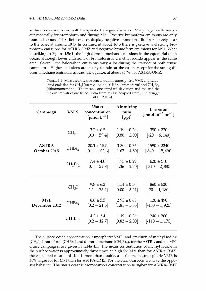
surface is over-saturated with the specific trace gas of interest. Many negative fluxes oc-cur especially for bromoform and during M91. Positive bromoform emissions are onlyfound at around 14◦S. Both cruises display negative bromoform fluxes relatively nearto the coast at around 10◦S. In contrast, at about 16◦S there is positive and strong bro-moform emissions for ASTRA-OMZ and negative bromoform emissions for M91. Whatis striking in Figure 4.5c is the high dibromomethane emissions in the equatorial openocean, although lower emissions of bromoform and methyl iodide appear in the samearea. Overall, the halocarbon emissions vary a lot during the transect of both cruisecampaigns. Higher emissions are mostly foundnear the coast, except for the strong di-bromomethane emissions around the equator, at about 85◦W, for ASTRA-OMZ.
TABLE 4.1: Measured oceanic concentration, atmospheric VMR and calcu-lated emission for CH3I (methyl iodide), CHBr3 (bromoform) and CH2Br2(dibromomethane). The mean ±one standard deviation and the and themaximum values are listed. Data from M91 is adapted from (Fuhlbrügge
et al., 2016a).
Campaign VSLSWater
concentration[pmol L−1]
Air mixingratio[ppt]
Emission[pmol m−2 hr−1]
CH3I3.3 ± 6.5
[0.0− 59.4]1.19 ± 0.28[0.80− 2.00]
350 ± 720[-20− 6, 140]
ASTRAOctober 2015
CHBr320.1 ± 15.5[0.1− 102.6]
3.30 ± 0.76[1.67− 4.80]
1590 ± 2240[-840− 15, 490]
CH2Br27.4 ± 4.0
[0.4− 22.8]1.73 ± 0.29[1.36− 2.70]
620 ± 610[-310− 2, 880]
CH3I9.8 ± 6.3
[1.1− 35.4]1.54 ± 0.50[0.00− 3.21]
860 ± 620[20− 4, 180]
M91December 2012
CHBr36.6 ± 5.5
[0.2− 21.5]2.93 ± 0.68[1.81− 5.85]
120 ± 490[-480− 1, 920]
CH2Br24.3 ± 3.4
[0.2− 12.7]1.19 ± 0.26[0.82− 2.00]
240 ± 300[-110− 1, 170]
The surface ocean concentration, atmospheric VMR, and emission of methyl iodide(CH3I), bromoform (CHBr3) and dibromomethane (CH2Br2), for the ASTRA and the M91cruise campaigns, are given in Table 4.1. The mean concentration of methyl iodide inthe surface water is approximately three times as high for M91 than for ASTRA-OMZ,the calculated mean emission is more than double, and the mean atmospheric VMR is30% larger for for M91 than for ASTRA-OMZ. For the bromocarbons we have the oppo-site behavior. The mean oceanic bromocarbon concentration is higher for ASTRA-OMZ
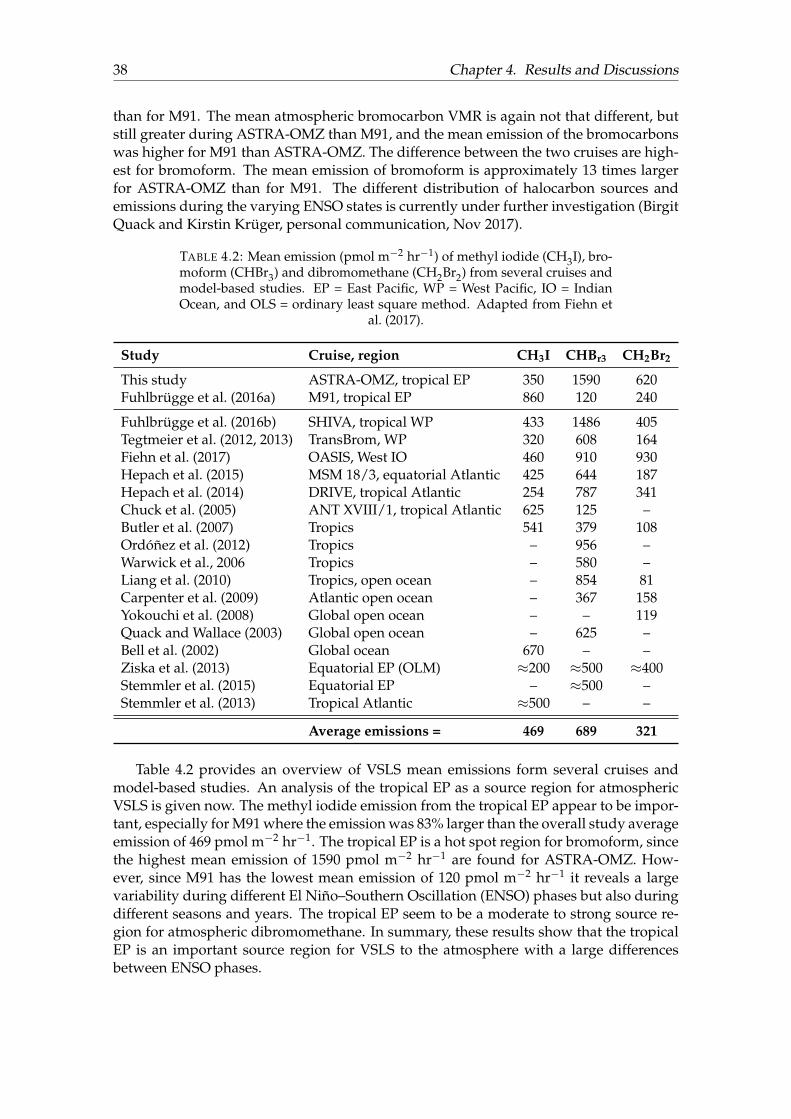
38 Chapter 4. Results and Discussions
than for M91. The mean atmospheric bromocarbon VMR is again not that different, butstill greater during ASTRA-OMZ than M91, and the mean emission of the bromocarbonswas higher for M91 than ASTRA-OMZ. The difference between the two cruises are high-est for bromoform. The mean emission of bromoform is approximately 13 times largerfor ASTRA-OMZ than for M91. The different distribution of halocarbon sources andemissions during the varying ENSO states is currently under further investigation (BirgitQuack and Kirstin Krüger, personal communication, Nov 2017).
TABLE 4.2: Mean emission (pmol m−2 hr−1) of methyl iodide (CH3I), bro-moform (CHBr3) and dibromomethane (CH2Br2) from several cruises andmodel-based studies. EP = East Pacific, WP = West Pacific, IO = IndianOcean, and OLS = ordinary least square method. Adapted from Fiehn et
al. (2017).
Study Cruise, region CH3I CHBr3 CH2Br2
This study ASTRA-OMZ, tropical EP 350 1590 620Fuhlbrügge et al. (2016a) M91, tropical EP 860 120 240
Fuhlbrügge et al. (2016b) SHIVA, tropical WP 433 1486 405Tegtmeier et al. (2012, 2013) TransBrom, WP 320 608 164Fiehn et al. (2017) OASIS, West IO 460 910 930Hepach et al. (2015) MSM 18/3, equatorial Atlantic 425 644 187Hepach et al. (2014) DRIVE, tropical Atlantic 254 787 341Chuck et al. (2005) ANT XVIII/1, tropical Atlantic 625 125 –Butler et al. (2007) Tropics 541 379 108Ordóñez et al. (2012) Tropics – 956 –Warwick et al., 2006 Tropics – 580 –Liang et al. (2010) Tropics, open ocean – 854 81Carpenter et al. (2009) Atlantic open ocean – 367 158Yokouchi et al. (2008) Global open ocean – – 119Quack and Wallace (2003) Global open ocean – 625 –Bell et al. (2002) Global ocean 670 – –Ziska et al. (2013) Equatorial EP (OLM) ≈200 ≈500 ≈400Stemmler et al. (2015) Equatorial EP – ≈500 –Stemmler et al. (2013) Tropical Atlantic ≈500 – –
Average emissions = 469 689 321
Table 4.2 provides an overview of VSLS mean emissions form several cruises andmodel-based studies. An analysis of the tropical EP as a source region for atmosphericVSLS is given now. The methyl iodide emission from the tropical EP appear to be impor-tant, especially for M91 where the emission was 83% larger than the overall study averageemission of 469 pmol m−2 hr−1. The tropical EP is a hot spot region for bromoform, sincethe highest mean emission of 1590 pmol m−2 hr−1 are found for ASTRA-OMZ. How-ever, since M91 has the lowest mean emission of 120 pmol m−2 hr−1 it reveals a largevariability during different El Niño–Southern Oscillation (ENSO) phases but also duringdifferent seasons and years. The tropical EP seem to be a moderate to strong source re-gion for atmospheric dibromomethane. In summary, these results show that the tropicalEP is an important source region for VSLS to the atmosphere with a large differencesbetween ENSO phases.
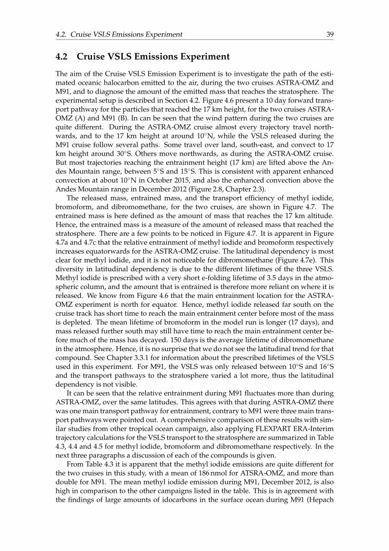
4.2. Cruise VSLS Emissions Experiment 39
4.2 Cruise VSLS Emissions Experiment
The aim of the Cruise VSLS Emission Experiment is to investigate the path of the esti-mated oceanic halocarbon emitted to the air, during the two cruises ASTRA-OMZ andM91, and to diagnose the amount of the emitted mass that reaches the stratosphere. Theexperimental setup is described in Section 4.2. Figure 4.6 present a 10 day forward trans-port pathway for the particles that reached the 17 km height, for the two cruises ASTRA-OMZ (A) and M91 (B). In can be seen that the wind pattern during the two cruises arequite different. During the ASTRA-OMZ cruise almost every trajectory travel north-wards, and to the 17 km height at around 10◦N, while the VSLS released during theM91 cruise follow several paths. Some travel over land, south-east, and convect to 17km height around 30◦S. Others move northwards, as during the ASTRA-OMZ cruise.But most trajectories reaching the entrainment height (17 km) are lifted above the An-des Mountain range, between 5◦S and 15◦S. This is consistent with apparent enhancedconvection at about 10◦N in October 2015, and also the enhanced convection above theAndes Mountain range in December 2012 (Figure 2.8, Chapter 2.3).
The released mass, entrained mass, and the transport efficiency of methyl iodide,bromoform, and dibromomethane, for the two cruises, are shown in Figure 4.7. Theentrained mass is here defined as the amount of mass that reaches the 17 km altitude.Hence, the entrained mass is a measure of the amount of released mass that reached thestratosphere. There are a few points to be noticed in Figure 4.7. It is apparent in Figure4.7a and 4.7c that the relative entrainment of methyl iodide and bromoform respectivelyincreases equatorwards for the ASTRA-OMZ cruise. The latitudinal dependency is mostclear for methyl iodide, and it is not noticeable for dibromomethane (Figure 4.7e). Thisdiversity in latitudinal dependency is due to the different lifetimes of the three VSLS.Methyl iodide is prescribed with a very short e-folding lifetime of 3.5 days in the atmo-spheric column, and the amount that is entrained is therefore more reliant on where it isreleased. We know from Figure 4.6 that the main entrainment location for the ASTRA-OMZ experiment is north for equator. Hence, methyl iodide released far south on thecruise track has short time to reach the main entrainment center before most of the massis depleted. The mean lifetime of bromoform in the model run is longer (17 days), andmass released further south may still have time to reach the main entrainment center be-fore much of the mass has decayed. 150 days is the average lifetime of dibromomethanein the atmosphere. Hence, it is no surprise that we do not see the latitudinal trend for thatcompound. See Chapter 3.3.1 for information about the prescribed lifetimes of the VSLSused in this experiment. For M91, the VSLS was only released between 10◦S and 16◦Sand the transport pathways to the stratosphere varied a lot more, thus the latitudinaldependency is not visible.
It can be seen that the relative entrainment during M91 fluctuates more than duringASTRA-OMZ, over the same latitudes. This agrees with that during ASTRA-OMZ therewas one main transport pathway for entrainment, contrary to M91 were three main trans-port pathways were pointed out. A comprehensive comparison of these results with sim-ilar studies from other tropical ocean campaign, also applying FLEXPART ERA-Interimtrajectory calculations for the VSLS transport to the stratosphere are summarized in Table4.3, 4.4 and 4.5 for methyl iodide, bromoform and dibromomethane respectively. In thenext three paragraphs a discussion of each of the compounds is given.
From Table 4.3 it is apparent that the methyl iodide emissions are quite different forthe two cruises in this study, with a mean of 186 nmol for ATSRA-OMZ, and more thandouble for M91. The mean methyl iodide emission during M91, December 2012, is alsohigh in comparison to the other campaigns listed in the table. This is in agreement withthe findings of large amounts of idocarbons in the surface ocean during M91 (Hepach
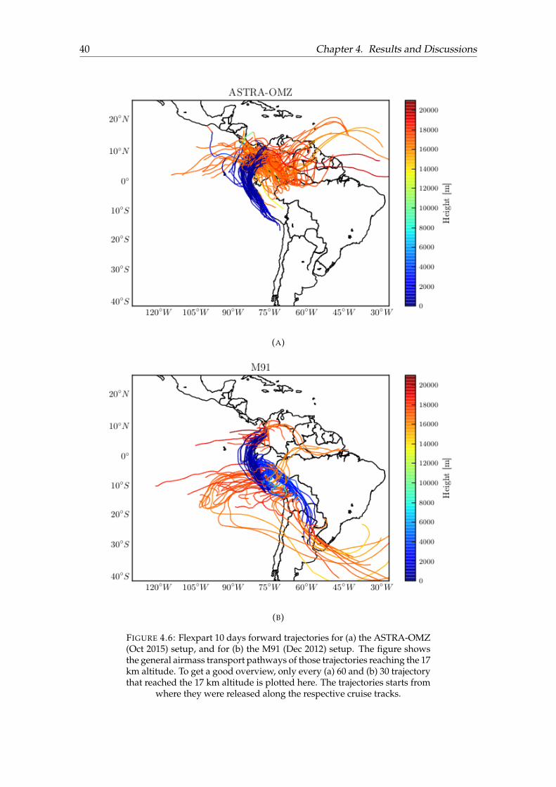
40 Chapter 4. Results and Discussions
(A)
(B)
FIGURE 4.6: Flexpart 10 days forward trajectories for (a) the ASTRA-OMZ(Oct 2015) setup, and for (b) the M91 (Dec 2012) setup. The figure showsthe general airmass transport pathways of those trajectories reaching the 17km altitude. To get a good overview, only every (a) 60 and (b) 30 trajectorythat reached the 17 km altitude is plotted here. The trajectories starts from
where they were released along the respective cruise tracks.
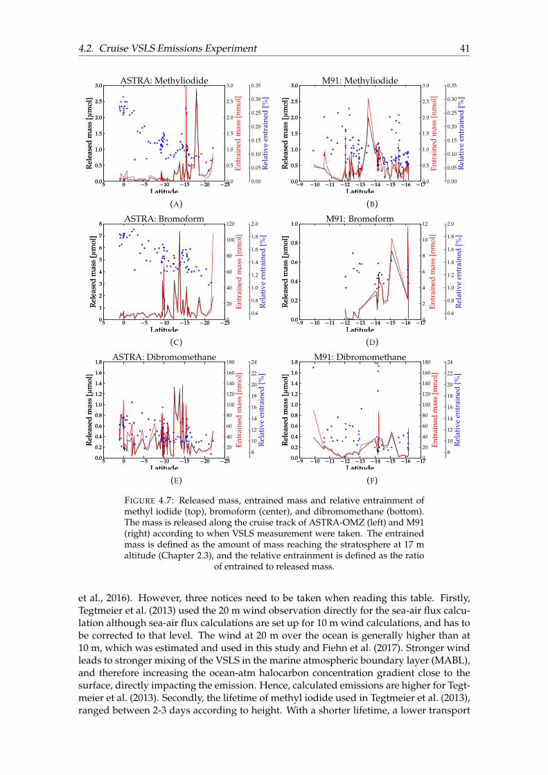
4.2. Cruise VSLS Emissions Experiment 41
0.0
0.5
1.0
1.5
2.0
2.5
3.0R
elea
sed
mas
s[µ
mol
]
−25−20−15−10−505Latitude
0.0
0.5
1.0
1.5
2.0
2.5
3.0
Entr
aine
dm
ass
[nm
ol]
0.00
0.05
0.10
0.15
0.20
0.25
0.30
0.35
Rel
ativ
een
trai
ned
[%]
0.0
0.5
1.0
1.5
2.0
2.5
3.0R
elea
sed
mas
s[µ
mol
]
−25−20−15−10−505Latitude
ASTRA: Methyliodide
(A)
0.0
0.5
1.0
1.5
2.0
2.5
3.0
Rel
ease
dm
ass
[µm
ol]
−17−16−15−14−13−12−11−10−9Latitude
0.0
0.5
1.0
1.5
2.0
2.5
3.0
Entr
aine
dm
ass
[nm
ol]
0.00
0.05
0.10
0.15
0.20
0.25
0.30
0.35
Rel
ativ
een
trai
ned
[%]
0.0
0.5
1.0
1.5
2.0
2.5
3.0
Rel
ease
dm
ass
[µm
ol]
−17−16−15−14−13−12−11−10−9Latitude
M91: Methyliodide
(B)
0
1
2
3
4
5
6
7
8
Rel
ease
dm
ass
[µm
ol]
−25−20−15−10−505Latitude
0
20
40
60
80
100
120
Entr
aine
dm
ass
[nm
ol]
0.6
0.8
1.0
1.2
1.4
1.6
1.8
2.0
Rel
ativ
een
trai
ned
[%]
0
1
2
3
4
5
6
7
8
Rel
ease
dm
ass
[µm
ol]
−25−20−15−10−505Latitude
ASTRA: Bromoform
(C)
0.0
0.2
0.4
0.6
0.8
1.0
Rel
ease
dm
ass
[µm
ol]
−17−16−15−14−13−12−11−10−9Latitude
0
2
4
6
8
10
12
Entr
aine
dm
ass
[nm
ol]
0.6
0.8
1.0
1.2
1.4
1.6
1.8
2.0
Rel
ativ
een
trai
ned
[%]
0.0
0.2
0.4
0.6
0.8
1.0
Rel
ease
dm
ass
[µm
ol]
−17−16−15−14−13−12−11−10−9Latitude
M91: Bromoform
(D)
0.0
0.2
0.4
0.6
0.8
1.0
1.2
1.4
1.6
1.8
Rel
ease
dm
ass
[µm
ol]
−25−20−15−10−505Latitude
0
20
40
60
80
100
120
140
160
180
Entr
aine
dm
ass
[nm
ol]
8
10
12
14
16
18
20
22
24
Rel
ativ
een
trai
ned
[%]
0.0
0.2
0.4
0.6
0.8
1.0
1.2
1.4
1.6
1.8
Rel
ease
dm
ass
[µm
ol]
−25−20−15−10−505Latitude
ASTRA: Dibromomethane
(E)
0.0
0.2
0.4
0.6
0.8
1.0
1.2
1.4
1.6
1.8
Rel
ease
dm
ass
[µm
ol]
−17−16−15−14−13−12−11−10−9Latitude
0
20
40
60
80
100
120
140
160
180
Entr
aine
dm
ass
[nm
ol]
8
10
12
14
16
18
20
22
24
Rel
ativ
een
trai
ned
[%]
0.0
0.2
0.4
0.6
0.8
1.0
1.2
1.4
1.6
1.8
Rel
ease
dm
ass
[µm
ol]
−17−16−15−14−13−12−11−10−9Latitude
M91: Dibromomethane
(F)
FIGURE 4.7: Released mass, entrained mass and relative entrainment ofmethyl iodide (top), bromoform (center), and dibromomethane (bottom).The mass is released along the cruise track of ASTRA-OMZ (left) and M91(right) according to when VSLS measurement were taken. The entrainedmass is defined as the amount of mass reaching the stratosphere at 17 maltitude (Chapter 2.3), and the relative entrainment is defined as the ratio
of entrained to released mass.
et al., 2016). However, three notices need to be taken when reading this table. Firstly,Tegtmeier et al. (2013) used the 20 m wind observation directly for the sea-air flux calcu-lation although sea-air flux calculations are set up for 10 m wind calculations, and has tobe corrected to that level. The wind at 20 m over the ocean is generally higher than at10 m, which was estimated and used in this study and Fiehn et al. (2017). Stronger windleads to stronger mixing of the VSLS in the marine atmospheric boundary layer (MABL),and therefore increasing the ocean-atm halocarbon concentration gradient close to thesurface, directly impacting the emission. Hence, calculated emissions are higher for Tegt-meier et al. (2013). Secondly, the lifetime of methyl iodide used in Tegtmeier et al. (2013),ranged between 2-3 days according to height. With a shorter lifetime, a lower transport
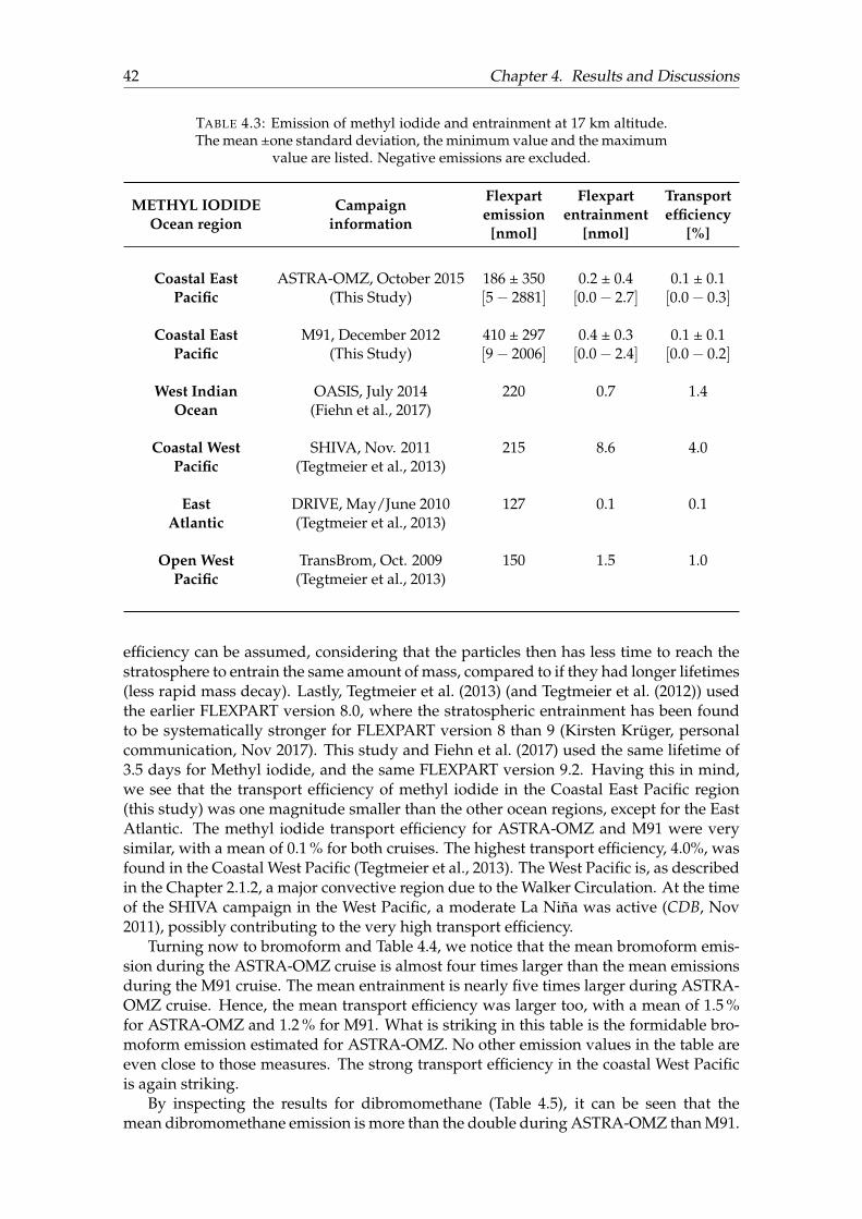
42 Chapter 4. Results and Discussions
TABLE 4.3: Emission of methyl iodide and entrainment at 17 km altitude.The mean ±one standard deviation, the minimum value and the maximum
value are listed. Negative emissions are excluded.
METHYL IODIDEOcean region
Campaigninformation
Flexpartemission
[nmol]
Flexpartentrainment
[nmol]
Transportefficiency
[%]
Coastal EastPacific
ASTRA-OMZ, October 2015(This Study)
186 ± 350[5− 2881]
0.2 ± 0.4[0.0− 2.7]
0.1 ± 0.1[0.0− 0.3]
Coastal EastPacific
M91, December 2012(This Study)
410 ± 297[9− 2006]
0.4 ± 0.3[0.0− 2.4]
0.1 ± 0.1[0.0− 0.2]
West IndianOcean
OASIS, July 2014(Fiehn et al., 2017)
220 0.7 1.4
Coastal WestPacific
SHIVA, Nov. 2011(Tegtmeier et al., 2013)
215 8.6 4.0
EastAtlantic
DRIVE, May/June 2010(Tegtmeier et al., 2013)
127 0.1 0.1
Open WestPacific
TransBrom, Oct. 2009(Tegtmeier et al., 2013)
150 1.5 1.0
efficiency can be assumed, considering that the particles then has less time to reach thestratosphere to entrain the same amount of mass, compared to if they had longer lifetimes(less rapid mass decay). Lastly, Tegtmeier et al. (2013) (and Tegtmeier et al. (2012)) usedthe earlier FLEXPART version 8.0, where the stratospheric entrainment has been foundto be systematically stronger for FLEXPART version 8 than 9 (Kirsten Krüger, personalcommunication, Nov 2017). This study and Fiehn et al. (2017) used the same lifetime of3.5 days for Methyl iodide, and the same FLEXPART version 9.2. Having this in mind,we see that the transport efficiency of methyl iodide in the Coastal East Pacific region(this study) was one magnitude smaller than the other ocean regions, except for the EastAtlantic. The methyl iodide transport efficiency for ASTRA-OMZ and M91 were verysimilar, with a mean of 0.1 % for both cruises. The highest transport efficiency, 4.0%, wasfound in the Coastal West Pacific (Tegtmeier et al., 2013). The West Pacific is, as describedin the Chapter 2.1.2, a major convective region due to the Walker Circulation. At the timeof the SHIVA campaign in the West Pacific, a moderate La Niña was active (CDB, Nov2011), possibly contributing to the very high transport efficiency.
Turning now to bromoform and Table 4.4, we notice that the mean bromoform emis-sion during the ASTRA-OMZ cruise is almost four times larger than the mean emissionsduring the M91 cruise. The mean entrainment is nearly five times larger during ASTRA-OMZ cruise. Hence, the mean transport efficiency was larger too, with a mean of 1.5 %for ASTRA-OMZ and 1.2 % for M91. What is striking in this table is the formidable bro-moform emission estimated for ASTRA-OMZ. No other emission values in the table areeven close to those measures. The strong transport efficiency in the coastal West Pacificis again striking.
By inspecting the results for dibromomethane (Table 4.5), it can be seen that themean dibromomethane emission is more than the double during ASTRA-OMZ than M91.
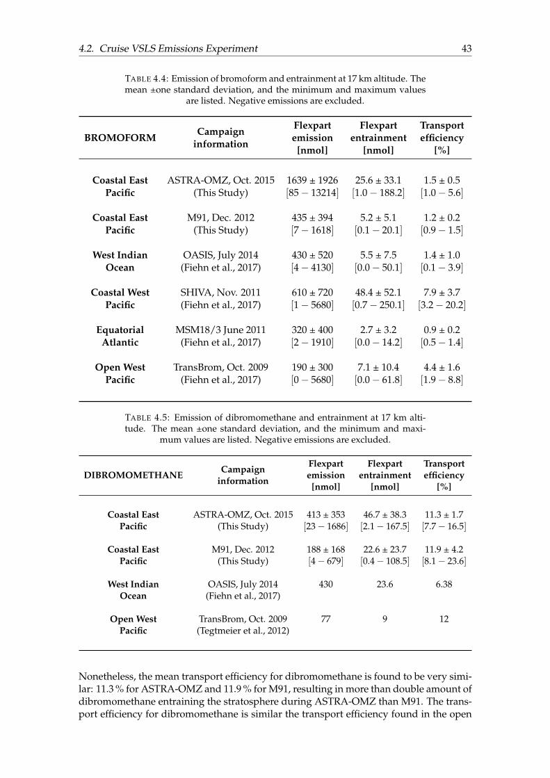
4.2. Cruise VSLS Emissions Experiment 43
TABLE 4.4: Emission of bromoform and entrainment at 17 km altitude. Themean ±one standard deviation, and the minimum and maximum values
are listed. Negative emissions are excluded.
BROMOFORMCampaign
information
Flexpartemission
[nmol]
Flexpartentrainment
[nmol]
Transportefficiency
[%]
Coastal EastPacific
ASTRA-OMZ, Oct. 2015(This Study)
1639 ± 1926[85− 13214]
25.6 ± 33.1[1.0− 188.2]
1.5 ± 0.5[1.0− 5.6]
Coastal EastPacific
M91, Dec. 2012(This Study)
435 ± 394[7− 1618]
5.2 ± 5.1[0.1− 20.1]
1.2 ± 0.2[0.9− 1.5]
West IndianOcean
OASIS, July 2014(Fiehn et al., 2017)
430 ± 520[4− 4130]
5.5 ± 7.5[0.0− 50.1]
1.4 ± 1.0[0.1− 3.9]
Coastal WestPacific
SHIVA, Nov. 2011(Fiehn et al., 2017)
610 ± 720[1− 5680]
48.4 ± 52.1[0.7− 250.1]
7.9 ± 3.7[3.2− 20.2]
EquatorialAtlantic
MSM18/3 June 2011(Fiehn et al., 2017)
320 ± 400[2− 1910]
2.7 ± 3.2[0.0− 14.2]
0.9 ± 0.2[0.5− 1.4]
Open WestPacific
TransBrom, Oct. 2009(Fiehn et al., 2017)
190 ± 300[0− 5680]
7.1 ± 10.4[0.0− 61.8]
4.4 ± 1.6[1.9− 8.8]
TABLE 4.5: Emission of dibromomethane and entrainment at 17 km alti-tude. The mean ±one standard deviation, and the minimum and maxi-
mum values are listed. Negative emissions are excluded.
DIBROMOMETHANECampaign
information
Flexpartemission
[nmol]
Flexpartentrainment
[nmol]
Transportefficiency
[%]
Coastal EastPacific
ASTRA-OMZ, Oct. 2015(This Study)
413 ± 353[23− 1686]
46.7 ± 38.3[2.1− 167.5]
11.3 ± 1.7[7.7− 16.5]
Coastal EastPacific
M91, Dec. 2012(This Study)
188 ± 168[4− 679]
22.6 ± 23.7[0.4− 108.5]
11.9 ± 4.2[8.1− 23.6]
West IndianOcean
OASIS, July 2014(Fiehn et al., 2017)
430 23.6 6.38
Open WestPacific
TransBrom, Oct. 2009(Tegtmeier et al., 2012)
77 9 12
Nonetheless, the mean transport efficiency for dibromomethane is found to be very simi-lar: 11.3 % for ASTRA-OMZ and 11.9 % for M91, resulting in more than double amount ofdibromomethane entraining the stratosphere during ASTRA-OMZ than M91. The trans-port efficiency for dibromomethane is similar the transport efficiency found in the open
44 Chapter 4. Results and Discussions
West Pacific (Tegtmeier et al., 2012). This is not the case for bromoform or methyl iodide.For methyl iodide, the transport efficiency is one magnitude lower for the East Pacificthan for the open West Pacific. For bromoform, it is about half an order of magnitudelower. In general, therefore, it seems that with longer lifetimes, the very source region ofthe VSLS becomes less important for the transport efficiency to the stratosphere.
In summary, this results show that VSLS from the East Pacific ocean do reach thestratosphere. The amount contributing to the tropical stratospheric halogen budget seemto be comparable to other ocean regions, with dibromomethane having the most impact,and methyl iodide the least. This is possibly, as suggested above, because the sourceregion of the VSLS becomes less important for the transport efficiency to the stratospherewith longer lifetimes. A strong latitudinal dependency on the transport efficiency ofmethyl iodide and bromoform prevailed. It was also found that the pathways of theVSL! (VSL!) to the stratosphere for the two cruises, ASTRA-OMZ (Oct 2015) and M91(Dec 2012), varied. Possibly affected by the anomalous strengthened convection at about10◦N, 80◦W in October 2015 due to the El Niño event, and the anomalous strengthenedconvection over the Andes Mountain range in December 2012. These findings furthersupport the idea that El Niño affects the stratospheric entrainment of VSLS, in this casemainly by influencing the position of the main entrainment centers which impact theentrainment to the stratosphere.
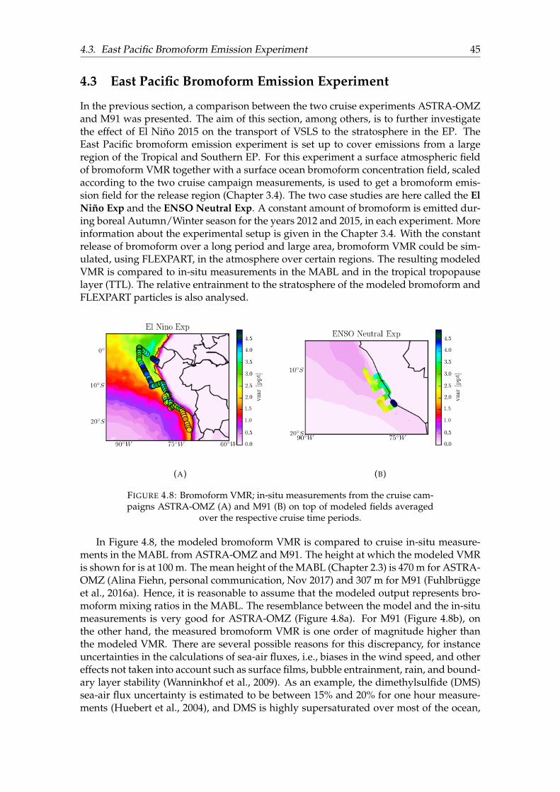
4.3. East Pacific Bromoform Emission Experiment 45
4.3 East Pacific Bromoform Emission Experiment
In the previous section, a comparison between the two cruise experiments ASTRA-OMZand M91 was presented. The aim of this section, among others, is to further investigatethe effect of El Niño 2015 on the transport of VSLS to the stratosphere in the EP. TheEast Pacific bromoform emission experiment is set up to cover emissions from a largeregion of the Tropical and Southern EP. For this experiment a surface atmospheric fieldof bromoform VMR together with a surface ocean bromoform concentration field, scaledaccording to the two cruise campaign measurements, is used to get a bromoform emis-sion field for the release region (Chapter 3.4). The two case studies are here called the ElNiño Exp and the ENSO Neutral Exp. A constant amount of bromoform is emitted dur-ing boreal Autumn/Winter season for the years 2012 and 2015, in each experiment. Moreinformation about the experimental setup is given in the Chapter 3.4. With the constantrelease of bromoform over a long period and large area, bromoform VMR could be sim-ulated, using FLEXPART, in the atmosphere over certain regions. The resulting modeledVMR is compared to in-situ measurements in the MABL and in the tropical tropopauselayer (TTL). The relative entrainment to the stratosphere of the modeled bromoform andFLEXPART particles is also analysed.
(A) (B)
FIGURE 4.8: Bromoform VMR; in-situ measurements from the cruise cam-paigns ASTRA-OMZ (A) and M91 (B) on top of modeled fields averaged
over the respective cruise time periods.
In Figure 4.8, the modeled bromoform VMR is compared to cruise in-situ measure-ments in the MABL from ASTRA-OMZ and M91. The height at which the modeled VMRis shown for is at 100 m. The mean height of the MABL (Chapter 2.3) is 470 m for ASTRA-OMZ (Alina Fiehn, personal communication, Nov 2017) and 307 m for M91 (Fuhlbrüggeet al., 2016a). Hence, it is reasonable to assume that the modeled output represents bro-moform mixing ratios in the MABL. The resemblance between the model and the in-situmeasurements is very good for ASTRA-OMZ (Figure 4.8a). For M91 (Figure 4.8b), onthe other hand, the measured bromoform VMR is one order of magnitude higher thanthe modeled VMR. There are several possible reasons for this discrepancy, for instanceuncertainties in the calculations of sea-air fluxes, i.e., biases in the wind speed, and othereffects not taken into account such as surface films, bubble entrainment, rain, and bound-ary layer stability (Wanninkhof et al., 2009). As an example, the dimethylsulfide (DMS)sea-air flux uncertainty is estimated to be between 15% and 20% for one hour measure-ments (Huebert et al., 2004), and DMS is highly supersaturated over most of the ocean,
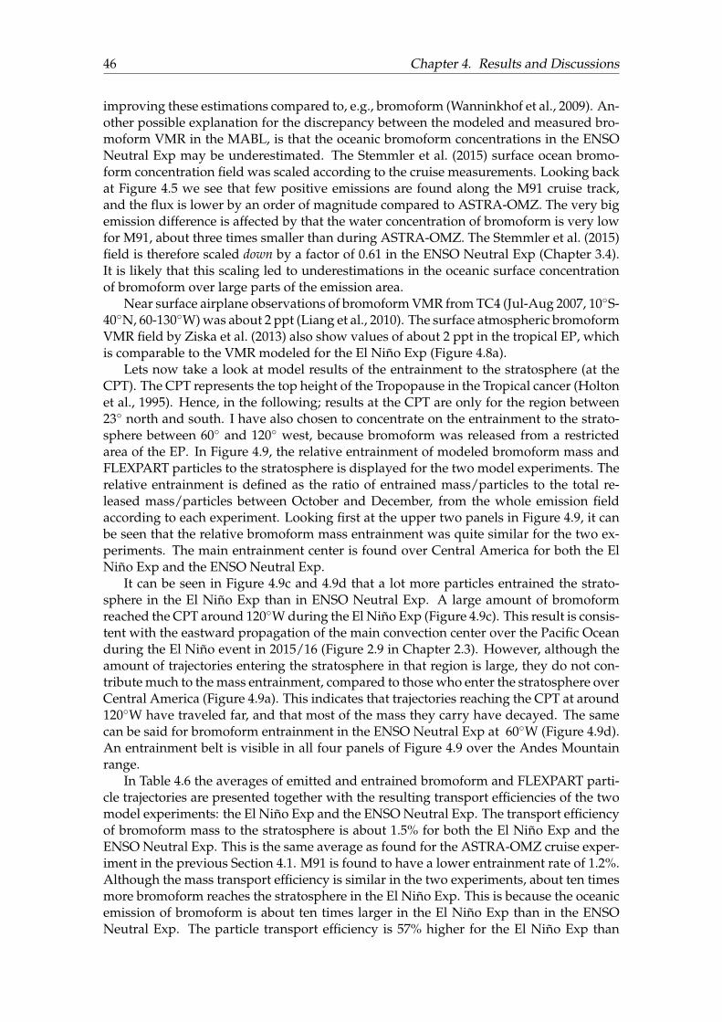
46 Chapter 4. Results and Discussions
improving these estimations compared to, e.g., bromoform (Wanninkhof et al., 2009). An-other possible explanation for the discrepancy between the modeled and measured bro-moform VMR in the MABL, is that the oceanic bromoform concentrations in the ENSONeutral Exp may be underestimated. The Stemmler et al. (2015) surface ocean bromo-form concentration field was scaled according to the cruise measurements. Looking backat Figure 4.5 we see that few positive emissions are found along the M91 cruise track,and the flux is lower by an order of magnitude compared to ASTRA-OMZ. The very bigemission difference is affected by that the water concentration of bromoform is very lowfor M91, about three times smaller than during ASTRA-OMZ. The Stemmler et al. (2015)field is therefore scaled down by a factor of 0.61 in the ENSO Neutral Exp (Chapter 3.4).It is likely that this scaling led to underestimations in the oceanic surface concentrationof bromoform over large parts of the emission area.
Near surface airplane observations of bromoform VMR from TC4 (Jul-Aug 2007, 10◦S-40◦N, 60-130◦W) was about 2 ppt (Liang et al., 2010). The surface atmospheric bromoformVMR field by Ziska et al. (2013) also show values of about 2 ppt in the tropical EP, whichis comparable to the VMR modeled for the El Niño Exp (Figure 4.8a).
Lets now take a look at model results of the entrainment to the stratosphere (at theCPT). The CPT represents the top height of the Tropopause in the Tropical cancer (Holtonet al., 1995). Hence, in the following; results at the CPT are only for the region between23◦ north and south. I have also chosen to concentrate on the entrainment to the strato-sphere between 60◦ and 120◦ west, because bromoform was released from a restrictedarea of the EP. In Figure 4.9, the relative entrainment of modeled bromoform mass andFLEXPART particles to the stratosphere is displayed for the two model experiments. Therelative entrainment is defined as the ratio of entrained mass/particles to the total re-leased mass/particles between October and December, from the whole emission fieldaccording to each experiment. Looking first at the upper two panels in Figure 4.9, it canbe seen that the relative bromoform mass entrainment was quite similar for the two ex-periments. The main entrainment center is found over Central America for both the ElNiño Exp and the ENSO Neutral Exp.
It can be seen in Figure 4.9c and 4.9d that a lot more particles entrained the strato-sphere in the El Niño Exp than in ENSO Neutral Exp. A large amount of bromoformreached the CPT around 120◦W during the El Niño Exp (Figure 4.9c). This result is consis-tent with the eastward propagation of the main convection center over the Pacific Oceanduring the El Niño event in 2015/16 (Figure 2.9 in Chapter 2.3). However, although theamount of trajectories entering the stratosphere in that region is large, they do not con-tribute much to the mass entrainment, compared to those who enter the stratosphere overCentral America (Figure 4.9a). This indicates that trajectories reaching the CPT at around120◦W have traveled far, and that most of the mass they carry have decayed. The samecan be said for bromoform entrainment in the ENSO Neutral Exp at 60◦W (Figure 4.9d).An entrainment belt is visible in all four panels of Figure 4.9 over the Andes Mountainrange.
In Table 4.6 the averages of emitted and entrained bromoform and FLEXPART parti-cle trajectories are presented together with the resulting transport efficiencies of the twomodel experiments: the El Niño Exp and the ENSO Neutral Exp. The transport efficiencyof bromoform mass to the stratosphere is about 1.5% for both the El Niño Exp and theENSO Neutral Exp. This is the same average as found for the ASTRA-OMZ cruise exper-iment in the previous Section 4.1. M91 is found to have a lower entrainment rate of 1.2%.Although the mass transport efficiency is similar in the two experiments, about ten timesmore bromoform reaches the stratosphere in the El Niño Exp. This is because the oceanicemission of bromoform is about ten times larger in the El Niño Exp than in the ENSONeutral Exp. The particle transport efficiency is 57% higher for the El Niño Exp than
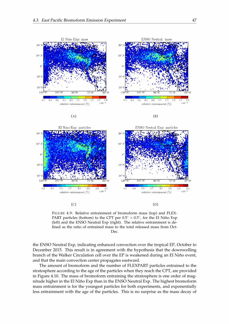
4.3. East Pacific Bromoform Emission Experiment 47
(A) (B)
(C) (D)
FIGURE 4.9: Relative entrainment of bromoform mass (top) and FLEX-PART particles (bottom) to the CPT per 0.5◦ × 0.5◦, for the El Niño Exp(left) and the ENSO Neutral Exp (right). The relative entrainment is de-fined as the ratio of entrained mass to the total released mass from Oct-
Dec.
the ENSO Neutral Exp, indicating enhanced convection over the tropical EP, October toDecember 2015. This result is in agreement with the hypothesis that the downwellingbranch of the Walker Circulation cell over the EP is weakened during an El Niño event,and that the main convection center propagates eastward.
The amount of bromoform and the number of FLEXPART particles entrained to thestratosphere according to the age of the particles when they reach the CPT, are providedin Figure 4.10. The mass of bromoform entraining the stratosphere is one order of mag-nitude higher in the El Niño Exp than in the ENSO Neutral Exp. The highest bromoformmass entrainment is for the youngest particles for both experiments, and exponentiallyless entrainment with the age of the particles. This is no surprise as the mass decay of
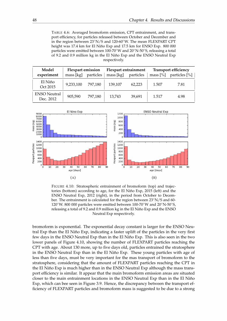
48 Chapter 4. Results and Discussions
TABLE 4.6: Averaged bromoform emission, CPT entrainment, and trans-port efficiency, for particles released between October and December andin the region between 23◦N/S and 120-60◦W. The mean FLEXPART CPTheight was 17.4 km for El Niño Exp and 17.5 km for ENSO Exp. 800 000particles were emitted between 100-70◦W and 20◦N-50◦S, releasing a totalof 9.2 and 0.9 million kg in the El Niño Exp and the ENSO Neutral Exp
respectively.
Model Flexpart emission Flexpart entrainment Transport efficiencyexperiment mass [kg] particles mass [kg] particles mass [%] particles [%]
El NiñoOct 2015
9,233,100 797,180 139,107 62,223 1.507 7.81
ENSO NeutralDec. 2012
905,590 797,180 13,743 39,691 1.517 4.98
(A) (B)
FIGURE 4.10: Stratospheric entrainment of bromoform (top) and trajec-tories (bottom) according to age, for the El Niño Exp, 2015 (left) and theENSO Neutral Exp, 2012 (right), in the period from October to Decem-ber. The entrainment is calculated for the region between 23◦N/S and 60-120◦W. 800 000 particles were emitted between 100-70◦W and 20◦N-50◦S,releasing a total of 9.2 and 0.9 million kg in the El Niño Exp and the ENSO
Neutral Exp respectively.
bromoform is exponential. The exponential decay constant is larger for the ENSO Neu-tral Exp than the El Niño Exp, indicating a faster uplift of the particles in the very firstfew days in the ENSO Neutral Exp than in the El Niño Exp. This is also seen in the twolower panels of Figure 4.10, showing the number of FLEXPART particles reaching theCPT with age. About 130 more, up to five days old, particles entrained the stratospherein the ENSO Neutral Exp than in the El Niño Exp. These young particles with age ofless than five days, must be very important for the mas transport of bromoform to thestratosphere, considering that the amount of FLEXPART particles reaching the CPT inthe El Niño Exp is much higher than in the ENSO Neutral Exp although the mass trans-port efficiency is similar. It appear that the main bromoform emission areas are situatedcloser to the main entrainment locations in the ENSO Neutral Exp than in the El NiñoExp, which can bee seen in Figure 3.9. Hence, the discrepancy between the transport ef-ficiency of FLEXPART particles and bromoform mass is suggested to be due to a strong
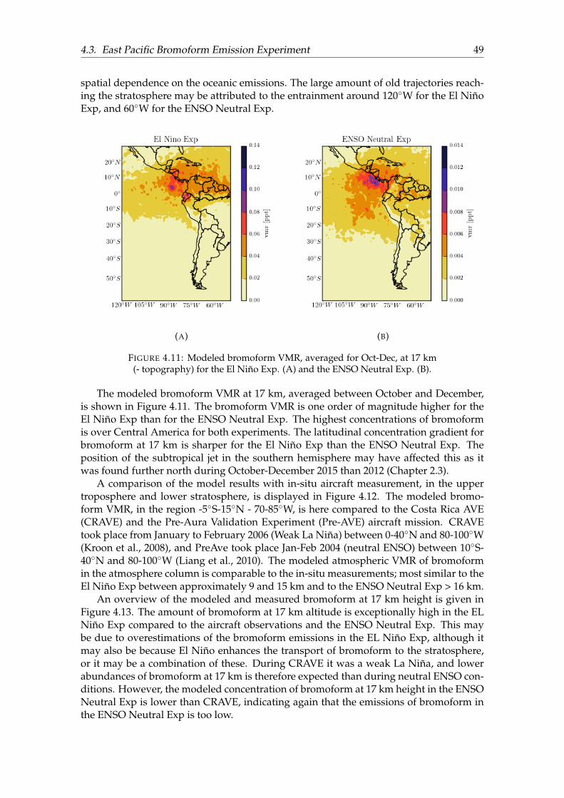
4.3. East Pacific Bromoform Emission Experiment 49
spatial dependence on the oceanic emissions. The large amount of old trajectories reach-ing the stratosphere may be attributed to the entrainment around 120◦W for the El NiñoExp, and 60◦W for the ENSO Neutral Exp.
(A) (B)
FIGURE 4.11: Modeled bromoform VMR, averaged for Oct-Dec, at 17 km(- topography) for the El Niño Exp. (A) and the ENSO Neutral Exp. (B).
The modeled bromoform VMR at 17 km, averaged between October and December,is shown in Figure 4.11. The bromoform VMR is one order of magnitude higher for theEl Niño Exp than for the ENSO Neutral Exp. The highest concentrations of bromoformis over Central America for both experiments. The latitudinal concentration gradient forbromoform at 17 km is sharper for the El Niño Exp than the ENSO Neutral Exp. Theposition of the subtropical jet in the southern hemisphere may have affected this as itwas found further north during October-December 2015 than 2012 (Chapter 2.3).
A comparison of the model results with in-situ aircraft measurement, in the uppertroposphere and lower stratosphere, is displayed in Figure 4.12. The modeled bromo-form VMR, in the region -5◦S-15◦N - 70-85◦W, is here compared to the Costa Rica AVE(CRAVE) and the Pre-Aura Validation Experiment (Pre-AVE) aircraft mission. CRAVEtook place from January to February 2006 (Weak La Niña) between 0-40◦N and 80-100◦W(Kroon et al., 2008), and PreAve took place Jan-Feb 2004 (neutral ENSO) between 10◦S-40◦N and 80-100◦W (Liang et al., 2010). The modeled atmospheric VMR of bromoformin the atmosphere column is comparable to the in-situ measurements; most similar to theEl Niño Exp between approximately 9 and 15 km and to the ENSO Neutral Exp > 16 km.
An overview of the modeled and measured bromoform at 17 km height is given inFigure 4.13. The amount of bromoform at 17 km altitude is exceptionally high in the ELNiño Exp compared to the aircraft observations and the ENSO Neutral Exp. This maybe due to overestimations of the bromoform emissions in the EL Niño Exp, although itmay also be because El Niño enhances the transport of bromoform to the stratosphere,or it may be a combination of these. During CRAVE it was a weak La Niña, and lowerabundances of bromoform at 17 km is therefore expected than during neutral ENSO con-ditions. However, the modeled concentration of bromoform at 17 km height in the ENSONeutral Exp is lower than CRAVE, indicating again that the emissions of bromoform inthe ENSO Neutral Exp is too low.
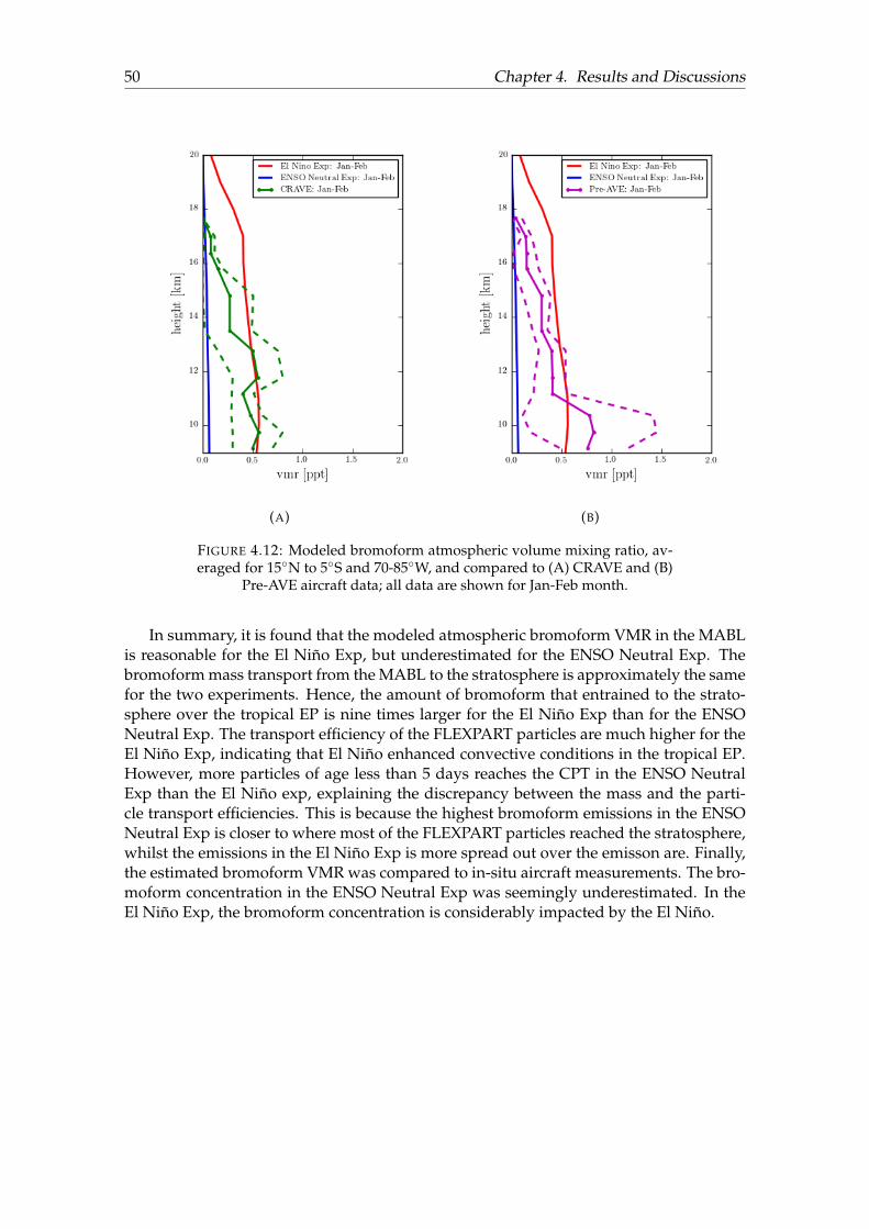
50 Chapter 4. Results and Discussions
(A) (B)
FIGURE 4.12: Modeled bromoform atmospheric volume mixing ratio, av-eraged for 15◦N to 5◦S and 70-85◦W, and compared to (A) CRAVE and (B)
Pre-AVE aircraft data; all data are shown for Jan-Feb month.
In summary, it is found that the modeled atmospheric bromoform VMR in the MABLis reasonable for the El Niño Exp, but underestimated for the ENSO Neutral Exp. Thebromoform mass transport from the MABL to the stratosphere is approximately the samefor the two experiments. Hence, the amount of bromoform that entrained to the strato-sphere over the tropical EP is nine times larger for the El Niño Exp than for the ENSONeutral Exp. The transport efficiency of the FLEXPART particles are much higher for theEl Niño Exp, indicating that El Niño enhanced convective conditions in the tropical EP.However, more particles of age less than 5 days reaches the CPT in the ENSO NeutralExp than the El Niño exp, explaining the discrepancy between the mass and the parti-cle transport efficiencies. This is because the highest bromoform emissions in the ENSONeutral Exp is closer to where most of the FLEXPART particles reached the stratosphere,whilst the emissions in the El Niño Exp is more spread out over the emisson are. Finally,the estimated bromoform VMR was compared to in-situ aircraft measurements. The bro-moform concentration in the ENSO Neutral Exp was seemingly underestimated. In theEl Niño Exp, the bromoform concentration is considerably impacted by the El Niño.
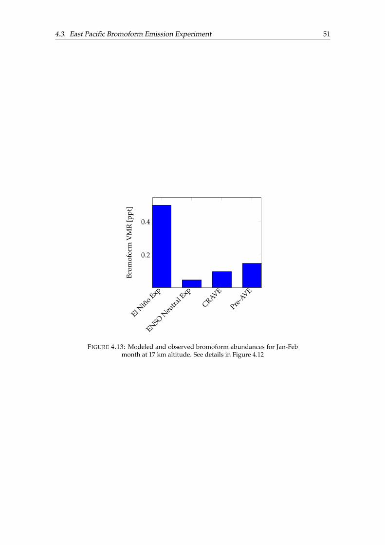
4.3. East Pacific Bromoform Emission Experiment 51
El Niño Exp
ENSONeu
tral Exp
CRAVE
Pre-AVE
0.2
0.4
Brom
ofor
mV
MR
[ppt
]
FIGURE 4.13: Modeled and observed bromoform abundances for Jan-Febmonth at 17 km altitude. See details in Figure 4.12

53
Chapter 5
Summary and Outlook
The main goal of this thesis was to analyze the contribution of the very short-lived halo-genated substances (VSLS) emitted from the tropical East Pacific (EP) to the stratosphere.The VSLS has mainly natural oceanic sources, and pronounced sea-air emissions of VSLShas been found in oceanic upwelling regions in the tropics and subtropics. The Peruvianupwelling in the tropical EP is therefore of interest in this topic of research. However,the tropical EP is also a region within the downwelling branch of the Walker Circula-tion. Hence, it is not certain how much of the VSLS from the tropical EP that reach thestratosphere as their lifetime in the free atmosphere is very short.
The effect of El Niño has been investigated by comparing in-situ cruise measurementsand model simulations between the very strong El Niño 2015/16 with the neutral ENSO2012/13. In-situ measurements from the ASTRA-OMZ (October 2012) cruise in the trop-ical EP have been analyzed in this thesis, and compared to the M91 (December 2012)cruise, which took place in the same region, an to other cruise campaigns in other tropicaloceans. Sea-air emissions of the three halocarbons; methyl iodide, bromoform and dibro-momethane, were calculated along the cruise tracks of ASTRA-OMZ and M91. Analy-sis of the cruise measurement results was focused on the first research question: 1. Towhat extent is the tropical EP a source for VSLS to the marine atmospheric boundarylayer (MABL)? It was found that the tropical EP is a considerable source region of VSLSin the MABL, compared to similar studies over other tropical oceans. However, the cal-culated sea-air fluxes were found to vary significantly between ENSO phases. Hence,the general importance of the tropical EP as a source region to the MABL need furtherinvestigation.
The FLEXPART model with ERA-Interim meteorological reanalysis fields was used tofollow the transport of the calculated emissions along the cruise tracks of ASTRA-OMZand M91. This experiment was designed to attribute the second research question: 2.How much of these VSLS are transported to the stratosphere? The mean transport effi-ciency of bromoform/dibromomethane to the stratosphere was found to be 1.5 %/11.3 %for ASTRA-OMZ and 1.2 %/11.9 % for M91. Since moderate to high transport efficiencieswas found fro bromocarbons over the tropical EP and since the Peruvian upwelling wasfound to be a major source region for atmospheric VSLS, it can be claimed that the tropi-cal EP contributes significantly to the stratospheric bromine loading. The mass transportefficiency to the stratosphere for methyl iodide was quite small (0.1 %), similar earlierfindings in the East Atlantic. Even when high sea-air fluxes of methyl iodide occured,the amount of methyl iodide entrained to the stratosphere was small. The transport effi-ciency of the VSLS to the stratosphere was mainly dependent on how close the VSLS werereleased to major stratospheric entrainment centers. This is especially true for methyl io-dide, because it has a particularly short lifetime in the free atmosphere (3.5 days).
Another model experiment was setup were bromoform was released over a large areaof the tropical and southern EP, again using ERA-Interim reanalysis and FLEXPART.For this experiment the Stemmler et al. (2015) surface ocean bromoform concentration
54 Chapter 5. Summary and Outlook
field was scaled according to the in-situ measurements from ASTRA-OMZ and M91, andused to calculate two bromoform emission fields, one for the El Niño Exp and one forthe ENSO Neutral Exp. First, in-situ measurements of atmospheric volume mixing ra-tio (VMR) of bromoform were compared to the modeled field values in the MABL. Agood agreement between ASTRA-OMZ and the El Niño Exp prevailed, but the modeledatmospheric VMR for the ENSO Neutral Exp was of about one magnitude lower than theM91 measurements. The bad correlation between the ENSO Neutral Exp and M91 wassuggested to be caused by uncertainties in the flux calculation, and that the scaling factorbased on M91 was not representative for the large area of the constructed emission fieldin the tropical EP.
The third research question was then investigated by comparing the same season, forthe El Niño Exp (2015/16) and the ENSO Neutral Exp (2012/13): 3. How does El Niñoaffect the VSLS transport from the tropical EP to the stratosphere? It was found that oneorder of magnitude more bromoform entered the stratosphere in the El Niño Exp than inthe ENSO Neutral Exp. The maximum entrainment locations was above Central Americafor both experiments. More stratospheric transport was observed towards the CentralPacific in the El Niño Exp than in the ENSO Neutral Exp, consistent with the developingCP El Niño Oct-Nov 2015. The FLEXPART particle transport efficiency was 37% higherfor the El Niño Exp than the ENSO Neutral Exp, demonstrating the major impact ElNiño has on the troposphere to stratosphere transport. However, although the transportefficiency of the FLEXPART particles is higher in the El Niño Exp, the transport efficiencyof bromoform mass, is approximately the same. The cause of this discrepancy was foundto be due to that the most pronounces bromoform emissions areas was situated closerto the maximum entrainment locations in the ENSO Neutral Exp than in the El NiñoExp. Finally, a comparison of the modeled VMR of bromoform above Central Americawas compared to in-situ aircraft measurements. Quite good agreement was found in thefree troposphere with the El Niño Exp, although comparisons at 17 km altitude prevailedthat the emissions in the El Niño Exp possibly was overestimated. The bromine VMR wasfount to be 0.5 ppt in the El Niño Exp, about three times higher than the highest meanobservational concentration. It is also possible that this very high VMR was mainly dueto enhanced stratospheric entrainment and oceanic emission of bromoform because of ElNiño 2015/16. However, the ENSO Neutral Exp was again found to have underestimatedthe sea-air fluxes of bromoform again, with lower VMR (of 0.05 ppt) than for observationsduring a weak La Niña 2005/06 (0.1 ppt), oposite of the expected.
The results of this thesis support the idea that the EP are an important source regionfor the stratospheric halogen loading though source gas injections of VSLS, especially forthe longer lived VSLS bromoform and dibromomethane. It was also found that El Niñoaffect this transport, by shifting the convective center over the tropical EP. The thesis hashelped to further enhance our understanding of the tropical EP as a source region for thestratospheric halogen loading, although much more research is needed.
A number of limitations in this thesis need to be considered. First, the scope of thisstudy was spatially and temporally limited in terms of in-situ measurements of halocar-bons in the ocean and atmosphere. Secondly, the sea-air flux calculations are not veryaccurate, and more precise surface oceanic and near surface atmospheric global concen-tration fields of VSLS are crucial. Uncertainties in the FLEXPART model using the ERA-Interim reanalysis should also be considered, i.e., the convection parameterization andthe boundary layer parameterization. Further research in the tropical EP is needed, es-pecially studying the strong variations in measured halocarbons between the differentENSO events.
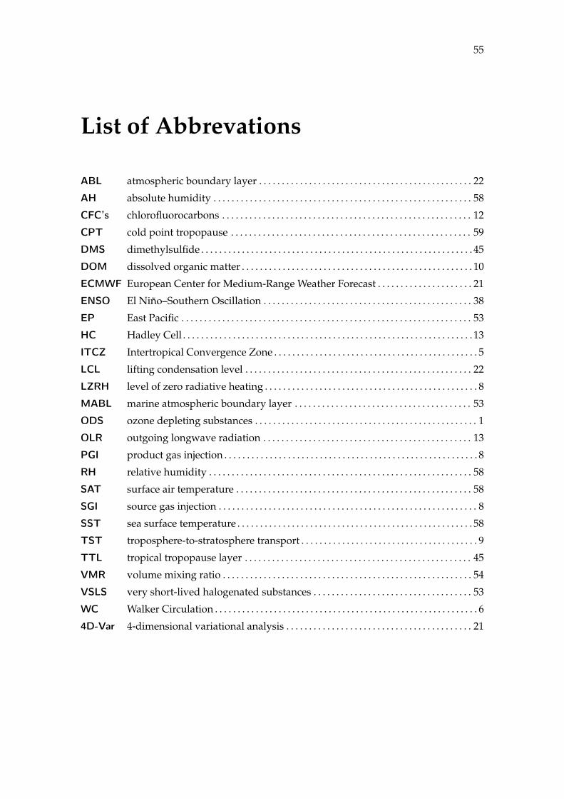
55
List of Abbrevations
ABL atmospheric boundary layer . . . . . . . . . . . . . . . . . . . . . . . . . . . . . . . . . . . . . . . . . . . . . . . 22
AH absolute humidity . . . . . . . . . . . . . . . . . . . . . . . . . . . . . . . . . . . . . . . . . . . . . . . . . . . . . . . . . 58
CFC’s chlorofluorocarbons . . . . . . . . . . . . . . . . . . . . . . . . . . . . . . . . . . . . . . . . . . . . . . . . . . . . . . . 12
CPT cold point tropopause . . . . . . . . . . . . . . . . . . . . . . . . . . . . . . . . . . . . . . . . . . . . . . . . . . . . . 59
DMS dimethylsulfide . . . . . . . . . . . . . . . . . . . . . . . . . . . . . . . . . . . . . . . . . . . . . . . . . . . . . . . . . . . . 45
DOM dissolved organic matter . . . . . . . . . . . . . . . . . . . . . . . . . . . . . . . . . . . . . . . . . . . . . . . . . . . 10
ECMWF European Center for Medium-Range Weather Forecast . . . . . . . . . . . . . . . . . . . . . 21
ENSO El Niño–Southern Oscillation . . . . . . . . . . . . . . . . . . . . . . . . . . . . . . . . . . . . . . . . . . . . . . 38
EP East Pacific . . . . . . . . . . . . . . . . . . . . . . . . . . . . . . . . . . . . . . . . . . . . . . . . . . . . . . . . . . . . . . . . 53
HC Hadley Cell . . . . . . . . . . . . . . . . . . . . . . . . . . . . . . . . . . . . . . . . . . . . . . . . . . . . . . . . . . . . . . . . 13
ITCZ Intertropical Convergence Zone . . . . . . . . . . . . . . . . . . . . . . . . . . . . . . . . . . . . . . . . . . . . . 5
LCL lifting condensation level . . . . . . . . . . . . . . . . . . . . . . . . . . . . . . . . . . . . . . . . . . . . . . . . . . 22
LZRH level of zero radiative heating . . . . . . . . . . . . . . . . . . . . . . . . . . . . . . . . . . . . . . . . . . . . . . . 8
MABL marine atmospheric boundary layer . . . . . . . . . . . . . . . . . . . . . . . . . . . . . . . . . . . . . . . 53
ODS ozone depleting substances . . . . . . . . . . . . . . . . . . . . . . . . . . . . . . . . . . . . . . . . . . . . . . . . . 1
OLR outgoing longwave radiation . . . . . . . . . . . . . . . . . . . . . . . . . . . . . . . . . . . . . . . . . . . . . . 13
PGI product gas injection . . . . . . . . . . . . . . . . . . . . . . . . . . . . . . . . . . . . . . . . . . . . . . . . . . . . . . . . 8
RH relative humidity . . . . . . . . . . . . . . . . . . . . . . . . . . . . . . . . . . . . . . . . . . . . . . . . . . . . . . . . . . 58
SAT surface air temperature . . . . . . . . . . . . . . . . . . . . . . . . . . . . . . . . . . . . . . . . . . . . . . . . . . . . 58
SGI source gas injection . . . . . . . . . . . . . . . . . . . . . . . . . . . . . . . . . . . . . . . . . . . . . . . . . . . . . . . . . 8
SST sea surface temperature . . . . . . . . . . . . . . . . . . . . . . . . . . . . . . . . . . . . . . . . . . . . . . . . . . . . 58
TST troposphere-to-stratosphere transport . . . . . . . . . . . . . . . . . . . . . . . . . . . . . . . . . . . . . . . 9
TTL tropical tropopause layer . . . . . . . . . . . . . . . . . . . . . . . . . . . . . . . . . . . . . . . . . . . . . . . . . . 45
VMR volume mixing ratio . . . . . . . . . . . . . . . . . . . . . . . . . . . . . . . . . . . . . . . . . . . . . . . . . . . . . . . 54
VSLS very short-lived halogenated substances . . . . . . . . . . . . . . . . . . . . . . . . . . . . . . . . . . . 53
WC Walker Circulation . . . . . . . . . . . . . . . . . . . . . . . . . . . . . . . . . . . . . . . . . . . . . . . . . . . . . . . . . . 6
4D-Var 4-dimensional variational analysis . . . . . . . . . . . . . . . . . . . . . . . . . . . . . . . . . . . . . . . . . 21

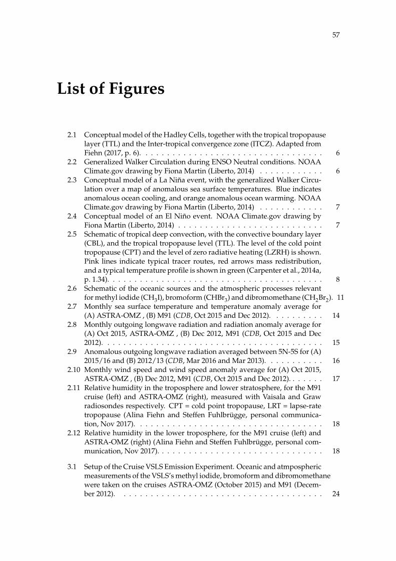
57
List of Figures
2.1 Conceptual model of the Hadley Cells, together with the tropical tropopauselayer (TTL) and the Inter-tropical convergence zone (ITCZ). Adapted fromFiehn (2017, p. 6). . . . . . . . . . . . . . . . . . . . . . . . . . . . . . . . . . 6
2.2 Generalized Walker Circulation during ENSO Neutral conditions. NOAAClimate.gov drawing by Fiona Martin (Liberto, 2014) . . . . . . . . . . . . 6
2.3 Conceptual model of a La Niña event, with the generalized Walker Circu-lation over a map of anomalous sea surface temperatures. Blue indicatesanomalous ocean cooling, and orange anomalous ocean warming. NOAAClimate.gov drawing by Fiona Martin (Liberto, 2014) . . . . . . . . . . . . 7
2.4 Conceptual model of an El Niño event. NOAA Climate.gov drawing byFiona Martin (Liberto, 2014) . . . . . . . . . . . . . . . . . . . . . . . . . . . 7
2.5 Schematic of tropical deep convection, with the convective boundary layer(CBL), and the tropical tropopause level (TTL). The level of the cold pointtropopause (CPT) and the level of zero radiative heating (LZRH) is shown.Pink lines indicate typical tracer routes, red arrows mass redistribution,and a typical temperature profile is shown in green (Carpenter et al., 2014a,p. 1.34). . . . . . . . . . . . . . . . . . . . . . . . . . . . . . . . . . . . . . . . 8
2.6 Schematic of the oceanic sources and the atmospheric processes relevantfor methyl iodide (CH3I), bromoform (CHBr3) and dibromomethane (CH2Br2). 11
2.7 Monthly sea surface temperature and temperature anomaly average for(A) ASTRA-OMZ , (B) M91 (CDB, Oct 2015 and Dec 2012). . . . . . . . . . 14
2.8 Monthly outgoing longwave radiation and radiation anomaly average for(A) Oct 2015, ASTRA-OMZ , (B) Dec 2012, M91 (CDB, Oct 2015 and Dec2012). . . . . . . . . . . . . . . . . . . . . . . . . . . . . . . . . . . . . . . . . 15
2.9 Anomalous outgoing longwave radiation averaged between 5N-5S for (A)2015/16 and (B) 2012/13 (CDB, Mar 2016 and Mar 2013). . . . . . . . . . . 16
2.10 Monthly wind speed and wind speed anomaly average for (A) Oct 2015,ASTRA-OMZ , (B) Dec 2012, M91 (CDB, Oct 2015 and Dec 2012). . . . . . . 17
2.11 Relative humidity in the troposphere and lower stratosphere, for the M91cruise (left) and ASTRA-OMZ (right), measured with Vaisala and Grawradiosondes respectively. CPT = cold point tropopause, LRT = lapse-ratetropopause (Alina Fiehn and Steffen Fuhlbrügge, personal communica-tion, Nov 2017). . . . . . . . . . . . . . . . . . . . . . . . . . . . . . . . . . . 18
2.12 Relative humidity in the lower troposphere, for the M91 cruise (left) andASTRA-OMZ (right) (Alina Fiehn and Steffen Fuhlbrügge, personal com-munication, Nov 2017). . . . . . . . . . . . . . . . . . . . . . . . . . . . . . . 18
3.1 Setup of the Cruise VSLS Emission Experiment. Oceanic and atmposphericmeasurements of the VSLS’s methyl iodide, bromoform and dibromomethanewere taken on the cruises ASTRA-OMZ (October 2015) and M91 (Decem-ber 2012). . . . . . . . . . . . . . . . . . . . . . . . . . . . . . . . . . . . . . 24
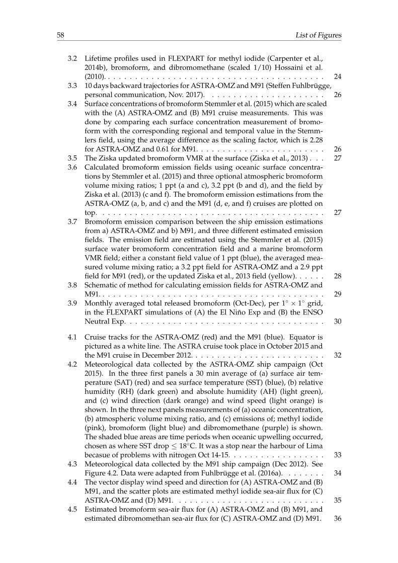
58 List of Figures
3.2 Lifetime profiles used in FLEXPART for methyl iodide (Carpenter et al.,2014b), bromoform, and dibromomethane (scaled 1/10) Hossaini et al.(2010). . . . . . . . . . . . . . . . . . . . . . . . . . . . . . . . . . . . . . . . . 24
3.3 10 days backward trajectories for ASTRA-OMZ and M91 (Steffen Fuhlbrügge,personal communication, Nov. 2017). . . . . . . . . . . . . . . . . . . . . . 26
3.4 Surface concentrations of bromoform Stemmler et al. (2015) which are scaledwith the (A) ASTRA-OMZ and (B) M91 cruise measurements. This wasdone by comparing each surface concentration measurement of bromo-form with the corresponding regional and temporal value in the Stemm-lers field, using the average difference as the scaling factor, which is 2.28for ASTRA-OMZ and 0.61 for M91. . . . . . . . . . . . . . . . . . . . . . . . 26
3.5 The Ziska updated bromoform VMR at the surface (Ziska et al., 2013) . . . 273.6 Calculated bromoform emission fields using oceanic surface concentra-
tions by Stemmler et al. (2015) and three optional atmospheric bromoformvolume mixing ratios; 1 ppt (a and c), 3.2 ppt (b and d), and the field byZiska et al. (2013) (c and f). The bromoform emission estimations from theASTRA-OMZ (a, b, and c) and the M91 (d, e, and f) cruises are plotted ontop. . . . . . . . . . . . . . . . . . . . . . . . . . . . . . . . . . . . . . . . . . 27
3.7 Bromoform emission comparison between the ship emission estimationsfrom a) ASTRA-OMZ and b) M91, and three different estimated emissionfields. The emission field are estimated using the Stemmler et al. (2015)surface water bromoform concentration field and a marine bromoformVMR field; either a constant field value of 1 ppt (blue), the averaged mea-sured volume mixing ratio; a 3.2 ppt field for ASTRA-OMZ and a 2.9 pptfield for M91 (red), or the updated Ziska et al., 2013 field (yellow). . . . . . 28
3.8 Schematic of method for calculating emission fields for ASTRA-OMZ andM91. . . . . . . . . . . . . . . . . . . . . . . . . . . . . . . . . . . . . . . . . . 29
3.9 Monthly averaged total released bromoform (Oct-Dec), per 1◦ × 1◦ grid,in the FLEXPART simulations of (A) the El Niño Exp and (B) the ENSONeutral Exp. . . . . . . . . . . . . . . . . . . . . . . . . . . . . . . . . . . . . 30
4.1 Cruise tracks for the ASTRA-OMZ (red) and the M91 (blue). Equator ispictured as a white line. The ASTRA cruise took place in October 2015 andthe M91 cruise in December 2012. . . . . . . . . . . . . . . . . . . . . . . . . 32
4.2 Meteorological data collected by the ASTRA-OMZ ship campaign (Oct2015). In the three first panels a 30 min average of (a) surface air tem-perature (SAT) (red) and sea surface temperature (SST) (blue), (b) relativehumidity (RH) (dark green) and absolute humidity (AH) (light green),and (c) wind direction (dark orange) and wind speed (light orange) isshown. In the three next panels measurements of (a) oceanic concentration,(b) atmospheric volume mixing ratio, and (c) emissions of; methyl iodide(pink), bromoform (light blue) and dibromomethane (purple) is shown.The shaded blue areas are time periods when oceanic upwelling occurred,chosen as where SST drop ≤ 18◦C. It was a stop near the harbour of Limabecasue of problems with nitrogen Oct 14-15. . . . . . . . . . . . . . . . . . 33
4.3 Meteorological data collected by the M91 ship campaign (Dec 2012). SeeFigure 4.2. Data were adapted from Fuhlbrügge et al. (2016a). . . . . . . . 34
4.4 The vector display wind speed and direction for (A) ASTRA-OMZ and (B)M91, and the scatter plots are estimated methyl iodide sea-air flux for (C)ASTRA-OMZ and (D) M91. . . . . . . . . . . . . . . . . . . . . . . . . . . . 35
4.5 Estimated bromoform sea-air flux for (A) ASTRA-OMZ and (B) M91, andestimated dibromomethan sea-air flux for (C) ASTRA-OMZ and (D) M91. 36
List of Figures 59
4.6 Flexpart 10 days forward trajectories for (a) the ASTRA-OMZ (Oct 2015)setup, and for (b) the M91 (Dec 2012) setup. The figure shows the gen-eral airmass transport pathways of those trajectories reaching the 17 kmaltitude. To get a good overview, only every (a) 60 and (b) 30 trajectorythat reached the 17 km altitude is plotted here. The trajectories starts fromwhere they were released along the respective cruise tracks. . . . . . . . . 40
4.7 Released mass, entrained mass and relative entrainment of methyl iodide(top), bromoform (center), and dibromomethane (bottom). The mass isreleased along the cruise track of ASTRA-OMZ (left) and M91 (right) ac-cording to when VSLS measurement were taken. The entrained mass isdefined as the amount of mass reaching the stratosphere at 17 m altitude(Chapter 2.3), and the relative entrainment is defined as the ratio of en-trained to released mass. . . . . . . . . . . . . . . . . . . . . . . . . . . . . 41
4.8 Bromoform VMR; in-situ measurements from the cruise campaigns ASTRA-OMZ (A) and M91 (B) on top of modeled fields averaged over the respec-tive cruise time periods. . . . . . . . . . . . . . . . . . . . . . . . . . . . . . 45
4.9 Relative entrainment of bromoform mass (top) and FLEXPART particles(bottom) to the cold point tropopause (CPT) per 0.5◦× 0.5◦, for the El NiñoExp (left) and the ENSO Neutral Exp (right). The relative entrainment isdefined as the ratio of entrained mass to the total released mass from Oct-Dec. . . . . . . . . . . . . . . . . . . . . . . . . . . . . . . . . . . . . . . . . . 47
4.10 Stratospheric entrainment of bromoform (top) and trajectories (bottom) ac-cording to age, for the El Niño Exp, 2015 (left) and the ENSO Neutral Exp,2012 (right), in the period from October to December. The entrainment iscalculated for the region between 23◦N/S and 60-120◦W. 800 000 particleswere emitted between 100-70◦W and 20◦N-50◦S, releasing a total of 9.2 and0.9 million kg in the El Niño Exp and the ENSO Neutral Exp respectively. 48
4.11 Modeled bromoform VMR, averaged for Oct-Dec, at 17 km (- topography)for the El Niño Exp. (A) and the ENSO Neutral Exp. (B). . . . . . . . . . . 49
4.12 Modeled bromoform atmospheric volume mixing ratio, averaged for 15◦Nto 5◦S and 70-85◦W, and compared to (A) CRAVE and (B) Pre-AVE aircraftdata; all data are shown for Jan-Feb month. . . . . . . . . . . . . . . . . . . 50
4.13 Modeled and observed bromoform abundances for Jan-Feb month at 17km altitude. See details in Figure 4.12 . . . . . . . . . . . . . . . . . . . . . 51

61
List of Tables
3.1 FLEXPART model setup for the three VSLS; methyl idode (CH3I), bromo-form (CHBr3), and dibromomehtane (CH2Br2). Two experiments are car-ried out for each compound. The runtime for the ASTRA-OMZ cruise ex-periment is shorter (see number in brackets), because meteorological inputdata were not available at the time of the thesis calculations. . . . . . . . . 23
3.2 Mean oceanic bromoform emissions for two experiments; the El Niño Expand the ENSO Neutral Exp. In the first column the mean of the corre-sponding cruise emission estimated are shown (ASTRA-OMZ for the ElNiño Exp and M91 for the ENSO Neutral Exp). For the other columns amean over the stated field is shown. The field averages were taken over abig enough lat-lon box to include the respective cruise track. The values inthe brackets includes negative emissions. . . . . . . . . . . . . . . . . . . . 29
3.3 FLEXPART model setup for the East Pacific bromoform emission experiment. 30
4.1 Measured oceanic concentration, atmospheric VMR and calculated emis-sion for CH3I (methyl iodide), CHBr3 (bromoform) and CH2Br2 (dibro-momethane). The mean ±one standard deviation and the and the maxi-mum values are listed. Data from M91 is adapted from (Fuhlbrügge et al.,2016a). . . . . . . . . . . . . . . . . . . . . . . . . . . . . . . . . . . . . . . . 37
4.2 Mean emission (pmol m−2 hr−1) of methyl iodide (CH3I), bromoform (CHBr3)and dibromomethane (CH2Br2) from several cruises and model-based stud-ies. EP = East Pacific, WP = West Pacific, IO = Indian Ocean, and OLS =ordinary least square method. Adapted from Fiehn et al. (2017). . . . . . . 38
4.3 Emission of methyl iodide and entrainment at 17 km altitude. The mean±one standard deviation, the minimum value and the maximum value arelisted. Negative emissions are excluded. . . . . . . . . . . . . . . . . . . . . 42
4.4 Emission of bromoform and entrainment at 17 km altitude. The mean ±onestandard deviation, and the minimum and maximum values are listed.Negative emissions are excluded. . . . . . . . . . . . . . . . . . . . . . . . . 43
4.5 Emission of dibromomethane and entrainment at 17 km altitude. Themean ±one standard deviation, and the minimum and maximum valuesare listed. Negative emissions are excluded. . . . . . . . . . . . . . . . . . . 43
4.6 Averaged bromoform emission, CPT entrainment, and transport efficiency,for particles released between October and December and in the regionbetween 23◦N/S and 120-60◦W. The mean FLEXPART CPT height was 17.4km for El Niño Exp and 17.5 km for ENSO Exp. 800 000 particles wereemitted between 100-70◦W and 20◦N-50◦S, releasing a total of 9.2 and 0.9million kg in the El Niño Exp and the ENSO Neutral Exp respectively. . . 48

63
Bibliography
Aguado, Edward and James E Burt (2010). Understanding weather and climate. PrenticeHall, Inc.
Aschmann, J, B-M Sinnhuber, MP Chipperfield, and R Hossaini (2011). “Impact of deepconvection and dehydration on bromine loading in the upper troposphere and lowerstratosphere”. In: Atmospheric Chemistry and Physics 11.6, pp. 2671–2687.
Ashfold, MJ, NRP Harris, EL Atlas, AJ Manning, and JA Pyle (2012). “Transport of short-lived species into the Tropical Tropopause Layer”. In: Atmospheric Chemistry and Physics12.14, pp. 6309–6322. DOI: 10.5194/acp-12-6309-2012.
Bange, HW (2013). “Surface Ocean–Lower Atmosphere Study (SOLAS) in the upwellingregion off Peru-Meteor Cruise No. M91”. In:
Bell, N, L Hsu, DJ Jacob, MG Schultz, DR Blake, JH Butler, DB King, JM Lobert, andE Maier-Reimer (2002). “Methyl iodide: Atmospheric budget and use as a tracer ofmarine convection in global models”. In: Journal of Geophysical Research: Atmospheres107.D17.
Bonazzola, M and PH Haynes (2004). “A trajectory-based study of the tropical tropopauseregion”. In: Journal of Geophysical Research: Atmospheres 109.D20.
Bowman, KP, JC Lin, A Stohl, R Draxler, P Konopka, A Andrews, and D Brunner (2013).“Input data requirements for Lagrangian trajectory models”. In: Bulletin of the Ameri-can Meteorological Society 94.7, pp. 1051–1058.
Butler, JH et al. (2007). “Oceanic distributions and emissions of short-lived halocarbons”.In: Global biogeochemical cycles 21.1.
Carpenter, LJ, CE Jones, RM Dunk, KE Hornsby, and J Woeltjen (2009). “Air-sea fluxes ofbiogenic bromine from the tropical and North Atlantic Ocean”. In: Atmospheric Chem-istry and Physics 9.5, pp. 1805–1816.
Carpenter, LJ, S Reimann (Lead Authors), JB. Burkholder, C Clerbaux, BD Hall, R Hos-saini, JC Laube, and SA Yvon-Lewis (2014a). “Ozone-Depleting Substances (ODSs)and Other Gases of Interest to the Montreal Protocol”. In: Chapter 1 in Scientific Assess-ment of Ozone Depletion: 2014, Global Ozone Research and Monitoring Project-Report No.55 55.
Carpenter, LJ et al. (2014b). “Update on ozone-depleting substances (ODSs) and othergases of interest to the Montreal protocol”. In: Scientific assessment of ozone depletion:2014, pp. 1–1.
Center, Climate Prediction. CDB. URL: http://www.cpc.ncep.noaa.gov/products/CDB(visited on 11/07/2017).
Chubachi, S (1984). “Preliminary result of ozone observations at Syowa station fromFebruary 1982 to January 1983”. In: Memoirs of National Institute of Polar Research. Spe-cial issue 34, pp. 13–19.
Chuck, AL, SM Turner, and PS Liss (2005). “Oceanic distributions and air-sea fluxes ofbiogenic halocarbons in the open ocean”. In: Journal of Geophysical Research: Oceans110.C10.
Dee, DP et al. (2011). “The ERA-Interim reanalysis: Configuration and performance ofthe data assimilation system”. In: Quarterly Journal of the royal meteorological society137.656, pp. 553–597.
64 BIBLIOGRAPHY
DeSombre, ER (2000). “The Experience of the Montreal Protocol: Particularly Remark-able, and Remarkably Particular”. In: UCLA J. Envtl. L. & Pol’y 19, p. 49.
Dorf, M et al. (2006). “Long-term observations of stratospheric bromine reveal slow downin growth”. In: Geophysical research letters 33.24.
Emanuel, KA and M Živkovic-Rothman (1999). “Development and evaluation of a con-vection scheme for use in climate models”. In: Journal of the Atmospheric Sciences 56.11,pp. 1766–1782.
Farman, JC, BG Gardiner, and JD Shanklin (1985). “Large losses of total ozone in Antarc-tica reveal seasonal ClOx/NOx interaction”. In: Nature 315.6016, pp. 207–210.
Fiehn, A (2017). “Transport of very short-lived substances from the Indian Ocean tothe stratosphere through the Asian monsoon”. PhD dissertation. Christian-Albrechts-University Kiel and University of Oslo.
Fiehn, A, B Quack, H Hepach, S Fuhlbrügge, S Tegtmeier, M Toohey, E Atlas, and KKrüger (2017). “Delivery of halogenated very short-lived substances from the westIndian Ocean to the stratosphere during the Asian summer monsoon”. In: AtmosphericChemistry and Physics 17.11, pp. 6723–6741.
Forster, C, A Stohl, and P Seibert (2007). “Parameterization of convective transport in aLagrangian particle dispersion model and its evaluation”. In: Journal of applied meteo-rology and climatology 46.4, pp. 403–422.
Fueglistaler, S and PH Haynes (2005). “Control of interannual and longer-term variabilityof stratospheric water vapor”. In: Journal of Geophysical Research: Atmospheres 110.D24.
Fueglistaler, S, H Wernli, and T Peter (2004). “Tropical troposphere-to-stratosphere trans-port inferred from trajectory calculations”. In: Journal of Geophysical Research: Atmo-spheres 109.D3.
Fueglistaler, S, AE Dessler, TJ Dunkerton, I Folkins, Q Fu, and Philip W Mote (2009).“Tropical tropopause layer”. In: Reviews of Geophysics 47.1.
Fuhlbrügge, S, K Krüger, B Quack, Et Atlas, H Hepach, and F Ziska (2013). “Impact of themarine atmospheric boundary layer conditions on VSLS abundances in the easterntropical and subtropical North Atlantic Ocean”. In: Atmospheric Chemistry and Physics13.13, pp. 6345–6357. DOI: 10.5194/acp-13-6345-2013.
Fuhlbrügge, S, B Quack, E Atlas, A Fiehn, H Hepach, and K Krüger (2016a). “Meteoro-logical constraints on oceanic halocarbons above the Peruvian upwelling”. In: Atmo-spheric Chemistry and Physics 16.18, p. 12205. DOI: 0.5194/acpd-15-20597-2015.
Fuhlbrügge, S, B Quack, S Tegtmeier, E Atlas, H Hepach, Q Shi, S Raimund, and K Krüger(2016b). “The contribution of oceanic halocarbons to marine and free tropospheric airover the tropical West Pacific”. In: Atmospheric Chemistry and Physics 16.12, pp. 7569–7585. DOI: 10.5194/acp-16-7569-2016.
Garratt, JR (1977). “Review of drag coefficients over oceans and continents”. In: Monthlyweather review 105.7, pp. 915–929.
Hatsushika, H and K Yamazaki (2003). “Stratospheric drain over Indonesia and dehy-dration within the tropical tropopause layer diagnosed by air parcel trajectories”. In:Journal of Geophysical Research: Atmospheres 108.D19.
Hegarty, J, R R Draxler, AF Stein, J Brioude, M Mountain, J Eluszkiewicz, Ts Nehrkorn, FNgan, and A Andrews (2013). “Evaluation of Lagrangian particle dispersion modelswith measurements from controlled tracer releases”. In: Journal of Applied Meteorologyand Climatology 52.12, pp. 2623–2637.
Hense, I and B Quack (2009). “Modelling the vertical distribution of bromoform in the up-per water column of the tropical Atlantic Ocean”. In: Biogeosciences (BG) 6.4, pp. 535–544.
BIBLIOGRAPHY 65
Hepach, H, B Quack, F Ziska, S Fuhlbruegge, EL Atlas, K Krüger, I Peeken, and DWRWallace (2014). “Drivers of diel and regional variations of halocarbon emissions fromthe tropical North East Atlantic”. In: Atmospheric Chemistry and Physics 14.3, p. 1255.
Hepach, H, B Quack, S Raimund, T Fischer, EL Atlas, and A Bracher (2015). “Halocar-bon emissions and sources in the equatorial Atlantic Cold Tongue”. In: Biogeosciences12.21, pp. 6369–6387.
Hepach, H et al. (2016). “Biogenic halocarbons from the Peruvian upwelling region astropospheric halogen source”. In: Atmospheric Chemistry and Physics Discussions, pp. 1–44.
Hill, VL and SL Manley (2009). “Release of reactive bromine and iodine from diatomsand its possible role in halogen transfer in polar and tropical oceans”. In: Limnologyand Oceanography 54.3, pp. 812–822.
Holton, James R, Peter H Haynes, Michael E McIntyre, Anne R Douglass, Richard B Rood,and Leonhard Pfister (1995). “Stratosphere-troposphere exchange”. In: Reviews of geo-physics 33.4, pp. 403–439.
Holton, JR (2004). An introduction to dynamic meteorology. Vol. 88. Elsiver Academic press.Hossaini, R, MP Chipperfield, BM Monge-Sanz, NAD Richards, E Atlas, and DR Blake
(2010). “Bromoform and dibromomethane in the tropics: a 3-D model study of chem-istry and transport”. In: Atmospheric Chemistry and Physics 10.2, pp. 719–735.
Hossaini, R, MP Chipperfield, W Feng, TJ Breider, E Atlas, SA Montzka, BR Miller, FMoore, and J Elkins (2012). “The contribution of natural and anthropogenic veryshort-lived species to stratospheric bromine”. In: Atmospheric Chemistry and Physics12.1, pp. 371–380.
Hossaini, R, MP Chipperfield, SA Montzka, A Rap, S Dhomse, and W Feng (2015). “Ef-ficiency of short-lived halogens at influencing climate through depletion of strato-spheric ozone”. In: Nature Geoscience 8.3, pp. 186–190.
Hu, Shineng and AV Fedorov (2017). “The extreme El Niño of 2015–2016: the role ofwesterly and easterly wind bursts, and preconditioning by the failed 2014 event”. In:Climate Dynamics, pp. 1–19.
Huebert, BJ, BW Blomquist, JE Hare, CW Fairall, JE Johnson, and TS Bates (2004). “Mea-surement of the sea-air DMS flux and transfer velocity using eddy correlation”. In:Geophysical Research Letters 31.23.
Kalnay, E (2003). Atmospheric modeling, data assimilation and predictability. Cambridge Uni-versity Press. Chap. 5, pp. 181–182.
Ko, MKW and G Poulet (2003). “Very Short-Lived Halogen and Sulfur Substances”. In:Chapter 1 in Scientific Assessment of Ozone Depletion: 2002. Global Ozone Research andmonitoring Project Report N. 47 55.
Kroon, M, I Petropavlovskikh, R Shetter, S Hall, Kirk Ullmann, JP Veefkind, RD McPeters,EV Browell, and PF Levelt (2008). “OMI total ozone column validation with Aura-AVE CAFS observations”. In: Journal of Geophysical Research: Atmospheres 113.D15.
Krüger, K, S Tegtmeier, and M Rex (2008). “Long-term climatology of air mass transportthrough the Tropical Tropopause Layer (TTL) during NH winter”. In: AtmosphericChemistry and Physics 8.4, pp. 813–823.
Laube, JC, A Engel, H Bönisch, T Möbius, DR Worton, WT Sturges, K Grunow, andU Schmidt (2008). “Contribution of very short-lived organic substances to strato-spheric chlorine and bromine in the tropics–a case study”. In: Atmospheric Chemistryand Physics 8.23, pp. 7325–7334.
Liang, Q, RS Stolarski, SR Kawa, JE Nielsen, AR Douglass, JM Rodriguez, DR Blake, ELAtlas, and LE Ott (2010). “Finding the missing stratospheric Br y: a global modelingstudy of CHBr 3 and CH 2 Br 2”. In: Atmospheric Chemistry and Physics 10.5, pp. 2269–2286.
66 BIBLIOGRAPHY
Liang, Q, E Atlas, D Blake, M Dorf, K Pfeilsticker, and S Schauffler (2014). “Convectivetransport of very short lived bromocarbons to the stratosphere”. In: Atmospheric Chem-istry and Physics 14.11, pp. 5781–5792.
Liberto, Tom Di (2014). The Walker Circulation: ENSO’s atmospheric buddy. URL: https://www.climate.gov/news-features/blogs/enso/walker-circulation-ensos-atmospheric-buddy (visited on 11/07/2017).
Lin, J (2013). Lagrangian modeling of the atmosphere. Vol. 200. John Wiley & Sons. Chap. 3.Mann, KH and JRN Lazier (2013). Dynamics of marine ecosystems: biological-physical inter-
actions in the oceans. John Wiley & Sons.Marandino, CA (2016). “RV SONNE SO243 Cruise Report / Fahrtbericht Guayaquil,
Ecuador: 05. October 2015 Antofagasta, Chile: 22. October 2015 SO243 ASTRA-OMZ:AIR SEA INTERACTION OF TRACE ELEMENTS IN OXYGEN MINIMUM ZONES”.In: DOI: 10.3289/CR_SO243.
Moore, RM, CE Geen, and VK Tait (1995a). “Determination of Henry’s law constants for asuite of naturally occurring halogenated methanes in seawater”. In: Chemosphere 30.6,pp. 1183–1191.
Moore, RM, R Tokarczyk, VK Tait, M Poulin, and C Geen (1995b). “Marine phytoplanktonas a natural source of volatile organohalogens”. In: Naturally-Produced Organohalogens.Springer, pp. 283–294.
Nightingale, PD, G Malin, and PS Liss (1995). “Production of chloroform and other lowmolecular-weight halocarbons by some species of macroalgae”. In: Limnology andOceanography 40.4, pp. 680–689.
Nightingale, PD, G Malin, CS Law, AJ Watson, PS Liss, MI Liddicoat, J Boutin, and RCUpstill-Goddard (2000). “In situ evaluation of air-sea gas exchange parameterizationsusing novel conservative and volatile tracers”. In: Global Biogeochemical Cycles 14.1,pp. 373–387.
Ordóñez, C, JF Lamarque, S Tilmes, DE Kinnison, EL Atlas, DR Blake, SG Santos, GBrasseur, and A Saiz-Lopez (2012). “Bromine and iodine chemistry in a global chemistry-climate model: description and evaluation of very short-lived oceanic sources”. In:Atmospheric Chemistry and Physics 12.3, pp. 1423–1447.
Paek, H, J Yu, and C Qian (2017). “Why were the 2015/2016 and 1997/1998 extreme ElNiños different?” In: Geophysical Research Letters 44.4, pp. 1848–1856.
Pascolini-Campbell, M, D Zanchettin, O Bothe, C Timmreck, D Matei, JH Jungclaus, andH-F Graf (2015). “Toward a record of Central Pacific El Niño events since 1880”. In:Theoretical and applied climatology 119.1-2, pp. 379–389.
Quack, B and DWR Wallace (2003). “Air-sea flux of bromoform: Controls, rates, and im-plications”. In: Global Biogeochemical Cycles 17.1.
Quack, B, I Peeken, G Petrick, and K Nachtigall (2007). “Oceanic distribution and sourcesof bromoform and dibromomethane in the Mauritanian upwelling”. In: Journal of Geo-physical Research: Oceans 112.C10.
Saiz-Lopez, A et al. (2015). “Injection of iodine to the stratosphere”. In: Geophysical Re-search Letters 42.16, pp. 6852–6859.
Salawitch, RJ, DK Weisenstein, LJ Kovalenko, CE Sioris, PO Wennberg, K Chance, MKWKo, and CA McLinden (2005). “Sensitivity of ozone to bromine in the lower strato-sphere”. In: Geophysical research letters 32.5.
Solomon, S (1999). “Stratospheric ozone depletion: A review of concepts and history”. In:Reviews of Geophysics 37.3, pp. 275–316.
Solomon, S, RR Garcia, and AR Ravishankara (1994). “On the role of iodine in ozonedepletion”. In: Journal of Geophysical Research: Atmospheres 99.D10, pp. 20491–20499.
Solomon, S, DJ Ivy, D Kinnison, MJ Mills, RR Neely, and A Schmidt (2016). “Emergenceof healing in the Antarctic ozone layer”. In: Science 353.6296, pp. 269–274.
BIBLIOGRAPHY 67
Stemmler, I, M Rothe, I Hense, and H Hepach (2013). “Numerical modelling of methyliodide in the eastern tropical Atlantic”. In: Biogeosciences (BG) 10.6, pp. 4211–4225.
Stemmler, I, I Hense, and B Quack (2015). “Marine sources of bromoform in the globalopen ocean-global patterns and emissions”. In: Biogeosciences (BG) 12.6, pp. 1967–1981.
Stohl, A, M Hittenberger, and G Wotawa (1998). “Validation of the Lagrangian particledispersion model FLEXPART against large-scale tracer experiment data”. In: Atmo-spheric Environment 32.24, pp. 4245–4264.
Stohl, A, C Forster, A Frank, P Seibert, and G Wotawa (2005). “Technical note: The La-grangian particle dispersion model FLEXPART version 6.2”. In: Atmospheric Chemistryand Physics 5.9, pp. 2461–2474.
Stramma, L, T Fischer, SD Grundle, G Krahmann, HW Bange, and CA Marandino (2016).“Observed El Niño conditions in the eastern tropical Pacific in October 2015”. In:Ocean Science 12.4, p. 861.
Sturges, WT, DE Oram, LJ Carpenter, A Engel, and SA Penkett (2000). “Bromoform as asource of bromine to the stratosphere”. In: Geophys. Res. Lett 27, pp. 2081–2084.
Tegtmeier, S, K Krüger, B Quack, EL Atlas, I Pisso, A Stohl, and X Yang (2012). “Emissionand transport of bromocarbons: from the West Pacific ocean into the stratosphere”.In: Atmospheric Chemistry and Physics 12.22, pp. 10633–10648.
Tegtmeier, S et al. (2013). “The contribution of oceanic methyl iodide to stratosphericiodine”. In: Atmospheric Chemistry and Physics 13.23, pp. 11869–11886.
Vogelezang, DHP and AAM Holtslag (1996). “Evaluation and model impacts of alter-native boundary-layer height formulations”. In: Boundary-Layer Meteorology 81.3-4,pp. 245–269.
Wallace, JM and PV Hobbs (2006). Atmospheric science: an introductory survey. Vol. 92. Aca-demic press.
Wang, G and HH Hendon (2017). “Why 2015 was a strong El Niño and 2014 was not”. In:Geophysical Research Letters 44.16, pp. 8567–8575.
Wanninkhof, R, WE Asher, DT Ho, C Sweeney, and WR McGillis (2009). “Advances inquantifying air-sea gas exchange and environmental forcing”. In:
Warwick, NJ, JA Pyle, GD Carver, X Yang, NH Savage, FM O’Connor, and RA Cox (2006).“Global modeling of biogenic bromocarbons”. In: Journal of Geophysical Research: At-mospheres 111.D24.
Wever, R and MA van der Horst (2013). “The role of vanadium haloperoxidases in theformation of volatile brominated compounds and their impact on the environment”.In: Dalton Transactions 42.33, pp. 11778–11786.
Yokouchi, Y et al. (2008). “Global distribution and seasonal concentration change of methyliodide in the atmosphere”. In: Journal of Geophysical Research: Atmospheres 113.D18.
Ziska, F et al. (2013). “Global sea-to-air flux climatology for bromoform, dibromomethaneand methyl iodide”. In: Atmospheric Chemistry and Physics 13.17, pp. 8915–8934.

69
AcknowledgementsI would like to thank Kirstin Krüger for being an excelent supervisor throughout thewhole one and a half year it took me to finish this thesis. She has given me constructiveand detailed feedback on my work and scientific writing, and has followed me closelywith many meetings. Alina Fiehn, my co-supervisor, deserves many thanks as well. Ihave been working closely with her as she has done her PhD within the same field. Alinahas helped me with a lot, e.g., setting up my FLEXPART runs, helping me to obtainsoource data, discussing my results and much more. I have learned so much from bothof my supervisors, and I am very grateful to them. There is one more person that hashelped me especially much; Anne Claire Fouilloux. She encouraged me to use Pyhtonfor the analysis of my data, which I have not regretted. Anne is a wonderful person, whohas always been happy to help me with my programming struggles.
Next, I would like to give my gratitudes to the captain and the crew on the R/V Sonnefor the ASTRA-OMZ cruise data, Birgit Quack (GEAOMAR) and Elliot L. Atlas (Univer-sity of Miami) for the VSLS data, Irene Stemmler (Max Planck Institute) for creating theVSLS emisson fields for the East Pacific model experiment, Uninett-SIGMA and NIRD(formerly known as NorStore) for the storage of my Master Thesis results, the Norwe-gian Institute for Air Research (NILU) for the FLEXPART model, and ECMWF for theERA-Interim data.
Many thanks to my fellow master students and everyone at MetOs for the warm andfriendly environment, and a special thank to Susanne Foldvik. I would also like to thankBærekreaftig Arbeidsmiljø WE Sustain for providing an office for me in Asker during thelast days of my thesis.
I am especially grateful to my mother Marianne Kristin Farstad. She has provided mewith all the confidence and courage I have needed so much. The years of my Master hasbeen the hardest time of my life. My mother was shockingly diagnosed with an agressivebrain tumor April 2016, and died just eight months later. I know she would have been sovery proud of me for finishing my Masters’ degree. I would also like to thank my fatherAnders Gjermo, brother Anders Iver Gjermo, my sister Martha Gjermo, my stephfatherHasse Storebakken, and my stephmother Anne Sigrid Nordby for all their encourage-ments, for helping me correcting typos, and helping me with the finishing touches ofmy thesis. To my beloved husband Mohammed Aslaoui: Thank you for standing by mein thick and thin; this accomplishment would not have been possible without you. Fi-nally I would like to thank our little baby who is on her way. She has been the very bestmotivator.
Copyright © 2022 FDOKUMEN