arX

iv:0

907.

1999

v3 [

gr-q

c] 1

8 M

ay 2

010

Translational invariance of the Einstein-Cartan action in any

dimension

N. Kiriushcheva

Department of Applied Mathematics,

University of Western Ontario, London, Canada∗

S.V. Kuzmin

Faculty of Arts and Social Science,

Huron University College and Department of Applied Mathematics,

University of Western Ontario, London, Canada†

(Dated: May 19, 2010)

Abstract

We demonstrate that from the first order formulation of the Einstein-Cartan action it is possible

to derive the basic differential identity that leads to translational invariance of the action in the

tangent space. The transformations of fields is written explicitly for both the first and second

order formulations and the group properties of transformations are studied. This, combined with

the preliminary results from the Hamiltonian formulation (arXiv:0907.1553 [gr-qc]), allows us to

conclude that without any modification, the Einstein-Cartan action in any dimension higher than

two possesses not only rotational invariance but also a form of translational invariance in the

tangent space. We argue that not only a complete Hamiltonian analysis can unambiguously give

an answer to the question of what a gauge symmetry is, but also the pure Lagrangian methods

allow us to find the same gauge symmetry from the basic differential identities.

∗Electronic address: nkiriush@uwo.ca†Electronic address: skuzmin@uwo.ca

1

I. INTRODUCTION

From the Hamiltonian analysis of the first order form of the Einstein-Cartan (EC) action

without coupling to matter and using the N-beins and connections as independent variables,

it is clear that the only gauge invariance that follows from the first class constraints, in

addition to the rotational (“Lorentz”) invariance in the tangent space, is some form of

translational invariance also in the tangent space (for some preliminary results using the

Hamiltonian analysis see [1]). In all dimensions higher than two this invariance must possess

a parameter with an internal index that corresponds to either the translational part of the

Poincare symmetry (as in the three dimensional case [2]) or a Poincare symmetry with a

“more general group structure that the original Poincare group” [3]. In a flat spacetime

limit this “more general group structure” is equivalent to the Poincare group, providing

a natural generalization of Poincare symmetry to curved spacetime [4]. In supergravity a

translational invariance in the tangent space was used for the first time by Breitenlohner [5] to

avoid “on-shell” closure of the commutator algebra. The paper which is most closely related

to our analysis (to both Hamiltonian [1, 2] and Lagrangian analysis) is one by Teitelboim

[6], where translational and rotational invariances in the tangent space were discussed and

the structure of the algebra of constraints for both gravity and supergravity, as well as

the resultant transformations of fields, were predicted using very general observations. The

explicit form of either the constraints or the structure functions were not given in [6], but

our Hamiltonian analysis of the EC action leads exactly to such a structure.

However a different opinion commonly appears in the literature about the ordinary EC

action (without considering any generalization and supersymmetrizations). For example, in

[7] it is stated that the EC action “is invariant under Lorentz rotations and diffeomorphisms,

but not under translations [italic of M.B.]”, and that only in three dimensions is the EC

action a gauge theory with both rotational and translational invariances. According to [8],

“... a closer analysis shows that only Lorentz rotations are symmetries of the action: the

translational part of the Poincare group does not leave the action invariant” and “...gravity

is not a gauge theory...”

The statements that there is no translational invariance in dimensions higher than three

have appeared in the literature without proof, but quite often the reference on Witten’s work

[9] is used. However, Witten did not draw this conclusion, only stating: “we cannot hope that

2

four-dimensional gravity would be a gauge theory in this sense” (in the sense that it would

be similar to the Chern-Simons action). We do not see how this statement was generalized

to saying that EC gravity is not a gauge theory in dimensions higher than three [8] or that

it is a theory with diffeomorphism as a gauge symmetry [8, 10–12] (with transformations in

the external space), in place of translational invariance in the internal space, which is a part

of Poincare or generalized Poincare symmetry.1 In many papers the authors switch without

justification from the translational invariance in the tangent space (which naturally arises

from the constraint structure in the first steps of the Hamiltonian formulation [1, 2], as well

as from the basic differential identities of the Lagrangian formulation (see next Section)) to

diffeomorphism invariance (translation in the external space) in an attempt to try to obtain

the “expected” result, for further “convenience” (see, e.g., [8, 10, 12–14]; this is even done

for the EC action in three dimensions [9, 15]). The EC action is manifestly diffeomorphism

invariant but this is not necessary a gauge invariance if by “gauge invariance” we mean a

transformation generated by the first class constraints of the theory. It has been stated that

there exist various ways to define the constraints of tetrad gravity which lead to different

gauge transformations [16]. However, at the Hamiltonian level, such changes are possible

only if one makes non-canonical transformations of variables. This erroneously assumes that

a unique characteristic of a theory, namely the gauge invariance which follows from the first

class constraints of the theory, can be chosen according to one’s preference.

All symmetries of the EC action are encoded in it (as in any field theory) and should

be found without any a priori knowledge of what symmetry we expect. One of many

symmetries of EC action is translational invariance (contrary to what is stated in some

references) and we will show that this symmetry follows from the Lagrangian in the most

natural way, just as the rotational symmetry can be derived from the Lagrangian, and there

is no need to modify the action to have such an invariance. The question whether translation

is a gauge symmetry which follows from the first class constraints of the EC action or it “is

not a gauge theory” [8] can be answered by using Hamiltonian methods.

In the Hamiltonian approach to constrained (singular) systems [17] there is the well-

defined criterion for a theory being a gauge theory: if first class constraints are present

1 In some papers Lorentz symmetry plus diffeomorphism are erroneously called the Poincare gauge symme-

try (see, for example, [10, 12]).

3

then the theory possesses a gauge symmetry that can be found uniquely from the Poisson

brackets (PBs) algebra of these first class constraints. To find this gauge symmetry and

the associated transformations of the fields, second class constraints have to be eliminated

(the Hamiltonian reduction), and by applying some standard methods (e.g. the oldest one

due to Castellani [18]), gauge transformations of the fields can be obtained. Of course,

the Hamiltonian procedure destroys manifest covariance, especially after elimination of the

second class constraints (which are always present in first order formulations), and if the

gauge transformations are covariant then restoring their covariant form requires labourious

calculations using solutions of second class constraints. (For some examples see [19], [2], and

[1].)

In contrast, if one is not interested in obtaining the reduced Hamiltonian by elimina-

tion of non-physical degrees of freedom, the explicit form of the constraints, the algebra of

PBs, etc., and is only interested in finding all symmetries of an action without determining

which of the symmetries is a gauge symmetry generated by the first class constraints and

which is not, then Lagrangian methods are preferable as they retain manifest covariance

making calculations much simpler and more transparent. In some works (e.g. see a recent

article of Samanta [20] and references therein), there are examples of such “Lagrangian”

approaches. However, in [20], covariance is needlessly broken and the approach presented

is just a modification of the Hamiltonian method of Castellani [18]. Such a modification

is unnecessary, especially because in applications of this “Lagrangian” method differential

identities (DIs) are taken for granted [20] and they are always in covariant form. If DIs are

known, the corresponding transformations of the fields are simply obtained. A method of

finding a general DI does not exist in these approaches; artificially destroying covariance in

such “Lagrangian” methods makes this task impossible without a priori knowledge of the

symmetries of the theory. Indeed, if one uses known symmetries of the theory in conjunction

with the corresponding DIs, one can obtain the associated Noether current in the theory

[21].

In model building many approaches are based on postulating particular symmetries and

constructing actions that support them. Our goal is different: using the EC action as an

example, we demonstrate that there is an algorithm for building differential identities that

allows us to find all symmetries of an action without a priori knowledge of what symmetries it

has (not to build an action that should possess some symmetries). We explicitly demonstrate

4

that statements that translational invariance in dimensions higher than three is absent are

groundless by deriving such transformations for the EC action. The translational invariance

that we find has been observed in [3, 4, 22].

In this paper, using the purely Lagrangian approach (Section II) we find the basic DIs

which directly lead to both rotational and translational invariances in the tangent space for

the EC action in all dimensions higher than three. In Section III the group structure of

some invariances and their different combinations are discussed. Using the equivalence of

the Lagrangian and Hamiltonian methods, in our conclusion we address the question “what

is a gauge symmetry and what is not?” [23]. We argue that pure Lagrangian methods also

can be used to unambiguously single out the same symmetry that follows from Hamiltonian

methods (i.e. originates with the first class constraints). This is what we refer to as a gauge

symmetry.

II. TRANSLATIONAL INVARIANCE OF THE EINSTEIN-CARTAN ACTION

The EC action in its first order form where N-bein fields eµ(α) and connections ωµ(αβ) =

ωµ(βα) are independent variables2 is (found, e.g., in [24, 25])

S (e, ω) =

∫

dDxL (e, ω) (1)

with the Lagrange density

L (e, ω) = −eAµ(α)ν(β)(

ων(αβ),µ + ωµ(αγ)ω(γ

ν β)

)

= −eeµ(α)eν(β)Rµν(αβ) = −

1

2eAµ(α)ν(β)Rµν(αβ)

(2)

where e = det(eγ(ρ)

), D is the dimension of spacetime and

Aµ(α)ν(β) = eµ(α)eν(β) − eµ(β)eν(α) = −Aµ(β)ν(α) = −Aν(α)µ(β).

The properties of Aµ(α)ν(β) and other similar functions which considerably simplify calcula-

tions are presented in Appendix A.

2 Usually variables eγ(ρ) and ων(αβ) are called tetrads and spin connection, but such names are specialized

for D = 4. As we consider the Lagrangian formulation in any dimension (D > 2), we will call eγ(ρ) and

ων(αβ) N-beins and connections, respectively.

5

We also use the Ricci tensor, antisymmetric in αβ and µν,

Rµν(αβ) = ων(αβ),µ − ωµ(αβ),ν + ωµ(αγ)ω(γ

ν β) − ων(αγ)ω(γ

µ β) = −Rνµ(αβ) = −Rµν(βα). (3)

Indices in brackets (..) denote the internal (“Lorentz”) indices, and indices without brackets

are external or “world” indices. Internal and external indices are raised and lowered by the

Minkowski tensor η(α)(β) = (−,+,+, ...) and the metric tensor gµν = eµ(α)e(α)ν , respectively.

We assume that the inverse eµ(α) exists and eµ(α)eγ(α) = δµγ , eµ(α)eµ(β) = δ

(α)(β) . Note that

neither the contravariant N-bein eµ(α) nor the metric tensor gµν are independent variables.

Variation of the action (1) with respect to the independent fields is given by

δS =

∫

dDx(Eµ(α)δeµ(α) + Eµ(αβ)δωµ(αβ)

)= 0 (4)

where the Euler derivatives (EDs) are

Eτ(ρ) =δL

δeτ(ρ)= −eBτ(ρ)µ(α)ν(β)

(

ων(αβ),µ + ωµ(αγ)ω(γ

ν β)

)

, (5)

Eτ(ρσ) =δL

δωτ(ρσ)

= eBν(α)µ(ρ)τ(σ)eν(α),µ − eAτ(ρ)ν(β)ω(σ

ν β) + eAτ(σ)ν(β)ω(ρ

ν β). (6)

Note that the EDs are the result of variation of an action with respect to the independent

fields. In this e = det(eγ(ρ)

)is also the part of the variation, and thus the EDs are different

from equations of motion (see, e.g. [20]) where e can be omitted, and other rearrangements

can be performed such as contraction with fields, taking different combinations of equations

of motion, etc.

Systematic studies of symmetries of any action can be performed by constructing differ-

ential identities which are linear combinations of EDs. DIs identically equal zero without

using solutions of the corresponding equations of motion (they are valid “off-shell”). In

general, coefficients of the EDs in such linear combinations are functions of the fields and/or

their derivatives. Such differential identities (if found) immediately lead to an invariance of

the action under the corresponding transformations of fields. For example, let us say, we

construct an identity which has one external index Iµ = 0. Multiplying it by a parameter

ξµ to form a scalar, we have∫

dDxIµξµ = 0, (7)

6

and so, both equations (4) and (7) are equivalent. Because the DIs are constructed to be

linear in the EDs, by performing integration(s) by parts and/or redefining dummy indices

in (7) we can easily obtain

∫

dDx

(...)︸︷︷︸

δeµ(α)

Eµ(α) + (...)︸︷︷︸

δωµ(αβ)

Eµ(αβ)

=

∫

dDx(Eµ(α)δeµ(α) + Eµ(αβ)δωµ(αβ)

)(8)

and we can just read off the transformation of the fields that correspond to a particular DI.

Construction of a DI is an iterative procedure and we will illustrate it by first finding DI

that generates a rotational (“Lorentz”) invariance which is well-known for N-bein gravity.

Such a DI arises quite naturally, because the simplest DI that one can think of is to start

from the derivative of the ED (6). Let us consider Eτ(ρσ),τ :

Eτ(ρσ),τ = −eBµ(α)τ(ρ)ν(β)eµ(α),τω

(σν β) + eBµ(α)τ(σ)ν(β)eµ(α),τω

(ρν β)

− eAτ(ρ)ν(β)ω(σ

ν β),τ + eAτ(σ)ν(β)ω(ρ

ν β),τ . (9)

(The first two terms in Eτ(ρσ),τ are eCλ(γ)ν(α)µ(ρ)τ(σ)eλ(γ),τeν(α),µ + eBν(α)µ(ρ)τ(σ)eν(α),µτ (using

(A10) for(eBν(α)µ(ρ)τ(σ)

),τ ), but both of them vanish because of antisymmetry of C and B

(see Appendix A).)

We start the iterative procedure by trying to express all terms with derivatives appearing

in (9) in terms of EDs by comparison with the corresponding contributions in (5) and (6).

Two first terms of (9) are exactly the first term in (6) contracted with a connection. The last

two terms are not exactly equal to any of the EDs, but because of the presence of derivatives

of connections, they can be related only to (5). It is obvious that trying to relate them to (5)

we have to perform a contraction of B with the N-bein field to obtain an expression similar

to (A11). Because Eτ(ρ) has only one free external index τ , then it must be a contraction of

this index and this fixes the choice of the indices in the expansion of B needed to simplify

this calculation. Contraction of (5) with e(σ)τ gives

e(σ)τ Eτ(ρ) = −ee(σ)τ Bτ(ρ)µ(α)ν(β)ων(αβ),µ − ee(σ)τ Bτ(ρ)µ(α)ν(β)ωµ(αγ)ω(γ

ν β). (10)

Using (A11) for the first term of the right-hand side of (10) and solving it for eAµ(ρ)ν(β)ω(σ

ν β),µ

we obtain

7

eAµ(ρ)ν(β)ω(σ

ν β),µ =1

2

[

e(σ)τ

(

Eτ(ρ) + eBτ(ρ)µ(α)ν(β)ωµ(αγ)ω(γ

ν β)

)

+ eη(σ)(ρ)Aµ(α)ν(β)ων(αβ),µ

]

.

(11)

Substituting the expression eAµ(ρ)ν(β)ω(σ

ν β),µ from (11) into the second line of (9) and using

the identity

eBµ(α)τ(ρ)ν(β)eµ(α),τ = Eν(ρβ) + eAν(ρ)τ(λ)ω(β

τ λ) − eAν(β)τ(λ)ω(ρ

τ λ) (12)

in the first line of (9), gives us

Eτ(ρσ),τ = −Eν(ρβ)ω

(σν β) + Eν(σβ)ω

(ρν β) −

1

2e(σ)τ Eτ(ρ) +

1

2e(ρ)τ Eτ(σ) +W (ρσ) (13)

where, as a result of the first iteration, all terms with derivatives are expressed in terms of

EDs. The remaining terms, all of them without derivatives, are collected in W (ρσ) :

W (ρσ) = −

(

eAν(ρ)τ(λ)ω(β

τ λ) − eAν(β)τ(λ)ω(ρ

τ λ)

)

ω(σ

ν β)+(

eAν(σ)τ(λ)ω(β

τ λ) − eAν(β)τ(λ)ω(σ

τ λ)

)

ω(ρ

ν β)

−

1

2e(σ)τ

[

eBτ(ρ)µ(α)ν(β)ωµ(αγ)ω(γ

ν β)

]

+1

2e(ρ)τ

[

eBτ(σ)µ(α)ν(β)ωµ(αγ)ω(γ

ν β)

]

. (14)

After performing an expansion of B and contracting with e(σ)τ using (A11), all terms have

the same structure: Aωω. A relabelling the dummy indices leads to a complete cancellation,

so that W (ρσ) = 0. The iterative procedure now stops and the rotational DI is

I(ρσ) = Eν(ρσ),ν + Eν(ρβ)ω

(σν β) −Eν(σβ)ω

(ρν β) −

1

2e(ρ)ν Eν(σ) +

1

2e(σ)ν Eν(ρ) = 0. (15)

Upon substitution of (15), contracted with the parameter of corresponding tensorial dimen-

sion and symmetries, r(γσ), into (8), making simple rearrangements and integration by

parts, we have

dS =

∫

dDxI(γσ)r(γσ) =

∫

dDx

(−e(γ)ν r(γσ)

)

︸ ︷︷ ︸

δeν(σ)

Eν(σ) +(

−r(ρσ),ν + ω(γ

ν σ)r(ργ) − ω(γ

ν ρ)r(σγ)

)

︸ ︷︷ ︸

δων(ρσ)

Eν(ρσ)

(16)

8

which gives the well-known rotational invariance for the first order N-bein gravity (the same

invariance was derived using the Hamiltonian approach to N-bein gravity in [1, 2, 26])

δreν(σ) = −e(γ)ν r(γσ) , (17)

δrων(ρσ) = −r(ρσ),ν + ω(γ

ν σ)r(ργ) − ω(γ

ν ρ)r(σγ) . (18)

Schwinger in [24] started from the transformations (17)-(18) (see page 1254, unnumbered

equation in the middle of the second column) and from them obtained the identity (15).

This is the standard way of “building” a DI by using a known invariance [21]. This actu-

ally underestimates the significance of the Lagrangian approach as DIs can be constructed

from the Euler derivatives and consequently the invariance can be found from the DIs.

Schwinger then used invariance of the fields eτ(σ) and ωτ(ρσ), which are both covariant vec-

tors in external indices, under the infinitesimal coordinate transformations in the external

space (diffeomorphism)

δdiffeτ(σ) = −eτ(σ),νξν− eν(σ)ξ

ν,τ , (19)

δdiffωτ(ρσ) = −ωτ(ρσ),νξν− ων(ρσ)ξ

ν,τ (20)

and obtained the second DI by substitution of (19) and (20) into (8) and then converting it

into the form of (7)

Iν = −Eτ(σ)eτ(σ),ν +(Eτ(σ)eν(σ)

)

,τ− Eτ(ρσ)ωτ(ρσ),ν +

(Eτ(ρσ)ων(ρσ)

)

,τ= 0. (21)

(This is Schwinger’s equation in our notation.) We note that δdiff (..) cannot be obtained

from the first class constraints of the Hamiltonian formulation of the EC action [1, 26, 27]

even though it is the transformation that leaves the action invariant.

Instead of (21), we will build the second DI in a way similar to the rotational one, starting

from derivatives of the second ED (5). If such an identity exists, we have translational

invariance in the tangent space. By performing explicit differentiation of (5) and using

(A10) we obtain

9

Eτ(ρ),τ = −eCλ(σ)τ(ρ)µ(α)ν(β)eλ(σ),τ

(

ων(αβ),µ + ωµ(αγ)ω(γ

ν β)

)

−eBτ(ρ)µ(α)ν(β)(

ων(αβ),µ + ωµ(αγ)ω(γ

ν β)

)

,τ.

(22)

In contrast to the rotational DI (15), here we have terms quadratic in the derivatives eλ(σ),τ

and ων(αβ),µ. Terms with either eλ(σ),τ or ων(αβ),µ are in the EDs (5) and (6) when contracted

with B. This suggests an expansion of C using the only one free (internal) index (ρ) as

in this case we have B’s with all indices which appear in front of either eλ(σ),τ or ων(αβ),µ.

When compared with the last step in the derivation of the rotational DI (where we had a

coefficient A and it was necessary to contract B with e(σ)τ ), the ED here is different: we

have the coefficient C which is the next “generation” of the ABC functions and it has to be

expanded in term of B’s. Using (A8) we obtain

Eτ(ρ),τ = −eeτ(ρ)Bλ(σ)µ(α)ν(β)

(

ων(αβ),µ + ωµ(αγ)ω(γ

ν β)

)

eλ(σ),τ

+eeλ(ρ)Bµ(σ)ν(α)τ(β)(

ων(αβ),µ + ωµ(αγ)ω(γ

ν β)

)

eλ(σ),τ

−eeµ(ρ)Bν(σ)τ(α)λ(β)eλ(σ),τ

(

ων(αβ),µ + ωµ(αγ)ω(γ

ν β)

)

+eeν(ρ)Bτ(σ)λ(α)µ(β)eλ(σ),τ

(

ων(αβ),µ + ωµ(αγ)ω(γ

ν β)

)

− eBτ(ρ)µ(α)ν(β)(

ωµ(αγ)ω(γ

ν β)

)

,τ. (23)

(Here we used the identity (A13): eBτ(ρ)µ(α)ν(β)ων(αβ),µτ = 0.)

In the first two lines, we immediately have a full expression for the contracted ED (5) and

in the third and fourth lines we have contributions which are equal to terms with derivatives

in the contracted ED (6). As the result, we convert (23) into

Eτ(ρ),τ = eτ(ρ)Eλ(σ)eλ(σ),τ − eλ(ρ)Eτ(σ)eλ(σ),τ

+eµ(ρ)Eν(αβ)(

ων(αβ),µ + ωµ(αγ)ω(γ

ν β)

)

− eν(ρ)Eµ(αβ)(

ων(αβ),µ + ωµ(αγ)ω(γ

ν β)

)

+W (ρ)

10

where

W (ρ) = eµ(ρ)[

eAν(α)ν′(β′)ω(β

ν′ β′) − eAν(β)ν′(β′)ω(α

ν′ β′)

] (

ων(αβ),µ + ωµ(αγ)ω(γ

ν β)

)

−eν(ρ)[

eAµ(α)ν′(β′)ω(β

ν′ β′) − eAµ(β)ν′(β′)ω(α

ν′ β′)

] (

ων(αβ),µ + ωµ(αγ)ω(γ

ν β)

)

− eBτ(ρ)µ(α)ν(β)(

ωµ(αγ),τω(γ

ν β) + ωµ(αγ)ω(γ

ν β),τ

)

. (24)

All terms with two derivatives have been expressed in terms of EDs from (5) and (6) and

we are left only with terms linear in the derivatives and terms without derivatives which

are of third order in the connections. We have to continue and try to express terms with

derivatives again through EDs.

The derivatives presented in W (ρ) correspond to the ED (5), Eλ(σ), contracted with

ωµ(αγ). Since eµ(ρ)Aν(α)ν′(β′) has the dimension of B, we can try to expand B to obtain

such combinations. However, because A (see (24)) has only two external indices that are

contracted with indices of derivative of connections, it is not immediately in the form of (5).

Performing an expansion of Bτ(ρ)µ(α)ν(β) in a free internal index, (A7), we obtain

eµ(ρ)Aν(α)τ(β)− eν(ρ)Aµ(α)τ(β) = −eτ(ρ)Aµ(α)ν(β)

−Bτ(ρ)µ(α)ν(β). (25)

This is exactly the combination that we have in (24) and this allows us to convert (24)

into a contraction of the expression that we used in our calculations of the rotational DI

(11). In addition, after substitution of (25) the last term in (24) cancels. At this step,

all derivatives have been eliminated and the rest of the terms, all of third order in the

connections, can be easily analyzed. As in the rotational case, all of them cancel, and we

have a new, translational, DI

I(ρ) = Eν(ρ),ν −eτ(ρ)Eν(β)eν(β),τ+eτ(ρ)Eν(β)eτ(β),ν−eµ(ρ)Eν(αβ)Rµν(αβ)+eτ(ρ)ωτ(γβ)e

(γ)ν Eν(β) = 0.

(26)

Contracting this with the corresponding parameter t(ρ) (in a way similar to what was

done for the rotational DI in (16)), we obtain

11

∫

dDx I(ρ)t(ρ) = 0. (27)

A simple rearrangement gives the transformations corresponding to this DI

δteν(β) = −t(β),ν − eτ(ρ)eν(β),τ t(ρ) + eτ(ρ)eτ(β),νt(ρ) + eτ(ρ)ωτ(γβ)e(γ)ν t(ρ), (28)

δtων(αβ) = −eµ(ρ)Rµν(αβ)t(ρ). (29)

Note that the identity (26) can be rewritten in a slightly different form. If we add and

subtract the term ωρ)

ν(β Eν(β) and rewrite one of these terms as eτ(ρ)e(γ)τ ων(βγ)E

ν(β), then

I(ρ) becomes

I(ρ) = Eν(ρ),ν − ω

ρ)ν(β Eν(β) + eτ(ρ)Tντ(β)E

ν(β)− eµ(ρ)Eν(αβ)Rµν(αβ) (30)

where

Tντ(β) ≡ eτ(β),ν − eν(β),τ + ωτ(γβ)e(γ)ν − ων(γβ)e

(γ)τ

is the torsion tensor (see, e.g. [28]),3 which is antisymmetric in external indices ν and τ .

With I(ρ) of (30), the transformation δteν(β) takes the form

δteν(β) = −t(β),ν − ωρ)

ν(β t(ρ) + eτ(ρ)Tντ(β)t(ρ). (31)

The first order formulation with two sets of independent variables leads to two sets of

EDs, two the simplest, basic, DIs and two symmetries. Many other DIs can be constructed

from these two basic identities and the corresponding symmetries of an action can be found,

and one particular DI (out of many possible) gives the diffeomorphism

Iν = eν(α)I(α) + ων(γβ)I

(γβ), (32)

which coincides with (21).

3 Note that Tντ(β) is different from the torsion tensor Γγ

[αβ] which appears in metric gravity when the affine

connection Γγαβ is assumed to be nonsymmetric: Γγ

[αβ] =12

(

Γγαβ − Γγ

βα

)

(see, e.g. [29]).

12

III. GROUP PROPERTIES OF THE TRANSFORMATIONS

The algebraic properties of the transformations found in the previous Section can be

analyzed by considering commutators of two successive transformations. (This is what

Bergmann and Komar [31] used to discuss group properties of diffeomorphism invariance of

the Einstein-Hilbert action where the basic DI indeed is the “world” vector, contrary to the

basic DIs of the Einstein-Cartan action.)

We find the commutators between two transformations of fields and using this identify

what algebra they obey. Let us start by calculating the commutator between two rotational

transformations (δr′′δr′ − δr′δr′′) eτ(σ). Using (17) we obtain

(δr′′δr′ − δr′δr′′) eτ(σ) = −e(λ)τ r(λσ) = δreτ(σ) (33)

where the new parameter is related to r′ and r′′ as

r(λσ) ≡ r′ γ)(λ r′′(γσ) − r

′′ γ)(λ r′(γσ). (34)

Similarly, using (18) we can find the commutator between two rotations for a connection

(δr′′δr′ − δr′δr′′)ωτ(ρσ) = −r(ρσ),τ + ω(λ

τ σ)r(ρλ) − ω(λ

τ ρ)r(σλ) = δrωτ(ρσ) (35)

with the same parameter r(λσ) as in (34).

For the commutator between a rotation and a translation we obtain

(δrδt − δtδr) eν(β) = −

(

r(ρβ)t(ρ)

)

,ν+ eλ(γ)eλ(β),ν

(

r(ργ)t(ρ)

)

− eλ(γ)eν(β),λ

(

r(ργ)t(ρ)

)

(36)

+ eτ(σ)ωτ(γβ)e(γ)ν

(

r(ρσ)t(ρ)

)

= δteν(β),

(δrδt − δtδr)ωτ(ρσ) = −eµ(β)Rµτ(ρσ)

(

r(γβ)t(γ)

)

= δtωτ(ρσ) (37)

with the new parameter

t(β) ≡ r(ρβ)t(ρ). (38)

Calculation of the commutator between two translations is more involved. For eν(β) it

gives

13

(δt′′δt′ − δt′δt′′) eν(β) = −eλ(ρ)eτ(γ)Rλτ(αβ)t′(ρ)t

′′(γ)e

(α)ν −

(eλ(ρ)eτ(γ)Tλτ(β)t

′(ρ)t

′′(γ)

)

,ν(39)

− ωσ)

ν(β eλ(ρ)eτ(γ)Tλτ(σ)t′(ρ)t

′′(γ) + eµ(σ)Tνµ(β)e

λ(ρ)eτ(γ)Tλτ(σ)t′(ρ)t

′′(γ)

= δreν(β) + δteν(β)

and for a connection ων(αβ) we obtain

(δt′′δt′ − δt′δt′′)ων(αβ) = −

(eλ(ρ)eτ(γ)Rλτ(αβ)t

′(ρ)t

′′(γ)

)

,ν(40)

+ eλ(ρ)eτ(γ)t′(ρ)t′′(γ)

(

Rλτ(σβ)ω(σ

ν α) − Rλτ(σα)ω(σ

ν β)

)

− eλ(ρ)eτ(γ)t′(ρ)t′′(γ)Tλτ(σ)e

µ(σ)Rµν(αβ)

= −r(αβ),ν + ω(γ

ν β)r(αγ) − ω(γ

ν α)r(βγ) − eµ(σ)Rµν(αβ)t(σ)

= δrων(αβ) + δtων(αβ)

where the new parameters are

r(αβ) ≡ eλ(ρ)eτ(γ)Rλτ(αβ)t′(ρ)t

′′(γ) (41)

and

t(σ) ≡ eλ(ρ)eτ(γ)Tλτ(σ)t′(ρ)t

′′(γ). (42)

Note that in the flat spacetime limit both Rλτ(αβ) and Tλτ(σ) are zero and in this limit

the ordinary Poincare symmetry is recovered. In addition, it is clear from (39) and (40)

that the algebra of translations is not closed by itself (without rotation). In the second

order formulation of the EC action only one ID, I(ρ), can be found from the variation of

the Lagrangian with respect to eτ(ρ) and the necessity of finding the second DI, I(αβ), is not

obvious without having some a priori knowledge. Possibly, non-closure of the algebra of

translations in the second order formulation provides a clue that we should seek another DI.

Commutators (33)/(35), (36)/(37) and (39)/(40) form a closed algebra; (33)/(35) and

(36)/(37) are part of the flat spacetime Poincare algebra while the commutators (39)/(40)

differs from Poincare and similar to found in [3, 4]. Consequently, transformations that

follow from the basic identities form the group with field dependent structure functions.

14

These transformations are not the only ones that leave the EC action invariant, as many

other DIs can be constructed that correspond to invariances of the action, and their group

properties can be studied. For example, the identity (21) corresponds to diffeomorphism

invariance of (19) and (20) and related to rotation and translation by (32). The commutator

of two diffeomorphism transformations gives

(δ′diffδ

′′diff − δ′′diffδ

′diff

)eν(λ) = −eρ(λ)ξ

ρ,ν − eν(λ),ρξ

ρ = δdiffeν(λ) (43)

with the new parameter

ξρ ≡ ξ′ρ,γξ′′γ

− ξ′′ρ,γ ξ′γ (44)

which is the same as found by Bergmann and Komar in [31].

We can also calculate the commutators among transformations that correspond to differ-

ent symmetries, e.g. diffeomorphism and rotation

(δrδdiff − δdiffδr) eν(λ) = δr(−eρ(λ)ξ

ρ,ν − eν(λ),ρξ

ρ)− δdiff

(−e(γ)τ r(γσ)

)(45)

= e(γ)ρ r(γλ)ξρ,ν −

(−e(γ)τ r(γσ)

)

,ρξρ −

(e(γ)σ ξσ,ν − e(γ)ν,σξ

σ)r(γλ)

= e(γ)ν r(γλ),ρξρ = −e(γ)ν r(γλ) = δre

(γ)ν

where

r(γλ) ≡ r(γλ),ρξρ, (46)

which shows the group property (it gives transformation under rotation again). Note that

this is not equivalent with what is reported in [25, 30, 32] where it is claimed that the first

class constraints that correspond to these transformations have zero PB. We found the only

one paper where the PB between the generator of rotation (“Lorentz” transformation) and

the generator of “three-dimensional general coordinate transformations” is proportional to

the generator of rotation [33].

Finally we can consider a commutator of diffeomorphism and translational transforma-

tions. This leads to the following result

(δtδdiff − δdiff δt) eν(λ) =(t(λ),ρξ

ρ)

,ν. (47)

15

It is clear that these two transformations do not form a group. This is consistent with the fact

that at the Lagrangian level diffeomorphism and translation are not independent as DI of

diffeomorphism can be expressed as a linear combination of rotational and translational DIs

(see (32)). At the Hamiltonian level, this probably is an indication that there is no canonical

transformation between variables in which the corresponding Hamiltonian formulations of

the same theory produce diffeomorphism and translation in the internal space as gauge

symmetries, respectively.

By construction of the DIs, the EC action (1)-(2) is automatically invariant “off-shell”

under the transformations (17)-(18) and (28)-(29). Direct demonstration of this is most

easily done if the ABC properties given in Appendix A are used. It is not difficult to check

that the variation of the Lagrange density under rotation is δrL = 0 and under translation

is δtL = −

(eeλ(ρ)Rt(ρ)

)

,λwhere R = eµ(α)eν(β)Rµν(αβ).

In addition, because L (e, ω) is equivalent to the second order formulation L (e), where

ων(αβ) is expressed in terms of eν(β) by using its equation of motion and is not an independent

field, it is unnecessary to recalculate the DI to find transformations for L (e). The solution

for connections in terms of N-beins is known and can be presented in terms of Aγ(τ)µ(ε) (see

[1])

ω (τλ)ν =

1

2eν(ε)

(Aγ(τ)µ(ε)e(λ)γ,µ + Aγ(ε)µ(λ)e(τ)γ,µ − Aγ(λ)µ(τ)e(ε)γ,µ

). (48)

Upon substitution of (48) into (31) we obtain

δteν(β) = −t(β),ν − ωρ)

ν(β t(ρ). (49)

The transformation of eν(β) under a rotation does not change when passing to the second

order formulation because (17) does not depend on the connection. The second transforma-

tion, (29), for the second order formulation can be derived from (48) and (49) if we express

Rµν(αβ) in terms of eν(β) and its derivatives. All term proportional to Tντ(β) disappear in

(49) if we move to the second order formalism.

Note that the connection ωρ)

ν(β in (49) is a function of eν(β) given in (48) and is not

an independent variable, if we consider the second order formalism. Ironically, exactly this

equation, (49), has been used for decades as the main argument that the EC action in not

invariant under a translation in dimensions higher than three. In the literature, equation

16

(49) is often accompanied by δtων(αβ) = 0 rather than (29) [34] (though in three dimensions

it is indeed true that δtων(αβ) = 0).

The transformations (17), (18) and (31), (29) are not new and have been presented,

e.g. in [3, 22]. However, the question whether these transformations represent the gauge

symmetry which follows from the Hamiltonian analysis was not discussed.

We consider basic IDs, (15) and (26), and one well known but not basic, (21), which

gives diffeomorphism transformation, but many other DIs and symmetries can be found

and group properties of the corresponding transformations can be studied. All of them,

as in the simple example above (see (47)), cannot be combined into a group but different

groups can be formed (e.g. diffeomorphism and rotation form a group as do translation

and rotation), but not every group follows from the first class constraints. The Hamiltonian

analysis leads uniquely to the gauge invariance (what follows from the structure of first class

constraints) without any ambiguity. Preliminary results of the Hamiltonian formulation of

the EC action [1, 2] show that even from first simple steps of the Dirac procedure, from

the tensorial dimension of primary first class constraints, the translation and rotation in the

tangent space follow unambiguously as a gauge symmetry. In conclusion we argue that the

Lagrangian methods also allow us to single out a unique gauge invariance of any theory, the

same invariance as follows from the Hamiltonian analysis.

IV. CONCLUSION

What invariances are true gauge invariances of the N-bein formulation of gravity? “What

is a gauge symmetry and what is not?” [23]. The rotational and translational transforma-

tions, (17), (18) and (31), (29), both have internal parameters and if a rotational invariance

is a gauge invariance, then should translational invariance. In the Hamiltonian analysis of

the first order formulation of N-bein gravity, exactly these two parameters emerge, both with

only internal indices [1, 2, 26]. This result which contradicts conventional wisdom motivated

us to perform the short investigation reported here, in which we examine what invariances

appear in the Lagrangian approach. In the Hamiltonian formulation, where elimination of

the second class constraints is needed [17], restoration of the manifestly covariant form of

the transformations is difficult. If one is not interested in finding the constraints and their

algebra, the manifestly covariant Lagrangian method is simpler. However, there is an appar-

17

ent “deficiency” in the Lagrangian method: we presented here a few differential identities

(see (15), (21), (26)), but linear combinations of these identities will lead to additional in-

variances of an original action. These cannot all be gauge symmetries generated by the first

class constraints. This is clear, as in the Hamiltonian formulation each gauge symmetry orig-

inates from primary first class constraints and, if all symmetries are to be accommodated,

more first class constraints than variables would be needed. This would be inconsistent as

it leads to a negative number of degrees of freedom which is an unacceptable result. Sim-

ilarly, both translational and diffeomorphism invariances cannot be simultaneously gauge

symmetries arising from the first class constraints in any Hamiltonian formulation of N-bein

gravity, though both are symmetries of the original action. We have also shown that at the

Lagrangian level they do not form a group (47). Indeed, it follows, for example, from (32)

that three invariances, rotation, translation and diffeomorphism, are not independent. Only

linearly independent identities contribute to independent symmetries of an action [21].

In the Hamiltonian formulation of the first order EC gravity when using the original

variables, eτ(ρ) and ων(αβ), diffeomorphism cannot be derived from the first class constraints

as a gauge symmetry (as we have shown in [1, 2, 26]). In addition, diffeomorphism has

never been obtained for N-bein gravity in the Hamiltonian formulation without some un-

justified assumptions, such as using a non-canonical change of variables, solving a first class

constraint, or fixing a “gauge” before the gauge symmetry was derived. In the Hamiltonian

formulation, both translational and diffeomorphism symmetries cannot simultaneously be

present as gauge symmetries and the only possibility of reconciling these two symmetries

as being gauge symmetries would be to find a canonical transformation between the origi-

nal variables, eγ(ρ) and ων(αβ), and some others in terms of which we have diffeomorphism

invariance.4 However, this is a faint possibility that such a transformation exists and it is

more likely that canonical transformations do not change a gauge symmetry arising from

the first class constraints [36] (see also Section 5 of [27]).

What we can call a gauge symmetry is not to be determined by our choice and all argu-

ments based on “convenience” or “custom” or referred to as being “physical”, “geometrical”

are not acceptable. A mathematical criterion has to be developed to answer this question.

4 Of course, having solely spatial diffeomorphism for a covariant theory is not acceptable. From the Hamil-

tonian point of view it guarantees that one has performed a non-canonical change of variables [27, 35].

18

It is dangerous and purely speculative to draw any conclusion about a gauge symmetry

without justifying it with the well-defined mathematical procedure. In any case, the gauge

symmetries of a system (i.e. those invariances which follow from the first class constraints

present) must be found by following the well prescribed procedure.

In the Lagrangian approach, there is nothing special in the question “diffeomorphism ver-

sus translational invariance”, as many differential identities can be built starting from basic

identities and their combinations. We can construct even different forms of translational

invariance with the same, internal, index by using, in addition to the naturally occurring

I(α) (26) (let us call this the “zero DI”, I(α)0 ), other differential identities; for example, from

Iµ (21) and I(αβ) (15) we can construct I(α)1 = eµ(α)ωµ(γβ)I

(γβ), I(α)2 = eµ(α)Iµ, etc., and ob-

tain from them the corresponding transformations. Moreover, for DIs of the same tensorial

dimension we can consider linear combinations of them with real coefficients I(α) =n∑

i=0

aiI(α)i

which lead to any number of translational symmetries. (Note that not all I(α)i are indepen-

dent; for example, I(α)2 = I

(α)0 + I

(α)1 .) However, all these symmetries cannot be generated

simultaneously by the first class constraints in the Hamiltonian formulation. Can all of them

be gauge symmetries (but not simultaneously)? Which of these “translations” form a group

and exhibit group properties with, for example, diffeomorphism and rotation? Translational

invariance and diffeomorphism together do not form a group (see (47)) but the commutator

of diffeomorphism and rotation does so (45), and thus from the Lagrangian point of view

they form a group [21]. This result contradicts to the “canonical” formulation of the EC

action where it is claimed that the PB among constraints responsible for diffeomorphism

and rotation are zero [25, 30, 32] which is an additional indication that these results should

be checked for correctness.

Finding translational invariance in N-bein gravity in any dimension is a very simple task

in the Lagrangian approach.5 The derivation of the translational invariance of N-bein gravity

in any dimension leads to a much more general question: which symmetries of an action can

5 The exception is the three dimensional case where totally antisymmetric Cτ(ρ)λ(σ)µ(α)ν(β) in (22) (that

has four indices internal or external) is manifestly zero (see (A6) or (A8)) and so it is necessary in the

Lagrangian approach to treat the three dimensional case separately in order to find its translational

invariance. This is also consistent with the Hamiltonian formulation where in D = 3 some peculiarities

appear that are not present in higher dimensions [2]. For peculiarities of sypersymmetric extension in

D = 3 see [37, 38].

19

be called gauge symmetries? The Hamiltonian approach allows us to address this question

and uniquely derive the gauge invariance for a particular formulation of any theory. This

is important, as in methods of quantization, such as in path integral quantization using

the Faddeev-Popov technique, it is necessary to fix a gauge and one must know which

symmetry (in the case of N-bein gravity) has to be fixed (internal translation, and which

one (I(α)0 , I

(α)1 , I

(α)2 , ...), or restrictions on possible coordinate transformations have to be

imposed). Some authors (see, e.g. [39]) have attempted to quantize vierbein gravity using

a gauge fixing which breaks rotational and diffeomorphism invariances, without considering

translational invariance. However, any conclusion about the quantum behaviour of gravity

should be made only after we understand which gauge has to be fixed.

If the transformations (17), (18) and (31), (29) are to be considered as the gauge trans-

formations, then the Hamiltonian formulation of the EC action has to have first class con-

straints which lead to a gauge generator that generates these transformations without any

field dependent redefinition of gauge parameters.

It is possible that the Lagrangian approach can be used to single out which symmetry

is a gauge symmetry, that can be derived from the structure of first class constraints of

the Hamiltonian formulation of the same theory. This conjecture is based on the following

observation [40]: in field theories (e.g. Maxwell, Yang-Mills, Einstein-Hilbert in its first or

second order formulations) the basic differential identities formed from the derivatives of

EDs lead to the invariance, exactly the same that follows from the first class constraints in

the Hamiltonian formulation of a theory. In the EC action, the basic differential identities

are (15) and (26) and these lead to translation and rotation in the tangent space. This is a

pure Lagrangian result; we expect the same in the Hamiltonian formulation. The equivalence

of Hamiltonian and Lagrangian methods leads to this conclusion and this equivalence also

shows itself at some intermediate steps; for example, the commutators of transformations

following from basic DIs and PBs among first class constraints responsible for such trans-

formations are in direct correspondence for known gauge theories [40]. For the EC action

the commutator of two rotations gives a rotation, (33)/(35), as when one computes the PB

between two rotational constraints in the Hamiltonian formulation [1, 2]; the commutator

of rotation and translation is proportional to translation only, (36)/(37), as we observe in

the Hamiltonian formulation of the EC action [1, 2]. The commutator of two translations

is proportional to a translation and a rotation; this must also be found for the PB of the

20

corresponding constraints in the Hamiltonian formulation. The complete Hamiltonian for-

mulation of the EC action is currently being investigated and the results will be reported

elsewhere. In addition, there is a correspondence that has to be studied in which the commu-

tators of transformations following from basic DIs can provide a clue about the PB algebra of

the first class constraints. If in the commutator of two consecutive transformations the new

parameter is expressed through old parameters without involving fields (as in (34) and (38)),

then the PB between the corresponding constraints does not have field dependent structure

functions. If there are no derivatives of parameters in the expression for the new parameter,

then the corresponding PB algebra is local (i.e. has no derivatives of delta functions). For

example, for the second order the Einstein-Hilbert action, the Lagrangian approach leads

to the known result (44) (see [31]), in which the new parameter involves derivatives of old

parameters and the corresponding PB algebra of constraints is non-local in this case. These

general properties of the Lagrangian and Hamiltonian formulations of field theories should

be applicable to the EC action and this is exactly what we have already found by considering

the Lagrangian method in this paper and the preliminary results following from the Hamil-

tonian formulation in [1, 2, 26]. This provides an answer to Matschull’s question posted for

the EC theory: “what is a gauge symmetry and what is not”. The gauge, basic, invariances

of the EC action which follow from its first class constraints are translation and rotation in

the tangent space, but not diffeomorphism. We found that the differential identities also

play important role in analyzing consistency of coupling of gravity with other fields. The

results will be reported elsewhere.

Acknowledgements

We would like to thank A.M. Frolov, D.G.C. McKeon, and J. Nowak for helpful discussion

and reading the manuscript.

Appendix A: ABC properties

Here we collect properties of the ABC functions that were introduced in considering the

Hamiltonian formulation of N-bein gravity [1, 2]. They turn out to also be very useful in

the Lagrangian approach.

These functions are generated by consecutive variation of the N-bein density

21

δ

δeν(β)

(eeµ(α)

)= e

(eµ(α)eν(β) − eµ(β)eν(α)

)= eAµ(α)ν(β), (A1)

δ

δeλ(γ)

(eAµ(α)ν(β)

)= eBλ(γ)µ(α)ν(β), (A2)

δ

δeτ(σ)

(eBλ(γ)µ(α)ν(β)

)= eCτ(σ)λ(γ)µ(α)ν(β), ... (A3)

The first important property of these density functions is their total antisymmetry: in-

terchange of two indices of the same nature (internal or external), e.g.

Aν(β)µ(α) = −Aν(α)µ(β) = −Aµ(β)ν(α) (A4)

with the same being valid for B, C, etc. In calculations presented here, nothing is needed

beyond C.

The second important property is their expansion using an external index

Bτ(ρ)µ(α)ν(β) = eτ(ρ)Aµ(α)ν(β) + eτ(α)Aµ(β)ν(ρ) + eτ(β)Aµ(ρ)ν(α), (A5)

Cτ(ρ)λ(σ)µ(α)ν(β) = eτ(ρ)Bλ(σ)µ(α)ν(β)− eτ(σ)Bλ(α)µ(β)ν(ρ) + eτ(α)Bλ(β)µ(ρ)ν(σ)

− eτ(β)Bλ(ρ)µ(σ)ν(α)

(A6)

or an internal index

Bτ(ρ)µ(α)ν(β) = eτ(ρ)Aµ(α)ν(β) + eµ(ρ)Aν(α)τ(β) + eν(ρ)Aτ(α)µ(β), (A7)

Cτ(ρ)λ(σ)µ(α)ν(β) = eτ(ρ)Bλ(σ)µ(α)ν(β)− eλ(ρ)Bµ(σ)ν(α)τ(β) + eµ(ρ)Bν(σ)τ(α)λ(β)

− eν(ρ)Bτ(σ)λ(α)µ(β).

(A8)

The third property involves their derivatives

(eAν(β)µ(α)

),σ =

δ

δeλ(γ)

(eAν(β)µ(α)

)eλ(γ),σ = eBλ(γ)ν(β)µ(α)eλ(γ),σ , (A9)

(eBτ(ρ)ν(β)µ(α)

),σ =

δ

δeλ(γ)

(eBτ(ρ)ν(β)µ(α)

)eλ(γ),σ = eCτ(ρ)λ(γ)ν(β)µ(α)eτ(ρ),σ . (A10)

22

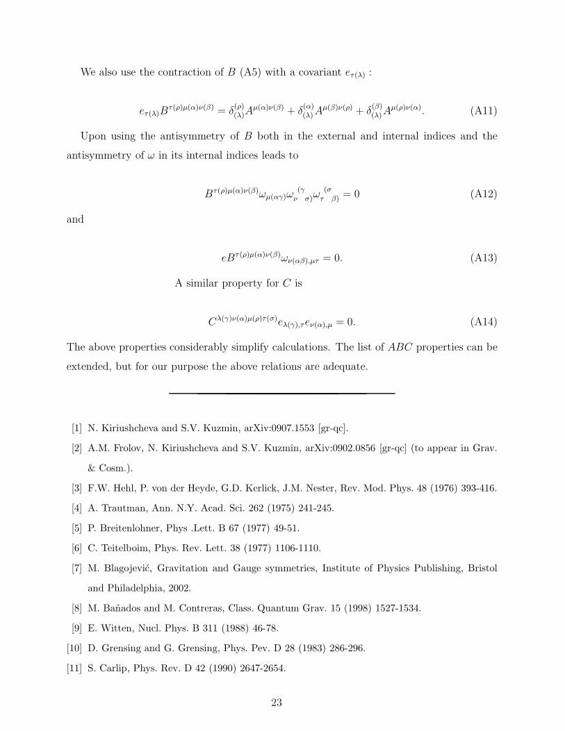
We also use the contraction of B (A5) with a covariant eτ(λ) :

eτ(λ)Bτ(ρ)µ(α)ν(β) = δ

(ρ)(λ)A

µ(α)ν(β) + δ(α)(λ)A

µ(β)ν(ρ) + δ(β)(λ)A

µ(ρ)ν(α). (A11)

Upon using the antisymmetry of B both in the external and internal indices and the

antisymmetry of ω in its internal indices leads to

Bτ(ρ)µ(α)ν(β)ωµ(αγ)ω(γ

ν σ)ω(σ

τ β) = 0 (A12)

and

eBτ(ρ)µ(α)ν(β)ων(αβ),µτ = 0. (A13)

A similar property for C is

Cλ(γ)ν(α)µ(ρ)τ(σ)eλ(γ),τeν(α),µ = 0. (A14)

The above properties considerably simplify calculations. The list of ABC properties can be

extended, but for our purpose the above relations are adequate.

[1] N. Kiriushcheva and S.V. Kuzmin, arXiv:0907.1553 [gr-qc].

[2] A.M. Frolov, N. Kiriushcheva and S.V. Kuzmin, arXiv:0902.0856 [gr-qc] (to appear in Grav.

& Cosm.).

[3] F.W. Hehl, P. von der Heyde, G.D. Kerlick, J.M. Nester, Rev. Mod. Phys. 48 (1976) 393-416.

[4] A. Trautman, Ann. N.Y. Acad. Sci. 262 (1975) 241-245.

[5] P. Breitenlohner, Phys .Lett. B 67 (1977) 49-51.

[6] C. Teitelboim, Phys. Rev. Lett. 38 (1977) 1106-1110.

[7] M. Blagojevic, Gravitation and Gauge symmetries, Institute of Physics Publishing, Bristol

and Philadelphia, 2002.

[8] M. Banados and M. Contreras, Class. Quantum Grav. 15 (1998) 1527-1534.

[9] E. Witten, Nucl. Phys. B 311 (1988) 46-78.

[10] D. Grensing and G. Grensing, Phys. Pev. D 28 (1983) 286-296.

[11] S. Carlip, Phys. Rev. D 42 (1990) 2647-2654.

23

[12] S.A. Ali, C. Cafaro, S. Capozziello, Ch. Corda, Int. J. Theor. Phys. 48 (2009) 3426-3448.

[13] T.W.B. Kibble, Journal of Math. Phys. 2 (1961) 212-221.

[14] I.A. Nicolic, Class. Quantum Grav. 12 (1995) 3103-3114.

[15] S. Carlip, Quantum Gravity in 2+1 Dimensions, Cambridge University Press, Cambridge,

1998.

[16] J.M. Charap, M. Henneaux and J.E. Nelson, Class. Quantum Grav. 5 (1988) 1405-1414.

[17] P.A.M. Dirac, Lectures on Quantum Mechanics, Belfer Graduate School of Sciences, Yeshiva

University, New York, 1964.

[18] L. Castellani, Ann. Phys. 143 (1982) 357-371.

[19] N. Kiriushcheva and S.V. Kuzmin, Ann. Phys. 321 (2006) 958-986.

[20] S. Samanta, Int. J. Theor. Phys. 48 (2009), 1436-1448, arXiv:0708.3300 [hep-th].

[21] E. Noether (M.A. Tavel’s English translation), arXiv:physics/0503066.

[22] M. Leclerc, Int. J. Mod. Phys. D 16 (2007) 655-680.

[23] H.-J. Matschull, Class. Quantum Grav. 16 (1999) 2599-2609.

[24] J. Schwinger, Phys. Rev. 130 (1963) 1253-1258.

[25] L. Castellani, P. van Nieuwenhuizen, M. Pilati, Phys. Rev. D 26 (1982) 352-367.

[26] N. Kiriushcheva and S.V. Kuzmin, arXiv:0912.5490 [gr-qc].

[27] N. Kiriushcheva and S.V. Kuzmin, arXiv:0912.3396 [gr-qc].

[28] S. Deser and B. Zumino, Phys. Lett. B 62 (1976) 335-337.

[29] M. Carmeli, Classical Fields, General Relativity and Gauge Theory, World Scoentific, New

Jersey, 2001.

[30] M. Henneaux, Phys. Rev. D 27 (1983) 986-989.

[31] P.G. Bergmann and A. Komar, Int. J. Theor. Phys. 5 (1972) 15-28.

[32] J.W. Maluf, Class. Quantum Grav. 8 (1991) 287-295.

[33] R. Di Stefano and R.T. Rauch, Phys. Rev. D 26 (1982) 1242-1253.

[34] G. Grignani and G. Nardelli, Phys. Rev. D 45 (1992) 2719-2731.

[35] N. Kiriushcheva and S.V. Kuzmin, arXiv:0809.0097 [gr-qc].

[36] A.M. Frolov, N. Kiriushcheva and S.V. Kuzmin, arXiv:0809.1198 [gr-qc].

[37] H. Nicolai, Nucl. Phys. B 353 (1991) 493-518.

[38] H.-J. Matschull and H. Nicolai, Nucl. Phys. B 411 (1994) 609-646.

[39] S. Deser, P. van Nieuwenhuizen, Phys. Rev. D 10 (1974) 411-420.

24

[40] N. Kiriushcheva and S.V. Kuzmin, in preparation.

25