INOM EXAMENSARBETE TEKNIK,GRUNDNIVÅ, 15 HP

, STOCKHOLM SVERIGE 2019

Trading volume at Avanza

GRETA KNUTSSON

KAMYAR ESPAHBODI

KTHSKOLAN FÖR TEKNIKVETENSKAP

Trading volume at Avanza GRETA KNUTSSON KAMYAR ESPAHBODIROYAL

Degree Projects in Applied Mathematics and Industrial Economics (15 hp) Degree Programme in Industrial Engineering and Management (300 hp) KTH Royal Institute of Technology year 2019 Supervisor at Avanza, Robert Ingemarsson Supervisors at KTH: Camilla Landén, Julia Liljegren Examiner at KTH: Jörgen Säve-Söderbergh

TRITA-SCI-GRU 2019:153 MAT-K 2019:09

Royal Institute of Technology School of Engineering Sciences KTH SCI SE-100 44 Stockholm, Sweden URL: www.kth.se/sci

Abstract

Producing a model explaining the trading volume can be attractive for companies

who’s main revenue resides on it. Previous studies have shown that factors such

as stock returns, volatility and uncertainty affects the trading volume.

The purpose of this work is to clarify the consensus that prevails and determine

the factors that impact Avanza’s customers trading volume. Factors such as daily

stock returns and economic, political and financial uncertainty are analyzed through

amultiple linear regression analysis with a daily time period between 2000-2019.

The work is thus designed within the framework of mathematical statistics and

industrial economics.

To be able to draw a conclusion, further investigation is required in the form of

a time series analysis in combination with a deeper understanding of the applied

area and the mathematical methods that have been used.

Keywords

Bachelor Thesis, Regression Analysis, Trading Volume, Economic Politic Uncer-

tainty, Stock Price, Avanza

i

Abstract

Att ta fram en modell som förklarar handelsvolymen kan vara eftertraktat hos

företag vars huvudintäkter beror av den. Tidigare forskning visar att faktorer

som prisförändringar på aktiemarknaden, volatilitet och osäkerhet påverkar han-

delsvolymen.

Syftet med arbetet är klargöra den konsensus som råder och fastställa de faktorer

som har störst påverkan gällande handelsvolymen för Avanza’s kunders. Fak-

torer som dagliga förändringar inom börsmarknaden och ekonomisk, politisk och

finansiell osäkerhet har genom en multipel linjär regressionsanalys analyserats

med en daglig tidsperiod mellan 2000-2019. Arbetet är således utformat inom

ramen för matematisk statistik och industriell ekonomi.

För att kunnadra en slutsats krävs vidare undersökning i formav en tidsserieanalys

och en djupare förståelse av det tillämpade området och metoderna som har an-

vänds.

Nyckelord

Kandidatexamensarbete, Regressionsanalys, Handelsvolym, Politisk Osäkerhet,

Börsindex, Avanza

ii

Acknowledgements

Wewould like to thankour supervisor at theRoyal Institute of Technology, Camilla

Johansson Landén from the Department of Mathematics, and Robert Ingemars-

son and Rasmus Åkerblom fromAvanza Holding Bank AB, whom assisted us with

relevant data and supported us throughout this thesis.

iii

Authors

Kamyar Espahbodi <kamyare@kth.se> and Greta Knutsson <gretak@kth.se>Industrial Engineering and ManagementKTH Royal Institute of TechnologyApplied Mathematics TMAI

Place for Project

Stockholm, Sweden

Supervisors

Camilla Johansson LandénLindstedtsvägen 25, 114 28, StockholmKTH Royal Institute of Technology

Julia LiljegrenLindstedtsvägen 30, 114 28, StockholmKTH Royal Institute of Technology

Robert IngemarssonRegeringsgatan 103, 111 39, StockholmAvanza Bank Holding AB

Contents

1 Introduction 11.1 Background . . . . . . . . . . . . . . . . . . . . . . . . . . . . . . . . 1

1.2 Problem . . . . . . . . . . . . . . . . . . . . . . . . . . . . . . . . . . 2

1.3 Economic Theory . . . . . . . . . . . . . . . . . . . . . . . . . . . . . 2

1.4 Goal and Purpose . . . . . . . . . . . . . . . . . . . . . . . . . . . . 4

1.5 Methodology . . . . . . . . . . . . . . . . . . . . . . . . . . . . . . . 6

1.6 Stakeholder Analysis . . . . . . . . . . . . . . . . . . . . . . . . . . . 6

1.7 Scope . . . . . . . . . . . . . . . . . . . . . . . . . . . . . . . . . . . 7

2 Regression Analysis 92.1 Multiple Regression . . . . . . . . . . . . . . . . . . . . . . . . . . . 9

2.2 Ordinary Least Squares (OLS) . . . . . . . . . . . . . . . . . . . . . 10

2.3 OLS Assumptions . . . . . . . . . . . . . . . . . . . . . . . . . . . . 11

2.4 Residual analysis . . . . . . . . . . . . . . . . . . . . . . . . . . . . . 14

2.5 Leverage and Influence . . . . . . . . . . . . . . . . . . . . . . . . . 17

2.6 Variable Selection . . . . . . . . . . . . . . . . . . . . . . . . . . . . 19

2.7 Transformations . . . . . . . . . . . . . . . . . . . . . . . . . . . . . 25

3 Data 273.1 Trading Volume . . . . . . . . . . . . . . . . . . . . . . . . . . . . . 27

3.2 Equity . . . . . . . . . . . . . . . . . . . . . . . . . . . . . . . . . . . 28

3.3 Volatility . . . . . . . . . . . . . . . . . . . . . . . . . . . . . . . . . 29

3.4 Economic Policy Uncertainty (EPU) . . . . . . . . . . . . . . . . . . 29

4 Result 314.1 Residual Analysis . . . . . . . . . . . . . . . . . . . . . . . . . . . . . 31

4.2 Leverage and influential points . . . . . . . . . . . . . . . . . . . . . 32

4.3 Transformations . . . . . . . . . . . . . . . . . . . . . . . . . . . . . 35

4.4 Variable Selection . . . . . . . . . . . . . . . . . . . . . . . . . . . . 36

4.5 Final Model . . . . . . . . . . . . . . . . . . . . . . . . . . . . . . . . 44

5 Discussion 465.1 Methodology . . . . . . . . . . . . . . . . . . . . . . . . . . . . . . . 46

v

5.2 Model Adequacy . . . . . . . . . . . . . . . . . . . . . . . . . . . . . 48

5.3 Previous studies . . . . . . . . . . . . . . . . . . . . . . . . . . . . . 48

5.4 Future Work . . . . . . . . . . . . . . . . . . . . . . . . . . . . . . . 49

5.5 Avanza . . . . . . . . . . . . . . . . . . . . . . . . . . . . . . . . . . 49

6 Conclusion 51

References 52

vi

1 Introduction

A traditional stockbroker is a person who executes buy and sell orders on the be-

half of their client. Nowadays, the influence of internet has enabled the stockbro-

ker to carry out orders at a lower commission rate than before, hence the birth

of the discount broker. The discount broker’s business is as such online based,

which implies low overhead costs and thus reduced commission rates and fees

for the client. The chosen strategy for battling the market competition being high

volume and low cost, the broker’s main income, in a broad sense, mainly depends

on the number of client transactions. Therefore, it lies in the broker’s interest

to fully understand the behaviour of the driving factors behind their customers

trading volume, since it directly correlates with their aggregated commission rev-

enue.

1.1 Background

Avanza BankHolding AB, formally founded 1999, is Sweden’s largest online stock

brokerwith over 800,000 customers.1 Its business idea is to, through low charges,

offer a broad variety of saving products and educational and supporting services

within the area of personal saving in Sweden. They also offer market competi-

tive mortgage loans and pension solutions 2 and have been ranked as having the

happiest customers nine times in a row for each year within the industry.3

As any other online stock broker, Avanza takes a share of each customers trade, a

commission, which constitutes their primary source of income. Hence, their ag-

gregated revenue is directly dependent on their trading volume, i.e. the number

of shares transacted every day. By understanding the underlying mechanisms af-

fecting their customers trading volume, it is possible for Avanza optimize their

resources through forecasting or developing new products based on the special

behaviour, streamlining their organization.

1Avanza©,History2Avanza Bank Holding AB, Årsredovisning 20183Svenskt Kvalitetsindex, Personlig service utmanar digitala tjänster

1

1.2 Problem

However, Avanza’s customers trading behaviour does not solely depend on inter-

nal factors, such as new user interface improvements or new functionality fea-

tures, in fact, their financial result is affected by market cyclical effects such as

stock market developments, volatility and federal funds rate. Avanza states, in

their annual report, that the previous year 2018 was characterized by political un-

certainty and that SIX return index (an index representing all of the stocks on the

Swedish market) decreased by 8% and that the number of transactions rose by

15% and the revenue by 8%, compared to the previous year [2017].4

It therefore lies inAvanza’s interest to knowhowmuchpower they have in control-

ling their own revenue stream, i.e. is there still room for internal innovations and

new product features that could potentially further raise the commission revenue,

or does it, to some extent, only depend on exogenous factors? In other words, how

much can they affect their revenue stream, and to what extent?

1.3 Economic Theory

Although no previous studies within the area was found, some key insights were

gained by studying previous literature. The trading activity of a population is a

complex phenomenon comprised of several factors both physiological, such as in-

vestor overconfidence, and systematic, such as calendar effects. The following sub

sections further investigates some of these factors.

1.3.1 Trading Volume

It is hard to predict future trading volumes, i.e. the number of shares being trans-

acted at a certain time point, because of its complexity and dependency on human

behaviour. In general, the trading volume is driven by at least two forces; changes

in heterogeneity of beliefs and the disposition effect.5 Summarized, these empir-

4Avanza Bank Holding AB, Årsredovisning 2018, pp. 49-505Shefrin, A Behavioral Approach to Asset Pricing

2

ically supported theories states that the investors overconfidence about their val-

uation and trading skills can explain the high observed trading volume.6

Since these drivers are relatively subjective and hard to measure, from a quanti-

tative approach, the psychological and individual factors of human being, such as

overconfidence, personal beliefs, irrationality, are disregarded in this study.

1.3.2 Factors

Focusing on more numerically obtainable factors, several stand out.

Several studies have shown that there exists a positive correlation between the

price changes of stocks and trading volume in financial markets.7, 8, 9 A study ex-

amining potential factors affecting trading volume in European markets found

the asymmetric price-volume relation in over 70 percent of the analyzed stocks.10

Based on these studies, one could assume that the price is of great importance

when analyzing trading volume. Another study that analyzed the daily trading vol-

ume volume of the Swedish stockmarket found that themarketplace of the stock,

contrary to belief, was irrelevant for explaining the volume, while the shareholder

structure, free float and the number of outstanding shares in a company were

relevant.11

Perfect information availability is a key aspect of a perfect competition, therefore

it is reasonable to assume that it affects the trading volume as well, since, for

instance, positive information might persuade investors to buy a stock and vice

versa. Economic Policy Uncertainty (EPU) is an index developed by researchers

to generally estimate the uncertainty about fiscal or monetary policies, tax regu-

lations, regime changes and uncertainty over electoral outcomes, in other words

—everything that might raise the uncertainty regarding economic and policy out-

comes. One study found that the EPU-index impacts the markets and that it has

6Statman, Vorkink, and Thorley, “Investor Overconfidence and Trading Volume”7Ying, “Stock Market Prices and Volumes of Sales”8Cornell, “The Relationship between Volume and Price Variability in Future Markets”9Clark, “A Subordinated Stochastic Process Model with Finite Variance for Speculative Prices”10Batrinca, Hesse, and Treleaven, “Examining drivers of trading volume in European markets”11Sevelin, “Swedish Stock market: Explaining trade volumes in single stocks”

3

a positive correlation with stock price volatility and reduced investment.12

The transaction cost is another factor to consider. One study found that that trad-

ing volume is measurably responsive to changes in transaction costs.13

Clearly, there are several factors that could help to explain the trading volume —

even calender days affect it.14

1.4 Goal and Purpose

In conclusion, the change in trading volume is complex and depends on several

factors. The challenge is to find an explanation of the behaviour of Avanza’s clients

trading activity in order to answer the question whether the effects on the trading

activity are exogenous or endogenous, i.e. can Avanza affect their customers trad-

ing volume — or does it mainly depend onmacroeconomic, financial and political

factors?

In summary, this thesis aims to answer the following:

1. Does uncertainty, in a financial, political and macroeconomic sense, along

with market indicators such as stock prices and volatility indices, impact

Avanza’s customers trading activity?

(a) Which factors should be studied and why?

2. What are the possible relationships between the factors and what do they

look like?

(a) Can a model, given certain a significance level, explaining the fluctua-

tions of the commission revenue be formulated?

3. How should possible relationships be implemented?

(a) What can Avanza do with this information to increase their revenue?

12Baker, Bloom, and Davis, “Measuring Economic Policy Uncertainty”13Epps, “TheDemand for Brokers’ Services: TheRelation between Security Trading Volume and

Transaction Cost”14Sakalauskas and Krikščiūnienė, “The Impact of Daily Trade Volume on the day-of-theweek

Effect in Emerging Stock Markets”

4

If the stated questions above are answered and assuming that there exists possi-

ble relationships, Avanza will have more information about their customers com-

pared to other competitors in the same business. Therefore, the information can

be seen as a tool for competitiveness.

The competitiveness for Avanza’s business can, for example, be analyzed trough

Michael Porter’s Five Forces-model, where an increase in a company’s competi-

tiveness possibly also implicates an increasing of the revenue. The five forces in

Porter’s model are:

1. Competition in the industry

2. Power of customers

3. Power of suppliers

4. Threats of substitutes

5. Potential of new entrants in the industry

By analyzing each and one of the forces, the purpose of the project can further be

clarified. The first aspect of rivalry, the competition in the industry, depends on

how diversified the company’s offer is, compared to other companies in the same

business. The power of customer and suppliers represents customers ability to

decrease prices on the output and the suppliers ability to bargain for increased

prices. Threats of substitutes can be a rivalry if there exists substitutes on the

market that can replace the service and goods provided by the company. Last

but not least, the potential of new entrants entering the market also affects the

competitiveness for the analyzed company.15

Given that the research questions are answered, Avanza will have more informa-

tion on what the trading volume depends on. Therefore, they can differentiate

their offer which possibly will lead to a stronger position relative to the competi-

tors within the industry. The power of customers can decrease as the knowledge

about Avanza’s customers trading behaviour increases, since the negotiation abil-

ity is usually stronger for the part with the most information.

The power of suppliers, threats of substitutes and potential new entrants in the

15Chappelow, Porter’s 5 Forces

5

industrywill probably remain the same, since the informationmainly concerns the

customers behaviour, which mainly affects the customers and the rivalry within

the industry.

1.5 Methodology

By examining relevant data, such as stock price, volatility, the EPU-index etc., the

purpose is to answer whether these chosen parameters are relevant in explaining

the trading volume. Future research can then apply these parameters without

having to investigate if they are relevant. Further, the result could help to more

thoroughly define the company’s ability in manipulating its revenue stream if it

mostly depends on exogenous factors.

The suggested statistical tool is multiple linear regression modeling. Extensively

used within finance, regression is a statistical method to establish of the relation-

ship between variables. In multiple regression analysis, a relationship between

the response variable y, i.e. the variable of interest, and a set of predictor vari-

ables x = [x1, x2, ..., xp] is examined.

By fitting the model with the response variable and the plausible relevant factors

affecting the response variable a multiple linear model explaining the response,

to some degree, can be obtained.

The literature used in the section of presenting the regression analysis is mainly

Introduction toLinearRegressionAnalysisbyMontgomery, Peck, andVining.16

1.6 Stakeholder Analysis

To investigate the stakeholders for this project, a stakeholder analysis is made

where both internal stakeholders within the company as well as external stake-

holders are included. The stakeholders can both be affected and affect the project,

depending on which stage the project is in and what result comes with it.

First of all, one internal stakeholder is the management of Avanza, since it lies in

16Montgomery, Peck, and Vining, Introduction to Linear Regression Analysis

6

their interest to investigate whether the trading volume depends on exogenous or

endogenous behaviour. The management influences the implementation of the

result, and therefore need to be informed whether any conclusions can be made.

The result of this degree project can therefore be used as a tool for themanagement

to analyze and evaluate the organization.

Second of all, the supervisors at Avanza can be seen as internal stakeholders. On

one hand, the supervisors provides the project with data and knowledge which

shows the importance and influence that the supervisors have on the project, while

on the other hand, the project can supply the supervisors with information re-

garding the trading volume. This information is interesting for the supervisors at

Avanza since the result can be further investigated and presented to the manage-

ment of the company.

The external stakeholders does not affect the project because of the lack of aware-

ness regarding this project. One possibly external stakeholder is the management

in other companies. Even though the analyzed data is given by Avanza, there

might be a general pattern representing investors all over the world and therefore

it could also be useful in the management in other companies. Another possibly

external stakeholder is Avanza’s customers. The customers can be affected of the

project depending on what the result indicates and whether any implementations

are made, but the customers will not affect the project.

1.7 Scope

Some aspects, that possibly could affect the outcome if they were examined, have

been excluded in this report.

First, this study is geographically limited to Avanza’s customer that mainly reside

in Sweden. Therefore, the conclusions can not be applied to trading activity be-

haviour in general. Second, the seasonal variation of the financial market have

not been taken into consideration in this report. For example, it has been shown

that there is exists a seasonal variation which affects Avanza’s trading volume (see

figure 1.1). 17

17Johanna Kull and Nicklas Andersson, Tips inför sommarbörsen

7

Figure 1.1: Plot of OMX against months for the time period 2000-2017

Furthermore, other factors that possibly could affect the trading volume and that

have been left out are the development of rents, taxes and inflation. For example,

taxes and rents affect the disposable income for the households18 and therefore

also the amount consumers can trade.

The inflation can affect the trading volume. If there is an increasing inflation dur-

ing a specified period of time, themoneywill be worth less which leads to the same

conclusion as for the rents and taxes, that the consumers will have less money to

trade and therefore trade less than usual.

Moreover, the time frame that this thesis is delimited to is from the 3rd of January

to the 29th of April 2019. This specified time period could affect the output of the

project, but since Avanza was founded in year 1999,19 this aspect does possibly not

have a great impact on the output.

18Carlgren,Hushållens inkomster19Avanza©,History

8

2 Regression Analysis

Regression analysis is a statistical technique for investigating and modeling the

relationship between variables.20 The word regression means ”a return to a pre-

vious and less advanced or worse state, condition, or way of behaving”, and may

be the most widely used statistical technique.21

The variables of interest are called response and predictor variables. The response

variable is often denoted as y and represents the observed outcome, given the pre-

dictor variable(s) x. When investigating a response variable that may be related

to several regressors, a multiple regression model is appropriate.

2.1 Multiple Regression

The multiple regression model is given by the equation

y = Xβ + ϵ (1)

where the response y consists of a vector of the response variables for each ob-

servation. The error ϵ consists of a vector of the errors for each observation. The

estimation coefficients, the ”betas”β, consists of a vector with beta coefficients for

each predictor, where β0 represents the intercept and p the number of predictor

variables. X is a matrix consisting of the predictor variables.

X =

1 x11 x12 . . . x1p

1 x21 x22 . . . x2p

......

.... . .

...

1 xn1 xn2 . . . xnp

, β =

β0

β1

...

βp

, y =

y1

y2...

yn

, ϵ =

ϵ1

ϵ2...

ϵn

(2)

By estimating the betas, given the data, the fitted model produces a line along the

data points through the equation

20Montgomery, Peck, and Vining, Introduction to Linear Regression Analysis pp. 121Definition of “regression” from the Cambridge Advanced Learner’s Dictionary & Thesaurus

©Cambridge University Press

9

y = Xβ (3)

where y represent the fitted values and β the estimated beta coefficients.

2.2 Ordinary Least Squares (OLS)

The aim of the estimation of the beta coefficients is to make it as accurate as pos-

sible. The OLS-method is a popular and widely used method for obtaining the

estimates β. OLS minimizes the sum of the squares of the differences between

the observations yi and the projected straight line and can be used to produce the

estimators of the multiple regression model in Equation (1). The least-squares

function is given by

S(β) =n∑

i=1

ϵ2i = ϵTϵ = (y−Xβ)T (y−Xβ) (4)

Developing the right hand side of the equation through multiplication and tak-

ing the derivative with respect to β and setting it equal to zero to find the mini-

mum, the least-squares normal equations stated inmatrix notation can be written

as

XTXβ = XTy (5)

Or equivalently, by solving the normal equations, as

β = (XTX)−1XTy (6)

Equation (6) is called the least squares estimation equation.

The Gauss-Markov Theorem states that the OLS estimator β is the best linear

unbiased estimator (BLUE). In other words, β has the smallest variance in the

class of all unbiased estimators that could be produced as linear combinations of

10

the data.22

2.3 OLS Assumptions

When fulfilled, the OLS assumptions allow the OLS method the create the best

possible estimates, best in the sense of having smallest variances. According to the

Gauss-Markov theorem, OLS produces the best estimators when the assumptions

presented down below hold. Further, the coefficients estimates β converge to the

actual population parameters when the sample size increases to infinity and given

that the assumptions are fulfilled.

2.3.1 Strict Exogenity

The randomerrors ϵ are assumed to havemean zero,meaning that the value of one

error does not depend on the value of any other regressor. This consequence fol-

lows directly from the strict exogenity assumption and can be expressed as

E[ϵ|X] = 0 (7)

Equation (7) implies that the independent predictor x is not dependent on the

dependent variable y, i.e. an exogenous variable is able to influence the system

without being influenced by it.

2.3.2 Homoscedasticity

Besides having a zero mean, the errors ϵ are assumed to have the same unknown

variance σ2 in each observation, i.e. the variance is constant for each observation.

The opposite is named heteroscedasticity and implies that the variance changes

for different observations, which reduces the precision of the OLS generated esti-

mators.22Montgomery, Peck, and Vining, Introduction to Linear Regression Analysis. pp. 587-588

11

Investigation of the residual plots is useful for controlling the OLS assumptions

and often recommended for other reasons as well, such as detecting outliers.23

Homoscedasticity can be investigated by plotting the residuals against the fitted

values yi. By plotting the externally studentized residuals ti against the corre-

sponding fitted value, the behaviour of the variance can be observed.

2.3.3 No Autocorrelation

The errors ϵ are assumed to be uncorrelated between the observations.

E[ϵiϵj|X] = 0 (8)

The opposite holds if, for instance, the error term of one observation is positive

and that it systematically increases the probability that the following error is posi-

tive (positive correlation). Autocorrelation is common in the context of time series

data, i.e. measurements over a certain amount of time.

If autocorrelation exists the OLS estimator is still unbiased but not BLUE and the

usual OLS standard errors and test statistics are no longer valid.

2.3.4 Normality

Thenormality assumptions assumes that the errors are normally distributed given

the regressors, i.e.

ϵ|X ∼ N (µ, σ2In) (9)

The OLSmethod does not require that the normality assumption is fulfilled, how-

ever fulfillment of the assumption enables the usage of hypothesis testing, gener-

ating reliable confidence and prediction intervals.

By constructing a normal probability plot of the residuals the normality assump-

tions can be checked. The cumulative normal distribution is constructed such that23Montgomery, Peck, and Vining, Introduction to Linear Regression Analysis. pp. 136

12

it will plot as a straight line against the externally studentized residuals, ranked

in increasing order. Since the errors are assumed to be normally distributed, the

desired observation should show the points as close as possible to the straight

line.

2.3.5 Multicollinearity

When multicollinearity occurs it causes lower precision of the OLS estimators.

Perfect correlation occurs when one of the variables changes by a fixed propor-

tion, the other also changes by the same fixed proportion. This indicates that the

two variables are linearly dependent. Since the OLS method cannot distinguish

the perfectly correlated variables a high enough correlation causes problem, i.e.

multicollinearity. One could imaginemulticollinearity as a two dimensional plane

residing on the data points. If the data points are not orthogonal the plane will be

unstable or ”wiggly” and therefore vary greatly.

Since the matrix XTX consists of the dimensions p × p (p being the number of

predictor variables) and the jth column of theXmatrix is given byXj, the matrix

can be represented asX = [X1,X2, ...,Xp].24 Multicollinearity is said to exist when

the vectors X1,X2, ...,Xp are linearly dependent, i.e. if there is a set of constants,

t1, t2, ..., tp not all zero, such that

p∑j=1

tjXj = 0 (10)

Variance Inflation Factors (VIF) One way of detecting multicollinearity is

to investigate the linear dependency among the regression variables, since the re-

gressors are the columns of the Xmatrix. By investigating the correlation matrix

C = (XTX)−1 , multicollinearity can be detected. The diagonal elements of the

correlation matrix are called variance inflation factors, since they provide an in-

dex measuring the inflation of the variance of an estimated regression coefficient

caused by collinearity.

24Montgomery, Peck, and Vining, Introduction to Linear Regression Analysis. pp. 286

13

Large VIF values associated with the regression coefficients indicate that they are

poorly estimated. What is meant by large values, 5 and 10 are often used based on

practical experience.25 The VIF’s can be calculated by the following formula.

VIFj = Cjj = (1−R2j )

−1 (11)

Condition Number Another way of detecting multicollinearity is by measur-

ing the spread of the eigenvalues of XTX, i.e. λ1, λ2, ..., λp. The condition number

K is defined as the fraction of the largest and lowest eigenvalue.

K =λmaxλmin

(12)

K > 100 indicates a problem with multicollinearity and K > 1000 indicates a se-

vere problem with multicollinearity. This is because the eigenvalues of a p × p

matrix A, that are given by the equation |A− λI| = 0, represent the characteristic

roots of the matrix. Hence, small values of the roots indicate near-linear depen-

dencies in the data and vice versa.

2.4 Residual analysis

Plotting residuals is a powerful technique for detecting outliers and estimating the

overall behaviour of the model. Autocorrelation can be detected through residual

plots where the plots displays residual versus time.

Residuals are defined as

ei = yi−yi, i = 1, 2, ..., n (13)

where yi is the observed value and yi is the corresponding fitted value. The resid-

ual can therefore be seen as the deviation between the data and the fit. Moreover,

the residual is also a measure of the variability in the response yi. If any assump-

25Montgomery, Peck, and Vining, Introduction to Linear Regression Analysis pp. 296

14

tions about the residuals are wrongfully made, it will be shown in the residual

analysis.

The approximate average variance of the residuals is given by∑ni=1(ei − e)2

n− p=

∑ni=1 e

2i

n− p=

SSresn− p

= MSres (14)

The residuals have n− p degrees of freedom, which makes the non-independence

of the residuals negligible as long as the number n of residuals is not small relative

to the number of coefficients β.

2.4.1 Studentized Residuals

Studentized Residuals is a way of improving the residual scaling by dividing ei

by the exact standard deviation of the ith residual. The residual can be written

as

e = (I−H)y = (I−H)ϵ

where the hat matrix can be written as

H = X(XTX)−1XT

using that y = Xβ + ϵ. Thus the covariance matrix of the residuals is

Var(e) = Var(I−H)ϵ = σ2(I−H)

Since thematrix (I−H) generally is not diagonal, the residuals have different vari-

ances and are also correlated. The variance of the ith residual is thus Var(ei) =

σ2(1−hii), where hii is the ith diagonal element in the matrixH. Now, by estimat-

ing σ2 byMSRes, the studentized residuals are given by

ri =ei√

MSRes(1− hii)(15)

15

For i, where i = 1, 2, ..., n, and√

MSRes(1− hii) is the standard deviation, i.e.√Var(ei).

Since hii is the measure of the location of the ith point in the x space, Var(ei) be-

comes smaller for the points xi that lies relatively far away from the center of the x

space. This in turn means that the studentized residuals becomes larger for these

points. Thus, analyzing studentized residuals makes it easier to detect influential

points which is where the violations of the basic assumptions are more likely to

occur.

2.4.2 PRESS Residual

PRESS is generally regarded as a measure of how well a regression model will

perform in predicting new data. The definition of the PRESS residual is

e(i) =ei

1− hii

, i = 1, 2...n (16)

Equation (16) shows that the PRESS-residual is the ordinary residual weighted

with the diagonal element from the hat matrix. Taking the denominator into con-

sideration, a large value on hii implicates a small denominator which makes the

deleted residual large. PRESS-residuals with small values are generally desired

for a model.

2.4.3 R-Student

Anothermethod to detect an outlier is theR-student. Compared to the studentized

residual, R-student uses an external scaling instead of the internal which is used

in the estimate of the mean square residual.

S2i =

(n− p)MSRes − e2i /(1− hii)

n− p− 1(17)

If an observation is influential, the estimation of the variance S2 will differ sig-

nificant fromMSRes. This will make the denominator close to zero and therefore

16

increase the residual. Now the R-student residual is given by

ti =ei√

S2i (1− hii)

(18)

2.4.4 Partial Regression and Partial Residual Plots

An effective way to check the adequacy of the fit of the regressionmodel is tomake

a residual plot. A partial regression plot is used in order to study the marginal re-

lationship between the regressor given the other variables in the model. The plot

shows if the assumption about the specified relationship between the response

and the regressor variables has been made correctly and can also be useful for

providing information about a variable that is not currently in the model. Com-

paring each of the regressor variables with the response, the partial regressor plot

shows the marginal relation for each of the regressors.

2.5 Leverage and Influence

Occasionally, certain data points that negatively influences themodel appear. These

points are defined as influential points. The leverage point, point A in the left plot

in Figure 2.1, depicts an usual x coordinate, but a y coordinate that seems to be

located on the regression line. TheA-point in the right plot displays an influential

point with both an unusual x and y coordinate. As the name tells, the influential

point influences the regression line to move away from the rest of data, i.e. from

its more natural trajectory.

Figure 2.1: Left: leverage point. Right: influential observation

17

A small subset of data can negatively influence the model to such a degree that

the estimates of the beta coefficients mostly rely on the subset data instead of the

majority mass of the data. Since the regression model should be a construct of

all of the data, these situations must be avoided. By finding and analyzing these

points their impact can be determined and understood relative to the end regres-

sion model, and even removed if they are ”bad”.

2.5.1 Cook’s Distance

The influence of one point can be measured with respect to its location in the x

space and its response. By removing one point from the sample Cook’s distance

can measure its influence and this can be used as a deletion diagnostic.

Di =(y(i) − y)T (y(i) − y)

pMSres(19)

where y(i) is obtainedwhen removing the ith observation from the data set. Points

with largeDi values greatly influences the beta estimates, whereDi > 1 are consid-

ered being large. Therefore, it is recommended to eliminate data points exceeding

the cutoff-ratio. It is important to remember that the cutoff-ratio only is a recom-

mendation and also based on the sample size n. However, for larger samples sizes,

the specified cutoff-ratio makes more sense.

2.5.2 DFFITS

Similar to Cook’s distance, DFFITS, difference in fit or difference in fitted y’s with

and without each data point, also measures the influence of one point and is given

by

DFFITSi =yi − y(i)√S2(i)hii

(20)

where yi is the fitted value including the point i and y(i) is the fitted value excluding

the point i. The factor S2(i) is the R-student estimate of the mean square residual

18

shown in Equation (17) and hii represents the diagonal element i from the hat

matrix.

The suggested cutoff-ratio is given by |DFFITSi| >√p/n. The DFFITS is a

measure of the number standard deviations the fitted value changes if the i:th

observation is removed from the model. It essentially a useful measure when de-

tecting both leverage and prediction error.

2.6 Variable Selection

Oftentimes, there are several regressor variables to choose from, making it diffi-

cult to pinpoint the likely few important ones. Variable selection is the procedure

of finding an appropriate subset of regressor for the model. Further, variable se-

lection is the most common procedure for solving the problems of multicollinear-

ity.26

2.6.1 Null Hypothesis

As mentioned in Section 2.3.4 the normality assumptions open up the possibil-

ity of using hypothesis testing and generating reliable confidence and prediction

intervals. The standard test uses the following hypotheses

H0 : β1 = β10 H1 : β1 = β10 (21)

where β10 is set to 0, and the goal is to conclude whether the regression coeffi-

cient β1 is non-zero. Since the errors are normally distributed with expected value

zero, the observations are also normally distributed with expected valueXβ, since

E[y] = E[Xβ + ϵ] = E[Xβ] + E[ϵ] = Xβ. If H0 : β1 = β10 = 0 cannot be rejected

the linear relationship between the predictor variable x and the response y either

does not exist, is not important for explaining the response or does not have a

linear relationship with the response.

26Montgomery, Peck, and Vining, Introduction to Linear Regression Analysis. pp. 328

19

2.6.2 t-test

The t-statistic is the ratio of the departure of the estimated value of a parameter

from its hypothesized value to its standard error. By assuming that Y is a random

variable following a normal distributionwithmean µ and variance σ2 we have Y ∼N (µ, σ2) → Z = Y−µ

σ∼ N (0, 1), implying that Z2 (Z being the standard normal

variable with 1 degree of freedom) follows a X 2 distribution, i.e. Z2 ∼ X 21 . Thus,

the square of a standard normal variable is a X 2 random variable with one degree

of freedom. If the null hypothesis given in Equation (21) is true, the t statistic t0

follows a tn−2 distribution.

t0 =β1 − β10√MSres/Sxx

(22)

The degree of freedom for t0 is the same as MSres. Using Equation (22) the ob-

served value t0 can be compared to the upper α/2 percentage point of the tn−2

distribution (tα/2,n−2). The t statistic for the null hypothesis is given by

t0 =β1√

MSres/Sxx

=β1

se(β1)(23)

since β10 = 0 from the Equation (21). If |t0| > tα/2,n−2, then the null hypothesis is

rejected.

2.6.3 F-test

The F-statistics shows the relationship between two independent variables where

both of the variables have the χ2 distribution with different degrees of freedom.

For example, if we introduce two variables X and Y where X ∼ χ2v and Y ∼ χ2

n.

Thus, the ratio is now given by

X/v

Y /n∼ Fv,n (24)

which is the F distribution with v and n degrees of freedom. This shows that the

20

ratio of two independent random variables that follow a χ2 distribution, follows

an F distribution.

Therefore, the F test can be used to test the null hypothesis. In this case, the null

hypothesis is that all of the regression coefficients are equal to zero, implying, if

the hypothesis is not rejected, that the model has no predictive capability. If the

null hypothesis is true, the following holds

MSR

MSres∼ F1,n−2 (25)

since MSR = SSR/1 has one degree of freedom and MSres = SSres/(n − 2) has

(n− 2) degrees of freedom.

F0 =MSR

MSres(26)

The null hypothesis is rejected if F0 > Fα,1,n−2, where α is the given level of signif-

icance.

2.6.4 All Possible Regressions

As stated earlier, it is desirable to choose a subset of the candidate regressors.

By fitting various combinations of the regressors and comparing them based on

certain criteria, models with a certain setup of parameters can be selected.

All possible regressions is one method of achieving this. By fitting the model with

the regressors one by one and comparing them with each other and choosing the

best ones, based on some criteria, the best regressionmodel can be selected.

Assuming that the intercept β0 is included in each model, there is a total of 2p

models to evaluate. One obvious drawback with the method is the exponentially

growing number of models based on p, for an instance 210 equals to 1024models,

however modern day computers and software have made the procedure relatively

simple to use.

21

2.6.5 Backward Elimination

Backward Elimination is a step-wise regression method used in situations where

all possible regressions can be burdensome computationally. This method begins

with the model including all p candidate regressors. The corresponding t-test or

F-test is computed for each of the regressor. Comparing these t-tests or F-tests to

a pre-selected value, called tleave for example, the regressor corresponding to the

smallest value of the t-test or F-test is removed from the model.

This procedure is repeated k times until the model contains a number of p − k

regressors, where each of the corresponding test statistic value is greater than the

cutoff value.

2.6.6 Cross Validation

In situations when there is no new fresh data to validate the model, tools as cross

validation can be used. The data set is split into two parts, one is the estimation

part, and the other is the prediction part. A new regression model is build, based

on the estimation data, and then validate the model with the prediction data. If

the original data is collected within a time frame, one can use time as the basis

when splitting the data set into these two components. However, the basis which

can be chosen arbitrarily has a probability of not stressing the model enough, and

therefore it would be preferable to use several estimation and prediction-sets to

improve the validation technique.

2.6.7 R-squared and Adjusted R-squared

To measure the overall adequacy of the model, one can use the coefficient of de-

termination called ”R squared”. The proportion of the variance in the dependant

variable that is predictable from the independent variable(s) is given by R2 . In

other words, R2 measures how close the observed data are to the fitted regression

line.

The residuals sum of squares (SSres), the discrepancy between the data and the es-

timatedmodel, divided by the total sum of squares (SStot), the squared differences

22

of each observation from the overall mean, minus 1 gives us R-squared.

R2 =Explained VariationTotal Variation

= 1− SSresSStot

∈ [0, 1] (27)

However, theR2-measure has some limitations, one of thembeing that it increases

when more predictors are added to the model. The modified version of the mea-

surement, the adjusted R squared R2adj, only increases when the added predictors

improves the model.

R2adj = 1− SSres/(n− p)

SStot(n− 1)(28)

Thus, highR-values are desirablewhenmeasuring the overallmodel adequacy.

2.6.8 Mallow’s Cp Statistic

Mallow’s Cp addresses the issue of overfitting, i.e. when a model contains more

parameters than can be justified by the data. The statistic is

Cp =SSresMSres

− n+ 2p (29)

where n denotes the number of observations and p the number of parameters. By

plotting Cp against p, the models showing lowest Cp-values and which also are

closest to the line Cp = p are the best. Figure 2.2 displays a graph of the statistic

and indicates that model C, with four parameters, although above the line Cp = p

compared to model A, is better than A, since it is below A, thus representing a

model with lower total error.

23

Figure 2.2: A Cp plot (fromMontgomery, Peck, and Vining (Introduction to Linear RegressionAnalysis) pp. 336)

Mallow’s Cp can be used as one of the criteria in the all possible regression proce-

dure for checking the model adequacy.

2.6.9 Akaike Information Criterion (AIC) and Bayesian Information Crite-rion (BIC)

Originating from the AIC, BIC is simply an extension of AIC. Acting as criteria,

for instance in the all possible regression procedure, these criteria help to choose

the best predictors by penalizing the addition of regressors as the sample size in-

creases.

Since some information almost alwayswill be lost during statisticalmodelingwhen

using themodel to represent the process, themodelswith the least loss of informa-

tion are preferred. AICmeasures the entropy of themodel, i.e. the expected infor-

mation of the model, were the lowest AIC values are most desirable and BIC mea-

sures the posterior probability of a model being true, meaning similar to AIC that

lower BIC-values are preferred. The most significant difference between these

criteria is their size of the penalty —BIC penalizes model complexity more heav-

ily.

Simply put, AIC and BIC consist of a ”measure of fit” and a ”complexity penalty

part”. The likelihood functionL, the plausibility of a value for the parameter given

some data, represents the goodness of fit while p, the number of parameters, rep-

24

resents the complexity.

AIC = −2 ln (L) + 2p = n ln(SSres

n

)+ 2p (30)

BIC = −2 ln (L) + p lnn = n ln(SSres

n

)+ p lnn (31)

Summarized, these criteria ask whether more regressors should be added to the

model, since SSres cannot increase when the number of regressors is increased,

there exists a trade-off between the goodness of the fit of the model and the com-

plexity of the model.

2.7 Transformations

When starting the regression analysis, the usual assumption about linearity is of-

ten made. With this assumption, the following needs to be satisfied:

1. The model errors have mean zero, constant variance and uncorrelated.

2. The model errors follows a normal distribution.

3. The form of the model is correct.

If these assumptions are incorrect, a transformation of the data needs to be done in

order to find a relationship between the regressor and the regressor variables.

2.7.1 Box-Cox

One suchmethod is called the Box-Coxmethod. Thismethod usesmaximum like-

lihood to find the power of λ to use in the transformation yλ. Because of the dis-

continuity when λ approaches zero, the equations are given by:

y(λ) =

yλ−1λzλ−1 , λ = 0;

zlny, λ = 0;(32)

25

Where z = ln−1[1/n∑n

i=1ln yi] is the geometric mean value of the observations

yi.

The Jacobian of the transformation and the divisor zλ−1 are related when convert-

ing y into y(λ) which ensures the residual sum of squares with different values of

the power λ to be comparable.

26

3 Data

By choosing the most popular stock and volatility indices, alongside well estab-

lished EPU indices, the idea was to include a mix of local and international mea-

sures on price and volatility changes and financial, political and economic un-

certainty. The equity and volatility indices were accessed through the Thomson

Reuters Eikon software. The data was transferred in an xlsx format into the

programming language R. The relevant information, such as Exchange Date and

Close, was extracted and aggregated.

Since indices put simply are, for example, aggregated stock prices, the relevant

information is whether or not an index has increased, since the nominal value

does not say much. Therefore, the daily returns of the indices are calculated by

dividing their respective closing prices pn for day n, with their previous price, i.e.

pn−1. Subtraction by one presents it percentage.

Daily Return =pnpn−1

− 1 (33)

Thus, an aggregated data frame consisting of thematching dates and daily returns

of the equity and volatility indices and the EPU indices was created.

However, since some of the rows of the date frame consisted of empty values,

because of indices notmatching opening exchange dates, these rows were omitted

from the data frame, i.e. rows that consisted of at least one N/A-element were

deleted. Therefore, the final data strongly depends on there being available and

consistent daily data for each index.

3.1 Trading Volume

For listed shares the trading volume can be defined as the total number of traded

shares over the day, i.e. the total number of all shares that changed hands, and in

our case —the total number of all of Avanza’s clients shares that changed hands.

Since each trade, generally, results in a commission fee, aggregating the commis-

sion revenue for each day produces an index representing the trading volume per

27

day, i.e. the revenue generated from the commission fees are in theory perfectly

correlated with Avanza’s customers activity.

3.2 Equity

Some of the stock indices used are described in this section while all of the vari-

ables, including the volatility and EPU indices, can be found in Table 3.1.

The Dow Jones Industrial Average DJI represents the stocks of 30 large and well-

knownU.S. companies covering all industries with the exception of transportation

and utilities. The stocks are selected by editors of The Wall Street Journal. The

index is price weighted.

The S&P 500 Index SPX represent over 500 large U.S. companies and captures

approximately 80% of available market capitalization.

Alongside SPX and DJI, the NASDAQ Composite Index IXIC is one of the three

most followed indices in the U.S. stock market. The index contains data of infor-

mation technology companies and includes over 3.300 common equities listed on

the exchange.

The S&P/TSXComposite Index GSPTSE represents the Canadian benchmark index

through about 250 companies and roughly 70 percentmarket capitalization on the

Toronto Stock Exchange.

The OMX Stockholm 30 Index OMXS30 is the Stockholm Stock Exchange’s lead-

ing share index. This index consists of the 30 most actively traded stocks on the

Stockholm Stock Exchange.

The OMXSSCPI Index consists of all Small Cap companies listed on NASDAQ OMX

Stockholm Exchanges. The group of Small Cap companies includes companies

whose shares have a market value of less than 150 million euro.

28

3.3 Volatility

The CBOE Volatility Index VIX represents the options on the Chicago Board Op-

tions Exchange (CBOE), i.e. options betting against S&P 500, that can be used to

hedge against volatility spikes. In other words, one could say the index measures

public concern —hence the nickname of the index: ”the fear index”.

The CBOE DJIA Volatility Index VXD, similar to VIX, is based on the prices of

options, but unlike VIX, options betting against DJI. Hence, it measures the in-

vestors near time expectancy (30-days) of the stock volatility.

TheEuro STOXXVolatility Index V2TX is based on the real time option prices in or-

der to reflect the market expectations of both short-term and long-term volatility.

Themeasurement is constructed by taking the square root of the implied variance

across all options of a given time to expiration.

3.4 Economic Policy Uncertainty (EPU)

EPU is an index of the frequency of relevant selected words in several news outlets

and there are several EPU indices to choose from country wise. Assuming that

investors are interested in following their investments in the respective country,

some indices aremore relevant than others. For example, as of now, out of the ten

most owned stocks by customers between the ages of 18 and30, seven are Swedish,

two are American and one is Canadian. Because of the geographical limitation to

the Swedish market, the American and the British indices were chosen since both

USA and UK influences the Swedish news.

The American EPU index consists of data from several different newspapers, for

example USA Today which is a national paper, but also smaller local ones. The

AmericanEPU index is constructed from three primary sources; ”economic/economy”,

”uncertain/uncertainty” and ”legislation/deficit/regulation/congress/federal re-

serve/white house”. If any of these three groups of words exist in the paper, the

index will rise. There are both monthly and daily indices of the EPU, where the

index ordered on a daily basis is chosen.27

27Nick Bloom, Scott R. Baker and Steven J. Davis, US Daily News Index

29

The British EPU index is used for investigating British policy-related economic

uncertainty. Both the American and the British index counts the number of ar-

ticles containing any of a pre-defined number of words, which for the British in-

dex is represented by ”policy”, ”tax”, ”spending”, ”regulation”, ”Bank of England”,

”budget” and ”deficit”.28

The Swedish index is constructed in the same way as for the American and British

indices,29 but because of the lack of data regarding this index, it had to be excluded

from further study. The data of the Swedish EPU index could only be generated

on a monthly basis, which is the reason why it was excluded since it significantly

reduced the number of observations in our study.

Variable Description

Commission Revenue Avanza’s aggregated daily commission revenue

DJI Dow Jones Industrial Average, equity index

SPX Standard & Poor’s 500, equity index

OMX Swedish stock market, equity index

IXIC Nasdaq Composite, equity index

NDX Nasdaq 100, equity index

SIX All listed Swedish companies, equity index

GSPTSE Canadian equivalent to the S&P 500, equity index

VIX CBOE Volatility Index, volatility index

VXN 30-day market expectations of the NDX, volatility index

V2TX Euro STOXX, volatility index

VXD CBOE DJIA, volatility index

GSPTXLV Composite High Beta, volatility index

EPU U.S. American economic policy uncertainty index

EPU U.K. British economic policy uncertainty index

FRED Federal Reserved Economic Data, volatility index

OMXSSCPI Stockholm Small Capital Price Index, volatility index

OMXSPI Stockholm Price Index, volatility index

TOPX Tokyo Stock Exchange Price Index, volatility index

STOXX Price weighted, equity index

Table 3.1: Description of the regressor variables

28Nick Bloom, Scott R. Baker and Steven J. Davis, UK Daily News Index29Nick Bloom and Davis, Sweden Monthly EPU Index

30

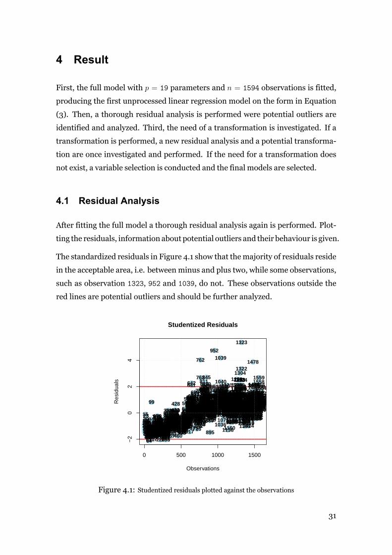
4 Result

First, the full model with p = 19 parameters and n = 1594 observations is fitted,

producing the first unprocessed linear regression model on the form in Equation

(3). Then, a thorough residual analysis is performed were potential outliers are

identified and analyzed. Third, the need of a transformation is investigated. If a

transformation is performed, a new residual analysis and a potential transforma-

tion are once investigated and performed. If the need for a transformation does

not exist, a variable selection is conducted and the final models are selected.

4.1 Residual Analysis

After fitting the full model a thorough residual analysis again is performed. Plot-

ting the residuals, information about potential outliers and their behaviour is given.

The standardized residuals in Figure 4.1 show that themajority of residuals reside

in the acceptable area, i.e. betweenminus and plus two, while some observations,

such as observation 1323, 952 and 1039, do not. These observations outside the

red lines are potential outliers and should be further analyzed.

0 500 1000 1500

−2

02

4

Studentized Residuals

Observations

Res

idua

ls

1234567891011121314

15

16171819

20

2122

2324

25262728

293031323334

3536

37

3839404142434445464748

49505152535455565758596061626364

656667686970717273747576777879

80818283848586878889909192

9394

9596

97

98

99

100101

102103104105106107108109110111112113114

115116117118119120121122123124125126127128129130131132133134135136137138139140141142143144145146

147148149150151152153154155156157158159160161162163

164

165

166

167168169170171172173174175176177

178179180181182183184185186187

188189190191192193194195196197

198199200201

202203204205206

207208209210211212

213214215216217218219220221222223224225226

227228229230231232233234235236237238239240241

242

243

244245246247248249250251252253254255256257258

259260261262263264

265266267268269270271272273274275276277278279280281282283284285286287

288289290291292293294295296297298299300301302

303304305306307308309310311312313314

315

316

317

318

319320321

322323324325326327328

329

330331332333334335336337338339340341

342

343344345

346347348349

350351352353354355356

357

358359360

361362363364365366367368369370371372373374375376

377

378379380381382

383

384385386387388

389390

391392393394395396397398399400401402403404405406407408409

410411412

413414415416417418419420421422423424

425426427

428429

430431432433434435436437438439440441442

443

444445446447448449450451452453454455456

457458459

460

461462463464465466467468469470471472473474475476477478479480

481

482483484485

486487488489490491492493494495496497498499500501502

503

504505506507508509510511512513514515516517518519520521522523

524

525526527

528529530531532533534535

536537538539540541542543544545

546547548

549

550551552553

554

555556557558559560561562

563564

565566567

568

569570

571572573574575576577578579580581582583584585586587588589590591592593594595

596

597598599600601602603604605606607

608609610

611

612

613614615616

617

618619620621

622623

624625626

627628629630631632633634635636637638639

640

641642

643644645646647

648649650

651652653

654

655656657658659

660661

662663

664665

666

667668669670671672673674

675

676677678679680681

682683

684

685

686

687688689

690691

692

693694

695696

697

698699700701702703704705706707708709

710711712713714715

716

717

718719720721722723724725

726

727

728

729730

731732733734

735736

737738739740741742

743744745746747748

749750751752

753

754

755756757758759760761

762

763

764765

766767

768769

770

771

772773

774775776777778779

780781782783

784785786787788789790791

792793794

795796

797798799800801802803

804

805

806

807

808809810

811

812

813814815816

817

818819

820821822823

824825826

827828829830831

832

833834835836

837

838839

840

841842

843

844

845

846847848

849

850

851852

853

854

855856

857858859

860861862863864

865866

867

868

869870871

872873

874875876877878879880

881

882883884885886887888

889890

891

892

893894

895

896897

898899900901902903904905906

907

908909910

911

912

913914915916917918

919920921922923924

925926927928929930931932933934

935936937

938

939940

941

942943

944945

946947948

949950

951

952

953954

955

956957958959960961962963964965966967968969970971972973

974975976977

978979980981982983984985986987988989990991992993994

99599699799899910001001

1002100310041005100610071008

100910101011

1012101310141015

1016

1017

10181019

1020

102110221023102410251026102710281029103010311032103310341035

1036

1037

1038

1039

1040

1041

1042104310441045104610471048

104910501051105210531054

105510561057

105810591060

1061

106210631064

106510661067

10681069

10701071

1072

1073

10741075107610771078107910801081

10821083108410851086108710881089

1090

109110921093109410951096

109710981099110011011102110311041105

11061107

1108110911101111111211131114111511161117111811191120

1121

1122

112311241125112611271128

112911301131113211331134113511361137

1138

1139114011411142

11431144114511461147114811491150115111521153115411551156

1157

11581159

1160

11611162

1163116411651166

116711681169117011711172117311741175117611771178

117911801181

118211831184

1185118611871188

118911901191119211931194

1195

11961197119811991200120112021203

1204120512061207

1208

1209121012111212

1213

12141215121612171218121912201221122212231224122512261227

1228122912301231123212331234

123512361237123812391240124112421243124412451246

12471248124912501251125212531254

1255125612571258

12591260

12611262

1263

1264126512661267126812691270

1271

127212731274127512761277

1278

12791280

1281

128212831284128512861287

1288

1289129012911292

12931294

129512961297

1298

1299

13001301

1302

1303

1304

1305

13061307

1308130913101311

1312

13131314

1315131613171318

131913201321

1322

1323

1324

13251326

1327

132813291330

13311332133313341335133613371338

1339

134013411342134313441345134613471348134913501351

13521353

1354

13551356

1357

135813591360136113621363

1364

1365

136613671368

1369

1370

13711372

13731374137513761377

137813791380

138113821383138413851386138713881389139013911392139313941395139613971398139914001401140214031404140514061407140814091410141114121413

1414

14151416141714181419

14201421

1422142314241425142614271428142914301431143214331434

1435143614371438

143914401441

1442144314441445144614471448

1449145014511452

1453145414551456

145714581459146014611462146314641465

1466

1467

146814691470147114721473147414751476

1477

1478

1479

1480148114821483

1484

1485

1486

1487

148814891490

1491

1492

1493

1494

14951496

149714981499150015011502150315041505

1506

150715081509151015111512

1513

151415151516

151715181519152015211522

1523

1524

1525

1526

152715281529153015311532153315341535

15361537

1538

153915401541

1542154315441545

1546

15471548154915501551155215531554155515561557

15581559

1560

15611562156315641565

1566

15671568156915701571157215731574

1575157615771578157915801581

158215831584

158515861587

158815891590159115921593

1594

Figure 4.1: Studentized residuals plotted against the observations

31

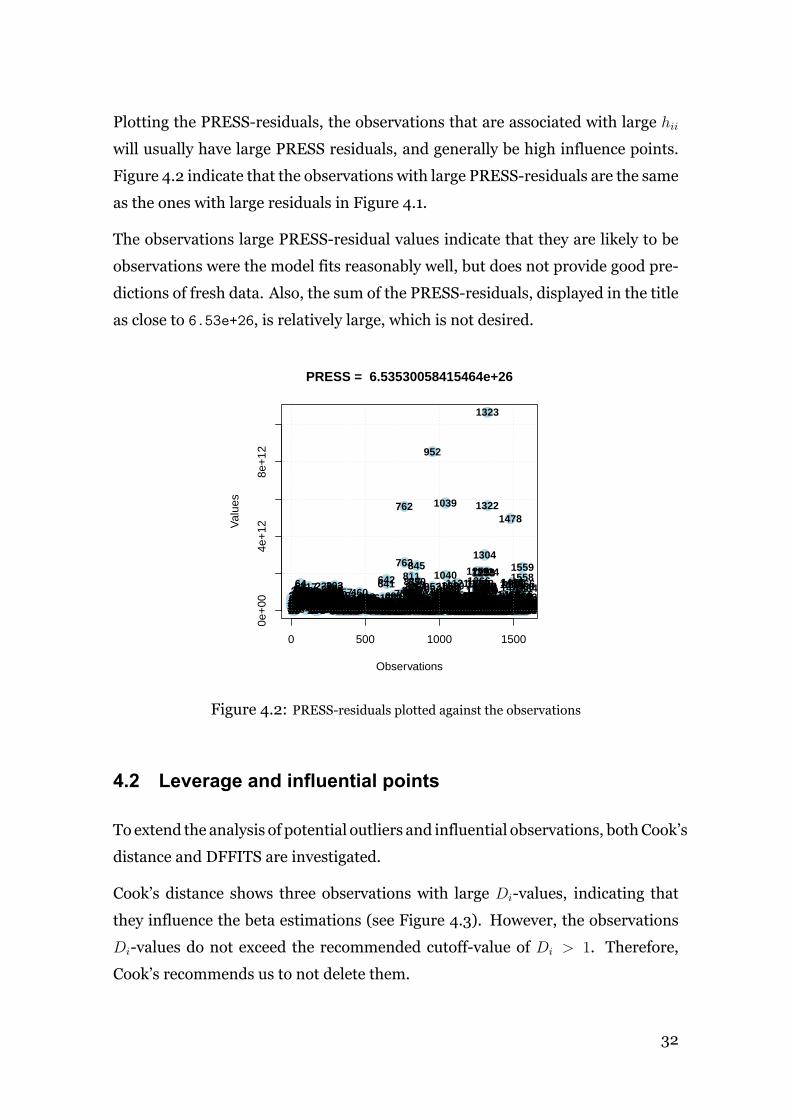
Plotting the PRESS-residuals, the observations that are associated with large hii

will usually have large PRESS residuals, and generally be high influence points.

Figure 4.2 indicate that the observations with large PRESS-residuals are the same

as the ones with large residuals in Figure 4.1.

The observations large PRESS-residual values indicate that they are likely to be

observations were the model fits reasonably well, but does not provide good pre-

dictions of fresh data. Also, the sum of the PRESS-residuals, displayed in the title

as close to 6.53e+26, is relatively large, which is not desired.

0 500 1000 1500

0e+

004e

+12

8e+

12

PRESS = 6.53530058415464e+26

Observations

Val

ues

12345678910111213141516171819202122232425262728293031323334353637383940414243444546474849505152535455565758596061626364

656667686970717273747576777879808182838485868788899091929394

9596979899100101102103104105106107108109110111112113114115116117118119120121122123124125126127128129130131132133134135136137138139140141142143144145146147148149150151152153154155156157158159160161162163164165166167168169170171172173174175176177178179180181182183184185186187188189190191192193194195196197198199200201202203204205206207208209210211212213214215216217218219220221222223224225226227228229230231232233234235236237238239240241242243244245246247248249250251252253254255256257258259260261262263264265266267268269270271272273274275276277278279280281282283284285286287288289290291292293294295296297298299300301302303304305306307308309310311312313314315316317318319320321322323324325326327328329330331332333334335336337338339340341342343344345346347348349350351352353354355356357358359360361362363364365366367368369370371372373374375376377378379380381382383384385386387388389390391392393394395396397398399400401402403404405406407408409410411412413414415416417418419420421422423424425426427428429430431432433434435436437438439440441442443444445446447448449450451452453454455456457458459460

461462463464465466467468469470471472473474475476477478479480481482483484485486487488489490491492493494495496497498499500501502503504505506507508509510511512513514515516517518519520521522523524525526527528529530531532533534535536537538539540541542543544545546547548549550551552553554555556557558559560561562563564565566567568569570571572573574575576577578579580581582583584585586587588589590591592593594595596597598599600601602603604605606607608609610611612613614615616

617618619620621622623624625626627628629630631632633634635636637638639640

641642

643644645646647648649650651652653654655656657658659660661662663664665666667668669670671672673674675676677678679680681682683684685686687688689690691692693694695696697698699700701702703704705706707708709710711712713714715716717718719720721722723724725726727728729730731732733734735736737738739740741742743744745746747748749750751752

753754755756757758759760761

762

763

764765766767768769770771772773774775776777778779780781782783784785786787788789790791792793794795796797798799800801802803804

805806807808809810

811

812813814815816

817

818819820821822823

824825826827828829830831

832833834835836837

838839840841842

843

844

845

846847848849

850

851852853

854

855856857858859860861862863864865866867868869870871872873874875876877878879880881882883884885886887888889890891892893894895896897898899900901902903904905906907908909910911912913914915916917918919920921922923924925926927928929930931932933934935936937938939940941942943944945946947948949950951

952

953954955956957958959960961962963964965966967968969970971972973974975976977978979980981982983984985986987988989990991992993994

995996997998999100010011002100310041005100610071008100910101011101210131014101510161017101810191020102110221023102410251026102710281029103010311032103310341035103610371038

1039

1040

10411042104310441045104610471048104910501051105210531054105510561057

10581059106010611062106310641065106610671068106910701071

1072

107310741075107610771078107910801081108210831084108510861087108810891090

109110921093109410951096109710981099110011011102110311041105110611071108110911101111111211131114111511161117111811191120

1121

11221123112411251126112711281129113011311132113311341135113611371138113911401141114211431144114511461147114811491150115111521153115411551156115711581159116011611162116311641165116611671168116911701171117211731174117511761177117811791180118111821183118411851186118711881189119011911192119311941195119611971198119912001201120212031204120512061207120812091210121112121213121412151216121712181219122012211222122312241225122612271228122912301231123212331234

123512361237123812391240124112421243124412451246124712481249125012511252125312541255125612571258

12591260

12611262

1263

12641265

1266

126712681269127012711272127312741275127612771278127912801281128212831284128512861287

12881289129012911292

1293

1294129512961297

1298

129913001301

1302

1303

1304

130513061307

1308130913101311

1312131313141315131613171318131913201321

1322

1323

1324

1325132613271328132913301331133213331334133513361337133813391340134113421343134413451346134713481349135013511352135313541355135613571358135913601361136213631364136513661367136813691370137113721373137413751376137713781379138013811382138313841385138613871388138913901391139213931394139513961397139813991400140114021403140414051406140714081409141014111412141314141415141614171418141914201421

14221423142414251426142714281429143014311432143314341435143614371438143914401441144214431444144514461447144814491450145114521453145414551456145714581459146014611462146314641465146614671468146914701471147214731474147514761477

1478

14791480148114821483

1484

148514861487148814891490

1491

1492

1493149414951496149714981499150015011502150315041505

1506

150715081509151015111512151315141515151615171518151915201521152215231524152515261527152815291530153115321533153415351536153715381539154015411542154315441545154615471548154915501551155215531554155515561557

15581559

156015611562156315641565

1566

156715681569157015711572157315741575157615771578157915801581158215831584

1585158615871588158915901591159215931594

Figure 4.2: PRESS-residuals plotted against the observations

4.2 Leverage and influential points

To extend the analysis of potential outliers and influential observations, bothCook’s

distance and DFFITS are investigated.

Cook’s distance shows three observations with large Di-values, indicating that

they influence the beta estimations (see Figure 4.3). However, the observations

Di-values do not exceed the recommended cutoff-value of Di > 1. Therefore,

Cook’s recommends us to not delete them.

32

0 500 1000 1500

0.00

0.10

0.20

0.30

Obs. number

Coo

k's

dist

ance

lm(Courtage ~ . − Date)

Cook's distance

1322

1323

952

Figure 4.3: Cook’s distance plotted against the observations

Compared to Cook’s distance, DFFITS displays several observations that are well

above the recommended threshold, the most extremes ones being 952 and 1196

(see Figure 4.4). DFFITS indicates that these observations should be deleted given

the√

p/n threshold.

0 500 1000 1500

−1.

00.

00.

51.

01.

52.

0

DFFITS

Index

dffit

s

123456789

1011121314

15

16171819

20

2122

23

2425262728

293031

3233

34

35

36

37

3839404142434445464748

49

5051525354555657585960

6162636465666768697071727374757677787980818283

8485868788899091929394

95969798

99

100

101102103104105106107108109110111112113114115116117118119120121122123124125126127128129130

131132133134135136137138139140141142143144145146147148149150

151152153154155156157158159160161162163164

165

166167168169170171172173174175176177

178179180181182183184185186187188189190191192193194195196197198199200201202203204205206207208209210211212213214215216217218219220

221

222223224225226227228229230231232233234235236237238239240

241242

243

244

245246247248249250251252

253

254

255256257258259260261262263264

265

266267268269270

271272273274275276277278279280281282283284285286287288289290291292293294295296297298299300301302303304305306307308309310311312313

314315316

317318319320321322323324325326327328329330331332333334335336337338339340341342343344345346347348349350351352353354355356357

358359360361362363364365366367368369370371372373374375376377378379380381382383384385386387388389390391392393394395396397398399400401402403404405406407408409410411412413414415416417418419420421422423424425426427

428

429430431432433434435436437438439440441442443

444445446447448449450451452453454455456

457

458459460

461

462463464465

466

467468469470471472473474

475476477478479480481

482

483484485486

487488489490491492493494495496497498499500501502503

504505506507508509510511512513514515516517518519520521522523

524

525526527528529530531532533534535536537538539540541542543544545546547548549550551552553554

555556557558559560561562

563564

565

566567568

569

570

571

572573574575576577578579580581582

583584585586587588589590591592593594595

596

597598599600601602603604605606

607608609

610

611

612

613614615616

617

618

619620621622623624625626

627628629630631632633634635636637638639640641642643644645646647648649650651652653654655656657658659660661662663664665666667668669670671672673674675

676

677678679680681682683684685686687688689690691

692

693

694695696697

698

699700701702703704705706707708709710711712713714715716

717718719720721722723724725

726

727

728

729

730731732733734735736737738739740741742743744745746747748749750751

752

753754755756757758759760761

762

763764

765766767

768

769770771772773774775776777778779

780

781782783784785786787788789790791792793794795796797798799800801802803804805806

807

808809810811812813814815816817818819820821822823

824

825826827828829830831832833834835836837

838839840

841842843

844

845

846847848849850851852853854

855856857858

859860861862863864

865

866867868869870871872873874875876877878879880881882883884885886887888889890

891

892893894895

896897898899900901902903904905906

907

908909910911912913914915916917918919920921922923924925926927928929930931932933934935936937938939940941942943944945946947948949950951

952

953954955956

95795895996096196296396496596696796896997097197297397497597697797897998098198298398498598698798898999099199299399499599699799899910001001

1002100310041005100610071008100910101011101210131014101510161017101810191020102110221023102410251026102710281029103010311032103310341035

1036

10371038

1039

10401041

104210431044104510461047104810491050105110521053105410551056105710581059106010611062

1063

106410651066106710681069107010711072

1073

1074

10751076107710781079108010811082108310841085108610871088108910901091109210931094109510961097109810991100110111021103110411051106110711081109111011111112111311141115111611171118

11191120

1121

11221123112411251126112711281129113011311132113311341135113611371138

1139

114011411142114311441145114611471148114911501151115211531154115511561157115811591160

116111621163

11641165116611671168116911701171117211731174117511761177117811791180118111821183118411851186118711881189119011911192119311941195

1196

119711981199120012011202120312041205120612071208

1209121012111212121312141215121612171218121912201221122212231224122512261227122812291230123112321233123412351236123712381239124012411242124312441245124612471248124912501251125212531254125512561257125812591260126112621263126412651266

126712681269127012711272127312741275127612771278

1279

1280128112821283128412851286128712881289129012911292

1293

12941295129612971298

1299130013011302

1303

1304

13051306130713081309131013111312131313141315131613171318131913201321

1322

1323

13241325

1326

1327

1328

13291330133113321333133413351336133713381339

134013411342134313441345134613471348134913501351

13521353

1354

135513561357

1358

13591360136113621363136413651366136713681369

1370

1371137213731374137513761377

137813791380

138113821383138413851386138713881389139013911392

1393139413951396139713981399140014011402140314041405140614071408140914101411141214131414141514161417141814191420142114221423142414251426142714281429143014311432143314341435143614371438143914401441144214431444144514461447144814491450145114521453145414551456145714581459146014611462146314641465146614671468146914701471147214731474147514761477

1478

147914801481148214831484

1485

1486

1487

1488148914901491

1492

14931494

1495

14961497149814991500150115021503150415051506

1507150815091510151115121513

1514

151515161517151815191520152115221523

1524

15251526

15271528152915301531153215331534153515361537

1538

1539154015411542154315441545154615471548154915501551155215531554155515561557155815591560156115621563156415651566

156715681569157015711572157315741575157615771578157915801581

1582

158315841585158615871588158915901591159215931594

Figure 4.4: DFFITS plotted against the observations

33

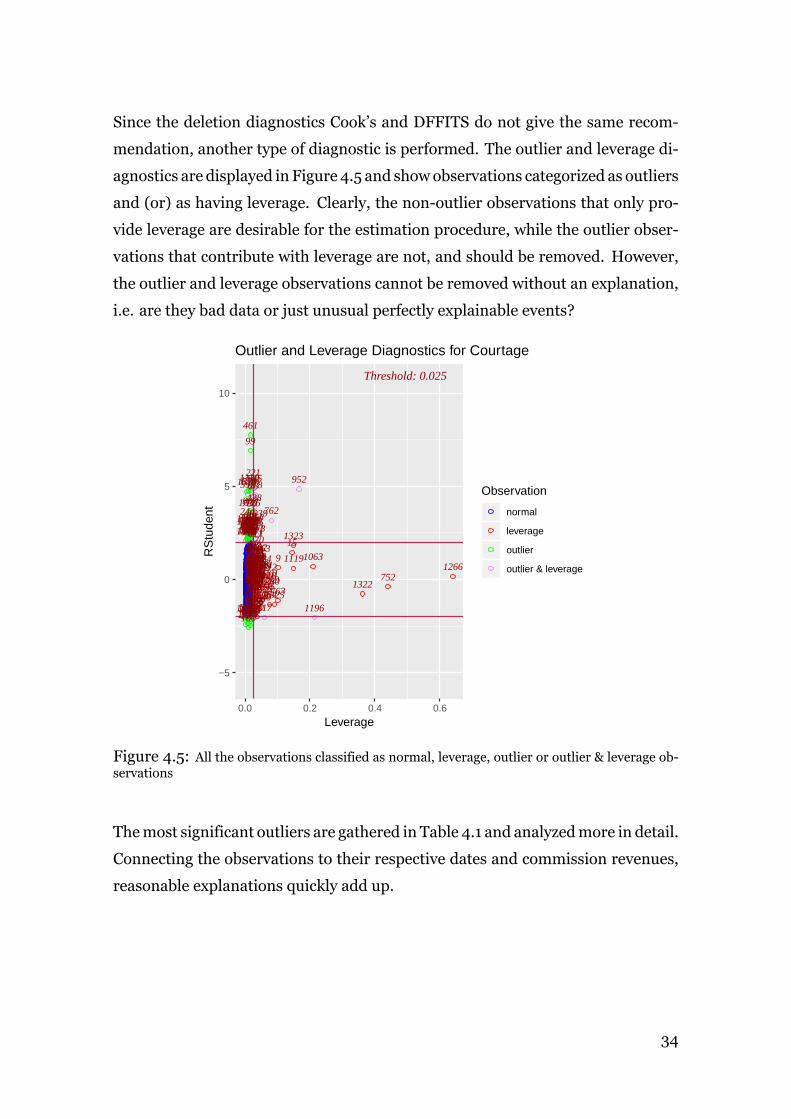
Since the deletion diagnostics Cook’s and DFFITS do not give the same recom-

mendation, another type of diagnostic is performed. The outlier and leverage di-

agnostics are displayed in Figure 4.5 and showobservations categorized as outliers

and (or) as having leverage. Clearly, the non-outlier observations that only pro-

vide leverage are desirable for the estimation procedure, while the outlier obser-

vations that contribute with leverage are not, and should be removed. However,

the outlier and leverage observations cannot be removed without an explanation,

i.e. are they bad data or just unusual perfectly explainable events?

9

15

20

23

24

283449

63

6580

84

95

99

100

144

151

165

166

198215

220

221

230

237

240

244

245

253

254

261

265

269270

296

297

322

349

358

364393

428

442

457

461

466

467

468

482

486503

511512

524565

569

571

573

596

611

617

618

633

676

692

693698

716

717

726

728

729

739752761

762

763764

773

780

781

801

807

824

843

844

845

851

852

854858

863

865

866867

868

869871

891

892

896907

920

951

952

9561000

1036

10371039

10401041

1063

1073

1074

10771118

11191120

1121

1138

1139

1143

114811491156

1161

1163

1169

11961208

12601266

1279

1280

1281

1282

1302

1304

1321

1322

1323

13241325

1328

13491353

1354

1355

1358

1369

1370

137713971477

1478

1479

1487

148814891490

1513

1515

1524

1527

1529

153815421582

1584

Threshold: 0.025

−5

0

5

10

0.0 0.2 0.4 0.6

Leverage

RS

tude

nt

Observation

normal

leverage

outlier

outlier & leverage

Outlier and Leverage Diagnostics for Courtage

Figure 4.5: All the observations classified as normal, leverage, outlier or outlier & leverage ob-servations

Themost significant outliers are gathered in Table 4.1 and analyzedmore in detail.

Connecting the observations to their respective dates and commission revenues,

reasonable explanations quickly add up.

34

Observation # Date ∆ Comission revenue Plausible explanation

952 2016-06-27 110.60% Brexit

1039 2016-11-09 56.05% Trump

1322 2018-02-05 30.21% Unexpected inflation

1323 2018-02-06 39.56% Unexpected inflation

Table 4.1: The most severe outliers and the date of their occurrences

Starting with outlier 952 and the events on its date 2016-06-27, Avanza’s cus-

tomers broke a record in the number of stock transactions during one day, with

Brexit acting as a catalyst.30 Secondly, regarding observation 1039 and on its

date 2016-11-09, Trump was elected as the president of the U.S. —resulting in

increased uncertainty and an overall decreased willingness to invest, increasing

Avanza’s commission revenue with over 50 percent.31 Finally, regarding the two

last observations, on both their dates 2018-02-05 and 2018-02-06, the largest

downfall on the stock exchange after BREXIT, took place, apparently caused by

a large downfall after unexpected high salaries numbers in the U.S. was presented

—indicating that the inflation might rise sooner than expected.32

In summary, these outliers are clearly unusual, however they are fully plausible

observations and should therefore not be removed from the data set since they

are not bad observations such as faulty measurements or incorrect recording of

data.

4.3 Transformations

After fitting the full model and conducting a thorough residual analysis, the need

for a transformation is investigated. By plotting the log-likelihood as a function of

λwith a 95% interval, Figure 4.6a show that λ is outside of the interval, indicating

a need for a transformation.30SvD, Rekordhandel på börsen efter brexit31Privata Affärer, Experterna spår kraftig börsnedgång32SvD, Största börstappet sedan Brexitomröstningen

35

−2 −1 0 1 2

−49

00−

4700

−45

00−

4300

λ

log−

Like

lihoo

d

95%

(a) Before transformation

−2 −1 0 1 2

−33

00−

3200

−31

00

λ

log−

Like

lihoo

d

95%

(b) After transformation

The value chosen for λ is 0.5 because of its appropriateness. After conducting the

same previous residuals analysis as before, the same outliers as in Table 4.1 are

identified by the residuals, Cook’s distance, DFFITS and the outlier and leverage

diagnostics. Further, after performing the box-cox method again, no indication

of a transformation is found, since λ = 1 is found in the 95% interval (see figure

4.6b).

4.4 Variable Selection

After identifying the outliers and performing eventual transformations, the task of

producing a finalmodel still exists. Through variable selection some finalmodel(s)

are produced.

4.4.1 All Possible Regressions

Proceeding with the all possible regressions analysis, criterion such R-squared,

adjusted R-squared, Mallow’s Cp and Schwartz’s BIC are chosen. The criterion

are displayed in Figure 4.6 were the black boxes on the x-axis display whether or

not the specific regressor variable is included for that specific model on the y-axis.

For example, observing the Mallow’s Cp plot, the model with the value Cp = 8

consists of the variables DJI, SPX, IXIC, VIX, V2TX and OMXSCCPI (excluding the

36

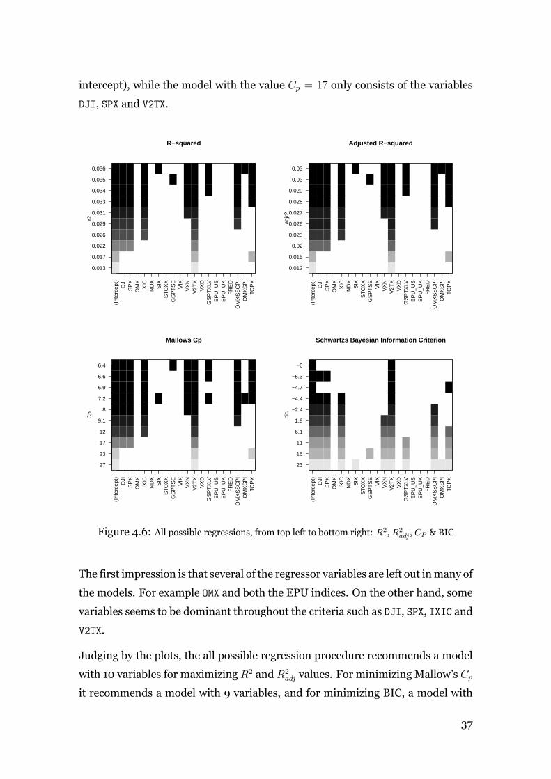
intercept), while the model with the value Cp = 17 only consists of the variables

DJI, SPX and V2TX.r2

(Int

erce

pt)

DJI

SP

XO

MX

IXIC

ND

XS

IXS

TOX

XG

SP

TS

EV

IXV

XN

V2T

XV

XD

GS

PT

XLV

EP

U_U

SE

PU

_UK

FR

ED

OM

XS

SC

PI

OM

XS

PI

TOP

X

0.013

0.017

0.022

0.026

0.029

0.031

0.033

0.034

0.035

0.036

R−squared

adjr2

(Int

erce

pt)

DJI

SP

XO

MX

IXIC

ND

XS

IXS

TOX

XG

SP

TS

EV

IXV

XN

V2T

XV

XD

GS

PT

XLV

EP

U_U

SE

PU

_UK

FR

ED

OM

XS

SC

PI

OM

XS

PI

TOP

X

0.012

0.015

0.02

0.023

0.026

0.027

0.028

0.029

0.03

0.03

Adjusted R−squared

Cp

(Int

erce

pt)

DJI

SP

XO

MX

IXIC

ND

XS

IXS

TOX

XG

SP

TS

EV

IXV

XN

V2T

XV

XD

GS

PT

XLV

EP

U_U

SE

PU

_UK

FR

ED

OM

XS

SC

PI

OM

XS

PI

TOP

X

27

23

17

12

9.1

8

7.2

6.9

6.6

6.4

Mallows Cp

bic

(Int

erce

pt)

DJI

SP

XO

MX

IXIC

ND

XS

IXS

TOX

XG

SP

TS

EV

IXV

XN

V2T

XV

XD

GS

PT

XLV

EP

U_U

SE

PU

_UK

FR

ED

OM

XS

SC

PI

OM

XS

PI

TOP

X

23

16

11

6.1

1.8

−2.4

−4.4

−4.7

−5.3

−6

Schwartzs Bayesian Information Criterion

Figure 4.6: All possible regressions, from top left to bottom right: R2, R2adj , CP & BIC

The first impression is that several of the regressor variables are left out inmany of

the models. For example OMX and both the EPU indices. On the other hand, some

variables seems to be dominant throughout the criteria such as DJI, SPX, IXIC and

V2TX.

Judging by the plots, the all possible regression procedure recommends a model

with 10 variables for maximizing R2 and R2adj values. For minimizing Mallow’s Cp

it recommends a model with 9 variables, and for minimizing BIC, a model with

37

only 1 variable.

4.4.2 Backward Elimination

Combining the all possible regressionsmethodof choosing variableswith the back-

ward eliminationmethod, amodel can be chosen. Remember that backward elim-

ination omits variables based on their t and F statistics. Backward elimination

creates a model with 9 variables, the same as the model minimizing the Mallow’s

Cp.

Intercept DJI SPX IXIC SIX VXN V2TX GSPTXLV OMXSPI TOPX

1286.4 11071.1 -13964.0 4664.9 -12151.6 246.9 174.3 -2097.5 11906.1 -724.2

Table 4.2: 9 variable model presented by backward elimination

However, by comparing the backward eliminationmodel (see Table 4.2)with, per-

haps, a model with lesser variables, the backward eliminationmodel seems some-

what over exaggerated. This is because the all possible regressions method show

that almost the same R2 and R2adj values can be achieved by omitting some vari-

ables. For example, by omitting two variables (OMXSPI and SIX) from the backward

elimination model with nine parameters, the R2adj only decreases with ∆R2

adj ≈−0, 00021. This is a relatively cheap trade-off for a less complex model.

4.4.3 Cross Validation

Having learned that removing somevariables from thebackward eliminationmodel

does not significantly damage the models overall performance, another useful

method for choosing variables is used.

The cross validation with k = 10 folds minimizes the root mean square error

(RMSE) andmeanabsolute error (MAE).ObservingFigure 4.7, themethod chooses

amodel with five variables. Compared to themodels containingmore or less vari-

ables, the model with five variables clearly differentiate itself from the other mod-

els. This model is desirable because of its low complexity and errors.

38

5 10 153.21

6497

e+12

3.21

6500

e+12

Index

mea

n.cv

.err

ors

Figure 4.7: 10-fold cross validation

The five variables are and their estimated coefficients are

(Intercept) DJI SPX IXIC V2TX OMXSSCPI

1285.332 11285.454 -15370.214 3715.533 200.584 -1871.988

Table 4.3: Final chosen model, proposed by 10-folded cross validation

In conclusion, the model chosen by ten-fold cross validation only differs∆R2adj ≈

−0, 00262 from the model chosen by all possible regressions R2 and R2adj, while

consisting of four less variables and lower mean error (compare index 5 and 9 in

Figure 4.7).

4.4.4 OLS-assumptions

Proceeding with the final model presented in Table 4.3, the OLS-assumptions are

checked.

As stated before, OLS assumes that the random errors have a mean of zero. Cal-

culating the mean of the fitted models residuals indicate a mean value near zero

(meanValue = -3.424928e-14 ≈ 0), indicating strict exogenity.

39

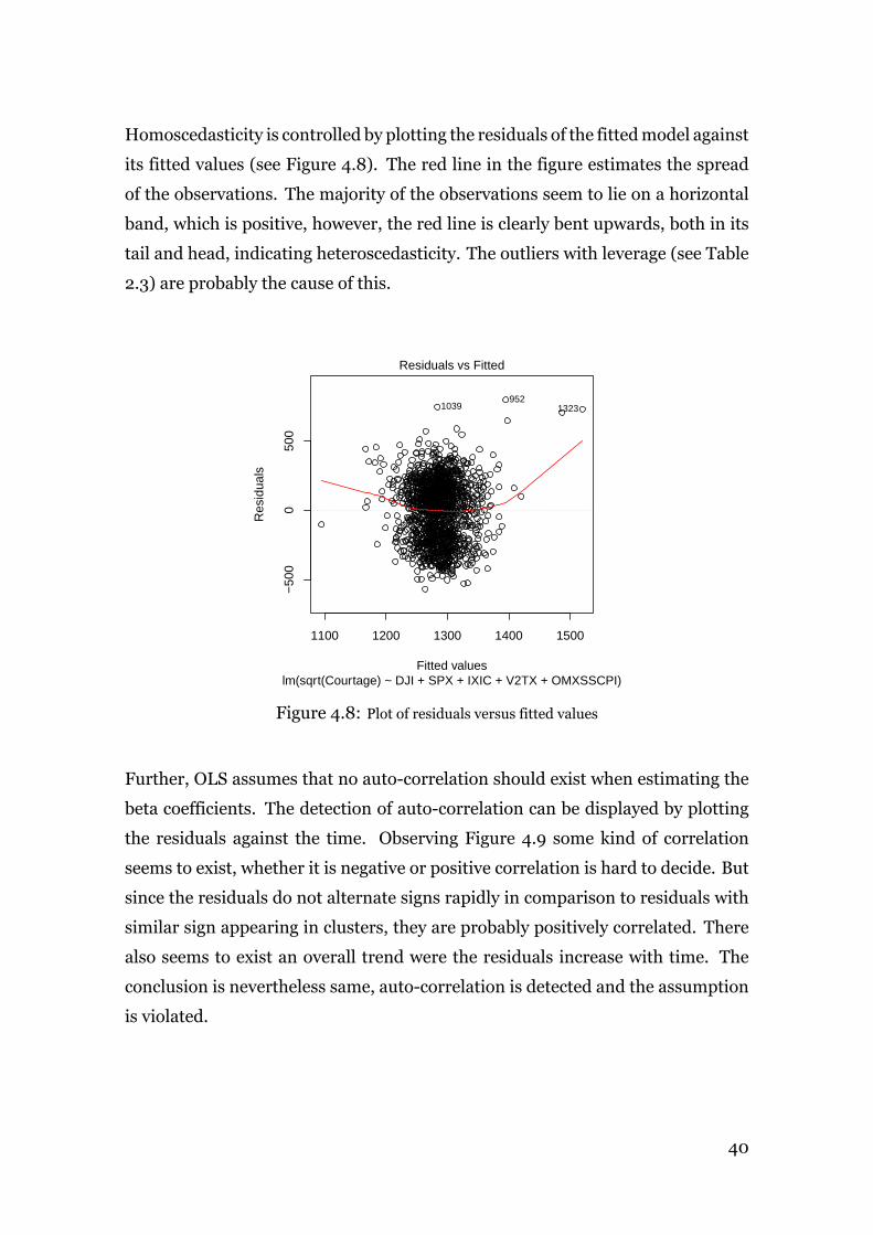
Homoscedasticity is controlled by plotting the residuals of the fittedmodel against

its fitted values (see Figure 4.8). The red line in the figure estimates the spread

of the observations. The majority of the observations seem to lie on a horizontal

band, which is positive, however, the red line is clearly bent upwards, both in its

tail and head, indicating heteroscedasticity. The outliers with leverage (see Table

2.3) are probably the cause of this.

1100 1200 1300 1400 1500

−50

00

500

Fitted values

Res

idua

ls

lm(sqrt(Courtage) ~ DJI + SPX + IXIC + V2TX + OMXSSCPI)

Residuals vs Fitted

9521039 1323

Figure 4.8: Plot of residuals versus fitted values

Further, OLS assumes that no auto-correlation should exist when estimating the

beta coefficients. The detection of auto-correlation can be displayed by plotting

the residuals against the time. Observing Figure 4.9 some kind of correlation

seems to exist, whether it is negative or positive correlation is hard to decide. But

since the residuals do not alternate signs rapidly in comparison to residuals with

similar sign appearing in clusters, they are probably positively correlated. There

also seems to exist an overall trend were the residuals increase with time. The

conclusion is nevertheless same, auto-correlation is detected and the assumption

is violated.

40

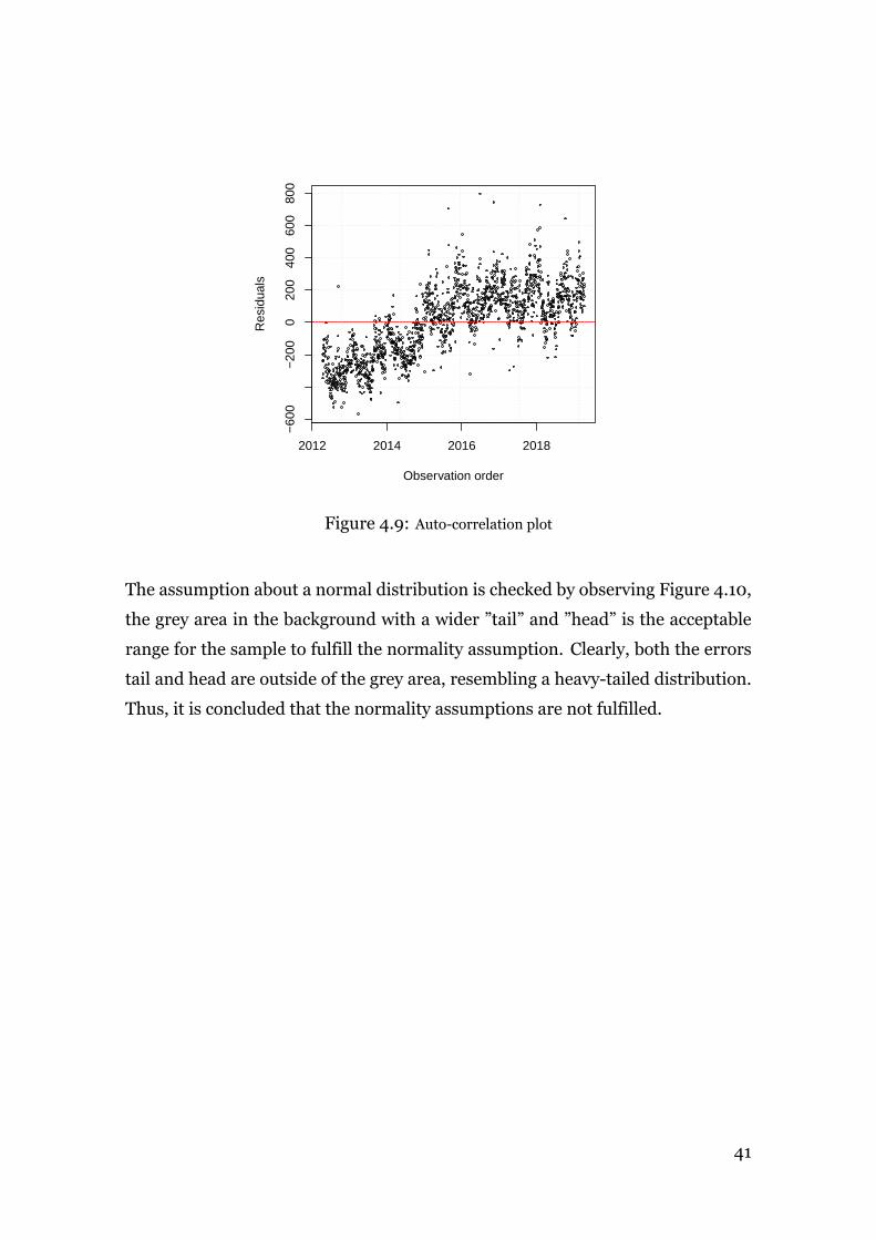
2012 2014 2016 2018

−60

0−

200

020

040

060

080

0

Observation order

Res

idua

ls

Figure 4.9: Auto-correlation plot

The assumption about a normal distribution is checked by observing Figure 4.10,

the grey area in the background with a wider ”tail” and ”head” is the acceptable

range for the sample to fulfill the normality assumption. Clearly, both the errors

tail and head are outside of the grey area, resembling a heavy-tailed distribution.

Thus, it is concluded that the normality assumptions are not fulfilled.

41

−1000

−500

0

500

1000

−2 0 2Theoretical

Sam

ple

Figure 4.10: Normality QQ-plot for checking normality distribution

Multicollinearity can be detected through the calculation of the VIF:s and the

eigenvalues. The VIF:s (see Table 4.4) exceed the recommended threshold val-

ues 5 and 10, indicating a case of multicollinearity for the choice of variables. The

eigenvalues, as well as the condition number, are also calculated. The condition

number well exceeds the recommended threshold 100 (K = 788.619) and is close

to threshold indicating severe multicollinearity, i.e. K = 1000. The condition

number confirms the VIF:s analysis of a case of severe multicollinearity.

DJI SPX IXIC V2TX OMXSSCPI

VIF 18.985775 41.715249 11.744280 1.490258 1.371106

Table 4.4: Variance inflation factors

TheOLS-assumptions, except formulticollinearity, are summarized inTable 4.5.

42

Value p-value Decision

Global Stat 109.184 0.000e+00 Assumptions NOT satisfied!

Skewness 1.434 2.312e-01 Assumptions acceptable.

Kurtosis 18.765 1.479e-05 Assumptions NOT satisfied!

Link Function 31.019 2.555e-08 Assumptions NOT satisfied!

Heteroscedasticity 57.966 2.665e-14 Assumptions NOT satisfied!

Table 4.5: OLS assumptions, level of significance = 0.05

Global Stat shows the relationship between the predictors and response and in-

dicates a non-linear relationship between at least one of the predictors versus the

response, since the p-value rejects the null hypothesis, i.e. p<0.05. The Skewness

is accepted, indicating that the distribution is neither positively nor negatively

skewed and that there is no need for transformation. Kurtosis is not satisfied,

indicating that the assumption of normality does not hold given the level of signif-

icance. A rejected Link Function indicates that an alternative form of the general-

ized linearmodel, such as logistic or binomial, should beused. Last, Heteroscedasticity

is the opposite of homoscedasticity, indicating that the errors do not have a con-

stant variance for each observation.

43

4.5 Final Model

In the end the best model, given the circumstances, is a model consisting of 5

variables with equity and volatility indices and no EPU indices on the form

√y = β0 + β1x1 + β2x2 + ...+ β5x5 (34)

More specifically the model consists of the coefficients in Table 4.6 leading to the

model on form (34) to be written as

√Daily aggregated commission revenue = 1286.4 + 11112 ∗ DJI

−14356 ∗ SPX + 4899.9 ∗ IXIC − 189.31 ∗ V2TX − 2093.6 ∗ OMXSSCPI(35)

The partial residual plots are displayed in Figure 4.11 and the estimates of the

coefficients and their limits in a 95 percent interval, alongside their p-values, are

presented in the Table 4.6

44

−0.005 0.000 0.005

−60

0−

200

200

600

DJI | others

sqrt

(Cou

rtag

e) |

oth

ers

952 1039 1323

1546

−0.004 −0.002 0.000 0.002 0.004

−60

0−

200

200

600

SPX | others

sqrt

(Cou

rtag

e) |

oth

ers

9521039

166

1490

−0.010 −0.005 0.000 0.005 0.010

−60

0−

200

200

600

IXIC | others

sqrt

(Cou

rtag

e) |

oth

ers

952 1039

1169

1490

−0.2 0.0 0.2 0.4 0.6

−60

0−

200

200

600

V2TX | otherssq

rt(C

ourt

age)

| o

ther

s

952 1039

1323

1325

−0.02 0.00 0.02 0.04

−60

0−

200

200

600

OMXSSCPI | others

sqrt

(Cou

rtag

e) |

oth

ers

9521039

617

952

Added−Variable Plots

Figure 4.11: Partial residuals plots

Coefficient Estimate Lower limit (5.0%) Upper limit (95%) p-value

Intercept 1285.903 1275.029 1296.777 2e-16

DJI 11806.870 6177.023 17436.72 4.11e-05

SPX -16824.578 -25022.71 -8626.443 5.98e-05

IXIC 4634.423 996.5248 8272.321 0.0126

V2TX 221.609 41.98532 401.2327 0.0157

OMXSSCPI -1246.238 -2779.493 287.0169 0.1112

Table 4.6: Coefficient confidence interval

45

5 Discussion

5.1 Methodology

As displayed in Table 4.6, the two most significant variables in the final model

are DJI and SPX. Since both are most certainly the largest and most popular stock

indices used within the financial market, it seems reasonable that they would cap-

ture some of the explanation, such as Great Britain leaving the E.U. or Trump

being elected as president.

Apart from the three equity indices, two volatility indiceswere included in the final

model. Although included, V2TX and OMXSCCPIwere not as significant as the equity

indices and further, more established volatility indices, such as the VIX, was en-

tirely excluded from the model (see Figure 4.6). This seems odd, since in general,

periods of increased volatility imply higher uncertainty and therefore a tendency

to invest less, while short periods of volatility spikes induces higher trading ac-

tivity. The latter, we believe, is somewhat shown in Avanza’s customers trading

behaviour. Based on the outlier analysis in Section 4.2, Avanza’s customers trad-

ing activity spiked during these unexpected events, as we would have predicted.

Again however, none of the volatility nor uncertainty indices were significant in

explaining these.

One possible explanation for the insignificance of the volatility and uncertainty in-

dices is lag. For example, extracting the four dates 2018-02-[02-05-06-07] and

their respective returns and commission revenue values, some observations can

be made (see Table 5.1). The U.S. EPU index more than doubles from the first to

the secondobservation, whileVIXand the commission revenue also increase. This

seems reasonable —a relevant event causes increased uncertainty and volatility,

which is noticed by Avanza’s customers, hence increasing their transaction activ-

ity and Avanza’s aggregated commission revenue. However, the following day the

U.S. EPU index falls substantially, while the transaction activity and VIX contin-

ues to increase, i.e. now the U.S. EPU index and Avanza’s commissions revenue

are negatively correlated as opposed to the day before.

One theory is that right at the moment when an unexpected event occurs both the

46

uncertainty indices and the investors trading activity correlate, but not after. The

day after the public learned about the unexpected inflation they maybe were not

so uncertain anymore, decreasing the EPU index, while the investors still traded,

causing a lag.

Observation # Date ∆ Comission revenue VIX EPU U.S.

1321 2018-02-02 8.41% 18.6% 22.9%

1322 2018-02-05 30.21% 32.2% 138%

1323 2018-02-06 39.56% 10.7% -36,5%

1324 2018-02-07 -43.25% -15.2% -37,0%

Table 5.1: The most severe outliers and the time of their occurrences

By our definition, unexpected means that the majority was not able to foresee it.

Hence, the surprised investors will try to trade as much as possible, as soon as

possible, to minimize their losses, while other investors might try to maximize

their returns given the time frame—increasing the overall trading activity during,

but also shortly after, the initial event has taken place.

On the other hand, the EPU index can also be flawed. Since it consists of key

words aggregated from major news outputs spread across a certain geographic

area, it depends on what gets written, and how much is written about it. Usually

the news will bombard with output weeks after special occurrences, potentially

increasing the uncertainty index although the uncertainty is gone.

In summary, there might exist a time delay between the unexpected event and the

investors activity. Further, the investors activity might continue for some time

after the event has become known to the public, which the uncertainty indices do

not reflect, while the commission revenue does. And vice versa, newspapersmight

write as much about events one week later as the day it happened, thus displaying

misleading correlation. But this still does not explain why the volatility index, that

is not built by the same method as the EPU indices, is not significant. Maybe the

adequacy of our model can act as a source of explanation.

47

5.2 Model Adequacy

The final model’s adjusted R-squared value is 0.01926, i.e. this model explains

approximately 1, 926% of the observed variance. The question of whether this is

a good or bad value is irrelevant, since it depends on how the variables are mea-

sured, whether any transformations have been done etc. and whether the model

can actually be trusted.

Avanza’s daily commission revenue is a time series, i.e. it is a series of data points

indexed in time order. When the response variable is a time series, much of the

response variable’s predictive power is often a result of its own history via lags,

differences and/or seasonal adjustments, which clearly seems to be the case here

as well (see Figure 4.9). Therefore, it is unwise to evaluate its predictive power

when we do not know what lies behind it.

Further, many of the OLS-assumptions are violated (see Figure 4.5). These as-

sumptions are vital for obtaining accurate estimations of theOLSbeta coefficients.

The presence of multicollinearity, a non-normal distribution, heteroscedasticity

and kurtosis all contribute to less accurate andmisleading beta estimations.

In summary, the model’s poor adequacy could be a potential source of explana-

tion when it comes to explaining certain factors, that in theory are significant for

explaining the trading volume, were ruled out as insignificant.

5.3 Previous studies

In general, there are numerous factors affecting individual trading behaviour. As

stated in the introduction, this has been shown by studies were factors such as

price changes, volatility and even uncertainty play a significant role. By that, it

seems as if the factors we have used in this study may be miss used, rather than

irrelevant, with regards to the investigation of their relationship with the response

variable.

One important distinction is the type ofmethod that we have used and the popula-

tion that was studied. First, regressionmodeling is a powerful and frequently used

statistical tool, especially within finance subjects, but almost no studies regarding

48

our subject using regression analysis were found. One reason might again be that

a time series analysis should be used instead of conducting a regression analysis,

mainly because of the lag and auto correlation. Secondly, usually when referring

to price and volume, the meaning of the concepts are the stock and its price and

volume. This report refers to several stock indices and Avanza’s aggregated com-

mission revenue. These two relationships are of course different, which is why the

established price-volume correlation between a stocks price and volume should

not be easily accepted here.

In conclusion, the studies found do neither strengthen nor weaken the results,

actually not much research about the fluctuating revenue streams of online stock

brokers and the cause of them has been found at all. However, the literature that

is used is still valuable for giving some insight into the mechanisms of investors

trading behaviour.

5.4 Future Work

There are several suggestionswhere to start (regarding) futurework. For example,

by using generalized linear models (GLM) one could surpass the assumptions of

no auto correlation and a normal distribution, since GLM does not assumes that

the errors are not auto correlated and can choose witch distribution to account for

in its modeling.

Moreover, a time series analysis would be recommended in order to analyze the

data with a more scientific and statistic approach to improve the reliability of the

outcome, since the data is taken at different time periods. The result given in

Figure 4.9 showed that the there is a possible trend in the residuals, which must

be accounted for.

5.5 Avanza

Because of the poormodel adequacy, the results cannot help to explain the overall

trading behaviour of their customers. The analyze of the competitiveness through

Porter’s five forces can therefore not be used in further implementation forAvanza.

49

Although some of their customer’s behaviour is known, such as taking the chance

to trade directly after unexpected events as when the Swedish bank Swedbank

was caught laundering money which led to an 89% increase of Avanza customers

buying Swedbank’s stock,33 not much fruitful comes out of it. Since these events

usually are unexpected, nobody can predict them.

Relevant information for Avanza might be information explaining both long and

short term behaviour of their customers. Perhaps, more in detail on how the cus-

tomers are affected by the seasons of the year, or how trading differs on Mondays

and Fridays etc. This could lead to key insights such as, for example, learning that

customers are more prone to invest in stocks during springs than autumns, or

that customers tend to save more of their salaries directly after receiving it, rather

than long after they have received. Information such as this could be used as pil-

lars when developing new products, or taken into account when streamlining, or

increasing themoney their customers save andperhaps used for forecasting future

earnings.

33Lans, Kraftig ökning av Swedbankaktieägare

50

6 Conclusion

In this study three main research questions were asked.

1. Does uncertainty, in a financial, political and macroeconomic sense, along

with market indicators such as stock prices and volatility indices, impact

Avanza’s customers trading activity?

2. What are the possible relationships and what do they look like?

3. How should the possible relationships be implemented?

Question two is answered in the final model were the possible relationships are

represented through a multiple linear regression model, and question three is an-

swered in Section 5.5.

The answer to question one is: ”we cannot say”. The hypothesis was that influen-

tial exogenous market factors such as political, economical and financial uncer-

tainty, stock price returns and volatility could help to explain Avanza’s customers

trading activity. However, scientifically the final model does not fulfill the basic

requirements for it to be reliable, hence the significance of its variables with re-

spect to the response variable, cannot be strengthened nor weakened.

51

References

[1] Avanza©. (). History, [Online]. Available: http://investors.avanza.se/

en/history. (accessed: May 28, 2019).

[2] Avanza Bank Holding AB, Årsredovisning 2018, Annual Report, 2018.

[3] Svenskt Kvalitetsindex, “Personlig service utmanar digitala tjänster,” Re-

search Report, Oct. 2018.

[4] Shefrin,H.,Abehavioral approach to asset pricing, 2nd ed. 2008, ch. 29.3,

pp. 499–500, ISBN: 978-0-12-374356-5. [Online]. Available: https : / /

www.sciencedirect.com/book/9780123743565/a-behavioral-approach-

to-asset-pricing.

[5] Statman, M., Vorkink, K., and Thorley, S., “Investor overconfidence and

trading volume,” The Review of Financial Studies, vol. Vol. 19, no. No.1,

pp. 1531–1565, Issue 4 2006. [Online]. Available: https://academic.oup.

com/rfs/article/19/4/1531/1580508.

[6] Ying, C. C., “Stock market prices and volumes of sales,” Econometrica, vol.

Vol. 34, no. No. 3, 1966. [Online]. Available: https://www.jstor.org/

stable/1909776?seq=1#metadata_info_tab_contents.

[7] Cornell, B., “The relationship between volume andprice variability in future

markets,” The Journal of Future Markets, vol. Vol. 41, no. No. 1, pp. 135–

155, 1981.

[8] Clark, P. K., “A subordinated stochastic process model with finite variance

for speculative prices,”Econometrica, vol. Vol. 1, pp. 303–316, Issue 3 1981.

[9] Batrinca, B., Hesse, C.W., and Treleaven, P. C., “Examining drivers of trad-

ing volume in europeanmarkets,” International Journal of Finance & Eco-

nomics, vol. Vol. 23, pp. 134–154, Issue 2 Apr. 2018.

[10] Sevelin, J., “Swedish stockmarket: Explaining trade volumes in single stocks,”

Bachelor’s Thesis, KTH Royal Institute of Technology, Jun. 2017. [Online].

Available: http://www.diva- portal.se/smash/get/diva2:1120590/

FULLTEXT01.pdf.

52

[11] Baker, S. R., Bloom, N., and Davis, S. J., “Measuring economic policy un-

certainty,” The Quarterly Journal of Economics, vol. Vol. 131, pp. 1593–

163, 4 Nov. 2016. [Online]. Available: http://www.policyuncertainty.

com/media/EPU_BBD_Mar2016.pdf.

[12] Epps, T. W., “The demand for brokers’ services: The relation between secu-

rity trading volume and transaction cost,” The Bell Journal of Economics,

vol. Vol. 7, no. No.1, pp. 163–194, Issue 4 1976. [Online]. Available: https:

/ / www . jstor . org / stable / 3003195 ? seq = 1 # metadata _ info _ tab _

contents.

[13] Sakalauskas, V. andKrikščiūnienė,D., “The impact of daily trade volume on

the day-of-theweek effect in emerging stock markets,” Information Tech-

nology and Control, vol. Vol. 36, no. No.1 A, 4 2007. [Online]. Available:

https://pdfs.semanticscholar.org/d32c/66eaadc7b6a111ba75cac01c386561b0c6ae.

pdf.

[14] Chappelow, J. (Apr. 2019). Porter’s 5 forces, [Online]. Available: https:

/ / www . investopedia . com / terms / p / porter . asp. (accessed: May 28,

2019).

[15] Montgomery, D. C., Peck, E. A., and Vining, G. G., Introduction to linear

regression analysis, 5th ed. 2012, ISBN: 978-0-470-54281-1.

[16] Johanna Kull and Nicklas Andersson, Ed. (Jun. 2018). Tips inför sommar-

börsen, [Online]. Available: https://blogg.avanza.se/avanza/avanzapodden-

tips-infor-sommarborsen/. (accessed: May 28, 2019).

[17] Carlgren, F. (Feb. 2019).Hushållens inkomster, [Online]. Available: https:

//www.ekonomifakta.se/fakta/ekonomi/hushallens-ekonomi/hushallens-

inkomster/. (accessed: May 28, 2019).

[18] Definition of “regression” from the cambridge advanced learner’s dictio-

nary & thesaurus ©cambridge university press.

[19] Nick Bloom, Scott R. Baker and Steven J. Davis, Ed. (2012). Us daily news

index, [Online]. Available: http : / / www . policyuncertainty . com / us _

daily.html. (accessed: May 28, 2019).

53

[20] Nick Bloom, Scott R. Baker and Steven J. Davis, Ed. (2012). Uk daily news

index, [Online]. Available: http : / / www . policyuncertainty . com / uk _

monthly.html. (accessed: May 28, 2019).

[21] Nick Bloom, S. R. B. and Davis, S. J. (). Sweden monthly epu index, [On-

line]. Available: http://www.policyuncertainty.com/sweden_monthly.

html. (accessed: May 28, 2019).

[22] SvD. (Jun. 2016). Rekordhandel på börsen efter brexit, [Online]. Available:

https://www.svd.se/rekordhandel- pa- borsen- efter- brexit. (ac-

cessed: May 28, 2019).

[23] PrivataAffärer, Ed. (Nov. 2016). Experterna spår kraftig börsnedgång, [On-

line]. Available: https://www.privataaffarer.se/articles/2016/11/

09/bors-risk-off-kraftiga-ras-spas-vid-trump-vinst-strateger/.

(accessed: May 28, 2019).

[24] SvD, Ed. (Feb. 2018). Största börstappet sedan brexitomröstningen, [On-

line]. Available: https://www.svd.se/borsen-dyker. (accessed: May 28,

2019).

[25] Lans, K. (Mar. 2019). Kraftig ökning av swedbankaktieägare, Placera, [On-

line]. Available: https://www.avanza.se/placera/redaktionellt/2019/

03/28/antalet-swedbankaktieagare-fordubblat.html. (accessed: May

28, 2019).

54

Appendices

List of Figures

1.1 Plot of OMX against months for the time period 2000-2017 . . . . . . . . . . 8

2.1 Left: leverage point. Right: influential observation . . . . . . . . . . . . . . . 17

2.2 A Cp plot (from Montgomery, Peck, and Vining (Introduction to Linear Regres-

sion Analysis) pp. 336) . . . . . . . . . . . . . . . . . . . . . . . . . . . 24

4.1 Studentized residuals plotted against the observations . . . . . . . . . . . . . 31

4.2 PRESS-residuals plotted against the observations . . . . . . . . . . . . . . . 32

4.3 Cook’s distance plotted against the observations . . . . . . . . . . . . . . . . 33

4.4 DFFITS plotted against the observations . . . . . . . . . . . . . . . . . . . 33

4.5 All the observations classified as normal, leverage, outlier or outlier & leverage

observations . . . . . . . . . . . . . . . . . . . . . . . . . . . . . . . . . 34

4.6 All possible regressions, from top left to bottom right: R2, R2adj , CP & BIC . . . . 37

4.7 10-fold cross validation . . . . . . . . . . . . . . . . . . . . . . . . . . . 39

4.8 Plot of residuals versus fitted values . . . . . . . . . . . . . . . . . . . . . . 40

4.9 Auto-correlation plot . . . . . . . . . . . . . . . . . . . . . . . . . . . . . 41

4.10 Normality QQ-plot for checking normality distribution . . . . . . . . . . . . . 42

4.11 Partial residuals plots . . . . . . . . . . . . . . . . . . . . . . . . . . . . 45

List of Tables

3.1 Description of the regressor variables . . . . . . . . . . . . . . . . . . . . . 30

4.1 The most severe outliers and the date of their occurrences . . . . . . . . . . . 35

4.2 9 variable model presented by backward elimination . . . . . . . . . . . . . . 38

4.3 Final chosen model, proposed by 10-folded cross validation . . . . . . . . . . 39

4.4 Variance inflation factors . . . . . . . . . . . . . . . . . . . . . . . . . . . 42

4.5 OLS assumptions, level of significance = 0.05 . . . . . . . . . . . . . . . . . 43

4.6 Coefficient confidence interval . . . . . . . . . . . . . . . . . . . . . . . . 45

5.1 The most severe outliers and the time of their occurrences . . . . . . . . . . . 47

55

TRITA -SCI-GRU 2019:153

www.kth.se