Trade Liberalization and Organizational Change∗

Paola ConconiUniversite Libre de Bruxelles (ECARES) and CEPR

Patrick LegrosUniversite Libre de Bruxelles (ECARES) and CEPR

Andrew F. NewmanBoston University and CEPR

Abstract

We embed a simple incomplete-contracts model of organization design in a standardtwo-country perfectly-competitive trade model to examine how the liberalization of productand factor markets affects the ownership structure of firms. In our model, managers decidewhether or not to integrate their firms, trading off the pecuniary benefits of coordinatingproduction decisions with the private benefits of operating in their preferred ways. Theprice of output is a crucial determinant of this choice, since it affects the size of the pecuniarybenefits. Organizational choices also depend on the terms of trade in supplier markets,which affect the division of surplus between managers. We show that, even when firms donot relocate across countries, the price changes triggered by the liberalization of productmarkets can lead to changes in ownership structures within countries. The removal ofbarriers to factor mobility can also induce widespread restructuring, which can lead toincreases in product prices (or declines in quality), hurting consumers worldwide.

JEL classifications: D23, F13, F23.Keywords: Theory of the Firm, Incomplete Contracts, Globalization.

∗We thank for their comments Pol Antras, Gordon Hanson, Kala Krishna, Emanuel Ornelas, Shang-Jin Wei,and seminar participants at Boston University, Penn State University, the NBER International Trade and Orga-nizations Working Group meeting, the LdA Conference on Outsourcing and Migration, the Harvard/MIT Eco-nomic Growth and Development Workshop, and the MWIEG Fall meeting at OSU. We thank Harald Fadinger forexcellent research assistance. This paper is produced as part of the project “Politics, Economics and Global Gov-ernance: The European Dimensions (PEGGED)” funded by the Theme Socio-economic sciences and humanitiesof the European Commission’s 7th Framework Programme for Research (Grant Agreement No. 217559).

1 Introduction

Recent decades have witnessed drastic reductions in barriers to commodity trade and factor

mobility around the world. Whether the result of liberalization policies — exemplified by the

proliferation of regional trade agreements and by successive rounds of multilateral trade negotia-

tions — or falling transport costs, the transformation of economic life has been dramatic. There

is ample evidence that the internationalization of product and factor markets has contributed

significantly to widespread organizational restructuring, most notably in the large — mergers

and outsourcing — but also in the small — changes in reporting structures or compensation

schemes.1 Yet the mechanisms by which changes in the global economy can effect changes in

the organization of firms are not well understood. The aim of this paper is to study one such

mechanism: liberalization of product and factor markets can alter firms’ integration decisions

via the induced changes in prices.

As with other papers in the recent literature on organizations in the international economy

(e.g., McLaren, 2000; Grossman and Helpman, 2002; Antras, 2003), we depart from the tradi-

tional trade framework by opening the “black box” of the neoclassical firm. We start from a

simple model of organizational design in which, as in Hart and Holmstrom (2010), a firm’s inte-

gration decision governs the trade-off between the managerial “quiet life” and the coordination

of its production activities. As shown by Legros and Newman (2009), this choice depends on two

key variables: the price at which the firm’s product is sold, and the terms of trade prevailing in

its supplier market. We embed this model of the firm in a perfectly competitive, specific-factor

model of international trade, in which trade between countries results from differences in their

factor endowments. The only significant departure from the standard framework is that the fac-

tors of production are supplier firms that are run by managers. The model provides a tractable

analytical framework in which the effects of falling trade barriers on organization can be grasped

by simple demand and supply analysis.

Intuitively, there are good reasons to believe that trade liberalization ought to have an im-

pact on the internal organization of firms. In general, organizational design mediates trade-offs

between organizational goals, such as profit, and private, non-contractible ones such as manage-

rial effort or vision. For instance, a downstream firm may vertically integrate with its supplier

because this forces better production coordination; this reorganization is not costless, since there

may be revenue losses due to inexpert decision-making by non-specialists who take control of

1For example, the restructuring of US automakers’ relations with their suppliers in the 1980s has been at-tributed largely to increased competition from Japanese imports and to some extent to the entry of foreignmanufacturers into US supplier markets (Dyer, 1996). Various studies have also found that the creation of re-gional trade agreements lead to organizational restructuring activities within as well as across member countries(e.g., Breinlich (2008) and Guadalupe and Wulf (2010) on the Canada-United States Free Trade Agreement;European Commission (1996) on the EU Single Market; Chudnovsky (2000) on the Mercosur customs union inLatin America). Other studies have stressed the impact of trade liberalization on the reallocation of resourcesacross individual plants and firms (e.g., Pavcnik, 2002; Trefler, 2004) or in work practices (Schmitz, 2005).

1

the upstream operations. Integration may be most valuable when profitability is too low to

attract upstream and downstream managers away from indulging their private interests. Since

profits depend on product price, changes in product markets (such as tariff reductions) affect

the terms of this trade-off and therefore lead to changes in the degree of integration. Similarly,

the amount of profit that needs to be sacrificed by the firm as a whole in order to accommodate

the private benefits of its stakeholders will be affected by supplier ; if these change (as when

capital is allowed to cross borders), so will organizational structure.

The basic “building block” model of organizational design we use to formalize this intuition

is one in which production requires the cooperation of two types of suppliers that can either in-

tegrate or deal at arm’s length (non-integration). The production technology essentially involves

the (non-contractible) adoption of standards: output (or, in an alternate interpretation, the like-

lihood that the good produced will actually work) is highest when the two suppliers coordinate,

i.e., adopt similar decisions about their production standards. However, managers have oppos-

ing preferences – derived perhaps from the differing protocols and capabilities of their respective

workforces – about the direction those decisions ought to go, and find it costly to accommo-

date the other’s approach.2 Under non-integration, managers make their decisions separately,

and this may lead to inefficient production. Integration solves this problem by delegating the

decisions rights to an additional party, called headquarters (HQ), who is motivated solely by

monetary concerns. HQ therefore maximizes the enterprise’s profit by enforcing common stan-

dards between suppliers. However, HQ’s will tend to undervalue managerial private benefits.

Non-integration is thus associated with high private benefits and low coordination, integration

with high coordination and high private costs. Organizational design depends on how much

managers value the extra output generated by integration.3

In this setting, the price of output is a crucial determinant of firms’ organizational choices.

In particular, non-integration is chosen at “low” prices: managers do not value the increase in

output brought by integration, since they are not compensated sufficiently for the high costs

they have to bear. Therefore, integration only occurs at higher prices.

The ownership structure of firms will also be affected by the terms of trade in the supplier

markets, which determine the division of surplus between managers. The performance of non-

integration depends sensitively on how profits are shared: both managers must receive substantial

shares in order to be willing to forgo the “quiet life” in favor of organizational objectives; unequal

shares result in low performance. By contrast, integration is more flexible in its ability to

2As noted above, the view of the firm follows Hart and Holmstrom (2010); the model is a multi-sector, multi-country variant of the one in Legros and Newman (2009). These papers are part of a literature pioneered byGrossman and Hart (1986) and Hart and Moore (1990) that identifies a firm’s boundaries with the extent ofdecision rights over assets and/or operations.

3Thus our model is consistent with the classic view of integration as the result of a tradeoff between spe-cialization and coordination. But it also reflects the perspective expressed by Grossman and Hart (1986) thatintegration does not so much remove incentive problems as replace one incentive problem with another. Thecosts of integration are therefore unlikely to be fixed and will depend instead on prices, the level of output, etc.

2

distribute surplus between suppliers — since they do not make decisions, the profit shares they

receive have no incentive effects — and will therefore tend to be adopted when the supplier

market strongly favors one side or the other.

We consider the effects of the successive liberalization of product and factor markets and

obtain two main results. First, even when supplier firms do not relocate across countries, freeing

trade in goods triggers price changes that can lead to significant changes in ownership structures

within countries (waves of mergers and divestitures). Second, following the liberalization of

product markets, the removal of barriers to factor mobility can induce further organizational

changes, by affecting terms of trade in supplier markets. In Home (the country will the more

productive suppliers), restructuring will entail a shift toward integration, while Foreign firms

will shift toward outsourcing.4

We also show that factor market liberalization can lead to increases in product prices (or

decreases in their quality). The intuition for this result is that, by inducing foreign exporting

firms to shift toward non-integration — the less efficient ownership structure — factor mobility

can lead to a reduction in world supply.5 Reorganization has thus implications for consumer

welfare. In principle, price increases/quality losses may occur in many markets simultaneously,

offsetting the normal benefits of factor market liberalization, possibly hurting consumers in all

countries.

Our paper contributes to an emerging literature on general equilibrium models with endoge-

nous organizations,6 and in particular to a recent stream of this literature which has examined

firms’ organizational choices in a global economy.7 Most papers have focused on how organiza-

tional design can explain the observed patterns of intra-firm trade. Much less attention has been

devoted to how firms’ boundaries respond to falling trade costs.8 Nor to our knowledge has the

4These predictions of our model about the organizational effects of trade liberalization are consistent with thefindings of recent empirical studies (Breinlich, 2008; Alfaro et al., 2010).

5This finding is in line with evidence of supply disruptions and quality losses often attributed to firms switchingfrom integration to non-integration. See, for example, the safety problems associated with American-designedtoys produced by Chinese contractors and sub-contractors (see “Mattel Recalls 19 Million Toys Sent From China,”New York Times, August 15, 2007) or customers’ frustration with the outsourcing of call centers (see “PleaseStay on the Line,” Wall Street Journal, March 24, 2009).

6General equilibrium models of an industry have been used to describe how firms’ organizational choices areaffected by wealth distributions and relative scarcities of supplier types (Legros and Newman, 1996, 2008) andsearch costs (McLaren, 2000; Grossman and Helpman, 2002).

7Antras (2003) embeds a hold-up model of organization in a two-country international trade model withmonopolistic competition, and is mostly concerned with explaining location decisions of multinational firms andthe patterns of intra-firm trade; it does not examine organizational responses to the liberalization of productand factor markets, which is our focus. Antras and Helpman (2004) and Grossman and Helpman (2004) studymodels in which firms choose their modes of organization and the location of their subsidiaries or suppliers;however there is no analysis of either the positive or welfare effects of product and factor market integration.Puga and Trefler (2010) explore the links between contractual incompleteness and product cycles, showing thatminor or incremental innovations can be important drivers of growth, particularly in emerging economies.

8An exception is Marin and Verdier (2002), which examines how trade integration affects the delegation ofauthority within monopolistically competitive firms in which managers cannot be given monetary incentives.Ornelas and Turner (2008, 2010) and Antras and Staiger (2008) examine how trade liberalization may mitigatehold-up problems by strengthening a foreign supplier’s investment incentives.

3

previous literature pointed out the potential negative effects that trade liberalization can have

on consumer welfare — even absent market power — through its impact on the organization of

production.

In the next section, we describe organizational choices in a closed economy. Section 3 extends

the model to two countries and examines the effects of the liberalization of the markets of final

goods on the ownership decision and on managers’ compensation schemes. Section 4 considers

the impact of the liberalization of supplier markets and its effects on consumers’ welfare. Section

5 concludes with discussion some empirical and policy implications of our analysis.

2 The Model

Our model is similar to a standard specific-factor trade model between two countries, Home and

Foreign (Foreign variables are denoted with a “*”), in which trade is the result of differences

in the endowments of specific factors. As discussed in Section 2.3 below, the crucial novelty of

our model is that production inputs are assets run by managers who trade off the pecuniary

benefits of coordinating their decisions with the private benefits of making these decisions in

their preferred way.

In what follows, we describe the building blocks of our model in its closed-economy form.

The effects of integrating goods and factor markets are studied in the following two sections.

2.1 Setup

In each economy, there are I + 1 sectors/goods, denoted by 0 and i = 1, . . . , I; good 0 is a

numeraire. The representative consumer’s utility (which is the same in Home and Foreign) can

be written as

u(c0, . . . , cI) ≡ c0 +I∑i=1

ui(ci), (1)

where c0 represents the consumption of the numeraire good, and ci represents consumption of

the other goods. The utility functions ui(·) are twice differentiable, increasing, strictly concave,

and satisfy the Inada conditions limci→0 u′i(ci) = ∞ and limci→∞ u

′i(ci) = 0. Domestic demand

for each good i can then be expressed as a function of its own price alone, Di(pi).

Production of good i requires the cooperation of two types of input supplier, denoted A and

Bi. Bi suppliers generate no value without being matched with an A; unmatched A suppliers,

however, can engage in stand-alone production of the numeraire good 0. Many interpretations

of the A and Bi firms are possible. For example, A ’s may represent light assembly plants or

basic inputs, such as energy or business services (e.g., IT, retailing, logistics) that can be used to

4

produce basic consumer goods or can be combined with other inputs (Bi suppliers) to produce

more complex goods.

The goods markets operate under conditions of perfect competition: consumers and producers

take prices {pi} as given when making their choices. Prices adjust to ensure that each good

market clears. Good 0 is always traded freely across the two countries. We choose units so that

both the Home and Foreign prices of good 0 are equal to unity, and we assume that aggregate

supply of A’s in each country is large enough to sustain production of a positive amount of this

good.

The supplier markets, in which A’s and Bi’s match to form enterprises that produce the

i-goods, are also frictionless and competitive: we model equilibrium in these markets as a stable

match, a core-like concept, defined below, that has become standard for modeling competition

in matching markets.9

2.2 Equilibrium in the supplier market

There is a continuum of A suppliers and Bi suppliers. Normalize the measure of A’s to unity,

and denote by ni the measure of Bi’s. The A’s are assumed to be the long side of the market:∑Ii=1 ni ≡ nB < 1. We will consider equilibria with full employment of factors, i.e., all of the

A’s and B’s in the economy will be actively engaged in producing the I + 1 goods.

All A’s are equally productive when matched with one of the Bi’s. However, A suppliers

have different outside options, depending on their good-0 productivity: a stand-alone A-firm

can produce α units of the numeraire good, where α is distributed among the A population

according to the continuous distribution F (α).

An equilibrium in the supplier market consists of a stable match, that is a mapping from

the set of Bi’s to the set of A’s, along with a payoff for each A and each Bi, satisfying three

conditions:

(1) Feasibility : the payoffs accruing to a matched A-Bi pair can be feasibly generated given

the price pi of the good they produce, the production technology, and the set of contracting

possibilities available to them; stand-alone Bi’s earn zero, while stand-alone A’s earn what they

can from producing the numeraire good.

(2) Stability: no (A,Bi) pair or individual A or Bi on his own could form an enterprise that

generates feasible payoffs for each manager that exceed their equilibrium levels.

(3) Measure consistency : the measure of matched A’s is equal to the measure of matched

Bi’s.

The derivation of the sets of feasible payoffs is discussed in detail in the next subsection.

Stability is a notion that applies to a market without any search frictions, since the implicit

9 See for instance, Roth and Sotomayor (1990). For an early application of a generalization of this concept(the “f-core”) to models of firm formation, see Legros and Newman (1996).

5

assumption is that at the matching stage, any unsatisfied A or Bi can instantaneously find

another partner with whom to to produce. Measure consistency is a technical condition imposed

in a continuum economy to rule out one-to-one matches between sets of unequal measure.10

Once the match has occurred, each (A,Bi)-pair signs a contract, described below, and is

locked in for the duration of the production period.

The supplier market outcome will have a particularly simple characterization. Measure con-

sistency implies that some A’s must remain unmatched and produce the numeraire good, since

they are the long side of the market. Any two A’s that participate in the production of the i

-goods must get the same payoff α, regardless of which industry i they are in: if not, the worse

treated A could offer the better treated A’s partner slightly more surplus and still gain for herself

(she could do so because she is just as productive in making the i-good as the better-treated A),

which would violate stability.

Moreover, in equilibrium only the A’s with lower opportunity costs (those with α < α) will be

matched with Bi’s, while more productive A’s (α > α) will produce the numeraire good. If this

were not true, any unmatched A with an opportunity cost below α would offer some matched

A’s partner more than she is currently receiving, again violating stability. Equilibrium surplus

of the A’s must therefore satisfy the condition11

F (α) = nB. (2)

The equilibrium A payoff α acts much like a Walrasian price for A services (but note its properties

are derived from the definition of equilibrium, not assumed). As discussed in Section 2.3.3 below,

α captures the terms of trade prevailing in the supplier market, and will play a crucial role in

organizational choices.

2.3 Individual enterprises

Our basic model of the firm shares two key features with the analysis of Hart and Holmstrom

(2010). First, managers in each firm enjoy monetary profits as well as private non-transferable

benefits associated with the operations of the firm; different managers view these operations dif-

ferently and so their private benefits come into conflict. For instance, a standardized production

line could be convenient for the sectorally-mobile A suppliers, but may not fit the specific design

10For instance, [0,0.1] can be mapped one-to-one onto [0,1], and measure consistency rules this out; measureconsistency is trivially satisfied in finite matching models. Conditions guaranteeing the existence of stable matchesare fairly weak and are satisfied by our model; further discussion can be found in the references in footnote 9.

11This condition requires that all Bi firms obtain a positive surplus after paying α to their A suppliers.Appendix A.1 discusses sufficient conditions for full employment in factor markets.

6

needs of the Bi suppliers.12 Second, some firm decisions (e.g., choosing production techniques,

deciding on marketing campaigns, etc.) cannot be agreed upon contractually; only the right to

make them can be transferred through transfers of ownership.

Consider an enterprise composed of an A and a Bi. For each supplier, a non-contractible

decision is rendered indicating the way in which production is to be carried out. Denote the A

and Bi decisions respectively by a ∈ [0, 1] and bi ∈ [0, 1]. For efficient production, it does not

matter which particular decisions are chosen, as long as there is coordination between the two

suppliers. More precisely, the enterprise will succeed with probability 1− (a− bi)2, in which case

it generates a unit of output; otherwise it fails, yielding 0 . Output realizations are independent

across firms.

Overseeing each supplier firm is a risk-neutral manager, who bears a private cost of the

decision made in his unit. The A manager’s utility is yA − (1 − a)2, while the Bi manager’s

utility is yi− b2i , where yA, yi are their respective incomes; thus the managers disagree about the

direction in which decisions should go. Since the primary function of managers is to implement

decisions and convince their units to agree, they continue to bear the cost of decisions even if

they don’t make them. We also assume limited liability: yA, yi ≥ 0.

While decisions themselves are not contractible, the right to make them can be contractually

reassigned. Revenues generated by the firm are also contractible, which allows monetary incen-

tives to be created. We assume that the managers have zero cash endowments with which to

make side payments, and so are restricted to writing contracts that share revenue contingently

on output.

Managers can remain non-integrated, in which case they retain control over their respective

decisions. Alternatively, they can integrate by contractually ceding control over a and bi to a

headquarters (HQ), via a sale of assets. HQ utility is yH : he is motivated only by monetary

considerations, incurring no direct costs or benefits from the decisions a and bi.

In the supplier market that opens before production, Bi managers match with A managers,

at which time they sign contracts specifying a sharing rule and an ownership structure. The

sharing rule is characterized by s ∈ [0, 1], the the share of managerial revenue accruing to

manager A, when there is success, with 1− s going to Bi. In case of failure, each receives zero.

The ownership structure is simply integration or non-integration.

For each match (A,Bi), total revenue in case of success is given by the product market price,

pi, which is taken as given by firms when they take their decisions and sign their contracts. After

contract signing, managers (or HQ) make their production decisions, output is realized, product

is sold, and revenue shares are distributed.

12Tensions about how a product should be produced could also arise because of the different types of expertiseof the suppliers (e.g., engineering and marketing departments). Other papers (e.g., Van den Steen, 2005) havestressed the importance for organization design of conflicting private benefits stemming from different corporatecultures and/or managerial vision.

7

2.3.1 Integration

As with the other markets in our model, the market for HQ’s is competitive. They are elastically

supplied at (opportunity) cost h < 12

(the restriction ensures that integration is not too costly to

be viable). Since HQ does not care directly about a and bi, he must receive financial compensa-

tion to cover this cost. Recall that the managers have no cash endowments, so this compensation

must take the form of a contingent share of the revenue, which we denote η: HQ receives ηpi in

case of success, and 0 in case of failure. HQ’s expected payoff is therefore η(1−(a−bi)2)pi, which

he maximizes by setting a = bi. (Thus, in a competitive equilibrium, HQ’s share is η = h/pi).

Among the choices in which a = bi, the Pareto-dominant one is that in which a = bi = 1/2, and

we assume HQ implements this choice. The private cost to each supplier manager is then 14, and

the payoffs to the A and B managers are

uIA(s, pi) = s(1− η)pi −1

4(3)

uIBi(s, pi) = (1− s)(1− η)pi −

1

4. (4)

Total managerial (A + Bi) welfare under integration is

W Ii (pi) = pi − h−

1

2(5)

and is fully transferable via adjustments in s, because production decisions and therefore profit

are unaffected by the managers’ shares.

2.3.2 Non-integration

Under non-integration, each manager retains control of his activity. The decisions chosen are

the (unique) Nash equilibrium of the game with payoffs (1− (a− bi)2) spi − (1− a)2 for A and

(1− (a− bi)2) (1− s)pi − b2i for B, which are

(aN , bNi

)=(1 + (1− s)pi

1 + pi,(1− s)pi

1 + pi

).

The resulting expected output is

QNi (pi) = 1− 1

(1 + pi)2, (6)

which increases with the price: as pi becomes larger, the revenue motive becomes more important

for managers and this pushes them to better coordinate. Indeed, QNi (0) = 0, and QN

i (pi)

approaches 1 as pi becomes unbounded.

8

The equilibrium payoffs under non-integration are given by

uNA (s, pi) = QNi (pi)spi − s2

(pi

1 + pi

)2

(7)

uNBi(s, pi) = QN

i (pi)(1− s)pi − (1− s)2(

pi1 + pi

)2

. (8)

Observe that each manager’s payoff is an increasing function of his share as well as of the product

price. Varying s, one obtains the Pareto frontier for non-integration. It is straightforward to

verify that this frontier is strictly concave and that the total managerial payoff

WNi (s, pi) ≡ QN

i (pi)pi − (s2 + (1− s)2)(

pi1 + pi

)2

(9)

is maximized at s = 1/2. It is minimized at s = 0 and s = 1, where we have

WNi (0, pi) = WN

i (1, pi) =p2i

1 + pi. (10)

2.3.3 Choice of organizational form

To determine the choice of organization that the managers make, we must combine the integra-

tion and non-integration frontiers to derive their overall Pareto frontier.

The relative positions of the two frontiers depend on the price pi. When it is low, non-

integration dominates integration: to verify this, notice from (3)-(4) and (7)-(8) that when pi is

near zero, integration yields negative payoffs, while non-integration payoffs are bounded below

by 0. As p increases to p ≡ 1+2h1−2h , the two frontiers coincide at the axes (i.e. where s = 0 or 1:

WN(0, p) = W I(p)), and integration dominates along the axes when p > p. On the other hand,

when s = 1/2, non-integration dominates integration at every price, i.e., WN(12, pi) > W I(pi)

for all pi. Thus, the two frontiers will “overlap” on an the interval of prices (p,∞].

The significance of this overlap, as depicted in Figure 1, which illustrates the frontiers for

a price pi > p, is that neither integration nor non-integration dominates globally. Rather, the

organization that managers choose depend on where they locate along the Pareto frontier, i.e., on

the terms of trade in the supplier market (the 45◦ line corresponds to s = 1/2). Thus ownership

structure will be the outcome of an interaction between the supplier and product markets.

Recall from Section 2.2 that, for the factor market to be in equilibrium, all A’s matched with

a Bi must receive a surplus equal to α. To facilitate the characterization of equilibrium, we make

the following restriction on the surplus of A’s when matched with a Bi:

Assumption 1 The distribution F (·) satisfies α ≡ F−1(nB) ≤ 12WN

(12, p).

Since WN(12, pi)

is increasing in pi, this assumption ensures that A’s get less than half of

9

uA

uBi

Integration

45◦

Non-integration

α0 α1

Figure 1: Frontiers

the surplus from producing good i for any price at which integration is not dominated as an

organizational choice (i.e., in Figure 1, the surplus allocation will lie above the 45◦-line whenever

pi is above some threshold that is less than p).

From (7), there is a unique value of the output share, s(α, pi) that generates a payoff equal to

α for A under non-integration; it is easy to verify that s(α, pi) is increasing in α and decreasing

in pi. If the payoff that remains for Bi under non-integration (WN(s(α, pi), pi)− α) exceeds the

corresponding payoff under integration (W I(pi) − α), managers will choose non-integration. If

instead WN(s(α, pi), pi) < W I(pi), they will choose integration.

It can be shown that under Assumption 1 there is one price, p(α), for which the total

surpluses from integration and non-integration are equal. Integration is chosen when pi > p(α).

In Figure 1, Bi is indifferent between the two ownership structures if A gets α1, but strictly

prefers integration if A gets α0. Suppose that the product price pi was equal to p(α1) and α

was equal to α1. If α fell to α0 while pi remained unchanged, then p(α0) < pi, so integration

would now be strictly preferred at pi. It follows that, for values of α that correspond to frontier

points above the 45◦-line, the set of prices at which integration is preferred increases (in the set

inclusion sense) when α falls.

The above discussion is summarized by (proof in Appendix):

Lemma 1 Under Assumption 1,

10

(i) There is one solution p(α) to the equation

WN(s(α, pi), pi) = W I(pi);

Integration is chosen if pi > p(α) and non-integration if pi < p(α).

(ii) p(α) is increasing.

Thus, when A’s share is not too large, a fall in α becomes a force for integration.13

To sum up, managers organizational preferences depend on product prices. At low prices,

despite integration’s better output performance, revenues are still small enough that managers

are more concerned with their private benefits and so remain non-integrated. At higher prices,

however, Bi managers know that revenue is large enough that under non-integration they would

be tempted to follow the A managers, who obtain little income from the firm and therefore would

choose a close to 1 (s is close to zero when the A’s share of surplus is small). Bi’s therefore

bear high private costs under non-integration, and prefer instead the relatively high revenue and

moderate cost that they incur under integration.

2.4 Industry equilibrium and the OAS curve

Equilibrium in each industry comprises a general equilibrium of the supplier and product mar-

kets. In product market i, the large number of firms implies that with probability one, the supply

is equal to the expected value of output given pi; equilibrium requires that this price adjust so

that the demand equals the supply.

To derive industry supply, suppose that a fraction θi of firms in industry i are integrated,

while the remaining 1 − θi non-integrated. Total supply at price pi is then (recall ni is the

measure of Bi suppliers)

S(pi, θi) = niθi + ni(1− θi)QNi (pi). (11)

Now θi itself is a correspondence that depends on the product price pi and the terms of trade

between suppliers α. When pi < p(α), θi = 0 and total supply is just the output when all ni firms

choose non-integration, which is increasing in pi.14 At pi = p(α), θi can vary between 0 and 1 ,

since managers are indifferent between the two forms of organization. Finally, for all pi > p(α),

θi = 1 and output is ni. Write S(pi, α) for the supply correspondence, the Organizationally

13Relaxing Assumption 1 would not change the main results of our analysis, but would enrich the set ofcomparative statics: if α were to exceed the critical threshold identified in Assumption 1, declines in α wouldfirst push toward non-integration (starting below the 45◦-line), then toward integration (once the 45◦ -line hasbeen crossed).

14If pi is very low, then A’s would not be able to obtain α in partnership with a Bi; in this case, full employmentof the Bi’s could not be part of an equilibrium. The demand restrictions discussed in the Appendix rule out thepossibility that such low prices would obtain in equilibrium, so we ignore prices in this range in what follows.

11

Augmented Supply (OAS) curve. The supply curve for a typical industry i is represented in

Figure 2. The dotted curve corresponds to what the industry supply would be if no firms were

integrated.

0 Qi

pi

ni

p(α)

NMix

I

Figure 2: Organizationally Augmented Supply

Given an equilibrium return of A equal to α, an equilibrium in the product market of good

i is a price and a quantity that equate supply and demand: Di(pi) = S(pi, α). There are three

distinct types of industry equilibria, depending on where along the supply curve the equilibrium

price occurs: those in which firms integrate (I), the mixed equilibria at the price p(α) in which

there is coexistence of integrated and non-integrated firms (M), and a pure non-integration

equilibrium (N).

Finally, the economy is in equilibrium when each industry is in equilibrium relative to the

(common) A-surplus α. Our assumptions ensure that such an equilibrium always exists.

There are two comparative statics of the industry supply that are worth noting for our

analysis of trade liberalization in the next two sections. First, from Lemma 1, the “integration

region” (the vertical segment labeled I in the Figure, consisting of the price range(p(α),∞

),

expands as α falls and contracts as α rises. This implies that countries with a lower α will also

be characterized by a broader integration region. Second, an increase in ni leads the OAS curve

for good i to shift to the right. This implies that if a country has a larger measure of Bi firms,

its supply curve in that sector will be positioned to the right of the other country’s supply curve.

In the analysis presented in this section, we have focused on equilibria in product and factor

markets in a closed economy. This is equivalent to a scenario in which there are prohibitive

12

barriers to trade in goods and factor mobility between Home and Foreign. In the next two

sections, we will examine the impact of the successive removal of barriers to commodity trade

and factor mobility on organizational choices. This sequencing will allow us to separate the effects

of the liberalization of goods markets from those induced by factor market liberalization; it also

reflects the experience of many regional trade agreements, in which policies aimed at improving

factor mobility have followed the removal of tariff and non-tariff barriers to commodity trade.

An example is provided by the process of European integration: free trade in goods among EU

member countries was achieved in 1968, with the the creation of the EEC customs union; free

mobility of capital and labor was only introduced in 1992, with the establishment of the Single

European Market.15

We will focus on the organizational changes triggered by the full integration of product and

factor markets. Our analysis can be readily extended to the case of positive — but not prohibitive

— trade barriers, to examine the effects of incomplete trade liberalization.16

3 Liberalization of Product Markets

Let us assume that Home and Foreign have identical demands and identical technologies in the

production of all goods i = 1, . . . , I. Trade is the result of endowment differences between the

two countries, i.e., differences in the measure of Bi suppliers. In particular, we order the goods

so that ni < n∗i for i ∈ {1, . . . ,m} and ni > n∗i for i ∈ {m + 1, . . . , I}. Ours is thus a standard

specific-factor trade model, in which A’s are the mobile factor and Bi’s represent the specific

factors. The main difference with the traditional formulation of this model (e.g., Mussa, 1974)

is that all factors are supplier firms run by managers, who care about non-pecuniary effects of

production decisions.

Under free trade, world markets for goods i ∈ {1, . . . ,m} clear when

Mi(pwi , α) = X∗i (pwi , α

∗), (12)

where pwi is the free trade equilibrium price, Mi(pwi , α) = Di(p

wi ) − S(pwi , α) denotes Home

imports, and X∗i (pwi , α∗) = S∗(pwi , α

∗) − D∗(pwi ) denotes Foreign exports. Symmetrically, the

market-clearing condition for goods i ∈ {1 +m, . . . , I} can be written as

M∗i (pwi , α

∗) = Xi(pwi , α). (13)

15Similar patterns can be observed at the multilateral level: since the creation of the General Agreement onTariffs and Trade (GATT) in 1947, successive rounds of multilateral trade negotiation have led to the progressiveliberalization of product markets; the removal of barriers to factor mobility has only recently become part of theagenda (e.g., the GATS and TRIMs agreements negotiated during the Uruguay Round).

16See Alfaro et al. (2010) for an analysis of the effects of tariff changes on ownership structures.

13

The Home country’s trade balance condition requires

m∑i=1

pwi Mi(pwi )−

I∑i=m+1

pwi Xi(pwi ) +R0 = 0, (14)

where R0 denotes the net transfer of the numeraire good to settle the trade balance. A similar

condition must hold for the Foreign country.

To isolate the effects of product market liberalization on organizational choices, we shall focus

here on trading economies with the same conditions in the supplier markets (i.e., α = α∗). The

role of factor market differences is considered in Section 4 below.

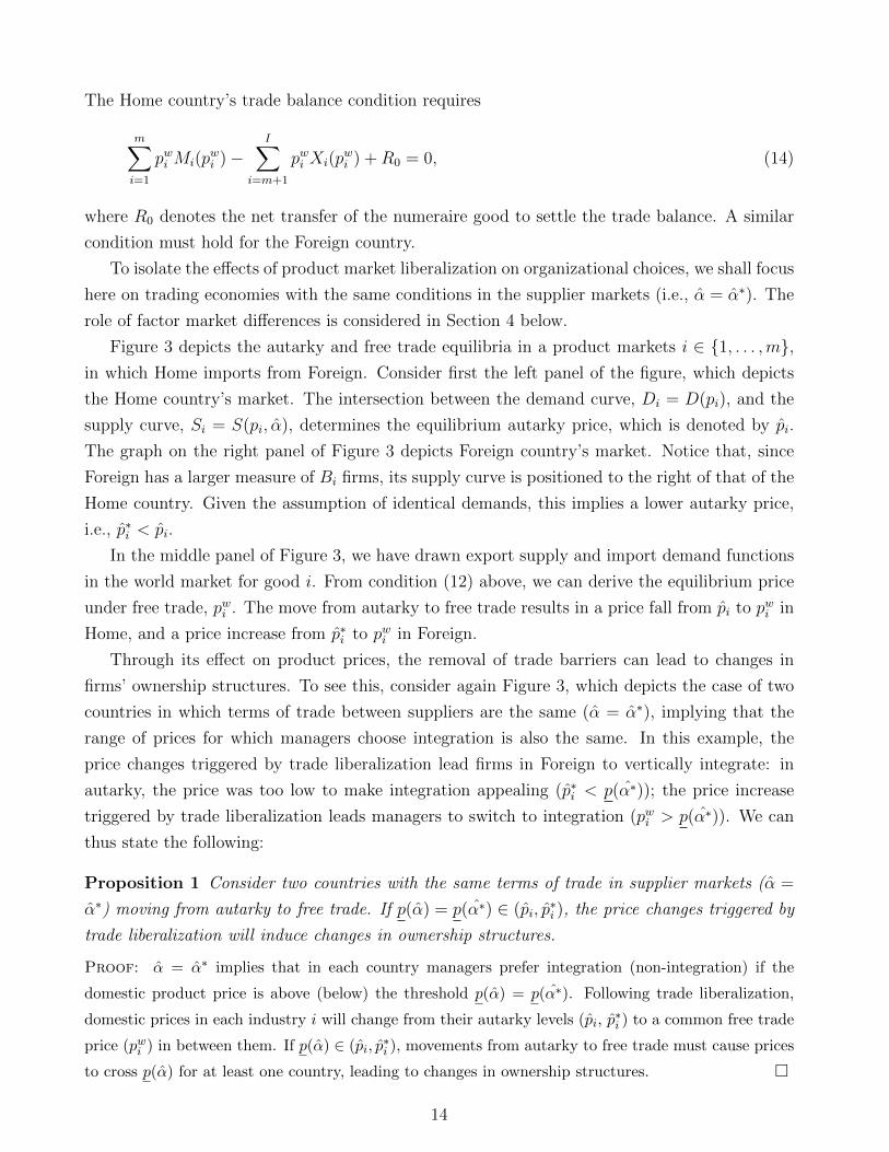
Figure 3 depicts the autarky and free trade equilibria in a product markets i ∈ {1, . . . ,m},in which Home imports from Foreign. Consider first the left panel of the figure, which depicts

the Home country’s market. The intersection between the demand curve, Di = D(pi), and the

supply curve, Si = S(pi, α), determines the equilibrium autarky price, which is denoted by pi.

The graph on the right panel of Figure 3 depicts Foreign country’s market. Notice that, since

Foreign has a larger measure of Bi firms, its supply curve is positioned to the right of that of the

Home country. Given the assumption of identical demands, this implies a lower autarky price,

i.e., p∗i < pi.

In the middle panel of Figure 3, we have drawn export supply and import demand functions

in the world market for good i. From condition (12) above, we can derive the equilibrium price

under free trade, pwi . The move from autarky to free trade results in a price fall from pi to pwi in

Home, and a price increase from p∗i to pwi in Foreign.

Through its effect on product prices, the removal of trade barriers can lead to changes in

firms’ ownership structures. To see this, consider again Figure 3, which depicts the case of two

countries in which terms of trade between suppliers are the same (α = α∗), implying that the

range of prices for which managers choose integration is also the same. In this example, the

price changes triggered by trade liberalization lead firms in Foreign to vertically integrate: in

autarky, the price was too low to make integration appealing (p∗i < p(α∗)); the price increase

triggered by trade liberalization leads managers to switch to integration (pwi > p(α∗)). We can

thus state the following:

Proposition 1 Consider two countries with the same terms of trade in supplier markets (α =

α∗) moving from autarky to free trade. If p(α) = p(α∗) ∈ (pi, p∗i ), the price changes triggered by

trade liberalization will induce changes in ownership structures.

Proof: α = α∗ implies that in each country managers prefer integration (non-integration) if the

domestic product price is above (below) the threshold p(α) = p(α∗). Following trade liberalization,

domestic prices in each industry i will change from their autarky levels (pi, p∗i ) to a common free trade

price (pwi ) in between them. If p(α) ∈ (pi, p∗i ), movements from autarky to free trade must cause prices

to cross p(α) for at least one country, leading to changes in ownership structures. �

14

0p i

Qi

Di

Si

pw i

Mi

pw i

p(α

)

0

pw i

Mi,X∗ i

pi

p∗ i

MiX∗ i

pw i

Mi

=X∗ i

0p∗ i

Q∗ i

Di

p∗ i

pw i

p(α

∗ )

S∗ i

X∗ i

Fig

ure

3:L

iber

aliz

atio

nof

pro

duct

mar

kets

15

Proposition 1 states that, even if suppliers do not relocate across countries (no “offshoring”),

the removal of trade barriers will lead to mergers or divestitures if autarky prices are “different

enough”, i.e., do not lie in a region of prices for which the same organization prevails.

If autarky prices are instead very similar, then trade liberalization will not trigger changes

in ownership structures. In fact, if both autarky prices lie in the integration range (p(α),∞), so

will pwi and thus there will be no ownership change. The same is true if autarky prices both lie

in the non-integration range (0, p(α)). Thus, the condition p(α) = p(α∗) ∈ (pi, p∗i ) is sufficient

and “almost necessary” for restructuring to occur.17

Notice that, even when ownership structures do not change as a result of trade liberalization,

we will expect changes in some organizational variables, such as the “power” of compensation

schemes (here represented by the size of the profit shares 1−s and s), which changes continuously

with prices. Indeed, as noted in the discussion leading up to Lemma 1, A’s profit share s

declines for a non-integrated firm when the industry price rises. In fact, it is easy to show that

the same comparative static results holds for integrated firms. Thus, following product market

liberalization, if the ownership structure does not change in industry i, the profit shares accruing

to Bi managers should increase if i is an export industry and fall if i is an import-competing

industry. The reason is that free trade leads prices to rise in the export industries and fall in the

import industries. Of course, profit shares will also change when there are changes in ownership

structure.

In light of these results, it is instructive to compare the findings in Breinlich (2008) and

Guadalupe and Wulf (2010), which study the organizational effects of the Canada-U.S. Free

Trade Agreement (CUSFTA). For Canada, which as the smaller member country would be ex-

pected to have experienced the largest price changes, Breinlich documents a significant increase

in the level of merger activity following CUSFTA; in the U.S., the corresponding effects were

much smaller. Guadalupe and Wulf (2010), in their sample of U.S. firms, nevertheless find con-

siderable evidence of reorganizations on a smaller scale, such as changes in reporting structures

and in the type of executive compensation schemes. Since the U.S. would have experienced

smaller price changes than Canada in the wake of CUSFTA, this is what our model would lead

us to expect.18

4 Factor Market Liberalization

The analysis carried out in the previous section focused on the organizational responses to price

changes triggered by the removal of barriers in product markets, in a setting in which input

17The omitted case is when p(α) happens to coincide with one of the autarky prices. In this case, firms in onecountry will be in “Mix” region in autarky and only some of them will restructure after liberalization.

18For example, our model would predict smaller price changes and less dramatic restructuring in Home, if thiswere endowed with a larger measure of Bi suppliers (nB > n∗B) and a proportionally larger population.

16

suppliers did not move across countries. In this section, we assume instead that product markets

are fully liberalized (so that product prices are determined by (12)-(13) above) and focus on the

organizational effects of factor market liberalization. It is worth noting that “factor mobility”

here means only that the A’s and/or Bi’s are able to move across borders; Bi’s remain immobile

across sectors.

4.1 Organizational changes

Consider first trading economies with similar factor markets. This is the scenario depicted

in Figure 3, in which the range at which integration occurs is the same in the two countries,

i.e., α = α∗. This implies that in both countries integration will be the prevailing form of

firm organization in industry i if the price exceeds p(α), while non-integration will be chosen

at lower prices. Since under free trade pi = p∗i = pwi , in this case, factor market integration

will have no impact on organizational choices. Therefore, once product markets are integrated,

we should expect factor market liberalization to have little effect on organizational choices in

trading economies with similar factor markets (e.g., France and Germany, or the United States

and Europe).

Consider next a scenario in which Home and Foreign differ in terms of their factor markets

(e.g., West and East Europe, or the United States and China). For simplicity, assume that the

total endowment of B firms is the same in the two countries (i.e., nB = n∗B), but the Home

country’s productivity distribution of A suppliers in the numeraire sector strictly stochastically

dominates the corresponding distribution for the Foreign country, i.e., F (α) < F ∗(α), whenever

F and F ∗ are not both 0 or 1.

The equilibrium condition in the integrated supplier market can be written as

F (αw) + F ∗(αw) = nB + n∗B, (15)

where αw is the equilibrium return for all A’s matched with B’s. Hence factor liberalization

leads to the convergence in the terms of trade between suppliers across countries. In turn, this

implies that the range of prices for which integration will be chosen will also be the same for the

two countries.

Figure 4 can be used to illustrate factor market equilibria with and without factor mobility.

In the no-mobility case, A suppliers in the Home country obtain a higher surplus when matched

with B ’s than do matched A’s in the Foreign country, i.e., α > α∗. Following the removal of

barriers to factor mobility, the integrated matching market will clear when condition (15) above

is satisfied. The equilibrium return to all matched A’s will be given by αw, with α∗ < αw < α.

Notice that convergence in factor prices can be achieved through (i) the relocation of some A

suppliers from Foreign to Home, (ii) the relocation of some B suppliers from Home to Foreign,

or a combination of both. In Figure 4, channel (i) is captured by the distribution function

17

12(F (α) + F ∗(α)), while channel (ii) is captured by shifts in nB and n∗B.

0

nB, n∗B

αα∗ α

nB = n∗B

F ∗(α)

F (α)

12(F (α) + F ∗(α))

αw

n′B

n∗′B

Figure 4: Pre- and post-liberalization equilibria in the factor markets

In Section 2.4, we have shown that an increase in α leads to an decrease in the range of prices

for which integration is chosen (Lemma 1). It follows that before factor market liberalization,

in every sector i, the range of prices for which integration is chosen is smaller in Home country

than in Foreign, i.e., p(α) > p(α∗).

Figure 5 shows the effects of factor market integration on organizational choices in a sector

i ∈ {1, . . . ,m} in which the Home country is an importer. Before liberalization, p(α∗) < pwi <

p(α), so firms are non-integrated in Home and integrated in Foreign. Following the removal of

barriers to factor mobility, terms of trade in supplier markets converge to αw, implying that

the “integration range” expands in Home and is reduced in Foreign. As a result, world supply

contracts and the world price increases from pwi to pw′

i (see Proposition 3 in the next subsection).

Notice that foreign firms switch from integration to non-integration: before liberalization, they

are integrated since pwi > p(α∗); after liberalization, they are non-integrated since pw′

i < p(αw).

In this example, no change in ownership structures occurs in Home: since pwi < p(α) and

pw′

i < p(αw), firms are non-integrated both before and after liberalization.

Proposition 2 Consider two countries that freely trade with each other, but have different terms

of trade in supplier markets (α > α∗). If pwi ∈ (p(α∗), p(α)), factor market liberalization will

induce changes in ownership structures. If the restructuring occurs at Home, it entails a move

to integration; if it occurs in Foreign, the move is to non-integration.

Proof: α > α∗ implies that p(α) > p(α∗). As a result of factor market liberalization, terms of trade

in supplier markets converge to αw in between α and α∗ and the integration range becomes(p(αw),∞

)18

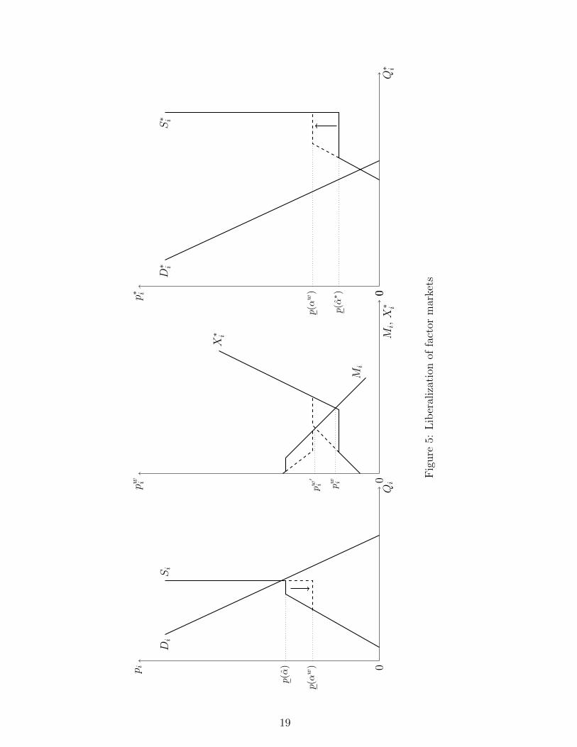
0p i

Qi

Di

Si

p(α

w)

p(α

)

0

pw i

Mi,X∗ i

X∗ i

Mi

pw i

pw

′

i

00p∗ i

Q∗ i

D∗ i

p(α

w)

p(α

∗ )

S∗ i

Fig

ure

5:L

iber

aliz

atio

nof

fact

orm

arke

ts

19

in both countries. Since managers face the same product prices and the same terms of trade in both

countries, the same organization must prevail in both countries.

If pwi ∈ (p(α∗), p(α)) firms are initially integrated at Home and non-integrated in Foreign. To

converge to a common organization following factor liberalization, ownership structures must thus

change in one country. If pw′

i < p(αw), non-integration prevails in both countries, implying divestitures

in Foreign. If instead pw′

i > p(αw), integration prevails, implying mergers in Home. �

Factor market liberalization will not trigger changes in ownership structures if the initial

world price is below p(α∗) or above p(α). Consider first the case in which pwi < p(α∗). Then

pwi < p(α) as well, and firms in both countries are initially non-integrated. The only way there

could be restructuring (i.e., some movement toward integration) is if the post-liberalization price

pw′

i were to exceed p(αw) and therefore pwi . But this cannot happen: since integration generates

more output per firm than non-integration, world supply would then be greater than it was

before liberalization, and the we would then have pw′

i < pwi , a contradiction. The reasoning is

similar for the case in which pwi > p(α) and firms in both countries are initially integrated. The

condition stated in Proposition 2 is thus sufficient and “almost necessary” for restructuring to

occur following factor market liberalization.19

It should be stressed that, in contrast to the removal of barriers to trade in goods — which

generates sector-specific effects on organization by affecting product prices — the removal of

barriers between factor markets affects all sectors in the economy, by changing the terms of

trade in supplier markets. Before liberalization, matched A suppliers obtain a surplus p(α)

(p(α∗)) in all sectors in Home (Foreign); after liberalization, their surplus becomes p(αw) in all

sectors in both Home and Foreign.

Notice also that the organizational changes triggered by factor market liberalization are

independent of the specific patterns of factor mobility, i.e., different factor movements have the

same impact on the terms of trade prevailing in supplier markets and on organizational choices.20

Proposition 2 suggests that countries that have already experienced organizational changes

as a result of the elimination of barriers to trade in goods (e.g., EU member countries after

the Customs Union formation in 1968) are likely to undergo further restructuring as a result of

the removal of barriers to factor mobility (e.g., increased M&A activities across EU members,

following the establishment of the Single Market, as documented by the study of the European

Commission, 1996). Such reorganizational (as distinct from relocational) activities 21 will be

19As for the case of product market liberalization, we omit the boundary cases in which pwi lies in the “Mix

region” for one of the countries (see footnote 17). Also observe that, if pw′

i happens to coincide with the thresholdp(αw), the restructuring will only be partial but still in the direction stated in the Proposition.

20To verify this, compare the case in which only the sectorally-mobile factor of production (A suppliers) movesacross countries with the case in which only the specific factors (Bi suppliers) relocate. In the first case, A firmsmove from Foreign to Home until all matched A’s obtain the same return αw; in the second case, Bi suppliersmove from Home to Foreign, until the surplus they have to pay to A suppliers is equal to αw in both countries.

21There is nothing in the model to prevent “re-partnering” after liberalization: reorganization may involve aBi supplier integrating with an A supplier, which may be different from the one it had dealt with at arm’s length

20

more intense between countries with large productivity differences (e.g., Germany and Romania)

rather than among those with similar productivity levels (e.g., Germany and France).

4.2 Product prices and quality

The analysis carried out above shows that factor liberalization can lead to changes in firms’

ownership structure, by affecting the division of surplus between managers of different supplier

firms. In the remaining of this section, we will examine the consequences of these changes from

the point of view of market performance.

Not only do prices affect organization design, but also organizational choices affect prices.

This is a simple consequence of the fact that integration generates more output than non-

integration at any price level. So a switch toward integration leads to an increase in the quantity

supplied, while the opposite is true for a switch to non-integration.

As shown in Figure 5 above, the liberalization of factor markets can trigger changes in

ownership structure which lead to a fall in world supply and to a price increase. The increase is

the result of outsourcing in the Foreign country. This will occur if pwi is initially above p(α∗), but

below p(αw); then, following liberalization, Foreign’s integration range shrinks, its supply falls

as its firms divest; meanwhile, Home firms remain non-integrated since p(α) > p(αw). Thus in

aggregate, supply falls, so pwi can no longer be an equilibrium price. The new price, pw′

i must be

higher than the initial pwi . In other cases, factor liberalization will lead to an increase in world

supply and a price decrease, or leave aggregate quantities and prices unchanged.

To sum up, we can state the following:

Proposition 3 Factor market liberalization leads to a price increase (decrease) if and only if

there is a switch toward non-integration (integration) in Foreign (Home).

Proof: Factor market liberalization has the following effects on product prices:

A price increase if

p(α∗) ≤ pwi < p(αw) (corresponding to a switch to non-integration in Foreign);

A price decrease if

p(αw) < pwi ≤ p(α) (corresponding to a switch to integration in Home);

No price change if

pwi > p(α) (firms in both countries remain integrated);

pwi < p(α∗) (firms in both countries remain non-integrated);

before; or a Bj spinning off an A to enter into a non-integrated relationship with another, either at home orabroad.

21

pwi = p(αw) (the fraction of firms that are integrated in the world is unchanged). �

Though systematic evidence corresponding to the effects of organizational changes on product

prices does not yet appear to have been assembled, there is at least some indicative evidence of

phenomena corresponding the price increases following reorganization that we have discussed.

In particular, there are numerous accounts of falling product quality resulting (especially) from

international outsourcing (see discussion below). Our model can be easily reinterpreted to explain

such accounts. One can interpret the “quantity” produced by a firm as quality under money-back

guarantees or threat of lost repeat business: the good either delivers the consumer a positive value

with probability QN(pi) (under non-integration, else QI(pi)) or nothing. Low success probability

corresponds to low quality. Thus instead of QN(pi)ni goods delivered with probability 1, we have

ni goods of quality QN(pi).

Proposition 3 shows that, even in a setting in which firms have no market power, allowing

suppliers to relocate freely across countries can negatively affect consumers by inducing inefficient

organizational changes that lead to price increases (quality losses). A stronger result can also

be derived:22

Proposition 4 Factor market liberalization may reduce consumer welfare in both countries.

Proof: see Appendix. �

The intuition for this result is as follows. Factor liberalization leads to a more efficient alloca-

tion of A suppliers across countries, resulting in a beneficial increase in aggregate production of

the numeraire good: in the Home country, the payoff accruing to A suppliers in the production of

i good falls from α to αw, leading some A’s to switch to the production of good 0; the opposite

happens in the Foreign country. It can easily be shown that the overall effect is an increase

in world production of the numeraire good, which is beneficial to consumers in both countries.

This is because more efficient A’s from Home replace less efficient foreign firms. However, the

increase in numeraire production may be quite small (depending on the distribution functions

F and F ∗), in which case the impact that factor liberalization has on consumer welfare depends

mainly on its effects on the prices of the i goods.

4.3 An illustration: the toy industry in China

The type of inefficient outsourcing described above can be illustrated by the safety problems

associated with American-designed toys assembled in China. Although some popular accounts

have attributed these problems to the re-location of production from the US to China, others

— and a careful look at the evidence — suggest instead that they were the result of purely

22See Legros and Newman (2009) for a more general welfare analysis that, which also takes account of man-agerial costs.

22

organizational changes within China: various tasks that were previously performed in factories

owned and operated by US companies (particularly Mattel) had been turned over to Chinese

contractors and sub-contractors. This calls for identifying the economic forces that led to such

apparently inefficient reorganizations, something our model is suited to do.23

By the 2000s, China had become the world’s leading producer of toys. In 2007, at the time of

the product recalls, about 80 percent of the world’s toy production, and nearly 80 percent of toys

imported into the U.S. were made in China. Mattel was the world’s largest toy maker, selling

two main types of products: “core products” with highly valued brand names such as Barbie

that sell for long periods of time; and “non-core products” that sell for a relatively short term,

such as licensed characters associated with newly released movies (Lee et al., 2008). Mattel was

a pioneer in manufacturing in Asia. The first Barbie doll, which was introduced in 1959, was

produced in Japan. In 2007, 65% of Mattel’s production was done in China. The company had

five wholly owned factories, responsible for roughly half of its toy production, a higher proportion

than that of other large toy makers such as Hasbro and RC2 (Jackson and Xiubao, 2008).

By 2007, however, Mattel was “squeezed between lower prices and higher costs” (Lee et al.,

2008). On one hand, it had to continually reduce prices in order to meet the demands of the big

retailers such as Wal-Mart and Target. On the other hand, costs were rising: in 2005, Beijing

let its currency float, and by 2007 the yuan had appreciated by more than 9 percent against the

dollar; fuel and raw materials costs had increased; and labor costs had also been increasing by

around 10 percent a year.

In response to these pressures, Mattel partially reorganized its toy production in China.

In particular, it started to outsource more of its “non-core” products to third-party suppliers,

while continuing to manufacture in wholly-owned factories its most popular toys, such as Barbie

dolls and Hot Wheels cars. The effects of this reorganization became apparent in August 2007,

when Mattel recalled 19 million Chinese-made toys from the world market because of safety fears

relating to lead paint and small magnets that could be swallowed by children.24 The substandard

toys recalled had been produced by Chinese suppliers (e.g., Lee Der Industrial Co. Ltd and Early

Light Industrial) rather than in Mattel’s wholly-owned factories (Jiangyong et al., 2009). In the

days following the recall, Mattel executives announced that they would try to “shift more of

their toy production into factories they own and operate — and away from Chinese contractors

and sub-contractors”.25

The forces identified in our model can be used to interpret Mattel’s organizational choices in

23Other evidence is provided by Lin and Ma (2008), who find that Korea’s experiment with service outsourcingfor the period 1985-2001 lead to a decline in productivity.

24On August 2, Mattel recalled 1.5 million Fisher-Price toys because of excessively high lead content in theirpaint. Though the bulk of the affected toys were recalled before they reached consumers, more than 300,000affected toys had already been sold. Within two weeks, on 14 August, Mattel announced a global recall ofanother 436,000 toys due to lead paint hazards and recalled another 18.2 million toys with small magnets thatcould become detached and easily swallowed by children.

25See the article “Mattel Recalls 19 Million Toys Sent From China,” New York Times, August 15, 2007.

23

China and its product recalls. Since China is the world’s leading toy exporter, the right-hand

panel of Figure 5 can represent its part of the world market for a typical subcategory of toys.26

Mattel’s experience of falling prices and increasing production costs corresponds to a drop in

pwi and rise in α∗. In our model, both types of pressures can lead to a switch from integration

to non-integration. A fall in the price of toy manufacturers’ output, whether due to changing

consumer tastes or growing retailer market power has the same implications for organizational

choice, namely a shift toward non-integration. A rise in the opportunity cost α∗ of the Chinese toy

assemblers, whether the result of growing world factor mobility or China’s prodigious economic

growth (leading to a rightward shift in its productivity distribution F ∗(·)), has a similar impact.

Either way, the effect is to raise the threshold p(α∗) above which firms prefer to integrate.

Finally, integration generates more output than non-integration, so as in Proposition 3 the

switch to non-integration leads to an increase in price or, equivalently, to a reduction in quality

(success probability), as manifested by Mattel’s product recalls.

5 Conclusions

In this paper, we have embedded organizational firms into a standard model of international

trade in order to examine the effects of the liberalization of product and factor markets on firm

boundaries. Our “building-block” model of the firm is particularly tractable and is based on a

simple tradeoff between the organizational objective (profit) and managers’ private objectives

(doings things in their preferred ways).

In line with recent theoretical work in organizational economics, our paper suggests that

market conditions can significantly affect firms’ ownership structures. In particular, falling

trade barriers and increased factor mobility can affect vertical integration decisions through

their impact on product prices and on the terms of trade prevailing in supplier markets. Another

implication of our analysis is that that convergence in corporate organization — the tendency

of industries to be characterized by the same ownership structure across countries — may result

not only from global cultural transmission or technological diffusion, but also from a standard

neoclassical market force, the law of one price.

We have studied the organizational changes of trade liberalization using a very stylized model,

in which barriers to trade are either prohibitive or non-existent. A follow-up paper by Alfaro et

al. (2010) extends the analysis by introducing import tariffs. The main prediction of this richer

version of the model is that higher tariffs on final goods, by raising product prices, should lead

protected firms to become more vertically integrated. Moreover, differences in ownership struc-

26China had become an exporter of toys as a result of its (partial) liberalization to foreign investors, whichhas attracted companies like Mattel and Hasbro. In our model, this could be captured by Bi suppliers movingfrom Home to Foreign due to differences in production costs (α∗ < α). Since barriers to factor mobility persist,so does a a cross-country gap in the opportunity costs of A suppliers.

24

tures between countries should be smaller in sectors characterized by similar levels of protection

and between members of regional trade agreements, especially customs unions. To examine the

evidence, Alfaro et al. (2010) construct firm-level vertical integration indices for a large set of

countries. Their empirical analysis, which exploits both cross-section and time-series variation

in import tariffs, supports the predictions of the model.

We conclude by briefly discussing some of the policy implications of our analysis. In the

standard competitive trade model, moving to full product and factor market liberalization will

maximize consumer welfare. Not so in the present model, which differs from the standard one

only by the presence of managers who decide firms’ ownership structures and compensation

schemes. One implication is that optimal trade policy is likely to differ from the standard one in

the presence of organizational firms. For instance, there may be a positive role for production or

export subsidies to countervail the effects of inefficient organizational choices. In the post-factor-

market liberalization situation depicted in Figure 5, a small subsidy may induce an exporting

firm’s managers to switch from (inefficient) non-integration to (efficient) integration by effectively

raising the price they receive for the goods they produce.

The analysis also suggests that policies that more directly address organizational inefficiencies

may complement trade policy. In our model, the managers (together with HQ in the case of

integration) are full claimants of enterprise revenue, as in family firms, or other closely-held

organizations. The model could easily be adjusted to describe “managerial firms,” in which the

primary decision makers have low financial stakes. Suppose the managers receive only a small

fraction λ < 1 of the revenues, with the remainder accruing to dispersed shareholders who have

little control over major organizational decisions. It is straightforward to show that managers

will decide to integrate only when product price exceeds p(α)/λ, a smaller range of prices than

in the case considered so far (for which λ was equal to 1).

The smaller is λ, the more shareholders’ interests diverge from those of management, because

they value revenue but not managerial private costs (and since they take prices as given, they

have no interest in restricting their firm’s output). Consumers also benefit from larger values of

λ, which imply that high-output integration is chosen more often. Corporate governance policy

that offers strong shareholder protection or gives them greater monitoring and/or control over

management effectively increases λ, and therefore benefits consumers.

In particular, good corporate governance reduces the likelihood that factor liberalization

leads to a price increase and thus to a loss in consumer surplus. Moreover, product market

liberalization becomes more effective: the gains from liberalization are larger if organization is

chosen to maximize output rather than managerial welfare. It is in this sense that we view

governance and trade policies as complementary, and it is not surprising that the European

Commission has proposed an Action Plan on corporate governance to “strengthen shareholders’

rights” and to “foster the efficiency and competitiveness of business, with special attention to

some specific cross-border issues” (see Commission press release, May 21 2003).

25

Appendix

A.1 Full Employment Equilibrium

Define p0(α) to be the lowest price at which an A who accrues all the surplus (s = 1) under

non-integration can obtain α : WN(1, p0(α)) = p0(α)2

1+p0(α)= α. Note this equation has a unique

solution, increasing in α, and independent of the sector. Consider a generic equilibrium in which

matched A suppliers obtain surplus αG. It follows from Assumption 1 that p0(αG) < p(αG),

implying that non-integration prevails at p0(αG).

To guarantee that all Bi’s are employed, we require that there is excess demand for good i

at p0(αG), implying that the equilibrium price must exceed p0(α

G). Let nGi be the endowment

of Bi’s. Then for full employment it is enough that

For all i ∈ {1, . . . , I}, u′i(nGi QN(p0(αG))) > p0(α

G). (16)

Since ui(·) is concave and p0(·) increasing, this condition is more stringent the larger is αG and

the larger is nGi . In the text we make assumptions on the model’s fundamentals that guarantee

that the Home autarky value α is an upper bound for all equilibrium values of matched-A payoffs.

The largest endowment to consider is the larger of the Home and Foreign endowments ni and

n∗i . We can therefore ensure that there is full employment in all scenarios we discuss with

Assumption 2 Condition 16 holds when αG = α and nGi = max{ni, n∗i }.

A.2 Proofs

Proof of Lemma 1

(i) Consider the function g(pi) defined as the unique solution to(pi

1 + pi

)2

(1 + pi + g(pi)) = pi −1

2− h.

Note that g(pi) is continuous (in fact, differentiable); it is straightforward to verify that it is

strictly increasing for 0 ≤ h < 12, and vanishes at pi = p ≡ 1+2h

1−2h .

Let PI (α) be the set of prices satisfying WN(s, pi) ≤ W I(pi), that is(pi

1 + pi

)2

(1 + pi + 2s(α, pi)(1− s (α, pi))) ≤ pi −1

2− h

where s (α, pi), the (unique) value of s satisfying uNA (s, pi) ≡(

pi1+pi

)2((2 + pi)s− s2) = α, is the

profit share that guarantees A a payoff of α under non-integration: integration is chosen only if

26

pi ∈ PI (α) . Equivalently, we need

2s (α, pi) (1− s(α, pi)) ≤ g(pi). (17)

Now, Assumption 1 ensures that s ∈ [0, 1/2] for any equilibrium α, and 2s(1 − s) is increasing

on [0, 1/2]. From (7), s (α, pi) is increasing in α and decreasing in pi.Thus (17) is satisfied if and

only if

s(α, pi) ≤ h(pi),

where h(·) is a continuous, increasing transformation of g(·). Since g is increasing, so is h. Thus

if p′i > pi, and integration is chosen at pi, we have

s(α, p′i) < s(α, pi) ≤ h(pi) < h(p′i),

and integration is also chosen at p′i. Thus, PI (α) can be written as an interval [p (α) ,∞). Note

that p(0) = p.

(ii) Since s increases with α, and WN(s, pi) increases in s on [0, 1/2], WN(s, pi) increases in

α. It follows that PI (α) is decreasing (in the sense of set inclusion), i.e., that p (α) is increasing.

Proof of Proposition 4

Proposition 3 shows that, even in a setting in which firms have no market power, allowing

suppliers to relocate freely across countries can negatively affect consumers by inducing inefficient

organizational changes. However, factor liberalization also leads to a more efficient allocation

of A suppliers across countries, resulting in a beneficial increase in aggregate production of the

numeraire good 0. In what follows, we derive a sufficient condition for factor market liberalization

to hurt consumers in both countries.

Recall that ni (n∗i ) denotes the measure of Bi firms in Home (Foreign) and that∑I

i=1 ni ≡ nB

and∑I

i=1 n∗i ≡ n∗B. Let us assume that nB = n∗B = n and that ni + n∗i = 2n/I, ∀i. This

guarantees that the world supply is the same across sectors. We also assume that all sectors

have the same aggregate demand. Together, these assumptions imply that the price changes and

the welfare effects of factor liberalization will be the same in all sectors of the economy. Using

the proof of Proposition 3, we can then identify conditions such that the equilibrium world price

will strictly increases after factor market integration. Let L > 0 be the resulting loss in welfare.

Let αw = 12(α + α∗), where F (α) = F ∗(α∗) = n and F (αw) + F ∗(αw) = 2n. That is, before

factor market liberalization A suppliers have outside options α and α∗ in Home and Foreign,

respectively, while they have outside option αw after the liberalization.

Now, since α > αw > α∗, some Home A suppliers that before liberalization were employed

27

in the production of I goods will start producing the numeraire good; at the same time, some

Foreign A suppliers that were originally producing the numeraire good will start producing the

other goods.

The change in numeraire production is then

δ =

∫ α

αw

αf(α)dα−∫ αw

α∗αf ∗(α)dα;

integrating by parts and using the equilibrium conditions F (α) = n , F ∗(α∗) = n and F (αw) +

F ∗(αw) = 2n, this becomes

δ =

[∫ αw

α∗F ∗(α)dα− n (αw − α∗)

]+

[n(α− αw)−

∫ α

αw

F (α)dα

].

Note that this is always positive. Since F and F ∗ are increasing,

δ < (F ∗(αw)− n) (αw − α∗) + (n− F (αw))(α− αw) (18)

and since αw = 12(α + α∗),

δ ≤ 1

2(F ∗(αw)− F (αw))(α− α∗). (19)

Consider two distribution functions F ∗(x; ε), F (x; ε) that are linear on the interval [α∗, α] and

that satisfy F ∗(α; ε) = n + ε and F (α∗; ε) = n − ε. Since there is no restriction on F (x; ε) and

on F ∗(x; ε) outside the interval [α∗, α], as ε varies it is possible to find ‘completions’ of these

functions such that the overall distributions are indeed distribution functions.

By construction, F ∗(αw; ε) − F (αw; ε) = ε. Therefore, by (18), for all ε < 2L/(α − α∗), the

welfare loss resulting from the increase in the price of all i -goods more than offsets the welfare

gain associated with increased consumption of the numeraire good.

References

Alfaro, L., P. Conconi, H. Fadinger, and A. F. Newman (2011). “Trade Policy and Firm

Boundaries,” NBER Working Paper No. 16118.

Antras, P. (2003). “Firms, Contracts, and Trade Structure,” Quarterly Journal of Economics

118, 1375-1418.

Antras, P., and H. Helpman (2004). “Global Sourcing,” Journal of Political Economy 112,

552-580.

Antras, P., and R. W. Staiger (2008). “Offshoring and the Role of Trade Agreements,” NBER

Working Paper 14285.

28

Breinlich, H. (2008). “Trade Liberalization and Industrial Restructuring through Mergers and

Acquisitions,” Journal of International Economics 76, 254-266.

Chudnovsky, D. (2000). “Industrial Restructuring Through Mergers and Acquisitions: The Case

of Argentina in the 1990s,” Transnational Corporations 9, 33-58.

Dyer, J. H. (1996). “How Chrysler Created and American Keiretsu,” Harvard Business Review,

July-August, 42-60.

European Commission (Directorate-General for Economic and Financial Affairs) (1996). “Eco-

nomic Evaluation of the Internal Market,” European Economy No. 4.

Grossman S. J., and O. D. Hart (1986). “The Costs and Benefits of Ownership: A Theory of

Vertical and Lateral Integration,” Journal of Political Economy 94, 691-719.

Grossman, G. M., and E. Helpman (2002). “Integration Versus Outsourcing In Industry Equi-

librium,” Quarterly Journal of Economics 117, 85-120.

Grossman, G. M., and E. Helpman (2004). “Managerial Incentives and the International Orga-

nization of Production,” Journal of International Economics 63, 237-262.

Guadalupe, M., and J. Wulf (2010). “The Flattening Firm and Product Market Competition:

The Effect of Trade Liberalization,” American Economic Journal: Applied Economics,

forthcoming.

Hart, O. D., and B. R. Holmstrom (2010). “A Theory of Firm Scope,” Quarterly Journal of

Economics, 125, 483-513.

Hart, O. D., and J. H. Moore (1990). “Property Rights and the Nature of the Firm,” Journal

of Political Economy 98, 1119-1158.

Jackson, G., and Y. Xiubao (2008). “Mattel Toys – Made in China (A),” Harvard Business

Review, case study HKU810.

Jiangyong, L., T. Zhigang, and Y. LinHui (2009). “Mattel’s Strategy after its Recall of Products

Made in China,” Harvard Business Review, case study HKU810.

Lee, H. L., M. M. Tseng, and D. Hoyt (2008). “Unsafe For Children: Mattel’s Toy Recalls and

Supply Chain Management,” Stanford University, Graduate School of Business, case study

GS63.

Legros, P., and A. F. Newman (1996). “Wealth Effects, Distribution, and the Theory of Orga-

nization,” Journal of Economic Theory 70, 312-341.

Legros, P., and A. F. Newman (2009). “A Price Theory of Vertical and Lateral Integration,”

mimeo, Boston University.

Lin, S., and C. A. Ma (2008). “Outsourcing and Productivity: Evidence from Korean Data,”

mimeo, University of San Diego.

Marin, D., and T. Verdier (2002). “Power Inside the Firm and the Market: a General Equilibrium

Approach,” CEPR Discussion Paper 3526.

29

McLaren, J. (2000). “Globalization and Vertical Structure,” American Economic Review 90,

1239-1254.

Mussa, M. (1974). “Tariffs and the Distribution of Income: the Importance of Sector Speci-

ficity, Substitutability and the Intensity in the Short and Long Run,” Journal of Political

Economy 82, 1191-1204.

Ornelas, E., and J. Turner (2008). “Trade Liberalization, Outsourcing, and the Hold Up Prob-

lem,” Journal of International Economics 74, 225-241.

Ornelas, E., and J. Turner (2010). “Protection and International Sourcing,” mimeo, London

School of Economics.

Pavcnik, N. (2002). “Trade Liberalization, Exit, and Productivity Improvements: Evidence

from Chilean Plants,” Review of Economic Studies 69, 245-276.

Puga, D. and D. Trefler (2010). “Wake Up and Smell the Ginseng: The Rise of Incremental

Innovation in Low-wage Countries,” Journal of Development Economics 64, 64-76.

Roth, A. E., and M. Sotomayor (1990). Two-Sided Matching: A Study in Game-Theoretic

Modeling and Analysis, Cambridge, Cambridge University Press.

Schmitz, J. A. (2005). “What Determines Productivity? Lessons from the Dramatic Recovery

of the U.S. and Canadian Iron Ore Industries Following Their Early 1980s Crisis,” Journal

of Political Economy 113, 582-625.

Trefler, D. (2004). “The Long and Short of the Canada-U.S. Free Trade Agreement,” American

Economics Review 94, 870-895.

Van den Steen, E. (2005). “Organizational Beliefs and Managerial Vision,” Journal of Law,

Economics, and Organization 21, 256-283.

30