Tracking the Mechanism of Water Oxidation in Photosystem II Using

X-ray Free Electron Laser Diffraction

by

Iris Diane Young

A dissertation submitted in partial satisfaction of the

requirements for the degree of

Doctor of Philosophy

in

Chemistry

in the

Graduate Division

of the

University of California, Berkeley

Committee in charge:

Professor John Kuriyan, Chair

Professor Jamie Doudna Cate

Professor James Hurley

Fall 2018

Tracking the Mechanism of Water Oxidation in Photosystem II Using

X-ray Free Electron Laser Diffraction

Copyright 2018

by

Iris Diane Young

Abstract

Tracking the Mechanism of Water Oxidation in Photosystem II Using

X-ray Free Electron Laser Diffraction

by

Iris Diane Young

Doctor of Philosophy in Chemistry

University of California, Berkeley

Professor John Kuriyan, Chair

The mechanism of water oxidation in oxygenic photosynthesis, the process

generating all oxygen on Earth, has remained elusive despite the maturity of the field of

photosynthetic research. Water oxidation takes place at the oxygen-evolving complex

(OEC) of photosystem II (PS II), a large dimeric protein located in the thylakoid

membrane, and proceeds by the same mechanism in cyanobacteria, algae and all higher

plants. Charge separation at the P680

pigment is followed by charge stabilization by

reduction of a plastoquinone and oxidation of the OEC. Over the five steps of the Kok

cycle and controlled by absorption of four photons at P680, the OEC stores four oxidizing

equivalents prior to oxidizing two substrate water molecules to dioxygen. These steps

take place on a microsecond to millisecond scale and may be activated in sequence by

illuminating dark-adapted PS II with short flashes of visible light.

Studying the mechanism of water splitting at the oxygen-evolving complex (OEC)

in photosystem II presents several challenges: it must be studied by a time-resolved

method in order to track transient states in the cycle, at room temperature in order for

the OEC to advance to these states, and with a method capable of resolving the

atomic-level structure of a large transmembrane protein. A pump-probe

"diffraction-before-destruction" experiment at an X-ray free electron laser (XFEL)

addresses all these challenges. Diffraction is collected from each in a series of

microcrystals, which may be advanced to a transient state and delivered to the XFEL

beam under ambient conditions.

This dissertation describes a series of XFEL experiments that revealed the

structure of PS II at high resolution in multiple illuminated states. PS II microcrystals

are delivered to the XFEL beam with either a liquid jet or a drop-on-demand system in

1

which droplets containing microcrystals are deposited by acoustic droplet ejection onto

a kapton conveyor belt. Using visible lasers positioned along the path of the jet or

droplets, crystals are illuminated to uniformly advance OEC centers, and the diffraction

patterns from hundreds of thousands of individual crystals are combined to generate the

diffraction dataset. X-ray emission spectra from the same crystals are collected

simultaneously for evaluation of the redox state of the cluster to confirm turnover.

This work focuses on the XFEL data processing methods developments that

enabled these experiments and analyzed the diffraction datasets they produced. An

overhaul of real-time data processing at the beamline included development of the

cctbx.xfel graphical user interface, which was used to filter crystallization batches and

sample delivery conditions and to provide feedback on quality and completeness of

datasets. Optimization of the crystal models allowed filtering of multiple crystal forms of

PS II and resolved some apparent nonisomorphism in the remaining distribution of unit

cells due to uncertainties during indexing. A position-dependent correction was applied

to integrated intensities to account for a highly asymmetric shadow on the detector, and

several improvements to the merging program cxi.merge were critical to successfully

merging these data. Finally, structure solution and analysis of a series of datasets were

streamlined with various custom tools for automation, parallelization and calculations

on the atomic positions.

PS II structures are reported in four metastable and two transient states of the

Kok cycle, of which four have never been reported to high resolution and two are

reported at the highest resolution at room temperature to date. Analysis of these

structures reveals water insertion between 150 and 400 µs after illumination of the S2

state, and a detailed analysis of the series of structures reveals possible channels for

substrate water approach. Another structure in the S3

state with ammonia bound reveals

the probable position of a water coordinating the OEC that does not participate in the

water oxidation mechanism. The aggregated evidence from these structures excludes at

least one proposed mechanism and produces three favored mechanisms for water

oxidation, involving some subset of the following in O-O bond formation: water W3

coordinated to Ca, water W2 coordinated to Mn4, bridging oxo O5 and inserted water

Ox. Investigation of additional transient states near O-O bond formation may

distinguish between these mechanisms and resolve the water oxidation mechanism.

2

To Team BLAGS:

Matthew Kolaczkowski, Lauren Nowak, Erin Creel, Andy Creel, and Alex Aaring

i

ii

Table of Contents 1 Introduction 1

1.1 Oxygenic Photosynthesis 1 1.1.1 History, Scale and Importance 1 1.1.2 Evolution of Oxygenic Photosynthesis 2

1.2 The Oxygen-Evolving Cycle 3 1.2.1 The Kok Cycle 3 1.2.2 Challenges in Studying the Oxygen-Evolving Cycle 6

1.3 X-ray Free Electron Laser (XFEL) Diffraction 6 1.3.1 Protein Crystallography 6 1.3.2 X-ray Free Electron Laser Diffraction 9 1.3.3 Challenges of XFEL Experiments 10

1.4 XFEL Crystallography of Photosystem II 12 1.4.1 Cryogenic XFEL Crystallography of Photosystem II 12 1.4.2 Room Temperature and Pump-Probe XFEL Crystallography of Photosystem II 12 1.4.3 Simultaneous X-ray Diffraction and X-ray Emission Experimental Design 13 1.4.4 XFEL Diffraction Data Processing 15

2 Experiments and Datasets 19 2.1 Photosystem II 19

2.1.1 Crystal Screening Time at the Advanced Light Source 19 2.1.2 XFEL Experiments at the Linac Coherent Light Source 19

2.2 Other XFEL Experiments 20 2.2.1 Allen Orville et al. 20

3 Data Processing and Fast Feedback at the X-ray Free Electron Laser Diffraction Experiment 21

3.1 Priorities for Real-Time Feedback 21 3.1.1 Experiment Geometry 21 3.1.2 Unit Cell and Space Group Determination 22 3.1.3 Early Identification of Problems 23 3.1.4 Diffraction Quality and Projected Merged Resolution 25 3.1.5 Structural Model and Map Features 25

3.2 Command Line Diffraction Data Processing 26 3.2.1 Initial Determination of the Detector Distance and Beam Center 26 3.2.2 Batch Processing of Diffraction Data at the Linac Coherent Light Source (LCLS) 27

iii

3.2.3 Batch Processing of Diffraction Data at SACLA 29 3.2.4 Diagnosis of Experiment Model Inaccuracies and Crystal Pathologies 31 3.2.5 Experiment-specific Adaptations to Command Line Processing 33 3.2.6 Updates to Command Line and Multiprocessing Tools 34

3.3 The cctbx.xfel Graphical User Interface 35 3.3.1 Initial Design 35 3.3.2 Development of Additional Features 36 3.3.3 Evolution of the Database 41 3.3.4 Evolution of Other Components 42

3.4 Experiment-Specific Fast Feedback 43 3.4.1 Multi-Detector Experiments 43 3.4.2 Radial Averaging 44 3.4.3 Unit Cell Monitoring 45

4 Improvement of the Experiment and Crystal Models 47 4.1 Iterative Improvement of Crystal and Experiment Models 47

4.1.1 Ensemble Refinement and Striping 47 4.2 Unit Cell Filtering and Clustering 48

4.2.1 Unit Cell Filtering 50 4.2.2 Unit Cell Clustering 50

4.3 Integrated Signal Correction for Absorption Effects 51 4.3.1 The Acoustic Droplet Ejection (ADE)-Drop on Tape (DOT) Sample Delivery System 52 4.3.2 The Kapton Absorption Correction 54

5 Merging 58 5.1 Merging with cxi.merge 58

5.1.1 Martialing and Filtering Images 58 5.1.2 Scaling and Merging the Data 59

5.2 Advancements in Merging 60 5.2.1 Filtering 60 5.2.2 Integration with DIALS framework 61 5.2.3 The ExaFEL Project and Processing at NERSC 62

6 Structure Solution of Photosystem II 63 6.1 Molecular Replacement and Structure Refinement in Phenix 65

6.1.1 Molecular Replacement 65 6.1.2 Rigid Body Refinement 65 6.1.3 Refinement 66

6.2 Automation and Parallelization of Structure Solution 66 6.2.1 Wrapper for Customized PS II Refinement in Phenix 66

iv

6.2.2 Parallelization Across Related Structures 67 6.3 Custom Geometry Restraints for Photosystem II 68

6.3.1 The Oxygen-Evolving Complex 68 6.3.2 Other Ligands 69

6.4 Resolution-Dependent Considerations 70 6.4.1 Noncrystallographic Symmetry 70 6.4.2 Restraints and Weights 70 6.4.3 Ordered Solvent 72

6.5 Refinement of Illuminated States 73 6.5.1 Estimation of the S-state Proportions 73 6.5.2 Partial Occupancy Multi-Model Refinement 74

7 Crystallographic Structure Analysis and Results 76 7.1 Model Interpretation 76

7.1.1 Hierarchical Model Construction 76 7.1.2 Comparisons Across Multiple Models 77

7.2 Tracking Temperature-Dependent Changes 77 7.2.1 Systematic Differences 77 7.2.2 Local Differences 79

7.3 Structure of the Oxygen-Evolving Complex 83 7.3.1 Bonding and Coordination Distances 83 7.3.2 Substrate Water Binding 86

7.4 Water and Hydrogen Bonding Networks 87 7.4.1 Changes of the Water Channels 87 7.4.2 Analysis of O-O Bond Forming Mechanisms 90

7.5 Estimations of Uncertainty 91 7.5.1 Simulated Annealing Omit Map Fitting 91 7.5.2 Map and Model Kicking with END/RAPID 91

8 Summary of Findings 93 8.1 Crystallization and Sample Delivery Conditions 93

8.1.1 Improving Crystal Hit Rates and Diffraction Quality 93 8.1.2 Dehydration-Dependent Nonisomorphism in Photosystem II 94

8.2 Room Temperature Structure of Photosystem II 94 8.2.1 Anisotropic Monomer and Dimer Expansion at Room Temperature 94 8.2.2 Temperature Dependence of Rotamer Populations 94

8.3 Structural Changes at the Oxygen-Evolving Complex 95 8.3.1 Structures in All Metastable and Two Transient States 95 8.3.2 Water Insertion in the S3 State 95 8.3.3 Coordinating Residue Shifts 95

v

8.4 Water Approach to the Oxygen-Evolving Complex 96 8.4.1 Water Network Analysis 96 8.4.2 Proposed Mechanisms 96 8.4.3 Hydrogen Bonding Network Analysis 96

9 Future Directions 97 9.1 Instrumentation and Experimental Design 97

9.1.1 New Drop-on-Demand Systems 97 9.2 Data Processing 98

9.2.1 Exascale Computing at NERSC 98 9.2.2 The cctbx.xfel GUI Refactor 98 9.2.3 Difference Refinement 98

9.3 Unresolved Questions 98 9.3.1 Approaching the Oxygen-Oxygen Bond-Forming Step 98 9.3.2 Tracking Water Approach and Dioxygen Release 99

Acknowledgements 99

References 100

Preface

The water-splitting mechanism of oxygenic photosynthesis has been the subject of

intense investigation in recent years. Parallel routes of inquiry by electron paramagnetic

resonance and X-ray spectroscopy, X-ray diffraction and quantum

mechanical/molecular dynamics simulations have furnished the field of photosynthesis

research with several proposed mechanisms of water oxidation and the associated

molecular structures of the oxygen-evolving complex, the Mn4CaO

5cluster in

photosystem II, which binds substrate water molecules and catalyzes their oxidation to

dioxygen.

Rapid advancements in methodology have accelerated these efforts. The advent of serial

femtosecond crystallography using X-ray free electron lasers heralded a new generation

of time-resolved studies of macromolecules, soon to be complemented by the

proliferation of synchrotron beamlines with serial crystallographic capabilities.

Diffraction data processing methods are keeping pace: developers are coordinating with

X-ray facilities, supercomputing centers and experimentalists to respond to the evolving

demands and opportunities of diffraction experiments.

We have leveraged the unique capabilities of X-ray free electron laser pulses to acquire

the first high resolution, room temperature structures of photosystem II in multiple

stages of the oxygen-evolving cycle. In 2016 we published the first medium-resolution

room temperature structures in the dark-adapted and twice-illuminated states and

revealed the room temperature structures of the oxygen-evolving complex in these

states. In the same study, we also deduced from an ammonia-bound, twice-illuminated

structure that a Mn-coordinated water in several proposed mechanisms is unlikely to

participate in water oxidation. Our most recent work in press elucidates the

dark-adapted, twice-illuminated, and four more illuminated states, including two

transient states, at room temperature and high resolution. We report oxygen-evolving

complex structures in all these states and a detailed analysis of the changes between

them, with further implications for the water oxidation mechanism.

This work describes these experiments and the advances in X-ray free electron laser

diffraction data processing contributing to their success. Improvements to live

experiment fast feedback, refinement of the crystal and diffraction detector models,

merging, structure solution and model visualization were all instrumental to this effort.

Many of these innovations have already served our collaborations on other X-ray free

electron laser experiments. We anticipate that our contributions to the open source

cctbx.xfel software framework will benefit many more experiments, including the

imminent complete resolution of the water oxidation mechanism.

vi

Acknowledgements

I am humbled by the support of the many people I have had the privilege of working

with during my time at Berkeley who have helped me in all aspects of my doctoral work.

I am deeply grateful to my advisers Drs. Jan Kern, Junko Yano and Vittal Yachandra of

the photosystem II group for the many ways they have supported me. I did not fully

appreciate collaborative work until working with this group. I am indebted to them for

their extraordinary mentorship, and I have immense respect for their work ethic after

the many late nights (and all-nights) we have worked together.

I am also deeply grateful to my adviser Dr. Nicholas Sauter of the cctbx.xfel team for his

willingness to shape a biochemist into a software developer and for giving me the full

independence and responsibilities of a member of his team. I have found my niche, and

I will endeavor to deserve his vote of confidence.

I have learned almost everything I know about scientific software development from Dr.

Aaron Brewster, whose patience, friendliness and enthusiasm know no bounds. He is

also an excellent scientist.

Dr. Ruchira Chatterjee, who taught me PS II purification and crystallization, is the

indefatigable powerhouse behind the PS II project. Everything that works is thanks to

her nights and weekends, and she keeps everyone fed and sane at beam times.

Other members of the Sauter and Kern/Yano/Yachandra groups, past and present, have

been excellent compatriots at Berkeley Lab and especially at beam times. I especially

thank Drs. Lee O'Riordan and Asmit Bhowmick for emergency provisions of coffee.

Phenix developers Drs. Nigel Moriarty, Pavel Afonine, Dorothee Liebschner, Billy Poon

an Oleg Sobolev, DIALS developer James Parkhurst, PRIME developer Dr. Monarin

Uervirojnangkoorn, cctbx.xfel GUI developer Dr. Artem Lyubimov and beamline

scientist Dr. James Holton have let me pester them with questions and graciously

answered all of them, or worked with me to find a solution. I have also learned a great

deal from them at group lunches and conferences and thoroughly enjoy their company.

I am grateful beyond words to Matthew Kolaczkowski, Lauren Nowak, Erin Creel, Andy

Creel and Alex Aaring of Team BLAGS/GFAST/Action Tuesday for their camaraderie

and support throughout our time at Berkeley. I will forever strive to be the friend you

have been to me.

Finally, thank you to Edie Young, Marna Knoer, Brighid Dubon, Kayla Feder Sensei, and

Barbara Warsavage, to whose good influences I owe everything.

vii

viii

Curriculum Vitae

Iris Diane Young

1 Cyclotron Road M/S 33R0345 • Berkeley, CA 94720 • 510-495-8055 (office) • 541-556-7453 (cell) idyoung@lbl.gov • iris.young@berkeley.edu

–––––––––––––––––––––––––––––––––––––––––––––––––––––––––––––––––––––––––––––––––––––– EDUCATION

Candidate for Ph.D. in Chemistry, University of California, Berkeley B.A. in Biological Chemistry, May 2013, Grinnell College, Grinnell, IA

–––––––––––––––––––––––––––––––––––––––––––––––––––––––––––––––––––––––––––––––––––––– RESEARCH EXPERIENCE

Photosynthesis Research with Drs. Nicholas Sauter, Junko Yano and Vittal Yachandra, Lawrence Berkeley National Laboratory (Ph.D. research), April 2014-Aug 2018 Open-source software development in cctbx and DIALS for X-ray free electron laser (XFEL)

diffraction data processing, development of the cctbx.xfel GUI for real-time feedback during XFEL diffraction experiments, refinement of the PS II structure in multiple illuminated states from room-temperature XFEL diffraction data, cryogenic X-ray crystallography at the Advanced Light Source, extraction and purification of photosystem II (PS II) from thylakoids of T. elongatus, PS II crystallization.

Organometallic Research with Professor T. Andrew Mobley, Grinnell College, May 2012-May 2013 Synthesis and characterization of novel organometallic compounds for analysis of W-Sn bond length and correlation with coupling constants

Materials Science Research with Dr. Adam Feinberg, Carnegie Mellon University, May-Aug 2011 Prepared extracellular matrix protein nanofabrics and characterized using field emission scanning electron microscopy (FE-SEM)

Biology Research with Professor Benjamin DeRidder, Grinnell College Jan-May 2011 Selected and carried forward transgenic strains of A. thaliana

–––––––––––––––––––––––––––––––––––––––––––––––––––––––––––––––––––––––––––––––––––––– PUBLICATIONS

"Structure of photosystem II and substrate binding at room temperature", Iris Young, Mohamed Ibrahim, Ruchira Chatterjee et al., Nature, 540:453-457 (2016).

"Structures of the intermediates of Kok's photosynthetic oxygen clock", Jan Kern et al., Nature, in press. "High-speed fixed-target virus crystallography", Philip Roedig et al, Nature Methods, 14:805-810 (2017). "Drop-on-demand sample delivery for studying biocatalysts in action at X-ray free-electron lasers",

Franklin Fuller, Sheraz Gul et al., Nature Methods, 14:443-449 (2017). "Concentric-flow electrokinetic injector enables serial crystallography of ribosome and photosystem II",

Raymond Sierra et al., Nature Methods 13:59-62 (2016). "Structural changes correlated with magnetic spin state isomorphism in the S2 state of the Mn4CaO5

cluster in the oxygen-evolving complex of photosystem II", Ruchira Chatterjee et al., Chemical Science 7:5236-5248 (2016).

"Towards characterization of photo-excited electron transfer and catalysis in natural and artificial systems using XFELs", Roberto Alonso-Mori et al., Faraday Discussions, 194:621-638 (2016).

"Improving signal strength in serial crystallography with DIALS geometry refinement", Aaron Brewster et al., Acta Cryst. D: in press.

"DIALS: implementation and evaluation of a new integration package", Graeme Winter et al., Acta Cryst. D74:85-97 (2018).

"Sample preparation and data collection for high-speed fixed-target serial femtosecond crystallography", Philip Roedig et al., Protocol Exchange, DOI: 10.1038/protex.2017.059 (2017).

"Processing XFEL data with cctbx.xfel and DIALS", Aaron Brewster et al., Computational Crystallography Newsletter 7:32-53 (2016).

––––––––––––––––––––––––––––––––––––––––––––––––––––––––––––––––––––––––––––––––––––––

ix

–––––––––––––––––––––––––––––––––––––––––––––––––––––––––––––––––––––––––––––––––––––– AWARDS

Beverley Green award for a graduate student speaker, 17th Annual Western Photosynthesis Conference, Oracle, AZ, Jan 2018

Springer Nature best poster award, 24th Congress and General Assembly of the International Union of Crystallography 2017, Hyderabad, India, Aug 2017

–––––––––––––––––––––––––––––––––––––––––––––––––––––––––––––––––––––––––––––––––––––– SELECTED PRESENTATIONS

5th Annual BioXFEL International Conference, New Orleans, LA, Feb 2018 27th Annual Western Photosynthesis Conference, Oracle, AZ, Jan 2018 Serial Crystallography Workshop, Berkeley, CA, Feb 2017 Photosynthetic and Respiratory Complexes: From Structure to Function, Verviers, Belgium, Aug 2016 25th Western Photosynthesis Meeting, Tabernash, CO, Jan 2016

–––––––––––––––––––––––––––––––––––––––––––––––––––––––––––––––––––––––––––––––––––––– ORGANIZING ACTIVITIES

Co-organizer, Photosynthesis, Carbon Fixation and the Environment Symposium, UC Berkeley and QB3, June 2018, UC Berkeley

Head organizer, Bioenergetics area seminar series at UC Berkeley and July 2016-July 2018, Lawrence Berkeley National Laboratory

Co-organizer, Photosynthesis, Carbon Fixation and the Environment Symposium, UC Berkeley and QB3, June 2017, UC Berkeley

–––––––––––––––––––––––––––––––––––––––––––––––––––––––––––––––––––––––––––––––––––––– SKILLS

Software development: Development of data processing software for X-ray free electron laser diffraction data as part of the cctbx.xfel and DIALS open-source projects. Programming languages: python (advanced) including wxPython GUI development; bash, sed, awk

Instrumentation and laboratory techniques: Protein crystallography, small molecule X-ray crystallography, structure refinement in Phenix, membrane protein purification and crystallization, dry box and Schlenk technique, 1D and 2D 1H and 13C NMR, IR, GCMS, FE-SEM

Languages: Japanese (advanced writing/proficient speaking), Spanish (advanced writing/proficient speaking), Italian (intermediate writing/intermediate speaking). All rusty, but recoverable.

–––––––––––––––––––––––––––––––––––––––––––––––––––––––––––––––––––––––––––––––––––––– TEACHING EXPERIENCE

Graduate student instructor for organic chemistry II for nonmajors (laboratory sections) for Prof. Steven Pedersen, UC Berkeley, Aug-Dec 2013 and Jan-May 2014 and 2016

Organic chemistry II grader for Prof. Erick Leggans, Grinnell College, Jan-May 2013 Organic chemistry I mentor for Prof. Erick Leggans, Grinnell College, Aug-Dec 2012 Organic chemistry II grader for Prof. Jim Lindberg, Grinnell College, Jan-May 2012 Linear algebra tutor in the Math Lab, Grinnell College, Aug-Dec 2010 Combinatorics grader for Prof. Christopher French, Grinnell College, Aug-Dec 2010 Biology mentor for Prof. Kathryn Jacobson, Grinnell College, Jan-May 2010

––––––––––––––––––––––––––––––––––––––––––––––––––––––––––––––––––––––––––––––––––––– SELECTED COURSEWORK

Graduate level: Biological Crystallography, Structure Analysis by X-ray Diffraction, Reaction Mechanisms, Introduction to Bonding Theory, Coordination Chemistry I, Organometallic Chemistry I, Fundamentals of Inorganic Chemistry.

Undergraduate level: Advanced Inorganic Chemistry; Inorganic and Analytical Chemistry; Organic Chemistry I and II; Physical Chemistry I and II; Instrumental Chemistry; Scientific Glassblowing; Introduction to Biological Chemistry; Molecules, Cells and Organisms; General Physics I and II; Abstract Algebra; Combinatorics; Linear Algebra; Symmetry (Special Topics in Mathematics); Discrete Mathematics and Probability Theory; The Structure and Interpretation of Computer Programs; Functional Problem Solving (Computer Science). All undergraduate courses except mathematics and computer science courses accompanied by laboratories.

––––––––––––––––––––––––––––––––––––––––––––––––––––––––––––––––––––––––––––––––––––––

x

–––––––––––––––––––––––––––––––––––––––––––––––––––––––––––––––––––––––––––––––––––––– REFERENCES

Dr. Nicholas Sauter, Molecular Biophysics and Integrated Bioimaging Division, Lawrence Berkeley National Laboratory, P.I., diffraction data processing software development: nksauter@lbl.gov

Dr. Junko Yano, Molecular Biophysics and Integrated Bioimaging Division, Lawrence Berkeley National Laboratory, P.I., photosystem II XFEL diffraction experiments: jyano@lbl.gov

Dr. Vittal Yachandra, Molecular Biophysics and Integrated Bioimaging Division, Lawrence Berkeley National Laboratory, P.I., photosystem II XFEL diffraction experiments: vkyachandra@lbl.gov

––––––––––––––––––––––––––––––––––––––––––––––––––––––––––––––––––––––––––––––––––––––

Chapter 1

Introduction

1.1 Oxygenic Photosynthesis

1.1.1 History, Scale and Importance

So disruptive was the evolution of oxygenic photosynthesis in the history of life on Earth

that the resulting change in the atmosphere and ecosystem is known as the Oxygen

Catastrophe, among other names. Prior to this event roughly 2.45 billion years ago,

Earth's atmosphere consisted of nitrogen, carbon dioxide, methane and several inert

gases (Zahnle, Schaefer, and Fegley 2010) and supported mainly obligate anaerobic life

— a thriving ecosystem of single-celled organisms intolerant of molecular oxygen. An

early Earth was rich in the feedstock minerals for various chemoautotrophs, some of

which maintain niches today at hydrothermal vents and in other extreme environments,

and was also home to anoxygenic photosynthetic bacteria, which harvest light energy to

drive electron transport and either reduce an electron carrier or generate an

electrochemical gradient across the cell membrane to drive ATP synthesis. The light

energy harvested by these early photoautotrophs provided the necessary energy input to

sustain life on Earth until the flourishing of oxygenic photosynthesis.

The evolution of an efficient light-harvesting mechanism that produced dioxygen was

initially not coupled with the evolution of oxygen-consuming biological processes, so

once the oxygen storage capacity in Earth's oceans, undersea rock formations and land

surfaces had been reached, oxygen began to build up in the atmosphere. Dioxygen is a

highly reactive, triplet diradical species and a strong oxidizer, capable of causing

oxidative stress even in oxygen-tolerant organisms. Rising oxygen levels precipitated the

Oxygen Catastrophe, or Great Oxygenation Event, a mass extinction of most obligate

anaerobic life on Earth. Reaction of oxygen with methane in the earlier methane-rich

atmosphere is also implicated in the cooling of the earth via the reduced greenhouse

effect, resulting in the 300-400 million year-long Huronian glaciation and a second

mass extinction event.

Surviving species evolved highly efficient responses to oxidative stress (antioxidants)

and damage by free radicals (scavengers), typically linked to signaling pathways so that

they can be quickly adjusted to environmental conditions. With sufficiently robust and

1

responsive mechanisms for limiting damage by oxygen, aerotolerant and eventually

obligate aerobic organisms established themselves. Although other forms of respiration

persist in hospitable microenvironments, aerobic respiration is now the predominant

cellular process generating chemical energy in the form of ATP. The use of dioxygen as

an electron acceptor in this process is key because of its superior reduction potential —

it is roughly 15 times more efficient than anaerobic respiration at producing ATP from

glucose. Similarly, although purple sulfur bacteria, green sulfur bacteria, and a handful

of other families of organisms continue to perform anoxygenic photosynthesis, oxygenic

photosynthesis is the predominant mechanism for light harvesting on Earth today.

Oxygenic photosynthesis is responsible for sequestering 109 metric tons of carbon

dioxide from the atmosphere every year (Flügge, Westhoff, and Leister 2016). Its

efficiency is limited by factors such as the proportion of incident sunlight outside the

photosynthetically active spectrum, the quantum efficiency of individual steps, and

competitive inhibition of RuBisCO by molecular oxygen resulting in energy loss by

photorespiration. It is estimated that the overall efficiency of oxygenic photosynthesis is

less than 1% under field conditions (Blankenship 2014). Recent efforts to understand

photosynthetic efficiency have been driven by mounting pressure to meet projected crop

yield needs without substantial changes to the amount of arable land dedicated to

agriculture, but in the immediate future only marginal improvements are expected (Zhu,

Long, and Ort 2010, 2008). One contributing factor is the fact that the process of

natural photosynthesis was built on "legacy biochemistry," making use of pre-existing

components previously optimized for other purposes, and no higher-efficiency process

is likely to supplant it at its current stage of considerable complexity and

interconnectivity with other biological processes (Gust et al. 2008). Another is the role

of competition in evolution, leading plants to favor shading their neighbors over

absorbing only as much light as they are able to use (Slattery, Ort, and Others 2014).

This leaves a couple doors open to future innovation.

A deeper understanding of natural photosynthesis also has the potential to inform the

field of artificial photosynthesis. Research efforts in biologically inspired materials and

catalysts and biological/synthetic interfaces in hybrid apparatuses are producing

promising early results. Water oxidation remains a target for either fully synthetic or

hybrid systems that combine the best of both worlds in terms of evolutionary

optimization and human intervention (Gust et al. 2008). Elucidation of the complete

natural water splitting cycle is anxiously anticipated by the artificial photosynthesis

community.

1.1.2 Evolution of Oxygenic Photosynthesis

Beginning almost certainly from a single ancestor, two main types of

membrane-embedded reaction center (RC) proteins evolved, maintaining structural

(but not sequence) similarity and accumulating different cofactors (Blankenship 2014).

The type I RCs appear to be the ancestors of modern-day photosystem I (PS I), which

2

drives the generation of a proton gradient across the thylakoid membrane, and type II

RCs appear to be the ancestors of photosystem II (PS II), which is responsible for

light-driven charge separation and the transfer of an energetic electron from water to PS

I, releasing molecular oxygen as a byproduct. In oxygenic photosynthetic organisms, PS

I and II are always co-localized in the thylakoid membrane along with the cytochrome

b6f complex, coupling both reaction centers via the plastoquinone pool, and ATP

synthase, which is fueled by the generated proton gradient to produce ATP.

The type I and II RCs are present independently in different organisms, with various

electron donors and electron flow pathways. In general, a RC is capable of either cyclic

electron flow mediated by membrane-bound cytochromes or linear electron flow from

an electron donor such as H2S or S

2O3

2-to an electron acceptor such as CO

2. Water

oxidation is only possible in organisms containing both PS I and PS II. How the two RCs

diverged so drastically and recoupled to produce the oxygen evolving mechanism

remains an open question. The evolution of the oxygen-evolving complex may have

taken place in an organism containing both early type I and II RCs, producing

anoxygenic type I and II RC-containing organisms upon loss of one or the other system,

or it may have been the result of genetic fusion or horizontal gene transfer between

organisms containing independently evolving type I and II RCs. The primitive versions

present in purple bacteria, green sulfur bacteria and a few others hint at the structures

of early type I and II RCs but do not conclusively indicate a pathway for the evolution of

oxygenic photosynthesis via coupled PS I and II.

In any event, all oxygenic photosynthetic organisms today share highly conserved PS I

and II proteins (Schubert et al. 1998) and the single CaMn4O

5complex located on the

lumenal side of PS II that oxidizes water and releases dioxygen. The origin of the

CaMn4O

5complex remains unknown but may have evolved from the incorporation of a

Mn oxide mineral present in the early Earth's crust (whose shape it roughly resembles)

adapted first to the task of oxidizing water to H2O

2, although this function is no longer

preserved if it was once present (Sauer and Yachandra 2002). Both the evolutionary

history of the complex and its stepwise assembly in modern PS II (Zhang et al. 2017;

Bao and Burnap 2016) remain intriguing open questions.

1.2 The Oxygen-Evolving Cycle

1.2.1 The Kok Cycle

Kok et al. discovered in 1970 that oxygen release during photosynthesis follows a cyclic,

four-step pattern activated by visible light illumination (Kok, Forbush, and McGloin

1970). This cycle is now known as the Kok cycle and recognized to contain four steps of

oxidation of the oxygen-evolving complex (OEC) followed by reduction back to the

starting state, with four of these steps depending on charge separation driven by light

absorption. The assignments of redox states to individual OEC atoms and the discovery

of the changing structure of the OEC over this cycle are still in progress, but the timings,

3

stages of proton and electron transfer, and route of electron transfer away from

substrate water are known.

4

The cycle is initiated by absorption of a photon by P680, a group of up to four

chlorophyll-a pigments (PD1, P

D2, ChlD1, Chl

D2) positioned so as to allow delocalization of

electrons across the four molecules (Yano and Yachandra 2014) (Figure 1). An excited

electron at P680

*is immediately shuttled via a nearby pheophytin, plastoquinone Q

Aand

Fe2+to a second plastoquinone Q

Bto form semiquinone Q

B•-

where the charge is

resonance-stabilized. An electron is then drawn from the OEC toward P680

•+to

regenerate P680, completing the link between light-driven charge separation and

oxidation of the OEC. For every two photons absorbed, QB

is reduced to a plastoquinol,

which exchanges in the membrane for another plastoquinone. For every four photons

absorbed, the OEC is oxidized four times leading up to oxidation of two substrate water

molecules and release of dioxygen. Mediation of water oxidation by the OEC allows for

OEC Mn atoms to be oxidized instead of oxygen directly, preventing the generation of

reactive peroxide species.

The four charge separation steps are subject to the readiness of the quinone or

semiquinone to soak up an extra electron. If an electron approaches this site after it has

acquired two electrons and before it has acquired two protons, been reduced to

plastoquinol, and been exchanged for a fresh plastoquinone, it will be rebuffed and

charge recombination will occur at P680. The rate of oxygen evolution is therefore limited

by the rates of reduction and exchange of plastoquinone. It is also limited by the rate of

redox chemistry at the OEC, as the ground state of P680

is not restored until the

resolution of each reaction step at YZ

/YZ

+, the tyrosine that directly oxidizes the OEC.

The longest individual step in the Kok cycle clocks in at 1.2 ms (Noguchi 2015; Klauss et

al. 2009).

Redox chemistry at the OEC is primarily a sequence of oxidations of OEC Mn atoms,

according to spectroscopic evidence, followed by oxidation of two substrate water

molecules to dioxygen by an unknown mechanism (Yano and Yachandra 2007, 2014;

Renger and Renger 2008; Vinyard, Ananyev, and Dismukes 2013; Chernev et al. 2016).

As mentioned above, the OEC acts as a redox capacitor to avoid generating highly

damaging reactive oxygen species as intermediates. The final oxidation of the OEC is

directly followed by generation and release of dioxygen without the need for an

additional photon, so that the structure of the OEC immediately prior to O-O bond

formation (S4) is transient and currently unknown. The other states, S

1-S3

and S0

(where

S1

is the dark-adapted state), are cryotrappable and have been studied individually by

various methods (Glöckner et al. 2013; Yano and Yachandra 2014; Cox et al. 2014;

Noguchi 2015), although the detailed 3-dimensional structures are not yet known for

any but the S1

state, the only state to be evaluated at sub-2 Å resolution (Umena et al.

2011; Suga et al. 2015).

The detailed S-state structures and the mechanism of O-O bond formation are perhaps

the most critical remaining unknowns in the biochemistry of oxygenic photosynthesis.

They are unchanged across nearly all photosynthetic organisms, excluding only a small

number of nonoxygenic photosynths such as purple and green sulfur bacteria. These

5

discoveries would be of outstanding interest to the natural photosynthesis and artificial

photosynthesis communities.

1.2.2 Challenges in Studying the Oxygen-Evolving Cycle

A number of challenges have emerged in the study of the Kok cycle and OEC structures.

As the OEC is not isolable outside the PS II core complex, already analysis is limited to

macromolecule-scale techniques with atomic-scale resolution. This eliminates direct

imaging techniques. Nuclear magnetic resonance (NMR) is also not applicable to

pump-probe studies for time delays in the sub-millisecond regime. X-ray absorption and

X-ray emission spectroscopies and X-ray crystallography are good matches for this

system.

The main challenge of spectroscopic analysis of PS II is that the signal from the protein

dwarfs the signal from the OEC. X-ray spectroscopies at energies near the Mn edge can

extract the signal from only the OEC Mn atoms, however; in the case of X-ray emission

spectroscopy, a position sensitive detector can be used to separate the Mn signal from

the light atom signal (Alonso-Mori, Kern, Gildea, et al. 2012; Alonso-Mori, Kern,

Sokaras, et al. 2012). Such methods are still subject to uncertainty in the 3-dimensional

arrangement of the cluster as they do not furnish the complementary information about

metal-oxygen bonds. The handedness of the metal scaffold is also not recovered — this

is only possible by joint analysis of metal-metal distances from spectroscopy and an

absolute, 3-dimensional structure from crystallography.

There are also limitations to the applicability of X-ray crystallography to PS II. First, the

catalytic metal cluster, which is highly radiation damage sensitive, accumulates

radiation damage over the course of an X-ray diffraction experiment. Even when taking

precautions to limit radiation dose, elongation of OEC bonding interactions is observed,

and the recovered structure of the OEC does not reflect the redox-active structure (Yano

et al. 2005; Grabolle et al. 2006; Glöckner et al. 2013). Second, radiation damage is

limited by conducting experiments at liquid nitrogen temperature where diffusion of

hydroxyl radicals, the principal mediators of radiation damage in protein crystals, is

slowed (Riley 1994). However, the cryogenic temperature complex also does not reflect

the biologically relevant structure to the required precision. Third, the structures of

greatest interest are those in the vicinity of substrate water binding and O-O bond

formation, structures which can only be studied by time-resolved techniques on the

microsecond time scale. In combination these present a significant methodological

barrier.

1.3 X-ray Free Electron Laser (XFEL) Diffraction

1.3.1 Protein Crystallography

6

Many biologically important systems, including most proteins, are both too small to

study by microscopy and too large to resolve by nuclear magnetic resonance (NMR) and

other small molecule structure determination techniques. Cryo-electron microscopy

(cryo-EM) becomes progressively more difficult for smaller particles due to

uncertainties in particle orientations (Henderson et al. 2011) although recent progress

allows determination of structures close to atomic resolution from large protein

complexes, including the photosystem II supercomplex at 3.2 Å resolution (Wei et al.

2016). Meanwhile, techniques like NMR that are routinely applied to small molecules

have been extended to larger systems including small proteins, but with limitations in

interpretability and often insurmountable roadblocks in sample preparation,

concentration, and the ability to distinguish the signal from an area of interest from the

signal from the rest of the sample. Various spectroscopic methods have proven

indispensable for probing the electronic structures of catalytic centers, but in the case of

the oxygen-evolving complex of PS II among many others, spectroscopic data alone are

insufficient to reproduce a molecular structure of a multi-atom catalytic site.

X-ray crystallography aptly fills this niche. In this technique, a crystalline sample is

irradiated with X-rays, and elastically scattered photons, having been diverted from

their paths according to the electron density they encountered, encode information

about the sample in their trajectories. They deposit energy in a detector in a

2-dimensional diffraction pattern, which is a sampling of a 3-dimensional pattern

depending on the orientation of the crystal, the wavelength of the incoming X-rays, and

the position of the detector. A sufficiently complete set of diffraction patterns from

different crystal orientations can then be used to reconstruct the electron density that

scattered the X-rays, and a molecular model of the sample can be built into this density.

When the crystal diffracts to high resolution (i.e., when the sample is highly ordered in

the lattice), the model encodes atomic-level details with implications for the sample's

chemistry.

The International Year of Crystallography celebrated by the United Nations in 2014 is

testament to the enormous impact of this technology in the little more than a hundred

years since the discovery of practical uses of X-rays. In addition to such iconic

discoveries as the helical structure of DNA (Franklin and Gosling 1953; Watson and

Crick 1953), a number of other discoveries accelerating chemical and biochemical

research were based on crystal structures, including the hexagonal symmetry of benzene

(which led to the concept of resonance) (Lonsdale 1928) and the presence of a

metal-alkene bond in Zeise's salt (the first conclusive evidence of π-bonding in

organometallic chemistry) (Black, Mais, and Owston 1969). Crystallography has become

a routine tool in chemical analysis and an indispensable component of drug design. The

proliferation of chemical structures made publicly available in the Cambridge

Crystallographic Database (and analogously, protein structures in the Protein Data

Bank) have also themselves become powerful tools (Groom and Allen 2014; Berman et

al. 2000).

7

Macromolecular crystallography is a younger field. The difficulty of structure solution

and comparatively low resolution of large structures have been the primary limiting

factors in the adaptation of crystallography to biological samples. In particular, the

factors guiding ordering of proteins (without inducing aggregation) are not well known,

and membrane-bound proteins (whose membrane-embedded regions usually do not

form good crystal contacts) and proteins with large disordered regions test the limits of

this method. Conditions yielding highly-ordered crystals are most often found by

extensive screening of buffers, additives, humidity and a host of other factors followed

by meticulous optimization to improve resolution, making crystallization the primary

bottleneck in macromolecular structure determination.

The physics of crystallography present certain challenges as well. Whereas in

microscopy, focusing with a lens enables an inverse Fourier transform of the diffracted

rays and recovery of the complete image, there is no material capable of focusing X-rays

in this manner, so the data collected in an X-ray diffraction experiment represent the

Fourier transform of the sample. Moreover, the energy deposited by the X-rays on a

diffraction detector is proportional to the amplitudes of the incoming photons, so that

the phase information is lost. Reconstruction of the sample by inverse Fourier transform

therefore depends on solving the phase problem, recovery of the diffracted rays'

phases by one of several methods. To further complicate matters, the crystal lattice

(which is necessary in order for every copy of the sample to be oriented the same way

and produce the same diffraction pattern) acts as a diffraction grating producing

constructive and destructive interference. The diffraction pattern collected on the

detector, then, corresponds to the amplitudes of the Fourier transform sampled only at

the positions of constructive interference, which for a single wavelength and a

3-dimensional diffraction grating is a spherical slice through a 3-dimensional grid of

points.

Moreover, there are assumptions and inaccuracies inherent in the data themselves. By

nature, a crystal structure represents the average of many slightly different molecular

structures, and important features and correlated motions may be averaged out. The

classic illustration of this phenomenon is the average of many photographs of a

galloping racehorse: the horse and jockey are clearly visible but the legs are a blur

(Muybridge 2012). Also, radiation damage accumulates in a sample over time, causing

both specific damage, localized to particular residues and cofactors, and general

damage, manifesting as perturbations to the structure factors and a uniform drop-off in

resolution (Shelley et al. 2018; Garman and Weik 2017). To mitigate radiation damage,

crystals are typically cooled to liquid nitrogen temperatures — this limits general

damage via the diffusion of hydroxyl radicals (Riley 1994), although more recent

evidence suggests damage also occurs by tunneling (Garman and Weik 2017) — but this

also means the recovered structure reflects a molecule very far from biologically relevant

conditions. For the same reason, structures of a crystalline sample do not always

faithfully reproduce structures of proteins in solution, although other types of

measurements of a protein in both these environments can be used to show when a

8

crystalline environment is "native-like" (e.g. catalytically active or spectroscopically

identical).

Nevertheless, the structural information from a three-dimensional crystal structure is

some of the most powerful and well-trusted information in the field of structural

biology, especially when combined with complementary measurements. The field of

structural biology is built upon the understanding that structure and function are

inextricably linked. Ligand binding, competitive and allosteric inhibition, denaturation,

knock-downs and knock-outs, oligomerization and aggregation, hydrophobicity, and

numerous other phenomena can be understood from examination of protein structures.

1.3.2 X-ray Free Electron Laser Diffraction

As a general rule, a given crystal has a certain total capacity for the radiation dose it can

receive before the damage accumulated degrades its crystallinity and quenches its

diffraction -- this is constant regardless of the distribution of the dose across individual

diffraction patterns, the flux or the exposure time (J. M. Holton and Frankel 2010;

Glaeser et al. 2000; Garman and Nave 2009). With this in mind, an optimal strategy

can be devised to strike a balance between thin slicing (introducing more shot noise)

and long exposure (limiting the granularity of information on each shot, including the

ability to track radiation damage as a smoothly-varying parameter over the course of a

data collection). The vast majority of the over 125,000 protein structures in the Protein

Data Bank acquired by X-ray crystallography were acquired with synchrotron radiation

(Berman et al. 2000).

It is possible to partly circumvent the issue of the dose limit of a crystal by merging the

diffraction patterns from many crystals to produce a single dataset and molecular

structure. That is, combining the diffraction from several small crystals is equally as

effective as acquiring the same diffraction from a single, larger crystal of the same total

volume (J. M. Holton and Frankel 2010). In the extreme case, hundreds of thousands of

microcrystals can be delivered by liquid jet into the path of an X-ray beam, producing

hundreds of thousands of diffraction patterns in random orientations — this technique

is known as serial crystallography (SX), or serial synchrotron crystallography (SSX) in

the case of a synchrotron radiation source.

The dose limit can be entirely circumvented in the case that a diffraction pattern is

acquired before the onset of the radiation damage, which appears to begin around 100 fs

(Lomb et al. 2011). This is possible at an X-ray free electron laser (XFEL), a radiation

source producing coherent X-ray pulses of roughly this duration. (This is, in fact, the

most prevalent use of serial crystallography currently, known as serial femtosecond

crystallography (SFX) in this regime of pulse lengths.) These fourth-generation light

sources, so called because they improve on third-generation synchrotron radiation by an

order of magnitude in one or more critical parameters (Winick 1997), are able to deliver

in these ~100 fs a pulse of equivalent intensity to ~1 s exposure of synchrotron

9

radiation, depositing potentially a much larger dose than the dose limit of the crystal,

but producing diffraction before the effects of radiation damage are observed. This has

been empirically validated for a number of systems (Chapman et al. 2011; T. R. M.

Barends et al. 2015; Kern et al. 2013; Hirata et al. 2014; Fuller and Gul et al. 2017). In

the context of crystallography, the diffraction-before-destruction paradigm

(Neutze et al. 2000) is the silver bullet that makes an extremely powerful but

destructive method usable with delicate biological samples (Doerr 2011).

The possibilities opened up by diffraction-before-destruction SFX are many. For one, it

has long been known that radiation damage slightly elongates bonding distances, as

bonding distances in radiation-damaged crystal structures are consistently longer than

distances acquired by less invasive techniques, including various spectroscopies

(Garman and Weik 2017). This effect is exacerbated at radiation damage-sensitive metal

clusters, which are often the components of interest in metalloproteins, but not

observed in structures acquired with short-duration XFEL pulses that have "outrun" the

damage (Kubin et al. 2018). It also means room-temperature work is possible. Whereas

synchrotron crystal structures are nearly always collected at cryogenic temperature to

minimize radiation damage as mentioned earlier, there is no reduced risk of radiation

damage for an XFEL crystal structure at cryogenic temperature, so most structures are

collected at room temperature, under near-ambient conditions. This is a significant

advantage, as both systematic and local differences have been observed between

cryogenic and room temperature structures of the same proteins (Young, Ibrahim and

Chatterjee et al. 2016; Fraser et al. 2011; Keedy et al. 2015). It is also possible to do

time-resolved pump-probe experiments, given an appropriate experimental design, with

every crystal probed in the same manner immediately prior to interaction with the

X-rays. Finally, samples at the limits of the capabilities of synchrotron crystallography

are sometimes amenable to XFEL crystallography due to the higher intensity pulses. For

example, nanocrystallography, in vivo crystallography and crystallography of samples

with very large unit cells are all possible with XFELs that produce sufficiently

high-intensity pulses.

1.3.3 Challenges of XFEL Experiments

In addition to the challenges inherent in diffraction experiments generally, the

diffraction-before-destruction method adds several new variables. For example, a

goniometer-mounted large, single crystal is a poor fit for a time-resolved serial

crystallography experiment. Rastering across grid-mounted samples is one alternative,

and a liquid jet injection method is another. Depending on the conditions preferred by

the crystals, several types of liquid jets are available, including some optimized for low

sample consumption of particularly precious and scarce samples (Muniyappan, Kim,

and Ihee 2015). As a result, time-resolved pump-probe experiments must also be

designed to advance a sample to a given state in situ, frequently within the constraints of

a target beamline at a particular XFEL facility (e.g. in vacuum, in a limited physical

space, or compatible with an existing sample delivery system).

10

For pump-probe experiments, it is diligent to implement some sort of in situ

perpendicular measurement to confirm diffracting crystals have reached the desired

state. This may take the form of an X-ray emission or X-ray absorption spectroscopic

measurement, for example. When a measurement from the diffracting crystals

themselves is not possible, an independent measurement of crystals under

near-identical conditions is prudent.

From the perspective of data processing, SFX breaks a number of assumptions upon

which data processing for synchrotron crystallography has relied for decades. The serial

aspect of SFX removes the constraint that each image in a dataset is related to its

neighbors by a known rotation of a single crystal. Instead, each shot represents not only

a different, unknown orientation of the same crystal but a different crystal entirely,

potentially with a different unit cell. Contaminants, poorly-diffracting crystals and

misses (shots with no crystal) further complicate this issue. Moreover, depending on the

instrument, the spectra of adjacent pulses in an XFEL experiment may differ

significantly, as is the case for a self-amplified spontaneous emission (SASE) beam, the

default mode of operation at the Linac Coherent Light Source (LCLS) in the U.S. and

other XFEL facilities (W. E. White, Robert, and Dunne 2015; Kumar, Kang, and Kim

2011; Giannessi et al. 2011; Saldin et al. 2000). These shot-to-shot differences must be

accounted for at each step of data processing by treating each image completely

independently of its neighbors and only at the merging step examining which integrated

reflections can be combined.

Another challenge is the extreme scarcity of beam time (access to the XFEL beam),

which is allocated to a small number of successful proposals fielded by the XFEL facility.

At the time of writing, four XFEL facilities are operational worldwide: LCLS in the U.S.,

SACLA in Japan, the European XFEL (EuXFEL) in Germany and the PAL XFEL in

South Korea (W. E. White, Robert, and Dunne 2015; Yabashi, Tanaka, and Ishikawa

2015; Cartlidge 2016; Park et al. 2018). The EuXFEL and PAL are recently completed

and running their first user experiments. However, the challenges associated with

establishing stable operation of a new facility are significant. Even at LCLS, the earliest

XFEL facility to be fully operational in 2010, no experiment is routine — facility staff are

actively involved in running every user experiment, and multitudinous challenges with

instrumentation are addressed during and between experiments as part of normal

operation. This, in addition to the fact that the design of a linear accelerator inherently

limits the number of simultaneous uses of the XFEL beam, places hard limits on the

number of hours of beam time available to users.

With beam time as a team's most precious resource, a concerted effort to provide fast

feedback at the beam line proves worthwhile. XFEL experiment proposals routinely

include members of data processing teams, and such teams support many experiments.

Custom, one-off solutions are often necessary for unique data processing challenges in

groundbreaking experiments. Depending on which components of an XFEL experiment

are scrapped and which are incorporated into the next experiment, custom code is also

11

either scrapped or incorporated into a larger framework. Furthermore, the most

resource-intensive steps in data processing may not be reasonable to execute during an

experiment, so that truncated data processing steps for fast feedback are often

necessary. The development of a flexible and robust toolkit for this purpose is a research

effort in its own right.

1.4 XFEL Crystallography of Photosystem II

1.4.1 Cryogenic XFEL Crystallography of Photosystem II

The atomic resolution structure of the biologically relevant photosystem II dimer was

published by (Umena et al. 2011). The Umena structure at 1.9 Å resolution determined

by synchrotron crystallography contains 19 of the 20 chains in the monomer (all except

protein Ycf12, a peripheral transmembrane helix), all biologically relevant pigments and

cofactors, and the catalytic oxygen-evolving complex (OEC), a CaMn4O

5cluster. The

identification of the positions of the metals, bridging oxo groups, and ligands

coordinating the metals at this resolution was welcomed by the quantum mechanics and

molecular dynamics communities, and proposed structures for OEC states beyond the

dark-adapted stable state quickly followed (Hatakeyama et al. 2016; Shoji et al. 2018;

Siegbahn 2013; Askerka et al. 2014).

A small amount of radiation damage was present in the Umena structure, as evidenced

by a slight but systematic elongation of metal-metal distances in the crystal structure

compared with spectroscopic measurements of the same protein (Suga et al. 2015).

(Note that spectroscopic measurements alone were insufficient to be able to assign

distances to specific pairs of atoms and reconstruct the shape of the cluster, but they

could be matched to metal-metal distances in the synchrotron structure once available.)

The first atomic resolution undamaged structure was published by the same group in

2015 to a similarly impressive 1.95 Å resolution, acquired at the SACLA XFEL (Suga et

al. 2015). Despite the slightly lower resolution, the atomic distances at the OEC that now

matched spectroscopic measurements were sufficiently precise to constitute an

improvement over the previous structure.

1.4.2 Room Temperature and Pump-Probe XFEL Crystallography of

Photosystem II

The next frontier in crystallography of PS II was a room temperature structure. The first

room temperature crystal structure of PS II was published by Kern et al. in 2012 to 6.56

Å, including all 20 chains but not otherwise furnishing any new structural information

about the native protein (Kern et al. 2012) (Figure 2). The work did, however, provide

the necessary proof-of-concept for diffraction experiments of PS II at an XFEL. All three

teams internationally that have been doing diffraction experiments on PS II have since

shifted to room temperature XFEL diffraction.

12

The following year, (Kern et al. 2013) set the groundwork for time-resolved studies of

the metastable and transient states of PS II, accessed by illuminating the dark-adapted

(S1) state with visible lasers. This work produced structures in the S

1and S

2states to 5.7

and 5.9 Å, respectively, and established a pump-probe experimental design that allowed

advancement of the dark-adapted PS II crystals to any of the metastable states in the

Kok cycle. These early works also introduced the pioneering XFEL data processing

software package cctbx.xfel and used the indexing program LABELIT (Sauter et al.

2013; Hattne et al. 2014).

Since this time, other groups have also published PS II structures in illuminated

(metastable) states using similar setups. At the time of writing, S1, S

2- and S3-enriched

structures have been published based on XFEL crystallographic datasets.

1.4.3 Simultaneous X-ray Diffraction and X-ray Emission

Experimental Design

The Kern et al. 2013 work was also the proof-of-concept for simultaneous collection of

X-ray emission spectra from the same crystals producing an X-ray diffraction dataset

(Kern et al. 2013). A von Hamos geometry analyzer crystal and X-ray emission detector

were positioned perpendicular to the path of the XFEL beam to collect X-ray emission

spectra with every shot, allowing post-experiment identification of any samples not

13

producing the expected emission signal and exclusion of these samples from the final

diffraction dataset (Figure 3) (Alonso-Mori, Kern, Gildea, et al. 2012; Kern et al.

2012). This in situ measurement validated the redox state of the OEC in each

crystallographic dataset and provided compelling evidence for advancement of PS II to

metastable Kok cycle states under the illumination conditions used in the XFEL

experiment. Separate oxygen evolution and electron paramagnetic resonance (EPR)

measurements of samples under equivalent conditions were also taken to confirm PS II

was active under these conditions.

Advancement of PS II using visible laser illumination was accomplished using visible

lasers feeding fiber optic cables affixed to the co-MESH electrospinning injector (Sierra

et al. 2016; Kern et al. 2013). Similar setups have been implemented for subsequent

14

experiments by this and other groups (Suga et al. 2017). In some cases, constraints at

the beam line guide the setup, e.g. when there is insufficient space to include all

components or insufficient time between experiments to set up and align the

spectrometer.

1.4.4 XFEL Diffraction Data Processing

As touched on previously, every diffraction detector image collected during an XFEL

diffraction experiment, known as an XFEL still image or simply a still since the

crystal is not rotated during the exposure, is independently processed by XFEL

diffraction data processing software and only later merged with other successfully

processed images. A well-established sequence of steps guides this process. Images are

first examined for the presence of Bragg reflections (spotfinding). Next, assignment of

Miller indices to the identified spots is attempted (indexing). This is usually first

attempted without any assumptions about crystal symmetry and repeated once a likely

symmetry is identified, producing a unit cell, crystal orientation, and set of indexed

strong spots. Finally, based on these parameters, predicted locations of all observable

Bragg reflections on the image are identified, and signal at all these locations is

integrated, followed by subtraction of local background (integration). The indexing

step is optimally (but not necessarily) guided by an expected unit cell and space group

called the target unit cell. All these steps can be run individually or in sequence, and

series of shots can be massively multiprocessed.

Once a group of XFEL stills has been processed, the integration results can be merged to

generate a dataset where many observations are combined to produce a single intensity

and estimated error at each Miller index. Many merging procedures are available. One

approach is Monte Carlo merging, which is effectively brute force averaging (T. Barends

et al. 2015; Kirian et al. 2010; Chapman et al. 2011; T. A. White et al. 2013). This

algorithm assumes the average of many measurements of a single value will

approximate the true value. It is flawed when certain types of systematic errors are

present (Sharma et al. 2017), and handles small datasets especially poorly, but is

otherwise robust.

An alternative algorithm attempts to fit parameters for crystal imperfection to acquire a

set of scale factors before averaging. Crystal imperfection can be observed in the fact

that Bragg reflections are larger than the reciprocal lattice points corresponding to an

array of locations of constructive interference. Namely, crystals are in fact collections of

small mosaic blocks of near-perfect crystal packing, each of which is slightly rotated

and may have slightly different packing with respect to its neighbors. The spread of the

angles of rotation of these blocks is the mosaicity parameter ω, the spread of unit cells

between blocks is δa, and the average size of a block is s (and there are alternative

names for each) (Nave 2014; Sauter et al. 2014). In an XFEL diffraction experiment this

means any given Bragg reflection is partly in diffraction conditions at best and never

fully measured; only by fitting these parameters can we estimate what proportion of the

15

spot was captured on a given still image and back-correct to the true, full intensity. (In

contrast, for a synchrotron rotation experiment, we simply rotate each spot through

diffracting conditions and integrate over the several images on which the reflection is

observed.) This is known as the partiality problem, and the fractions of Bragg spots

observed on XFEL stills are often called partials (Figure 4). When spots are

individually inflated to estimated full intensities before merging, this step is called

postrefinement, a term borrowed from synchrotron crystallography where it

encompasses different types of post-integration corrections, and it has a profound

impact on data quality (Colletier et al. 2016; Lyubimov et al. 2016; Uervirojnangkoorn

et al. 2015) (Figure 5).

For any merging algorithm, there is also the choice of whether to use a per-image

resolution cutoff, the purpose of which is to avoid averaging in noise from the images

diffracting to lower resolution than the final merged resolution. Application of a

per-image resolution cutoff measurably improves the quality of some datasets (Sawaya

et al. 2014). Excluding low-resolution images from large datasets entirely is another

approach applied recently to PS II (Suga et al. 2017; Kern et al., in press). Although in

principle all available data add information, there is also merit to discarding

poor-quality data that introduce systematic errors (Diederichs and Karplus 2013), and

16

for large datasets, computational expense may also factor into a decision to curate data

before merging.

An orthogonal question is how stringent a unit cell cutoff to use. It is common practice

in the field to discard unit cell outliers but to merge all other images within a relatively

broad range. Experience shows that this usually produces a reasonable unit cell and

merging statistics. Still, the origin of such large distributions of unit cells as are

routinely observed in XFEL datasets (of several tens of Ångstroms or worse) is a

concern, as if these are understood to be true physical variations among crystals, the

notion of a crystal as a rigid lattice of fixed dimensions is called into question. It was

recently shown that these variations can be dramatically reduced by ensemble

refinement of the indexing results, a procedure that allows one detector model and

many crystal models to refine to minimize deviations of the observed centroids from

predicted positions, indicating that this variation is an artifact caused by improper

modeling of variations in the experimental conditions and not a property of the crystals

themselves (Brewster et al., in press). With this in mind, a nonphysically permissive

unit cell cutoff may be considered reasonable during merging, although refinement of

the models prior to merging may at some future date be the preferred route.

Finally, regardless of merging algorithm, one additional scale factor should be applied to

each image to account for differences between the illuminated volume of crystal in each

shot and the different total intensity of each XFEL pulse. Both of these vary dramatically

from shot to shot in most XFEL experiments.

A successfully merged dataset is accompanied by several data quality metrics indicating

quantities such as completeness and internal consistency. Most of these are drawn from

the synchrotron crystallography community, wholesale where applicable, but in a couple

cases with significant divergence from the original meaning. For example, the

correlation coefficient between randomly selected halves of a dataset, CC1/2, retains its

17

original meaning of precision, with the caveat that CC1/2

in high resolution bins ought to

approach unity when data quality is low: high correlation typically means

measurements agree, but measurements of zero at high resolution agree very well too,

and these are common in XFEL datasets where many images will contribute

measurements of zero in high resolution bins containing no signal if a per-image

resolution cutoff is not applied. In some cases, a metric from rotation crystallography

ought not to be used at all, since its meaning has been so thoroughly corrupted to suit

the XFEL case, and a new metric might be introduced instead. There are ongoing

discussions to this end, and in coming years one should expect further changes to the

statistics reported for XFEL datasets.

18

Chapter 2

Experiments and Datasets

This work describes the collection and preliminary analysis of data from over 30 XFEL

beam times at LCLS and SACLA. Of these, data from five PS II XFEL experiments were

carried through structure solution, detailed analysis and publication. Data processing

methods development described here was carried out for the primary purpose of XFEL

crystallography of PS II, although it has been informed by challenges encountered in

several other experiments and applied to many others since.

2.1 Photosystem II

2.1.1 Crystal Screening Time at the Advanced Light Source

Crystal batches were analyzed for unit cell distribution and limiting resolution in

frequent screening times at Advanced Light Source (ALS) beamlines 5.0.2 and 8.2.1.

During optimization of PS II purification and crystallization protocols, multiple crystal

forms were observed during most ALS screening times. Buffer conditions and the

lengths of time spent dehydrating or resting in the final buffer were extensively tested

for their effect on unit cell distribution and resolution. This partial understanding of the

factors governing partitioning among crystal forms informed analysis of unit cells

during PS II beam times at LCLS.

2.1.2 XFEL Experiments at the Linac Coherent Light Source

We conducted simultaneous XRD/XES experiments with PS II at the CXI, XPP and

MFX endstations at LCLS. The LG36 experiment at CXI was conducted with the

coMESH liquid jet (Sierra et al. 2016) with visible laser illumination by fiber optic cables

affixed to the sample delivery capillary. Recently improved crystallization conditions

(Hellmich et al. 2014) contributed to the successful collection of a dark-adapted dataset

at 3.0 Å and an ammonia-bound, twice-illuminated (2F-NH3, S

3-enriched) dataset at 2.8

Å acquired during this beam time, constituting significant improvements in resolution

over the previously published work at room temperature (Kern et al. 2012). The

ammonia-bound structure provided key insights into substrate water binding by process

of elimination of the ammonia binding site.

19

Two XRD/XES experiments were conducted at the XPP endstation, LI61 and LK47,

using a new "drop-on-demand" sample delivery method in early testing stages (Fuller

and Gul et al. 2017). Due to challenges with the sample delivery system, the LI61

experiment did not produce a complete dataset, but room temperature datasets in

multiple illuminated states were acquired at LK47. The first version of the cctbx.xfel

graphical user interface was used during LK47.

Another three PS II experiments, LM51, LN84 and LQ39, were conducted at the MFX

endstation. Further updates to the purification and crystallization protocols and

dramatically improved stability of the drop-on-demand sample delivery system enabled

collection of high resolution, room temperature data in several illuminated states at

each of these beam times. In parallel, we made major advancements in beam time

feedback and diffraction data processing.

A native 2F (S3-enriched) dataset including data from LM51 and LK47 was incorporated

into our publication describing the LG36 data at the request of reviewers. Starting with

LM51, we switched to a more reliable visible laser illumination scheme, and data

collected before this experiment were excluded from subsequent analysis. Data from

LM51, LN84 and LQ39 was curated based on analysis of the XES data and combined to

generate several high resolution room temperature datasets, including datasets in all

metastable Kok cycle states as well as the first datasets in two transient states. Detailed

analysis of the S-state differences and the water insertion step were carried out on these

data.

2.2 Other XFEL Experiments

The Berkeley group has ongoing collaborations with several other research groups on

XFEL projects, most of which are not described here. We have also provided on-site and

remote data processing efforts for a number of other experiments.

2.2.1 Phytochromes

We collaborated with the group of Allen Orville, previously at Brookhaven National

Laboratory and presently at Diamond Light Source in the UK, on time-resolved serial

femtosecond crystallography of conformational switching in the Deinococcus

radiodurans proteobacterial phytochrome (Li et al. 2015). The Orville group was also

involved in development of the drop-on-demand system, particularly the early

collaboration with Labcyte to engineer acoustic droplet ejection of protein crystals

(Fuller and Gul et al. 2017), and Orville group members at Diamond Light Source have

assisted in providing beam time fast feedback on multiple other collaborating

experiments.

20

Chapter 3

Data Processing and Fast Feedback at the X-ray

Free Electron Laser Diffraction Experiment

XFEL beam time is an extraordinarily precious resource. LCLS is able to grant beam

time for approximately one in ten proposals submitted, and an hour of LCLS beam time

comes at an operating cost on the order of $40,000 (“SLAC National Accelerator

Laboratory Annual Laboratory Plan FY 2016,” 2016). The effective use of every minute

of beam time is paramount. To make the best use of XFEL beam time, on-site data

processing efforts led by XFEL data processing experts are requested for most

experiments, and the development of high-throughput data processing and intuitive

data visualization software is a central component of these efforts. Put simply, there is

no such thing as a routine XFEL experiment, and efforts to improve both data

processing and data visualization are ongoing, major undertakings.

3.1 Priorities for Real-Time Feedback

3.1.1 Experiment Geometry

The first data processing task at an XFEL experiment is discovery and validation of the

geometry of the diffraction experiment (Figure 6). This is necessary for diffraction

pattern indexing — an incorrect geometry is the most frequent reason for a large

number of patterns observed by eye and a very small number of indexing results. In the

typical case, geometry discovery consists of the positioning of a diffraction detector

relative to the interaction region of the sample with the XFEL beam. (Some experiments

involve more than one detector or a sample injection system that delivers sample to a

range of positions along the beam in the normal course of operation.) Beamline

scientists usually supply an estimated sample-to-detector distance based on optical

measurements and motor positions of the rail or robot arm supporting the detector, and

a data processing team is tasked with refining this distance and discovering any other

parameters (e.g. detector tilt, beam center) necessary for accurate diffraction pattern

indexing. Different data processing packages have different tolerances for uncertainty in

these parameters, but by and large, detector distance and beam center should be

accurate to within 0.05 mm to avoid compromising the indexing rate.

21

3.1.2 Unit Cell and Space Group Determination

For some experiments, the sample unit cell and space group is known and no further

effort in this direction is required. For others, the unit cell at room temperature or under

different buffer conditions varies slightly from a unit cell previously determined during

another beam time, and determination of a new unit cell is necessary in the early hours

of data collection. A slightly incorrect unit cell may be inferred from a skewed

distribution of one or more unit cell dimensions in the lattices successfully indexed. This

is an effect of resolution-dependent uncertainty: If a dataset is indexed using a correct

target unit cell, one expects Gaussian distributions of cell dimensions centered on the

target values. When the target cell is off, indexing produces unit cell dimensions closer

to the true unit cell for higher resolution images, so that the distribution skews toward

the true (mean) dimensions. There are several ways to identify a better target cell once

this symptom has been recognized.

It is also possible for a sample to crystallize in multiple forms, even with multiple space

groups, and for data processing to involve attempting indexing with two or more of

these sets of parameters. In a few cases, the sample is completely unknown and all

crystal parameters must be determined from scratch. In such cases, indexing may be

carried out without any target unit cell. In the cctbx.xfel software package, steps

identifying candidate Bragg reflections and lattice basis vectors are unchanged, and a

step in which candidate basis vectors are sorted by similarity to the target cell

22

dimensions is discarded. A "short list" of lattice dimensions selected in this manner is

used to attempt an indexing solution, and it is more likely to be egregiously wrong if it is

not selected for similarity to the target, so only unambiguous, high-resolution lattices

survive this step. Nevertheless, a small number of successfully indexed patterns with no

target cell can be used to seed a second attempt at indexing using the average cell from

the previous attempt, which usually produces much more homogenous and reasonable

indexing results.

The unit cell determination step is particularly fraught for XFEL data because of the

limitations inherent in extracting this information from each shot individually. As each

lattice is observed on one shot only, neither information about the unit cell nor

information about the crystal orientation can be carried over from shot to shot, resulting

in a staggering number of unknowns. Some very interesting systematic errors can result

from naive handling of single-shot indexing results without additional corrections

(Brewster et al., in press). During a beam time, however, time constraints dictate that

bulk diffraction data processing must be limited to single-pass spotfinding, indexing and

integration steps. In our experience, early identification of target unit cells in limited

duration indexing trials is a good compromise between precision and responsiveness.

3.1.3 Early Identification of Problems

XFEL beam time is an incredibly scarce resource, and with precious little time to test

various instruments and procedures at the beam line, efficient troubleshooting during a

beam time is mission critical. Several types of problems are routinely encountered,

divided for the purposes of this discussion into problems with sample, problems with

sample injection, problems with diffraction detection, and problems with data

processing.

Problems with sample most frequently manifest as poor diffraction quality, or no

diffraction at all from crystals that look good under a microscope. In this case the goal is

to identify quickly that crystals are being successfully delivered into the path of the

beam but are not producing good-quality diffraction. The relevant metrics in our

experience are solvent hit rate, the proportion of images containing a solvent ring,

indicating crystals should have been in the path of the beam; crystal hit rate, the

proportion of images with diffraction; and indexing rate, the proportion of

successfully indexed images. A high solvent hit rate and low crystal hit rate usually

indicates either a low concentration of crystals, which can be checked against crystal

concentration measured by the sample preparation team, or crystals that are not

diffracting at all. When crystal hit rate is high and indexing rate is very low, crystals may

be diffracting poorly, and this can be confirmed by manual examination of a

representative group of images. (More frequently, data processing parameters need to

be fine-tuned, e.g. to mask out regions producing spurious spots that throw off attempts

at indexing.) Rarely, too highly concentrated samples produce many overlapping lattices

on each image, complicating the selection of basis vectors during indexing and

23

preventing all but a handful of strong lattices from being indexed. This case also

manifests as a high crystal hit rate and low indexing rate, and is a poster child for the

importance of regular, manual examination of images.

Other problems with sample include unexpected unit cells or space groups and multiple

crystal forms. These are also discovered by high crystal hit rate and low indexing rate,

but in contrast to the cases above, examination of the images shows high-quality

diffraction patterns and no more than 1-2 lattices per image.

Problems with sample injection depend heavily on the sample injection system. The

major categories of systems are fixed targets, jets and droplets. Fixed target systems are

goniometer-mounted apparatuses of various constructions, often with grids and

motor-controlled so they can be rastered across. In the absence of technical difficulties,

the limiting factor for rastering setups tends to be density and placement of crystals,

which is easily observed by examination of the loaded grid or other support.

For liquid jets, the limiting factors are stability of the jet and precision of positioning the

jet in the path of the XFEL beam. These can be very difficult to tune — especially with

limited feedback if high-speed cameras from multiple points of view are not available —

to the point that settling into stable jetting conditions consumes the majority of many

beam times. Stability of the jet is affected by the composition of the liquid, jet speed,

atmosphere composition (or vacuum), and the shockwaves after the jet is hit by the

XFEL beam (Sierra et al. 2016; Stan et al. 2016). As the latter cannot be tested without

both the XFEL beam and a stable jet in the absence of the beam, it is particularly

difficult to account for. Finally, solvent composition affects both jet stability and crystal

survival. An experimental team may discover an additive that ensures stable jetting,

only to find it decimates the resolution of the crystals. The simultaneous use of cameras

to track the jet and the various data metrics described above is critical for discovery of

acceptable parameters for the experiment.

Droplet delivery systems rely on precise timing of movement of droplets containing

crystals into the path of the beam, but some complications such as the shockwave are

avoided (Roessler et al. 2016; Mafuné et al. 2016; Fuller and Gul et al. 2017). A

significant effort up front is necessary to tune the parameters controlling the droplet

delivery system, either involving timing ejection of droplets to be hit by the beam in mid

air, or involving deposition of droplets onto a support that moves them into the path of

the beam. Even so, once stable operating conditions are found, droplet systems are less

prone to stochastic interruptions and aberrations — the acoustic droplet ejection

(ADE)-drop on tape (DOT) sample delivery system developed at Lawrence Berkeley Lab

has achieved droplet hit rates upward of 90% for hours at a time (Fuller and Gul et al.

2017). Direct monitoring of droplet delivery and solvent hit rate tracking are again

critical for maintaining stable operation.

Pump-probe experiments require additional instrumentation and additional controls to

ensure smooth operation. For some experiments, a change in unit cell is expected, and

24

the data processing team is tasked with monitoring unit cell distributions from run to

run and batch to batch. For most, it is helpful to be able to filter results by one or more

variables (e.g. illumination conditions, crystallization batch) to confirm expected

behavior. Unexpected changes in unit cell in particular can cripple an experiment, as

lattices with different unit cells cannot be merged together and comparisons between

datasets with different unit cells are subject to limitations. Filtering by variables also

allows experimenters to compare resolution under different conditions and optimize

early for high resolution diffraction.

3.1.4 Diffraction Quality and Projected Merged Resolution

Merging at regular intervals is a powerful cross-check on diffraction quality as

determined during indexing. It is also the only way to determine the completeness,

multiplicity and final resolution of a dataset. Progress toward certain target statistics

can be helpful in assessing the quality of a sample and estimating when to be ready to

switch to another sample. This turns out to be important for decision-making

mid-experiment, where as previously mentioned, access to the XFEL beam is a team's

most precious resource. Experiment goals may need to be adjusted, and the sooner any

adjustments in priorities are made, the sooner any associated changes can be made in

sample preparation (potentially requiring several hours lead time) and instrumentation.

During experiments with several samples or several conditions to be tested, careful

rationing of beam time, and therefore careful timing of crystal preparation, is

paramount. To this end we find it helpful to track an approximate time to completion of

each diffraction dataset. We estimate time to completion as the number of images

necessary to complete a dataset to a target resolution, back-calculated from merging

results partway into the experiment. The program cxi.merge applies a resolution cutoff

to each diffraction pattern based on a threshold I/sig(I) (set to 0.5 by default) to avoid

averaging in a great deal of noise from poorly diffracting images. Logs from merging

report the number of images accepted in each resolution bin of the final dataset, both as

absolute numbers and as percentages of the accepted image set. Assuming sample

quality is relatively stable and there is no issue with preferred orientation of the crystals,

these proportions of high resolution images can be used to predict progress toward a

complete dataset to that resolution. When combined with indexing rates and the

diffraction detector repetition rate (rate of diffraction image collection), it is possible to

predict the remaining time until the accumulated indexing results can be merged to the

target resolution, and samples can be prepared accordingly.

3.1.5 Structural Model and Map Features

At the end of the data processing pipeline, the successfully merged dataset is passed to

lab group members with structure solution experience for phasing or molecular

replacement. For previously unknown structures, the structure solution itself is the

culmination of the experiment. For others, the researchers should carefully examine the

25

model and electron density maps for chemically or biologically important features. That

is, scientific conclusions should be supported by evidence in both the refined molecular

model and the electron density maps. Where evidence is uncertain, a variety of tools

such as simulated annealing, omit maps, kicked (noise-added) maps and data quality

metrics may be used as tests. Isomorphous difference maps comparing a single

structure across several related states or conditions are particularly powerful analytical

tools, revealing subtle movements or changes and unambiguously identifying

differences between datasets.

Although traditionally considered the final step in the experiment, iterative merging and

structure solution can be informative. Namely, the presence or absence of expected

features can guide reorganization of experiment priorities in the best (and worst) cases.

Early indication of low metal loading, loss of catalytic activity, wrong redox states,

incomplete or excessive dehydration, or lack of differences between high-resolution

structures may prompt cutting a structure series short. On the other hand, pronounced

differences between structures in a time series might be cause for adding additional time

points, and successful conversion of a system might be best followed by any relevant

controls.

3.2 Command Line Diffraction Data Processing

3.2.1 Initial Determination of the Detector Distance and Beam Center

In contrast to comparatively streamlined operations at most synchrotron facilities, beam

times at XFEL facilities typically begin with instrument setup and alignment followed by

attempts to determine the precise relative positions of the sample interaction point with

the XFEL beam and any detectors in use. This involves a sizeable effort on the part of

the users (or an external data processing team collaborating on the experiment for this

express purpose).

The position of the diffraction detector relative to the XFEL beam and sample position

can be determined by collecting a powder pattern of a well-characterized reference

sample. This reference should diffract to high resolution, have a very stable unit cell

invariant with temperature, and produce a powder pattern with rings spaced far enough

apart that the detector distance matching the pattern is unambiguous, but not so sparse

that any modules on a multi-panel detector are missed by the powder diffraction. In our

work supporting various protein and virus crystallography XFEL experiments, we have

favored silver behenate (AgBeh) as a reference sample for all these reasons.

The researchers position a capillary containing AgBeh powder at the position they plan

to deliver sample and collect 200-500 images. The dxtbx.image_average script is used

to generate a composite maximum, average and standard deviation from this series of

images, and a data processing team member examines either of the first two of these. An

overlay in the dials.image_viewer utility displays the predicted AgBeh powder rings

26

(Blanton et al. 1995) and allows the user to adjust beam center and detector distance

until the overlaid rings and image are aligned. These parameters can then be adjusted

for all data processing thereafter, and new image composite maxima and averages can

be generated to confirm that the adjusted parameters are correct.

Occasionally an unintentional change in detector position is discovered too late to

collect a matching AgBeh pattern, or for some other reason no powder pattern is

collected. A "pseudo-powder pattern" can be generated by taking the composite

maximum of a large number of diffraction patterns from protein or virus crystals (the

sample under investigation) and a beam center can be derived by fitting the resulting

rings. The detector distance usually cannot be determined this way due to the very fine

spacing between the rings, but a beam center can be obtained, and even in the worst

case where the putative detector distance is very far off, a grid search of indexing

attempts at different detector distances will produce a distribution of numbers of

successfully indexed images centered on the correct distance.

Some experimental designs necessitate frequently moving the diffraction detector such

that calibration with AgBeh after every disturbance is untenable. So long as

determination of each new detector position relative to a reference position is possible

to reasonably high precision (0.5 mm), only a single initial AgBeh calibration need be

carried out. This method is highly reliable when the detector position is tracked by

motor encoder — even if the encoder reads out an incorrect absolute position, a precise

difference between two positions is easily obtained. The main caveat to this method is

detector tilt. Detector tilt has the effect that a distance difference as measured at the

center of the detector may not match the distance difference at the detector origin,

traditionally at the corner of the detector, that is propagated to the updated data

processing parameters. With modern detectors on robot arms with negligible tilt, this

complication is rare.

3.2.2 Batch Processing of Diffraction Data at the Linac Coherent Light

Source (LCLS)

The Linac Coherent Light Source (LCLS) located at the SLAC National Accelerator

Laboratory in Menlo Park, CA, was the first XFEL facility in operation and has

established a precedent for the organization and handling of XFEL data. In the LCLS

paradigm, data are grouped into runs of arbitrary length, delineated by a beamline

scientist at the time of data collection, and runs are written to disk by the data

acquisition system (DAQ) in one or more chunks as separate files in the form of

xtc streams. The xtc streams are available on a fast feedback (ffb) solid-state drive

filesystem for a short time and also in a semi-permanent location on a larger spinning

disk filesystem. The latter filesystem is organized by experiment.

Demarcation of data into runs allows researchers to segregate data from different

samples or under different conditions and to process groups of data differently. This

27

may take the form of merging all runs of a given sample under anoxic conditions,

processing groups of runs before and after movement of the detector with different

parameters for detector distance, excluding runs where visible lasers were misaligned,

or comparing the solvent background and crystal hit rate over groups of runs with

different sample flow rates. To this end, a meticulous log of the experiment with per-run

granularity is particularly valuable during initial processing as well as when revisiting

the data months or years after the experiment, and it is advised that a new run be

started anytime there is a significant shift in experimental parameters.

An orthogonal direction of data sorting is data processing, which cctbx.xfel organizes

into trials, hypothetically increasing in number with progressively better treatment of

the data. For example, as a more accurate unit cell is discovered for a sample, the same

data are reprocessed in a new trial. In terms of file organization, processing results are

grouped initially by run and in subdirectories by trial, with consistent naming so that all

processing results from a given trial can be easily located.

The two major aims of the cctbx.xfel framework are record-keeping and automation:

data processing leaves behind a directory structure, scripts and parameter files that fully

describe the work carried out and how to reproduce it, and with minimal manual input

from the user, it communicates with the LCLS filesystem to locate the data and submit

processing jobs in parallel to the LCLS computing cluster. Importantly, a job only fails if

unexpected errors are encountered — that is, failure to index an image, and other

expected errors, are simply reported, and the job proceeds to the next image. The

researcher is encouraged to examine the log and determine whether any errors reported

there are in fact unexpected. All images failing at a particular step is usually a sign of a

parameter poorly matched to the data. Errors that cause the job to crash include being

unable to locate the detector at the designated detector address, processors receiving no

images to process, and other cases that require user intervention.

Automated processing in cctbx.xfel executes all the steps of single-image processing in a

modular fashion, short-circuiting if any step fails — abandoning that image and

skipping to the next. First, spotfinding is carried out to determine whether there are

recognizable Bragg spots on the image. If so, these strong spots are used to identify

candidate basis vectors describing the unit cell and orientation of the crystal that

produced them. If a target unit cell is provided, that information is used to sort the

candidates as well. If a strong candidate is identified, refinement of the crystal model

proceeds and an indexing solution is recorded. The indexing solution is used to predict

all locations of spots that should be observed on the image, and integration of signal is

carried out at these positions, producing integration results.

Each of these steps is separately parameterized by a sub-scope of the processing phil

scope. Phil stands for python hierarchical interface language and describes a

parameter-storing notation and file format. Phil parameters have default values (which

may be None), types (float, string, Boolean, file path, and others, including custom

types) and helpstrings describing their purposes. Parameters can be grouped into scopes

28

and scopes can be nested, resulting in, for example, minimum and maximum spot sizes

in a filter subscope of the spotfinding scope in a phil file. cctbx.xfel writes phil files

containing all parameters used to process each run — including default values — so that

by copying and modifying this file, the user can test the effect of changing any of the

parameters in any of the stages of processing. As previously mentioned, it also serves the

purpose of record-keeping, allowing others to reproduce the same results arbitrarily far

in the future. As more and more voluminous data are produced from XFEL diffraction

experiments, archival of all intermediate results becomes untenable. Keeping a

collection of the parameters used to generate these intermediates is a not-so-unwieldy,

and fully equivalent, alternative to archiving the intermediates themselves. 1

A happy side-effect of parameter record-keeping is the opportunity to directly apply best

practices determined in one experiment to another, making only the minimum

necessary changes, e.g. a new detector address or a different multiprocessing option.

The final step in on-site data processing during an XFEL experiment is merging.

Batched merging jobs at LCLS use mpi multiprocessing and are submitted to the LCLS

computing cluster where, depending on the resolution limit, the unit cell and the

amount of data to be merged, they churn for minutes to hours. As in the earlier

discussion of data processing intermediates, it is recommended to save the merging

parameters, the log file and the final merged mtz file, but not necessarily the other

intermediate files generated.

3.2.3 Batch Processing of Diffraction Data at SACLA

Experiments at the SPring-8 Ångstrom Compact Free Electron Laser (SACLA), the

XFEL facility in Japan, require less beamline staff support and custom instrumentation

in exchange for being less customizable in comparison with experiments at LCLS.

SACLA provides all necessary components and controls to run a diffraction experiment

of a particular design. Beamline staff provide support for installing or running

alternative sample injection systems, alternative pump-probe systems, spectroscopy

equipment, or other instrumentation according to the availability of resources and the

staff with the associated expertise. SACLA users are encouraged to use a well-tested data

processing pipeline using the Cheetah software for hitfinding (identification of images

with Bragg spots) and the CrystFEL package for indexing and integration (Barty et al.

2014; T. A. White et al. 2012). The Cheetah software is the only route by which the raw

data location and image corrections are exposed to the user. As the Cheetah hitfinder

acts as a quite permissive filter, this step reduces the dataset to a more manageable size

for transport overseas by hard drive that still includes all images with even weak

diffraction, and users may choose to use this preprocessing step prior to indexing and

integration of SACLA data with cctbx.xfel.

1Practically speaking, this requires that the version of the software used to produce these results is also

archived. Binary bundles distributed with the Phenix or DIALS packages serve this purpose, and

developers working from live sources may choose to archive these states of the software themselves.

29

30

Batch data processing with cctbx.xfel proceeds with job submission to the cluster

handled by cxi.mpi_submit and individual multiprocessing jobs running

dials.stills_process. The xtc stream-related code is not used, as results of Cheetah

hitfinding are h5 files. Processing begins with spotfinding on these h5 files and proceeds

otherwise identically to processing at LCLS.

Batch job submission is handled slightly differently at SACLA due to the policy of

chunking runs into separate h5 files and storing each chunk in a separate subdirectory.

Whereas at LCLS the designation of a run is sufficient for cctbx.xfel to locate the raw

data, at SACLA it is also required to provide the target chunk, and so at present, data

from multiple chunks in one run are not aggregated. Outside of image averaging, which

is also per-chunk instead of per-run, this has no effect on the final data processing.

3.2.4 Diagnosis of Experiment Model Inaccuracies and Crystal

Pathologies

As described previously, shortcomings of the processed data are important to diagnose

early in an XFEL experiment in order to distinguish between the cases of data

processing challenges, which may be overcome with time and effort, and pathologies of

the crystals themselves (or any other experimental factor affecting the raw diffraction

data), which cannot be corrected away. It is also important to be able to differentiate

between sources of random error and sources of systematic error, impacting whether

collecting more data will solve the problem. We find there is a hierarchy of conditions to

check to ensure the experiment is running smoothly (Figure 7). Identifying the

bottleneck, whether it is an inherent property of the experiment, and what parameters

to investigate further is the main role of an XFEL diffraction data processing team.

Any problems with the sample injection or crystals themselves are top priority to

diagnose. Crystal quality is frequently blamed preemptively when one of many

individually unlikely other problems have occurred. When no diffraction at all is

observed, most likely there are no crystals in the beam, and the sample delivery system

must be adjusted. Very seldom, there are crystals in the beam that are not diffracting at

all, or their diffraction is completely swamped by a high solvent background, or the

beam flux is so low that readout noise is drowning the signal. These cases can only be

distinguished by investigating every possibility. If possibilities besides crystal quality

can be ruled out, a positive control such as thermolysin should be tested to confirm.

A few recurring problems during spotfinding are unambiguously identifiable and most

of these are easily fixed. For example, spotfinding may fail by always picking up false

spots in the same region. Masking the beam stop shadow, dead pixels, hot pixels,

nonbonded pixels, and other detector problem areas should relieve this. Beam flares,

salt crystal Bragg diffraction and PEG or other contaminant powder rings are also easily

identified by examination of individual images but are harder to account for. Larger

regions may be masked out if these affect a majority of images. In the worst case

31

scenario, images with these symptoms must be thrown out to avoid contaminating the

dataset. Another strange symptom of spotfinding failure is a large number of spotfinder

results near the interface between the two gain modes on the CSPAD (Hart et al. 2012),

a detector frequently operated in a dual gain mode in which low- and high-resolution

regions record different signals for the same number of integrated photons as a way to

prevent overloads at low resolution. Errant spotfinding at the gain mode interface

occurs when a faulty gain correction is applied and the difference between adjacent pixel

intensities on either side of this barrier exceeds the signal-to-noise threshold. The user

can manually tune the gain correction until false spots are no longer picked up. Finally,

overloads will also be obvious during spotfinding adjustment if the correct overload

value is set in the image header. Datasets with too many overloads are unreliable — the

strongest intensities in a dataset have a disproportionately large effect (J. Holton, 2016),

and at present overloaded spots are not corrected to estimated full intensities (even

before partiality correction) with any kind of profile fitting — so overloads are another

problem requiring adjustment of the experiment itself, in this case either beam

attenuation or switching to low gain in the relevant detector region.

Failure to index is usually straightforward to diagnose but difficult to resolve. The

problem may lie with the experimental geometry, the target unit cell, or both. If a small

number of successfully indexed images can be accumulated, the program

cctbx.xfel.detector_residuals should be run on a refined experiments json, a dictionary

file describing the crystal and experiment model, from this set. This program produces

plots of observed minus predicted spot positions that help identify an incorrect beam

center among other inaccuracies of the detector model. Ensemble refinement can be run

on the set of indexed images if any of these problems are identified, with an

appropriately chosen selection of fixed and moving detector parameters (Brewster et al.,

in press) (see also the chapter on Improvement of the Experiment and Crystal Models

for a more in-depth discussion of this step). If no strange symptoms are observed, the

unit cell may be at fault. The distribution of unit cells should be generated and a new

target unit cell for reindexing should be chosen as the mean of the distribution, after

excluding outliers. If not enough images were indexed for this analysis, reindexing with

no target unit cell should first be attempted to generate a set of poorly indexed images

for this purpose, as in any case the entire dataset will be reindexed once a more accurate

detector metrology and unit cell can be identified. Multiple adjustments may be

required before results are within the radius of convergence of the DIALS indexing

algorithm, which should be able to correct for very small deviations from beam center

and unit cell parameters to best fit the observed spots.

Successfully indexed images may still produce pathological merged data in some cases

due to problems with integration masks. Integration results should be examined

manually to identify common problems. Some of these have recently been addressed in

DIALS: contamination of one spot's background with another spot's signal, for example,

was previously an issue. Now, no pixels marked as foreground (available to integrate)

can be used as background (to be subtracted off) by any other spots, and if foreground

pixels overlap between any two indexed spots, both those spots are thrown out entirely.

32

The signal and background areas for correctly indexed spots may still be sources of

systematic error, especially when spot shapes are unusual due to high mosaicity,

parallax effects or bleeding on charge-coupled detectors. Finally, if slightly incorrect

crystal orientations or unit cells contribute to misindexing at high resolution, signal will

drop off at high resolution (more quickly according to the integration results than is

actually true of the diffraction pattern) which will harm the high resolution bins during

merging.

3.2.5 Experiment-specific Adaptations to Command Line Processing

Some samples or experimental designs present unique data processing challenges. We

address these on a case-by-case basis with branches of the cctbx.xfel code base that we

develop live during the experiment and freeze once processing is complete.

For PS II, a persistent problem has been the unusually large distribution of unit cells

that result from incomplete or inconsistent dehydration even within a single batch.

Diffraction quality is best when crystals are dehydrated for a very particular interval at a

very particular concentration of PEG 3000, and optimization of a crystal batch for these

conditions has usually resulted in part of a batch in at least one other dehydration state,

often more, and often with ambiguous boundaries between them due to the difficulty of

determining an accurate unit cell from a single still image. As a result, at one point in

time we found it helpful to impose a constraint on the unit cells (and simply discard any 2

indexing attempts that do not fit). This allows crystal hit rates and indexing rates

obtained from these initial results to include from the start only those data that will

eventually be merged together, and it guarantees that datasets under many conditions

can be merged with identical unit cells for better comparison in isomorphous difference

maps. Although it would be incorrect to impose the same unit cell on datasets that may

differ, when we observe the same distribution across each dataset, we impose the

average unit cell from the whole set.

In early PS II datasets, we also observed a particular type of misindexing in which spots

would be assigned to the wrong Miller indices when the beam center was far enough off.

The telltale sign of this effect, we discovered, was collections of "corrected" beam centers

(as determined during indexing in the program LABELIT in earlier versions of

cctbx.xfel) an integer multiple of min(a*, b*, c*) spacings from the average beam center

(Figure 8). Our solution was to exclude outliers (the incorrect beam centers, which

may be anisotropically distributed) and then take the mean of the redetermined beam

centers, then reindex all data with this starting beam center. In later versions of

cctbx.xfel this step became unnecessary as the radius of convergence for beam center

determination increased, and we no longer observed this symptom.

2 Since discovering this problem we have adopted a more rigorous approach described in (Brewster et al.,

in press) that still allows determination of the unit cell independently for each dataset.

33

3.2.6 Updates to Command Line and Multiprocessing Tools

Historically a number of command line scripts such as cxi_mpi_submit.py and

xtc_process.py in the cctbx.xfel package have been written as standalone,

single-purpose programs. As the use cases have proliferated and we have generalized

beyond support for

experiments exclusively at the

CXI endstation of the Linac

Coherent Light Source, we

have found it necessary to

abstract some core

functionality away from

command line programs and to

refactor and subclass others.

The program cxi.xtc_process is

a prime example. Originally

intended only for use at LCLS

with XTC streams, writing

output to a specific location in

a specific format and accessing

files and metadata at LCLS in a

predetermined manner, it was

a highly specialized end-to-end

processing pipeline for XFEL

diffraction data. As other file

formats have been made

available and the volume of

data produced at an LCLS

experiment has expanded to

the point that the number of

file handles generated by this

program was sufficient to

disable the filesystem, we have

made critical updates to file handling, including a default option to aggregate indexing

and integration results in one file per process instead of each as separate files. Matching

changes to downstream programs expecting individual files were also made. In

anticipation of the use of the same pipeline for processing at other facilities, we have

adopted a subclassing scheme. Multiprocessing has also been abstracted away to a new

location in mp.py for general use and switched to a subclassing scheme for the major

queueing systems (LSF, SGE, PBS), Shifter images and custom methods.

The merging program cxi.merge has taken a different path to modernization. One by

one, hard-coded values (such as pixel size) and behaviors (such as discarding

34

measurements of negative intensities) have been replaced by more flexible ones, and

numerous new options have been exposed to the user. Parameters to cxi.merge are

passed in a python hierarchical interface language (phil) file or on the command line.

New parameters or entire new subscopes of the cxi.merge phil parameter scope have

been made available to handle new behaviors such as tracking another measure of

multiplicity for more accurate comparison to other merging algorithms, assistance in

identifying poor detector metrology by excluding one panel of a multipanel detector at a

time, filtering images by resolution, and exiting early after identifying which images are

acceptable. These changes have been made with careful attention to the objective of

retaining backward compatibility so that merged dataset quality metrics remain

comparable and merging results can be reproduced years after the fact. Changes to

cxi.merge have nearly always been engineered to leave the default behavior untouched,

as top priority in this case is reproducibility. As cxi.merge is now considered legacy

code, innovative and breaking changes are currently being tested in new programs that

will (soon) replace cxi.merge entirely, a move designed to address a backlog of feature

requests.

3.3 The cctbx.xfel Graphical User Interface

3.3.1 Initial Design

XFEL experiments routinely allocate for an on-site team of data processing experts.

Even with improved automation and remote support, we expect on-site data processing

to be critically important to the success of an XFEL experiment, but not all the tasks

previously carried out by experts require expert knowledge, and automating some of

these means (1) less advanced users can participate in or even lead data processing

efforts, (2) data processing experts are freed up to address time-critical questions that

require their full attention, and (3) fewer catastrophic typos threaten the experiment. To

this end, we have developed the cctbx.xfel graphical user interface (GUI), a program for

automated job submission, file handling, metadata aggregation and display of key data

quality metrics during an XFEL diffraction experiment.

The original program design included a MySQL database for unmerged reflections and a

wxPython GUI to display a "time to completion" metric based on completeness at a

target resolution. We encountered two fatal problems in the first live test of this design.

First, time to completion was inaccurate when calculated from unmerged data by more

than a factor of 2. This is due in part to the fact that any preferential orientation of the

sample in the liquid jet (in this case) meant total reflection count was inherently

divorced from completeness, and in addition, filtering and postrefinement steps tend to

slightly reduce the completeness in each resolution bin. Although the physical existence

of the "status tab" showing time to completion persisted for some time, this metric was

abandoned.

35

The second stumbling block was that within the first live experiment, we filled the

MySQL table and became unable to update our aggregate data statistics. We examined

two alternative approaches: we could select representative reflections at a range of

resolutions from which to draw all statistics, or we could bin data into 20 resolution bins

and only store values for these bins rather than all reflections. After some deliberation

we adopted the second approach. To ensure crystals of different qualities contributed in

a meaningful and consistent way to binned aggregate data, we only accepted images

matching a target crystal form, or isoform, for any given trial and any indexing results

meeting our criteria were assigned exactly the isoform unit cell. This allowed

aggregation of a much larger quantity of data before the MySQL database would be

overwhelmed.

Automated job submission was successful from its first implementation. This feature

allowed vastly simplified handling and record-keeping of processing jobs with

cxi.xtc_process. The cctbx.xfel GUI stores phil parameters relevant to groups of runs

(e.g. detector format, sample-to-detector distance, target unit cell) and writes copies of

these parameters as well as the full processing command to the same directory it

populates with processing results, which has proven invaluable when revisiting datasets

months and years later. Parameter checking before launching jobs also prevents running

large numbers of jobs that consume computing resources but fail midway through

processing.

3.3.2 Development of Additional Features

One of the first features added to the cctbx.xfel GUI was the ability to plot unit cell

dimensions from all successfully indexed images, grouped by sample tag, called the Unit

Cell Tab (Figure 9). We established a system whereby each run could be assigned any

number of tags, and we encouraged users to choose tags for sample name, crystallization

batch, flow rate and other parameters we found relevant when comparing groups of

data. Plotting unit cell distributions side by side for the same sample in different

conditions allowed us to confirm changing conditions would not prevent us from

merging the data, or when this was not the case, it allowed us to tune conditions for the

most homogeneous unit cell. Later updates to this feature included expanding data

selection to enable unions and intersections of tags for further control of comparisons.

Another use we discovered for this tab was the ability to detect incorrect detector

distances, as this would produce a skew in the unit cell distribution toward the correct

distance (Figure 10). This is an effect of higher-resolution indexing results placing

stronger restraints on the indexing solution, forcing the detector distance to stray from

the incorrectly specified target distance, whereas low resolution indexing results more

easily absorbed the error in detector distance into the unit cell dimensions.

36

Figure 9. Unit cell plots of PS II in the Unit Cell Tab of the cctbx.xfel graphical user interface. The observation of multiple crystal forms during the second shift prompted a comparison of batches of PS II purified and crystallized by all combinations of the Berlin and Berkeley protocols. The combination of purification and crystallization conditions producing only the high resolution isoform was reproduced in batch 8 (dark green), matching results from shift 1 (dark blue).

The feature that has had the greatest impact on experiment success has been the Run

Stats Tab, a visual display of shot-by-shot and run-by-run metadata and summary data

quality metrics (Figure 11). We developed this feature piecewise over the course of a

series of experiments to answer specific questions asked by the experimentalists about

their data in real time. The earliest version plotted number of spots identified by

spotfinder, indexing rate, and overall <I/sig(I)> of the integrated image on three panels

sharing a time axis. Number of spots above a threshold of around 40 (depending on the

sample and detector distance) is a good approximation of crystal hit rate, which can be

compared against indexing rate to reveal when indexing parameters need to be tuned.

Indexing rate is the single most important real-time statistic during a beam time, as it is

the most direct measure of progress toward dataset completeness that can be

approximated before merging the data. Finally, <I/sig(I)> was an early way of tracking

whether indexing results were good quality and high resolution. We have explored

several replacement measurements for image quality, discussed below.

37

Figure 10. Skews in the b axis dimension of cyclophilin A toward a correct unit cell near 52.9 Ångstroms can be observed in unit cell distributions in green and cyan where the detector distance was off by a large margin. Slightly incorrect detector distance will still produce slightly shifted unit cell distributions, in red and blue.

We added coloring of points in the top panel according to whether or not the image

indexed so we could identify the case where large numbers of spots are found but

indexing fails. When images with hundreds of spots are frequently failing to index, it is

worth examining spotfinding results manually. Indexing can easily be thrown off by

false positives, which tend to occur when the beam stop shadow is not fully masked and

at the edges of panels, where sudden jumps between low and high intensity are

erroneously recognized as Bragg spots. If spotfinder results look entirely reasonable,

indexing without a target unit cell is in order. The process of examining spotfinder

results can be sped up with another tool in the run stats tab: two text boxes are

displayed that list indexed images and images that failed to index ("should have indexed

images"), filtered by a minimum number of spotfinder spots the user specifies elsewhere

in the same panel (Figure 12). These text boxes are accompanied by buttons that write

these lists of images to disk (if they have not been already) and open them in the DIALS

image viewer.

On the middle panel we retained the indexing rate moving average and added a solvent

hit rate moving average. As we noticed we were examining the strength of the water

scattering ring on individual images to see if we were hitting the jet or droplets, we

shifted to computing radial averages and identified a reference two theta value against

which we could compare the water ring. An image is recognized as a solvent hit when

the ratio of the intensities at the water ring and reference angle is above a user-defined

threshold, and the solvent hit rate is reported as a moving average of the percentage of

solvent hits. This is useful for tracking when the jet has strayed from the XFEL beam or

when the droplet timing is out of sync with the XFEL pulses. We also added a multiples

hit rate, defined as the rate at which more than one lattice is indexed on a single image,

38

useful for optimizing crystal density, as too many lattices per image eventually hampers

first lattice indexing and reduces the number of lattices that can be extracted from the

dataset overall.

On the lower panel, we shifted from displaying <I/sig(I)> overall to displaying

<I/sig(I)> for the low resolution and high resolution bins in different colors and a

moving average of images where <I/sig(I)> in the high resolution bin was above 1, and

finally we abandoned the <I/sig(I)> metric in favor of directly displaying the highest

resolution bin populated in the MySQL database for that image. Where the resolution

cutoff is chosen to be the highest resolution bin where I/sig(I) remains at or above 1, this

metric is equivalent to previous versions but much more visually intuitive, especially for

dense displays of many runs of data.

39

Finally, at the base of the plot we have added summary statistics for quantitative

comparisons across runs. In the "full experiment" display mode, vertical lines indicating

boundaries between runs are not plotted, and the summary statistics are reported for all

active (not overridden) runs in the trial.

Runs may be excluded from plotting and further processing by removing them from

groups of "active" runs, or by overriding groups at a time with new parameters

describing a better understanding of the experiment. Runs are organized first into

groups describing all aspects of the diffraction experiment (e.g. sample-to-detector

distance, address and pixel dimensions of the diffraction detector, wavelength if

overriding metadata) except the crystal parameters, which are described in trials, along

with other processing preferences that change as we understand the sample better. Runs

may be deactivated when we discover the sample has run out, for example, or when the

beamline staff has paused data collection to collect a series of detector darks. The

process of deactivating and reactivating groups and trials has been significantly

streamlined, and if a group from one trial is updated, the same update is applied to all

40

other trials containing that group. Although in most use cases one run belongs to only

one active trial, whichever has the most up to date processing parameters, occasionally

there are compelling reasons to simultaneously process the same run two (or more)

different ways. One of these cases is when a small amount of a precious crystal sample is

not washed from the syringe upon running out, and instead is allowed to contaminate

the next sample. Indexing the same runs with two different target unit cells ensures both

may be recognized.

Another practical consideration is queued job handling. In addition to streamlined job

submission to a computing cluster, it is convenient to be able to monitor job status and

to be able to restart or delete jobs. Job status in the queue was added to run stats plots

since the plots display some odd features while a job is still running: since images that

are successfully indexed and integrated take longer to process, low-resolution images

populate the database slightly earlier and data quality appears to drop off toward the

end of a run. (Once the job is completed, since images are sorted by timestamp, this

effect disappears.) There is also a tab in the GUI dedicated to monitoring job status and

deleting or restarting individual jobs. The ID assigned by the queue is also listed in the

GUI so that a user can investigate the job directly if necessary.

A merging tab, which is not yet hooked up with automated merging, has still found use

as a record-keeping tool. Selecting a set of tags (interpreted as a union) produces a list of

the locations of the corresponding data that the user may copy over to a merging script.

3.3.3 Evolution of the Database

In order to be able to plot the solvent (droplet or jet) hit rate in the run stats plot, we

added calculation of the radial average of each image to the processing pipeline and

added logging of two intensities in the radial average to the MySQL database. The ratio

of these two intensities is compared to a threshold value determined by the user at the

time of plotting to decide whether to report a solvent hit. The timing of calculation of

this and other statistics, either at the time of querying the MySQL database or at the

time of plotting, generally depends on whether a calculation will be affected by

user-defined parameters. For example, an array of <I/sig(I)> is stored instead of a

boolean of <I/sig(I)> ≥ 1 if the user may adjust the threshold of 1.

We have recently found it helpful to plot the number of multiple lattices per image as a

moving average in addition to the total indexing rate, since the presence of too many

lattices per image will hinder indexing in the worst cases but may still produce a

reasonable overall indexing rate. For this purpose we now store number of lattices per

image directly in the database, a simplification from the previous calculations involving

sorting by timestamp and identifying duplicates. Preventing duplicate timestamps also

dramatically simplifies calculations of moving averages, which previously were

calculated over a fixed number of images and then normalized to the actual time

spanned by the interval.

41

Throughout the evolution of the MySQL database it has been important to be conscious

of the dependencies of tables on each other (Figure 13). For example, it is critical to

avoid circular dependencies and to update methods for deleting events so that entries

are removed from the various tables in the right order.

3.3.4 Evolution of Other Components

An early dispatcher cxi.xtc_process was written for processing of XFEL data in the form

of XTC streams, the native experimental data format at LCLS until recently, acquired at

the CXI endstation, hence the name. As processing of XFEL data has expanded beyond

this use case, multiple steps of abstraction or generalization have been necessary. The

first was in parallel with the LCLS facility's update from the pyana to the psana system

for accessing, interpreting and correcting raw data. Whereas pyana dispatched

processing serially of all modules (e.g. for hitfinding, indexing and integration of

42

diffraction images) specified in a config file, the psana interface dispensed with config

files and adopted a more modular design with direct software links for user-defined

python programs. Another major change independent of LCLS was the option to read

HDF5 raw images instead of XTC streams, at which stage it also became worthwhile to

support reading HDF5 format images collected at other facilities.

During development of the cctbx.xfel GUI, various links were added to the data

processing pipeline to populate the MySQL database with results. As feedback for

experiments outside of LCLS emerged as a priority but development of the GUI

remained very much a custom project for LCLS, database logging was extracted once

again from the core data processing components and moved to wrappers for use with

the cctbx.xfel GUI. At the time of writing there is a hierarchy of wrappers for the various

possible use cases: cctbx.xfel.xtc_process remains available for processing XTC streams,

although this is not the default data format for any current LCLS experiments. There is

also a legacy program cxi.xtc_process that uses pre-DIALS indexing software. For

processing data in any image format with the cctbx.xfel GUI, the recommended program

is cctbx.xfel.process, and for processing any still image diffraction data in any image

format with the DIALS tools, including serial synchrotron diffraction data,

dials.stills_process may be used. All of these are available from within the GUI,

although the GUI is not supported outside of LCLS.

As other XFEL facilities have come online, options for fast feedback at these other

locations has also become a priority. The cctbx.xfel GUI requires a MySQL database

administered by the experimental facility, currently only available at LCLS, and a

refactoring for another method of data storage is planned to coincide with the effort to

scale up for exascale computing. In the meantime our group has already been involved

in several XFEL diffraction experiments outside of LCLS. To fill this gap we have

constructed command-line wrappers for the data visualization programs in the

cctbx.xfel GUI. Correct ordering of image collection over time can even be inferred from

filename where applicable. Although encountering computational resource limitations is

still a frequent occurrence, in principle fast feedback using tools available in cctbx.xfel is

already possible.

3.4 Experiment-Specific Fast Feedback

3.4.1 Multi-Detector Experiments

Innovative experiment designs present unique challenges during data processing. For

example, occasionally a group has access to more than one diffraction detector during a

single experiment, and the ability to use indexing solutions from the more conveniently

positioned detector to index reflections on the other ensures our indexing solutions are

self-consistent and any subsequent geometry refinement does not disrupt this. We have

encountered this case several times with two CSPAD detectors located directly

downstream of the XFEL beam, where enough diffraction passes through the central

43

aperture of the front detector positioned very close to the crystals to populate the rear

detector positioned ~ 2.5 m further. The diffraction on the back detector is quite sparse,

so much more reliable indexing solutions that are obtained on the front detector and

applied to the back detector tend to result in more accurate integration results on the

back detector (Brewster et al., in press).

3.4.2 Radial Averaging

Most diffraction experiments at XFELs use one of many liquid-mediated sample

delivery systems. A popular option is the gas dynamic virtual nozzle (GDVN), a

contraption that propels a suspension of crystals toward the X-ray beam, shaping the

liquid jet with an outer sheath of gas to create a narrow profile at the interaction point of

the jet with the beam (DePonte et al. 2008). Sharpening of the jet after exiting the glass

nozzle prevents clogging, the bane of most other liquid jet systems. One drawback of the

GDVN is its high flow rate of 10-40 µL/min making it a poor choice for samples

prepared in small quantities and at great cost, such as PS II.

For less robust liquid jet systems, some proportion of XFEL shots miss the jet

altogether. In order to report comparable crystal hit and indexing rates across runs

where jet stability varies even slightly, we have found it helpful to calculate solvent hit

rate and to be able to compute crystal hit and indexing rates relative to the number of

shots with solvent background. To do this, solvent hits are differentiated from misses by

examining the background, namely the radial profile of the non-Bragg scattering. A shot

is classified as a hit if the average intensity of the water ring is stronger than the average

intensity at a reference 2θ angle, scaled by a user-defined constant. Solvent hit rate can

vary between <1% for chronically unstable jets to nearly 100% for apparatuses like the

drop-on-demand system (for further discussion, see the section "The Acoustic Droplet

Ejection (ADE)-Drop on Tape (DOT) Sample Delivery System"). Solvent hit rate is

occasionally valuable feedback on its own: In some cases it is sample- or

batch-dependent, such as when polydisperse or large crystals are prone to clogging, and

in other cases concentrations of cellulose, polyethylene glycol (PEG) or other additives

may be adjusted to promote more stable jetting. For spectroscopy experiments (either

simultaneously with diffraction experiments or as standalone solution spectroscopy

experiments), it can also be used to filter out suspension or solution misses before

summing spectra to improve signal-to-noise. Finally, a stable solvent hit rate and gently

declining crystal hit rate is a classic indicator of the tail end of a sample, giving the

sample preparation team time to ready the next sample reservoir.

An unexpected off-label use of the radial average tool was discovered by Alex Wolff, a

graduate student at UCSF, in conjunction with Michael Thompson's LCLS and SACLA

proposals on temperature-dependent studies of dynamic enzymes. He executed singular

value decomposition of per-image radial averages to track temperature change with

infrared laser illumination. The modular nature of the cctbx.xfel data processing

44

pipeline made it trivial to add writing complete radial averages to a plain text file for

Alex's scripts to scrape.

3.4.3 Unit Cell Monitoring

Tracking indexed unit cell parameters is useful beyond identifying problems with the

experiment geometry. Heating of the crystal slurry can be identified by gentle shifts of

the unit cell dimensions. Dehydration due to prolonged exposure to the hutch

environment of air, helium or vacuum can be identified by more dramatic shifts in cell

dimensions or splitting into multiple forms, typically with loss of resolution. For the

same reason, changing concentrations of additives like PEG to the buffer at any stage of

crystallization or sample delivery may also shift distributions of crystal forms. Tracking

unit cell parameters can be either a positive control when a change is expected or a

negative control otherwise.

In the case of the PS II experiments, exposure to helium or vacuum, the precise

compositions of the crystallization and sample delivery buffers, and the time spent at

each concentration of PEG 3000 were all found to influence unit cell parameters and

resolution limits. We discovered the extent of the problem in 2014 when comparing

runs with variable concentrations of PEG and ethylene glycol (EG) in the final buffer

used for sample delivery: several independent crystal isoforms could be observed in the

same crystallization batch (Figure 14, Table 1). Moreover, most buffer conditions

produced a mixture of two or more isoforms, with the cryoprotectant concentrations

shifting the distributions. Resolution limits were also found to vary across isoforms. We

identified conditions producing predominantly the highest-resolution isoform as the

baseline for further optimization in later experiments.

Table 1. Isoforms of PS II observed at LCLS. All isoforms are in the P212121 space group with

α=β=γ=90º, and a, b, and c dimensions are given in Ångstroms.

Isoform A B C D E F

a 117.5 117.9 ~141 ~138 ~148 ~132

b 223.6 223.1 ~223 ~223 ~223 ~227

c 329.5 310.7 ~310 ~282 ~282 ~282

The discovery of multiple PS II isoforms from a single crystallization batch was the

inspiration for the unit cell tab in the cctbx.xfel GUI. This tool was used to great effect in

a recent PS II diffraction experiment at LCLS (Figure 9). Crystals from all

permutations of cell preps and crystallization batches were examined in a series of runs

to determine the origin of persistent differences between crystals prepared by the

Berkeley (Yachandra/Yano) and Berlin (Athina Zouni) groups. Plotting cell parameters

45

for these several runs revealed that both cell prep and crystallization protocols had an

effect, and a combination producing a single isoform was identified.

46

Chapter 4

Improvement of the Experiment and Crystal

Models

The cctbx.xfel GUI is designed from the ground up as a single pipeline for

high-throughput processing of an entire dataset during the XFEL experiment, with a

focus on data visualization. Following the experiment, a different set of tools (mainly on

the command line) can be used to revisit oddities and examine the data with a

fine-toothed comb. Post-experiment geometry refinement is always recommended, and

some other procedures for improvement of the integrated data quality are becoming

routine as well.

4.1 Iterative Improvement of Crystal and Experiment Models

4.1.1 Ensemble Refinement and Striping

Ensemble refinement is the process of refining a common detector model for a group of

indexed images. This is a good approximation whenever the detector has not moved and

the sample-to-detector distance has not changed significantly (i.e. not more than the

uncertainty of the crystal position from shot to shot, which is an effect of sample

delivery jet instability or droplet volume). As a first approximation, any contiguous

group of runs can be grouped together for ensemble refinement if there was no known

perturbation to the sample such as a syringe change. The effect of such operations that

are not intended to affect sample-to-detector distance are best tested by ensemble

refinement before and after the perturbation — a comparison of the refined detector

models before and after will show if the runs can be combined.

Successful ensemble refinement produces both better detector models as well as better

crystal models. As sample-to-detector distance and unit cell lengths are codependent

during experiment refinement, determination of a more accurate detector position also

improves accuracy of unit cell parameters even in the absence of prior knowledge of the

true unit cell, which we have established quantitatively for thermolysin (Brewster et al.,

in press) (Figure 15) and have observed for many other samples at XFEL experiments.

In particular, the unit cell axes roughly parallel to the X-ray beam are poorly determined

and throw off single-crystal indexing solutions. Fixing a single sample-to-detector

47

distance limits this effect. (Restraining a group of indexed lattices to the average unit

cell would also address the problem, but this is much more computationally intensive).

Ensemble refinement is available in DIALS with a large number of parameters exposed

to the user. The full pipeline begins with combination of indexed (not integrated)

experiment models and reflection tables in DIALS with the command

dials.combine_experiments. These results are then refined with dials.refine and

parameterized so that a single detector model is refined for all images but all crystal

models are independent. Assuming the internal detector geometry has been refined

already, we recommend

fixing all detector

parameters except the

distance and possibly

the X and Y shifts — for

a single-panel detector,

this would mean fixing

the tau angles, and for a

multi-panel detector,

one would also need to

specify excluding

individual panel

positions from

refinement. Finally,

results of refinement are

reintegrated.

The validation of

ensemble refinement

using the thermolysin

dataset, including an

in-depth discussion of

how to tell if the data

quality has improved, is available in (Brewster et al., in press) and in the associated wiki

at https://github.com/phyy-nx/dials_refinement_brewster2018.

4.2 Unit Cell Filtering and Clustering

In addition to cases where systematic errors may be reduced by refining groups of data

together, there are also cases where inclusion of certain data poisons the result. This

may not be recognized until the merging step if the researchers are not aware of the

possibility. The most obvious case is unit cell nonisomorphism, which is evident

immediately from plots of unit cell dimensions accepted during merging of all

successfully indexed PS II images in a given illuminated state (Table 2). Unit cell

outlier rejection does not identify cases where two similar unit cells in similar

48

proportions are present since both sets of parameters lie close to the mean. Although

cxi.merge can exclude unit cells diverging beyond certain relative or absolute limits

relative to a target, this must be specified by the user, and there is no check on whether

the user has made a reasonable selection. An asymmetric skew may still produce a mean

close to the target, in which case the nonisomorphism will not cause merging to fail even

when reasonable limits are specified. It is always prudent to check the logs produced by

the merging program for cases such as this. cxi.merge produces tables of accepted unit

cells, reasons for rejecting images, tables of resolution cutoffs of individual images, and

other useful lenses through which the dataset can be evaluated.

The options for selecting lattices that can reasonably be merged together include

filtering and clustering. Filtering is simply removal of data from the final dataset, and

clustering is sorting into multiple groups to process independently. Experiments

producing crystals in multiple isoforms are good candidates for clustering, since

additional datasets in different unit cells may be useful as controls or for multi-crystal

averaging.

Table 2. A merged unit cell distribution contaminated by additional unit cells. The

correct unit cell with c ≈ 310 Å dominates but the mean c axis length is skewed nearly

half an Ångstrom away from the target value.

c edge  range: 281.64 - 335.29  mean: 311.23 +/- 5.79 on N = 18011  reference: 310.71  281.64 - 284.32: 3  284.32 - 287.01: 3  287.01 - 289.69: 4  289.69 - 292.37: 10  292.37 - 295.05: 20  295.05 - 297.74: 37  297.74 - 300.42: 85  300.42 - 303.10: 139  303.10 - 305.78: 155  305.78 - 308.47: 731  308.47 - 311.15: 14978  311.15 - 313.83: 323  313.83 - 316.51: 14  316.51 - 319.19: 6  319.19 - 321.88: 11  321.88 - 324.56: 8  324.56 - 327.24: 33  327.24 - 329.92: 828  329.92 - 332.61: 619  332.61 - 335.29: 4 

49

4.2.1 Unit Cell Filtering

The simplest form of filtering to remove unit cell outliers is a cutoff applied to one or

more unit cell dimensions. In early PS II experiments we indexed with a target c axis of

330 Ångstroms, and upon observing small numbers of diverging c axes, we filtered to

remove lattices differing by more than 1% from the target values. Work in 2013-2014

revealed the presence of two major isoforms in the PS II XFEL diffraction data, with c

axes near 310 and 330 Å. The greater number of images and higher quality diffraction

were observed for c=330 Å, so we filtered to select indexing results with 325 ≤ c ≤ 340 Å

to merge (Figure 16).

4.2.2 Unit Cell Clustering

When more than one group of indexing results is visible by eye in a unit cell scatterplot,

it is almost always advisable to switch to a clustering approach. There are options with

different strengths and weaknesses depending on the distribution of the data. There is 3

already available in cctbx a convenient utility, cluster.unit_cell, for clustering indexed

images by unit cell parameters (Zeldin et al. 2015). It uses the G6 space distance metric,

which takes into account all six unit cell parameters when computing similarity between

pairs of lattices (Andrews and Bernstein 2014). We caution, however, that misindexed

images will be poorly categorized by this method: the distance metric will adequately

3 For an excellent comparison of several popular clustering algorithms and the data they treat best, see https://towardsdatascience.com/the-5-clustering-algorithms-data-scientists-need-to-know-a36d136ef68

50

treat images that may be indexed either in the correct higher symmetry space group or a

lower symmetry space group, but misindexing with symmetry that is not present will

result in inaccurate unit cell parameters when expanded to P1. If the space group is at all

uncertain, indexing all images in P1 and clustering these results may be safer than

clustering results of indexing in a probable higher symmetry space group mixed with P1

indexing results.

The intended use case of cluster.unit_cell is the grouping of datasets that may be

separately merged, such as the PS II data in multiple crystal forms. The clustering step

was from the beginning a priority to incorporate into cctbx.xfel.stripe_experiment.

Although we discovered that selection of a single isoform to carry through ensemble

refinement reduced the magnitude of the improvement in data quality, clustering is still

a recommended step in processing PS II and other datasets known to contain multiple

crystal forms, and it may be carried out after striping to take advantage of ensemble

refinement of the complete dataset. (The integration step may be turned off to avoid this

unnecessary work in this use case.)

Internal consistency metrics such as CC1/2, the half-dataset correlation coefficient,

should improve when merging a single cluster as compared with merging all clusters in

a heterogeneous dataset. The distributions of a, b, c, α, β and γ (if applicable) should

also be roughly Gaussian for correctly culled data. The presence of any remaining

outliers may be addressed by tuning the outlier rejection parameters in cxi.merge. There

are fractional and absolute unit cell length tolerances and fractional angle tolerances

exposed as phil parameters, and if the target unit cell is discovered to be far from the

mean of a Gaussian distribution of a particular parameter, this may be overridden as

another parameter in either the outlier rejection stage or the merging stage.

4.3 Integrated Signal Correction for Absorption Effects

Systematic errors in integrated intensities propagate to systematic errors in merged

intensities and affect the final quality of a dataset. Some of these, like the partiality

problem, have well-understood origins but remain extremely difficult to model. Other

effects are not well understood at all and must be treated empirically. Absorption effects

occupy a sweet spot in the sense that their physical origins are known and, when we can

precisely determine the compositions, positions and thicknesses of materials

obstructing the detector, we have an opportunity to correct for them. While this is not a

realistic undertaking for obstructions changing shape and position minute-to-minute

(such as buffer splatter on the detector), and it may not be necessary if the effect is quite

uniform (as in the case of an air or helium atmosphere between the sample and

detector), an attempt may be made for a static and nonuniform obstruction.

51

4.3.1 The Acoustic Droplet Ejection (ADE)-Drop on Tape (DOT)

Sample Delivery System

Sample delivery for XFEL experiments is an area of perpetual innovation and

improvement due to the premium placed on beam time and the pressure to do science

with every XFEL pulse. In 2013, indexing rates for PS II (calculated as the number of

indexed lattices per XFEL shot delivered) were ~0.5% using the co-MESH

electrospinning jet developed at SLAC (Sierra et al. 2016). More stable liquid injection

methods were completely untenable due to unacceptably high sample consumption

rates. The PS II data acquired by this method were nonetheless complete to around 3 Å

and were sufficient to produce groundbreaking discoveries published in 2016 (Young,

Ibrahim and Chatterjee et al. 2016). In parallel, other members of the Berkeley team

worked on a new system for sample delivery whose design was inherently more stable

and that avoided discarding crystals between XFEL pulses, which trigger for only 40 fs

at a maximum rate of 120 Hz at LCLS. This design, coined "drop-on-demand" sample

delivery, wedded generation of droplets containing protein microcrystals by acoustic

droplet ejection (ADE) to a conveyor belt delivering the deposited droplets into the path

of the XFEL beam (Fuller and Gul et al. 2017).

A series of incarnations of this apparatus improved its stability, flexibility and remote

tunability. The earliest live test during an LCLS beam time featured a contraption that

spit droplets onto a continuously unspooling film reel that ran for a maximum of two

minutes without human intervention. Drives, motors, tensioners and the ADE

component have been iteratively improved until the conveyor belt ran uninterrupted for

>12 hours, the film reel was replaced with a closed loop kapton conveyor belt, and

automatic kapton tape cleaning and drying systems (the "jacuzzi" and "blow dryers")

were added so that the contraption could be driven from the LCLS control room

(Figure 17, Figure 18). A region for timed illumination by visible lasers or reaction

initiation by gas diffusion lies between the droplet deposition and XFEL interaction

regions, and IR and visible light cameras are distributed along the same stretch of tape

to monitor droplet position and timing. In addition, it remains modular enough to

deconstruct and reconstruct for transport to other endstations and XFEL facilities, and a

plastic bag completes the front half of its enclosure so that the experiment can be

conducted in helium (to limit X-ray attenuation by air) and so the apparatus remains

accessible for any necessary adjustments by hand and for the periodic sample change

operation.

The improvements to the drop-on-demand system were evident from orders of

magnitude improvements in indexing rate over the series of experiments where the tape

drive was tested. Droplet hit rates were stable at nearly 100% once all components were

running smoothly, and the number of indexed images acquired in a single experiment

improved from ~3000 in the final PS II jet experiment in 2014 to >150,000 with the

tape drive in 2016 (Figure 19).

52

Figure 18. Top and front views of a recent incarnation of the drop-on-demand system developed by (Fuller and Gul et al. 2017) . Droplets containing crystals are deposited by a transducer onto a narrow conveyor belt of kapton tape which moves through an initiation region (usually equipped with visible lasers, or alternatively a gas exchange chamber) to reach the X-ray interaction point in a precisely controlled manner. Photos courtesy of Allen Orville.

53

4.3.2 The Kapton Absorption Correction

A new data processing issue introduced by the drop-on-demand system was the shadow

of the kapton tape on one half of the detector. Although the tape does not traverse the

path of the XFEL beam, X-rays scattering from the crystal pass through the tape to

reach nearly half the detector area, causing a noticeable absorption effect (Figure 20).

Moreover, the path through the tape, and therefore the absorption magnitude, is

variable. In the region the attenuation is changing most rapidly, local background

subtraction would be a poor approximation and the final integrated intensity would be

mismeasured. Correction for absorption before background subtraction is important for

the accurate measurement of Bragg intensities in this case.

Fortunately, with very few assumptions about the geometry of the experiment, the

absorption behavior of the tape can be modeled and corrected for (Figure 21, Figure

22, see also Supplemental File). The short dimension of the tape is parallel with the

XFEL beam and the detector is presumed to be perpendicular to the beam, but the

direction of travel of the tape may be slightly off vertical. We parameterize this vertical

angle as Θ (not to be confused with lowercase θ, associated with the angle of

diffraction). Based on a standard droplet position in the center of the tape, we use the

parameter w (for half-width) to model the distance between the crystal and the edge of

the tape nearest the detector, although in practice this is empirically determined and

need not be half the tape width. The tape thickness t is known a priori, and the crystal

height h above the tape is also estimated empirically.

54

A good fit of all these parameters (except t, which is never adjusted) can be obtained

with a plugin to the DIALS or cctbx image viewer that overlays either the absorption as a

shadow or the absorption boundary conditions on an average or representative image

(Figure 23). Boundary conditions are given by the planes of intersection of the crystal

and the near and far edges of the tape, since the near edge matches a path length of zero

through the tape and the far edge is the maximum possible distance traversed by the

X-ray through the tape. Therefore, by obtaining a visual match of the boundary

conditions as represented by overlays and those observed in the image directly, the

geometry of the absorption effect can be modeled, and this model can later be used to

correct every raw pixel in the integrated data, both background and foreground.

55

56

The absorption correction to the integrated data is implemented as an optional add-on

to the integration step in DIALS, and uncertainties in the determination of these

parameters are also propagated to uncertainties in the final intensities. This accounts

for variation in crystal position within the drop and a small degree of tape flexibility. As

the absorption behavior is described by parameters of the tape, and projection onto the

detector occurs only during per-pixel corrections, the detector distance may change

without introducing any change in the absorption model. This allows the same kapton

parameters to be used across multiple detector distances, where applicable.

57

Chapter 5

Merging

Merging of a crystallographic dataset is the reconstruction of a single intensity and

uncertainty for every Miller index up to the resolution limit of the dataset given the

measurements from thousands to millions of individual images. In rotation

experiments, images in a series are related in a well-defined manner and already of

roughly comparable quality. In the XFEL case, each integrated image derives from a

separate crystal and each shot may have a different X-ray pulse profile. In other words,

there is no guarantee the integrated images are compatible with each other. To some

degree it falls to the user to curate a homogeneous dataset for merging, but some filters

are necessary at the merging stage regardless, and certain controls within the merging

program help to avoid the accidental inclusion of completely unrelated or poor quality

data. Furthermore, scaling the images together to account for the varying pulse profiles,

crystal volumes and backgrounds from shot to shot is an indispensable component of

merging for XFEL datasets and a particular challenge. Finally, it is prudent to critically

examine data quality metrics in the logs produced by a merging job to confirm that the

results will be meaningful (which means, of course, that it is also prudent for merging

programs to produce meaningful and human-readable data metrics).

5.1 Merging with cxi.merge

5.1.1 Martialing and Filtering Images

The first task of a merging program is to locate all the images in a dataset and load them

into memory. cxi.merge merges results provided as individual files ("integration

pickles") or compressed archives of these. As images are loaded into memory, the

merging program extracts individual integrated intensities with their Miller indices

along with a host of metadata ranging from the detector pixel size to the crystal

orientation. Some of these data will be used to make modifications such as the

polarization correction to the raw data. Others will be used to filter data before merging.

Several filtering options are available in cxi.merge. An "A-list" may be provided as a sort

of whitelist for which images to include. This is useful when calling merging with a

location including images from multiple samples or multiple states that should be

merged separately. Another possible filter is the isoform. Integration pickles may be

58

written out with an isoform specified as an additional key-value pair. If an isoform is

included as a parameter to cxi.merge, only images with the matching value will be

included during merging. A similar mechanism is used to filter on unit cell, space group,

correlation coefficient to the rest of the dataset (at a later stage), and other criteria.

In cxi.merge, each frame is also cut to a separate resolution limit during this step. XFEL

still datasets incorporate crystals of potentially widely varying resolution limits, and to

avoid drowning out a very small high resolution signal on the best images with noise

from the many more poor quality images, integrated reflections that do not contain

measurable signal should not be included. Therefore, integrated images are binned by

resolution and trimmed at the first bin where the <I/sig(I)> drops below 0.5 (excluding

this and all higher resolution bins). This process is executed separately for regions of the

detector with and without a kapton shadow, if applicable, since the attenuated

reflections should be cut to a lower resolution than the unattentuated ones. Although a

few real measurements at high resolution will be discarded from bins where <I/sig(I)>

has dropped below 0.5, a reasonably coarse binning is necessary to avoid erroneously

low resolution cutoffs by chance from very narrow (or empty) bins. The overall effect on

the merged data is an improvement in signal-to-noise particularly in the high resolution

bins where images dominated by noise in this region have been excluded.

5.1.2 Scaling and Merging the Data

The scaling process steps through each individual frame stored in memory, compares its

individual reflection measurements to those in a reference merged dataset to determine

a scale factor, and then adds the scaled, unmerged intensities from that frame to an

aggregated set. A reference merged dataset is required for cxi.merge but is not necessary

in general; some other programs execute a first iteration of merging without scaling and

use those results to scale another iteration of merging, usually converging on a

reasonable solution within 2-3 iterations. For each new unit cell of PS II for which a

reference is not available, we merge first with PRIME (Uervirojnangkoorn et al. 2015), a

program that uses the iterative approach, and use this result as the reference for

cxi.merge.

Once data have been aggregated, frames may be filtered by correlation coefficient to the

complete dataset (if requested) and the final I/sig(I) for each merged reflection can be

calculated. Several other calculations on the aggregated data are also carried out at this

stage. Multiplicity of the data is calculated relative to all Miller indices observed and

relative to all Miller indices possible in the same resolution limits. These calculations are

always carried out for the asymmetric unit. Correlation coefficients, R factors, and

completeness can be calculated for each bin and for the entire merged dataset as well.

Referencing the record of which frames survived all relevant filtering steps, tables or

plots can also be made displaying the distributions of unit cells and resolution limits in

the merged images. The former is useful in confirming the filtering and clustering was

carried out correctly, and the latter is useful in assessing the quality of a sample

59

generally (mid-experiment, in particular) and in identifying a new target resolution limit

for merging if the completeness or signal appears too low.

5.2 Advancements in Merging

5.2.1 Filtering

Datasets can sometimes be improved by the exclusion of data (Diederichs and Karplus

2013). Although this is well-understood in theory, the selection of which data to discard

can be a thorny issue, and researchers must take exquisite care to ensure any decision to

discard data is defensible to reviewers and the community at large. Sloppy data

processing can, at worst, lead to setting bad precedents that harm honest researchers. In

addition to showing that the quality of the data improves with removal of the subset in

question, it is helpful to be able to explain why a certain subset of the data poisons the

rest. As an added incentive, the origin of the poor quality data can occasionally be

addressed in subsequent experiments as well.

One recurring case of dataset poisoning is rooted in detector metrology refinement for

multipanel detectors. Typically the outermost panels on such a detector collect the

fewest total observations, resulting in these being the most poorly determined during

metrology refinement (Figure 24). This effect can be partially mitigated by selecting

only high-resolution images for metrology refinement, ensuring a more even

distribution of reflections across the panels. Very poor spot predictions may still remain

on some panels containing only a few reflections. Misindexing of a couple spots may

easily pull such a panel into a stable, wrong position, and observations of reflections on

this panel will detract from merged signal and half-dataset correlations. We developed a

60

method to identify such a case for the CSPAD (Hart et al. 2012), which is especially

prone to this issue: data from one panel at a time can be excluded from merging, and

much-improved CC1/2

in the absence of a particular panel would indicate fatal problems

with that panel. The exclusion of the nth panel is specified as a parameter to cxi.merge as

validation.exclude_CSPAD_sensor=n, where n is an integer between 0 and 63. The

same concept can be applied (at greater computational cost) to identification of bad

images by excluding one image at a time from merging, or more quickly with a binary

search. This proved necessary for identification of one problem image in a 2014 PS II

XFEL dataset that had an abnormally large effect on the merged data quality metrics.

Another common case where excluding data is beneficial is the aforementioned

heterogeneity of XFEL image resolution limits. On first glance this issue appears to be

addressed by the use of per-image resolution cutoffs during merging, and indeed, this

treatment dramatically improves merged signal. However, high resolution reflections

also aid in orientation refinement, producing better indexing solutions and better

matches of the selections of integrated pixels to the signal, including at low resolution.

That is to say, images with only low resolution indexing and integration results

contribute low signal-to-noise reflections even at low resolution. Empirically, XFEL

experimentalists have found success merging only the medium-to-high resolution

subsets of their images (Suga et al. 2015). We have adopted this approach in our recent

PS II work as well. By specifying lattice_rejection.d_min in the parameters for

cxi.merge, one can include only images diffracting to at least this resolution.

We are also cognizant of the imperative to use all available information (Diederichs and

Karplus 2013; Sauter 2015; J. Holton, 2016). We anticipate that this filter may

eventually become unnecessary following the development of an improved ensemble

refinement process that uses high resolution indexing solutions to inform low resolution

indexing and that upweights the best-determined lattice parameters during refinement

of individual indexing solutions. This modified procedure could be validated by

comparison of signal-to-noise and half-dataset correlation coefficients to show the

indexing solutions at low resolution are improved.

5.2.2 Integration with DIALS framework

cxi.merge was written for merging of integration pickles generated by indexing in

LABELIT and integration by associated code in cctbx. With the development of the

DIALS crystallographic data processing framework, which has been from its beginnings

the joint effort of the team at Diamond Light Source in the UK supporting the

synchrotron use case ("DIALS East") and the team in Berkeley primarily supporting the

XFEL use case ("DIALS West"), XFEL data processing with cctbx has shifted toward

using dials.stills_process and other components of the DIALS toolbox. This necessitated

a translation step between DIALS format integration results and integration pickles

readable by cxi.merge, accomplished by the new utility cctbx.xfel.frame_extractor.

There is also a command line utility frame.unpickler for reproducing DIALS-format

61

reflection tables and experiment lists from cctbx-format integration pickles, intended

only for use in tests. cctbx.xfel.frame_extractor has since been incorporated into other

areas of the cctbx code base such as cluster.unit_cell for compatibility with

DIALS-format input, expanding the interoperability of various regions of the cctbx

framework.

5.2.3 The ExaFEL Project and Processing at NERSC

Handling of exponentially growing data rates have been an increasing issue for XFEL

science across the areas of data collection (e.g. detector readout rates), real-time

feedback, end-to-end data processing, and data storage and archival. Many data

processing steps are already highly parallel and are good candidates for taking

advantage of cutting-edge computational resources such as the National Energy

Research Scientific Computing Center (NERSC) at Lawrence Berkeley Lab. Other steps

are inherently serial or difficult to scale. The cctbx.xfel GUI, for example, uses a MySQL

database and will require a ground-up redesign to be able to handle data rates at

LCLS-II and the European XFEL (Galayda 2014; Cartlidge 2016).

The ExaFEL project, a collaboration between the Stanford Linear Accelerator Center,

Lawrence Berkeley National Laboratory and Los Alamos National Laboratory, is the

effort to develop the necessary tools in cctbx.xfel for data analytics for these staggering

new data rates and to integrate them with new instrumentation and computational

resources at LCLS. Although this project is in its early stages, work has already begun on

a new merging program to replace cxi.merge that will enable researchers to examine

their merged data minute-by-minute and adjust the experiment as necessary. As a

stopgap and a testbed, development versions of cxi.merge have been adapted for use at

NERSC that separate merging into a parallelizable step and a combination step. The

first step can be executed on small blocks of data to load, filter, scale and aggregate

results. The second step accepts results from these blocks and combines them into a

final merged dataset. In this manner, datasets too large to hold in memory as currently

implemented in the legacy version of cxi.merge can be processed piecewise and finally

combined to produce a merged mtz file. Similar paradigm shifts will be necessary in

other steps of data processing in preparation for the era of exascale scientific computing

in crystallography.

62

Chapter 6

Structure Solution of Photosystem II

Whereas protein crystallization is labor-intensive, protein crystal structure solution is

either impossible (without the necessary heavy metal derivatives or other additional

datasets) or facile, assisted by extensive automation. After phasing or molecular

replacement (MR), the initial structural model should be allowed to approach

agreement with the data while (1) maintaining a physically and chemically reasonable

model at all stages and (2) avoiding model bias. Chemical knowledge restraints and the

exclusion of a small number of reflections for the Rfree

calculation are necessary but not

sufficient requirements for meeting the above conditions. A methodical hierarchy of

refinement steps and any necessary custom restraints informed by knowledge of the

molecular structure (e.g. the best approximation of the model as a set of rigid bodies, or

the hydrophilic and hydrophobic regions) can aid in producing a biologically accurate

model and clean, interpretable electron density maps.

In the case of our work with PS II, we were fortunate to be able to start from high

resolution structures deposited in the Protein Data Bank. As we have been unable to

reproduce the crystallization protocol that produced the 1.9 Å and 1.95 Å structures

(Umena et al. 2011; Suga et al. 2015), the crystal structures produced by the

Yano/Yachandra/Zouni collaboration differ in crystal form from those produced by the

Shen group. The space group is the same but the unit cell dimensions differ

considerably, and on closer analysis, a different crystal packing can be observed

(Figure 25). We also observe one chain from native PS II that appears to be lost in the

Shen group purification or crystallization protocol, which we placed separately during

MR. Following MR, early structural refinement was geared toward allowing the PS II

dimers to settle into place in a different crystal packing. Late-stage refinement and

adjustment of the models in Coot (Emsley and Cowtan 2004) adjusted sidechain

rotamers, brought the dozens of ligands and lipids present in the structure into

reasonable positions, placed water molecules in the first hydration sphere where there

was sufficient electron density, and tuned restraints affecting the oxygen-evolving

complex (OEC) to minimize Fobs-F

calc map difference density.

A major part of the structure solution effort was refining structures for several

illuminated states in parallel, with identical parameters outside of the dataset,

resolution limit and (in late-stage refinement only) OEC restraints. Working on the

assumption that it would be energetically unfavorable for regions of PS II far from the

OEC to change dramatically over the course of the Kok cycle, we devised a way to refine

63

64

only one model through the initial stages of refinement and split it into individual

illuminated states for late-stage refinement, discussed in the section "Automation and

Parallelization of Structure Solution." This allowed us to maintain near-identical models

of areas of PS II that do not change during the Kok cycle, limiting erroneous features in

the isomorphous difference map attributable to differences in refinement so that

isomorphous difference maps between illuminated states would emphasize changes

related to oxygen evolution. We count ourselves largely successful in this effort, due in

no small part to extensive guidance and help from the Phenix developers.

6.1 Molecular Replacement and Structure Refinement in

Phenix

6.1.1 Molecular Replacement

Molecular replacement of our first PS II structures was carried out in phaser (McCoy et

al. 2007) with two copies of the high resolution dark-adapted PS II structures from T.

vulcanus, PDB ID 3WU2 prior to 2015 (Umena et al. 2011) and 4UB6 after (Suga et al.

2015). The additional chain present in native PS II, missing from these structures but

present in a lower resolution PS II structure from T. elongatus, PDB ID 4PJ0 (Hellmich

et al. 2014), was placed separately. Once medium-to-high resolution room temperature

structures were refined from these starting models, they were used for molecular

replacement of all additional PS II structures, beginning with our 2.8 Å

ammonia-treated, twice-illuminated structure PDB ID 5KAI (Young, Ibrahim and

Chatterjee et al. 2016) and later a 1.98 Å unpublished model refined from the combined

data from three XFEL experiments and all illuminated states. Ligands were always

included in the MR models, as these make up a considerable part of the protein and

there was no obvious advantage to placing them as a separate step.

6.1.2 Rigid Body Refinement

All refinement steps were carried out in Phenix (Adams et al. 2010). For structures

using the 3WU2 or 4UB6 MR reference structures, unit cell dimensions differed from

those of the reference structures, and special care was taken to allow the new crystal

packing to guide refinement of the structure. This was accomplished by carrying out

three stages of rigid body refinement for 3 macrocycles each prior to advancing to

coordinate refinement in Phenix. In the first stage, the entire PS II dimer was treated as

a rigid body. In the second stage, PS II monomers were treated as rigid bodies, and in

the final stage, each of the 40 chains was identified as a rigid body. A very reasonable

coarse-grained structure was obtained at the end of these steps.

65

6.1.3 Refinement

Early stage refinement of medium-resolution datasets was carried out with

phenix.refine, with XYZ coordinate refinement enabled, noncrystallographic symmetry

(NCS) restraints enabled, group B factor refinement enabled, weight optimization

disabled, and automatic water placement disabled, for 36 macrocycles. Scale factors

wxc_scale and wxu_scale were kept at [low] default values to maintain strong

weighting of the chemical restraints relative to the data during individual coordinate

and group B-factor refinement, respectively, at this stage. In later macrocycles for high

resolution datasets, weights were optimized and individual B-factor refinement was

enabled.

Model building following the first 36 macrocycles was performed in Coot (Emsley and

Cowtan 2004), using blobfinder to identify regions of poor fit of the model to the data.

Feature-enhanced maps were also used to trace highly flexible loops, ligand tails and

detergent molecules and to identify mismodeled sidechain rotamers (Afonine et al.

2015). In the vicinity of the OEC, and for some ligands, custom restraints were

necessary, as we observed refinement converging consistently on incorrect geometries

(discussed below). Variable numbers of additional macrocycles were necessary as these

restraints evolved. Finally, polder omit maps, which omit bulk solvent from a larger

region surrounding the omitted atoms, allowing weaker features to emerge, were used to

locate first hydration sphere waters and to test example regions for model bias

(Liebschner et al. 2017). Additional polder omit maps were calculated with real space

refinement or simulated annealing of the model after setting affected atoms to zero

occupancy, and these also confirmed a lack of model bias in multiple test regions.

6.2 Automation and Parallelization of Structure Solution

6.2.1 Wrapper for Customized PS II Refinement in Phenix

Custom scripts submit_PSII.py and refine_PSII.py were developed to execute

molecular replacement and refinement of PS II from start to finish on the computational

crystallography initiative (CCI) computing cluster. The scripts, written in python 2.7

with calls to bash, sed and awk, expect a fasta sequence, a reference model for MR, a

merged mtz, a separate mtz describing the Rfree

set, and paths to CIF files describing

restraints for the OEC and chlorophyll-a. Much of the work carried out by these scripts

is parsing parameter files and writing out updated parameter files according to user

specifications, overriding the appropriate defaults in phaser and phenix.refine through a

simplified interface. The handoffs between these two programs and between

66

macrocycles of phenix.refine with different specifications are handled seamlessly so the

user may be spared from waking at all hours to check for completed jobs in the queue.

Reading and validating inputs, loading the environment with the requested version of

Phenix, setting up log files and submitting jobs to the queue with requests for

appropriately large memory allocations is handled by submit_PSII.py. The jobs

submitted to the queue run refine_PSII.py, which steps through each of the stages of

MR and model refinement, writing customized parameter files for phaser and

phenix.refine and running these through system calls. refine_PSII.py also handles

renaming of chains and chlorophylls, as the MR step produces models where these are

consistent from run to run but inconsistent with any other deposited model, and

placement of the water molecules coordinating the Mg2+in some of the chlorophylls via

a call to phenix.superpose. Although automatic water placement can easily identify

these water positions, automatic water placement results in random residue IDs that are

not compatible with use of a single coordination restraints ("edits") file to match

chlorophylls with their respective coordinated waters. This and other intricacies of PS II

refinement are time-consuming when handled manually, and considerable time has

been saved by automating them.

6.2.2 Parallelization Across Related Structures

The parallelization of PS II refinement with submit_PSII.py and refine_PSII.py is not

the traditional type, producing substantial time savings by running at once what

previously ran serially, but rather for the aim of consistency across structures — a single

model is carried through the steps that refine a coarse-grained model so that features at

this level of granularity are similar. This is a safe assumption for PS II since the redox

chemistry at the OEC does not require large rearrangements of the rest of the protein,

and in the 36 macrocycles of coordinate refinement following MR and rigid body

refinement, large shifts contradicting this assumption could certainly emerge. The

advantage of this approach, then, is preventing large differences from cropping up due

to the stochastic nature of refinement in Phenix where there are no true differences

between datasets.

This approach requires running several steps with a single model and dataset. We have

addressed this by merging all data from a set of illuminated states to generate a

"combined" dataset and generating a "combined" model from these initial steps. At the

level of rigid body refinement we expect differences between illuminated states will not

impact the quality of the fit of the model to the data, and once the individual models are

allowed to refine to fit the individual datasets, the differences can be resolved.

The scripted parallel refinement method was originally designed for parallel refinement

of one model and dataset with many different versions of OEC restraints, generating

models differing only at the OEC which could be examined for difference density and for

the quality of fit of the OEC model to the data. A detailed analysis of OEC structure did

67

not prove possible by this method, at least at the 2.8 Å resolution of the data on which it

was originally tested. The ability to split one model into many did prove useful for

comparison of several illuminated states, which we did not have in hand when the

scripts were first drafted.

6.3 Custom Geometry Restraints for Photosystem II

6.3.1 The Oxygen-Evolving Complex

Our first restraints for the OEC were based on the structure reported by (Umena et al.

2011), PDB ID 3WU2, using the average bond distances and angles across the two PS II

monomers in the asymmetric unit to define the restraints. (For all refinements we have

applied the same restraints to both monomers and allowed them to diverge only in

violation of these restraints.) At medium resolution these restraints were set with bond

sigmas of 0.05 Å and angle sigmas of 5º. Note that sigmas do not denote the standard

deviation of anything in particular, as these are simply the inverses of weights applied to

the associated terms during minimization, and the weights themselves are subject to

additional weights for chemical and other a priori knowledge relative to the data. As a

result, a sigma of zero has no meaning, and a very small sigma (say, 0.001 Å) does not

guarantee a very small deviation from the ideal, but does derail refinement as all other

parts of the model distort egregiously to try to fit the single measurement with a very

strong weight.

At higher resolution bonds and angles were weighted with sigmas of 0.1 Å and 10º and

ideal values were set to match spectroscopic (XES and EXAFS) data (Glöckner et al.

2013; Yano and Yachandra 2014; Dau et al. 2008). For analysis of illuminated state

structures where an inserted water was possibly present, we refined versions of the

models with the inserted water included in the model and the ideal distances matching

one of several proposed arrangements that could accommodate the additional oxygen

atom. A combination of consensus among several versions and trends toward particular

bonding distances informed the choices of models and restraints carried forward — the

observation that a metal-oxygen bond would approach 2.1 Å in violation of restraints

both tighter and looser than this, for example, was strong evidence in favor of setting

this ideal value. In late cycles of refinement where only minor corrections to the bulk

protein were necessary, we used tighter OEC restraints fixed at ideal values taken from

the latest available refined models. As models are perturbed with every macrocycle

(much more disruptively by Phenix than by Refmac), we considered these

model-derived restraints to be a necessary safeguard against runaway stochastic errors

for additional refinement steps meant only to correct errors elsewhere in the models.

The water molecules coordinated to the OEC at Mn4 and Ca were included in the OEC

CIF restraints during refinement to ensure these positions were stable throughout cycles

of automatic water placement and to give the atoms static names for ease of

identification during automated distance and angle calculations. These coordination

68

interactions were consistently observed to differ slightly between the two PS II

monomers even when they were restrained identically. In the latest refined models of

the S0-enriched state, two partial-occupancy positions are modeled at each monomer for

one of the coordinated waters, with the minor conformer position differing between the

monomers. As this behavior was revealed first during refinement and only later

parameterized with CIF restraints, we are confident that this is not an effect of model

bias imposed by the restraints, although we do not yet fully understand the origin of the

alternate water position. Differences between the PS II monomers in general appear to

be unique to the crystal structure and therefore likely due to crystal packing (Hellmich

et al. 2014; Zhang et al. 2017). We observe slightly different distributions of B-factors

across the monomers, for example, which may impact the kinetics of water oxidation.

6.3.2 Other Ligands

In the case of chlorophyll-a molecules, two stereoisomers differing by position of the

Mg2+ion were present and neither was well-modeled by the restraints distributed with

Phenix: the Mg2+was held too near the plane of the porphyrin ring, while F

obs-Fcalc

difference density indicated it should be permitted to drift to one side or the other of the

plane according to the location of the water or histidine it coordinates (Balaban 2005;

Balaban et al. 2009). For medium resolution datasets the stereoisomers were separated

and labeled either CLA or LBA during refinement, denoting the alpha and beta

stereoisomers, and modified CIF restraints held the metal ion close enough to the

appropriate position for the data to guide its correct placement. (All chlorophyll labels of

CLA were restored prior to deposition in the Protein Data Bank.) At higher resolution, a

single mmCIF describing chlorophyll-a with sufficient flexibility in the position of the

Mg2+ ion was suitable for both stereoisomers.

Additional CIF restraints were generated for unknown detergent-like ligands (denoted

STE and modeled as part or all of the stearic acid molecule) and unknown lipid

components (denoted UNL and modeled as saturated hydrocarbon chains). Placement

was aided by feature-enhanced maps at multiple stages of refinement and by

identification of regions likely to be hydrophobic or hydrophilic. Even at high resolution,

many electron density features remained ambiguous, and STE and UNL ligands should

be regarded as uncertain in all respects. They represent a compromise between

modeling all substantial features in the 2Fobs-F

calcelectron density map and avoiding

overfitting by declining to model ambiguous density.

Water molecules in fixed, known positions were renamed as OOO to exclude them from

automatic water placement cycles if they were identified as relevant to water channels or

other structural analysis. CIF restraints describing OOO were copied from the standard

library restraints for water so that these fixed water molecules would be handled

identically to those labeled HOH in all other subprocesses of refinement.

69

6.4 Resolution-Dependent Considerations

6.4.1 Noncrystallographic Symmetry

Noncrystallographic symmetry (NCS), the presence of entities in the crystallographic

asymmetric unit related by local symmetry, can inform an additional set of restraints

during refinement to reduce the number of independent variables. NCS is found in half

to a third of protein crystal structures, often describing symmetry internal to a

molecular assembly, as is the case for PS II. At low resolution it is often helpful to

directly average the related areas of the electron density map to boost signal to noise in

these regions. This comes at the cost of washing out differences between

compositionally identical units that may nonetheless exhibit slight differences in

conformation due to crystal packing, which at high resolution is not an acceptable

tradeoff. NCS restraints are a good compromise in medium to high resolution (< 2.7 Å)

structures, so long as large differences between the NCS-related units are not observed

and the starting model is accurate enough for these restraints to be meaningfully

applied.

Slight differences in the OEC structure between the two PS II monomers in the P212121

space group have been independently confirmed by multiple groups (Umena et al. 2011;

Hellmich et al. 2014; Young, Ibrahim and Chatterjee et al. 2016; Zhang et al. 2017;

Tanaka, Fukushima, and Kamiya 2017). The NCS-related monomers are alike in all

regions except at crystal contacts and exhibit only small bond and angle differences at

the OEC, so we have continued to use NCS restraints during refinement. We hypothesize

that the differences at the OEC are not biologically meaningful — it has not been

observed outside the crystal structures, and there is no known rationale for asymmetric

activity of the PS II monomers. The differences may be an artifact of crystal packing in

which monomers with unequal exposure to bulk solvent or unequal B-factor have

different oxygen evolution reaction turnover rates, or there may be differences in

protonation patterns with no effect on turnover. It is also possible that the differences

represent only a disparity in data quality. In lieu of a compelling explanation, we have

avoided treating the monomers differently. For illuminated states where we have good

estimates of partial occupancy of multiple metastable states, we have applied these

occupancies to both monomers, so true skews toward one or the other could affect the

geometry of the OEC structures refined into these data.

6.4.2 Restraints and Weights

Protein crystal structure solution is an underdetermined problem; it relies on chemical

information in the form of restraints and constraints to guide refinement of a reasonable

structure. As an illustrative oversimplification, refinement as a whole can be expressed

70

as a minimization problem for a target function including terms for both model Φ

reasonableness and agreement with the data:

E w Σ (|F | F |)Φ = chem + a hkl1

σ2 obs − | calc2

: chemical energy termEchem

: relative weight of the datawa

: estimated uncertainty of a structure factorσ2

: observed structure factor amplitudes from the merged data||F obs

: calculated structure factor amplitudes from the current modelF || calc

: sum over all Miller indices in the asymmetric unitΣhkl

In practice, model refinement is grouped into macrocycles including reciprocal space

and real space steps. In real space, the model is first randomly perturbed and then

adjusted to approach agreement with chemical restraints. The default behavior of

phenix.refine includes (x,y,z) coordinate and real space refinement, isotropic atomic

B-factor refinement and occupancy refinement, and the selection of steps to include can

be adjusted according to the quality of the data and the type of refinement most likely to

improve the model (e.g. including translation-libration-screw (TLS) refinement for a

structure with a hinging motion). The electron density calculated for the adjusted model

is transformed back to structure factors by fast Fourier transform (FFT), at which point

reciprocal space refinement is carried out, bringing structure factor amplitudes back

into agreement with the measured amplitudes (technically the square roots of the

measured intensities, which will always be nonnegative). An inverse Fourier transform

(FFT-1) produces new electron density and concludes the macrocycle.

The optimal weighting of priors versus data is heavily dependent on resolution — a high

resolution dataset supplies refinement with a much more favorable ratio of knowns to

unknowns than a low resolution dataset, which instead relies heavily on adherence to

standard bond lengths, angles, rotamers, secondary structure interactions, and so on.

Parameters wxc_scale and wxu_scale are scale factors on the weights of the data during

coordinate and B-factor refinement, respectively, and can be adjusted to increase or

decrease the ability of the model to try to fit the data in violation of geometry restraints.

Restraints specific to individual ligands and amino acids can also be tuned to upweight

or downweight the priority of approaching that group's ideal geometry. As a note of

caution, as mentioned earlier, restraints for a particular ligand much stronger than

restraints on surrounding entities disproportionately affect the target function and lead

to "thrashing," disruptive changes over many cycles that do not improve the overall

model while the refinement struggles to relieve the strain in the strongly restrained

ligand. The overall scale factors are effective when individual restraints are on the same

general scale.

Restraints inconsistent with the data quality result in unrealistic proportions of

geometric outliers. A classic symptom of overconfidence in the data can be observed in a

Ramachandran plot, a scatter plot of protein backbone dihedral angles φ and ψ with

71

favored, disfavored/allowed, and disallowed regions identified by color. The vast

majority of backbone dihedral angles in an average protein should be favored, but an

overfitted low resolution structure will contain a large number of disfavored and

disallowed dihedral angles. At the other extreme, over-restrained models exhibit close to

ideal geometry but poor fits to the electron density, as evident from large Fobs-F

calc

difference peaks.

In the case of PS II, we found it necessary to provide strong restraints for the OEC in low

resolution datasets to prevent bridging oxo groups from wandering, as oxygen density

was overwhelmed by metal density in the cluster. In our more recent structures we have

downweighted individual bonds and angles but added dihedral and planarity restraints

to maintain the overall shape of the cluster while allowing relatively free movement of

the atoms within this shape. We have also shifted to restraints based on spectroscopic

measurements of metal-metal bond distances and the other bonds and angles matching

these, as there were no available 3-dimensional structures on which to base restraints

for the illuminated states. (At the time of publishing, this was also true of our first 2F,

S3-enriched state, which has since been recovered at high resolution by both the

Yano/Yachandra/Zouni and the Shen groups.)

It is challenging to assess the ideal geometry of the OEC in the illuminated states for

which these are the first available experimental structures. Although we have taken

steps to reduce difference density at the OEC, the possibility of overfitting remains. One

way to address this in future studies would be to compare multiple observations of the

same structure. The comparison across monomers gives some approximation of this,

although as previously mentioned, there may be a true difference between OEC

structures due to crystal packing effects. A more robust route would be to independently

refine models from nonoverlapping datasets in the same states, as was done by Suga and

coworkers for the dark-adapted S1

state in 2015 (Suga et al. 2015). Improvements in

crystal quality, sample delivery and fast feedback have improved data acquisition rates

to the point that this will be a feasible option moving forward.

6.4.3 Ordered Solvent

At high resolution, water molecules can be distinguished from bulk solvent. The Phenix

tool for automatic water placement identifies positive difference density peaks and add

waters at these positions in every macrocycle. It also removes waters from positions

where negative difference density peaks occur and refines the positions of the surviving

waters during coordinate and real space refinement; by default, waters are excluded

from occupancy refinement but included in B-factor refinement. We have manually

curated the water positions produced during refinement with Phenix to remove waters

beyond the first hydration sphere and any in hydrophobic regions, as these are likely to

be overfitting. In hydrophobic regions with persistent, continuous positive difference

density, we have instead modeled unknown ligand (UNL) fragments, short lengths of

saturated hydrocarbons, based on the understanding that disordered detergent should

be present in these regions under our crystallization conditions.

72

We have noticed large negative difference density in some hydrophobic regions, away

from the modeled protein and ligands. We hypothesize that these are regions with

neither solvent nor disordered detergent, and that the negative difference density is the

result of the bulk solvent model. The Phenix developers agree that excluding

hydrophobic regions from the bulk solvent mask should be an option in cases like this,

and plan to add this feature in an upcoming release.

6.5 Refinement of Illuminated States

6.5.1 Estimation of the S-state Proportions

The dark-adapted PS II structure is

mainly in the S1

state. Negligible

proportions of the other metastable

states are present, and some small

proportion of PS II centers do not turn

over upon illumination, but the

structures of these redox inactive states

are not known, so we model the 0F

(zero-flash, dark-adapted and not

illuminated) data with a single S1 state

structure. We have recently acquired

datasets in the 1F, 2F and 3F metastable

states, illuminated with one, two or

three visible laser flashes at 0.2 s

intervals, and datasets 2F(150µs) and

2F(400µs), accessing transient states 150 µs and 400 µs after the second flash (Kern et

al., in press) (Figure 26). As some proportion of redox active PS II centers fail to

advance with each flash, illuminated state datasets represent combinations of S-states,

which we attempt to approximate during structure refinement.

Electron paramagnetic resonance (EPR) and membrane inlet mass spectrometry

(MIMS) measurements of oxygen evolution upon flashed illumination have been used to

estimate turnover rates of PS II centers in our crystals. EPR measurements produced a

miss parameter of 10% (i.e., with every flash a random 10% of PS II centers do not

advance) and MIMS measurements produced a miss parameter of 22%. During the

XFEL diffraction experiment, we also used X-ray emission spectra (XES) to track redox

states of the OEC Mn centers in the PS II microcrystals, which we consider to be the

most reliable measurement for our purposes since it was taken directly from the crystals

producing the diffraction data. Estimates for S-state contributions from all three

methods (Table 3) were taken into account when choosing to model the 1F state as

100% S2, the 2F state as 70% S

3, 30% S2, and the 3F state as 60% S

0, 40% S3. As the

transient states include contributions from structures 150 µs and 400 µs after both the

73

S1

and S2

states, these contributions cannot be disentangled, and these states are

modeled with a single structure for each dataset.

6.5.2 Partial Occupancy Multi-Model Refinement

As described above, the 2F and 3F datasets were modeled with major and minor

conformers reflecting contributions from two S-states. To allow ligating sidechains to

the OEC to also shift between S-states, a region around the OEC containing parts of

chains A, B and D was selected for split-conformer modeling in each PS II monomer.

The S2

state model refined into the 1F dataset was incorporated at 30% occupancy in the

2F model by aligning each 1F monomer onto the equivalent monomer in the 2F model

(refined up to this point as 100% occupancy of a single conformer), copying the selected

regions of chains A, B and D (or a, b and d in the second monomer) including the OEC

into the 2F model as alternate conformers, and adjusting occupancies of both

components. The updated 2F model was refined for an additional 15 cycles with the S2

(1F) component excluded from refinement. Once a final 2F model was obtained, the

process was repeated to update the 3F model, copying over the aligned S3

component of

the 2F model at 40% occupancy, and the 3F model was also refined for an additional 15

cycles with the S3 (2F) component excluded from refinement.

74

Table 3. Estimated S-state populations in each metastable illuminated dataset based on

in situ and ex situ measurements, as percentages. The S-state proportions modeled as

major and minor conformers in each dataset were chosen based on holistic assessments

of all available estimates and rounded to the nearest 10%.

0F 1F 2F 3F

S1

modeled 100.0 0.0 0.0 0.0

in situ XES 100.0 8.0 2.2 1.7

ex situ EPR 100.0 10.0 2.6 1.9

MIMS 100.0 22.0 4.8 1.0

S2

modeled 0.0 100.0 30.0 0.0

in situ XES 0.0 92.0 30.3 5.5

ex situ EPR 0.0 90.0 31.0 18.4

MIMS 0.0 78.0 34.3 11.3

S3

modeled 0.0 0.0 70.0 40.0

in situ XES 0.0 0.0 67.5 42.9

ex situ EPR 0.0 0.0 66.4 19.9

MIMS 0.0 0.0 60.8 40.1

S0

modeled 0.0 0.0 0.0 60.0

in situ XES 0.0 0.0 0.0 49.9

ex situ EPR 0.0 0.0 0.0 59.8

MIMS 0.0 0.0 0.0 47.5

75

Chapter 7

Crystallographic Structure Analysis and Results

Manual examination of molecular models reveals qualitative trends and differences

among structures. Quantifying these observations is a separate challenge, and the same

quantitative methods may sometimes be used to discover additional differences not

visible to the naked eye. In the comparison of a series of highly similar structures,

systematic, quantitative analyses are even more powerful. Here we briefly examine

several newly-available lines of inquiry and the crystallographic structure analysis and

visualization methods that informed them.

7.1 Model Interpretation

7.1.1 Hierarchical Model Construction

We wrote a custom PDB file parser, hierarchical model class, and auxiliary functions for

interpretation of refined PS II structures. Initial parsing and interpretation of the model

is slow, but operations on the hierarchical model in memory are much faster than

repeated operations on PDB files. This enabled expedient analysis and comparison of

the refined and reference PS II models.

PDB parsing tools were designed with the punched card format of the PDB file format in

mind: functions read one line (or "record") at a time and either validate its type (e.g.

isatom, isaniso, isheader) or read part or all of the record (e.g. get_resname, get_xyz,

get_ucell). To accommodate frequently used if statements in the hierarchical model

construction, a particular format internally referred to as "res_chain_id" (containing

the residue 3-letter code, the chain name, and the residue number) was used to identify

each residue or ligand by a single unique string.

Hierarchical PDB models store coordinates as attributes of atoms. To answer specific

questions about model geometries, dictionaries of pairs of atoms were constructed and

distances between these pairs were calculated. Angles were calculated by trigonometric

derivation from the three relevant pairwise distances.

Parsing tools also included functions to write out modified records to a new file. This

was used, for example, during calculation of pigment movements. Once all four

76

porphyrin nitrogen atoms in a chlorophyll or pheophytin had been found, the mean of

the four positions was calculated and written to an atom with the code CTR in a new file,

with all other record fields copied from one of the nitrogens. All other pigments and

selected other ligands were also written to the new file along with the original PDB

header and CRYST1 record containing the unit cell and space group information. The

new file could be loaded in Coot or PyMol where the placeholder atoms could be

visualized along with the pigments. When calculations of distance differences (discussed

in the next section) were complete, these differences were written to the B-factor fields

in yet another file so that simplified pigment stick models could be colored according to

their movements.

7.1.2 Comparisons Across Multiple Models

Comparisons between structures were also vastly simplified by the use of models

derived from the common components of two or more hierarchical models. We called

these "gcd" models, after the principle of greatest common denominators in fractions.

They were constructed in three steps: first, a simple conversion script was used to

relabel chains and selected ligand residue IDs in reference structures to match the

naming system used in the refined models. Second, the individual hierarchical models

were constructed by parsing the modified PDB files. Third, a gcd model was constructed

from each hierarchical model by discarding components not found in each of the other

structures. This last step is computationally expensive, but much less so for hierarchical

models organized as nested dictionaries of chains, residues and atoms than for flat PDB

files.

Superpositions of gcd models were also helpful for model visualization and calculation

of shifts of components among models. For example, waters identified as potentially

relevant to the water-splitting mechanism were given consistent labels during

refinement for the purpose of comparison across the illuminated states. Superposition

of the gcd models preserved these positions and enabled calculations of the shifts of

selected waters throughout the Kok cycle.

7.2 Tracking Temperature-Dependent Changes

7.2.1 Systematic Differences

We discovered when overlaying our PS II structures with other deposited structures that

the alignment was not exact, and a slight difference in relative orientation of the two

monomers was visible when comparing room temperature structures to those collected

at cryogenic temperature (Figure 27). Upon further examination, there was also a

slight expansion of the individual room temperature monomers relative to the cryogenic

monomers. For example, we observed chlorophyll-chlorophyll distances within a

monomer to be 1-3.5% further apart in room temperature structures than in cryogenic

77

structures. We calculated shifts in centers of mass of large units (dimer, monomer, and

transmembrane helices) and shifts between ligand central sites (denoting the center of a

chlorophyll or pheophytin as the average of the positions of the porphyrin nitrogens, for

example) to confirm these observations.

As we discovered that shifts of the room temperature structures relative to the cryogenic

structures were anisotropic, we also split them into components in the plane of the

thylakoid membrane and perpendicular to this plane, separately for each monomer. The

plane was calculated in steps: first, an axis was defined between the non-heme iron and

the center between the chlorophylls composing the special pair P680. Then a plane

perpendicular to this axis was defined, intersecting the center of P680. Next, centers of all

the chlorophylls in the monomer were calculated, and the position and angle of the

plane were refined to minimize the sum of the squares of the distances of chlorophyll

centers from the plane. The procedure was designed to maximize agreement of the

placement of the plane across multiple PS II structures so that distances in the plane

and perpendicular to it would also be comparable.

These calculations showed slight expansion of the room temperature monomers

perpendicular to the membrane plane (chlorophylls in 5KAF expanded on average -0.01

Å and 0.06 Å relative to 4PJ0 and 4UB6, respectively) and more dramatic expansion

within the plane relative to cryogenic structures (0.31 Å and 0.34 Å, 5KAF relative to

4PJ0 and 4UB6, respectively) (Figure 28). These differences are above the level of

uncertainty in our coordinates and physiologically relevant. Furthermore, this

anisotropic expansion cannot be explained by an error in unit cell. The membrane plane

does not align with the crystallographic axes, and a planar expansion cannot be

reproduced by rescaling any of the unit cell dimensions. The planes calculated in this

manner were also used to estimate the hinging of the dimer. We measured an interplane

angle increase of ~0.6º for the room temperature structure relative to the cryogenic

structures.

78

7.2.2 Local Differences

We also identified differences between PS II structures at individual sidechains. We

identified candidate residues automatically by calculating the RMSD between

corresponding pairs of residues after least-squares fitting a moving window of 5-20

79

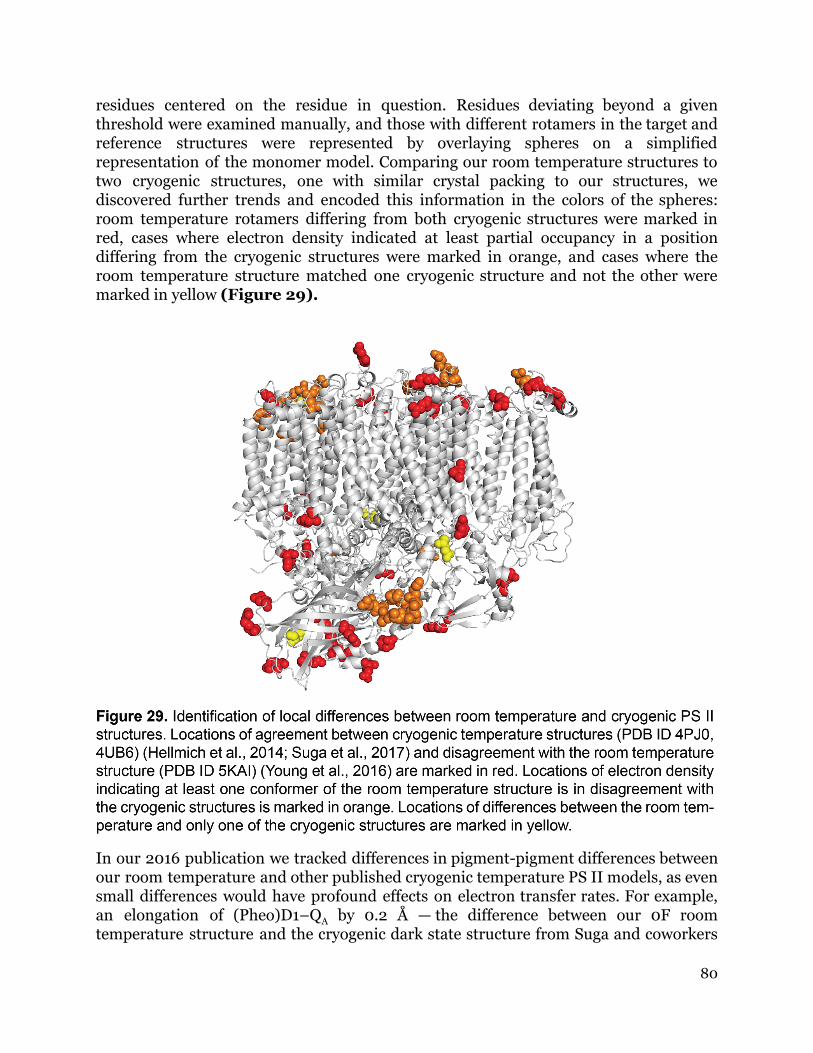
residues centered on the residue in question. Residues deviating beyond a given

threshold were examined manually, and those with different rotamers in the target and

reference structures were represented by overlaying spheres on a simplified

representation of the monomer model. Comparing our room temperature structures to

two cryogenic structures, one with similar crystal packing to our structures, we

discovered further trends and encoded this information in the colors of the spheres:

room temperature rotamers differing from both cryogenic structures were marked in

red, cases where electron density indicated at least partial occupancy in a position

differing from the cryogenic structures were marked in orange, and cases where the

room temperature structure matched one cryogenic structure and not the other were

marked in yellow (Figure 29).

In our 2016 publication we tracked differences in pigment-pigment differences between

our room temperature and other published cryogenic temperature PS II models, as even

small differences would have profound effects on electron transfer rates. For example,

an elongation of (Pheo)D1–QA

by 0.2 Å — the difference between our 0F room

temperature structure and the cryogenic dark state structure from Suga and coworkers

80

— is calculated to slow electron transfer rates between these sites by 25% (Moser et al.

1992). Despite a small sample size that precluded determination of statistical

significance, we identified pairs of pigments that appear to differ between the cryogenic

and room temperature structures as well as pairs of pigments that appear to be affected

by crystal packing (Figure 30). Some pairs of cofactors appear to vary with crystal

packing, some appear to be temperature-dependent, and no trend consistent across

both monomers is visible for others.

81

82

7.3 Structure of the Oxygen-Evolving Complex

7.3.1 Bonding and Coordination Distances

We analyzed metal-metal and metal-oxygen bonding distances in the OEC as well as

lengths of interactions between the OEC and coordinating waters and ligands for models

in all S-states (Figure 31). We adjusted rigidities of bonding restraints within the OEC

to minimize both difference density and deviation from spectroscopically and chemically

reasonable distances, where applicable. Refined metal-metal distances at the close of

refinement are in good agreement with spectroscopic data and changes primarily to the

light atoms at/near the OEC can be observed, including small changes to residues near

the OEC (Figure 32).

Water insertion by the S3 state is observed in the 2F structure and supported by the

inserted water omit map (Figure 33). The nearby glutamate shifts to accommodate the

83

84

new coordination of Ca to the inserted Ox so the coordination number does not change.

The position of Ox differs from the recently-reported O6 in the same state (Suga et al.

2017). The distance we model does not support a bond between O5 and Ox (2.1 Å apart)

as was modeled between O5 and O6 (1.5 Å apart) in the structure by Suga and

coworkers. This is in better agreement with the redox states of the Mn in the S3

state and

the expected energy landscape at this stage in the Kok cycle.

The timing of water insertion is trackable with isomorphous difference maps between

the S2

and S3

states (Figure 34). Ox is visible starting from the structure 400 µs after

the second illumination. Isomorphous difference maps in other regions of the protein in

the metastable states match turnover of the OEC (Figure 35), which is independently

supported by analysis of the XES data collected on the same crystals (Figure 36).

85

7.3.2 Substrate Water Binding

We have reported an ammonia-bound 2F structure where ammonia is bound in place of

water at one of the metal centers (Young, Ibrahim and Chatterjee et al. 2016). The

ammonia-treated crystals are redox-active, implying that the site of ammonia binding at

the OEC is not the site of a water molecule participating in the water-splitting

mechanism. The two waters W1 and W2 coordinating Mn4 and the bridging oxo O5 are

possible sites of ammonia binding. As we do not observe disruption to the geometry of

the cluster upon ammonia binding, which would be expected with the substitution of an

amido or imido bridge for the µ-oxo bridge, we eliminate O5 as a binding site. Weak

electron density and an altered coordination environment at the W2 site relative to a

native 2F structure implicate W2 as the most likely ammonia binding site (Figure 37).

Based on this evidence, W2 is disfavored as a possible site for substrate water binding.

Proposed mechanisms for O-O bond formation have favored using W1, W2, W3, W4, O4

and/or O5 as substrate oxygen atoms (Cox et al. 2014; Chernev et al. 2016; Askerka et

al. 2014; Dau et al. 2008; Noguchi 2015) (Figure 38). Based on the ammonia binding

study, we disfavor mechanisms including W2. The presence of an inserted Ox in the S3

state suggests involvement of this oxygen, although it may also be a position where

water is held to refill another position after dioxygen release. Favored mechanisms

include a radical reaction where the O-O bond is formed between O5 and Ox, refilling

the cluster from W3, and nucleophilic attack of W3 at O5, with Ox held in reserve to

refill the O5 position.

86

7.4 Water and Hydrogen Bonding Networks

7.4.1 Changes of the Water Channels

A series of channels connect the OEC to bulk solvent (Figure 39). They have been

analyzed previously by crystallography and molecular dynamics simulations to test the

possibility of substrate water access by each channel (Ho and Styring 2008; Vassiliev,

Zaraiskaya, and Bruce 2012; Murray and Barber 2007; Gabdulkhakov et al. 2009;

Umena et al. 2011; Sakashita et al. 2017). We identify five water channels, of which

three are interrupted in at least one S-state. These might function as gated channels or

only as hydrogen bonding networks capable of proton transfer. Appearance and

disappearance or shifts of waters between S-states can also be seen in three channels

(Figure 40). All the water channels approach the OEC via W3.

Changes in water positions in three of the channels may be relevant to substrate water

approach to the OEC. The toggling behavior of the W26-O1 distance between long and

short over the cycle of four metastable states is consistent with a switchable hydrogen

bonding interaction possibly connected to water movement. Movements in W26-30 also

suggest involvement of the O1 channel in water approach to the OEC. An alternative

hypothesis is water approach via the Cl1 water channel: appearance and disappearance

of W20 could be the mechanism of a valve on this channel.

Connection of the OEC to all water channels via W3 implies W3 is involved in the water

oxidation mechanism in some capacity, if not as a substrate then in association with

water replacement after dioxygen release. The fact that the W3B position is observed

only in the S0 state lends support to a role in restoring the OEC: use of W3 to restore the

87

88

S0

structure would match replacement of W3 from bulk solvent, in which case the partial

occupancy W3B might be explained as a temporary position of the replacement water.

89

7.4.2 Analysis of O-O Bond Forming Mechanisms

Based on the above evidence, we favor mechanisms for water oxidation involving W3

and Ox either as substrates or as refilling another position upon release of dioxygen. We

describe three mechanisms that meet these requirements (Figure 41).

90

7.5 Estimations of Uncertainty

7.5.1 Simulated Annealing Omit Map Fitting

The maximum likelihood estimate of coordinate error written to PDB headers during

refinement is a limited measurement of positional uncertainty. Large units may be

placed with high accuracy while atoms in flexible loops have highly uncertain positions.

In our earlier structures, we estimated positional precision of representative structural

units by setting zero occupancy of these units, generating a simulated annealing omit

map of the unit, acquiring the rigid body fit of the full occupancy unit to the difference

density, and measuring the magnitude of the shift between the centers of mass of the

alpha carbons before and after this process. For transmembrane helices the shift was

less than 0.08 Å in all structures (ranging from 3.0 to 2.25 Å resolution), while a

chlorophyll experienced at most a 0.13 Å shift (Young, Ibrahim and Chatterjee et al.

2016). This method had the advantage of producing context-dependent uncertainties,

but at significant computational cost.

7.5.2 Map and Model Kicking with END/RAPID

To estimate the uncertainties in the OEC structures in our most recent results (Kern et

al., in press), we used command line tool END/RAPID and the Phenix package to

effectively add error bars to both the model and the data (Lang et al. 2014). We

randomly perturbed structure factor amplitudes by ±|Fobs

- Fmodel| to add noise

proportional to the error in the model, and we "kicked" models in Phenix prior to the

start of refinement. We repeated this procedure over 100 trials and assessed the

agreement of the re-refined models. The position of any size group from an individual

atom to a complete protein could be determined from these results, and although the

procedure was even more computationally expensive than the previous method, it was

easily submitted as a series of jobs to a computing cluster, required less human

intervention and subjective interpretation, and was not limited to preselected structural

units.

To visualize results of the analysis with END/RAPID, we again automated generation of

diagrams in Illustrator. Starting from the distance calculation and visualization tools

described above, we added scripts to select OEC distances from the csv files, calculate

means and standard deviations of these distances over the 100 trials, and reformat these

for importing into Adobe Illustrator figures displaying the OEC geometry uncertainties

(Figure 42).

91

92

Chapter 8

Summary of Findings

The structure of photosystem II (PS II) has been reported to high resolution (Umena et

al. 2011), damage-free (Kern et al. 2013; Suga et al. 2015), at room temperature (Kern et

al. 2013; Suga et al. 2017), and in metastable illuminated states under all of the above

conditions (Young, Ibrahim and Chatterjee et al. 2016; Suga et al. 2017). We have also

recently accessed additional metastable and transient illuminated states (Kern et al., in

press). In less than a decade we have advanced in our understanding of the water

splitting, oxygen evolving mechanism from early proposed models of metal cluster

structures to fine-grained analysis of structural changes at the catalytic center on the

microsecond time scale, informed by complementary methods including EPR,

measurement of oxygen evolution under flashed illumination by Clark electrode or

MIMS, QM/MM, XRD, XES, EXAFS and X-ray absorption near edge structure (XANES)

(Hellmich et al. 2014; Glöckner et al. 2013; Wei et al. 2016; Siegbahn 2013; Askerka et

al. 2014; Vittal K. Yachandra et al. 1986; V. K. Yachandra et al. 1987; Renger and

Renger 2008; Vinyard, Ananyev, and Dismukes 2013; Chernev et al. 2016; Cox et al.

2014; Noguchi 2015; Dau et al. 2008; Tanaka, Fukushima, and Kamiya 2017). We are

poised to approach the question of how water approaches the oxygen-evolving complex

(OEC) and by what route(s) dioxygen escapes, and we are equipped to examine electron

transfer rates and to design mutations to study the involvement of sidechains in the

water splitting mechanism, possible valved water channels, and hydrogen bonding

networks.

8.1 Crystallization and Sample Delivery Conditions

8.1.1 Improving Crystal Hit Rates and Diffraction Quality

We have established reproducible conditions for acquiring high resolution PS II

diffraction. Prior to 2015 the quality of diffraction from PS II crystals was a major

barrier, and until 2016 crystal hit rates were the secondary limiting factor in dataset

quality. Advancements in crystallization procedures to produce monodisperse PS II

microcrystals (Ibrahim et al. 2015) and the development of the drop-on-demand sample

delivery system (Fuller and Gul et al. 2017) have alleviated these limitations. New

feedback capabilities in the cctbx.xfel GUI have made it possible to screen crystal

diffraction quality in real time, further improving rates of high resolution diffraction

93

data collection. Finally, new software in the cctbx.xfel framework has improved the

quality of data obtained from XFEL diffraction image sets (Winter et al. 2018; Sauter

2015; Brewster et al., in press). At the time of writing, we are continuing to investigate

optimal treatment of the data from three recent PS II XFEL experiments.

8.1.2 Dehydration-Dependent Nonisomorphism in Photosystem II

A particular challenge has been isolation of the crystallization and sample delivery

conditions producing uniform crystal forms and high resolution diffraction. We

discovered six crystal forms produced under similar conditions and identified the

factors controlling the partitioning between these forms: concentrations of

cryoprotectants used in crystallization and sample delivery buffers, the speed of the

dehydration steps, and the length of time exposed to air, helium or vacuum during

sample delivery all influenced dehydration and impacted the proportions of crystal

forms observed. The crystal forms also differed in diffraction quality, with the trend that

crystals with c axes measuring ~310 Å consistently diffracted to higher resolution than

those with c axes near 280 or 330 Å. A crystal form with a=117.5 Å, b=222.8 Å, c=309.6

Å, α=β=γ=90° and the space group P212121 was identified as the form diffracting to the

highest resolution. During LQ39 we identified the conditions producing predominantly

this form and collected datasets in multiple metastable and transient illuminated states

under these conditions. These data were successfully merged with data collected in two

previous experiments, LN84 and LM51, after filtering out batches for which analysis of

the XES spectra indicated poor reaction center turnover.

8.2 Room Temperature Structure of Photosystem II

8.2.1 Anisotropic Monomer and Dimer Expansion at Room

Temperature

Systematic differences between PS II structures indicate an anisotropic expansion of the

PS II monomers at room temperature relative to structures at cryogenic temperature

(Young, Ibrahim and Chatterjee et al. 2016). The monomers exhibit small isotropic

expansions and larger expansions in the plane of the thylakoid membrane. PS II dimers

also exhibit a hinging motion with temperature change. Although the published

structures of PS II at cryogenic temperature are good models for simulations at larger

scales, excitation and electron transfer rates are highly sensitive to inter-cofactor

distances. For calculations sensitive to precision in cofactor-cofactor distances, high

resolution structures at room temperature are necessary to reproduce the expected

behavior in natural systems.

8.2.2 Temperature Dependence of Rotamer Populations

94

We recently showed there are also many more sites of multiple conformers at room

temperature than at cryogenic temperature, as well as cases where single conformers at

room temperature differ from those at cryogenic temperature (Young, Ibrahim and

Chatterjee et al. 2016). Not surprisingly, a majority of temperature-dependent rotamer

differences were observed in solvent-exposed regions of the protein, where interactions

with the solvent would be affected by the different behaviors of liquid water and vitreous

ice. These observations are in line with similar trends in other systems (Keedy et al.

2015).

8.3 Structural Changes at the Oxygen-Evolving Complex

8.3.1 Structures in All Metastable and Two Transient States

We report the highest resolution room temperature structures of the 0F (S

1,

dark-adapted), 1F (S2-enriched), 2F (S

3-enriched) and 3F (S0-enriched) metastable

states and the first transient state structures, probed 150 and 400 µs after the 2nd

illumination (Kern et al., in press). An open cubane-like structure at the catalytic cluster

is preserved throughout the Kok cycle, and only slight metal movements are observed.

Isomorphous difference maps at plastoquinone B show features consistent with

reduction to the semiquinone in the S2

state and replacement of the fully reduced quinol

with a new quinone in the S3

state. Features of isomorphous difference maps of the

states between S2

and S3

relative to the dark state match the temporary reduction of

plastoquinone A prior to completing electron transfer to semiquinone B. XES data also

confirm turnover in all metastable states.

8.3.2 Water Insertion in the S3 State

The site and timing of water insertion at the OEC has recently been the subject of

contradictory results or interpretations (Young, Ibrahim and Chatterjee et al. 2016;

Suga et al. 2017). Our previous structure in the S3

state did not exhibit clear indication

of an inserted water, while the alternative structure at comparable resolution modeled

an O6 inserted water position at a peroxide bond-forming distance from O5 in this state.

At the present higher resolution, we have resolved the position of an inserted water in

the S3

state (Kern et al., in press). The inserted water or hydroxide Ox is bound to Mn1

and Ca and located 2.1 Å from the nearby O5 in the metastable S3

state, and it first binds

between 150 µs and 400 µs after illumination of the S2

state. At this position, Ox is not

interacting with O5, and multiple possible pairs of oxygen atoms remain eligible to

participate in O-O bond formation.

8.3.3 Coordinating Residue Shifts

95

We observe small shifts in residues coordinating the OEC that are mostly consistent

between monomers. Only the shift of Glu 189 is linked to a change in coordination state:

the glutamate pulls away from Ca in the S3

state, in which Ca coordinates Ox instead,

allowing Ca to remain 8-coordinate throughout the cycle.

8.4 Water Approach to the Oxygen-Evolving Complex

8.4.1 Water Network Analysis

Examination of water positions across the most recent series of structures revealed

significant changes between the S-states, consistent across monomers. Movements in

W26-30 and the connection of all channels to the OEC via W3 suggest participation of

W3 as the access point of the OEC to the bulk solvent. W3 may function as either a

substrate or a position of a water kept in store for replacement of another OEC oxygen

atom, explaining the partial occupancy W3B in the S0 state.

8.4.2 Proposed Mechanisms

An ammonia-bound, redox-active S3

state structure provides evidence that W2 does not

participate in the water splitting mechanism. Several proposed mechanisms forming the

O-O bond with W2 are disfavored on this basis. An inserted water Ox bound to Mn1 in

our most recent high resolution structure of the S3

state is likely to be involved as either

a substrate water or the water refilling the O5 position after dioxygen release. We

identify three proposed mechanisms satisfying these conditions and with water

approach via W3 as the most likely mechanisms for water oxidation.

8.4.3 Hydrogen Bonding Network Analysis

Some water channels contain bottlenecks preventing connection of the OEC to bulk

water by these routes. These channels remain hydrogen bonding networks for possible

proton transfer, however. Other channels appear to have bottlenecks in only some

S-states. These may also be functional as valved water channels, regulating the timing of

water exchange.

96

Chapter 9

Future Directions

New directions of inquiry remain for all components of the work discussed here. The

sample delivery and data processing efforts are areas of particular promise where major

advancements are anticipated over the next years. Improving reliability of the PS II

crystallization procedure and better understanding the factors leading to multiple

crystal forms from a single batch is another priority in the near term. The next goal in

PS II analysis is investigation of transient states near the O-O bond forming step,

hopefully producing direct evidence in support of a particular mechanism. Based on the

progress made so far and the anticipated rates of data acquisition in upcoming

experiments, we estimate elucidation of the complete mechanism of water oxidation in

PS II is within reach in five years.

9.1 Instrumentation and Experimental Design

9.1.1 New Drop-on-Demand Systems

Additional improvements to the acoustic droplet ejection/drop-on-tape system are

underway with the engineering and testing of a new design. The next generation of the

drop-on-demand system reduces instability by switching from a free conveyor belt to a

circular, solid support from which a kapton tape protrudes along one edge. X-rays pass

through the tape nearly perpendicular to the axis of rotation, missing the tape on the far

side of the circle. Kapton absorption is uniform and much reduced in this geometry.

Early experiments using this design at SACLA were successful and also revealed areas

for improvement.

Engineering of a design that can be used at multiple facilities is also a priority.

Construction of LCLS-II, the next generation of the linear accelerator delivering 1

million pulses per second, will interrupt user access to LCLS for a year starting in

December 2018. We plan to test the new drop-on-demand system at SACLA starting in

2019 and again at LCLS in 2020. In the long term we hope the system can also be used

for serial synchrotron crystallography.

97

9.2 Data Processing

9.2.1 Exascale Computing at NERSC

Pending the design of diffraction experiments that take advantage of these capabilities,

data collection rates at the European XFEL and LCLS-II can be expected to overwhelm

current data processing capabilities. Moreover, data triaging is predicted to become a

requirement at such experiments. The ExaFEL project plans to address these concerns

in the coming years, beginning by taking full advantage of multiprocessing capabilities

at NERSC. Upcoming EuXFEL experiments will provide excellent testing ground for

progress in this direction.

9.2.2 The cctbx.xfel GUI Refactor

A complete redesign of the cctbx.xfel GUI will be necessary for support of XFEL

experiments producing significantly more data than current LCLS experiments. As the

timing will coincide with the shift to Python 3 throughout the cctbx code, the next GUI

will likely switch from wxWidgets to QT. A higher-capacity replacement for the MySQL

database will also be necessary. The refactor is in the early design stages and will be

informed by lessons learned during the very successful lifetime of the first generation

cctbx.xfel GUI.

9.2.3 Difference Refinement

Moving toward comparison of many closely-related datasets makes difference

refinement a promising alternative to standard structure refinement and examination of

isomorphous difference maps (Terwilliger and Berendzen 1995). We have immediate

plans to investigate our existing PS II datasets by this method.

9.3 Unresolved Questions

9.3.1 Approaching the Oxygen-Oxygen Bond-Forming Step

Present datasets are of sufficiently high resolution to resolve oxygen positions.

Obtaining PS II datasets in transient states near the O-O bond forming step would allow

direct investigation of metal and oxygen movements in the OEC accommodating this

reaction. Although we will not be able to distinguish between oxo and hydroxyl groups

by identification of protons, metal-oxygen distances will provide complementary

information that will help resolve the mechanism. We plan to continue this investigation

at LCLS and SACLA.

98

9.3.2 Tracking Water Approach and Dioxygen Release

Analysis of water networks in our present datasets has already been highly informative

as to possible routes of water approach to the OEC. Continuing this line of inquiry with

additional structures between the S3 and S

0 states is another exciting possibility.

Acknowledgements

This work was supported by NIH Grant GM117126.

99

References

Adams, Paul D., Pavel V. Afonine, Gábor Bunkóczi, Vincent B. Chen, Ian W. Davis,

Nathaniel Echols, Jeffrey J. Headd, et al. 2010. “PHENIX: A Comprehensive

Python-Based System for Macromolecular Structure Solution.” Acta

Crystallographica. Section D, Biological Crystallography 66 (Pt 2): 213–21.

Afonine, Pavel V., Nigel W. Moriarty, Marat Mustyakimov, Oleg V. Sobolev, Thomas C.

Terwilliger, Dusan Turk, Alexandre Urzhumtsev, and Paul D. Adams. 2015. “FEM:

Feature-Enhanced Map.” Acta Crystallographica. Section D, Biological

Crystallography 71 (Pt 3): 646–66.

Alonso-Mori, Roberto, Jan Kern, Richard J. Gildea, Dimosthenis Sokaras, Tsu-Chien

Weng, Benedikt Lassalle-Kaiser, Rosalie Tran, et al. 2012. “Energy-Dispersive

X-Ray Emission Spectroscopy Using an X-Ray Free-Electron Laser in a

Shot-by-Shot Mode.” Proceedings of the National Academy of Sciences of the

United States of America 109 (47): 19103–7.

Alonso-Mori, Roberto, Jan Kern, Dimosthenis Sokaras, Tsu-Chien Weng, Dennis

Nordlund, Rosalie Tran, Paul Montanez, et al. 2012. “A Multi-Crystal Wavelength

Dispersive X-Ray Spectrometer.” The Review of Scientific Instruments 83 (7):

073114.

Andrews, Lawrence C., and Herbert J. Bernstein. 2014. “The Geometry of Niggli

Reduction: BGAOL -Embedding Niggli Reduction and Analysis of Boundaries.”

Journal of Applied Crystallography 47 (Pt 1): 346–59.

Askerka, Mikhail, Jimin Wang, Gary W. Brudvig, and Victor S. Batista. 2014. “Structural

Changes in the Oxygen-Evolving Complex of Photosystem II Induced by the S1 to

S2 Transition: A Combined XRD and QM/MM Study.” Biochemistry 53 (44):

6860–62.

Balaban, Teodor Silviu. 2005. “Relevance of the Diastereotopic Ligation of Magnesium

Atoms of Chlorophylls in the Major Light-Harvesting Complex II (LHC II) of Green

Plants.” Photosynthesis Research 86 (1-2): 251–62.

Balaban, Teodor Silviu, Paula Braun, Christof Hättig, Arnim Hellweg, Jan Kern,

Wolfram Saenger, and Athina Zouni. 2009. “Preferential Pathways for

Light-Trapping Involving Beta-Ligated Chlorophylls.” Biochimica et Biophysica

Acta 1787 (10): 1254–65.

Bao, Han, and Robert L. Burnap. 2016. “Photoactivation: The Light-Driven Assembly of

the Water Oxidation Complex of Photosystem II.” Frontiers in Plant Science 7

(May): 578.

Barends, Thomas R. M., Lutz Foucar, Albert Ardevol, Karol Nass, Andrew Aquila,

Sabine Botha, R. Bruce Doak, et al. 2015. “Direct Observation of Ultrafast Collective

Motions in CO Myoglobin upon Ligand Dissociation.” Science 350 (6259): 445–50.

Barends, Thomas, Thomas A. White, Anton Barty, Lutz Foucar, Marc Messerschmidt,

Roberto Alonso-Mori, Sabine Botha, et al. 2015. “Effects of Self-Seeding and Crystal

Post-Selection on the Quality of Monte Carlo-Integrated SFX Data.” Journal of

Synchrotron Radiation 22 (3): 644–52.

100

Barty, Anton, Richard A. Kirian, Filipe R. N. C. Maia, Max Hantke, Chun Hong Yoon,

Thomas A. White, and Henry Chapman. 2014. “Cheetah: Software for

High-Throughput Reduction and Analysis of Serial Femtosecond X-Ray Diffraction

Data.” Journal of Applied Crystallography 47 (Pt 3): 1118–31.

Berman, H. M., J. Westbrook, Z. Feng, G. Gilliland, T. N. Bhat, H. Weissig, I. N.

Shindyalov, and P. E. Bourne. 2000. “The Protein Data Bank.” Nucleic Acids

Research 28 (1): 235–42.

Black, M., R. H. B. Mais, and P. G. Owston. 1969. “The Crystal and Molecular Structure

of Zeise’s Salt, KPtCl3.C2H4.H2O.” Crystallographica Section B. https://onlinelibrary.wiley.com/doi/abs/10.1107/S0567740869004699.

Blankenship, Robert E. 2014. Molecular Mechanisms of Photosynthesis. John Wiley &

Sons.

Blanton, T. N., T. C. Huang, H. Toraya, C. R. Hubbard, S. B. Robie, D. Louër, H. E.

Göbel, G. Will, R. Gilles, and T. Raftery. 1995. “JCPDS—International Centre for

Diffraction Data Round Robin Study of Silver Behenate. A Possible Low-Angle

X-Ray Diffraction Calibration Standard.” Powder Diffraction 10 (02): 91–95.

Brewster, Aaron S., David G. Waterman, James M. Parkhurst, Richard J. Gildea, Iris D.

Young, Lee J. O’Riordan, Junko Yano, Graeme Winter, Gwyndaf Evans, and

Nicholas K. Sauter. in press “Improving Signal Strength in Serial Crystallography

with DIALS Geometry Refinement.” Acta Crystallogr D Biol Crystallogr. Cartlidge, Edwin. 2016. “European XFEL to Shine as Brightest, Fastest X-Ray Source.”

Science 354 (6308): 22–23.

Chapman, Henry N., Petra Fromme, Anton Barty, Thomas A. White, Richard A. Kirian,

Andrew Aquila, Mark S. Hunter, et al. 2011. “Femtosecond X-Ray Protein

Nanocrystallography.” Nature 470 (7332): 73–77.

Chernev, Petko, Ivelina Zaharieva, Emanuele Rossini, Artur Galstyan, Holger Dau, and

Ernst-Walter Knapp. 2016. “Merging Structural Information from X-Ray

Crystallography, Quantum Chemistry, and EXAFS Spectra: The Oxygen-Evolving

Complex in PSII.” The Journal of Physical Chemistry. B, October.

https://doi.org/10.1021/acs.jpcb.6b05800. Colletier, Jacques-Philippe, Michael R. Sawaya, Mari Gingery, Jose A. Rodriguez, Duilio

Cascio, Aaron S. Brewster, Tara Michels-Clark, et al. 2016. “De Novo Phasing with

X-Ray Laser Reveals Mosquito Larvicide BinAB Structure.” Nature 539 (7627):

43–47.

Cox, Nicholas, Marius Retegan, Frank Neese, Dimitrios A. Pantazis, Alain Boussac, and

Wolfgang Lubitz. 2014. “Photosynthesis. Electronic Structure of the

Oxygen-Evolving Complex in Photosystem II prior to O-O Bond Formation.”

Science 345 (6198): 804–8.

Dau, Holger, Alexander Grundmeier, Paola Loja, and Michael Haumann. 2008. “On the

Structure of the Manganese Complex of Photosystem II: Extended-Range EXAFS

Data and Specific Atomic-Resolution Models for Four S-States.” Philosophical

Transactions of the Royal Society of London. Series B, Biological Sciences 363

(1494): 1237–43; discussion 1243–44.

DePonte, D. P., U. Weierstall, K. Schmidt, J. Warner, D. Starodub, J. C. H. Spence, and

R. B. Doak. 2008. “Gas Dynamic Virtual Nozzle for Generation of Microscopic

101

Droplet Streams.” Journal of Physics D: Applied Physics 41 (19): 195505.

Diederichs, K., and P. A. Karplus. 2013. “Better Models by Discarding Data?” Acta

Crystallographica. Section D, Biological Crystallography 69 (Pt 7): 1215–22.

Doerr, Allison. 2011. “Diffraction before Destruction.” Nature Methods 8 (4): 283.

Emsley, Paul, and Kevin Cowtan. 2004. “Coot: Model-Building Tools for Molecular

Graphics.” Acta Crystallographica. Section D, Biological Crystallography 60 (Pt

12 Pt 1): 2126–32.

Flügge, Ulf-Ingo, Peter Westhoff, and Dario Leister. 2016. “Recent Advances in

Understanding Photosynthesis.” F1000Research 5 (December): 2890.

Franklin, R. E., and R. G. Gosling. 1953. “Molecular Configuration in Sodium

Thymonucleate.” Nature 171 (4356): 740–41.

Fraser, James S., Henry van den Bedem, Avi J. Samelson, P. Therese Lang, James M.

Holton, Nathaniel Echols, and Tom Alber. 2011. “Accessing Protein Conformational

Ensembles Using Room-Temperature X-Ray Crystallography.” Proceedings of the

National Academy of Sciences of the United States of America 108 (39): 16247–52.

Fuller, Franklin D., Sheraz Gul, Ruchira Chatterjee, E. Sethe Burgie, Iris D. Young, Hugo

Lebrette, Vivek Srinivas, et al. 2017. “Drop-on-Demand Sample Delivery for

Studying Biocatalysts in Action at X-Ray Free-Electron Lasers.” Nature Methods 14

(4): 443–49.

Gabdulkhakov, Azat, Albert Guskov, Matthias Broser, Jan Kern, Frank Müh, Wolfram

Saenger, and Athina Zouni. 2009. “Probing the Accessibility of the Mn4Ca Cluster

in Photosystem II: Channels Calculation, Noble Gas Derivatization, and

Cocrystallization with DMSO.” Structure 17 (9): 1223–34.

Galayda, John. 2014. “The New LCLS-II Project : Status and Challenges.” In

Proceedings, 27th Linear Accelerator Conference, LINAC2014: Geneva,

Switzerland, August 31-September 5, 2014, TUIOA04.

Garman, Elspeth F., and Colin Nave. 2009. “Radiation Damage in Protein Crystals

Examined under Various Conditions by Different Methods.” Journal of

Synchrotron Radiation 16 (Pt 2): 129–32.

Garman, Elspeth F., and Martin Weik. 2017. “Radiation Damage in Macromolecular

Crystallography.” Methods in Molecular Biology 1607: 467–89.

Giannessi, L., A. Bacci, M. Bellaveglia, F. Briquez, M. Castellano, E. Chiadroni, A.

Cianchi, et al. 2011. “Self-Amplified Spontaneous Emission Free-Electron Laser

with an Energy-Chirped Electron Beam and Undulator Tapering.” Physical Review

Letters 106 (14): 144801.

Glaeser, R., M. Facciotti, P. Walian, S. Rouhani, J. Holton, A. MacDowell, R. Celestre, D.

Cambie, and H. Padmore. 2000. “Characterization of Conditions Required for

X-Ray Diffraction Experiments with Protein Microcrystals.” Biophysical Journal 78

(6): 3178–85.

Glöckner, Carina, Jan Kern, Matthias Broser, Athina Zouni, Vittal Yachandra, and

Junko Yano. 2013. “Structural Changes of the Oxygen-Evolving Complex in

Photosystem II during the Catalytic Cycle.” The Journal of Biological Chemistry

288 (31): 22607–20.

Grabolle, Markus, Michael Haumann, Claudia Müller, Peter Liebisch, and Holger Dau.

2006. “Rapid Loss of Structural Motifs in the Manganese Complex of Oxygenic

102

Photosynthesis by X-Ray Irradiation at 10-300 K.” The Journal of Biological

Chemistry 281 (8): 4580–88.

Groom, Colin R., and Frank H. Allen. 2014. “The Cambridge Structural Database in

Retrospect and Prospect.” Angewandte Chemie 53 (3): 662–71.

Gust, Devens, David Kramer, Ana Moore, Thomas A. Moore, and Wim Vermaas. 2008.

“Engineered and Artificial Photosynthesis: Human Ingenuity Enters the Game.”

MRS Bulletin / Materials Research Society 33 (4): 383–87.

Hart, P., S. Boutet, G. Carini, A. Dragone, B. Duda, D. Freytag, G. Haller, et al. 2012.

“The Cornell-SLAC Pixel Array Detector at LCLS.” In 2012 IEEE Nuclear Science

Symposium and Medical Imaging Conference Record (NSS/MIC), 538–41.

Hatakeyama, Makoto, Koji Ogata, Katsushi Fujii, Vittal K. Yachandra, Junko Yano, and

Shinichiro Nakamura. 2016. “Structural Changes in the S3 State of the Oxygen

Evolving Complex in Photosystem II.” Chemical Physics Letters 651 (May):

243–50.

Hattne, Johan, Nathaniel Echols, Rosalie Tran, Jan Kern, Richard J. Gildea, Aaron S.

Brewster, Roberto Alonso-Mori, et al. 2014. “Accurate Macromolecular Structures

Using Minimal Measurements from X-Ray Free-Electron Lasers.” Nature Methods

11 (5): 545–48.

Hellmich, Julia, Martin Bommer, Anja Burkhardt, Mohamed Ibrahim, Jan Kern, Alke

Meents, Frank Müh, Holger Dobbek, and Athina Zouni. 2014. “Native-like

Photosystem II Superstructure at 2.44 Å Resolution through Detergent Extraction

from the Protein Crystal.” Structure 22 (11): 1607–15.

Henderson, Richard, Shaoxia Chen, James Z. Chen, Nikolaus Grigorieff, Lori A.

Passmore, Luciano Ciccarelli, John L. Rubinstein, R. Anthony Crowther, Phoebe L.

Stewart, and Peter B. Rosenthal. 2011. “Tilt-Pair Analysis of Images from a Range of

Different Specimens in Single-Particle Electron Cryomicroscopy.” Journal of

Molecular Biology 413 (5): 1028–46.

Hirata, Kunio, Kyoko Shinzawa-Itoh, Naomine Yano, Shuhei Takemura, Koji Kato, Miki

Hatanaka, Kazumasa Muramoto, et al. 2014. “Determination of Damage-Free

Crystal Structure of an X-Ray-Sensitive Protein Using an XFEL.” Nature Methods

11 (7): 734–36.

Ho, Felix M., and Stenbjörn Styring. 2008. “Access Channels and Methanol Binding Site

to the CaMn4 Cluster in Photosystem II Based on Solvent Accessibility Simulations,

with Implications for Substrate Water Access.” Biochimica et Biophysica Acta 1777

(2): 140–53.

Holton, James. Personal correspondence, 2016.

Holton, James M., and Kenneth A. Frankel. 2010. “The Minimum Crystal Size Needed

for a Complete Diffraction Data Set.” Acta Crystallographica. Section D, Biological

Crystallography 66 (Pt 4): 393–408.

Ibrahim, Mohamed, Ruchira Chatterjee, Julia Hellmich, Rosalie Tran, Martin Bommer,

Vittal K. Yachandra, Junko Yano, Jan Kern, and Athina Zouni. 2015.

“Improvements in Serial Femtosecond Crystallography of Photosystem II by

Optimizing Crystal Uniformity Using Microseeding Procedures.” Structural

Dynamics (Melville, N.Y.) 2 (4). https://doi.org/10.1063/1.4919741. Keedy, Daniel A., Lillian R. Kenner, Matthew Warkentin, Rahel A. Woldeyes, Jesse B.

103

Hopkins, Michael C. Thompson, Aaron S. Brewster, et al. 2015. “Mapping the

Conformational Landscape of a Dynamic Enzyme by Multitemperature and XFEL

Crystallography.” eLife 4 (September). https://doi.org/10.7554/eLife.07574. Kern, Jan, Roberto Alonso-Mori, Julia Hellmich, Rosalie Tran, Johan Hattne, Hartawan

Laksmono, Carina Glöckner, et al. 2012. “Room Temperature Femtosecond X-Ray

Diffraction of Photosystem II Microcrystals.” Proceedings of the National Academy

of Sciences of the United States of America 109 (25): 9721–26.

Kern, Jan, Roberto Alonso-Mori, Rosalie Tran, Johan Hattne, Richard J. Gildea,

Nathaniel Echols, Carina Glöckner, et al. 2013. “Simultaneous Femtosecond X-Ray

Spectroscopy and Diffraction of Photosystem II at Room Temperature.” Science

340 (6131): 491–95.

Kern, Jan, Ruchira Chatterjee, Iris D. Young, Franklin D. Fuller, Louise Lassalle,

Mohamed Ibrahim, Sheraz Gul, et al. in press “Structures of the Intermediates of

Kok’s Photosynthetic Water Oxidation Clock.” Nature. Kirian, Richard A., Xiaoyu Wang, Uwe Weierstall, Kevin E. Schmidt, John C. H. Spence,

Mark Hunter, Petra Fromme, Thomas White, Henry N. Chapman, and James

Holton. 2010. “Femtosecond Protein Nanocrystallography-Data Analysis Methods.”

Optics Express 18 (6): 5713–23.

Klauss, André, Roland Krivanek, Holger Dau, and Michael Haumann. 2009. “Energetics

and Kinetics of Photosynthetic Water Oxidation Studied by Photothermal Beam

Deflection (PBD) Experiments.” Photosynthesis Research 102 (2-3): 499–509.

Kok, B., B. Forbush, and M. McGloin. 1970. “Cooperation of Charges in Photosynthetic

O2 Evolution-I. A Linear Four Step Mechanism.” Photochemistry and

Photobiology 11 (6): 457–75.

Kubin, Markus, Jan Kern, Meiyuan Guo, Erik Källman, Rolf Mitzner, Vittal K.

Yachandra, Marcus Lundberg, Junko Yano, and Philippe Wernet. 2018.

“X-Ray-Induced Sample Damage at the Mn L-Edge: A Case Study for Soft X-Ray

Spectroscopy of Transition Metal Complexes in Solution.” Physical Chemistry

Chemical Physics: PCCP 20 (24): 16817–27.

Kumar, Sandeep, Heung-Sik Kang, and Dong Eon Kim. 2011. “Generation of Isolated

Single Attosecond Hard X-Ray Pulse in Enhanced Self-Amplified Spontaneous

Emission Scheme.” Optics Express 19 (8): 7537–45.

Lang, P. Therese, James M. Holton, James S. Fraser, and Tom Alber. 2014. “Protein

Structural Ensembles Are Revealed by Redefining X-Ray Electron Density Noise.”

Proceedings of the National Academy of Sciences of the United States of America

111 (1): 237–42.

Liebschner, Dorothee, Pavel V. Afonine, Nigel W. Moriarty, Billy K. Poon, Oleg V.

Sobolev, Thomas C. Terwilliger, and Paul D. Adams. 2017. “Polder Maps:

Improving OMIT Maps by Excluding Bulk Solvent.” Acta Crystallographica.

Section D, Structural Biology 73 (Pt 2): 148–57.

Li, Feifei, E. Sethe Burgie, Tao Yu, Annie Héroux, George C. Schatz, Richard D. Vierstra,

and Allen M. Orville. 2015. “X-Ray Radiation Induces Deprotonation of the Bilin

Chromophore in Crystalline D. Radiodurans Phytochrome.” Journal of the

American Chemical Society 137 (8): 2792–95.

Lomb, Lukas, Thomas R. M. Barends, Stephan Kassemeyer, Andrew Aquila, Sascha W.

104

Epp, Benjamin Erk, Lutz Foucar, et al. 2011. “Radiation Damage in Protein Serial

Femtosecond Crystallography Using an X-Ray Free-Electron Laser.” Physical

Review. B, Condensed Matter and Materials Physics 84 (21): 214111.

Lonsdale, K. 1928. “The Structure of the Benzene Ring.” Nature. https://www.nature.com/articles/122810c0.

Lyubimov, Artem Y., Monarin Uervirojnangkoorn, Oliver B. Zeldin, Qiangjun Zhou,

Minglei Zhao, Aaron S. Brewster, Tara Michels-Clark, et al. 2016. “Advances in

X-Ray Free Electron Laser (XFEL) Diffraction Data Processing Applied to the

Crystal Structure of the Synaptotagmin-1 / SNARE Complex.” eLife 5 (October).

https://doi.org/10.7554/eLife.18740. Mafuné, Fumitaka, Ken Miyajima, Kensuke Tono, Yoshihiro Takeda, Jun-Ya Kohno,

Naoya Miyauchi, Jun Kobayashi, et al. 2016. “Microcrystal Delivery by Pulsed

Liquid Droplet for Serial Femtosecond Crystallography.” Acta Crystallographica.

Section D, Structural Biology 72 (Pt 4): 520–23.

McCoy, Airlie J., Ralf W. Grosse-Kunstleve, Paul D. Adams, Martyn D. Winn, Laurent C.

Storoni, and Randy J. Read. 2007. “Phaser Crystallographic Software.” Journal of

Applied Crystallography 40 (Pt 4): 658–74.

Moser, C. C., J. M. Keske, K. Warncke, R. S. Farid, and P. L. Dutton. 1992. “Nature of

Biological Electron Transfer.” Nature 355 (6363): 796–802.

Muniyappan, Srinivasan, Seong Ok Kim, and Hyotcherl Ihee. 2015. “Recent Advances

and Future Prospects of Serial Crystallography Using XFEL and Synchrotron X-Ray

Sources.” Bio Des 3: 98–110.

Murray, James W., and James Barber. 2007. “Structural Characteristics of Channels

and Pathways in Photosystem II Including the Identification of an Oxygen

Channel.” Journal of Structural Biology 159 (2): 228–37.

Muybridge, Eadweard. 2012. Animals in Motion. Courier Corporation.

Nave, Colin. 2014. “Matching X-Ray Beam and Detector Properties to Protein Crystals

of Different Perfection.” Journal of Synchrotron Radiation 21 (Pt 3): 537–46.

Neutze, R., R. Wouts, D. van der Spoel, E. Weckert, and J. Hajdu. 2000. “Potential for

Biomolecular Imaging with Femtosecond X-Ray Pulses.” Nature 406 (6797):

752–57.

Noguchi, Takumi. 2015. “Fourier Transform Infrared Difference and Time-Resolved

Infrared Detection of the Electron and Proton Transfer Dynamics in Photosynthetic

Water Oxidation.” Biochimica et Biophysica Acta 1847 (1): 35–45.

Park, Sang Han, Minseok Kim, Changi-Ki Min, Intae Eom, Inhyuk Nam, Heung-Soo

Lee, Heung-Sik Kang, et al. 2018. “PAL-XFEL Soft X-Ray Scientific Instruments

and X-Ray Optics: First Commissioning Results.” The Review of Scientific

Instruments 89 (5): 055105.

Renger, Gernot, and Thomas Renger. 2008. “Photosystem II: The Machinery of

Photosynthetic Water Splitting.” Photosynthesis Research 98 (1-3): 53–80.

Riley, P. A. 1994. “Free Radicals in Biology: Oxidative Stress and the Effects of Ionizing

Radiation.” International Journal of Radiation Biology 65 (1): 27–33.

Roessler, Christian G., Rakhi Agarwal, Marc Allaire, Roberto Alonso-Mori, Babak Andi,

José F. R. Bachega, Martin Bommer, et al. 2016. “Acoustic Injectors for

Drop-On-Demand Serial Femtosecond Crystallography.” Structure 24 (4): 631–40.

105

Sakashita, Naoki, Hiroshi C. Watanabe, Takuya Ikeda, and Hiroshi Ishikita. 2017.

“Structurally Conserved Channels in Cyanobacterial and Plant Photosystem II.”

Photosynthesis Research 133 (1-3): 75–85.

Saldin, E. L., W. Sandner, Z. Sanok, H. Schlarb, G. Schmidt, P. Schmuser, J. R.

Schneider, et al. 2000. “First Observation of Self-Amplified Spontaneous Emission

in a Free-Electron Laser at 109 Nm Wavelength.” Physical Review Letters 85 (18):

3825–29.

Sauer, Kenneth, and Vittal K. Yachandra. 2002. “A Possible Evolutionary Origin for the

Mn4 Cluster of the Photosynthetic Water Oxidation Complex from Natural MnO2

Precipitates in the Early Ocean.” Proceedings of the National Academy of Sciences

of the United States of America 99 (13): 8631–36.

Sauter, Nicholas K. 2015. “XFEL Diffraction: Developing Processing Methods to

Optimize Data Quality.” Journal of Synchrotron Radiation 22 (2): 239–48.

Sauter, Nicholas K., Johan Hattne, Aaron S. Brewster, Nathaniel Echols, Petrus H.

Zwart, and Paul D. Adams. 2014. “Improved Crystal Orientation and Physical

Properties from Single-Shot XFEL Stills.” Acta Crystallographica. Section D,

Biological Crystallography 70 (Pt 12): 3299–3309.

Sauter, Nicholas K., Johan Hattne, Ralf W. Grosse-Kunstleve, and Nathaniel Echols.

2013. “New Python-Based Methods for Data Processing.” Acta Crystallographica.

Section D, Biological Crystallography 69 (Pt 7): 1274–82.

Sawaya, Michael R., Duilio Cascio, Mari Gingery, Jose Rodriguez, Lukasz Goldschmidt,

Jacques-Philippe Colletier, Marc M. Messerschmidt, et al. 2014. “Protein Crystal

Structure Obtained at 2.9 Å Resolution from Injecting Bacterial Cells into an X-Ray

Free-Electron Laser Beam.” Proceedings of the National Academy of Sciences of

the United States of America 111 (35): 12769–74.

Schubert, Wolf-Dieter, Olaf Klukas, Wolfram Saenger, Horst Tobias Witt, Petra

Fromme, and Norbert Krauß. 1998. “A Common Ancestor for Oxygenic and

Anoxygenic Photosynthetic Systems: A Comparison Based on the Structural Model

of Photosystem I11Edited by R. Huber.” Journal of Molecular Biology 280 (2):

297–314.

Sharma, Amit, Linda Johansson, Elin Dunevall, Weixiao Y. Wahlgren, Richard Neutze,

and Gergely Katona. 2017. “Asymmetry in Serial Femtosecond Crystallography

Data.” Acta Crystallographica. Section A, Foundations and Advances 73 (Pt 2):

93–101.

Shelley, Kathryn L., Thomas P. E. Dixon, Jonathan C. Brooks-Bartlett, and Elspeth F.

Garman. 2018. “RABDAM: Quantifying Specific Radiation Damage in Individual

Protein Crystal Structures.” Journal of Applied Crystallography 51 (Pt 2): 552–59.

Shoji, Mitsuo, Hiroshi Isobe, Ayako Tanaka, Yoshimasa Fukushima, Keisuke Kawakami,

Yasufumi Umena, Nobuo Kamiya, Takahito Nakajima, and Kizashi Yamaguchi.

2018. “Understanding Two Different Structures in the Dark Stable State of the

Oxygen-Evolving Complex of Photosystem II: Applicability of the Jahn-Teller

Deformation Formula.” ChemPhotoChem 2 (3): 257–70.

Siegbahn, Per E. M. 2013. “Water Oxidation Mechanism in Photosystem II, Including

Oxidations, Proton Release Pathways, O-O Bond Formation and O2 Release.”

Biochimica et Biophysica Acta 1827 (8-9): 1003–19.

106

Sierra, Raymond G., Cornelius Gati, Hartawan Laksmono, E. Han Dao, Sheraz Gul,

Franklin Fuller, Jan Kern, et al. 2016. “Concentric-Flow Electrokinetic Injector

Enables Serial Crystallography of Ribosome and Photosystem II.” Nature Methods

13 (1): 59–62.

“SLAC National Accelerator Laboratory Annual Laboratory Plan FY 2016.” 2016.

https://www-group.slac.stanford.edu/oa/documents/SLAC-FY16-ALP_5-13-16_FI

NAL.pdf. Slattery, R. A., D. R. Ort, and Others. 2014. “Improving Photosynthetic Efficiency for

Improved Yield: Are Crop Plants Too Green?” Aspects of Applied Biology /

Association of Applied Biologists, no. 124: 1–4.

Stan, Claudiu A., Despina Milathianaki, Hartawan Laksmono, Raymond G. Sierra,

Trevor A. McQueen, Marc Messerschmidt, Garth J. Williams, et al. 2016. “Liquid

Explosions Induced by X-Ray Laser Pulses.” Nature Physics 12 (May): 966.

Suga, Michihiro, Fusamichi Akita, Kunio Hirata, Go Ueno, Hironori Murakami, Yoshiki

Nakajima, Tetsuya Shimizu, et al. 2015. “Native Structure of Photosystem II at 1.95

Å Resolution Viewed by Femtosecond X-Ray Pulses.” Nature 517 (7532): 99–103.

Suga, Michihiro, Fusamichi Akita, Michihiro Sugahara, Minoru Kubo, Yoshiki

Nakajima, Takanori Nakane, Keitaro Yamashita, et al. 2017. “Light-Induced

Structural Changes and the Site of O=O Bond Formation in PSII Caught by XFEL.”

Nature 543 (7643): 131–35.

Tanaka, Ayako, Yoshimasa Fukushima, and Nobuo Kamiya. 2017. “Two Different

Structures of the Oxygen-Evolving Complex in the Same Polypeptide Frameworks

of Photosystem II.” Journal of the American Chemical Society 139 (5): 1718–21.

Terwilliger, T. C., and J. Berendzen. 1995. “Difference Refinement: Obtaining

Differences between Two Related Structures.” Acta Crystallographica. Section D,

Biological Crystallography 51 (Pt 5): 609–18.

Uervirojnangkoorn, Monarin, Oliver B. Zeldin, Artem Y. Lyubimov, Johan Hattne,

Aaron S. Brewster, Nicholas K. Sauter, Axel T. Brunger, and William I. Weis. 2015.

“Enabling X-Ray Free Electron Laser Crystallography for Challenging Biological

Systems from a Limited Number of Crystals.” eLife 4 (March).

https://doi.org/10.7554/eLife.05421. Umena, Yasufumi, Keisuke Kawakami, Jian-Ren Shen, and Nobuo Kamiya. 2011.

“Crystal Structure of Oxygen-Evolving Photosystem II at a Resolution of 1.9 Å.”

Nature 473 (7345): 55–60.

Vassiliev, Sergey, Tatiana Zaraiskaya, and Doug Bruce. 2012. “Exploring the Energetics

of Water Permeation in Photosystem II by Multiple Steered Molecular Dynamics

Simulations.” Biochimica et Biophysica Acta 1817 (9): 1671–78.

Vinyard, David J., Gennady M. Ananyev, and G. Charles Dismukes. 2013. “Photosystem

II: The Reaction Center of Oxygenic Photosynthesis.” Annual Review of

Biochemistry 82 (March): 577–606.

Watson, J. D., and F. H. Crick. 1953. “The Structure of DNA.” Cold Spring Harbor

Symposia on Quantitative Biology 18: 123–31.

Wei, Xuepeng, Xiaodong Su, Peng Cao, Xiuying Liu, Wenrui Chang, Mei Li, Xinzheng

Zhang, and Zhenfeng Liu. 2016. “Structure of Spinach Photosystem II-LHCII

Supercomplex at 3.2 Å Resolution.” Nature 534 (7605): 69–74.

107

White, Thomas A., Anton Barty, Francesco Stellato, James M. Holton, Richard A.

Kirian, Nadia A. Zatsepin, and Henry N. Chapman. 2013. “Crystallographic Data

Processing for Free-Electron Laser Sources.” Acta Crystallographica. Section D,

Biological Crystallography 69 (Pt 7): 1231–40.

White, Thomas A., Richard A. Kirian, Andrew V. Martin, Andrew Aquila, Karol Nass,

Anton Barty, and Henry N. Chapman. 2012. “\it CrystFEL: A Software Suite for

Snapshot Serial Crystallography.” Journal of Applied Crystallography 45 (2):

335–41.

White, William E., Aymeric Robert, and Mike Dunne. 2015. “The Linac Coherent Light

Source.” Journal of Synchrotron Radiation 22 (3): 472–76.

Winick, H. 1997. “Fourth Generation Light Sources.” In Proceedings of the 1997 Particle

Accelerator Conference (Cat. No.97CH36167), 1:37–41 vol.1.

Winter, Graeme, David G. Waterman, James M. Parkhurst, Aaron S. Brewster, Richard

J. Gildea, Markus Gerstel, Luis Fuentes-Montero, et al. 2018. “DIALS:

Implementation and Evaluation of a New Integration Package.” Acta

Crystallographica. Section D, Structural Biology 74 (Pt 2): 85–97.

Yabashi, Makina, Hitoshi Tanaka, and Tetsuya Ishikawa. 2015. “Overview of the SACLA

Facility.” Journal of Synchrotron Radiation 22 (3): 477–84.

Yachandra, Vittal K., R. D. Guiles, Ann McDermott, R. David Britt, S. L. Dexheimer,

Kenneth Sauer, and Melvin P. Klein. 1986. “The State of Manganese in the

Photosynthetic Apparatus: 4. Structure of the Manganese Complex in Photosystem

II Studied Using EXAFS Spectroscopy. The S1 State of the O2-Evolving

Photosystem II Complex from Spinach.” Biochimica et Biophysica Acta (BBA) -

Bioenergetics 850 (2): 324–32.

Yachandra, V. K., R. D. Guiles, A. E. McDermott, J. L. Cole, R. D. Britt, S. L. Dexheimer,

K. Sauer, and M. P. Klein. 1987. “Comparison of the Structure of the Manganese

Complex in the S1 and S2 States of the Photosynthetic O2-Evolving Complex: An

X-Ray Absorption Spectroscopy Study.” Biochemistry 26 (19): 5974–81.

Yano, Junko, Jan Kern, Klaus-Dieter Irrgang, Matthew J. Latimer, Uwe Bergmann,

Pieter Glatzel, Yulia Pushkar, et al. 2005. “X-Ray Damage to the Mn4Ca Complex in

Single Crystals of Photosystem II: A Case Study for Metalloprotein

Crystallography.” Proceedings of the National Academy of Sciences of the United

States of America 102 (34): 12047–52.

Yano, Junko, and Vittal Yachandra. 2014. “Mn4Ca Cluster in Photosynthesis: Where

and How Water Is Oxidized to Dioxygen.” Chemical Reviews 114 (8): 4175–4205.

Yano, Junko, and Vittal K. Yachandra. 2007. “Oxidation State Changes of the Mn4Ca

Cluster in Photosystem II.” Photosynthesis Research 92 (3): 289–303.

Young, Iris D., Mohamed Ibrahim, Ruchira Chatterjee, Sheraz Gul, Franklin Fuller,

Sergey Koroidov, Aaron S. Brewster, et al. 2016. “Structure of Photosystem II and

Substrate Binding at Room Temperature.” Nature 540 (7633): 453–57.

Zahnle, Kevin, Laura Schaefer, and Bruce Fegley. 2010. “Earth’s Earliest Atmospheres.”

Cold Spring Harbor Perspectives in Biology 2 (10): a004895.

Zeldin, Oliver B., Aaron S. Brewster, Johan Hattne, Monarin Uervirojnangkoorn, Artem

Y. Lyubimov, Qiangjun Zhou, Minglei Zhao, William I. Weis, Nicholas K. Sauter,

and Axel T. Brunger. 2015. “Data Exploration Toolkit for Serial Diffraction

108

Experiments.” Acta Crystallographica. Section D, Biological Crystallography 71

(Pt 2): 352–56.

Zhang, Miao, Martin Bommer, Ruchira Chatterjee, Rana Hussein, Junko Yano, Holger

Dau, Jan Kern, Holger Dobbek, and Athina Zouni. 2017. “Structural Insights into

the Light-Driven Auto-Assembly Process of the Water-Oxidizing Mn4CaO5-Cluster

in Photosystem II.” eLife 6 (July). https://doi.org/10.7554/eLife.26933. Zhu, Xin-Guang, Stephen P. Long, and Donald R. Ort. 2008. “What Is the Maximum

Efficiency with Which Photosynthesis Can Convert Solar Energy into Biomass?”

Current Opinion in Biotechnology 19 (2): 153–59.

———. 2010. “Improving Photosynthetic Efficiency for Greater Yield.” Annual Review of

Plant Biology 61: 235–61.

109