~

! N ( 1\'

.. .. .. .. •• •• ••

: J . .. ··; .. ~7 ••

. •

VICINITY MAP t"Lt 0# ••u•

---·-• • 0 0 • 0 I 0 0 0 0 f

.....,._.. __ _ ,. .. l . . - ,,. _. __ _

I

nit d St t nm nt

TECHNICAL REPORT HL-89-20

THERMAL ANALYSIS OF PROMPTON RESERVOIR MODIFICATION, PENNSYLVANIA

Numerical Model Investigation

by

Richard E. Price, Jeffery P. Holland

Hydraulics Laboratory

DEPARTMENT OF THE ARMY Waterways Experiment Station, Corps of Engineers

3909 Halls Ferry Road, Vicksburg, Mississippi 39180-6199

September 1989

Final Report

Approved For Public Release: Distribution Unlimited

R:=2EAR:H LIGRARY US ARMY C: ::1.; ::::-1 \~:t.-::?\WAYS

E'lo f'~--' -A- , . 'T r - .. -, ...._,~J ~ '-f •••4·-· • '""""o 11 \ . ~ - •

VIC!<SiJUn.J, fJ.:SCISSIPPI

Prepared tor US Army Engineer District, Philadelphia Philadelphia, Pennsylvania 19106-2991

USACEWES

TA7 W34 no.HL-8~20 c.3

IIIOCm~lm~I~IOOfl~iWnilll 3 5925 00095 1365

Destroy this report when no longer needed. Do not return it to the originator.

The findings in this report are not to be construed as an official Department of the Army position unless so designated

by other authorized documents.

The contents of this report are not to be used for advertising, publication, or promotional purposes. Citation of trade names does not constitute an official endorsement or approval of the use of

such commercial products.

Unclassified SECURITY CLASSIFICATION OF TI-41S PAGE

REPORT DOCUMENTATION PAGE Form AfJP'OWd OMB No. 0704-{)rSB

1 a . REPORT SECURITY CLASSIFICATION l b. RES TRICTIVE MARKINGS

Unclassified 2a. SECURITY CLASSIFICATION AUTHORITY 3 . DIS TRIBUTION I AVAILABILITY OF REPORT

Appr oved fo r publi c re l eas e; 2b. DECLASSIFICATION I DOWNGRADING SCHe DULE dis tribut i on unlimi ted.

4. PERFORMING ORGANIZATION REPORT NUMBER(S) 5. MONITORING ORGANIZATION REPORT NUMBER(S)

Technical Report HL-89- 20 ~. NAME OF PERFORMING ORGANIZATION 6b. OFFICE SYMBOL 7a. NAME OF MONITORING ORGANIZATION

USAEWES (If •pplic•bl•)

Hydr aulics Labora t or y CEWES- HS-H 6c. ADDRESS (City, St•t•. •nd ZIP Code) 7b. ADDRESS (Ci ty, St•t•. 4nd ZIP Code)

3909 Halls Ferry Road Vicksburg, MS 39180-6199

b . NAME OF FUNDING I SPONSORING 8b. OFFICE SYMBOL 9. PROCUREMENT INSTRUMENT IOENTIFICA TION NUMBER ORGANIZATION (tf •pplic•bl•)

USAED, Philadel phia 8c. ADDRESS (Ci ty, St•t•. •nd ZIP Code) 10. SOURCE OF FUNDING NUMBERS

US Custom House PROGRAM PROJECT TASK WORK UNIT 2nd & Chestnut Streets ELEMENT NO. NO. NO. ACCESSION NO.

Philadelphia, PA 19 106-299 1 1 1. TITLE (Inc/~ S.cumy Cl•mticanon)

Thermal Analys i s of Prompton Reservoir Modif i cation, Pennsylvania ; Numerical Mode l Investigati on

12. PERSONAL AUTHOR(S) Price, Richard E • ; Holland , Jeff ery P .

1 la. TYPE OF REPORT 1 lb. TIME COVERED 14. DATE OF REPORT (Y••r. Momlt, O•y) 1 S. PAGE COUNT

Final report FROM TO September 1989 67 16. SUPPLEMENTARY NOTATION

Available from National Technical I n fo rmation Service , 5285 Port Royal Road, Springfield , VA 22161.

17. COSA Tl CODES 18. SUBJECT TERMS (Concnu• on reverw 1f Mc•suty •nd icMntrfy by block number)

FIELD GROUP SUB-GROUP Numerical model Thermal Optimizat ion Wa t er supply Pr ompt on Reservoir

19, ABSTRACT (Contrnu• on ,..verw If Mc•SUIY •nd identify by block number)

Hydrologic studies of t he De lawa r e River Estuary have indicated that du r ing low flow

or drought periods , excessive sal ini ty intrusion int o the estuary may threaten water sup-plies in the Delaware River Basin . To assis t in the pr evention of this excessive salinity

intrusion, additional wate r s uppl y storage to Pr ompton Reservoir has been proposed. This additional storage would raise t he pool and possibly affect the thermal stratification and subsequent release temperature from the dam. To add r ess this concern , a one- dimensional numerical model was used to simulat e existing conditions and conditions with the pr oposed

pool modification . An optimization routine coupled to the model was used t o identify the optimum number and location of ports to maintain release temperatures within the State of Pennsyl vania Water Quality Criteria .

(Continued)

20. DISTRIBUTION I AVAILABILITY OF ABSTRACT 21 . ABSTRACT SECURITY CLASSIFICATION

(8i UNCLASSIFIED/UNLIMITED 0 SAME AS RPT 0 OTIC USERS Tlnrl.:!~~ifi~>rl

22a. NAME OF RESPONSIBLE INDIVIDUAL 22b TELEPHONE (lnclu~ Aru COO.) I 22c. OFFICE SYMBOL

I DO Form 1471. JUN 86 Prevtous ~rt1ons .,. obsol•tw. SECURITY CLASSIFICATION OF THIS PAGE

Unclassified

Unclassified

19. ABSTRACT (Continued).

Results of the numerical simulations indicated a three-port structure with the abil­ity to operate two ports simultaneously would meet the release criteria during a normal year. However, during a dry or drought year when the pool would be drawn down to meet downstream flow demands, a significant drop in the release temperature was predicted. To prevent this drop, two additional alternatives were examined: a submerged weir and lake destratification. The submerged weir did not improve the release temperature condition, but the destratification system when operated during the spring and early summer months did maintain release temperatures within criteria limits.

The recommendations for this study were a three-port structure with the ability to operate two ports simultaneously and a destratification system to be operated during years in which the water supply storage is used.

Unclassified

PREFACE

The numerical model investigation of the Prompton Reservoir, Pennsylva­

nia, reported herein, was conducted by the US Army Engineer Waterways Experi­

ment Station (WES) at the request of the US Army Engineer District,

Philadelphia.

The investigation was conducted during the period October 1986 to May

1988 in the Hydraulics Laboratory (HL), WES, under the direction of

Messrs. F. A. Herrmann, Jr., Chief, HL; J. L. Grace, Jr., former Chief, Hy­

draulics Structures Division (HSD); and G. A. Pickering, Chief, HSD; and under

the direct supervision of Dr. J. P. Holland, Chief, Reservoir Water Quality

Branch (RWQB). This report was prepared by Dr. R. E. Price, RWQB, and

Dr. Holland and edited by Mrs. M. C. Gay, Information Technology Laboratory,

WES.

Acting Commander and Director of WES during preparation of this report

was LTC Jack R. Stephens, EN. Technical Director was Dr. Robert W. Whalin • .

1

CONTENTS

PREFACE • ••••••••••••••••••••••••••••••••••••••••••• • • • • • • • • • • • • • • • • • • •

CONVERSION FACTORS, NON-S I TO SI (METRIC) UNITS OF MEASUREMENT. • • • • • • •

PART I: INTRODUCTION • •••••••••••••••••••••••••.••••• • • • • • • • • • • • • • • •

Background . ..........................•.........•...•• · · • • • • • • • • · · Purpose and Scope ••••••••••••••••••••••••••••••••••••••••••••••••

PART II: MATHEMATICAL METHODOLOGY ••••••••••••••••••••••••••• • ••• ••••

PART

Thermal Model Inputs •••••••••••••••••••••••••••••••••••••••••• •• • Study Years •••••.•••••••••••••••.•••••••••••••••••••••••••••••• •• Meteorological Data ••••••••••••••••••••••••••••••••••••••••••••• • Release Temperature Criteria ••••••••••••••••••••••••••••••••••••• Inflow Temperature •••••••••••••••••••••••••••••••••••••••••••••• • Model Adjustment ••••••••••••••••••••••••••••••••••••••••••••••••• Withdrawal Angle . ..........•...•.••..•......•..•...•....•...••• · • Model Verification ••••••••••••••••••••••••••••••••••••••••••••••• Release Temperature •••••••••••••••••••••••••••••••••••••••••••••• Operational Scenarios •••••••••••••••••••••••••••••••••••••••••••• Structure Configurations ••••••••••••••••••••••••••••••••••••••••• Optimization Process ••••••••••••••••••••••••••••••••••••••••••••• Objective Function Description •••••••••••••••••••••••••••••••••••

III: DISCUSSION OF RESULTS OF SYSTEM OPTIMIZATION •• • • • • • • • • • • • • •

Optimization Results ••••••••••••• Final Optimum Structure Design •••

• • • • • • • • • • • • • • • • • • • • • • • • • • • • • • • •

• • • • • • • • • • • • • • • • • • • • • • • • • • • • • • • •

PART IV: EVALUATION OF SUBMERGED WEIR. • • • • • • • • • • • • • • • • • • • • • • • • • • • • • •

Background . ....•...•...........••......•••.•.•.....•....•......•• Modification to Numerical Model •••••••••••••••••••••••••••••••••• Results of Numerical Simulation Using a Submerged Weir •• • • • • • • • • •

PART V: EVALUATION OF RESERVOIR DESTRATIFICATION. • • • • • • • • • • • • • • • • • •

Background •••••••••••••••••••••••• Modification to Numerical Model ••• Results of Simulation Using Lake

• • • • • • • • • • • • • • • • • • • • • • • • • • • • • • • • • • • • • • • • • • • • • • • • • • • • • • • • • • • • • •

Destratification ••••••••••••••• • • • • • • • • • • • • • • • • • • • • • • • • • • • • • • • • PART VI: CONCLUSIONS AND RECOMMENDATIONS. • • • • • • • • • • • • • • • • • • • • • • • • • • •

REFERENCES •• • • • • • • • • • • • • • • • • • • • • • • • • • • • • • • • • • • • • • • • • • • • • • • • • • • • • • • • • • •

APPENDIX A: PROMPTON RESERVOIR NEAR-FIELD PHYSICAL MODEL INVESTIGATION • •••••••••••••••••••••••••••••••••••••••••••

Purpose . ..•..........•...................................••.•.... Model Description •••••••••••••••••••••••••••••••••••••••••••••••• Testing Procedure •••••••••••••••••••••••••••••••••••••••••••••••• Results . ........................................................ . Conclusions . .................................................... .

l

2

Page

1

3

5

5 8

9

9 9

10 10 14 15 16 19 23 23 23 25 26

28

28 36

43

43 43' 44

46

46 46

47

54

56

A1

Al A1 A3 A4 A6

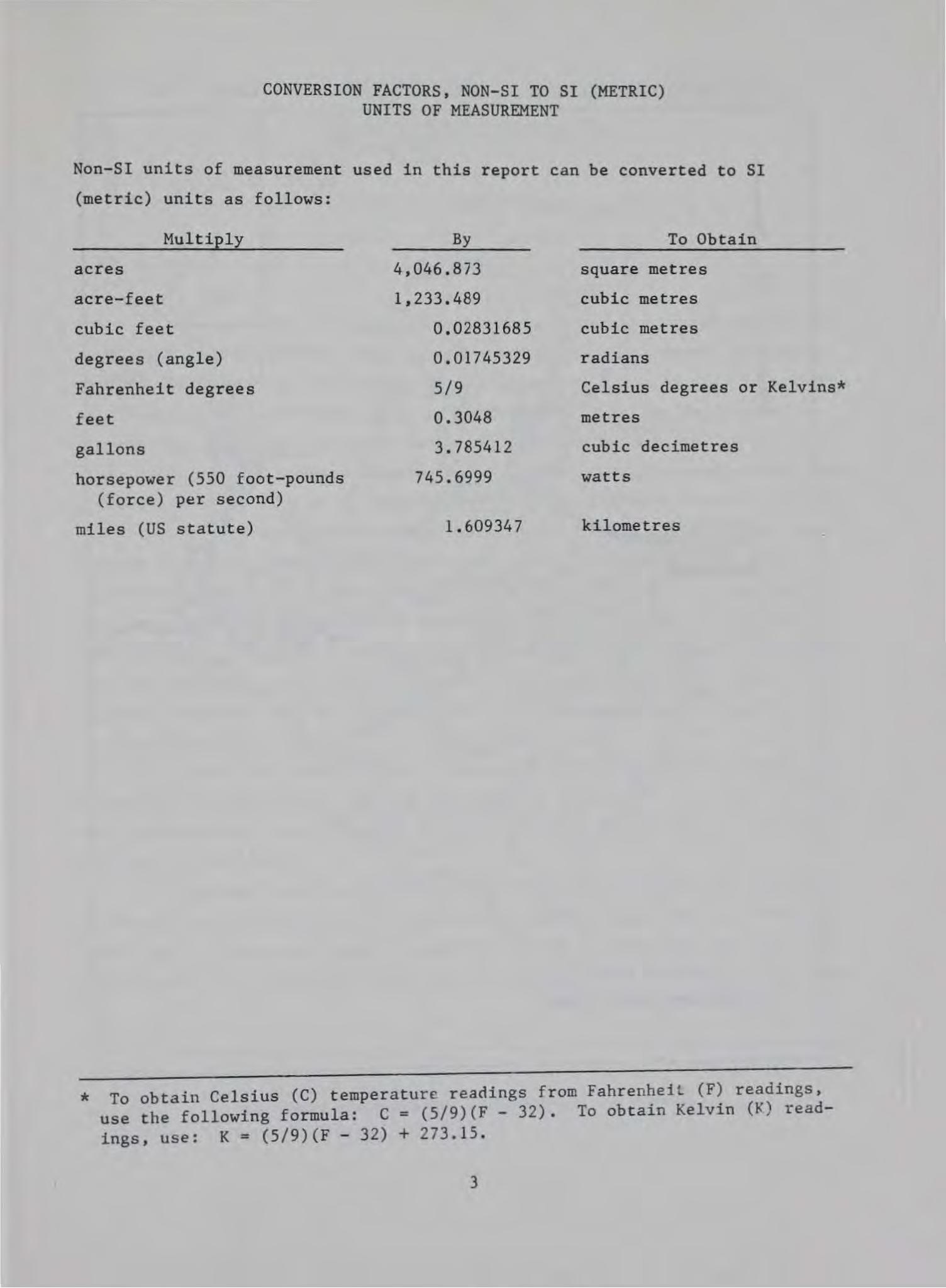
CONVERSION FACTORS, NON-SI TO SI (METRIC) UNITS OF MEASUREMENT

Non-SI units of measurement used in this report can be converted to SI

(metric) units as follows:

Multiply

acres

acre-feet

cubic feet

degrees (angle)

Fahrenheit degrees

feet

gallons

horsepower (550 foot-pounds (force) per second)

miles (US statute)

By

4,046.873

1,233.489

0.02831685

0.01745329

5/9

0.3048

3.785412

745.6999

1.609347

To Obtain

square metres

cubic metres

cubic metres

radians

Celsius degrees or Kelvins*

metres

cubic decimetres

watts

kilometres

* To obtain Celsius (C) temperature readings from Fahrenheit (F) readings, use the following formula: C = (5/9)(F- 32). To obtain Kelvin(¥) read-ings, use: K = (5/9)(F- 32) + 273.15.

3

2

PROMPTON DAM

-

SCALE IN MILES

0 2 .. 6

Figure 1.

..

Oomotcut - ..J liD lo ... . ,..

I

-

.. ~ • ,• •

VICINITY MA~ IC.Oll ~ ••~II

10 0 t I t 4 M

RIVE-9 J'._,J' r r

r"W

~f

8 10

Location map for Prompton Reservoir

4

1HERMAL ANALYSIS OF PROMPTON RESERVOIR MODIFICATION, PENNSYLVANIA

Numerical Model Investigation

PART I: INTRODUCTION

Background

1. Prompton Dam and Reservoir, which was authorized by the US Congress

on 30 June 1948 to provide flood control on the Lackawaxen River, Pennsylva­

nia, is located on the west branch of the Lackawaxen River 31 miles* above the

confluence with the Delaware River in northeastern Pennsylvania (Figure 1).

The existing 1,200- ft - long zoned earth-fill dam reaches a height of 140 ft

above the streambed. The spillway, which is an uncontrolled perched-type open

channel, is 50 ft wide at el 1205** with a maximum discharge capacity of 9,200

cfs. Normal releases are currently passed over a 30-ft weir at el 1125 and

through an ungated morning- glory type drop inlet structure. A low-level

coolwater intake with an invert located at el 1091 leads up to a low-level

weir located in the center of the main weir . This 10-ft- wide low-flow weir

has its crest at el 1122.8 and provides coolwater releases when the reservoir

pool is between el 1125 . 0 and el 1122.8. The conduit through the dam has a

maximum discharge capacity of 3,500 cfs. The existing outlet structure is

shown in Figure 2.

2. Since the current project is ungated and therefore uncontrolled, no

operation is required for the pool to remain at a constant elevation. Inflows

from storm events cause a rise in the pooJ, but the normal pool is usually

reached in a few days.

3. The west branch of the Lackawaxen River is classified by the State

of Pennsylvania as high-quality water and is stocked with trout. A routine

water quality monitoring program conducted by the US Army Engineer District,

Philadelphia, also indicates that the existing reservoir water is of excellent

* A table of factors for converting non-SI units of measurement to SI (metric) units is found on page 3 .

** All elevations (el) and sta~es cited l1erein are in feet referred to the National Geodetic Vertical Datum (NGVD).

5

STILLING BASIN

SCALE 50 0 50 lOOFT

PLAN

TOP OF DAM

SPILLWAY DESIGN FLOOD EL 1212.9 I

RE ERVOIR DESIGN FLOOD EL. 1168.7 RECREATION POOL EL. 1125.0 ~SOFDAM

''60------''40------

''<o ______ _

1100--­-------c:

- ttoo -I 100-=--=:: ------''<o------II 11(1-....._ ---.......

1250

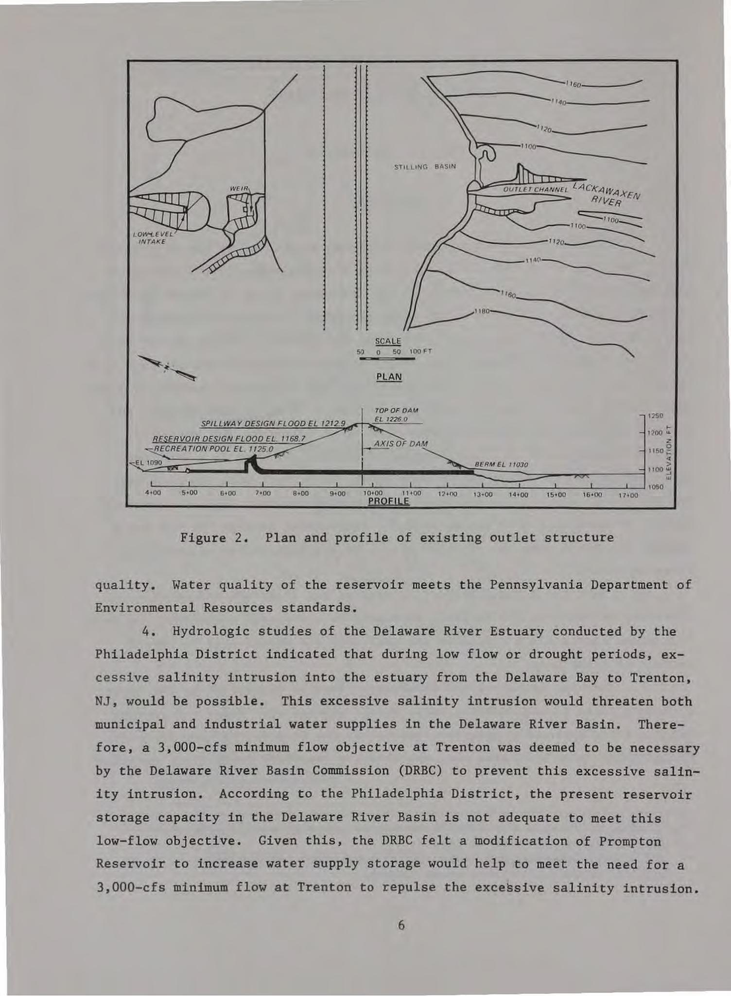
Figure 2. Plan and profile of existing outlet structure

quality. Water quality of the reservoir meets the Pennsylvania Department of

Environmental Resources standards.

4. Hydrologic studies of the Delaware River Estuary conducted by the

Philadelphia District indicated that during low flow or drought periods, ex­

cessive salinity intrusion into the estuary from the Delaware Bay to Trenton,

NJ, would be possible. This excessive salinity intrusion would threaten both

municipal and industrial water supplies in the Delaware River Basin. There­

fore, a 3,000-cfs minimum flow objective at Trenton was deemed to be necessary

by the Delaware River Basin Commission (DRBC) to prevent this excessive salin­

ity intrusion. According to the Philadelphia District, the present reservoir

storage capacity in the Delaware River Basin is not adequate to meet this

low-flow objective. Given this, the DRBC felt a modification of Prompton

Reservoir to increase water supply storage would help to meet the need for a

3,000-cfs minimum flow at Trenton to repulse the exce~sive salinity intrusion.

6

This increase would require raising the Prompton pool approximately 55 ft from

el 1125 to el 1180, thereby adding 31,000 acre-ft of water for water supply

(Figure 3). The DRBC could then request specific releases from Prompton

Reservoir depending on flow conditions in the Delaware River at Trenton.

5. Concerns about raising the pool center on the impacts to the reser­

voir thermal stratification and on release temperature. Previous studies by

Schneider and Price ( : 988) and Holland (1982) involving reallocation of water

storage resources for water supply at different projects recommended addi­

tional selective withdrawal (SW) capability to maintain downstream temperature

objectives. Since the Philadelphia District has determined that a new struc­

ture must be added to the Prompton project to provide operational control over

releases, SW capability may be required to enable the selection of the temper­

ature of release water to meet State standards. The vertical location of the

desired temperature in the pool for release downstream will vary depending

upon the depth of the pool, degree of thermal stratification, and time of

year. Therefore simulation of the proposed operating conditions was neces·sary

to identify design criteria for the suggested outlet structure.

1240

1230

1220

1210

1200

1190

1180

1170 z 0 I- 1160 <t > w _J 1150 w

1140

1130

1120

1110

II 00

1090

0

I

10 20 30

SURFACE A REA IN 100 ACRES

15 14 13 12 II 10 9 8 7 6 5 4 3 2 0

40

--TOP OF DAM EL 1226.0

-- TOP OF FLOOD CONTROL POOL EL 1205.0

TOP OF PROPOSED POOL

TOP OF RECREATION POOL -EL 1125 0

50 60 70 80 90

CAPACITY IN 1000 ACRE-FT

100 I I 0

F . 3 Capa c1' t y-area curve f or Pr omp ton Reservo1r 1gure •

7

Purpose and Scope

6. The Philadelphia District is currently investigating the modifica­

tion of Prompton Dam to add the storage discussed in paragraph 4 for water

supply and recreation purposes. This modification would raise the existing

normal pool (3,355 acre-ft) from 35 ft deep (el 1125) to approximately 90 ft.

Since the existing release structure consists of an uncontrolled weir at

el 1125, a modification to the existing structure is necessary to provide the

additional storage as well as the capability to release water on demand. To

maintain release temperatures in accordance with State standards, the Phila­

delphia District determined that an SW structure was necessary.

7. This investigation was undertaken to identify the capacity, number,

and location of SW ports in the modified structure to release temperatures

within the criteria set by the State of Pennsylvania. This simulation used a

numerical thermal simulation model coupled with numerical optimization rou­

tines. Adjustment of SW parameters (withdrawal angle) in the numerical model

was made based on results obtained in a physical model. Various port configu­

rations and capacities were then simulated to determine the optimum structure

design for the given objective.

i

8

PART II: MATHEMATICAL METHODOLOGY

8. The in-lake and release temperature characteristics for Prompton

Reservoir were modeled using a one-dimensional thermal simulation model. The

model WESTEX, which was developed at the US Army Engineer Waterways Experiment

Station (WES), was used to examine the balance of thermal energy within the

reservoir. This one-dimensional model includes computational methods for pre­

dicting dynamic changes in thermal content of a body of water through simula­

tion of heat transfer at the air-water interface, heat advection due to in­

flows and outflows, and internal dispersion of thermal energy. The reservoir

is conceptualized as a series of homogeneous layers stacked vertically. The

time-history of thermal energy in each layer is determined through solving for

conservation of mass and energy at each time increment subject to an equation

of state regarding density. The boundary conditions at the water surface and

inflow and outflow regions are required to conduct these simulations. A nu­

merical procedure for the withdrawal zone computation allows prediction of re­

lease temperature. Mathematical optimization routines are also coupled to

this model enabling the systematic evaluation of optimal outlet configurations

subject to specified release water temperature objectives. A more detailed

discussion of the WESTEX model may be found in Holland (1982).

Thermal Model Inputs

9. The WESTEX model requires input data on the physical, meteorologi­

cal, and hydrologic characteristics of Prompton Reservoir for each study year.

Further, initial verification of the model requires determination of appropri­

ate surface exchange and internal mixing coefficients. This verification pro­

cedure and the various inputs to the thermal model are described in the

following paragraphs for this study.

Study Years

10. The years studied in this investigation were determined in cons ul­

tation with the Philadelphia District and were based on inflow during the

spring of each year. Along with normal hydrologic conditions , ex treme condi ­

tions such as drought or flood periods should be ~odeled since these may

9

present the most difficulty in meeting State standards. Therefore, 1983 was

chosen as an average year (84,275 acre-ft total inflow), 1984 as a wet year

(89,619 acre-ft total inflow), and 1985 as a dry year (61,861 acre-ft total

inflow). The daily inflow for these years is shown in Figure 4. Since the

outlet operates as an uncontrolled weir, release quantity is based on pool

elevation, which, in turn, is based on inflow quantity. Therefore, release

rate traces the inflow rate. The impacts of meteorological and hydrologic

conditions on the thermal stratification for each year are shown in Figure 5.

In 1983, a typical stratification developed with the onset of summer, but the

1984 hydrologic conditions (high-flow year) prevented a significant level of

stratification from developing. The 1985 conditions (dry year) permitted a

strong stratification pattern to develop. Simulations during initial model

verification were run from January through December, although optimization

simulations were run only between 1 April and 1 December. During the 1 Decem­

ber to 15 February period the lake was isothermal; therefore, release tempera­

ture was not affected by port location. Subsequently, the releases during the

period were unaffected by the SW design and were not included in the design

optimization.

Meteorological Data

11. Meteorological data required by the WESTEX model consist of daily

average values for air temperature, dew point, wind speed, and cloud cover.

These data are available from the National Oceanic and Atmospheric Administra­

tion Local Climatological Data Monthly Summaries, which were provided by the

Philadelphia District. The station used in the study was the Wilkes-Barre/

Scranton Airport weather station. In addition, daily air temperature during

the week was available at Prompton Reservoir. Equilibrium temperatures, sur­

f ace heat exchange coefficients, and daily average solar radiation quantities

for the years of study were computed using the HEATEX program (Eiker 1977).

Release Temperature Criteria

12. The release temperature criteria* for Prompton Reservoir as set by

the State of Pennsylvania are as follows:

* Personal communication, 30 November 1987, from Mr. Dave Erickson, US Army Engineer District, Philadelphia, Philadelphia, PA. ·

10

Time of Year

2/1S to 7/31

Remainder of year

Criteria

No rise when ambient temperature* is 74° F (23.3° C) or above; not more than so F (2.78° C) rise above ambient temperature until stream temperature reaches 74° F; not more than 2° F (1.1° C) change in any 1-hr period.

No rise when ambient temperature is 87° F (30.So C) or above; not more than S° F (2.78° C) above ambient temperature until stream tempera­ture reaches 87° F; not more than 2° F (1.1° C) change during any 1-hr period.

* Ambient temperature is defined as the stream temperature that would occur in the receiving basin prior to some discharge.

In addition, the Pennsylvania Fish Commission recommends that the release tem­

perature from Prompton Reservoir be between 33° F (O.S° C) and 72° F (22.2° C)

with S0° F (10° C) to 70° F (21.1° C) as the preferred range. The Commission

also recommends no more than 2°-3° F (1.1°-1.6° C) change per hour or S0 -10° F

(2.8°-S.So C) change in 24 hr. For the purpose of this investigation, the

slight difference between the State of Pennsylvania and the Pennsylvania Fish

Commission criteria was considered insignificant. Therefore, the State

criteria were used in this investigation.

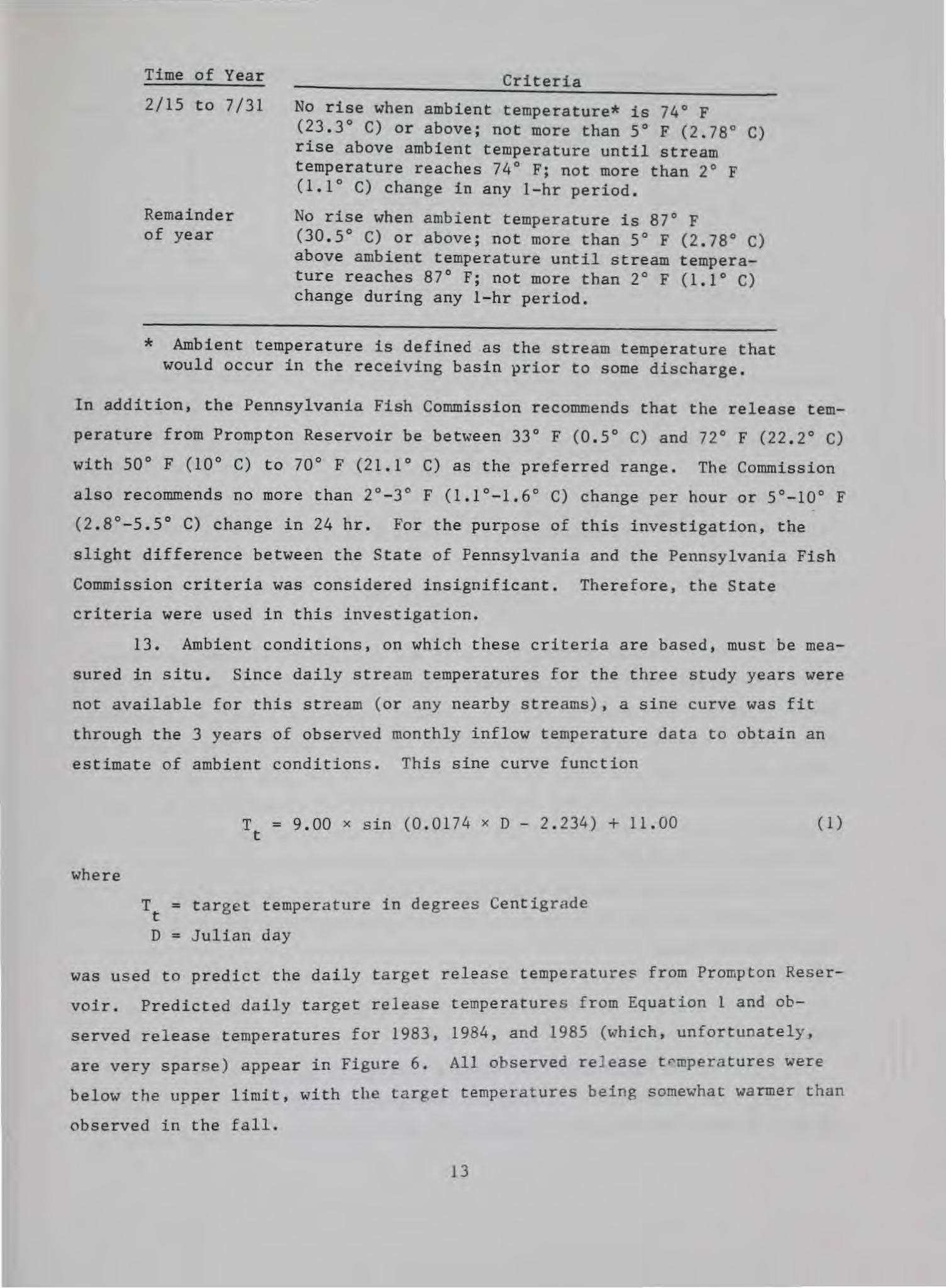
13. Ambient conditions, on which these criteria are based, must be mea­

sured in situ. Since daily stream temperatures for the three study years were

not available for this stream (or any nearby streams), a sine curve was fit

through the 3 years of observed monthly inflow temperature data to obtain an

estimate of ambient conditions. This sine curve function

where

Tt - 9.00 x sin (0.0174 x D - 2.234) + 11.00

Tt - target temperature in degrees Centigrade

D - Julian day

(1)

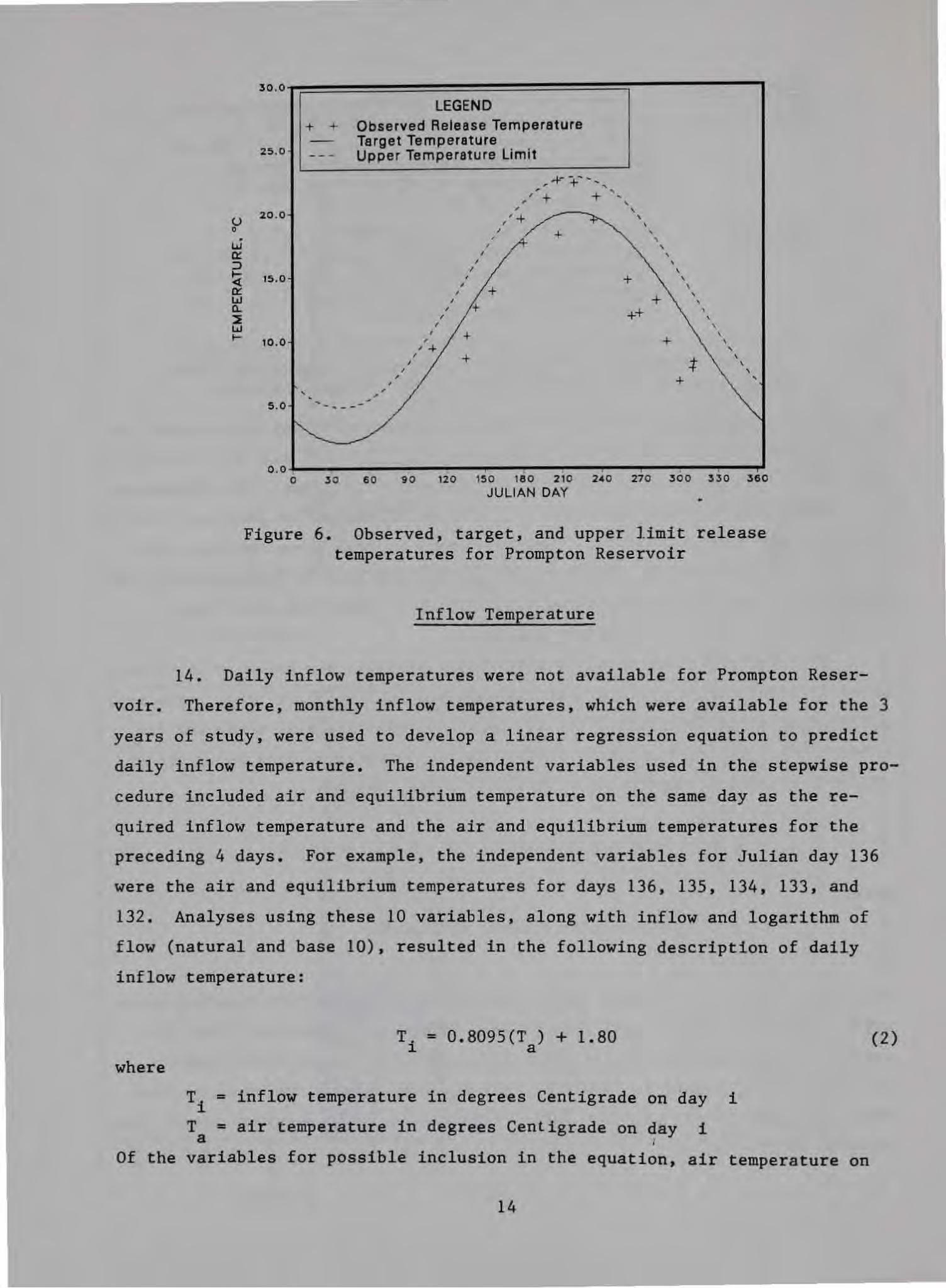
was used to predict the daily target release temperatures from Prompton Reser­

voir. Predicted daily target release temperatures from Equation 1 and ob­

served release temperatures for 1983, 1984, and 198S (which, unfortunately,

are very sparse) appear in Figure 6. All observed re l ease t~mperatures were

below the upper limit, with the target tempera t ures being somewhat warmer than

observed in the fall.

13

(.) 0

• w IX ::> ~ IX w a.. ~ w ....

30 .0

LEGEND + + Observed Release Temperature

25.0 Target Temperature Upper Temperature Limit

....fr"' - -.. ..... , , + .... ,

" I + + ~

" ' , ' 20 .0 I+ \

r \ / + ' " \

I ' I ' I ' / \ 15. 0 I + \

I

I + I +

/ + ++ / I \

I + \

10 .0 I \ / + ' I + t \ I \

I \ / + ' I

' " '

, '

, 5.0 - ... -- -

0.0~--~--~--~--~.~~~--~--~--~--~--~--~--~ 0 3 0 6 0 9 0 120 15 0 180 2 10 240 270 3 00 33 0 360

JULIAN DAY ..

Figure 6. Observed, target, and upper limit release temperatures for Prompton Reservoir

Inflow Temperature

14. Daily inflow temperatures were not available for Prompton Reser­

voir. Therefore, monthly inflow temperatures, which were available for the 3

years of study, were used to develop a linear regression equation to predict

daily inflow temperature. The independent variables used in the stepwise pro­

cedure included air and equilibrium temperature on the same day as the re­

quired inflow temperature and the air and equilibrium temperatures for the

preceding 4 days. For example, the independent variables for Julian day 136

were the air and equilibrium temperatures for days 136, 135, 134, 133 , and

132. Analyses using these 10 variables, along with inflow and logarithm of

flow (natural and base 10), resulted in the following description of daily

inflow temperature:

T.- 0.8095 (T) + 1.80 l. a (2)

where

Ti - inflow temperature • l.n degrees Centigrade on day i

T - air temperature in degrees Centigrade on day i a I

Of the variables for possible inclusion in the equation, air temperature on

14

the day of the inflow was the most important. The value of which is an

indicator of the amount of variance in inflow temperature that is accounted

for by the equation, was 0.82.

Model Adjustment

15. The WESTEX model requires determination of dimensionless coeffi­

cients characterizing certain reservoir processes. Two hydrodynamic proc­

esses, representing entrainment of inflows and internal mixing resulting from

circulation within the reservoir, are approximated through the application of

mixing coefficients a 1 and a2 , respectively. The distribution of thermal

energy absorbed into the pool through the air-water interface is governed by

the coefficient for the percentage of incoming shortwave radiation absorbed in

the surface layer 8 and a light extinction coefficient A • These model

coefficients were modified until simulated conditions most nearly matched

field observations for the year 1983. The resultant model coefficients were

as follows:

a1

- 0.05

8 - 0.99

A - 0.99

16. Initial verification of the numerical mode l included comparison of

predicted lake stage with observed lake stage, given historical inflow and

outflow. These comparisons indicated that the model predicted within 0 .1 ft

of the observed s tage in most cases. Initial comparison of temperature pro­

files with those observed was not as successful. The profiles indicated that

not enough warming was occurring in the surface layers. Further anaJysis of

the inflow data indicated that inflows from sta 4 (approximately 20 ,000 ft up­

stream from the dam) were much cooler than those from sta 3 (approximately

14,000 ft upstream from the dam), which is in the headwaters of Prompton Res­

ervoir. The linear regression model (Equation 2) for inflow temperature was

15

then recomputed using equilibrium temperature and data from sta 3. The

resulting equation was as follows:

where T is the equilibrium temperature in degrees Centigrade. Computed e

daily inflow temperatures for 1983, 1984, and 1985 appear in Figure 7. The

(3)

addition of this equation to the model improved the profiles so that they more

closely matched the observed data. Further improvements were made using the

observed air temperature at the project for computation of equilibrium temper­

ature. Some deviations of predicted versus observed profiles may be due to

the small volume of water located in the bottom layers (less than 2 percent of

the volume is located in the bottom 10 ft) so that when withdrawal zones ex­

tended into the lower layers, the cooler water was exhausted quickly. Al­

though some variation between the predicted and observed profiles existed, the

general shape of the profiles matched the observed for 1983 (Figure 8). Are­

liability index (RI) that has been formulated (Martin 1986) was used to com­

pare predicted with observed profile data. The closer the predicted profile

is to the observed profile, the closer the RI is to 1.00. From previous stud­

ies (Schneider and Price 1988), an RI between 1.00 and 1.10 indicates good

agreement of model and prototype profiles. The RI for these 1983 comparisons

was 1.055.

Withdrawal Angle

17. In the WESTEX model, the withdrawal angle parameter must be set.

This parameter, whose value was initially assumed to be 3.14 radians, is used

to account for topographic effects on the withdrawal zone. At Prompton Reser­

voir the proposed structure will be located near the west bank end of the dam.

This location may influence the limits of withdrawal by constricting the

lateral area from which the structure may draw water. This in turn may cause

the withdrawal zone to expand vertically, thus modifying the release tempera­

ture. Therefore, to promote accurate predictions with the numerical model,

the effects of the local topography on this parameter were investigated in a

physical model. The discussion and results of this investigation appear in I

Appendix A. This investigation indicated that the local topography has no

16

u 0

w a:: :::> 1-< a:: w a. ~ w 1-

...... '-.)

30.0~----------------------------------------------------~

1983 25.0

20 0

15.0

10.0

5.0

~ 0.0~~~~~--------------------------------------------~

0 30 60 90 120 150 180 210 240 270 300 330 360 JULIAN DAY

30.0

25.0

u 20.0-0 . w a:: :::> 1-< 15.0 a:: w a. ~ w 1- 10 .0

5 .0 - h ~ 0.0

0 30 60 90 120

30.0

25.0

u 0

20.0

w a:: :::> '< 15.0 a:: w a. ~ w 1- 10.0

5.0

0.0 0

f'v tl 'V

150 180 210 240 JULIAN DAY

1984

\~ .

~ ~~ ~ v

~

0-- n A

3 0 60 90 120 150 180 210 240 270 300 330 360 JULIAN DAY

1985

v ~

~ ~

270 3 00 330 360

Figure 7. Predicted daily inflow temperature for Prompton Reservoir

1,14 0.0 ~--------------------------------------------... 1, 14 0 .0~----------------------------------------------.

DAY138 DA Y178

1,130 .0 1,130.0

+ t- t-.... + .... • 1 ,1 20 . 0 . 1,120 .o

z

-'-z

0 0 - -t- t-• ~ > 1,110 .0 -t- > 1 ,11 0.0 ..... ..... ..J ..J ..... -1 '- .....

1.100 .o + 1, 100 .o

+ l,o t o.o~ ........ ~ .......................... ~~----~

0 . 0 11 . 0 10 .0 10 . 0 ZO .O Z O . O l!O . O 1,0 8 0.0~------~--~--~------~------~------~----~

0.0 0.0 1 0 . 0 10 .0 zo.o z o.o • 0 . 0 TEI.4 PERATURE, •c TEI.4PERAT U RE, •c

1,14o.ow-----------------------------------------------. DAY 206 DAY 236

1,130.0 1.130 .0

t- + t- + .... a.. • 1.120.0 + • Ll20 .0 z z +

0 0 - + t- t- + • ~ > 1,1 10.0 > 1 , 110 . 0 ..... ..... ..J ..J ..... .....

1 . 100 .o + 1, 100 .0

+ 1,080.0~------.---~--.. ------~------~------~----~ 0.0 ~ .0 10 .0 10 . 0 ZO .O ZD . O •o .O 0 . 0 !1 . 0 10 . 0 ID . O 20 . 0 2 0 . 0 s o 0

T EI.4PERATURE , oc TE 1.4 PERA TURE, °C

t,t4o .ow----------------------------------------------, DAY 26~

1 , 1~ 0 . 0

t- + LEGEND a.. 1,120.0

+ Predicted Temperature z 0 + + Observed Temperatu re t- + • > 1 . 110 .0 l.tJ + .J .....

+ 1.10 0 .o +

1,080 .0~------.-------~------~------~----~~----~ o.o s .o tci.o u . o 2o .o zs . o .s o . o

TEI.f PERATURE, °C

Figure 8. Predicted and observed temper a ture profiles for 1983

I

18

impact on the proposed structure at its current proposed location. Therefore,

no modification of the withdrawal angle parameter was made in the numerical

model.

Model Verification

18. The 1984 and 1985 data sets were used for verification of the

model. Simulations with these data sets indicated the hydrologic conditions

for these years matched the observed conditions well. Deviations between pre­

dicted and observed stages of the pool were usually less than 0.1 ft with a

maximum of 0.3 ft. The comparison of predicted with observed temperature pro­

files for 1984 indicated the model predicted warmer temperatures during the

early spring (day 109, 19 April) but matched the upper layers by day 180

(29 June), as shown in Figure 9. As with the 1983 data, the model predicted

warmer hypolimnetic layers. This was probably due to the withdrawal limits

extending into these layers (Figure 10) in the spring, causing evacuation of

this cooler water. Since these layers contain a relatively small volume of

water, and there is no other source of cool water (i.e., inflows), the hypo­

limnetic water that is released is replaced by warmer layers from above,

thereby warming the overall profile. In contrast to the profiles collected in

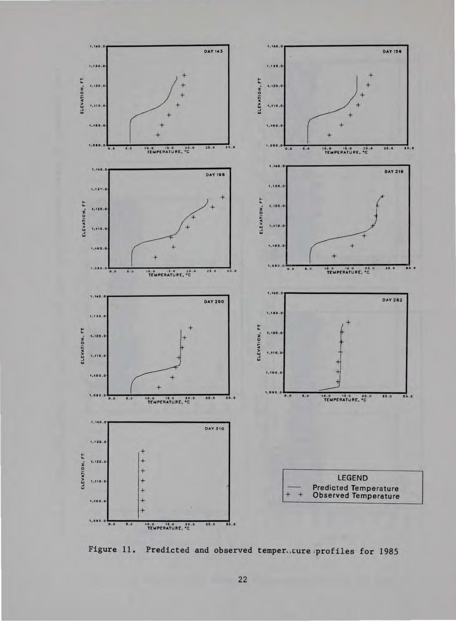
1984, which was a high-flow year, 1985 profiles (Figure 11) were warmer than

predicted during the spring. With the onset of summer, the predicted profiles

more closely matched the observed profiles. The deviations occurring in the

lower layers may again be attributed to the relatively small volume of water

in these layers. The differences in the spring profiles may be due to errors

in predicted inflow temperature or to the advective factors that dominate dur­

ing the high inflow periods. The hydraulic residence time, which can be used

as an indicator of an advectively dominated system, was very short during the

spring. However, beginning in July, the residence time usually increased,

allowing the system to become meteorologically dominated. For example, in the

1985 verification year, predicted profiles were consistently 3° to 4° C cooler

than observed up to day 198 (17 July), after which much closer fits were ob­

served. Simultaneously, the residence time began to increase about day 198

and peaked in October. The RI for all comparison profiles for 1984 was 1.051

and for 1985 was 1.098.

19

.... ... . z 0 .... <(

> ... ..J w

... ... . z 0 .... <(

> ... ..J w

.... ... . :z 0 i= <(

> "' ..J w

... .. . z 0

~ > IJ .J ...

1,140 . 0~--------------------------------------------..,

I,UO.O

t,U:O . O

1.110 . 0

+ + +

+ + +

OAY I09

:; I.OIO .o·~ ............ -. .. ~----~~--~~~--~~.~0~--·~·o . o o . o 0 .0 1 0.0 10 . 0 %0.0 z . -

T£WPER4TUR£. " C

1.140.0~ ............................................ ..,

1.uo.o

t,t20.0

t.llo.o

+ +

OAYI80

+ +

1,0 10 ,0~-------------.------~~------~--~~----~ o.o :t.o to.o te.o .zo.o .ze. o 1 0 . 0

TEWPERATUR£, •c

1.140.0 OAY234

'·, .ao . a

+ '· 120 .o .

-1.110.0 +

+ 1.100.0 +

+ 1,010.0

o . o s .o t O.O t.S.O 20 . 0 2S . O JO . O TEt.IPERATUR£, •c

1,140.0

04Y 29 0

1,1 ao .o

+ I. 120.0

/f-t,tto . o

r+-+

t,too .o , -i

1,0 1 0 0

+ +

0 , 0 5 .0 to . o IS , O 20 . 0

TEt.IPERATU R E, •c

LEGEND Predicted Temperature Observed Temperature

u .o JO . O

.... ... . z 0

~ > ... ..J w

... ... . z 0 .... <(

> u -'

"'

.... .. . z 0 .... <(

> ... ..1

"'

.... .. z 0 t= <(

> ... ..J ...

1.140 .0~--------------------------------------------..,

I.ISO.O

1,120.0

1,110 .o

1, 100 .0 +

+ + + + +

OAY 13~

/ 1,010.0,~------~~--~~~--~~~--~~~--~~~--~ o.o o.o so .o to. o zo.o za.o 1o .o

f£WPERATUI!E, •c

1 , 140.0~----------------------------------------------,

1.uo.o

t,t20 . 0

t.ltO . O

+ +

OAY 207

+ + + +

I 1,0 10.0~ ............................ ~.-----~ .. ----~

too ''o zoo 2ao a o . o 0 0 5 . 0 TEWPERATURE, •c

.. 140 .o

DAY 263

•••• o .o

-r t . ••a .o +

+ 1.110 . 0 +

+ 1, 100 . 0 +

+ 1.0 1 0 . 0

0 . 0 s .o 10 . 0 1 3 , 0 2:0 . 0 230 10 . 0 TEt.IPERATUR£. •c

1,14 0 . 0

DAY 3 11

'· t 10 . 0

+ 1.120 .0 +

+ 1,110.0 +

+ 1,100.0

+

1,o e o . o o . o s .o to . o u . o 20 .0

TCI.IPERATURC, •c 2>0 , 0 . 0

i

Figure 9. Predicted and observed temperature profiles for 1984

N -

1,190.0

1,180.0

1,170.0

1,160 0

.... - 1.150 0 . z 0

~ w ...J w

1,140 0

1,130,0

1,120.0

1,, 10 0

1. 100. 0

1,090 0

1983

I '

.

0 30 60

1,190,0

1,180,0

1984 1,17 0.0

1.160,0

.... ... 1,150.0

z 0

~ 1,140.0

> w

.,rJ I'-- ,, TYP . rn.~ nllr '

~~~~ I

' ' I

II I ' I I :I I I I ' ' I I I .I I I I

II I

i I I I I 111111111

'

' I . I •I

I I

...J 1,130.0 w

1,120.0

1,11 0.0

1,100 .0

'

90 120 ISO 160 210 240 270 :3 CO 330 360 3 0 60 90 120 ISO 180 21 0 240 270 3 00 330 360 JULIAN DAY JULIAN DAY

1,190.0 ...-----------------------------,

I, 180 0

1985 I, 170 0

1,160 0

.... - 1,150 0 . z 0

~ >

1,140.0

w ...J 1.1 JO . O w

1-~~ l1r: -I. 120 0

I I

1,110 (\

I, 100 (\

, • (\!I 0 0 JIU.II,I;.---'I.w.LWI.J,IU.W.UW,..-..... --_.,... ~ -_,..--,----r---+.loll.l..i&..folloli.lolol.lly..l;.-3 0 60 90 120 ISO 11!0 210 240 27C 300 330 3ov

JULIAN DAY

Figure 10 . Withdrawal limits for 1983, 1984, and 1985 . Band indicates extent of withdrawal zone

t. t.ao . o . .... o.o OAY1.3 0AY151

t.130.0 1.1 .0 . 0

+ + .. .... ... .... + e. 120 . a + 1, 120 .o .

z z 0 + 0 + ;:: ...

~ ~ > + > 1,11o .o + w '·" 0.0 w ~ .J w + w +

t.t oo.o + 1,100 . 0 + + +

1,0 10 .0 50 . 0 I,O tO .O to . o ;o.o zo.o •o .o 0 . 0 ••• 10 . 0 ,. 0 10.0 :o . o o.o ••• 10.0

T£1o1PERATU RE, •c TEioiPERATUR£, •c

. . ... o.o •·••o.a DAY 21S.

DAY1V8

•. • so .o 1.1 ~ "\.0

+ ,_ ,_ ... ... + . 1,120.0 ft' . •• 120 .o % z 0 -0 + ... ... <( <( > t.ttO . O > ... ... .... '0 .o .J .J w + w

+ •.• oo . o + 1,.100 .0

+ + 1,01 0 . 0

10 0 •• 0 20 0 •• 0 ao o 1,010.0 0 • e .o 0 . 0 • . u 10.0 .. 0 , ... %~ . 0 J o . 0 T£1o1P£1UTU R£. •c

Tl:loiPI:RATUR£, •c

1.1 .. 0 . 0 1.1 .. 0 . 0

DAY 260 DAY 282

.... 0 . 0 t.1 JO . O

+ .... ,+ .... ...

If-... 1 ,110 . 0 1.120.0 + % z 0

t-0

ft .. .... <(

<( > t,tto . o . ... > t, ltO .O .J ... -; ..J w + ...

-4 1,100 . 0 -+ 1.too . o +

-+ +

1 , 010 . 0 o .o s .o to .o 1-' . 0 20 .0 2S . O so . o 1.0 1 0.0

u .o 2 0.0 2.S .O so .o TCioiPCRATU RC. •c 0 .0 s .o 10 .0 TCIAPCRATU R£. •c

1.140 . 0

DAY 310

1.130.0

,_ + ... + . 1.1%0.0

z 0 + 1-

LEGEND ~ > + u 1,110.0 ~

Predicted Temperature .., + + + Observed Temperature

••• oo . o + +

1,010 . 0 o. o s .o 10 .0 tS . O 20 .o 25.0 ao . o

TCt.l PI:RATU R C, •c

Figure 11. Predicted and observed temper .. cure .profiles for 1985

22

Release Temperature

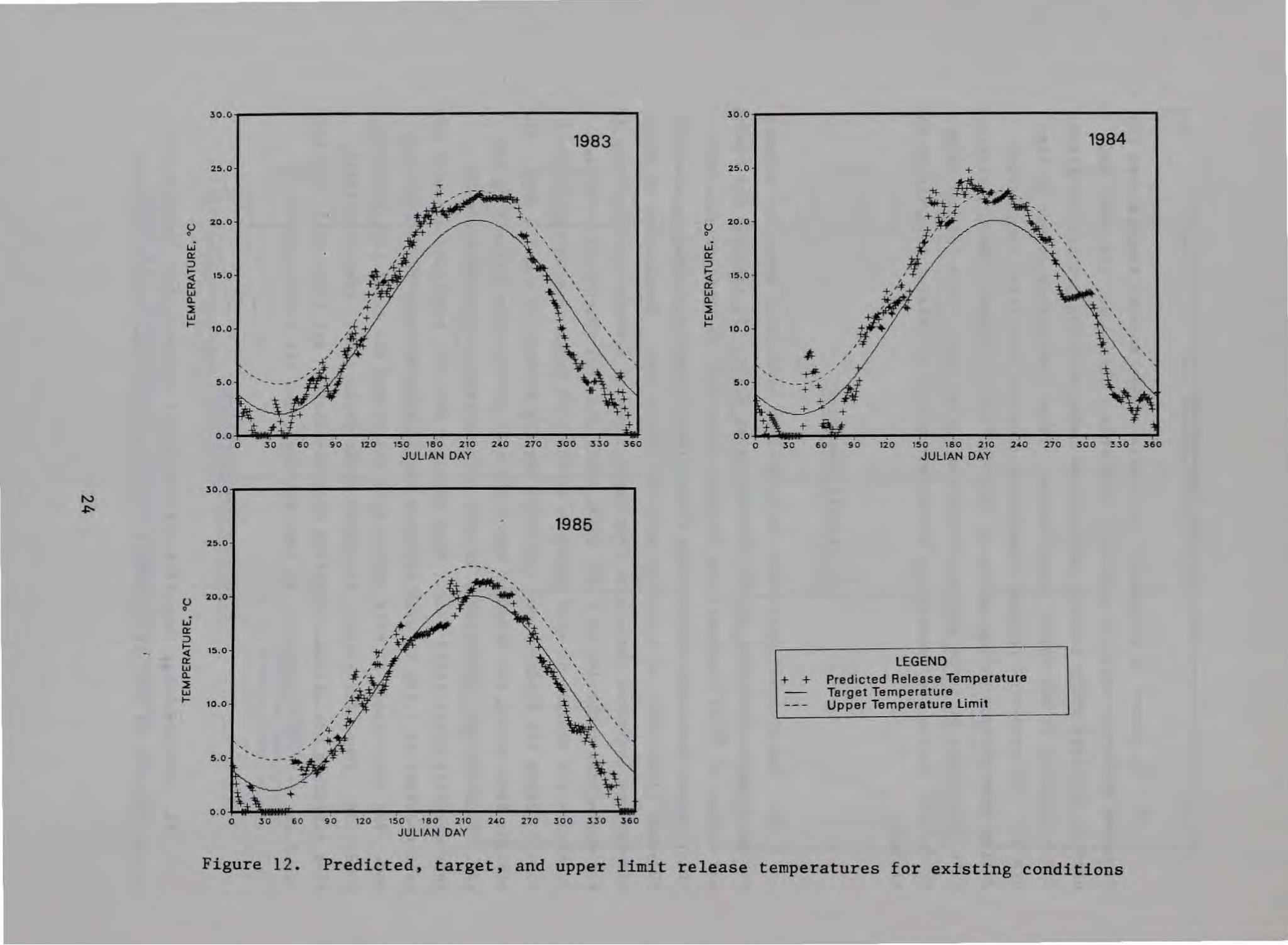
19. As stated in paragraph 13, observed daily release temperatures for

Prompton Reservoir were not generally available. Therefore, the model was

used to simulate daily release temperatures using existing project conditions

for comparison to the target temperatures. These comparisons appear in Fig­

ure 12. The predicted release temperature exceeded the target temperature

during some periods in the spring of 1983 and 1984. However, these deviations

were the result of large inflows mixing the entire lake. Once inflows began

to decline during the summer, the day-to-day change in release temperature was

minimal.

Operational Scenarios

20. The proposed pool raise is to provide additional water for release

during drought conditions in the Delaware River Basin. To identify the timing

and volume of flows required from Prompton Reservoir, the Philadelphia Dis­

trict used a Hydrologic Engineering Center (HEC) computer program to simulate

50 years (1927-1977) of operation with the raised pool. Examination of these

simulations indicated there were four basic types of drawdown corresponding to

the operations occurring in 1930, 1957, 1964, and 1965 (Figure 13). These

scenarios are similar in that drawdown of the pool began in midsummer with the

time to reach the minimum pool (el 1113) varying between 73 and 279 days. The

minimum flow during the drawdown was 6 cfs with the maximum approaching 650

cfs. From the HEC simulations, it also appears that a drawdown occurred

approximately every third year. When releases were not required, the pool was

held constant at 1,180 ft with releases essentially equaling the inflow vol­

ume. For the purpose of this study, this was termed the level pool operating

condition. Thus, for each of the three study years (1983, 1984, and 1985),

five different operational scenarios were simulated: (a ) level pool; (b ) 1930

drawdown; (c) 1957 drawdown; (d) 1964 drawdown; and (e ) 1965 drawdown.

Structure Configurations

21. Two discharge scenar1os were simulated in the model: maximum di s ­

charge capacity of 220 cfs through a 7- by 8-ft port; and 325-cfs capac i t y

23

30.0 30.0

1983 1984

25.0 25.0 +

~ ~#~ :U' ', 20.0

() 20.0

() l ' ~\ 0 0

&...I &...I \.. \ a: ' a: ' ~ ' ~

' ' 1-1- 15 . 0 ' <{ 15.0 ' <{ \ a: a:

' ' &...I w ' (l.

' (l. ' ~ ' ~ \

' &...I ' &...I ' 1- ' 1- 10.0 \ ' 10.0

\ ' ' ' \ ' \: ',, ' • ' / ' ' ' -t-*- , ,

5 .0 ' -'- - -* 5 .0

~ +

\ ~ +

0.0 0 . 0 . 0 60 90 120 150 180 210 240 270 300 33 0 360 0 3 0 60 90 120 150 180 210 240 270 3 00 ~30 360

JULIAN DAY JULIAN DAY

30.0~------------------------------------------------------,

1985 25.0

() 20.0

0 ' . ,

\ &...I

'* ' a: -~+ ' ~ ' 1- ' ..-: \ <{ 15.0 iJ' ' LEGEND ' a: ;'1~ ' w

' (l. J- ' + + Pred icted Release Temperat ure ~ ' ' Target Temperature &...I ' 1- 10.0

~\',, Upper Temperat ure Limit

' + , ' ,4-, * '

5 .0 +

~¥. o.o .

0 30 60 90 120 150 180 210 240 270 300 330 360 JULIAN DAY

Figure 12 . Predicted, target, and upper limit release t emperatures for existing conditions

~ ..... ~

z 0 1-<(

> w ..J w

1190 . 0

1180.0

117 0 - 0

1180 .0

11!10 .0

1140 . 0

1 1 3 0.0

1 120.0

1110 . 0

110 0.0

109 0.0 0

_ 'i1 (TYP.) - ---- ~:

/~~ ~:~

/

LEGEND Level Pool 1930 Operating Scenario 1957 Operat ing Scenano 1964 Operating Scenario 1965 Operatmg Scenario

I .

. · . 1 -~-• I \ : I

: I I , I

:_,~-• I . --· .. .. - --

\-- -.

30 60 90 12 0 150 18 0 2 10 24 0 27 0 3 00 33 0 360 JULIAN DAY

Figure 13. Operational scenarios for Prompton Reservoir

through an 8- by 8-ft port (the flows and port dimensions were specified by

the Philadelphia District). These flow rates represent the 95 and 99 percent

exceedence flow rates for the project. Two wet well configurations were also

tested: a single wet well with only one port operating at a time and a dual

wet well with simultaneous operation of two ports (one each per wet well). In

the initial design optimization, the flood-control port was not allowed to

operate simultaneously with other ports; however, in the simulations using the

final design, the flood-control port was allowed to operate simultaneously al­

though it did not significantly improve the ability to meet the release tem­

perature objective. The flood-control outlet was defined as a 30- by 30-ft

gate with an invert elevation of 1095.

Optimization Process

22. Design of an efficient outlet structure to meet the release tem­

perature objectives under the raised pool conditions requires the determina­

tion of the number and location of additional intakes. This design process

was greatly simplified by Dortch and Holland (1984), who coupled the WESTEX

model to mathematical optimization techniques. This effectively allowed the

consideration of numerous hydrologic, meteorological, physic8l, and operation­

al conditions in the formulation of intake structure design. The use of the

optimization techniques enhances structure design by allowing systematic

25

evaluation of the structure configurations needed in the design to meet the

release temperature objectives. The systematic evaluation is carried out

using an objective function as a measure of performance of each candidate

system configuration. This function is discussed in the following paragraphs.

Objective Function Description

23. An objective function value is an index used to evaluate the degree

to which releases from a given intake configuration meet a set of prescribed

temperature objectives. In this study the objective function value was formu­

lated as the difference between the predicted (model) release temperature for

a given day and the target temperature for that day. This value was squared

and summed for the period from 1 April to 1 December. The option to invoke

mathematical penalties for a release temperature deviating from the prescribed

temperature objective band also exists. For example, the release temperature

for Prompton Reservoir is never to exceed 2.78° C above the ambient. There­

fore, to penalize for deviations greater than 2.78° C above the ambient, these

deviatior.s were multiplied by 10, then squared and added to the objective

function value. Because deviations below the ambient were not specified in

the release criteria from the State of Pennsylvania, these deviations invoked

no penalty. The target temperature and the upper temperature limit above

which the penalty was imposed are shown in Figure 6.

24. The optimum capacity, location, and number of ports for the SW

structure were determined by numerical optimization. This, in turn, involved

minimization of the objective function value described in the previous para­

graph. The optimized structure design consisted of selection of

a. Port capacity (220 or 325 cfs).

b. Number of wet wells (single or dual wet well).

c. Operating condition (level pool, 1930, 1957, 1964, or 1965 release scenarios).

d. Number of ports to locate (1, 2, 3, or 4*).

e. Optimum elevation for each port sited.

These data were input to the WESTEX model with the optimization routine. The

* Initial optimization results indicated little improvement in objective function with more than four ports. '

26

model then computed the objective function value for the initial elevation of

the port(s). The optimization process then selected a new elevation of the

first port for simulation. Upon completion of this simulation, the objective

function value was compared to the previous objective function value and a new

port elevation that was closer to the elevation with the lower objective func­

tion value was selected and simulated in the model. This process continued

until the difference in elevation between the new and previous elevation did

not exceed a predetermined value (4.0 ft in this study). This process was re­

peated for each input parameter listed to identify the optimum release struc­

ture for each set of conditions and structure configuration.

25. The two wet well configurations discussed previously (one or two

wet wells) were included in this investigation to allow determination of the

need for multiport blending operations to meet the release temperature objec­

tive. At the time of this study, the only accepted methodology within the

Corps of Engineers for blending release water from two different elevations in

the water column required the use of dual wet well systems. This convention

was adhered to within this study. However, since the conclusion of this in­

vestigation, considerable research on multiport operations in a single wet

well has been completed. This research indicates that density stratification

in a reservoir can strongly affect efforts to achieve a desired blend of water

from two elevations using a s ingle wet well; however, these concerns can be

overcome by construction of individual controls on each port to allow for

partial opening of a port. Thus, a single wet well represents a potentially

viable option for multiport release water quality operations that might merit

future consideration by the Philadelphia District.

2 7

PART III: DISCUSSION OF RESULTS OF SYSTEM OPTIMIZATION

Optimization Results

26. The results of the optimization simulations are presented in Fig­

ures 14 through 18. The various operating scenarios were simulated in the

order discussed in paragraph 20. In Figure 14, objective function values for

each structure configuration of one, two, three, and four ports, both port

capacities, and both wet wells for all 3 years of meteorological conditions

are shown.

27. In the first series of tests, which simulated a level pool operat­

ing condition, there was little reduction of the objective function values by

increasing the number of ports (Figure 14). The dual wet well configurations

slightly improved the objective function values compared to the single well

runs. The more pronounced differences were for the 1985 meteorological condi­

ticns. In a similar manner, the 325-cfs port capacity was slightly better

than the 220-cfs capacity. The larger capacity provided more flexibility in

meeting required release volumes for the release temperature objective. The

slight difference between the one port and multiple ports (two, three, or four

ports) suggested that one port would be sufficient with blending of releases

through the flood-control port. However, it may be difficult to operate the

flood-control gate at low flows (down to 6 cfs). Therefore, a two-port dual

wet well structure with 325-cfs capacity of each port is the recommended

structure for the level pool operation.

28. Simulation of the drawdown operating plans indicated much more dif­

ficulty in meeting the release temperature objective than for the level pool

scenario. The order of magnitude difference in the objective function values

(Figures 15 through 18) for several of the drawdown scenarios as compared to

the level pool operation (Figure 14) indicated that in some cases the penalty

function (described in paragraph 23) was used by the model. This penalty sig­

nified that some release temperatures exceeded the upper bound as set by the

State.

29. Simulation of the 1930 operating

the potential utility of the dual wet well.

rule curve (Figure

Simulation of the

15) revealed

single wet well

structures for 1983 resulted in larger objective function values than did I

either of the dual wet well designs. In addition, the 325-cfs port capacity

28

provided superior temperature control. The 1984 meteorological conditions,

however, created no difficulty in meeting release temperature criteria for

either the single or dual well design. Further, no apparent differences were

observed between the 220- and 325-cfs port capacity runs. This is contrasted

with the 1985 simulations, which were influenced more by the number of ports

rather than number of wet wells. For 1985 conditions, three ports in a dual

wet well with 325-cfs capacity per port was the optimum configuration.

30. Results of optimization simulations using the 1957 operating

scenario (Figure 16) were similar to the 1930 operating scenario results. For

the 1983 meteorological data, the increase in capacity to 325 cfs for the

single wet well configuration improved the objective function value. However,

the three-port, 325-cfs-capacity dual wet well appeared to be the optimum con­

figuration for the 1957 operating scenario for the 1985 conditions.

31. The 1964 operating scenario (Figure 17) was influenced for all

three meteorological years more by the addition of ports than by port capacity

or number of wet wells. The minimal improvement in the objective function

with addition of a third or fourth port indicates that for 1983 and 1984 a

two-, three-, or four-port structure could be recommended. However, the

three-port configuration minimized the objective function value for the 1985

operating conditions. Therefore, as with previous rule curves, the three­

port, dual wet well, 325-cfs-capacity structure appeared to be the optimum

configuration for the 1964 operational scenario.

32. The 1965 operating scenario (Figure 18) showed some variation

between single and dual wet wells in 1983 and more variation in 1985. As with

previous scenarios, release temperature control for 1984 meteorological condi­

tions was equally good for the various combinations of number of ports, capac­

ity, and number of wet wells. Therefore, for the 1983 and 1984 conditions, a

two-, three-, or four-port dual wet well structure would provide similiar re­

lease temperature control. For the 1985 condition, the three-port, dual wet

well structure was the optimum.

33. In general, the optimization results showed that the release tem­

perature objective was not impacted by structural design for the 1984 meteoro­

logical conditions. Since the 1984 study year was considered a wet year with

a number of storm events mixing the lake (an example of the 1984 stratifica­

tion pattern will be shown later in Figure 21) to a more uniform temperature

distribution from surface to the bottom, there was increased flexibility in

31

"' 18.0 "' 18 .0 0 0 ........ 16.5

........ 16.5 X X

15.0 1983 15.0 1984

w w ::J 13 . 5 ::J 13.5 _j _j

a: a:: > 12.0 > 12.0

z 10 . 5 z 10.5

0 0 1-4

..... (-I 9.0 E-o 9.0 u (.)

z 7.5 z 7.5

::J ::> u.. I.&..

6.0 6.0 w w > 4.5

> -1.5 ...... 1-4

£- (-I :ss;; u 3.0 u 3.0 ; ; w w J 1.5

I 1.5 ID ID 0 0

0.0 0.0 1 2 3 4 1 2 3 i

NUMBER OF' PORTS NUMBER OF' PORTS

M 18.0 0 ..... X 16.5

w 15.0 1985 ::J 13.5 _j a:: > 12 . 0

z 10.5 0 ...... LEGEND £- 9.0 0 0 220-CFS Capacity, Single W et Well (.) z 0 ..... 325-CFS Capac1ty, Single Wet Well ~

::J 7.5 [}. c:. 220-CFS Capacity. Dual Wet We ll u.. + + 325-CFS Capac1ty, Dual Wet Well w 6.0 • • Final Optimum Configuration > ...... "'l.5 f-u 3.0 w I CD 1.5 0

0.0 1 2 3 4

NUMBER OF PORTS

Figure 16 . Optimization r esul ts for 1957 operati ng scenario

32

M 18.0 0 18.0 .., ..... a )( 16.5 .-1 16.5 )(

15 . 0 1983 w 15.0 1984 ::::> 13.5 w _] ::::> 13 . 5 cc _]

> 12 . 0 cc > 12 . 0

z 10 . 5 0 z 10.5 ...... 0 r 9.0 H

{_) H 9 . 0 z 7 . 5

u ::::> z 7 . 5 l... ::::>

6.0 u.. w • 6.0 > 'l.5

w ...... > i.S I-I ...... u 3.0 I-I

~ w {_) 3.0 I w m 1.5 I I ' 0 m 1.5 '\'

0 . 0 0

0.0 2 3 'i 1 2 I I

3 i NUMBER OF PORTS NUMBER OF PORTS

n 18 . 0 0 .....

16 . 5 )(

15.0 1985 w ::J 13 . 5 _J a: > 12.0

z 10 . 5 0 LEGEND ...... r 9 . 0 c 0 220-CFS Capactty, Single W et Well {_) 0 0 325-CFS Capac tty, Single W et Well z ::::> 7.5 l:l l:l 220-CFS Capactty, Dua l W et Well u.. + + 325-CFS Capactty. Dual Wet Well

6.0 ,. • Final Opt tmum Configura t ton w > 4.5 ...... f-< u 3.0 w J

1 . s m D

0.0 1 2 3 1

NUMBER Of PORTS

Figure 17 . Optimization results for 1964 operating scenario

33

18.0 .. 18 . 0 .. 0 0 ..-t

..-t 16.5 X 16.5 X

15.0 15 . 0 1984 w 1983 w ::J 13.5 ::J 13.5 ..J ..J a: a: 1:2.0 > 1:2.0 > z 10.5 z 10.5 0 0 ....... .....

9 .0 !--< 9 .0 !--< u u z 7.5 z 7.5 ::J ::J u... u... 6.0 6 . 0 w w > 4.5 > -4.5 ,_... .....

!--< (-< 3.0 u 3.0 u w w I

1.5 I 1.5 ! i u ~ CD CD 0 0 0.0 0.0

i 2 3 4 1 2 3 'l NUMBER Of PORTS NUMBER Of PORTS

... 18.0 0 ,....,

16.5 X

15 . 0 1985 w ::J 13.5 ..J a:

1~ . 0 > z 10 . 5

LEGEND 0 ......

0 220-CFS Capacity, Single Wet Well (-< 9.0 0 u 0 0 325-CFS Capacity, Sing le Wet Well z 7.5 6 6 220-CFS Capacity, Dual Wet We ll ::J u... + + 325-CFS Capacity, Dual Wet Well 6.0 • • Final Optimum Configuration w > i. S ..... • !--< u 3.0 w I 1.5 en 0 o.o

1 2 3 4 NUMBER Of PORTS

Figure 18. Optimization results for 1965 operating scenario

(

34

deciding where to locate a port. Therefore, with this pattern of stratifica­

tion, there was a wider range of port elevations to choose from that provided

the required thermal resource as opposed to that range for a stronger strati­

fication that was essentially two layers. For example, during the optimiza­

tion process, movement of a port would produce a corresponding change in the

release temperature, hence a change in the objective function value. Due to

the uniformity of the 1984 stratification patterns, the corresponding

in the objective function due to modifying port elevation and capacity

• cnanges

were

small. Further, due again to this uniformity, very little benefit was derived

from blending resources from differing elevations in the dual wet well config­

uration. Thus, little difference was noted between the wet well scenarios.

Still, although increasing the number of ports had little impact on the ob­

jective function value for most operating scenarios, some improvement was ob­

served with the 1957 and the 1964 operating scenarios with the two-port,

325-cfs-capacity dual wet well configuration. Therefore, this configuration

is recommended for the 1984 meteorological conditions.

34. This configuration, however, was not recommended for the 1983 and

1985 study years. In both years, the stratification pattern was stronger than

in 1984 and appeared more like a two-layer stratification. Thus, while move­

ment of the location of a port within the epilimnion or the hypolimnion re­

sulted in little change in the release temperature (hence little change in the

objective function value), movement near the thermocline produced significant

change in release temperature (and, therefore, impacted the objective function

value). For the 1983 meteorological conditions, the ability to release water

from two distinct pool elevations using a dual wet well resulted in better

performance with all drawdown scenarios. Thus, with all drawdown scenarios

using the 1983 study year, the two-port, dual wet well, 325-cfs-capacity con­

figuration performed the best.

35 . For the 1985 meteorological conditions, all drawdown scenarios were

significantly impacted by the addition of ports. The trends observed with the

1983 optimization results were even more obvious for the 1985 res ults. Since

the 1985 meteorological conditions were considered repre senta tive o f a dry

year, and stratification in the pool was stronger than in 1983 (e ssentially

two layer), location of ports in each of the two layers provided enhanced

flexibility in meeting downstream temperature requirements . The difference s

between the single and dual wet well results indicate that the ability t o

35

blend between two elevations during the drawdowns will be beneficial during a

strong stratification. The larger capacity (325 cfs) was beneficial in the

1930 and 1957 operational scenarios, but appeared to have little impact on the

other two drawdown scenarios. Therefore, considering all operating scenarios

of the 1985 meteorological conditions, the three-port, 325-cfs-capacity dual

wet well configuration is the recommended design.

36. Since the purpose for the raising of the pool is to supply water

downstream during drought conditions, the 1985 meteorological conditions would

be somewhat representative of conditions under which a drawdown would most

likely occur. Therefore, the structure configuration recommended from the

1985 simulations may be the most appropriate for meeting release temperature

objectives under a drawdown of the reservoir.

Final Optimum Structure Design

37. The results of optimization determined an elevation for each port

located for each given operating condition. Since each operating condition

produced a slightly different set of elevations, determination of a final

structure design was necessary to arrive at a recommended common design for

all the conditions tested. The three-port, 325-cfs-capacity dual wet well was

recommended for the 1985 meteorological conditions; thus, these results were

included in the determination of the final design. Further, given that a

drawdown could occur under weaker stratifications, the port configurations for

the two-port, 325-cfs-capacity dual wet well for 1983 and 1984 as recommended

in the previous section were also included in the design.

38. The final optimum configuration of ports was determined by consoli­

dating the optimum center-line elevations as recommended in the previous para­

graph. This consolidation resulted in three obvious groups of elevations.

The upper port was determined from the average of the first grouping of

condition-specific optimum ports, which ranged from el 1172.0 to 1175.0. The

middle port was determined from the second group of port elevations, which

ranged from el 1150.2 to 1164.0. The lower port was determined from the aver­

age of the third group of port elevations, which ranged from el 1132.7 to

1144.7. The following tabulation summarizes these results. The final optimum

configuration was then used to simulate the release temperature for each of

the study years and operating scenarios. Objective function results of these

36

Elevation of Range of Ports in Final Number of

Port Optimum Elevations Optimum Configuration Wet Wells Upper 1172.0-1175.0 1174.2 1 Middle 1150.2-1164.0 1159.9 2 Lower 1132.7-1144.7 1141.7 1

simulations, along with the previous dual wet well, 325-cfs port capacity re­

sults, appear in Figures 14 through 18 labeled as the final optjmum configura­

tion. The combining of port elevations to achieve a common optimum design

resulted in a very slight increase in some objective function values over the

individual optimum designs; however, this increase generally resulted in a

negligible change in release temperature. There were three cases in which the

final optimum configuration performed worse than the individual optimum con­

figurations. Two of these were for the 1985 meteorological conditions with

the 1964 and 1965 operational scenarios. Although the scenario-specific opti­

mum port elevations for the 1964 operating scenario were within 3 ft of the

final optimum configuration, the upper two final optimum ports were located at

higher elevations than those scenario-specific configurations. During the

drawdown, the higher port elevations required switching to lower ports sooner,

thereby creating larger deviations in release temperature, and consequently a

larger objective function value, than obtained for the scenario-specific simu­

lations. The 1965 operational scenario began with a low pool and never al­

lowed the pool to fill completely. Thus, the scenario-specific optimization

results from this scenario recommended port elevations significantly lower

than the final optimum configuration. Simulation of the 1983 meteorological

conditions using the 1964 operational scenario with the final optimum configu­

ration also resulted in a poorer objective function value compared to its

individual optimum configuration. The final optimum configuration port eleva­

tions were 3 ft lower than the individual optimization simulation, resulting

in deviations of release temperature similiar to those mentioned previously.

39. Results for individual operating conditions with the final optimum

configuration indicated that the release temperature criteria can be easily

met under the level pool operating conditions. The level pool operation with

the 1985 meteorological conditions resulted in the largest objective function

value among the three study years for th1s scenario. These conditions re­

quired that only two of the available three ports be operated as shown in

37

Figure 19; however, the release criteria were easily met with only minor devi­

ations. The daily release temperature fluctuation was also reduced from the

existing pool condition prior to pool raising (Figure 12).

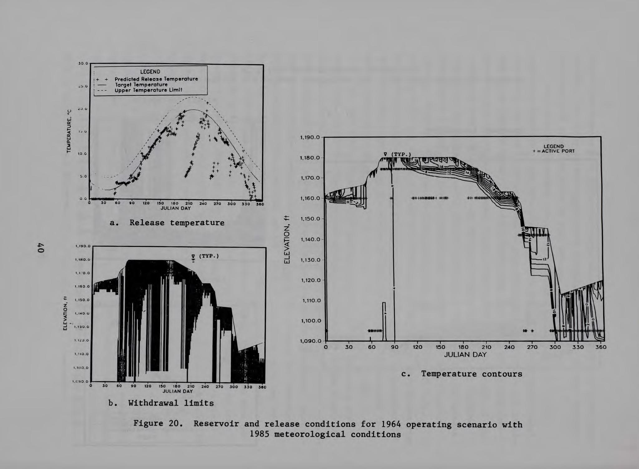
40. When the drawdown operational scenarios were simulated, higher

objective function values were computed. With the 1985 meteorological condi­

tions and the 1964 operating scenario (the simulation resulting in the largest

objective function value), all three ports were operated. The release tem­

perature did not exceed the upper bound; however, during gate changes, a con­

siderable drop in temperature was observed (Figure 20). When the drawdown

began, the discharge increased from 20 to 92 cfs. This impacted the release

temperature by expanding the withdrawal zone into the cooler hypolimnetic

layers. However, the large deviation that occurred on day 202 (21 July, a

14.5° C drop) was due to a shift from the upper to the middle gate rather than

being flow related. A similar situation occurred on day 245 (2 September)

when flow was shifted from the middle to the lower port. This resulted in a

release temperature drop of 13.4° C.

41. The 1984 meteorological conditions with the 1965 operating sce­

nario, und~r which the final optimum configuration resulted in the lowest ob­

jective function value, were investigated next to determine if similar release

temperature deviations occurred under the best operating conditions. Examina­

tion of the release temperature from this simulation (Figure 21) indicated

similar trends to the simulation of 1985 meteorological data with the 1964

operating scenario. During January-March, reservoir temperatures were rela­

tively uniform top to bottom; therefore, releases during this period were not

affected by port operation. In addition, deviations above the release tem­

perature objective were due to reservoir temperatures that were above the

release temperature objective. When the flow was increased from 26 to 481 cfs

on day 254 (11 September), the expansion of the withdrawal zone into the

hypolimnion resulted in a cooler release temperature (3.9° C change). By day

256 (13 September), when the lower port was no longer submerged and all flow

had to be released through the flood-control gates, the temperature dropped

another 5.5° C. The remaining drawdown scenarios displayed similar results as

indicated by the objective function values. When the discharge was increased,

expansion of the withdrawal zone caused a drop in release temperature. With

the falling pool and subsequent shift to lower gates, an even larger drop in

release temperature was observed.

38

42. The temperature criteria as given by the State of Pennsylvania

(paragraph 12) do not contain criteria for maximum allowable temperature

deviations below the objective. Therefore, a meeting with the Philadelphia

District was held 19 November 1987 to discuss these preliminary results. At

this meeting, the temperature deviation was discussed and determined to be un­

acceptable. A number of alternatives were discussed; however, only two ap­

peared to be feasible: a movable submerged weir and reservoir destratifica­

tion. Analyses of those options are presented in the next two parts of this

report.

42

PART IV: EVALUATION OF SUBMERGED WEIR

Background

43. Submerged weirs have been used on several projects to minimize the

release of hypolimnetic water. The technique involves construction of an

impermeable submerged weir upstream of the intake structure. The crest of the

weir is located to constrict the lower withdrawal limit and thereby release

predominantly epilimnetic water. For example, Clarence Cannon Dam, which is

operated by the St. Louis District, was constructed with a submerged weir in

front of the dam. This weir improves the quality of release by minimizing the

depth of the withdrawal zone during hydropower releases. This concept works

well for projects with minimum water level fluctuation. However, the weir is

fixed; therefore, the range of pool elevations over which the weir is effec­

tive is limited. In addition, there is no provision for lowering the pool be­

low the crest of the weir. At Prompton Reservoir, a moveable weir could pos­

sibly be designed into the proposed outlet structure. This is envisioned as a

series of stop logs stacked in a bulkhead or gate slot. As the water level is

dropped, the stop logs are removed to ensure submergence of the weir crest.

Modification to Numerical Model

44. The use of a moveable submerged weir to allow more epilimnetic

water to be released during the drawdown to minimize the temperature drop when

the discharge is increased was evaluated using the numerical model. The model

was modified to use a moveable submerged weir as a release structure. Since

the proposed structure would have a 30- ft-wide gate, a 30-ft-wide weir was

conceptualized as a series of 2-ft-high gates (as suggested by the Philadel­

phia District) which were stacked in a single gate slot much like stop logs.

Flow would be controlled by a gate in the wet well. As the discharge was in­

creased during the drawdown scenario, and the pool dropped subsequently, the

gates were pulled to always allow between 1 and 3 ft of water over the weir.

During pool filling the gates were replaced, resulting in the same condition

of 1 to 3 ft of submergence.

43

Results of Numerical Simulation Using a Submerged Weir

45. Using the 1985 meteorological conditions with the 1964 operating

scenario, a simulation was run using only weir flows. These conditions were

chosen since they represent the most difficult for the final optimum configu­

ration to meet. The thermal stratification in the pool (Figure 22) was only

minimally impacted by the weir flows and appeared very similar to the optimum

condition as shown in Figure 20. However, as with previous drawdown scenar­

ios, when the flow was increased, the withdrawal zone expanded, causing a drop

in the release temperature. For example, on day 294 (21 October) the dis­

charge was increased from 57 to 497 cfs, resulting in a release temperature

drop from 12.0° to 8.1° C. In addition, a considerable degree of daily varia­

tion in release temperature was observed due to the loss of selective with­

drawal control; and during the spring, the release temperature exceeded the

upper limit on several occasions as a result of withdrawal from the surface

layer during minimum flow events. Since this alternative did not satisfy re­

lease temperature requirements any better than previous port simulations,

further si~ulations using other drawdown and meteorological conditions were

suspended. Although a hybrid wet well consisting of both gates and a weir

could minimize some of the fluctuation, the increase in the withdrawal zone

when the drawdown occurs would still impact release temperature.

46. From this simulation it was apparent that large discharges during

the stratified period produced considerable drops in temperature downstream no

matter what type of release structure was used. Therefore, the drawdown

scenarios create a problem that is bounded by resources rather than the type

or design of the release structure. Thus, a second alternative involving

modification of the thermal structure in the pool to reduce the release tem­

perature fluctuation was evaluated.

(

44

PART V: EVALUATION OF RESERVOIR DESTRATIFICATION

Background

47. The destratification of the pool may minimize fluctuation of the

release temperature associated with the drawdown scenarios by modifying the

in-reservoir temperature profile to near-uniform conditions (allowing for a

minimal temperature difference between the surface and the bottom of the

pool). This prevents the density stratification, which defines the limits for

withdrawal zone formation. This makes the withdrawal zone extend from roughly

surface to bottom regardless of discharge, and effectively makes the release

temperature independent of discharge.

48. There are a number of destratification devices currently in use.

These include mechanical pumps that transport surface water downward into the

hypolimnion and aeration systems that release air bubbles near the bottom to

create circulation cells as the bubbles rise to the surface. The method by

which Prompton Reservoir would be destratified was not investigated. However,

for this study, the model assumed that it could be destratified.

49. Using the destratification design guidance developed from previous

research at WES (Holland and Dortch 1984), a lake destratification system

could be designed. For example, three 40-hp surface mixers typically used in

hydraulic mixing applications could destratify the entire lake in approxi­

mately 9 days.

Modification to Numerical Model

50. To investigate the effects of destratification on release tempera­

ture, the numerical model was again modified to add a simplified destratifica­

tion routine. Since previous research indicated that an 80 percent mixed con­

dition is the design condition that is the most feasible (Dortch 1979), the

model was modified to simulate an 80 percent mixed state throughout the entire

reservoir. This was simulated by removing 80 percent of the volume of each

layer in the reservoir, mixing these removed volumes together to a uniform

temperature, and then adding the mixed volume back to the respective layer. A

stable density profile was then enforced to achieve the destratified

46

condition. For this study, this resulted in a surface-to-bottom temperature

difference usually less than 6° c.

Results of Simulation Using Lake Destratification

51. The 1985 meteorological condition with the 1964 operating scenario

(as used with previous simulations) was used to investigate the impacts of the

destratification system on release temperature objectives. The simulation

with the destratificatio•' system operating from day 3 (3 January) to day 365

(31 December) reduced the release temperature fluctuations from those pre­

viously predicted (compare Figure 20 with Figure 23); however, the reservoir

retained more heat, thereby exceeding the upper limit of the release criteria

during the late summer. Since the destratification system is ineffective in

the winter when little stratification exists, a second simulation was run in

which the destratification routine was initiated on day 45 (14 February).

Also, the previous simulations indicated that heat retention by the reservoir

resulted in release temperature exceeding the objective. Therefore, the simu­

lation was repeated with the destratification system operating only from

day 45 through day 160 (9 June). The results of this simulation are given in

Figure 24. The release temperature followed the objective temperature much

more closely, deviating only when the highest port was no longer submerged and

the operation switched to the next lower port. A similar temperature drop oc­

curred with the switch from ports 2 and 3 to the flood-control gate operation.

The spring destratification produced a weaker stratification prior to the

drawdown, allowing the selective withdrawal capability of the structure to be

used to meet the release temperature criteria. Prior to destratification, the

release temperature deviations, which were 2 .78° C above or below the objec­

tive temperature, occurred on 74 days. This was also reflected by the objec­

tive function value (5930). However, the use of the destratification system

reduced the number of days the release deviated from the objective band to 10,

which was also reflected in the objective function value (300). These 10 days

were during the fall (mostly November) when the lake volume was relatively

small as a result of the drawdown. This period was therefore more sensitive

to meteorological conditions and was cooler than the objective temperature.

Simulation of the remaining drawdown scenarios with destratification resulted

in relatively low objective function values as well as reductions in the

47

number of days the release temperature deviated from the objective (Table 1).

As with the 1985 simulation of the 1964 operating condition with the destrati­

fication system, most occurrences of the deviation were during the late fall

(October-November) when the reservoir volume was small. All of the deviations

were below (more than 2.78° C) the objective temperature with only two excep­

tions. The simulation using the 1985 meteorological conditions with the 1965

operating scenario resulted in warmer lake temperatures during the spring when

the reservoir was filling; consequently, these releases were warmer than the

release temperature objective (Figure 25). The simulation using the 1984

meteorological conditions with the 1964 operating scenario resulted in a

larger objective function value than the same simulation without destratifica­

tion due to fall releases that exceeded the upper limit of the target release

temperature (Figure 26). Although these two simulations did not result in

decreases in the objective function values, the number of days that deviations

of release temperature from the objective occurred were reduced significantly

from the same simulation without destratification. Further, the large release

temperature changes associated with increased discharge or gate charges were

eliminated through use of destratification.

Table 1

Objective Function (OBF) Values and Number of Days of Release Temperature

Objective Deviations With and Without Destratification

Without With Meteorological Operating Destratification Destratification

Condition Scenario days OBF days OBF

1983 1930 61 2820 33 1920 1957 82 4440 41 1900 1964 93 5580 22 608 1965 66 2650 35 907

1984 1930 46 1500 22 604 1957 48 2050 27 536 1964 42 1520 25 3170 1965 35 848 25 576

1985 1930 39 3540 16 448 1957 65 5100 4 32 1 1964 74 5930 10 320 1965 60 4210 17 4590

50

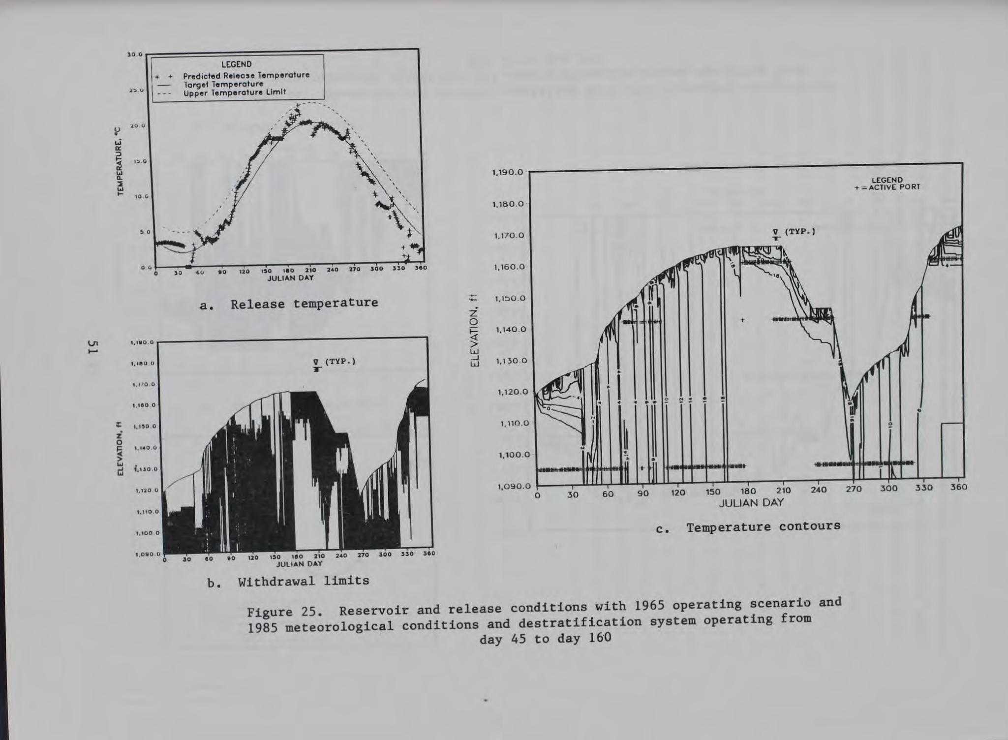
52. The results for these simulations indicate that the three-port dual

wet well structure with 325-cfs capacity per port in combination with a lake

destratification system will generally provide the control necessary to meet

the release temperature criteria.

53

PART VI: CONCLUSIONS AND RECOMMENDATIONS

53. The proposed increase in storage of Prompton Reservoir will require

modification of the existing uncontrolled release structure. This proposed

storage increase will raise the pool approximately 55 ft. In order to main­

tain acceptable release temperatures downstream. the modified structure was

proposed with selective withdrawal capability. This investigation was under­

taken to determine the optimum number. capacity. and location of selective

withdrawal ports in the release structure. Using an optimization routine

coupled to a one-dimensional thermal model, an optimum structure consisting of

three ports with 325-cfs capacity per port in a dual wet well configuration

was recommended. Upon closer examination of simulations of the release tem­

perature from this structure, the level pool operating condition met the re­

lease temperature criteria; however, with initiation of any of the four draw­

down scenarios, a considerable deviation in release temperature from the

objective was observed as a result of increased release volume during the

drawdown and its resulting shifts to lower ports.

54. Because the temperature deviation was deemed unacceptable by the

Philadelphia District, two alternatives were examined. One alternative in­

volved a submerged weir, configured as a stop log structure, which could be

lowered with the pool; however, a considerable variation in daily release tem­

perature was observed through its use. The second alternative involved the

use of lake destratification to minimize the thermal stratification and

thereby minimize the release temperature deviations associated with the draw­

down. This alternative, in conjunction with multilevel selective withdrawal

capability, met the release temperature criteria. This recommended three-port

structure, in conjunction with a lake destratification system, will be re­

quired to meet release temperature objectives during all of the four drawdown

scenarios. It is recommended that prior to construction of the new release

structure, a more detailed investigation of destratification methods be con­

ducted to determine operational guidance of the system.

55. Since the initiation of this investigation, considerable research

has been conducted on the simultaneous operation of multilevel ports in a

single wet well (as opposed to the operation of a single port in a single well

as simulated in this investigation). Although this single wet well technology (

has not been fully integrated into design tools at this time, results of that

54

research indicate that a single wet well with the same total capacity as a

dual wet well design would provide much of the same release temperature capa­

bilities as a dual wet well provided that it has the ability to throttle flow

through individual ports. However, there are some tradeoffs in operational

flexibility with the use of a single wet well compared to a dual wet well

design. This alternative may merit investigation.

I

55

REFERENCES

Davis, J. D., Holland, J. P., Schneider, M. L., and Wilhelms, s. C. 1987 (Mar). "SELECT: A Numerical, One-Dimensional Model for Selective With­drawal," Instruction Report E-87-2, US Army Engineer Waterways Experiment Station, Vicksburg, MS.

Dortch, M. S., Loftis, B., Fontane, D. G., and Wilhelms, S. C. 1976 (Dec). "Dickey-Lincoln School Lakes Hydrothermal Model Study," Technical Report H-76-22, US Army Engineer Waterways Experiment Station, Vicksburg, MS.

Dortch, M. s. 1979 (Apr). "Artificial Destratification of Reservoirs; Hy­draulic Laboratory Investigation," Technical Report E-79-1, US Army Engineer Waterways Experiment Station, Vicksburg, MS.

Dortch, M. S., and Holland, J. P. 1984 (Nov). "A Technique to Optimally Locate Multilevel Intakes for Selective Withdrawal Structures," Technical Report HL-84-9, US Army Engineer Waterways Experiment Station, Vicksburg, MS.

Eiker, E. 1977 (Nov). "Thermal Simulation of Lakes," Program Number 722-F5-E1010, US Army Engineer District, Baltimore, Baltimore, MD.

Holland, J. P. 1982 (Apr). "Effects of Storage Reallocation on Thermal Char­acteristics of Cowanesque Lake, Pennsylvania; Numerical Model Investigation," Technical Report HL-82-9, US Army Engineer Waterways Experiment Station, Vicksburg, MS.

Holland, J. P., and Dortch, M. S. 1984 (Aug). "Design Guidance on Hydraulic Destratification," Environmental and Water Quality Operation Studies, Informa­tion Exchange Bulletin E-84-4, US Army Engineer Waterways Experiment Station, Vicksburg, MS.

Howington, S. E. 1989 (Jul). Dam, Oregon," Technical Report Station, Vicksburg, MS.

"Intake Structure Operation Study, Lost Creek HL-89-13, US Army Engineer Waterways Experiment

Martin, J. L. 1986 (Mar). "Application of a Two-Dimensional Model of Hydro­dynamics and Water Quality (CE-QUAL-W2) to DeGray Lake, Arkansas," Technical Report E-87-1, US Army Engineer Waterways Experiment Station, Vicksburg, MS.

Schneider, M. L., and Price, R. E. 1988 (Sep). "Temperature Analysis, Howard A. Hanson Reservoir, Washington; Mathematical Model Investigation," Technical Report HL-88-22, US Army Engineer Waterways Experiment Station, Vicksburg, MS.

I

56

APPENDIX A: PROMPTON RESERVOIR NEAR-FIELD PHYSICAL MODEL INVESTIGATION

Purpose

1. Previous studies (Howington 1989; Dortch et al. 1976)* had indicated

that local topography can influence the withdrawal characteristics. An

undistorted-scale near-field physical model of the Prompton Reservoir in the

vicinity of the proposed new release structure was constructed to evaluate the

effect of the local topography upon the withdrawal characteristics of the

project. By developing a site-specific description of withdrawal from the

physical model results, these local effects were accounted for in a numerical

model through adjustment of the withdrawal angle parameter. This information

was used in conjunction with the numerical simulation to determine the optimum

port configuration to meet release temperature requirements at the project.

Model Description

2. The scaling procedure used with these types of model studies is

based on Froudian similitude. The model must be scaled such that the Froude

number, which is the ratio of inertial to gravitational forces, is similar

between the model and the prototype. This results in a length scaling that is

equal to the established model scale. Since the minimum prototype length

that needed to be reproduced was 100ft (depth of the pool), the scale of

1 ft in the model to 50 ft in the prototype would allow use of a 2-ft-deep

flume. Previous selective withdrawal work performed in physical models has

used scales ranging from 1:40 to 1:100 (Howington 1989 ) . The established

scaling parameters follow (dimensions are in terms of length):

Dimension Length L r

Velocity v r

Discharge Qr

Density difference 6p r

Ratio - L

- L1/2 r

- LS/2 r

- 1

Scale Relation Model:Prototype

1: 50

1 : 7

1:17,677

1 : 1

* References cited in this Appendix are included in the References at the end of the main text.

A1

3.

(model to

.,

-~-- --1

---1----- ' .. ,. \ - --- -

4

f

T L , I ]_

t/

r --

--- l + •

__ j-

Figure A1. Prompton physical model

The physical model (Figure A1) was constructed to a 1:50 scale 3 prototype) in an 800-ft flume and reproduced the area of the proj-

ect within approximately 250 ft in all directions from the release structure.

Previous selective withdrawal work had indicated that the topographic influ­

ences are limited laterally to the distance approximately equal to two with­

drawal zones. Since the maximum withdrawal zone thickness could not exceed

the maximum pool depth (90ft), the topography had to extend at least 180ft

in all directions from the structure. The prototype intake structure was

modeled to approximate external dimensions. Due to the uncertainty of the

number and location of ports in the proposed structure, the front of the

structure was removable to allow different locations, as well as sizes, of

ports to be modeled. Initial tests were conducted using the three-port dual

wet well structure recommended in paragraph 38 (main text). Since operation

of the flood-control gate was not considered as part of the selective with­

drawal system by the Philadelphia District, it was not modeled. Because the

possibility for a dual wet well structure existed, the ;model structure was

A2

constructed with a partition to simulate separate wet wells, each controlled

by a gate valve. Total flow from the structure was controlled by a single

gate valve downstream of a rotameter used to determine total flow in gallons

per minute. Topography was reproduced using plywood and metal with the

structure reproduced with Plexiglas.

Testing Procedure

4. Density stratification within the lake resulting from temperature

stratification was simulated in the model using fresh and salt water. Since

the densimetric Froude number similitude between the model and the prototype

is significantly more dependent upon the density difference rather than the

absolute water density, actual densities were not simulated. To achieve this

density stratification, the flume was filled in layers. Salt water was added

to represent the hypolimnion. Fresh water used to represent the epilimnion

was added on top of the salt water using a moveable weir structure. Upon cqm­

pletion of filling, the stratification was allowed to stabilize. Then a ver­

tical temperature and conductivity profile was taken at discrete intervals and

used to compute a density profile. A particular port operation was then set

and the desired flow from the port was measured using the rotameter. To de­

termine the impacts of a range of flows, four flow rates were tested in this

investigation (50, 100, 220, and 325 cfs corresponding to 1.27, 2.54, 5.58,

and 8.25 gpm, respectively, in the model). The larger flow rates, 220 and

325 cfs, were the maximum flows under cons ideration by the Philadelphia Dis­

trict. To determine the shape and limits of the withdrawal zone, crystalline

dye was dropped in front of the release structure. A fixed grid located in

front of the operating port was used to measure the shape and limits of the

withdrawal pattern. The dye streak displacement was filmed through the trans­

parent flume walls with a video camera. This allowed the development of the

withdrawal pattern to be accelerated or slowed t o accurately determine the

level of maximum withdrawal and the withdrawal limits.

5. The port geometry flow and test density profile were input into the

numerical model SELECT (Davis et al. 1987) to compute withdrawal characteris­

tics. This model contains the essential selective withdrawal parameters and

computational procedures that are contained in the withdrawa: routines in the

WESTEX model. Therefore the withdrawal characteristic simulated by the SELECT

A3

model would be the same as the WESTEX model. The SELECT model predicted

values were compared to the physical model observed values to determine the

impacts of the local topography.

Results

6. Tests were completed for each of the three ports recommended by the

WESTEX optimization results (paragraph 37, main text) using the four flow

rates and a range of stratification patterns (from linear to two-layer). The

two-layer stratification series with the uppermost port was conducted twice,

yielding a total of 28 tests. The observed test conditions (port flow, eleva­

tion, and density stratified) were also simulated in the SELECT model.

7. The results of the model investigation were analyzed by comparison

of physical model observation to those predicted by the SELECT model. The

comparison of the SELECT-predicted limit to the upper limit observed in the

physical model (Figure A2) indicated the predictability improved as the limit

approached the surface. This is probably a result of the limit extending to

the upper boundary (surface) rather than an improvement in predictability.

Once the upper limit reached the surface, location of the limit both in the

numerical and physical model was dependent on the surface elevation. The

maximum difference between the SELECT-predicted values and those observed in

the physical model was 6.5 ft (prototype).

8. The comparison of the SELECT-predicted to observed physical model

lower limit (Figure A2) was more accurate than that of the upper limit with

the maximum difference between predicted and observed of 4.5 ft. As mentioned

earlier (paragraph 1, Appendix A), local topography could have an influence on

formation of the withdrawal zone. This could be manifested perhaps by the

lower limit interacting with the bottom, thereby modifying the shape or upper

limits of the withdrawal zone. Since the lower limit did not reach the bot­

tom, the boundary had no impact on the withdrawal zone. In addition, the com­

parison of the SELECT-predicted upper and lower limits to those observed in

the physical model indicated good agreement requiring no modification to the

assumed withdrawal angle.

9. The comparison of the elevation of maximum withdrawal (Figure A3)

was much more variable with deviations of SELECT-predicted elevation from

those observed in the physical model of up to 14.5 ft. ' However, the average

A4

-.,._ •

1-

2 .....1

a:: w (L (L

:::> 0 w 1-u 0 w a:; (L

-.... . 1--~ .....1

a:; w 3 0 .....1

0 w 1-u 0 w a:: (L

1, 1 90.0~-------------------------------------------------~

1,180.0

+

+

1, 170.0

1,160.0 -.J_

+ + +

+ ..,... .....

'-k 1,, 50.0 7.::-:::-:::----:-~-=------------~------!

I, 15 0. 0 1, 1 6 0 . 0 t , 17 0. 0 1 1 e 0. 0 1,190.0

OBSERVED UPPER LIMIT, ft

a . Upper limit comparison

t, 17o.or-------------------------

1, 160.0~

1.150.0

1,140. 0-

1,130. 0- + +

..... ..,..

+ + :;: +

+

+ +

+ +

+

1. 120 .0~--------~------------------------------------------~ ;,130.0 1, ' 4 0.0 1,150.0 1,160 0 1,170.C 1,1:!0.0

Figure A2 .

OBSERVED LOWER LIM I- , ft

b. Lower limit comparison

Comparison of predicted with observed limits of withdr awal

AS

-... ~

~ <{

!: <{ 0:: a I ......

!: ~ :J ~ -X <{ ~

a UJ I-(.) -0 UJ 0:: a..

1, 1 80 . (•..,....---------------------~

..1.. • ...-+

1' 170 Co .J.. T ..... ~ .

1.160 . 0-

++

+ -r- +

1.150.0-

++- ++

1, 140 . 0 -", -----""!'.-----~.-----...,.... ____ ___,. 1,140.0 1,150.0 1,160 .0 1,170. 0 1,1e 0.0

OBSERVED MAXIMUM WITHDRAWAL.., ft

Figure A3. Comparison of predicted with observed maximum withdrawal

deviation was only 2.4 ft. The parabolic shape of the withdrawal zone made

determination of the limits fairly precise. However, the layer of maximum

withdrawal was much more difficult to determine since the maximum layer may

extend over a range of 10 to 20 ft in the prototype. As with the limit com­

parison discussed previously, comparison of the SELECT-predicted layer of

maximum withdrawal with those observed in the model indicated relatively good

agreement.

10. The final comparison was that of the SELECT-predicted density with

release density observed from the physical model (Figure A4). As with the

previous comparison, the SELECT-predicted release density compared favorably

with those observed from the physical model. The maximum difference observed

(0.0005 g/cc) was just above the limits of detection (0.0002 g/cc), indicating

good agreement between the numerical and physical model.

Conclusions

11. The key parameter, as discussed in paragraph 1 (Appendix A) used to

A6

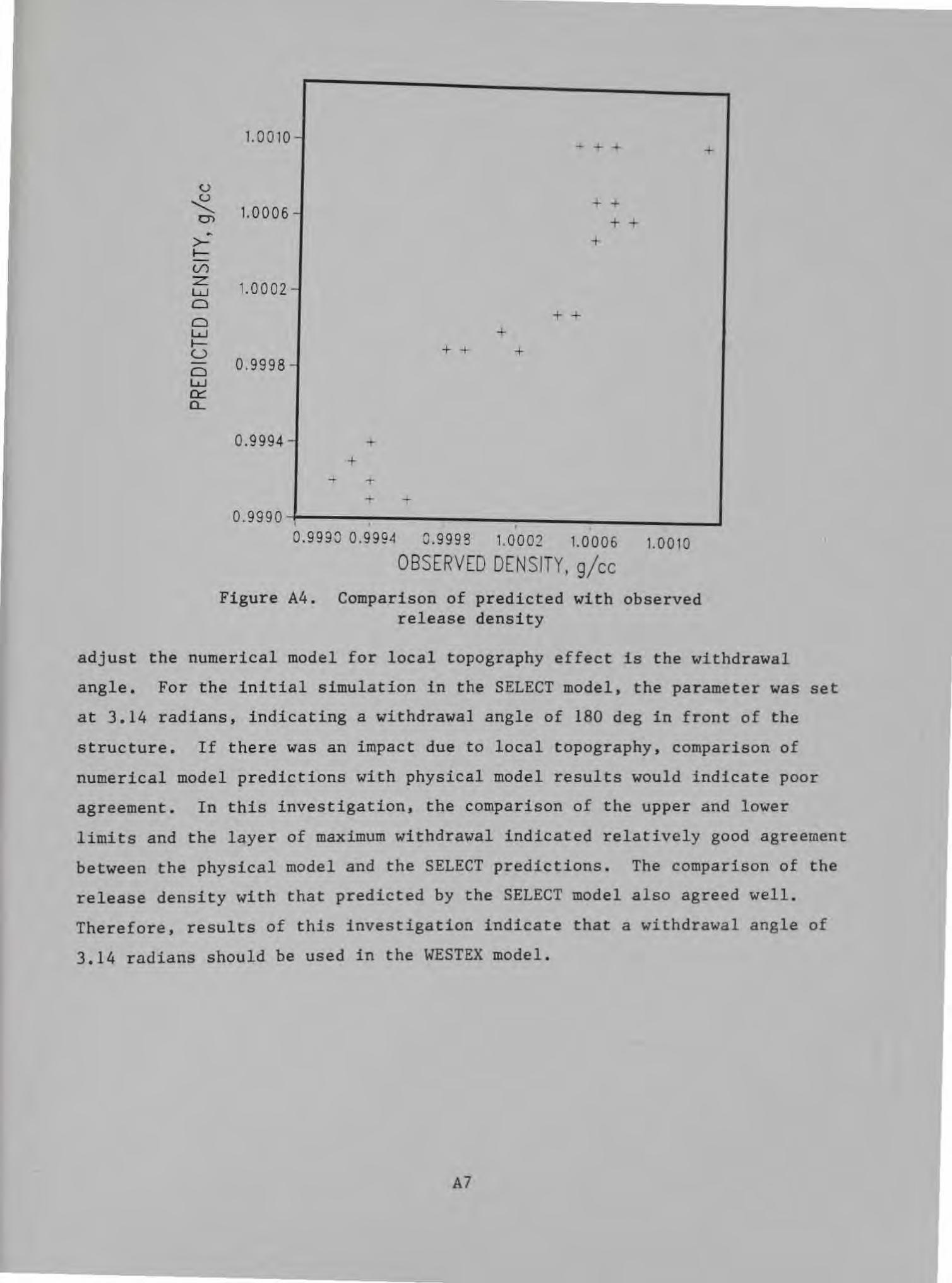
u

~ 0)

... >-..___ -(/)

:z w 0

0 w ..___ (_)

0 w a:::: a_

+ 1.0010-

..J... + +

1.0006 -+ +

+ + +

1.0002 -

+ + +

+ + + 0.9998 -

0.9994 - + +

-t T

T -0.9990 -r----------------..J

o.999o 0.9994 a .9998 1.0002 1.ooo5 1.0010

OBSERVED DENSITY, g/cc

Figure A4. Comparison of predicted with observed release density

adjust the numerical model for local topography effect is the withdrawal

angle. For the initial simulation in the SELECT model, the parameter was set

at 3.14 radians, indicating a withdrawal angle of 180 deg in front of the

structure. If there was an impact due to local topography, comparison of

numerical model predictions with physical model results would indicate poor

agreement. In this investigation, the comparison of the upper and lower

limits and the layer of maximum withdrawal indicated relatively good agreement

between the physical model and the SELECT predictions. The comparison of the

release density with that predicted by the SELECT model also agreed well.

Therefore, results of this investigation indicate that a withdrawal angle of

3.14 radians should be used in the WESTEX model.

A7