
Towards the simulation of dense suspensions: a numerical tool
25
ESAIM: PROCEEDINGS, August 2009, Vol. 28, p. 55-79 M. Ismail, B. Maury & J.-F. Gerbeau, Editors TOWARDS THE SIMULATION OF DENSE SUSPENSIONS: A NUMERICAL TOOL *, ** S. Faure 1 , S. Martin 2 , B. Maury 2 and T. Takahashi 3 Abstract. We present a numerical tool which aims at investigating the rheology of dense suspensions of entities such as spheres, red blood cells, polymer chains, or any kind of rigid or deformable bodies, in a viscous fluid. We shall pay a special attention to the short-range interactions between those entities (contact forces, lubrication forces). As for the fluid itself, our strategy consists in avoiding the direct and costly solution of the Stokes equations by integrating only the interaction forces which are likely to play a significant role in the overall behaviour of the suspension, in the spirit of Stokesian Dynamics. We present some preliminary results for suspensions of spheres, Red Blood Cells, and polymer-like chains. R´ esum´ e. Nous pr´ esentons un outil num´ erique permettant d’´ etudier la rh´ eologie de suspensions denses d’entit´ es telles que des sph` eres, des globules rouges, des chaˆ ınes de polym` ere et, d’une mani` ere g´ en´ erale, des objets rigides ou d´ eformables dans un fluide visqueux. Nous portons une attention particuli` ere aux interactions ` a courte distance entre ces entit´ es (forces de contact, forces de lubrification). En ce qui concerne le fluide lui-mˆ eme, notre strat´ egie consiste ` a´ eviter le calcul direct (et coˆ uteux) de la solution des ´ equations de Stokes, en d´ eterminant uniquement les forces d’interaction qui jouent un rˆ ole significatif dans le comportement g´ en´ eral de la suspension, dans l’esprit de la m´ ethode dite de Dynamique Stokesienne. Nous pr´ esentons quelques r´ esultats pr´ eliminaires pour des suspensions de sph` eres, de globules rouges, et de chaˆ ınes de polym` ere. 1. Introduction 1.1. On the determination of the behaviour of dilute and dense suspensions Theoretical approaches aiming at describing the behaviour of suspensions of deformable or rigid bodies have been limited for a long time to dilute suspensions. This approach has begun with the seminal work of Einstein [17, 18] in 1906 and 1911 on the effective viscosity of a dilute suspension of rigid spheres and, since then, it has been completed by numerous works (Batchelor [3,4], Brenner [9], Jeffrey & Acrivos [32], Russel [44], Davis & Acrivos [14]) related to the framework of dilute suspensions. From the prediction point of view, most of these works deal with weak solid concentrations in which pairwise interactions lead the behaviour of the suspensions. * The authors are truly indebted to Aline Lefebvre-Lepot for fruitful discussions on the contact algorithms. ** This work has been supported by the ANR project MOSICOB “Mod´ elisation et Simulation de Fluides Complexes Biomim´ etiques” 1 CNRS & Universit´ e Paris-Sud 11, D´ epartement de Math´ ematiques, Bˆatiment 425, 91405 Orsay cedex (France) 2 Universit´ e Paris-Sud 11, D´ epartement de Math´ ematiques, Bˆ atiment 425, 91405 Orsay cedex (France) 3 Institut ´ Elie Cartan UMR 7502 (INRIA, Nancy-Universit´ e & CNRS), POB 239, 54506 Vandœuvre-l` es-Nancy cedex (France) and Team-project CORIDA, INRIA Nancy-Grand Est c EDP Sciences, SMAI 2009 Article published by EDP Sciences and available at http://www.edpsciences.org/proc or http://dx.doi.org/10.1051/proc/2009039
-
Upload
khangminh22 -
Category
Documents
-
view
3 -
download
0
Transcript of Towards the simulation of dense suspensions: a numerical tool

ESAIM: PROCEEDINGS, August 2009, Vol. 28, p. 55-79
M. Ismail, B. Maury & J.-F. Gerbeau, Editors
TOWARDS THE SIMULATION OF DENSE SUSPENSIONS:A NUMERICAL TOOL ∗, ∗∗
S. Faure1, S. Martin2, B. Maury2 and T. Takahashi3
Abstract. We present a numerical tool which aims at investigating the rheology of dense suspensionsof entities such as spheres, red blood cells, polymer chains, or any kind of rigid or deformable bodies, ina viscous fluid. We shall pay a special attention to the short-range interactions between those entities(contact forces, lubrication forces). As for the fluid itself, our strategy consists in avoiding the directand costly solution of the Stokes equations by integrating only the interaction forces which are likely toplay a significant role in the overall behaviour of the suspension, in the spirit of Stokesian Dynamics.We present some preliminary results for suspensions of spheres, Red Blood Cells, and polymer-likechains.
Resume. Nous presentons un outil numerique permettant d’etudier la rheologie de suspensions densesd’entites telles que des spheres, des globules rouges, des chaınes de polymere et, d’une maniere generale,des objets rigides ou deformables dans un fluide visqueux. Nous portons une attention particuliere auxinteractions a courte distance entre ces entites (forces de contact, forces de lubrification). En cequi concerne le fluide lui-meme, notre strategie consiste a eviter le calcul direct (et couteux) de lasolution des equations de Stokes, en determinant uniquement les forces d’interaction qui jouent unrole significatif dans le comportement general de la suspension, dans l’esprit de la methode dite deDynamique Stokesienne. Nous presentons quelques resultats preliminaires pour des suspensions despheres, de globules rouges, et de chaınes de polymere.
1. Introduction
1.1. On the determination of the behaviour of dilute and dense suspensions
Theoretical approaches aiming at describing the behaviour of suspensions of deformable or rigid bodieshave been limited for a long time to dilute suspensions. This approach has begun with the seminal work ofEinstein [17, 18] in 1906 and 1911 on the effective viscosity of a dilute suspension of rigid spheres and, sincethen, it has been completed by numerous works (Batchelor [3,4], Brenner [9], Jeffrey & Acrivos [32], Russel [44],Davis & Acrivos [14]) related to the framework of dilute suspensions. From the prediction point of view, mostof these works deal with weak solid concentrations in which pairwise interactions lead the behaviour of thesuspensions.
∗ The authors are truly indebted to Aline Lefebvre-Lepot for fruitful discussions on the contact algorithms.∗∗ This work has been supported by the ANR project MOSICOB “Modelisation et Simulation de Fluides Complexes Biomimetiques”
1 CNRS & Universite Paris-Sud 11, Departement de Mathematiques, Batiment 425, 91405 Orsay cedex (France)2 Universite Paris-Sud 11, Departement de Mathematiques, Batiment 425, 91405 Orsay cedex (France)3 Institut Elie Cartan UMR 7502 (INRIA, Nancy-Universite & CNRS), POB 239, 54506 Vandœuvre-les-Nancy cedex (France)
and Team-project CORIDA, INRIA Nancy-Grand Estc© EDP Sciences, SMAI 2009
Article published by EDP Sciences and available at http://www.edpsciences.org/proc or http://dx.doi.org/10.1051/proc/2009039
56 ESAIM: PROCEEDINGS
When dealing with dense suspensions, a new approach is required. It deals with two major challengingdifficulties:
− the determination of multi-body (hydrodynamic) interactions between the particles,− the determination of the time-space distribution of the entities.
The determination of multi-body (hydrodynamic) interactions between the particles is a complex procedure.Although very complex, analytical results on hydrodynamic interactions were given by Mazur & van Saarloos[42, 45], in some specific geometrical situations. These computations do not apply to the general setting of asuspension (in which the geometrical configuration is not known a priori and evolves in time) but they providesome understanding on the importance of three-body (and generally multi-body) effects, as shown by Beenakker& Mazur [6], Beenakker [5]. However the determination of these interactions reveals two types of difficulties:
− in the case of dense suspensions (with high solid concentrations), lubrication forces play a leading rolein the dynamics of the macroscopic structure. These forces are due to the presence of a thin layer ofviscous fluid between two entities at quasi-contact. One of the major effects of the lubrication relies onthe fact that the relative motion between two entities tends to zero as their distance tends to zero.
− long-range interactions have to be taken into account in suspensions. Indeed, a particle immerged ina Stokes flow leads to a perturbation of the velocity field (in the fluid) that decreases in 1/r, where rdenotes the separation between the particle and the current position considered in the fluid. These far-field interactions have to be considered in dilute or dense suspensions as resulting of all the perturbationsof the velocity field due to the presence of numerous entities evolving in the fluid. It also highlights theimportance of the multi-body effects in the interactions.
The determination of the time-space distribution of the entities plays a key-role in the identification ofmacroscopic properties of the suspensions. In suspensions, the microstructure cannot be specified a priori buthas to be considered as an unknown part of the problem: the entities evolve in the fluid, submitted to notonly non-hydrodynamic forces (which can be modelled very easily, in most of the cases) but also hydrodynamicforces (which may be very difficult to identify, as mentioned before). In particular, we focus on regimes whichare far from equilibrium so that there is no simple procedure which can predict the microstructure, even insome simple configurations.
1.2. On the direct simulation of suspensions
Several strategies have been proposed in the last two decades to simulate the motion of rigid bodies in aviscous fluid. A first class of methods relies on methods with a mesh in the fluid domain, by computing theflow in the fluid domain (which is complex because of the inclusions). Then, it is possible to compute theforces exerted on the particles and, as a consequence, the velocity perturbations. The position is deduced fromthis procedure and the mesh has to be redefined in the new fluid domain, by using several techniques suchas a ALE-type mesh displacement, before renewing the procedure for the next time step (see e.g. [29, 34, 41]).The conforming character of the mesh ensures a good accuracy in space; in particular hydrodynamic forces, onwhich lies the fluid particle coupling, are estimated in a proper way. But it presents some drawback in terms ofcomputational cost: the unstructured character of the mesh rules out the possibility to use standard fast solvers,and the problem of dynamic mesh generation can become delicate and costly, especially in the three-dimensionalsetting.
Another possibility for avoiding the above difficulties relies on the use of a mesh which covers the wholedomain. Fictitious domain methods allow us to overcome the problems related to the complex geometry byusing Cartesian grids in the whole domain. The presence of the entities in the fluid is dealt with an iterativealgorithm on an auxiliary field (composed of Lagrange multipliers) which permits to take into account therigid motion constraint of the particles (see e.g. [22, 23]). Alternative fictitious domain methods are based onpenalty principles: the rigid motion constraint is handled in a relaxed way by adding a term to the variationalformulation, which amounts to replace rigid zone by highly viscous ones (see [11, 31]). Finally, using that rigid
ESAIM: PROCEEDINGS 57
velocities are polynomials of degree 1, it is possible to take into account the rigid motion by combining the finiteelements of the mesh that correspond to the rigid domain: this method is developed and studied in [46].
Lattice Boltzmann methods are perhaps the most used procedures in the simulation of rigid or deformableentities in a Stokes flow. It is necessarily coupled with a specific algorithm dealing with the modeling andcomputation of the fluid-structure interactions such as the immersed boundary method or the boundary integralmethod (see [16,53,56]).
A wide variety of alternate methods is available. Let us cite a few of them: a so-called “front-tracking”method1 coupled to the immersed boundary method (for the interaction between the fluid and the deformablemembrane of the red blood cell which is considered as a viscous drop.) is used in [2]. The Immersed FiniteElement Method coupled to a meshfree method (Smoothed Particle Hydrodynamics) is used in [36].
Due to computer capabilities and blow up of the complexity with the number of entities, they are restrictedto a limited number of bodies, say a few thousands for three-dimensional simulations. Besides, although theoryasserts that no collision between immerged smooth bodies can occur (see [27, 28]), the possibility of very smallinterparticle distances or even numerical overlapping calls for a special treatment of close range interactionphenomena. Finally, some of those methods can be adapted to the case of deformable bodies, but a straightdiscretization of the corresponding fluid-structure interaction problem reduces the scope of this approach to afew entities.
In an attempt to address these limitations of direct methods, the approach we propose here, which is inbetweendirect simulations and heuristic strategies, is designed to handle the motion of many-body suspensions of rigidor deformable entities, in situations where close range interaction forces (including contact forces) are likely toplay a significant role.
1.3. Organization of the paper
The so-called “Stokesian Dynamics” method has been introduced by Brady & Bossis [7,8] and used primarilyfor non-equilibrium suspensions. It is based on the determination of both hydrodynamic interactions betweenthe entities inside the fluid and the microstrucure of the suspension. Computational efficiency of the methodis directly related to a pairwise assumption of the interactions: although not justified, this assumption leads toreasonable computational costs and does not alter the solution, as the Stokesian Dynamics has been proven toprovide excellent agreement with experiments.
In this framework, let us point out some of the key features of our contribution with respect to the StokesianDynamics: the solution technique, as proposed by Brady & Bossis, takes into account lubrication forces thatdo not allow contacts between the small entities. Nevertheless, from a numerical point of view, discretization intime may lead to possible contacts (and overlapping) between the bodies. We propose a numerical method (seeSection 2) that guarantees no-overlapping: at each time step, the computation of the velocity is based upon1) the evaluation of a so-called predicted velocity (due the dynamics) and 2) a projection procedure onto a setof admissible velocities that guarantees the no-overlapping situation. In some sense, this procedure selects theadmissible velocity which is the closest one from the predicted velocity.
This paper is organized as follows:• In Section 2, we present an algorithm which allows us to handle with contacts between rigid spheres (no
fluid is considered at this stage). Then, we present how it is possible to define macro-objects that arebuilt from a given number of elementary rigid spheres, by defining suitable interaction forces betweenthem. This leads to a deformable macro-object (e.g. a red blood cell, a polymer-like chain etc.).
• In Section 3, we describe the behaviour of a macro-object in a bulk fluid. Considering a macro-objectimmersed in a bulk fluid, the hydrodynamic force exerted on the macro-object is estimated, based onFaxen law. In return, the determination of the hydrodynamic force leads to the determination of thevelocity of the macro-object. Let us point out that although the use of Faxen law is not rigorously
1This method is based on the multifluid Stokes system as analysed by Nouri, Poupaud and Demay [15], and a finite-differences
discretization.
58 ESAIM: PROCEEDINGS
justified when applied to a collection of rigid spheres (at contact or near-contact), this procedure allowsus to capture some typical behaviour of a red blood cell in a shear flow. As a challenging problem, wepresent the simulation of dense suspensions based on the use of this very dilute assumption (Faxen law);again, although not valid, the use of Faxen law can be viewed as the main order (neglecting the multi-body interactions which become the leading ones in the case of dense suspensions) of the behaviour ofthe suspension and this problem reveals a challenging problem for our approach.
• In Section 4, we briefly present the Stokesian Dynamics, designed to simulate concentrated suspensions.We present a numerical procedure, based on the decomposition of the different regimes (large-fieldinteractions, intermediate interaction, short-range or lubrication interactions). Let us point out thatwhen dealing with dense suspensions, lubrication forces become predominant: this highlights the interestof the contact / no-overlapping algorithm presented in Section 2. We finally present a numericalsimulation of red blood cells in a flow at rest and illustrate the influence of the lubrication forceson the distribution of the macro-objects.
2. A numerical tool for an efficient handling of contacts between objects
In this section, we briefly present a numerical program called SCoPI (“Simulation of Collections of Particlesin Interaction”). In particular we first present an algorithm which allows us to handle with contacts betweenrigid spheres. Then we present how it is possible to create macro-objects of (nearly) any shape (based on thestructured association of rigid spheres), contacts being still handled by the numerical procedure. Notice that,at this point, SCoPI is a “granular-oriented” program in the sense that the macro-objects are not immerged ina fluid. The fluid-structure interaction will be discussed in the next section but is important to understand thegeneral idea and main interest of the program.
2.1. Contacts between rigid spheres: an algorithm
Consider N rigid spheres (mass mi, radius ai). They obey the following equation:
M · dUdt
= Fext, in R3N
where M = diag(mi I3×3) is the mass matrix, U the velocity of the N spheres, Fext the external force exertedon the spheres. We aim at investigating the motion of the spheres, thus characterized by the position vector q(or the velocity vector U)
q(t) =
q1
...qi...
qN
(t), U(t) =dqdt
(t),
where qi is a three-component vector describing the space position of sphere i.We aim at simulating the behaviour of a large number of spheres. From both theoretical and numerical points
of view, the spheres should not overlap; this nonlinear phenomenon introduces some constraint on the way tosolve the problem. It can be overcome by using a projection of the velocities onto a set of admissible velocitiesand penalty method (see [40]). From a numerical point of view, the simplest idea for the dynamic simulationof such a system consists in defining a time step h (assumed to be constant for the sake of simplicity) and theexplicit Euler procedure: {
Un+1 = Un + hM−1 · Fnext,qn+1 = qn + hUn+1,
ESAIM: PROCEEDINGS 59
where Un (resp. qn) denotes the velocity (resp. position) of the particles at time tn = nh. In a similar way,Fnext denotes the external forces exerted on the particles at time tn. This procedure is not valid as it is highlypossible that particles overlap at time tn+1 even if they do not overlap at time tn. Thus we have to treat in aspecific way the contact between particles. For this reason we define the set
K(qn) ={V ∈ R3N , Dij(qn) + hGij(qn) ·V ≥ 0, ∀i < j
}where
Dij(qn) =∣∣qni − qnj
∣∣− ai − ajdenotes the signed distance between two particles i and j and
Gij(qn) = ∇Dij = (..., 0,−eij , 0, ..., 0, eij , 0, ...), eij =qj − qi|qj − qi|
is the gradient of the distance. Our purpose is to solve the dynamics problem by constraining the velocity fieldof the particles to belong to the set of admissible velocity fields, at each time step, in order to prevent theparticles from overlapping.
Remark 2.1. Denote E(qn) ={V ∈ R3N , Dij(qn + hV) ≥ 0, ∀i < j
}the set of velocity fields V such that
particles, at position qn at time tn and with velocity V, do not overlap at the next time step. The constraintDij(qn) + hGij(qn) ·V ≥ 0 is the linearized form of the constraint Dij(qn + hV) ≥ 0 and, furthermore, it canbe shown that K(qn) ⊂ E(qn). It means in particular that particles with admissible velocities at time tn donot overlap at time tn+1.
In order to solve the no-overlapping problem, the following splitting procedure is proposed: at a first step,we first use the Euler scheme without taking into account the possible overlapping of the particles and, at asecond step, we use a projection method in order to satisfy the no-overlapping condition. Thus the algorithmreads:
(P)
Un+1/2 = Un + hM−1 · FnextUn+1 = minimizer of
{∣∣∣V −Un+1/2∣∣∣2 , V ∈ K(qn)
}qn+1 = qn + hUn+1
The interest of the procedure relies in the possibility to use any suitable solver for the computation of thedynamics. Contacts are handled at a second stage, without any consideration of the proper dynamics. At somepoint, it allows the use of any solver for the resolution of the dynamics problem: then the so-called predictedvelocity field is projected onto the set of admissible velocity fields.
The numerical treatment of the constraint is based on an equivalent formulation of the minimization problem,as it is is treated as a saddle-point problem, by using the introduction of Lagrange multipliers:{
Find (Un+1,Λn+1) ∈W such thatL(Un+1, λ) ≤ L(Un+1,Λn+1) ≤ L(V,Λn+1), ∀(V, λ) ∈W,
with W = R3N × RN(N−1)/2+ and
L(V, λ) =12
∣∣∣V −Un+1/2∣∣∣2 − ∑
1≤i<j≤N
λij (Dij(qn) + hGij(qn) ·V) .
Notice that the number of Lagrange multipliers corresponds to the number of possible contacts. In particular,if there is no contact between particles i and j, then λij = 0 and the Lagrange multiplier is not activated;conversely, if there is a contact between the two spheres, then λij may be positive and the correspondingauxiliary field allows the velocity field to satisfy the no-overlapping constraint. The approximate reaction fields
60 ESAIM: PROCEEDINGS
Λn+1 = (Λn+1ij ) is the dual component of a solution to the associated saddle-point problem. Note that Un+1
and Λn+1 are related by
M ·Un+1 = M ·Un + hFnext + h∑
1≤i<j≤N
Λn+1ij Gij(qn).
This problem is solved by an Uzawa algorithm (see, e.g., Ciarlet [13]).
2.2. Definition of macro-objects
SCoPI is a program which is based on the handling of contacts between spheres only. The way to handlewith macro-objects of any form relies on the possibility to describe the considered macro-object as a collectionof a given number of spheres. The way to define macro-objects can be summarized in the following list:
• each macro-body is made of a fixed number of rigid spheres;• the shape of the RBC is obtained by defining two- / three-body interactions between the spheres: the
so-called “cohesion” forces (Cα, Cβ and Cγ are constant parameters):− interaction between two spheres i and i+ 1:
Fi = Cα(|qi+1 − qi| − Cβ)ei i+1, Fi+1 = −Fi,
− interaction between three spheres i− 1, i and i+ 1:
Fi−1 = − Cγ|qi−1 − qi|
(ei i+1 − (qi−1 − qi) · (qi+1 − qi)ei i−1) ,
Fi+1 = − Cγ|qi+1 − qi|
(ei i−1 − (qi−1 − qi) · (qi+1 − qi)ei i+1) ,
Fi = −Fi−1 − Fi+1,
• a “fake” overlapping of the spheres belonging to a macro-object is possible;• an imposed contact with a specified distance between two spheres is also available.
The stability and (small) deformation of the macro-object are obtained by the definition of internal forcesbetween the spheres belonging to each macro-object. From a programming point of view, each sphere of amacro-object is submitted to at least cohesion forces (which guarantees the stability of the macro-object) andpossibly other forces modelling the external forces exerted on the macro-objects2.
The definition of a class of macro-objects takes advantage of all the functionalities of SCoPI. Indeed theimplementation of macro-objects only relies on the definition of a new class of objects. Moreover, the handlingof contacts between macro-objects does not need further implementation: contacts between macro-objects aretaken into account by SCoPI in a classical way, as the distance between two spheres belonging to two distinctmacro-objects is equal to 0.
We also introduce some “fake” overlapping of the spheres belonging to the same macro-object. The optionaloverlapping of spheres inside a macro-object introduces some facilities in the shape definition of the macro-object without breaking the handling of contacts in SCoPI. More precisely, for each sphere (with radius R),we define an internal radius Rint and an external (effective) radius Rext := R. In all the cases, the externalradius corresponds to the effective sphere and the internal one is artificial in the following sense: on one hand,when considering spheres belonging to a macro-object, contact may be handled either by the internal sphereor the external sphere: in the first option, overlapping between external spheres (of the same macro-object) ispossible, even if the handling of contacts, by SCoPI, is still active by means of the internal radii. On the otherhand, when considering two spheres belonging to different macro-objects, then contact is always handled by the
2The external forces are either exerted on each sphere of the macro-object or on a specified sphere of the macro-object.
ESAIM: PROCEEDINGS 61
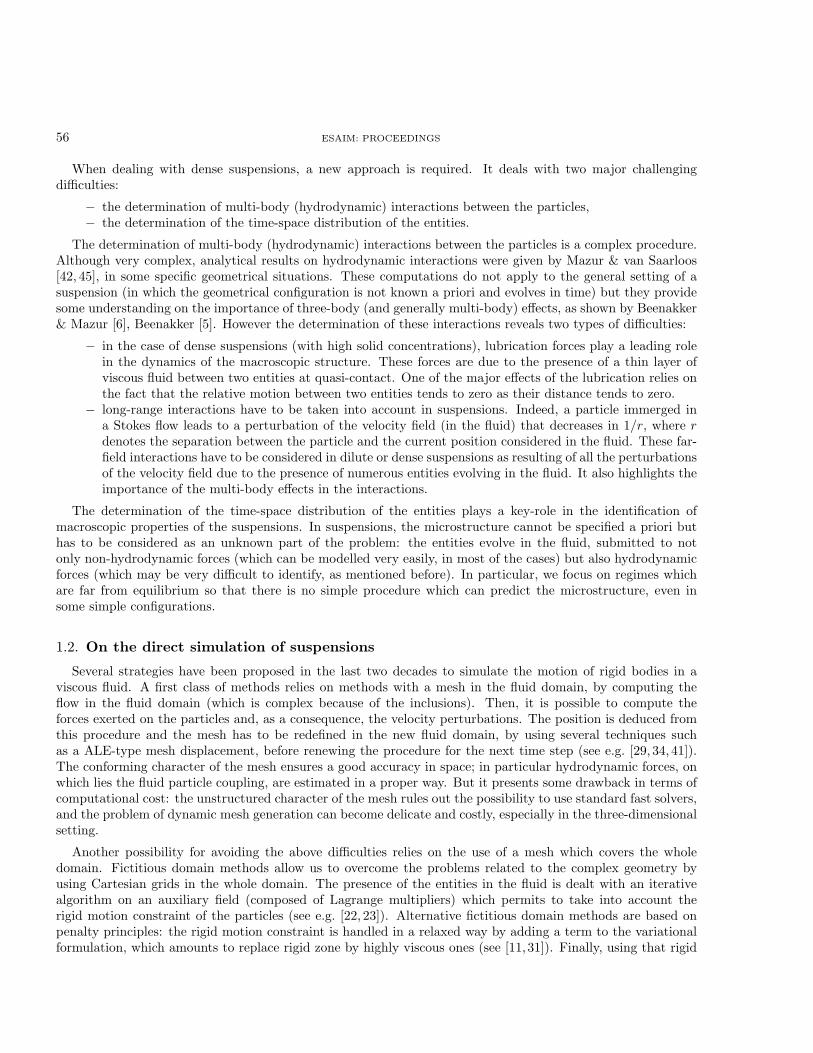
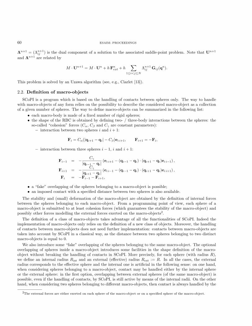
Figure 1. A red blood cell made of 11 rigid spheres with fake overlapping defined by: a two-body force between the center sphere and an annular sphere (on the left), a two-body forcebetween annular spheres (in the middle), a three-body force between annular spheres (on theright).
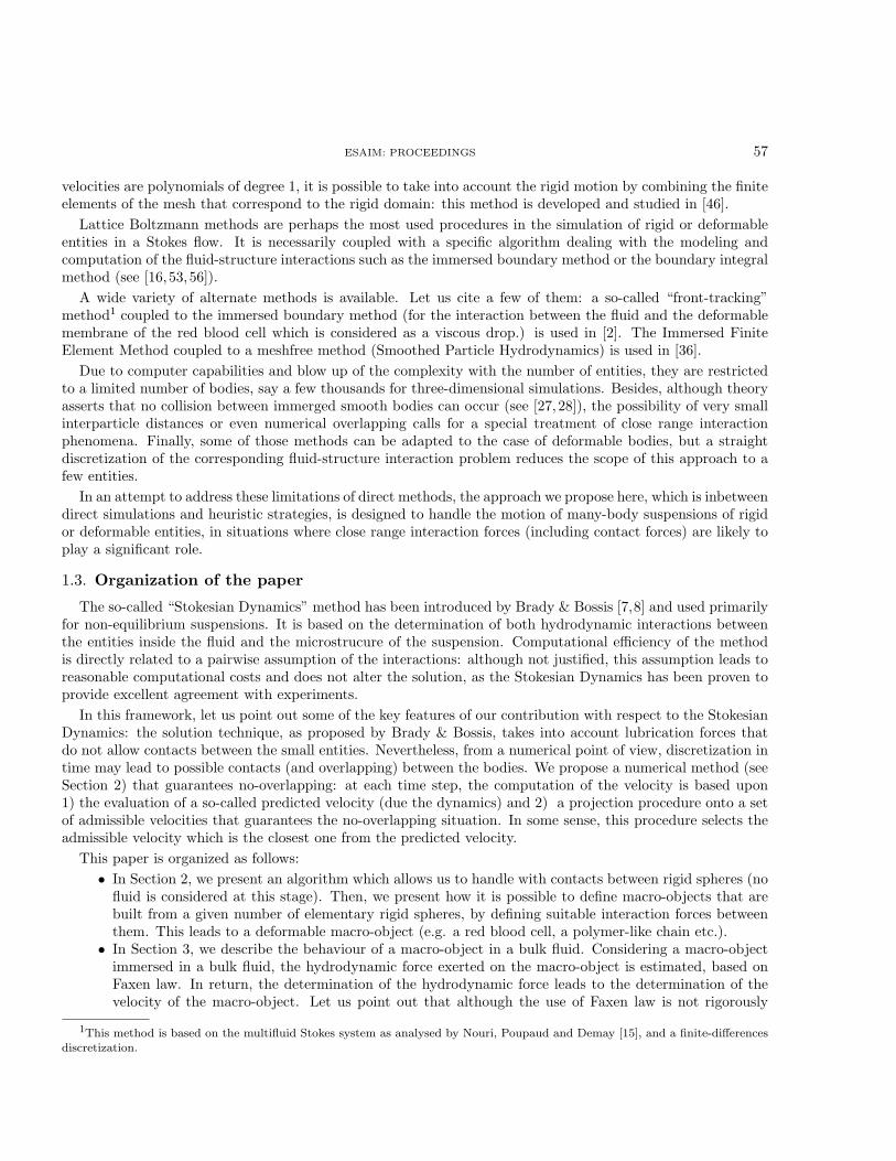
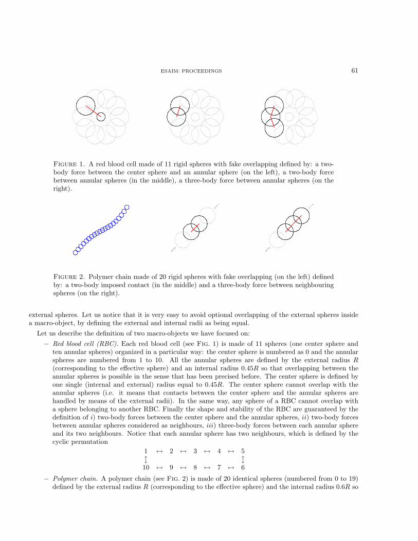
Figure 2. Polymer chain made of 20 rigid spheres with fake overlapping (on the left) definedby: a two-body imposed contact (in the middle) and a three-body force between neighbouringspheres (on the right).
external spheres. Let us notice that it is very easy to avoid optional overlapping of the external spheres insidea macro-object, by defining the external and internal radii as being equal.
Let us describe the definition of two macro-objects we have focused on:
− Red blood cell (RBC). Each red blood cell (see Fig. 1) is made of 11 spheres (one center sphere andten annular spheres) organized in a particular way: the center sphere is numbered as 0 and the annularspheres are numbered from 1 to 10. All the annular spheres are defined by the external radius R(corresponding to the effective sphere) and an internal radius 0.45R so that overlapping between theannular spheres is possible in the sense that has been precised before. The center sphere is defined byone single (internal and external) radius equal to 0.45R. The center sphere cannot overlap with theannular spheres (i.e. it means that contacts between the center sphere and the annular spheres arehandled by means of the external radii). In the same way, any sphere of a RBC cannot overlap witha sphere belonging to another RBC. Finally the shape and stability of the RBC are guaranteed by thedefinition of i) two-body forces between the center sphere and the annular spheres, ii) two-body forcesbetween annular spheres considered as neighbours, iii) three-body forces between each annular sphereand its two neighbours. Notice that each annular sphere has two neighbours, which is defined by thecyclic permutation
1 ↔ 2 ↔ 3 ↔ 4 ↔ 5l l10 ↔ 9 ↔ 8 ↔ 7 ↔ 6
− Polymer chain. A polymer chain (see Fig. 2) is made of 20 identical spheres (numbered from 0 to 19)defined by the external radius R (corresponding to the effective sphere) and the internal radius 0.6R so

62 ESAIM: PROCEEDINGS
that overlapping between the spheres is possible. The shape of the chain is guaranteed by the definitionof i) two-body imposed contacts between annular spheres considered as neighbours , ii) three-bodyforces between each sphere (from 1 to 18) and its two neighbours. Notice that each sphere has twoneighbours, except spheres 0 and 19 which only have one single neighbour. This is summarized by thechain describing the neighbours:
0 ↔ 1 ↔ · · · ↔ 18 ↔ 19
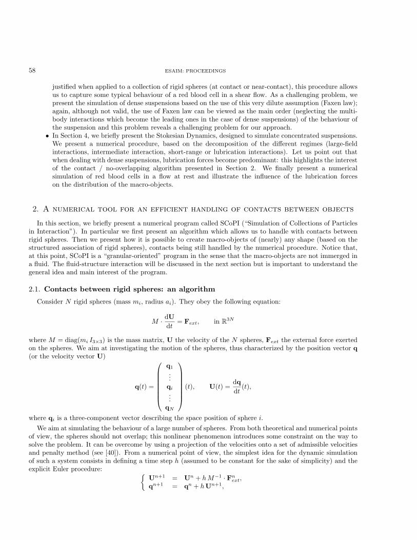
In the numerical procedure, visualizing tools are used (in some optional way): SCoPI is coupled to VTK3,which allows us to control in real time the formation of the macro-object (e.g. a red blood cell or a polymerchain for the numerical illustrations) when starting from an unrealistic geometrical configuration to some fixedtime at which the macro-object has formed and remains stable. Then, a post-processing visualizing procedurecan also be used with POV-Ray4 whose main effect is to smooth the contours of the objects (by introducingiso-surfaces of scalar fields, i.e. their surface is defined by the strength of the field in each point.): this producesmore realistic pictures and still respects the contact distance between the macro-objects: Fig. 3 shows thepost-processed pictures related to the VTK ones (only the angle and focus of the camera have been changed).
Once a macro-object has been defined (e.g. a red blood cell, a polymer chain, a vesicle...), the directsimulation of a suspension of such objects in a fluid needs further discussion: as mentioned before, a couplingprocedure between a fluid solver and the structure solver (SCoPI) can be used. Guided by a cost reduction,we present in the next section a way to simulate the hydrodynamic effects on the red blood cells (for dilute ordense suspensions) without computing the fluid flow: this is the so-called Stokesian Dynamics method.
3. Dilute suspensions
In this section, we explain the numerical procedure for the simulation of a finite number of macro-objects(composed of rigid spheres) in a sheared Stokes flow. We aim at avoiding the computation of the fluid flow and,for this reason, the method is based on the determination of hydrodynamic interactions between the objects,due to the influence of the surrounding fluid.
Consider a rigid sphere (radius a, velocity U) in a Stokes flow (viscosity µ, velocity field v∞). The velocityfield of the fluid is described as if it is not perturbed by the inclusion of the particle; here, it is defined on thewhole space. Faxen introduced a relation for a sphere velocity U to the drag force FH exerted on the sphere(see the Appendix for a brief justification). It reads:
FH = −6πµa (U− v∞(q)) + πµa3 ∆v∞(q)
where v∞(q) denotes evaluation of the function v∞ to which it is affixed at the center of the sphere (positionq of the sphere). In the case of a simple shear flow, the bulk macroscopic flow is governed by
v∞(x, y, z) = γ y ex.
and Faxen law reduces toFH = −6πµa (U− v∞(q)) .
Noteworthily, this regime has been the subject of intensive studies related to the behaviour of biomimeticobjects such as vesicles or red blood cells. In particular, depending on the intensity of the shear stress, theviscosity, the membrane elasticity and the geometry, the particle exhibits different motions: tumbling, tank-treading and swinging (periodic shape deformation and inclination oscillation while the membrane is rotatingaround the liquid inside). More precisely, by decreasing the shear-stress value, a bifurcation appears from steadytank-treading to pure tumbling. This phenomena is observed by Skotheim & Secomb [50] for red blood cells
3http://www.vtk.org/4http://www.povray.org/

ESAIM: PROCEEDINGS 63
Figure 3. A red blood cell visualized with VTK (on the left) and after a POV-Ray post-processing (on the right).
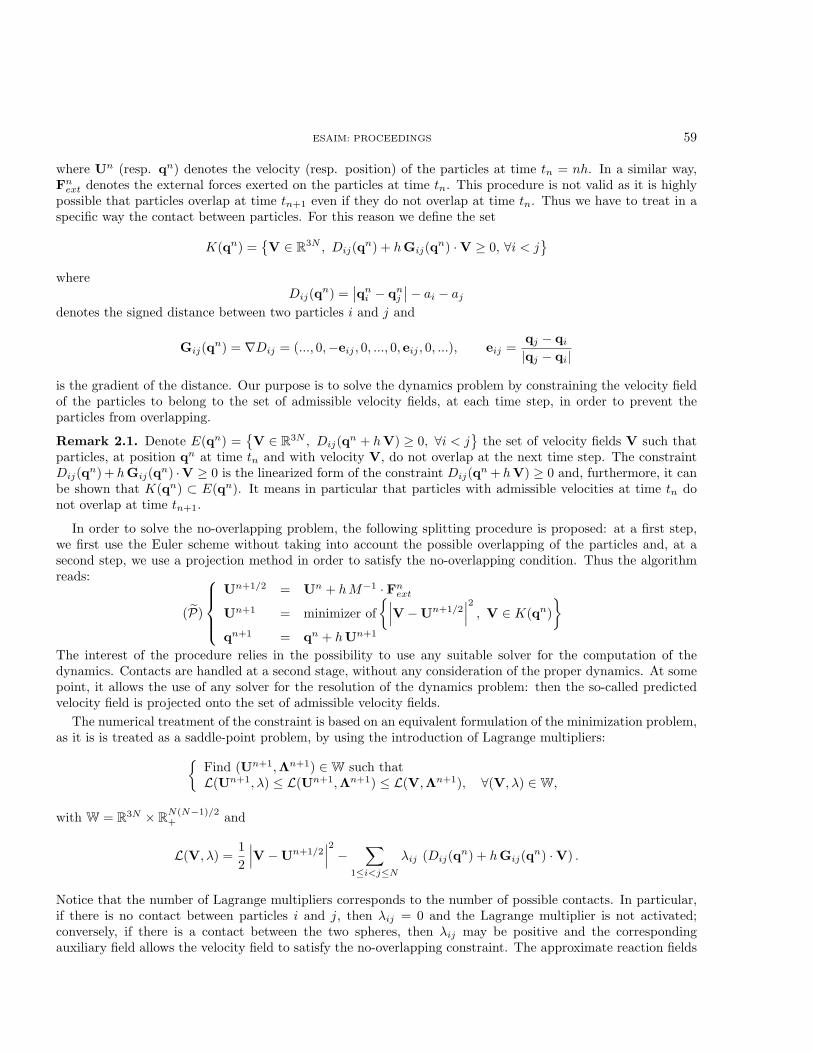
Figure 4. A polymer chain visualized with VTK (on the left) and after a POV-Ray post-processing (on the right).
and other nonspherical microcapsules. Many models have been proposed to recover these motions: Abkarian,Faivre & Viallat [1] consider a model based on a fluid ellipsoid surrounded by a viscoelastic membrane initiallyunstrained (shape memory); Rioual, Biben & Misbah [43] use an approach – the advected field approach – akinto phase field, which is flexible and, unlike boundary integral formulation, allows to incorporate non Newtonianconstitutive laws for the enclosed fluid as well as the ambient one; Sui, Low, Chew & Roy [51,52] investigate thedynamic motion of three-dimensional capsules in a shear flow by direct numerical simulation, they also simulatethe dynamic motion of red blood cells in simple shear flow under a broad range of shear rates; Faivre [21] focuseson the deformability and behavior under flow of drops, vesicles and red blood.
As emphasized in the above references, tank-treading motion and tumbling motion are commonly observedwhen experiencing the behaviour of biomimetic capsules. This is illustrated by pictures presented on Fig. 6.
Although exact in the case of a single rigid sphere, the first Faxen law is not rigorous anymore in the caseof a collection of rigid spheres. Indeed, Faxen law applied to each sphere supposes that the spheres do notinteract, as if they were isolated in the fluid. In other words, it means that the fluid velocity is not perturbed bythe collection of spheres and that multi-body hydrodynamic interactions are neglected. At short separations,neglecting the multi-body interactions inside the collections of spheres may be surprising, but in the case of ared blood cell which is described as a macro-object made of eleven spheres it can be analysed as a way to applythe first Faxen law to a non-spherical body. In particular, hydrodynamic interactions between the spheres of a

64 ESAIM: PROCEEDINGS
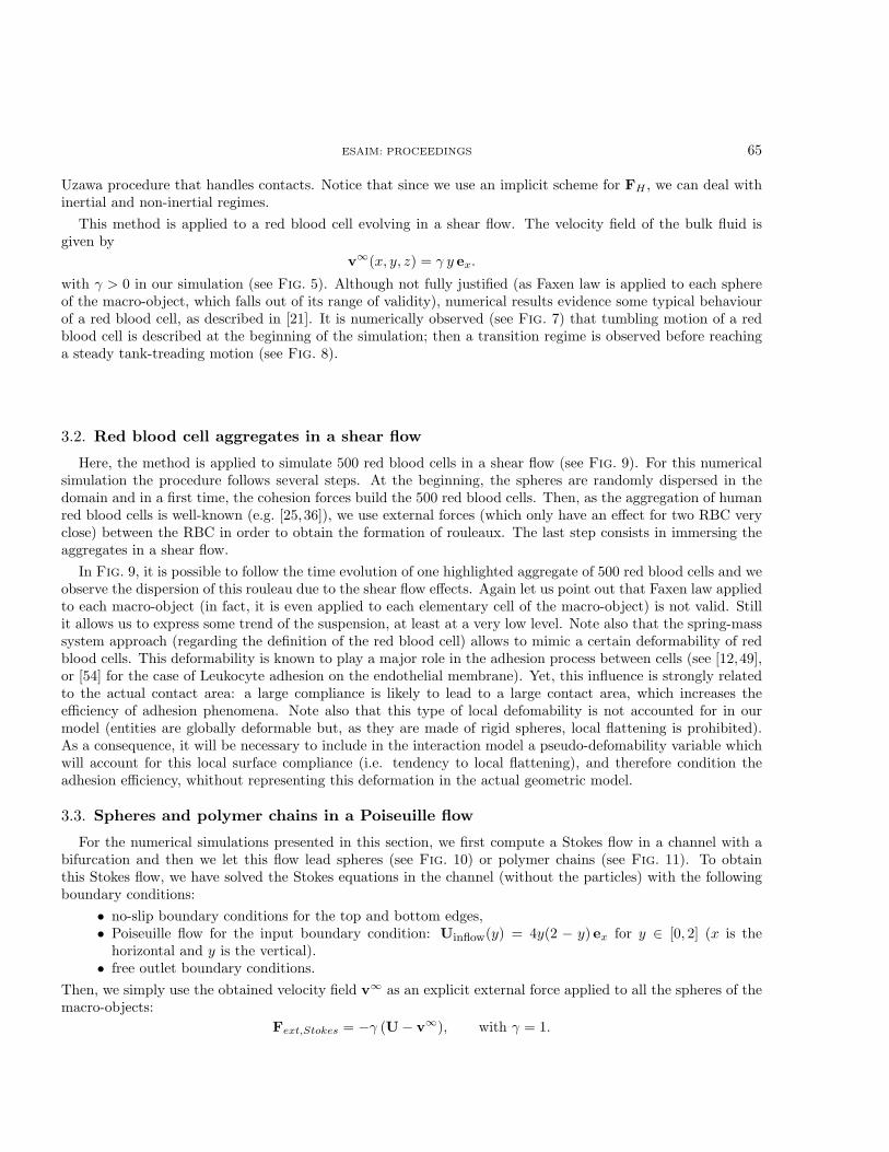
x
y
Figure 5. Velocity field of a linear shear flow.
Figure 6. Tank-treading motion (t) and tumbling motion (b) of a vesicle (see Faivre [21,39]).
given macro-object have no physical evidence, as the collection of spheres only serves for the definition of themacro-object.
3.1. Red blood cell in a shear flow
We simulate the motion of a red blood cell in a shear flow by assuming that Faxen law applies on each sphereof the macro-object. The Langevin equation is written as
M · dUdt
= FH + FP ,
where FH denotes the hydrodynamic forces and FP denotes the non-hydrodynamic forces exerted on the spheres(e.g. gravity, colloıdal forces,...). Using the first Faxen formula applied to each sphere, we express FH as afunction of U and, use the Euler scheme for the Langevin equation with an implicit discretization of thehydrodynamic force. In this way, the predicted velocity field can be computed very easily before using the
ESAIM: PROCEEDINGS 65
Uzawa procedure that handles contacts. Notice that since we use an implicit scheme for FH , we can deal withinertial and non-inertial regimes.
This method is applied to a red blood cell evolving in a shear flow. The velocity field of the bulk fluid isgiven by
v∞(x, y, z) = γ y ex.
with γ > 0 in our simulation (see Fig. 5). Although not fully justified (as Faxen law is applied to each sphereof the macro-object, which falls out of its range of validity), numerical results evidence some typical behaviourof a red blood cell, as described in [21]. It is numerically observed (see Fig. 7) that tumbling motion of a redblood cell is described at the beginning of the simulation; then a transition regime is observed before reachinga steady tank-treading motion (see Fig. 8).
3.2. Red blood cell aggregates in a shear flow
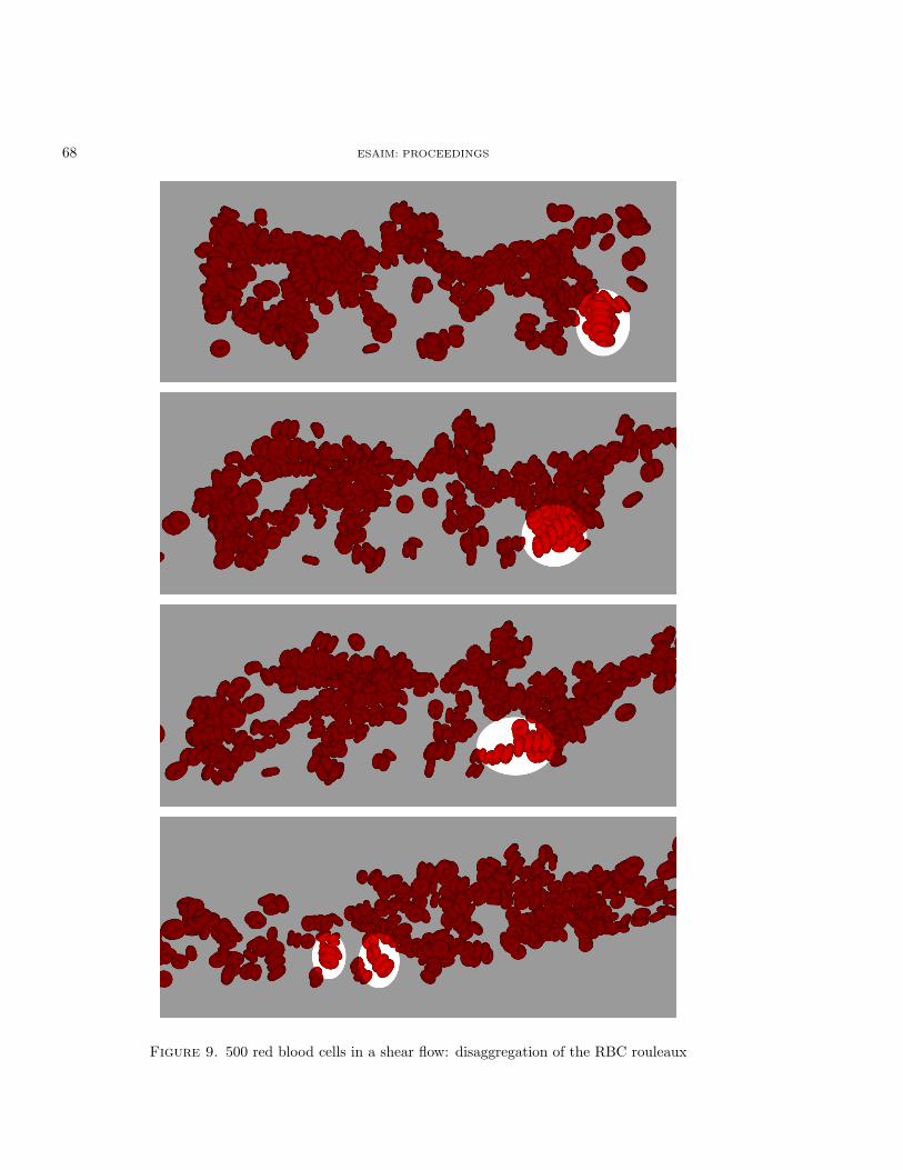
Here, the method is applied to simulate 500 red blood cells in a shear flow (see Fig. 9). For this numericalsimulation the procedure follows several steps. At the beginning, the spheres are randomly dispersed in thedomain and in a first time, the cohesion forces build the 500 red blood cells. Then, as the aggregation of humanred blood cells is well-known (e.g. [25,36]), we use external forces (which only have an effect for two RBC veryclose) between the RBC in order to obtain the formation of rouleaux. The last step consists in immersing theaggregates in a shear flow.
In Fig. 9, it is possible to follow the time evolution of one highlighted aggregate of 500 red blood cells and weobserve the dispersion of this rouleau due to the shear flow effects. Again let us point out that Faxen law appliedto each macro-object (in fact, it is even applied to each elementary cell of the macro-object) is not valid. Stillit allows us to express some trend of the suspension, at least at a very low level. Note also that the spring-masssystem approach (regarding the definition of the red blood cell) allows to mimic a certain deformability of redblood cells. This deformability is known to play a major role in the adhesion process between cells (see [12,49],or [54] for the case of Leukocyte adhesion on the endothelial membrane). Yet, this influence is strongly relatedto the actual contact area: a large compliance is likely to lead to a large contact area, which increases theefficiency of adhesion phenomena. Note also that this type of local defomability is not accounted for in ourmodel (entities are globally deformable but, as they are made of rigid spheres, local flattening is prohibited).As a consequence, it will be necessary to include in the interaction model a pseudo-defomability variable whichwill account for this local surface compliance (i.e. tendency to local flattening), and therefore condition theadhesion efficiency, whithout representing this deformation in the actual geometric model.
3.3. Spheres and polymer chains in a Poiseuille flow
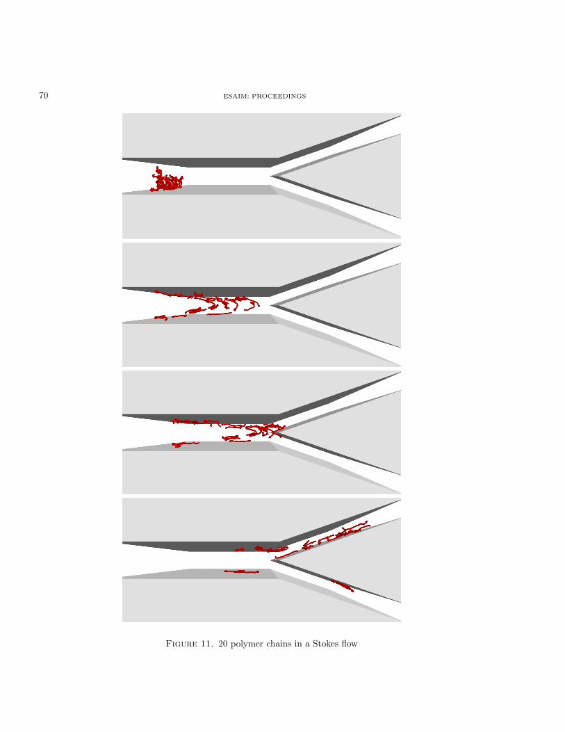
For the numerical simulations presented in this section, we first compute a Stokes flow in a channel with abifurcation and then we let this flow lead spheres (see Fig. 10) or polymer chains (see Fig. 11). To obtainthis Stokes flow, we have solved the Stokes equations in the channel (without the particles) with the followingboundary conditions:
• no-slip boundary conditions for the top and bottom edges,• Poiseuille flow for the input boundary condition: Uinflow(y) = 4y(2 − y) ex for y ∈ [0, 2] (x is the
horizontal and y is the vertical).• free outlet boundary conditions.
Then, we simply use the obtained velocity field v∞ as an explicit external force applied to all the spheres of themacro-objects:
Fext,Stokes = −γ (U− v∞), with γ = 1.

66 ESAIM: PROCEEDINGS
Figure 7. Tumbling motion obtained by applying Faxen law to each elementary sphere of ared blood cell in a linear shear flow. Figures should be read from top to bottom, left to right.

ESAIM: PROCEEDINGS 67
Figure 8. Transition from tumbling motion to tank-treading motion, obtained by applyingFaxen law to each elementary sphere of a red blood cell in a linear shear flow. Figures shouldbe read from top to bottom, left to right.
68 ESAIM: PROCEEDINGS
Figure 9. 500 red blood cells in a shear flow: disaggregation of the RBC rouleaux

ESAIM: PROCEEDINGS 69
Figure 10. 1000 spheres in a Stokes flow
70 ESAIM: PROCEEDINGS
Figure 11. 20 polymer chains in a Stokes flow
ESAIM: PROCEEDINGS 71
On Fig. 10 and Fig. 11 we can see the evolution of the spheres or of the polymer chains when we have addedthe external force Fext,Stokes. There are no other forces in these simulations and the mass of each sphere isequal to 1. In both cases, for the spheres and for the polymer chains, we can easily recognize the profile of thePoiseuille flow when the objects are transported in the channel.
4. Towards the simulation of dense suspensions
We end this paper by presenting some considerations on the possibility to integrate a more sophisticateddescription of the fluid motion to this approach. In the present paper, we shall restrict ourselves to a simpleillustration of this approach: at the end of this section, we investigate how the integration of short-range(lubrication) forces is likely to affect significantly the motion of red blood cells in the plasma.
We assume that the particles evolve in a fluid with viscosity µ. Let us recall the equation of motion (withrespect to the particles only):
M · dUdt
= FH + FP , in R3N
where N is the total number of spheres to be considered. As before, FH denotes the hydrodynamic forcesand FP denotes the non hydrodynamic forces. In the prospect of the simulation of dense suspensions, wehave to define in a suitable way the hydrodynamic forces in order to mimic the influence of the fluid on themacro-objects.
From a practical point of view, we use a result provided by Happel & Brenner [26] and Brenner & O’Neil [10],which relates the hydrodynamic forces to the particles velocity. For this, we restrict ourselves to a specificframework which provides the validity of the forthcoming method:
• the particles are rigid, non-Brownian and spherical;• the bulk macroscopic flow is a shear Stokes flow: the velocity fluid (without inclusions) is defined on
the whole space by:v∞(x, y, z) = γ y ex.
We introduce the rate-of-strain tensor E (symmetrized gradient of the velocity field) and the spin vectorω (half the vorticity vector):
E =12
(∇v∞ + (∇v∞)∗) =γ
2
0 1 01 0 00 0 0
, ω =12∇∧ v∞ = −γ
2
001
.
so that the velocity field at some point x can be decomposed into v∞(x) = E · x + ω ∧ x. It means inparticular that the flow is decomposed into a pure deformation flow and a pure rotation flow.
• the Reynolds particle number is small: ReP = γaρ/µ ≤ 1, where a denotes the value of a sphere radius.Then the relationship between velocities of the spheres located at position q and hydrodynamic forces exerted
on them [10,26] is given byFH = −R · (U− E · q) + Φ : E .
The interest of this formula relies on the fact that matrices R (the so-called “grand resistance matrix”) andΦ (the so-called “grand shear resistance matrix”) only depend on the instantaneous geometrical configuration:the definition of the matrices is only related to the separations of the spheres. In the same way, it is possible todefine the so-called “grand mobility matrix” M = R−1.
Assume that the grand matrices are known; then the SCoPI algorithm reduces to:
(P)
(M + h Rn) ·Un+1/2 = M ·Un + h Rn · (E · qn) + Φn : E + hFnP
Un+1 = minimizer of{∣∣∣V −Un+1/2
∣∣∣2 , V ∈ K(qn)}
qn+1 = qn + hUn+1.
72 ESAIM: PROCEEDINGS
In the algorithm, the matricesRn and Φn are evaluated at time tn, meaning that they depend on the geometricalconfiguration at time tn which is known; in this way, Un+1/2 is computed by solving a linear system and, afterthe projection of the velocity field on the set of admissible velocities, the position of the particles at time tn+1 isobtained. This last step allows us to define Rn+1 and Φn+1 before passing to the next time step. The procedureevidences the fact that, the matrices need to be computed at each time step as the geometrical configurationevolves in time.
4.1. Stokesian Dynamics method: the assumption of pairwise additivity of the interac-tions
Pairwise additivity of the interactions is assumed in order to reduce numerical costs and build the grandresistance matrix. This assumption can be taken into account in two different ways:
• the first method relies on the superposition of the velocity disturbances, i.e. the additivity in thebuilding of the grand mobility matrix;
• the second method relies on the superposition of forces, i.e. the additivity in the building of the grandresistance matrix.
Clearly, these two methods are not equivalent. Brady & Bossis [8] have shown that the superposition of forcessuited more the proper physics as lubrication forces prevent particles from overlapping. These lubrication forcesare not preserved when superposing the velocity disturbances so that particles may overlap unless additionalrepulsive forces (which lack physical evidence) are introduced. More precisely, the superposition of velocitydisturbances can be considered as a strict pairwise additivity of the interactions in the sense that the interactionbetween two particles 1 and 2 is taken into account as if they were isolated from other particles in the fluid. Thismethod leads to situations in which the relative velocity between two particles does not vanish as the distancetends to 0 so that overlapping is possible. Brady & Bossis have shown that the superposition of forces is quitedifferent: when the resistance matrix is inverted to get the velocity field and evaluate the new positions, all theparticles are considered simultaneously so that the multi-body effects are included in the search of the particlestrajectories.
4.2. Stokesian Dynamics method: computation of the grand resistance matrix
The resolution of the N particles problem needs an approximation: the pairwise additivity assumption, whichhas been discussed in the previous subsection. For two particles, the resistance and mobility matrices are knownexactly, for any separation between the particles. Thus, the pairwise additivity assumption allows building thegrand resistance matrix by taking into account all the pairwise contributions.
How to build the grand resistance matrix from a practical point of view? Brady & Bossis use the fact thatthe lubrication effects are treated more easily in the resistance formulation (i.e. the superposition of forces isused) while the multi-body long-range interactions are incorporated in a more suitable way with the mobilityformulation (i.e. the superposition of velocity disturbances is used).
Pairwise additivity, in any form, is an approximation which has been proven to be useful and efficient innumerical simulation of suspensions. Moreover, in dense suspensions, lubrication forces play a major role dueto the high number of pairwise near-contact or contact configurations and they are correctly modelled by thesuperposition of forces. The multi-body long-range interactions obtained by far-range expressions are neglectedwhen the distance between the macro-objects becomes small. In a dilute suspension, most of interactions arepairwise and, again, pairwise additivity is a fair approximation.
In the case of two spheres, all the elements of the resistance matrix are known exactly. This is due to thesimplicity of the geometric configuration which only relies on a unique vector: the distance vector between thetwo particles. Although exact, there is no close analytic form of the expressions valid for any separation distanceand one has to use expressions corresponding to different separation regimes.
ESAIM: PROCEEDINGS 73
• Far-field forces5 are implemented in the mobility formulation by the method of reflections (see Smolu-chowski [48] for the historical reference, Luke [38] for the numerical analysis, Guazzelli [24] for a concisedescription). The approximation is given by (see the Appendix for a brief justification):
Ui = − Fi6πµa
− 18πµ
[I3
|qi − qj |+
(qi − qj)⊗ (qi − qj)|qi − qj |3
]· Fj
− a2
4πµ
[I3
3|qi − qj |3− (qi − qj)⊗ (qi − qj)
|qi − qj |5
]· Fj
+O(|qi − qj |−4
).
• Lubrication forces (Jeffrey & Onishi [33], Dance & Maxey [19]) are expressed by using lubricationtheory. The lubrication forces for two identical spheres with radius a are expressed as
Fj→i · eij = 6πµa(− 1
4Dij(q)+
940
logDij(q) +3
112Dij(q) logDij(q) +O(1)
)(Ui −Uj) · eij
Fj→i · tij = 6πµa(
16
logDij(q) +O(1))
(Ui −Uj) · tij ,
for any tangential vector tij orthogonal to eij (normal vector from sphere i to sphere j).• Intermediate-field forces (see Kim & Karrila [35]) provide the continuous path between long-range
interactions and short-range interactions. They are implemented as tabulations.Notice that the far-field expressions lead to the definition, by pairwise additivity, of a long-range mobility
matrixM∞ that has been built for any separation distance. In the same way, the lubrication expressions lead tothe definition of a short-range resistance matrix R2B . Then the grand resistance matrix is defined by gatheringall these informations: once constructed, the grand mobility matrix is inverted to yield a far-field approximation;but this approximation to the resistance matrix would still lack lubrication. Thus, to each element of (M∞)−1,we add the known exact two-sphere resistance interactions modelled by the matrix R2B . However, the far-fieldparts of the two-sphere resistance interactions have already been included upon the inversion ofM∞. Thus, inorder not to count these interactions twice, we must subtract off the two-body interactions already included in(M∞)−1: this can be done by inverting a two-sphere mobility matrix to the same level of approximation as inM∞. Denoting this resistance matrix as R∞2B , our approximation to the grand resistance matrix that includesnear-field lubrication and far-field many-body interactions is
R = (M∞)−1 +R2B −R∞2B .
The procedure may lead to heavy computational costs due to the inversion of the long-range mobility matrix.Let us illustrate the influence of the lubrication forces in a suspension of 30 red blood cells. For convenience,
only the main order of the normal lubrication forces has been implemented: although this is a simplification, thismakes sense in the absence of imposed shear stress (γ = 0). Additionally, long-range interactions are not takeninto account. From a numerical point of view, the difficulties are still challenging as a linear system remainsto solve due to the treatment of the lubrication resistance matrix. Fig. 12 and 13 capture the main effectsof the lubrication forces on the distribution of the macro-objects. In particular, In the absence of lubrication,the distribution remains homogeneous, as the RBC evolve with contacts between the macro-objects. In thelubrication setting, when the distance between two RBC tends to vanish, so does the relative velocity: thelubrication forces play the role of a trap.
5In the approximation of order 0, the solution for two particles at long distance is formed by the superposition of the fieldsproduced by the particles considered as isolated. Thus, we neglect the hydrodynamic interactions between the particles (equivalently,
we simply apply the Faxen law to each particle). Then, the method is based on the idea that the ambient field for each particle
is made of an original ambient field to which we must add a perturbed field due the presence of the other particle. This methodis iterative as a correction of the ambient field on a particle generates a new solution of perturbation for this particle and this, in
return, modifies the ambient field related to the other particle.

74 ESAIM: PROCEEDINGS
Figure 12. Red blood cells submitted to no force at some fixed time.
Figure 13. Red blood cells submitted to lubrication forces at some fixed time.
ESAIM: PROCEEDINGS 75
5. Conclusion and future prospects
In this exploratory study, we have proposed a strategy for the numerical modeling of dilute and densesuspensions by using a numerical tool which is efficient in the handling of contacts between macro-objects.Although partial results are available, a large number of implementations need to be realized.
Far-field forces need to be treated in a more efficient way: because of the long-range nature of the interactions,the mobility matrix is not sparse. In dense suspensions, we can assume that macro-objects at large separationsdo not mainly interact due to a screening effect: the main interactions related to a macro-object are closelyrelated to the main neighbours. In this prospect, a cut-off distance (Satoh, 2001) for the long-range interactionscan be introduced: this allows us to neglect the far-range interactions between particles which are not dominantin the general behaviour of the suspension. From a numerical point of view, the introduction of a cut-off distanceleads us to consider a sparse mobility matrix.
Intermediate-field forces should be implemented with the tabulations given by Kim & Karrilla [35]. Thisprocedure allows us to provide a continuous implementation of the hydrodynamic forces between the long-rangeforces (determined by the method of reflections) and the short-range forces (obtained by lubrication theory).
Periodic boundary conditions remain one of the final goals of this study, as we aim at simulating the behaviourof dense suspensions in a viscometer. This would provide a numerical tool for the simulation of dense suspensionsin a viscometer and it would apply to any suspension of macro-objects that fall into the scope of the Stokesiandynamics.
Nomenclature
ai radius of rigid sphere imi mass of rigid sphere iM mass matrix of a collection of rigid spheresq position vector of the rigid spheresU, V velocity vector of the rigid spheresFext external force field exerted on the rigid spheresFH hydrodynamic force field exerted on the rigid spheresFP non-hydrodynamic force field exerted on the rigid spheresDij(q) signed distance between spheres i and j. Dij(qn) = |qi − qj | − ai − ajeij normal vector from sphere i to sphere j, i.e. eij = (qj − qi)/ |qj − qi|Gij(q) gradient between spheres i and j, i.e. Gij = (..., 0,−eij , 0, ..., 0, eij , 0, ...)h time step·n discretized quantity evaluated at time tn = nhK(q) set of admissible velocity fieldsE(q) set of velocity fields with no-overlapping at the next time stepL functional associated to the saddle-point problem (constraint minimization problem)λ, Λ auxiliary field in the minimization problem (Lagrange multipliers)γ shear rateReP particle Reynolds numberv∞ velocity field of the bulk fluidµ fluid viscosityρ fluid densityE rate-of-strain tensor (symmetrized gradient of the velocity field), i.e. E = 1
2 (∇v∞ + (∇v∞)∗)ω spin vector (half the vorticity vector), i.e. ω = 1
2∇∧ v∞
R grand resistance matriceM grand mobility matriceΦ grand shear-resistance matrice
76 ESAIM: PROCEEDINGS
References
[1] M. Abkarian, M. Faivre & A. Viallat, Swinging of red blood cells under shear flow, Phys. Rev. Lett. 98 (18):188302 (2007).
[2] P. Bagchi, P. Johnson & A. S. Popel, Computational fluid dynamic simulation of aggregation of deformable cells in a shearflow, J. Biomech. Eng. 127 (7), 1070–1080 (2005).
[3] G. K. Batchelor, Transport properties of two-phase materials with random structure, Ann. Rev. Fluid Mech. 6, 227–255 (1974).
[4] G. K. Batchelor, Developments in microhydrodynamics, In: Koiter WT, editor, Theoretical and Applied Mechanics. IUTAMCongress, Amsterdam, New York, Oxford: North Holland-Elsevier Science Publishers, 33–55 (1976).
[5] C. W. J. Beenakker, The effective viscosity of a concentrated suspension of spheres (and its relation to diffusion), Physica. A
128, 48–81 (1984).[6] C. W. J. Beenakker & P. Mazur, Self-diffusion of spheres in a concentrated suspension, Physica. A 120, 388–410 (1983).
[7] G. Bossis & J. F. Brady, Dynamic simulation of sheared suspensions. I. General method, J. Chem. Phys. 80, 5141–5154 (1984).
[8] J. F. Brady & G. Bossis, Stokesian Dynamics, Ann. Rev. Fluid Mech. 20, 111–157 (1988).[9] H. Brenner, Rheology of a dilute suspension of axisymmetric Brownian particles, Int. J. Multiphase Flow 1, 195–341 (1974).
[10] H. Brenner & M. E. O’Neill, On the Stokes resistance of multiparticle systems in a linear shear field, Chemical EngineeringScience 27 (7):1421–39 (1972).
[11] S. Vincent, J. P. Caltagirone, P. Lubin & T. N. Randrianarivelo, An adaptative augmented Lagrangian method for three-
dimensional multimaterial flows, Computers and Fluids 33, 1273–1289 (2004).[12] S. Chien, L. A. Sung, S. Simchon, M. M. Lee, K. M. Jan & R. Skalak, Energy balance in red cell interactions, Ann. N.Y. Acad.
Sci. 416 (1), 190–206 (1983).
[13] P. G. Ciarlet, Introduction a l’analyse numerique matricielle et a l’optimisation, Masson, Paris (1990).[14] R. H. Davis & A. Acrivos, Sedimentation of noncolloidal particles at low Reynolds numbers, Ann. Rev. Fluid Mech. 17, 91–118
(1985).
[15] Y. Demay, A. Nouri & F. Poupaud, An existence theorem for the multi-fluid Stokes problem, Quart. Appl. Math. 55, 421–435(1997).
[16] E. J. Ding & C. K. Aidun, Direct numerical simulation of flow of red blood cells with a rigid membrane, Proc. American
Physical Society, (2003).[17] A. Einstein, Eine neue Bestimmung der Molekudimensionen, Annalen der Physik 19, 289–306 (1906).
[18] A. Einstein, Berichtigung zu meiner Arbeit: “Eine neue Bestimmung der Molekudimensionen”, Annalen der Physik 34,591–592 (1911).
[19] S. L. Dance & M. R. Maxey, Incorporation of lubrication effects into the force-coupling method for particulate two-phase flow,
J. Comp. Phys. 189 (1), 212–238 (2003).[20] L. Durlofsky, J. F. Brady & G. Bossis, Dynamic simulation of hydrodynamically interacting particles, J. Fluid. Mech. 180,
21–49 (1987).
[21] M. Faivre, Gouttes, vesicules et globules rouges: deformabilite et comportement sous ecoulement, These de doctorat del’Universite Joseph-Fourier - Grenoble 1, (2006).
[22] R. Glowinski, T. W. Pan, T. I. Hesla, D. D. Joseph & J. Periaux, A fictitious domain approach to the direct numerical
simulation of incompressible viscous flow past moving rigid bodies: application to particulate flow, J. Comp. Phys. 169,363–427 (2001).
[23] R. Glowinski, Finite element methods for incompressible viscous flow, In: Handbook of Numerical Analysis, Vol. IX, P. G.
Ciarlet and J.-L. Lions eds., Ed. North-Holland, Amsterdam (2003).[24] E. Guazzelli, Microhydrodynamique : cours de base sur les suspensions, Polycopie de l’IUSTI Marseille (2003).
[25] L. Haider, P. Snabre & M. Boynard, Rheology and ultrasound scattering from aggregated red cell suspensions in shear flow,Biophysical Journal, 87, 2322–2334 (2004).
[26] J. Happel & H. Brenner, Low Reynolds number hydrodynamics, Martinus Nijhoff, Dordrecht (1986) (reprint of the 1963edition).
[27] M. Hillairet & T. Takahashi, Collision in 3D fluid structure interactions problems, SIAM Journal on Mathematical Analysis,to appear (2009).
[28] M. Hillairet, Lack of collision between solid bodies in a 2D incompressible viscous flow, Comm. Partial Differential Equations,32 (7-9), 1345–1371 (2007).
[29] H. H. Hu, Direct simulation of flows of solid-liquid mixtures, Int. J. Multiphase Flow 22 (2), 335–352 (1996).[30] K. Ichiki & J. F. Brady, Many-body effects and matrix inversion in low-Reynolds number hydrodynamics, Phys. Fluids 13 (1),
350–353 (2001).[31] J. Janela, A. Lefebvre & B. Maury, A penalty method for the simulation of fluid - rigid body interaction, ESAIM Proc. 14,
115–123 (2005).[32] D. J. Jeffrey & A. Acrivos, The rheological properties of suspensions of rigid particles, AIChEJ 22 (3), 417–32 (1976).[33] D. J. Jeffrey & Y. Onishi, Calculation of the resistance and mobility functions for two unequal rigid spheres in low-Reynolds-
number flow, J. Fluid Mech. 139, 261–290 (1984).

ESAIM: PROCEEDINGS 77
[34] A. A. Johnson & T. E. Tezduyar, Simulation of multiple spheres falling in a liquid-filled tube, Computer Methods in AppliedMechanics and Engineering, 134 (3), 351–373 (1996).
[35] S. Kim & S. Karrila, Microhydrodynamics: principles and selected applications, Butterworth-Heinemann, Boston, 500 pp.
(1991).[36] Y. Liu & W. M. Liu, Rheology of red blood cell aggregation by computer simulation, J. Comp. Phys. 220 (1), 139–154 (2006).
[37] S. Lomholt, Numerical investigations of macroscopic particle dynamics in microflows, Ph.D. Thesis, Riso National Laboratory,
Roskilde, Denmark (2000).[38] J. H. C. Luke, Convergence of a multiple reflection method for calculating Stokes flow in a suspension, SIAM J. Appl. Math.
49 (6), 1635–1651 (1989).
[39] M. A. Mader, C. Misbah & T. Podgorski, Dynamics and rheology of vesicles in a shear flow, Microgravity Sci. Technol.XV III − 3/4:199–203 (2006).
[40] B. Maury, A time-stepping scheme for inelastic collisions, Numer. Math. 102 (4), 649–679 (2006).
[41] B. Maury, Direct simulations of 2D fluid-particle flows in biperiodic domains, Journal of Computational Physics 156, 325–351(1999).
[42] P. Mazur & W. van Saarloos, Many-sphere hydrodynamic interactions and mobilities in a suspension, Physica A 115, 21–57(1982).
[43] F. Rioual, T. Biben & C. Misbah, An analytical analysis of vesicle tumbling under a shear flow, Phys. Rev. E Stat. Nonlin.
Soft Matter Phys. 69 (1-6):061914 (2008).[44] W. B. Russel, A review of the role of colloıdal forces in the rheology of suspensions, J. Rheo. 24, 287–317 (1980).
[45] W. van Saarloos & P. Mazur, Many-sphere hydrodynamic interactions II: mobilities at finite frequencies, Physica A 120,
77–103 (1983).[46] J. San Martın, J.-F. Scheid, T. Takahashi & M. Tucsnak, Convergence of the Lagrange–Galerkin method for the equations
modelling the motion of a fluid-rigid system, SIAM J. Numer. Anal., 43 (4), 1539–1571, (2005).
[47] A. Satoh, Comparison of approximations between additivity of velocities and additivity of forces for Stokesian dynamicsmethods, Journal of Colloid and Interface Science 243, 342–350 (2001).
[48] M. Smoluchowski, Uber die Wecxhselwirkung von Kugeln, die sich in einer zahen Flussigkeit bewegen, Bull. Int. Acad. PolonaiseSci. Lett. 1A, 28–39 (1911).
[49] R. Skalak & C. Zhu, Rheological aspects of red blood cell aggregation, Biorheology 27 (3-4), 309–325 (1990).
[50] J. M. Skotheim & T. W. Secomb, Red blood cells and other nonspherical capsules in shear flow: oscillatory dynamics and thetank-treading-to-tumbling transition, Phys. Rev. Lett. 98 (7):078301 (2008).
[51] Y. Sui, H. T. Low, Y. T. Chew & P. Roy, Tank-treading, swinging, and tumbling of liquid-filled elastic capsules in shear flow,
Phys. Rev. E Stat. Nonlin. Soft Matter Phys. 77 (1):016310 (2008).[52] Y. Sui, Y. T. Chew, P. Roy, Y. P. Cheng & H. T. Low, Dynamic motion of red blood cells in simple shear flow, Phys. Fluids
20, 112106–112110 (2008).
[53] C. Sun & L. Munn, Lattice-Boltzmann simulation of blood flow in digitized vessel networks, Computers and Mathematics withApplications 55 (7), 1594–1600 (2008).
[54] D. F. Tees & D. J. Goetz, Leukocyte adhesion: an exquisite balance of hydrodynamic and molecular forces, News Physiol. Sci.
18, 186–190 (2003).[55] T. Wang, T. W. Pan & R. Glowinski, Numerical simulation of aggregability of red blood cells in a micro-vessel by Lagrange
multiplier / fictitious domain method, Preprint (2008).[56] J. Zhang, P. C. Johnson & A. S. Popel, Red blood cell aggregation and dissociation in shear flows simulated by lattice Boltzmann
method, J. Biomech. 41 (1), 47–55 (2008).
Appendix: Faxen’s laws
We recall here some ideas on how to obtain the Faxen laws.
Faxen law with one sphere
Let us consider a ball B of center q and of radius a. We assume that this ball is immersed in a viscousincompressible fluid so that the hydrodynamic force applied on the ball is
FH = −∫∂Bσ(v, p) · n dΓ, (1)
whereσ(v, p) = 2µD(v)− pI3,

78 ESAIM: PROCEEDINGS
and where (v, p) is the solution of the Stokes system:
−µ∆v +∇p = 0 in F , (2)div v = 0 in F , (3)
lim|x|→∞
v = 0 (4)
v = U on ∂B (5)
The explicit solution of the above system is known:
v(x) =3a4
[U
|x− q|+
(U · (x− q)) (x− q)|x− q|3
]+a3
4
[U
|x− q|3− 3
(U · (x− q)) (x− q)|x− q|5
], (6)
p(x) =3a2µ
U · (x− q)|x− q|3
. (7)
Using this solution and (1), we deduce that
FH = −6πµaU. (8)
If we replace (5) by
lim|x|→∞
v = v∞,
then, (8) is transformed into
FH = −6πµa (U− v∞(q)) + πµa3 ∆v∞(q). (9)
Faxen law with two spheres widely separated
Let us consider two balls (with radii ai, center positions qi, i = 1, 2). We denote Fi (resp. Ui) thehydrodynamic force exerted on (resp. the velocity of) sphere i. To obtain the Faxen laws in that case we usethe reflexion method (see for instance [10], [35]). More precisely, at a first step, we use only (8), assuming eachball is “isolated”: the corresponding velocities (also referred to as velocity at zeroth order) for each ball is givenby
U(0)i = − Fi
6πµai.
Then, at a second step, we use the velocities U(0)i to compute v∞,i by using formula (6): this could be written
as
v∞,i = vS,j +(aj)2
6∆vS,j (10)
where
vS,j(x) = − 18πµ
[I3
|x− qj |+
(x− qj)⊗ (x− qj)|x− qj |3
]· Fj . (11)
Inserting the formula (10) in the Faxen law (9) for one sphere and neglecting the term in |qi−qj |−4, we deduce
Ui = − Fi6πµai
+ vS,j +(ai)2 + (aj)2
6∆vS,j
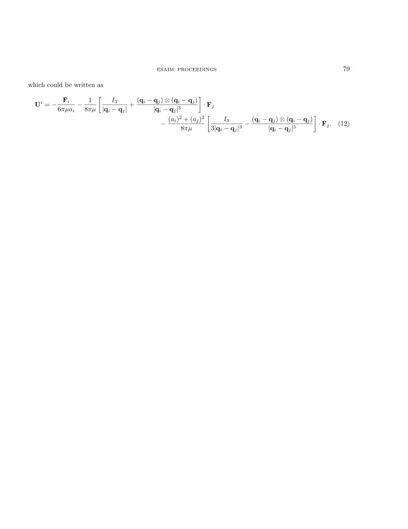
ESAIM: PROCEEDINGS 79
which could be written as
Ui = − Fi6πµai
− 18πµ
[I3
|qi − qj |+
(qi − qj)⊗ (qi − qj)|qi − qj |3
]· Fj
− (ai)2 + (aj)2
8πµ
[I3
3|qi − qj |3− (qi − qj)⊗ (qi − qj)
|qi − qj |5
]· Fj . (12)