TOWARD MODELING EROSION ON UNPAVED ROADS IN ...

TOWARD MODELING EROSION ON UNPAVED ROADS IN MOUNTAINOUS NORTHERN THAILAND

A DISSERTATION SUBMITTED TO THE GRADUATE DIVISION OF THE UNIVERSITY OF HAWAII IN PARTIAL FULFILLMENT

OF THE REQUIREMENTS FOR THE DEGREE OF

DOCTOR OF PHILOSOPHY

IN

GEOGRAPHY

MAY 2000

by

Alan D. Ziegler

Dissertation Committee:

Thomas W. Giambelluca, Chair

Ross A. Sutherland

Everett A. Wingert

Deborah Woodcock

Guillermo H. Goldstein

We certify that we have read this dissertation; and that it is, in

our opinion, satisfactory in scope and quality as a dissertation

for the degree of Doctor of Philosophy in Geography.

■7 ^ chair

I thank the following folks for their help in this research: Asuh, Atabuu, Atachichi, and Aluong

(brawn); Kalaya (the General); Yun, Mae and Paa (kinsmanship); Paluk and Nadi Lamu (sharing

their home), S. Yamasam, Geography, Chiang Mai University (support in Chiang Mai); J. Pintong,

Agriculture Dept., Chiang Mai University (soil analyses); J. F. Maxwell (plant taxonomy and

drinks); Mike Nullet and John Allison (engineering prowess); Chumnien and Amphai (support in

Bangkok); T.T. Vana (field assistance in Thailand); Alexis Lee, J. Bussen, N. Thompson, J. Nagle,

C.T Lee, and M. Gilbeaux (lab/field assistance in Hawaii); Don Plondke (GIS); Sathapom Jaiaree,

and Sawasdee Boonchee, the Soil and Land Conservation Division of the Dept, of Land

Development, Bangkok and Chiang Mai offices (expertise); Yinglek Pongpayack, the Soil

Analysis Division of the Dept, of Land Development, Bangkok (soil analyses); Servillano Lamer,

Department of Agronomy and Soil Science, University of Hawaii (support at UH test facility); C.

Southern, and R. Gouda (construction and design of rainfall simulation apparatus); D. Ko, P.

Malaspina, and E. Lind, Integrated Training Area Management Division, Schofield Barracks (use

of ITAM facility at Schofield); Midwest Industrial Supply, Inc. (freely providing Soil Sement™).

I especially thank professors Thomas W. Giambelluca and Ross A. Sutherland for their

advice, field assistance, and manuscript review during this project. This dissertation work was

partially funded by the National Science Foundation Award (grant no. 9614259) and a seed money

grant from the University of Hawaii. I was additionally supported by an Environmental Protection

Agency Star Fellowship and a Horton Hydrology Research Award (Hydrological Section,

American Geophysical Union); and I recieved travel money from the UH International

Agreements Fund and the Arts and Sciences Advisory Council.

Acknowledgments

Ill

Abstract

Contributions of road networks and unstable agricultural activities to downstream sedimentation,

water shortages, and flooding in mainland SE Asia are not easily determined because scientific

understanding of mnoff and erosion processes operating on roads is limited. This dissertation

work, conducted within the Pang Khum Experimental Watershed (PKEW) in northern Thailand,

supports that owing to low saturated hydraulic conductivity (Kj < 1 6 mm h-'), Horton overland

flow (HOF) generation occurs more frequently on unpaved PBCEW roads than on other watershed

surfaces having higher infiltrability (e.g., mean for agricultural surfaces ranges from 130 to 320

mm h >)- Because of frequent HOF generation, the road system contributes to stream sedimenta

tion throughout the rainy season. The highly compacted (bulk density = 1.45 Mg m-3) PKEW road

surface typically underlies a layer of loose material of finite depth. Instantaneous sediment trans

port (Sj) on roads varies because the supply of easily transported surface sediment is constantly

altered by overland flow events, traffic, road maintenance, and mass wasting events, both during

and between storms. As surface material is removed during an overland flow event, normalized

S( declines from an initial peak rate of ~ 3 g J-* to a steady rate of =0.5 g J‘f The mechanical

stress associated with vehicle passes during a storm increases the availability of loose material,

producing 2-4 fold increases in S, and sediment concentration (C;) values. Herein, rainfall simu

lation data, surveys of traffic phenomena, and soil property measurements were used to parame

terize the physics-based KINER0S2 model for simulating road runoff and erosion. During model

validation, instantaneous discharge was simulated well (root mean squared error (RMSE) = 14%).

However, because KINEROS2 equations do not “describe” road erosion processes accurately, S(

was simulated poorly (RMSE = 51.6%). To improve modeling, a methodology recognizing the

dynamic erodibility (DE) of a road surface was introduced. By explicitly simulating removal of a

layer of loose material, the DE modeling technique improved prediction of (RMSE decreased

to 35.4 %). Finally, a systematic approach is presented to implement DE modeling on any road

surface where baseline erodibility and sediment availability can be quantified.

IV

Description Page

Title page ...............................................................................................................................................iSignature p a g e ......................................................................................................................................iiAcknowledgments............................................................................................................................... iii

A bstract................................................................................................................................................. ivTable of contents ................................................................................................................................. v

List of ta b le s ......................................................................................................................................viiiList of figures ......................................................................................................................................ix1, Introduction ....................................................................................................................................1

1.1 IMPACTS OF UNSTABLE AGRICULTURAL PRACTICES ANDROAD SYSTEMS IN NORTHERN THAILAND ............................................................... I

1.2 THAILAND ROADS PROJECT........................................................................................... 21.3 OBJECTIVE OF THE DISSERTATION RESEARCH ......................................................31.4 LAYOUT OF THE DISSERTATION .................................................................................. 4

2, Background......................................................................................................................................52.1 STUDY AREA: PANG KHUM EXPERIMENTAL WATERSHED..................................52.2 ROAD EROSION M OD ELING............................................................................................82.3 THE THREE-DIMENSIONAL ROAD PRISM ................................................................... 9

3, Experiment I: Runoff Generation and Sediment Production on Unpaved Roads, Footpaths, and Agricultural Surfaces in Northern Thailand ................................................11

3.1 A BSTRA CT...........................................................................................................................113.2 OBJECTIVE...........................................................................................................................123.3 METHODS AND MATERIALS..........................................................................................12

3.3.1 Study site .................................................................................................................... 123.3.2 Simulation treatments ................................................................................................ 123.3.3 Measurement of physical properties.......................................................................... 143.3.4 Rainfall simulator and plot d es ig n ............................................................................ 143.3.5 Simulation data collection and calculations.............................................................163.3.6 Measuring road discharge during natural events...................................................... 173.3.7 Data analysis................................................................................................................17

3.4 RESULTS............................................................................................................................... 183.4.1 Compaction ind ices.....................................................................................................183.4.2 Instantaneous discharge and time to runoff .............................................................18

Table of Contents

3.4.3 Sediment output ........................................................................................................ 203.4.4 Sediment concentration............................................................................................ 21

3.5 DISCUSSION.......................................................................................................................22

3.5.1 Influence of compaction on and runoff generation.............................................223.5.2 Erosion on path complexes .......................................................................................233.5.3 Surface preparation and sediment transport............................................................243.5.4 Representativeness of the ROAD simulation data ................................................. 26

3.6 CONCLUSION..................................................................................................................... 30

4. Experiment II: Partitioning total erosion on unpaved roads into splash and hydraulic components: interstorm surface preparation and dynamic erodibility . .31

4.1 ABSTRACT..........................................................................................................................314.2 OBJECTIVE..........................................................................................................................314.3 METHODS AND MATERIALS........................................................................................ 31

4.3.1 Research sites .............................................................................................................314.3.2 Rainfall simulation experiments................................................................................32

4.4 RESULTS.............................................................................................................................. 344.5.1 Runoff d a ta .................................................................................................................344.5.2 Sediment output d a ta ................................................................................................. 35

4.5 DISCUSSION....................................................................................................................... 364.5.1 Role of surface preparation in road e ro s io n ............................................................364.5.2 Dynamic erodibility and implications for modeling road e rosion .........................37

4.6 SUMMARY AND CONCLUSIONS................................................................................. 40COLOR P L A T E S ...........................................................................................................................415. Experiment III: Interstorm surface preparation and sediment detachmenthy vehicle traffic on unpaved mountain r o a d s ...................................................................50

5.1 A BSTRA CT......................................................................................................................... 505.2 OBJECTIVE......................................................................................................................... 505.3 METHODS AND MATERIALS........................................................................................51

5.3.1 Survey of vehicle usage and surface physical characteristics............................... 515.3.2 Rainfall simulation experiments...............................................................................515.3.3 Rainfall simulator and plot d es ig n ...........................................................................525.3.4 Simulation data collection and calculations............................................................ 535.3.5 Statistical analysis..................................................................................................... 54

5.4 RESULTS............................................................................................................................. 545.4.1 Road survey ...............................................................................................................545.4.2 FILL simulations....................................................................................................... 56

VI

5.4.3 MOTORCYCLE and TRUCK simulations ............................................................ 565.5 DISCUSSION....................................................................................................................... 57

5.5.1 Interstorm surface preparation................................................................................. 57

5.5.2 Hydrological and geomorphological consequences of maintenance activities . . .615.5.3 Sediment detachment by vehicles ............................................................................625.5.4 Vehicle detachment in a prior study; a comparison ...............................................635.5.5 Toward modeling vehicular tra ffic ...........................................................................64

5.6 CONCLUSION.....................................................................................................................6 8

6 . Experiment IV: Erosion prediction on unpaved mountain roads in northern Thailand: validation of dynamic erodibility modeling using K IN ER O S2...........................69

6.1 A BSTRACT.........................................................................................................................696.2 OBJECTIVE.........................................................................................................................696.3 METHODS AND MATERIALS........................................................................................70

6.3.1 Soil physical property measurements......................................................................706.3.2 Rainfall simulation ....................................................................................................706.3.3 K IN E R 0S2................................................................................................................706.3.4 Model calibration and model error assessment........................................................736.3.5 Model validation....................................................................................................... 74

6.4 RESULTS............................................................................................................................. 766.4.1 Model calibration ...................................................................................................... 766.4.2 The ROADI2457 parameter s e t ...............................................................................806.4.3 ROAD validation.......................................................................................................826.4.4 HILL validation......................................................................................................... 826.4.5 WET validation......................................................................................................... 85

6.5 DISCUSSION...................................................................................................................... 876.5.1 Soil m oisture............................................................................................................. 876.5.2 Sediment availability................................................................................................876.5.3 Dynamic erodibility.................................................................................................. 8 8

6.5.4 General implementation of dynamic erodibility modeling ....................................926 . 6 SUMMARY .......................................................................................................................... 95

7. C onclusion................................................................................................................................... 967.1 SUMMARY OF RESULTS................................................................................................967.2 IMPLICATIONS OF THIS W O RK .................................................................................. 97

APPENDIX A: Horizon soil properties at the 4 climate stations in PKEW ............................. 98APPENDIX B: Rainfall and streamflow in PKEW .....................................................................99References c i te d ..............................................................................................................................100

Vll

Table Description Page

3.1 Soil properties on and adjacent to the road surface at P K E W ..........................................13

3.2 Mean slope, antecedent soil mass wetness (w), rainfall intensity (r) and energy

flux density (EFD) for rainfall simulation experiments.................................................... 15

3.3 Mean values of compaction and infiltration variables for the six simulation surfaces .19

3.4 Mean runoff and sediment transport data for rainfall simulation experiments

producing runoff ..................................................................................................................2 0

4.1 Physical properties of the unpaved road surface at the Thailand and

Hawaii research sites ........................................................................................................... 33

4.2 Median runoff-related and sediment transport-related data for the Hawaii and

Thailand simulations ........................................................................................................... 34

5.1 Mean slope, wetness, and rainfall variables for FILL, ROAD,

MOTORCYCLE, and TRUCK rainfall simulations ........................................................ 54

5.2 Mean runoff and sediment transport data for FILL, ROAD,

MOTORCYCLE, and TRUCK rainfall simulations ........................................................ 57

6.1 Soil properties of the road surface soil at PKEW ..............................................................71

6.2 The ROAD 12457 parameter set following calibration ..................................................... 75

6.3 Event characteristics and output for rainfall simulation experiments

used for validation of K1NER0S2.....................................................................................77

6.4 Errors between observed and KJNER0S2-predicted discharge........................................79

6.5 Errors between observed and KINER0S2-predicted sediment ou tp u t.............................79

6 . 6 Errors between observed and KINER0S2-predicted sediment concentration ............... 80

6.7 Parameter assignments for DE simulations......................................................................... 93

List of Tables

vm

Figure Description Page

1.1 Pang Khum Village in northern Thailand.............................................................................3

2.1 The Pang Khum Experimental Watershed (PKEW) ........................................................... 6

2.2 PKEW landcover in 1995 ..................................................................................................... 7

2.3 Three-dimensional road p r is m .............................................................................................10

3.1 Normalized instantaneous discharge and runoff coefficients during simulation on

roads and nonroad lands.......................................................................................................19

3.2 Normalized instantaneous sediment output during simulation on roads

and nonroad lands ............................................................................................................... 2 1

3.3 (a) Sediment output versus event discharge; (b) sediment concentration values

for four surfaces..................................................................................................................... 2 2

3.4 Energy required to remove 1 kg of sediment from the simulation plots...........................25

3.5 Comparison of discharge and sediment transport variables for simulated and

natural events..........................................................................................................................27

3.6 Total sediment concentration versus total discharge for rainfall simulations

and natural events.................................................................................................................. 29

4.1 Temporal variation in mean sediment output for SPLASH and

NO SPLASH treatments .................................................................................................... 35

4.2 Time-dependent contributions of splash and hydraulic erosion components to

total sediment output...........................................................................................................36

4.3 Comparison of measured splash with KINER0S2 splash erosion and WEPP

interrill erosion values ........................................................................................................3 9

5.1 Instantaneous sediment output and concentration for the FILL

and ROAD simulations .......................................................................................................58

5.2 Sediment output and concentration for pre-pass and post-pass phases of the

MOTORCYCLE simulations..............................................................................................59

5.3 Sediment output concentration for pre-pass and post-pass phases of the

TRUCK simulations ...........................................................................................................59

List of Figures

IX

5.4 (a) Comparison of sediment transport on the road during WET and DRY

conditions and (b) cumulative sediment transport compared with

runoff coefficients under DRY conditions..........................................................................60

5.5 Conceptual methodology for modeling vehicular detachment during a s to rm .............. 6 6

5.8 Comparison of post-pass sediment transport for the TRUCK

simulations and a prior study ..............................................................................................67

6.1 Comparison of rainfall simulation data and KINER0S2-predicted

values (events 1,2,4,5, and 7 ) ........................................................................................... 78

6.2 Comparison of predicted splash and hydraulic erosion with measured v a lues ...............81


values (events 3, 6 , and 8 ) ................................................................................................ 83


values (event ROAD368) .................................................................................................. 84


values (HILL event) ........................................................................................................... 85

6 . 6 Comparison of rainfall simulation data and KINER0S2-predicted

values (WET event) ........................................................................................................... 8 6

6.7 Sediment transport rate and concentration for ROADI2457 using dynamic

erodibility methodology (D E )..............................................................................................89

6 . 8 Sediment transport rate and concentration for HILL using dynamic

erodibility methodology (D E )..............................................................................................91

6.9 Relationship between road surface sediment and DE erodibility values .......................92

6.10 Sediment transport rate and concentration for ROAD events 3, 6 , and 8

using DE methodology.........................................................................................................94

1.1 IMPACTS OF UNSTABLE AGRICULTURAL PRACTICES AND ROAD SYSTEMS

IN NORTHERN THAILAND

Current water shortage, flooding, and excessive sedimentation problems in lowland areas of

Thailand are often blamed on agricultural practices of highland ethnic hilltribe groups, who have

migrated to Thailand from China, Myanmar, and Lao over the last several decades. These groups,

including the the Ahka, Hmong, Karen, and Lisu, traditionally practiced short-term swidden agri

culture, involving the clearing of small (0.5-1.0 ha) plots on forested slopes for cultivation. Once

crop production declined, the farmers moved to a new site, probably before their presence great

ly impacted watershed hydrology and geomorphology. However, as mountain populations

increased, available land decreased, thereby reducing the mobility of the swidden farmers. In

response, traditional short-term, subsistence-based swidden practices were replaced by long-term,

intensive cultivation of marketable crops (cf. Schmidt-Vogt, 1998, 1999). In some areas of north

ern Thailand, this intensified system has contributed to cumulative watershed effects both on-site

locally and off-site downstream in major river systems, such as the Chao Pray a. As a result,

domestic and international conservation projects conducted in highland watersheds have focused

primarily on the agricultural practices of ethnic minority groups. The international paradigm has

traditionally been that swidden agriculture is synonymous with accelerated erosion.

This critical attention has helped foster a general perception that unwise agricultural prac

tices of hilltribe minorities are the predominant cause of lowland water shortages, more frequent

flooding, and excessive sedimentation. While improper cultivation techniques on steep slopes are

certainly responsible for serious downstream effects in some areas, expansion of the rural road net

work may be equally or more important. The impacts of road systems, which have been rapidly

expanding in the mountains of northern Thailand during the last three decades, have generally

been overlooked by conservation projects. Road systems throughout the world are now general

ly recognized as important agents in disrupting watershed hydrological and geomorphological

processes and contributing to adverse cumulative watershed effects (Reid, 1993; Montgomery,

1. Introduction

1994). In some instances, road impacts may be greater than those of other recognized disruptive

activities. Megahan and Ketcheson (1996) state the primary sediment source from logging activ

ities in western USA is forest access roads, rather than other timber management activities (e.g.,

Megahan and Kidd, 1972). In a study near Melbourne Australia, Grayson et al. (1993) determined

that timber harvesting activities did not greatly affect stream physical and chemical water quality,

but improperly placed or poorly maintained roads contributed substantial sediment quantities to

stream systems. In northern Thailand, unpaved mountain roads were found to disrupt hydrologi

cal and erosional processes disproportionately to their areal extent, compared with agriculture-

related lands (Ziegler and Giambelluca, 1997a,b). This study lead to the hypothesis that in some

watersheds in northern Thailand the impacts of roads are comparable to those of agricultural prac

tices. However, to date, there is insufficient supportive research on hydrological and erosion

processes operating on highly compacted road surfaces to fully assess their environmental signif

icance, relative to agricultural lands. Furthermore, the methods and modeling tools available to

assess road impacts are largely based on research on agricultural lands, and therefore, they may

not be appropriate for studying road-related erosion.

1.2 THAILAND ROADS PROJECT

The Thailand Roads Project (TRP) was initiated in 1997 by Dr. Thomas W. Giambelluca, Dr. Ross

A. Sutherland, and myself (all of the University of Hawaii, Geography Dept.) to study hydrolog

ical and geomorphological impacts of unpaved roads near Pang Khum village in northern Thailand

(Figure 1.1). Objectives of TRP were to (1) construct a database of hydrologic, erosion, and soil-

vegetation-atmosphere-transfer (SVAT) variables for several land-cover types; (2) determine the

degree to which hydrologic processes in tropical watersheds are disrupted by roads; (3) establish

the importance of roads in initiating hydrologic change and contributing to erosion processes—

and in so doing, obtain a detailed understanding of erosion processes operating on and adjacent to

road surfaces; and (4) quantify erosional and hydrological impacts associated with the expansion

of road networks. In preparation for TRP, two pilot studies were conducted by the research team.

The first, conducted in 1995, investigated runoff generation on mountainous roads at two sites in

100 105

Figure 1.1. The study site is near Pang Khum Village in northern Thailand.

northern Thailand. The second, conducted in Hawaii in the fall of 1996, developed and tested the

rainfall simulation methodology that would be the primary field research methodology in TRP.

This dissertation results from my involvement in TRP from January 1997 to November 1999, and

the two prior pilot studies. The dissertation work is a subset of that undertaken by TRP. It focus

es primarily on the need for, and the development of, a realistic road erosion modeling methodol

ogy that will be used subsequently to achieve all the objectives of TRP.

1J OBJECTIVE OF THE DISSERTATION RESEARCH

The objective of this dissertation research is to employ field rainfall simulation experiments, soil

property measurements, and surveys of road-related phenomena (e.g., traffic intensity, physical

dimensions) to develop a methodology that allows physically realistic modeling of runoff and ero

sion on unpaved roads in mountainous northern Thailand. Once developed, this methodology can

then be used by others to quantify hydrological and erosional impacts resulting from road net

works versus those from agricultural activities in steeply sloped areas of Montane Mainland

Southeast Asia (MMSEA), which is the goal of the larger Thailand Roads Project. The modeling

approach is designed to be applicable to all watersheds, tropical or temperate, lowland or high

land. The work should allow managers and policy makers to better manage road networks in

MMSEA.

1.4 LAYOUT OF THE DISSERTATION

This dissertation is composed of four experiments. Chapters 3-6, each working toward develop

ing a modeling methodology for road erosion. Experiment I (Chapter 3) establishes the unique

ness of runoff generation and sediment transport of roads, compared with agricultural activities in

the study area. Experiment II (Chapter 4) addresses the partitioning of total road erosion into

splash and hydraulic erosion subprocesses, which is needed to parameterize the KINER0S2 phys

ically-based model used in subsequent experiments. Experiment III (Chapter 5) shows the impor

tance of vehicular traffic and maintenance practices in enhancing the erodibility of a road surface

by detaching material that is subsequently removed during overland flow events. Experiment IV

(Chapter 6 ), introduces the dynamic erodibility modeling methodology, which is based on the idea

that road erodibility is a variable process, dependent on the amount of loose, easily entrained sur

face material present on the road. Additionally, the supply of this loose material varies in response

to maintenance practices and traffic since the last overland flow event.

Chapter 2 provides the background needed to allow each experiment to be an independ

ent work. All experiments are currently in press or have been accepted for publication (pending

revision) in the following journals: Earth Surface Processes Landforms (Experiment I), Water

Resources Research (Experiment II), Earth Surface Processes Landforms special issue on roads

(invited. Experiment III), and Hydrological Processes (Experiment IV). A synthesis of this dis

sertation work will be published in Agriculture, Ecosystems, and Environment (invited).

2.1 STUDY AREA: PANG KHUM EXPERIMENTAL WATERSHED

The study area for the dissertation research is near Pang Khum village (19°3’N, 98°39’E) in north

ern Thailand (Figure 1.1). Pang Khum is within the Samoeng District of Chiang Mai Province,

approximately 60 km NNW of Chiang Mai, in the eastern range of the Thanon Thongchai

Mountains. Field research was conducted in the 93.7-ha Pang Khum Experimental Watershed

(PKEW; Figure 2.1). PKEW is part of the larger Khan River Basin, which drains into the Ping

River, which in turn empties into the Chao Praya River. Bedrock is Triassic granite (field obser

vation; Geological Map of Thailand, 1979). PKEW soils are Ultisols, Alfisols, and Inceptisols

(Appendix A). Roads comprise < 1% of the PKEW area. Roads, access paths, and dwelling sites

each comprise < 1% of the PKEW area. Approximately 12% of the basin area is agricultural land

(cultivated, upland fields, and < 1.5 year-old abandoned); 13%, fallow lands (not used for 1.5-4

years); 31 and 12% are young (4-10 years) and advanced secondary vegetation, respectively; and

31% is disturbed, primary forest. The original pine-dominated forest has been altered by hundreds

of years of swidden cultivation by Karen, Hmong, and, recently, Lisu ethnic groups. Most lower

basin slopes are cultivated by Lisu villagers who migrated to Pang Khum from Mae Hong Son

Province about 20 years ago. Population density in the area is now about 16 people km ’ (J. Fox,

East-West Center, Honolulu, pers. comm.). Figure 2.2 shows the landcover in PKEW for 1995.

The farming system now resembles a long-term cultivation system with short fallow periods, as

opposed to the traditional Lisu long fallow system (cf. Schmidt-Vogt, 1998). Major crops include

upland rice, com, cabbage, onions, flowers, fmit, and some paddy rice. Opium was an important

crop before governm ent eradication began about 10 years ago.

Original forest was probably dominated by pine (J.F. Maxwell, Herbarium, Chiang Mai

University, pers. comm., 1998). Some attempts have been made to regenerate deforested areas by

planting Pinus kisiya Roy. ex Gord. Additionally, Castanopsis diversifolia King ex Hk. f.,

Glochidion sphaerogynum (M.-A.) Kurz, Helicia nilagirica Bedd., Phyllanthus emblica L., Schima

wallichii (DC.) Korth, and Styrax benzoides Craib are commonly found in secondary forests. In the

disturbed primary forests, Castanopsis tribuloides (Sm.) A. DC., Lithocarpus elegans (Bl.) Hatus.

ex Soep., Phoebe lanceolata (Nees) Nees, Rhus chinensis Mill., Saurauia roxburghii Wall., and

2. Background

UpperPKEWRoad

monitored road section

LowerPKEWRoad

u Road discharge gauging station

Stream gauge Stream network

• Ciimate station 1 Simuiation site

0.5 0.25 0 km 0.5

contour = 4 m

Figure 2.1. The 93.7-ha Pang Khum Experimental Watershed (PKEW).

Wendlandia tinctoria (Roxb.) CD. tinctoria are present. Understory vegetation in both primary and

secondary forests commonly includes Dioscorea glabra Roxb. van glabra, Flemingia sootepensis

Craib., Microstegium vagans (Nees ex Steud.) A. Camus, Panicum notatum Retz., Rubus ble-

pharoneurus Card., Scleria lithosperma (L.) Sw. van lithosperma, Setaria palmifolia (Koen.) Stapf

Agriculture

Fallow

Young Secondary Veg

Advanced Secondary Veg

Disturbed Primary Forest

Road

Figure 2.2. PKEW landcover in 1995; determined from airphoto interpretation (1:50,000).

var. palmifolia, Thelypteris subelata (Bak.) K. Iw., and Thunbergia similis Craib. Vegetation

descriptions are based on surveys performed by J.F. Maxwell and me in the dry season of

November and December, 1998. Some important wet-season species may therefore be absent from

the description.

The Upper and Lower PKEW Roads are important source areas for sediment entering the

stream channel network. At the beginning of the rainy season, loose road surface material that

accumulates during the dry season is flushed by surface flow during the first few rainstorms.

Thereafter, daily traffic detaches sediment and creates ruts for gully initiation. Filling of gullies

with unconsolidated material, practiced by villagers as a means of temporary road repair, is an addi-

tional source of easily eroded material. Because HOF is frequently generated on roads (Ziegler and

Giambelluca, 1997a), surface ranoff consistently transports sediment and incises concentrated flow

channels throughout the wet period.

2.2 ROAD EROSION MODELING

Although the geomorphological importance of unpaved roads has been recognized for almost a cen

tury (Gilbert, 1917), intensive road field research did not begin until after the mid-1970s (e.g.,

Anderson, 1975; Hafley, 1975; Megahan, 1975; Wald, 1975; Reid and Dunne, 1984). While recent

studies in the Pacific NW have advanced understanding of road impacts (e.g., Jones and Grant,

1996, Megahan and Ketcheson, 1996; Bowling and Lettenmaier, 1997; Foltz and Elliot, 1997; La

Marche and Lettenmaier, 1998; Thomas and Megahan, 1998; Wemple, 1998; Ketcheson et al.,

1999; Luce and Black, 1999), the ability to assess the hydrological and erosional impacts of road

versus nonroad activities is still developing. Physically based models can be important tools in

understanding road dismption of basin functions, provided that ( 1 ) the model realistically describes

underlying runoff generation and erosion processes, (2 ) necessary parameters and datasets can be

obtained to force the model, and (3) validation can be performed to ensure model accuracy.

Early attempts at modeling road-related erosion include the RoSED model (Simons et al.,

1977) and subsequent modifications (e.g., Simons et al., 1978; Ward, 1983). Few studies have

attempted to derive road-related parameters used in the equations of physically based watershed

runoff and erosion models (e.g., Simons et al., 1982; Ward and Seiger, 1983; Flerchinger and

Watts, 1987; Luce and Cundy, 1994; Elliot et al., 1995, Ulman and Lopes, 1995). There are cur

rently three dominant trends in road modeling: (1 ) building road features into the topology of ver

satile, physically based runoff/erosion m odels, such as KINEROS (e.g., Ziegler and Giambelluca,

1997b) or WEPP (Elliot et al., 1995); (2) incorporating road-related phenomena, e.g., interception

of subsurface flow, into distributed soil-vegetation-atmosphere-transfer (SVAT) models (e.g.,

DHVSM, Wimosta et al., 1994; La Marche and Lettenmaier, 1998; Storck et al., 1998; Wigmosta

and Perkins, unpublished); and (3) integrating road erosion data with spatial stmctures in geo

graphical information system (GIS) models, such as ROADMOD (Anderson and MacDonald,

1998), and SEDMOD (Wold et al., 1998). Despite growing interest in modeling road erosion, no

current modeling approach has been fully successful in simulating on-road erosion processes.

2,3. THE THREE-DIMENSIONAL ROAD PRISM

Understanding the principal hydrological and erosional processes on roads is essential to develop

ing a modeling methodology. Results from the Thailand pilot study (Ziegler and Giambelluca,

1997 a,b) indicate the importance of focusing on the entire three-dimensional “road prism,” as

runoff generation, and subsequently sediment transport, are affected by both surface and subsurface

hydrology. The conceptualized road prism in Figure 2.3, which is representative for most moun

tain roads in general, serves as the basis for the following definitions. One common source of road

surface runoff (RO) is Horton overland flow (HOF). Because road surface infiltration rates are usu

ally very low (owing to compaction), HOF is generated quickly on road surfaces (HOF^) even dur

ing relatively low-magnitude rainfall events (Ziegler and Giambelluca, 1997a). In some instances,

Horton flow generated on adjacent landuse surfaces (HOFy) may flow onto the road surface,

increasing runoff. Antecedent soil moisture content (©„) also governs HOF generation: time to

runoff (TTRO) is shorter on a wet road compared with the same road under dry conditions. Road

surface ©„ is affected by evaporation rate (EVAP) and by the depth to the underlying water table,

which may also play an important role in overland flow generation. For example, saturation over

land flow (SOF) occurs when the water table rises above the road surface, and the ground water

exfiltrates onto the road. Based on preliminary work, SOF is currently believed to be rare in

PKEW. Variability in the height of the rising water table is signified by the broken line and double

arrow in Figure 2.3.

Once generated, surface runoff often remains on the road for tens to hundreds of meters

until it typically exits at a stream crossing or onto the side of a hillslope (Xj^). The high connec

tivity of the road system ensures that a large percentage of the surface flow is delivered to the

stream network. In locations where mnoff flows onto a hillside, water may either infiltrate (I) or

cause channelization of the hillslope (ec), developing flow paths that eventually terminate in the

stream network. In PKEW, transport efficiency of on-road water to the stream network may exceed

75% (field-based estimate). Relatively small volumes of overland flow can entrain loose surface

material resting on the road surface. As runoff flows down the road network, depth and velocity

increase, thus shear stress increases. At some threshold, mnoff erodes the compacted road surface

(e-r); incision is often initiated in existing mts or tire tracks.

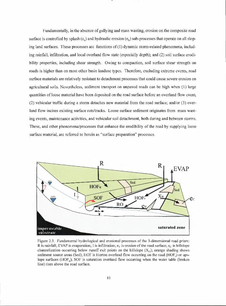
Fundamentally, in the absence of gullying and mass wasting, erosion on the composite road

surface is controlled by splash (e^) and hydraulic erosion (ej,) sub-processes that operate on all slop

ing land surfaces. These processes are functions of (1) dynamic storm-related phenomena, includ

ing rainfall, infiltration, and local overland flow state (especially depth); and (2 ) soil surface erodi

bility properties, including shear strength. Owing to compaction, soil surface shear strength on

roads is higher than on most other basin landuse types. Therefore, excluding extreme events, road

surface materials are relatively resistant to detachment processes that could cause severe erosion on

agricultural soils. Nevertheless, sediment transport on unpaved roads can be high when (1) large

quantities of loose material have been deposited on the road surface before an overland flow event,

(2) vehicular traffic during a storm detaches new material from the road surface; and/or (3) over

land flow incises existing sinface ruts/tracks. Loose surface sediment originates from mass wast

ing events, maintenance activities, and vehicular soil detachment, both during and between storms.

These, and other phenomena/processes that enhance the erodibility of the road by supplying loose

surface material, are referred to herein as “surface preparation” processes.

E V A P

im p e rm e a b les u b s tra te

Figure 2.3. Fundamental hydrological and erosional processes o f the 3-dimensional road prism: R is rainfall; EVAP is evaporation; I is infiltration; ej- is erosion o f the road surface; e^ is hillslope channelization occurring below runoff exit points on the hillslope (Xjj); orange shading shows sediment source areas (Sed); HOF is Horton overland flow occurring on the road (HOF^) or upslope surfaces (H O FJ; SOF is saturation overland flow occurring when the water table (broken line) rises above the road surface.

10

3. EXPERIM ENT I: Runoff generation and sediment production on unpaved

roads, footpaths, and agricultural land surfaces in northern Thailand

3.1 ABSTRACT

Rainfall simulation was used to examine runoff generation and sediment transport on roads, paths,

and three types of agricultural fields in PKEW. Because interception of subsurface flow by the

road prism is rare in PKEW, work focused on Horton overland flow (HOF). Under dry antecedent

soil moisture conditions, roads generated HOF in =1 min and have event runoff coefficients

(ROCs) of 80% during 45-min, =105 mm h-> simulations. Runoff generation on agricultural fields

required greater rainfall depths to initiate HOF; these surfaces had total ROCs ranging from 0-

20%. Footpaths are capable of generating erosion-producing overland flow within agricultural

landscapes where HOF generation is otherwise rare. Paths had saturated hydraulic conductivity

(Kj) values 80-120 mm h * lower than those of adjacent agricultural surfaces. Sediment produc

tion on roads exceeded that of footpaths and agricultural lands by more than eight times (1.23 ver

sus < 0.15 g J-'). Typically, high road runoff volumes (owing to low K , =15 mm h‘0 transported

relatively high sediment loads. Initial road sediment concentrations exceeded 100 g L-', but

decayed with time as loose surface material was removed. Compared with the loose surface layer,

the compacted, underlying road surface was resistant to detachment forces. Sediment concentra

tions for road simulations were slightly higher than data obtained from a 165-m road section dur

ing a comparable natural event. Initial simulation concentrations were substantially higher, but

were nearly equivalent to those of the natural event after 20-min simulation time. Higher sedi

ment concentration in the simulations was related to differences in the availability of loose surface

material, which was more abundant during the dry-season simulations than during the rainy sea

son natural event. Sediment production on PKEW roads is sensitive to surface preparation

processes affecting the supply of surface sediment, including vehicle detachment, maintenance

activities, and mass wasting. The simulation data represent a foundation from which to begin

parameterizing a physically based runoff/erosion model to study erosional impacts of roads in the

study area.

11

3.2 OBJECTIVE

The objectives of this experiment are to (1) use rainfall simulation to quantify runoff generation

and sediment transport on roads, footpaths, and agricultural lands and (2 ) compare data from small

plot rainfall simulation experiments on roads with those from a natural rainfall event on a larger-

scale road plot. The goal of this work is to examine whether processes operating on roads differ

in type or magnitude from those on agricultural lands and to obtain parameters needed to simulate

runoff and erosion using a physically based model (Experiment IV, Chapter 6 ).

3.3 METHODS AND MATERIALS

3.3.1 Study site

All work was performed within the 93.7-ha PKEW (Figure 2.2). Soil properties determined on

the Lower PKEW Road and adjacent fallow fields are listed in Table 3.1. The Upper and Lower

PKEW Roads are important source areas for material entering the stream channel network. At the

beginning of the rainy season, loose road surface material accumulated during the dry season is

flushed by surface flow during the first few rainstorms. Thereafter, light daily traffic (= 4 motor

cycles and 2 trucks per day. Chapter 5) detaches more sediment and creates ruts for gully initia

tion. Filling of gullies with unconsolidated material is an additional source of easily eroded mate

rial. Because HOF is commonly generated on roads (Ziegler and Giambelluca, 1997a), surface

runoff frequently transports sediment and incises concentrated flow channels throughout the wet

period. During the largest rain event of 1998 (STORM, discussed below), HOF from the 1650 m

Lower PKEW Road comprised 10% of the basin storm hydrograph for the first hour. Because

road runoff exit points tend to be where the road intersects stream channels, conveyance efficien

cy to the stream network is = 75% (based on field survey).

3.3.2 Simulation treatments

In February of 1998 and 1999 (dry seasons), 27 rainfall simulations were performed on a 50-m

road section and five other surfaces within an upland rice field, including ( 1 ) hoed field, (2 ) upland

field, (3) basin access path, (4) field maintenance path, and (5) fallow field. The rice field, con

sisting of 0.25 to 0.50 m rice stubble at the time of fieldwork (40-60% standing cover), was har-

12

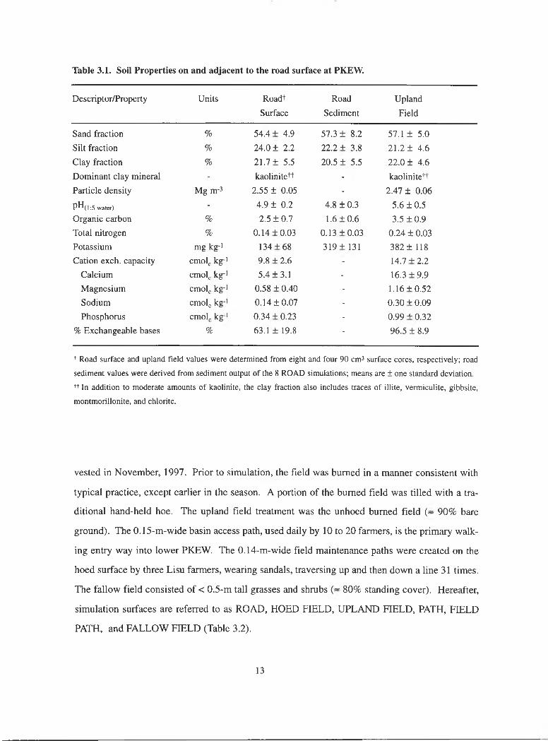
Table 3.1. Soil Properties on and adjacent to the road surface at PKEW.

Descriptor/Property Units Roadt Road Upland

Surface Sediment Field

Sand fraction % 54.4+ 4.9 57.3 ± 8.2 57.1 ± 5.0Silt fraction % 24.0 ± 2.2 22 .2+ 3.8 21.2 ± 4.6Clay fraction % 21.7 ± 5.5 20.5+ 5.5 22.0 ± 4.6Dominant clay mineral - kaolinitett - kaolinite''Particle density Mg m-3 2.55 ± 0.05 - 2.47 ± 0.06

PH(1:5 water) - 4.9 ± 0.2 4.8 ± 0.3 5.6 ± 0.5Organic carbon % 2.5 ± 0.7 1.6+ 0.6 3.5 + 0.9Total nitrogen % 0.14 + 0.03 0.13 + 0.03 0.24 ± 0.03Potassium mg kg-> 134 + 68 319+ 131 3 8 2 ± 118Cation exch. capacity cmolj, kg-' 9.8 + 2.6 - 14.7 + 2.2

Calcium cmolj. kg-' 5 .4+ 3.1 - 16.3 + 9.9Magnesium cmolj, kg-' 0.58 + 0.40 - 1.16 + 0.52Sodium cmol^ kg-' 0.14 ±0.07 - 0.30 + 0.09Phosphorus cmol(. kg ' 0.34 + 0.23 - 0.99 + 0.32

% Exchangeable bases % 63.1 ± 19.8 - 96.5 ± 8 .9

+ Road surface and upland field values were determined from eight and four 90 cm^ surface cores, respectively; road

sediment values were derived from sediment output of the 8 ROAD simulations; means are ± one standard deviation,

tt In addition to moderate amounts o f kaolinite, the clay fraction also includes traces of illite, vermiculite, gibbsite,

montmorillonite, and chlorite.

vested in November, 1997. Prior to simulation, the field was burned in a manner consistent with

typical practice, except earlier in the season. A portion of the burned field was tilled with a tra

ditional hand-held hoe. The upland field treatment was the unhoed burned field (~ 90% bare

ground). The 0.15-m-wide basin access path, used daily by 10 to 20 farmers, is the primary walk

ing entry way into lower PKEW. The 0.14-m-wide field maintenance paths were created on the

hoed surface by three Lisu farmers, wearing sandals, traversing up and then down a line 31 times.

The fallow field consisted of < 0.5-m tall grasses and shrubs (~ 80% standing cover). Hereafter,

simulation surfaces are referred to as ROAD, HOED FIELD, UPLAND FIELD, PATH, FIELD

PATH, and FALLOW FIELD (Table 3.2).

13

3.3.3 Measurement of physical properties

Prior to rainfall simulation, soil physical properties for each plot were measured either 1 m below

or above the simulation plot. Surface bulk density (pj,) and antecedent soil moisture (©„) were

determined by sampling the upper 5 cm with a 90 cm^ core (n > 3 for each plot), then oven dry

ing for 24 h at 105° C. Subsurface bulk densities were determined similarly at 5 and 10 cm depths.

Soil penetrability, a measure of the ease with which an object can be pushed into the soil

(Bradford, 1986), was measured with a static Lang^^ penetrometer (Gulf Shores, AL). The pen

etrometer provides an index of normal strength, termed penetration resistance (PR), for the upper

soil surface, typically = 0.5 cm in depth. Plot slope angles were determined with an Abney level.

Saturated hydraulic conductivity was estimated from infiltration measurements taken in situ with

Vadose Zone Equipment Corporation (Amarillo, TX) disk permeameters, linked to Campbell

(Logan, Utah) 21X data loggers. Use of this instrument in PKEW is explained by Ziegler and

Giambelluca (1997a).

3.3.4 Rainfall simulator and plot design

The rainfall simulator consisted of two vertical 4.3-m risers, each directing one 60° axial full cone

nozzle (70 mm orifice diameter) toward the surface. Water from a refillable storage container

(1850 L minimum) was fed to the simulator through 2.5 cm diameter PVC hose by a 750 W cen

trifugal pump and 2.5 kW gasoline-powered generator at 172 kPa (25 psi). This operating pres

sure produces rainfall energy flux densities (EFDs) of 1700-1900 J m-2 h-*, which approximates

energies sustained for 10-20 min during the largest annual PKEW storms (based on data from

Ziegler and Giambelluca, 1997a). Tubular, sand-filled geotextile bags (3.0 m x 0.2 m x 0.1 m)

were arranged to form rectangular plots. The bags were created from low permeability LINQ GTF

200 geotextile. Plot dimensions are shown in Table 3.2. Within PATH and FIELD PATH plots, the

compacted path surface occupied only -18 and 16% of the respective areas; the remaining sur

faces were similar to UPLAND FIELD and HOED FIELD, respectively. Nonpath surfaces were

included within path treatments to investigate sediment transport from the entire path complex;

i.e., erodible nonpath surfaces of relatively high infiltrability juxtaposed with compacted path sur

faces that frequently generate HOF.

14

Table 3.2. Mean slope, antecedent soil mass wetness (w), rainfall intensity (r), and energy flux density (EFD) for rainfall simulation experiments.

Treatment plot dim (m) slope (m m >) w (g g-') r (mm h->) EFD (J m-2 h->)

ROAD 8 3.75 X 0.85 0.15 ± 0 .02 att 0.12 ± 0.03 b 105 ± 10 a 1774 ± 175 a

HOED FIELD 4 3.25 x 0.85 0.23 ± 0.02 b 0.06 ± 0.01 a 110± 13a 1753 ± 218 a

UPLANDFIELD/PATH

7 3.25 X 0.85ttt 0.20 ± 0.02 b 0.05 ± 0.01 a 107 ± 10 a 1818 ± 177 a

FIELD PATH 4 3.25 X 0.85 0.21 ±0.02 b 0.06 ± 0.01 a 105 ± 15 a 1807 ± 262 a

FALLOW 4 3.25 X 0.85 0.32 ± 0.02 c 0.04 ± 0.01 a 97 ± 7 a 1634 ± 125 a

t n is the number o f “true” simulation replications; all replications were performed on previously untested plots, tt Column values with same letter are NOT statistically different (ANOVA B-D, p = 0.05); values are ± one standard deviation.ttt PATH plot length was 3.75 m.

At the base of all plots, geotextile bags were aligned such that runoff was funneled into

a shallow drainage trench. A V-shaped aluminum trough, inserted into the vertical trench wall,

allowed event-based sampling. On nonroad plots, the trench face and triangular surface area

immediately above the outlet were treated with a 5:1 mixture of water and Soil Sement^’ (an

acrylic vinyl acetate polymer from Midwest Industrial Supply, Inc., OH) to prevent sediment

detachment on these nonplot areas. The = 0.2l-m^ triangular area (in addition to plot areas above)

contributed runoff, but not sediment. Rainfall was measured for 40 to 50 min with manual gauges

placed on the plot borders. Energy flux density (J m-2 h’O of simulated rainfall was calculated

as :

e f d = ■ ^V 2

(3.1)

where r is event rainfall intensity (m h ') and Vdjq is the volume (m^) of the median-diameter (D50)

raindrop, determined by

fa / \%

3

(3.2)

In Eq. 3.1, m is the mass [kg] of the D50 drop, which is estimated as

(3.3)

15

where p , and Paj are 1000 kg m- and 1.29 kg m- , respectively. Factor v in Eq. 3.1 is the fall

velocity m s"' of the Djq drop, determined by the equation from Best (1950);

v = y„

(3.4)

with V ,^ = 9.5 (m s ') ,b = 1.77, and P= 1.147 (fromMualemand Assouline, 1986). Median drop

size was estimated from nozzle manufacturer engineering data. Rainfall EFD is more informative

than rainfall intensity because terminal velocity and drop size distributions from rainfall simula

tors differ from those of natural rainfall. Simulators with the same rainfall intensity, but different

architectures, will have different EFDs.

3.3.5 Simulation data collection and calculations

Time to runoff (TI RO) was recorded during each event. Runoff samples were collected at TTRO,

then again at 2.5, 5, or 10 min intervals. Most simulations were conducted for 60 min after

TTRO; PATH simulations were conducted for only 45 min. Discharge was determined by meas

uring the time to fill of a 525 mL bottle. After settling, the supernatant was decanted and discharge

samples were oven dried at 105°C for 24 h to determine mass of material transported. Sample dis

charge volumes were reduced to account for the presence of sediment. Values for instantaneous

concentrations (C,) were calculated as sediment mass per corrected discharge volume.

Instantaneous discharge and sediment output values were adjusted to rates per unit area by divid

ing by filling time and plot area (plot areas for sediment and discharge calculations were different,

see above). The rates were then divided by EFD values. Normalized instantaneous discharge (Qj)

and sediment output (S() therefore have units L J-' and kg J-*, respectively. Cumulative discharge

(Qcum) was calculated as total plot runoff volume prior to any time t, divided by EFD since TTRO.

Calculated slightly differently, cumulative sediment (Sj-um) output was total sediment mass at time

t divided by EFD since the beginning of the simulation. Values were normalized differently

because EFD prior to TTRO contributes differently to subprocesses controlling runoff generation

and sediment transport: i.e. at the beginning of rainfall, sediment is detached by raindrop impact

and material is transported downslope via rainsplash. In essence, energy prior to TTRO con

16

tributes to the sediment supply that will be transported throughout the event after runoff com

mences. With discharge, rainfall is infiltrated, then ponded, before HOF generation. Only by

contributing to surface sealing, which may speed up runoff generation, does energy prior to TTRO

contribute to all-event discharge. Total normalized event discharge and sediment output are

referred to as Qevem and Sgyent-

3.3.6 Measuring road discharge during natural events

To compare ROAD simulation data with discharge and sediment transport data from natural runoff

events, a discharge collection station was constructed at the footslope of a 165-m road section near

the watershed mouth (Figure 2.2). A trench was dug across the road to a depth and width of = 0.5

X 0.75 m. Vertical trench walls were re-enforced with 4 mm steel. Depressions in the transition

al area between the road surface and the reinforced walls were filled with concrete to prevent inci

sion. The trench bottom was covered with corrugated aluminum roofing, which was shaped in a

semi-circle and sloped (10%) to minimize sedimentation during events. The trench was covered

by a perforated steel grate to accommodate traffic. A tipping bucket rain gauge (0.254-mm thresh

old) and datalogger were used to measure 1-min rainfall intensities at the site. A typical road

cross-section was composed of = 1.9 m of compacted track and 1.3 m of less compacted surface.

This 3.2 m width represents the surface commonly traveled upon by vehicle (automobile and

motorcycle), pedestrian, and animal traffic. Tracks were occasionally incised 5-15 cm. Nontrack

surfaces often were often vegetated. Slopes for consecutive 20 m intervals starting at the trench

were: 0.12, 0.23, 0.25, 0.18, 0.09,0.07, 0.11, and 0.12 m m *. Discharge and sediment output val

ues were measured similarly to those in the ROAD simulations. Values were divided by filling

time, contributing area (3.2 m x 165 m), and event EFD, which was calculated using raindrop size

data from Baruah (1973) and Eqs. 3.1-3.4.

3.3.7 Data analysis

Because simulation durations occasionally differed, most data were analyzed based on simulation

times of 45 min. The lone HOED FIELD simulation producing mnoff was conducted for only 25

min following TTRO. Because there was no replication, HOED was not included in statistical

17

analysis. Similarly, FALLOW FIELD was not included because none of the four replications pro

duced runoff. All data were analyzed, after log jg transformation, using one-way analysis of vari

ance (ANOVA), followed by post-hoc multiple comparison testing with the Bonferroni/Dunn test

(B-D) when the F-values were significant at p = 0.05 (Gagnon et al., 1989). On compacted ROAD

and PATH surfaces, = 62% of the 250 PR values reached a maximum value of 6.7 MPa; rarely

was the maximum reached on other surfaces. The distributions of road and path PR values were

therefore truncated. Bounded data usually require special statistical treatment, but because ROAD

and PATH data were substantially higher than those of the other surfaces, and the focus was not

on differences between these two treatments, the use of ANOVA was justified. The nonparamet-

ric Spearman rank correlation coefficient (rj) was used to evaluate the relationship between com

paction indices (PR and pj,) and TTRO data.

3.4 RESULTS

3.4.1 Compaction indices

ROAD and PATH surfaces had statistically higher pb(o-s cm) values, compared with the

other surfaces (p = 0.05; Table 3.3). FIELD PATH, UPLAND FIELD, HOED FIELD, and FAL

LOW FIELD had surface P(, values statistically indistinguishable. ROAD and PATH surfaces had

the highest PR values (means = 6.4 MPa); HOED FIELD and FALLOW FIELD were the least

compacted surfaces by this measure (< 2.0 MPa). Compaction on roads and paths extended down

to at least 15 cm, although subsurface values were not statistically different from those of the other

surfaces (Table 3.3).

3.4.2 Instantaneous discharge and time to runoff

Figure 3.1 shows instantaneous discharge (Qj) and other related runoff data for the simulation sur

faces. Each data point is a mean of all simulations producing runoff. Each series begins at its

mean time to runoff (TTRO). To indicate the proportion of rainfall transported from the plots as

discharge, runoff coefficients (ROC = discharge volume/rainfall volume x 100%) based on mean

rainfall data from all simulations are shown. Values below treatment identifiers represent rainfall

depths falling on the plot before TTRO. Road surface runoff stands out, with mean TTRO occur-

18

Table 3.3 Mean values of compaction- and infiltration-related variables for six simulations.

Treatment Pb(0 - 5 cm)^

(Mg m-3)

Pb(5 - 10 cm)

(Mg m-3)

Pb(10-15cm )

(Mg m-3)

PR

(MPa)

Ks

(mm h-i)

ROAD 1.45 ±0.13 1.36 ±0.11 1.35 ±0 .10 6.4 ± 0.4 15 ± 9(74) b (16) a (16) a (160) d (26) a

PATH 1.40 ±0.11 1.37 ±0.09 1.32 ±0.14 6.4 ± 0 .7 8 ± 5

(21) b (3) a (3) a (90) d (6) a

FIELD PATH 1.24 ±0.11 1.25 ±0.16 1.28 ±0.12 2.8 ± 1.1 244 ± 88(22) a (4) a (4) a (40) b (10) b

UPLAND FIELD 1.20 ±0.09 1.25 ±0.15 1.23 ±0.13 4.7 ± 1.4 133 ± 7 7(36) a (5) a (5) a (98) c (6 )b

HOED FIELD 1.19 ±0.06 1.22 ±0.03 1.30 ±0.07 1.8 ± 1.2 316 ± 129(22) a (4) a (4) a (40) a (10)b

FALLOW FIELD 1.11 ±0.05 - - 1.7 ± 0 .9 129 ± 38

(6) a (60) a (6 )bt Pi, is bulk density at indicated depth; PR is penetration resistance, and is saturated hydraulic conductivity; val

ues are means ± one standard deviation; values in parentheses are sample sizes; values in each column with the

same letter are NOT statistically different (ANOVA B-D, p = 0.05).

1-5

C>

0.1 T

0.01

0.001 - -

0.0001- -

0 .00001-

T> r> o o

PATH23 mm

FIELDPATH48 mm

UPLAND FIELD HOED FIELD60 mm 100 mm

ROCs100% 75%

-J0 10 20 30 40 50 60 70 80 90

Total Sim ulation Tim e (m in)

Figure 3.1. Normalized instantaneous discharge (Q,) plotted since the beginning of rainfall simulation.

Values are normalized by rainfall energy flux density (EFD) and plot area. Data series begin at mean time

to runoff (TTRO). Values below surface identifiers refer to rainfall depths falling on the plot before TTRO.

Runoff coefficients (ROCs) are based on rainfall intensity data for all simulations. HOED has no replication, as only one of four events produced runoff FALLOW FIELD (not shown) did not produce runoff.

19

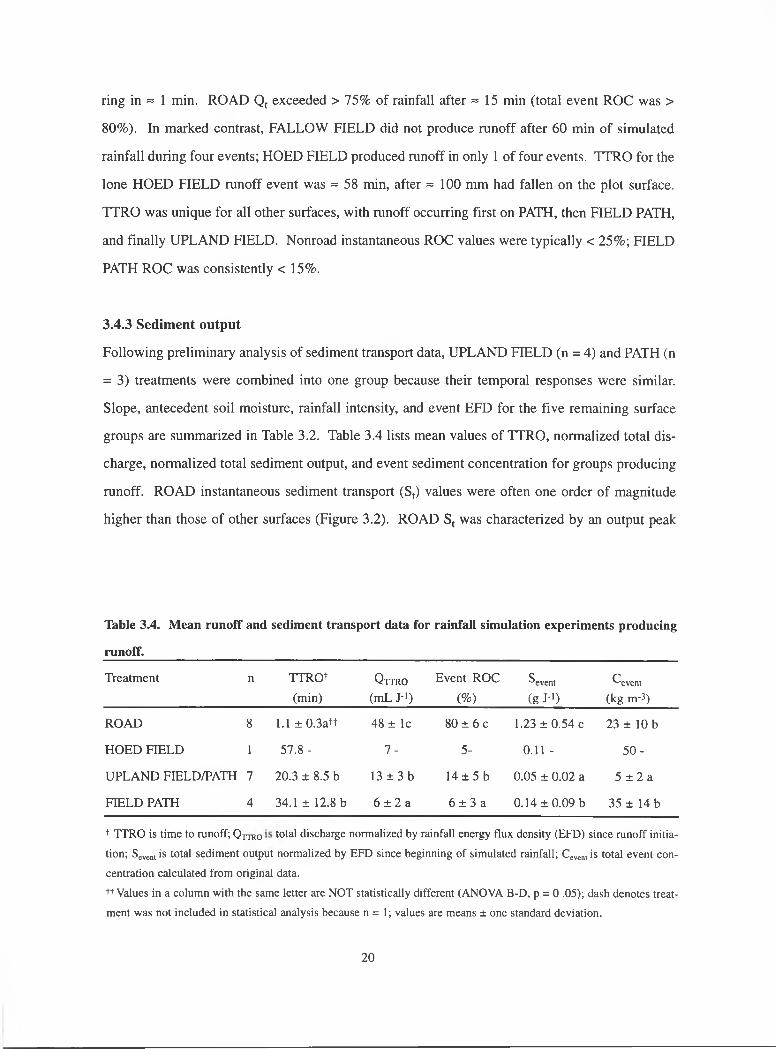
ring in » 1 min. ROAD Q; exceeded > 75% of rainfall after =15 min (total event ROC was >

80%). In marked contrast, FALLOW FIELD did not produce runoff after 60 min of simulated

rainfall during four events; HOED FIELD produced ranoff in only 1 of four events. TTRO for the

lone HOED FIELD runoff event was = 58 min, after =100 mm had fallen on the plot surface.

TTRO was unique for all other surfaces, with runoff occurring first on PATH, then FIELD PATH,

and finally UPLAND FIELD. Nonroad instantaneous ROC values were typically < 25%; FIELD

PATH ROC was consistently < 15%.

3.4.3 Sediment output

Following preliminary analysis of sediment transport data, UPLAND FIELD (n = 4) and PATH (n

= 3) treatments were combined into one group because their temporal responses were similar.

Slope, antecedent soil moisture, rainfall intensity, and event EFD for the five remaining surface

groups are summarized in Table 3.2. Table 3.4 lists mean values of TTRO, normalized total dis

charge, normalized total sediment output, and event sediment concentration for groups producing

runoff. ROAD instantaneous sediment transport (S,) values were often one order of magnitude

higher than those of other surfaces (Figure 3.2). ROAD S, was characterized by an output peak

Table 3.4. Mean runoff and sediment transport data for rainfall simulation experiments producing

runofi*.

Treatment n TT'ROt

(min)Qttro

(mL J-i)Event ROC

(%)event

(g J->)

c'-'event (kg m-3)

ROAD 8 1.1 ±0.3att 4 8 ± Ic 8 0 ± 6 c 1.23 ± 0.54 c 23 ± 10 b

HOED HELD 1 57.8 - 7 - 5- 0.11 - 5 0 -

UPLAND FIELD/PATH 7 20.3 ± 8.5 b 1 3 ± 3 b 1 4 ± 5 b 0.05 ± 0.02 a 5 ± 2 a

FffiLD PATH 4 34.1 ± 12.8 b 6 ± 2 a 6 ± 3 a 0.14 ± 0.09 b 35 ± 14 b

t TTRO is time to runoff; Qttro total discharge normalized by rainfall energy flux density (EFD) since runoff initia

tion; Severn is total Sediment output normalized by EFD since beginning of simulated rainfall; Cevc„,is total event con

centration calculated from original data.

tt Values in a column with the same letter are NOT statistically different (ANOVA B-D, p = 0 .05); dash denotes treat

ment was not included in statistical analysis because n = 1; values are means ± one standard deviation.

20

3.5 T -Q -R O A D

UPLAND FIELD/PATH

- 1 1 - HOED FIELD

-• -F IE L D PATH

0 5 10 15 20 25 30 35 40 45Time (min)

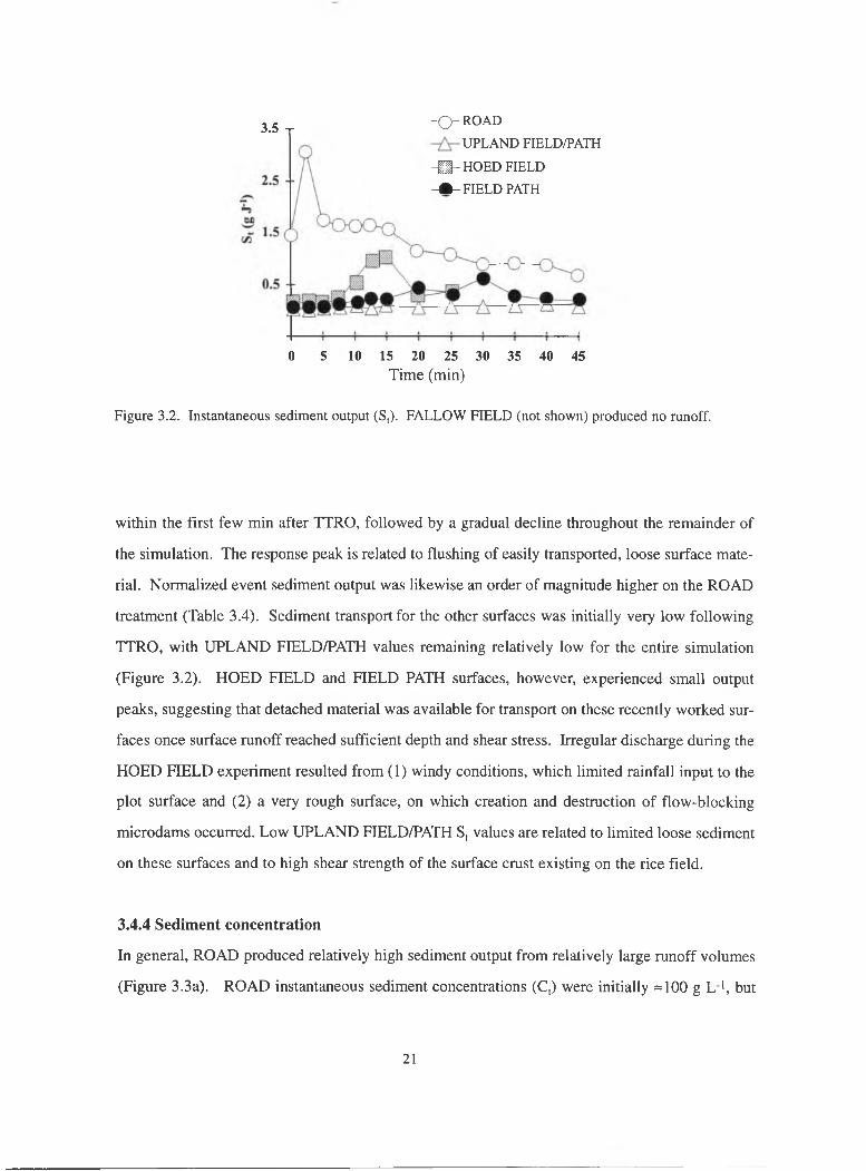
Figure 3.2. Instantaneous sediment output (S,). FALLOW FIELD (not shown) produced no mnoff.

within the first few min after TTRO, followed by a gradual decline throughout the remainder of

the simulation. The response peak is related to flushing of easily transported, loose surface mate

rial. Normalized event sediment output was likewise an order of magnitude higher on the ROAD

treatment (Table 3.4). Sediment transport for the other surfaces was initially very low following

TTRO, with UPLAND FIELD/PATH values remaining relatively low for the entire simulation

(Figure 3.2). HOED FIELD and FIELD PATH surfaces, however, experienced small output

peaks, suggesting that detached material was available for transport on these recently worked sur

faces once surface mnoff reached sufficient depth and shear stress. Irregular discharge during the

HOED FIELD experiment resulted from (1) windy conditions, which limited rainfall input to the

plot surface and (2 ) a very rough surface, on which creation and destmction of flow-blocking

microdams occurred. Low UPLAND FIELD/PATH S, values are related to limited loose sediment

on these surfaces and to high shear strength of the surface cmst existing on the rice field.

3.4.4 Sediment concentration

In general, ROAD produced relatively high sediment output from relatively large mnoff volumes

(Figure 3.3a). ROAD instantaneous sediment concentrations (C,) were initially =100 g L *, but

21

Q event (L J ) Time after runoff initiation (min)

Figure 3.3. (a) Normalized event sediment output (Severn) versus normalized event discharge (Qevem)- Sediment values were normalized by rainfall energy flux density (EFD) since the beginning of the simula

tion; discharge values were normalized by the energy since runoff initiation, (b) Instantaneous sediment con

centration (C,).

fell rapidly over time as loose material was flushed from the surface (Figure 3.3b). In compari

son, the other surfaces produced less total sediment from smaller volumes of runoff (Figure 3.3a).

Owing to very low discharge, HOED FIELD and FIELD PATH Cj values were at times the high

est of all events; and total event concentrations for these surfaces were greater than those of

ROAD (Table 3.4). However, total sediment output from these surfaces was minimal. Although

more study is clearly needed to understand sediment transport on these surfaces, high C, values

are realistic, as hoeing detached a generous supply of loose material. Sediment concentration on

the UPLAND FIELD/PATH treatments were the lowest of all treatments, again owing to surface

resilience on the upland field.

3.5 DISCUSSION

3.5.1 Influence of compaction on and runoff generation

Highly compacted surfaces, such as roads and paths, often have low infiltration rates because soil

aggregates have been destroyed by compaction and the surface layer may be sealed by fine mate-

22

rial. Significant negative correlation existed between and the two compaction indices, pb(o-5cm)

and PR: r = -0.668 (P < 0.0001) and- 0.821 (P < 0.0001), respectively. Penetration resistance

was sensitive to thin surface crusts not detectable with the 5-cm core. With respect to runoff

generation, TTRO showed strong negative correlation with Pt, and PR: r = -0.766 (P = 0.0008)

and r = -0.753 (P = 0.001), respectively. TTRO could be well predicted using step-wise regres

sion from Pb(o-5cm) = 0.822 (P < 0.0001). Correlation between compaction indices

and infiltration-related phenomena suggest easily obtained p,, and PR data can be used to extrap

olate Kj and TTRO data sets, when sufficient experimentation is prohibited by time restraints or

physically unfavorable conditions (e.g., steep slopes). The above correlations may change under

wetter experimental conditions, because PR and TTRO are dependent on soil moisture.

Comparing HOED FIELD and FIELD PATH compaction and TTRO data is informative

because the path treatment was created on the hoed surface. One research hypothesis was that

compaction from walking would enhance HOF generation on the FIELD PATH surface. The

small number of passes during dry antecedent moisture conditions increased Pb(o-5cm) by < 5%, but

significantly increased PR from 1.8 to 2.8 MPa (Table 3.3). Additionally, Kj was reduced by 23%

as foot traffic destroyed most large aggregates and clods. Using the bulk density methodology, the

shallow compaction on the hoed surface could not be detected, but the resulting thin mechanical

crust was detectable using the penetrometer and disk permeameter. In terms of runoff generation,

the foot traffic increased runoff generation: TTRO occurred after == 34 min of rainfall during all

four FIELD PATH events, compared with no runoff generation after 90-1- min on three of the four

HOED FIELD simulation experiments.

3.5.2 Erosion on path complexes

Juxtaposition of compacted footpaths with more-erodible planting surfaces could result in sub

stantial surface erosion if sufficient HOF is generated on the path surfaces. TTRO data in Figure

3.1 support enhanced runoff generation on the path surfaces: i.e., PATH < UPLAND FIELD and

FIELD PATH < HOED FIELD. Again, the compacted surface of PATH and FIELD PATH com

prised < 20% of the simulation surface; the remaining surface was similar to UPLAND FIELD

and HOED FIELD, respectively. The intention of including both path and nonpath surfaces in

23

simulation plots was to investigate the interaction of path-generated HOF with the erodible agri

cultural surface. For the two path treatments, mnoff was initiated on the path portion of the sim

ulation plot, and occurred on most of the PATH plot by the end of simulation. The nonpath por

tion of FIELD PATH did not contribute noticeably to mnoff. Had path surfaces comprised the

entire plot, TTRO would certainly have decreased and mnoff would have increased for both treat

ments, as Kj on the compacted portion of the plots was lower than that of the field portion by 80-

120 mm h-i (Table 3.3).

Sediment transport was not substantial for either path treatment (Table 3.4, Figure 3.2),

because (1) little HOF was generated on FIELD PATH (ROC < 15%), and (2) the nonpath surface

of PATH had high strength (PR = 4.7 MPa), thereby resisting detachment/entrainment by rain

splash and path-generated HOF. Concentration data (Figure 3.3) support the potential for high

sediment transport on complexes resembling FIELD PATH if sufficient HOF is generated. For

example, FIELD PATH Cj values were the highest of all treatments = 20 min after TTRO (Figure

3.3b), and relatively high Sgyen, was generated from low discharge volumes (Figure 3.3a). Some

sediment output was nonpath material entrained by on-path flow. Although walking impact

enhanced mnoff generation, it did not increase surface shear strength enough to resist hydraulic

erosion. The path surface was susceptible to micro-rill incision and headward expansion as knick

points migrated upslope (cf. flume studies of Bryan and Poesen, 1989; Merz and Bryan, 1993).

Decreases in sediment output after = 30 min mnoff may be related to armoring. The hydrological

behavior of the artificial NEW PATH surface may not represent compacted field paths that evolve

over the course of a growing season. These older paths have pj,, PR, and values more similar

to those of the PATH, as opposed to NEW PATH. Thus, mnoff generation may be better repre

sented by the PATH treatment. If this is the case, and sediment output is similar to FIELD PATH,

the potential for significant sediment transport exists.

3.5.3 Surface preparation and sediment transport

PKEW road surfaces have high sediment production rates in part because relatively high discharge

volumes flush readily available, loose surface sediment. Discharge is high because road surfaces

are highly compacted, thus infiltrability is low and a large percentage of rainfall becomes mnoff

24

(Ziegler and Giambelluca, 1997a). Loose sediment is made available by surface preparation

processes occurring between and during storms (Bryan, 1996). Surface preparation is any process

that influences the availability, erodibility/detachability, or transport of surface material. For

example, vehicle traffic is a principal mechanism responsible for detaching sediment during both

dry and wet periods. Additionally, some sediment entrained during runoff events is redistributed

on the road surface, and is available for transport during the next overland flow event. Although

nonroad surfaces also undergo various surface preparation processes, surface runoff on these sur

faces is more rare. Furthermore, vehicle detachment on roads is a daily phenomena; preparation

processes on other lands occur less frequently. For example, weeding on agricultural lands, which

breaks up crusted/compacted surfaces, may occur only a few times during the rainy period.

Hoeing may occur only once annually.

Under dry antecedent soil moisture conditions, substantial sediment transport from

PKEW agricultural surfaces will require significant rainfall depth (either as one large event, or as

a series of showers that shorten TTRO by increasing soil moisture content) to generate significant

HOF. Much less rainfall energy is required to generate runoff and remove loose surface materi-

Time after runoff initiation (min)

Figure 3.4. Energy required to remove 1 kg of sediment from the simulation plots.

25

al from roads. Figure 3.4 shows instantaneous rainfall energy needed to remove 1 kg of sediment

from the small-scale simulation plots (Sutherland et al., 1996). ROAD has the lowest values, with

agricultural surfaces typically having higher values. If rainfall prior to TTRO were included in

this calculation, nonroad values would substantially increase, particularly those for the one HOED

event that required » 60 min of rainfall (EFD = 1700 J m-2 h O to produce runoff. At hillslope

scales where roads channel runoff along the surface for substantial distances, sediment transport

can be enhanced by high shear stresses that transport large aggregates and gravel not entrained by

lower magnitude flows, such as those in the plot studies above. Furthermore, during high magni

tude storm events, overland flow on long slopes can incise the compact road surface, especially in

sections where ruts have already been formed.

3.5.4 Representativeness of the ROAD simulation data

One research goal was to use rainfall simulation data to assign parameters in KINEROS2 (Smith

et al., 1995), a physically based model that will be used to describe road runoff and erosion

processes (Chapter 6 ). Simulation data, obtained at a small scale, must therefore be representative

of larger-scale natural phenomena, when normalized similarly. To assess the degree of similitude,

ROAD Q( and C, were compared with data collected at the road discharge collection station dur

ing several natural rainstorms. This comparison is shown in Figure 3.5 for the rainstorm that most

closely resembled the simulated events, both in intensity and duration (referred to hereafter as

STORM). Rainfall intensities (Figure 3.5c) are plotted with respect to individual TTRO values

(time 0). Simulated rainfall begins =1 min before TTRO. During the natural event, rainfall was

first recorded 24 min before TTRO, with surface saturation, ponding, and interplot HOF also

occurring well before runoff initiation. STORM rainfall intensity was highly variable compared

with near-constant simulated rainfall intensity. During the high-energy portion of STORM (0-30

min), mean rainfall intensity (89 mm h >) was only slightly lower than the simulation rate of = 105

mm h’k However, EFD was substantially higher for STORM (= 2640 vs. 1775 J m-2 h-'), owing

to median raindrop size being = 50% larger than that of simulated rainfall.

Normalized ROAD and STORM Q( were comparable during the first 30 min following

TTRO when the natural rainfall rates were highest. Although falling limbs of the discharge hydro-

26

B

1a'«Pi

160

120

80

40 +

0

ROAD

wave-related spike

40 50 60

PARTIAL SAT

PONDING

SAT

HOF

J JL-LSTORM

-ROAD—

11-30 -20 -10 0 10 20 30 40 50 60

Time before or after TTRO (min)

Figure 3.5. Comparison between simulated (ROAD) and natural event (STORM) (a) sediment concentra

tion (C,); (b) instantaneous diseharge (Q,); and (e) rainfall intensities. Discharge and sediment-related out

put data are plotted relative to their individual time to runoff (TTRO). Data from the simulation and natu

ral event are normalized similarly. Partial saturation (PARTIAL SAT), ponding, saturation (SAT), and interplot Horton overland flow (HOF) correspond to the natural event.

graphs appear different, they are comparable when differences in plot lengths are considered.

After rainfall was discontinued, ROAD plots typically drained in = 0.75 min, time equivalent to «

29 min when scaled to the 165-m monitored road section. The STORM falling limb ended after

24 min. One critical difference between the two data sets is that at the base of the road section, a

‘wave’ of runoff water arrived from upslope « 1 min after TTRO (Figure 3.5b). This phenomena

27

was not detectable during small-scale ROAD simulations. The STORM C, spike shortly thereafter

(Figure 3.5c) was associated with the discharge wave, which brought both loose material from

upslope and the energy needed to entrain sediment near the plot outlet. Prior to the concentration

spike, ROAD C, was much higher than STORM C,. Afterwards, ROAD C, was only slightly

higher. Sediment transport decreased at both scales over time, as the supply of easily removed

surface material became depleted. Post-event observations on the road section indicate a second

ary mechanism contributing to the output decline may have been armoring, as sediment became

oriented in crevices of road ruts.

ROAD C( was higher than that of STORM despite raindrop impact energy and hydraulic

energy being greater for the hillslope-scale natural event than for the simulation experiments.

ROAD values were higher predominantly because simulations were performed in the dry season

when ample loose material had collected on the road surface since the last FlOF event several

weeks prior. STORM was one of a series of wet-season rainshowers that continually depleted sur

face sediment created by traffic between events. Initial ROAD C( values (= first 5 min) may be

uncharacteristically high to represent wet season phenomena in general. However, they may be

typical of concentrations achieved after long dry periods with frequent traffic or at the beginning

of the rainy season before the dry season sediment accumulation is removed.

Comparing ROAD results with other field studies provides another opportunity to assess

data integrity. The high initial C( values are similar to those measured following truck passes in a

40-nP simulation plot in New Zealand (30 min, 32-38 mm h * events) (Coker et al., 1993). When

compared with event concentration (Cgygn,) and discharge (Qevem) data determined from culvert

runoff during natural events for 10 road segments in Washington, USA (Reid and Dunne, 1984),

ROAD data (unshaded circles in Figure 3.6) correspond most closely to roads undergoing heavy

usage. Because PKEW roads are lightly used, these comparisons suggest that ROAD Cj values

are high. However, ROAD values were similar to those of 30 min, 50 mm h * simulation experi

ments on = 60 m2 plots in two western states of the USA (Elliot et al., 1995); the ellipse in Figure

3.6 encompasses 24 data points that were generated from simulations at eight different sites, vary

ing in soil type, during each of dry, wet, and very wet soil conditions. In addition, ROAD simu

lation values are only slightly higher than those recorded during seven storms on the monitored

28

PKEW road section in August 1998 (solid squares in Figure 3.6). General agreement between

simulation and natural event data supports good similitude of the ROAD simulation data for nat

ural phenomena in PKEW, but reveals limitations of comparing data at different scales. In addi

tion, similar storm events on physically similar road sections could result in substantially differ

ent sediment output data if two sites differ in variables affecting erodibility (texture, clay miner

alogy, shear strength, organic material, rock content) and/or availability of loose, entrainable mate

rial (as affected by age since construction, usage, maintenance activities, and mass wasting

processes). High values from this study, compared with the Reid and Dunne findings on similar

slopes, may relate to differences in soil erodibility, although one would surmise that soil originat-

Qevent (L/®)

Figure 3.6. Total ‘event’ sediment concentration (Ce„g„t) plotted against total ‘event’ discharge (Qevent) ^ r the ROAD simulations (unshaded circles) and the natural events (squares). Open square is STORM data

from Figure 3.5. Mean values occurring at time := 10, 20, and 30 min during ROAD simulations are repre

sented by filled circles. The labeled lines are fitted values determined on varying length roads during nat

ural events in Washington state, for different levels of traffic (from Reid and Dunne, 1984). The ellipse sur

rounds 24 values determined in the simulation study of Elliot et al. (1995).

29

ing from the siltstone, sandstone, and graywackes bedrock material of the Washington study

would be more erodible than the granitic-derived soil in PKEW.

Finally, the STORM value in Figure 3.6 does not continue the general trend of Cevem

increasing with Qevent> suggested by the Reid and Dunne data and the lower-volume PKEW

rainstorm events. PKEW road surfaces are composed of an erodible surface layer (loose materi

al of limited supply) and a less-erodible underlying layer (compacted road surface). After some

critical discharge volume has removed the loose material, sediment production diminishes because

the underlying surface is resistant to detachment/entrainment.

3.6 CONCLUSION

Rainfall simulation was useful in ascertaining unique differences in runoff generation and sedi

ment transport processes for roads, footpaths, and agricultural lands. Roads, having very low sat

urated hydraulic conductivities, generated runoff quickly (= 1 min) during high intensity events

and produced event runoff coefficients > 80%. Agriculture-related land surfaces often required

very large rainfall depths to produce overland flow when soils were initially dry. The dry season

simulations may understate the importance of agricultural fields to a basin sediment budget, as

erosion-producing HOF should occur more frequently under wetter soil conditions. Footpaths,

like roads, increase the frequency of runoff, demonstrating their potential to enhance surface ero

sion by acting as source areas for surface runoff on agricultural lands where HOF is otherwise rare.

High road discharge volumes flushed loose sediment that had accumulated on the surface

between or during rainfall events. Sediment transport on PKEW roads is initially high, then

steadily declines over time as loose surface sediment becomes depleted. Sediment output is sen

sitive to processes altering the supply of loose surface material, and may be more affected by these

processes than by the erodibility of the underlying compacted road surface. If large quantities of

surface material are present, such as might occur before the first large wet-season storm, or fol

lowing any extended dry period, sediment production can be substantial. When compared with

discharge and sediment transport on a 165-m road section during natural events, simulation con

centration data from this study were slightly higher. Some caution is therefore needed when using

these results to validate a physically based erosion model (Experiment IV, Chapter 6 ).

30

4. EXPERIMENT II: Partitioning total erosion on unpaved roads into splash and

hydraulic components: interstorm surface preparation and dynamic erodibility

4.1 ABSTRACT

Field rainfall simulation experiments at two sites are used to partition sediment transport on

unpaved roads into splash and hydraulic erosion components. Rainsplash processes contributed 38

to 45% of total sediment output, with instantaneous contributions being variable throughout 60-

min high-energy events. For low- and medium-magnitude rainstorms, splash erosion on roads is

initially controlled by the removal of easily erodible material, followed by a dramatic reduction in

sediment output associated with limited detachment from the resistant, highly compacted road sur

face. A conceptual model explaining temporal variations in splash and hydraulic erosion as func

tions of pre-storm surface preparation (via traffic, maintenance, mass wasting processes) is pre

sented. For situations where loose sediment is readily available, rainsplash energy is less impor

tant to sediment detachment. If the loose layer is diminished (e.g., following an overland flow

event) or protected by a surface crust, splash energy is needed to detach material from the road

surface. Equations in most physically based erosion models do not predict temporal variations in

road sediment transport that result from the removal of a loose surface layer of finite depth. A

strategy that successfully treats this removal as changes in road erodibility is introduced.

4.2 OBJECTIVE

The objective of the study was to (1) provide a physical basis for parameterizing erosion equations

for model sediment transport on unpaved roads; (2 ) identify temporal variations in erosion sub-

processes and the underlying mechanisms causing variations; and (3) assess the ability of model

equations to describe splash and hydraulic erosion processes on roads. This information is impor

tant for parameterizing the physically based model to be tested in Experiment IV, Chapter 6 .


4.3.1 Research Sites

Rainfall simulation was performed on two roads, one in Thailand, the other in Hawaii, USA. The

Thailand site was in the Pang Khum Experimental Watershed (PKEW, Figure 2.2, described in

31

Chapter 2). The test road section is a relatively new detour bypassing a steep hillslope. Maximum

slope was about 0.20 m m-F Ruts created from vehicle wheels incise the surface to depths of 0.10

to 0.15 m. Lowering from compaction and erosion processes is 0.1 m y->. Daily traffic includes

approximately 4 motorcycle, 2 truck passes, and an occasional passing water buffalo. The

Hawaiian study site is located at the base of the Waianae mountain range on Schofield Barracks

(US Army) in central-west Oahu Island, Hawaii. Rainfall is seasonal, with about 75% of the

annual 1000-1100 mm occurring from October to April. Unlike the Thailand site, there is typi

cally no prolonged period without rainfall events large enough to generate surface runoff. Road

surface material is a composite of Kolekole Oxisol, Helemano Inceptisol, weathered oxidic ash,

and exposed regolith/bedrock (Soil Conservation Service, 1981). Slope on experiment road varies

from about 0.05 to 0.35 m m-L The simulations were performed on an 80-m road section, for

which the road surface lies 1-4 m below the adjacent roadside margin. Enhanced surface lowering

results predominately from erosional and maintenance activities. Visible tracks and ruts are pres

ent on the road surface; however, traffic is now infrequent, as the section has been closed since

slope failure below the experimental site in early 1997.

4.3.2 Rainfall Simulation Experiments

In August 1997, six rainfall simulation experiments were performed at the Hawaii site. Eight sim

ulations were performed in PKEW in February, 1998. Each simulation run was a true replication,

usually performed 6-10 m above the previous simulation plot. The simulator used at both sites

consisted of two vertical, 4.3 m risers, each directing one 60° axial full cone nozzle (70 mm ori

fice diameter) toward the surface. The operating pressure of 172 kPa (25 psi) produced rainfall

energy flux densities (EFD) of 1700-1900 J m'^ h'* (100-115 mm h-*), approximating energy sus

tained for 10-20 min during the largest annual PKEW storms (based on preliminary analysis of 2

years of rainfall data). Cylindrical, sand-filled, geotextile bags (3.0 x 0.2 x 0.1 m) were arranged

to form two side-by-side rectangular subplots. For each simulation, one subplot was designated

as a rainsplash treatment (referred to herein as SPLASH); the other was covered with 2-mm wire

screen suspended 0.1 m above the road surface to retard raindrop energy (NO SPLASH). The

design is similar to Hudson’s (1957) mosquito gauze treatments of experiment no. 3 in Rhodesia.

Sediment output from the NO SPLASH treatment is assumed to result entirely from hydraulic ero

32

sion processes; and the difference between SPLASH (rainsplash + hydraulic erosion) and NO

SPLASH (only hydraulic erosion) treatments represents the sediment contributed by rainsplash,

i.e., detachment and rain-affected flow. Subplot dimensions for Schofield simulations were 3.50

(L) X 0.75 (W) m; the Thailand plots were slightly larger, 3.75 (L) x 0.85 (W) m. At the base of

each sub-plot, geotextile bags were arranged to funnel mnoff into a shallow drainage trench dug

into the road surface. A V-shaped trough constmcted from aluminum flashing was inserted into

the vertical wall of the trench to allow event-based sampling. The face of the drainage trench and

the triangular area below the main plot were treated with a 5:1 mixture of water and Soil SemenH*^

(an acrylic vinyl acetate polymer from Midwest Industrial Supply, Inc., OH) to prevent sediment

detachment on these nonplot areas. The sealed triangular area (an additional plot length of 0.5 m)

contributed only mnoff to the plot output; and discharge values were corrected accordingly.

Rainfall was measured during each event with 12 manual gauges placed on the plot borders. Table

4.1 shows physical properties associated with the road surfaces at the two sites. Mean values of

plot slope, antecedent mass soil wetness, and simulation rainfall intensity are shown in Table 4.2.

Instantaneous discharge (Q,), sediment output (Sj), and concentration (C() values were

measured at time to mnoff (TTRO) and then at 2.5 or 5 min intervals. Discharge volume was

reduced to account for presence of sediment in the samples. Values of Qj and S( were adjusted to

rates per unit area by dividing by filling time and plot area. The mnoff coefficient (ROC) was cal-

Table 4.1. Physical properties of the unpaved road surface at the Thailand and Hawaii research sites

Descriptor/Property'’ Units Hawaii Thailand Tied P-value

Pb (0 to 5 cm) M g m-3 1.32±0.02+t 1.42 ± 0 .02 0.0008 (36, 48)

Pb (5 to 10 cm) M g m -3 1.09 ±0.06 1.36 ±0.03 0.0004 (7, 16)

Pb (10 to 15 cm) M g m-3 1.05 ±0.05 1.36 ±0.03 0.0004 (7, 16)

PR MPa 5.8 ±0.1 6. 4 ± 0.0 <0.0001 (61, 160)

K. mm h-' 28.4 ± 4.5 13.6 ±2.1 0.0051 (12, 12)

tpi, is bulk density; PR is penetration resistance; is saturated hydraulic conductivity. Tied P-values are the results

of statistical testing with the nonparametric Mann-Whitney U test; values in parentheses indicate the sample number

for Hawaii and Thailand, respectively; values < 0.05 reflect significant differences between Hawaii and Thailand sites

'''M ean values ± one standard error.

33

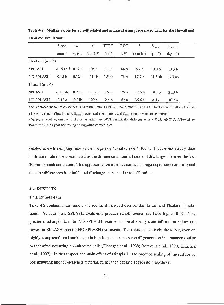
Table 4.2. Median values for runoff-related and sediment transport-related data for the Hawaii and

Thailand simulations.

Slope wt r TTRO ROC f event c' event

(mm-*) (gg-') (mmh*) (min) (%) (mm h-*) (gm-2) (kgm-3)

Thailand (n = 8)

SPLASH 0.15 abtt 0.12 a 105 a 1.1 a 84 b 6.2 a 19.0 b 19.3 b

NO SPLASH 0.15 b 0.12 a 111 ab 1.5 ab 75 b 17.7 b 11.5 ab 13.3 ab

Hawaii (n = 6)

SPLASH 0.13 ab 0.21 b 113 ab 1.5 ab 75 b 17.6 b 19.7 b 21.3 b

NO SPLASH 0.12 a 0.21b 129 a 2.4 b 62 a 36.6 c 8.4 a 10.3 a

t w is antecedent soil mass wetness, r is rainfall rate, TTRO is time to runoff, ROC is the total event runoff coefficient,

f is steady-state infiltration rate, is event sediment output, and is total event concentration.

ttValues in each column with the same letters are NOT statistically different at a = 0.05, ANOVA followed by

Bonferroni/Dunn post hoc testing on logiQ-transformed data.

culated at each sampling time as discharge rate / rainfall rate * 100%. Final event steady-state

infiltration rate (f) was estimated as the difference in rainfall rate and discharge rate over the last

30 min of each simulation. This approximation assumes surface storage depressions are full; and

thus the differences in rainfall and discharge rates are due to infiltration.

4.4. RESULTS

4.4.1 Runoff data

Table 4.2 contains mean runoff and sediment transport data for the Hawaii and Thailand simula

tions. At both sites, SPLASH treatments produce rnnoff sooner and have higher ROCs (i.e.,

greater discharge) than the NO SPLASH treatments. Final steady-state infiltration values are

lower for SPLASH than for NO SPLASH treatments. These data collectively show that, even on

highly compacted road surfaces, raindrop impact enhances runoff generation in a manner similar

to that often occurring on cultivated soils (Flanagan et al., 1988; Rbmkens et al., 1990; Gimenez

et al., 1992). In this respect, the main effect of rainsplash is to produce sealing of the surface by

redistributing already-detached material, rather than causing aggregate breakdown.

34

4.4.2 Sediment output data

Total sediment transport (Severn) and sediment concentration (Cevent) at both sites is higher for the

SPLASH treatments than the NO SPLASH (Table 4.2). SPLASH sediment output is characterized

by an initial flush of material, followed by a sharp decline, and then a stabilization in output

toward the end of the 60-min simulations (Figure 4.1). NO SPLASH output is typically less than

SPLASH; and in the Hawaii experiment output fluctuations are damped. In Figure 4.2 (c,d) total

erosion (e-j-) is partitioned into splash (e ) and hydraulic erosion (e^) components. Panels a and b

show percent contributions of e and e,, to total erosion. At the Thailand site, e,, dominates e-j- at

the beginning of the simulation, but is only slightly greater than after 60 min. In contrast, e at

the Hawaii site is greater than hydraulic erosion for the first 20 min, after which e^ predominates.

Total splash contribution to Cj at the Thailand and Hawaii sites is 37 and 48%, respectively. In

comparison, Ulman and Lopes (1995) reported the eg contribution to e-j- to range from 44 to 60%

for sites in Idaho and Colorado.

Time after TTRO (min) Time after TTRO (min)

Figure 4.1. Temporal variation in mean sediment output for SPLASH and NO SPLASH treatments on (a) Thailand

(n = 8) and (b) Hawaii (n = 6) unpaved road sites. Error bars represent ± one standard error; TTRO represents time to

runoff. Under the assumptions of the investigation, NO SPLASH values result from hydraulic erosion processes and

SPLASH values combine splash and hydraulic erosion processes.

35

(b) Hawaii

0 20

Time after TTRO (min)

40 60

Figure 4.2. Time dependent sediment contributions (%) of splash (e^) and hydraulic (e^) erosion components

to total sediment output (ej) for (a) Thailand and (b) Hawaii experimental sites; and temporal variations of Oj, e^, and eq- during 60 min of simulation for (c) Thailand and (d) Hawaii sites.

4.5 DISCUSSION

4.5.1 Role of surface preparation in road erosion

Surface preparation results from pre-storm events or processes that affect availability or trans

portability of sediment during storm events (cf., Bryan). Sediment detachment by vehicular traf

fic, maintenance activities, mass wasting events, and sediment deposition/removal during prior

storms are important preparation processes affecting sediment availability. Temporal and spatial

36

variations in road sediment transport are related to pre-storm surface preparation, except, possibly,

for high-magnitude events. For example, the early output peak during the Thailand dry-season

simulations results from the flushing of loose, easily entrained material, which was generated on

the road surface by vehicle detachment since the last overland flow event several weeks before

(Figure 4.2c). The energy of flowing water was sufficient to entrain this material, as evidenced

by the early importance of e to e^. After the loose material was removed, however, splash ener

gy was needed to entrain material from interrill areas adjacent to well-defined flowpaths into the

rill system. By simulation’s end, both hydraulic and splash subprocesses were greatly contribut

ing to net erosion. Had less loose material been available at the beginning, e - would likely have

been more equally partitioned between e and % throughout the simulation. Time since the last

overland flow event dictates the initial relationship between and ej,. In general, holding traffic

and maintenance constant, the longer the period between storms, the greater the opportunity for

surface preparation to occur, and the greater the initial role of e^ in sediment transport.

Similarity in total sediment output (Sgygn,, Table 4.2) at the Thailand and Hawaii sites sug

gest that the dissimilar eg and e responses result largely from site-specific differences in surface

preparation, as opposed to differences in soil erodibility. Because of differences in usage and rain

fall seasonality, the abandoned Hawaii road had received less cumulative surface disruption than

had the active Thailand road. Again, while the Thailand simulations were performed during a

lengthy dry period, the Hawaii experiments were performed only two weeks after the last over

land flow event. Prior to simulation, the Hawaii road surface contained a mechanical crust; and

little loose surface material was present. During simulation, limited material could be entrained

by surface flow alone. Rainsplash energy was important during the early simulation phase

because it disrupted the cmst and detached material. Had pre-storm traffic been greater, more

loose material would have been present, and sediment transport would likely have resembled that

on the Thailand road. At simulation’s end, ej, was only slightly higher than eg, as it was in the

Thailand experiment. These data indicate that the fundamental differences in sediment transport

response between the two sites resulted from availability of loose material, which was controlled

by differences in cumulative surface preparation since the last overland flow event.

37

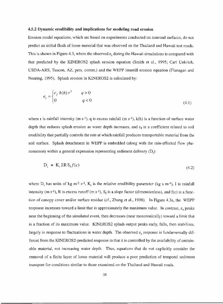
4.5.2 Dynamic erodibility and implications for modeling road erosion

Erosion model equations, which are based on experiments conducted on nonroad surfaces, do not

predict an initial flush of loose material that was observed on the Thailand and Hawaii test roads.

This is shown in Figure 4.3, where the observed during the Hawaii simulations is compared with

that predicted by the KINER0S2 splash erosion equation (Smith et al., 1995; Carl Unkrich,

USDA-ARS, Tuscon, AZ, pers. comm.) and the WEPP interrill erosion equation (Flanagan and

Nearing, 1995). Splash erosion in KINEROS2 is calculated by:

Cf k{h) r" q > Q

0 ^<0(4.1)

where r is rainfall intensity (m S'l), q is excess rainfall (m s-'), k(h) is a function of surface water

depth that reduces splash erosion as water depth increases, and Cf is a coefficient related to soil

erodibility that partially controls the rate at which rainfall produces transportable material from the

soil surface. Splash detachment in WEPP is embedded (along with the rain-affected flow phe

nomenon) within a general expression representing sediment delivery (Dj):

D, = K J R S ,/ ( c ) 4 2)

where Dj has units of kg m-2 s*', Kj is the relative erodibility parameter (kg s m-^), I is rainfall

intensity (m s-*), R is excess runoff (m s-’), Sf is a slope factor (dimensionless), and f(c) is a func

tion of canopy cover and/or surface residue (cf., Zhang et al., 1998). In Figure 4.3a, the WEPP

response increases toward a limit that is approximately the maximum value. In contrast, e peaks

near the beginning of the simulated event, then decreases (near monotonically) toward a limit that

is a fraction of its maximum value. KINER0S2 splash output peaks early, falls, then stabilizes,

largely in response to fluctuations in water depth. The observed response is fundamentally dif

ferent from the KINER0S2-predicted response in that it is controlled by the availability of entrain-

able material, not increasing water depth. Thus, equations that do not explicitly consider the

removal of a finite layer of loose material will produce a poor prediction of temporal sediment

transport for conditions similar to those examined on the Thailand and Hawaii roads.

38

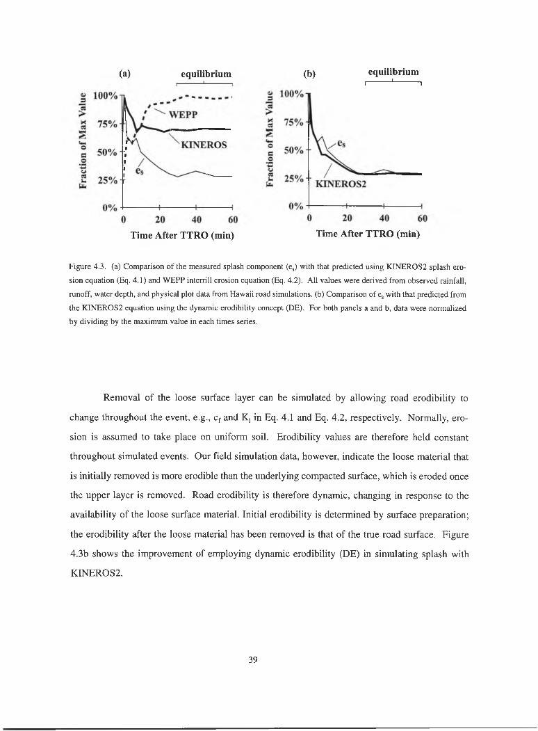
(a) equilibrium (b) equilibriumI--------'-------- 1

Time After TTRO (min) Time After TTRO (min)

Figure 4.3. (a) Comparison of the measured splash component (e,) with that predicted using KINEROS2 splash ero

sion equation (Eq. 4.1) and W EPP interrill erosion equation (Eq. 4.2). All values were derived from observed rainfall,

runoff, water depth, and physical plot data from Hawaii road simulations, (b) Comparison o f Cj with that predicted from

the KINEROS2 equation using the dynamic erodibility concept (DE). For both panels a and b, data were normalized

by dividing by the maximum value in each times series.

Removal of the loose surface layer can be simulated by allowing road erodibility to

change throughout the event, e.g., Cf and Kj in Eq. 4.1 and Eq. 4.2, respectively. Normally, ero

sion is assumed to take place on uniform soil. Erodibility values are therefore held constant

throughout simulated events. Our field simulation data, however, indicate the loose material that

is initially removed is more erodible than the underlying compacted surface, which is eroded once

the upper layer is removed. Road erodibility is therefore dynamic, changing in response to the

availability of the loose surface material. Initial erodibility is determined by surface preparation;

the erodibility after the loose material has been removed is that of the true road surface. Figure

4.3b shows the improvement of employing dynamic erodibility (DE) in simulating splash with

KINER0S2.

39

4.6. SUMMARY AND CONCLUSIONS

Rainsplash enhances ranoff generation and contributes greatly to sediment detachment/entrain-

ment on unpaved roads. Even on these highly compacted surfaces raindrop impact reduces the

infiltration rate in a manner similar to that occurring on aggregated agricultural and range land

soils. Total event splash contribution to the total erosion process during 60-min rainfall simula

tions on two road surfaces ranged from 38 to 45%. On the Thailand test road, splash erosion was

less than hydraulic erosionat all times during the simulation. On the Hawaii road however, spalsh

erosion dominated hydraulic erosion for the first third of the event, then became less than

hydraulic erosion for the last 40 min of the simulation. On compacted roads, variability in splash

and hydraulic erosion subprocesses is initially controlled by the availability of surface sediment

and finally by the shear strength of the underlying road surface. Pre-storm availability of loose

material is a function of cumulative surface preparation since the previous overland flow event.

Physically based erosion models that do not explicitly describe the removal of a loose material

layer of finite depth will fail to predict road sediment transport response for roads where sediment

preparation is important. If road erodibility is allowed to change during computer simulation (e.g.,

as in the DE methodology presented herein), removal of the loose surface layer can be simulated

with conventional erosion models.

40

Plate 3

People of Pang Khum. (1) Alima, with other Lisu women at a spirit ritual; (2) Dailom (front) and other

Karen friends on a hand-made cart; (3) Ataboo’s fether (back) and the near-mute Lisu basketmaker, (4) two

Karen boys brandishing worldly icons that are now common in Pang Khum: a rose, symbolic of cash-based

flower farming; and a football— the world’s most popular sport; (5) the young Lisu father, Apon, and his son.

Pang Khum Experimental W atershed. (6) station 406, dedicated to measuring rainfall and

road surface soil moisture change, located at the base of the monitored road section; RAS is measuring

saturated hydraulic conductivity; (7) station 405, a weir construtted in the Loei stream at the mouth of

PKEW; Asu is removing trapped sediment; (8) climate station 402 within Atachichi’s upland rice field; (9)

the research vehicle parked outside the fieldhouse in the Karen village at Pang Khum; (10) sensors of cli

mate station 401 rest above a 17-m primary forest canopy.

Plate 12

Plate 13

Surface preparation and road-related erosion. ( I I ) surface lowering in excess of 0.5 m

was observed on the road from Pang Khum to Pa Pae in 1996; (12) repairing of roads with a tractor and

blade usually occurs only on major arteries (the road to Pa Pae, November, 1998); (13) severe gullying on

the road from Pa Pae (1996); (14) road sections often terminate at stream channels; thus, road sediment

is transported directly to the stream network; ( 15) hand-filling of ruts is the dominant maintenance method

on Pang Khum roads (Paluk and other Karen men, the road to Samoeng, 1999).

Landscape of Pang Khum. (16) a cleared hillslope awaiting planting: (17) furrows and paths with

in agricultural fields serve as source areas for overland flow and erosion; (18) Doi Mon Ang Ket, the high

est point in PKEW, as seen from the Lisu village in Pang Khum; (19) flower field beside a Lisu field house;

(20) mixed swidden field (cabbage, onions, corn, papaya, taro) and Lisu farmers during harvesting season

(taken from station 401).

Plate 24 Plate 25

Rainfall simulator. (21) Lisu helpers prepare the FILL plots by filling ruts with material taken from

the roadside; (22) Asu draining water from the collection ditch at the plot base, TRUCK simulations,

February, 1999; (23) A D Z with pump, generator, and 1500 L supply tank, which was filled with water piped

from a stream about 500 m upslope; (24) FILL simulation experiment, February, 1999; (25) practice run

on an agricultural field.

Plate 29 Plate 30

Agricultural simulations. (26) Asu, Aluong, and Atachichi creating the N E W PATH treatment,

1998; (27) testing on the HOED FIELD treatment, 1998; (28) A D Z observing N E W PATH (left) and

H OED (right) treatments during February, 1998 rainfall simulations: (29) Atachichi burning the rice field

to create the UPLAND FIELD treatment, 1998; (30) FALLOW treatments, 1999.

Plate 34

Road-related rainfall simulations. (31) RAS collecting runoff from the SPLASH treatment dur

ing the SPLASH/NO SPLASH simulations, 1998; (32) RAS observing a large rut created during the TRUCK

simulations, 1999; (33) Ayong driving a motorcycle through the simulation plot during the MOTORCYCLE

simulations, 1998; (34) Disrupted road surface following four passes of the Isuzu Rodeo during TRUCK

simulations, 1999; Assam looking on in amazement.

Plate 36

Plate 37

Lisu helpers. (35) Atachichi, A D Z, Asu, &

Aluong taking measurements during the

UPLAND FIELD simulations, 1998; (36) Lisu men

and women laying the water pipeline that fed the

simulator, (37) Asu and Atachichi showing they

too can be hotshot researchers; (38) Asu seeing

how one hotshot Western researcher measures

up to Lisu standards.Plate 38

5. EXPERIM ENT III: Interstorm surface preparation and sediment detachment

by vehicle traffic on unpaved mountain roads

5.1 ABSTRACT

Road survey and field rainfall simulation experiments support that the erodibility of a road surface

is dynamic. In the absence of extreme runoff events, dynamic erodibility results from the gener

ation and removal of easily entrained surface material by human road surface maintenance activ

ities, vehicular detachment, and overland flow events. Maintenance activities introduce, easily

transportable material to the road surface where it can be entrained by overland flow. Traffic in

dry conditions detaches material that is quickly removed during subsequent overland flow events.

The pre-storm erodibility of a road is therefore largely a function of maintenance and vehicle

activity since the last overland flow event. During rainstorms, vehicle passes increase sediment

production by detaching/redistributing surface material and creating efficient overland flow path

ways for sediment transport. However, if incision of tracks by overland flow does not occur, post

pass sediment transport quickly returns to pre-pass rates. Field rainfall simulation data suggest

sediment transport resulting from during-storm vehicle passes is greatly influenced by the pres

ence of existing loose material, which again is a function of prior road usage and maintenance

activities. Incorporation of vehicular phenomena into physically based road erosion models may

be possible by parameterizing both storm and inter-storm changes in the supply of loose surface

material as changes in surface erodibility.

5.2 OBJECTIVE

The objective of this experiment was to use rainfall simulation to investigate sediment production

associated with road maintenance practices in northern Thailand (i.e., manual filling of ruts), and

to study sediment detachment by motorcycles and pickup trucks on unpaved roads. An addition

al objective was to establish links between road sediment production and various human activities

by synthesizing physical property measurements, road usage information, and rainfall simulation

results. This information is vital to the development of a general methodology for physically mod

eling road erosion (Experiment IV, Chapter 6 ).

50


5.3.1 Survey of vehicle usage and surface physical characteristics

The following investigations were performed on the lower road mnning through the 93.7-ha

PKEW (Figure 2.2, described in detail in Section 2.2): (a) a survey of vehicle usage; (b) meas

urements of cross-sectional physical characteristics; (c) an inventory of sediment sources; and (d)

a survey of exit points for road runoff. The traffic survey was conducted for 225 h on 44 days

between July, 1998 and February, 1999. During each survey session (usually 4 to 5 h beginning at

an arbitrary time of day), each vehicle pass was recorded, noting the type of vehicle, road and

weather conditions, and presence/absence of tire chains. Session values were converted to values

of passes per 12-h work day using a simple weighting function. A total of 32 cross-sections were

established 50 m apart, beginning 25 m inside the watershed boundary. One suite of cross-sec

tional measurements was conducted in the dry season, March, 1998; a second, 7 months later near

the end of the wet season.

At each cross-section, numerous physical phenomena were recorded, including road

width, surface condition (e.g., track vs. nontrack), two-dimensional slope, lowering estimates,

rut/gully dimensions, and availability of loose surface material. Area-based volumetric and gravi

metric estimates of surface material availability were determined by collecting surface sediment

from a 0.10 m swath across the road surface at each cross-section. The loose material was col

lected with a brush and a trowel, taking care not to detach new material from the road surface.

Also along the road, a detailed survey was made of sediment sources, preferential overland flow

pathways, and runoff entry/exit points.

5.3.2 Rainfall simulation experiments

The rainfall simulator and plot design are described in Experiment I, Chapter 3. Three rainfall sim

ulation experiments were conducted, including one investigating sediment transport on fill mate

rial used to repair the road surface (FILL). Two other experiments investigated sediment detach

ment during motorcycle (MOTORCYCLE) and truck passes (TRUCK). Data from the prior

ROAD simulations (Chapter 3) were used as a road control. Experimental designs for each sim

ulation are as follows:

51

(I) FILL simulations were performed in February 1999 on 1.3 m (W) x 3.75 m (L) plots

on the steepest road section in PKEW (median slope = 0.18 m m-i). For each of four FILL sim

ulations on separate plots, a large surface rut (median dimensions = 0.45 m (W) x 0.13 m (D))

running length-wise down the slope was filled with soil taken directly from the roadside margin.

The material was excavated and applied with a hand-held hoe by Lisu farmers in a manner con

sistent with typical road maintenance in PKEW. The fill material was compacted by stomping.

Rainfall was applied for 45 min following time to runoff (TTRO).

(II) The MOTORCYCLE simulations were performed in February 1998 on the same plots

as the ROAD simulations (Experiment I, Chapter 3), one day following the ROAD experiments.

Thus, initial soil moisture was relatively high approximately 22 vs. a value of 12 g g-i recorded

during the ROAD experiments) and loose surface sediment was reduced from what normally

would be expected during the dry season. Rain was applied to eight different pairs of 0.85 m (W)

X 3.75 m (L) subplots for 10 min after TTRO. After rain cessation, a 100 cc Honda motorcycle

(street tires = 5 cm wide, mass = 85 kg) was twice driven up and down through each plot. Thus,

each wave of motorcycle activity consisted of four passes through the plot. After a 15-min delay

to complete the passes, rainfall was applied for another 1 0 min period, followed by a second iden

tical wave of motorcycle passes and a second 15-min delay. A final 30 min of simulated rainfall

was then applied.

(III) TRUCK simulations were conducted on the four FILL simulation plots (described

above) on the following morning, approximately 18 h after the FILL simulations ended. Rainfall

was initially applied for 20 min. The research vehicle (1993 Isuzu Rodeo; street tires = 20 cm

wide, mass = 1700 kg) was then driven once up and then back down through the test plot. Each

plot was wide enough only to allow two of the four wheels to pass over the simulated surface; thus,

during each pass phase the surface was exposed to detachment by a total of four tires. After a 10-

min delay to complete the passes, rainfall was applied for 25 min. In all, four TRUCK simula

tions were conducted.

5.3.3 Rainfall simulator and plot design

The rainfall simulator consisted of two vertical, 4.3 m risers, each directing one 60° axial full cone

nozzle (70 mm orifice diameter) toward the surface. The operating pressure of 172 kPa (25 psi)

52

produced rainfall energy flux densities (EFD) of about 1650-2040 J m-2 h > (100-120 mm h-i),

approximating energy sustained for 10-20 min during the largest annual PKEW storms (based on

preliminary analysis of 2 years of rainfall data). Rainfall rate was measured during each event

with several manual gauges placed on the plot borders. Cylindrical, sand-filled, low permeabili

ty geotextile bags (3.0 x 0.2 x 0.1 m) were arranged to form two side-by-side rectangular subplots.

At the base of each sub-plot, geotextile bags were arranged to funnel runoff into a shallow

drainage trench dug into the surface. A V-shaped trough constructed from aluminum flashing was

inserted into the vertical wall of the trench to allow event-based sampling. Mean values of plot

slope, pre-simulation soil wetness, rainfall intensity, and EFD for all simulation experiments are

shown in Table 5.1.

5.3.4 Simulation data collection and calculations

During each experiment, instantaneous discharge and sediment output were recorded at time to

runoff (TTRO), then again at 1.0, 2.5, or 5.0 min intervals until the end of simulation or until a

scheduled break to conduct a vehicle passes. Discharge volume was reduced to account for pres

ence of sediment in the samples. Instantaneous discharge and sediment output values were adjust

ed to rates per unit area by dividing by filling time and plot area. The rates were then divided by

energy flux density (EFD) values of the simulated rainfall (described in Chapter 3). Normalized

instantaneous discharge (QJ and sediment output (Sj) therefore have units m^ J-i and kg J-*,

respectively. Total normalized event discharge and sediment output, Qevent Sgygnt, were cal

culated as event total values divided by total event EFD. Runoff coefficients (ROCs) were calcu

lated at each sampling time as the fraction of rainfall leaving the plot as discharge. Final event

steady-state infiltration rates (fjj) were estimated from the event rainfall intensity (r) and the final

event runoff coefficient (ROCfinal, determined over the last 15 min of simulation time) as

This approximation assumes surface storage depressions are full; and thus the difference in rain

fall and discharge rate is the fjj.

53

Table 5.1. Mean slope, soil mass wetness, and rainfall variables for all simulation experimentsTreatment nt slope

(m m‘*)

W

(g g’L

r

tmm h‘LEFD

("J m '^h'UFILL 4 0.20 ± 0 .06 't 0.10 ±0.05 9 8 ± 11 1654 ± 188R O A D tt 8 0.15 ±0.02 0.12 ±0.03 110 ± 12 1836 ± 209

MOTORCYCLE

Pre-pass 8 0.15 ±0.02 0.22 ± 0.01 109 ± 12 1853 ± 198Post-pass 1 8 0.15 ±0.02 - 108 ± 16 1826 ± 269Post-pass 2 8 0.15 ±0.02 - 109 ± 16 1838 ± 262

TRUCK

Pre-pass 4 0.20 ± 0.06 0.28 ± 0.01 104 ± 13 1665 ± 362Post-pass 4 0.20 ± 0.06 - 120 ± 17 2037 ± 294tw is pre-simulation mass wetness, r is rainfall rate, EFD is energy flux density; values are means ± one standard dev.

■*"1 ROAD data are from Chapter 3.

5.3.5 Statistical Analysis

For comparing FILL with ROAD data, slope, antecedent soil wetness (w), r, event energy flux

density (EFD), TTRO, Qevent> ROC, f s, Sevens ^nd Cevent data were analyzed using the nonpara-

metric Mann-Whitney U-test (M-W U). For the MOTORCYCLE simulations, the data were

log 10-transformed then analyzed using one-way analysis of variance (ANOVA); multiple compar

ison testing was then conducted with the Fisher’s protected least squares difference test (PLSD)

when the F-values were significant at p = 0.05 (Gagnon et al., 1989). For comparison of

MOTORCYCLE pre-pass S, values with ROAD simulation data, repeated measures (RM)

ANOVA was performed on logig-transformed data. The pre-pass and post-pass TRUCK simula

tion data were analyzed with M-W U.

5.4 RESULTS

5.4.1 Road survey

The traffic survey revealed the Lower PKEW Road receives 4.1 ± 0.5 (std. error) motorcycle and

1.8 ± 0.3 truck passes per 12-h work day. Daily motorcycle traffic is that from farmers going to

54

and from their fields. Truck traffic is generally from small pickups taking crops to the village or

market; few villagers who utilize PKEW own a truck. Occasionally a caravan of 1 to 4 trekking

jeeps will pass through. An army personnel transport truck ( 6 wheels, mass > 4400 kg) passes

through once or twice a year carrying troops conducting opium eradication. Well-defined tire

tracks/ruts exist throughout the entire 1.65 km length; in some areas a center motorcycle track par

allels existing truck ruts. On steep sections, incised tracks provide a rough, exhilarating driving

challenge during both wet and dry periods. Surface lowering, < about 0.10 m y >, is detectable

mainly on steep sections (> 0.15 m m '). which occupy < 30% of the total road length. This low

ering value is based on one-year and five-year estimates made on the new detour section where

the FILL simulations were conducted. In comparison, on one steep (> 0.20 m m ’) section of the

main artery leading to Pang Khum, lowering in excess of 0.75 m was observed during the 1996

rainy season.

Road cross-section measurements conducted in the 1998 dry season revealed 8.59 Mg

(2.17 kg m-2) of loose surface material on the Lower PKEW Road (1650 m (L) x 2.4 m (W) = 3960

m2) Cross-sectional measurements taken during the rainy season verify significantly less (M-W

U, tied-P value <0.0001) loose road material (3.13 Mg, 0.79 kg m-2). Texture of this material, 58%

sand, 19% silt, 23% clay, is indistinguishable from that of the compacted road surface and adja

cent fields. Some locations with the greatest sediment depth were found on and immediately

below the steepest roads sections, but no significant correlation existed between sediment depth

and slope. Most surface material present during the survey is road material detached by vehicle

traffic. Other nonroad sediment sources include (1) material removed from the roadside margin

for repair; (2 ) infrequent bank failures (e.g., at entry points to upslope fields) and side slope slump

ing; (3) localized excavation sites for harvesting plants, insects, etc. Some of the wet-season mate

rial includes sediment deposited during prior overland flow events. The wet-season value, which

is one-third that of the dry-season value, may be higher than what typically exists during the

wettest part of the rainy season (June-August), for the survey was conducted during an extended

dry period.

Conveyance efficiency (CE) of road runoff to the stream network varies spatially and tem

porally. For any given road section, erosion processes, maintenance, and mass wasting changes

55

the overland flow pathways and runoff exit points. During large storms, overland flow may

bypass typical flow channels, thereby altering the conveyance efficiency. In PKEW, a total of

1263 m of the lower road terminates at the stream network. Assuming that runoff exiting else

where infiltrates on the hillside (supported by field observations) and that no evaporation or sur

face storage occurs, the maximum CE estimate for the Lower PKEW Road is 76%. During large

storms, some overland flow leaves the road surface at ephemeral exits points, where it again infil

trates into the hillside. Factoring in these losses, the minimum CE estimate is 56%. For most

storms, including STORM discussed below, estimated CE for the lower PKEW road is about 70%

(field observation).

5.4.2 FILL simulations

Data in Table 5.2 show both hydrological and geomorphological differences between the FILL and

ROAD simulations. For example, TTRO was much slower on the repaired/filled surface; addi

tionally, total event discharge (Qevem) ^”d event ROC were lower for FILL compared with the

ROAD control. Bulk density of the fill surface was 1.05 Mg m-3 (taken in situ after the repair),

significantly lower (M-W U, a = 0.05, n=12) than the 1.42 Mg m-3 of the road surface. ROAD

and FILL steady state infiltration rates were statistically indistinguishable, implying ending ROCs

(thus final discharge) were similar. Total event sediment output for the FILL simulations was

about 40% higher than for the ROAD simulations. Instantaneous sediment transport for the two

simulation surfaces were very similar for the first 15 min, but then separated for the final 30 min,

as FILL S, remained relatively high, and ROAD S, diminished (Figure 5.1a). Total sediment con

centration was 2.5 times higher for the FILL versus the ROAD simulations (Table 5.2). Figure

5.1b shows FILL instantaneous sediment concentrations (C,) to be consistently higher than those

for ROAD. The maximum C, during the FILL simulation was almost twice as high as that for

ROAD (320 vs. 170 g L-i).

5.4.3 MOTORCYCLE and TRUCK simulations

Runoff and sediment transport data from the MOTORCYCLE and TRUCK simulations are shown

in Tables 5.2. For both types of simulations, post-pass phases had higher event discharge and

56

Table 5.2. Mean runoff and sediment transport data for all simulationsTreatment TTRO!

(min)Qevent(L J-l)

ROC

(%)fss

(mm h-')^event(gJ-')

c'-event(g L-1)

FILL 6.1 ± 3 .4 a 0.043 ± 0.01 a 60 ± 14 a 12.0 ±11.3 a 1.7 ± 0 .6 a 44 ± 9 bR O A D tt 1.1 ± 0.3 b 0.053 ± 0.01 a 82 ± 4 b 6.2 ± 4 .1a 1.2 ± 0 .6 a 21 ± 9 a

M OTORCYCLEttt

Pre-pass 0.6 ± 0.3 b 0.013 ± 0.003 a 69 ± 10 a 16.4 ± 9 .6 a 0.9 ± 0.4 a 17 ± 9 abPost-pass 1 0.4 ± 0.2 a 0.014 ± 0.003 a 7 5 ± 8 b 12.1 ± 8 .4 a 1.3 ± 0 .7 a 22 ± 10 bPost-pass 2 0.3 ±0.1 a 0.047 ± 0.008 b 8 6 ± 5 c 9.8 ±5.1 a 2.8 ± 1.2 b 1 5 ± 6 a

T R U C K tttt

Pre-pass 0.8 ± 0.2 b 0.043 ± 0.007 a 73 ± 1 2 a 12.1 ± 11.8 a 1.2 ± 0 .3 a 2 5 ± 7 aPost-pass 0.5 ± 0.2 a 0.051 ±0.007 a 8 6 ± 7 a 7.0 ± 6.6 a 3.8 ± 0.6 b 6 8 ± 8 b

■'TTRO is time to runoff, Qgvem total normalized event discharge, ROC is the total event runoff coefficient (total

runoff/total rainfall), Ls is estimated steady-state infiltration rate (from Eq. 5.1), and is normalized event sedi

ment output, Cgven, is total event concentration; values are means ± one standard dev.

■"ROAD and FILL data in each column with the same letter are NOT statistically different at p = 0.05, nonparametric

Mann-Whitney U-test; ROAD data are from Chapter 3.

t " MOTORCYCLE simulation data in each column with the same letter are NOT statistically distinguishable at p =

0.05, ANO^VA followed by Fisher’s PLSD post hoc testing on logig-transformed data.

t t t t t r u c k simulation data in each column with same letter are NOT statistically different at p = 0.05, M-W U.

ROCs. These increases may result from the creation of well-defined flow channels by the vehi

cle tires, but may also be artifacts of the post-pass phases having higher soil moisture values than

the previous phases. The truck passes initiated significant increases in total event sediment out

put and concentration. The motorcycle passes increased sediment transport without causing the

doub ling in event sedim ent concentration that w as present in the T R U C K sim ulations. F igures 5.2

and 5.3 show sharp increases in instantaneous sediment transport and concentration occurring

immediately following truck and motorcycle passes. These spikes were soon followed by sharp

declines to pre-pass values within 10-30 min.

5.5 DISCUSSION

5.5.1 Interstorm surface preparation

Although traffic in PKEW is light (based on definitions of Reid and Dunne, 1984), the roads are

important sediment sources for material, particularly loose surface sediment, entering the stream

57

ex

200 T

150 ■■

Jex 1 0 0 - L

50 -■

(b)

FILL

ROAD

Tim e after TTRO (min)5 15 25 35

Tim e after TTR O (min)

45

Figure 5.1. (a) Instantaneous sediment output (Sj) and (b) instantaneous sediment concentration (C,) for the FILL and ROAD simulations. Data are means ± one standard error.

channel network. Abundance of loose road surface material at any given time is a function of

vehicle traffic and other surface preparation processes occurring since the last overland flow event.

Surface preparation refers to any phenomenon that contributes to the availability,

erodibility/detachability, or transport of material (cf. Bryan, 1996) Interstorm preparation in

PKEW is extensive during the 4-5 month dry season. During the wet season, the supply of loose

material generated before each storm is diminished because the interstorm period is shortened.

Importance in the length of the interstorm preparation period is illustrated in Figure 5.4a, where

sediment transport on a road section during simulated rainfall after a long dry period (DRY) is

compared with that on the same section one day following an approximately 80-mm rainfall event

(WET, all data based on the ROAD and MOTORCYCLE simulations discussed below).

Instantaneous sediment transport (S,) for the DRY condition is significantly greater (RM ANOVA,

a = 0.05) than for WET at all time periods during the short, high-intensity (mean = 110 mm h-')

event. Absent from the WET time series is the large initial flush of loose material that was pres

ent during the DRY time series. The material comprising this flush was generated by truck and

motorcycle passes that occur for many weeks prior to the rainfall event. In the case of the WET

58

2.0 T

10 20 30 40 50 60 70 80

Time after TTR O (min) Time after TTR O (min)

Figure 5.2 (a) Normalized instantaneous sediment output (Sj) and (b) instantaneous sediment concentration

(C() for the pre-pass and two post-pass phases of the MOTORCYCLE simulations. Rainfall was stopped for

15 min to make the motorcycle passes. Each phase time series begins when runoff was generated. Values are means ± one standard error.


Figure 5.3. (a) Normalized instantaneous sediment output (Sj) and (b) instantaneous sediment concentration

(C,) for the pre-pass and post-pass phases of the TRUCK simulations. Rainfall was stopped for 10 min to

make truck passes. Each phase time series begins when runoff was generated. Data are means ± one standard error.

59

simulation, the previous overland flow event on the previous day removed most loose surface

material.

When interstorm sediment preparation is great, relatively small overland flow volumes

can transport significant sediment loads. Figure 5.4b shows that one-third of the total sediment

for the DRY road simulation is removed within the first 10 min of the 45 min event, when ROCs

were far below event maximum values. Furthermore, nearly two-thirds of the material was

removed before the midpoint of the storm (22.5 min). For shorter storm events, larger percent

ages of total event material will be removed early. For example, if the event lasts only 15 min,

approximately 40% of the total sediment output will occur in the first 5 min. Figures 5.4a,b col

lectively indicate that if loose material is available, much will be transported soon after overland

flow generation—even low-magnitude events are capable of entraining sediment on the road sur

face. Because of a high conveyance efficiency for the PKEW network, most of this material goes

directly into the stream system

(b)


Figure 5.4.(a) Comparison of instantaneous sediment transport (Sj) on a road surface during DRY conditions

with St one day after an 80 mm rainfall simulation event (WET). Values are means ± one standard error,

(b) Cumulative sediment transport (Sg„n,) as a percentage of total output plotted with instantaneous runoff

coefficients (ROC, dots) for the DRY road simulations shown in Figure 5.4a. Values are means ± one stan

dard error.

60

5.5.2 Hydrological and geomorphological consequences of maintenance activities

Road maintenance is another interstorm preparation activity affecting sediment availability. In

PKEW, less than 10% of the road requires some type of repair during or following the rainy sea

son (field survey). Many attempts by villagers to make the road passable by filling gullies with

cutslope material are quick-fix solutions, where much of the fill is quickly eroded during subse

quent large storm events. The FILL simulations demonstrate the vulnerability of this type of

repair. The fill material, being significantly less compacted than the road surface, infiltrated more

rain water, delaying runoff generation by 5 min (Table 5.2). Throughout the simulation, the fill

material temporarily stored rainwater that otherwise would have become HOF on the compacted

road surface. During later stages of the simulation, subsurface stormflow exited the fill as return

flow near the bottom of the plot. Post-event mnoff from the ROAD simulation plots subsided

within 1 min. In comparison, runoff continued on the FILL plots for several min after rainfall was

discontinued. Although the fill had a higher infiltrability, water storage was limited; and the long

term infiltration rate was governed by that of the underlying, compact road surface. Thus, the

repair represents a nonconsolidated layer resting atop a less-permeable surface that is subject to

failure by two mechanisms: ( 1 ) sliding on the underlying compacted surface where infiltrated

water flows laterally on steep road sections, and (2) surface erosion and incision by HOF.

With respect to surface erosion, both FILL and ROAD surfaces experienced an initial

flush of easily removed surface material during rainfall simulation (Figure 5.1a). Again, much of

the total event sediment for ROAD was removed in the first few minutes following runoff gener

ation. In contrast, only a little more than half the total FILL output was transported after 25 min.

Fluctuations in the FILL S( data (e.g., 15 to 35 min) result from the creation and destmction of sur

face microdams (observed), processes that are common on bare, rough agricultural surfaces. FILL

sediment response resembles a hybrid of that found on road and agricultural surfaces. To date, the

FILL surface is the most erodible surface complex in PKEW—eclipsed perhaps only by field ero

sion resulting from HOF generated on agricultural maintenance paths. The term “complex” is

used because it is the juxtaposition of an erodible material with a compact surface capable of gen

erating sufficient HOF that produces high sediment output. Because the erodibility of this type of

repaired surface is different from that of non-repaired road sections, it is important to discriminate

between the two surface types when modeling.

61

5.5.3 Sediment detachment by vehicles

The MOTORCYCLE simulations demonstrate the role of vehicular traffic in enhancing sediment

transport on unpaved roads during rain events (Figure 5.2, Table 5.2). Sediment transport during

these experiments was relatively low because the simulation plots were used the preceding day for

the ROAD simulations. The pre-pass simulation stage (0 to 10 min) demonstrates a supply-lim

ited situation in which little loose surface material was present; most sediment output therefore,

was material detached from the road surface by raindrop impact and rain-affected flow processes.

By the end of this 10-min phase, S, was probably approaching a baseline rate. Following the first

wave of motorcycle passes, sediment output immediately doubled. Over the next 10 min S,

declined, but remained higher than the final pre-pass rate. Following the second set of motorcy

cle passes, S, nearly doubled from the preceding value. Once again Sj declined during the remain

der of the simulation. After about 15 min, S, values were lower than those at the end of the pre

pass phase, indicating the motorcycle passes detached a limited supply of material that was

removed in 1 0 to 15 min.

Although the passes created visible tire tracks, overland flow did not incise them— inci

sion would have produced protracted, high S, values. Nevertheless, the first motorcycle passes

doubled total sediment production from what would have been expected without the disturbance

(calculations based on S( data from the 10-min post-pass phase). Similarly, the second motorcy

cle passes increased total sediment production by about 60% in the final simulation phase.

Sediment concentrations increased significantly following each wave of the passes (Figure 5.2b).

Concentration was significantly higher only at the initial post-pass sampling time when ROCs

were still relatively low (about 40%). Just 2.5 min later when ROCs increased to about 80%, C,

values dropped to approximately their pre-pass values. This “elastic” response in C, results from

the detached material being stored temporarily within or near the well-defined tire tracks, where

it could be removed quickly by channelized flow.

The S( and C, responses to truck passes were generally similar to those of the MOTOR

CYCLE simulations (Figure 5.3), with an exception being the magnitude of the sediment output

spike following truck passes. TRUCK S, increased to more than 5 times the pre-pass value, as

compared with an approximate doubling of S, following motorcycle passes. The greater TRUCK

62

response results from two conditions: (1) the TRUCK simulations were performed on a more

erodible surface (the FILL simulation plots discussed above)— in fact, nearly all pre-pass TRUCK

S, values were > the maximum MOTORCYCLE pre-pass S, value; and (2) the heavier trucks

(1700 vs. 85 kg) with wider tires (20 cm vs. 5 cm) detached more material than did the motorcy

cles. Following the truck passes, S, peaked immediately, then declined over time. The final out

put value, however, remained higher than the final pre-pass value, indicating that the new materi

al detached by the truck passes was not completely removed during the final 25 min of simulation.

It may also indicate that incision of the newly formed truck tracks by overland flow was con

tributing substantially to sediment transport (incision on the fill was observed during some exper

iments). The truck passes generated 2.5 times more sediment output than would have been expect

ed without the passes; this value is slightly higher than the doubling response witnessed during the

first set of motorcycle passes. Initial post-pass sediment concentration (approximately 165 g L ')

increased almost 8 times over the ending pre-pass values. Somewhat different from the MOTOR

CYCLE concentration response, post-pass TRUCK C, remained high for several minutes.

Unfortunately, because the TRUCK and MOTORCYCLE simulation methodologies were differ

ent, it is not possible to estimate reliably how much more sediment was detached by the truck ver

sus the motorcycle passes.

5.5.4 Vehicle detachment in a prior study: a comparison

Similar to this study, Coker et al. (1993) found elevated sediment concentrations following tmck

passes (2 passes of a 3000 kg, 6 -wheel dump tmck) on a wet road during simulated rainfall (400

m2 plot, 30 min, 38 mm h-i) in the Marlborough Sounds of New Zealand. In all, 5 groups of two

passes were made approximately 5 min apart. Immediately following dump tmck passes, sedi

ment concentrations at one site initially rose by an order of magnitude to > 120 g L >. Within 2.5

min, C, fell to roughly the pre-pass value. For each successive pair of tmck passes, large post-pass

C, peaks were generated; however, successive peak values constantly decreased, with the final

peak value only reaching about 60 g L '. In comparison, the diminishing concentration peak phe

nomena did not occur during the MOTORCYCLE simulations, and the post-pass TRUCK C, val

ues didn’t return to the range of pre-pass values until after about 10 to 15 min.

63

Aside from being related to differences in soil erodibility, differences between the simu

lation results and those in the Marlborough experiment are likely related to surface preparation.

The Marlborough plots were raked prior to simulation to insure the presence of a loose layer of

uniformly distributed material. Most loose material on the Thailand plots was removed by prior

rainfall simulation events. Therefore, most of the post-pass sediment transport during the

MOTORCYCLE and TRUCK simulations was that of newly detached material. Post-pass sedi

ment output at Marlborough was probably a combination of material detached by the truck pass

es and loose pre-simulation material that the dump truck passes redistributed into efficient over

land flow pathways (i.e., newly formed tracks). Concentration peaks declined over time not

because the passing trucks were necessarily detaching less material, but probably because the sup

ply of loose surface material became depleted over the course of the simulation. Some differences

between the two studies could be related to scale, as sediment output on the small-scale Thailand

plots is sensitive to sediment detachment at the bottom of the plots. Nevertheless, these two field-

based studies emphasize that vehicle-induced sediment output is substantially influenced by avail

ability of loose surface material, which is influenced by pre-event surface preparation, e.g., traffic

(cf., Reid and Dunne, 1984).

5.5.5 Toward modeling vehicular traffic

The rainfall simulations have provided knowledge about two specific mechanisms by which

vehicular traffic influences sediment transport on unpaved roads: (1 ) interstorm surface prepa

ration; and (2 ) detachment of new material and/or redistribution of existing material during rain

storms. Both mechanisms generate new material to be flushed from the road surface either dur

ing the next overland flow event (in the case of interstorm preparation) or within the next few

minutes (in the case of detachment during an overland flow-producing storm). A third mecha

nism, incision of tire ruts/tracks, was not investigated.

An on-going goal in erosion research is to use physically based models to simulate sed

iment production on unpaved roads (Simons et al., 1977; 1978; Ward, 1985; Elliot et al., 1995).

This endeavor is difficult because model sediment transport equations, which are often based

on agricultural or range land experiments, typically do not describe the observed sediment

64

transport response on unpaved roads poorly (e.g., that of ROAD in Figure 5.1a). The next chap

ter introduces the dynamic erodibility (DE) methodology to simulate the initial flush of loose

material and the ensuing decay in sediment transport by explicitly modeling the removal of a

finite layer of loose material. The DE methodology recognizes erodibility changes both as

material is detached during the interstorm period and during a storm as surface sediment is

removed by overland flow. Initial erodibility for any given storm is a function of sediment

availability; once all loose material is removed, erodibility is that of the compacted road sur

face.

Surfaces represented by FILL above, can be modeled with DE by assigning repaired

road sections initial erodibility parameters that are higher than those of the surrounding com

pacted road surface. Eventually erodibility will decrease as the easily transported material is

removed. Again, extreme events where gullying and mass wasting occur are not considered.

Other researchers have reported decreases in road erosion rates over time following grading on

gravel roads (Luce and Black, 1999) and road constmction (e.g., Megahan, 1974, Riley, 1988,

and Beschta, 1978). In most cases, the decline results, in part, from preferential depletion of

fine, highly credible fractions (others have referred to this process as armoring, e.g., Megahan,

1974; Black and Luce, 1999). With DE, one would treat preferential depletion as a shift to a

less erodible material (i.e., the course and/or consolidated material left behind).

Modeling vehicle detachment during storms is difficult because users must simulate the

process by manipulating model splash and hydraulic erosion parameters. A plausible approach

using DE is to treat vehicle-induced increases in the supply of surface material as temporary

increases in road erodibility. In the case of interstorm surface preparation, erodibility is a func

tion of sediment availability, which is related to total traffic since the last overland flow event.

Modeling vehicle passes during a storm requires employing DE at a shorter time scale. Sediment

transport following a vehicle pass increases because a new limited supply of material becomes

available on the road surface where it can be entrained immediately by overland flow. For mod

eling, each pass marks the transition to a higher state of erodibility. After the new material is

removed, sediment transport rate—hence erodibility—returns to that of the pre-pass state.

65

Figure 5.5 conceptualizes modeling vehicular detachment during a storm employing DE.

Sediment production on the road surface (SRoaj, from ROAD data) decreases over time as easily

entrained surface material is removed. Thus, for a lengthy storm without during-event traffic a

road surface passes through several states of decreasing erodibility. Initial road erodibility (E„) is

determined by sediment availability. Times Tj and T2 mark transitions to states of lower erodi

bility (i.e., E„ > E„_i > E„_2). The thin line represents the sediment output generated following a

vehicle pass (based on post-pass TRUCK S, rates minus the pre-pass equilibrium rate). The thick

line is the combined sediment production from the road and that generated by the truck pass:

SRoad+Truck = Road + The passiug of the truck immediately produces a transition to a higher

erodibility state (i.e., E„ i > E„). After several minutes of high sediment production, SRoad+j ick

declines; and at time T3, the surface erodibility switches to the preceding value, E„. As time pro

gresses, erodibility values reduce to En., at T4 ; then E„_2 at T5 .

UoCL(/iea

a>§

c/D1

1 0 0 % T

75% --

Road + Truck

50% -E„

•.= 25%Eo

Z 0%

Figure 5.5. Conceptual methodology for modeling vehicular detachment during a storm. is sediment

transport on the road surface. is the sediment transport resulting from tmck passes. SRo^d+Truckthe total sediment transport following the truck passes. All values are normalized by dividing by the max

imum SRoad+Xfucij value. Values of E (where E„ > E^.j) represent the road surface erodibility, which

decreases as loose material is removed and increases as vehicle passes detach new material from the com

pacted road. T„ values mark transitions to lower erodibility states (described in the text). The time scale is on the order of 2-3 h.

66

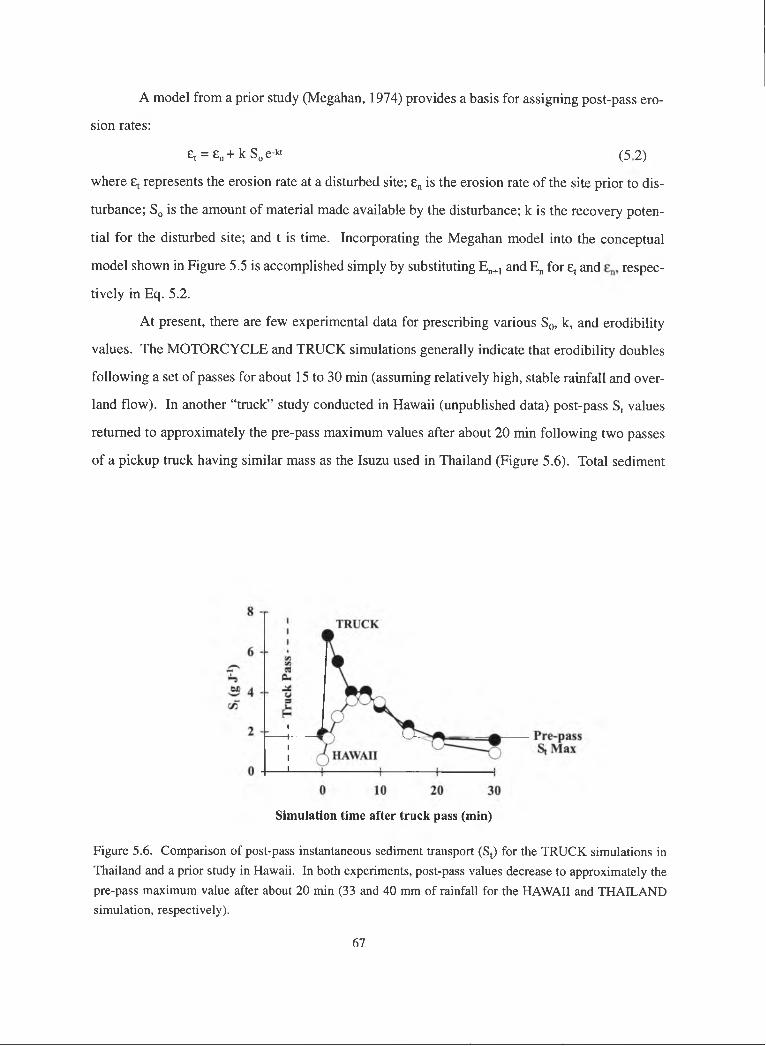
A model from a prior study (Megahan, 1974) provides a basis for assigning post-pass ero

sion rates:

e, = en+kS„e-kt (52 )

where £( represents the erosion rate at a disturbed site; E„ is the erosion rate of the site prior to dis

turbance; So is the amount of material made available by the disturbance; k is the recovery poten

tial for the disturbed site; and t is time. Incorporating the Megahan model into the conceptual

model shown in Figure 5.5 is accomplished simply by substituting E„+, and E„ for e, and respec

tively in Eq. 5.2.

At present, there are few experimental data for prescribing various Sq, k, and erodibility

values. The MOTORCYCLE and TRUCK simulations generally indicate that erodibility doubles

following a set of passes for about 15 to 30 min (assuming relatively high, stable rainfall and over

land flow). In another “track” study conducted in Hawaii (unpublished data) post-pass Sj values

returned to approximately the pre-pass maximum values after about 2 0 min following two passes

of a pickup track having similar mass as the Isuzu used in Thailand (Figure 5.6). Total sediment

Simulation time after truck pass (min)

Figure 5.6. Comparison of post-pass instantaneous sediment transport (Sj) for the TRUCK simulations in

Thailand and a prior study in Hawaii. In both experiments, post-pass values decrease to approximately the

pre-pass maximum value after about 20 min (33 and 40 mm of rainfall for the HAWAII and THAILAND simulation, respectively).

67

output attributed to the HAWAII truck passes was less than that determined in the TRUCK simu

lations, emphasizing that various states of erodibility are inherently determined by the physical

properties of the road soil surface. Erodibilities will probably have to be determined experimen

tally for different locations. Although the knowledge base to make such prescriptions is nascent,

Figure 5.5 represents a framework from which to direct future research.

5.6 CONCLUSION

Knowledge of pre-storm surface preparation phenomena, especially vehicular and maintenance

activities, is crucial to understanding sediment transport on unpaved roads. During typical rain

fall events where overland flow does not greatly incise the surface, much of the sediment trans

ported on PKEW roads is loose, easily entrained material that was present prior to the event. This

loose material is predominantly generated by vehicular detachment and maintenance activities

during the interstorm period. In general, for any given usage level, the longer the interstorm peri

od, the greater the supply of loose material; thus, the greater the event sediment transport.

Vehicular traffic during rainstorms initiates high sediment transport rates by detaching new mate

rial from the road surface and creating efficient overland flow paths. Additionally, a vehicle pass

redistributes existing loose material into flow paths where it can be entrained. Sediment transport

response to a vehicle pass is therefore related to interstorm surface preparation, as well as to the

more obvious variables associated with the passing vehicle, in situ soil, and rain event. Because

the supply of loose material is in constant flux, the road behaves like a surface with changing

erodibility. Through adopting this concept of dynamic erodibility, one can parameterize mainte

nance and vehicular activities during physically based modeling of road-related erosion.

68

6. EXPERIM ENT IV: Erosion prediction on unpaved mountain roads in northern

Thailand: validation of dynamic erodibility modeling using KINEROS2

6.1 ABSTRACT

Work investigated the application of the event- and physics-based KINER0S2 runoff/erosion

model for predicting overland flow generation and sediment production on unpaved mountain

roads. Field rainfall simulations provided independent data for model calibration and validation.

Validation showed KINER0S2 could simulate total discharge, sediment transport, and sediment

concentration on small-scale road plots, for a range of slopes, during simulated rainfall events.

Predicted hydrographs for aggregated validation experiments had root mean square errors

(RMSEs) <25% using the calibration parameter set. KINER0S2, however, did not accurately

predict time-dependent changes in sediment output and concentration (RMSE > 50 and 100%,

respectively). In particular, early flush peaks and the temporal decay in sediment output were not

predicted, owing to the inability of KINER0S2 to model removal of a surface sediment layer of

finite depth. For typical events in the study area, material from the upper layer is predominantly

detached and entrained by surface overland flow. During long events, sediment transport declines

as supply of loose superficial material becomes depleted. Modeled erosion response was

improved by allowing road erodibility to vary during an event. Assigning unique model erosion

detachment parameters to periods defined by road surface sediment availability improved RMSE

of predicted sediment transport by 30-40% for the validation events. A predictive relationship was

shown to exist between road erodibility states and road surface sediment depth. This relationship

allows implementation of the dynamic erodibility (DE) method for events where pre-storm sedi

ment depth is estimated from road usage since the last overland flow event.

6.2 OBJECTIVE

The objective of this experiment is develop a methodology for using the KINEROS2 model for

predicting road runoff and erosion on unpaved roads in northern Thailand. KINEROS2 will be

validated using discharge and sediment transport data from several small-scale field rainfall sim

ulation experiments on unpaved roads in PKEW. Refinements, based on the change in erodibili

ty of a road surface, will then be introduced to improve model prediction.

69


6.3.1 Soil physical property measurements

All work for this experiment was performed on the lower road in PKEW (Figure 2.2; described

in detail in Section 2.1). Soil properties determined on this road are listed in Table 6.1. Moisture

retention data (soil moisture characteristic) were determined from 45 cm^ cores collected from the

road surface using standard procedures described in Klute (1986). Five matric potentials (\|/) were

selected with a range from -5 kPa to -1500 kPa. Preferential porosity was computed as the dif

ference in water content between \i/ = 0 kPa (saturation) and that at -10 kPa (Mbagwu, 1997).

Mesoporosity was computed as the difference in water content between \)/ at -100 kPa and -10 kPa;

microporosity, between \\f at -1500 kPa and -100 kPa (Mbagwu, 1997). Methods for determining

other soil properties are described in Chapter 3. Description of measuring cross-sectional physi

cal characteristics are described in Chapter 5.

6.3.2 Rainfall simulation

In February 1998 and 1999, rainfall simulation experiments were conducted on the Lower PKEW

Road (locations shown in Figure 2.2). Eight simulations (ROAD) were conducted on a road sec

tion with slope ranging from 0.13 to 0.18 (m m ')- Four simulations were performed on the steep

est road section in PKEW (HILL, slope = 0.29 m m-i). One day following the ROAD simulations,

an additional simulation was performed on each ROAD plot to investigate sediment transport dur

ing successive storms (WET). The rainfall simulator, plot design, and calculations of instanta

neous concentrations (C,), discharge (Q,), and sediment output (S,) are described in previous chap

ters.

6.3.3 KINEROS2

KINER0S2 (Smith et al., 1995), the second-generation version of KINEROS (Woolhiser et al.,

1990), is an event- and physics-based mnoff and erosion model. Application and testing of

KINEROS is documented elsewhere (Smith, 1976; Zevenbergen and Peterson, 1988; Smith et al.,

1995). Dynamic, distributed flow modeling in KINEROS2 is well-suited to describe road runoff

and erosion processes in PKEW, where (1) runoff generation is dominated by HOF, with minimal

70

Table 6.1. Soil Properties of the road surface soil at PKEW

Descriptor/Property Units n mean ± SD

Sand fraction % 8 54.4 ± 4.9Silt fraction % 8 24.0 ± 2.2Clay fraction % 8 21. 7+ 5.5Dominant clay mineral - 4 kaolinitelSaturated hydraulic conductivity mm h'* 26 15.0 ±8 . 6Wetness at saturation (also saturated porosity) m3 m‘3 26 0.44 ± 0.05Water retained at -330 kPa m3 m'3 5 0.30 ± 0.01Water retained at -1500 kPa m3 m'3 5 0.13 ±0.01Preferential porosity m3 m‘3 5 0.10 ±0.03Meso-porosity m3 m‘3 5 0.07 ± 0.01Micro-porosity m3 m‘3 5 0.15 ±0.01Bulk density (0-5 cm) Mg m‘3 lA 1.45 ±0.13Bulk density (5-10 cm) Mg m‘3 16 1.36 ±0.11Bulk density (10-15 cm) Mg m‘3 16 1.35 ±0 .10Penetration resistance MPa 160 6.4 ± 0.4Particle density Mg m‘3 8 2.55 ± 0.05pH (l:5 water) - 16 4.8 ± 0.3Organic carbon % 16 1.6 ±0 . 6Total nitrogen % 16 0.13 ±0.03Cation exchange capacity cmolg kg‘* 16 9.8 ± 2.6Exchangeable Bases % 16 63.1 ± 19.8

t In addition to moderate amounts of kaolinite, PKEW soil also contains traces of illite, vermiculite, gibbsite, mont-

morillonite, and chlorite.

contributions from interception of subsurface flow by the road prism and (2 ) sediment transport

on the road surface varies throughout the course of a storm. The following description of

KINEROS2 is based on Smith et al. (1995) and C. Unkrich (unpublished manuscript, Southwest

Watershed Research Center, USDA-ARS, Tuscon, AZ):

Horton overland flow simulation in KINEROS2 utilizes the kinematic wave method to

solve the dynamic water balance equation:

d h d Q . .

d t d X(6 .1 )

71

where h is water storage per unit area, <2 (x,t) is water discharge, x is distance downslope, t is time,

and q(x,t) is net lateral inflow rate. Solution of Eq. 6 .1 requires estimates of time- and space-

dependent rainfall r(x,t) and infiltration f(x,t) rates:

q { x , t ) ^ r { x , t ) - f { x , t )(6 .2)

The infiltration model in KINEROS2 utilizes several parameters describing a one- or two-layer

soil profile: saturated hydraulic conductivity (K^), integral capillary drive or matric potential (G),

porosity ((})), and pore size distribution index (?i). The coefficient of variation for can be spec

ified to account for spatial variation in infiltration. Inclusion of two soil layers allows modeling a

restrictive surface or subsurface layer. The general one-layer infiltrability (f ,) model is a function

of cumulative infiltration (I):

1 -b «

(6.3)

where a is a parameter related to soil type (fixed at 0.85 in KINER0S2) and B = (G + h^)(©s-

0 j), where h^ is surface water depth and the second term, unit storage capacity, is the difference

of effective saturation (©j) and soil moisture (©j).

Simulating erosion involves solving the dynamic sediment mass balance equation:

(6.4)

where A is cross-sectional area, is local sediment concentration, e is net erosion/deposition rate,

q(x,t) is water inflow rate and c(x,t) is the corresponding concentration of the inflowing water.

KINEROS2 does not explicitly separate rill and interrill erosion processes (often there are no

rills); rather it divides e j into two additive components: rainsplash (eg) + net hydraulic erosion (Oh).

Splash erosion is calculated from Eq. 4.1. Elow-induced net hydraulic erosion is the difference

between particle detachment (dependent on slope, flow depth, flow velocity, particle size) and

deposition. In KINER0S2, e,, is calculated as a function of current local sediment concentration

Cs(x,t) and transport capacity (C„,x):

72

where A is cross-sectional area of the flowing water; and Cg is a transfer rate coefficient, which is

equal to soil particle settling velocity (v ) / hydraulic depth (h) during deposition; and Cg is less

than Vj/h during erosion on cohesive soils.

Drainage basins in KJNER0S2 are treated as a cascading network of surface, channel, and

pond elements. Channels receive flow from adjacent surfaces or upslope channels. Rectangular

surfaces may be cascaded or arranged in parallel to represent complex topography or erosion fea

tures. A road section could be represented as one element or subdivided into parallel flow planes

representing distinct features, such as ruts, gullies, or tracks. Each element is characterized by

assigning parameter values that control runoff generation and erosion processes. Dynamic, dis

tributed flow modeling in KINER0S2 requires a temporal record of rainfall rate at one or more

spatial locations.

6.3.4 Model calibration and model error assessment

Five of the eight ROAD simulation events were randomly chosen to produce a model calibration

dataset (events 1,2,4,5, and 7). Nonrectangular simulation plots were modeled in KINEROS2 as

a singular rectangular element, having length and area equal to those in the field simulations; ele

ment widths were reduced to give equal areas. Median measured instantaneous and total discharge

Q (m2 s '), sediment transport S (kg s-i), and sediment concentration C (kg m-2) values for

observed event (ROAD 12457) were compared to the time series predicted by KINEROS2.

Element parameters controlling runoff generation (e.g., capillary drive and K ) and erosion

processes (e.g., splash erosion and soil cohesion coefficients), which were initially assigned based

on physical property data, were adjusted during calibration to reduce the error in predicted Q and

S. Five measures of model error or performance were used:

Percent error in total estimate: ^ irvn(6 .6)

^ to ta l

Percent error in peak value estimate: £ ^peak) ^qq^peak

73

Root mean square error (%): RMSE = (6.8)

Coefficient of determination: 'tio.-ofCD = - ^ -------------

Model efficiency (ME, Nash and Sutcliffe, 1970):

(=1

1,(0,-Pf

(6.9)

1=1

1 (0 , - O ) ’V 1=1

(6 .10)

where Pjotai and Oto,ai are event total predicted and observed values; Ppg k and Opga are peak event

predicted and observed values; Pj and Oj are predicted and observed instantaneous values; and O

is the mean of the observed data. If predicted and observed values are equal, Eto,ai, Epggj , RMSE,

CD, and R^ produce optimal values of 0, 0, 0, 1, and 1. Lower limits for E,Qtaj, Epg j., RMSE, and

CD are zero; model efficiency R2 can be negative. CD indicates the proportion of total variance

of observed data that is explained by the predicted data. A negative R2 value indicates model val

ues are worse estimates than the observed mean (Loague and Green, 1991). Appropriateness of

these error indices are described elsewhere (Green and Stevenson, 1986; Loague and Green,

1991). Calibration first focused on reducing Ej^pj to ± 0.5% for runoff; further refinements were

then made to produce a better fit of the predicted runoff hydrograph, as indicated by the other per

formance indices (i.e., RMSE, CD, and ME). The subsequent adjustments maintained an E,g,ij of

+ 0.5%. Following runoff calibration, adjustments were made to splash and hydraulic detachment

parameters to first reduce S total error ± 0.5%, and then produce the best fit of modeled versus

observed values, as defined by RMSE, CD, and ME. Changing sediment detachment parameters

do not produce detectable differences in predicted runoff in KINER0S2.

6.3.5 Model validation

Validation of the ROAD 12457 parameter set (Table 6.2) was performed on three datasets: (1) the

three ROAD simulations not used for calibration (events 3,6, and 8 ); (2) the HILL simulations;

74

Table 6.2. The ROAD12457 parameter set following calibration.

Parameter^ Description Value Units Calculated/estimation methodTH Thickness of soil layer 1 0.15 m Field examination of soil profile

Ks,l, Saturated hydraulic

conductivity

4.05 mm h‘* Reduced from Table 6.1 value

durine calibration

CvKs Coefficient of variation

for K,

0.61 - Table 6.1

Gi Layer 1 capillary drive 15 mm Reduced during calibration from

value in Rawls et al. (1982) for sandy clay loam.

G2 Layer 2 capillary drive 36 mm Same as for Gj

X Pore size distribution

index

0.25 - Rawls et al. (1982) for sandy clay loam

SAT Initial relative saturation 0.47 Calculated as pre-storm soil wet

ness divided by wetness at

saturation

f l . f 2 Layer 1 and 2 porosity 0.43 m3 m‘3 Estimated at soil wetness at

saturation

Cf Rain splash coefficient 261.6 tt s m 'l Determined during calibration

from estimated value (Figure 6.2)

"g Soil cohesion coefficient 0.0196tt - Same as for Cf

RELIEF Average microtopo-

graphic relief

100 mm Field measurements

SPACING Average microtopo- graphic spacing

0.40 m Field measurements

Ps Particle density 2.55 Mg m-3 Table 6.1MAN Manning’s n roughness

coefficient0.015 ftl/6 Comparison of field conditions

with values in M orean (1995)

INT Interception depth 0 mm Field measurementsROCK Volumetric rock fraction

of the soil column

1 % Field measurements

Subscripts refer to an upper (1) or lower (2) soil layer utilized by the infiltration subcomponent.

++ For dynamic erosion (DE) modeling, Cf = 139.95 and c„ = 0.0105.

75

and (3) the WET simulations. The first dataset allowed validation under initial conditions similar

to those of ROAD12457. The HILL dataset allowed validation on a steeper road section, with

drier antecedent moisture conditions and different surface preparation than ROAD 12457. Surface

preparation refers to events/phenomenon contributing to availability, detachment, or entrainment

of surface material (e.g., vehicular traffic, maintenance, mass wasting. Chapter 5). The WET

dataset allowed validation during typical wet season conditions, i.e., when high initial soil mois

ture content produces rapid runoff generation and prior HOF events have reduced loose surface

sediment availability. One validation goal was to identify parameters sensitive to physical differ

ences related to topography, soil moisture, and surface preparation.

6.4 RESULTS

6.4.1 Model calibration

Table 6.3 lists rainfall intensity, storm duration, plot slope, an index of initial soil moisture (SAT

in Table 6.2), runoff (RO), total sediment output (S), and total sediment concentration (C) for rain

fall simulation events modeled during KINER0S2 calibration and validation experiments. Events

are referred to by simulation type (i.e., ROAD, HILL, or WET) and one or a string of digits indi

cating a specific simulation number, or referring to the median values of several sites (e.g.,

ROAD368, refers to the median of ROAD simulations 3, 6 , and 8 ).

Median instantaneous discharge (Qj), sediment transport (Sj), and concentration (C,) val

ues for calibration event ROAD12457 are shown with KINER0S2-predicted values in Figure 6 .1.

Following parameter optimization, errors in predicted total RO and S were < 0.5 % (Tables 6.4-

6.5). The Qt time series is well-modeled by KINER0S2 (RMSE = 14%; CD = 0.80; R2 = 0.84);

modeled peak discharge is underestimated by only = 3% (Figure 6.1a). Substantially higher pre

diction error exists for instantaneous and peak Sj and Cj (Tables 6 .5-6.6). The sediment peak in

the first 2 0 min of the event, and the corresponding high C( values, are not predicted by

KINER0S2 (Figure 6.1 b,c). RMSE for predicted S and C are > 50 and 100%, respectively; and

S, and C( peaks are underestimated by > 41 and 78%, respectively. Only during the middle third

of ROAD 12457 is Sj well-described by KINER0S2. Low Ejotai for KINEROS2-predicted S

results from a balance of under-prediction of S, at the beginning of the event, and over-prediction

toward the end.

76

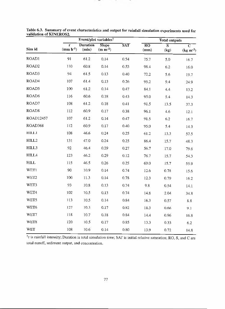
Table 6.3. Summary of event characteristics and output for rainfall simulation experiments used for validation of KINEROS2._______________________________________________________________________

Event/plot variablest Total outputsr Duration Slope SAT RO S C

Sim id (mm h'l) (min) (m m'l) (mm) (kg) (kg m’3)

ROADI 91 61.2 0.14 0.54 75.7 5.0 16.7

R 0A D 2 110 60.8 0.14 0.53 98.4 6.2 16.0

R0A D 3 94 61.5 0.13 0.40 72.2 5.6 19.7

R 0A D 4 107 61.4 0.13 0.26 95.2 9.4 24.9

ROAD5 100 61.2 0.14 0.47 84.1 4.4 13.2

ROAD6 116 60.6 0.18 0.43 95.0 5.4 14.3

ROAD7 108 61.2 0.18 0.41 91.5 13.5 37.3

ROAD8 112 60.9 0.17 0.38 96.1 4.6 12.1

ROAD12457 107 61.2 0.14 0.47 91.5 6.2 16.7

ROAD368 112 60.9 0.17 0.40 95.0 5.4 14.3

HILLI 108 46.6 0.24 0.25 61.2 13.3 57.5

H1LL2 131 47.0 0.24 0.25 86.4 15.7 48.3

HILL3 92 46.4 0.29 0.27 56.7 17.0 79.6

H1LL4 123 46.2 0.29 0.12 76.7 15.7 54.3

h i l l 115 46.5 0.26 0.25 69.0 15.7 55.9

W ETl 90 10.9 0.14 0.74 12.6 0.78 15.6

WET2 100 11.3 0.14 0.78 12.3 0.79 16.2

WET3 93 10.8 0.13 0.74 9.8 0.54 14.1

WET4 102 10.5 0.13 0.74 14.8 2.04 34.8

WET5 113 10.5 0.14 0.84 16.3 0.57 8.8

WET6 127 10.3 0.17 0.82 18.3 0.66 9.1

WET7 118 10.7 0.18 0.84 14.4 0.96 16.8

WET8 120 10.5 0.17 0.85 13.3 0.33 6.2

WET 108 10.6 0.14 0.80 13.9 0.72 14.8

Ir is rainfall intensity; Duration is total simulation time; SAT is initial relative saturation; RO, S, and C are total runoff, sediment output, and concentration.

77

Simulation time (min)

Figure 6.1. Comparison of (a) discharge (Q,), (b) sediment transport rate (S,), and (c) concentration (C,) between measured rainfall simulation data (circles) used in model calibration and KINER0S2-predicted

values. Measured values are medians from ROAD events 1,2,4,5, and 7; error bars are ± one median absolute deviation about the median. KINEROS2 was run using the calibration parameter set (Table 6.2).

78

Table 6.4. E rro rs between observed and KINERO S2-predicted runoff.

O bserved Predicted Ejotai^ RM SE CD M E

_____________________ (mm) (mm) (% ) (% ) (% ) (r^) (R2)

ROAD12457tt 91.5 91.1 -0.47 -3.44 14.0 0.82 0.84

ROAD368 95.0 91.2 3.84 -2.22 23.4 0.80 0.65

R 0A D 3 72.2 80.9 12.03 -1.96 29.6 0.87 0.52

R 0A D 6 95.00 103.1 8.47 34.21 62.5 0.37 -1.15

R0A D 8 96.2 100.0 4.02 -9.46 22.6 0.92 0.68

HILL 69.0 74.2 7.52 -1.11 17.6 0.79 0.81

W ET 13.9 16.5 18.98 0.43 21.5 0.67 0.85

t E,o,a| is error in total output estimate (Eq. 6.6); is error in peak estimate (Eq. 6.7); RMSE is root mean

squared error (Eq. 6.8); CD is coefficient of determination (Eq. 6.9); ME is model efficiency (Eq. 6.10).

tt Events modeled using dynamic erodibility methodology have same discharge values as event reported here.

Table 6.5. E rro rs between observed and KIN ERO S2-predicted sedim ent output.

O bserved Predicted (mm) (mm)

Etotal^(% )

Epeak(% )

RM SE(% )

CD(r2)

M E(R2)

ROAD 12457ft 6.22 6.23 0.22 -41.2 51.6 1.64 0.77

ROAD368 5.39 7.92 46.8 -41.9 87.1 0.72 0.44

R0A D 3 5.63 4.96 -11.9 -68.5 75.9 2.14 0.61

R0A D 6 5.39 9.83 82.3 -26.3 117.9 0.76 0.09

R0A D 8 4.63 8.88 92.1 -36.0 96.8 0.51 0.32

HILL 15.69 10.66 -32.1 -67.0 70.1 3.22 0.62

WET 0.72 1.25 73.4 56.2 84.0 0.34 0.38

ROAD12457 D E ff 6.22 6.47 4.04 -3.93 35.4 1.11 0.89

HILL DE 15.69 14.64 -6.69 -21.9 44.6 0.97 0.85

R 0A D 3 DE 5.63 5.23 -7.07 -61.3 71.4 1.55 0.66

R 0A D 6 DE 5.39 8.07 49.6 -39.9 92.3 0.91 0.44

R0A D 8 DE 4.63 6.84 48.0 -26.9 64.5 0.63 0.70

t E,o,ai is error in total output estimate (Eq. 6.6); Epg j; is error in peak estimate (Eq. 6.7); RMSE is root mean

squared error (Eq. 6.8); CD is coefficient of determination (Eq. 6.9); ME is model efficiency (Eq. 6.10).It Events modeled using dynamic erodibility methodology have same discharge values as event reported here.

79

^^Table 6.6. Errors between observed and KINEROS2-predicted sediment concentration. Sim id Observed Predicted Ejgjail Epggi RMSE CD ME

____________________ (kgm-3) (kgm-3) ( % ) ( % ) ( % ) ( r 2) (R 2)

R O A D 1245?tt 16.7 20.1 20.6 -78.4 104.8 3.05 0.38ROAD368 14.3 25.5 78.3 -69.1 102.1 1.44 0.49R0A D 3 19.7 18.0 -8.36 -77.6 118.6 3.03 0.32R 0A D 6 14.3 28.1 95.9 -82.7 154.9 3.68 0.23R0A D 8 12.1 26.1 115.2 -72.5 84.2 1.72 0.60HILL 56.0 44.9 -19.7 -84.5 116.5 7.94 0.29WET 14.8 22.3 50.4 51.6 88.4 0.45 0.35ROAD12457 D E tt 16.7 20.9 25.1 -64.7 97.0 2.04 0.47HI LLDE 56.0 61.7 10.3 -61.9 103.4 2.23 0.44R 0A D 3D E 19.7 19.0 -3.33 -67.2 113.3 2.09 0.38R 0A D 6D E 14.3 23.0 60.8 -76.9 141.5 3.24 0.36R 0A D 8D E 12.1 20.1 65.8 -63.0 62.8 1.88 0.78

1 E,o,ai is error in total output estimate (Eq. 6.6); Epg j is error in peak estimate (Eq. 6.7); RMSE is root mean

squared error (Eq. 6.8); CD is coefficient of determination (Eq. 6.9); ME is model efficiency (Eq. 6.10).

t ' Events modeled using dynamic erodibility methodology have same discharge values as event reported here.

6.4.2 The ROAD12457 parameter set

The calibration stage produced a parameter set (ROAD 12457) for use during model validation. In

the ROAD12457 parameter set (Table 6.2), the soil is modeled as a two-layer colunui, with the

upper layer having thickness (TH) 0.15 m. Layer one depth was determined from field profile

observations and bulk density measurements (Table 6.1). Numeric subscripts in Table 6.2 refer to

upper (1) or lower (2) soil layers (depth is not specified). The parameter specification approach

initially used field-measured values; changes having physical basis were then allowed during cal

ibration. For example, field-measured (15.0 mm h") was replaced by 4.1 mm h ', a value

slightly less than the rainfall simulation-derived estimate of steady state infiltration (5.4 mm h '.

Table 4.2). The original coefficient of variation for the data was retained for CvK . Capillary

drive values G[ and G2 for the highly disturbed road surface were reduced by an order of magni

tude during calibration from recommended values for sandy clay loam soils (Rawls et al., 1982).

Pore size distribution index ()i) corresponds to that of sandy clay loam soil in Rawls et al. (1982).

Initial soil saturation (SAT) was calculated as initial soil moisture divided by soil moisture at sat

uration (Table 6.1). RELIEF refers to vertical changes in microtopography over the prescribed

SPACING interval. Porosity (<])) and particle density (Pj) were determined in situ (Table 6.1).

80


Figure 6.2. Comparison of predicted and observed (a) splash (Eq. 4.1) and (b) hydraulic (Eq. 6.5) erosion

for ROAD rainfall simulation events 1,2,4,5, and 7. Coefficients Cf and Cg in Eqs. 4.1 and 6.5 were chosen

to reduce the root mean squared error between predicted and observed values over the final 50 min of sim

ulation, following the initial flush of loose material. These optimal values were then used as initial estimates

for KINER0S2 Cf and c„ parameters prior to model calibration.

First-guess values of Cf and Cg were assigned by solving Eq. 4.1 and 6.5, respectively,

using observed discharge, concentration, and water depth data from Experiment II (Chapter 4).

Values of Cf and Cg were selected that produced the lowest RMSE between equation-predicted and

81

observed splash and hydraulic erosion during the final 45-min of the ROAD rainfall simulation

events 1,2,4,5, and 7 (Figure 6.2). The initial 15-min period containing the flush of loose surface

material was not included in the calculation, because we wanted the erodibilities to be that of the

true road surface. The final values shown in Table 6.2 were determined during model calibration

by reducing the initial Cf and Cg values equivalently, to retain the proportionality between splash

and hydraulic erosion.

6.4.3 ROAD validation

The results of the ROAD 12457 parameter set validation using ROAD events 3, 6 , and 8 are shown

in Figures 6.3 and 6.4, and Tables 6.4-6.6. Runoff was slightly over-predicted for all events and

RMSE error values were higher than those during calibration. During events 3 and 8 , total varia

tion in RO was better described than during ROADI2457 (CD = 0.87 and 0.92, respectively);

however, model efficiency (R2) values were lower. Event 6 was poorly modeled, as indicated by

comparatively high values for Epeak and RMSE, low CD, and a negative value for model efficien

cy (Table 6.4). Error values for the median ROAD368 event were reasonable. Total RO was

under-predicted by only about 4%, Epg k was lower than during calibration, and CD was nearly

identical. RMSE and R^ were higher for ROAD368 compared with ROAD 12457 because of over

prediction during the first 2 0 min of simulation.

KINER0S2 over-predicted total sediment transport for ROAD368 by 47%, but under-pre

dicted median peak values by = 42% (Table 6.5; Figure 6.4). For the individual events, Etotai

ranged from -12% to 92%, RMSE values were > 75%, and R was as low as 0.09. As in the cal

ibration simulations, over-prediction of S, resulted from inability of KINER0S2 to predict the ini

tial flush and subsequent decline in sediment output over time. Unlike the calibration phase, ini

tial under-prediction was not enough to compensate for over-prediction at the end of the events.

As a result, errors in predicted concentration values were generally high (Table 6 .6 ).

6.4.4 HILL validation

Simulation of the median HILL time series using the ROAD 12457 parameter set is shown in

Figure 6.5. The runoff hydrograph was predicted reasonably, with E,otai = 7.5% and RMSE = 18%

82

0.14

ooU)

140 ^ 120 -

U 100 ■

X 80 +^ 60

40

20

0

O

oQ

ROAD3

O measured KINER0S2

o o

o

ROAD6O measured

KINER0S2

15 25 35 45 55 65

: t ^ ^ O O O O f O ^

5 15 25 35 45 55 65


O

ROAD8O measured

KINER0S2

15 25 35 45 55 65

Figure 6.3. Comparison of discharge (Q,), sediment transport rate (St), and concentration (C,) between measured rainfall simulation data (circles) and

KINEROS2-predicted values for ROAD events 3,6, and 8. KINEROS2 results were obtained using the calibration parameter set (Table 6.2).


Figure 6.4. Comparison of (a) discharge (Qj), (b) sediment transport rate (Sj), and (c) concentration (C^)

between measured rainfall simulation data (circles) and KlNEROS2-predicted values for ROAD368.

Measured values are medians from ROAD events 3,6, and 8; error bars are + one median absolute deviation about the median. KINEROS2 results were obtained using the calibration parameter set (Table 6.2).

(Table 6.4). CD and ME for the predictions were only slightly lower than those during

ROAD 1245Vcalibration. In contrast to over-predicting S during ROAD368 validation,

KINEROS2 under-predicted sediment transport for HILL. Total error in S and C were = -32% and

84

(a)

(b)

(c)

555 15 25 35 45Simulation time (min)

Figure 6.5. Comparison of (a) discharge (Q,), (b) sediment transport rate (S,), and (c) concentration (Cj) between measured rainfall simulation data (circles) and KINEROS2-predicted values for the HILL validation. Measured values are medians from four HILL events; error bars are ± one median absolute deviation

about the median. KINER0S2 results were obtained using the calibration parameter set (Table 6.2).

-20%, with much larger errors in peak estimates (Tables 6.5, 6 .6 ). RMSE for HILL-predicted S

was = 70%, but was smaller than that for ROAD368; RMSE in the C prediction was again

greater than 1 0 0 %.

85

6.4.5 WET validation

Wet validation results are shown in Figure 6 . 6 and Tables 6.4-6.6. Predicted discharge was = 19%

higher than the observed median value. Much of this error results from over-prediction during the

first 5 min of this short event, for which there were few data points for evaluation of model per

formance. The error in peak output was less than 1%; and model efficiency R^was higher than

that of the calibration event. Total sediment transport was over-predicted by = 73% on this wet

■J■3SU

(a)

(b)

(c)


Figure 6.6. Comparison of (a) discharge (Qf), (b) sediment transport rate (Sj), and (c) concentration (C()

between measured rainfall simulation data (circles) and KINER0S2-predicted values for the W ET valida

tion. Measured values are medians from 8 WET events; error bars are ± one median absolute deviation about the median. KINEROS2 results were obtained using the calibration parameter set (Table 6.2).

86

surface, where most loose sediment was removed in the previous simulation (Table 6.5, Figure

6 .6 b). Model efficiency for the S prediction was the lowest of all median-based validation sets.

6.5 DISCUSSION

6.5.1 Soil moisture

Experimental conditions for ROAD368 were similar to those under which the calibration param

eter set was produced. HILL sites had greater slope and lower soil moisture content than the

RO ADI 2457 site; and WET had higher initial soil moisture (Table 6.3). Runoff was well pre

dicted in ROAD368 and HILL validation tests (Etooi was within ± 7.5%). Thus, KINEROS2 han

dled slope and soil moisture changes on these surfaces. Runoff during the WET validation was

over-predicted by = 19%. In comparison, the WEPP model used by Elliot et al. (1995) over-pre

dicted total event runoff values on 46.4 m plots by 3-6% for dry, wet, and very wet soil moisture

conditions. Much of the error for our WET simulations is related to the small time series for the

observed data during the 10-min rainfall simulations (n = 5 time steps).

6.5.2 Sediment availability

Sediment transport was poorly predicted for ROAD368, HILL, and WET events using the

ROAD 12457 calibration parameter set (Ejotai = 47, -32, and 73%, respectively). Although,

under-prediction of S for HILL could be related to higher erosive energy of hydraulic flow on the

steeper slope, we believe the predominant cause for poor prediction at all sites is differences in

availability of loose surface material. During the ROAD12457 rainfall simulation experiments,

most sediment removed up to some time t was loose, previously detached material. In contrast,

sediment output for the WET simulations was comparatively low because most loose material was

removed on the previous day of rainfall simulation. KINER0S2 over-predicted S because the ero

sion parameters were determined for a road having a loose layer of surface material, i.e., the con

ditions for the ROAD simulations. Similarly, Elliot et al. (1995) reported WEPP did not predict

declines in erosion rates with successive storms.

KINEROS2 under-predicted S on HILL plots because these surfaces have more loose

material than the ROAD 12457 plots. Large quantities of loose surface material on the HILL

87

plots result from higher vehicle-detachment rates on this comparatively steep surface. The sedi

ment depth survey showed the HILL road section contained 3 times more loose sediment than the

ROAD plots (5.4 versus 1.8 kg m-2). HILL total sediment transport is best modeled by

KINER0S2 using Cf and Cg values 3.55 times greater than those in the ROAD12457 calibration

parameter set (not shown), suggesting that S is largely a function of sediment availability.

Disparity in sediment transport between ROAD 12457 and ROAD368 is related to high spatial

variability in sediment depth on the road surface resulting from variability in interstorm prepara

tion processes, including mass wasting, road maintenance, and traffic.

6.5.3 Dynamic erodibility

In PKEW the road surface at any given time consists of a compacted, resilient surface underlying

a layer of loose material of finite depth. Because the supply of road surface sediment is dynam

ic, road sediment transport response varies both during and between events. Sediment production

is often high, such as following a long dry period where traffic has generated a substantial layer

of loose material. In general, roads receiving high traffic volumes tend to have high sediment pro

duction rates (cf., Reid and Dunne, 1984). Sediment transport is initially controlled by the abili

ty of rain-affected surface flow to remove the loose surface layer, then by the ability to detach pre

viously unavailable material from the compacted road surface. Both the underlying and loose

material layers have unique erodibilities, with the loose layer generally being much more erodi

ble. Thus, during a storm event, the road surface passes through two or more ‘states’ of erodibil

ity. This dynamic erodibility can be represented by the following expression:

p =road

E2 0 < < C2 J,

where Ejoaj is the dynamic erodibility (DE) of the composite road. For implementation in

KINEROS2, Efoad represents a scalar to multiply to baseline Cf and Cg parameters. The variable

E2 is the erodibility of the loose surface material at the start of a storm; Eg is the baseline erodi

bility of the compacted road surface; E, is an intermediate erodibility value following the initial

flush of loose material; dj is an index of sediment availability at the beginning of the storm (e.g.,

mass per area is used herein); Cj and are values between 0 and 1 ; and dgyn, is a value between

0 and dj that represents cumulative removal of the surface material. Erogj at any time t is related to

pre-storm sediment availability (via dj) and the amount of sediment removed during the current

storm (dcum)- After d .yn, surpasses thresholds defined by C2 and c,, E oad drops to that of a lower

state. Implementation of the DE method requires empirical experimentation to determine values

for C], C2 , Eq, Ej, and E2 . Sediment availability values, dg, are also required for each storm mod

eled. As a modification to Eq. 6.11, any number of erodibility states could be specified; ulti

mately, it could be represented as a continuous function.

5 ■

4 •

3 ■w

2 ■

1 ■

0

140 ■■

1 2 0 ■■

1 0 0 ■■

w 80 ■■

u 60 ■■40

2 0 ■■0 +

ROAD12457O measured

KINER0S2DE

(b)

15 25 35 45 55Simulation time (min)

65

Figure 6.7. Modeling of (a) sediment transport rate (S,) and (b) concentration (Cj) using the dynamic erodi

bility methodology (DE, Eq. 6.11). Measured values are medians from ROAD rainfall simulation events

1,2,4,5, and 7 (circles); error bars are ± one median absolute deviation about the median. KINER0S2

results were obtained using the calibration parameter set, but with Cf and Cg of 139.95 and 0.0105, respec

tively. Table 6.7 lists erodibility values and corresponding transition information used to implement DE modeling on this surface.

89

Figure 6.7 shows calibration results for KINER0S2 modeling of ROAD 12457 using the

dynamic erodibility method. Values for Eq, Ej, E2 , d , Cj, and C2 in Eq. 6.11 were assigned as fol

lows: 1. Baseline splash and hydraulic erodibility values for the underlying compacted road sur

face were established by optimizing KINEROS2 Cf and Cg parameters to minimize RMSE in pre

dicted sediment transport for the 10-min WET simulations. Most loose material was removed

from these plots on the previous day; therefore, WET sediment output resulted from detachment

of new material from the compacted road surface. Optimization yielded values of 139.95 and

0.0105 for Cf and Cg, respectively.

2. Initial erodibility (E2 = 3.4) was determined by increasing baseline Cf and Cg values to

reduce RMSE for sediment transport during the initial sediment output peak for ROAD12457 (i.e.,

roughly the first 15 min). Optimization during the period 20-40 min determined E, to be =1/2 E2 .

Finally, Eg = 1 (i.e, the baseline erodibility values).

3. Sediment availability (dj) was assigned the value determined during the dry-season

cross-section survey (1.8 kg m-2). Sediment transport data for ROAD simulations 1,2,4,5, and 7

suggested that the transitions between states E2 and Ej, and then Ej and Eg, occurred after = 53%

(C2) and 84% (cj) of the material, respectively, had been removed from the plots.

Using the DE method, RMSE for predicted S improved from 52 to 35% (Table 6.5).

Although total error increased slightly to 4%, compared with < 0.5% error for the ROAD 12457

calibration simulation, CD was reduced from 1.64 to 1.11; and ME R^ increased to 0.89, indicat

ing the DE-predicted values were better estimates of observed time series than were the

KENER0S2-predicted values. The improved estimates of S produced better estimates of concen

tration; although, errors in the C estimate were still high, owing to poor estimation of the initial

concentration spike following ranoff generation. Temporal sediment response of ROAD 12457 DE

more closely describes the observed flush peak and the subsequent decline produced by the deple

tion of superficial material (Figure 6.7). Although more difficult to implement— for DE requires

calibration and validation for all specified erodibilities—the dynamic erodibility method provides

an improved approach for physically modeling removal of a loose road surface layer of finite

depth. Figure 6.2 highlights the inability of Eq. 4.1 to predict road splash response using observed

discharge and water depth data. Predicted splash stabilizes after a few min because water depth.

90


Figure 6.8. Modeling of (a) sediment transport rate (S,) and (b) concentration (C,) using the dynamic erodi

bility methodology (DE, Eq. 6.11). Measured values are medians from all HILL rainfall simulation events

(circles); error bars are ± one median absolute deviation about the median. KINER0S2 results were

obtained using the calibration parameter set, but with Cf and Cg of 139.95 and 0.0105, respectively. Table

6.7 lists sediment depth, erodibility values, and corresponding transition information used to implement DE

modeling on this surface.

which is calculated as a function of runoff, stabilizes on the small-scale plots. Observed splash

continues to decline because it is controlled by sediment availability, not increasing water depth,

as modeled in Eq. 4.1. The DE methodology addresses the change in sediment availability by

modifying model parameters for erodibility.

Results from a second calibration of the DE modeling technique using HILL data are

shown in Figure 6 .8 . Initial erodibility (E2 = 6.1) was determined by reducing RMSE of

KINEROS2-predicted sediment transport during the initial flush of the HILL data. A value of Ej

91

= 1.9 was determined by optimizing model erosion parameters during the middle 20 min of the

HILL simulations. The sediment cross-section survey value of 5.4 kg m-2 was used for d . Similar

to the ROAD 12457 DE simulation, Cj and C2 were assigned values 53 and 84%, respectively. The

KINER0S2-predicted values for HILL DE are shown in Figure 6 .8 . Simulation using the DE

methodology substantially improved the “goodness of fit” of the predicted Sj values: RMSE

reduced from 70 to 45%, CD improved from 3.22 to 0.97, and model efficiency R2 increased from

0.62 to 0.85. The CD value was the best of all simulations; and R2 was second only to that of the

RO ADI 2457 DE simulation.

6.5.4 General implementation of dynamic erodibility modeling

Using data from the ROAD12457 DE and HILL DE simulations, a predictive relationship between

road sediment depth and the Eroaj values was developed (Figure 6.9). This relationship makes

possible a general implementation of dynamic erodibility modeling using KINER0S2. Initial

erodibility, E2 , is determined from the amount of sediment present on the road surface at the begin

ning of an event. In Figure 6.9, this value is represented by the thick line fitted through the val-

Sediment availability (kg m'^)Figure 6.9. Relationship between surface sediment (mass per area) and erodibility values (Ei and E 2 ) used to implement the dynamic erosion method (Eq. 6.11).

92

ues of E2 used in the WET, ROAD 12457 DE, and HILL DE events reported above. Ej is calcu

lated based on the amount of sediment remaining after some percentage of the initial sediment

supply has been removed from the road (represented by C2 above). The value of Ej is determined

by the thin lined fitted through the values of Ej used in the WET, ROAD12457 DE, and HILL DE

events above. Two unique functions are required for representing E, and E2 because the relation

ship between erodibility and sediment availability changes following the initial flush of material.

Erodibility is initially high, as sediment transport is limited by the transport capacity of the flow

ing water. After the flush, entrainment becomes more difficult as material must be moved into

defined flow channels from upslope sediment sources or detached from the road surface.

Armoring occurs as material becomes “lodged” in surface depressions, thereby reducing sediment

output. For all DE events, baseline road erodibility, Eq, is 1. Values C2 = 53% and Cj = 84% can

be used to define transition points between successive erodibility states, or the values could be

determined from empirical data. Although based on limited rainfall simulation data, the prediction

functions in Figure 6.9 represent a systematic method for estimating Eroad values using pre-storm

estimates of road sediment depth.

Figure 6.10 shows the results from modeling ROAD events 3, 6 , and 8 employing dynam

ic erodibility, with Eroaj values predicted from Figure 6.9. Table 6.7 lists sediment depth estimates

and corresponding E2 , Ej, and Eq values for the three modeled events. Predicted values of S and

C are shown with prediction errors in Tables 6.5-6.6. Predicted discharge is the same for the DE

event as for the standard KINER0S2 predictions presented above (Table 6.4). The DE imple-

Table 6.7. Param eter assignm ents for DE sim ulations.

Sim ulation(kg m-2)

E 2 El Eo C2 Cl

ROAD 12457 DE 1.80 3.60 1.70 1 0.53 0.84

H ILLD E 5.40 6.10 1.90 1 0.53 0.84

R0A D 3 DE 1.62 3.00 1.61 1 0.53 0.84

R 0A D 6 DE 1.56 3.14 1.69 1 0.53 0.84

ROADS DE 1.33 2.59 1.46 1 0.53 0.84

'^Variables are defined in Eq. 6.11; E 2 , E j, Eg, C2 , and Cj are dimensionless.

93

0.14

VO4

*5U

120

100

80

60

40

20

0

O

ROAD3O measured

— KINEROS2 DE KINEROS2

o

15 25 35 45 55 65

ROAD6O measured

KINER0S2 DE KINEROS2

o O O O O O oi 1----- 1------1— ■

o ROADS(3 measured

KJNEROS2 DE KINEROS2

5 15 25 35 45 55 65


5 15 25 35 45 55 65

Figure 6.10. Modeling of discharge (Q,), sediment transport rate (S,), and concentration (C,) using the dynamic erodibility methodology (DE, Eq. 6.11).

Measured values are for ROAD events 3, 6, and 8 (circles). KINER0S2 DE results (thick line) were obtained using the calibration parameter set, but with

Cf and Cg of 139.95 and 0.0105, respectively. Results from standard KINEROS modeling are indicated by thin lines. Table 6.7 lists sediment depth, erodibility values and corresponding transition information used to implement DE modeling on this surface.

mentation greatly improved sediment production estimates for all three events. for ROAD

events 6 and 8 reduced from 82 and 92% to < 50%. Improvements in RMSE and ME R2 indicate

a better fit of modeled instantaneous values. In general, concentration estimates also improved,

although error values remained high, owing to the inability to predict initially high Sj values, asso

ciated with the flushing of sediment early in an event. These high Sj and C, values might be bet

ter predicted by adding more erodibility states to the general DE model (Eq. 6.11). Finally, the

over-prediction of ending Sj values in ROAD6 and R0AD8 suggest that the baseline erodibility

Eq value may be too high.

Both Cf and Cg were multiplied by Erogj. One could argue that, based on the poor fit of

predicted to observed splash erosion values in Figure 6.2 (as compared with the good fit of the

predicted hydraulic erosion values), only the splash parameter Cg need be multiplied by E oa j.

However, as shown in Chapter 4, the splash erosion subcomponent was less than the hydraulic

component at all times during the 60-min rainfall simulations on the Thailand road site.

Adjusting only the Cg parameter would have violated this relationship. In other physical set

tings, unique scalar multipliers for Cf and Cg may be required.

6 . 6 SUMMARY

KINER0S2 can be parameterized to predict discharge hydrographs on small-scale plots under

varying slope and soil moisture conditions. Temporal response in sediment transport on unpaved

roads in the study area is best modeled when the superficial layer of loose sediment is explicitly

considered. The dynamic erodibility approach introduced herein recognizes roads have more than

one state of erodibility, which changes both between and during storm events. Initial road erodi

bility for any storm is related to availability of loose surface material, which is a function of inter

storm sediment detachment processes. After removal of this upper layer, road erodibility is that

of the compacted road surface itself. Using field rainfall simulation and KINER0S2 simulation

data we developed a predictive relationship between sediment availability on the road surface and

erosion parameter values needed to model erosion states. By implementing the DE methodology,

sediment transport and concentration values, observed during small-scale road rainfall simulation

events, were modeled more realistically.

95

7.1 SU M M A R Y O F R ESU LTS

Runoff generation and sediment transport are unique on roads, paths, and agricultural land-sur-

faces in PKEW (Chapter 3). Sediment transport on roads can be high when large amounts of loose

material are present on the road surface before a rainfall event. Compacted roads, owing to low

saturated hydraulic conductivities, produce runoff after relatively light rainfall. Because HOF is

generated on unpaved roads during most rain events, the road system contributes to stream sedi

mentation throughout the rainy season. Horton overland flow generation within PKEW agricul

tural fields is rare during dry antecedent soil moisture conditions, except on path surfaces.

Footpaths, like roads, accelerate runoff, thereby potentially enhancing in-field surface erosion by

acting as source areas for surface runoff.

The partitioning of total erosion on roads into splash and hydraulic components varies

over the course of a storm (Chapter 4). In PKEW, hydraulic erosion dominated total erosion at the

beginning of an event. Energy associated with overland flow was adequate to transport loose

material from the road surface, but once the sediment supply was depleted, rainsplash impact ener

gy was needed to detach previously unavailable material from the compacted road surface. Thus,

after 60 min of rainfall simulation, hydraulic and splash components were nearly equivalent. At

the Hawaii site where the supply of loose material was limited, splash energy was needed to ini

tiate erosion at the beginning of an overland flow event. The difference between the two sites sup

ports that road erosion in a function of pre-storm availability of loose material, which itself is a

function of cumulative surface preparation since the last overland flow event. Importantly, the

greater the intensity of preparation (via traffic, maintenance, and mass wasting) and the greater the

time interval between flushing events, the more erodible the road will be at the beginning of any

given storm.

The road surface at any given time consists of a compacted, resilient surface that under

lies a layer of loose material of finite depth. Vehicular activity and road maintenance activities are

principal mechanisms generating loose material on the PKEW road surface between storms

7. Conclusion

96

(Chapter 5). Vechicle passes during rainstorms detach material that is immediately transported on

the road by overland flow. In the absence of incision of tracks by surface flow, during-storm vehi

cle passes temporarily boost the erodibility of the road until the newly detached material is

removed. Because the supply of road surface sediment is dynamic, sediment transport response

varies during and between events. Temporal response in sediment transport on PKEW unpaved

roads is best modeled when the superficial layer of loose material is explicitly considered (Chapter

6 ). Because the dynamic erodibility (DE) modeling methodology introduced in this work address

es the changing erodibility of the road surface, it produces a better prediction of road sediment

transport and concentration time series than conventional techniques.

7 .2 IM P L IC A T IO N S O F T H IS W O R K

Because the DE modeling technique utilizes sediment depth estimates to determine pre-storm

erodibility, it can be implemented in any watershed. It can additionally be used to model vehicle

detachment of sediment during storm events provided a relationship between sediment availabil

ity and vehicle passes can be established. The versatility of the technique allows managers to

quantify road impacts in a variety of environmental settings.

This dissertation extends current scientific knowledge of road versus agricultural impacts

in montane mainland SE Asian watersheds. For example, in some basins, the road impacts may

be greater than those of seemingly unstable agricultural activities. Some adverse effects of long

term cultivation on steep slopes may be attributed to overland flow generation on compacted path

or trails. Because vehicle usage and maintenance activities contribute to road sediment produc

tion by generating entrainable surface material, stream sedimentation may in some instances be

reduced by regulating traffic volume or improving maintenance practices. This work supports the

need to properly design mountain roads to minimize slope angles and lengths, thereby reducing

( 1 ) the velocity of overland flow that erodes the road surface, and (2 ) runoff volumes exiting onto

unprotected hillslopes or directly into stream channels. Finally, managers should understand that

road development in some watersheds may not be a sustainable practice under any circumstance.

97

APPENDIX A: Horizon soil properties at the 4 climate stations in PKEW

H Depth Pb Pp Ks ROOT Sand SUt Clay pH OC Mgm-3 Mgm-3 mm h-i km m' % % % - %cm

TN CEC BASE% cmoL kg-i %

§I3yn

c'•Mstn

oBo■s3y:

B_o3yi

ABABtlBt2Bt3

15-2040-50

90150

200+

Ap 15-20 A2 35-40 B tl 60-70 Bt2 100-110 Bt3 150 Bt4 200

1.151.191.311.381.36

1.121.081.221.441.501.56

ABBtlBt2Bt3Bw

20-4080120160

200+

A 5-15 AB 30/45 Btl 100-110 Bt2 150-160 Bt3 200+

1.03 1.26 1.36 1.47 1.60

0.871.03 1.31 1.56 1.64

2.442.46 2.582.48 2.56

2.46 2.502.482.48 2.53 2.55

2.522.462.612.54 2.60

2.342.382.512.54 2.68

82154228

273

11389

A 5-10 0.96 2.35 20187

76

1137938

12.0 48.8 16.4 34.8 4.7 3.02 0.19 15.5 22.04.0 42.3 19.5 38.2 4.3 1.39 0.24 9.0 14.10.3 39.2 18.6 42.2 4.2 0.63 0.06 6.6 11.10.8 38.3 22.8 38.9 4.4 0.01 0.07 5.8 10.42.2 43.9 18.5 37.6 4.3 0.34 0.04 4.4 12.1

4.3 52.2 26.8 21.0 4.7 2.52 0.18 12.7 26.40.0 52.0 21.9 26.1 4.6 1.82 0.15 12.0 33.70.0 50.9 18.4 30.7 4.9 0.70 0.09 7.6 50.10.0 47.2 19.2 33.6 4.9 0.30 0.05 6.3 51.40.0 46.8 23.7 29.5 4.7 0.45 0.04 6.4 50.10.0 48.2 20.3 31.5 5.0 0.23 0.04 5.8 52.8

110.2 51.4 29.5 19.1 5.6 4.38 0.28 22.5 53.218.5 49.4 28.5 22.1 4.9 2.69 0.20 14.0 17.72.4 52.2 31.2 16.6 4.5 0.48 0.05 8.1 9.52.2 54.0 25.5 20.5 4.4 0.28 0.08 5.6 9.72.8 59.4 27.1 13.5 4.4 0.20 0.02 4.7 13.50.0 67.6 24.9 7.5 4.5 0.13 0.02 3.5 10.7

40.7 49.5 23.7 26.8 4.7 5.12 0.41 26.8 7.914.5 45.6 21.6 32.8 4.4 2.20 0.15 11.2 3.84.2 45.5 19.0 35.5 4.5 0.64 0.06 5.5 5.81.0 48.6 14.9 36.5 4.6 0.15 0.04 3.7 3.83.7 56.9 26.1 17.0 4.7 0.01 0.02 2.7 5.2

H is horizon; pp is bulk density; Pp is particle density; is saturated hydraulic conductivity; ROOT is root density,

calculated from 45 cm^ cores using a modified version of the method of Tennant (1975); OC is organic carbon; TN is

total Nitrogen; CEC is cation exchange capacity; and BASE is base saturation. Sample size for most variables is one; n = 4 for Kj, Pp, and ROOT. For each site, the three values were determined from disk permeameter measurements at depths o f 0, 0.50, and 1.20 m. Clay minerals for all sites include: Kaolinite (small-moderate); Gibbsite (trace- small); Illite, Vermiculite, and interstratisfied 10 & 14A° (trace). Soil orders for the four sites are likely: Ultisol (401), Alfisol (402), Inceptisol (403), and Ultisol (404).

20-min Soil Temperature for Station 404 (50-cm depth)

11/1/98 1/1/99 3/1/99 5/1/99 7/1/99 9/1 /99

98

APPENDIX B: Rainfall and Streamflow in PKEW

Eg§c■<5

coE

1997 1998 1999 M edian

Jan 1 0 5 1

Feb 0 0 16 0

Mar 6 18 35 18

Apr 21 22 87 22

May 125 159 330 159

Jun 125 151 231 151

Jul 252 194 220 220

Aug 298 214 367 298

Sep 221 255 255 255

Oct 201 86 197 197

Nov 40 42 91 42

Dec 0 0 0 0

A nnual 1290 1141 1833 1290

Rainfall data are based on (a) six rain gauges within PKEW; (b) one rain gauge in Pang Khum village, approximately 3 km SE of PKEW; and(c) one rain gauge at a flower farm, approximately 4 km SW of PKEW. All gauges are tipping bucket, recording at one-min resolution.

Year 1999 was probably an unusually wet year; therefore, typical annual rainfall ranges from 1100-1300 mm.

1363 (sum of monthly medians)

99

References cited

Anderson, D.M., and MacDonald, L.H. 1998. Modelling road surface sediment production using a vector geographic information system. Earth Surface Processes Landforms 23: 95-107.

Anderson, H.W. 1975. Relative contributions of sediment from source areas and transport processes. In Present and Prospective Technology fo r Predicting Sediment Yields and Sources, 66-73. U.S. Dept. Agriculture, Ag. Research Service, ARS-S-40. Wash., D.C.

Baruah, RC. 1973. An investigation of drop size distribution of rainfall in Thailand. Ph.D. dissertation. Asian Institute of Technology, Bangkok, Thailand.

Beschta RL. 1978. Long term patterns of sediment production following road construction and logging in the Oregon Coast Range. Water Resources Research 14(6):1011-1016.

Best, A.C. 1950. The size distribution of raindrops. Quarterly Journal o f the Royal M eterological Society 76:16-36.

Bilby R.E., Sullivan K., and Duncan, S.H. 1989. The generation and fate of road-surface sediment in forested watersheds in southwestern Washington. Forest Science 35: 453-468.

Black T and Luce C. 1999. Changes in erosion from gravel surface forest roads through time. Proceedings of the International Mountain Logging and 10th Pacific Northwest Skyline Symposium, sponsored by Dept. Forest Engineering, Oregon State University and Intemat. Union of Forestry. Research Org., Corvallis, OR March 28-April 1, 1999, pp 204-218.

Bradford, J. M. 1986. Penetrability. In Klute, A.(Editor), Methods o f Soil Analysis, Part I. Physical and Mineralogical Methods-Agronomy Monograph no. 9 (Second edition). American Society of Agronomy- Soil Science Society of America, Madison, WI, pp. 463-478.

Bruijnzeel, L.A. and Bremmer, C.N. 1989. Highland-lowland interactions in the Ganges Brahmaputra River Basin, A review of published literature. ICIMOD Occasional Paper 11, International Centre for Integrated Mountain Development, Kathamandu, Nepal.

Bryan, R. B. 1996. Erosional response to variations in interstorm weathering conditions. In: Anderson, M.G. and Brooks, S.M. (Editors), Advances in Hillslope Processes, Vol. 1. John Wiley & Sons Ltd., Chichester, England, pp. 589-612.

Bryan, R.B. and Poesen, J. 1989. Laboratory experiments on the influence of slope length on runoff, percolation and rill development. Earth Surface Processes and Landforms 14: 211-231.

Burroughs Jr., E.R., Watts, F.J., and Haber, D.F. 1984. Surfacing to reduce erosion of forest roads built in granitic soils. In O ’Loughlin, C.L. and Pierce, A.J., (Editors), Proceedings o f a Symposium on Effects o f Forest Land Use on Erosion and Slope Stability, pp. 255-264, May 7-11, 1984. Honolulu, HI: University of Hawai’i, East-West Center.

Coker R.J., Fahey, B.D., and Payne, J.J. 1993. Fine sediment production from truck traffic. Queen Charlotte Forest, Marlborough Sounds, New Zealand. Journal o f Hydrology (NZ) 31: 56-64.

Cook, F.J., Lilley, G.P., and Nunns, R.A. 1993. Unsaturated hydraulic conductivity and sorptivity: Laboratory measurement. In Carter, M.R.(Editor), Soil Sampling and M ethods o f Analysis. Baco Raton, FL: CRC Press, Inc.

Elliot, W.J., Foltz, R.B., and Luce, C.H. 1995. Validation of Water Erosion Prediction Project (WEPP) model for low-volume forest roads, in Proceedings o f Sixth International Conference on Low-Volume Roads, vol 1, 178-186, Minneapolis, MN, June, 1995. National Acadamy Press, Washington, D.C.

Elliot, W.J., Laflen, J.M., and Foster, G.R. 1993. Soil erodibility nomographs for the WEPP model.

100

Paper no 932046, American Society of Agricultural Engineers & Canadian Society of Agricultural Engineering meeting, Spokane WA, June. 22 p.

Flanagan, D.C., and Nearing, M.A.(Editors). 1995. USDA-Water Erosion Prediction Project: technical documentation. NSERL Rep. no. 10. Natl. Soil Erosion Res. Lab., West Lafayette, IN.

Flanagan, D.C., Foster, G.R. and Moldenhauer, W.C. 1988. Storm pattern effect on infiltration, runoff and erosion. Transactions o f the American Society o f Agricultural Engineers 31:337-350.

Flerchinger, G.N., and Watts, F.J. 1987. Predicting infiltration parameters for a road sediment model. Transactions o f the American Society o f Agricultural Engineers 30(6): 1700-1705.

Foltz R.B. 1996. Traffic and no-traffic on an aggregate surfaced road: sediment production differences, paper for FAO seminar on Environmentally Sound Forest Road and Wood Transport, Sinaia, Romania. Intermountain Research Station, USDA, Forest Service, Moscow, ID.

Fox, J., Krummel, J., Yarnasam, S., Ekasingh, M. and Podger, N. 1995. Landuse and landscale dynamics in northern Thailand: Assessing change in three upland watersheds since 1954. Ambio 24(6): 328-334.

Gagnon J, Roth J.M., Finzer W.F., Haycock K.A., Feldman Jr, D.S., and Simpson J. 1989. Super ANOVA™ - Accessible General Linear Modeling. Abacus Concepts, Inc., Berkeley, CA.

Geological Map of Thailand, Scale 1:250 000. A. Hess and K.E. Koch compilers. Federal Inst, for Geosciences and Natural Resources, Stuttgart, Germany, 1979.

Gilbert, G. K. 1917. Hydraulic-mining debris in the Sierra Nevada, U.S. G eological Survey Professional P aper 105, 154 pp.

Gimenez, D., Dirksen, C., Miedema, R., Eppink, L.AA..J. and Schoonderbeek, D. 1992. Surface sealing and hydraulic conductances under varying-intensity rains. Soil Science Society o f Am erica Journal 56: 234-242.

Grayson R.B., Haydon S.R., Jayasuriya M.D.A., and Finlayson, B.L. 1993. Water quality in the mountainous ash forest— separating the impacts of roads from those of logging operations. Journal o f Hydrology 150: 459-480.

Green, I.R.A., and Stephenson, D. 1986. Criteria for comparison of single event models. Hydrological Sciences Journal 31: 395-411.

Hafley, W.L. 1975. Rural road systems as a source of sediment pollution— A case study, in Watershed M anagement, pp. 393-405, Irrigation and Drainage Division, American Society of Civil Engineers, New York.

Hillel, D. 1982. Introduction to Soil Physics. Academic Press, San Diego, CA, 364 p.

Hudson, N.W. 1957. Progress report on experiments at Henderson Research Station 1953-1956. The Rhodesia Agricultural Journal. 54(3): 297-323.

Jones, J.A. and Grant, G.E. 1996. Peak flow responses to clear-cutting and roads in small and large basins, western Cascades, Oregon. Water Resources Research 32: 959-974.

Ketcheson, G.L., Megahan, W.F, and King, J.G. 1999. “R1-R4” and “BOISED” sediment prediction model tests using forest roads in granitics. Journal o f the American Water Resources Association 35 (1): 83-98.

Kinnell, P.I.A. 1991. The effect of flow depth on sediment transport induced by raindrops impacting shallow flows. Transactions o f the American Society o f Agricultural Engineers 34:161-168.

Klute, A. 1986. Water retention: Laboratory methods. In Klute, A. (Editor), Methods o f Soil Analysis, P art 1. Physical and M ineralogical Methods-Agronomy Monograph no. 9 (2nd edition). American Society of Agronomy-Soil Science Society of American, Madison, WI, pp. 636-662.

Kubiniok J. 1992. Soils and weathering as indicators of landform development in the mountains and

101

basins of Northern Thailand. Zeitschrift f iir Geomorphologie 91: 67-78.

La Marche, J., and Lettenmaier, D. P. 1998. Forest road effects on flood flows in the Deschutes River Basin, Washington. Water Resource Series Tech. Report. No 158, University of Washington, Department of Civil Engineering, 178 p.

Loague, K.M., and Freeze, R.A. 1985. A comparison of rainfall-runoff modeling techniques on small upland catchments. Water Resources Research 21: 229-248.

Loague, K., and Green, R.E. 1991. Statistical and graphical methods for evaluating solute transport models: Overview and application. Journal o f Contaminant Hydrology 7: 51-73.

Luce, C.H., and Black, T.A. 1999. Sediment production from forest roads in western Oregon. Water Resources Research 35 (8): 2561-2570.

Luce, C.H., and Cundy, T.W. 1994. Parameter identification for a runoff model for forest roads. Wafer Resources Research 30: 1057-1069.

Mbagwu, J.S.C. 1997. Quasi-steady infiltration rates of highly permeable tropical moist savannah soils in relation to landuse and pore size distribution. Soil Technology 11:185-195.

Megahan, WF. 1974. Erosion over time: a model. USDA-Forest Service Research Paper Report INT- 156. Intermountain Research Station, Ogden UT, 14 p.

Megahan, W F. 1975. Sedimentation in relation to logging activities in mountains of central Idaho. In Present and Prospective Technology fo r Predicting Sediment Yields and Sources, 74-92. USDA, Ag. Research. Serv., ARS-S-40, Washington, D.C., 285p.

Megahan, W.F, and Ketcheson, G.L. 1996. Predicting downslope travel of granitic sediments from forest roads in Idaho, Water Resources Bulletin 32(2): 371-382.

Megahan, W.F, and Kidd, W.J. 1972. Effects of logging and logging roads on erosion and sediment depostition from steep terrain. Journal o f Forestry 7:136-141.

Merz W. and Bryan, R.B. 1993. Critical conditions for rill initiation on sandy loam Brunisols: Laboratory and field experiments in southern Ontario, Canada. Geoderma 57: 357-385.

Meyer, L. D. 1994. Rainfall simulators for soil erosion research. In Lai, R. (Editor), Soil Erosion Research Methods (Second edition). St. Lucie Press, Delray Beach, FL, pp. 83-103.

Montgomery, D.R. 1994. Road surface drainage, channel initiation, and slope stability. Water Resources Research 30: 1925-1932.

Morgan, R.P.C. 1995. Soil Erosion and Conservation. Longman Group Limited, Esses, UK. 198 p.

Moss, A. J. and Green, P. 1983. Movement of solids in air and water by raindrop impact: effects of drop- size and water-depth variations. Australian Journal o f Soil Research 21: 257-269.

Mualem, Y. and Assouline, S. 1986. Mathematical model for rain drop distribution and rainfall kinetic energy. Transactions o f the American Society o f Agricultural Engineers 29(2):494-500.

Nash, I.E. and Sutcliffe, J.V. 1970. River flow forecasting through conceptual models. Part 1 - A discussion of priniciples. Journal o f Hydrology 10: 282-290.

Perroux, K.M. and White. I. 1988. Designs for disc permeameters. Soil Science Society o f America Jou rn a ls!: 1205-1215.

Philip, J.R. 1957. The theory of infiltration: 1. The infiltration equation and its solution. Soil Science 83: 345-357.

Pransutjarit, C. 1983. Impacts of land use evolution on streamflow and suspended sediment in Mae Taeng

102

watershed, Chiengmai. M.S. Thesis. Environmental Science, Department of Forestry, Kasetsart University, Bangkok, Thailand.

Rawls, W.J., Brakensiek, D.L., and Saxton, K.E. 1982. Estimation of soil water properties. Transactions o f the American Society o f Agricultural Engineers 25(5): 1316-1320, 1328.

Reid, L.M. 1993. Research and cumulative watershed effects. US Dept. Ag., Forest Service, General Tech. Report, PSW-GTR-141. 118 p.

Reid, L.M. and Dunne, T. 1984. Sediment production from forest road surfaces. Water Resources ResearchlO : 1753-1761.

Reid L.M., Dunne T., and Cederhom, C.J. 1981. Application of sediment budget studies to the evaluation of logging road impact. Journal o f Hydrology (NZ) 29: 49-62.

Rijsdijk, A., and Bruijnzeel, L.A. 1990. Erosion, sediment yield and land-use patterns in the upper Konto watershed. East Java, Indonesia, Part 11: Results of the 1987 - 1989 measuring campaign. Project Communication 18, Konto River Project, Kingdom of the Netherlands, Ministry of Foreign Affairs, Director General of International Cooperation.

Rijsdijk, A., and Bruijnzeel, L.A. 1991. Erosion, sediment yield and land-use patterns in the upper Konto watershed. East Java, Indonesia, Part 111: Results of the 1989 - 1990 measuring campaign. Project Communication 18, Konto River Project, Kingdom of the Netherlands, Ministry of Foreign Affairs, Director General of International Cooperation.

Riley, SJ. 1988. Soil loss from road batters in the Karuah State Forest, Eastern Australia. Soil Technology 1: 313-332.

Romkens, M.J.M., Prasad, S.N., and Parlange, J.Y. 1990. Surface seal development in relation to rainstorm intensity. Catena Supplement 17:1-11.

Schmidt-Vogt, D. 1998. Defining degradation: The impacts of swidden on forests in northern Thailand. Mountain Research and Developm ent 18 (2): 135-149.

Schmidt-Vogt, D. 1999. Swidden farm ing and fa llow vegetation in northern Thailand. Geoecological Research, vol 8. Franz Steiner Verlag, Stuttgart, Germany, 373 p.

Simons, D.B., Li, R.M., and Ward., T.J. 1978. Simple road sediment yield model, Colorado State University Report CER77-78DBS-RML-TJW-LYS41, Ft. Collins, CO, USA, 70 p.

Simons, D.B., Li, R.M., and Anderson, B.A. 1982. Soil erosion and sedimentation analysis of forest roads in northern California. Colorado State University Report CER81-82DBS-RML-BAA74, Ft. Collins, CO, USA, 113 p.

Simons, D.B., Li, R.M., and Shiao, L.Y 1977. Formulation of a road sediment model. Colorado State University Report CER76-77DBS-RML-LYS50, Ft. Collins, CO, USA, 107 p.

Smetten, K.R.J., Ross, P.J., Haverkamp, R., and Parlange, J.Y. 1995. Three-dimensional analysis of infiltration from the disk infiltrometer. 3. Parameter estimation using a double-disk tension infiltrometer. Water Resources Research 31: 2491-2495.

Smith, R.E. 1976. Field test of a distributed watershed erosion/sedimentation model. Soil Erosion, Prediction, and Control. Soil Conservation Society of America Special Publication 21. Ankeny, lA, pp. 201-209.

Smith, R.E., Goodrich, D.C., and Quinton, J.N. 1995. Dynamic, distributed simulation of watershed erosion: the KINER0S2 and EUROSEM models. Journal o f Soil and Water Conservation 50(5): 517-520.

Soil Conservation Service 1981. Erosion and Sediment Control, Guide fo r Hawaii. United States Dept. Ag., Soil Conservation Service, Honolulu, HI, 178 p.

103

Stearns, H. 1966. G eology o f the State o f Hawaii. Pacific Books, Palo Alto, CA. 266 pp,

Storck, P., Bowling, L., Wetherbee, P., and Lettenmaier, D. 1998. Application of a GIS-based distributed hydrology model for prediction of forest harvest effects on peak stream flow in the Pacific Northwest. H ydrological Processes 12: 889-904.

Sutherland, R.A., Wan, Y., Ziegler, A.D., Lee, C-T. and El Swaify, S.A. 1996. Splash and wash dynamics: An experimental investigation using an Oxisol. Geoderma 69: 85-103.

Tennant, D. 1975 A test of a modified line intersect method of estimating root length. Journal o f Ecology 63: 995-1001.

Thomas, R.B., and Megahan, WF. 1998. Peak flow responses to clear-cutting and roads in small and large basins, western Cascades, Oregon: A second opinion. Water Resources Research 34(12): 3393-3403.

Ulman, P.L., and Lopes, V.L. 1995. Determining interrill soil erodibility parameters for forest roads. Carry the Torch fo r Erosion Control: An Olympic Task. Proceedings of Conference XXVI, Feb. 25 - March 3, 1995, Atlanta, GA. International Erosion Control Association, pp. 345-357.

Van der Plas, M.C., and Bruijnzeel, L.A. 1993. Impact of mechanized selective logging of rainforest on topsoil infiltrability in the Upper Segama Area, Sabah, Malaysia. Hydrology o f Warm Humid Regions (Proceedings of the Yokohama Symposium, July 1993, lAHS Publ. 216)

Wald, A.R. 1975. Impact of truck traffic and road maintenance on suspended sediment yield for 14’ standard forest roads. M.S. Thesis, University of Washington, Seattle, WA, USA, 38 p.

Ward T.J. 1985. Sediment yield modeling of roadways, in El-Swaify S.A., Moldenhauer W.C., Lo, A. (Editors), Soil Erosion and Conservation. Soil Cons. Society of America, Ankeny, lA., pp. 188-199.

Ward, T.J. and Seiger, A.D. 1983. Adaptation and Application o f a Surface Erosion M odel fo r New M exico Forest Roadways. Tech. Completion Rep. Proj. Nos. 1423669 & 1345667. New Mexico Water Resour. Research. Inst., New Mexico State University, Las Cruces, NM.

Wemple, B.D. 1998. Investigations of Runoff Production and Sedimentation on Forest Roads. Ph.D. dissertation. Forest Science, Oregon State University, Corvallis OR, 30 Nov. 1998, 168 p.

Wigmosta, M.S., Vail, L.W. and Lettenmaier, D.P. 1994. A distributed hydrology-vegetation model for complex terrain. Water Resources Research 30 (6): 1665-1679.

Wischmeier, W H . and Smith, D.D. 1978. Predicting rainfall erosion losses, USDA Agricultural Research Service Handbook 537, Washington DC.

Wold, W., Dube, K., and McCalmon, M. 1998. Technical Documentation for SEDMOD, Boise Cascade Road Erosion/Delivery Model, d ra f t.

Woolhiser, D.A., Smith, R.E., and Goodrich, D.A. 1990. KINEROS, A Kinematic Runoff and Erosion Model: Documentation and User Manual. U SD A -A gricu ltu ra l R esearch Serv ice , A R S -77 , 130 p.

Zevenbergen, L.W., and M.R. Peterson. 1988. Evaluation and testing of storm-event hydrologic models. Proceedings of ASCE National Conference on Hydraulic Engineering. Colorado Springs, CO, Aug. 6-12, pp. 467-472.

Zhang, X.C., Nearing, M.A., Miller, W.P., Norton, L.D., and West, L.T. 1998. Modeling interrill sediment delivery. Soil Science Society o f America Journal 62:438-444.

Ziegler, A.D. and Giambelluca, T.W 1997a. Importance of rural roads as source areas for runoff in mountainous areas of northern Thailand. Journal o f Hydrology 196 (1/4): 204-229.

Ziegler, A.D. and Giambelluca, T.W. 1997b. Simulation of runoff and erosion on mountainous roads in northern Thailand: a first look. In: Human Impact on Erosion and Sedimentation (Proceedings of Rabat Symposium S6, April 1997) lAHS Publ. no 245: 21-29

104

TOWARD MODELING EROSION ON UNPAVED ROADS IN ...

Documents

Transcript of TOWARD MODELING EROSION ON UNPAVED ROADS IN ...