Toward Greater Financial Stability in the Asian Region ...

Research Papers and Policy Recommendations

on

Commissioned by ASEAN Secretariat

February 2008

Institute for International Monetary Affairs

Toward Greater Financial Stability in the Asian Region: Measures for Possible Use of Regional Monetary Units for

Surveillance and Transaction

2

Table of Contents Executive Summary ............................................................................................................................. 4 Chapter1 : Explore the specific measures in calculating and utilizing RMUs (Regional Monetary

Units) for surveillance .............................................................................................. 7 1-1. Calculate RMUs for surveillance.................................................................................... 7 1-2. The relationship between NEERs and RMU, RMU Deviation Indicators........................... 8 1-3. The relationship between International Trade and RMU, RMU Deviation Indicators .......... 9 1-4. Conclusion ................................................................................................................. 15

Chapter 2 : Strengthen regional surveillance utilizing various economic and financial indicators including RMUs.......................................................................................................61

Introduction......................................................................................................................... 61 2-1. Regional surveillance for crisis prevention and intra-regional exchange rate stability ....... 62

2-1-1. Information sharing, peer review/peer pressure, and due diligence ..................... 62 2-1-2. Enhancing the function of ASEAN+3 ERPD .................................................... 62

2-2. Useful economic and financial indicators for surveillance .............................................. 64 2-2-1. Main economic and financial indicators ........................................................... 64 2-2-2. Indicators useful for an early warning system (EWS) ........................................ 65 2-2-3. RMUs versus parity grid ................................................................................. 66

2-3. IMF surveillance ......................................................................................................... 67 2-3-1. Bilateral surveillance ...................................................................................... 67 2-3-2. Regional surveillance...................................................................................... 68 2-3-3. Multilateral surveillance.................................................................................. 69 2-3-4. Strengthening surveillance .............................................................................. 69

2-4. Complementary relationship between IMF surveillance and regional surveillance in East Asia 69

2-4-1. IMF surveillance tools are useful for regional surveillance as well ..................... 69 2-4-2. What the region can and the IMF can not do for regional surveillance ................ 71

Chapter 3 : EC’s Economic Surveillance during the EMS Period ......................................................77 Introduction......................................................................................................................... 77 3-1. EEC as a basis of cooperation ...................................................................................... 77 3-2. Failure of policy coordination in the 1970s ................................................................... 79 3-3. Economic surveillance during the EMS (1979-93) ......................................................... 80

3-3-1. Overview ....................................................................................................... 80 3-3-2. Objectives of economic surveillance at the Monetary Committee ....................... 82 3-3-3. Contents of discussions at the Monetary Committee.......................................... 82 3-3-4. Monetary Committee pulls policy strings ......................................................... 86

3-4. ECU as a divergence indicator ..................................................................................... 94 3-4-1. ECU as an “early warning system” .................................................................. 94 3-4-2. How the DI worked ........................................................................................ 95 3-4-3. Problems with the DI and failure as a policy instrument .................................... 97

3-5. Implications for East Asia ............................................................................................ 97 3-5-1. Existence of regional institutions with a clear objective ..................................... 97 3-5-2. Personal trust among experts with technical expertise........................................ 98 3-5-3. Failure of ECU as a Divergence Indicator......................................................... 99

Chapter 4 : The Desired Roles of Public and Private Sectors to Promote RMU (Regional Monetary Unit) Denominated Transactions ...........................................................................102

Introduction....................................................................................................................... 102 4-1. The characteristics, utilities and effects of RMU for transaction.................................... 102

4-1-1. The characteristics ........................................................................................ 102

3

4-1-2. Utilities........................................................................................................ 103 4-1-3. Effects ......................................................................................................... 104

4-2. Conditions to promote the use of RMUs ..................................................................... 106 4-2-1. Stability of the RMU value............................................................................ 106 4-2-2. Low transaction cost of the RMU .................................................................. 107 4-2-3. Network externalities .................................................................................... 108 4-2-3. Economies of scale ....................................................................................... 109 4-2-4. Enhancing economic and financial integration .................................................111

4-3. Sequencing of the use of RMUs ..................................................................................111 4-3-1. Starting by using RMUs solely in the private sector .........................................111 4-3-2. Involving the public sector in the private use of RMUs.................................... 113

4-4. Measures to promote the use of RMUs ....................................................................... 114 4-4-1. Promoting regional economic and financial integration ................................... 114 4-4-2. Convertibility of component currencies: capital account liberalization vs stability of

regional foreign exchange rates ..................................................................... 122 4-4-3. Features to take into account when designing RMU denominated financial products

so as to attract demand .................................................................................. 124 4-4-4. Financial regulations and supervisions............................................................... 125

4-5. Policy implications for East Asia ................................................................................ 125 Chapter 5 : Roadmap to RMU ..........................................................................................................130

5-1. Imprecations from the previous chapters ..................................................................... 130 5-1-1. The use of RMU as a monitoring device for regional surveillance .................... 130 5-1-2. RMU as a center of independent regional surveillance in East Asia .................. 130 5-1-3. Learning from EC’s Economic Surveillance during the EMS Period................. 131 5-1-4. Promotion of RMU denominated transaction and facilitating regional economic and

financial integration are mutually complementary. .......................................... 132 5-1-5. RMU-denominated transaction should be promoted by the measures to stabilize

intra-regional exchange rates such as monitoring of RMU in regional surveillance.................................................................................................................... 132

5-2. Roadmap to RMU ..................................................................................................... 133 5-2-1. Two paths and regional integration................................................................. 133 5-2-2. Path 1. Surveillance path ............................................................................... 133 5-2-3. Path 2. Private-sector transaction path ............................................................ 134

5-3. Policy Recommendations .......................................................................................... 135 5-3-1. Short-term Measures..................................................................................... 135 5-3-2. Medium-term and Long-term Measures ......................................................... 136

List of Authors ..............................................................................................................................138

4

Executive Summary

This study focuses on the definition of RMU for surveillance, the way to utilize RMU in regional

surveillance, and how to promote RMU denominated transactions.

(The definition of RMU for surveillance)

RMU and RMU deviation Indicators (DIs) as a monitoring device would be effective in avoiding

misalignment and excess volatility of intra-regional exchange rates, thereby contributing to the

economic and financial stability and the growth in the region. If and when the RMU is to be used for

ASEAN+3 surveillance process, it should consist of the thirteen currencies. However, there is no

consensus on what is the best weighting scheme. Here we calculate the weights based on the shares

of two variables, GDP, and intra-regional trade. Regarding GDP, GDP measured in PPP-exchange

rate and GDP measured in market-exchange rate are applied. In addition, capital market size is

included as a third variable for calculating the weights. Thus, four types of RMU are constructed.

The best one should most powerfully explain variables such as effective exchange rates, exports, and

imports of regional countries. However, statistical analysis finds out that the levels of statistical

significance and the estimated coefficients do not differ so much depending on the types of RMUs.

Therefore, it would be recommended that we try to reach an agreement on selecting a certain

experimental RMU and monitoring that RMU and RMU DIs for ASEAN+3 regional surveillance

process.

The choice of benchmark year of RMU DI affects the present degree of deviation. The benchmark

year should be selected when exchange rates are close to the equilibrium levels. However, estimated

levels of equilibrium exchange rates will differ significantly depending on the estimating approaches.

The IIMA propose 2000/2001 as a benchmark year citing the relatively small size in the current

account balances in the year.

(Regional surveillance)

In parallel with the IMF surveillance, ERPD, an independent regional surveillance in East Asia, is

expected to play an important role. Regional surveillance is expected to do: monitoring contagion,

spill-over, or transmission of macro-economic conditions and risks in the region; solving coordination

failure of exchange rate policy; or dealing with problems arising from the access limit to the IMF

lending. Therefore, monitoring RMU and RMU DIs, in addition to the main economic and financial

indicators and those used for early warning system such as the ratio of short-term external debt to

foreign reserves, will make regional surveillance more effective. Also, European experience of

5

regional surveillance could be learned, which shows the importance of the existence of regional

institutions and the personal trust among high ranking officials.

(RMU for transaction)

RMUs for transaction, which can be composed of selective convertible currencies, offer instruments

for diversification of foreign exchange risk with the weighted average interest rates of their

component currencies. They will work as a bridge between savings and investment within the region,

leading to further deepening of the regional economic and financial integration.

It is effective to enhance the use of RMUs through expanding network externalities where people use

the RMU because others are doing so. Network externalities can be better enhanced with official

supports to the use of any RMU, such as in preferential treatment in foreign exchange laws and

taxation, issuing RMU-denominated public debt securities, or defining and creating an official RMU

in the region.

The increase in the use of RMUs will be supported by facilitating regional economic and financial

integration, increasing the number of convertible currencies in the region, and dealing with technical

issues on designing RMU-denominated financial instruments. Particularly, facilitating financial

integration is an important challenge, as financial integration lags far behind economic integration in

this region.

Stable value of the RMUs is also essential for enhancing the use of the RMUs. RMU-denominated

transaction should be promoted, if such measures as monitoring the RMU for regional surveillance are

taken to stabilize intra-regional exchange rates.

(Roadmap to RMU)

The roadmap to introduce RMUs has two paths. One path is for surveillance, which is different from

the one for transaction. These two paths can converge into one, with sufficient economic and

financial intra-regional integration in the longer-term.

An RMU for surveillance on exchange rate policy can be started immediately. It is recommended that

the authorities would reach an agreement to define a certain kind of RMU for surveillance, announce

the RMU value every day, and monitor RMU DIs in ASEAN+3 ERPD. As for enhancing the use of

RMUs for transactions, official support would be effective, in addition to exploring the needs of

RMUs for transactions in the private sector. In order to steadily take the actions mentioned above, it

should be emphasized that establishing a permanent secretariat is indispensable.

6

CHAPTER 1

EXPLORE THE SPECIFIC MEASURES IN

CALCULATING AND UTILIZING RMUs

(REGIONAL MONETARY UNITS) FOR

SURVEILLANCE AND TRANSACTAIAON

7

Chapter1 : Explore the specific measures in calculating and utilizing RMUs (Regional Monetary Units) for surveillance

1-1. Calculate RMUs for surveillance

The method of defining the basket weights for the RMU has been a controversial topic. In our last

research report, purposes of creating RMUs were discussed and various arrangements of RMUs

composed of some different groups of countries in East Asia were proposed. It is important to

recognize that both the best composition of currencies and the most desirable basket weights

depends on what the purpose of their usage.

In this chapter, the RMUs as a surveillance indicator are focused on. As for the surveillance indicator,

RMUs can serve as a useful benchmark in monitoring overvaluation and undervaluation of a

regional currency compared with a weighted average of regional currencies. Accordingly, the

weights of RMU for surveillance might be most desirable when the RMU adequately represent the

collective value of all composite currencies. In the previous research, the basket weights of RMUs

for surveillance purpose were calculated based on the shares of GDP and intra-trade volumes. The

intra-regional trade volumes were calculated as a sum of exports and imports within the region.

Regarding the GDP, both PPP-exchange-rate GDP and market-exchange-rate GDP were applied.

There are a large difference between the sizes of PPP-exchange-rate GDP and market-exchange-rate

GDP. While PPP-exchange-rate GDP represents the size of the economy taking into account standard

of living, in another word real values of consumption and investment, while market-exchange-rate

GDP represents the best proxy for the size of economy. In the previous research, both of the

PPP-exchange-rate GDP and the market-exchange-rate GDP were applied to create different RMUs.

If the data of PPP-exchange-rate GDP were applied to calculate basket weights, the Chinese yuan

had the highest share among the ASEAN+3 currencies. To the contrary, the Japanese yen had the

highest share if the data of market-exchange-rate GDP were applied.

In addition to them, the size of capital market is considered to be another economic indicator to

decide basket weights in response to the previous meeting discussion. There were some suggestions

that some sort of economic indicators, which represent each country’s capital market size, should be

considered. This time, a new economic indicator “capital market size” is included to calculate basket

shares. It is a total volume of local currency bond market (Government, Corporate and Financial

Institution) and domestic stock market capitalization. The former data are from BIS and the later are

from World Federation of Exchanges. For Brunei, Cambodia, Lao, Myanmar and Vietnam, zero

weight is applied since no local capital market data are available at the moment. Appendix 1 shows

the size of local capital market in East Asia. It indicates that the size of Japanese capital market is

8

remarkably larger than other East Asian countries. Accordingly, the Japanese basket share becomes

larger if the data of capital market size are included.

Then, four different types of RMUs composed of 13 East Asian currencies are tested as follows:

1. RMU1based on PPP-exchange-rate GDP + Intra-trade Share

2. RMU2 based on Market-exchange-rate GDP + Intra-trade Share

3. RMU3 based on RMU3: PPP-exchange-rate GDP + Intra-trade Share +Capital market size

4. RMU4 based on Market-exchange-rate GDP + Intra-trade Share + Capital market size

(In each case, basket shares are calculated as the arithmetic average of each economic data.1)

Tables 1 to 4 show the basket shares and weights of RMU1, RMU2, RMU3, and RMU4, respectively.

Among them, the basket share of the Chinese yuan is the highest in the case of RMU1 (37.85%). On

the other hand, the basket share of the Japanese yen becomes higher if capital market size is included

into the basket share. It is the highest in the case of RMU 4 (52.36%). Figure 1 shows the movement

of four different types RMUs.2 Among them, RMU4 looks most volatile since the Japanese yen’s

movement dominates it. To the contrary, RMU1 looks stable since its basket shares are well

balanced.

We calculate RMU deviation indicators (DIs) corresponding to four different RMUs, too. Figures 2

to 5 show the movement of RMU1 DIs, RMU2 DIs, RMU3 DIs and RMU4 DIs, respectively.

Comparing each RMU DI’s positional relationship, there are not so much differences among four

RMUs. However, their ranges of fluctuation are somewhat different. In the case of RMU1, their

range of fluctuation is almost within +/- 30 percent. In the case of RMU4, it widens to +/- 35

percent.

1-2. The relationship between NEERs and RMU, RMU Deviation Indicators

At first, the differences of functional role for surveillance between RMUs and nominal effective

exchange rates (NEERs) are investigated, from the viewpoint of intra-regional exchange rate

stability or avoiding misalignment of the external value of Asian currencies as a whole. Monthly data

of NEER are used for this research in order to meet monthly RMU and RMU deviation indicators in

nominal term.3 For the reference, Figure 6 shows the movement of NEER of East Asian countries.4 1 We assign latest three years average of these economic data. 2 The value of RMUs is quoted in terms of a weighted average of the US dollar and the euro because both the United States and EU countries are important trading partners for East Asia. The weighted average of the US dollar and the euro (hereafter, US$-euro) is based on the East Asian countries’ trade shares with the United States and the euro area. The weights on the US dollar and the euro are set at 65% and 35%, respectively 3 Monthly RMUs and RMU Deviation Indicators are calculated as the monthly average of daily-calculated RMUs and RMU Deviation Indicators, respectively.

9

Following the methodology of Ogawa and Shimizu (2007), which investigated how the movements

of AMU and AMU Deviation Indicators could explain the movements of nominal effective exchange

rates, the following equation is estimated for each country’s NEER.5

( ) ( ) ( )DIRMUdiffRMUdiffNEERdiff kikiki ,2,10, loglog ⋅+⋅+= βββ (1)

where i represents sample countries and k represents 4 different types of RMUs.

The sample period is from Jan 2000 to Aug 2007.

Table 5 shows the results. It confirms that both RMUs and RMU DIs are significantly related with

each NEER in all sampled countries. In all cases, the coefficients of RMU DIs are close to a unity

and they are far larger than those of RMUs. It means that watching RMU DIs is very important for

monetary authorities in order to monitor their NEER movement. The purpose of this estimation is to

compare the difference of explanation power among four RMUs. Although there are some

differences in the size of coefficients and adjusted R-squared among four RMUs, the best explained

RMU differ with each country. Accordingly it is rather impossible to choose the best RMU. In other

word, every RMU DIs can be a useful surveillance indicator from the standpoint of good relationship

with NEER.

1-3. The relationship between International Trade and RMU, RMU Deviation Indicators

Second, the differences of functional role for surveillance between international trade and RMU,

RMU DIs are investigated. In this section, RMU and RMU DIs are in real terms, not in nominal

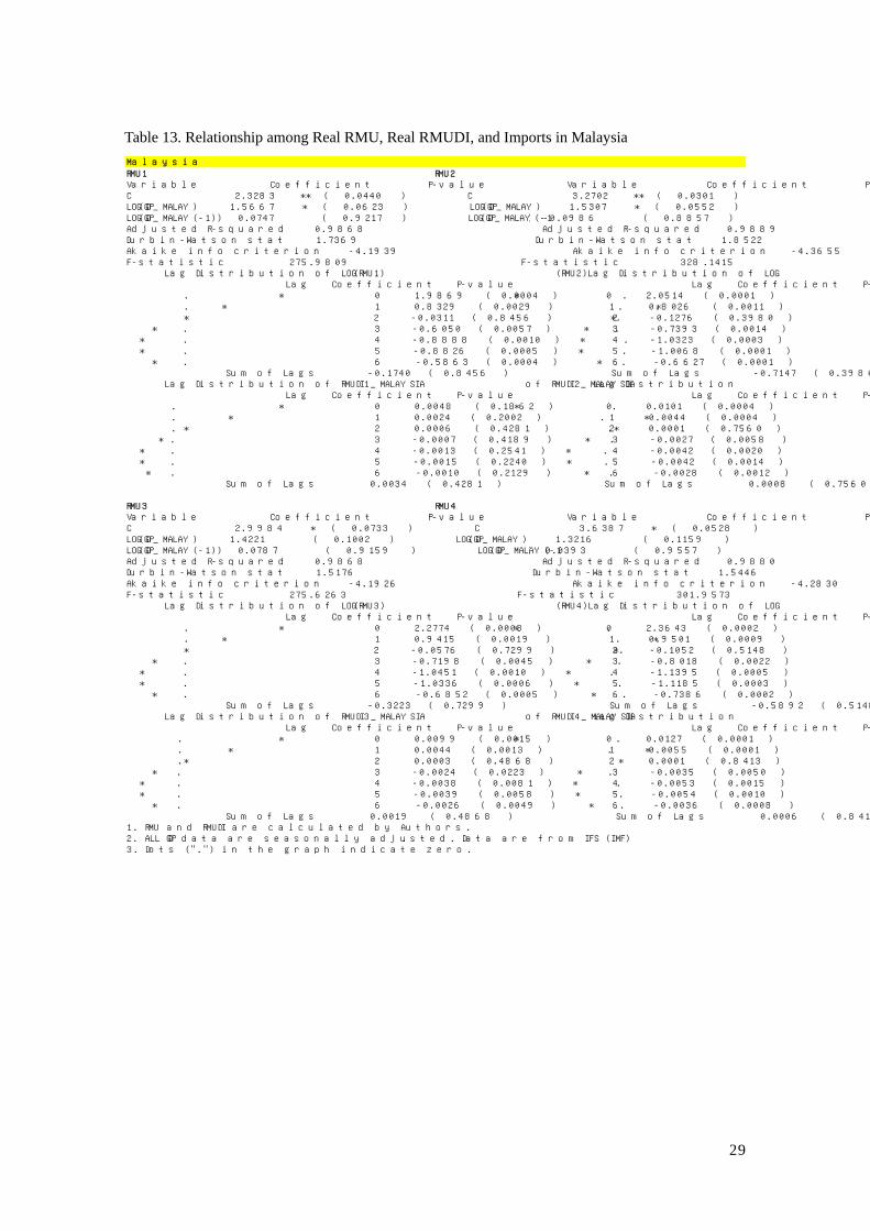
terms 6. Figures 7 to 19 show graphic representation of each country’s relationship between trade

data and four kind of RMU DIs. From these figures, it seems that RMU DIs might have some

4 The data of NEER are from IFS (IMF) for all sampled countries except for Korea, Singapore and Thailand whose data are from BIS. 5 The data of NEER and RMUs are transposed into the difference of logarithm. The data of AMU Deviation Indicators are transposed into 1st difference since they are quoted in the percent of change. 6We calculate an RMU Deviation Indicator in real terms by taking into account inflation rate differentials. Given a Nominal RMU Deviation Indicator, we calculate the Real RMU Deviation Indicator according to the following equation:

We use Consumer Price Index (CPI) data as the price index in calculating the Real RMU Deviation Indicator. Since the CPI data are available only on a monthly basis, we calculate the Real RMU Deviation Indicator monthly. As for the inflation rates in the RMU area, we calculate a weighted average of the CPI for the RMU area using the AMU shares, which is the combination of shares in intra-trades and GDP measured at PPP.

10

relationship with trade data. Then, we make a statistical analysis to investigate each effect both of

RMUs and RMUDIs on exports and imports by using Polynomial Distributed Lag Model (Almon

lag). This time, quarterly data of RMUs and RMU DIs are used since other control variables, such as

GDP data, are available only in quarterly basis. Almon lag model, with 6 lags, 2nd-degree

polynomial and far end constraints, is estimated in the case of imports and exports respectively.

Sampled countries include Japan, China, Indonesia, South Korea, Malaysia, the Philippines,

Singapore and Thailand.

In the estimation results, each sum of the estimated coefficients on the distributed lag is focused on.

It has the interpretation of the long run effect of RMUs and RMU DIs on exports and imports. Since

an increase in RMU DIi implies appreciation of currencyi vis-à-vis RMU, coefficients on RMU DIi is

expected to be positive for countryi’s imports while coefficients on RMU DIi is expected to be

negative for its exports.

• Effects on Imports

The following regression equation is estimated for each of the sample countries:

( ) ( ) ( )( )( )ki

ki

iii

RMUDIPDL

RMUPDLGDPGDPRTWorldIIMPO

,)2,6(

,)2,6(

210

log()1(logloglog

+

+−⋅+⋅+=

　　　　　　　　　　　　　　　　　

　　　　　　　　　　　　　　　　　

ααα

where i represents a sample country and k represents each of the four different types of RMUs. If

k=1, the type of RMU represents currency basket composed of 13 East Asian currencies weighted by

PPP-exchange-rate GDP and intra-trade share. If k=2, RMU is weighted by market-exchange-rate

GDP and intra-trade share. If k=3, RMU is weighted by. PPP-exchange-rate GDP, intra-trade share

and capital market size. If k=4, RMU is weighted by market-exchange-rate GDP, intra-trade share

and capital market size. Table1 to Table4 show their weights in detail. PDL(6,2) represent s a

Polynomial Distributed Lag Model with 6 lags and 2nd-degree polynomial with end constraints.

WorldIMPORTi is country i’s total import from rest of the world. GDPi is country i’s GDP calculated

at market rate. Both of the data on imports and GDP are seasonally adjusted.

Signs of coefficients on RMU and RMU DIi are expected to be positive for countryi’s imports.

Tables 9 to 16 show the analytical results of effects of RMU and RMU DIi on imports of each of the

sample countries. The tables report not only coefficients on the RMU and the RMU DIi with each

time lag but also a sum of the coefficients on the RMU and the RMU DIi with time lags at the

bottom line. In addition, they report coefficients on the current GDP and the GDP with time lag.

(1) Japan

11

In the case of Japan, the sums of estimated coefficients on all of the RMU DIs except for RMUDI1

are significant and positive, where the positive sign is consistent with the sign to be expected.. In the

long- run, most of the RMU DIs have positive effects on imports. In the short-run, most coefficients

of RMU DIs with the second and the third time lags are positive and statistically significant. The

results indicate that the RMU DIs themselves can explain imports in Japan both in the long-run and

the short-run.

(2) China

In the case of China, the sums of estimated coefficients on RMU1 are positive but statistically

insignificant. In the long-run, both the RMUs and the RMU DIs have insignificant effects. In the

short-run, all of the coefficients on current RMUs are significant and positive The results indicate

that current RMUs can explain Chinese imports in the short-run.

(3) Indonesia

In the case of Indonesia, the sums of estimated coefficients on all of the RMUs and the RMU DIs

except for RMUDI2 are significant and positive where the positive sign is consistent with the sign to

be expected. In the long-run, all of the RMUs and most of the RMU DIs have significantly positive

effects on imports. In the short-run, most coefficients of current and lagged values of RMUs and

RMU DIs are significantly positive. The results indicate that RMUs and RMU DIs themselves can

explain Indonesian imports very well both in both the long-run and the short-run.

(4) Korea

In the case of Korea, the sums of estimated coefficients on all of the RMUs except for RMU1 are

significant and positive, which is consistent with sign to be expected. Moreover, all of the RMU DIs

are positive although they are statistically insignificant. In the long-run, these RMUs have

significantly positive effects on imports. In the short-run, coefficients on the current and some

lagged values of RMUs and RMU DIs are significantly positive. The results indicate that the RMUs

and the RMU DIs can explain Korean imports very well both in the long-run and the short-run.

(5) Malaysia

In the case of Malaysia, the sums of estimated coefficients on all of the RMU DIs are positive but

statistically insignificant. In the long-run, all of the RMU DIs have positive effects on imports

although they are statistically insignificant. In the short-run, all of the coefficients on current and the

first lagged RMUs and RMU DIs except for RMU DI1 are significant and positive. The results

indicate that the RMUs and the RMU DIs themselves can explain imports in Malaysia very well in

the short-run.

(6) Philippines

12

In the case of the Philippines, the sums of estimated coefficients on most of the RMUs and the RMU

DIs are positive but insignificant. In the long-run, most of the RMUs and the RMU DIs have positive

effects on imports but statistically insignificant. In the short-run, all of the coefficients on the current

value and most of first lagged values of RMUs are significant and positive. The results indicate that

the RMUs themselves can explain imports in the Philippines very well in the short-run.

(7) Singapore

In the case of Singapore, the sums of estimated coefficients on all of the RMUs and the RMU DIs

except for RMUDI1 are negative, which is opposite in sign to expected. In the short-run, all of the

coefficients on the current and lagged RMUs and RMU DIs are insignificant or significantly

negative. The results indicate that RMUs and RMU DIs themselves cannot explain imports in

Singapore both in the long-run and the short-run.

(8) Thailand

In the case of Thailand, the sums of estimated coefficients on all of the RMUs except for RMU1 are

significant and positive. In the long-run, most of the RMUs have significantly positive effects on

imports. In the short-run, most coefficients on current and first to second lagged values of RMUs are

significant and positive. The results indicate that RMUs themselves can explain imports in Thailand

very well both in the long-run and the short-run.

The signs on coefficients on RMU and RMU DIi are expected to be positive for countryi’s imports.

Tables 6 to 13 show the analytical results of effects of RMU and RMU DIi on imports for each of the

sample countrires. Table 7 summarizes the analytical results for all of the sample countries. RMU2

and RMU3 are the best measurement for showing effects on imports for the long-run effect while all

of the RMU have the same performances for the short-run effect when we compare performances of

showing significantly expected positive effects on exports among RMU1, RMU2, RMU3, and

RMU4. On one hand, RMU1DI, RMU3DI, and RMU4DI are better than RMU2DI for the long-run

effect while RMU2DI, RMU3DI, and RMU4DI are better than RMU1DI for the short-run effect

when we compare performances of showing significantly expected negative effects on imports

among RMU1DI, RMU2DI, RMU3DI, and RMU4DI. After comparing the performances of RMU

and RMUDI for both the long-run and short-run effects on imports, both RMU3 and RMU3DI seem

relatively better than other RMUs and RMUDIs.

• Effects on Exports

The following regression equation is estimated for each of the sample countries:

13

( ) ( ) ( )( )( )ki

ki

realreali

RMUDIPDL

RMUPDLOECDGDPOECDGDPTWorldEXPOR

,)2,6(

,)2,6(

210

)log()1(logloglog

+

+−⋅+⋅+=

　　　　　　　　　　　　　　　　　

　　　　　　　　　　　　　　　　　

βββ

where i represents a sample country and k represents each of the four different types of RMUs.

PDL(6,2) represents a Polynomial Distributed Lag Model with 6 lags and 2nd-degree polynomial

with end constraints. WorldEXPORTi is country i’s total export to rest of the world. OECDGDPreal is

a total real GDP of OECD countries. Both of the data on exports and GDP are seasonally adjusted.

Signs of coefficients on RMU and RMU DIi are expected to be negative for countryi’s export in both

the long run and the short run. Tables 17 to 24 show the results of each of the sample countries. The

tables report not only coefficients on the RMU and the RMU DIi with each time lag but also a sum

of the coefficients on the RMU and the RMU DIi with time lags at the bottom line. In addition, they

report coefficients on the current GDP and the GDP with time lag.

(1) Japan

In the case of Japan, the sums of estimated coefficients on all of the RMUs are negative but

statistically insignificant. In the long-run, all of the RMUs have negative effects on exports but they

are statistically insignificant. In the short-run, most coefficients on current and 3rd to 6th lagged

values of RMUs and RMU DIs are significant and negative. The results indicate that RMUs and

RMU DIs themselves can explain exports in Japan very well especially in the short-run.

(2) China

In the case of China, the sums of estimated coefficients on all of the RMU DIs are significant and

negative, which is consistent in sign to be expected. In the long-run, all of the RMU DIs have

significantly negative effects on exports. In the short-run, most coefficients on current and 1st to 2nd

lagged values of RMU DIs are significant and negative The results indicate that RMU DIs

themselves can explain exports in China very well both in the long-run and the short-run.

(3) Indonesia

In the case of Indonesia, the sum of estimated coefficients on RMU DI1 is negative but insignificant.

In the long-run, all of the RMUs and the RMU DIs cannot explain exports in Indonesia. Also, in the

short-run, all the coefficients on 4th to 6th lagged values of RMU DIs are negative and significantly

estimated. The results indicate that RMU DIs themselves can explain exports in Indonesia very well

both in the short-run.

(4) Korea

In the case of Korea, the sums of estimated coefficients on all of the RMUs except for RMU4 and

the RMU DIs except for RMU DI1 are significant and negative, which is consistent in sign to be

14

expected. In the long-run, most of the RMUs and the RMU DIs have significantly negative effects

on exports in Korea. In the short-run, many coefficients on lagged values of RMUs and RMU DIs

are negative and significantly estimated. The results indicate that the RMUs and the RMU DIs

themselves can explain exports in Korea very well both in the long-run and the short-run.

(5) Malaysia

In the case of Malaysia, the sums of estimated coefficients on all of the RMUs and the RMU DIs

except for RMU DI1 are significant and negative, which is consistent in sign to be expected. In the

long-run, all of the RMUs and most of the RMU DIs have significantly negative effects on exports.

In the short-run, most coefficients on lagged values of RMUs and RMU DIs are negative and

significantly estimated. The results indicate that RMU DIs themselves can explain Malaysian

exports very well both in the long-run and the short-run.

(6) Philippines

In the case of the Philippines, the sums of estimated coefficients on all of the RMUs are negative but

statistically insignificant. In the long-run, all of the RMUs and the RMU DIs cannot explain exports.

In the short-run, some coefficients on current and lagged values of RMU1 and RMU2 are negatively

and significantly estimated. The results indicate that RMU1 and RMU2 can explain exports in the

Philippines at least in the short-run.

(7) Singapore

In the case of Singapore, the sums of estimated coefficients on all of the RMUs and the RMU DIs

are significant and negative, which is consistent in sign to be expected. In the long-run, all of the

RMUs and the RMU DIs have significantly negative effects on exports. In the short-run, most

coefficients of the current and 1st to 2nd lagged values of RMUs and 2nd to 4th lagged values of RMU

DIs are significant and negative. The results indicate that the RMUs and the RMU DIs themselves

can explain exports in Singapore very well both in the long-run and the short-run.

(8) Thailand

In the case of Thailand, the sum of estimated coefficients on RMU1 is significant and negative. In

the long-run, RMU1 can explain exports. In the short-run, the coefficient on 2nd lagged value of

RMU1 is negatively and significantly estimated. The results indicate that at least RMU1 can explain

exports in Thailand very well both in the long-run and the short-run.

The signs of coefficients on RMU and RMU DIi are expected to be negative for countryi’s exports.

Tables 17 to 24 show the analytical results of effects of RMU and RMU DIi on exports of each of the

sample countrires. Table 8 summarizes the analytical results for all of the sample countries. RMU1 is

15

the best measurement for showing effects on exports both for the long-run and short-run effects

when we compare performances of showing significantly expected negative effects on exports

among RMU1, RMU2, RMU3, and RMU4. On one hand, RMU2DI, RMU3DI, and RMU4DI are

better than RMU1DI for the long-run effect while RMU2DI and RMU3DI are the best for the

short-run effect when we compare performances of showing significantly expected negative effects

on exports among RMU1DI, RMU2DI, RMU3DI, and RMU4DI. After comparing the performances

of RMU and RMUDI for both the long-run and short-run effects on exports, RMU1 seems relatively

better than other RMUs in terms of the effects of RMU on exports while both RMU2DI and

RMU3DI seem relatively better than other RMUDIs in terms of the effects of RMUDI on exports.

The findings are summarized as follows: firstly, both RMU3 and RMU3DI seem relatively better

than other RMUs and RMUDIs when we compare performances of showing effects of RMUs and

RMUDIs on imports. Secondly, performances of showing effects of RMUs and RMUDIs on exports

are a little mixture. RMU1 seems relatively better than other RMUs in terms of the effects of RMU

on exports while both RMU2DI and RMU3DI seem relatively better than other RMUDIs in terms of

the effects of RMUDI on exports. Thirdly, it is possible for us to conclude that a RMU and a RMU

DI should consistently explain effects on both imports and exports among East Asian countries. It is

partly because trade structure of the East Asian countries has been so complicated due to its

expanding production base or production network in the region in recent years, and partly because

export competitions in many sectors have increased within Asian countries. These movements seem

to make complicate to figure out the effects of exchange rates on exports and imports.

We can point out one more important issue related with the above empirical analysis. Statistical

improvements of economic data, which include GDP, are desirable. It is usual that both real

exchange rate data and real GDP data are required to conduct the empirical analysis related with

effects of RMU and RMU DI on exports and imports. However, not all of ASEAN+3 countries have

reliable price data set to convert nominal RMU DIs and nominal GDP into real terms. In the daily

surveillance over nominal position of each currency among East Asian currencies, RMU DIs in

nominal terms is enough benchmark in monitoring overvaluation or undervaluation of the currency

in the region. However, RMU DIs in real terms should be needed for macro economic surveillance

in the longer run.

1-4. Conclusion

We find that all types of RMUs combined with RMU DIs have statistically significant and positive

relationships with NEERs (nominal effective exchange rates) in all the sampled countries. In

addition, they have statistically significant effects on exports in the countries whose basket weights

are rather high. These results suggest that it is meaningful to use RMUs and RMU DIs for regional

16

surveillance. We also find that levels of statistical significance and the estimated coefficients do not

differ so much depending on the types of RMUs. This implies that the four RMU candidates are

indifferent in terms of their effects on NEERs, exports, and imports and that trying to find other

desirable ways of calculating the weights in RMUs could be an ongoing discussion.

Other aspects of basket weights also should be discussed. For example, although there are crucial

difference between the basket shares calculated by PPP-exchange-rate GDP and those by

market-exchange-rate GDP, there is not much difference between RMU1 and RMU2 from their

explanation power of NEERs or trade data. However, from the standpoint of basket weight revision,

using PPP-exchange-rate GDP will be better than using market-exchange-rate GDP in the long run.

It is because the fluctuations of market-exchange-rate GDP caused by fluctuations of market

exchange rates are basically larger than those of PPP-exchange-rate GDP, so the basket shares will

be changed a lot at every revision time if market-exchange-rate GDP is used as a basket share.

Regarding RMU Deviation indicators (RMU DIs), they show the deviation of the value of regional

currencies against the RMU from their values in a benchmark period, which are useful as indicators

for gauging the development of intra-regional value of these currencies. The value of RMU DIs

depends on the benchmark year as shown in Appendix3. There seems to be tendency that the more

flexible the exchange rate system is, the more easily the value changes depending the selection of

benchmark year. Furthermore, although the benchmark year should be selected when exchange rates

are close to the equilibrium levels, estimated levels of equilibrium exchange rates will differ

significantly depending on the estimating approaches, data availability, definition and measurement,

estimation and filtering techniques. Even after considering such drawbacks of RMU DIs, monitoring

RMU DIs should play an important role in regional surveillance.

It is meaningful to continue studying the most desirable way to calculate RMUs. However, it would

be rather important to try to reach an agreement on selecting a certain kind of RMU and using the

RMU and the RMU DIs for regional surveillance in ASEAN+3 ERPD, in an attempt to facilitate the

intra-regional exchange rate stability without giving rise to the misalignments of exchange rates.

References

Ogawa, Eiji and Junko Shimizu (2006), "AMU Deviation Indicator for Coordinated Exchange Rate

Policies in East Asia and its Relation with Effective Exchange Rates," The World Economy, issue

29:12, p1691-1708.

17

Tables and Charts

Table 1.

RMU 1's Basket Shares and Weights of East Asian Currencies

(Benchmark year=2000/2001)

Intra-Tradeshare* %

GDPmeasured at

PPP** %

Arithmeticaverage

shares %(a)

Benchmarkexchangerate*** (b)

AMU weights(a)/(b)

Brunei 0.33 0.33 0.33 0.589114 0.0056Cambodia 0.19 0.23 0.21 0.000270 7.6219

China 23.99 51.70 37.85 0.125109 3.0251Indonesia 6.47 5.31 5.89 0.000113 522.9228

Japan 24.79 25.28 25.04 0.009065 27.6235South Korea 13.01 6.66 9.83 0.000859 114.4362

Laos 0.08 0.08 0.08 0.000136 5.7474Malaysia 8.10 1.72 4.91 0.272534 0.1801Myanmar 0.32 0.32 0.32 0.159215 0.0202Philippines 2.66 2.56 2.61 0.021903 1.1926Singapore 11.71 0.81 6.26 0.589160 0.1063Thailand 6.36 3.46 4.91 0.024543 2.0005Vietnam 1.98 1.55 1.76 0.000072 246.5203

Calculated by authors.* : Intra-Trade share is calculated as the average of total export and import volumes in 2003,2004 and 2005 taken from DOTS (IMF).**: GDP measured at PPP is the average of GDP measured at PPP in 2003, 2004 and 2005taken from the World Development Report, World Bank. For Brunei and Myanmar, we againuse the same share of trade volume since no GDP data are available for these countries.

*** : The Benchmark exchange rate ($-euro/Currency) is the average of the daily exchangerate in terms of US$-euro in 2000 and 2001.

18

Table 2.



Intra-Tradeshare* %

NominalGDP ** %

Arithmeticaverage

shares %(a)


AMU weights(a)/(b)

Brunei 0.33 0.07 0.20 0.589114 0.0034Cambodia 0.19 0.06 0.12 0.000270 4.6059

China 23.99 24.43 24.21 0.125109 1.9351Indonesia 6.47 3.25 4.86 0.000113 431.4425

Japan 24.79 56.78 40.78 0.009065 44.9939South Korea 13.01 8.78 10.89 0.000859 126.7796

Laos 0.08 0.03 0.05 0.000136 4.0133Malaysia 8.10 1.49 4.79 0.272534 0.1759Myanmar 0.32 0.09 0.21 0.159215 0.0129Philippines 2.66 1.11 1.89 0.021903 0.8610Singapore 11.71 1.34 6.53 0.589160 0.1108Thailand 6.36 2.00 4.18 0.024543 1.7038Vietnam 1.98 0.57 1.28 0.000072 178.3679

Calculated by authors.

**: Nominal GDP is the average of Nominal GDP in 2003, 2004 and 2005 taken from IFS (IMF).

*** : The Benchmark exchange rate ($-euro/Currency) is the average of the daily exchangerate in terms of US$-euro in 2000 and 2001.

* : Intra-Trade share is calculated as the average of total export and import volumes in 2003,2004 and 2005 taken from DOTS (IMF).

19

Table 3.



Intra-Tradeshare* %

GDPmeasured at

PPP** %

Size ofCapital

Market***, %

Arithmeticaverage

shares %(a)

Benchmarkexchange

rate**** (b)

AMU weights(a)/(b)

Brunei 0.33 0.33 0.00 0.22 0.589114 0.0037Cambodia 0.19 0.23 0.00 0.14 0.000270 5.0813

China 23.99 51.70 9.06 28.25 0.125109 2.2582Indonesia 6.47 5.31 0.93 4.24 0.000113 376.2514

Japan 24.79 25.28 75.51 41.86 0.009065 46.1845South Korea 13.01 6.66 8.77 9.48 0.000859 110.3034

Laos 0.08 0.08 0.00 0.05 0.000136 3.8316Malaysia 8.10 1.72 1.89 3.90 0.272534 0.1431Myanmar 0.32 0.32 0.00 0.21 0.159215 0.0135Philippines 2.66 2.56 0.50 1.91 0.021903 0.8707Singapore 11.71 0.81 2.11 4.88 0.589160 0.0828Thailand 6.36 3.46 1.23 3.68 0.024543 1.5010Vietnam 1.98 1.55 0.00 1.18 0.000072 164.3469

Calculated by authors.* : Intra-Trade share is calculated as the average of total export and import volumes in 2003, 2004 and 2005taken from DOTS (IMF).**: GDP measured at PPP is the average of GDP measured at PPP in 2003, 2004 and 2005 taken from theWorld Development Report, World Bank. For Brunei and Myanmar, we again use the same share of tradevolume since no GDP data are available for these countries.

*** : Size of Capital Market is calculated as the average of total volume of local currency bond market(Government, Corporate and Financial Institution) and domestic market capitalization in end of Dec 2004,2005 and 2006. The former data are from BIS and the later are from World Federation of Exchanges. ForBrunei, Cambodia, Lao, Myanmar and Vietnam, we assign zero share since no capital market data areavailable.**** : The Benchmark exchange rate ($-euro/Currency) is the average of the daily exchange rate in terms ofUS$-euro in 2000 and 2001.

20

Table 4.



Intra-Tradeshare* %

NominalGDP ** %

Size ofCapital

Market***, %

Arithmeticaverage

shares %(a)


AMU weights(a)/(b)

Brunei 0.33 0.07 0.00 0.13 0.589114 0.0023Cambodia 0.19 0.06 0.00 0.08 0.000270 3.0706

China 23.99 24.43 9.06 19.16 0.125109 1.5315Indonesia 6.47 3.25 0.93 3.55 0.000113 315.2645

Japan 24.79 56.78 75.51 52.36 0.009065 57.7647South Korea 13.01 8.78 8.77 10.19 0.000859 118.5323

Laos 0.08 0.03 0.00 0.04 0.000136 2.6755Malaysia 8.10 1.49 1.89 3.82 0.272534 0.1403Myanmar 0.32 0.09 0.00 0.14 0.159215 0.0086Philippines 2.66 1.11 0.50 1.42 0.021903 0.6496Singapore 11.71 1.34 2.11 5.05 0.589160 0.0858Thailand 6.36 2.00 1.23 3.20 0.024543 1.3032Vietnam 1.98 0.57 0.00 0.85 0.000072 118.9119

Calculated by authors.

**** : The Benchmark exchange rate ($-euro/Currency) is the average of the daily exchange rate in terms ofUS$-euro in 2000 and 2001.

* : Intra-Trade share is calculated as the average of total export and import volumes in 2003, 2004 and 2005taken from DOTS (IMF).

**: Nominal GDP is the average of Nominal GDP in 2003, 2004 and 2005 taken from IFS (IMF).

*** : Size of Capital Market is calculated as the average of total volume of local currency bond market(Government, Corporate and Financial Institution) and domestic market capitalization in end of Dec 2004,2005 and 2006. The former data are from BIS and the later are from World Federation of Exchanges. ForBrunei, Cambodia, Lao, Myanmar and Vietnam, we assign zero share since no capital market data areavailable.

21

Table 5. The Relationship between NEERs and RMU, RMU Deviation Indicators

Cofficient Std.Dev. Cofficient Std.Dev. Cofficient Std.Dev. Cofficient Std.Dev.

ChinaIntercept 0.0251 (0.1049) -0.0088 (0.0640) 0.0177 (0.0573) 0.0113 (0.0570) DLOG(RMUi)*100 0.2602 ** (0.1026) 0.2835 *** (0.0716) 0.4660 *** (0.0770) 0.5161 *** (0.0706) D(RMUDI China) 1.1007 *** (0.0750) 1.0084 *** (0.0487) 1.0612 *** (0.0451) 1.0366 *** (0.0443) AR(1) -0.5119 *** (0.0950) -0.5307 *** (0.0935) -0.5324 *** (0.0933) Adj. R2 0.7158 0.7665 0.8108 0.8127

IndonesiaIntercept -0.1114 (0.0918) -0.1156 (0.0860) -0.1338 (0.1183) -0.1389 (0.1302) DLOG(RMUi)*100 0.0791 (0.0477) 0.0692 * (0.0408) 0.3449 *** (0.0367) 0.4198 *** (0.0315) D(RMUDI Indonesia) 0.7973 *** (0.0558) 0.7460 *** (0.0546) 0.8734 *** (0.0411) 0.8766 *** (0.0379) AR(1) 0.4193 *** (0.1031) 0.3536 *** (0.1075) 0.6611 *** (0.0857) 0.7080 *** (0.0812) Adj. R2 0.7697 0.7499 0.8695 0.8826

JapanIntercept -0.0267 (0.0420) -0.0328 (0.0515) -0.0227 (0.0282) -0.0216 (0.0310) DLOG(RMUi)*100 0.2123 *** (0.0429) 0.1285 *** (0.0340) 0.4738 *** (0.0397) 0.4861 *** (0.0406) D(RMUDI Japan) 0.9887 *** (0.0491) 0.7243 *** (0.0402) 0.9928 *** (0.0354) 0.9191 *** (0.0358) AR(1) 0.1630 (0.1219) -0.0571 (0.1602) 0.0360 (0.1562) Adj. R2 0.8242 0.8122 0.9116 0.9109

South KoreaIntercept -0.0147 (0.0683) -0.0412 (0.0721) -0.0029 (0.0483) -0.0062 (0.0460) DLOG(RMUi)*100 0.1629 ** (0.0692) 0.1852 *** (0.0574) 0.5360 *** (0.0480) 0.5899 *** (0.0393) D(RMUDI South Korea) 1.0417 *** (0.0228) 1.0214 *** (0.0236) 1.0263 *** (0.0153) 1.0209 *** (0.0144) AR(1) 0.0000 *** (0.0000) 0.0000 *** (0.0000) 0.0000 *** (0.0000) Adj. R2 0.9632 0.9589 0.9817 0.9834

MalaysiaIntercept -0.0391 (0.0443) -0.0673 (0.0565) -0.0110 (0.0247) -0.0072 (0.0242) DLOG(RMUi)*100 0.2202 *** (0.0449) 0.2182 *** (0.0442) 0.5474 *** (0.0250) 0.6130 *** (0.0203) D(RMUDI Malaysia) 1.0484 *** (0.0348) 1.0604 *** (0.0453) 0.9648 *** (0.0196) 0.9487 *** (0.0184) AR(1)Adj. R2 0.9280 0.8841 0.9781 0.9788

PhilippinesIntercept -0.0381 (0.0581) -0.0246 (0.0624) -0.0143 (0.0307) -0.0071 (0.0301) DLOG(RMUi)*100 0.1519 *** (0.0575) 0.1126 ** (0.0497) 0.6431 *** (0.0400) 0.6621 *** (0.0368) D(RMUDI Philippines) 1.2560 *** (0.0429) 1.6068 *** (0.0611) 1.2403 *** (0.0383) 1.3685 *** (0.0514) AR(1)Adj. R2 0.9117 0.8979 0.9753 0.9763

SingaporeIntercept -0.0290 (0.0520) -0.0388 (0.0516) -0.0253 (0.0357) -0.0252 (0.0355) DLOG(RMUi)*100 0.2803 *** (0.0530) 0.1896 *** (0.0429) 0.5817 *** (0.0505) 0.5862 *** (0.0499) D(RMUDI Singapore) 1.1799 *** (0.0615) 0.8993 *** (0.0468) 1.2098 *** (0.0441) 1.1147 *** (0.0429) AR(1)Adj. R2 0.8100 0.8124 0.9108 0.9117

ThailandIntercept -0.0095 (0.0384) -0.0046 (0.0460) -0.0060 (0.0215) -0.0019 (0.0227) DLOG(RMUi)*100 0.1696 *** (0.0385) 0.1402 *** (0.0374) 0.4812 *** (0.0259) 0.5290 *** (0.0268) D(RMUDI Thailand) 0.8774 *** (0.0624) 0.6589 *** (0.0618) 0.9427 *** (0.0330) 0.8984 *** (0.0333) AR(1)Adj. R2 0.6972 0.5658 0.9052 0.8943

2. * , ** and *** show significance levels of 1%, 5% and 10%, respectively.

1. 4types RMU and RMUDI are calculated by authors. The data of NEERs(Nominal Effective Exchange Rates) ofChina, Indonesia, Japan, Malaysia, Philippine are from IFS(IMF), and South Korea, Singapore and Thailand fromBIS.

RMU1 RMU2 RMU3 RMU4

22

Table 6. Long-term Relationship among Real RMU, Real RMUDI, and Imports / Exports

Coefficient Std.Dev. Coefficient Std.Dev. Coefficient Std.Dev. Coefficient Std.Dev.

ChinaImports LOG(RMU) 0.1715 (0.6836) -0.5754 (0.5593) -0.5439 (0.6191) -0.6429 (0.5547)

RMUDI -0.0233 *** (0.0078) -0.0079 ** (0.0034) -0.0072 * (0.0037) -0.0051 (0.0032)Adj. R2 0.9843 0.9849 0.9836 0.9847

Exports LOG(RMU) -0.0200 (0.4929) 0.0517 (0.5168) 0.0550 (0.5495) 0.0623 (0.5504)RMUDI -0.0147 ** (0.0054) -0.0084 *** (0.0023) -0.0082 *** (0.0025) -0.0063 *** (0.0022)Adj. R2 0.9930 0.9927 0.9928 0.9926

IndonesiaImports LOG(RMU) 7.2536 *** (1.5018) 9.9301 *** (1.7847) 11.2414 *** (1.9119) 12.9683 *** (2.1715)

RMUDI 0.0079 (0.0046) 0.0069 (0.0047) 0.0089 * (0.0046) 0.0133 ** (0.0052)Adj. R2 0.9778 0.9807 0.9809

Exports LOG(RMU) 1.0824 (0.9583) 2.0840 * (1.1119) 2.1833 * (1.2091) 2.9459 ** (1.2569)RMUDI -0.0010 (0.0027) 0.0010 (0.0027) 0.0009 (0.0027) 0.0028 (0.0029)Adj. R2 0.9829 0.9850 0.9848 0.9865

JapanImports LOG(RMU) -1.5493 ** (0.6341) -1.4143 ** (0.6480) -1.4954 ** (0.6826) -1.3286 * (0.6978)

RMUDI 0.0017 (0.0024) 0.0061 * (0.0031) 0.0060 * (0.0031) 0.0100 ** (0.0047)Adj. R2 0.9819 0.9812 0.9817 0.9814

Exports LOG(RMU) -0.2601 (0.4389) -0.2108 (0.4145) -0.2051 (0.4686) -0.1911 (0.4623)RMUDI 0.0038 *** (0.0013) 0.0059 *** (0.0015) 0.0059 *** (0.0017) 0.0078 *** (0.0027)Adj. R2 0.9935 0.9937 0.9929 0.9929

South KoreaImports LOG(RMU) -2.2505 *** (0.6561) 1.4333 * (0.8012) 1.5419 * (0.8069) 2.6268 *** (0.6458)

RMUDI 0.0245 *** (0.0058) 0.0029 (0.0094) 0.0073 (0.0091) 0.0028 (0.0052)Adj. R2 0.9900 0.9823 0.9834 0.9891

Exports LOG(RMU) -2.5176 *** (0.4452) -1.2918 *** (0.4207) -1.1940 ** (0.4574) -0.6998 (0.5005)RMUDI 0.0006 (0.0060) -0.0111 *** (0.0032) -0.0103 *** (0.0033) -0.0097 *** (0.0029)Adj. R2 0.9966 0.9955 0.9957 0.9960

MalaysiaImports LOG(RMU) -0.1740 (0.8820) -0.7147 (0.8275) -0.3223 (0.9207) -0.5892 (0.8886)

RMUDI 0.0034 (0.0042) 0.0008 (0.0025) 0.0019 (0.0027) 0.0006 (0.0030)Adj. R2 0.9868 0.9889 0.9868 0.9880

Exports LOG(RMU) -1.9208 *** (0.5725) -2.1548 *** (0.5506) -1.9757 *** (0.6014) -2.0657 *** (0.5900)RMUDI 0.0000 (0.0025) -0.0058 *** (0.0014) -0.0055 *** (0.0016) -0.0081 *** (0.0018)Adj. R2 0.9957 0.9960 0.9954 0.9955

PhilippinesImports LOG(RMU) -1.0254 (1.0678) 0.3895 (0.9549) 0.4224 (1.0341) 0.7094 (1.0223)

RMUDI 0.0061 (0.0052) 0.0054 (0.0037) 0.0055 (0.0039) 0.0064 (0.0042)Adj. R2 0.9182 0.9254 0.9211 0.9201

Exports LOG(RMU) -1.0063 (1.3105) -0.2650 (1.1414) -0.2896 (1.2253) -0.2801 (1.1865)RMUDI 0.0136 ** (0.0056) 0.0102 *** (0.0032) 0.0103 *** (0.0034) 0.0089 ** (0.0036)Adj. R2 0.8939 0.8978 0.8946 0.8948

SingaporeImports LOG(RMU) -1.7837 *** (0.5196) -3.0663 *** (0.7196) -2.9734 *** (0.7004) -2.9616 *** (0.8895)

RMUDI -0.0333 (0.0242) -0.0275 *** (0.0083) -0.0281 *** (0.0088) -0.0283 *** (0.0087)Adj. R2 0.9931 0.9898 0.9896 0.9876

Exports LOG(RMU) -2.1270 *** (0.5424) -3.6387 *** (0.8576) -3.4820 *** (0.8484) -3.3837 *** (0.9443)RMUDI -0.0358 * (0.0172) -0.0271 *** (0.0058) -0.0276 *** (0.0061) -0.0283 *** (0.0061)Adj. R2 0.9928 0.9930 0.9928 0.9923

ThailandImports LOG(RMU) 1.6630 ** (0.7911) 3.3263 *** (0.8192) 3.5764 *** (0.8760) 3.0401 *** (0.8827)

RMUDI -0.0124 (0.0124) -0.0175 ** (0.0066) -0.0161 ** (0.0067) -0.0113 * (0.0058)Adj. R2 0.9748 0.9818 0.9815 0.9806

Exports LOG(RMU) -0.8987 ** (0.3783) -0.4370 (0.5535) -0.4994 (0.5887) -0.2304 (0.5633)RMUDI 0.0049 (0.0073) 0.0044 (0.0049) 0.0044 (0.0050) 0.0031 (0.0043)Adj. R2 0.9915 0.9915 0.9915 0.9916

1. 4types RMU and RMUDI are calculated by authors. ALL GDP data are seasonally adjusted. Data are from IFS (IMF).2. * , ** and *** show significance levels of 1%, 5% and 10% respectively.3. Intercept, log of real GDP of each country (only for import cases) and log of real GDP of OECD countries (only for export cases) are included avariables but not reported.4. Reported numbers are sum of coefficients on current and lagged value of RMU and RMUDI and standard deviations in parentheses.

RMU1 RMU2 RMU3 RMU4

23

Table 7. Relationship among Real RMU, Real RMUDI, and Imports

Long-termRMU RMUDI RMU RMUDI RMU RMUDI RMU RMUDI

Japan × △ × ○ × ○ × ○China △ × × × × × × ×Indonesia ○ ○ ○ △ ○ ○ ○ ○South Korea × ○ ○ △ ○ △ ○ △Malaysia × △ × △ × △ × △Philippines × △ △ △ △ △ × △Singapore × × × × × × × ×Thailand △ × ○ × ○ × ○ ×Short-term

RMU RMUDI RMU RMUDI RMU RMUDI RMU RMUDIJapan none none none 2-3 none 2-3 none 2-5China 0-1 none 0 none 0 none 0 noneIndonesia 0-2 2-3 0-3 0-1 0-3 0-2 0-3 0-2South Korea 0-1 1-6 2 none 1-2 none 0-2 noneMalaysia 0-1 none 0-1 0-1 0-1 0-1 0-1 0-1Philippines 0 none 0-1 none 0-1 none 0-1 noneSingapore none none none none none none none noneThailand 1-2 none 0-2 none 0-2 none 0-3 none1. 4types RMU and RMUDI are calculated by authors.2. ○, △ and × in upper table indicates that estimated coefficient ispositive and statistically significant at 10% level (○),positive but statistically insignificant (△) and negative (×).3. Lower table shows lags that are positively estimated and statistically significant at 10% level.

RMU1 RMU2 RMU3 RMU4

RMU1 RMU2 RMU3 RMU4

24

Table 8. Relationship among Real RMU, Real RMUDI, and Exports

Long-termRMU RMUDI RMU RMUDI RMU RMUDI RMU RMUDI

Japan △ × △ × △ × △ ×China △ ○ × ○ × ○ △ ○Indonesia × △ × × × × × ×South Korea ○ × ○ ○ ○ ○ △ ○Malaysia ○ × ○ ○ ○ ○ ○ ○Philippines △ × △ × △ × △ ×Singapore ○ ○ ○ ○ ○ ○ ○ ○Thailand ○ × △ × △ × △ ×Short-term

RMU RMUDI RMU RMUDI RMU RMUDI RMU RMUDIJapan 3-6 3-6 3-6 5-6 3-6 5-6 3-6 noneChina none 0-3 none 0-2 none 0-2 none 0-2Indonesia none 4-6 none 4-6 none 4-6 none 4-6South Korea 2-6 none 2-5 0-4 2-5 0-3 3-6 0-3Malaysia 2-6 3-6 2-6 2-6 2-6 2-6 2-6 2-6Philippines 3-6 none 4-5 none none none none noneSingapore 0-2 2-4 0-3 2-5 0-2 2-3 0-2 2Thailand 2 none none none none none none none1. 4types RMU and RMUDI are calculated by authors.2. ○, △ and × in upper table indicates that estimated coefficient isnegative and statistically significant at 10% level (○),negative but statistically insignificant (△) and positive (×).3. Lower table shows lags that are negatively estimated and statistically significant at 10% level.

RMU1 RMU2 RMU3 RMU4

RMU1 RMU2 RMU3 RMU4

25

Table 9. Relationship among Real RMU, Real RMUDI, and Imports in Japan

RMU1 RMU2Variable Coefficient P-value Variable Coefficient P-valueC -15.1513 *** ( 0.0002 ) C -15.1521 *** ( 0.0001 )LOG(GDP_JAPAN) 1.3613 ( 0.3570 ) LOG(GDP_JAPAN) 1.2809 ( 0.3874 )LOG(GDP_JAPAN(-1)) 4.3673 *** ( 0.0025 ) LOG(GDP_JAPAN(-1)) 4.4533 *** ( 0.0026 )Adjusted R-squared 0.9819 Adjusted R-squared 0.9812Durbin-Watson stat 1.4703 Durbin-Watson stat 1.4327Akaike info criterion -3.9541 Akaike info criterion -3.9152F-statistic 199.9932 F-statistic 192.2657 Lag Distribution of LOG(RMU1) Lag Distribution of LOG(RMU2)

Lag Coefficient P-value Lag Coefficient P-value * . 0 -0.4577 ( 0.4301 ) * . 0 -0.2046 ( 0.7005 ) * . 1 -0.3622 ( 0.2160 ) * . 1 -0.2392 ( 0.3857 ) * . 2 -0.2767 ( 0.0240 ) * . 2 -0.2525 ( 0.0412 ) * . 3 -0.2012 ( 0.1991 ) * . 3 -0.2446 ( 0.0869 ) * . 4 -0.1358 ( 0.5292 ) * . 4 -0.2154 ( 0.2624 ) * . 5 -0.0805 ( 0.7077 ) * . 5 -0.1649 ( 0.3874 ) *. 6 -0.0352 ( 0.8061 ) * . 6 -0.0931 ( 0.4653 )

Sum of Lags -1.5493 ( 0.0240 ) Sum of Lags -1.4143 ( 0.0412 ) Lag Distribution of RMUDI1_JAPAN Lag Distribution of RMUDI2_JAPAN

Lag Coefficient P-value Lag Coefficient P-value * . 0 -0.0015 ( 0.3714 ) * . 0 -0.0012 ( 0.5904 ) * . 1 -0.0005 ( 0.5823 ) .* 1 0.0002 ( 0.8761 ) . * 2 0.0003 ( 0.4693 ) . * 2 0.0011 ( 0.0608 ) . * 3 0.0008 ( 0.1808 ) . * 3 0.0016 ( 0.0761 ) . * 4 0.0010 ( 0.1812 ) . * 4 0.0018 ( 0.1167 ) . * 5 0.0010 ( 0.1903 ) . * 5 0.0016 ( 0.1437 ) . * 6 0.0006 ( 0.1974 ) . * 6 0.0010 ( 0.1617 )

Sum of Lags 0.0017 ( 0.4693 ) Sum of Lags 0.0061 ( 0.0608 )

RMU3 RMU4Variable Coefficient P-value Variable Coefficient P-valueC -14.7893 *** ( 0.0001 ) C -14.9851 *** ( 5.79E-05 )LOG(GDP_JAPAN) 1.2216 ( 0.4082 ) LOG(GDP_JAPAN) 1.1803 ( 0.423584019 )LOG(GDP_JAPAN(-1)) 4.4339 *** ( 0.0024 ) LOG(GDP_JAPAN(-1)) 4.5224 *** ( 0.002219892 )Adjusted R-squared 0.9817 Adjusted R-squared 0.9814Durbin-Watson stat 1.4666 Durbin-Watson stat 1.4423Akaike info criterion -3.9412 Akaike info criterion -3.9281F-statistic 197.4051 F-statistic 194.7978 Lag Distribution of LOG(RMU3) Lag Distribution of LOG(RMU4)

Lag Coefficient P-value Lag Coefficient P-value * . 0 -0.2382 ( 0.7026 ) * . 0 -0.0484 ( 0.9359 ) * . 1 -0.2623 ( 0.4132 ) * . 1 -0.1631 ( 0.6050 ) * . 2 -0.2670 ( 0.0405 ) * . 2 -0.2373 ( 0.0714 ) * . 3 -0.2524 ( 0.0946 ) * . 3 -0.2709 ( 0.0489 ) * . 4 -0.2184 ( 0.3075 ) * . 4 -0.2640 ( 0.1764 ) * . 5 -0.1649 ( 0.4451 ) * . 5 -0.2165 ( 0.2753 ) * . 6 -0.0922 ( 0.5264 ) * . 6 -0.1285 ( 0.3384 )


Lag Coefficient P-value Lag Coefficient P-value * . 0 -0.0012 ( 0.5746 ) * . 0 -0.0019 ( 0.5715 ) .* 1 0.0001 ( 0.9055 ) .* 1 0.0003 ( 0.8701 ) . * 2 0.0011 ( 0.0681 ) . * 2 0.0018 ( 0.0467 ) . * 3 0.0016 ( 0.0673 ) . * 3 0.0027 ( 0.0409 ) . * 4 0.0018 ( 0.1039 ) . * 4 0.0030 ( 0.0716 ) . * 5 0.0016 ( 0.1295 ) . * 5 0.0026 ( 0.0950 ) . * 6 0.0010 ( 0.1469 ) . * 6 0.0016 ( 0.1116 )

Sum of Lags 0.0060 ( 0.0681 ) Sum of Lags 0.0100 ( 0.0467 )1. RMU and RMUDI are calculated by Authors.2. ALL GDP data are seasonally adjusted. Data are from IFS (IMF).3. Dots (".") in the graph indicate zero.

Japan

26

Table 10. Relationship among Real RMU, Real RMUDI, and Imports in China

RMU1 RMU2Variable Coefficient P-value Variable Coefficient P-valueC 10.4729 *** ( 0.0000 ) C 10.3405 *** ( 0.0000 )LOG(GDP_CHINA) 0.1443 ( 0.2924 ) LOG(GDP_CHINA) 0.1681 ( 0.2092 )LOG(GDP_CHINA(-1) 0.2863 ** ( 0.0427 ) LOG(GDP_CHINA(-1 0.3384 ** ( 0.0193 )Adjusted R-squared 0.9843 Adjusted R-squared 0.9849Durbin-Watson stat 1.3449 Durbin-Watson stat 1.4851Akaike info criterion -4.2976 Akaike info criterion -4.3376F-statistic 231.1079 F-statistic 240.6617 Lag Distribution of LOG(RMU1) Lag Distribution of LOG(RMU2)

Lag Coefficient P-value Lag Coefficient P-value . * 0 1.1522 ( 0.0211 ) . * 0 0.9767 ( 0.0218 ) . * 1 0.5122 ( 0.0540 ) . * 1 0.3569 ( 0.1001 ) * 2 0.0306 ( 0.8044 ) *. 2 -0.1027 ( 0.3159 ) * . 3 -0.2925 ( 0.0241 ) * . 3 -0.4024 ( 0.0017 ) * . 4 -0.4571 ( 0.0077 ) * . 4 -0.5419 ( 0.0012 ) * . 5 -0.4632 ( 0.0066 ) * . 5 -0.5213 ( 0.0015 ) * . 6 -0.3108 ( 0.0065 ) * . 6 -0.3407 ( 0.0017 )

Sum of Lags 0.1715 ( 0.8044 ) Sum of Lags -0.5754 ( 0.3159 ) Lag Distribution of RMUDI1_CHINA Lag Distribution of RMUDI2_CHINA

Lag Coefficient P-value Lag Coefficient P-value * . 0 -0.0081 ( 0.0378 ) *. 0 0.0000 ( 0.9943 ) * . 1 -0.0060 ( 0.0179 ) * . 1 -0.0009 ( 0.5038 ) * . 2 -0.0042 ( 0.0070 ) * . 2 -0.0014 ( 0.0306 ) * . 3 -0.0027 ( 0.0095 ) * . 3 -0.0017 ( 0.0126 ) * . 4 -0.0015 ( 0.0919 ) * . 4 -0.0017 ( 0.0474 ) * . 5 -0.0007 ( 0.3964 ) * . 5 -0.0014 ( 0.0905 ) *. 6 -0.0002 ( 0.7333 ) * . 6 -0.0008 ( 0.1265 )

Sum of Lags -0.0233 ( 0.0070 ) Sum of Lags -0.0079 ( 0.0306 )

RMU3 RMU4Variable Coefficient P-value Variable Coefficient P-valueC 10.3499 *** ( 0.0000 ) C 10.3392 *** ( 0.0000 )LOG(GDP_CHINA) 0.1723 ( 0.2179 ) LOG(GDP_CHINA) 0.1730 ( 0.2022 )LOG(GDP_CHINA(-1) 0.3327 ** ( 0.0258 ) LOG(GDP_CHINA(-1 0.3362 ** ( 0.0226 )Adjusted R-squared 0.9836 Adjusted R-squared 0.9847Durbin-Watson stat 1.4444 Durbin-Watson stat 1.5770Akaike info criterion -4.2557 Akaike info criterion -4.3225F-statistic 221.5101 F-statistic 237.0111 Lag Distribution of LOG(RMU3) Lag Distribution of LOG(RMU4)

Lag Coefficient P-value Lag Coefficient P-value . * 0 1.0550 ( 0.0370 ) . * 0 1.0436 ( 0.0268 ) . * 1 0.3939 ( 0.1253 ) . * 1 0.3784 ( 0.1097 ) *. 2 -0.0971 ( 0.3901 ) * . 2 -0.1148 ( 0.2601 ) * . 3 -0.4180 ( 0.0031 ) * . 3 -0.4359 ( 0.0011 ) * . 4 -0.5687 ( 0.0028 ) * . 4 -0.5850 ( 0.0012 ) * . 5 -0.5493 ( 0.0036 ) * . 5 -0.5620 ( 0.0017 ) * . 6 -0.3597 ( 0.0042 ) * . 6 -0.3670 ( 0.0021 )

Sum of Lags -0.5439 ( 0.3901 ) Sum of Lags -0.6429 ( 0.2601 ) Lag Distribution of RMUDI3_CHINA Lag Distribution of RMUDI4_CHINA

Lag Coefficient P-value Lag Coefficient P-value . * 0 0.0003 ( 0.9128 ) . * 0 0.0025 ( 0.2961 ) * . 1 -0.0006 ( 0.6482 ) . * 1 0.0005 ( 0.6623 ) * . 2 -0.0013 ( 0.0681 ) * . 2 -0.0009 ( 0.1307 ) * . 3 -0.0016 ( 0.0249 ) * . 3 -0.0018 ( 0.0132 ) * . 4 -0.0017 ( 0.0716 ) * . 4 -0.0022 ( 0.0223 ) * . 5 -0.0014 ( 0.1210 ) * . 5 -0.0020 ( 0.0320 ) * . 6 -0.0009 ( 0.1588 ) * . 6 -0.0013 ( 0.0395 )

Sum of Lags -0.0072 ( 0.0681 ) Sum of Lags -0.0051 ( 0.1307 )1. RMU and RMUDI are calculated by Authors.2. ALL GDP data are seasonally adjusted. Data are from IFS (IMF).3. Dots (".") in the graph indicate zero.

China

27

Table 11. Relationship among Real RMU, Real RMUDI, and Imports in Indonesia

RMU1 RMU2Variable Coefficient P-value Variable Coefficient P-valueC -10.3887 *** ( 0.0009 ) C -18.6835 *** ( 0.0000 )LOG(GDP_INDONESIA) 3.3567 * ( 0.0959 ) LOG(GDP_INDONESIA) 3.9433 ** ( 0.0433 )LOG(GDP_INDONESIA(-1)) 0.9131 ( 0.6430 ) LOG(GDP_INDONESIA(-1) 2.1501 ( 0.2503 )Adjusted R-squared 0.9778 Adjusted R-squared 0.9801Durbin-Watson stat 1.6784 Durbin-Watson stat 1.5796Akaike info criterion -2.3712 Akaike info criterion -2.4801F-statistic 162.3293 F-statistic 181.3214 Lag Distribution of LOG(RMU1) Lag Distribution of LOG(RMU2)

Lag Coefficient P-value Lag Coefficient P-value . * 0 5.4655 ( 0.0002 ) . * 0 5.1298 ( 0.0001 ) . * 1 3.1195 ( 0.0001 ) . * 1 3.2624 ( 0.0000 ) . * 2 1.2953 ( 0.0001 ) . * 2 1.7732 ( 0.0000 ) * 3 -0.0072 ( 0.9808 ) . * 3 0.6622 ( 0.0278 ) * . 4 -0.7880 ( 0.0668 ) * 4 -0.0706 ( 0.8333 ) * . 5 -1.0471 ( 0.0182 ) * . 5 -0.4252 ( 0.2022 ) * . 6 -0.7844 ( 0.0095 ) * . 6 -0.4017 ( 0.0767 )

Sum of Lags 7.2536 ( 0.0001 ) Sum of Lags 9.9301 ( 0.0000 ) Lag Distribution of RMUDI1_INDONESIA Lag Distribution of RMUDI2_INDONESIA

Lag Coefficient P-value Lag Coefficient P-value . * 0 0.0003 ( 0.8374 ) . * 0 0.0041 ( 0.0076 ) . * 1 0.0010 ( 0.2687 ) . * 1 0.0025 ( 0.0182 ) . * 2 0.0014 ( 0.0989 ) . * 2 0.0012 ( 0.1519 ) . * 3 0.0016 ( 0.0951 ) . * 3 0.0003 ( 0.7001 ) . * 4 0.0016 ( 0.1113 ) * . 4 -0.0003 ( 0.7579 ) . * 5 0.0013 ( 0.1274 ) * . 5 -0.0005 ( 0.4727 ) . * 6 0.0008 ( 0.1408 ) * . 6 -0.0004 ( 0.3315 )


RMU3 RMU4Variable Coefficient P-value Variable Coefficient P-valueC -18.8848 *** ( 0.0000 ) C -23.2324 *** ( 0.0000 )LOG(GDP_INDONESIA) 4.5495 ** ( 0.0205 ) LOG(GDP_INDONESIA) 4.7999 ** ( 0.0150 )LOG(GDP_INDONESIA(-1)) 1.6001 ( 0.3804 ) LOG(GDP_INDONESIA(-1) 2.2936 ( 0.2097 )Adjusted R-squared 0.9807 Adjusted R-squared 0.9809Durbin-Watson stat 1.6889 Durbin-Watson stat 1.6583Akaike info criterion -2.5132 Akaike info criterion -2.5242F-statistic 187.5051 F-statistic 189.6080 Lag Distribution of LOG(RMU3) Lag Distribution of LOG(RMU4)

Lag Coefficient P-value Lag Coefficient P-value . * 0 6.0045 ( 0.0001 ) . * 0 5.5470 ( 0.0001 ) . * 1 3.7778 ( 0.0000 ) . * 1 3.7667 ( 0.0000 ) . * 2 2.0074 ( 0.0000 ) . * 2 2.3158 ( 0.0000 ) . * 3 0.6933 ( 0.0175 ) . * 3 1.1941 ( 0.0004 ) * 4 -0.1645 ( 0.6287 ) . * 4 0.4017 ( 0.1849 ) * . 5 -0.5660 ( 0.1100 ) * 5 -0.0615 ( 0.8298 ) * . 6 -0.5111 ( 0.0381 ) *. 6 -0.1954 ( 0.3164 )


Lag Coefficient P-value Lag Coefficient P-value . * 0 0.0045 ( 0.0037 ) . * 0 0.0092 ( 0.0001 ) . * 1 0.0029 ( 0.0071 ) . * 1 0.0054 ( 0.0003 ) . * 2 0.0016 ( 0.0666 ) . * 2 0.0024 ( 0.0182 ) . * 3 0.0006 ( 0.4667 ) * 3 0.0002 ( 0.7908 ) * 4 0.0000 ( 0.9540 ) * . 4 -0.0011 ( 0.2061 ) * . 5 -0.0004 ( 0.5934 ) * . 5 -0.0016 ( 0.0409 ) * . 6 -0.0003 ( 0.4063 ) * . 6 -0.0012 ( 0.0140 )


Indonesia

28

Table 12. Relationship among Real RMU, Real RMUDI, and Imports in Korea

RMU1 RMU2Variable Coefficient P-value Variable Coefficient P-valueC 14.2961 ** ( 0.0134 ) C -6.9581 ( 0.3974 )LOG(GDP_KOREA) -2.1190 * ( 0.0609 ) LOG(GDP_KOREA) 0.9556 ( 0.4477 )LOG(GDP_KOREA(-1)) 1.3148 ( 0.1702 ) LOG(GDP_KOREA(-1)) 2.8201 * ( 0.0860 )Adjusted R-squared 0.9900 Adjusted R-squared 0.9823Durbin-Watson stat 1.8993 Durbin-Watson stat 0.8546Akaike info criterion -3.9175 Akaike info criterion -3.3483F-statistic 363.7681 F-statistic 204.7304 Lag Distribution of LOG(RMU1) Lag Distribution of LOG(RMU2)

Lag Coefficient P-value Lag Coefficient P-value . * 0 2.3478 ( 0.0021 ) . * 0 1.2626 ( 0.2428 ) . * 1 0.7651 ( 0.0098 ) . * 1 0.6947 ( 0.1527 ) * . 2 -0.4019 ( 0.0027 ) . * 2 0.2559 ( 0.0888 ) * . 3 -1.1530 ( 0.0004 ) *. 3 -0.0536 ( 0.8718 ) * . 4 -1.4884 ( 0.0005 ) * . 4 -0.2340 ( 0.6185 ) * . 5 -1.4081 ( 0.0006 ) * . 5 -0.2852 ( 0.5388 ) * . 6 -0.9119 ( 0.0006 ) * . 6 -0.2072 ( 0.5009 )

Sum of Lags -2.2505 ( 0.0027 ) Sum of Lags 1.4333 ( 0.0888 ) Lag Distribution of RMUDI1_KOREA Lag Distribution of RMUDI2_KOREA

Lag Coefficient P-value Lag Coefficient P-value . * 0 0.0028 ( 0.1037 ) * . 0 -0.0007 ( 0.8129 ) . * 1 0.0038 ( 0.0044 ) * 1 0.0000 ( 0.9957 ) . * 2 0.0044 ( 0.0004 ) . * 2 0.0005 ( 0.7645 ) . * 3 0.0045 ( 0.0003 ) . * 3 0.0008 ( 0.5791 ) . * 4 0.0040 ( 0.0004 ) . * 4 0.0009 ( 0.4753 ) . * 5 0.0032 ( 0.0008 ) . * 5 0.0008 ( 0.4260 ) . * 6 0.0018 ( 0.0013 ) . * 6 0.0005 ( 0.4033 )


RMU3 RMU4Variable Coefficient P-value Variable Coefficient P-valueC -3.2287 ( 0.6864 ) C -9.7723 ** ( 0.0269 )LOG(GDP_KOREA) 0.7486 ( 0.5340 ) LOG(GDP_KOREA) 1.5452 * ( 0.0963 )LOG(GDP_KOREA(-1)) 2.2394 ( 0.1631 ) LOG(GDP_KOREA(-1)) 2.8551 ** ( 0.0189 )Adjusted R-squared 0.9834 Adjusted R-squared 0.9891Durbin-Watson stat 0.8821 Durbin-Watson stat 1.2034Akaike info criterion -3.4087 Akaike info criterion -3.8345F-statistic 217.6512 F-statistic 334.6054 Lag Distribution of LOG(RMU3) Lag Distribution of LOG(RMU4)

Lag Coefficient P-value Lag Coefficient P-value . * 0 1.9938 ( 0.1014 ) . * 0 1.5230 ( 0.0339 ) . * 1 1.0197 ( 0.0662 ) . * 1 0.9342 ( 0.0120 ) . * 2 0.2753 ( 0.0705 ) . * 2 0.4691 ( 0.0006 ) * . 3 -0.2392 ( 0.4851 ) . * 3 0.1277 ( 0.3650 ) * . 4 -0.5240 ( 0.2948 ) *. 4 -0.0898 ( 0.6808 ) * . 5 -0.5791 ( 0.2460 ) * . 5 -0.1836 ( 0.4194 ) * . 6 -0.4044 ( 0.2245 ) * . 6 -0.1537 ( 0.3226 )

Sum of Lags 1.5419 ( 0.0705 ) Sum of Lags 2.6268 ( 0.0006 ) Lag Distribution of RMUDI3_KOREA Lag Distribution of RMUDI4_KOREA

Lag Coefficient P-value Lag Coefficient P-value . * 0 0.0002 ( 0.9505 ) * . 0 -0.0011 ( 0.5665 ) . * 1 0.0009 ( 0.6749 ) * . 1 -0.0002 ( 0.8899 ) . * 2 0.0013 ( 0.4357 ) . * 2 0.0005 ( 0.6002 ) . * 3 0.0015 ( 0.3058 ) . * 3 0.0009 ( 0.2702 ) . * 4 0.0015 ( 0.2544 ) . * 4 0.0011 ( 0.1721 ) . * 5 0.0012 ( 0.2379 ) . * 5 0.0010 ( 0.1472 ) . * 6 0.0007 ( 0.2351 ) . * 6 0.0006 ( 0.1415 )


Korea

29

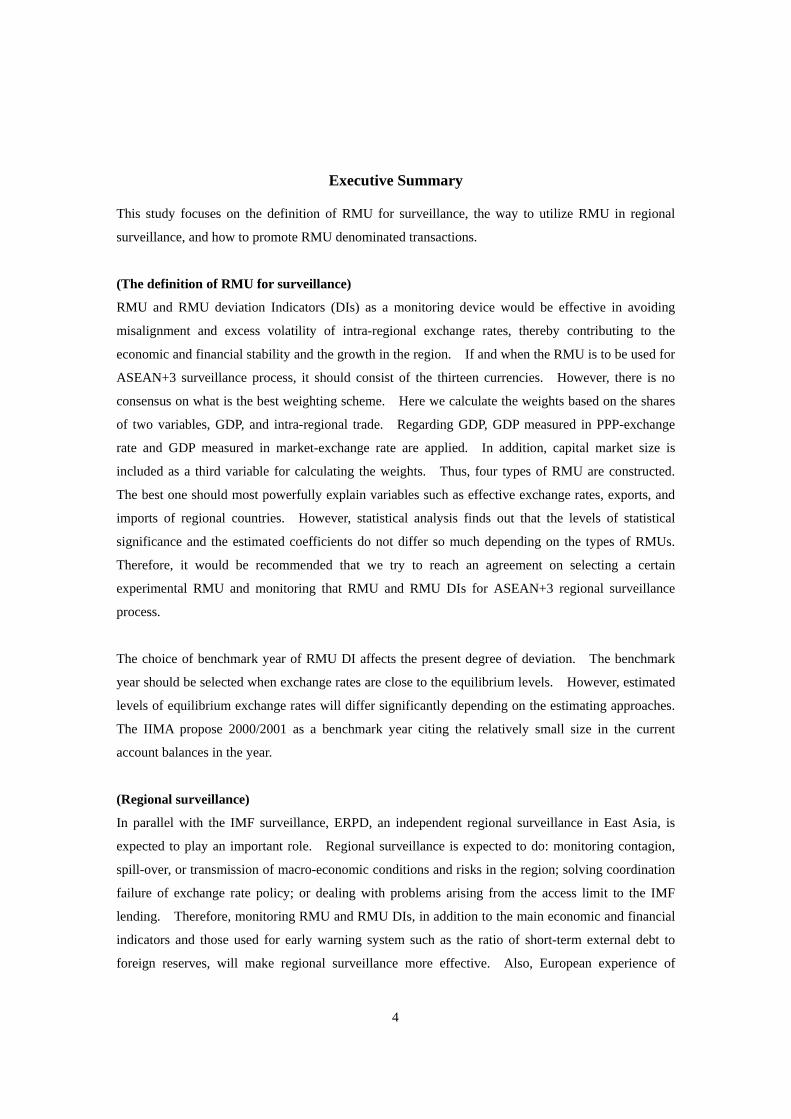
Table 13. Relationship among Real RMU, Real RMUDI, and Imports in Malaysia

RMU1 RMU2Variable Coefficient P-value Variable Coefficient P-valueC 2.3283 ** ( 0.0440 ) C 3.2702 ** ( 0.0301 )LOG(GDP_MALAY) 1.5667 * ( 0.0623 ) LOG(GDP_MALAY) 1.5307 * ( 0.0552 )LOG(GDP_MALAY(-1)) 0.0747 ( 0.9217 ) LOG(GDP_MALAY(-1) -0.0986 ( 0.8857 )Adjusted R-squared 0.9868 Adjusted R-squared 0.9889Durbin-Watson stat 1.7369 Durbin-Watson stat 1.8522Akaike info criterion -4.1939 Akaike info criterion -4.3655F-statistic 275.9809 F-statistic 328.1415 Lag Distribution of LOG(RMU1) Lag Distribution of LOG(RMU2)

Lag Coefficient P-value Lag Coefficient P-value . * 0 1.9869 ( 0.0004 ) . * 0 2.0514 ( 0.0001 ) . * 1 0.8329 ( 0.0029 ) . * 1 0.8026 ( 0.0011 ) * 2 -0.0311 ( 0.8456 ) *. 2 -0.1276 ( 0.3980 ) * . 3 -0.6050 ( 0.0057 ) * . 3 -0.7393 ( 0.0014 ) * . 4 -0.8888 ( 0.0010 ) * . 4 -1.0323 ( 0.0003 ) * . 5 -0.8826 ( 0.0005 ) * . 5 -1.0068 ( 0.0001 ) * . 6 -0.5863 ( 0.0004 ) * . 6 -0.6627 ( 0.0001 )

Sum of Lags -0.1740 ( 0.8456 ) Sum of Lags -0.7147 ( 0.3980 ) Lag Distribution of RMUDI1_MALAYSIA Lag Distribution of RMUDI2_MALAYSIA

Lag Coefficient P-value Lag Coefficient P-value . * 0 0.0048 ( 0.1862 ) . * 0 0.0101 ( 0.0004 ) . * 1 0.0024 ( 0.2002 ) . * 1 0.0044 ( 0.0004 ) . * 2 0.0006 ( 0.4281 ) .* 2 0.0001 ( 0.7560 ) * . 3 -0.0007 ( 0.4189 ) * . 3 -0.0027 ( 0.0058 ) * . 4 -0.0013 ( 0.2541 ) * . 4 -0.0042 ( 0.0020 ) * . 5 -0.0015 ( 0.2240 ) * . 5 -0.0042 ( 0.0014 ) * . 6 -0.0010 ( 0.2129 ) * . 6 -0.0028 ( 0.0012 )


RMU3 RMU4Variable Coefficient P-value Variable Coefficient P-valueC 2.9984 * ( 0.0733 ) C 3.6387 * ( 0.0528 )LOG(GDP_MALAY) 1.4221 ( 0.1002 ) LOG(GDP_MALAY) 1.3216 ( 0.1159 )LOG(GDP_MALAY(-1)) 0.0787 ( 0.9159 ) LOG(GDP_MALAY(-1) 0.0393 ( 0.9557 )Adjusted R-squared 0.9868 Adjusted R-squared 0.9880Durbin-Watson stat 1.5176 Durbin-Watson stat 1.5446Akaike info criterion -4.1926 Akaike info criterion -4.2830F-statistic 275.6263 F-statistic 301.9573 Lag Distribution of LOG(RMU3) Lag Distribution of LOG(RMU4)



Lag Coefficient P-value Lag Coefficient P-value . * 0 0.0099 ( 0.0015 ) . * 0 0.0127 ( 0.0001 ) . * 1 0.0044 ( 0.0013 ) . * 1 0.0055 ( 0.0001 ) .* 2 0.0003 ( 0.4868 ) * 2 0.0001 ( 0.8413 ) * . 3 -0.0024 ( 0.0223 ) * . 3 -0.0035 ( 0.0050 ) * . 4 -0.0038 ( 0.0081 ) * . 4 -0.0053 ( 0.0015 ) * . 5 -0.0039 ( 0.0058 ) * . 5 -0.0054 ( 0.0010 ) * . 6 -0.0026 ( 0.0049 ) * . 6 -0.0036 ( 0.0008 )


Malaysia

30

Table 14. Relationship among Real RMU, Real RMUDI, and Imports in Philippines

RMU1 RMU2Variable Coefficient P-value Variable Coefficient P-valueC 4.8178 * ( 0.0569 ) C 2.7748 ( 0.1417 )LOG(GDP_PHILI) 1.7900 ( 0.1968 ) LOG(GDP_PHILI) 2.1251 ( 0.1062 )LOG(GDP_PHILI(-1)) -0.8762 ( 0.5091 ) LOG(GDP_PHILI(-1)) -0.7520 ( 0.5548 )Adjusted R-squared 0.9182 Adjusted R-squared 0.9254Durbin-Watson stat 2.2379 Durbin-Watson stat 2.3766Akaike info criterion -2.9914 Akaike info criterion -3.0841F-statistic 38.3971 F-statistic 42.3576 Lag Distribution of LOG(RMU1) Lag Distribution of LOG(RMU2)

Lag Coefficient P-value Lag Coefficient P-value . * 0 1.9962 ( 0.0458 ) . * 0 1.9805 ( 0.0216 ) . * 1 0.7457 ( 0.1186 ) . * 1 0.8905 ( 0.0468 ) *. 2 -0.1831 ( 0.3484 ) * 2 0.0696 ( 0.6877 ) * . 3 -0.7901 ( 0.0104 ) * . 3 -0.4824 ( 0.0077 ) * . 4 -1.0753 ( 0.0104 ) * . 4 -0.7653 ( 0.0046 ) * . 5 -1.0386 ( 0.0117 ) * . 5 -0.7792 ( 0.0051 ) * . 6 -0.6802 ( 0.0127 ) * . 6 -0.5241 ( 0.0056 )

Sum of Lags -1.0254 ( 0.3484 ) Sum of Lags 0.3895 ( 0.6877 ) Lag Distribution of RMUDI1_PHILIPPINES Lag Distribution of RMUDI2_PHILIPPINES

Lag Coefficient P-value Lag Coefficient P-value * . 0 -0.0012 ( 0.6451 ) . * 0 0.0009 ( 0.6194 ) .* 1 0.0002 ( 0.9107 ) . * 1 0.0010 ( 0.3007 ) . * 2 0.0011 ( 0.2503 ) . * 2 0.0010 ( 0.1614 ) . * 3 0.0017 ( 0.1695 ) . * 3 0.0009 ( 0.3395 ) . * 4 0.0018 ( 0.1885 ) . * 4 0.0008 ( 0.4853 ) . * 5 0.0016 ( 0.2079 ) . * 5 0.0006 ( 0.5713 ) . * 6 0.0010 ( 0.2222 ) . * 6 0.0003 ( 0.6250 )


RMU3 RMU4Variable Coefficient P-value Variable Coefficient P-valueC 3.0123 ( 0.1281 ) C 2.3215 ( 0.2109 )LOG(GDP_PHILI) 2.0117 ( 0.1367 ) LOG(GDP_PHILI) 2.1822 ( 0.1082 )LOG(GDP_PHILI(-1)) -0.6863 ( 0.6004 ) LOG(GDP_PHILI(-1)) -0.7064 ( 0.5926 )Adjusted R-squared 0.9211 Adjusted R-squared 0.9201Durbin-Watson stat 2.4989 Durbin-Watson stat 2.4943Akaike info criterion -3.0277 Akaike info criterion -3.0158F-statistic 39.9058 F-statistic 39.4043 Lag Distribution of LOG(RMU3) Lag Distribution of LOG(RMU4)

Lag Coefficient P-value Lag Coefficient P-value . * 0 2.1220 ( 0.0356 ) . * 0 1.8787 ( 0.0391 ) . * 1 0.9547 ( 0.0668 ) . * 1 0.8812 ( 0.0688 ) * 2 0.0754 ( 0.6873 ) .* 2 0.1267 ( 0.4957 ) * . 3 -0.5158 ( 0.0089 ) * . 3 -0.3848 ( 0.0140 ) * . 4 -0.8189 ( 0.0080 ) * . 4 -0.6531 ( 0.0090 ) * . 5 -0.8340 ( 0.0096 ) * . 5 -0.6785 ( 0.0106 ) * . 6 -0.5610 ( 0.0107 ) * . 6 -0.4608 ( 0.0119 )

Sum of Lags 0.4224 ( 0.6873 ) Sum of Lags -0.5892 ( 0.5148 ) Lag Distribution of RMUDI3_PHILIPPINES Lag Distribution of RMUDI4_PHILIPPINES

Lag Coefficient P-value Lag Coefficient P-value . * 0 0.0010 ( 0.6005 ) . * 0 0.0023 ( 0.2292 ) . * 1 0.0010 ( 0.2968 ) . * 1 0.0017 ( 0.1114 ) . * 2 0.0010 ( 0.1763 ) . * 2 0.0011 ( 0.1484 ) . * 3 0.0009 ( 0.3590 ) . * 3 0.0007 ( 0.4696 ) . * 4 0.0007 ( 0.5058 ) . * 4 0.0004 ( 0.7378 ) . * 5 0.0006 ( 0.5924 ) .* 5 0.0001 ( 0.8904 ) . * 6 0.0003 ( 0.6463 ) * 6 0.0000 ( 0.9811 )


Philippines

31

Table 15. Relationship among Real RMU, Real RMUDI, and Imports in Singapore

RMU1 RMU2Variable Coefficient P-value Variable Coefficient P-valueC 0.4768 ( 0.6811 ) C 3.0640 ** ( 0.0356 )LOG(GDP_SING) 1.5703 *** ( 0.0001 ) LOG(GDP_SING) 1.1051 *** ( 0.0045 )LOG(GDP_SING(-1)) 0.5345 ( 0.1215 ) LOG(GDP_SING(-1)) 0.4256 ( 0.3071 )Adjusted R-squared 0.9931 Adjusted R-squared 0.9898Durbin-Watson stat 2.2794 Durbin-Watson stat 1.9199Akaike info criterion -4.4573 Akaike info criterion -4.0718F-statistic 479.3180 F-statistic 325.2250 Lag Distribution of LOG(RMU1) Lag Distribution of LOG(RMU2)

Lag Coefficient P-value Lag Coefficient P-value * . 0 -1.0041 ( 0.0643 ) * . 0 -0.3698 ( 0.4610 ) * . 1 -0.6214 ( 0.0171 ) * . 1 -0.4870 ( 0.0556 ) * . 2 -0.3185 ( 0.0026 ) * . 2 -0.5476 ( 0.0004 ) *. 3 -0.0953 ( 0.5632 ) * . 3 -0.5514 ( 0.0073 ) .* 4 0.0481 ( 0.8308 ) * . 4 -0.4986 ( 0.0446 ) . * 5 0.1118 ( 0.6134 ) * . 5 -0.3891 ( 0.0948 ) . * 6 0.0958 ( 0.5141 ) * . 6 -0.2229 ( 0.1397 )

Sum of Lags -1.7837 ( 0.0026 ) Sum of Lags -3.0663 ( 0.0004 ) Lag Distribution of RMUDI1_SINGAPORE Lag Distribution of RMUDI2_SINGAPORE

Lag Coefficient P-value Lag Coefficient P-value . * 0 0.0076 ( 0.2974 ) . * 0 0.0110 ( 0.1002 ) *. 1 -0.0003 ( 0.9549 ) . * 1 0.0018 ( 0.5506 ) * . 2 -0.0060 ( 0.1841 ) * . 2 -0.0049 ( 0.0036 ) * . 3 -0.0093 ( 0.0267 ) * . 3 -0.0090 ( 0.0017 ) * . 4 -0.0104 ( 0.0079 ) * . 4 -0.0106 ( 0.0035 ) * . 5 -0.0092 ( 0.0042 ) * . 5 -0.0096 ( 0.0051 ) * . 6 -0.0057 ( 0.0031 ) * . 6 -0.0061 ( 0.0064 )


RMU3 RMU4Variable Coefficient P-value Variable Coefficient P-valueC 3.1012 ** ( 0.0491 ) C 3.7498 ( 0.0720 )LOG(GDP_SING) 1.1380 *** ( 0.0041 ) LOG(GDP_SING) 1.0109 ** ( 0.0176 )LOG(GDP_SING(-1)) 0.3877 ( 0.3984 ) LOG(GDP_SING(-1)) 0.3793 ( 0.4640 )Adjusted R-squared 0.9896 Adjusted R-squared 0.9876Durbin-Watson stat 1.9352 Durbin-Watson stat 1.6811Akaike info criterion -4.0535 Akaike info criterion -3.8774F-statistic 319.2770 F-statistic 267.3555 Lag Distribution of LOG(RMU3) Lag Distribution of LOG(RMU4)

Lag Coefficient P-value Lag Coefficient P-value * . 0 -0.4032 ( 0.5236 ) *. 0 -0.0078 ( 0.9903 ) * . 1 -0.4914 ( 0.1100 ) * . 1 -0.3207 ( 0.2944 ) * . 2 -0.5310 ( 0.0004 ) * . 2 -0.5288 ( 0.0033 ) * . 3 -0.5220 ( 0.0178 ) * . 3 -0.6324 ( 0.0195 ) * . 4 -0.4644 ( 0.1027 ) * . 4 -0.6313 ( 0.0591 ) * . 5 -0.3582 ( 0.1912 ) * . 5 -0.5255 ( 0.0956 ) * . 6 -0.2034 ( 0.2584 ) * . 6 -0.3151 ( 0.1234 )


Lag Coefficient P-value Lag Coefficient P-value . * 0 0.0113 ( 0.1252 ) . * 0 0.0099 ( 0.2069 ) . * 1 0.0018 ( 0.5784 ) . * 1 0.0012 ( 0.7036 ) * . 2 -0.0050 ( 0.0046 ) * . 2 -0.0051 ( 0.0039 ) * . 3 -0.0093 ( 0.0025 ) * . 3 -0.0089 ( 0.0108 ) * . 4 -0.0109 ( 0.0052 ) * . 4 -0.0103 ( 0.0207 ) * . 5 -0.0099 ( 0.0075 ) * . 5 -0.0093 ( 0.0276 ) * . 6 -0.0062 ( 0.0094 ) * . 6 -0.0059 ( 0.0324 )


Singapore

32

Table 16. Relationship among Real RMU, Real RMUDI, and Imports in Thailand

RMU1 RMU2Variable Coefficient P-value Variable Coefficient P-valueC -6.0396 ** ( 0.0495 ) C -9.6407 *** ( 0.0000 )LOG(GDP_THAI) 1.5138 ( 0.2694 ) LOG(GDP_THAI) 2.2987 * ( 0.0644 )LOG(GDP_THAI(-1)) 1.9044 ( 0.1864 ) LOG(GDP_THAI(-1)) 1.9218 ( 0.1008 )Adjusted R-squared 0.9748 Adjusted R-squared 0.9818Durbin-Watson stat 1.6499 Durbin-Watson stat 1.7860Akaike info criterion -3.0808 Akaike info criterion -3.4036F-statistic 142.8226 F-statistic 198.2543 Lag Distribution of LOG(RMU1) Lag Distribution of LOG(RMU2)

Lag Coefficient P-value Lag Coefficient P-value . * 0 2.0040 ( 0.0178 ) . * 0 1.7669 ( 0.0085 ) . * 1 1.0370 ( 0.0086 ) . * 1 1.1136 ( 0.0031 ) . * 2 0.2970 ( 0.0484 ) . * 2 0.5940 ( 0.0006 ) * . 3 -0.2162 ( 0.4098 ) . * 3 0.2079 ( 0.1071 ) * . 4 -0.5025 ( 0.1648 ) * 4 -0.0445 ( 0.7994 ) * . 5 -0.5619 ( 0.1141 ) *. 5 -0.1633 ( 0.3708 ) * . 6 -0.3944 ( 0.0942 ) *. 6 -0.1485 ( 0.2375 )

Sum of Lags 1.6630 ( 0.0484 ) Sum of Lags 3.3263 ( 0.0006 ) Lag Distribution of RMUDI1_THAILAND Lag Distribution of RMUDI2_THAILAND

Lag Coefficient P-value Lag Coefficient P-value * . 0 -0.0091 ( 0.0020 ) * . 0 -0.0034 ( 0.0863 ) * . 1 -0.0053 ( 0.0062 ) * . 1 -0.0033 ( 0.0009 ) * . 2 -0.0022 ( 0.3260 ) * . 2 -0.0031 ( 0.0153 ) * 3 -0.0001 ( 0.9839 ) * . 3 -0.0028 ( 0.1160 ) . * 4 0.0012 ( 0.6687 ) * . 4 -0.0023 ( 0.2350 ) . * 5 0.0017 ( 0.5015 ) * . 5 -0.0017 ( 0.3267 ) . * 6 0.0013 ( 0.4103 ) * . 6 -0.0009 ( 0.3937 )


RMU3 RMU4Variable Coefficient P-value Variable Coefficient P-valueC -9.5490 *** ( 0.0000 ) C -9.1023 *** ( 0.0000 )LOG(GDP_THAI) 2.2719 * ( 0.0689 ) LOG(GDP_THAI) 2.2827 * ( 0.0748 )LOG(GDP_THAI(-1)) 1.9318 ( 0.1022 ) LOG(GDP_THAI(-1)) 1.8161 ( 0.1293 )Adjusted R-squared 0.9815 Adjusted R-squared 0.9806Durbin-Watson stat 1.7218 Durbin-Watson stat 1.5671Akaike info criterion -3.3883 Akaike info criterion -3.3406F-statistic 195.2158 F-statistic 186.0014 Lag Distribution of LOG(RMU3) Lag Distribution of LOG(RMU4)

Lag Coefficient P-value Lag Coefficient P-value . * 0 2.0471 ( 0.0081 ) . * 0 1.4466 ( 0.0229 ) . * 1 1.2605 ( 0.0032 ) . * 1 0.9457 ( 0.0100 ) . * 2 0.6386 ( 0.0006 ) . * 2 0.5429 ( 0.0026 ) .* 3 0.1815 ( 0.1744 ) . * 3 0.2381 ( 0.0504 ) *. 4 -0.1110 ( 0.5704 ) * 4 0.0315 ( 0.8371 ) * . 5 -0.2387 ( 0.2511 ) *. 5 -0.0771 ( 0.6282 ) * . 6 -0.2017 ( 0.1620 ) *. 6 -0.0876 ( 0.4266 )

Sum of Lags 3.5764 ( 0.0006 ) Sum of Lags 3.0401 ( 0.0026 ) Lag Distribution of RMUDI3_THAILAND Lag Distribution of RMUDI4_THAILAND

Lag Coefficient P-value Lag Coefficient P-value * . 0 -0.0032 ( 0.1077 ) *. 0 -0.0001 ( 0.9795 ) * . 1 -0.0031 ( 0.0019 ) * . 1 -0.0012 ( 0.1710 ) * . 2 -0.0029 ( 0.0258 ) * . 2 -0.0020 ( 0.0649 ) * . 3 -0.0025 ( 0.1534 ) * . 3 -0.0024 ( 0.1338 ) * . 4 -0.0021 ( 0.2846 ) * . 4 -0.0024 ( 0.1840 ) * . 5 -0.0015 ( 0.3799 ) * . 5 -0.0020 ( 0.2164 ) * . 6 -0.0008 ( 0.4474 ) * . 6 -0.0012 ( 0.2383 )


Thailand

33

Table 17. Relationship among Real RMU, Real RMUDI, and Exports in Japan

RMU1 RMU2Variable Coefficient P-value Variable Coefficient P-valueC -58.2577 *** ( 0.0000 ) C -60.4870 *** ( 0.0000 )LOG(OECDGDP) 1.3603 ( 0.4219 ) LOG(OECDGDP) 1.6299 ( 0.3167 )LOG(OECDGDP(-1)) 2.7153 * ( 0.0894 ) LOG(OECDGDP(-1)) 2.5757 * ( 0.0994 )Adjusted R-squared 0.9935 Adjusted R-squared 0.9937Durbin-Watson stat 1.9394 Durbin-Watson stat 1.9369Akaike info criterion -5.2554 Akaike info criterion -5.2995F-statistic 558.5809 F-statistic 583.8982 Lag Distribution of LOG(RMU1) Lag Distribution of LOG(RMU2)

Lag Coefficient P-value Lag Coefficient P-value . * 0 0.5937 ( 0.0539 ) . * 0 0.5566 ( 0.0461 ) . * 1 0.2266 ( 0.1432 ) . * 1 0.2160 ( 0.1370 ) *. 2 -0.0464 ( 0.5602 ) *. 2 -0.0376 ( 0.6166 ) * . 3 -0.2253 ( 0.0335 ) * . 3 -0.2042 ( 0.0238 ) * . 4 -0.3102 ( 0.0210 ) * . 4 -0.2837 ( 0.0126 ) * . 5 -0.3009 ( 0.0198 ) * . 5 -0.2762 ( 0.0117 ) * . 6 -0.1975 ( 0.0198 ) * . 6 -0.1816 ( 0.0119 )


Lag Coefficient P-value Lag Coefficient P-value . * 0 0.0053 ( 0.0001 ) . * 0 0.0053 ( 0.0006 ) . * 1 0.0027 ( 0.0001 ) . * 1 0.0029 ( 0.0001 ) .* 2 0.0007 ( 0.0090 ) . * 2 0.0011 ( 0.0010 ) * . 3 -0.0007 ( 0.0330 ) *. 3 -0.0002 ( 0.6252 ) * . 4 -0.0014 ( 0.0023 ) * . 4 -0.0010 ( 0.1396 ) * . 5 -0.0016 ( 0.0010 ) * . 5 -0.0012 ( 0.0667 ) * . 6 -0.0011 ( 0.0007 ) * . 6 -0.0009 ( 0.0442 )


RMU3 RMU4Variable Coefficient P-value Variable Coefficient P-valueC -60.7898 *** ( 0.0000 ) C -62.5967 *** ( 0.0000 )LOG(OECDGDP) 1.6683 ( 0.3352 ) LOG(OECDGDP) 1.7725 ( 0.3009 )LOG(OECDGDP(-1)) 2.5551 ( 0.1220 ) LOG(OECDGDP(-1)) 2.5562 ( 0.1240 )Adjusted R-squared 0.9929 Adjusted R-squared 0.9929Durbin-Watson stat 1.9769 Durbin-Watson stat 1.9698Akaike info criterion -5.1756 Akaike info criterion -5.1692F-statistic 515.5264 F-statistic 512.2085 Lag Distribution of LOG(RMU3) Lag Distribution of LOG(RMU4)

Lag Coefficient P-value Lag Coefficient P-value . * 0 0.5193 ( 0.1292 ) . * 0 0.4605 ( 0.1658 ) . * 1 0.2006 ( 0.2607 ) . * 1 0.1769 ( 0.3187 ) *. 2 -0.0366 ( 0.6663 ) *. 2 -0.0341 ( 0.6837 ) * . 3 -0.1923 ( 0.0508 ) * . 3 -0.1725 ( 0.0472 ) * . 4 -0.2665 ( 0.0381 ) * . 4 -0.2383 ( 0.0369 ) * . 5 -0.2592 ( 0.0398 ) * . 5 -0.2315 ( 0.0411 ) * . 6 -0.1703 ( 0.0421 ) * . 6 -0.1520 ( 0.0451 )


Lag Coefficient P-value Lag Coefficient P-value . * 0 0.0054 ( 0.0010 ) . * 0 0.0058 ( 0.0076 ) . * 1 0.0029 ( 0.0002 ) . * 1 0.0033 ( 0.0015 ) . * 2 0.0010 ( 0.0021 ) . * 2 0.0014 ( 0.0087 ) *. 3 -0.0003 ( 0.5918 ) * 3 0.0000 ( 0.9881 ) * . 4 -0.0011 ( 0.1371 ) * . 4 -0.0008 ( 0.4144 ) * . 5 -0.0013 ( 0.0680 ) * . 5 -0.0011 ( 0.2546 ) * . 6 -0.0009 ( 0.0462 ) * . 6 -0.0008 ( 0.1916 )


Japan

34

Table 18. Relationship among Real RMU, Real RMUDI, and Exports in China

RMU1 RMU2Variable Coefficient P-value Variable Coefficient P-valueC -49.2825 *** ( 0.0000 ) C -59.4013 *** ( 0.0000 )LOG(OECDGDP) -0.2295 ( 0.8852 ) LOG(OECDGDP) 0.6029 ( 0.7306 )LOG(OECDGDP(-1)) 3.7365 ** ( 0.0308 ) LOG(OECDGDP(-1)) 3.4943 ** ( 0.0446 )Adjusted R-squared 0.9930 Adjusted R-squared 0.9927Durbin-Watson stat 2.1225 Durbin-Watson stat 2.0921Akaike info criterion -5.1380 Akaike info criterion -5.0944F-statistic 521.5958 F-statistic 499.1904 Lag Distribution of LOG(RMU1) Lag Distribution of LOG(RMU2)

Lag Coefficient P-value Lag Coefficient P-value . * 0 0.3351 ( 0.3074 ) . * 0 0.1089 ( 0.6948 ) . * 1 0.1415 ( 0.4211 ) . * 1 0.0522 ( 0.7267 ) * 2 -0.0036 ( 0.9680 ) .* 2 0.0092 ( 0.9213 ) * . 3 -0.1000 ( 0.2975 ) * . 3 -0.0200 ( 0.8560 ) * . 4 -0.1479 ( 0.2227 ) * . 4 -0.0356 ( 0.7830 ) * . 5 -0.1472 ( 0.2130 ) * . 5 -0.0374 ( 0.7561 ) * . 6 -0.0979 ( 0.2119 ) * . 6 -0.0256 ( 0.7431 )

Sum of Lags -0.0200 ( 0.9680 ) Sum of Lags 0.0517 ( 0.9213 ) Lag Distribution of RMUDI1_CHINA Lag Distribution of RMUDI2_CHINA

Lag Coefficient P-value Lag Coefficient P-value * . 0 -0.0065 ( 0.0161 ) * . 0 -0.0046 ( 0.0259 ) * . 1 -0.0044 ( 0.0123 ) * . 1 -0.0029 ( 0.0085 ) * . 2 -0.0026 ( 0.0131 ) * . 2 -0.0015 ( 0.0018 ) * . 3 -0.0013 ( 0.0626 ) * . 3 -0.0005 ( 0.3301 ) *. 4 -0.0004 ( 0.5553 ) .* 4 0.0002 ( 0.8004 ) * 5 0.0002 ( 0.7530 ) . * 5 0.0005 ( 0.4916 ) .* 6 0.0003 ( 0.4303 ) . * 6 0.0004 ( 0.3701 )


RMU3 RMU4Variable Coefficient P-value Variable Coefficient P-valueC -59.5037 *** ( 0.0000 ) C -62.8305 *** ( 0.0000 )LOG(OECDGDP) 0.5387 ( 0.7595 ) LOG(OECDGDP) 0.8062 ( 0.6604 )LOG(OECDGDP(-1)) 3.5644 ** ( 0.0403 ) LOG(OECDGDP(-1)) 3.4909 ** ( 0.0452 )Adjusted R-squared 0.9928 Adjusted R-squared 0.9926Durbin-Watson stat 2.1341 Durbin-Watson stat 2.1121Akaike info criterion -5.1065 Akaike info criterion -5.0857F-statistic 505.3387 F-statistic 494.8790 Lag Distribution of LOG(RMU3) Lag Distribution of LOG(RMU4)

Lag Coefficient P-value Lag Coefficient P-value . * 0 0.1452 ( 0.6489 ) . * 0 0.0451 ( 0.8819 ) . * 1 0.0681 ( 0.6887 ) . * 1 0.0260 ( 0.8715 ) .* 2 0.0098 ( 0.9213 ) . * 2 0.0111 ( 0.9110 ) * . 3 -0.0297 ( 0.7992 ) * 3 0.0005 ( 0.9969 ) * . 4 -0.0504 ( 0.7183 ) * . 4 -0.0060 ( 0.9667 ) * . 5 -0.0524 ( 0.6915 ) * . 5 -0.0082 ( 0.9512 ) * . 6 -0.0356 ( 0.6793 ) * . 6 -0.0062 ( 0.9430 )

Sum of Lags 0.0550 ( 0.9213 ) Sum of Lags -0.6429 ( 0.2601 ) Lag Distribution of RMUDI3_CHINA Lag Distribution of RMUDI4_CHINA

Lag Coefficient P-value Lag Coefficient P-value * . 0 -0.0045 ( 0.0402 ) * . 0 -0.0040 ( 0.0612 ) * . 1 -0.0028 ( 0.0152 ) * . 1 -0.0024 ( 0.0227 ) * . 2 -0.0015 ( 0.0033 ) * . 2 -0.0011 ( 0.0108 ) * . 3 -0.0005 ( 0.3715 ) * 3 -0.0002 ( 0.7478 ) .* 4 0.0002 ( 0.7992 ) . * 4 0.0004 ( 0.6676 ) . * 5 0.0005 ( 0.5142 ) . * 5 0.0006 ( 0.4832 ) . * 6 0.0004 ( 0.3998 ) . * 6 0.0005 ( 0.4027 )


China

35

Table 19. Relationship among Real RMU, Real RMUDI, and Exports in Indonesia

RMU1 RMU2Variable Coefficient P-value Variable Coefficient P-valueC -111.9886 *** ( 0.0000 ) C -114.9216 *** ( 0.0000 )LOG(OECDGDP) -2.3208 ( 0.5253 ) LOG(OECDGDP) -1.0859 ( 0.7522 )LOG(OECDGDP(-1)) 9.4142 ** ( 0.0182 ) LOG(OECDGDP(-1)) 8.3539 ** ( 0.0244 )Adjusted R-squared 0.9829 Adjusted R-squared 0.9850Durbin-Watson stat 1.8883 Durbin-Watson stat 1.7901Akaike info criterion -3.4918 Akaike info criterion -3.6277F-statistic 211.1719 F-statistic 242.2889 Lag Distribution of LOG(RMU1) Lag Distribution of LOG(RMU2)

Lag Coefficient P-value Lag Coefficient P-value . * 0 0.5362 ( 0.5008 ) . * 0 0.8742 ( 0.1658 ) . * 1 0.3458 ( 0.4064 ) . * 1 0.5979 ( 0.1083 ) . * 2 0.1933 ( 0.2720 ) . * 2 0.3721 ( 0.0756 ) . * 3 0.0788 ( 0.6751 ) . * 3 0.1968 ( 0.2503 ) * 4 0.0022 ( 0.9934 ) .* 4 0.0719 ( 0.7074 ) * . 5 -0.0365 ( 0.8912 ) * 5 -0.0025 ( 0.9892 ) * . 6 -0.0372 ( 0.8362 ) *. 6 -0.0265 ( 0.8294 )


Lag Coefficient P-value Lag Coefficient P-value . * 0 0.0020 ( 0.0150 ) . * 0 0.0029 ( 0.0012 ) . * 1 0.0007 ( 0.1431 ) . * 1 0.0014 ( 0.0231 ) *. 2 -0.0002 ( 0.7224 ) .* 2 0.0002 ( 0.7185 ) * . 3 -0.0008 ( 0.1828 ) * . 3 -0.0006 ( 0.2071 ) * . 4 -0.0010 ( 0.0836 ) * . 4 -0.0010 ( 0.0370 ) * . 5 -0.0010 ( 0.0546 ) * . 5 -0.0011 ( 0.0125 ) * . 6 -0.0007 ( 0.0423 ) * . 6 -0.0007 ( 0.0064 )

Sum of Lags -0.0010 ( 0.7224 ) Sum of Lags 0.0010 ( 0.7185 )


Lag Coefficient P-value Lag Coefficient P-value . * 0 1.0135 ( 0.1757 ) . * 0 1.2058 ( 0.0629 ) . * 1 0.6683 ( 0.1256 ) . * 1 0.8324 ( 0.0404 ) . * 2 0.3899 ( 0.0860 ) . * 2 0.5261 ( 0.0295 ) . * 3 0.1783 ( 0.2882 ) . * 3 0.2868 ( 0.0947 ) .* 4 0.0335 ( 0.8660 ) . * 4 0.1145 ( 0.4919 ) * 5 -0.0445 ( 0.8233 ) * 5 0.0093 ( 0.9525 ) *. 6 -0.0556 ( 0.6814 ) *. 6 -0.0289 ( 0.7811 )


Lag Coefficient P-value Lag Coefficient P-value . * 0 0.0029 ( 0.0016 ) . * 0 0.0042 ( 0.0007 ) . * 1 0.0014 ( 0.0263 ) . * 1 0.0021 ( 0.0072 ) .* 2 0.0002 ( 0.7357 ) .* 2 0.0005 ( 0.3490 ) * . 3 -0.0006 ( 0.1963 ) * . 3 -0.0006 ( 0.2190 ) * . 4 -0.0011 ( 0.0340 ) * . 4 -0.0012 ( 0.0155 ) * . 5 -0.0011 ( 0.0115 ) * . 5 -0.0013 ( 0.0032 ) * . 6 -0.0007 ( 0.0059 ) * . 6 -0.0009 ( 0.0013 )


Indonesia

36

Table 20. Relationship among Real RMU, Real RMUDI, and Exports in Korea

RMU1 RMU2Variable Coefficient P-value Variable Coefficient P-valueC -73.8296 ** ( 0.0269 ) C -132.5738 *** ( 0.0000 )LOG(OECDGDP) -2.0163 ( 0.4159 ) LOG(OECDGDP) 2.2929 ( 0.2564 )LOG(OECDGDP(-1)) 6.9356 *** ( 0.0005 ) LOG(OECDGDP(-1)) 6.0558 *** ( 0.0070 )Adjusted R-squared 0.9966 Adjusted R-squared 0.9955Durbin-Watson stat 1.6436 Durbin-Watson stat 1.2644Akaike info criterion -4.9722 Akaike info criterion -4.6935F-statistic 1076.9107 F-statistic 814.3096 Lag Distribution of LOG(RMU1) Lag Distribution of LOG(RMU2)

Lag Coefficient P-value Lag Coefficient P-value . * 0 0.5812 ( 0.3001 ) . * 0 0.0679 ( 0.8795 ) * 1 -0.0207 ( 0.9226 ) * . 1 -0.1093 ( 0.6336 ) * . 2 -0.4496 ( 0.0000 ) * . 2 -0.2307 ( 0.0060 ) * . 3 -0.7055 ( 0.0053 ) * . 3 -0.2962 ( 0.0016 ) * . 4 -0.7885 ( 0.0160 ) * . 4 -0.3059 ( 0.0330 ) * . 5 -0.6986 ( 0.0247 ) * . 5 -0.2598 ( 0.0791 ) * . 6 -0.4358 ( 0.0310 ) * . 6 -0.1578 ( 0.1166 )

Sum of Lags -2.5176 ( 0.0000 ) Sum of Lags -1.2918 ( 0.0060 ) Lag Distribution of RMUDI1_KOREA Lag Distribution of RMUDI2_KOREA

Lag Coefficient P-value Lag Coefficient P-value * . 0 -0.0019 ( 0.0733 ) * . 0 -0.0030 ( 0.0064 ) * . 1 -0.0007 ( 0.4625 ) * . 1 -0.0025 ( 0.0015 ) * 2 0.0001 ( 0.9162 ) * . 2 -0.0020 ( 0.0024 ) . * 3 0.0007 ( 0.5626 ) * . 3 -0.0015 ( 0.0171 ) . * 4 0.0009 ( 0.3955 ) * . 4 -0.0011 ( 0.0765 ) . * 5 0.0009 ( 0.3089 ) * . 5 -0.0007 ( 0.1825 ) . * 6 0.0006 ( 0.2586 ) * . 6 -0.0003 ( 0.3027 )

Sum of Lags 0.0006 ( 0.9162 ) Sum of Lags -0.0111 ( 0.0024 )

RMU3 RMU4Variable Coefficient P-value Variable Coefficient P-valueC -129.4447 *** ( 0.0000 ) C -131.8889 *** ( 0.0000 )LOG(OECDGDP) 2.2995 ( 0.2466 ) LOG(OECDGDP) 3.2758 * ( 0.0884 )LOG(OECDGDP(-1)) 5.8676 *** ( 0.0082 ) LOG(OECDGDP(-1)) 5.0365 ** ( 0.0189 )Adjusted R-squared 0.9957 Adjusted R-squared 0.9960Durbin-Watson stat 1.2893 Durbin-Watson stat 1.2889Akaike info criterion -4.7268 Akaike info criterion -3.8345F-statistic 841.9317 F-statistic 334.6054 Lag Distribution of LOG(RMU3) Lag Distribution of LOG(RMU4)

Lag Coefficient P-value Lag Coefficient P-value . * 0 0.2017 ( 0.6980 ) . * 0 0.3494 ( 0.4054 ) *. 1 -0.0415 ( 0.8752 ) . * 1 0.0748 ( 0.7444 ) * . 2 -0.2132 ( 0.0167 ) * . 2 -0.1250 ( 0.1774 ) * . 3 -0.3135 ( 0.0021 ) * . 3 -0.2498 ( 0.0000 ) * . 4 -0.3423 ( 0.0356 ) * . 4 -0.2997 ( 0.0033 ) * . 5 -0.2996 ( 0.0775 ) * . 5 -0.2747 ( 0.0135 ) * . 6 -0.1855 ( 0.1091 ) * . 6 -0.1748 ( 0.0246 )

Sum of Lags -1.1940 ( 0.0167 ) Sum of Lags -0.6998 ( 0.1774 ) Lag Distribution of RMUDI3_KOREA Lag Distribution of RMUDI4_KOREA

Lag Coefficient P-value Lag Coefficient P-value * . 0 -0.0031 ( 0.0046 ) * . 0 -0.0029 ( 0.0062 ) * . 1 -0.0024 ( 0.0017 ) * . 1 -0.0023 ( 0.0019 ) * . 2 -0.0018 ( 0.0053 ) * . 2 -0.0017 ( 0.0032 ) * . 3 -0.0013 ( 0.0406 ) * . 3 -0.0013 ( 0.0239 ) * . 4 -0.0009 ( 0.1548 ) * . 4 -0.0008 ( 0.1130 ) * . 5 -0.0005 ( 0.3207 ) * . 5 -0.0005 ( 0.2694 ) * . 6 -0.0002 ( 0.4838 ) * . 6 -0.0002 ( 0.4375 )


Korea

37

Table 21. Relationship among Real RMU, Real RMUDI, and Exports in Malaysia

RMU1 RMU2Variable Coefficient P-value Variable Coefficient P-valueC -58.3496 *** ( 0.0000 ) C -49.3448 *** ( 0.0000 )LOG(OECDGDP) -1.0802 ( 0.5173 ) LOG(OECDGDP) -1.5057 ( 0.3690 )LOG(OECDGDP(-1)) 5.0634 *** ( 0.0042 ) LOG(OECDGDP(-1)) 4.9628 *** ( 0.0032 )Adjusted R-squared 0.9957 Adjusted R-squared 0.9960Durbin-Watson stat 2.0765 Durbin-Watson stat 2.1308Akaike info criterion -5.3117 Akaike info criterion -5.3728F-statistic 851.8617 F-statistic 905.6899 Lag Distribution of LOG(RMU1) Lag Distribution of LOG(RMU2)

Lag Coefficient P-value Lag Coefficient P-value . * 0 0.0513 ( 0.8509 ) . * 0 0.0483 ( 0.8507 ) * . 1 -0.1838 ( 0.2251 ) * . 1 -0.2102 ( 0.1267 ) * . 2 -0.3430 ( 0.0032 ) * . 2 -0.3848 ( 0.0009 ) * . 3 -0.4263 ( 0.0024 ) * . 3 -0.4755 ( 0.0014 ) * . 4 -0.4336 ( 0.0056 ) * . 4 -0.4825 ( 0.0037 ) * . 5 -0.3650 ( 0.0099 ) * . 5 -0.4055 ( 0.0067 ) * . 6 -0.2205 ( 0.0143 ) * . 6 -0.2447 ( 0.0097 )


Lag Coefficient P-value Lag Coefficient P-value . * 0 0.0034 ( 0.1623 ) . * 0 0.0029 ( 0.0971 ) . * 1 0.0015 ( 0.2407 ) . * 1 0.0006 ( 0.3988 ) * 2 0.0000 ( 0.9899 ) * . 2 -0.0010 ( 0.0006 ) * . 3 -0.0010 ( 0.0566 ) * . 3 -0.0021 ( 0.0019 ) * . 4 -0.0014 ( 0.0612 ) * . 4 -0.0025 ( 0.0052 ) * . 5 -0.0014 ( 0.0698 ) * . 5 -0.0023 ( 0.0079 ) * . 6 -0.0010 ( 0.0755 ) * . 6 -0.0015 ( 0.0099 )

Sum of Lags 0.0000 ( 0.9899 ) Sum of Lags -0.0058 ( 0.0006 )

RMU3 RMU4Variable Coefficient P-value Variable Coefficient P-valueC -50.6272 *** ( 0.0000 ) C -46.0579 *** ( 0.0001 )LOG(OECDGDP) -1.1521 ( 0.5175 ) LOG(OECDGDP) -1.3772 ( 0.4432 )LOG(OECDGDP(-1)) 4.6852 *** ( 0.0073 ) LOG(OECDGDP(-1)) 4.6436 *** ( 0.0067 )Adjusted R-squared 0.9954 Adjusted R-squared 0.9955Durbin-Watson stat 1.9507 Durbin-Watson stat 1.9579Akaike info criterion -5.2442 Akaike info criterion -5.2638F-statistic 796.0760 F-statistic 811.8391 Lag Distribution of LOG(RMU3) Lag Distribution of LOG(RMU4)

Lag Coefficient P-value Lag Coefficient P-value . * 0 0.0727 ( 0.8199 ) . * 0 0.0956 ( 0.7622 ) * . 1 -0.1805 ( 0.2790 ) * . 1 -0.1804 ( 0.2602 ) * . 2 -0.3528 ( 0.0037 ) * . 2 -0.3689 ( 0.0023 ) * . 3 -0.4441 ( 0.0046 ) * . 3 -0.4700 ( 0.0039 ) * . 4 -0.4545 ( 0.0118 ) * . 4 -0.4836 ( 0.0102 ) * . 5 -0.3839 ( 0.0202 ) * . 5 -0.4099 ( 0.0174 ) * . 6 -0.2324 ( 0.0279 ) * . 6 -0.2486 ( 0.0239 )


Lag Coefficient P-value Lag Coefficient P-value . * 0 0.0026 ( 0.1696 ) . * 0 0.0026 ( 0.1737 ) . * 1 0.0005 ( 0.5124 ) .* 1 0.0003 ( 0.7408 ) * . 2 -0.0010 ( 0.0021 ) * . 2 -0.0014 ( 0.0003 ) * . 3 -0.0019 ( 0.0061 ) * . 3 -0.0025 ( 0.0033 ) * . 4 -0.0023 ( 0.0147 ) * . 4 -0.0028 ( 0.0086 ) * . 5 -0.0021 ( 0.0211 ) * . 5 -0.0026 ( 0.0129 ) * . 6 -0.0013 ( 0.0256 ) * . 6 -0.0016 ( 0.0161 )


Malaysia

38

Table 22. Relationship among Real RMU, Real RMUDI, and Exports in Philippines

RMU1 RMU2Variable Coefficient P-value Variable Coefficient P-valueC -13.3367 ( 0.5163 ) C -23.6194 ( 0.1310 )LOG(OECDGDP) 0.5704 ( 0.9135 ) LOG(OECDGDP) 1.1837 ( 0.8175 )LOG(OECDGDP(-1)) 0.7349 ( 0.8790 ) LOG(OECDGDP(-1)) 0.7225 ( 0.8815 )Adjusted R-squared 0.8939 Adjusted R-squared 0.8978Durbin-Watson stat 2.1589 Durbin-Watson stat 2.2097Akaike info criterion -2.9131 Akaike info criterion -2.9502F-statistic 31.8988 F-statistic 33.2059 Lag Distribution of LOG(RMU1) Lag Distribution of LOG(RMU2)

Lag Coefficient P-value Lag Coefficient P-value . * 0 1.4624 ( 0.1572 ) . * 0 1.0091 ( 0.2417 ) . * 1 0.5189 ( 0.2926 ) . * 1 0.4041 ( 0.3771 ) *. 2 -0.1797 ( 0.4515 ) * 2 -0.0473 ( 0.8188 ) * . 3 -0.6335 ( 0.0838 ) * . 3 -0.3451 ( 0.1051 ) * . 4 -0.8424 ( 0.0762 ) * . 4 -0.4893 ( 0.0890 ) * . 5 -0.8064 ( 0.0780 ) * . 5 -0.4798 ( 0.0962 ) * . 6 -0.5256 ( 0.0801 ) * . 6 -0.3167 ( 0.1026 )

Sum of Lags -1.0063 ( 0.4515 ) Sum of Lags -0.2650 ( 0.8188 ) Lag Distribution of RMUDI1_PHILIPPINES Lag Distribution of RMUDI2_PHILIPPINES

Lag Coefficient P-value Lag Coefficient P-value . * 0 0.0002 ( 0.9369 ) . * 0 0.0019 ( 0.3943 ) . * 1 0.0015 ( 0.3366 ) . * 1 0.0019 ( 0.0980 ) . * 2 0.0024 ( 0.0261 ) . * 2 0.0018 ( 0.0046 ) . * 3 0.0028 ( 0.0136 ) . * 3 0.0016 ( 0.0447 ) . * 4 0.0028 ( 0.0267 ) . * 4 0.0014 ( 0.1743 ) . * 5 0.0023 ( 0.0445 ) . * 5 0.0010 ( 0.2947 ) . * 6 0.0014 ( 0.0614 ) . * 6 0.0005 ( 0.3818 )


RMU3 RMU4Variable Coefficient P-value Variable Coefficient P-valueC -23.3817 ( 0.1462 ) C -25.8477 * ( 0.0878 )LOG(OECDGDP) 1.1924 ( 0.8187 ) LOG(OECDGDP) 0.9174 ( 0.8608 )LOG(OECDGDP(-1)) 0.7001 ( 0.8869 ) LOG(OECDGDP(-1)) 1.1177 ( 0.8219 )Adjusted R-squared 0.8946 Adjusted R-squared 0.8948Durbin-Watson stat 2.1616 Durbin-Watson stat 2.1348Akaike info criterion -2.9198 Akaike info criterion -2.9215F-statistic 32.1310 F-statistic 32.1922 Lag Distribution of LOG(RMU3) Lag Distribution of LOG(RMU4)


Sum of Lags -0.2896 ( 0.8156 ) Sum of Lags -0.2801 ( 0.8158 ) Lag Distribution of RMUDI3_PHILIPPINES Lag Distribution of RMUDI4_PHILIPPINES

Lag Coefficient P-value Lag Coefficient P-value . * 0 0.0019 ( 0.4054 ) . * 0 0.0024 ( 0.2890 ) . * 1 0.0019 ( 0.1038 ) . * 1 0.0020 ( 0.0906 ) . * 2 0.0018 ( 0.0066 ) . * 2 0.0016 ( 0.0208 ) . * 3 0.0017 ( 0.0497 ) . * 3 0.0012 ( 0.1505 ) . * 4 0.0014 ( 0.1755 ) . * 4 0.0009 ( 0.3865 ) . * 5 0.0010 ( 0.2909 ) . * 5 0.0006 ( 0.5539 ) . * 6 0.0006 ( 0.3746 ) . * 6 0.0003 ( 0.6606 )


Philippines

39

Table 23. Relationship among Real RMU, Real RMUDI, and Exports in Singapore

RMU1 RMU2Variable Coefficient P-value Variable Coefficient P-valueC -91.4501 *** ( 0.0000 ) C -72.7717 *** ( 0.0001 )LOG(OECDGDP) 0.4388 ( 0.8823 ) LOG(OECDGDP) -1.5729 ( 0.5522 )LOG(OECDGDP(-1)) 5.4898 ( 0.1023 ) LOG(OECDGDP(-1)) 6.4066 ** ( 0.0408 )Adjusted R-squared 0.9928 Adjusted R-squared 0.9930Durbin-Watson stat 2.7390 Durbin-Watson stat 2.9267Akaike info criterion -4.1570 Akaike info criterion -4.1851F-statistic 504.3687 F-statistic 518.7805 Lag Distribution of LOG(RMU1) Lag Distribution of LOG(RMU2)

Lag Coefficient P-value Lag Coefficient P-value * . 0 -1.2226 ( 0.0238 ) * . 0 -1.1197 ( 0.0209 ) * . 1 -0.7519 ( 0.0032 ) * . 1 -0.8697 ( 0.0013 ) * . 2 -0.3798 ( 0.0009 ) * . 2 -0.6498 ( 0.0004 ) * . 3 -0.1065 ( 0.5603 ) * . 3 -0.4598 ( 0.0297 ) .* 4 0.0682 ( 0.7781 ) * . 4 -0.2998 ( 0.2082 ) . * 5 0.1442 ( 0.5393 ) * . 5 -0.1699 ( 0.4362 ) .* 6 0.1214 ( 0.4325 ) *. 6 -0.0699 ( 0.6172 )


Lag Coefficient P-value Lag Coefficient P-value * . 0 -0.0031 ( 0.6611 ) . * 0 0.0022 ( 0.7332 ) * . 1 -0.0052 ( 0.2244 ) * . 1 -0.0020 ( 0.4730 ) * . 2 -0.0064 ( 0.0505 ) * . 2 -0.0048 ( 0.0001 ) * . 3 -0.0068 ( 0.0579 ) * . 3 -0.0064 ( 0.0157 ) * . 4 -0.0063 ( 0.0967 ) * . 4 -0.0068 ( 0.0519 ) * . 5 -0.0051 ( 0.1363 ) * . 5 -0.0058 ( 0.0814 ) * . 6 -0.0029 ( 0.1692 ) * . 6 -0.0035 ( 0.1026 )



Lag Coefficient P-value Lag Coefficient P-value * . 0 -1.3687 ( 0.0204 ) * . 0 -1.1617 ( 0.0412 ) * . 1 -0.9596 ( 0.0020 ) * . 1 -0.8604 ( 0.0037 ) * . 2 -0.6218 ( 0.0006 ) * . 2 -0.6042 ( 0.0019 ) * . 3 -0.3551 ( 0.1014 ) * . 3 -0.3932 ( 0.1105 ) * . 4 -0.1596 ( 0.5406 ) * . 4 -0.2272 ( 0.4314 ) *. 5 -0.0352 ( 0.8863 ) * . 5 -0.1064 ( 0.6913 ) * 6 0.0180 ( 0.9110 ) *. 6 -0.0306 ( 0.8592 )


Lag Coefficient P-value Lag Coefficient P-value *. 0 -0.0002 ( 0.9801 ) * . 0 -0.0030 ( 0.6517 ) * . 1 -0.0030 ( 0.3043 ) * . 1 -0.0043 ( 0.1089 ) * . 2 -0.0049 ( 0.0002 ) * . 2 -0.0051 ( 0.0002 ) * . 3 -0.0059 ( 0.0370 ) * . 3 -0.0052 ( 0.0718 ) * . 4 -0.0058 ( 0.1130 ) * . 4 -0.0048 ( 0.2006 ) * . 5 -0.0049 ( 0.1690 ) * . 5 -0.0038 ( 0.2886 ) * . 6 -0.0029 ( 0.2071 ) * . 6 -0.0022 ( 0.3462 )


Singapore

40

Table 24. Relationship among Real RMU, Real RMUDI, and Exports in Thailand


Lag Coefficient P-value Lag Coefficient P-value * . 0 -0.4704 ( 0.3445 ) * . 0 -0.0215 ( 0.9564 ) * . 1 -0.2979 ( 0.2116 ) * . 1 -0.0560 ( 0.7974 ) * . 2 -0.1605 ( 0.0277 ) * . 2 -0.0780 ( 0.4391 ) * . 3 -0.0582 ( 0.6373 ) * . 3 -0.0875 ( 0.2791 ) .* 4 0.0090 ( 0.9611 ) * . 4 -0.0844 ( 0.4401 ) . * 5 0.0411 ( 0.8260 ) * . 5 -0.0688 ( 0.5409 ) . * 6 0.0381 ( 0.7618 ) * . 6 -0.0407 ( 0.5972 )

Sum of Lags -0.8987 ( 0.0277 ) Sum of Lags -0.4370 ( 0.4391 ) Lag Distribution of RMUDI1_THAILAND Lag Distribution of RMUDI2_THAILAND

Lag Coefficient P-value Lag Coefficient P-value . * 0 0.0001 ( 0.9282 ) * . 0 -0.0019 ( 0.1891 ) . * 1 0.0006 ( 0.5369 ) * . 1 -0.0003 ( 0.5852 ) . * 2 0.0009 ( 0.5147 ) . * 2 0.0008 ( 0.3776 ) . * 3 0.0010 ( 0.5644 ) . * 3 0.0015 ( 0.2561 ) . * 4 0.0010 ( 0.5946 ) . * 4 0.0017 ( 0.2278 ) . * 5 0.0008 ( 0.6132 ) . * 5 0.0016 ( 0.2161 ) . * 6 0.0005 ( 0.6256 ) . * 6 0.0010 ( 0.2099 )



Lag Coefficient P-value Lag Coefficient P-value * . 0 -0.0490 ( 0.9141 ) . * 0 0.0286 ( 0.9359 ) * . 1 -0.0745 ( 0.7652 ) * . 1 -0.0124 ( 0.9513 ) * . 2 -0.0892 ( 0.4063 ) * . 2 -0.0411 ( 0.6869 ) * . 3 -0.0930 ( 0.2505 ) * . 3 -0.0575 ( 0.4640 ) * . 4 -0.0860 ( 0.4698 ) * . 4 -0.0616 ( 0.5273 ) * . 5 -0.0682 ( 0.5877 ) * . 5 -0.0534 ( 0.5879 ) * . 6 -0.0395 ( 0.6493 ) * . 6 -0.0329 ( 0.6243 )

Sum of Lags -0.4994 ( 0.4063 ) Sum of Lags -0.2304 ( 0.6869 ) Lag Distribution of RMUDI3_THAILAND Lag Distribution of RMUDI4_THAILAND

Lag Coefficient P-value Lag Coefficient P-value * . 0 -0.0018 ( 0.2089 ) * . 0 -0.0020 ( 0.1455 ) * . 1 -0.0003 ( 0.6318 ) * . 1 -0.0005 ( 0.3570 ) . * 2 0.0008 ( 0.3852 ) . * 2 0.0006 ( 0.4704 ) . * 3 0.0015 ( 0.2689 ) . * 3 0.0013 ( 0.2780 ) . * 4 0.0017 ( 0.2413 ) . * 4 0.0015 ( 0.2348 ) . * 5 0.0016 ( 0.2299 ) . * 5 0.0014 ( 0.2173 ) . * 6 0.0010 ( 0.2239 ) . * 6 0.0009 ( 0.2080 )


Thailand

41

Figure 1. Various RMUs

Various RMUs in Real Term(Monthly, Jan 2000-Aug 2007)

0.8

0.85

0.9

0.95

1

1.05

1.1

Jan-

00

Apr-00

Jul-00

Oct-0

0

Jan-

01

Apr-01

Jul-0

1

Oct-0

1

Jan-

02

Apr-02

Jul-02

Oct-0

2

Jan-

03

Apr-03

Jul-03

Oct-0

3

Jan-

04

Apr-04

Jul-04

Oct-0

4

Jan-

05

Apr-05

Jul-05

Oct-0

5

Jan-

06

Apr-06

Jul-06

Oct-0

6

Jan-

07

US$-euro/RMU

RMU1Real: PPP-exchange-rate GDP + Intra-Trade share RMU1

RMU2Real: Market-exchange-rate GDP + Intra-Trade share RMU2

RMU3Real: PPP-exchange-rate GDP + Intra-Trade share + Size of LocalCapital Market RMU3

RMU4Real: Market-exchange-rate GDP + Intra-Trade share + Size of LocalCapital Market RMU4

Figure 2. The RMU1 Deviation Indicators

The RMU 1 Deviation Indicators(based on PPP-exchange-rate GDP+Intra-Trade Volume, benchmark year=2000/2001)

-30

-20

-10

0

10

20

30

40

50

Jan

-01

Mar

-01

May

-01

Jul-

01

Sep-

01

Nov-

01

Jan

-02

Mar

-02

May

-02

Jul-

02

Sep-

02

Nov-

02

Jan

-03

Mar

-03

May

-03

Jul-

03

Sep-

03

Nov-

03

Jan

-04

Mar

-04

May

-04

Jul-

04

Sep-

04

Nov-

04

Jan

-05

Mar

-05

May

-05

Jul-

05

Sep-

05

Nov-

05

Jan

-06

Mar

-06

May

-06

Jul-

06

Sep-

06

Nov-

06

Jan

-07

Mar

-07

May

-07

Jul-

07

(%)

Brunei Darussalam Cambodia China,P.R. Indonesia

Japan South Korea Laos Malaysia

Myanmar Philippines Singapore Thailand

Vietnam

42


The RMU 2 Deviation Indicators(based on Market-exchange-rate GDP+Intra-Trade Volume, benchmark year=2000/2001)

-30

-20

-10

0

10

20

30

40

50

Jan

-01

Mar

-01

May

-01

Jul-

01

Sep-

01

Nov-

01

Jan

-02

Mar

-02

May

-02

Jul-

02

Sep-

02

Nov-

02

Jan

-03

Mar

-03

May

-03

Jul-

03

Sep-

03

Nov-

03

Jan

-04

Mar

-04

May

-04

Jul-

04

Sep-

04

Nov-

04

Jan

-05

Mar

-05

May

-05

Jul-

05

Sep-

05

Nov-

05

Jan

-06

Mar

-06

May

-06

Jul-

06

Sep-

06

Nov-

06

Jan

-07

Mar

-07

May

-07

Jul-

07

(%)




Vietnam


The RMU 3 Deviation Indicators(based on PPP-exchange-rate GDP+Intra-Trade Volume+Size of Local Capital Market Size)

benchmark year=2000/2001

-30

-20

-10

0

10

20

30

40

50

Jan

-01

Mar

-01

May

-01

Jul-

01

Sep-

01

Nov-

01

Jan

-02

Mar

-02

May

-02

Jul-

02

Sep-

02

Nov-

02

Jan

-03

Mar

-03

May

-03

Jul-

03

Sep-

03

Nov-

03

Jan

-04

Mar

-04

May

-04

Jul-

04

Sep-

04

Nov-

04

Jan

-05

Mar

-05

May

-05

Jul-

05

Sep-

05

Nov-

05

Jan

-06

Mar

-06

May

-06

Jul-

06

Sep-

06

Nov-

06

Jan

-07

Mar

-07

May

-07

Jul-

07

(%)




Vietnam

43


The RMU 4 Deviation Indicators(based on Market-exchange-rate GDP+Intra-Trade Volume+Size of Local Capital Market Size)

benchmark year=2000/2001

-30

-20

-10

0

10

20

30

40

50

Jan

-01

Mar

-01

May

-01

Jul-

01

Sep-

01

Nov-

01

Jan

-02

Mar

-02

May

-02

Jul-

02

Sep-

02

Nov-

02

Jan

-03

Mar

-03

May

-03

Jul-

03

Sep-

03

Nov-

03

Jan

-04

Mar

-04

May

-04

Jul-

04

Sep-

04

Nov-

04

Jan

-05

Mar

-05

May

-05

Jul-

05

Sep-

05

Nov-

05

Jan

-06

Mar

-06

May

-06

Jul-

06

Sep-

06

Nov-

06

Jan

-07

Mar

-07

May

-07

Jul-

07

(%)




Vietnam

Figure 6. The movement of NEER in East Asia

The movement of NEERs in East Asia

60.00

70.00

80.00

90.00

100.00

110.00

120.00

2000

M1

2000

M4

2000

M7

2000

M10

2001

M1

2001

M4

2001

M7

2001

M10

2002

M1

2002

M4

2002

M7

2002

M10

2003

M1

2003

M4

2003

M7

2003

M10

2004

M1

2004

M4

2004

M7

2004

M10

2005

M1

2005

M4

2005

M7

2005

M10

2006

M1

2006

M4

2006

M7

2006

M10

2007

M1

2007

M4

2000=100

China NEER

Japane NEER

Malaysia NEER

Philippines NEER

Singapore NEER

SouthKorea NEER

Indonesia NEER

Thailand NEER

44

Figure 7 The Relationship between Trade data and RMUDI-Brunei

The Relationship between Trade data and RMU Deviation Indicators <Brunei>

0

200

400

600

800

1000

1200

1400

1600

1800

2000

2000

Q1

2000

Q2

2000

Q3

2000

Q4

2001

Q1

2001

Q2

2001

Q3

2001

Q4

2002

Q1

2002

Q2

2002

Q3

2002

Q4

2003

Q1

2003

Q2

2003

Q3

2003

Q4

2004

Q1

2004

Q2

2004

Q3

2004

Q4

2005

Q1

2005

Q2

2005

Q3

2005

Q4

2006

Q1

2006

Q2

2006

Q3

2006

Q4

2007

Q1

Trade Volume(US$, million)

-4.0

-2.0

0.0

2.0

4.0

6.0

8.0

10.0

12.0

RMU DIsBalance of Payment Import Export

RMU1Deviation Indicator RMU2Deviation Indicator RMU3Deviation Indicator

RMU4Deviation Indicator

Figure 8 The Relationship between Trade data and RMUDI-Cambodia

The Relationship between Trade data and RMU Deviation Indicators <Cambodia>

-400

-200

0

200

400

600

800

1000

1200

1400

2000

Q1

2000

Q2

2000

Q3

2000

Q4

2001

Q1

2001

Q2

2001

Q3

2001

Q4

2002

Q1

2002

Q2

2002

Q3

2002

Q4

2003

Q1

2003

Q2

2003

Q3

2003

Q4

2004

Q1

2004

Q2

2004

Q3

2004

Q4

2005

Q1

2005

Q2

2005

Q3

2005

Q4

2006

Q1

2006

Q2

2006

Q3

2006

Q4

2007

Q1


-15.0

-10.0

-5.0

0.0

5.0

10.0

15.0




45

Figure 9 The Relationship between Trade data and RMUDI-China

The Relationship between Trade data and RMU Deviation Indicators <China>

-50,000

0

50,000

100,000

150,000

200,000

250,000

300,000

2000

Q1

2000

Q2

2000

Q3

2000

Q4

2001

Q1

2001

Q2

2001

Q3

2001

Q4

2002

Q1

2002

Q2

2002

Q3

2002

Q4

2003

Q1

2003

Q2

2003

Q3

2003

Q4

2004

Q1

2004

Q2

2004

Q3

2004

Q4

2005

Q1

2005

Q2

2005

Q3

2005

Q4

2006

Q1

2006

Q2

2006

Q3

2006

Q4

2007

Q1


-8.0

-6.0

-4.0

-2.0

0.0

2.0

4.0

6.0

8.0

10.0

12.0




Figure 10 The Relationship between Trade data and RMUDI-Indonesia

The Relationship between Trade data and RMU Deviation Indicators <Indonesia>

0

5,000

10,000

15,000

20,000

25,000

30,000

35,000

2000

Q1

2000

Q2

2000

Q3

2000

Q4

2001

Q1

2001

Q2

2001

Q3

2001

Q4

2002

Q1

2002

Q2

2002

Q3

2002

Q4

2003

Q1

2003

Q2

2003

Q3

2003

Q4

2004

Q1

2004

Q2

2004

Q3

2004

Q4

2005

Q1

2005

Q2

2005

Q3

2005

Q4

2006

Q1

2006

Q2

2006

Q3

2006

Q4

2007

Q1


-20.0

-15.0

-10.0

-5.0

0.0

5.0

10.0

15.0

20.0




46

Figure 11 The Relationship between Trade data and RMUDI-Japan

The Relationship between Trade data and RMU Deviation Indicators <Japan>

0

20,000

40,000

60,000

80,000

100,000

120,000

140,000

160,000

180,000

200,000

2000

Q1

2000

Q2

2000

Q3

2000

Q4

2001

Q1

2001

Q2

2001

Q3

2001

Q4

2002

Q1

2002

Q2

2002

Q3

2002

Q4

2003

Q1

2003

Q2

2003

Q3

2003

Q4

2004

Q1

2004

Q2

2004

Q3

2004

Q4

2005

Q1

2005

Q2

2005

Q3

2005

Q4

2006

Q1

2006

Q2

2006

Q3

2006

Q4

2007

Q1


-10.0

-8.0

-6.0

-4.0

-2.0

0.0

2.0

4.0

6.0

8.0




Figure 12 The Relationship between Trade data and RMUDI-South Korea

The Relationship between Trade data and RMU Deviation Indicators <South Korea>

0

10,000

20,000

30,000

40,000

50,000

60,000

70,000

80,000

90,000

100,000

2000

Q1

2000

Q2

2000

Q3

2000

Q4

2001

Q1

2001

Q2

2001

Q3

2001

Q4

2002

Q1

2002

Q2

2002

Q3

2002

Q4

2003

Q1

2003

Q2

2003

Q3

2003

Q4

2004

Q1

2004

Q2

2004

Q3

2004

Q4

2005

Q1

2005

Q2

2005

Q3

2005

Q4

2006

Q1

2006

Q2

2006

Q3

2006

Q4

2007

Q1


-10.0

-5.0

0.0

5.0

10.0

15.0

20.0

25.0

30.0




47

Figure 13 The Relationship between Trade data and RMUDI-Lao

The Relationship between Trade data and RMU Deviation Indicators <Lao PDR>

-300

-200

-100

0

100

200

300

400

500

600

2000

Q1

2000

Q2

2000

Q3

2000

Q4

2001

Q1

2001

Q2

2001

Q3

2001

Q4

2002

Q1

2002

Q2

2002

Q3

2002

Q4

2003

Q1

2003

Q2

2003

Q3

2003

Q4

2004

Q1

2004

Q2

2004

Q3

2004

Q4

2005

Q1

2005

Q2

2005

Q3

2005

Q4

2006

Q1

2006

Q2

2006

Q3

2006

Q4

2007

Q1


-35.0

-30.0

-25.0

-20.0

-15.0

-10.0

-5.0

0.0

5.0

10.0

15.0




Figure 14 The Relationship between Trade data and RMUDI-Malaysia

The Relationship between Trade data and RMU Deviation Indicators <Malaysia>

0

5,000

10,000

15,000

20,000

25,000

30,000

35,000

40,000

45,000

2000

Q1

2000

Q2

2000

Q3

2000

Q4

2001

Q1

2001

Q2

2001

Q3

2001

Q4

2002

Q1

2002

Q2

2002

Q3

2002

Q4

2003

Q1

2003

Q2

2003

Q3

2003

Q4

2004

Q1

2004

Q2

2004

Q3

2004

Q4

2005

Q1

2005

Q2

2005

Q3

2005

Q4

2006

Q1

2006

Q2

2006

Q3

2006

Q4

2007

Q1


-8.0

-6.0

-4.0

-2.0

0.0

2.0

4.0

6.0

8.0

10.0

12.0




48

Figure 15 The Relationship between Trade data and RMUDI-Myanmar

The Relationship between Trade data and RMU Deviation Indicators <Myanmar>

-800

-600

-400

-200

0

200

400

600

800

1000

1200

1400

2000

Q1

2000

Q2

2000

Q3

2000

Q4

2001

Q1

2001

Q2

2001

Q3

2001

Q4

2002

Q1

2002

Q2

2002

Q3

2002

Q4

2003

Q1

2003

Q2

2003

Q3

2003

Q4

2004

Q1

2004

Q2

2004

Q3

2004

Q4

2005

Q1

2005

Q2

2005

Q3

2005

Q4

2006

Q1

2006

Q2

2006

Q3

2006

Q4

2007

Q1


-8.0

-6.0

-4.0

-2.0

0.0

2.0

4.0

6.0

8.0




Figure 16 The Relationship between Trade data and RMUDI-Philippines

The Relationship between Trade data and RMU Deviation Indicators <Philippines>

-4,000

-2,000

0

2,000

4,000

6,000

8,000

10,000

12,000

14,000

16,000

18,000

2000

Q1

2000

Q2

2000

Q3

2000

Q4

2001

Q1

2001

Q2

2001

Q3

2001

Q4

2002

Q1

2002

Q2

2002

Q3

2002

Q4

2003

Q1

2003

Q2

2003

Q3

2003

Q4

2004

Q1

2004

Q2

2004

Q3

2004

Q4

2005

Q1

2005

Q2

2005

Q3

2005

Q4

2006

Q1

2006

Q2

2006

Q3

2006

Q4

2007

Q1


-25.0

-20.0

-15.0

-10.0

-5.0

0.0

5.0

10.0

15.0




49

Figure 17 The Relationship between Trade data and RMUDI-Singapore

The Relationship between Trade data and RMU Deviation Indicators <Singapore>

0

10,000

20,000

30,000

40,000

50,000

60,000

70,000

80,000

2000

Q1

2000

Q2

2000

Q3

2000

Q4

2001

Q1

2001

Q2

2001

Q3

2001

Q4

2002

Q1

2002

Q2

2002

Q3

2002

Q4

2003

Q1

2003

Q2

2003

Q3

2003

Q4

2004

Q1

2004

Q2

2004

Q3

2004

Q4

2005

Q1

2005

Q2

2005

Q3

2005

Q4

2006

Q1

2006

Q2

2006

Q3

2006

Q4

2007

Q1


-6.0

-4.0

-2.0

0.0

2.0

4.0

6.0

8.0

10.0

12.0




Figure 18 The Relationship between Trade data and RMUDI-Thailand

The Relationship between Trade data and RMU Deviation Indicators <Thailand>

-10,000

-5,000

0

5,000

10,000

15,000

20,000

25,000

30,000

35,000

40,000

2000

Q1

2000

Q2

2000

Q3

2000

Q4

2001

Q1

2001

Q2

2001

Q3

2001

Q4

2002

Q1

2002

Q2

2002

Q3

2002

Q4

2003

Q1

2003

Q2

2003

Q3

2003

Q4

2004

Q1

2004

Q2

2004

Q3

2004

Q4

2005

Q1

2005

Q2

2005

Q3

2005

Q4

2006

Q1

2006

Q2

2006

Q3

2006

Q4

2007

Q1


-10.0

-5.0

0.0

5.0

10.0

15.0

20.0

25.0




50

Figure 19 The Relationship between Trade data and RMUDI-Vietnam

The Relationship between Trade data and RMU Deviation Indicators <Vietnam>

-4,000

-2,000

0

2,000

4,000

6,000

8,000

10,000

12,000

14,000

2000

Q1

2000

Q2

2000

Q3

2000

Q4

2001

Q1

2001

Q2

2001

Q3

2001

Q4

2002

Q1

2002

Q2

2002

Q3

2002

Q4

2003

Q1

2003

Q2

2003

Q3

2003

Q4

2004

Q1

2004

Q2

2004

Q3

2004

Q4

2005

Q1

2005

Q2

2005

Q3

2005

Q4

2006

Q1

2006

Q2

2006

Q3

2006

Q4

2007

Q1


-20.0

-15.0

-10.0

-5.0

0.0

5.0

10.0




51

Appendix 1:

Size of Local Capital Market (as of Dec 2006)

0

2,000

4,000

6,000

8,000

10,000

12,000

14,000

China Indonesia Japan South Korea Malaysia Philippines Singapore Thailand

Billiobs of US$

Stock Market Capitalization

Size of LCY Bond Market (Fin. Inst.)

Size of LCY Bond Market (Corporate)

Size of LCY Bond Market (Government)

1,850

174

12,928

1,658

346 90 373 238

Appendix 2:

Figure1. The Relationship between Capital flow and RMUDI- Cambodia

The Relationship between Capital Flow data and RMU Deviation Indicators <Cambodia>

-400

-300

-200

-100

0

100

200

300

400

2000

Q1

2000

Q2

2000

Q3

2000

Q4

2001

Q1

2001

Q2

2001

Q3

2001

Q4

2002

Q1

2002

Q2

2002

Q3

2002

Q4

2003

Q1

2003

Q2

2003

Q3

2003

Q4

2004

Q1

2004

Q2

2004

Q3

2004

Q4

2005

Q1

2005

Q2

2005

Q3

2005

Q4

2006

Q1

2006

Q2

2006

Q3

2006

Q4

2007

Q1

Capital Volume(US$, million)

-15.0

-10.0

-5.0

0.0

5.0

10.0

15.0

RMU DIsCapital Flow net Capital Flow In Capital Flow out



52

Figure 2. The Relationship between Capital flow and RMUDI-Indonesia

The Relationship between Capital Flow data and RMU Deviation Indicators <Indonesia>

-4,000

-3,000

-2,000

-1,000

0

1,000

2,000

3,000

4,000

2000

Q1

2000

Q2

2000

Q3

2000

Q4

2001

Q1

2001

Q2

2001

Q3

2001

Q4

2002

Q1

2002

Q2

2002

Q3

2002

Q4

2003

Q1

2003

Q2

2003

Q3

2003

Q4

2004

Q1

2004

Q2

2004

Q3

2004

Q4

2005

Q1

2005

Q2

2005

Q3

2005

Q4

2006

Q1

2006

Q2

2006

Q3

2006

Q4

2007

Q1


-20.0

-15.0

-10.0

-5.0

0.0

5.0

10.0

15.0

20.0

RMU DIs

Capital Flow net Capital Flow In Capital Flow out



Figure 3. The Relationship between Capital flow and RMUDI-Japan

The Relationship between Capital Flow data and RMU Deviation Indicators <Japan>

-150,000

-100,000

-50,000

0

50,000

100,000

150,000

2000

Q1

2000

Q2

2000

Q3

2000

Q4

2001

Q1

2001

Q2

2001

Q3

2001

Q4

2002

Q1

2002

Q2

2002

Q3

2002

Q4

2003

Q1

2003

Q2

2003

Q3

2003

Q4

2004

Q1

2004

Q2

2004

Q3

2004

Q4

2005

Q1

2005

Q2

2005

Q3

2005

Q4

2006

Q1

2006

Q2

2006

Q3

2006

Q4

2007

Q1


-10.0

-8.0

-6.0

-4.0

-2.0

0.0

2.0

4.0

6.0

8.0




53

Figure 4. The Relationship between Capital flow and RMUDI-South Korea

The Relationship between Capital Flow data and RMU Deviation Indicators <South Korea>

-25,000

-20,000

-15,000

-10,000

-5,000

0

5,000

10,000

15,000

20,000

25,000

30,000

2000

Q1

2000

Q2

2000

Q3

2000

Q4

2001

Q1

2001

Q2

2001

Q3

2001

Q4

2002

Q1

2002

Q2

2002

Q3

2002

Q4

2003

Q1

2003

Q2

2003

Q3

2003

Q4

2004

Q1

2004

Q2

2004

Q3

2004

Q4

2005

Q1

2005

Q2

2005

Q3

2005

Q4

2006

Q1

2006

Q2

2006

Q3

2006

Q4

2007

Q1


-10.0

-5.0

0.0

5.0

10.0

15.0

20.0

25.0

30.0

RMU DIs




Figure 5 The Relationship between Capital flow and RMUDI-Philippines

The Relationship between Capital Flow data and RMU Deviation Indicators <Philippines>

-4,000

-3,000

-2,000

-1,000

0

1,000

2,000

3,000

4,000

5,000

2000

Q1

2000

Q2

2000

Q3

2000

Q4

2001

Q1

2001

Q2

2001

Q3

2001

Q4

2002

Q1

2002

Q2

2002

Q3

2002

Q4

2003

Q1

2003

Q2

2003

Q3

2003

Q4

2004

Q1

2004

Q2

2004

Q3

2004

Q4

2005

Q1

2005

Q2

2005

Q3

2005

Q4

2006

Q1

2006

Q2

2006

Q3

2006

Q4

2007

Q1


-25.0

-20.0

-15.0

-10.0

-5.0

0.0

5.0

10.0

15.0




54

Figure 6 The Relationship between Capital flow and RMUDI-Singapore

The Relationship between Capital Flow data and RMU Deviation Indicators <Singapore>

-30,000

-25,000

-20,000

-15,000

-10,000

-5,000

0

5,000

10,000

15,000

20,000

2000

Q1

2000

Q2

2000

Q3

2000

Q4

2001

Q1

2001

Q2

2001

Q3

2001

Q4

2002

Q1

2002

Q2

2002

Q3

2002

Q4

2003

Q1

2003

Q2

2003

Q3

2003

Q4

2004

Q1

2004

Q2

2004

Q3

2004

Q4

2005

Q1

2005

Q2

2005

Q3

2005

Q4

2006

Q1

2006

Q2

2006

Q3

2006

Q4

2007

Q1


-6.0

-4.0

-2.0

0.0

2.0

4.0

6.0

8.0

10.0

12.0




Figure 7 The Relationship between Capital flow and RMUDI-Thailand

The Relationship between Capital Flow data and RMU Deviation Indicators <Thailand>

-10,000

-5,000

0

5,000

10,000

15,000

2000

Q1

2000

Q2

2000

Q3

2000

Q4

2001

Q1

2001

Q2

2001

Q3

2001

Q4

2002

Q1

2002

Q2

2002

Q3

2002

Q4

2003

Q1

2003

Q2

2003

Q3

2003

Q4

2004

Q1

2004

Q2

2004

Q3

2004

Q4

2005

Q1

2005

Q2

2005

Q3

2005

Q4

2006

Q1

2006

Q2

2006

Q3

2006

Q4

2007

Q1


-10.0

-5.0

0.0

5.0

10.0

15.0

20.0

25.0

RMU DIs




55

Figure 8 The Relationship between Capital flow and RMUDI-Vietnam

The Relationship between Capital Flow data and RMU Deviation Indicators <Vietnam>

-1,000

-500

0

500

1,000

1,500

2,000

2000

Q1

2000

Q2

2000

Q3

2000

Q4

2001

Q1

2001

Q2

2001

Q3

2001

Q4

2002

Q1

2002

Q2

2002

Q3

2002

Q4

2003

Q1

2003

Q2

2003

Q3

2003

Q4

2004

Q1

2004

Q2

2004

Q3

2004

Q4

2005

Q1

2005

Q2

2005

Q3

2005

Q4

2006

Q1

2006

Q2

2006

Q3

2006

Q4

2007

Q1


-20.0

-15.0

-10.0

-5.0

0.0

5.0

10.0




56

Appendix 3: Selection of benchmark year.

Table 1.

How does the value of RMU DIs change depending on the selection of benchmark year? (%)

Benchmark year 1999 2000-2001 2002 2003 2004 2005Brunei Darussala 6.3 7.2 5.8 6.2 5.2 4.4Cambodia -9.3 -11.1 -13.7 -10.5 -7.0 -3.8China, P.R. 3.2 0.3 -2.8 0.2 2.4 2.1Indonesia -18.0 -5.8 -7.7 -12.3 -6.6 2.2Japan -9.4 -11.2 -5.8 -10.1 -14.3 -12.0Korea, R. 22.0 20.3 20.7 18.9 16.6 5.2Laos -46.4 -26.5 -28.8 -26.2 -22.4 -5.2Malaysia 5.1 2.1 -1.1 2.0 4.2 4.7Myanmar -6.8 -5.7 -7.7 -9.6 -5.0 -4.2Philippines -20.8 -6.9 -1.6 6.5 12.7 11.5Singapore 6.3 7.2 5.8 6.1 5.2 4.4Thailand 11.0 20.3 18.8 18.2 17.1 18.0Vietnam -17.0 -16.2 -14.4 -10.3 -7.0 -5.6

Remarks: All the figures are RMU deviation indicators during Jan. to Aug. in 2007 based on RMU1

Deviation Indicator (RMU1) in various benchmark periods

Benchmark year: 1999

The RMU 1 Deviation Indicators(based on PPP-exchange-rate GDP+Intra-Trade Volume, benchmark year=1999)

-50

-40

-30

-20

-10

0

10

20

30

40

Jan

-99

Mar

-99

May

-99

Jul-

99

Sep-

99

Nov-

99

Jan

-00

Mar

-00

May

-00

Jul-

00

Sep-

00

Nov-

00

Jan

-01

Mar

-01

May

-01

Jul-

01

Sep-

01

Nov-

01

Jan

-02

Mar

-02

May

-02

Jul-

02

Sep-

02

Nov-

02

Jan

-03

Mar

-03

May

-03

Jul-

03

Sep-

03

Nov-

03

Jan

-04

Mar

-04

May

-04

Jul-

04

Sep-

04

Nov-

04

Jan

-05

Mar

-05

May

-05

Jul-

05

Sep-

05

Nov-

05

Jan

-06

Mar

-06

May

-06

Jul-

06

Sep-

06

Nov-

06

Jan

-07

Mar

-07

May

-07

Jul-

07

(%)Brunei Darussalam Cambodia China,P.R. Indonesia



Vietnam

57

Benchmark year: 2000-2001

The RMU 1 Deviation Indicators(based on PPP-exchange-rate GDP+Intra-Trade Volume, benchmark year=2000/2001)

-30

-20

-10

0

10

20

30

40

50

Jan

-01

Mar

-01

May

-01

Jul-

01

Sep-01

Nov-

01

Jan

-02

Mar

-02

May

-02

Jul-

02

Sep-02

Nov-

02

Jan

-03

Mar

-03

May

-03

Jul-

03

Sep-03

Nov-

03

Jan

-04

Mar

-04

May

-04

Jul-

04

Sep-04

Nov-

04

Jan

-05

Mar

-05

May

-05

Jul-

05

Sep-05

Nov-

05

Jan

-06

Mar

-06

May

-06

Jul-

06

Sep-06

Nov-

06

Jan

-07

Mar

-07

May

-07

Jul-

07

(%)




Vietnam



-40

-30

-20

-10

0

10

20

30

40

50

Jan

-00

Mar

-00

May

-00

Jul-

00

Sep-

00

Nov-

00

Jan

-01

Mar

-01

May

-01

Jul-

01

Sep-

01

Nov-

01

Jan

-02

Mar

-02

May

-02

Jul-

02

Sep-

02

Nov-

02

Jan

-03

Mar

-03

May

-03

Jul-

03

Sep-

03

Nov-

03

Jan

-04

Mar

-04

May

-04

Jul-

04

Sep-

04

Nov-

04

Jan

-05

Mar

-05

May

-05

Jul-

05

Sep-

05

Nov-

05

Jan

-06

Mar

-06

May

-06

Jul-

06

Sep-

06

Nov-

06

Jan

-07

Mar

-07

May

-07

Jul-

07

(%)




Vietnam

58



-30

-20

-10

0

10

20

30

40

50

Jan

-00

Mar

-00

May

-00

Jul-

00

Sep-00

Nov-

00

Jan

-01

Mar

-01

May

-01

Jul-

01

Sep-01

Nov-

01

Jan

-02

Mar

-02

May

-02

Jul-

02

Sep-02

Nov-

02

Jan

-03

Mar

-03

May

-03

Jul-

03

Sep-03

Nov-

03

Jan

-04

Mar

-04

May

-04

Jul-

04

Sep-04

Nov-

04

Jan

-05

Mar

-05

May

-05

Jul-

05

Sep-05

Nov-

05

Jan

-06

Mar

-06

May

-06

Jul-

06

Sep-06

Nov-

06

Jan

-07

Mar

-07

May

-07

Jul-

07

(%)




Vietnam



-30

-20

-10

0

10

20

30

40

50

Jan

-00

Mar

-00

May

-00

Jul-

00

Sep-

00

Nov-

00

Jan

-01

Mar

-01

May

-01

Jul-

01

Sep-

01

Nov-

01

Jan

-02

Mar

-02

May

-02

Jul-

02

Sep-

02

Nov-

02

Jan

-03

Mar

-03

May

-03

Jul-

03

Sep-

03

Nov-

03

Jan

-04

Mar

-04

May

-04

Jul-

04

Sep-

04

Nov-

04

Jan

-05

Mar

-05

May

-05

Jul-

05

Sep-

05

Nov-

05

Jan

-06

Mar

-06

May

-06

Jul-

06

Sep-

06

Nov-

06

Jan

-07

Mar

-07

May

-07

Jul-

07

(%)




Vietnam

59



-30

-20

-10

0

10

20

30

40

50

Jan

-00

Mar

-00

May

-00

Jul-

00

Sep-

00

Nov-

00

Jan

-01

Mar

-01

May

-01

Jul-

01

Sep-

01

Nov-

01

Jan

-02

Mar

-02

May

-02

Jul-

02

Sep-

02

Nov-

02

Jan

-03

Mar

-03

May

-03

Jul-

03

Sep-

03

Nov-

03

Jan

-04

Mar

-04

May

-04

Jul-

04

Sep-

04

Nov-

04

Jan

-05

Mar

-05

May

-05

Jul-

05

Sep-

05

Nov-

05

Jan

-06

Mar

-06

May

-06

Jul-

06

Sep-

06

Nov-

06

Jan

-07

Mar

-07

May

-07

Jul-

07

(%)Brunei Darussalam Cambodia China,P.R. Indonesia



Vietnam

CHPTER 2

STRENGTHEN REGIONAL SURVEILLANCE

UTILIZING VARIOUS ECONOMIC AND

FINANCIAL INDICATORS INCLUDING RMUs

Chapter 2 : Strengthen regional surveillance utilizing various economic and

financial indicators including RMUs

Introduction As economic conditions and policies of a country may more easily spill over to affect many other

countries and regions with the globalization of the world economy, regional surveillance mechanisms

that have the functions of information exchange, peer review and pressure, and due diligence have

become increasingly important.

The IMF conducts a three-tier surveillance; bilateral, regional and multilateral on the global economy.

As regards bilateral surveillance, the “1977 Executive Board Decision on Surveillance over Exchange

Rate Policies”, which had been applied for 30 years was reviewed and “the Decision on Bilateral

Surveillance over Members’ Policies” was adopted in June 2007.

Under the ASEAN + 3 framework, a meeting focusing on policy dialogue concerning economic

situations and policy issues of member countries has been held twice annually since 2002 among the

deputies of the Finance Ministers and Central Bank governors with the understanding that it is critical

to accurately grasp the regional economic situation to activate the swap arrangements. This is in

addition to the annual ASEAN + 3 Finance Ministers’ dialogue on economic situations and policy

issues. The regional economic surveillance framework is called the Economic Review and Policy

Dialogue (ERPD). In May 2005, an agreement was reached on the integration of the ASEAN+3

economic surveillance into the CMI framework and to enhance regional surveillance, and the Group

of Experts (GOE) and Technical Working Group of Economic Financial Monitoring (ETWG) were

established to examine the regional economic situation.

This chapter will study the pending issues in utilizing a RMU for regional surveillance based on the

current situation of the surveillance mechanism in Asia. Then the relationship between the ERPD,

which is a regional framework, and the IMF’s surveillance system, which is global in nature, and their

respective roles will be reviewed.

62

2-1. Regional surveillance for crisis prevention and intra-regional exchange rate

stability 2-1-1. Information sharing, peer review/peer pressure, and due diligence

Regional surveillance plays the function of mutually monitoring the economic situation of the regional

countries and is indispensable for avoiding currency crises. It is also expected to contribute to the

regional economic and financial stability.

Regional surveillance can be categorized into the following three based on their functions.

The first is information sharing. This means sharing of information on the economic conditions, policy

options, constraints, and objectives of the countries in the region. It provides opportunities for

improving data and statistical system of member countries. Information on neighboring countries’

economic conditions and policies would be useful for policymaking. Frequent contacts and meetings

for information sharing would nurture a sense of trust and human networks among member countries.

The second is peer review and peer pressure. Moving one step further from just information sharing,

discussions would be held on economic issues that affect the region and the member countries, and

would lead to recommendations, soft persuasion, and pressure on members’ economic policies.

There would, of course, be no means of enforcement or penalties.

The third is due diligence. It involves assessment of the ability of a potential borrowing country to pay

from the lens of a potential lending country. Based on the assessments, loan details, such as amount,

duration, and interest rate, and supplementary conditions that the borrowing country must adhere to

would be determined in loan agreements as part of financial support.

Information sharing, peer review/ peer pressure, and due diligence are mutually complementary.

Information sharing provides the foundation for peer review and peer pressure, and due diligence. In

economic surveillance, it is possible to strengthen both peer review/peer pressure and due diligence.

Both are mutually complementary.

2-1-2. Enhancing the function of ASEAN+3 ERPD

2-1-2-1. Crisis prevention

Surveillance is essential for lenders to invoke emergency loans such as the CMI with confidence.

Under the Bilateral Swap Agreement (BSA) of the CMI, the size of swaps that could be withdrawn

without the IMF-supported program had been 10% but was increased to 20% in May 2005 when the

ERPD, the surveillance mechanism created under the ASEAN + 3 Finance Ministers process, was

63

developed to some extent.

It is understood that under the ERPD scheme, the Asian Development Bank (ADB) is reporting on the

economic conditions and structural issues of the individual countries and the region, and individual

members are explaining and conducting Q&A sessions on the economic conditions, economic policies

and structural issues of their countries. It seems that the ERPD is currently closest to the information

sharing category among those shown in 2-1-1. If the function of peer review and peer pressure should

be added to the information sharing, the ERPD should be able to greatly contribute to preventing

currency crises in the future.

In addition to peer review and peer pressure, the functions of the ERPD should develop so that it could

provide due diligence which is necessary for the ERPD to activate the BSA in the CMI. This would be

discussed in the integration process of the ERPD into the CMI. In activating the BSA in the CMI, a

collective decision making procedure is adopted, such as “to seek support only from a pre-delegated

coordinating country when a country needs assistance in a crisis” and “the country that would be

delegated to coordinate must hold a meeting within a set period and conclude the decision making

process.” In the process of collectively deciding the context and supplementary conditions for

activating the BSA, the ERPD should play a more assertive role in due diligence.

2-1-2-2. Intra-regional exchange rate stability

From a longer perspective, the goal of regional surveillance could include facilitating regional

exchange rate stability in addition to preventing currency crises. In the final report of the East Asia

Study Group (EASG) in 2002, to “pursue a more closely coordinated regional exchange rate

mechanism” was included as one of the nine medium and long-term measures along with to “establish

a regional financing facility.”

The first reason why regional exchange rate stability could be an objective of regional surveillance is

the deepening of economic integration. Regional economic integration is deepening through the

increase of foreign trade and foreign direct investment. Regional trade ratio has increased from below

40% in 1985 to 58.5% in 2005 (ref: Asian Regional Integration Center website). Under such a

circumstance, the benefit to reduce excessive volatility of regional foreign exchange rate is increasing.

It is of course necessary to remember that the equilibrium exchange rate could change drastically in

view of the dynamic economic growth in Asia. Therefore, to try reduce the excessive volatility does

not mean to stick to a certain level of exchange rate or postpone a necessary adjustment, which

could exacerbate the exchange rate misalignment (deviation from the equilibrium exchange rate).

64

The second reason is global imbalances. On one hand, the United States runs a huge current account

deficit (5-6% of the GDP), while Asian countries and oil exporting countries have a huge current

account surplus. If a hard landing scenario of the global imbalance accompanied by a sharp decline of

the US dollar rate is realized, it could bring about turmoil in the foreign exchange market of the Asian

currencies against the US dollar which could destabilize also the exchange rates among Asian

currencies. If such a shock changes the exchange rates among Asian currencies very disproportionately,

it could result in destabilizing the regional economy as a whole. This is where it becomes worthwhile

to cooperate so as to facilitate regional exchange rate stability.

The third reason is that possible capital account liberalization in Asian countries can exacerbate the

exchange rate volatility in the future.. Before the 1997-98 currency crisis, many Asian countries were

moving toward liberalization of cross-border financial and capital transactions. Such a move was

reversed after the crisis. Recently, most of the Asian countries have a current account surplus and there

is a continued capital inflows from abroad. This has increased the amount of foreign reserves in these

countries, making them less aware of the risk of currency crisis. Therefore, in the future, these

countries could return to the move before the crisis and could progress capital account liberalization,

which would increase the exchange rate volatility.

2-1-2-3. Establishing a permanent secretariat

Establishing a high-quality, permanent secretariat is an important factor in order to meet the various

goals mentioned above. Currently, the joint-chairs of the ASEAN+3 take turns in preparing for the

Finance Ministers’ meetings, and the ADB and the ASEAN secretariat are assisting in the process. It

would become increasingly important to have a permanent secretariat as financial cooperation deepens

so that experience and knowledge would accumulate in one place and there would be continuity in

various efforts.

2-2. Useful economic and financial indicators for surveillance What are the indicators that should be examined in economic surveillance?

2-2-1. Main economic and financial indicators

It would first be necessary to monitor the main economic indicators that measure the health of the

basic macro-economy as part of economic surveillance. The main economic indicators are economic

growth rate, inflation rate, budget balance, balance of payments, external debt, foreign currency

reserve, etc.

65

As seen in the currency and financial crises of the past, importance of the financial sector is increasing,

and basic variables for financial supervision, such as capital adequacy ratio and ratio of

non-performing loans are useful indicators to be monitored.

Though some of them overlap with the main economic and financial indicators, the following

indicators are useful for an early warning system as well as RMUs and would play an important role

in regional surveillance.

2-2-2. Indicators useful for an early warning system (EWS)

Indicators that are useful for an early warning system could play an important role in economic

surveillance. An EWS is a model that aims to predict a currency crisis from economic and financial

indicators and is useful in the following ways: to develop an economic structure that could best avoid

economic crises, to detect a crisis and prevent it from happening, and if a crisis should occur, to

analyze whether it is caused by fundamentals or by transmission or contagion.

It has been pointed out that the model that takes the various types of crises into account performs

better as an EWS than the basic model that does not distinguish among the developing countries (Ito

and Orii (2006)). This implies that the type of crises that occur in various regions differs, though to

different degrees, so that the indicators that are useful for an EWS are valuable for regional

surveillance.

In relation to RMUs that will be touched on in the following section, it is necessary to minimize the

possible economic and financial turbulence of the RMU component countries so that the RMUs for

surveillance (Chapter 1) and the RMUs for transaction (Chapter 4) would function effectively. This is

another reason why the indicators that are useful for an early warning system should be monitored as

part of regional surveillance.

There is a criticism that if an EWS begins to predict crises accurately, then the authorities would take

that into account with the result that the EWS would lose the ability to predict accurately. In other

words, there would be more incidents when the EWS would signal an alert but there would not be a

crisis because the authorities would deal with the situation accordingly. Accuracy of an EWS is

certainly important but such a situation would actually be desirable since the ultimate objective is to

prevent a crisis.

According to the ADB (2005), the indicators that are useful for an early warning system are the

following:

66

Deviation of the real exchange rate against the US dollar from its trend, ratio of short-term external

debt to foreign reserves, ratio of deposits in Bank for International Settlements (BIS) banks to foreign

reserves,ratio of broad money (M2) to foreign reserves, and ratio of current account balance to gross

domestic investment (GDI).

2-2-3. RMUs versus parity grid

As regional economic and financial integration deepens, regional exchange rate stability would bring

more benefit to the region. If regional countries are competing severely to export to a third country’s

market, then the volatility in the regional exchange rate would bring a huge impact on those regional

countries. Stabilizing the regional exchange rates would be beneficial for the region as a whole in such

a case. Monitoring the RMU and RMU DI as indicators to measure stability would be effective in

promoting the regional foreign exchange rate stability. (refer to Chapter 1)

If, in the future, the situation should move on from monitoring the RMU and RMU DI as part of

regional surveillance to aiming for regional exchange rate stability by determining a fluctuation limit,

there would be two ways of doing so. The first is to confine the exchange rate of the regional

currencies against the RMU within a certain fluctuation band. This means confining the RMU DI

within determined upper and lower limits. The second is to set the upper and lower limits of the

foreign exchange rates between member currencies. In the case of the EMS in Europe, the table of the

upper and lower limits of the exchange rates between member currencies was called the parity grid.

The EMS adopted the second way rather than the first, except in its early stage.

If there were a close foreign exchange rate policy coordination that would involve coordination of

domestic macro-economic policies such as monetary and fiscal policies in order to stabilize the

regional foreign exchange rates, then foreign exchange rate coordination by using RMUs as depicted

in the first of the two choices would have a tendency to promote convergence toward some average

level of monetary and price development in the region. This is because a RMU is the weighted

average value of the component currencies of the region.

On the other hand, the exchange rate coordination using a parity grid would have a tendency to

promote convergence toward the level of monetary and price development of the core country in the

regional coordination. This is because the target of the coordination is the stability of the value of

individual currencies against other currencies within the region, rather than the stability of individual

currencies against the RMU (refer to Chapter 3).

Such a difference between a RMU and a parity grid would not be an issue, as long as monitoring of

67

the RMU DI is under the framework of regional surveillance. This is because the concept of a

fluctuation limit of member currencies would not arise , as long as the RMU DI is monitored through

regional surveillance. However, the difference would become significant, once there were close policy

coordination and fluctuation limit of regional currencies were bound informally or formally.

The current debate is still at a stage of considering the ERPD monitoring the RMU DI regularly. It

would also take a number of years before foreign exchange rate coordination with fluctuation limit

were realized in Asia, because of the significantly divergent levels of economic development of the

countries in the region. Though this means that the difference between a RMU and a parity grid would

not be an issue for the time being, it should nevertheless be noted.

2-3. IMF surveillance The following is a brief description of IMF surveillance, extracted from the releases and documents of

the IMF.

IMF surveillance takes three forms: bilateral, regional, and multilateral. Bilateral surveillance

traditionally has been and will be the core surveillance activity. In addition, regional and multilateral

surveillance have assumed greater importance in recent years, as the need for more systematic

treatment of contagion and cross-country themes in bilateral surveillance became obvious.

2-3-1. Bilateral surveillance

Bilateral surveillance under Article IV is mandatory for all member countries of the IMF. The 1977

Decision on Surveillance over Exchange Rate Policies are designed to implement bilateral

surveillance. The Decision was replaced by 2007 Decision on Bilateral Surveillance over Members’

Policies.

Such updating was needed because the 1977 Decision did not address the developments that have

most challenged the stability of the international financial system in the past thirty years. Most

exchange rate-related problems since 1977 have been, for the domestic reasons, the maintenance of

overvalued or undervalued exchange rate pegs and, more recently, capital account vulnerabilities often

arising form balance sheet imbalances. The 2007 Decision gives clear guidance on how member

countries should run their exchange rate policies, what is acceptable to the international community,

and what is not.

The most striking change is the introduction of the concept of “external stability.” The Decision

68

clarifies that country surveillance should be focused on assessing whether countries’ policies promote

external stability. That means that surveillance should mainly focus on exchange rate, monetary, fiscal,

financial policies and on the assessment of risks and vulnerabilities. The external stability requires

both (i) an underlying current account broadly in equilibrium situation in which the country’s net

external asset position is evolving consistently with the economy’s structure and fundamentals; and

(ii) a capital and financial account that does not create risks of abrupt shifts in capital flows, whether

through the presence of financing constraints or the build up of maintenance of vulnerable external

balance sheet structures.

Fundamental exchange rate misalignment, an important indicator of external instability under the 2007

Decision, is a deviation of the real effective exchange rate from its equilibrium level-that is, the level

consistent with a current account in line with economic fundamentals. While the concept of

misalignment is clear, it is subject to significant measurement uncertainties. Accordingly, the IMF will

exercise appropriate caution in reaching conclusions about misalignments. Moreover, an exchange rate

would only be judged to be fundamentally misaligned if the misalignment was significant.

According to Faulkner-MacDonagh (2007), there are four broad approaches to estimate equilibrium

exchange rate: the reduced-form equilibrium real exchange rate (ERER) approach, the

macroeconomic balance (MB) approach, the external sustainability (ES) approach, and the global

general equilibrium model approach (GGEM). Estimates of the value vary widely depending on the

approach used, due to the inherent “conceptual” differences of these approaches and other factors such

as data availability, definition and measurement, as well as estimation and filtering techniques.

2-3-2. Regional surveillance

Regional surveillance, which complements bilateral ones, takes regional developments and policies

pursued by supra-national authorities into account. Formal procedure exists for conducting regional

surveillance over the monetary and exchange rate policies of the Euro area, the West African

Economic and Monetary Union (WAEMU), the Central African Economic and Monetary Community

(CEMAC), and the East Caribbean Currency Union (ECCU).

In Asia, in addition to the regional office in Tokyo, the IMF had been designated as the technical

secretariat of the Manila Framework Group (MFG) that was established specifically to undertake

macroeconomic surveillance. However, MFG halted its activity in 2005. The IMF also maintains

dialogues with the ASEAN and the Gulf Cooperation Council (GCC). However, a formal procedure

does not exist for conducting regional surveillance over the policies of the ASEAN+3.

69

2-3-3. Multilateral surveillance

Multilateral surveillance plays an important role in the IMF’s effort to strengthen surveillance.

Multilateral consultations, the World Economic Outlook (WEO) report, the Regional Economic

Outlook (REO) report, the Global Financial Stability Report (GFSR), and the Annual Review of

Exchange Arrangement and Exchange Restrictions (AREAER) are key instruments for multilateral

surveillance.

The first multilateral consultation was launched in 2006, and particularly focused in a comprehensive

and collective way on the issue of global imbalances, and involved members important to the issue

—China, the Euro Area, Japan, Saudi Arabia, and the United States. The five participants reported

their policy plans in considerable detail to the semi-annual meeting of the IMF members in April 2007,

and their reports were well received.

2-3-4. Strengthening surveillance

A number of initiatives have been taken to enhance the effectiveness of bilateral surveillance and

crisis prevention. These initiatives include external vulnerability assessments, strengthening financial

sector surveillance (including the Financial Sector Assessment Program (FSAP), combating money

laundering and terrorism financing, and offshore financial center assessments), improving data

provision to the IMF, re-examining surveillance in program countries, and strengthening international

standards and codes.

As regards strengthening international standard and codes, these standards consist of two tiers: the

General Data Dissemination System (GDDS), which is a voluntary general standard that applies to all

IMF members and focuses on improving statistical systems; and a more demanding standard, the

Special Data Dissemination Standard (SDDS), that applies to those member countries having and

seeking access to international capital markets.

2-4. Complementary relationship between IMF surveillance and regional

surveillance in East Asia 2-4-1. IMF surveillance tools are useful for regional surveillance as well .

Unique exchange rate systems are adopted by some countries:( de facto multiple foreign

exchange rate system (Myanmar), dollarization, where the ratio of the dollar-denominated

deposits and loans are high (Cambodia, Laos, Vietnam), etc. Having de facto multiple exchange

rates must be problematic in managing a foreign exchange rate policy. Dollarization limits the

scope of autonomy and in turn limits the effectiveness of monetary policy on the domestic

70

economy. For these countries, correcting their exchange rate systems is the first step to utilize the

RMU for surveillance effectively in their economic policy management. “A home currency with a

single exchange rate being used extensively in the country” is a condition for having a shared

basis of discussing exchange rate systems, exchange rate policies, and monetary and fiscal

policies with other countries that are participating in regional surveillance. Having such a shared

basis of discussion would be the condition for allowing regional surveillance to function

effectively.

The framework and results of the IMF surveillance, which is bilateral, regional, and multilateral,

can be used in regional surveillance of East Asia as they are. In the case of the EMS in Europe,

the IMF’s surveillance framework and outcomes were utilized effectively where there were

shortage of personnel that could conduct regional surveillance.

In order to make an effective use of the framework and results of the IMF surveillance, the

following conditions must be met: (i) Meeting the data disclosure standards of the IMF (SDDS,

GDDS); (ii) Participating in FSAP(Fiscal Sector Assessment Program and ROSC(Report on the

Observance of Standards and Codes) of the IMF; (iii) Having accepted the Article VIII of the

Agreement of the IMF; and (iv) Having accepted the disclosure obligations of the Public Information

Notice (PIN) regarding the Article IV consultation of the IMF. The current situation is as follows and

the countries that have not met the conditions must make efforts to do so.

71

ASEAN+3 countries and the IMF

GDDSParticipatingContrries (as of31/12/07)

SDDS SubscribingCountry (as of31/12/07)

Acceptance ofArticle VIII (as of31/12/07)

Economies withPublishedROSCs (as of30/09/07)

Burunei Darussalam x xCambodia x x xChina x xHong Kong x x xIndonesia x x xJapan x x xKorea x x xLao P. D. RepMalaysia x x xMyanmarPhilippines x x xSingapore x x xThailand x x xVietnam x x x

(Notes) x denotes that the country is applicable. SDDS is more demanding standard than GDDS.

(Abbreviations) GDDS: General Data Dissemination System SDDS: Special Data Dissemination Standards ROSC: Report on Observance of Standards and Codes

Soueces: IMF

2-4-2. What the region can and the IMF can not do for regional surveillance

2-4-2-1. Raison d’etre of regional surveillance

There is often an argument that surveillance should be left only to the IMF. It is true that the IMF

with its bilateral, regional and multilateral three-tier surveillance system has accumulated

experience and conducts surveillance in a well-organized way. Hence, surveillance by the IMF is

valuable for regional surveillance and can be utilized as it is.

However, that does not mean that independent surveillance by a region is unnecessary. For the

following reasons, independent regional surveillance framework is necessary in East Asia.

First, globalization is not intensifying at the same speed around the world. The economic and

financial links within East Asia is stronger than their extra-regional links, which means that the

economic conditions and policies of a country in East Asia affect the regional members more

quickly and strongly than countries outside the region. Consequently, the benefits of a regional

surveillance are larger for intra-regional countries than for extra-regional countries. The regional

surveillance would promote regional integration, which would be a shared benefit for the region,

improving the economic performance of the individual countries through policy coordination and

cooperation. Therefore, serious and achievable efforts to establish and improve regional

surveillance with a sense of ownership would materialize only through regional efforts and not

72

through a global framework.

The second is that the IMF is not fully cognizant of Asia’s unique circumstances. If there had

been a regional surveillance framework at the time of the Asian currency crisis, the prescriptions

included in the conditionalities for IMF-supported program might have been adjusted to more

adequately reflect the situations in Asia. If that had been possible, the price paid to calm and to

recover from the crisis could have been much smaller. Still now, the IMF does not always have

the expertise or experience necessary to cover all issues that may at times be critical to a

country’s or a region’s macroeconomic stability. The number of resident representatives that the

IMF can send is up to a few economists, quite often borrowing an office in the central bank, and

they are not necessarily the specialists of that country.

The limitations that a huge global organization like the IMF face most powerfully justify the

establishment of a regional surveillance framework in East Asia. It is true that the Article IV

consultation of the IMF is seen as helpful to many of the applicable countries in the region. The

IMF has been attending the ASEAN + 3 deputies meetings since 2005 and has contributed in the

areas that it specializes on. This type of cooperation should be maintained in the future.

However, the IMF should not have such rights that could have a serious impact on policy

management for a region or for a country in a region, such as making it a condition to accept an

IMF program in order to be provided liquidity during a crisis. Such a decision should be left to

the due diligence process of regional surveillance and not to an IMF program.

2-4-2-2. The role of regional surveillance

What can an independent regional surveillance do that the IMF cannot do?

The first is to conduct regional surveillance by being fully aware of the contagion, spill-over and

cross-country issues in the region and among the countries in the region. The IMF conducts

regional surveillance on currency unions but lacks a regional surveillance mechanism for Asia.

Independent regional surveillance would also be able to make use of the many specialists who

have deep understanding of the unique aspects of the region.

The second is that a regional framework would be able to cope better with coordination failures in

the region than the IMF framework. As mentioned in 2-1-2. and 2-2-3., there are countries in East

Asia which are competing for third country markets with each other. For example, such a

73

competitive relationship exists between Japan and South Korea, and China and the ASEAN

members, which could lead to coordination failures on exchange rate policies in the region.

When there are countries that peg their home currency to the dollar, and if one of them moves to

another exchange rate system, then this country could lose its competitiveness. So even if an

exchange rate system that could be superior in stabilizing real effective exchange rates, such as

pegging to a currency basket, were to be developed, it would be difficult for those countries to

adopt the system. This is another form of regional coordination failure. A regional framework

would be able to cope better with such a situation than the IMF framework.

The third is to supplement the lending extended by the IMF. The IMF has various lending systems,

but access is limited by quotas. Looking at the experience of the Asian currency crisis,

independent regional loan systems in East Asia, which is currently the CMI, should supplement

the IMF system. Independent East Asian loan system would require an independent due diligence

process and the role is expected to be played by a regional surveillance framework.

2-4-2-3. Challenges for regional surveillance at the moment

Looking at the global economy and the economic situation in Asia, the importance of regional

surveillance in Asia could become acute quite rapidly.

Asian economy deteriorated temporarily because of the currency crisis during 1997-98. However,

it has recovered and returned to a strong growth path since then. Though there are differences

among the regional economies, the region as a whole enjoys current account surpluses and

increase in foreign currency reserves, and there seems to be a very low concern for the resurgence

of another currency crisis. Foreign currency reserves increased because the authorities intervened

in the foreign exchange market by buying foreign currencies and selling home currencies in order

to suppress the upward pressure on the value of the home currency created by the capital flows

into Asia. Such interventions in the foreign exchange markets are bringing about an increase in

the domestic liquidity. Sterilized intervention is being used to suppress the increase of domestic

liquidity. The effect, however, is not as adequate as hoped for, because the financial markets and

financial system are not fully developed.

As a result, exchange rates of Asian currencies to the dollar and asset values, such as stock values,

have been rising in the past years. Since last August, the sub-prime problem has been affecting

74

the foreign exchange markets and equity values. Notwithstanding, some countries have not been

affected much. In such an environment, whether the increase of stock values is due to

fundamentals or how far it is a bubble, whether there would be something akin to a collapse of

the bubble in the near future, are economic questions that are critical to the whole Asian region. If

a bubble should burst in one country, the effect could be spread to other countries. This would be

a significant issue that should be dealt with through regional surveillance.

Regional surveillance would also have a major role to play in avoiding the risk of the regional

exchange rates destabilizing in Asia because of currency adjustments due to global imbalances as

mentioned in 2-1-2, and to deal with the situation if the risk should materialize.

Different kinds of risks from those during the 1997-78 currency crisis seem to be accumulating

now in Asia. The IMF surveillance should be utilized effectively to deal with them. In parallel to

it, regional surveillance should contribute to solving the issues by sharing information and

applying peer review/peer pressure among the regional countries. Regional surveillance is

invaluable for analyzing the problems unique to the region and to coordinate cooperation and

adjust interests among the countries in the region. The current Asian economic conditions can be

seen as providing an invaluable opportunity to prove the value and effectiveness of regional

surveillance.

The ERPD, which is the regional surveillance mechanism that has been conducted until now,

should be strengthened in order to avoid the risks that Asian economies are subject to from

materializing and to deal with them competently if they should materialize. Improving its

effectiveness by including RMUs and RMU DIs as indicators to be monitored in regional

surveillance would be a means of strengthening the ERPD.

References

ADB (2005), Early Warning Systems for Financial Crises, Palgrave Macmillan.

Berg, Andrew, Eduardo Borensztein, and Catherine Pattillo (2004), Assessing Early Warning Systems:

How Have They Worked in Practice?” IMF Working Paper WP/04/52.

Faulkner-MacDonagh, Christopher, Papa N’Diaye, Yougesh Khatri, Sumiko Ogawa, Michael Keen,

Elena Loukoianova, and Shinobu Nakagawa (2007) “Japan: Selected Issues,” IMF Country

Report No. 07/281

75

Fritz-Krockow, Bernhard and Parmeshwar Ramlogan (eds) (2007), International Monetary Fund

Handbook; its Functions, Policies, and Operations, IMF, Secretary’s Dpt.

Ito, Takatoshi and Keisuke Orii (2006) “Tsuka Kiki no Yochi to Yobo (in Japanese),” Financial

Review, April, pp. 177-200

Ito, Takatoshi (2007) “Asian Currency and the International Monetary Fund. 10 Years Later:

Overview,” Asian Economic Policy Review, Vol. 2, No. 1, pp. 16-49

Masahiro, Kawai and Cindy Houser (2007) “Evolving ASEAN+3 ERPD: Towards Peer Reviews or

Due Diligence?” ADB Institute Discussion Paper No. 79 September.

Murase, Tetsuji (2007) The Regional Monetary and Financial Cooperation in East Asia (in Japanese),

Keisou Shobou

Shirono, Kazuko (2007) Real Effects of Common Currencies in East Asia, IMF Working Paper

WP/07/166.

76

CHPTER 3

EC’s ECONOMIC SURVEILLANCE DURING

THE EMS PERIOD

Chapter 3 : EC’s Economic Surveillance during the EMS Period

Introduction

The economic surveillance and policy coordination form an integral part of overall economic policies

in the European Union. There are few academics, if any, who raise doubts about the importance of

economic surveillance in the Economic and Monetary Union (hereafter EMU), especially in the euro

area today.

The picture looks quite different when the subject of economic surveillance and policy coordination is

discussed for the period of the European Monetary System (EMS) that preceded the EMU for twenty

years from 1979 to 98. Was economic surveillance carried out at all among EC member states that

participated in the EMS and its Exchange Rate Mechanism (ERM)? Was the economic policy

coordinated among member states and how far was it done? What were the major objectives and

contents of economic surveillance? Who (what institutions) were in charge, and how effective was

such a surveillance process?

The ECU (European Currency Unit) was supposed to play a central role in the EMS as a currency

basket against which central rates were defined. As a divergence indicator, the ECU was expected to

play the role of an early warning system that would trigger prompt economic policy responses for the

maintenance of stable exchange rates within the ERM. However, “the divergence indicator never

played the role for which its proponents had hoped, and after some time, it was virtually abandoned as

a tool of policy and analysis” (Ungerer [1997] page 163). How was the divergence indicator structured,

and why did it not function as had been hoped for?

This chapter tries to comment on, and answer, these issues in order to draw lessons in promoting

monetary and financial cooperation, and when the time matures, in designing and implementing a

regional exchange rate coordination arrangement in East Asia. The author would like to express

sincere appreciation to Dr. Günter Grosche, Special Advisor to the President of the Eurogroup and

former Secretary of the Economic and Financial Committee and Economic Policy Committee, for an

interview to discuss the captioned subject in detail and valuable comments to draft papers.

3-1. EEC as a basis of cooperation It should not be overlooked that the creation and existence of the European Economic Community

(EEC) itself fostered the economic cooperation among its member states from two perspectives; the

real economy and the framework of the Treaty of Rome.

78

From the perspective of the real economy, the completion of the customs union (a common market)

and further efforts towards the single market intensified mutual economic dependence within the

Community, which required the stability of exchange rates as much as possible. For nearly a decade

after the creation of the EEC, the Bretton Woods fixed exchange rate regime was a matter of course in

economic activities in the Community, but when it started to demise around the turn of the 1970s, the

issue of maintaining exchange rate stability among member states became a matter of high priority.

This held true in particular for the Common Agricultural Policy, another pillar of the EEC, which had

to maintain common agricultural prices and could function well only on the basis of stable exchange

rates, as evidenced by the complicated and unsatisfactory replacement system called “green rates”

when EC currencies floated or adjusted their parities frequently. Was the Treaty of Rome of any help?

It stipulated the necessity of economic policy coordination, but in practice the member states were left

at their will as to the scope and kinds of policies to be implemented.

Article 6 (the original treaty unless otherwise indicated hereafter):

1. Member states shall, in close cooperation with the institutions of the Community (author’s note:

e.g. the Council and Commission), coordinate their respective policies to the extent necessary to

attain the objectives of this Treaty.

2. The institutions of the Community shall take care not to prejudice the internal and external

financial stability of the Member States.

In the Title II Economic Policy of the Treaty, important clauses were incorporated to foster

cooperation and coordination of economic policies regarding business cycles and balance of payments.

Especially worth taking note is the establishment of the Monetary Committee, which is to be

described in detail later.

Article 103

1. Member States shall regard their conjunctural policies as a matter of common concern. They

shall consult each other and the Commission on the measures to be taken in the light of the

prevailing circumstances.

2. ……the Council may, acting unanimously on a proposal from the Commission, decide upon the

measures appropriate to the situation……

Article 104

Each Member State shall pursue the economic policy needed to ensure the equilibrium of its overall

balance of payments and to maintain confidence in its currency, while taking care to ensure a high

level of employment and a stable level of prices.

Article 105

1. In order to facilitate attainment of the objectives set out in Article 104, Member States shall

coordinate their economic policies. They shall for this purpose provide for cooperation between

their appropriate administrative departments and between central banks.

79

The Commission shall submit to the Council recommendations on how to achieve such

cooperation.

2. In order to promote coordination of the policies of Member States in the monetary field to the full

extent needed for the functioning of the common market, a Monetary Committee with advisory

status is hereby set up. It shall have the following tasks:

- to keep under review the monetary and financial situation of the Member States and of the

Community and the general payment system of the Member States and to report regularly

thereon to the Council and to the Commission;

- to deliver opinions at the request of the Council or the Commission or on its own initiative,

for submission to these institutions.

The Member States and the Commission shall each appoint two members of the Monetary

Committee.

Article 107

1. Each Member State shall treat its policy with regard to rates of exchange as a matter of common

concern.

2. If a Member State makes an alternation in its rate of exchange which is inconsistent with the

objectives set out in Article 104 and which seriously distorts conditions of competition, the

Commission may, after consulting the Monetary Committee, authorize other Member States to

take for a strictly limited period the necessary measures, the conditions and details of which it

shall determine, in order to counter the consequences of such alteration.

Article 108

1. Where a Member State is in difficulties or seriously threatened with difficulties as regards its

balance of payments……the Commission, after consulting the Monetary Committee, recommend to

the Council the granting of mutual assistance and appropriate methods therefore (bold types by the

author).

3-2. Failure of policy coordination in the 1970s During the last days of the tumbling Bretton Woods System, European political leaders attempted to

retain as much exchange rate stability as possible by establishing an exchange rate mechanism called

the “Snake” (the joint floating of EC currencies against the dollar). But faced by challenges of higher

energy prices and turbulences in the internationalized financial markets in the post Bretton Woods

monetary order, many EC member states were too preoccupied with their own national economic

problems to give sufficient heed to the common concern of the Community, with the result that many

currencies came under market pressure and had to leave the “Snake” mechanism which shrank to

a ”mini-Snake” of DM bloc currencies in the latter half of the 70s.

80

Robert Marjolin deplored in 1975 “the national economic and monetary policies have never been

more disharmonized nor more diverging than today…The coordination of national policies is a sincere

wish, which can hardly ever be realized in the practice” (Tietmeyer [2005] page 66).

To help correct this situation, a more detailed framework for policy coordination was set up7. In 1974

the so-called “Convergence Decision” was adopted, together with other decisions to supplement it8,

with the aim to “establish quite a sophisticated system, with quantitative objectives and formal

procedures to coordinate national economic policies through a process centralized at the Commission,

and as a first step toward the transference of sovereignty in the macroeconomic sphere” (Ghymers

[2003] page 39). An “Annual Economic Report” on the Community economy was introduced to be

prepared by the Commission (Directorate-General for Economic and Financial Affairs: DG ECFIN).

These centralistic attempts of coordination failed because not sufficient consensus emerged among

member states as to the philosophy and contents of economic policies. “No centralized

policy-coordinating procedure can work among a group of sovereign countries if national options

regarding their concrete content are divergent…content prevails over procedure; what is important is

not so much the institutional aspect, the establishment of obligatory formal procedures, but the ability

to narrow down the differences in economic analyses and choices through the development of

appropriate incentives tending to interest the national authorities in an exchange of opinions and

information” (Ghymers ditto).

3-3. Economic surveillance during the EMS (1979-93) 3-3-1. Overview

Faced with a limitedly functioning “mini-Snake” and a lack of international monetary guidance

provided by a weak dollar, German Chancellor Helmut Schmidt and French President Giscard

d’Estang in the late 1970s took a political initiative to create a “zone of monetary stability in Europe”,

leading to the creation of a European Monetary System (EMS) and its Exchange Rate Mechanism

(ERM). “The ideas of both initiators aimed obviously at more exchange rate stability and common

7 41971Y0327(01) Resolution of the Council and of the Representatives of the Governments of the Member States of 22 march 1971 on the attainment by stages of economic and monetary union in the Community (OJ C 028, 27/03/1971, pp. 0001-0004) 8 74/120/EEC Council Decision of 18 February 1974 on the attainment of a high degree of convergence of the economic policies of the Member States of the European Economic Community (OJ L 063, 05/03/1974, p. 0016) 74/121/EEC Council Directive of 18 February 1974 on stability, growth and full employment in the Community (OJ L 063, 05/03/1974, p. 0019) 74/122/EEC Council Decision of 18 February 1974 setting up an Economic Policy Committee (OJ L 063, 05/03/1974, pp. 0021-0022)

81

holding of foreign reserves in order to reduce intra-European tensions, and to make Europe more

independent from the American monetary policy” (Tietmeyer p. 70).

There was no formal surveillance procedure within the EMS until the start of the first stage of the

EMU in 1990, when the so-called “new Convergence Decision” was adopted9. Throughout the whole

period of EMS, however, substantive surveillance was conducted de facto at the Monetary Committee

as an advisory organ to both the Ecofin Council and Commission, and within the network of central

banks.

At the initial stage from 1979 to 1983, and under the external shock of the second oil crisis, central

rates had to be realigned seven times because of continuing divergent economic policies of

participating countries. The period of “trials and errors” was over with the 7th realignment, when the

French government turned its basic economic policy 180 degrees around by subordinating domestic

economic policies to the overriding objective of exchange rate stability by adopting a package of

restrictive measures in budgetary, monetary, and foreign exchange fields.

For the smooth functioning of the EMS and stability of exchange rates from 1983 onwards, the role of

the DM as an anchor currency and the dissemination of stability-oriented monetary policy and the

credibility of the Deutsche Bundesbank were of crucial importance. The confidential exercise of

regional surveillance at the Monetary Committee and the Ecofin Council, supported by the

Commission, and the regular concertations (daily telephone conferences) and consultations among

central banks worked relatively well during the “good times,” that is, when the DM as the key

currency firmly anchored the EMS. It became increasingly clear among EMS participants that the

exchange rate stability depended mainly on domestic policies of each member country.

These good times were interrupted in 1992-93 as an aftermath to the fall of Berlin Wall in November

1989. This event can be characterized as an external economic shock for EC member states. German

reunification in October 1990 with the need to rebuild Eastern Germany left the German government

no other choice than an expansionary budgetary policy, with the Bundesbank responding to mounting

inflationary pressures by raising the policy interest rate to historically high levels. This combination of

German economic policies effectively called into question the deutschmark’s role as an anchor

9 90/141/EEC Council Decision of 12 March 1990 on the attainment of progressive convergence of economic policies and performance during stage one of economic and monetary union (OJ L 078, 24/03/1990, p. 0023-0024) 90/142/EEC Council Decision of 12 March 1990 amending Council Decision 64/300/EEC on cooperation between the central banks of the Member States of the European Economic Community (OJ L 078, 24/03/1990, p. 0025-0026)

82

currency because other members had difficulty to follow its interest rate policy, which led to the

European currency crises in 1992/93. This situation reminds of the dollar’s declining role as an anchor

currency in the late 1960s which led to the demise of the Bretton Woods System, but that time it was

because of the overvaluation of the leading currency (as a result of the Vietnam war and subsequent

inflation). One can observe that the economic surveillance in the EMS, both formal and de facto, had

to acknowledge its limitations, when the basic presumption of the system was overturned.

3-3-2. Objectives of economic surveillance at the Monetary Committee

The confidential de facto economic surveillance was practiced at the Monetary Committee (hereafter

MC) consisting of two representatives of each EC member state; a vice finance minister and a central

bank deputy governor. The major emphasis of discussions at the MC was placed on fostering a smooth

functioning of the EMS in changing economic circumstances, by preventing currency crises and

maintaining stable, but if necessary adjustable, exchange rates of participating currencies. The basic

approach of the MC was to leave it to individual member states to take the policies and measures

necessary to secure the currency stability. However, it should be noted that the fact of being a member

of the EMS forced member states, through its rules and market disciplines, to align their monetary and,

to a lesser degree, other economic policies.

“The EMS, with its accent on exchange rate performance and its determining factors, made it

possible for there to be an authentic internalization of the external effects of the national policies: any

divergence in monetary and/or fiscal policy had increased consequences in terms of the exchange rates,

and the institutional commitment regarding the parities increased the visibility and political cost of

non-compliance. This internalization helped to solve the fundamental issue of coordination, which is

how to impose a common discipline, because by ‘tying their hands,’ each political authority was more

motivated to adjust its own behavior. Thus, coordination became progressively the automatic result of

an optimized combination of national policies under compulsory rules and vis-à-vis some markets that

could seriously sanction the national authorities” (Ghymers [2003] p.40).

3-3-3. Contents of discussions at the Monetary Committee

(i) Regular surveillance

The MC normally began its monthly (except in August) routine meetings with discussing the “Recent

economic development and outlook,” on the basis of a brief report prepared by the Commission (DG

ECFIN) for the MC. The report covered mainly the macroeconomic and monetary situation (e.g.

growth rate, inflation prospects, currency movements and interest rate developments) in the

Community, focusing on some current issues of common interests for discussion. The fiscal policy

was not much brought to a fore in those days. There was no formal surveillance template to be

83

provided by national authorities, but issues of individual member states such as their balance of

payments and monetary policy were an agenda item as deemed necessary.

The monthly discussion offered an opportunity to detect irregularities and risks in the economy of

individual countries and the Community (to report that something may be going wrong), or as a

mechanism of Early Warning. In preparing papers for the MC, the economists at the DG ECFIN

utilized fully their intense network of information with national governments, central banks, private

research institutes etc. Members representing central banks reported latest movements in foreign

exchange and other markets.

The chairman of the MC summed up the discussion and reported orally to the Ecofin Council. In

ordinary monthly meetings, the MC closed discussions without policy recommendations to any

particular member state, but in exceptional country cases the chairman wrote a confidential letter with

recommendations addressed to the economic and finance ministers of the countries concerned

(normally drafted by the Secretary).

Since mid-1970s an “Annual Economic Report” was produced by the DG ECFIN, and it was

published from the beginning of the EMS period in the European Economy series (the Annual

Economic Report was renamed the EU Economic Review in 1999). Moreover, comprehensive country

reports were prepared informally at an interval of 2-3 years for the Monetary Committee by country

experts at the DG ECFIN. Country reports ceased to be produced, when the multilateral surveillance

started (the new “Convergence Decision”) in 1990 at the first stage of the EMU.

In September 1987 the Ecofin Council and governors of central banks agreed on measures to

strengthen the EMS (the Basel-Nyborg Agreement). The MC was requested to exercise a six-monthly

surveillance and monthly examinations of exchange and interest rate development10. This has been

10 Excerpt from a press communiqué dated September 12, 1987 “A. Measures designed to increase convergence and avoid conflicting policies which would threaten the cohesion of the System: -A six-monthly Monetary Committee surveillance procedure using economic indicators and projections (in line with the G-7 framework) will be carried out, designed to highlight any policy inconsistencies between EMS countries and incompatible approaches to third currencies. -A Monetary Committee monthly examination of the latest exchange and interest rate developments has been set up to consider what conclusions can be drawn. -a Committee of Governors monthly monitoring procedure will take place, focusing on simultaneous consideration of intervention, exchange rate and interest rate policies to discuss appropriate policy responses regarding not only EMS currencies but also third currencies and the ECU.” (Source: Occasional Paper 73 The European Monetary System: Development and Perspectives, IMF, November 1990)

84

carried out in a round at its monthly meetings.

(ii) Central rate realignments

When EMS member states changed their central rates in the Exchange Rate Mechanism, they had to

consult the MC first before governments and central banks participating in the System took a

decision11. The MC held a meeting physically over a weekend, only in exceptional cases agreements

among MC members were reached over telephone as was the case of the devaluation of the Irish

pound in August 1986. At the time of central rate realignments, the MC discussed usually economic

measures that the relevant member states were advised to take in connection with realignments, and

such recommended measures were made public in the official communiqué.

EMS: Economic Measures in Connection with Realignments before 1990

Realignment date

Changes in central rate Major economic measures in official communique

Sep 24, 1979 DK-3.0, DM+2.0 - Nov 30, 1979 DK-4.8 DK: Short-term price and wage freeze. Increase in

direct personal wealth and corporate taxes etc. Mar 23, 1981 ITL-6.0 ITL: Discount rate +2.5%, Government spending cut

plans Oct 5, 1981 DM+5.5, FF-3.0, ITL-3.0,

NLF+5.5 FF: Temporary price and profit freeze. F10.15 bio government expenditure in suspense

Feb 22, 1982 BF-8.5, DK-3.0 BF: Temporary wage and price freeze etc. Jun 14, 1982 DM+4.25, FF-5.75, ITL-2.75,

NLF+4.25 FF: Freeze of wage. Revision of 1983 budget etc. ITL: Budgetary austerity measures.

Mar 21, 1983 BF+1.5, DK+2.5, DM+5.5, FF-2.5, IRP-3.5, ITL-2.5, NLF+3.5

FF: Package of restrictive measures in budgetary, monetary and foreign exchange fields

Jul 20, 1985 BF+2.0, DK+2.0, DM+2.0, FF+2.0, IRP+2.0, ITL-6.0, NLF+2.0

ITL: Package of revenue raising measures. Modification of wage indexation mechanism.

Apr 6, 1986 BF+1.0, DK+1.0, DM+3.0, FF-3.0, NLF+3.0

FF: Steps to slow nominal wage growth and to reduce government budget deficit etc.

Aug 2, 1986 IRP-8.0 - Jan 12, 1987 BF+2.0, DM3.0, NLF+3.0 - Jan 8, 1990 ITL-3.7 ITL: Pledge to maintain budget deficit within

forecast limit. Swifter reduction in inflation. (Source: IMF Occasional Paper 73, 1990, Ungerer et al. “The European Monetary System: Development and Perspectives,” Ungerer, H. [1997] Table 15.1)

(iii) Due diligence for medium-term credits

If “a member state is in difficulties or seriously threatened with difficulties as regards its balance of

11 So far as central rate realignments were concerned, the Ecofin Council was not involved in the decision-making process. The EMS/ERM existed outside the Treaty framework; therefore the Ecofin Council had no decision-making authority.

85

payments (Article 108),” the Ecofin Council could grant financial assistance to a member state. The

financial assistance was extended in the form of the “Medium-term Financial Assistance (MTFA)”

established in 1971, and later “Medium-term Financial Support (MTFS)” that combined the MTFA

with the Community Loan Mechanism in 1988. The MC played an important role in advising the

Commission in the design of these credit facilities, and was in charge of surveying policy

recommendations linked to the grant of such loans to individual member states in collaboration with

the Commission (DG ECFIC).

The Council Decision12 establishing the MTFA in 1971 stipulates:

Article 1

1. Member States shall make available…medium-term credits granted in the form of mutual

assistance by directive or decision taken by a qualified majority by the Council on a

recommendation of the Commission which shall for this purpose consult the Monetary

Committee pursuant to Article 108.

2. Where a Member State in difficulties or seriously threatened with difficulties as regards its

balance of payments proposes to call upon sources of medium-term credit outside the Community,

it shall first consult the Commission and the other Member States in order to examine, among

other things, the possibilities of financial assistance from within the European Economic

Community. Such consultation shall be held within the Monetary Committee.

The Council Regulation13 establishing the MTFS in 1988 stipulates:

Article 1

1. A Community facility providing medium-term financial support shall be established…

2. To this end, in accordance with a decision adopted by the Council…and after consulting the

Monetary Committee, the Commission shall be empowered, on behalf of the European Economic

Community, to contract loans on the capital markets or with financial institutions.

Article 2 Where a Member State proposes to call upon sources of financing, outside the Community,

which are subject to economic policy requirements14, it shall first consult the Commission and the

other Member States in order to examine, among other things, the possibilities available under the

Community facility for medium-term financial support. Such consultation shall be held within the

Monetary Committee (bold type and underline by the author).

12 71/143/EEC: Council Decision of 22 March 1971 setting up machinery for medium-term financial assistance (OJ L 073, 27/03/1971 p. 0015-0017) 13 Council Regulation (EEC) No 1968/88 of 24 June 1988 establishing a single facility providing medium-term financial assistance for Member States’ balances of payments (OJ L 178, 08/07/1988 p. 0001-0004) 14 One can interpret the intention of the Article 2 being to exclude credit contracts with conditionality by member states with a third party such as the IMF.

86

(iv) Relations with the IMF surveillance

An IMF occasional paper questioned in 1983 “whether the Fund’s and the EMS’s approaches to the

same problems might differ and whether conflicts might arise. These doubts concentrated on three

areas: surveillance over exchange rate policies, conditionality in credit operations, and the creation of

the international liquidity (Ungerer et al. [1983] page 19).”

There was no clear incompatibility of goals or of general policy orientation between the IMF and EC.

There were no serious doubts as to the appropriateness of exchange rate decisions taken by the EMS

member countries. As to the conditionality in credit operations, differences in the nature of adjustment

policies could arise, but such differences would be considered consistent with the IMF’s policy of

paying due regards with members’ particular circumstances (Ibid., page 20). The EMS did not create

international liquidity, except in a statistical sense (creation of the ECU against the market price of

gold vs. its book value at national monetary authorities).

The Commission maintained friendly relationship with the IMF. There were close personal

connections (staff were seconded to each other. Dr. Günter Grosche had been Executive Director

representing Germany at the IMF before taking the position as Secretary of the MC). The IMF was

strongly interested in the EC approach, and vice versa. Cross reading of papers was done extensively.

As the Commission (DG ECFIN) was understaffed in doing full research work related to country

papers and due diligence for member states, it relied often on materials the IMF produced in Article IV

consultations (there was no IMF regional surveillance prior to the establishment of the EMU).

There was no division of labor or friction between the Commission and IMF. As to the economic

outlook of member states, the Commission competed in a healthy way with the IMF and OECD as to

their accuracy and likeliness of hitting the forecast.

3-3-4. Monetary Committee pulls policy strings15

(i) The Monetary Committee’s official roles and its informal power

The MC can be described as a place where politicians’ concepts and intentions, be it the EMS or the

rescue of a member state in difficulties, were discussed and worked out in detail into programs for

implementation. The homepage of the European Union (European Dialogue) featured the MC in 1997,

and described its informal power as follows:

15 European Dialogue: Jul-Aug 1997 issue 4: EU at work

87

“The Monetary Committee is unique. It was set up by the Treaty of Rome to advise both the

Commission and the Council on monetary policy. It groups together senior civil servants from finance

ministries and central banks. The committee has become synonymous with extraordinary and mystical

economic power.

The committee advises the Commission and prepares meetings of the Economic and Finance Council

(known as Ecofin), and any decisions reached by it are usually adopted by the ministers16. This is

because the members are close advisers to ministers. Due to the participation of central bankers, they

also have more in-depth expertise in monetary economics than do the politicians responsible.

The secretariat, headed by Günter Grosche from 1993 onwards, included only two secretaries and

three experts. It was based on the fourth floor of the Commission’s Beaulieu building in Brussels. The

committee’s meetings were usually confidential, although its work had become widely known, mainly

as a result of crunch meetings on exchange-rate realignments which culminated in 1992-93 in crisis

meetings to save the old-style exchange rate mechanism (ERM) of the European Monetary System

(EMS) which eventually led to enlarging the margins around the central rates…

Under the Treaty on European Union, which came into force in November 1993, the committee was

given extra powers to prepare meetings of Ecofin, although this was “without prejudice” to the powers

of EU ambassadors (grouped together in Coreper17). This had led to turf battles between the

ambassadors and the committee members who report directly to their ministers and often by-pass the

Brussels-based mission…

The committee helped to draft the Union’s broad economic guidelines, which are meant to guide

economic policy for all member states over a thee-year time frame. It played also a key role in the

excessive deficit procedure…

The committee played a central role in multilateral surveillance and multi-annual programmes

‘to ensure closer co-ordination of economic policies and sustained convergence of the economic

performance’ of member states. Every year the committee also examines the situation on the

movement of capital and freedom of payments.

16 The European Dialogue mentions an exceptional case: “Only once, in August 1993, did the committee have to call the ministers in together with the central bank governors. This was the seminal occasion when the ERM bands, which had allowed most currencies to fluctuate only 2.25% either side of a central rate against ECU, were widened to 15%. This was done to cope with massive speculative attack on the system. The Monetary Committee had been incapable of reaching such a highly charged political decision.” 17 French acronym of a committee consisting of the Permanent Representatives of the Member States. Article 207 of the Treaty on European Union stipulates the Coreper “shall be responsible for preparing the work of the Council and for carrying out the tasks assigned to it by the Council.”

88

At the start of the third stage of EMU an Economic and Financial Committee will be set up and the

Monetary Committee dissolved…” (the underline and bold types by the author). It is worth noting,

however, that the successor EFC took on the same assignments, roles and procedures as the Monetary

Committee had (the main reason for the name change having been to reserve the term “monetary” to

the activities of the newly created European Central Bank).

Regarding to the above sentence with an underline, the MC was assigned by the Treaty on European

Union (Article 114, which corresponds to the aforementioned Article 105 of the original Treaty of

Rome)18 to prepare the work of the Ecofin Council referred in following articles (major ones only,

explanatory remark by the author):

Article 59 Drafting safeguard measures against movements of capital

Article 60 Drafting urgent measures on the movement of capital and on payments

Article 99 Formulation of a broad guideline of economic policies of Member States and the

Community

Article 100 Granting of Community financial assistance

Article 104 Formulation of opinion on excessive government deficits

Article 116 Assessment of economic and monetary convergence in the second stage of EMU

Article 121 Assessing whether Member States fulfill the necessary conditions for the

adoption of the single currency

(ii) How the Monetary Committee worked

Up to the EC accession of Austria, Finland and Sweden in 1995, the MC consisted of a

comfortable size of total 28 members (two representatives each from 12 member states, chairman,

Director General and his deputy of the Commission DG ECFIN and Secretary), who used to sit around

a round table without country name plates so to underline their role as “experts” who act in their

personal capacity in the interest of the European common goal (cf. the present Economic and

Financial Committee of total 60 members out of 27 member states, the Commission, ECB and

secretary). Each member had one vote regardless the size of his home country (but normally the

Committee acted by consensus).

The vice finance minister and deputy central bank governor that were chosen from each member state

(as was usually the case) reported directly to the minister in charge/the central bank governor at the

home country, unlike other committees in the EC, which had to channel information through the

Coreper. In case of central rate realignments, for example, once the MC reached a tentative conclusion, 18 Article 114 European Union consolidated version of the Treaty on European Union and of the Treaty establishing the European Community (OJ C 321E of 29 December 2006)

89

the MC took a brief recess, during which members consulted with their ministers/governors over the

telephone. When the MC reconvened, members took the formal decision and issued a communique on

behalf of their governments and central banks. The MC was a group of experts in economic and

monetary fields, who were trusted advisors to ministers/governors at home, thus able to think and act

in political categories albeit in full knowledge of the technicalities.

Members served for long periods (normally as long as they kept office at home) that nurtured

friendship and trust among each other (personality mattered and words were honored). Papers and

discussions were kept confidential with no press contacts. The minutes were kept short and factual.

Access to the meeting room was restricted. In such circumstances members could discuss frankly, and

could also be adventurous in developing ideas.

In preparing the EMU related issues of the Maastricht Treaty and designing details for the

implementation of the EMU, the MC could contribute substantially and efficiently, not least because

its members were mostly identical with the members of the Inter-Governmental Conference to prepare

a treaty draft, or with the group of central bankers that drafted the statute of the European System of

Central Banks.

The chairman of the MC served usually for two years, and sometimes longer (e.g. Sir Nigel Wicks

(UK) 1993-98), unlike other committees in the EC, whose chairmen rotate every six months in

principle in the pattern of EC chairmanship. The chairperson was elected among the peers, and had

three important powers: he set the agenda, summed up the discussion and reported back to ministers

on his own responsibility. “When he goes to meetings of the Ecofin, he makes short recommendations

to the meeting, which sets the tone for the political discussions (European Dialogue).” Among the

chairmen in recent years, such names can be found as Jean-Claude Trichet (present ECB President),

Hans Tietmeyer (former Bundesbank President) and Horst Köhler (former IMF Managing Director

and present German President).

The secretariat played a crucial role in promoting the informal power the MC. Unlike secretariats of

other Council committees, which belong to the fairly big Council Secretariat machinery under the

guidance of Coreper, the MC’s secretariat belonged to the Commission (Directorate- General for

Economic and Financial Affairs or DG ECFIN). The chief secretary’s post was equivalent to the level

of a director next to the Director General. DG ECFIN made available all information and logistic

services to the Committee through the secretariat. The staff (a few secretaries and experts), recruited

within DG ECFIN or seconded from member states, was highly qualified mostly with the background

of economics, and with their own personal information network. The last (chief) secretary served for

90

11 years. His main tasks were to make sure that the meetings were well prepared and proceeded

smoothly, and to support the chairman in every respect.

Council of Economic and Finance Ministers (Ecofin)

Decision-making body

Monetary Committee Advisory body & surveillance

Chairman Director General & Deputy DG ECFIN Secretary Vice Finance Ministers Deputy Central Bank Governors

European Commission (DG ECFIN)

Secretariat of Monetary Committee Country economists Functional experts Logistic services

Committee of Central Bank Governors

EMS operations and surveillance

Member states Finance Ministry Economic Ministry Statistical office Central Bank

International organizations (IMF, OECD etc.) Research institutions Others

opinions, reports

opinions, reports

requests,assignments

requests, services

info & suggestions

information netw

ork

Work flow of (informal) surveillance during the EMS period

91

Rules governing the Monetary Committee

(31958Q1006 OJ B 017, 06/10/1958 p. 0390-0392)

Article 1 The Committee shall keep under review the monetary and financial situation of Member

States and of the Community and also the general payments system of Member States, and shall

report regularly to the Council and to the Commission thereon.

Article 2 When examining the monetary and financial situation of Member States, the Committee

shall endeavour in particular to foresee any difficulties which may affect their balance of payments.

It shall address to the Council and to the Commission any suggestions designed to avert these

difficulties while at the same time preserving the internal and external financial stability of each

Member State.

Article 3 In respect to the general payments system of Member States, the Committee shall, in

particular, keep under review the implementation of Article 106…

Article 4 The opinion of the Monetary Committee must be obtained either by the Council or, in the

cases provided for in Article 69…by the Commission.

The opinion of the Committee may also be obtained in other cases by the Council or the

Commission. In any event, the Committee has the power and the obligation to draw up opinions on

its own initiative whenever it considers it necessary for the proper fulfillment of its task.

Article 5 Member States and the Commission shall each appoint two members of the Committee. The

members of the Committee and the alternates must be selected from among experts possessing

outstanding competence in the monetary field. As a general rule, each Member State shall select one

member from among senior officials of the administration and the other member on the proposal of

the central bank; the alternates may be selected in the same way.

Members of the Committee and alternates shall be appointed in their personal capacity and shall, in

the general interests of the Community, be completely independent in the performance of their

duties.

The term of the office of the members of the Committee and of the alternates shall be two years. It

shall be renewable. It shall end on death, voluntary resignation, or compulsory retirement. In such

cases the new member of alternate shall be appointed for the remainder of the term of office. A

member of the Committee or an alternate may be compulsorily retired against his wishes only by the

authority which appointed him and then only if the member or alternate no longer fulfils the

conditions required for the performance of his duties.

Article 6 Each member of the Committee shall have one vote.

Article 7 The Committee shall appoint from among its members a chairman and two vice-chairmen

to be elected by a majority of eight votes for a period of two years. If a chairman or vice-chairman

ceases to hold office before his full term has expired, the vacancy thus caused shall be filled for the

92

remainder of the term of the office.

The term of office of a chairman or vice-chairman is only renewable once.

Article 8 Unless the Committee decides otherwise, alternates may attend meetings of the Committee.

They shall not take part in the discussions and shall not vote.

A member who is unable to attend a meeting of the Committee may delegate his functions to one of

the alternates; he may also delegate them to another member.

Article 9 The Committee shall meet not less than six times a year.

It shall be convened by the chairman on his own initiative or at the request of the Council or of the

Commission or of two members of the Committee.

Article 10 Opinions of the Committee, within the meaning of Article 4, shall be adopted by a

majority of eight votes. The minority may set out its views in a document attached to the opinion of

the Committee.

Where a majority within the meaning of the preceding subparagraph is not obtained, and in the case

of any other decision, suggestion or communication intended for the Council or the Commission, the

Committee shall submit a report setting out either the unanimous opinion of its members or the

various opinions expressed in the course of the discussion.

Article 11 The Committee may propose to the Council or to the Commission that one or more of its

members be attached to these institutions in order to comment orally on any document which may be

addressed to them by the Committee.

Article 12 The Committee may entrust the study of specific questions to working parties composed of

members of the Committee or alternates. The Committee and the working parties may call upon

experts to assist them.

Article 13 In important cases the Committee may, before drawing up a report or delivering an

opinion on a specific country, request all necessary information.

Article 14 ……

Article 15 Discussion of the Committee and of the working parties shall be confidential.

Article 16 The Committee shall be assisted by a secretariat. The staff needed for this shall be

supplied by the Commission.

The expenses of the Committee shall be included in the estimates of the Commission.

Article 17 The Committee shall adopt its own rules of procedure.

Done at Strasbourg, 18 March 1958

For the Council the President

(5) Effectiveness of surveillance in the EC and its limitations

(i) Success during the 1980s

There was basically no change in the institutional framework of surveillance and policy

93

coordination between the “Snake period” and the EMS period up to the first stage of EMU. However,

in contrast to the 1970s when there was effectively no surveillance, the surveillance, carried out

mostly informally by the Monetary Committee and the network of central banks, was successful

during the 1980s in the sense that the EMS was stabilized with less frequent central rate realignments.

A study in the late 1980s by the IMF staff describes “The evidence…indicates effectiveness on the

part of EMS toward the achievement of greater stability in exchange rates. Of particular importance is

the absence of indications of fundamental misalignments within the ERM…the weight of evidence

points to the significant progress made in the coordination of monetary policies among countries in the

ERM…The record is substantially less clear with regard to developments in the fiscal sector (Guitian

et al. [1988] pp11-13).”

This relative success of surveillance and policy coordination can be attributed to following factors:

1. “Consensus regarding the content of economic policies is a necessary condition to ensure the

success of coordination. It involves the countries having a similar vision regarding the working of

the economy, i.e. a minimum consensus regarding the so-called underlying economic model.

2. Institutional or practical modalities of coordination play two leading roles: the first is to build

progressively a collegial culture and a climate of trust through personal contacts between the

technical decision-makers in order to encourage emulation between the national authorities. The

second is to establish, through rules and procedures, some visible signals serving to transmit the

quality of the policies to public opinion and to the markets. This makes it possible to accelerate

the rewards to or sanctions upon the national authorities (Ghymers [2003] page 41)”.

The first factor is clearly displayed by the performance of the EMS, after the French government

decided to follow the stability-oriented policy of “franc fort”. The second factor is illustrated well in

the way the Monetary Committee functioned, monitoring macro-economic and market developments.

(ii) The 1992-93 crisis and the limitations of surveillance

The question arises that if the surveillance had been effective, the European currency crisis might have

been anticipated and averted. Maybe yes, but practically unlikely in the author’s opinion.

A report that reviewed the 1992-93 crises pointed out, together with the importance of analysis and

assessment of underlying macro-economic development in each ERM country and the credibility of

national policies (the track record of individual governments and central banks), the importance of

surveillance of exchange rate relationships to function as an Early Warning System. At the same time,

the report admitted the difficulty of assessment of ERM parities.

94

From 1983 to 1998 the ERM functioned well with the DM as an anchor, the Bundesbank being the

leader of monetary policy, which was followed closely by other ERM central banks. The surveillance

and policy coordination, especially in monetary policy, were carried out with such a basic consensus

and presumption. However, once such a presumption was no longer valid because of the unexpected

external economic shock of the German reunification with its economic consequences of a boom

period in Germany and the tightening of the monetary policy of the anchor currency’s central bank,

other participating currencies had difficulties in following with their interest rate policies and tensions

emerged. Once the markets realized those tensions, they reacted with massive forces.

It would have been extremely difficult for monetary authorities to foresee such unexpected

developments of ERM currencies and to agree in time to a different exchange rate structure (parity

grid), which could have prevented the tensions in the system. Markets were content with rates before

the shock and it would have been extremely difficult to fix new equilibrium central rates “against the

markets”. It is doubtful if any regional exchange rate regime could have mastered such a situation

without letting the market fathom new levels at least temporarily, before a new regime could be

reconstructed. In the ERM, the broadening of fluctuations margins around the central rates in 1993

served this purpose well, assisted, obviously, by the prospect of Monetary Union and the need for

prospective participants to adjust their domestic economic policies in such a way as to fulfill the

entrance criteria, among them exchange rate stability.

3-4. ECU as a divergence indicator 3-4-1. ECU as an “early warning system”

One of the important roles that EMS initiators had expected of the ECU was as an indicator (DI:

divergence indicator) that shows the divergence of a currency from the average of other currencies,

and at the same time signals the tension among currencies as in an “early warning system,” which

should induce policy measures and interventions by countries concerned (BMF [1979] page 43).

The Council Resolution of December 5, 1978 stipulated following provisions:

> “An ECU basket formula will be used as an indicator to detect divergences between

Community currencies. A ‘threshold of divergence’ will be fixed at 75% of the maximum

spread of divergence for each currency. It will be calculated in such a way as to eliminate

the influence of weight on the probability to reach the threshold (Section 3.5)

>When a currency crosses its ‘threshold of divergence,’ this results in a presumption that the

authorities concerned will correct this situation by adequate measures, namely:

(a) Diversified intervention;

95

(b) Measures of domestic monetary policy;

(c) Changes in central rates;

(d) Other measures of economic policy.

In case such measures, on account of special circumstances, are not taken, the reasons for this shall

be given to the other authorities, especially in the ‘concertation between Central Banks.’

Consultations will, if necessary, then take place in the appropriate Community bodies, including the

Council of Ministers (Section 3.6)”.

3-4-2. How the DI worked19

The DI was calculated so that the differing weights of ECU composite currencies do not influence the

probability of a currency in reaching the threshold at the 75% of the maximum spread of divergence.

The spread is measured by the percentage between the ECU market rate and ECU central rate of a

currency. The maximum divergence spread is calculated:+/－2.25×(1－p), where p is the weight of

the currency, for which the divergence spread is calculated.

Taking Belgian franc (Luxemburg franc) as an example, the weight of BFR is 9.63%

(3.80/39.46×100=9.63%: refer Table 2). The maximum divergence spread is +/－2.03

(+/－2.25×(1－0.0963)＝＋/－2.03: refer Table 2 & 3). The threshold of divergence is +/－1.52 (+/

－2.03×0.75＝＋/－1.52: refer Table 4). Suppose the ECU market rate of BFR on the 27th March

1979 is 39.8226, the divergence spread (D) can be calculated: D= (39.8226 －

39.4582)/39.4582×100=0.92%. The divergence indicator (DI) is: DI= 0.92/2.03×100=45.

Table1. EMS currencies: ECU central rates and central rates against BFR/LFR

Currency (1) Central rate 1ECU= Bilateral central rate against BFR (1unit of (1) = BFR)

BFR/LFR 39.4582 1.0HFL 2.72077 14.5026DKR 7.08592 5.56852DM 2.51064 15.7164LIT 1148.15 0.0343668FF 5.79831 6.80512UKL (0.663247) (59.4925)IRL 0.662638 59.5471

19 The information source of this subsection is Kommission der Europäischen Gemeinden/Generaldirektion Wirtschaft und Finanzen: Europäische Wirtschaft-Seiten 88-94, Nr. 3 Juli 1979 „Das Europäische Währungssytem.“

96

Table2. Central rate and limit rate of ECU in BFR/LFR

Value of ECU components in BFR, when Every currency remains at central rate against BFR

Every currency drops by 2.25% against BFR

ECU composition

BFR BFR BFR/LFR 3.80 3.80 3.80HFL 0.286 4.15 4.0544DKR 0.217 1.21 1.1812DM 0.828 13.01 12.7204LIT 109.0 3.74 3.6617FF 1.15 7.83 7.6498UKL 0.0885 5.27 5.1514IRL 0.00759 0.45 0.44181 ECU = 39.46 38.66

Depreciation in %: 2.03

Table3. Percentage effect that other EMS currencies give to the ECU rate in BFR, when they

depreciate by 2.25%

(1) currency (2) depreciation (3) weight (%) of currencies (1) in ECU

(4) effect in % (2)×(3)/100

BFR/LFR - - -HFL －2.25 10.51 －0.24DKR －2.25 3.06 －0.07DM －2.25 32.98 －0.74LIT －2.25 9.50 －0.21FF －2.25 19.83 －0.44UKL －2.25 13.34 －0.30IRL －2.25 1.15 －0.03Total －2.25 90.37 － 2.03 ＝ depreciation

of ECU in BFR

Table4. Maximum divergence spread and threshold of divergence

(1) currency (2) maximum divergence spread (%)

(3) threshold of divergence, 75% of (2)

BFR/LFR +/－2.03 +/－1.52HFL +/－2.01 +/－1.51DKR +/－2.18 +/－1.64DM +/－1.51 +/－1.13LIT +/－5.43* +/－4.07*FF +/－1.80 +/－1.35UKL -* -*IRL +/－2.22 +/－1.67*Please note that for LIT and UKL the real spread margin is applied, although for the calculation of other currencies the hypothetical margin of 2.25% is used also for LIT and UKL.

97

3-4-3. Problems with the DI and failure as a policy instrument

One must keep in mind the basic reason why the EMS was based upon the parity grid of ERM

participating currencies and the ECU-based DI became only a supplementary early warning device. It

was the ECUs built-in tendency to promote convergence not necessarily toward monetary stability but

rather toward some average level of monetary and price development (Ungerer et al. [1983] p.15)20.

The DI, therefore, was not given the legal enforcement power to trigger actions automatically, but

only to attempt to induce actions mentioned in the Council Resolution above.

The DI had a technical flaw in its design. When only one currency diverged clearly from the average

of other currencies, the threshold of divergence gave signals as an early warning. But when two

currencies moved strongly in opposite directions, the margin limit of ±2.25% was reached without the

DI giving an early warning signal. Suppose that (i)DKR appreciates to its ceiling of +2.25% against

BFR and (ii)BFR depreciates to its floor of －2.25％ against DKR, while other currencies remain in

the middle (±1.125%), in such a case the DIs of neither DKR nor BFR reach its threshold as shown

below (source same as (2) above):

(i) The ECU rate in BFR drops: (2.25×3.06/100) + (1.125×87.31/100)= 1.05%

DI of BFR: 1.05/2.03×100= 52 (－) <75%

(ii) The ECU rate in DKR rises: (2.25×9.63/100) + (1.125×87.31/100)= 1.20%

DI of DKR: 1.20/2.18×100=55 (+) <75%

In addition, the inclusion of the pound sterling, which did not join the ERM, and the Italian lira, which

moved in a wider band of 6%, resulted in distortions in calculating DIs despite adjustments made. Due

to such technical problems, the DI diminished its importance as an early warning system, and was

abandoned as a policy instrument.

3-5. Implications for East Asia 3-5-1. Existence of regional institutions with a clear objective

The European surveillance during the EMS period took place within the institutional framework of the

European Communities to achieve the objective of the European zone of monetary stability, for which

the EMS was created. Its legal provisions provided with institutions (the Council of Ministers, the

European Commission, the Monetary Committee, the Committee of central bank governors and etc.)

20 The controversy in designing the EMS between the French, who insisted on the balance of burden of both deficit and surplus countries by making the ECU a reference criterion for parity, and the Germans, who insisted to use the ECU simply as a numerair (unit of account) and to adopt a parity grid of bilateral central rates, related to the characteristic of the ECU itself as a currency basket (for details, refer Tietmeyer [2005] chapter 7).

98

that were indispensable for effective surveillance.

The surveillance evolved over the years with trials and errors, sometimes facing critical moments like

March 1983, when France had to choose virtually to leave or remain in the ERM, and the European

currency crises of 1992-93. The surveillance, mostly informal ones at the Commission and MC,

helped the EC not only to overcome difficult times, but to make Member States realize the importance

of economic convergence to maintain monetary stability.

Unlike in Europe, the regional integration in East Asia has been driven mostly by private market

forces. The institutional framework is still in the process of shaping in a relatively loose form without

a legal binding instrument like a treaty. For the ASEAN+3 it may not be appropriate for the moment to

have a rigid regional framework, but a minimum level of institutional infrastructure (the equivalent of

the Commission and others) needs to be created. When the ASEAN+3 decides in future to deepen the

present monetary and financial cooperation (crisis prevention and management) further in “pursuit of

a more closely coordinated exchange rate mechanism” (East Asian Study Group Final Report) in

future, a standing secretariat will be indispensable for an effective surveillance with substance.

3-5-2. Personal trust among experts with technical expertise

Despite its status as an advisory organ to the Ecofin Council and Commission, the Monetary

Committee played a crucial role in monetary and financial affairs, and increasingly in economic

surveillance in the EC. The source of its influential power lay in its composition of highly qualified

experts, tightly tied by personal trust, not formally representing their national governments, but acting

as individuals for the common interests of the Community in a discussion forum shielded from outside

pressures. The MC was supported by its small but capable secretariat and the Commission experts.

In Latin America, the project of Macroeconomic Dialogue Network (REDIMA I: acronym in Spanish)

was implemented in 2000 through 03, supported by the United Nations Economic Commission for

Latin America and the Caribbean (ECLAC) with the technical contribution and financial sponsorship

of the European Union. The purpose of the REDIMA I project was to create an instrument of

communication and dialogue between high-level macroeconomists from ministry of finance and

central banks in three sub-regions of Latin America: the Andean Community, the Southern Common

Market (Mercosur) and the Central-American Common Market (CACM). An expert of the European

Commission DG ECFIN (Christian Ghymers) was on secondment at the ECLAC for this project. The

second phase REDIMA II was carried out in 2005 and 06 supported by the ECLAC and EU21. The

21 http://www.eclac.cl (Refer the page RED DE DIALOGO MACROECOMICO (REDIMA))

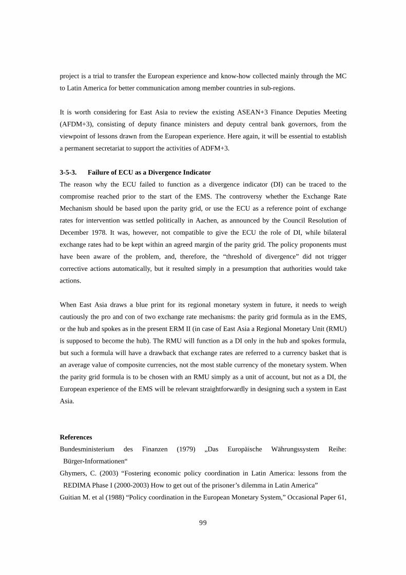
99

project is a trial to transfer the European experience and know-how collected mainly through the MC

to Latin America for better communication among member countries in sub-regions.

It is worth considering for East Asia to review the existing ASEAN+3 Finance Deputies Meeting

(AFDM+3), consisting of deputy finance ministers and deputy central bank governors, from the

viewpoint of lessons drawn from the European experience. Here again, it will be essential to establish

a permanent secretariat to support the activities of ADFM+3.

3-5-3. Failure of ECU as a Divergence Indicator

The reason why the ECU failed to function as a divergence indicator (DI) can be traced to the

compromise reached prior to the start of the EMS. The controversy whether the Exchange Rate

Mechanism should be based upon the parity grid, or use the ECU as a reference point of exchange

rates for intervention was settled politically in Aachen, as announced by the Council Resolution of

December 1978. It was, however, not compatible to give the ECU the role of DI, while bilateral

exchange rates had to be kept within an agreed margin of the parity grid. The policy proponents must

have been aware of the problem, and, therefore, the “threshold of divergence” did not trigger

corrective actions automatically, but it resulted simply in a presumption that authorities would take

actions.

When East Asia draws a blue print for its regional monetary system in future, it needs to weigh

cautiously the pro and con of two exchange rate mechanisms: the parity grid formula as in the EMS,

or the hub and spokes as in the present ERM II (in case of East Asia a Regional Monetary Unit (RMU)

is supposed to become the hub). The RMU will function as a DI only in the hub and spokes formula,

but such a formula will have a drawback that exchange rates are referred to a currency basket that is

an average value of composite currencies, not the most stable currency of the monetary system. When

the parity grid formula is to be chosen with an RMU simply as a unit of account, but not as a DI, the

European experience of the EMS will be relevant straightforwardly in designing such a system in East

Asia.

References

Bundesministerium des Finanzen (1979) „Das Europäische Währungssystem Reihe:

Bürger-Informationen“

Ghymers, C. (2003) “Fostering economic policy coordination in Latin America: lessons from the

REDIMA Phase I (2000-2003) How to get out of the prisoner’s dilemma in Latin America”

Guitian M. et al (1988) “Policy coordination in the European Monetary System,” Occasional Paper 61,

100

IMF

Kommission der Europäischen Gemeinschften/Generaldirektion Wirtschaft und Finazen (1979) Das

Europäische Währungssystem, „Europäische Wirtschaft Nr. 3“

Tietmeyer, H. (2005) “Herauforderung Euro,” Carl Hanser Verlag

Ungerer, H. et al. (1983) „The European Monetary System: the experience, 1979-82,“

Occasional Paper 19, IMF

Ungerer, H. (1997) “A Concise history of European monetary integration- from EPU to EMU,”

Quorum Books

101

CHAPTER 4

THE DESIRED ROLE OF PUBLIC AND

PRIVATE SECTORS TO PROMOTE RMU

DENOMINATED TRANSACTIONS

Chapter 4 : The Desired Roles of Public and Private Sectors to Promote RMU

(Regional Monetary Unit) Denominated Transactions

Introduction RMUs for transaction can be used as a unit of account in contracts and transactions. They can be

utilized as a unit of account in both the public and private sectors for international transactions, in

other words, in current account and capital transactions. This chapter will review what role the public

and private sectors can play in promoting the use of RMUs in the Asian region.

Based on last year’s report (IIMA(2006-2007)), the characteristics, utilities, and effects of RMUs will

be reviewed and the conditions to promote the use of RMUs will be presented. Then two options, one

stemming from their use in the private sector and the other involving the public sector, will be laid out.

Then possible measures for enhancing the use of RMUs will be considered. Discussions on the

means of promoting the use of RMUs tend to focus on the technical aspects, such as the designing of

the RMU denominated financial products, but in this chapter, a more comprehensive approach will be

taken to explore how RMU utilization could be expanded based on economic rationale and various

aspects will be considered including the economic environment.

The RMUs for transaction that are discussed in this chapter consist of convertible Asian currencies

whose component ratio is determined by using the weights calculated on the basis of fixed criteria and

have a different concept from the RMUs for surveillance discussed in Chapter 1. The RMUs for

transaction are the equivalent of the Core-RMUs introduced in last year’s report. (for details of

Core-RMUs, please refer to Chapter 1 of IIMA (2006-2007))

4-1. The characteristics, utilities and effects of RMU for transaction Let us review the characteristics, utilities and effects of RMU for transaction.

4-1-1. The characteristics

RMUs have the following two important characteristics.

The first is foreign exchange risk diversification. This is evident from the fact that a RMU is a

composite of a range of Asian currencies.

The second is that it offers the weighted average interest rate of the component currencies. As long as

foreign exchange risks are within acceptable bounds, the countries with relatively low interest rates

among the Asian economies can conduct their fund management in the RMU denominated financial

103

instruments, thereby being able to benefit from higher interest rates than if management operations

were conducted in their own currencies. On the other hand, by raising funds through RMU

denominated financial instruments, those with relatively high interest rates can raise funds with lower

interest rates than through financial instruments in home currency denominations. Because of such

features, RMU denominated financial products can be the bridge between the abundant savings and

high investment demand in the region.

4-1-2. Utilities

There are public and private means of utility.

4-1-2-1. Utilization in the public sector

The following are the possible means of official use. Table 1 shows the conceptual categorization.

(1) RMUs can be used as the accounting unit for public sector or multilateral institutions, or as the

denomination for asset and liabilities contracts among governments in the region. In more concrete

terms, a RMU can be used as a unit of account by the ADB or for ASEAN + 3 activities. The upper

limit for swap agreements in the Chiang Mai Initiative could also be denominated in a RMU.

(2) RMUs could be used for payments among governments or between governments and multilateral

institutions in the region, as the denomination for account transfers.

(3) RMUs could be used as foreign currency reserves. European countries used to hold the ECU

(European Currency Unit) as part of their foreign currency reserves, with their central banks paying in

20% of their gold reserve and 20% of their dollar reserve to the European Monetary Cooperation

Fund.

4-1-2-2. Utilization in the private sector

RMUs could be used in the following ways in the private sector.

(1) They could be used as the denominating currency for current account and capital account

transactions.

(2) They could be used as the vehicle, transaction and settlement currency in current and capital

account transactions. (This would, however, be difficult to realize unless there was a RMU

denominated fund settlement system)

(3) They could be used in asset denomination. Assets could include deposits, loans, securities and

derivatives.

104

Table1: Conceptual categorization of private and official use of RMUs

For private use For oficial use

Unit of account Denomination currency incurrent and capital transactions

Accounting unit of pulic sectorand multilateral institutions,Denomination for financialclaims and obligations amonggovernments

Medium of ExchnageVehicle, transaction, andsetllement currency in currentand capital transactions

Payment among governmentsand multilateral institutions

Store of value

Issuance of or investment inassets (deposits, loans,securities, derivatives, and soon)

Foreign reserves

4-1-3. Effects

4-1-3-1. Serving as a bridge between savings and investment in the region and contributing to

the development of the financial and capital markets.

The Asian currency crisis of 1997-98 brought an acute awareness that Asian financial and capital

markets had not been serving adequately as the intermediary between savings and investment.

Before the Asian currency crisis, savings from Asia took a roundabout route – first to the financial

institutions and markets in the developed countries, then from the financial institutions and investors

of the developed countries to the governments, financial institutions and corporations in Asia. Such

capital flows tended to be short-term, denominated in extra-regional currencies, such as the US dollar,

which were invested in tangible and financial assets in Asia. The investments were denominated in the

home currencies and were medium to long-term. As a result, the recipients of the investment ended up

being exposed to both foreign exchange and interest rate risks. Unfortunately, they did not fully

appreciate the risks and neglected to manage them.

This was due to the fact that some of the Asian economies had adopted the policy of applying an

exchange rate system akin to a dollar-peg system, while liberalizing cross-border flow of capital and

pursuing an autonomous monetary policy at the same time. Such a policy is contrary to the

“Impossible Trinity” thesis of international finance, which states that it is possible to meet two of the

three conditions but not all three simultaneously: exchange rate stability, free cross-border movement

of capital, and autonomy of monetary policy.

The contradiction was exposed by the precipitous withdrawal of funds from Asia in the 1997-98

period, the risks materialized as real losses and the situation developed into the Asian currency crisis.

The fundamental cause of the crisis was the application of policies that were contrary to “the

105

Impossible Trinity.” However, if the savings in regional currencies had been bridged to investment in

regional currencies in Asia, the risks would not have been so significant and even if they had

materialized, they could have been manageable (see Figure 1).

Savings

The Asian region

Investment intangible andfi i l

Financial institutions andinvstors outside the Region

Inflows of funds to theregion denominated incurrencies ouside theregion

Exchange rate risks areincurred by the entitieswithin the region

Figure 1 : Bridging between Savings and Investment within the Asian region

Case1: Bridge between savings and investment throughfinancial insitutions and investors outside the region

Savings Investment intangible andfinancial assets

Financial andcapital marketswithin the region

Outflows offunds to theoutside of theregion

Case2: Bridge between savings and investmentthrough financial and capital markets within the

iThe entities within the region are free from exchange rate risks aganstthe currencies outside the Region.The more stable the intra-regional exchnage rates are, the less exchangerate risks are incurred by the entities within the region.

Inprovement in financial and capital markets within theregion is being promoted by Asian Bond Markets Initiative(ABMI), Asian Bond Fund (ABF), or other initiavies.

The Asian region

Because a RMU diversifies foreign exchange risks and offers the weighted average interest rate of the

component currencies, RMU denominated financial products would promote bridging between Asian

savings and investment and contribute to the development of regional financial and capital markets.

Looking back at the experience of the Asian currency crisis, such a contribution would be highly

significant. The promotion of RMU use has the possibility of providing added support to the

development of Asian Bond Market Initiative (ABMI) and Asian Bond Fund (ABF), which are

endorsed to better organize the Asian financial and capital markets.

4-1-3-2. The increase of the extra-regional transactions denominated in RMU would contribute

to the lowering of foreign exchange risks which the region is exposed to

RMU denominated financial products would provide the weighted average value of the component

Asian currencies and interest rates. This would well suit foreign investors who want to invest not in

individual countries but in Asia as a whole. If the RMU denominated financial products are

recognized by non-regional investors as highly convenient for investment in Asia and if the

extra-regional governments, financial institutions and investors begin to deal in these products, then

funds would flow through the borders of Asia without the Asian fund raisers being exposed to foreign

exchange risks. For example, when Japanese investors bought the ECU bonds in the 80s and 90s, they

regarded the investment as “purchasing Europe by purchasing ECU bonds with the added benefit of

the higher interest rate than the German mark bonds.”

106

If the proportion of RMU denominated transactions should increase in the flow of capital between

Asia and other regions, then the foreign exchange risk that Asia as a region would be exposed to

would decrease and non-Asian regions would carry more of the burden.

4-2. Conditions to promote the use of RMUs What are the conditions for promoting the use of RMUs? To put it in another way, what are the

conditions for expanding the use of RMUs as a result of actions that are rational from the economic

perspective when there is nothing to enforce their use? The answer to “what conditions does a

currency have to meet to be chosen as a key currency from among a wide range of choices?” should

lie in the stability of the value of the currency and its low transaction cost. Similarly, the condition for

promoting the use of RMUs should lie in the stability of their value and their low transaction cost.

Unless the value is stable, it is not suitable as an accounting unit or a means for storing value, and

unless the transaction cost is low, it would not be logical to adopt it as a payment method.

In order to secure the stability of the value and the low transaction cost, network externalities,

economies of scale, and intra-regional economic and financial integration would play important roles.

4-2-1. Stability of the RMU value

What does the stability of RMU value mean? The RMU has an extra-regional (external) and an

intra-regional (internal) value.

Of the two, it is not realistic to aim for the stability of its external value. It is hardly possible to try to

stabilize the value of an Asian RMU against the dollar and the Euro, which are extra-regional

currencies. On the other hand, the stability of the RMU’s internal value could be achieved by close

cooperation within the region.

The stability of the RMU value, which is the key to promoting the use of RMUs, ｔranslates into the

stability of internal value, as the discussions presuppose the use of the RMU in the region. It is clear

that the stability of the internal value of a RMU is the same as the stability of the intra-regional foreign

exchange rates. As discussed in Chapter 1, monitoring the value of regional currencies against the

RMU for surveillance under the framework of regional surveillance in Asia is the most effective

method to stabilize the intra-regional foreign exchange rates. Although it would be difficult to

coordinate the foreign exchange rate policies in the region, discussions towards coordination should

begin.

107

The history of the use of the ECU in Europe also makes it clear that stability of the value is critical to

the use of a RMU. For example, the use of the ECU dropped precipitously when the foreign exchange

rate within Europe became volatile due to the European currency crisis in 1992-1993. The use of the

ECU recovered once the prospect of the ECU becoming the single currency, the Euro, became evident,

but if it had not been for such a prospect, the use of the ECU might not have recovered.

4-2-2. Low transaction cost of the RMU

The transaction cost of the RMU is the cost that is incurred when trading RMU denominated financial

products. This includes the cost that is incurred when hedging the foreign exchange and interest rate

risks that are associated with buying or selling RMU denominated financial products.

Apparently, a low transaction cost is important in promoting the use of RMUs. In addition to the

transaction cost, there is also the information cost associated with collecting information related to any

transaction. In the following section, the term “transaction cost” includes such information cost.

The following two conditions must be met to lower the transaction cost and for the low transaction

cost to promote the use of RMUs.

4-2-2-1. Transaction cost of the composite currencies of the RMU must be reasonably low

A market participant who has RMU short position in his balance sheet can hedge his foreign exchange

risk by buying RMU denominated financial assets or RMU forward contracts at the equal amount with

his short position in the market. However, if it should be difficult to buy RMU in the market as a

shortage of liquidity of RMU, it would be necessary to purchase the composite currencies of the RMU

at the ratio equivalent to the weight of the currencies within the RMU. This is called as bundling of the

RMU composite currencies. The opposite operation is called unbundling of the RMU composite

currencies.

This means that the cost of bundling and unbundling the RMU must be low enough for the RMU

transaction cost to be reasonably low. Since bundling and unbundling are purchasing and selling of

composite currencies, it would be critical for the transaction cost of the RMU composite currencies to

be low.

4-2-2-2. RMU transaction cost must be lower than the transaction cost of unbundling and

unbundling of the RMU.

It is important to note that the RMU transaction cost must be lower than the transaction cost of the

RMU composite currencies to promote the use of the RMU.

108

If the latter is lower, then it would be logical to break up the RMU denominated financial product into

financial products denominated in RMU composite currencies according to their weighted ratio and to

trade those products rather than to trade RMU denominated financial products.

In the case of the SDR, which was composed of five major currencies, US dollar, Japanese yen, West

German mark, French franc and British pound, there was no difference in the costs between

transactions in the SDR and transactions in individual currencies, so the market participants lost

interest in SDR denominated transactions. This was because the transaction cost of bundling and

unbundling of the SDR was low enough and management and fund raising in each currency could be

conducted freely. The transaction cost of the SDR was not low enough compared to the transaction

cost of its component currencies.

In Asia, with only a few exceptions, currencies do not have adequate convertibility. Financial and

capital markets have not developed enough, making the transaction cost for most currencies quite dear.

So the transaction cost of the possible composite currencies of an Asian RMU would be much higher

than those of SDR composite currencies.

In retail transactions, it may be possible for RMU transaction cost to be adequately lower than the

transaction cost of the RMU composite currencies, as it may be costly for retail customers to put

together RMU financial products out of the RMU composite currencies. However, as the size of

transactions increases, the difference between the two could easily shrink, and some serious thinking

is necessary to assure that “the RMU transaction cost is lower than the transaction cost of bundling

and unbundling of the RMU composite currencies.” Such a condition would be met if the effect of

“network externalities”, laid out in the next section, should spread sufficiently.

4-2-3. Network externalities

Externalities arising from network-effect are critical to lowering transaction costs. It is the case for

circulation of money.

The same applies for RMUs. In order to promote the use of a RMU, a mechanism must be created

whereby “people use the RMU because others are doing so.” If such a mechanism should be

developed, RMU denominated transactions would increase and the economies of scale would kick in

to decrease the transaction cost. Currently most of the cross-border transactions in Asia are

denominated in the US dollar and one would instinctively think that it is much more convenient to use

the dollar than RMUs. Hence some creative thinking is necessary to introduce the mechanism where

109

“a RMU is used because others are using it.”

How can network externalities be realized? One way could be through activities solely in the private

sector. The other is to enhance the benefits by involving the public sector. These possibilities will be

touched on in section “4-3., Sequencing to promote the use of RMUs.”

4-2-3. Economies of scale

Economies of scale are an important factor in lowering transaction costs. Due partly to the ABMI and

ABF, the size of the regional bond market is continuing to increase and conditions should be favorable

for the economies of scale to take effect and for transaction cost to decrease (see Table 2). Even then,

the transaction cost for bonds denominated in regional currencies, which is one of the costs, cannot be

said to be low. The data on bid-ask-spread for the bonds proves the point (see Table 3). If not only the

bond issuing balance but also the volume of transactions grow, then the economies of scale should

take effect, and the transaction cost and information cost should further decrease. Investors in Asian

bond market tend to buy and hold, and it is important to develop the secondary market as well as the

primary market.

110

Table 2: Outstandings of Bonds Issued in Local Currencies in East Asia

(Issued by governments, corporate business, and financial institutions)

Percent of GDP in billion US$ Percent of GDP in billion US$China 12.2 116.4 52.9 1,350.6Hong Kong 26.4 45.8 51.0 96.2Indonesia 1.9 4.6 15.2 53.4Korea 25.1 130.4 109.3 959.0Malaysia 56.4 57.0 82.5 121.3Philippines 20.5 16.9 37.5 43.9Singapore 24.8 23.8 74.3 99.2Thailand 6.7 10.5 57.6 112.0Vietnam - - 8.9 4.9Total 17.3 405.3 61.5 2,840.4

(Issued by govenments)

Percent of GDP in billion US$ Percent of GDP in billion US$China 7.1 67.4 34.4 877.9Hong Kong 7.6 13.1 9.0 16.9Indonesia 0.4 0.9 13.3 46.6Korea 4.2 21.6 53.5 469.1Malaysia 19.2 19.4 41.4 60.9Philippines 20.1 16.6 37.2 43.5Singapore 13.6 13.1 41.9 55.9Thailand 0.2 0.3 38.3 74.6Vietnam - - 8.2 4.5Total 6.5 152.4 35.7 1,649.9

(Issued by corporate business and financial institutions)

Percent of GDP in billion US$ Percent of GDP in billion US$China 5.1 49.0 18.5 472.7Hong Kong 18.8 32.7 42.0 79.3Indonesia 1.6 3.7 2.0 6.8Korea 20.9 108.8 55.8 489.8Malaysia 37.2 37.6 41.1 60.4Philippines 0.4 0.3 0.3 0.4Singapore 11.2 10.7 32.4 43.3Thailand 6.5 10.2 19.2 37.4Vietnam - - 0.8 0.4Total 9.0 253.0 25.8 1,190.5Source: Asian Bond Online （http://asianbondsonline.adb.org/regional/regional.php）

End of December 1997 End of December 2006



111

Table 3: Bid-ask-spread in secondary bond markets in East Asia

2000 2006 2000 2006China - 10.8 15.0 7.6Hong Kong 8.0 6.3 3.5 3.0Indonesia 100.0 68.8 100.0 16.9Korea 5.0 3.0 1.8 1.4Malaysia 15.0 18.8 4.9 2.3Phillipines 40.0 30.0 47.5 25.3Singapore 10.5 5.5 1.6 2.7Thailand 10.0 10.8 2.8 3.0Vietnam - 14.9 N/A N/AJapan 9.3 6.0 0.6 0.6Source: Asian Bond Online （http://asianbondsonline.adb.org/regional/regional.php）

Issued by corporate business andfinancial institutions

（basis points）

Issued by governments（basis points）

4-2-4. Enhancing economic and financial integration

As the regional economic and financial integration deepens, in other words, as interdependence in the

regional transaction of goods and services as well as in financial and capital transaction grows, the

mechanism of “I will use the RMU because the others are” should work better.

It would be easier for the economies of scale to take effect as regional economic and financial

integration deepens, as that would lead to the increase in the volume of regional goods and services

transactions and the expansion of regional financial and capital markets.

At the same time, the benefit of stable regional foreign exchange rates should also increase as regional

economic and financial integration deepens. This means that as integration deepens, it is possible that

cooperation towards regional foreign exchange stability would strengthen. If such cooperation should

materialize, that would enhance the stability of the RMU value.

Regional economic and financial integration would not only lead to the lowering of transaction costs

but also contribute to the stability of the RMU value.

4-3. Sequencing of the use of RMUs In view of the conditions for promoting the use of RMUs as shown in 4-2., there are two routes in

which the use of RMUs could be promoted. One is to start by using RMUs solely in the private sector

and the other is to involve the public sector.

4-3-1. Starting by using RMUs solely in the private sector

An agreement within the region would, of course, be necessary to realize an official RMU, which does

112

not seem likely at this point. If the promotion of the use of RMUs must begin in the private sector, the

following conditions are presupposed.

• Since there is no single official or private RMU in existence, the component currencies and

their weight would have to be defined by those involved in creating the RMUs. The RMUs

would be “made-to-order” and contracts and transactions would be based on the agreed

definition, which means that there would be multiple RMUs.

• Since it would be difficult to limit to one RMU, it would not be easy to establish a RMU

denominated fund settlement system like the ECU Clearing System which exited in Europe in

the 1980-90s. The settlement of RMU denominated transactions would have to be conducted by

exchanging the amount of existing currencies equivalent to the RMU settlement amount.

If a RMU denominated fund settlement system could not be established because there could not be

one RMU, it would be difficult to benefit from “network externalities,” which is “I will use the RMU

because the others are.”

However, if there were a private financial institution that would systematically deal with RMU

denominated transactions for some reason and function as a RMU fund settlement system, and

user-friendly RMU services were offered by the institution, then “network externalities” whereby “I

will use that private financial institution because others are” cycle could be created.

The following things become clear by studying the use of the ECU in the private sector in Europe.

• The use of a RMU begins with long-term financial products and moves to short-term products.

This is because without the establishment of the RMU denominated fund settlement system, it

is difficult to promote the use of RMUs for short-term financial products.

• While a RMU denominated fund settlement system is not available, the promotion of RMU

denominated bonds, loans, deposits, investment funds and index transactions could be promoted

by settling transactions in the equivalent amount of existing currencies.

• Although it is possible to promote the use of RMUs in financial (capital) transactions, their

promotion would be limited in commercial (current account) transactions. Diversifying foreign

exchange risks and providing weighted average interest rates, which are the characteristics of

RMUs, are attractive in financial transactions, however, could only bring about complications in

commercial transactions because companies aim to maximize profits in the home currency.

Although it may be difficult to establish a RMU denominated fund settlement system for the time

being, it is necessary to try to establish one at an early stage in the process of increasing the use of

RMU for transaction.

113

4-3-2. Involving the public sector in the private use of RMUs

In considering the involvement of the public sector in the private use of RMUs, the following choices

can be studied.

(i) Official support to the private use of RMUs

There could be an official support of RMU denominated transactions in the private sector even if there

is no official RMU. Drawing from the experience of the ECU in Europe (IIMA (200-2007), Chapter 3),

the following means of official support are possible; excluding RMU denominated transactions from

the list of products regulated under the Foreign Exchange Law, providing favorable tax treatment such

as concerning the withholding tax, issuance of RMU denominated public debt securities by

governments and multilateral institutions, and supporting the establishment of a RMU denominated

settlement system. These measures would have the effect of promoting RMU denominated

transactions.

(ii) Definition of an official RMU and its creation

As seen in 4-1-3., it is possible to define a single official RMU with the agreement of the regional

authorities and use it for ASEAN + 3 activities, accounting unit for the ADB, unit of quotation for

asset and liabilities among the regional authorities, and as an unit to indicate the swap size under the

Chiang Mai Initiative.

In Europe, the member central banks paid in 20% of their gold holdings and 20% of their dollar

foreign reserve to the European Monetary Co-operation Fund and held the equivalent of the two as

foreign currency reserve in the ECU. However, a RMU denominated foreign currency reserve could

be created in Asia in the same way, only if the RMU gains enough credibility among the regional

governments.

Once the definition of an official RMU is clarified and its use prevails in the private sector, it would

make it easier to establish a RMU fund settlement system, leading to the expansion of private and

official use of the RMU.

(iii) Using the official RMU for transactions between the official and the private sectors

The official ECU was used in Europe only for transactions within the public sector – among

governments and between governments and multilateral institutions – but not for payments to the

private sector. Transactions between the official and the private ECU were prohibited.

Revoking this ban would encourage the involvement of the public sector in RMUs. The official ECU

114

could be used for payment to the private sector and the private RMU that the public sector receives

from the private sector could be used as an official RMU for payments among governments. This

would mean supplying RMU denominated liquidity from the public to the private sector as well as

withdrawal of liquidity, possibly influencing liquidity in the financial markets and interest rates of the

member countries. To allow transactions between the official and private RMUs, the government

authorities in the region must be able to demonstrate that they can adequately control liquidity and

interest rates.

(iv) Accepting the official RMU as another legal tender

There is a possibility of accepting an official RMU as another legal tender along with the legal

currency. However, when there are two legal tenders in a country, funds could shift from one to the

other based on interest rate and foreign exchange rate fluctuations or expectations of such fluctuations,

and could destabilize the financial system. Such side-effects should be taken into account and weighed

carefully when considering the possibility of accepting an official RMU as another legal tender.

The significance of public sector involvement is in promoting the use of RMUs in the private sector

through the “network externalities” effect. However, (iv) and (iii) were not applied in the case of the

ECU in Europe, and side effects to the regional financial markets and monetary policies could not be

small. This means that the realistic approach is to start a dialogue among the regional authorities on (i)

and (ii). It is crucial to expand the market size for RMU transaction large enough in the initial stage,

so that the use of the RMU prevails in the region. In other words, exceeding critical mass is important.

Public sector involvement would be able to play an important role in it, through the effects of network

externalities and economies of scale.

4-4. Measures to promote the use of RMUs The key factor when considering the means to promote the use of RMUs is how to create the situation

under which the demand for RMU denominated financial products would grow. It is also important to

develop an environment where the RMU denominated transactions would increase based on the

economic rationale of low RMU transaction cost and price stability.

4-4-1. Promoting regional economic and financial integration

Regional economic and financial integration is a significant factor in furthering the attraction of

RMUs, and the two complement each other. It is especially important to encourage regional financial

integration, which is far behind economic integration. Here, lessons will be drawn from the process

under which the German mark became the key currency in Europe in the 1980s. The importance of the

115

link among various financial and capital markets in the process of financial integration will also be

made clear.

4-4-1-1. Promotion of regional economic and financial integration and expanding the use of

RMUs are mutually complementary

Why is it important to enhance regional economic and financial integration to increase the attraction

of using RMUs? This is because a positive cycle could start whereby regional economic and financial

integration deepens, which would promote the utilization of RMUs, which would further deepen

regional economic and financial integration.

As mentioned above, promotion of regional integration would strengthen interdependence in the

region, and when regional transactions increase, RMU transaction costs should decline through

network externalities and the effects of the economies of scale. Also, when regional integration

deepens, regional foreign exchange rate stability becomes more important, and because the regional

authorities could strengthen their cooperation to realize that stability, the value of RMUs could also

stabilize. If the attraction of RMUs should increase for the private sector, RMU transactions would

increase. This would enhance the bridging of savings and investment in the region, contribute to the

development of financial and capital markets in the region and further contribute to the promotion of

regional economic and financial integration.

If the deepening of regional economic and financial integration should influence the policies of the

regional governments concerning political cooperation towards regional integration and if it should

become possible to achieve an agreement among regional governments concerning RMU’s official use,

then the RMU transaction cost would further lower through network externalities, which would

promote the use of the RMU. Figure 2 shows this mechanism. As is clear, the promotion of Asian

regional economic and financial integration is indispensable to the promotion of RMU utilization, and

the two are mutually complementary.

116

Network externalities

Figure 2: Virtuous Circle of the Use of RMU for Transaction and Regional Integration in Asia

Economic and financialintegration in the region

Increase in the privateuse of RMUs

Closer coordinationtoward intra-regionalexchnage rate stability

The Official use of RMUs

Economy of scale

Lower transaction costsof RMUs

More stable valueof RMUs

Bridge between savings and investment in the regionDevelopment of financial and capital market in the region

Political cooperation towardreginal intergartion

*

* Refer to 4-4-1-3.Asian Bond Markets Initiative (ABMI)Asian Bond Fund (ABF)

4-4-1-2. The importance of promoting regional financial integration

Until now, Asian economic integration has been market-led, not policy-led. Production networks were

established through direct investment by foreign-affiliated companies and that contributed to the

expansion of regional trade. More recently, since the beginning of this millennium, the number of free

trade agreements (FTA) signed among the regional economies has multiplied, and there is likely to be

a network of FTAs in Asia in the near future. This means that now, economic integration in Asia is

supported both by policy and markets.

Here, it must be emphasized that financial integration is still far behind economic integration. The

regional trade ratio, which indicates the extent of economic integration, was 59% for imports and 50%

for exports on average in 2005 (see Table 4). But financial integration is nowhere near the economic

integration. Statistics that help to grasp the regional flow of funds comprehensively is still lacking.

However, looking at cross-border portfolio investment, outflows from East Asia to the intra-regional

countries as a percentage of the outflows to the world is 6.5%, and inflows from the intra-regional

countries to the East Asia as a percentage of the inflows to the world is 9.4% (see Table 5).

117

Table 4: Trade Flows

2005 From (In billions of US dollars) (Percentage of sub total)

NAFTA EU25 East AsiaRest of theWorld

WorldTotal NAFTA EU25 East Asia

Rest of theWorld

WorldTotal

In NAFTA 805 364 564 372 2,105 38.3 17.3 26.8 17.7 100.0EU25 216 2,642 415 727 3,999 5.4 66.1 10.4 18.2 100.0East Asia 234 239 1,371 476 2,320 10.1 10.3 59.1 20.5 100.0Rest of the World 205 741 397 628 1,970 10.4 37.6 20.1 31.9 100.0World Total 1,461 3,984 2,747 2,202 10,394 14.1 38.3 26.4 21.2 100.0

(Percentage of sub total) (Percentage of World Total)NAFTA 55.1 9.1 20.5 16.9 20.3 7.7 3.5 5.4 3.6 20.3EU25 14.8 66.3 15.1 33.0 38.5 2.1 25.4 4.0 7.0 38.5East Asia 16.0 6.0 49.9 21.6 22.3 2.3 2.3 13.2 4.6 22.3Rest of the World 14.0 18.6 14.4 28.5 19.0 2.0 7.1 3.8 6.0 19.0World Total 100.0 100.0 100.0 100.0 100.0 14.1 38.3 26.4 21.2 100.0

2001 From (In billions of US dollars) (Percentage of sub total)

NAFTA EU25 East AsiaRest of theWorld

WorldTotal NAFTA EU25 East Asia

Rest of theWorld

WorldTotal

In NAFTA 639 254 376 189 1,458 43.8 17.4 25.8 12.9 100.0EU25 180 1,623 234 361 2,398 7.5 67.7 9.8 15.1 100.0East Asia 187 151 693 217 1,248 15.0 12.1 55.5 17.4 100.0Rest of the World 145 407 193 294 1,039 14.0 39.1 18.6 28.3 100.0World Total 1,151 2,436 1,496 1,061 6,144 18.7 39.6 24.4 17.3 100.0


Note: East Asia = Japan, China, Hong Kong, Singapore Indonesia, Malaysia, Philippines, and ThailandSource: IMF, Direction of Trade Statistics

Table 5: Cross-Border Portfolio Invetment Flows

2005 From (in billions of US dollars) (Pecentage of sub total)

NAFTA EU15EastAsia

Rest of theWorld

WorldTotal NAFTA EU15

EastAsia

Rest of theWorld

WorldTotal

In NAFTA 767 2,309 911 2,076 6,063 12.7 38.1 15.0 34.2 100.0EU15 2,086 8,146 960 1,789 12,981 16.1 62.8 7.4 13.8 100.0East Asia 834 755 184 185 1,958 42.6 38.5 9.4 9.5 100.0Rest of the World 1,383 1,951 755 770 4,859 28.5 40.2 15.5 15.9 100.0World Total 5,070 13,161 2,810 4,820 25,860 19.6 50.9 10.9 18.6 100.0

(Pecentage of sub total) (Pecentage of World Total)NAFTA 15.1 17.5 32.4 43.1 23.4 3.0 8.9 3.5 8.0 23.4EU15 41.1 61.9 34.2 37.1 50.2 8.1 31.5 3.7 6.9 50.2East Asia 16.5 5.7 6.5 3.8 7.6 3.2 2.9 0.7 0.7 7.6Rest of the World 27.3 14.8 26.9 16.0 18.8 5.3 7.5 2.9 3.0 18.8World Total 100.0 100.0 100.0 100.0 100.0 19.6 50.9 10.9 18.6 100.0

2001 From (in billions of US dollars) (Percentage of sub total)

NAFTA EU15EastAsia

Rest of theWorld

WorldTotal NAFTA EU15

EastAsia

Rest of theWorld

WorldTotal

In NAFTA 415 1,300 585 1,206 3,506 11.8 37.1 16.7 34.4 100.0EU15 1,264 3,603 585 857 6,309 20.0 57.1 9.3 13.6 100.0East Asia 325 303 86 126 840 38.7 36.0 10.2 15.0 100.0Rest of the World 560 799 359 338 2,056 27.3 38.8 17.5 16.4 100.0World Total 2,565 6,005 1,615 2,526 12,711 20.2 47.2 12.7 19.9 100.0


Note: East Asia = Japan, China, Hong Kong, Singapore Indonesia, Malaysia, Philippines, and ThailandSource: IMF, Coordinated Portfolio Inverment Survey

However, promotion of financial integration is especially important for the promotion of RMUs

because the kind of transaction where the dual RMU attraction of providing foreign exchange risk

118

diversification and weighted average interest rate of the regional currencies can be utilized is a

financial transaction rather than trade related transaction. The fact that the ECU was used for financial

and capital transactions rather than in trade transactions supports this assertion. The demand for

RMUs would only increase with the expansion of the regional capital flow through financial

integration.

What are the factors that encourage financial integration? On this, the work by Cowen, Salgado, Shah,

Teo, and Zanello (2006) gives a detailed analysis. The index of their work is as follows:

Strengthening Capital Markets

Developing institutional investors

Strengthening corporate governance

Improving transparency

Building Market Infrastructures

Enhancing market depth and liquidity

Linking clearing and settlement systems

Regional credit rating and benchmarks

Minimizing Risks

Moving towards risk-based supervision

Addressing cross-sectoral and cross-boarder issues

Removing Impediments

Further capital account liberalization

Liberalization of financial services and prudential regulation

Harmonizing Rules and Practices

Strengthening implementation of global standards and best practices

Regional efforts at harmonization

Improving International and Regional Cooperation

4-4-1-3. Lessons from the process in which the German mark became the key currency in the

1980s.

The process in which the German mark became the key and the intermediary currency of Europe in

the 1980s indicates how RMU utilization could be increased when regional financial integration

lowers the transaction cost of the RMU (refer to Soko (1996) for details).

The US dollar had been the key currency in Europe, but the German mark strengthened its role as the

key currency in the 1980s. The background to this development was the fact that as regional financial

119

integration deepened, the foreign exchange trading spread among the regional currencies shrunk

significantly, and it became cheaper to use the German mark as the intermediary of regional currency

trading than to use the US dollar. This enhanced the mark’s role as the key currency. The buying and

selling of European currencies were necessary for the bundling and unbundling of the ECU and as the

German mark increased its role as the key currency, the process would also have lowered the trading

cost of European currencies and the transaction cost of the ECU denominated products.

The above process could have encouraged the use of the private ECU in Europe. Although it is not an

easy task to provide a point by point evidence of the effects, it is safe to say that the way in which the

German mark became the key currency in Europe provides an invaluable indication of how the use of

RMUs could be promoted in Asia today.

<The European experience>

Generally speaking, foreign exchange bid-ask spread shrinks as the volume of foreign exchange

trading increases and foreign exchange rate fluctuation becomes smaller. The spread for foreign

exchange trading between regional currencies would become smaller as economic and financial

integration deepens, the volume of foreign exchange trading of the currency increases and regional

foreign exchange policy coordination strengthens.

Economic and financial integration was continuing in the 1980s in Europe, but the important

development was the increase of capital flow in the region, which deepened financial integration. The

increase was due to the rise in the amount of European currency denominated bonds issued in the Euro

market, the increased flow of household savings to institutional investors, the increase of foreign

portfolio in the investment made by institutional investors, etc. This led to the rise in cross-border

portfolio investment in the region where an investor from a member country would buy securities

from another member country, and expanded the volume of foreign exchange trading among the

regional currencies.

It should be emphasized that a dramatic increase in the foreign exchange trading of regional currencies

was possible with the expansion of cross-border portfolio investment, which is the deepening of

financial integration, and would have been very difficult to achieve merely from the deepening of

economic integration such as an increase in intra-regional trade.

At the same time, the volatility of regional currencies’ exchange rates dropped sharply due to the

European Monetary System (EMS), and became far less than the volatility of the foreign exchange

rate of the European currencies against the dollar. This helped to shrink the foreign exchange bid-ask

spread among the European currencies.

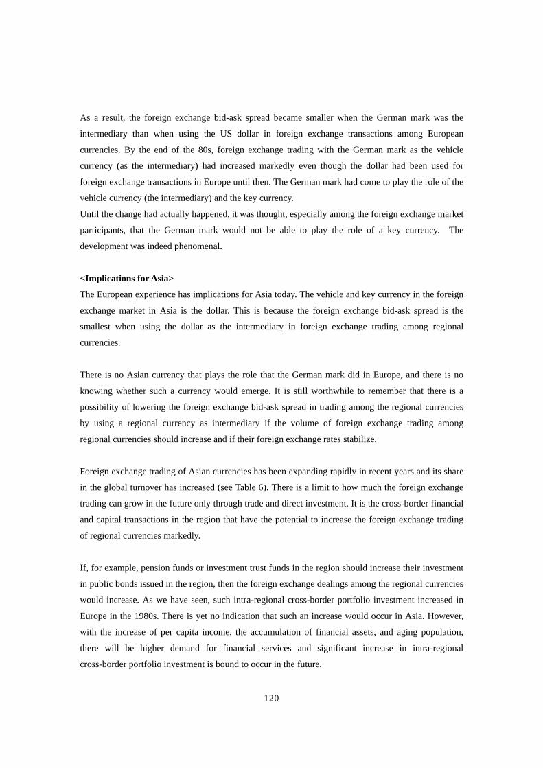
120

As a result, the foreign exchange bid-ask spread became smaller when the German mark was the

intermediary than when using the US dollar in foreign exchange transactions among European

currencies. By the end of the 80s, foreign exchange trading with the German mark as the vehicle

currency (as the intermediary) had increased markedly even though the dollar had been used for

foreign exchange transactions in Europe until then. The German mark had come to play the role of the

vehicle currency (the intermediary) and the key currency.

Until the change had actually happened, it was thought, especially among the foreign exchange market

participants, that the German mark would not be able to play the role of a key currency. The

development was indeed phenomenal.

<Implications for Asia>

The European experience has implications for Asia today. The vehicle and key currency in the foreign

exchange market in Asia is the dollar. This is because the foreign exchange bid-ask spread is the

smallest when using the dollar as the intermediary in foreign exchange trading among regional

currencies.

There is no Asian currency that plays the role that the German mark did in Europe, and there is no

knowing whether such a currency would emerge. It is still worthwhile to remember that there is a

possibility of lowering the foreign exchange bid-ask spread in trading among the regional currencies

by using a regional currency as intermediary if the volume of foreign exchange trading among

regional currencies should increase and if their foreign exchange rates stabilize.

Foreign exchange trading of Asian currencies has been expanding rapidly in recent years and its share

in the global turnover has increased (see Table 6). There is a limit to how much the foreign exchange

trading can grow in the future only through trade and direct investment. It is the cross-border financial

and capital transactions in the region that have the potential to increase the foreign exchange trading

of regional currencies markedly.

If, for example, pension funds or investment trust funds in the region should increase their investment

in public bonds issued in the region, then the foreign exchange dealings among the regional currencies

would increase. As we have seen, such intra-regional cross-border portfolio investment increased in

Europe in the 1980s. There is yet no indication that such an increase would occur in Asia. However,

with the increase of per capita income, the accumulation of financial assets, and aging population,

there will be higher demand for financial services and significant increase in intra-regional

cross-border portfolio investment is bound to occur in the future.

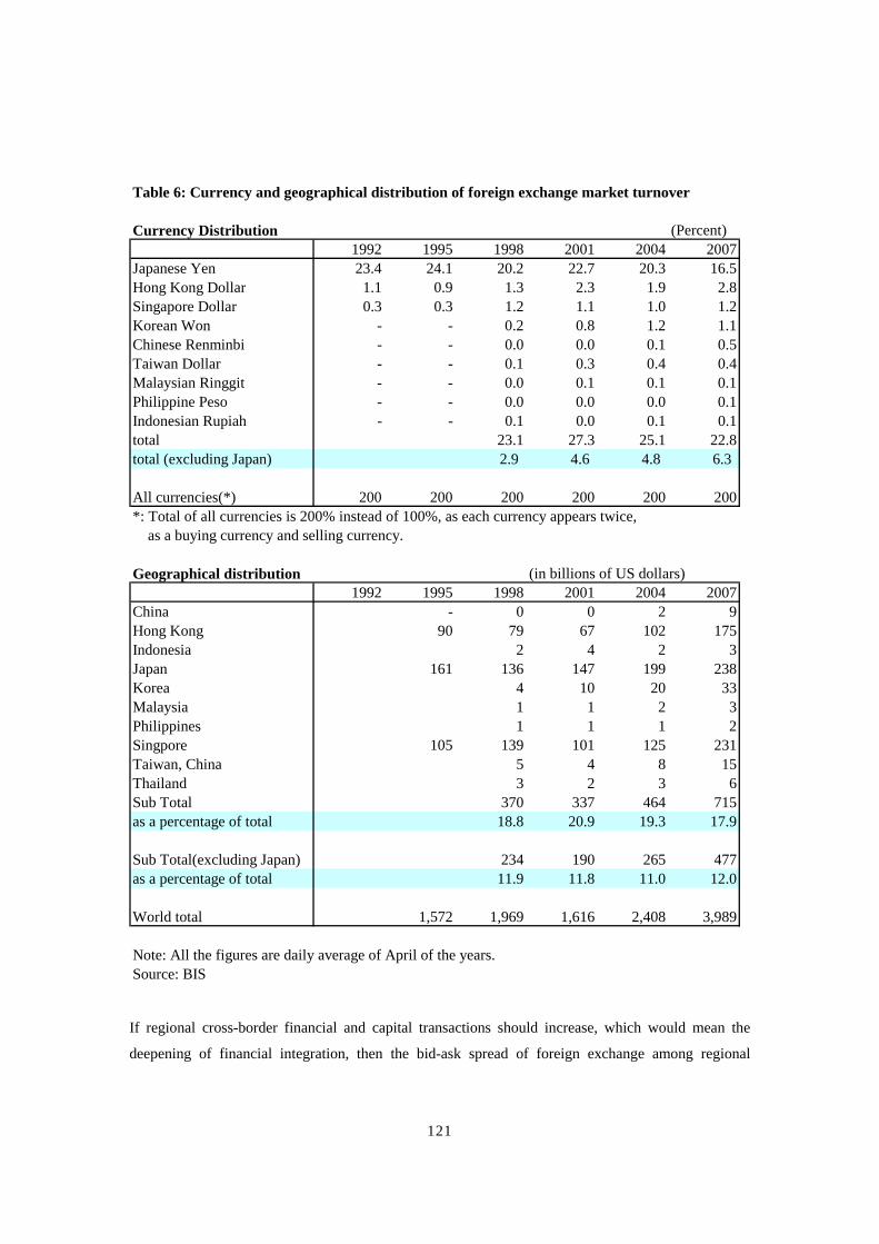
121

Table 6: Currency and geographical distribution of foreign exchange market turnover

Currency Distribution (Percent)1992 1995 1998 2001 2004 2007

Japanese Yen 23.4 24.1 20.2 22.7 20.3 16.5Hong Kong Dollar 1.1 0.9 1.3 2.3 1.9 2.8Singapore Dollar 0.3 0.3 1.2 1.1 1.0 1.2Korean Won - - 0.2 0.8 1.2 1.1Chinese Renminbi - - 0.0 0.0 0.1 0.5Taiwan Dollar - - 0.1 0.3 0.4 0.4Malaysian Ringgit - - 0.0 0.1 0.1 0.1Philippine Peso - - 0.0 0.0 0.0 0.1Indonesian Rupiah - - 0.1 0.0 0.1 0.1total 23.1 27.3 25.1 22.8total (excluding Japan) 2.9 4.6 4.8 6.3

All currencies(*) 200 200 200 200 200 200*: Total of all currencies is 200% instead of 100%, as each currency appears twice, as a buying currency and selling currency.

Geographical distribution (in billions of US dollars)1992 1995 1998 2001 2004 2007

China - 0 0 2 9Hong Kong 90 79 67 102 175Indonesia 2 4 2 3Japan 161 136 147 199 238Korea 4 10 20 33Malaysia 1 1 2 3Philippines 1 1 1 2Singpore 105 139 101 125 231Taiwan, China 5 4 8 15Thailand 3 2 3 6Sub Total 370 337 464 715as a percentage of total 18.8 20.9 19.3 17.9

Sub Total(excluding Japan) 234 190 265 477as a percentage of total 11.9 11.8 11.0 12.0

World total 1,572 1,969 1,616 2,408 3,989

Note: All the figures are daily average of April of the years.Source: BIS

If regional cross-border financial and capital transactions should increase, which would mean the

deepening of financial integration, then the bid-ask spread of foreign exchange among regional

122

currencies would be reduced due to the increase in foreign exchange turnover. This would lower the

cost of trading among Asian currencies, which is necessary for RMU bundling and unbundling, and

lower the transaction cost of using RMUs. The European experience implies that the deepening of

financial integration combined with the intra-regional exchange rate stability due to the EMS is

critical for the promotion of RMU utilization.

4-4-1-4. The importance of the linkage among the financial and capital markets

Arbitrary transactions are conducted among the foreign exchange, money, bond and securities markets

through the mechanisms of foreign exchange swap spread, yield curve, return on equity investment

and interest rates. Since these markets are linked, their development is mutually complementary.

For example, nurturing of the repo market, which is a short-term financial market, is indispensable for

the nurturing of a bond market, especially its secondary market. In order to develop a bond market,

especially its secondary market, it is necessary for the bond-holding investors to be able to trade bonds

flexibly and to use the portfolio to raise or manage funds with ease. For this, the investors must be

able to conduct bond repurchasing transactions with ease. This means that the nurturing of the

secondary market for bonds and the nurturing of the bond repo market are complementary and in close

relation to each other.

Efforts are being made to develop the regional bond markets through the ABMI and ABF. However, it

is also important to nurture and maintain markets besides the bond market, since their development is

all mutually complementary.

The institutions that issue RMU denominated financial products or those holding such products would

need to manage foreign exchange and interest rate risks or to hedge such risks flexibly. In order to

meet such needs, the foreign exchange markets of the component currencies, money markets and bond

markets need to be developed adequately.

4-4-2. Convertibility of component currencies: capital account liberalization vs stability of

regional foreign exchange rates

Convertibility of the component currencies of a RMU is an indispensable condition for the bundling

and unbundling of the RMU and for risk-hedging associated with asset and liabilities holdings in

RMU denomination. To put it in other way, it is a condition for adequately lowering the transaction

cost of the RMU. Convertibility means that not only the residents but also non-residents are able to

directly or indirectly, through the financial institutions of the country, have access to the foreign

exchange market of the currency of that country and be able to trade that currency.

123

Convertibility of the RMU component currencies is also important in order to maintain a market

mechanism where the value of an official RMU and private RMU would converge through arbitrary

transaction, if an official RMU is created and if the RMU with the same definition should be used in

the private sector.

It would, of course, be putting the horse before the cart, if capital account liberalization should be

advanced in order to promote the use of RMUs. Capital account liberalization should move in tandem

with economic and financial development, and the home currency should become convertible at a

suitable timing within that process. This is one of the lessons to be learned from the Asian currency

crisis.

If a country still needs some regulations to limit the convertibility of its home currency, it may be able

to promote the use of RMUs by permitting its home currency to be convertible only when the currency

is traded in transactions related to RMUs. Such a policy was seen in several countries in Europe in the

1980s.

There is an important aspect to be emphasized at this point. That is the contradiction between capital

account deregulation and stability of intra-regional foreign exchange rates. There are two scenarios

(A) and (B).

Capital account deregulation full convertibility of RMU’s component currencies increase the

foreign exchange trading of the component currencies

(A) Increase the liquidity of trading lowering of the foreign exchange bid-ask spread

lowering of the transaction cost associated with the bundling and unbundling of RMUs

(B) increase the volatility of the foreign exchange rates

The outcome of (A) is desirable while (B) is not. As the “Impossible Trinity” shows, this is because if

the autonomy of national monetary policies is assumed, then it is not possible to achieve both progress

in the convertibility of component currencies, which is part of capital account liberalization, and

stability of the intra-regional foreign exchange rates.

Looking at the situation in Europe in the 1980s, financial globalization was much less advanced

compared to what it is now and the amount of funds that moved over borders freely was not so large.

So it was less difficult to stabilize the intra-regional foreign exchange rates while accepting the free

movement of capital, and the contradiction between (A) and (B) was not significant. However, with

124

the massive development in financial globalization, the problems emerging from the contradiction

must be seriously taken into account.

That is why the measures to reduce the volatility of the regional foreign exchange rates discussed

under the RMU for surveillance has an important connotation for RMU for transaction. If a member

country joins RMU for transaction as a composite currency by achieving full convertibility of the

currency, it is inevitable to step forward more close intra-regional coordination of macro-economic

policies in order to avoid an excessive volatility of the currency.

In the future, there could be a framework for intra-regional coordination of macro-economic economic

policies including exchange rate policy. The most binding measure for intra-regional exchange rate

stability would be the construction of regional exchange rate regime like the EMS. There could be

discussions on the kind of regional exchange rate regime to be established in the era of financial

globalization. Some regional exchange rate regime would be necessary to make the value of RMUs

stable enough so that the use of RMU for transaction would be significantly increased.

4-4-3. Features to take into account when designing RMU denominated financial products so

as to attract demand

4-4-3-1. Characteristics of a RMU as a pre-packaged product

RMU denominated financial instruments would be used for fund management and raising by financial

institutions, institutional investors, and large companies. They would be also used by retail customers

such as small and medium-sized companies and individuals. Retails investors can avoid the hassle of

buying individual currencies by purchasing a RMU denominated product in which multiple Asian

currencies have been packaged. For example, recently in Japan, more retail investors are interested in

diversified international investment. Therefore, RMU denominated investment instruments could

become attractive as a pre-packaged product among them, if the liquidity of the market is sufficient.

4-4-3-2. Possibilities of products that have the same or similar economic effect as RMUs

In the course of promoting the use of RMUs, the possibility of the following financial products is

worth considering.

• Define a RMU in the private sector and design RMU denominated financial products based on

that definition.

(Example) RMU denominated bonds and loans, RMU denominated index trading:

If there is a possibility that the composition and weighting scheme of the RMU product could

change before maturity, it would be necessary to clearly define whether the product would be

125

applied a closed basket method, where the value of the RMU would be calculated using the initial

definition even after the change of the composition and weighting scheme, or an open basket

method, where the value would be adjusted according to the new definition. For developing RMU

market, open basket method would be better than closed basket method. This is because single

RMU would prevail in the market with open basket method, while there can be several kinds of

RMUs in the market with closed basket method such as RMU based on the definition in year X or

the one in year Y. Several kinds of RMUs in the same market seem complicated for the market

participants.

• Products that could have a similar economic effect even though it is not defined as a RMU

product.

It is possible to design a financial product that has the similar economic effect as a RMU

denominated financial product by mixing financial products denominated in multiple regional

currencies in the asset-backed securities method or investment trust fund method.

4-4-3-3. Transparency of data necessary for calculating RMUs

It is necessary to clearly define not only the means of calculating a RMU and the weight of component

currencies but also the data which is used to calculate the RMU such as the foreign exchange rates of

the component currencies and interest rates. Foreign exchange rates and interest rates could be very

different depending on the market maker, so highly transparent data must be provided to enhance the

efficiency of markets.

When the official RMU is defined and created, information on the official RMU must be provided just

as the IMF publicizes the SDR rate everyday. This could be done by establishing an ASEAN + 3

Secretariat and disseminating the information from there or any other institution commissioned by it

could provide the information.

4-4-4. Financial regulations and supervisions

As is pointed out in the previous sections, enlargement of the use of RMU is desirable for the

development of financial and capital market in the region as well as regional financial integration.

However, as there is a exchange rate risk between a home currency and a RMU, RMU denominated

financial products must be under regulations and supervisions which are applied to foreign currency

denominated financial product in each country in the region.

4-5. Policy implications for East Asia The studies in this chapter can be summarized as follows.

126

The RMU for transaction, which is composed of multiple convertible currencies, has the function of

diversifying foreign exchange risks and providing a weighted average interest rate of the component

currencies. It can be used as a unit of account, medium of exchange and store of value in the private

and public sectors. The increase of RMU denominated transactions would contribute to the

development of regional financial and capital markets by bridging the savings and investment in the

region. If the extra-regional RMU denominated transactions should increase, that would contribute to

reducing the foreign exchange risk contained in the region.

Stability of the value (same as the stability of intra-regional foreign exchange rates) and low

transaction cost are necessary to promote the use of RMUs. In order to meet these conditions, network

externality, which is “I will use the RMU because the others are”, economies of scale, and regional

economic and financial integration would play important roles. Public sector involvement is especially

important in initiating the usefulness of network externality. There are a number of ways in which the

public sector could be involved such as preferential treatment under the foreign exchange law or tax

laws, issuance of RMU denominated public bonds, and creation of official RMUs. All the possibilities

could be discussed among governments in the region. It is also important to note that bridging the

savings and investment in the region would have the effect of further promoting the regional economic

and financial integration.

The experience in Europe leads one to believe that the stability of the EMS and financial integration

played an important role in promoting the use of a RMU. In East Asia, however, the intra-regional

trade ratio is high, while the intra-regional cross-border portfolio investment ratio is low. Therefore, in

order to facilitate financial integration, markets should be strengthened, financial infrastructure should

be more developed, capital account liberalization should be orderly enhanced, and more

harmonization should be created in legal system and practices of countries in the region.

It is important to remember that there is an inherently contradictory aspect in going ahead with capital

account liberalization aimed at enhancing the convertibility of regional currencies. On one hand it has

the effect of lowering transaction costs, on the other it has the danger of increasing the volatility of

foreign exchange rates. Therefore, taking measures to stabilize the intra-regional foreign exchange

rates is indispensable for the promotion of RMU utilization. In order to achieve foreign exchange rate

stability in the region, there must be a keen awareness that RMU for surveillance, which aims for

regional foreign exchange stability, and RMU for transaction, which helps promote regional economic

and financial integration, are mutually complementary.

127

It is necessary to continue studying the product designs in order to increase the demand for RMU

denominated financial products.

Following are the policy implications based on the above analysis.

(I) The promotion of regional economic and financial integration and promotion of RMU utilization

have the effect of promoting each other and are mutually complementary. Even if the efforts towards

regional economic and financial integration do not have the direct effect on promoting the use of

RMUs, they do have indirect effects on RMU promotion. Economic integration has progressed but

financial integration has come only half way. Financial transaction rather than commercial transaction

seems attractive for RMU utilization. This leads to the conclusion that the promotion of financial

integration is especially important for the promotion of RMU utilization.

(II) In order to lower the transaction cost of using RMUs and to increase the utility of RMUs, the

mechanism of “I will use the RMU because the others are” is important. In this regard, the

involvement of the public sector is important and the following measures would be effective.

(1) Denomination of bond issuance by the government; (2) Denomination of swap arrangements

under CMI; (3) Preferential treatment of Core-RMU related operations in foreign exchange

regulations (If an outright liberalization of capital control is difficult, the authorities could exempt

capital market transactions related to the RMU products.); (4) Acknowledgment of the private

Core-RMU legally or de facto as a “foreign currency”; (5) Harmonizing accounting and tax

treatment including RMU products; (6) Daily announcement of RMU value; (7) the use of RMU

in budget by ADB (and ADBI) or a permanent ASEAN+3 Secretariat when it is established; and

(8) supporting the establishment of a RMU fund settlement system.

(III) Capital account liberalization to provide convertibility for currencies, which is a condition for a

currency to become a component currency in the RMU for transaction, has the effect of lowering the

RMU transaction cost, while at the same time it could increase volatility of foreign exchange rates,

making the RMU value less stable. It is important to note that the efforts to stabilize the foreign

exchange rates through RMU for surveillance and promoting the use of RMUs for transaction are

mutually complementary, and this fact should be reflected on the CMI, ERPD and ABMI, all of which

will be expanded in the future. For the stability of the RMU value, which is the pre-requisite for the

expansion of the use of RMU for transaction, some regional exchange rate regime would be necessary.

References:

128

Cowen, David, Ranil Salgado, Hemant Shah, Leslie Teo, and Alessandro Zanello (2006) “Financial

Integration in Asia: Recent Developments and Next Steps,” IMF Working Paper WP/06/196.

EMEAP Working Group on Financial Markets (2006) “Review of the Asian Bond Fund 2 Initiative,”

No. 79 June.

Institute for International Monetary Affairs (IIMA) (2006-2007), Toward Greater Financial Stability in

the Asian Region: Exploring Steps to Create Regional Monetary Units (RMUs), ASEAN+3

Research Group Studies.

Kawai, Masahiro (2007) “Toward a Regional Exchange Rate Regime in East Asia,” ADB Institute

Discussion Paper No.68.

Matsuyama, Kiminori, Nobuhiro Kiyotaki, and Akihiko Matsui (1993) “Toward a Theory of

International Currency,” Review of Economic Studies 60, 283-307.

Tanaka, Soko (1996) European Monetary System (in Japanese), Yuhikaku

Wragg, L. de V. Cowen (ed.) (1984) Composite Currencies: SDRs, ECUs and other instruments,

Euromoney Publications.

129

CHPTER 5

ROADMAP to RMU

Chapter 5 : Roadmap to RMU

This chapter will summarize the implications from Chapter 1 to Chapter4. Then the roadmap to RMU

and policy recommendations will be presented.

5-1. Imprecations from the previous chapters Implications from the previous chapters are summarized in the following five points.

5-1-1. The use of RMU as a monitoring device for regional surveillance

An RMU and the value of regional currencies against the RMU should be used in regional

surveillance. The RMU as a monitoring device would be effective in avoiding misalignment and

excess volatility of intra-regional exchange rates, thereby contributing to the economic and financial

stability and growth in the region. There are various ways to define the structures of RMUs, depending

on the component currencies and the weighting scheme. However, estimating the relationship between

RMU combined with RMU DIs and various variables such as NEERs (nominal effective exchange

rates), exports and imports of individual countries finds out that the levels of statistical significance

and the estimated coefficients do not differ so much depending on the types of RMUs. Although it is

meaningful to continue studying the most desirable way of calculating the structure of RMUs, it

would be recommended that we try to reach an agreement on selecting a certain experimental RMU

and monitoring that RMU for regional surveillance in ASEAN+3 ERPD(Economic Review and Policy

Dialogue), in an attempt to help facilitate intra-regional stability of exchange rates while avoiding the

misalignment.

RMU Deviation indicators (RMU DIs), which show the deviation of the value of regional currencies

against the RMU from their values in benchmark period, are useful as indicators for gauging the

development of value of these currencies. The value of RMU DIs depends on the benchmark year.

Although the benchmark year should be selected when exchange rates are close to the equilibrium

levels, estimated levels of equilibrium exchange rates will differ significantly depending on the estimating approaches, data availability, definition and measurement, estimation and filtering

techniques. Even after considering such drawbacks of RMU DIs, monitoring RMU DIs should play an

important role in regional surveillance.

5-1-2. RMU as a center of independent regional surveillance in East Asia

In parallel with the IMF surveillance, ERPD (Economic Review and Policy Dialogue), an independent

regional surveillance in East Asia, is expected to play an important role. Regional surveillance that

covers countries in the region and the region as a whole, is assuming greater importance in the era of

131

globalization. For these countries, serious cooperation toward regional surveillance will be possible, as

they share common interest coming from regional integration facilitated by regional surveillance.

Intra-regional countries are more cognizant of the region’s unique circumstances than the

extra-regional countries are. Due diligence for the provision of liquidity in the region, such as CMI,

should be done by regional surveillance, rather than IMF.

Regional surveillance by ASEAN+3 is expected to do: monitoring contagion, spill-over, or

transmission of macro-economic conditions and risks in the region; solving problems coming from

coordination failure of macro-economic policy including exchange rate policy; or dealing with

problems arising from the access limit to the IMF lending.

Monitoring RMU and RMU DIs, in addition to the main economic and financial indicators and those

used for early warning system such as the ratio of short-term external debt to foreign reserves, will

make regional surveillance more effective.

Monitoring RMU will assume greater importance also in dealing with concerns that intra-regional

exchange rate stability could be undermined by the global imbalances, as well as risks accumulated by

such macro-economic imbalances in some countries in the region as large current account surplus,

excessive liquidity, and sharp rise in asset prices.

5-1-3. Learning from EC’s Economic Surveillance during the EMS Period

In Europe, there was no formal surveillance procedure within the EMS until the start of the first stage

of the EMU (European Monetary Union) in September 1990. Substantive de facto surveillance was

conducted informally at the Monetary Committee (MC), an advisory organ to both the Ecofin Council

(the Economic and Finance Ministers’ Council) and the European Commission. The MC consisted

effectively of two representatives of each member state; a vice finance minister and a central bank

deputy governor, which is similar to the ASEAN+3 Finance and Central Bank Deputies’ Meetings

(AFDM+3). The MC played an important role in the surveillance for information sharing, peer

review/peer pressure, and due diligence. The surveillance worked well, as it had a clear objective of

fostering smooth functioning of the EMS by preventing currency crises and maintaining stable, and if

necessary, adjustable exchange rates of member currencies. The important factor of its success was the

personal trust among high-ranking officials with technical expertise within the MC.

In Europe, the parity grid scheme, instead of the relationship to the ECU, was used as a reference

point of exchange rates for intervention for the intra-regional exchange rate stability. This was mainly

because the ECU had a built-in tendency to promote convergence not toward the most stable currency,

132

but rather toward an average level of monetary and price development in the region. The experience in

Europe as noted above should give us a lesson when East Asia discusses the introduction of an RMU

and RMU DIs for a regional surveillance and possible exchange rate policy coordination.

5-1-4. Promotion of RMU denominated transaction and facilitating regional economic and

financial integration are mutually complementary.

RMUs for transaction, which can be composed of selective convertible currencies, offer instruments

for diversification of foreign exchange risk with the weighted average interest rates of their

component currencies. They are expected to be used in both the private sector and the public sector, as

a unit of account, as a medium of exchange, and as a means of storing value. Increased use of RMUs

is expected to facilitate the development of financial and capital markets and work as a bridge

between savings and investment within the region, leading to further deepening of the regional

economic and financial integration.

Low transaction costs are essential for enhancing the use of RMUs in transactions. It is effective to

reduce the costs through expanding network externalities where people use the RMU because others

are doing so. Network externalities can be better enhanced with official supports to the use of RMU,

such as in preferential treatment in foreign exchange laws and taxation, issuing RMU-denominated

public debt securities, or defining and creating an official RMU in the region. The increase in the use

of RMUs will also be supported by facilitating regional economic and financial integration, increasing

the number of convertible currencies in the region, and dealing with technical issues on designing

RMU-denominated financial instruments. Particularly, facilitating financial integration is an important

challenge, as financial integration lags far behind economic integration in this region.

Thus, promotion of RMU denominated transaction and facilitating regional economic and financial

integration are mutually complementary.

5-1-5. RMU-denominated transaction should be promoted by the measures to stabilize

intra-regional exchange rates such as monitoring of RMU in regional surveillance.

Stable value of RMU, which is essential for enhancing the use of RMUs in transactions, translates into

intra-regional exchange rate stability. Although capital account liberalization reduces the transaction

costs of RMUs, it also could increase the intra-regional exchange volatility leading to the instability in

the value of RMUs, which in turn might discourage their use. Therefore, monitoring RMU is

important in promoting the use of RMUs for transaction through facilitating intra-regional exchange

stability. Establishing regional framework for coordination of macro-economic policies including

exchange rate policy for intra-regional exchange rate stability, or regional exchange rate system like

133

EMS should be discussed as an challenge for the future.

5-2. Roadmap to RMU The implications stipulated so far show that the roadmap to RMU presented in the previous project

has been and will be appropriate in enhancing the use of RMUs.

5-2-1. Two paths and regional integration

The roadmap to introduce RMUs has two paths. One path is for surveillance, which is different from

the other one for transaction. First, RMUs for surveillance are to be used for macro-economic

surveillance. All the currencies of member countries should be included in that surveillance. Second,

RMUs for transaction can serve as a composite currency for financial products. Only currencies that

meet several specified criteria, including convertibility, should be included in this composite.

These two paths can converge into one, with sufficient regional economic and financial integration

achieved in the longer-term. Eventually the differences between developed high income

countries---Japan, Korea, and Singapore―and middle-income developing countries---China, Thailand,

Malaysia, Indonesia, and the Philippines---will become less and less in every respect of the economies,

particularly in the maturity levels of their financial and capital markets.

These two paths would facilitate regional economic and financial integration as well. RMUs for

surveillance would contribute, with strengthened mechanism of regional surveillance, to avoiding

intra-regional exchange rate misalignments and excess volatility, thereby facilitating regional

economic integration. RMUs for transaction would promote financial intermediation (bridging

between savings and investment) within the region, through offering financial products for

diversification of foreign exchange risk with weighted average interest rates of their component

currencies, thereby facilitating regional financial integration.

Thus, two paths for RMUs and regional economic and financial integration are mutually

complementary.

5-2-2. Path 1. Surveillance path

RMUs for surveillance on exchange rate policy can be started immediately, and it will be an

appropriate tool in identifying misalignment and excess volatility of intra-regional exchange rates. It is

recommended that the authorities (would) reach an agreement to define a certain kind of RMU for

134

surveillance, announce the RMU value every day, and monitor RMU DIs in ASEAN+3 ERPD.

From a longer perspective, several stages of surveillance path to monetary integration are proposed:

‐ Stage 1: one tool in macroeconomic surveillance: deviation may be benign or malicious

‐ Stage 2: Use as an Early Warning signal

‐ Stage 3: policy coordination and joint intervention to keep the deviation within the band

‐ Stage 4: narrow the band (cf. ERM, stage I)

‐ Stage 5: fix the exchange rates (cf. ERM, stage II)

‐ Stage 6: Single currency (cf. Euro)

Details are described in the report of IIMA under the ASEAN+3 project (2006-2008) on “Toward

Greater Financial Stability in the Asian Region: Exploring Steps to Create Regional Monetary

Units”(hereafter termed as the previous project).

5-2-3. Path 2. Private-sector transaction path

The first stage of the transaction path is to create a financial product that has basket currency

denomination and to have the product sold and traded in some markets.

At present, all transactions are free from controls in the following currencies (vis-a-vis major globally

traded currencies): Japanese yen, Korean Won, Hong Kong dollar, and Singaporean Dollar (recall

Chapter 1). Therefore RMU for transaction, named Core-RMU-hard, should be composed of those

four currencies. Two additional currencies, Thai baht and Chinese RMB are almost free from controls

in current account transactions. Capital account transactions of these currencies still have substantial

controls, but for current account transactions they are relatively free from controls. The

Core-RMU-soft should include these two currencies.

Therefore, the following arrangement is possible for stage 1,:

Core-RMU-hard: Japan, South Korea, Hong Kong, and Singapore;

Core RMU-soft: Japan, South Korea, Hong Kong, Singapore, China, and Thailand

A sequence of stages toward full integration in terms of private-sector use of RMUs is not as clear as

that of the surveillance path, since the sequence is basically up to the private sector. However, the

following stages may be a natural sequence, if the past trends of the income and structural reforms

continue into the future:

・ Stage 1: Current status

‐ Core-RMU hard: Japan, Hong Kong, SAR, South Korea and Singapore

135

‐ Core-RMU soft: Core-RMU hard + China and Thailand, with expectations that they will

remove all controls on current account transactions, and so perceived by the market, in the matter of

months.

・ Stage 2: Malaysia, the Philippines and Indonesia join the soft group, removing the

remaining exchange controls related to current account transactions.

** the following stages are projections only, and exact progression depends on efforts of respective

governments:

・ Stage 3: China and Thailand join the hard group. The two countries completely remove the

restrictions on capital account transactions, domestic restrictions discriminating foreigners in asset and

stock ownership.

・ Stage 4: Brunei joins the soft group

・ Stage 5: Cambodia, Viet Nam, Lao, and Myanmar join the soft group, unifying the exchange

rates; establishing credibility around domestic currencies; removing foreign exchange controls related

to all current account transactions.

・ Stage 6: Brunei, Malaysia, the Philippines and Indonesia join the hard group

・ Stage 7: Cambodia, Viet Nam, Lao, and Myanmar join the hard group. The

ASEAN10+3+Hong Kong join the Core-RMU-hard group, so that the differentiation of “core” will

disappear.

Details are described in the report of IIMA under the previous project.

5-3. Policy Recommendations How could we carry out the plan stipulated in the roadmap to RMU? Measures to implement it should

be considered from multifaceted angles. There are various kinds of measures to directly or indirectly

encourage utilizing RMUs for surveillance and transaction, to improve the circumstance surrounding

the use of RMUs, and to increase the benefit given by the use of RMUs.

5-3-1. Short-term Measures

Short-term measures to encourage and enhance using RMU directly are as follows.

RMU for surveillance:

(1) define an RMU for surveillance purpose;

(2) announce RMU value every day; and

136

(3) Monitor RMU and RMU deviation indicators for regional surveillance.

RMU for private sector transaction:

(1) Issuance of RMU denominated bonds by governments or multilateral institutions;

(2) Preferential treatment of Core-RMU related operations in foreign exchange regulations (If an

outright liberalization of capital control is difficult, the authorities could exempt capital market

transactions related to the RMU products.);

(3) Legal or de facto acknowledgment of the private Core-RMU as a “foreign currency”;

(4) Harmonizing accounting and tax treatment on RMU-included products; and

(5) Supporting the establishment of an RMU fund settlement system.

5-3-2. Medium-term and Long-term Measures

Medium-to-long-term measures that are expected to require political consensus through negotiations

in the medium-to-long term, those for improving the circumstance and environment surrounding the

use of RMUs, or those to increase the benefits given by the use of RMUs are summarized in the

following.

Official involvement in RMUs

・Create and define an official RMU for transaction (Core-RMU) and daily announce its value.

・Use RMU for official transaction such as:

(1) Denomination of swap arrangements under CMI;

(2) In the budget of ADB (and ADBI) or a permanent ASEAN+3 Secretariat when it is established.

Intra-regional exchange rate stability

・Explore the regional framework to enhance intra-regional exchange rate stability while avoiding

exchange rate misalignments through coordination of economic policies including exchange rate

policy

Currency convertibility of member countries in the region

・Encourage member countries to promote capital account liberalization in tandem with economic

development and sophistication of financial infrastructure

Facilitate economic integration

・Promote FTA/EPA in the region

137

Facilitate financial integration

・Develop further CMI and ABMI

・ Strengthen surveillance mechanism, enhance domestic financial systems and facilitate the

development and orderly integration of financial markets in the region

Establish Permanent Secretariat

In order to smoothly and steadily take the actions mentioned above, it should be emphasized that

establishing a permanent secretariat is indispensable.

138

List of Authors

Takatoshi Ito, Project Leader

Professor, Graduate School of Economics, The University of Tokyo

Eiji Ogawa, Co-leader

Professor, Graduate School of Commerce and Management, Hitotsubashi University

Tetsuji Murase

Professor, The International Center, Kyoto University

Junko Shimizu

Associate Professor, Faculty of Economics, Meikai University

Taiyo Yoshimi

Graduate School of Commerce and Management, Hitotsubashi University

Hajime Shinohara

Managing Director, Institute for International Monetary Affairs

Masaharu Takenaka

Director & Chief Economist, Institute for International Monetary Affairs

Yozo Nishimura

Senior Economist, Institute for International Monetary Affairs

Sumino Kamei

Lead Economist, Institute for International Monetary Affairs

Toward Greater Financial Stability in the Asian Region ...

Documents

Transcript of Toward Greater Financial Stability in the Asian Region ...