TOTAL DECOUPLING OF GENERAL QUADRATIC PENCILS,PART I: THEORY

MOODY T. CHU∗ AND NICOLETTA DEL BUONO†

Abstract. The notion of quadratic pencils, λ2M + λC + K, where M , C, and K are n× n real matrices with orwithout some additional properties such as symmetry or positive definiteness, plays critical roles in many importantapplications. It has been long desirable, yet with very limited success, to reduce a complicated high-degree-of-freedomsystem to some simpler low-degree-of-freedom subsystems. Recently Garvey et al. [J. Sound Vibration, 258(2002),pp. 885-909] proposed a promising approach by which, under some mild assumptions, a general quadratic pencils canbe converted by real-valued isospectral transformations into a totally decoupled system. This approach, if numericallyfeasible, would reduce the original n-degree-of-freedom second order system to n totally independent single-degree-of-freedom second order subsystems. Such a claim would be a striking breakthrough in the common knowledge thatgenerally no three matrices M , C, and K can be simultaneously diagonalized. This paper intends to serve threepurposes: to clarify some of the ambiguities in the original proposition, to simplify some of the computational detailsand, most importantly, to complete the theory of existence by matrix polynomial factorization tactics.

Key words. quadratic pencil, Lancaster structure, structure preserving, multiple-degree-of-freedom system,model reduction, matrix polynomial factorization, equivalence transformation, canonical form, simultaneous diago-nalization

AMS subject classifications. 15A22, 70H15, 93B10

1. Introduction. The quadratic eigenvalue problem (QEP) involves finding scalars λ andnonzero vectors u to satisfy the equation

Q(λ)u = 0, (1.1)

where Q(λ) is the quadratic pencil

Q(λ) := Q(λ;M,C,K) = λ2M + λC +K (1.2)

defined by three given n × n matrices M , C and K. The scalars λ and the corresponding vectorsu are called, respectively, eigenvalues and eigenvectors of the quadratic pencil Q(λ). It is knownthat the QEP has 2n finite eigenvalues over the complex field, provided that the leading matrixcoefficient M is nonsingular. We shall consider only real-valued coefficient matrices in this paper.

The QEP has been studied extensively because its formation arises frequently in wide rangingdisciplines, including applied mechanics, electrical oscillation, vibro-acoustics, fluid mechanics, andsignal processing. In a recent treatise, Tisseur and Meerbergen [9] surveyed a good many applica-tions, mathematical properties, and a variety of numerical techniques for the QEP. The QEP arisingin practice often entails some additional conditions on the coefficient matrices. Consider, for exam-ple, the three-degree-of-freedom mass-spring system depicted in Figure 1.1, where mj , cνj , and kj

represent the mass, damping and stiffness parameters, respectively. It is not difficult to see that thecorresponding equation of motion has the following specifically structured matrix coefficients [2]m1 0 0

0 m2 00 0 m3

x1

x2

x3

+ cν1 0 0

0 cν2 −cν2

0 −cν2 cν2

x1

x2

x3

+ k1 + k2 + k4 −k2 −k4

−k2 k2 + k3 −k3

−k4 −k3 k3 + k4

x1

x2

x3

= f1(t)f2(t)f3(t)

.∗Department of Mathematics, North Carolina State University, Raleigh, NC 27695-8205. (chu@math.ncsu.edu)

This research was supported in part by the National Science Foundation under grants CCR-0204157.†Dipartimento di Matematica, Università degli Studi di Bari, Via E. Orabona 4, I-70125 Bari, Italy. (del-

buono@dm.uniba.it)

1

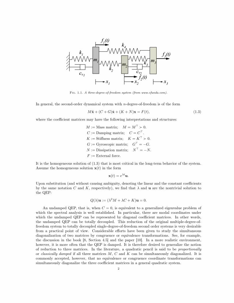
Fig. 1.1. A three-degree-of-freedom system (from www.efunda.com).

In general, the second-order dynamical system with n-degree-of-freedom is of the form

M x + (C +G)x + (K +N)x = F (t), (1.3)

where the coefficient matrices may have the following interpretations and structures:

M := Mass matrix; M = M> 0.C := Damping matrix; C = C>.

K := Stiffness matrix; K = K> 0.G := Gyroscopic matrix; G> = −G.N := Dissipation matrix; N> = −N.F := External force.

It is the homogeneous solution of (1.3) that is most critical in the long-term behavior of the system.Assume the homogeneous solution x(t) in the form

x(t) = eλtu.

Upon substitution (and without causing ambiguity, denoting the linear and the constant coefficientsby the same notation C and K, respectively), we find that λ and u are the nontrivial solution tothe QEP:

Q(λ)u := (λ2M + λC +K)u = 0.

An undamped QEP, that is, when C = 0, is equivalent to a generalized eigenvalue problem ofwhich the spectral analysis is well established. In particular, there are modal coordinates underwhich the undamped QEP can be represented by diagonal coefficient matrices. In other words,the undamped QEP can be totally decoupled. This reduction of the original multiple-degree-of-freedom system to totally decoupled single-degree-of-freedom second order systems is very desirablefrom a practical point of view. Considerable efforts have been given to study the simultaneousdiagonalization of two matrices by congruence or equivalence transformations. See, for example,the discussion in the book [8, Section 4.5] and the paper [10]. In a more realistic environment,however, it is more often that the QEP is damped. It is therefore desired to generalize the notionof reduction to three matrices. In the literature, a quadratic pencil is said to be proportionallyor classically damped if all three matrices M , C and K can be simultaneously diagonalized. It iscommonly accepted, however, that no equivalence or congruence coordinate transformations cansimultaneously diagonalize the three coefficient matrices in a general quadratic system.

2

In two recent papers [3, 4], Garvey et al. proposed a different way to perceive the simultaneousdiagonalization of three matrices. We outline their ideas below. It is easy to show that the QEP(1.1) is equivalent to the generalized eigenvalue problem

L(λ)[

uv

]= 0, (1.4)

where

L(λ) := L(λ;M,C,K) =[C MM 0

]λ+

[K 00 −M

]. (1.5)

Clearly, if M is nonsingular, then v = λu. The arrangement in the symmetrically linearized pencilL(λ) is referred to as the Lancaster structure. If there exist nonsingular 2n×2n matrices Π` and Πr

such that the equivalence transformation applied to (1.5) maintains the Lancaster structure, that is,

Π`L(λ)Πr =[CD MD

MD 0

]λ+

[KD 00 −MD

], (1.6)

and such that MD, CD and KD are all diagonal matrices, then the QEP (1.1) is equivalent to thetotally decoupled system

(λ2MD + λCD +KD)z = 0. (1.7)

In this case, the eigenvectors u and z are related by[uλu

]= Πr

[zλz

], (1.8)

provided that MD and M are nonsingular. Most importantly, the two quadratic systems (1.1) and(1.7) are isospectral.

The notion outlined above is different from the usual task of simultaneously diagonalizing thecoefficient matrices in the linearized pencil L(λ). Rather, by maintaining the Lancaster structure,the approach links a multiple-degree-of-freedom system directly to a single-degree-of-freedom system.For the idea to work, the following questions must be addressed:

1. Do the structure preserving transformations Π` and Πr exist?2. Can the transformations Π` and Πr be real-valued so that the resulting diagonal matricesMD, CD and KD remains to be real-valued?

3. Is there any relationship between Π` and Πr, say, Π` = Π>r ?4. How to find the real-valued transformations Π` and Πr numerically?

According to Garvey et al. [3], the answers to Questions 1 and 2 are affirmative. The proof wasdelineated in an appendix of [3] which, in our view, contains some ambiguities. We also think theinstructions suggested in [3] for the construction of matrices Π` and Πr contain some errors and areunnecessarily complicated. The goal of this paper is to reconfirm the fact that the canonical formdescribed in (1.6) is achievable by offering a clearer and simpler proof. Along the way, we can answerQuestion 3 which is an open problem speculated in [3]. We are able to advance to the completionof the theory by applying a useful notion from matrix polynomial factorization described in [7].

This paper contains two main parts: The first part addresses general pencils. In section 3 weprove the existence of equivalence transformations by which almost all general quadratic pencils canbe totally decoupled. Some of the original arguments by Garvey et al. are fixed and remarkablysimplified [3]. Assuming the availability of spectral decomposition, the proof itself is constructive andcan be converted into an algorithm. The second part addresses self-adjoint pencils. In section 4 we

3

begin with an outline of matrix polynomial factorization, showing that the real-valued eigenvaluesof self-adjoint quadratic pencils are necessarily divided into two categories. We then show thatthe total decoupling can be achieved by congruence transformations. We believe these results areinnovative and the theory is now complete.

Needless to say, it would be of great theoretical and practical significance if almost all n-degree-of-freedom systems can be completely decoupled into n single-degree-of-freedom subsystems. Thispaper establishes the theoretical fundation that such a reduction is possible.

2. Nonlinear Relationship. It has to be made clear that the procedure offered either in thispaper or from [3] begins with the spectral decomposition of the pencil L(λ), so the proof itself cannotserve as a numerical means to answer Question 4. We do have a numerical way working on the triplet(M,C,K) to reduce it to the triplet (MD, CD,KD), but the details will have to be discussed in aseparate paper [1]. See also [5]. It is worth noting that the isospectral transformation from thetriplet (M,C,K) to the triplet (MD, CD,KD) is not the conventional equivalence transformation.Rather, it is a nonlinear relationship among all three matrices (M,C,K).

Indeed, denoting

Π` =[`11 `12`21 `22

], Πr =

[r11 r12r21 r22

], (2.1)

where each `ij or rij is an n×n matrices, in order to maintain the Lancaster structure in the productΠ`L(λ)Πr it is necessary that the following five equations hold:

−`11Kr12 + `12Mr22 = 0,−`21Kr11 + `22Mr21 = 0,

`21Cr12 + `22Mr12 + `21Mr22 = 0, (2.2)`11Cr12 + `12Mr12 + `11Mr22 = `21Cr11 + `22Mr11 + `21Mr21

= −`21Kr12 + `22Mr22.

Additionally, we are seeking Π` and Πr so that

−`21Kr12 + `22Mr22 = MD,

`11Cr11 + `12Mr11 + `11Mr21 = CD, (2.3)`11Kr11 − `12Mr21 = KD,

are diagonal matrices. The conditions (2.2) and (2.3) together constitute a nonlinear algebraicsystem of 8n2 − 3n equations in 8n2 unknowns, but the system is not easy to solve.

The extra degrees of freedom in the underdetermined system (2.2) and (2.3) suggest that both(M,C,K) and (MD, CD,KD) reside on some nontrivial manifold. A structure preserving isospec-tral flow, that is, a differentiable path, starting from (M,C,K) is characterized in [5]. We shalldescribe a closed-loop feedback control system in the forthcoming paper [1] to drive such a flow to(MD, CD,KD) numerically. The remaining of this paper shall concentrate on the theoretical issues.

3. General Pencil and Equivalence Transformation. In this section, we detail steps to-ward proving the existence of the canonical form (1.6) for a quadratic pencil with general coefficientmatrices M , C and K in Rn×n. For convenience, define

A :=[−K 00 M

], B :=

[C MM 0

]. (3.1)

Let (λj ,xj), j = 1, . . . , 2n, denote the j-th right eigenpair of the pencil λB −A, that is, assume

Axj = λjBxj . (3.2)4

In general, the spectrum will be a mix of complex-valued and real-valued eigenvalues. Recall thatthe corresponding eigenvector uj of the original quadratic pencil Q(λ;M,C,K) can be recoveredfrom the fact that

xj =[

uj

λjuj

]. (3.3)

To fix the idea, we shall begin with a spectral decomposition where the following scheme concerningreal and complex eigenvalues and the associated eigenvectors holds:

• Each pair of complex conjugated eigenvalues and the corresponding eigenvectors is placednext to each other, and

• The eigenvectors corresponding to real-valued eigenvalues are real-valued.This scheme will be changed along our later development. Define

Λ := diag λ1, λ2, . . . , . . . , λ2n ∈ C2n×2n, (3.4)X := [x1,x2, . . . ,x2n] ∈ C2n×2n, (3.5)

respectively. Likewise, let (λj ,yj), j = 1, . . . , 2n, denote the j-th left eigenpair of the pencil λB−A,that is, assume

y>j A = λjy>j B. (3.6)

Denote the corresponding matrix of left eigenvectors by Y ∈ C2n×2n. Be aware that we use “trans-pose" rather than “conjugate transpose" for the left eigenvectors.

For simplicity, we shall assume henceforth that all eigenvalues of L(λ) are simple, that is, weshall assume that the diagonal matrix Λ has distinct diagonal entries. We think our argument belowcan be generalized in a straightforward yet tedious way to the case where nontrivial Jordan chainsoccur, but we shall not elaborate the details in this paper.

Observe from (3.2) and (3.6) that the relationship

Y >BXΛ = ΛY >BX = Y >AX (3.7)

holds. The first equality in (3.7) indicates that Y >AX commutes with the diagonal matrix Λ whichhas distinct entries. It follows that the two matrices A1 and B1 defined by

A1 := Y >AX,

B1 := Y >BX, (3.8)

must also be diagonal. Assume further that A−11 exists. Clearly, the scaled columns

X [2] := XA−1/21 , (3.9)

Y [2] := Y A−1/21 , (3.10)

where diagonal entries of A1/21 are the principal square roots of those of A1, are still the right and

left eigenvectors of L(λ), respectively. By using this set of scaled eigenvectors, we see that

A2 := Y [2]>AX [2] = I2n,

B2 := Y [2]>BX [2] = Λ−1, (3.11)

where I2n stands for the 2n× 2n identity matrix. In order to achieve (3.11), it is important to notethat the scaled eigenvectors x[2]

i and y[2]i corresponding to the real eigenvalues λi can become purely

imaginary, if y>i Axi < 0.5

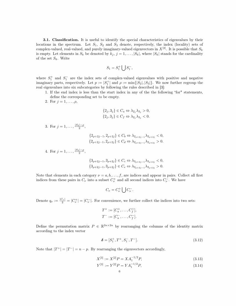
3.1. Classification. It is useful to identify the special characteristics of eigenvalues by theirlocations in the spectrum. Let S1, S2 and S3 denote, respectively, the index (locality) sets ofcomplex-valued, real-valued, and purely imaginary-valued eigenvectors in X [2]. It is possible that Sk

is empty. Let elements in Sk be denoted by kj , j = 1, . . . , |Sk|, where |Sk| stands for the cardinalityof the set Sk. Write

S1 = S+1

⋃S−1 ,

where S+1 and S−1 are the index sets of complex-valued eigenvalues with positive and negative

imaginary parts, respectively. Let p := |S+1 | and ρ := min|S2|, |S3|. We now further regroup the

real eigenvalues into six subcategories by following the rules described in [3]:1. If the end index is less than the start index in any of the the following “for" statements,

define the corresponding set to be empty.2. For j = 1, . . . , ρ,

2j , 3j ∈ Ca ⇔ λ2jλ3j

> 0,2j , 3j ∈ Cf ⇔ λ2j

λ3j< 0.

3. For j = 1, . . . , |S2|−ρ2 ,

2ρ+2j−1, 2ρ+2j ∈ Cb ⇔ λ2ρ+2j−1λ2ρ+2j< 0,

2ρ+2j−1, 2ρ+2j ∈ Cd ⇔ λ2ρ+2j−1λ2ρ+2j> 0.

4. For j = 1, . . . , |S3|−ρ2 ,

3ρ+2j−1, 3ρ+2j ∈ Cc ⇔ λ3ρ+2j−1λ3ρ+2j < 0,3ρ+2j−1, 3ρ+2j ∈ Ce ⇔ λ3ρ+2j−1λ3ρ+2j > 0.

Note that elements in each category ν = a, b, . . . , f , are indices and appear in pairs. Collect all firstindices from these pairs in Cν into a subset C+

ν and all second indices into C−ν . We have

Cν = C+ν

⋃C−ν .

Denote qν := |Cν |2 = |C+

ν | = |C−ν |. For convenience, we further collect the indices into two sets:

T+ := [C+a , . . . , C

+f ],

T− := [C−a , . . . , C−f ].

Define the permutation matrix P ∈ R2n×2n by rearranging the columns of the identity matrixaccording to the index vector

δ = [S+1 , T

+, S−1 , T−]. (3.12)

Note that |T+| = |T−| = n− p. By rearranging the eigenvectors accordingly,

X [3] := X [2]P = XA−1/21 P, (3.13)

Y [3] := Y [2]P = Y A−1/21 P, (3.14)

6

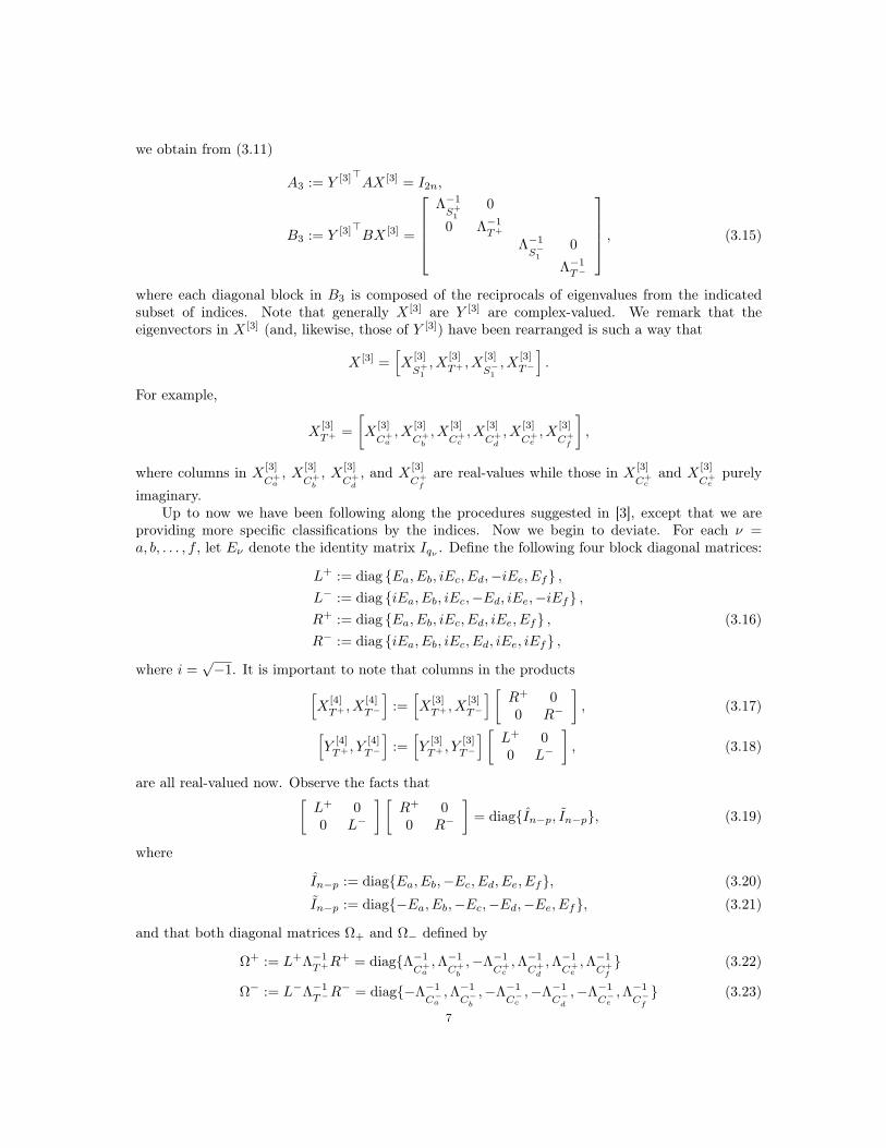
we obtain from (3.11)

A3 := Y [3]>AX [3] = I2n,

B3 := Y [3]>BX [3] =

Λ−1

S+1

0

0 Λ−1T+

Λ−1

S−10

Λ−1T−

, (3.15)

where each diagonal block in B3 is composed of the reciprocals of eigenvalues from the indicatedsubset of indices. Note that generally X [3] are Y [3] are complex-valued. We remark that theeigenvectors in X [3] (and, likewise, those of Y [3]) have been rearranged is such a way that

X [3] =[X

[3]

S+1, X

[3]T+ , X

[3]

S−1, X

[3]T−

].

For example,

X[3]T+ =

[X

[3]

C+a, X

[3]

C+b

, X[3]

C+c, X

[3]

C+d

, X[3]

C+e, X

[3]

C+f

],

where columns in X[3]

C+a, X [3]

C+b

, X [3]

C+d

, and X[3]

C+f

are real-values while those in X[3]

C+c

and X[3]

C+e

purely

imaginary.Up to now we have been following along the procedures suggested in [3], except that we are

providing more specific classifications by the indices. Now we begin to deviate. For each ν =a, b, . . . , f , let Eν denote the identity matrix Iqν

. Define the following four block diagonal matrices:

L+ := diag Ea, Eb, iEc, Ed,−iEe, Ef ,L− := diag iEa, Eb, iEc,−Ed, iEe,−iEf ,R+ := diag Ea, Eb, iEc, Ed, iEe, Ef , (3.16)R− := diag iEa, Eb, iEc, Ed, iEe, iEf ,

where i =√−1. It is important to note that columns in the products[

X[4]T+ , X

[4]T−

]:=[X

[3]T+ , X

[3]T−

] [R+ 00 R−

], (3.17)[

Y[4]T+ , Y

[4]T−

]:=[Y

[3]T+ , Y

[3]T−

] [ L+ 00 L−

], (3.18)

are all real-valued now. Observe the facts that[L+ 00 L−

] [R+ 00 R−

]= diagIn−p, In−p, (3.19)

where

In−p := diagEa, Eb,−Ec, Ed, Ee, Ef, (3.20)

In−p := diag−Ea, Eb,−Ec,−Ed,−Ee, Ef, (3.21)

and that both diagonal matrices Ω+ and Ω− defined by

Ω+ := L+Λ−1T+R

+ = diagΛ−1

C+a,Λ−1

C+b

,−Λ−1

C+c,Λ−1

C+d

,Λ−1

C+e,Λ−1

C+f

(3.22)

Ω− := L−Λ−1T−R

− = diag−Λ−1

C−a,Λ−1

C−b,−Λ−1

C−c,−Λ−1

C−d,−Λ−1

C−e,Λ−1

C−f (3.23)

7

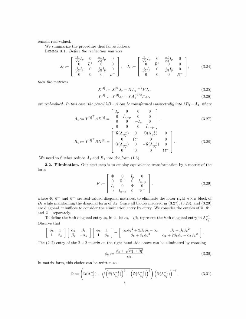
remain real-valued.We summarize the procedure thus far as follows.Lemma 3.1. Define the realization matrices

J` :=

1√2Ip 0 −i√

2Ip 0

0 L+ 0 01√2Ip 0 i√

2Ip 0

0 0 0 L−

, Jr :=

1√2Ip 0 −i√

2Ip 0

0 R+ 0 01√2Ip 0 i√

2Ip 0

0 0 0 R−

, (3.24)

then the matrices

X [4] := X [3]Jr = XA−1/21 PJr, (3.25)

Y [4] := Y [3]J` = Y A−1/21 PJ`, (3.26)

are real-valued. In this case, the pencil λB−A can be transformed isospectrally into λB4−A4, where

A4 := Y [4]>AX [4] =

Ip 0 0 00 In−p 0 00 0 −Ip 00 0 0 In−p

, (3.27)

B4 := Y [4]>BX [4] =

<(Λ−1

S+1) 0 =(Λ−1

S+1) 0

0 Ω+ 0 0=(Λ−1

S+1) 0 −<(Λ−1

S−1) 0

0 0 0 Ω−

. (3.28)

We need to further reduce A4 and B4 into the form (1.6).

3.2. Elimination. Our next step is to employ equivalence transformation by a matrix of theform

F :=

Φ 0 Ip 00 Ψ+ 0 In−p

Ip 0 Φ 00 In−p 0 Ψ−

, (3.29)

where Φ, Ψ+ and Ψ− are real-valued diagonal matrices, to eliminate the lower right n× n block ofB4 while maintaining the diagonal form of A4. Since all blocks involved in (3.27), (3.28), and (3.29)are diagonal, it suffices to consider the elimination entry by entry. We consider the entries of Φ, Ψ+

and Ψ− separately.To define the k-th diagonal entry φk in Φ, let αk + iβk represent the k-th diagonal entry in Λ−1

S>1.

Observe that[φk 11 φk

] [αk βk

βk −αk

] [φk 11 φk

]=[αkφk

2 + 2βkφk − αk βk + βkφk2

βk + βkφk2 αk + 2βkφk − αkφk

2

].

The (2, 2) entry of the 2× 2 matrix on the right hand side above can be eliminated by choosing

φk :=βk +

√α2

k + β2k

αk. (3.30)

In matrix form, this choice can be written as

Φ :=

(=(Λ−1

S+1) +

√(<(Λ−1

S+1))2

+(=(Λ−1

S+1))2)(

<(Λ−1

S+1))−1

. (3.31)

8

Likewise, let k-th entries of Ω+ and Ω− be denoted as ω+k and ω−k , respectively. Observe that[

ψ+k 11 ψ−k

] [ω+

k 00 ω−k

] [ψ+

k 11 ψ−k

]=

[ω+

k (ψ+k )2 + ω−k ω+

k ψ+k + ω−k ψ

−k

ω+k ψ

+k + ω−k ψ

−k ω+

k + ω−k (ψ−k )2

].

In order to eliminate the (2,2) entry, we must choose

ψ−k := ±

√−ω+

k

ω−k. (3.32)

One immediate concern is whether (3.32) is a real number, but that concern is perfectly addressedin the specific way we choose signs when defining the four matrices L± and R±.

Lemma 3.2. By the way the index subsets Cν , ν = a, b, . . . f are defined and, subsequently, thediagonal matrices Ω+ and Ω− are arranged, ω+

k and ω−k have opposite sighs.At its the first glance, the choice of sign in (3.32) does not seem important. But if we want to

maintain the diagonal form when the same equivalence transformation is applied to A4, the signsof ψ+

k and ψ−k must be selected more carefully. The reason can be seen from the following twocalculations: [

ψ+k 11 ψ−k

] [1 00 1

] [ψ+

k 11 ψ−k

]=

[(ψ+

k )2 + 1 ψ+k + ψ−k

ψ+k + ψ−k 1 + (ψ−k )2

],

[ψ+

k 11 ψ−k

] [1 00 −1

] [ψ+

k 11 ψ−k

]=

[(ψ+

k )2 − 1 ψ+k − ψ−k

ψ+k − ψ−k 1− (ψ−k )2

].

Depending on whether the k-th diagonal entry in the product In−pIn−p is positive or negative one,we have to choose ψ+

k = −ψ−k or ψ+k = ψ−k , accordingly, in order to keep the off-diagonal entries of

the 2× 2 matrices on the right hand side above zero. In matrix form, if we choose

Ψ+ :=√−Ω+(Ω−)−1, (3.33)

then

Ψ− := −In−pIn−pΨ+. (3.34)

The elimination process is summarized as follows.Lemma 3.3. Form the real-valued matrix F in (3.29) with diagonal matrices Φ, Ψ+ and Ψ−

given by (3.31), (3.33) and (3.34), respectively. Define

X [5] := X [4]F = XA−1/21 PJrF, (3.35)

Y [5] := Y [4]F = Y A−1/21 PJ`F, (3.36)

then the two matrices

A5 := Y [5]>AX [5] =

A[11]5 0

0 A[22]5

, (3.37)

B5 := Y [5]>BX [5] =

B[11]5 B

[12]5

B[12]5 0

, (3.38)

where all A[kj]5 and B[kj]

5 , j, k = 1, 2, are diagonal matrices, form a real-valued pencil isospectral tothe original λB −A.

9

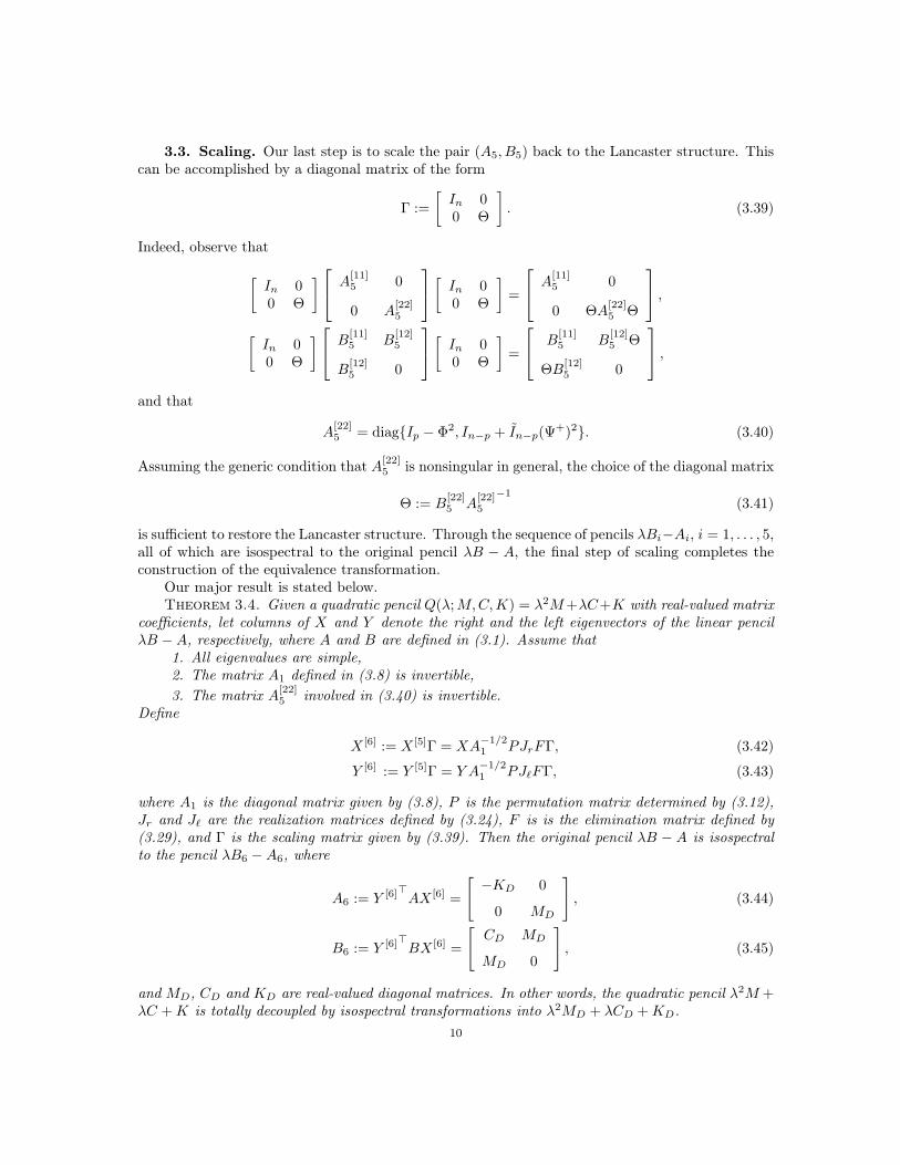
3.3. Scaling. Our last step is to scale the pair (A5, B5) back to the Lancaster structure. Thiscan be accomplished by a diagonal matrix of the form

Γ :=[In 00 Θ

]. (3.39)

Indeed, observe that[In 00 Θ

] A[11]5 0

0 A[22]5

[ In 00 Θ

]=

A[11]5 0

0 ΘA[22]5 Θ

,[In 00 Θ

] B[11]5 B

[12]5

B[12]5 0

[ In 00 Θ

]=

B[11]5 B

[12]5 Θ

ΘB[12]5 0

,and that

A[22]5 = diagIp − Φ2, In−p + In−p(Ψ+)2. (3.40)

Assuming the generic condition that A[22]5 is nonsingular in general, the choice of the diagonal matrix

Θ := B[22]5 A

[22]5

−1(3.41)

is sufficient to restore the Lancaster structure. Through the sequence of pencils λBi−Ai, i = 1, . . . , 5,all of which are isospectral to the original pencil λB − A, the final step of scaling completes theconstruction of the equivalence transformation.

Our major result is stated below.Theorem 3.4. Given a quadratic pencil Q(λ;M,C,K) = λ2M+λC+K with real-valued matrix

coefficients, let columns of X and Y denote the right and the left eigenvectors of the linear pencilλB −A, respectively, where A and B are defined in (3.1). Assume that

1. All eigenvalues are simple,2. The matrix A1 defined in (3.8) is invertible,3. The matrix A[22]

5 involved in (3.40) is invertible.Define

X [6] := X [5]Γ = XA−1/21 PJrFΓ, (3.42)

Y [6] := Y [5]Γ = Y A−1/21 PJ`FΓ, (3.43)

where A1 is the diagonal matrix given by (3.8), P is the permutation matrix determined by (3.12),Jr and J` are the realization matrices defined by (3.24), F is is the elimination matrix defined by(3.29), and Γ is the scaling matrix given by (3.39). Then the original pencil λB − A is isospectralto the pencil λB6 −A6, where

A6 := Y [6]>AX [6] =

[−KD 0

0 MD

], (3.44)

B6 := Y [6]>BX [6] =

[CD MD

MD 0

], (3.45)

and MD, CD and KD are real-valued diagonal matrices. In other words, the quadratic pencil λ2M +λC +K is totally decoupled by isospectral transformations into λ2MD + λCD +KD.

10

The desirable structure preservation transformations Π` and Πr are given by

Π` := Y [6]>, (3.46)Πr := X [6], (3.47)

which by our construction described above are real-valued.

3.4. Numerical Example. We conclude this section with a numerical example. Up to thispoint, note that the theory is for general quadratic pencils where the matrix coefficients are generalmatrices in Rn×n. We emphasize that the construction of the equivalence transformation beginswith the availability of the complete spectral information, the so called Jordan triplet in [6].

For the easy running of text, we report only four numeric digits even though all calculationsinvolved are accurate to the machine accuracy. Consider the case

M =

0.7621 0.4447 0.7382 0.91690.4565 0.6154 0.1763 0.41030.0185 0.7919 0.4057 0.89360.8214 0.9218 0.9355 0.0579

, C =

0.3710 −1.0226 0.3155 0.50450.7283 1.0378 1.5532 1.86452.1122 −0.3898 0.7079 −0.3398

−1.3573 −1.3813 1.9574 −1.1398

,

K =

−0.2111 −0.6014 −2.0046 1.2366

1.1902 0.5512 −0.4931 −0.6313−1.1162 −1.0998 0.4620 −2.3252

0.6353 0.0860 −0.3210 −1.2316

.Its spectrum in ascending order of moduli is given by

0.0348,−0.0877, 0.5453,−2.0162± 1.4196i, 0.1815± 2.5083i, 3.0425,

among which the four real eigenvalues are classified into

Cd = 3, 8, Cf = 2, 1.

Be aware of the order in Cf because the eigenvector corresponding to the eigenvalue 0.0348 is purelyimaginary. The structure preserving transformation matrices Π` and Πr are given by

Π` =

0.4189 0.9173 0.0945 −0.4584 −2.0559 −1.9378 −0.0730 1.2765−6.9347 12.4232 −0.9207 −2.4408 3.2216 −7.7792 −14.4484 −8.8834−0.5439 0.0331 1.9456 −2.3711 −0.4656 −0.4208 2.0679 −1.4933−0.3465 −10.1901 −3.9018 12.2692 −0.0115 0.0231 −0.0563 0.0023

0.3381 0.3187 0.0120 −0.2100 −0.9446 −0.3678 0.0461 0.3881−0.5094 1.2300 2.2846 1.4046 −7.1196 12.8698 −0.0912 −1.9307

0.2807 0.2536 −1.2465 0.9001 0.4631 0.9430 −2.5265 0.8583−3.7728 7.5521 −18.4169 0.7416 −0.1468 −10.5898 −2.9272 12.2299

,

Πr =

0.3340 −3.7885 0.5893 −8.7045 0.0300 0.9596 −0.8007 −8.7108−0.2226 −14.6629 1.0132 12.2692 −0.0866 3.9812 −0.2769 0.7416−0.8990 10.1808 −2.4537 −4.3424 −0.4661 2.5332 1.0515 −13.8562

0.9328 6.0803 −1.6896 −2.5127 0.3928 −3.4286 0.8571 −9.4260−0.1822 −6.0687 1.3284 −0.0266 0.2132 −3.4401 −2.2834 −8.2435

0.5264 −25.1784 0.4594 0.0023 0.1265 −13.2174 0.0197 12.22992.8341 −16.0210 −1.7445 −0.0423 0.9806 11.1005 1.3190 −3.6091

−2.3881 21.6836 −1.4220 −0.0288 −0.6509 4.8354 1.3855 −2.0139

.

11

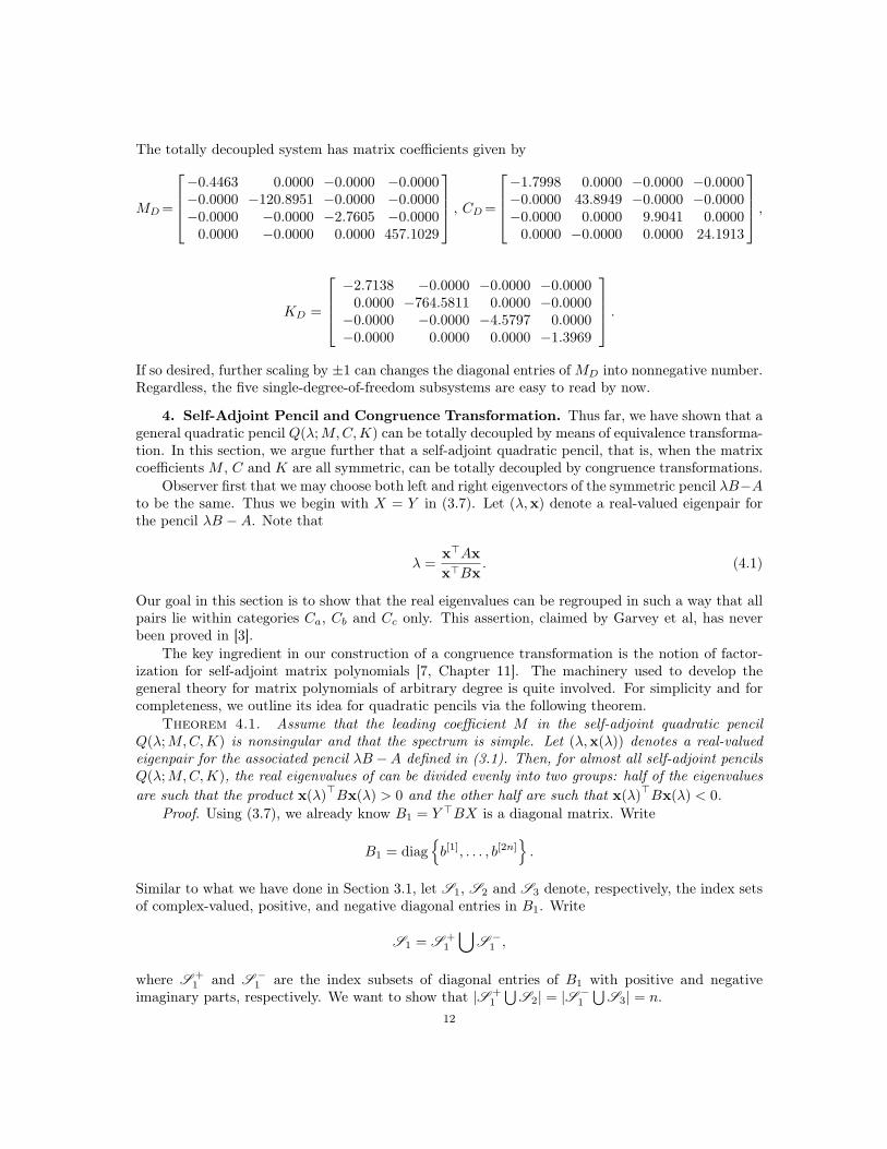
The totally decoupled system has matrix coefficients given by

MD =

−0.4463 0.0000 −0.0000 −0.0000−0.0000 −120.8951 −0.0000 −0.0000−0.0000 −0.0000 −2.7605 −0.0000

0.0000 −0.0000 0.0000 457.1029

, CD =

−1.7998 0.0000 −0.0000 −0.0000−0.0000 43.8949 −0.0000 −0.0000−0.0000 0.0000 9.9041 0.0000

0.0000 −0.0000 0.0000 24.1913

,

KD =

−2.7138 −0.0000 −0.0000 −0.0000

0.0000 −764.5811 0.0000 −0.0000−0.0000 −0.0000 −4.5797 0.0000−0.0000 0.0000 0.0000 −1.3969

.If so desired, further scaling by ±1 can changes the diagonal entries of MD into nonnegative number.Regardless, the five single-degree-of-freedom subsystems are easy to read by now.

4. Self-Adjoint Pencil and Congruence Transformation. Thus far, we have shown that ageneral quadratic pencil Q(λ;M,C,K) can be totally decoupled by means of equivalence transforma-tion. In this section, we argue further that a self-adjoint quadratic pencil, that is, when the matrixcoefficients M , C and K are all symmetric, can be totally decoupled by congruence transformations.

Observer first that we may choose both left and right eigenvectors of the symmetric pencil λB−Ato be the same. Thus we begin with X = Y in (3.7). Let (λ,x) denote a real-valued eigenpair forthe pencil λB −A. Note that

λ =x>Axx>Bx

. (4.1)

Our goal in this section is to show that the real eigenvalues can be regrouped in such a way that allpairs lie within categories Ca, Cb and Cc only. This assertion, claimed by Garvey et al, has neverbeen proved in [3].

The key ingredient in our construction of a congruence transformation is the notion of factor-ization for self-adjoint matrix polynomials [7, Chapter 11]. The machinery used to develop thegeneral theory for matrix polynomials of arbitrary degree is quite involved. For simplicity and forcompleteness, we outline its idea for quadratic pencils via the following theorem.

Theorem 4.1. Assume that the leading coefficient M in the self-adjoint quadratic pencilQ(λ;M,C,K) is nonsingular and that the spectrum is simple. Let (λ,x(λ)) denotes a real-valuedeigenpair for the associated pencil λB −A defined in (3.1). Then, for almost all self-adjoint pencilsQ(λ;M,C,K), the real eigenvalues of can be divided evenly into two groups: half of the eigenvaluesare such that the product x(λ)>Bx(λ) > 0 and the other half are such that x(λ)>Bx(λ) < 0.

Proof. Using (3.7), we already know B1 = Y >BX is a diagonal matrix. Write

B1 = diagb[1], . . . , b[2n]

.

Similar to what we have done in Section 3.1, let S1, S2 and S3 denote, respectively, the index setsof complex-valued, positive, and negative diagonal entries in B1. Write

S1 = S +1

⋃S −

1 ,

where S +1 and S −

1 are the index subsets of diagonal entries of B1 with positive and negativeimaginary parts, respectively. We want to show that |S +

1

⋃S2| = |S −

1

⋃S3| = n.

12

One of the two sets S +1

⋃S2 and S −

1

⋃S3 will have cardinality at least n. We may assumed,

without loss of generality, that |S +1

⋃S2| ≥ n. The other case can be argued similarly. Denote

ρ1 := |S +1 | and ρ2 := |S2|. Consider the matrix

Z := XS +1

SS2

=[x1+

1, . . . ,x1+

ρ1x21 , . . .x2ρ2

]∈ C2n×ρ1

⊕R2n×ρ2 ,

whose columns are selected from those of X with column indices given by S +1

⋃S2. By assumption,

the matrix Z is of full column rank ρ1 + ρ2. Using the relationship (3.3), write

Z =[

UUΥ

],

where

U := US +1

SS2

=[u1+

1, . . . ,u1+

ρ1u21 , . . .u2ρ2

]∈ Cn×ρ1

⊕Rn×ρ2 , (4.2)

denote the upper half of the matrix Z and

Υ := ΛS +1

SS2

(4.3)

denotes the corresponding portion from the diagonal matrix Λ defined in (3.4). We want to showthat U is of full column rank. If this is true, then because we have assumed ρ1 + ρ2 ≥ n, it must beρ1 + ρ2 = n.

By construction, we know that Z>BZ is a diagonal matrix with some complex-valued entries.If the adjoint Z∗, that is, the transpose of the complex conjugate of Z, is used instead, we observethat

D := Z∗BZ = diag

0, . . . 0, b[21], . . . , b[2ρ2 ]

has nonnegative entries. Suppose Uz = 0 for some z ∈ Cρ1+ρ2 . It is easy to see that

z∗Dz = [0 (UΥz)∗][C MM 0

] [0

UΥz

]= 0.

It follows that Dz = 0. This is equivalent to

U∗MUΥz = 0 (4.4)

and, hence (UΥz)∗MUΥz = 0.The set of symmetric matrices (M,C,K) such that

u ∈ Cn×n|u∗Mu = 0⋂UΥz ∈ Cn×n|z ∈ Cρ1+ρ2 ,MUΥ2 + CUΥ +KU = 0 6= ∅

forms an algebraic variety in the space of Rn×n × Rn×n × Rn×n. This variety has measure zero.That is, for almost all self-adjoint quadratic pencils Q(λ;M,C,K), the condition (4.4) implies thatUΥz = 0. We have thus proved that z is in the null space of Z. Since Z is of full column rank, itmust be z = 0 and, hence, U is of full column rank.

We remark that in [6] these two sets S +1

⋃S2 and S −

1

⋃S3 are said to be B-nonnegative and

B-nonpositive, respectively. It is also worth pointing out that the proof in [6, 7] is for the factorizationof monic self-adjoint matrix polynomials, that is, the leading matrix coefficient is the identity matrix.The proof can easily be modified if the leading matrix coefficient is positive definite. What we haveproved, however, is that the factorization remains true for almost all regular self-adjoint quadraticpencils. We have observed this phenomenon numerically.

13

4.1. With Positive Definite Coefficients. One of the most important quadratic pencils inapplication is the class when M is symmetric and positive definite and both C and K are symmetricand positive semidefinite. It is known in this case that all eigenvalues of Q(λ) lie in the the lefthalf-plane. In particular, all real eigenvalues are nonnegative. The following result therefore is ofgreat consequence in practice.

Theorem 4.2. Any self-adjoint pencil Q(λ;M,C,K) with positive definite matrix coefficientscan be totally decoupled by congruence transformations.

Proof. It suffices to show that |S2| = |S3|. If this is true, then all real-value eigenvalues arecategorized into the single group Ca. It follows that L+ = R+, L− = R− and, hence, J` = Jr.In other words, the equivalence transformation involved in (3.44) and (3.45) becomes congruencetransformation because Y [6] = X [6].

The classification of S2 and S3 is based on the signs of the products x>Ax where x is a real-valued eigenvector associated with a real-valued eigenvalue. By Theorem 4.1, we have alreadyknown that there precisely half of these eigenvectors are such that x>Bx is positive and the otherhalf eigenvectors give rise to negative products. Since all real-values eigenvalues are of one sign, by(4.1) we know that precisely half of these eigenvectors are such that x>Ax is positive and the otherhalf leads to negative x>Ax. This shows |S2| = |S3|.

4.2. Without Positive Definite Coefficients. There is no specific pattern for real-valuedeigenvalues of a general self-adjoint quadratic pencil. However, for any given real-valued eigenpair(λ,x), the signs of λ, x>Ax, and x>Bx are related through the relationship

sgn(x>Ax) = sgn(λ)sgn(x>Bx). (4.5)

This relationship together with Theorem 4.1 enables us to refine the classification described inSection 3.1 as follows.

Case 1. Suppose that ρ = min|S2|, |S3| 6= 0. Assume λ2s> 0 for a certain s. Then necessarily

x>2sAx2s

> 0. By (4.5), we must have the corresponding x>2sBx2s

> 0. By definition, we always havex>3j

Ax3j< 0 among all possible eigenvalues λ3j

. By Theorem 4.1, it cannot be so that x>3jBx3j

> 0for all j. There must be a certain t such that x>3t

Bx3t < 0. By (4.5) again, we have the correspondingλ3t

> 0. We therefore can pair 2s, 2t ∈ Ca. Likewise, a given λ2s< 0 can be paired with a certain

λ3t< 0. Repeating this argument, we see that Cf = ∅ since no pairs of eigenvalues should be placed

in Cf . Only Ca is needed and contains ρ pairs.Case 2. After we have exhausted as many pairs in Ca as possible, suppose there are some

leftovers in S2 but none in S3. Denote this remaining subset of S2 by S2. Note that x>2jAx2j > 0 for

all 2j ∈ S2. Assume that one such eigenvalue λ2s> 0. Then x>2s

Bx2s> 0. However, by Theorem 4.1,

it cannot be so that x>2jBx2j > 0 for all the remaining 2j ∈ S2. There must be a certain 2t ∈ S2

such that x>2tBx2t < 0. By (4.5), we must have the corresponding λ2t > 0. Therefore, the pair

(2s, 2t) is categorized into Cb. Likewise, a given λ2s< 0 from the remaining subset S2 can be paired

with a certain λ2t< 0 with 2t ∈ S2. Repeating this argument, we see that no pairs of eigenvalues

from S2 should be places in Cd. Only Cb is needed and Cd = ∅.Case 3. Suppose that Case 2 does not happen. Rather, suppose that after we have exhausted as

many pairs in Ca as possible, there are some leftovers in S3 but none in S2. Denote this remainingsubset of S3 by S3. Note that x>3j

Ax3j< 0 for all 3j ∈ S3. Assume that one such eigenvalue

λ3s> 0. Then x>3sBx3s

< 0. However, by Theorem 4.1, it cannot be so that x>3jBx3j

< 0 for allthe remaining 3j ∈ S3. There must be a certain 3t ∈ S3 such that x>3t

Bx3t> 0. By (4.5), we must

have the corresponding λ3t< 0. Therefore, the pair (3s, 3t) is categorized into Cc. Likewise, a given

λ3s< 0 from the remaining subset S3 can be paired with a certain λ3t

> 0 with 3t ∈ S3. Repeatingthis argument, we see that no pairs of eigenvalues from S3 should be places in Ce. Only Cc is neededand Ce = ∅.

14

By now, we have generalized Theorem 4.2 to the general self-adjoint quadratic pencil.Theorem 4.3. Almost all self-adjoint pencil Q(λ;M,C,K) with simple spectrum can be totally

decoupled by congruence transformations.Proof. The arguments in the above three cases show that the real-valued eigenvalues can be

regrouped in such a way that all pairs lie with the categories Ca, Cb and Cc only. An examinationof the structure defined in (3.16) shows that L+ = R+, L− = R− and, hence, J` = Jr.

5. Conclusion. It is commonly accepted that there is no equivalence transformation that cansimultaneously diagonalize the three coefficient matrices in a general quadratic pencil. Followingthe ideas by Garvey et al., however, we have shown that real-valued transformations that decouplesthe original n-degree-of freedom system as the direct sum of n single-degree-of-freedom subsystemsdo exist for all most all quadratic pencils. The turning point that makes this advancement is thatthe notion of diagonalization is replaced by the Lancaster structure.

Our contributions in this paper are threefold: We offer a complete mathematical procedureshowing how a given spectral decomposition which usually is complex-valued can be converted intoreal-valued equivalence transformations. Our approach, particularly in the steps of elimination andscaling, is easier and more straightforward than that suggested in [3]. In case of self-adjoint quadraticpencils, we employ the notion of matrix polynomial factorization to prove a conjecture in [3] thatthe equivalence transformation is indeed a congruence transformation. This fact has never beenjustified before.

A prerequisite of the maneuver outlined in this paper is the availability of a spectral decompo-sition of the original quadratic pencil, which makes the process numerically infeasible. To develop amore effective numerical method to realize such a decoupling process is an interesting open problem.

REFERENCES

[1] M. T. Chu and N. Del Buono, Total decoupling of a general quadratic pencil, Part II: Structural PreservingIsospectral Flows, preprint, 2005.

[2] Equations of motion for MDOF systems, available online from eFunda, Inc., seehttp://www.efunda.com/formulae/vibrations/mdof_eom.cfm.

[3] S. D. Garvey, M. I. Friswell, and U. Prells, Co-ordinate tranfromations for second order systems, I: Generaltransformations, J. Sound Vibration, 258(2002), 885–909.

[4] S. D. Garvey, M. I. Friswell, and U. Prells, Co-ordinate transformations for second order systems, II: Elementarystructure-preserving transformations, J. Sound Vibration, 258 (2002), 911–930.

[5] S. D. Garvey, U. Prells, M. Friswell, and Z. Chen, General isospectral flows for linear dynamic systems, LinearAlg. Appl., 385(2004), 335-368.

[6] I. Gohberg, P. Lancaster, and L. Rodman, Spectral analysis of selfadjoint matrix polynomials, Ann. Math.,112(1980), 33-71.

[7] I. Gohberg, P. Lancaster, and L. Rodman, Matrix Polynomials, Computer Science and Applied Mathematics.Academic Press, Inc., New York-London, 1982.

[8] R. A. Horn and C. R. Johnson, Matrix Analysis, Cambridge University Press, New York, 1991.[9] F. Tisseur and K. Meerbergen, The quadratic eigenvalue problem, SIAM Rev. 43 (2001),235–286.

[10] F. Uhlig, A canonical form for a pair of real symmetric matrices that generate a nonsingular pencil, Linear Alg.Appl., 14, 189-209.

15