TOTAL DECOUPLING OF GENERAL QUADRATIC PENCILS,

PART II: STRUCTURE PRESERVING ISOSPECTRAL FLOWS

MOODY T. CHU∗AND NICOLETTA DEL BUONO†

Abstract. Quadratic pencils, λ2M + λC + K, where M , C, and K are n× n real matrices with or without someadditional properties such as symmetry, connectivity, bandedness, or positive definiteness, arise in many importantapplications. Recently an existence theory has been established, showing that almost all n-degree-of-freedom secondorder systems can be reduced to n totally independent single-degree-of-freedom second order subsystems by real-valued isospectral transformations. In contrast to the common knowledge that generally no three matrices can bediagonalized simultaneously by equivalence transformations, these isospectral transformations endeavor to maintaina special linearization form called the Lancaster structure and do break down M , C and K into diagonal matricessimultaneously. However, these transformations depend on the matrices in a rather complicated way and, hence, aredifficult to construct directly. In this paper, a second part of a continuing study, a closed-loop control system thatpreserves both the Lancaster structure and the isospectrality is proposed as a means to achieve the diagonal reduction.Consequently, these transformations are acquired.

Key words. quadratic pencil, Lancaster structure, structure preserving, multiple-degree-of-freedom system,equivalence transformation, closed-loop control, simultaneous diagonalization

AMS subject classifications. 15A22, 70H15, 93B10

1. Introduction. Given n× n real matrices M0, C0 and K0, the task of finding scalars λ ∈ C

and nonzero vectors u ∈ Cn satisfying

Q(λ)u = 0, (1.1)

where

Q(λ) := Q(λ; M0, C0, K0) = λ2M0 + λC0 + K0, (1.2)

is known as the quadratic eigenvalue problem (QEP). The scalars λ and the corresponding vectors x

are called, respectively, eigenvalues and eigenvectors of the quadratic pencil Q(λ). It is known thatthe QEP possesses 2n eigenvalues over the complex field, provided the leading coefficient matrix Mis nonsingular. The eigeninformation (λ,u) is critical to the understanding of the dynamical system

M0x + C0x + K0x = f(t), (1.3)

which arises frequently in many important applications, including applied mechanics, electrical os-cillations, vibro-acoustics, fluid mechanics, and signal processing.

There are extensive discussions about the QEPs. Both the theory and the numerical methodsare fairly complete. See, for example, the review article [15], the books [9, 13] and the referencescontained therein. One principal tool used for analyzing QEPs is to linearize a quadratic pencilto a linear pencil. The linearization may appear in several different forms among which one is ofparticular interest to us — the so called Lancaster structure in the linear pencil

L(λ) := L(λ; M0, C0, K0) =

[C0 M0

M0 0

]λ +

[K0 00 −M0

]. (1.4)

∗Department of Mathematics, North Carolina State University, Raleigh, NC 27695-8205. (chu@math.ncsu.edu)This research was supported in part by the National Science Foundation under grants CCR-0204157.

†Dipartimento di Matematica, Università degli Studi di Bari, Via E. Orabona 4, I-70125 Bari, Italy. (del-buono@dm.uniba.it)

1

The equivalence between Q(λ) and L(λ) can be seen from the fact that

([C0 M0

M0 0

]λ +

[K0 00 −M0

])[u

v

]= 0 (1.5)

if and only if

{(λC0 + K0)u + λM0v = 0,

λM0u − M0v = 0.(1.6)

Indeed, if M is nonsingular, then we know further that v = λu. Obviously, the Lancaster structureimplies that if Q(λ) is self-adjoint, then so is L(λ).

The main reason that the Lancaster structure is important to us is because it has been provedrecently that for almost all quadratic pencils there exists real-valued 2n × 2n real matrices Πℓ andΠr such that

Π⊤ℓ L(λ)Πr = L(λ; MD, CD, KD) =

[CD MD

MD 0

]λ +

[KD 00 −MD

], (1.7)

where MD, CD, KD are all real-valued n × n diagonal matrices [2, 5, 6]. In other words, thereexists a real-valued equivalence transformation which not only preserves the Lancaster structurebut also transforms the pencil L(λ) isospectrally into a pencil with diagonal blocks. Note that theeigenstructure is equivalent in the sense that

(λ2MD + λCD + KD

)z = 0 ⇔

[u

λu

]= Πr

[z

λz

].

Such a transformation is significant in that it links the dynamical behavior of a multiple-degree-of-freedom system directly to that of a system consisting of n independent single-degree-of-freedomsubsystems. It breaks down the interlocking connectivity in the original system into totally discon-nected subsystems while preserving the entire spectral properties. Thus it will be of great valuein practice if the transformations Πℓ and Πr can be found from any given pencil. The theory ofexistence of Πℓ and Πr in [2, 5] was established on the basis of the complete spectral information ofL(λ). To construct Πℓ and Πr from the availability of spectral information certainly is impractical.The focus of this paper is to construct Πℓ and Πr numerically by structure preserving isospectralflows without knowing the spectral information.

The isospectral transformation from the triplet (M0, C0, K0) to the triplet (MD, CD, KD) is notan ordinary equivalence transformation. It depends nonlinearly on matrices (M0, C0, K0). To seethis relationship, denote

Πℓ =

[ℓ11 ℓ12

ℓ21 ℓ22

], Πr =

[r11 r12

r21 r22

], (1.8)

where each ℓij or rij is an n × n matrices. In order to maintain the Lancaster structure in theproduct Π⊤

ℓ L(λ)Πr, it is necessary that the following five equations hold:

−ℓ⊤11K0r12 + ℓ⊤21M0r22 = 0,

−ℓ⊤12K0r11 + ℓ⊤22M0r21 = 0,

ℓ⊤12C0r12 + ℓ⊤22r12 + ℓ⊤12M0r22 = 0, (1.9)

ℓ⊤11C0r12 + ℓ⊤21M0r12 + ℓ⊤11M0r22 = ℓ⊤12C0r11 + ℓ⊤22M0r11 + ℓ12M0r⊤21

= −ℓ⊤12K0r12 + ℓ⊤22M0r22.

2

Additionally, the matrices Πℓ and Πr must be such that the left-hand sides of the following threeexpressions,

−ℓ⊤12K0r12 + ℓ⊤22M0r22 = MD,

ℓ⊤11C0r11 + ℓ⊤21M0r11 + ℓ⊤11M0r21 = CD, (1.10)

ℓ⊤11K0r11 − ℓ⊤21M0r21 = KD,

are diagonal matrices. The conditions (1.9) and (1.10) together constitute a homogeneous second-degree polynomial system of 8n2 − 3n equations in 8n2 unknowns. It is not obvious how the systemcould be solved analytically. The underdetermined system does suggest, however, that there isplenty of leeway to choose the transformation matrices Πℓ and Πr. In particular, the “orbit" ofL(λ) under (Lancaster) structure preserving equivalence transformations is a nontrivial manifold onwhich perhaps a smooth path connecting (M0, C0, K0) to (MD, CD, KD) can be defined.

A special kind of isospectral flow preserving the Lancaster structure has been proposed in [7].What is needed is a more specific control of the flow so that it starts from (M0, C0, K0) and movestoward (MD, CD, KD). Our contribution in this paper is that we describe a closed-loop feedbackcontrol system to drive such a flow. The resulting dynamical system can be tracked numerically.

2. Isospectral flow. Our closed-loop feedback control system is built upon the structure pre-serving isospectral flows proposed in [7]. For later reference, we briefly review what has been intro-duced in [7]. It is important to note that the flows described in this section can only maintain theLancaster structure and the isospectrality. The flows will have to be modified in order to acquirethe additional capability of reducing matrices to diagonals.

For convenience, denote the Lancaster pair in (1.4) by (A0, B0), that is,

A0 =

[K0 00 −M0

], B0 =

[C0 M0

M0 0

]. (2.1)

We are interested in characterizing two one-parameter families of structured preserving transfor-mations TL(t), TR(t) ∈ R2n×2n, with TL(0) = TR(0) = I2n. Let the actions of these families oftransformations on (A0, B0) be denoted by

A(t) = T⊤L (t)A0TR(t), B(t) = T⊤

L (t)B0TR(t), (2.2)

respectively. Clearly, regardless how TL(t) and TR(t) are defined, (A(t), B(t)) is isospectral to(A0, B0) for any t. A special class of transformations is to require that matrices TL(t) and TR(t)satisfy, respectively, the following differential systems:

dTL(t)

dt= TL(t)L(t)= TL(t)

[L11(t) L12(t)L21(t) L22(t)

], (2.3)

dTR(t)

dt= TR(t)R(t)= TR(t)

[R11(t) R12(t)R21(t) R22(t)

], (2.4)

where each Lij(t) or Rij(t), i, j = 1, 2, is a n × n real one-parameter matrix yet to be defined. Thetask now is to impose conditions on the matrices L(t) and R(t) so that the resulting (A(t), B(t))maintains the Lancaster structure for every t.

For convenience, denote the differentiation dgdt

of any function g(t) by the symbol g. It is easyto see from (2.2) that

A = T⊤L A0TR + TLA0TR= L⊤A + AR,

B = T⊤L B0TR + TLB0TR= L⊤B + BR.

3

It is interesting to note that these differential equations are similar to those discussed in [1] whichleads to a Lie-Poisson system. By insisting that (A(t), B(t)) maintains the Lancaster structure, thatis,

A(t) =

[K(t) 0

0 −M(t)

], B(t) =

[C(t) M(t)M(t) 0

], (2.5)

we see that[

K 0

0 −M

]=

[L⊤

11K + KR11 −L⊤21M + KR12

L⊤12K − MR21 −L⊤

22M − MR22

], (2.6)

[C M

M 0

]=

[L⊤

11C + CR11 + L⊤21M + MR21 L⊤

11M + MR22 + CR12

L⊤12C + L⊤

22M + MR11 L⊤12M + MR12

]. (2.7)

It follows that the following five equations must be satisfied by the matrices Lij and Rij , i, j = 1, 2:

KR12 − L⊤21M = 0,

L⊤12K − MR21 = 0,

L⊤12M + MR12 = 0, (2.8)

L⊤11M − L⊤

22M + CR12 = 0,

MR11 − MR22 + L⊤12C = 0.

The conditions in (2.8) constitute a homogeneous linear system of 5n2 for the 8n2 entries in thematrices Lij and Rij , i, j = 1, 2. It is a much easier system than the nonlinear system (1.9) and(1.10). Its solution space contains 3n2 free parameters which we can identify as three n × n matrixparameters. The transformations TL(t) and TR(t) can now be characterized in terms of these threefree matrix parameters.

In fact, by assuming that the matrix M(t) is invertible, we may set forth the first matrixparameter D(t) ∈ Rn×n by requiring that the relationship

R12(t) = −D(t)M(t)

holds between R12(t) and M(t). It is not difficult to derive after some algebraic manipulations thatthe solutions to the system (2.8) can now be identified as follows:

R12 = −DM, (2.9)

R21 = DK, (2.10)

L12 = D⊤M⊤, (2.11)

L21 = −D⊤K⊤, (2.12)

L11 − L22 = D⊤C⊤, (2.13)

R11 − R22 = −DC. (2.14)

Now that we have obtained these formulas, it is worth mentioning in retrospect that even withoutthe assumption that M(t) is nonsingular the matrices defined by (2.9) to (2.14) satisfy the system(2.8). Note also that implicit in (2.13) and (2.14) are the other two free matrix parameters. Thereare several possible ways to arrange the diagonal blocks of L(t) and R(t). The choice suggested in[7] is to define L(t) and R(t) according to the following formulas:

L =

[D⊤ 00 D⊤

] [C⊤

2−M⊤

−K⊤ −C⊤

2

]+

[N⊤

L 00 N⊤

L

], (2.15)

R =

[D 00 D

] [−C

2−M

K C2

]+

[NR 00 NR

], (2.16)

4

where the matrices D(t), NL(t) and NR(t) are free matrix parameters in Rn×n. Upon substitutingthe blocks of L and R into the differential system (2.6) and (2.7), we obtain a flow of the triplet(M(t), C(t), K(t)) which is governed by the autonomous system:

K =1

2(CDK − KDC) + N⊤

L K + KNR,

C = (MDK − KDM) + N⊤L C + CNR, (2.17)

M =1

2(MDC − CDM) + N⊤

L M + MNR.

We could also choose to define L(t) and R(t), for example, in the following way,

L =

[D⊤ 00 D⊤

] [0 −M⊤

−K⊤ C⊤

]+

[NL 00 NL

], (2.18)

R =

[D 00 D

] [0 −MK C

]+

[NR 00 NR

]. (2.19)

The corresponding differential system for (M(t), C(t), K(t)) becomes somewhat simpler:

K = N⊤L K + KNR

C = (MDK − KDM) + N⊤L C + CNR (2.20)

M = (MDC − CDM) + N⊤L M + MNR

It is interesting to note that simplicity does not necessarily mean benefit because the first equationin (2.20) implies K(t) is an equivalent transformation of K0, which might limit the way K(t) canchange. We shall concentrate on the system defined in (2.17) henceforth. The main question now ishow to exploit the three free matrix parameters D, NL, and NR so that the resulting flow behavesin some desirable ways.

3. Selecting free parameters. In this section we demonstrate some of the possible choicesof the three parameters in the system (2.17). Ultimately, we want to control the free parameters D,NL and NR in such a way that the isospectral flow (M(t), C(t), K(t)) is driven into a block diagonaltriplet (MD, CD, KD).

3.1. Maintaining symmetry. In additional to the Lancaster structure, it might be desirableto maintain the symmetry in the initial value (M0, C0, K0), if there is any, throughout the flow(M(t), C(t), K(t)) for all t. This task can be accomplished by selecting the free matrix parameterswith proper symmetric properties. Several sufficient conditions have already been mentioned in [5].For example, by assuming NR(t) = NL(t), the symmetry specified for the matrix parameter D inTable 3.1 will preserve the symmetry for the flow (M(t), K(t), C(t)) defined by the dynamical system(2.17).

D(t) M(t) C(t) K(t)

skew-symmetric symmetric symmetric symmetricsymmetric symmetric skew-symmetric symmetricsymmetric skew-symmetric skew-symmetric skew-symmetric

skew-symmetric skew-symmetric symmetric skew-symmetricTable 3.1

Preserving symmetries of (M(t), C(t), K(t)) by D(t), if NR(t) = NL(t).

5

3.2. Nahm equations. Another choice of the free matrix parameters might be worth men-tioning because it makes a remarkable connection to the Nahm equations [17]. More specifically, ifwe choose NR(t) = NL(t) = N(t) to be an arbitrary one-parameter flow and define

D(t) := S(t)T (t), (3.1)

where S(t) and T (t) are solution flows to the linear system

S = −NS, (3.2)

T = −TN⊤, (3.3)

then D(t) satisfies the differential equation

D = −ND − DNT (3.4)

and remains skew-symmetric if D(0) is skew-symmetric. In this way, we know from Table 3.1 thatthe triplet (M(t), C(t), K(t)) defined by (2.17) remains symmetric if (M0, C0, K0) is symmetric tobegin with. Using S(t) and T (t) to define the equivalent transformation:

M(t) = T (t)M(t)S(t), C(t) = T (t)C(t)S(t), K(t) = T (t)K(t)S(t), (3.5)

we find from straightforward substitution that the transformed triplet (M(t), C(t), K(t)) satisfiesthe differential system

˙M = [M,

1

2C],

˙C = [M, K], (3.6)

˙K = [

1

2C, K],

where [X, Y ] := XY −Y X represents the Lie bracket operator. The system (3.6) bears considerableresemblance to the system known as the Nahm equations arising in the study of Yang-Hills theory.On the other hand, observe that the solution flow (M(t), C(t), K(t)) in (3.6) depends only on the

initial value (M(0), C(0), K(0)) and is independent of how S(t) and T (t) at any other t. In otherwords, the selection of N(t) will not affect the dynamics of the system (3.6). Though interesting,this choice of free matrix parameters might not be helpful in diagonalizing the triplet (M0, C0, K0).

3.3. Gradient flow. One possible way to force the flow (M(t), C(t), K(t)) to converge to thediagonal form (MD, CD, KD) is to construct the structure preserving isospectral flow (A(t), B(t))defined in (2.5) in such a way that it is also a gradient flow for a certain properly selected objectivefunction. To see how this can be achieved, we outline the idea below.

Consider the following open-loop optimal control problem:

minx∈Rn

f(x),

subject to x = g(x)u, x(0) = x0, (3.7)

where the objective function f : Rn → R is sufficient smooth, g : R

n → Rn×p is piecewise continuous

with rank(g(x)) = p, and u = u(t) ∈ Rp is the control. The problem as is given is not well-posed inthat there are infinitely many ways to administer the control. Some additional constraints must beimposed on the admissible control u(t). We shall not pursue that avenue in this discussion. For ourapplication, however, we notice that without the differential equation constraint, a natural direction

6

for x to move to minimize f(x) is the steepest descent direction. Now that the motion of x isgoverned by (3.7), perhaps one way we can do is to choose the control u so that the vector x is asclose to −∇f(x) as possible. This amounts to the selection of the least squares solution u definedby

u(t) = −g(x(t))†∇f(x(t)), (3.8)

where g(x)† stands for the Moore-Penrose generalized inverse of g(x). In this way, the closed-loopdynamical system,

x = −g(x)g(x)†∇f(x), (3.9)

defines a descent flow x(t) for the objective function f(x).In our setting, we seek matrix parameters NR, NL and D to minimize the following objective

function

f(K, C, M) :=1

2

{‖offdiag(M)‖2

F + ‖offdiag(C)‖2F + ‖offdiag(K)‖2

F

}

+ δh(diag(M), diag(C), diag(K)), (3.10)

subject to the condition that (M(t), C(t), K(t)) is governed by the differential system (2.17). Inthe above, ‖ · ‖F denotes the Frobenius matrix norm, diag(M) denotes the diagonal matrix of M ,offdiag(M) denotes the complementary part of diag(M) in M , and h is a scalar function dependingupon the diagonal entries of M , C and K. Our idea is to minimize the off-diagonal entries of(M, C, K) while using the function h to monitor the behavior of diagonal entries by a factor of δ.Such a monitoring is sometimes important because our structure preserving isospectral flows arenot norm preserving. Our experience indicates that the diagonal entries can evolve to fairly large orsmall numbers. By choosing, for example,

h1(diag(M), diag(C), diag(K)) =1

(min(diag(M)))2+

1

(min(diag(C)))2+

1

(min(diag(K)))2, (3.11)

where min(diag(M)) denote the minimum entry in the diagonal of M , we can penalize small diagonalentries in M , C and K and, hence, avoid singular pencils. Likewise, by choosing

h2(diag(M), diag(C), diag(K)) = ‖diag(M)‖2F + ‖diag(C)‖2

F + ‖diag(K)‖2F , (3.12)

we can damp the growth of diagonal entries. At the moment, the choice of h is on an ad hoc basiswhich varies from problem to problem. We do not know of a general rule by which h should be used,but we do want to point out that modifying the definition of h and, hence, the objection function fwith the hope to effect the behavior of the isospectral flow is not difficult to do. We even can modifythe objective function adaptively during the integration and, hence, offer a dynamical control ofthe flow. The free matrix parameters D, NL and NR are used as controls to direct the flow. It isimportant to note that the dynamical system (2.17) is linear in the matrix parameters D, NL andNR. So our situation fits well to the model described in (3.8). In particular, the “controls" D, NL

and NR can be obtained as the least squares solution to the equation

1

2(K ⊗ C − C ⊗ K) K ⊗ I I ⊗ KK ⊗ M − M ⊗ K C ⊗ I I ⊗ C

1

2(C ⊗ M − M ⊗ C) M ⊗ I I ⊗ M

vec(D)vec(N⊤

L )vec(NR)

=

vec(−offdiag(K) − δ ∂h

∂K)

vec(−offdiag(C) − δ ∂h∂C

)vec(−offdiag(M) − δ ∂h

∂M)

, (3.13)

where vec(X) denotes the vectorization of the matrix X by columns and ∂h∂K

denotes the partialgradient of h with respect to K. Once these controls are calculated, they are fed to (2.17) to definethe flow (M(t), C(t), K(t)).

7

4. Self-adjoint pencils. Thus far, we have been considering general quadratic pencils. Inapplications, often we are facing a self-adjoint quadratic pencil, that is, the matrix coefficients M , Cand K are all symmetric. Many of the discussions above can be simplified due to the fact establishedin [2] that a self-adjoint quadratic pencil can be totally decoupled by congruence transformations.

To exploit this congruence transformation, we may take TR(t) = TL(t) := T (t) and reduce thetransformations (2.2) to merely

A(t) = T⊤(t)A0T (t), B(t) = T⊤(t)B0T (t), (4.1)

while T (t) satisfies (2.4). The algebraic system (2.8) which is necessary for maintaining the Lancasterstructure is reduced to

KR12 − R⊤21M = 0,

R⊤12M + MR12 = 0, (4.2)

MR11 − MR22 + R⊤12C = 0.

Note the second equation in (4.2) is symmetric, so the conditions (4.2) constitute a linear algebraicsystem of n(n + 1)/2 + 2n2 equations in the 4n2 unknowns matrices Rij . In other words, in theself-adjoint case, a total of n(n − 1)/2 + n2 parameters can be chosen arbitrarily for the structurepreserving isospectral flows. Motivated by the fact that MR12 has to be skew-symmetric, we setforth the first matrix parameters D(t) by assuming that the matrix M(t) is invertible and that

R12 = −DM

for some skew-symmetric matrix D ∈ Rn×n. Upon substitution, we find that the solution to the

system (4.2) can be parameterized as follows:

R12 = −DM, with D⊤ = −D, (4.3)

R21 = DK, (4.4)

R11 − R22 = −DC. (4.5)

We choose to define the R matrix in (2.4) in exactly the same way as in (2.16), i.e.,

R =

[D 00 D

] [−C

2−M

K C2

]+

[N 00 N

](4.6)

where the matrices N ∈ Rn×n is the second free matrix parameter. The corresponding differentialequations for (M(t), C(t), K(t)) are given by

K =1

2(CDK − KDC) + N⊤K + KN,

C = (MDK − KDM) + N⊤C + CN, (4.7)

M =1

2(MDC − CDM) + N⊤M + MN,

respectively. The system (4.7) is a special case of (2.17) under the additional conditions that NL =NR and D⊤ = −D.

In the same spirit as that proposed in Section 3.3, we may choose the controls D and N toformulate structure preserving isospectral gradient flow with the hope that the self-adjoint triplet(M(t), C(t), K(t)) will converge to a diagonal triplet (MD, CD, KD). Obviously, the symmetry hasthe advantage that the size of the optimal control problem is nearly halved. The implementation,however, requires some extra efforts to reflect that D is skew-symmetric and that only the uppertriangular part of (M(t), C(t), K(t)) is needed for the computation. We shall report some numericalexperiments in the next section without elaborating upon the programming details.

8

5. Coordinate transformation flows. We have developed a gradient flow for the triplet(M(t), C(t), K(t)) which in theory preserves the Lancaster structure and maintains the isospectrality.In practice, however, we have to caution that traditional ODE integrators generally cannot preservethese properties in the long run. Isospectral flows need to be solved by using special integrationtechniques. The recently developed research area, known as the geometric integration, is for thatpurpose. In geometric integration the underlying geometric structure which influences the qualitativenature of the phenomena are built into the numerical method, which gives the method markedlysuperior performance and accuracy. See for example, the web site [4], the review paper [12] and themany linkages or references contained therein. In this paper we have not investigated the applicabilityof any geometric integration method to our flow yet. We do want to point out, however, that forour application maybe it is sufficient to consider only the flow for the transformations TL(t) andTR(t) instead of the flow for the triplet (M(t), C(t), K(t)). Our idea is that the geometric structureimposed on the transformation matrices are automatically satisfied by the way we define the matricesL and R. We apply the transformations to (A0, B0) as in (2.2) only at the end of integration toobtain the reduced form. In this way, we are saved from worrying about the loss of isospectrality inthe course of integration.

Using the self-adjoint pencils to illustrate the approach and writing

T (t) =

[T11(t) T12(t)T21(t) T22(t)

],

we see that the differential system governing the transformation flow T (t) is given by

T11 = T11

(N−

D(T⊤

11C0T11+T⊤11M0T21+T⊤

21M0T21

)

2

)+T12D

(T⊤

11K0T11−T⊤21M0T21

),

T12 = T11D(T⊤

12K0T12−T⊤22M0T22

)+T12

(N +

D(T⊤

11C0T11+T⊤11M0T21+T⊤

21M0T21

)

2

),

T21 = T21

(N−

D(T⊤

11C0T11+T⊤11M0T21+T⊤

21M0T21

)

2

)+T22D

(T⊤

11K0T11−T⊤21M0T21

),

T22 = T21D(T⊤

12K0T12−T⊤22M0T22

)+T22

(N +

D(T⊤

11C0T11+T⊤11M0T21+T⊤

21M0T21

)

2

),

which makes no reference to the intermediate values M(t), C(t) and K(t). The computation is notas complicated as it appears because many of the matrices repeatedly occur. We can rewrite theobjective function (3.10) in terms of T whose gradient can easily be calculated. Since T dependslinearly on D and N , the model (3.7) remains applicable. The idea of closed loop control describedin Section 3.3 can now be used to obtain the matrix parameters D and N for a gradient flow T (t).

6. Numerical experiments. In this section we report some experimental results from usingthe above-mentioned dynamical system of gradient flow. At the moment, our primary concernis not so much on the efficiency of the method. Rather, our goal is to establish some numericalevidence showing that the proposed structure preserving isospectral gradient flows work. To makethis approach computationally effective requires additional ruminations, such as a specially designedgeometric integrator, which are not investigated in this paper.

For demonstration purpose, we shall employ existing routines in Matlab as the ODE integrator.It is understood that many other ODE solvers can be used as well, although none of these packagesare designed to preserve our geometric properties for a long period of time. The ODE Suite [14] inMatlab contains in particular a Klopfenstein-Shampine, quasi-constant step size stiff system solver

9

ode15s and the classical Adams-Bashforth-Molton solver ode113. We find that the isospectralityis deteriorated quicker by ode15s than by ode113, though neither solver can maintain the isospec-trality in the long run. We set both local tolerance AbsTol = RelTol = 10−12 while maintainingall other parameters at the default values of the Matlab codes. The numerical tests have been con-ducted using randomly generated initial values for the dynamical system matrices in M, C, K. Thechoice of the penalty function h depends on how we want to effect the flow. In the first two examplesbelow, h2 is used where the penalty factor is taken to be δ = 10−1. In the third example, h1 withδ = 10−8 is used to keep the flow from converging to a singular pencil. For the ease of running text,we shall report all numerals in 5 digits only.

Example 1. Consider the three-degree of freedom mass-spring system depicted in Figure 6.1.

Fig. 6.1. A three-degree-of-freedom system (from www.efunda.com).

Assume that the mass, damping and stiffness matrices given by

M0 =

2

4

0.5056 0 0

0 0.9198 0

0 0 0.9440

3

5 C0 =

2

4

0.9814 0 0

0 0.9602 −0.45820 −0.4582 1.0794

3

5 , K0 =

2

4

1.1550 −0.4673 −0.2788−0.4673 0.5849 −0.1176−0.2788 −0.1176 0.3964

3

5

Our theory asserts that this interlocking self-adjoint system can be decoupled into three single-degree-of-freedom subsystems which bear exactly the same spectral information. To obtain thesesubsystems, we integrate our gradient flow (4.7) with D and N being defined in the same spirit of(3.8), that is, the free matrix parameters D and N are selected in such a way that the resulting

vector field (M, C, K) is the least squares approximation to the negative gradient of the objectionfunction (3.10). At t ≈ 16 we find that the triplet (M, C, K) has evolved into

M =

2

4

2.6362e+00 1.5263e−08 1.7655e−08

1.5263e−08 3.8736e+00 2.4375e−08

1.7655e−08 2.4375e−08 4.8376e+00

3

5 ,

C =

2

4

4.0251e+00 5.0428e−08 −9.0397e−09

5.0428e−08 5.8081e+00 −7.6755e−08

−9.0397e−09 −7.6755e−08 5.3330e+00

3

5 ,

K =

2

4

5.0903e+00 −1.3823e−07 −3.9939e−08

−1.3823e−07 2.9065e+00 −5.9834e−09

−3.9939e−08 −5.9834e−09 1.1113e+00

3

5 ,

suggesting that the matrices are being diagonalized as t goes to infinity.

Example 2. To demonstrate that our gradient flow works reasonably well in general, in oursecond experiment we generate three 8× 8 self-adjoint initial matrices randomly with no concern ofwhether the resulting quadratic pencil is physically realizable or not. The initial matrices are givenas follows.

10

M0 =

2

6

6

6

6

6

6

6

6

6

4

5.3235e+00 −7.7083e−01 −1.7021e+00 5.2962e−01 6.3322e−01 −9.2241e−01 −6.3554e−01 5.8556e−01

−7.7083e−01 9.2417e+00 −1.7353e+00 5.1740e+00 −3.7535e+00 2.6184e−02 −3.2625e+00 1.2013e+00

−1.7021e+00 −1.7353e+00 9.2284e+00 −6.4989e+00 −1.8649e+00 3.0272e+00 7.9076e+00 2.6297e−01

5.2962e−01 5.1740e+00 −6.4989e+00 9.4077e+00 2.1911e−01 −4.3342e+00 −7.3370e+00 3.840e+00

6.3322e−01 −3.7535e+00 −1.8649e+00 2.1911e−01 6.0898e+00 −9.8487e−01 2.0184e+00 −7.3590e−01

−9.2241e−01 2.6184e−02 3.0272e+00 −4.3342e+00 −9.8487e−01 9.1233e+00 6.2714e+00 −2.9034e+00

−6.3554e−01 −3.2625e+00 7.9076e+00 −7.3370e+00 2.0184e+00 6.2714e+00 1.4541e+01 −1.7151e+00

5.8556e−01 1.2013e+00 2.6297e−01 3.840e+00 −7.3590e−01 −2.9034e+00 −1.7151e+00 4.5468e+00

3

7

7

7

7

7

7

7

7

7

5

,

C0 =

2

6

6

6

6

6

6

6

6

6

4

1.0777e+01 5.0180e−01 2.6108e−01 4.6112e+00 −2.8607e+00 −3.6377e+00 −2.3615e+00 2.9215e+00

5.0180e−01 3.8908e+00 2.8436e−01 1.8618e−01 8.6016e−01 3.0443e−01 −9.6059e−01 4.4675e−01

2.6108e−01 2.8436e−01 1.1905e+01 2.2132e−01 −4.3222e+00 −2.9963e+00 4.2085e+00 5.4883e+00

4.6112e+00 1.8618e−01 2.2132e−01 4.7964e+00 5.1232e−01 −1.108e+00 −8.7565e−01 1.6242e+00

−2.8607e+00 8.6016e−01 −4.3222e+00 5.1232e−01 9.4669e+00 4.3679e+00 8.9368e−01 −1.5694e+00

−3.6377e+00 3.0443e−01 −2.9963e+00 −1.108e+00 4.3679e+00 6.6132e+00 −6.5587e−01 1.1057e+00

−2.3615e+00 −9.6059e−01 4.2085e+00 −8.7565e−01 8.9368e−01 −6.5587e−01 5.4341e+00 4.2017e+00

2.9215e+00 4.4675e−01 5.4883e+00 1.6242e+00 −1.5694e+00 1.1057e+00 4.2017e+00 1.1347e+01

3

7

7

7

7

7

7

7

7

7

5

,

K0 =

2

6

6

6

6

6

6

6

6

6

4

5.095e+00 −3.1576e+00 −1.2604e+00 −3.4265e+00 8.6552e−01 2.7751e+00 1.1638e+00 −5.3069e+00

−3.1576e+00 9.6212e+00 −1.4043e+00 8.5129e−01 3.9745e−01 −1.0149e+00 3.1666e+00 6.4578e+00

−1.2604e+00 −1.4043e+00 4.2248e+00 −1.4245e+00 −1.9488e+00 1.5413e+00 −2.5609e+00 −6.7258e−01

−3.4265e+00 8.5129e−01 −1.4245e+00 7.0133e+00 2.3293e+00 −5.8867e+00 6.2474e−01 4.2150e+00

8.6552e−01 3.9745e−01 −1.9488e+00 2.3293e+00 7.1340e+00 −4.0990e+00 3.7037e+00 1.8451e+00

2.7751e+00 −1.0149e+00 1.5413e+00 −5.8867e+00 −4.0990e+00 7.9290e+00 −9.4201e−01 −5.7685e+00

1.1638e+00 3.1666e+00 −2.5609e+00 6.2474e−01 3.7037e+00 −9.4201e−01 7.2946e+00 1.3111e+00

−5.3069e+00 6.4578e+00 −6.7258e−01 4.2150e+00 1.8451e+00 −5.7685e+00 1.3111e+00 9.0110e+00

3

7

7

7

7

7

7

7

7

7

5

.

Again, we use the gradient flow (4.7) to seek the diagonalization of the above three matrices.As the integration marches on, we find that at t = 18 the triplet (M(t), C(t), K(t)) has evolved intothe following matrices:

M =

2

6

6

6

6

6

6

6

6

6

4

9.8696e+00 1.8872e−06 −2.9059e−06 −1.7974e−05 2.1019e−07 −1.2046e−05 −1.3155e−06 −3.6771e−07

1.8872e−06 3.9277e+01 −3.3041e−07 2.3073e−06 −4.2645e−07 2.9113e−06 4.6964e−07 −3.3942e−07

−2.9059e−06 −3.3041e−07 5.0117e+01 −9.2381e−07 2.3446e−07 −1.0293e−07 1.0538e−06 6.2995e−07

−1.7974e−05 2.3073e−06 −9.2381e−07 1.1038e+01 7.5763e−07 −6.3820e−05 6.170e−07 1.0678e−06

2.1019e−07 −4.2645e−07 2.3446e−07 7.5763e−07 1.5349e+01 3.4752e−07 −7.0162e−09 1.8576e−07

−1.2046e−05 2.9113e−06 −1.0293e−07 −6.3820e−05 3.4752e−07 8.2547e+00 1.1788e−06 1.9319e−07

−1.3155e−06 4.6964e−07 1.0538e−06 6.170e−07 −7.0162e−09 1.1788e−06 3.8841e+01 2.4136e−07

−3.6771e−07 −3.3942e−07 6.2995e−07 1.0678e−06 1.8576e−07 1.9319e−07 2.4136e−07 9.3683e−02

3

7

7

7

7

7

7

7

7

7

5

,

C =

2

6

6

6

6

6

6

6

6

6

4

3.1910e+01 −4.3944e−07 5.2498e−06 4.3910e−06 2.9588e−07 9.6416e−07 2.0965e−07 1.0194e−06

−4.3944e−07 9.1654e+00 2.8050e−07 −1.2528e−06 1.0689e−07 −1.0687e−06 −6.8847e−07 −5.1075e−08

5.2498e−06 2.8050e−07 4.9507e+01 2.8435e−07 −4.2462e−07 −5.540e−07 −2.8281e−07 −9.6140e−07

4.3910e−06 −1.2528e−06 2.8435e−07 1.1911e+01 −8.5491e−08 1.3644e−05 −6.8026e−07 3.8892e−08

2.9588e−07 1.0689e−07 −4.2462e−07 −8.5491e−08 6.0835e+01 5.380e−07 −1.3286e−07 −2.7331e−07

9.6416e−07 −1.0687e−06 −5.540e−07 1.3644e−05 5.380e−07 1.8138e+01 9.3527e−07 5.4394e−07

2.0965e−07 −6.8847e−07 −2.8281e−07 −6.8026e−07 −1.3286e−07 9.3527e−07 3.2757e+01 1.3056e−07

1.0194e−06 −5.1075e−08 −9.6140e−07 3.8892e−08 −2.7331e−07 5.4394e−07 1.3056e−07 5.9449e+01

3

7

7

7

7

7

7

7

7

7

5

,

K =

2

6

6

6

6

6

6

6

6

6

4

1.6621e+00 −9.6927e−07 −1.3292e−05 1.1156e−06 −9.4317e−06 6.8078e−07 1.4116e−06 −1.5211e−06

−9.6927e−07 2.1574e+01 −6.0898e−08 −2.9165e−07 1.3859e−07 −6.8694e−07 1.7096e−08 8.0610e−07

−1.3292e−05 −6.0898e−08 1.5674e+01 −2.2511e−07 −9.8188e−07 4.0419e−07 −3.7487e−07 1.6344e−06

1.1156e−06 −2.9165e−07 −2.2511e−07 3.4844e+01 −2.6431e−07 1.2303e−05 −1.0540e−07 −1.7776e−07

−9.4317e−06 1.3859e−07 −9.8188e−07 −2.6431e−07 2.6028e−01 −7.705e−07 5.3461e−07 −2.8792e−07

6.8078e−07 −6.8694e−07 4.0419e−07 1.2303e−05 −7.705e−07 2.3699e+01 −1.5434e−06 −1.0864e−06

1.4116e−06 1.7096e−08 −3.7487e−07 −1.0540e−07 5.3461e−07 −1.5434e−06 4.9072e+01 −3.5570e−07

−1.5211e−06 8.0610e−07 1.6344e−06 −1.7776e−07 −2.8792e−07 −1.0864e−06 −3.5570e−07 1.0512e+01

3

7

7

7

7

7

7

7

7

7

5

.

It might be more illustrative to represent the data in the initial triplet (M0, C0, K0) and thetriplet (M(t), C(t), K(t)) graphically in Figure 6.2 where entries of each matrix are plotted as z-values over a rectangle grid.

The dynamical behavior of the corresponding flow is depicted in Figure 6.3 where we plotthe sums of norms of the three diagonal matrices (dashed line), the three off-diagonal matrices(dotted line), and the absolute value of the objective function (solid line), respectively, versus theindependent variable t. The dip in the solid line for the objective function is a resolution artifactdue to |f(K, C, M)| ≈ 0 or ln(|f(K, C, M)|) ≈ −∞ at that particular point. The near parallelismof the solid line and the dashed line when t > 8 shows that the objective value the the norm of

11

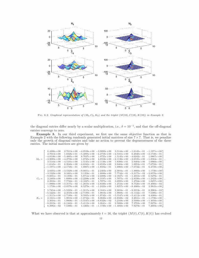
Fig. 6.2. Graphical representation of (M0, C0, K0) and the triplet (M(18), C(18), K(18)) in Example 2.

the diagonal entries differ nearly by a scalar multiplication, i.e., δ = 10−1, and that the off-diagonalentries converge to zero.

Example 3. In our third experiment, we first use the same objective function as that inExample 2 with the following randomly generated initial matrices of size 7× 7. That is, we penalizeonly the growth of diagonal entries and take no action to prevent the degenerateness of the theseentries. The initial matrices are given by

M0 =

2

6

6

6

6

6

6

6

4

6.4206e+00 2.7013e+00 −4.0538e+00 −3.9093e+00 3.5144e+00 −1.6145e−01 −1.1971e+00

2.7013e+00 1.0326e+01 −5.4895e+00 −4.2758e+00 −4.5101e+00 6.2040e+00 −2.1748e−01

−4.0538e+00 −5.4895e+00 8.7637e+00 1.0725e+00 1.5145e+00 −4.6242e−01 1.0867e+00

−3.9093e+00 −4.2758e+00 1.0725e+00 4.8558e+00 −2.1136e+00 −2.6535e+00 −1.8584e−01

3.5144e+00 −4.5101e+00 1.5145e+00 −2.1136e+00 1.8306e+01 2.9484e+00 1.6960e+00

−1.6145e−01 6.2040e+00 −4.6242e−01 −2.6535e+00 2.9484e+00 1.0953e+01 −7.6732e−01

−1.1971e+00 −2.1748e−01 1.0867e+00 −1.8584e−01 1.6960e+00 −7.6732e−01 6.4739e+00

3

7

7

7

7

7

7

7

5

,

C0 =

2

6

6

6

6

6

6

6

4

2.8355e+00 −3.5329e+00 −9.0051e−01 2.2403e+00 2.3916e−01 −1.8860e+00 1.1730e+00

−3.5329e+00 9.1601e+00 3.1358e−01 1.6880e+00 7.7742e−01 −3.3175e−02 −2.0576e+00

−9.0051e−01 3.1358e−01 5.8714e+00 −2.2298e+00 −2.1827e−01 −1.2010e+00 6.5279e−01

2.2403e+00 1.6880e+00 −2.2298e+00 8.3197e+00 1.7075e−01 −2.8330e+00 −1.2423e+00

2.3916e−01 7.7742e−01 −2.1827e−01 1.7075e−01 3.0995e+00 1.2724e+00 1.8257e+00

−1.8860e+00 −3.3175e−02 −1.2010e+00 −2.8330e+00 1.2724e+00 8.7520e+00 −8.4060e−02

1.1730e+00 −2.0576e+00 6.5279e−01 −1.2423e+00 1.8257e+00 −8.4060e−02 2.3845e+00

3

7

7

7

7

7

7

7

5

,

K0 =

2

6

6

6

6

6

6

6

4

5.7454e+00 −5.5223e−01 −1.3115e+00 2.1641e+00 2.3034e−01 −9.2219e−01 8.3982e−02

−5.5223e−01 2.3549e+00 −2.7189e−01 1.9810e+00 1.9808e−01 −6.1442e−01 7.5386e−01

−1.3115e+00 −2.7189e−01 9.5935e+00 −1.0742e−01 −5.5547e+00 −5.4112e+00 4.4360e−01

2.1641e+00 1.9810e+00 −1.0742e−01 8.0620e+00 −6.8328e−02 3.2041e−01 −1.1730e+00

2.3034e−01 1.9808e−01 −5.5547e+00 −6.8328e−02 5.2168e+00 2.5000e+00 −1.4050e+00

−9.2219e−01 −6.1442e−01 −5.4112e+00 3.2041e−01 2.5000e+00 7.2703e+00 7.9278e−01

8.3982e−02 7.5386e−01 4.4360e−01 −1.1730e+00 −1.4050e+00 7.9278e−01 7.2693e+00

3

7

7

7

7

7

7

7

5

.

What we have observed is that at approximately t = 16, the triplet (M(t), C(t), K(t)) has evolved

12

0 2 4 6 8 10 12 14 16 1810

−8

10−6

10−4

10−2

100

102

104

106

EVOLUTION OF DIAGONALIZATION PROCESS

NO

RM

SQ

UAR

ED

TIME

Objective (abs value)DiagonalOff−diagonal

Fig. 6.3. Behavior of the objective function

into the following matrices:

M =

2

6

6

6

6

6

6

6

4

2.2153e−13 2.1177e−06 −6.8153e−07 −1.8384e−07 1.1511e−06 −7.0594e−07 −4.8310e−07

2.1177e−06 2.7777e+01 −8.5516e−07 −2.4470e−06 −9.9352e−07 1.7505e−06 3.8014e−07

−6.8153e−07 −8.5516e−07 3.1307e+01 3.1516e−07 3.2599e−07 2.9865e−07 −1.7375e−07

−1.8384e−07 −2.4470e−06 3.1516e−07 2.8390e+00 −4.9293e−07 −1.3284e−07 1.4923e−07

1.1511e−06 −9.9352e−07 3.2599e−07 −4.9293e−07 8.8150e+01 5.4243e−07 3.7747e−07

−7.0594e−07 1.7505e−06 2.9865e−07 −1.3284e−07 5.4243e−07 4.8753e+01 −3.1072e−07

−4.8310e−07 3.8014e−07 −1.7375e−07 1.4923e−07 3.7747e−07 −3.1072e−07 3.1905e+01

3

7

7

7

7

7

7

7

5

,

C =

2

6

6

6

6

6

6

6

4

−3.1703e−13 −1.2169e−06 −4.0357e−07 −1.6317e−06 −6.7147e−08 −4.3025e−07 −1.6132e−08

−1.2169e−06 4.2699e+01 1.9723e−07 1.3068e−06 1.1515e−07 −3.7094e−07 −3.0443e−07

−4.0357e−07 1.9723e−07 2.2568e+01 −3.4856e−07 5.2178e−08 −2.2798e−07 6.8085e−09

−1.6317e−06 1.3068e−06 −3.4856e−07 3.3206e+01 2.1429e−07 −5.4923e−07 −2.2280e−07

−6.7147e−08 1.1515e−07 5.2178e−08 2.1429e−07 1.2109e+01 2.9003e−08 2.0453e−07

−4.3025e−07 −3.7094e−07 −2.2798e−07 −5.4923e−07 2.9003e−08 4.5150e+01 2.8697e−08

−1.6132e−08 −3.0443e−07 6.8085e−09 −2.2280e−07 2.0453e−07 2.8697e−08 5.6642e+00

3

7

7

7

7

7

7

7

5

,

K =

2

6

6

6

6

6

6

6

4

2.1121e−13 −2.5786e−07 −2.1259e−08 2.6425e−06 2.2480e−07 −3.9657e−07 −1.3054e−07

−2.5786e−07 4.5693e+00 1.6895e−07 −3.3515e−07 5.4747e−07 −1.0080e−07 3.1232e−07

−2.1259e−08 1.6895e−07 4.3968e+01 −3.6565e−07 −1.0213e−06 −1.1184e−06 1.5553e−07

2.6425e−06 −3.3515e−07 −3.6565e−07 4.1656e+01 −2.3364e−07 4.4752e−07 −2.2251e−07

2.2480e−07 5.4747e−07 −1.0213e−06 −2.3364e−07 6.1404e+00 8.2303e−07 −2.8470e−07

−3.9657e−07 −1.0080e−07 −1.1184e−06 4.4752e−07 8.2303e−07 1.5933e+01 1.5514e−07

−1.3054e−07 3.1232e−07 1.5553e−07 −2.2251e−07 −2.8470e−07 1.5514e−07 3.3756e+01

3

7

7

7

7

7

7

7

5

.

This example demonstrates that the triplet (M(t), C(t), K(t)) may converge to a singular pencil,which is not desirable.

A remedy might come if we penalize the decaying of diagonal entries to zero by adding in thepenalty function g1 defined in (3.11). However, the penalty factor δ has to be chosen carefully. If δis too large, the flow tends to put more emphasis on discouraging the decay of the diagonal entriesat the price of slowing down the convergence of the off-diagonal entries. If δ is too small, the flowconverges to a near-singular pencil. For our experiment, we adaptively use δ = 10−8 to discouragethe diagonal entries from going to zero and δ = 0 to encourage the off-diagonal entries to convergeto zero. At the moment, the adaptive scheme is inserted into the integration process manually and

13

subjectively. We are able to improve the convergence to the following matrices.

M =

2

6

6

6

6

6

6

6

4

1.4618e−01 8.4229e−21 −7.1889e−20 −2.2598e−20 −3.1102e−20 2.2559e−19 −1.6235e−20

−1.4672e−15 5.2520e+00 4.4173e−20 8.5578e−20 8.7294e−21 2.7976e−05 −1.8820e−07

5.0709e−15 4.5057e−16 3.9248e+00 −4.7978e−20 −1.2110e−20 1.2027e−19 3.3292e−21

1.9132e−15 1.1803e−14 −8.9042e−15 1.7497e−01 1.0212e−19 3.5002e−20 2.0289e−20

1.4079e−15 2.8080e−15 −6.7490e−15 2.6045e−16 9.6442e−01 −3.2220e−19 −6.3030e−21

−1.2395e−18 2.7976e−05 −2.3740e−19 5.4627e−19 −2.0220e−19 5.9730e−08 −2.5479e−05

4.3913e−15 −1.8820e−07 1.3186e−15 −2.8604e−15 −1.5211e−14 −2.5479e−05 9.1884e+00

3

7

7

7

7

7

7

7

5

,

C =

2

6

6

6

6

6

6

6

4

4.9848e+00 8.3472e−23 4.2650e−21 3.3450e−20 3.1178e−20 −5.3475e−19 2.2401e−20

−3.8580e−14 6.9063e+00 1.4369e−20 4.7488e−20 6.4548e−20 −3.4666e−05 −4.3162e−07

−5.9428e−15 −6.6258e−15 7.5498e−01 −3.7208e−20 1.7218e−21 −2.3996e−20 6.0364e−21

1.4816e−14 3.6117e−15 3.5201e−16 1.0704e+01 1.6483e−20 −1.9994e−19 −4.5170e−20

−2.3898e−14 6.6073e−15 3.4875e−14 2.9369e−14 4.5047e+00 1.0176e−19 −3.0356e−20

−4.9065e−19 −3.4666e−05 −2.6450e−18 −1.3797e−19 2.4698e−18 6.1934e−08 −4.4886e−05

−6.2580e−15 −4.3162e−07 1.9122e−15 −3.4434e−14 −2.4793e−14 −4.4886e−05 6.1427e+00

3

7

7

7

7

7

7

7

5

,

K =

2

6

6

6

6

6

6

6

4

8.9073e−04 −6.7678e−20 −6.0650e−20 −7.9906e−20 −3.3974e−21 3.9575e−19 7.8452e−21

−9.1039e−16 4.9464e+00 −3.5549e−20 3.5156e−20 6.6650e−20 1.9716e−05 6.0100e−07

1.0159e−14 8.8236e−15 4.6964e+00 −6.7415e−20 2.3783e−22 −1.2507e−19 −3.4392e−20

−8.1779e−16 3.8584e−16 −2.4487e−15 4.2010e+00 6.4197e−21 2.1525e−19 6.5043e−20

4.7487e−15 −9.4770e−15 −3.7846e−15 1.6717e−14 1.6497e+01 −4.4318e−20 1.0721e−19

−1.3417e−19 1.9716e−05 −6.3702e−19 1.2723e−19 −7.8421e−19 8.5473e−09 8.9375e−05

−2.4348e−15 6.0100e−07 1.0354e−15 −2.5474e−15 −1.0384e−14 8.9375e−05 5.6434e+00

3

7

7

7

7

7

7

7

5

.

7. Conclusion. In an earlier study, we have shown in theory that all most all quadratic pencilsλ2M + λC + K can be transformed isospectrally into pencils with diagonal matrix coefficients.This result has two significant implications: First, it shows that the conventional persuasion thatno three general matrices can be simultaneously diagonalized is perhaps because the question ofdiagonalization of a quadratic pencil has not been posed in an appropriate context. Perhaps aright way to ask the question is how to block diagonalizing the Lancaster structure. Secondly, itasserts that the dynamical behavior of almost all n-degree-of-freedom second order systems can beidentified from that of n independent single-degree-of-freedom second-order subsystems. Despite theimportance, the transformations involved in the reduction are rather complicated and difficult torealize numerically. The theoretical proof requires the knowledge of the entire spectral information.Without using the spectral information, there does not seem to have any numerical algorithm in theliterature for this purpose.

In this paper, we exploit the free matrix parameters in the structure preserving isospectralflows. In particular, we propose a simple closed-loop control that amends the structure preservingisospectral flow into a gradient flow. The gradient flow intends to reduce the magnitude of off-diagonal elements. Since the gradient flow can be tracked by available ODE integrator, it is feasiblefor numerical computation. Computer simulations seem to suggest the working of this approach.

Lot of room remains for further study. The most imperative topic is to develop special geometricintegrator for the isospectral flow described in this paper. Since the structure preserving equivalencetransformations do not form a group, we do not think that current Lie group methods are applicable.Also, it remains to be studied on whether the system (1.9) and (1.10) could be tackled by somestructure preserving iterative schemes.

REFERENCES

[1] A. M. Bloch and A. Iserles, On an isospectral Lie-Poisson system and its Lie algebra, DAMTP Tech. Rep.2005/NA01, Found. Comp. Math., to appear.

[2] M. T. Chu and N. Del Buono, Total decoupling of a general quadratic pencil, Part I: Theory, preprint, 2005.[3] Equations of motion for MDOF systems, see http://www.efunda.com/formulae/vibrations/mdof_eom.cfm,

eFunda, Inc., California.[4] Geometric integration interest group, FoCM, see http://www.focm.net/gi/.[5] S. D. Garvey, M. I. Friswell, and U. Prells, Co-ordinate tranfromations for second order systems, I: General

transformations, J. Sound Vibration, 258(2002), 885–909.

14

[6] S. D. Garvey, M. I. Friswell, and U. Prells, Co-ordinate transformations for second order systems, II: Elementarystructure-preserving transformations, J. Sound Vibration, 258 (2002), 911–930.

[7] S. D. Garvey, U. Prells, M. Friswell, and Z. Chen, General isospectral flows for linear dynamic systems, LinearAlg. Appl., 385(2004), 335-368.

[8] I. Gohberg, P. Lancaster, and L. Rodman, Spectral analysis of selfadjoint matrix polynomials, Ann. Math.,112(1980), 33-71.

[9] I. Gohberg, P. Lancaster, and L. Rodman, Matrix Polynomials, Computer Science and Applied Mathematics.Academic Press, Inc., New York-London, 1982.

[10] U. B. Holz, G. H. Golub, and K. H. Law, A subspace approximation method for the quadratic eigenvalueproblem, SIAM J. Matrix Anal. Appl., 26(2005), 498-521.

[11] R. A. Horn and C. R. Johnson, Matrix Analysis, Cambridge University Press, New York, 1991.[12] A. Iserles, H. Z. Munthe-Kaas, S. P. Nørsett, and A. Zanna, Lie-group methods, Acta Numerica, 9(2000),

215-365.[13] P. Lancaster, Lambda-Matrices and Vibrating System, Pergamon Press, Oxford, UK, 1966.[14] L. F. Shampine and M. W. Reichelt, The MATLAB ODE suite, SIAM J. Sci. Comput., 18(1997), 1-22.[15] F. Tisseur and K. Meerbergen, The quadratic eigenvalue problem, SIAM Rev. 43 (2001),235–286.[16] F. Uhlig, A canonical form for a pair of real symmetric matrices that generate a nonsingular pencil, Linear Alg.

Appl., 14, 189-209.[17] P. Van Eetvelt, private communication, Nottingham University, UK, 2004.

15