Topology Control for Maintaining NetworkConnectivity and Maximizing Network Capacity

Under the Physical ModelYan Gao, Jennifer C. Hou and Hoang Nguyen

Department of Computer ScienceUniversity of Illinois at Urbana Champaign

Urbana, IL 61801E-mail:{yangao3,jhou,hnguyen5}@uiuc.edu

Abstract—In this paper we study the issue of topology controlunder the physical Signal-to-Interference-Noise-Ratio (SINR)model, with the objective of maximizing network capacity. Weshow that existing graph-model-based topology control capturesinterference inadequately under the physical SINR model, andas a result, the interference in the topology thus induced is highand the network capacity attained is low. Towards bridging thisgap, we propose a centralized approach, called Spatial ReuseMaximizer (MaxSR), that combines a power control algorithmT4P with a topology control algorithm P4T. T4P optimizes theassignment of transmit power given a fixed topology, where byoptimality we mean that the transmit power is so assigned thatit minimizes the average interference degree (defined as thenumber of interferencing nodes that may interfere with the on-going transmission on a link) in the topology. P4T, on the otherhand, constructs, based on the power assignment made in T4P, anew topology by deriving a spanning tree that gives the minimalinterference degree. By alternately invoking the two algorithms,the power assignment quickly converges to an operational pointthat maximizes the network capacity. We formally prove theconvergence of MaxSR. We also show via simulation that thetopology induced by MaxSR outperforms that derived fromexisting topology control algorithms by 50%-110% in terms ofmaximizing the network capacity.

I. INTRODUCTION

Topology control and management – how to determine thetransmit power of each node so as to maintain network con-nectivity, mitigate interference, improve spatial reuse, whileconsuming the minimum possible power – is one of themost important issues in wireless multi-hop networks [1].Instead of transmitting using the maximum possible power,wireless nodes collaboratively determine their transmit powerand define the topology by the neighbor relation under certaincriteria.

A common notion of neighbors adopted in most topologycontrol algorithms [2], [3], [4], [5], [6], perhaps except thosein [7], [8], is that two nodes are considered neighbors and awireless link exists between them in the corresponding com-munication graph, if their distance is within the transmissionrange (as determined by the transmit power, the path lossmodel, and the receiver sensitivity). Algorithms that adoptthis notion are collectively called graph-model-based topologycontrol. Under this notion, topology control aims to keep

the node degree in the communication graph low, subject tothe network connectivity requirement. This is based on thecommon assertion that a low node degree usually implies lowinterference.

We claim that this assertion no longer holds under the phys-ical Signal-to-Interference-Noise-Ratio (SINR) model. This isbecause under the physical model, whether the interference— the sum of all the signals of concurrent, competing trans-missions received at the receiver — affects the transmissionactivity of interest depends on the SINR at the receiver, whichin turn depends on the transmit power of all the transmittersand their relative positions to the receiver of interest. The nodedegree under the graph model, however, does not adequatelycapture interference. In particular, a transmission of interestmay fail because other concurrent transmissions cause theSINR at the receiver to fall below the minimal SINR requiredfor the receiver to decode the symbols correctly. This couldoccur even if competing transmitters are outside the transmis-sion range of the receiver.

There are two undesirable consequences as a result ofthe inadequacy of graph-model-based topology control underthe physical model. First, because the node degree does notcapture interference adequately, the interference in the result-ing topology may be high, rendering low network capacity.Second, a wireless link that exists in the communication graphmay not in practice exist under the physical model, because ofhigh interference (and consequently low SINR). As a result,the network connectivity may not even be sustained.

In this paper, first we formally argue that a node with asmall node degree in the communication graph may sufferfrom high interference. Then, we define the interference graphthat faithfully captures interference under the physical model.An interesting question is whether or not there exists apower assignment that enables the communication graph ofthe topology to represent its interference graph as well. Weformally prove that such a power assignment exists only if thetopology satisfies a certain criterion. Unfortunately, most of thetopologies generated by existing graph-model-based topologycontrol do not satisfy this criterion.

In order to mitigate interference, improve network capacity,

while maintaining network connectivity, we propose a cen-tralized approach, called Spatial Reuse Maximizer (MaxSR),that consists of two component algorithms: T4P and P4T.Conceptually, given the topology induced by certain topologycontrol algorithm, each node may, instead of using the minimalpossible power to reach its farthest neighbor (as defined inthe communication graph), increase its transmit power inorder to increase the SINR at the receiver and better tolerateinterference. On the other hand, if every node transmits withhigh power, it contributes more to the interference as perceivedby other nodes. MaxSR seeks to strike a balance between in-creasing the SINR and controlling the interference as perceivedby others to an acceptable level. Specifically, T4P optimizesassignment of the transmit power given a fixed topology, whereby optimality we mean that the transmit power is so assignedthat it minimizes the average interference degree (defined asthe number of nodes that will interfere with transmission on alink), and (ii) P4T constructs, based on the power assignmentmade in T4P, a new topology by deriving a spanning tree thatgives the minimal interference degree. By alternately invokingthe two algorithms, the power assignment quickly convergesto an operational point that maximizes network capacity. Weformally prove the convergence of MaxSR, and show viasimulation that the topology induced by MaxSR outperformsthat derived from existing topology control algorithms by 50-110% in terms of maximizing network capacity.

The remainder of the paper is organized as follows. Wefirst introduce in Section II the notation and the assumptionsmade throughout this paper. Then we formally argue that asmall node degree does not necessarily imply low interferencein Section III. Following that, we investigate in Section IVthe issue of whether or not a feasible power assignmentexists that enables the communication graph to represent theinterference graph as well. After obtaining a negative answer,we devise in Section V a new topology control algorithm,called MaxSR, that alternatively invokes T4P and P4T untilthe power assignment converges to an optimal operationalpoint. We also formally prove its convergence there. Wepresent in Section VI simulation results. Finally, we providean overview of related work in Section VII, and conclude thepaper in Section VIII with a list of future research agendas.

II. PHYSICAL INTERFERENCE MODEL

In this section, we first give the notation used and theassumptions made throughout in the paper. Then we explicitlydefine interference under the physical model.

A. Notation and Assumptions

We envision a wireless network as a set of nodes V locatedin the Euclidean plane. All nodes are stationary or havelow mobility. Let (X, Y ) denote the Euclidean coordinates,v ∈ V the shorthand of v(x, y), x ∈ X and y ∈ Y , anddij = d(vi, vj) the Euclidean distance between two nodesvi and vj . Every node vi is configured with a transmitpower pt(i) and Pt denotes the transmit power assignment{pt(1), pt(2), ..., pt(n)}, where n = |V |.

The large-scale path loss model is used to describe howsignals attenuate along the transmission path. Let gij be thechannel gain from node vi to node vj (which is usuallyassumed to be a constant independent of the distance), thenthe received power can be expressed as

pr(i, j) =gi,j · pt(i)

dαi,j

,

where α is the path loss exponent. The value of α typicallyranges between 2 and 4, depending on which propagationmodel is used (e.g. α = 2 for the free space model and α = 4for the two-ray ground model).

Whether a transmission succeeds or not is determined bytwo factors: namely the receive sensitivity and the signal tointerference and noise ratio (SINR). Specifically, let RXmin

be the threshold for the receiver to decode the receivedsignal correctly, and β the SINR threshold. A signal can besuccessfully received and decoded only if the following twoconstraints are satisfied:

pr(i, j) =gi,j · pt(i)

dαi,j

≥ RXmin, (1)

and

SINRi,j =gi,j · pt(i) · d−α

i,j

N + Ij≥ β, (2)

where N denotes the noise power, and Ij the interferenceperceived at receiver vj and contributed by other concurrenttransmissions. We will elaborate on Ij in Section II-B. Eq. (1)also defines the minimal power required to reach a receiverat a distance of di,j away. In this paper, we assume that allnodes are homogeneous, i.e., they have the same maximumpower level Pmax, SINR threshold β, and receiver sensitivityRXmin.

Definition 1. A link (i, j) is said to exist (i.e., node vi cansend packets to node vj that is di,j away, without considerationof interference) if and only if

pt(i) ≥dα

i,jRXmin

gi,j.

We also define an edge as a bi-directional link. That is, anedgei,j exists if and only if pt(i) ≥ dα

i,jRXmin/gi,j andpt(j) ≥ dα

i,jRXmin/gj,i.Given all the definitions, the communication graph of a

network is represented by a graph G = (V, E), where E isa set of undirected edges. Note that following the definitionof an edge given in Definition 1, E is actually determinedby the power assignment Pt. In other words, given a powerassignment Pt, E is induced according to Definition 1. Thisis the graphic model used in conventional topology control.Note that the same model is also used in [9] [4] and [2].

B. Interference Model

As mentioned in Section I, mitigating interference is oneof the major objectives of topology control. However, mostexisting topology control algorithms characterize interferencewith the node degree, and argue that a low node degree implies

low interference. While this is an appropriate assumptionunder the graphic model, this may not be valid under thephysical model. Before delving into the analysis, we firstdefine interference under the physical model.

Recall that in Section II-A, the constraint in Eq. (1) is usedto define the existence of a communication link. We now useEq. (2) to define the interference in terms of the interferencedegree.

Definition 2. Interfering node: A node vk ∈ V is said to bean interfering node for link (vi, vj) if

pt(i)d−αi,j

N + pt(k)d−αk,j

< β. (3)

The physical meaning of the above definition is that if nodevk transmits with power pt(k), then the transmission on link(vi, vj) can not proceed simultaneously, i.e., the receiver vj isunable to decode the received signal due to the violation of theSINR constraint. The transmission activity which node vk isengaged will either be blocked or collide with the transmissionactivity on (vi, vj).

Definition 3. The interference degree of a link (vi, vj) isdefined as the number of interfering nodes for (vi, vj). LetVI(vi, vj) denote the set of v ∈ V containing all interferingnodes of (vi, vj), then the interference degree DI(vi, vj)

4=

|VI(vi, vj)|.A link with a high interference degree implies multiple

nodes can interfere with its transmission activity, causing chan-nel competition and/or collision. This is undesirable becauseboth channel competition and collision degrade the networkcapacity (i.e., the number of bytes that can be simultaneouslytransported by the network). Indeed it is the interfering nodes(rather than the communication neighbors) that substantiallyaffect the throughput capacity under the physical model.Hence, the interference degree is a better index than the nodedegree in quantifying the interference. In Section III, we willshow that the interference degree does not necessarily relateto the node degree.

Given the definition of the interference degree, we are ina position to define the link interference graph which is thecounterpart of the communication graph under the physicalmodel.

Definition 4. A link interference graph represents the inter-ference of a link (vi, vj) as GI(VI(vi, vj), EI(vi, vj)), whereVI(vi, vj) = VI(vi, vj) ∪ vi ∪ vj and EI(linki,j) is the set ofedges such that (w, vj) ∈ EI(vi, vj), w ∈ VI(vi, vj) \ {vj}.

III. INTERFERENCE UNDER THE PHYSICAL MODEL

In this section we show that a small node degree doesnot directly relate to low interference under the physicalmodel. Hence, the topology rendered by conventional topologycontrol algorithms may not be capacity-efficient. Moveover,we show that the interference can be reduced by adequatepower adjustment.

As mentioned in Section II-A, the topology is a graphinduced by the transmit power assignment. Most existing

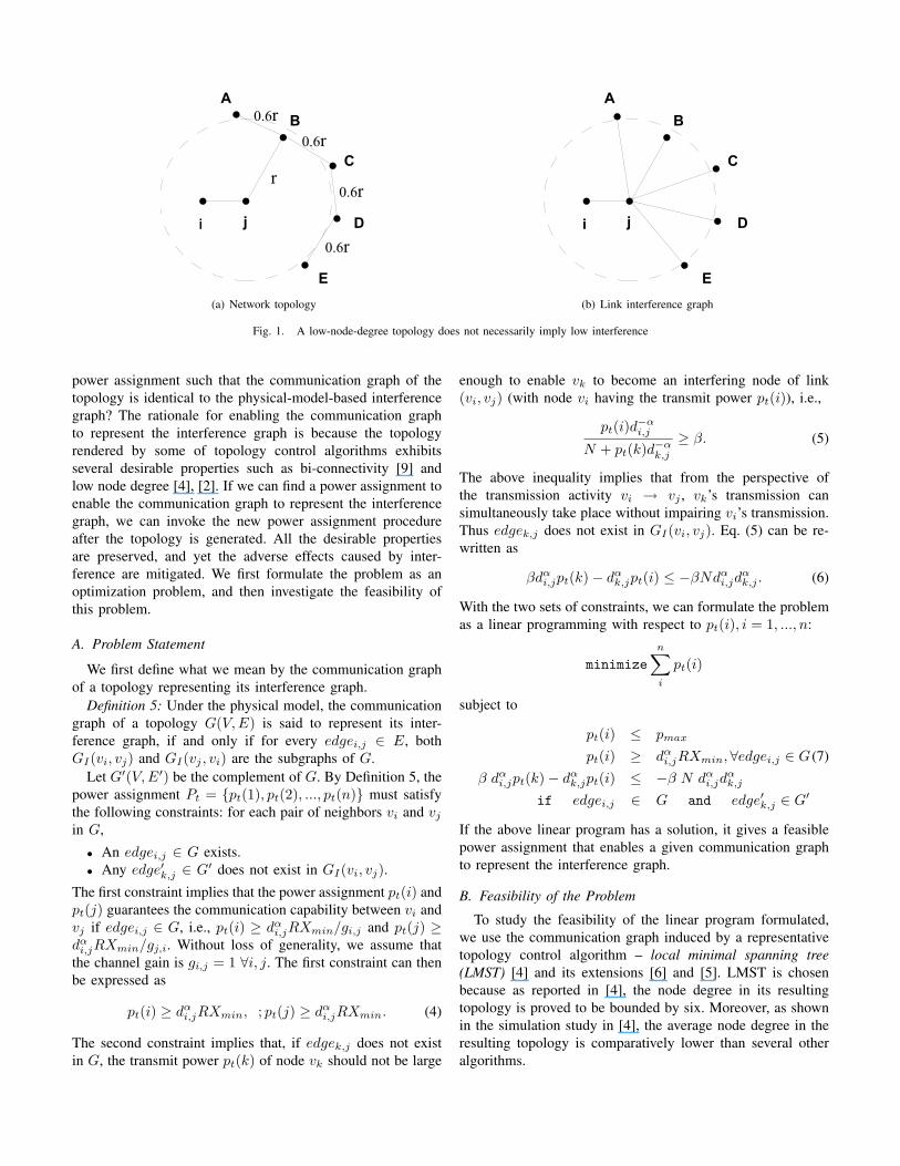
topology control algorithms produce topologies by simplyassigning the minimum possible power so as to ensure edgesexist for network connectivity. Figure 1 gives an example thatshows that this type of power assignment does not serve thepurpose of mitigating interference under the physical model.Consider a link (i, j) in Figure 1 (a) and compare its interfer-ence degree against node j’s degree. The node degree of j is2. Let β = 10, α = 4 and N = 0, and each node be configuredwith the minimal power so that it can communicate with itsfarthest neighbor (i.e., Eq. (1) holds). Under this configuration,the transmission activities of all the other nodes (A, B, C, Dor E) transmitting lead to SINRi,j = 1/0.64 = 7.7 < 10.That is, by Definition 2. all the other nodes are the interferingnodes to link (i, j), rendering the link interference graph oflink (i, j) in Figure 1(b). Although the node degree of j is onlytwo, link (i, j) has six interfering nodes, i.e., the transmissionactivity on link (i, j) may have to compete for channel accesswith 5 other potential transmissions. As a result, the attainablelink capacity is much lower than it is expected to be. Suchhigh interference, induced by graph-model-based topologycontrol (and its associated power assignment), is obviouslyundesirable.

The above example also demonstrates that the interferencedegree dose not necessarily relate to the node degree. As amatter of fact, the interference degree is affected by severalparameters such as β, N , α and pt. Among them, N andα are environmentally determined and not controllable. β isa controllable parameter, and in the interest of Shannon’scapacity, should be set to a reasonable large value. In thispaper we thus focus on adjusting the transmit power pt.

Now we show, by using the same example, that adjustingthe transmit power (with the physical SINR model in mind)can indeed mitigate the interference. If the transmit power ofnode i is raised to 1.5 times of that in Figure 1. Even if anyother node transmits concurrently with node i, SINRi,j nowincreases to 1.5/0.64 = 11.5. This implies, instead of using theminimum power to maintain network connectivity, an adequatepower level can substantially reduce the effect of concurrentlytransmitting nodes and thus improve the link capacity. Notealso that a similar observation is also made by Moscibroda etal. in [10]. Note that the above example considers only peerinterference. If the cumulative interference (i.e., interferencecontributed by multiple, concurrent transmissions) is consid-ered, the interference in the topology induced by graph-model-based topology control will become even more severe.

The inadequacy of graph-model-based topology control isrooted at the fact that the underlying communication topologyit induces does not capture the interference appropriately underthe physical model. An interesting question is then whether ornot there exists a power assignment that enables the communi-cation graph to represent the corresponding interference graphas well. We will address this question in Section IV.

IV. POWER CONTROL IN KNOWN TOPOLOGIES

In this section, we seek the answer to the following question:given a communication topology, is it possible to find a

(a) Network topology (b) Link interference graph

Fig. 1. A low-node-degree topology does not necessarily imply low interference

power assignment such that the communication graph of thetopology is identical to the physical-model-based interferencegraph? The rationale for enabling the communication graphto represent the interference graph is because the topologyrendered by some of topology control algorithms exhibitsseveral desirable properties such as bi-connectivity [9] andlow node degree [4], [2]. If we can find a power assignment toenable the communication graph to represent the interferencegraph, we can invoke the new power assignment procedureafter the topology is generated. All the desirable propertiesare preserved, and yet the adverse effects caused by inter-ference are mitigated. We first formulate the problem as anoptimization problem, and then investigate the feasibility ofthis problem.

A. Problem Statement

We first define what we mean by the communication graphof a topology representing its interference graph.

Definition 5: Under the physical model, the communicationgraph of a topology G(V, E) is said to represent its inter-ference graph, if and only if for every edgei,j ∈ E, bothGI(vi, vj) and GI(vj , vi) are the subgraphs of G.

Let G′(V, E′) be the complement of G. By Definition 5, thepower assignment Pt = {pt(1), pt(2), ..., pt(n)} must satisfythe following constraints: for each pair of neighbors vi and vj

in G,

• An edgei,j ∈ G exists.• Any edge′k,j ∈ G′ does not exist in GI(vi, vj).

The first constraint implies that the power assignment pt(i) andpt(j) guarantees the communication capability between vi andvj if edgei,j ∈ G, i.e., pt(i) ≥ dα

i,jRXmin/gi,j and pt(j) ≥dα

i,jRXmin/gj,i. Without loss of generality, we assume thatthe channel gain is gi,j = 1 ∀i, j. The first constraint can thenbe expressed as

pt(i) ≥ dαi,jRXmin, ; pt(j) ≥ dα

i,jRXmin. (4)

The second constraint implies that, if edgek,j does not existin G, the transmit power pt(k) of node vk should not be large

enough to enable vk to become an interfering node of link(vi, vj) (with node vi having the transmit power pt(i)), i.e.,

pt(i)d−αi,j

N + pt(k)d−αk,j

≥ β. (5)

The above inequality implies that from the perspective ofthe transmission activity vi → vj , vk’s transmission cansimultaneously take place without impairing vi’s transmission.Thus edgek,j does not exist in GI(vi, vj). Eq. (5) can be re-written as

βdαi,jpt(k)− dα

k,jpt(i) ≤ −βNdαi,jd

αk,j . (6)

With the two sets of constraints, we can formulate the problemas a linear programming with respect to pt(i), i = 1, ..., n:

minimizen∑

i

pt(i)

subject to

pt(i) ≤ pmax

pt(i) ≥ dαi,jRXmin,∀edgei,j ∈ G (7)

β dαi,jpt(k)− dα

k,jpt(i) ≤ −β N dαi,jd

αk,j

if edgei,j ∈ G and edge′k,j ∈ G′

If the above linear program has a solution, it gives a feasiblepower assignment that enables a given communication graphto represent the interference graph.

B. Feasibility of the Problem

To study the feasibility of the linear program formulated,we use the communication graph induced by a representativetopology control algorithm – local minimal spanning tree(LMST) [4] and its extensions [6] and [5]. LMST is chosenbecause as reported in [4], the node degree in its resultingtopology is proved to be bounded by six. Moreover, as shownin the simulation study in [4], the average node degree in theresulting topology is comparatively lower than several otheralgorithms.

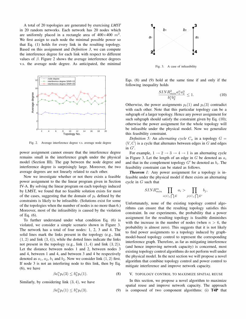
A total of 20 topologies are generated by exercising LMSTin 20 random networks. Each network has 20 nodes whichare uniformly placed in a rectangle area of 400×400 m2.We first assign to each node the minimal possible power sothat Eq. (1) holds for every link in the resulting topology.Based on this assignment and Definition 3, we can computethe interference degree for each link with respect to differentvalues of β. Figure 2 shows the average interference degreesv.s. the average node degree. As anticipated, the minimal

2 4 6 8 10 12 14 16 18 200

2

4

6

8

10

12

Topology No.

Ave

rage

deg

ree

node degreeinterference degree SINR=10interference degree SINR=20

Fig. 2. Average interference degree v.s. average node degree

power assignment cannot ensure that the interference degreeremains small in the interference graph under the physicalmodel (Section III). The gap between the node degree andinterference degree is surprisingly large. Moreover, the twoaverage degrees are not linearly related to each other.

Now we investigate whether or not there exists a feasiblepower assignment to the the linear program given in SectionIV-A. By solving the linear program on each topology inducedby LMST, we found that no feasible solution exists for mostof the cases, suggesting that the domain of pt defined by theconstraints is likely to be infeasible. (Solutions exist for someof the topologies when the number of nodes is no more than 6.)Moreover, most of the infeasibility is caused by the violationof Eq. (6).

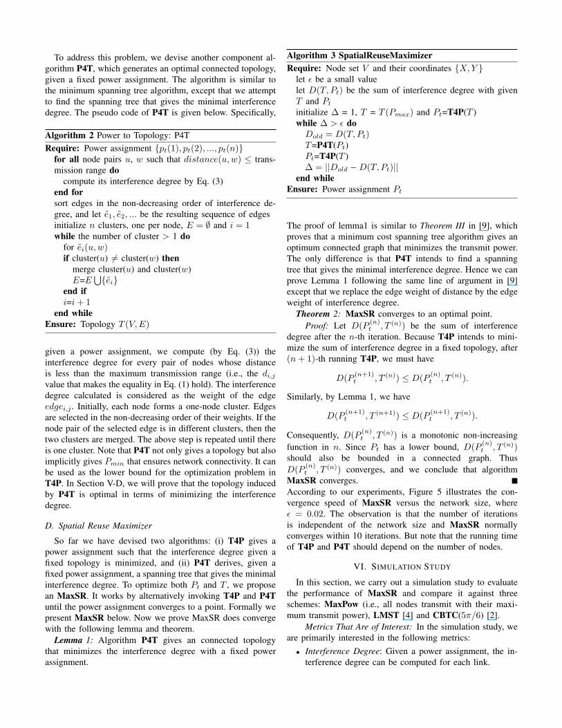
To further understand under what condition Eq. (6) isviolated, we consider a simple scenario shown in Figure 3.The network has a total of four nodes: 1, 2, 3 and 4. Thesolid lines mark the links present in the topology (e.g., link(1, 2) and link (3, 4)), while the dotted lines indicate the linksnot present in the topology (e.g., link (1, 4) and link (3, 2)).Let the distance between nodes 1 and 2, between nodes 3and 4, between 1 and 4, and between 3 and 4 be respectivelydenoted as a1, a2, b1 and b2. Now we consider link (1, 2) first.If node 3 is not an interfering node to this link, then by Eq.(6), we have

βaα1 pt(3) ≤ bα

2 pt(1). (8)

Similarly, by considering link (3, 4), we have

βaα2 pt(1) ≤ bα

1 pt(3). (9)

Fig. 3. A case of infeasibility

Eqs. (8) and (9) hold at the same time if and only if thefollowing inequality holds

SINR2minaα

1 aα2

bα1 bα

2

≤ 1. (10)

Otherwise, the power assignments pt(1) and pt(3) contradictwith each other. Note that this particular topology can be asubgraph of a larger topology. Hence any power assignment forsuch subgraph should satisfy the constraint given by Eq. (10);otherwise the power assignment for the whole topology willbe infeasible under the physical model. Now we generalizethis feasibility constraint.

Definition 5: An alternating cycle Ca in a topology G =(V, C) is a cycle that alternates between edges in G and edgesin G′.

For example, 1 → 2 → 3 → 4 → 1 is an alternating cyclein Figure 3. Let the length of an edge in G be denoted as ai

and that in the complement topology G′ be denoted as bi. Thefeasibility constraint can be stated as follows.

Theorem 1: Any power assignment for a topology is in-feasible under the physical model if there exists an alternatingcycle in G such that

SINRmmin

∏

i∈Ca

⋂E

ai >∏

j∈Ca

⋂E′

bj ,

Unfortunately, none of the existing topology control algo-rithms can ensure that the resulting topology satisfies thisconstraint. In our experiments, the probability that a powerassignment for the resulting topology is feasible diminisheswith the increase in the number of nodes (when n > 6, theprobability is almost zero). This suggests that it is not likelyto find power assignments to a topology induced by graph-model-based topology control to represent the correspondinginterference graph. Therefore, as far as mitigating interference(and hence improving network capacity) is concerned, mostexisting topology control algorithms do not perform well underthe physical model. In the next section we will propose a novelalgorithm that combine topology control and power control tomitigate interference and improve network capacity.

V. TOPOLOGY CONTROL TO MAXIMIZE SPATIAL REUSE

In this section, we propose a novel algorithm to maximizespatial reuse and improve network capacity. The approachis composed of two component algorithms: (i) T4P that

computes a power assignment that maximizes spatial reusewith a fixed topology, and (ii) P4T that generates a topologythat maximizes spatial reuse with a fixed power assignment.By alternately invoking the two component algorithms, boththe topology and the power assignment converge to a pointthat globally maximizes the network capacity.

A. Spatial Reuse Metric

Conceptually, spatial reuse is referred to the capability of anetwork to accommodate concurrent transmissions. Althougha number of studies have been carried out on spatial reuse,there have not been explicit metrics defined to characterizethe level spatial reuse. Most topology control algorithms useinterference as an implicit metric, based on the intuition thatlow interference implies high spatial reuse. Although the intu-ition is correct, we show in Section IV that graph-model-basedtopology control inadequately captures interference under thephysical model. Indeed, the interference degree, rather thanthe node degree, affects the link capacity. From a link’s pointof view, if there are less interfering nodes in its vicinity, it willhave more chances to access the channel. From the network’spoint of view, if every link has a small number of interferingnodes, then the network will be able to accommodate moreconcurrent transmissions. Based on the above observation, weuse the average interference degree as the metric for spatialreuse. It is obtained by taking all interference degree over allnodes in the network.

B. Topology to Power assignment: T4P

Under the physical model, whether some other concurrenttransmission interferes an ongoing transmission of interestdepends on several factors. If the transmit power is high, theongoing transmission may tolerate interference better becauseof a higher SINR. On the other hand, if every node transmitswith high power, the interference is likely high, depending onthe relative positions of competing transmitters to the receiverof interest. In Section II, we have defined an interfering node inEq. (3). Let the left hand side of Eq. (3) be defined as βk(i, j).Then we define an indicator function to denote whether a nodek is an interfering node to link (vi, vj)

I(βk(i, j)) ={

1, βk(i, j) < β0, βk(i, j) ≥ β

(11)

Locally minimizing the interference degree may cause highinterference to others. Hence all the nodes within the interfer-ence range must cooperate to achieve some level of globaloptimality. As such, we formulate the T4P problem as anoptimization problem:

minimize∑

link(i,j)∈T

∑

k 6=i,j

I(βk(i, j))

subject to

Pmin ≤ Pt ≤ Pmax.

The above problem is an integer program because of theexistence of indicator functions. Fortunately, as indicated in

[11], the hard SINR requirement can be “softened” by the sig-moid function. The sigmoid function is a continuous functionexpressed as

sig(x) =1

1 + e−a(x−b). (12)

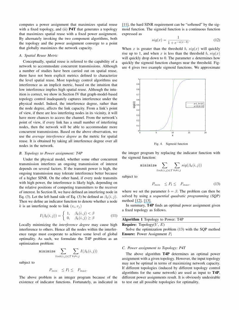
When x is greater than the threshold b, sig(x) will quicklyrise up to 1, and when x is less than the threshold b, sig(x)will quickly drop down to 0. The parameter a determines howquickly the sigmoid function changes near the threshold. Fig-ure 4 gives two example sigmoid functions. We approximate

0 5 10 15 200

0.1

0.2

0.3

0.4

0.5

0.6

0.7

0.8

0.9

1

xsi

g(x) a=1, b=10

a=10,b=10

Fig. 4. Sigmoid function

the integer program by replacing the indicator function withthe sigmoid function:

minimize∑

link(i,j)∈T

∑

k 6=i,j

sig(βk(i, j))

subject to

Pmin ≤ Pt ≤ Pmax. (13)

where we set the parameter b = β. The problem can then besolved by using a sequential quadratic programming (SQP)method [12], [13].

In summary, T4P finds an optimal power assignment givena fixed topology as follows.

Algorithm 1 Topology to Power: T4PRequire: Topology(V , E)

Solve the optimization problem (13) with the SQP methodEnsure: Power Assignment Pt

C. Power assignment to Topology: P4T

The above algorithm T4P determines an optimal powerassignment with a given topology. However, the input topologymay not be optimal in terms of maximizing network capacity.If different topologies (induced by different topology controlalgorithms for the same network) are used as input to T4P,different power assignments result. It is obviously undesirableto test out all possible topologies for optimality.

To address this problem, we devise another component al-gorithm P4T, which generates an optimal connected topology,given a fixed power assignment. The algorithm is similar tothe minimum spanning tree algorithm, except that we attemptto find the spanning tree that gives the minimal interferencedegree. The pseudo code of P4T is given below. Specifically,

Algorithm 2 Power to Topology: P4TRequire: Power assignment {pt(1), pt(2), ..., pt(n)}

for all node pairs u, w such that distance(u,w) ≤ trans-mission range do

compute its interference degree by Eq. (3)end forsort edges in the non-decreasing order of interference de-gree, and let e1, e2, ... be the resulting sequence of edgesinitialize n clusters, one per node, E = ∅ and i = 1while the number of cluster > 1 do

for ei(u,w)if cluster(u) 6= cluster(w) then

merge cluster(u) and cluster(w)E=E

⋃{ei}end ifi=i + 1

end whileEnsure: Topology T (V, E)

given a power assignment, we compute (by Eq. (3)) theinterference degree for every pair of nodes whose distanceis less than the maximum transmission range (i.e., the di,j

value that makes the equality in Eq. (1) hold). The interferencedegree calculated is considered as the weight of the edgeedgei,j . Initially, each node forms a one-node cluster. Edgesare selected in the non-decreasing order of their weights. If thenode pair of the selected edge is in different clusters, then thetwo clusters are merged. The above step is repeated until thereis one cluster. Note that P4T not only gives a topology but alsoimplicitly gives Pmin that ensures network connectivity. It canbe used as the lower bound for the optimization problem inT4P. In Section V-D, we will prove that the topology inducedby P4T is optimal in terms of minimizing the interferencedegree.

D. Spatial Reuse Maximizer

So far we have devised two algorithms: (i) T4P gives apower assignment such that the interference degree given afixed topology is minimized, and (ii) P4T derives, given afixed power assignment, a spanning tree that gives the minimalinterference degree. To optimize both Pt and T , we proposean MaxSR. It works by alternatively invoking T4P and P4Tuntil the power assignment converges to a point. Formally wepresent MaxSR below. Now we prove MaxSR does convergewith the following lemma and theorem.

Lemma 1: Algorithm P4T gives an connected topologythat minimizes the interference degree with a fixed powerassignment.

Algorithm 3 SpatialReuseMaximizerRequire: Node set V and their coordinates {X, Y }

let ε be a small valuelet D(T, Pt) be the sum of interference degree with givenT and Pt

initialize ∆ = 1, T = T (Pmax) and Pt=T4P(T )while ∆ > ε do

Dold = D(T, Pt)T=P4T(Pt)Pt=T4P(T )∆ = ||Dold −D(T, Pt)||

end whileEnsure: Power assignment Pt

The proof of lemma1 is similar to Theorem III in [9], whichproves that a minimum cost spanning tree algorithm gives anoptimum connected graph that minimizes the transmit power.The only difference is that P4T intends to find a spanningtree that gives the minimal interference degree. Hence we canprove Lemma 1 following the same line of argument in [9]except that we replace the edge weight of distance by the edgeweight of interference degree.

Theorem 2: MaxSR converges to an optimal point.Proof: Let D(P (n)

t , T (n)) be the sum of interferencedegree after the n-th iteration. Because T4P intends to mini-mize the sum of interference degree in a fixed topology, after(n + 1)-th running T4P, we must have

D(P (n+1)t , T (n)) ≤ D(P (n)

t , T (n)).

Similarly, by Lemma 1, we have

D(P (n+1)t , T (n+1)) ≤ D(P (n+1)

t , T (n)).

Consequently, D(P (n)t , T (n)) is a monotonic non-increasing

function in n. Since Pt has a lower bound, D(P (n)t , T (n))

should also be bounded in a connected graph. ThusD(P (n)

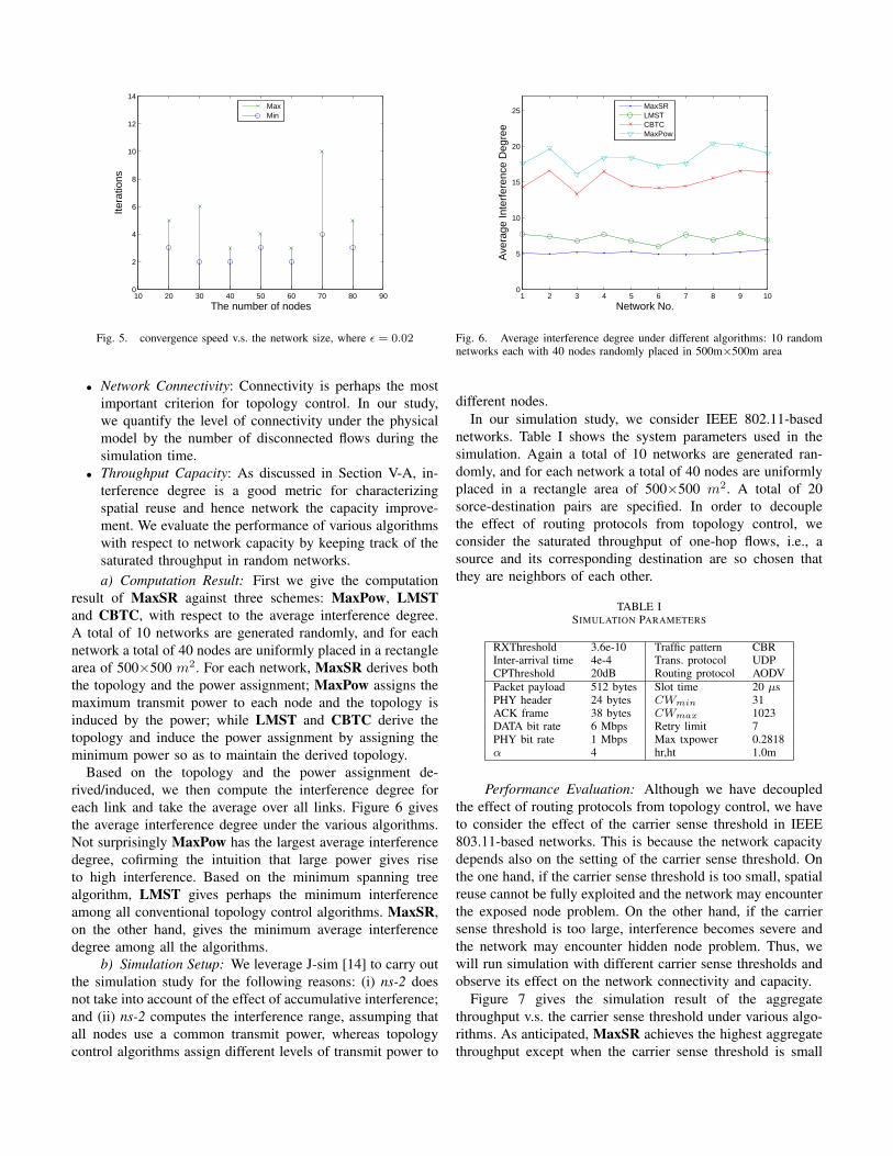
t , T (n)) converges, and we conclude that algorithmMaxSR converges.According to our experiments, Figure 5 illustrates the con-vergence speed of MaxSR versus the network size, whereε = 0.02. The observation is that the number of iterationsis independent of the network size and MaxSR normallyconverges within 10 iterations. But note that the running timeof T4P and P4T should depend on the number of nodes.

VI. SIMULATION STUDY

In this section, we carry out a simulation study to evaluatethe performance of MaxSR and compare it against threeschemes: MaxPow (i.e., all nodes transmit with their maxi-mum transmit power), LMST [4] and CBTC(5π/6) [2].

Metrics That Are of Interest: In the simulation study, weare primarily interested in the following metrics:• Interference Degree: Given a power assignment, the in-

terference degree can be computed for each link.

10 20 30 40 50 60 70 80 900

2

4

6

8

10

12

14

The number of nodes

Itera

tions

MaxMin

Fig. 5. convergence speed v.s. the network size, where ε = 0.02

• Network Connectivity: Connectivity is perhaps the mostimportant criterion for topology control. In our study,we quantify the level of connectivity under the physicalmodel by the number of disconnected flows during thesimulation time.

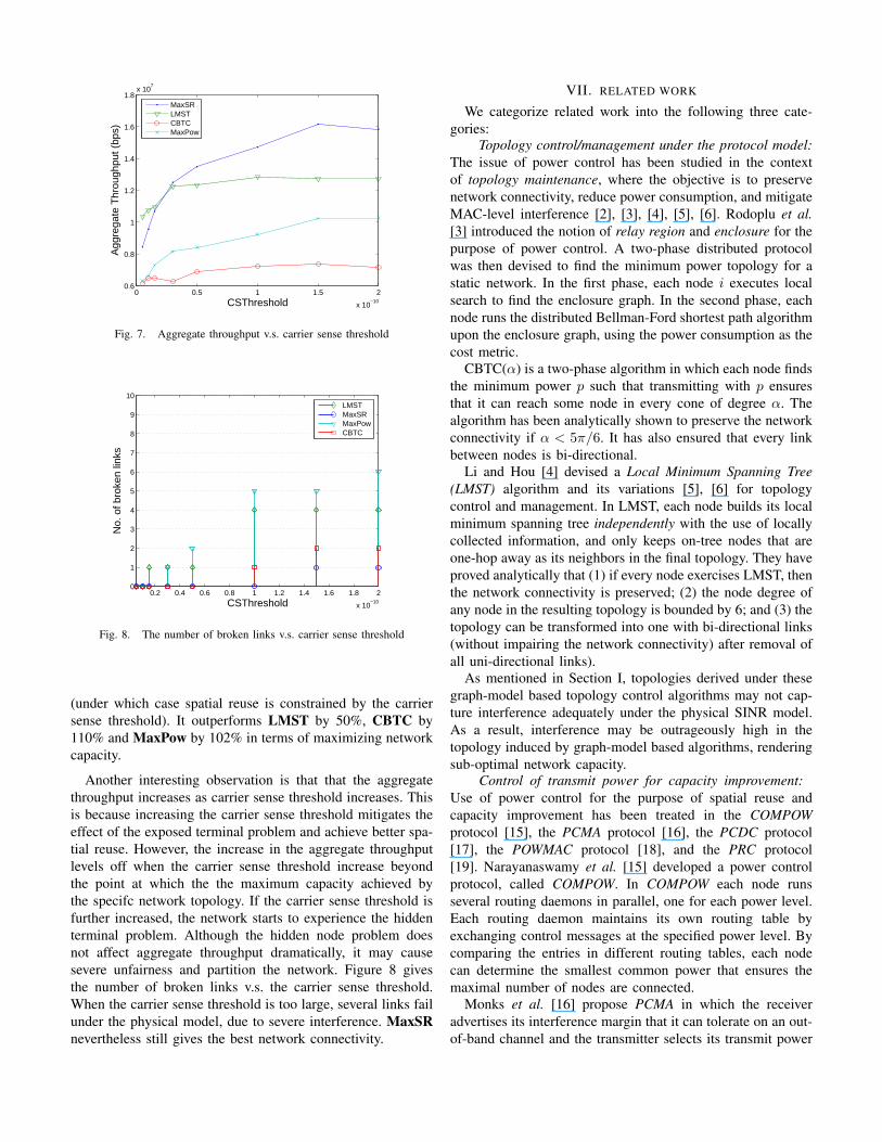
• Throughput Capacity: As discussed in Section V-A, in-terference degree is a good metric for characterizingspatial reuse and hence network the capacity improve-ment. We evaluate the performance of various algorithmswith respect to network capacity by keeping track of thesaturated throughput in random networks.a) Computation Result: First we give the computation

result of MaxSR against three schemes: MaxPow, LMSTand CBTC, with respect to the average interference degree.A total of 10 networks are generated randomly, and for eachnetwork a total of 40 nodes are uniformly placed in a rectanglearea of 500×500 m2. For each network, MaxSR derives boththe topology and the power assignment; MaxPow assigns themaximum transmit power to each node and the topology isinduced by the power; while LMST and CBTC derive thetopology and induce the power assignment by assigning theminimum power so as to maintain the derived topology.

Based on the topology and the power assignment de-rived/induced, we then compute the interference degree foreach link and take the average over all links. Figure 6 givesthe average interference degree under the various algorithms.Not surprisingly MaxPow has the largest average interferencedegree, cofirming the intuition that large power gives riseto high interference. Based on the minimum spanning treealgorithm, LMST gives perhaps the minimum interferenceamong all conventional topology control algorithms. MaxSR,on the other hand, gives the minimum average interferencedegree among all the algorithms.

b) Simulation Setup: We leverage J-sim [14] to carry outthe simulation study for the following reasons: (i) ns-2 doesnot take into account of the effect of accumulative interference;and (ii) ns-2 computes the interference range, assumping thatall nodes use a common transmit power, whereas topologycontrol algorithms assign different levels of transmit power to

1 2 3 4 5 6 7 8 9 100

5

10

15

20

25

Network No.

Ave

rage

Inte

rfer

ence

Deg

ree

MaxSRLMSTCBTCMaxPow

Fig. 6. Average interference degree under different algorithms: 10 randomnetworks each with 40 nodes randomly placed in 500m×500m area

different nodes.In our simulation study, we consider IEEE 802.11-based

networks. Table I shows the system parameters used in thesimulation. Again a total of 10 networks are generated ran-domly, and for each network a total of 40 nodes are uniformlyplaced in a rectangle area of 500×500 m2. A total of 20sorce-destination pairs are specified. In order to decouplethe effect of routing protocols from topology control, weconsider the saturated throughput of one-hop flows, i.e., asource and its corresponding destination are so chosen thatthey are neighbors of each other.

TABLE ISIMULATION PARAMETERS

RXThreshold 3.6e-10 Traffic pattern CBRInter-arrival time 4e-4 Trans. protocol UDPCPThreshold 20dB Routing protocol AODVPacket payload 512 bytes Slot time 20 µsPHY header 24 bytes CWmin 31ACK frame 38 bytes CWmax 1023DATA bit rate 6 Mbps Retry limit 7PHY bit rate 1 Mbps Max txpower 0.2818α 4 hr,ht 1.0m

Performance Evaluation: Although we have decoupledthe effect of routing protocols from topology control, we haveto consider the effect of the carrier sense threshold in IEEE803.11-based networks. This is because the network capacitydepends also on the setting of the carrier sense threshold. Onthe one hand, if the carrier sense threshold is too small, spatialreuse cannot be fully exploited and the network may encounterthe exposed node problem. On the other hand, if the carriersense threshold is too large, interference becomes severe andthe network may encounter hidden node problem. Thus, wewill run simulation with different carrier sense thresholds andobserve its effect on the network connectivity and capacity.

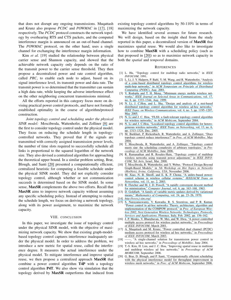
Figure 7 gives the simulation result of the aggregatethroughput v.s. the carrier sense threshold under various algo-rithms. As anticipated, MaxSR achieves the highest aggregatethroughput except when the carrier sense threshold is small

0 0.5 1 1.5 2

x 10−10

0.6

0.8

1

1.2

1.4

1.6

1.8x 10

7

CSThreshold

Agg

rega

te T

hrou

ghpu

t (bp

s)MaxSRLMSTCBTCMaxPow

Fig. 7. Aggregate throughput v.s. carrier sense threshold

0.2 0.4 0.6 0.8 1 1.2 1.4 1.6 1.8 2

x 10−10

0

1

2

3

4

5

6

7

8

9

10

CSThreshold

No.

of b

roke

n lin

ks

LMSTMaxSRMaxPowCBTC

Fig. 8. The number of broken links v.s. carrier sense threshold

(under which case spatial reuse is constrained by the carriersense threshold). It outperforms LMST by 50%, CBTC by110% and MaxPow by 102% in terms of maximizing networkcapacity.

Another interesting observation is that that the aggregatethroughput increases as carrier sense threshold increases. Thisis because increasing the carrier sense threshold mitigates theeffect of the exposed terminal problem and achieve better spa-tial reuse. However, the increase in the aggregate throughputlevels off when the carrier sense threshold increase beyondthe point at which the the maximum capacity achieved bythe specifc network topology. If the carrier sense threshold isfurther increased, the network starts to experience the hiddenterminal problem. Although the hidden node problem doesnot affect aggregate throughput dramatically, it may causesevere unfairness and partition the network. Figure 8 givesthe number of broken links v.s. the carrier sense threshold.When the carrier sense threshold is too large, several links failunder the physical model, due to severe interference. MaxSRnevertheless still gives the best network connectivity.

VII. RELATED WORK

We categorize related work into the following three cate-gories:

Topology control/management under the protocol model:The issue of power control has been studied in the contextof topology maintenance, where the objective is to preservenetwork connectivity, reduce power consumption, and mitigateMAC-level interference [2], [3], [4], [5], [6]. Rodoplu et al.[3] introduced the notion of relay region and enclosure for thepurpose of power control. A two-phase distributed protocolwas then devised to find the minimum power topology for astatic network. In the first phase, each node i executes localsearch to find the enclosure graph. In the second phase, eachnode runs the distributed Bellman-Ford shortest path algorithmupon the enclosure graph, using the power consumption as thecost metric.

CBTC(α) is a two-phase algorithm in which each node findsthe minimum power p such that transmitting with p ensuresthat it can reach some node in every cone of degree α. Thealgorithm has been analytically shown to preserve the networkconnectivity if α < 5π/6. It has also ensured that every linkbetween nodes is bi-directional.

Li and Hou [4] devised a Local Minimum Spanning Tree(LMST) algorithm and its variations [5], [6] for topologycontrol and management. In LMST, each node builds its localminimum spanning tree independently with the use of locallycollected information, and only keeps on-tree nodes that areone-hop away as its neighbors in the final topology. They haveproved analytically that (1) if every node exercises LMST, thenthe network connectivity is preserved; (2) the node degree ofany node in the resulting topology is bounded by 6; and (3) thetopology can be transformed into one with bi-directional links(without impairing the network connectivity) after removal ofall uni-directional links).

As mentioned in Section I, topologies derived under thesegraph-model based topology control algorithms may not cap-ture interference adequately under the physical SINR model.As a result, interference may be outrageously high in thetopology induced by graph-model based algorithms, renderingsub-optimal network capacity.

Control of transmit power for capacity improvement:Use of power control for the purpose of spatial reuse andcapacity improvement has been treated in the COMPOWprotocol [15], the PCMA protocol [16], the PCDC protocol[17], the POWMAC protocol [18], and the PRC protocol[19]. Narayanaswamy et al. [15] developed a power controlprotocol, called COMPOW. In COMPOW each node runsseveral routing daemons in parallel, one for each power level.Each routing daemon maintains its own routing table byexchanging control messages at the specified power level. Bycomparing the entries in different routing tables, each nodecan determine the smallest common power that ensures themaximal number of nodes are connected.

Monks et al. [16] propose PCMA in which the receiveradvertises its interference margin that it can tolerate on an out-of-band channel and the transmitter selects its transmit power

that does not disrupt any ongoing transmissions. Muqattashand Krunz also propose PCDC and POWMAC in [17], [18]respectively. The PCDC protocol constructs the network topol-ogy by overhearing RTS and CTS packets, and the computedinterference margin is announced on an out-of-band channel.The POWMAC protocol, on the other hand, uses a singlechannel for exchanging the interference margin information.

Kim et al. [19] studied the relationship between physicalcarrier sense and Shannon capacity, and showed that theachievable network capacity only depends on the ratio ofthe transmit power to the carrier sense threshold. They thenpropose a decentralized power and rate control algorithm,called PRC, to enable each node to adjust, based on itssignal interference level, its transmit power and data rate. Thetransmit power is so determined that the transmitter can sustaina high data rate, while keeping the adverse interference effecton the other neighboring concurrent transmissions minimal.

All the efforts reported in this category focus more on de-vising practical power control protocols, and have not formallyestablished optimality in the course of algorithm/protocolconstruction.

Joint topology control and scheduling under the physicalSINR model: Moscibroda, Wattenhofer, and Zolliner [8] arethe first to consider topology control under the physical model.They focus on reducing the schedule length in topology-controlled networks. They proved that if the signals aretransmitted with correctly assigned transmission power levels,the number of time slots required to successfully schedule alllinks is proportional to the squared logarithm of the networksize. They also devised a centralized algorithm for approachingthe theoretical upper bound. In a similar problem setting, Brar,Blough, and Santi [20] presented a computationally efficient,centralized heuristic for computing a feasible schedule underthe physical SINR model. They did not explicitly considertopology control, although whether or not communicationsucceeds is determined based on the SINR model. In somesense, MaxSR complements the above two efforts. Recall thatMaxSR aims to improve network capacity without assumingany specific scheduling policy. Instead of attempting to reducethe schedule length, we focus on deriving a network topology,along with its power assignment, to maximize the networkcapacity.

VIII. CONCLUSION

In this paper, we investigate the issue of topology controlunder the physical SINR model, with the objective of maxi-mizing network capacity. We show that existing graph-model-based topology control captures interference inadequately un-der the physical model. In order to address the problem, weintroduce a new metric for spatial reuse, called the interfer-ence degree. It measures the actual interference under thephysical model. To mitigate interference and improve spatialreuse, we then propose a centralized approach MaxSR thatcombine a power control algorithm T4P with a topologycontrol algorithm P4T. We also show via simulation that thetopology derived by MaxSR outperforms that induced from

existing topology control algorithms by 50-110% in terms ofmaximizing the network capacity.

We have identified several avenues for future research.We will design, based on the insight shed from the studyreported in this paper, a decentralized version of MaxSR thatmaximizes spatial reuse. We would also like to investigatehow to combine MaxSR with a scheduling policy (such asthat proposed in [20]) so as to maximize network capacity inboth the spatial and temporal domains.

REFERENCES

[1] L. Hu, “Topology control for multihop radio networks,” in IEEEINFOCOM, 1991.

[2] L. Li, J. Y. Halpern, P. Bahl, Y.-M. Wang, and R. Wattenhofer, “Analysisof a cone-based distributed topology control algorithms for wirelessmulti-hop networks,” in ACM Symposium on Principle of DistributedComputing (PODC), Aug. 2001.

[3] V. Rodoplu and T. H. Meng, “Minimum energy mobile wireless net-works,” IEEE Journal on Selected Areas in Communications, vol. 17,no. 8, pp. 1333–1344, Aug. 1999.

[4] N. Li, J. C.Hou, and L. Sha, “Design and analysis of a mst-baseddistributed topology control algorithm for wireless ad-hoc networks,”IEEE Trans. on Wireless Communications, vol. 4, no. 3, pp. 1195–1207,May 2005.

[5] N. Li and J. C. Hou, “FLSS: a fault-tolerant topology control algorithmfor wireless networks,” in ACM Mobicom, September 2004.

[6] N. Li and J. C.Hou, “Localized topology control algorithms for hetero-geneous wireless networks,” IEEE Trans. on Networking, vol. 13, no. 6,pp. 1313–1324, Dec. 2005.

[7] M. Burkhart, P. Rickenbach, R. Wattenhofer, and A. Zollinger, “Doestopology control reduce interference?” in Proc. of ACM MobiHoc, May2004.

[8] T. Moscibroda, R. Wattenhofer, and A. Zollinger, “Topology controlmeets sinr: the scheduling complexity of arbitrary topologies,” in Pro-ceedings of ACM MobiHoc, June 2006.

[9] R. Ramanathan and R. Rosales-Hain, “Topology control of multihopwireless networks using transmit power adjustment,” in IEEE INFO-COM, Tel Aviv, Israel, Mar. 2000.

[10] T. Moscibroda, R. Wattenhofer, and Y. Weber, “Protocol Design BeyondGraph-Based Models,” in 5th Workshop on Hot Topics in Networks(HotNets), Irvine, California, USA, November 2006.

[11] M. Xiao, N. B. Shroff, and E. K. P. Chong, “A utility-based power-control scheme in wireless cellular systems,” IEEE/ACM Trans onNetworking, vol. 11, no. 2, 2003.

[12] R. Fletcher and M. J. D. Powell, “A rapidly convergent descent methodfor minimization,” Computer Journal, vol. 6, pp. 163–168, 1963.

[13] D. Goldfarb, “A family of variable metric updates derived by variationalmeans,” Mathematics of Computing, vol. 24, pp. 23–26, 1970.

[14] http://www.j-sim.org/.[15] S. Narayanaswamy, V. Kawadia, R. S. Sreenivas, and P. R. Kumar,

“Power control in ad-hoc networks: Theory, architecture, algorithm andimplementation of the COMPOW protocol,” in Proc. of European Wire-less 2002, Next Generation Wireless Networks: Technologies, Protocols,Services and Applications, Florence, Italy, Feb. 2002, pp. 156–162.

[16] J. P. Monks, V. Bharghavan, W. Mei, and W. Hwu, “A power controlledmultiple access protocol for wireless packet networks,” in Proceedingsof IEEE INFOCOM, March 2001.

[17] A. Muqattash and M. Krunz, “Power controlled dual channel (PCDC)medium access protocol for wireless ad hoc networks,” in Proceedingsof IEEE INFOCOM, March 2003.

[18] ——, “A single-channel solution for transmission power control inwireless ad hoc networks,” in Proceedings of MobiHoc, June 2004.

[19] T.-S. Kim, H. Lim, and J. C. Hou, “Improving spatial reuse in multirateand multihop wireless ad hoc networks,” in Proceedings of ACMMOBICOM, September 2006.

[20] G. Brar, D. Blough, and P. Santi, “Computationally efficient schedulingwith the physical interference model for throughput improvement inwireless mesh networks,” in Proc. of ACM Mobicom, September 2006.