arX

iv:1

012.

4750

v3 [

hep-

ph]

20

Jul 2

011

CERN-PH-TH/2010-314

Top polarization, forward-backward asymmetry and new physics

Debajyoti Choudhurya, Rohini M. Godboleb,1, Saurabh D. Rindanic, Pratishruti Sahaa

a Department of Physics and Astrophysics, University of Delhi, Delhi 110 007, India.

b Theory Unit, CERN, CH-1211, Geneva 23, Switzerland.

c Theoretical Physics Division, Physical Research Laboratory, Navrangpura, Ahmedabad 380 009, India.

Abstract

We consider how the measurement of top polarization at the Tevatron can be usedto characterise and discriminate among different new physics models that have beensuggested to explain the anomalous top forward-backward asymmetry reported at theTevatron. This has the advantage of catching the essence of the parity violating effectcharacteristic to the different suggested new physics models. Other observables con-structed from these asymmetries are shown to be useful in discriminating between themodels, even after taking into account the statistical errors. Finally, we discuss somesignals at the 7 TeV LHC.

PACS Nos:14.65.Ha,13.88.+e

Key Words:top,asymmetry,polarization

1Permanent Address: Centre for High Energy Physics, Indian Institute of Science, Bangalore 560 012,India

1

1 Introduction

The study of the third generation quarks in the Standard Model(SM) fermions continues tothrow up surprises. Be it a ∼ 3σ deviation in Ab

FB in the SM fit to the electroweak(EW) pre-cision measurements at LEP [1], a forward-backward asymmetry in top-pair production [2–6]significantly larger than what the SM predicts or the discrepancy in the value of the B0

s–B0s

mixing as suggested by the recent measurement of the inclusive dimuon asymmetry [7] at theTevatron, some deviations from the SM remain. While, individually, none of them are largeenough to merit the status of a discovery of physics beyond the SM, they are, nonetheless,intriguingly poised to warrant serious attention. This is especially so on account of the large-ness of the third generation fermion masses. With the top quark mass scale being very closeto the EW scale, it is quite conceivable that the third generation (or, at least, the top quark)plays an important role in electroweak symmetry breaking itself. Indeed, very many ideasgoing beyond the SM quite often also predict discernible new physics effects for processesinvolving the third generation. On the experimental front, constraints on the universality ofinteractions are far less restrictive for these fermions as opposed to those for the first twogenerations. Hence, on very generic grounds, top quark physics studies at the Tevatron andthe LHC, hold potential for probing new physics [8]. It is, therefore, a small wonder thatvery many “explanations” of the physics responsible for the aforementioned discrepancieshave been offered and a majority of them accord a special role to the third generation. Inthis article, we concentrate on the anomaly in the forward-backward (FB) asymmetry intop-pair production.

Within the SM, the dominant tt production mode at the Tevatron is a pure QCD one and isFB symmetric at the tree-level. Weak interactions are highly subdominant and give a verysmall asymmetry (AFB ≪ 1%). It is the interference of the tree-level QCD amplitudes andhigher order terms that yields the dominant SM contribution to this asymmetry and resultsin AFB ∼ 5% [9,10]. This has led to several authors [11,12] advocating the measurement ofAFB as a tool for probing physics beyond the SM.

The CDF and the D0 experiments at the Tevatron kindled a great deal of interest in top-pairproduction by reporting a FB asymmetry (AFB) of 17% [2] and 12% [3] respectively2. Manypossible New Physics (NP) scenarios have been offered as explanations. In a later update,CDF revised this number to 19.3%. [4] Although the analysis of more data has reduced thesignificance of the CDF result to about 1.8σ (AFB = 15%) [5] and D0 has presented a newervalue of 8% [6], the deviation from the SM is still non-negligible and, coupled with the otherlongstanding discrepancies in certain third-generation observables, continues to elicit muchinterest [13–18].

Forward-backward asymmetry, at the Tevatron, is defined as

AFB =σ(cos θt > 0)− σ(cos θt < 0)

σ(cos θt > 0) + σ(cos θt < 0)(1.1)

where θt is the angle made by the top quark with the direction of the proton in the lab-frame.Experimentally, the measurement is made in the semi-leptonic channel, where the angle (θh)made by the hadronically decaying top(anti-top) with the proton beam and the charge Ql of

2The measurements reported by D0 are uncorrected for kinematic acceptance.

2

the decay lepton from the anti-top(top) are together used to construct the net top currentin the direction of the proton beam. cos θt above is thus equivalent to −Ql · cos θh [4]. CPinvariance is assumed to hold good.

Naively, a non-zero AFB seems to be an indication of some violation of a discrete symmetryand, indeed, most models that purport to explain this anomaly have invoked a parity-violating interaction for the top-quark. While this assumption certainly holds true for anys-channel NP contribution to qq → tt, clearly, it is not applicable when t- or u-channelcontributions are present as well. In other words, the measured AFB, in the presence of anyNP interactions, may accrue from either explicit parity violation(dynamics) or the effects oft-(u)-channel propagators(kinematics) or a combination of both. We believe this issue hasnot been stressed sufficiently in the literature. The new physics explanations have differinglevels of parity violation encoded in the chiral structure of the interactions. As this is reflectedin the AFB to varying amounts, it would be interesting to construct a probe thereof. Thepolarization of a single top offers one such probe. In fact, this observation was first madein Ref. [19] in the context of sfermion exchange contributions to tt production in R-parityviolating MSSM (an analog of this model is one of the candidates for an explantaion of theobserved AFB).

It is a thankful coincidence that the top quark polarization is also a quantity that is amenableto an experimental measurement due to the large mass of the t. Being heavy, the topquark decays before it hadronizes and thus the decay products carry the memory of itsspin direction. This correlation between the kinematic distribution of the decay productsand the top spin direction, can be used to get information about the latter. In fact, manystudies exploring the use of the polarization of the top quark as a probe and discriminatorof new physics [20], as a means to sharpen up the signal of new physics [21] and to obtaininformation on tt production mechanism [19,22,23] exist in literature. Different probes of thetop polarisation which use the above mentioned correlation have been constructed [23–25],the angular distribution of the decay leptons providing a particularly robust probe due toits insensitivity to higher order corrections [26] and to possible new physics in the tbWvertex [27–29].

A single-top polarization asymmetry(AP ) can be defined as

AP =σ(+)− σ(−)

σ(+) + σ(−), (1.2)

where + or − denote the helicity of the top quark and the helicities of the t are summedover. The SM prediction for this arises due to EW effects and is expected to be small.In this note, we explore the predictions for AP originating from the different new physicsexplanations of the FB asymmetry. Spin polarization studies are a part of the agenda atthe Tevatron as well as the LHC [30]. Both the CDF [31] and the D0 [32] experiments atthe Tevatron have reported measurements of spin correlation coefficients. In addition, CDFalso reports a measurement of tt helicity fractions [31]. We would like to point out that,while these observables may also be able to distinguish between the different NP scenariosunder consideration, they involve measurement of the polarization of the top as well as theanti-top and hence, are experimentally more challenging. This is underscored by the factthat the aforementioned measurements are accompanied by fairly large error bars. On theother hand, measurement of AP requires knowledge of the polarization of only the top andthus provides an advantage in terms of the statistics that may be obtained.

3

The rest of the article is organised as follows. In the next section, we discuss the rudiments ofthe models we use as templates, with particular emphasis on the features that are germane tothe issue at hand. This is followed, in section 3, by a comparative discussion of the structureof some observables and their efficacy in distinguishing certain features. The numericalresults, pertaining to the resolving powers of various observables, are presented in section 4.Finally, we summarise in section 6.

2 Model Templates

Rather than probe each and every model that has been proposed, we select some that, toour mind, serve as templates. Broadly speaking, four classes of explanations have beensuggested. The first two involve new t-channel exchanges in qq → tt while the third involvess-channel contributions to the same. For very large masses of the exchanged bosons, all threereduce to four-fermion contact interactions which constitute the fourth category. We do notdiscuss the last-mentioned explicitly as it can be approached from each of the other cases inthe appropriate limit3. The particle exchanged in the t-channel could either be a scalar ora vector and we shall discuss an example of each. Scalar exchanges in the s-channel do notcontribute to AFB. On the other hand, s-channel vector exchanges are fairly commonplacein new physics scenarios and this constitutes our third template. Finally, we omit tensorexchanges because no such well-motivated model leading to large AFB exists. We now discusseach template in turn.

2.1 A flavour-nondiagonal Z ′

While additional U(1) gauge symmetries are well-studied and very often well-motivated,it is easy to see that most common variations would not lead to a substantial AFB. Inmodels where the Z ′ appears in the s-channel in the qq → tt process, the NP amplitudecannot have a non-zero interference with the QCD contributions. Consequently, obtainingthe required AFB requires large Z ′ couplings resulting in too large a correction to σ(tt). Onthe other hand, a flavour-changing Z ′ [13] would appear in the t-channel in, say, uu → tt.The corresponding contribution to AFB has two sources, viz. kinematic (due to the t-channelpropagator) and, possibly a dynamic one as well (if the Z ′ coupling is chiral). Analogous tcZ ′

or cuZ ′ couplings are disfavoured as these would set up flavour-changing neutral currents.Similarly, consistency with B-physics observables is simpler if the Z ′ does not couple to theb-quark necessitating that the coupling to the top be right-chiral, thus leaving us with aLagrangian of the form [13]

L ∋ gX Z′µ u γ

µ PR t + h.c. . (2.1)

The model also includes a small flavor-diagonal coupling to u quarks in order to avoidexperimental constraints from like-sign top production data from the Tevatron [13]. However,

3In principle, there could be scenarios wherein more than one such NP effect could play a role, albeit todifferent degrees. Once again we desist from discussing these explicitly as the gross features thereof can bededuced by judiciously combining the templates that we do examine hereafter.

4

this as well as issues regarding anomaly cancellation are not relevant to the discussion athand and, hence, we shall ignore them.

2.2 Diquarks

Particles carrying a baryon number of ±2/3 occur in many models, most frequently in thoseconcerned with grand unification [33]. While both scalars and vectors are possible, the latterwould, typically, have a mass as large as the symmetry breaking scale. The scalars can belight, though, and may couple to a pair of quarks. Indeed, an example of such couplingscan be found within the minimal supersymmetric standard model (MSSM) if R-parity werenot conserved. Once again, the presence of such couplings would generate a non-zero AFB,for both kinematic and, if the coupling is chiral, dynamic reasons. The fermion assignmentswithin the SM ensures that the couplings are indeed chiral in nature. Of the various differentdiquark fields that are possible, clearly the one that couples a u to a t can generate themaximal amount of AFB for given mass and coupling strength. In other words, the relevantpiece of the Lagrangian is [14]

L ∋ Φa tc T a (yS + yP γ5) u+ h.c., (2.2)

where Ta denotes the appropriate color-coupling structure. As can be expected, the cross-sections for Φa transforming as a 6 of SU(3)C differs from that for a 3 only in colour factors.We will not discuss the two situations separately and will restrict to the color triplet diquark4.While Ref. [14] admits generic yS and yP , it is easy to see that consistency in the b-sectormotivates the choice of right-chiral couplings, viz, yS = yP .

2.3 Axigluons

Originally motivated as residues of unifiable chiral color models [34], wherein the high en-ergy strong interaction gauge group SU(3)L ⊗ SU(3)R is spontaneously broken to the usualSU(3)C , the axigluon Aa

µ was nothing but the octet gauge boson of the broken symmetryhaving a purely axial vector coupling—of strength gs—with the SM fermions. This modelhas been probed, at Tevatron, both in the dijet [35] as well as the tt channel [12,36,37] andmasses ∼< 1TeV have been ruled out. Although such a scenario immediately predicts AFB,it has the right sign for this quantity only for small values of mA, well below the Tevatronlimits [12]. For larger mA, the sign of AFB flips.

Motivated by this, Ref. [15] considered a variation with a different embedding of the colorgroup into a SU(3)A ⊗ SU(3)B. The gluon and axigluon are now admixtures of the SU(3)Aand SU(3)B with a non-trivial mixing angle θA. Anomaly cancellation requires a fourthgeneration of quarks. The new axigluon is ‘flavor non-universal’ as its couplings with the 3rd

and 4th generation quarks are different from those with quarks of the first two generations,the essential trick being to reverse the sign of the axial coupling of the top-quark, thereby

4Ref. [14] also investigated scalars (with vanishing baryon numbers) in 8 and 1 representations of SU(3)Cbut those were not found to be very successful in consistently reproducing the relevant experimental data.

5

reversing the sign of AFB. In the bargain, additional vector-like couplings are introduced forthe axigluon, leading to

L ∋ ψ γµ (gxV + gxA γ5) Ta ψA

µa . (2.3)

While the vector coupling is generation universal (gxV = −gs cot 2θA), the axial coupling isnot, with gqA = −gs cosec2θA for the first two generations and gtA = +gs cosec2θA for thelast two. Note that, unlike in cases of the diquark and the Z ′, wherein the new physicscontribution only appears in the sub-process uu→ tt, for the axigluon, all quark flavors areinvolved.

3 Analytical Issues

As we are interested in the polarization asymmetry, we must calculate the cross-sections fordifferent final state helicity combinations. While the details are presented in the Appendix,note that, in each case, the square of the amplitude can be decomposed as

|M(λt, λt)|2 = A+ λtλt B + (λt − λt) C .

where λt, λt = ±1 are twice the helicities of the top (antitop). For observables relating to asingle polarization, such as that we are interested in, the other must be summed over.

It is easy to see that while the total tt cross-section and AFB receive contributions fromonly from A, the polarization asymmetry AP ∼ C/A. It is, thus, worthwhile to examine thedependence of these terms on the coupling constants. As far as the diquark is concerned(see eq. A.4), the terms A (and B) are even in both the (pseudo)-scalar couplings yS (yP ),and thus, the ensuing AFB is insensitive to their (yS,P ) sign (and, hence, to the chiralitystructure of the theory). The term C being proportional to the product yS yP , the polarizationasymmetry picks up the chirality structure unerringly. And while eq.A.5, does not reflectthis explicitly (owing to the fact that a V +A structure was chosen), the story is similar forthe Z ′.

For the axigluon, the situation is bit more complicated. There exist pieces in A (and B),that are odd in the individual axigluon couplings, but being parity odd, most of them donot contribute to σtt. The only such piece that contributes to σtt does so only away fromthe resonance—with the sign reversing as one crosses it—resulting in a subdominant contri-bution. Of course, AFB is very sensitive to the relative signs of the couplings in question,which was the original motivation of this model vis-a-vis the flavour-universal axigluon. Onceagain, the sign of AP would provide additional information about the aforementioned rela-tive signs, thereby serving to establish the actual structure of the embedding of SU(3)C inthe larger gauge group.

Finally, note that, for each of the three cases, the piece C has a different angular dependence,including a parity-odd piece. This leads one to hope that the construction of a rapidity-dependent AP would lend additional resolving power.

6

4 Numerical Results

From the discussions in the preceding section, one expects, in general, that each of the threemodels would be associated with a different correlation between the three observables σ,AFB and AP . However, since the particular values of these quantities depend sensitively onthe parameters of the model (i.e. the boson masses and couplings), it is conceivable that themodels could lead to similar values for these observables for some unrelated points in theparameter space. Since such a degeneracy would lead to the models being indistinguishablefrom each other, at least as far as such observables are concerned, we begin by delineatingthe situations where this might occur.

To this end, we scan the parameter space for each of these models with the restriction thatthe couplings be perturbative5. For the Z ′, this implies gX < 2π. For the diquark theory, (toensure that there are no relative normalization factors between the couplings in the differentmodels under consideration) the same limit is imposed on gy =

√2y where, y ≡ (y2S+y

2P )

1/2.In the case of axigluons, the perturbativity condition is imposed on the couplings gA and gB(associated with SU(3)A and SU(3)B, respectively) with both gA, gB < 2π. This, in turn,translates to 10°< θA < 45° [15].

As far as masses are concerned, the lower limits are model-specific. It is easy to appreciatethough that, for very large masses, all the models would, essentially, be equivalent to contactinteractions. For very large masses, engendering a large enough AFB would, then, need verylarge couplings, thereby coming into conflict with the perturbativity requirement discussedabove. In effect, only Mnew ∼< 3000 GeV is relevant. Furthermore, we impose direct limitsby taking into account various considerations as detailed below.

In case of diquarks, one could argue for mΦ > 350GeV, motivated by the limits on squarksearches at the Tevatron [1]. However, for a scalar decaying primarily into a top (or abottom) and a jet, these limits do not apply and the corresponding limits are expectedto be much weaker. Although such a dedicated study is yet to be reported, preliminaryinvestigations [38] suggest that mΦ ∼> 200GeV cannot yet be ruled out, and we shall adoptthis.

As for the Z ′ model, much depends on the flavor structure of its coupling. If the Z ′ isvery light, then the branching fraction for t → Z ′ + u is no longer negligible. Further, ifthe Z ′ decays hadronically, this would lead to an enhancement in the contribution to the ttproduction from the lepton+jets channel as compared to the contribution from the dileptonchannel giving rise to deviations from the experimental measurements in the two channels.Ref. [13] has already considered this to find that mZ′ ∼> 120GeV is consistent with currentdata and we shall adopt this limit as well.

The limits on the flavor non-universal axigluon mass need more thought though. Exper-imental searches, so far, have only considered flavor universal axigluons. Based on these,

5We impose this condition only until the 10 TeV scale. Were we to demand that the theory remainperturbative until a significantly higher scale, the parameter space would be further restricted. However, inthe absence of any knowledge of the ultraviolet completion, we desist from this.

7

mA ∼< 1250GeV is ruled out by direct searches while the distortion in the mtt spectrum [39]is too severe for mA ∼< 1400GeV. However, it should be noted that the resonant productioncross sections for flavor non-universal axigluons differ on account of the differences in theircoupling to light quarks. Nonetheless, we do restrict to mA ∼> 1400GeV.

The parameter spaces thus defined, the numerical calculation is done using a parton levelMonte Carlo routine. We use the CTEQ6L [40] parton distributions with the factorizationscale set to mt with the later held to 172.5 GeV to be consistent with the value used inmeasurements of cross-section [41] and AFB [5]. A K-factor [42] of 1.33 is used to estimatethe cross-section at NLO6.

-1

-0.5

0

0.5

1

-0.6 -0.4 -0.2 0 0.2 0.4 0.6 0.8

AP

AFB

ΦZ′A

(a)

-0.2

-0.1

0

0.1

0.2

0.3

-0.05 0 0.05 0.1 0.15 0.2 0.25 0.3 0.35

AP

AFB

ΦZ′A

(b)

Figure 1: (a) Correlation between AP and AFB for different models. The vertical solid (dot-ted) lines correspond to the central value and 1-σ bands of the new (old) CDF measurementof AFB, namely 15.0% ± 5.5% (19.3% ± 6.9%). The ‘star’ corresponds to the SM value atNLO. For each model, the scan is limited to only perturbative coupling strengths. (b) As inthe previous panel, but restricted to only those points that are consistent with the experimen-tally observed cross-section at the 1-σ level and with restrictions on Mboson as described inthe text.

For each parameter-space point we calculate σtt, AFB and AP as defined above. Our calcu-lation of AFB includes the SM part [9]. As for AP , the SM contribution is miniscule. Thisis primarily because a non-zero AP can arise only when the production mechanism treatspositive and negative helicity states differently. Consequently, a pure QCD process can nevergive rise to a non-zero AP . In the SM, AP will arise only due to electroweak effects, eitherat the tree level or through mixed EW-QCD higher order corrections, and is, hence, rathersmall (O(10−3)). Given this, we restrict ourselves to the tree-level value of AP as indicatedin the previous section.

In Fig.1(a), we show the correlation between AP and AFB for each of the three modelsalongwith the experimentally allowed 1-σ band for AFB. No restrictions have been imposedon the physical observables, barring the aforementioned perturbative limit on the couplings.Note that the splayed-finger like structure for Φ is but a reflection of the sampling densityin the masses and a finer sampling would have resulted in a dense region in this plane. It

6In the absence of NLO calculations that incorporate the new physics effects under consideration, we usethe SM K-Factor.

8

immediately transpires that the three models under discussion have very different correla-tions between the observables. However, this is evidently misleading as a large faction of theparameter space depicted here gives rise to a AFB well outside the experimentally allowedrange. This is even more so for the total cross section. Clearly, large values of the asymme-tries would occur only for substantially large NP couplings and these, typically, give rise totoo large a cross section.

Imposing the restriction that the total tt production cross section should lie within 1σ of theexperimentally observed value and restricting Mboson as described earlier, eliminates bulk ofthe parameter points and leads to the correlation plot of Fig.1(b). One feature immediatelystands out. For each of the models, the allowed regions split into two, one close to the SMpoint and the other distinctly separate.

5

6

7

8

9

10

0 1 2 3 4 5 6

σ (

pb)

gy = y√2

MΦ = 200 GeVMΦ = 400 GeVMΦ = 600 GeVMΦ = 800 GeVMΦ = 1000 GeVMΦ = 1500 GeV

(a)

-0.1

0

0.1

0.2

0.3

0.4

0 1 2 3 4 5 6

AF

B

gy = y√2

MΦ = 200 GeVMΦ = 400 GeVMΦ = 600 GeVMΦ = 800 GeVMΦ = 1000 GeVMΦ = 1500 GeV

(b)

Figure 2: Variation in σ(tt) and AFB with coupling for different choices of MΦ.

For the Z ′ and the diquark, the reason for this is easy to understand. Clearly, for small valuesof the NP coupling, the cross-section is close to that within the SM and, hence, consistentwith the measured value. However, for such small couplings, the AFB generated is also smalland not in consonance with the experimental observation. For a given boson mass, as oneconsiders larger values of the coupling, sufficient AFB can be produced while the cross-sectionis prevented from becoming too large because of the destructive interference between the SMand NP pieces. In fact, for an intermediate range of the coupling, the cross section falls wellbelow the SM value. The location and the extent of the range naturally depends on themass of the boson. For the case of the diquark, this is illustrated in Fig.2. The situation isanalogous for the Z ′.

For the axigluon, the situation is somewhat more complicated. Here the interference may beconstructive or destructive depending upon the values of s andMA under consideration. ForMA > 1400 GeV, the interference is mostly destructive though. For θA ≈ 45°, the situationis identical to that in the case of the flavor universal axigluon, with the exception that nowthe relative minus sign between the gqA and gtA yields AFB that is of the right sign as wellas the right magnitude. As θA decreases, the destructive interference takes over leading toσ(tt) values that are too low (see Fig.3(a)). For MA < 2000 GeV, a further increase in thestrength of the couplings allows the pure NP term to become dominant and the cross-sectionincreases once again to become consistent with data. Due to this, a part of the range of θA

9

below 25° gets ruled out. Again, the actual location and extent of the range depend on theparticular value of MA. On the other hand, for θA ∼< 20°, AFB is only produced in smallamounts (Fig.3(b)). The resultant picture that emerges is the tail of points near the bottomleft of Fig.1(b) which are consistent with the measurement of σ(tt) but not with that of AFB.

5

6

7

8

9

10

10 15 20 25 30 35 40 45

σ (

pb)

θ

MA = 1450 GeVMA = 1700 GeVMA = 2000 GeVMA = 2300 GeVMA = 2600 GeVMA = 3000 GeV

(a)

-0.1

0

0.1

0.2

0.3

0.4

10 15 20 25 30 35 40 45

AF

Bθ

MA = 1450 GeVMA = 1700 GeVMA = 2000 GeVMA = 2300 GeVMA = 2600 GeVMA = 3000 GeV

(b)

Figure 3: Variation in cross-section and AFB with θ for different choices of MA.

It is interesting to note that, in Fig.1(b), for the regions that are consistent with the measuredAFB values (whether the old measurement or the new one), there is no overlap between thethree models. It is true that, consistently flipping the relative sign between the axial–and vector–like couplings7, would flip the sign of AP while σ and AFB remain unaltered.However, even after such a variation, the flavor non-universal axigluon case would still retainits distance, in the AFB−AP plane, from the other two models. Thus, a measurement of AP

should, in principle, be able to distinguish the models even before the corresponding bosonhas been directly observed, this being particularly true of the axigluon.

Let us also note at this point that analyses of Ref. [23] indicate that polarization values ofaround 15%–20% can be measured at the Tevatron with 10 fb−1, with good significance.Further, in addition to the azimuthal asymmetry explored in Ref. [23], a simple forwardbackward asymmetry of the decay lepton w.r.t. the beam direction, may also be used at theTevatron and hence one would be able to increase the sensitivity further. From Fig. 1(b)one sees thus that the values of polarization predicted by the different models seem largeenough to afford measurement at the Tevatron.

While discrimination of the axigluon model from the other two seems clear, that betweenthe diquark and the Z’ models is not so straightforward. For one, they lead to overlappingranges in both AP and AFB. Furthermore, Figs.1 have been drawn with the error barssuppressed. Incorporating the latter would render the two apparently disparate populationzones overlapping. If, however, one were to flip the relative sign between the scalar andpseudoscalar couplings of the diquark, the dissimilarity between the models would becomequite conspicuous.

7Of course, this would necessitate a different embedding in the gauge group.

10

0.26

0.28

0.3

0.32

0.34

0.36

0.38

0.4

0.42

0.12 0.14 0.16 0.18 0.2 0.22 0.24

RA

FB

AFB

ΦZ′

(a)

0.1

0.2

0.3

0.4

0.5

0.6

0.7

0.8

0.12 0.14 0.16 0.18 0.2 0.22 0.24 0.26

RA

P

AP

ΦZ′

(b)

Figure 4: RA vs A for forward-backward asymmetry and polarization asymmetry. The pointsdepicted are consistent with the CDF measurementc of σ(tt) and AFB at the 1-σ level. Alsoimposed are the perturbativity constraint on the couplings and the constraints on Mboson asdescribed in the text.

Nevertheless, even without changing the relative signs of yS and yP and with a view to makinga more robust distinction between the two models, we propose observables that exploit therapidity distributions in the two scenarios. With the typical values of the t-channel massesbeing different in the two scenarios (see Figs.2 & 3), it is but natural that the typical rapiditieswould be different. To this end, we define the ratios RAP

and RAFBwhere

RA =A(|∆y| < 1)

A(|∆y| ≥ 1),

and ∆y is the difference between the rapidities of the top and the anti-top. The CDFCollaboration does report a measurement of AFB in different ∆y regions [5], leading toRAFB

= 0.043±0.194 with the SM expectation being RAFB(SM) = 0.317±0.053. While this

seems to offer a potentially strong discriminator, as we shall soon see, the associated errorsdo not, yet, allow for discrimination between models. Instead, we advocate an examinationof correlations involving RAP

and RAFB.

In Fig.4, RAFBand RAP

are plotted against AFB and AP respectively. For consistent com-parison with CDF results [5], the asymmetries are calculated in the tt rest frame and includethe NLO contribution from the SM [5]. It can be seen that the diquark and Z ′ modelspopulate different regions in the RAFB

− AFB and RAP− AP planes and the separation is

quite distinct.

Once again, Fig. 4 does not incorporate errors in the measurement of the quantities plotted.The statistical part thereof can be easily estimated. We obtain the efficiencies (i.e. includ-ing kinematic cuts, event selection efficiencies etc.) from the number of events reportedin the CDF AFB measurement [5], and assume that the corresponding efficiencies for AP

measurement would be similar. Calculating the expected number of events in this way, wethen add the errors in quadrature. While this might seem a trifle optimistic, we compensateby restricting our projections to an integrated luminosity (∼ 4.2 fb−1) less than what hasalready been analysed in Ref. [5].

11

0.1

0.2

0.3

0.4

0.5

0.6

0.7

0.08 0.1 0.12 0.14 0.16 0.18 0.2 0.22 0.24 0.26

RA

FB

AFB

ΦZ′

(a)

0

0.1

0.2

0.3

0.4

0.5

0.6

0.7

0.8

0.9

1

1.1

0.08 0.1 0.12 0.14 0.16 0.18 0.2 0.22 0.24 0.26 0.28

RA

P

AP

ΦZ′

(b)

Figure 5: Correlations involving AFB, RAFB, AP and RAP

after inclusion of error bars. Thepoints depicted are consistent with the same constraints as explained in the caption of Fig.4.

In Fig.5, we redraw Fig.4 along with the error bars computed as described above. Althoughthe central values in the two scenarios are widely separated, a significant overlap betweenthe error bars persists, thus makes it difficult to distinguish between them. Indeed, the sizeof the errorbars also shows that the RAFB

measurement, on its own, is, as yet, incapable ofconclusively distinguishing the models from even the SM. On the other hand, the correlationbetween RAP

and RAFB, (Fig.6) looks more promising. While some overlap exists still, the

extent of overlap is distinctly smaller. While a quantitative analysis confirms this, we desistfrom sharpening our conclusions at this stage. It should also be realized that an analysismore sophisticated than what we have performed and including all the data on tape, is quitelikely to further reduce the relative sizes of the errors.

0

0.1

0.2

0.3

0.4

0.5

0.6

0.7

0.8

0.9

1

1.1

0.1 0.2 0.3 0.4 0.5 0.6 0.7

RA

P

RAFB

ΦZ′

Figure 6: Correlation between RAFBand RAP

. The points depicted are consistent with thesame constraints as explained in the caption of Fig.4.

It should be realized that RAPis not the only direction-dependent asymmetry variable. Of

the many such possible, we consider only one namely AP as calculated separately for theforward and backward hemispheres. In particular, we plot, in Fig.7, the ratio of AP in thetwo hemispheres against the total AP . Again, one finds that the diquark and Z ′ models giverise to markedly different correlations.

12

0.6

0.8

1

1.2

1.4

1.6

1.8

2

0.12 0.14 0.16 0.18 0.2 0.22 0.24 0.26

APF/A

PB

AP

ΦZ′

Figure 7: Correlation between the ratio of AP in the forward and backward hemispheres andtotal AP . The points depicted are consistent with the same constraints as explained in thecaption of Fig.4.

However, as the experience with RAPhas shown, the effect of the separation is likely to be

diluted by the errors involved. With experimental errors under control, a combination ofobservables as described above, can be expected to distinguish between the “explanations”for the AFB “anomaly” quite successfully.

5 Observables at the LHC

The initial state being symmetric at the LHC implies that no simple forward-backwardasymmetry w.r.t the beam direction can be defined. Hence, we limit ourselves to the cor-relation between AP and σ(tt)8. For the parameter space points that are consistent withthe Tevatron measurements of cross-section and AFB at the 1-σ level, we find that the threemodels correspond to different correlations (see Fig. 8). In going from the Tevatron to theLHC, the relative contribution from the gg → tt sub-process (which does not contribute tosuch asymmetries) increases as compared to the qq → tt subprocess. The quark initiatedsubprocess suffers a further suppression as anti-quark fluxes are diminished at a pp collider.As a result, the magnitudes of AP at the LHC are lower than those observable at the Teva-tron. Nonetheless, it is interesting to see that the separation of the expected values of AP

into different islands is a trend that persists. That the AP for the axigluon is now almostuniversally negative (as oposed to the Tevatron where positive AP were allowed) is but aconsequence of the fact that a resonance is more easily hit at the LHC.

It should also be borne in mind here that the values of polarization presented here correspondto those obtained by integrating over the entire kinematical range. It is clear that by makingsuitable cuts on the observables such as mtt and/or p

tT , the polarization may be enhanced

substantially, as has been seen in Ref. [23]. It is also clear that the optimal cuts will be againdifferent for different production mechanisms of the NP top pairs.

8The K-Factor in this case is estimated by taking the ratio of the NLO cross-section quoted in Ref. [43]and our own LO calculation resulting in K=1.8.

13

-0.1

-0.05

0

0.05

0.1

0.15

0.2

100 150 200 250 300

AP

σtt- (pb)

ΦZ′A

Figure 8: Correlation between AP and σ(tt) at the LHC (√s = 7 TeV). The vertical lines

show the 1-σ interval of the CMS [43] (dot-dashed) and ATLAS [44] (dashed) measurementsof the tt cross-section. The points depicted are also consistent with the constraints mentionedin the caption of Fig.4.

At the LHC, there also exists the possibility of direct detection of these models throughthe production of the corresponding boson. For diquarks and axigluons (albeit, the flavoruniversal variety), the production cross-sections have been calculated in Refs. [14] and [12]respectively. For the Z ′, direct detection is possible through pair production of Z ′s orproduction of a Z ′ in association with a t. We present the corresponding cross-sectionsfor these processes in Fig. 9, assuming that eq.(2.1) is the only term in the interactionLagrangian.

10-3

10-2

10-1

1

10

0.4 0.8 1.2 1.6 2.0

σ/g

X2 [

pb]

MZ’ [TeV]

(a) Z’ + Z’

√s = 14 TeV√s = 7 TeV

10-3

10-2

10-1

1

10

102

0.4 1.2 2.0 2.8 3.6

σ/g

X2 [

pb]

MZ’ [TeV]

(b) Z’ + t

√s = 14 TeV√s = 7 TeV

10-3

10-2

10-1

1

10

102

103

2 4 6 8 10 12 14

σ/g

X2 [

pb]

MZ’ [TeV]

(c) Likesign top-pair

√s = 14 TeV√s = 7 TeV

Figure 9: Several production cross sections at the LHC for the Z ′ model. Note that obtainingthe requisite AFB at the Tevatron requires the coupling to be typically larger (gX & 1).

Although the cross-sections for the first two processes seem quite large, claims about de-tectability should be made cautiously. Note that such Z ′ would decay into a top and a lightquark (unless other couplings are switched on). Thus, these production processes would,essentially, lead to a tt pair accompanied by one or two hard jets. The QCD background forthe same is quite large. While invariant mass reconstruction would, in principle, distinguishbetween signal and background, in practice this is not an easy task [38], especially with twotop-quarks present. This observations holds for diquark production as well.

14

Relatively easier to look for is the production of a like-sign top-pair, for which this modelpredicts a large rate. Indeed, as Fig. 9(c) shows, with the projected luminosities at the LHC,such a Z ′ could be measured upto several TeVs even for gX = 1 (which, essentially, takesus to the limit of a contact interaction). It should be noted, though, that a very large mZ′

necessitates a large gX for producing the correct AFB. Such a scenario should have made itspresence felt in the very same process at the Tevatron itself.

6 Summary

The anomalously large forward-backward asmymmetry in top-pair production observed atthe Tevatron continues to puzzle. Several models have been proposed to “explain” this.While some of them have their roots in well-motivated scenarios originally proposed toaddress other issues, some of the others are purely phenomenological in nature. The veryfact that many different models of new physics can explain this anomaly renders difficult theidentification of the best solution.

In this note we have analysed the role that the longitudinal top polarization (AP ) can playin discriminating between such models. The scenarios proposed, typically, differ from eachother in their chiral structure and in the relative amount of FB asymmetry that is generatedby the dynamics as opposed to kinematic effects. AP , being a pure parity violating effect,probes the former aspect.

To illustrate this point we choose from among the different proposed models, three templatesand calculate the predictions for AP in each. As expected, we find different correlationsbetween AP and AFB in the three cases and some scenarios can be clearly distinguishedfrom others purely on this account. However, bearing in mind that experimental errorsmay reduce this apparent separation between the models, we further construct the ratiosRA ≡ A(|∆y| < 1)/A(|∆y| > 1), with ∆y being the rapidity separation between the toppair. Correlation between RAP

− RAFBseems quite promising in its ability to separate the

different models even after the inclusion of errors. Given that such measurements are alreadybeing made at the Tevatron, we hope that the adoption of our algorithm would serve to solvethis vexing issue.

We also look at the case of the LHC briefly. Again, a scan over the parameter ranges ofthe three template models, consistent with the Tevatron data, shows that they occupy threedisjoint islands in the AP − σtt space. Although the magnitude of AP is smaller, owing tothe increased importance of the gg → tt subprocess, the situation could be improved furtherby the adoption of apropriate kinematic restrictions. In this particular exploratory exercise,as far as the LHC is concerned, we refrain from carrying out such studies.

While most of the models to explain AFB had been chosen by the respective authors, soas to evade current direct search bounds, this would not be the state of the matter inthe LHC era. As we have demonstrated, the production cross-sections for new particlesinherent to such models, are likely to be large at the LHC. Given the peculiar couplingsof such particles, commensurate search strategies need to be devised, but, by no means,

15

is this an insurmountable problem. Indeed, even if the new particles were all heavy, theeffective Lagrangian responsible for generating the AFB would, typically, leave its mark onSM processes at the LHC (see Sec.5).

It should be noted that, by their very nature, most of the scenarios proposed are phenomenog-ical in nature and have concentrated on explaining AFB while taking care of consistency withonly the most obvious of other observables. Indeed, a global fit would render many of them in-consistent. For example, the diquark model would take Rℓ ≡ Γ(Z → hadrons)/Γ(Z → ℓ−ℓ+)away from the LEP/SLC measurements [45]. As for the Z ′ model, the couplings and massesrequired to give a good fit to both σtt and the new measurements of AFB are disfavoured bythe lack of observation of like-sign top pairs at the Tevatron [13]. The flavor non-universal ax-igluon, on the other hand, is disfavoured by B-physics observables [17]. While such problemsmight seem specific to these models, variations of these and others such are almost endemicto all such endeavours. They can, of course, be cured by introducing compensatory effects inthe respective models. Thus, rather than rejecting them on account of such disagreements,direct searches are the best bet.

It is here that algorithms such as those we propose are particularly useful. Apart fromdiscriminating betweeen models, such analyses can also serve to form an information basison which more sophisticated model-building can be based.

Note Added : As we were finalising the manuscript, two papers, [46] and [47], haveappeared. In the former, the authors have studied different polarization observables, one ofthem being the polarization of the t quark that we consider. While they look at differentmodels proposed to explain the AFB, they concentrate solely on the LHC (at 7 TeV as wellas 14 TeV) and do not consider correlation with AFB. Ref. [47], on the other hand, looks atthe effects at the Tevatron but it is an extension of model-independent analysis of AFB donein their earlier paper [18] to predictions for correlations of t and t polarizations. Since CPconservation relates t and t polarizations, we consider it sufficient to study the polarizationof either one of t or t, which gives us the advantage of larger statistics. Further, the analysisof Ref. [18] is valid only when masses of exchanged particles are much higher than the cutoff scale and hence there is no direct, easy comparison between the two approaches.

After the submission of our manuscript, the CDF Collaboration published a new analysis ofAFB [48] including its dependence on the mass and rapidity of the tt pair. The analysis indifferent rapidity regions is identical to that in Ref. [5] which we have already considered.Further, Ref. [48] reported that AFB is found to be larger in the high invariant mass region(mtt ≥ 450 GeV) than in the low invariant mass region (mtt < 450 GeV). While Ref. [48]itself pointed out that the analysis is still fraught with theoretical uncertainties, we carriedout a preliminary investigation which showed that this feature is borne out by all the modeltemplates that we have studied (Fig.10) and does not offer any additional resolution betweenthe models under consideration. In fact, this was to be expected in view of the facts that (a)the total cross section, which is dominated by the small mtt range agrees very well with theSM expectations and (b) the measured AFB is substantial. Furthermore, even if uncertainties,both theoretical and experimental, can be reduced, the crucial fact is that, unlike AP , thisobservable has little sensitivity to the chiral nature of the new physics couplings.

16

-0.2

0

0.2

0.4

0.6

0.08 0.1 0.12 0.14 0.16 0.18 0.2 0.22 0.24

AF

B (

mt- t)

AFBtotal

Φ (mt-t < 450 GeV)Φ (mt-t ≥ 450 GeV)Z′ (mt-t < 450 GeV)Z′ (mt-t ≥ 450 GeV)

A (mt-t < 450 GeV)A (mt-t ≥ 450 GeV)

CDF (mt-t < 450 GeV)CDF (mt-t ≥ 450 GeV)

Figure 10: AFB in the regions mtt < 450 GeV and mtt ≥ 450 GeV compared to the totalAFB. AFB is calculated in the tt rest frame. The points depicted are consistent with thesame constraints as explained in the caption of Fig.4.

ACKNOWLEDGEMENT

R.G. and S.D.R. wish to acknowledge support from the Department of Science and Technol-ogy, India under the J.C. Bose Fellowship scheme under grant nos. SR/S2/JCB-64/2007 andSR/S2/JCB-42/2009 respectively. P.S. would like to thank CSIR, India for assistance underSRF Grant 09/045(0736)/2008-EMR-I. This work was initiated during the XI th Workshopon High Energy Physics Phenomenology held at PRL, Ahmedabad. R.G. and P.S. would liketo thank the organisers of the Workshop and the coordinators of the LHC Physics WorkingGroup for their hospitality and cooperation.

17

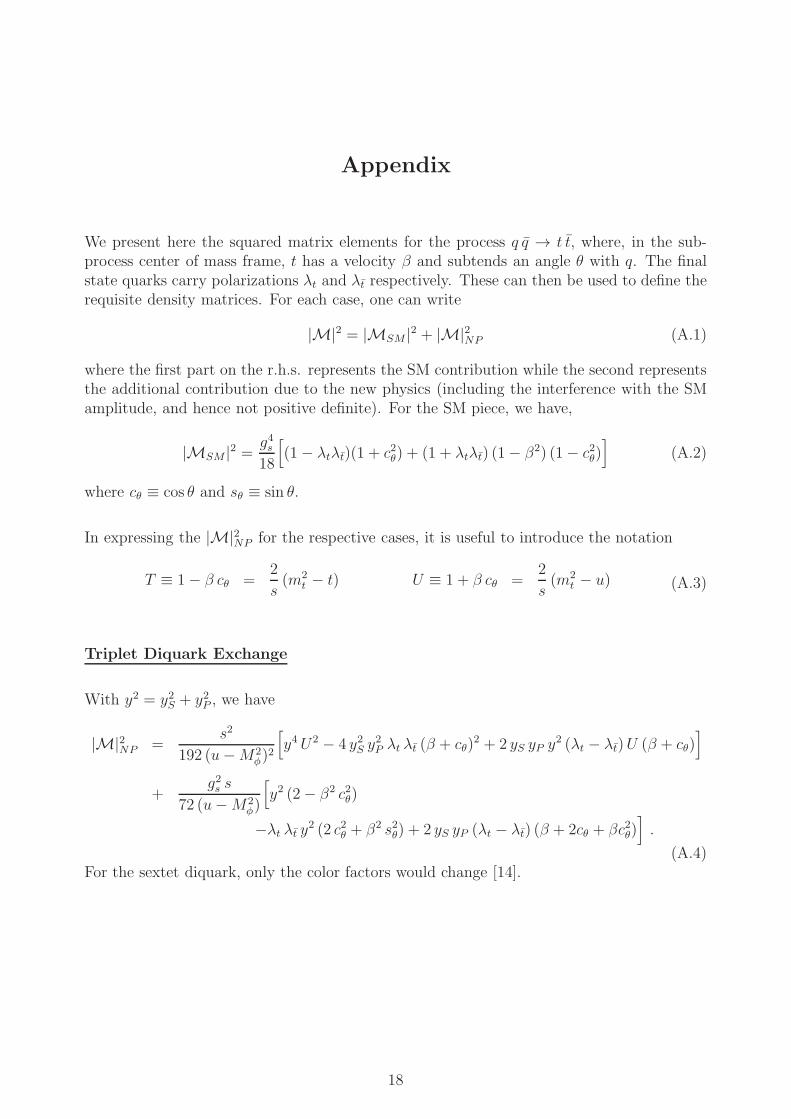
Appendix

We present here the squared matrix elements for the process q q → t t, where, in the sub-process center of mass frame, t has a velocity β and subtends an angle θ with q. The finalstate quarks carry polarizations λt and λt respectively. These can then be used to define therequisite density matrices. For each case, one can write

|M|2 = |MSM |2 + |M|2NP (A.1)

where the first part on the r.h.s. represents the SM contribution while the second representsthe additional contribution due to the new physics (including the interference with the SMamplitude, and hence not positive definite). For the SM piece, we have,

|MSM |2 = g4s18

[

(1− λtλt)(1 + c2θ) + (1 + λtλt) (1− β2) (1− c2θ)]

(A.2)

where cθ ≡ cos θ and sθ ≡ sin θ.

In expressing the |M|2NP for the respective cases, it is useful to introduce the notation

T ≡ 1− β cθ =2

s(m2

t − t) U ≡ 1 + β cθ =2

s(m2

t − u) (A.3)

Triplet Diquark Exchange

With y2 = y2S + y2P , we have

|M|2NP =s2

192 (u−M2φ)

2

[

y4U2 − 4 y2S y2

P λt λt (β + cθ)2 + 2 yS yP y

2 (λt − λt)U (β + cθ)]

+g2s s

72 (u−M2φ)

[

y2 (2− β2 c2θ)

−λt λt y2 (2 c2θ + β2 s2θ) + 2 yS yP (λt − λt) (β + 2cθ + βc2θ)]

.

(A.4)For the sextet diquark, only the color factors would change [14].

18

Z ′ Exchange

Defining x ≡ m2t/2m

2Z′, we have

|M|2NP =g4X s

2

16 (t−M2Z′)2

[

{

U2 + 2 x (1− β2) + x2 T 2}

−λtλt{

(β + cθ)2 + 2 x (1− β2) c2θ + x2 (β − cθ)

2}

+(λt − λt) {(β + cθ)U + 2 x (1− β2) cθ − x2 (β − cθ)T}]

− g2sg2X s

18 (t−M2Z′)

[

{U2 + 1− β2 + x (T 2 + 1− β2)}−λtλt

{

(1 + x) (2 c2θ + β2 s2θ) + 2 (1− x) β cθ}

+(λt − λt){

β (1− x) (1 + c2θ) + 2 (1 + x) cθ}

]

.

(A.5)

Flavor Non-Universal Axigluon Exchange

Defining combinations of couplings as

SQ ≡ (gqV )2 + (gqA)

2 PQ ≡ gqV gqA PV ≡ gqV g

tV

S±T ≡ (gtV )

2 ± (gtA)2 PT ≡ gtV g

tA PA ≡ gqA g

tA

(A.6)

we have

|M|2NP =sJA

18 [(s−M2A)

2 + Γ2AM

2A]

, (A.7)

where

JA = s[

SQ S+

T (1 + β2c2θ) + SQ S−T (1− β2) + 8PQPT β cθ

−λtλt{

SQ S+

T (β2 + c2θ) + SQ S−T (1− β2) c2θ + 8PQPT β cθ

}

+(λt − λt){

2SQPT β (1 + c2θ) + 4PQ

(

(gtV )2 + β2(gtA)

2

)

cθ

}]

+ g2s (s−M2A)

[

{4PA β cθ + 2PV (2− β2 s2θ)}−λtλt

{

4PA β cθ + 2PV (2 c2

θ + β2 s2θ)}

+(λt − λt){

4gqAgtV cθ + 2gqV g

tAβ(1 + c2θ)

}]

.

(A.8)

For brevity’s sake, we are not presenting the SM expressions for gg → tt.

19

References

[1] K. Nakamura et al. [Particle Data Group], J. Phys. G37, 075021 (2010).

[2] T. Aaltonen et al. [CDF Collaboration], Phys. Rev. Lett. 101, 202001 (2008)[arXiv:0806.2472 [hep-ex]].

[3] V. M. Abazov et al. [D0 Collaboration], Phys. Rev. Lett. 100, 142002 (2008)[arXiv:0712.0851 [hep-ex]].

[4] CDF Conference Note 9724,http://www-cdf.fnal.gov/physics/new/top/public tprop.html

[5] CDF Conference Note 10185,http://www-cdf.fnal.gov/physics/new/top/public tprop.html

[6] D0 Conference Note 6062,http://www-d0.fnal.gov/Run2Physics/WWW/results/prelim/TOP/T90/

[7] V. M. Abazov et al. [D0 Collaboration], Phys. Rev. D82 (2010) 032001 [arXiv:1005.2757[hep-ex]].

[8] For a review, see for example,W. Bernreuther, J. Phys. G35, 083001 (2008) [arXiv:0805.1333 [hep-ph]];T. Han, Int. J. Mod. Phys. A23, 4107 (2008) [arXiv:0804.3178 [hep-ph]].

[9] J. H. Kuhn and G. Rodrigo, Phys. Rev. Lett. 81, 49 (1998) [arXiv:hep-ph/9802268];Phys. Rev. D 59, 054017 (1999) [arXiv:hep-ph/9807420].

[10] M. T. Bowen, S. D. Ellis and D. Rainwater, Phys. Rev. D73, 014008 (2006) [arXiv:hep-ph/0509267];L. G. Almeida, G. F. Sterman and W. Vogelsang, Phys. Rev. D78, 014008 (2008)[arXiv:0805.1885 [hep-ph]].

[11] L. M. Sehgal and M. Wanninger, Phys. Lett. B200, 211 (1988).

[12] D. Choudhury, R. M. Godbole, R. K. Singh and K. Wagh, Phys. Lett. B 657, 69 (2007)[arXiv:0705.1499 [hep-ph]].

[13] S. Jung, H. Murayama, A. Pierce and J. D. Wells, Phys. Rev. D 81, 015004 (2010)[arXiv:0907.4112 [hep-ph]].

[14] J. Shu, T. M. P. Tait and K. Wang, Phys. Rev. D 81, 034012 (2010) [arXiv:0911.3237[hep-ph]].

[15] P. H. Frampton, J. Shu and K. Wang, Phys. Lett. B 683, 294 (2010) [arXiv:0911.2955[hep-ph]].

[16] C. H. Chen, G. Cvetic and C. S. Kim, arXiv:1009.4165 [hep-ph];Y. K. Wang, B. Xiao and S. H. Zhu, arXiv:1008.2685 [hep-ph];B. Xiao, Y. K. Wang and S. H. Zhu, Phys. Rev. D 82, 034026 (2010) [arXiv:1006.2510[hep-ph]];Q. H. Cao, D. McKeen, J. L. Rosner, G. Shaughnessy and C. E. M. Wagner, Phys. Rev.

20

D 81, 114004 (2010) [arXiv:1003.3461 [hep-ph]];V. Barger, W. Y. Keung and C. T. Yu, Phys. Rev. D 81, 113009 (2010) [arXiv:1002.1048[hep-ph]];J. Cao, Z. Heng, L. Wu and J. M. Yang, Phys. Rev. D 81, 014016 (2010)[arXiv:0912.1447 [hep-ph]];A. Arhrib, R. Benbrik and C. H. Chen, Phys. Rev. D 82, 034034 (2010) [arXiv:0911.4875[hep-ph]];K. Cheung, W. Y. Keung and T. C. Yuan, Phys. Lett. B 682, 287 (2009)[arXiv:0908.2589 [hep-ph]];A. Djouadi, G. Moreau, F. Richard and R. K. Singh, Phys. Rev. D 82, 071702 (2010)[arXiv:0906.0604 [hep-ph]];C. Degrande, J. M. Gerard, C. Grojean, F. Maltoni and G. Servant, arXiv:1010.6304[hep-ph];M. V. Martynov and A. D. Smirnov, arXiv:1010.5649 [hep-ph];I. Dorsner, S. Fajfer, J. F. Kamenik and N. Kosnik, Phys. Rev. D 81, 055009 (2010)[arXiv:0912.0972 [hep-ph]];G. Burdman, L. de Lima and R. D. Matheus, arXiv:1011.6380 [hep-ph];E. Alvarez, L. Da Rold and A. Szynkman, arXiv:1011.6557 [hep-ph];J. A. Aguilar-Saavedra, Nucl. Phys. B 843, 638 (2011) [arXiv:1008.3562 [hep-ph]].

[17] R. S. Chivukula, E. H. Simmons and C. P. Yuan, Phys. Rev. D 82, 094009 (2010)[arXiv:1007.0260 [hep-ph]].

[18] D. W. Jung, P. Ko, J. S. Lee and S. h. Nam, Phys. Lett. B 691, 238 (2010)[arXiv:0912.1105 [hep-ph]].

[19] K. I. Hikasa, J. M. Yang, B. L. Young, Phys. Rev. D60, 114041 (1999), [hep-ph/9908231].

[20] E. Boos, H. U. Martyn, G. A. Moortgat-Pick, M. Sachwitz, A. Sherstnev and P. M. Zer-was, Eur. Phys. J. C 30, 395 (2003) [arXiv:hep-ph/0303110];T. Gajdosik, R. M. Godbole and S. Kraml, JHEP 0409, 051 (2004) [arXiv:hep-ph/0405167];M. Perelstein and A. Weiler, JHEP 0903, 141 (2009) [arXiv:0811.1024 [hep-ph]];M. M. Nojiri and M. Takeuchi, JHEP 0810, 025 (2008) [arXiv:0802.4142 [hep-ph]];M. Arai, K. Huitu, S. K. Rai and K. Rao, JHEP 1008, 082 (2010) [arXiv:1003.4708[hep-ph]];K. Huitu, S. K. Rai, K. Rao, S. D. Rindani and P. Sharma, arXiv:1012.0527 [hep-ph].

[21] K. Agashe, A. Belyaev, T. Krupovnickas, G. Perez and J. Virzi, Phys. Rev. D 77,015003 (2008) [arXiv:hep-ph/0612015].

[22] P. S. Bhupal Dev, A. Djouadi, R. M. Godbole, M. M. Muhlleitner and S. D. Rindani,Phys. Rev. Lett. 100, 051801 (2008) [arXiv:0707.2878 [hep-ph]].

[23] R. M. Godbole, K. Rao, S. D. Rindani and R. K. Singh, JHEP 1011, 144 (2010)[arXiv:1010.1458 [hep-ph]]; AIP Conf. Proc. 1200, 682 (2010) [arXiv:0911.3622 [hep-ph]]; B. C. Allanach et al., arXiv:hep-ph/0602198.

[24] R. M. Godbole, S. D. Rindani and R. K. Singh, JHEP 0612, 021 (2006) [arXiv:hep-ph/0605100].

21

[25] J. Shelton, Phys. Rev. D 79, 014032 (2009) [arXiv:0811.0569 [hep-ph]];D. Krohn, J. Shelton, L. T. Wang, JHEP 1007 (2010) 041. [arXiv:0909.3855 [hep-ph]].

[26] M. Jezabek and J. H. Kuhn, Nucl. Phys. B 320, 20 (1989);A. Czarnecki, M. Jezabek and J. H. Kuhn, Nucl. Phys. B 351, 70 (1991);A. Brandenburg, Z. G. Si and P. Uwer, Phys. Lett. B 539, 235 (2002) [arXiv:hep-ph/0205023].

[27] B. Grzadkowski and Z. Hioki, Phys. Lett. B 476, 87 (2000) [arXiv:hep-ph/9911505];Phys. Lett. B 557, 55 (2003) [arXiv:hep-ph/0208079]; Phys. Lett. B 529, 82 (2002)[arXiv:hep-ph/0112361];Z. Hioki, arXiv:hep-ph/0210224; arXiv:hep-ph/0104105;K. Ohkuma, Nucl. Phys. Proc. Suppl. 111, 285 (2002) [arXiv:hep-ph/0202126].

[28] S. D. Rindani, Pramana 54, 791 (2000) [arXiv:hep-ph/0002006].

[29] R. M. Godbole, S. D. Rindani and R. K. Singh, Phys. Rev. D 67, 095009 (2003)[Erratum-ibid. D 71, 039902 (2005)] [arXiv:hep-ph/0211136].

[30] CERN Notes, http://cdsweb.cern.ch/record/814352; http://cdsweb.cern.ch/record/973111.

[31] CDF Conference Note 10211,http://www-cdf.fnal.gov/physics/new/top/confNotes/

[32] D0 Conference Note 5950,http://www-d0.fnal.gov/Run2Physics/WWW/results/prelim/TOP/T84/

[33] J. L. Hewett and T. G. Rizzo, Phys. Rept. 183, 193 (1989).

[34] P. H. Frampton and S. L. Glashow, Phys. Lett. B 190, 157 (1987); Phys. Rev. Lett. 58,2168 (1987).

[35] T. Aaltonen et al. [CDF Collaboration], Phys. Rev. D 79, 112002 (2009)[arXiv:0812.4036 [hep-ex]].

[36] O. Antunano, J. H. Kuhn and G. Rodrigo, Phys. Rev. D 77, 014003 (2008)[arXiv:0709.1652 [hep-ph]].

[37] T. Aaltonen et al. [CDF Collaboration], Phys. Lett. B 691, 183 (2010) [arXiv:0911.3112[hep-ex]].

[38] D. Choudhury, M. Datta and M. Maity, Phys. Rev. D 73, 055013 (2006) [arXiv:hep-ph/0508009].

[39] T. Aaltonen et al. [CDF Collaboration], Phys. Rev. Lett. 102, 222003 (2009)[arXiv:0903.2850 [hep-ex]].

[40] J. Pumplin, D. R. Stump, J. Huston, H. L. Lai, P. M. Nadolsky and W. K. Tung, JHEP0207, 012 (2002) [arXiv:hep-ph/0201195].

[41] CDF Conference Note 9913,http://www-cdf.fnal.gov/physics/new/top/public xsection.html

22

[42] M. Cacciari, S. Frixione, M. L. Mangano, P. Nason and G. Ridolfi, JHEP 0809, 127(2008) [arXiv:0804.2800 [hep-ph]];See also,S. Moch and P. Uwer, Phys. Rev. D 78, 034003 (2008) [arXiv:0804.1476 [hep-ph]];N. Kidonakis and R. Vogt, Phys. Rev. D 78, 074005 (2008) [arXiv:0805.3844 [hep-ph]].

[43] V. Khachatryan et al. [CMS Collaboration], arXiv:1010.5994 [hep-ex].

[44] ATLAS Collaboration, arXiv:1012.1792 [hep-ex].

[45] G. Bhattacharyya, D. Choudhury and K. Sridhar, Phys. Lett. B 355, 193 (1995)[arXiv:hep-ph/9504314].

[46] J. Cao, L. Wu and J. M. Yang, arXiv:1011.5564 [hep-ph].

[47] D. W. Jung, P. Ko and J. S. Lee, arXiv:1011.5976 [hep-ph].

[48] T. Aaltonen et al. [The CDF Collaboration], arXiv:1101.0034 [hep-ex].

23