Tools and algorithms to advance interactive intrusion analysis via

Machine Learning and Information Retrieval

Javed Aslam, Sergey Bratus, Virgil Pavlu

Abstract

We consider typical tasks that arise in the intrusion analysis of log data from the perspectives of MachineLearning and Information Retrieval, and we study a number of data organization and interactive learn-ing techniques to improve the analyst’s efficiency. In doing so, we attempt to translate intrusion analysisproblems into the language of the abovementioned disciplines and to offer metrics to evaluate the effect ofproposed techniques. The Kerf toolkit contains prototype implementations of these techniques, as well asdata transformation tools that help bridge the gap between the real world log data formats and the ML andIR data models.

We also describe the log representation approach that Kerf prototype tools are based on. In particu-lar, we describe the connection between decision trees, automatic classification algorithms and log analysistechniques implemented in Kerf.

Chapter 1

Introduction

In this chapter we formalize the role and model of log analysis in computer intrusion investigations, andidentify the common tasks that are the prime candidates for automation.

1.1 Intrusion analysis background

We consider application of Machine Learning and Information Retrieval techniques to the problem of intru-sion analysis, the area of operational computer security that remains something of a black art. In this paperwe attempt to model the actions of an intrusion analyst and suggest helpful automations. We describe theprototype implementations of these ideas in the Kerf toolkit.

Whereas some techniques used for intrusion analysis are also applied in the much more widely studiedfield of intrusion detection, there are fundamental differences between these tasks. We summarize these inTable 1.1.

Intrusion Detection Intrusion analysistime requirement real-time or close post factumcontext available limited by required reac-

tion timeall logged events

agent fully automatic human in the loopdefinition of normal ac-tivity

pre-existing policy orstatistical model

derived during analysis

definition of anomalousactivity

pre-existing rules or sta-tistical model

derived from analysis

output labeling of observedevents

hypothesized timeline ofthe intrusion

Table 1.1: Intrusion Analysis vs. Intrusion Detection

It should be noted that the difference in the amount of context available to an intrusion detection systemfor its labeling decisions and to an intrusion analyst is crucial. An IDS can only maintain a very limitedamount of state for each decision because of the performance cost associated with maintaining this stateinformation; whereas stateless systems are likely to fall prey to avoidance techniques exploiting the differencebetween the IDS’s and the target’s representation of events (see, for example, [PN98]). For post-hoc intrusionanalysis such limitations are largely removed, while other factors, characteristic of IR and ML problems, comeinto play.

In this paper we focus on the information that can be gained from log data (which is, of course, onlyone possible source for an intrusion analyst, besides direct observations of intruder activity, forensic analysis

1

of disk and memory images from compromised machines, binary analysis of intruder software, etc.) Wesuggest a number of IR and ML techniques to help the analyst with labor-intensive log analysis tasks, forwhich we developed prototype implementations in our Kerf toolkit, and we discuss our experience with theseimplementations. We also outline the data and algorithmic issues specific to host and network logs that setthis class of problems apart from other areas where IR and ML methods are applied and describe auxiliarytools that we developed to address them.

The Kerf toolkit consists of a centralized relational database-backed logging framework, the SawQLdomain-specific query language designed to succinctly express time and resource correlations between records,and GUI applications that accept SawQL queries, present their results, and allow users to manipulate, classifyand annotate the records, in his search for the form of presentation in which intrusion-related records aremost easily found. The user’s initial view of query results and subsequent adjustments to it are driven bydata organization and ML algorithms. Some of these algorithms are unsupervised, others take advantage ofuser feedback.

The Kerf logging architecture, query language and the correlation engine that implements it are describedin detail in [gro04a, gro04b]. The data organization component, Treeview, is intended to help the usernavigate large result sets of log records (or pairs, triples, etc. of related log records) produced by thecorrelation engine.

For each dataset, Treeview provides an initial hierarchical presentation, whose top level serves as acompact summary, which can be further expanded in the parts that look interesting. It does so by applyingan unsupervised data organization algorithm, discussed in Section 1.3.3. Essentially, the records are foldedinto groups, recursively, to produce a tree and the folding order is chosen to highlight statistical peculiaritiesof the set. This presentation should save the user time and effort understanding the structure of the resultset and expose anomalous values and correlations that exist in it.

The tool also accepts user tags for the records and their groups, and helps the user to find records similaror related to those marked, via one of its supervised learning algorithms (the user has the choice of severalimplemented methods to find one that best matches his data). We cover these algorithms in Section 3.1.

Kerf was designed to be largely independent of the log data source, recognizing the fact that an analystmay not have control of the format of the logs he is called upon to analyze. In particular, these logs mayexist as free text, not well suited for parsing (e.g., UNIX syslog). To simplify the parsing task, we providethe PatternHelper tool (described in 1.2.1) that attempts to automate generation of patterns to parse thevalues of interest out of syslog-like free text.

We applied our tool to several real and generated datasets. The annotated test data that we used forevaluating our algorithms was generated using the DARPA Cyber Panel Grand Challenge Problem tools(GCP4.1) which synthesize IDS alerts based on a scenario where a global player is under large scale strategiccyber attack. The IDS alerts are in standard IDMEF XML format and are created from templates basedon real IDS reports generated by popular IDS tools which are widely used. The simulated network includesseveral large computing centers and many satellite centers, which have both publicly accessable platforms(web servers, email relays) and private platforms (workstations, VPN’s). The alerts created by these toolsare of sufficient fidelity to be used by researchers evaluating cyber situation awareness and alert fusiontechnologies. Two data sets were generated, one with both attack and background alerts, and one withattack-only alerts. The attack-only data set was then used to mark the attack alerts in the attack plusbackground data set. The resulting marked data set was stored in a MySQL database and consisted of56,350 records representing 1520 networked computers where 14,843 of the records were attack related.

1.2 The log analysis model

In order to make use of IR and ML tools, we must first process the log data to bring it into the suitable form.In this section we discuss the challenges involved in such transformations, and describe the PatternHelpertool that we developed to aid in parsing of syslog and syslog-like sources.

2

1.2.1 Logs: ideal and reality

We would like to adopt the view of log data taken by the Machine Learning (ML) and Information Retrieval(IR) communities, namely, that data comes in neat records with well-defined fields, and the records, thoughtof as feature vectors, can be usefully ranked and retrieved based on the values of these fields. We will followthe ML and IR terminology that describes the process of data preparation as transformations of raw datafirst into raw named features and then into vectors of processed features.

Some logs are indeed produced in this form or can be easily converted into it (e.g., the Snort IDS canlog directly into a relational database), but many others start out as more or less human-readable free text,and need to be parsed.

The syslog facility in UNIX uses printf-like format strings, and we estimated that over 150 differentformat strings are found in the syslog of a typical RedHat FC 1 workstation. Even narrowly specializedsystems such as the wireless access points produce over 20 different types of syslog messages whose formatvaries substantially from vendor to vendor.

Regexp-based tools such as logwatch and swatch were written to automate syslog parsing, but adaptingthem to new formats requires the administrator to write (and debug) a regexp for each new type of recordand provides no assistance in this task. Also, while an administrator may have invested significant effort intopatterns for parsing his regular logs, for an intrusion analyst there is a high chance that relevant informationwill be contained in free text logs.

PatternHelper. Recognizing this need for automating freetext log conversion into the feature vector form,we developed our heuristic PatternHelper tool that helps the system administrator to develop patternsfor parsing a large number of syslog-type text messages, in which variable fields are generally delimitedby whitespace.1 The tool uses simple Bayesian models for most of its probabilistic decisions, and in itsapllication, PatternHelper

1. inputs large amounts of log records and pre-tokenizes them on whitespace,

2. separates the resulting token sequences into groups that appear likely to have been generated from thesame format string,

3. for the largest group, determines the position of variable fields, based on a dictionary of values ofpreviously observed field values,

4. for each field, suggests a name, based on the nearby tokens, and reverse dictionaries of the previouslyobserved values,

5. presents the user with a new pattern, hypothesized as the result of the above, for editing and confir-mation, and

6. based on the user input, adjusts its dictionaries and count tables, and returns to (3) in case the sizeof the next largest group is greater than a threshold value and otherwise returns to (1) and requestsmore input data.

The accuracy of guesses can be improved by extracting strings that appear to be format strings for logmessages from application binaries on the target system. The field name guesses that cannot be easily madebased on the apparent type of the value (such as IP addresses or URLs) use a dictionary of commonly usedEnglish nouns and prepositions.

The resulting patterns look as follows. Named fields in which whitespace is allowed are prefixed with%%, others with a single %. For most fields in this example, PatternHelper came up with the correct names

1For classic syslog, tokenization on whitespace would sometimes lead to errors, because whitespace in values such as filenamesis not escaped or delimited by any standard convention. Consequently, it is to distinguish whitespace present in the formatstring to separate tokens from whitespace that is part of a field value. Statistically, however, most whitespace in syslog servesto delimit tokens.

3

for the field, derived from the surrounding tokens, but some user intervention was required for clarity, forexample, in changing the host field in the second rule to src_host.

#------- ipop3d: --------------------------------ipop3d:Login user=%%user host=[%host_ip] nmsgs=%num1/%num2Auth user=%%user host=%src_host [%src_ip] nmsgs=%nmsgs

...#------- sshd: --------------------------------sshd:Failed %auth for illegal user %%user from %src_ip port %portAccepted %auth for %%user from %src_ip port %port

...

Here the overall format of input lines is assumed to be syslog(3), so a fixed common regexp pattern isused to match the timestamp, the hostname, and the service ident string (possibly followed by the processid or other useful information included in the ident tag by the application). Based on such patterns, thefree text input is parsed into feature value tuples, forming records of named features. The resulting records,augmented with processed features if necessary, are inserted into a relational database.

1.2.2 The log analysis model

In the above terms, we describe the general intrusion analysis problem as follows. A certain unknown subsetA of the set of all available records R consists of records relevant to the intrusion (the initial penetrationand the subsequent activities of the attacker). We define the goal of the intrusion analyst as finding allthe records of A in R. The completeness requirement is essential for analysis, since an undetected relevantrecord may result in an underestimated scope of the compromise. We assume that the human analyst canrecognize most attack records directly, or distinguish them from others based on context and the previouslyfound subset of A, once he is presented with them. Thus a major purpose of intrusion analysis tools is toorganize the data and present it in such a way as to maximize the chance that the analyst will encounterthe records from A in his browsing.

Our toolkit approaches this task from several different directions. Firstly, the data is initially presented ina hierarchical form so that similar records likely to have the same relationship to A are folded together. Thusa large class of similar records would not distract the analyst’s attention from smaller, possibly anomalousclasses. Secondly, the hierarchy is chosen (by an unsupervised data organization algorithm) to favor thepattern when the majority of records can be folded away into a small number of groups, leaving the anomalous“tail of the distribution” cases more visible from the outset. Thirdly, user feedback is utilized to re-rankthe records based on a correspondingly adjusted measure of similarity (the supervised learning approach).Finally, the active learning prototype component presents the user with individual records, which appearimportant based on the user markup and previous classification.

1.3 Data organization

One of the fundamental tasks of log analysis is browsing large amounts of records or their tuples (returnedby a correlating query, e.g., pairs of logged request-response events) for apparent anomalies. In practiceit is usually hard to rigorously define what constitutes an anomaly in the logs, even though the systemadministrator may immediately recognize it as such, e.g., an unusual value of a feature (say, a source IP orpayload length of a request), an unusual frequency count on a record, or an unusual dependency betweenvalues of two features (say, an unusual pattern of connections for a machine or a user). In many cases,the analyst does not have a baseline picture of “normal” system behavior and needs to establish both the“normal” behavior statistics and, at the same time, to spot and classify the outliers. In other words, theanalyst’s descriptions of “normality” and “suspiciousness” change based on ongoing observation.

4

We model this process as the construction of a decision/classification tree with records as leaves andfunctions of features as predicates in the intermediary nodes, determining the place of each record in thetree. The choice of these functions, i.e., of the manner in which the records are recursively grouped, is drivenby the desire of the analyst to separate the “normal” records, undoubtedly in R−A, from those that meritfurther investigation. Thus the tree structure should separate the “normal” from “suspicious” (likely in A)as close to the root of the tree as possible, so that heavy intermediary nodes near the top of the tree wouldcorrespond entirely to “normal” behavior (i.e. all of their leaves in R−A), or entirely to the attack (all leavesin A), while the branching factor at the top levels of the tree remains low. In other words, the hierarchicaldata representation should agree with the partition of R into A and R−A as well as possible, while keepingthe number of sibling intermediary nodes small enough to permit efficient browsing.

The simplest way to hierarchically group the data is by consecutively splitting it on distinct values of araw or processed feature at each level. In this case the analyst is interested in choosing the sequence of suchsplitting features that best separates the records as above. A good example of a processed feature would bea tuple of features that show an interesting correlation pattern as their values co-occur in records, such as(user, host) in authentication records or (protocol, src_ip) in IDS alerts. The fact of such correlation,as well as the outliers of the joint distribution, are usually of direct interest to the analyst. In particular,the analyst may consider a feature to be a good classifier because its distribution has a few outliers besidesa small number of frequent values.

We propose a data organization technique based on the fundamental concepts of Information Theory(following their exposition in [CT91]) for choosing the sequence of splitting features.

1.3.1 Entropy and anomalies

Entropy-based measures of anomaly for feature distributions have been successfully used for intrusion de-tection (e.g., [LX01]). We use such measures for the task of hierarchical data organization rather than forflagging anomalous records, but similar intuition applies.

Consider the frequency of user logins to a system. Given frequency counts f1, f2, . . . , fn for n suchpossible events, and f =

∑ni=1 fi, the total number of such events in R, the entropy of the feature f is

H(f) =n∑

i=1

fi

flog2

f

fi.

The perplexity of f , 2H(f), can be viewed as the effective number of different values of the feature f presentin the data. Thus if f in the above example is user identity, the vast majority of login events will correspondto 2H(f) users. If we observe that 2H(f) � n, then we know that users fall into several groups with respectto their login frequencies. Some of these logins may be anomalous, and the analyst may want to furtherexamine the distribution of other features across these groups to classify them.

The mutual information I(f ; g) between two features f and g is defined as

I(f ; g)def= H(f) + H(g)−H(f , g)= H(f)−H(f |g)= H(g)−H(g|f)

where H(f , g) is the entropy of the joint distribution of these two features, i.e., of the pairs of co-occurringvalues observed (fi, gi) across R. The values H(f |g) and H(g|f), for which the above equation can beconsidered as their definition, are called conditional entropies and represent the uncertainty that we haveabout f knowing g and about g knowing f , respectively.

Mutual information is used to characterize the correlation between values of f and g, or, more precisely,to quantify how much information observing a certain value of f gives us about the value of g in the samerecord. In the above example, if g is the host on the local network to which the user logs in, then a highvalue of I(f ; g) would suggest that most users strongly prefer particular machines (while a low value indicates

5

that users in general tend to use the machines uniformly, without a particular preference pattern). A usercontradicting the common pattern may be of interest to the analyst, so grouping the login events in R bythe value of (user, host) may be useful.

Thus we can see how facts about entropy and mutual information of feature distributions over R canserve the analyst as useful leads in his handling of log data and locating the records in A. In the followingsections we will suggest ways to build data organization tools in which the presentation of data to the userwill be driven by such facts. However, before we introduce the formal framework in Section 1.3.3, we willconsider a characteristic example of the current analysis practices, and we show that these practices convergeto many of the same intuitions (although taking advantage of them requires a lot of trial-and-error gruntwork which we aim to automate).

1.3.2 Anomaly browsing

The kind of log analysis that we refer to as anomaly browsing is best illustrated by the Burnett tuto-rial [Bur03]. In this example, the administrator is searching web server logs for clues regarding a break-inthat occurred some time in the past, supposedly through a CGI script vulnerability.

The log records exist as records in a relational database table and are extracted with SQL queries. Thusthe columns of the table are raw features, and a small amount of processing with SQL’s functions turns theminto processed features. In order to locate the traces of the attack, the administrator repeats the followingsequence of steps, which we believe is characteristic of this browsing pattern:

1. Chooses a feature or a pair of features from the feature (column) set.

2. Groups all records by the distinct values of the chosen feature or composite feature.

3. Examines the resulting values according to their frequency distribution. Typically the items of interestare found either among the top few or the bottom few in the frequency order.

4. Discards the choice of feature(s) if the distribution looks uniform, or no statistical anomaly is apparent,or the values are too numerous to examine, and repeats the above steps, or uses the anomalous value(s)to refine the set of considered records by a WHERE clause or subquery, and continues the analysis onthis smaller set.

Formalizing this scheme, we suggest that automatically ranking the possible choices of features and theirsimple combinations to favor ones with the above properties and using them to organize the data for the userwill save significant amounts of time and effort often spent manually looking for the usable presentations ofrecord sets while browsing for anomalies.

It is interesting to notice that the groupings that are investigated further are those with a small numberof frequent values, and refinements result from those distributions which would be favored by our entropicranking defined below.

1.3.3 Entropic splitting

We now formalize the intuitions from the previous section using models based on information theory metrics.Given a record set R = {R1, R2, . . . , RN}, let f = {f1, . . . , fn} be a feature which takes on n different

values with frequences f1, . . . , fn and let F = {fj} the set of all such features, raw or processed, availablefor the record set R. We will denote the value of a feature f of a record R ∈ R by R(f).

We choose the first splitting feature as

fk1 = argmin{f |f∈F,H(f) 6=0}

2H(f)

or

fk1 = argmin{f |f∈F,H(f) 6=0}

(2H(f)

)α

·(

distinct(f)N

)1−α

6

where for a feature f the entropy and the number of distinct values distinct(f) are taken for the distributionof the values of f over R, and α is a weighting constant. We exclude features with zero entropy becausethose features have only one value, common for all the records in R and thus cannot serve to distinguishbetween records.

The intuition behind this method is to choose the feature f that has the least effective number of distinctvalues, measured by the perplexity 2H(f) of its distribution. This favors distributions where the weight ofthe distribution is spread between a few values, possibly with some outlying values as well. The secondfactor in the second formula adds a factor that disfavors distributions with too many distinct values eventhough their perplexity is low, on the grounds that creating too many sibling groups for infrequent valuesof a feature may be inefficient for the analyst, who should not be made to read through many screenfuls ofdata if it can be avoided.

We then perform the same choice recursively to obtain a hierarchical grouping of R. The resultingintermediate nodes are labeled with the fixed distinct values of the features previously chosen, which uniquelydefine the path to the root of the tree, plus representations of the ranges of the remaining features over thesubset of R that forms the leaves under that intermediary node. The label serves as a summarization of therecord group; other methods of summarization can be chosen as a customization.

An alternative method consists in constructing the chain of splitting features (fk1 , fk2 , . . .) such that

fki= argmax

{f |∈F,H(f) 6=0}H(f |fki−1), i > 1.

This will order the features by their mutual information with the first splitting feature chosen as above.When this method of hierarchical grouping is used, the correlations between feature values become apparent.When the mutual information I(fki ; fki+1) between two features adjacent in this ranking exceeds a specifiedthreshold, we merge these features into one composite tuple feature, and adjust the grouping and the labelsaccordingly.

Treeview. We implemented the above entropic rankings in Treeview, our data organization tool for theKerf toolkit. It receives the result set of a user query and produces its hierarchical representation based onthe splitting algorithm outlined above, then displays it in a standard GTK tree control.

An example of such presentation can be seen in Figure 1.1, where the hierarchical grouping chosen by ourdata organization algorithm makes apparent the correlation between user identities and the hosts of origin forSSH login authentication records in an actual (anonymized) log fragment. For example, it becomes obviousthat the bulk of successful logins (589 out of 600) were made by a single user from one and the same host.Additional grouping is performed to conserve screen space.

The initial presentation of the data set produced by Treeview is designed to help the user understandthe overall structure of the result set while presenting him with as few screenfuls of data to scroll though aspossible, and also to alert him of correlations between feature values. The same algorithms can be appliedto any subtree, to refine the classification.

The user can build his own classification taking this tree for a starting point, by creating new nodeswith his own predicates, applying different grouping algorithms to rebuild some subtrees (or the entire tree),saving and loading previous tree templates, adding new records to the existing tree (the added records willbe highlighted), sort sibling nodes on precomputed and new features, export the records in a subtree toa different instance to treeview to apply a different splitting algorithm and cross-reference the results, andperform other operations. Treeview also gives the user several modes of tagging the nodes. This user markupis used by the learning modules of Treeview to adjust ranking of records or the shape of the tree.

7

Figure 1.1: Treeview data presentation shows high correlation between user name and host of origin for SSHlogins.

8

Chapter 2

Log as a computational object

In this chapter we describe our approach to representing logs and discuss its connections with other usefuldevelopments in computer security. We proceed to outlining our design for constructing such representationsof logs.

2.1 Introduction

A number of approaches to storing, presenting and querying logs have been tried to take log analysis beyondmere manual examination of text files. In our previous technical report we gave a detailed overview of those.To summarize, existing practical approaches can be divided into several broad categories:

1. The log is considered as a stream of text records, to which regular expressions are applied, and theresults are piped through a number of filters, sorted and grouped to derive a statistical summary ofthe information contained in the log, or to find the records that match a combination of patterns.

2. The log is considered as a relational database table, and SQL queries are run against it to extractrecords that fit hypotheses expressed in the relational data model, primarily as joins of tables andviews. We note that the choice of this representation and SQL as a query language de facto determinesthe choice of the class from which hypotheses are drawn.

3. The log is considered as a set of records treated as in the classical Information Retrieval problem oflocating records relevant to a query and ranking them according to their relevance. This approachis becoming popular with the success of search engines that follow this model for general documents(e.g., the Splunk product1)

We propose a new model for representing logs that combines elements of the above approaches. We treatthe log as a tree-like hierarchical object, in which position of an individual record is determined either by a setof rules that determine grouping and ancestry relations between records and record groups, or by statisticalalgorithms, based on the distributions of record field values across the entire data set or its subsets. Queriesapplied to this log object take into account its hierarchical structure; they can be thought of as queries ontrees, with primitives borrowed from the Xpath language.

The reference to trees and tree-based languages is not incidental. A decision tree has become the standardway of formulating and representing security policies.

For example, the Netfilter/IPtables GNU/Linux firewall architecture2 has evolved from the flat set ofrules that were applied to incoming traffic in sequence, the first rule matching a packet resulting in acceptingor rejecting it, to the full decision tree structure that supports user-defined branches (so-called chains) that

1http://www.splunk.com2http://www.netfilter.org/

9

can be arranged to form trees of arbitrary depth and complexity3. Whereas IPtables is one of the bestexamples of this approach, other policy languages (e.g., various ACL languages) started following the samedesign principle.

The intention of such architectures is to match the often complex concepts involved in classifying networktraffic to and from an organization’s network; the same applies to other kinds of monitored events.

Most policies involve some kind of logging in connection with their rules, especially rejecting ones. Ac-cordingly, this brings us to the following important observation: The log records resulting from a decisiontree structured policy, acquire a natural tree structure themselves. Conversely, a tree structure on the logssuggests a decision tree-like policy.

In this paper, we focus on algorithms for constructing log tree objects from a flat log. Queries andtransformations of trees have been well-studied outside of the log analysis community, and we refer thereader to Xpath4 and XSLT5.

2.2 Simple example: system call logs

Our early experiments were with system call logs. Such logs were the object of a number of studies (e.g.,[LS00, LNY+00]), prompted by the IDS evaluations based on the famous Lincoln Labs datasets. We realizedthat a natural way of organizing, summarizing and querying syscall records was to arrange them in a treestructure in which systems calls made by a process were arranged sequentially in the order they were made,whereas system calls that created new processes (such as exec, fork, vfork) served as nodes where the callsequences of the corresponding child process were attached. The result was a tree of system call recordsarranging all records in a single structure.

Our prototype system worked with both Solaris BSM logs (the format used by the Lincoln Labs datasets),and with the GNU/Linux Snare 6 syslog traces. We had to modify Snare to support logging of all systemcalls that created new processes, to maintain tree connectivity. Views produced by our software combinedthe information provided by the UNIX tools pstree and strace.

This tree of syscalls could be filtered by the types of syscalls or by the resources (files or sockets) accessed.It provided summaries of the system’s activity, and was helpful in reverse engineering and behavioral analysisof malware. We used a CGI interface to implement it, with forms to specify custom filters and multiplehyperlinks to other views and pre-written filters. The filter specification language allowed color-codingschemes for better visualization of syslog trees.

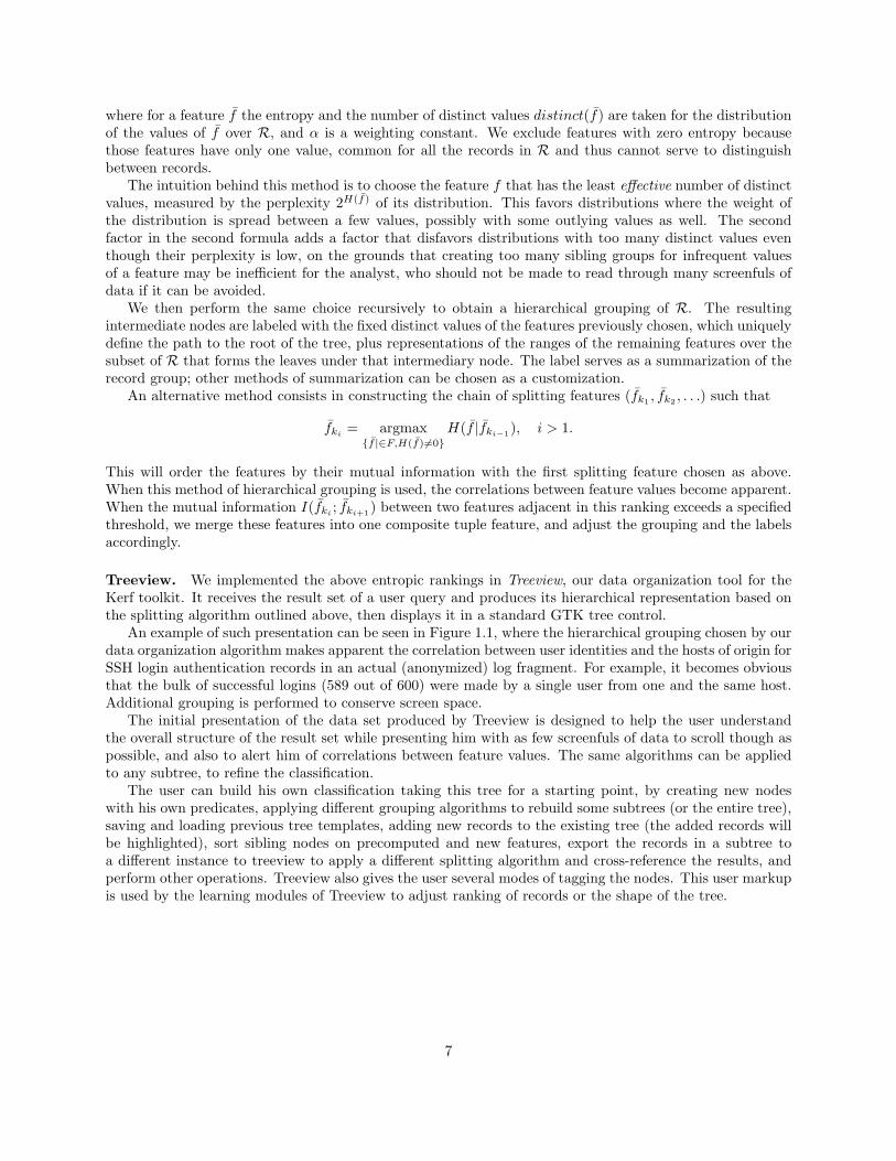
A working demo of our syscall log browsing tool can be found on the project website7. Various views of thesyscall logs generated by the tool are presented in Figures 2.2– 2.2. The first two views show summarizationsof the system call log by process, whereas others show the reconstructed system call tree, first filtered toshow only the process creation related calls, and then all logged calls.

3More precisely, a matching rule can either accept or reject the packet, or hand it off to a new chain, that is, a new sequenceof rules defined by the user; a packet may traverse many chains before hitting a rule that decides its fate.

4http://www.w3.org/TR/xpath5http://www.w3.org/TR/xslt6http://www.intersectalliance.com/projects/Snare/7http://kerf.cs.dartmouth.edu/syscalls/

10

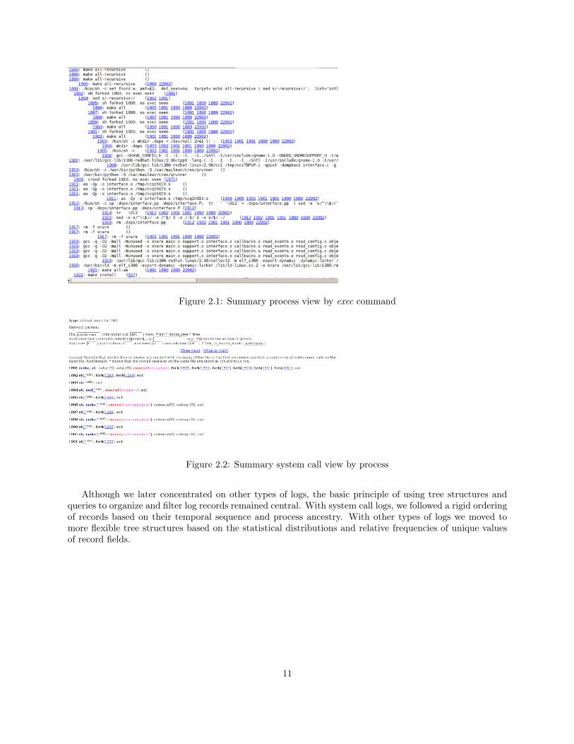
Figure 2.1: Summary process view by exec command

Figure 2.2: Summary system call view by process

Although we later concentrated on other types of logs, the basic principle of using tree structures andqueries to organize and filter log records remained central. With system call logs, we followed a rigid orderingof records based on their temporal sequence and process ancestry. With other types of logs we moved tomore flexible tree structures based on the statistical distributions and relative frequencies of unique valuesof record fields.

11

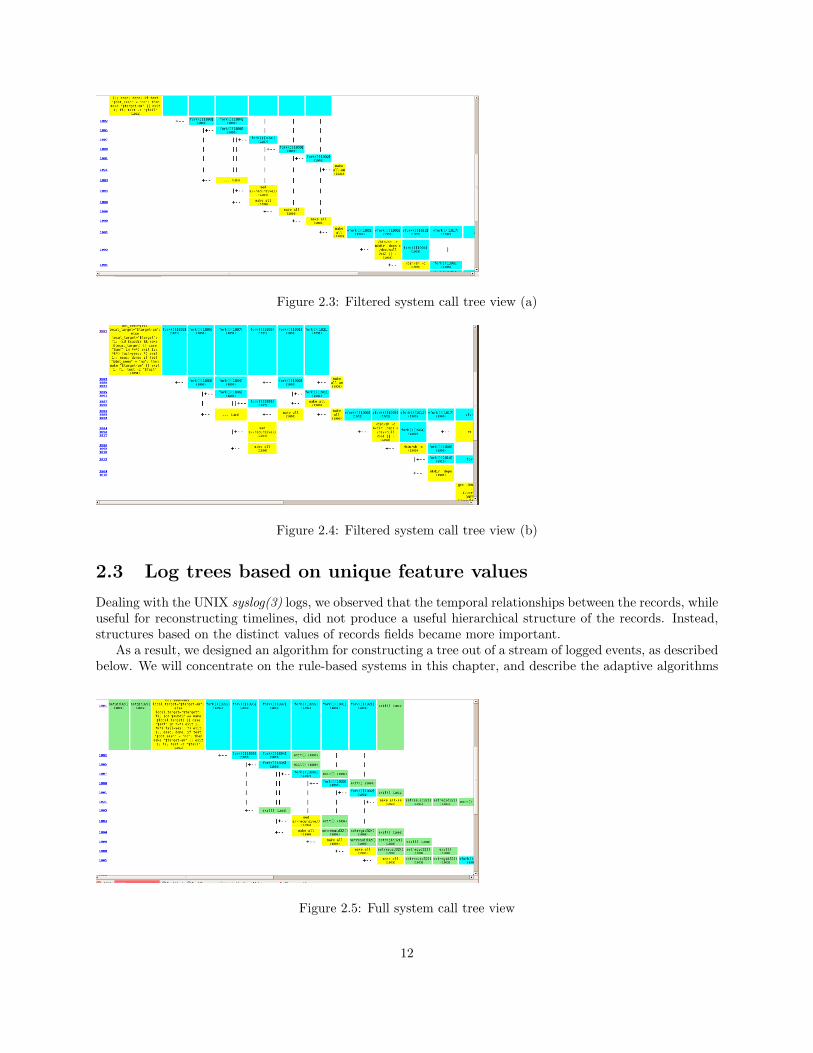
Figure 2.3: Filtered system call tree view (a)

Figure 2.4: Filtered system call tree view (b)

2.3 Log trees based on unique feature values

Dealing with the UNIX syslog(3) logs, we observed that the temporal relationships between the records, whileuseful for reconstructing timelines, did not produce a useful hierarchical structure of the records. Instead,structures based on the distinct values of records fields became more important.

As a result, we designed an algorithm for constructing a tree out of a stream of logged events, as describedbelow. We will concentrate on the rule-based systems in this chapter, and describe the adaptive algorithms

Figure 2.5: Full system call tree view

12

that highlight statistical anomalies in the relative frequency distributions of record fields in the next chapter.In the following sections, we will refer to the individual rules for constructing our trees as templates; we

chose this term because the nodes of the tree that represents the log in our viewer, TreeView, were generatedfrom them in the manner similar to other template instantiation designs.

2.3.1 The tree construction model

One can imagine the algorithm for constructing the tree out of an input record set as the operation of a“coin sorter” device, in which records (“coins”) pass though a number of “separator” nodes that direct themdown one of the possible chutes based on the results of testing each “coin”. Of course, records typically havemore features to be separated on than coins do, so several layers of separators are necessary for a reasonableclassification.

Taken alone, each individual separator node would sort the incoming records into a number of “bins”,one per chute, based on a simple test. Their tree-like combination, where instances of other separator nodesare placed under the output chutes instead of collecting “bins”, will perform a more complex sorting of the“coins” as they percolate down through these nodes, from a single entry point (the tree’s root). For reasonsthat will soon become apparent, it is better to think of the “bins” as having no bottoms, letting the coinsfall through to the next separator, but still registering their passage somehow.

As records (“coins”) pass through a node (specifically, a “bin” node), it counts them and displays someform of a summary of the subset of records that ended up under it. When this mechanism is done with a setof “coins”, these summaries displayed on the intermediate “bin” nodes should help the user in his searchesand browsing by helping him choose the right bin to drill down to at each level of the tree.

In the TreeView display, the intermediate nodes correspond to “bins” in the above scheme. Their labels,summarizing the record subset contained in the subtrees under these nodes, correspond to the summary infodisplayed by the “bins”. The separators themselves are not shown in the TreeView, but are fully describedin the template.

The most common type of the separator corresponds to a single feature of the incoming records and hasa separate output chute for each unique value of that feature. Since, practically speaking, these values arenot known beforehand, we speak of chutes and bins as being “created” as needed by the passage of record“coins”. This corresponds to instantiating nodes from a template to accommodate a record.

Figure 2.3.1 shows an example of a two-tiered tree in which the first (and only) tier “separator” separatesrecords based on the destination port value, and the second tier separators break the resulting groups basedon their source IP value. These second tier separators can be thought of as identical instances of a “by-source-ip” separator, cloned as needed (one for each new output “bin” of the first tier separator, i.e. for eachunique value of its separating feature).

In this tree, there are only two types of separator nodes. There is only one instance of the first type,because it is at the root of the tree (the root can be thought of as the “funnel” through which the recordsenter). The number of instances of the second type depends on the dataset and is equal to the number ofdistinct values of source IP in it.

We now look at the template for this tree as it is used by TreeView. The full template for this tree is asfollows, in XML format:

<rootnode name="root" next="by_dst_port"label="Snort portscan alerts" >

<node name="by_dst_port"hashkey="%dst_port"label="dst_port: %dst_port src_ip: @summary(src_ip)"sortkey="%num_leaves"next="by_src_ip"

/><node name="by_src_ip"

hashkey="%src_ip"

13

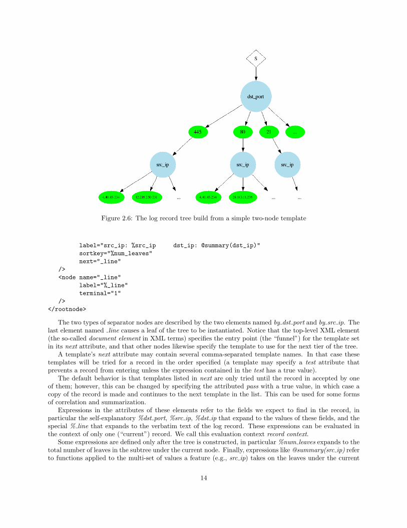
Figure 2.6: The log record tree build from a simple two-node template

label="src_ip: %src_ip dst_ip: @summary(dst_ip)"sortkey="%num_leaves"next="_line"

/><node name="_line"

label="%_line"terminal="1"

/></rootnode>

The two types of separator nodes are described by the two elements named by dst port and by src ip. Thelast element named line causes a leaf of the tree to be instantiated. Notice that the top-level XML element(the so-called document element in XML terms) specifies the entry point (the “funnel”) for the template setin its next attribute, and that other nodes likewise specify the template to use for the next tier of the tree.

A template’s next attribute may contain several comma-separated template names. In that case thesetemplates will be tried for a record in the order specified (a template may specify a test attribute thatprevents a record from entering unless the expression contained in the test has a true value).

The default behavior is that templates listed in next are only tried until the record in accepted by oneof them; however, this can be changed by specifying the attributed pass with a true value, in which case acopy of the record is made and continues to the next template in the list. This can be used for some formsof correlation and summarization.

Expressions in the attributes of these elements refer to the fields we expect to find in the record, inparticular the self-explanatory %dst port, %src ip, %dst ip that expand to the values of these fields, and thespecial % line that expands to the verbatim text of the log record. These expressions can be evaluated inthe context of only one (“current”) record. We call this evaluation context record context.

Some expressions are defined only after the tree is constructed, in particular %num leaves expands to thetotal number of leaves in the subtree under the current node. Finally, expressions like @summary(src ip) referto functions applied to the multi-set of values a feature (e.g., src ip) takes on the leaves under the current

14

node. These are the so-called range expressions (the choice of the name reflects the fact that they are oftenused to summarize value ranges of features in subtrees). We call the context in which these expressions canbe evaluated node context, because it assumes a node (the so-called current node) and a list of leaf recordsin the subtree under this node.

Examples of such expressions include @max(src port), the largest value of the source port under thecurrent node, or @H(src ip), the entropy of the frequency distribution of the src ip values under the currentnode. More information about the language of expressions permissible in different contexts of a templatecan be found in the TreeView manual.

Let us list the different type of “separator” nodes that can be produced from the node elements of thetemplate.

1. Hash node: The main type of the “separator” node. This node contains an expression (the so-calledhashkey) that is evaluated on each passing record, and places the record into the bin corresponding tothe value of this expression, creating it if this value has not been seen before. The node will end uphaving as many children as there are unique values of the hashkey expression on the current record set.

The hashkey attribute is required for this type of node and defines its type.

A hash node can also have a test attribute, described below, which slightly changes its operation (onlyrecords satisfying the test expression are admitted into the node and go on to be separated into “bins”based on the hashkey value).

The label attribute is required and serves to generate the labels for the “bin” nodes, the immediatechildren of this node.

In the TreeView display the hash nodes themselves are hidden whenever possible, only the bin nodesare displayed, to make the tree display more compact.

The operation of the hash node is different from other types describes below: it creates not only the“separator” but also the “bin” nodes (to which its label actually applies).

2. Drop node: Records that reach this node are dropped, incrementing a “dropped records” counter. Adrop node may have a function attribute defining a function that is called on each record before it isdropped and gathers some further statistics that gets saved in the node and displayed on its label. Adrop node is created from a drop XML element or by explicitly providing the type attribute that equalsdrop on a node.

These nodes are visible in TreeView. They have no leaves or children, and their label attribute isusually chosen to display some statistics about the dropped records that reached that node.

3. Deferred node: Leaves that reach this node immediately become its leaves without any computation,not even of a label for the leaf node created (the default label is “dummy”). This type of node isexpected to contain a command attribute that contains the command to be run on this node after thetree construction for the input record set is finished. This command is expected to reshape the subtreeunder that node, so any actions during the tree construction besides the simple attachment of a recordunder the deferred node would be wasted.

A deferred node is typically replaced by the results of the command (typical commands are “autosplitvia algorithm” or “apply saved template file”).

A deferred node is created from a deferred XML element or by supplying the explicit type argumentequal to deferred.

Note that the command attribute is not limited to deferred nodes, is indeed allowed on any kind ofnode, and need node change the shape the tree (but may, e.g., result in marking all leaves under thecurrent node that satisfy some condition).

4. Leaf node: A record that reaches a leaf node template becomes a leaf, labelled according to the node’slabel attribute. This attribute typically includes the full text of the record for syslog–type records, butmay be an arbitrary expression for other kinds of records, e.g., packets or IDS alerts.

15

The standard template node named line is appended to a template set by the TemplateReader parserif the input file does not contain a template with that name.

A leaf node template is created from a leaf XML element.

5. List node: Sometimes it is desirable to create an extra node in the tree for the purposes of summarizinga group of records satisfying a given condition. This is the intention of the list nodes that define nohashkey and do not explicitly specify any of the above types. A list node may have a test attribute, inwhich case only records satisfying the test expression will be allowed to enter and proceed through it; amissing test attribute is not an error, but means that the node is either merely decorative or serves toaccumulate as leaves the records that did not pass the tests of its sibling nodes (see examples below).

In the TreeView display, list nodes are visible (as intermediary nodes). The label is required and willbe placed on that node and serves as a summary for the set of leaves in the subtree under it. A listnode will also be created from a list XML element in the template.

An example of a list node is the standard default node, supplied for a template set by the Tem-plateReader if a node by that name is not explicitly defined. This template gets instantiated wheneverin a series of sibling templates each one contains a test, and some record does not satisfy any of thesetests. Instead of being quietly dropped, the record ends up as a leaf under a default list node.

6. Case node: When placed inside a hash node element, a case node specifies a special path to take forthe value of the parent hash node’s hashkey specified in the value attribute of the case node. This typeof node may specify a different label to apply to the bin, or a different path for the record to take (inits next attribute, different from the parent hash node’s next attribute), or an entirely different set oftemplates, valid only for the subtree under the “bin” derived from this case. This is done by nestingthese templates in the case element in question.

test attributes are not allowed on case nodes (the logic is simple – if a record is prevented from enteringits proper bin determined by the hashkey value, where would it go?)

Case nodes are specified by XML elements of type case.

Case nodes result in visible TreeView “bins” among the other “bin” siblings–children of the (invisible)parent hash node.

The following is the list of all allowed attributes with explanations and limitations.

1. name: Each template node must have a name. Names starting with the underscore are reserved, andshould not be used. These names are used in the next attributes to connect the templates and are themeans of references by which multi-tiered trees of “separator” nodes can be formed.

2. next: Specified one or more nodes to direct the record to after the node instantiated from the currenttemplate is done with it. A comma-separated list of names is allowed here, and is expected if the firstname in the list refers to a template with a test attribute. See also pass attribute.

3. hashkey: The expression at the heart of a hash node separator. To be useful, it should refer to one ormode features (“fields”) of a record, and be evaluatable in the record context as defined above. That is,range expressions @func name(feature expr) are not allowed in hashkeys, because the hashkey shouldbe computable in the context of a single record, whereas range expressions can only be evaluated inthe context of a tree node after the tree construction is complete; range expressions apply to the setof leaves in the subtree under the node on which they are evaluated.

4. label: The label expressions are intended to label “bins” to which separator nodes direct records (andthus usually include the hashkey expression that would expand into the “bin”’s unique value of thehashkey expression once a bin node is instantiated), and also to show a brief summary of other featurevalues in the subtree under the node being labelled (and thus also usually contain range expressions

16

for the features of interest). The labels on all nodes except leaves are evaluated in the node context,and their evaluation is delayed until the tree for the input record set is complete.

The semantics of label are slightly different between the hash node templates and other template types.Namely, in a hash node the label is used to make the (different) labels for all the “bin” nodes, whereasin other types of nodes the label is used for the node instantiated from the template.

It should be noted that label on intermediate nodes must be re-evaluated when the tree changes shapeas a result of a user action or command, on the entire path from the node acted upon to the root, topreserve consistency of the summaries.

5. sortkey: This attribute is not used while the tree is constructed, but is essential when it is displayed.The children of nodes generated from templates (in particular, of hash and list nodes) are stored in noparticular order, but need a fixed order in which they can be displayed in the TreeView. This order isestablished by evaluating the sortkey expression on all the siblings, and then sorting them accordingto these values. Sorting is in descending order by default, ascending order is forced by setting thesortorder attribute to asc.

The default value for sortkey, supplied by the TemplateReader if not present in a template, is %num -leaves, a special variable available in the context of a node that evaluates to the number leaves in thesubtree under the current node. Another possible choice is %num children, another special variable,the number of direct children of the current node.

6. sortorder: “asc” will cause the sortkey to be applied in ascending order.

7. test: This expression will be evaluated on a record to determine if it is allowed to enter (and instantiate,if not already instantiated) a template node. It has the same limitations as the hashkey attribute.

8. terminal: Identifies leaf templates. A “truth” value (e.g., “1”) is the only meaningful one.

9. type: Determines the type of the node. Allowed values are hash (implied as long as the hashkeyattribute is present, may be omitted), drop, deferred, leaf (may be omitted if terminal=”1” is given)and list (implied if none of the above is given, may be omitted).

10. value: Allowed only for case templates, which are themselves meaningful only as children of a hashnode parent. Specifies the value of the parent’s hashkey for which the special action described by thiscase should be taken.

11. pass: If specified and set to a true value (e.g., “1”), this attribute specifies that the current templatedoes not “capture” the passing records, i.e. they are duplicated and the duplicate is allowed to proceedto the next template named in the previous tier node’s next.

This behavior can be used in combination with drop nodes for gathering different kind of statisticswith different functions, and then displaying them on the labels of different nodes.

12. command: Specifies a TreeView command that can be carried out before the tree is displayed. Nodesgenerated from templates with a command attribute are entered into a queue together with theircommands, and then carried out once the tree construction from the current input set is over (in thecontexts of their respective nodes). For commands that change the shape of the subtree under theircurrent nodes, the use of deferred nodes is recommended to save processing time.

13. function: This attribute specifies a function to call immediately on the record and the node justcreated from the record, also passing it the value of the template’s arg attribute as the third argument(if any). The function is passed the node and the record by reference, and can therefore compute andadd new fields to the record or modify the existing ones, and register variables to be stored in the nodefor later evaluation by calling the node’s set user variable(key, value) method (they will later availableto the ExpressionEvaluator via the usual %varname syntax).

Use with caution, because the function has access to all the node internals.

17

14. postfunction: This attribute specifies a function to call on a node once the tree is fully constructed(but before the deferred commands specified in the command attributes). Otherwise it is similar inoperation of the function attribute. Note that the function–named function will be called for eachrecord that reaches the node generated from the template containing the function attribute, whereaspostfunction will be called only once. In typical usage, the function will gather information from passingrecords and store it in the node, whereas the postfunction will process and summarize it.

Use with caution, as above.

15. arg: Specifies a node-specific argument for the function attribute. Optional (the function will getundef if omitted).

Using these attributes, one can create complex (possibly, Turing-complete) templates, use the savedtemplate sets as subsets for subtrees of the constructed tree, or even write self-modifying templates.

18

Chapter 3

Learning Components

In this chapter we describe our applications of various Machine Learning and Information Retrieval techniquesto log browsing tasks.

3.1 Introduction

Learning and data mining provide a variety of techniques for understanding, exploring, classifying anddescribing large amounts of data. More and more applications, particularly in security, incorporate learn-ing/data mining algorithms. As shown in previous sections, our toolkit organizes and presents data inuser-friendly fashion which makes browsing through the log data more efficient, for moderate sizes of resultsets; however for large and complex logs the user (system administrator) is still confronted with a diffi-cult task. This is where learning comes into play: the primary purpose of the learning algorithm(s) is toautomatically detect and suggest records that are more interesting (i.e., likely associated with an attack)than others, therefore making the user search more efficient. A secondary purpose of the learning task is tocombine the learning algorithm with an active learning strategy, that is a strategy to optimally select newrecords to expand the set of records explicitly classified by the user (the so-called training set in ML and IRterms), minimizing user effort in providing the marked records to derive the desired complete classificationof the log data with respect to its relation to an attack.

3.1.1 Data organization

A clear distinction should be made between unsupervised learning (of which clustering is the most frequentform) and supervised learning. Clustering is used to group similar records to give the user a startingpoint for the search, when no records are yet judged (classified and marked) as “normal”/non-relevant or“attack”/relevant. This is the main advantage of using a clustering-like method, that it does not requireany effort from the user in marking records before it can run; the disadvantage is that the record groupingproduced does not always meet the user’s purpose and can sometimes be misleading in the sense that the treeproduced, while reflecting the general structure of the record set, is not very useful for record classificationpurposes with respect to a particular attack.

3.1.2 Supervised learning

Supervised learning infers classification labels for records from a training set of marked records that isprovided by the user. This implies that the user marks a number of records prior to running the learningalgorithm. In the classical ML and IR settings, training sets can be quite large (70% or more of the entireset), which can make the initial labelling effort difficult. In many cases training sets are based on history,like records of patients in a hospital or sales records over periods of years, and in such cases obtaining

19

training sets requires no extra effort. The advantage of supervised learning is that it can produce highlyaccurate results (1% error or less). There are many successful learning algorithms developed over last threedecades, including: decision trees, neural networks, nearest neighbor, boosting, support vector machines,Bayesian networks and information diffusion. While some algorithms are very different than others in termsof performance, computation time, or the type of problem they solve, it is always the case that the largerthe training set is, the better the performance.

Applying supervised learning methods to intrusion log analysis has a number of pecularities and challengesthat set it apart from other applications. We discuss these in the next section.

3.1.3 Learning for intrusion analysis

For terminology we use “attack”/relevant and “normal”/non-relevant for records marked by user and “suspi-cious” and “non-suspicious” for inferences made by the learning algorithm. The learning task for our toolkitis for now reduced to classification of records by labelling each record with a score that allows our tool torank them from the most suspicious to the least suspicious, and to present them to the user accordingly.The algorithm is given a training set (of marked records) and outputs a real number label for every record,indicating the degree of suspiciousness, that is, the likelihood that the record is attack-related (belonging toset A, in terms of our proposed formalism).

The quality of the learning process is evaluated with the average precision measure on the list of recordsranked by the suspiciousness label. Average precision (AP) [BYRN99] is the most commonly used measurein Information Retrieval for assessing the quality of a retrieved lists of documents returned in response toa give user query (consider lists returned by web search engines). This measure greatly weights retrievingrelevant documents in the top ranks of a list at the expense of lower ranks; that is AP is high if and only ifmost of the relevant results are ranked near the top of the list returned. We believe it fits our learning taskbecause this measure evaluates both the precision at finding records relevant to attack near the top of thereturned list of results and the recall (the fraction of relevant records returned).

In practice, the user is likely to be able to concentrate his attention on only a small top portion of theranked list, so our ranking, possibly combined with data organization, must work within this budget of userattention.

Very limited amounts of labelled data. Although in many applications the training set is significantin size, we cannot count on this for our application: if there are 100,000 log records, a 10% training set wouldrequire 10,000 marks by the user, which is not a feasible user effort. The biggest challenge in designing alearning algorithm for our setup is that it has to work on very small training sets (at most hundreds ofmarks). Grouping records, and allowing the user to mark entire groups at a time helps, but not enough toremove this challenge.

Computation time. The second challenge is computation time. Our goal is to automated an iterative andinteractive process with the human user in the loop. Therefore it is important than the learning componentsproduce results in minutes and not in days.

Self-similarity of data. Because our data sets are log records, although they may be very large, theyare rather “easy” from learning point of view. For many attacks prior research has identified featuresthat separate their traces from normal activity, and logging practices catch up to include these. Oftenattacks involve an abnormally repetitive pattern of accesses which are easily separated by our entropic dataorganization and can be classified as a whole. In particular, when an attack involves a DOS componentgenerated by simple tools, it usually leaves many identical log records, which can be easily classified andmoved out of the way.

This is why learning can be useful and fast even with very small training sets. We have implementedthree algorithms: Nearest Neighbor, Information Diffusion and an IR strategy. In the sections that follow,

20

we discuss each of these methods in turn.

3.2 Nearest Neighbor

In its simplest form, the K-Nearest Neighbor algorithm [Mit97] first defines a distance between datapoints(often the Euclidian distance when data representation allows it), then it classifies every datapoint by takingthe majority vote of the closest K training points, according to the distance. For example, K=1 means theoutput label of any (non-training) datapoint is simply the label of its closest marked neighbor. We haveimplemented two variants.

The Discrete Nearest Neighbor (DNN) uses the Hamming editing distance, essentially counting thenumber of different attributes

editdist(R1, R2) =∑

f

δ(R1(f), R2(f))

where

δ(a, b) ={

1 if a 6= b0 if a = b

and R(f) denotes the value for the feature f in record R ( if f=username then R(f) is the actual usernamein the log record R). For classification, note that this distance can take only discrete values in the set{0, 1, 2, ..., |F |}; the label output by DNN for a record R is the majority vote of the labelled records atminimal distance from R. It mimics K=1, but it takes into account that there might be more than onenearest neighbor.

training set size 0.01% 0.05% 0.1% 1%DNN AP (large set) 0.75 0.79 0.87 0.92

Table 3.1: DNN results on a set of 110,000 records, with a component DOS attack. Therunning time of DNN is proportional with training set size, 80min for the largest one on2.0Ghz 64bit machine.

training set size 0.01% 0.05% 0.1% 1%DNN AP (medium set) 0.73 0.83 0.88 0.97

Table 3.2: DNN results on a set of 56,000 records, with a component DOS attack. The runningtime of DNN is proportional with training set size, 30min for the largest one on 2.0Ghz 64bitmachine.

3.2.1 Continuous Nearest Neighbor

Continuous Nearest Neighbor (CNN) is a variant in which the features in the distance formula are weighted

editdist(R1, R2) =∑

f

δ(R1(f), R2(f)) · (wR1(f) + wR2(f)),

where wRi(f) is a weight associated with the value R1(f) of the feature f in the record Ri ∈ R (we willcall this value an attribute of the record for short), or with the entire distribution of the feature f across R.

21

Weights make some attributes or features matter more than others; for example, we might want very frequentattributes to cause small changes and infrequent attributes to cause big changes; or in authentication recordsfor remote access to a service like www or ssh, we might want to weight changes in the features username,dest_port more than changes on feature source_port, because the latter is likely to be randomly anduniformly distributed. Weights can be automatically computed with information theoretic characteristics offeature value distribution, or can be manually set up based on prior knowledge administrator has about thesystem and attack. Because this weighted formula makes the distance continuous, for label computation wewould not consider as in DNN the marked records at minimal distance; instead will take the average of themarked records at distance smaller than a constant threshold fixed by the user.

For experiments we used two log data sets. The large set has 110,000 records but only five manuallyselected features per record for a total of about 10,000 resources while the medium set has 56,000 records with16 manually selected features per record for a total of about 5,000 resources. The tables 3.1 and 3.3 presentthe results of the Nearest Neighbor algorithms on the large set (110,000 records) and the tables 3.2 and 3.4present the results of the Nearest Neighbor algorithms on the medium set (56,000 records). The discreteversion of the algorithm works better because many records are simply duplicates and K = 1 means that allduplicates are labelled the same as their closest marked record, which is most likely one of the duplicates.

It is important to mention that a small change (even as small as 0.05) in average precision is sometimesnoticeable to an experienced user by looking at retrieved results. The outstanding performance of thealgorithm — notice that the best result in Table 3.2 is the AP of 0.97 — is likely due, in part, to the highdegree of data homogeneity. Such a ranking list of results is almost “perfect,” that is, almost all the relevantrecords are placed above all the non-relevant ones.

training set size 0.01% 0.05% 0.1% 1%CNN AP (large set) 0.43 0.77 0.77 0.79

Table 3.3: CNN results on a set of 110,000 records, with a component DOS attack. Therunning time of CNN is proportional with training set size, 40 min for the largest one on2.0Ghz 64bit machine.

training set size 0.01% 0.05% 0.1% 1%CNN AP(medium set) 0.67 0.74 0.76 0.88

Table 3.4: CNN results on a set of 56,000 records, with a component DOS attack. The runningtime of CNN is proportional with training set size, 15 min for the largest one on 2.0Ghz 64bitmachine.

The Nearest Neighbor algorithm is simple and has the advantage of providing good intuition of whatit does, when it works (usually producing reasonably good results) and when it does not work; becauseof its simplicity, we use it as a base-line comparison. The downside is that there are certain log sets onwhich the algorithm fails, where the distance(s) defined above show high similarity of records (because manyresources — but not all — are common), but do not separate attack records well. Also the running time ofthe algorithm is proportional to the size of the training set making it slow for cases with large numbers ofmarked records.

3.3 IR Rank retrieval (IRR)

The field of Information Retrieval (IR) is concerned primarily with extracting useful information efficientlyfrom unorganized data, best known instances being web search engines like Google, Yahoo etc. Techniquesdeveloped in IR are in many cases ad-hoc in nature but highly efficient in practice.

22

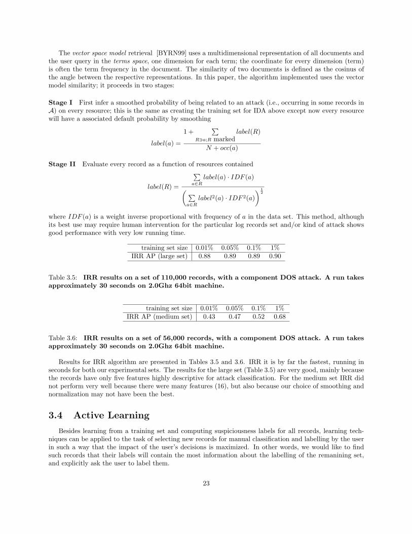
The vector space model retrieval [BYRN99] uses a multidimensional representation of all documents andthe user query in the terms space, one dimension for each term; the coordinate for every dimension (term)is often the term frequency in the document. The similarity of two documents is defined as the cosinus ofthe angle between the respective representations. In this paper, the algorithm implemented uses the vectormodel similarity; it proceeds in two stages:

Stage I First infer a smoothed probability of being related to an attack (i.e., occurring in some records inA) on every resource; this is the same as creating the training set for IDA above except now every resourcewill have a associated default probability by smoothing

label(a) =

1 +∑

R3a;R markedlabel(R)

N + occ(a)

Stage II Evaluate every record as a function of resources contained

label(R) =

∑a∈R

label(a) · IDF (a)( ∑a∈R

label2(a) · IDF 2(a)) 1

2

where IDF (a) is a weight inverse proportional with frequency of a in the data set. This method, althoughits best use may require human intervention for the particular log records set and/or kind of attack showsgood performance with very low running time.

training set size 0.01% 0.05% 0.1% 1%IRR AP (large set) 0.88 0.89 0.89 0.90

Table 3.5: IRR results on a set of 110,000 records, with a component DOS attack. A run takesapproximately 30 seconds on 2.0Ghz 64bit machine.

training set size 0.01% 0.05% 0.1% 1%IRR AP (medium set) 0.43 0.47 0.52 0.68

Table 3.6: IRR results on a set of 56,000 records, with a component DOS attack. A run takesapproximately 30 seconds on 2.0Ghz 64bit machine.

Results for IRR algorithm are presented in Tables 3.5 and 3.6. IRR it is by far the fastest, running inseconds for both our experimental sets. The results for the large set (Table 3.5) are very good, mainly becausethe records have only five features highly descriptive for attack classification. For the medium set IRR didnot perform very well because there were many features (16), but also because our choice of smoothing andnormalization may not have been the best.

3.4 Active Learning

Besides learning from a training set and computing suspiciousness labels for all records, learning tech-niques can be applied to the task of selecting new records for manual classification and labelling by the userin such a way that the impact of the user’s decisions is maximized. In other words, we would like to findsuch records that their labels will contain the most information about the labelling of the remanining set,and explicitly ask the user to label them.

23

The new record labelled is going to be included in the training set; the purpose here is not necessarily toselect a relevant (attack) record but rather to select a record that is useful to learn from. In an online fashion,(selecting, judging, expanding the training set) is an episode of active learning. Using the new training set,the learning algorithm is being rerun, then a new active learning episode takes place and so on until thereare enough training records.

From an information theoretic point of view,

0 2 4 6 8 10 120.7

0.75

0.8

0.85

0.9

0.95

1

Active Learning training set size (percent)

AP

Active Learning for IRR algorithm

AP for 10%randomtraining set

AP for 3.3%Active Learntraining set

3.3 10

Figure 3.1: Performance on Active Learning builttraining sets

actively selected training data means choosingthe maximally informative points while ran-domly chosen training points are only randomlyinformative. It has been convincingly shown([SOS92, Ang87, CGJ95, HKS92, ZLG03]) thattraining sets built with active learning strate-gies are very effective and that they can bemuch smaller than, for example, training setsobtained by randomly choosing datapoints thusrequiring less user effort for bootstrapping theclassification.

In designing an active learning strategy twofactors are particularly important: first, howto choose a new record each episode and howmuch computation time that requires; secondwhen training set includes the new record justmarked by the user, it is desirable to find ashortcut in updating the learning computationinstead of re-running the learning algorithmfrom scratch. We implemented active learningfor Nearest Neighbor and IRR learning com-ponents. In both cases the record selected for labelling each episodes maximizes (in expectation) the numberof records that would have their computed labels changed if the new record is included in the training set.Given the simplicity of computation formulas for both Nearest Neighbor and IRR algorithms, it is not hardto get the learning updated after an active learning episode; that only requires updates on counts on everyresource marks.

In Figure 3.1 we present IRR performance on training sets built with Active Learning strategy, on a “toy”set of 1,300 records. There are two ways to interpret the advantage of active learning built training sets (bluesolid line) vs the random training set (red dash line): first, the performance of a randomly chosen trainingset of size 10% (130 records) is matched by an actively-built training set of only 3.3% (43 records), whichmeans same performance is achieved with an user labelling effort reduced by 66%; second, if we are to useactive learning but to consider same size training set, 10%, we get a boost in performance from AP = 0.79to AP = 0.94.

3.5 Resource graph and Information Diffusion

Accurate learning methods like Support Vector Machines or Information Diffusion often require definition ofa similarity metric between datapoints, sometimes called a kernel ; however computation for these methodsis intensive because the matrices involved have N2 elements, where N is the size of the data set. In our setupN (the number of records) can be as large as several hundred thousand therefore kernel methods cannotbe applied directly. Instead, we are going to “move” the learning task from the record space, where N isvery large to the resource space, where the number of resources is the sum of the number of usernames, thenumber of IPs, the number of ports etc., total on the order of hundreds.

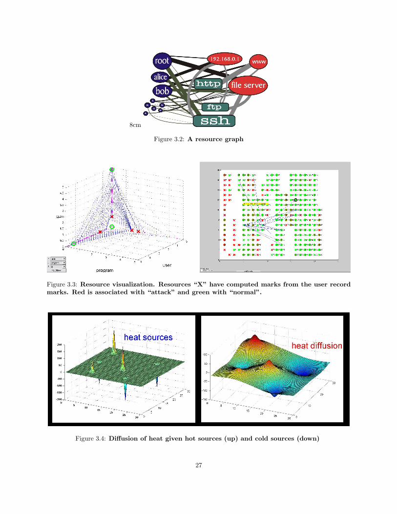
We formalize this transformation of the data by introducing the resource graph (Figure 3.2), whosevertices are resources referred to by feature values (attributes). Two resources are connected by an edgewhen they co-occur in a record. Each edge thus corresponds to a subset of the set of records consisting of

24

records where such co-occurrence takes place, and can be labelled with a label derived from this set (e.g.,with the size of the subset, or a function of timestamps). Typically resources are the feature values (or dataattributes) like usernames alice,bob etc, ip addresses 129.170.39.103 or ports 25,80 etc.; resources canalso be pairs of attributes (alice,80). Even with pairs included, the total number of resources is on theorder of thousands which is very small in comparison with the number of records. The resource graph isparticularly important beyond the learning task because it provides a simple and complete way of modelingthe log data.

3.6 Information Diffusion

The Information Diffusion algorithm (IDA) is a recent learning development by Zhu et al. ([ZGL03])and it closely follows the law of harmonic energy minimization which in nature is realized by heat diffusion(Figure 3.4). Given this analogy, IDA propagates the information from sources (training examples) to therest of the datapoints.It uses W as similarities matrix (wij=similarity between datapoints i and j) to compute a labelling function

f that minimizes the energy function

E(f) =12

∑i,j

wij(f(i)− f(j))2

It is known that f has many nice proprieties including being unique, harmonic and having a desired smooth-ness on a graph of datapoints.

We implement IDA having resources as datapoints.The algorithm works as follows:• given :W = (wij)= similarities matrix, wij=similarity between datapoints i and jdi =

∑j wij degrees of nodes in the graph ; D =diag(di)

∆ = D −W is the combinatorial Laplacian• compute f = labelling function, minimizes the energy function

E(f) =12

∑i,j

wij(f(i)− f(j))2

• this means f = Pf , where P = D−1W which implies f is harmonic ,i.e. it satisfies ∆f = 0 on unlabelledset of points U . f is unique and is either a constant or satisfies 0 < f(j) < 1∀j (Boyle & Snell,1984); fharmonic means the desired smoothness on the graph

f(j) =1dj

∑i∼j

wijf(i)

• exact computation: if we split W ,f, P over labelled and unlabelled points, assuming labelled points get

the upper-left corner, W =[

Wll Wlu

Wul Wuu

]and f =

[fl

fu

]then

fu = (Duu −Wuu)−1Wulfl = (I − Puu)−1Pulfl

Using the resources as datapoints, the output of IDA is going to be a suspiciousness label for everyresource which later will be combined to obtain suspiciousness labels for records. In order to apply IDA forresources we need to set up several things:

1. A similarity measure for resources. This is done using occ(a) = number of records in which resource aoccur and occ(a, b) = number of records in which resources a and b co-occur:

sim(a, b) =occ(a, b) · (wa + wb)occ(a)wa + occ(b)wb

25

where wa is a weight associated with resource a, often inverse proportional with the frequency of a,also called inverse document frequency (IDF) value.

2. A resources training set. That is, we have to label a subset of resources with suspiciousness valuesbefore running the IDA; these labels are computed from the training set of records as follows:

label(a) =

∑R3a;R marked

label(R)

occ(a)

which gives 1 if and only if all labelled records containing a are marked 1 and 0 if and only if all labelledrecords containing a are marked 0.

3. After running the IDA we need to compute for records suspicious labels from resource labels. It canbe done as a simple sum :

label(R) =∑a∈R

label(a)

Tables 3.7 and 3.8 show results using the IDA on the two log sets. Even though we are using IDA inthe resource space, which is considerable smaller, the algorithm can take time to run and, more importantsignificant memory space (the largest experiment described used took 1.6GB of RAM). It has however theadvantages that the results are likely accurate and that it can handle data complexity well. So if time andresources allows it, IDA is desirable.

training set size 0.01% 0.05% 0.1% 1%IDA AP(large set) 0.80 0.82 0.84 0.90

Table 3.7: IDA results on a set of 110,000 records, with a component DOS attack. A run takesapproximately 12 minutes on 2.0Ghz 64bit machine.

training set size 0.01% 0.05% 0.1% 1%IDA AP (medium set) 0.67 0.82 0.85 0.92

Table 3.8: IDA results on a set of 56,000 records, with a component DOS attack. A run takesapproximately 5 minutes on 2.0Ghz 64bit machine.

26

8cm

Figure 3.2: A resource graph

Figure 3.3: Resource visualization. Resources “X” have computed marks from the user recordmarks. Red is associated with “attack” and green with “normal”.

Figure 3.4: Diffusion of heat given hot sources (up) and cold sources (down)

27

Chapter 4

Related work

Several free software and commercial tools offer some form of automation for analysis of system logs frommultiple sources. Tina Bird compiled an excellent survey of these, together with a collection of links to remotelogging tutorials and system-specific information [Bir02]. Practical issues of log processing and correlationhave also been discussed in many professional publications (e.g., [All02, Chu02, Rom00]). We draw on thisand other work for the definition of applied intrusion analysis tasks that we aim to automate.

A great corpus of work has been devoted to application of ML techniques in the field of IntrusionDetection. We will not attempt to survey this work here, because most of it is based on different premisesabout available data, context and time limitations, as we have outlined in the Introduction. Discussionsof IR and ML techniques to aid specifically in Intrusion Analysis tasks can be found in [ES02]. Variousapplications of visualization techniques to analysis of log data are surveyed in [Mar01]. A brief overview ofavailable data visualization tools can be found in [She02].

The MINDS system [EEL+04, EEL+03] implemented grouping of similar IDS alerts under a single tablerow in its display tables, based on an association mining ML technique. MINDS data presentation isspecifically tuned to IDS alert messages, while Kerf aims to provide a general technique, usable on a widevariety of log sources. Also, Kerf’s records grouping is nested and hierarchical, while data views of MINDSare table-based.

4.1 Acknowledgements

We would like to thank George Bakos and Bill Stearns for many useful discussions regarding the practicalitiesof log analysis, Greg Conti for discussions of log visualization and connecting us with security researchersat Georgia Tech. We would also like to thank everyone who provided us with log data samples, and sharedtheir observations on the issues encountered in analyzing logs.

This research program is a part of the Institute for Security Technology Studies, supported under Awardnumber 2000-DT-CX-K001 from the U.S. Department of Homeland Security, Science and Technology Direc-torate. Points of view in this document are those of the authors and do not necessarily represent the officialposition of the U.S. Department of Homeland Security or the Science and Technology Directorate.

28

Bibliography

[All02] Jared Allison. Automated log processing. ;login:, 27(6):17–20, 2002.

[Ang87] Dana Angluin. Queries and concept learning. Machine Learning, 2(4):319–342, 1987.

[Bir02] Tina Bird. Log analysis resources. www.counterpane.com/log-analysis.html, 2002. .

[Bur03] Mark Burnett. Forensic log parsing with microsoft’s logparser.http://www.securityfocus.com/infocus/1712, July 2003. .

[BYRN99] Ricardo Baeza-Yates and Berthier Ribeiro-Neto. Modern Information Retrieval. ACM Press, 1999.

[CGJ95] D. Cohn, Z. Ghahramani, and M. Jordan. Active learning with statistical models, 1995. .

[Chu02] Anton Chuvakin. Advanced log processing. http://online.securityfocus.com/infocus/1613, August 2002..

[CT91] T. M. Cover and J. A. Thomas. Elements of Information Theory. John Wiley & Sons, Inc., 1991.

[EEL+03] L. Ertoz, E. Eilertson, A. Lazarevic, P. Tan, P. Dokas, J. Srivastava, and V. Kumar. Detection andsummarization of novel network attacks using data mining. Technical Report, 2003. .

[EEL+04] L. Ertoz, E. Eilertson, A. Lazarevic, P. Tan, P. Dokas, J. Srivastava, and V. Kumar. The minds -minnesota intrusion detection system. In Next Generation Data Mining. MIT Press, 2004.

[ES02] Robert F. Erbacher and Karl Sobylak. Improving intrusion analysis effectiveness. Technical report,University at Albany - SUNY, 2002. .

[gro04a] The Kerf group. The Kerf toolkit for intrusion analysis. IEEE Security and Privacy, 2(6):42–52, Novem-ber/December 2004. .

[gro04b] The Kerf group. The Kerf toolkit for intrusion analysis. Technical Report TR2004-493, March 2004. .

[HKS92] David Haussler, Michael Kearns, and Robert Schapire. Bounds on the sample complexity of Bayesianlearning using information theory and the VC dimension. Technical Report UCSC-CRL-91-44, 1992. .

[LNY+00] Wenke Lee, Rahul Nimbalkar, Kam Yee, Sunil Patil, Pragnesh Desai, Thuan Tran, , and Sal Stolfo. Adata mining and CIDF based approach for detecting novel and distributed intrusions. In Proceedings ofthe Third International Workshop on Recent Advances in Intrusion Detection (RAID 2000), volume 1907of Lecture Notes in Computer Science, pages 49–65. Springer-Verlag, Toulouse, France, October 2000. .

[LS00] Wenke Lee and Salvatore J. Stolfo. A framework for constructing features and models for intrusiondetection systems. ACM Transactions on Information and System Security, 3(4):255, 2000. .

[LX01] Wenke Lee and Dong Xiang. Information-theoretic measures for anomaly detection. In Proc. of the 2001IEEE Symposium on Security and Privacy, pages 130–143, May 2001. .

[Mar01] David J. Marchette. Computer Intrusion Detection and Network Monitoring: A statistical viewpoint.Springer, 2001.

[Mit97] Tom M. Mitchell. Machine Learning. McGraw-Hill, New York, 1997.

[PN98] Thomas H. Ptacek and Timothy N. Newsham. Insertion, evasion, and denial of service: Eluding networkintrusion detection. Secure Networks, Inc., January 1998. .

[Rom00] Steve Romig. Correlating log file entries. ;login:, pages 38–44, November 2000. .

[She02] Brian K. Sheffler. The design and theory of data visualization tools and techniques, March 2002. .

29

[SOS92] H. S. Seung, Manfred Opper, and Haim Sompolinsky. Query by committee. In Computational LearningTheory, pages 287–294, 1992. .

[ZGL03] X. Zhu, Z. Ghahramani, and J. Lafferty. Semi-supervised learning using Gaussian fields and harmonicfunctions, 2003. .

[ZLG03] X. Zhu, J. Lafferty, and Z. Ghahramani. Combining active learning and semi-supervised learning usinggaussian fields and harmonic functions, 2003. .

30