Tolerance Analysis of Mechanical Parts

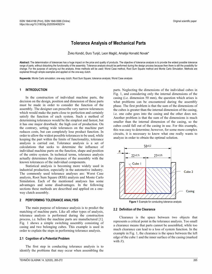
TEHNIČKI GLASNIK 14, 3(2020), 265-272 265

ISSN 1846-6168 (Print), ISSN 1848-5588 (Online) Original scientific paper https://doi.org/10.31803/tg-20200504092314

Tolerance Analysis of Mechanical Parts

Živko Kondić, Đuro Tunjić, Leon Maglić, Amalija Horvatić Novak*

Abstract: The determination of tolerances has a huge impact on the price and quality of products. The objective of tolerance analysis is to provide the widest possible tolerance range of parts, without disturbing the functionality of the assembly. Tolerance analysis should be performed during the design process because then there is still the possibility for change. For the purpose of carrying out the analysis, three methods will be used: Worst Case method, Root Sum Square method and Monte Carlo Simulation. Methods are explained through simple examples and applied on the one-way clutch. Keywords: Monte Carlo simulation; one-way clutch; Root Sum Square; tolerance analysis; Worst Case analysis 1 INTRODUCTION

In the construction of individual machine parts, the decision on the design, position and dimension of these parts must be made in order to consider the function of the assembly. The designer can prescribe very narrow tolerances which would make the parts close to perfection and certainly satisfy the function of each system. Such a method of determining tolerances would be the simplest and fastest, but it has one major drawback: the high cost of production. On the contrary, setting wide tolerances on the machine part reduces costs, but can completely lose product function. In order to allow the widest possible tolerances to be used, while keeping the part within the limits of functionality, tolerance analysis is carried out. Tolerance analysis is a set of calculations that seeks to determine the influence of individual machine parts on the function, shape and position of the entire system. In technical terms, tolerance analysis actually determines the clearance of the assembly with the known tolerances of the individual components.

Statistical analysis is becoming more widely used in industrial production, especially in the automotive industry. The commonly used tolerance analyses are: Worst Case analysis, Root Sum Square (RSS) analysis and Monte Carlo Simulation. Each of the mentioned analyses has some advantages and some disadvantages. In the following sections these methods are described and applied on a one-way clutch assembly. 2 PERFORMING TOLERANCE ANALYSIS

The main purpose of tolerance analysis is to predict the matching of machine parts. Like all other types of analysis, tolerance analysis is performed during the construction process, i.e. before the machine parts are manufactured [1]. Fig. 1 shows a simple switching assembly consisting of casing and two belonging cubes. This example is used in order to explain the steps in performing tolerance analysis. 2.1 Cognition of a Potential Problem

The first step in conducting tolerance analysis is to identify the problems that may occur when assembling the

parts. Neglecting the dimensions of the individual cubes in Fig. 1, and considering only the internal dimensions of the casing (i.e. dimension 50 mm), the question which arises is what problems can be encountered during the assembly phase. The first problem is that the sum of the dimensions of the cubes is greater than the internal dimension of the casing, i.e. one cube goes into the casing and the other does not. Another problem is that the sum of the dimensions is much smaller than the internal dimension of the casing, so the cubes could fall out of the casing in use. For this example, this was easy to determine; however, for some more complex circuits, it is necessary to know what one really wants to analyze in order to obtain the optimal solution.

Figure 1 Example for conducting tolerance analysis

2.2 Definition of the Clearance

Clearance is the space between two objects that represents a critical point in the tolerance analysis. Too small a clearance means that parts cannot be assembled, while too much clearance can lead to a loss of system function. In the example in Fig. 1, the clearance is the space between the left edge of the cube 1 and the inner surface of the casing (marked with R).

Živko Kondić et al.: Tolerance Analysis of Mechanical Parts

266 TECHNICAL JOURNAL 14, 3(2020), 265-272

2.3 Defining Requirements

The requirement is a value that represents the boundary between an acceptable and an unacceptable clearance. The requirement for any system is to fulfill a particular function. In order for the assembly in Fig. 1 to function, the cubes must fit into the casing, i.e. the clearance must be larger than zero. Another requirement is that the clearance should not be larger than 2 mm to prevent the cubes from falling out of the casing: 0 mm 2 mmR< < (1) 2.4 Creating a Tolerance Chain

This step determines the dimensions that are essential to the tolerance analysis. The tolerance chain begins on one side of the clearance and ends on the other. This chain can be thought of a vector summation and the result must be a clearance which is going to be analyzed. There are three types of tolerance chain according to dimensionality: one-dimensional (linear), two-dimensional (non-linear), and three-dimensional (spatial) [2]. For performing the one-dimensional analysis for the example in Fig. 1, important dimensions are as follows: internal dimension of the casing (50 mm), the length of the cube 1 (22 mm) and the length of the cube 2 (27 mm). The graph of the tolerance chain is then plotted as shown in Fig. 2. It is defined that if vector is inclined to the right, it is positive, and it is negative if it is inclined to the left. The tolerance chain graph begins with the internal length of the casing (L1) and is inclined to the right, and continues with the length of the cube 2 (L2) and the length of the cube 1 (L3) which is inclined to the left. Summing these vectors, the clearance can be obtained as shown in Eq. (2).

1 2 3L L L R− − = (2)

Figure 2 Tolerance chain

2.5 Research of Dimensions

If the tolerance chain is made correctly, then this step is very simple. The value of the dimension corresponding to

each vector in the chain is searched and then entered in the commemorative table. Fig. 2 shows that L1 = 50 mm, L2 = 27 mm and L3 = 22 mm. In this example, the tolerance chain vectors correspond exactly to the given dimensions on the design, but it may happen that some dimensions that are important for the tolerance chain are not specified in the drawing and have to be calculated using other dimensions. 2.6 Drawing a Table and Getting a Solution

After determining which dimension value corresponds to which vector, a table is formed. The table is used to improve the transparency of the analysis and to obtain solutions. Once the table is filled, the solution will be obtained by simply summing the values of the vectors in the tolerance chain as shown in Tab. 1.

Table 1 Summing of vector values and tolerances Vector Description Amount, mm Tolerance, mm

L1 Housing internal length 50 ± 0.2 L2 Length of cube 2 −27 ± 0.05 L3 Length of cube 1 −22 ± 0.15 Clearance 1 ± 0.4

Table 1 shows that the clearance value is equal to 1 mm

with a tolerance of ± 0,4 mm. The result of analysis shows that the selected dimensions satisfy requirement given in (1).

3 STATISTICAL CONSIDERATIONS

Fig. 3 shows a symbol that indicates statistical tolerances in technical drawings. The symbol was addressed for the first time in standard ASME Y14.5M-1994. The standard establishes rules, symbols, definitions and requirements for the geometric dimensioning and tolerancing (GD&T). The latest revision of the standard is Y14.5-2018.

Figure 3 Symbol for marking statistical tolerances [3]

Depending on the different circumstances, the resulting

solution from the tolerance analysis can be evaluated on an arithmetic or statistical basis. Each of these methods has its advantages and disadvantages. The arithmetic method only touches on the minimum and maximum values of the solution, and the statistical method is more focused on determining the probability that the given requirements will be fulfilled. In simple terms, the arithmetic method describes what can happen, and the statistical method what is most likely to happen.

3.1 Arithmetic Method

Arithmetic method uses a simple summation model of tolerances. In literature, it can be found under many kind of names, such as the extreme value method, the minimum-maximum method, and the worst case method. Basically, this method means that parts will always be able to be assembled,



i.e. no inconsistencies are anticipated [4]. This is not very desirable in large-scale production because it causes high costs, so this method is only used for critical systems [5].

The arithmetic method calculates the tolerance of clearance as the sum of the tolerances of all the vectors that make up the tolerance chain as shown by the Eq. (3).

R0

n

ii

T T=

= ∑ (3)

3.2 Statistical Methods

In order to see the purpose of the statistical method and to show the difference against the arithmetic, a simple example is clarified. Two companies produce the same product in million pieces. The first company decided that each of these millions of pieces has to meet the given tolerances, costing them 10 kn/pc. Another company decided to pay a little less attention to the given tolerances and it costs them 9.9 kn/pc, but they have 1000 non-compliant products. The question is which company made the better decision. By a simple calculation, this can be verified. The total cost of the first company is HRK 10 million. The total cost of another company is HRK 9.9 million, but costs for non-compliant products still need to be added to this value, and then the total cost climbs to slightly less than HRK 9.91 million. It is obvious that the second company has made the right decision.

This is the basic difference between the arithmetic and the statistical method. The arithmetic method ensures that all products meet the requirements, which causes high costs, and the statistical method allows for some products to not meet the requirements in order to reduce production costs.

The terms that are important for studying this method are the following: output (the measurement we are interested in, i.e. the result we want to get), input (variables that determine the output), and the functional equation (the relationship, i.e. the relationship between input and output).

In order to get the most accurate result from the analysis, the method of distributing data, i.e. whether it is normal, continuous, triangular or similar, must also be known. The distribution of data answers the question of whether a product will be closer to the nominal measure or closer to the extreme values. The manufacturing process is usually approximated by the normal distribution.

Statistical method answers the following questions [6]: • What is the mean value of the output? • What is the standard deviation of the output? • What is the percentage of output that is within the set

limits? • What is the distribution of the output? • Which of the input variables has the greatest impact on

the changeability (variability) of the output? • Which of the input variables must satisfy the given

conditions and how is quality control of the product tested?

3.2.1 Root Sum of Squares

When referring to the statistical method of analysis, one actually refers to RSS method. Root Sum of Squares or RSS

method is a more reasonable method than arithmetic, and requires milder tolerance of components, thereby obtaining lower manufacturing costs. This method involves the possible occurrence of nonconformities in the production process. It is the most commonly used method in large-scale production. RSS method is based on the assumption that individual parts of a system are manufactured with a capability level of ±3σ and that the distribution of data can be approximated by a normal distribution. RSS method guarantees that 99.73% of products in the batch will be within the given limits; respectively, for 0.27% of products, RSS method does not guarantee that they will be in defined specification limits. For a linear tolerance chain, this method is written mathematically as shown by the Eq. (4).

2R R

03

n

ii

T Tσ=

= = ∑ (4)

For nonlinear tolerance chains, the RSS method is

calculated by linearizing the input function using Taylor orders. Taylor order is a common way of linearizing nonlinear functions. In the tolerance analysis, the Taylor orders are limited to the first (linear analysis) or second order. The output as a result of the RSS method is used to predict the expected mean value and the standard deviation of the process. To calculate this data, a functional connection of the input and output data is required as shown in the relation (5), where Y represents an output variable, and X input variable of the process. Applying the Taylor order to the input function (5), it is obtained that the total variance of the process is equal to the sum of the squares of the individual variances and their first derivatives as shown by the Eq. (6). The standard deviation is calculated according to Eq. (7), and the expected mean value according to Eq. (8).

1 2 3( , , , ..., )nY f X X X X= (5) 2

2 2

1

n

Y Xiii

fX

σ σ=

∂= ⋅ ∂ ∑ (6)

22

1

n

Y Xiii

fX

σ σ=

∂= ⋅ ∂ ∑ (7)

22

21 2 31

1( , , )2

n

Y X X X Xii i

ffX

µ µ µ µ σ=

∂= + ⋅ ∂

∑ (8)

Generally speaking, the process is considered

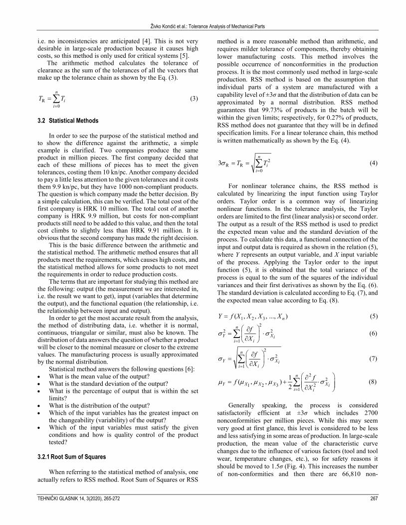
satisfactorily efficient at ±3σ which includes 2700 nonconformities per million pieces. While this may seem very good at first glance, this level is considered to be less and less satisfying in some areas of production. In large-scale production, the mean value of the characteristic curve changes due to the influence of various factors (tool and tool wear, temperature changes, etc.), so for safety reasons it should be moved to 1.5σ (Fig. 4). This increases the number of non-conformities and then there are 66,810 non-



conformities per million pieces. As a result, new solutions are being sought to reduce this number.

Figure 4 Shift of a mean value for 1,5σ [7]

3.2.2 Monte Carlo simulation

Monte Carlo simulation is recognized as an approach that incorporates the basics of modern technology. The method is widely used for non-linear statistical tolerance analysis [8]. It is a statistical simulation based on random events. Each random event generated represents one experimentally set outcome. Using a proper data scatter curve and a random value generator, a real data distribution of the output variable is obtained. This technique is used to describe a measurement whose value depends on several factors or variables, the relationship between these variables and the measurement is known, and random data is assumed. The algorithm to perform the simulation is as follows: for the input variable X, the output variable is formulated using a previously written algorithm Y, the process is repeated M times to obtain the M values of the output variable Y, which is used to determine the scattering function of the output data [9]. The expected value of the output variable Y, the standard deviation and the interval for the given probability level P are then estimated from the experimental curve.

4 TOLERANCE ANALYSES FOR ONE-WAY CLUTCH

One-way clutch is a mechanism used in two-way drive

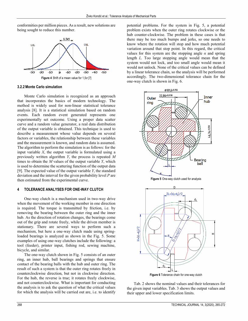
when the movement of the working member in one direction is required. The torque is transmitted by friction, i.e. by removing the bearing between the outer ring and the inner hub. As the direction of rotation changes, the bearings come out of the grip and rotate freely, while the driven member is stationary. There are several ways to perform such a mechanism, but here a one-way clutch made using spring-loaded bearings is analyzed as shown in the Fig. 5. Some examples of using one-way clutches include the following: a tool (feeder), printer input, fishing rod, sewing machine, bicycle, and similar.

The one-way clutch shown in Fig. 5 consists of an outer ring, an inner hub, ball bearings and springs that ensure contact of the bearing balls with the hub and outer ring. The result of such a system is that the outer ring rotates freely in counterclockwise direction, but not in clockwise direction. For the hub, the reverse is true; it rotates freely clockwise, and not counterclockwise. What is important for conducting the analysis is to ask the question of what the critical values for which the analysis will be carried out are, i.e. to identify

potential problems. For the system in Fig. 5, a potential problem exists when the outer ring rotates clockwise or the hub counter-clockwise. The problem in these cases is that there may be too much bumps and jerks, so one needs to know where the rotation will stop and how much potential variation around that stop point. In this regard, the critical values for this system are the stopping angle α and spring length L. Too large stopping angle would mean that the system would not lock, and too small angle would mean it would not unlock. None of the critical values can be defined by a linear tolerance chain, so the analysis will be performed accordingly. The two-dimensional tolerance chain for the one-way clutch is shown in Fig. 6.

Figure 5 One-way clutch used for analysis

Figure 6 Tolerance chain for one-way clutch

Tab. 2 shows the nominal values and their tolerances for

the given input variables. Tab. 3 shows the output values and their upper and lower specification limits.



Table 2 Input variables and their tolerances Input variable Symbol Unit Nominal values Tolerance

± Hub height H mm 46.74 ± 0.156

Diameter of ball bearing 1 d1 mm 22.86 ± 0.013

Diameter of ball bearing 2 d2 mm 22.86 ± 0.013

Inner ring diameter D mm 101.6 ± 0.156

Table 3 Output variables Output variables Symbol Unit LSL USL Stopping angle α ° 27.5 28.5 Spring length L mm 6.5 7.5

The relationship between input and output values is

shown in Eqs. (9) and (10). Once the relationship between input and output variables is defined, analysis can be accessed. An analytical and statistical method will be implemented, and results will be compared.

1 21

1 2

2cos

2

d dH

d dDα −

+ + = + −

(9)

2 21 2 1 2 1 21

2 2 2 2d d d d d dL D H

+ + + = ⋅ − − + − (10)

4.1 Example of the Worst Case Method

As this is not a linear analysis, the tolerances of individual members from the tolerance chain cannot be summed up. In order to perform the arithmetic method, it is necessary to determine the minimum and maximum dimensions for critical values. It is evident from Eq. (9) that the stopping angle will be minimal when the variables H, d1 and d2 are maximal, and variable D minimal. The maximal stopping angle value will be obtained in reverse, i.e. when variables H, d1 and d2 are minimal, and D maximal. In Tab. 4 minimal and maximal values for the individual input variables are given. The length of the spring in term (10) will be minimal when variables H, d1 and d2 are maximal, and variable D minimal, and opposite. Eqs. (11) to (14) show the computational portion of obtaining these critical values.

Table 4 Minimum and maximum values for input variables Input data MIN, mm MAX, mm

H 46.584 46.896 d1 22.847 22.873 d2 22.847 22.873 D 101.444 101.756

1min

22 873 22 87346 8962cos 27 38

22 873 22 873101 4442

. ...

. ..α −

+ + = = ° + −

(11)

1max

22 847 22 84746 8962cos 28 371

22 847 22 847101 7562

. ...

. ..α −

+ + = = ° + −

(12)

( ) ( )2 2min

1 ( 101 444 22 873 46 896 22 8732

22 873) 6 631 mm

L . . . .

. .

= ⋅ − − + −

− = (13)

( ) ( )2 2max

1 ( 101 756 22 847 46 586 22 8472

22 847) 7 325 mm

L . . . .

. .

= ⋅ − − + −

− =(14)

From the results obtained by the arithmetic method i.e.

worst case method, it is possible to calculate the mean value of results. The mean value is calucated as the arithmetic mean of the maximum and minimum values. The results of are shown in Tab. 5.

Table 5 The results of worst case method Symbol MIN MAX Mean value Range

α , ° 27.380 28.371 27.876 0.496 L, mm 6.631 7.325 6.978 0.347 When the obtained results are compared with the set

requirements in Tab. 3, then it can be seen that the obtained minimum value for the stopping angle is less than the set requirement (27,380° < LSL). That means a number of non-confirming units will occur in the process. Assuming a normal distribution in the process, 1000 simulations for both stopping angle and spring length were undertaken. Seven non-conformities have occurred.

With aim of eliminating non-conformities for given dimensions and specification limits, it is necessary to improve manufacturing process and therefore lower the result deviations.

4.2 Example of RSS Method

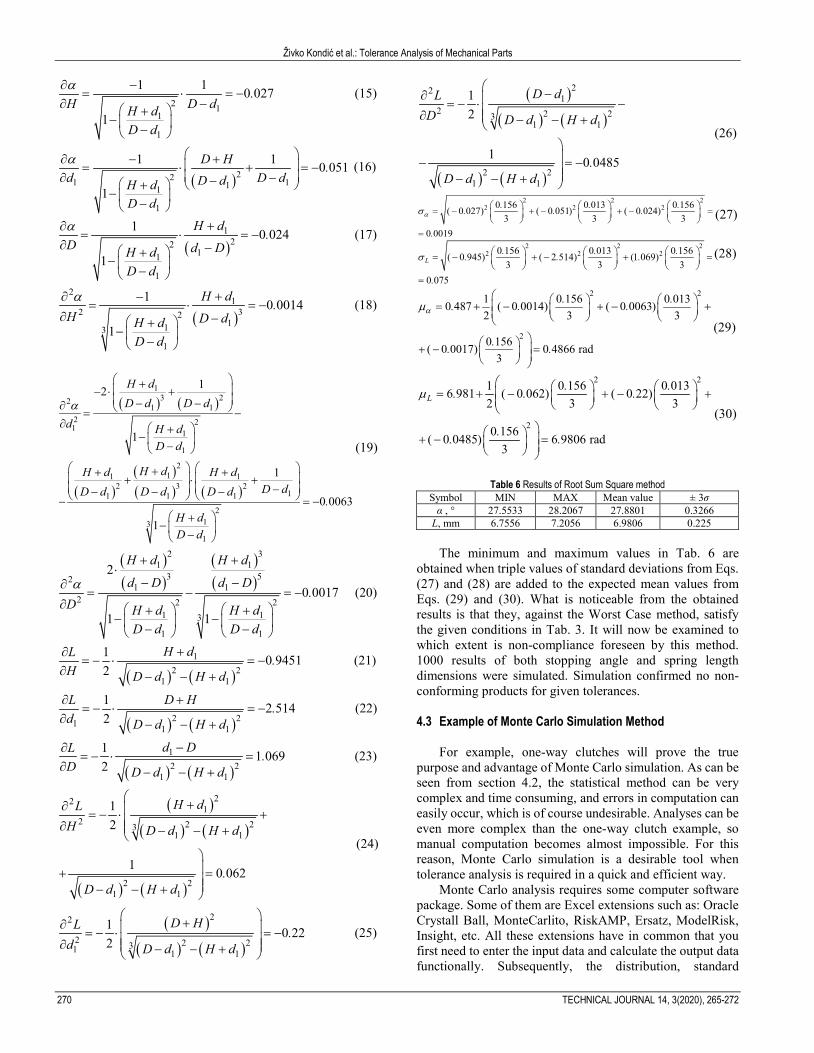
The Eqs. (7) and (8) will be used to perform that statistical method Root Sum Square for the one-way clutch. According to these terms, it is evident that the first and second derivatives need to be calculated in order to obtain the standard deviation and the mean value. These derivatives will be calculated using the MathCad computer program. To facilitate derivation, the ball bearing diameters d1 and d2 will be assumed to be the same in each case and will only be denoted by d1. Eqs. (15) to (20) show first and second derivations for the stopping angle, and from (21) to (26) for the length of spring. It should be noted that the results for the stopping angle in radians were obtained, so this should be taken into account when calculating the mean value and standard deviation. In order to obtain the derivation result, the nominal values from Tab. 2 are entered as variables. After the derivatives are calculated, the standard deviation is calculated as shown in relations (27) and (28), where the value for the stopping angle in radians and for the spring length in millimeters is obtained. In Eqs. (29) and (30), the mean expected value for stopping angle and spring length were calculated.



2 11

1

1 1 0 027

1

.H D dH d

D d

α∂ −= ⋅ = −

∂ − +− −

(15)

( )221 111

1

1 1 0 051

1

D H .d D dD dH d

D d

α ∂ − + = ⋅ + = − ∂ −− +

− −

(16)

( )1

2211

1

1 0 024

1

H d .D d DH d

D d

α +∂= ⋅ = −

∂ − +− −

(17)

( )

21

2 32113

1

1 0 0014

1

H d .H D dH d

D d

α +∂ −= ⋅ = −

∂ − +− −

(18)

( ) ( )

( )( )( ) ( )

13 22

1 12 21 1

1

211 1

2 3 211 1 1

213

1

12

1

1

0 0063

1

H dD d D d

d H dD d

H dH d H dD dD d D d D d

.H dD d

α

+ − ⋅ + − −∂ = −

∂ +− −

++ + + ⋅ + −− − − − = −

+− −

(19)

( )( )

( )( )

2 31 1

3 521 1

2 2 21 13

1 1

2

0 0017

1 1

H d H d

d D d D.

D H d H dD d D d

α

+ +⋅

− −∂= − = −

∂ + +− − − −

(20)

( ) ( )1

2 21 1

1 0 94512

H dL .H D d H d

+∂= − ⋅ = −

∂ − − + (21)

( ) ( )2 21 1 1

1 2 5142

L D H .d D d H d

∂ += − ⋅ = −

∂ − − + (22)

( ) ( )12 2

1 1

1 1 0692

d DL .D D d H d

−∂= − ⋅ =

∂ − − + (23)

( )( ) ( )

( ) ( )

221

2 2 231 1

2 21 1

12

1 0 062

H dLH D d H d

.D d H d

+∂ = − ⋅ +∂ − − ++ =− − +

(24)

( )( ) ( )

22

2 2 231 1 1

1 0 222

D HL .d D d H d

+∂ = − ⋅ = − ∂ − − +

(25)

( )( ) ( )

( ) ( )

221

2 2 231 1

2 21 1

12

1 0 0485

D dLD D d H d

.D d H d

−∂ = − ⋅ −∂ − − +− = −− − +

(26)

2 2 22 2 20 156 0 013 0 156( 0 027) ( 0 051) ( 0 024)

3 3 30 0019

. . .. . .

.

ασ = − + − + − =

=

(27)

2 2 22 2 20 156 0 013 0 156( 0 945) ( 2 514) (1 069)

3 3 30 075

L. . .. . .

.

σ = − + − + =

=

(28)

2 2

2

1 0 156 0 0130 487 ( 0 0014) ( 0 0063)2 3 3

0 156( 0 0017) 0 4866 rad3

. .. . .

.. .

αµ = + − + − +

+ − =

(29)

2 2

2

1 0 156 0 0136 981 ( 0 062) ( 0 22)2 3 3

0 156( 0 0485) 6 9806 rad3

L. .. . .

.. .

µ = + − + − +

+ − =

(30)

Table 6 Results of Root Sum Square method

Symbol MIN MAX Mean value ± 3σ α , ° 27.5533 28.2067 27.8801 0.3266

L, mm 6.7556 7.2056 6.9806 0.225

The minimum and maximum values in Tab. 6 are obtained when triple values of standard deviations from Eqs. (27) and (28) are added to the expected mean values from Eqs. (29) and (30). What is noticeable from the obtained results is that they, against the Worst Case method, satisfy the given conditions in Tab. 3. It will now be examined to which extent is non-compliance foreseen by this method. 1000 results of both stopping angle and spring length dimensions were simulated. Simulation confirmed no non-conforming products for given tolerances. 4.3 Example of Monte Carlo Simulation Method

For example, one-way clutches will prove the true purpose and advantage of Monte Carlo simulation. As can be seen from section 4.2, the statistical method can be very complex and time consuming, and errors in computation can easily occur, which is of course undesirable. Analyses can be even more complex than the one-way clutch example, so manual computation becomes almost impossible. For this reason, Monte Carlo simulation is a desirable tool when tolerance analysis is required in a quick and efficient way.

Monte Carlo analysis requires some computer software package. Some of them are Excel extensions such as: Oracle Crystall Ball, MonteCarlito, RiskAMP, Ersatz, ModelRisk, Insight, etc. All these extensions have in common that you first need to enter the input data and calculate the output data functionally. Subsequently, the distribution, standard



deviation, and mean for the input data are defined. The higher the number of simulations, the more accurate the results will be, but the simulation will be slower. After everything is defined, simulation is initiated.

In order to conduct statistical tolerance analysis using Monte Carlo simulation, software package Minitab trial version was used. Input variables H, d1, d2 and D were simulated. Each input variable was simulated 1000 times, and uniform data distribution was assumed. The output variables α and L were calculated using the expression given with Eqs. (10) and (11).

Tab. 7 shows the results of the Monte Carlo simulation. The output data follow normal distribution (Fig. 7).

Table 7 Results of Monte Carlo simulation

µ σ MIN MAX ± 3σ α , ° 27.878 0.183 27.329 28.427 0.549

L, mm 6.978 0.127 6.597 7.359 0.381

a) b)

Figure 7 Monte Carlo Simulation output: a) stopping angle, b) spring clearance

Figure 8 Process capability report for spring clearance

The process capability analyses were calculated using

the normal distribution. The process capability report for stopping angle α is given in Fig. 8, while the process capability report for spring clearance L is given in Fig. 9.

Potential process capability for stopping angle is 0.91, which means that the process is not capable to produce conforming units. The Monte Carlo simulation predicts 20,018 non-conforming units per million pieces, i.e. 2 %. According to the simulation, all non-conforming products have stopping angle smaller than lower specification limit (LSL).

Potential process capability for spring clearance L calculated from simulated data shows that the process is

capable (Pp > 1). The Monte Carlo simulation predicts 98 non-conforming units per million pieces, i.e. 0.01 %.

Figure 9 Process capability report for spring clearance

5 CONCLUSION

Tolerance analysis is performed to allow for the widest possible tolerances of the components of a system without compromising its functional properties. In order to carry out tolerance analysis, it is necessary to determine the critical value, i.e. the problem to be solved. After that it is necessary to determine what influences this problem and describe it with some functional connection. For linear systems, this is easy to determine, and a tolerance chain is drawn to further reduce the analysis to simple addition and subtraction. For nonlinear systems, computing becomes quite complex, and in some cases impossible.

The analysis methods used were: Worst Case method, Root Sum Square method and Monte Carlo simulation method. Each of these methods has its advantages and disadvantages. The advantage of the Worst Case method is that it is easy to understand, but no inconsistencies are anticipated, which causes high production costs. Therefore, this method is only used for critical systems. The Root Sum Square is provided for wider dimensions of the assembly components, thereby automatically reducing the cost of production at the expense of inconsistent components in the process. The disadvantage of this method is that for nonlinear systems, computing becomes complicated and time consuming, sometimes impossible. Monte Carlo simulation method is based on generating random numbers from probability density functions for each input variable and calculating output variables by combining different statistical distributions of input variables.

In the example of the one-way clutch, the limits of the requirements were set and it was compared how the individual methods would predict the behavior of the process with respect to these requirements. The Worst Case method showed the occurrence of a small number of non-conforming products.

The RSS method turned out to be quite complicated and time-consuming for this example. The result predicted none

1st Quartile 27,753Median 27,8783rd Quartile 28,001Maximum 28,309

27,866 27,889

27,863 27,893

0,176 0,192

A-Squared 0,69P-Value 0,070

Mean 27,878StDev 0,183Variance 0,034Skewness 0,014153Kurtosis -0,450485N 1000

Minimum 27,417

Anderson-Darling Normality Test

95% Confidence Interval for Mean

95% Confidence Interval for Median

95% Confidence Interval for StDev

28,25028,12528,00027,87527,75027,62527,500

Summary Report for stopping angle

1st Quartile 6,8929Median 6,97783rd Quartile 7,0639Maximum 7,2784

6,9704 6,9861

6,9666 6,9900

0,1213 0,1324

A-Squared 0,68P-Value 0,077

Mean 6,9783StDev 0,1266Variance 0,0160Skewness 0,019061Kurtosis -0,465792N 1000

Minimum 6,6613

Anderson-Darling Normality Test

95% Confidence Interval for Mean

95% Confidence Interval for Median

95% Confidence Interval for StDev

7,27,17,06,96,86,7

Summary Report for spring clearance, mm



of non-compliant pieces in the process. The Monte Carlo simulation showed that in case of stopping angle, process is not capable to produce conforming parts, and the predicted number of non-conforming products is around 2 %. In case when analyzing dimension of spring length, simulated data shows that the process is capable. Potential capability is 1.32 and only 0.01 % of non-conforming products is expected.

6 REFERENCES

[1] Tynes, J. (2012). Make it fit: Introduction to tolerance analysis

for mechanical engineers. Create Space Independent Publishing Platform

[2] Chen, H., Jin, S., Li, Z & Lai, X. (2014). A comprehensive study of three dimensional tolerance analysis methods. Computer-Aided Design, 53, 1-13. https://doi.org/10.1016/j.cad.2014.02.014

[3] GD&T Symbols Reference Guide from Sigmetrix. https://www.sigmetrix.com/gdt-symbols/

[4] A Handbook for Geometrical Product Specification using ISO and ASME Standards (2006). Geometrical Dimensioning and Tolerancing for Design, Manufacturing and Inspection.

[5] Dantan, J.-Y. & Quereshi, A.-J. (2009). Worst-case and statistical tolerance analysis based on quantified constraint satisfaction problems and Monte Carlo simulation. Computer-Aided Design, 41(1), 1-12 https://doi.org/10.1016/j.cad.2008.11.003

[6] Cox, N. D. (1986). How to perform statistical tolerance analysis. American Society for Quality Control.

[7] MITCalc: Tolerance analysis of linear dimensional chains. http://www.mitcalc.com/doc/tolanalysis1d/help/en/tolanalysis1d.htm

[8] Nigam, S. D. & Turner, J. U. (1995). Review of statistical approaches to tolerance analysis. Computer-Aided Design, 27(1), 6-15. https://doi.org/10.1016/0010-4485(95)90748-5

[9] Piljek, P., Runje, B., Keran, Z., & Škunca, M. (2017). Monte Carlo Simulation of Measurement Uncertainty in Modified Hydraulic Bulging Determination of Flow Stress. Technical Gazette, 24 (3), 649-653. https://doi.org/10.17559/TV-20140828211548

Authors’ contacts: Živko Kondić, Full Professor University North, University Center Varaždin, Jurja Križanića 31b, 42 000 Varaždin, Croatia [email protected] Đuro Tunjić, Assistant Professor TUV Croatia d.o.o. Bani 110, 10 010 Zagreb, Croatia [email protected] Leon Maglić, Full Professor University of Slavonski Brod, Mechanical Engineering Faculty, Trg Ivane Brlić Mažuranić 2, 35 000 Slavonski Brod, Croatia [email protected] Amalija Horvatić Novak, Postdoctoral Researcher (Corresponding author) University of Zagreb, Faculty of Mechanical Engineering and Naval Architecture, Ivana Lučića 5, 10 000 Zagreb, Croatia [email protected]

https://doi.org/10.1016/0010-4485(95)90748-5

https://doi.org/10.1016/0010-4485(95)90748-5

https://doi.org/10.1016/0010-4485(95)90748-5

Tolerance Analysis of Mechanical Parts

Documents

Transcript of Tolerance Analysis of Mechanical Parts